D Geo Pipeline User Manual DGeo
User Manual: Pdf DGeoPipeline-Manual
Open the PDF directly: View PDF ![]() .
.
Page Count: 346 [warning: Documents this large are best viewed by clicking the View PDF Link!]
- 1 General Information
- 2 Getting Started
- 3 General
- 4 Input
- 5 Calculations
- 6 View Results
- 6.1 Report selection
- 6.2 Report
- 6.2.1 Report – Drilling Fluid Pressure
- 6.2.2 Report – Settlements of soil layers below the pipeline
- 6.2.3 Report – Subsidence
- 6.2.4 Report – Soil Mechanical Data
- 6.2.5 Report – Data for Stress Analysis
- 6.2.6 Report – Stress Analysis
- 6.2.7 Report – Operation Parameters (Trenching)
- 6.2.8 Report – Face Support Pressures and Thrust Forces (Micro tunneling)
- 6.3 Drilling Fluid Pressures Plots
- 6.4 Operation Parameter Plots
- 6.5 Stresses in Geometry
- 6.6 Subsidence Profiles
- 7 Graphical Geometry Input
- 8 Tutorial 1: Calculation and assessment of the drilling fluid pressure
- 9 Tutorial 2: Stress analysis of steel pipes and polyethylene pipes
- 10 Tutorial 3: Influence of soil behavior on drilling fluid pressures and soil load on the pipe
- 10.1 Introduction to the case
- 10.2 Geometry of the longitudinal cross section
- 10.3 Soil layer properties
- 10.4 Finishing the geometry of the longitudinal cross section
- 10.5 Soil behavior
- 10.6 Calculated reduced soil load for pipe stress analysis
- 10.7 Calculated drilling fluid pressures
- 10.8 Drilling fluid pressure and groundwater pressure
- 10.9 Conclusion
- 11 Tutorial 4: Exporting soil mechanical data for an extended stress analysis
- 12 Tutorial 5: Drilling with a horizontal bending radius
- 13 Tutorial 6: Installation of bundled pipelines
- 14 Tutorial 7: Face support pressure for micro tunneling
- 15 Tutorial 8: Uplift and thrust forces for micro tunneling
- 16 Tutorial 9: Settlement and soil mechanical parameters for micro tunneling
- 17 Tutorial 10: Subsidence after micro tunneling
- 18 Tutorial 11: Installation of pipeline in a trench
- 18.1 Introduction to the case
- 18.2 Model
- 18.3 Geometry of the longitudinal cross section
- 18.4 Soil layer properties
- 18.5 Finishing the geometry of the longitudinal cross section
- 18.6 Adding a waterway
- 18.7 Calculation Verticals
- 18.8 Boundaries Selection
- 18.9 Trench configuration and pipe material
- 18.10 Engineering Data
- 18.11 Results: Soil Mechanical Parameters
- 19 Tutorial 12: Trenching: uplift and heave
- 20 Design of a pipeline
- 21 Calculation of soil mechanical data
- 21.1 Neutral vertical stress
- 21.2 Passive vertical stress
- 21.3 Reduced neutral vertical stress
- 21.4 Initial vertical stress
- 21.5 Neutral horizontal stress
- 21.6 Vertical modulus of subgrade reaction
- 21.7 Horizontal modulus of subgrade reaction
- 21.8 Ultimate vertical bearing capacity
- 21.9 Ultimate horizontal bearing capacity
- 21.10 Vertical displacement
- 21.11 Maximal axial friction
- 21.12 Displacement at maximal friction
- 21.13 Global determination of the soil type
- 21.14 Traffic load
- 22 Drilling fluid pressures calculation
- 22.1 Minimum required drilling fluid pressure
- 22.1.1 Static pressure of the drilling fluid column p1
- 22.1.2 Excess pressure to maintain flow of drilling fluid p2
- 22.1.3 Minimum drilling fluid pressure for Stage 1 (pilot pipe in the pilot hole)
- 22.1.4 Minimum drilling fluid pressure for Stage 2 (drill pipe in the pre-ream hole)
- 22.1.5 Minimum drilling fluid pressure for Stage 3 (product pipe in the borehole)
- 22.2 Maximum allowable drilling fluid pressure
- 22.3 Equivalent diameter for a bundled pipeline
- 22.4 Equilibrium between drilling fluid pressure and pore pressure
- 22.1 Minimum required drilling fluid pressure
- 23 Strength pipeline calculation
- 23.1 Buoyancy control
- 23.2 Pulling force in a flexible pipeline
- 23.3 Maximum representative pulling force
- 23.4 Pulling force for a bundled pipeline
- 23.5 Strength calculation
- 23.5.1 Strength calculation for Load Combination 1A: start of the pullback operation
- 23.5.2 Strength calculation for Load Combination 1B: end of the pullback operation
- 23.5.3 Strength calculation for Load Combination 2: application of internal pressure
- 23.5.4 Strength calculation for Load Combination 3: pipeline in operation, without internal pressure
- 23.5.5 Strength calculation for Load Combination 4: pipeline in operation, with internal pressure
- 23.6 Check of calculated stresses
- 23.7 Deflection of the pipe
- 23.8 Implosion of the polyethylene pipe
- 24 Micro tunneling
- 25 Trenching
- 26 Effective Stress and Pore Pressure
- 27 Benchmarks
- Bibliography

User Manual
D-Geo PiPeline
Design of pipeline installation
D-GEO PIPELINE
Design of pipeline installation
User Manual
Version: 16.1
Revision: 00
9 February 2016
D-GEO PIPELINE
, User Manual
Published and printed by:
Deltares
Boussinesqweg 1
2629 HV Delft
P.O. 177
2600 MH Delft
The Netherlands
telephone: +31 88 335 82 73
fax: +31 88 335 85 82
e-mail: info@deltares.nl
www: https://www.deltares.nl
For sales contact:
telephone: +31 88 335 81 88
fax: +31 88 335 81 11
e-mail: sales@deltaressystems.nl
www: http://www.deltaressystems.nl
For support contact:
telephone: +31 88 335 81 00
fax: +31 88 335 81 11
e-mail: support@deltaressystems.nl
www: http://www.deltaressystems.nl
Copyright © 2016 Deltares
All rights reserved. No part of this document may be reproduced in any form by print, photo
print, photo copy, microfilm or any other means, without written permission from the publisher:
Deltares.

Contents
Contents
1 General Information 1
1.1 Preface .................................... 1
1.2 Installation of pipelines ............................ 2
1.2.1 Horizontal Directional Drilling technique . . . . . . . . . . . . . . . . 2
1.2.2 Micro Tunneling ............................ 3
1.2.3 Installation in trench ......................... 4
1.3 Features in standard module (HDD) ...................... 5
1.3.1 Soil profile .............................. 5
1.3.2 Pipeline materials ........................... 5
1.3.3 Factors ................................ 5
1.3.4 Results ................................ 5
1.4 Features in additional modules ........................ 6
1.4.1 Micro Tunneling module . . . . . . . . . . . . . . . . . . . . . . . 6
1.4.2 Trenching module ........................... 7
1.5 History .................................... 9
1.6 Minimum System Requirements . . . . . . . . . . . . . . . . . . . . . . . 11
1.7 Definitions and Symbols ........................... 11
1.8 Getting Help ................................. 16
1.9 Getting Support ................................ 16
1.10 Deltares ................................... 18
1.11 Deltares Systems ............................... 19
1.12 On-line software (Citrix) . . . . . . . . . . . . . . . . . . . . . . . . . . . . 19
2 Getting Started 21
2.1 Starting D-GEO PIPELINE ........................... 21
2.2 Main window ................................. 21
2.2.1 The menu bar . . . . . . . . . . . . . . . . . . . . . . . . . . . . 22
2.2.2 The icon bar ............................. 22
2.2.3 View Input .............................. 23
2.2.4 Info bar ................................ 26
2.2.5 Title panel .............................. 26
2.2.6 Status bar .............................. 26
2.3 Files ..................................... 27
2.4 Tips and Tricks ................................ 27
2.4.1 Keyboard shortcuts . . . . . . . . . . . . . . . . . . . . . . . . . . 27
2.4.2 Exporting figures and reports . . . . . . . . . . . . . . . . . . . . . 28
2.4.3 Copying part of a table . . . . . . . . . . . . . . . . . . . . . . . . 28
3 General 29
3.1 File menu ................................... 29
3.1.1 General options . . . . . . . . . . . . . . . . . . . . . . . . . . . . 29
3.1.2 Option ”Export Results as csv” . . . . . . . . . . . . . . . . . . . . 30
3.2 Tools menu .................................. 32
3.2.1 Program Options - View . . . . . . . . . . . . . . . . . . . . . . . 33
3.2.2 Program Options - General . . . . . . . . . . . . . . . . . . . . . . 33
3.2.3 Program Options - Locations . . . . . . . . . . . . . . . . . . . . . 34
3.2.4 Program Options - Language . . . . . . . . . . . . . . . . . . . . . 35
3.2.5 Program Options - Modules . . . . . . . . . . . . . . . . . . . . . . 35
3.3 Help menu .................................. 36
3.3.1 Error Messages ........................... 36
3.3.2 Manual ................................ 36
3.3.3 Deltares Systems Website . . . . . . . . . . . . . . . . . . . . . . 36
Deltares iii

D-GEO PIPELINE
, User Manual
3.3.4 Support ................................ 36
3.3.5 About D-GEO PIPELINE . . . . . . . . . . . . . . . . . . . . . . . . 37
4 Input 39
4.1 Project menu ................................. 39
4.1.1 Model ................................ 39
4.1.2 Project Properties . . . . . . . . . . . . . . . . . . . . . . . . . . 40
4.1.3 View Input File . . . . . . . . . . . . . . . . . . . . . . . . . . . . 42
4.2 Soil menu ................................... 42
4.2.1 Materials – Standard ......................... 43
4.2.2 Materials – Settlement Koppejan . . . . . . . . . . . . . . . . . . . 43
4.2.3 Materials – Settlement Isotache . . . . . . . . . . . . . . . . . . . . 45
4.2.4 Materials – Database ......................... 46
4.3 Geometry menu ............................... 46
4.3.1 New ................................. 47
4.3.2 New Wizard ............................. 47
4.3.3 Import ................................ 50
4.3.4 Import geometry from database . . . . . . . . . . . . . . . . . . . . 50
4.3.5 Export ................................ 51
4.3.6 Export as Plaxis/DOS ......................... 51
4.3.7 Limits ................................. 51
4.3.8 Points ................................ 52
4.3.9 Import PL-line . . . . . . . . . . . . . . . . . . . . . . . . . . . . 53
4.3.10 PL-Lines ............................... 53
4.3.11 Phreatic Line ............................. 54
4.3.12 Layers ................................ 54
4.3.13 PL-lines per Layer . . . . . . . . . . . . . . . . . . . . . . . . . . 56
4.3.14 Check Geometry ........................... 58
4.4 GeoObjects menu .............................. 58
4.4.1 Boundaries Selection ......................... 59
4.4.2 Calculation Verticals ......................... 59
4.5 Loads menu ................................. 60
4.5.1 Traffic Loads ............................. 60
4.6 Pipe menu .................................. 61
4.6.1 Pipeline Configuration . . . . . . . . . . . . . . . . . . . . . . . . 61
4.6.1.1 Pipeline Configuration for HDD . . . . . . . . . . . . . . . 61
4.6.1.2 Pipeline Configuration for Micro tunneling . . . . . . . . . . 63
4.6.1.3 Pipeline Configuration for Construction in trench . . . . . . 64
4.6.2 Product Pipe Material Data . . . . . . . . . . . . . . . . . . . . . . 65
4.6.2.1 Product Pipe Material Data for HDD . . . . . . . . . . . . 66
4.6.2.2 Product Pipe Material Data for Micro tunneling . . . . . . . 69
4.6.3 Engineering Data ........................... 71
4.6.3.1 Engineering Data for HDD . . . . . . . . . . . . . . . . . 71
4.6.3.2 Engineering Data for Micro tunneling . . . . . . . . . . . . 73
4.6.3.3 Engineering Data for Construction in trench . . . . . . . . 74
4.6.4 Drilling Fluid Data ........................... 75
4.7 Defaults menu ................................ 76
4.7.1 Factors ................................ 76
4.7.1.1 Factors for HDD . . . . . . . . . . . . . . . . . . . . . . 76
4.7.1.2 Factors for Micro tunneling . . . . . . . . . . . . . . . . . 82
4.7.1.3 Factors for Construction in trench . . . . . . . . . . . . . . 83
4.7.2 Special Stress Analysis . . . . . . . . . . . . . . . . . . . . . . . . 84
5 Calculations 87
iv Deltares

Contents
5.1 Start Calculation ............................... 87
5.2 Special Stress Analysis (only for HDD) . . . . . . . . . . . . . . . . . . . . 88
5.3 Warning and Error messages ......................... 88
5.3.1 Warning messages . . . . . . . . . . . . . . . . . . . . . . . . . . 88
5.3.2 Error messages ........................... 89
6 View Results 91
6.1 Report selection ............................... 91
6.2 Report .................................... 91
6.2.1 Report – Drilling Fluid Pressure . . . . . . . . . . . . . . . . . . . . 92
6.2.1.1 Report – Drilling Fluid Data . . . . . . . . . . . . . . . . . 93
6.2.1.2 Report – Equilibrium between Drilling Fluid Pressure and
Pore Pressure ....................... 94
6.2.2 Report – Settlements of soil layers below the pipeline . . . . . . . . . 95
6.2.3 Report – Subsidence ......................... 95
6.2.4 Report – Soil Mechanical Data . . . . . . . . . . . . . . . . . . . . 96
6.2.4.1 Soil Mechanical Parameters for HDD . . . . . . . . . . . . 96
6.2.4.2 Soil Mechanical Parameters for Micro tunneling . . . . . . . 98
6.2.4.3 Soil Mechanical Parameters for Construction in trench . . . 99
6.2.5 Report – Data for Stress Analysis . . . . . . . . . . . . . . . . . . . 100
6.2.6 Report – Stress Analysis . . . . . . . . . . . . . . . . . . . . . . . 102
6.2.6.1 Stress Analysis HDD . . . . . . . . . . . . . . . . . . . . 102
6.2.7 Report – Operation Parameters (Trenching) . . . . . . . . . . . . . . 106
6.2.8 Report – Face Support Pressures and Thrust Forces (Micro tunneling) 108
6.3 Drilling Fluid Pressures Plots . . . . . . . . . . . . . . . . . . . . . . . . . 109
6.4 Operation Parameter Plots . . . . . . . . . . . . . . . . . . . . . . . . . . 110
6.4.1 Operation Parameter Plots for Micro Tunneling . . . . . . . . . . . . 110
6.4.2 Operation Parameter Plots for Construction in trench . . . . . . . . . 112
6.5 Stresses in Geometry . . . . . . . . . . . . . . . . . . . . . . . . . . . . . 113
6.6 Subsidence Profiles ..............................114
7 Graphical Geometry Input 115
7.1 Geometrical objects ..............................115
7.1.1 Geometry elements . . . . . . . . . . . . . . . . . . . . . . . . . . 115
7.1.2 Construction elements . . . . . . . . . . . . . . . . . . . . . . . . 116
7.2 Assumptions and restrictions . . . . . . . . . . . . . . . . . . . . . . . . . 116
7.3 View Input Window ..............................116
7.3.1 General ................................117
7.3.2 Buttons ................................118
7.3.3 Legend ................................120
7.4 Geometry modeling ..............................122
7.4.1 Create a new geometry . . . . . . . . . . . . . . . . . . . . . . . . 122
7.4.2 Set limits . . . . . . . . . . . . . . . . . . . . . . . . . . . . . . . 123
7.4.3 Draw layout ..............................123
7.4.4 Generate layers . . . . . . . . . . . . . . . . . . . . . . . . . . . 124
7.4.5 Add piezometric level lines . . . . . . . . . . . . . . . . . . . . . . 125
7.5 Graphical manipulation . . . . . . . . . . . . . . . . . . . . . . . . . . . . 125
7.5.1 Selection of elements . . . . . . . . . . . . . . . . . . . . . . . . . 125
7.5.2 Deletion of elements . . . . . . . . . . . . . . . . . . . . . . . . . 126
7.5.3 Using the right-hand mouse button . . . . . . . . . . . . . . . . . . 127
7.5.4 Dragging elements . . . . . . . . . . . . . . . . . . . . . . . . . . 129
8 Tutorial 1: Calculation and assessment of the drilling fluid pressure 131
8.1 Introduction to the case . . . . . . . . . . . . . . . . . . . . . . . . . . . . 131
Deltares v

D-GEO PIPELINE
, User Manual
8.2 Project ....................................132
8.2.1 Start . . . . . . . . . . . . . . . . . . . . . . . . . . . . . . . . . 132
8.2.2 Project Properties . . . . . . . . . . . . . . . . . . . . . . . . . . 133
8.2.3 Model ................................134
8.3 Geometry . . . . . . . . . . . . . . . . . . . . . . . . . . . . . . . . . . . 135
8.3.1 Soil layer properties . . . . . . . . . . . . . . . . . . . . . . . . . 136
8.3.2 Phreatic Line . . . . . . . . . . . . . . . . . . . . . . . . . . . . . 137
8.3.3 Layers ................................137
8.3.4 PL-Lines per Layers . . . . . . . . . . . . . . . . . . . . . . . . . 137
8.3.5 Check Geometry . . . . . . . . . . . . . . . . . . . . . . . . . . . 138
8.4 Pipeline Configuration . . . . . . . . . . . . . . . . . . . . . . . . . . . . . 138
8.5 Soil behavior . . . . . . . . . . . . . . . . . . . . . . . . . . . . . . . . . 139
8.6 Calculation Verticals . . . . . . . . . . . . . . . . . . . . . . . . . . . . . 140
8.7 Product Pipe Material Data . . . . . . . . . . . . . . . . . . . . . . . . . . 141
8.8 Drilling Fluid Data . . . . . . . . . . . . . . . . . . . . . . . . . . . . . . . 142
8.9 Factors ....................................143
8.10 Results ....................................144
8.11 Conclusion ..................................145
9 Tutorial 2: Stress analysis of steel pipes and polyethylene pipes 147
9.1 Introduction to the case . . . . . . . . . . . . . . . . . . . . . . . . . . . . 147
9.2 Project Properties . . . . . . . . . . . . . . . . . . . . . . . . . . . . . . . 149
9.3 Product Pipe Material Data . . . . . . . . . . . . . . . . . . . . . . . . . . 149
9.4 Engineering Data . . . . . . . . . . . . . . . . . . . . . . . . . . . . . . . 150
9.5 Factors ....................................151
9.6 Calculation and Results (Tutorial-2a) . . . . . . . . . . . . . . . . . . . . . 152
9.6.1 Results of the pulling force calculation . . . . . . . . . . . . . . . . 152
9.6.2 Results of the pipe stress analysis of the steel pipe . . . . . . . . . . 154
9.7 Special Pipe Stress Analysis (Tutorial-2b) . . . . . . . . . . . . . . . . . . . 156
9.8 Polyethylene Product Pipe (Tutorial-2c) . . . . . . . . . . . . . . . . . . . . 157
9.9 Conclusion ..................................159
10 Tutorial 3: Influence of soil behavior on drilling fluid pressures and soil load on
the pipe 161
10.1 Introduction to the case . . . . . . . . . . . . . . . . . . . . . . . . . . . . 161
10.2 Geometry of the longitudinal cross section . . . . . . . . . . . . . . . . . . 163
10.3 Soil layer properties ..............................163
10.4 Finishing the geometry of the longitudinal cross section . . . . . . . . . . . . 164
10.5 Soil behavior . . . . . . . . . . . . . . . . . . . . . . . . . . . . . . . . . 166
10.6 Calculated reduced soil load for pipe stress analysis . . . . . . . . . . . . . 167
10.7 Calculated drilling fluid pressures . . . . . . . . . . . . . . . . . . . . . . . 168
10.8 Drilling fluid pressure and groundwater pressure . . . . . . . . . . . . . . . 169
10.9 Conclusion ..................................170
11 Tutorial 4: Exporting soil mechanical data for an extended stress analysis 171
11.1 Introduction to the case . . . . . . . . . . . . . . . . . . . . . . . . . . . . 171
11.2 Settlement model . . . . . . . . . . . . . . . . . . . . . . . . . . . . . . . 172
11.3 Geometry of the longitudinal cross section . . . . . . . . . . . . . . . . . . 173
11.4 Soil layer properties ..............................174
11.5 Finishing the geometry of the longitudinal cross section . . . . . . . . . . . . 175
11.6 Calculated soil mechanical parameters in export file . . . . . . . . . . . . . . 176
11.7 Conclusion ..................................178
12 Tutorial 5: Drilling with a horizontal bending radius 179
12.1 Introduction to the case . . . . . . . . . . . . . . . . . . . . . . . . . . . . 179
vi Deltares

Contents
12.2 Pipeline Configuration . . . . . . . . . . . . . . . . . . . . . . . . . . . . . 180
12.3 Calculation of the pulling force and pipe stress analysis . . . . . . . . . . . . 182
12.4 Conclusion ..................................183
13 Tutorial 6: Installation of bundled pipelines 185
13.1 Introduction to the case . . . . . . . . . . . . . . . . . . . . . . . . . . . . 185
13.2 Product Pipe Material Data . . . . . . . . . . . . . . . . . . . . . . . . . . 187
13.3 Drilling Fluid Data . . . . . . . . . . . . . . . . . . . . . . . . . . . . . . . 187
13.4 Engineering Data . . . . . . . . . . . . . . . . . . . . . . . . . . . . . . . 188
13.5 Factors ....................................189
13.6 Results ....................................190
14 Tutorial 7: Face support pressure for micro tunneling 191
14.1 Introduction to the case . . . . . . . . . . . . . . . . . . . . . . . . . . . . 191
14.2 Model selection ................................192
14.3 Geometry . . . . . . . . . . . . . . . . . . . . . . . . . . . . . . . . . . . 194
14.3.1 Soil layer properties . . . . . . . . . . . . . . . . . . . . . . . . . 195
14.3.2 Phreatic Line . . . . . . . . . . . . . . . . . . . . . . . . . . . . . 195
14.3.3 Layers ................................195
14.3.4 PL-Lines per Layers . . . . . . . . . . . . . . . . . . . . . . . . . 196
14.3.5 Check Geometry . . . . . . . . . . . . . . . . . . . . . . . . . . . 197
14.4 Pipeline Configuration . . . . . . . . . . . . . . . . . . . . . . . . . . . . . 197
14.5 Pipe Material Data ..............................198
14.6 Soil behavior . . . . . . . . . . . . . . . . . . . . . . . . . . . . . . . . . 198
14.7 Calculation Verticals . . . . . . . . . . . . . . . . . . . . . . . . . . . . . 199
14.8 Engineering Data . . . . . . . . . . . . . . . . . . . . . . . . . . . . . . . 200
14.9 Results: Operation Parameter Plots . . . . . . . . . . . . . . . . . . . . . . 201
15 Tutorial 8: Uplift and thrust forces for micro tunneling 203
15.1 Introduction to the case . . . . . . . . . . . . . . . . . . . . . . . . . . . . 203
15.2 Geometry of the longitudinal cross section . . . . . . . . . . . . . . . . . . 204
15.3 Soil layer properties ..............................205
15.4 Soil behavior . . . . . . . . . . . . . . . . . . . . . . . . . . . . . . . . . 206
15.5 Pipeline Configuration . . . . . . . . . . . . . . . . . . . . . . . . . . . . . 207
15.6 Calculation Verticals . . . . . . . . . . . . . . . . . . . . . . . . . . . . . 208
15.7 Engineering Data . . . . . . . . . . . . . . . . . . . . . . . . . . . . . . . 209
15.8 Results ....................................210
15.8.1 Thrust Force . . . . . . . . . . . . . . . . . . . . . . . . . . . . . 210
15.8.2 Uplift safety ..............................210
16 Tutorial 9: Settlement and soil mechanical parameters for micro tunneling 213
16.1 Introduction to the case . . . . . . . . . . . . . . . . . . . . . . . . . . . . 213
16.2 Settlement ..................................214
16.3 Geometry of the longitudinal cross section . . . . . . . . . . . . . . . . . . 215
16.4 Soil layer properties ..............................217
16.5 Finishing the geometry of the longitudinal cross section . . . . . . . . . . . . 217
16.6 Calculated soil mechanical parameters in export file . . . . . . . . . . . . . . 218
16.7 Conclusion ..................................221
17 Tutorial 10: Subsidence after micro tunneling 223
17.1 Introduction to the case . . . . . . . . . . . . . . . . . . . . . . . . . . . . 223
17.1.1 Volume loss along the tunnel excavation . . . . . . . . . . . . . . . 223
17.1.2 Modification of the drilling line . . . . . . . . . . . . . . . . . . . . . 224
17.2 Pipeline Configuration . . . . . . . . . . . . . . . . . . . . . . . . . . . . . 226
17.3 Material data . . . . . . . . . . . . . . . . . . . . . . . . . . . . . . . . . 227
Deltares vii

D-GEO PIPELINE
, User Manual
17.4 Engineering Data . . . . . . . . . . . . . . . . . . . . . . . . . . . . . . . 228
17.5 Results: Subsidence . . . . . . . . . . . . . . . . . . . . . . . . . . . . . 229
18 Tutorial 11: Installation of pipeline in a trench 231
18.1 Introduction to the case . . . . . . . . . . . . . . . . . . . . . . . . . . . . 231
18.2 Model .....................................232
18.3 Geometry of the longitudinal cross section . . . . . . . . . . . . . . . . . . 233
18.4 Soil layer properties ..............................233
18.5 Finishing the geometry of the longitudinal cross section . . . . . . . . . . . . 234
18.5.1 Phreatic Line . . . . . . . . . . . . . . . . . . . . . . . . . . . . . 234
18.5.2 Layers ................................234
18.5.3 PL-Lines per Layer . . . . . . . . . . . . . . . . . . . . . . . . . . 235
18.6 Adding a waterway ..............................236
18.7 Calculation Verticals . . . . . . . . . . . . . . . . . . . . . . . . . . . . . 237
18.8 Boundaries Selection . . . . . . . . . . . . . . . . . . . . . . . . . . . . . 238
18.9 Trench configuration and pipe material . . . . . . . . . . . . . . . . . . . . 238
18.10 Engineering Data . . . . . . . . . . . . . . . . . . . . . . . . . . . . . . . 240
18.11 Results: Soil Mechanical Parameters . . . . . . . . . . . . . . . . . . . . . 240
19 Tutorial 12: Trenching: uplift and heave 243
19.1 Introduction to the case . . . . . . . . . . . . . . . . . . . . . . . . . . . . 243
19.2 Materials . . . . . . . . . . . . . . . . . . . . . . . . . . . . . . . . . . . 244
19.3 Phreatic level . . . . . . . . . . . . . . . . . . . . . . . . . . . . . . . . . 245
19.4 Calculation Verticals . . . . . . . . . . . . . . . . . . . . . . . . . . . . . 246
19.5 Factors ....................................248
19.6 Results ....................................248
19.6.1 Uplift safety for trenching in Peat layer (Tutorial-12a) . . . . . . . . . 248
19.6.2 Uplift safety for trenching in Soft Organic Clay layer (Tutorial-12b) . . . 249
19.6.3 Hydraulic Heave Safety . . . . . . . . . . . . . . . . . . . . . . . . 250
19.7 Lowering the hydraulic head (Tutorial-12c) . . . . . . . . . . . . . . . . . . 251
20 Design of a pipeline 255
20.1 Design of a pipeline crossing using the HDD technique . . . . . . . . . . . . 255
20.1.1 Location of entry and exit points . . . . . . . . . . . . . . . . . . . 255
20.1.2 Inclination at the entry and exit points . . . . . . . . . . . . . . . . . 255
20.1.3 The limitations of the object to be crossed . . . . . . . . . . . . . . 255
20.1.4 Determination of allowable curve radius . . . . . . . . . . . . . . . . 256
20.1.5 Determination of combined bending radius . . . . . . . . . . . . . . 258
20.2 Design of a pipeline crossing using the micro tunneling technique . . . . . . . 258
20.3 Design of a pipeline using a trench . . . . . . . . . . . . . . . . . . . . . . 258
21 Calculation of soil mechanical data 259
21.1 Neutral vertical stress . . . . . . . . . . . . . . . . . . . . . . . . . . . . . 259
21.2 Passive vertical stress . . . . . . . . . . . . . . . . . . . . . . . . . . . . 260
21.3 Reduced neutral vertical stress . . . . . . . . . . . . . . . . . . . . . . . . 261
21.3.1 Reduced neutral vertical stress in compressible soil layers . . . . . . 261
21.3.2 Reduced neutral vertical stress in non-compressible soil layers . . . . 262
21.4 Initial vertical stress ..............................263
21.5 Neutral horizontal stress . . . . . . . . . . . . . . . . . . . . . . . . . . . 264
21.5.1 Pipelines installed using the HDD technique . . . . . . . . . . . . . 264
21.5.2 Pipelines installed in a trench or using micro tunneling . . . . . . . . 264
21.6 Vertical modulus of subgrade reaction . . . . . . . . . . . . . . . . . . . . . 265
21.6.1 Pipelines installed using a drilling technique . . . . . . . . . . . . . 265
21.6.2 Pipelines installed in a trench . . . . . . . . . . . . . . . . . . . . . 266
21.7 Horizontal modulus of subgrade reaction . . . . . . . . . . . . . . . . . . . 267
viii Deltares

Contents
21.7.1 Pipelines installed using a drilling technique . . . . . . . . . . . . . 267
21.7.2 Pipelines installed in a trench . . . . . . . . . . . . . . . . . . . . . 267
21.8 Ultimate vertical bearing capacity . . . . . . . . . . . . . . . . . . . . . . . 267
21.9 Ultimate horizontal bearing capacity . . . . . . . . . . . . . . . . . . . . . . 268
21.9.1 Pipelines installed using the HDD technique . . . . . . . . . . . . . 268
21.9.2 Pipelines installed in a trench or using micro tunneling . . . . . . . . 268
21.10 Vertical displacement . . . . . . . . . . . . . . . . . . . . . . . . . . . . . 270
21.10.1 Isotache model . . . . . . . . . . . . . . . . . . . . . . . . . . . . 270
21.10.2 Koppejan model . . . . . . . . . . . . . . . . . . . . . . . . . . . 272
21.11 Maximal axial friction . . . . . . . . . . . . . . . . . . . . . . . . . . . . . 273
21.11.1 Pipelines installed using the HDD technique . . . . . . . . . . . . . 273
21.11.2 Pipelines installed in a trench or using micro tunneling . . . . . . . . 273
21.12 Displacement at maximal friction . . . . . . . . . . . . . . . . . . . . . . . 275
21.12.1 Pipelines installed using the HDD technique . . . . . . . . . . . . . 275
21.12.2 Pipelines installed in a trench or using micro tunneling . . . . . . . . 275
21.13 Global determination of the soil type . . . . . . . . . . . . . . . . . . . . . 276
21.14 Traffic load ..................................276
22 Drilling fluid pressures calculation 279
22.1 Minimum required drilling fluid pressure . . . . . . . . . . . . . . . . . . . . 279
22.1.1 Static pressure of the drilling fluid column p1. . . . . . . . . . . . . 279
22.1.2 Excess pressure to maintain flow of drilling fluid p2. . . . . . . . . . 280
22.1.3 Minimum drilling fluid pressure for Stage 1 (pilot pipe in the pilot hole) . 281
22.1.4 Minimum drilling fluid pressure for Stage 2 (drill pipe in the pre-ream
hole) . . . . . . . . . . . . . . . . . . . . . . . . . . . . . . . . . 282
22.1.5 Minimum drilling fluid pressure for Stage 3 (product pipe in the borehole)282
22.2 Maximum allowable drilling fluid pressure . . . . . . . . . . . . . . . . . . . 282
22.2.1 Maximum allowable drilling fluid pressure in undrained layers . . . . . 283
22.2.2 Maximum allowable drilling fluid pressure in drained layers . . . . . . 284
22.3 Equivalent diameter for a bundled pipeline . . . . . . . . . . . . . . . . . . 285
22.4 Equilibrium between drilling fluid pressure and pore pressure . . . . . . . . . 285
23 Strength pipeline calculation 287
23.1 Buoyancy control . . . . . . . . . . . . . . . . . . . . . . . . . . . . . . . 287
23.2 Pulling force in a flexible pipeline . . . . . . . . . . . . . . . . . . . . . . . 288
23.2.1 Roller-lane ..............................288
23.2.2 Straight part of the borehole . . . . . . . . . . . . . . . . . . . . . 288
23.2.3 Curved part of the borehole . . . . . . . . . . . . . . . . . . . . . . 288
23.2.4 Friction due to soil reaction in the curved part . . . . . . . . . . . . . 289
23.2.5 Friction due to curved forces . . . . . . . . . . . . . . . . . . . . . 289
23.3 Maximum representative pulling force . . . . . . . . . . . . . . . . . . . . . 290
23.4 Pulling force for a bundled pipeline . . . . . . . . . . . . . . . . . . . . . . 290
23.5 Strength calculation ..............................291
23.5.1 Strength calculation for Load Combination 1A: start of the pullback
operation . . . . . . . . . . . . . . . . . . . . . . . . . . . . . . . 291
23.5.2 Strength calculation for Load Combination 1B: end of the pullback op-
eration ................................292
23.5.3 Strength calculation for Load Combination 2: application of internal
pressure . . . . . . . . . . . . . . . . . . . . . . . . . . . . . . . 293
23.5.4 Strength calculation for Load Combination 3: pipeline in operation,
without internal pressure . . . . . . . . . . . . . . . . . . . . . . . 294
23.5.5 Strength calculation for Load Combination 4: pipeline in operation,
with internal pressure . . . . . . . . . . . . . . . . . . . . . . . . . 295
23.6 Check of calculated stresses . . . . . . . . . . . . . . . . . . . . . . . . . 297
Deltares ix

D-GEO PIPELINE
, User Manual
23.6.1 Check of calculated stresses according to the Dutch standard NEN . . 297
23.6.1.1 Check of calculated stresses acc. to the Dutch standard
NEN: Steel pipe . . . . . . . . . . . . . . . . . . . . . . 297
23.6.1.2 Check of calculated stresses acc. to the Dutch standard
NEN: Polyethylene pipe . . . . . . . . . . . . . . . . . . 299
23.7 Deflection of the pipe . . . . . . . . . . . . . . . . . . . . . . . . . . . . . 299
23.8 Implosion of the polyethylene pipe . . . . . . . . . . . . . . . . . . . . . . 300
23.8.1 Check on implosion during the pull-back operation . . . . . . . . . . 300
23.8.2 Check on implosion when the pipe is in operation . . . . . . . . . . . 300
24 Micro tunneling 303
24.1 Support pressures and thrust forces . . . . . . . . . . . . . . . . . . . . . 303
24.1.1 Target support pressure . . . . . . . . . . . . . . . . . . . . . . . 303
24.1.2 Minimal support pressure . . . . . . . . . . . . . . . . . . . . . . . 303
24.1.3 Maximal support pressure . . . . . . . . . . . . . . . . . . . . . . 307
24.1.4 Thrust force . . . . . . . . . . . . . . . . . . . . . . . . . . . . . 307
24.2 Uplift Safety ..................................308
24.3 Subsidence ..................................308
25 Trenching 311
25.1 Uplift Safety ..................................311
25.2 Bursting of the trench bottom (heaving) . . . . . . . . . . . . . . . . . . . . 312
26 Effective Stress and Pore Pressure 315
26.1 Hydraulic head from piezometric level lines . . . . . . . . . . . . . . . . . . 315
26.2 Phreatic line . . . . . . . . . . . . . . . . . . . . . . . . . . . . . . . . . 316
26.3 Stress by soil weight . . . . . . . . . . . . . . . . . . . . . . . . . . . . . 316
26.4 Distribution of stress by loading . . . . . . . . . . . . . . . . . . . . . . . . 316
26.4.1 Stress increment caused by a line load . . . . . . . . . . . . . . . . 316
26.4.2 Stress increment caused by a strip load . . . . . . . . . . . . . . . . 317
26.5 Effective stress and pore pressure . . . . . . . . . . . . . . . . . . . . . . 317
27 Benchmarks 319
Bibliography 321
x Deltares

List of Figures
List of Figures
1.1 HDD / Pilot drilling (DCA-guidelines) . . . . . . . . . . . . . . . . . . . . . 2
1.2 HDD / Pre-reaming (DCA-guidelines) . . . . . . . . . . . . . . . . . . . . . 2
1.3 HDD / Pull back operation (DCA-guidelines) .................. 3
1.4 Reamer and cutting wheel .......................... 3
1.5 Jacking frame and micro tunneling machine in the start shaft . . . . . . . . . 4
1.6 Pipeline installation in a trench ........................ 4
1.7 Face support pressures ............................ 6
1.8 Modelisation of the effect of arching ...................... 7
1.9 Pipeline installation in trench ......................... 8
1.10 Compaction of the fill after pipeline installation . . . . . . . . . . . . . . . . 9
1.11 Co-ordinate system .............................. 11
1.12 ‘Products’ menu of Deltares Systems website (www.deltaressystems.com) . . 17
1.13 Support window, Problem Description tab ................... 18
1.14 Send Support E-Mail window ......................... 18
2.1 Main Window ................................. 21
2.2 D-GEO PIPELINE menu bar . . . . . . . . . . . . . . . . . . . . . . . . . . 22
2.3 D-GEO PIPELINE icon bar ........................... 22
2.4 View Input window, Geometry tab . . . . . . . . . . . . . . . . . . . . . . 23
2.5 View Input window, Input tab . . . . . . . . . . . . . . . . . . . . . . . . . 24
2.6 View Input window, Top View tab . . . . . . . . . . . . . . . . . . . . . . . 24
2.7 Selection of different parts of a table using the arrow cursor . . . . . . . . . . 28
3.1 New File window ............................... 29
3.2 3D configuration in SCIA Pipeline . . . . . . . . . . . . . . . . . . . . . . . 30
3.3 Program Options window, View tab . . . . . . . . . . . . . . . . . . . . . . 33
3.4 Program Options window, General tab . . . . . . . . . . . . . . . . . . . . 33
3.5 Program Options window, Locations tab . . . . . . . . . . . . . . . . . . . . 34
3.6 Program Options window, Language tab ................... 35
3.7 Program Options window, Modules tab . . . . . . . . . . . . . . . . . . . . 35
3.8 Error Messages window ........................... 36
3.9 About D-GEO PIPELINE window . . . . . . . . . . . . . . . . . . . . . . . 37
4.1 Model window ................................ 39
4.2 Project Properties window, Identification tab . . . . . . . . . . . . . . . . . 40
4.3 Project Properties window, View Input tab . . . . . . . . . . . . . . . . . . 41
4.4 Materials window, Parameters tab . . . . . . . . . . . . . . . . . . . . . . . 43
4.5 Materials window, Parameters tab (Settlement acc. to Koppejan) . . . . . . . 44
4.6 Materials window, Parameters tab (Settlement acc. to Isotache) . . . . . . . . 45
4.7 Materials window, Database tab ....................... 46
4.8 New Wizard window (Basic Layout) . . . . . . . . . . . . . . . . . . . . . . 47
4.9 New Wizard window (Top Layer Shape) . . . . . . . . . . . . . . . . . . . . 48
4.10 New Wizard window (Top Layer Specification) . . . . . . . . . . . . . . . . 48
4.11 New Wizard window (Material Types) ..................... 49
4.12 New Wizard window (Summary) ....................... 50
4.13 Geometry Limits window ........................... 51
4.14 Points window ................................ 52
4.15 Confirm window for deleting used points ................... 52
4.16 Options for Import of PL-line window ..................... 53
4.17 PL-Lines window ............................... 53
4.18 Phreatic Line window ............................. 54
4.19 Layers window, Boundaries tab . . . . . . . . . . . . . . . . . . . . . . . . 55
4.20 Layers window, Materials tab ......................... 56
Deltares xi

D-GEO PIPELINE
, User Manual
4.21 PL-line per Layer window ........................... 57
4.22 PL-lines and vertical pressure distribution . . . . . . . . . . . . . . . . . . . 58
4.23 Information window to confirm a valid geometry . . . . . . . . . . . . . . . . 58
4.24 Boundaries Selection window for (a) HDD/Micro-tunneling and (b) for Trenching 59
4.25 Calculation Verticals window ......................... 60
4.26 Traffic Loads window ............................. 61
4.27 Pipeline Configuration window (for HDD) ................... 62
4.28 Schematization of the pipeline (HDD) . . . . . . . . . . . . . . . . . . . . . 63
4.29 Pipeline Configuration window (for Micro tunneling) . . . . . . . . . . . . . . 64
4.30 Pipeline Configuration window (Construction in trench) . . . . . . . . . . . . 65
4.31 Product Pipe Material Data window (Steel) . . . . . . . . . . . . . . . . . . 66
4.32 Steel pipes library window .......................... 67
4.33 Product Pipe Material Data window (Polyethylene) . . . . . . . . . . . . . . 68
4.34 PE pipes library window ........................... 69
4.35 Product Pipe Material Data window, Pipe material sub-window . . . . . . . . 69
4.36 Product Pipe Material Data window (Steel or Concrete pipe, Micro Tunneling
model) .................................... 70
4.37 Product Pipe Material Data window (Synthetic pipe, Micro tunneling model) . . 70
4.38 Engineering Data window (HDD) . . . . . . . . . . . . . . . . . . . . . . . 71
4.39 Definition of the bedding angle βand the load angle α. . . . . . . . . . . . 73
4.40 Engineering Data window (Micro tunneling) . . . . . . . . . . . . . . . . . . 73
4.41 Engineering Data window (Construction in trench) . . . . . . . . . . . . . . 74
4.42 Drilling Fluid Data window ........................... 75
4.43 Factors window (HDD) for polyethylene pipe, acc. to the Dutch standard NEN . 77
4.44 Factors window (HDD) for steel pipe, acc. to the Dutch standard NEN . . . . . 79
4.45 Factors window (HDD) for polyethylene pipe, acc. to the European standard
CEN ..................................... 81
4.46 Factors window (HDD) for steel pipe, according to the European standard CEN 82
4.47 Factors window (Micro tunneling) . . . . . . . . . . . . . . . . . . . . . . . 82
4.48 Factors window (Construction in trench) . . . . . . . . . . . . . . . . . . . . 83
4.49 Special Stress Analysis window (HDD) . . . . . . . . . . . . . . . . . . . . 84
5.1 Warning window (before calculation) about allowable radius . . . . . . . . . . 88
5.2 Error Messages window ........................... 89
6.1 Report Selection window ........................... 91
6.2 Report window, Drilling Fluid Data section . . . . . . . . . . . . . . . . . . 93
6.3 Report window, Equilibrium between Drilling Fluid Pressure and Pore Pres-
sure section ................................. 94
6.4 Report window, Settlements of soil layers below the pipeline section . . . . . 95
6.5 Report window, Subsidence section ..................... 96
6.6 Report window – Soil Mechanical Parameters section (for HDD) . . . . . . . 97
6.7 Report window – Soil Mechanical Parameters section (for Micro tunneling) . . 98
6.8 Report window – Soil Mechanical Parameters section (for Construction in trench) 99
6.9 Report window, Buoyancy Control section . . . . . . . . . . . . . . . . . . 100
6.10 Report window, Calculation pulling force section . . . . . . . . . . . . . . . 101
6.11 Locations of the characteristic points T1 to T6 . . . . . . . . . . . . . . . . . 102
6.12 Report window, Stress analysis for load combination 1A . . . . . . . . . . . 102
6.13 Report window, Stress analysis for load combination 1B . . . . . . . . . . . 103
6.14 Report window, Stress analysis for load combination 2 . . . . . . . . . . . . 103
6.15 Report window – Stress analysis for load combination 3 . . . . . . . . . . . 104
6.16 Report window, Stress analysis for load combination 4 . . . . . . . . . . . . 104
6.17 Report window, Check on calculated stresses section (steel pipe) . . . . . . . 105
6.18 Report window, Check on calculated stresses section (PE pipe) . . . . . . . 106
xii Deltares

List of Figures
6.19 Report window, Check on deflection section . . . . . . . . . . . . . . . . . 106
6.20 Report window, Check for implosion section . . . . . . . . . . . . . . . . . 106
6.21 Report window, Uplift Check section . . . . . . . . . . . . . . . . . . . . . 107
6.22 Report window, Hydraulic Heave Check section . . . . . . . . . . . . . . . 107
6.23 Report window, Operation Parameters section for Micro tunneling . . . . . . 108
6.24 Drilling Fluid Pressures Plots window . . . . . . . . . . . . . . . . . . . . . 109
6.25 Operation Parameter Plots window, Face support pressures tab . . . . . . . . 110
6.26 Operation Parameter Plots window, Thrust pressures tab . . . . . . . . . . . 111
6.27 Operation Parameter Plots window, Safety uplift tab . . . . . . . . . . . . . . 112
6.28 Operation Parameter Plots window, Safety uplift tab . . . . . . . . . . . . . . 112
6.29 Operation Parameter Plots window, Safety hydraulic heave tab . . . . . . . . 113
6.30 Stresses in Geometry window . . . . . . . . . . . . . . . . . . . . . . . . 113
6.31 Subsidence Profiles window . . . . . . . . . . . . . . . . . . . . . . . . . 114
7.1 View Input window, Geometry tab . . . . . . . . . . . . . . . . . . . . . . 117
7.2 View Input window, Geometry tab (legend displayed as Layer Numbers). . . 120
7.3 Legend, Context menu . . . . . . . . . . . . . . . . . . . . . . . . . . . . 120
7.4 View Input window, Geometry tab (legend displayed as Material Numbers). . 121
7.5 View Input window, Geometry tab (legend displayed as Material Names). . . 121
7.6 Legend, Context menu (for legend displayed as Materials). . . . . . . . . . 121
7.7 Color window .................................122
7.8 View Input window, Geometry tab . . . . . . . . . . . . . . . . . . . . . . 122
7.9 Right Limit window . . . . . . . . . . . . . . . . . . . . . . . . . . . . . . 123
7.10 Representation of a polyline . . . . . . . . . . . . . . . . . . . . . . . . . . 123
7.11 Examples of configurations of (poly)lines . . . . . . . . . . . . . . . . . . . 124
7.12 Example of invalid point not connected to the left limit . . . . . . . . . . . . . 125
7.13 Selection accuracy as area around cursor . . . . . . . . . . . . . . . . . . . 125
7.14 Selection accuracy as area around cursor . . . . . . . . . . . . . . . . . . . 126
7.15 Example of deletion of a point . . . . . . . . . . . . . . . . . . . . . . . . . 126
7.16 Example of deletion of a geometry point . . . . . . . . . . . . . . . . . . . 126
7.17 Example of deletion of a line . . . . . . . . . . . . . . . . . . . . . . . . . 127
7.18 Pop-up menu for right-hand mouse menu (Select mode) . . . . . . . . . . . 127
7.19 Layer window (Property editor of a layer) . . . . . . . . . . . . . . . . . . . 128
7.20 Point window (Property editor of a point) . . . . . . . . . . . . . . . . . . . 128
7.21 Boundary window (Property editor of a polyline) . . . . . . . . . . . . . . . 128
7.22 Boundary window (Property editor of a line) . . . . . . . . . . . . . . . . . . 129
7.23 PL-line window (Property editor of a PL-line) . . . . . . . . . . . . . . . . . 129
7.24 Example of dragging of a point . . . . . . . . . . . . . . . . . . . . . . . . 129
8.1 Pipeline configuration for Tutorial 1 . . . . . . . . . . . . . . . . . . . . . . 131
8.2 New File window ...............................132
8.3 View Input window . . . . . . . . . . . . . . . . . . . . . . . . . . . . . . 133
8.4 Project Properties window, Identification tab . . . . . . . . . . . . . . . . . 133
8.5 Project Properties window, View input tab . . . . . . . . . . . . . . . . . . . 134
8.6 Model window ................................135
8.7 Left Limit window . . . . . . . . . . . . . . . . . . . . . . . . . . . . . . . 135
8.8 View Input window, Geometry tab . . . . . . . . . . . . . . . . . . . . . . 136
8.9 Materials window . . . . . . . . . . . . . . . . . . . . . . . . . . . . . . . 136
8.10 Phreatic Line window . . . . . . . . . . . . . . . . . . . . . . . . . . . . . 137
8.11 Layers window, Materials tab . . . . . . . . . . . . . . . . . . . . . . . . . 137
8.12 PL-lines per Layers window . . . . . . . . . . . . . . . . . . . . . . . . . . 138
8.13 Check Geometry window . . . . . . . . . . . . . . . . . . . . . . . . . . . 138
8.14 Pipeline Configuration window . . . . . . . . . . . . . . . . . . . . . . . . 139
8.15 View Input window, Input tab . . . . . . . . . . . . . . . . . . . . . . . . . 139
Deltares xiii

D-GEO PIPELINE
, User Manual
8.16 Boundaries Selection window . . . . . . . . . . . . . . . . . . . . . . . . . 140
8.17 Calculation Verticals window . . . . . . . . . . . . . . . . . . . . . . . . . 141
8.18 Product Pipe Material Data window . . . . . . . . . . . . . . . . . . . . . . 142
8.19 Drilling Fluid Data window . . . . . . . . . . . . . . . . . . . . . . . . . . . 143
8.20 Factors window ................................144
8.21 Drilling Fluid Pressures window . . . . . . . . . . . . . . . . . . . . . . . . 145
9.1 Pipeline configuration for Tutorial 2 . . . . . . . . . . . . . . . . . . . . . . 147
9.2 Product Pipe Material Data window . . . . . . . . . . . . . . . . . . . . . . 150
9.3 Engineering Data window . . . . . . . . . . . . . . . . . . . . . . . . . . . 151
9.4 Bedding and load angles on the pipeline (according to Figure D.2 of NEN 3650-1)151
9.5 Factors window ................................152
9.6 Report window, Calculation pulling force (filling percentage = 22%) . . . . . . 153
9.7 Schematic overview of the characteristic points . . . . . . . . . . . . . . . . 153
9.8 Report window, Calculation pulling force (filling percentage = 0%) . . . . . . . 154
9.9 Report window, Results Stress Analysis (Tutorial-2a) . . . . . . . . . . . . . 154
9.10 Report window, Check on calculated stresses (Tutorial-2a) . . . . . . . . . . 155
9.11 Report window, Soil Mechanical Parameters (Tutorial-2a) . . . . . . . . . . . 156
9.12 Special Stress Analysis window . . . . . . . . . . . . . . . . . . . . . . . . 157
9.13 Report window, Check on calculated stresses (Tutorial-2b) . . . . . . . . . . 157
9.14 Product Pipe Material Data window (Tutorial-2c) . . . . . . . . . . . . . . . . 158
9.15 Report window, Check on calculated stresses (Tutorial-2c) . . . . . . . . . . 159
9.16 Report window, Check for Implosion (Tutorial-2c) . . . . . . . . . . . . . . . 159
10.1 Pipeline configuration for Tutorial 3 . . . . . . . . . . . . . . . . . . . . . . 161
10.2 Arching around the borehole . . . . . . . . . . . . . . . . . . . . . . . . . 162
10.3 View Input window, Geometry tab . . . . . . . . . . . . . . . . . . . . . . 163
10.4 Materials window . . . . . . . . . . . . . . . . . . . . . . . . . . . . . . . 164
10.5 Phreatic Line window . . . . . . . . . . . . . . . . . . . . . . . . . . . . . 164
10.6 Layers window, Materials tab . . . . . . . . . . . . . . . . . . . . . . . . . 165
10.7 View Input window, Geometry tab . . . . . . . . . . . . . . . . . . . . . . 165
10.8 PL-lines per Layer window ..........................166
10.9 Boundaries Selection window . . . . . . . . . . . . . . . . . . . . . . . . . 167
10.10 The effect of arching with increasing depth (Meijers and De Kock, 1995) . . . 167
10.11 Report window, Calculation Pulling Force . . . . . . . . . . . . . . . . . . . 168
10.12 Drilling Fluid Pressures window . . . . . . . . . . . . . . . . . . . . . . . . 169
10.13 Report window, Equilibrium between drilling fluid pressure and pore pressure . 170
11.1 Pipeline configuration for Tutorial 4 . . . . . . . . . . . . . . . . . . . . . . 171
11.2 Model window ................................173
11.3 Point window . . . . . . . . . . . . . . . . . . . . . . . . . . . . . . . . . 173
11.4 View Input window, Geometry tab . . . . . . . . . . . . . . . . . . . . . . 174
11.5 Materials window . . . . . . . . . . . . . . . . . . . . . . . . . . . . . . . 175
11.6 Layers window, Materials tab . . . . . . . . . . . . . . . . . . . . . . . . . 176
11.7 Program Options window, Locations tab . . . . . . . . . . . . . . . . . . . . 176
11.8 Report window, Settlements along pipeline . . . . . . . . . . . . . . . . . . 177
11.9 Content of the export file for Tutorial 4 . . . . . . . . . . . . . . . . . . . . . 177
12.1 Pipeline configuration of Tutorial 5 . . . . . . . . . . . . . . . . . . . . . . . 180
12.2 Pipeline Configuration window . . . . . . . . . . . . . . . . . . . . . . . . 181
12.3 View Input window, Top View tab . . . . . . . . . . . . . . . . . . . . . . . 181
12.4 View Input window, Input tab . . . . . . . . . . . . . . . . . . . . . . . . . 182
12.5 Report window, Calculation Pulling Force . . . . . . . . . . . . . . . . . . . 182
12.6 Report window, General Data . . . . . . . . . . . . . . . . . . . . . . . . . 183
xiv Deltares

List of Figures
13.1 Product Pipe Material Data window . . . . . . . . . . . . . . . . . . . . . . 187
13.2 Drilling Fluid Data window . . . . . . . . . . . . . . . . . . . . . . . . . . . 188
13.3 Engineering Data window . . . . . . . . . . . . . . . . . . . . . . . . . . . 189
13.4 Factors window ................................189
13.5 Report window, Calculation Pulling Force . . . . . . . . . . . . . . . . . . . 190
14.1 Pipeline configuration for Tutorial 7 . . . . . . . . . . . . . . . . . . . . . . 191
14.2 Model window ................................193
14.3 Project Properties window, View input tab . . . . . . . . . . . . . . . . . . . 193
14.4 Left Limit window . . . . . . . . . . . . . . . . . . . . . . . . . . . . . . . 194
14.5 View Input window, Geometry tab . . . . . . . . . . . . . . . . . . . . . . 194
14.6 Materials window . . . . . . . . . . . . . . . . . . . . . . . . . . . . . . . 195
14.7 Phreatic Line window . . . . . . . . . . . . . . . . . . . . . . . . . . . . . 195
14.8 Layers window, Materials tab . . . . . . . . . . . . . . . . . . . . . . . . . 196
14.9 PL-lines per Layers window . . . . . . . . . . . . . . . . . . . . . . . . . . 196
14.10 Check Geometry window . . . . . . . . . . . . . . . . . . . . . . . . . . . 197
14.11 Pipeline Configuration window . . . . . . . . . . . . . . . . . . . . . . . . 197
14.12 View Input window, Input tab . . . . . . . . . . . . . . . . . . . . . . . . . 198
14.13 Product Pipe Material Data window . . . . . . . . . . . . . . . . . . . . . . 198
14.14 Boundaries Selection window . . . . . . . . . . . . . . . . . . . . . . . . . 199
14.15 Calculation Verticals window . . . . . . . . . . . . . . . . . . . . . . . . . 200
14.16 Engineering Data window . . . . . . . . . . . . . . . . . . . . . . . . . . . 200
14.17 Schematization of stress condition for micro-tunneling . . . . . . . . . . . . . 201
14.18 Operation Parameter Plots window, Face support pressure tab . . . . . . . . 202
15.1 Soil layers and pipeline configuration for Tutorial 8 . . . . . . . . . . . . . . . 203
15.2 Co-ordinates of the lower boundary of the Peat layer (before enlarging the right
limit) .....................................204
15.3 Right Limit window . . . . . . . . . . . . . . . . . . . . . . . . . . . . . . 205
15.4 Materials window . . . . . . . . . . . . . . . . . . . . . . . . . . . . . . . 205
15.5 Layers window, Materials tab . . . . . . . . . . . . . . . . . . . . . . . . . 206
15.6 View Input window, Geometry tab . . . . . . . . . . . . . . . . . . . . . . 206
15.7 Boundaries Selection window . . . . . . . . . . . . . . . . . . . . . . . . . 207
15.8 Pipeline Configuration window . . . . . . . . . . . . . . . . . . . . . . . . 208
15.9 Calculation Verticals window . . . . . . . . . . . . . . . . . . . . . . . . . 209
15.10 Engineering Data window . . . . . . . . . . . . . . . . . . . . . . . . . . . 209
15.11 Operation Parameter Plots window, Thrust Force tab . . . . . . . . . . . . . 210
15.12 Operation Parameter Plots window, Safety uplift tab . . . . . . . . . . . . . . 211
15.13 Report window, Uplift Factors section . . . . . . . . . . . . . . . . . . . . . 211
16.1 Soil layers and pipeline configuration for Tutorial 9 . . . . . . . . . . . . . . . 213
16.2 Model window ................................215
16.3 Points window ................................216
16.4 View Input window, Geometry tab . . . . . . . . . . . . . . . . . . . . . . 216
16.5 Materials window . . . . . . . . . . . . . . . . . . . . . . . . . . . . . . . 217
16.6 Layers window, Materials tab . . . . . . . . . . . . . . . . . . . . . . . . . 218
16.7 Program Options window, Locations tab . . . . . . . . . . . . . . . . . . . . 218
16.8 Report window, Settlements of soil layers below the pipeline . . . . . . . . . 219
16.9 Report window, Soil Mechanical Parameters . . . . . . . . . . . . . . . . . 220
16.10 Content of the CSV export file for Tutorial 9 . . . . . . . . . . . . . . . . . . 220
17.1 Bore hole section . . . . . . . . . . . . . . . . . . . . . . . . . . . . . . . 223
17.2 Pipeline configuration of Tutorial 10 . . . . . . . . . . . . . . . . . . . . . . 225
17.3 Pipeline Configuration window . . . . . . . . . . . . . . . . . . . . . . . . 226
17.4 View Input window, Top View tab . . . . . . . . . . . . . . . . . . . . . . . 227
Deltares xv

D-GEO PIPELINE
, User Manual
17.5 View Input window, Input tab . . . . . . . . . . . . . . . . . . . . . . . . . 227
17.6 Product Pipe Material Data window . . . . . . . . . . . . . . . . . . . . . . 228
17.7 Engineering Data window . . . . . . . . . . . . . . . . . . . . . . . . . . . 228
17.8 Subsidence Profiles window for vertical 1 . . . . . . . . . . . . . . . . . . . 229
18.1 Geometry of Tutorial 11 . . . . . . . . . . . . . . . . . . . . . . . . . . . . 231
18.2 Model window ................................232
18.3 View Input window, Geometry tab . . . . . . . . . . . . . . . . . . . . . . 233
18.4 Materials window . . . . . . . . . . . . . . . . . . . . . . . . . . . . . . . 234
18.5 Phreatic Line window . . . . . . . . . . . . . . . . . . . . . . . . . . . . . 234
18.6 Layers window, Materials tab . . . . . . . . . . . . . . . . . . . . . . . . . 235
18.7 View Input window, Geometry tab . . . . . . . . . . . . . . . . . . . . . . 235
18.8 PL-lines per Layer window ..........................236
18.9 View Input window, Geometry tab (steps for drawing a waterway) . . . . . . . 236
18.10 Points window ................................237
18.11 Calculation Verticals window . . . . . . . . . . . . . . . . . . . . . . . . . 237
18.12 Boundaries Selection window . . . . . . . . . . . . . . . . . . . . . . . . . 238
18.13 Pipeline Configuration window . . . . . . . . . . . . . . . . . . . . . . . . 238
18.14 View Input window, Input tab . . . . . . . . . . . . . . . . . . . . . . . . . 239
18.15 View Input window, Top View tab . . . . . . . . . . . . . . . . . . . . . . . 239
18.16 Engineering Data window . . . . . . . . . . . . . . . . . . . . . . . . . . . 240
18.17 Report window, Soil Mechanical Parameters section . . . . . . . . . . . . . 241
19.1 Pipeline configuration for Tutorial 12 . . . . . . . . . . . . . . . . . . . . . . 243
19.2 Materials window . . . . . . . . . . . . . . . . . . . . . . . . . . . . . . . 245
19.3 Layers window, Materials tab . . . . . . . . . . . . . . . . . . . . . . . . . 245
19.4 PL-Line 1 window . . . . . . . . . . . . . . . . . . . . . . . . . . . . . . . 246
19.5 PL-lines per Layer window ..........................246
19.6 Calculation Verticals window . . . . . . . . . . . . . . . . . . . . . . . . . 247
19.7 View Input window, Input tab (Tutorial-12a) . . . . . . . . . . . . . . . . . . 247
19.8 Factors window ................................248
19.9 Operation Parameter Plots window, Safety uplift tab (Tutorial-12a) . . . . . . 248
19.10 Report window, Uplift Factors section (Tutorial-12a) . . . . . . . . . . . . . . 249
19.11 Layers window, Materials tab (Tutorial-12b) . . . . . . . . . . . . . . . . . . 249
19.12 Report window, Uplift Factors section (Tutorial-12b) . . . . . . . . . . . . . . 250
19.13 Operation Parameter Plots window, Safety hydraulic heave tab (Tutorial-12b) . 251
19.14 Report window, Hydraulic heave of the trench bottom section (Tutorial-12b) . . 251
19.15 View Input window, Geometry tab (Tutorial 12c) . . . . . . . . . . . . . . . . 252
19.16 Points window (Tutorial 12c) . . . . . . . . . . . . . . . . . . . . . . . . . 252
19.17 Operation Parameter Plots windows, Safety hydraulic heave tab (Tutorial 12c) . 253
19.18 Report windows, Hydraulic heave of the trench bottom section (Tutorial 12c) . 253
20.1 Launch and reception shafts of the micro tunneling machine . . . . . . . . . 258
21.1 Schematic diagram for calculation of the neutral vertical stress . . . . . . . . 259
21.2 Schematic diagram for the definition of parameters H1,H2,γunsat and γsat
(Figure C.5 of NEN 3650-1) . . . . . . . . . . . . . . . . . . . . . . . . . . 260
21.3 The mobilization of the angle of internal friction in the development of the arch-
ing mechanism ................................261
21.4 Definitions of H,hand hh. . . . . . . . . . . . . . . . . . . . . . . . . . 262
21.5 Schematic diagram of Hand hp. . . . . . . . . . . . . . . . . . . . . . . 263
21.6 Pipe soil interaction modeled by springs . . . . . . . . . . . . . . . . . . . . 265
21.7 Values Kqand Kcaccording to Brinch Hansen (Figure C.14 of the NEN 3650-1)269
21.8 Creep Isotache pattern . . . . . . . . . . . . . . . . . . . . . . . . . . . . 270
21.9 Influence of the tshift =trparameter on the creep tail . . . . . . . . . . . . . 271
xvi Deltares

List of Figures
21.10 Koppejan settlement . . . . . . . . . . . . . . . . . . . . . . . . . . . . . 272
21.11 Schematization of the forces acting on the pipe . . . . . . . . . . . . . . . . 273
21.12 Traffic load as a function of the depth and the pipe diameter, for both load
models, according to NEN 3650-1 . . . . . . . . . . . . . . . . . . . . . . . 277
22.1 Schematization of h1 and h2 . . . . . . . . . . . . . . . . . . . . . . . . . 284
23.1 Schematization of the buoyancy control . . . . . . . . . . . . . . . . . . . . 287
24.1 Upper and lower bound for the stability ratio N(Davis et al., 1980) . . . . . . 304
24.2 Values for KA3 ................................305
24.3 Active soil wedge with soil column (Broere, 1994) . . . . . . . . . . . . . . . 306
25.1 Definition of parameters Hd,d1;d and d2;d (Figure 18 of NEN 6740:2006) . . . 313
25.2 Factor ffor the contribution of the layers above the bottom of the excavation
(Figure 19 of NEN 6740:2006) . . . . . . . . . . . . . . . . . . . . . . . . 313
26.1 Pore pressure as a result of piezometric level lines . . . . . . . . . . . . . . 315
26.2 Stress distribution under a load column . . . . . . . . . . . . . . . . . . . . 316
26.3 Stress distribution under a load column . . . . . . . . . . . . . . . . . . . . 317
Deltares xvii

D-GEO PIPELINE
, User Manual
xviii Deltares

List of Tables
List of Tables
2.5 Keyboard shortcuts for D-GEO PIPELINE . . . . . . . . . . . . . . . . . . . 27
4.10 Unsaturated and saturated weight of the predefined materials . . . . . . . . . 49
8.1 Properties of the silty sand layer (Tutorial 1) . . . . . . . . . . . . . . . . . . 132
8.2 Properties of steel material (Tutorial 1) . . . . . . . . . . . . . . . . . . . . 132
9.1 Pipe properties (Tutorial 2) . . . . . . . . . . . . . . . . . . . . . . . . . . 148
10.1 Layer properties (Tutorial 3) . . . . . . . . . . . . . . . . . . . . . . . . . . 162
11.1 Settlement parameters (acc. Koppejan) of the soil layers (Tutorial 4) . . . . . 172
11.2 Coordinates of the top of the soil mass . . . . . . . . . . . . . . . . . . . . 173
13.1 Pipes properties (Tutorial 6) . . . . . . . . . . . . . . . . . . . . . . . . . . 186
14.1 Properties of the silty sand layer (Tutorial 7) . . . . . . . . . . . . . . . . . . 192
14.2 Properties of steel material (Tutorial 7) . . . . . . . . . . . . . . . . . . . . 192
15.1 Properties of the layers (Tutorial 8) . . . . . . . . . . . . . . . . . . . . . . 204
16.1 Settlement parameters (acc. Koppejan) of the soil layers (Tutorial 9) . . . . . 214
16.2 Coordinates of the top of the soil mass . . . . . . . . . . . . . . . . . . . . 215
18.1 Layer properties (Tutorial 11) . . . . . . . . . . . . . . . . . . . . . . . . . 232
19.1 Layer properties (Tutorial 12) . . . . . . . . . . . . . . . . . . . . . . . . . 244
20.2 Values of constant C (according to table E.1 of NEN 3650-1) . . . . . . . . . 256
20.3 Soil type as a function of the cohesion and the friction angle . . . . . . . . . 257
20.5 Bending factor (acc. to table 6 of NEN 3650-3) . . . . . . . . . . . . . . . . 257
21.7 Values of parameter µaccording to NEN 3650-1 . . . . . . . . . . . . . . . 264
21.19 Friction displacement . . . . . . . . . . . . . . . . . . . . . . . . . . . . . 276
21.20 Classification of the soil type . . . . . . . . . . . . . . . . . . . . . . . . . 276
23.12 Moment and deflection coefficients for indirectly and directly transmitted stress
as a function of the bedding angle β, according to Table D.2 of NEN 3650-1 . . 294
23.17 Set for calculation of the maximum stresses for load combination 1A . . . . . 298
23.18 Set for calculation of the maximum stresses for load combination 1B . . . . . 298
23.19 Set for calculation of the maximum stresses for load combination 3 . . . . . . 298
23.20 Set for calculation of the maximum stresses for load combination 4 . . . . . . 299
Deltares xix

D-GEO PIPELINE
, User Manual
xx Deltares

1 General Information
D-GEO PIPELINE
(formerly known as MDrill) has been developed especially for geotechnical
engineers and mechanical engineers.
D-GEO PIPELINE
’s graphical interactive interface re-
quires just a short training period for novice users. This means that skills can focus directly on
the input of geotechnical and engineering data and on the drilling fluid pressure calculations
and strength pipeline calculations.
1.1 Preface
D-GEO PIPELINE
is a graphical interactive Windows tool for designing pipelines installed by
using one of the three following techniques:
the horizontal directional drilling (HDD) technique
the micro-tunneling technique
the construction in trench technique
In case of HDD technique,
D-GEO PIPELINE
can be used to calculate the maximum allowable
pressure of the drilling fluid and to assess whether this maximum pressure remains higher
than the minimum required drilling pressure. The design is completed by means of a pipe
stress analysis.
In case of micro-tunneling,
D-GEO PIPELINE
can be used to calculate the minimal face support
pressure to prevent the possibility of collapse in of the soil in front of the micro tunneling shield
and also the maximum face support pressure which should not be exceeded to prevent uplift
of the soil above the micro tunneling machine or a blow out of drilling fluid towards the surface.
In case of installation in a trench,
D-GEO PIPELINE
can be used to check the uplift safety as the
soil cover above the pipeline may be insufficient to withstand the buoyant force of an empty
pipeline.
Easy and efficient
D-GEO PIPELINE
has proved to be a powerful tool in the everyday engineering practice of
designing pipelines constructed by means of horizontal directional drilling, micro tunneling
or trenching.
D-GEO PIPELINE
’s graphical user interface allows both frequent and infrequent
D-GEO PIPELINE
users to evaluate the feasibility of pipeline configurations.
Complete functionality
D-GEO PIPELINE
provides the complete functionality for the design of pipelines installation.
Product integration
D-GEO PIPELINE
is an integrated component of the Deltares Systems. This means that rel-
evant data with MGeoBase (central project database),
D-GEO STABILITY
formerly known as
MStab (stability analysis), MSeep (seepage) and
D-SETTLEMENT
, formerly known as MSet-
tle (settlements) can be exchanged. MGeobase is used to create and maintain a central
project database containing data on the measurements, geometry and soil properties of sev-
eral cross-sections.
D-GEO PIPELINE
also interacts with Scia Pipeline program for advanced structural analysis of
pipeline behavior by exporting the
D-GEO PIPELINE
results in a csv file.
Deltares 1 of 324
D-GEO PIPELINE
, User Manual
1.2 Installation of pipelines
Pipelines are an important part of the linear infrastructure. They are the lifelines of our modern
society. Successful operation of a pipeline system on long term is strongly related to the
quality of the engineering works carried out before the installation of the pipeline.
The installation of pipelines is carried out in trenches from times immemorial. After excavation
of the trench the pipeline is installed on the bottom of the trench and is subsequently covered
by the excavated soil. Since the seventies, last century, other techniques for pipeline instal-
lation are introduced. These so called trench less techniques such as horizontal directional
drilling and micro tunneling are applied on a large scale since the eighties. They provide a log-
ical alternative when pipelines need to cross roads, railways, dikes, wetlands, rivers and other
structures that have to remain intact. These techniques minimize the impact of installation
activities in densely populated and economical sensitive areas.
The program
D-GEO PIPELINE
provides tools for the design of pipeline installation in a trench
and trench less, by using the micro tunneling technique or the horizontal directional drilling
technique. The tools allow the user to minimize the risks during and after installation.
1.2.1 Horizontal Directional Drilling technique
HDD technique
D-GEO PIPELINE
enables the fast design of a pipeline configuration, installed
using the horizontal directional drilling technique. With the horizontal directional drilling tech-
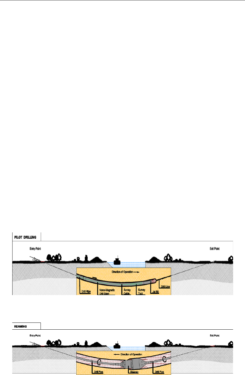
nique, three installation stages are considered:
Pilot drilling
Reaming the initial pilot borehole
Pulling back the pipeline
Figure 1.1: HDD / Pilot drilling (DCA-guidelines)
Figure 1.2: HDD / Pre-reaming (DCA-guidelines)
2 of 324 Deltares
General Information
Figure 1.3: HDD / Pull back operation (DCA-guidelines)
During the final stage, a drilling is carried out, using a relatively small drill bit, under the object
that has to be crossed – for example, a road, railway, waterway or a nature reserve. This initial
borehole is called a pilot hole. The diameter of the pilot hole is then enlarged using a reamer.
Depending on the required final borehole diameter, the borehole can be enlarged in several
stages using reamers of increasing diameters. After reaming, the diameter of the borehole
should be 1.3 to 1.5 times larger than the diameter of the pipeline. After preparing the pipeline
near the exit point of the borehole, the pipeline is finally pulled into the borehole.
Figure 1.4: Reamer and cutting wheel
During all drilling stages, drilling fluid is pumped under pressure into the borehole. The main
function of drilling fluid is to transport cuttings from the drilling head through the borehole
and to the ground surface. A specific minimum pressure is required for the transport function
of the drilling fluid. However, the fluid pressure in the borehole should not exceed a specific
maximum value. The maximum value is related to the strength of the soil around the borehole.
If the maximum fluid pressure is exceeded, a ‘blow-out’ may occur. Besides the pressure of
the drilling fluid, other factors play a role in the design process. Both the strength of the
pipeline during the pull back operation and the strength of the pipeline in operation need to be
sufficient to withstand the forces acting on the pipeline.
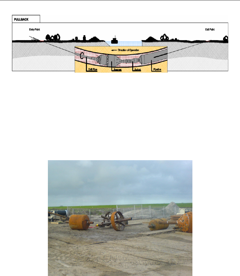
1.2.2 Micro Tunneling
Micro tunneling is the technique which uses a micro tunneling boring machine (MTBM) to
remove the soil. Micro tunneling usually starts horizontal at a certain level below the surface.
Start and reception shafts are created for the micro tunneling machine. In the start shaft a
Deltares 3 of 324
D-GEO PIPELINE
, User Manual
jacking frame and micro tunneling machine in front of pipe sections are installed. The jacks
push the pipe elements section by section ahead towards the reception shaft. As the length
of the advancing micro tunnel increases, the friction forces along the micro tunneling machine
and the pipe segments will increase. Lubrication fluid may be applied to reduce the friction.
Very often at the front of the Micro tunneling machine drilling fluid is used for soil removal and
front stabilization.
Figure 1.5: Jacking frame and micro tunneling machine in the start shaft
1.2.3 Installation in trench
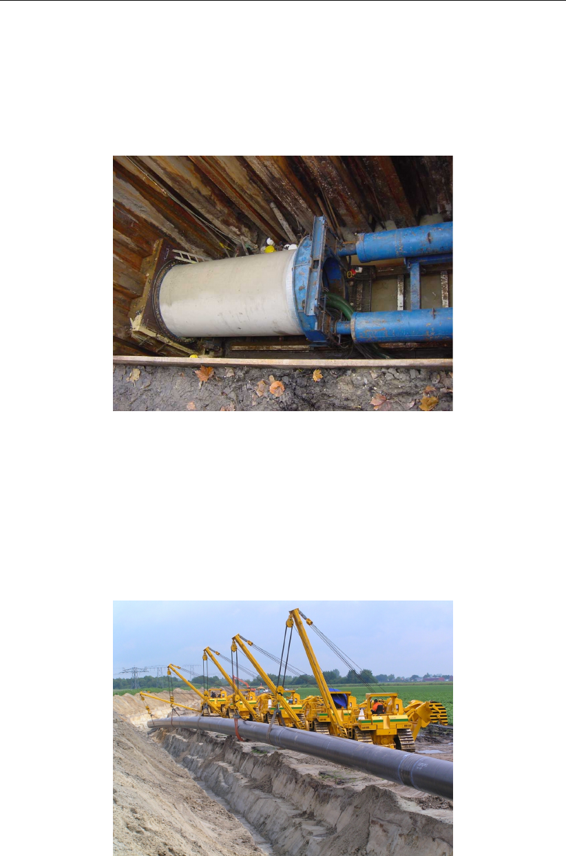
The majority of the underground pipelines are installed in a trench. After excavation of the
trench the pipeline is installed on the bottom of the trench (Figure 1.6) and is subsequently
covered by the excavated soil. The interaction between the pipe and the condition of the soil
material, which is placed back in the trench plays an important role in the engineering of the
pipe.
Figure 1.6: Pipeline installation in a trench
4 of 324 Deltares

General Information
1.3 Features in standard module (HDD)
In the Netherlands, HDD technique has been used on a large scale since the 1980s. Since
the 1970s, Deltares (formerly known as GeoDelft) has been involved in the development and
execution of trench less technologies. Years of research have resulted in one of the first
design codes for HDD, as well as in a computer program. Since the release of the first version
in 1995,
D-GEO PIPELINE
provides users with the minimum and maximum drilling fluid pressure
during the different phases of construction.
D-GEO PIPELINE
can also analyze the stresses in
the pipeline during and after the installation for different pipeline materials.
This section contains an overview of
D-GEO PIPELINE
’s options available for Horizontal Direc-
tional Drilling (standard module).
1.3.1 Soil profile
Multiple layers. The two-dimensional soil structure can be composed of several soil
layers with an arbitrary shape and orientation. Each layer is connected to a particular
soil type.
Verticals. By placing verticals in the geometry, the coordinates for which output results
will be displayed can be defined.
Soil properties. The well-established constitutive models are based on common soil
parameters for strength and deformation of behavior of specific soil types.
1.3.2 Pipeline materials
D-GEO PIPELINE
is capable of dealing with pipelines made of different materials: steel and
polyethylene. For both pipe materials, a database containing the material data is available.
The database enables a quick re-calculation for alternative material types and dimensions.
1.3.3 Factors
D-GEO PIPELINE
applies partial safety factors to the soil parameters (weight, cohesion, friction
angle and Young’s modulus) and to the loads according either to the NEN series or to the
European Standard CEN.
1.3.4 Results
Following the analysis,
D-GEO PIPELINE
can display results in long table and graphical form.
The tabular report contains:
an echo of the input
soil mechanical calculation results per vertical
drilling fluid pressures calculation results per vertical
pulling force in the pipeline per characteristic point
strength pipeline calculation results
settlement results per vertical
A graphical output of the drilling fluid pressures for all drilling stages and vertical stresses per
vertical can also be viewed.
Deltares 5 of 324
D-GEO PIPELINE
, User Manual
1.4 Features in additional modules
D-GEO PIPELINE
comes as a standard module (section 1.3), which can be extended further
with other modules to fit three other applications related to pipeline installation:
Micro Tunneling module (section 1.4.1)
Trenching module (section 1.4.2)
1.4.1 Micro Tunneling module
Face support pressures
The micro tunneling machine changes the stress conditions in the soil. The deviations from
the original stress conditions are largely determined by the size of the overcut and the applied
shield. Small deviations from the original conditions are acceptable as the stability of the soil
adjacent to the micro tunneling machine is maintained. A relative low face support pressure
may lead to collapse of the soil in front of the shield, which in turn may lead to subsidence
of the surface or to settlement of soil layers below a construction or pipeline. A relatively
high face support pressure can lead to a blow out of drilling fluid or may lead to heave of the
surface.
Figure 1.7: Face support pressures
While drilling the shield pressures have to be kept between certain limits. To prevent the
possibility of collapse in of the soil in front of the micro tunneling shield, causing subsidence,
the soil at the front is kept stable by maintaining a minimal face pressure. Depending on the
soil type the minimal face support pressure can be calculated using Jancsecz and Steiner
theory (Jancesz and Steiner,1994), or Broms and Bennermark theory (Broms and Benner-
mark,1967). A maximum support pressure should not be exceeded to prevent uplift of the
soil above the micro tunneling machine or a blow out of drilling fluid towards the surface. The
support pressure, the target pressure during drilling should be in between the two limits. At
the target pressure, the face support pressure is in equilibrium with the current horizontal soil
pressure.
6 of 324 Deltares
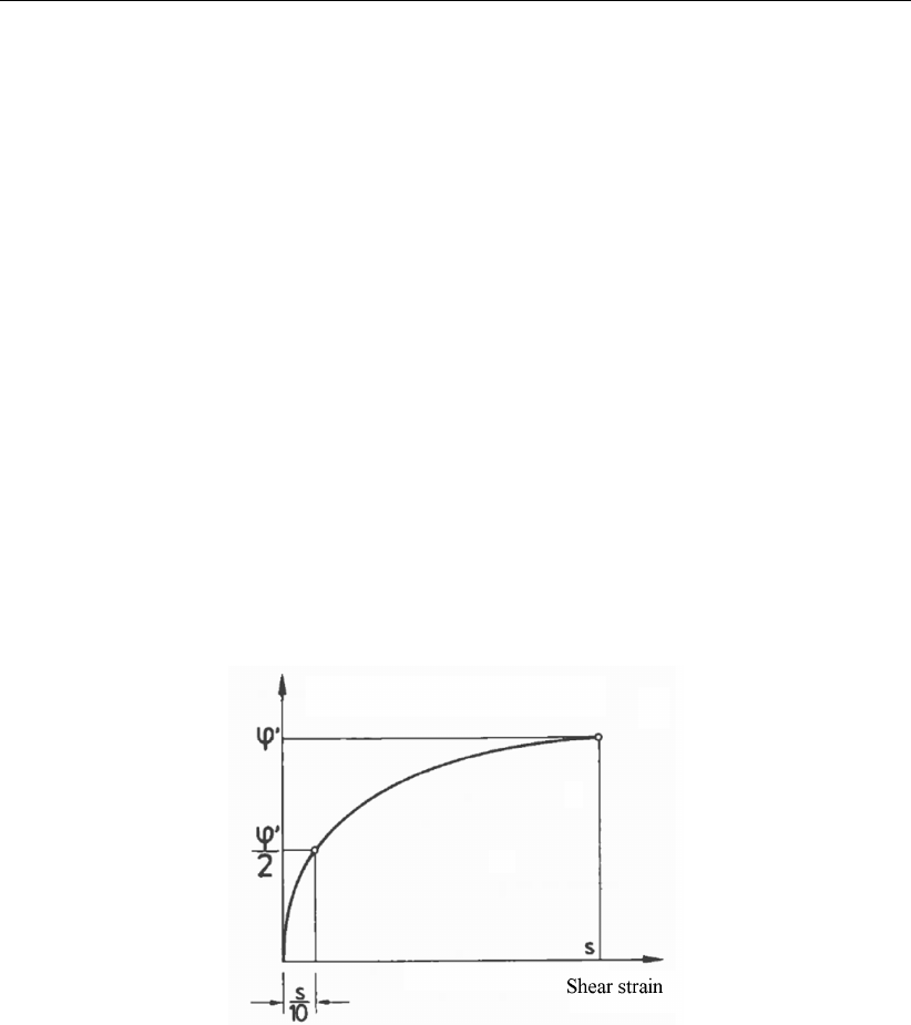
General Information
Thrust force
The micro tunneling machine is at the front of the advancing pipe sections. As the length of
the advancing micro tunnel increases, the friction forces along the micro tunneling machine
and the pipe segments increases. Lubrication fluid may be applied to reduce the friction.
D-GEO PIPELINE
compares the predicted thrust force with the maximum allowable thrust force
of the pipeline.
Surface subsidence
During the micro tunneling drilling process the volume of removed soil is generally larger than
the volume of the tunnel (overcut). The volume difference will lead to soil movement towards
the borehole, which in turn will lead to surface subsidence. The magnitude of the subsidence
(trough) is also calculated.
Arching effect
D-GEO PIPELINE
applies a reduced neutral soil load to incorporate the effect of arching. The
amount of reduction depends on the depth of the pipeline, diameter and the soil properties.
For micro tunneling the effect of arching on the soil load is calculated. Due to the relative
small overcut around the borehole arching is not completely developed.
Figure 1.8: Modelisation of the effect of arching
Pipeline stress analysis
For pipe stress analysis very often special programs need to be used. These programs need
an advanced set of soil mechanical parameters, provided by
D-GEO PIPELINE
. This will gener-
ate a complete spring model around the pipeline for further analysis.
1.4.2 Trenching module
Installation in a trench is the most common way of pipeline installation. In case of pipeline
installation in a trench the interaction between the pipe and the soil material, which is placed
back in the trench plays an important role in the development of the soil load. Besides the
condition of the soil material with which the trench is back-filled, the following parameters
determine the soil load for a pipeline in a trench:
Dimensions of the trench
Soil type in which the trench is excavated
Soil type with which the trench is back-filled
Deltares 7 of 324
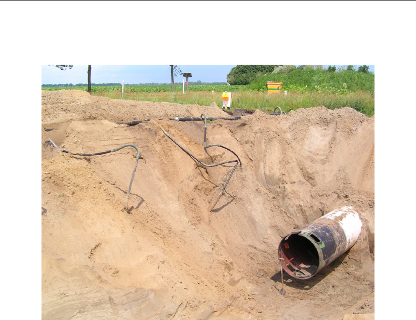
D-GEO PIPELINE
, User Manual
Unit weight of the soil material with which the trench is back-filled
The stiffness of the pipeline
Figure 1.9: Pipeline installation in trench
Features
Graphical user interface for input of soil data.
Advanced input of the ground water pressure distribution.
Upheaval and Uplift check.
Graphical output of the calculated uplift safety factor.
Graphical output of the calculated upheaval safety.
3 dimensional pipeline configuration.
Calculation of settlement of the soil layers below the pipeline.
Output of soil mechanical parameters for an extensive pipeline stress analysis.
Initial soil load
For advanced pipe stress analyses very often special programs need to be used. These
programs need an advanced set of soil mechanical parameters, provided by
D-GEO PIPELINE
.
The programs will generate a complete spring model around the pipeline for further analyses.
The soil mechanical parameters include the initial soil load. In the period directly after the
installation of the pipeline in the trench, the compaction of the fill plays an important role in the
soil pipe interaction. The compaction of the fill leads to differential settlement of the fill above
the pipe and adjacent to the pipe.
8 of 324 Deltares
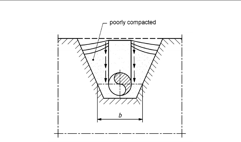
General Information
Figure 1.10: Compaction of the fill after pipeline installation
Uplift safety
Pipeline installation in wet soft soil environments may lead to buoyant behavior of the pipeline.
In case of superficial installation the soil cover above the pipeline may be insufficient to with-
stand the buoyant force of an empty pipeline.
1.5 History
D-GEO PIPELINE
is formerly known as MDrill until version 5.1. This program is a dedicated tool
for designing pipelines constructed using the horizontal directional drilling technique (HDD),
the micro tunnelingor the construction in trench. Deltares has been developing
D-GEO PIPELINE
since 1992.
The first successful pipeline installation using the HDD technique Horizontal Directional Drilling
was carried out under a river in the US. From 1979 onwards, the HDD technique gradually
broke through internationally. The first application in The Netherlands was in 1983/1984 for
the construction of a gas pipeline under the Buiten IJ in Amsterdam. Unlike conventional
construction methods, the HDD technique can be used to construct pipelines without digging
trenches and pits – for example, using sag pipes, pipe jacking or micro tunneling. And it also
significantly shortens the construction time.
After the first application of the HDD technique, the NV Nederlandse Gasunie (Dutch Gas
Corporation) took the initiative to form a research team to investigate the new construction
technique. GeoDelft was a member of that research team, which investigated the construction
of two pilot projects in the Netherlands.
The two pilot horizontal directional drillings were carried out in 1985. While the pipeline was
being installed, measurements were taken to gain a greater understanding of the behavior
of the soil around the borehole. The results of the research were used to define preliminary
guidelines that must be taken into account when designing and constructing pipelines using
the HDD method.
Since the first pilot projects, a large number of HDD’s have been carried out, and the HDD
technique has become a quick and reliable method for constructing cables and pipelines under
Deltares 9 of 324

D-GEO PIPELINE
, User Manual
waterways and other objects.
Continuation of the research has led to a greater store of knowledge about soil behavior, the
stresses in the pipes, and the fluid pressures in the borehole. The
D-GEO PIPELINE
computer
program was developed on the basis of this knowledge.
MDrill version 1.0 was first released in 1995. Some new features, such as the option for
performing a strength calculation, were added in 1998.
MDrill version 4.0 includes an adapted calculation of maximum allowable drilling fluid pres-
sures and an adjusted strength calculation according to the NEN 3650 series.
MDrill version 5.1 includes an adapted calculation of maximum allowable drilling fluid pres-
sures and an adjusted strength calculation according to the new NEN 3650 series. Horizontal
curves can be taken into account. The settlement calculation using the Koppejan or the Iso-
tache models is also added. Bundled pipeline are now supported. A library with standard
pipes for steel and polyethylene is available. The mud pressure charts have been improved.
Exporting soil parameters in versatile format (*.csv) is possible.
D-GEO PIPELINE
version 6.1 (2010) includes two new techniques for pipeline installation: the
Micro tunneling module (section 1.2.2) and the Construction in trench module (section 1.2.3).
New tutorials (7 to 12) have been added to explain the use of both techniques. Small bugs
have been solved: pulling forces for bundled pipes, (horizontal) projected length needed for
vertical testing and mud pressure plots, default values for maximum deflection of Steel and
PE have been exchanged, factor on modulus of subgrade reaction correctly used, in case of
bundles the load angle and bedding angle are given by user (not automatically set to 30 de-
grees any more), the maximum test pressure is increased. Moreover some minor changes in
the report have been made.
D-GEO PIPELINE
version 6.2 (2012) includes an adaptation for dead end pipe ("Dead end"
pipe has no production phase). Moreover some minor issues have been solved.
D-GEO PIPELINE
version 6.3 (2013) includes the following changes: the changes in the Dutch
norm NEN 3650:2012 series (NEN,2012a,b,c) and NEN 3651:2012 (NEN,2012d) are incor-
porated, it is possible to add traffic loads, safety factors from the European Standard CEN are
added, the report is available in French, the temperature stresses are calculated, the known
issue about thrusting forces is solved and the wrong usage of boundaries (for micro-tunneling)
is solved.
D-GEO PIPELINE
version 14.1 (2014) For micro tunneling, the calculation of the minimum and
maximum face support pressures is updated so that the target value is between the minimum
and maximum values. The “Check on calculated stresses for load combination 1 (HDD)” is
now correctly performed. The linear settlement coefficient αgis now a user-defined value in
the Pipe Engineering window (section 4.6.3.1). For HDD - Strength calculation, the load factor
on installation finstall is used for the calculation of the axial bending stress σb(Equation 23.23).
D-GEO PIPELINE
version 15.1 (2015) The default value of the allowable deflection of pipe for
steel is changed to 15% (instead of 5%), as prescribed by the NEN. For bundle, the piggability
is checked using the diameter of the considered pipe, not the equivalent diameter. A toggle
button Same scale X and Y axis is implemented in the Input and Top View windows
(Figure 2.1), to switch between same scale for X and Y-axis and not same scale for X and
Y-axis. A Reset button in the Defaults window (Figure 4.43) is added to get the default factors
prescribed by the selected norm (NEN or CEN); when a factor differs from the norm, it is
displayed in red.
10 of 324 Deltares
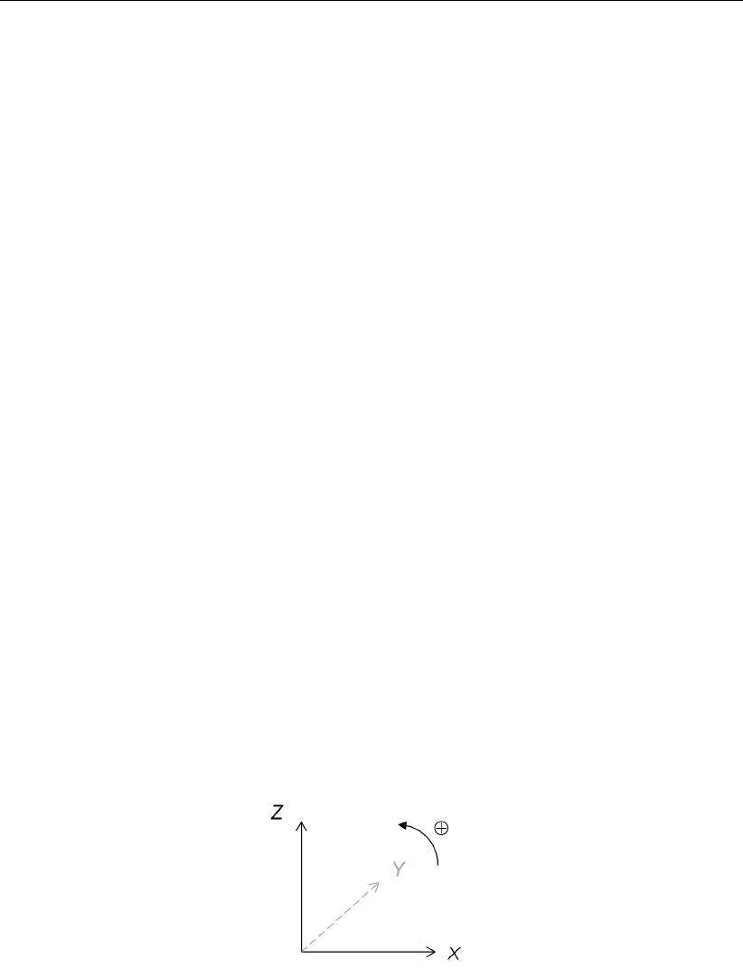
General Information
D-GEO PIPELINE
version 16.1 (2016) With this version, license(s) can be borrowed for a cer-
tain period allowing working without connection to the licence server (see section 3.2.5 for
more information).
1.6 Minimum System Requirements
The following minimum system requirements are needed in order to run and install the
D-GEO PIPELINE
software, either from CD or by downloading from the Deltares website via MS Internet Ex-
plorer:
Operating systems:
Windows 2003,
Windows Vista,
Windows 7 – 32 bits
Windows 7 – 64 bits
Windows 8
Hardware specifications:
1 GHz Intel Pentium processor or equivalent
512 MB of RAM
400 MB free hard disk space
SVGA video card, 1024 ×768 pixels, High colors (16 bits)
CD-ROM drive
Microsoft Internet Explorer version 6.0 or newer (download from www.microsoft.com)
1.7 Definitions and Symbols
Co-ordinate system
The horizontal axis is defined as the Xaxis. The vertical axis is defined to be the Z-direction.
Upward is positive and downward negative. Perpendicular to the cross section is the Ydi-
rection. The Lco-ordinate is the projection of the horizontal co-ordinate Xalong the pipeline
trajectory.
Figure 1.11: Co-ordinate system
Geometric data
ACross-section of the pipe: A=π(r2
0−r2
i)mm2
DoOuter diameter of the pipe mm
Deq Equivalent diameter of the bundled pipeline mm
DgAverage diameter of the pipe: Dg=Do−dnmm
DiInner diameter of the pipe: Di=Do−2dnmm
dMinimum wall thickness of the pipe: d=dn(1 −δt/100) mm
dnNominal wall thickness of the pipe mm
dn;eq Equivalent nominal wall thickness of a bundled pipeline mm
IbMoment of inertia of the pipe: Ib=π(D4
o−D4
i)/64 mm4
Deltares 11 of 324

D-GEO PIPELINE
, User Manual
IwMoment of inertia of the wall: Iw=d3
n/12 mm4/mm
lovercut Difference between the hole radius and the outer radius of the prod-
uct pipe (micro tunneling)
mm
r0Outer radius of the pipe mm
rgAverage radius of the pipe mm
riInner radius of the pipe mm
WbResisting moment of the pipe: Wb= 2 Ib/Domm3
WwResisting moment of the wall: Ww=d2
n/6mm3/mm
δtNegative wall thickness tolerance %
Pipe material data
EbYoung’s modulus of the pipe N/mm2
Reb Yield strength of the steel pipe N/mm2
Reb;short Yield strength of the polyethylene pipe at sort term N/mm2
Reb;long Yield strength of the polyethylene pipe at long term N/mm2
γbUnit weight of the pipe material kN/m3
Process data
pdDesign pressure N/mm2
ptTest pressure N/mm2
∆tTemperature variation K
Pipeline configuration
Xleft X-coordinate of the left point m
Yleft Y-coordinate of the left point m
Zleft (Vertical) Z-coordinate of the left point m
Xright X-coordinate of the right point m
Yright Y-coordinate of the right point m
Zright (Vertical) Z-coordinate of the right point m
ϕleft Left angle of the pipe radians
ϕright Right angle of the pipe radians
Zlowest Lowest level of the pipe m
Rleft Vertical bending radius of the pipe at the left side m
Rright Vertical bending radius of the pipe at the right side m
Rrol Bending radius of the rollers m
Soil properties
aAdhesion kN/m2
aDirect compression index acc. to Isotache model –
bSecular compression index acc. to Isotache model –
cCoefficient of secular compression rate acc. to Isotache model –
cCohesion kN/m2
cuUndrained cohesion kN/m2
CpPrimary compression coefficient below Pc–
Cp’ Primary compression coefficient above Pc–
CsSecondary compression coefficient below Pc–
Cs’ Secondary compression coefficient above Pc–
EYoung’s modulus kN/m2
GShear modulus: G=E/ (2 (1 + ν)) kN/m2
OCR Over-consolidation ratio –
12 of 324 Deltares

General Information
PcPreconsolidation pressure kN/m2
P OP Pre-overburden pressure kN/m2
δFriction angle between the soil and the pipeline Radians
ϕFriction angle Radians
γunsat Unsaturated (dry) unit weight kN/m3
γsat Saturated (wet) unit weight kN/m3
γwUnit weight of water kN/m3
νPoisson’s ratio –
Soil mechanical data
alub fluid Adhesion of the lubrification fluid N/mm2
BWidth of the foundation element (=Do) m
B1Half width of the covered ground column m
CCompression index (soil dependent constant) –
dcDepth factor for the effect of the cohesion –
dqDepth factor for the effect of the soil cover –
FrPermanent friction due to arching effect N/mm2
Fmax Maximal adhesion N/mm2
hSoil cover above the borehole m
hpSoil cover above the borehole in the incompressible layer m
HSoil cover above the top of the pipe if the pipe is situated in a com-
pressible layer or thickness of the compressible layer if the pipe is
situated in an incompressible layer
m
khHorizontal modulus of subgrade reaction kN/m3
kv;df Modulus of subgrade reaction of the drilling fluid kN/m3
kv;lub fluid Modulus of subgrade reaction of the lubrification fluid (micro tunnel-
ing)
kN/m3
kv,pipe Vertical modulus of subgrade reaction of the pipe kN/m3
kv,top Vertical modulus of subgrade reaction of the soil upward kN/m3
kv,bottom Vertical modulus of subgrade reaction of the soil downward kN/m3
KaActive earth pressure ratio –
K0Neutral earth pressure ratio: K0= 1 −sin ϕ–
KcLoad coefficient according to Brinch Hansen –
KqLoad coefficient according to Brinch Hansen –
LLength of foundation element m
NcBearing capacity factor for the effect of the cohesion –
NqBearing capacity factor for the effect of the soil cover –
NγBearing capacity factor for the effect of the effective weight of the
soil under the foundation surface
–
pmax’ Maximum passive vertical stress N/mm2
Pwe Ultimate vertical bearing capacity N/mm2
qhe Horizontal bearing capacity N/mm2
qh,n Neutral horizontal stress of the soil N/mm2
qh,r Neutral reduced horizontal stress of the soil N/mm2
qkInitial vertical stress of the soil N/mm2
qnNeutral vertical stress of the soil N/mm2
qn,r Reduced neutral vertical stress of the soil N/mm2
qn,r,v Reduced neutral vertical stress increased with a possible traf-
fic load, including safety factors: qn,r,v =fQn1 ×fQn2 ×
(qn;r +fqv ×qv)
N/mm2
qpPassive vertical stress of the soil N/mm2
qp;max Maximum passive vertical stress N/mm2
Deltares 13 of 324

D-GEO PIPELINE
, User Manual
qvTraffic load N/mm2
scShape factor due to cohesion –
sqShape factor due to soil cover –
sγShape factor due to effective weight of the soil under the foundation
element
–
WMaximal axial friction along the pipeline kN/m
zmax Maximal displacement m
δdRelative displacement of the soil column m
δlub fluid Delta lubrification fluid Radians
ϕbAverage friction angle over the height of the borehole Radians
µPercentage of compaction depending on the type of fill and type of
compaction
–
σ0’ Effective isotrope stress: σ0
0= (σ0
v+σ0
h)/2N/mm2
σcVertical effective stress at the compressibility border N/mm2
σh’ Effective horizontal stress at the pipe center:σ0
h=K×sigma0
vN/mm2
σv’ Effective vertical stress at the pipe center N/mm2
Stress analysis data
f1Factor of friction between pipe and pipe-rollers –
f2Friction between pipe and drilling fluid N/mm2
f3Factor of friction between pipe and soil –
Frr Direct re-rounding factor –
Frr’ Indirect re-rounding factor –
gtCurved force N/mm
KbMoment coefficient for directly transmitted stress at the bottom of
the pipeline, depending on the bedding angle β
–
Kb’ Moment coefficient for indirectly transmitted stress at the bottom of
the pipeline, depending on the bedding angle β
–
KtMoment coefficient for directly transmitted stress at the top of the
pipeline, depending on the bedding angle β
–
Kt’ Moment coefficient for indirectly transmitted stress at the top of the
pipeline, depending on the bedding angle β
–
kyDirect deflection factor depending on the bedding angle β–
ky’ Indirect deflection factor depending on the bedding angle β–
LbLength of the curved part of the pipeline mm
Lrol Length of the pipeline on the roller-lane mm
Ltotal Length of the pipeline from the entry to the exit point mm
L2Length of the pipeline in the straight part of the borehole mm
TTotal pulling force in the pipeline N
T1Pulling force due to friction of the pipeline on the roller-lane N
T2Pulling force due to friction between pipe and drilling fluid N
T3a Pulling force in the curved part of the borehole due to soil reaction N
T3b Pulling force in the curved part of the borehole due to curved forces N
PwPart of pipe filled with fluid during the pull-back operation %
qrSoil reaction N/mm2
QWeight of the pipeline filled with water N/mm
Qeff Effective weight of the pipeline N/mm
Qfilling Weight of the filling (water) N/mm
Quplift Uplift force N/mm
Qpipe Weight of the pipeline N/mm
RBending radius mm
yMaximum displacement mm
αLoad angle Radians
14 of 324 Deltares

General Information
αAlpha pipe material (for polyethylene) –
βBedding angle Radians
δyCalculated deflection of the pipe %
δ0Allowable deflection of the pipe %
δ1Allowable deflection of the pipe (piggability) %
γfill Unit weight of the filling fluid N/mm3
λCharacteristic stiffness pipeline-soil mm−1
σbAxial bending stress N/mm2
σpt Internal stress around the pipeline caused by test pressure ptN/mm2
σpx Axial internal stress N/mm2
σpy Internal stress around the pipeline caused by design pressure pdN/mm2
σqn Tangential stress (directly transmitted) as a result of the bending N/mm2
σqr Tangential stress (indirectly transmitted) as a result of the bending N/mm2
σtAxial stress due to pull-back N/mm2
Drilling fluid data
dp/dz Flow resistance per unit length of borehole kN/m3
floss Circulation loss factor –
hHeight between drilling head and exit point of the drilling fluid m
LDistance in the borehole between the drilling head and the exit point
of the drilling fluid
m
pmax;d Maximum drilling fluid pressure for drained conditions kN/m2
pmax;und Maximum drilling fluid pressure for undrained conditions kN/m2
p1Static pressure of the drilling fluid column kN/m2
p2Excess pressure necessary to maintain the annular flow of drilling
fluid with cuttings in the borehole
kN/m2
QCalculated flow rate m3/s
Qann Annular back-flow rate m3/s
Qreq Requested flow rate necessary to initiate flow of drilling fluid m3/s
RbRadius of the borehole m
Rp;max Maximum allowable radius of the plastic zone m
uPore pressure kN/m2
εg;max Maximum deformation of the borehole –
γdf Unit weight of the drilling fluid kN/m3
µdf Plastic viscosity of the drilling fluid kN.s/m2
τdf Yield point of the drilling fluid kN/m2
Partial safety factors
fburst Safety factor on hydraulic heave –
fsilo Overburden factor on silo effect –
fuSafety factor on water pressure u–
fuplift Safety factor on uplift –
fσhSafety factor on the horizontal effective stress –
NStability ratio for the calculation of the minimal support pressure –
SFactor of importance –
δ0Maximum allowable deflection of the pipe %
δ1Maximum allowable deflection of the pipe for piggability %
γimp;long Safety factor on implosion at long term –
γimp;short Safety factor on implosion at short term –
γmPartial material factor (only for steel). –
γm;test Partial material factor test pressure (only for steel) –
Deltares 15 of 324

D-GEO PIPELINE
, User Manual
Contingency factors
fcContingency factor on the cohesion (cor cu) –
fcover Contingency factor on soil cover –
fEContingency factor on the Young’s modulus E–
fkOverall factor on bending moment: fk=fM×finstall ×fR–
fkv Contingency factor on the bedding constant kv–
fMContingency factor on the bending moment M–
fpress;bore Contingency factor on the pressure borehole –
fpull Contingency factor on the pulling force T–
fQn2 Contingency factor on the soil load qn–
fRContingency factor on bending radius R–
fthrust Contingency factor on thrsut force –
fϕContingency factor on the tangent of the friction angle ϕ–
fγContingency factor on the total unit weight γ–
Load factors
finstall Load factor on installation –
fpd Load factor on design pressure pd–
fpd;comb Load factor on design pressure pdin combination –
fpt Load factor on test pressure pt–
fQn1 Load factor on soil load qn–
ftemp Load factor on stress due to the temperature variation ∆t–
fqv Load factor on traffic load qv–
Abbreviations
HDD Horizontal Directional Drilling
MTBM Micro Tunneling Boring Machine
PE Polyethylene
LC Load Combination
1.8 Getting Help
From the Help menu, choose the Manual option to open the User Manual of
D-GEO PIPELINE
in PDF format. Here help on a specific topic can be found by entering a specific word in the
Find field of the PDF reader.
1.9 Getting Support
Deltares Systems tools are supported by Deltares. A group of 70 people in software develop-
ment ensures continuous research and development. Support is provided by the developers
and if necessary by the appropriate Deltares experts. These experts can provide consultancy
backup as well.
If problems are encountered, the first step should be to consult the online Support at:
www.deltares.com in menu ‘Software’. Different information about the program can be found
on the left-hand side of the window (Figure 1.12):
In ‘Support - Frequentely asked questions’ are listed the most frequently asked technical
questions and their answers.
In ‘Support - Known issues’ are listed the issues of the program.
In ‘Release notes D-Geo Pipeline’ are listed the differences between an old and a new
version.
16 of 324 Deltares

General Information
Figure 1.12: ‘Products’ menu of Deltares Systems website (www.deltaressystems.com)
If the solution cannot be found there, then the problem description can be e-mailed (preferred)
or faxed to the Deltares Systems support team. When sending a problem description, please
add a full description of the working environment. To do this conveniently:
Open the program.
If possible, open a project that can illustrate the question.
Choose the Support option in the Help menu. The System Info tab contains all relevant
information about the system and the DSeries software. The Problem Description tab
enables a description of the problem encountered to be added.
Deltares 17 of 324

D-GEO PIPELINE
, User Manual
Figure 1.13: Support window, Problem Description tab
After clicking on the Send button, the Send Support E-Mail window opens, allowing
sending current file as an attachment. Marked or not the Attach current file to mail
check-box and click OK to send it.
Figure 1.14: Send Support E-Mail window
The problem report can either be saved to a file or sent to a printer or PC fax. The document
can be emailed to geo.support@deltaressystems.nl or alternatively faxed to +31(0)88 335
8111.
1.10 Deltares
Since January 1st 2008, GeoDelft together with parts of Rijkswaterstaat /DWW, RIKZ and
RIZA, WL |Delft Hydraulics and a part of TNO Built Environment and Geosciences are form-
ing the Deltares Institute, a new and independent institute for applied research and special-
ist advice. Founded in 1934, GeoDelft was one of the world’s most renowned institutes for
geotechnical and environmental research. As a Dutch national Grand Technological Institute
(GTI), Deltares role is to obtain, generate and disseminate geotechnical know-how. The insti-
tute is an international leader in research and consultancy into the behavior of soft soils (sand
clay and peat) and management of the geo-ecological consequences which arise from these
activities. Again and again subsoil related uncertainties and risks appear to be the key factors
18 of 324 Deltares

General Information
in civil engineering risk management. Having the processes to manage these uncertainties
makes Deltares the obvious partner in risk management for all parties involved in the civil and
environmental construction sector. Deltares teams are continually working on new mecha-
nisms, applications and concepts to facilitate the risk management process, the most recent
of which is the launch of the concept "GeoQ" into the geotechnical sector.
For more information on Deltares, visit the Deltares website: www.deltares.com.
1.11 Deltares Systems
Deltares Systems (formerly known as Delft GeoSystems) converts Deltares’s knowledge into
practical geo-engineering services and software. Deltares Systems has developed a suite
of software for geotechnical engineering. Besides software, Deltares Systems is involved in
providing services such as hosting on-line monitoring platforms, hosting on-line delivery of
site investigation, laboratory test results, etc. As part of this process Deltares Systems is
progressively connecting these services to their software. This allows for more standardized
use of information, and the interpretation and comparison of results. Most software is used
as design software, following design standards. This however, does not guarantee a design
that can be executed successfully in practice, so automated back-analyses using monitoring
information are an important aspect in improving geotechnical engineering results. For more
information about Deltares Systems’ geotechnical software, including download options, visit
www.deltaressystems.com.
1.12 On-line software (Citrix)
Besides purchased software, Deltares Systems tools are available as an on-line service. The
input can be created over the internet. Heavy duty calculation servers at Deltares guarantee
quick analysis, while results are presented on-line. Users can view and print results as well
as locally store project files. Once connected, clients are charged by the hour.
For more information, please contact the Deltares Sales team:
sales@deltaressystems.com.
Deltares 19 of 324

D-GEO PIPELINE
, User Manual
20 of 324 Deltares

2 Getting Started
This Getting Started chapter aims to familiarize the user with the structure and user interface
of
D-GEO PIPELINE
. The Tutorial section which follows uses a selection of case studies to
introduce the program’s functions.
2.1 Starting D-GEO PIPELINE
To start
D-GEO PIPELINE
, click Start on the Windows menu bar and then find it under Programs,
or double-click a
D-GEO PIPELINE
input file that was generated during a previous session.
For an
D-GEO PIPELINE
installation based on floating licenses, the Modules window may ap-
pear at start-up (section 3.2.5). Check that the correct modules are selected and click OK.
When
D-GEO PIPELINE
is started from the Windows menu bar, the last project that was worked
on will open automatically, unless the program has been configured otherwise under Tools:
Program Options (section 3.2).
2.2 Main window
When
D-GEO PIPELINE
is started, the main window is displayed (Figure 2.1). This window
contains a menu bar (section 2.2.1), an icon bar (section 2.2.2), a View Input window (sec-
tion 2.2.3) displaying the pre-selected or most recently accessed project, an info bar (sec-
tion 2.2.4), a title panel (section 2.2.5) and a status bar (section 2.2.6).
Figure 2.1: Main Window
The first time
D-GEO PIPELINE
is started after installation, the View Input window will be closed.
When a new file is created, the default model is Horizontal directional drilling and the project
name is Project1.
Deltares 21 of 324
D-GEO PIPELINE
, User Manual
2.2.1 The menu bar
To access the
D-GEO PIPELINE
menus, click one of the items on the menu bar.
Figure 2.2: D-GEO PIPELINE menu bar
The menus contain the following functions:
File Standard Windows options for opening, saving and sending files as well
as several
D-GEO PIPELINE
options for exporting and printing the active
window and reports (section 3.1).
Project Definition of the model types, options for Project Properties and View
Input File (section 4.1).
Soil Definition of soil type properties (section 4.2).
Geometry Definition of layers, soil types and piezometric lines (section 4.3).
GeoObjects Definition of the border between compressible top layers and underly-
ing non-compressible soil layers, the border between impermeable and
permeable soil layers and definition of the verticals (X-coordinates) for
which results will be shown (section 4.4).
Loads Definition of the traffic loads if present (section 4.5).
Pipe Definition of the pipeline configuration and input of pipeline parameters
(section 4.6).
Defaults Input of factors (section 4.7).
Calculation A wide range of calculation options. Determine the settlements and
stresses along the verticals (chapter 5).
Results Graphical or tabular output of the results (chapter 6).
Tools Options for editing
D-GEO PIPELINE
program default settings (sec-
tion 3.2).
Window Default Windows options for arranging the
D-GEO PIPELINE
windows
and choosing the active window.
Help Online Help (section 1.8).
2.2.2 The icon bar
The buttons on the icon bar can be used to quickly access frequently used functions (see
below).
Figure 2.3: D-GEO PIPELINE icon bar
Click on the following buttons to activate the corresponding functions:
Start a new
D-GEO PIPELINE
project.
Open the input file of an existing project.
Save the input file of the current project.
Print the contents of the active window.
22 of 324 Deltares
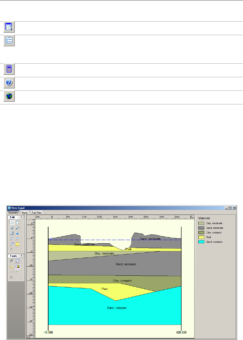
Getting Started
Display a print preview of the current contents of the View Input window.
Open the Project Properties window. Here the project title and other identification
data can be entered, and the View Layout and Graph Settings for the project can be
determined.
Start the calculation.
Display the contents of online Help.
Display the first page of the Deltares Systems website: www.deltaressystems.com
2.2.3 View Input
The View Input window displays the geometry and additional
D-GEO PIPELINE
input for the
current project. The window has three tabs:
Geometry
In this view (Figure 2.4), the positions and soil types of different layers can be de-
fined, inspected and modified. For more information about these general options for
geometrical modeling, see chapter 7. See also the description of the Geometry menu
(section 4.3).
Figure 2.4: View Input window, Geometry tab
Input
In this view (Figure 2.5), the additional
D-GEO PIPELINE
-specific input can be defined,
inspected and modified. See below in this section for more information about the various
options.
Deltares 23 of 324
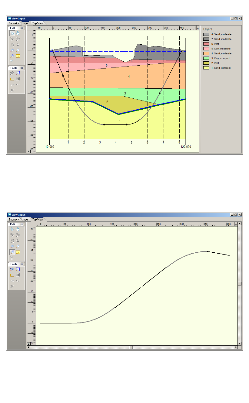
D-GEO PIPELINE
, User Manual
Figure 2.5: View Input window, Input tab
Top View
In this view (Figure 2.6), the top view of the pipeline longitudinal cross section is shown.
Figure 2.6: View Input window, Top View tab
The panel on the left of the view includes buttons for entering data and manipulating the
graphical view. Click the following buttons to activate the corresponding functions:
24 of 324 Deltares
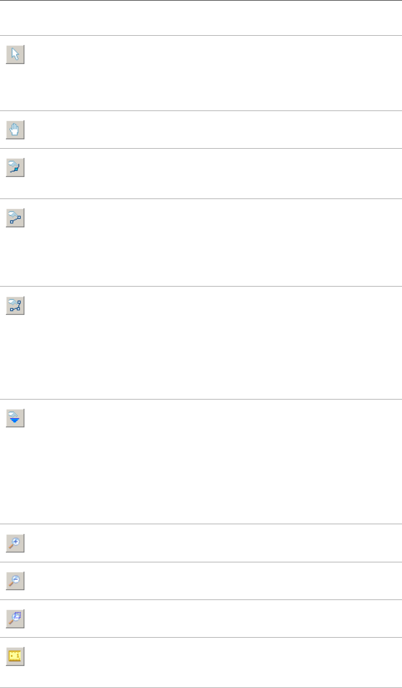
Getting Started
Select and Edit mode
In this mode, the left-hand mouse button can be used to select a previously-defined
verticals or loads in the View Input mode. Item can then be deleted or modified
by dragging or resizing, or by clicking the right-hand mouse button and choosing
options from the menu displayed. Pressing the Escape key return the user to this
Select and Edit mode.
Pan button
Click this button to change the visible part of the drawing by clicking and dragging
the mouse.
Add point(s) to boundary / PL-line
Click this button to add points to all types of lines (lines, polylines, boundary lines,
PL-lines). By adding a point to a line, the existing line is split into two new lines. This
provides more freedom when modifying the geometry.
Add single lines(s)
Click this button to add single lines. When this button is selected, the first left-hand
mouse click will add the info bar of the new line and a “rubber band” is displayed
when the mouse is moved. The second left-hand mouse click defines the end point
(and thus the final position) of the line. It is now possible to either go on clicking start
and end points to define lines, or stop adding lines by selecting one of the other tool
buttons, or by clicking the right-hand mouse button, or by pressing the Escape key.
Add polyline(s)
Click this button to add poly-lines. When this button is selected, the first left-hand
mouse click adds the starting point of the new line and a “rubber band” is displayed
when the mouse is moved. A second left-hand mouse click defines the end point
(and thus the final position) of the first line in the poly-line and activates the “rubber
band” for the second line in the poly-line. Every subsequent left-hand mouse click
again defines a new end point of the next line in the poly-line. It is possible to end
a poly-line by selecting one of the other tool buttons, or by clicking the right-hand
mouse button, or by pressing the Escape key.
Add PL-line(s)
Click this button to add a piezometric level line (PL-line). Each PL-line must start
at the left limit and end at the right limit. Furthermore, each consecutive point must
have a strictly increasing X co-ordinate. Therefore, a PL-line must be defined from
left to right, starting at the left limit and ending at the right limit. To enforce this, the
program will always relocate the first point clicked (left-hand mouse button) to the left
limit by moving it horizontally to this limit. If trying to define a point to the left of the
previous point, the rubber band icon indicates that this is not possible. Subsequently
clicking on the left side of the previous point, the new point will be added at the end
of the rubber band icon instead of the position clicked.
Zoom in
Click this button to enlarge the drawing, then click the part of the drawing which is to
be at the center of the new image. Repeat if necessary.
Zoom out
Click this button, then click on the drawing to reduce the drawing size. Repeat if
necessary.
Zoom rectangle
Click this button then click and drag a rectangle over the area to be enlarged. The
selected area will be enlarged to fit the window. Repeat if necessary.
Measure the distance between two points
Click this button, then click the first point on the View Input window and place the
cross on the second point. The distance between the two points can be read at the
bottom of the View Input window. To turn this option off, click the escape key.
Deltares 25 of 324

D-GEO PIPELINE
, User Manual
Add calculation vertical
Click this button to graphically define the position of a vertical.
Undo zoom
Click this button to undo the zoom. If necessary, click several times to retrace each
consecutive zoom-in step that was made.
Zoom limits
Click this button to display the complete drawing.
Same scale for X and Y axis
Click this button to use the same scale for the horizontal and vertical directions.
Automatic regeneration of geometry on/off
When selected, the program will automatically try to generate a new valid geometry
whenever geometry modifications require this. During generation, (poly)lines (solid
blue) are converted to boundaries (solid black), with interjacent layers. New layers
receive a default material type. Existing layers keep the materials that were assigned
to them. Invalid geometry parts are converted to construction elements.
Automatic regeneration may slow down progress during input of complex geometry,
because validity will be checked continuously.
Undo
Click this button to undo the last change(s) made to the geometry.
Redo
Click this button to redo the previous Undo action.
Delete
Click this button to delete a selected element. Note that this button is only available
when an element is selected.
2.2.4 Info bar
This bar situated at the bottom of the View Input window displays the co-ordinates of the
current position of the cursor and the distance between two points when the icon Measure the
distance between two points is selected from the Edit panel.
2.2.5 Title panel
This panel situated at the bottom of the main window displays the project titles, as entered on
the Identification tab in the Project Properties window (section 4.1.2).
2.2.6 Status bar
This bar situated at the bottom of the main window displays a description of the selected icon
of the icon bar (section 2.2.2) or of the View Input window (section 2.2.3).
26 of 324 Deltares
Getting Started
2.3 Files
*.dri Input file (ASCII):
Contains the
D-GEO PIPELINE
specific input. After interactive generation, this file
can be used in subsequent
D-GEO PIPELINE
analyses.
*.drd Dump file (ASCII):
Contains calculation results used for graphical output.
*.drs Setting file (ASCII):
Working file with settings data. This file does not contain any information that is
relevant for the calculation, but only settings that apply to the representation of
the data, such as the grid size.
*.drd Dump file (ASCII):
Contains calculation results used for graphical and report output.
*.geo Input file (ASCII):
Contains the geometry data that can be shared with other D-Series programs.
*.set Working file (ASCII):
Contains program settings data.
*.err If there are any errors in the input, they are described in this file.
*.gef Measurements data in self describing Geotechnical Exchange Format.
2.4 Tips and Tricks
2.4.1 Keyboard shortcuts
Keyboard shortcuts given in Table 2.5 are another way to reach the features of
D-GEO PIPELINE
directly without selecting it from the bar menu. These shortcuts are also indicated in the
corresponding sub-menus.
Table 2.5: Keyboard shortcuts for D-GEO PIPELINE
Keyboard shortcut Opened window
Ctrl + N New
Ctrl + O Open
Ctrl + S Save
F12 Save As
Shift + Ctrl + C Copy Active Window to Clipboard
Ctrl + P Print Report
Ctrl + M Model
Ctrl + T Materials
F9 Start Calculation
Ctrl + R Report
Ctrl + U Drilling Fluid Pressures Plots
Deltares 27 of 324
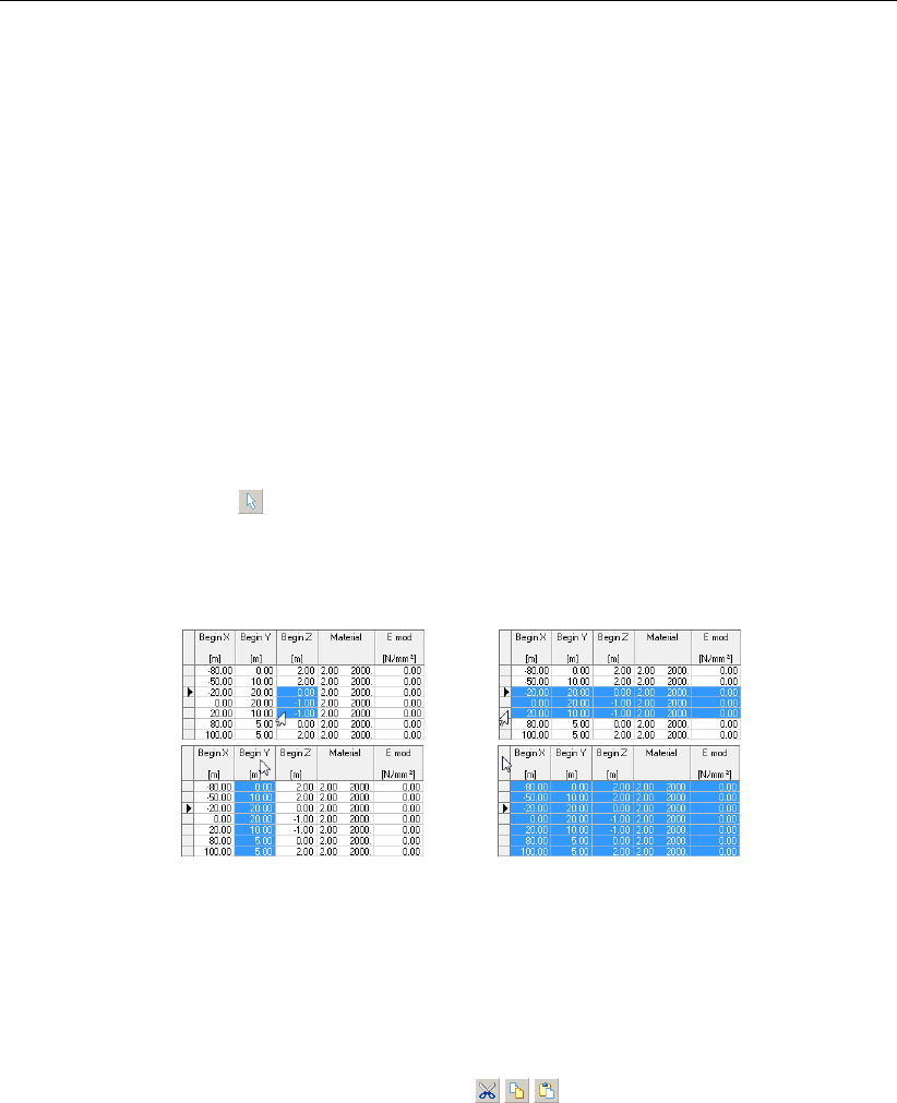
D-GEO PIPELINE
, User Manual
2.4.2 Exporting figures and reports
All figures in
D-GEO PIPELINE
such as top view and graphical output can be exported in WMF
(Windows Meta Files) format. In the File menu, select the option Export Active Window to
save the figures in a file. This file can be later imported in a Word document for example or
added as annex in a report. The option Copy Active Window to Clipboard from the File menu
can also be used to copy directly the figure in a Word document.
The report can be entirely exported as PDF (Portable Document Format) or RTF (Rich Text
Format) file. To look at a PDF file Adobe Reader can be used. A RTF file can be opened
and edited with word processors like MS Word. Before exporting the report, a selection of the
relevant parts can be done with the option Report Selection (section 6.1).
2.4.3 Copying part of a table
It is possible to select and then copy part of a table in another document (an Excel sheet for
example). If the cursor is placed on the left-hand side of a cell of the table, the cursor
changes in an arrow which points from bottom left to top right. Select a specific area by using
the mouse (see a in Figure 2.7). Then, using the copy button (or ctrl+C) this area can be
copied.
a) b)
c) d)
Figure 2.7: Selection of different parts of a table using the arrow cursor
To select a row, click on the cell before the row number (see b) in Figure 2.7). To select a
column, click on the top cell of the column (see c) in Figure 2.7). To select the complete table,
click on the top left cell (see d) in Figure 2.7).
In some tables the buttons Cut,Copy, and Paste are also present at the left hand.
28 of 324 Deltares
3 General
This chapter contains a detailed description of the available menu options for inputting data
for a project, and for calculating and viewing the results. The examples in the Tutorial section
provide a convenient starting point for familiarization with the program.
3.1 File menu
3.1.1 General options
Besides the familiar Windows options for opening and saving files, the File menu contains a
number of options specific to
D-GEO PIPELINE
:
New
Select this option to display the New File window (Figure 3.1). Three choices are avail-
able to create a new geometry:
Select New geometry to display the View Input window, showing only the geome-
try limits (with their defaults values) of the geometry;
Select New geometry wizard to create a new geometry faster and easier using
the wizard option (involving a step-by-step process for creating a geometry, see
section 4.3.2);
Select Import geometry to use an existing geometry.
Figure 3.1: New File window
Copy Active Window to Clipboard
Use this option to copy the contents of the active window to the Windows clipboard so
that they can be pasted into another application. The contents will be pasted in either
text format or Windows Meta File format.
Export Active Window
Use this option to export the contents of the active window as a Windows Meta File
(*.wmf), a Drawing Exchange File (*.dxf) or a text file (*.txt).
Export Report
This option allows the report to be exported in a different format, such as PDF or RTF.
Export Results as xml
This option allows the inputs and results to be exported in an XML format.
Export Results as csv
This option allows the inputs and results to be exported with the SCIA pipeline wizard
in a csv format (Excel). For detailed information, refer to section 3.1.2.
Deltares 29 of 324
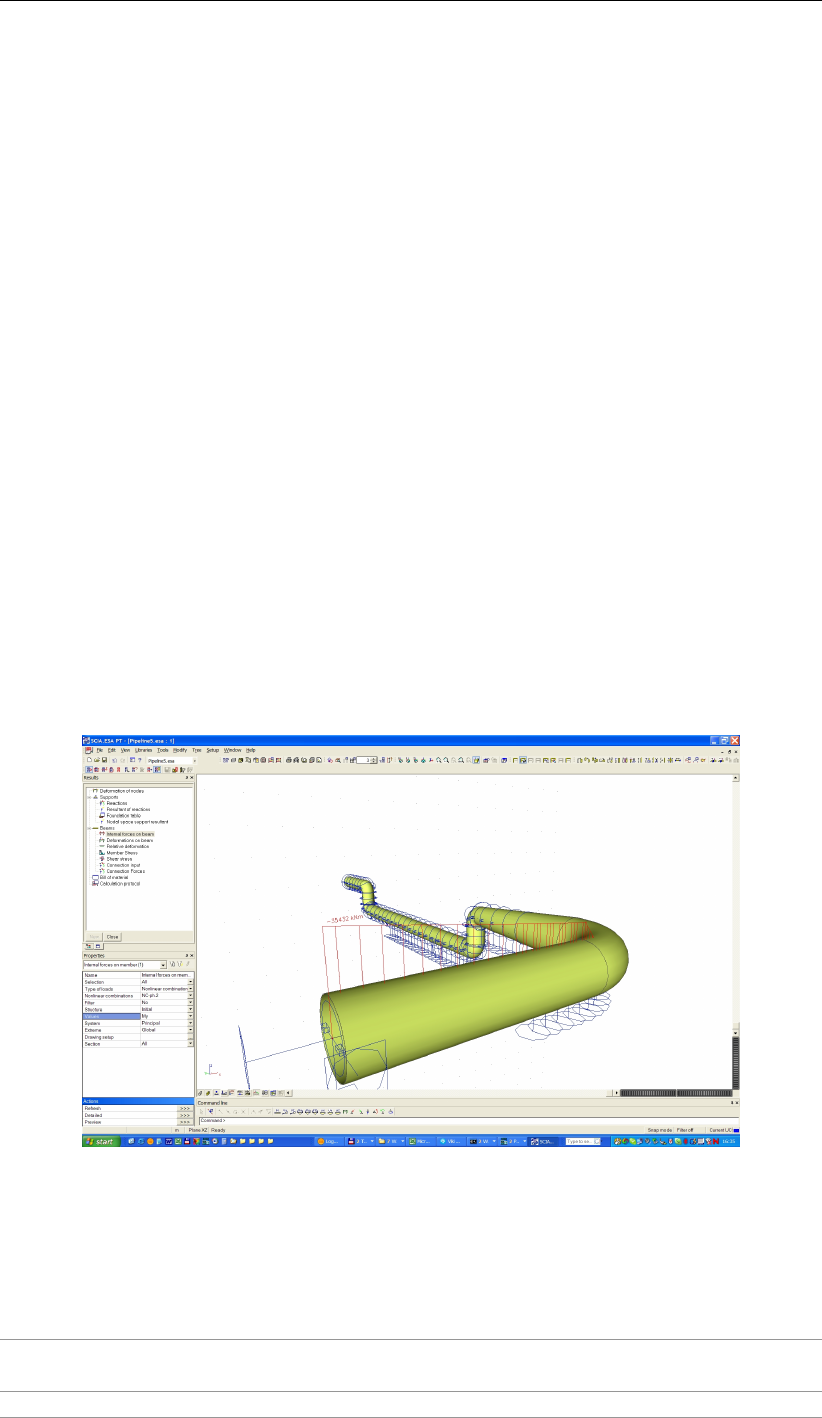
D-GEO PIPELINE
, User Manual
Page Setup
This option allows definition of the way
D-GEO PIPELINE
plots and reports are to be
printed. The printer, paper size, orientation and margins can be defined as well as
whether and where axes are required for plots. Click Autofit to get
D-GEO PIPELINE
to
choose the best fit for the page.
Print Preview Active Window
This option will display a print preview of the current contents of the View Input or
Results windows.
Print Active Window
This option prints the current contents of the View Input or Results windows.
Print Preview Report
This option will display a print preview of the calculation report.
Print Report
This option prints the calculation report.
3.1.2 Option ”Export Results as csv”
For advanced structural analyses, for example the SCIA Pipeline program (Sci) can be used or
an other program. Such a program has advanced options for structural modeling and allows
for accurate analyses of stress distribution (Figure 3.2). In order to do so, such a program
for an advanced pipe stress analysis needs accurate soil mechanical parameters, which are
supplied by
D-GEO PIPELINE
in a CSV (comma-separated values) format file by means of the
option Export Results as csv from the File menu bar of
D-GEO PIPELINE
.
Figure 3.2: 3D configuration in SCIA Pipeline
The CSV file contains the following data’s (calculated without safety factors).
General
Company [-] Name of the company who performed the calculation
with
D-GEO PIPELINE
.
Software [-] Version number of
D-GEO PIPELINE
used.
30 of 324 Deltares
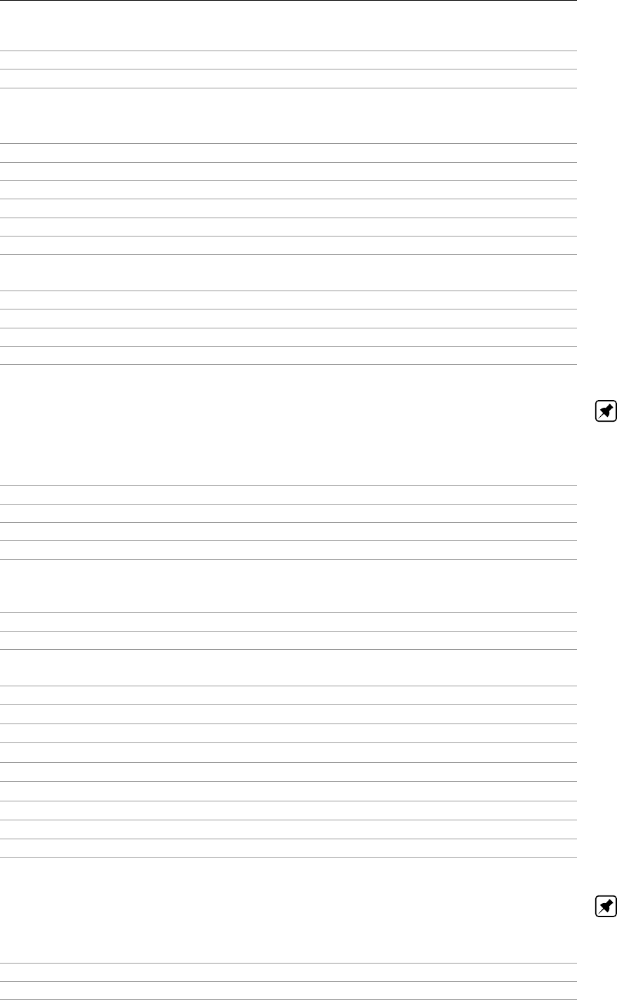
General
Date [yyyy/mm/dd] Date of the calculation with
D-GEO PIPELINE
.
Time [hh:mm:ss] Time of the calculation with
D-GEO PIPELINE
.
Pipeline data’s
P1(x) [m] X co-ordinate of the begin point of the pipeline.
P1(y) [m] Y co-ordinate of the begin point of the pipeline.
P1(z) [m] Z co-ordinate of the begin point of the pipeline.
P2(x) [m] X co-ordinate of the end point of the pipeline.
P2(y) [m] Y co-ordinate of the end point of the pipeline.
P2(z) [m] Z co-ordinate of the end point of the pipeline.
Length Pipe [m] Length along the pipeline between the begin point P1
and the end point P2.
Pipe nr [-]
Diameter Tube [mm] Diameter of the pipe.
Thickness Tube [mm] Wall thickness of the pipe.
Material Tube [-]
Note: Pipeline data’s are not calculated (only user inputted), but are needed in order to
prepare the SCIA Pipeline file.
Calculation verticals
Section nr [-] Number of the calculation vertical.
x [m] X co-ordinate of the calculation vertical.
y [m] Y co-ordinate of the calculation vertical.
z [m] Z co-ordinate of the calculation vertical.
Horizontal soil mechanical data
From [m] Position along the pipeline.
Curved [boolean] Presence or not of curved part along the pipeline.
Delta [m] Horizontal position of the pipeline measured perpen-
dicular from line P1-P2.
f [m] Horizontal settlement of the soil.
Qa [kN/m2] Horizontal active soil pressure.
Qn [kN/m2] Horizontal neutral soil pressure.
Qc [kN/m2] Horizontal consolidation pressure.
Qp [kN/m2] Horizontal passive soil pressure.
C1 [kN/m3] Horizontal modulus of subgrade reaction of the soil.
C2 [kN/m3] Horizontal modulus of subgrade reaction of the soil.
Gap [mm] Gap
UCF(XX) [-] Uncertainty on parameter XX.
Note: Horizontal soil mechanical data are given at both left and right sides of the pipe section.
Vertical soil mechanical data
From [m] Position along the pipeline.
Curved [boolean] Presence or not of curved part along the pipeline.
Deltares 31 of 324
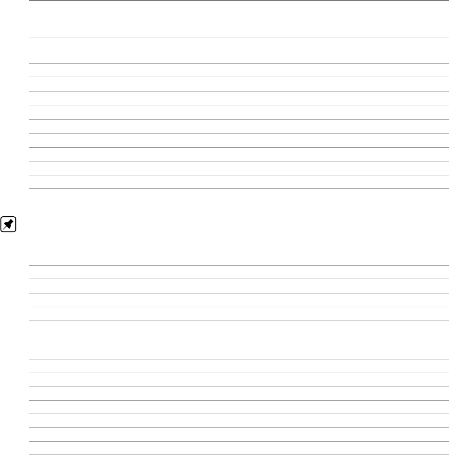
D-GEO PIPELINE
, User Manual
Delta [m] Vertical position of the pipeline measured perpendicu-
lar from line P1-P2.
f [m] Vertical settlement of the soil.
Qa [kN/m2] Vertical active soil pressure.
Qn [kN/m2] Vertical neutral soil pressure.
Qc [kN/m2] Vertical consolidation pressure.
Qp [kN/m2] Vertical passive soil pressure.
C1 [kN/m3] Vertical modulus of subgrade reaction of the soil.
C2 [kN/m3] Vertical modulus of subgrade reaction of the soil.
Gap [mm] Gap
UCF(XX) [-] Uncertainty on parameter XX.
Note: Vertical soil mechanical data are given at both top and bottom sides of the pipe section.
Water
Water height [mm]
C1 [kN/m3] Unit weight of water.
QP [kN/m2] Water pressure.
UCF(XX) [-] Uncertainty on parameter XX.
Axial soil data for friction
From [m] Position along the pipeline.
Coef_Mu_x [-] Friction coefficient in axial direction.
Cx [kN/m3] Stiffness of the friction spring.
Coef_Mu_rx [-] Friction coefficient in axial direction.
Crx [kN/m3] Stiffness of the friction spring.
Factor [-] Factor on friction.
UCF(XX) [-] Uncertainty on parameter XX.
3.2 Tools menu
On the menu bar, click Tools and then choose Options to open the Program Options window.
In this window, the user can optionally define their own preferences for some of the program’s
default values through the following tabs:
(section 3.2.1)View tab
(section 3.2.2)General tab
(section 3.2.3)Locations tab
(section 3.2.4)Language tab
(section 3.2.5)Modules tab
32 of 324 Deltares
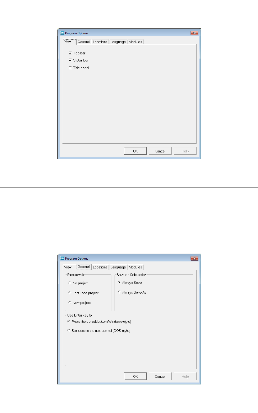
General
3.2.1 Program Options - View
Figure 3.3: Program Options window, View tab
Toolbar
Status bar
Mark the relevant check-box to display the tool bar and/or status bar
(section 2.2.6) each time
D-GEO PIPELINE
is started.
Title panel Mark this check-box to display the project titles, as entered on the Iden-
tification tab of the Project Properties window (section 4.1.2), in the title
panel (section 2.2.5) at the bottom of the View Input window.
3.2.2 Program Options - General
Figure 3.4: Program Options window, General tab
Deltares 33 of 324
D-GEO PIPELINE
, User Manual
Startup with Click one of these toggle buttons to determine how a project should be
initiated each time
D-GEO PIPELINE
is started.
No project: Use the buttons in the toolbar or the options in the File
menu to open an existing project or to start a new one.
Last used project: The last project to be worked on is opened automat-
ically.
New project: A new project is created comprising a sheet pile wall with
a "dummy" soil layer on both sides.
Note that the Startup with option is ignored when
D-GEO PIPELINE
is
started by double-clicking on an input file.
Save on
Calculation
The toggle buttons determine how input data is saved prior to calcu-
lation. It can either be saved automatically, using the same file name
each time, or a file name can be specified every time the data is saved.
Use Enter key to Use the toggle buttons to determine the way the Enter key is used in
D-GEO PIPELINE
: either as an equivalent of pressing the default button
(Windows style) or to shift the focus to the next item in a window (for
users accustomed to the DOS version(s) of the program).
3.2.3 Program Options - Locations
Figure 3.5: Program Options window, Locations tab
Working
directory
D-GEO PIPELINE
will start up with a working directory for selection and
saving of files. Either choose to use the last used directory, or specify
a fixed path.
Use MGeobase
database
Enable this check-box to specify the location of the MGeoBase
database with material data, geometric data etc. Use of this option also
requires once-off local installation of Interbase client software, assum-
ing that the database is residing on a server on which server software
has already been installed.
Settlement
program
The calculation of the settlement of the soil layers below the pipeline
is performed externally by
D-SETTLEMENT
(formerly known as MSet-
tle), the settlement calculation program of the Deltares Systems tools.
Therefore, the directory where the program is installed must be speci-
fied by clicking the Browse button.
34 of 324 Deltares
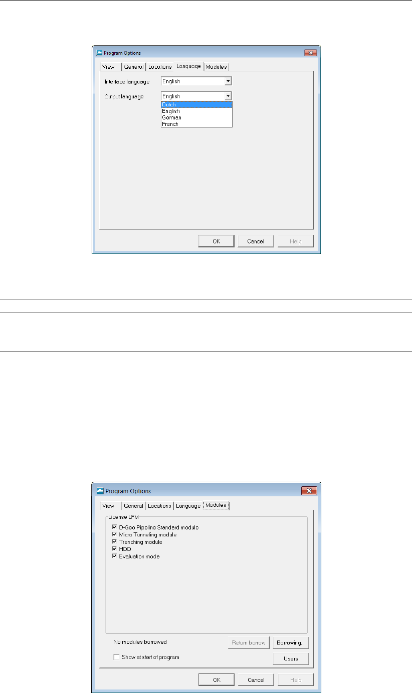
General
3.2.4 Program Options - Language
Figure 3.6: Program Options window, Language tab
Interface language Currently, the only available interface language is English.
Output language The output languages English, German, Dutch and French are sup-
ported. The selected output language will be used in all exported
reports and output plots.
3.2.5 Program Options - Modules
For a
D-GEO PIPELINE
installation based on floating licenses, the Modules tab can be used to
claim a license for the particular modules that are to be used. If the Show at start of program
check-box is marked then this window will always be shown at start-up.
For a
D-GEO PIPELINE
installation based on a license dongle, the Modules tab will just show
the modules that may be used.
Figure 3.7: Program Options window, Modules tab
Deltares 35 of 324
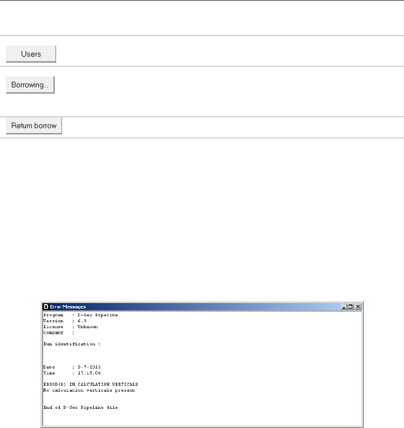
D-GEO PIPELINE
, User Manual
Click this button to see which modules are (at this moment) in used and
who (within the company) is using them.
Click this button to borrow the selected modules for a certain period. The
modules will be taken from the server pool and will be available on this
computer even if no connection to the license server is available. Set the
date and time for the expiration of the borrowing and press OK.
Click this button to end the borrow immediately.
3.3 Help menu
The Help menu allows access to different options.
3.3.1 Error Messages
If errors are found in the input, no calculation can be performed and
D-GEO PIPELINE
opens
the Error Messages window displaying more details about the error(s). Those errors must
be corrected before performing a new calculation. To view those error messages, select the
Error Messages option from the Help menu. They are also written in the *.err file. They will
be overwritten the next time a calculation is started.
Figure 3.8: Error Messages window
3.3.2 Manual
Select the Manual option from the Help menu to open the User Manual of
D-GEO PIPELINE
in
PDF format. Here help on a specific topic can be found by entering a specific word in the Find
field of the PDF reader.
3.3.3 Deltares Systems Website
Select Deltares Systems Website option from the Help menu to visit the Deltares Systems
website (www.deltaressystems.com) for the latest news.
3.3.4 Support
Use the Support option from the Help menu to open the Support window in which program
errors can be registered. Refer to section 1.9 for a detailed description of this window.
36 of 324 Deltares
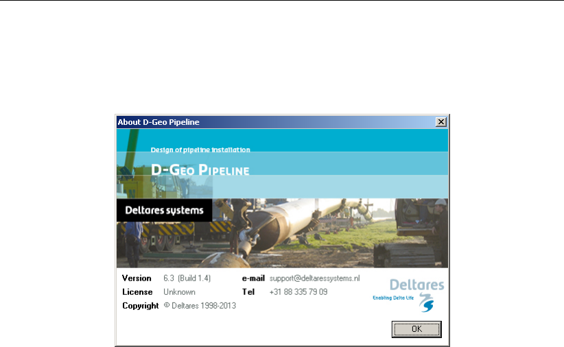
General
3.3.5 About D-GEO PIPELINE
Use the About option from the Help menu to display the About
D-GEO PIPELINE
window which
provides software information (for example the version of the software).
Figure 3.9: About D-GEO PIPELINE window
Deltares 37 of 324

D-GEO PIPELINE
, User Manual
38 of 324 Deltares
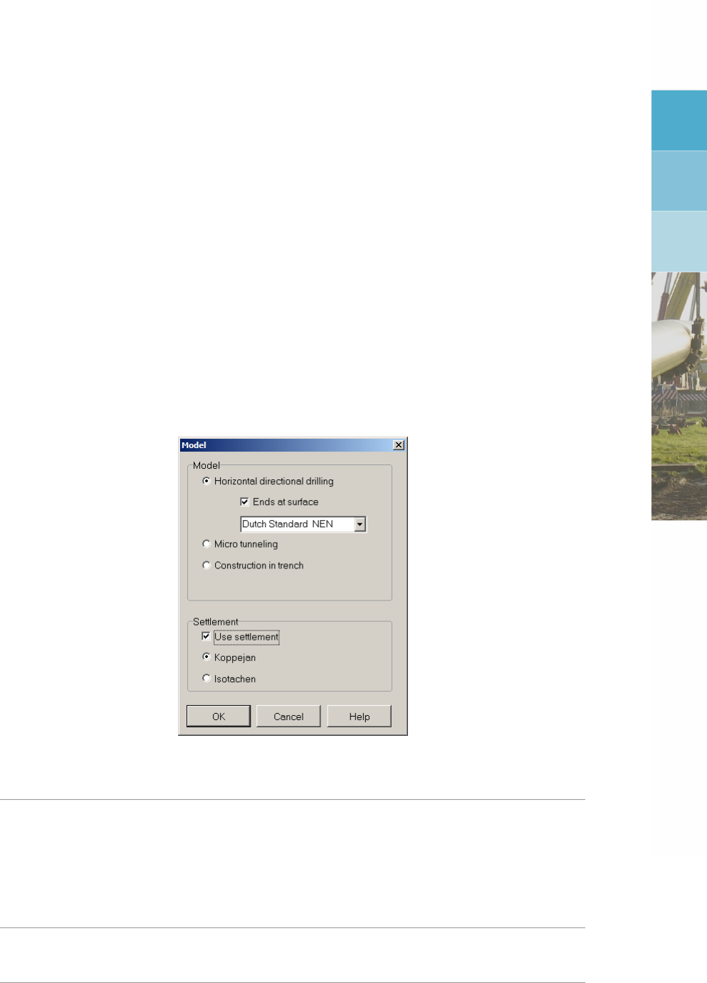
4 Input
Before the design calculations can be started, data for the project needs to be input. The
examples presented in the Tutorial section (chapter 8) can be a convenient starting point.
4.1 Project menu
On the menu bar (section 2.2.1), click Project to display the following menu options:
(section 4.1.1)Model to select the required analysis model.
(section 4.1.2)Properties to enter a project identification and change the default settings
for viewing data.
(section 4.1.3)View Input File to inspect the
D-GEO PIPELINE
ASCII input file.
4.1.1 Model
On the menu bar, click Project and then choose Model to open the Model window.
Figure 4.1: Model window
Model Select the technique for pipeline installation:
Horizontal directional drilling, see section 1.3;
Micro tunneling, see section 1.4.1;
Construction in trench, see section 1.4.2;
If Horizontal directional drilling is selected, the safety factors according
to either the Dutch Standard NEN or to the European Standard CEN
can be applied. For more information, refer to section 4.7.1.1.
Ends at surface Enable this check-box if the pipeline ends at surface. In this case,
D-GEO PIPELINE
will automatically calculate the vertical co-ordinate Z
of the exit point of the pipeline (see section 4.6.1).
Deltares 39 of 324
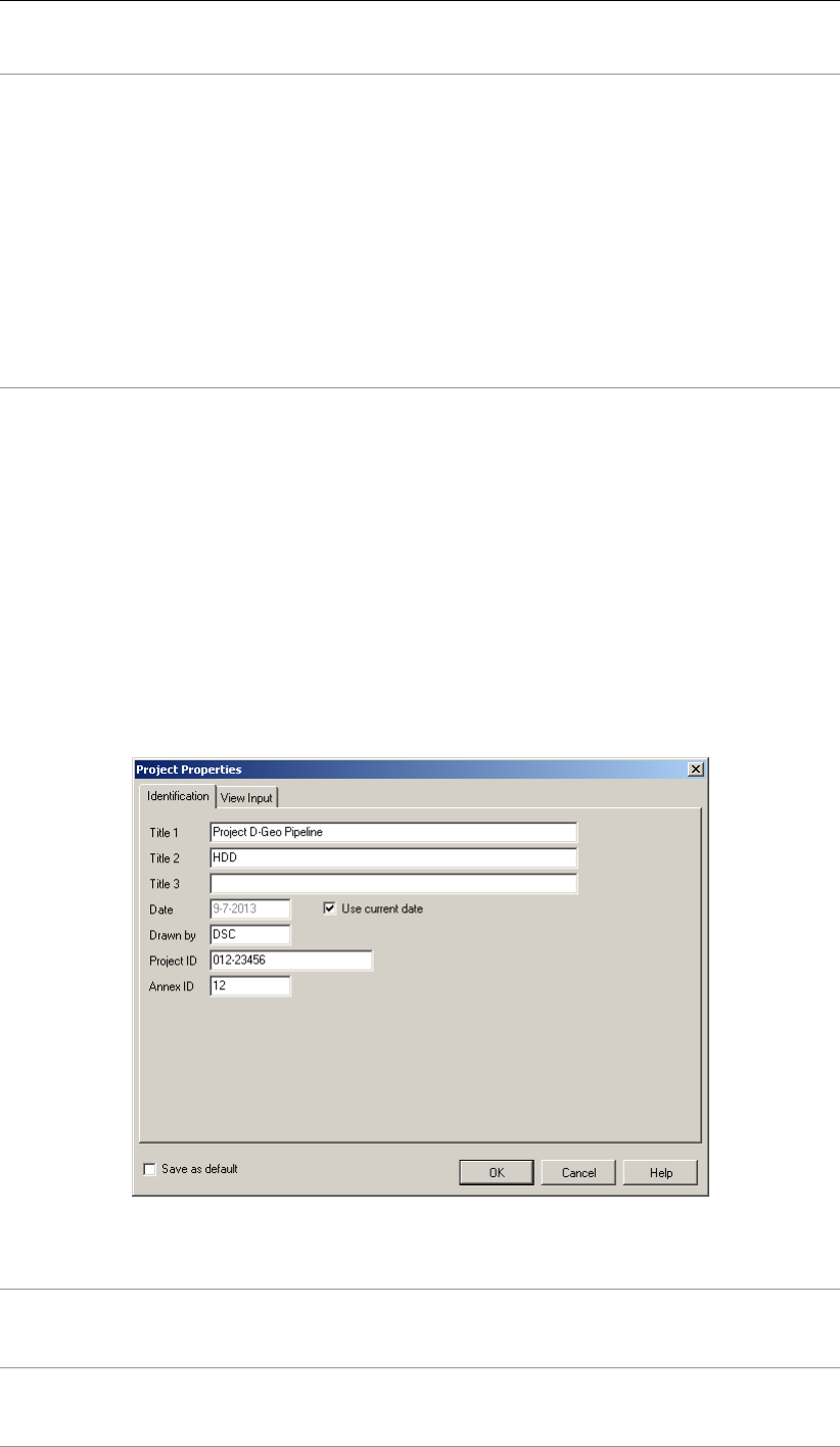
D-GEO PIPELINE
, User Manual
Settlement Enable the check-box Use settlement to calculate the vertical displace-
ment of the soil below the pipeline due to installation.
D-GEO PIPELINE
will use the
D-SETTLEMENT
computer program. The required settlement
model (Koppejan or Isotache) must be selected. For background infor-
mation, see section 21.10.2 and section 21.10.1 respectively for Koppe-
jan and Isotache models.
Note: The check-box Use settlement is available only when the pro-
gram
D-SETTLEMENT
(formerly known as MSettle) is installed, and when
the location of the executable (DSettlement.exe) is specified in the Lo-
cations tab of the Program Options window (section 3.2.3).
Note: The pipeline settlement can also be entered manually (if avail-
able) in the Calculation Verticals window (refer to section 4.4.2).
4.1.2 Project Properties
On the menu bar, click Project and then choose Properties to open the input window. The
Project Properties window has two tabs, which allow the settings for the current project to be
changed:
Identification, to specify project identification data.
View Input, to define the appearance of items in the View Input window.
Project Properties - Identification
Use the Identification tab to specify the project identification data:
Figure 4.2: Project Properties window, Identification tab
Titles Use Title 1 to give the project a unique, easily recognizable name. Title
2and Title 3 can be added to indicate specific characteristics of the
calculation. The three titles will be included on printed output.
Date The date entered here will be used on printouts and graphic plots for
this project. Either mark the Use current date check-box to automati-
cally use the current date on each printout, or enter a specific date.
40 of 324 Deltares

Input
Drawn by Enter the name of the user performing the calculation or generating the
printout.
Project ID Enter a project identification number.
Annex ID Specify the annex number of the printout.
Enable the check-box Save as default to use these settings every time
D-GEO PIPELINE
is
started or a new project is created.
Project Properties – View Input
Use the View Input tab to define the appearance of the View Input window (section 2.2.3).
Figure 4.3: Project Properties window, View Input tab
Display
Info Bar Enable this check-box to display the information bar at the bot-
tom of the Outline View window.
Legend Enable this check-box to display the legend.
Same scale for x and y
axis
Enable this check-box to display the x and y axis with the same
scale.
Layer colors Enable this check-box to display the layers in different colors.
Rulers Enable this check-box to display the rulers.
Origin Enable this check-box to draw a circle at the origin.
Large Cursor Enable this check-box to use the large cursor instead of the small
one.
Calculation Verticals Enable this check-box to display the verticals.
Points Enable this check-box to display the points.
Labels
Points Enable this check-box to display the point labels.
Calculation Verticals Enable this check-box to display the vertical labels.
Layers Enable this check-box to display the layer labels.
Deltares 41 of 324
D-GEO PIPELINE
, User Manual
Layers labels as
This choice is available only if the Layers check-box of the Labels sub-window is marked.
There are three ways to display the legend of the layers:
Layer Numbers The legend displays one box for each layer. Each layer (and
therefore each box) is displayed in a different standard color.
Next to each box, the layer number and the material name are
displayed, corresponding to the color and number of the layer in
the adjacent Geometry window.
Material Numbers The legend displays one box for each material. Each material
(and therefore each box) is displayed in a different color which
can be changed by the user (see section 7.3.3). Next to each
box, the material number and name are displayed, correspond-
ing to the color and number of the material in the adjacent Ge-
ometry window.
Material Names The legend displays one box for each material. Each material
(and therefore each box) is displayed in a different color which
can be changed by the user (see section 7.3.3). Next to each
box, only the material name is displayed, corresponding to the
color and name of the material in the adjacent Geometry win-
dow.
Grid
Show grid Enable this check-box to display the grid points.
Snap to Grid Enable this check-box to ensure that objects align to the grid
automatically when they are moved or positioned in a graph.
Grid distance Enter the distance between two grid points.
Enable the Save as default check-box to use the current settings every time
D-GEO PIPELINE
is started.
4.1.3 View Input File
On the menu bar, click Project and then choose View Input File to display an overview of the
input data.
The data will be displayed in the
D-GEO PIPELINE
main window. Click on the Print Active
Window icon to print the file.
4.2 Soil menu
The Soil menu is used to enter the soil properties for the analysis. In the Soil menu, choose
Materials to open the Materials input window in which the soil type properties can be defined.
The Properties can either be imported directly from an MGeoBase database (Database tab),
or be inputted manually (Parameters tab):
Manual input of standard parameters (section 4.2.1);
Manual input of settlement parameters acc. to Koppejan (section 4.2.2);
Manual input of settlement parameters acc. to Isotache (section 4.2.3);
Import from database (section 4.2.4).
42 of 324 Deltares
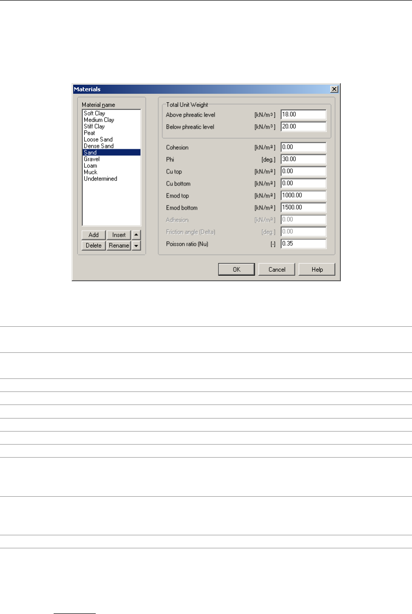
Input
4.2.1 Materials – Standard
If the Use settlement check-box in the Model window (section 4.1.1) is unmarked, the following
window is displayed.
Figure 4.4: Materials window, Parameters tab
Total Unit Weight
Above phreatic level
The unit weight of the unsaturated soil above the user-defined
phreatic line.
Total Unit Weight Below
phreatic level
The unit weight of the saturated soil below the user-defined
phreatic line.
Cohesion Cohesion of the soil.
Phi Angle of internal friction of the soil.
Cu top The apparent undrained cohesion cuat the top of the layer.
Cu bottom The apparent undrained cohesion cuat the bottom of the layer.
Emod top Young’s modulus of the soil at the top of the layer.
Emod bottom Young’s modulus of the soil at the bottom of the layer.
Adhesion Adhesion of the soil. The adhesion is only available if the Con-
struction in trench or Micro Tunneling model have been selected
in the Model window (section 4.1.1).
Friction angle (Delta) Friction angle between soil and pipeline. The delta friction angle
is only available if the Construction in trench or Micro Tunneling
model have been selected in the Model window (section 4.1.1).
Poisson ratio (Nu) Poisson ratio of the soil.
The Young’s modulus Eand the Poisson ratio νare used to calculate G, the shear modulus:
G=E
2(1 + ν)(4.1)
4.2.2 Materials – Settlement Koppejan
If the Use settlement check-box in the Model window (section 4.1.1) is marked and the Koppe-
jan model is selected,
D-GEO PIPELINE
will calculate the settlements according to the Koppejan
model. Therefore, the Koppejan parameters need to be put in as shown in Figure 4.5. For
background information, refer to section 21.10.2.
Deltares 43 of 324
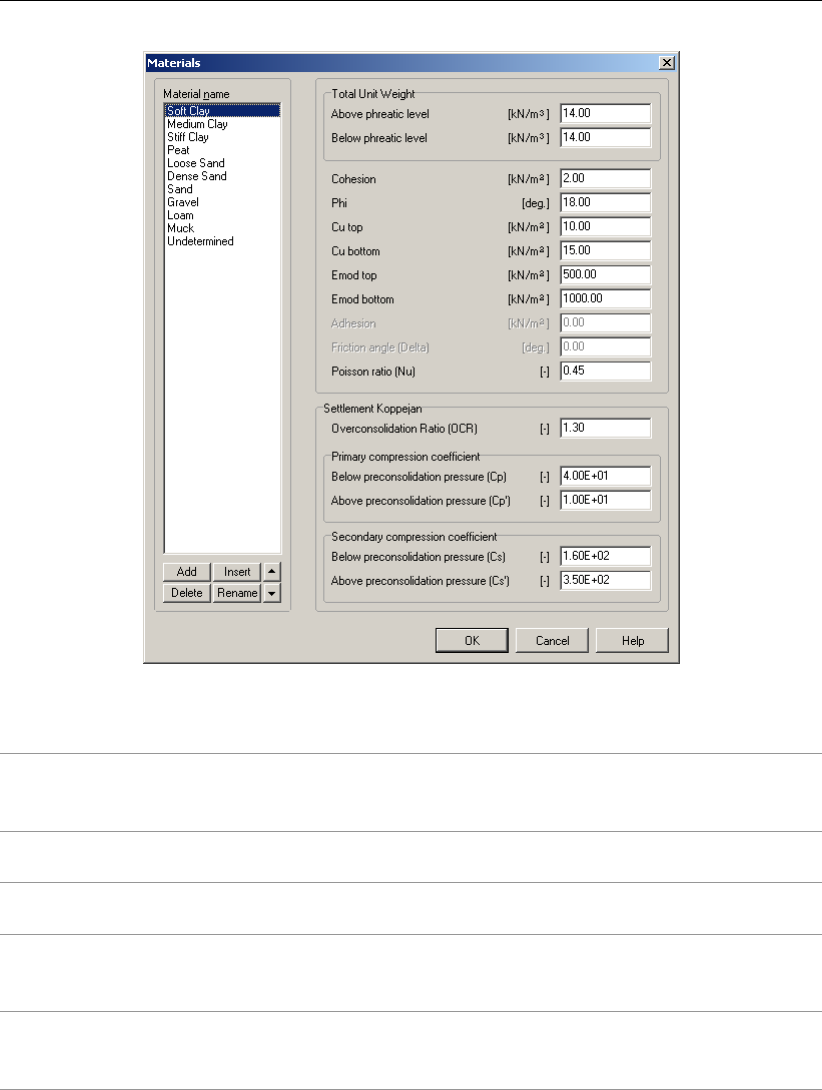
D-GEO PIPELINE
, User Manual
Figure 4.5: Materials window, Parameters tab (Settlement acc. to Koppejan)
Over-consolidation Ratio (OCR) The Over-Consolidation Ratio (OCR) is defined
as the ratio of pre-consolidation pressure and
initial in situ vertical effective stress.
Primary compression coefficient below
preconsolidation pressure (Cp)
The primary compression coefficient Cpis used
to calculate the primary settlement.
Primary compression coefficient above
preconsolidation pressure (Cp’)
The primary compression coefficient Cp’ is used
to calculate the primary settlement.
Secondary compression coefficient
below preconsolidation pressure (Cs)
The secondary compression coefficient Csis
used to calculate the secondary (time depen-
dent) settlement.
Secondary compression coefficient
above preconsolidation pressure (Cs’)
The secondary compression coefficient Cs’ is
used to calculate the secondary (time depen-
dent) settlement.
44 of 324 Deltares
Input
4.2.3 Materials – Settlement Isotache
If the Use settlement check-box in the Model window [section 4.1.1] is unmarked and the
Isotache model is selected,
D-GEO PIPELINE
will calculate the settlements according to the
Isotache model. Therefore, the Isotache parameters need to be put in as shown in Figure 4.6.
For background information, see section 21.10.1.
Figure 4.6: Materials window, Parameters tab (Settlement acc. to Isotache)
Direct compression
index (a)
The direct compression index arelates natural strain during re-
compression or swell to the change of vertical effective stress.
Secular compression
index (b)
The secular compression index brelates natural strain during
virgin loading to the change of vertical effective stress.
Coefficient of secular
compression rate (c)
The coefficient of secular compression rate crelates natural
strain to the change of time. A zero value indicates non-creeping
soil.
Pre-overburden
pressure (POP)
The Pre-Overburden Pressure (P OP ) is defined as the pre-
consolidation pressure minus the initial in situ vertical effective
stress.
Overconsolidation
ratio (OCR)
The Over-Consolidation Ratio (OCR) is defined as the ratio
of pre-consolidation pressure and initial in situ vertical effective
stress.
Deltares 45 of 324
D-GEO PIPELINE
, User Manual
4.2.4 Materials – Database
The Database tab in the Materials window is only available if a location of an MGeobase
database was specified in the Locations tab of the Program Options window (section 3.2.3).
Select the Database tab in the Materials window to see the available soil types. Select a soil
type, and use the Import button to import the soil type with associated properties.
Figure 4.7: Materials window, Database tab
4.3 Geometry menu
On the menu bar, click Geometry to display the menu options. These options are explained
in the following sections.
New (section 4.3.1). Start creating a new geometry manually.
New Wizard (section 4.3.2). Create a new geometry using a wizard.
Import (section 4.3.3). Import a geometry file in the D-series exchange format.
Import geometry from database (section 4.3.4). Import geometry from a database.
Export (section 4.3.5). Save a geometry file for exchange with other Deltares Systems
programs.
Export as Plaxis/Dos (section 4.3.6). Save a geometry file in a different format.
Limits (section 4.3.7). Set the range of the horizontal coordinates.
Points (section 4.3.8). Add or manipulate points.
Import PL-line (section 4.3.9). Import a PL-line file in the D-Series exchange format.
PL-lines (section 4.3.10). Add or manipulate piezometric level lines.
Phreatic line (section 4.3.11). Define phreatic level lines.
Layers (section 4.3.12). Define or modify layer boundaries and corresponding soil
types.
PL-lines per layer (section 4.3.13). Select the piezometric level line at the bottom and
top of each layer.
Check geometry (section 4.3.14). Check the validity of the geometry.
46 of 324 Deltares
Input
4.3.1 New
Select this option to display the View Input (Geometry) window, showing only the geometry
limits (with their default values) of the geometry. It is possible to now start modeling the
geometry (for more information on this subject, see chapter 7). However, it is possible to
create a new geometry faster and easier using the Geometry Wizard (section 4.3.2). This
wizard involves a step-by-step process for creating geometry.
4.3.2 New Wizard
The New Wizard is usually the fastest and easiest way to start creating new geometry. The
wizard uses predefined shapes and soil types.
To use the geometry wizard, click the Geometry menu and choose New Wizard. This wizard
provides the following step-by-step guidance:
Basic layout
Shape selection
Shape definition
Material types
Summary
New Wizard – Basic Layout
Figure 4.8: New Wizard window (Basic Layout)
In the Basic Layout window (Figure 4.8), the basic framework within which the project is
defined can be entered. The graphic at the top of the window explains the required input.
When satisfied with the input, just click the Next button to display the next input screen.
Deltares 47 of 324
D-GEO PIPELINE
, User Manual
New Wizard – Shape Selection
Figure 4.9: New Wizard window (Top Layer Shape)
In the Top Layer Shape window (Figure 4.9), one of nine default top-layer shapes can be
selected. A red frame indicates the selected shape. Click the Previous button to return to the
Basic Layout screen, or the Next button to display the next input screen with shape-specific
input data.
New Wizard – Shape definition
Figure 4.10: New Wizard window (Top Layer Specification)
48 of 324 Deltares
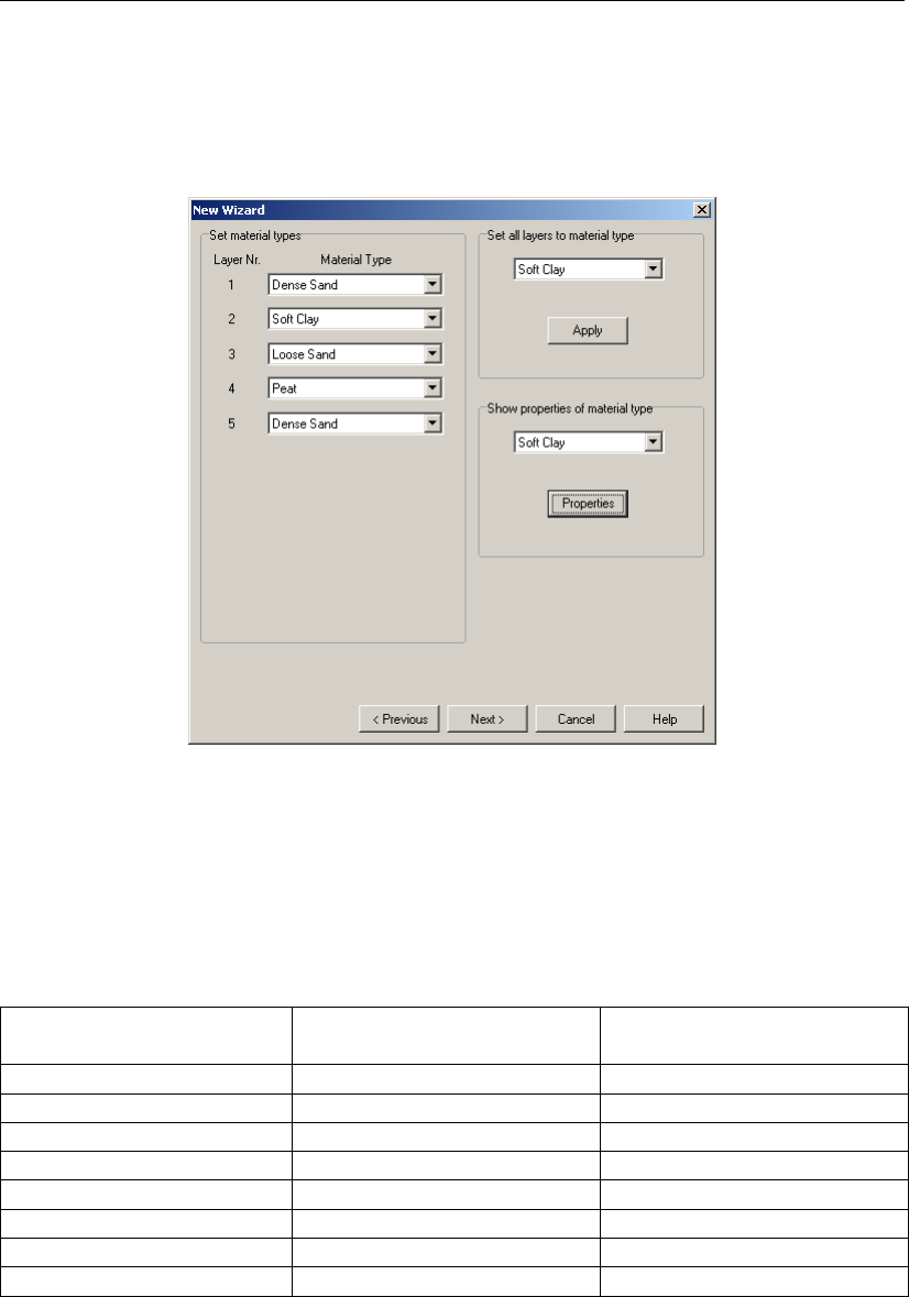
Input
The Top Layer Specification window (Figure 4.10) enables to specify the sizes of the selected
top layer shape.
New Wizard – Material Types
Figure 4.11: New Wizard window (Material Types)
In the Material Types window (Figure 4.11), the materials used for the layers in the project
can be specified. The number of layers was defined in the first screen (Basic Layout). The
materials that can be chosen from are predefined (see Table 4.10).
Table 4.10: Unsaturated and saturated weight of the predefined materials
Material type Unsaturated weight
[kN/m3]
Saturated weight
[kN/m3]
Soft Clay 14 14
Medium Clay 17 17
Stiff Clay 19 19
Loose Sand 17 19
Dense Sand 19 21
Loose Aggregate 17 19
Dense Aggregate 19 21
Peat 12 12
The materials for each layer can be selected individually (using the selection boxes at the
left-hand side of the screen) or one material for each layer at once can be selected (using the
selection box at the top right of the screen). The parameters of each material can also be
reviewed.
Deltares 49 of 324
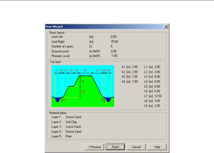
D-GEO PIPELINE
, User Manual
New Wizard – Summary
Figure 4.12: New Wizard window (Summary)
The Summary window (Figure 4.12) displays an overview of the data entered in the previous
wizard screens. If necessary, click Previous to go back to any screen and change the data
as required. Clicking Finish will confirm the input and display the geometry in the View Input
Geometry window. In this window, the geometry can be edited or completed graphically as
described in chapter 7. Of course, the Geometry menu options can also be used for this
purpose (section 4.3).
4.3.3 Import
This option displays a standard file dialog in which an existing geometry can be selected
stored in a geometry file, or in an existing input file for
D-GEO STABILITY
(formerly known as
MStab),
D-SETTLEMENT
(formerly known as MSettle), MSeep and
D-SHEET PILING
(formerly
known as MSheet). For a full description of these programs and how to obtain them, visit
www.deltaressystems.com.
When selecting the geometry, it is imported into the current project, replacing the current
geometry. The imported geometry is displayed in the View Input (Geometry) window. It is
also possible to use this option to analyze the settled geometry at different stages, as all other
input is retained.
4.3.4 Import geometry from database
To be able to import a geometry from a database, this option has to be provided with the
purchased version of
D-GEO PIPELINE
.
To import a geometry from a database do the following:
Click Import from Database in the Geometry menu.
The Select Geometry dialog will appear.
50 of 324 Deltares

Input
Again, the imported geometry will replace the current one and will be displayed in the View
Input (Geometry) window.
Note: This option is only available when the correct database directory has been specified
using the Locations tab in the Program Options menu (see section 3.2.3). For more informa-
tion on MGeoBase, visit www.deltaressystems.com.
4.3.5 Export
This option displays a standard Save As dialog that enables the user to choose a directory, a
file name and a format in which to save the current geometry to a file. The file will be saved in
the standard geometry format for the Deltares Systems programs (*.geo). Files in this format
can be used in a multitude of Deltares Systems programs, such as
D-GEO STABILITY
(formerly
known as MStab),
D-SETTLEMENT
(formerly known as MSettle), MSeep and
D-SHEET PILING
(formerly known as MSheet). For a full description of these programs and how to obtain them,
visit www.deltaressystems.com.
4.3.6 Export as Plaxis/DOS
This option displays the Save As Plaxis/DOS dialog that enables the user to choose a di-
rectory and a file name in which to save the current geometry. The file will be saved using
the old DOS-style geometry format for the Deltares Systems programs. Files in this format
can be used by the finite element program Plaxis and in old DOS-based versions of Deltares
Systems programs such as
D-GEO STABILITY
(DOS) and MZet (DOS).
Saving files of this type will only succeed, however, if the stringent demands imposed by the
old DOS style are satisfied:
number of layers ≤20
number of PL-lines ≤20
number of lines per boundary <50
total number of points ≤500
To be able to differentiate between an old DOS-style file and a normal geometry file, the file
dialog that prompts for a new file name for the old DOS-style geometry file suggests a default
file name, prefixing the current name with a ‘D’.
4.3.7 Limits
Use this option to edit the geometry limits.
Figure 4.13: Geometry Limits window
A limit is a vertical boundary defining the ‘end’ at either the left or right side of the geometry.
It is defined by an X-coordinate only.
Deltares 51 of 324
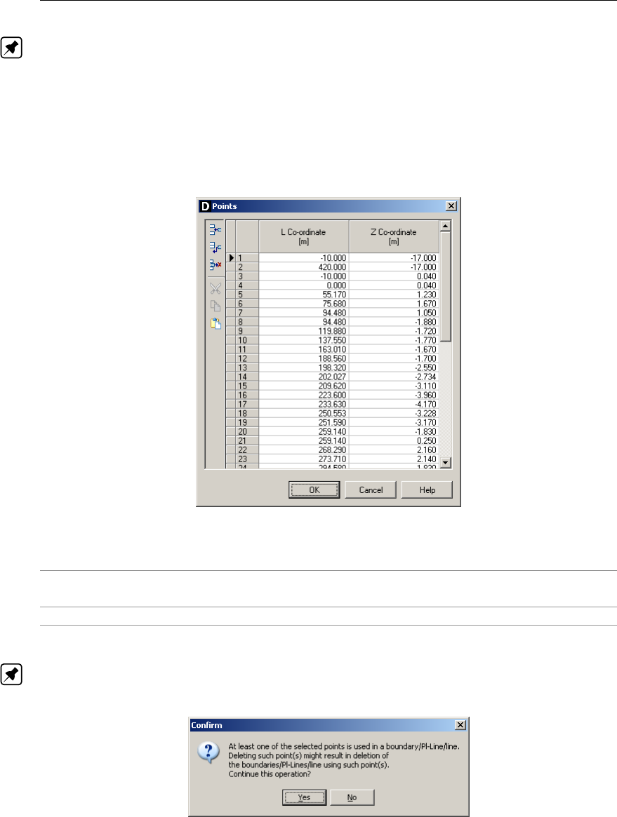
D-GEO PIPELINE
, User Manual
Note: This is the only type of element that cannot be deleted. Moreover, the values entered
here are ignored if they resulted in an invalid geometry.
4.3.8 Points
Use this option to add or edit points that can be used as part of layer boundaries or PL-lines. A
point is a basic geometry element defined by its coordinates. Since the geometry is restricted
to two dimensions, it is allowed to define an Land Zco-ordinates only.
Figure 4.14: Points window
L Co-ordinate Projection of the horizontal co-ordinate along the pipeline trajec-
tory.
Z Co-ordinate Vertical co-ordinate.
Note: When a point is to be deleted, the system will check whether the point is used as part
of a PL-line or layer boundary. If so, a message will be displayed.
Figure 4.15: Confirm window for deleting used points
When Yes is clicked, all layer boundaries and/or PL-lines using the point will also be deleted.
Every change made using this window (Figure 4.14) will only be displayed in the underlying
View Input (Geometry) window after closing this window using the OK button. When this
button is clicked, a validity check is performed on the geometry. Any errors encountered
during this check are displayed in a separate window. These errors must be corrected before
52 of 324 Deltares
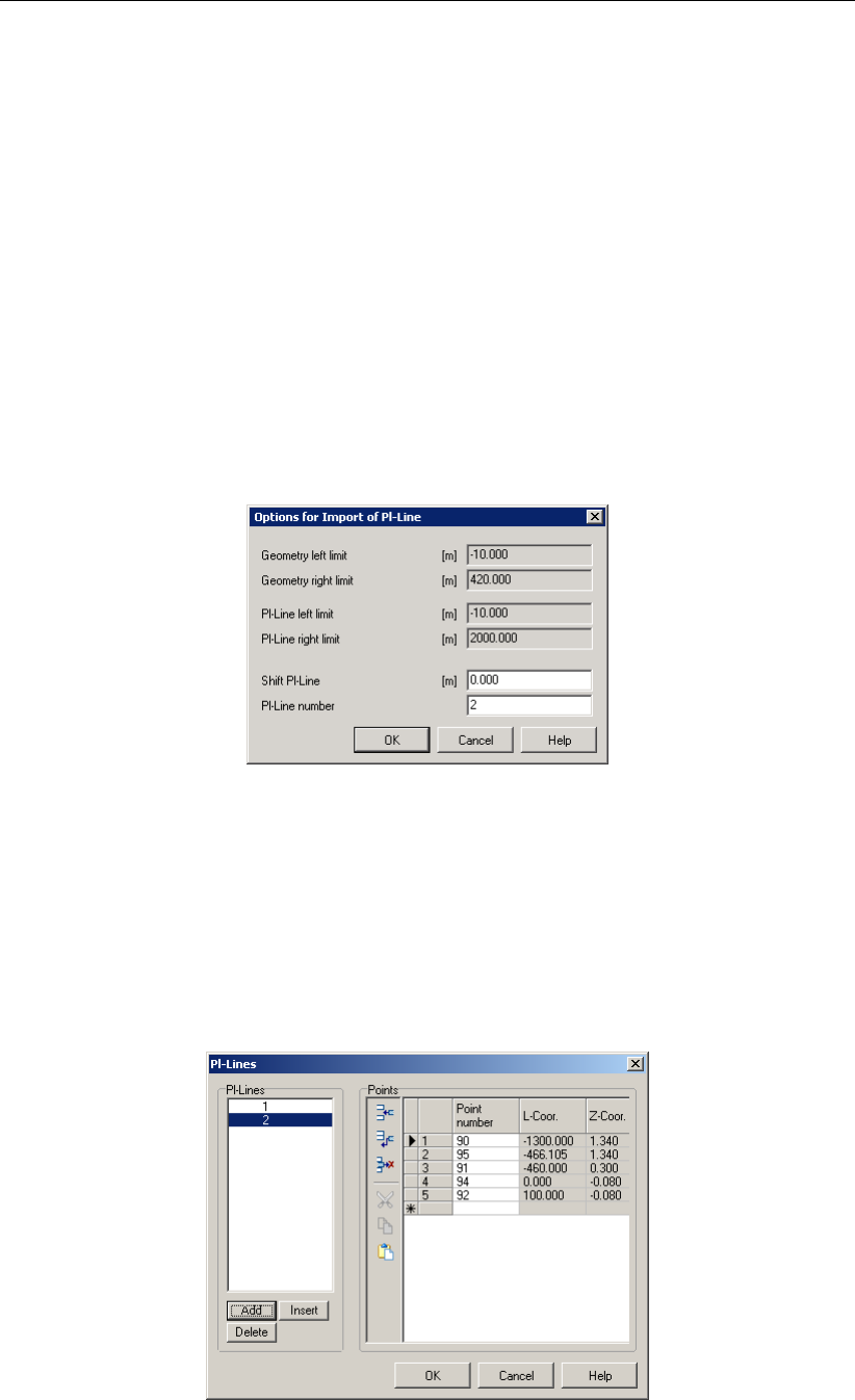
Input
closing this window by clicking the OK button. Of course, it is always possible to close the
window using the Cancel button, but this will discard all changes.
4.3.9 Import PL-line
This option displays a standard file dialog in which an existing PL-line, created with the pro-
gram WATEX and stored in a PL-line file (*.mpl), can be selected.
WATEX (Deltares,2004) is a reliable prediction tool to assess the pore pressure behavior. It
consists of transient analytical solutions, put together by the conditions of continuity of head
and discharge. The user specifies a number of locations, where the pore pressure response
is required.
When a PL-line file is selected, the Options for Import of Pl-line window (Figure 4.16) is
displayed. When clicking the OK button, then the PL-line is added to the current PL-lines
in the project.
Figure 4.16: Options for Import of PL-line window
4.3.10 PL-Lines
Use this option to add or edit Piezometric Level lines (PL-lines) to be used in the geometry. A
PL-line represents the hydraulic head Hydraulic head of the water in the pores of the soil. A
PL-line can be defined for the top and bottom of each soil layer (see section 4.3.13). The bot-
tom soil layer is assumed to be infinitely thick. Here, therefore, only one PL-line is necessary
for the top of that layer. Pore pressures in this layer are hydrostatic with increasing depth.
Figure 4.17: PL-Lines window
Deltares 53 of 324
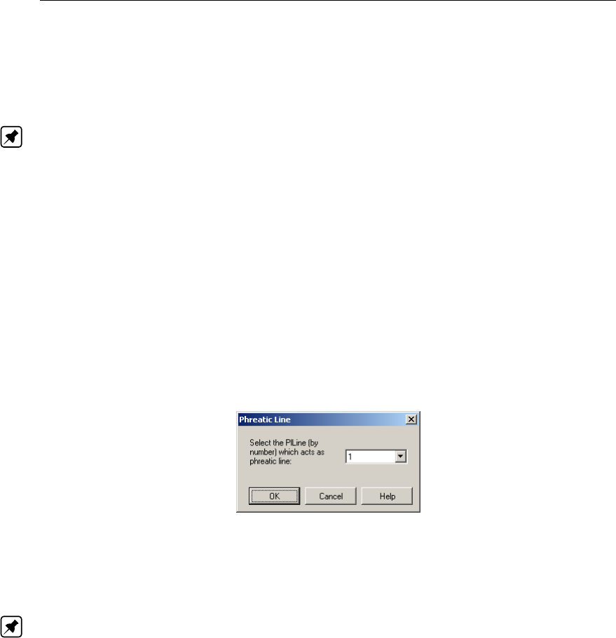
D-GEO PIPELINE
, User Manual
In the lower part of the window, the buttons Add,Insert and Delete PL-lines can be used. The
selection box on the left can be used to navigate between PL-lines that have already been
defined. Use the table to add/edit the points identifying the PL-lines. It is only possible to
select points that are not attached to layer boundaries (section 4.3.12).
Note: It is only possible to manipulate the Point number column – that is, the coordinate
columns are purely for informative purposes. To edit the coordinates of the points, choose the
Points option from the Geometry menu (see section 4.3.8).
Every change made using this window will only be displayed in the underlying View Input
(Geometry) window after closing this window using the OK button. When clicking this button,
a validity check is performed on the geometry. Any errors encountered during this check are
displayed in a separate window. These errors must be corrected before closing this window
using the OK button. Of course, it is always possible to close the window using the Cancel
button, but this will discard all your changes.
4.3.11 Phreatic Line
Use this option to select the PL-line that acts as a phreatic line. The phreatic line (or ground-
water level) is used to mark the border between dry and wet soil.
Figure 4.18: Phreatic Line window
Select the appropriate line number from the drop-down list and click the OK button.
Note: At least one PL-line has to be defined to be able to pick a phreatic line from the
drop-down list.
4.3.12 Layers
This option enables to add or edit layers to be used in the geometry. A layer is defined by its
boundaries and its material. Use the Boundaries tab to define the boundaries for all layers by
choosing the points that identify each boundary.
54 of 324 Deltares
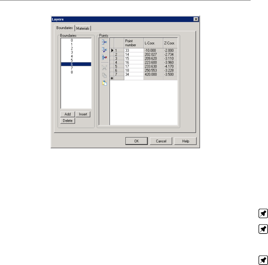
Input
Figure 4.19: Layers window, Boundaries tab
On the left-hand side of the window, it is possible to add, insert, delete or select a boundary.
In the table on the right, it is possible to modify or add the points that identify the selected
boundary.
Note: It is only possible to select points that are not attached to PL-lines (section 4.3.10).
Note: It is only possible to manipulate the Point number column, because the coordinate
columns are purely for informative purposes. To manipulate the coordinates of the points,
choose the Points option in the Geometry menu (see section 4.3.8).
Note: When inserting or adding a boundary, all points of the previous boundary (if this exists)
are automatically copied. By default, the material of a new layer is set equal to the material of
the existing layer just beneath it.
The Materials tab enables to assign materials to the layers.
Deltares 55 of 324

D-GEO PIPELINE
, User Manual
Figure 4.20: Layers window, Materials tab
On the left of the screen, a list containing all defined materials (see the Materials option in the
Soil menu in section 4.2.1) is displayed. On the right, a list of all defined layers together with
their assigned materials (if available) is displayed.
To assign a material to a layer, first select that layer on the right of the window. Then select
the required material on the left of the window. Finally, click the Assign button .
In case of settlement calculation using the Koppejan or the Isotache model (section 4.1.1), the
loading is defined by marking the Load check-box of one or several layers.
D-GEO PIPELINE
assumes that those layers are non-uniform loads.
Every change made using this window will only be displayed in the underlying View Input
(Geometry) window after closing this window by clicking the OK button. When clicking this
button, a validity check is performed on the geometry. If errors are encountered, a dialog
window asks if auto-correction should be tried. Remaining errors are reported and can be
corrected manually. The error correction is confirmed by clicking the OK button and discarded
by clicking the Cancel button.
4.3.13 PL-lines per Layer
Use this option to define the top and bottom PL-lines for the defined layers. The PL-lines
represent the pore pressure in a soil layer. For each soil layer (except the deepest layer), two
PL-line numbers can be entered – one that corresponds to the top of the soil layer, and one
that corresponds to the bottom. Therefore, different PL-lines can be defined for the top and
bottom of each soil layer. To do this, select the appropriate PL-line at top / PL-line at bottom
field and enter the appropriate number.
56 of 324 Deltares
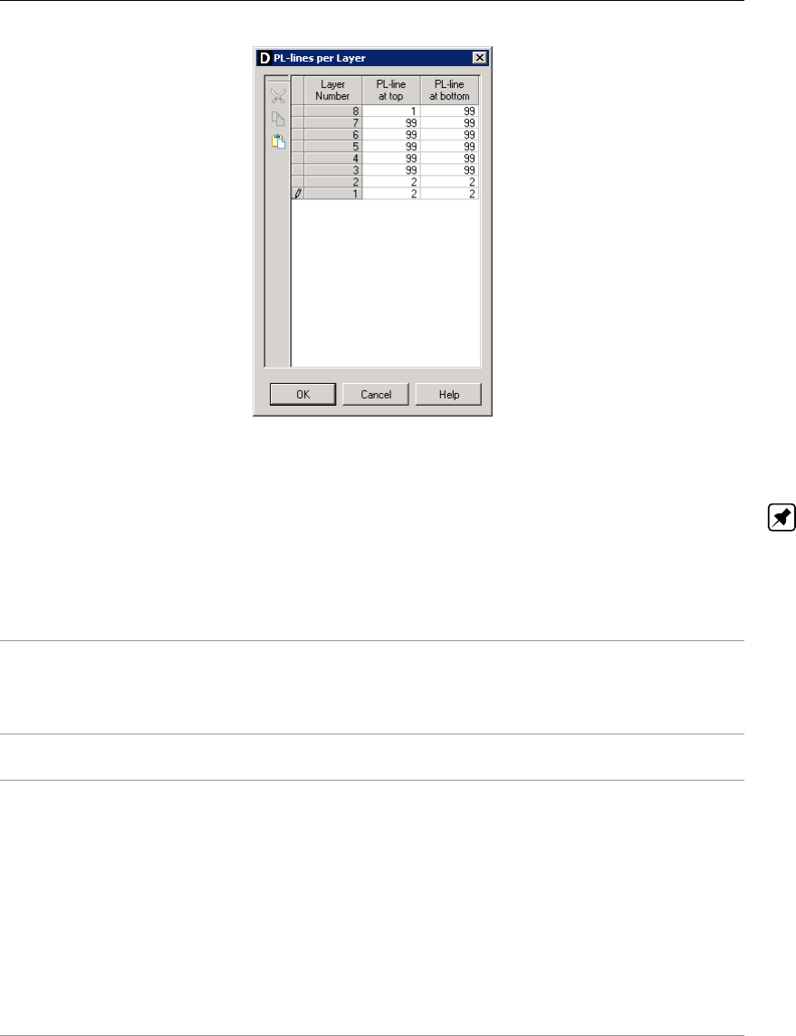
Input
Figure 4.21: PL-line per Layer window
Note: For the deepest soil layer, no second PL-line number is required. For this layer a
hydrostatic increase of the pore pressure is automatically assumed from the pore pressure at
the top of the layer downwards.
The following values can be used as PL-line numbers (N):
0<N<99 The number corresponds to one of the PL-lines defined during the geometry
input. Capillary water pressures are not used – that is, if a negative water
pressure is calculated for a point above the phreatic line, the water pressure
in that point is defined as 0.
N = 0 Each point within the layer has a water pressure equal to 0 (define 0 for PL-
line at top of layer).
N = 99 It is possible to have a number of overlying soil layers with a non-hydrostatic
pore pressure (for example, a number of layers consisting of cohesive soil). In
this case, a large number of PL-lines would have to be calculated, one or two
for each layer. To avoid this, D-series software is able to interpolate across
layer boundaries. For layers with a non-hydrostatic pore pressure, 99 can be
entered as the PL-line number. For this layer, the interpolation will take place
between the PL-line belonging to the first soil layer above with a real PL-line
number, and the PL-line belonging to the first soil layer below with a real PL-
line number. The first and the last soil layer must therefore always have a real
PL-line number.
Note: A real PL-line number is not equal to 99.
Water pressures above the phreatic line are set to zero. An example using two different PL-
lines is given in Figure 4.22 showing how the pore pressure varies in the vertical.
Deltares 57 of 324
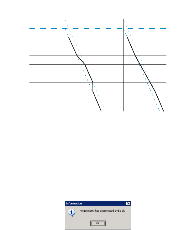
D-GEO PIPELINE
, User Manual
PL-line 2
PL-line 1
SAND
CLAY
SAND
CLAY2
SAND
1
1
1
2
2
2
2
1
1
1
1
99
99
99
99
99
2
Figure 4.22: PL-lines and vertical pressure distribution
When clicking the OK button, the program performs a validity check on the geometry. Any
errors encountered during this check are reported. A dialog window enables to disregard or
correct the errors. The error correction is confirmed by clicking the OK button and discarded
by clicking the Cancel button.
4.3.14 Check Geometry
When this option is selected, the program checks the validity of the geometry (section 7.2) with
respect to the requirements. If the geometry complies with all the requirements, a message
will confirm this.
Figure 4.23: Information window to confirm a valid geometry
If any errors are encountered during this check, they are displayed in a separate window.
4.4 GeoObjects menu
58 of 324 Deltares
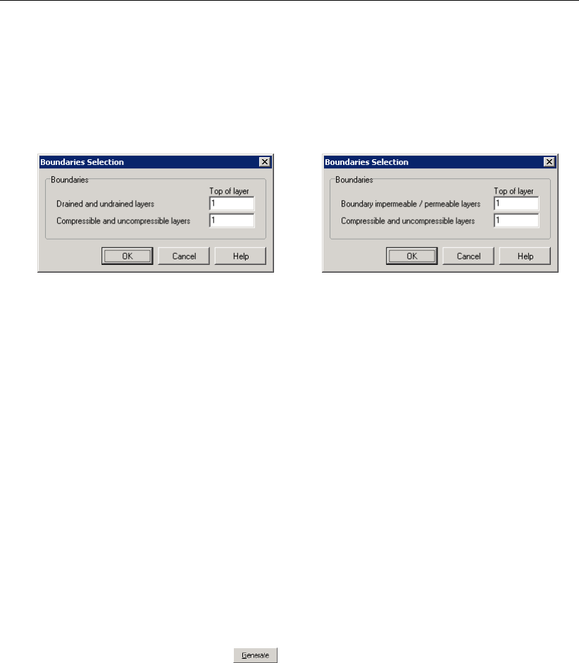
Input
4.4.1 Boundaries Selection
Click GeoObjects on the menu bar and select Boundaries Selection to define the boundaries
between compressible top layers and under laying non-compressible layers and the boundary
between drained (i.e. cohesive) top layers and under laying non-cohesive (i.e. undrained)
layers (Figure 4.24). This is done by choosing the layer number of the underlying layer.
a) b)
Figure 4.24: Boundaries Selection window for (a) HDD/Micro-tunneling and (b) for
Trenching
The boundary between compressible and non-compressible layers is drawn as a blue bold
line and the boundary between drained and undrained layers (i.e. impermeable and perme-
able layers) is drawn as a black bold line in the Input tab of the View Input window (see
section 2.2.3).
4.4.2 Calculation Verticals
Click GeoObjects on the menu bar and select Calculation Verticals to define the L-coordinate
for each vertical.
D-GEO PIPELINE
will perform calculations along each of these verticals. At
least one vertical is necessary to perform any calculation.
The verticals must be placed within the left and right project limits.For an accurate impression
of the change in drilling fluid pressure along the pipeline, it is advised to use at least 10-15
verticals.
It is possible to generate a number of verticals using the Auto generation of L co-ordinates op-
tion and clicking the Generate button .
D-GEO PIPELINE
will generate verticals between
the First and Last co-ordinates with a fixed width, entered in the Interval field.
Deltares 59 of 324
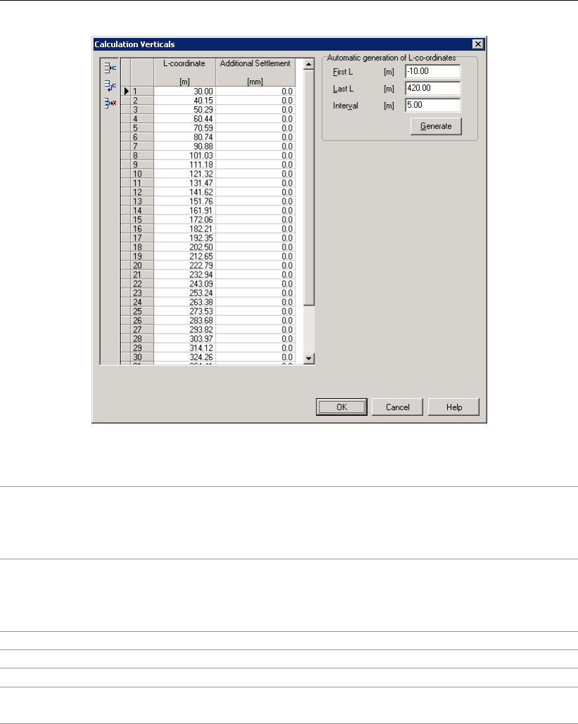
D-GEO PIPELINE
, User Manual
Figure 4.25: Calculation Verticals window
L-coordinate Defines the locations in geometry in the Ldirection where the calcula-
tions are performed. Lrepresents distance along the pipe line projec-
tion in the horizontal plane incremented with the entry coordinate. The
L-coordinate value must increase with each vertical.
Additional
Settlement
Enter an additional settlement for the selected vertical. This settlement
will be added to the calculated settlement (according to Koppejan or
Isotache) in the table of the Deformation section of the Report window
(section 6.2.2).
First L Lco-ordinate of the starting point of generated verticals.
Last L Lco-ordinate of the ending point of generated verticals.
Interval Interval between generated verticals.
Generate Click this button to generate automatically verticals from First to Last L
with the mentioned Interval.
4.5 Loads menu
4.5.1 Traffic Loads
On the menu bar, click Loads and then choose Traffic Loads to open the corresponding in-
put window in which the positions of traffic loads can be defined. Traffic loads will have an
influence on the calculated soil load stress, only for the calculation verticals situated
60 of 324 Deltares
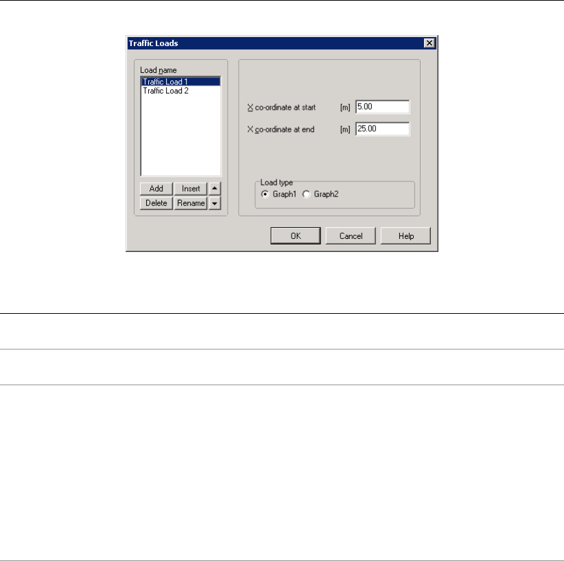
Input
Figure 4.26: Traffic Loads window
X co-ordinate at
start
Enter the Xco-ordinate of the starting point of the selected traffic load.
X co-ordinate at
end
Enter the Xco-ordinate of the ending point of the selected traffic load.
Load type According to article C.5.1 of NEN 3650-1 (NEN,2012a), two load mod-
els are considered, depending on the type of road:
For dual carriageways and regional roads, Graph I (i.e. ’Load
Model 3’ of European standard EN NEN-1991-2) is assumed;
For other roads, Graph II (i.e. ’Fatigue Load Model 2, Lorry 4’
of European standard EN NEN-1991-2) is assumed. This load
model covers the ’set of frequent lorries’ which can occur on Eu-
ropean roads, such as described in EN NEN-1991-2, with excep-
tion of the special transports).
For more information, refer to section 21.14.
4.6 Pipe menu
4.6.1 Pipeline Configuration
On the menu bar, click Pipe and then choose Pipeline Configuration to open the correspond-
ing input window in which the geometric characteristics of the pipeline can be defined. The
Pipeline Configuration window displayed depends on the selected model.
4.6.1.1 Pipeline Configuration for HDD
If the Horizontal directional drilling option in the Model window (section 4.1.1) is selected, the
Pipeline Configuration window shown in Figure 4.27 is displayed.
Deltares 61 of 324
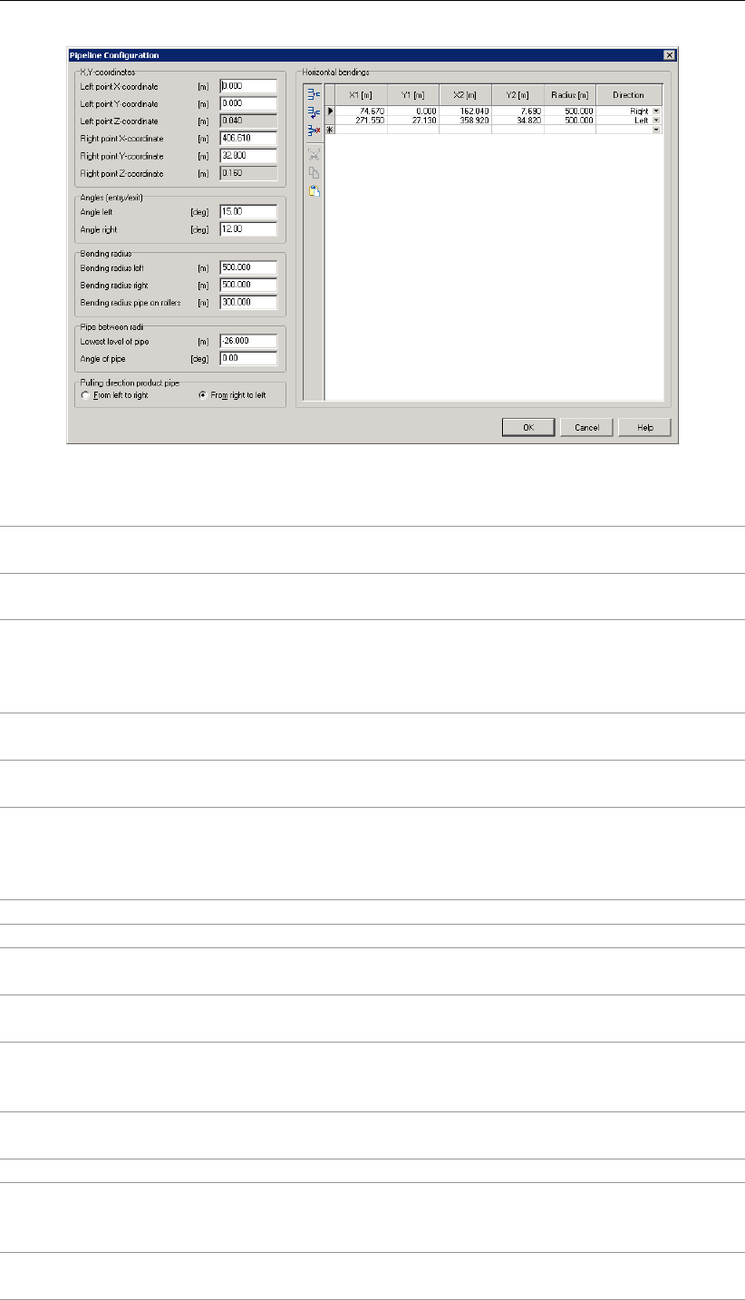
D-GEO PIPELINE
, User Manual
Figure 4.27: Pipeline Configuration window (for HDD)
Left point
X-coordinate
X-coordinate of the left point which corresponds whether the entry or
the exit point of the pipeline (called Xleft in Figure 4.28).
Left point
Y-coordinate
Y-coordinate of the left point which corresponds whether the entry or
the exit point of the pipeline (called Yleft in Figure 4.28).
Left point
Z-coordinate
Z-coordinate (i.e. vertical level) of the left point which corresponds
whether the entry or the exit point of the pipeline (called Zleft in Fig-
ure 4.28). This coordinate corresponds with the surface level for
X=Xleft and is automatically calculated by the program.
Right point
X-coordinate
X-coordinate of the right point which corresponds whether the entry or
the exit point of the pipeline (called Xright in Figure 4.28).
Right point
Y-coordinate
Y-coordinate of the right point which corresponds whether the entry or
the exit point of the pipeline (called Yright in Figure 4.28).
Right point
Z-coordinate
Z-coordinate of the right point which corresponds whether the entry or
the exit point of the pipeline (called Zright in Figure 4.28). This coordi-
nate corresponds with the surface level for X=Xright and is automati-
cally calculated by the program.
Angle left Left angle of the pipe (called ϕleft in Figure 4.28).
Angle right Right angle of the pipe (called ϕright in Figure 4.28).
Bending radius
left
Bending radius of the pipe at the left side (called Rleft in Figure 4.28).
Bending radius
right
Bending radius of the pipe at the right side (called Rright in Figure 4.28).
Bending radius
pipe on rollers
Only available for HDD model. Bending radius on the pipe roller, de-
pending on the diameter of the product pipe (called Rrollers in Fig-
ure 4.28).
Lowest level of
pipe
Lowest level of the pipe (called Zlowest in Figure 4.28).
Angle of pipe Horizontal angle of the lowest straight part of the configuration.
Pulling direction
product pipe
The pulling force at characteristics points can be calculated for a pulling
direction From left to right (i.e. the left point is the entry point) and From
right to left (i.e. the right point is the entry point).
X1 X co-ordinate of the beginning point of the horizontal bending (see Fig-
ure 4.28).
62 of 324 Deltares
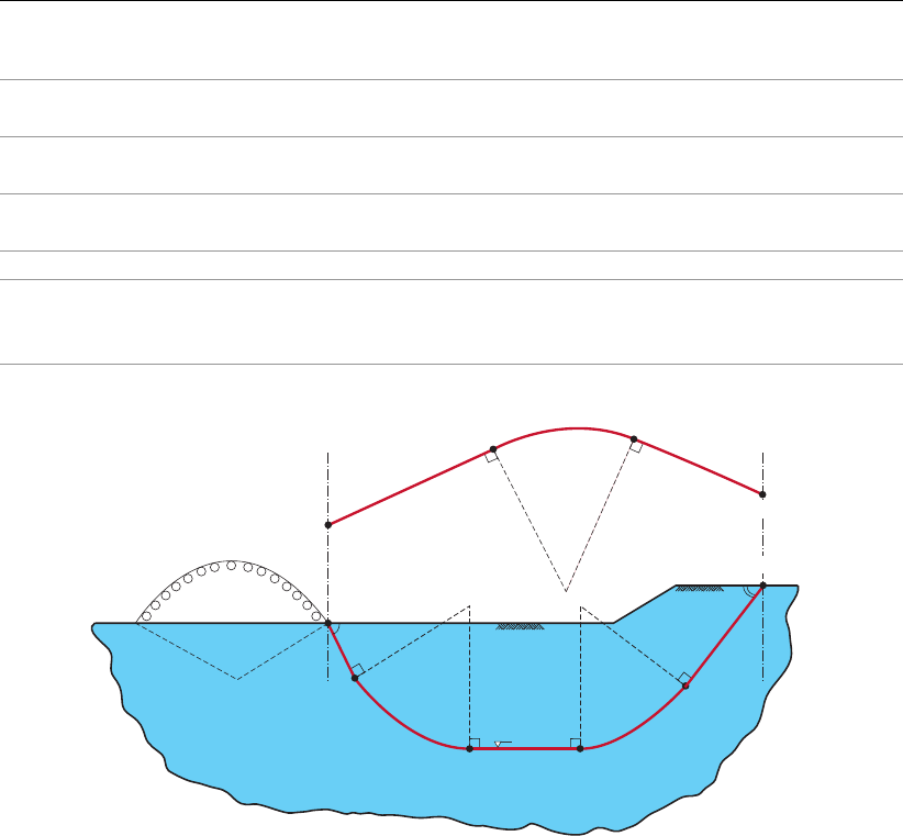
Input
Y1 Y co-ordinate of the beginning point of the horizontal bending (see Fig-
ure 4.28).
X2 X co-ordinate of the ending point of the horizontal bending (see Fig-
ure 4.28).
Y2 Y co-ordinate of the ending point of the horizontal bending (see Fig-
ure 4.28).
Radius Radius of the horizontal bending (called Rbending in Figure 4.28).
Direction From the drop-down menu, select the direction of the horizontal bend-
ing (Left or Right). For example, the horizontal bending of Figure 4.28
has a left direction.
Top view(X2 ; Y2)(X1 ; Y1)
(Xright ; Yright)
(Xright ; Zright)
(Xleft ; Yleft)
(Xleft ; Zleft)
Rbending
Rrollers
entry
exit
ϕleft
ϕright
Rleft
Rright
Zlowest
Figure 4.28: Schematization of the pipeline (HDD)
Needless to say, the coordinates must be defined properly. For example, the X-coordinate of
the right point must have a higher value than the coordinate of the left point.
The pipeline configuration is given at the center of the pipe. It is assumed that during all
drilling stages (pilot, drill and pullback) the defined center of the pipeline is the same. From
each pipe, the diameter of the pipe as well as the diameter of the hole must be known.
4.6.1.2 Pipeline Configuration for Micro tunneling
If the Micro tunneling option in the Model window (section 4.1.1) is selected, the Pipeline
Configuration window shown in Figure 4.29 is displayed.
Deltares 63 of 324

D-GEO PIPELINE
, User Manual
Figure 4.29: Pipeline Configuration window (for Micro tunneling)
Thrusting direction
product pipe
The thrusting force can be calculated for a pulling direction From left
to right (i.e. the left point is the entry point) and From right to left
(i.e. the right point is the entry point).
Refer to the table above for the definition of the other parameters
Note: To model a horizontal micro-tunneling, enter an Angle left and an Angle right of 0.
4.6.1.3 Pipeline Configuration for Construction in trench
If the Construction in trench option in the Model window (section 4.1.1) is selected, the
Pipeline Configuration window shown in Figure 4.30 is displayed. Different pipe materials
can be defined along the pipeline.
64 of 324 Deltares
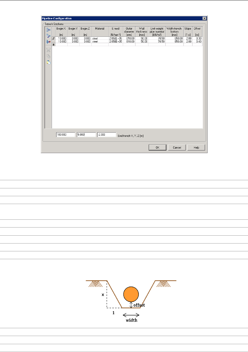
Input
Figure 4.30: Pipeline Configuration window (Construction in trench)
Begin X X co-ordinate of the begin point of the trench section.
Begin Y Y co-ordinate of the begin point of the trench section.
Begin Z Z co-ordinate of the begin point of the trench section.
Material quality Description of the material quality. The data in this field is
used in the report.
Outer diameter Outer diameter of the pipe in mm.
Wall thickness Wall thickness of the pipe in mm.
Unit weight pipe material Unit weight of the pipe material.
Width trench bottom Width of the trench bottom.
Slope 1:x Slope of the trench.
Offset Distance between the bottom of the trench and the bottom of
the pipeline.
End trench X X co-ordinate of the end point of the last trench section.
End trench Y Y co-ordinate of the end point of the last trench section.
End trench Z Z co-ordinate of the end point of the last trench section.
4.6.2 Product Pipe Material Data
Deltares 65 of 324
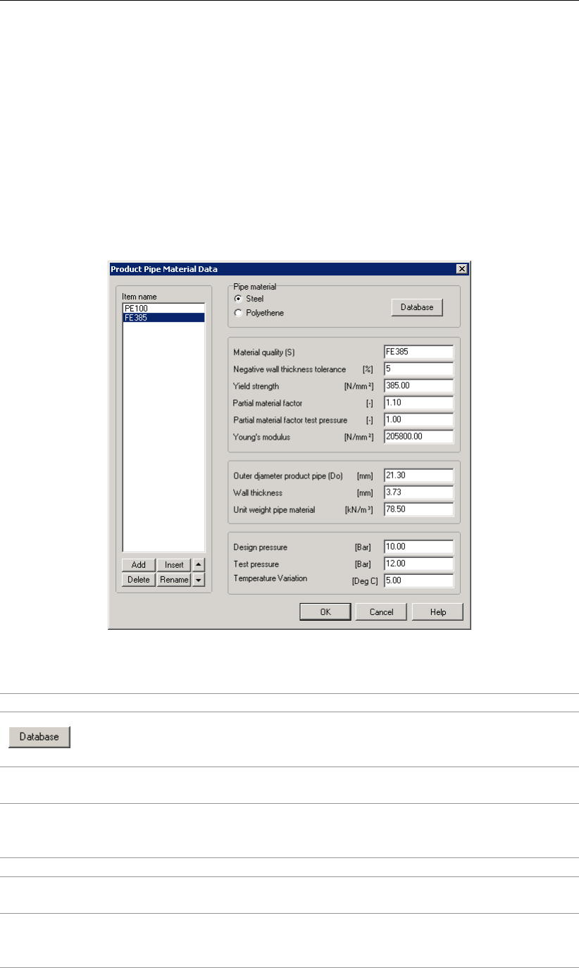
D-GEO PIPELINE
, User Manual
4.6.2.1 Product Pipe Material Data for HDD
If the Horizontal directional drilling option in the Model window (section 4.1.1) is selected, click
Pipe on the menu bar and then choose Product Pipe Material Data to open the Product Pipe
Material Data window in which the characteristics of the pipe material can be entered. This
data will be used for the strength calculation. Depending on the choice between steel and
polyethylene, different values for the parameters need to be specified.
Steel pipe
Different types of steel pipes can be selected from the database (see Figure 4.31). User-
defined values can also be defined for a steel pipeline.
Figure 4.31: Product Pipe Material Data window (Steel)
Pipe material Choice between steel or polyethylene.
Click this button to import the name, the outer diameter, the
wall thickness and the yield strength of a pipe material from
the
D-GEO PIPELINE
library (see Figure 4.31).
Material quality Description of the steel quality. The data in this field is used
in the report.
Negative wall thickness
tolerance
Tolerance on the wall thickness of the pipe (δt) in %. This
value is used to determine the minimum wall thickness in the
strength calculation.
Yield strength Yield strength of the pipe (Reb) in N/mm2.
Partial material factor Partial material factor of the pipe (γm). The default value is
1.1.
Partial material factor test
pressure
Partial material factor of the pipe used for the calculation of
the stresses caused by test pressure (γm;test). The default
value is 1.
66 of 324 Deltares
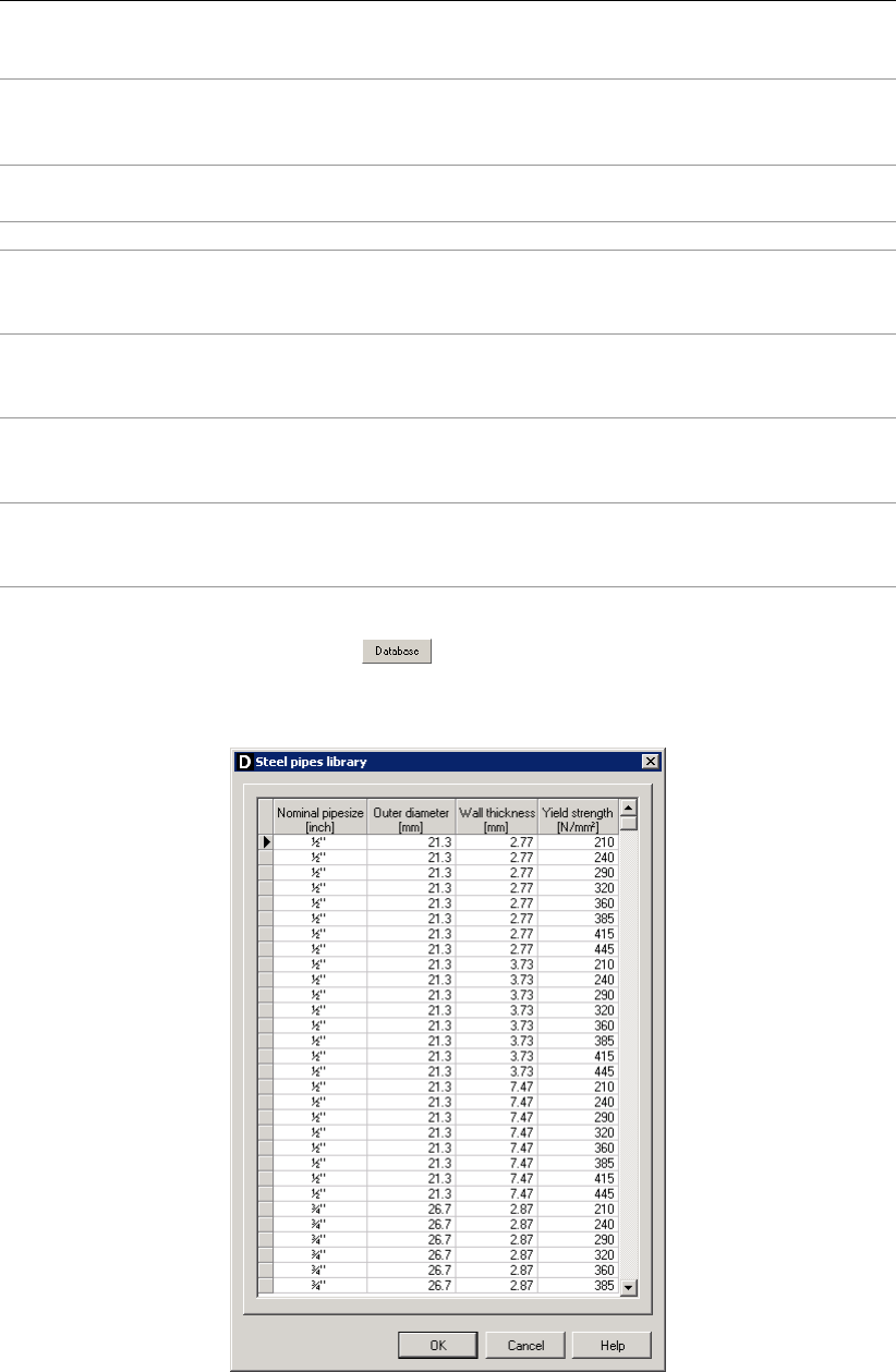
Input
Young’s modulus Modulus of elasticity of the pipe (Eb) in N/mm2. For steel, the
default value is 205800 N/mm2. It is used to determine the
stresses in the pipeline in a strength calculation.
Outer diameter product
pipe (Do)
Outer diameter of the product pipe (Do) in mm.
Wall thickness Wall thickness of the pipe (dn) in mm.
Unit weight pipe material Unit weight of the pipe material (γb), used to determine the
pulling force in the pipeline. For steel, the default value is
78.5 kN/m3.
Design pressure Design pressure (pd) in Bar, used to determine the stresses
caused by internal pressure in LC 2 (section 23.5.3) and in
LC 4 (section 23.5.5).
Test pressure Test pressure (pt) in Bar, used to determine the stresses
caused by test pressure in LC 2 (section 23.5.3) and in LC 4
(section 23.5.5).
Temperature variation Temperature variation (∆t) in ◦C, used to determine the
stresses caused by temperature variation in LC 4 (sec-
tion 23.5.5).
When clicking the Database button , the Steel pipes library window appears (Fig-
ure 4.32) in which the material quality (i.e. nominal pipe size), the outer diameter, the wall
thickness and the yield strength of different steel pipes can be imported.
Figure 4.32: Steel pipes library window
Polyethylene pipe
Different types of polyethylene pipes can be selected from the database (see Figure 4.34).
User-defined values can also be defined for a PE pipeline.
Deltares 67 of 324

D-GEO PIPELINE
, User Manual
Figure 4.33: Product Pipe Material Data window (Polyethylene)
Pipe material Choice between steel or polyethylene.
Click this button to import the name, the outer diameter, the
wall thickness and the yield strength of a pipe material from
the
D-GEO PIPELINE
library (see Figure 4.34).
Material quality Description of the polyethylene quality. The data in this field
is used in the report.
Young’s modulus (short) Modulus of elasticity of the pipe (Eb) at short term in N/mm2.
Young’s modulus (long) Modulus of elasticity of the pipe (Eb) at long term in N/mm2.
Allowable strength (short) Yield strength of the pipe at sort term (Reb;short) in N/mm2.
Allowable strength (long) Yield strength of the pipe at long term (Reb;long) N/mm2.
Tensile factor The tensile factor a(also called alpha pipe material) is the
relation between the allowable tensile strength and the allow-
able bending strength. The default value is 0.65.
Outer diameter product
pipe (Do)
Outer diameter of the product pipe (Do) in mm.
Wall thickness Wall thickness of the pipe (dn) in mm, used to determine the
stresses in a strength calculation.
Unit weight pipe material Unit weight of the pipe material (γb), used to determine the
pulling force in the pipeline. For PE, the default value is
9.54 kN/m3.
Design pressure Design pressure (pd) in Bar, used to determine the stresses
caused by internal pressure in LC 2 (section 23.5.3) and in
LC 4 (section 23.5.5).
Test pressure Test pressure (pt) in Bar, used to determine the stresses
caused by test pressure in LC 2 (section 23.5.3) and in LC 4
(section 23.5.5).
Temperature variation Temperature variation (∆t) in ◦C, used to determine the
stresses caused by temperature variation in LC 4 (sec-
tion 23.5.5).
68 of 324 Deltares
Input
When clicking the Database button , the PE pipes library window appears (Figure 4.34)
in which the material quality, the Young’s modules (short and long), the allowable strengths
(short and long), the outer diameter and the wall thickness of different PE pipes can be im-
ported.
Figure 4.34: PE pipes library window
4.6.2.2 Product Pipe Material Data for Micro tunneling
If the Micro tunneling option in the Model window (section 4.1.1) is selected, click Pipe on
the menu bar and then choose Product Pipe Material Data to open the Product Pipe Material
Data window in which the characteristics of the pipe material can be entered. Depending on
the choice between steel, synthetic and concrete (Figure 4.35), different parameters need to
be specified.
Figure 4.35: Product Pipe Material Data window, Pipe material sub-window
Steel or Concrete pipe
Deltares 69 of 324
D-GEO PIPELINE
, User Manual
Figure 4.36: Product Pipe Material Data window (Steel or Concrete pipe, Micro Tunneling
model)
Material quality Description of the material quality. The data in this field is
used in the report.
Outer diameter product
pipe (Do)
Outer diameter of the product pipe (Do) in mm.
Overcut on radius Difference between the hole radius and the outer radius of the
product pipe (lovercut) in mm.
Wall thickness Wall thickness of the pipe (dn) in mm.
Young’s modulus Modulus of elasticity of the pipe (Eb) in N/mm2.
Unit weight pipe material Unit weight of the pipe material (γb) in kN/m3. Default values
are 78.5 and 26 kN/m3respectively for Steel and Concrete
pipe.
Synthetic pipe
Figure 4.37: Product Pipe Material Data window (Synthetic pipe, Micro tunneling model)
Material quality Description of the material quality. The data in this field is
used in the report.
Outer diameter product
pipe (Do)
Outer diameter of the product pipe (Do) in mm.
70 of 324 Deltares
Input
Overcut on radius Difference between the hole radius and the outer radius of the
product pipe (lovercut)in mm.
Wall thickness Wall thickness of the pipe (dn) in mm.
Young’s modulus (short) Modulus of elasticity of the pipe (Eb) at short term in N/mm2.
Young’s modulus (long) Modulus of elasticity of the pipe (Eb) at long term in N/mm2.
Unit weight pipe material Unit weight of the synthetic material (γb) in kN/m3. The de-
fault value is 9.54 kN/m3.
4.6.3 Engineering Data
In the Pipe menu, choose the Engineering Data option to open the Engineering Data window.
The window displayed depends on the selected model.
4.6.3.1 Engineering Data for HDD
If the Horizontal directional drilling option in the Model window (section 4.1.1) is selected, the
Engineering Data window shown in Figure 4.38 is displayed in which data on the strength
calculation of the pipe can be defined (see chapter 23 for background information).
Figure 4.38: Engineering Data window (HDD)
Deltares 71 of 324

D-GEO PIPELINE
, User Manual
Standard/Advanced Select Advanced to display and modify some of the Miscel-
laneous parameters (Relative displacement,Compression in-
dex,Modulus of subgrade reaction of drilling fluid,Phi drilling
fluid,Cohesion drilling fluid). If Standard is selected, then
D-GEO PIPELINE
will use the default values for the five mentioned
parameters).
Pipe filled with water on
rollers
Mark this check-box if the pipe is filled with water on rollers.
Pipe always filled
(implosion)
Mark this check-box if the pipe is filled with water in all stages.
If the pipe is completely filled, the filling fluid gives an internal
fluid pressure called filling resistance pfill, see Equation 23.68 in
section 23.8.1.
Part of pipe filled with
fluid during pull back
Part of the cross-section of the pipe filled with fluid (Pw) in %.
Uplift forces resulting from buoyancy of the product pipe can be
reduced by filling a part of the cross-section with water. This will
reduce the pulling force.
Unit weight fluid Unit weight of the fluid filling (γfill).
Bedding angle The bedding angle β(see Figure 4.39). The default value is
120◦.
Load angle The load angle α(see Figure 4.39). The default value is 180◦.
Relative displacement Relative displacement between soil columns, necessary for full
development of friction (δd). The default value is 10 mm.
Compression index Average compression index of the layers in which the pipe is
installed (C). The default value for a very compressible soil se-
quence is 6.
Linear settlement coeff.
(alpha_g) for steel
Linear settlement coefficient αgfor steel (average over the tem-
perature variation ∆t). The default value for steel is 0.0000117
(mm/mm)K-1.
Linear settlement coeff.
(alpha_g) for PE
Linear settlement coefficient αgfor PE (average over the tem-
perature variation ∆t). The default value for PE is 0.00018
(mm/mm)K-1.
Modulus of subgrade
reaction of drilling
fluid (Kv)
The modulus of subgrade reaction (also called bedding constant)
of the drilling fluid after stiffening (kv;df). The default value is
500 kN/m3.
Phi drilling fluid Angle of internal friction of the stiffened drilling fluid (ϕdf). The
default value is 15◦.
Cohesion drilling fluid Cohesion of the stiffened drilling fluid (cdf). The default value is
5 kN/m2.
Factor of friction
pipe-roller (f1)
Factor of friction between the product pipe and the rollers on the
pipe-roller (f1). During the pullback operation this part of the
pulling force will decrease. The default value is 0.1.
Friction pipe-drilling
fluid (f2)
Friction between the drilling fluid and the pipeline (f2). The de-
fault value is 0.00005 N/mm2.
Factor of friction
pipe-soil (f3)
Factor of friction between the product pipe and the soil (f3). The
friction between pipe and soil is influenced by buoyancy of the
pipeline in the drilling fluid. The default value is 0.2.
72 of 324 Deltares
Input
Figure 4.39: Definition of the bedding angle βand the load angle α
4.6.3.2 Engineering Data for Micro tunneling
If the Micro tunneling option in the Model window (section 4.1.1) is selected, the Engineering
Data window shown in Figure 4.40 is displayed. See chapter 24 for background information.
Figure 4.40: Engineering Data window (Micro tunneling)
Standard/Advanced Select Advanced to display and modify some of the Miscella-
neous parameters (Relative displacement, Compression index,
Modulus of subgrade reaction of the stiffened drilling fluid, Phi
drilling fluid, Cohesion drilling fluid). If Standard is selected, then
D-GEO PIPELINE
will use the default values for the five mentioned
parameters).
Allowable thrust force The maximum allowable thrust force is usually specified by the
manufacturer of the pipe.
Volume loss as per-
centage of overcut area
The volume loss determines the subsidence at the surface (i.e.
the excess soil removed by the Micro Tunneling Boring Machine).
Deltares 73 of 324
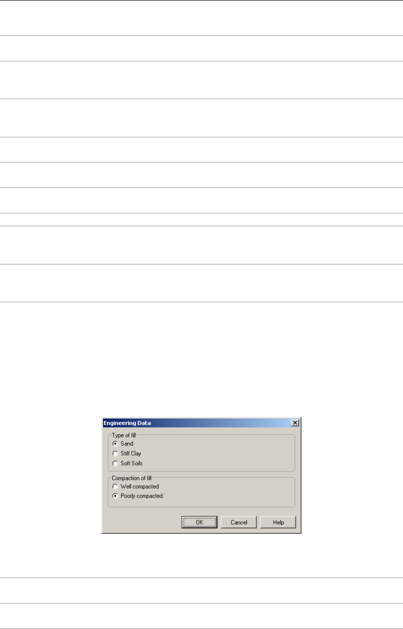
D-GEO PIPELINE
, User Manual
Relative displacement Relative displacement between soil columns, necessary for full
development of friction (δd). The default value is 10 mm.
Compression index Average compression index of the layers in which the pipe is
installed (C). The default value for a very compressible soil se-
quence is 6.
Modulus of subgrade
reaction of lubrification
fluid
The modulus of subgrade reaction (also called bedding con-
stant) of the lubrification fluid (kv;lub fluid). The default value is
500 kN/m3.
Phi lubrication fluid Angle of internal friction of the lubrification fluid (ϕlub fluid). The
default value is 15◦.
Adhesion lubrification
fluid
Adhesion of the lubrification fluid (alub fluid). The default value is
5 kN/m2.
Factor phi for reduced
soil load
Safety factor applied on the reduced soil stress. The default
value is 0.5.
Delta lubrification fluid Delta angle of the lubrification fluid. The default value is 7.5◦.
Friction with injection of
lubricant
The friction between the soil and the pipe in case of injection
of lubricant (M) used for the calculation of the thrust forces Fm
(see Equation 24.8 in section 24.1.4).
Friction without
injection of lubricant
The friction between the soil and the pipe in case of no injection
of lubricant (M) used for the calculation of the thrust forces Fm
(see Equation 24.8 in section 24.1.4).
4.6.3.3 Engineering Data for Construction in trench
If the Construction in trench option in the Model window (section 4.1.1) is selected, the En-
gineering Data window shown in Figure 4.41 is displayed. In this window, information about
the filling can be entered and will be used to determine the value of the percentage of com-
paction µused in the calculation of the initial (or actual) vertical stress, see section 21.4 for
background information.
Figure 4.41: Engineering Data window (Construction in trench)
Type of fill Select the type of fill used for the filling of the trench: Sand,Stiff
Clay or Soft Soils.
Compaction of fill Select the type of compaction of the filling soil: Well compacted
or Poorly compacted.
74 of 324 Deltares

Input
4.6.4 Drilling Fluid Data
In the Pipe menu, choose the Drilling Fluid Data option to open the Drilling Fluid Data window
in which the drill pipe and borehole dimensions, the characteristics of drilling fluid flow, and
the properties of the drilling fluid can be defined. For background information, see chapter 22.
Figure 4.42: Drilling Fluid Data window
Outer diameter pilot hole Outer diameter of the hole during the pilot hole drilling [m].
Outer diameter pilot pipe Outer diameter of the pipe during the pilot hole drilling [m].
Outer diameter pre-ream
hole
Outer diameter of the hole during the pre-reaming of the prod-
uct pipeline [m].
Outer diameter drill pipe Outer diameter of the pipe during the pre-reaming of the prod-
uct pipeline [m].
Outer diameter borehole Outer diameter of the hole during the pullback of the product
pipeline [m].
Outer diameter product
pipe (Do)
Outer diameter of the (bundled) pipe during the pullback of
the product pipeline. This value is automatically calculated by
the program using the pipe diameters of the different pipes
as inputted in the Product Pipe Material Data window (see
section 4.6.2.1). The following formula is used:
Deq =qPn
i=1 D2
o;i
Annular back flow rate pilot
boring
Annular back flow rate (Qann) during the pilot hole drilling, in
liter/minute.
Annular back flow rate pre-
reaming
Annular back flow rate (Qann) during the pre-reaming stage,
in liter/minute.
Annular back flow rate
ream and pullback
Annular back flow rate (Qann) during the pullback stage, in
liter/minute.
Circulation loss factor pilot
boring
Circulation loss factor (floss) during the pilot-hole drilling. The
default value is 0.3.
Deltares 75 of 324

D-GEO PIPELINE
, User Manual
Circulation loss factor pre-
reaming
Circulation loss factor (floss) during the pre-reaming stage.
The default value is 0.2.
Circulation loss
factor ream and pull-back
Circulation loss factor (floss) during the pullback stage . The
default value is 0.2.
Unit weight (γ)Unit weight of the drilling fluid (γdf). The default value is
11.1 kN/m3.
Yield point (τ)Yield point of the drilling fluid (τdf). The default value is
0.014 kN/m2.
Plastic viscosity (µ)Plastic viscosity of the drilling fluid (µdf). The default value is
0.00004 kN.s/m2.
The annular back-flow depends mainly on the size of the borehole and the pump system on
the type of drilling rig used. The circulation loss factor depends on the soil layers through
which the drilling is performed. The circulation loss factor indicates the loss of the drilling fluid
in the soil surrounding the borehole.
The properties of the drilling fluid (γdf,τdf and µdf) can be obtained from the drilling fluid
manufacturer.
4.7 Defaults menu
4.7.1 Factors
In the Defaults menu, choose the Factor option to open the Factor input window. The content
of the window depends on the model:
Refer to section 4.7.1.1 for HDD
Refer to section 4.7.1.2 for Micro tunneling
Refer to section 4.7.1.3 for Construction in trench
4.7.1.1 Factors for HDD
If the Horizontal directional drilling option in the Model window (section 4.1.1) is selected, the
factors for loads and strength parameters according to either the Dutch standard NEN 3650
or the European standard CEN can be specified in the Factors window. Depending on the
choice of the type of material (steel or polyethylene), different factors need to be specified.
Factors for HDD – Dutch standard NEN – Polyethylene pipe
If the Dutch standard NEN was selected in the the Model window (section 4.1.1) and if a
polyethylene material was selected in the Product Pipe Material Data window (section 4.6.2.1),
the window in Figure 4.43 is displayed.
76 of 324 Deltares
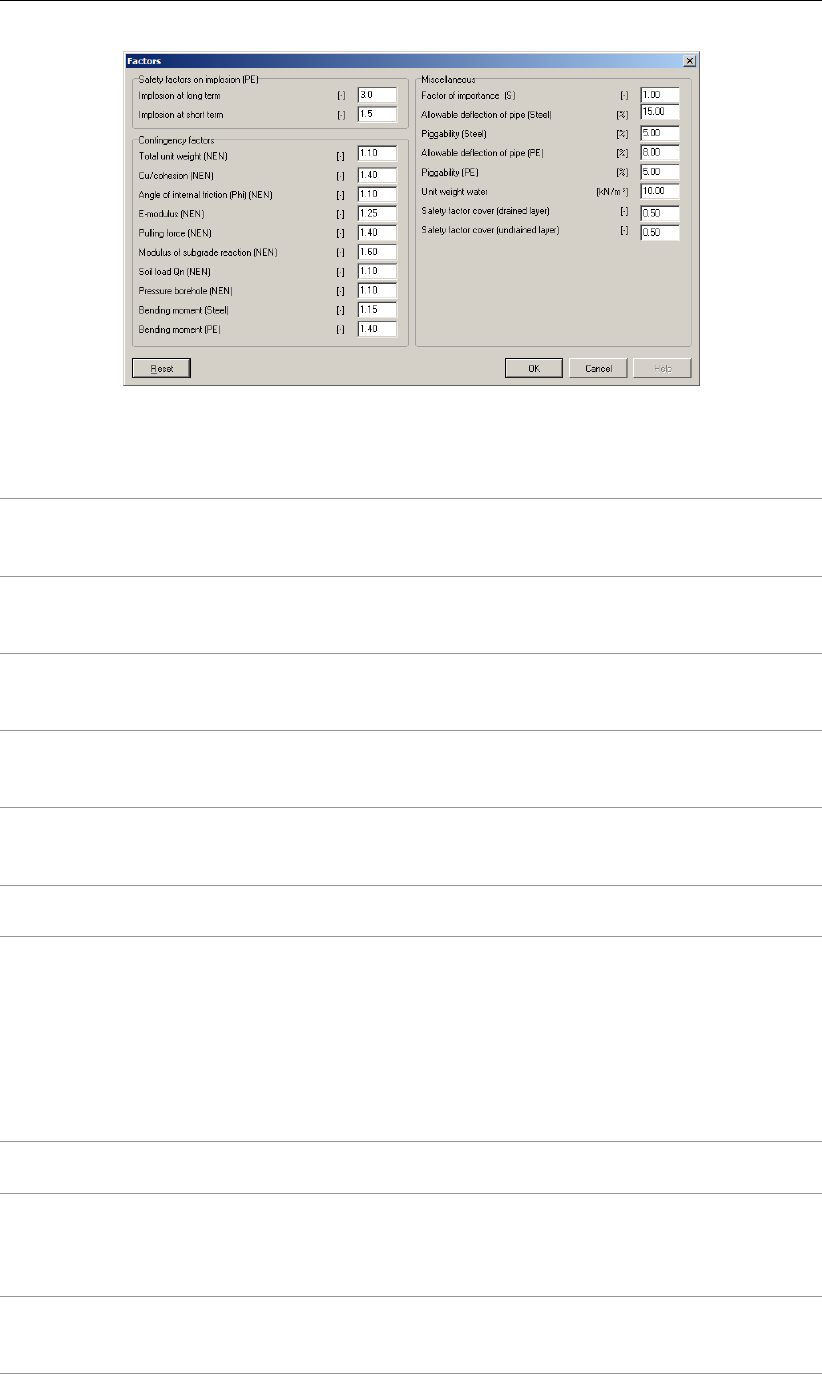
Input
Figure 4.43: Factors window (HDD) for polyethylene pipe, acc. to the Dutch standard
NEN
Implosion at long
term
Safety factor on implosion at long term (γimp;long). The default value
is 3, as prescribed in paragraph 8.5.5.1 of NEN 3650-3 (NEN,
2012c).
Implosion at short
term
Safety factor on implosion at short term (γimp;short). The default value
is 1.5, as prescribed in paragraph 8.5.5.1 of NEN 3650-3 (NEN,
2012c).
Total unit weight Contingency factor on the total unit weight above and below the
phreatic level (fγ). The default value is 1.1, as prescribed in Table
B.2 of NEN 3650-1 (NEN,2012a).
Cu/cohesion Contingency factor on the cohesion for drained and undrained con-
ditions (fc). The default value is 1.4, as prescribed in Table B.2 of
NEN 3650-1 (NEN,2012a).
Angle of internal
friction (Phi)
Contingency factor on the angle of internal friction (fϕ). The de-
fault value is 1.1, as prescribed in Table B.2 of NEN 3650-1 (NEN,
2012a).
E-modulus Contingency factor on the Young’s modulus (fE). The default value
is 1.25, as prescribed in Table B.2 of NEN 3650-1 (NEN,2012a).
Pulling force Contingency factor on pulling forces (f), to take into account the
stochastic distribution in the value of the different friction compo-
nents and the uncertainty on the model. The default value is 1.4, as
prescribed in paragraph E.1.2.1 of NEN 3650-1 (NEN,2012a).
NOTE: According to the NEN 3650-1 (article E.1.2.3), the contin-
gency factor on the pulling force for bundled pipelines should be in-
creased to 1.8 because due to the pull back of the bundled pipelines
the risk on higher pulling forces than calculated is present.
Modulus of
subgrade reaction
Contingency factor on the modulus of subgrade reaction (fkv). The
default value is 1.6.
Soil load Qn Contingency factor on the reduced neutral soil stress Qn,r (fQn1),
used for the strength calculation of the pipeline (see section 23.5).
The default value is 1.1, as prescribed in Table B.3 of NEN 3650-1
(NEN,2012a).
Pressure borehole Contingency factor on the pressure borehole (fpress;bore), used to
check the equilibrium between drilling fluid pressure and pore pres-
sure, see section 22.4. The default value is 1.1.
Deltares 77 of 324
D-GEO PIPELINE
, User Manual
Bending moment
(Steel)
Contingency factor on the bending moment (fM) for steel. In para-
graph E.1.3 of NEN 3650-1 (NEN,2012a), an overall factor on bend-
ing moment (fk) of 1.4 is prescribed. As this overall factor includes
different contingency factors (i.e. fk=fM×finstall ×fR) and as
finstall = 1.1 and fR= 1.1, a default factor of 1.15 should be inputted
for fMto get fk= 1.4 as prescribed by NEN.
Bending moment
(PE)
Contingency factor on the bending moment (fM) for PE. In para-
graph E.1.3 of NEN 3650-1 (NEN,2012a), an overall factor on bend-
ing moment (fk) of 1.4 is prescribed. As this overall factor includes
different contingency factors (i.e. fk=fM×finstall ×fR) and
as finstall = 1 and fR= 1, a default factor of 1.4 should be inputted
for fMto get fk= 1.4 as prescribed by NEN.
Factor of
importance (S)
Factor of importance (S). The default value is 1 (for HDD), as pre-
scribed in paragraph 6.5 of NEN 3651 (NEN,2012d).
Allowable deflection
of pipe (Steel)
Maximum allowable deflection of the pipe (δ0). The default value
is 15% of the pipe diameter for steel, as prescribed in paragraph
11.1.5 of NEN 3651 (NEN,2012d).
Piggability (Steel) Maximum allowable deflection of the pipe for piggability (δ1). If this
value is exceeded, the pig (i.e. tool or vehicle that moves through
the interior of the pipeline for purposes of inspecting, dimensioning,
or cleaning) can be damaged or stuck. The default value is 5% of
the pipe diameter.
Allowable deflection
of pipe (PE)
Maximum allowable deflection of the pipe (δ0). The default value is
8% of the pipe diameter for PE, as prescribed in paragraph 11.4.1.1
of NEN 3651 (NEN,2012d).
Piggability (PE) Maximum allowable deflection of the pipe for piggability (δ1). If this
value is exceeded, the pig (i.e. tool or vehicle that moves through
the interior of the pipeline for purposes of inspecting, dimensioning,
or cleaning) can be damaged or stuck. The default value is 5% of
the pipe diameter.
Unit weight water Unit weight of water (γw). The default value is 10 kN/m3.
Safety factor cover
(drained layer)
The ratio between the maximum allowable radius of the plastic zone
Rp;max and the soil cover H(vertical distance between the ground
level and the pipe center) for the calculation of the maximum allow-
able drilling fluid pressure in drained layer (i.e. sand), see Equa-
tion 22.28 in section 22.2.2. The default value is 0.5, as prescribed
in paragraph E.2.2.2 of NEN 3650-1 (NEN,2012a): Rp,max = 0.5 H.
Safety factor cover
(undrained layer)
The ratio between the maximum allowable radius of the plastic zone
Rp;max and the soil cover H(vertical distance between the ground
level and the pipe center) for the calculation of the maximum allow-
able drilling fluid pressure in undrained layer (i.e. clay and peat),
see Equation 22.22 in section 22.2.1. The default value is 0.5,
as prescribed in paragraph E.2.2.2 of NEN 3650-1 (NEN,2012a):
Rp,max = 0.5 H.
Click this button to reset all values to the default values prescribed
in the Dutch Standard NEN.
NOTE: If the input values in the Factors window differ from the de-
fault values prescribed by NEN, the value appears in red color.
78 of 324 Deltares
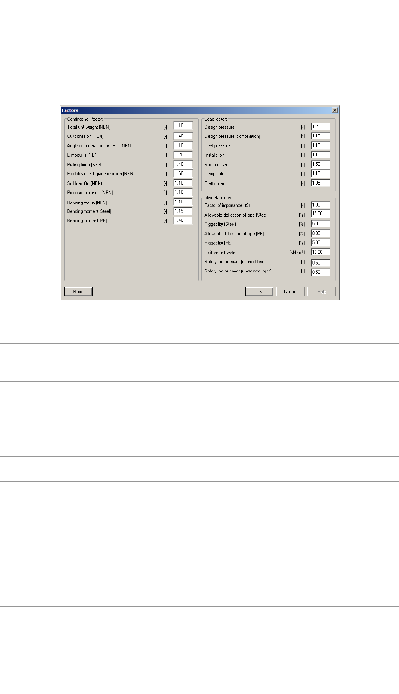
Input
Factors for HDD – Dutch standard NEN – Steel pipe
If the Dutch standard NEN was selected in the the Model window (section 4.1.1) and if a steel
material was selected in the Product Pipe Material Data window (section 4.6.2.1), the window
in Figure 4.44 is displayed. Load factors are used for the strength calculation of the pipeline
(see section 23.5).
Figure 4.44: Factors window (HDD) for steel pipe, acc. to the Dutch standard NEN
Total unit weight Contingency factor on the total unit weight above and below the
phreatic level (fγ). The default value is 1.1, as prescribed in Table
B.2 of NEN 3650-1 (NEN,2012a).
Cu/cohesion Contingency factor on the cohesion for drained and undrained con-
ditions (fc). The default value is 1.4, as prescribed in Table B.2 of
NEN 3650-1 (NEN,2012a).
Angle of internal
friction (Phi)
Contingency factor on the angle of internal friction (fϕ). The de-
fault value is 1.1, as prescribed in Table B.2 of NEN 3650-1 (NEN,
2012a).
E-modulus Contingency factor on the Young’s modulus (fE). The default value
is 1.25, as prescribed in Table B.2 of NEN 3650-1 (NEN,2012a).
Pulling force Contingency factor on pulling forces (f), to take into account the
stochastic distribution in the value of the different friction compo-
nents and the uncertainty on the model. The default value is 1.4, as
prescribed in paragraph E.1.2.1 of NEN 3650-1 (NEN,2012a).
NOTE: According to the NEN 3650-1 (article E.1.2.3), the contin-
gency factor on the pulling force for bundled pipelines should be in-
creased to 1.8 because due to the pull back of the bundled pipelines
the risk on higher pulling forces than calculated is present.
Modulus of
subgrade reaction
Contingency factor on the modulus of subgrade reaction (fkv). The
default value is 1.6.
Soil load Qn Contingency factor on the reduced neutral soil stress Qn,r (fQn1),
used for the strength calculation of the pipeline (see section 23.5).
The default value is 1.1, as prescribed in Table B.3 of NEN 3650-1
(NEN,2012a).
Pressure borehole Contingency factor on the pressure borehole (fpress;bore), used to
check the equilibrium between drilling fluid pressure and pore pres-
sure, see section 22.4. The default value is 1.1.
Deltares 79 of 324

D-GEO PIPELINE
, User Manual
Bending radius Contingency factor on the bending radius (fR) used for the deter-
mination of the axial stress in the strength calculation, see sec-
tion 23.5. The default value is 1.1.
Bending moment
(Steel)
Contingency factor on the bending moment (fM) for steel. In para-
graph E.1.3 of NEN 3650-1 (NEN,2012a), an overall factor on bend-
ing moment (fk) of 1.4 is prescribed. As this overall factor includes
different contingency factors (i.e. fk=fM×finstall ×fR) and as
finstall = 1.1 and fR= 1.1, a default factor of 1.15 should be inputted
for fMto get fk= 1.4 as prescribed by NEN.
Bending moment
(PE)
Contingency factor on the bending moment (fM) for PE. In para-
graph E.1.3 of NEN 3650-1 (NEN,2012a), an overall factor on bend-
ing moment (fk) of 1.4 is prescribed. As this overall factor includes
different contingency factors (i.e. fk=fM×finstall ×fR) and
as finstall = 1 and fR= 1, a default factor of 1.4 should be inputted
for fMto get fk= 1.4 as prescribed by NEN.
Design pressure Load factor on the design pressure (fpd). The default value is 1.25
as prescribed in Table 2 of NEN 3650-2 (NEN,2012b).
Design pressure
(combination)
Load factor on the design pressure when used in combination
(fpd;comb). The default value is 1.15 as prescribed in Table 2 of
NEN 3650-2 (NEN,2012b).
Test pressure Load factor on the test pressure (fpt). The default value is 1.1 as
prescribed in Table 2 of NEN 3650-2 (NEN,2012b).
Installation Load factor on the installation (finstall). The default value is 1.1 as
prescribed in Table 2 of NEN 3650-2 (NEN,2012b).
Soil load Qn Load factor on the reduced neutral soil stress Qn,r (fQn2). The de-
fault value is 1.5.
Temperature Load factor on the stress due to temperature variation (ftemp). The
default value is 1.1 as prescribed in Table 2 of NEN 3650-2 (NEN,
2012b).
Traffic load factor The load factor on the traffic load fqv, see section 21.14. The default
value is 1.35, as prescribed in Table 2 of NEN 3650-2 (NEN,2012b).
Factor of
importance (S)
Factor of importance (S). The default value is 1 (for HDD), as pre-
scribed in paragraph 6.5 of NEN 3651 (NEN,2012d).
Allowable deflection
of pipe (Steel)
Maximum allowable deflection of the pipe (δ0). The default value
is 15% of the pipe diameter for steel, as prescribed in paragraph
11.1.5 of NEN 3651 (NEN,2012d).
Piggability (Steel) Maximum allowable deflection of the pipe for piggability (δ1). If this
value is exceeded, the pig (i.e. tool or vehicle that moves through
the interior of the pipeline for purposes of inspecting, dimensioning,
or cleaning) can be damaged or stuck. The default value is 5% of
the pipe diameter.
Allowable deflection
of pipe (PE)
Maximum allowable deflection of the pipe (δ0). The default value is
8% of the pipe diameter for PE, as prescribed in paragraph 11.4.1.1
of NEN 3651 (NEN,2012d).
Piggability (PE) Maximum allowable deflection of the pipe for piggability (δ1). If this
value is exceeded, the pig (i.e. tool or vehicle that moves through
the interior of the pipeline for purposes of inspecting, dimensioning,
or cleaning) can be damaged or stuck. The default value is 5% of
the pipe diameter.
Unit weight water Unit weight of water (γw). The default value is 10 kN/m3.
80 of 324 Deltares
Input
Safety factor cover
(drained layer)
The ratio between the maximum allowable radius of the plastic zone
Rp;max and the soil cover H(vertical distance between the ground
level and the pipe center) for the calculation of the maximum allow-
able drilling fluid pressure in drained layer (i.e. sand), see Equa-
tion 22.28 in section 22.2.2. The default value is 0.5, as prescribed
in paragraph E.2.2.2 of NEN 3650-1 (NEN,2012a): Rp,max = 0.5 H.
Safety factor cover
(undrained layer)
The ratio between the maximum allowable radius of the plastic zone
Rp;max and the soil cover H(vertical distance between the ground
level and the pipe center) for the calculation of the maximum allow-
able drilling fluid pressure in undrained layer (i.e. clay and peat),
see Equation 22.22 in section 22.2.1. The default value is 0.5,
as prescribed in paragraph E.2.2.2 of NEN 3650-1 (NEN,2012a):
Rp,max = 0.5 H.
Click this button to reset all values to the default values prescribed
in the Dutch Standard NEN.
NOTE: If the input values in the Factors window differ from the de-
fault values prescribed by NEN, the value appears in red color.
Factors for HDD – European standard CEN – Polyethylene pipe
If the European standard CEN was selected in the the Model window (section 4.1.1) and if a
polyethylene material was selected in the Product Pipe Material Data window (section 4.6.2.1),
the window in Figure 4.45 is displayed.
Figure 4.45: Factors window (HDD) for polyethylene pipe, acc. to the European standard
CEN
For the definition of the parameters refer to the window for the Dutch standard NEN (see
Figure 4.43), only the default values are different.
Click the button to reset all values to the default values prescribed in the European
standard CEN. If the input values in the Factors window differ from the default values pre-
scribed by CEN, the value appears in red color.
Deltares 81 of 324
D-GEO PIPELINE
, User Manual
Factors for HDD – European standard CEN – Steel pipe
If the European standard CEN was selected in the the Model window (section 4.1.1) and if a
steel material was selected in the Product Pipe Material Data window (section 4.6.2.1), the
window in Figure 4.46 is displayed.
Figure 4.46: Factors window (HDD) for steel pipe, according to the European standard
CEN
For the definition of the parameters refer to the window for the Dutch standard NEN (see
Figure 4.44), only the default values are different.
Click the button to reset all values to the default values prescribed in the European
standard CEN. If the input values in the Factors window differ from the default values pre-
scribed by CEN, the value appears in red color.
4.7.1.2 Factors for Micro tunneling
If the Micro tunneling option in the Model window (section 4.1.1) is selected, the Factors
window of Figure 4.47 is displayed in which the safety factors for soil parameters can be
specified.
Figure 4.47: Factors window (Micro tunneling)
82 of 324 Deltares
Input
Cu/cohesion The safety factor on the cohesion for drained and undrained con-
ditions (fc). The default value is 1.4, as prescribed in Table B.2
of NEN 3650-1 (NEN,2012a).
Angle of internal
friction (Phi)
The safety factor on the angle of internal friction (fϕ). The default
value is 1.1, as prescribed in Table B.2 of NEN 3650-1 (NEN,
2012a).
Horizontal effective
stress
The safety factor on the horizontal effective stress (fσh). The
default value is 1.5.
Safety factor water
pressure
The safety factor on the water pressure u(fu). The default value
is 1.05.
Safety factor uplift The safety factor on uplift (fuplift). The default value is 1.
Contingency factor soil
cover
The contingency factor on soil cover (fcover). The default value is
1.1.
Overburden factor silo
effect
The overburden factor on silo effect (fsilo). The default value is
2.
Stability ratio N The stability ratio (N). The default value is 3. This ratio is used
for the calculation of the minimal support pressure in undrained
conditions, see Equation 24.2 in section 24.1.2.
Unit weight water The unit weight of water (γw). The default value is 10 kN/m3.
Click this button to reset all values to the default values.
NOTE: If the input values in the Factors window differ from the
default values, the value appears in red color.
4.7.1.3 Factors for Construction in trench
If the Construction in trench option in the Model window (section 4.1.1) is selected, the Factors
window of Figure 4.48 is displayed in which the safety factor for uplift and the unit weight of
water can be specified.
Figure 4.48: Factors window (Construction in trench)
Safety factor uplift The safety factor on uplift (fuplift). The default value is 1.
Safety factor hydraulic
heave
The safety factor on hydraulic heave (fburst). The default value is
1.
Unit weight water Unit weight of water (γw). The default value is 10 kN/m3.
Click this button to reset all values to the default values.
NOTE: If the input values in the Factors window differ from the
default values, the value appears in red color.
Deltares 83 of 324
D-GEO PIPELINE
, User Manual
4.7.2 Special Stress Analysis
If the Horizontal directional drilling option in the Model window (section 4.1.1) is selected,
the Special Stress Analysis window of Figure 4.49 is displayed when selecting Special Stress
Analysis from the Defaults menu. In this window, it is possible to choose between three types
of stress analysis: a standard, a per vertical or a special analysis, as explained below.
Figure 4.49: Special Stress Analysis window (HDD)
Stress analysis options Three types of stress analysis are available:
•AStandard stress analysis, performed from the Start option
of the Calculation menu (see section 5.1), which uses the max-
imum reduced neutral soil stress and the maximum modulus of
subgrade reaction of the soil calculated by
D-GEO PIPELINE
be-
tween all the verticals and the minimum bending radius present
in the pipeline configuration.
•A stress analysis Per vertical, performed from the Start op-
tion of the Calculation menu (see section 5.1), which uses the
reduced neutral soil stress and the modulus of subgrade reac-
tion of the soil calculated by
D-GEO PIPELINE
per vertical and the
bending radius of the pipeline trajectory cut by the vertical.
NOTE: If the vertical cut a straight part of the pipeline trajec-
tory,
D-GEO PIPELINE
assumes a very large bending radius of
100000 m.
•A “Special Stress Analysis”, performed from the Special Stress
Analysis option of the Calculation menu (see section 5.2) using
Stress calculation data (i.e user-defined values for the reduced
neutral soil stress, for the modulus of subgrade reaction of the
soil and for the bending radius).
If the option Use stress calculation data is selected, the following values must be inputted:
Soil load (neutral or
reduced neutral) Qn
raised by a traffic load
if any
Enter the user-defined reduced neutral soil stress (in kN/m2),
used for a Special Stress Analysis (section 5.2).
Modulus of subgrade
reaction
Enter the user-defined modulus of subgrade reaction of the soil
(in kN/m3), used for a Special Stress Analysis (section 5.2).
84 of 324 Deltares


D-GEO PIPELINE
, User Manual
86 of 324 Deltares

5 Calculations
5.1 Start Calculation
On the menu bar, click Start in the Calculation menu to perform the following calculations:
Calculation of soil mechanical data
The passive, neutral and reduced vertical stresses of the soil, the vertical coefficient of
subgrade reaction, and the ultimate bearing capacity for each vertical are calculated and
written to a report file (see section 6.2.4). For background information, see chapter 21].
Calculation of drilling fluid pressures (only for HDD)
In directional drilling first a bore hole is made by a pilot drilling. This bore hole has
a relatively small diameter. During the second drilling stage the initial bore hole is
enlarged by pre-reaming. When the requested diameter is reached the product pipe
is pulled into the bore hole. During all drilling stages a minimum required drilling fluid
pressure is necessary. The bore fluid pressure induces a return flow of drilling fluid
from the drilling head to the entry or exit point. The return flow transports loosened soil
material. The necessary fluid pressure depends on:
The difference in elevation between the bore hole and the exit point of the return
flow;
The minimum required pressure necessary to cause a return flow (soil material
included) over a certain distance.
When the entry and exit points are not on the same level, the minimum required drilling
fluid pressure depends on the direction of the drilling (from left to right or from right to
left).
D-GEO PIPELINE
calculates the minimum required drilling fluid pressure for both
cases.
The maximum allowable pressure depends on the strength of the soil around the bore-
hole. When the required drilling pressure is higher than the maximum allowable pres-
sure, there is a risk a blow out may occur. In that case, the pipeline configuration must
be changed. For instance, by choosing a lower pipe level or by moving the entry or exit
point.
The calculations of the minimum and maximum drilling fluid pressures for the three
stages (pilot, pre-ream and pull-back) are performed in the user defined verticals. The
results of the calculations are written to a report file (see section 6.2.1). For background
information, see chapter 22.
Pipe stress analysis (only for HDD)
In the pipe stress analysis, the pulling forces during the pull-back operation, the max-
imum acting stresses in the pipe material and the deflection of the pipeline are cal-
culated. The calculated stresses are compared to the allowable short and long term
stresses for a PE pipeline, while for a steel pipeline a total stress is calculated and
compared with the allowable stress. With this option, the strength calculation is per-
formed with the calculated reduced neutral soil load and bedding constant after the
soil mechanical data has been calculated. The results of the calculations are written
to a report file (see section 6.2.5 and section 6.2.6). For background information, see
chapter 23.
Settlements
The settlements of soil layers below the pipeline are calculated. For Micro Tunneling
model, the subsidence are also calculated. The results of the calculations are written
to a report file (see section 6.2.2 and section 6.2.3). For background information, see
section 21.10 and section 24.3.
Deltares 87 of 324
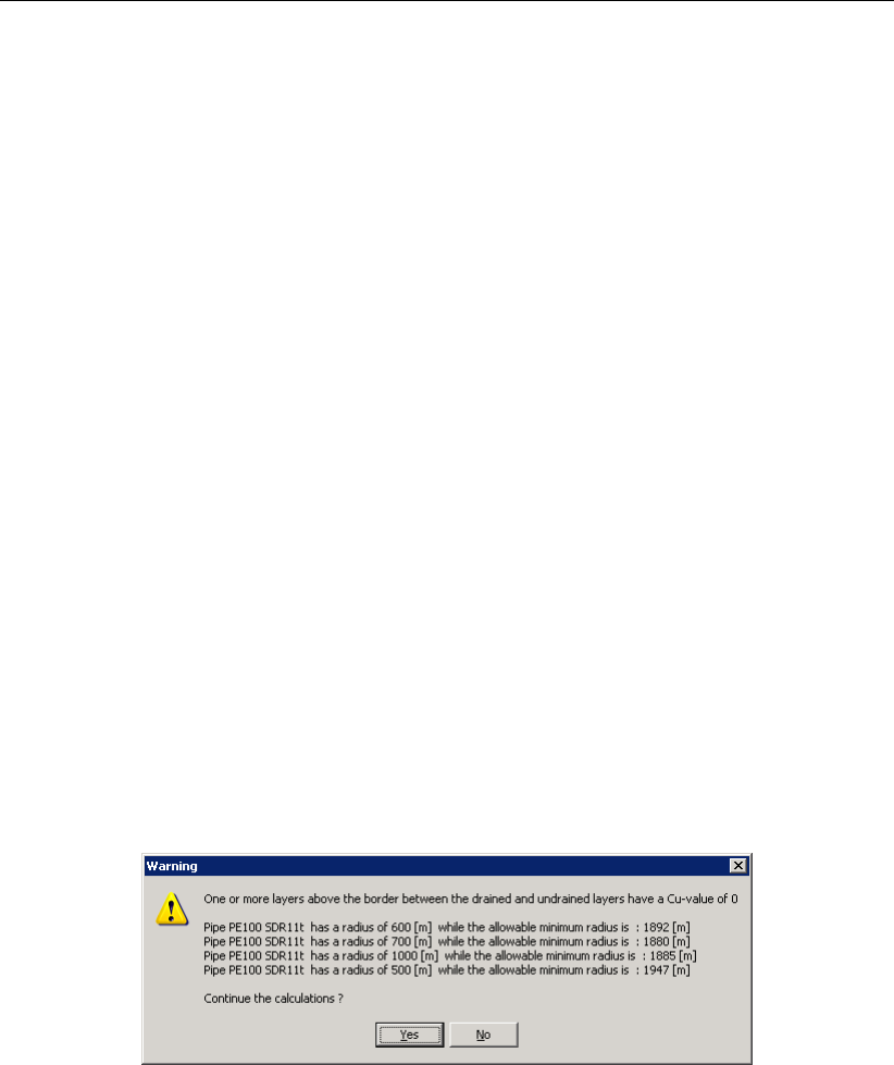
D-GEO PIPELINE
, User Manual
Operation parameters
the uplift check and the hydraulic heave check for Trenching; for background infor-
mation, see chapter 25.
the uplift check, the face support pressures and the thrust forces for Micro tunnel-
ing; for background information, see section 24.1 and section 24.2.
The results of the calculations are written to a report file (see section 6.2.7 and sec-
tion 6.2.8).
5.2 Special Stress Analysis (only for HDD)
On the menu bar, click Special Stress Analysis in the Calculation menu to perform a pipe
stress calculation with the user-defined values for the reduced neutral soil stress, the modulus
of subgrade reaction and the bending radius, specified in the Special Stress Analysis window
(section 4.7.2) instead of the calculated values.
D-GEO PIPELINE
will not apply safety factors
on those three specified values, assuming they are already included. A special stress analysis
must always be started separately.
5.3 Warning and Error messages
5.3.1 Warning messages
Before calculation, warning messages might be displayed in the Warning window after starting
the calculation. The calculation will be paused. If clicking Yes the calculations will continue,
whereas if clicking No the calculations will be aborted. Figure 5.1 gives an example of warning
messages displayed when an undrained layer has an undrained cohesion cuof 0 and when
determining the allowable curve radius in accordance with section 20.1.4.
Figure 5.1: Warning window (before calculation) about allowable radius
88 of 324 Deltares
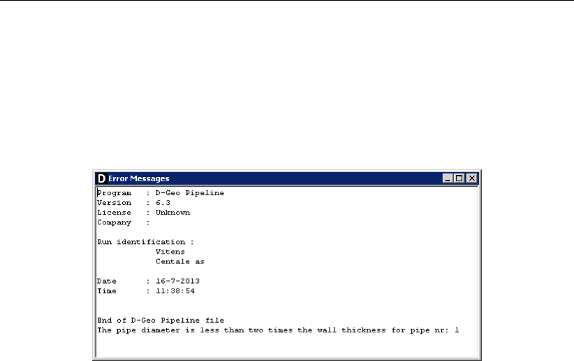
Calculations
5.3.2 Error messages
If errors are found in the input, no calculation can be performed and
D-GEO PIPELINE
opens
the Error Messages window displaying more details about the error(s). Those errors must be
corrected before performing a new calculation. To view those error messages, select the Error
Messages option from the Help menu (section 3.3.1). They are also writing in the *.err file.
They will be overwritten the next time a calculation is started.
Figure 5.2: Error Messages window
Deltares 89 of 324

D-GEO PIPELINE
, User Manual
90 of 324 Deltares
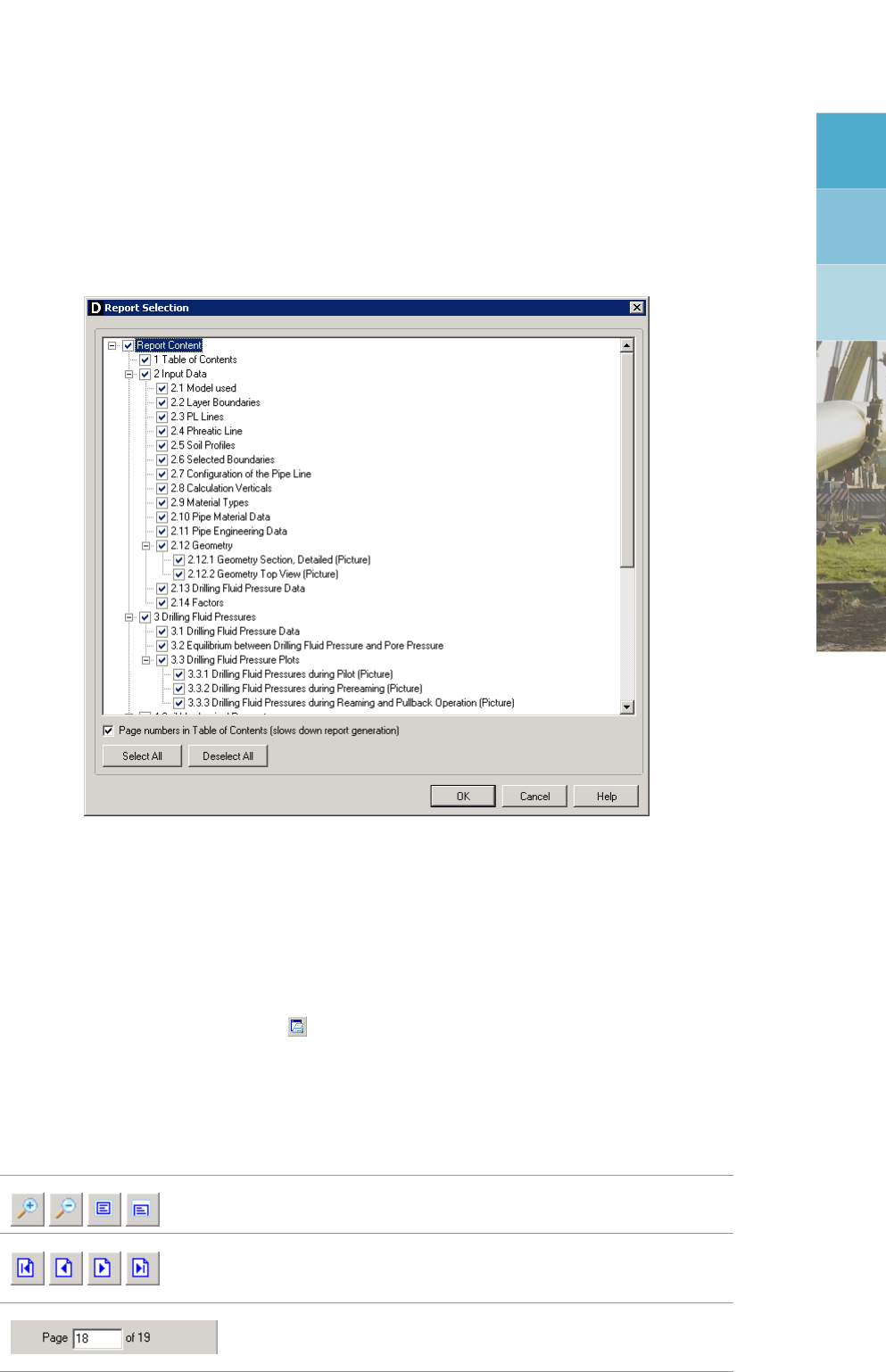
6 View Results
6.1 Report selection
On the menu bar, click Results and then choose Report Selection to open the corresponding
input window in which the content of the final report can be selected.
Figure 6.1: Report Selection window
6.2 Report
On the menu bar, click Results and then choose Report to open the Report window displaying
the selected results (section 6.1) of the calculation. This window displays the contents of the
ASCII file with extension ‘.drd’.
Click the Print active window button on the icon bar to print the report.
Use the Export Report option in the File menu to export the report in RTF, PDF, TXT or HTML
format.
The report has its own toolbar:
Those four buttons enable the user to zoom in, to zoom out,
to zoom the full page or to zoom the page width.
Those four buttons enable the user to browse through the
report by respectively moving to first page, moving to previous
page, moving to next page or moving to last page.
Another way of quickly browsing through the report is by en-
tering a page number in the input field on the toolbar and
pressing the Enter key.
Deltares 91 of 324

D-GEO PIPELINE
, User Manual
The output file consists of:
First page
Date and time of report
File name
Project identification (as inputted in section 4.1.2)
Table of Contents
Input Data chapter gives an echo of the input
Drilling Fluid Pressures chapter gives the results (plots and tables) of the drilling fluid
pressures calculation for the three stages of the HDD technique (section 6.2.1)
Deformations chapter gives:
the settlements of soil layers below the pipeline (section 6.2.2)
the subsidence for Micro Tunneling model (section 6.2.3)
Soil mechanical parameters chapter which gives the soil mechanical data (section 6.2.4)
Data for Stress analysis chapter includes buoyancy control and pulling forces calcula-
tion of the HDD technique (section 6.2.5)
Stress analysis chapter gives the stress results for the 5 load combinations (1A, 1B, 2,
3 and 4) of the HDD technique (section 6.2.6)
Operation Parameters chapter gives:
the uplift check and the hydraulic heave check for Trenching (section 6.2.7)
the uplift check, the face support pressures and the thrust forces for Micro Tunnel-
ing (section 6.2.8)
The following sections describe the output in more detail. The calculation process can be
aborted, after which a message is appended to the output file and the file is closed. All results
until the moment the calculation was stopped remain in the file.
6.2.1 Report – Drilling Fluid Pressure
92 of 324 Deltares
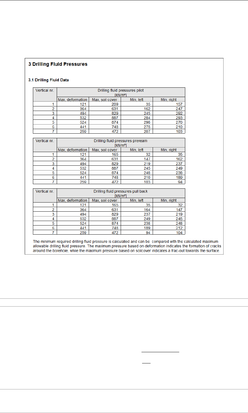
View Results
6.2.1.1 Report – Drilling Fluid Data
In the Drilling Fluid Data section, the results of the drilling fluid pressures calculation for the
three stages (pilot hole drilling, pre-reaming of the borehole and pullback of the product pipe)
are displayed.
Figure 6.2: Report window, Drilling Fluid Data section
The following is an explanation of the column headings:
Vertical nr. [-] Number of the calculation vertical.
Max, deformation
Max, soil cover
[kN/m2] Maximum drilling fluid pressure: refer to Equation 22.28 in
section 22.2.2 for drained layers and to Equation 22.22 in
section 22.2.1 for undrained layers.
For drained layers, the determination of the maximum al-
lowable radius of the plastic zone (Rp;max), can be related:
either to the deformation of the bore hole:
Rp;max =sR2
b
Q×2εg;max;
or to the soil cover: Rp;max = 0.5H
(Refer to section 22.2 for the definition of the parameters.)
Min,left [kN/m2] Minimum drilling fluid pressure assuming that the drilling
of the pilot is from left to right (see section 22.1 for back-
ground information).
Deltares 93 of 324
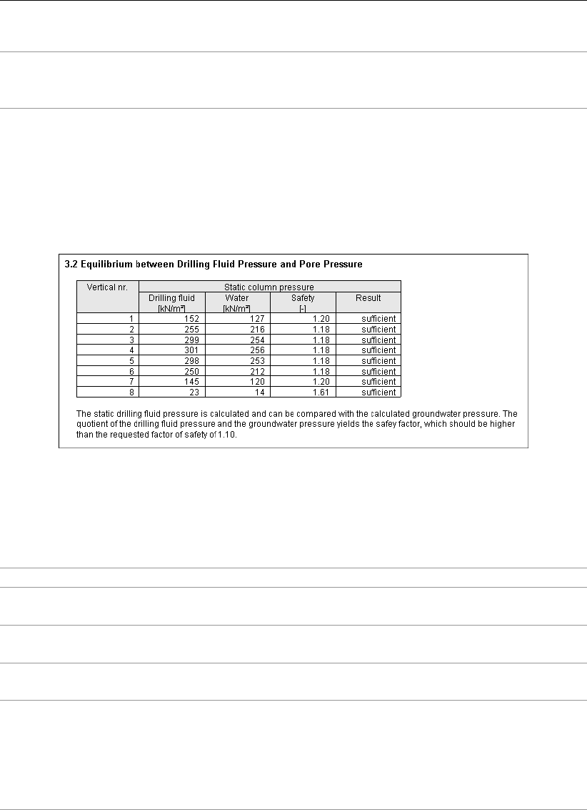
D-GEO PIPELINE
, User Manual
Min,right [kN/m2] Minimum drilling fluid pressure assuming that the drilling
of the pilot is from right to left (see section 22.1 for back-
ground information).
6.2.1.2 Report – Equilibrium between Drilling Fluid Pressure and Pore Pressure
In the Equilibrium between Drilling Fluid Pressure and Pore Pressure section, the static drilling
fluid p1is calculated and compared with the calculated pore pressure u, for each vertical. The
ratio p1/u yields the safety factor, which should be higher than the (user-defined) requested
safety factor.
Figure 6.3: Report window, Equilibrium between Drilling Fluid Pressure and Pore Pres-
sure section
The following is an explanation of the column headings:
Vertical nr. [-] Number of the calculation vertical.
Drilling fluid [kN/m2] Static column pressure of the drilling fluid (p1), see Equa-
tion 22.2 in section 22.4.
Water [kN/m2] Calculated pore pressure u, see Equation 26.4 in sec-
tion 26.5.
Safety [-] Calculated safety factor: ratio between the static drilling fluid
pressure and the pore pressure.
Result If the calculated safety factor is higher than the required safety
factor, then the drilling fluid pressure is Sufficient, otherwise it
is Not sufficient.
NOTE: The required safety factor is defined in the Factors
window under the field Contingency factor – Pressure bore-
hole, see section 4.7.1.1.
94 of 324 Deltares
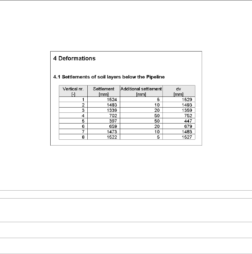
View Results
6.2.2 Report – Settlements of soil layers below the pipeline
This section is available only if the Use settlement option in the Model window (section 4.1.1)
has been selected before performing a calculation.
Figure 6.4: Report window, Settlements of soil layers below the pipeline section
The following is an explanation of the column headings:
Vertical nr. [-] Number of the calculation vertical.
Settlement [mm] Settlement calculated with the selected model, Koppejan or Iso-
tache (section 4.1.1). For background information, see sec-
tion 21.10.
Additional
settlement
[mm] Additional settlement as inputted in the Calculation Verticals win-
dow (section 4.4.2).
dv [mm] Total settlement (sum of the Settlement and the Additional set-
tlement columns).
6.2.3 Report – Subsidence
This section is available only if the Micro tunneling option in the Model window (section 4.1.1)
has been selected. Due to the overcut surface subsidence occurs. Subsidence is calculated
for each vertical at different horizontal distances of the z-axis (i.e. 0 until 3W, where Wis the
vertical distance between the surface level and the pipe center). For background information,
refer to Equation 24.14 in section 24.3. Results are given in tables and in graphs.
Deltares 95 of 324
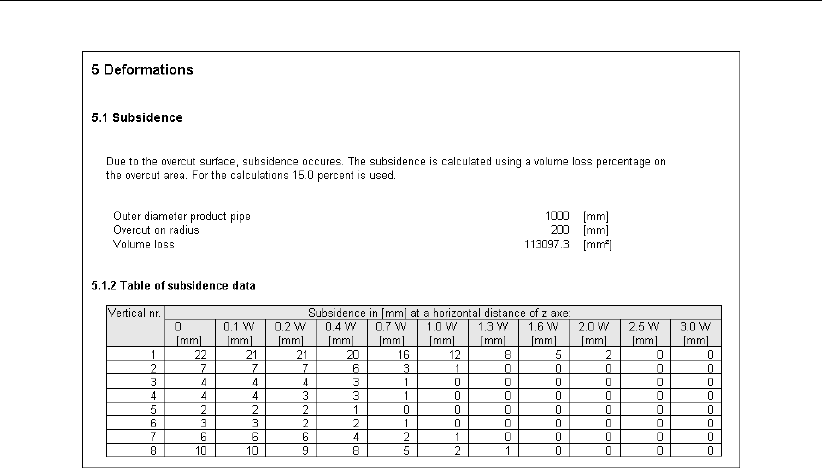
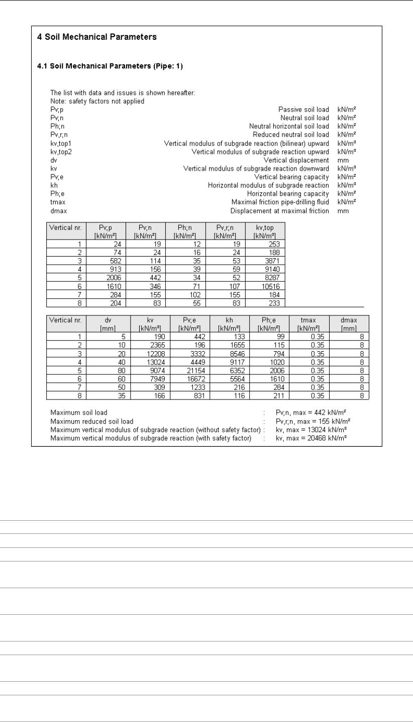
View Results
Figure 6.6: Report window – Soil Mechanical Parameters section (for HDD)
The following is an explanation of the column headings:
Vertical nr. [-] Number of the calculation vertical.
Pv;p [kN/m2] Passive soil load (see Equation 21.2 in section 21.2).
Pv;n [kN/m2] Neutral vertical soil load (see Equation 21.1 in section 21.1).
Ph;n [kN/m2] Neutral horizontal soil load (see Equation 21.12 in sec-
tion 21.5.1).
Pv,r;n [kN/m2] Reduced neutral soil load (see Equation 21.4 and Equation 21.8
in section 21.3).
kv;top [kN/m3] Vertical modulus of subgrade reaction at the top of the pipe (see
Equation 21.14 in section 21.6.1).
dv [mm] Vertical displacement (see section 21.10).
kv [kN/m3] Vertical modulus of subgrade reaction at the bottom of the pipe
(see Equation 21.14 in section 21.6.1).
Pv;e [kN/m2] Vertical bearing capacity (see Equation 21.26 in section 21.8).
kh [kN/m3] Horizontal modulus of subgrade reaction (see Equation 21.24 in
section 21.7.1).
Deltares 97 of 324
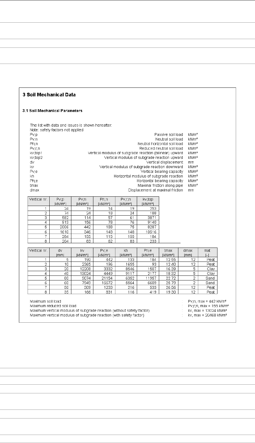
D-GEO PIPELINE
, User Manual
Ph;e [kN/m2] Horizontal bearing capacity (see Equation 21.28 in sec-
tion 21.9.1).
tmax [kN/m2] Maximal axial friction along the pipeline (see section 21.11.1).
dmax [mm] Displacement necessary to develop the maximal axial friction
along the pipeline (see section 21.12.1).
6.2.4.2 Soil Mechanical Parameters for Micro tunneling
Figure 6.7: Report window – Soil Mechanical Parameters section (for Micro tunneling)
The following is an explanation of the column headings:
Vertical nr. [-] Number of the calculation vertical.
Pv;p [kN/m2] Passive soil load (see Equation 21.2 in section 21.2).
Pv;n [kN/m2] Neutral vertical soil load (see Equation 21.1 in section 21.1).
Ph;n [kN/m2] Neutral horizontal soil load (see Equation 21.13 in sec-
tion 21.5.2).
Pv,r;n [kN/m2] Reduced neutral soil load (see section 21.3).
kv;top [kN/m3] Vertical modulus of subgrade reaction upward (see Equa-
tion 21.14 in section 21.6.1).
dv [mm] Vertical displacement (see section 21.10).
98 of 324 Deltares
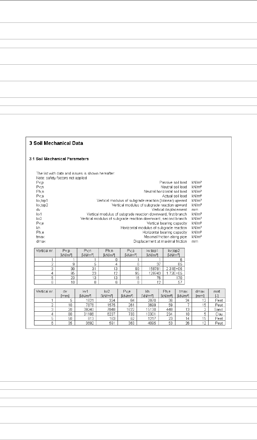
View Results
kv [kN/m3] Vertical modulus of subgrade reaction downward (see Equa-
tion 21.14 in section 21.6.1).
Pv;e [kN/m2] Vertical bearing capacity (see Equation 21.26 in section 21.8).
kh [kN/m3] Horizontal modulus of subgrade reaction (see Equation 21.24 in
section 21.7.1).
Ph;e [kN/m2] Horizontal bearing capacity (see Equation 21.29 in sec-
tion 21.9.2).
tmax [kN/m2] Maximal axial friction along the pipeline (see Equation 21.52 in
section 21.11.2).
dmax [mm] Displacement at maximal friction (see section 21.12.2).
mat [-] The corresponding type of material (see section 21.13).
6.2.4.3 Soil Mechanical Parameters for Construction in trench
Figure 6.8: Report window – Soil Mechanical Parameters section (for Construction in
trench)
The following is an explanation of the column headings:
Vertical nr. [-] Number of the calculation vertical.
Pv;p [kN/m2] Passive soil load (see Equation 21.2 in section 21.2).
Pv;n [kN/m2] Neutral vertical soil load (see Equation 21.1 in section 21.1).
Ph;n [kN/m2] Neutral horizontal soil load (see Equation 21.13 in sec-
tion 21.5.2).
Pv;a [kN/m2] Initial soil load, also called actual soil load (see Equation 21.9 in
section 21.4).
Deltares 99 of 324
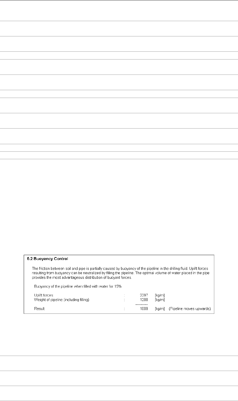
D-GEO PIPELINE
, User Manual
kv;top1 [kN/m3] Vertical modulus of subgrade reaction upward (see sec-
tion 21.6.2).
kv;top2 [kN/m3] Vertical modulus of subgrade reaction upward (see sec-
tion 21.6.2).
dv [mm] Vertical displacement (see section 21.10).
kv1 [kN/m3] Vertical modulus of subgrade reaction downward of the first and
second branch (see section 21.6.2).
kv2 [kN/m3] Vertical modulus of subgrade reaction downward of the first and
second branch (see section 21.6.2).
Pv;e [kN/m2] Vertical bearing capacity (see Equation 21.26 in section 21.8).
kh [kN/m3] Horizontal modulus of subgrade reaction (see Equation 21.25 in
section 21.7.2).
Ph;e [kN/m2] Horizontal bearing capacity (see Equation 21.29 in sec-
tion 21.9.2).
tmax [kN/m2] Maximal axial friction along the pipeline (see Equation 21.52 in
section 21.11.2).
dmax [mm] Displacement at maximal friction (see section 21.12.2).
mat [-] The corresponding type of material (see section 21.13).
6.2.5 Report – Data for Stress Analysis
Buoyancy Control
The magnitude of the pulling force is caused in part by friction between the soil around the
borehole and the product pipe. In turn, the magnitude of the friction is dependent on the
degree of buoyancy of the pipeline in the drilling fluid. Uplift forces resulting from buoyancy
can be neutralized by filling the pipeline with water. The optimum volume of water placed in
the pipeline provides the most advantageous distribution of buoyant forces. If the resulting
force is a positive value, the pipeline will move upwards. If the resulting force is a negative
value the pipeline will move downwards.
Figure 6.9: Report window, Buoyancy Control section
The following is an explanation of the content:
Uplift forces Weight of the drilling fluid in kg/m (see Equation 23.1 in sec-
tion 23.1).
Weight of pipeline
(including filling)
Weight of the pipeline filled with water in kg/m (see Equation 23.4
in section 23.1).
Resulting Effective weight of the pipeline in kg/m (see Equation 23.5 in
section 23.1).
100 of 324 Deltares
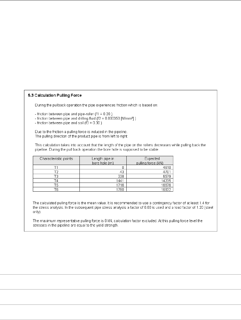
View Results
See section 23.1 for background information on buoyancy control.
Calculation pulling forces
This part of the report displays the calculated pulling forces (without applying a contingency
factor), for characteristic locations along the drilling line. In a case without horizontal bending,
six characteristic points are calculated. Their location is given in Figure 6.11. In case of
horizontal bending, the beginning and ending points of each horizontal bending will be defined
as characteristic points.
Figure 6.10: Report window, Calculation pulling force section
The following is an explanation of the column headings:
Characteristic points Points at different locations along the drilling line (see Fig-
ure 6.11). T1 and T6 are the entry and exit points, respectively.
Length pipe in borehole Length of the pipe between the entry point and the characteristic
point.
Expected pulling force Calculated pulling forces without using a contingency factor (see
Equation 23.6 in section 23.2).
Deltares 101 of 324
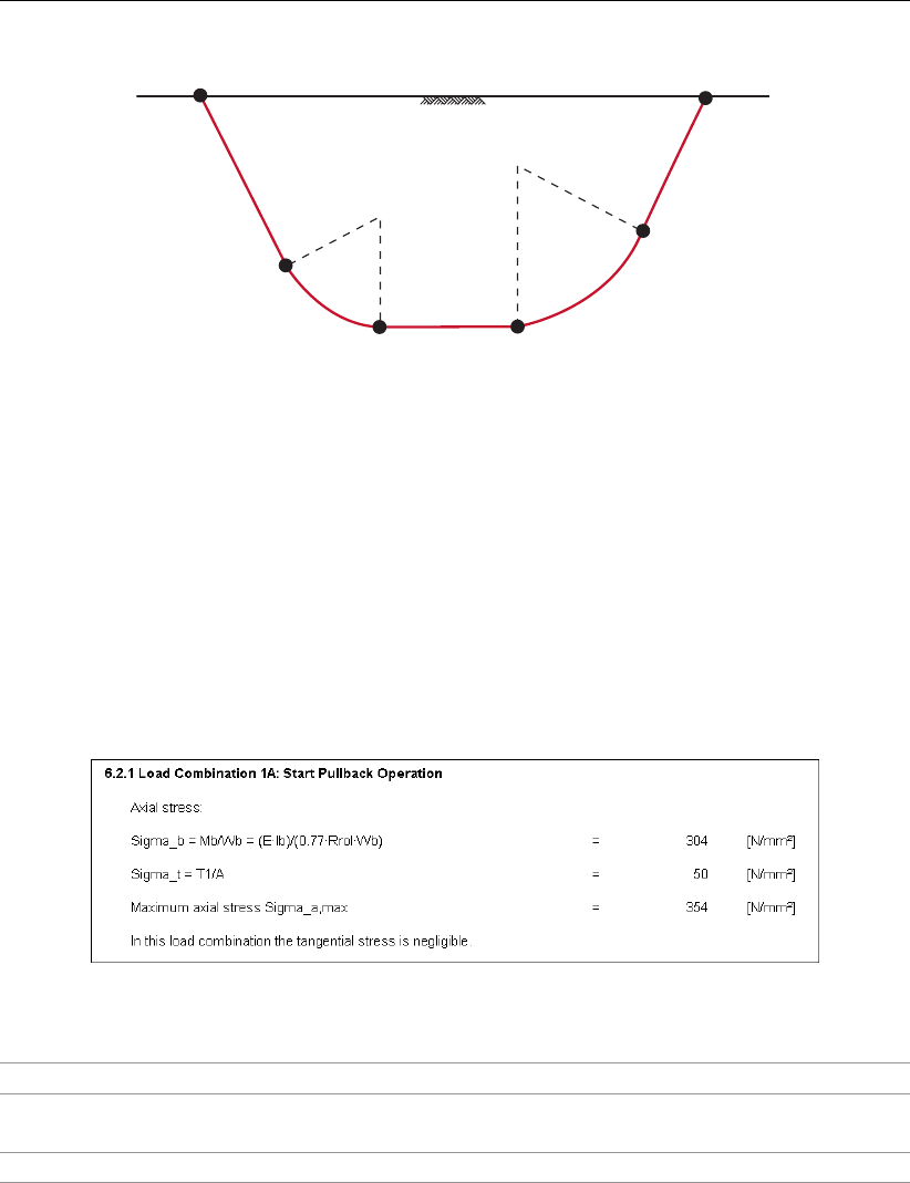
D-GEO PIPELINE
, User Manual
entry point exit point
ground level
T1
T2
T5
T6
T3 T4
Figure 6.11: Locations of the characteristic points T1 to T6
6.2.6 Report – Stress Analysis
6.2.6.1 Stress Analysis HDD
Load Combination 1A: Start pull-back operation
This part of the report displays the calculated axial and tangential stresses at the start of the
pull-back operation. See section 23.5.1 for background information.
Figure 6.12: Report window, Stress analysis for load combination 1A
Sigma_b Axial bending stress in N/mm2, see Equation 23.23.
Sigma_t Axial stress due to friction of the pipeline on the roller-lane, in N/mm2,
see Equation 23.25.
Sigma_a,max Maximum axial stress in N/mm2, see Equation 23.26.
Load Combination 1B: End pull-back operation
This part of the report displays the calculated axial and tangential stresses at the end of the
pullback operation. See section 23.5.2 for background information.
102 of 324 Deltares
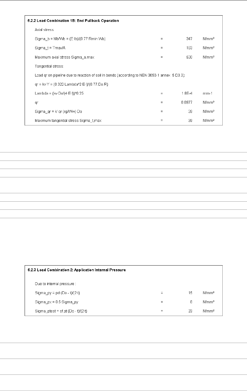
View Results
Figure 6.13: Report window, Stress analysis for load combination 1B
Sigma_b Axial bending stress in N/mm2, see Equation 23.27.
Sigma_t Axial stress due to pull-back in N/mm2, see Equation 23.28.
Sigma_a,max Maximum axial stress in N/mm2, see Equation 23.29.
Lambda Characteristic stiffness between the pipeline and the soil in mm−1, see
Equation 23.13.
qr Soil reaction in N/mm2, see Equation 23.11.
Sigma_qr Stress due to soil reaction in N/mm2, see Equation 23.31.
Sigma_t,max Maximum tangential stress in N/mm2, see Equation 23.32.
Load Combination 2: Application internal pressure
This part of the report displays the calculated stresses when the internal pressure is applied.
See section 23.5.3 for background information.
Figure 6.14: Report window, Stress analysis for load combination 2
Sigma_py Internal stress due to design pressure in N/mm2, see Equation 23.33
for thin pipe and Equation 23.35 for thick pipe.
Sigma_px Internal axial stress due to design pressure in N/mm2, see Equa-
tion 23.37.
Sigma_ptest Internal stress due to test pressure in N/mm2, see Equation 23.34 for
thin pipe and Equation 23.36 for thick pipe.
Deltares 103 of 324
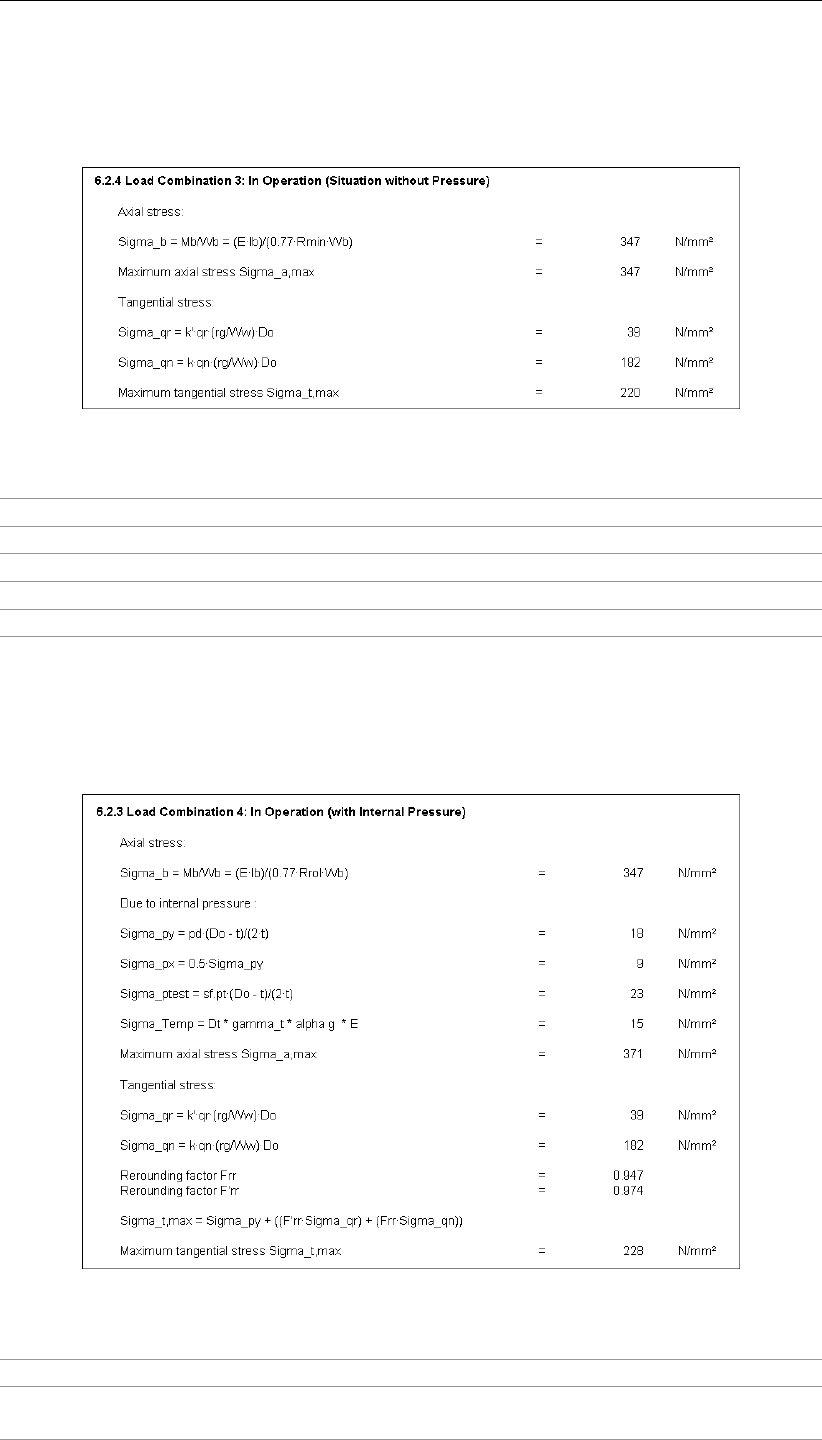
D-GEO PIPELINE
, User Manual
Load Combination 3: In operation (situation without pressure)
This part of the report displays the calculated axial and tangential stresses when the pipe is
in operation without internal pressure. See section 23.5.4 for background information.
Figure 6.15: Report window – Stress analysis for load combination 3
Sigma_b Axial bending stress in N/mm2, see Equation 23.38.
Sigma_a,max Maximum axial stress in N/mm2, see Equation 23.39.
Sigma_qr Stress due to soil reaction in N/mm2, see Equation 23.40.
Sigma_qn Stress due to reduced vertical load in N/mm2, see Equation 23.41.
Sigma_t,max Maximum tangential stress in N/mm2, see Equation 23.42.
Load Combination 4: In operation (with internal pressure)
This part of the report displays the calculated axial and tangential stresses when the pipe is
in operation with internal pressure. See section 23.5.5 for background information.
Figure 6.16: Report window, Stress analysis for load combination 4
Sigma_b Axial bending stress in N/mm2, see Equation 23.43.
Sigma_py Ring stress due to internal design pressure in N/mm2, see Equa-
tion 23.44.
104 of 324 Deltares
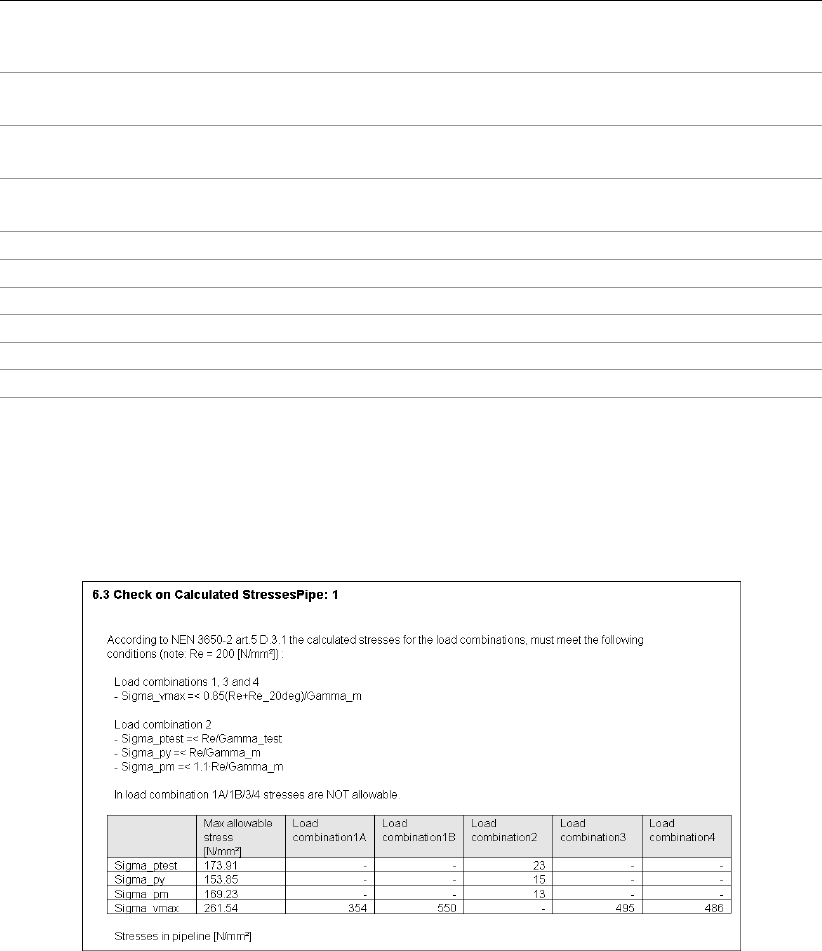
View Results
Sigma_px Axial stress due to internal design pressure in N/mm2, see Equa-
tion 23.47.
Sigma_ptest Ring stress due to internal test pressure in N/mm2, see Equation 23.45
for steel and Equation 23.46 for PE.
Sigma_Temp Axial stress due to temperature variation in N/mm2, see Equa-
tion 23.48.
Sigma_a,max Maximum axial stress in N/mm2, see Equation 23.49.
Sigma_qr Stress due to soil reaction in N/mm2, see Equation 23.50.
Sigma_qn Stress due to reduced vertical load in N/mm2, see Equation 23.51.
Frr Direct re-rounding factor in N/mm2, see Equation 23.53.
Frr’ Indirect re-rounding factor in N/mm2, see Equation 23.54.
Sigma_t,max Maximum tangential stress in N/mm2, see Equation 23.52.
Check on calculated stresses (Steel)
This part of the report displays a table in which the calculated combined stresses of the differ-
ent load combinations are compared to the maximum allowable stress (see section 23.6.1.1
for background information).
Figure 6.17: Report window, Check on calculated stresses section (steel pipe)
Check on calculated stresses (PE)
This part of the report displays a table in which the calculated combined stresses of the differ-
ent load combinations are compared to the maximum allowable stress (see section 23.6.1.2
for background information).
Deltares 105 of 324
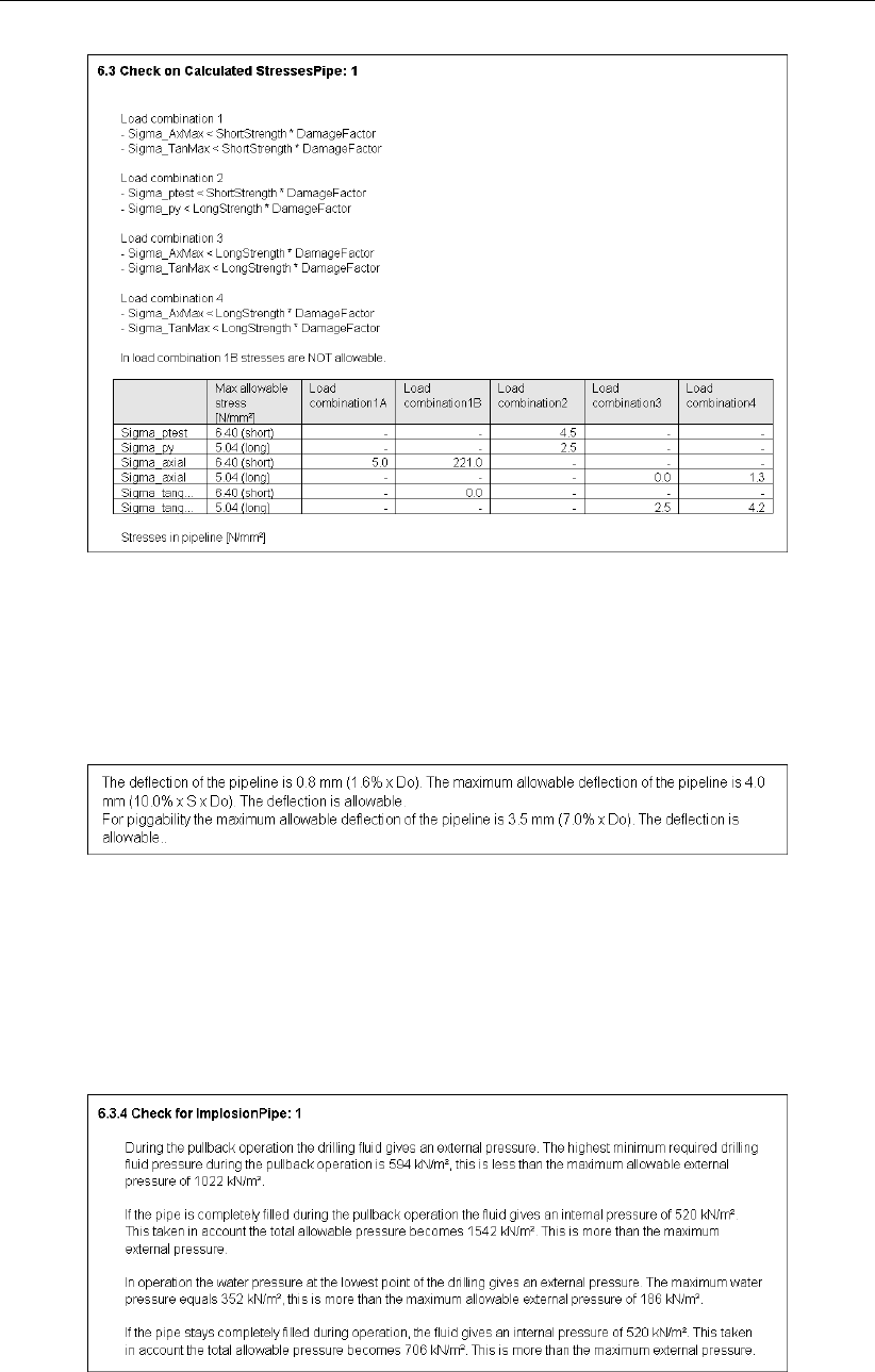
D-GEO PIPELINE
, User Manual
Figure 6.18: Report window, Check on calculated stresses section (PE pipe)
Check on deflection
This part of the report displays the calculated deflection of the pipeline and compares it to the
maximum allowable deflection (see section 23.7 for background information).
Figure 6.19: Report window, Check on deflection section
Check for implosion (only for PE pipe)
This calculation is performed only for a polyethylene pipe. The maximum allowable external
pressure is calculated (see section 23.8 for background information) in the short and long term
for the pullback operation (Stage 2) and the pipeline in operation (Stage 3a), respectively.
Figure 6.20: Report window, Check for implosion section
6.2.7 Report – Operation Parameters (Trenching)
106 of 324 Deltares

View Results
Uplift Check
Due to buoyancy of an empty pipeline below the groundwater table, the uplift should be
checked. Results are given per vertical in a table (Figure 6.21) and in graphs.
Figure 6.21: Report window, Uplift Check section
Vertical nr. [-] Number of the calculation vertical.
Safety factor
calculated
[-] The calculated safety factor for uplift, see Equation 25.5 in sec-
tion 25.1.
Safety factor
required
[-] The required safety factor for uplift as specified by the user in the
Factors window (section 4.7.1.3).
Hydraulic Heave Check
In case of trenching in soil layers which cover an aquifer with high pore pressures, bursting of
the bottom of the trench can be an installation risk which needs to be checked. Results are
given per vertical in a table (Figure 6.22) and in graphs.
Figure 6.22: Report window, Hydraulic Heave Check section
Vertical nr. [-] Number of the calculation vertical.
Safety factor
calculated
[-] The calculated safety factor for hydraulic heave, see Equa-
tion 25.7 in section 25.2.
Deltares 107 of 324
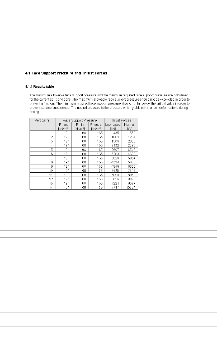
D-GEO PIPELINE
, User Manual
Safety factor
required
[-] The required safety factor for hydraulic heave as defined by the
user in the Factors window (section 4.7.1.3).
6.2.8 Report – Face Support Pressures and Thrust Forces (Micro tunneling)
Results are given per vertical in a table (Figure 6.23) and in graphs.
Figure 6.23: Report window, Operation Parameters section for Micro tunneling
The following is an explanation of the column headings:
Vertical nr. [-] Number of the calculation vertical.
Pmax [kN/m2]Pmax is the maximum allowable face support pressure which
should not be exceeded in order to prevent the following possi-
ble failure mechanisms:
Soil failure due to pushing a soil wedge in upward direction
A blow out to the surface due to hydraulic fracturing
Horizontal hydraulic fracturing at the transition of soil layers.
Refer to Equation 24.7 in section 24.1.3.
Pmin [kN/m2]Pmin is the minimum face support pressure required for stable
conditions of the soil adjacent to the micro tunneling machine. Re-
fer to Equation 24.2 for undrained layers and to Equation 24.4 for
drained layers, in section 24.1.2.
Pneutral [kN/m2]Pneutral is the target pressure, i.e. the total neutral horizontal soil
pressure. Refer to Equation 24.1 in section 24.1.1.
Thrust
Forces
[kN] The thrust force is the force required to install a micro tunnel or
pipeline in between the launch pit and the reception pit. Thrust
forces are calculated in both cases: injection of lubricant (Lubri-
cated) or not (Normal). Refer to Equation 24.8 in section 24.1.4.
108 of 324 Deltares

View Results
6.3 Drilling Fluid Pressures Plots
Only available if the Horizontal directional drilling model in the Model window (section 4.1) is
selected. In the Results menu, choose the Drilling Fluid Pressures Plots option to display the
following plots for the three boring stages (pilot, pre-ream and pullback):
——- Maximum allowable drilling fluid pressure (plastic zone related to deforma-
tion bore hole)
Refer to Equation 22.28 in section 22.2.2 for drained layers and to Equation 22.22
in section 22.2.1 for undrained layers. For drained layers, the determination of the
maximum allowable radius of the plastic zone Rp;max is related to the deformation
of the bore hole:
Rp;max =sR2
b
Q×2εg;max
−·−Maximum allowable drilling fluid pressure (plastic zone related to soil cover)
Refer to Equation 22.28 in section 22.2.2 for drained layers and to Equation 22.22
in section 22.2.1 for undrained layers. For drained layers, the determination of the
maximum allowable radius of the plastic zone is related to the soil cover:
Rp;max = 0.5H
−−− Minimum drilling fluid pressure assuming that the pilot is drilled from the
left side to the right side
Refer to section 22.1 for background information.
----- Minimum drilling fluid pressure assuming that the pilot is drilled from the
right side to the left side
Refer to section 22.1 for background information.
To select the stage, click on one of the three tabs of the Drilling Fluid Pressures Plots window
(Figure 6.24): Pilot,Prereaming or Reaming and pullback operation.
Figure 6.24: Drilling Fluid Pressures Plots window
Use the Pan and Zoom buttons to select the part to be viewed in detail.
Deltares 109 of 324
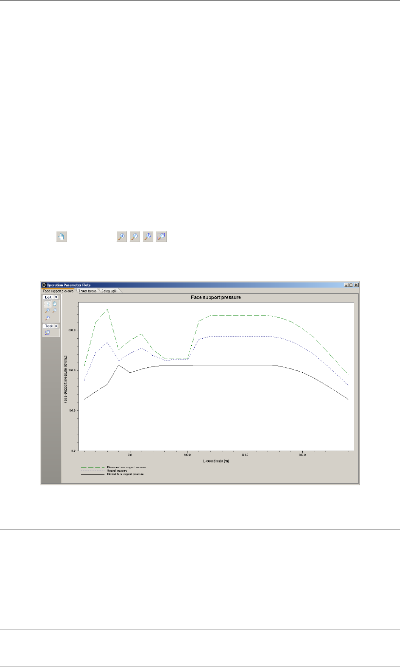
D-GEO PIPELINE
, User Manual
6.4 Operation Parameter Plots
In the Results menu, choose the Operation Parameter Plots option. The content of the Oper-
ation Parameter Plots window depends on the selected model:
Refer to section 6.4.1 for Micro tunneling;
Refer to section 6.4.2 for Construction in trench.
6.4.1 Operation Parameter Plots for Micro Tunneling
For Micro tunneling model, the Operation Parameter Plots window displays three different
plots by clicking on one of the three tabs:
the face support pressures at the micro tunneling machine (Figure 6.25);
the thrust pressures along the micro tunnel or pipe segments (Figure 6.26);
the uplift safety factor along the micro tunneling (Figure 6.27).
Use the Pan and Zoom buttons to select the part to be viewed in detail.
For background information, refer to chapter 24.
Figure 6.25: Operation Parameter Plots window, Face support pressures tab
Maximum face support
pressure
The maximum allowable face support pressure which should not
be exceeded in order to prevent the following possible failure
mechanisms:
Soil failure due to pushing a soil wedge in upward direction
A blow out to the surface due to hydraulic fracturing
Horizontal hydraulic fracturing at the transition of soil lay-
ers.
For background information, refer to section 24.1.3.
Neutral pressure The neutral pressure is the pressure with the lowest soil defor-
mation, i.e. the total neutral horizontal soil pressure. For back-
ground information, refer to section 24.1.1.
110 of 324 Deltares
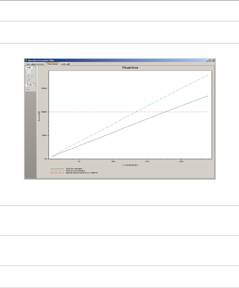
View Results
Minimum face support
pressure
The minimum face support pressure is the pressure required for
stable conditions of the soil adjacent to the micro tunneling ma-
chine. For background information, refer to section 24.1.2.
Figure 6.26: Operation Parameter Plots window, Thrust pressures tab
Thrust force lubricated The thrust force lubricated is the force required to install a micro
tunnel in between the launch pit and the reception pit in case of
injection of lubricant. For background information, refer to sec-
tion 24.1.4.
Thrust force not
lubricated
The thrust force lubricated is the force required to install a micro
tunnel in between the launch pit and the reception pit in case
of no injection of lubricant. For background information, refer to
section 24.1.4.
Maximum allowable
thrust force
The maximum allowable thrust force is usually given by the man-
ufacturer of the pipe and specified in the Engineering Data win-
dow (section 4.6.3).
Deltares 111 of 324
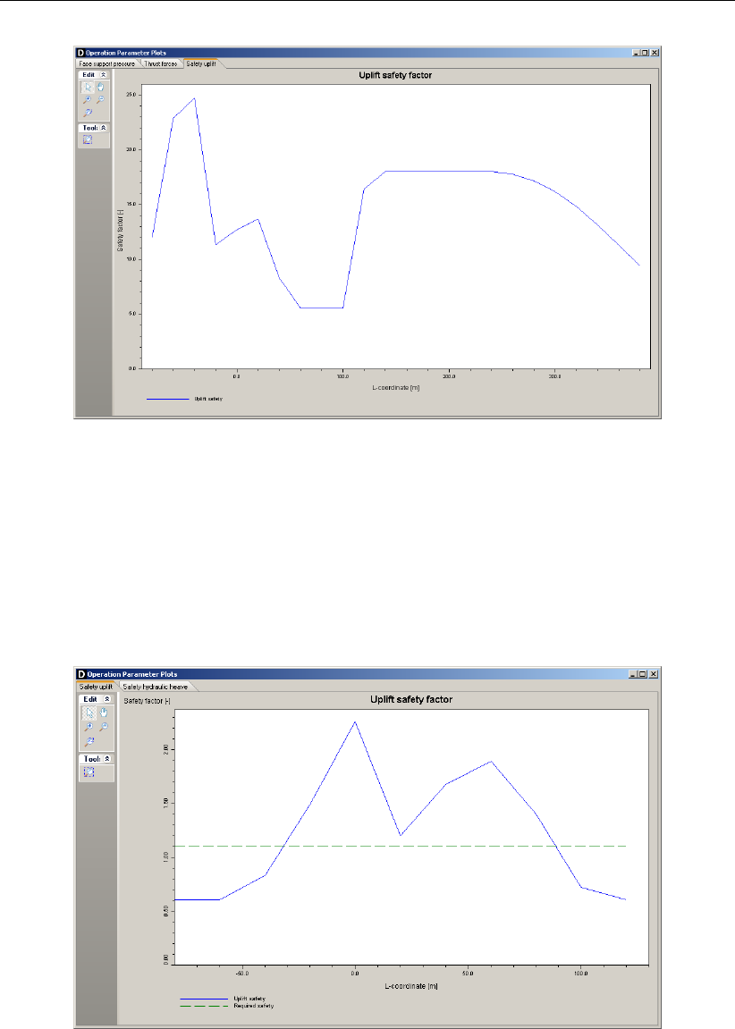
D-GEO PIPELINE
, User Manual
Figure 6.27: Operation Parameter Plots window, Safety uplift tab
6.4.2 Operation Parameter Plots for Construction in trench
For Construction in trench model, the Operation Parameter Plots window displays two different
plots by clicking on one of the two tabs:
the safety factor for uplift along the bottom of the trench (Figure 6.28);
the safety factor for hydraulic heave along the bottom of the trench (Figure 6.30);
Figure 6.28: Operation Parameter Plots window, Safety uplift tab
112 of 324 Deltares
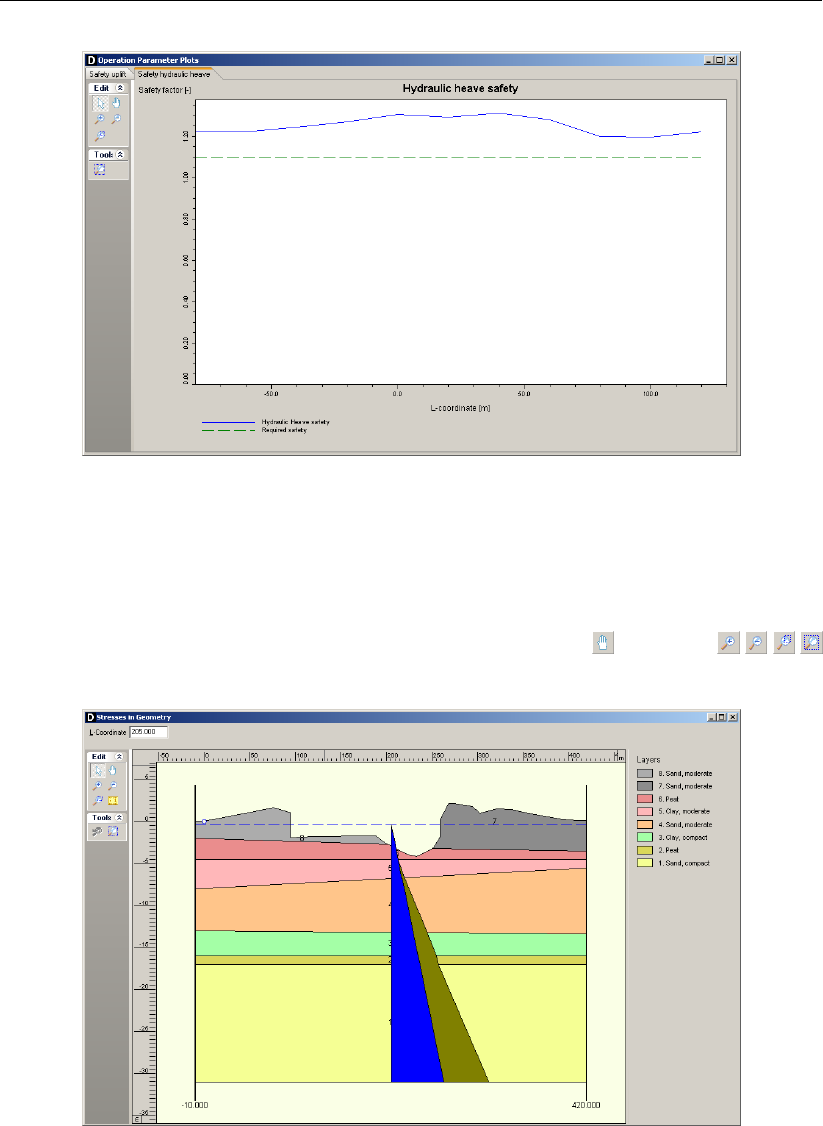
View Results
Figure 6.29: Operation Parameter Plots window, Safety hydraulic heave tab
6.5 Stresses in Geometry
In the Results menu, choose the Stresses in Geometry option to display the vertical stress
per vertical drawn in the geometry. The blue part represents the water pressure and the dark
green part represents the additional effective stress. Use the Pan and Zoom
buttons to select the part to be viewed in detail.
Figure 6.30: Stresses in Geometry window
Deltares 113 of 324
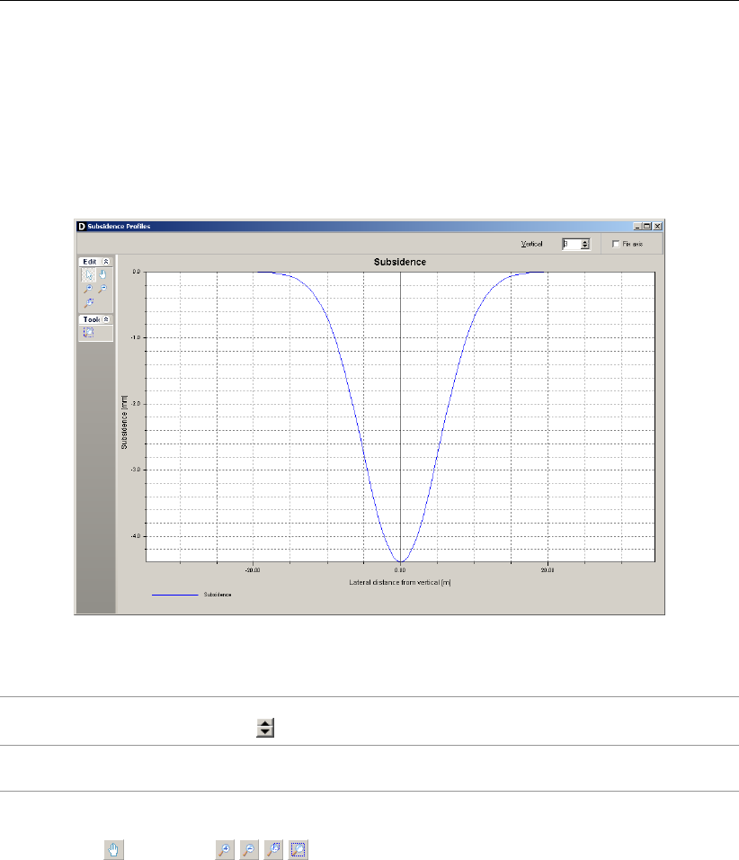
D-GEO PIPELINE
, User Manual
6.6 Subsidence Profiles
Only available if the Micro tunneling model in the Model window (section 4.1) is selected. In
the Results menu, choose the Subsidence Profiles option to display the calculation results for
the subsidence trough as apparent at surface. Subsidence is related to the volume loss due
to the tunnel excavation, e.g. the excess soil removed by the Micro Tunneling Boring Machine
(MTBM). The subsidence mechanism is described in detail in section 24.3.
Figure 6.31: Subsidence Profiles window
Vertical Type the vertical number that must be displayed or click the arrow-up and
arrow-down keys to scroll through the available verticals.
Fix axis Enable this check-box to fix the range of the vertical axis of the graph of
subsidence whatever the selected time step.
Use the Pan and Zoom buttons to select the part to be viewed in detail.
114 of 324 Deltares
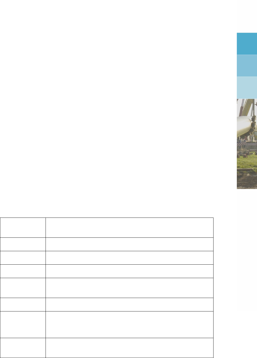
7 Graphical Geometry Input
This chapter explains how to define the soil layers in a two-dimensional cross section by
drawing, using the shared D-Series options for geometry modeling.
section 7.1 introduces the basic geometrical elements that can be used.
section 7.2 lists the restrictions and assumptions that the program imposes during ge-
ometry creation.
section 7.3 gives an overview of the functionality of the View Input window.
section 7.4 describes the creation and section 7.5 describes the manipulation of general
graphical geometry using the View Input window.
Besides graphical input, the geometry can also be imported or tabular forms can be used
(see section 4.3.2). See the MGeoBase manual for a description of special features to create
cross-section geometry semi-automatically from CPT and/or boring records.
7.1 Geometrical objects
Geometry can be built step-by-step through the repetitive use of sketching, geometry creation
and geometry manipulation. Each step can be started by using line-shaped construction ele-
ments (section 7.1.2) to add line drawings. After converting these drawings to valid geometry
parts, the specific geometry elements created can be manipulated (section 7.1.1).
7.1.1 Geometry elements
Geometry can be composed from the following geometry elements:
Points A point is a basic geometry element defined by its co-ordinates. As
stated earlier, the geometry is restricted to two dimensions, allowing to
define X and Z co-ordinates only.
Boundary lines A boundary line is a straight line piece between two points and is part
of a boundary.
Boundaries A boundary is a collection of connected boundary lines that forms the
continuous boundary between layers.
PL-lines A piezometric level line is a collection of connected straight line pieces
defining a continuous piezometric level.
Phreatic line This is a PL-line that acts as phreatic line. The phreatic line (or ground-
water level) is used to mark the border between saturated and unsatu-
rated soil.
Layers A layer is the actual soil layer. Its geometrical shape is defined by its
boundaries, and its soil type is defined by its material.
Materials A material defines the actual soil material (or soil type). It contains the
parameters belonging to the soil type, such as its unsaturated weight
and its saturated weight. A material can be connected to a layer in
order to define the soil type of the layer.
Limits A limit is a vertical boundary defining the ‘end’ at either the left or right
side of the geometry. It is defined by an X co-ordinate only. Note that
this is the only type of element that cannot be deleted.
Adding, moving and deleting the above-mentioned elements are subject to the conditions for
a valid geometry (see section 7.2). For example, while dragging selected geometry elements,
the program can perform constant checks on the geometry validity (section 7.4.4). Invalid
parts will be shown as construction elements (thick blue lines).
Deltares 115 of 324
D-GEO PIPELINE
, User Manual
7.1.2 Construction elements
Besides the D-Series geometry elements (section 7.1.1), special construction elements can
also be used for sketching the geometry graphically. These elements are not a direct part of
the geometry and the restrictions on editing (adding, moving, and deleting); these elements
are therefore far less rigid. The only restriction that remains is that these elements cannot be
moved and/or defined beyond the limits of the geometry.
Lines A line Construction consists of a starting point and end point, both de-
fined by a left-hand mouse click in the graphic input screen.
Poly-lines A poly-line Construction consists of a series of connected lines, all de-
fined by a left-hand mouse click in the graphic input screen.
Construction elements will be displayed as solid blue lines. Valid constructions elements
are converted to geometry elements as soon as the geometry is (re-) generated. For more
information on adding lines and poly-lines, see section 7.4.
7.2 Assumptions and restrictions
During geometrical modeling, the program uses the following assumptions.
Boundary number 0 is reserved for the base.
A soil layer number is equal to the boundary number at the top of the layer.
The boundary with the highest number defines the soil top surface.
A material (soil type) must be defined for each layer – except for layer 0 (base). Different
layers can use the same material.
All the boundaries must start and end at the same horizontal co-ordinates.
Boundaries should not intersect, but they may coincide over a certain length.
All horizontal co-ordinates on a boundary must be ascending – that is, the equation
X[i+ 1] ≥X[i]must be valid for each following pair of Xco-ordinates (vertical parts
are allowed).
PL-lines may intersect and may coincide with each other over a certain length.
PL lines and layer boundaries may intersect.
All PL-lines must start and end at the same horizontal co-ordinate.
All Xco-ordinates on a PL-line must be strictly ascending – that is, the equation
X[i+ 1] > X[i]must be valid for each following pair of Xco-ordinates (no verti-
cal parts allowed).
One way for inputting geometry data is through the Geometry menu, as explained in the
Reference section (section 4.3). This section describes an other way to create and manipulate
geometry graphically using the tool buttons of the View Input window.
7.3 View Input Window
116 of 324 Deltares

Graphical Geometry Input
7.3.1 General
To use the View Input option, click the Geometry tab to activate it in the regular View Input
window or use the menu to select it.
Figure 7.1: View Input window, Geometry tab
When the Geometry tab in the View Input window is selected, it displays a graphical repre-
sentation of only the geometrical data. On the left of the window, the Edit and Tools buttons
are displayed (section 7.3.2). On the right, the legend belonging to the geometry is displayed
(section 7.3.3). At the bottom of the window, the title panel and the info bar are displayed.
The title panel displays the project titles defined using the Properties option in the Project
menu. The info bar provides information (from left to right) about the current cursor position,
the current mode and the object currently selected. The legend, title panel and info bar are
optional and can be controlled using the Properties option in the Project menu.
It is possible to use three different modes when working in the Geometry tab of the View Input
window:
Select The Select mode is the default mode and enables the user to select existing
elements in the window.
Add The Add mode allows the addition of elements using one of the Add buttons.
By selecting one of these buttons, one switches to the Add mode. As long as
this mode is active, the user can add the type of element which is selected.
Zoom The Zoom mode allows the user to view the input geometry in different sizes.
By selecting one of the Zoom buttons or the Pan button, one activates the
Zoom mode. While in this mode, the user can repeat the zoom or pan actions
without re-selecting the buttons.
It is possible to change modes in the following ways. When in Add or Zoom mode, it is
possible to return to the Select mode by clicking the right-hand mouse button, or by pressing
the Escape key, or by clicking the Select mode button. To activate the Add mode, select one
of the Add buttons. To activate the Zoom mode, select one of the Zoom buttons or the Pan
button.
Note: The current mode is displayed on the info bar at the bottom of the View Input window.
Deltares 117 of 324
D-GEO PIPELINE
, User Manual
7.3.2 Buttons
Edit panel:
Select and Edit mode
In this mode, the left-hand mouse button can be used to graphically select a pre-
viously defined grid, load, geotextile or forbidden line. Items can then be deleted
or modified by dragging or resizing, or by clicking the right-hand mouse button and
choosing an option from the menu displayed. Pressing the Escape key will return
the user to this Select and Edit mode.
Pan
Click this button to change the visible part of the drawing by clicking and dragging
the mouse.
Add point(s) to boundary / PL-line
Click this button to add points to all types of lines (lines, poly-lines, boundary lines,
PL-lines). By adding a point to a line, the existing line is split into two new lines. This
provides more freedom when modifying the geometry.
Add single lines(s)
Click this button to add single lines. When this button is selected, the first left-hand
mouse click will add the info bar of the new line and a “rubber band” is displayed
when the mouse is moved. The second left-hand mouse click defines the end point
(and thus the final position) of the line. It is now possible to either go on clicking start
and end points to define lines, or stop adding lines by selecting one of the other tool
buttons, or by clicking the right-hand mouse button, or by pressing the Escape key.
Add polyline(s)
Click this button to add poly-lines. When this button is selected, the first left-hand
mouse click adds the starting point of the new line and a “rubber band” is displayed
when the mouse is moved. A second left-hand mouse click defines the end point
(and thus the final position) of the first line in the poly-line and activates the “rubber
band” for the second line in the poly-line. Every subsequent left-hand mouse click
again defines a new end point of the next line in the poly-line. It is possible to end
a poly-line by selecting one of the other tool buttons, or by clicking the right-hand
mouse button, or by pressing the Escape key. This also stops adding poly-lines al-
together.
A different way to end a poly-line is to double-click the left-hand mouse button. Then
the poly-line is extended automatically with an ‘end line’. This end line runs horizon-
tally from the position of the double-click to the limit of the geometry in the direction
the last line of the poly-line was added. Therefore, if the last line added was defined
left to right, the ‘end line’ will stop at the right limit. Note that by finishing adding a
poly-line this way, it is possible to start adding the next poly-line straight away.
118 of 324 Deltares
Graphical Geometry Input
Add PL-line(s)
Click this button to add a piezometric level line (PL-line). Each PL-line must start
at the left limit and end at the right limit. Furthermore, each consecutive point must
have a strictly increasing X co-ordinate. Therefore, a PL-line must be defined from
left to right, starting at the left limit and ending at the right limit. To enforce this, the
program will always relocate the first point clicked (left-hand mouse button) to the left
limit by moving it horizontally to this limit. If trying to define a point to the left of the
previous point, the rubber band icon indicates that this is not possible. Subsequently
clicking on the left side of the previous point, the new point will be added at the end
of the rubber band icon instead of the position clicked.
As with poly-lines, it is also possible to end a PL-line by double-clicking the left-hand
mouse button. In this case, the automatically added ‘end line’ will always end at the
right limit.
To stop adding PL-lines, select one of the other tool buttons, or click the right-hand
mouse button, or press the Escape key.
Zoom in
Click this button to enlarge the drawing, then click the part of the drawing which is to
be at the center of the new image. Repeat if necessary.
Zoom out
Click this button, then click on the drawing to reduce the drawing size. Repeat if
necessary.
Zoom rectangle
Click this button then click and drag a rectangle over the area to be enlarged. The
selected area will be enlarged to fit the window. Repeat if necessary.
Measure the distance between two points
Click this button, then click the first point on the View Input window and place the
cross on the second point. The distance between the two points can be read at the
bottom of the View Input window. To turn this option off, click the escape key.
Add calculation vertical
Click this button to graphically define the position of a vertical.
Tools panel:
Undo zoom
Click this button to undo the zoom. If necessary, click several times to retrace each
consecutive zoom-in step that was made.
Zoom limits
Click this button to display the complete drawing.
Same scale for X and Y axis
Click this button to use the same scale for the horizontal and vertical directions.
Automatic regeneration of geometry on/off
When selected, the program will automatically try to generate a new valid geometry
whenever geometry modifications require this. During generation, (poly)lines (solid
blue) are converted to boundaries (solid black), with interjacent layers. New layers
receive a default material type. Existing layers keep the materials that were assigned
to them. Invalid geometry parts are converted to construction elements.
Automatic regeneration may slow down progress during input of complex geometry,
because validity will be checked continuously.
Undo
Click this button to undo the last change(s) made to the geometry.
Deltares 119 of 324
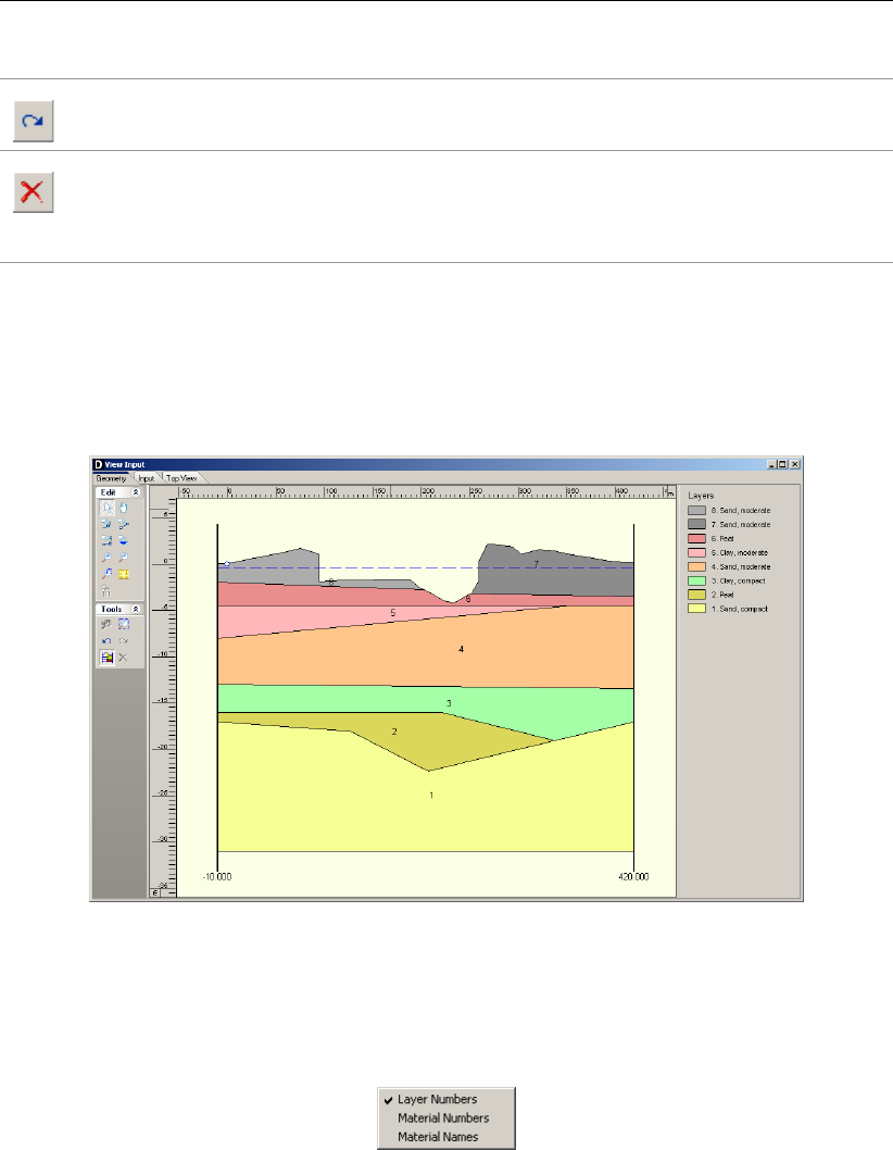
D-GEO PIPELINE
, User Manual
Redo
Click this button to redo the previous Undo action.
Delete
Click this button to delete a selected element. Note that this button is only available
when an element is selected. See section 7.5.2 for more information on how using
this button.
7.3.3 Legend
At the right side of the View Input window (Figure 7.2) the legend belonging to the geometry
is shown. This legend is present only if the Legend check-box in the View Input tab of the
Project Properties window is activated (see section 4.1.2).
Figure 7.2: View Input window, Geometry tab (legend displayed as Layer Numbers)
In the Geometry tab of the View Input window, it is possible to change the type of legend.
When a soil type box in the legend is right clicked, the menu from Figure 7.3 is displayed.
Figure 7.3: Legend, Context menu
With this menu, there are three ways to display the legend of the layers:
As Layer Numbers: the legend displays one box for each layer. Each layer (and there-
fore each box) is displayed in a different standard color. Next to each box, the layer
number and the material name are displayed, corresponding to the color and number
of the layer in the adjacent Geometry window (see Figure 7.2).
As Material Numbers: the legend displays one box for each material. Each material
(and therefore each box) is displayed in a different color which can be changed by
the user (see below). Next to each box, the material number and name are displayed,
corresponding to the color and number of the material in the adjacent Geometry window
(see Figure 7.4).
120 of 324 Deltares

Graphical Geometry Input
As Material Names: the legend displays one box for each material. Each material (and
therefore each box) is displayed in a different color which can be changed by the user
(see below). Next to each box, only the material name is displayed, corresponding to
the color and name of the material in the adjacent Geometry window (see Figure 7.5).
Figure 7.4: View Input window, Geometry tab (legend displayed as Material Numbers)
Figure 7.5: View Input window, Geometry tab (legend displayed as Material Names)
Unlike the standard colors used to display layers with their layer colors, it is possible to define
different colors used when displaying materials. To change the color assigned to a material,
right click the material box. The menu from Figure 7.6 is displayed.
Figure 7.6: Legend, Context menu (for legend displayed as Materials)
Deltares 121 of 324
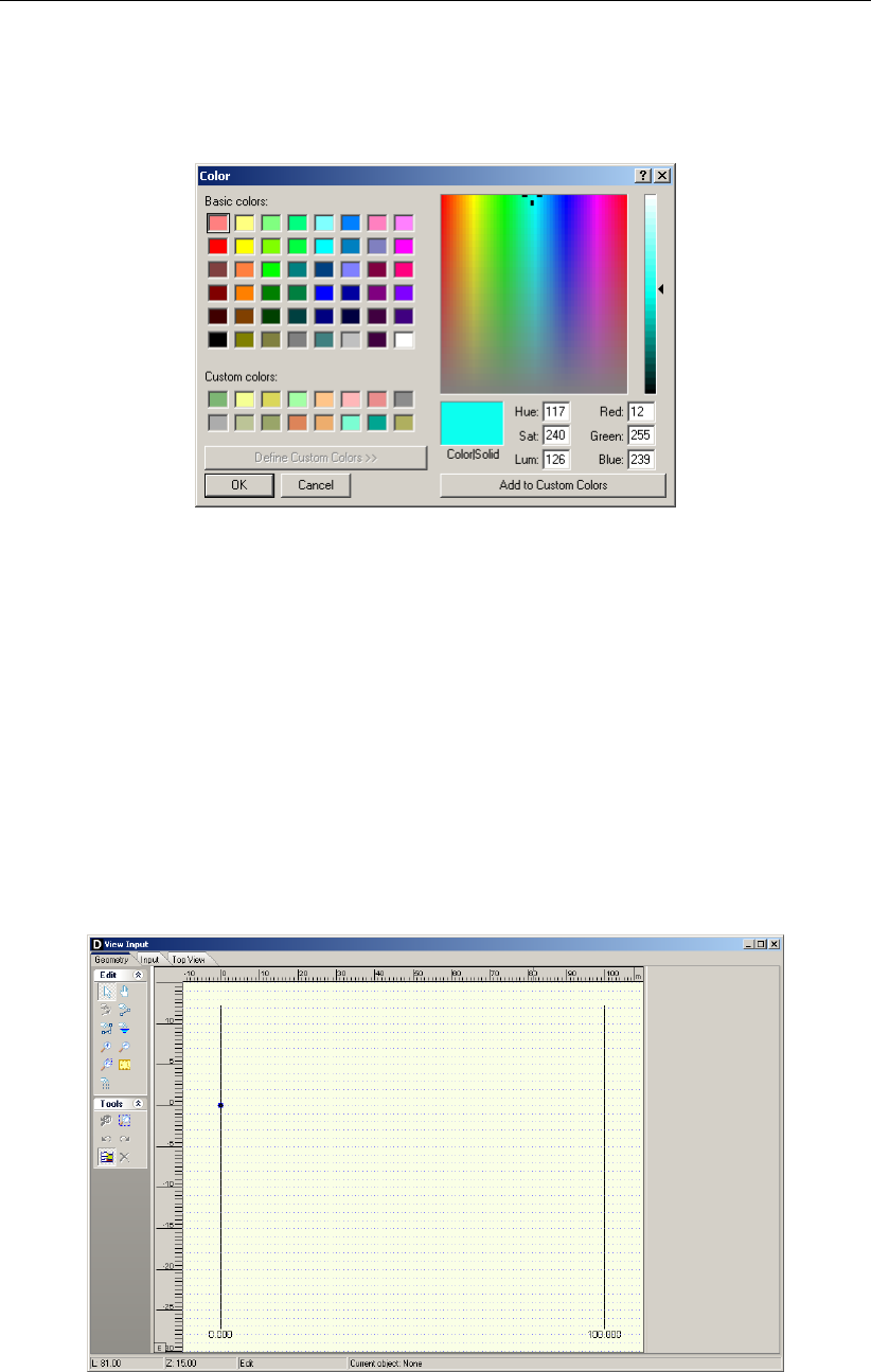
D-GEO PIPELINE
, User Manual
When selecting Material Colors the Color window appears (Figure 7.7), in which the user can
pick a color or even define customized colors himself (by clicking the Define Custom Colors
button).
Figure 7.7: Color window
7.4 Geometry modeling
7.4.1 Create a new geometry
There are two ways to create a new geometry without the wizard:
Open the Geometry menu and choose New.
Open the File menu and choose New. In the New File window displayed, select New
Geometry and click OK (see section 4.3.2).
In both cases, the Geometry tab of the View Input window is displayed (Figure 7.8) with the
default limits of the geometry (from 0 to 100 m).
Figure 7.8: View Input window, Geometry tab
122 of 324 Deltares

Graphical Geometry Input
7.4.2 Set limits
The first thing to do when creating new geometry is to set the model limits. This is possible by
selecting and then dragging the limits to their proper place one by one. It is also possible to
select a limit and edit its value by clicking the right-hand mouse button after selecting the limit
and then choosing the Properties option in the pop-up menu. The property window belonging
to the selected limit is displayed (Figure 7.9), enabling to define the new X co-ordinate for this
limit.
Figure 7.9: Right Limit window
7.4.3 Draw layout
It is possible to use the Add single line(s),Add polyline(s) and Add point(s) to boundary / PL-
line buttons to draw the layout of the geometry. See section 7.3.2 for more information’s on
how using those buttons.
Add single line(s) and Add polyline(s)
Each (poly)line is displayed as a solid blue line, and each point as a small black rectangle
(Figure 7.10).
Figure 7.10: Representation of a polyline
The position of the different points of a (poly)line can be modified by dragging the points as
explained in section 7.5.4 or by editing the (poly)line. This is done by clicking the right-hand
mouse button after selecting the (poly)line and then choosing the Properties option in the
pop-up menu.
The underlying grid helps the user to add and edit (poly)lines. Use the Properties option in
the Project menu to adjust the grid distance and force the use of the grid by activating Snap to
grid. When this option is activated, each point is automatically positioned at the nearest grid
point.
The specified line pieces must form a continuous line along the full horizontal width of the
model. This does not mean that each line piece has to be connected exactly to its predecessor
and/or its successor. Intersecting line pieces are also allowed, as shown in the examples of
Figure 7.11.
Deltares 123 of 324
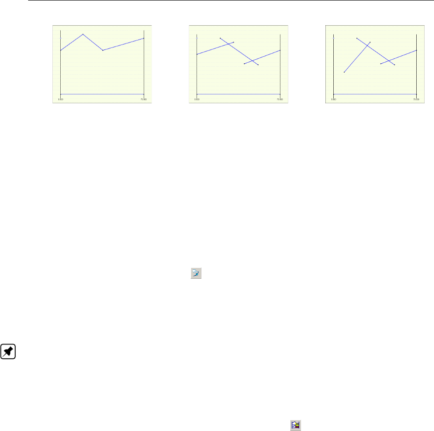
D-GEO PIPELINE
, User Manual
(1) (2) (3)
Figure 7.11: Examples of configurations of (poly)lines
Configuration (1) is allowed. The different lines are connected and run from boundary
to boundary
Configuration (2) is also allowed. The different are connected. They are defined as
being connected because they intersect. The line construction runs from boundary to
boundary.
Configuration (3) is illegal, as there is no connection with the left boundary.
Add point(s) to boundary / PL-line
Use this button to add extra points to lines (lines, polylines, boundary lines, PL-lines). By
adding a point to a line, the existing line is split into two new lines. This provides more freedom
when modifying the geometry.
Note: When the Add point(s) to boundary/PL-line button is clicked, each left-hand mouse
click adds a new point to the nearest line until one of the other tool buttons is selected, or click
the right-hand mouse button, or press the Escape key.
7.4.4 Generate layers
Use the Automatic regeneration of geometry on/off button to start or stop the automatic
conversion of construction elements to actual boundaries and layers. Valid (poly)lines are
converted to boundaries, which are displayed as black lines. Invalid lines remain blue.
Layers are generated between valid boundaries, and default soil types are assigned.
It is possible to modify the soil type assigned to a layer by first selecting the layer and then
clicking the right-hand mouse button and choosing the Layer Properties option in the pop-
up menu to display the Layer window (see Figure 7.19 in section 7.5.3). Once a material
has been assigned to a layer, this material will continue to be associated to that layer in
subsequent conversions of construction elements as long as the layer is not affected by those
conversions.
The most common cause of invalid (poly)lines is that they are not part of a continuous poly-
line running from limit to limit. Sometimes, lines appear to start/end at a limit without actually
being on a limit. Figure 7.12 gives an example: on the left geometry (1), the end of the line
seems to coincide with the boundary. However, zooming in on the point (geometry (2) on the
right) reveals that it is not connected to the boundary. Therefore the geometry is considered
invalid.
124 of 324 Deltares
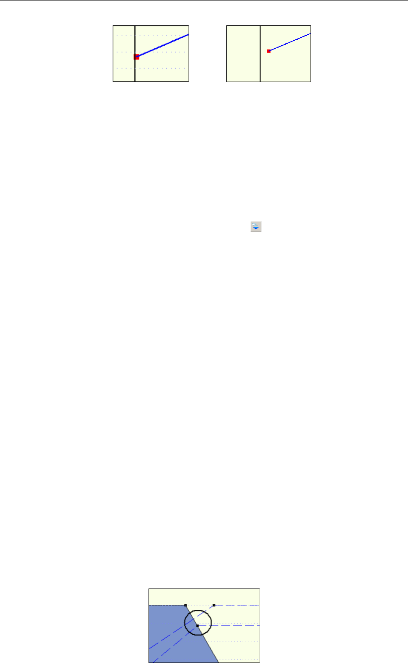
Graphical Geometry Input
(1) (2)
Figure 7.12: Example of invalid point not connected to the left limit
It is possible to correct this by dragging the point to the limit while the specific area is zoomed
in or by selecting the point, clicking the right-hand mouse button, choosing the Properties
option in the pop-up menu (section 7.5.3) and making the X co-ordinate of the point equal to
the X co-ordinate of the limit.
7.4.5 Add piezometric level lines
It is possible to use the Add PL-line(s) to add PL-lines button. When adding a PL-line,
D-GEO PIPELINE
imposes the limitation that the subsequent points of the PL-line have an in-
creasing X co-ordinate. Furthermore the first point of a PL-line is to be set on the left boundary
and the last point on the right boundary.
It is possible to change the position of the different points of a PL-line by dragging the points
as explained in section 7.5.4 or by editing the PL-line. This is done by selecting the PL-line,
clicking the right-hand mouse button and choosing the Properties option in the pop-up menu
(section 7.5.3).
7.5 Graphical manipulation
7.5.1 Selection of elements
After selecting a geometry element it is possible to manipulate it. In order to be able select a
geometry element, the select mode should be active. Then it is possible to select an element
by clicking the left-hand mouse button. To select a layer, click on the layer number, material
number or material name, depending on the option chosen in the Properties dialog in the
Project menu. When successfully selected, the element will be displayed highlighted (for
example, a point will be displayed as a large red box instead of a small black box).
The following remarks are relevant to selection accuracy and ambiguity.
Ambiguous selection
A selection of geometrical elements can be ambiguous. Figure 7.13 gives an example: a user
may want to select a point, a boundary line, a boundary or a PL-line. As several elements are
in close proximity to each other,
D-GEO PIPELINE
does not automatically select an element.
Figure 7.13: Selection accuracy as area around cursor
Deltares 125 of 324
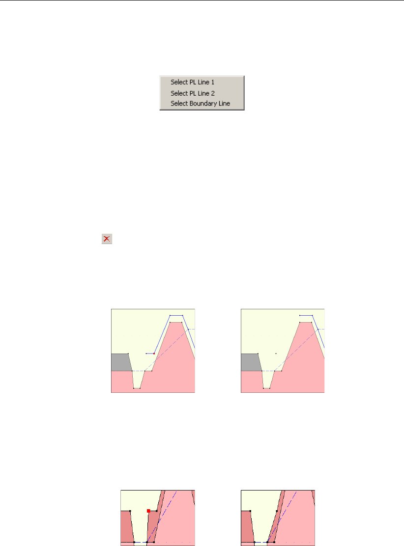
D-GEO PIPELINE
, User Manual
In this case
D-GEO PIPELINE
requires the user to assign the element that is to be selected by
displaying a pop-up menu (Figure 7.14) with the available types of elements within the range
of the selection click. It is possible to select the element from this menu.
Figure 7.14: Selection accuracy as area around cursor
Clear selection
It is possible to clear a selection by clicking in an area without geometry elements in the direct
area.
7.5.2 Deletion of elements
Click the Delete button to delete a selected element. This button is only available when an
element is selected.
When a point is selected and deleted, it and all lines connected to it are deleted as shown in
Figure 7.15.
Before After
Figure 7.15: Example of deletion of a point
When a geometry point (a point used in a boundary or PL-line) is selected and deleted, the
program deletes the point and its connected boundary lines as shown in Figure 7.16. It then
inserts a new boundary that reconnects the remaining boundary lines to a new boundary.
Before After
Figure 7.16: Example of deletion of a geometry point
Deletion of a geometry element (boundary, boundary line, geometry point, PL-line) can result
in automatic regeneration of a new valid geometry, if the Automatic regeneration option is
switched on.
When a line is selected and then deleted, the line and its connecting points are deleted as
shown in Figure 7.17. In addition the layer just beneath that boundary is deleted. All other line
parts that are not part of other boundaries will be converted to construction lines.
126 of 324 Deltares
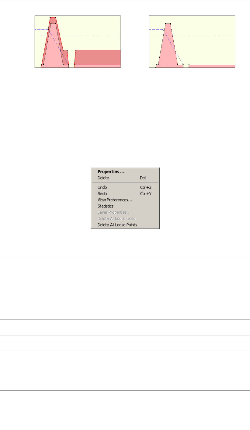
Graphical Geometry Input
Before After
Figure 7.17: Example of deletion of a line
7.5.3 Using the right-hand mouse button
When using the mouse to make geometrical manipulations, the right mouse button enables
full functionality in a pop-up menu, while the left button implies the default choice. The options
available in the pop-up menu depend on the selected geometrical element and the active
mode.
When the Select mode is active and the right-hand mouse button is clicked, the pop-up menu
of Figure 7.18 is displayed.
Figure 7.18: Pop-up menu for right-hand mouse menu (Select mode)
Properties... When this option is clicked, the property editor for the selected object
is displayed. This procedure is performed by first selecting an object by
clicking on it with the left-hand mouse button. Then clicking the right-
hand mouse button anywhere in the graphic window will display the
pop-up menu. It is possible to use the property editor to quickly adapt
the values (properties) of the selected object. Each type of element
requires its own properties and therefore its own property editor as
shown from Figure 7.20 to Figure 7.23 below.
Delete This option deletes the element that has been selected (see the com-
ments for the Delete button in section 7.5.2).
Undo This option will undo the last change(s) made to the geometry.
Redo This option will redo the previous Undo action.
View
Preferences...
This option opens the Properties dialog in the Project menu as dis-
played in.
Statistics It is possible to use this option to view a window displaying all the vital
statistics of the input data. Note that in the window construction lines
are called free lines.
Layer
Properties...
This option is a special feature that edits the material properties of lay-
ers. It is possible to click anywhere in a layer and directly choose this
option to edit its properties (Figure 7.19). Clicking outside the geometry
layers will display the menu with the Layer Properties option disabled,
as there is no layer for which properties can be displayed.
Deltares 127 of 324
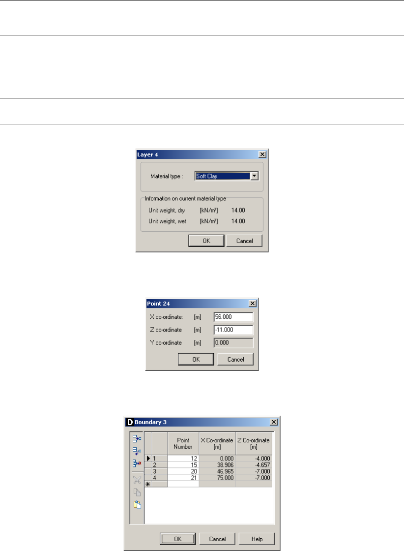
D-GEO PIPELINE
, User Manual
Delete All Loose
Lines
This option will delete all loose lines. Loose lines are actually construc-
tion lines that are not part of the boundaries or PL-lines (therefore, all
lines displayed as solid blue lines). With this option, it is possible to
quickly erase all the “leftover bits” of loose lines that may remain after
converting lines to a geometry.
Delete All Loose
Points
This option will delete all loose points.
Figure 7.19: Layer window (Property editor of a layer)
Figure 7.20: Point window (Property editor of a point)
Figure 7.21: Boundary window (Property editor of a polyline)
128 of 324 Deltares

Graphical Geometry Input
Figure 7.22: Boundary window (Property editor of a line)
Figure 7.23: PL-line window (Property editor of a PL-line)
Note: In the Boundary and PL-line properties windows, only the point’s number can be
modified, not the X and Z co-ordinates.
7.5.4 Dragging elements
One way to modify elements is to drag them to other locations. To drag an element, first select
it. Once the element has been selected, it is possible to drag it by pressing and holding down
the left-hand mouse button while relocating the mouse cursor. Dragging of geometry elements
can result in automatic regeneration of geometry, if this option is switched on (section 7.4.4)
as shown in the example of Figure 7.24: when the selected point is moved upwards, a new
geometry will be created.
D-GEO PIPELINE
creates new layers according to this new geometry.
Before After
Figure 7.24: Example of dragging of a point
Deltares 129 of 324

D-GEO PIPELINE
, User Manual
130 of 324 Deltares

8 Tutorial 1: Calculation and assessment of the drilling fluid
pressure
This first exercise considers installation of a steel pipeline by using the horizontal directional
drilling technique. The exercise focuses on the calculation of the minimal required drilling
fluid pressure which is necessary to perform a horizontal directional drilling and the maximum
allowable drilling fluid pressure, which depends on the strength and deformability of the soil
through which the drilling is carried out.
The objectives of this tutorial are:
To learn how to start up a calculation in
D-GEO PIPELINE
;
To calculate the minimum required drilling fluid pressure;
To calculate the maximum allowable drilling fluid pressure;
Assessment of the calculated drilling fluid pressures.
The following module is needed:
D-GEO PIPELINE
Standard module (HDD)
This tutorial is presented in the file Tutorial-1.dri.
8.1 Introduction to the case
The horizontal directional drilling technique is used to install a steel pipeline in a silty sand
layer. The pipeline configuration is shown in Figure 8.1. The soil properties are provided in
Table 8.1.
15º 15º
pipeline
silty sand
R= 400m
R= 400m
entry: X= -90m
exit: X= 190m
-15m
+5m
0m
Figure 8.1: Pipeline configuration for Tutorial 1
Deltares 131 of 324

D-GEO PIPELINE
, User Manual
Table 8.1: Properties of the silty sand layer (Tutorial 1)
Dry unit weight [kN/m3] 18
Wet unit weight [kN/m3] 20
Cohesion [kN/m2] 0
Angle of internal friction [◦] 30
Undrained strength top [kN/m2] 0
Undrained strength bottom [kN/m2] 0
E modulus top [kN/m2] 10000
E modulus bottom [kN/m2] 15000
Poisson’s ratio [-] 0.35
The pipeline material used in this tutorial is a steel 240 and its properties are given in Table 8.2.
Table 8.2: Properties of steel material (Tutorial 1)
Material quality Steel 240
Negative wall thickness tolerance [%] 0
Yield strength [N/mm2] 240
Partial material factor [-] 1.1
Partial material factor test pressure [-] 1
Young’s modulus [N/mm2] 205800
Outer diameter [mm] 323.9
Wall thickness [mm] 7
Unit weight pipe material [kN/m3] 78.50
Design pressure [Bar] 8
Test pressure [Bar] 9
Temperature variation [◦C] 5
8.2 Project
8.2.1 Start
To create a new project, follow the steps described below:
1. Start
D-GEO PIPELINE
from the Windows task-bar (Start/Programs/Deltares Systems/
D-GEO PIPELINE
).
2. Click File and choose New on the menu bar to start a new project.
3. In the New File window, select the option New geometry to start (Figure 8.2).
Figure 8.2: New File window
This will result in the empty geometry window shown in Figure 8.3.
132 of 324 Deltares

Tutorial 1: Calculation and assessment of the drilling fluid pressure
Figure 8.3: View Input window
4. Save the project by clicking Save As in the File menu and by entering <Tutorial-1>as
project name.
5. Click Save to close this window.
8.2.2 Project Properties
To give the project a meaningful description, follow the steps described below:
6. On the menu bar, click Project and then choose Properties to open the Project Properties
window (Figure 8.4).
Figure 8.4: Project Properties window, Identification tab
7. Fill in <Tutorial 1 for
D-GEO PIPELINE
>and <Calculation of the drilling fluid pressure>for
Title 1 and Title 2 respectively in the Identification tab.
Deltares 133 of 324
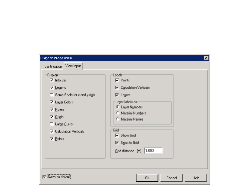
D-GEO PIPELINE
, User Manual
In the other tab of the Project Properties window, some defaults values are modified in order
to make the graphical geometry more understandable.
8. Select the View Input tab (Figure 8.5) to change the settings of the View Input window.
Figure 8.5: Project Properties window, View input tab
9. Mark the Points check-box of the Labels sub-window in order to display the point’s number.
10. Mark the Snap to grid check-box in order to ensure that objects align to the grid automati-
cally when they are moved or positioned.
11. Before closing the Project Properties window, mark the Save as default check-box to use
the settings previously inputted every time
D-GEO PIPELINE
is started, which means for the
other tutorials.
12. Click OK to confirm.
8.2.3 Model
The horizontal directional drilling technique is used in this first tutorial.
13. Select Model from the Project menu bar to open the Model window (Figure 8.6).
14. Check that the Horizontal directional drilling model is selected (default model).
15. Click OK to confirm.
134 of 324 Deltares
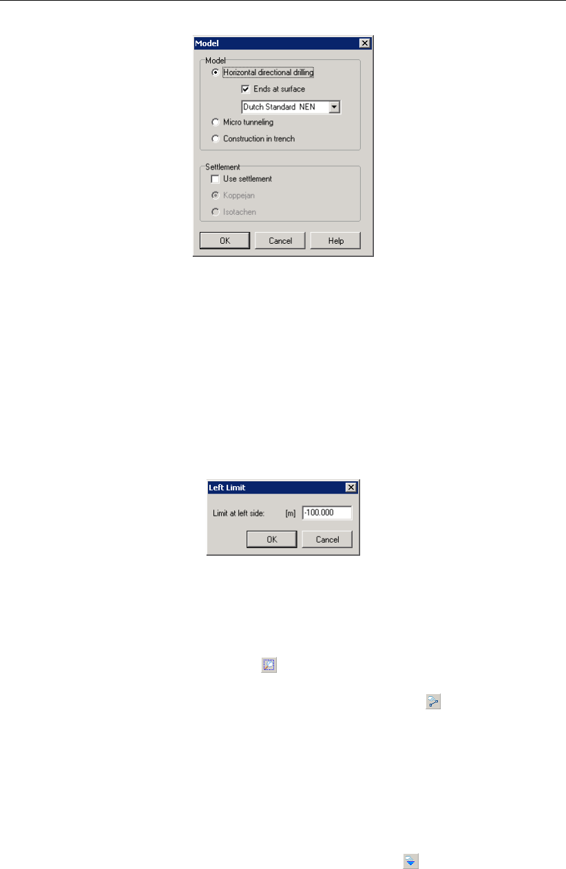
Tutorial 1: Calculation and assessment of the drilling fluid pressure
Figure 8.6: Model window
8.3 Geometry
Firstly, the geometry of Figure 8.1 needs to be put in
D-GEO PIPELINE
. In order to do this, the
following actions should bee performed:
16. First enlarge the dimensions of the geometry window by selecting the left boundary by
clicking the left mouse button, then click the right button and select Properties. This will re-
sult in the coordinate window for the left boundary as shown in Figure 8.7. Enter coordinate
Xof <-100 m>.
Figure 8.7: Left Limit window
17. Repeat the previous described actions for the right boundary and shift the boundary to
coordinate Xof <200 m>. The width in between the left and the right boundary is now
300 m.
18. Choose the drawing option Zoom limits from the Tools section so that the drawn geom-
etry appears in the center of the screen.
19. Choose the drawing option from the edit-window Add single line to draw the surface
line of the longitudinal cross section of the horizontal directional drilling and position the
straight surface line at Z= 5 m. Use the right mouse button to finish the line.
20. Choose the drawing option Add single line to draw the lower boundary of the longitudinal
cross section of the horizontal directional drilling and position the straight lower boundary
line at Z= –40 m.
21. Choose the drawing option from the Tools section Automatic regeneration of geometry so
that the geometry as shown in Figure 8.8 appears. If the Automatic regeneration option
already is selected, click on the Edit icon to regenerate the geometry.
22. Choose the drawing option from the edit-window Add pl-line(s) and position the level of
the groundwater at coordinate Z= 0 m. The blue dashed line represents the groundwater
line (PL line).
Deltares 135 of 324
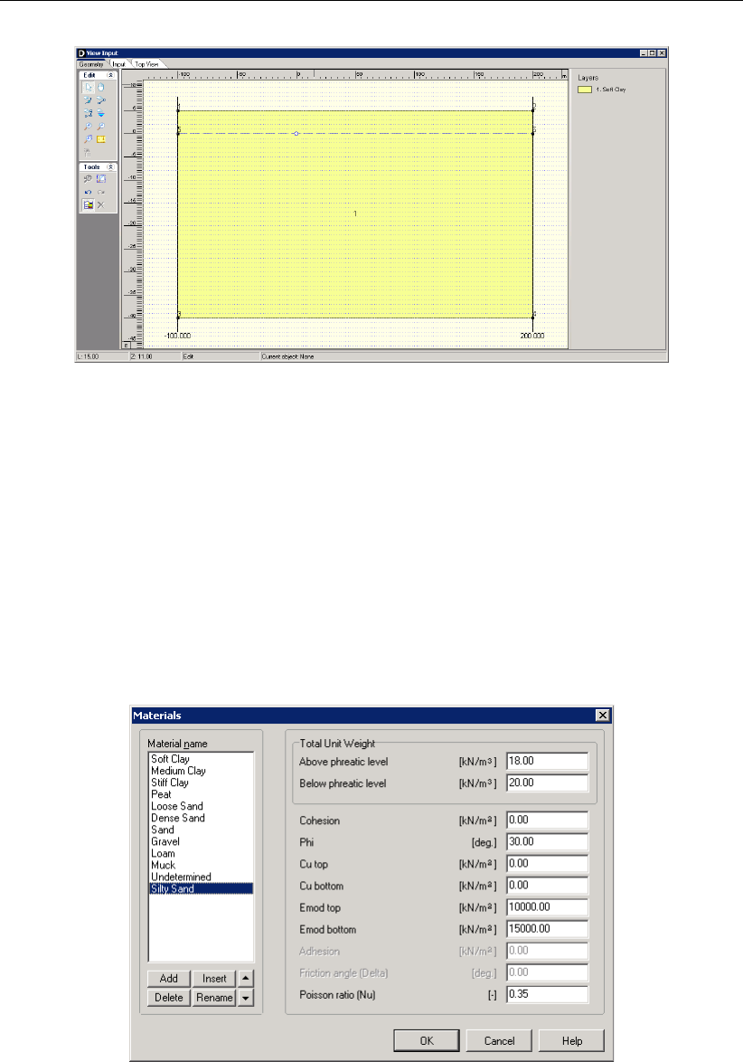
D-GEO PIPELINE
, User Manual
Figure 8.8: View Input window, Geometry tab
8.3.1 Soil layer properties
The properties of the soil layers should be specified in the menu materials which can be
entered by clicking soil. In this tutorial only one soil layer is considered.
23. Click Soil and select Materials on the menu bar to open the Materials window (Figure 8.9)
and enter the soil data.
24. Add a new material by choosing Add button below the materials list on the left side of the
window with the new <Silty Sand>.
25. Enter the soil data as given in Table 8.1.
26. Finish the input of soil data by clicking OK.
Figure 8.9: Materials window
The defined soil properties and the groundwater level have to be assigned to the drawn ge-
ometry of the longitudinal cross section. The assignments can be carried out by clicking
geometry and choosing the subsequent described options on the menu bar.
136 of 324 Deltares
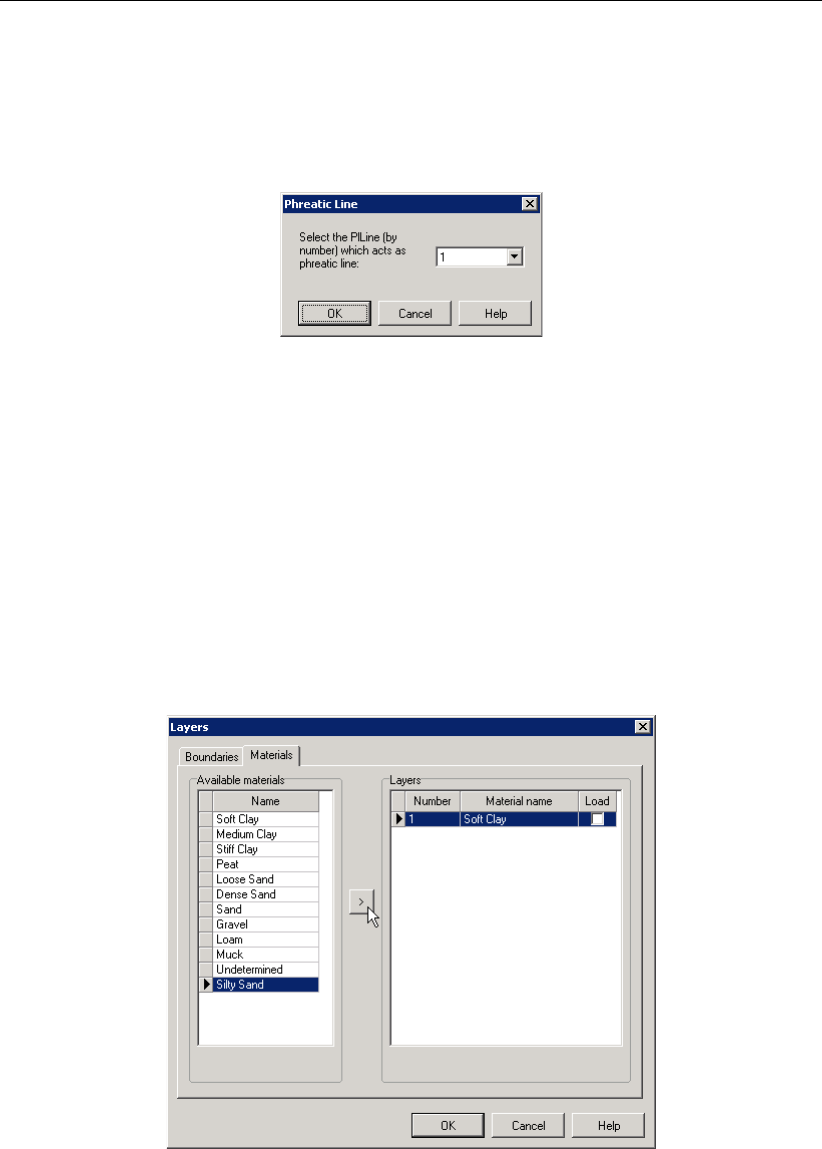
Tutorial 1: Calculation and assessment of the drilling fluid pressure
8.3.2 Phreatic Line
27. On the Geometry menu, select Phreatic Line to open Phreatic Line window (Figure 8.10)
in which the phreatic line for calculation of the groundwater pressures can be selected.
28. Choose PL–line nr. <1>(only one phreatic line is available) and click OK.
Figure 8.10: Phreatic Line window
8.3.3 Layers
29. Click Geometry and select Layers on the menu bar to assign the soil properties to the soil
layers in the longitudinal cross section. To assign a material to a layer, select the Material
tab.
30. Assign the properties of the defined layer Silty Sand to layer number one in the longitudinal
cross section. The available soil layers with defined properties are shown in left column
of the materials window. The layers in the longitudinal cross section are shown in the
right column of the materials window. The defined properties are assigned to layer nr 1
by clicking the arrow in between the columns. This will result in the Material tab shown in
Figure 8.11.
Figure 8.11: Layers window, Materials tab
31. Click OK to quit the window and return to the geometry window to watch the change of
layer name in the legend.
8.3.4 PL-Lines per Layers
32. Click Geometry and select PL–lines per Layers on the menu bar to open the PL–lines
per Layer window (Figure 8.12) in which the defined PL–lines to the soil layers in the
longitudinal cross section can be defined. This window contains the information for the
Deltares 137 of 324
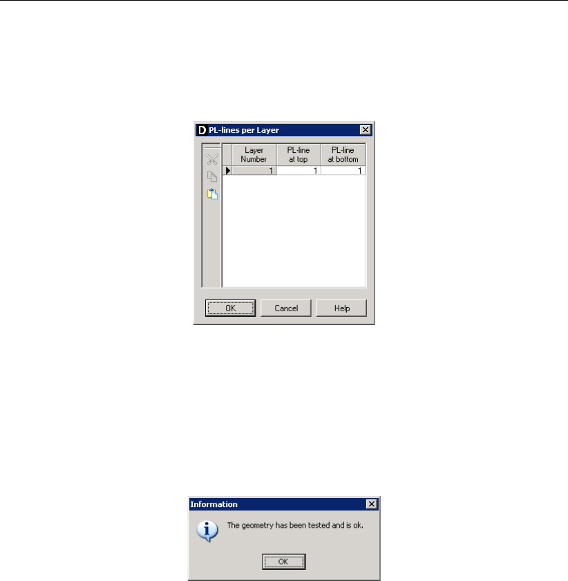
D-GEO PIPELINE
, User Manual
calculation of the groundwater pressure distribution. In this tutorial only one PL–line is
defined. The groundwater pressure at the top of the silty sand layer and the bottom of this
layer should be calculated based on the hydraulic head of PL–line 1.
33. Click OK to close the window.
Figure 8.12: PL-lines per Layers window
8.3.5 Check Geometry
34. The geometry can be tested by clicking Geometry and selecting Check Geometry on the
D-GEO PIPELINE
menu bar. If the geometry is entered properly, the message shown in
Figure 8.13 appears.
35. Click OK to close the window.
Figure 8.13: Check Geometry window
8.4 Pipeline Configuration
36. Click Pipe and select Pipeline Configuration on the menu bar to open the Pipeline config-
uration window in which the pipeline configuration can be put in.
37. Enter the values given in Figure 8.1 of the introduction.
38. Select a Pulling direction product pipe <From left to right>as indicated in Figure 8.14.
138 of 324 Deltares
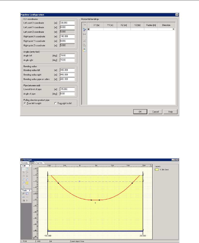
Tutorial 1: Calculation and assessment of the drilling fluid pressure
Figure 8.14: Pipeline Configuration window
39. Confirm by clicking OK.
40. Watch the entered pipeline configuration on the Input tab of the View Input window (Fig-
ure 8.15).
Figure 8.15: View Input window, Input tab
8.5 Soil behavior
When the borehole is created, the drilling fluid will exert pressure on the borehole wall and the
soil next to the borehole. When the pressure rises above a certain value, plastic deformation
of the soil will occur, initially adjacent to the borehole. When the pressure is increased further
beyond this value, the zone with plastic deformation will increase. If the zone with plastic
deformation reaches the surface a blow-out will occur. Besides the growth of the plastic zone
due to high drilling fluid pressures, formation of cracks in the borehole wall in granular soils will
take place before the plastic zone reaches its maximum expansion. The formation of cracks
around the borehole in granular soils is dependent on the strain of the bore hole wall which
occurs when the drilling fluid pressure is increasing and the borehole is expanding.
Crack formation and growth of the plastic zone are dependent upon soil characteristics. Soil
layers with a very high strength and/or a very high stiffness are suitable for drilling with high
Deltares 139 of 324
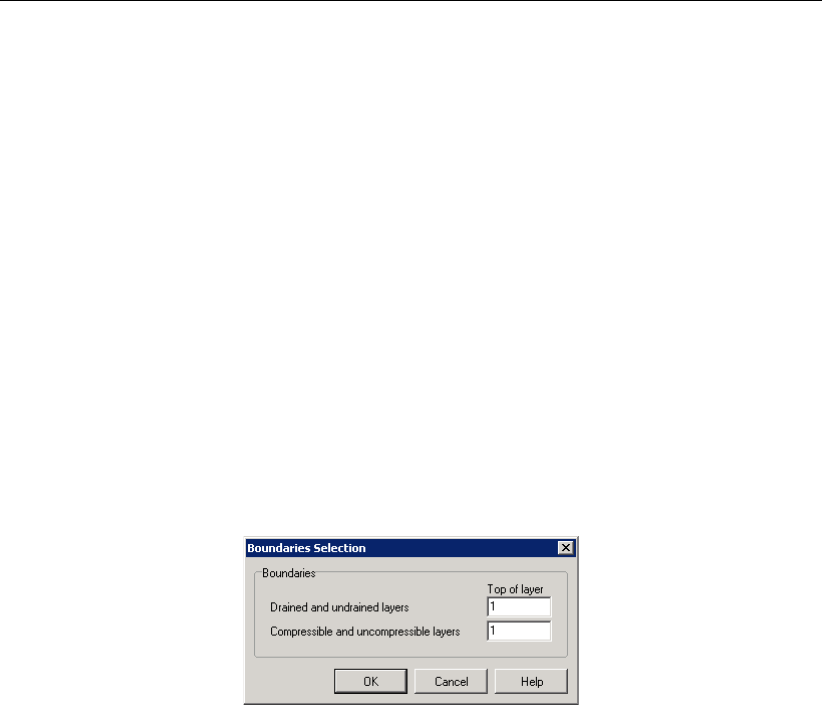
D-GEO PIPELINE
, User Manual
drilling fluid pressures.
Strength of soil layers is dependent on the drained or undrained behavior of soil layers during
application the drilling fluid pressure on the bore hole wall. Depending on the permeability
of the soil layer, the soil will behave drained or undrained. The coarser granular soils are
usually well permeable so that the excess water pressure due to the drilling fluid pressures
will dissipate easily. The strength of the soil which exhibits this drained behavior can be
calculated using the drained (effective) strength parameters effective cohesion (c) and angle
of internal friction (ϕ). In case of undrained behavior, which usually occurs in very fine grained
cohesive soils, the strength of the soil should be calculated using the undrained cohesion (cu).
41. Click GeoObjects and select Boundaries Selection on the menu bar to select the input win-
dow specification of the soil behavior. This will result in the Boundaries Selection window
shown in Figure 8.16.
42. Choose the boundary between the undrained and drained layer on top of layer nr 1. This
choice results in drained behavior of layer nr 1. The other in the boundaries window men-
tioned boundary in between compressible and incompressible layers can be chosen on top
of layer nr 1 (see tutorial 3 for explanation about this compressibility boundary).
Figure 8.16: Boundaries Selection window
8.6 Calculation Verticals
The locations in the longitudinal cross section at which a calculation should be carried out
must be specified by the user. The user is able to perform calculations at uniform distances
along the longitudinal cross section but is also able to perform more calculations at short
distances at areas of interest.
43. Click GeoObjects and select Calculation Verticals on the menu bar to select the Calculation
Verticals window for specification of the calculation locations along the longitudinal cross
section.
44. Choose the Automatic generation of L co-ordinates option on the right side of the window
and choose the following values: <–80 m>for First,<180 m>for Last and <20 m>for
Interval.
45. Click on the Generate button and watch the result of automatic vertical generation on
the left side of the Calculation Verticals window. This will result in the window shown in
Figure 8.17.
46. Click OK to confirm the selected verticals and switch to the input window to watch the
location of the verticals in the longitudinal cross section.
140 of 324 Deltares
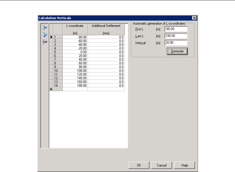
Tutorial 1: Calculation and assessment of the drilling fluid pressure
Figure 8.17: Calculation Verticals window
8.7 Product Pipe Material Data
The dimensions and the properties of the product pipe which should be installed in the reamed
borehole should be specified. Especially the outer diameter is important for the calculation of
the drilling fluid pressures during the pull back operation.
47. Click Pipe and select Product Pipe Material Data on the menu bar to open the Product Pipe
Material Data window for specification of the dimensions and properties of the product pipe.
48. Click on the button Add on the left side of the window to declare a pipeline with the name
<Pipe 1>.
49. Enter the values given in Table 8.2 for Pipe 1 in the fields on the right side of the window
as shown in Figure 8.18.
50. Click OK to confirm.
Deltares 141 of 324
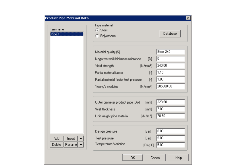
D-GEO PIPELINE
, User Manual
Figure 8.18: Product Pipe Material Data window
8.8 Drilling Fluid Data
Various types of drilling fluids exist; the drilling fluid has properties to transport the cuttings
from the borehole to the surface. The flow behavior, which depends on the drilling fluid prop-
erties, is an important characteristic for the development of drilling fluid pressure during the
different drilling stages.
Generally, the flow behavior of drilling fluid can be described with the Bingham model. The
Bingham model is used in
D-GEO PIPELINE
and describes the fluid by means of a viscosity
term and a threshold term from which flow is initialized. The threshold is called the yield point.
D-GEO PIPELINE
calculates the required minimum fluid pressure at the calculation verticals.
During all stages of the drilling process, a pipe is present in the borehole, drill pipe or product
pipe. The return flow of drilling fluid with cuttings occurs in the annulus between the borehole
wall and the pipe. The required fluid pressure to initiate flow depends on the width of the
annulus (radius borehole minus radius drill pipe), the properties of the drilling fluid and the
required annular fluid flow rate.
The properties of the drilling fluid and the operation parameter values should be specified in
D-GEO PIPELINE
.
51. Click Pipe on the menu bar and select Drilling Fluid Data to open the Drilling Fluid Data
window for specification of properties of the drilling fluid and the operation parameter val-
ues.
52. Enter the values given in Figure 8.19.
53. Click OK to confirm the input.
142 of 324 Deltares
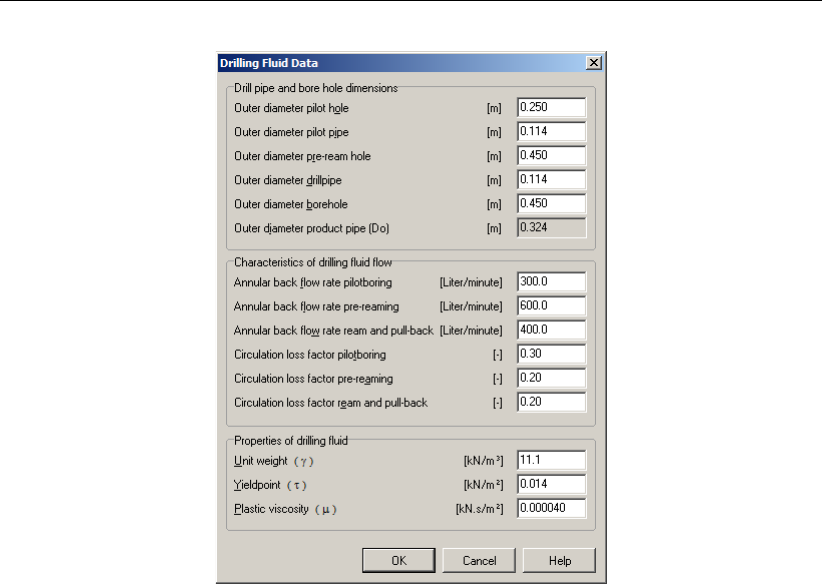
Tutorial 1: Calculation and assessment of the drilling fluid pressure
Figure 8.19: Drilling Fluid Data window
8.9 Factors
D-GEO PIPELINE
performs the calculations of the maximum allowable drilling fluid pressures
according the Dutch regulations described in the NEN 3650 and 3651. The safety philosophy
described in the NEN 3650-1 Annex B and D (NEN,2012a) is applied on the calculations.
54. Click Defaults on the menu bar and select Factors to open the Factors window in which
the default values of the contingency and safety factors are shown and can be modified.
Since the window shown in Figure 8.20 shows all factors according to the Dutch regulations
adapting the values is not necessary.
55. Click OK to confirm.
Deltares 143 of 324

D-GEO PIPELINE
, User Manual
Figure 8.20: Factors window
8.10 Results
The calculation of the drilling fluid pressures during the three stages of installation of the steel
pipe using the horizontal directional drilling technique can be started from the
D-GEO PIPELINE
menu.
56. Click Calculation and select Start on the menu bar to start the calculation or press the
function key F9.
D-GEO PIPELINE
automatically saves the file during the calculation.
57. Click Results and select Drilling fluid pressure plots on the menu bar to watch the results of
the drilling fluid pressure calculations for the pilot drilling. The window shown in Figure 8.21
will appear. The graph shows the maximum allowable pressures (upper limit related to soil
cover and lower limit related to deformation of the borehole) and the minimal required
drilling fluid pressure for transportation of the cuttings.
144 of 324 Deltares
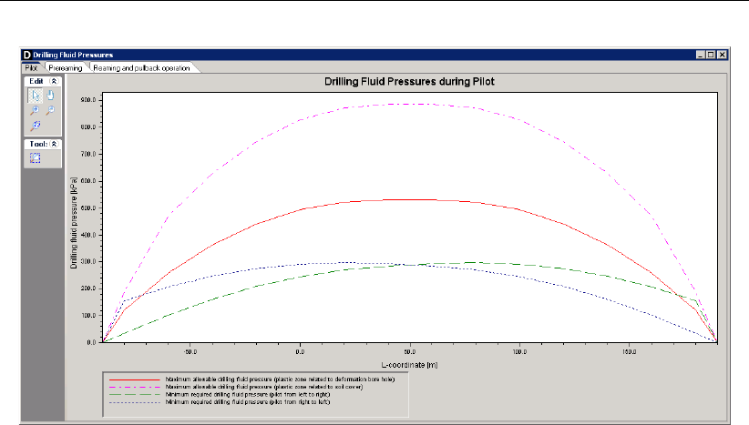
Tutorial 1: Calculation and assessment of the drilling fluid pressure
Figure 8.21: Drilling Fluid Pressures window
58. Click on the tabs Prereaming and Reaming and pullback to watch the results of the other
drilling stages.
59. Close the window to return to the main window.
Notice that the minimal required drilling fluid pressure is lower than the maximal allowable
drilling fluid pressure in the pilot drilling stage. The risk on a blow out is therefore very small.
Of course, due to the decreasing soil cover, the last meters of the pilot drilling the minimal
required drilling fluid pressure is higher than the allowable drilling fluid pressure, but in this
situation the distance where the minimal required drilling fluid is higher than the maximum
allowable pressure is very small.
8.11 Conclusion
Various input windows are used to enter the details of a project that is to be modeled and
analyzed. Once these details have been put in, they can be used to calculate a range of
results, including drilling fluid pressures during the three stages of the HDD technique. One
way to view these results is to display them graphically on the screen.
Deltares 145 of 324

D-GEO PIPELINE
, User Manual
146 of 324 Deltares

9 Tutorial 2: Stress analysis of steel pipes and polyethylene pipes
This second exercise considers installation of a steel pipeline and installation of a polyethy-
lene pipeline by using the technique horizontal directional drilling. The exercise focuses on
the stress analysis for the different installation stages, which is required to assess whether
installation of the pipeline according the design is executable or not.
The objectives of this tutorial are:
To calculate the pulling force on the pipeline during the pull back operation.
To calculate the stresses in the pipeline during the different installation stages.
Assessment of the calculated stresses in the pipeline.
To perform a Special Stress Analysis.
To perform a calculation for a polyethylene pipe.
The following module is needed:
D-GEO PIPELINE
Standard module (HDD)
This tutorial is presented in the files Tutorial-2a.dri, Tutorial-2b.dri and Tutorial-2c.dri.
9.1 Introduction to the case
The pipeline configuration and the soil type is the same as those modeled in the first tutorial
(Figure 9.1).
15º 15º
pipeline
silty sand
R= 400m
R= 400m
entry: X= -90m
exit: X= 190m
-15m
+5m
0m
Figure 9.1: Pipeline configuration for Tutorial 2
Different calculations will be performed using two pipe materials:
A steel pipe with the properties given in Table 9.1 (Tutorial 2a),
The same pipe as Tutorial 2a, but performing a Special Stress Analysis (Tutorial 2b).
A polyethylene pipe with the properties given in Table 9.1 (Tutorial 2c).
Deltares 147 of 324
D-GEO PIPELINE
, User Manual
Table 9.1: Pipe properties (Tutorial 2)
Tutorials 2a / 2b Tutorial 2c
Pipe material Steel Polyethylene
Material quality Steel 355 PE 100
Negative wall thickness tolerance [%] 0 n.a.
Young’s modulus [N/mm2] 205800 1200
Young’s modulus (long term) [N/mm2] n.a. 300
Allowable/Yield strength [N/mm2] 355 10
Allowable strength (long term) [N/mm2] n.a. 8
Partial material factor [-] 1.1 n.a.
Partial material factor test pressure [-] 1 n.a.
Tensile factor [-] n.a. 0.65
Outer Diameter [mm] 323.9 400
Wall thickness [mm] 8 36.4
Unit weight pipe material [kN/m3] 78.5 9.54
Design pressure [Bar] 8 4
Test pressure [Bar] 9 5
Temperature variation [◦C] 5 5
In the first tutorial, the assessment whether the proposed drilling line and borehole dimensions
according the design is executable or not was performed. The second tutorial considers the
assessment of stresses in pipeline during the different installation stages and after installation.
In
D-GEO PIPELINE
it is assumed that the pipeline remains fixed at the specified location and
that settlement of the soil layers below the pipeline does not influence the pipeline. Therefore
a relative simple pipe stress analysis can be performed.
The first installation stage at which the stresses in the pipeline are considered is the start
of the pull back operation. The pipeline with the connected pullback equipment is situated
on the rollers. Often the pipeline is not filled with water on the rollers in order to reduce the
required pulling force to pull the pipeline over the rollers. Of course when the pipeline enters
the borehole filling of a part of the pipeline (percentage of the cross section area) is sometimes
useful.
In this stage a pulling force is exerted on the pipe, which results in axial stress in the pipeline.
Near the exit point, the rollers are often configured with a certain bending radius (the so-called
overbend), so that additional axial stresses occur due to bending. The tangential stresses for
the pipeline on the rollers are negligible.
The second stage at which the stresses in the pipeline are considered is the maximum pulling
force situation during the pull back operation. At the end of the pull back operation the pulling
force usually reaches the maximum pulling force. The pulling force is calculated according
the Dutch regulations described in NEN 3650 and is mainly based on the normal forces of
the pipeline perpendicular to the borehole wall. The normal forces are caused by the buoyant
weight of the pipeline and soil reaction forces due to the bending moment in the pipeline in
the bends of the drilling line. In the second stage both the axial stresses due to pulling and
bending are calculated and the tangential stresses due to soil reaction forces are calculated.
The third stage at which the stresses in the pipeline are considered is the long term stage after
installation. When the pipeline is installed, a situation without internal pressure and a situation
with internal pressure are considered. In this final stage the drilling fluid in the borehole is
148 of 324 Deltares

Tutorial 2: Stress analysis of steel pipes and polyethylene pipes
assumed to be consolidated, so that the contribution of soil pressure on the pipeline is taken
into account for the calculation of the tangential stress.
The stresses in the pipeline are calculated for the different installation stages. According
NEN 3650 an additional calculation is made for application of internal pressure on the pipeline.
Therefore in the stress analysis according the NEN 3650, four Load Combinations (LC) are
considered:
LC 1A: start of the pullback operation
LC 1B: end of the pullback operation
LC 2: application of internal pressure on the pipeline
LC 3: pipeline after installation, without internal pressure
LC 4: pipeline after installation, with internal pressure
The calculated stresses are assessed according NEN 3650 for the steel pipelines and accord-
ing NEN 3652 for the polyethylene pipelines.
9.2 Project Properties
This tutorial is based on continuation of the file used in Tutorial 1 (chapter 8).
1. Click File and select Open on the menu bar to select the Open window for the choice of
the
D-GEO PIPELINE
file created at the end of tutorial 1.
2. Select Tutorial–1 and click the Open button to open de file.
3. Click File and select Save as on the menu bar to select the save file window and rename
the file into <Tutorial–2a>.
4. Click the Save button to save the file for Tutorial 2a.
5. On the menu bar, click Project and then choose Properties to open the Project Properties
window.
6. Fill in <Tutorial 2 for
D-GEO PIPELINE
>and <Stress analysis of steel and polyethylene
pipes>for Title 1 and Title 2 respectively in the Identification tab.
7. Click OK.
9.3 Product Pipe Material Data
The dimensions and the properties of the product pipe which should be installed in the reamed
borehole should be specified for a pipe stress analysis.
8. Click Pipe on the menu bar and select Product Pipe Material Data to open the Product
Pipe Material Data window for specification of the dimensions and properties of the
product pipe.
9. For Pipe 1, enter the values given in Figure 9.2.
10. Click OK to confirm the specified product pipe material data.
Deltares 149 of 324

D-GEO PIPELINE
, User Manual
Figure 9.2: Product Pipe Material Data window
9.4 Engineering Data
The first step of the pipe stress analysis is the calculation of the pulling force. The magnitude
of the pulling force plays an important role in the stress distribution in the pipe during the
pill back operation. The pulling force is calculated according the specifications described in
NEN 3650.
During the pull back operation the moving pipeline contacts the wall of the borehole and
pushes with a certain forces perpendicular to the wall of borehole. These perpendicular forces
(normal forces) determine the magnitude of the shear force in axial direction during the pull
back operation.
In order to reduce the normal forces on the borehole wall the pipeline is sometimes ballasted
during the pull back operation. In the part of the HDD without significant bends, the distribution
of the normal forces on the bore hole wall is determined by the effective weight of the pipeline.
The effective weight is defined as follows:
geff =g−guplift (9.1)
with:
guplift =π×r2
e×γdf (9.2)
where:
reis the outer radius of the pipeline, in m;
guplift is the upward force of the pipeline, in kN/m;
gis the weight of the ballasted pipeline, in kN/m;
γdf is the unit weight of the drilling fluid, in kN/m3.
150 of 324 Deltares
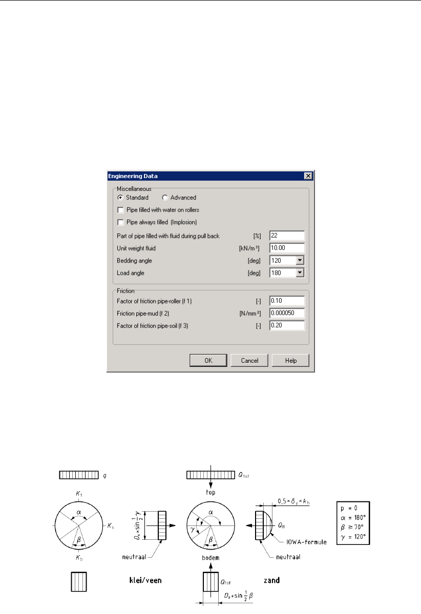
Tutorial 2: Stress analysis of steel pipes and polyethylene pipes
Using the above described equation it can be calculated that filling the product pipe for 22 %
results in a nearly weightless pipe in the bore hole. Of course it is wise not to fill the product
pipe on the rollers so that the pulling force during the first part of the pull back operation can
be reduced.
11. Click Pipe and select Engineering Data on the menu bar to open the Engineering Data
window.
12. Do not mark the Pipe filled with water on rollers check-box and enter the values given in
Figure 9.3.
13. Click on the OK button to confirm the input of the specified values.
Figure 9.3: Engineering Data window
The bedding (β) and the load angle (α) are shown in Figure 9.4. The values are used in the
pipe stress analysis to determine the moment coefficients.
Figure 9.4: Bedding and load angles on the pipeline (according to Figure D.2 of
NEN 3650-1)
9.5 Factors
D-GEO PIPELINE
performs the calculations for the pipe stress analysis according the Dutch
regulations described in the NEN 3650 and 3651. The safety philosophy described in Annex
B and D of the NEN 3650-1 (NEN,2012a) is applied on the calculations.
Deltares 151 of 324
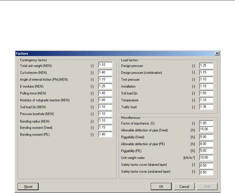
D-GEO PIPELINE
, User Manual
14. Click Defaults on the menu bar and select Factors to open the Factors window for watching
the default values or for alternating these values. Since the window shown in Figure 9.5
shows all factors according the Dutch regulations adapting the values is not necessary.
15. Click OK to confirm.
Figure 9.5: Factors window
9.6 Calculation and Results (Tutorial-2a)
The results of the pulling force calculation are shown in the
D-GEO PIPELINE
report which is
created automatically after finishing the calculations.
16. To start the calculations click Calculation and select Start on the menu bar or press the
function key F9.
9.6.1 Results of the pulling force calculation
17. Click Results and select Report on the menu bar to look at the results of the pulling force
calculation. The results can be found in paragraph 5.3 (Figure 9.6).
152 of 324 Deltares
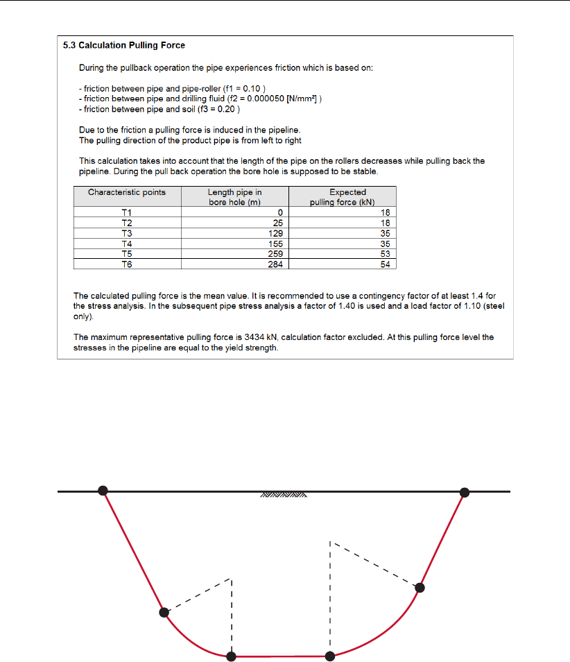
Tutorial 2: Stress analysis of steel pipes and polyethylene pipes
Figure 9.6: Report window, Calculation pulling force (filling percentage = 22%)
18. In Figure 9.7 the characteristic locations along the drilling line at which the pulling force is
calculated are shown. Notice that the maximum pulling force is 54 kN.
entry point exit point
ground level
T1
T2
T5
T6
T3 T4
Figure 9.7: Schematic overview of the characteristic points
19. Switch back and click Pipe and select Engineering Data on the menu and alter the Part of
pipe filled with fluid during pull back to <0%>.
20. Start the calculations again by clicking Calculation and select Start on the menu bar or by
pressing the function key F9.
21. Click Results and select Report on the menu bar to watch the results of the pulling force
calculation. Notice that the pulling force has increased to 64 kN (Figure 9.8).
Deltares 153 of 324

D-GEO PIPELINE
, User Manual
Figure 9.8: Report window, Calculation pulling force (filling percentage = 0%)
9.6.2 Results of the pipe stress analysis of the steel pipe
The pipe stress analysis is described in the report. For each load combination the axial and
tangential stresses in the product pipe are calculated. The stresses are used to calculate the
maximum combined stress in the pipeline.
22. Click Results and select Report on the menu bar to watch the results of the calculated
axial and tangential stresses for each load combination/installation stage in paragraph 6.2
(see Figure 9.9).
Figure 9.9: Report window, Results Stress Analysis (Tutorial-2a)
23. Continue looking at the report and scroll down to paragraph 6.3. In the table in para-
graph 6.3, the stress assessment is carried out: the calculated stresses are compared
with the yield strength of steel according to the specifications described in NEN 3650. Be-
low the stress assessment table, the results of the deflection calculation are given (see
154 of 324 Deltares
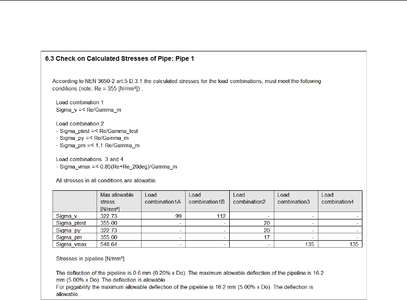
Tutorial 2: Stress analysis of steel pipes and polyethylene pipes
Figure 9.10).
Figure 9.10: Report window, Check on calculated stresses (Tutorial-2a)
24. Notice that the calculated stresses for all load combinations are allowable. The deflection
is lower than the allowable value.
25. Look at the calculated soil load and the calculated modulus of subgrade reaction on para-
graph 4.1.
Deltares 155 of 324
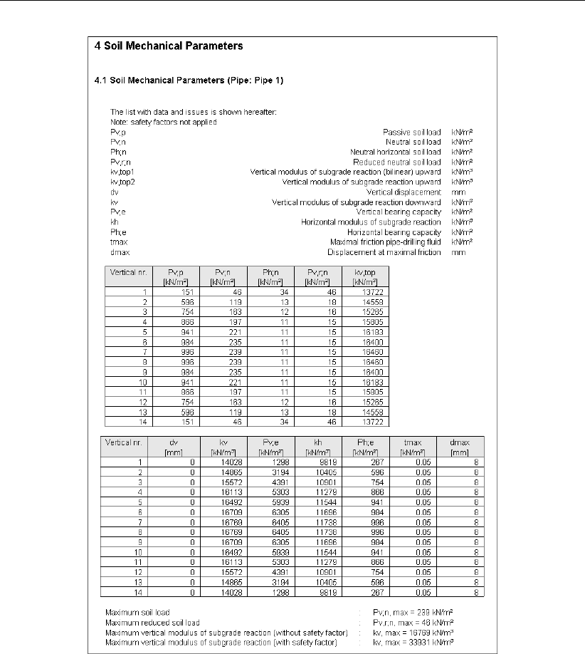
D-GEO PIPELINE
, User Manual
Figure 9.11: Report window, Soil Mechanical Parameters (Tutorial-2a)
9.7 Special Pipe Stress Analysis (Tutorial-2b)
The option special stress analysis can be used for a pipe stress analysis in case of additional
loads at certain location along the longitudinal cross section. Additional loads can for example
be induced by traffic or by constructions.
Assume that vertical 1 is located below a highway which will result in an additional load on
the pipeline. The load induced by soil stress is already calculated by
D-GEO PIPELINE
and is
assessed in the report (see section 9.6.2). The additional load at the depth of the pipeline can
be determined using load distribution theories.
26. Click File and select Save As on the menu bar to select the Save As window and rename
the file into <Tutorial-2b>.
27. Click the Save button to save the file for Tutorial-2b.
28. Click Defaults and select Special Stress on the menu bar to open the Special Stress Anal-
ysis window and enter the data for the special pipe stress analysis. In this window (Fig-
ure 9.12), the soil load enhanced with the traffic load should be specified. The reduced
156 of 324 Deltares

Tutorial 2: Stress analysis of steel pipes and polyethylene pipes
soil load equals <18 kN/m2>and the modulus of subgrade reaction is independent of
the load and remains <17000 kN/m3>. The radius is the same as defined in the pipeline
configuration <400 m>.
Figure 9.12: Special Stress Analysis window
29. Click OK to confirm.
30. Click Calculation and select Special Stress Analysis on the menu bar to start the calcula-
tion.
31. Click Results and select Report on the menu bar to look at the results on paragraph 4.3
(see Figure 9.13). Notice the difference with Figure 9.10 for Tutorial-2a.
Figure 9.13: Report window, Check on calculated stresses (Tutorial-2b)
9.8 Polyethylene Product Pipe (Tutorial-2c)
Besides a pipe stress analysis on steel pipes a pipe stress analysis on PE-pipes can be
carried out using
D-GEO PIPELINE
.
32. Click File and select Save As on the menu bar to select the Save As window and rename
the file into <Tutorial-2c>.
Deltares 157 of 324
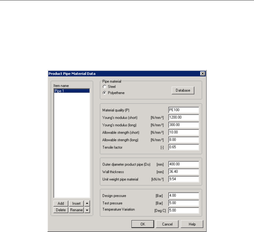
D-GEO PIPELINE
, User Manual
33. Click the Save button to save the file for Tutorial-2c.
34. Click Pipe and select Product Pipe Material Data on the menu bar to open the Product Pipe
Material Data window for specification of the dimensions and properties of the product pipe.
35. Select Polyethylene as Pipe material for Pipe 1.
36. Enter the values given in Table 9.1.
37. Click OK to confirm.
Figure 9.14: Product Pipe Material Data window (Tutorial-2c)
38. To start the calculations, click Calculation and select Start on the menu bar or press the
function key F9.
39. Click Results and select Report on the menu bar to look at the results of the calculated
axial and tangential stresses for each load combination/installation stage in paragraph 6.2.
40. Continue looking at the report and scroll down to paragraph 6.3. In the table (Figure 9.15),
the stress assessment is carried out: the calculated stresses are compared with allowable
stresses according to the specifications described in the NEN 3650 series.
158 of 324 Deltares
Tutorial 2: Stress analysis of steel pipes and polyethylene pipes
Figure 9.15: Report window, Check on calculated stresses (Tutorial-2c)
41. Below the assessment table in paragraph 6.3, a check on short term and long term implo-
sion is described (see paragraph 6.4 in Figure 9.16). Notice that the short term implosion
check is based on the drilling fluid pressure during the pull back operation. The long term
implosion check is based on the water pressure at the level of the pipeline.
Figure 9.16: Report window, Check for Implosion (Tutorial-2c)
9.9 Conclusion
This second tutorial analyzes the strength calculations during different stages of the HDD
technique for steel and polyethylene pipes. In both cases, the report shows that all stresses
for the different stages are allowable.
Deltares 159 of 324

D-GEO PIPELINE
, User Manual
160 of 324 Deltares
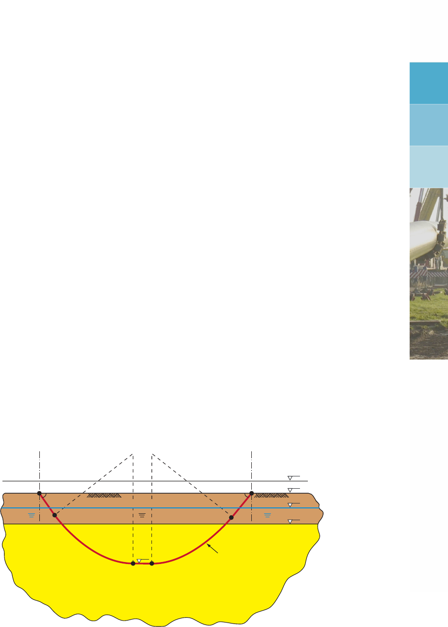
10 Tutorial 3: Influence of soil behavior on drilling fluid pressures
and soil load on the pipe
This third exercise considers installation of a polyethylene pipeline by using the technique
horizontal directional drilling. The exercise focuses on the soil behavior and elucidates the
effect of drained and undrained soil layers on the calculation of the drilling fluid pressures and
elucidates the effect of compressible and incompressible layers on the calculation of the soil
load on the pipeline.
The objectives of this tutorial are:
To calculate the drilling fluid pressures for a layered soil sequence;
To calculate the soil load for a layered soil sequence;
Schematization of a layered soil sequence with artesian groundwater.
The following module is needed:
D-GEO PIPELINE
Standard module (HDD)
This tutorial is presented in the file Tutorial-3.dri.
10.1 Introduction to the case
This tutorial is based on continuation of the file used in Tutorial-2c (chapter 9). The steel pipe
is the same but the layered soil sequence is different as shown in Figure 10.1. The properties
of the two layers are given in Table 10.1.
15º 15º
pipeline
silty sand
soft organic clay
R= 400m
R= 400m
entry: X= 90m
exit: X= 190m
-15m
+5m
+8m
0m
-5m
PL-line 2
PL-line 1
Figure 10.1: Pipeline configuration for Tutorial 3
Deltares 161 of 324
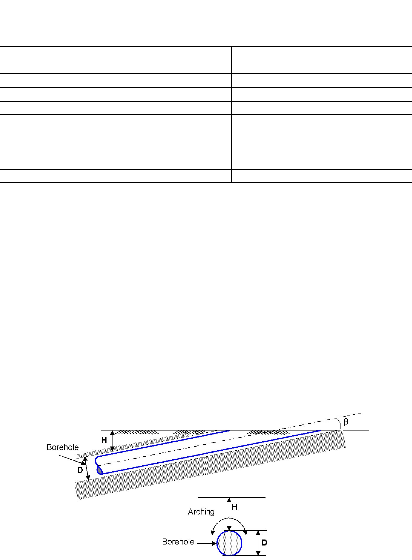
D-GEO PIPELINE
, User Manual
Table 10.1: Layer properties (Tutorial 3)
Coarse sand Soft organic clay
Dry unit weight [kN/m3] 18 13
Wet unit weight [kN/m3] 20 13
Cohesion [kN/m2] 0 2
Angle of internal friction [◦] 35 18
Undrained strength top [kN/m2] 0 10
Undrained strength bottom [kN/m2] 0 30
E modulus top [kN/m2] 15000 500
E modulus bottom [kN/m2] 25000 1000
Poisson’s ratio [-] 0.35 0.45
During drilling a borehole is protected from collapsing by filling it with drilling fluid. However,
arching in the surrounding soil contributes to the stability of the borehole. As a result, arching
also reduces the total amount of soil load acting on the installed pipe.
For an ideal granular stratum, Terzaghi’s derivation has up until now been considered to be
appropriate for the situation where arching occurs and is accordingly incorporated in Dutch
pipeline standard NEN 3650 series. However, for cohesive soil layers consolidation may occur
over a period of time and this will result in a reduction of the arching effect, thereby increasing
the vertical load on the installed pipe. The latter process is added to the Dutch pipeline
standard.
For the development of arching a certain depth diameter ratio is required (Figure 10.2). At
shallow depths near the exit and entry point, the soil cover is not sufficient for turning off the
soil load above the borehole to the soil layers next to the borehole.
Figure 10.2: Arching around the borehole
During the pilot drilling the highest drilling fluid pressures occur. The risk on a blow out to the
surface or the formation of cracks around the borehole often exists. This risk is related to the
strength of the soil layers around the borehole. The strength of soil layers is dependent on
the drained or undrained behavior of soil layers during application the drilling fluid pressure
on the bore hole wall. Depending on the permeability of the soil layer, the soil will behave
drained or undrained. The coarser granular soils are usually well permeable so that the excess
water pressure due to the drilling fluid pressures will dissipate easily. The strength of the soil
which exhibits this drained behavior can be calculated using the drained (effective) strength
162 of 324 Deltares
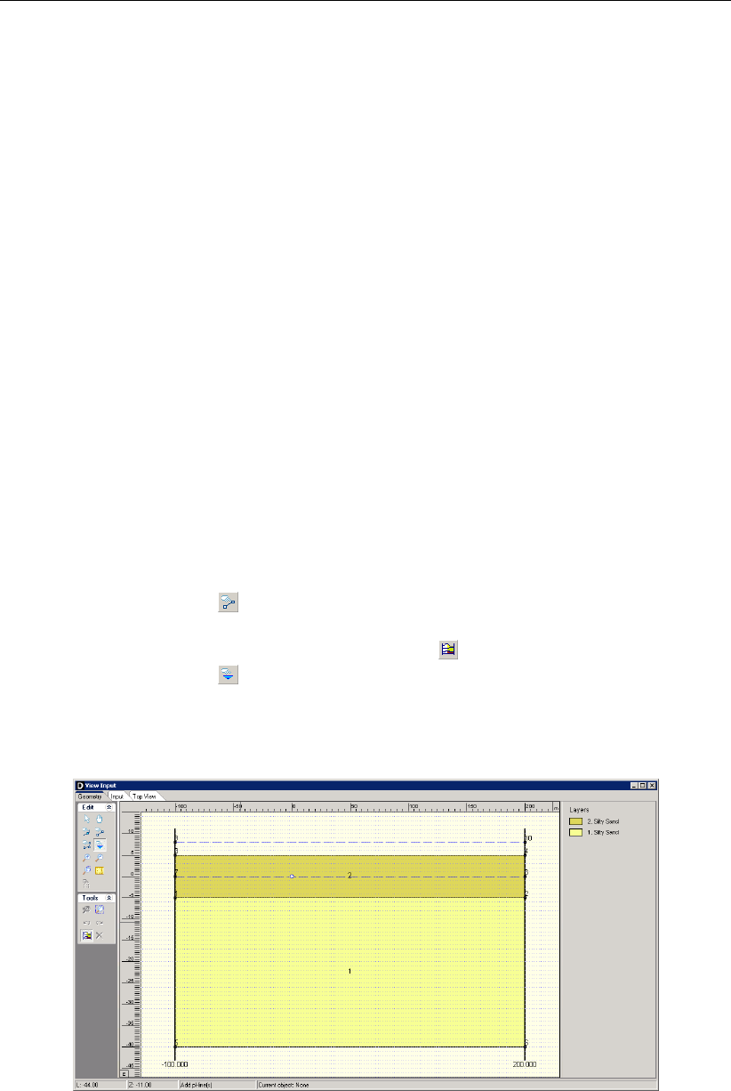
Tutorial 3: Influence of soil behavior on drilling fluid pressures and soil load on the pipe
parameters. In case of undrained behavior, which usually occurs in very fine grained cohesive
soils, the strength of the soil should be calculated using the undrained strength parameters.
1. Click File and select Open on the menu bar to open the Open window.
2. Select Tutorial-2c and click the Open button to open the file.
3. Click File and select Save as on the menu bar to open the Save As window and rename
the file into <Tutorial-3>.
4. Click the Save button to save the file for Tutorial 3.
5. On the menu bar, click Project and then choose Properties to open the Project Properties
window.
6. Fill in <Tutorial 3 for
D-GEO PIPELINE
>and <Influence of soil behavior>for Title 1 and
Title 2 respectively in the Identification tab.
7. Click OK.
10.2 Geometry of the longitudinal cross section
This tutorial considers a layered soil sequence. The typical Dutch soil sequence of a soft
organic clay layer on top of a coarse sand layer will be considered. The organic clay layer is
compressible and exhibits a low permeability, while the sand layer is assumed incompressible
and exhibits a high permeability. The new soil layers should be specified in the geometry
window.
8. In the View Input window, switch to the Geometry tab to edit the existing soil layer se-
quence
9. Click the Add single line icon from the Edit sub-window to draw an additional top line of
a soil and position the straight line at Z= -5 m.
10. Click the Automatic regeneration of geometry on/off icon to regenerate the geometry.
11. Click the Add pl-line(s) icon from the Edit sub-window and position the level of the
artesian groundwater at coordinate Z= 8 m. The blue dashed line, which appears in the
longitudinal cross section, represents the second groundwater line (PL line). The second
groundwater line is used to specify the water pressure distribution in the sand aquifer.
Figure 10.3: View Input window, Geometry tab
10.3 Soil layer properties
The properties of the soil layers in the layered soil sequence should now be specified.
12. Click Soil and select Materials on the menu bar to enter the soil data.
Deltares 163 of 324
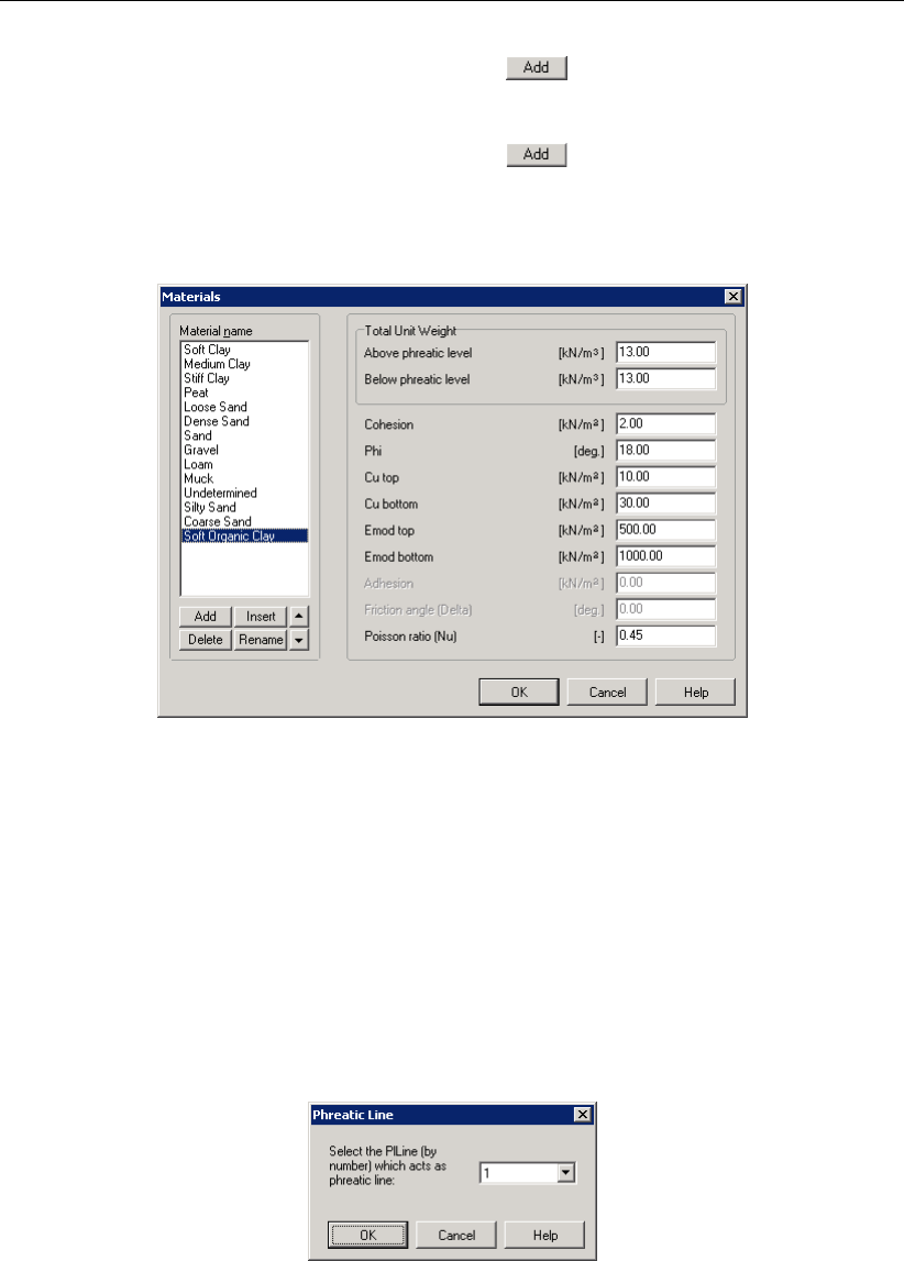
D-GEO PIPELINE
, User Manual
13. Add a new material by choosing the Add button below the materials list on the left
side of the window. Enter the soil material <Coarse Sand>.
14. Enter the soil data as given in Table 10.1.
15. Add a new material by choosing the Add button below the materials list on the left
side of the window. Enter the soil material <Soft Organic Clay>.
16. Enter the soil data given in Table 10.1.
17. Finish the input of soil data by clicking OK.
Figure 10.4: Materials window
10.4 Finishing the geometry of the longitudinal cross section
The defined soil properties and the groundwater levels have to be assigned to the drawn ge-
ometry of the longitudinal cross section. The assignments can be carried out in the Geometry
menu.
18. Click Geometry and select Phreatic Line on the menu bar to open the Phreatic Line window
(Figure 10.5) and select PL-line <1>as phreatic line for calculation of the groundwater
pressures.
19. Click OK.
Figure 10.5: Phreatic Line window
20. Click Geometry and select Layers on the menu bar to open the Layers window. Select the
Materials tab (Figure 10.6) to assign the soil properties to the soil layers in the longitudinal
cross section.
164 of 324 Deltares
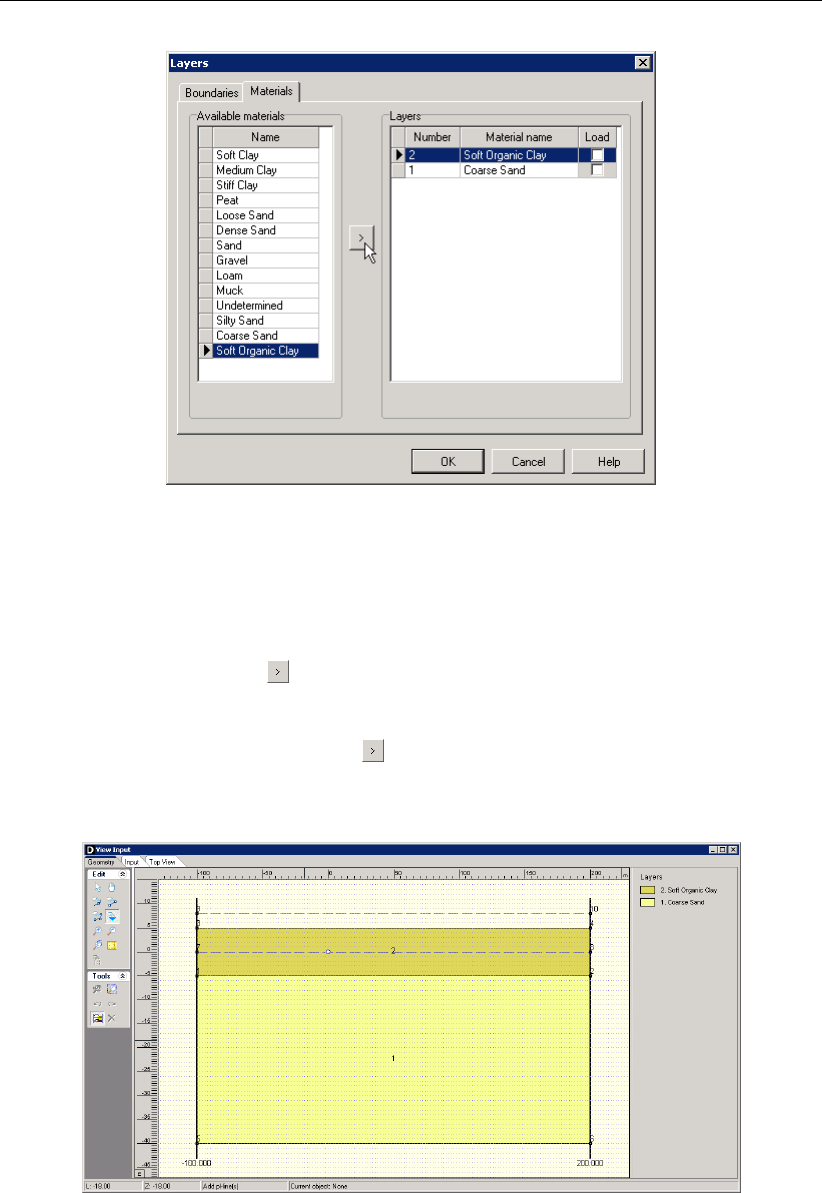
Tutorial 3: Influence of soil behavior on drilling fluid pressures and soil load on the pipe
Figure 10.6: Layers window, Materials tab
21. Assign the properties of the defined layer Coarse Sand to layer Number 1 in the longitudi-
nal cross section. The available soil layers with defined properties are shown in left column
of the materials window. The layers in the longitudinal cross section are shown in the right
column of the materials window. The defined properties are assigned to layer Number 1
by clicking the Assign icon in between the left and the right columns.
22. Assign the properties of the defined layer Soft Organic Clay to layer number 2 in the lon-
gitudinal cross section. The defined properties of Soft Organic Clay are assigned to layer
Number 2 by clicking the Assign icon in between the left and the right column.
23. Click on the OK button to quit the window and return to the Geometry tab of the View Input
window to look at the change of layers name in the legend (Figure 10.7).
Figure 10.7: View Input window, Geometry tab
24. Click Geometry and select Pl-lines per Layers on the menu bar to open the PL-lines per
Layers window to assign the defined PL–lines to the soil layers in the longitudinal cross
section. Those information’s are used for the calculation of the groundwater pressure
distribution.
25. The groundwater pressure at the top of the Soft Organic Clay layer should be calculated
based on the hydraulic head of PL–line 1, the phreatic line (Figure 10.1). Since the Coarse
Deltares 165 of 324
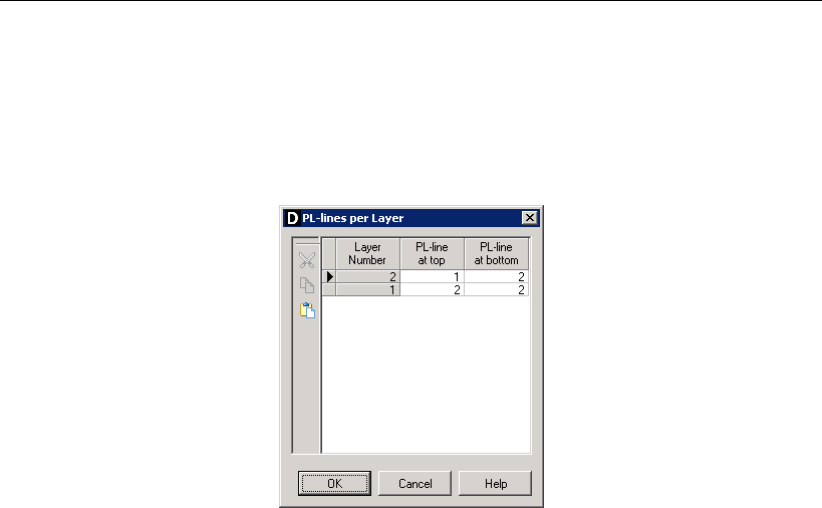
D-GEO PIPELINE
, User Manual
Sand layer is an aquifer with an enhanced artesian groundwater pressure, the groundwater
pressure at the bottom of the clay layer should be calculated based on the hydraulic head
of PL–line 2. Of course the water pressure at the top and at the bottom of the coarse sand
layer should be calculated based on the hydraulic head of PL–line 2. This will result in the
Pl-lines per layer window shown in Figure 10.8.
Figure 10.8: PL-lines per Layer window
26. Click OK to confirm.
27. The geometry can be tested by clicking Geometry on the menu bar and selecting Check
Geometry. If the geometry is entered properly, the message Geometry has been tested
and is OK appears.
28. Click OK to close this window.
10.5 Soil behavior
Strength of soil layers is dependent on the drained or undrained behavior of soil layers during
application the drilling fluid pressure. Depending on the permeability of the soil layer, the soil
will behave drained or undrained. The Coarse Sand layer is well permeable so that the excess
water pressure due to the drilling fluid pressures will dissipate easily. The strength of this soil
layer can be calculated using the drained (effective) strength parameters effective cohesion
(c) and angle of internal friction (ϕ). In case of undrained behavior in the impermeable Soft
Organic Clay layer, the strength of the soil can be calculated using the undrained strength
parameter undrained cohesion (cu).
The soil load on the pipeline after finishing the installation is dependent on the soil pipeline
interaction, which is in turn largely dependent on the soil behavior. In
D-GEO PIPELINE
it is as-
sumed that the pipeline remains fixed at the specified location and that there’s no settlement
of the soil layers below the pipeline. This assumption allows
D-GEO PIPELINE
to perform a rel-
ative simple pipe stress analysis based on a reduced soil load due to arching. As described in
section 10.2, arching develops completely in incompressible soil layers, while in compressible
layers the reduced soil load on the pipeline is higher due to compression of the soil next to the
pipeline.
29. Click GeoObjects and select Boundaries Selection on the menu bar to open the Bound-
aries Selection window for specification of the soil behavior.
30. Choose the boundary between the undrained and drained layer on top of layer number
<1>(Figure 10.9). This choice results in drained behavior of layer number 1.
31. Choose the boundary between the compressible and incompressible layer on top of layer
number <1>. This choice results in full development of arching in layer number 1 while in
layer number 2 arching is not fully developed.
166 of 324 Deltares
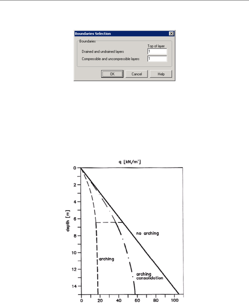
Tutorial 3: Influence of soil behavior on drilling fluid pressures and soil load on the pipe
32. Click OK to close this window.
Figure 10.9: Boundaries Selection window
10.6 Calculated reduced soil load for pipe stress analysis
The layered soil sequence results in a different reduced neutral soil load at different depths.
Due to the compressible top layer, the reduced neutral soil load increases considerable with
increasing depth (Figure 10.10). In the sand layer, the reduced neutral soil load reduces due
to the full development of arching.
Figure 10.10: The effect of arching with increasing depth (Meijers and De Kock,1995)
33. To start the calculations, click Calculation and select Start on the menu bar or press the
function key F9.
34. Click Results and select Report on the menu bar to look at the results of the pipe stress
analysis.
Deltares 167 of 324
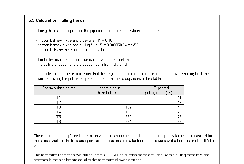
D-GEO PIPELINE
, User Manual
Figure 10.11: Report window, Calculation Pulling Force
10.7 Calculated drilling fluid pressures
The existence of soft organic soil layer with low strength and high deformability characteristics
influences the results of the maximal allowable drilling fluid pressures.
35. Click Results and select Drilling Fluid Pressure Plots on the menu bar to open the Drilling
Fluid Pressure window (Figure 10.12) and to look at the results of the drilling fluid pressure
calculations for the pilot drilling.
The graph shows the maximum allowable pressures (upper limit related to soil cover and lower
limit related to deformation of the borehole) and the minimal required drilling fluid pressure for
transportation of the cuttings. Notice that for the pilot stage the minimal allowable drilling
fluid pressure is higher than the maximal allowable drilling fluid pressure at the last part of the
upward bend of the drilling. This means that the risk of a blow out is present, so that measures
are required.
168 of 324 Deltares
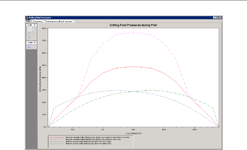
Tutorial 3: Influence of soil behavior on drilling fluid pressures and soil load on the pipe
Figure 10.12: Drilling Fluid Pressures window
36. Click on the tabs Prereaming and Reaming and pullback operation to look at the results of
the other drilling stages.
37. Close the window to return to the main menu.
10.8 Drilling fluid pressure and groundwater pressure
During the stages of horizontal directional drilling the borehole is filled with drilling fluid. The
drilling fluid has a certain unit weight, which is largely dependent on the initial unit weight of the
drilling fluid and the amount of cut soil material in the drilling fluid. If the borehole is located
in soil layers with an artesian water pressure (aquifers), the risk of leakage of groundwater
through the borehole to the surface exists. The leakage of groundwater will result in flow of
water through the borehole, which in turn will lead to borehole instability (when the drilling
fluid is flown out of the borehole located in coarser granular layers). This risk is automatically
assessed when a
D-GEO PIPELINE
calculation is performed.
38. Click Results and select Report on the menu bar to watch the results of leakage assess-
ment in paragraph 3.2 (equilibrium between drilling fluid pressure and pore pressure).
Notice that the artesian water pressure is higher than the drilling fluid pressure so that
measures against leakage are required (Figure 10.13).
Deltares 169 of 324
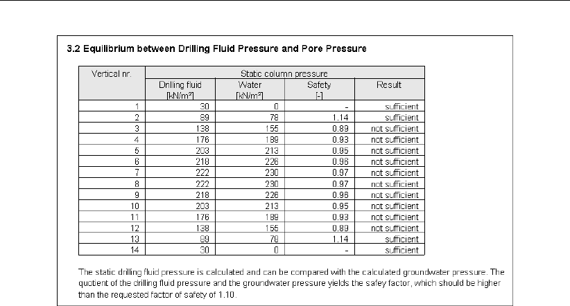
D-GEO PIPELINE
, User Manual
Figure 10.13: Report window, Equilibrium between drilling fluid pressure and pore pres-
sure
10.9 Conclusion
In this tutorial, a layered soil sequence has been modeled and the drilling fluid pressures have
been calculated. Using the table called Equilibrium between drilling fluid pressure and pore
pressure in the
D-GEO PIPELINE
report, it can be concluded if the drilling fluid pressures are or
are not sufficient.
170 of 324 Deltares
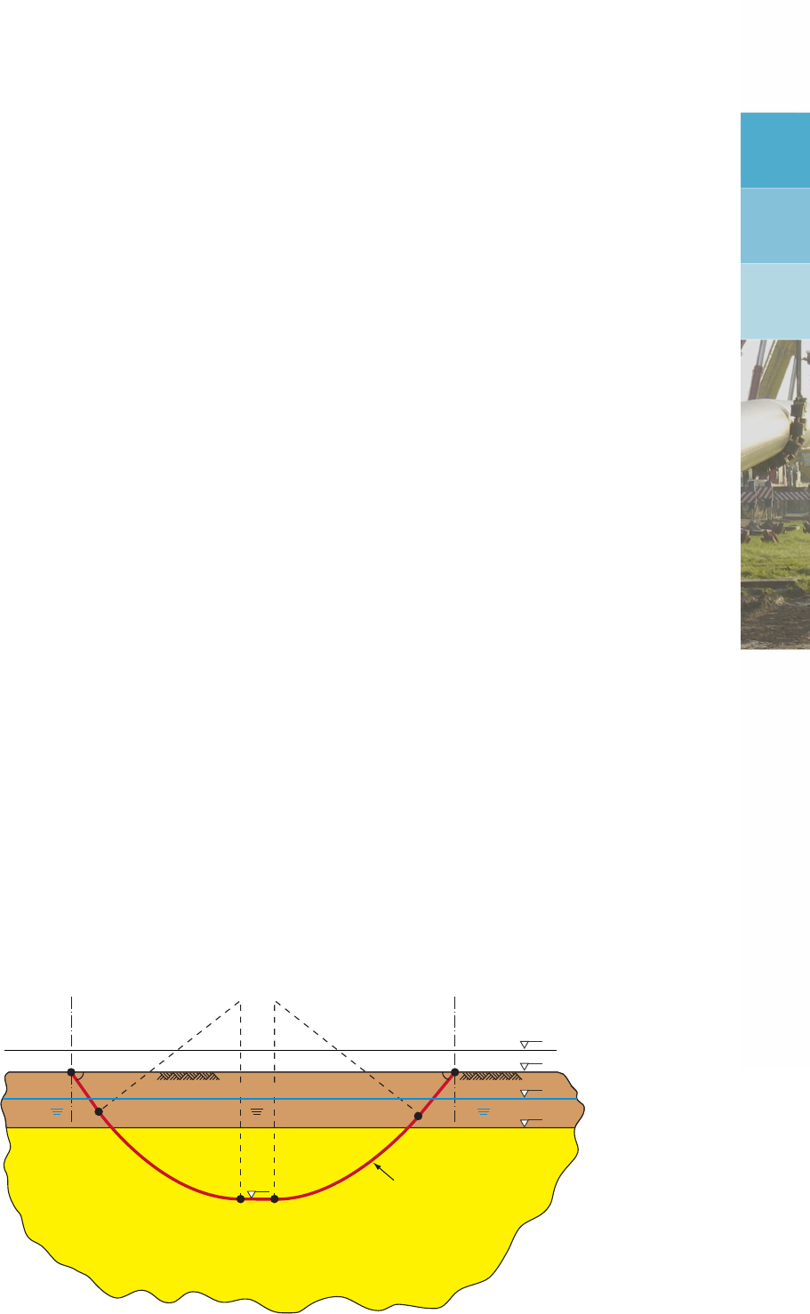
11 Tutorial 4: Exporting soil mechanical data for an extended stress
analysis
This exercise considers the installation of a polyethylene pipeline by using the horizontal di-
rectional drilling technique. The exercise focuses on the calculation of soil mechanical pa-
rameters for an extended pipe stress analysis. A settlement calculation forms also part of the
exercise.
The objectives of this tutorial are:
To calculate the soil mechanical parameters for an extended pipe stress analysis;
To perform a settlement calculation;
To export the soil mechanical parameters.
The following module is needed:
D-GEO PIPELINE
Standard module (HDD)
License for
D-SETTLEMENT
(formerly known as MSettle)
This tutorial is presented in the file Tutorial-4.dri.
11.1 Introduction to the case
In
D-GEO PIPELINE
it is assumed that the pipeline remains fixed at the specified location and
that there’s no settlement of the soil layers below the pipeline. No temperature effects are
taken into account in
D-GEO PIPELINE
. Therefore a relative simple pipe stress analysis can be
performed.
In case compressible soil layers are present below the pipeline and an additional load is
carried out on theses compressible soil layers, settlement can be expected. If settlement
of the layers below the pipeline occurs in most cases, an extended pipe stress analysis is
required. The extended pipe stress analysis can not be performed using
D-GEO PIPELINE
, but
should be carried out using other software. For instance SCIA pipeline can be used for such
an analysis.
15º 15º
pipeline
silty sand
soft organic clay
R= 400m
R= 400m
entry: X= 90m
exit: X= 190m
-15m
+5m
+8m
0m
-5m
PL-line 2
PL-line 1
Figure 11.1: Pipeline configuration for Tutorial 4
Deltares 171 of 324
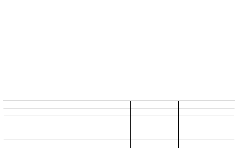
D-GEO PIPELINE
, User Manual
Vertical displacement of soil below and around the pipeline that occurs after installation is an
important factor in assessing the stresses in the pipeline. Settlement may be entered manually
if the vertical settlements results are available. For more accurate results,
D-GEO PIPELINE
can use the
D-SETTLEMENT
computer program (formerly known as MSettle) without additional
input. Settlement deals with soil compaction due to imposed loading. In
D-GEO PIPELINE
the
loading consists of an extra layer as created in the geometry. The calculation of the settlement
is performed externally by
D-SETTLEMENT
, the settlement calculation program of the Deltares
Systems tools. Details on the calculation of settlement are beyond the scope of this manual,
a thorough description can be found in the user manual of
D-SETTLEMENT
(Deltares).
Table 11.1: Settlement parameters (acc. Koppejan) of the soil layers (Tutorial 4)
Coarse sand Soft organic clay
Over-consolidation ratio 1.3 1.3
Primary compression coefficient below Pc 10940
Primary compression coefficient above Pc 10910
Secondary compression coefficient below Pc 109160
Secondary compression coefficient above Pc 10935
This tutorial is based on continuation of the file used in Tutorial 3 (chapter 10).
1. Click File and select Open on the menu bar to open the Open window.
2. Select the file Tutorial-3 and click the Open button.
3. ClickFile and select Save as on the menu bar to open the Save As window and rename
the file into <Tutorial-4>.
4. Click the Save button to save the file for Tutorial 4.
5. On the menu bar, click Project and then choose Properties to open the Project Properties
window.
6. Fill in <Tutorial 4 for
D-GEO PIPELINE
>and <Exporting soil mechanical data>for Title 1
and Title 2 respectively in the Identification tab.
7. Click OK.
11.2 Settlement model
Settlement calculations can be performed using the in the Netherlands often used Koppejan
model or the more recent developed Isotache model which is based on Terzaghi’s settlement
model.
8. Click Project and select Model on the menu bar to open the Model window (Figure 11.2).
9. Select the Horizontal directional drilling method and mark the Use settlement check-box.
10. Select the Koppejan model.
11. Click OK to confirm the choice.
172 of 324 Deltares
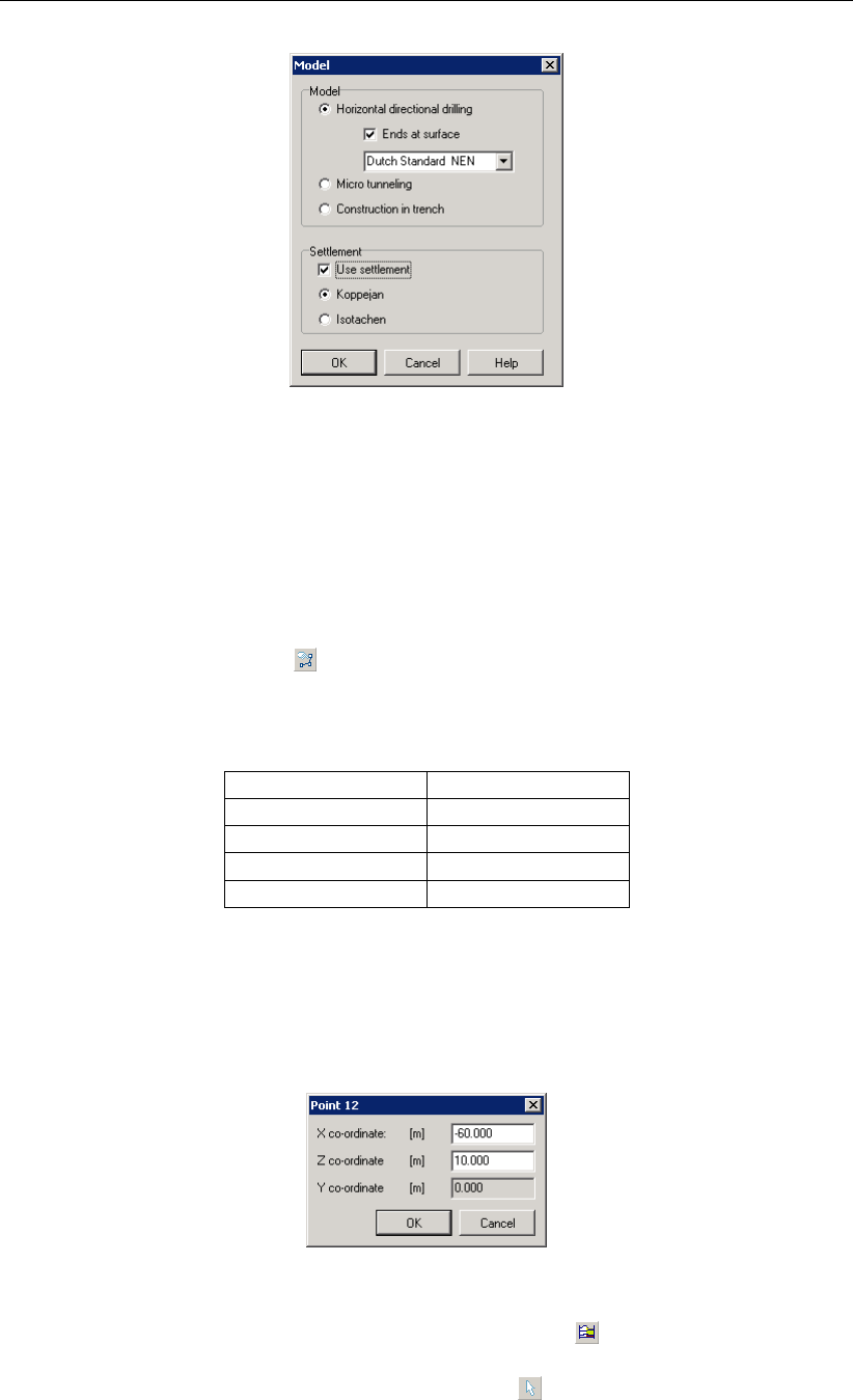
Tutorial 4: Exporting soil mechanical data for an extended stress analysis
Figure 11.2: Model window
11.3 Geometry of the longitudinal cross section
This tutorial considers a layered soil sequence described in Tutorial 3 (chapter 10). In the
longitudinal cross section, a load (soil mass) has to be defined.
12. Switch to the Geometry tab in the View Input window to edit the existing soil layer se-
quence.
13. Select the Add polyline icon from the Edit sub-window to draw an additional layer (soil
mass) on top of the existing soil layers with coordinates given in Table 11.2.
Table 11.2: Coordinates of the top of the soil mass
X coordinate [m] Z coordinate [m]
-75 5
-60 10
30 10
45 5
14. Quit editing by clicking the right mouse button.
15. To check or modify the added points, select a point by clicking the left mouse button. The
point will become a red square.
16. Click the right-hand mouse button and select Properties. In the window displayed (Fig-
ure 11.3), the co-ordinates can be checked and modified if needed.
Figure 11.3: Point window
17. Select the Automatic regeneration of geometry on/off icon from the Tools sub-window
so that the geometry as shown in Figure 11.4 appears. If the Automatic regeneration of
geometry icon already is selected, click on the Edit icon to regenerate the geometry.
Notice that the soil mass is located on the left side above the section where the pipeline is
located in the Soft Organic Clay layer.
Deltares 173 of 324
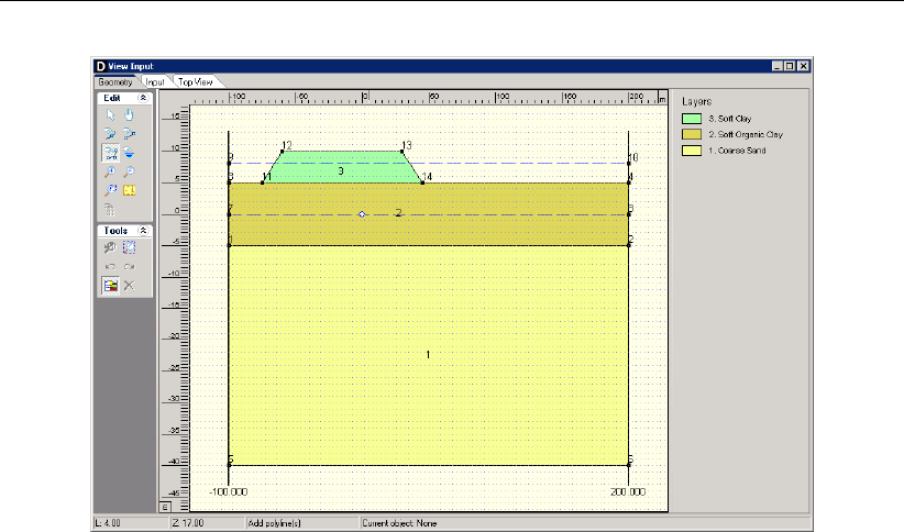
D-GEO PIPELINE
, User Manual
Figure 11.4: View Input window, Geometry tab
11.4 Soil layer properties
The settlement properties of the soil layers in the layered soil sequence should now be speci-
fied. The properties of the soil mass should be entered too.
18. Click Soil and select Materials on the menu bar to open the Materials window.
19. Select the soil name Silty Sand in the left column of the Materials window and enter the
properties given in Figure 11.5.
20. Select the soil name Coarse Sand and enter the Settlement Koppejan data given in Ta-
ble 11.1.
21. Select the soil name Soft Organic Clay and enter the Settlement Koppejan data given in
Table 11.1.
22. Finish the input of soil data by clicking OK.
174 of 324 Deltares

Tutorial 4: Exporting soil mechanical data for an extended stress analysis
Figure 11.5: Materials window
11.5 Finishing the geometry of the longitudinal cross section
The defined soil properties have to be assigned to the drawn geometry of the longitudinal
cross section (groundwater levels are assigned already). The assignments can be carried out
by clicking geometry and choosing the subsequent described options on the menu bar.
23. Click Geometry and select Layers on the menu bar to open the Layers window to assign
the soil properties to the soil layers in the longitudinal cross section.
24. Click on the tab Materials.
25. Assign the soil properties given in Figure 11.6.
26. Click OK to confirm the assignments.
Deltares 175 of 324
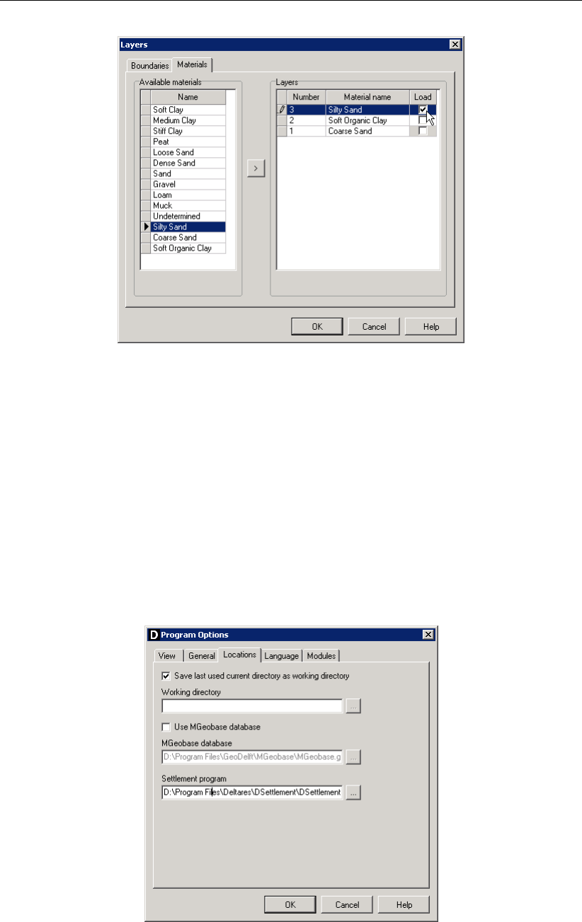
D-GEO PIPELINE
, User Manual
Figure 11.6: Layers window, Materials tab
11.6 Calculated soil mechanical parameters in export file
The calculation of the settlement of the soil layers below the pipeline is performed exter-
nally by
D-SETTLEMENT
(formerly known as MSettle), the settlement calculation program of
the Deltares Systems tools. Therefore, the directory where the program is installed must be
given:
27. Click Tools on the menu bar and select Program Options to open the Program Options
window. Then select the Locations tab (Figure 11.7).
28. If needed, change the directory where the Settlement program is installed by clicking the
Browse button.
29. Click OK to confirm.
Figure 11.7: Program Options window, Locations tab
The other soil mechanical parameters are calculated automatically in
D-GEO PIPELINE
.
176 of 324 Deltares
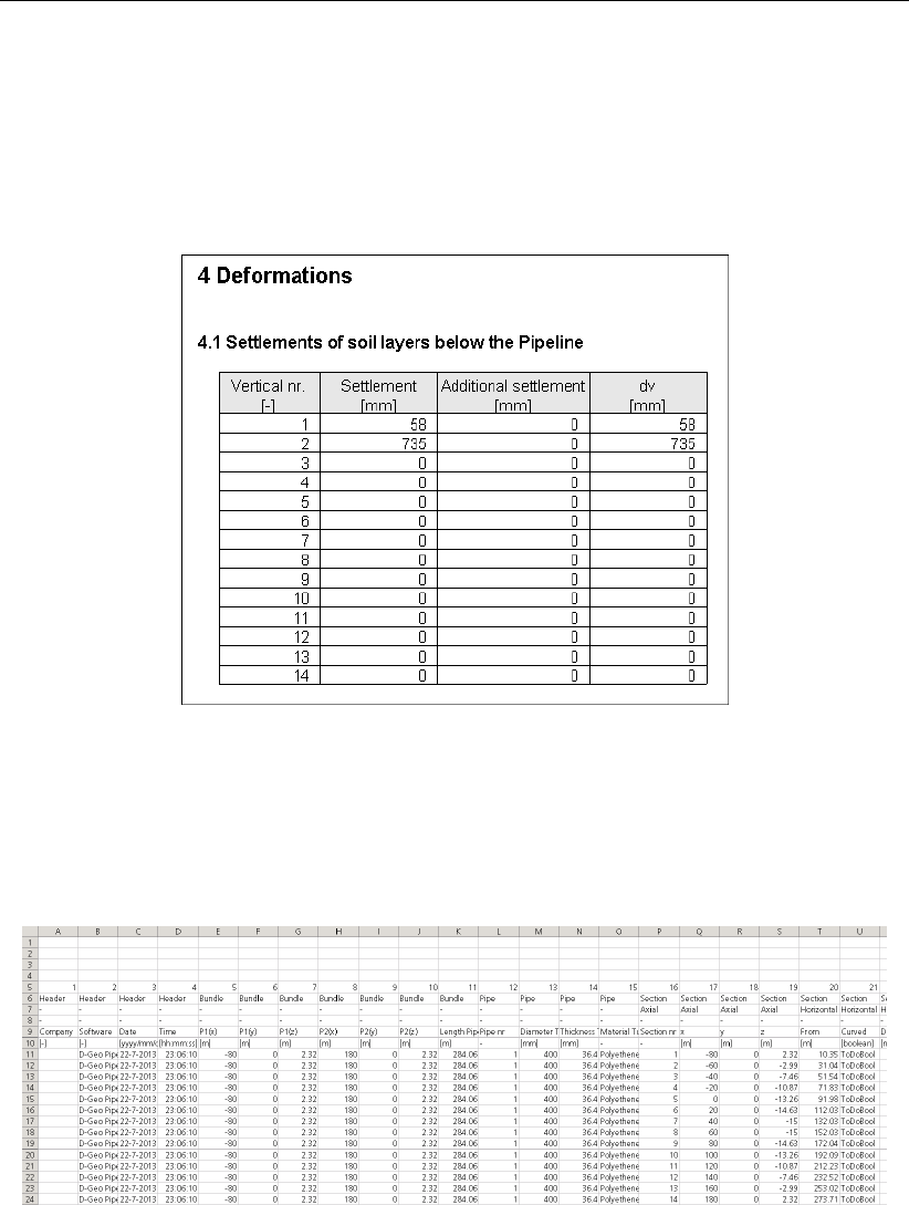
Tutorial 4: Exporting soil mechanical data for an extended stress analysis
30. To start the calculations click Calculation and select Start on the menu bar to or press
the function key F9. Ignore the message of Cu values of 0 above the drained undrained
boundary.
31. Click Results and select Report on the menu bar to look at the results of the settlement
calculation in paragraph 3.1 (Figure 11.8) and the calculation of the soil mechanical pa-
rameters in paragraph 4.1.
Figure 11.8: Report window, Settlements along pipeline
32. Click File and select Export Results as csv. . . on the menu bar to create an export file with
the soil mechanical parameters.
33. Click on the Save button. The export file is saved on the same directory as Tutorial 4 and
can be opened using the Excel program for example (see Figure 11.9).
Figure 11.9: Content of the export file for Tutorial 4
The export file contains:
Horizontal soil data
Vertical soil data
Soil data for friction
Data of pipeline
For more information, refer to section 3.1.2.
Deltares 177 of 324

D-GEO PIPELINE
, User Manual
11.7 Conclusion
A pipe stress and settlement analysis has been performed for a polyethylene pipe in a layered
soil. The inputs and results of this calculation have been exported in a csv file in order to
perform an extended stress analysis using an other program such as SCIA pipeline.
178 of 324 Deltares

12 Tutorial 5: Drilling with a horizontal bending radius
This fifth exercise considers installation of a polyethylene pipeline by using the technique
horizontal directional drilling. The exercise focuses on a horizontal bending radius in the
design of the drilling line.
The objectives of this tutorial are:
To schematize a horizontal bending;
To calculate pulling forces in the horizontal bending;
To perform a pipe stress analysis for the design with a horizontal bending radius.
The following module is needed:
D-GEO PIPELINE
Standard module (HDD)
This tutorial is presented in the file Tutorial-5.dri.
12.1 Introduction to the case
A horizontal bending radius in the design drilling line is observed more frequent. Often the
horizontal bend is part of one of the vertical bending radii. In case the horizontal bending
radius coincides with part of a vertical bending radius, a combined 3-dimensional bending
radius is formed. For the design of the horizontal directional drilling line, the pull back force and
the strength calculation it is necessary to determine the value of the 3 dimensional bending
radius.
The value of the three dimensional bending radius can be calculated as follows:
Rcombi =sR2
h×R2
v
R2
h+R2
v
(12.1)
where:
Rcombi is the combined bending radius, in m;
Rhis the horizontal bending radius, in m;
Rvis the vertical bending radius, in m.
The combined bending radius is used to calculate the pulling force during the pull back oper-
ation and is used in the pipe stress analysis in
D-GEO PIPELINE
.
Deltares 179 of 324
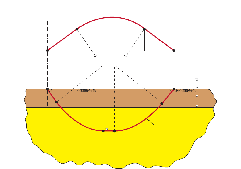
D-GEO PIPELINE
, User Manual
15º 15º
pipeline
silty sand
soft organic clay
R= 400m
R= 400m
entry: X= 90m
exit: X= 190m
70m
4m
4m
70m
R= 1500m
Top view
-15m
+5m
+8m
0m
-5m
PL-line 2
PL-line 1
Figure 12.1: Pipeline configuration of Tutorial 5
This tutorial is based on continuation of the file used in Tutorial 3 (chapter 10).
1. Click File and select Open on the menu bar to open the Open window.
2. Select Tutorial-3 and click the Open button to open the file.
3. Click File and select Save as on the menu bar to open the Save As window and rename
the file into <Tutorial-5>.
4. Click the Save button to save the file for Tutorial 5.
5. On the menu bar, click Project and then choose Properties to open the Project Properties
window.
6. Fill in <Tutorial 5 for
D-GEO PIPELINE
>and <Drilling with a horizontal bending radius>
for Title 1 and Title 2 respectively in the Identification tab.
7. Click OK.
12.2 Pipeline Configuration
The horizontal bend must be specified in the pipeline configuration window.
8. Click Pipe and select Pipeline Configuration on the menu bar to open the Pipeline Config-
uration window.
180 of 324 Deltares
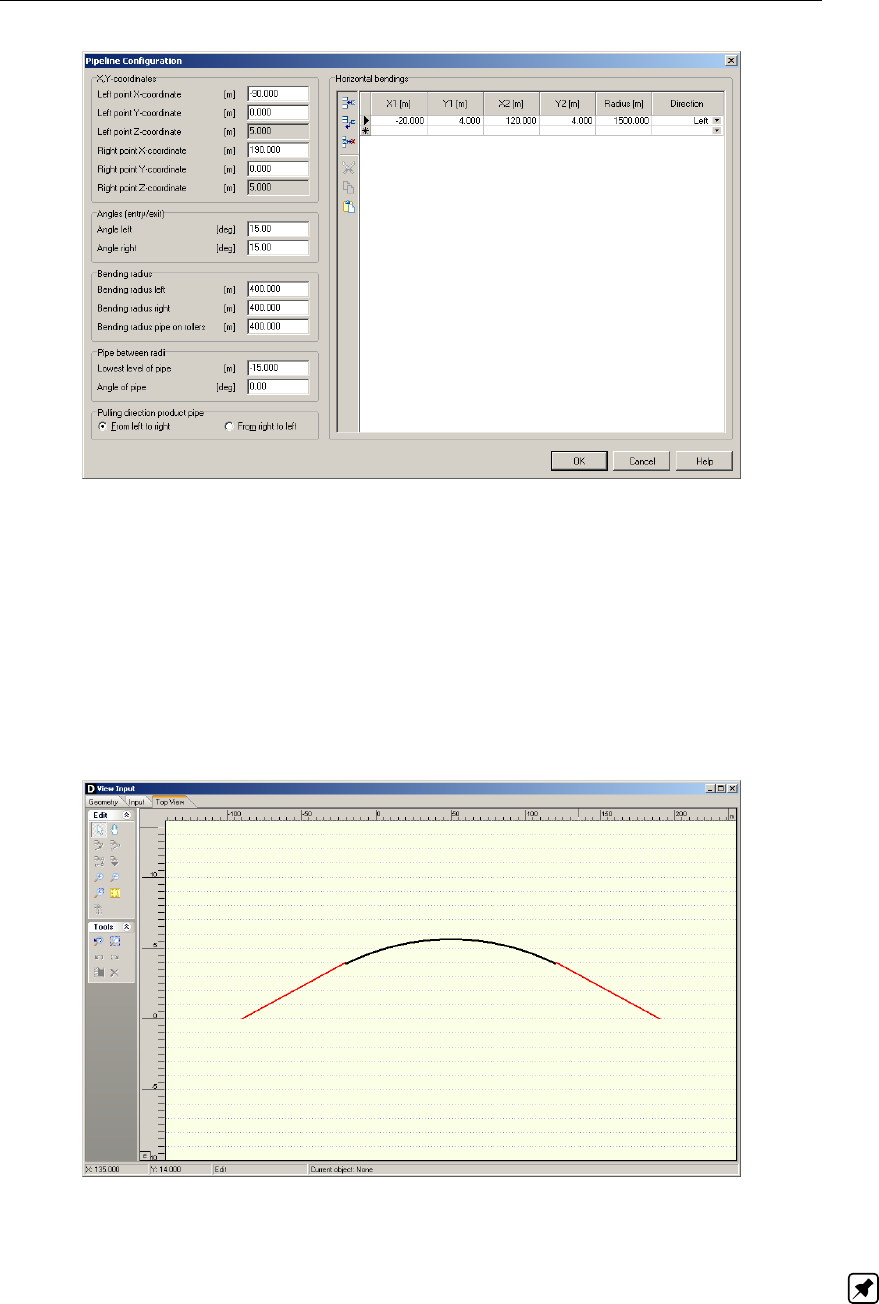
Tutorial 5: Drilling with a horizontal bending radius
Figure 12.2: Pipeline Configuration window
9. Enter the values given in Figure 12.1.
10. Click OK to confirm.
11. Look at the entered horizontal bending on the Top View tab of the View Input window
(Figure 12.3).
12. Look at the longitudinal cross section on the Input tab of the View Input window and notice
the elongation of the longitudinal cross section. Therefore it is recommended to check, in
case of projects with changing 3D pipeline configurations, if the soil layer sequence in the
longitudinal cross section is still reliable (according to the soil investigation data).
Figure 12.3: View Input window, Top View tab
Note: The horizontal bending is indicated with a black bold line in the longitudinal cross
section (Figure 12.4).
Deltares 181 of 324
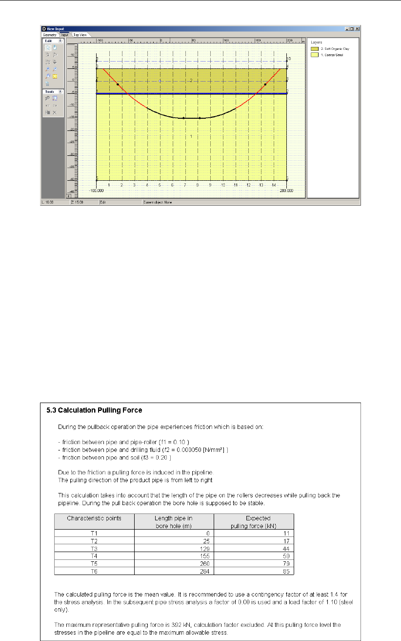
D-GEO PIPELINE
, User Manual
Figure 12.4: View Input window, Input tab
12.3 Calculation of the pulling force and pipe stress analysis
The results of the pulling force calculation are shown in the
D-GEO PIPELINE
report which is
created automatically after finishing the calculations.
13. To start the calculations click Calculation and select Start on the menu bar or press the
function key F9.
14. Click Results and select Report n the menu bar to look at the results of the pulling force
calculations. The results can be found on paragraph 5.3 (Figure 12.5).
Note the increase in pulling force due the horizontal bending radius compare to the case
without bending (see results of Tutorial 3 in Figure 10.11).
Figure 12.5: Report window, Calculation Pulling Force
In paragraph 5.1 (Figure 12.6), the data for the pipe stress analysis is given. The value of the
182 of 324 Deltares
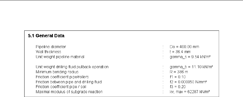
Tutorial 5: Drilling with a horizontal bending radius
minimal bending radius is equal to Rmin = 386 m.
Figure 12.6: Report window, General Data
The minimum bending radius is used to calculate the stresses in the pipeline. In the assess-
ment table in paragraph 6.3 of the report, the influence of a smaller bending radius is visible:
higher axial and tangential stresses in both the installation stages and the operational stage
after installation.
12.4 Conclusion
This tutorial models a horizontal bending in the pipeline configuration. The calculated pulling
forces increase compare to the case without horizontal bending presented in Tutorial 3.
Deltares 183 of 324

D-GEO PIPELINE
, User Manual
184 of 324 Deltares

13 Tutorial 6: Installation of bundled pipelines
This sixth tutorial considers installation of a bundle consisting of five polyethylene pipelines by
using the technique horizontal directional drilling. The exercise focuses on the background of
the automatic bundle calculation in
D-GEO PIPELINE
.
The objectives of the exercise are:
To calculate the drilling fluid pressures for the pull back operation;
To calculate the pulling force on the bundled pipelines during the pull back operation;
To perform an automatic pipe stress analysis for the pipelines in the bundle.
The following module is needed:
D-GEO PIPELINE
Standard module (HDD)
This tutorial is presented in the file Tutorial-6.dri.
13.1 Introduction to the case
The calculations required for the installation of bundled pipelines using the horizontal direc-
tional drilling technique are rather similar to those for the installation of a single pipeline.
Differences exist in the calculations:
For the minimal required drilling fluid pressure during the pull back operation
For the pulling force during the pull back operation
For the pipe stress analysis (differences in assumptions)
Ad 1) Of course the available space for the back flow of the drilling fluid is different in case of a
bundled pipeline. For calculation of the minimal required drilling fluid pressure,
D-GEO PIPELINE
assumes flow of the drilling fluid
through the space in between the bundle and the borehole wall
and through the space in the bundle, in between the pipelines.
Ad 2) Important parameters for the calculation of the pulling force during the pullback operation
are the total effective weight of the (filled) pipelines in the bundle and the total stiffness of the
bundle which determines the soil reaction force in curved sections of the drilling line. In
D-GEO PIPELINE
the pulling force is calculated for an equivalent pipeline with the weight and
stiffness parameters of the bundled pipelines.
EIeq =
i=1
X
n
EiIi(13.1)
Gtot =
i=1
X
nπ
4D2
o;i −π
4(D0;i −2dn;i)2×γi(13.2)
where:
nis the total number of pipelines in the bundle;
Do;i is the outer diameter of pipeline i, in m;
dn;i is the wall thickness of pipeline i, in m;
γiis the unit weight of pipeline i, in kN/m3;
Eiis the Young’s modulus of pipeline i, in kN/m2;
Deltares 185 of 324
D-GEO PIPELINE
, User Manual
Iiis the moment of inertia of pipeline i, in m4;
Ieq is the moment of inertia of the bundle, in m4.
The calculated pulling force is acting on all the pipelines in the bundle. The magnitude of the
pulling force of a pipeline in the bundle is derived by dividing the total pulling force over the
cross section area of the wall of the pipelines with equal stiffness.
In case the stiffness of the pipeline materials is significantly different (for example a combined
bundle of steel and PE pipelines), a different approach is applied. In addition to the previous
described dividing procedure, the total pulling force is assigned to the stiffer pipeline (steel
pipeline).
Ad 3) The pipe stress analysis for a pipeline in the bundle is quite similar to the pipe stress
analysis for a single pipeline in the bore hole. The only difference in the pipe stress analysis
is the contact between the pipeline and the surrounding soil (single pipeline) and the contact
between the pipeline and the adjacent pipelines (bundle). Therefore the load angle and the
bedding angle should be adapted in case of a bundled pipeline. In this tutorial angle values
of 30 degrees are assumed and entered manually.
Table 13.1: Pipes properties (Tutorial 6)
Pipe 1 Pipe 2
Material quality PE80 PE80
Young’s modulus (short term) [N/mm2] 1000 1000
Young’s modulus (long term) [N/mm2] 200 200
Allowable strength (short term) [N/mm2] 10 10
Allowable strength (long term) [N/mm2] 8 8
Tensile factor [-] 0.65 0.65
Outer Diameter [mm] 400 160
Wall thickness [mm] 36.4 12.3
Unit weight pipe material [kN/m3] 9.54 9.54
Design pressure [Bar] 4 4
Test pressure [Bar] 5 5
Temperature variation [◦C] 5 5
This tutorial is based on continuation of the file used in Tutorial 5 (chapter 12).
1. Click File and select Open on the menu bar to open the Open window.
2. Select Tutorial-5 and click the Open button to open the file.
3. Click File and select Save as on the menu bar to open the Save As window and rename
the file into <Tutorial-6>.
4. Click the Save button to save the file for Tutorial 6.
5. On the menu bar, click Project and then choose Properties to open the Project Properties
window.
6. Fill in <Tutorial 6 for
D-GEO PIPELINE
>and <Installation of bundled pipelines>for Title 1
and Title 2 respectively in the Identification tab.
7. Click OK.
186 of 324 Deltares
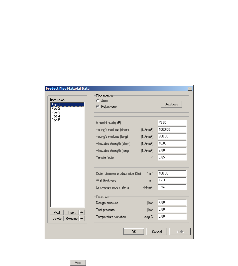
Tutorial 6: Installation of bundled pipelines
13.2 Product Pipe Material Data
The dimensions and the properties of the product pipes in the bundle should be specified.
8. Click Pipe and select Product Pipe Material Data on the menu bar to open the Product
Pipe Material Data window for specification of the dimensions and properties of the product
pipes in the bundle.
9. Change the following values for Pipe 1 in the fields on the right side of the window (Fig-
ure 13.1).
Figure 13.1: Product Pipe Material Data window
10. Click on the Add button on the left side of the window to declare a pipeline with the
name <Pipe 2>.
11. Enter the values for Pipe 2 (Table 13.1), in the fields on the right side of the window.
12. Click on the Add button on the left side of the window three times to add three more pipes.
Notice that the material properties of Pipe 2 are automatically copied to these pipes.
13. Use the Rename button on the left side of the window to rename the new pipes into
<Pipe 3>,<Pipe 4>and <Pipe 5>.
14. Click on OK to confirm the specified product pipe material data.
The bundle now consists of five pipes:
Pipe nr. 1: 400 mm SDR 11 PE 80
Pipe nr. 2: 160 mm SDR 13 PE 80
Pipe nr. 3: 160 mm SDR 13 PE 80
Pipe nr. 4: 160 mm SDR 13 PE 80
Pipe nr. 5: 160 mm SDR 13 PE 80
13.3 Drilling Fluid Data
The properties of the drilling fluid and the operation parameter values should be specified for
the bundle.
Deltares 187 of 324
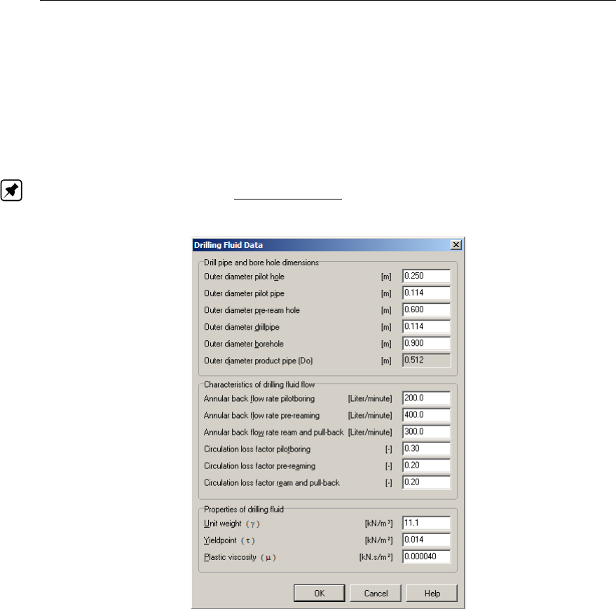
D-GEO PIPELINE
, User Manual
15. Click Pipe and select Drilling Fluid Data on the menu bar to open the Drilling Fluid Data
window for specification of properties of the drilling fluid.
16. Enter the values of Figure 13.2 for installation of the bundle. The bedding and the load
angle are 30 degrees since contacts in between the pipelines are expected. These values
are used in the pipe stress analysis to determine the moment coefficients. The values for
the special pipe stress analysis do not have to be entered.
17. Click on the OK button to confirm the input of the specified value.
Note: The equivalent diameter of the bundle is calculated automatically. The equivalent
diameter amounts to Deq =√0.42+4×0.162= 0.512 m.
Figure 13.2: Drilling Fluid Data window
13.4 Engineering Data
Since the engineering properties for a bundle are different from single pipeline installation
properties, values of the engineering properties have to be changed.
18. Click Data and select Engineering data on the menu bar to select the Engineering Data
window. This will result in the window shown in Figure 13.3.
19. Do not fill the pipe on the rollers and enter the values of Figure 13.3 in the standard input
window.
20. Click on the OK button to confirm the input of the specified values.
188 of 324 Deltares
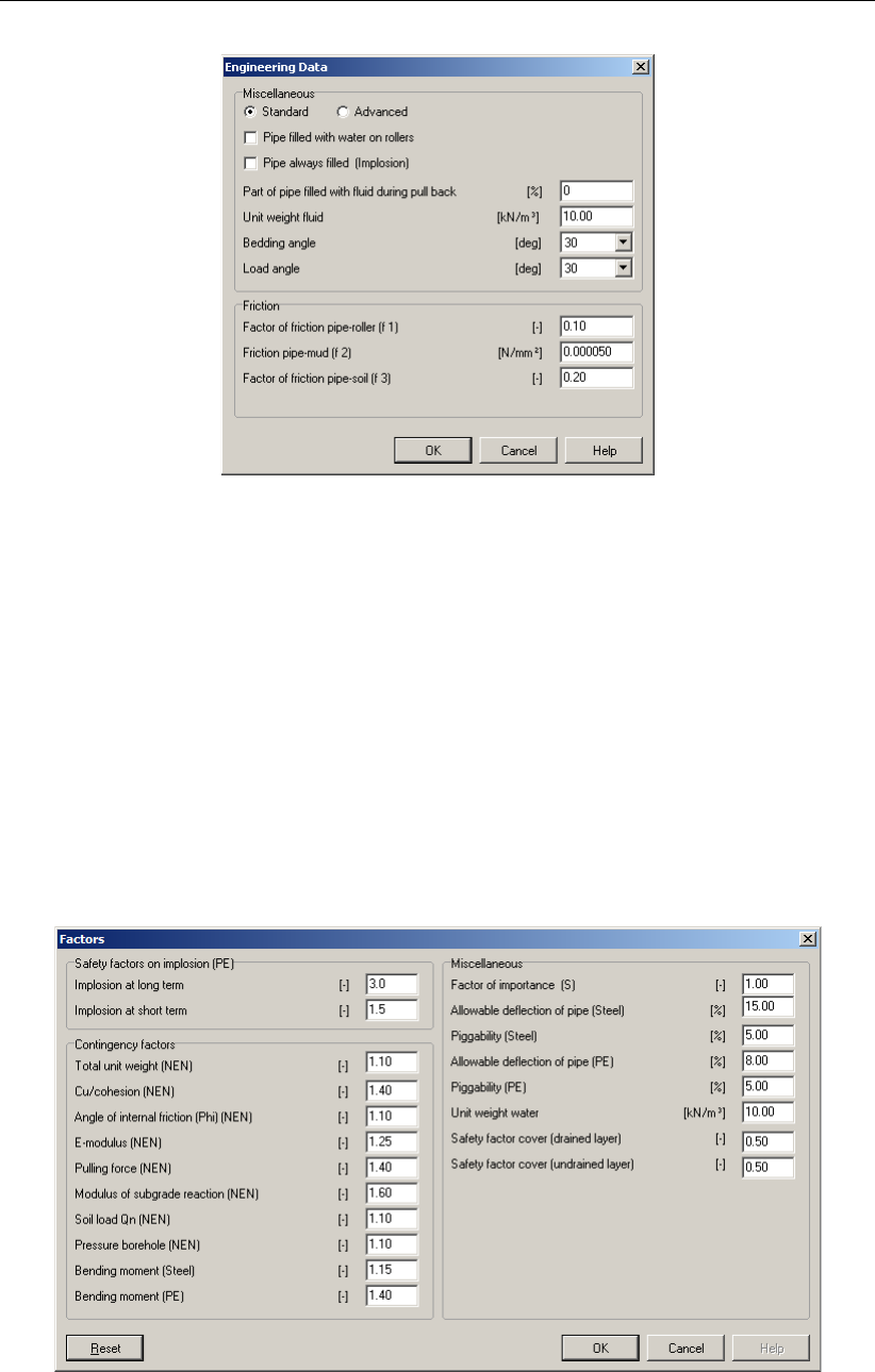
Tutorial 6: Installation of bundled pipelines
Figure 13.3: Engineering Data window
13.5 Factors
D-GEO PIPELINE
performs the calculations of the drilling fluid pressures according the Dutch
regulations described in the NEN 3650 series (NEN,2012a,b,c) and in NEN 3651 (NEN,
2012d). The safety philosophy described in the NEN 3650-1 Annex B and D is applied on the
calculations.
21. Click Defaults and select Factors on the menu bar to select the contingency and safety
factors window for watching the default values or adapting this values.
22. Due to the pull back of the bundled pipelines the risk on higher pulling forces than calcu-
lated is present. According to the NEN 3650-1 (article E.1.2.3), the contingency factor on
the pulling force should be 1.8. Change this value into <1.8>as shown in Figure 13.4.
23. Click OK to confirm.
Figure 13.4: Factors window
Deltares 189 of 324
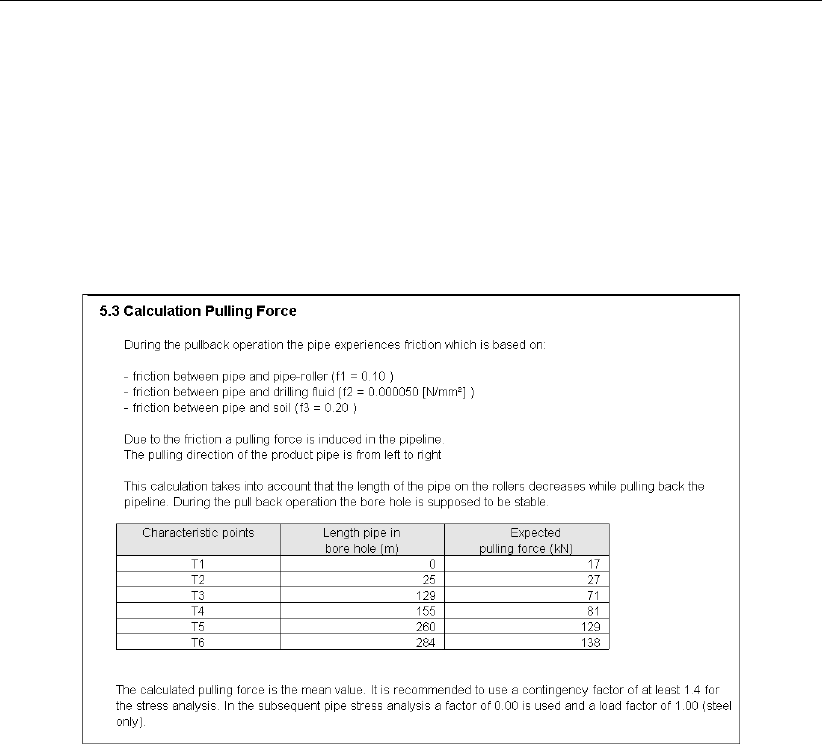
D-GEO PIPELINE
, User Manual
13.6 Results
The results of the pulling force calculation are shown in the report which is created automati-
cally after finishing the calculations.
24. To start the calculations click Calculation and select Start on the menu bar to tart the
calculation or press the function key F9.
25. Click Results and select Report on the menu bar to view the results of the pulling force
calculations. The results can be found in paragraph 5.3 (Figure 13.5).
Figure 13.5: Report window, Calculation Pulling Force
Notice that the total pulling force is divided over the pipelines in the bundle for pipe stress
analysis purposes. The pipe stress analysis per pipeline is described in the paragraphs 6 to
10.
190 of 324 Deltares

14 Tutorial 7: Face support pressure for micro tunneling
This seventh tutorial considers installation of a gas pipeline crossing underneath a railway by
using micro-tunneling. The gas pipeline consists of steel pipe sections. The exercise focuses
on the basic calculation set up for micro-tunneling in
D-GEO PIPELINE
.
The objectives of the exercise are:
To make a schematization of the pipeline installation by micro tunneling;
To evaluate the minimal required and maximal allowable shield pressure at the face of
the tunneling machine.
The following modules are needed:
D-GEO PIPELINE
Standard module (HDD)
Micro Tunneling module
The result of this tutorial is presented in the file Tutorial-7.dri.
14.1 Introduction to the case
Micro-tunneling in general uses a remote controlled micro tunnel boring machine (MTBM).
The micro tunnel usually starts horizontal at a certain level below the surface. Drive and
reception shafts are created for the MTBM. In the drive shaft a jacking frame and MTBM are
installed. The jacks will push the pipe section elements section by section ahead towards
the reception shaft. The MTBM is at the front of the advancing micro tunnel. As the length
of the advancing micro tunnel increases so do the friction forces along the pipe segments.
Lubrication fluid may be applied for lubrication.
Figure 14.1: Pipeline configuration for Tutorial 7
Very often at the face of the MTBM drilling fluid is used for, soil removal and front stabilization.
Careful planning and monitoring of the face support pressures is required: When the pressure
is excessive this may cause a blow out; if the pressure is too low collapse of the soil in at
the drilling front may cause excessive subsidence. The pipeline configuration is shown in
Figure 14.1.
Deltares 191 of 324
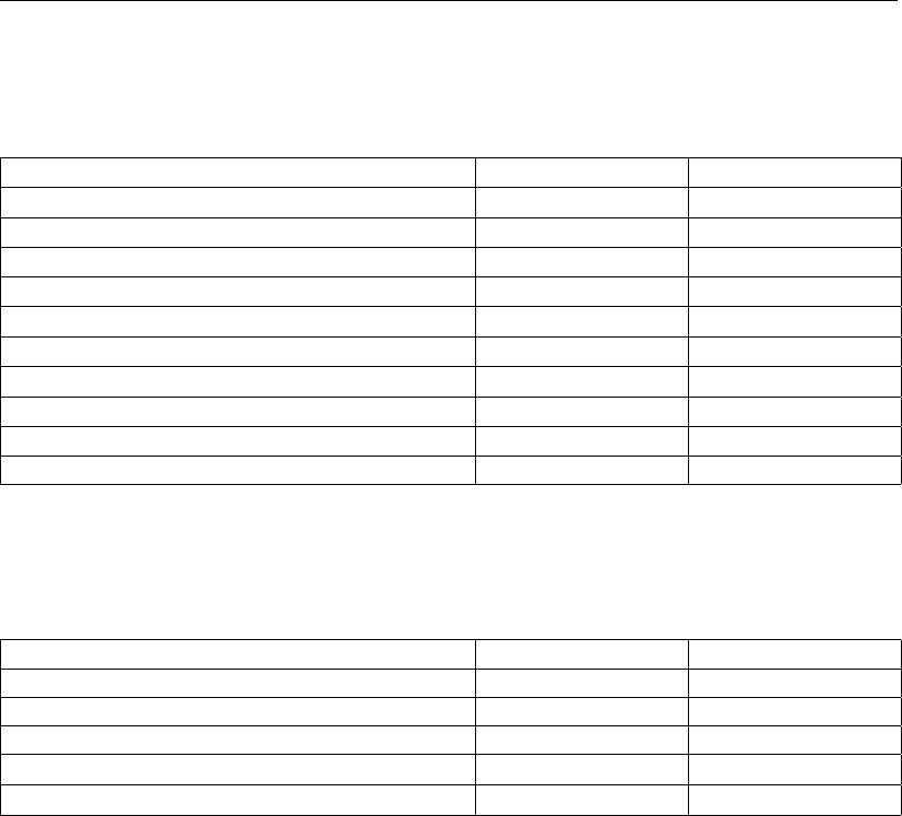
D-GEO PIPELINE
, User Manual
The soil properties of the silty sand layer are provided in Table 14.1.
Table 14.1: Properties of the silty sand layer (Tutorial 7)
Dry unit weight [kN/m3] 18
Wet unit weight [kN/m3] 20
Cohesion [kN/m2] 0
Angle of internal friction [◦] 30
Undrained strength top [kN/m2] 0
Undrained strength bottom [kN/m2] 0
E modulus top [kN/m2] 10000
E modulus bottom [kN/m2] 15000
Adhesion [kN/m2] 0
Friction angle (Delta) [◦] 20
Poisson’s ratio [-] 0.35
The pipeline material used in this tutorial is a steel 240 with the properties given in Table 14.2.
Table 14.2: Properties of steel material (Tutorial 7)
Pipe material Steel 240
Outer diameter [mm] 1200
Overcut [mm] 15
Wall thickness [mm] 22.4
Young’s modulus [N/mm2] 205800
Unit weight pipe material [kN/m3] 78.50
This tutorial starts with the selection of the pipeline installation model.
14.2 Model selection
The micro tunneling model must be selected to carry out the current tutorial.
noitemsep
1. Click File and choose New on the menu bar to start a new project.
2. In the New File window select the option New geometry to start. This will result in an
empty geometry.
3. Save the project by clicking Save As in the File menu and by entering <Tutorial-7>as
project name.
4. Click Save to close this window.
5. On the menu bar, click Project and then choose Model to open the Model window (Fig-
ure 14.2).
6. Select Micro tunneling and click OK.
192 of 324 Deltares

Tutorial 7: Face support pressure for micro tunneling
Figure 14.2: Model window
7. On the menu bar, click Project and then choose Properties to open the Project Properties
window.
8. Fill in <Tutorial 7 for
D-GEO PIPELINE
>and <Gas pipeline installation by micro tunneling>
for Title 1 and Title 2 respectively in the Identification tab.
9. In the other tab of the Project Properties window, modify (if not already done) some defaults
values according to Figure 14.3 in order to make the graphical geometry more understand-
able.
10. Click OK.
Figure 14.3: Project Properties window, View input tab
Deltares 193 of 324
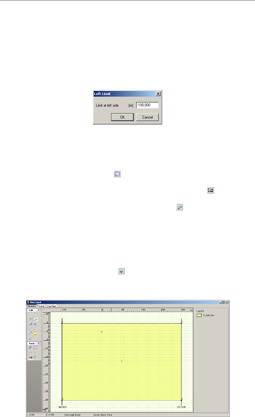
D-GEO PIPELINE
, User Manual
14.3 Geometry
Firstly, the geometry of Figure 14.1 needs to be given in
D-GEO PIPELINE
. In order to do this,
the following actions should be performed:
11. First enlarge the dimensions of the geometry window by selecting the left boundary by
clicking the left mouse button, then click the right button and select Properties. This will
result in the coordinate window for the left boundary as shown in Figure 14.4. Enter coor-
dinate Xof <100 m>.
Figure 14.4: Left Limit window
12. Repeat the previous described actions for the right boundary and shift the boundary to
coordinate Xof <200 m>. The width in between the left and the right boundary is now
300 m.
13. Select the drawing button Zoom limits from the Tools panel so that the drawn geometry
appears in the center of the screen.
14. Unselect the drawing button Automatic regeneration of geometry on/off from the Tools
panel.
15. Select the drawing button from the Edit panel Add single line to draw the surface line of
the longitudinal cross section of the horizontal directional drilling and position the straight
surface line at Z= 5 m. Use the right mouse button to finish the line.
16. Select again the drawing button Add single line to draw the lower boundary of the lon-
gitudinal cross section of the horizontal directional drilling and position the straight lower
boundary line at Z= –40 m. Use the right mouse button to finish the line.
17. Select the drawing button Automatic regeneration of geometry on/off from the Tools panel
so that the geometry as shown in Figure 14.5 appears.
18. Select the drawing button Add pl-line(s) from the Edit panel and position the level of the
groundwater at coordinate Z= 0 m. Use the right mouse button to finish the line. The blue
dashed line represents the groundwater line (PL line).
Figure 14.5: View Input window, Geometry tab
194 of 324 Deltares
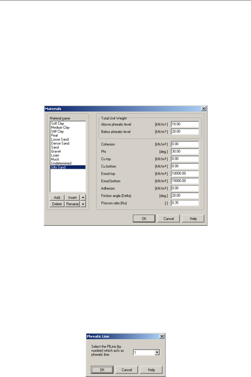
Tutorial 7: Face support pressure for micro tunneling
14.3.1 Soil layer properties
The properties of the soil layers should be specified in the menu materials, which can be
entered by clicking soil. In this tutorial only one soil layer is considered.
19. Click Soil and select Materials on the menu bar to open the Materials window (Figure 14.6)
and enter the soil data.
20. Add a new material by choosing Add button below the materials list on the left side of the
window with the new <Silty Sand>.
21. Enter the soil data as given in Table 14.1.
22. Finish the input of soil data by clicking OK.
Figure 14.6: Materials window
The defined soil properties and the groundwater level have to be assigned to the drawn ge-
ometry of the longitudinal cross section. The assignments can be carried out by clicking
geometry and choosing the subsequent described options on the menu bar.
14.3.2 Phreatic Line
23. On the Geometry menu, select Phreatic Line to open Phreatic Line window (Figure 14.7)
in which the phreatic line for calculation of the groundwater pressures can be selected.
24. Choose PL–line nr. <1>(only one phreatic line is available) and click OK.
Figure 14.7: Phreatic Line window
14.3.3 Layers
25. Click Geometry and select Layers on the menu bar to assign the soil properties to the soil
layers in the longitudinal cross section. To assign a material to a layer, select the Material
tab.
Deltares 195 of 324

D-GEO PIPELINE
, User Manual
26. Assign the properties of the defined layer Silty Sand to layer nr 1 in the longitudinal cross
section. The available soil layers with defined properties are shown in left column of the
materials window. The layers in the longitudinal cross section are shown in the right column
of the materials window. The defined properties are assigned to layer nr 1 by clicking the
arrow in between the columns. This will result in the Material tab shown in Figure 14.8.
Figure 14.8: Layers window, Materials tab
27. Click OK to quit the window and return to the geometry window to watch the change of
layer name in the legend.
14.3.4 PL-Lines per Layers
28. Click Geometry and select PL–lines per Layers on the menu bar to open the PL–lines
per Layer window (Figure 14.9) in which the defined PL–lines to the soil layers in the
longitudinal cross section can be defined. This window contains the information for the
calculation of the groundwater pressure distribution. In this tutorial only one PL-line is
defined. The groundwater pressure at the top of the silty sand layer and the bottom of this
layer should be calculated based on the hydraulic head of PL-line 1.
29. Click OK to close the window.
Figure 14.9: PL-lines per Layers window
196 of 324 Deltares
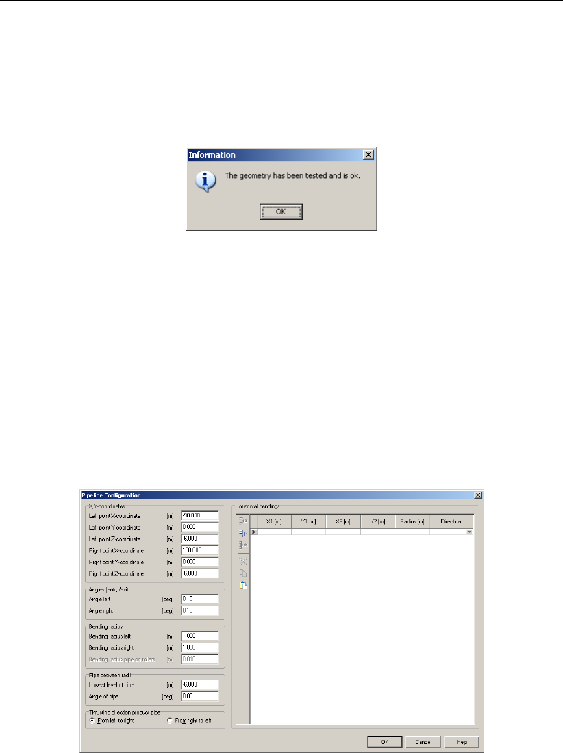
Tutorial 7: Face support pressure for micro tunneling
14.3.5 Check Geometry
30. The geometry can be tested by clicking Geometry and selecting Check Geometry on
the menu bar. If the geometry is entered properly, the message shown in Figure 14.10
appears.
31. Click OK to close the window.
Figure 14.10: Check Geometry window
14.4 Pipeline Configuration
The pipe is installed in the silty sand layer starting and ending at respectively the start and
reception shaft at a level 11 m below surface. As the pipe trajectory is horizontal, the smallest
angle of entry allowed by
D-GEO PIPELINE
is defined, i.e. 0.1 degree. A small bending radius
restricts the curved part of the pipe near the entry and exit of the pipe, thus the rest of the
pipe will be exact along the lowest level of the pipe.
32. Click Pipe from the menu and select Pipeline Configuration to open the Pipeline Configu-
ration window.
33. Enter the values as presented in Figure 14.11.
Figure 14.11: Pipeline Configuration window
34. Click OK to confirm.
35. Now examine the micro tunnel trajectory in the Input tab (Figure 14.12) and Top View tab
of the View Input window.
Deltares 197 of 324

D-GEO PIPELINE
, User Manual
Figure 14.12: View Input window, Input tab
14.5 Pipe Material Data
The pipe material of the pipe which will be installed by micro tunneling is chosen. The char-
acteristics of the pipe must be specified as well.
36. Click Pipe from the menu and select Product Pipe Material Data to open the Product Pipe
Material Data window.
37. Enter the values as presented in Figure 14.13.
Figure 14.13: Product Pipe Material Data window
The effect of the overcut on the radius of the pipe is explained in tutorial 9 (chapter 16).
14.6 Soil behavior
The strength of soil layers is dependent on the drained or undrained behavior of soil layers
during application the drilling fluid pressure at the front of the MTBM. Depending on the per-
meability of the soil layer, the soil will behave drained or undrained. A Sand layer is a well
permeable so called drained frictional material. The strength of this soil layer can be cal-
culated using the drained (effective) strength parameters effective cohesion (c) and angle of
internal friction (ϕ). In case of undrained behavior in other soil types, the strength of the soil
198 of 324 Deltares
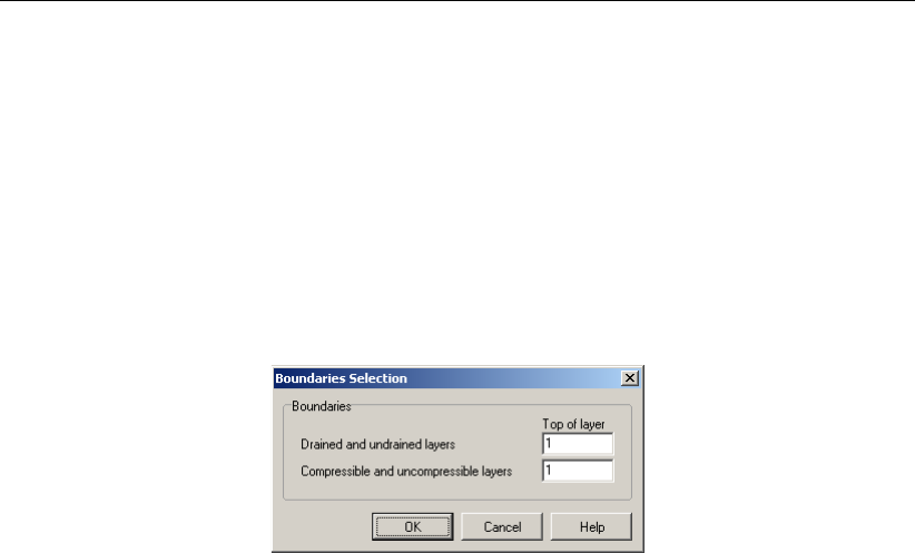
Tutorial 7: Face support pressure for micro tunneling
can be calculated using the undrained strength parameter undrained cohesion (cu).
38. Click GeoObjects and select Boundaries Selection on the menu bar to open the Bound-
aries Selection window for specification of the soil behavior.
39. Choose the boundary between the undrained and drained layer on top of layer nr <1>
(Figure 14.14). This choice results in drained behavior of layer nr 1.
40. Choose the boundary between the compressible and incompressible layer on top of layer
nr <1>. This choice results is used for the calculation of the soil mechanical parameters.
Compressible layers yield higher soil loads on the pipeline due to incomplete arching.
41. Click OK to close this window.
Figure 14.14: Boundaries Selection window
14.7 Calculation Verticals
The locations in the longitudinal cross section at which a calculation should be carried out
must be specified by the user. The user is able to perform calculations at uniform distances
along the longitudinal cross section but is also able to perform more calculations at short
distances at locations of interest.
42. Click GeoObjects and select Calculation Verticals on the menu bar to select the Calculation
Verticals window for specification of the calculation locations along the longitudinal cross
section.
43. Choose the Automatic generation of L co-ordinates option on the right side of the window
and choose the following values: <–80 m>for First,<180 m>for Last and <20 m>for
Interval.
44. Click on the Generate button and watch the result of automatic vertical generation on
the left side of the Calculation Verticals window. This will result in the window shown in
Figure 14.15.
45. Click OK to confirm the selected verticals and switch to the input window to watch the
location of the verticals in the longitudinal cross section.
Deltares 199 of 324
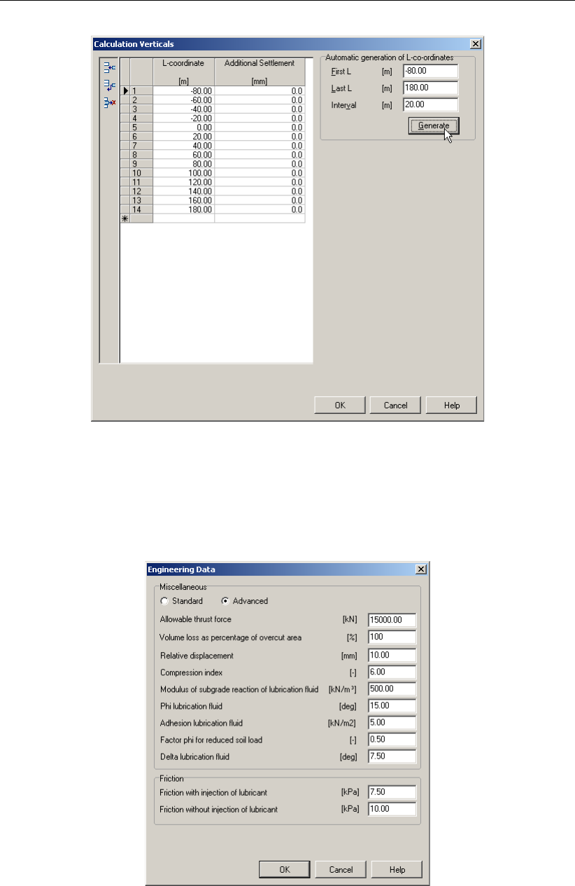
D-GEO PIPELINE
, User Manual
Figure 14.15: Calculation Verticals window
14.8 Engineering Data
46. Select Engineering Data from the Pipe menu bar to open the Engineering Data window.
47. Enter the values as given in Figure 14.16.
Figure 14.16: Engineering Data window
The maximum allowable thrust force is usually specified by the manufacturer of the pipe. The
volume loss determines the subsidence at the surface.
200 of 324 Deltares
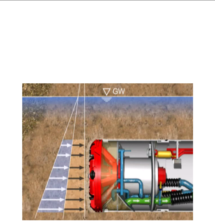
Tutorial 7: Face support pressure for micro tunneling
14.9 Results: Operation Parameter Plots
The micro-tunneling machine changes the stress conditions in the soil. The deviations from
the original stress conditions (Figure 14.17) are largely determined by the size of the overcut
and the applied shield. Small deviations from the original conditions are acceptable as the
stability of soil adjacent to the micro-tunneling machine is maintained. A relative low face
support pressure may lead to collapse of the soil in front of the shield, which in turn may lead
to subsidence of the surface or to settlement of soil layers below a construction or pipeline.
A relatively high face support pressure can lead to a blow out of drilling fluid or may lead to
heave of the surface.
Figure 14.17: Schematization of stress condition for micro-tunneling
While drilling the shield pressures have to be kept between certain limits. To prevent the
possibility of collapse in of the soil in front of the micro tunneling shield, causing subsidence,
the soil at the front is kept stable by maintaining a minimal face pressure. Depending on the
soil type the minimal support pressure can be calculated using Jancsecz and Steiner theory
(drained behavior of the soil) (Jancesz and Steiner,1994), or Broms and Bennermark theory
(undrained behavior of the soil) (Broms and Bennermark,1967). In this tutorial the soil layer
which consists of silty sand exhibits drained soil behavior.
A maximum support pressure should not be exceeded to prevent uplift of the soil above the
micro-tunneling machine or a blow out of drilling fluid towards the surface. The support pres-
sure, at which the soil deformations are minimal during drilling should be in between the two
limits. At the neutral pressure, the face support pressure is in equilibrium with the current
horizontal soil pressure.
48. To start the calculations click Calculation and select Start on the menu bar or press the
function key F9.
49. Click Results and select Operation Parameter Plots from the menu bar to open the Oper-
ation Parameter Plots window.
Deltares 201 of 324
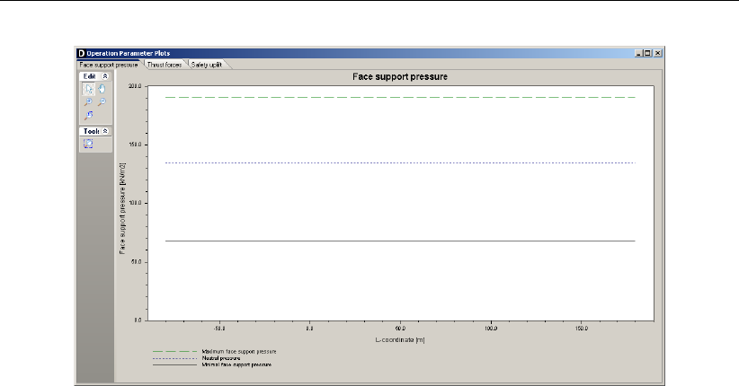
D-GEO PIPELINE
, User Manual
Figure 14.18: Operation Parameter Plots window, Face support pressure tab
From the graph (Figure 14.18) it can be observed that for this simple tutorial situation the target
face support pressure during the pipeline installation should be between the determined limits
of the maximum allowable face support pressure and the minimum required face support
pressure. At the neutral pressure the face support pressure is in equilibrium with the current
horizontal soil pressure.
202 of 324 Deltares
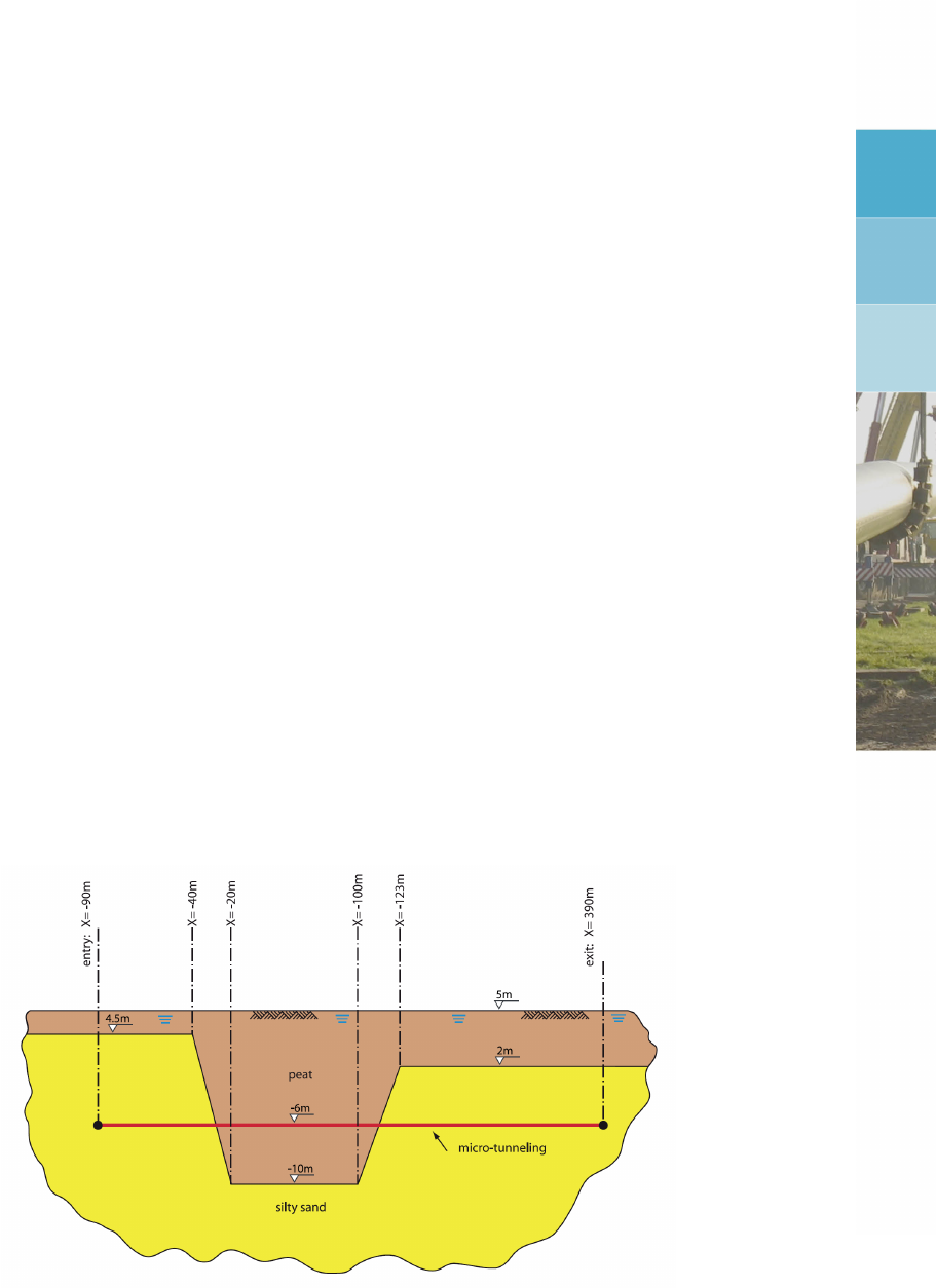
15 Tutorial 8: Uplift and thrust forces for micro tunneling
This tutorial concentrates on the installation of a pipeline by using the micro-tunneling tech-
nique and is a continuation of the previous tutorial. It considers installation of a gas pipeline
consisting of welded steel pipes. The pipeline crosses underneath a railway by using micro-
tunneling.
The objectives of the exercise are:
To evaluate the thrust force;
To perform a check on the uplift safety.
The following modules are needed:
D-GEO PIPELINE
Standard module (HDD)
Micro Tunneling module
This tutorial is presented in the file Tutorial-8.dri.
15.1 Introduction to the case
This tutorial considers a peat layer on top of the existing silty sand layer. The risk on uplift
of the empty pipeline in the peat layer is evaluated. The possibility of an alternative, longer,
micro tunneling trajectory is evaluated in this tutorial. A longer pipe string yields increased
friction forces which could possibly exceed the maximum allowable thrust force of the pipeline
or the jacking frame.
Figure 15.1: Soil layers and pipeline configuration for Tutorial 8
The soil properties are provided in Table 15.1.
Deltares 203 of 324

D-GEO PIPELINE
, User Manual
Table 15.1: Properties of the layers (Tutorial 8)
Silty Sand Peat
Dry unit weight [kN/m3] 18 10.2
Wet unit weight [kN/m3] 20 10.2
Cohesion [kN/m2] 0 2
Angle of internal friction [◦] 30 15
Undrained strength top [kN/m2] 0 10
Undrained strength bottom [kN/m2] 0 20
E modulus top [kN/m2] 10000 1000
E modulus bottom [kN/m2] 15000 1500
Adhesion [kN/m2] 0 2
Friction angle (Delta) [◦] 20 5
Poisson’s ratio [-] 0.35 0.45
This tutorial is based on continuation of the file used in Tutorial 7 (chapter 14).
1. Click File and select Open on the menu bar to open the Open window.
2. Select Tutorial-7 and click the Open button to open the file.
3. Click File and select Save as on the menu bar to open the Save As window and rename
the file into <Tutorial-8>.
4. Click the Save button to save the file for Tutorial 8.
5. On the menu bar, click Project and then choose Properties to open the Project Properties
window.
6. Fill in <Tutorial 8 for
D-GEO PIPELINE
>and <Micro tunneling: uplift and thrust forces>
for Title 1 and Title 2 respectively in the Identification tab.
7. Click OK.
15.2 Geometry of the longitudinal cross section
This tutorial considers a layered soil sequence. The typical Dutch soil sequence of a peat
layer on top of a silty sand layer will be considered. The peat layer is compressible and
exhibits a low permeability, while the sand layer is assumed incompressible and exhibits a
high permeability. The new soil layers should be specified in the geometry window.
8. In the View Input window, switch to the Geometry tab to edit the existing soil layer se-
quence.
9. Click the Add polyline(s) button from the Edit panel to draw an additional line which rep-
resents the lower boundary of the peat layer on top of the silty sand layer. The coordinates
of the cursor are given in the lower left side of the geometry window. Make the polyline
by clicking on the subsequent co-ordinates (Figure 15.2). Click the right mouse button to
escape from the polyline drawing.
Figure 15.2: Co-ordinates of the lower boundary of the Peat layer (before enlarging the
right limit)
204 of 324 Deltares
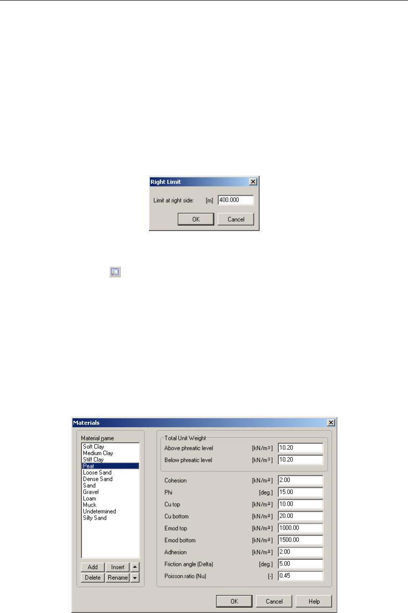
Tutorial 8: Uplift and thrust forces for micro tunneling
10. After finishing the polyline, mis-clicks can be corrected using the Edit button: select points
of the polyline by clicking on it with the left mouse button. Once the point is selected
(indicated with a red color), use the right mouse button to select the option Properties. . .
and to correct the co-ordinates of the lower boundary of the peat layer.
11. Change the position of the phreatic groundwater: select both points of the PL line (i.e. blue
dashed line) by clicking on it with the left mouse button, then select the option Properties. . .
and change the co-ordinate into Z= 5 m.
12. Enlarge the dimensions of the geometry window by selecting the right boundary by clicking
the right mouse button, then click the right button and select Properties. . . . This will result
in the coordinate window for the right boundary as shown in Figure 15.3. Enter coordinate
Xof <400 m>.
Figure 15.3: Right Limit window
13. Click the Zoom limits button from the Tools panel so that the drawn geometry appears
in the center of the screen.
15.3 Soil layer properties
The properties of the soil layers in the layered soil sequence should now be specified.
14. Click Soil and select Materials on the menu bar to enter the soil data.
15. Select the existing soil material Peat.
16. Enter the soil data as given in Table 15.1.
17. Click OK.
Figure 15.4: Materials window
The defined soil properties have to be assigned to the drawn geometry of the longitudinal
cross section. The assignments can be carried out in the Geometry menu.
18. Click Geometry and select Layers on the menu bar to open the Layers window.
Deltares 205 of 324
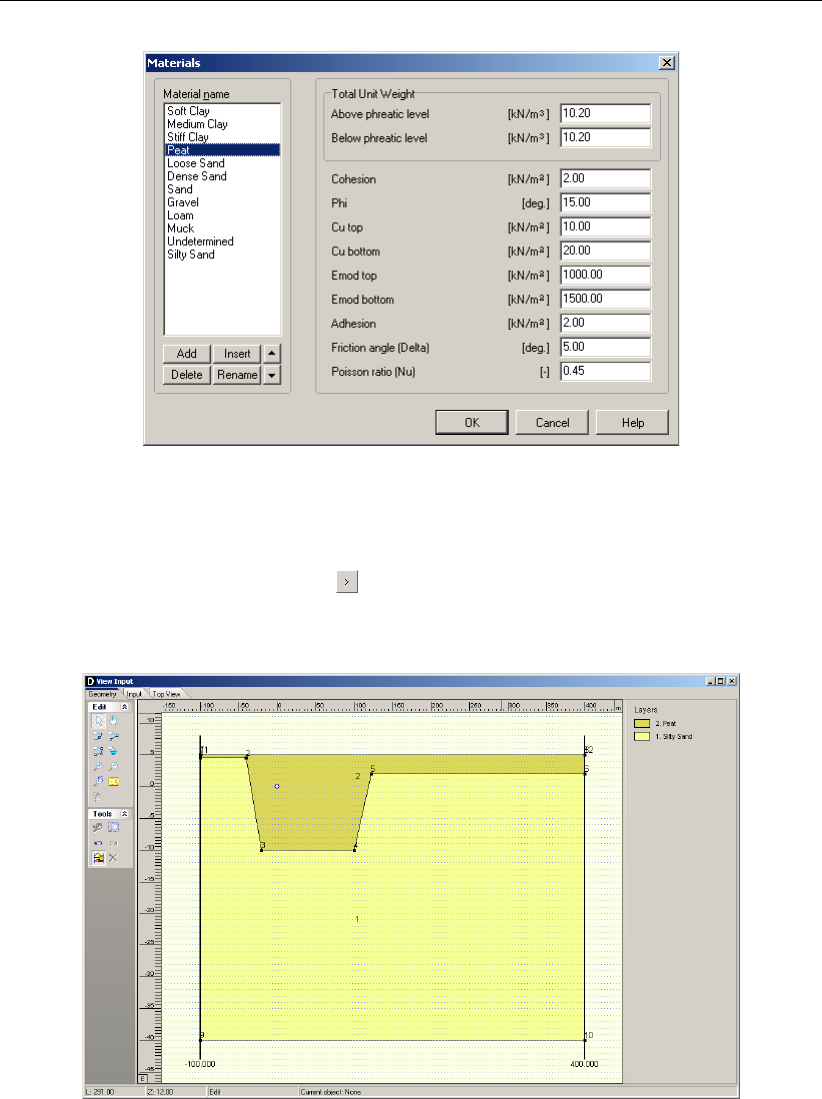
D-GEO PIPELINE
, User Manual
Figure 15.5: Layers window, Materials tab
19. Select the Materials tab.
20. Assign the properties of the defined layer Peat to layer number 2 in the longitudinal cross
section by clicking the Assign icon in between the left and the right column.
21. Click on the OK button to quit the window and return to the Geometry tab of the View Input
window to look at the change of layers name in the legend (Figure 15.6).
Figure 15.6: View Input window, Geometry tab
22. The geometry can be tested by clicking Geometry on the menu bar and selecting Check
Geometry. If the geometry is entered properly, the message Geometry has been tested
and is OK appears.
23. Click OK to close this window.
15.4 Soil behavior
Strength of soil layers is dependent on the drained or undrained behavior of soil layers during
application the drilling fluid pressure. Depending on the permeability of the soil layer, the soil
will behave drained or undrained. The Silty Sand layer is well permeable so that the behavior
206 of 324 Deltares
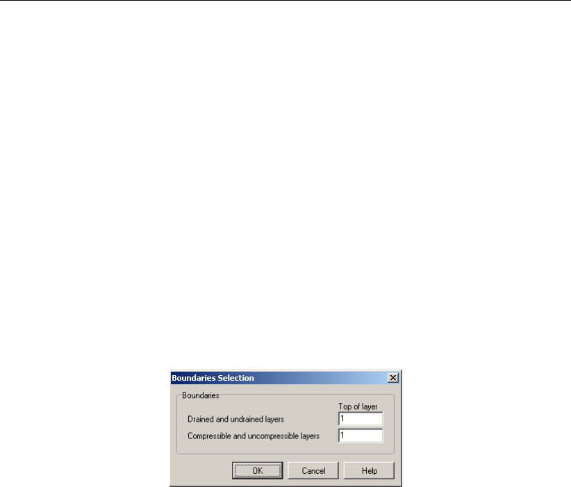
Tutorial 8: Uplift and thrust forces for micro tunneling
of the silty sand layer is drained. The strength of this soil layer can be calculated using the
drained (effective) strength parameters effective cohesion (c) and angle of internal friction (ϕ).
In case of undrained behavior in the impermeable Peat layer, the strength of the soil can be
calculated using the undrained strength parameter undrained cohesion (cu).
The soil load on the pipeline after finishing the installation is dependent on the soil pipeline in-
teraction, which is in turn largely dependent on the soil behavior. As described in section 10.2
arching develops completely in incompressible soil layers, while in compressible layers the
reduced soil load on the pipeline is higher due to compression of the soil next to the pipeline.
24. Click GeoObjects and select Boundaries Selection on the menu bar to open the Bound-
aries Selection window for specification of the soil behavior.
25. Choose the boundary between the Drained and undrained layers on top of layer number
<1>(Figure 15.7). This choice results in drained behavior of layer number 1.
26. Choose the boundary between the Compressible and uncompressible layers on top of
layer number <1>. This choice results in full development of arching in layer number 1
while in layer number 2 arching is not fully developed.
27. Click OK to close this window.
Figure 15.7: Boundaries Selection window
15.5 Pipeline Configuration
The tunneling length will be increased by changing the entry and exit locations.
28. Click Pipe and select Pipeline Configuration from the menu bar to open the Pipeline Con-
figuration window.
29. Change the X-coordinates of the left and right points to respectively <-90>and <390>
as shown in Figure 15.8.
30. Click OK.
Deltares 207 of 324
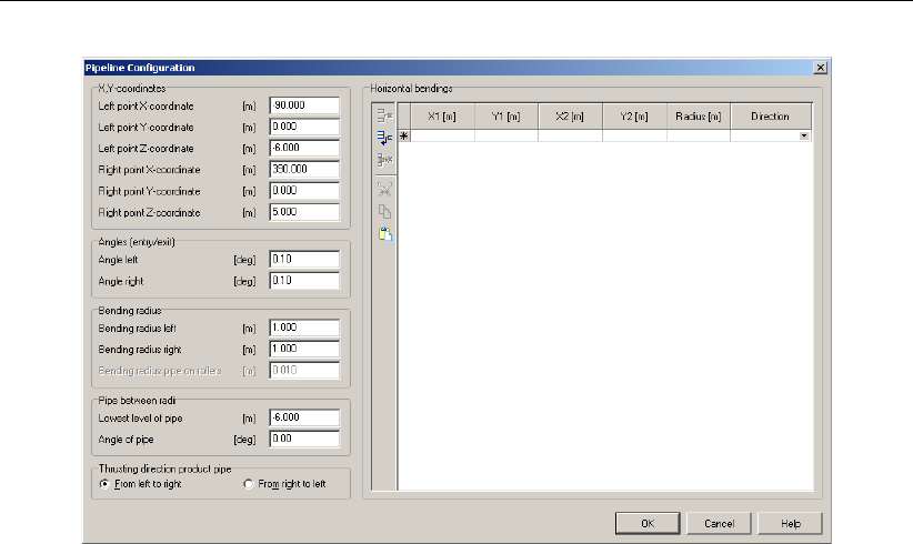
D-GEO PIPELINE
, User Manual
Figure 15.8: Pipeline Configuration window
15.6 Calculation Verticals
The locations in the longitudinal cross section at which a calculation should be carried out
must be specified by the user. The user is able to perform calculations at uniform distances
along the longitudinal cross section but is also able to perform more calculations at short
distances at areas of interest.
31. Click GeoObjects and select Calculation Verticals on the menu bar to select the Calculation
Verticals window for specification of the calculation locations along the longitudinal cross
section. This will result in the window shown in Figure 15.9.
32. Choose the Automatic generation of L co-ordinates option on the right side of the window
and choose the following values: <–80 m>for First,<380 m>for Last and <20 m>for
Interval.
33. Click on the Generate button and watch the result of automatic vertical generation on the
left side of the Calculation Verticals window.
34. Click OK to confirm the selected verticals and switch to the input window to watch the
location of the verticals in the longitudinal cross section.
208 of 324 Deltares
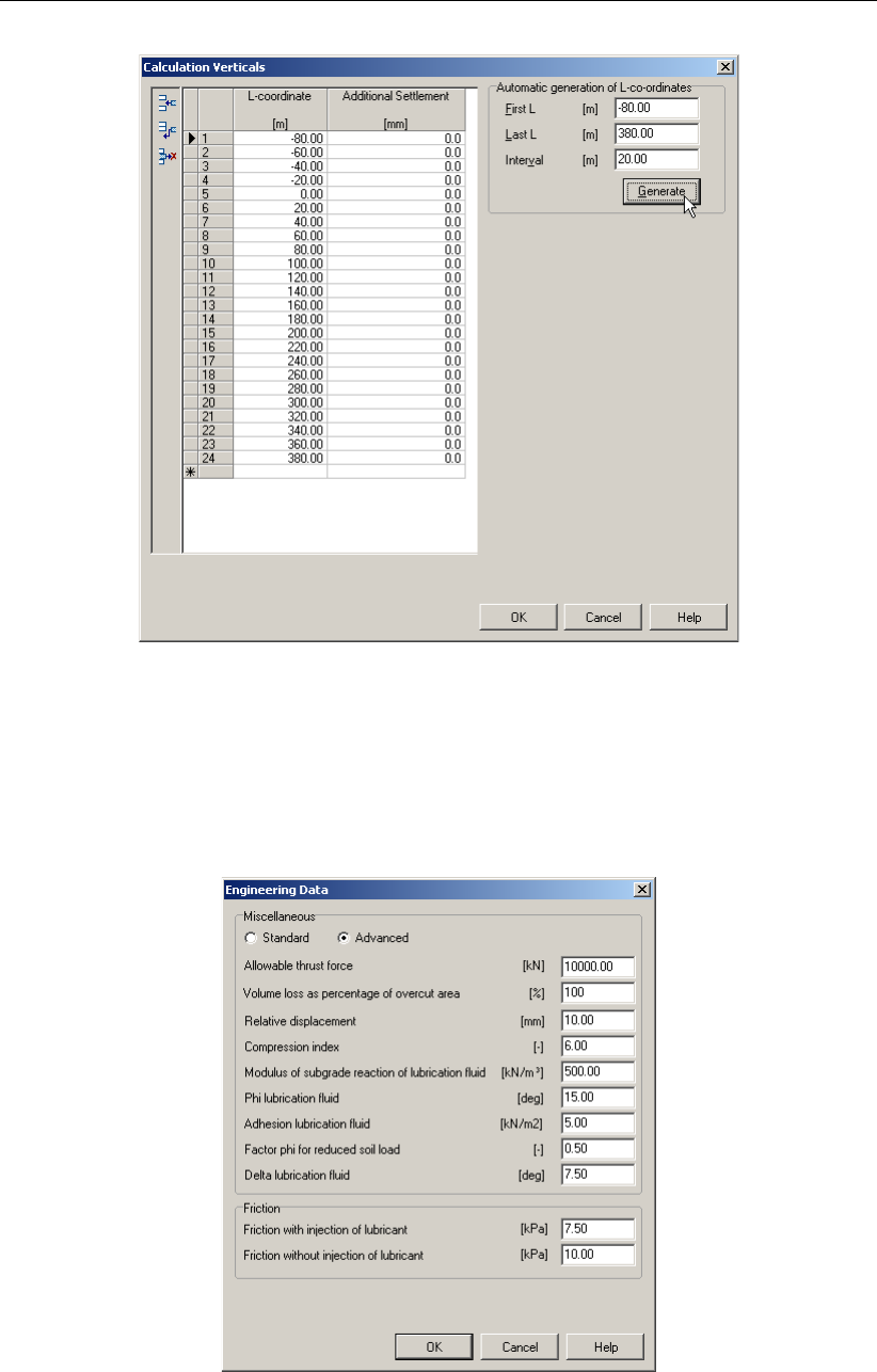
Tutorial 8: Uplift and thrust forces for micro tunneling
Figure 15.9: Calculation Verticals window
15.7 Engineering Data
35. Select Engineering Data from the Pipe menu bar to open the Engineering Data window.
36. Enter the values as given in Figure 15.10.
37. Click OK.
Figure 15.10: Engineering Data window
Deltares 209 of 324
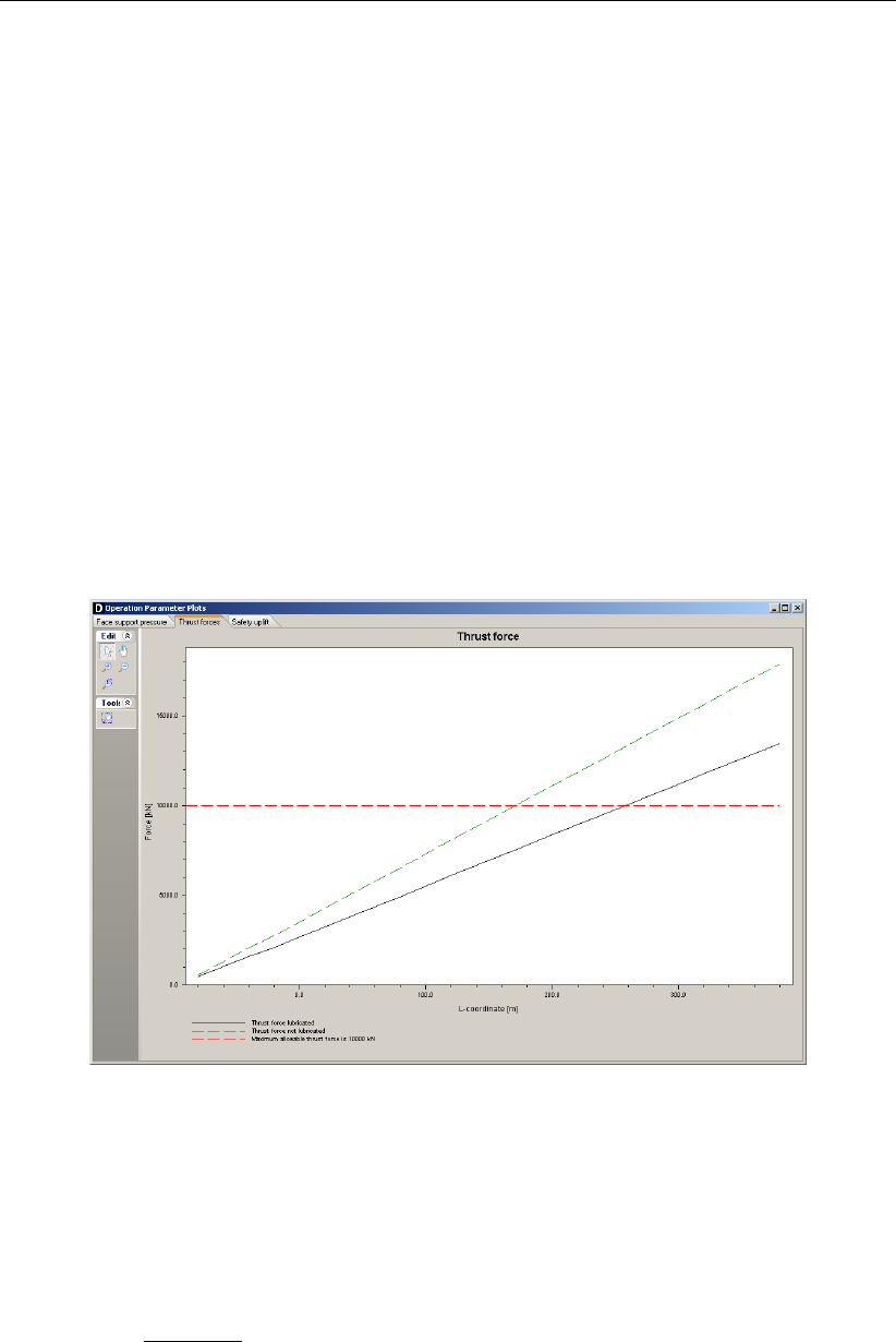
D-GEO PIPELINE
, User Manual
15.8 Results
The schematization of the longitudinal cross section along the pipeline which will be installed
by using micro tunneling is changed. A calculation can now be performed.
38. To start the calculations click Calculation and select Start on the menu bar or press the
function key F9.
15.8.1 Thrust Force
39. Open the Operation Parameter Plots window from the Results menu and select the Thrust
forces tab (Figure 15.11).
This graph shows the calculated thrust force versus the length of pipe jacked into the sub-
surface. It is easily recognized that the lubricated as well as the dry thrust force exceed the
maximum allowable thrust force as indicated by the manufacturer of the pipe sections.
It should be mentioned that the capacity of the jacks is limited as well. In general the maximum
capacity is about 600 ton (6000 kN) so that for larger lengths intermediate jacks are required.
Figure 15.11: Operation Parameter Plots window, Thrust Force tab
15.8.2 Uplift safety
Since the pipeline is installed in a soft soil layer with a relative low wet density. The uplift
behavior of the empty pipeline should be evaluated.
D-GEO PIPELINE
calculates the uplift safety
factor fuplift using the following formula:
fuplift =σ0
v+gpipe
guplift
(15.1)
where:
σ0
vis the vertical effective stress;
gpipe is the buoyancy of the pipe depending on the diameter of the pipeline and the water
level. Partial submerging is taken into account by
D-GEO PIPELINE
;
guplift is the uplift force.
210 of 324 Deltares
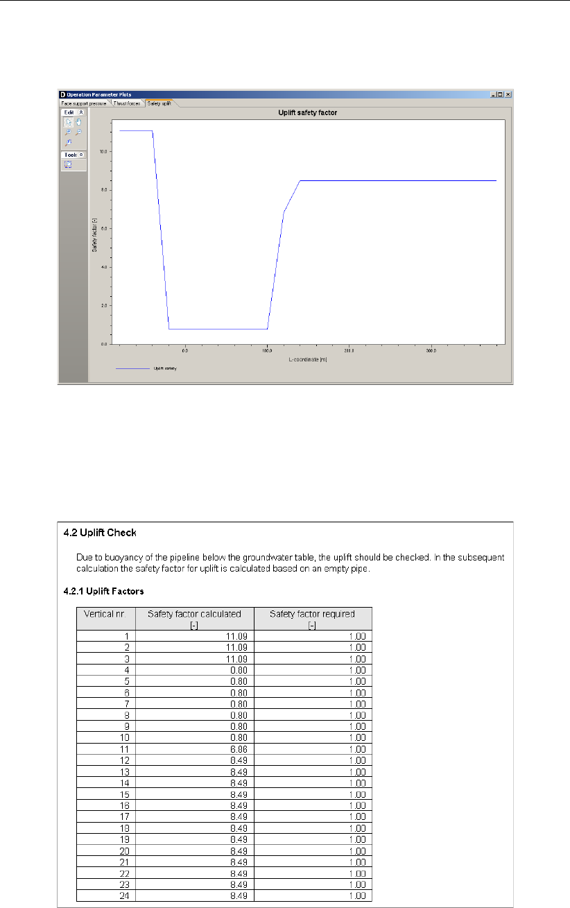
Tutorial 8: Uplift and thrust forces for micro tunneling
40. Select the Safety uplift tab. As can be seen in Figure 15.12, the uplift safety is more than
the required safety factor of 1.
Figure 15.12: Operation Parameter Plots window, Safety uplift tab
The uplift safety appears to be insufficient in the peat layer. The uplift safety factor equals 0.8.
The safety factors are shown in the report in paragraph 4.2.1. The reported table is shown
subsequently.
Figure 15.13: Report window, Uplift Factors section
Deltares 211 of 324

D-GEO PIPELINE
, User Manual
212 of 324 Deltares
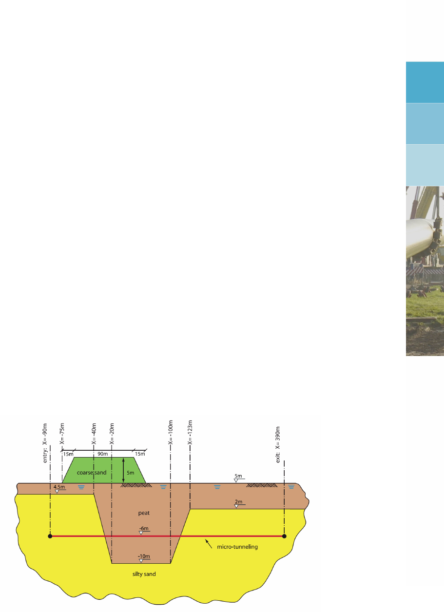
16 Tutorial 9: Settlement and soil mechanical parameters for micro
tunneling
This tutorial provides some detail on settlement and calculation of soil mechanical parameters
in
D-GEO PIPELINE
. For a pipe stress analysis the knowledge of the soil-pipeline interaction is
required. The soil pipeline interaction is described by the soil mechanical parameters. The
vertical displacement (very often settlement) of the layers below and around the pipeline is
one of the soil mechanical parameters.
The objectives of the exercise are:
To calculate the soil mechanical parameters
To calculate the settlements due to construction of an embankment
The following modules are needed:
D-GEO PIPELINE
Standard module (HDD)
Micro Tunneling module
License for
D-SETTLEMENT
(formerly known as MSettle)
This tutorial is presented in the file Tutorial-9.dri.
16.1 Introduction to the case
The same project as Tutorial 8 (chapter 15) is considered with an additional load carry on the
compressible soil layers (Figure 16.1). Settlement can be therefore expected.
Figure 16.1: Soil layers and pipeline configuration for Tutorial 9
For advanced pipe stress analyses special programs need to be used. These programs need
an advanced set of soil mechanical parameters, provided by
D-GEO PIPELINE
. The programs
will generate a complete spring model around the pipeline for further analyses. The soil
mechanical parameters provided by
D-GEO PIPELINE
are:
neutral vertical soil load
passive vertical soil load
Deltares 213 of 324

D-GEO PIPELINE
, User Manual
reduced vertical soil load
vertical modulus of sub grade reaction
horizontal modulus of sub grade reaction
ultimate vertical bearing capacity
ultimate horizontal bearing capacity
neutral horizontal soil load
vertical displacement
maximal axial friction
friction displacement
Vertical displacement of soil below and around the pipeline that occurs after installation is an
important factor in assessing the stresses in the pipeline. Settlement may be entered manually
if the vertical settlements results are available. For more accurate results,
D-GEO PIPELINE
can use the
D-SETTLEMENT
computer program (formerly known as MSettle) without additional
input. Settlement deals with soil compaction due to imposed loading. In
D-GEO PIPELINE
the
loading consists of an extra layer as created in the geometry. The calculation of the settlement
is performed externally by
D-SETTLEMENT
, the settlement calculation program of the Deltares
Systems tools. Details on the calculation of settlement are beyond the scope of this manual,
a thorough description can be found in the user manual of
D-SETTLEMENT
(Deltares).
Table 16.1: Settlement parameters (acc. Koppejan) of the soil layers (Tutorial 9)
Coarse Sand Silty Sand Peat
Over-consolidation ratio (OCR) 1 1.3 1.3
Primary compression coeff. below Pc (Cp) 10910940
Primary compression coeff. above Pc (Cp’) 10910910
Secondary compression coeff. below Pc (Cs) 109109160
Secondary compression coeff. above Pc (Cs’) 10910935
This tutorial is based on the geometry made in Tutorial 8.
1. Click File and select Open on the menu bar to open the Open window.
2. Select Tutorial-8 and click the Open button to open de file.
3. Click File and select Save as on the menu bar to open the Save As window and rename
the file into <Tutorial-9>.
4. Click the Save button to save the file for Tutorial 9.
5. On the menu bar, click Project and then choose Properties to open the Project Properties
window.
6. Fill in <Tutorial 9 for
D-GEO PIPELINE
>and <Micro tunneling: settlement and soil mech.
param.>for Title 1 and Title 2 respectively in the Identification tab.
7. Click OK.
16.2 Settlement
For calculation of settlement a license for
D-SETTLEMENT
is required. If this license and soft-
ware is available the model option Settlement will be available in
D-GEO PIPELINE
. For this
purpose an embankment that will act as a load is introduced.
Settlement calculations can be performed using the in the Netherlands often used Koppejan
model or the more recent developed Isotache model which is based on Terzaghi’s settlement
model.
8. Click Project and select Model on the menu bar to open the Model window.
214 of 324 Deltares

Tutorial 9: Settlement and soil mechanical parameters for micro tunneling
9. Mark the Use settlement check-box and select the Koppejan model (Figure 16.2).
10. Click OK to confirm the choice.
Figure 16.2: Model window
16.3 Geometry of the longitudinal cross section
This tutorial considers a layered soil sequence described in Tutorial 8 (chapter 15). In the
longitudinal cross section, a load (soil mass) has to be defined.
11. Switch to the Geometry tab in the View Input window to edit the existing soil layer se-
quence.
12. Select the Add polyline icon from the Edit sub-window to draw an additional layer (soil
mass) on top of the existing soil layers with coordinates given in Table 16.2.
Table 16.2: Coordinates of the top of the soil mass
X co-ordinate [m] Z co-ordinate [m]
-75 5
-60 10
30 10
45 5
13. Quit editing by clicking the right mouse button.
14. To check or modify the added points, select a point by clicking the left mouse button. The
point will become a red square.
15. Click the right-hand mouse button and select Properties. . . . In the window displayed (Fig-
ure 16.3), the co-ordinates can be checked and modified if needed.
Deltares 215 of 324
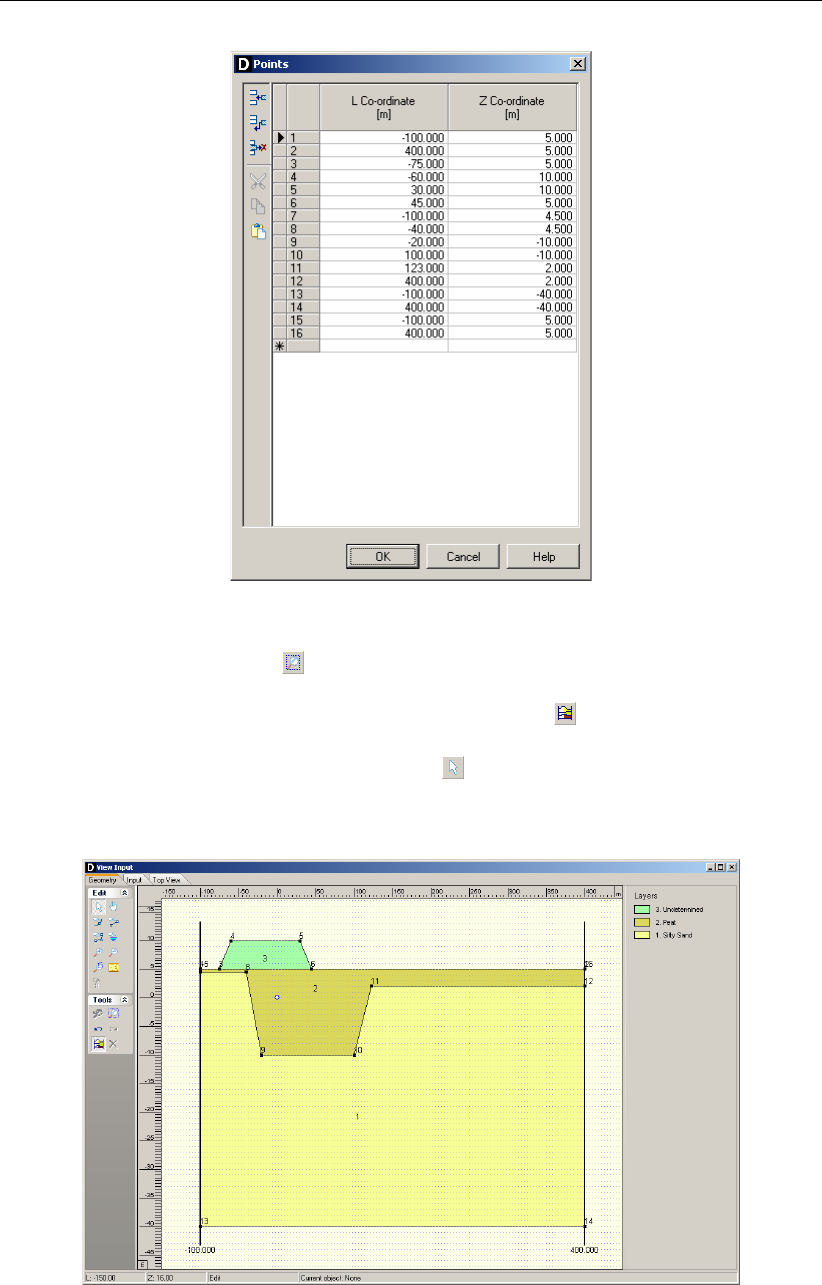
D-GEO PIPELINE
, User Manual
Figure 16.3: Points window
16. Click the Zoom limits button from the Tools panel so that the drawn geometry appears
in the center of the screen.
17. Select the Automatic regeneration of geometry on/off icon from the Tools sub-window
so that the geometry as shown in Figure 16.4. If the Automatic regeneration of geometry
icon already is selected, click on the Edit icon to regenerate the geometry. Notice that
the soil mass is located on the left side above the section where the pipeline is located in
the peat layer.
Figure 16.4: View Input window, Geometry tab
216 of 324 Deltares
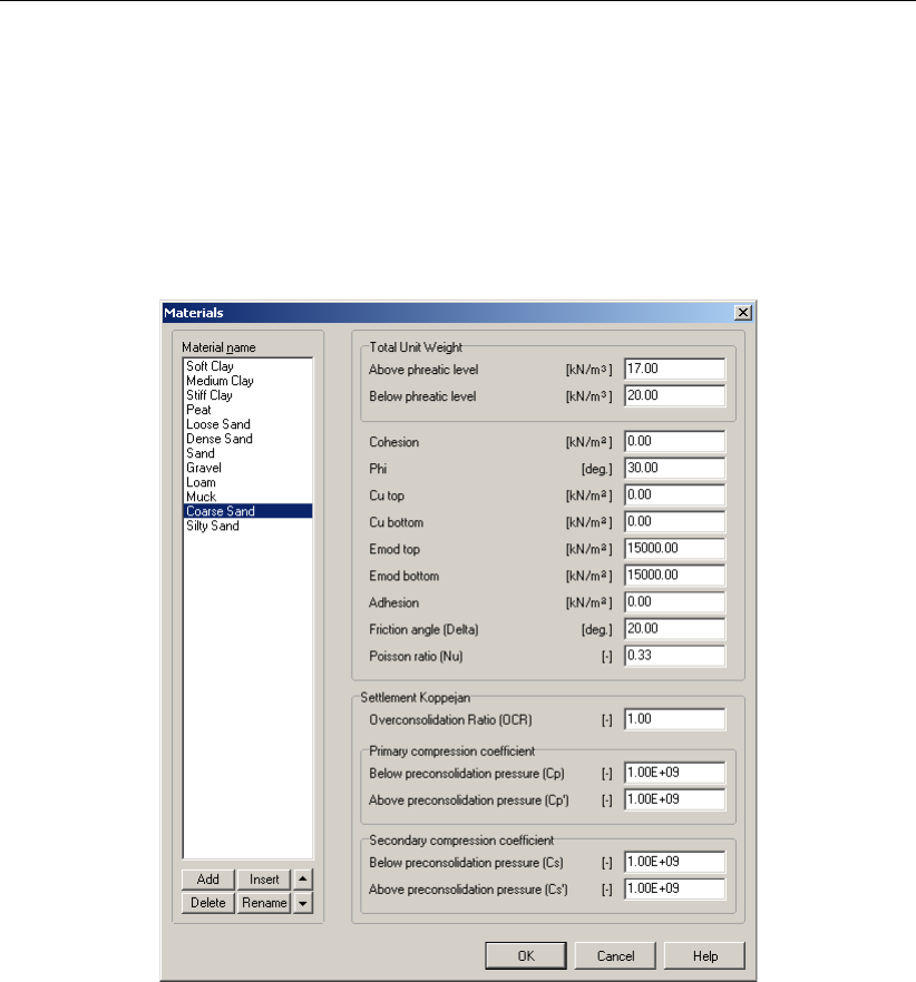
Tutorial 9: Settlement and soil mechanical parameters for micro tunneling
16.4 Soil layer properties
The settlement properties of the soil layers in the layered soil sequence should now be speci-
fied. The properties of the soil mass should be entered too.
18. Click Soil and select Materials on the menu bar to open the Materials window.
19. Select the soil name Undetermined in the left column of the Materials window and rename
it with <Coarse Sand>. Enter the properties given in Figure 16.5.
Figure 16.5: Materials window
20. Select the soil name Silty Sand and enter the Settlement Koppejan data given in Ta-
ble 16.1.
21. Select the soil name Peat and enter the Settlement Koppejan data given in Table 16.1.
22. Finish the input of soil data by clicking OK.
16.5 Finishing the geometry of the longitudinal cross section
The defined soil properties have to be assigned to the drawn geometry of the longitudinal
cross section (groundwater levels are assigned already). The assignments can be carried out
by clicking geometry and choosing the subsequent described options on the menu bar.
23. Click Geometry and select Layers on the menu bar to open the Layers window to assign
the soil properties to the soil layers in the longitudinal cross section.
24. Click on the tab Materials.
25. Assign the soil properties given in Figure 16.6.
26. Click OK to confirm the assignments.
Deltares 217 of 324

D-GEO PIPELINE
, User Manual
Figure 16.6: Layers window, Materials tab
16.6 Calculated soil mechanical parameters in export file
The calculation of the settlement of the soil layers below the pipeline is performed exter-
nally by
D-SETTLEMENT
(formerly known as MSettle), the settlement calculation program of
the Deltares Systems tools. Therefore, the directory where the program is installed must be
given:
27. Click Tools on the menu bar and select Program Options to open the Program Options
window. Then select the Locations tab (Figure 16.7).
28. If needed, change the directory where the Settlement program is installed by clicking the
Browse button.
29. Click OK to confirm.
Figure 16.7: Program Options window, Locations tab
The other soil mechanical parameters are calculated automatically in
D-GEO PIPELINE
.
218 of 324 Deltares
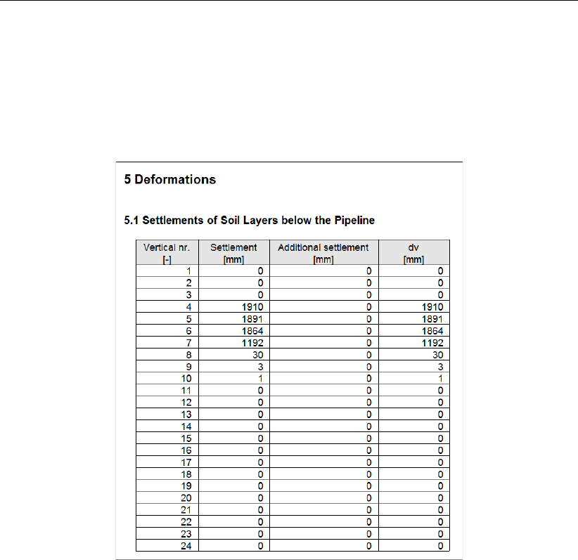
Tutorial 9: Settlement and soil mechanical parameters for micro tunneling
30. To start the calculations click Calculation and select Start on the menu bar to or press
the function key F9. Ignore the message of Cu values of 0 above the drained undrained
boundary.
31. Click Results and select Report on the menu bar to look at the results of the settlement
calculation in paragraph 5.1 (Figure 16.8) and the calculation of the Soil Mechanical Pa-
rameters in paragraph 3.1 (Figure 16.9).
Figure 16.8: Report window, Settlements of soil layers below the pipeline
Deltares 219 of 324
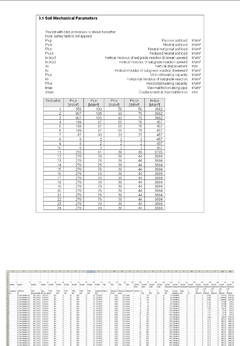
D-GEO PIPELINE
, User Manual
Figure 16.9: Report window, Soil Mechanical Parameters
32. Click File and select Export Results as csv. . . on the menu bar to create an export file with
the soil mechanical parameters.
33. Click on the Save button. The export file is saved on the same directory as Tutorial 9 and
can be opened using the Excel program for example (see Figure 16.10).
Figure 16.10: Content of the CSV export file for Tutorial 9
The export file contains the following data’s:
General data about the
D-GEO PIPELINE
project
Pipeline data
Horizontal soil mechanical data at the left and right of the pipe
Vertical soil mechanical data at the top and bottom of the pipe
220 of 324 Deltares

Tutorial 9: Settlement and soil mechanical parameters for micro tunneling
Water data
Axial soil data for friction
For more information, refer to section 3.1.2.
16.7 Conclusion
A pipe stress and settlement analysis has been performed for a polyethylene pipe in a layered
soil. The inputs and results of this calculation have been exported in a csv file in order to
perform an extended stress analysis using an other program.
Deltares 221 of 324

D-GEO PIPELINE
, User Manual
222 of 324 Deltares

17 Tutorial 10: Subsidence after micro tunneling
This tutorial provides some detail on subsidence calculations in
D-GEO PIPELINE
. Subsidence
is related to surface level changes due to excavation of the subsurface by the micro tunneling
machine.
The objectives of the exercise are:
To enter a non linear bore path;
To evaluate the subsidence along the pipeline.
The following modules are needed:
D-GEO PIPELINE
Standard module (HDD)
Micro Tunneling module
This tutorial is presented in the file Tutorial-10.dri.
17.1 Introduction to the case
17.1.1 Volume loss along the tunnel excavation
Subsidence is related to the volume loss along the tunnel excavation, e.g. the excess soil
removed by the Micro Tunneling Boring Machine (MTBM). The subsidence mechanism is
described in detail in section 24.3.
To reduce the friction between pipe and wall of the drilling hole, and allow the optional use
of friction reducing fluids, the drilling diameter (R) is usually somewhat larger then the pipe
diameter (r).
Figure 17.1: Bore hole section
The space created between pipe and wall is called overcut: the distance R−r. See sec-
tion 4.6.2.2 for entering the overcut. The overcut is generally filled by lubrication fluid depend-
ing on the type of lubrication fluid the amount of filling may reduce during or after installation:
Part of the soil above subsides during operation
Compaction/consolidation of the lubrication fluid after installation
The volume loss as percentage of the overcut area is defined as.
Vs=υ π R2−r2(17.1)
Deltares 223 of 324
D-GEO PIPELINE
, User Manual
Note: If one wants to model subsidence due to drilling with a low face support pressure or to
model the influence of densification of granular soils this value may be set above 100%.
The volume loss causing subsidence is in
D-GEO PIPELINE
based on the expected overcut of
the soil.
Vs=υ π
4(Do+ 2 lovercut)2−D2
o(17.2)
where:
υis the percentage volume loss, in %;
VSis the differential volume, in m3/m;
Dois the pipe diameter, in m;
lovercut is the overcut on radius, in m.
The volume created by the over cut is initially filled with lubrication fluid. Within a time period
the lubrication fluid will consolidate and the overburden will subside into space created by
consolidation. The subsidence wat the surface is calculated as follows:
w=Vs
√2πi2exp −r2
2i2, z < z0(17.3)
where:
iis the distance in between the center of the tunnel or pipeline and the inflection point
of the trough, in m;
z0is the depth of the center of the pipeline or tunnel, in m;
zis the depth at which the settlement is calculated, in m;
VSis the differential volume, in m3/m.
For detail on the shape factor i, see section 24.3.
17.1.2 Modification of the drilling line
A vertical and a horizontal bending radius in the design drilling line for micro tunneling is a
possibility. In this tutorial the drilling line is modified in order to avoid drilling through the peat
layer.
224 of 324 Deltares

Tutorial 10: Subsidence after micro tunneling
Figure 17.2: Pipeline configuration of Tutorial 10
Often the horizontal bend is part of one of the vertical bending radii. In case the horizontal
bending radius coincides with part of a vertical bending radius, a combined 3-dimensional
bending radius is formed. For the design of the horizontal directional drilling line, the pull back
force and the strength calculation it is necessary to determine the value of the 3 dimensional
bending radius.
The value of the three dimensional bending radius can be calculated as follows:
Rcombi =sR2
h×R2
v
R2
h+R2
v
(17.4)
where:
Rcombi is the combined bending radius, in m;
Rhis the horizontal bending radius, in m;
Rvis the vertical bending radius, in m.
As has to be mentioned that the current version of
D-GEO PIPELINE
does not take the soil
reaction forces into account in the curve. Therefore the effect on the friction caused by soil
reaction effects in curves is not considered in
D-GEO PIPELINE
.
This tutorial is based on continuation of the file used in Tutorial 9 (chapter 16).
1. Click File and select Open on the menu bar to open the Open window.
2. Select <Tutorial-9>and click the Open button to open de file.
3. Click File and select Save As on the menu bar to open the Save As window and rename
the file into <Tutorial-10>.
4. Click the Save button to save the file for Tutorial 10.
5. On the menu bar, click Project and then choose Properties to open the Project Properties
window.
Deltares 225 of 324
D-GEO PIPELINE
, User Manual
6. Fill in <Tutorial 10 for
D-GEO PIPELINE
>and <Subsidence after micro tunneling>for Title
1and Title 2 respectively in the Identification tab.
7. Click OK.
8. In the Model window from the Project menu, unselect the option Use settlement.
9. Click OK.
17.2 Pipeline Configuration
The horizontal and vertical curves must be specified in the pipeline configuration window.
10. Click Pipe and select Pipeline Configuration on the menu bar to open the Pipeline Config-
uration window.
11. Enter the values given in Figure 17.3.
12. Click OK to confirm.
Figure 17.3: Pipeline Configuration window
13. Look at the entered horizontal bending on the Top View tab of the View Input window
(Figure 17.4).
14. Look at the longitudinal cross section on the Input tab of the View Input window and notice
the elongation of the longitudinal cross section. Therefore it is recommended to check, in
case of projects with changing 3D pipeline configurations, if the soil layer sequence in the
longitudinal cross section is still reliable (according to the soil investigation data).
226 of 324 Deltares
Tutorial 10: Subsidence after micro tunneling
Figure 17.4: View Input window, Top View tab
Note: The horizontal bending is indicated with a black bold line in the top view (Figure 17.4).
Figure 17.5: View Input window, Input tab
17.3 Material data
After the input of the drilling line, the pipe material is chosen.
15. Click Pipe from the menu and select Product Pipe Material Data to open the Product Pipe
Material Data window.
16. Enter the values as presented in Figure 17.6.
Deltares 227 of 324
D-GEO PIPELINE
, User Manual
Figure 17.6: Product Pipe Material Data window
The overcut on the radius amounts to 20 mm, which equals 40 mm on the diameter of the
pipeline.
17.4 Engineering Data
The percentage of volume loss is specified in the Engineering Data window. In this tutorial a
value of 110 % is chosen, so that the effect of drilling with a relative low face pressure (lower
than the neutral face pressure) is incorporated.
17. Select Engineering Data from the Pipe menu bar to open the Engineering Data window.
18. Enter the values as given in Figure 17.7.
Figure 17.7: Engineering Data window
228 of 324 Deltares
Tutorial 10: Subsidence after micro tunneling
17.5 Results: Subsidence
To view the calculation results for the subsidence trough as apparent at surface:
19. To start the calculations click Calculation and select Starton the menu bar or press the
function key F9.
20. Click Results and select Subsidence Profiles from the menu bar to open the Subsidence
Profiles window (Figure 17.8).
21. Check the box labeled “Fix axis”, click on the vertical number edit box. Now move through
the verticals by using the up/down arrows on the key board.
Figure 17.8: Subsidence Profiles window for vertical 1
Deltares 229 of 324

D-GEO PIPELINE
, User Manual
230 of 324 Deltares

18 Tutorial 11: Installation of pipeline in a trench
This tutorial considers installation of a concrete sewer by means of trenching. A trench is
made by excavation, the pipe is installed, and the trench is often filled with the soil derived from
the excavation itself. The risks involved during installation include slope failure and bursting of
the trench bottom. After installation uplift of the pipe and pipe deformation due to settlement
are problems that may occur.
The objectives of the exercise are:
To schematize the soil layers with groundwater with different hydraulic heads;
To calculate the soil mechanical parameters for a pipeline in a trench.
The following modules are needed:
D-GEO PIPELINE
Standard module (HDD)
Trenching module
This tutorial is presented in the file Tutorial-11.dri.
18.1 Introduction to the case
In this tutorial a simple trench is modeled. The trench passes a small waterway. The geometry
of tutorial 7 forms the base of this tutorial.
Figure 18.1: Geometry of Tutorial 11
This tutorial is based on continuation of the file used in Tutorial 7 (chapter 14).
1. Click File and select Open on the menu bar to open the Open window.
2. Select Tutorial-7 and click the Open button to open de file.
3. Click File and select Save as on the menu bar to open the Save As window and rename
the file into <Tutorial-11>.
Deltares 231 of 324

D-GEO PIPELINE
, User Manual
Table 18.1: Layer properties (Tutorial 11)
Silty Sand Soft Organic Clay
Dry unit weight [kN/m3] 18 13
Wet unit weight [kN/m3] 20 13
Cohesion [kN/m2] 0 2
Angle of internal friction [◦] 10 18
Undrained strength top [kN/m2] 0 10
Undrained strength bottom [kN/m2] 0 30
E modulus top [kN/m2] 10000 500
E modulus bottom [kN/m2] 15000 1000
Adhesion [kN/m2] 0 2
Friction angle [0] 20 9
Poisson’s ratio [-] 0.35 0.45
4. Click the Save button to save the file for Tutorial 11.
5. On the menu bar, click Project and then choose Properties to open the Project Properties
window.
6. Fill in <Tutorial 11 for
D-GEO PIPELINE
>and <Installation of pipeline in a trench>for Title
1and Title 2 respectively in the Identification tab.
7. Click OK.
18.2 Model
Since this tutorial considers an installation of the pipeline in a trench the model trench should
be selected.
8. On the menu bar, click Project and then choose Model to open the Model window.
9. Select Construction in trench, and click OK.
Figure 18.2: Model window
232 of 324 Deltares
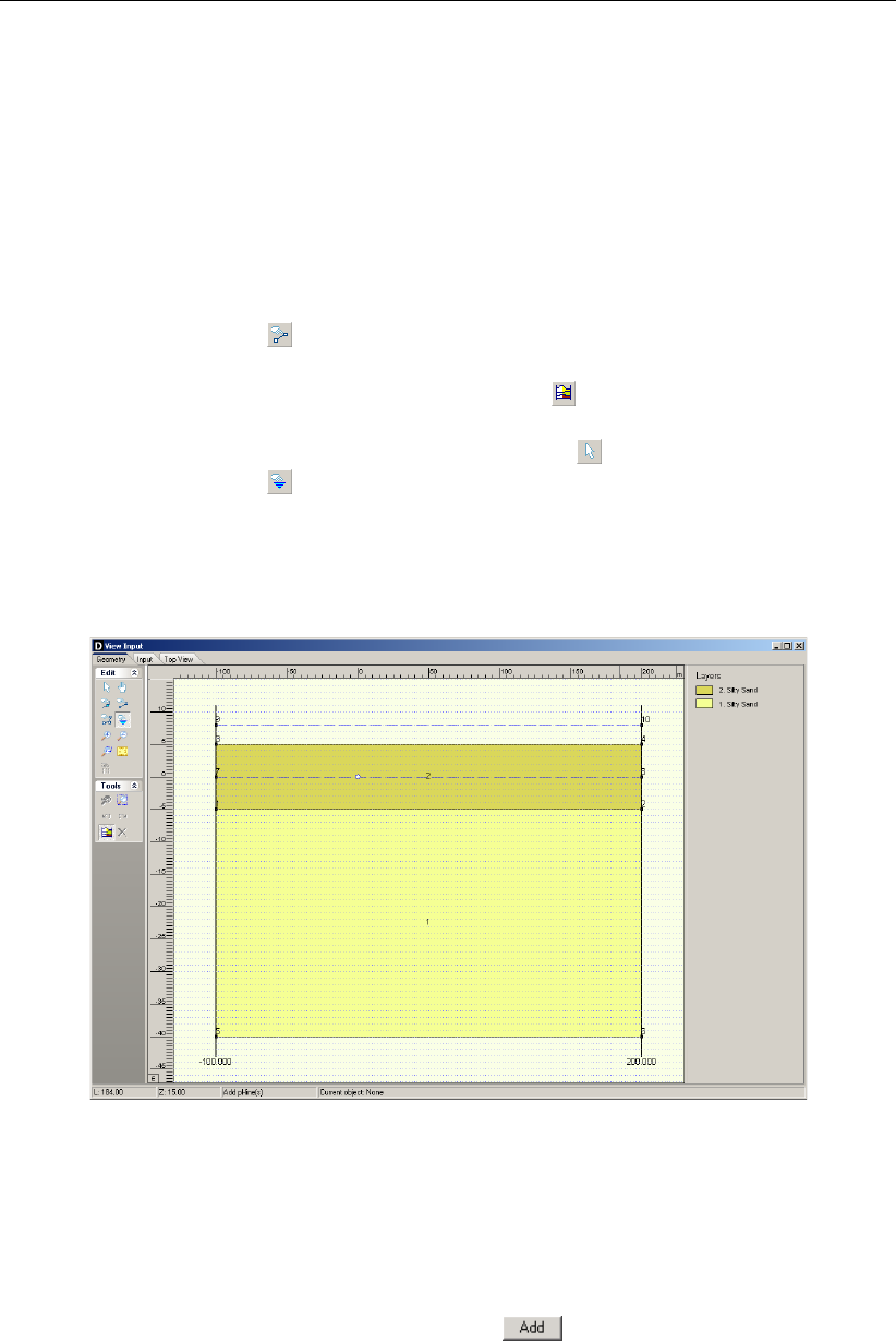
Tutorial 11: Installation of pipeline in a trench
18.3 Geometry of the longitudinal cross section
This tutorial considers a layered soil sequence. The typical Dutch soil sequence of a soft
organic clay layer on top of a coarse sand layer will be considered. The organic clay layer is
compressible and exhibits a low permeability, while the sand layer is assumed incompressible
and exhibits a high permeability. The new soil layers should be specified in the geometry
window.
10. In the View Input window, switch to the Geometry tab to edit the existing soil layer se-
quence.
11. Click the Add single line icon from the Edit sub-window to draw an additional top line of
a soil and position the straight line at Z= -5 m.
12. Click the Automatic regeneration of geometry on/off icon from the Tools sub-window
so that the geometry as shown in Figure 18.3 appears. If the Automatic regeneration of
geometry icon is already selected, click on the Edit icon to regenerate the geometry.
13. Click the Add pl-line(s) icon from the Edit sub-window and position the level of the
artesian groundwater at coordinate Z= 8 m. The blue dashed line, which appears in the
longitudinal cross section, represents the second groundwater line (PL line 2). This second
groundwater line will be used in section 18.5.3 to specify the water pressure distribution in
the sand aquifer.
Figure 18.3: View Input window, Geometry tab
18.4 Soil layer properties
The properties of the soil layers in the layered soil sequence should now be specified.
14. Click Soil and select Materials on the menu bar to enter the soil data.
15. Add a new material by choosing the Add button below the materials list on the left
side of the window. Enter the soil material name <Soft Organic Clay>.
16. Enter the soil data given in Table 18.1.
17. Finish the input of soil data by clicking OK.
Deltares 233 of 324
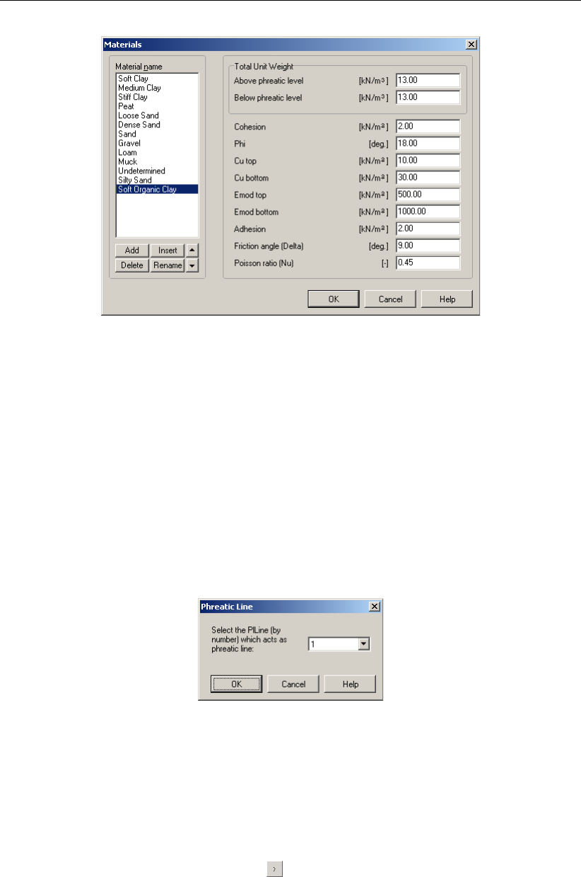
D-GEO PIPELINE
, User Manual
Figure 18.4: Materials window
18.5 Finishing the geometry of the longitudinal cross section
The defined soil properties and the groundwater levels have to be assigned to the drawn ge-
ometry of the longitudinal cross section. The assignments can be carried out in the Geometry
menu.
18.5.1 Phreatic Line
18. Click Geometry and select Phreatic Line on the menu bar to open the Phreatic Line window
(Figure 18.5) and select PL-line <1>as phreatic line for calculation of the groundwater
pressures.
19. Click OK.
Figure 18.5: Phreatic Line window
18.5.2 Layers
20. Click Geometry and select Layers on the menu bar to open the Layers window. Select the
Materials tab to assign the soil properties to the soil layers in the longitudinal cross section.
21. Assign the properties of the defined layer Soft Organic Clay to layer number 2 in the lon-
gitudinal cross section. The defined properties of Soft Organic Clay are assigned to layer
Number 2 by clicking the Assign icon in between the left and the right column (Fig-
ure 18.6).
234 of 324 Deltares

Tutorial 11: Installation of pipeline in a trench
Figure 18.6: Layers window, Materials tab
22. Click on the OK button to quit the window and return to the Geometry tab of the View Input
window to look at the change of layers name in the legend (Figure 18.7).
Figure 18.7: View Input window, Geometry tab
18.5.3 PL-Lines per Layer
23. Click Geometry and select Pl-lines per Layers on the menu bar to open the PL-lines per
Layer window to assign the defined PL–lines to the soil layers in the longitudinal cross
section. Those information’s are used for the calculation of the groundwater pressure
distribution.
24. The groundwater pressure at the top of the Soft Organic Clay layer should be calculated
based on the hydraulic head of PL–line 1, the phreatic line (Figure 18.5). Since the Coarse
Sand layer is an aquifer with an enhanced artesian groundwater pressure, the groundwater
pressure at the bottom of the clay layer should be calculated based on the hydraulic head
of PL–line 2. Of course the water pressure at the top and at the bottom of the coarse sand
layer should be calculated based on the hydraulic head of PL–line 2. This will result in the
Deltares 235 of 324
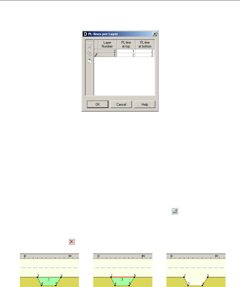
D-GEO PIPELINE
, User Manual
Pl-lines per layer window shown in Figure 18.8.
Figure 18.8: PL-lines per Layer window
25. Click OK to confirm.
26. The geometry can be tested by clicking Geometry on the menu bar and selecting Check
Geometry. If the geometry is entered properly, the message Geometry has been tested
and is OK appears.
27. Click OK to close this window.
18.6 Adding a waterway
A small waterway will now be drawn in the geometry.
28. Select the Geometry tab and select the Add poly line(s) button .
29. Draw a profile line as in Figure 18.9a. Remove points that are not required by clicking the
right mouse button and selecting the option Delete All Loose Lines.
30. Select the top line (between points 3 and 6 as shown in Figure 18.9b.
31. Click the Delete button . This should result in Figure 18.9c.
a) b) c)
Figure 18.9: View Input window, Geometry tab (steps for drawing a waterway)
Now give the exact location of the waterway:
32. Check and enter the exact coordinates of the points by opening the Points window from
the Geometry menu.
33. Enter correct values for points 2, 3, 4 and 5 as shown in Figure 18.10.
236 of 324 Deltares
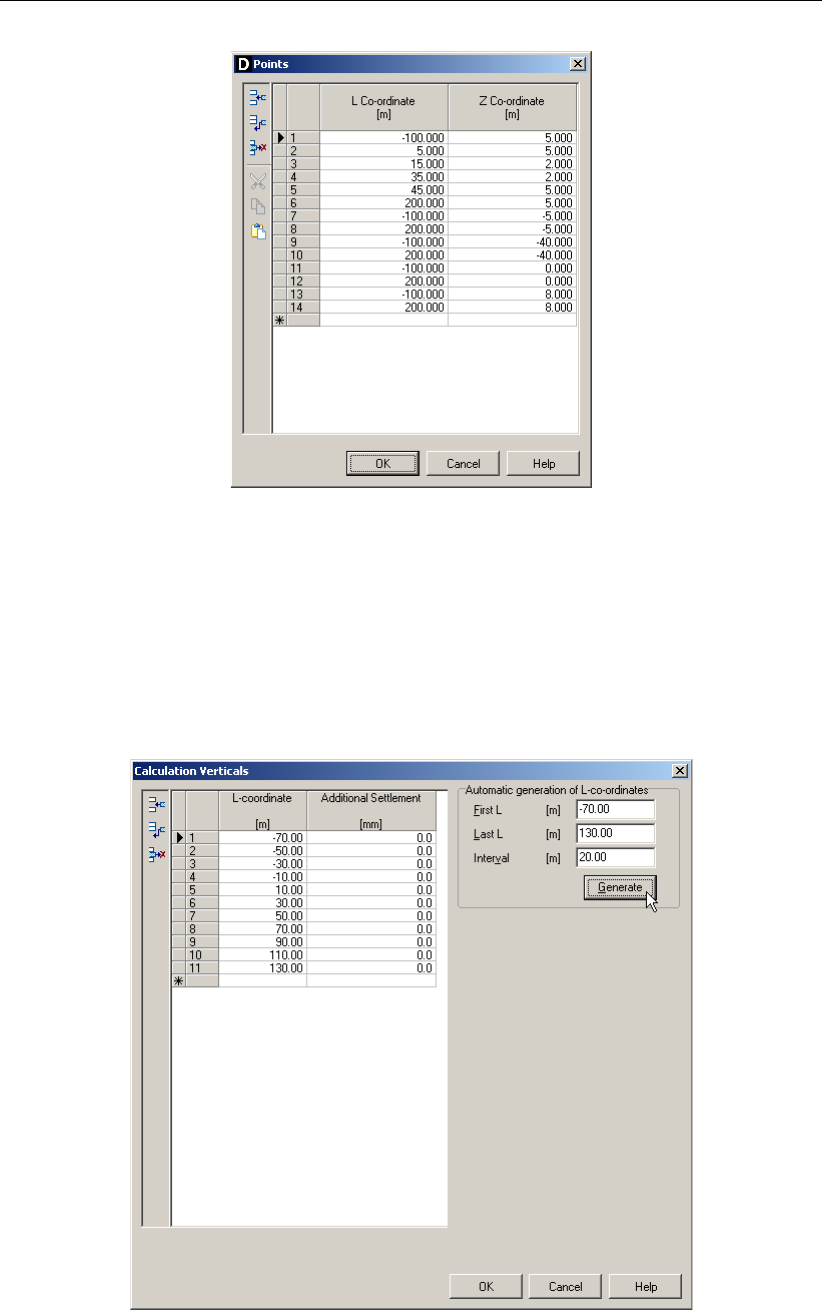
Tutorial 11: Installation of pipeline in a trench
Figure 18.10: Points window
18.7 Calculation Verticals
In the subsequent table the verticals for the location of the calculations are given.
34. Open the Calculation Verticals window.
35. Enter <-70>and <130>for the First and Last L values and an Interval of <20>.
36. Click the Generate button.
Figure 18.11: Calculation Verticals window
Deltares 237 of 324

D-GEO PIPELINE
, User Manual
18.8 Boundaries Selection
To indicate the boundary compressible/uncompressible layers and impermeable/permeable
layers, the top of a specific layer is used. In this case it is evident that this is the top of the
coarse sand layer.
37. From the main menu click GeoObjects and select Boundaries Selection.
38. Select Top of layer <1>as both boundaries.
39. Click OK.
Figure 18.12: Boundaries Selection window
18.9 Trench configuration and pipe material
As the trench passes a small waterway, for practical reasons it has to subduct. An initial
distance of about 1.5 meter is chosen between trench and bottom waterway.
40. Click Pipe and select Pipeline Configuration from the menu bar to open the Pipeline Con-
figuration window.
41. Enter the values as presented in Figure 18.13.
42. Click OK to accept the entries.
Figure 18.13: Pipeline Configuration window
238 of 324 Deltares
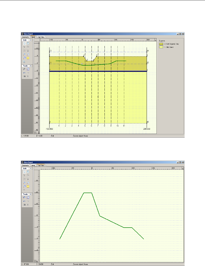
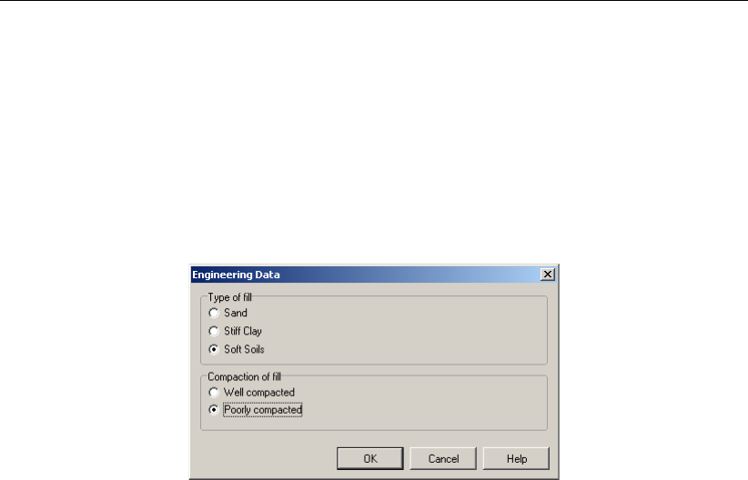
D-GEO PIPELINE
, User Manual
18.10 Engineering Data
Next the engineering data is added. The trench is excavated in organic clay, and filled with
the excavated material, the fill is poorly compacted.
44. Click Pipe from the menu bar and select Engineering Data to open the Engineering Data
window.
45. Select <Soft Soils>as Type of fill and <Poorly compacted>as Compaction of fill.
46. Click OK to confirm.
Figure 18.16: Engineering Data window
18.11 Results: Soil Mechanical Parameters
47. To start the calculations click Calculation and select Start on the menu bar or press the
function key F9.
48. Open the Report window from the Results menu to view the results of the Soil Mechanical
Parameters. The results can be found in paragraph 3.1 (Figure 18.17).
Since the fill of the trench is assigned the property “poorly compacted” a relatively high initial
soil load on the pipe is expected.
240 of 324 Deltares
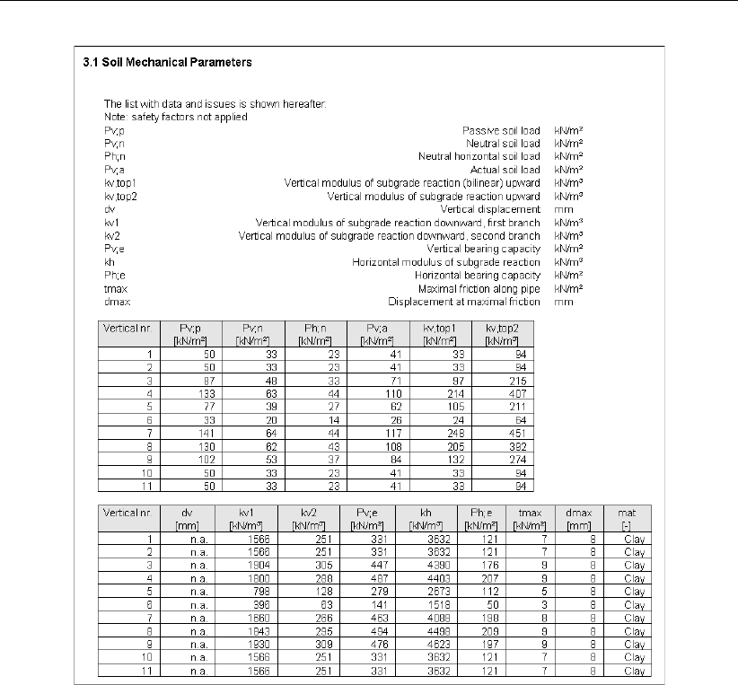
Tutorial 11: Installation of pipeline in a trench
Figure 18.17: Report window, Soil Mechanical Parameters section
The initial soil load Pv;a may be reduced by changing the fill property to “well compacted”
(see Equation 21.9 in section 21.4). Note that in reality this requires an extra compaction
treatment after installation of the pipe. In the software this can be adjusted in the Engineering
Data window under the Pipe menu.
Deltares 241 of 324

D-GEO PIPELINE
, User Manual
242 of 324 Deltares

19 Tutorial 12: Trenching: uplift and heave
This tutorial is the continuation of tutorial 11 (chapter 18) and considers installation of a con-
crete sewer by means of trenching.
The objectives of the exercise are:
To evaluate the risk on heave of the bottom of the trench during installation;
To evaluate possible uplift of the empty pipe after installation.
The following modules are needed:
D-GEO PIPELINE
Standard module (HDD)
Trenching module
This tutorial is presented in the files Tutorial-12a.dri, Tutorial-12b.dri and Tutorial-12c.dri.
19.1 Introduction to the case
During the excavation of a trench the groundwater conditions may play an important role. In
case a trench is excavated below the phreatic groundwater table or in case the hydraulic head
of an aquifer is relatively high, heave of the bottom of the trench is a serious risk. An other
risk, which may occur after excavation of the trench below the phreatic groundwater table, is
the uplift due to fill with a low density soil.
In this tutorial, the top layer consists of peat instead of organic clay. The peat exhibits a low
density. Besides a low density top layer, this tutorial considers a situation with a phreatic
groundwater table at the surface level.
Figure 19.1: Pipeline configuration for Tutorial 12
Deltares 243 of 324
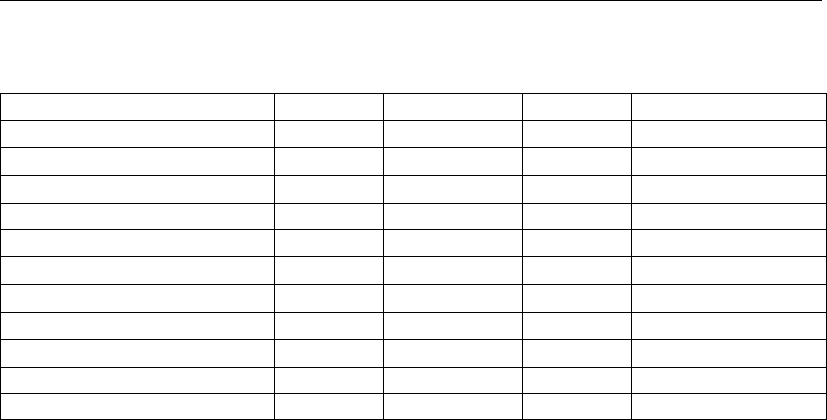
D-GEO PIPELINE
, User Manual
Table 19.1: Layer properties (Tutorial 12)
Silty Sand Peat Soft Organic Clay
Dry unit weight [kN/m3] 18 10.2 13
Wet unit weight [kN/m3] 20 10.2 13
Cohesion [kN/m2] 0 2 2
Angle of internal friction [◦] 10 15 18
Undrained strength top [kN/m2] 0 10 10
Undrained strength bottom [kN/m2] 0 20 30
E modulus top [kN/m2] 10000 1000 500
E modulus bottom [kN/m2] 15000 1500 1000
Adhesion [kN/m2] 0 2 2
Friction angle [◦] 20 5 9
Poisson’s ratio [-] 0.35 0.45 0.45
This tutorial is based on continuation of the file used in Tutorial 11 (chapter 18).
1. Click File and select Open on the menu bar, and select Tutorial-11.
2. Click File and select Save as on the menu bar to open the Save As window and rename
the file into <Tutorial-12a>.
3. Click the Save button to save the file for Tutorial 12a.
4. On the menu bar, click Project and then choose Properties to open the Project Properties
window.
5. Fill in <Tutorial 12 for
D-GEO PIPELINE
>and <Trenching: uplift and heave>for Title 1
and Title 2 respectively in the Identification tab.
19.2 Materials
The soil investigation showed presence of peat layers instead of organic clay. First, peat is
added to the material list.
6. Click Soil and select Materials on the menu bar to open the Materials window.
7. Select the existing Peat material in the left side of the window and enter the values as
given in Table 19.1.
8. Click OK.
244 of 324 Deltares
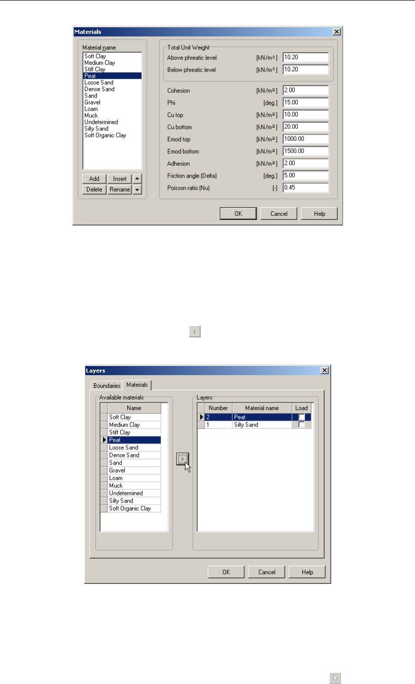
Tutorial 12: Trenching: uplift and heave
Figure 19.2: Materials window
Assign this material type to the top layer:
9. Click Geometry and select Layers on the menu bar.
10. To assign a material to a layer, select the Material tab. Select <Peat>as well as layer
number <2>and via the arrow button assign the soil to the layer (Figure 19.3).
11. Accept the input and return to the main window by clicking OK.
Figure 19.3: Layers window, Materials tab
19.3 Phreatic level
The phreatic line (groundwater table) is located at the surface level in this tutorial.
12. In the Geometry tab of the View Input window, select the Edit button and click on the
PL line 1 in order to select the phreatic line by choosing Select PL Line 1.
13. Once the PL line 1 has been selected, drag it to the surface level by pressing and holding
down the left-hand mouse button while relocating the mouse cursor.
Deltares 245 of 324
D-GEO PIPELINE
, User Manual
14. Check and possibly correct the level of the line as shown in Figure 19.4.
Figure 19.4: PL-Line 1 window
Now the PL-line levels are defined at the correct levels, they have to be assigned to the correct
layers.
15. Open the PL-lines per Layer window from the Geometry menu.
16. Enter the PL–line numbers as given in Figure 19.5.
Figure 19.5: PL-lines per Layer window
19.4 Calculation Verticals
In the subsequent table the verticals for the location of the calculations are given.
17. Open the Calculation Verticals window.
18. Enter <-80>and <180>for the First and Last L values and an Interval of <20>.
19. Click the Generate button.
246 of 324 Deltares
D-GEO PIPELINE
, User Manual
19.5 Factors
The required safety factors must be specified to evaluate the risk on bursting or heave of the
bottom of the trench.
21. Open the Factors window from the Defaults menu.
22. Enter <1.1>and <1.2>for the Safety factor uplift respectively Safety factor heave val-
ues.
23. Click OK.
Figure 19.8: Factors window
19.6 Results
Now the calculations can be performed.
24. To start the calculations click Calculation and select Start on the menu bar or press the
function key F9.
19.6.1 Uplift safety for trenching in Peat layer (Tutorial-12a)
To examine the risk of uplift the graph with the uplift safety factor can be opened
25. Open the Operation Parameters Plots window from the Results menu.
Figure 19.9: Operation Parameter Plots window, Safety uplift tab (Tutorial-12a)
248 of 324 Deltares
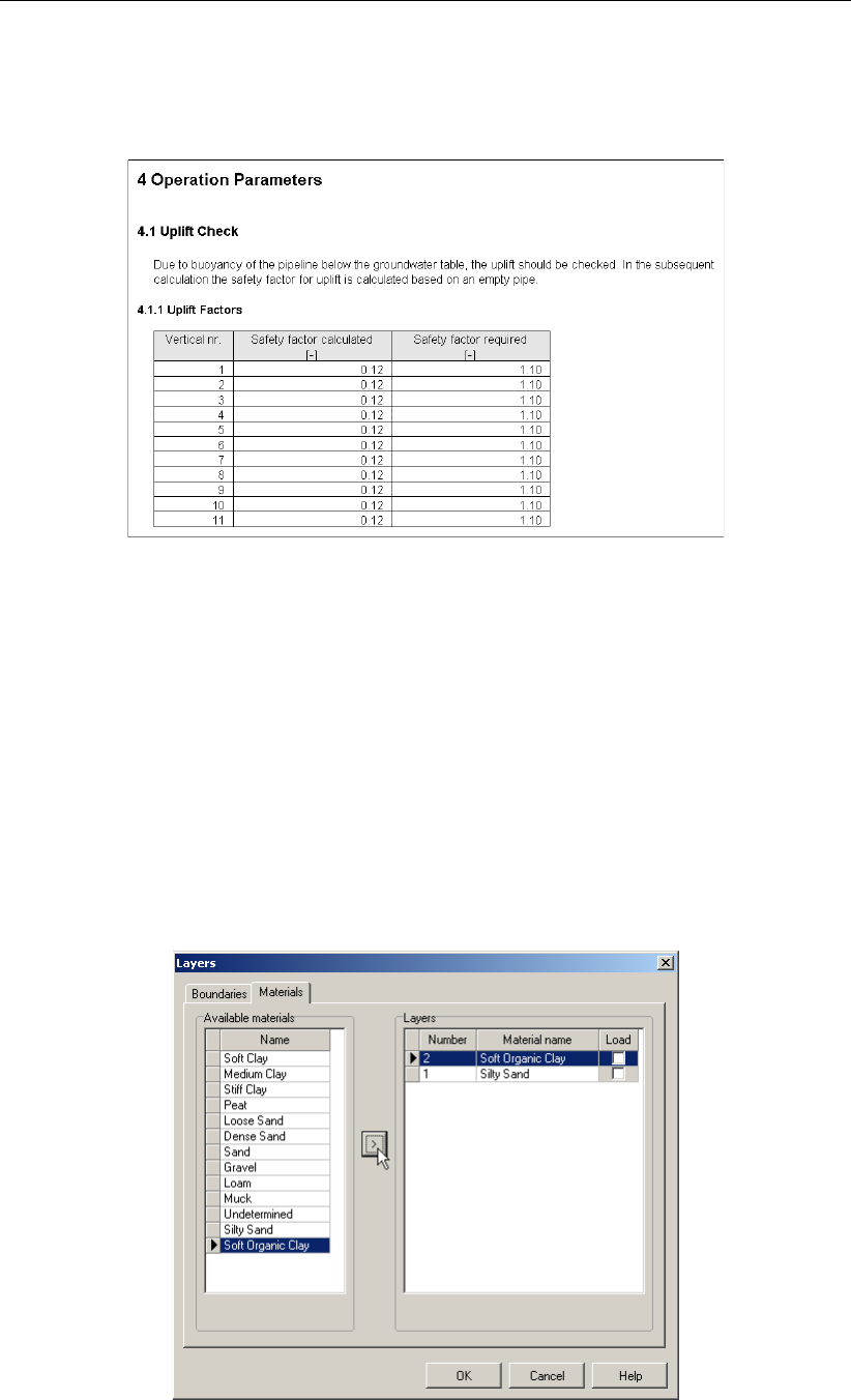
Tutorial 12: Trenching: uplift and heave
For a detailed examination, refer to paragraph 4.1.1 of the Report window (Figure 19.10). As
can be seen, the uplift safety of the trenched pipe is not OK as the calculated uplift factor
(0.12) is lower than the required uplift factor (1.1).
Figure 19.10: Report window, Uplift Factors section (Tutorial-12a)
19.6.2 Uplift safety for trenching in Soft Organic Clay layer (Tutorial-12b)
The trench fill should be modified. The low density of the peat causes uplift problems. The
effect of filling the trench with organic clay can easily be checked by changing the soil se-
quence.
26. Click File and select Save as on the menu bar to open the Save As window and rename
the file into <Tutorial-12b>.
27. Click the Save button to save the current project as Tutorial 12b.
28. Click Geometry and select Layers on the menu bar to open the Layers window. Select the
Materials tab (Figure 19.11) to assign the soil properties to the soil layers in the longitudinal
cross section.
Figure 19.11: Layers window, Materials tab (Tutorial-12b)
Deltares 249 of 324
D-GEO PIPELINE
, User Manual
29. Assign the properties of the defined layer Soft Organic Clay to layer Number 2 in the
longitudinal cross section. The defined properties of Soft Organic Clay are assigned to
layer Number 2 by clicking the Assign icon in between the left and the right column.
30. Click on the OK button to quit the window and return to the Geometry tab of the View Input
window to look at the change of layers name in the legend.
31. To start the calculations again click Calculation and select Start on the menu bar or press
the function key F9.
32. Open the Operation Parameters Plots window from the Results menu.
33. Open the Report window from the Results menu.
34. Go to paragraph 4.1.1 of the report (Figure 19.12). As can be seen, the uplift safety of the
trenched pipe is still not OK as the calculated uplift factor (0.12) is lower than the required
uplift factor (1.1).
Figure 19.12: Report window, Uplift Factors section (Tutorial-12b)
19.6.3 Hydraulic Heave Safety
To examine the risk of heave of the trench bottom the graph with the heave safety factor can
be opened.
35. Select the Safety hydraulic heave tab of the Operation Parameters Plots window (Fig-
ure 19.13).
250 of 324 Deltares
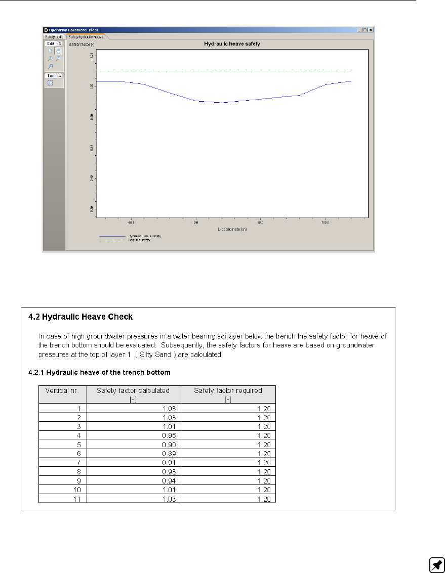
Tutorial 12: Trenching: uplift and heave
Figure 19.13: Operation Parameter Plots window, Safety hydraulic heave tab (Tutorial-
12b)
Figure 19.14: Report window, Hydraulic heave of the trench bottom section (Tutorial-12b)
Note: In the report (Figure 19.14) the hydraulic heave safety of the trenched pipe is not OK for
all verticals, the calculated safety factors are lower than the required safety factor specified at
the default factors. Especially below the waterway the risk on bursting or heave of the bottom
of the trench is relatively high.
19.7 Lowering the hydraulic head (Tutorial-12c)
The problem of heave of the bottom of the trench can be solved by drainage of the subsequent
silty sand layer. By dewatering the silty sand layer, the hydraulic head can be lowered to the
required level. Lowering the level of the hydraulic head in the silty sand layers can be done as
follows:
36. Click File and select Save as on the menu bar to open the Save As window and rename
Deltares 251 of 324

D-GEO PIPELINE
, User Manual
the file into <Tutorial-12c>.
37. Click the Save button to save the current project as Tutorial 12c.
38. Return to the Geometry tab of the View Input window and select the button Add point(s)
to boundary / PL-line .
39. Click the four additional points on PL-line 2 as shown in Figure 19.15 (points 15 to 18).
40. Click the Geometry option from the menu bar and select the option Points. In the Points
window, enter the co-ordinates of points 15 to 18 (i.e. PL-line number 2 for the hydraulic
head in the sand layer) as given in Figure 19.16.
Figure 19.15: View Input window, Geometry tab (Tutorial 12c)
Figure 19.16: Points window (Tutorial 12c)
Now the results can be checked:
41. Start the calculations by clicking Start on the Calculation menu bar or by pressing the
function key F9.
252 of 324 Deltares

Tutorial 12: Trenching: uplift and heave
42. Open the Operation Parameter Plots window from the Results menu and select the Safety
hydraulic heave tab.
From the plots (Figure 19.17), it is clear that the drainage yields a higher calculated safety
factor for hydraulic heave safety.
Figure 19.17: Operation Parameter Plots windows, Safety hydraulic heave tab (Tutorial
12c)
43. Open the Report window to look at the calculated values (Figure 19.18): the minimum
calculated safety factor for Hydraulic Heave is 1.46 which is more than the required factor
of 1.20.
Figure 19.18: Report windows, Hydraulic heave of the trench bottom section (Tutorial
12c)
Deltares 253 of 324

D-GEO PIPELINE
, User Manual
254 of 324 Deltares

20 Design of a pipeline
D-GEO PIPELINE
can be used for designing a pipeline using four different techniques:
the HDD technique (section 20.1)
the micro-tunneling technique (section 20.2)
the trench technique (section 20.3)
20.1 Design of a pipeline crossing using the HDD technique
The horizontal directional drilling technique is used to install pipelines. A pipe is installed
from one point in a geometry with soil materials to another by means of horizontal directional
drilling.
D-GEO PIPELINE
can be used for the design of pipelines or the assessment of prelimi-
nary designs of pipelines constructed by means of horizontal directional drilling. Calculations
are based on the pipeline configuration, the drill pipe and borehole dimensions and the drilling
fluid data.
D-GEO PIPELINE
calculates the maximum allowable drilling fluid pressure and the
minimum drilling fluid pressure at user-specified calculation verticals.
The configuration of a proposed pipeline that has to cross an object is determined by:
the location of the entry and exit points (section 20.1.1)
the entry and exit angles (section 20.1.2)
the limitations of the object to be crossed, specified by the owner of the objects con-
cerned (section 20.1.3)
the minimum value of curve radius (section 20.1.4)
the value of the combined bending radius (section 20.1.5)
20.1.1 Location of entry and exit points
The entry point is the location where the drilling rig is positioned during the pilot drilling. The
exit point is located at the other side of the object that has to be crossed. When the locations
of the entry and exit points are determined, it must be taken into account that a minimum
distance is required to the object in order to cross the object at a sufficient depth.
20.1.2 Inclination at the entry and exit points
The magnitude of the entry and exit angle is usually between 6◦and 15◦. The angle can be
larger for small drilling rigs. The greater the bending stiffness of the pipeline is, the smaller
the entry and exit angles are. Before starting to drill the curved parts of the drilling line, the
first 30 to 40 m (3 to 4 drill pipes) must be drilled in a straight line. The magnitude of the exit
angle influences the pull-back operation of the pipe through the borehole. The larger the exit
angle, the higher the pipeline has to be lifted in order to pull it into the borehole. A small exit
angle increases the risk that a blow-out will occur.
20.1.3 The limitations of the object to be crossed
The owner or manager of the object to be crossed may have certain requirements with regard
to the crossing depth of the pipeline. Such requirements can be related to the presence
of sheet piles or foundation piles. Another reason for special requirements can involve the
building plans of structures on piles. Such points are boundary conditions for preparing the
pipeline configuration.
Deltares 255 of 324
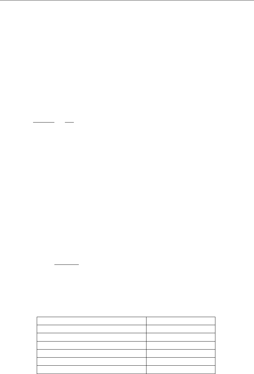
D-GEO PIPELINE
, User Manual
20.1.4 Determination of allowable curve radius
The borehole containing a pipeline is usually characterized by an upward and a downward
curve. Sometimes a horizontal or combined radius forms part of the drilling line. The smallest
possible radius of such a curve depends on the bending stiffness and the yield stress of the
pipeline or the drill pipes. For pipes with a relatively small bending stiffness, such as PE pipes,
the stiffness of the drill pipes is often the determining factor for the minimum radius of curved
sections in the drilling line.
Allowable curve radius for steel pipes
The design radius should be checked for strength:
R≥γ×Eb
Reb ×Do
2(20.1)
where:
Ebis the modulus of elasticity of the pipe material, in kN/m2;
Dois the outer diameter of the pipe, in m;
γis the partial safety factor for the bending moment;
Reb is the minimum specified yield strength, in kN/m2.
(For a pipeline with the following properties: Eb= 210000 N/mm2;Reb = 240 N/mm2;γ= 1.1,
about half the strength of the steel is available for bending stresses, while the remaining half
is used for stresses due to pulling force, internal pressure, etc. . . )
The design radius Rfor steel pipes should also be checked for soil reaction pressure due to
bending, according to article E.1.4 of NEN 3650-1:
R≥1000 ×Dofor small pipe diameter (Do≤0.4 m)(20.2)
R≥C×pDo×dnfor large pipe diameter (Do>0.4 m)(20.3)
where Cis a constant (without dimension) depending on the soil type as shown in Table 20.2.
Table 20.2: Values of constant C (according to table E.1 of NEN 3650-1)
Soil type C[-]
Dense packed sand 8500
Moderate packed sand 9400
Loose packed sand 10200
Stiff Clay 10500
Medium stiff clay 11500
Soft clay and Peat 12500
In
D-GEO PIPELINE
, the soil type is a function of the cohesion and the friction angle of the soil,
as shown in Table 20.3.
256 of 324 Deltares

Design of a pipeline
Table 20.3: Soil type as a function of the cohesion and the friction angle
Soil type ϕ[◦]c[kN/m2] Constant C[-]
Dense sand ϕ > 32.5 c≤0.5 8500
Medium dense sand ϕ > 32.5 c > 0.5 9400
Medium dense sand 30 < ϕ ≤32.5 9400
Loose sand 25 < ϕ ≤30 c≤1 10200
Stiff sandy clay 25 < ϕ ≤30 c > 1 10500
Stiff sandy clay 22.5 < ϕ ≤25 c > 5 10200
Clayey sand 22.5 < ϕ ≤25 c≤5 10500
Stiff clay 20 < ϕ ≤22.5 c > 10 10500
Medium stiff clay 20 < ϕ ≤22.5 c≤10 11500
Stiff clay 17 < ϕ ≤20 c > 10 10500
Medium stiff clay 17 < ϕ ≤20 5 < c ≤10 11500
Soft clay 17 < ϕ ≤20 c≤5 12500
Peat /organic clay ϕ≤17 12500
In the case of a layered sub-soil, the highest C-value of a layer with a significant thickness is
normative. In the case of a sub-soil with an alternation of layers with relative small thicknesses,
a weighted interpolation can be performed to determine the C-value:
Cd=
n
X
i=1 Ci×di
dtotal with dtotal =
n
X
i=1
di(20.4)
where:
nis the total number of layers in the curve;
Ciis the C-value of layer i;
diis the thickness of layer i, in m;
dtotal is the total thickness of all layers in the curve, in m.
Allowable curve radius for polyethylene pipes
According to article 8.6.4 of NEN 3650-3 (NEN,2012c), the minimal curve-radius for PE pipes
is equal to the bending factor as given in Table 20.5 times the diameter.
Table 20.5: Bending factor (acc. to table 6 of NEN 3650-3)
Diameter in mm Bending factor
63 →160 50
200 →250 75
315 →355 100
400 →630 100
710 →800 125
Deltares 257 of 324
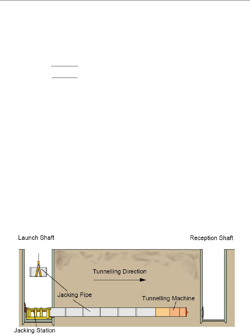
D-GEO PIPELINE
, User Manual
20.1.5 Determination of combined bending radius
In case the horizontal bending radius coincides with part of a vertical bending radius, a com-
bined 3-dimensional bending radius is formed. For the design of the horizontal directional
drilling line, the pull back force and the strength calculation it is necessary to determine the
value of the 3-dimensional bending radius. This value can be determined as follows:
Rcombi =sR2
h×R2
v
R2
h+R2
v
(20.5)
where:
Rcombi is the combined bending radius, in m;
Rhis the horizontal bending radius, in m;
Rvis the vertical bending radius, in m.
20.2 Design of a pipeline crossing using the micro tunneling technique
The micro tunneling technique is often used for installation of pipelines and small tunnels in
densely populated areas. Micro tunneling usually starts horizontal at a certain level below
the surface in a so-called launch shaft. The pipe segments included in the micro tunneling
machine are placed behind the tunneling machine and pushed in the direction of the reception
shaft by means of a jacking frame (Figure 20.1).
The so-called thrust force which has to be provided by the jacking frame is an important
parameter in the design of tunnels and pipelines installed by means of micro tunneling. Of
course the jacking frame must be able to produce this force.
Figure 20.1: Launch and reception shafts of the micro tunneling machine
20.3 Design of a pipeline using a trench
Very often, under normal circumstances, pipelines are installed in an excavated trench. In
the not very densely populated areas such as agricultural areas and not developed areas, the
slopes of the trenches can often be excavated under.
The main risk associated with trenching is instability of the slopes of the trench. This risk is can
not be considered in
D-GEO PIPELINE
. Use of other computer programs such as
D-GEO STABILITY
is recommended to evaluate this risk.
258 of 324 Deltares
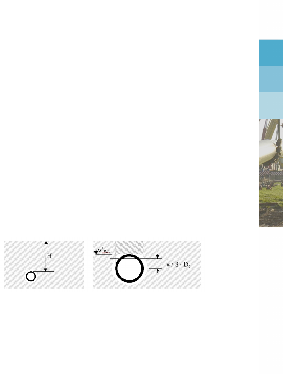
21 Calculation of soil mechanical data
This section includes background information on the calculation of:
neutral vertical stress (section 21.1)
passive vertical stress (section 21.2)
reduced vertical stress (section 21.3)
actual vertical stress (section 21.4)
neutral horizontal stress (section 21.5)
vertical modulus of subgrade reaction (section 21.6)
horizontal modulus of subgrade reaction (section 21.7)
ultimate vertical bearing capacity (section 21.8)
ultimate horizontal bearing capacity (section 21.9)
vertical displacement (section 21.10)
maximal axial friction and friction displacement (section 21.11)
displacement at maximal friction (section 21.12)
global determination of the soil type (section 21.13)
traffic load (section 21.14)
If the definition of some parameters in the equations of this chapter is missing, refer to sec-
tion 1.7.
21.1 Neutral vertical stress
Figure 21.1: Schematic diagram for calculation of the neutral vertical stress
According to article C.4.2.2 of NEN 3650-1 (NEN,2012a), the neutral vertical stress qnis
defined as (Figure 21.1):
qn=σ0
v(H) + (0.5−π/8) ×γ0×Do(21.1)
where:
σ0
v(H)is the vertical effective stress at depth H, in kN/m2:
σ0
v(H) = γunsat ×H1+ (γsat −γw)×H2(see Figure 21.2 for the definition of
H1and H2).
His the soil cover above the top of the pipe, in m (see Figure 21.2).
γ’ is the effective unit weight of the soil, in kN/m3:γ0=γunsat above the phreatic
line and γ0=γsat −γwbelow the phreatic line.
Deltares 259 of 324
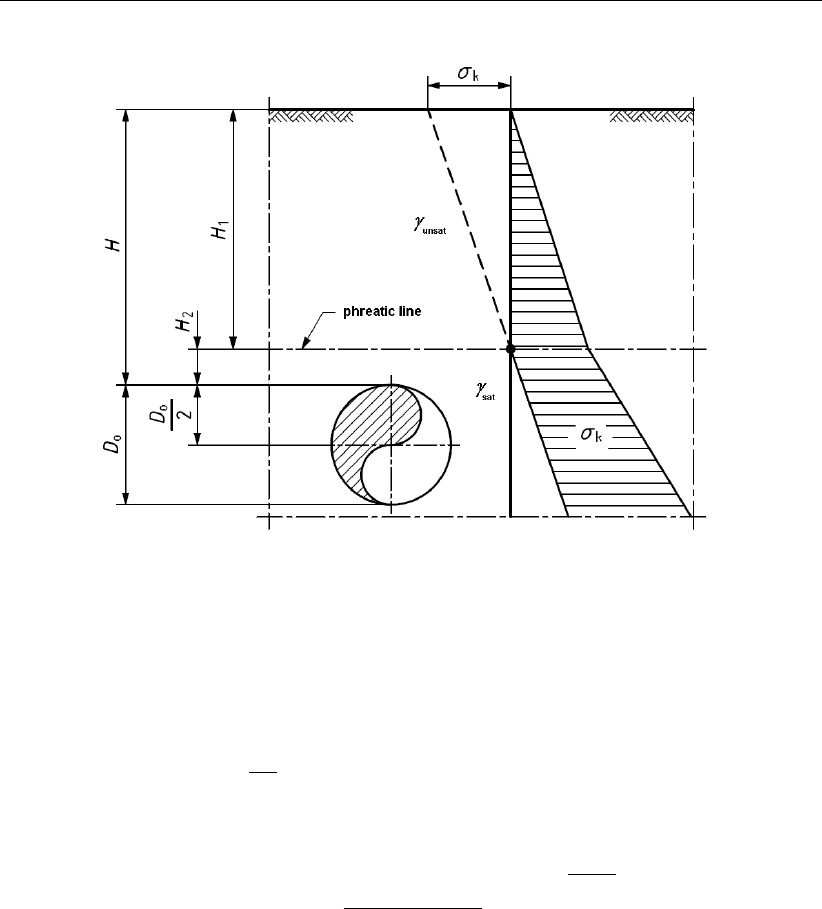
D-GEO PIPELINE
, User Manual
Figure 21.2: Schematic diagram for the definition of parameters H1,H2,γunsat and γsat
(Figure C.5 of NEN 3650-1)
21.2 Passive vertical stress
According to article C.4.2.4.2 of NEN 3650-1, the passive vertical stress qpis defined as:
qp=qn×1+0.3H
Do≤p0
max (21.2)
with:
p0
max = (p0
f+c×cot ϕ)×"0.5×Do
0.5×Do+H2
+q#
−sin ϕ
1+sin ϕ
−c×cot ϕ(21.3)
where:
p0
max is the maximum passive vertical stress, in kN/m2;
p0
fis σ0
0(1 + sin ϕ) + c×cos ϕ, in kN/m2;
qis (σ0
0×sin ϕ+c×cos ϕ)/G, in kN/m2;
σ0’ is the effective isotrope stress, in kN/m2:σ0
0= (σ0
v+σh)/2;
σv,h’ is the vertical respectively horizontal effective stress;
c,ϕ,Gare the soil parameters at the pipe center.
260 of 324 Deltares
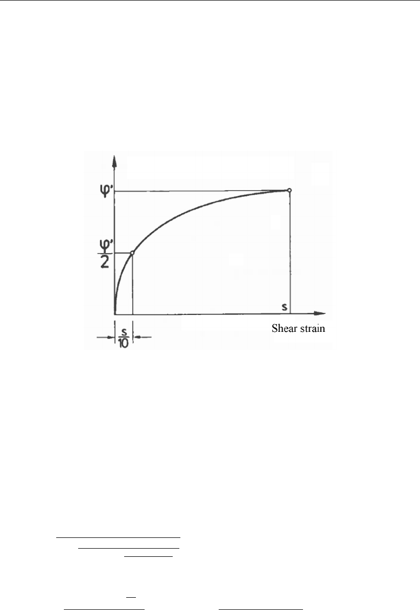
Calculation of soil mechanical data
21.3 Reduced neutral vertical stress
In case a drilling technique is used for the installation of the pipeline, the vertical soil load is
reduced due to arching. A pipeline installed using the horizontal directional drilling technique
is loaded by a strongly reduced soil loads due to arching. For micro tunneling the effect of
arching on the soil load is calculated by
D-GEO PIPELINE
as well. Due to the relative small
borehole arching is not completely developed. The relatively small available strain yields
incomplete mobilization of the shear strength. The soil load in case of micro tunneling should
therefore be calculated using half the value of the angle of internal friction.
Figure 21.3: The mobilization of the angle of internal friction in the development of the
arching mechanism
21.3.1 Reduced neutral vertical stress in compressible soil layers
According to article C.4.8.3 of NEN 3650-1 (NEN,2012a), in compressible soil layers (i.e. clay
and peat), the reduced neutral vertical stress qn,r is defined as:
qn,r =h×γ0−Fr/2B1if z > 8B1
qnif z≤8B1
(21.4)
with:
Fr=0.9Fmax
1 + B1×(3H−2h)×α
2C×Hδd+Fmax
2B1×kv;drill fluid
(21.5)
Fmax = 2B1×(h×γ0−qn,r1)(21.6)
qn,r1 =
B1×γ0−c
B1
K×tan ϕ×1−exp −K×tan ϕ×h
B1 (21.7)
where:
B1is the half width of the covered ground column, in m:
B1= 0.5Do+Do×tan (45◦−ϕb/2 ) ≥R;
ϕbis the average friction angle over the height of the borehole, in degree;
his the soil cover above the borehole, in m (see Figure 21.4);
c,ϕ,γ’ are the average soil parameters between the surface and the pipe center;
Fris the permanent friction due to arching effect, in kN/m2:
Deltares 261 of 324
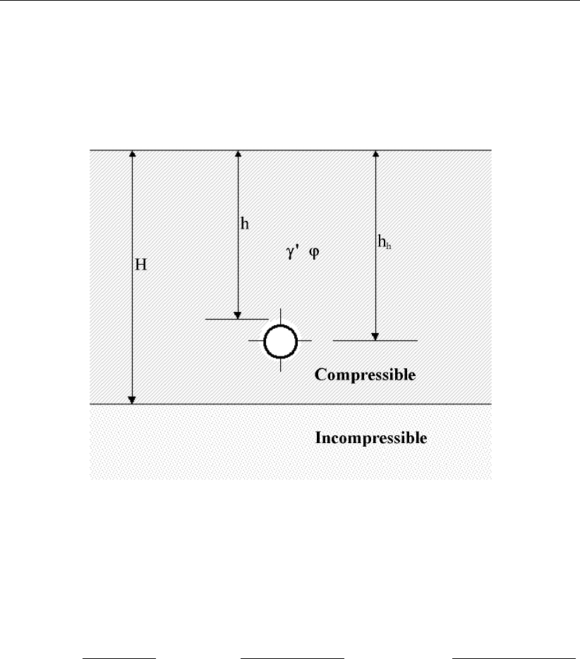
D-GEO PIPELINE
, User Manual
Fmax is the maximal adhesion, in kN/m2;
qn,r1 is the reduced neutral vertical stress on the pipe, in kN/m2;
His the thickness of the compressible layers, in m (see Figure 21.4);
αis a dimensionless factor: α= ln(h/href)with href = 1 m;
Figure 21.4: Definitions of H,hand hh
21.3.2 Reduced neutral vertical stress in non-compressible soil layers
According to articles C.4.8.3 and C.4.8.4 of NEN 3650-1 (NEN,2012a), in incompressible soil
layers (i.e. sand) situated below compressible soil layers, the reduced neutral vertical stress
qn,r is defined as (if h > 8B1):
qn,r =B1×γ0
K×tan ϕ1−exp −K·tan ϕ·hp
B1+σcexp −K×tan ϕ×hp
B1
(21.8)
where:
γ’ is the average effective unit weight of the soil between the compressibility border
and the pipe center, in kN/m3;
hpis the soil cover above the borehole in the incompressible layers (see Figure 21.5),
in m;
ϕis the average friction angle between the compressibility border and the pipe center,
in degrees;
σcis the vertical effective stress at the compressibility border, in kN/m2(see Fig-
ure 21.5).
262 of 324 Deltares

Calculation of soil mechanical data
Figure 21.5: Schematic diagram of Hand hp
If hp<8B1,Equation 21.8 is not applicable for the determination of qn,r. In such case, the
following applies:
1) 0< hp<2B1:qn,r is constant and equal to qn,r-border, see section 21.3.1;
2) 2B1≤hp≤4B1: interpolation between qn,r-border and qn,r-incompressible for
hp= 4B1;
3) hp≥4B1:qn,r-incompressible as a function of hp.
If qn,r-incompressible (hp= 4B1) is larger than qn,r-border, then 1) is prescribed and 2) is
applicable for 0< hp<4B1.
21.4 Initial vertical stress
According to article C.4.2.3 of NEN 3650-1 (NEN,2012a), the initial vertical stress qk(also
called actual vertical stress) for construction in trench is defined as:
qk=qn+kv,tot ×µ×Do≤qp(21.9)
with:
1
kv,tot
=1
kv,top
+1
kv,pipe
+1
kv,bottom
(21.10)
kv,pipe =EIw
ky×Do×D3
g
(21.11)
where:
qnis the neutral vertical stress of the soil, in kN/m2, see Equation 21.1;
qpis the passive vertical stress of the soil, in kN/m2, see Equation 21.2;
kv,tot is the vertical modulus of subgrade reaction upward, in kN/m3, see Equa-
tion 21.15;
Deltares 263 of 324
D-GEO PIPELINE
, User Manual
kv,bottom is the minimum vertical modulus of subgrade reaction downward, in kN/m3, cal-
culated according to section 21.6.2;
kv,pipe is the vertical modulus of subgrade reaction of the pipe, in kN/m3;
µis the percentage of compaction depending on the type of fill and type of com-
paction as shown in Table 21.7.
Table 21.7: Values of parameter µaccording to NEN 3650-1
Compaction Type of fill
Soft soil Stiff clay Sand
Poorly 0.20 0.15 0.075
Well 0.10 0.075 0.02
21.5 Neutral horizontal stress
21.5.1 Pipelines installed using the HDD technique
According to article C.4.8.6 of NEN 3650-1, the neutral reduced horizontal soil load qh,r for a
pipeline installed using the horizontal drilling technique can be calculated using the following
equation:
qh,r =qn,r ×(1 −sin ϕdf)(21.12)
where:
qn,r is the reduced neutral vertical stress of the soil, in kN/m2, as calculated in sec-
tion 21.3;
ϕdf is the angle of internal friction of the drilling fluid, as defined in the Engineering
Data window (section 4.6.3.1). The default value is 15◦.
21.5.2 Pipelines installed in a trench or using micro tunneling
The neutral horizontal soil load qh,n for a pipeline installed in a trench or using the micro
tunneling technique can be calculated using the following equation:
qh,n =qn×(1 −sin ϕb)(21.13)
where:
qnis the neutral vertical stress of the soil, in kN/m2, as calculated in Equation 21.1 in
section 21.1;
ϕbis the average angle of internal friction of the soil over the height of the borehole.
In micro tunneling the space in between the pipeline or tunnel is usually relatively small,
moreover the space in between the bore hole wall and the pipeline or tunnel is often filled with
grout after installation.
264 of 324 Deltares
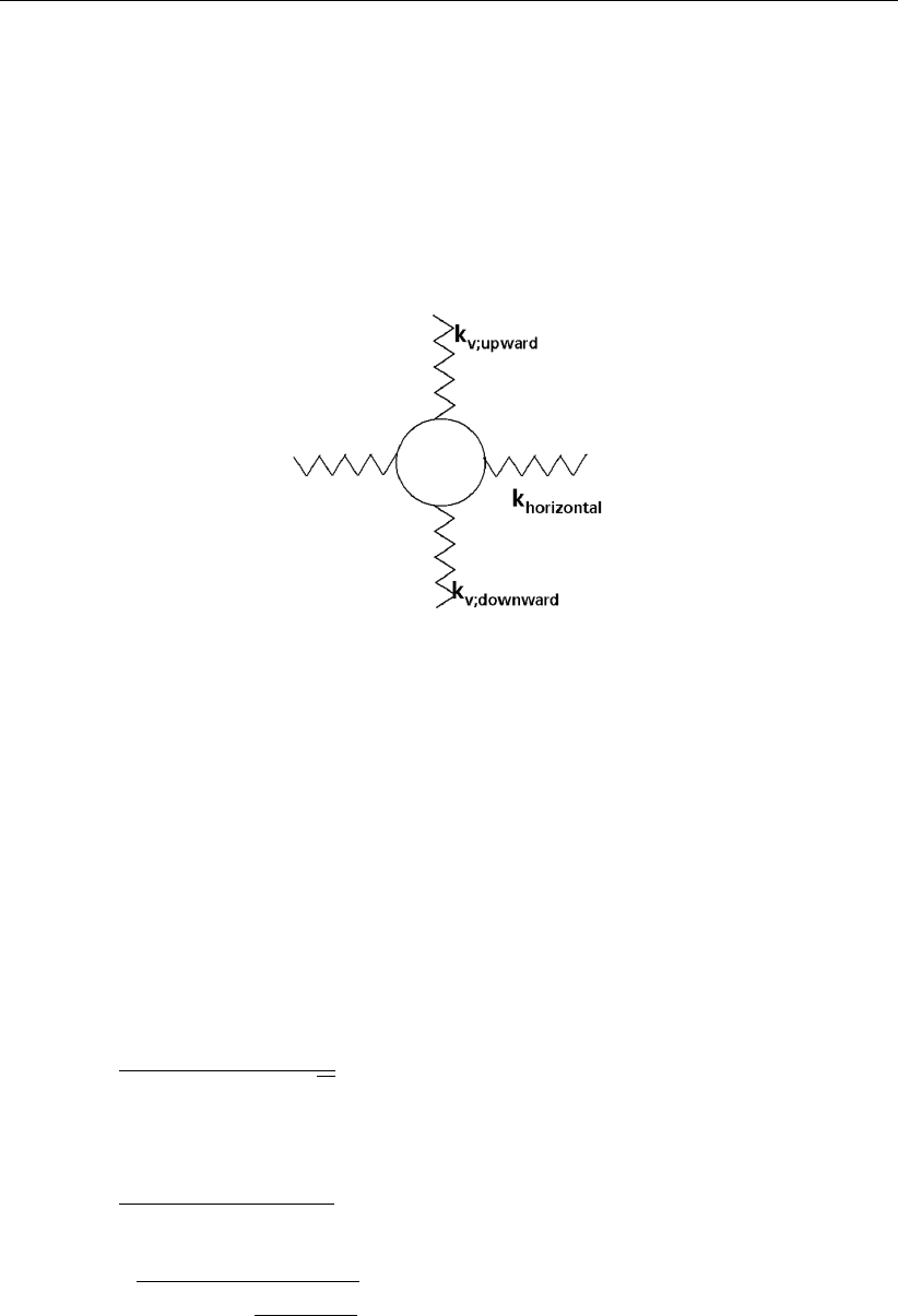
Calculation of soil mechanical data
21.6 Vertical modulus of subgrade reaction
Due to the soil-pipe interaction, induced by either the pipe or the soil, soil deformations and
pipe displacement will occur. The deformations lead to increase or decrease of the soil load on
the pipe. This soil reaction behavior is modeled by using a spring model. By locating springs
around the pipe, the displacement and related stress changes can be calculated (Figure 21.6).
The increase or decrease of the soil reaction stress is usually calculated by linear or bi-linear
springs. The stiffness of the spring is expressed as a modulus of subgrade reaction.
Figure 21.6: Pipe soil interaction modeled by springs
Since the soil-pipe interaction is influenced by the installation method, different calculation
methods to determine the moduli of subgrade reaction exist:
For installation using a drilling technique (HDD or micro tunneling), refer to section 21.6.1;
For Installation in a trench, refer to section 21.6.2;
21.6.1 Pipelines installed using a drilling technique
According to article C.4.3.3 c) of NEN 3650-1, the stiffness of the spring below (kv,bottom) and
above the pipe (kv,top) is:
kv=fE×E
m×(1 −ν2)×√A(21.14)
with:
m=52.31 + `/b
51.90 + 3.596 ×`/b
`=π/λ
λ=4
rkv×fkv ×Do
4Eb×Ib
where:
E,νare the average parameters of the soil along a distance of 5 Doabove the top of
the pipeline for kv,top and below the bottom of the pipeline for kv,bottom;
Ais `×b= support area, in m2;
bis the minimum support width, in m: b=Do;
`is the minimum support length, in m;
λis the characteristic stiffness pipeline-soil, in m−1;
Deltares 265 of 324
D-GEO PIPELINE
, User Manual
Ibis the moment of inertia of the pipeline, in m4:Ib=π
64 D4
o−(Do−2dn)4
mis the shape coefficient, depending on `/b.
21.6.2 Pipelines installed in a trench
Vertical modulus of subgrade reaction upward
According to article C.4.3.2 of NEN 3650-1, the vertical modulus of subgrade reaction upward
are:
v,top =qp−qn
zmax
(21.15)
kv,top,max =qp
zmax
(21.16)
with:
zmax =0.25 ×Do
E1.5×qH
Do
for clay and peat (21.17)
zmax =0.20 ×Do
E0.5×qH
Do
for sand (21.18)
where:
qpis the passive vertical soil load, see Equation 21.2;
qnis the neutral vertical soil load, see Equation 21.1;
zmax is the maximum displacement, in m;
Eis the average Young’s modulus of the soil along a distance of 5 Doabove the top
of the pipeline, in MPa;
His the soil cover above the top of the pipe, in m.
Vertical modulus of subgrade reaction downward
The vertical modulus of subgrade reaction downward is characterized by a bi-linear spring.
kv,1 is the modulus of subgrade reaction in between 0 and 2/3 of the vertical bearing capacity,
while kv,2 is the modulus of subgrade reaction in between 2/3 of the vertical bearing capacity
and the vertical bearing capacity.
For clay and peat, the modules of subgrade reaction downward are:
kv,1 = 0.25 ×cu×Pwe
Do
(21.19)
kv,2 = 0.04 ×cu×Pwe
Do
(21.20)
For sand, the modules of subgrade reaction downward are:
kv,1 = 0.5×E×Pwe
Do
(21.21)
kv,2 = 0.1×E×Pwe
Do
(21.22)
266 of 324 Deltares

Calculation of soil mechanical data
where cuand E(in kN/m2respectively MN/m2) are the average parameters of the soil along
a distance of 5 Dobelow the bottom of the pipeline and Pwe is the vertical bearing capacity
determined according to section 21.8.
If cuis nil, a fictive undrained cohesion is used by the program:
cu,fictive =1
2(1 + K0)×σ0
h×sin ϕ+c×cos ϕ(21.23)
21.7 Horizontal modulus of subgrade reaction
21.7.1 Pipelines installed using a drilling technique
The horizontal modulus of subgrade reaction is:
kh= 0.7kv,bottom (21.24)
where kv,bottom is the vertical modulus of subgrade reaction at the bottom of the pipe as deter-
mined in Equation 21.14.
21.7.2 Pipelines installed in a trench
According to article C.4.3.4.1 of NEN 3650-1, the horizontal modulus of subgrade reaction
upward is:
kh=qhe
ymax ×(1 −0.3×B)
A(21.25)
where:
qhe is the ultimate horizontal bearing capacity, see Equation 21.29;
ymax is the maximal displacement, in m: ymax =Do×h0.05 + 0.03 ×Z
Do+ 0.5i
Ais a constant (A= 0.145);
Bis a constant (B= 0.855).
21.8 Ultimate vertical bearing capacity
According to article C.4.4.2 of NEN 3650-1 (NEN,2012a), the ultimate vertical bearing capac-
ity is:
Pwe = 0.95 [0.5γ0B NγSγdγ+SqNqdq(qn+c×cot ϕ)−c×cot ϕ]
(21.26)
where:
c,ϕ,γ’ are the average soil parameters along the sliding plane;
Bis the width of the foundation element, in m (for pipeline: B=Do);
Zis the depth until the pipe, in m: Z=H+Do/2;
His the soil cover above the pipe, in m;
Lis the length of the foundation element, in m: L= 10 B;
Nγis the bearing capacity factor for the effect of the effective weight of the soil under
the foundation surface: Nγ= 1.5×(Nq−1) ×tan ϕ
sγis the shape factor for the effect of effective weight of the soil under the foundation
surface: sγ= 1 −0.4B/L;
dγis the depth factor for the effect of the effective weight (dγ= 1);
Deltares 267 of 324

D-GEO PIPELINE
, User Manual
Nqis the bearing capacity factor for the effect of the soil cover:
Nq= expπ×tan ϕ×tan2π
4+ϕ
2;
sqis the shape factor for the effect of soil cover: sq= 1 + sin ×B/L;
dqis the depth factor for the effect of the soil cover:
dq= 1 + 2 tan ϕ(1 −sin ϕ)2arctan (Z/B).
If ϕ= 0, the ultimate vertical bearing capacity is:
Pwe = 0.95 [σ0
v+c(π+ 2) ×(1 + sc+dc)] (21.27)
where:
scis the shape factor for the effect of cohesion: sc= 0.2B/L = 0.02;
dcis the depth factor for the effect of cohesion: dc= 0.4 arctan (Z/B).
21.9 Ultimate horizontal bearing capacity
21.9.1 Pipelines installed using the HDD technique
The horizontal bearing capacity qhe is of equal magnitude as the maximum vertical passive
soil load p0
max (see Equation 21.3) and is therefore defined as:
qhe =p0
max = (p0
f+c×cot ϕ)×"0.5Do
0.5Do+H2
+q#
−sin ϕ
1+sin ϕ
−c×cot ϕ
(21.28)
Refer to section 21.2 for the definition of the parameters.
Similar to the determination of the maximum vertical passive soil load, for shallow depth of the
pipeline (H < 5Do) the soil load should be calculated according the formula for the horizontal
bearing capacity for trench or micro tunneling.
21.9.2 Pipelines installed in a trench or using micro tunneling
According to article C.4.4.3a, the horizontal bearing capacity qhe of a pipeline in a trench or
using the micro tunneling technique is calculated as follows:
qhe =Kq×σ0
v+ 0.7×α×Kc×c(21.29)
where:
Kqis the load coefficient according to Brinch Hansen, see Figure 21.7 and Equa-
tion 21.30;
Kcis the load coefficient according to Brinch Hansen, see Figure 21.7 and Equa-
tion 21.31;
σ0
vis the effective vertical stress at the pipe center, in kN/m2;
αis a coefficient: α= 0.6 for trench and α= 1 for micro tunneling.
268 of 324 Deltares
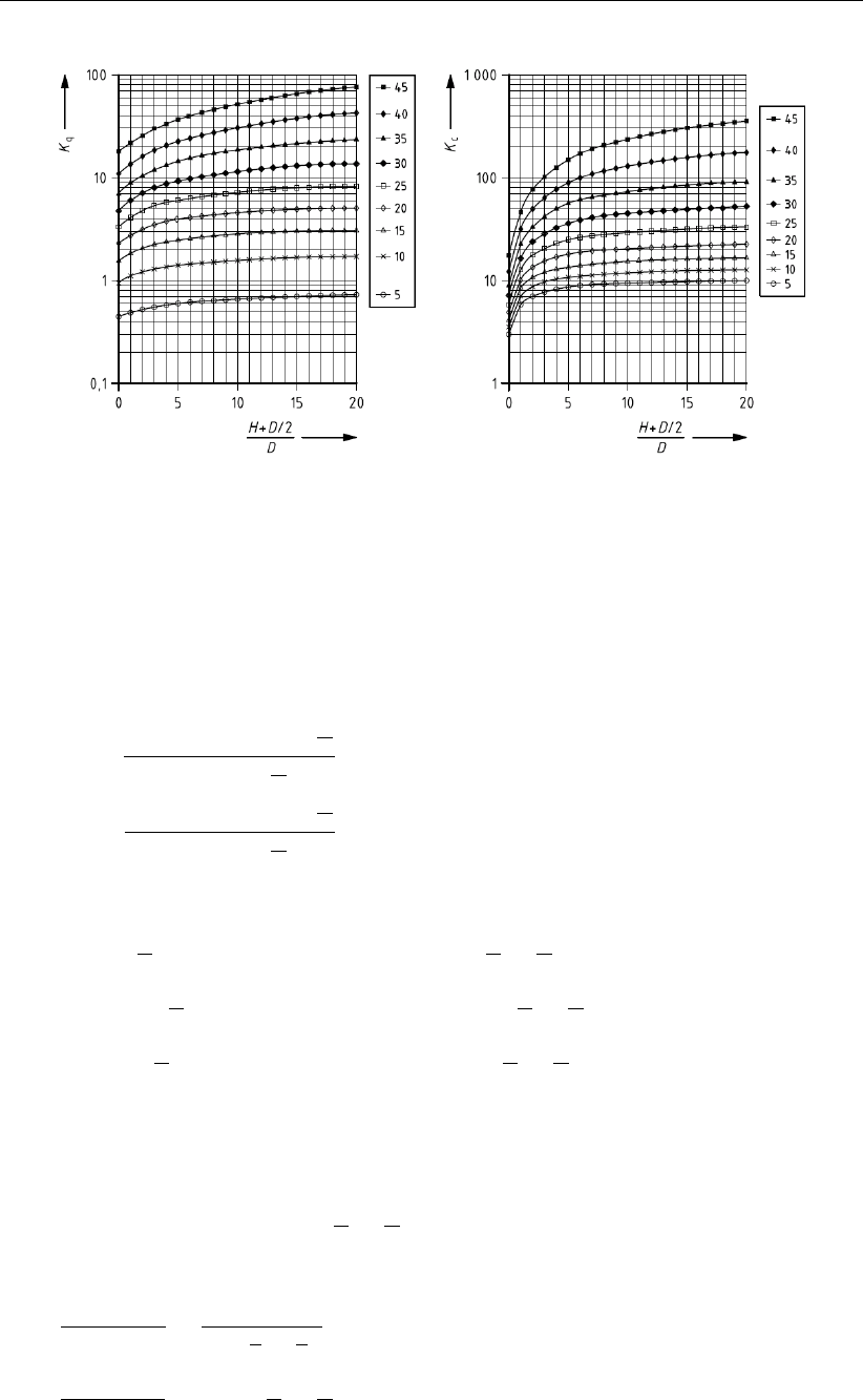
Calculation of soil mechanical data
Figure 21.7: Values Kqand Kcaccording to Brinch Hansen (Figure C.14 of the
NEN 3650-1)
The angle of internal friction ϕand the cohesion cfor the calculation of the load coefficients
Kqand Kcis determined for the soil layers 2.5 Doabove and 2.5 Dobelow the axis of the
pipeline. The minimum value is used. According to Brinch Hansen (Brinch Hansen,1970),
the load coefficients are:
Kq=K0
q+K∞
q×αq×D
B
1 + αq×D
B
(21.30)
Kc=K0
c+K∞
c×αc×D
B
1 + αc×D
B
(21.31)
where:
K0
q= exp hπ
2+ϕ×tan ϕi×cos ϕ×tan π
4+ϕ
2
−exp h−π
2+ϕ×tan ϕi×cos ϕ×tan π
4−ϕ
2
K0
c=nexp hπ
2+ϕ×tan ϕi×cos ϕ×tan π
4+ϕ
2−1o×cot ϕ
K∞
q=K∞
c×K0×tan ϕ
K∞
c=Nc×d∞
c
d∞
c= 1.58 + 4.09 ×tan4ϕ
Nc=hexp (π×tan ϕ)×tan2π
4+ϕ
2−1i×cot ϕ
K0= 1 −sin ϕ
αq=K0
q
K∞
q−K0
q×K0×sin ϕ
sin π
4+ϕ
2
αc=K0
c
K∞
c−K0
c×2 sin π
4+ϕ
2
Deltares 269 of 324
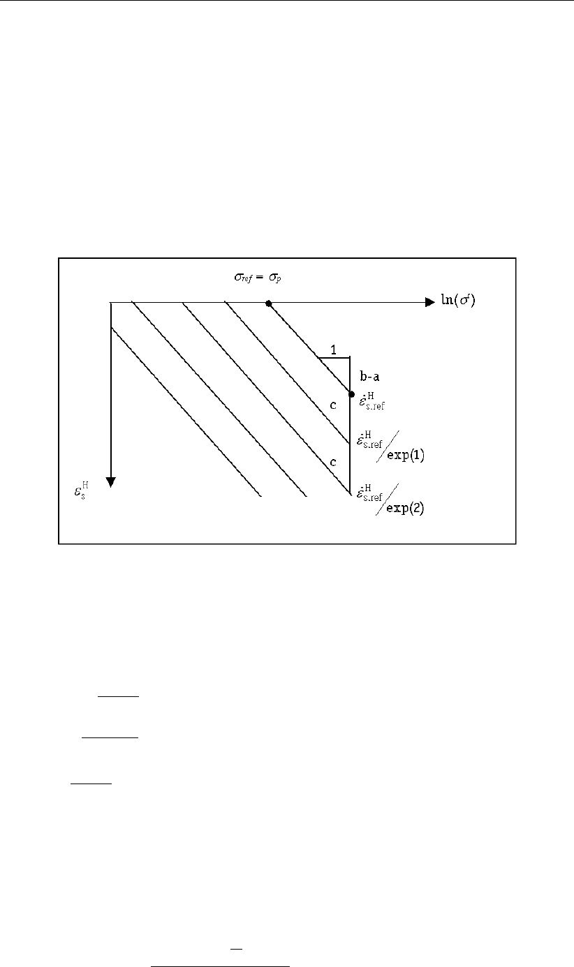
D-GEO PIPELINE
, User Manual
21.10 Vertical displacement
The vertical displacement of the soil layers below the pipeline due to an increased load on
these layers can be calculated using the Isotache method or the Koppejan method. In ad-
dition to the calculated vertical displacement by
D-GEO PIPELINE
, a given value for vertical
displacement can be entered manually (see section 4.4.2).
21.10.1 Isotache model
Creep Isotaches are lines of equal rate (speed, velocity) of secular (visco-plastic) strain εH
s
in a plot of (natural) strain versus (natural) logarithm of vertical effective stress. These are
displayed in the Figure 21.8.
Figure 21.8: Creep Isotache pattern
The Isotaches are all parallel with slope b−a. The Isotache aparameter determines the direct
(elastic) strain component εH
d. The band cparameters determine the secular (visco-plastic)
creep component εH
s.
b−a=dεH
s
dln σ0(21.32)
c=−dεH
s
dln ( ˙εH
s)(21.33)
a=dεH
d
dln σ0(21.34)
εH=εH
s+εH
d(21.35)
The reference Isotache starts at pre-consolidation stress σref =σpand is characterized by a
reference creep strain rate ˙εH
s.ref.
The secular creep rate is given by:
˙εH
s= ˙εH
s.ref exp
(b−a) ln σ0
σp−εH
s
c
(21.36)
270 of 324 Deltares

Calculation of soil mechanical data
It can be shown that the secular creep rate is related to a so-called intrinsic time τ, which is
related to the common time tby a time shift tshift.
˙εH
s=c
τwith τ=t−tshift (21.37)
This time shift in fact represents the creep history of the soil.
The total rate of strain is the sum of the elastic and secular rates:
˙εH= ˙εH
s+ ˙εH
d(21.38)
Time integration of Equation 21.38 finally yields Equation 21.39.
εH=aln σ0
σ0+cln 1 + Zt
0σ0
σpb−a
cdτ
τ0(21.39)
The reference time τ0is set by default to 1 day.
τ0=1 day (21.40)
During a constant stress period after virgin loading, Equation 21.39 simplifies to:
εH=aln σp
σ0
+bln σ0
σp
+cln τ
τ0
(21.41)
This equation applies to the creep tail when σ’ has become constant, and this is the familiar
relation for one-dimensional creep, with strain depending on logarithm of time.
Here, however, apart from using natural strain, the time to use is the intrinsic time τ. This
removes the age-old difficulty of defining the origin of time to use in the compression law, e.g.
years A.D. (Buisman: dykes of Marken island), time after loading, time after last loading stage,
etc.
Figure 21.9 illustrates the effect of the tshift parameter (denoted by tr) on the creep tail.
Figure 21.9: Influence of the tshift =trparameter on the creep tail
While H– log tplots can be either steepening or flattening, the H– log τplot is linear.
Steepening occurs for relatively small load increments, and is due to changing the origin of
time to the start of the new increment. Flattening occurs for relatively large load increments.
The linear relationship with intrinsic time therefore allows a more accurately identification and
interpretation of the creep tail.
Deltares 271 of 324
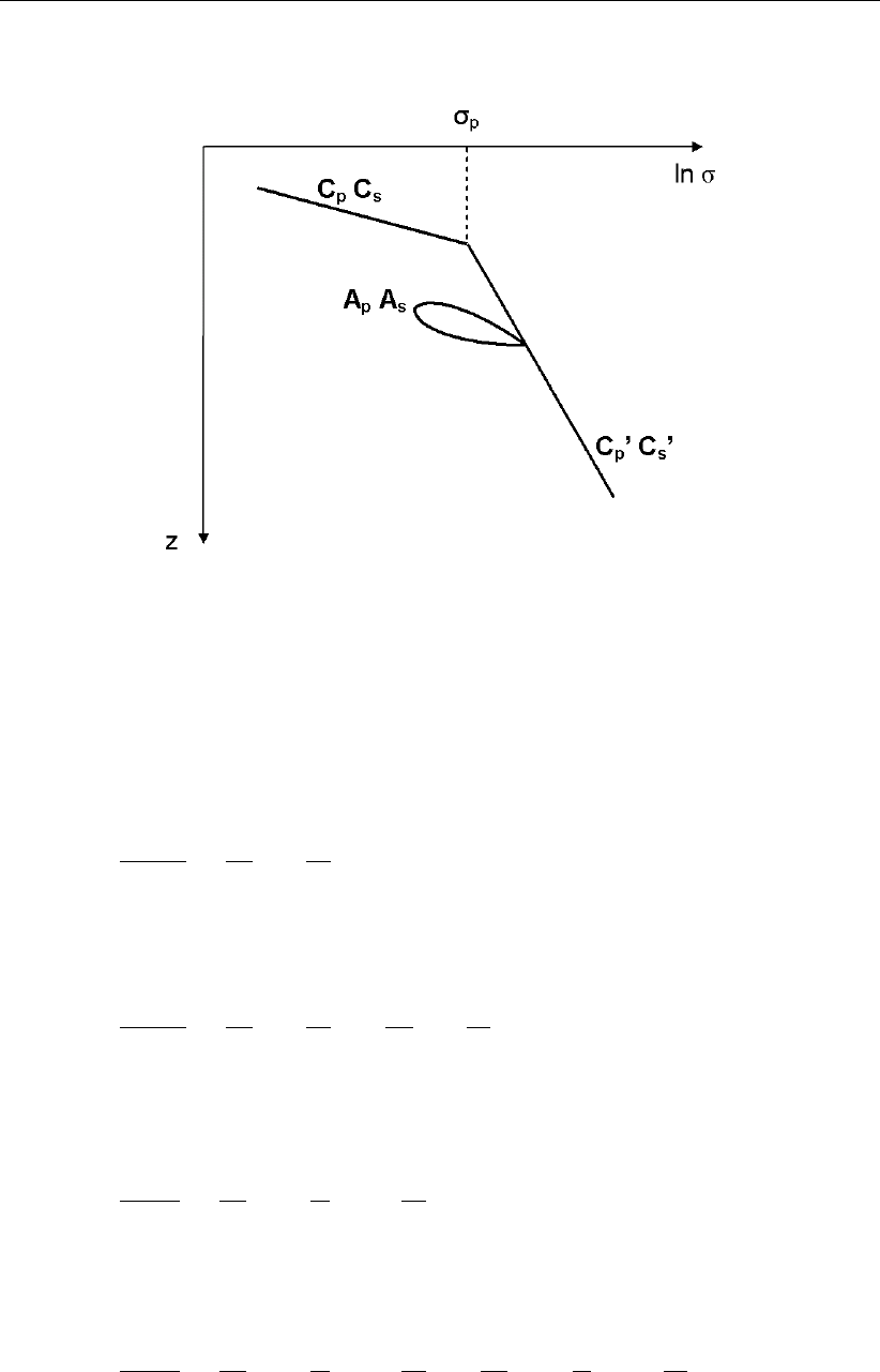
D-GEO PIPELINE
, User Manual
21.10.2 Koppejan model
Figure 21.10: Koppejan settlement
Four different situations can be distinguished for Koppejan:
If the vertical effective stress is smaller than the pre-consolidation pressure, the primary
settlement can be calculated from:
∆hprim
h0
=1
Cp
ln σ0
σ0, σ0< σ0< σp(21.42)
If the vertical effective stress is larger than the pre-consolidation pressure, the primary
settlement can be calculated from:
∆hprim
h0
=1
Cp
ln σp
σ0+1
C0
p
ln σ0
σ0, σ0< σp< σ0(21.43)
If vertical effective stress is smaller than the pre-consolidation pressure, the secondary
settlement for one loading can be calculated from:
∆hsec
h0
=1
Cs
log t
t0ln σ0
σ0, σ0< σ0< σp(21.44)
If the vertical stress is larger than the pre-consolidation pressure, the secondary settle-
ment for one loading can be calculated using Equation 21.45:
∆hsec
h0
=1
Cs
log t
t0ln σp
σ0+1
C0
s
log t
t0ln σ0
σp, σ0< σp< σ0
(21.45)
where:
Cpis the primary compression coefficient below pre-consolidation pressure;
272 of 324 Deltares
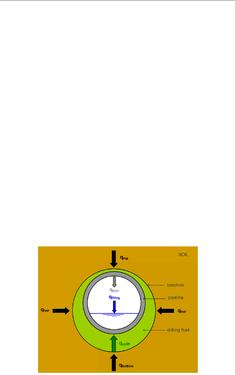
Calculation of soil mechanical data
Cp’ is the primary compression coefficient above pre-consolidation pressure;
Csis the secondary compression coefficient below pre-consolidation pressure;
Cs’ is the secondary compression coefficient above pre-consolidation pressure;
∆hprim is the primary settlement contribution of a layer, in m;
h0is the initial layer thickness, in m;
σ0is the initial vertical effective stress, in kN/m2;
σpis the pre-consolidation pressure, in kN/m2;
∆hsec is the secondary settlement contribution of a layer, in m;
tis the time, in days;
t0is the reference time, in days.
21.11 Maximal axial friction
The friction between the pipe wall and the surrounding soil depends on the relative displace-
ment between the pipe wall and the soil. When the relative displacement between the soil
and the pipe reaches a maximal value, the friction does not increase anymore. The friction
depends on:
The stresses around the pipe
The adhesion between the soil and the pipe wall
The roughness of the pipe wall
The angle of friction of the soil
21.11.1 Pipelines installed using the HDD technique
The maximal axial friction along the pipeline can be put in the Engineering Data window
(section 4.6.3) as parameter f2(friction between pipe – drilling fluid). The conditions directly
after the installation are considered as critical.
21.11.2 Pipelines installed in a trench or using micro tunneling
Figure 21.11: Schematization of the forces acting on the pipe
The following forces are acting on the pipe (Figure 21.11):
Deltares 273 of 324

D-GEO PIPELINE
, User Manual
a) Uplift force:
quplift =π
4×D2
o×γdf (21.46)
b) Weight of the pipeline:
qpipe =π
4×D2
o−D2
i×γb(21.47)
c) Weight of the filling (water):
qfilling =π
4×D2
i×γw×Pw(21.48)
d) Stress at the top of the pipe:
qtop =max [qn; min (−qeff;qp)] for trenching
max [qn,r; min (−qeff;qp)] for micro tunneling (21.49)
e) Stress at the bottom of the pipe:
qbottom =max (qn+qeff;Pwe)for trenching
max (qn,r +qeff;Pwe)for micro tunneling (21.50)
The effective weight of the pipeline is defined as:
qeff =qpipe +qfilling −quplift (21.51)
where:
qnis the neutral vertical stress, see Equation 21.1 in section 21.1;
qpis the passive vertical stress, see Equation 21.2 in section 21.2;
qn,r is the reduced neutral vertical stress, see section 21.3;
Pwe is the vertical bearing capacity, see Equation 21.26 in section 21.8.
The maximal axial friction along the pipeline is defined as follows:
W=Wtop +Wbottom + 2Whor (21.52)
with:
Wt=π
4Do(qt×tan δt+ 0.6×at)for trenching
π
4Do(qt×tan δlub fluid +alub fluid)for micro tunneling
Wb=π
4Do(qb×tan δb+ 0.6×ab)for trenching
π
4Do(qb×tan δlub fluid +alub fluid)for micro tunneling
Whor =π
4Do(K0×σ0
v×tan δm+ 0.6×am)for trenching
π
4Do(Ka×σ0
v×tan δlub fluid +alub fluid)for micro tunneling
where:
Wis the maximal friction, in kN/m;
at,ab,amare the adhesion’s of the soil at the top, respectively bottom and middle of the
pipe, in kN/m2;
274 of 324 Deltares

Calculation of soil mechanical data
δt,δb,δmare the delta friction angles of the soil at the top, respectively bottom and
middle of the pipe, in radians. For sand, δcan be approximated by 2/3 ϕ,
while in clay and peat the value of the friction angle can be neglected (δ= 0).
alub fluid is the adhesion of the lubrification fluid, in kN/m2, as defined in the Engineer-
ing Data window (section 4.6.3.2);
δlub fluid is the delta lubrification fluid, in radians, as defined in the Engineering Data
window (section 4.6.3.2);
K0is the neutral earth pressure ratio: K0= 1 −sin ϕ;
Kais the active earth pressure ratio: Ka=cos ϕ
1+sin ϕ2
;
ϕis the friction angle of the soil at the middle of the pipe, in radians;
σv’ is the effective vertical stress at the middle of the pipe, in kN/m2.
21.12 Displacement at maximal friction
21.12.1 Pipelines installed using the HDD technique
The displacement necessary to develop the maximal axial friction along the pipeline is esti-
mated between 6 and 9 mm.
D-GEO PIPELINE
uses an average value of 7.5 mm.
21.12.2 Pipelines installed in a trench or using micro tunneling
The displacement necessary to develop the maximal axial friction along the pipeline is deter-
mined using Table 21.19.
Deltares 275 of 324
D-GEO PIPELINE
, User Manual
Table 21.19: Friction displacement
Soil type ϕ
[◦]
c
[kN/m2]
Friction displacement
[mm]
Dense sand ϕ > 32.5 c≤0.5 1-3
Medium dense sand 30 < ϕ ≤32.5 c≤0.5 3-5
Stiff clay ϕ > 30 c>0.5 2-4
Loose sand 25 < ϕ ≤30 c<1 5-8
Stiff sandy clay 25 ≤ϕ≤30 c≥1 4-6
Clayey sand 22.5 < ϕ < 25 c<5 5-8
Stiff sandy clay ϕ≥22.5 c≥5 2-4
Stiff clay ϕ > 17 c≥10 2-4
Medium stiff clay 20 < ϕ ≤22.5 4-6
Medium stiff clay 17 ≤ϕ≤20 c≥5 4-6
Soft clay 17 ≤ϕ≤20 c<5 6-10
Peat /organic clay ϕ < 17 10-15
21.13 Global determination of the soil type
The global soil type in which the pipeline is installed is used for the determination of safety
factors which are required for a pipe stress analysis. The classification of global soil types
given in Table 21.20 is applied in
D-GEO PIPELINE
.
Table 21.20: Classification of the soil type
Global soil type ϕ
[◦]
c
[kN/m2]
Sand ϕ > 32.5 c≤0.5
Sand 30 < ϕ ≤32.5 c≤0.5
Clay ϕ > 30 c>0.5
Sand 25 < ϕ ≤30 c<1
Clay 25 ≤ϕ≤30 c≥1
Sand 22.5 < ϕ < 25 c<5
Clay ϕ≥22.5 c≥5
Clay ϕ > 17 c≥10
Clay 20 < ϕ ≤22.5
Clay 17 ≤ϕ≤20 c≥5
Clay 17 ≤ϕ≤20 c<5
Peat ϕ < 17
21.14 Traffic load
According to C.5.1 of NEN 3650-1 (NEN,2012a) two load models are considered, depending
on the type of road:
For dual carriageways and regional roads, ’Load Model 3’ (i.e. Graph I) according to
EN NEN-1991-2 (this concerns special transports) is assumed;
For other roads, the ’Fatigue Load Model 2, Lorry 4’ (i.e. Graph II) is assumed according
to EN NEN-1991-2 (this load model covers the ’set of frequent lorries’ wich can occur
on European roads, such as described in EN NEN-1991-2, with exception of the special
transports).
276 of 324 Deltares
Calculation of soil mechanical data
Figure 21.12: Traffic load as a function of the depth and the pipe diameter, for both load
models, according to NEN 3650-1
For both load models (Graph I and Graph II), the spreading of the traffic load qvalong the depth
is given in Figure 21.12 for four pipe diameters: 200, 600, 1000 and 1600 mm. Intermediary
diameters are linearly interpolated.
D-GEO PIPELINE
uses the following formulas to calculate
qvas a function of the depth Z, derived from Figure 21.12:
For Graph I:
For 200 mm: qv= 53.988 ×Z−1.058
For 600 mm: qv= 51.403 ×Z−1.016
For 1000 mm: qv= 46.522 ×Z−0.94
For 1600 mm: qv= 39.448 ×Z−0.804
For Graph II:
For 200 mm: qv= 31.716 ×Z−1.457
For 600 mm: qv= 29.501 ×Z−1.4
For 1000 mm: qv= 26.776 ×Z−1.324
For 1600 mm: qv= 21.963 ×Z−1.172
Deltares 277 of 324

D-GEO PIPELINE
, User Manual
278 of 324 Deltares

22 Drilling fluid pressures calculation
This section includes background information on the calculation of the following drilling fluid
pressures:
Minimum required drilling fluid pressure (section 22.1)
Maximum allowable drilling fluid pressure (section 22.2)
22.1 Minimum required drilling fluid pressure
Drilling fluid consists of a mixture of water and bentonite or may have another composition
(polymers) . This mixture has some special properties. The flow behavior of the fluid is
an important characteristic for the development of drilling fluid pressure during the different
drilling stages. Various types of drilling fluids exist. Generally, the flow behavior of drilling fluid
can be described with the Bingham model. The Bingham model describes the fluid by means
of a viscosity term and a threshold term from which flow is initialized. The threshold is called
the yield point.
D-GEO PIPELINE
calculates the required minimum fluid pressure at predefined locations. In
these calculations, the flow properties of the drilling fluid (density, viscosity and yield point)
play an important role.
During all stages of the drilling process, a pipe is present in the borehole, drill pipe or product
pipe. The return flow of drilling fluid with cuttings occurs in the annulus between the borehole
wall and the pipe. The required fluid pressure to initiate flow depends on the width of the
annulus (radius borehole minus radius drill pipe), the properties of the drilling fluid and the
required annular fluid flow rate.
To obtain the minimum required pressure pmud;min, the following pressure values must be
calculated and added up:
pmud;min =p1+p2(22.1)
where:
p1is the static pressure of the drilling fluid column, in kN/m2.
p2is the excess pressure necessary to maintain the annular flow of drilling fluid with
cuttings in the borehole, in kN/m2.
22.1.1 Static pressure of the drilling fluid column p1
As the drilling head is at a lower level than the exit point of the drilling fluid, a pressure differ-
ence has to be overcome which is equal to the difference in height times the unit weight of the
drilling fluid:
p1=γdf ×(Zexit −Z)(22.2)
where:
γdf is the unit weight of the drilling fluid, in kN/m3;
Deltares 279 of 324

D-GEO PIPELINE
, User Manual
Zexit is the vertical co-ordinate of the exit point of the drilling fluid, in m, depending on
the direction of the drilling:
If the drilling is from left to right, then the exit point of the drilling fluid is the
left point: Zexit =Zleft;
If the drilling is from right to left, then the exit point of the drilling fluid is the
right point: Zexit =Zright
Refer to section 4.6.1.1 for the definitions of Zleft and Zright.
Zis the vertical co-ordinate at pipe center, in m.
22.1.2 Excess pressure to maintain flow of drilling fluid p2
To initiate the flow of drilling fluid, a specific shear resistance in the fluid must be overcome.
The drilling fluid flows through an annulus. The required excess fluid pressure depends on
the width of the annulus (difference between borehole and drill pipe or product pipe radius),
the flow properties of the drilling fluid, and the required flow rate.
The required excess pressure necessary to maintain the annular flow of drilling fluid with
cuttings in the borehole p2is obtained by multiplying the pressure per unit length with the
length of the borehole in which the drilling fluid is flowing:
p2=dp
dz ×L(22.3)
where:
dp/dz is the flow resistance per unit length of borehole, in kN/m3;
Lis the distance in the borehole between the boring front and the exit point of the
drilling fluid, in m.
Flow resistance dp/dz
The minimum required pressure dp/dz is the optimal value for which the calculated flow rate
Qis equal to the requested flow rate Qreq (necessary to initiate flow of drilling fluid).
Calculated flow rate Q
The calculated flow rate Qis the contribution of five components:
Q=Q1,1 +Q1,2 +Q2+Q3,1 +Q3,2 (22.4)
with:
Q1,1=−2π−τdfR3
0
3µdf −dp
dz
R2
1
4µdf R4
0
4R2
1−λ2R2
0ln R0
R1−1
2R2
0+1
2C2R2
0 (22.5)
Q1,2= 2π−τdfr3
0
3µdf −dp
dz
R2
1
4µdf r4
0
4R2
1−λ2r2
0ln r0
R1−1
2r2
0+1
2C2r2
0 (22.6)
Q2=πr2
1−r2
0"−τdf
µdf
r0−dp
dz
R2
1
4µdf r0
R12
−2λ2ln r0
R1+C2!# (22.7)
Q3,1=−2πτdf
3µdf
r3
1−dp
dz
R2
1
4µdf r4
1
4R2
1−λ2r2
1ln r1
R1−1
2r2
1+1
2C4r2
1 (22.8)
Q3,2= 2πτdf
3µdf
R3
1−dp
dz
R4
1
8µdf 1
2+λ2+C4 (22.9)
where:
280 of 324 Deltares

Drilling fluid pressures calculation
τdf is the yield point of the drilling fluid, as defined in the Drilling Fluid Data window
(section 4.6.4), in kN/m2;
µdf is the plastic viscosity of the drilling fluid, as defined in the Drilling Fluid Data window
(section 4.6.4), in kN.s/m2.
The constants are:
λ2=2τdf ×r0
R2
1×dp
dz
+r0
R12
(22.10)
C2=4τdf
R2
1×dp
dz ×r0×ln R0
R1−R0−R0
R12
+ 2 r0
R12
×ln R0
R1
(22.11)
C4=4τdf
R1×dp
dz −1(22.12)
r1=2τdf
dp
dz
+r0(22.13)
r0is the solution to the following equation:
τ2
df
dp
dz
+τdfr0"1 + ln 2τdf
dp
dz
+r0!R0
r0R1!#−τdf (R0+R1) + 1
4
dp
dz R2
1−R2
0
+1
2
dp
dz r2
0ln " 2τdf
dp
dz
+r0!R0
r0R1#= 0 (22.14)
Requested flow rate Qreq
The requested flow rate Qreq is equal to:
Qreq =Qann ×(1 −floss)(22.15)
where:
floss is the circulation loss factor;
Qann is the annular back flow rate, in kN/m3.
22.1.3 Minimum drilling fluid pressure for Stage 1 (pilot pipe in the pilot hole)
For the first drilling stage of the horizontal directional drilling process, the minimum drilling fluid
pressure is calculated for the drilling direction from the left and the right, using the following
formulas:
ppilot
min,left =p1+Lleft ×dp
dz pilot
(22.16)
ppilot
min,right =p1+ (L−Lleft)×dp
dz pilot
(22.17)
where:
Deltares 281 of 324
D-GEO PIPELINE
, User Manual
Lleft is the distance in the borehole between the drilling head and the left exit point of the
drilling fluid, in m;
Lis the total length of the borehole, in m.
22.1.4 Minimum drilling fluid pressure for Stage 2 (drill pipe in the pre-ream hole)
ppre-ream
min,left = min "Ppilot
min,right;p1+Lleft ×dp
dz pre-ream#(22.18)
ppre-ream
min,right = min "Ppilot
min,left;p1+ (L−Lleft)×dp
dz pre-ream#(22.19)
22.1.5 Minimum drilling fluid pressure for Stage 3 (product pipe in the borehole)
ppull
min,left = min "Ppre-ream
min,right ;p1+Lleft ×dp
dz pull#(22.20)
ppull
min,right = min "Ppre-ream
min,left ;p1+ (L−Lleft)×dp
dz pull#(22.21)
22.2 Maximum allowable drilling fluid pressure
In the borehole, an excess drilling fluid pressure is maintained to enable sufficient outflow
of drilling fluid and cuttings. At high pressures, the borehole will fail through uncontrolled
expansion. The cavity expansion theory describes the definition of the maximum allowable
drilling fluid pressure at which the wall of the borehole becomes unstable. Such limit pressure
is the highest pressure that can be sustained by a cavity in the soil. Logically, this forms an
upper boundary for the drilling fluid pressure in the borehole.
When the borehole is created, the drilling fluid will exert pressure on the soil. When the
pressure rises above a certain value, plastic deformation of the soil will occur, initially adjacent
to the borehole. When the pressure is increased further beyond this value, the zone with
plastic deformation will increase. If the zone with plastic deformation reaches the surface a
blow-out will occur.
In granular materials (drained soil layers), the drilling fluid pressure may lead to development
of cracks around the borehole when the pressure exceeds a certain maximal value which is
related to the strain of the borehole wall.
In order to prevent blow-outs or damage to structures close to the borehole, care should
be taken that the plastic zone remains within a safe radius around the hole. Therefore the
pressure that creates a plastic zone that does not extend beyond the established safe radius
must be determined.
To determine the maximum allowable drilling fluid pressure, different formulas are used, de-
pending on the soil material sequence above the pipeline.
282 of 324 Deltares
Drilling fluid pressures calculation
22.2.1 Maximum allowable drilling fluid pressure in undrained layers
In undrained layers, the maximum allowable drilling fluid pressure pmax;und is:
pmax;und =σ0
0+Cu;f "1−ln Cu;f
Gf
+R0
Rp;max 2!#+u≤0.9plim;und (22.22)
with:
plim;und =σ0
0+Cu;f 1−ln Cu;f
Gf+u(22.23)
σ0
0=3
4
σ0
v
fγ
(22.24)
where:
plim;und is the limit drilling fluid pressure, in kN/m2;
Cu,f is the average factorized undrained cohesion, in kN/m2:Cu;f=Cu/fc;
fcis the partial safety factor on the cohesion.The default value is set to 1.4;
cuis the average undrained cohesion, in kN/m2;
σ0’ is the initial effective stress, in kN/m2;
σv’ is the vertical effective stress at the pipe center, in kN/m2;
fγPartial safety factor on the unit weight.
Gfis the average factorized shear modulus, in kN/m2:Gf=E
fE×2 (1+ν);
fEis the partial safety factor on Young modulus;
Rbis the radius of the hole, in m;
Rp,max is the maximum allowable radius of the plastic zone, in m: Rp;max = 0.5H. The
default ratio between Rp;max and the soil cover H(default 0.5) can be defined by
the user in the Factors window (section 4.7.1.1) under the field Safety factor cover
(Undrained layer);
His the vertical distance between the ground level and the pipe center, in m;
uis the pore pressure at pipe center, in kN/m2, see Equation 26.4.
Note: Parameters Cu;fand Gfare determined using the distance depth average between
the ground level and the pipe centre. For example, the weight average undrained cohesion in
the configuration in Figure 22.1 is:
cu=
Cu,2 ×1
h1−1
h1+h2+Cu,1 ×1
0.5Do−1
h1
1
0.5Do−1
h1+h2
(22.25)
Deltares 283 of 324
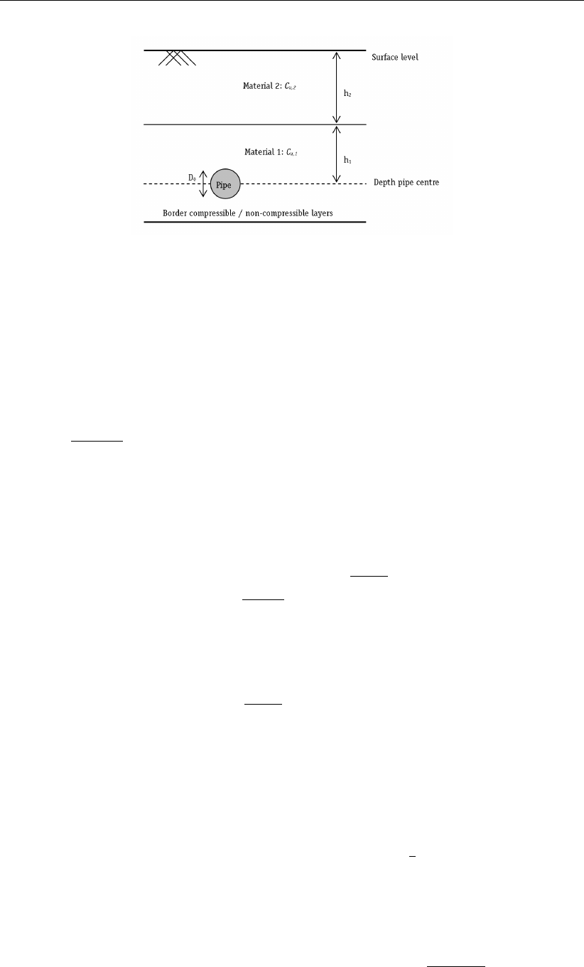
D-GEO PIPELINE
, User Manual
Figure 22.1: Schematization of h1 and h2
In case no data about the undrained strength of the soil is available, an estimated cuvalue
can be obtained using the subsequent formula:
cu=c×cos ϕ+p×sin ϕ(22.26)
with:
p=σ0
v+σ0
h
2(22.27)
22.2.2 Maximum allowable drilling fluid pressure in drained layers
According to article E.2.2 of NEN 3650-1 (NEN,2012a), the maximum allowable drilling fluid
pressure in non-compressible drained layers pmax;d is:
pmax;d = (p0
f+cf×cot ϕf)"Rb
Rp;max 2
+Q#
−sin ϕf
1+sin ϕf
−cf×cot ϕf+u≤0.9plim;d (22.28)
with:
plim;d = (p0
f+cf×cot ϕf)×Q
−sin ϕf
1+sin ϕf−cf×cot ϕf+u(22.29)
p0
f=σ0
0×(1 + sin ϕf) + cf×cos ϕf(22.30)
where:
plim;d is the limit drilling fluid pressure, in kN/m2;
p0
fis the effective drilling fluid pressure at which the first plastic deformation appears,
in kN/m2;
σ0’ is the initial effective stress of the soil, in kN/m2:σ0
0=3
4σ0
v/fγ;
ϕfis the factorized friction angle, in ◦:ϕf= arctan (tan ϕ/fϕ);
cfis the average factorized cohesion, in kN/m2:cf=c/fc;
Rbis the radius of the borehole, in m;
Qis (σ0
0×sin ϕf+cf×cos ϕf)/G;
Gfis the average factorized shear modulus between the border of compressible/non-
compressible layers and the pipe center, in kN/m2:Gf=E
fE×2(1+ν);
284 of 324 Deltares
Drilling fluid pressures calculation
Rp;max is the maximum allowable radius of the plastic zone, in m. The plastic zone can
be related:
either to the soil cover: Rp;max = 0.5H
or to the deformation of the bore hole: Rp;max =qR2
b
Q×2εg;max
The calculation of the maximum drilling fluid pressure is performed using values
determined by both methods for the calculation of the maximum allowable radius
of the plastic deformation zone Rp;max, after which the minimum value for the
maximum allowable drilling fluid pressure is taken.
uis the pore pressure at pipe center, in kN/m2;
His the distance between the border of compressible/non-compressible layers and
the pipe center, in m;
εg;max is the maximum deformation of the borehole. For sand, εg;max = 0.05.
For the definition of the other symbols, refer to section 23.5.2.
Parameters c,ϕand Gare determined using two methods:
Linear weighted average between the ground level and the pipe center;
Distance depth average between the ground level and the pipe center.
22.3 Equivalent diameter for a bundled pipeline
In case of a bundled pipeline, the following equivalent diameter is used for the calculation of
the drilling fluid pressures during the pull back operation:
Deq =v
u
u
t
n
X
i=1
D2
o;i (22.31)
Note: This equivalent diameter is calculated by
D-GEO PIPELINE
in the Drilling Fluid Data
window of the Pipe menu.
22.4 Equilibrium between drilling fluid pressure and pore pressure
The ratio between the static pressure of the drilling fluid column p1and the pore pressure
uyields the safety factor, which should be higher than the (user-defined) requested safety
factor, which writes:
f=p1
u≥fpress;bore (22.32)
where:
p1is the static pressure of the drilling fluid column (i.e. pressure due to the
difference of level between the drilling head and the exit point of the drilling
fluid), in kN/m2, see Equation 22.2 in section 22.1.1:
p1=γdf ×(Zexit −Z);
uis the calculated pore pressure (see Equation 26.4 in section 26.5);
fpress;bore is the required safety factor, as defined in the Factors window under the field
Contingency factor – Pressure borehole, see section 4.7.1.1.
Deltares 285 of 324

D-GEO PIPELINE
, User Manual
286 of 324 Deltares
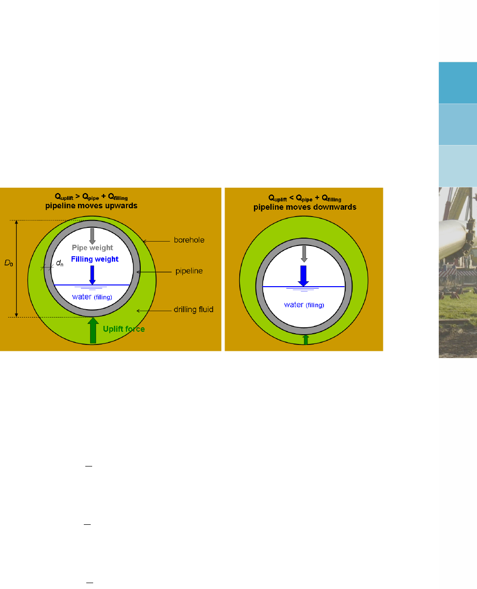
23 Strength pipeline calculation
23.1 Buoyancy control
The friction between soil and pipe is partially caused by buoyancy of the pipeline in the drilling
fluid. Uplift forces resulting from buoyancy can be neutralized by filling the pipeline. The
optimal volume of water (Pw) placed in the pipe provides the most advantageous distribution
of buoyant forces, as illustrated in Figure 23.1.
Figure 23.1: Schematization of the buoyancy control
The forces acting on the pipeline are:
a) Uplift force:
Quplift =π
4×D2
o×γdf (23.1)
b) Weight of the pipeline:
Qpipe =π
4×D2
o−D2
i×γb(23.2)
c) Weight of the filling (water):
Qfilling =π
4×D2
i×γw×Pw(23.3)
The weight of the pipeline filled with water is therefore:
Q=Qpipe +Qfilling (23.4)
and the effective weight of the pipeline is defined as:
Qeff =|Q−Quplift|(23.5)
Deltares 287 of 324

D-GEO PIPELINE
, User Manual
23.2 Pulling force in a flexible pipeline
According to article E.1.2.1 of NEN 3650-1 (NEN,2012a), the total pulling force is the contri-
bution of five components:
T=T1+T2+T3a +T3b +T3c (23.6)
23.2.1 Roller-lane
According to article E.1.2.2 of NEN 3650-1 (NEN,2012a), the design pulling force due to
friction of the pipeline on the roller-lane T1is:
T1=finstall ×Lrol ×Q×f1(23.7)
where:
finstall is the total factor for stochastic variation and model uncertainty, called Load factor
installation in the Factors window (section 4.7.1.1). The default value is set to 1.1;
Lrol is the length of the pipeline on the roller-lane, in mm;
Qis the weight of the pipeline filled with water, in N/mm, see Equation 23.4;
f1is the factor of friction of the roller-lane, defined in the Engineering Data window, see
section 4.6.3.1. The default value is set to 0.1.
23.2.2 Straight part of the borehole
According to article E.1.2.3 of NEN 3650-1 (NEN,2012a), the pulling force in the straight part
of the borehole due to friction between pipe and drilling fluid is:
T2=finstall ×L2×(π Do×f2+Qeff ×f3)(23.8)
where:
finstall is the total factor for stochastic variation and model uncertainty, called Load factor
installation in the Factors window (section 4.7.1.1). The default value is set to 1.1;
L2is the length of the pipeline in the straight part of the borehole, in mm;
f2is the friction between the pipeline and the drilling fluid, in N/mm2, defined in
the Engineering Data window, see section 4.6.3.1. The default value is set to
0.00005 N/mm2;
Qeff is the effective weight of the pipeline, in N/mm, see Equation 23.5;
f3is the factor of friction between the pipeline and the borehole wall, defined in the
Engineering Data window, see section 4.6.3.1. The default value is set to 0.2.
23.2.3 Curved part of the borehole
According to article E.1.2.4.1 of NEN 3650-1 (NEN,2012a), the pulling force in the curved
part of the borehole due to friction between pipe and drilling fluid T3a is:
T3a =finstall ×Lb×(π Do×f2+Qeff ×f3)(23.9)
where:
Lbis the length of the pipeline in the curved part of the borehole, in mm.
For the definition of the other symbols, refer to section 23.5.2.
288 of 324 Deltares

Strength pipeline calculation
23.2.4 Friction due to soil reaction in the curved part
According to article E.1.2.4.2 of NEN 3650-1 (NEN,2012a), the pulling force in the curved
part of the borehole due to soil reaction T3b is:
T3b =finstall ×4×qr
2×Do×π
λ×f3(23.10)
with:
qr=kv×y(23.11)
y=0.3224 ×λ2×Eb×Ib
Do×R(23.12)
λ=4
rfkv ×kv×Do
4EbIb
(23.13)
where:
qris the maximum soil reaction, in N/mm2;
kvis the vertical modulus of subgrade reaction, in N/mm3;
yis the maximum displacement, in mm;
λis the characteristic stiffness pipeline-soil, in mm-1;
fkv is the contingency factor on the modulus of subgrade reaction. The default value is
1.6;
Ebis the Young’s modulus of the pipe, in N/mm2;
Ibis the moment of inertia of the pipe, in mm4;
Ris the bending radius, in mm;
f3is the factor of friction between the pipeline and the borehole wall, defined in the
Engineering Data window, see section 4.6.3.1. The default value is set to 0.2.
23.2.5 Friction due to curved forces
According to article E.1.2.4.3 of NEN 3650-1 (NEN,2012a), the pulling force in the curved
part of the borehole due to curved forces T3c is:
T3c =finstall ×Lb×gt×f3(23.14)
where:
Lbis the length of the curve, in mm: Lb= 2 ×R×2π×α/360;
αis the half angle of the curved part, in degrees;
gtis the curved force, in N/mm: gt= (2 Tsin α)/Lb;
Tis the total pulling force in the pipeline, in N, see Equation 23.6.
Deltares 289 of 324

D-GEO PIPELINE
, User Manual
23.3 Maximum representative pulling force
The maximum representative pulling force Tmax;rep in a single pipeline is:
For steel pipe:
Pmax;rep =A×1
2−σqr +qσ2
qr −4−2.25 R2
eb +σ2
qr−σb(23.15)
For polyethylene pipe:
Pmax;rep =A×(Reb;short −α×σb)(23.16)
where:
Ais the cross-section of the pipe, in mm2:A=π×(r2
0−r2
i);
Reb is the allowable strength for steel, in N/mm2, as defined in the Product Pipe
Material Data window (see section 4.6.2.1);
Reb;short is the allowable strength at short term for PE, in N/mm2, as defined in the Product
Pipe Material Data window (see section 4.6.2.1);
αis the tensile factor, as defined in the Product Pipe Material Data window (see
section 4.6.2.1);
δtis the negative wall thickness tolerance, in %, as defined in the Product Pipe
Material Data window (see section 4.6.2.1);
σqr is the maximum tangential stress in LC 1B, in N/mm2, see Equation 23.31;
σbis the axial stress in LC 1B, in N/mm2, see Equation 23.27.
23.4 Pulling force for a bundled pipeline
Important parameters for the pullback operation are the total weight of the (filled/ not filled)
pipelines with respect to drilling fluid, which determines the soil reaction force on the bore hole
wall in straight sections of the drilling line and the total stiffness of the bundled pipeline, which
determines the soil reaction force in curved sections of the drilling line. The pulling force is
calculated for an equivalent pipeline with the parameters of the bundle.
EIeq =
n
X
i=1
EIi(23.17)
Gtot =
n
X
i=1 1
4πD2
0;i−1
4π(D0;i−2dn;i)2×γi(23.18)
Deq =f×
n
X
i=1
Do;i (23.19)
The equivalent diameter can be used to determine the equivalent wall thickness of the pipeline:
Gtot
γeq
=1
4πD2
eq −(Deq −2dn;eq)2(23.20)
290 of 324 Deltares

Strength pipeline calculation
dn;eq =
Deq −sD2
eq −
n
X
i=1
D2
0;i−(Do;i −2dn;i)2
2(23.21)
where:
nis the number of pipelines in bundle;
Do;i is the outer diameter of pipeline number i, in m;
Deq is the equivalent diameter of the pipeline, in m;
dn;i is the wall thickness of pipeline number i, in m;
dn;eq is the equivalent wall thickness of the pipeline, in m;
γiis the unit weight of the material of pipeline number i, in kN/m3;
γeq is the equivalent unit weight of the pipeline material, in kN/m3;
fis a factor: f= 1/n0.3.
The calculated pulling force is acting on all the pipelines in the bundle. The magnitude of the
pulling force of a single pipeline can be determined as follows:
Ti=π
4D2
o;i −π
4(Do;i −2dn;i)2
n
X
i=1 π
4D2
o;i −π
4(Do;i −2dn;i)2×Ttotal (23.22)
In case the stiffness of the pipeline materials is significantly different (for example a combined
bundle of steel and PE pipelines), a different approach is applied. In addition to the previous
align, the total pulling force is divided over the stiff steel pipelines. The PE pipelines are then
considered as single pulled in pipelines.
23.5 Strength calculation
In order to consider the strength of the pipeline, calculations for five load combinations are
carried out according to NEN 3650:
Load combination 1A: start of the pullback operation (section 23.5.1)
Load combination 1B: end of the pullback operation (section 23.5.2)
Load combination 2: application of internal pressure (section 23.5.3)
Load combination 3: pipeline in operation, without internal pressure (section 23.5.4)
Load combination 4 : pipeline in operation, with internal pressure (section 23.5.5)
23.5.1 Strength calculation for Load Combination 1A: start of the pullback operation
Axial stress:
At start of the pull back operation, the axial bending stress σbis:
σb=Mb
Wb
=fk×Eb×Ib
Rrol ×Wb
(23.23)
Note: fkis the overall safety factor on moment, as prescribed in article E.1.3 of NEN 3650-1.
Deltares 291 of 324

D-GEO PIPELINE
, User Manual
In
D-GEO PIPELINE
, this overall factor is indeed the contribution of three safety factors:
fk=fM×finstall
fR
(23.24)
where:
fMis the contingency factor on moment: 1.27 for steel pipe and 1.4 for PE pipe;
fRis the contingency factor on bending radius: 1.1 for steel pipe and 1 for PE pipe;
finstall is the load factor on installation: 1.1 for steel pipe and 1 for PE pipe.
The axial stress due to pull-back is:
σt=fpull ×T1
A(23.25)
where:
T1is the design pulling force due to friction of the pipeline on the roller-lane, see Equa-
tion 23.7.
For the definition of the other symbols, refer to section 23.5.2.
The maximum axial stress is:
σa;max = max (|σt+α×σb|;|σt−α×σb|)(23.26)
Tangential stress:
At start of the pull back operation, the pipeline is situated on the rollers, the tangential stress
is negligible.
23.5.2 Strength calculation for Load Combination 1B: end of the pullback operation
Axial stresses:
At the end of the pull back operation, the axial bending stress:
σb=Mb
Wb
=fk×Eb×Ib
Rmin ×Wb
(23.27)
The axial stress due to pull-back is:
σt=fpull ×Tmax
A(23.28)
The maximum axial stress is:
σa;max = max (|σt+α×σb|;|σt−α×σb|)(23.29)
where:
292 of 324 Deltares
Strength pipeline calculation
Rmin is the minimum bending radius of the pipeline configuration (i.e. minimum between
Rleft,Rright and the horizontal bending radius), in m. In case of a combined 3-
dimensional bending radius, see Equation 20.5.
Tmax is the maximum pulling force, in kN (see section 23.2).
Note: fkis the overall safety factor on moment, as prescribed in article E.1.3 of NEN 3650-1.
In
D-GEO PIPELINE
, this overall factor is indeed the contribution of three safety factors:
fk=fM×finstall
fR
(23.30)
Tangential stresses:
The tangential stress (indirectly transmitted) as a result of the bending is:
σqr = max (σqr;b;σqr;t)(23.31)
with:
σqr;b =K0
b×qr×rg
Ww×Do(at the bottom of the pipe)
σqr;t =K0
t×qr×rg
Ww×Do(at the top of the pipe)
where:
qris the soil reaction, in kN/m2, see Equation 23.11 with R= the minimum bending
radius;
Kb’ is the moment coefficient for indirectly transmitted stress at the bottom of the
pipeline, depending on the bedding angle βas shown in Table 23.12;
Kt’ is the moment coefficient for indirectly transmitted stress at the top of the pipeline,
depending on the bedding angle βas shown in Table 23.12;
Wwis the wall resisting moment in m3/m: Ww=d2
n/6.
For the definition of the other symbols, refer to section 23.5.2.
The maximum tangential stress is:
σt;max =σqr (23.32)
23.5.3 Strength calculation for Load Combination 2: application of internal pressure
According to article 8.5.2.1 of NEN 3651 (NEN,2012d), the ring stresses around the pipeline
σpy and σpt caused by design (pd) respectively test (pt) internal pressure are:
For piles with a thin wall (Dg/d < 20):
σpy =fpd ×pd×Dg
2×d(23.33)
σpt =fpt ×pt×Dg
2×d(23.34)
Deltares 293 of 324
D-GEO PIPELINE
, User Manual
Table 23.12: Moment and deflection coefficients for indirectly and directly transmitted
stress as a function of the bedding angle β, according to Table D.2 of
NEN 3650-1
Load angle Direct coefficients Indirect coefficients
β KtKbkyK0
tK0
bk0
y
0◦0.150 0.294 0.116 0.080 0.239 0.074
30◦0.148 0.235 0.113 0.078 0.179 0.071
60◦0.143 0.189 0.105 0.073 0.134 0.064
70◦0.141 0.178 0.102 0.071 0.122 0.061
90◦0.137 0.157 0.096 0.067 0.102 0.055
120◦0.131 0.138 0.089 0.061 0.083 0.048
150◦0.126 0.128 0.085 0.056 0.073 0.043
180◦0.125 0.125 0.083 0.055 0.070 0.042
For piles with a thick wall (Dg/d ≥20):
σpy =fpd ×pd×r2
0+r2
i
r2
0−r2
i
(23.35)
σpt =fpt ×pt×r2
0+r2
i
r2
0−r2
i
(23.36)
The axial internal stress σpx is:
σpx =ν×σpt = 0.5×σpt (23.37)
23.5.4 Strength calculation for Load Combination 3: pipeline in operation, without internal
pressure
Axial stresses:
When the pipeline is in operation, the axial bending stress σbis:
σb=Mb
Wb
=fk×Eb×Ib
Rmin ×Wb
(23.38)
The maximum axial stress is:
σa;max =α×σb(23.39)
Tangential stresses:
The tangential stress (indirectly transmitted) as a result of the bending is:
σqr = max (σqr;b;σqr;t)(23.40)
with:
σqr;b =K0
b×qr×rg
Ww×Do(at the bottom of the pipe)
σqr;t =K0
t×qr×rg
Ww×Do(at the top of the pipe)
294 of 324 Deltares
Strength pipeline calculation
The tangential stress (directly transmitted) as a result of the bending is:
σqn = max (σqn;b;σqn;t)(23.41)
with:
σqn;b =Kb×qn,r,v ×rg
Ww×Do(at the bottom of the pipe)
σqn;t =Kt×qn,r,v ×rg
Ww×Do(at the top of the pipe)
qn,r,v =fQn1 ×fQn2 ×(qn,r +qv)
The maximum tangential stress is:
σt;max =α×max (|σqr;b +σqn;b|;|σqr;t +σqn;t|)(23.42)
where:
fQn1 is the load factor on soil stress qn, as defined in the Factors window (see sec-
tion 4.7.1.1). The default value is set to 1.5 for steel and 1 for polyethylene;
fQn2 is the contingency factor on soil stress qn, as defined in the Factors window (see
section 4.7.1.1). The default value is set to 1.1;
Kbis the moment coefficient for directly transmitted stress at the bottom of the pipeline,
depending on the bedding angle βas shown in Table 23.12;
Ktis the moment coefficient for directly transmitted stress at the top of the pipeline,
depending on the bedding angle βas shown in Table 23.12;
qn,r,v is the (maximum) reduced vertical stress qn,r increased with a possible traffic load
qv, including safety factors, in kN/m2;
qn,r is the neutral reduced soil stress, in kN/m2, see section 21.3;
qvis the traffic load, in kN/m2, see section 21.14;
For the definition of the other symbols, refer to section 23.5.2.
23.5.5 Strength calculation for Load Combination 4: pipeline in operation, with internal
pressure
Axial stresses:
The axial bending stress σbis:
σb=Mb
Wb
=fk×Eb×Ib
Rmin ×Wb
(23.43)
The ring stresses around the pipeline caused by design internal pressure and σpy and test
internal pressure σpt are
σpy =fpd;comb ×pd×Do−d
2×d(23.44)
σpt =fpt ×pt×Do−d
2×dfor steel (23.45)
σpt =fpt ×pt×r2
0+r2
i
r2
0−r2
i
for polyethylene (23.46)
Deltares 295 of 324

D-GEO PIPELINE
, User Manual
The axial internal stress σpx is:
σpx =ν×σpy = 0.5σpy (23.47)
The axial internal stress due to temperature variation σtemp is, according to article D.2.2 of
NEN 3650-1:
σtemp = ∆t×αg×Eb(23.48)
where:
∆tis the temperature variation in ◦c, as defined in the Product Pipe Material Data
window, see section 4.6.2.1;
αgis the linear settlement coefficient, in (mm/mm)K−1, as defined in the Engineering
Data window, see section 4.6.3.1;
Ebis the Young’s modulus of the pipe (at long term for polyethylene), in kN/m2.
The maximum axial stress is:
σa;max =α×σb+σpx (23.49)
Tangential stresses:
The tangential stress (indirectly transmitted) as a result of the bending is:
σqr = max (σqr;b;σqr;t)(23.50)
with:
σqr;b =K0
b×qr×rg
Ww×Do(at the bottom of the pipe)
σqr;t =K0
t×qr×rg
Ww×Do(at the top of the pipe)
The tangential stress (directly transmitted) as a result of the bending is:
σqn = max (σqn;b;σqn;t)(23.51)
with:
σqn;b =Kb×qn,r,v ×rg
Ww×Do(at the bottom of the pipe)
σqn;t =Kt×qn,r,v ×rg
Ww×Do(at the top of the pipe)
qn,r,v =fQn1 ×fQn2 ×(qn,r +qv)
Refer to section 23.5.4 for the definition of the symbols.
The maximum tangential stress is:
σt;max =σpy +α×(F0
rr ×σqr +Frr ×σqn)(23.52)
296 of 324 Deltares

Strength pipeline calculation
with:
Frr =1
1 + 2pd×r3
g×ky
Eb×Iw
(23.53)
F0
rr =1
1 + 2pd×r3
g×k0
y
Eb×Iw
(23.54)
where:
Frr is the direct re-rounding factor;
Frr’ is the indirect re-rounding factor;
Iwis the moment of inertia of the wall, in m3:Iw=d3
n/12;
kyis the direct deflection factor depending on the bedding angle βas shown in Ta-
ble 23.12;
ky’ is the indirect deflection factor depending on the bedding angle βas shown in Ta-
ble 23.12;
For the definition of the other symbols, refer to section 23.5.2.
23.6 Check of calculated stresses
23.6.1 Check of calculated stresses according to the Dutch standard NEN
23.6.1.1 Check of calculated stresses acc. to the Dutch standard NEN: Steel pipe
According to article D.3.1 of NEN 3650-2 (NEN,2012b), the calculated stresses (for the load
combinations) must meet the following conditions:
For Load Combinations 1A and 1B:
σV≤Reb/γm(23.55)
For Load Combination 2:
σpy ≤Reb/γm(23.56)
σpt ≤Reb/γm;test (23.57)
σpm ≤1.1Reb/γm(23.58)
For Load Combinations 3 and 4:
σV;max ≤0.85 (Reb +Re;20◦)/γm(23.59)
with:
σV=qσ2
x+σ2
y−σx×σy(23.60)
σV;i =qσ2
x;i +σ2
y;i −σx;i ×σy;i (23.61)
σpm =qσ2
px +σ2
py −σpx ×σpy (23.62)
where:
σV;max is the maximum acting stress, in kN/m2:σV;max = max (σV;1;σV;2;σV;3;σV;4);
Deltares 297 of 324
D-GEO PIPELINE
, User Manual
σV;i is the calculated acting stress, in kN/m2:
–i=1 (σV;1) corresponds to the primary membrane stress
–i=2 (σV;2) corresponds to the total primary stress
–i=3 (σV;3) corresponds to the total membrane stress
–i=4 (σV;4) corresponds to the resultant of primary and secondary stresses.
For the determination of σV;i, four combinations of (σx;i;σy;i) are tested (top and
bottom of the pipe combined with inside or outside), and the maximum value is
used for the check. Those four combinations are given in Table 23.17 to Ta-
ble 23.20;
σpy is the tangential stress due to design pressure, in kN/m2;
σptest is the tangential stress due to test pressure, in kN/m2;
σx;i is the axial stress, in kN/m2;
σy;i is the tangential stress, in kN/m2;
γmis the partial material factor, as defined in the Product Pipe Material Data window
(see section 4.6.2.1;
γm;test is the partial material factor for test pressure, as defined in the Product Pipe Ma-
terial Data window (see section 4.6.2.1;
Reb is the yield strength, in kN/m2, as defined in the Product Pipe Material Data window
(see section 4.6.2.1);
Re;20 is the yield strength at a temperature of 20◦c, in kN/m2.
Table 23.17: Set for calculation of the maximum stresses for load combination 1A
Top outside Top inside Bottom inside Bottom outside
σxσt−α×σbσt−α×σbσt+α×σbσt+α×σb
σy0 0 0 0
Table 23.18: Set for calculation of the maximum stresses for load combination 1B
Top outside Top inside Bottom inside Bottom outside
σxσt−α×σbσt−α×σbσt+α×σbσt+α×σb
σy−σqr;t σqr;t σqr;b −σqr;b
Table 23.19: Set for calculation of the maximum stresses for load combination 3
Top outside Top inside Bottom inside Bottom outside
σx;2 0 0 0 0
σy;2 −σqr;t σqr;t σqr;b −σqr;b
σx;3 −α×σb−α×σbα×σbα×σb
σy;3 0 0 0 0
σx;4 −α×σb−α×σbα×σbα×σb
σy;4 −σqr;t −σqn;t σqr;t +σqn;t σqr;b +σqn;b −σqr;b −σqn;b
298 of 324 Deltares
Strength pipeline calculation
Table 23.20: Set for calculation of the maximum stresses for load combination 4
Top outside Top inside Bottom inside Bottom outside
σx;1 σpx σpx σpx σpx
σy;1 σpy σpy σpy σpy
σx;2 σpx σpx σpx σpx
σy;2 σpy −Frr ×σqn;t σpy +Frr ×σqn;t σpy +Frr ×σqn;b σpy −Frr ×σqn;b
σx;3 σpx −α×σbσpx −α×σbσpx +α×σbσpx +α×σb
σy;3 σpy σpy σpy σpy
σx;4 σpx −α×σbσpx −α×σbσpx +α×σbσpx +α×σb
σy;4 σpy −α(Frr ×σqn;t
+F0
rr ×σqr;t)
σpy +α(Frr ×σqn;t
+F0
rr ×σqr;t)
σpy +α(Frr ×σqn;b
+F0
rr ×σqr;b)
σpy −α(Frr ×σqn;b
+F0
rr ×σqr;b)
Note: αis the tensile factor (only used for polyethylene), as defined in the Product Pipe
Material Data window (see section 4.6.2.1).
Note: For load combination 4, the acting stresses σV;1 to σV;4 are calculated with a load
factor “in combination” (fpd;comb) for the design pressure.
23.6.1.2 Check of calculated stresses acc. to the Dutch standard NEN: Polyethylene pipe
The calculated stresses must meet the following conditions:
σ≤S×Reb;short for LC 1 and 2 (test pressure) (23.63)
σ≤S×Reb;long for LC 2 (internal pressure), 3 and 4 (23.64)
where:
σis the calculated stress, in kN/m2;
Reb;short is the allowable strength at short term, in kN/m2;
Reb;long is the allowable strength at long term, in kN/m2;
Sis the factor of importance, as defined in the Factors window (see section 4.7.1.1).
23.7 Deflection of the pipe
According to article D.4.2 (case 5 - HDD) of NEN 3650-1 (NEN,2012a), the deflection of the
pipeline is:
δy=Do×r3
g
Eb×Iw×ky×qn,r,v + 0.083 ×qh,r +k0
y×qr(23.65)
where:
qn,r,v is the corrected neutral reduced vertical stress qn;r (see section 21.3) increased
with a possible traffic load qv(see section 21.14), including safety factors, in kN/m2:
qn,r,v =fQn1 ×fQn2 ×(qn;r +qv);
qh,r is the neutral reduced horizontal stress in kN/m2, see Equation 21.12;
qris the soil reaction in kN/m2, see Equation 23.11 with R= the minimum bending
radius.
kyis the direct deflection coefficient depending on the bedding angle β, see Ta-
ble 23.12;
ky’ is the indirect deflection coefficient depending on the bedding angle β, see Ta-
ble 23.12;
Deltares 299 of 324

D-GEO PIPELINE
, User Manual
fQn1 is the load factor on soil stress qn, as defined in the Factors window (see sec-
tion 4.7.1.1). The default value is set to 1.5 for steel and 1 for polyethylene;
fQn2 is the contingency factor on soil stress qn, as defined in the Factors window (see
section 4.7.1.1). The default value is set to 1.1;
Ebis the Young’s modulus of the pipe. For PE, the modulus at long term is used.
23.8 Implosion of the polyethylene pipe
According to article 8.5.5.1 of NEN 3650-3 for polyethylene, the maximum allowable external
pressure p0is:
p0=1
γimp (1 −ν2)×24 ×Eb×Iw
D3
g
(23.66)
where:
Ebis the Young’s modulus of the polyethylene pipe, in kN/m2;
νis the Poisson ratio of polyethylene: ν= 0.4;
γimp is the safety factor on implosion, as defined in the Factors window (see sec-
tion 4.7.1.1).
For the definition of the other symbols, refer to section 23.5.2.
The check on implosion is performed during the pull-back operation (section 23.8.1) and at
serviceability limit state when the pipe is in operation (section 23.8.2).
23.8.1 Check on implosion during the pull-back operation
During the pull-back operation, the drilling fluid pressure gives an external pressure on the
pipe. The highest minimum required drilling fluid pressure should not exceed the maximum
allowable external pressure. This writes:
max (pmud;min)≤p0(23.67)
where γ= 1.5 and Eis the module at short term, for the calculation of p0.
If the pipe is completely filled, the filling fluid gives an internal fluid pressure called filling
resistance pfill of:
pfill = (min (Zleft;Zright)−Zbottom)×γfill (23.68)
The maximum allowable external pressure becomes therefore p0+pfill and the check on
implosion becomes:
max (pmud;min)≤p0+pfill (23.69)
23.8.2 Check on implosion when the pipe is in operation
In operation, the water pressure at the lowest point of the drilling gives an external pressure
on the pipe. This maximum pore pressure should not exceed the maximum allowable external
pressure. This writes:
umax ≤p0(23.70)
where γ= 3 and Eis the module at long term, for the calculation of p0.
300 of 324 Deltares

Strength pipeline calculation
If the pipe is completely filled, the maximum allowable external pressure becomes p0+pfill
and the check on implosion becomes:
umax ≤p0+pfill (23.71)
Deltares 301 of 324

D-GEO PIPELINE
, User Manual
302 of 324 Deltares

24 Micro tunneling
24.1 Support pressures and thrust forces
Drilling through the soil changes the stress conditions in the soil. The deviations from the
original stress conditions are largely determined by the size of the overcut and the face sup-
port pressure of the applied shield. Small deviations form the original stress conditions are
acceptable as the stability of soil adjacent to the micro tunneling machine is maintained. A
relative low support pressure may lead to settlement in front of the tunneling machine which in
turn may lead to settlement of the surface or to settlement of soil layers below a construction
or pipeline. A relative high support pressure can lead to a blow out of drilling fluid or may lead
to heave of the surface.
24.1.1 Target support pressure
In order to minimize the effect on the stress conditions, the drilling should be performed using
a target support pressure σT;ac which is close to the neutral horizontal pressure:
σT;ac =σ0
h,n +u(24.1)
where:
uis the pore pressure, in kN/m2at the shield center, see Equation 26.4.
σ0
h,n is the horizontal effective pressure at the shield center, in kN/m2:
σ0
h,n =σ0
v×(1 −sin ϕb);
σ0
vis the vertical effective stress at the shield center, in kN/m2, see Equation 26.5;
ϕbis the average angle of internal friction of the soil over the height of the shield.
24.1.2 Minimal support pressure
Under normal circumstances, a relative low support pressure is usually sufficient for stable
conditions of the soil adjacent to the micro tunneling machine. The minimal required support
pressure is often a little higher than the water pressure. The relative low required minimal
support pressure is determined by the type of soil in front of the tunneling machine.
Minimal support pressure in undrained conditions
In case of micro tunneling in an undrained soil type, according to Broms & Bennermark 1967
(Broms and Bennermark,1967), the minimal support pressure σmin;und is determined by the
undrained strength of the soil:
σmin;und =fcover ×σ0
v+fu×u−N×su
fc≥fu×u(24.2)
where:
suis the average undrained shear strength between the surface and the top of the
shield of the micro tunneling machine , in kN/m2;
fcis the safety factor on cohesion as defined in the Factors window, see section 4.7.1.2
(default is 1.4).
fcover is the contingency factor on soil cover as defined in the Factors window, see sec-
tion 4.7.1.2 (default is 1.1);
fuis the safety factor on water pressure as defined in the Factors window, see sec-
tion 4.7.1.2 (default is 1.05);
Nis the face stability ratio as defined in the Factors window, see section 4.7.1.2;
Deltares 303 of 324
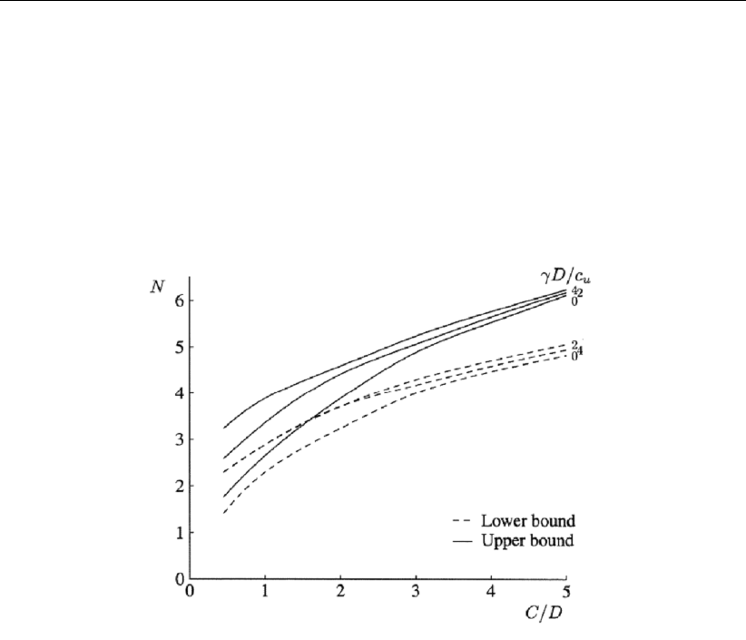
D-GEO PIPELINE
, User Manual
σ0
vis the vertical effective stress at the shield center, in kN/m2, see Equation 26.5;
uis the pore pressure, see Equation 26.4.
The required stability index Ndepends upon the depth/diameter ratio of the tunneling ma-
chine. In Figure 24.1 the upper and lower boundaries according to (Davis et al.,1980) are
described.
Figure 24.1: Upper and lower bound for the stability ratio N(Davis et al.,1980)
Minimal support pressure in drained conditions
In granular soils which behave drained during drilling, the minimal support pressure based
on 3 dimensional effects can be calculated using the method which is developed by (Jancesz
and Steiner,1994). The minimal effective stress required for stability of the soil next to the
shield is defined as follows:
σ0
h=fσh×KA3 ×σ0
v(24.3)
The total minimal support pressure is drained layers σmin;d can be calculated as follows:
σmin;d =fσh×KA3 ×σ0
v+fu×u(24.4)
where:
fuis the safety factor on water pressure as defined in the Factors window, see sec-
tion 4.7.1.2 (default is 1.05);
fσhis the safety factor on horizontal effective stress as defined in the Factors window,
see section 4.7.1.2 (default is 1.5);
KA3 is a 3 dimensional coefficient of active earth pressure, see Equation 24.5;
uis the pore pressure, in kN/m2, see Equation 26.4;
σ0
his the effective horizontal soil pressure at the shield center, in kN/m2;
σ0
vis the effective vertical stress at the shield center, in kN/m2, see Equation 26.5. In
case of arching effect over the depth C1(i.e. C1/Do> fsilo), the vertical effective
stress σ0
vis reduced to σ0
v;1 as explained below (see Equation 24.6).
304 of 324 Deltares
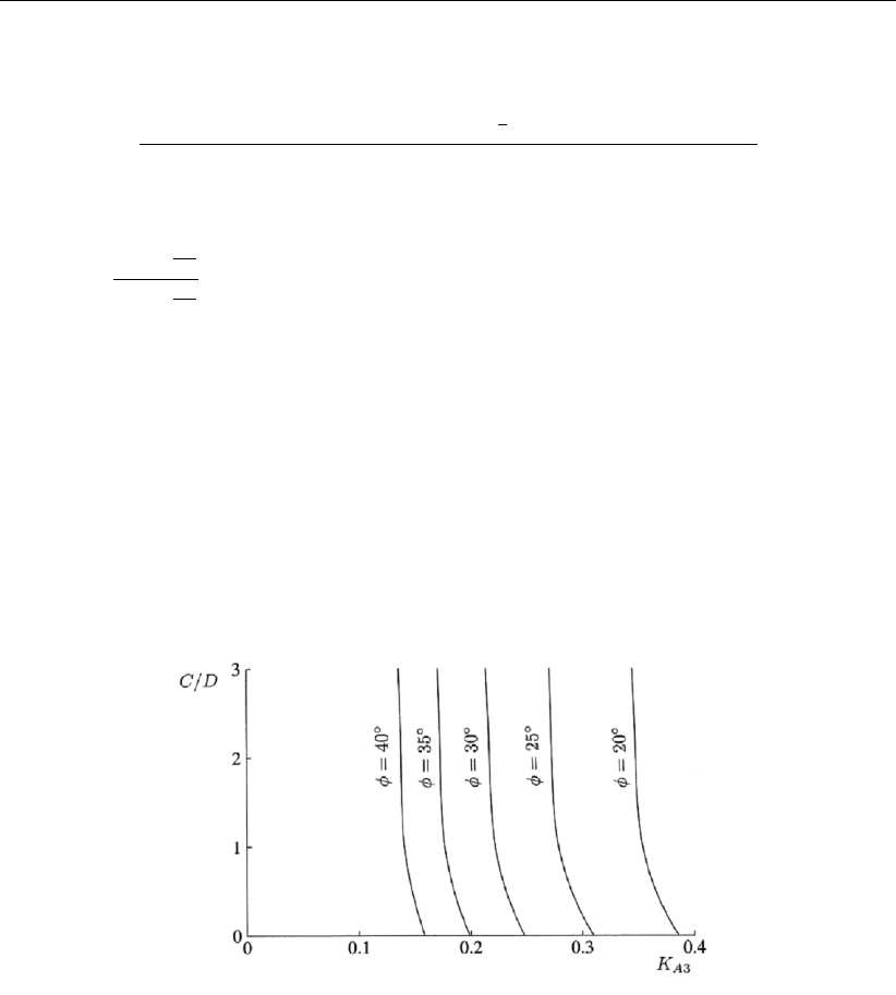
Micro tunneling
The 3 dimensional coefficient of active earth pressure is calculated as follows:
KA3 =sin β×cos β−cos2β×tan ϕ−2
3K×α×cos β×tan ϕ
cos β×sin β+ tan ϕ×sin2β(24.5)
with:
α=1+3C1
Do
1+2C1
Do
where:
C1is the distance between the drained/undrained border and the top of the shield of
the micro tunneling machine, in m;
βis the angle of the slip surface of the active wedge, in degree;
ϕis the angle of internal friction, in degree.
In the subsequent figure the values for different angles of internal friction for a series of
depth/diameter ratios are shown.
Figure 24.2: Values for KA3
The method described by Jancsecz and Steiner Jancesz and Steiner (1994) has the opportu-
nity to take the effect of vertical stress reduction due to arching in account. In Figure 24.3, the
arching over the depth Ccan reduce the vertical stress on the active wedge which determines
the minimal support pressure. It should be noticed that the arching can only occur if a relative
small soil deformation (settlement of the soil column above the active soil wedge) is allowed.
Deltares 305 of 324
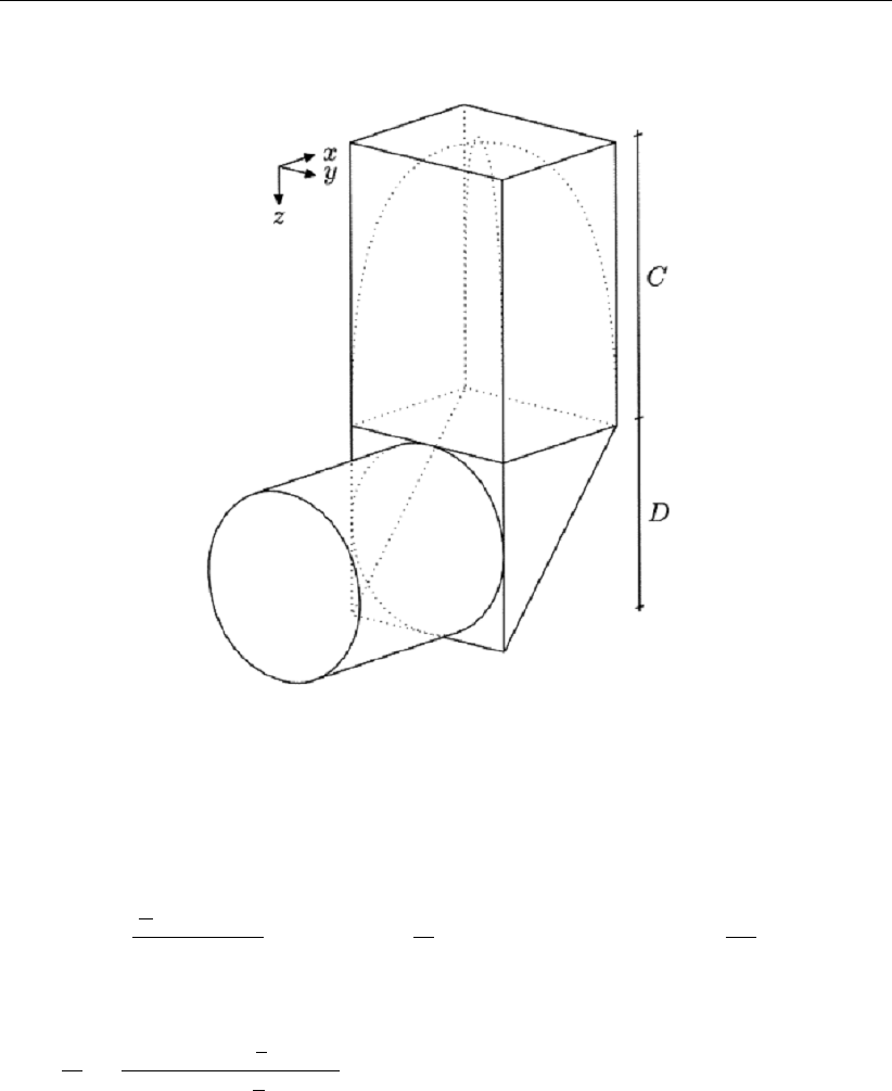
D-GEO PIPELINE
, User Manual
Figure 24.3: Active soil wedge with soil column (Broere,1994)
For a layered soil the following equation can be used to calculate the effect of two dimensional
arching according to Terzaghi (Terzaghi,1943) on the active wedge:
σ0
v;1 =
A
O×γ0−cd
K0×tan ϕd1−exp −O
A×C2×K0×tan ϕd+Do
2×γ0
b(24.6)
with:
O
A=21 + tan π
2−β
Do×tan π
2−β
where:
Ais the area of the soil column, in m2;
cdis the cohesion of the slip surface of the active wedge (i.e. average between the
drained/undrained border and the top of the shield of the micro tunneling machine),
in kN/m2;
C2is the distance between the ground level and the top of the shield of the micro
tunneling machine, in m;
K0is the coefficient of neutral earth pressure: K0= 1 −sin ϕd;
Ois the circumference of the soil column, in m;
ϕdis the average angle of internal friction between the drained/undrained border and
the top of the shield of the micro tunneling machine, in degrees;
γ0is the average effective unit weight between the ground level and the top of the shield
of the micro tunneling machine, in kN/m3;
γ0
bis the average effective unit weight between the top and the center of the shield of
the micro tunneling machine, in kN/m3.
306 of 324 Deltares

Micro tunneling
24.1.3 Maximal support pressure
In case of a high support pressure, several possible failure mechanism may occur:
Soil failure due to pushing a soil wedge in upward direction
A blow out to the surface due to hydraulic fracturing
Horizontal hydraulic fracturing at the transition of soil layers
The maximal allowable support pressure σmax for micro tunneling can be determined as fol-
lows:
σmax =σ0
v
fcover
+u×fu(24.7)
where:
σ0
vis the effective vertical stress (see Equation 26.5);
uis the pore pressure, in kN/m2, see Equation 26.4;
fcover is the contingency factor on soil cover as defined in the Factors window, see sec-
tion 4.7.1.2 (default is 1.1).
fuis the safety factor on water pressure as defined in the Factors window, see sec-
tion 4.7.1.2 (default is 1.05);
Obvious the total allowable support pressure is equal to the sum of the allowable effective
support pressure and the water pressure at the drilling line.
24.1.4 Thrust force
The thrust force which is required to install a pipeline or micro tunnel in between the launch
pit and the reception pit. The magnitude of the thrust force is determined by the pressure on
the shield (head of the tunneling machine) and friction along the circumference of the tunnel
or pipeline. The thrust force due to pressure on the shield is relative small compared to the
force due to friction and can therefore be neglected. The thrust force Fmdue to friction can
be calculated as follows:
Fm=π×Do×L×M(24.8)
where:
Dois the diameter of the pipeline or the tunnel, in m;
Lis the length, in m;
Mis the friction between the soil and the pipe per surface area, in kN/m2. The friction
Mis defined in the Engineering Data window (section 4.6.3.3) where two cases are
considered: friction with or without injection of lubricant.
The friction per surface area is partly determined by the soil type, through which the micro
tunneling is carried out, but is mainly determined by the overcut and the usage of lubricants,
which reduce the friction in between the tunnel or pipeline and the surrounding soil. Since
the bending radii of the curves in a micro tunneling drilling line are generally smooth the soil
reaction forces in the curves are not considered in
D-GEO PIPELINE
.
Deltares 307 of 324

D-GEO PIPELINE
, User Manual
24.2 Uplift Safety
Due to buoyancy of the pipeline below the groundwater table, the uplift should be checked:
fuplift < fuplift;all (24.9)
where fuplift;all is the allowable safety factor on uplift, as defined in the Factors window, see
section 4.7.1.2.
The forces acting on the pipeline are:
the uplift force:
guplift =π
4×D2
o×γw(24.10)
the weight of the pipeline:
gpipe =π
4×D2
o−(Do−2dn)2×γb(24.11)
The effective weight of the pipeline is defined as:
geff =gpipe −guplift (24.12)
and the uplift safety factor fuplift is:
fuplift =geff
n
X
i=1
γ0
i×di
(24.13)
where:
γ0
iis the buoyant unit weight of soil layer i, in kN/m3;
nis the number of soil layers;
diis the thickness of soil layer iabove the pipeline, in m.
24.3 Subsidence
The drilling process micro tunneling leads to a larger amount of removed soil material than the
volume of the installed tunnel or pipeline (Overcut). Of course injection of lubricants may lead
to a reduction of the differential volume of removed soil and installed elements. The differential
volume will lead to soil movement towards the bore hole, which in turn will lead to subsidence.
The magnitude of the subsidence w(trough shaped) can be calculated as follows:
w=Vs
√2πi2exp −r2
2i2z < z0(24.14)
with:
Vs=Vloss
100 ×Do+ 2 lovercut
2
2−Do
2
2
where:
iis the shape factor, see below;
308 of 324 Deltares

Micro tunneling
lovercut is the overcut in radius, in m;
ris the horizontal distance in between the center of the tunnel or pipeline and the
inflection point of the trough, in m;
z0is the depth of the center of the pipeline or tunnel, in m;
zis the depth at which the settlement is calculated, in m;
Vloss is the volume loss as percentage of overcut area, in %, as defined in the Engineer-
ing Data window, see section 4.6.3.2;
Vsis the differential volume, in m3/m.
The shape factor idepends upon the soil behavior above the tunnel or pipeline and is there
dependent upon the soil properties of the upper soil layers. The factor ican empirically be
determined based on differences in soil sequences. The empirical method is described by O
Reilly (O’ Reilly and New,1982):
i= 0.43 Dbas + 0.28 Dtop + 1.1for incompressible granular soil on compressible soil
i= 0.43 Dbas + 1.1for compressible soil
i= 0.23 Dbas + 0.43 Dtop −0.1for compressible soil on incompressible granular soil
i= 0.28 Dbas −0.1for incompressible granular soil
where:
Dbas is the thickness of the Basal layer above the tunnel or pipeline, in m;
Dtop is the thickness of the upper layer above the tunnel or pipeline, in m.
Deltares 309 of 324

D-GEO PIPELINE
, User Manual
310 of 324 Deltares

25 Trenching
Installation of the pipeline in a trench is the oldest and a relatively easy method. One of
the main installation risk associated with trenching is instability of the slopes of the trench.
This risk can not be considered in
D-GEO PIPELINE
. Use of other computer programs such as
D-GEO STABILITY
(formerly known as MStab) is recommended.
In case of installed pipelines with a relatively thin soil cover in a wet environment, uplift can
be an installation risk (section 25.1). In case of trenching in soil layers which cover an aquifer
with high pore pressures, bursting of the bottom of the trench (heaving) can be an installation
risk (section 25.2).
25.1 Uplift Safety
Due to buoyancy of the pipeline below the groundwater table, the uplift should be checked:
fuplift < fuplift;all (25.1)
where fuplift;all is the allowable safety factor on uplift, as defined in the Factors window, see
section 4.7.1.3.
The forces acting on an empty pipe are:
the uplift force:
guplift =π
4×D2
o×γw(25.2)
the weight of the pipeline:
gpipe =π
4×D2
o−(Do−2dn)2×γb(25.3)
The effective weight of the pipeline is defined as:
geff =gpipe −guplift (25.4)
and the uplift safety factor fuplift is:
fuplift =geff
n
X
i=1
γ0
i×di
(25.5)
where:
γ0
iis the buoyant unit weight of soil layer i, in kN/m3;
nis the number of soil layers;
diis the thickness of soil layer iabove the pipeline, in m.
Deltares 311 of 324

D-GEO PIPELINE
, User Manual
25.2 Bursting of the trench bottom (heaving)
The check of the bursting of the trench bottom is performed according to paragraph 14.3.1 of
the Dutch standard NEN 6740:2006 (NEN,2006). The calculated safety factor fburst should
not exceed the allowable safety factor on hydraulic heave fburst;all, as defined in the Factors
window, see section 4.7.1.3.
fburst;all > fburst (25.6)
The safety factor on bursting fburst is:
fburst =Wtot
pz;d
(25.7)
where:
pz;d is the upward water pressure, in kN/m2, see Equation 25.11.
Wtot is the total weight above the aquifer, in kN/m2, see Equation 25.8;
Total weight above the aquifer
Wtot =Wtot;1 +Wtot;2 (25.8)
Wtot;1 =f×γ1;d ×d1;d (25.9)
Wtot;2 =
n
X
j=1
γj;d ×dj;d (25.10)
with:
f=2
π1 + b
a×arctan d2;d
a+b−b
a×arctan d2;d
b
where:
ais the width (horizontally) of the slope of the trench, in m;
bis the depth of the slope of the trench, in m;
d1;d is the sum of the thickness of the layers above the excavation level, in m;
d2;d is the sum of the thickness of the layers below the pipe (excavation level) and
above the aquifer, in m.
fis the factor for the contribution of the layers above the excavation level according
to Figure 25.2;
Wtot;1 is the weight of the soil layers above the trench bottom, in kN/m2;
Wtot;2 is the weight of the overburden soil layers below the trench bottom, in kN/m2;
γ1;d is the average unit weight of the layers above the excavation level, in kN/m3;
Upward water pressure
pz;d =Hd×γw(25.11)
where:
312 of 324 Deltares
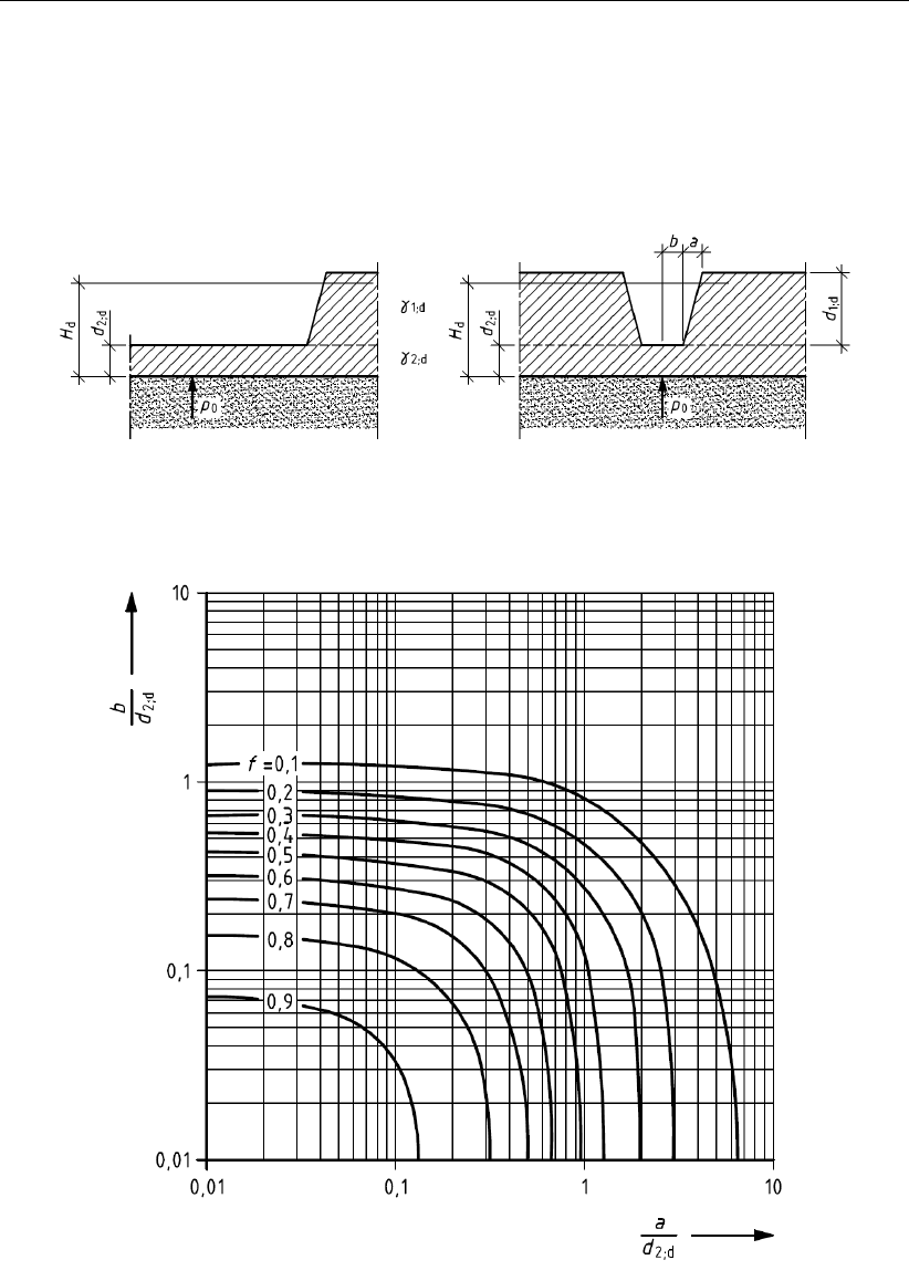
Trenching
Hdis the hydraulic head with respect to the upper boundary of the aquifer, calculated
according to section 26.1;
γwis the unit weight of water, in kN/m3.
Figure 25.1: Definition of parameters Hd,d1;d and d2;d (Figure 18 of NEN 6740:2006)
Figure 25.2: Factor ffor the contribution of the layers above the bottom of the excavation
(Figure 19 of NEN 6740:2006)
Deltares 313 of 324

D-GEO PIPELINE
, User Manual
314 of 324 Deltares

26 Effective Stress and Pore Pressure
26.1 Hydraulic head from piezometric level lines
A piezometric level line (PL-line) represents the initial and transient hydraulic water heads in
the soil, excluding the excess component. Several PL-lines can be defined in the PL-Lines
window (section 4.3.10). A PL-line for the top and bottom of each soil layer can be defined in
the Pl-lines per Layer window (section 4.3.13).
PL-line 2
PL-line 1
SAND
CLAY
SAND
CLAY2
SAND
1
1
1
2
2
2
2
1
1
1
1
99
99
99
99
99
2
Figure 26.1: Pore pressure as a result of piezometric level lines
D-GEO PIPELINE
calculates the hydraulic pore pressure along a vertical in the following way:
The pore pressure inside a layer is calculated by linear interpolation between the pore pres-
sures at the top and bottom. The pore pressure at the top or bottom is equal to the vertical
distance between this point and the position of the PL-line that belongs to this layer, multiplied
by the unit weight of water.
If PL-line number 99 is specified for the top and/or bottom of any soil layer, at that boundary
D-GEO PIPELINE
will use the PL-line of the nearest soil layer above or below, which has a
thickness larger than zero and a PL-line number not equal to 99. If the interpolation point
is located above the phreatic line, the pore pressure is assumed to be zero or a capillary
pressure, depending on the sign of the PL-line number. The following options are available,
therefore, for PL-line numbers:
Positive integer:
Capillary pore pressures are not used – that is, if negative pore pressures are calculated
for points above the phreatic line they become zero;
Zero:
All points within the layer obtain a pore pressure of 0 kN/m;
99:
The pore pressure depends on the first layer above and/or below the point with a PL-line
Deltares 315 of 324
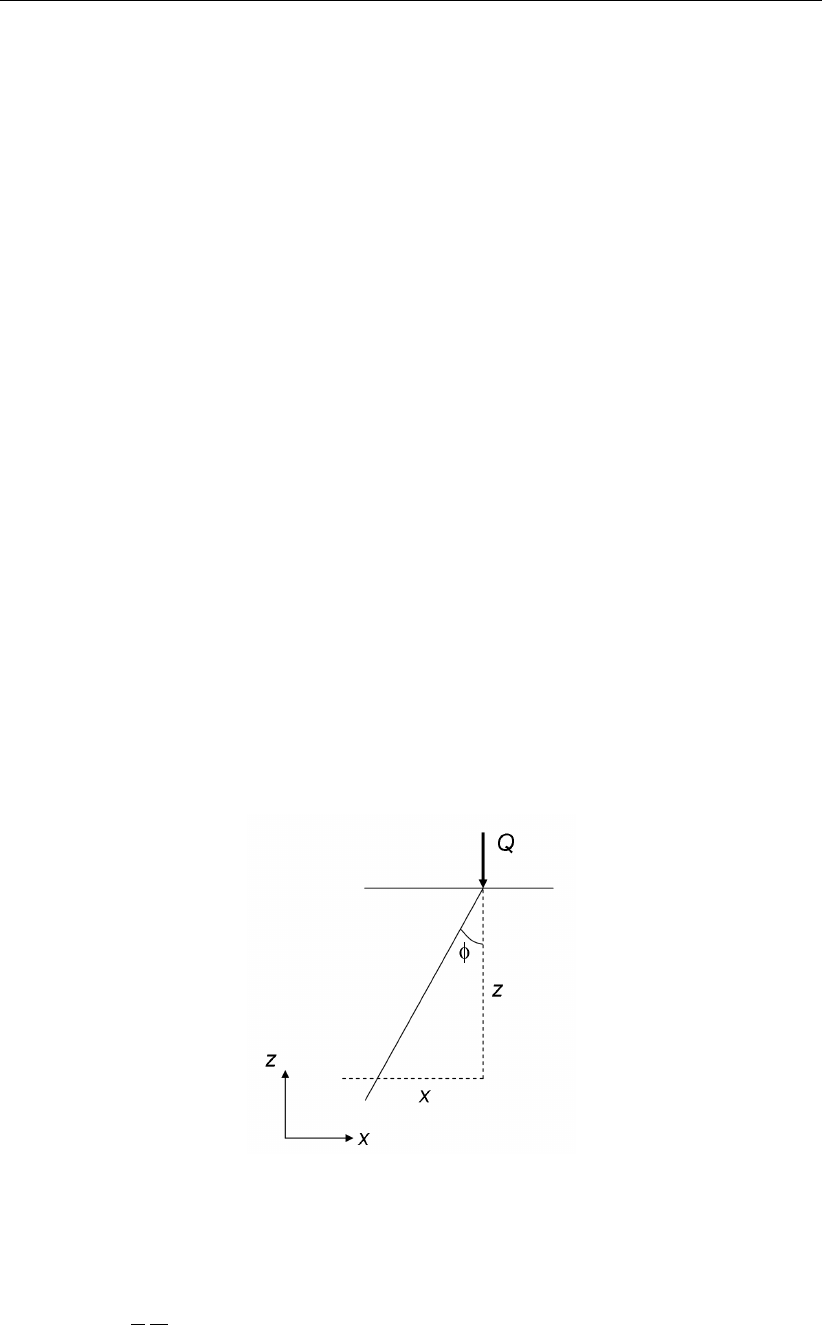
D-GEO PIPELINE
, User Manual
number unequal to 99.
26.2 Phreatic line
The phreatic line (or groundwater level) marks the border between dry and wet soil. The
phreatic line is treated as if it was a PL-line, and can also be used as such. The PL-line acting
as the phreatic line is determined while the geometry is being defined. If no phreatic line is
entered, then all the soil is assumed to be dry.
26.3 Stress by soil weight
The total stress at depth zdue to soil weight is:
σsoil (z) = γunsat ×zif z > zwater
γunsat ×zwater +γsat ×(zwater −z)if z≤zwater
(26.1)
where:
γunsat is the unit weight of soil above phreatic level, in kN/m3;
γsat is the unit weight of soil below phreatic level, in kN/m3;
zis the vertical co-ordinate, in m;
zwater is the vertical co-ordinate of the phreatic level, in m.
26.4 Distribution of stress by loading
D-GEO PIPELINE
uses Boussinesq’s formula (Boussinesq,1885) to determine the additional
vertical stress due to the surcharge loads.
26.4.1 Stress increment caused by a line load
Figure 26.2: Stress distribution under a load column
The vertical stress increment ∆σzdue to a line load Qis:
∆σz=2
π
Q
zcos4φ(26.2)
where:
zis the depth, in m;
316 of 324 Deltares
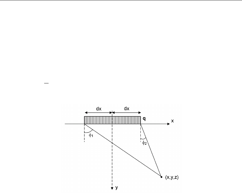
Effective Stress and Pore Pressure
Qis the line load, in kN;
φis the angle with the vertical, in radians.
26.4.2 Stress increment caused by a strip load
The stress increments in a point (x,y) due to a strip load can be found by integration of the
line load along the width 2 dx of the strip load in Equation 26.2:
∆σload =q
π[(φ1−φ2) + sin φ1cos φ1−sin φ2cos φ2](26.3)
Figure 26.3: Stress distribution under a load column
26.5 Effective stress and pore pressure
The pore pressure uat vertical position zis defined as:
u(z) = σwater (z)−max [h(z)−z; 0] ×γw(26.4)
The effective stress σ’ at vertical position zis defined as:
σ0(z) = σsoil (z)+∆σload (z)−u(z)(26.5)
with:
σwater (z) = max (zwater −zsurface; 0) ×γw
where:
zis the vertical co-ordinate, in m;
zwater is the vertical position of the phreatic level , in m;
zsurface is the vertical position of the ground level , in m;
his the user-defined hydraulic head in the Pl-lines per Layer window (sec-
tion 4.3.13), see section 26.1;
σsoil is the stress due to soil weight, in kN/m2, see Equation 26.1;
σwater is the stress due to a water level above the soil surface, in kN/m2;
∆σload is the incremental stress due to loads, in kN/m2, see Equation 26.3.
Deltares 317 of 324

D-GEO PIPELINE
, User Manual
318 of 324 Deltares

27 Benchmarks
Deltares Systems commitment to quality control and quality assurance has leaded them to
develop a formal and extensive procedure to verify the correct working of all of their geotech-
nical engineering tools. An extensive range of benchmark checks have been developed to
check the correct functioning of each tool. During product development these checks are run
on a regular basis to verify the improved product. These benchmark checks are provided
in the following sections, to allow the user to overview the checking procedure and verify for
themselves the correct functioning of
D-GEO PIPELINE
. The benchmarks are subdivided into
five separate groups as described below.
Group 1 – Benchmarks from literature (exact solution) Simple benchmarks for which
an exact analytical result is available from literature.
Group 2 – Benchmarks from literature (approximate solution) More complex bench-
marks described in literature for which an approximate solution is known.
Group 3 – Benchmarks from spread sheets Benchmarks which test program features
specific to
D-GEO PIPELINE
.
Group 4 – Benchmarks generated by
D-GEO PIPELINE
Benchmarks for which the ref-
erence results are generated using
D-GEO PIPELINE
.
Group 5 – Benchmarks compared with other programs Benchmarks for which the
results of
D-GEO PIPELINE
are compared with the results of other programs.
The number of benchmarks in group 1 may grow in the future. The benchmarks in this chapter
are well documented in literature. There are no exact solutions available for these problems,
however in the literature estimated results are available. When verifying the program, the
results should be close to the results found in the literature. The number of benchmarks
in group 2 will grow as new versions of the program are released. These benchmarks are
designed so that (new) features specific to the program can be verified. The benchmarks are
kept as simple as possible so that only one specific feature is verified from one benchmark
to the next. As much as software developers would wish they could, it is impossible to prove
the correctness of any non-trivial program. Re-calculating all the benchmarks, and making
sure the results are as they should be, proves to some degree that the program works as it
should. Nevertheless, there will always be combinations of input values that will cause the
program to crash or to produce wrong results. Hopefully by using the verification procedure
the number of ways this can occur will be limited. The benchmarks are all described in details
in the Verification Report available in the installation directory of the program.
Deltares 319 of 324

D-GEO PIPELINE
, User Manual
320 of 324 Deltares

Bibliography
“SCIA Pipeline.” (integrated in the program Scia Engineer) http://www.scia-
online.com/en/pipeline-calculation.html.
Boussinesq, J., 1885. Application des Potentiels á l’Etude de l’Equilibre et du Mouvement des
Solides Elastiques. Gauthier-Villars, Paris.
Brinch Hansen, J., 1970. “A revised and extended formula for bearing capacity.” Lyngby
Bulletin No. 28. Danish Geotechnical Institute.
Broere, W., 1994. Tunnel face stability and new cpt applications. DUP Science. Delft.
Broms, B. B. and H. Bennermark, 1967. “Stability of clay at vertical openings.” American
Society of Civil Engineers, Journal of Soil Mechanics and Foundation Division pages 71-
95.
Davis, E. H., M. J. Gunn, R. J. Mair and H. N. Seneviratne, 1980. “The stability of shallow
tunnels and underground openings in cohesive material.” Geotechnique 30 pages 397-416.
Deltares. D-Settlement User Manual. Deltares Systems.
Deltares, 2004. WATEX Manual. Delft GeoSystems.
Jancesz, S. and W. Steiner, 1994. “Face support for a large mix shield in heterogeneous
ground conditions.” Proc conf. Tunnelling London.
Meijers, P. and R. A. J. de Kock, 1995. “A calculation method for earth pressure on directional
drilled pipelines.” Pipeline technology conference Ostend.
NEN, 2006. NEN 6740:2006. Geotechniek - TGB 1990 - Basiseisen en belastingen (Geotech-
nics - TGB 1990 - Basic requirements and loads), in Dutch.
NEN, 2012a. NEN 3650-1:2012. Eisen voor buisleidingsystemen - Deel 1: Algemene eisen
(Requirements for pipeline systems - Part 1: General requirements), in Dutch.
NEN, 2012b. NEN 3650-2:2012. Eisen voor buisleidingsystemen - Deel 2: Aanvullende eisen
voor leidingen van staal (Requirements for pipeline systems - Part 2: Additional specifica-
tions for steel pipelines), in Dutch.
NEN, 2012c. NEN 3650-3:2012. Eisen voor buisleidingsystemen - Deel 3: Aanvullende eisen
voor leidingen van kunststof (Requirements for pipeline systems - Part 3: Additional speci-
fications for plastic pipelines), in Dutch.
NEN, 2012d. NEN 3651:2012. Aanvullende eisen voor buisleidingen in of nabij belangri-
jke waterstaatswerken (Additional requirements for pipelines in or nearby important public
works), in Dutch.
O’ Reilly, M. P. and B. M. New, 1982. “Settlements above tunnels in U.K. ˝
U their magnitude
and prediction.” Tunneling Š82 pages 173 - 181.
Terzaghi, K., 1943. Theoretical soil mechanics. John Wiley & Sons, Inc. New York.
Deltares 321 of 324

D-GEO PIPELINE
, User Manual
322 of 324 Deltares

PO Box 177
2600 MH Del
Rotterdamseweg 185
2629 HD Del
The Netherlands
+31 (0)88 335 81 88
sales@deltaressystems.nl
www.deltaressystems.nl
