D RealTimeControl User Manual RTC_User_Manual RTC
User Manual: Pdf D-RTC_User_Manual
Open the PDF directly: View PDF ![]() .
.
Page Count: 82
- List of Figures
- List of Tables
- 1 A guide to this manual
- 2 Module D-RTC: Overview
- 3 Module D-RTC: Getting started
- 4 Module D-RTC: All about the modelling process
- 5 Module D-RTC: Simulation and model output
- 6 Module D-RTC: Technical reference
- A D-RTC build instructions on Linux
- References
Delft3D flexible Mesh suite
1D/2D/3D Modelling suite for integral water solutions
User Manual
D-Real Time Control
DRAFT
DRAFT
DRAFT
D-Real Time Control
D-Real Time Control (D-RTC) in Delta Shell
User Manual
Released for:
Delft3D FM Suite 2018
D-HYDRO Suite 2018
SOBEK Suite 3.7
Version: 1.4
SVN Revision: 54906
April 18, 2018
DRAFT
D-Real Time Control, User Manual
Published and printed by:
Deltares
Boussinesqweg 1
2629 HV Delft
P.O. 177
2600 MH Delft
The Netherlands
telephone: +31 88 335 82 73
fax: +31 88 335 85 82
e-mail: info@deltares.nl
www: https://www.deltares.nl
For sales contact:
telephone: +31 88 335 81 88
fax: +31 88 335 81 11
e-mail: software@deltares.nl
www: https://www.deltares.nl/software
For support contact:
telephone: +31 88 335 81 00
fax: +31 88 335 81 11
e-mail: software.support@deltares.nl
www: https://www.deltares.nl/software
Copyright © 2018 Deltares
All rights reserved. No part of this document may be reproduced in any form by print, photo
print, photo copy, microfilm or any other means, without written permission from the publisher:
Deltares.

DRAFT
Contents
Contents
List of Figures vii
List of Tables ix
1 A guide to this manual 1
1.1 Introduction .................................. 1
1.2 Overview ................................... 1
1.3 Manual version and revisions ......................... 1
1.4 Changes with respect to previous versions .................. 1
2 Module D-RTC: Overview 3
2.1 Introduction: Feedback control and feedforward control . . . . . . . . . . . . 3
2.2 Introduction: D-RTC windows ......................... 5
2.3 Controlgroup ................................. 7
2.4 Flow chart .................................. 8
2.5 The Properties ................................ 9
2.6 Examples ................................... 10
2.6.1 Minimal controlflow . . . . . . . . . . . . . . . . . . . . . . . . . . 10
2.6.2 Combinations of conditions and rules . . . . . . . . . . . . . . . . . 10
3 Module D-RTC: Getting started 17
3.1 Introduction .................................. 17
3.2 Getting started ................................ 17
3.2.1 The integrated model ......................... 17
3.2.2 The D-Flow 1D model . . . . . . . . . . . . . . . . . . . . . . . . 18
3.3 A simple D-RTC model . . . . . . . . . . . . . . . . . . . . . . . . . . . . 19
3.3.1 Add a Control Group ......................... 19
3.3.2 Construct a minimal controlflow . . . . . . . . . . . . . . . . . . . . 20
3.3.3 Perform a simulation ......................... 21
3.4 View the simulation results . . . . . . . . . . . . . . . . . . . . . . . . . . 21
3.4.1 Introduction .............................. 21
3.4.2 Table view .............................. 21
3.4.3 Side-view ............................... 22
3.5 A more complex control flow ......................... 23
3.5.1 Multiple controlled parameters on one structure . . . . . . . . . . . . 23
3.5.2 Multiple controlled structures . . . . . . . . . . . . . . . . . . . . . 26
3.6 Control flows with conditions ......................... 27
3.6.1 A controlflow with a condition . . . . . . . . . . . . . . . . . . . . . 27
3.6.2 A controlflow with two conditions: logical AND . . . . . . . . . . . . 29
3.6.3 A controlflow with two conditions: logical OR . . . . . . . . . . . . . 29
4 Module D-RTC: All about the modelling process 31
4.1 Conditions .................................. 31
4.1.1 Hydro condition . . . . . . . . . . . . . . . . . . . . . . . . . . . . 31
4.1.2 Time condition . . . . . . . . . . . . . . . . . . . . . . . . . . . . 32
4.2 Rules ..................................... 34
4.2.1 Lookup table rule ........................... 34
4.2.2 Time rule ............................... 36
4.2.3 PID rule ............................... 37
4.2.3.1 Introduction . . . . . . . . . . . . . . . . . . . . . . . . 37
4.2.3.2 PID rules in D-RTC . . . . . . . . . . . . . . . . . . . . . 38
4.2.3.3 PID rule calibration . . . . . . . . . . . . . . . . . . . . . 39
4.2.4 Interval rule .............................. 39
Deltares iii

DRAFT
D-Real Time Control, User Manual
4.2.5 Relative from time/value rule . . . . . . . . . . . . . . . . . . . . . 41
4.2.6 Invertor rule ............................. 42
5 Module D-RTC: Simulation and model output 45
6 Module D-RTC: Technical reference 47
6.1 Overview ................................... 47
6.2 General purpose components ......................... 48
6.2.1 Accumulation ............................. 48
6.2.2 Expression .............................. 48
6.2.3 Gradient ............................... 48
6.2.4 lookupTable ............................. 48
6.2.5 Lookup2DTable . . . . . . . . . . . . . . . . . . . . . . . . . . . . 49
6.2.6 MergerSplitter . . . . . . . . . . . . . . . . . . . . . . . . . . . . 49
6.2.7 UnitDelay ............................... 49
6.3 Operating rules and controllers . . . . . . . . . . . . . . . . . . . . . . . . 49
6.3.1 Constant ............................... 49
6.3.1.1 Functional principle . . . . . . . . . . . . . . . . . . . . . 49
6.3.1.2 Application ......................... 49
6.3.2 DateLookupTable ........................... 49
6.3.3 DeadBandValue ........................... 50
6.3.4 GuideBand .............................. 50
6.3.5 Interval ................................ 51
6.3.6 Limiter ................................ 51
6.3.7 PID rule ............................... 51
6.3.7.1 Functional principle . . . . . . . . . . . . . . . . . . . . . 51
6.3.7.2 Application ......................... 52
6.3.7.3 Example . . . . . . . . . . . . . . . . . . . . . . . . . . 52
6.3.8 The absolute time rule (timeAbsolute). . . . . . . . . . . . . . . 55
6.3.8.1 Functional principle . . . . . . . . . . . . . . . . . . . . . 55
6.3.8.2 Application ......................... 55
6.3.8.3 Example . . . . . . . . . . . . . . . . . . . . . . . . . . 55
6.3.9 The relative time rule (timeRelative). . . . . . . . . . . . . . . . 57
6.3.9.1 Functional principle . . . . . . . . . . . . . . . . . . . . . 57
6.3.9.2 Application ......................... 57
6.3.9.3 Example . . . . . . . . . . . . . . . . . . . . . . . . . . 57
6.4 Triggers .................................... 59
6.4.1 Introduction .............................. 59
6.4.2 Standard ............................... 59
6.4.3 The time trigger . . . . . . . . . . . . . . . . . . . . . . . . . . . . 59
6.4.3.1 Functional principle . . . . . . . . . . . . . . . . . . . . . 59
6.4.3.2 Application ......................... 59
6.4.4 deadBandTrigger ........................... 60
6.4.4.1 Functional principle . . . . . . . . . . . . . . . . . . . . . 60
6.4.4.2 Application ......................... 60
6.4.4.3 Example . . . . . . . . . . . . . . . . . . . . . . . . . . 60
6.4.5 deadBandTime . . . . . . . . . . . . . . . . . . . . . . . . . . . . 63
6.4.6 polygonLookup . . . . . . . . . . . . . . . . . . . . . . . . . . . . 63
6.4.7 set .................................. 63
6.4.8 Expression .............................. 64
A D-RTC build instructions on Linux 65
A.1 Prerequisites ................................. 65
A.2 Build D-RTC ................................. 65
iv Deltares


DRAFT
D-Real Time Control, User Manual
vi Deltares

DRAFT
List of Figures
List of Figures
2.1 Feedback control and feedforward control . . . . . . . . . . . . . . . . . . . 3
2.2 Example flow chart with feedback control . . . . . . . . . . . . . . . . . . . 4
2.3 Example of an RTC-model in the Project window . . . . . . . . . . . . . . . 5
2.4 Example of a flow chart ............................ 6
2.5 Example of the properties window for a Time rule . . . . . . . . . . . . . . . 6
2.6 D-RTC modelling concept and data flow .................... 7
2.7 Components and basic concept of the flowchart . . . . . . . . . . . . . . . . 9
2.8 Example minimal controlflow ......................... 10
2.9 Example minimal controlflow with a condition . . . . . . . . . . . . . . . . . 10
2.10 Example of two conditions that combined form an AND trigger . . . . . . . . 11
2.11 Example of two conditions that combined form an OR trigger . . . . . . . . . 11
2.12 Example of three conditions: 1 ∧(2 ∨3) . . . . . . . . . . . . . . . . . . . 12
2.13 Example of three conditions: 1 ∨(2 ∧3) . . . . . . . . . . . . . . . . . . . 12
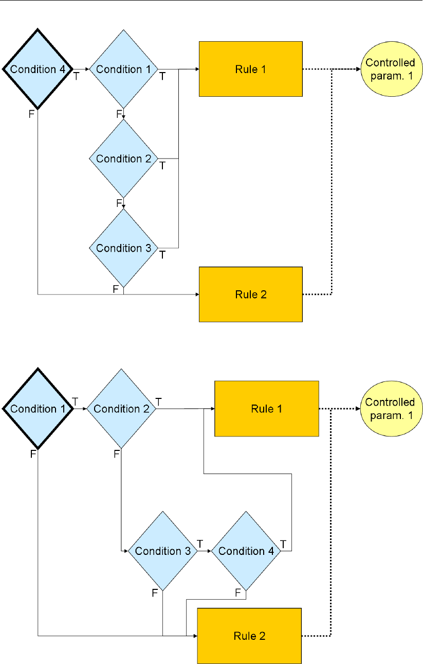
2.14 Example of four conditions: 4 ∨(1 ∧2∧3) . . . . . . . . . . . . . . . . . . 13
2.15 Example of four conditions: 1 ∧2∧(3 ∨4) . . . . . . . . . . . . . . . . . . 13
2.16 Example of four conditions: (1 ∨2) ∧(3 ∨4) . . . . . . . . . . . . . . . . . 14
2.17 Example of four conditions: (1 ∧(3 ∨4)) ∨(2 ∧4) . . . . . . . . . . . . . . 14
2.18 Example of four conditions: 4 ∧(1 ∨2∨3) . . . . . . . . . . . . . . . . . . 15
2.19 Example of four conditions: (1 ∧2) ∨(3 ∧4) . . . . . . . . . . . . . . . . . 15
3.1 Integrated model default properties . . . . . . . . . . . . . . . . . . . . 17
3.2 Integrated model, settings for a coupled simulation with D-RTC and D-Flow 1D
........................................ 17
3.3 Integrated model in the Project window . . . . . . . . . . . . . . . . . . . . 18
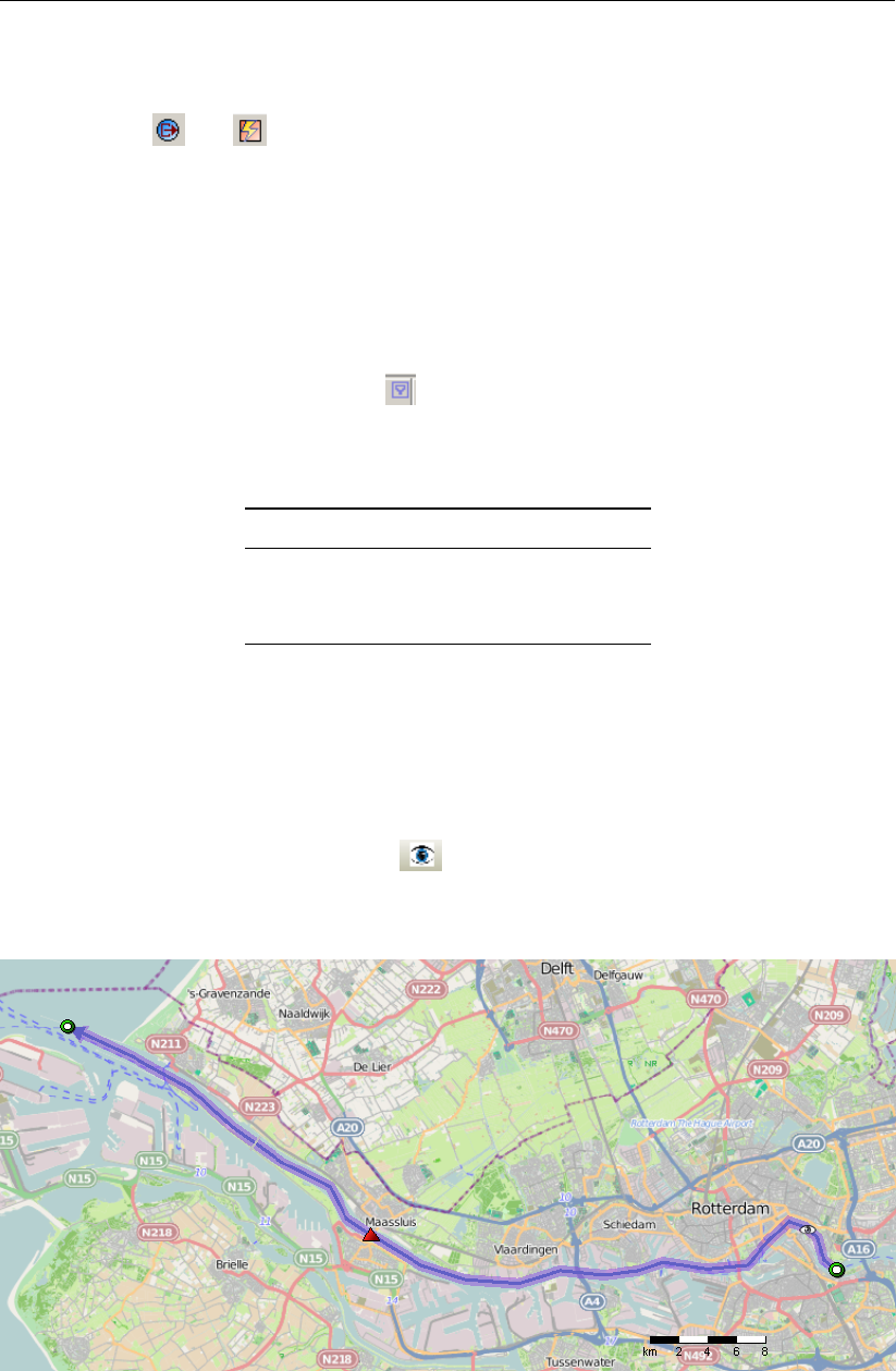
3.4 Example water flow model schematisation with an OpenStreet background
map (http://openstreetmap.org). . . . . . . . . . . . . . . . . . 19
3.5 Options for default controlgroups . . . . . . . . . . . . . . . . . . . . . . . 19
3.6 Empty controlgroup .............................. 20
3.7 Minimum flow chart with a Time Rule . . . . . . . . . . . . . . . . . . . . . 20
3.8 Project window after a coupled simulation with D-RTC and D-Flow 1D. . . . . 22
3.9 Table and chart view D-RTC output . . . . . . . . . . . . . . . . . . . . . . 22
3.10 Sideview with water level and crest level of the structure . . . . . . . . . . . 23
3.11 Flowchart for example with two controlled parameters for one weir. . . . . . . 24
3.12 Structure selected on the map view of simulation output . . . . . . . . . . . . 24
3.13 Select output coverage . . . . . . . . . . . . . . . . . . . . . . . . . . . . 24
3.14 Crest level, crest width and water level over time for the weir. A point in time
has been selected in the diagram, the corresponding line is selected in the table. 25
3.15 Chart properties window, the chart title “Simulation results” has been added. . 26
3.16 D-Flow 1D network with two weirs. . . . . . . . . . . . . . . . . . . . . . . 26
3.17 D-Flow 1D network with one weir and a single observation point upstream. . . 27
3.18 Flowchart with a Hydro Condition and a Time Rule. The rule is connected with
the true-output of the condition. . . . . . . . . . . . . . . . . . . . . . . . . 28
3.19 Data origin for the structure . . . . . . . . . . . . . . . . . . . . . . . . . . 28
3.20 Flowchart with two Hydro conditions in an AND combination combined with a
Time rule. ................................... 29
3.21 Flowchart with two Hydro conditions in an OR combination and a Time rule. . . 30
4.1 Example of a flowchart with a hydro condition . . . . . . . . . . . . . . . . . 32
4.2 A hydro condition in the Properties Window . . . . . . . . . . . . . . . . . 32
4.3 Example of a flowchart with a time condition . . . . . . . . . . . . . . . . . 33
4.4 A time condition in the Properties window . . . . . . . . . . . . . . . . . . 34
4.5 A Lookup table rule in the flowchart (right) and on the map (left) . . . . . . . . 35
Deltares vii

DRAFT
D-Real Time Control, User Manual
4.6 A Lookup table rule in the Properties window . . . . . . . . . . . . . . . . . 36
4.7 A time rule in the flowchart . . . . . . . . . . . . . . . . . . . . . . . . . . 36
4.8 A time rule in the Properties window . . . . . . . . . . . . . . . . . . . . . 37
4.9 A PID rule in the flowchart . . . . . . . . . . . . . . . . . . . . . . . . . . 38
4.10 A PID rule in the Properties window . . . . . . . . . . . . . . . . . . . . . 39
4.11 An interval rule in the flowchart . . . . . . . . . . . . . . . . . . . . . . . . 40
4.12 An interval rule in the Properties window . . . . . . . . . . . . . . . . . . . 41
4.13 D-Flow 1D model of the River Meuse with close-up for the “Maasplassen” re-
gion (Roermond, the Netherlands); background map: http://openstreetmap.
org ..................................... 42
4.14 Two lateral sources connected with an invertor rule . . . . . . . . . . . . . . 43
4.15 Table and graph for the relation between water level and discharge for the
lateral source that represents the upstream end of the bypass . . . . . . . . . 43
5.1 D-RTC-model selected in the Project window . . . . . . . . . . . . . . . . . 45
6.1 Hierarchical definition of deadBand and standard triggers . . . . . . . . . . . 47
6.2 Graphical representation of guideBand rule . . . . . . . . . . . . . . . . . . 50
6.3 Simple channel model (SOBEK 3.3) . . . . . . . . . . . . . . . . . . . . . 53
6.4 PID controlled crest level of the weir and corresponding water level at the
observation point ............................... 54
6.5 Longitudinal profile of water level for two time steps and crest level of the weir . 54
6.6 Time rule time series ............................. 56
6.7 Time rule side-view .............................. 56
6.8 Relative time rule function and relative time from Value 2.5 . . . . . . . . . . 58
6.9 Crest level controlled with relative time rule and “FromValue” parameter true/-
false and the corresponding water level over time . . . . . . . . . . . . . . . 58
6.10 Expected results ............................... 60
6.11 On-off control triggered by head difference . . . . . . . . . . . . . . . . . . 61
6.12 Adding a dead band reduces the number of weir operations . . . . . . . . . . 62
6.13 Example for the application of the polygon trigger to the definition of warning
levels for controlling a lake release at Lake Thun, Canton Bern, Switzerland . . 64
viii Deltares

DRAFT
List of Tables
List of Tables
3.1 Discharge boundary condition table for the upstream end . . . . . . . . . . . 19
3.2 Time Rule data for crest level ......................... 21
3.3 Time series for the crest width (rule 2) . . . . . . . . . . . . . . . . . . . . 23
3.4 Time series of crest level for a second structure . . . . . . . . . . . . . . . . 27
3.5 Parameter-Data table for condition . . . . . . . . . . . . . . . . . . . . . . 28
3.6 Parameter-Data table for the second condition . . . . . . . . . . . . . . . . 29
4.1 Example Lookup table rule for structure . . . . . . . . . . . . . . . . . . . . 34
6.1 Target water level for the observation point . . . . . . . . . . . . . . . . . . 52
6.2 Time rule time series example . . . . . . . . . . . . . . . . . . . . . . . . 55
6.3 Relative time rule lookup table for the crest level of a weir . . . . . . . . . . . 57
6.4 Time trigger time series example . . . . . . . . . . . . . . . . . . . . . . . 59
Deltares ix

DRAFT
D-Real Time Control, User Manual
x Deltares

DRAFT
1 A guide to this manual
1.1 Introduction
This User Manual concerns the module D-Real Time Control.
This module is part of several Modelling suites, released by Deltares as Deltares Systems
or Dutch Delta Systems. These modelling suites are based on the Delta Shell framework.
The framework enables to develop a range of modeling suites, each distinguished by the
components and — most significantly — the (numerical) modules, which are plugged in. The
modules which are compliant with the Delta Shell framework are released as D-Name of the
module, for example: D-Flow Flexible Mesh, D-Waves, D-Water Quality, D-Real Time Control,
D-Rainfall Run-off.
Therefore, this user manual is shipped with several modelling suites. In the start-up screen
links are provided to all relevant User Manuals (and Technical Reference Manuals) for that
modelling suite. It will be clear that the Delta Shell User Manual is shipped with all these
modelling suites. Other user manuals can be referenced. In that case, you need to open the
specific user manual from the start-up screen in the central window. Some texts are shared
in different user manuals, in order to improve the readability.
1.2 Overview
To make this manual more accessible we will briefly describe the contents of each chapter.
If this is your first time to start working with D-RTC we suggest you to read Section 3.2,Getting
started. This chapter provides a tutorial.
Chapter 2:Module D-RTC: Overview, gives a brief introduction on D-RTC.
Chapter 3:Module D-RTC: Getting started, provides examples of D-RTC with a tutorial.
Chapter 4:Module D-RTC: All about the modelling process, provides practical information
on the GUI, setting up so-called Control groups presented as a Flow chart and validating the
model.
Chapter 5:Module D-RTC: Simulation and model output, describes how the simulation results
can be accessed.
Chapter 6:Module D-RTC: Technical reference, gives technical background information on
the principles of feedback control.
1.3 Manual version and revisions
This manual applies to SOBEK 3 suite (version 3.7 and higher), D-HYDRO Suite (version
2018 and higher) and Delft3D Flexible Mesh Suite (version 2018 and higher).
1.4 Changes with respect to previous versions
New in this edition is Chapter 6:Module D-RTC: Technical reference.
Deltares 1 of 70

DRAFT
D-Real Time Control, User Manual
2 of 70 Deltares
DRAFT
2 Module D-RTC: Overview
The D-RTC (Real Time Control) plug-in can be used for the modelling of feedback control
of hydraulic structures. It can be applied to rainfall-runoff, hydraulics and water quality com-
putations. The D-RTC module is used in a integrated model and is always combined to a
hydrodynamic model, such as D-Flow 1D or D-Flow FM.
2.1 Introduction: Feedback control and feedforward control
Feedback is a control principle where the control actions are determined based on a control
error (i.e. the difference between target value and actual value). The control action feeds back
on the control error. Feedforward control uses a control signal from outside the system to
determine control actions. The control action does not impact the feedforward control signal.
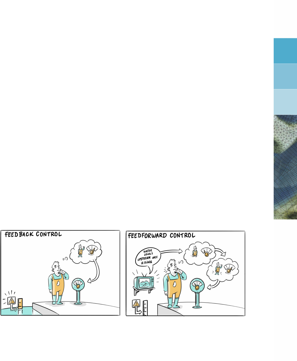
Figure 2.1 shows an example of these techniques. In both cases, the operator aims to main-
tain the water level below a certain threshold by means of a hydraulic structure for flood
protection. In Figure 2.1a the operator controls the water level with the help of information
from the system: if the water level reaches a certain level, he takes action, and the action
feeds back on the water level itself. When measurements of disturbances are used to form
control decisions the control method is called feedforward control. In Figure 2.1b the operator
checks information from a location which is outside the system (e. g. a weather forecast) and
controls accordingly. This allows him to anticipate to certain extent on a future situation, and
his control operation does not affect the information his decision is based on.
(a) feedback control (b) feedforward control
Figure 2.1: Feedback control and feedforward control
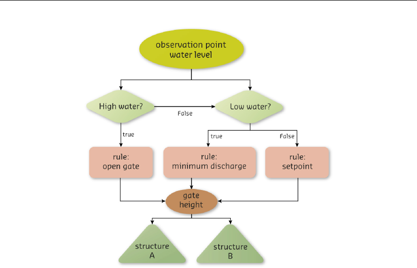
Feedback control and feedforward control can usually be represented as a flow chart or deci-
sion tree with the following elements:
trigger (condition)
operating rules (controller-actuator)
input data location (connection to an observation point or a measurement station, e.g. a
river gauge)
output data location (connection to a structure node)
An example of such a flow chart is given in Figure 2.2.
Deltares 3 of 70
DRAFT
D-Real Time Control, User Manual
Figure 2.2: Example flow chart with feedback control
A trigger implements conditions for
defining when an operating rule / controller or another trigger is applied
returning true or false, e.g. if a threshold is crossed or not.
A trigger represents a switch, an alarm level or a man-made decision in a real-time control
model. Usually it returns true and false, but there are also trigger implementations that return
numierical values.
An operating rule
defines how a structure operates, and
returns a value for a controlled parameter, e.g. a gate opening or turbine release.
Very simple operating rules define operational modes for hydraulic structures like “pump
switched on” and “pump switches off”, or “gate open” and “gate closed”. In this case the
rule does not specify how exactly the hydraulic structure is operated, but for many model ap-
plications this is sufficient. More advanced operating rules comprise closing speeds for gates
or model a complete controller actuator system. An example for such an operating rule is
a motor (the actuator) drives the segment of a weir and is switched on and off by a floating
switch (the controller itself).
4 of 70 Deltares

DRAFT
Module D-RTC: Overview
2.2 Introduction: D-RTC windows
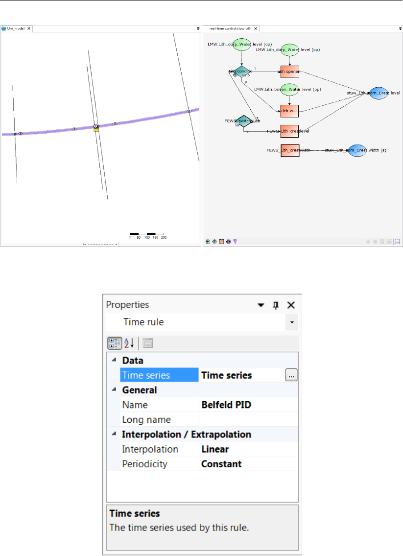
A D-RTC model has three main windows in Delta Shell: the Project window, the map with the
Flow chart, and the Properties window.
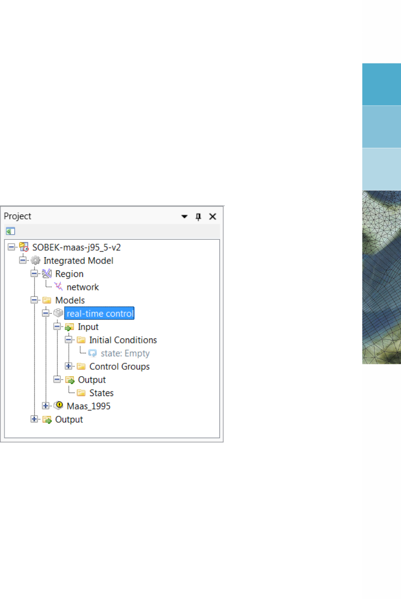
The Project window is used to show a total overview of all D-RTC model objects, while the
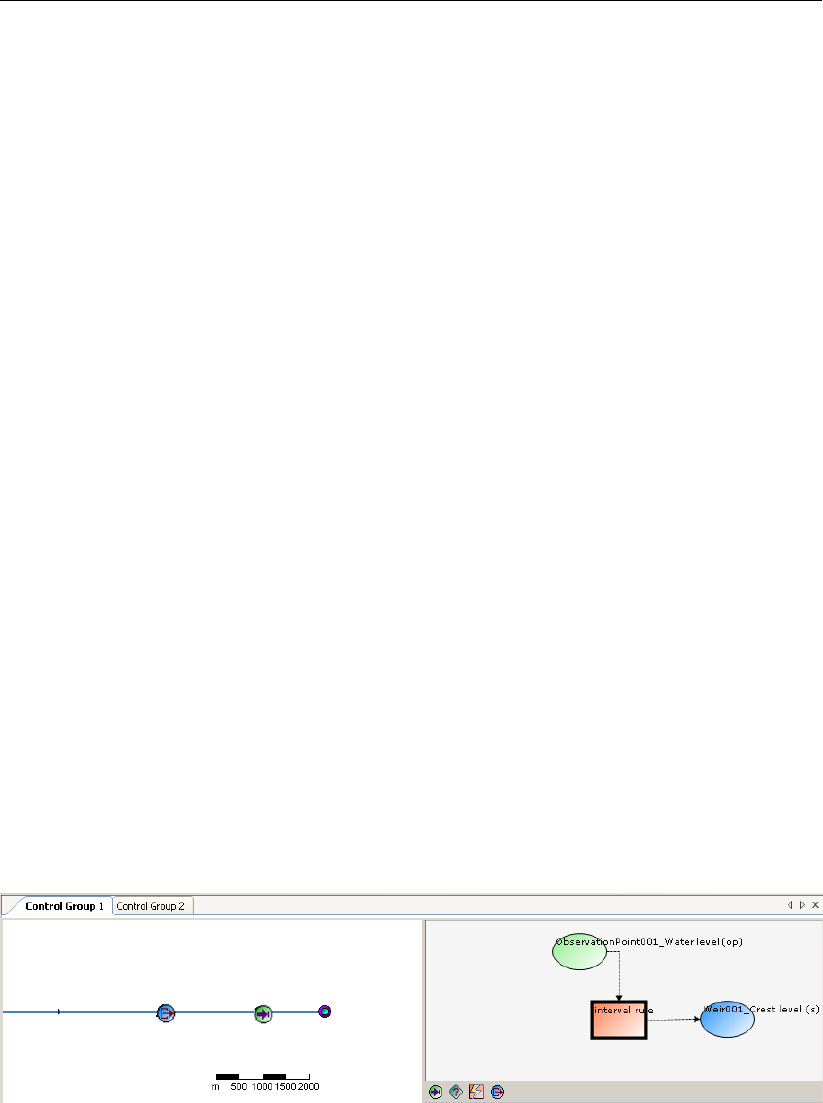
map and flow chart show the relations between the D-RTC components. Figure 2.3 shows
an example of a D-RTC-model in the Project window. In this case the composite model
contains a D-Flow 1D model and the D-RTC model. The D-RTC model consists of a set of
controlgroups and an output folder. This is described in more detail in section 2.3.Figure 2.4
shows an example of a flowchart. Flowcharts are described in section 2.4. The Properties
window shows details of the RTC-components and facilitates editing (see also section 2.5).
Figure 2.5 shows an example of the Properties window for a Time rule (see also chapter 4).
Figure 2.3: Example of an RTC-model in the Project window
Deltares 5 of 70
DRAFT
D-Real Time Control, User Manual
Figure 2.4: Example of a flow chart
Figure 2.5: Example of the properties window for a Time rule
Figure 2.6 gives an overview of the RTC modelling concept. D-RTC uses observed values of
control parameters to determine the values of controlled parameters. These observed values
can consist of actual measurements or observations from the hydrodynamic model. Examples
of control parameters are:
Hydraulic parameters at an observation point, such as discharge or waterlevel
Water quality parameters at an observation point
Rainfall
6 of 70 Deltares

DRAFT
Module D-RTC: Overview
External data, such as meteorological conditions, diversions due to building or mainte-
nance activities etc.
Controlled parameters are positions of moving elements of the structures that are directed by
D-RTC. Examples are
Crest level or crest width of weirs
Discharge of pumps
Gate opening at gated weirs
Valve opening at Culverts
Figure 2.6: D-RTC modelling concept and data flow
D-RTC uses the input from control parameters to evaluate conditions that trigger rules that set
the controlled parameters. For example, if a pump operates during the night with a capacity
of 500 m3/s and is shut down during the day, the condition is true during the night and false
during the day. The rule connected to the "true" output sets the discharge to 500 m3/s, while
the rule connected to "false" output set the discharge of the pump to 0 m3/s.
Rules contain the actual algorithms that D-RTC uses to calculate the values of a controlled
parameter.
Conditions trigger a rule to be active or not. Both the true and false outcome of a condition
can be used to activate rules.
By connecting a sequence of conditions and rules, a control flow is generated for a controlled
parameter. This controlflow is visualized in a flowchart, which is described in more detail
below.
D-RTC uses the objects from a hydraulic model such as a D-Flow 1D model, but has no
knowledge of the model itself and no spatial information. The objects from a hydraulic model
used by D-RTC are passive objects which can not be edited in D-RTC. D-RTC directs the
controlflow, which means that the only editable objects are rules and conditions.
2.3 Controlgroup
A D-RTC model consists of one or multiple controlgroups which are shown in the Project
window. A controlgroup is a set of D-RTC components. Each controlgroup consists of
Deltares 7 of 70

DRAFT
D-Real Time Control, User Manual
one flow chart with one ore more controlflows (see section 2.4)
a list of observation points which supply the values of the control parameters
a list of conditions used in the controlflow(s)
a list of rules used in the controlflow(s)
a list of structure output locations for the controlled parameters
The set of elements in a single flowchart is a single controlgroup and one or more control-
groups form a D-RTC model.
The controlgroup can be used to organize the D-RTC model. For example, a user can decide
to group the controlflows per
controlled parameter; each controlled parameter has its own controlflow and a control-
group has one controlflow,
controlled structure; a controlled structure can have controlflows for each controlled pa-
rameter (for example, both crest level and crest width are controlled of a single weir). Each
controlgroup can then have more than one controlflow,
compound structure; several structures combined can form one large complex, such as
Haringvlietsluizen, which consist of 17 individual locks. It can be convenient to group D-
RTC around these compound structures. Each controlgroup can then contain more than
one controlflow, one for each controlled parameter.
Deciding how to group the controlflows is finding a balance between transparancy and easier
modeling in the controlgroups, and having a good overview of the total model. It is recom-
mended to use as few controlflows as possible within a single controlgroup. Only use more
than one controlflow per controlgroup if the Project window becomes too complex.
2.4 Flow chart
The flow chart is the visual interpretation of the controlgroup. While the Project window only
shows a list of all components of a controlgroup, the flowchart shows how the components of
the controlgroup relate to one another.
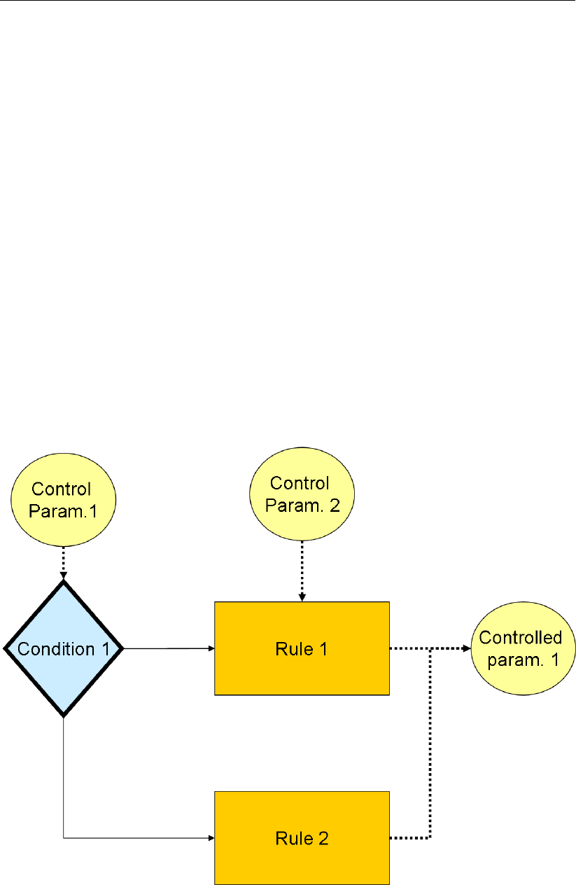
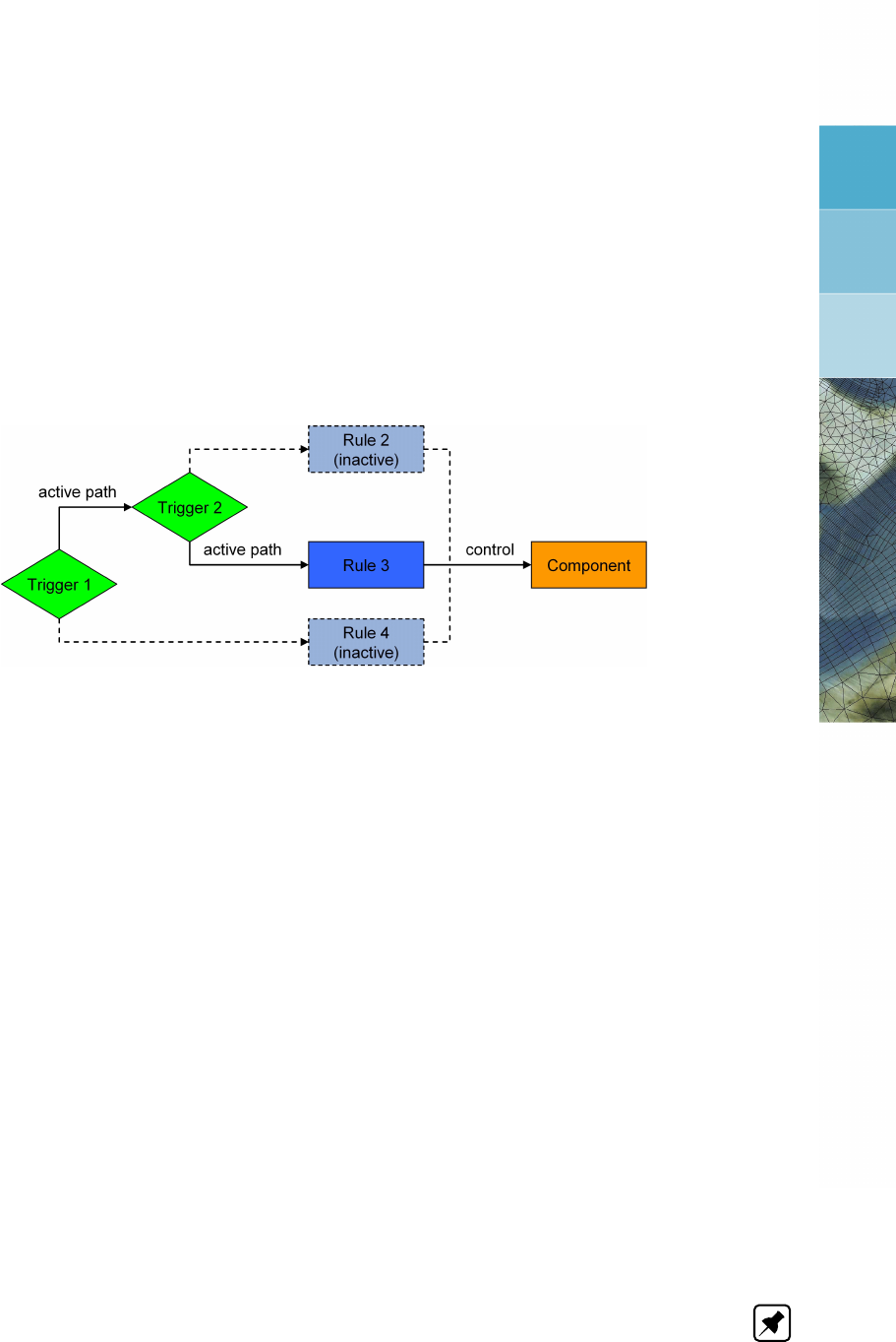
D-RTC is built around the concept of controlflows. Figure 2.7 shows the concept of a con-
trolflow and its components. The controlflow in a flow chart always:
has one starting point for each controlled parameter (depicted with a thick black line
around the controlflow component, see Figure 2.7),
has at least one controlled parameter and one rule,
can combine multiple conditions and rules,
shows the controlflow with solid arrows, and data input or output with dashed arrows, see
Figure 2.7,
has exactly one active path per controlled parameter (no 2 rules for the same controlled
parameter are active at the same time).
In section 2.6 examples are described in more detail.
8 of 70 Deltares
DRAFT
Module D-RTC: Overview
2.5 The Properties
window Similarly to other Delta Shell modules in D-RTC the Properties window shows details
of a D-RTC schematisation object by clicking on an item in the Project window or on the
flowchart. The corresponding parameters can be edited in this window. An additional table
window is shown if necessary. Examples for properties of different D-RTC objects are given
below:
Condition parameters:
condition type
the table in case of a lookup table controller
control parameters:
discharge
waterlevel
salinity
controlled locations and parameters
Rule parameters:
rule type
the table of a lookup table controller
rule-specific parameters
Figure 2.7: Components and basic concept of the flowchart
Deltares 9 of 70
DRAFT
D-Real Time Control, User Manual
2.6 Examples
In this section several examples of controlflows are presented. These examples also form the
basis for the tutorial in section 3.2.
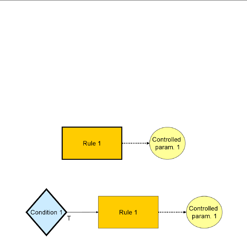
2.6.1 Minimal controlflow
Figure 2.8 shows the minimal controlflow; a parameter controlled by a rule. Depending on
the type of rule, there may be also be control data required. In addition to a rule, conditions
can be added that (de)activate a rule, Figure 2.9. An example for Figure 2.8 could be that the
water level is 3 m on the first day and 6 m on day two at a specified location. A condition for
that rule is added in Figure 2.9 and could imply that the rule is only active when the discharge
at a certain observation point is higher than a specified value. chapter 4 explains which types
of rules and conditions are available and what they do.
Figure 2.8: Example minimal controlflow
Figure 2.9: Example minimal controlflow with a condition
2.6.2 Combinations of conditions and rules
In this section an overview is given of basic combinations of conditions and rules.
A condition can be used on its own, but will often be used in combinations. The most elemen-
tary combinations of two conditions are AND and OR. An AND combination of two conditions
means that both conditions have to be true for the rule to be active. As soon as one of the two
conditions is false, the rule becomes inactive. The controlflow first checks the first condition,
and only if this condition is true, the controlflow proceeds to check the second condition. If
either the first or second condition is false, another rule can be activated. It is not required to
have a different rule for the false-scenario; if a structure only has to perform an action if the
conditions are true, no second rule is required. A second rule is only required if the structure
also has to perform an action once the conditions are false.
An OR combination of two conditions means that only one of the two conditions has to be true
for the rule to be active. Only if both conditions are false, the rule becomes inactive.
10 of 70 Deltares

DRAFT
Module D-RTC: Overview
Figure 2.10: Example of two conditions that combined form an AND trigger
Figure 2.11: Example of two conditions that combined form an OR trigger
By adding conditions the controlflow may be expanded to more complex situations. Figures
2.12 and 2.13 show some possibilites by using three conditions in a single controlflow. All
possibilities for combinations of three conditions are:
1∧2∧3
1∨2∨3
1∧(2 ∨3) (Figure 2.12)
1∨(2 ∧3) (Figure 2.13)
Deltares 11 of 70

DRAFT
D-Real Time Control, User Manual
Figure 2.12: Example of three conditions: 1 ∧(2 ∨3)
Figure 2.13: Example of three conditions: 1 ∨(2 ∧3)
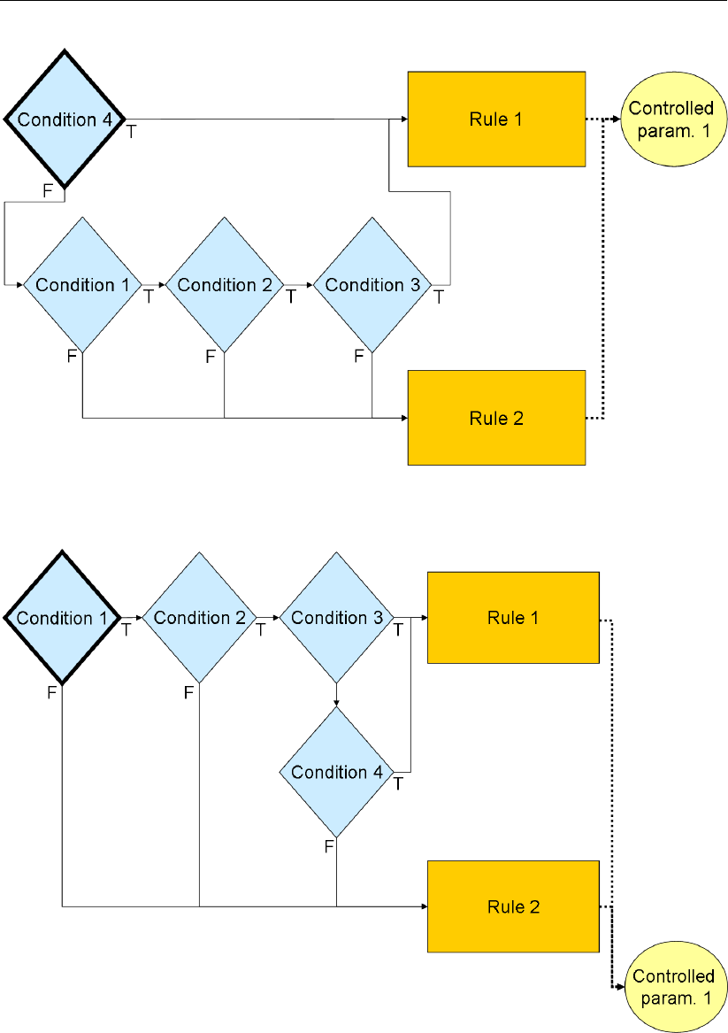
Similarly, the control flow can be extended with even more conditions and rules. Figures 2.14
to 2.19 give examples for a situation with four conditions.
12 of 70 Deltares
DRAFT
Module D-RTC: Overview
Figure 2.14: Example of four conditions: 4 ∨(1 ∧2∧3)
Figure 2.15: Example of four conditions: 1 ∧2∧(3 ∨4)
Deltares 13 of 70
DRAFT
D-Real Time Control, User Manual
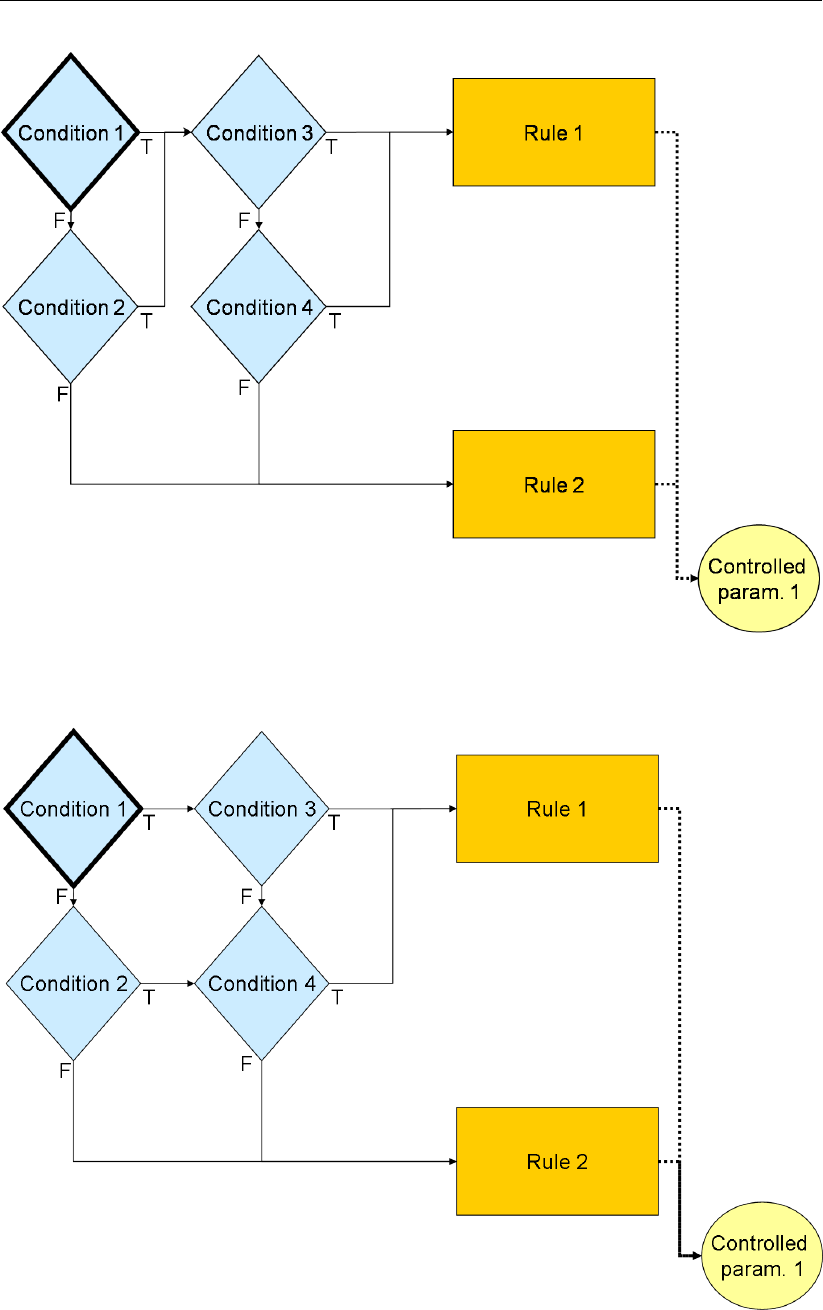
Figure 2.16: Example of four conditions: (1 ∨2) ∧(3 ∨4)
Figure 2.17: Example of four conditions: (1 ∧(3 ∨4)) ∨(2 ∧4)
14 of 70 Deltares
DRAFT
Module D-RTC: Overview
Figure 2.18: Example of four conditions: 4 ∧(1 ∨2∨3)
Figure 2.19: Example of four conditions: (1 ∧2) ∨(3 ∧4)
Note the difference between Figures 2.16 and 2.17; there is only a small difference in flowchart
(the arrow going from the true side of Condition 2 to Condition 3), but a large difference in
Deltares 15 of 70

DRAFT
D-Real Time Control, User Manual
meaning!
16 of 70 Deltares
DRAFT
3 Module D-RTC: Getting started
3.1 Introduction
In this chapter we will provide examples of D-RTC with a tutorial. The D-RTC module can not
be used on its own: an RTC model uses information and determines the values of parameters
of another model, typically a D-Flow 1D model or D-Flow FM model. However, this can also be
a water quality model or a rainfall-runoff model. We start with the tutorial model of D-Flow 1D.
3.2 Getting started
3.2.1 The integrated model
Applying control with D-RTC on a D-Flow 1D model is integrated modeling (or coupled mod-
eling). To develop an integrated model in Delta Shell right-mouse click on the project, e.g.
<Project1>, in the Project window. Select Add →New Model. . . . A Select model . . . di-
alog appears. Choose “1D Integrated Model”. In the central window the Integrated Model
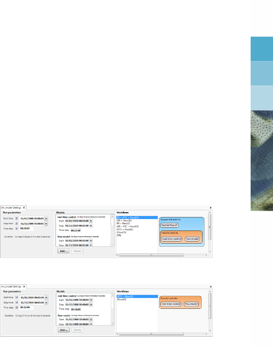
Settings dialog appear (Figure 3.1). Under Models delete all items but “Real-Time Control”
and “Flow1D” with the Delete button. Set the Run Parameters in such a way that the simu-
lation period begins on 2000-01-01 and ends on 2000-01-05. Set the time step to one hour.
The window should now look like the one in Figure 3.2.
Figure 3.1: Integrated model default properties
Figure 3.2: Integrated model, settings for a coupled simulation with D-RTC and D-
Flow 1D
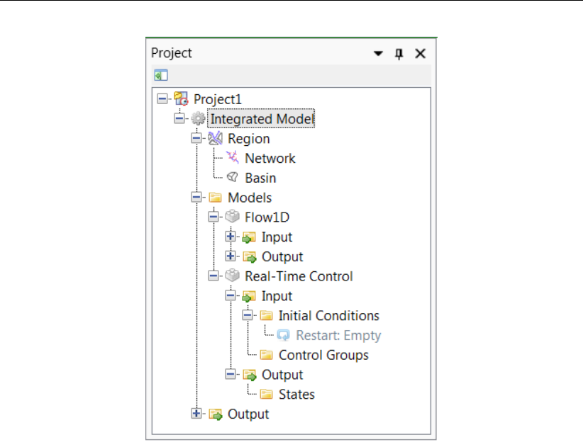
The Project window now looks like Figure 3.3. The <Region>folder contains schematisa-
tions for the models: a network for the D-Flow 1D model and a basin for rainfall-runoff models.
The latter one is not used in this tutorial. Under <Models>we find the D-Flow 1D model
“Flow1D” and the D-RTC model “Real-Time Control”. Note that the network of the D-Flow 1D
model is a link to the network under <Region>.
Deltares 17 of 70
DRAFT
D-Real Time Control, User Manual
Figure 3.3: Integrated model in the Project window
3.2.2 The D-Flow 1D model
Create a simple D-Flow 1D model:
(Optional) Enable OpenStreetMap WMS layer
Add one branch with a length of about 60 km long to the network.
Add a cross-section of type YZ with default properties.
Add a Weir node with default properties.
Create a computational grid.
Set a constant water level of −2 m at the downstream boundary.
Set a transient discharge boundary condition at the upstream end (Table 3.1).
Set the current crest level and the current crest width of structures as output parameter.
Set the current water level and the current discharge of observation points as output pa-
rameter.
Save the project.
Validate the model.
Run the model.
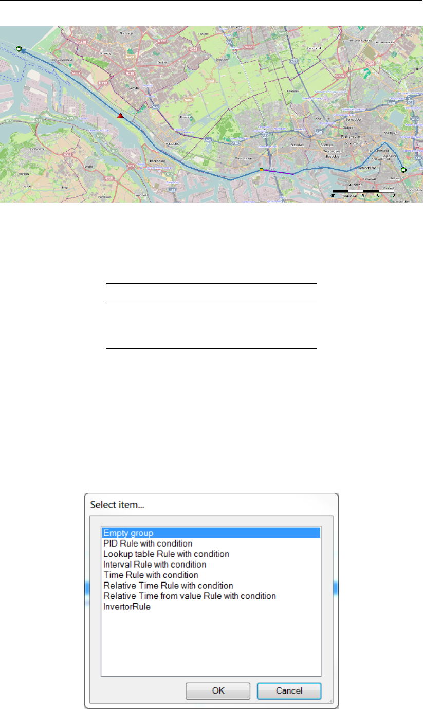
The flow model schematisation (<network>) then should look more or less like the one given
with Fig. 3.4.
18 of 70 Deltares
DRAFT
Module D-RTC: Getting started
Figure 3.4: Example water flow model schematisation with an OpenStreet background
map (http://openstreetmap.org)
Table 3.1: Discharge boundary condition table for the upstream end
Date Discharge [m3s−1]
2000-01-01 00:00:00 300
2000-01-02 00:00:00 300
2000-01-05 00:00:00 500
3.3 A simple D-RTC model
3.3.1 Add a Control Group
Right-mouse click on <Control Groups>in the Project window and select Add New Control
Group. . . . A menu (Figure 3.5) appears where the user can choose between a set of default
available control groups. Select empty group. Control Group 1 is now added to the set of
Control Groups in the Project window. The Control Group window is currently empty.
Figure 3.5: Options for default controlgroups
Deltares 19 of 70
DRAFT
D-Real Time Control, User Manual
Figure 3.6: Empty controlgroup
3.3.2 Construct a minimal controlflow
Select (toolbar below the empty flow chart on the right-hand side of the Control Group
editor) and click in the Control Group window. This tool adds an output location to the flow
chart. Select under the flow chart and click in the flow chart to add a rule. Connect the two
objects to obtain a flow chart as shown in Figure 3.7: move the mouse over the rule object,
left-click on the anchor point of the rule object on its right side, hold the mouse clicked and
find the anchor point on the left side of the output location object. Release the mouse button.
Figure 3.7: Minimum flow chart with a Time Rule
Now set the crest level of the weir as output location: right-click click on the output location
object and navigate through the menus. From the available locations in the network of the
flow model select the weir as location and crest level as controlled parameter. The output
location ellipsoid turns blue after having specified the parameters. Note that now in the map
the available location are highlighted.
The default rule is a PID rule. In this tutorial we use a Time rule, because this is the simplest
one. Right-mouse click on the rule and select Convert PID Rule to Time Rule. The data of the
time rule can be edited in the Properties window. Under Data click on <Time Series>and
the drop down menu to open the table editor. Fill in the data from Table 3.2. Use the arrow
keys to switch between cells and the return key to add a new line. With the F2 key you can
address the date value. Select periodicity constant and interpolation linear (default values).
Save the project.
20 of 70 Deltares

DRAFT
Module D-RTC: Getting started
Table 3.2: Time Rule data for crest level
Date Crest level [m]
2000-01-01 00:00:00 1
2000-01-02 00:00:00 1
2000-01-05 00:00:00 -8
3.3.3 Perform a simulation
To perform a coupled flow simulation right-click on the <integrated model>in the Project
window and choose Run Model.
3.4 View the simulation results
3.4.1 Introduction
Both the D-Flow 1D model and RTC run simultaneously and exchange data with each other
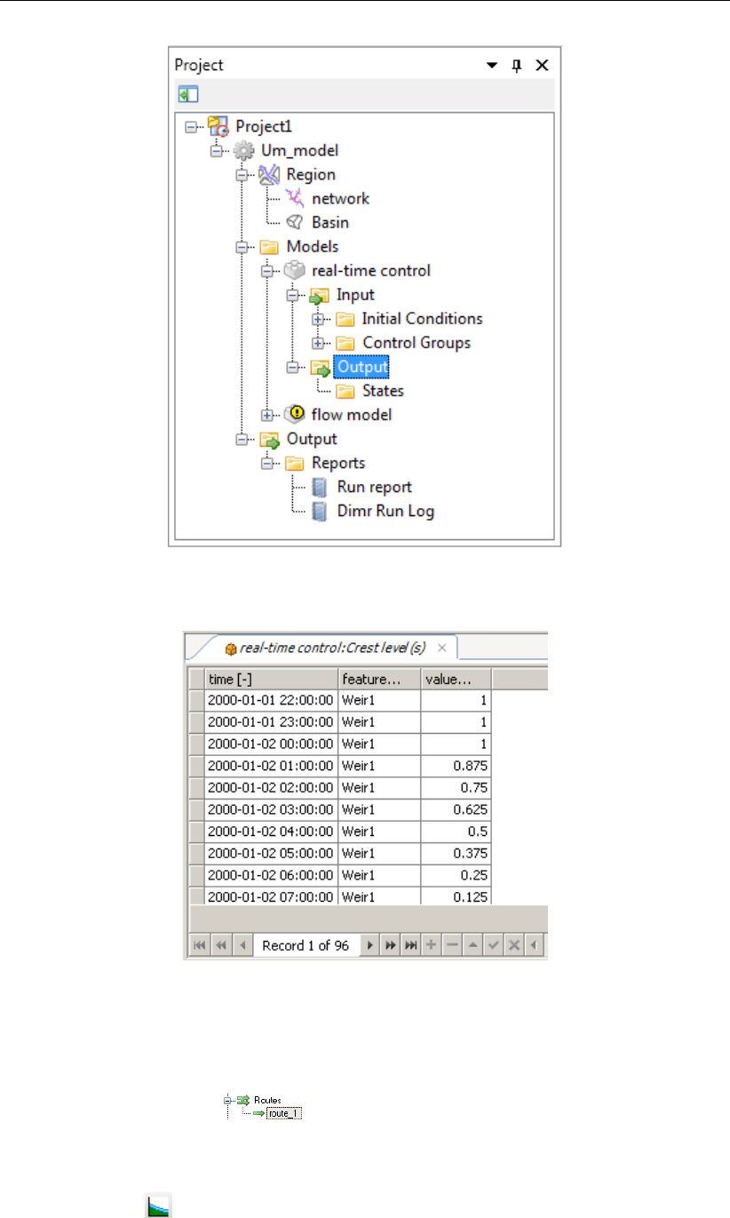
during run-time on a time stap basis. Figure 3.8 shows the Project window after the simulation
run. Both D-RTC and D-Flow 1D generate their own output; the output time step of the D-
Flow 1D model is set by the user. The RTC model uses this time step and puts out the values
of the controlled parameters per timestep. Note that the output of D-RTC is the input for the
next timestep D-Flow 1D computes.
3.4.2 Table view
Double click on <real-time control> <output> <crest level (s)>in the Project window (Fig-
ure 3.8) and select table and chart view. A tab opens in which the crest levels are shown as
a function of time (Figure 3.9). A mouse-click on the top left corner of the table selects the
content. The data can now be copied and pasted to a file.
Deltares 21 of 70
DRAFT
D-Real Time Control, User Manual
Figure 3.8: Project window after a coupled simulation with D-RTC and D-Flow 1D.
Figure 3.9: Table and chart view D-RTC output
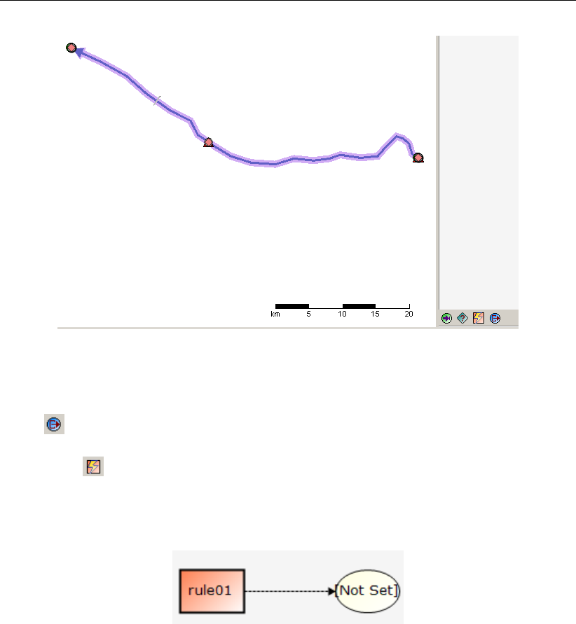
3.4.3 Side-view
To create a side-view double-click on <input> <network>in the water flow model to open
the network editor. Select in the ribbon and click in the map to create a network
route along the branch. For this purpose, click on the start of the branch (the most upstream
point) and click on the end of the branch (most downstream point). A route between the two
points is created. The created route can be deleted in Region Contents under <network>
<Routes>. Click in the ribbon to open the sideview. Right-mouse click in the side-view.
Select Select Coverages. Choose “Discharge” and “Crest level (s)” from the list. Navigate
through the time steps with the time series navigator to explore the simulation results in time
22 of 70 Deltares
DRAFT
Module D-RTC: Getting started
along the chainage of the channel.
Figure 3.10: Sideview with water level and crest level of the structure
3.5 A more complex control flow
3.5.1 Multiple controlled parameters on one structure
Save the project under a new name. Open the editor for Control Group 1. Select and click
in the flow chart to add an output location. Select and click in the flow chart to add a rule.
Connect the two objects.
Select the output location and right-mouse click to specify Weir1 as location and crest width
as controlled parameter. Select the new rule and right-mouse click to convert the standard
PID rule into a Time rule. Fill in the values from Table 3.3 under TimeSeries in the properties
window. The flow chart now looks as in Figure 3.11.
Table 3.3: Time series for the crest width (rule 2)
Date Crest width [m]
2000-01-01 00:00:00 5
2000-01-02 00:00:00 5
2000-01-05 00:00:00 20
Deltares 23 of 70

DRAFT
D-Real Time Control, User Manual
Figure 3.11: Flowchart for example with two controlled parameters for one weir.
Run the integrated model again. Save the project. In addition to <crest level>, also <crest
width>is now available under <Output>of the real-time control model in the Project window.
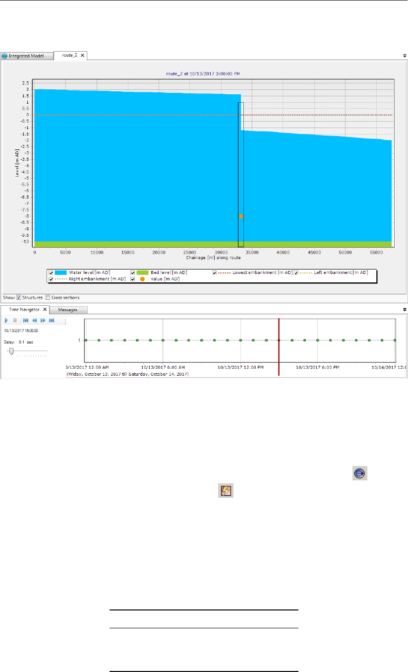
To visualize the simulation results coherently, double click on <water flow model> <Output>
<water level>. If the structure feature is not visible in the map, change the view in the Map
Contents window: switch layers on or off or drag the network layer on top. Select the structure
feature on the map (Figure 3.12).
Figure 3.12: Structure selected on the map view of simulation output
Figure 3.13: Select output coverage
24 of 70 Deltares

DRAFT
Module D-RTC: Getting started
Then select the Query Time Series tool . Press the Control key on your keyboard and
choose crest level, crest width and water level from the water flow 1d model as output cover-
age (Figure 3.13). These parameters are now plotted over time for the selected Weir Node
(Figure 3.14). Click with the mouse in the diagram or select rows in the table.
Figure 3.14: Crest level, crest width and water level over time for the weir. A point in time
has been selected in the diagram, the corresponding line is selected in the
table.
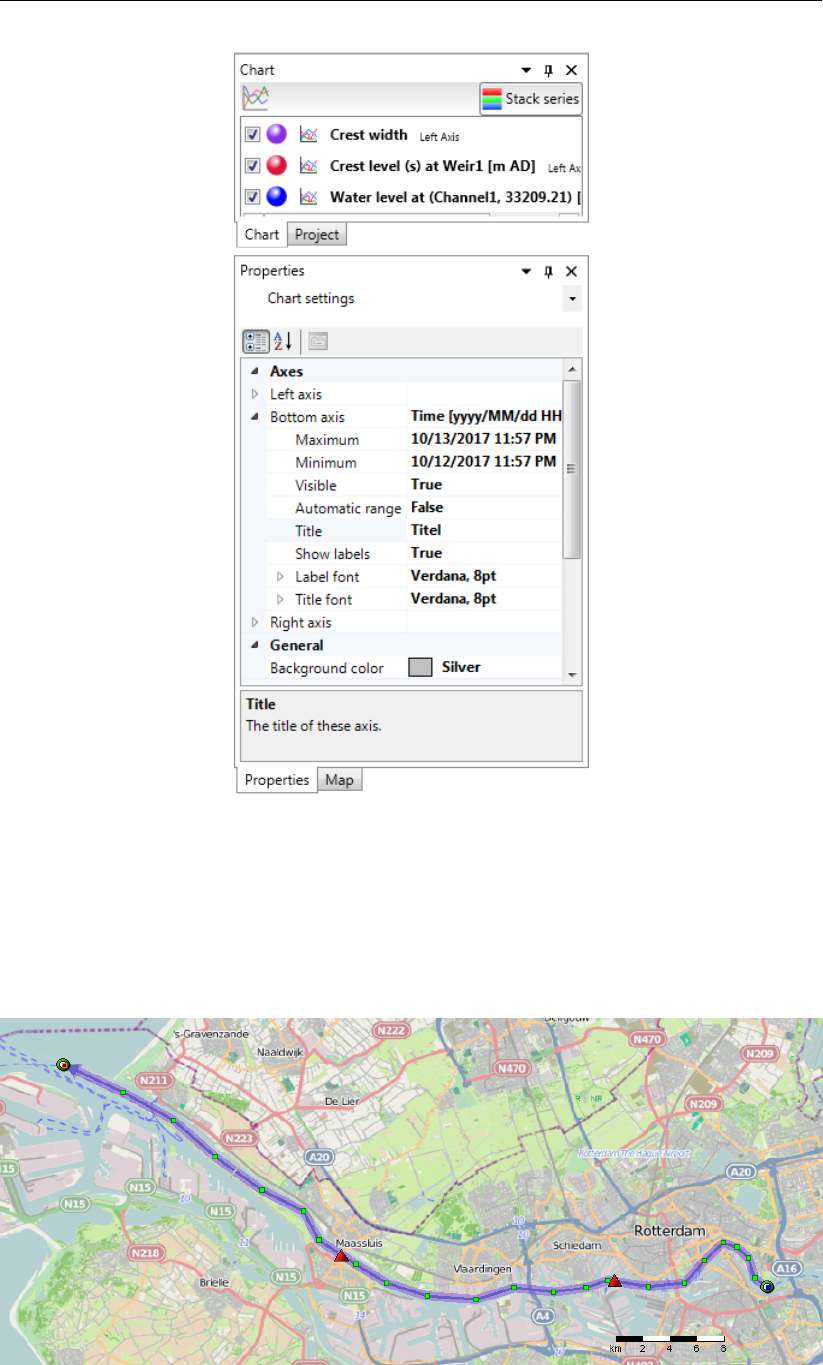
Add a title for the chart in the chart Properties window (Figure 3.15).
Deltares 25 of 70
DRAFT
D-Real Time Control, User Manual
Figure 3.15: Chart properties window, the chart title “Simulation results” has been added.
3.5.2 Multiple controlled structures
Save the project under a new name. Add a second weir to the network of the water flow
model. The network should now look like the one given in Figure 3.16. Change the crest
width to 30 m and the crest level to −4 m.
Figure 3.16: D-Flow 1D network with two weirs.
26 of 70 Deltares
DRAFT
Module D-RTC: Getting started
Add a new control group to the D-RTC model: right-click on <Control Groups>in the Project
window and select empty group. Add an output location and a Time Rule to the new Control
Group (buttons and , convert to Time Rule). Note that the name of the rule is rule01.
This name is also used in the first Control Group. Within one Control Group the names have
to be unique.
Fill in the table of the Time Rule properties with the data from Table 3.4. Select the output
location and set it to Weir2 and Crest level. Run the integrated model. Save the project.
Double-click on <crest level>in the Project window under <real time control> <output>
and select Table and Chart View to open the output for the crest levels. The output of both
weirs is now visible in the table. Select to filter the individual weirs. Apply a custom filter
on the value column to find out when the crest level of Weir1 is lower than −6 m.
Table 3.4: Time series of crest level for a second structure
Date Crest level [m]
2000-01-01 00:00:00 -4
2000-01-02 00:00:00 -4
2000-01-05 00:00:00 -9
3.6 Control flows with conditions
3.6.1 A controlflow with a condition
Save the project under a different name. Add an observation point to the network with the
help of the Create Observation Point tool in the ribbon to the in the upstream part of the
network, close to the upstream boundary. Remove the second weir. The network should now
look like Figure 3.17.
Figure 3.17: D-Flow 1D network with one weir and a single observation point upstream.
Remove Control Group 1 from the D-RTC model. Save the project.
Go to Control Group 2. Let the Rule control the crest level of the weir.
Deltares 27 of 70
DRAFT
D-Real Time Control, User Manual
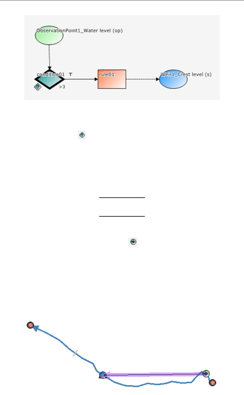
Figure 3.18: Flowchart with a Hydro Condition and a Time Rule. The rule is connected
with the true-output of the condition.
Add a condition by selecting and a mouse-click in the flowchart. Connect the right-side
of the condition (true-output) to the left side of the time rule. Note that the condition is now
shown with a thick, black line instead of the rule, indicating that the controlflow now starts with
the condition instead of the rule. Select the condition and fill in the Properties window with
data from Table 3.5. This is a so-called Hydro Condition, which evaluates input data and puts
out true or false.
Table 3.5: Parameter-Data table for condition
Operation >
Value 3
Add an input location to the Control Flow: select and mouse-click in the flowchart. Select
the observation point as data location and the water level as control parameter. Connect the
bottom anchor point of the data location object to the top anchor point of the condition. The
flowchart now looks like Figure 3.18.
The condition now checks whether the water level in the observation is higher than 3 m. If this
is the case, the condition returns ’true’, which activates the rule. If this is not the case, the
condition ’false’ as result, which means that the rule is inactive. The data origin for the control
of the structure is shown on the map (Figure 3.19).
Figure 3.19: Data origin for the structure
28 of 70 Deltares
DRAFT
Module D-RTC: Getting started
Save the project. Run the integrated model.
Right-click on <real-time control>and choose Open last working directory. Open the file
<timeseries_0000.csv>and analyze the output of the computational core of D-RTC (RTC-
Tools)1.
3.6.2 A controlflow with two conditions: logical AND
Save the project under a new name.
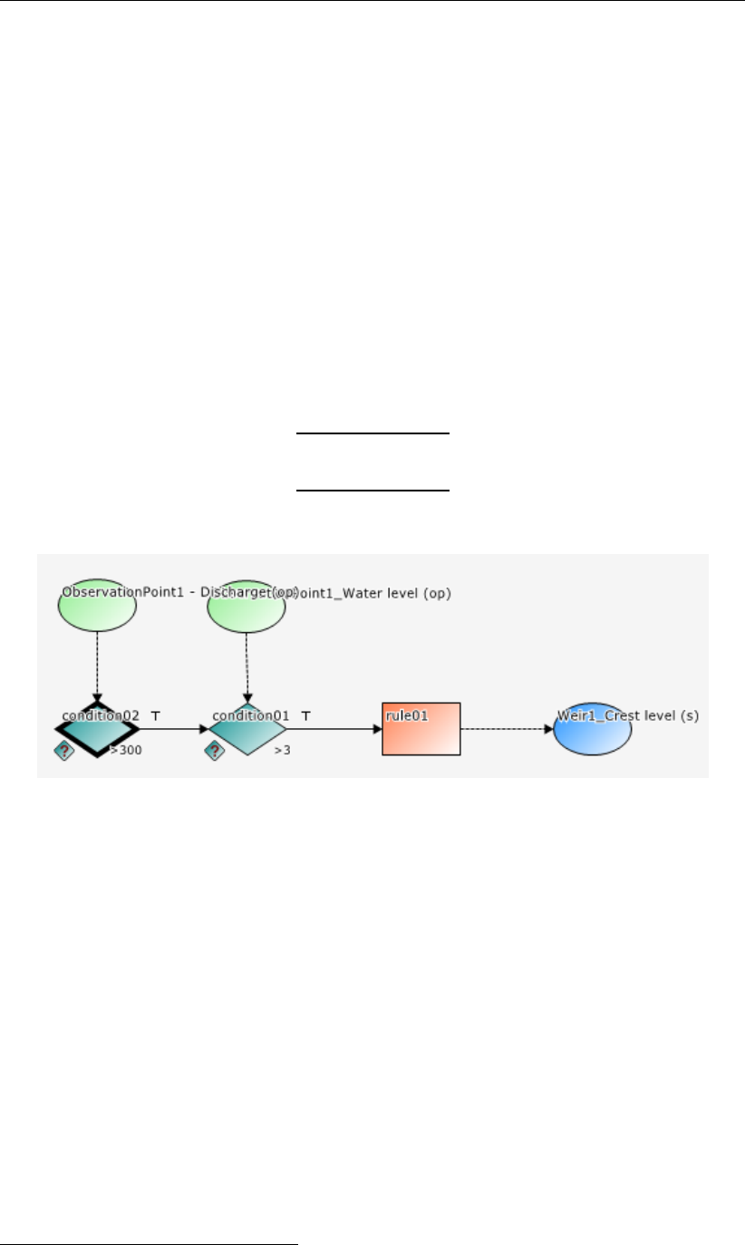
Add a new hydro condition to the flow chart and fill in the Properties window with the data
given in Table 3.6. Add a data location object, select the observation point and choose Dis-
charge as control parameter. Connect the true-output of the new condition with the input of
the first condition. The flowchart now looks like Figure 3.20.
Table 3.6: Parameter-Data table for the second condition
Operation >
Value 300
Figure 3.20: Flowchart with two Hydro conditions in an AND combination combined with
a Time rule.
This flow chart represents a logical AND combination of two conditions. The rule is only active
if both the first and the second condition are active.
Run the integrated model and analyze the simulation results. Check when the rule is active
and the status of the conditions during simulation time.
3.6.3 A controlflow with two conditions: logical OR
Save the project under a new name.
Select the connection between the two conditions and delete it with the Delete-key on your
keyboard. Connect the bottom anchor point of condition01 (the false-output of the condition
that evaluates the water level) to the left side of condition02 (evaluates discharge). Then
connect the right side anchor point of condition02 to the left anchor point of the rule. Arrange
the elements in such a way that the flowchart looks like Figure 3.21.
1Future versions of SOBEK will provide more features to analyze simulation results of D-RTC
Deltares 29 of 70

DRAFT
D-Real Time Control, User Manual
Figure 3.21: Flowchart with two Hydro conditions in an OR combination and a Time rule.
This is an example of two conditions in an OR combination. Whereas in Figure 3.20 both
conditions had to be true for the rule to be active, in Figure 3.21 only one of the two conditions
needs to be true for the rule to be active.
Run the integrated model, save the project and analyze the results.
30 of 70 Deltares

DRAFT
4 Module D-RTC: All about the modelling process
4.1 Conditions
In D-RTC there are two types of conditions:
1 Hydro condition
2 Time condition
The hydro condition uses data to assess whether a rule should be active or not, while the time
rule uses a timetable and is therefore independent of data.
4.1.1 Hydro condition
Figure 4.1 shows an example of the use of a hydro condition in a flowchart. A hydro condition
always needs input data, which are connected to the condition at the top side. These data
are the control parameters and can be any parameter available at a control location, i.e. water
level, discharge, velocity, but also salt concentration or water temperature, depending on the
modules used.
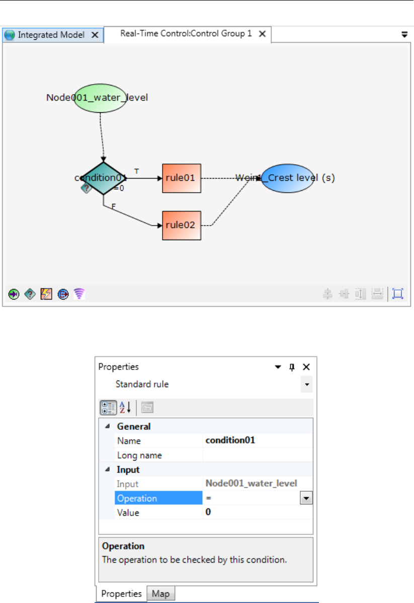
Figure 4.2 shows the Properties window for a hydro condition. A hydro condition has as
parameters:
input
Operation
Value
id
name
The input is equal to the selected control location and parameter (in this case waterlevel at
observation point 1). The value is the setpoint of the control parameter. The hydro condition
checks with the operation how the actual value of the control parameter relates to the setpoint.
In the example in Figure 4.2 the hydro condition checks if the waterlevel at the observation
point is larger than zero. If this is the case, the operation is true and the hydro condition is
also true. If this is not the case, the operation is false as is the hydro condition. The following
operations are available
>(larger)
<(smaller)
=(equal)
<> (not equal)
>=(larger or equal)
<=(smaller or equal)
If the hydro condition is true, the rule connected to the true side (right side of the condition) is
activated and the rule connected to the false side (bottom side of the condition) is deactivated.
Otherwhise, if the condition is false, the rule connected to the true side is deactivated and the
rule connected to the false side is activated.
The id is obligatory and unique for the control group in which it is used. The name is not
obligatory and not necessarily unique.
Deltares 31 of 70
DRAFT
D-Real Time Control, User Manual
Figure 4.1: Example of a flowchart with a hydro condition
Figure 4.2: A hydro condition in the Properties Window
4.1.2 Time condition
Figure 4.3 shows an example of the use of a time condition. The main difference in flowchart
compared to a hydro condition is the absence of input data. The time condition is independent
of simulation results or measurements. It only needs a time table in which is stated during
which time the condition is true or false.
32 of 70 Deltares

DRAFT
Module D-RTC: All about the modelling process
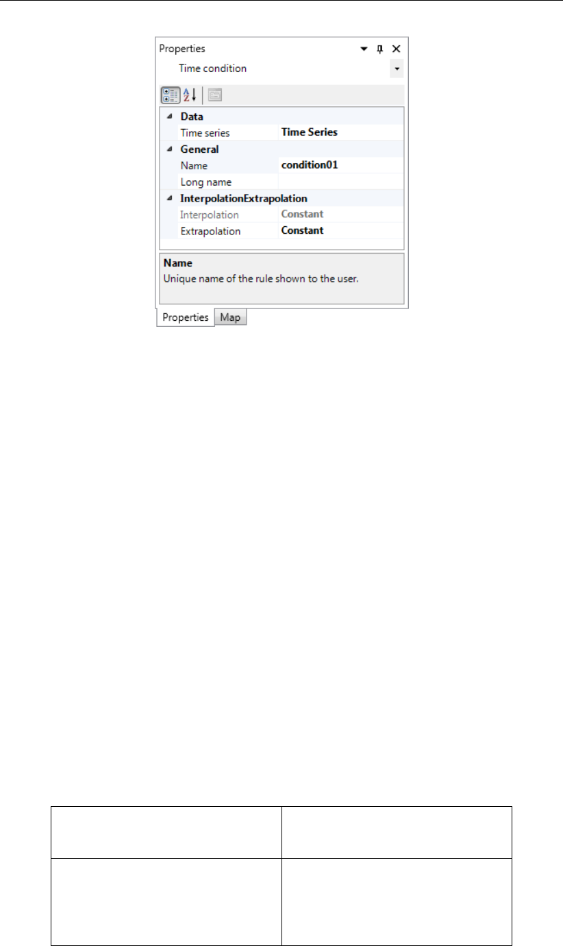
Figure 4.4 shows the Properties window for a time condition. A time condition has the follow-
ing parameters:
Time Series
Extrapolation (constant, periodic, none)
Id: obligatory, unique for each Control Group
Name: optional and not necessarily unique
By clicking on Time Series and selecting a window pops up in which the time table can be
entered. For each time entry true or false can be checked. Between two consecutive entries
the value of the first time entry is maintained. If the condition is true, the rule connected to the
true (right) side of the condition is activated, otherwise deactivated. Similarly, if the condition
is false, the rule connected to the false (bottom) side of the condition is activated, otherwise
deactivated.
The parameter extrapolation controls what happens outside the ranges of the defined timetable.
Three options are possible:
Constant: the first and last value of the timetable are used for each time before and after
the defined timetable respectively.
Periodic: the time table is repeated before its first and after its last time entry.
None: no extrapolation, before the first and after the last time entry no rules are triggered
and the value of the controlled parameter is unaffected by RTC.
Figure 4.3: Example of a flowchart with a time condition
Deltares 33 of 70
DRAFT
D-Real Time Control, User Manual
Figure 4.4: A time condition in the Properties window
4.2 Rules
In D-RTC there are six different types of rules:
Lookup table rule
Time rule
PID rule
Interval rule
Relative from time/value rule
Invertor rule
All rules will be discussed below.
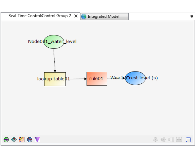
4.2.1 Lookup table rule
The Lookup table rule can be used to operate a structure as a function of a control parame-
ter, such as waterlevel or discharge at an observation point. The rule looks up the controlled
parameter from a table, where a relation between the control parameter (input) and the con-
trolled parameter (output) must be specified. An example of such a table is Table 4.1. Here
the crest level of a weir (controlled parameter, output) is determined in dependence of the
water level at an observation point in the model. The control parameter must be available as
model output.
Table 4.1: Example Lookup table rule for structure
Control parameter:
water level at observation point
Controlled parameter:
crest level of weir m AD
3 1.8929
4 2.9965
5 4.1001
6 5.2037
34 of 70 Deltares
DRAFT
Module D-RTC: All about the modelling process
Figure 4.5: A Lookup table rule in the flowchart (right) and on the map (left)
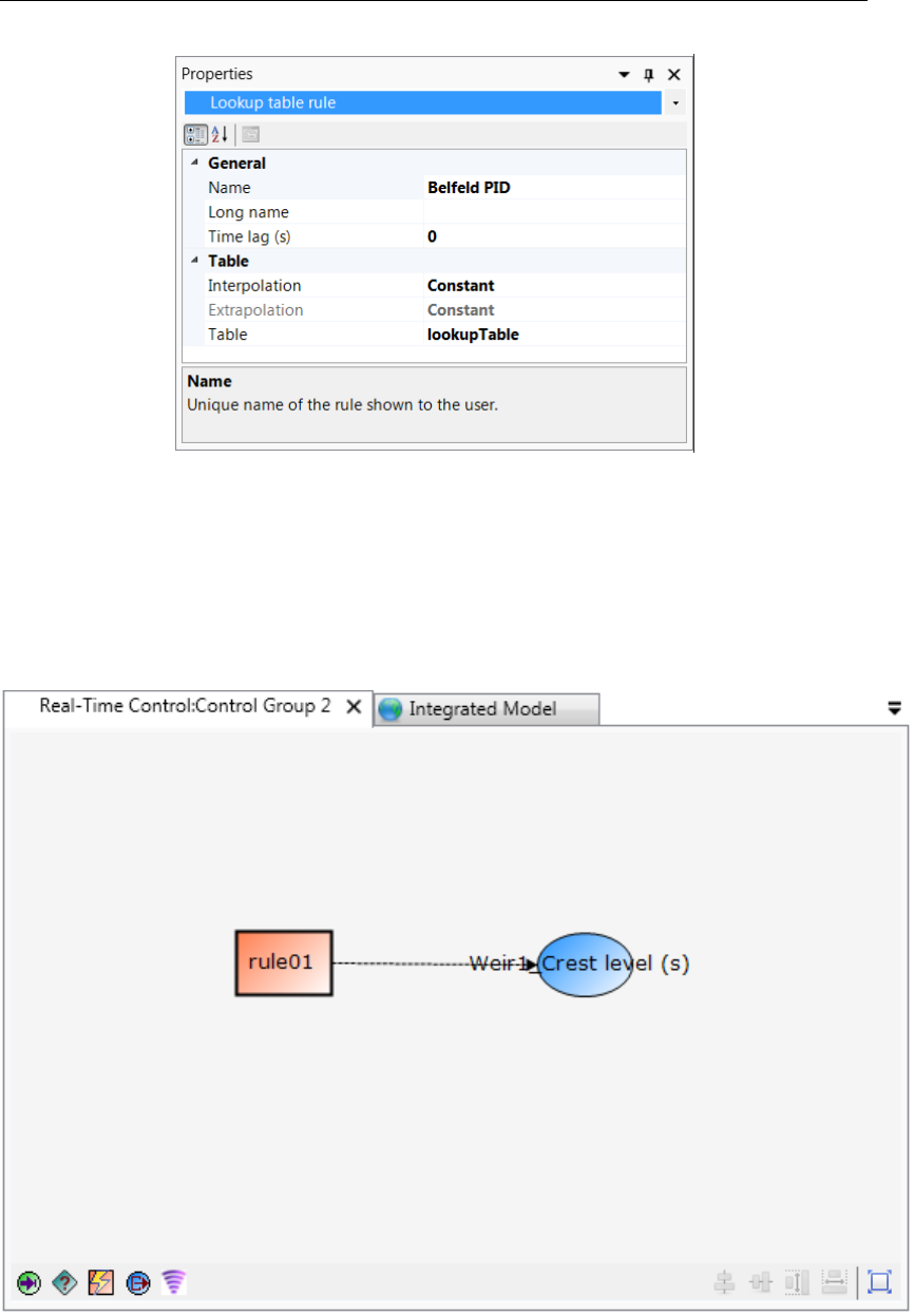
Figure 4.6 shows the Properties window for the Lookup table rule. The following parameters
can be set:
Id: obligatory and unique for the control group
Name: not obligatory and not necessarily unique
TimeLag (always given in seconds)
Extrapolation: extrapolation of table. Always constant
Interpolation: interpolation of table (constant or linear)
Table: Table with relation between control parameter and controlled parameter
The user can specify a time lag to be applied to the control parameter. If the time lag is greater
than zero, not the current value, but values from previous time steps are used. For example, if
the time lag is 1 day (86400 s), the value of the control parameter is taken from the day before,
and not the value that corresponds to the current time step.
If a time lag different to zero is applied, care must be taken for the initial phase of the simula-
tion. Until a simulation period equal to the time lag is computed, no input data is available for
the Lookup table rule. So the rule gives no output and no controlled parameter is transferred
to the structure connected to the rule. Consequently, the structure is considered to be not
controlled by D-RTC. For the simulation the parameter value specified for the structure in the
D-Flow 1D model is used in this case. Hence, for modeling studies where a time lag for a
Lookup table rule is specified the user either has to
take into account the lack of input data for control in the initial phase in the analysis of
results or
use initial conditions from restart (a state saved previously; see D-Flow 1D, User Manual.
Deltares 35 of 70
DRAFT
D-Real Time Control, User Manual
Figure 4.6: A Lookup table rule in the Properties window
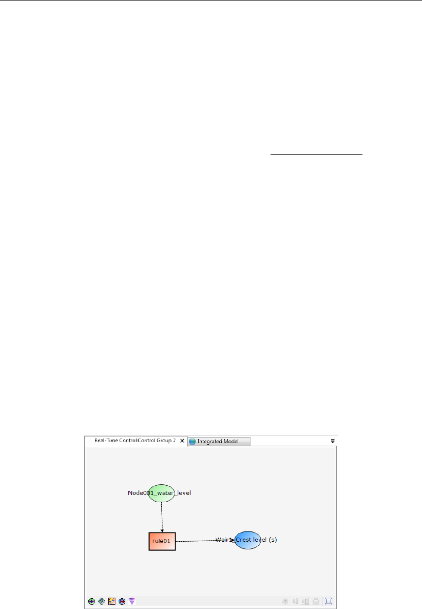
4.2.2 Time rule
The time rule is the simplest rule; the controlled parameter is defined explicitly as a function
of time. The time rule is therefore the only rule without input data from a control parameter.
Figure 4.7 shows an example of the use of the time rule in the flowchart.
Figure 4.7: A time rule in the flowchart
Figure 4.8 shows the time rule in the Properties window. The time rule has the following
parameters:
Timeseries: timetable of the controlled parameter as a function of time
36 of 70 Deltares

DRAFT
Module D-RTC: All about the modelling process
Interpolation: interpolation within the time table (linear or constant)
Periodicity: extrapolation of time table. The options are
Constant: the last value is maintained
Periodic: the table is repeated (both before and after the times in the table)
Id: obligatory and unique for the control group
Name: not obligatory and not necessarily unique
Figure 4.8: A time rule in the Properties window
4.2.3 PID rule
Warning:
Previous versions of SOBEK3 an SOBEK2
This PID rule will behave differently from the PID controller in previous releases of
SOBEK 3.7.4 and SOBEK 2. Therefor, after openeing an old SOBEK model we recom-
mend to calibrate the PID rule again to obtain reliable results.
4.2.3.1 Introduction
The PID (Proportional Integral Derivative) rule is a control loop feedback mechanism used to
operate a structure in such way that a specified hydraulic control parameter (e.g. water level
or discharge) is maintained. The control parameter can be the water level or the discharge at
a specified observation point in the network.
The PID-rule can been seen as a external force on the system using three tuning parameters
and read:
f(t) = Kpe(t) + KiZt
0
e(τ)dτ +Kd
de(t)
dt ,(4.1)
where
Kpgain factor proportional to e(t),
Kigain factor proportional to the time integral of e(t)and
Kdgain factor proportional to the time derivative of e(t).
with e(t)the error (deviation) from the setpoint (e(t) = xsp −x(t)). These gain factors must
be adjusted for each situation. By adjusting the values the user puts the emphasis of the
Deltares 37 of 70
DRAFT
D-Real Time Control, User Manual
rule on current deviations from the setpoint of the control parameter (Kp), previous deviations
(Kd) and all previous deviations (Ki). This allows the user to set the behavior of the rule such
that the structure responds fast or that the response is dampened by previous events. Wheras
the interval rule can become unstable with many fluctuations in the controlled parameter, by
optimizing the factors the PID rule can be stabilized.
To prevent the whole history of deviations the PID-rule Equation (4.1) is linearized and read
in discrete form:
fn=fn−1+Kpen−en−1+Ki∆tnen+Kd
en−2en−1+en−2
∆t(4.2)
If necessary, the new value of the control parameter f(t)is adjusted to fit within the physical
limits of the structure (i.e. Minimum, MaxSpeed, Maximum).
Gain factors can be positive or negative. The choice of the sign depends on the type of the
control structure (e.g. crest level, crest width or gate lower edge level) and the location and
type of the hydraulic parameter (e.g. water level or discharge) that is controlled by the PID rule.
For example, consider a PID rule that at a bifurcation tries to maintain a constant discharge
flowing into one branch by manipulating the crest level of a River weir located in the branch
that should receive this constant discharge. In case the discharge flowing into the branch of
which its discharge is controlled is too large, this means that the deviation ein the equation
above is negative (i.e. the deviation from the actual discharge <0). From a hydraulic point
of view the crest level (f(t)) of the river weir is to be raised in order to reduce the discharge
flowing into the controlled branch. In order to achieve this, the Kpgain factor should be
negative.
4.2.3.2 PID rules in D-RTC
Figure 4.9 shows an example of the use of a PID rule in the flowchart.
Figure 4.9: A PID rule in the flowchart
Figure 4.10 shows the PID rule in the Properties window. The PID rule uses the following
parameters:
Setpoint: setpoint of control parameter
IsUsingConstantSetpoint: true if the setpoint is constant in time, false if the setpoint is
a function of time
38 of 70 Deltares

DRAFT
Module D-RTC: All about the modelling process
ConstantSetpoint: value of the setpoint if IsUsingConstantSetpoint is true
Table: table with setpoints as a function of time if IsUsingConstantSetpoint is false
TableExtrapolation/Interpolation: Linear or block interpolation and constant or periodic
extrapolation
Gain factors: Kp,Kiand Kd.
Limits: Physical limits of the structure
Minimum: minimum value of the controlled parameter
Maximum: maximum value of the controlled parameter
MaxSpeed: maximum velocity with which the controlled parameter is adjusted
Id: obligatory and unique for the controlgroup
Name: not obligatory and not necessarily unique
Figure 4.10: A PID rule in the Properties window
4.2.3.3 PID rule calibration
The gain factors Kp,Ki,Kdmust be calibrated for optimal performance of the PID rule. For
example the calibration can be carried out as follows:
Take Kd,Kiequal to zero, and increase the value of Kpgradually from a small value
until the solution starts to oscillate. The sign of Kpmust be chosen dependent of the type
of structure and the chosen control parameter (see technical background below)
Next divide the resulting value of Kpin half and start increasing Kiwith a factor times
Kp. Again the value of Kiis increased until oscillations appear. Kdremains equal to
zero
Finally increase the value of Kd(sign of Kdmay be opposite of sign of Ki)
A strict procedure for this calibration cannot be presented, since the procedures and results
are dependent on the type of model.
4.2.4 Interval rule
The interval rule can be used to operate a structure in such a way that a specified hydraulic
parameter is maintained. This controlled parameter can be the water level at a specified
observation point in the network, the discharge at a specified observation point in the network.
Figure 4.11 shows an example of the use of an interval rule in the flowchart. An interval rule
always needs the input of a control parameter.
Deltares 39 of 70
DRAFT
D-Real Time Control, User Manual
Figure 4.12 shows the Properties window for an interval rule. There are several parameters
available for the interval rule:
Setpoints control parameter; this is either a constant set point or a time series. Once a
time series has been generated, this is used as set point
Interpolation: only used when set points as a function of time are available. The interpo-
lation is between the values in the time-series for the set points. Possibilities are
constant
linear
Below/above limits: Values for controlled parameter when control parameter is above or
below the setpoint
Deadband: a region in which the interval rule does not respond to deviations in the control
parameter from the setpoint
Deadband Type: the deadband region can be defined absolute or as a percentage
IntervalType: fixed or variable
Fixedinterval or Maxspeed: one of the two depending on the IntervalType must be entered
When the interval type is set to fixed, the controlled parameter is adjusted with a fixed amount
each timestep. This fixed amount is the parameter FixedInterval. In this mode the value of
the controlled parameter is independent of the actual timestep. If the controlled parameter is
crest level of a weir and the FixedInterval is set to 1, the crest level will be adjusted with 1
meter every timestep (within the limits of the structure set by the values Below and Above),
regardless whether the timestep is a minute or an hour. It is up to the user to set an appropriate
value for the FixedInterval.
When the interval type is set to variable, the controlled parameter is adjusted with a velocity,
specified by the parameter Maxspeed. This velocity is a maximum velocity. D-RTC checks
whether within that timestep the limits of the structure are reached. If so, the actual adjustment
is smaller and hence also the actual velocity. In this mode, the actual adjustment of the
structure is a function of the timestep. If the timestep is twice as long, the adjustment will be
twice as large (within the limits of the structure).
Figure 4.11: An interval rule in the flowchart
40 of 70 Deltares

DRAFT
Module D-RTC: All about the modelling process
Figure 4.12: An interval rule in the Properties window
4.2.5 Relative from time/value rule
The relative time rule can be used to specify the controlled parameter as a function of time,
where the time (in seconds) is given relative to the moment that the rule is activated for the first
time by a condition. When the rule is activated for the first time, the relative time table is made
absolute (= computational time + relative time), thereafter the rule starts at the top of the table
and continues downward until the rule is deactivated by a condition. The rule table will remain
absolute during the user-defined so called Start period. In case the rule is activated after this
start period has passed, the table will be made absolute again. Start period= 0, means that
the table is made absolute each and every time that the rule is activated. In case the user
defined value for d(value)/dt is too small to allow for the in the Table defined changes in control
parameter, D-RTC will divert from these defined parameter values in such way as to best fit
the overall table. d(value)/dt= 0, means that there is no restriction in change in parameter over
one time step. When it reaches the end of the table, the value of the controlled parameter is
kept constant at the last value.
The relative from value rule is similar, except that the table is started not at the top, but at the
value of the controlled parameter.
Deltares 41 of 70

DRAFT
D-Real Time Control, User Manual
Figure 4.13: D-Flow 1D model of the River Meuse with close-up for the “Maas-
plassen” region (Roermond, the Netherlands); background map: http:
//openstreetmap.org
4.2.6 Invertor rule
The output of the invertor rule is the input with a changed sign. Invertor rules can be used
to model hydraulic bypasses in a river network by connecting lateral sources. An application
example are the “Maasplassen” near Roermond in the Netherlands. Maasplassen are gravel
pits that are hydraulically connected to the Meuse river. The name “Maasplassen” is also used
for the region that is shaped by the gravel pits (Becker et al.). Figure 4.13 shows a map with
a section of a D-Flow 1D model for the “Maasplassen”.
During high water the gravel pits are flooded by the river Meuse. Hydraulically the pits act
like short cuts in the meandering course of the river, which reduces the travel time of the
flood wave. In the model for the river Meuse this bypass effect has been accounted for by
introducing two lateral sources into the hydraulic that are virtually connected with the help of
the invertor rule (Fig. 4.14). The input location of the invertor rule is the lateral source that
represents the upstream end of the bypass (ID 317), and the output location is set to 318,
which is the lateral source that represents the downstream end of the virtual bypass.
The lateral source at the upstream end of the bypass with ID 317 has a waterlevel–discharge
relation. Beginning with an elevation of 20.58 m, water is extracted from the river course in
dependence of the water level. Lateral source 318 has a constant discharge value of 0. This
value is overwritten by the invertor rule, where the lateral source 318 is set as output location.
Technically, data from the input location of the invertor rule is passed with changed sign to the
receiving lateral source in the next time step.
42 of 70 Deltares

DRAFT
Module D-RTC: All about the modelling process
Figure 4.14: Two lateral sources connected with an invertor rule
Figure 4.15: Table and graph for the relation between water level and discharge for the
lateral source that represents the upstream end of the bypass
Deltares 43 of 70

DRAFT
D-Real Time Control, User Manual
44 of 70 Deltares
DRAFT
5 Module D-RTC: Simulation and model output
The simulation results of D-RTC can be accessed as described in section 3.4. D-RTC Simu-
lation results are also written into a temporary directory of the user’s local settings:
c:\Documents and Settings\<user>\Local Settings\Temp\
where <user>is a placeholder for the user’s name.
Figure 5.1: D-RTC-model selected in the Project window
Right-click in the Project window and choose Open last working directory to navigate to the
current working directory where the simulation input and output is stored. The file <timeseries_0000.csv>
contains the time series of all model objects of the D-RTC model as comma-separated value
table. This file can be easily opened and postprocessed with text editors or programs like
Microsoft Excel or Matlab in order to analyze the simulated values related to input and output
locations and the status of D-RTC objects coherently.
Furthermore, the following files can be found in the temporary directory:
<rtcDataConfig.xml>
<tcRuntimeConfig.xml>
<rtcToolsConfig.xml>
<state_import.xml>
<statePI.xml>
<timeseries_export.xml>
With this set of xml-files a complete RTC-Tools model is given. RTC-Tools is the computational
core of D-RTC and can be considered as the research version of D-RTC (see http://oss.
deltares.nl/web/rtc-tools for details). <diag.xml>and <state_export.xml>are
RTC-Tools output files.
Deltares 45 of 70

DRAFT
D-Real Time Control, User Manual
46 of 70 Deltares
DRAFT
6 Module D-RTC: Technical reference
6.1 Overview
D-RTC is always coupled to an hydraulic model, such as D-Flow 1D, D-Flow FM (2D/3D Flex-
ible Mesh) or D-RR (Rainfall Runoff). Hydraulic structures in these models can be controlled
by operating rules and controllers in combination with triggers. Consequently, D-RTC distin-
guishes basically two layers: (1) triggers, and (2) operating rules. This chapter covers layers
(1) and (2), beside general purpose components such as the lookup table which are used in
both layers.
Figure 6.1: Hierarchical definition of deadBand and standard triggers
According to our definition, a trigger implements conditions for
defining when an operating rule, controller or another trigger is applied,
returning true or false, e. g. if a threshold is crossed or not.
Operating rules and controllers
define how a structure operates, and
return a value for a control parameter, e. g. a gate opening or turbine release, which is
picked up by the hydraulic model the D-RTC model is coupled to.
A combination of triggers with operating rules and controllers forms a binary decision trees
such as given in Figure 2.2. Triggers may connect to other triggers. This feature makes
it possible to build complex decision trees, such that a hydraulic structure is controlled with
different rules for each case, respectively (Figure 6.1). Decision trees must be constructed
such that there is only one active path at a time towards a hydraulic structure. Rules and
triggers that are connected to an output path of a trigger (true or false) that is not active in the
current time step are not evaluated.
From a mathematical point of view, all features in this chapter compute their outputs from
available data either from the previous time step k−1(explicit) or from output of previous
components of the same time step k(implicit).
Note: triggers are always evaluated before rules.
Deltares 47 of 70

DRAFT
D-Real Time Control, User Manual
6.2 General purpose components
6.2.1 Accumulation
The component adds an input xto the state y. The equation of the "accumulation" compo-
nents reads
yk=yk−1+xk(6.1)
This component is used to get the accumulation of a value over the simulation period. This
feature is not yet supported by the user interface, but can be configured by modifying the
corresponding input file.
6.2.2 Expression
The expression consists of a mathematical equation of the form
yk=xk−1∨k
1+xk−1∨k
2(6.2)
The following operators are supported:
+(summation)
−(subtraction)
∗(multiplication)
/(division)
min (minimum)
max (maximum).
The recursive use of expressions (another expression as one of the two terms or for both)
enables the implementation of more complex mathematical expressions (check the example
in the configuration section).
Expressions are used for a wide range of applications. A very common example is the com-
putation of a difference in water level upstream and downstream of a barrier. This difference
is used as input for a trigger within a decision tree.
This feature is not yet supported by the user interface, but can be configured by modifying the
corresponding input file.
6.2.3 Gradient
The governing equation of the gradient reads:
yk=xk−xk−1
∆t(6.3)
This feature is not yet supported by the D-RTC user interface, but can be used by configuring
the corresponding input file.
6.2.4 lookupTable
The rule supplies a piecewise linear 1D lookup table according to
yk=f(xk−1∨k)(6.4)
The lookup table rule (section 4.2.1) uses this feature. This rule is a simpler version of the
dateLookupTable (section 6.3.2).
48 of 70 Deltares

DRAFT
Module D-RTC: Technical reference
6.2.5 Lookup2DTable
The rule supplies a piecewise linear 2D lookup table according to
yk=f(xk−1∨k
1, xk−1∨k
2)(6.5)
This feature is not yet supported by the D-RTC user interface, but can be used by configuring
the corresponding input file.
6.2.6 MergerSplitter
The merger rule provide a simple data hierarchy by choosing the output yequal to the first
of several input values x1, x2, ..., xnwhich is non-missing. Furthermore, additional output
includes the sum of all input values.
This feature is not yet supported by the D-RTC user interface, but can be used by configuring
the corresponding input file.
6.2.7 UnitDelay
The unit delay operator is an auxiliary tool for making data from time steps prior to the previous
time step available in the simulation. By using this operator, we can refer to a historical
release, for example in an operating rule, without abandoning the restarting features of the
model based on the system state of a single time step. It reads
yk+1 =xk.(6.6)
6.3 Operating rules and controllers
6.3.1 Constant
6.3.1.1 Functional principle
This simple rule defines a user-defined constant output ykaccording to
yk= const.(6.7)
6.3.1.2 Application
A constant rule is typically applied in combination with triggers (see Section 6.4) for on-off
control (Åström and Hägglund,1995), e.g. a weir fully opened or fully closed. The true- and
the false output of a trigger are each connected with one constant rule.
6.3.2 DateLookupTable
The date lookup table is a 2D lookup table with the time axis as one of its dimensions. Its
discrete form reads
yk=f(t, xk−1∨k)(6.8)
The resolution of the time axis tis in days of the year. The value axis xmay have any range.
A typical application of the rule would be the definition of a minimum release of a reservoir
as a function of the day of the year and the water level of the reservoir. This feature is not
yet supported by the D-RTC user interface, but can be used by configuring the corresponding
input file.
Deltares 49 of 70

DRAFT
D-Real Time Control, User Manual
xmin xmax
ymin
ymax
Figure 6.2: Graphical representation of guideBand rule
6.3.3 DeadBandValue
The dead band value rule is a discrete rule for suppressing the output of another rule until its
rate of change becomes higher than a certain threshold. It reads
xk=xk−1if
xk−xk−1
<threshold
xkotherwise (6.9)
It is often applied to limit the number of adjustments to movable elements of hydraulic struc-
tures in order to increase their life time. This feature is not yet supported by the D-RTC user
interface, but can be used by configuring the corresponding input file.
6.3.4 GuideBand
The guide band rule provides a linear interpolation from input xto output y, if xis between
two input threshold xmin and xmax. Otherwise, the output is limited to defined minimum and
maximum output threshold ymin and ymax. The rule reads
yk=
ymin if xk−1∨k≤xmin
ymin +xk−1∨k(ymax−ymin)
xmax−xmin ,if xmin < xk−1∨k< xmax
ymax if xmax ≤xk−1∨k
(6.10)
A graphical representation of the rule is presented in Figure 6.2.
The input and output thresholds xmin, xmax, ymin, ymax can be constant, a function of time or
provided by a time series, e.g. from an external input or a result from the execution of a prior
rule.
A typical application of the rule is the enforcement of a reservoir storage sbetween a cer-
tain range and the use of the available storage for equalizing the release. If the storage is
approaching or down-crossing the lower storage limit smin, the release is set to the minimum
flow (zero is no minimum flow is defined). If the storage is approaching or up-crossing the
upper limit smax, the release is set to maximum capacity. This feature is not yet supported by
the D-RTC user interface, but can be used by configuring the corresponding input file.
50 of 70 Deltares

DRAFT
Module D-RTC: Technical reference
6.3.5 Interval
The interval controller is a simple feedback controller according to the control law
yk=
ymax if xk−1> spk+1
2D
ymin if xk−1< spk−1
2D
yk−1otherwise
(6.11)
where xk−1is an input variable, spkis a setpoint, Dis a dead band around the setpoint, and
ykis the controller output.
6.3.6 Limiter
In contrary to the deadBand rule defined above, the discrete limiter rule restricts the change
of a variable to a relative threshold p. It reads
yk=
(1 −p)xk−1if xk<(1 −p)xk−1
(1 + p)xk−1if xk>(1 + p)xk−1
xkotherwise
(6.12)
where pis the maximum relative rate of change. The configuration also accounts for an
absolute rate of change according to the condition xk<∆p xk−1where ∆pis the absolute
rate of change.
A typical application of the rule is the limitation of release changes from a reservoir for avoiding
too steep flow gradients downstream.
6.3.7 PID rule
6.3.7.1 Functional principle
The Proportional-Integral-Derivative controller (PID controller) is a generic feedback controller
including an optional disturbance term commonly used in industrial control systems (see
Åström and Hägglund,1995, for more information). It reads
e(t) = xsp(t)−x(t)
y(t) = Kpe(t) + KiZt
0
e(τ)dτ +Kd
d
dte(t)(6.13)
where e(t)is the difference between a process variable x(t)and a setpoint xsp(t),Kp, Ki, Kd
are the proportional, integral and derivate gain factors, respectively. y(t)is the controller out-
put.
The proportional gain factor Kpcontrols according to the deviation of the process variable x
to the target value (the setpoint) xsp. Consequently, to some extent the gain factor Kpis a
conversion factor between units of the controller output yand the proces variable x. If, for
example, a PID controller is used to achieve a certain discharge setpoint in a river by means
of controlling the crest level of a weir, Kpwill be in the order of magnitude of the ratio between
a typical discharge and a typical crest level value. The integral gain takes into account the
cumulated historical deviations between setpoint and process variable. The differential gain
factor controls according to the current rate of change of deviation between setpoint and
process variable.
Deltares 51 of 70

DRAFT
D-Real Time Control, User Manual
The discrete form of the linearized Equation (6.13) in D-RTC reads
yk=yk−1+Kpek−ek−1+Ki∆t ek+Kd
ek−2ek−1+ek−2
∆t(6.14)
ymin ≤yk≤ymax (6.15)
with the user-defined lower and upper bounds of the controller output ymin and ymax, where
ek=spk−xk−1(6.16)
The implementation allows to limit the rate of change to a user-defined maximum velocity
vmax. The lower and upper bounds are modified as follows:
yk
max = min yk−1+ ∆t vmax, ymax(6.17)
yk
min = max yk−1−∆t vmax, ymin(6.18)
6.3.7.2 Application
The PID controller is used to achieve strive or target values (e.g. water levels) in a water
system.
PID controllers can also be applied for the calibration of hydraulic models with hydraulic struc-
tures when the control parameters are unknown, but water levels in the vicinity of the structure
(mostly upstream of weirs). The approach is to use a measured water level as setpoint. Cali-
bration parameter is the roughness value of the river bed. So the weir is always controlled in
such a way that the weir operational mode (i. e. the crest level) is not of influence for the water
level. In principle a water level boundary condition is set for the upstream reach. Note that in
this case the past aggregation for a PID setpoint time series is suitable.
6.3.7.3 Example
The schematization and the computational grid of a simple SOBEK channel flow model are
shown in Figure 6.3a. The channel has a constant slope of 0.0002 and a trapezoidal cross
section as shown in Figure 6.3b. The simulation time step size is 10 min. The channel has an
upstream a discharge boundary condition with a constant value of 5 m3s−1 and a downsteam
water level boundary condition with 2 m. At chainage 10 000 m is a weir, upstream of the weir
is an observation point.
The weir in the channel is controlled with a PID controller rule. The PID controller must control
the weir (i. e. move the crest level) in such a way that the water level at the observation point
upstream of the weir meets the target values in Table 6.1. Values between the entries of Table
6.1 are to be interpolated. The target values from Table 6.1 are used as setpoint time series
for the PID controller, and the controller parameters are Kp=Kd= 2 and Ki= 0.
Table 6.1: Target water level for the observation point
time step kwall clock time time series value xin m
1 2000-01-20 00:00:00 4.5
2 2000-01-22 12:00:00 4.5
3 2000-01-22 20:00:00 5.5
4 2000-01-25 00:00:00 5.5
52 of 70 Deltares
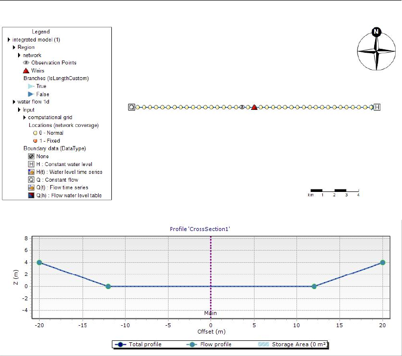
DRAFT
Module D-RTC: Technical reference
(a) Schematization and computational grid
(b) Cross section
Figure 6.3: Simple channel model (SOBEK 3.3)
Figure 6.5 shows the computed crest level of the weir and the water level at the observation
point over simulation time. The results show a very good match between setpoint and com-
puted water level. Figure 6.4 shows the water level along two longitudinal profiles for two time
steps and the corresponding crest levels at the weir.
Deltares 53 of 70

DRAFT
D-Real Time Control, User Manual
setpoint for water level at observation point
weir crest level
water level at observation point
elevation [m]
1
2
3
4
5
6
7
time
2000-01-22
08:00
2000-01-22
12:00
2000-01-22
16:00
2000-01-22
20:00
2000-01-23
00:00
2000-01-23
04:00
Figure 6.4: PID controlled crest level of the weir and corresponding water level at the
observation point
weir
water level 2000-01-22 20:00:00
water level 2000-01-21 00:00:00
crest level 2000-01-21 00:00:00
crest level 2000-01-22 20:00:00
bed level
elevation [m]
0
2
4
6
8
river chainage [m]
0 5000 15000 20000
Figure 6.5: Longitudinal profile of water level for two time steps and crest level of the weir
54 of 70 Deltares

DRAFT
Module D-RTC: Technical reference
6.3.8 The absolute time rule (timeAbsolute)
6.3.8.1 Functional principle
A time rule is a time series that defines the state of a control variable. The time series is given
as as absolute time stamps in wall clock time. It can be interpreted as a boundary condition
for structure parameters. In most cases the future aggregation is desired. This means that a
point in time is to be interpreted as “from now on”.
This rule reads
yk=xk(6.19)
where xis an external time series or output of a previous model.
6.3.8.2 Application
Common application cases for the absolute time rule are the following:
Calibration of a hydraulic model with structures: the position of crest levels is known as
historical value. The historical values are applied as absolute time rule.
Hydraulic models in operational systems: control has been determined outside the hy-
draulic model, and the control settings are applied as time series.
6.3.8.3 Example
An example time series for an absolute time rule is given with Table 6.2. This time series is
applied for the weir node in the simple SOBEK model, which is described in section 6.3.7.3.
A close-up of the simulation results and the discrete values from line 2 and 3 6.2 in are shown
in the diagram in Figure 6.6. Beginning at 12.00 h the crest level of a weir rises from 2.0 m up
to 5.0 m within 8 h. The corresponding time rule output is shown as solid line. The crest rises
not before 12.00 h and the movement of the crest stops at 20.00 h.
Table 6.2: Time rule time series example
time step kwall clock time time series value xin m
1 2000-01-20 00:00:00 2.0
2 2000-01-22 12:00:00 2.0
3 2000-01-22 20:00:00 5.0
4 2000-01-25 00:00:00 5.0
Deltares 55 of 70
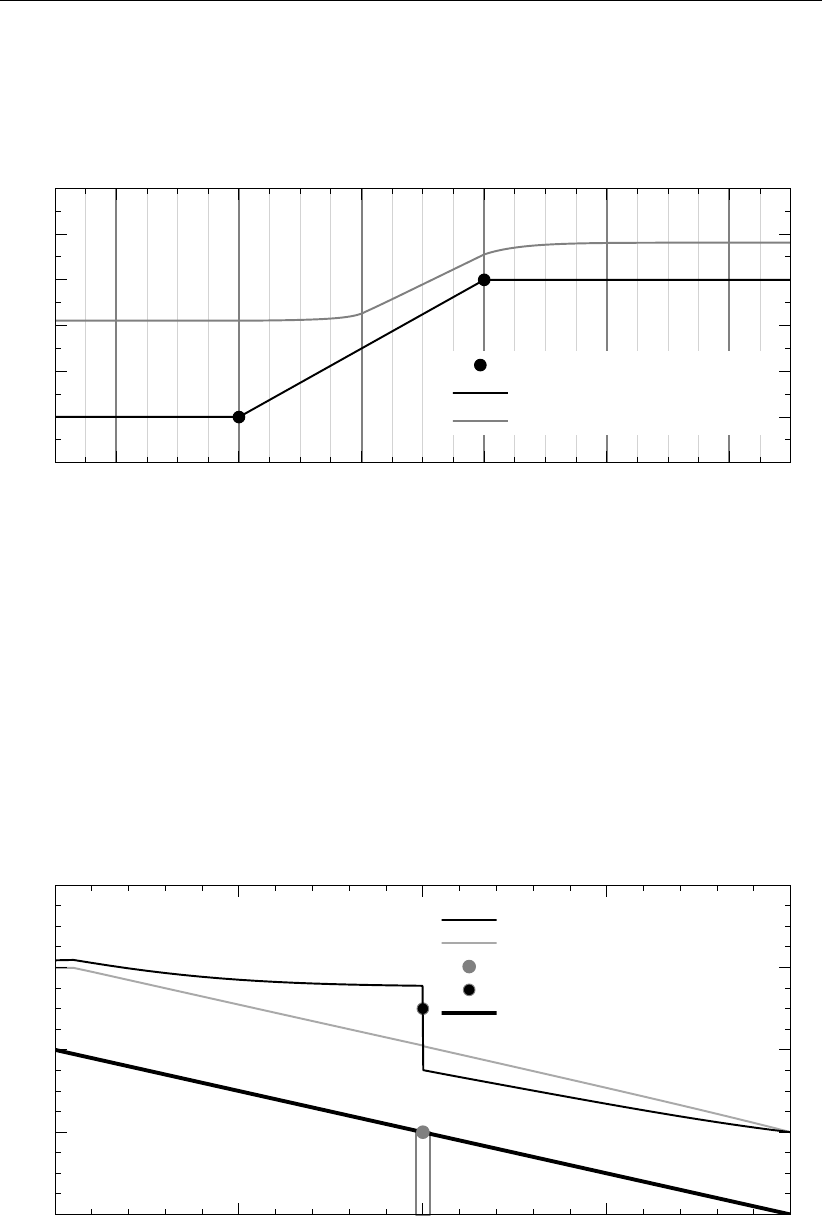
DRAFT
D-Real Time Control, User Manual
operating rule setpoints
computed crest level
computed water level
elevation [m]
1
2
3
4
5
6
7
time
2000-01-22
08:00
2000-01-22
12:00
2000-01-22
16:00
2000-01-22
20:00
2000-01-23
00:00
2000-01-23
04:00
Figure 6.6: Time rule time series
weir
water level 2000-01-22 20:00:00
water level 2000-01-21 00:00:00
crest level 2000-01-21 00:00:00
crest level 2000-01-22 20:00:00
bed level
elevation [m]
0
2
4
6
8
river chainage [m]
0 5000 15000 20000
Figure 6.7: Time rule side-view
56 of 70 Deltares

DRAFT
Module D-RTC: Technical reference
6.3.9 The relative time rule (timeRelative)
6.3.9.1 Functional principle
The Relative Time Rule creates a time series for a control variable relative to the current time
step. The time series is based on function between relative time steps and the values of the
control variable.
This rule reads
yk=xτ(6.20)
where τis a relative time reference. When the rule is switched on, the relative time is either
1 put to zero or
2 put to a value based on an existing yfor which equation (6.20) is fulfilled.
6.3.9.2 Application
The relative time rule applies for large structures like weirs or gates that move slowly and the
opening and closure time must be taken into account for the model. A relative time rule works
in combination with hydraulic triggers when the exact points in time of the control time series
are not known beforehand.
6.3.9.3 Example
Table 6.3 contains a linear relation between the relative time in seconds and the crest level
of a weir. Figure 6.8 shows a graphical representation of Table 6.3. The slope of the curve
defines the speed the crest level moves, in the current example this is
vweir =5−2
28800 m s−1= 1.0416 ×10⁻⁴m s−1.(6.21)
The relative time rule is related to the current time step. The parameter “FromValue” defines
at which point to start when the rule is activated. If the parameter “FromValue” is set to
false, the rule starts with the first entry (time reference option “zero” in section 6.3.9), if it is
true, the relative time period starts at the position the crest level has at the current time step
(second time reference option in section 6.3.9). Figure 6.9 shows the effect of the “FromValue”
parameter: before activating the relative time rule at 22-01-2000, 12:00 hours, the crest level
is at 2.5 m. If the “FromValue” propertiy is set to false, the crest level goes down to the first
entry of the Table 6.3 which is 2.0 m, before it rises to 5.0 m according to Table 6.3. When
“FromValue” is set to true, the starting point in relative time that corresponds to the initial crest
level of 2.5 m is determined first, and the closure of the weir starts from this value. The total
operation of the weir is shorter, because not the full range of the table is used.
Table 6.3: Relative time rule lookup table for the crest level of a weir
relative time in s crest level in m
0 2.0
28800 5.0
Deltares 57 of 70
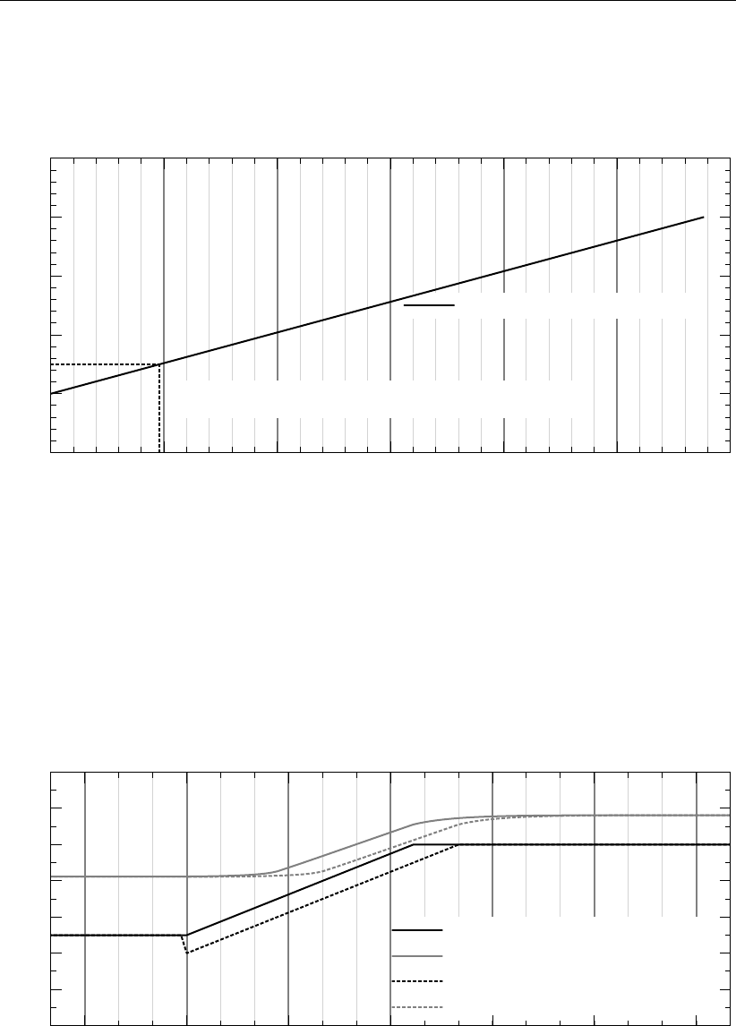
DRAFT
D-Real Time Control, User Manual
x = 4800: relative time from value y = 2.5
relative time rule function
crest level [m]
1
2
3
4
5
6
relative time [s]
0 5000 10000 20000 25000 30000
Figure 6.8: Relative time rule function and relative time from Value 2.5
crest level
water level
crest level (fromValue = false)
water level (fromValue = false)
elevation [m]
0
1
2
3
4
5
6
7
time
2000-01-22
09:00
2000-01-22
12:00
2000-01-22
15:00
2000-01-22
18:00
2000-01-22
21:00
2000-01-23
00:00
2000-01-23
03:00
Figure 6.9: Crest level controlled with relative time rule and “FromValue” parameter true/-
false and the corresponding water level over time
58 of 70 Deltares

DRAFT
Module D-RTC: Technical reference
6.4 Triggers
6.4.1 Introduction
Originally a trigger is an element of a fire arm that actuates a mechanism to fire a bullet. In
electronics the word trigger describes a specific type of an electronic circuit that releases a
signal or a switching operation at a certain event. In an analogue way we use the trigger
to describe an abstract mechanism that releases (or triggers) another trigger mechanism
or a control action, which is then described by an operating rule. A very simple triggering
mechanism is an alarm clock signal upon which an operator switches off a pump at a specific
point in time. The more advanced triggers in computer models usually need input data.
A trigger output yin RTC-Tools is true or false, which will be represented as y= 1 (true)
or y= 0 (false) in the following. So technically, a trigger in RTC-Tools operates as a switch
between two states.
6.4.2 Standard
The standard trigger compares two input values and returns true (1) or false (0):
yk=1if xk−1∨k
1> xk−1∨k
2
0otherwise (6.22)
Beside the >operator that is used in Equation (6.22) the following operators are supported:
>, ≥,=,6=,≤, <. The standard trigger is the basis of the D-RTC hydro condition (sec-
tion 4.1.1).
6.4.3 The time trigger
6.4.3.1 Functional principle
A time trigger models a timer. The trigger output yfor time step kis given in a time series x.
The time trigger is the basis of the D-RTC time condition (section 4.1.2). An example for such
a time series is given in Table 6.4.
Table 6.4: Time trigger time series example
time step kwall clock time time series value x
1 2000-01-15 00:00:00 false
2 2000-01-16 00:00:00 true
3 2000-01-17 00:00:00 false
When using a time trigger, care must be taken for the aggregation. With future aggregation,
the control action that is connected to the trigger follows the trigger with delay with one time
step. This will be a desired behaviour for many feedback control applications. If a time lag is
not desired, it can make sense to apply past aggregation.
yk=xk−1future aggregation (6.23)
yk=xkpast aggregation (6.24)
6.4.3.2 Application
winter/summer operational mode
inclusion of external decisions (feedforward control), for example “high water forecasted?
(yes/no)”
Deltares 59 of 70
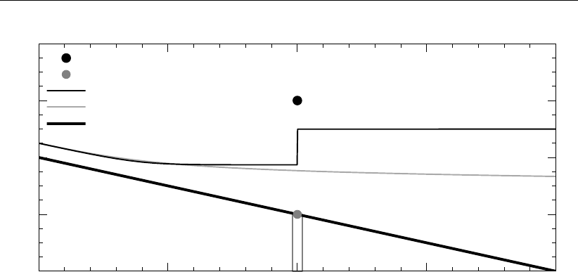
DRAFT
D-Real Time Control, User Manual
weir
crest level 2000-01-20 12:00:00 (closed)
crest level 2000-01-20 22:00:00 (open)
water level 2000-01-20 12:00:00
water level 2000-01-20 22:00:00
bed level
elevation [m]
0
2
4
6
8
river chainage [m]
0 5000 15000 20000
Figure 6.10: Expected results
model calibration when control parameters are known.
6.4.4 deadBandTrigger
6.4.4.1 Functional principle
The dead band trigger checks the input data for an upper or lower threshold crossing. The
trigger returns true in case of an up-crossing of the upper threshold bup. It is inactive in case
of a down crossing of the lower threshold bdown. In the range in-between, the trigger keeps
its former state. The rule reads
yk=
1if xk−1∨k
1> bupk−1∨k
0if xk−1∨k
2< bdownk−1∨k
yk−1otherwise
(6.25)
where x1and x2are time series or constant values. The dead band range given by upper and
lower threshold can be constant or time series, too. The following operators are supported: >
,≥,=,6=,≤, <. This feature is not yet supported by the user interface, but can be configured
by modifying the corresponding input file.
6.4.4.2 Application
Dead band triggers are used to switch on and off pumps or turbines and the dead band
ensures that the device is not switched on or off too often.
6.4.4.3 Example
Given the simple SOBEK model, which is described in section 6.3.7.3 under tidal sea level
variations, the control task is to control the weir in such a way that it is closed (i.e. the crest
level is 6 m) if the head difference at the weir is smaller or equal 0.3 m in order to protect the
hinterland from sea flooding and salt water intrusion during high tide. If the head difference is
larger than 0.3 m the weir must be open (i.e. the crest level is 2 m) in order to discharge water
towards the sea during low tide. The expected result is given in Figure 6.10.
With the help of an expression (see section 6.2.2) the head difference upstream and down-
stream the weir is computed. The weir is controlled with two constant rules section 6.3.1:
60 of 70 Deltares
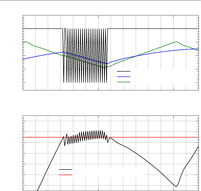
DRAFT
Module D-RTC: Technical reference
crest level
water level upstream of weir
water level downstream of weir
Elevation (m)
2
3
4
5
6
7
Time
2000-01-20
12:00
2000-01-21
12:00
head difference
threshold for open/close of weir
Head difference (m)
−0.6
−0.4
−0.2
0
0.2
0.4
0.6
Time
2000-01-20
12:00
2000-01-21
12:00
Figure 6.11: On-off control triggered by head difference
Weir open returns a crest level of 2m
Weir closed returns a crest level of 6m.
With a standard trigger (section 6.4.2) produces the result Figure 6.11. After the head differ-
ence exceeds the threshold of 0.3 m, the weir is opened. This has the effect on the the water
levels: the water level upstream decreases and the water level upstream increases, so the
head difference goes below the threshold, which means that the weir must be closed again.
This again increases the head difference towards a value above the threshold, which means
that the weir must be opened again.
Figure 6.12 shows a simulation result where a dead band trigger has been applied with a dead
band of 0.3 m for bup and 0.05 m for bdown. The weir is not opened before the head difference
of 0.3 m is reached, but the closing of the weir is not carried out before the head difference
decreases to 0.05 m.
Deltares 61 of 70
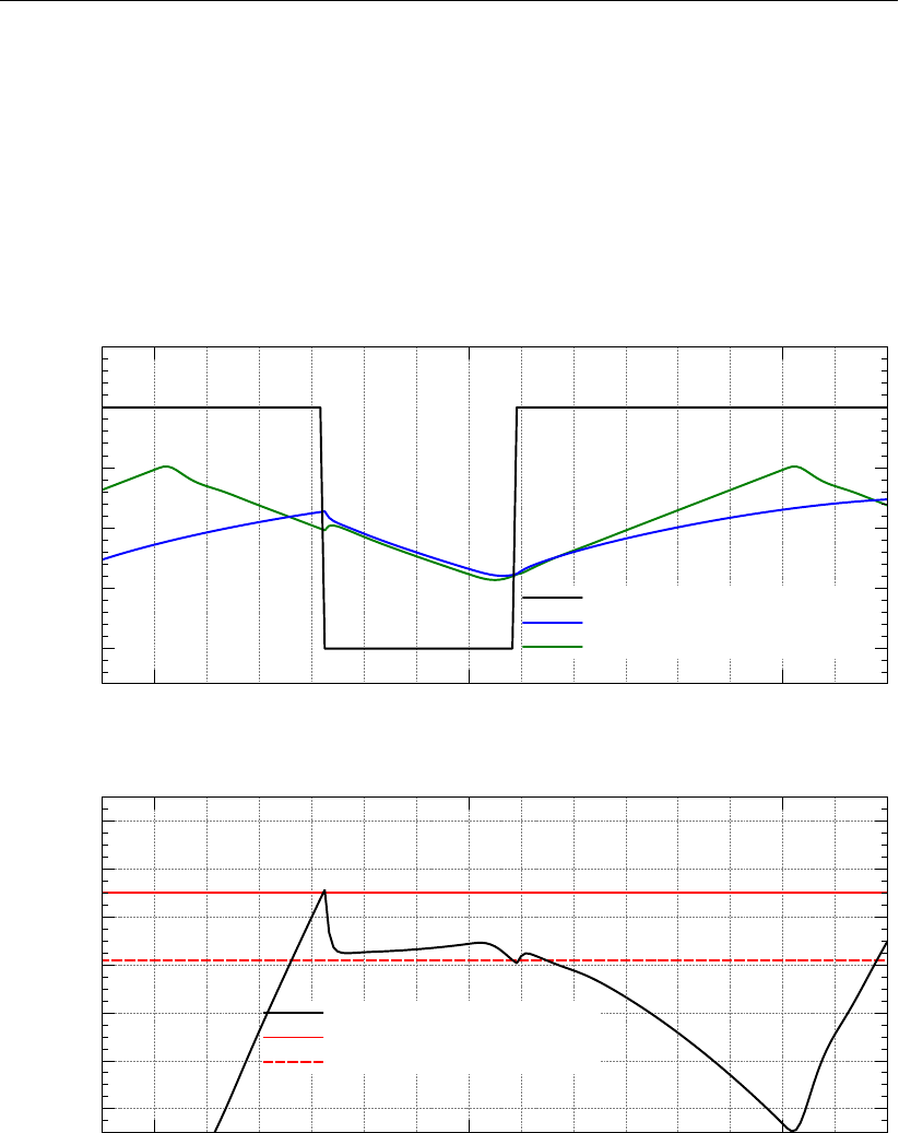
DRAFT
D-Real Time Control, User Manual
crest level
water level upstream of weir
water level downstream of weir
Elevation (m)
2
3
4
5
6
7
Time
2000-01-20
12:00
2000-01-21
12:00
head difference
dead band upper boundary
dead band lower boundary
Head difference (m)
−0.6
−0.4
−0.2
0
0.2
0.4
0.6
Time
2000-01-20
12:00
2000-01-21
12:00
Figure 6.12: Adding a dead band reduces the number of weir operations
62 of 70 Deltares

DRAFT
Module D-RTC: Technical reference
6.4.5 deadBandTime
The dead band time trigger checks a time series for a number of subsequent up-crossings
nup or down-crossing ndown from its current value. If the crossing is observed for at least the
user-defined number of time steps, the new value is used. The trigger reads
xk=
xkif {xk−nup+1, ..., xk}> xk−nup
xkif {xk−ndown+1, ..., xk}< xk−ndown
xk−1otherwise
(6.26)
An application for this trigger is the activation or deactivation of alarm levels. The increase
of alarm level may happen immediately (nup = 0), whereas the decrease of an alarm level
could be done only after a number of ntime steps have passed (ndown =n) without further
threshold crossings.
This feature is not yet supported by the user interface, but can be configured by modifying the
corresponding input file.
6.4.6 polygonLookup
The polygon lookup trigger checks, if a point is inside of a set of polygons. If this is the case,
it returns the user-defined value of the specific polygon. The point is defined by the values of
two time series, referred to as the x1and x2coordinate of the point. The rule reads
yk=
y1if (xk−1∨k
1, xk−1∨k
2)∈P1
.
.
..
.
.
ynif (xk−1∨k
1, xk−1∨k
2)∈Pn
ydefault otherwise
(6.27)
where yis the result of the rule and {P1, ..., Pn}is a set of polygons.
Figure 6.13 presents an example for the application of the trigger to the definition of warning
level for controlling a lake release in Canton Bern, Switzerland.
This feature is not yet supported by the user interface, but can be configured by modifying the
corresponding input file.
6.4.7 set
The trigger enables a logical combination of other triggers, combined by a logical operator. It
reads
yk=xk−1∨k
1∧xk−1∨k
2(6.28)
The following operators are supported: ∧(AND), ∨(OR), ⊕(XOR).
If more than two terms needs to be combined, the set can be used recursively by defining
another set as one of the two terms. Therefore, the expression yk=xk
1∧(xk
2∨xk
3)is
represented by a hierarchy of two sets (check the example in the configuration chapter).
This feature is not yet supported by the user interface, but can be configured by modifying the
corresponding input file.
Deltares 63 of 70
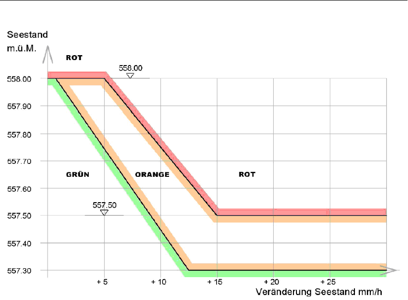
DRAFT
D-Real Time Control, User Manual
Figure 6.13: Example for the application of the polygon trigger to the definition of warning
levels for controlling a lake release at Lake Thun, Canton Bern, Switzerland
6.4.8 Expression
The expression trigger works like the expression component in section 6.2.2. Because trig-
gers are evaluated before components within the time step simulation, it can make sense to
use the expression trigger instead of an expression component in order to prepare data of the
current time step.
This feature is not yet supported by the user interface, but can be configured by modifying the
corresponding input file.
64 of 70 Deltares

DRAFT
A D-RTC build instructions on Linux
A.1 Prerequisites
Before building D-RTC, make sure the following applications are present in you environment:
Compilers: gcc and g++
cmake 3.0.0 or higher
tortoise svn
A.2 Build D-RTC
1 Make a directory <D-RTC>, and inside there make other three directories: boost, repo,
build.
2 Build boost (see section A.3).
3 Download the following repository inside the repo folder using svn (it might take up to
30 min, due to the inclusion in the third party directory of precompiled boost binaries for
windows).
https://svn.oss.deltares.nl/repos/rtc-tools/branches/FBC-Tools/
FBCTools
4 In the build directory run the following cmake command:
cmake -DBOOST_ROOT:PATHNAME=/u/carniato/D-RTC/boost/boost_1_65_0_install
../repo/FBCTools
Explanation: the first option points to your boost installation directory, the second option
points to the source dir of D-RTC (substitute the part “/u/carniato” with the appropriate
path in your system).
5 Type make for building D-RTC. Binaries are made inside repo/FBCTools/bin/Release.
A.3 Build boost
1 Download <boost_1_65_0.tar.gz>from
https://dl.bintray.com/boostorg/release/1.65.0/source/
and copy it inside the boost directory
2 Untar the tarball in the boost directory:
tar -zxvf boost_1_65_0.tar.gz
3 Create a new directory <boost_1_65_0_install>
4 Move inside boost_1_65_0 (the source code directory) and build boost (do not worry about
possible errors in building boost/python, it is not used by D-RTC).
./bootstrap.sh
./b2 install -prefix=../boost_1_65_0_install
A.4 Using D-RTC library with a Delft3D DIMR installation
In order to use the D-RTC binaries in a dimr-run it is sufficient to prepend the LD_LIBRARY_PATH
with the D-RTC library directory before executing the <run_dimr.sh>script (<run_dimr.sh>
resides in the Delft3D DIMR installation). Below an example:
export libdir=/u/carniato/FBC-Tools/repo/FBCTools/bin/Release
export LD\_LIBRARY\_PATH=$libdir:$LD\_LIBRARY\_PATH
/u/carniato/delft3dOSS/trunk/src/bin/run_dimr.sh -d 8 -m dimr.xml
Make sure the library name is correct in the <dimr.xml>configuration file (i.e. FBCTools_BMI)
<component name="myNameRTC">
<library>FBCTools_BMI</library>
Deltares 65 of 70

DRAFT
D-Real Time Control, User Manual
<workingDir>rtc</workingDir>
<!-- component specific -->
<inputFile>.</inputFile>
</component>
66 of 70 Deltares

DRAFT
References
Åström, K. J. and T. Hägglund, 1995. PID controllers: theory, design and tuning. Instrument
Society of America, Research Triangle Park, NC, USA, 2nd ed.
Becker, B., C. Sprengers and T. Ochterbeck. “AMICE: Action 6. Hydraulic Sobek-model for
the Dutch part of the Meuse.”
Deltares 67 of 70

DRAFT
D-Real Time Control, User Manual
68 of 70 Deltares
DRAFT

PO Box 177
2600 MH Del
Boussinesqweg 1
2629 VH Del
The Netehrlands
+31 (0)88 335 81 88
sales@deltaressystems.nl
www.deltaressystems.nl
DRAFT
