SWITCH User Manual D Water_Quality_Switch_Technical_Reference_Manual Water Quality Technical Reference

User Manual: Pdf D-Water_Quality_Switch_Technical_Reference_Manual

Open the PDF directly: View PDF .
Page Count: 42

D-Water Quality

Water quality and aquatic ecology modelling suite

Technical Reference Manual

SWITCH

DRAFT

DRAFT

DRAFT

SWITCH

Prediction of the nutrient fluxes across the sediment-

water interface

Technical Reference Manual

D-Water Quality

Version: 4.00

SVN Revision: 52614

April 18, 2018

DRAFT

SWITCH, Technical Reference Manual

Published and printed by:

Deltares

Boussinesqweg 1

2629 HV Delft

P.O. 177

2600 MH Delft

The Netherlands

telephone: +31 88 335 82 73

fax: +31 88 335 85 82

e-mail: info@deltares.nl

www: https://www.deltares.nl

For sales contact:

telephone: +31 88 335 81 88

fax: +31 88 335 81 11

e-mail: software@deltares.nl

www: https://www.deltares.nl/software

For support contact:

telephone: +31 88 335 81 00

fax: +31 88 335 81 11

e-mail: software.support@deltares.nl

www: https://www.deltares.nl/software

Copyright © 2018 Deltares

All rights reserved. No part of this document may be reproduced in any form by print, photo

print, photo copy, microfilm or any other means, without written permission from the publisher:

Deltares.

DRAFT

Contents

Contents

List of Figures v

List of Tables vii

1 Introduction 1

2 Spatial schematisation and processes 3

3 Aerobic layer and the sediment oxygen demand 9

4 Denitrifying layer and nitrate 11

5 Detritus 13

6 Ammonium 17

7 Phosphate 19

8 Silicate 25

9 Temperature dependency and dispersion 27

References 29

Deltares iii

DRAFT

SWITCH, Technical Reference Manual

iv Deltares

DRAFT

List of Figures

List of Figures

2.1 Schematisation of the sediment layer in SWITCH . . . . . . . . . . . . . . . 3

2.2 Overview of the processes included in SWITCH . . . . . . . . . . . . . . . . 4

Deltares v

DRAFT

SWITCH, Technical Reference Manual

vi Deltares

DRAFT

List of Tables

List of Tables

2.1 Initialisation parameters for SWITCH . . . . . . . . . . . . . . . . . . . . . 4

2.1 Initialisation parameters for SWITCH . . . . . . . . . . . . . . . . . . . . . 5

2.2 Numerical input parameters for SWITCH . . . . . . . . . . . . . . . . . . . 5

2.3 Physical input parameters for SWITCH .................... 5

2.3 Physical input parameters for SWITCH .................... 6

2.4 (Bio)chemical input parameters for SWITCH . . . . . . . . . . . . . . . . . 6

2.4 (Bio)chemical input parameters for SWITCH . . . . . . . . . . . . . . . . . 7

2.4 (Bio)chemical input parameters for SWITCH . . . . . . . . . . . . . . . . . 8

Deltares vii

DRAFT

SWITCH, Technical Reference Manual

viii Deltares

DRAFT

1 Introduction

SWITCH was made as a sub-model of the surface water eutrophication model DBS for the

prediction of the nutrient fluxes across the sediment-water interface (WL | Delft Hydraulics,

1992). The acronym stands for Sediment Water Interaction by Transport and Chemistry.

SWITCH distinguishes four sediment layers and calculates the thicknesses of the aerobic and

denitrifying layers on the basis of a steady state approach. The concentrations of detritus,

ammonium, nitrate, phosphate and silicate in the sediment and the pore water are simulated

dynamically using mass balance equations.

SWITCH is applied as part of the eutrophication models, specific configurations of DELWAQ

among which DBS and GEM. The link between these models and sub-model SWITCH is

formed by the sediment-water exchange fluxes of dissolved oxygen, nutrients and organic

matter. SWITCH acts directly on substances in the water column, just like any other process

routine in DELWAQ. Specific facilities have been developed for the coupling of SWITCH to

DELWAQ. These include a fractional step numerical computation procedure and an sediment-

water aggregation procedure. The fractional step procedure takes care that SWITCH operates

according to an appropriate computational time step, equal to or smaller than the DELWAQ

time step, in order to maintain computational stability at steep concentration gradients and

large mass fluxes between water and sediment. The sediment-water aggregation procedure

allows the aggregation of several water segments with respect to SWITCH in order to establish

a reduction of the computational burden. This means that the exchange of substances with

the sediment underlying such a group of water segments is computed by SWITCH in one

stroke. Both procedures are described in the process documentation regarding SWITCH in

Chapter 8 of this manual.

Details with respect to background, objectives, starting-points and formulations of SWITCH

have been described in WL | Delft Hydraulics (1994b,c). The first version of SWITCH and

the first application for Lake Veluwe, the sediment of which is a mixture of silt and sand, have

also been described by Smits and Van der Molen (1993). Other applications of SWITCH

concerned the Lake Volkerak-Zoommeer (WL | Delft Hydraulics,1995), with deep gullies and

silty sediment, the peat lakes Geerplas and Nannewijd (WL | Delft Hydraulics,1997) and the

sandy coastal strip of the North Sea.

Volume units refer to bulk ( ) or to water ( ).

Deltares 1 of 32

DRAFT

SWITCH, Technical Reference Manual

2 of 32 Deltares

DRAFT

2 Spatial schematisation and processes

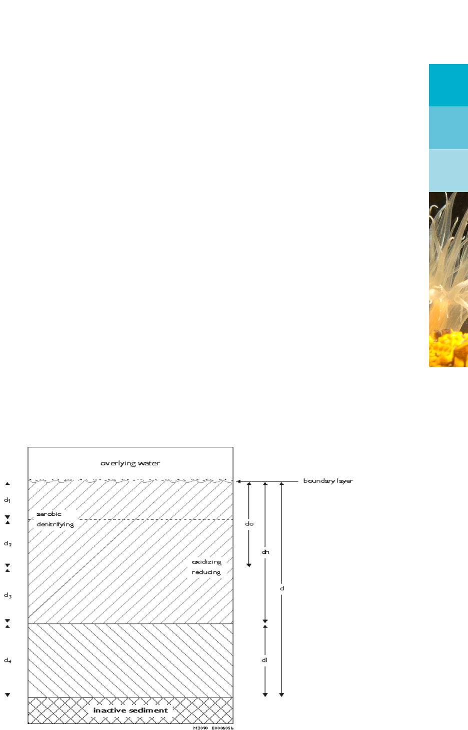
Figure 2.1 depicts the vertical schematisation of the ’active’ sediment layer in SWITCH. An

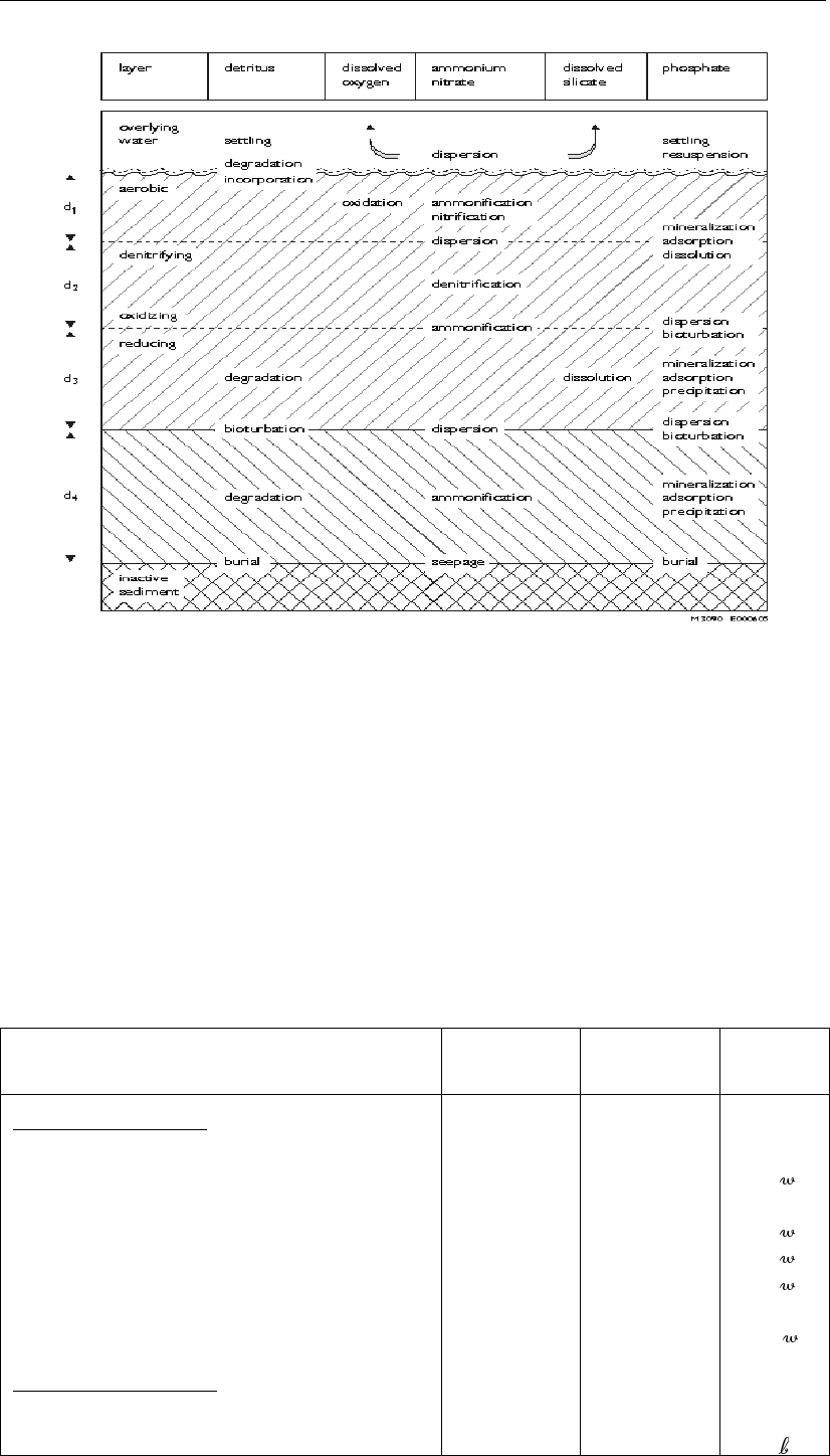
overview of the processes included in SWITCH is given in Figure 2.2. The ’active’ sediment

layer has a constant thickness (d), and is divided in 4 sub-layers. An upper layer (dh) and

a lower layer (dl=d4) have been defined in order to account for vertical characteristics such

as decomposition of organic matter, dispersion and porosity. These layers are also fixed.

A second partition follows from chemical differences. A thin top layer (do) is oxidising, the

remaining part (dh-do = d3,>minimal value) of the upper layer is reducing. The oxidising

layer is divided in an oxygen containing layer d1and a denitrifying layer d2. Both d1and d2

are variable, and are deduced from steady-state solutions of the mass balance equations for

dissolved oxygen and nitrate. In order to avoid numerical problems neither do nor d1may

become infinitely thin, a minimal thickness (d1m) has therefore been defined. However, the

denitrifying layer disappears entirely, when the nitrate concentration drops below a critical

value (Cnc).

Additionally, a very thin meta-stable boundary layer has been defined, which contains the

detritus settled from the overlying water (and produced from microphytobenthos). From this

layer detritus is incorporated in the sediment as the consequence of bioturbation. Nutrients

produced from decomposition of detritus in the boundary layer are allocated to the oxygen

containing top layer. The same goes for the dissolved oxygen fluxes pertaining to these

processes. The boundary layer as such may affect the dispersion of dissolved substances

across the sediment-water interface, which can be taken into account in SWITCH.

Table 2.1 upto Table 2.4 present an overview of the input parameters for SWITCH. In addition

SWITCH needs mass fluxes from the water column connected with the settling of particu-

late substances and the dissolved concentrations in the water column for the calculation of

diffusive exchange and downwelling seepage.

Figure 2.1: Schematisation of the sediment layer in SWITCH

Deltares 3 of 32

DRAFT

SWITCH, Technical Reference Manual

Figure 2.2: Overview of the processes included in SWITCH

As mentioned in the introduction SWITCH is applied as part of the eutrophication models,

specific configurations of DELWAQ among which DBS and GEM. In this setting the meta-

stable boundary layer is modelled as the S1 sediment layer, which contains so-called “inactive

substances” such as detritus and benthic algae, together shaping up the benthic complex.

(However, benthic algae may be excluded from the simulation). All nutrient fluxes inferred by

the algae are accounted for, either directly in the boundary layer (S1) or in the upper sediment

layer 1 in SWITCH. Algae are incorporated from the boundary layer into the sediment in

exactly the same way as detritus, which is taken care of by the process called “burial”. The

way settling particulate matter is added to boundary layer S1 or directly to the upper sediment

layer 1 is described in the process description in Chapter 8of this manual.

Table 2.1: Initialisation parameters for SWITCH

Parameter Symbol in

appendix

Value

(indicative)

Units

Dissolved substances

Nitrate:

Layer 1 Cn11.0 gN m−3

Ammonium:

Layer 1: Ca11.5 gN m−3

Layer 2–3: Ca23.0 gN m−3

Layer 4: Ca44.0 gN m−3

Silicate:

Layer 1–1: Cs18.0 gSi m−3

Partitioned substances

Total inorganic phosphate content:

Layer 1–2: Cp1140.0 gP m−3

4 of 32 Deltares

DRAFT

Spatial schematisation and processes

Table 2.1: Initialisation parameters for SWITCH

Parameter Symbol in

appendix

Value

(indicative)

Units

Layer 3: Cp3105.0 gP m−3

Layer 4: Cp484.0 gP m−3

Fraction of phosphate in vivianite:

Layer 1–2: fpp10.1 -

Layer 3: fpp30.3 -

Layer 4: fpp40.5 -

Fraction of phosphate in stable mineral:

Layer 1–2: fmp10.4 -

Layer 3: fmp30.4 -

Layer 4: fmp40.4 -

Particulate substances

Detritus content in the upper layer 1–3

Carbon Cd1700.0 gC m−3

Nitrogen Cnd140.0 gN m−3

Phosphorus Cpd13.5 gP m−3

Detritus content in the lower layer 4

Carbon Cd 4160.0 gC m−3

Nitrogen Cnd47.0 gN m−3

Phosphorus Cpd40.7 gP m−3

Refractory detritus content in layer 1–4

Carbon Crd10.0 gC m−3

Nitrogen Crn10.0 gN m−3

Phosphorus Crp10.0 gP m−3

Table 2.2: Numerical input parameters for SWITCH

Parameter Symbol in

appendix

Value Units

Minimal thickness (depth) of the aerobic layer 1 d1m0.0005 m

Crit. thickness layer 1 for obt. red. sorp. capac-

ity

dom0.0009 m

Crit. (=max) nitrate conc. for sulphate reduction Cnc0.05 gN m−3

Table 2.3: Physical input parameters for SWITCH

Parameter Symbol in

appendix

Value Units

The sediment

Thickness (depth) of the aerobic top layer 11) d10.001 m

Thickness (depth) of the denitrifying layer 21) d20.004 m

Deltares 5 of 32

DRAFT

SWITCH, Technical Reference Manual

Table 2.3: Physical input parameters for SWITCH

Parameter Symbol in

appendix

Value Units

Thickness (depth) of the upper reducing layer

31)

d30.015 m

Thickness (depth) of the lower reducing layer 4 d4= dl 0.08 m

Thickness (mixing length) of the water bound-

ary layer

l 0.001 m

Porosity of the upper layer p10.75 m3m−3

Porosity of the lower layer p40.65 m3m−3

Specific weight (density) of dry matter Ws 2400.0 kg m−3

Mass transport

Seepage (- downwelling or + upwelling) vs 0.0 m/day

Ammonium conc. at lower boundary in upw.

water

Ca54.0 gN m−3

Phosphate conc. at lower boundary in up-

welling water

Cdp50.05 gP m−3

Silicate conc. at lower boundary in upwelling

water

Cs510.0 gSi m−3

Sedimentation rate (gross sediment accretion

rate)

Fs 0.0 m3m−2

d−1

Resuspension rate Fr 0.0 m3m−2

d−1

Fraction of surface area closed by the benthic

complex

fc 0.0 -

Molecular diffusion coefficient oxygen Dmo5.5·10−5m2d−1

Molecular diffusion coefficient ammonium Dma9.0 „ m2d−1

Molecular diffusion coefficient nitrate Dmn9.3 m2d−1

Molecular diffusion coefficient phosphate Dmp4.2 „ m2d−1

Molecular diffusion coefficient silicate Dms4.7 „ m2d−1

Bio-irrigation multiplication factor;

mean bt 3.0 -

amplitude 2.0 -

period 365 d

phase 0.2 -

Bioturbation dispersion coefficient;

mean Db 1.0·10−6m2d−1

amplitude 1.0·10−6m2d−1

period 365 d

phase 0.2 -

1) d1, d2and d3shape up the upper layer dh, which is constant in thickness just as dl (=d4).

Table 2.4: (Bio)chemical input parameters for SWITCH

Parameter Symbol in

appendix

Value Units

Detritus

6 of 32 Deltares

DRAFT

Spatial schematisation and processes

Table 2.4: (Bio)chemical input parameters for SWITCH

Parameter Symbol in

appendix

Value Units

Incorp. rate from bound. layer into up. layer at

20 ◦C1)

rc20 0.04 d−1

Temperature coefficient for incorporation* kti 1.07 -

Mineralisation rate in the boundary layer at 20

◦C2)

kc20

b0.075 d−1

Mineralisation rate in the upper layer at 20 ◦C kc20

10.055 d−1

Mineralisation rate in the lower layer at 20 ◦C kc20

40.0065 d−1

Temperature coefficient for mineralisation ktc 1.07 -

Add. frac. detritus turned into refractory org.

matter

frf 1.0 -

Ammonium and Nitrate

Nitrification rate kn20 50.0 d−1

Temperature coefficient for nitrification ktn 1.07 -

Denitrification rate at 20 ◦C kd20 50.0 d−1

Temperature coefficient for denitrification ktd 1.07 -

Stoich. constant for nitrogen in refractory org.

matter

aa 0.04 gN gC−1

Phosphate

Adsorption capacity of oxidising layer 1-2 Caco0.8 gP

kgDM−1

Adsorption capacity of upper reducing layer 3 Cacr0.4 or -999 gP

kgDM−1

Half saturation constant for adsorption at 20 ◦C Ks20 0.1 gP m−3

Temperature coefficient for half saturation con-

stant

kta 1.0 -

Precipitation rate at 20 ◦C kp20 0.8 d−1

Fraction precipitated phosphate into the stable

mineral

fm 0.0 -

Saturation concentration for precipitation Cdps0.05 gP m−3

Temperature coefficient for precipitation ktp 1.0 -

Dissolution / oxidation rate of vivianite at 20 ◦C kdp20 0.01 m−2.01

gP0.67

d−1

Temperature coefficient for dissolution ktdp 1.0 -

Stoich. constant for phosphorus in refract. org.

matter

ap 0.004 gP gC−1

Silicate

Dissolution rate of opal silicate at 20 ◦C ks20 0.09 d−1

Saturation concentration for dissolution Css10.0 gSi m−3

Temperature coefficient for dissolution kts 1.0 -

Oxygen

Stoich. constant for consump. at mineralis. of

detritus

ac 3.1 gO2

gC−1

Stoich. constant for consump. at nitrification an 4.57 gO2

gN−1

Deltares 7 of 32

DRAFT

SWITCH, Technical Reference Manual

Table 2.4: (Bio)chemical input parameters for SWITCH

Parameter Symbol in

appendix

Value Units

Fraction oxygen in water at sediment-water in-

terface

fo 0.6 -

Fraction reduced substances retained from ox-

idation;

mean fro 0.0 -

amplitude 0.0 -

period 365 d

phase 0.2 -

1) The incorp. rate is dealt with in the input for S1 detritus as a burial rate in 1/d, that can be

made approx. temperature dependent by providing a time dependent function.

2) The decomposition rates and temperature coefficients for detritus in the boundary layer are

input for the S1 module of DELWAQ. Rates and coefficients have to be provided for org. C,

org. N and org. P.

8 of 32 Deltares

DRAFT

3 Aerobic layer and the sediment oxygen demand

The thickness of the aerobic layer is dependent on the oxygen consumption rate according to

the following steady-state equation:

d1=p2·p1·D·fo ·CoO/Ro (3.1)

d1=d1mif d1<d1m

in which:

CoOoxygen concentration in the overlying water [g m−3]

d1mminimal thickness of the aerobic layer [m]

D dispersion coefficient [m2d−1]

fo ratio of the oxygen concentrations at the upper and lower sides of the water

boundary layer [-]

p porosity [-]

Ro oxygen consumption rate [g m3bottom d−1]

A subscript figure indicates a layer number or an interface number!

The introduction of ratio fo relates to the existence of a relatively stagnant boundary layer

in the overlying water, which contains a part of the oxygen gradient at the sediment-water

interface. The oxygen concentration at the interface is a certain fraction of the average oxygen

concentration in the water column.

Oxygen is consumed in the degradation of detritus in the boundary layer (complex-detritus

in the terminology of DBS) and of detritus in the aerobic layer, in the nitrification and in the

chemical oxidation. The oxygen consumption rate Ro is formulated as follows:

Ro =Fob/d1+ac ·kc1·Cd1+p1·an ·kn ·Ca1+Foc/d1(3.2)

in which:

ac stoichiometric constant [gO2gC−1]

an stoichiometric constant [gO2gN−1]

Cd1detritus concentration in the upper layer [gC m−3B]

Ca1ammonium concentration in the aerobic layer [gN m−3PW]

Foboxygen consumption in the boundary layer [gO2m−2d−1]

Focchemical oxygen demand [gO2m−2d−1]

kc1degradation rate of detritus in the upper layer [d−1]

kn nitrification rate [d−1], equal to zero if Co0= 0.0

The oxygen consumption in the boundary layer is connected with the degradation of detritus

on top of the sediments and is equal to:

Fob=ac ·kcb·Cdb(3.3)

in which:

Cdbamount of complex-detritus in the boundary layer [gC m2]

kcbdegradation rate of complex-detritus in the boundary layer [d−1]

The chemical oxygen demand concerns the oxidation of reduced substances, such as iron(II),

manganese(II), sulphide and methane originating from the degradation of detritus in the anaer-

obic part of the ’active’ bottom. However, the reduced substances will not be oxidising com-

pletely. A part of the sulphide resulting from sulphate reduction precipitates with iron and may

Deltares 9 of 32

DRAFT

SWITCH, Technical Reference Manual

accumulate in the reduced part of the sediments. Methane may escape from the sediments

in gas bubbles. Consequently, the actual chemical oxygen demand is formulated as a fraction

of the potential chemical oxygen demand:

Foc= (1 −fro)·ac ·(kc1·Cd1·(d2+d3) + kc4·Cd4·d4)(3.4)

in which:

fro fraction reduced substances permanently removed or fixed [-]

kc4degradation rate of detritus in the lower layer [d−1]

Note that the degradation of detritus in the denitrifying layer has been included entirely in

the chemical oxygen demand. This is not correct as such, since the elementary nitrogen

produced by denitrification is chemically inert. It is not oxidised, but escapes from the bottom.

A correction for the amount of nitrate consumed by denitrification can be made with fro. No

correction was made in the second version of SWITCH.

The sediment oxygen demand is quantified with:

Fo =Fob+ (ac ·kc1·Cd1+p1·an ·kn ·Ca1)·d1+Foc(3.5)

Maintaining a bottom oxygen demand under anaerobic conditions in the water column (kn =

0.0!) leads to a negative oxygen concentration in the water quality model representing the

surplus of reduced substances.

10 of 32 Deltares

DRAFT

4 Denitrifying layer and nitrate

Nitrate is formed from ammonium through nitrification in the aerobic top layer. It is subjected

to vertical transport and denitrification in the zone just below this layer (Vanderborght et al.,

1977a). The thickness of the denitrifying layer follows from the (approximate) steady-state

solution of the differential equation for nitrate in this layer:

d2= 2(Cn1−Cnc)/Cn1·pD/kd (4.1)

d2= 0.0if Cn1≤Cnc

in which:

kd first order denitrifcation rate [d−1]

Cn1nitrate concentration in the top layer [gN m−3]

Cnccritical nitrate concentration [gN m−3]

The critical nitrate concentration is the maximal concentration at which sulphate reduction is

possible, about 0.1 gN m−3.

The nitrate concentration in the aerobic and denitrifying layers follow from:

dCn1

dt = (Fnb−Fn0+Fn1)/(p1·d1) + kn ·Ca1(4.2)

with:

Fn0= 2p1·D·(Cn1−Cn0)/(l+d1)

Fn1=−2p1·kd ·Cn2·pD/kd

Cn2=1

2Cn1

in which:

Ca1ammonium concentration in the top layer [gN m−3]

Fnbflux from the boundary layer [gN m−2d−1]

Fn0dispersive return flux to the overlying water [gN m−2d−1]

Fn1flux to the denitrifying layer [gN m−2d−1]

l thickness of the water boundary layer [m]

Deltares 11 of 32

DRAFT

SWITCH, Technical Reference Manual

12 of 32 Deltares

DRAFT

5 Detritus

Organic carbon

All organic matter, which settles on the sediments is considered as detritus, regardless of its

origin. GEM distinguishes:

live phytoplankton, which enters the complex-detritus pool in the boundary layer due to

settling;

dead microphytobenthos, which enters the complex-detritus pool in the boundary layer

due to mortality;

fast decomposing detritus and slow decomposing detritus, that enter the complex-detritus

pool in the boundary layer as the net result of settling and resuspension; and

refractory detritus, which enters the slow decomposing detritus pool in the lower layer due

to settling.

SWITCH transfers the complex-detritus to the relatively fast decomposing sediment-detritus

pool. Resuspension (if occurring) leads to reincorporation of the detritus into the water column

as fast decomposing detritus. The model converts a fraction of the sediment-detritus into

refractory humic matter, which is stored in the sediment.

Summarising, detritus is subjected to settling, resuspension, incorporation from the boundary

layer into the sediment, degradation, humification and burial (Berner,1974). The degradation

rate decreases while the organic matter is transported downwards in the sediment.

The concentrations of detritus in the boundary layer and the bottom layers are described with

the following differential equations:

d Cdb

dt =Fds−Fdb−kcb·Cdb(5.1)

d Cd1

dt = (Fdb−Fb3·Cd1+Fd3)/dh −kc1·Cd1(5.2)

d Cd4

dt = (Fxds+Fb3·Cd1−Fd3)/d4−(1 + frf)·kc4·Cd4(5.3)

with:

Fds=sc ·Cd0

Fdb=rc ·Cdb

Fb3=Fs −Fr ≥0.0

Fb4=Fb3·(1 −p1)/(1 −p4)

Fd3= 2Db ·(Cd4/(1 −p4)−Cd1/(1 −p1))/(dh +d4)

Fxds=sc ·Cxd0

in which:

Cd0detritus concentration in the overlying water [gC m−3]

Cdbamount of detritus in the boundary layer [gC m−2]

Cd1detritus concentration in the upper layer [gC m−3B]

Cd4detritus concentration in the lower layer [gC m−3B]

Cxd0refractory detritus concentration in the overlying water [g m−3]

Db bioturbation dispersion coefficient (m2 d−1)

frf factor for the conversion of detritus into refractory organic matter [-]

Fb burial flux based on displaced bottom volume (m3B m−2d−1)

Deltares 13 of 32

DRAFT

SWITCH, Technical Reference Manual

Fd bioturbation flux [gC m−2d−1]

Fdbflux of detritus incorporated in the upper layer [gC m−2d−1]

Fdsflux of detritus settled from the overlying water [gC m−2d−1]

Fr resuspension flux based on displaced bottom volume [m3B m−2d−1]

Fs sedimentation flux based on displaced bottom volume [m3B m−2d−1]

kcbdegradation rate of detritus in the boundary layer [d−1]

rc rate of incorporation in the upper layer [d−1]

sc sedimentation rate for detritus [m d−1]

Fxdsflux of refractory detritus incorporated in the sediment [gC m−2d−1]

The amount of detritus in the boundary layer (Cdb) is not calculated in SWITCH itself but

in the S1 sediment module of DELWAQ (DBS or GEM). The decomposition rate and the

incorporation (burial) rate are input to this S1 module.

Notice that the conversion of detritus into refractory organic matter has been formulated as a

process that is proportional and additive to decomposition at the same time. frf can be seen

as an amplification factor. frf/(1 −frf)delivers the fraction of the degradable organic matter

that is converted into refractory organic matter.

SWITCH has input parameters with respect to settling and resuspension. The difference Fs-

Fr is in fact the net sediment accretion rate or the burial rate in case of a positive value, not to

be confused with the incorporation rate, which may also be called a burial rate. Notice that the

formulations in SWITCH regarding detritus are only valid for burial. Moreover, it is assumed

that all detritus has been degraded or converted before it arrives at the lower boundary of the

’active’ bottom layer, so that burial does not remove degradable detritus from the lower layer.

Only the ’average’ concentration of the refractory organic matter is calculated for the ’active’

bottom. The concentration is derived from:

d Crd1

dt = (−Fb4·Crd1+frf ·kc4·Cd4·d4)/(dh +d4)(5.4)

Organic nitrogen

Similar equations have been formulated for organic nitrogen. The decomposable organic

nitrogen in detritus is converted into ammonium and into refractory organic nitrogen in the

following way:

d Cndb

dt =Fnds−Fndb−kndb·Cndb(5.5)

d Cnd1

dt = (Fndb−Fb3·Cnd1+Fnd3)/dh −(1 + fa1)·kc1·Cnd1(5.6)

d Cnd4

dt = (Fxns+Fb3·Cnd1−Fnd3)/d4−(1 + fa4+frf)·kc4·Cnd4(5.7)

with:

fa1= (Cnd1/Cd1−aa)/aa

fa4= (Cnd4/Cd4−aa)/aa

Fnds=sc ·Cnd0

Fndb=rc ·Cndb

Fnd3= 2Db ·(Cnd4/(1 −p4)−Cnd1/(1 −p1))/(dh +d4)

Fxns=sc ·Cxn0

in which:

14 of 32 Deltares

DRAFT

Detritus

aa stoichiometric constant for nitrogen in refractory detritus [gN gC−1]

Cnd0detritus nitrogen concentration in the overlying water [gN m−3]

Cndbamount of detritus nitrogen in the boundary layer [gN m−2]

Cnd1detritus nitrogen concentration in the upper layer [gN m−3B]

Cnd4detritus nitrogen concentration in the lower layer [gN m−3B]

Cxn0slow decomposing detritus nitrogen (OON) concentration in overlying water [gN

m−3]

fa correction factor for organic nitrogen degradation rate [-]

Fnd bioturbation flux [gN m−2d−1]

Fndbflux of detritus nitrogen incorporated in the upper layer [gN m−2d−1]

Fndsflux of detritus nitrogen settled from the overlying water [gN m−2d−1]

Fxnsflux of slow decomposing detritus nitrogen (OON) incorp. in sediment [gN m−2

d−1]

kndbdegradation rate of detritus nitrogen in the boundary layer [d−1]

The amount of detritus nitrogen in the boundary layer (Cndb) is not calculated in SWITCH

itself but in the S1 sediment module of DELWAQ (DBS or GEM). The decomposition rate and

the incorporation (burial) rate are input to this S1 module.

The degradation rates of organic nitrogen are adjusted in such a way that the organic matter

is gradually stripped from nitrogen in excess of the nitrogen in refractory organic matter.

The ’sediment-average’ concentration of the refractory organic nitrogen follows from:

d Crn1

dt = (−Fb4·Crn1+frf ·kc4·Cnd4·d4)/(dh +d4)(5.8)

Organic phosphorus

The following equations describe the organic phosphorus in accordance with the above:

d Cpdb

dt =Fpds−Fpdb−kpdb·Cpdb(5.9)

d Cpd1

dt = (Fpdb−Fb3·Cpd1+Fnd3)/dh −(1 + fp1)·kc1·Cpd1(5.10)

d Cpd4

dt = (Fxps+Fb3·Cpd1−Fnd3)/d4−(1 + fp4+frf)·kc4·Cpd4(5.11)

with:

fp1= (Cpd1/Cd1−ap)/ap

fp4= (Cpd4/Cd4−ap)/ap

Fpds=sc ·Cpd0

Fpdb=rc ·Cpdb

Fpd3= 2Db ·(Cpd4/(1 −p4)−Cpd1/(1 −p1))/(dh +d4)

Fxps=sc ·Cxp0

in which:

ap stoichiometric constant for phosphorus in refractory detritus [gP gC−1]

Cpd0detritus phosphorus concentration in the overlying water [gP m−3]

Cpdbamount of detritus phosphorus in the boundary layer [gP m−2]

Cpd1detritus phosphorus concentration in the upper layer [gP m−3B]

Cpd4detritus phosphorus concentration in the lower layer [gP m−3B]

Deltares 15 of 32

DRAFT

SWITCH, Technical Reference Manual

Cxp0slow decomposing detritus phosphorus (OOP) concentration overlying water

[gP m−3]

fp correction factor for organic phosphorus degradation rate [-]

Fpd bioturbation flux [gP m−2d−1]

Fpdbflux of detritus phosphorus incorporated in the upper layer [gP m−2d−1]

Fpdsflux of detritus phosphorus settled from the overlying water [gP m−2d−1]

Fxpsflux of slow decomp. detritus phosphorus (OOP) incorp. in sediment [gP m−2

d−1]

kpdbdegradation rate of detritus phosphorus in the boundary layer [d−1]

The amount of detritus phosphorus in the boundary layer (Cndb) is not calculated in SWITCH

itself but in the S1 sediment module of DELWAQ (DBS or GEM). The decomposition rate and

the incorporation (burial) rate are input to this S1 module.

The ’sediment-average’ concentration of the refractory organic phosphorus follows from:

d Crp1

dt = (−Fb4·Crp1+frf ·kc4·Cpd4·d4)/(dh +d4)

16 of 32 Deltares

DRAFT

6 Ammonium

Ammonium is released the degradation of detritus and is nitrified by bacteria under aerobic

conditions (Berner,1974;Vanderborght et al.,1977b). Ammonium adsorbs to a certain extent

to clays in the sediments. The adsorption equilibrium is pH dependent. It is estimated that

about 25 to 50 % of the ammonium present in silty sediments may be adsorbed (partition

coefficient ≈1). This is a relatively small quantity compared to the high turn-over rates of

ammonium in sediments. Thus, the adsorption offers only a small buffering capacity, which

implies that no large mass fluxes are involved in the adsorption of ammonium. A change of

ammonification is quickly followed by a proportional change of the ammonium concentration

in the pore water. It is therefore justified to ignore the adsorption of ammonium in SWITCH.

The ammonium concentrations in the aerobic top layer, the remaining part of the upper layer

(d2+d3) and the lower reducing layer (dl) are described with:

d Ca1

dt = (Fab−Fa0+Fa1+Fas0−Fas1)/(p1·d1) + (1 + fa1)·kc1·Cnd1/p1−kn ·Ca1

(6.1)

d Ca2

dt = (−Fa1+Fa3+Fas1−Fas3)/(p1·(d2+d3)) + (1 + fa1)·kc1·Cnd1/p1

(6.2)

d Ca4

dt = (−Fa3+Fas3−Fas4)/(p4·d4) + (1 + fa4)·kc4·Cnd4/p4(6.3)

with:

Fab=kndb·Cdb

Fa0= 2p1·D·(Ca1−Ca0)/(l+d1)

Fa1= 2p1·D·(Ca2−Ca1)/do

Fa3= (p1+p4)·D·(Ca4−Ca2)/(d−d1)

Fas0=−vs ·Ca0if vs <0.0

Fas1=−vs ·Ca1

Fas3=−vs ·Ca2

Fas4=−vs ·Ca4

Fas0=−vs ·Ca1if vs >0.0

Fas1=−vs ·Ca2

Fas3=−vs ·Ca4

Fas4=−vs ·Ca5

in which:

Ca5ammonium concentration in the lower boundary layer [gN m−3]

Fabflux from degradation detritus in boundary layer [gN m−2d−1]

Fa0dispersive return flux to the overlying water [gN m−2d−1]

Fa1−3dispersive flux between two adjacent layers [gN m−2d−1]

Fas0seepage flux at the sediment-water interface [gN m−2d−1]

Fas1−3seepage flux between two adjacent layers [gN m−2d−1]

Deltares 17 of 32

DRAFT

SWITCH, Technical Reference Manual

Fas4seepage flux at the lower boundary [gN m−2d−1]

kndbdegradation rate of detritus nitrogen in the boundary layer [d−1]

vs seepage velocity [m d−1]

It is assumed that no dispersive transport occurs across the interface of the ’active’ and ’in-

active’ parts of the bottom. The assumption implies that the concentration of a dissolved

substance is the same at both sides of the lower boundary of the bottom in the model. It

is a reasonable assumption when seasonal variations in the concentration of a dissolved

substance is small at the lower boundary. Moreover, a long-term shift in the ammonium con-

centration in the ’inactive’ bottom does hardly affect the sediment-water exchange fluxes.

SWITCH stops nitrification (kn = 0.0) when the dissolved oxygen concentration in the water

column is equal to or less than 0.0.

18 of 32 Deltares

DRAFT

7 Phosphate

Bacterial activity liberates phosphate from organic matter just like ammonium. In contrast

with ammonium, phosphate adsorbs strongly to several components of the sediments, the

hydroxides of iron(III) and aluminum in particular. Iron(III) hydroxide is present in a relatively

high concentration in the oxidising layer, where it is stable. The concentration declines at

the interface of the oxidising and reducing layers and goes down further in the reducing layer

under the influence of reduction processes. Consequently, the adsorption is much stronger in

the oxidising layer than in the reducing layer (Van Raaphorst et al. (1988); Brinkman and Van

Raaphorst (1986); Lijklema (1980); Berner (1974)).

Phosphate also precipitates in minerals, the identity of which has not been determined un-

equivocally (WL | Delft Hydraulics,1994a). Vivianite (iron(II)phosphate) is being mentioned

as the main mineral, but vivianite is not stable under oxidising conditions. Apatite (calcium

phosphate) may be present as a stable mineral in marine water sediments. Coprecipitation

with several carbonates and sulphides is also possible.

SWITCH assumes equilibrium for the adsorption process, whereas precipitation and dissolu-

tion are formulated as slow processes. The assumption of equilibrium has the advantage, that

only inorganic phosphate and precipitated phosphate need to be calculated explicitly on the

basis of mass balances. The dissolved and adsorbed phosphate concentrations follow from

the equilibrium condition for adsorption. The following four fractions are distinguished:

Cpp =fpp ·Cp (7.1)

Cmp =fmp ·Cp

Cdp =fdp ·Cp/p

Cap =fap ·Cp

fap +fdp +fpp +fmp = 1

in which:

Cp total inorganic phosphate concentration [gP m−3B]

Cap adsorbed phosphate concentration [gP m−3B]

Cdp dissolved phosphate concentration [gP m−3PW]

Cmp concentration of phosphate in a stable mineral [gP m−3B]

Cpp concentration of phosphate in vivianite [gP m−3B]

fap adsorbed fraction [-]

fdp dissolved fraction [-]

fmp stable mineral fraction [-]

fpp vivianite fraction [-]

These fractions are relevant for the mass balance equation for total inorganic phosphate,

because the processes affect only one or two of the fractions.

The mineral phosphate fractions can be determined after solution of the mass balance equa-

tions for these components. The precipitation process is formulated with first order kinetics.

The driving force is the difference between the actual concentration and the saturation con-

centration of ortho-phosphate dissolved in the pore water. In principle, the latter may be

determined from the solubility product of the phosphate mineral, when its identity has been

established. No distinction was made between the precipitation rates and the saturation con-

centrations of vivianite and the stable mineral, as the in-situ properties of these minerals are

unknown. The precipitation rate is a function of the driving force, the nature of which depends

Deltares 19 of 32

DRAFT

SWITCH, Technical Reference Manual

on the rate limiting mechanism. The function is linear when diffusion to the surface of the min-

eral is the rate limiting process. In case that the surface reaction is rate limiting, the function

may be non-linear. However, the assumption of simple first order reaction kinetics ignoring

the role of coprecipitants seems reasonable in this stage, considering that the precipitation

rate has not yet been determined accurately and that the dissolved iron concentration is not

simulated.

The development of the concentrations of the stable mineral phosphate is described with:

d Cmp1

dt =p1·fm ·kp ·(fdp1·Cp1/p1−Cdps)+

(−Fr ·fmp1·Cp1−Fb2·fmp1·Cp1)/do+

2Db ·(fmp3·Cp3−fmp1·Cp1)/(1 −p1)/(do +d3)/do (7.2)

d Cmp3

dt =p1·fm ·kp ·(fdp3·Cp3/p1−Cdps)+

(Fb2·fmp1·Cp1−Fb3·fmp3·Cp3)/d3−

2Db ·(fmp3·Cp3−fmp1·Cp1)/(1 −p1)/(do +d3)/d3+

2Db ·(fmp4·Cp4/(1 −p4)−fmp3·Cp3/(1 −p1))/(d3+d4)/d3(7.3)

d Cmp4

dt =p4·fm ·kp ·(fdp4·Cp4/p4−Cdps)+

(Fb3·fmp3·Cp3−Fb4·fmp4·Cp4)/d4−

2Db ·(fmp4·Cp4/(1 −p4)−fmp3·Cp3/(1 −p1))/(d3+d4)/d4(7.4)

in which:

Cdpssaturation concentration for dissolved ortho-phosphate [gP m−3PW]

fm fraction of precipitated phosphorus stored in the stable mineral [-]

Fr resuspension flux based on bottom volume [m3m−2d−1]

kp precipitation rate [d−1]

Vivianite forms in the reducing parts of the sediments. It dissolves gradually when transported

into the oxidising layer by means of bioturbation of the sediments. This hypothesis can be

justified as follows:

Vivianite (iron(II) phosphate) is unstable under oxidising conditions (Lijklema,1980).

The concentration of dissolved Fe(II), and in some parts also the concentration of dis-

solved ortho-phosphate, is much higher in the reducing layer than in the oxidising layer.

The solubility product is probably only exceeded in the reducing layer.

The formulation of the dissolution process is not straight forward. The dissolution is probably

characterised by two steps: a) the oxidation of dissolved Fe2+, b) the dissolution of vivianite

at a very low dissolved Fe2+-concentration. The driving force may therefore be the difference

between the Fe2+-concentration near the vivianite crystals and the average dissolved Fe2+-

concentration. The latter may approximately be equal to zero, due to oxidation.

The dissolution rate may then be formulated as follows:

Rdis =kdis ·Cpp ·Cfe (7.5)

in which:

Cfe dissolved Fe2+-concentration near the surface of vivianite crystals [gFe m−3]

kdis (second order) dissolution rate constant [m3gFe−1d−1]

20 of 32 Deltares

DRAFT

Phosphate

Rdis dissolution rate [gP m−3d−1]

The dissolved Fe2+-concentration near the surface of the crystals is calculated from the solu-

bility product (equilibrium constant) and the dissolved phosphate concentration with:

Cfe = (Ls/Cdp2)0.33 (7.6)

in which:

Lssolubility product of vivianite

Equations (7.5)–(7.6) have been combined to make the dissolution rate dependent on the

dissolved phosphate concentration (power -0.67). The solubility product becomes an implicit

part of the dissolution rate constant. The resulting formulation meets the demand that the

dissolution process slows down when the dissolved phosphate concentration increases.

The mass balances for phosphate in vivianite in three layers are:

d Cpp1

dt =−kdp ·fpp1·Cp1·(fdp1·Cp1/p1)−0.67+

(−Fr ·fpp1·Cp1−Fb2·fpp1·Cp1)/do+

2Db ·(fpp3·Cp3−fpp1·Cp1)/(1 −p1)/(do +d3)/do (7.7)

d Cpp3

dt =p1·kp ·(fdp3·Cp3/p1−Cdps)+

(Fb2·fpp1·Cp1−Fb3·fpp3·Cp3)/d3−

2Db ·(fpp3·Cp3−fpp1·Cp1)/(1 −p1)/(do +d3)/d3+

2Db ·(fpp4·Cp4/(1 −p4)−fpp3·Cp3/(1 −p1))/(d3+d4)/d3(7.8)

d Cpp4

dt =p4·kp ·(fdp4·Cp4/p4−Cdps)+

(Fb3·fpp3·Cp3−Fb4·fpp4·Cp4)/d4−

2Db ·(fpp4·Cp4/(1 −p4)−fpp3·Cp3/(1 −p1))/(d3+d4)/d4(7.9)

in which:

kdp dissolution rate (m−2.01 gP0.67 d−1)

The dissolved fraction can be derived from the following Langmuir adsorption isoterm:

Cap =Cam ·Cdp/(Ks +Cdp)(7.10)

Cam =Cac ·(1 −p)·Ws

in which:

Cac adsorption capacity [gP kg−1DM]

Cam maximal concentration of adsorbed phosphate [gP m−3B]

Ks half saturation concentration [gP m−3PW]

Ws specific weight of the sediments [kg m−3]

The adsorption capacity depends on the oxidising iron (III) and aluminum contents of the sed-

iments. This sediment property is different for the oxidising layer and the reducing layer. The

oxidising iron content and (therefore) the adsorption capacity decrease in a downward direc-

tion. Iron(III) is reduced to iron(II) in connection with the degradation of organic matter. The

oxidising iron gradient is smoothed by bioturbation of the sediment, which results in upward

transport of iron(II) formed in the reducing layer and in downward transport of iron(III) formed

Deltares 21 of 32

DRAFT

SWITCH, Technical Reference Manual

in the oxidising layer. Moreover, the adsorption capacities change in time due to changes

of the temperature dependent rates of degradation of organic matter and bioturbation. Both

processes affect the position of the interface between the layers and the amounts of oxidising

iron present in the layers. This is taken into account in SWITCH, whereas the dependency on

pH and salinity of the adsorption parameters is not considered explicitly.

Tentative simulations with the complex chemical model HADES showed that the iron(III) con-

tents of the oxidising layer and the reducing layer are related to the thickness of the oxidis-

ing layer (WL | Delft Hydraulics,1991). The adsorption capacity increases with increasing

thickness of the oxidising layer. However, it has not been possible yet to formulate this rela-

tion deterministically. Empirical relations, determined by means of model calibration for Lake

Veluwe, have been introduced in SWITCH in stead. The relations used in SWITCH are:

Cam1=fac1·Cac ·(1 −p1)·Ws

Cam3=fac1·fac3·Cac ·(1 −p1)·Ws

Cam4= 0.5fac4·Cac ·(1 −p4)·Ws

fac1= ((d1+d2)/0.005)0.25

fac3= ((d1+d2)/dh)0.25

fac4=dh/(dh +d4)

in which:

Cam1maximal concentration of adsorbed phosphate in the oxidising layer [gP m−3B]

Cam3maximal concentration of adsorbed phosphate in the upper reducing layer [gP

m−3B]

Cam4maximal concentration of adsorbed phosphate in the lower reducing layer [gP

m−3B]

Cac time average adsorption capacity of the oxidising layer [gP kg−1DM]

fac empirical factor linking up the ads. capacity with layer thickness [-]

The adsorption capacity of the oxidising layer becomes bigger than the ’average’ capacity

(Cac) when the thickness of the oxidising layer becomes bigger than 0.005 m, which is about

half the maximal thickness of the oxidising layer. The adsorption capacities of the reducing

layers depend also on the values of dh and d4 (input parameters for SWITCH). The thicker the

reducing layers are, the smaller their depth average adsorption capacities are. This is logical

considering the fact that the capacity decreases with depth.

The adsorption capacity of the oxidising layer is set equal to the capacity of the upper reducing

layer, when the depth of the oxidising layer (do=d1+d2) becomes smaller than critical thickness

dom. It is assumed in fact that the excess adsorption capacity in the upper layer disappears

completely, when the oxidising layer collapses. Consequently, the concentration gradient of

dissolved phosphate increases steeply, which generates so-called “explosive” phosphate re-

turn fluxes.

An earlier approach, which defined the adsorption capacities of the lower reducing layer 4

as a constant fraction (=0.2) of the adsorption capacity of the upper reducing layer 3, is also

available in SWITCH as an alternative option.

SWITCH requires input for the adsorption capacity of the oxidising top layer (layers 1–2) and

the adsorption capacity of the upper reducing layer 3. The model uses the constant ratio

option when the adsorption capacity of the upper reducing layer is given a positive value. In

case this parameter obtains a negative value (for instance -999), the layer depth dependent

option is applied.

22 of 32 Deltares

DRAFT

Phosphate

A quadratic equation in fdp is obtained when equation (7.10) is substituted in equations (7.1).

The positive root is:

fdp ={(1 −fmp −fpp)·Cp −p·Ks −Cam+

√((1 −fmp −fpp)·Cp −p·Ks −Cam)2+ 4(1 −fmp −fpp)·Cp ·p·Ks /(2Cp)

(7.11)

Having defined al four phosphate fractions, the mass balances for total inorganic phosphate in

the oxidising layer, the upper reducing layer and the lower reducing layer have been formulated

as follows:

d Cp1

dt = (Fpb+Fps−Fp0+Fp2+Fps0−Fps2−

Fr ·Cp1+Fpd2−Fb2·Cp1)/do + (1 + fp1)·kc1·Cpd1(7.12)

d Cp3

dt = (−Fp2+Fp3+Fps2−Fps3−Fpd2+Fpd3+

Fb2·Cp1−Fb3·Cp3)/d3 + (1 + fp1)·kc1·Cpd1(7.13)

d Cp4

dt = (−Fp3+Fps3−Fps4−Fpd3+

Fb3·Cp3−Fb4·Cp4)/d4+ (1 + fp4)·kc4·Cpd4(7.14)

with:

Fpb=kpdb·Cpdb

Fp0= 2p1·D·(fdp1·Cp1/p1−fdp0·Cp0)/(l+do)

Fp2= 2D·(fdp3·Cp3−fdp1·Cp1)/(do +d3)

Fp3= (p1+p4)·D·(fdp4·Cp4/p4−fdp3·Cp3/p1)/(d3+d4)

Fpd2= 2Db ·((fpp3+fmp3+fap3)·Cp3−(fmp1+fap1)·Cp1)/(1 −p1)/(do +d3)

Fpd3= 2Db ·((fpp4+fmp4+fap4)·Cp4/(1 −p4)−(fpp3+fmp3+fap3)·Cp3/(1 −p1))/(d3+d4)

Fps0=−vs ·fdp0·Cp0/p1if vs <0·0

Fps2=−vs ·fdp1·Cp1/p1

Fps3=−vs ·fdp3·Cp3/p1

Fps4=−vs ·fdp4·Cp4/p4

Fps0=−vs ·fdp1·Cp1/p1if vs >0·0

Fps2=−vs ·fdp3·Cp3/p1

Fps3=−vs ·fdp4·Cp4/p4

Fps4=−vs ·Cdp5

in which:

Cdp5dissolved phosphate concentration in the lower boundary layer [gP.m−3]

Fb burial flux based on sediment volume [m3m−2d−1]

Fr resuspension flux based on sediment volume [m3m−2d−1]

Fpbflux from degradation detritus in boundary layer [gP m−2d−1]

Deltares 23 of 32

DRAFT

SWITCH, Technical Reference Manual

Fpssedimentation flux of adsorbed phosphate [gP m−2d−1]

Fp0dispersive return flux to the overlying water [gP m−2d−1]

Fp2−3dispersive flux between two adjacent layers [gP m−2d−1]

Fpd2−3bioturbation flux between two adjacent layers [gP m−2d−1]

Fps0seepage flux at the sediment-water interface [gP m−2d−1]

Fps2−3seepage flux between two adjacent layers [gP m−2d−1]

Fps4seepage flux at the lower boundary [gP m−2d−1]

Notice, that the resuspension of phosphate is taken into account explicitly, because of the

importance for the phosphate budget in the overlying water. Phosphate adsorbed to resus-

pended sediments may desorb in the water column.

24 of 32 Deltares

DRAFT

8 Silicate

Reactive silicate enters the sediment primarily in the form of opal silicate, the remains of

diatom skeletons. Opal silicate dissolves gradually, because pore water is undersaturated with

respect to silicate. The process is retarded by coating of the particles with minerals of iron

and aluminum. Dissolved silicate may adsorb onto aluminum silicates and may precipitate

in stable minerals (Berner,1974;Vanderborght et al.,1977a;Schink and Guinasso,1978).

Because all these processes are very slow and poorly understood, it was decided to include

in SWITCH only the dissolution process.

Furthermore it is assumed that opal silicate is present in abundance in estuarine sediment.

This seems a reasonable assumption considering the high productivity of diatoms and the

slowness of the dissolution process. The rate is than only dependent on the difference be-

tween the saturation concentration and the actual dissolved concentration of silicate.

Sub-layers are not distinguished with respect to silicate. The mass balance of dissolved sili-

cate in the pore water of the sediment is:

d Cs1

dt = (Fsb−Fs0+Fss0−Fss4)/(pa ·d)−ks ·(Cs1−Css)(8.1)

with:

pa = (p1·dh +p4·dl)/d

Fs0= 2pa ·D·(Cs1−Cs0)/(l+dh)

Fss0=−vs ·Cs0if vs <0·0

Fss4=−vs ·Cs1

Fss0=−vs ·Cs1if vs >0·0

Fss4=−vs ·Cs5

in which:

Cs1dissolved silicate concentration [gSi m−3]

Cs5dissolved silicate concentration in the lower boundary layer [gSi m−3]

Csssaturation dissolved silicate concentration [gSi m−3]

Fsbdissolution flux of opal silicate in the boundary layer [gSi m−2d−1]

Fs0dispersive return flux to the overlying water [gSi m−2d−1]

Fss0seepage flux at the sediment-water interface [gSi m−2d−1]

Fss4seepage flux at the lower boundary [gSi m−2d−1]

ks dissolution rate [d−1]

pa average porosity [-]

Deltares 25 of 32

DRAFT

SWITCH, Technical Reference Manual

26 of 32 Deltares

DRAFT

9 Temperature dependency and dispersion

All process rates are temperature dependent according to:

k=k20kt(T−20) (9.1)

in which:

k first order process rate [d−1]

k20 first order process rate at 20 ◦C [d−1]

kt temperature coefficient [-]

Temperature coefficients may vary between 1.04 and 1.12.

Dispersion in the pore water is the result of molecular diffusion and bio-irrigation. The disper-

sion coefficient is defined as:

D=Dm + (bt −1)Dm (9.2)

in which:

D dispersion coefficient [m2d−1]

Dm molecular diffusion coefficient [m2d−1]

bt amplification factor for bio-irrigation [-]

The amplification factor can be provided to the model as a sinus function with a period of one

year and a maximum in the summer. The dispersion coefficient for bioturbation (Db) can be

assigned a similar function.

The dispersion coefficient at the water-sediment interface is multiplied with (1-fc), which re-

duces the dispersion flux according to the fraction of the surface area closed by mats of

benthic algae.

Deltares 27 of 32

DRAFT

SWITCH, Technical Reference Manual

28 of 32 Deltares

DRAFT

References

Berner, R., 1974. The Sea: Marine Chemistry, vol. 5, chap. Kinetic models for the early

diagenesis of nitrogen, sulphur, phosphorus and silicon in anoxic marine sediments, pages

427–450. John Wiley & Sons, New York, pp.

Brinkman, A. and W. van Raaphorst, 1986. De fosfaathuishouding van het Veluwemeer.

Master’s thesis, Twente University, The Netherlands. (in Dutch).

Lijklema, L., 1980. “Interaction of ortho-phosphate with iron(III) and aluminum hydroxides.”

Envir. Sci. Technol 14: 537–541.

Schink, D. and N. Guinasso, 1978. “Effects of bioturbation on sediment seawater interaction.”

Mar. Geology 23: 133–154.

Smits, J. and D. Van der Molen, 1993. “Application of SWITCH, a model for sediment-water

exchange of nutrients, to Lake Veluwe in the Netherlands.” Hydrobiologia 253: 281–300.

Van Raaphorst, W., P. Ruardij and A. Brinkman, 1988. The Ecosystem of the Western Wad-

den Sea: Field Research and Mathematical modelling, chap. The assessment of benthic

phosphorus regeneration in an estuarine ecosystem model, pages 23–36. Netherlands

Institute for Sea Research, Texel.

Vanderborght, J., R. Wollast and G. Billen, 1977a. “Kinetic models of diagenesis in disturbed

sediments: Part I. Mass transfer properties and silica diagenesis.” Limnol. Oceanogr 22:

787–793.

Vanderborght, J., R. Wollast and G. Billen, 1977b. “Kinetic models of diagenesis in disturbed

sediments: Part II. Nitrogen diagenesis.” Limnol. Oceanogr 22: 794–803.

WL | Delft Hydraulics, 1991. HADES; Ontwikkeling en verkennende berekeningen. Research

report T584, WL | Delft Hydraulics, Delft, The Netherlands. (in Dutch; N.M. de Rooij).

WL | Delft Hydraulics, 1992. Process formulations DBS. Model documentation T542, WL |

Delft Hydraulics, Delft, The Netherlands. (in Dutch; F.J. Los et al.).

WL | Delft Hydraulics, 1994a. Phosphate minerals in sediment: Literature study and analysis

of field data. Research report T584, WL | Delft Hydraulics, Delft, The Netherlands. (N.M.

de Rooij and J.J.G. Zwolsman; in Dutch).

WL | Delft Hydraulics, 1994b. Switch, a model for sediment-water exchange of nutrients;

Part 1: Formulation; Part 2: Calibration/Application for Lake Veluwe. Research report

T542/T584, WL | Delft Hydraulics, Delft, The Netherlands. (J.G.C. Smits).

WL | Delft Hydraulics, 1994c. SWITCH, a model for sediment-water exchange of nutrients.

Part 3: Reformulation and recalibration for Lake Veluwe. Research report T584, WL | Delft

Hydraulics, Delft, The Netherlands. (J.G.C. Smits).

WL | Delft Hydraulics, 1995. Application DBS Lake Volkerak-Zoommeer, Phase 1. Tech. Rep.

T1440/T880, WL | Delft Hydraulics, Delft, The Netherlands. (in Dutch; B.F. Michielsen).

WL | Delft Hydraulics, 1997. Testing of DB-SWITCH regarding the applicability on peat lakes

Geerplas and Nannewijd. Research report T1697, WL | Delft Hydraulics, Delft, The Nether-

lands. (in Dutch; J.G.C. Smits).

Deltares 29 of 32

DRAFT

SWITCH, Technical Reference Manual

30 of 32 Deltares

DRAFT

PO Box 177

2600 MH Del

Rotterdamseweg 185

2629 HD Del

The Netherlands

+31 (0)88 335 81 88

sales@deltaressystems.nl

www.deltaressystems.nl

Photo by: Mathilde Matthijsse, www.zeelandonderwater.nl

DRAFT