Delft3D WAQ User Manual D Water_Quality_User_Manual Water Quality
User Manual: Pdf D-Water_Quality_User_Manual
Open the PDF directly: View PDF ![]() .
.
Page Count: 400 [warning: Documents this large are best viewed by clicking the View PDF Link!]
- List of Figures
- List of Tables
- 1 A guide to this manual
- 2 Introduction to D-WAQ (SOBEK)
- 2.1 SOBEK-Rural 1DWAQ (Water Quality)
- 2.1.1 Introduction
- 2.1.2 About schematisations
- 2.1.3 Water Balance
- 2.1.4 Modelling the substance specific source term
- 2.1.5 Integration options
- 2.1.6 Processes
- 2.1.7 Output times
- 2.1.8 Output options
- 2.1.9 Schematisation
- 2.1.10 Use substances aliases when defining WQ boundary conditions
- 2.1.11 Simulation
- 2.1.12 Results in maps
- 2.1 SOBEK-Rural 1DWAQ (Water Quality)
- 3 Introduction to D-WAQ (Delft3D)
- 4 Getting started (Delft3D)
- 5 Graphical User Interface
- 5.1 Processes Library Configuration Tool (PLCT)
- 5.2 Using the hydrodynamic result (Delft3D)
- 5.3 Define input (Delft3D): WAQ-GUI
- 5.3.1 Description
- 5.3.2 Hydrodynamics
- 5.3.3 Dispersion
- 5.3.4 Substances
- 5.3.5 Time frame
- 5.3.6 Initial conditions
- 5.3.7 Boundary conditions
- 5.3.8 Process parameters
- 5.3.9 Numerical options
- 5.3.10 Discharges
- 5.3.11 Observation points
- 5.3.12 Output options
- 5.3.13 Saving the scenario file
- 5.3.14 Addition of a sediment grid
- 6 Running and post-processing (Delft3D)
- 7 Tutorials
- 7.1 Tutorial D-Water Quality for free surface flow (Delft3D-WAQ)
- 7.2 Tutorial Water Quality related to sewer overflows (SOBEK-Rural 1DWAQ + 1DFLOW modules)
- 7.2.1 How to set up a water quality model
- 7.2.1.1 Getting started
- 7.2.1.2 Task block: Import network
- 7.2.1.3 Task block: Settings
- 7.2.1.4 The predefined subset
- 7.2.1.5 Process coefficients
- 7.2.1.6 Initial conditions
- 7.2.1.7 Meteorology
- 7.2.1.8 Task block: Schematisation
- 7.2.1.9 Working with NETTER
- 7.2.1.10 The schematisation
- 7.2.1.11 Model data
- 7.2.1.12 Simulation of the reference model
- 7.2.1.13 Presentation of the simulation results
- 7.2.2 Creating cases for several overflow situations
- 7.2.3 Simulations in batch mode
- 7.2.4 Presentation and analysis of the results
- 7.2.5 Fraction calculations
- 7.2.1 How to set up a water quality model
- 8 Conceptual description
- 9 Principles of water quality modelling
- 9.1 Introduction
- 9.2 Salinity, chloride, tracers and continuity
- 9.3 Water temperature and temperature dependency of rates
- 9.4 Coliform bacteria
- 9.5 Dissolved oxygen and BOD
- 9.6 Suspended sediment, sedimentation and erosion
- 9.7 Nutrients, detrital organic matter and electron-acceptors
- 9.8 Primary producers: phytoplankton
- 9.9 Primary consumption
- 9.10 Heavy metals and organic micro-pollutants
- 9.11 Sediment modelling
- 9.12 Pre-defined sets, SOBEK only
- 10 Numerical aspects
- 10.1 Dispersion and turbulent diffusion
- 10.2 Introduction to algorithmic implementation
- 10.3 Conceptual description
- 10.4 Numerical discretisation
- 10.5 Numerical schemes in D-WAQ
- 10.5.1 Upwind scheme (Scheme 1)
- 10.5.2 Second order Runge-Kutta (Scheme 2)
- 10.5.3 Lax Wendroff method (Scheme 3)
- 10.5.4 Alternating Direction Implicit (2D) method (Scheme 4)
- 10.5.5 Flux Correct Transport (FCT) Method (Scheme 5)
- 10.5.6 Scheme 6
- 10.5.7 Scheme 7
- 10.5.8 Scheme 8
- 10.5.9 Scheme 9
- 10.5.10 Implicit Upwind scheme with a direct solver (Scheme 10)
- 10.5.11 Horizontal Upwind scheme, Vertical: implicit in time and central discretisation (Scheme 11)
- 10.5.12 Horizontal: FCT scheme, Vertical: implicit in time and central discretisation (Scheme 12)
- 10.5.13 Horizontal: Upwind scheme, Vertical: implicit in time and upwind discretisation (Scheme 13)
- 10.5.14 Horizontal: FCT scheme, Vertical: implicit in time and upwind discretisation (Scheme 14)
- 10.5.15 Implicit Upwind scheme with an iterative solver (Scheme 15)
- 10.5.16 Implicit Upwind scheme in horizontal, centrally discretised vertically, with an iterative solver (Scheme 16)
- 10.5.17 Scheme 17
- 10.5.18 Scheme 18
- 10.5.19 ADI scheme for 3D models (horizontal: higher order scheme, vertical: central discretisation (Scheme 19)
- 10.5.20 ADI scheme for 3D models (horizontal: higher order scheme, vertical: upwind discretisation (Scheme 20))
- 10.5.21 Local-theta flux-corrected transport scheme (Scheme 21 and 22)
- 10.6 Artificial vertical mixing due to co-ordinates
- 11 Special features
- References
- A File descriptions
- B Standard substance files
- C Statistical output functions
- D Command-line arguments
- E User-defined wasteloads
D-Water Quality
Water quality and aquatic ecology modelling suite
User Manual
Water Quality and Aquatic Ecology
DRAFT
DRAFT
DRAFT
D-Water Quality
Versatile water quality modelling in 1D, 2D or 3D sys-
tems including physical, (bio)chemical and biological
processes
User Manual
Released for:
Delft3D FM Suite 2018
D-HYDRO Suite 2018
SOBEK Suite 3.7
WAQ Suite 2018
Version: 5.06
SVN Revision: 55238
April 18, 2018
DRAFT
D-Water Quality, User Manual
Published and printed by:
Deltares
Boussinesqweg 1
2629 HV Delft
P.O. 177
2600 MH Delft
The Netherlands
telephone: +31 88 335 82 73
fax: +31 88 335 85 82
e-mail: info@deltares.nl
www: https://www.deltares.nl
For sales contact:
telephone: +31 88 335 81 88
fax: +31 88 335 81 11
e-mail: software@deltares.nl
www: https://www.deltares.nl/software
For support contact:
telephone: +31 88 335 81 00
fax: +31 88 335 81 11
e-mail: software.support@deltares.nl
www: https://www.deltares.nl/software
Copyright © 2018 Deltares
All rights reserved. No part of this document may be reproduced in any form by print, photo
print, photo copy, microfilm or any other means, without written permission from the publisher:
Deltares.

DRAFT
Contents
Contents
List of Figures ix
List of Tables xv
1 A guide to this manual 1
1.1 Introduction .................................. 1
1.2 How to use this manual ............................ 3
1.3 Typographical conventions .......................... 4
1.4 Glossary ................................... 5
1.5 Technical specifications ............................ 6
1.6 Changes with respect to previous versions .................. 6
1.7 What’s new? ................................. 7
1.8 Backward compatibility ............................ 9
2 Introduction to D-WAQ (SOBEK) 11
2.1 SOBEK-Rural 1DWAQ (Water Quality) . . . . . . . . . . . . . . . . . . . . 11
2.1.1 Introduction .............................. 11
2.1.2 About schematisations . . . . . . . . . . . . . . . . . . . . . . . . 13
2.1.3 Water Balance . . . . . . . . . . . . . . . . . . . . . . . . . . . . 14
2.1.4 Modelling the substance specific source term . . . . . . . . . . . . . 16
2.1.5 Integration options . . . . . . . . . . . . . . . . . . . . . . . . . . 17
2.1.6 Processes .............................. 19
2.1.6.1 Selecting a predefined configuration . . . . . . . . . . . . 20
2.1.6.2 Configuring the Processes Library . . . . . . . . . . . . . 20
2.1.7 Output times ............................. 23
2.1.8 Output options . . . . . . . . . . . . . . . . . . . . . . . . . . . . 23
2.1.9 Schematisation . . . . . . . . . . . . . . . . . . . . . . . . . . . . 24
2.1.10 Use substances aliases when defining WQ boundary conditions . . . 36
2.1.11 Simulation .............................. 38
2.1.12 Results in maps ........................... 39
3 Introduction to D-WAQ (Delft3D) 41
3.1 Areas of application .............................. 41
3.2 Coupling to other modules . . . . . . . . . . . . . . . . . . . . . . . . . . 42
3.3 Utilities .................................... 42
4 Getting started (Delft3D) 43
4.1 Starting Delft3D ................................ 43
4.2 Water Quality module ............................. 43
4.3 Select working directory . . . . . . . . . . . . . . . . . . . . . . . . . . . . 46
4.4 Starting WAQ-GUI .............................. 47
4.4.1 Accessing data groups . . . . . . . . . . . . . . . . . . . . . . . . 47
4.4.2 Saving a D-WAQ scenario file . . . . . . . . . . . . . . . . . . . . . 47
4.5 Exiting the WAQ-GUI ............................. 49
4.6 Steps in water quality modelling . . . . . . . . . . . . . . . . . . . . . . . . 50
4.7 Data flow diagram ............................... 50
5 Graphical User Interface 53
5.1 Processes Library Configuration Tool (PLCT) . . . . . . . . . . . . . . . . . 53
5.1.1 Introduction .............................. 53
5.1.2 Opening the PLCT . . . . . . . . . . . . . . . . . . . . . . . . . . 53
5.1.3 Processes Library Configuration Tool (PLCT) . . . . . . . . . . . . . 54
5.2 Using the hydrodynamic result (Delft3D) . . . . . . . . . . . . . . . . . . . 59
Deltares iii

DRAFT
D-Water Quality, User Manual
5.2.1 Couple GUI .............................. 62
5.2.2 Description .............................. 63
5.2.3 Hydrodynamics . . . . . . . . . . . . . . . . . . . . . . . . . . . . 63
5.2.4 Dispersion .............................. 68
5.2.5 Running the coupling ......................... 68
5.3 Define input (Delft3D): WAQ-GUI . . . . . . . . . . . . . . . . . . . . . . . 69
5.3.1 Description .............................. 71
5.3.2 Hydrodynamics . . . . . . . . . . . . . . . . . . . . . . . . . . . . 72
5.3.3 Dispersion .............................. 78
5.3.4 Substances .............................. 80
5.3.5 Time frame .............................. 80
5.3.6 Initial conditions ........................... 82
5.3.7 Boundary conditions ......................... 85
5.3.8 Process parameters ......................... 90
5.3.9 Numerical options . . . . . . . . . . . . . . . . . . . . . . . . . . 93
5.3.10 Discharges .............................. 95
5.3.11 Observation points . . . . . . . . . . . . . . . . . . . . . . . . . . 100
5.3.12 Output options . . . . . . . . . . . . . . . . . . . . . . . . . . . . 102
5.3.13 Saving the scenario file . . . . . . . . . . . . . . . . . . . . . . . . 109
5.3.14 Addition of a sediment grid . . . . . . . . . . . . . . . . . . . . . . 109
6 Running and post-processing (Delft3D) 111
6.1 Running . . . . . . . . . . . . . . . . . . . . . . . . . . . . . . . . . . . 111
6.1.1 Pre-processing: input verification . . . . . . . . . . . . . . . . . . . 111
6.1.2 List file <∗.lst>. . . . . . . . . . . . . . . . . . . . . . . . . . . 112
6.1.3 Report file <∗.lsp>. . . . . . . . . . . . . . . . . . . . . . . . . 112
6.1.4 Running D-Water Quality . . . . . . . . . . . . . . . . . . . . . . . 115
6.2 Post-processing ................................116
6.2.1 Output files ..............................117
7 Tutorials 119
7.1 Tutorial D-Water Quality for free surface flow (Delft3D-WAQ) . . . . . . . . . 119
7.1.1 Introduction ..............................119
7.1.2 Specifications of tutorial case ’tut_fti_waq’ . . . . . . . . . . . . . . 120
7.1.3 Conversion of the hydrodynamic results . . . . . . . . . . . . . . . . 120
7.1.3.1 Coupling module . . . . . . . . . . . . . . . . . . . . . . 120
7.1.3.2 Definition of the input . . . . . . . . . . . . . . . . . . . . 121
7.1.3.3 Saving input and running the coupling module . . . . . . . 124
7.1.4 Preparing the water quality scenario . . . . . . . . . . . . . . . . . 125
7.1.4.1 Description . . . . . . . . . . . . . . . . . . . . . . . . . 125
7.1.4.2 Hydrodynamics . . . . . . . . . . . . . . . . . . . . . . . 125
7.1.4.3 Dispersion . . . . . . . . . . . . . . . . . . . . . . . . . 126
7.1.4.4 Substances . . . . . . . . . . . . . . . . . . . . . . . . 127
7.1.4.5 Time frame . . . . . . . . . . . . . . . . . . . . . . . . . 128
7.1.4.6 Initial conditions . . . . . . . . . . . . . . . . . . . . . . 129
7.1.4.7 Boundary conditions . . . . . . . . . . . . . . . . . . . . 130
7.1.4.8 Process parameters . . . . . . . . . . . . . . . . . . . . 132
7.1.4.9 Numerical options . . . . . . . . . . . . . . . . . . . . . 135
7.1.4.10 Discharges . . . . . . . . . . . . . . . . . . . . . . . . . 136
7.1.4.11 Observation points . . . . . . . . . . . . . . . . . . . . . 139
7.1.4.12 Output options . . . . . . . . . . . . . . . . . . . . . . . 142
7.1.5 Running the ’tut_fti_waq’ scenario . . . . . . . . . . . . . . . . . . 148
7.1.6 Visualising results . . . . . . . . . . . . . . . . . . . . . . . . . . 150
iv Deltares

DRAFT
Contents
7.2 Tutorial Water Quality related to sewer overflows (SOBEK-Rural 1DWAQ +
1DFLOW modules) ..............................156
7.2.1 How to set up a water quality model . . . . . . . . . . . . . . . . . 156
7.2.1.1 Getting started . . . . . . . . . . . . . . . . . . . . . . . 156
7.2.1.2 Task block: Import network . . . . . . . . . . . . . . . . 157
7.2.1.3 Task block: Settings . . . . . . . . . . . . . . . . . . . . 157
7.2.1.4 The predefined subset . . . . . . . . . . . . . . . . . . . 161
7.2.1.5 Process coefficients . . . . . . . . . . . . . . . . . . . . 162
7.2.1.6 Initial conditions . . . . . . . . . . . . . . . . . . . . . . 163
7.2.1.7 Meteorology . . . . . . . . . . . . . . . . . . . . . . . . 165
7.2.1.8 Task block: Schematisation . . . . . . . . . . . . . . . . 166
7.2.1.9 Working with NETTER . . . . . . . . . . . . . . . . . . . 168
7.2.1.10 The schematisation . . . . . . . . . . . . . . . . . . . . 170
7.2.1.11 Model data . . . . . . . . . . . . . . . . . . . . . . . . . 174
7.2.1.12 Simulation of the reference model . . . . . . . . . . . . . 179
7.2.1.13 Presentation of the simulation results . . . . . . . . . . . . 179
7.2.2 Creating cases for several overflow situations . . . . . . . . . . . . . 180
7.2.2.1 The Case manager (I) . . . . . . . . . . . . . . . . . . . 180
7.2.2.2 Model data . . . . . . . . . . . . . . . . . . . . . . . . . 181
7.2.2.3 The Case Manager (II) . . . . . . . . . . . . . . . . . . . 182
7.2.3 Simulations in batch mode . . . . . . . . . . . . . . . . . . . . . . 182
7.2.3.1 Simulations . . . . . . . . . . . . . . . . . . . . . . . . . 183
7.2.3.2 Special settings . . . . . . . . . . . . . . . . . . . . . . 183
7.2.4 Presentation and analysis of the results . . . . . . . . . . . . . . . . 184
7.2.4.1 Making a graph in the Case Analysis Tool (CAT) . . . . . . 185
7.2.4.2 Results in maps . . . . . . . . . . . . . . . . . . . . . . 186
7.2.5 Fraction calculations . . . . . . . . . . . . . . . . . . . . . . . . . 187
7.2.5.1 Settings . . . . . . . . . . . . . . . . . . . . . . . . . . 188
7.2.5.2 User defined objects . . . . . . . . . . . . . . . . . . . . 188
7.2.5.3 Preparation of the network . . . . . . . . . . . . . . . . . 190
7.2.5.4 Simulation and presentation of the results . . . . . . . . . 191
7.2.5.5 Epilogue . . . . . . . . . . . . . . . . . . . . . . . . . . 193
8 Conceptual description 195
8.1 Introduction ..................................195
8.2 Mass balances ................................195
8.3 Spatial schematisation . . . . . . . . . . . . . . . . . . . . . . . . . . . . 196
8.4 Advection-diffusion equation . . . . . . . . . . . . . . . . . . . . . . . . . 198
8.4.1 Advective transport . . . . . . . . . . . . . . . . . . . . . . . . . . 198
8.4.2 Dispersive transport . . . . . . . . . . . . . . . . . . . . . . . . . 199
8.4.3 Transport from sources . . . . . . . . . . . . . . . . . . . . . . . . 199
8.4.4 Mass transport by advection and dispersion . . . . . . . . . . . . . . 200
8.5 Boundary conditions . . . . . . . . . . . . . . . . . . . . . . . . . . . . . 201
8.5.1 Closed boundaries . . . . . . . . . . . . . . . . . . . . . . . . . . 202
8.5.2 Open boundaries . . . . . . . . . . . . . . . . . . . . . . . . . . . 202
8.5.3 Time lags and return time . . . . . . . . . . . . . . . . . . . . . . . 202
9 Principles of water quality modelling 205
9.1 Introduction ..................................205
9.2 Salinity, chloride, tracers and continuity . . . . . . . . . . . . . . . . . . . . 205
9.3 Water temperature and temperature dependency of rates . . . . . . . . . . . 206
9.4 Coliform bacteria . . . . . . . . . . . . . . . . . . . . . . . . . . . . . . . 207
9.4.1 Concepts . . . . . . . . . . . . . . . . . . . . . . . . . . . . . . . 207
9.4.2 Modelling framework . . . . . . . . . . . . . . . . . . . . . . . . . 208
Deltares v

DRAFT
D-Water Quality, User Manual
9.4.3 Process equation . . . . . . . . . . . . . . . . . . . . . . . . . . . 208
9.5 Dissolved oxygen and BOD . . . . . . . . . . . . . . . . . . . . . . . . . . 209
9.5.1 Concepts . . . . . . . . . . . . . . . . . . . . . . . . . . . . . . . 209
9.5.2 Modelling framework . . . . . . . . . . . . . . . . . . . . . . . . . 211
9.5.3 Process equations . . . . . . . . . . . . . . . . . . . . . . . . . . 214
9.6 Suspended sediment, sedimentation and erosion . . . . . . . . . . . . . . . 216
9.6.1 Concepts . . . . . . . . . . . . . . . . . . . . . . . . . . . . . . . 216
9.6.2 Modelling framework . . . . . . . . . . . . . . . . . . . . . . . . . 218
9.6.3 Processes ..............................220
9.7 Nutrients, detrital organic matter and electron-acceptors . . . . . . . . . . . 226
9.7.1 Concepts . . . . . . . . . . . . . . . . . . . . . . . . . . . . . . . 226
9.7.2 Modelling framework . . . . . . . . . . . . . . . . . . . . . . . . . 227
9.7.3 Process equations . . . . . . . . . . . . . . . . . . . . . . . . . . 241
9.8 Primary producers: phytoplankton . . . . . . . . . . . . . . . . . . . . . . 248
9.8.1 Concepts . . . . . . . . . . . . . . . . . . . . . . . . . . . . . . . 248
9.8.2 Modelling framework . . . . . . . . . . . . . . . . . . . . . . . . . 250
9.8.3 Process equations . . . . . . . . . . . . . . . . . . . . . . . . . . 256
9.9 Primary consumption . . . . . . . . . . . . . . . . . . . . . . . . . . . . . 260
9.9.1 Concepts . . . . . . . . . . . . . . . . . . . . . . . . . . . . . . . 260
9.9.2 Modelling framework . . . . . . . . . . . . . . . . . . . . . . . . . 261
9.9.3 Process equations . . . . . . . . . . . . . . . . . . . . . . . . . . 263
9.10 Heavy metals and organic micro-pollutants . . . . . . . . . . . . . . . . . . 264
9.10.1 Concepts . . . . . . . . . . . . . . . . . . . . . . . . . . . . . . . 265
9.10.2 Modelling framework . . . . . . . . . . . . . . . . . . . . . . . . . 265
9.10.3 Process equations . . . . . . . . . . . . . . . . . . . . . . . . . . 269
9.11 Sediment modelling ..............................272
9.11.1 Concepts . . . . . . . . . . . . . . . . . . . . . . . . . . . . . . . 272
9.11.2 Modelling framework . . . . . . . . . . . . . . . . . . . . . . . . . 275
9.11.3 Process equations . . . . . . . . . . . . . . . . . . . . . . . . . . 276
9.12 Pre-defined sets, SOBEK only . . . . . . . . . . . . . . . . . . . . . . . . 277
9.12.1 Simple oxygen model (Streeter Phelps) . . . . . . . . . . . . . . . . 277
9.12.1.1 General . . . . . . . . . . . . . . . . . . . . . . . . . . 277
9.12.1.2 State variables . . . . . . . . . . . . . . . . . . . . . . . 277
9.12.1.3 Processes . . . . . . . . . . . . . . . . . . . . . . . . . 278
9.12.1.4 Overview of all processes working on the state variables . . 279
9.12.1.5 Overview of input items . . . . . . . . . . . . . . . . . . . 280
9.12.1.6 Output items . . . . . . . . . . . . . . . . . . . . . . . . 280
9.12.2 Simple eutrophication model . . . . . . . . . . . . . . . . . . . . . 280
9.12.2.1 General . . . . . . . . . . . . . . . . . . . . . . . . . . 280
9.12.2.2 State variables . . . . . . . . . . . . . . . . . . . . . . . 281
9.12.2.3 Processes . . . . . . . . . . . . . . . . . . . . . . . . . 281
9.12.2.4 Overview of all processes working on the state variables . . 284
9.12.2.5 Overview of input items . . . . . . . . . . . . . . . . . . . 284
10 Numerical aspects 289
10.1 Dispersion and turbulent diffusion . . . . . . . . . . . . . . . . . . . . . . . 289
10.2 Introduction to algorithmic implementation . . . . . . . . . . . . . . . . . . 293
10.3 Conceptual description . . . . . . . . . . . . . . . . . . . . . . . . . . . . 294
10.3.1 Partial differential equations . . . . . . . . . . . . . . . . . . . . . 294
10.3.2 Differential equations for computational cells . . . . . . . . . . . . . 294
10.4 Numerical discretisation . . . . . . . . . . . . . . . . . . . . . . . . . . . . 296
10.4.1 Introduction ..............................296
10.4.2 Time discretisation and stability criteria . . . . . . . . . . . . . . . . 297
10.4.3 Discretisation of transport and numerical diffusion . . . . . . . . . . 298
vi Deltares

DRAFT
Contents
10.5 Numerical schemes in D-WAQ . . . . . . . . . . . . . . . . . . . . . . . . 300
10.5.1 Upwind scheme (Scheme 1) . . . . . . . . . . . . . . . . . . . . . 302
10.5.2 Second order Runge-Kutta (Scheme 2) . . . . . . . . . . . . . . . . 303
10.5.3 Lax Wendroff method (Scheme 3) . . . . . . . . . . . . . . . . . . 303
10.5.4 Alternating Direction Implicit (2D) method (Scheme 4) . . . . . . . . 304
10.5.5 Flux Correct Transport (FCT) Method (Scheme 5) . . . . . . . . . . . 304
10.5.6 Scheme 6 ..............................304
10.5.7 Scheme 7 ..............................305
10.5.8 Scheme 8 ..............................305
10.5.9 Scheme 9 ..............................305
10.5.10 Implicit Upwind scheme with a direct solver (Scheme 10) . . . . . . . 305
10.5.11 Horizontal Upwind scheme, Vertical: implicit in time and central dis-
cretisation (Scheme 11) . . . . . . . . . . . . . . . . . . . . . . . 306
10.5.12 Horizontal: FCT scheme, Vertical: implicit in time and central discreti-
sation (Scheme 12) . . . . . . . . . . . . . . . . . . . . . . . . . . 307
10.5.13 Horizontal: Upwind scheme, Vertical: implicit in time and upwind dis-
cretisation (Scheme 13) . . . . . . . . . . . . . . . . . . . . . . . 307
10.5.14 Horizontal: FCT scheme, Vertical: implicit in time and upwind discreti-
sation (Scheme 14) . . . . . . . . . . . . . . . . . . . . . . . . . . 307
10.5.15 Implicit Upwind scheme with an iterative solver (Scheme 15) . . . . . 308
10.5.16 Implicit Upwind scheme in horizontal, centrally discretised vertically,
with an iterative solver (Scheme 16) . . . . . . . . . . . . . . . . . 309
10.5.17 Scheme 17 ..............................309
10.5.18 Scheme 18 ..............................309
10.5.19 ADI scheme for 3D models (horizontal: higher order scheme, vertical:
central discretisation (Scheme 19) . . . . . . . . . . . . . . . . . . 309
10.5.20 ADI scheme for 3D models (horizontal: higher order scheme, vertical:
upwind discretisation (Scheme 20)) . . . . . . . . . . . . . . . . . . 310
10.5.21 Local-theta flux-corrected transport scheme (Scheme 21 and 22) . . . 310
10.6 Artificial vertical mixing due to σco-ordinates . . . . . . . . . . . . . . . . . 311
11 Special features 315
11.1 Built-in coupling with Delft3D-FLOW . . . . . . . . . . . . . . . . . . . . . 315
11.2 Domain decomposition . . . . . . . . . . . . . . . . . . . . . . . . . . . . 315
11.3 Online coupling between Delft3D-FLOW and SOBEK . . . . . . . . . . . . . 316
11.4 Converting results of a hydrodynamic model using Z-model . . . . . . . . . . 317
11.5 1D–3D Coupling . . . . . . . . . . . . . . . . . . . . . . . . . . . . . . . 318
11.5.1 Mathematical background . . . . . . . . . . . . . . . . . . . . . . 318
11.5.2 Software implementation . . . . . . . . . . . . . . . . . . . . . . . 320
11.5.3 Tutorial ................................320
11.5.3.1 Hydrodynamic input files for the water quality simulation . . 320
11.5.3.2 Other input for the water quality simulation . . . . . . . . . 322
11.5.3.3 Arranging the coupling between the 1D and 3D domains . . 323
11.5.4 Tips & Tricks . . . . . . . . . . . . . . . . . . . . . . . . . . . . . 328
References 331
A File descriptions 337
A.1 Overview of files . . . . . . . . . . . . . . . . . . . . . . . . . . . . . . . 337
A.2 Description of file formats . . . . . . . . . . . . . . . . . . . . . . . . . . . 341
A.2.1 Observation file <∗.obs>. . . . . . . . . . . . . . . . . . . . . . 341
A.2.2 Observation area file <∗.dmo>. . . . . . . . . . . . . . . . . . . 342
A.2.3 Time-series file <∗.tim>. . . . . . . . . . . . . . . . . . . . . . . 342
A.2.4 Dispersion array <∗.dsp>. . . . . . . . . . . . . . . . . . . . . . 346
Deltares vii

DRAFT
D-Water Quality, User Manual
A.2.5 Simple locations/table <∗.∗>. . . . . . . . . . . . . . . . . . . . 346
A.2.6 Segment function <∗.∗>. . . . . . . . . . . . . . . . . . . . . . . 347
A.2.7 QUICKIN data file <∗.qin>. . . . . . . . . . . . . . . . . . . . . . 348
A.2.8 QUICKIN 3D data file <∗.q3d>. . . . . . . . . . . . . . . . . . . 349
B Standard substance files 351
B.1 Introduction ..................................351
B.2 Salinity and tracers (fractions) . . . . . . . . . . . . . . . . . . . . . . . . . 351
B.2.1 General ................................351
B.2.2 Introduction ..............................352
B.2.3 Description of processes . . . . . . . . . . . . . . . . . . . . . . . 352
B.2.4 Notes . . . . . . . . . . . . . . . . . . . . . . . . . . . . . . . . . 353
B.2.5 Output items . . . . . . . . . . . . . . . . . . . . . . . . . . . . . 353
B.3 Basic coliform model . . . . . . . . . . . . . . . . . . . . . . . . . . . . . 353
B.3.1 General ................................353
B.3.2 Introduction ..............................354
B.3.3 Description of processes . . . . . . . . . . . . . . . . . . . . . . . 354
B.3.4 Notes . . . . . . . . . . . . . . . . . . . . . . . . . . . . . . . . . 356
B.3.5 Output items . . . . . . . . . . . . . . . . . . . . . . . . . . . . . 356
B.4 Basic dissolved oxygen model . . . . . . . . . . . . . . . . . . . . . . . . 357
B.4.1 Introduction ..............................357
B.4.2 Description of processes . . . . . . . . . . . . . . . . . . . . . . . 359
B.4.3 Notes . . . . . . . . . . . . . . . . . . . . . . . . . . . . . . . . . 361
B.4.4 Output items . . . . . . . . . . . . . . . . . . . . . . . . . . . . . 361
B.5 Basic suspended sediment model . . . . . . . . . . . . . . . . . . . . . . . 361
B.5.1 General ................................361
B.5.2 Introduction ..............................362
B.5.3 Description of processes . . . . . . . . . . . . . . . . . . . . . . . 363
B.5.4 Inorganic Matter (suspended and settled) . . . . . . . . . . . . . . . 363
B.5.5 Notes . . . . . . . . . . . . . . . . . . . . . . . . . . . . . . . . . 365
B.5.6 Output items . . . . . . . . . . . . . . . . . . . . . . . . . . . . . 365
B.6 References ..................................365
C Statistical output functions 367
C.1 Descriptive statistical parameters (stadsc) . . . . . . . . . . . . . . . . . . . 367
C.2 Geometric mean (stageo) . . . . . . . . . . . . . . . . . . . . . . . . . . . 367
C.3 Depth-average mean (stadpt) . . . . . . . . . . . . . . . . . . . . . . . . . 368
C.4 Periodical mean (staday) . . . . . . . . . . . . . . . . . . . . . . . . . . . 368
C.5 Quantiles (staqtl) . . . . . . . . . . . . . . . . . . . . . . . . . . . . . . . 368
C.6 Percentage exceedance (staprc) . . . . . . . . . . . . . . . . . . . . . . . 369
D Command-line arguments 371
D.1 Command-line arguments for the user-interface . . . . . . . . . . . . . . . . 371
D.2 Command-line arguments for the computational core . . . . . . . . . . . . . 371
E User-defined wasteloads 373
E.1 Introduction ..................................373
E.2 IT-background . . . . . . . . . . . . . . . . . . . . . . . . . . . . . . . . . 373
E.3 The dynamic link library . . . . . . . . . . . . . . . . . . . . . . . . . . . . 374
E.4 delwaq_user_wasteload subroutine . . . . . . . . . . . . . . . . . . . . . . 374
E.5 “wasteload” derived type . . . . . . . . . . . . . . . . . . . . . . . . . . . 375
E.6 Utility function find_wasteload . . . . . . . . . . . . . . . . . . . . . . . . . 376
E.7 Utility function find_substance . . . . . . . . . . . . . . . . . . . . . . . . . 376
E.8 Recapitulation ................................377
E.9 Example source code delwaq_user_inlet_outlet . . . . . . . . . . . . . . . . 377
viii Deltares

DRAFT
List of Figures
List of Figures
2.1 Edit User Defined Object window . . . . . . . . . . . . . . . . . . . . . . 31
2.2 Add New Branch Object window . . . . . . . . . . . . . . . . . . . . . . . 32
2.3 Flow Model window ............................. 32
2.4 Data Edit for Link window, WQ Parameters tab, Edit Coefficient Values No
coefficients selected. ............................. 33
2.5 Data Edit for Link window, WQ Parameters tab, Selection of Coefficients,
selected coefficient group is “Process parameters” . . . . . . . . . . . . . . 34
2.6 Data Edit for Link window, WQ Parameters tab, Edit Coefficient Values, se-
lected coefficient “Dispersion Coefficient” . . . . . . . . . . . . . . . . . . . 35
4.1 Title window of Delft3D . . . . . . . . . . . . . . . . . . . . . . . . . . . . 43
4.2 Main window of Delft3D-MENU . . . . . . . . . . . . . . . . . . . . . . . . 44
4.3 Selection window for Water quality . . . . . . . . . . . . . . . . . . . . . . 44
4.4 Select working directory window . . . . . . . . . . . . . . . . . . . . . . 46
4.5 File navigation window to select a new working directory . . . . . . . . . . . 46
4.6 Current working directory ........................... 47
4.10 Saving the input file .............................. 47
4.7 Optional directory structure for running water quality simulations . . . . . . . 48
4.8 Main window of WAQ-GUI . . . . . . . . . . . . . . . . . . . . . . . . . . 48
4.9 Hydrodynamics Data Group . . . . . . . . . . . . . . . . . . . . . . . . . . 49
4.11 Exiting the WAQ-GUI through File →Exit . . . . . . . . . . . . . . . . . . . 49
4.12 Window to save <∗.scn>file before quitting . . . . . . . . . . . . . . . . . 49
4.13 Overview of the modules and data flow diagram in D-Water Quality. Modules
are shown in grey rectangles. Files they share are indicated on the arrows. . . 52
5.1 Main windows of the Processes Library Configuration Tool . . . . . . . . . . 54
5.2 Select Groups window of the PLCT. Highlighted groups ‘Suspended matter’
and ‘Oxygen-BOD’ are selected and displayed in the right side column . . . . 55
5.3 Select Substances window for the Oxygen-BOD group. Highlighted sub-
stances ‘Dissolved Oxygen’ and ‘Carbonaceous BOD (first pool) at 5 days’
are selected and displayed in the right side column . . . . . . . . . . . . . . 56
5.4 Select Processes window for ’Dissolved Oxygen’. Activated process are
checked and an Edit. . . button is shown . . . . . . . . . . . . . . . . . . . . 57
5.5 Specify Process window for the Reaeration of oxygen . . . . . . . . . . . . 58
5.6 (A) Correct repetition of a tidal cycle of 12 hours stored on the communication
file, for a D-WAQ simulation of 36 hours. (B) Incorrect repetition of a hydrody-
namic cycle; rewinding results in a major jump in water level. . . . . . . . . . 61
5.7 Principle of vertical and horizontal aggregation . . . . . . . . . . . . . . . . 61
5.8 Use of hydrodynamic files via rewinding. . . . . . . . . . . . . . . . . . . . 62
5.9 Hydrodynamic coupling selection window . . . . . . . . . . . . . . . . . . 62
5.10 Opening screen of the COUP-GUI . . . . . . . . . . . . . . . . . . . . . . 63
5.11 Description window with three lines. The maximum length of the description
lines is 39 characters ............................. 63
5.12 Hydrodynamics window in the COUP-GUI. A communication file <com-f35_waq.dat>
is loaded ................................... 64
5.13 Select aggregation files window in case of DD models . . . . . . . . . . . . 66
5.14 Layer editor. Left screen shows the original 10 hydrodynamic layers. The right
screen shows a vertical aggregation into 5 layers that will be applied in the
water quality simulation. . . . . . . . . . . . . . . . . . . . . . . . . . . . . 67
5.15 Dispersion window in the COUP-GUI . . . . . . . . . . . . . . . . . . . . . 69
5.16 View report files selection window . . . . . . . . . . . . . . . . . . . . . . 70
Deltares ix

DRAFT
D-Water Quality, User Manual
5.17 Main window of the WAQ-GUI. The buttons on the left side of the window
represent distinct data groups. . . . . . . . . . . . . . . . . . . . . . . . . 70
5.18 Description Data Group. The maximum length of the text is 39 characters . . . 71
5.19 Data Group Hydrodynamics . . . . . . . . . . . . . . . . . . . . . . . . . . 72
5.20 Example FEM grid .............................. 73
5.21 Interpolation of flow fields. A) Flow 1 – angle 53◦, length 5.00; B) Flow 2 –
angle 243◦, length 2.24; C) 50 % Flow1 + 50 % Flow2 – angle 45◦, length
1.41; D) 25 % Flow1 + 75 % Flow2 – angle 198◦, length 0.79. . . . . . . . . . 75
5.22 Schematic representation of combining hydrodynamic results. . . . . . . . . . 76
5.23 Combining hydrodynamic results. Four periods are defined. . . . . . . . . . . 77
5.24 Dispersion window .............................. 79
5.25 Substances Data Group. The standard substance file for dissolved oxygen
<oxy_general_04.sub>was selected . . . . . . . . . . . . . . . . . . . . 81
5.26 Data Group Time frame ............................ 82
5.27 Data Group Initial conditions. By default all concentrations are set to zero. . . 83
5.28 Data for: <substance>window opened for Ammonium. A constant value
can be specified ............................... 83
5.29 Details for quantity window for selection between constant or spatially vary-
ing initial conditions .............................. 84
5.30 Import data file window. A D-WAQ map file <∗.map>is selected. The Ecoli
concentration on August 05, 1990 20:30 will be used as initial condition . . . . 85
5.31 Ranges and typical values window. Values are derived from the <watqual.d3d>
file. No information is available for CBOD5 . . . . . . . . . . . . . . . . . . 86
5.32 Data Group Boundary conditions ....................... 86
5.33 Setting Data properties. By default boundary conditions are set to ‘Constant
in depth’ and ‘Constant in time’ . . . . . . . . . . . . . . . . . . . . . . . . 87
5.34 Depth varying boundary conditions. A concentration has to be specified for
every active substance and every layer. The number between brackets behind
the layer number refers to the vertical aggregation. . . . . . . . . . . . . . . 88
5.35 Time varying boundary conditions . . . . . . . . . . . . . . . . . . . . . . . 89
5.36 Difference between linear and block interpolation of a time-series of water tem-
perature in 2003 ............................... 90
5.37 Data Group Process parameters. A time-series is specified for the water tem-
perature, a segment function for salinity. All other process parameters have
constant values ................................ 91
5.38 Data Group Numerical options . . . . . . . . . . . . . . . . . . . . . . . . 93
5.39 Data Group Discharges............................ 96
5.40 Data Group Observation points . . . . . . . . . . . . . . . . . . . . . . . . 99
5.41 Data Group Output options . . . . . . . . . . . . . . . . . . . . . . . . . . 103
5.42 Specification of output files. The output in NEFIS format is switched off . . . . 104
5.43 Select output to files window . . . . . . . . . . . . . . . . . . . . . . . . 104
5.44 Select statistical output main window . . . . . . . . . . . . . . . . . . . . 105
5.45 Periods in statistical output . . . . . . . . . . . . . . . . . . . . . . . . . . 106
5.46 Advanced statistics window. For NH4 three advanced statistics are defined:
periodic averages, exceedance times, and a 90% quantile . . . . . . . . . . 107
5.47 Details for balance output window . . . . . . . . . . . . . . . . . . . . . . 108
6.1 Select input file ................................111
6.2 Window with running information about the WAQ pre-processor . . . . . . . . 112
6.3 Running a simulation. The simulation time relative to the reference time is
displayed . . . . . . . . . . . . . . . . . . . . . . . . . . . . . . . . . . . 116
7.1 ‘Friesian Tidal Inlet’: an opening between two islands in the north of The
Netherlands ..................................119
x Deltares

DRAFT
List of Figures
7.2 Vertical aggregation using the Layer editor . . . . . . . . . . . . . . . . . . 122
7.3 COUP-GUI - Data Group Hydrodynamics . . . . . . . . . . . . . . . . . . . 123
7.4 Screen output of the Coupling program . . . . . . . . . . . . . . . . . . . . 124
7.5 Meta data displayed in the Description window . . . . . . . . . . . . . . . . 125
7.6 Data displayed in the Hydrodynamics window . . . . . . . . . . . . . . . . 126
7.7 Datagroup Dispersion window . . . . . . . . . . . . . . . . . . . . . . . . 127
7.8 Data Group Substances showing <coli_04.sub>. . . . . . . . . . . . . . . 128
7.9 Time frame window . . . . . . . . . . . . . . . . . . . . . . . . . . . . . 129
7.10 Initial conditions window . . . . . . . . . . . . . . . . . . . . . . . . . . 130
7.11 Boundary conditions window . . . . . . . . . . . . . . . . . . . . . . . . 131
7.12 Data Group Process parameters . . . . . . . . . . . . . . . . . . . . . . . 132
7.13 Specifying Timeseries in the Properties window . . . . . . . . . . . . . . . 133
7.14 Time breakpoints in Edit data window after specifying Data Properties . . . . 133
7.15 Irradiation values for the 10-day calculation . . . . . . . . . . . . . . . . . . 134
7.16 Numerical options for tutorial case . . . . . . . . . . . . . . . . . . . . . . 135
7.17 Discharges converted by the Coupling module . . . . . . . . . . . . . . . . 136
7.18 Discharges Data Group including the E.Coli discharge and the IM1 discharge . 137
7.19 Discharge data of the E.Coli discharge . . . . . . . . . . . . . . . . . . . . 138
7.20 Discharge data of the IM1 discharge . . . . . . . . . . . . . . . . . . . . . 138
7.21 Observation points (crosses), discharge location (diamond) and open bound-
ary (bold line) . . . . . . . . . . . . . . . . . . . . . . . . . . . . . . . . . 142
7.22 Output Options - Timers . . . . . . . . . . . . . . . . . . . . . . . . . . . 142
7.23 Select Output options →Files, showing window Select output files . . . . . 143
7.24 Select Output options →Select, showing window Select output to files . . . 143
7.25 Window Select statistical output . . . . . . . . . . . . . . . . . . . . . . 144
7.26 Statistics - period definition . . . . . . . . . . . . . . . . . . . . . . . . . . 145
7.27 Advanced statistics - Periodic averages . . . . . . . . . . . . . . . . . . . . 145
7.28 Advanced statistics - Geometric mean . . . . . . . . . . . . . . . . . . . . 146
7.29 Water quality and ecology selection window . . . . . . . . . . . . . . . . . 148
7.30 Waq (1) - Pre-processing file selection . . . . . . . . . . . . . . . . . . . . 149
7.31 Waq (1) window; pre-processing finished with ’Normal end’ . . . . . . . . . . 149
7.32 Waq (2) window showing the progress of the calculation. . . . . . . . . . . . 150
7.33 Time-series E.Coli concentration at monitoring stations (note the difference in
scale); LEFT LOWER and LEFT UPPER (upper plot) and RIGHT LOWER and
RIGHT UPPER (lower plot) . . . . . . . . . . . . . . . . . . . . . . . . . . 151
7.34 Mass Balances E.Coli; upper plots: monitoring station north of tidal inlet, lower
plots: stations south of inlet . . . . . . . . . . . . . . . . . . . . . . . . . . 152
7.35 Contour plots of E.Coli in the surface layer on 8 August 1990: 03:30 hr (upper
left), 07:30 hr (upper right), 11:30 hr (lower left) and 15:30 hr (lower right) . . . 153
7.36 Inorganic matter concentration in the surface layer on 15 August 1990 12:30 hr
(upper) and averaged over the simulation period (lower) . . . . . . . . . . . . 154
7.37 Water quality parameters in the surface layer averaged over time; E.Coli (up-
per left), extintion UV light (lower left), mortality rate (upper right) and salinity
(lower left) ..................................155
7.38 The case manager window. . . . . . . . . . . . . . . . . . . . . . . . . . . 157
7.39 The Settings window. . . . . . . . . . . . . . . . . . . . . . . . . . . . . . 158
7.40 The tab with the time settings for the hydraulic calculation: simulation period
and the time step for calculation. . . . . . . . . . . . . . . . . . . . . . . . 158
7.41 The tab for the adjustment of the time step in the computation and the simula-
tion period of the water quality simulation. . . . . . . . . . . . . . . . . . . . 159
7.42 The tab where the numerical solver can be selected and some dispersion
parameters can be adjusted. . . . . . . . . . . . . . . . . . . . . . . . . . 160
7.43 Click this button to unveil the tabs "chart output" and "map output" . . . . . . 161
7.44 Selecting a predefined subset. . . . . . . . . . . . . . . . . . . . . . . . . 162
Deltares xi

DRAFT
D-Water Quality, User Manual
7.45 The table of process coefficients. . . . . . . . . . . . . . . . . . . . . . . . 163
7.46 The Initial data tab. ..............................164
7.47 Global Initial Values for Substances. . . . . . . . . . . . . . . . . . . . . . 164
7.48 The Meteorological Data window. . . . . . . . . . . . . . . . . . . . . . . 165
7.49 The Schematisation window. . . . . . . . . . . . . . . . . . . . . . . . . . 166
7.50 The hypothetical town (SOBEK CITY) . . . . . . . . . . . . . . . . . . . . . 167
7.51 The menu Edit Network.. . . . . . . . . . . . . . . . . . . . . . . . . . . 168
7.52 The menu Node.. . . . . . . . . . . . . . . . . . . . . . . . . . . . . . . 169
7.53 The button bars in NETTER. . . . . . . . . . . . . . . . . . . . . . . . . . 170
7.54 The (provisional) model schematisation in NETTER. . . . . . . . . . . . . . 172
7.55 The menu ’Edit reach vectors’. . . . . . . . . . . . . . . . . . . . . . . . . 172
7.56 The completed 1DWAQ tutorial schematization. . . . . . . . . . . . . . . . . 173
7.57 The Model Data Window . . . . . . . . . . . . . . . . . . . . . . . . . . . 175
7.58 The data editor for hydrological data. . . . . . . . . . . . . . . . . . . . . . 175
7.59 Boundary condition concentrations. . . . . . . . . . . . . . . . . . . . . . . 176
7.60 Defining the cross section. . . . . . . . . . . . . . . . . . . . . . . . . . . 178
7.61 Selecting output parameters in ‘History Results of Water Quality’. . . . . . . . 179
7.62 The oxygen concentration for the reference situation. (Graph may differ de-
pending on the segment numbering and length of your schematisation) . . . . 180
7.63 The time series of the sewer overflow for the case ’T1’. . . . . . . . . . . . . 181
7.64 Specifying the batch simulation. . . . . . . . . . . . . . . . . . . . . . . . . 183
7.65 Using the previous simulation results. . . . . . . . . . . . . . . . . . . . . . 184
7.66 The Case Analysis Tool. . . . . . . . . . . . . . . . . . . . . . . . . . . . 185
7.67 The simulation results of oxygen after four events with repeat times T1, T2, T5
and T10. . . . . . . . . . . . . . . . . . . . . . . . . . . . . . . . . . . . 186
7.68 The simulation results of oxygen after an event with a repeat time of 10 years.
The minimum oxygen concentration is shown. . . . . . . . . . . . . . . . . . 187
7.69 In this window the ‘User Defined Objects’ are created. . . . . . . . . . . . . 188
7.70 Defining a new Node object. . . . . . . . . . . . . . . . . . . . . . . . . . 189
7.71 The available objects. At the bottom are two new user defined objects: ’River
node ’and ’Overflow node’. . . . . . . . . . . . . . . . . . . . . . . . . . . 190
7.72 Preparing a graph. ..............................192
7.73 The results of the fraction calculations. . . . . . . . . . . . . . . . . . . . . 192
8.1 Division of a lake into small boxes with a finite volume; a structured three
dimensional grid is used . . . . . . . . . . . . . . . . . . . . . . . . . . . 196
8.2 Schematisation of an estuary with 11 computational cells and 5 boundary cells 197
8.3 Thatcher-Harleman boundary time lag . . . . . . . . . . . . . . . . . . . . 203
9.1 General overview of substances included in D-WAQ . . . . . . . . . . . . . 205
9.2 Overview of substances. Coliform bacteria . . . . . . . . . . . . . . . . . . 207
9.3 Overview of substances. Dissolved oxygen and BOD . . . . . . . . . . . . . 209
9.4 The distribution of gross primary production over a day . . . . . . . . . . . . 215
9.5 Overview of substances. Suspended sediment, sedimentation and erosion . . 217
9.6 Overview of substances. Nutrients, detrital organic matter and electron-acceptors226
9.7 Overview of substances. Primary producers: phytoplankton . . . . . . . . . . 249
9.8 Overview of substances. Primary consumption . . . . . . . . . . . . . . . . 261
9.9 Overview of substances. Heavy metals and organic micro-pollutants . . . . . 265
9.10 Overview of substances. Substances that are considered in the S1-S2 ap-
proach for sediment are encircled. . . . . . . . . . . . . . . . . . . . . . . 273
10.1 Estuary represented as a 1-dimensional model . . . . . . . . . . . . . . . . 290
10.2 Effect of turbulent fluctuations ∆vxon the net transport . . . . . . . . . . . . 291
xii Deltares

DRAFT
List of Figures
10.3 “Dispersion” by inhomogeneity of flow in a cross-sectionally averaged one-
dimensional model ..............................292
10.4 Finite Volume for diffusive fluxes and pressure gradients . . . . . . . . . . . 312
10.5 Left and right approximation of a strict horizontal gradient . . . . . . . . . . . 313
11.1 Data Group Output →Storage to switch on Export WAQ input . . . . . . . . 315
11.2 Approach for coupling of 3D and 1D model. . . . . . . . . . . . . . . . . . . 318
11.3 Illustration of coupling of D-WAQ and SOBEK-WQ 1D model. . . . . . . . . . 318
11.4 Overview of activated modules. . . . . . . . . . . . . . . . . . . . . . . . . 319
11.5 Settings task for “1DFLOW(Rural)” module; Simulation Settings tab form. . . . 321
11.6 Warning message. ..............................321
11.7 Settings task for “Delft3D-FLOW” module; Time Settings tab form (note that
file names shown have no specific meaning). . . . . . . . . . . . . . . . . . 321
11.8 FLOW-GUI: Sub-data group Output →Storage →Export WAQ input.. . . . 322
11.9 Datagroup Boundary conditions . . . . . . . . . . . . . . . . . . . . . . . . 324
11.10 Settings for D-WAQ window (note that file name shown has no specific meaning).324
11.11 Case manager main window, ready for simulation task. . . . . . . . . . . . . 325
11.12 Simulation task Flow Module window. . . . . . . . . . . . . . . . . . . . . . 326
11.13 Simulation task; warning for overwriting D-WAQ results. . . . . . . . . . . . . 326
11.14 Simulation task progress window; pre-processing. . . . . . . . . . . . . . . . 327
11.15 Simulation task progress window; processing. . . . . . . . . . . . . . . . . . 327
11.17 Accessing Help and Simulation messages . . . . . . . . . . . . . . . . . . 327
11.16 Case manager main window, simulation task successfully completed. . . . . . 328
Deltares xiii

DRAFT
D-Water Quality, User Manual
xiv Deltares

DRAFT
List of Tables
List of Tables
4.1 Overview of files in D-Water Quality. Output files can be input files for other
modules ................................... 50
6.1 Output files of D-WAQ and post-processing program . . . . . . . . . . . . . 116
7.1 Specifications of tutorial case ’tut_fti_waq’ . . . . . . . . . . . . . . . . . . . 120
7.5 Initial Conditions . . . . . . . . . . . . . . . . . . . . . . . . . . . . . . . 130
7.9 Settings for the 4 observation points. . . . . . . . . . . . . . . . . . . . . . 140
7.12 Overview of substance used for TEWOR . . . . . . . . . . . . . . . . . . . 161
9.1 Typical values for oxygen demanding waste waters (values in g O2/m3, data
from Thomann and Mueller (1987)) . . . . . . . . . . . . . . . . . . . . . . 211
9.11 Major processes for ammonium, nitrate, phosphate and silica as occurring in
sediment layers ................................274
10.1 Common ranges of horizontal dispersion terms in aggregated models with a
finite grid . . . . . . . . . . . . . . . . . . . . . . . . . . . . . . . . . . . 293
A.1 Files in D-Water Quality . . . . . . . . . . . . . . . . . . . . . . . . . . . 337
Deltares xv

DRAFT
D-Water Quality, User Manual
xvi Deltares

DRAFT
1 A guide to this manual
1.1 Introduction
This User Manual concerns the water quality module, D-Water Quality, developed by Deltares.
The manual will guide you through the mathematical and numerical framework, guide you
through and explain the possibilities of the Graphical User Interface (GUI) used in the Delft3D
and SOBEK suite and illustrate the basic principles of water quality modelling.
The substances and processes to be modelled with the water quality module are selected
from its Processes Library. The content of the Processes Library is different for Delft3D and
Sobek. This manual focuses on water quality modelling with Delft3D, but also contains a
Chapter on water quality modelling with Sobek. A further integration of the contents of the
Processes Library for Delft3D and Sobek is foreseen.
The Processes Library contains a comprehensive set of substances and processes, that cov-
ers a wide range of water quality parameters. In view of making the water quality module,
D-Water Quality, available as open source modelling software, the Processes Library has
been optimised into one coherent standard set of substances and processes for Delft3D.
Usually only a part of this will be implemented in a specific water quality model. A selection
can be made with Delft3D’s user interface. To facilitate the quick selection of substances
and processes for a specific type of model such as a model for eutrophication or a model for
dissolved oxygen Deltares intends to make available predefined sets. However, the manual
is equally applicable to all selections, because the operation of the water quality module in
pre-processing, processing and postprocessing is exactly the same for any selection.
Presently, this manual does not cover all options for water quality modelling with D-Water
Quality. The modelling of sediment-water interaction as based on the present standard set
of processes can be included by means of a simplified approach and an advanced approach.
The user interface supports only the simplified ‘S1-S2’ approach, for which additional sub-
stances represent two sediment layers. The comprehensive ‘layered sediment’ approach in-
volves adding a sediment grid to the computational grid and including a sediment specific
transport process. This can be done by manual editing of the input file that is produced by the
user interface. Two additional user manuals are avalaible for this: ‘Documentation of the input
file’ and ‘Sediment Water Interaction’. The substances and processes are the same for wa-
ter and sediment in the layered sediment approach as the formulations of the processes are
generic. Processes turn out differently in water and sediment depending on local conditions,
such as the dissolved oxygen concentration.
To make this manual more accessible we briefly describe the contents of each chapter and
appendix. If this is the first time that you will work with D-Water Quality, please refer to
section 1.2 to get started.
Chapter 1:A guide to this manual. The current chapter provides guidelines on how to
use this manual. If you are an experienced water quality modeller you will probably need a
different type of information than if this is your first encounter. Terminological conventions will
help you read the manual.
Chapter 2 and chapter 3. These chapters give a brief overview of the area of application and
outlines the potential the water quality model has to address a wide range of issues. Also, the
place of the water quality module in the SOBEK or Delft3D suite is specified.
Chapter 4:Getting started (Delft3D) starts with the basic operation of Delft3D, explaining
the Delft3D-MENU and taking a first look at the D-WAQ Graphical User Interface (GUI). File
Deltares 1 of 382

DRAFT
D-Water Quality, User Manual
management is briefly described.
Chapter 5:Graphical User Interface leads you in detail through the pre-processing of a
water quality simulation with D-Water Quality. It describes the full functionality of the Coupling
module, the Processes Library Configuration Tool (PLCT) and the WAQ-GUI.
Chapter 6:Running and post-processing (Delft3D) describes how to run a simulation,
once you have defined a water quality scenario. It explains how to inspect the input and what
output is generated too.
Chapter 7:Tutorials contains a worked out example of a discharge of coliform bacteria.
The tutorial leads you through all the steps from the coupling to running the simulation and
inspecting the results.
Chapter 8:Conceptual description explains the basic principles of water quality modelling
in D-Water Quality. The explanation is focussed on the mass balances and the advection-
diffusion equation.
Chapter 9:Principles of water quality modelling describes in broad outlines the princi-
ples of physical, (bio)chemical and biological processes in the natural aquatic environment.
Subsequently, the chapter focuses on how these are implemented in D-Water Quality. A com-
prehensive description of the formulations and the input and output items of the processes
can be found in Technical Reference Manual, Detailed description of processes (D-WAQ
TRM,2013). Some processes developed by Deltares are not discussed in this manual. These
modules can be made available upon request. As the water quality module is open source
software it also has a facility to modify the formulations of existing processes or to add new
substances and processes. This is described in ‘Open Processes Library, User Manual’.
Some processes are not discussed in this manual either because they have not been inte-
grated into the standard set of processes or because they are under development such as
module DEB for grazers (shell fish), module MICROPHYT for microphytobenthos, and a mod-
ule for aquatic macrophytes. These modules can be made available upon request.
Chapter 10:Numerical aspects. D-WAQ is a numerical model. Therefore, knowledge of the
numerical aspects is needed when working with water quality models. Chapter 10 gives you a
background on numerical aspects such as (numerical) dispersion. Also, the numerical solvers
that are available in D-WAQ are explained in detail.
Chapter 11:Special features gives an overview of special features like online coupling with
Delft3D-FLOW, domain decomposition, coupling between Delft3D and SOBEK.
References gives a list of publications and documents referenced in this document, and a list
of related publications.
Appendix A:File descriptions gives brief descriptions of input and output file types (file
content and file format).
Appendix B:Standard substance files. Examples of predefined sets of substances and
processes afor coliform bacteria, dissolved oxygen / BOD, and suspended sediment are pro-
vided in this Appendix. They can give you a head start when you want to simulate specific
issues.
Appendix C:Statistical output functions. Detailed description of various statistical output
functions.
2 of 382 Deltares

DRAFT
A guide to this manual
Appendix D:Command-line arguments. Some basic commands to start the WAQ-GUI and
the D-Water Quality computational core.
Appendix E:User-defined wasteloads. Occasionally a user of the WAQ water quality mod-
ule needs to program wasteloads in a way that is not standard supported by the WAQ system
and user interface. Examples are real-time control applications where a wasteload magnitude
is made depending on the actual concentration values of substances. Another example is the
combination of (multiple) intake(s) and (multiple) outlet(s), as common with power stations.
1.2 How to use this manual
Working with any simulation package requires knowledge. We distinguish three types that are
required for modelling of water quality:
1 Theoretical knowledge on water quality processes in natural systems.
2 Knowledge on how to operate the Delft3D or SOBEK software tools: the Graphical User
Interface, visualisation of results, etc.
3 Numerical and mathematical knowledge on modelling and the simulation package.
The level of knowledge you need, depends on what you intend to do with the water quality
model. Usually there is no need to be a theoretical water quality expert, but a decent level of
knowledge is required to be able to understand the rather complex interaction of processes
and to assess the correctness and suitability of the result. Remember that due to numerical
artefacts or inadequate input models can do predictions that are not realistic. It is up to
the modeller to recognise this and to reject the simulation results. For example, a dissolved
oxygen concentration of 100 mg/l should make you extremely suspicious as the normal range
is 0 to 20 mg/l. If you have a suitable water quality background, D-WAQ could be a feast of
recognition for you!
Obviously, working with D-WAQ requires you to have knowledge on how to work with the
software. Basically this involves knowing which buttons to press, where to enter which input
item, and how to format data to be used in the water quality modelling.
Finally, theoretical water quality knowledge has been synthesised in mathematical formula-
tions. Additionally the flow of water and the way it transports substances through a water
system makes advection and dispersion (i.e. transport) an essential and vital part of mod-
elling water quality in natural systems (think of a river discharging nutrients and suspended
matter into the sea). Water quality modelling in D-WAQ involves numerically solving the so-
called advection-dispersion-reaction equation. Knowledge on the principles of this equation
and its implementation in D-WAQ is necessary. Numerical skills are not required as D-WAQ
will solve the equation for you, but you should be able to recognise numerical artefacts.
If you are not familiar with the theoretical water quality discipline, we advise you to start with
the concepts on water quality modelling (Chapter 8) and the principles of water quality (Chap-
ter 9) and even to study a handbook such as:
Chapra (1996)
Thomann and Mueller (1987)
Chapman (1996)
Laws (1993)
If you are a more experienced water quality modeller, the concepts in Chapter 8 are a good
starting point as well and you will probably understand quickly the background of D-WAQ.
Deltares 3 of 382

DRAFT
D-Water Quality, User Manual
After that, you should start with the tutorial in Chapter 7 as it will guide you through the screens
and the basic functionalities of the D-WAQ framework, without overwhelming you with a lot of
details and the many possibilities and alternatives D-WAQ contains.
The remaining chapters and appendices provide you with detailed information and can be
checked whenever you need more information on a specific subject. Once you are familiar
with the concepts of water quality modelling with D-WAQ, these chapters and appendices will
be your guide to further optimise your utilisation of D-WAQ.
1.3 Typographical conventions
Throughout this manual the following typographical conventions help you to distinguish be-
tween different elements of text to help you learn about the Graphical User Interface.
Example Description
Module
Project
Title of a window or a sub-window are in given in bold.
Sub-windows are displayed in the Module window and
cannot be moved.
Windows can be moved independently from the Mod-
ule window, such as the Visualisation Area window.
Save Item from a menu, title of a push button or the name of
a user interface input field.
Upon selecting this item (click or in some cases double
click with the left mouse button on it) a related action
will be executed; in most cases it will result in displaying
some other (sub-)window.
In case of an input field you are supposed to enter input
data of the required format and in the required domain.
<\tutorial\wave\swan-curvi>
<siu.mdw>
Directory names, filenames, and path names are ex-
pressed between angle brackets, <>. For the Linux
and UNIX environment a forward slash (/) is used in-
stead of the backward slash (\) for PCs.
“27 08 1999” Data to be typed by you into the input fields are dis-
played between double quotes.
Selections of menu items, option boxes etc. are de-
scribed as such: for instance ‘select Save and go to
the next window’.
delft3d-menu Commands to be typed by you are given in the font
Courier New, 10 points.
In this User manual, user actions are indicated with this
arrow.
[m s−1] [−] Units are given between square brackets when used
next to the formulae. Leaving them out might result in
misinterpretation.
4 of 382 Deltares

DRAFT
A guide to this manual
1.4 Glossary
We include here a glossary for several reasons. First, some words will occur frequently in
the text and a quick reference guide could be useful. Second, in the D-WAQ modelling termi-
nology some words may have a slightly different meaning than you are used to. Hence it is
important to realise their definition. Third, throughout the manual specific terms related to the
model will be introduced. These terms are compiled here for easy reference.
Substance A D-WAQ state variable. D-WAQ models the transport of active sub-
stances by solving the advection-diffusion equation numerically. The
concentration of in-active substances is not affected by advective
or dispersive transport. The D-WAQ process-library contains water
quality and transport processes. The concentration of active and
inactive substances can be affected by water quality processes.
Active (substance) Active substances are substances that can be transported by the
flow of water, thus dissolved and particulate material in the water
column.
Inactive (substance) Inactive substances are substances that can not be transported by
the flow of water. Substances that are part of the sediment are inac-
tive substances.
Process Processes can be divided into water quality processes and transport
processes. A water quality process is associated with the transfor-
mation of substances (e.g. nitrification or mineralisation) and it gen-
erates one or more fluxes. A transport process is associated with the
redistribution of substances and it generates one or more velocities
or dispersions (e.g. sedimentation or vertical dispersive transport in
a stratified water system). A process may also generate process
output. Some processes calculate process output solely, e.g. the
calculation of the extinction of light.
Process output Fluxes, velocities and dispersions influence the concentration of spe-
cific substances. In case of a water quality process the calculated
flux is linked to the related substance through a stoichiometric rela-
tion.
Flux A change of mass per unit of time and volume connected to a specific
water quality process (for example the nitrification flux is the amount
of ammonium converted to nitrate per unit of time and volume).
Segment related and
exchange related
information
Process input and process output is divided into segment related
and exchange related information. Segment related information is
known for each segment of the schematisation (e.g. parameters).
Exchange related information is known for each exchange area of
the schematisation (e.g. additional velocities).
Segment Computational element of the water quality schematisation of the
study area.
Exchange The D-WAQ model considers computational elements (or segments)
as volumes that are linked to each other. The links or exchanges are
defined by the segment number on both sides of the contact area.
Exchange area The contact area of two linked computational elements (or segments).
Segment function File (usually binary) that contains information for an input parameter
that varies in time and space.
Constant Input parameter that does not vary in time nor in space.
BLOOM A Deltares software program to model multi-species algae growth
and mortality. D-WAQ contains an interface to BLOOM in the form of
the process D40BLO.
CONSBL A process module of the Processes Library of D-WAQ to model graz-
Deltares 5 of 382

DRAFT
D-Water Quality, User Manual
ing of phytoplankton and detritus on the basis of grazer biomass forc-
ing.
Parameter An input item that varies in space.
Function An input item that varies over time.
1.5 Technical specifications
This version of the manual is based on the following versions of the programs:
Program Description Version
Delft3D-MENU Main Delft3D program to navigate through the indi-
vidual Delft3D modules
2.05.01
Delft3D WAQ-GUI Pre-processing Graphical User Interface for D-WAQ 3.32.00
PLCT Processes Library Configuration Tool 5.04.00
<coup203.exe>Executable for coupling the hydrodynamic database 2.48.09
<delwaq1.exe>Pre-processor of water quality simulation 5.01.01
<delwaq2.exe>Executes water quality simulation 5.01.01
<proc_def.dat>and
<proc_def.def>
Process definition file(s) containing the data base of
water quality processes
5.01.2013
060701
1.6 Changes with respect to previous versions
Version Description
5.00 Sections about one-dimensional water quality modelling with hydrodynamics
from SOBEK added.
4.04 section 11.4 added; Converting results of a hydrodynamic model using z-layers
4.03 section 5.3.12, Percentile changed to Percentage.
The Open PLCT button moved from the Far-field water quality selection win-
dow to the Tools window.
4.02 Remark added: A directory name may not contain an apostrophe (‘).
Remark added: A scenario name may not contain blanks (spaces).
Select statistical output window redesigned.
Defining horizontal dispersion in the COUP-GUI has been removed.
MENU screens updated.
Limitation of 4 Gb for NEFIS files added.
Introduction of the Hydrodynamic coupling selection window to Define input
for the coupling and to Start the coupling.
In COUP-GUI and WAQ-GUI options File →Close and File →Print removed.
In equation (10.33) second term in RHS: ∆t2changed to ∆t.
section A.2.3 adjusted: ‘metric-coordinates’ should be ‘metric coordinates’.
section 5.3.5: when starting from scratch, the start and stop of the simulation
will be used as default for the output period, as long as you do not specify
timings yourself.
Appendix E (User-defined wasteloads) added.
6 of 382 Deltares

DRAFT
A guide to this manual
Version Description
4.01 Chapter 11 renamed to Chapter References.
New Chapter 11 with special features added.
Functionality WAQ DD (multi domains) described in Chapter 11.
Functionality Online Coupling with FLOW described in Chapter 11.
In Appendix A the descriptions of the monitoring area file <∗.dmo>, the
QUICKIN data file <∗.qin>and the QUICKIN 3D data file <∗.q3d>added.
Appendix C added with details on the statistical output.
Appendix D added with some command-line options.
Bookmarks added for PDF version.
Operation of Change working directory updated in Chapter 3.
Functionality added in Section 9.6: Anticreep.
Description of observation file corrected.
Improved Visualisation Area in Chapter 5.
4.00 Improved layout of manual.
Description of Graphical User Interface.
1.7 What’s new?
This section gives a concise overview of new features in the D-WAQ user-interface and the
manual.
This manual concerns version xxxx of D-WAQ, which is the first open source version. In
this version, the processes library of D-WAQ has undergone modifications that resulted in a
revised standard set of substances and processes. These modifications have been carried
out to remove duplications and redundancies from the Processes Library and to integrate
coherent clusters of smaller processes into larger units, which enhances the transparency of
the Processes Library and reduces the risk of accidentally leaving out relevant processes in
a model application. Extensions have been made as well to enlarge the modelling potential.
The changes include:
The definition of subsets of processes, called ”configurations”, has been removed.
Processes which are not routinely used have been removed.
The state variables (substances) DetC, DetN, DetP, DetSi, OOC, OON, OOP and OOSi
have been replaced by POC1, PON1, POP1, POC2, PON2, POP2 and Opal. All pro-
cesses dealing with the state variables DetC, DetN, DetP, DetSi, OOC, OON, OOP and
OOSi representing organic matter have been removed.
The processes dealing with the state variables POC1-4, PON1-4, POP1-4 and Opal have
been extended to include the precise formulations previously used for DetX and OOX.
All processes dealing with resuspension, burial and digging for the state variables repre-
senting the S1-S2 sediment layers have been integrated in one single process per state
variable called S12TraXXXX, where XXXX equals the state variable name (substance
name). This single process makes use of the supporting processes Res_DM, Bur_DM
and Dig_DM, where DM refers to total sediment dry matter.
The state variables (substances) GreenS1 and GreenS2, representing Green algae after
settling to the bed, have been removed. Green algae that settle are now instantaneously
converted to detritus, just like the present practice with settling of BLOOM algae. Similarly,
Diat algae that settle are now instantaneously converted to detritus.
The state variables DiatS1 and DiatS2 now exclusively represent benthic algae (micro-
phytobenthos), that may grow on the sediment. Settling water Diat algae are no longer
converted into benthic DiatS1 algae, while resuspending benthic DiatS1 and DiatS2 algae
Deltares 7 of 382

DRAFT
D-Water Quality, User Manual
are no longer converted into water Diat algae.
The previous processes Salin and Chloride have been replaced by the new Salinchlor
process.
The process Tau has been renamed to CalTau.
All processes previously dealing with the extinction of visible light (VL) and ultraviolet light
(UV) have been integrated in two overall processes Extinc_VLG and Extinc_UVG.
The processes calculating aggregated parameters of organic pools (e.g. POC) in water
and sediment have been integrated with the overall composition processes for water and
sediment Compos, S1_Comp and S2_Comp.
The processes calculating aggregated settling fluxes of organic matter have been inte-
grated with the overall aggregated settling fluxes process Sum_Sedim.
A host of new state variables (substances) has been included to extend the modelling
potential of D-Water Quality, particularly relevant for the modelling of sediment-water in-
teraction modelling and greenhouse gases. This includes state variables VIVP, APATP
(phosphate minerals), SO4 (sulphate), SUD, SUP (dissolved and particulate sulphide),
POC5, PON5, POP5 (non-transportable detritus, see below), POS1, POS2, POS3, POS4,
POS5, DOS (particulate and dissolved organic sulphur), FeIIIpa, FeIIIpc, FeIIId, FeS,
FeS2, FeCO3, FeIId (dissolved and particulate iron species) TIC (total inorganic carbon
and alkalinity), CH4 (methane). TIC replaces CO2. State variable EnCoc was added to
represent bacterial pollutant Enterococci.
Several new processes have been included to support the modelling of the new state
variables. This includes VIVIANITE, APATITE (precipitation of phosphate), CONSELAC
(consumption of oxygen, nitrate, iron and sulphate, and the production of methane in
the mineralization of organic matter), SPECSUD, OXIDSUD, SULPHOX, SPECSUDS1,
SPECSUDS2, PRECSUL (speciation, oxidation and precipitation of sulphide), SPEC-
IRON, IRONOX, IRONRED, PRIRON (speciation, oxidation, reduction and precipitation of
iron) OXIDCH4, VOLATCH4, EBULCH4 (oxidation, volatilization and ebullition of methane),
SPECCARB, REARCO2, SATURCO2 (speciation and water-atmosphere exchange of dis-
solved inorganic carbon), and EnCocMRT (mortality of Enterococci).
A new module has been included for the mortality and (re-)growth of terrestrial drowned
vegetation. This concerns additional state variables VBNN, where NN is a number from 01
to 09, and POC5, PON5, POP5, POS5, into which the non-transportable detrital biomass
(stems, branches, roots) is released at mortality.
Enhancements dd. January 2013 (version 4.99.29102):
The manual has been revised in view of the revised and extended standard set of sub-
stances and processes in the Processes Library of D-Water Quality, the extension of D-
Water Quality with an option for advanced sediment-water interaction, and the transition
to open source D-Water Quality.
The manual has been extended with a Chapter on water quality modelling with Sobek.
Enhancements dd. November 2006 (version 3.29.37):
Select statistical output window redesigned.
Defining horizontal dispersion in the COUP-GUI has been removed.
Introduction of the Hydrodynamic coupling selection window to Define input for the cou-
pling and to Start the coupling.
Section 5.3.5: when starting from scratch, the start and stop of the simulation will be used
as default for the output period, as long as you do not specify timings yourself.
Appendix E (User-defined wasteloads) added.
Enhancements dd. November 2005 (version 3.29.08):
8 of 382 Deltares

DRAFT
A guide to this manual
Detailed description of the statistical output functions
Online coupling with Delft3D-FLOW
Coupling in case of domain-decomposition
Online coupling between SOBEK and D-Water Quality
Detailed description of the balance output options
1.8 Backward compatibility
The present version of open source D-Water Quality is generally backward compatible with
the previous non open source version. However, there are a few non-backward compatible
items in the Processes Library. With very few exceptions older input files of existing models
are still supported. The input processor delwaq1.exe makes the necessary modifications and
reports them in the .lsp message file. Non-backward compatible items are printed as warnings
with a reference number. These references are listed here.
1 void.
2 The concentration of detritus N, P and Si as well as OON, OOP, OOSi in the deep sediment
boundary (layer ”S3”) are now specified directly as a solid phase concentration (FrDetNS3
in gN/gDM, FrDetPS3, FrDetSiS3, FrOONS3, FrOOPS3, FrOOSiS3). In previous versions,
the carbon to X ratio was used (C-NDetCS3, C-PDetCS3, C-SDetCS3, C-NOOCS3, C-
POOCS3, C-SOOCS3). If one of the latter constants has been detected in your input
file, please replace by the appropriate new constant. Note: these numbers only have a
meaning if the item SWDigS2 = 1.
3 The concentration of AAP in the deep sediment (layer ”S3”) is now specified directly as a
solid phase concentration (FrAAPS3 in gP/gDM. In previous versions, the concentration
in TIM was used (FrAAPTIMS3). If the latter constant has been detected in your input file,
please replace by the new constant. Note: this number only has a meaning if the item
SWDigS2 = 1.
4 The concentration of metals (As, Cd, Cr, Cu, Hg, Ni, Pb, Va, Zn) in the deep sediment
(layer ”S3”) is now specified directly as a solid phase concentration (e.g. QCdDMS3 in
mg/kgDM). In previous versions, this concentration was specified via the concentrations
in IM1, IM2, IM3, Phyt and POC (e.g. QCdIM1S3, QCdIM2S3, QCdIM3S3, QCdPHYTS3,
QCdPOCS3). If one of the latter constants has been detected in your input file, please
replace by the appropriate new constant. Note: these numbers only have a meaning if the
item SWDigS2 = 1
5 The concentration of organic chemicals (153, Atr, BaP, Diu, Flu, HCB, HCH, Mef, OMP)
in the deep sediment (layer ”S3”) is now specified directly as a solid phase concentration
(e.g. QAtrDMS3 in mg/kgDM). In previous versions, this concentration was specified via
the concentrations in Phyt and POC (e.g. QAtrPHYTS3, QAtrPOCS3). If one of the latter
constants has been detected in your input file, please replace by the appropriate new
constant. Note: these numbers only have a meaning if the item SWDigS2 = 1.
6 Where previously up to two substances represented biogenic silica (DetSi and OOSi),
the Processes Library now uses just one substance (Opal). DELWAQ will automatically
convert DetSi to Opal, and neglect OOSi. Biogenic silica formed within the model domain
as a result of algae mortality will be released as Opal, will dissolve and will be available
for uptake by algae. A problem exists if the user has specified an inflow of biogenic silica
to the model domain in the form of the substance OOSi via boundary conditions and/or
waste loads. This part of the biogenic silica will no longer dissolve, will not be available for
algae and will not count in the output parameter total silica (TotSi). To avoid this problem,
the user has to add the boundary concentrations and waste loads of OOSi to the boundary
concentrations and waste loads of DetSi or Opal.
Deltares 9 of 382

DRAFT
D-Water Quality, User Manual
10 of 382 Deltares

DRAFT
2 Introduction to D-WAQ (SOBEK)
2.1 SOBEK-Rural 1DWAQ (Water Quality)
2.1.1 Introduction
General
Water quality modelling is a proven and accepted tool to support water quality management
and integrated water management. It answers questions like: What are the effects of the
current water management policy? What happens if we implement alternative policies? Which
policy is the most effective? Etc.
SOBEK allows you to build water quality models for areas which have been modelled already
in the Water Flow module of SOBEK-Rural. It offers you some interesting features to make use
of experience gained by previous users of SOBEK, without taking away the flexibility to build
your own tailor-made water quality model. This chapter will introduce water quality modelling
with SOBEK to you. Before you start, we expect you to be familiar with SOBEK-Rural Water
Flow module.
The current introduction is meant for users of both the Rural version and the River/Estuary
version of SOBEK. Most of the theory presented herein can be used and understood in both
model suites. On a few occasions however, we will provide specific information for either the
Rural/Urban version (SOBEK-Rural/Urban) or the River/Estuary version (SOBEK-River). This
will be indicated clearly.
Features SOBEK-Rural 1DWAQ (Water Quality)
Based on the Delwaq- program, which offers you more than 20 years of collective water
quality modeling experience world-wide.
Models almost any water quality variable and its related water quality processes
Highly flexible due to the many standard options and user-defined options available
Uses a library of 600 processes and substances, including eutrophication, adsorption,
desorption, nutrients, bacteria, oxygen, phytoplankton, heavy metals and micro-pollutants
The interactive processes editor allows you to select the water quality variables and pro-
cesses you want to model
Pre-defined sets of water quality variables and processes can be used for particular prob-
lems or following the standard set of rules and regulations for specific regions
To analyse the origin of pollutants in any water system, fraction computations can be easily
made.
No additional input data is required for fraction computations, which makes it easy to trace
water or pollutants from to its source throughout the network
State-of-the-art numerical schemes use a finite volume approach and display mass bal-
ances
Fully integrated with the standard user interface, which means that standard network edit-
ing, animations, graphs and other post-processing facilities of SOBEK are used.
Automated link to the SOBEK-Urban product lines, which allows you to view water quality
in an integrated urban-rural context
Various options are available to avoid the tedious job of defining your boundary conditions.
For example defining default boundary values for clusters of inflow locations. The possibil-
ity to overwrite these defaults for specific locations, and the option to link your own ASCII
input file with boundary data
Deltares 11 of 382

DRAFT
D-Water Quality, User Manual
What is a water quality model?
A water quality model has one or more "state variables", "pollutants" or "substances", which
enter the modelled area through model boundaries or lateral inflows. They move with the
currents through the modelled area. At the same time they may show their own specific
behavior in the aquatic environment. This can be a simple decay, but also an interaction of
transformation between different state variables.
Water quality modelling can be applied to a wide range of water quality problems. Each one
of those problems requires the modelling of a specific pollutant or group of pollutants. It is
often necessary to include groups of state variables, if the model equations for the individual
state variables are connected to each other. For example, the decay of the state variable BOD
causes the consumption of an equivalent amount of the state variable dissolved oxygen. An-
other example: the sedimentation of the state variable(s) representing inorganic suspended
particles causes an equivalent sedimentation of the state variable adsorbed cadmium. Usu-
ally, the relevant processes are determined to a large extent by environmental conditions: the
forcing functions.
Pollution problem State variable(s) Important pro-
cesses
Forcing functions
Bacteria pollution Coliform bacteria Mortality of bacteria Solar radiation
Oxygen problems BOD (biochemical
oxygen demand),
dissolved oxygen
Decay of BOD,
consuming oxygen
and reaeration (ex-
change of oxygen
between water and
atmosphere)
Water temperature,
wind speed, stream-
flow velocity
Eutrophication Algae, inorganic
nutrients (N-NH4,
N-NO3, P-PO4,
Si), particulate
organic matter
Growth and mortality
of algae, mineralisa-
tion of particulate or-
ganic matter
Solar radiation, water
temperature
Heavy metals Inorganic sus-
pended solids,
heavy metal
Partitioning, sedimen-
tation, resuspension
Streamflow velocity,
wind and waves
The table provides an overview of common pollution problems, the associated state variables,
the important relations between state variables and the main forcing functions. Note that the
table is indicative only: it is not intended to be a prescription for water quality modelling.
Integrated modelling of Water Flow and Water Quality
Using SOBEK to make a water quality model implies that you work in an integrated context:
you use the Water Flow module and optionally the Rainfall-Runoff module of SOBEK to predict
the water movement in the modelled area. Thus, you can analyze the water quality in the
surface water as a function of:
hydrological conditions;
meteorological conditions;
water quality on open boundaries;
water quantity management strategies;
12 of 382 Deltares

DRAFT
Introduction to D-WAQ (SOBEK)
discharges of pollutants.
Overview of input items
SOBEK can deal with all types of water quality problems mentioned above. The Water Quality
module operates based on the schematisation already set up for the Water Flow model and
the flows computed by the Water Flow model. This means that you only have to specify a
limited amount of input data:
the time frame of the computation;
the definition of the segments;
the concentration of all state variables on the open boundaries and in the lateral dis-
charges;
the initial concentrations of the state variables;
the dispersion coefficient;
the substance specific processes;
forcing functions;
information about the numerical method and the time step.
Two types of forcing functions are usually relevant: hydraulic forcing functions, and meteoro-
logical forcing functions. The hydraulic forcing functions are automatically derived from the
Water Flow module. These functions are time and space dependent. They are in particular:
the horizontal surface area (from which the Water Quality module automatically computes
the water depth);
the width of the Water Quality-segment;
the Chézy coefficient;
the stream flow velocity.
The following meteorological forcing functions are included in the Water Quality module:
the wind velocity;
the water temperature;
the solar radiation.
These functions are time dependent.
2.1.2 About schematisations
Basic schematisation elements
The water quality module operates based on the schematisation already set up for the hy-
drodynamic model. Therefore, the computation of the water quality does not require any
additional elements to represent the schematisation. The relevant elements are:
branches, optionally divided in up to 4 parallel sections (SOBEK-River ONLY)
connection nodes (SOBEK-Rural/Urban) / nodes (SOBEK-River)
lateral flow nodes (SOBEK-Rural/Urban) / lateral discharges (SOBEK-River)
structure nodes (SOBEK-Rural/Urban) / (compound) structures (SOBEK-River)
boundary condition nodes (SOBEK-Rural/Urban) / nodes (SOBEK-River)
calculation points (SOBEK-Rural/Urban) / grid points (SOBEK-River)
Remark:
Although it is possible to work with object ID’s of more than 20 characters in modules
Deltares 13 of 382

DRAFT
D-Water Quality, User Manual
such as Flow, the Water Quality module can only work with ID’s of 20 characters or
less. Because ID’s can be prefixed with an ’n’ when using Water Quality, any network
objects used during a Water Quality simulation should have a maximum ID length of 19
characters.
Control volumes
Some of these elements have a volume: the branches and some nodes (SOBEK-Rural/Urban
only). The parts of branches between 2 grid points and the nodes with a volume are called
control volumes. The water quality computations are done on a grid which is based on these
control volumes. Each water quality segment or Water Quality-segment coincides with one ore
more control volumes. The user has the liberty to make a one-to-one projection of the Water
Quality-segments on the control volumes, or to aggregate several control volumes into one
Water Quality-segment. A one-to-one projection yields the maximum accuracy, but also the
highest number of Water Quality-segments and the longest computation time. An aggregation
will speed up the computation, but may result in a loss of accuracy. SOBEK-River does
not offer too many possibilities to manage the Water Quality-segments, whereas SOBEK-
Rural/Urban offers efficient tools to search and find the optimum between accuracy on one
hand and computational speed on the other hand.
2.1.3 Water Balance
Water balance for control volumes
The connection between the Water Flow module and the Water Quality module is through the
water balance. For the benefit of the Water Quality module, the water balance is defined for
two types control volumes:
for (sub-sections of) grid cells (called reach-segments in SOBEK-River), the balance is
defined by:
its water volume;
the inflow and the outflow at the calculation points;
optionally, 1 or more lateral discharges;
for nodes with a water volume (SOBEK-Rural/Urban ONLY), the balance is defined by:
its water volume;
the inflow and the outflow from and to all connected reaches;
optionally 1 or more lateral discharges.
Water balance check
A Water Quality model is no more than a mass balance for a number of state variables. Since
these state variables are all transported by the surface water, a consistent Water Quality
model can only be built upon a consistent water balance: the change of the water volume of a
certain segment over time, should equal the sum of the inflowing and outflowing discharges.
In SOBEK the Water Quality model derives the water balance from the Water Flow module.
Therefore, the water balance is in principle always correct. Nevertheless, it is a good modelling
practice to check the water balance in the Water Quality model. This can be done as follows:
Make a simulation with one state variable.
No decay or transformation processes are applied.
The initial concentration is 1 everywhere.
The boundary concentration is constant and 1 everywhere.
14 of 382 Deltares

DRAFT
Introduction to D-WAQ (SOBEK)
The solution should be constant and 1 everywhere.
SOBEK-Rural/Urban allows you to make such a check automatically in a fraction computation.
In SOBEK-River this facility is available from version 2.51 onwards: if you define the state vari-
able "Continuity", SOBEK provides the necessary boundary conditions and initial conditions
to perform the water balance check. In older versions of SOBEK-River, you can make the
check manually.
If you find that the water balance check does not work out, there are a few things you can do:
check the mass conservation of the Water Flow module, and improve it if errors are found
(this is only possible in SOBEK-Rural/Urban, whereas SOBEK-River guarantees mass
conservation of the Water Flow module);
check the schematisation if you are a SOBEK-River user: segment limits must coincide
with grid points, but lateral discharges should not be placed on grid points, especially not
if the grid point coincides with a segment limit.
If these actions do not have the desired effect, please contact the SOBEK Helpdesk.
Fraction computations
A very important factor in water quality computations is the transport of pollutants within the
channel network. The transport of pollutants determines how far the effect of individual pol-
lution sources reaches into the network. Since the transport of pollutants is governed by
the water flows, also the transport of pollutants depends on the hydrological conditions, the
meteorological conditions and the applied water quantity management strategy.
Fraction computations can provide a valuable insight in the transport of pollutants in the net-
work. In a fraction computation, you distinguish several water types which you think are
important for the water quality. A water type or fraction is defined as the water originating from
one or more open boundaries and/or lateral discharges. For example, in the province of Fries-
land the responsible authorities consider 4 types of water for the water quality management
of the regional surface water network:
water taken from the adjacent IJsselmeer lake;
water from the polders with a sand bottom;
water from the polders with a clay bottom;
water from the polders with a peat bottom.
Every fraction is represented by a state variable in the Water Quality model. For all open
boundaries and lateral discharges you specify which fraction it belongs to: the model makes
the concentration 100 (%) for that state variable and 0 for the other state variables. A simu-
lation run with those boundary conditions and lateral discharges will tell you how far and how
strong the effect of certain groups of water sources reaches.
Deltares 15 of 382

DRAFT
D-Water Quality, User Manual
Evaporation
In SOBEK-Rural/Urban it is possible to make a boundary or lateral discharge of the type
"Evaporation". This means that SOBEK removes the associated water flow from the evalua-
tion of the substances mass balances. In other words: a boundary or lateral discharge of the
type "Evaporation" does not cause a transport of pollutants. Consequently, a water balance
check in such a case would not produce correct results! In order to check the water balance
the type name "Evaporation" should temporarily be changed into something else.
Transport of pollutants around structures
In order to model correctly the transport of substances around structures, two aspects are
important, especially relate to closed structures: (1) to have separate Water Quality-segments
on both sides of the structure, and (2) to make the dispersion coefficient zero at the location
of the structure.
In the present version of SOBEK-Rural/Urban, the modelling of the water quality around struc-
tures may present a problem. Structure nodes are situated somewhere within a reach seg-
ment. Since the smallest possible control volume for the Water Quality module is a complete
reach-segment, it is not possible to separate the reach-segment parts upstream and down-
stream of the structure over two Water Quality-segments. The complete reach-segment is
considered a mixed volume in the Water Quality module, even if the structure is closed. We
expect that this problem will not be severe. It is probably only noticeable just after a structure
closes or opens.
In the present version of SOBEK-River, it is very well possible to separate the grid cells up-
stream and downstream of the structure over two Water Quality-segments. However, to make
the dispersion zero locally is only possible if a separate branch is created for the structure,
since the dispersion coefficient is necessarily constant over a branch.
2.1.4 Modelling the substance specific source term
The Delwaq Processes Library
So far, we have discussed the inflow of pollutants over open boundaries and via lateral dis-
charges and the transport of pollutants within the open channel or sewer network, governed
by the water flows computed by the Water Flow module.
In many practical cases there is a significant contribution of a wide range of "other processes".
They are substance-specific and they depend on the characteristics of the substance at hand.
The Water Quality module includes a process library from which the user can select the ap-
propriate processes. For details we refer to the TRM belonging to the computational core of
the Water Quality module (D-WAQ TRM,2013).
The processes library contains the joint 20 years experience of many DELWAQ users all over
the world. It contains many ready-for-use processes formulations for most of the common
water quality problems.
16 of 382 Deltares

DRAFT
Introduction to D-WAQ (SOBEK)
Using the Delwaq Processes Library
You have access to the processes library through 2 User Interface modules:
for expert users: the Processes Library Configuration Tool (PLCT);
for end-users: the Processes Library Coefficient Editor (PLCE).
The PLCT allows you to:
select state variables;
select processes contributing to the substance specific source term;
select the input parameters accessible to the end-users;
select "extra" output parameters (on top of the concentration of the state variables).
The PLCE allows you to:
set the values of the input parameters or coefficients which are accessible to the end-
users;
manage sets of these values, by using DELWAQ default values, project default values,
and by making import and export actions.
The end-users can avoid using the PLCT by using so-called "predefined sets", for example
TEWOR+(for computing the effect of storm water overflows). Thus, the end-user benefits
optimally from existing experience. The expert user however, has the full flexibility to configure
the processes library according to his own needs. He can create new predefined sets and
modify existing ones.
SOBEK users can easily exchange predefined sets and sets of coefficient values between
each others applications. They can simply exchange the associated SOBEK files: files with
the extension <∗.sub>and <∗.0>for a predefined set and files with the extension <∗.plc>
for sets of coefficient values.
2.1.5 Integration options
The Water Quality-module is able to use different numerical methods to solve the governing
equations. Furthermore, some sub-options exist to arrange certain details of those methods.
These selections are specified in the "Integration Options" tab form. This form also takes care
of the selection of the model wide dispersion coefficient.
Click the "Integration Options" tab.
Select the appropriate numerical method.
Tick your choice for the three numerical sub-options.
Provide a model-wide dispersion coefficient.
The meaning of these actions is further discussed below.
Note: The model-wide dispersion coefficient will be ADDED to the optional space-dependent
dispersion coefficient you can specify in the ’Schematisation’ task.
Deltares 17 of 382

DRAFT
D-Water Quality, User Manual
Numerical method
The user can select the numerical technique the model will use to solve the advection-diffusion
equation. The details of these options are discussed in the D-WAQ TRM (2013). However,
the selected numerical method may impose a stability limit on the time step. This holds for
so-called explicit methods. If the stability criterion for an explicit method is violated, the wq
simulation crashes without giving an appropriate message.
The available explicit methods are:
backward in space and time
modified 2nd order Runge Kutta
second order Lax Wendroff
modified Flux Corrected Transport
The stability limit is determined by the residence time of the Water Quality-segments: the time
needed to replace their water volume by inflowing water from boundaries, lateral discharges
or adjacent Water Quality-segments. In a simulation without dispersion, this criterium can be
expressed as follows:
∆t≤F×∆x
u(2.1)
where:
∆ttime step [s]
Ffactor ranging from 0.2 to 1.0 [−]
∆xlength of Water Quality-segment [m]
ustreamflow velocity [m/s]
This expression can not be applied to nodes with a water volume. An alternative way of
expressing it is:
∆t≤F×V ol
PQin
(2.2)
where:
V ol volume of Water Quality-segment [m3]
Qin inflow [m3/s]
The value of Fdepends on the explicit numerical method which is selected, but also on
the simulation conditions, which are hard to quantify. Note that adding dispersion results in
increasing transports, a decreasing residence time and a decreasing allowed time step.
Two implicit numerical methods are available which do not have a stability criterium:
1 fully implicit direct method
very robust;
not so accurate;
suited for small schematisations;
2 fully implicit iterative method
less robust;
not so accurate;
very effective for complicated schematisations (a lot of branches with interaction).
18 of 382 Deltares

DRAFT
Introduction to D-WAQ (SOBEK)
Note in relation to implicit methods that:
the necessary computation time of implicit methods may be longer than that of some
explicit methods;
even if there is no stability limit on the time step, increasing the time step too far will
influence the accuracy;
there may be a stability limit from the other water quality processes.
Numerical sub-options
The user can switch on or off:
Switch Advised
use
allow dispersive transport where and when the flow is zero, even if the dis-
persion coefficient is >0
YES
allow dispersive transport over open boundaries and lateral inflows, even if
the dispersion coefficient is >0
NO
enforce upwind transport over model boundaries, even if the selected nu-
merical method uses another technique elsewhere
YES
The details of these options are discussed in the D-WAQ TRM (2013).
2.1.6 Processes
The WQ module of SOBEK uses the so-called "Processes Library" of the computation model
DELWAQ. The Processes tab form takes care of the selection of the appropriate configuration
of the Processes Library for the problem at hand. This comes down to the selection of state
variables, processes, extra output variables and process parameters. In a second step you
can edit the values of the selected process parameters.
Click the WQ Processes tab. The related tab form appears.
Tick "Calculate water quality transport".
Tick "Use predefined processes" and use the list box to select a predefined configuration
of the Processes Library.
Tick "Do not use predefined processes" and click the "Define Processes:" Edit button to
change the configuration of the Processes Library.
Click the "Process Coefficients:" Edit button to change the values of the selected process
parameters.
The explanation of this part of the input starts by explaining the selection of predefined con-
figurations of the Processes Library Followed by a section with a brief description of the main
features of the Processes Library and we will explain how to set up your own configuration of
th e Processes Library and we explain how to edit the values of the input parameters.
If you are satisfied about a configuration of substances and processes, you may want to use
this configuration in other projects as well. In this case you use the Export button to store
your configuration with an unique name. The next time when you open the Settings module
Deltares 19 of 382

DRAFT
D-Water Quality, User Manual
this configuration will be available in your "Use predefined processes" list box.
2.1.6.1 Selecting a predefined configuration
In order to select a predefined configuration of the Processes Library, you can proceed in two
ways follows.
Method 1
Tick Use predefined processes and use the list box to select a predefined configuration
of the Processes Library.
The program presents a predefined configuration, if a set of three files is available:
1 a file <SOBEK\FIXED\DELWAQ\name.0>,
2 a file <SOBEK\FIXED\DELWAQ\name.SUB>, and
3 a file <SOBEK\FIXED\DELWAQ\name.DES>.
The first two files are regular output files from the program ProcEdit. The last file is a one line
ASCII file holding a description of the predefined configuration.
Method 2
Tick "Do not use predefined processes" and click the "Define Processes:" Edit button in
the "Processes" tab form.
Wait for the PLCT to load its input files.
Click the "File" menu in the Water Quality window.
Use the "Import" option to select and load a Processes Library configuration file (a file with
the extension <*.0>).
Use the "Save" option to save the configuration file in the present case.
Use the "Exit" option to leave the PLCT.
Note: If you follow this procedure, you can make modifications in the Processes Library
configuration for the current case, without affecting the predefined configuration file.
2.1.6.2 Configuring the Processes Library
The "Processes Library"
The Processes Library includes software to model many relevant water quality processes to
address the different types of water quality problems mentioned above. This generic library
has been composed of dedicated software made during 20 years of WL |Delft Hydraulics’
research and application projects. It is regularly updated with extended or new process for-
mulations. The present scope of the library is the following:
microbiological pollution;
dissolved oxygen;
nutrients and eutrophication (simple and complex);
heavy metals and phosphorus sorption (simple and complex);
organic toxic substances like pesticides and PCB’s.
In the Processes Library, a process is defined as follows: it is a physical, chemical or bio-
20 of 382 Deltares

DRAFT
Introduction to D-WAQ (SOBEK)
chemical phenomenon which is responsible for (a part of) the term S, for one or more potential
state variables. The actual value of its contribution to the term S is referred to as the process
flux. The Processes Library consists of individual pieces of computer code (subroutines),
which each represent a process.
A process is defined in terms of:
input items (state variables, model parameters, forcing functions);
output items;
computed fluxes;
effect of fluxes on state variables.
This definition is kept in a process definition file (PDF). The PDF also contains default values
for the input items, if they are relevant.
Output items play a vital role. On one hand they allow the user to monitor the correct set-up of
the S term. On the other hand, an output item of one process can be an input item for another
one. Thus, an inter-linked set of processes can be built. An example: the process primary
production has an input item light efficiency, which is computed by a separate process, which
uses the light extinction coefficient, which is computed by yet another process.
An important feature of the Processes Library is the availability of alternative versions for clus-
ters of processes. Typically, simple and more elaborate alternatives are available. Examples
are the simple and more complex approaches for phytoplankton growth, sediment modelling
and sorption of heavy metals. On a smaller scale, some processes feature different alterna-
tives: the reaeration process for example features 9 alternative formulas.
Selecting processes from the Processes Library
You can set or change the configuration of the Processes Library with the help of the Pro-
cesses Library Configuration Tool (PLCT).
Tick "Do not use predefined processes" and click the "Define Processes:" Edit button in
the WQ Processes tab form.
The PLCT is started, see section 5.1
Editing the selected process parameters
The values of all input parameters selected for editing can be changed by the user. The
tool which offers this functionality is called Processes Library Coefficient Editor (PLCE) The
parameters are presented in groups. Two types of groups exist:
Simple lists: groups of associated process parameters which are edited in a list.
Tables: groups of associated process parameters which are edited in a table. The table
form is used if the same process parameter occurs for more than one state variable or
more than one process. Examples are: the adsorption parameters for different heavy
metals, or the stoichiometry parameters for different algae species.
Note: for expert users
The subdivision of the parameters in groups is arranged in the file
<\SOBEK***\FIXED\DELWAQ\COEFEDIT.DAT>.
Deltares 21 of 382

DRAFT
D-Water Quality, User Manual
The user can use two sets of default values to fall back upon:
The "General defaults": these are the values present in the program DELWAQ, which are
documented in the Technical Reference Manual of DELWAQ’s Processes Library.
The "Project defaults".
Furthermore, the user can manage sets of coefficient values outside SOBEK, through the
"Import", "Export" and "Compose" options.
Click the "Process Coefficients:" Edit button on the "Processes" tab form.
Wait for the PLCE to load its input files. The Edit Process Coefficients window appears.
The process parameters can be constant or time-depended. By ticking the Edit-box, time-
series can be entered for the selected process parameter. The tables are also accessible
with Ctrl+T and the menu by selecting ‘Edit’ - ‘Table’.
General defaults can be imported via the menu: ‘File’ - ‘Import’ - ‘General defaults’.
Click the "Available Coefficient Groups" list box to find out which groups of input parame-
ters you can edit.
Select the appropriate group. If the selected group is of the list type, a coefficient list
appears. If the selected group is of the table type, a coefficient table appears.
Note: You have to use the "Process Coefficients" Edit button and leave with OK in order to
make the changes in the Processes Library effective!!!
Change the parameter values by typing the new value in the appropriate box.
Save your modifications: use the menu item ‘File’ - ‘Save’.
Go back to the "Processes" tab form without saving the changes: use the ‘escape’ key.
Restore the DELWAQ defaults: use the menu item ‘File’ - ‘Import’ - ‘General Defaults’.
Restore the project defaults: use ‘File’ - ‘Import’ - ‘Project Defaults’.
Replace the project defaults by the current parameter values: use ‘File’ - Export’ - ‘Project
Defaults’.
Save the current parameter values in an external file: use ‘File’ - ‘Export’.
Restore the parameter values from an external file: use ‘File’ - ‘Import’.
Restore the parameter values from different external files: use ‘File’ - ‘Compose’.
The ‘Import’ and ‘Export’ functions allow you to communicate with external files with the ex-
tension <*.plc>(Processes Library Coefficients).
The ‘Compose’ option allows you to set a "primary" source file for process coefficients at the
top of the window. Below, it allows you to replace the coefficients in up to 5 groups of the
primary file by those in 5 different secondary files.
Note: By default there is only one coefficient group available after installing SOBEK; "Process
Parameters". More coefficient groups can be distinguished by editing the file COEFEDIT.DAT
in the directory <\SOBEK***\PROGRAMS\DELWAQ\FIXED\>.
It is however highly recommended NOT to edit this file. Different versions of this file can be
received from Deltares.
22 of 382 Deltares

DRAFT
Introduction to D-WAQ (SOBEK)
2.1.7 Output times
Three tab forms allow you to define the output times:
The "Chart Output" tab form: for History Results of Water Quality in the "results in charts"
task (.his output).
The "Map Output" tab form: for "results in maps" (.map output).
The "Balance Output" tab form: for Balance Results of Water Quality in the "results in
charts" task (-bal.his output) and for the Monitoring message file in the "Simulation" task
(.mon output).
These forms each allow you to specify the output period and output intervals for the related
output types, for example:
Click the "Mass Balances Output" tab.
The "Mass Balances Output" tab form appears.
Select the output interval, expressed as a multiple of the time step: the corresponding
time interval can be read from the text box on the right.
Select the output period: either accept the start and stop time of the simulation, or specify
another period manually.
Note: The effective output period is always limited to the simulation period, even if you select
an output period starting before or ending after the simulation period.
2.1.8 Output options
The "Output options" form allows you to create and manage restart files and to switch the
mass balances output option on and off.
Click the "Output Options" tab.
Click the check box under "Restart data" to make the 1DWAQ module write a restart file.
If you want a restart file: provide a file name without an extension!! (restart file name has
a limited character dimension of 8)
Push the Edit Info button to type comments about the restart file you are going to create.
Use the list box as well as the View Info and Delete buttons to keep track of existing restart
files and to remove the obsolete ones.
Set the desired output locations for history and mass balances output: "write output for all
segments" or "write output for monitoring stations only".
Set the desired output variables for history and map output (see below).
Click the check box to switch the mass balances output option on or off.
Click the check box to switch the balance of loads output option on or off.
The options for the output variables for history and map output are:
"state variables only": only the modelled substances will be written in the output file;
"extra output variables only": only the variables ticked as "output" in the Processes Library
Configuration Tool will be written in the output file;
"both state variables and extra output variables": the combination of the first two options.
Note: Selecting restart files as input for the current simulation is done on the "Simulation
Options" tab form.
Deltares 23 of 382

DRAFT
D-Water Quality, User Manual
Warning:
Since the water quality module lacks the possibility to check whether or not a restart file
is valid for a given simulation, we advise you to use the Edit Info button to register the
number and the order of the state variables.
2.1.9 Schematisation
Boundary concentrations in the Fraction computation
You do not have to specify the boundary concentrations in a Fraction computation. If you do
not take any action, a Fraction computation has two or three fractions:
water from open boundaries;
water from lateral discharges;
"initial water" (the occurrence of this fraction depends on the selected initial conditions).
Apart from those two or three fractions, an additional fraction is created for every new fraction
you defined in the Edit User-defined objects window.
Note: If the first 4 characters of a fraction are equal to "EVAP", the associated water flows are
neglected for the computation of substances transport!! As a consequence, during a fraction
calculation the fraction ’check’ might no longer be equal to 1 for locations where evaporation
is modelled.
Creating user-defined object types
SOBEK uses so-called user-defined object types (or UDO’s) to assist the user with the task
of supplying space dependent input data. In particular, the UDO’s can be used to facilitate
the input of 1) boundary concentrations, and 2) space dependent input parameters. They
allow the user to automatically create boundary concentrations for groups of boundaries and
lateral discharges rather than for individual boundaries and lateral discharges. They can also
be used to automatically create space dependent model parameters for groups of control
volumes rather than for individual control volumes. This makes life considerably easier for
you.
A user-defined object type establishes a link between one of the basic schematisation object
types and 1) a Fraction or Boundary Type, and 2) a Surface Water Type. Default SOBEK dis-
tinguishes two Boundary Types: "Flow Boundaries" and "Lateral inflows". Further Boundary
Types can be created by the user. Similarly, SOBEK knows by default only one Surface Water
Type: "Normal". Further Surface Water Types can be created by the user.
A UDO is characterised by its "parent type" (one of the basic schematisation object types) and
a selected Boundary Type (if the parent type has a boundary) and a selected Surface Water
Type (if the parent type has a water volume).
First, you have to introduce the Boundary Types and the Surface Water Types you wish to use
in your model:
Click "Edit user-defined objects" in the selection window of the "Schematisation" task: the
Edit User-Defined Objects window appears.
Click the Add button in the "Fractions" list box on the left to create a new fraction. The
Add Fraction window appears.
Type a name and click OK.
24 of 382 Deltares

DRAFT
Introduction to D-WAQ (SOBEK)
Use the Rename and Delete buttons to edit the list of active fractions.
Similarly, click the Add button in the "Surface Water Types" list box on the left to create a
surface water type. The Add Surface Water Type window appears.
Type a name and click OK.
Use the Rename and Delete buttons to edit the list of active Surface Water Types.
Now you create user-defined object types for every relevant combination of one of the basic
schematisation object types and one of the newly defined Fractions and Surface Water Types.
Click the Add button in the "Node Objects" list box on the upper right to create a new
User-Defined Object type. The Edit Node Object window appears.
Type the name of the User-Defined object.
Select a Fraction from the list.
Select a Surface Water Type from the list.
Select a "parent object type" from the list.
Click OK.
Note: If the first 4 characters of a fraction are equal to "EVAP", the associated water flows
are not taken into account for the computation of substances transport! As a consequence,
during a fraction calculation the fraction ’check’ might no longer be equal to 1 for locations
where evaporation is modelled.
Note: If you have made changes related to User Defined Objects, you have to enter "Edit
Model" and save the network, in order to be sure that your changes have the desired effect.
See also item 2.1.9 Linking user-defined object types to map objects.
Definition of Monitoring Areas
Monitoring area’s are the basic spatial units for the history and balance output. They have
been created for a number of reasons.
Schematisations may be very large. If the model becomes more and more complex from
the processes point of view, the mass balance output file may become very large. This
can be avoided by using Monitoring Areas.
Segment numbers change easily. The Monitoring Area however, represents the same
location, independent of the water quality segment definition.
It may be interesting to view output for an area which typically includes more than one
segment. Monitoring Areas can be used to compute spatial averages over larger areas.
Monitoring Areas are defined from the Model Data window.
Select an object which has a water volume.
Click Edit. The Data Edit window appears with a "Monitoring Area" tab.
Click the "Monitoring Area" tab: the associated form appears.
Use the "Monitoring Area for Current Object" to make the current object a part of one of
the existing Monitoring Areas. It is of course possible that an object does not belong to
any Monitoring Area at all!
Use the "Available Monitoring Areas" list and the buttons Add New,Rename and Delete to
manage the existing Monitoring Areas. Use the Details button to see which other objects
belong to a certain Monitoring Area.
Warning:
If a Water Quality-segment covers more than one object with a volume, it is possible
Deltares 25 of 382

DRAFT
D-Water Quality, User Manual
to attribute only a part of a segment to a Monitoring Area, or even to attribute different
parts of the same segment to different Monitoring Areas. The program deals with this
complication as follows: a segment is included in a Monitoring Area if at least one of
the objects it consists of belongs to that Monitoring Area.
Description of the task Meteorological Data
The "Meteorological Data" tasks takes care of the input of two additional forcing functions for
the Water Quality module: solar radiation and water temperature.
You have already specified the wind data while preparing the input for the Water Flow module.
The same data are passed to the Water Quality module. In order to define the other two
Meteorological functions:
Click the "Water Temperature and Solar Radiation" list box and choose between "Enter
constant values" and "Daily values for selected precipitation period".
Click the Edit button.
If you have selected "Edit constant values" the Edit Temperature window appears and after-
wards a similar window to edit the Solar Radiation.
If you have selected "Daily values for selected precipitation period" the Edit daily values for
Temperature window appears which also allows you to edit the Solar Radiation.
Warning:
The meaning of the Solar Radiation function in the WQ module is ambiguous. In the
coliform bacteria model you have to specify the total radiation, since that number affects
their mortality. In the algae model you have to specify the fraction of the radiation which
can be used by algae for photosynthesis. As a guideline, that fraction is about 45 % of
the total radiation.
Description of the task Schematisation
The "Schematisation" task takes care of:
the definition of the Water Quality segments;
the input of the concentration of the state variables on the open boundaries and in the
lateral discharges (boundary concentrations);
the definition of so-called "monitoring stations": fixed output locations;
the input of space-dependent model parameters.
The definition of the Water Quality segments comes down to specifying which control volumes
or clusters of control volumes derived from the Water Flow module will be used to set up the
pollutants balances. SOBEK is equipped with an automatic grid generator to create the Water
Quality segments. After generating them, the user is able to modify the created Water Quality
segments.
Mathematically speaking, you have to define the boundary concentrations on every open
boundary and for every lateral discharge. In practice, SOBEK has a number of options to
make life easy for you:
When you start a model, the default for all boundary concentrations is zero. If you take no
further action, the computation will proceed without errors, although the results will not be
very significant.
26 of 382 Deltares

DRAFT
Introduction to D-WAQ (SOBEK)
You may define Fractions or Boundary Types, representing groups of open boundaries
and/or lateral discharges, for which you set the boundary concentrations group-wise.
You have the possibility to overwrite the concentrations per Fraction or Boundary Type for
individual open boundaries or lateral discharges.
You have the possibility to derive Water Quality module state variables from measured
parameters (substanc.def).
Finally, you can add a user-defined ASCII input file which contains information that com-
pletes or even overwrites all other input. This is done in the "Settings" task.
Since the Water Quality segments can be redefined and/or changed easily, the definition of
output locations is not trivial. In the ’Settings’ task you can optionally define fixed locations
("monitoring stations") which will occur in the model output under the same name, regardless
the lay-out of the Water Quality segments.
For the same reason it is not trivial to define space-dependent model parameters. ’Schema-
tisation’ also takes care of this SOBEK feature: you define the parameters for the objects in
the flow schematisation. SOBEK automatically translates your values to the Water Quality
segments, no matter their lay-out.
Click the "Schematisation" task box: a selection window appears.
Defining and modifying the Water Quality schematisation
You can generate a Water Quality schematisation as follows:
Click "Edit model" in the selection window.
Click the "Edit" menu.
Click the option "DELWAQ Segments".
The DELWAQ segments window appears.
Before pushing the Auto button you have to make sure you have selected the proper option
for generating Water Quality segments:
Click Options and Automatic.
There are four predefined automatic options to generate Water Quality-segments:
"By Reach Grid": nodes with volume and individual reach-segments will become Water
Quality segments;
"By Reach Grid Stretch";
"By Reach": reach-segments between connection nodes will be grouped into one Water
Quality-segment;
"By Reach Stretch": reach-segments between bifurcations will be grouped into one Water
Quality-segment.
Select the proper option for generating Water Quality segments.
Click Auto to generate the Water Quality segments.
Besides the automatic option of generating a schematisation it is also possible for the user
to generate a delwaq schematisation by hand, or edit an automatically generated network
(splitting and merging of segments).
"If you want to show the numbers of the generated segments on the map".
Deltares 27 of 382

DRAFT
D-Water Quality, User Manual
Click Options on the NETTER task bar.
Click Network Data.
Tick on "Delwaq Id" on the "Nodes" tab form.
Tick on "Delwaq Id" on the "Links" tab form.
Click OK.
If you want to join two or more Water Quality segments into one bigger Water Quality segment
proceed as follows:
Select the Water Quality segment you want to expand in the list box.
Click on the map somewhere inside the Water Quality segment you want to add to the one
selected in the list.
Repeat this procedure as long as you want.
Use the Renum button to remove empty segment numbers.
If you are satisfied with the schematisation, save it for use in the simulation:
Click the File menu in the Delwaq segments window.
Click Save, and Exit.
Edit variables for Water Quality boundary conditions
An example of the format is given below, for a model with three state variables: ‘DetN’, ‘NH4’
and ‘NO3’.
FRACTION ‘Boundary Flow’
USEFOR ‘DetN’ ‘Total-N’ - ‘NH4-N’ - ‘NO3-N’ MIN 0.0
USEFOR ‘NH4’ ‘NH4-N’
USEFOR ‘NO3’ ‘NO3-N’
FRACTION ‘Lateral Inflow’
USEFOR ‘DetN’ ‘Kjel-N’ - ‘NH4-N’ MIN 0.0
USEFOR ‘NH4’ ‘NH4-N’
USEFOR ‘NO3’ ‘NO3-N’
This file specifies different substances definitions for two fractions, one of them creates a user
defined list of variables consisting of ‘Total-N’, ‘NH4-N’ and ‘NO3-N’, and the other creates a
user defined list of variables consisting of ‘Kjeldahl-N’, ‘NH4-N’ and ‘NO3-N’. In both cases
the result of the expression is limited to a value of zero, to avoid negative values.
Note:
For the sake of clarity, this example shows different names of ammonium and nitrates
in the user defined substances list (‘NH4-N’ and ‘NO3-N’) and in the state variables list
(‘NH4’ and ‘NO3’). This is not strictly necessary.
The fraction names are read case-insensitive!
Editing space dependent model coefficients
The coefficients used by the Processes Library can be made space dependent. The same
holds for the dispersion coefficient. You have to provide values of a space dependent coeffi-
cient for all schematisation objects which carry a water volume ("control volumes").
Note:
You do not provide values directly for the Water Quality segments. Their relation to the
schematisation objects is easily changed by the user, which would lead to a loss of data if
28 of 382 Deltares

DRAFT
Introduction to D-WAQ (SOBEK)
the space dependent coefficient values would be defined at the Water Quality segment level.
In stead, they are defined at the level of the schematisation objects, and converted to the
Water Quality segments by the coupling program. The conversion is volume averaged for
all coefficients except the dispersion coefficient, for which SOBEK uses a length-weighted
average. In this respect, the "length" of a point object is computed as the square root of its
horizontal surface.
It would be quite a job to provide values of a space dependent coefficient for all individual
schematisation objects. SOBEK uses the different "Surface Water Types" as groups of objects
for which you can enter a common value. Of course, you can override these Surface Water
Type values for individual objects. Standard, SOBEK-Rural Water Quality distinguishes only
one Surface Water Type: "normal". You can create additional Types by using User Defined
Objects (see ’Schematisation’ task).
Click Edit model in the selection window.
Click the Edit menu.
Click the Model data option: the Model Data window appears.
In this window you find a list box with all objects belonging to a selected type. This is either a
basic schematisation object type or a user-defined object type. You can change the selected
object type at the bottom of the window.
Select an object type: the list of objects belonging to the selected type appears.
Select one of the objects in the list and click Edit: the Data Edit for Node ... window
appears which allows you to edit the data for this object.
Click the Process Coefficients tab to bring up the Process Coefficients tab form.
In this tab form you find a drop-down list box which shows the coefficient you are editing
("Dispersion Coefficient" in the figure) and allows you to switch to other coefficients. You also
find a Select Coefficients button to manage the list of editable coefficients.
Below that you find room to edit an optional value to overwrite the Surface Water Type default
value. At the bottom you find a list with all existing Surface Water Types and the default values
for the current coefficient.
Fill out the list of parameter values for the Surface Water Types at the bottom.
Optionally: specify a value for the current object overwriting the Surface Water Type default
value. You can switch back to the Type default by ticking the "Use default" switch.
Click the Select Coefficients button to enter a separate window to manage the list of ed-
itable coefficients.
In this window you find the "gross list" of existing process coefficients on the left side, and
the list of coefficients selected for space dependent editing on the right side. The "Activated"
switch refers to the space dependent parameter being used in the current simulation. It allows
you to keep a set of values you have typed for later use, without actually using them in the
current simulation. You can use this feature to quickly compare simulations with and without
the use of space dependency for a given coefficient.
The gross list is structured with the help of coefficient groups (the same as in the Processes
Library Coefficient Editor in the ’Settings’ task). Within a group the coefficients are ordered
alphabetically. One additional group with one coefficient is available here: the dispersion
coefficient.
Select a coefficient group at the upper left corner.
Deltares 29 of 382
DRAFT
D-Water Quality, User Manual
Select a coefficient in the list box on the left.
Move it to the list of Coefficients Selected for space dependent editing on the right by using
the button.
Decide if you want the space dependent parameters to be active in the current simulation
and tick the "Activated" switches accordingly.
Delete items from the Selected Coefficients list by using the button.
Click the Edit Coefficients button to return to editing mode.
Note: There is no direct relation between the selection and editing of "Editable" coefficients
in the ’Settings’ task and the selection and editing of space dependent coefficients here. The
Water Quality simulation model will evaluate both parts of its input and it will treat Activated
space dependent coefficients from the ’Schematisation" task with preference over constant
coefficient values from the ’Settings’ task.
Note: The space-dependent dispersion coefficient will be ADDED to the model wide disper-
sion coefficient you can specify in the ’Settings’ task.
Linking user-defined object types to map objects
Once you have created UDO’s, you have to indicate which individual schematisation objects
on the map belong to the user-defined object types. Proceed as follows:
Click the button Edit Network of the similar menu.
In this example two new user defined objects are available: ‘Type 48 Sewer overflow’ en ‘Type
49 Upstream boundary’. In the network two existing objects will be replaced by these two new
nodes.
Click the new object type: .
Click the button Set node type of the menu ‘Node’: .
Click the node with lateral inflow, that you want to change into the new object type.
Click the object type: .
Click the button Set node type of the menu ‘Node’: .
Click the boundary node that you want to change into the new object type.
Note: Use the Zoom option to visualize the nodes you are modifying.
Note: You can always check your network and the actions you have done by asking Node
Info.
To get Node Info proceed as follows:
Make sure the "Edit" "Network" option is not ticked.
Click on the node for which you want information.
Click the Right mouse button and select "Info".
Make sure that you Save the network after editing it:
Click the "File" menu.
Click the option "Save >Network".
30 of 382 Deltares

DRAFT
Introduction to D-WAQ (SOBEK)
Warning:
If you delete a user-defined object type the objects you have linked to that particular
object type will not be automatically reset to the corresponding basic schematisation
object type. You will have to do that manually.
Setting spatially dependant parameters and dispersion
In SOBEK it is possible to create locally dependant parameters and dispersion. The easiest
way is to create a special network object, a so called Surface water type. This makes it easier
to identify and edit spatially dependant parameters
Take the following steps:
1 Create a Surface water type in the schematisation task block, edit user defined objects:
2 Go to edit network and apply the newly created branch object
3 Right mouse-click the branch object, edit model to edit the parameters
Create a new surface water type
In Edit User Defined Object, create a new branch object:
Figure 2.1: Edit User Defined Object window
First, add a new Active surface water type, then add a new branch object and link this the
object to the new Surface water type:
Deltares 31 of 382

DRAFT
D-Water Quality, User Manual
Figure 2.2: Add New Branch Object window
Edit network
Next, open Netter to edit the network. A new channel flow object is available:
Figure 2.3: Flow Model window
Select this object and apply it.
Select a branch and right mouse-click to “edit model” and go to the tab “WQ Parameters”:
32 of 382 Deltares
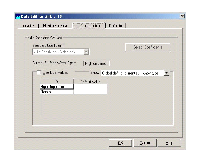
DRAFT
Introduction to D-WAQ (SOBEK)
Figure 2.4: Data Edit for Link window, WQ Parameters tab, Edit Coefficient Values No
coefficients selected.
First, click the select coefficients button. Now you can select the desired parameters. A user
can define initial conditions, dispersion coefficients and process parameters by using the drop
down box. Move the selected parameters to the right screen:
Deltares 33 of 382
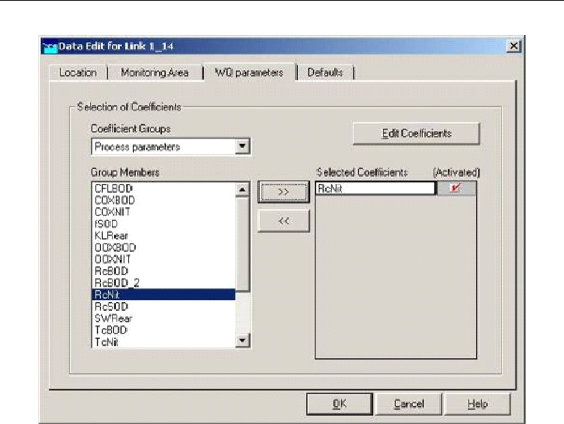
DRAFT
D-Water Quality, User Manual
Figure 2.5: Data Edit for Link window, WQ Parameters tab, Selection of Coefficients,
selected coefficient group is “Process parameters”
Next, select the edit coefficients button to enter the values for the parameters.
Spatially dependent parameters will be attached to surface water types of individual branch
id’s. To use an individual id, select the “use local value” option.
34 of 382 Deltares
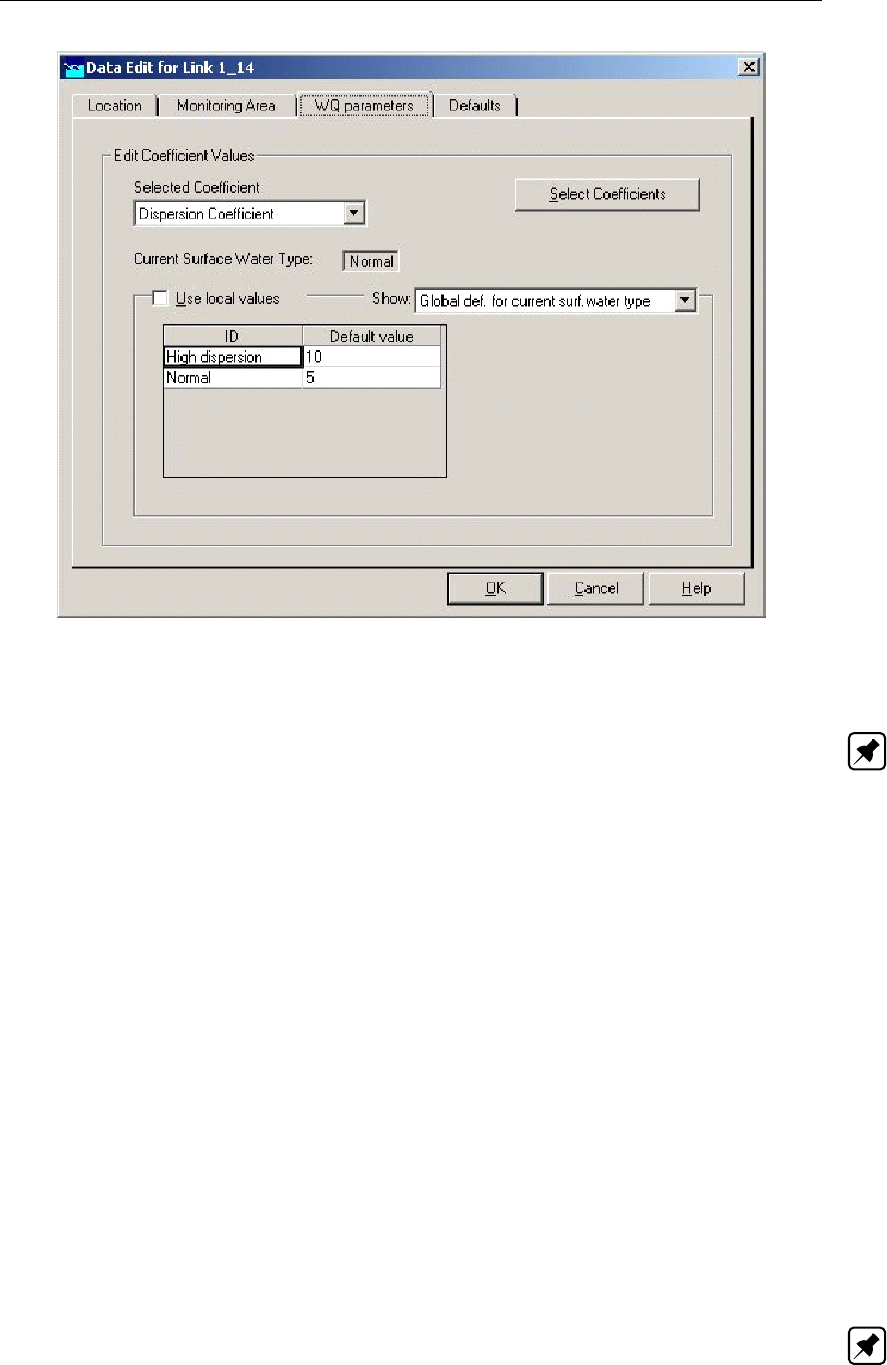
DRAFT
Introduction to D-WAQ (SOBEK)
Figure 2.6: Data Edit for Link window, WQ Parameters tab, Edit Coefficient Values, se-
lected coefficient “Dispersion Coefficient”
Note:
There are three levels of parameters:
Global, set in the Settings Taskblock
Locally by surface water type, overwrites the global value
Locally by branch id, overwrites both global value and surface water type value.
The definition of water quality boundary concentrations
Contrary to the Fraction computations, you have to specify the boundary concentrations ex-
plicitly in Water Quality computations.
Click "Edit model" in the selection window.
Click the "Edit" menu.
Click the "Model data" option: the Model Data window appears.
In this window you find a list box with all objects belonging to a selected type. This is either a
basic schematisation object type or a user-defined object type. You can change the selected
object type at the bottom of the window.
Select an object type: the list of objects belonging to the selected type appears.
Select one of the objects in the list and click Edit: the Data Edit for Node ... window
appears which allows you to edit the data for this object.
Click the "Water Quality" tab to bring up the "Water Quality" tab form.
Note: this tab is inactive when no DELWAQ schematisation is available for the selected
object.
Deltares 35 of 382

DRAFT
D-Water Quality, User Manual
This is a complex window which has the following characteristics:
A "Show" list box to switch between "global definition for this fraction" (the boundary type)
and "local definition for current object" (individual object values). For both items values
can be defined.
With help of the "use local value" tick box the user can select which data are used (global
or local).
A set of options to switch between "Constant Concentrations" and "Time Dependent Con-
centrations".
Click "Time Dependent Concentrations" to enter time dependent data. The layout of the
window changes again.
With help of the Add Row,Insert Row and Delete Row it is possible to manage the number
of timesteps/rows in the list.
With help of the Import Table and Export Table the user is able to export and import ASCII
database files <*.prn>with the following file format:
*CONCENTRATION Cl EColi TColi OXY CBOD5
"2001-01-31;00:00:00" 20 5000 10000 5.5 1.2
"2001-02-01;00:00:00" 20 5000 10000 5.5 1.2
"2001-02-02;00:00:00" 20 5000 10000 5.5 1.2
Note:
If the first 4 characters of a fraction are equal to "EVAP", the associated water flows are
neglected for the computation of substances transport!! As a consequence, during a fraction
calculation the fraction ’check’ might no longer be equal to 1 for locations where evaporation
is modelled.
Note:
The substance list in this tab page corresponds with the SOBEK-WQ state variables as de-
fined by the user. However, if the user has defined some transformation rules these variables
are overruled by the ones defined by the user.
2.1.10 Use substances aliases when defining WQ boundary conditions
The list of state variables used in complex water quality models often not completely matches
the list of monitored variables. This goes for example for organic nitrogen and algae biomass.
Some of these state variables can easily be derived from monitored variables. Organic nitro-
gen can be calculated from the measured total nitrogen and/or Kjeldahl nitrogen value and
the ammonium and nitrate concentrations. Algae biomass can be determined by means of
the measured chlorophyll concentration. SOBEK is able to transform monitored variables into
state variables via user defined computation rules1.
Methodology
Computation rules for transformation of monitored variables into state variables can be de-
fined by the user in the file <substanc.def>. This ASCII file is empty by default. It is acces-
sible via the option "edit variables for WQ boundary conditions under the schematisation task
block. It should be created before starting the input of the boundary conditions. The User
Interface module responsible for the input of the boundary conditions uses the information
in <substanc.def>. It checks if a transformation has to be applied for a certain boundary
or lateral discharge object. If that is the case, the UI uses the transformation rules to derive
auser defined substsances list which replaces the list of SOBEK-WQ state variables in the
input menu.
1This functionality was formerly known as the "substanc.def functionality" in older versions of Deltares’ water
quality modelling software.
36 of 382 Deltares

DRAFT
Introduction to D-WAQ (SOBEK)
The transformation from an arbitrary set of input variables to the SOBEK-WQ state variables
needs to be defined exactly by the user. This definition is subject to the following conditions:
A SOBEK-WQ state variable needs to be expressed in a so-called complex substance
alias, which consists of:
an arbitrary amount of user defined variables;
an arbitrary amount of real numbers;
using the arithmetic symbols "+", "-", "/" and "*".
It is possible to limit the result of an expression to a certain minimum or maximum value.
SOBEK-WQ state variables that are left out are given values of "zero" after the transfor-
mation.
The ensemble of all substance aliases, also called a substance definition, may be defined
separately for every fraction in the WQ model.
If no substance definition is defined for a certain fraction, no transformation is applied for
the boundary objects belonging to this particular fraction.
Format of the new <substanc.def>file
An example of the format is given below, for a model with three state variables: ‘DetN’, ‘NH4’
and ‘NO3’.
FRACTION ‘Boundary Flow’
USEFOR ‘DetN’ ‘Total-N’ - ‘NH4-N’ - ‘NO3-N’ MIN 0.0
USEFOR ‘NH4’ ‘NH4-N’
USEFOR ‘NO3’ ‘NO3-N’
FRACTION ‘Lateral Inflow’
USEFOR ‘DetN’ ‘Kjel-N’ - ‘NH4-N’ MIN 0.0
USEFOR ‘NH4’ ‘NH4-N’
USEFOR ‘NO3’ ‘NO3-N’
This file specifies different substances definitions for two fractions, one of them creates a user
defined list of variables consisting of ‘Total-N’, ‘NH4-N’ and ‘NO3-N’, and the other creates a
user defined list of variables consisting of ‘Kjel-N’, ‘NH4-N’ and ‘NO3-N’. In both cases the
result of the expression is limited to a value of zero, to avoid negative values.
Note:
For the sake of clarity, this example shows different names of ammonium and nitrates
in the user defined substances list (‘NH4-N’ and ‘NO3-N’) and in the state variables list
(‘NH4’ and ‘NO3’). This is not strictly necessary.
The fraction names are read case-insensitive!
Use space between the substances, the arithmetic symbols "+", "-", "/" and "*" and the
numbers!
Practical aspects
It will happen many times that either the list of SOBEK-WQ state variables changes or the
transformation rules change during the course of a project. If boundary conditions have been
defined already, some boundary conditions data may become meaningless. The User In-
terface treats such cases as follows: it reads all values which have been put in before, but
maintains only those which have a meaning. If the user saves the data, all meaningless data
are lost.
A boundary condition for a state variable computed by a complex substance alias becomes a
missing value if at least one of the user defined variables in the substance alias represents a
Deltares 37 of 382

DRAFT
D-Water Quality, User Manual
missing value.
The computational core uses the information in the <substanc.def>file to translate the
boundary conditions for the user defined variables to the boundary conditions for the list of
SOBEK-WQ state variables. However, the computational core does not read this information
directly from the <substanc.def>file. The User Interface copies the relevant substance def-
inition before every block of boundary conditions data in the files <boundwq.typ>(fraction)
or <boundwq.dat>(object). These two files are then passed on to the computational core.
If the user changes the <substanc.def>file, he or she has to start the boundary conditions
UI module to copy the changes to <boundwq.typ>and <boundwq.dat>. It is advised to
enter all objects or boundary types for which the substance definition has been changed and
explicitly save the data, to make sure that the changes have become effective.
In relation to the previous aspect, expert users should take care while supplying ready made
<boundwq.typ>and <boundwq.dat>files to SOBEK. If they contain substance definitions
(necessary to make the computational core run) the user should be aware of the fact that
these will be replaced by the ones in <substanc.def>as soon as the UI is activated.
Remark:
This functionality was formerly known as the "substanc.def functionality" in older ver-
sions of Deltares’ water quality modelling software.
User defined boundary conditions
Complex water quality models often use a set of state variables which does not match the
list of monitored variables. SOBEK is able to perform the transformation of an arbitrary set
of water quality variables to SOBEK-Rural Water Quality state variables. This transformation
needs to be defined exactly by the user. The total of all substance definitions is stored in a file
called <substanc.def>. This file is accessible by an ASCII editor through one of the buttons
under the "Schematisation" task box. This file is empty by default. It should be created before
starting the input of the boundary conditions.
The User Interface module responsible for the input of the boundary conditions uses the
information in <substanc.def>. It checks if a transformation has to be applied for a certain
boundary or lateral discharge object. If that is the case, the UI uses the transformation rules
to derive a user defined substances list which replaces the list of SOBEK-Rural Water Quality
state variables in the input menu.
2.1.11 Simulation
Description of the task
After you have finished the input tasks, you can try to run the model.
Double-click the "Simulation" task. Rainfall-Runoff models (optional), Emission models
(optional) and the Water Flow module (necessary) will first run: they will compute the
necessary flow data for the Water Quality module.
The second time you run the "Simulation" task, it may not be necessary to rerun the Rainfall-
Runoff, Emission and the Water Flow modules. This is the case if you have not changed
anything in the input for these modules. SOBEK detects that there is output from the Water
Flop module available and asks you whether you want to use this output.
The WQ model run consists of the following steps (you will see windows opening and closing
38 of 382 Deltares

DRAFT
Introduction to D-WAQ (SOBEK)
for each of these steps):
Pre-processing (preparation of simulation);
Quantity to Quality (conversion of output from CF module, preparation of boundary condi-
tions for Fraction computation);
DELWAQ1 (reading and checking of input for WQ module, and processing the config-
uration of the Processes Library for extra water quality processes; is skipped in case of
fraction computations and when the "processes active" switch has been disabled (Settings
module);
DELBEL (if balance of loads output option is activated in Settings module)
DELWAQ2 (performing the simulation);
Postprocessing (conversion of output, in particular mass balances output).
You may want to check the simulation messages, especially if an error occurs.
Click the right mouse button while it is positioned in the "Simulation" task box.
Click "Simulation Messages". The Simulation Messages window appears.
Select the appropriate messages file and click the View button.
The available files are:
Pre-processing;
List file of pre-processing: output from DELWAQ1 (<*.lst>and <*.lsp>files);
List file of loads computation: output from DELBEL (<*.lst>file);
Monitoring file: output from DELWAQ2 (<*.mon>file).
2.1.12 Results in maps
Description of the task
Double-click the "Results in maps" task box. The NETTER programme is started
After \File\Open, the Select item window appears.
Select the appropriate output file and click the OK button, or double click on the output file
name description itself.
The available water quality output files are:
Map Results of Water Quality: regular output from DELWAQ, consisting of the state vari-
ables and/or the other selected output parameters (as defined within the Settings module);
Balance of Loads: regular output file from DELBEL, consisting the waste loads over the
boundaries per state variable.
Deltares 39 of 382

DRAFT
D-Water Quality, User Manual
40 of 382 Deltares

DRAFT
3 Introduction to D-WAQ (Delft3D)
Deltares has developed a unique, fully integrated computer software suite for a multi-disciplinary
approach and multi-dimensional computations for oceanic, marine, coastal, estuarine and
river areas. It can carry out simulations of flows, sediment transport, waves, morphological
developments, water quality and ecology. It has been designed for experts and non-experts
alike. The Delft3D and SOBEK suite are composed of several modules, grouped around a
mutual interface, while being capable to interact with each other. D-Water Quality, the subject
of this manual, is one of these modules.
3.1 Areas of application
D-WAQ is a multi-dimensional water quality model framework. It solves the advection-diffusion-
reaction equation on a predefined computational grid and for a wide range of model sub-
stances. D-WAQ allows great flexibility in the substances to be modelled, as well as in
the processes to be considered. D-WAQ is not a hydrodynamic model, so information on
flow fields is derived from Delft3D-FLOW or SOBEK (Delft3D-FLOW UM,2013;SOBEK UM,
2013), although any description of the movement of water would be suitable if available in the
right format.
A wide range of model substances is available in D-WAQ including:
conservative substances (salinity, chloride, continuity and up to five tracers)
degradable substances (up to five degradable tracers)
suspended sediment (up to three fractions)
temperature
nutrients (ammonia, nitrate, phosphate, adsorbed P, vivianite-P, apatite-P, silicate, opal)
organic matter (subdivided in carbon, nitrogen, phosphorus and sulphur components)
dissolved oxygen
inorganic sulphur components (sulphate, sulphide)
iron components (up to 7 oxidized and reduced dissolved and particulate components)
methane
total dissolved inorganic carbon (carbon dioxide)
BOD and COD (respectively Biological and Chemical Oxygen Demand)
phytoplankton biomass (algae species)
microphytobenthos biomass (benthic diatoms)
grazers biomass (modelled as forcing function)
terrestrial vegetation biomass (drowned vegetation)
bacterial pollutants (4 species)
heavy metals
organic micro-pollutants
D-WAQ allows you to specify an even wider range of physical, (bio)chemical and biological
processes. The processes are stored in the so-called Process Library from which any subset
of substances and processes can be selected. Examples of the processes included are:
settling (sedimentation) and resuspension
reaeration of oxygen
algae growth and mortality
mineralization of organic matter
(de)nitrification
phosphate adsorption and precipitation
partitioning (adsorption, precipitation) of heavy metals
partitioning, degradation and volatilization of organic micro-pollutants
Deltares 41 of 382

DRAFT
D-Water Quality, User Manual
mortality of bacterial pollutants
D-WAQ has a wide applicability. Basically, it can be used whenever any (combination) of
the substances mentioned above is of interest. The only requirement is the availability of a
hydrodynamic description of the water system. For example, D-WAQ has been applied for
studying:
eutrophication of lakes, reservoirs, estuaries and seas with or without sediment diagenesis
dissolved oxygen depletion in stratified systems
impact of a sewage outfall on nutrient concentrations and primary production
transport of heavy metals through an estuary
accumulation of organic micro-pollutants in fresh water basins
the emission of greenhouse gases from reservoirs
sediment transport
water temperature as related to outfalls
etc.
Not all options are GUI-PLCT supported, the option for advanced ‘layered sediment’ modelling
in particular, but additional manuals are available for application. Moreover, some processes
developed by Deltares are not discussed in this manual because they have not been inte-
grated into the standard set of processes. This concerns the simplified pH process pH_SIMP,
the advanced module DEB for grazers (shell fish), the advanced module MICROPHYT for mi-
crophytobenthos, and the module for aquatic macrophytes (the biological modules are under
development). These modules can be made available upon request.
3.2 Coupling to other modules
D-WAQ makes use of the hydrodynamic conditions (velocities, water elevations, density, salin-
ity, vertical eddy viscosity and vertical eddy diffusivity) calculated in the Delft3D-FLOW or
SOBEK module. In combination with Delft3D-FLOW also wave characteristics (wave height,
wave length and wave period), which are be important in sedimentation-erosion studies in
relatively shallow areas, can be derived from the Delft3D-WAVE module (WAVE UM,2013).
3.3 Utilities
For using D-WAQ the following utilities are important:
QUICKIN for preparing and manipulating grid oriented data, such initial con-
ditions or spatially varying process parameters or forcing functions.
See manual QUICKIN UM (2013)
D-Waq DIDO or
WQINT
for horizontally aggregating the hydrodynamic result in order to re-
duce computation time. See manual DIDO UM (2013)
D-Waq PLCT for selecting the substances needed for the water quality model.
GPP for visualisation and animation of simulation results. See manual
GPP UM (2013)
Delft3D-QUICKPLOT another tool for visualisation and animation of simulation results. See
manual QUICKPLOT UM (2013)
For details on using these utility programs you are referred to the respective User Manual.
42 of 382 Deltares
DRAFT
4 Getting started (Delft3D)
4.1 Starting Delft3D
The Delft3D suite is a range of modules that can be run independently of one another. The
main menu of Delft3D provides access to each of the main modules. Delft3D-MENU can be
started either:
In Microsoft®Windows, select Delft3D in the Programs Menu or click on the Delft3D icon
on the desk-top
In Linux/UNIX, type delft3d-menu on the command line.
Next the title window of Delft3D is displayed, Figure 4.1:
Figure 4.1: Title window of Delft3D
After a short while the main window of the Delft3D-MENU appears, Figure 4.2.
Whether or not you may use specific Delft3D modules and features depends on the license
file you have (delft3d_hostid.lic in your DS_Flex directory).
There are two ways to exit the Delft3D-MENU:
Click Exit.
Click the ‘close’ button (×) in the top-right corner of the menu bar.
4.2 Water Quality module
The water quality selection window is opened by selecting Water Quality in the main menu.
The Far-field water quality selection window is shown in Figure 4.3.
The Water quality (WAQ) window shows the steps that you have to take one by one to un-
dertake a water quality simulation. The steps can be subdivided in pre-processing (Coupling,
Processes,Define input), processing (Waq (1),Waq (2)), post-processing (Reports,GPP,
QUICKPLOT ) and additional tools (Tools).
The steps are briefly described below and will be dealt with in more detail in the next chapters.
Processes Activates the Processes Library Configuration Tool (PLCT)
Deltares 43 of 382

DRAFT
D-Water Quality, User Manual
Figure 4.2: Main window of Delft3D-MENU
Figure 4.3: Selection window for Water quality
44 of 382 Deltares

DRAFT
Getting started (Delft3D)
With the PLCT you can select the state variables and water quality
processes you want to include in the simulation.
Define input Create or edit input file
The Graphical User Interface (GUI) is started in which you can define
the input for a water quality computation. The information will be
stored in a scenario <∗.scn>file and an input file (<∗.inp>).
Waq (1) Run pre-processors
Two pre-processors will check the input file for errors and activate
the user-defined water quality processes. The pre-processing will
create a <∗.lst>and a <∗.lsp>file which you can check under the
Reports menu item.
Waq (2) Run D-WAQ model
The water quality simulation is started. The model will create bi-
nary output files (<∗.map>,<∗.ada>,<∗.his>,<∗.hda>and
<∗.bal>) which can be visualised with the GPP and QUICKPLOT
packages and an ASCII output file (<∗.mon>) which can be in-
spected under the Reports menu item.
Coupling Convert and/or aggregate Hydrodynamic results.
D-Water Quality uses the grid layout and the results from a hydro-
dynamic calculation in a particular form. The output files from the
model that provides these results may or may not fit the form D-
Water Quality expects. If not, a separate coupling step is required.
Note: however, that with recent versions of Delft3D-FLOW this
step is no longer needed, as the relevant files are written directly
by Delft3D-FLOW (see section 5.2).
Reports View report files
This option allows you to inspect the ASCII report files generated by
D-Water Quality.
GPP Post-processing with GPP
Starts the GPP visualisation package.
QUICKPLOT Post-processing with Delft3D-QUICKPLOT
Starts the QUICKPLOT visualisation package.
Tools Additional tools
Configure your own Processes Library using the Open PLCT.
Boundary conditions for a certain model domain can be derived from
a larger model domain. This so-called nesting can be performed
under Tools.
Remark:
It is possible to skip steps, if certain information is already available. For example, if you
already have assembled the substances and water quality processes in a so-called sub-
stances file (via the Processes step, you can skip that step, similarly for the Coupling)
step.. The menu works completely modular and modules can be run independently in
any order.
Deltares 45 of 382
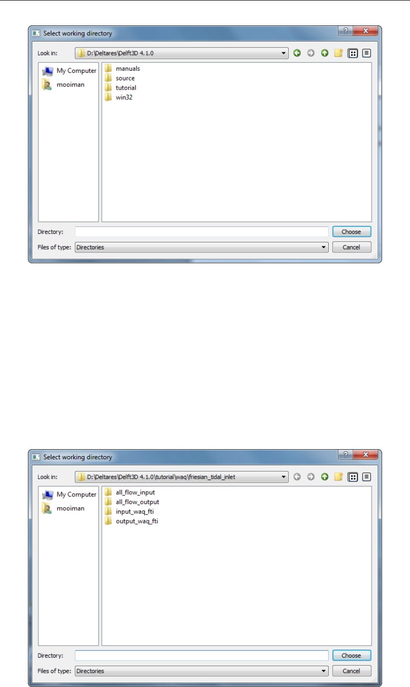
DRAFT
D-Water Quality, User Manual
Figure 4.4: Select working directory window
4.3 Select working directory
It is possible to select and/or change the default working directory in which the input is located
and to which the output files will be written.
The Select working directory button opens the Select working directory window in which
the current working directory is identified as shown in Figure 4.4.
The current working directory can be changed by browsing to the desired directory. Browse
for instance to the <delft3d\tutorial\waq\f35>folder. Close the Select working directory
window by clicking Choose, see Figure 4.5.
Figure 4.5: File navigation window to select a new working directory
46 of 382 Deltares
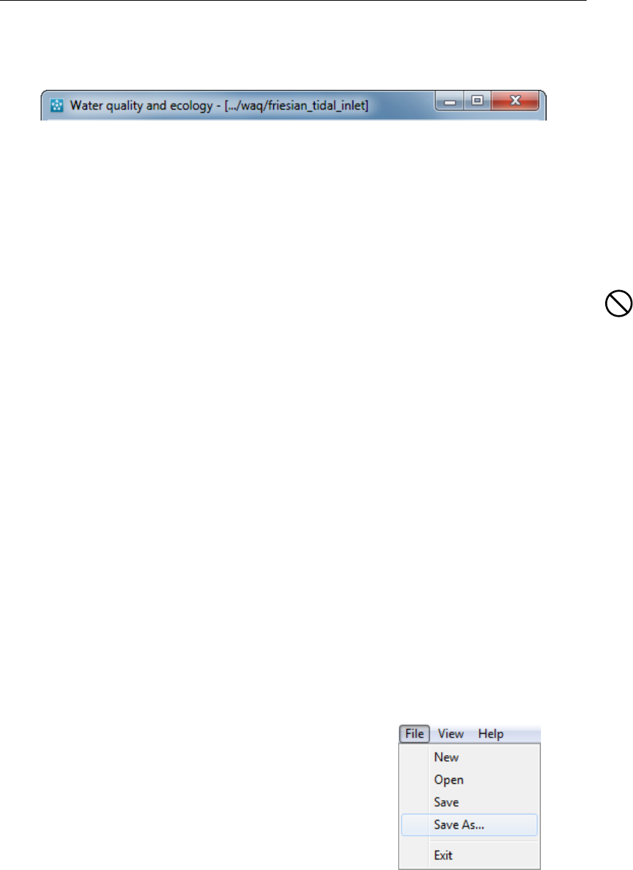
DRAFT
Getting started (Delft3D)
Next the Water quality (WAQ) window is re-displayed, but now the changed current working
directory is displayed in the title bar, see Figure 4.6.
Figure 4.6: Current working directory
Creating a useful and comprehensible directory structure is worthwhile. As a water quality
simulation is built up from several blocks (hydrodynamics, substances selection, discharges,
etc.), a possible set-up is to store each block in a separate directory. Then it is essential that
you set the working directory correctly so that the files are stored in the correct directory. A
possible directory structure is shown to the right. Note that calibration runs and scenario runs
are stored in separate directories.
Restriction:
A directory name may not contain an apostrophe (‘).
4.4 Starting WAQ-GUI
The WAQ-GUI is started by selecting the Define input from the Water quality (WAQ) selection
window. The main window of WAQ-GUI is shown in Figure 4.8.
The menu bar at the top of the screen provides options for opening and saving files, for editing
tables, for visualisation of the grid layout and for obtaining help.
4.4.1 Accessing data groups
A data group is accessed by clicking on the corresponding button on the left-hand side of the
WAQ-GUI window. For example, clicking Hydrodynamics opens the data group window as
shown in Figure 4.9.
Clicking other datagroups in the main window will show the input screen for the respective
data group. Changes made in any of the data group windows will be retained by WAQ-GUI.
You will be prompted to save this data in a scenario file <∗.scn>when the WAQ-GUI session
is ended.
4.4.2 Saving a D-WAQ scenario file
Figure 4.10: Saving the input file
In order to preserve changes and additions to the data
groups, it is necessary to save the data defined in the
data groups in a scenario data file <∗.scn>. You can
continue making changes and save them regularly to
the scenario file. Also, the scenario file can be re-
opened to edit.
If you have to define several water quality simulations
in which part of the input is identical, you can simply
open an existing scenario file; adapt the part that is
different (e.g. different waste load) and save the scenario file under another name (preferably
— but not necessarily — in another directory!). There is no need to start the input definition
all over again.
You can save the scenario file by clicking menu item File →Save (or Save As. . . ) in the
menu bar as shown in Figure 4.10. Note that the scenario file is by default saved in the
Deltares 47 of 382
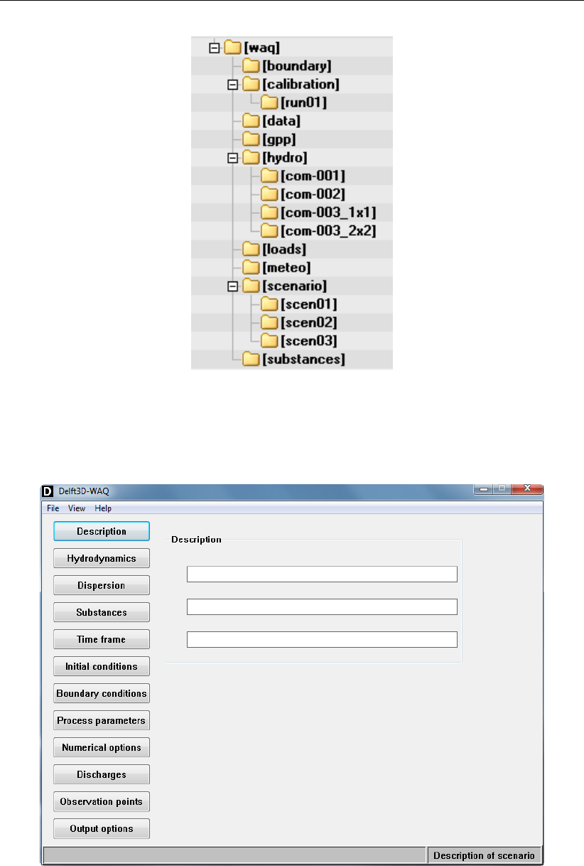
DRAFT
D-Water Quality, User Manual
Figure 4.7: Optional directory structure for running water quality simulations
working directory you have defined earlier.
Figure 4.8: Main window of WAQ-GUI
48 of 382 Deltares
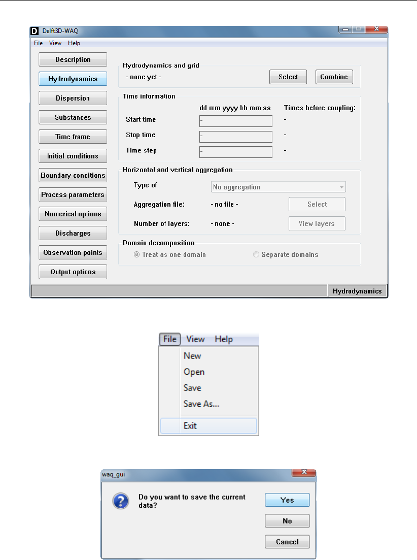
DRAFT
Getting started (Delft3D)
Figure 4.9: Hydrodynamics Data Group
Figure 4.11: Exiting the WAQ-GUI through File →Exit
Figure 4.12: Window to save <∗.scn>file before quitting
4.5 Exiting the WAQ-GUI
A WAQ-GUI session is ended by selecting File →Exit from the menu bar as shown in Fig-
ure 4.11. The GUI will first ask whether you wish to save the <∗.scn>file before proceeding
as shown in Figure 4.12.
After quitting WAQ-GUI, you are returned to the Water quality (WAQ) window. Selecting
Return brings you back in the Far-field water qualtity selection window. Selecting Return
again, you are back in the main Delft3D menu. You can then exit Delft3D entirely by selecting
Exit.
Deltares 49 of 382

DRAFT
D-Water Quality, User Manual
4.6 Steps in water quality modelling
Water quality modelling with D-WAQ is very flexible. Hydrodynamics, substances, water qual-
ity processes, output variables, etc. are all free for you to choose. However, this means that
you have to make decisions on what to do or what to use many times. It’s best to work very
structured and organised. The Delft3D-MENU and the WAQ-GUI help you with that. If you
systematically go through the data groups in the order they are presented on the screen, you
will automatically pass all the required input and will be ‘forced’ to make decisions at every
point.
The basic steps in water quality modelling are:
1 Pick-up the result from the hydrodynamic simulation and make it suitable for application in
your water quality simulation.
2 Define the substances and water quality processes you want to include.
3 Define the water quality simulation using the outcome of the first and second step. You will
have to define initial conditions, boundary conditions, waste loads, simulation time, output
variables, etc.
4 Run the simulation.
5 Check the output.
After step 5 you are either ready or you can return to step 1, 2 or 3 depending on the items
you want to change. Usually, steps 3 to 5 are repeated multiple times.
4.7 Data flow diagram
A complete listing and description of files is given in Appendix A.
Going through the steps of water quality modelling, you will pass several tools and computer
programs. Output from one program can be input for another program. The tools and the files
they share, are shown in Figure 4.13 and Table 4.1.
Table 4.1: Overview of files in D-Water Quality. Output files can be input files for other
modules
Module Input file Output file
Delft3D-
FLOW
<∗.mdf> <com-∗.dat>and <com-∗.def>
DIDO <∗.grd>
<∗.dwq>
<∗.dwq>
Couple <com-∗.dat>and <com-∗.def>
<∗.dwq>
<couplnef.inp>
<∗.hyd>
<com-∗.flo>,<com-∗.vol>, etc.
<couplnef.out>
PLCT <∗.0> <∗.sub>
<∗.0>
WAQ-GUI <∗.hyd>
<∗.sub>
<∗.scn>
<∗.stt>
<∗.scn>
<∗.inp>
<∗.stt>
50 of 382 Deltares

DRAFT
Getting started (Delft3D)
Module Input file Output file
Compute wa-
ter quality
<∗.inp>
<com-∗.flo>,<com-∗.vol>, etc.
<∗.lst>
<∗.lsp>
<∗.mon>
<∗.ada>and <∗.adf>
<∗.hda>and <∗.hdf>
<∗.his>
<∗.map>
Text editor (in-
spect results)
<couplnef.out>
<∗.lst>
<∗.lsp>
<∗.mon>
–
GPP
Delft3D-
QUICKPLOT
<∗.ada>and <∗.adf>
<∗.hda>and <∗.hdf>
<∗.his>
<∗.map>
–
Deltares 51 of 382
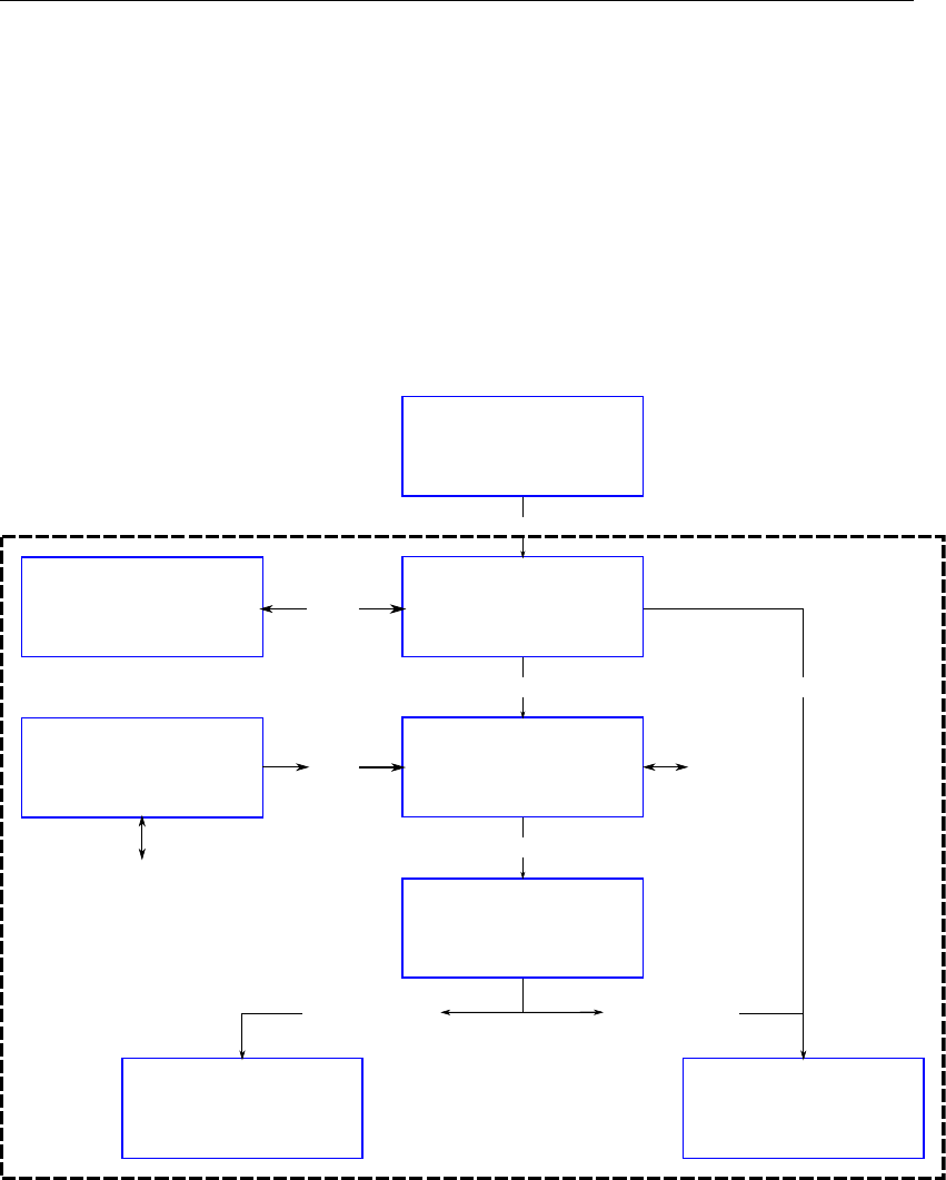
DRAFT
D-Water Quality, User Manual
Hydrodynamics
(Delft3D-FLOW)
Aggregation
(DIDO) Couple
Water Quality
input
(WAQ-GUI)
Simulation
(DELWAQ)
Visualise results
(QUICKPLOT,
GPP)
Inspect results
(editor)
Processes Tool
(PLCT)
*.dwq
*.hyd
*.sub
*.0
*.inp
map/history-files *.lsp, *.lst, *.mon
couplnef.out
com*.dat
*.scn
Figure 4.13: Overview of the modules and data flow diagram in D-Water Quality. Modules
are shown in grey rectangles. Files they share are indicated on the arrows.
52 of 382 Deltares

DRAFT
5 Graphical User Interface
5.1 Processes Library Configuration Tool (PLCT)
5.1.1 Introduction
The Processes Library Configuration Tool (PLCT) allows you to select:
state variables (called substances in D-Water Quality)
water quality processes
process input parameters
output variables
The information is stored in a PLCT file <∗.0>which can be (re)opened in the PLCT and
a substance file <∗.sub>, which can be selected when defining a water quality simulation.
It is not possible to add or remove any of these items mentioned above once you are in the
WAQ-GUI (Delft3D) or WQ-module (SOBEK). For changes, you will have to return to the
PLCT, make your changes, save the <∗.0>and <∗.sub>files and after that import the new
<∗.sub>file again in the WAQ-GUI/WQ-module.
You create a substance file in several steps:
Choose the substance group
Select the substances
Select the associated processes
Specify the input for the processes, select editable parameters and output variables
Specify the input for the extra processes
There are many substances, processes, parameters and output variables. Basically, you have
to make a choice for each and every item. Therefore, you have to work methodically through
the PLCT making your choices as you go along. Remember however, that you can always
return to the <∗.sub>file and make adaptations. Also, standard substance files are available
ready to use or to serve as basis for extensions (Appendix B).
To work with the PLCT and the water quality processes it is essential that you are familiar
with the mathematical formulation of the processes. When you see a process for the first
time, refer to the accompanying description in the Technical Reference Manual (D-WAQ TRM,
2013) for an explanation of parameters and for directives for use.
5.1.2 Opening the PLCT
Opening the PLCT (SOBEK)
You can set or change the configuration of the Processes Library with the help of the Pro-
cesses Library Configuration Tool (PLCT).
Tick "Do not use predefined processes" and click the "Define Processes:" Edit button in
the "Processes" tab form.
The PLCT is started.
Deltares 53 of 382

DRAFT
D-Water Quality, User Manual
Opening the PLCT (Delft3D)
Clicking Processes in the Water quality and ecology window and than the ECO button, the
PLCT will open in ecology mode (ECO, use BLOOM algae).
5.1.3 Processes Library Configuration Tool (PLCT)
Initially, the PLCT consists of three windows (Figure 5.1):
1Processes
Library Configu-
ration Tool
File managing window for opening and saving files and exiting the
PLCT. The window also gives an overview of the substances se-
lected so far.
2Select Groups Overview of available substances groups, and entry point to select
substances. Also, entry point to Extra processes
3Messages Window displays messages when errors occur, mostly related to
missing information.
Figure 5.1: Main windows of the Processes Library Configuration Tool
The Processes Library Configuration Tool window displays the version number, the name
of the file you are currently working on and the configuration (ECO, WAQ). Note that a <∗.0>
and <∗.sub>file generated for example with the ECO configuration, can not be opened auto-
matically in the WAQ configuration. The configuration is included in the first line of the <∗.0>
file (for example configuration ‘ECO’) and can be changed manually here (e.g. configuration
‘WAQ’). The PLCT will give a warning when you try to open the <∗.0>file.
The menu bar has the following options:
File New Start a new scenario — clear all input.
Open. . . Open an existing PLCT <∗.0>file.
Save Save the current PLCT <∗.0>file using the previously given
name, or the default name <substate.0>. A substance file <∗.sub>
is saved simultaneously.
54 of 382 Deltares
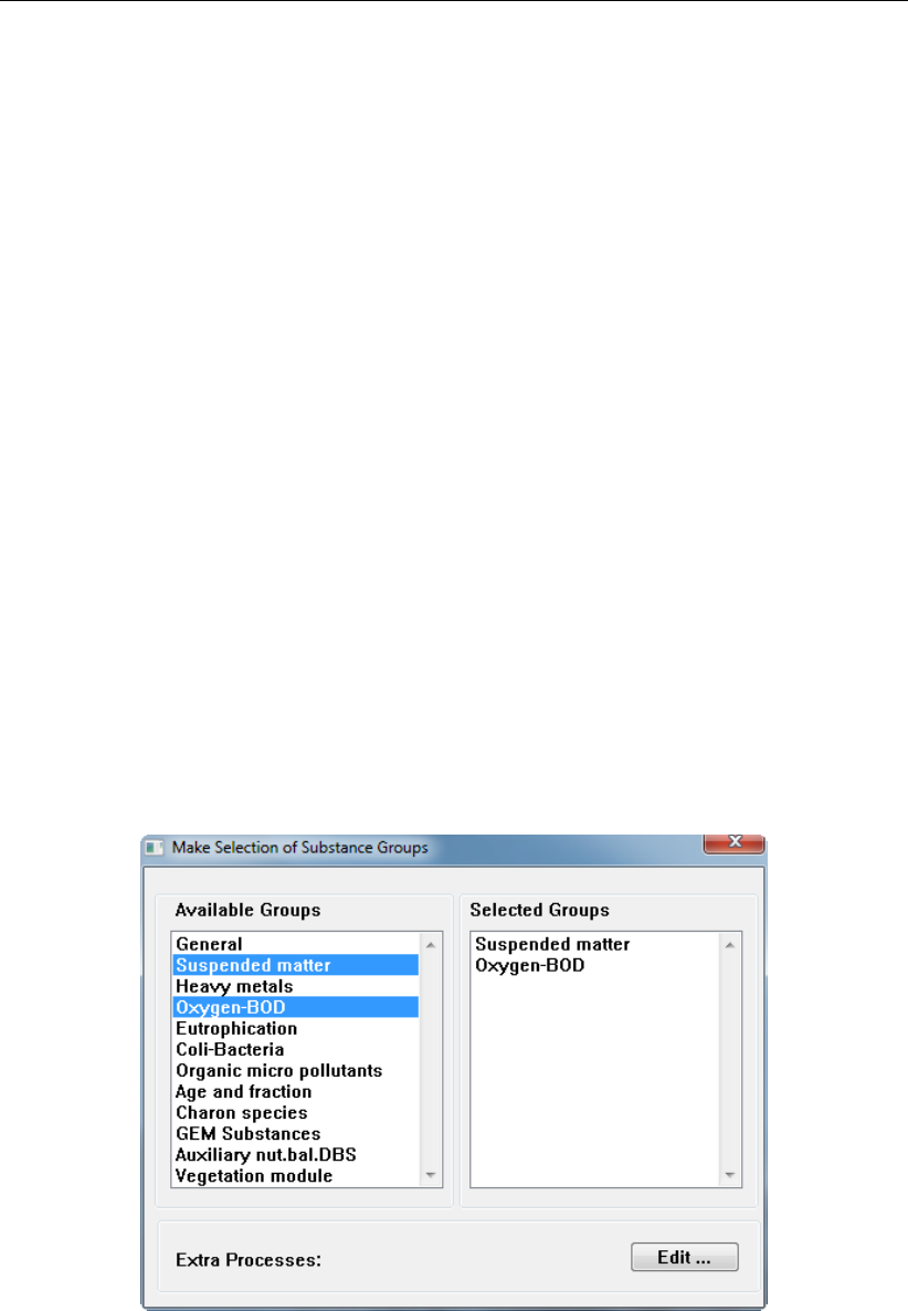
DRAFT
Graphical User Interface
Save as. . . Save the current PLCT <∗.0>file and specify its filename. A
substance file <∗.sub>is saved simultaneously.
Exit Exit the PLCT.
Select groups
The Make Selection of Substances Groups window has three parts:
1Available
Groups
Shows the available substance groups within the configuration se-
lected.
You can select a specific group by a mouse click or standard key-
board controls. Selected substance groups will be displayed in the
Selected Groups part on the right side of the window. Multiple
groups can be selected by holding the Control key on your key-
board and selecting the second or further substance group.
2Selected
Groups
Substance groups that are highlighted in the Available Groups on
the left side of the window are displayed. Clicking on one of the
selected substance groups here opens the Make Selction of Sub-
stances window, displaying the substances that are included in the
substance group.
3Extra Processes Clicking Edit. . . opens a window with all the Extra processes that
are required for the water quality processes.
Extra Processes are processes that do not calculate a mass flux
on one of the selected substances. This can be for post-processing
purposes (e.g. calculating Total-Nitrogen), but lump mass fluxes as
well (e.g. total resuspension).
Figure 5.2: Select Groups window of the PLCT. Highlighted groups ‘Suspended matter’
and ‘Oxygen-BOD’ are selected and displayed in the right side column
Select substances
The Make Selection of Substances window works analogous to the Make Selection of
Substances Groups window. Every substance group has its own Select Substances win-
dow. If you have selected multiple substance groups, you have to select the substances per
group separately.
Deltares 55 of 382
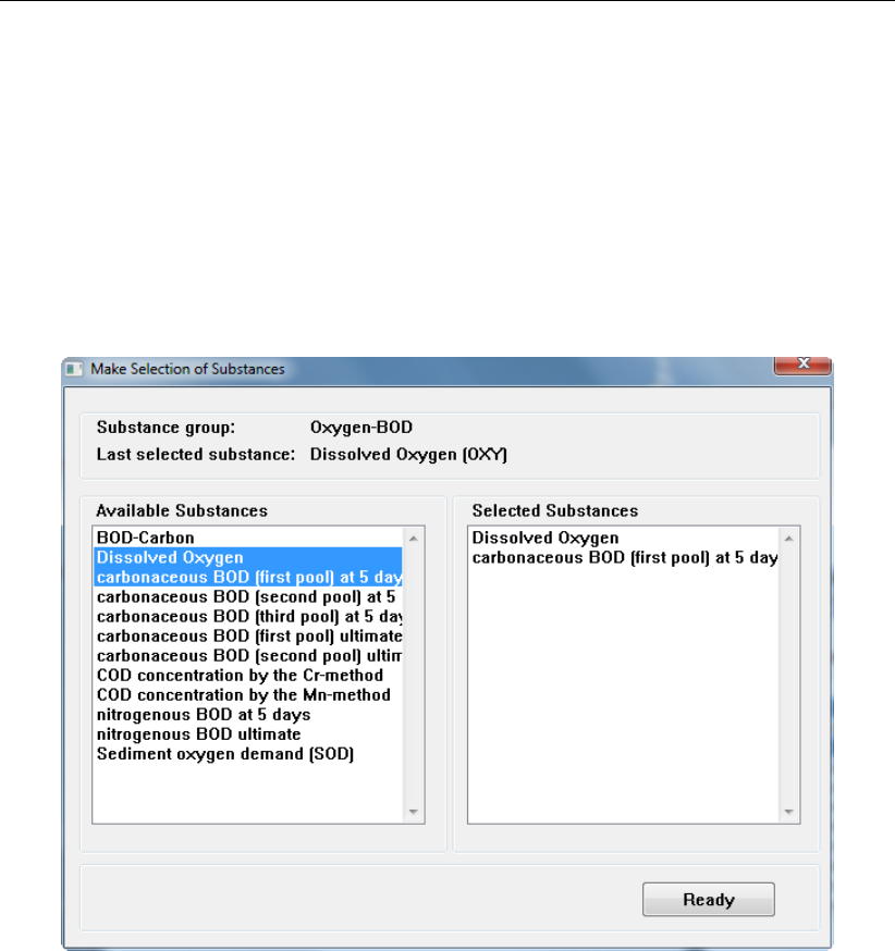
DRAFT
D-Water Quality, User Manual
You can select available substances by a mouse click or standard keyboard controls. Selected
substances will be displayed in the Selected substances part on the right side of the window.
Multiple substances can be selected by holding the CTRL-key on your keyboard and selecting
the second or more substance by mouse.
Clicking on one of the available substances opens the Select Processes window, displaying
all the water quality processes that are available for this substance.
Clicking Ready closes the window and bring you back to the Select Substance Group win-
dow.
Figure 5.3: Select Substances window for the Oxygen-BOD group. Highlighted sub-
stances ‘Dissolved Oxygen’ and ‘Carbonaceous BOD (first pool) at 5 days’
are selected and displayed in the right side column
Select processes
The Select Processes window displays all processes that are available for the selected sub-
stance (Figure 5.4). You can select or ‘activate’ a process by checking the check box behind
the process. An Edit. . . button will appear. Checking the check box once again, deactivates
the process and Edit. . . will disappear. By clicking Edit. . . , you will open the Specify Process
window (see Figure 5.5, also next section).
Occasionally, instead of the Edit. . . button, a Define. . . button will appear. A Define. . . button
is displayed when the input for that specific process is not completely defined and your input is
required: the Specify Process window will open automatically in this case. An Edit. . . button
indicates that there is no missing input. There is no check on the correctness on the input,
only on the completeness of the input.
After selecting and editing all required processes, you can close the Select Processes win-
dow by clicking Ok. Clicking Cancel will loose all changes you made since opening the win-
dow. No warning is given.
56 of 382 Deltares
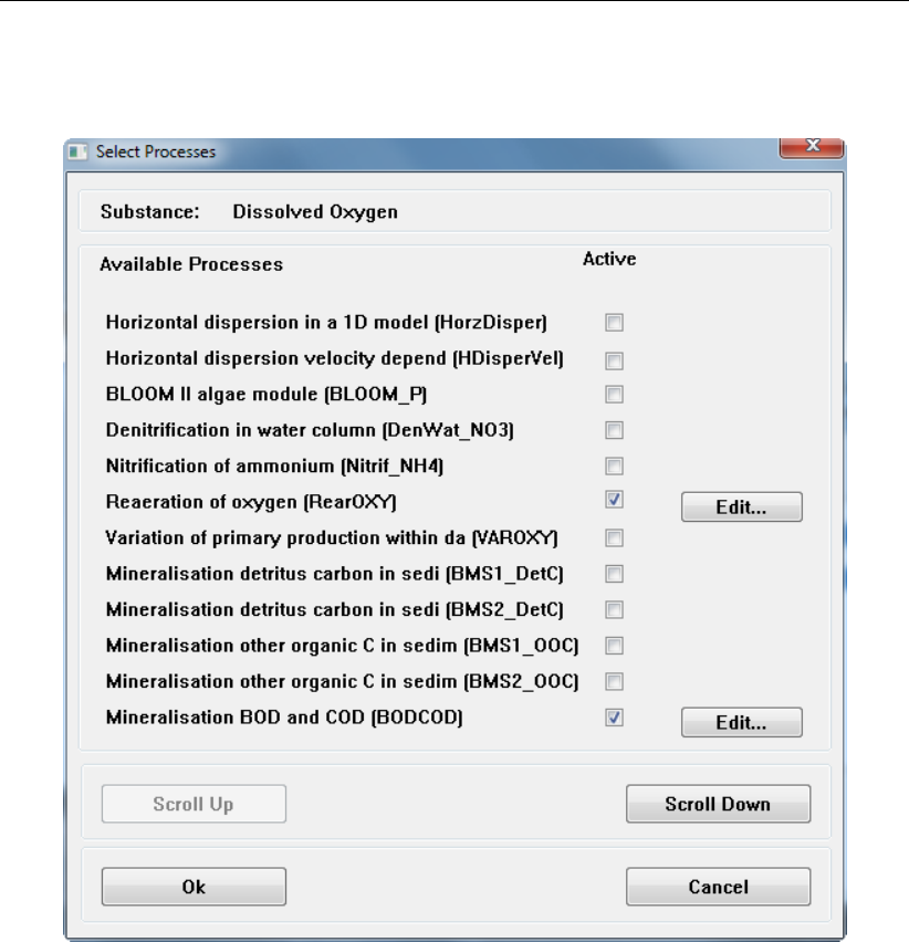
DRAFT
Graphical User Interface
If the number of available processes is more than 12, the Scroll Up and Scroll Down buttons
enable you to go through the listing of the processes.
Figure 5.4: Select Processes window for ’Dissolved Oxygen’. Activated process are
checked and an Edit. . . button is shown
Specify process
The Specify Process window is opened by clicking Edit. . . in the Select Processes window.
The information on the Specify Process window is divided in six columns:
1 Description and name of the process parameter
2 Type of process parameter
Two options:
Constant
Derived from another process
A list box indicates that you have the option to make the process parameter a constant or
to derive it from another process. If no list box is available, the process parameter can not
be derived from another process and automatically is a constant.
3 Value of the process parameter
When the process parameters is defined as a constant, the default value is shown.
‘-999’ is identified as a missing value, and you will have to define a value.
Modelled: the process parameter is chosen as a substance or the process parameter
is available from the hydrodynamic simulation (e.g. Volume).
Deltares 57 of 382
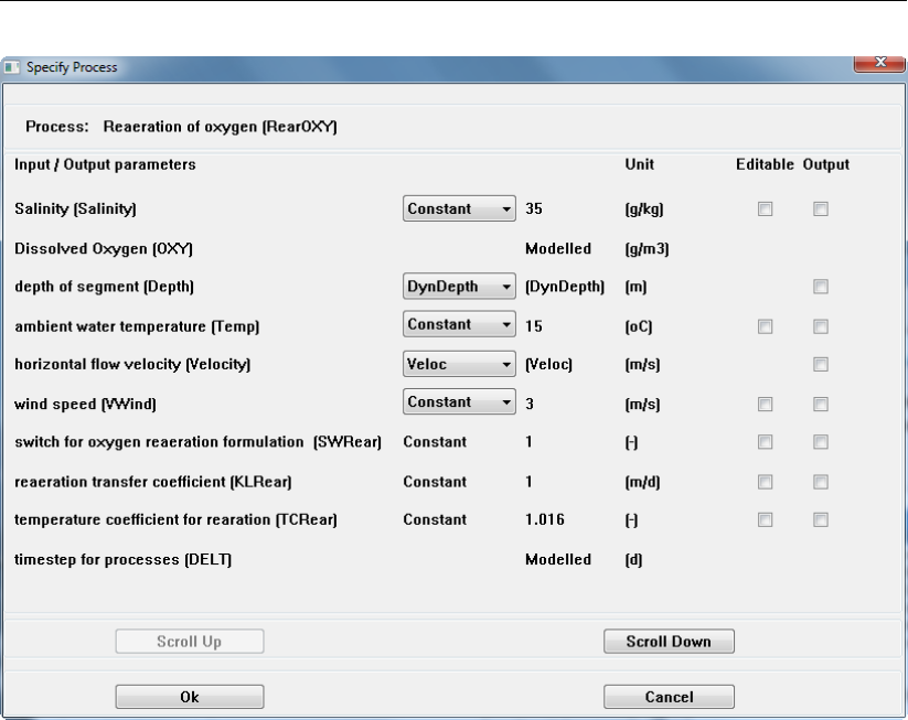
DRAFT
D-Water Quality, User Manual
Figure 5.5: Specify Process window for the Reaeration of oxygen
Output: the process parameter is an output variable only, and no input value is re-
quired.
(Text string between brackets): the process parameter is derived from another pro-
cess. The process name is indicated between brackets.
4 Unit
Unit of the process parameter
5Editable check box
Only available for process parameters defined as Constant. Checking the Editable box
will save the process parameter to the <∗.0>and <∗.sub>files. In the WAQ-GUI under
Process Parameters, these process parameters can be given a constant value other than
the default value, a time-series or a segment function. For process parameters that are
not made editable the default value will be used in the water quality simulation.
6Output check box
Checking the Output box will save the process parameter to the <∗.0>and <∗.sub>files
as output variables. The value of the process parameter will be written to the respective
output files during a water quality simulation.
After selecting and editing all required process parameters, you can close the Specify pro-
cess window by clicking Ok. Clicking Cancel will loose all changes you made since opening
the window. No warning is given.
If the number of available process parameters is more than 12, the Scroll Up and Scroll Down
buttons enable you to go through the listing of the process parameters.
Each process has its own description and directives for use, see Technical Reference Manual
(D-WAQ TRM,2013).
58 of 382 Deltares

DRAFT
Graphical User Interface
Extra processes
Finally, after you have selected all the substance groups, the substances, their processes and
the process parameters, you have to check the Extra Processes. The PLCT automatically
accumulates all processes that do not directly calculate mass fluxes of substances. These
processes are compiled in the Specify Extra Processes window. The window is analogous
to the Select Processes window, with the exception that you are not allowed to deactivate
processes here. If you want to deactivate an extra process, you have to go to the location in
aSpecify Process window where the process is selected. The process parameter should be
changed to constant, instead of being derived from the (extra) process.
Clicking Edit. . . opens a Specify Process window.
Note that new extra processes can be added as well if you make such a change in a Specify
Process window. You should check the Extra Processes list for new extra processes.
When finished you can save the PLCT file <∗.0>and simultaneously a substance <∗.sub>
file will be saved. Exit the PLCT through File →Exit.
Substances and processes not supported by the WAQ-GUI
Substances and processes not supported by the WAQ-GUI but present in the Processes
Library can be added by manual editing. Two additional user manuals are avalaible for this:
D-WAQ TRM (2013) and D-WAQ Input file (2013).
5.2 Using the hydrodynamic result (Delft3D)
The transport of substances is based on a Delft3D-FLOW (Delft3D-FLOW UM,2013) or D-
Flow FM (D-Flow FM UM,2015) result, though coupling to other three-dimensional hydrody-
namic models, such as UNTRIM and TELEMAC is possible as well. Delft3D-FLOW generates
either a so-called communication file, consisting of a data file and a definition file and contain-
ing the "raw" hydrodynamic information that needs to be converted by an auxiliary program
(the coupling program) or, via a builtin coupling procedure, a set of ready-to-use files.
Method 1: the builtin coupling
The builtin coupling is the preferred mode of coupling Delft3D-FLOW to D-Water Quality.
With this mode the required input files with the grid layout and the hydrodynamic results are
written directly and therefore a separate coupling step is not needed anymore. There is one
drawback: you have to decide at the start of the hydrodynamic calculation how to aggregate in
time and space (both horizontally and vertically). The other method allows you to store the full
result of the hydrodynamic calculation in so-called communication files and do the coupling
afterwards.
This method can also be used for ’classic’ domain decomposition Delft3D-FLOW calculations
where the user sets up the model using multiple connected grids, and for automatic parallel
calculations of Delft3D-FLOW, where the model grid is divided automatically into smaller parts
via a builtin procedure.
The builtin coupling is enabled in Delft3D-FLOW via the user-interface using the Export WAQ
input checkbox and the Edit WAQ input button.
The output should encompass a representative period with a sufficient time resolution. Exam-
ples of a representative period are a single tide and a spring-neap cycle. A time resolution is
Deltares 59 of 382

DRAFT
D-Water Quality, User Manual
sufficient when the essence of the hydrodynamic system is described. For example, a repeat-
ing 12 hours tidal cycle should have a maximum time resolution of one hour. A larger time
step would filter out some of the tidal essence of the system.
Method 2: the communication file
The so-called communication file actually consists of two files. The filenames are always
<com-∗.dat>and <com-∗.def>respectively, where ‘∗’ indicates a run ID of the Delft3D-
FLOW simulation.
D-WAQ allows you to extend the simulation beyond the period stored in the communication
file. When it reaches the end of the period, D-WAQ will rewind the hydrodynamic file and
repeat it (Figure 5.6) until it reaches the end of the D-WAQ simulation.
As D-WAQ will rewind the hydrodynamic result, it is important that the start and the end of the
representative period are similar. In Figure 5.6(A) the water level is the same at the start and
the end. If only 6 hours were stored on the communication file, rewinding would result in a
water level as shown in Figure 5.6(B). Obviously, this is incorrect, but D-WAQ does not check
this closure error. You should check this yourself by plotting the change in water level due to
a rewind.
Hydrodynamic modelling usually requires a more detailed schematisation or grid than water
quality modelling. Therefore, generally it is allowed to reduce the number of computational
cells in the water quality modelling. This process is called aggregation. Aggregation is divided
in horizontal aggregation and vertical aggregation (Figure 5.7).
Aggregation of the hydrodynamic results inevitably results in loss of information. This is not
necessarily a problem. It is up to you to decide if the aggregation is allowed. For example,
if stratification is essential in your water system you should not use vertical aggregation to
obtain a 2DH schematisation. A good check on aggregation is to repeat the salinity simulation
that was carried out with Delft3D-FLOW, with D-Water Quality. When you use exactly the
same input (initial condition, boundary conditions, etc.) the results should be the same or very
similar. If the deviation is too large, one reason could be that the aggregation has led to too
coarse a grid. Other reasons can be numerical problems, or too large a time step.
Rewinding the hydrodynamic result files
D-Water Quality allows you to calculate a longer period than the period covered in the hydro-
dynamic result files, so that you may calculate a whole year based on a single tidal cycle or
perhaps a spring-neap cycle of tides. It does this by reusing the hydrodynamic files from the
start if it reaches the end. This has two aspects that need to be clarified in some detail:
Closure errors occur if the volume at the end of the hydrodynamic file is not the same as
at the start. This can be compensated for by computing a closure error correction factor.
This is controlled by a constant in the input file (D-WAQ Input file (2013, Section 7.3.1.1)).
It is important, however, to keep this correction as small as possible. So it is important to
select the time covered by the hydrodynamics carefully. One rule of thumb is to start at
high water and end at high water, as closure errors will then have the least relative effect.
The last record in the hydrodynamic files is used in a slightly different way than all the
others (Figure 5.8). To illustrate this: in the figure a hydrodynamic result with five times
(records) is sketched. If the time step is one hour, then the result cover four hours only,
as the last record is used to connect the end with the beginning. The volumes in the last
record (last time) are used to compare them to the volumes at the start of the file – the
ratio is actually the closure error correction factor. The flows and areas of the last time are
60 of 382 Deltares
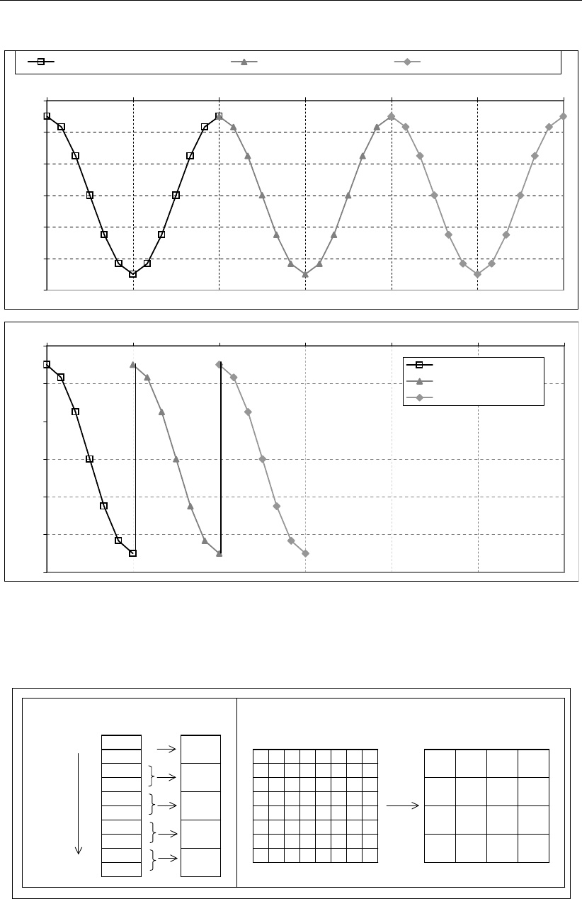
DRAFT
Graphical User Interface
- 1 . 2
- 0 . 8
- 0 . 4
0
0 . 4
0 . 8
1 . 2
0 : 0 0 6 : 0 0 1 2 : 0 0 1 8 : 0 0 0 : 0 0 6 : 0 0 1 2 : 0 0
w a t e r l e v e l ( m )
t i d a l c y c l e o n c o m m u n i c a tio n f i le f i r s t r e p e a t e d t i d a l c y c le s e c o n d r e p e a t e d t i d a l c y c le
( A )
- 1 . 2
- 0 . 8
- 0 . 4
0
0 . 4
0 . 8
1 . 2
0 : 0 0 6 : 0 0 1 2 : 0 0 1 8 : 0 0 0 : 0 0 6 : 0 0 1 2 : 0 0
w a t e r l e v e l ( m )
f i r s t c y c l e
f i r s t r e p e a te d c y c le
s e c o n d r e p e a te d c y c le
( B )
Figure 5.6: (A) Correct repetition of a tidal cycle of 12 hours stored on the communica-
tion file, for a D-WAQ simulation of 36 hours. (B) Incorrect repetition of a
hydrodynamic cycle; rewinding results in a major jump in water level.
surface layer 1 1
2
3 2
4
5 3
6
7 4
8
9 5
bottom layer 10
Vertical aggregation Horizontal aggregation
1 x 1 2 x 2
Figure 5.7: Principle of vertical and horizontal aggregation. Here the vertical aggregation
combines 10 layers in the hydrodynamic simulation to 5 layers in the water
quality simulation. The horizontal aggregation combines 4 computational cells
in the hydrodynamic simulation to 1 computational cell in the water quality
simulation.
Deltares 61 of 382

DRAFT
D-Water Quality, User Manual
Time in simulation
12345
12345
12345
Figure 5.8: Use of hydrodynamic files via rewinding.
not actually used, but they need to be present to keep the three files in sync.
5.2.1 Couple GUI
To couple a hydrodynamic result select Coupling from the Water quality (WAQ) window (Fig-
ure 4.3). From the Hydrodynamic coupling selection window first select Define input, see
Figure 5.9. When you need a coupling from a domain decomposition hydrodynamic simulation
you have to define the input for each domain separately.
Figure 5.9: Hydrodynamic coupling selection window
Next, the window in Figure 5.10 appears, the COUP-GUI. As you will see later, the window
is exactly the same as the Delft3D-WAQ GUI, with the difference that many option are not
sensitive. Only three data groups are sensitive: Description,Hydrodynamics and Dispersion.
The menu bar has three options:
File New Start a new scenario — clear input in all data groups
Open Open an existing scenario <∗.hyd>file
Save Save the current scenario file using the previously given
name, or the default name <com-∗.hyd>
Save As . . . Save the current scenario file and specify its filename
Exit Exit the GUI
View Disabled in coupling mode
Help Contents Opens the general help menu of D-Water Quality
About Displays the version number of the GUI
62 of 382 Deltares
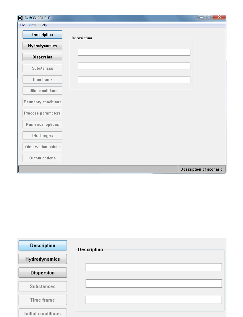
DRAFT
Graphical User Interface
Figure 5.10: Opening screen of the COUP-GUI
5.2.2 Description
Selecting Description opens a screen in which you can enter three lines of text. The lines can
be used to describe the coupling/aggregation. The maximum length of each of the lines is
39 characters.
Figure 5.11: Description window with three lines. The maximum length of the description
lines is 39 characters
5.2.3 Hydrodynamics
The Hydrodynamics window has four frames:
Deltares 63 of 382

DRAFT
D-Water Quality, User Manual
1 Hydrodynamics
and grid
Select the hydrodynamic communication file <com-∗.dat>or the
domain decomposition file <∗.ddb>. This automatically results
in setting the grid schematisation. Clicking Com-file opens a file
browser, which enables you to select a <com-∗.dat>file. Note
that it is not required that the <com-∗.dat>file is located in the
working directory. Clicking DD-bound opens a file browser, which
enables you to select a <∗.ddb>file.
2 Time information After selecting the communication file, this part shows the times
stored in the communication file (start time, stop time and time
step). Also, three input fields allow you to set the start time, stop
time and time step for the coupling.
3 Horizontal and
vertical aggrega-
tion
You have to select the horizontal aggregation here. Choices are
explained below. Furthermore, set the vertical aggregation (com-
bining hydrodynamic layers).
4 Domain decom-
position
The multiple FLOW domains can be combined to 1 (one) water
quality domain, or, treated as separate domains.
Figure 5.12: Hydrodynamics window in the COUP-GUI. A communication file <com-
f35_waq.dat>is loaded
Hydrodynamics and grid
The button marked DD-bound has a similar function as the button Com-file to select a so-
called communication file. Use this option if you want to convert a hydrodynamic database
that was computed with the domain decomposition feature of Delft3D-FLOW.
When you have used automatic domain decomposition to a parallel Delft3D-FLOW run, you
do not have to do anything in the coupling user interface. You can simply press the DD start
64 of 382 Deltares

DRAFT
Graphical User Interface
button, give the name of the ddb-file that was produced during the run, and answer ’yes’ to the
question: ’Has this ddb-file been created by a MPI-based parallel Delft3D FLOW run (y/n)?’.
Instead of individual communication files (such as <com-f35_waq.dat>) you now select a file
describing the relation between the various domains. The names of the communication files
that belong to each domain are derived from this information.
Once you have selected this “DD-bound” file, the user-interface is capable of dealing with all
domains at once. In fact, as far as possible the user-interface tries to hide the distinction
between single-domain and multi-domain databases. This is not always possible due to the
nature of the conversion process.
Time information
The right side of the frame displays the times stored in the hydrodynamic communication file.
The start time, stop time and time step to be stored in the coupled hydrodynamics can be
specified.
The Start time,Stop time and Time step of the coupled hydrodynamics have to satisfy the
following conditions:
The start time of the coupled hydrodynamics has to be equal to or later than the start time
in the communication file.
The start time of the coupled hydrodynamics has to be before the stop time in the com-
munication file.
The stop time of the coupled hydrodynamics has to be before or equal to the stop time in
the communication file.
The stop time of the coupled hydrodynamics has to be later than the start time in the
communication file.
The stop time in the coupled hydrodynamics has to be later than the start time in the
coupled hydrodynamics.
The time step in the coupled hydrodynamics has to be equal to or an integer multiplica-
tion of the time step in the communication file. So if the time step in the communication
file is 15 minutes, the time steps allowed in the coupled hydrodynamics are 15 minutes,
30 minutes, 45 minutes, 1 hour, etc.
The total time between the start time and the stop time in the coupled hydrodynamics has
to be an integer multiplication of the time step in the coupled hydrodynamics.
Finally, if the hydrodynamic simulation contains walking discharges, aggregation of the time
step is not allowed. A warning is given when you try to couple anyway.
Horizontal and vertical aggregation
There are three options for the horizontal aggregation of the hydrodynamic grid:
1 No aggregation
(e.g. for D-Waq
PART)
No aggregation is applied, the hydrodynamic grid will be coupled
horizontally unchanged. This option is required if you want to use
numerical schemes 4, 19 or 20 (refer to section 10.5), or if you
want to run D-Waq PART. (D-Waq PART makes use of the same
Coupling procedure).
2 Use aggregation
file (DIDO)
If you select this option the Select button will be activated. Clicking
Select opens a file browser, in which you have to select the DIDO
<∗.dwq>aggregation file you have prepared with DIDO.
Deltares 65 of 382
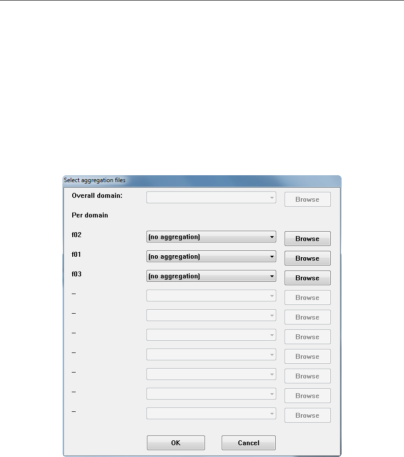
DRAFT
D-Water Quality, User Manual
3 Remove inactive
cells
No horizontal aggregation is applied and as such this option is
equal to the first option. Inactive computational cells such as dry
points or cells lying on the land are excluded. The benefits of this
option are the reduced file sizes of the coupled hydrodynamics and
some D-WAQ output files. However, you can not use numerical
schemes 19 or 20 with this option.
The aggregation tool DIDO can be started from the Tools menu. Please refer to the DIDO
manual (DIDO UM,2013) on how to prepare a <∗.dwq>file. Note that it is not required that
the <∗.dwq>file is located in the working directory.
Figure 5.13: Select aggregation files window in case of DD models
If you select a multi-domain hydrodynamic database, then aggregation will be done per do-
main, see Figure 5.13:
You select an aggregation file created by DIDO for a particular domain;
or you decide not to use an aggregation file. To keep the aggregation options for all
domains consistent, the option Remove inactive cells is turned on instead.
To vertically aggregate layers click Edit layers. The Layer editor window will open listing
the number of layers in the hydrodynamic simulation. When you open the screen for the
first time, by default each layer in the coupled hydrodynamics is set equal to one layer in the
hydrodynamic simulation. Note that a 2DH hydrodynamic simulation has no possibility for
vertical aggregation.
Figure 5.14 shows the Layer editor for a hydrodynamic simulation that has 5 layers. By
entering an integer number in one of the input boxes, you indicate the number of hydrodynamic
layers that have to be included in the specific water quality layer. In Figure 5.14 the first layer
in the water quality simulation contains the first and second hydrodynamic layers. The second
66 of 382 Deltares
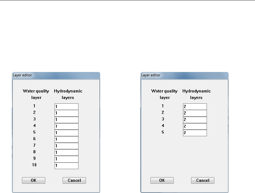
DRAFT
Graphical User Interface
layer in the water quality simulation contains the third and fourth hydrodynamic layers. The
third layer in the water quality simulation contains the fifth hydrodynamic layer. Entering a
number greater than 1, means that water quality layers will be removed from the bottom (note
that layer 1 is the surface layer). Lowering the number in a text box, means that water quality
layers will be added at the bottom. The sum of the hydrodynamic layers will always be equal
to the original number of layers, e.g. (10 ∗1) = (3 + 2 + 2 + 2 + 1) in Figure 5.14.
Figure 5.14: Layer editor. Left screen shows the original 10 hydrodynamic layers. The
right screen shows a vertical aggregation into 5 layers that will be applied in
the water quality simulation.
You are not allowed to enter a zero; a warning will be given if you do. Also, if the number you
enter is higher than the number of hydrodynamic layers available, a warning will be given and
the number will be truncated to the maximum allowed.
When coupling to a multi-domain hydrodynamic database, certain restrictions hold. This can
be best described via an example. Suppose you have three domains:
One with three layers (40, 40 and 20 % of the total depth)
One with six layers (20, 20, 20, 20, 10 and 10 % of the total depth)
One with two layers (40 and 60 % respectively)
Domain 1 Domain 2 Domain 3
+-------------------+-------------------+-----------------+
| | | |
| | | |
| +-------------------+ |
| | | |
| | | |
+-------------------+-------------------+-----------------+
| | | |
| | | |
| +-------------------+ |
| | | |
| | | |
+-------------------+-------------------+ |
| | | |
| +-------------------+ |
| | | |
+-------------------+-------------------+-----------------+
Deltares 67 of 382

DRAFT
D-Water Quality, User Manual
Only those interfaces that run through all domains without a jump can be maintained in the
final conversion. So in the above situation, the three domains will result in a two-layers system,
defined by the third domain.1
Domain decomposition
You have two options for the actual conversion2:
Merge the domains into a single one, so that the subsequent water quality computation
works on a single domain. Numerical schemes 19 and 20 are not allowed in this case.
Convert the hydrodynamic databases separately per domain. In that case the water quality
computation will be done in a multi-domain mode too.
Warning:
The second option is not implemented yet.
Even in the first case it will still be possible to run the water quality module on individual
domains (in that case you simply select the hydrodynamic description for that particular
domain and there is no relationship with the others).
5.2.4 Dispersion
The following only applies for a 3D hydrodynamic database.
Clicking Dispersion opens the window shown in Figure 5.15. Note that, any value that you
enter here, can still be changed when you define the input for a water quality simulation.
The coupling automatically takes over the vertical dispersions calculated by the hydrodynamic
model. However, as these values may be unrealistically small, you can enter a minimal value
for the vertical dispersion here. The text boxes become active when you check the Use min-
imum values box. The water column can be split. You can enter a different value below and
above a certain interface, including the depth of this interface.
5.2.5 Running the coupling
Once you have defined the conversion of the hydrodynamic <com-∗.dat>file, you can save
the coupled hydrodynamics file <∗.hyd>by selecting File →Save or File →Save As. . . .
Default the name of the coupled hydrodynamics file is <com-∗.hyd>.We advise you to save
the <∗.hyd>file in the working directory.
Leave the COUP-GUI by selecting File →Exit in the menu bar. When you need a coupling
from a domain decomposition hydrodynamic simulation you have to define the input for each
domain separately.
Back in the Hydrodynamic coupling selection window (see Figure 5.9), select Start or DD
Start to execute the coupling. Information about the coupling will be displayed in a new
window. You can close this window when the coupling has finished.
Information on the coupling is written to the <couplnef.out>or <name-ddcouple.out>file.
You can check this file. First select Return in the Hydrodynamic coupling selection window;
you will be back in the Water quality (WAQ) selection window. From this window select the
1(april 2005) It is possible to create sets of layer thicknesses that would result in a single layer. Unfortunately
the user-interface will currently report an error, rather than revert to a single layer.
2(april 2005) The multi-domain option is not fully supported yet. Use the single-domain for the moment.
68 of 382 Deltares
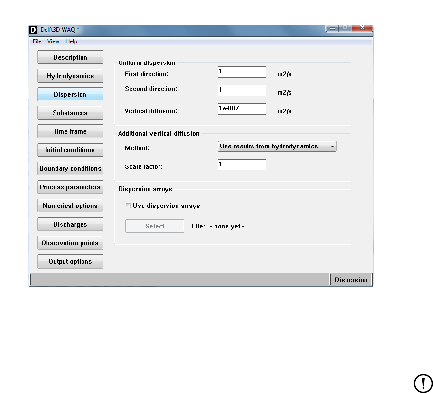
DRAFT
Graphical User Interface
Figure 5.15: Dispersion window in the COUP-GUI
Reports item. The View report files selection window will then open, see Figure 5.16.
From the View report files window select Coupling to view the information on the coupling.
Remark:
The coupled hydrodynamics and the file <couplnef.out>or <name-ddcouple.out>is
stored in the working directory.
Important information you get from the coupling, is the minimum residence time. Explicit
numerical schemes require that the time step in the water quality simulation is smaller than
the minimal residence time (also refer to Chapter 10). The excerpt of the <couplnef.out>file
displayed below indicates that the minimal residence is 498.1 seconds.
5.3 Define input (Delft3D): WAQ-GUI
Select Define input (Figure 4.3) to start the input procedure for the water quality calculation.
The main window is visualised in (Figure 5.17).
The Graphical User Interface for water quality calculations consists of:
The menu items: File,View,Tools and Help
The data groups: Description,Hydrodynamics,Dispersion,Substances,Time frame,Ini-
tial conditions,Boundary conditions,Process parameters,Numerical options,Discharges,
Observation points and Output options
Additional information in the bottom row of the window, like version number and identifica-
tion of data group you are working in
To prepare a water quality calculation all data groups must be specified. It is recommended to
follow the order in which they appear (from top to bottom) in the main window, although this is
Deltares 69 of 382
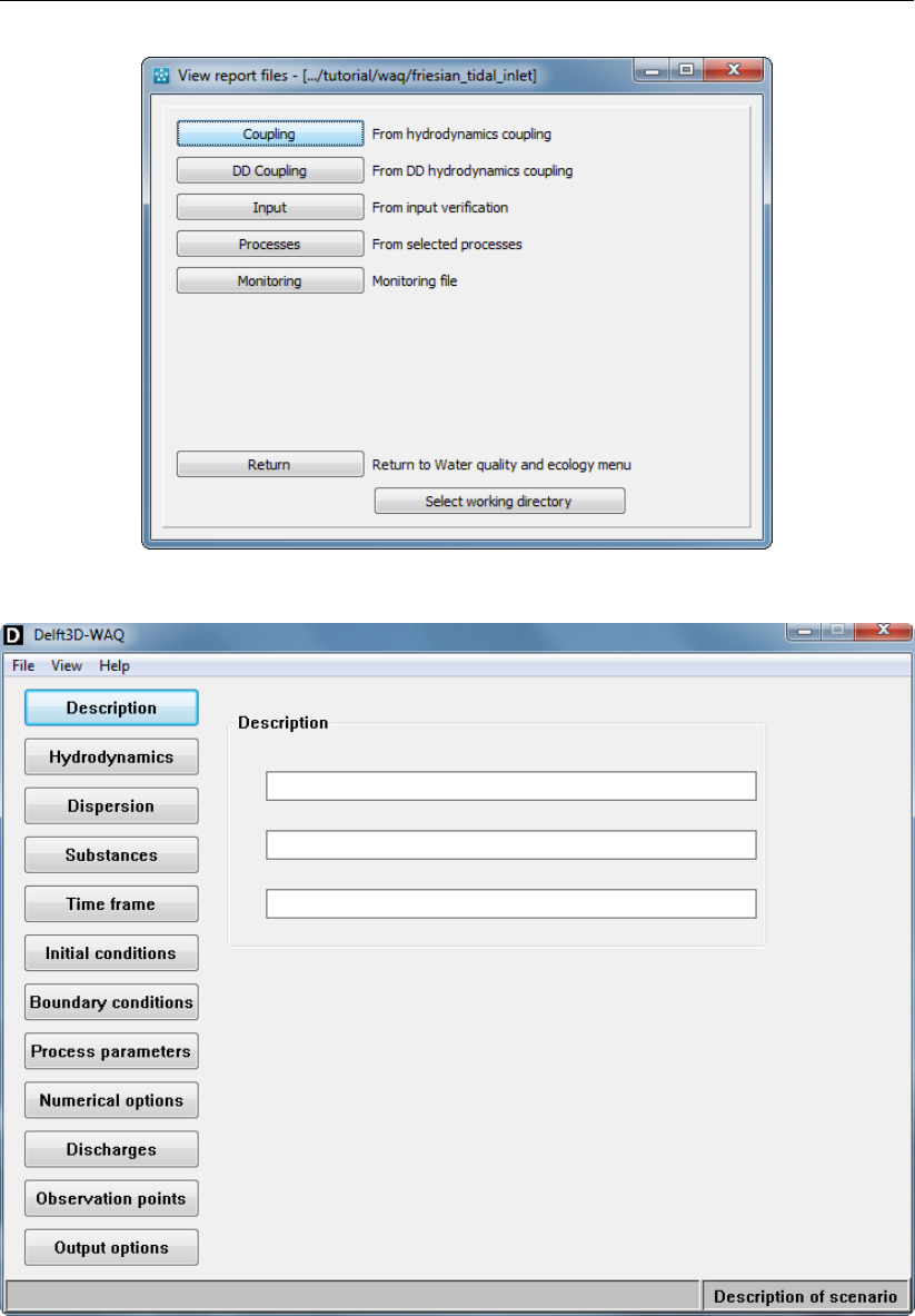
DRAFT
D-Water Quality, User Manual
Figure 5.16: View report files selection window
Figure 5.17: Main window of the WAQ-GUI. The buttons on the left side of the window
represent distinct data groups.
not obliged. After selecting one of the data groups, the right side of the window will show the
data specification for that data group. When you select another data group information will be
saved automatically.
The menu bar has four options:
70 of 382 Deltares
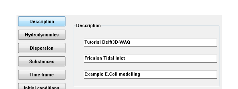
DRAFT
Graphical User Interface
Figure 5.18: Description Data Group. The maximum length of the text is 39 characters
File New Start a new scenario — clear input in all
data groups
Open Open an existing scenario <∗.scn>file
Save Save the current scenario file using the pre-
viously given name, or the default name <wqnew.scn>
Save As. . . Save the current scenario file and specify
its filename
Exit Exit the WAQ-GUI
View Visualise area The visualisation area is a tool for display-
ing objects bound to a geographical loca-
tion. This tool is present in several Delft3D
models. In the WAQ-GUI, it can be used
for visualisation, addition and modification
of discharge locations, observation points
and open boundaries. For a visual refer-
ence, the original hydrodynamic grid is dis-
played.
Help Contents Opens the general help menu of D-Water
Quality
About Displays the version number of the GUI
5.3.1 Description
In the Data Group Description you can specify three lines of meta-information about the cal-
culation (Figure 5.18).
The individual text boxes have a length of 39 characters each. Specifying longer text strings
seem possible, but the text exceeding 39 characters will be truncated and will not be saved.
Deltares 71 of 382
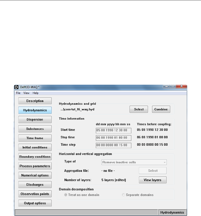
DRAFT
D-Water Quality, User Manual
5.3.2 Hydrodynamics
In the Data Group Hydrodynamics you can specify which coupled hydrodynamic file(s) should
be used in the water quality calculation.
From top to bottom, the following four frames can be distinguished (Figure 5.19):
Hydrodynamics and grid
Time information
Horizontal and vertical aggregation
Domain decomposition
Figure 5.19: Data Group Hydrodynamics
Hydrodynamics and grid
In this frame you can either Select a single coupled hydrodynamic file <∗.hyd>, a previously
generated multiple hydrodynamics file <∗.mhy>or generate a multiple hydrodynamic file
<∗.mhy>using the Combine button.
By clicking Select you can browse to the right file and press OK in the file dialogue for confir-
mation. By pressing Combine you can build a new combination of hydrodynamic files without
running Delft3D-FLOW. This option can be very useful, for example if you want to model dif-
ferent seasons that are represented by two different hydrodynamic calculations, in one water
quality calculation. Details about combining hydrodynamics can be found in the Intermezzo.
The hydrodynamic description file contains almost all the information the user-interface needs
to deal with the hydrodynamic database. This includes:
The type of grid:
The user-interface currently supports two types of hydrodynamic grids, regular curvilinear
grids (with or without horizontal aggregation) or so-called unstructured or finite-element
grids. This latter type of grid must consist of triangles, by far the most common type for
72 of 382 Deltares
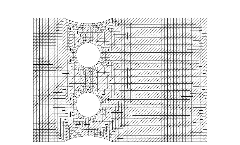
DRAFT
Graphical User Interface
Figure 5.20: Example FEM grid
finite-element grids. (Another aspect of the grid is the type of vertical layers. For details
see section 11.4)
Single domain or multiple domains:
Most information to be defined for the water quality computation will hold for all domains
as a whole, but some data, notably initial conditions may be given per domain. It is up to
the user-interface to make sure that the computation is started for all domains at once.
Time information:
The water quality computation must refer to the correct times in the hydrodynamic database,
both in case of a single database and in case of a combination of databases.
Other information:
The hydrodynamic description file also contains a list of waste loads and their locations,
as found in the hydrodynamic database, the names of the files that consitute this database
and so on. All this information is needed at some point or other.
Finite-element grids
The actual coupling to unstructured or finite-element grids is done outside the Delft3D suite
itself at the moment. But the hydrodynamic description file is used to pass all the necessary
information to the graphical user-interface. Here are the specifics about this type of grid:
The keyword grid-type must be set to “finite-elements”.
As there is no distinction in two horizontal directions possible, the user-interface presents a
single value for determining the location of boundaries and of waste loads and observation
points.
The visualisation area is adapted to show this type of grid, as well as show the location of
special points and boundaries (see Figure 5.20).
Deltares 73 of 382

DRAFT
D-Water Quality, User Manual
Time information
Details specified in the Time information frame are derived from the selected hydrodynamic
file and are visualised for information purposes only. Changes to (coupled hydrodynamic) time
step, start and stop times can not be made here. The Data Group Time frame deals with the
specification of the timers in the water quality calculation.
Horizontal and vertical aggregation
Displays the horizontal aggregation that is applied in the selected (coupled) hydrodynamic file.
No changes to the horizontal aggregation can be made in the WAQ-GUI. If you want to change
the horizontal aggregation, you will have to return to the Coupling routine (Section 5.2.1).
Displays the vertical aggregation that is applied in the selected hydrodynamic file. No changes
to the vertical aggregation can be made in the WAQ-GUI. If you want to change the vertical
aggregation, you will have to return to the Coupling routine (section 5.2.1).
Intermezzo: Combining hydrodynamics
D-WAQ allows you to base a water quality simulation on more than one (coupled) hydrody-
namic simulation. There are two options to combine hydrodynamic results:
Chaining of hydrodynamic results: use one hydrodynamic result during one period and
another during the following period.
Interpolation of hydrodynamic results: use two (or more) hydrodynamic results during the
same period, for instance to get a smooth transition between two periods.
The combination of hydrodynamic results to describe the movement of water over a prolonged
period is usually a substitute for a hydrodynamic simulation over that complete period. Gen-
erally, a hydrodynamic simulation over a long period (say one year) takes an unrealistically
long computation time. An alternative is to choose two or more (hydrodynamically) repre-
sentative periods that take much shorter computation time, and to interpolate between these
representative periods for the rest of the total period.
Representative periods can be distinguished by:
River discharges (annual minimum, annual average and annual maximum)
Wind speed and direction (typical for monsoon regions with alternating wind directions
during the wet and the dry seasons)
Spring tide versus neap tide
Be aware that combining hydrodynamic results can never replace actual hydrodynamic mod-
elling; it is no more and no less than a surrogate.
Chaining hydrodynamic results
Suppose you want to do a calculation that covers two or more seasons, a period of six months.
One, rather inconvenient way to do this, is to run the hydrodynamic model for this period of
six months. This will give a huge data set <com-∗.dat>, will probably take a long time to
finish and maybe the hydrodynamic model will calculate the same typical flow field for several
months and only then switch to another flow field. The alternative is to do a short calculation
for the first season, of say two days, and another short calculation for the second season, also
two days.
74 of 382 Deltares

DRAFT
Graphical User Interface
A C
100% Flow1
50% Flow1 + 50% Flow2
100% Flow2
25% Flow1 + 75% Flow2
B D
Figure 5.21: Interpolation of flow fields. A) Flow 1 – angle 53◦, length 5.00; B) Flow 2 –
angle 243◦, length 2.24; C) 50 % Flow1 + 50 % Flow2 – angle 45◦, length
1.41; D) 25 % Flow1 + 75 % Flow2 – angle 198◦, length 0.79.
D-WAQ then allows you to say:
Use the first result during the first three months
Use the second result during the second three months
Just as with a single hydrodynamic result, D-WAQ will rewind the coupled hydrodynamics files
if it reaches their end, before the end of the water quality calculation. It will continue to use
(and thus rewind if necessary) the first result until the beginning of the new period.
It is preferable to include a transition period, during which the flow field can adjust relatively
smoothly. This is where the second type of combination becomes important.
Interpolation between hydrodynamic results
Interpolation of hydrodynamic results is straightforward. Interpolation is linear and takes into
account a weight factor as demonstrated in Figure 5.21.
As mass conservation needs to be preserved, the option for interpolating the flow fields is
limited: you can superimpose any number of flow fields, as long as the weighting factors are
constant. So a transition period of three days as in the above example might be specified as:
The flow field during the first day is 75 % of the first result and 25 % of the second.
The flow field during the second day is 50 % of the first result and 50 % of the second.
During the third day it is 25 % of the first result and 75 % of the second.
This is illustrated in Figure 5.22.
The weight factors should add up to 100 %. There is no limitation on the number of hydrody-
namic results used in the interpolation. In fact, you can use several flow fields for simulating
special effects, like:
The first result is the flow field without wind
The second is the result with a wind speed of 10 m/s
Combining the two via the following formula allows you (under simplified assumptions) to
Deltares 75 of 382
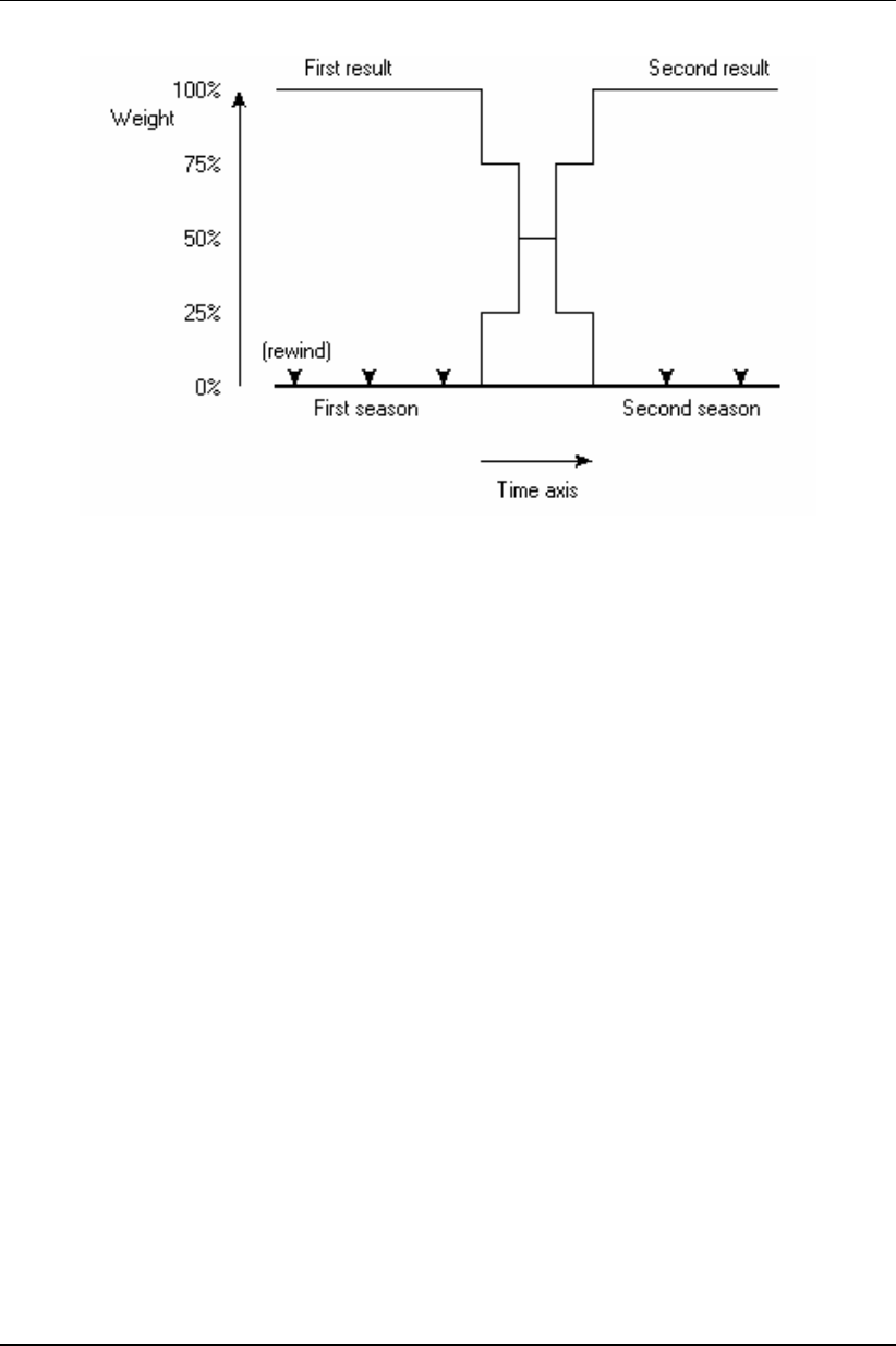
DRAFT
D-Water Quality, User Manual
Figure 5.22: Schematic representation of combining hydrodynamic results.
estimate the flow field under any wind speed:
New flow field =first flow field +factor ×(second flow field −first flow field)
= (1 −factor)×first flow field +factor ×second flow field
Adding a third flow field that contains the effect of, say, a large river will make further com-
binations possible. Note that the fact that such combinations are logically possible, does not
mean that they are physically realistic.
Hydrodynamic results can be combined only if they are based on the same water quality grid:
The underlying hydrodynamic grid must be the same.
The layers must have the same (relative) thicknesses and the number of layers must the
same.
If horizontal aggregation is applied, this must be the same for all results.
The open boundaries must be the same.
The discharges that have a flow rate in the hydrodynamics will have to be handled in a
special way: it is very cumbersome for you to specify the flow rates and concentrations
properly (see the section Treating discharges).
Of course the transition from one period to the next must be smooth enough, for instance,
the transition occurs during the time of high water, so that any differences in water level are
minimal in terms of the total water depth. To achieve that it is possible to shift the time frame
in the hydrodynamic results (see the section Adjusting time frames).
The user-interface takes care of most of the details:
After clicking Combine in the Hydrodynamics Data Group, a dialog appears (see Fig-
ure 5.23).
You will select one or more hydrodynamic results for each period.
Each result is assigned a weighting factor and an offset in the results file (normally zero,
see the section Adjusting time frames).
76 of 382 Deltares
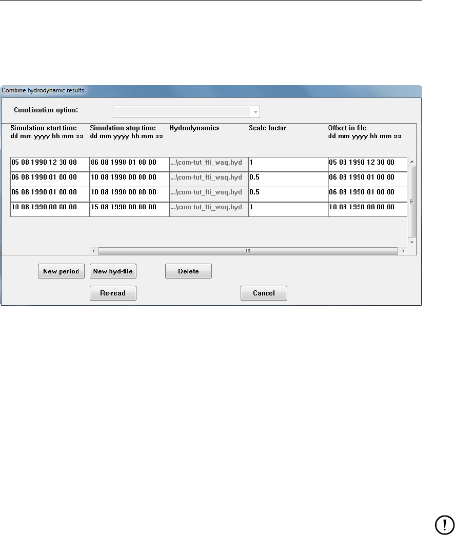
DRAFT
Graphical User Interface
The user-interface checks that the hydrodynamic results are based on the same grid and
determines a default calculation period from the given periods. For these checks the first
selected hydrodynamic result is used.
Figure 5.23: Combining hydrodynamic results. Four periods are defined.
In this dialogue the buttons have the following meanings:
New period Create a new period for which a hydrodynamic file <∗.hyd>can be
selected.
New hyd file Add a hydrodynamic file <∗.hyd>to the period that is being edited.
The start time and stop time will be the same as the first hydrody-
namic file <∗.hyd>that belongs to this period.
Delete Remove the selected record. If there is only one record left for this
period, then the period is removed as well.
Re-read Exit the Combine hydrodynamic results window and save the com-
bined hydrodynamics information.
Cancel Exit the Combine hydrodynamics results without saving the com-
bined hydrodynamics information.
Remarks:
Because a lot of other information depends on the selection of the hydrodynamic result,
you should first close the dialogue before doing anything else in the user-interface.
The simulation start and stop times shown in Figure 5.23 are the times after coupling.
The list of hydrodynamic results is stored in a file with the extension <∗.mhy>. This file
can be used as if it were an ordinary hydrodynamic description file. It can be selected via
the Select button in stead of a <∗.hyd>file, but it can not be selected in the combination
dialogue, as this would lead to a nested list of hydrodynamic results.
Adjusting time frames
You can shift the hydrodynamics in time. For this the offset time is used. An example may
clarify this. Suppose the high water in a spring tide occurs at 2 o’clock in the afternoon,
whereas the high water in a neap tide occurs at noon. If you combine these two tidal cycles
to estimate the transition from spring tide to neap tide, then you would like to get matching
Deltares 77 of 382

DRAFT
D-Water Quality, User Manual
phases. In other words: the cycle for neap tide must be shifted backwards by 2 hours or
the cycle for spring tide must be shifted forwards by 2 hours to get a match. This is done by
specifying the offset time as either +2 or -2 hours.
Treating discharges
One final remark must be made about the treatment of discharges defined in the hydrody-
namic calculations. When dealing with a single hydrodynamic result, the discharge rates are
taken from the hydrodynamic result files and displayed as an ordinary time-series initially
defined over the same period as the hydrodynamic result. Beyond that time interval, the
discharge pattern is repeated as long as necessary.
To get an equivalent definition with multiple hydrodynamic results the user-interface would
have to interpret the specified multiple hydrodynamics and create a time-series that fills the
entire period covered by that specification. For instance: during the first season in the previous
example the discharge is defined over a period of two days by 10 breakpoints. This pattern
should then be repeated until the transition period, so three months later, because only then a
different pattern becomes necessary. The user-interface would construct a time-series of 450
breakpoints for these first three months.
So, rather than have the user-interface construct a time-series that covers the complete pe-
riod, a different approach is chosen:
The user-interface constructs a time-series consisting of two breakpoints only: the first
time and the last time of the period for which the hydrodynamic results are defined. The
flow rate is set to the special value -999.0.
The computational program interprets this special value as an instruction to derive the
instantaneous flow rate from the flow field directly.
You need to specify the concentrations only — at breakpoints that are independent of the
hydrodynamics.
You are free to change the flow rate. This new flow rate will be used to calculate the
amount of substance to be added, but be aware that the original flow is still part of the
hydrodynamic flow field and thus will be responsible for taking out mass.
5.3.3 Dispersion
In the Data Group Dispersion you can specify the horizontal and vertical dispersion.
From top to bottom, the following three frames are visible (Figure 5.24):
Uniform dispersion
Additional vertical diffusion
Dispersion arrays
78 of 382 Deltares

DRAFT
Graphical User Interface
Figure 5.24: Dispersion window
Uniform dispersion
Dispersion coefficients are required to solve the advection-dispersion-equation. Initially, de-
fault values are given, but these values can be adapted. In case of a 2D calculation, only the
horizontal (i.e. first and second) directions can be edited. To define the ‘first’ and ‘second’
direction you should open the visualise area to display the simulation grid. By moving the
mouse, the M and/or N values (right upper corner) change. Moving the mouse from bottom
to top changes the M-values. This is the ‘first’ direction. Moving the mouse from left to right
changes the N-values. This is the ‘second’ direction. The third direction (only valid in 3D
calculations) is the vertical direction and is not visible in the visualisation area.
It is very unusual to take a different value in the 1st and 2nd direction.
Additional vertical diffusion
If you select the option Use results from hydrodynamics, the vertical diffusion derived from the
hydrodynamic simulation will be used. This value will be added to the value specified in the
uniform dispersion for the third direction. A scale factor can be applied as well.
The option No additional diffusion indicates that only the uniform vertical dispersion will be
used.
Deltares 79 of 382

DRAFT
D-Water Quality, User Manual
Dispersion arrays
Dispersion values are valid for all exchanges. If you want to exclude a number of exchanges or
define a specific dispersion value for a specific region, you can define a so-called ‘dispersion
array’. A dispersion array is defined with an ASCII-file containing the overridings (exceptions)
of the uniform dispersion value. Both exchange number and dispersion value should be spec-
ified. The ASCII-file should have the extension <∗.dsp>. Use semi-colons (;) to separate the
values from comments. The file content is as follows:
2 ; 2 = option "additional dispersion with default"
1.0 5.0 ; scale factor and default dispersion in the first direction
3 ; number of overridings in the first direction
exchange_#1 new_dispersion_value
exchange_#2 new_dispersion_value
exchange_#3 new_dispersion_value
1.0 5.0 ; scale factor and default dispersion in the second direction
2 ; number of overridings in the second direction
exchange_#4 new_dispersion_value
exchange_#5 new_dispersion_value
Refer to the file description in section A.2.3 on how to retrieve the exchange numbers.
5.3.4 Substances
In the Data Group Substances you specify the state variables (modelled substances), the
water quality processes and output parameters (Figure 5.25).
You click Select and browse to a substance file <∗.sub>, which was created with the PLCT
(Processes Library Configuration Tool, refer to section 5.1). This file contains all relevant
information about the substances, processes, parameters and output of the water quality
simulation.
Changes to state variables, output parameters, etc. can not be made in this data group. For
any changes you will have to return to the PLCT, make the desired changes and reopen the
<∗.sub>in the WAQ-GUI. The frames Substances in calculation,Output parameters and
Active processes are displayed for reference purposes only.
5.3.5 Time frame
The start time, stop time and time step of the water quality simulation are defined in the Data
Group Time frame.
The Time frame Data Group has two frames (Figure 5.26):
Times in coupled hydrodynamics
Times in water quality calculation
Times in coupled hydrodynamics
The times from the coupled hydrodynamics are displayed for reference purposes only and can
not be edited.
80 of 382 Deltares
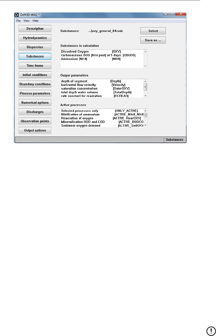
DRAFT
Graphical User Interface
Figure 5.25: Substances Data Group. The standard substance file for dissolved oxygen
<oxy_general_04.sub>was selected
Times in water quality calculation
Timers in D-WAQ always have the format ‘dd mm yy hh mm ss’, or day - month - year - hour -
minute - second. The start time, stop time and time step of the water quality simulation have
to satisfy these conditions:
The start time of the water quality simulation has to be equal to or later than the start time
in the coupled hydrodynamics.
The stop time of the water quality simulation has to be later than the start time in the water
quality simulation.
The time step in the water quality simulation has to be equal to or an integer division of the
time step in the coupled hydrodynamics. So if the time step in the coupled hydrodynamics
is 15 minutes, the time steps allowed in the water quality simulation are 15 minutes, 7.5
minutes, 5 minutes, etc.
The minimum time step allowed is one 1 second.
The total time between the start time and the stop time in the water quality simulation has
to be an integer multiplication of the time step in the water quality simulation.
The WAQ-GUI will check if the specified start time, stop time and time step comply with these
conditions when you exit the Time frame Data Group or when you click Time frame.
Note that it is allowed to extend the water quality simulation beyond the stop time of the
coupled hydrodynamics. D-WAQ will rewind and repeat the coupled hydrodynamics as often
as required to cover the time period specified. As explained in Section 4.1.1 you have to take
care that no extreme transition in for example water level occur as a result of the rewinding.
Remarks:
When setting up a scenario from scratch, the start and stop times of the simulation
period will be used as defaults for the start and stop times in time-series for boundaries,
Deltares 81 of 382
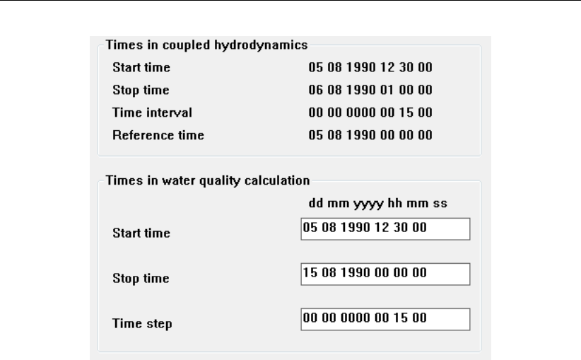
DRAFT
D-Water Quality, User Manual
Figure 5.26: Data Group Time frame
process parameters, discharges and output period. This holds as long as you do not
specify timings yourself.
When changing the start or stop time in an existing scenario, the start and stop time of
other time-series or output period are not adjusted.
The water quality time frame may not differ more than 5 years from the hydrodynamic
time frame.
5.3.6 Initial conditions
Initial conditions are the concentrations of substances at the start of the simulation. By default
they are all zero. Initial conditions have to be specified for all substances that are included
in the substances file <∗.sub>. Note that as long as no substance file <∗.sub>has been
selected this window will be empty.
The Initial conditions Data Group contains a list of substances and entry boxes in which a
constant initial concentration can be specified simply by typing an entry. Always make sure
that the units are correct.
At the bottom of the data group there are two buttons:
Edit data
Information
In case you want to specify non-constant initial conditions you have to use Edit data. Non-
constant conditions are spatially varying such as a salinity field or temperature profiles. Non-
constant initial conditions have to be specified for every computational cell and are therefore
usually derived from secondary input files.
When selecting an edit field, the value can be edited by directly typing or clicking Edit data.
The latter opens the Data for: <substance>window (Figure 5.28). The following menu
items are available (menu-item Help is not explained here):
82 of 382 Deltares
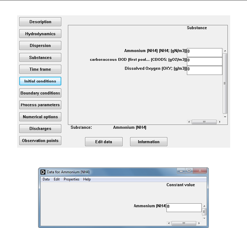
DRAFT
Graphical User Interface
Figure 5.27: Data Group Initial conditions. By default all concentrations are set to zero.
Figure 5.28: Data for: <substance>window opened for Ammonium. A constant value
can be specified
Data Import. . . Select a secondary file to import initial con-
ditions; the Import data file window is opened.
Quit Closes the Data for: <substance>win-
dow without saving changes; a confirma-
tion is asked.
Save and exit Closes the Data for: <substance>win-
dow and saves the input.
Edit (no options)
Properties Details Opens the Details for quantity window (Fig-
ure 5.29) in which you can specify whether
the initial condion is a constant value or a
scalar filed (i.e. spatially varying). In case
of the latter a data file has to be imported
using the Data →Import. . . item.
Deltares 83 of 382

DRAFT
D-Water Quality, User Manual
Figure 5.29: Details for quantity window for selection between constant or spatially vary-
ing initial conditions
Import data file
Non-uniform values (i.e. a scalar field) are imported from an external file. The following types
are allowed:
QUICKIN data file (<∗.qin>)
QUICKIN 3D data file (<∗.q3d>)
D-WAQ map file (<∗.map>)
D-WAQ (NEFIS) map file (<∗.ada>)
D-WAQ segment function (<∗.∗>)
For a detailed definition of the files refer to Appendix A. QUICKIN (QUICKIN UM,2013) is a
Delft3D software package that is used to generate the bathymetry for hydrodynamic simula-
tions. However, you can use it to generate a non-uniform parameter field as well. QUICKIN
files are generated on the (non-aggregated) hydrodynamic grid and can be used in all water
quality simulations based on this hydrodynamic grid. If an aggregated grid is used in the water
quality simulation, values will be aggregated through simple averaging.
The D-WAQ map files (<∗.map>and <∗.ada>) are output files from a previous simulation.
They can only be used if the grid is identical: the grid of the map file has to match the grid in
the current water quality simulation. An error message is displayed if this is not the case.
Remark:
A 2D WAQ map file can be used as initial condition for a 3D model if the horizontal grid
is the same.
Finally, the D-WAQ segment function is a binary file with values for all computational cells.
Water temperature <∗.tem>, salinity <∗.sal>, shear stress <∗.tau>and vertical diffusion
<∗.vdf>can be derived from the hydrodynamic simulation and are examples of segment
functions. Also, segment functions can be prepared with simple programs (see Appendix A).
Use the File type dropdown box to specify the right type and click Select for browsing to and
selecting the file. After opening the file, the window looks as displayed in Figure 5.30.
Subsequently, specify the desired parameter and time (map files and segment functions can
have more than one time step). The corresponding values will be ‘extracted’ from the file after
pressing Import. The edit field behind the substance is now indicating ‘[from file]’. To review
which file was selected, return to the Import data file window.
If you click Import all, the WAQ-GUI will compare the substances with the available information
84 of 382 Deltares
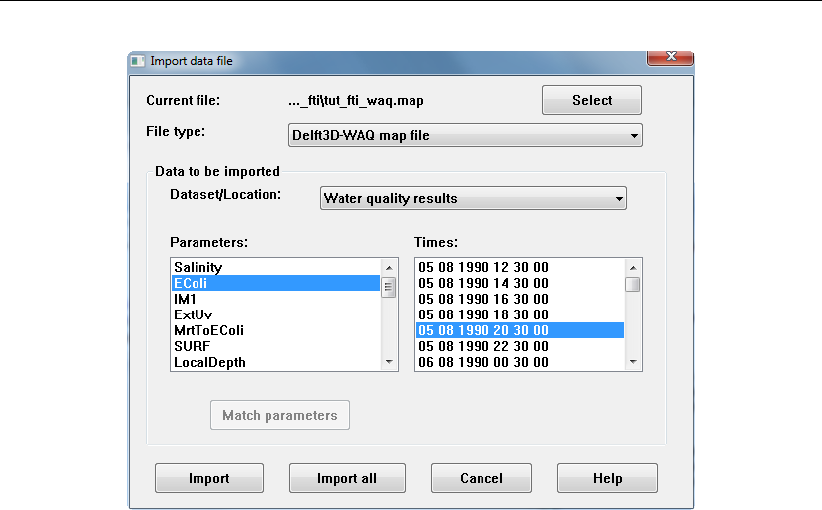
DRAFT
Graphical User Interface
Figure 5.30: Import data file window. A D-WAQ map file <∗.map>is selected. The Ecoli
concentration on August 05, 1990 20:30 will be used as initial condition
in the selected file and initial conditions will be set for all substances for which a matching
name is found in the selected file. This prevents unnecessary repetition of actions in case you
have to set the initial condition for a lot of substances.
A special type of <∗.map>file is the restart file <∗_res.map>in which the concentration
of all substances on the final time step of the water quality simulation are stored. The restart
file <∗_res.map>can be used too as initial condition for a new simulation. This might be
especially useful in cases where the spin-up time of the model is long.
Ranges and typical values
For informative purposes the Information button opens the Ranges and typical values win-
dow. It gives a range of values for each of the substances (if available). The values of around
20 common substances are stored in an internal Delft3D file <watqual.d3d>and will be avail-
able after installing D-Water Quality. These values can be modified by changing this (internal)
file.
5.3.7 Boundary conditions
In this data group you can specify the boundary conditions at the open boundaries of the
model grid (outside world). Open boundaries are those boundaries of the model grid that
have a cross-section with a non-zero water flow. You have to specify the concentrations of
all active substances and they are required for all time steps in the model. No boundary
concentrations are needed for the inactive substances as they can not be transported and
thus can not enter over the model boundaries. If the stop time of the water quality simulation
is later than the last time step for which boundary conditions are specified, D-WAQ will repeat
/ rewind the time-series from the beginning.
Usually, boundaries are defined in the hydrodynamic simulation and therefore do not need to
be redefined in D-Water Quality. Pre-defined boundaries sections might be split in smaller
sections if you want to assign different concentrations within a pre-defined boundary section.
Deltares 85 of 382
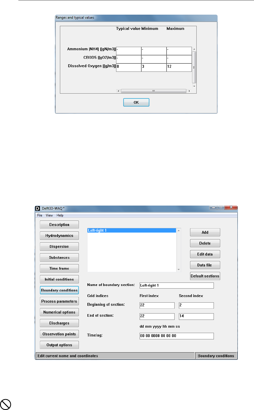
DRAFT
D-Water Quality, User Manual
Figure 5.31: Ranges and typical values window. Values are derived from the
<watqual.d3d>file. No information is available for CBOD5
Boundary section: definition
A boundary section is a part of the model boundary for which boundary conditions are uniform
in horizontal direction, have the same profile in vertical direction, and have the same time
dependency. Boundary sections are defined by giving the grid indices (the (M,N) indices) of
the first and last segment of the section. Thus, boundary sections are either sections with a
fixed M, but varying N, or vice versa. For aggregated grids, still the grid indices of the original
grid are used.
Figure 5.32: Data Group Boundary conditions
The window contains a list of open boundary sections, several buttons at the right-hand side
and text boxes displaying the details of the selected boundary section (Figure 5.32).
Restriction:
86 of 382 Deltares
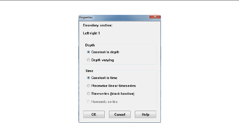
DRAFT
Graphical User Interface
Figure 5.33: Setting Data properties. By default boundary conditions are set to ‘Con-
stant in depth’ and ‘Constant in time’
The name of a boundary section is restricted to 39 characters.
Editing sections
By default, the boundary sections from the hydrodynamics are displayed. If you want to define
new boundary sections, press Add. Selecting a boundary section and pressing Delete will
remove that specific section. Pressing Edit data will open the Data for: <Name of boundary
section>window, in which you can specify the concentrations. Pressing Data file will open
the Select boundary data file window, in which you can specify which file will be used for
the boundary concentrations, buttonSelect. Then you have to check Use selected file instead
of the editable boundary data to overrule the manual editted data and you have to specify the
file format of the chosen file. Pressing Default sections will restore the original boundaries
derived from the hydrodynamic simulation.
It is compulsory to define concentrations for all boundary sections. The concentration may be
zero, but a value has to be specified. Therefore, no entire boundaries or parts of boundaries
may be missing. The WAQ-GUI will check whether this condition is fulfilled, when you leave
the Data Group Boundary conditions or when you press Boundary conditions. Boundaries
will be restored in case of an error and a warning will be given.
The Data for: <Name of boundary section>window in the Data Group Boundary condi-
tions is analogous to that in the Data Group Initial conditions (Figure 5.28).
The following menu items are available (menu-item Help is not explained here):
Data Copy. . . Copies data from another boundary sec-
tion.
Import. . . Select a secondary file to import boundary
conditions; the Import data file window is
opened.
Quit Closes the Data for: <Name of boundary
section>window without saving changes;
a confirmation is asked.
Save and exit Closes the Data for: <Name of boundary
section>window and saves the input.
Deltares 87 of 382
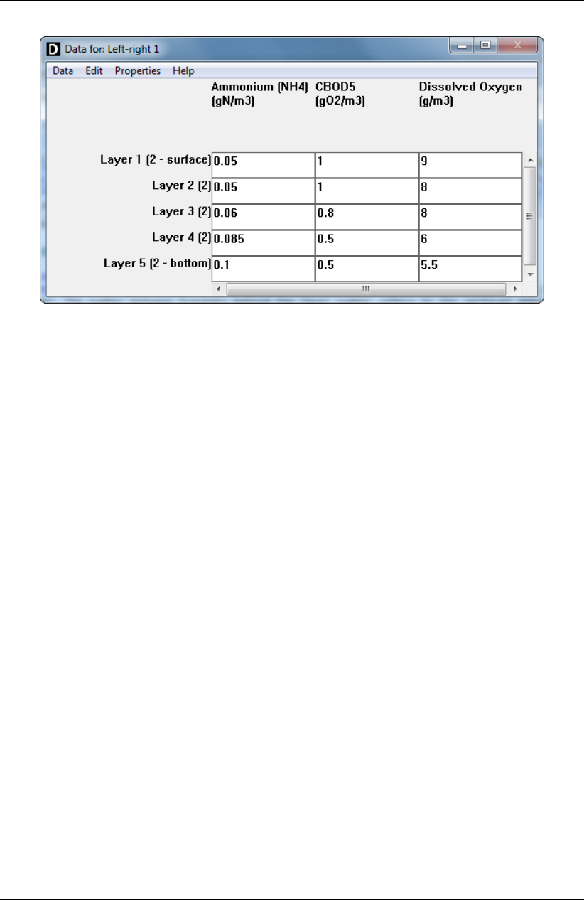
DRAFT
D-Water Quality, User Manual
Figure 5.34: Depth varying boundary conditions. A concentration has to be specified
for every active substance and every layer. The number between brackets
behind the layer number refers to the vertical aggregation.
Edit Copy row or Ctrl+K Copies the row containing the prompt and
put the new row above it in a table.
Delete row Deletes a row from a table.
Fill column Copies the selected value into the whole
column.
Properties Data properties You can set two options (Figure 5.33):
Are the boundary conditions constant
in time or varying in time? Variation in
time can be as a block function or as a
linear function.
Are the boundary conditions constant
over depth of varying over depth?
Setting the boundary conditions to either depth or time varying properties will result in a table
in the Data for: <Name of boundary section>window. If the boundary conditions are depth
varying a boundary concentration has to be specified for every (active) substance and every
layer (Figure 5.34). If the boundary conditions are time varying a boundary concentration has
to be specified for every (active) substance and every time step (Figure 5.35). Variation in
time can be carried out either through linear or block interpolation. Refer to the Intermezzo for
an explanation.
Both time and depth varying boundary conditions are not yet supported by the WAQ-GUI.
However, it is possible to included both time and depth varying boundary conditions in the in-
put file <∗.inp>. An additional manual is available for manual editing of this input file:‘Documentation
of the input file, User Manual’. Contact Delf3D-support for information.
Intermezzo: Linear and Block interpolation
Figure 5.36 demonstrates the difference between a linear interpolation of a time-series and a
block interpolation. You have to specify time breakpoints (left column in Figure 5.36) and pa-
rameter values or concentrations at those time breakpoints (right column in Figure 5.36). For
88 of 382 Deltares
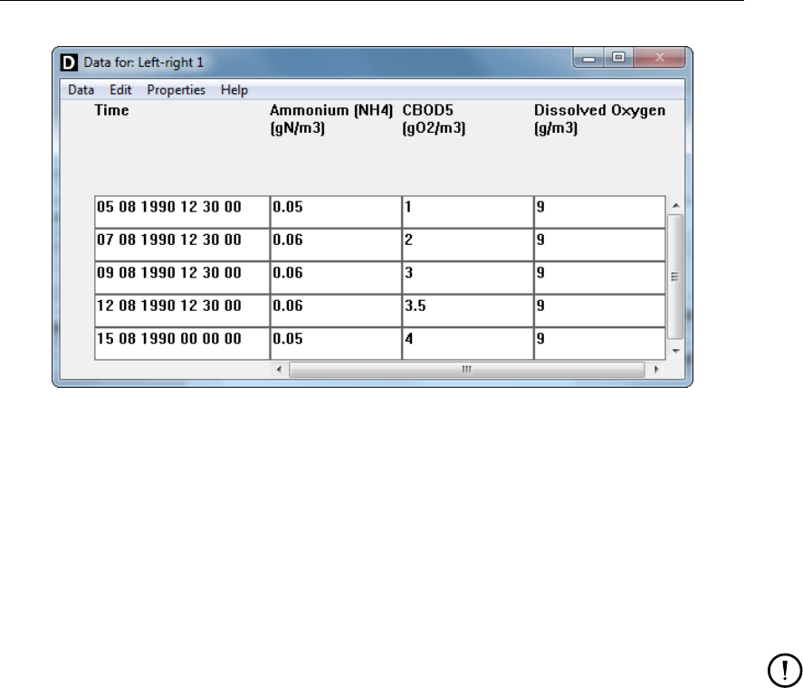
DRAFT
Graphical User Interface
Figure 5.35: Time varying boundary conditions. A concentration has to be specified for
every active substance and every time step. The number between brackets
behind the layer number refers to the vertical aggregation. The type of in-
terpolation (linear of block) can be reviewed through the Properties →Data
Properties
linear interpolation the parameter values or concentrations in between the time breakpoints
are calculated based on a linear average between the two adjacent time breakpoints. In case
of block interpolation, the parameter value or concentration remains constant until the next
time breakpoint and then instantly changes to the new value.
Remarks:
If the stop time of the water quality simulation is later than the last time breakpoint in the
time-series, the time-series will be repeated from the first time breakpoint (rewinding
occurs).
Note that in block interpolation the last time breakpoint is not used.
Visualisation Area
The Visualisation Area (VA) can be opened to view the location(s) of the boundary section(s).
Select the menu-option View →Visualise area for opening the VA. You can also use the VA
for defining new sections. A section can be defined by drawing a line with your mouse from
the first to the last segment of the section. Boundary sections appear with a red colour. Note
that if you create a new boundary section, you have to delete some segments from another
section since every segment can be defined only once.
Deltares 89 of 382
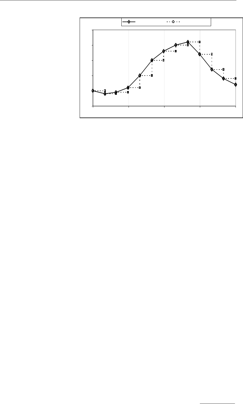
DRAFT
D-Water Quality, User Manual
dd mm yyyy hh mm ss
Temperature
01 01 2003 00 00 00
5.0
01 02 2003 00 00 00
4.0
01 03 2003 00 00 00
4.5
01 04 2003 00 00 00
6.0
01 05 2003 00 00 00
10.0
01 06 2003 00 00 00
15.0
01 07 2003 00 00 00
18.0
01 08 2003 00 00 00
20.0
01 09 2003 00 00 00
21.0
01 10 2003 00 00 00
17.0
01 11 2003 00 00 00
12.0
01 12 2003 00 00 00
9.0
01 01 2004 00 00 00
7.0
0
5
10
15
20
25
1-1-03 2-4-03 2-7-03 1-10-03 31-12-03
T e m p e r a t u r e (
o
C )
linear interpolation
block interpolation
Figure 5.36: Difference between linear and block interpolation of a time-series of water
temperature in 2003
Timelag
The edit field Time lag allows you to specify a time lag for the selected boundary section.
This time lag uses a Thatcher-Harleman transition to smooth the transition between inflow
and outflow on boundaries. The time lag is given in the format “dd mm yyyy hh mm ss”, as
for all date/time values. Refer to Section 8.5 for more information on the Thatcher-Harleman
time lag.
Boundary conditions may have an important effect on the final model results. Therefore, the
model grid schematisation should be large enough to prevent any unwanted concentration
fluctuations resulting from these boundaries, or from irregularities in the hydrodynamic flows
across these boundaries. In case the boundaries are far away from the area of interest (a
discharge location, an estuary, a harbour, a regional sea, etc.) it usually suffices to take
constant boundary conditions (obviously, the constant values should be chosen carefully).
However, for studies over longer periods of time, time-dependent boundary conditions are
still required. Probably, you will have to specify different boundary conditions for all default
boundary sections. Default boundary sections are not adjacent and may have very different
flow and concentration distributions. Pressing Default sections will restore the original number
of boundary sections and set the properties of each back to ‘constant in depth’ and ‘constant
in time’.
5.3.8 Process parameters
In this data group you can specify the process parameters which are available through the
selected substance file <∗.sub>. A listing of available parameters is shown in Figure 5.37.
By default the process parameters will be constant in time and space. However, process
parameters can vary in time and/or space. Initially process parameters will have the default
value that is taken from the PLCT. These values may be altered in the Process parameters
Data Group. When you select a new substance file <∗.sub>in the Data Group Substances,
identical process parameters will not be overwritten with the default values and therefore in-
formation will be conserved. Obviously, process parameters that are new in the substance file
<∗.sub>will be added to the list with their default value.
In some occasions the default value may be ‘-999’ which is interpreted as a missing value.
You have to specify a value in order to activate the process(es) that uses this value.
90 of 382 Deltares
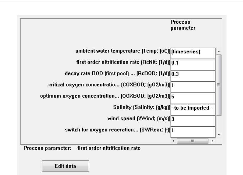
DRAFT
Graphical User Interface
Figure 5.37: Data Group Process parameters. A time-series is specified for the water
temperature, a segment function for salinity. All other process parameters
have constant values
Importing of time-series <∗.tim>will automatically adjust the properties.
Editing data
By selecting an edit field and pressing Edit Data the Data for: <substance name>window
appears. The following options are available (menu-item Help is not explained here):
Data Import. . . Select a secondary file to import parame-
ter values; the Import data file window is
opened.
Quit Closes the Data for: <substance name>
window without saving changes; a confir-
mation is asked.
Save and exit Closes the Data for: <substance name>
window and saves the input.
Edit Copy row Copies the row containing the prompt and
put the new row above it in a table.
Delete row Deletes a row from a table.
Fill column Copies the selected value into the whole
column.
Properties Data properties You can set two options (Figure 5.33):
Are the boundary conditions constant
in time or varying in time? Variation in
time can be as a block function or as a
linear function.
Are the boundary conditions constant
Deltares 91 of 382

DRAFT
D-Water Quality, User Manual
over depth of varying over depth?
Details Opens the Details for quantity window (Fig-
ure 5.29) in which you can specify whether
the process parameter is a constant value
or a time-series or a scalar filed (i.e. spa-
tially varying). In case of the latter a data
file has to be imported using the Data →
Import. . . item.
Import data file
Non-uniform values can be imported from an external file. Non-uniform values can be time-
series or spatially varying. The following types are allowed:
Time-series:
Time-series file <∗.tim>(Note that the name of the process parameter in the <∗.tim>
file has to match the name in the WAQ-GUI exactly.)
Simple locations / table <∗.∗>
Spatially varying (Scalar field):
QUICKIN data file (<∗.qin>)
QUICKIN 3D data file (<∗.q3d>)
D-WAQ map file (<∗.map>)
D-WAQ (NEFIS) map file (<∗.ada>)
D-WAQ segment function (<∗.∗>)
For a detailed description of the files refer to Appendix A. Use the File type dropdown box to
specify the right type and click Select for browsing to and selecting the file.
QUICKIN is a Delft3D software package that is used to generate the bathymetry for hydrody-
namic simulations. However, you can use it to generate a non-uniform parameter field as well.
QUICKIN files are generated on the (non-aggregated) hydrodynamic grid and can be used in
all water quality simulations based on this hydrodynamic grid. If an aggregated grid is used in
the water quality simulation, values will be aggregated through simple averaging.
The D-WAQ map files (<∗.map>and <∗.ada>) are output files from a previous simulation.
They can only be used if the grid is identical: the grid of the map file has to match the grid in
the current simulation. An error message is displayed if this is not the case.
Finally, the D-WAQ segment function is a binary file with values for all computational cells.
Water temperature <∗.tem>, salinity <∗.sal>, shear stress <∗.tau>and vertical diffusion
<∗.vdf>can be derived from the hydrodynamic simulation and are examples of segment
functions. Also, segment functions can be prepared with simple programs (see Appendix A).
92 of 382 Deltares
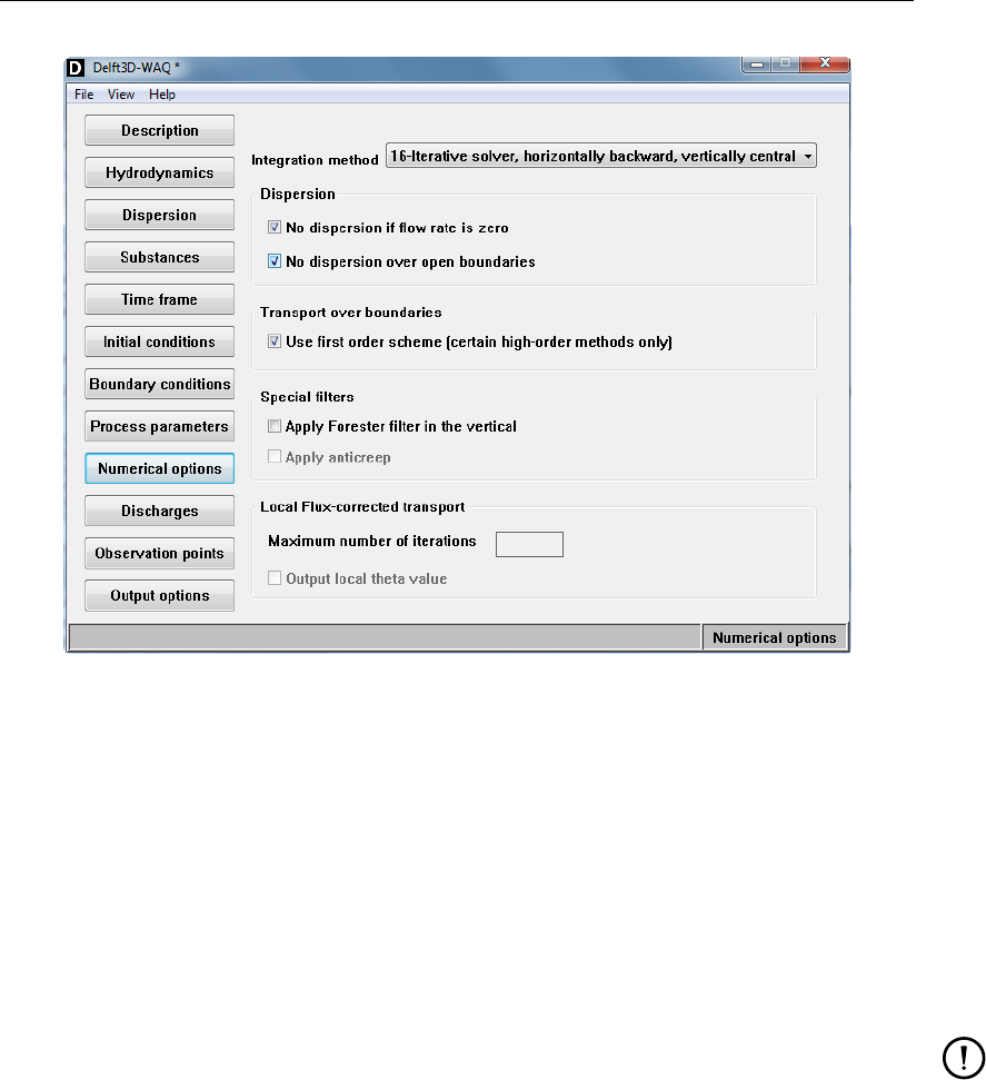
DRAFT
Graphical User Interface
Figure 5.38: Data Group Numerical options
5.3.9 Numerical options
In this data group the numerical scheme to solve the advection-dispersion equation can be
selected. The window contains a drop-down box and three frames for defining more detailed
numerical options for boundary conditions, dispersion and special filters (Figure 5.38).
You can scroll the Integration method drop-down box and you can select the numerical scheme.
Time-explicit and time-implicit methods are available. Numerical options also differ in their
handling of the vertical direction. In Section 10.5 more information about numerical integra-
tion methods can be found.
Remark:
If you have merged the multi-domain flow results into a single domain water quality
model, numerical schemes 19 and 20 are not allowed.
Numerical options for dispersion
Two options for dispersion are available:
No dispersion if the flow rate is zero. It is advised to tick off this checkbox for calculations
with tidal flats (areas that can be temporarily dry). Tidal flats require that for zero flow
there is no dispersive transport.
No dispersion over open boundaries. It is advised to select this checkbox in situations
where the boundaries are far away from your area of interest. In other words: preferably
the boundary sections should not influence the situation in your area of interest. The
(uniform) dispersion coefficient is a system property and is used to calibrate the system.
An (additional) dispersion effect over the open boundaries is unwanted in these cases.
Deltares 93 of 382

DRAFT
D-Water Quality, User Manual
Numerical options for transport over boundaries
One option is available for advective transport over the boundaries. It is advised to tick off this
checkbox in order to prevent numerical oscillations (boundary reflections) at the boundaries
for higher order spatial discretised schemes.
D-WAQ is especially designed for far-field modelling of large systems. In most of these cases
these three checkboxes will be ticked off.
Special filter - Forester
The Forester filter (in the vertical) is available for numerical schemes 3, 11, 12, 16 and 19.
It is well-known that second or higher order advective difference methods on coarse grids
may exhibit non-physical oscillations near regions of steep gradients. The different numerical
schemes do not guarantee positive solutions and consequently negative concentrations may
occur. In case of negative concentrations an iterative filter procedure based on local diffusion
followed by a vertical filter is started in order to remove the negative values. The filtering
technique in this procedure is the so-called Forester filter (Forester,1979), a non-linear ap-
proach which removes the computational noise without inflicting significant amplitude losses
in sharply peaked solutions.
If concentration cm,n,k is negative, then the iterative, mass conservative filtering process is
described (for the sake of simplicity only in one direction) by:
cp+1
m,n,k =cp
m,n,k+cp
m+1,n,k −cp
m,n,k
4min 1,Vm+1,n,k
Vm,n,k +cp
m−1,n,k −cp
m,n,k
4min 1,Vm−1,n,k
Vm,n,k
(5.1)
with Vm,n,k denoting the volume of cell (m, n, k). Only in grid cells with a negative concentra-
tion this filter is applied. The superscript pdenotes the iteration number. The filter smoothes
the solution and reduces the local minima (negative concentrations). Equation (5.1) can be
interpreted as an approximation of the following advection-diffusion equation:
∂c
∂t =α−β
4
∆x
∆t
∂c
∂x +α+β
4
∆x2
∆t
∂2c
∂x2+higher order terms (5.2)
with:
α= min 1,Vm+1,n,k
Vm,n,k ,
and:
β= min 1,Vm−1,n,k
Vm,n,k .
The Forester filter introduces an artificial advection and diffusion. The numerical diffusion
coefficient of the horizontal filter is:
Dnum =α+β
4
∆x2
∆t≤∆x2
2∆t.(5.3)
Thus the filter introduces numerical diffusion but only locally. Maximal 100 iterations are car-
ried out. If there is still a grid cell with a negative concentration after 100 iterations, then a
94 of 382 Deltares

DRAFT
Graphical User Interface
warning is generated. To further understand the influence of the Forester filter, we rewrite
Equation (5.1) as:
cp+1
m,n,k =1−α+β
4cp
m,n,k +α
4cp
m+1,n,k +β
4cp
m−1,n,k.(5.4)
As both α≤1and β≤1all coefficients of Equation (5.4) are positive. Consequently, a
positive concentration will remain positive, i.e. it will not introduce negative concentrations ir-
respective the steepness of the concentration gradients. A negative concentration surrounded
by positive concentrations, usually the result of ill represented steep gradients (wiggles), will
be less negative after one iteration and is effectively removed after several iterations by adding
enough (local) diffusion to force the concentration to become positive.
Local maxima and minima in temperature or salinity in the vertical direction, generated by the
computational method may give physically unstable density profiles and can also better be
removed by a numerical filter then by turbulent vertical mixing. A similar filtering technique
as in the horizontal direction is applied for points with a local maximum or minimum in the
vertical.
Special filter - Anticreep
For steep bottom slopes combined with vertical stratification, sigma transformed grids intro-
duce numerical problems for the accurate approximation of horizontal gradients in the horizon-
tal diffusion term. Due to truncation errors artificial vertical mixing may occur; see section 10.6
for details.
The anticreep filter can only be used for numerical schemes 19 and 20.
5.3.10 Discharges
In the Data Group Discharges, the discharge locations and specific details can be specified.
Figure 5.39 shows a list of discharges and geographical details of the selected discharge at
the lower half of the window. At the right-side, four buttons allow you to manage the discharges
and import the corresponding data or new discharge locations.
Discharges already present in the hydrodynamic calculation automatically transferred to the
water quality simulation and appear in the window with their names; the suffix ‘(new)’ is added
to distinguish them. For some discharges a numbered suffix can be added in order to dis-
tinguish between various layers. The number between brackets then refers to the number of
hydrodynamic layers in the water quality layer.
Restriction:
The name of a discharge is restricted to 20 characters.
Discharges can be specified with the use of the Visualisation Area (menu item View →Vi-
sualise area). After opening, use the Edit menu for selecting Discharges and use the Edit
Mode for setting the action (Add,Delete,Modify). If you use Add, every click within the model
area will add a new discharge. Details can be specified in the edit fields in the main window.
By selecting Delete and subsequent clicking on an existing discharge, the discharge will be
deleted. Modify means moving the discharge to another location. By selecting this option,
you can select an existing discharge, then click a new location within the model grid and the
discharge will move to this new location.
Deltares 95 of 382
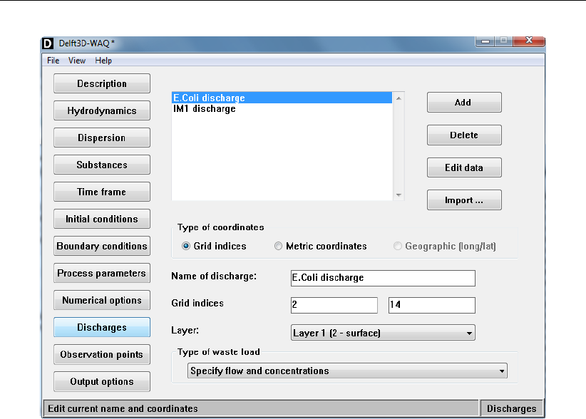
DRAFT
D-Water Quality, User Manual
Figure 5.39: Data Group Discharges.
Import data
Data of discharges (location and concentration!) can be imported from a file using the Im-
port. . . option. Data is usually available in a spreadsheet and — when set in the right format
— can be directly imported in the WAQ-GUI. Two file types are allowed:
Time-series file <∗.tim>
Simple locations/table file <∗.∗>
For a detailed description of the file formats refer to Appendix A. The files should contain
discharge names, co-ordinates and concentrations or mass loads. Again, concentrations can
only be used if the flow rate is not equal to zero. If the flow rate is zero, the value will be
interpreted as a mass load.
Edit data
Discharges can also be defined by specification of the grid indices and the layer number by
hand. By selecting a discharge in the list box and pressing Edit data, flows and concentrations
of the discharge can be specified.
The Data for: <Discharge name>window contains the following menu items:
Data Copy. . . Copies data from another discharge.
Import. . . Select a secondary file to import parame-
ter values; the Import data file window is
opened.
Quit Closes the Data for: <Discharge name>
window without saving changes; a confir-
mation is asked.
Save and exit Closes the Data for: <Discharge name>
96 of 382 Deltares

DRAFT
Graphical User Interface
window and saves the input.
Edit Copy row Copies the row containing the prompt and
put the new row above it in a table.
Delete row Deletes a row from a table.
Fill column Copies the selected value into the whole
column.
Properties Data properties You can set two options (Figure 5.33):
Are the boundary conditions constant
in time or varying in time? Variation in
time can be as a block function or as a
linear function.
Are the boundary conditions constant
over depth of varying over depth?
Additional to the concentrations of the substance in the discharge, each discharge has a flow
rate (in [m3/s]) as well. Discharges taken from the hydrodynamic simulation always have a
non-zero flow rate.
Layer specification
The layer in which the discharge is placed, can be selected in the drop-down box at the
bottom of the window. When you select the option Uniform over depth, the discharge will
be distributed over the complete water column. The discharge will be scaled in accordance
with the vertical aggregation. Thus, if three hydrodynamic layers are aggregated to two water
quality layers (depth ratio 1:2), 1/3 of the discharge will be placed in the single layer, while 2/3
will be placed in the double layer.
The option Uniform over depth is only available for a 3D water quality model.
Type of waste load
Seven types of waste load modelling are supported:
Specify flow and concentrations
Specify mass
Uniform waste load at surface
Uniform waste load at bed
Uniform waste load at bank
Waste load modelling rainfall
Waste load modelling seepage en infiltration
The description of these waste loads is followed by the special case of Automated Intake –
Outlet coupling.
Deltares 97 of 382

DRAFT
D-Water Quality, User Manual
Specify flow and concentrations
The discharge is specified as a combination of flow rate (in m3/s) and concentration (per m3).
If the specified flow is positive, then the values for the substances are used as concentrations
and mass is determined by multiplying them with this flow rate. If the specified flow is neg-
ative and the concentrations are not zero, the specified concentrations are withdrawn. If the
specified flow is negative and the concentrations are zero, the model concentrations will be
withdrawn.
Specify mass
The discharge is specified as a load [g/s]. In this case the flow rate is implicitly taken to be
one. Withdrawals can be specified using negative loads.
Uniform waste load at surface
The discharge is proportional the surface of the cell, for each computational cell that has a
water surface. The general rules for positive/negative flow and (non-)zero concentrations from
Specify flow and concentrations apply. Specified values are /m2.
Uniform waste load at bed
The discharge is proportional to the horizontal surface area for each computational cell that
has a water bed underneath. The general rules for positive/negative flow and (non-)zero
concentrations from Specify flow and concentrations apply. Specified values are /m2.
Uniform waste load at bank
The discharge is proportional to the length of a cell’s embankment. It is meant to support the
effect of diffuse influxes from riparian land into rivers and estuaries. This special waste load
requires the presence of a parameter or segment function with the ID LENGTH for all cells. To
be able to define this parameter in the WAQ-GUI, the following code needs to be add is to the
substance file that is used:
parameter ’Length’
description ’Bank length’
unit ’(m)’
value 0.0000E-00
end-parameter
You need to import the subtance file into the WAQ-GUI again after adding the parameter.
Specified values are /m.
Waste load modelling rainfall
This is a special case of Uniform waste load at surface. The specified concentrations are used
by D-WAQ if the flow is positive (rainfall) and zero concentrations are always used if the flow
is negative (like for evaporation).
Waste load modelling seepage en infiltration
This is a special case of Uniform waste load at bed. This indicates that the specified con-
centration should be used if the flow is positive (seepage) and that the model concentration
should always be used if the flow is negative (for infiltration to the groundwater).
98 of 382 Deltares
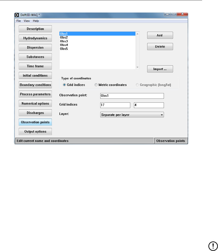
DRAFT
Graphical User Interface
Figure 5.40: Data Group Observation points
Automated Intake – Outlet coupling
When modelling power plants two coupled discharges are used: the water withdrawn at the
intake is discharged at the outlet. If the user-defined concentration at the intake is 0 then the
concentration at the intake is used in the withdrawn water and the discharged water. If the
user-defined concentration at the intake is not 0, then this concentration is used at the outlet.
At the outlet the discharge rate and concentration are irrelevant. The mass extracted at the
intake is discharged at the outlet.
If the FLOW model contains discharges in the form of power plants, opening the hyd-file will
result in couples of discharges with a predefined name: INLETx and OUTLETx, followed by
the FLOW discharge name.
Remark:
Every time you import a hydrodynamic file <∗.hyd>the discharges that are present in
the hydrodynamic simulation are added to the list of discharges. The WAQ-GUI does
not check if the discharges already exist. If double counting occurs, discharges should
be removed from the list.
Deltares 99 of 382

DRAFT
D-Water Quality , User Manual
5.3.11 Observation points
In the Data Group Observation points you define the locations (computational cells) for which
you want to write information to the history files (<∗.his>and <∗.hda>), the balance file
<∗-bal.his>and the monitoring file <∗.mon>.
A listing of observation points is shown with three buttons at the right in the upper half of the
window. On the lower half the details of the selected observation point are displayed and are
available for editing.
There are three ways to specify observation points:
Import co-ordinates from an ASCII file
Use the Visualisation Area
Use Add and specify co-ordinates in the edit fields
Restriction:
The name of an observation point is restricted to 20 characters.
Importing from text file
If you click Import. . . , a dialog appears where you have essentially two choices:
Select and use a file with so-called observation areas (file name by default: <∗.dmo>).
Observation areas are collections of individual computational cells, the concentration in
each cell is averaged and the mass balances, if any, are computed for the cells as a
whole. There can be only one such file and the contents can not be edited. Instead you
can use a program like D-Waq DIDO to generate the file.
Select a file with individual cells that become monitoring points (file name by default:
<∗.obs>).
Files with observation areas are supposed to have the following layout:
# Structure of a *.dmo file:
# The file may contain comment lines at the start
# After the comments:
# - The number of observation areas
# - Per observation area:
# - the name (enclosed in single quotes)
# - the number of grid cells in the observation areas
# - a list of indices of grid cells (separated by spaces)
#
# Example:
2
’Area_1’ 5
12345
’Area_2’ 4
6789
Remark:
Between the last comment line and the line with the number of areas, there may not be
a blank line.
The definition of an <∗.obs>file is explained below.
100 of 382 Deltares

DRAFT
Graphical User Interface
# Structure of an *.obs file:
# The file is a comma-separated ASCII-file,
# containing a header and on each line an observation point.
# The format of the header is fixed!
# The header contains: x-co-ordinate, y-co-ordinate, layer, name
# If layer is 0 then it will be "Uniform over depth".
#
#
# Example:
# x, y, layer, name
18000, 22625, 1, central obs-point
13373, 11621, 0, southwestern obs-point
22462, 23552, 4, northwestern obs-point
Click Open and the observation points are added to the list. Details of each observation point
can be adjusted or added if necessary. A warning will be given if an observation point is not
within the active model grid.
Remarks:
The co-ordinates in the <∗.obs>file should be in the same projection / co-ordinate
system as the model grid
Files with observation points should contain the actual grid cell numbers that also take
the layer number into account.
Moving Monitoring points
A special feature is the "moving monitoring point" for which the location is not fixed in time.
The monitoring point can be used to compare model data with moving measurement devices
like drifters or vessels sailing a trajectory. This is a single segment observation point with a
name starting with "MOVING", if there exists a function (see process parameters) with exactly
the same name then the segment number of the observation point will be set with the value of
the function evaluated at the current time. The value of the function is the segment number.
Since the value is discrete one should use only block functions to specify a moving monitoring
point. If there is no observation for a certain period a value of 0 can be specified. For this
period the output of the moving monitoring point will be a missing value. The segment number
in the specification of the monitoring point should be given but is not used. To create a list
of segment numbers from coordinates is not trivial. Fortran code is available to create the
function from coordinates for Delft3D kind of grids.
Example of a function to specify a moving monitoring point called MOVING_Ferrybox:
FUNCTIONS MOVING_Ferrybox
BLOCK DATA
2012/01/01-00:00:00 0
2012/01/22-08:24:00 2207
2012/01/22-08:25:00 2206
2012/01/22-08:26:00 2206
...
...
2012/01/22-18:21:00 2091
2012/01/22-18:22:00 0
2013/01/01-00:00:00 0
Using the Visualisation Area
Observation points can also be specified with the use of the Visualisation Area (menu item
View →Visualise area). After opening, use the Edit menu for selecting Observation points
and use the Edit Mode for setting the action (Add,Delete,Modify). If you use Add, every
Deltares 101 of 382

DRAFT
D-Water Quality, User Manual
click within the model area will add a new observation point. Details can be specified in the
edit fields in the main window. By selecting Delete and subsequent clicking on an existing
observation point, the point will be deleted. Modify means moving the observation point to
another location. By selecting this option, you can select an existing observation point, then
click a new location within the model grid and the observation point will move to this new
location.
Using Add
The third way to add observation points is to use the Add button. By clicking Add, the list
with observation points is extended and is showing “(new)”. Specify grid indices or metric
co-ordinates (a warning will appear if the co-ordinates are not within the active grid). Other
details can be specified as well.
Removing an observation point
Selecting the observation point in the list and clicking Delete will delete the observation point
(after confirmation).
Layer
The options Averaged over depth and Separate per layer only apply to a 3D water quality
model.
By selecting the option Separate per layer for the Layer position of the observation point,
output will be generated for each layer at that position. In the output files the name of the
observation point will be extended with the number of the layer between brackets to distinguish
between the layers.
It is useful to specify observation points at locations where data from measuring campaigns
are available. Information from observation points may also be used to check input of dis-
charges, or simply the compliance with standards.
5.3.12 Output options
In this data group a selection from the numerous output results can be made in order to
reduce the sizes of the output files. Graphical output can be plotted with Delft3D’s Graphical
Post-Processing package GPP or with QUICKPLOT.
The window is divided into three parts (Figure 5.41), from top to bottom:
Timer information
File type information
Output options (which files, which substances and statistics)
Timer Information
The upper frame (Times in water quality calculation) shows the timers specified in the Data
Group Time frame. They are indicated for informative purposes only, as they are useful to
specify the timers for which you would like to have output.
102 of 382 Deltares

DRAFT
Graphical User Interface
Figure 5.41: Data Group Output options
Output timers
D-WAQ generates three main types of output files:
1. Monitor output Results for observation points will be printed in an ASCII report file
<∗.mon>. Results will be given in the period with a start time, a
stop time and a certain time interval. Start time,Stop time and Time
interval for this output can be specified in the corresponding edit
fields. Default: time interval in coupled hydrodynamics.
2. History output Time-series information for the observation points will be written to
either a binary file or a NEFIS file (or both). Start time,Stop time and
Time interval for this output can be specified in the corresponding
edit fields. Default: time interval in coupled hydrodynamics.
3. Map output Spatial plots of concentration distribution will be written to either a
binary file or a NEFIS file (or both). Start time,Stop time and Time
interval for this output can be specified in the corresponding edit
fields. Default: time interval in coupled hydrodynamics.
Output files
By pressing Files you can specify the Type of output files in the Select output files window
(Figure 5.42).
D-WAQ produces output files suitable for several platforms: output files can be either:
PC based (binary or NEFIS) or:
Linux/UNIX based (binary/unformatted or NEFIS);
NEFIS and binary files contain the same information, so that it is not necessary to select both
(if you select both, a lot of redundant information is stored).
Deltares 103 of 382
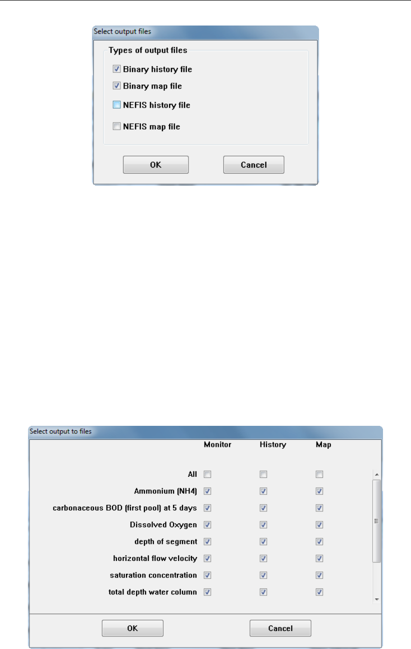
DRAFT
D-Water Quality, User Manual
Figure 5.42: Specification of output files. The output in NEFIS format is switched off
For post-processing using GPP or QUICKPLOT you need to specify the following data set/file
types.
binary/binary-unformatted;
DELWAQ | binary history file (<∗.his>);
DELWAQ | binary map file (<∗.map>);
NEFIS:
DELFT3D | water quality history file (<∗.hda>);
DELFT3D | water quality map file (<∗.ada>);
Parameters to output
You can (un)select specific output parameters for the different types of output files. Press
Select at the bottom of your window; the Select output to files window will pop up.
Figure 5.43: Select output to files window
You may activate the kind of output required by ticking on or off the check box. You can use
the checkbox All to (un)select the whole column for that output file at once.
104 of 382 Deltares
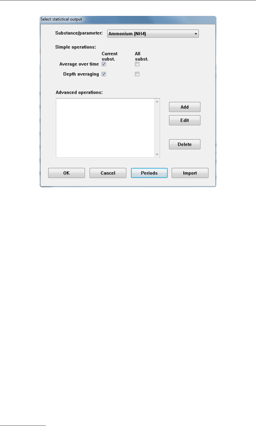
DRAFT
Graphical User Interface
Figure 5.44: Select statistical output main window
Statistics
By clicking Statistics, you can specify statistical output of your water quality calculation. The
Select statistics output window is displayed in Figure 5.44.
For more information on the statistical output functions see Appendix C.
The window consist of a drop-down list containing all substances and checkboxes to switch
statistics on or off. Checkboxes for every substances and output parameter are available. You
can use All subst. to switch all substances on/off. Statistics are divided into:
Average over time
Depth averaging
Advanced operations
The selected statistics are generated for each defined period.
At the bottom, the following options are available:
OK - Confirming your statistical output settings and go back to the main Output options
window.
Cancel - Cancelling your statistical output settings and go back to the main Output op-
tions window.
Periods - Specification of the time periods to use in the statistical analysis.
Import - Select and import an existing statistical file <∗.stt>.
Defining Periods
In order to retrieve statistical output, you can define specific period(s) for which you want to
have statistical output. By clicking Periods you can specify new periods or get an overview
Deltares 105 of 382
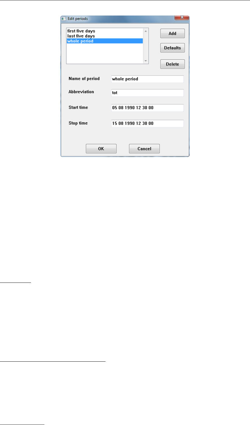
DRAFT
D-Water Quality, User Manual
Figure 5.45: Periods in statistical output
of the periods you have defined so far (Figure 5.45). A period is defined by its name, a start
time and a stop time. An abbreviation is used to distinguish the periodical statistical output
in the output files (<∗.map>,<∗.his>,<∗.mon>, etc.). Statistical output is generated for
each period. For example, in Figure 5.45 three periods are defined. If Average over time is
selected, an average value will be calculated for the three periods independently. Note that
periods may overlap.
The Add button adds a period to the list. You can specify name, abbreviation, start and stop
time in the edit fields underneath the list. Delete will remove the selected period. By clicking
Defaults, the start and stop time of the selected period will be set to the start and stop time of
the water quality calculation as specified in the Data Group Time frame.
Output files
Two additional files are generated that contain the output of the statistical analysis:
A monitor file containing the monitor output (<∗-stat.mon>). This is an ASCII file contain-
ing the values for all observation points defined in the Data Group Observation points.
Map file (<∗-stat.map>) containing the statistical output for every grid cell of the model
area.
Statistical time-series such as daily averages are added to the history file (<∗.his>or <∗.hda>).
Average over time (Standard Statistics)
For the standard statistics the following output is produced per period:
Minimum value
Maximum value
Mean value
Standard Deviation
Depth averaging
For the depth averaging statistics the following output is produced per period:
106 of 382 Deltares
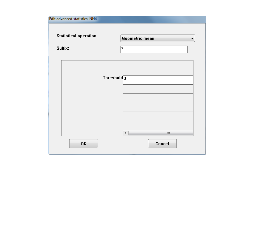
DRAFT
Graphical User Interface
Figure 5.46: Advanced statistics window. For NH4 three advanced statistics are de-
fined: periodic averages, exceedance times, and a 90% quantile
Minimum depth average value
Maximum depth average value
Mean depth average value
Standard deviation of the depth average value
Advanced statistics
By clicking Add or select an advanced statistical operation and then Edit, the Edit advanced
statistics window will open (Figure 5.46).
Four advanced operations are available:
Geometric mean: Useful for substances with a large range and relatively high values (e.g.
coliform bacteria concentrations). You have to set a Threshold value as well, as negative
and zero values are not allowed in a geometric (i.e. logarithmic) mean calculation.
Periodic averages: If you want to have for example hourly or daily averages, you can use
the data-time string (“dd mm yyyy hh mm ss”) to set this Period. Daily averages will be
“01 00 0000 00 00 00”). You can specify a Start time, if necessary.
Percentage (Exceedance time): This statistical method calculates the time that the se-
lected substance is above (Exceedance = “Yes”) or beneath (Exceedance = “No”) a certain
value (Critical concentration).You have to specify the critical value.
Quantiles: This method calculates the value that is not being exceeded for a certain %
of the time (Quantile in % to be reported). You can specify the number of buckets (more
bins is more accurate) and a lower and upper boundary. The actual concentration that
you model, should fall within this range.
By using Add you can add a statistical operation. By clicking Edit you can redesign and by
clicking Delete you can delete the advanced statistics for the selected substance or output
parameter.
If you switch to another data group (after closing all relevant windows of the statistics) the
statistical specifications will be stored in a separate file, the <∗.stt>file. You can re-use this
Deltares 107 of 382
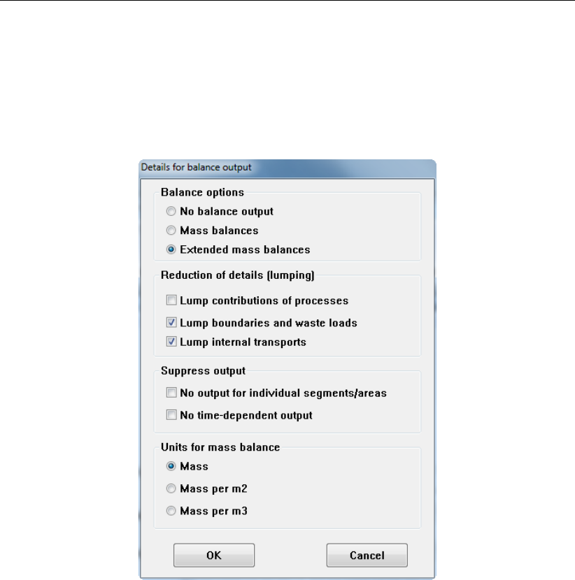
DRAFT
D-Water Quality, User Manual
file in other water quality calculations by using the Import . . . option in the Select statistical
output window (Figure 5.44).
Balances
The balance output for D-WAQ includes a number of options (see Figure 5.47)
Figure 5.47: Details for balance output window
The overall option selects the type of balance information:
No balance output: there will be no information about mass balances beyond what is
written to the monitoring file.
Mass balances: The computational program will write detailed information about the
mass balances (transport fluxes of each substance, contributions of the various wa-
ter quality processes and so on) in the monitoring points and monitoring areas to a
separate history file.
Extended mass balances: The program will write extra information with respect to the
model area as a whole to a report file.
A number of sub-options are available with the extended mass balances option:
The level of detail can be set:
◦You can either have the contribution of all individual processes reported or have
them “lumped” into a single term.
◦The same thing is separately possible with transports over the boundaries and
waste loads and with the internal transports.
You can suppress output for individual monitoring points (segments) and monitoring
areas (leaving only the overall mass balance term) and for the monitoring timesteps
(leaving only the terms accumulated over time).
108 of 382 Deltares

DRAFT
Graphical User Interface
These options are meant to help you get a useful report:
If you want an overview, then suppressing a lot of the details can help you to focus on
the overall features.
However, if you have a problem (some strange or unexplained results in some region
of the model for instance), then it can be very helpful to get as much details as you
can.
In general, the overall report gives you insight in the behaviour of the model as a whole.
The unit for the mass balance terms can selected:
The terms can simply be the total mass [g].
The terms can be divided by the total surface area [g/m2].
The terms can be divided by the total volume [g/m3].
Each option can be useful at times, depending on the kind of analysis you want to make.
5.3.13 Saving the scenario file
As you went to all data groups, the input for the scenario is now completed. Under the menu
item File, you can Save (or Save As. . . ) the scenario. Note that the extension of the scenario
should be <∗.scn>. This file stores the scenario for further adaptation or inspection with the
WAQ-GUI. Simultaneously, a file with the extension <∗.inp>is saved with the same run ID
as the <∗.scn>file. The <∗.inp>file is used by the pre-processors and the water quality
module.
Restriction:
The run ID may not contain blanks.
5.3.14 Addition of a sediment grid
After completion of the model set-up (substances, processes, hydrodynamics, computational
grid, loads, forcing, boundaries, etc.) a sediment grid can be added to the water grid. How-
ever, this is not supported by the present GUI. Once you have produced a complete model
input file and ran the resulting model successfully using the WAQ-GUI, the sediment grid and
the additional required input with respect to the sediment (composition, transport process,
deep boundary, etc.) can be added to the input file (ascii) by means of manual editing. Two
additional user manuals are available for this: ’Documentation of the input file’ and ’Sediment
Water Interaction’.
Deltares 109 of 382

DRAFT
D-Water Quality, User Manual
110 of 382 Deltares
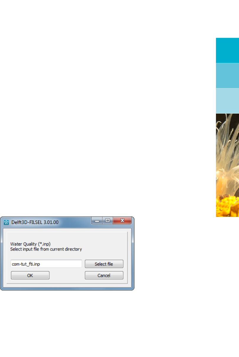
DRAFT
6 Running and post-processing (Delft3D)
6.1 Running
6.1.1 Pre-processing: input verification
After definition of a water quality scenario the simulation can be carried out. Basically, running
a simulation involves three steps:
1 Pre-processing Check whether the input for the simulation is complete and correct.
2 Processing Carry out the simulation and generate output.
3 Post-processing Check the output and present results.
Pre-processing a water quality simulation is easy. By clicking Waq (1) in the Water quality
and ecology window, the pre-processing is started.
By clicking Waq (1) a file selection window is opened (Figure 6.1) in which you have to specify
the name of the input file <∗.inp>. The input file <∗.inp>has the same run ID as the
scenario file <∗.scn>; they are both saved by the WAQ-GUI. A file can be selected through
the Select file dialogue. However, it is required that the input file <∗.inp>is located in the
working directory. If this is not the case, you will have to change the working directory first.
How to change the working directory is described in section 4.3.
Figure 6.1: Select input file
The pre-processor runs in a new window, see Figure 6.2.
You can close this window if the pre-processor finishes with a ‘Normal end’.
The pre-processing generates two files that are available for inspection:
1 List file <∗.lst>
The list file <∗.lst>checks whether the input is complete and the syntax of the input file
<∗.inp>is correct.
2 Report file <∗.lsp>
The Report file <∗.lsp>(or ‘list of processes’ file) determines which water quality pro-
cesses are selected (switched on) and determines where to retrieve the parameter input
for the processes.
Deltares 111 of 382

DRAFT
D-Water Quality, User Manual
Figure 6.2: Window with running information about the WAQ pre-processor
6.1.2 List file <∗.lst>
The list file <∗.lst>can be reviewed through the Reports |Input options in the Water quality
(WAQ) selection window (Figure 4.3). The file will be opened in the default text editor. The list
file <∗.lst>is in ASCII format and can be inspected in every text editor.
The list file <∗.lst>provides an overview of all the input specified in the WAQ-GUI. Usually it
is no use trying to review the complete file. One of the last lines of the list file <∗.lst>should
read:
Number of ERRORS during input : 0
If errors are found, you can search for the word ‘ERROR’ in the <∗.lst>to find the place of
the error. Subsequently, changes can be made in the WAQ-GUI. If the input file <∗.inp>was
generated with the WAQ-GUI, errors are normally not encountered.
Apart from errors, the list file <∗.lst>may give warnings. As the number of warnings is not
given at the end of the list file <∗.lst>, you should always look for the word ‘WARNING’ in
the list file <∗.lst>. Warnings usually deal with non-existing files, for example when files are
moved to another directory.
6.1.3 Report file <∗.lsp>
The report file <∗.lsp>can be reviewed through the Reports |Processes options in the
Water quality (WAQ) selection window (Figure 4.3). The file will be opened in the default text
editor. The reports file <∗.lsp>is in ASCII format and can be inspected in every text editor.
The report file contains the blocks listed below. The blocks are separated by the ’#’ character.
#1 Overview of processes that are switched on and determination per process whether the
input is complete. A warning is given if the input is incomplete.
#2 Fluxes, velocities and dispersions per substance.
#3 Additional processes for process-output only.
#4 Detailed process-input items for each active process.
#5 Identification if input parameters defined by you that are not used by the process system.
#6 Locating requested output from active processes.
112 of 382 Deltares

DRAFT
Running and post-processing (Delft3D)
#7 Updated memory requirement for the computational core (delwaq2).
#8 Presented messages (information, warning and errors).
Block 1
An overview of all processes selected in the substance file <∗.sub>and thus all processes
that are included in the water quality simulation. For each active process is reported if the
input is complete. If this is the case, the report file <∗.lsp>contains the following message:
Input for [RearOXY ] Reaeration of oxygen
Process is activated
Such a message is given for every activated process.
If for one or more input parameter no input is available a warning is given. The parameter for
which no input is available is specified like in the following message:
Input for [RearOXY ] Reaeration of oxygen
WARNING : activated process can NOT be switched on
Not found:[Depth ] depth of segment
Usually, the parameter has a missing value which can be specified either by entering a value or
deriving it from another process. You should go back to the WAQ-GUI or the PLCT to resolve
the problem. Note that the water quality simulation will run anyway: only the processes are
not taken into account resulting in an unwanted and therefore incorrect result. It is therefore
important that you check if all the processes are activated correctly.
Block 2
This is a very important block for you to check whether the right selection of processes from
the library has been made.
In this block an overview of the activated fluxes, dispersions and velocities that act on each
selected substance is given. Furthermore, you are informed which process will calculate the
flux, dispersion or velocity. So, except for the advective transport fluxes and discharges, this
block gives you the terms of the mass balance for each substance.
In the example below, four fluxes, one dispersion and no (settling) velocities for dissolved
oxygen (OXY) are found in the library (fictive example). The dispersion and the four fluxes are
used in the simulation; no velocities are found.
-Fluxes for [OXY ]
Found flux [dNITRIF ] nitrification flux
from proces [Nitrif\_NH4] Nitrification of ammonium
Process is switched on.
Found flux [dREAROXY ] reaeration flux
from proces [RearOXY ] Reaeration of oxygen
Switching [RearOXY ] on.
Found flux [dOxyBODCOD] oxygen consumption flux of BOD and COD
from proces [BODCOD ] Mineralisation BOD and COD
Process is switched on.
Found flux [dOxSOD ] oxygen consumption from SOD
from proces [SedOXYDem ] Sediment oxygen demand
Switching [SedOXYDem ] on.
-Dispersion for [OXY ]
Found dispersion[VertDisp ] vertical dispersion
from proces [VertDisp ] Vertical dispersion (segment -} exchange)
Process is switched on.
Deltares 113 of 382

DRAFT
D-Water Quality , User Manual
-Velocity for [OXY ]
No velocity found
Block 3
This block lists the additional processes that are switched on as a result of the segment
related process-output requested by you. The first item between straight brackets is the name
of the process (e.g. [DynDepth]) that calculates the requested output which is specified in the
second item between straight brackets (e.g. [Depth]).
# Locating processes for requested output
Switching [DynDepth ] on for output [Depth ]
Switching [Veloc ] on for output [Velocity ]
Switching [SaturOXY ] on for output [SaturOXY ]
Switching [TotDepth ] on for output [TotalDepth]
Block 4
In this block the status of all the processes that are switched on and for which the input
is complete is reported to you. For each process the report file <∗.lsp>specifies what
information is used for each parameter.
Information can be retrieved in eight different ways:
1 substance: The process parameter is included as a substance.
2 output from process: The process parameter is derived from another process.
3 segment function: The process parameter is included as a segment function (variable in
both time and space).
4 function: The process parameter is defined as a time-series (variable in time only).
5 parameter: The process parameter is included as a parameter (variable in space only).
6 DELWAQ: The process parameter is derived from the hydrodynamic model or an internal
D-WAQ variable for which no further specification is necessary.
7 constant: You have specified a constant value for the process parameter in the WAQ-GUI
<∗.scn>.
8 default: No input is specified in the WAQ-GUI <∗.scn>, the default value is used. The
default value is given as well.
Except for the ‘parameter’ all types of input occur in the example below:
Input for [RearOXY ] Reaeration of oxygen
[OXY ] Oxygen
Using substance nr 3
[Depth ] depth of segment
Using output from proces [DynDepth ]
[Temp ] ambient water temperature
Using function nr 1
[Velocity ] horizontal stream velocity
Using output from proces [Veloc ]
[VWind ] wind velocity
Using constant nr 5
[SWRear ] switch for oxygen reaeration formulation \file{1-11}
Using constant nr 6
[KLRear ] reaeration transfer coefficient
Using constant nr 7
[TCRear ] reaeration temperature coefficient
Using default value: 1.01600
[DELT ] timestep for processes
Using DELWAQ timestep in days
[SaturOXY ] saturation concentration
114 of 382 Deltares

DRAFT
Running and post-processing (Delft3D)
Using output from proces [SaturOXY ]
[Salinity ] Salinity
Using segment function nr 1
The numbers for the respective constants and (segment) functions refer to the order in the
scenario file <∗.scn>(or the input file <∗.inp>). For the values refer to these values or
check in the WAQ-GUI.
Block 5
In this block the input that is not recognised by the process system, is listed. Always check
block 5 of the report file! If an item is incorrectly spelled and not recognised by the process
system probably a default is used. Check the correct spelling either in block 4 of the report
file or in the Technical Reference Manual.
# Determine the use of the DELWAQ input
Constant [RcDetQ ] is NOT used by the process system
Parameter [Depht ] is NOT used by the process system
Function [Tempp ] is NOT used by the process system
Segment function [Zurfp ] is NOT used by the process system
Block 6
The sixth block of the report file <∗.lsp>specifies the origin of all output parameters you
request. Output variables are included in the substance file <∗.sub>and can be reviewed
in the WAQ-GUI. Output variables can be derived from processes as shown in the example
below, but can also be constants, default values, (segment) functions or parameters. Note
that the substances themselves are not reported here. They are by default included in the
output.
# Locating requested output from active processes
Output [Depth ] from proces [DynDepth ]
Output [Velocity ] from proces [Veloc ]
Output [SaturOXY ] from proces [SaturOXY ]
Output [RCREAR ] from proces [RearOXY ]
Output [SatPercOXY] from proces [RearOXY ]
Output [TotalDepth] from proces [TotDepth ]
Output [LocalDepth] from proces [TotDepth ]
Block 7
This block gives some technical information on computer memory etc. The information is only
in rare exceptions relevant for water quality simulations and can be taken for granted.
Block 8
Finally, the last block indicates the number of informative messages, warnings and errors. All
messages should be checked, as they may or may not be of relevance to you.
6.1.4 Running D-Water Quality
After pre-processing and checking that the input is correct, you can run the water quality
simulation. Click Waq (2) to start the simulation. No input file is requested anymore as it is
assumed that the last pre-processed input file (in the current working directory!) is the one
to be run. Make sure that you pre-process first after you made adaptations, before running
a simulation, otherwise these adaptations will not be incorporated in the actual simulation.
The pre-processors generate a ranges of temporary working files <∗.wrk>that are used in
Deltares 115 of 382
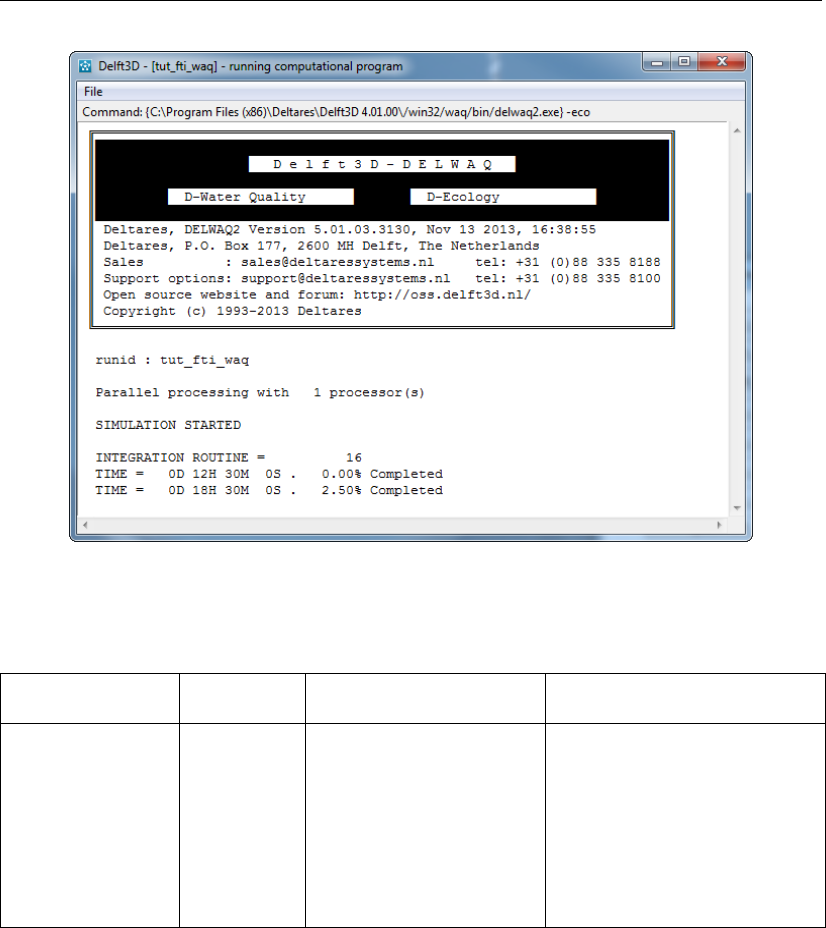
DRAFT
D-Water Quality, User Manual
Figure 6.3: Running a simulation. The simulation time relative to the reference time is
displayed
Table 6.1: Output files of D-WAQ and post-processing program
type of output file type file extension (format) post-processing program
time-series history file <∗.his>(binary) GPP, QUICKPLOT
<∗.hda>(NEFIS) GPP, QUICKPLOT
spatial map file <∗.map>(binary) GPP, QUICKPLOT
<∗.ada>(NEFIS) GPP, QUICKPLOT
mass balance balance file <∗-bal.his>(binary) GPP, QUICKPLOT
<∗=bal.prn>(ASCII) text editor
monitor monitor file <∗.mon>(ASCII) text editor
the water quality simulation. If you do not run the pre-processors, Waq (2) will use the old
<∗.wrk>files.
The simulation runs in a new window. The progress of the simulation can be viewed relative
to the reference time of the simulation (Figure 6.3). The time step is determined by the time
step of the monitoring file; refer to section 5.3.12 on how to change this time step.
6.2 Post-processing
116 of 382 Deltares

DRAFT
Running and post-processing (Delft3D)
6.2.1 Output files
A D-WAQ simulation generates different types of results (Table 6.1).
Time-series and spatial information are available in two formats: binary and NEFIS. As they
contain exactly the same information, usually only one type of format is selected. The type of
format can be selected in the Output options Data Group (refer to section 5.3.12). Time-series
information is saved for every observation point specified. Spatial information is saved for all
computational elements. Refer to the GPP and Delft3D-QUICKPLOT User Manuals on how
to visualise the results (GPP UM,2013;QUICKPLOT UM,2013).
Mass balances are available if the balance output option is selected in the Output options
Data Group. Mass balance information is available for every substance for every observation
point specified. The balance terms represent the accumulated fluxes during the time step in
the monitor file. For example, if the time step in the balance file is one day, the unit of the
fluxes is g/d. If the time step in the balance file is one week, the unit of the fluxes is g/week.
The balance file <∗-bal.his>has the same time step as the monitor file <∗.mon>. Refer to
the GPP User Manual on how to visualise the results.
The monitor file <∗.mon>contains information per observation point such as concentrations
of the substances and values of the output parameters. Also, a total mass balance for the
complete model area is given consisting of the terms: total mass in system, changes by
processes, changes by loads, boundary inflows and boundary outflows. The balance terms
represent the accumulated fluxes during the time step in the monitor file.
If the balance output option is switched on, a mass balance consisting of the same terms
is included for each observation point in the monitor file <∗.mon>. Note that contrary to
the balance file <∗-bal.his>no individual process fluxes are specified in the monitor file
<∗.mon>.
Deltares 117 of 382

DRAFT
D-Water Quality, User Manual
118 of 382 Deltares
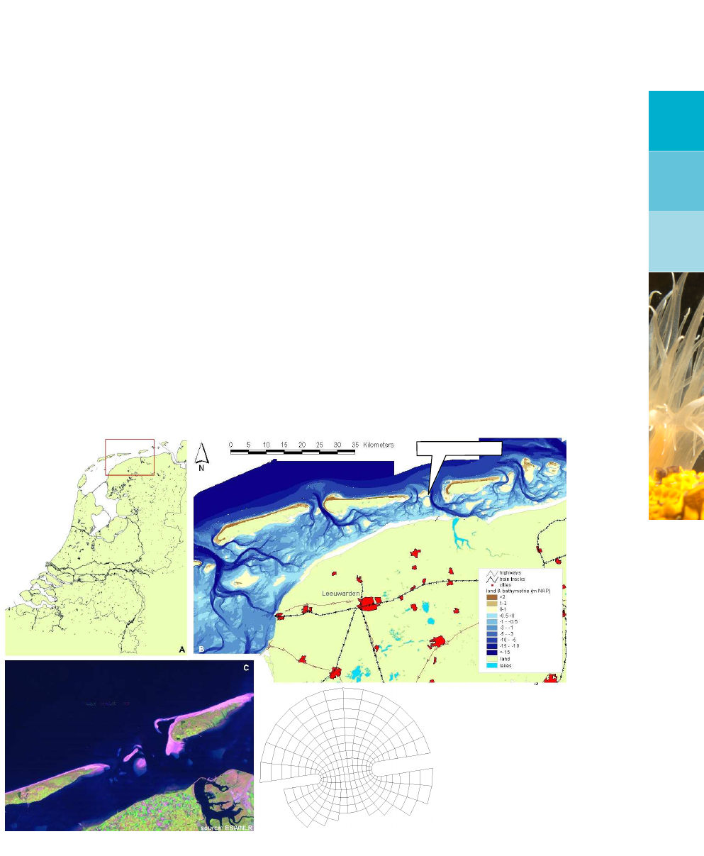
DRAFT
7 Tutorials
This tutorial contains two sections, one section about the 2/3-dimensional Delft3D-suite for
free surface flows, see section 7.1, and one section about the 1/2-dimensional SOBEK-suite
for free surface (1D/2D) and pressurized (1D) flow, see section 7.2.
7.1 Tutorial D-Water Quality for free surface flow (Delft3D-WAQ)
7.1.1 Introduction
This chapter can be used to get acquainted with the procedure to set up a water quality
calculation. A schematised case is used to guide you through the different steps and actions
necessary to perform a simulation.
The tutorial case concerns the area of the ‘Friesian Tidal Inlet’, which represents an opening
between the islands Ameland and Schiermonnikoog. We will perform a simulation of E.Coli
bacteria on a 1×1×2 aggregation of the hydrodynamic database.
D
A - Topographical map of the Netherlands
B - Topographical map indicating the
Friesian Tidal Inlet
C - Satellite image of the Friesian Tidal Inlet
D - Model grid of the Friesian Tidal Inlet
Friesian Tidal Inlet
Figure 7.1: ‘Friesian Tidal Inlet’: an opening between two islands in the north of The
Netherlands
This chapter gives both descriptive information about the steps to take to set up a water quality
calculation and GUI-operations to complete each step. The GUI-operations are displayed in
the textboxes with the grey header.
The input data will be generated on the directory <.../tutorial/waq/friesian_tidal_inlet>
Deltares 119 of 382

DRAFT
D-Water Quality, User Manual
7.1.2 Specifications of tutorial case ’tut_fti_waq’
Table 7.1 presents the specifications of the tutorial case.
Table 7.1: Specifications of tutorial case ’tut_fti_waq’
Area Friesian Tidal Inlet
Hydrodynamic database 12.5 hours, 15 min time step
(<com-tut_fti_waq.dat>,<com-tut_fti_waq.def>)
Horizontal aggregation inactive cells removed
Vertical layer aggregation 5 water quality layers
(10 hydrodynamic layers)
Time step aggregation none
Substance E.Coli
The D-WAQ model framework is started from the Delft3D-MENU as described in Chapter 5.
1. STARTING THE DELFT3D-MENU
Start Delft3D
Start Delft3D-MENU by using the desktop icon/Start button.
Click Water Quality.
Click Select working directory, and browse to the tutorial directory:
<.../tutorial/waq/friesian_tidal_inlet>
Click OK to confirm and to close the selection of your current working directory.
7.1.3 Conversion of the hydrodynamic results
7.1.3.1 Coupling module
2. STARTING THE COUPLING MODULE
In the Water quality and ecology window, select Coupling (Figure 4.3).
To start the COUP-GUI, select Define input, see Figure 5.9.
You are now accessing the GUI of the coupling module (Figure 5.11). The GUI is similar to
the general WAQ-GUI, but only the first three data groups are enabled. They will be described
in the following section.
120 of 382 Deltares

DRAFT
Tutorials
7.1.3.2 Definition of the input
The three datagroups which are enabled are:
Description
Hydrodynamics
Dispersion
The menu-items File and Help are also available.
7.1.3.2.1 Description
With Description you can add a file description in order to produce some meta-information
about the coupling. Three lines of descriptive information are available.
3. EDITING THE DESCRIPTION DATA GROUP
In the COUP-GUI, click Description.
Enter 3 lines (of max. 39 characters) of meta-information.
1 Friesian Tidal Inlet
2 Hydro: Flow tutorial with 10 layers
3 WAQ: Vertical aggregation to 5 layers
See Figure 5.11.
7.1.3.2.2 Hydrodynamics
With the Data Group Hydrodynamics the hydrodynamic database is selected. By clicking
Com-file, you can browse to and select one single <com-name.dat>file, which can be found
in the <delft3d\tutorial\waq\friesian_tidal_inlet\input_waq_fti>directory. By clicking Open,
the <com-tut_fti_waq.dat>file will be loaded into the GUI and information about this file will
be displayed.
Aggregation in time
The timers in the file will automatically appear in the Time information frame. Time steps can
be increased, for example in order to reduce the required disk space for storage. Hereto,
adapt the time step in the menu, but increase it only with an integer number (2 times, 3 times
etc.).
In this tutorial we do not aggregate in time, so no adjustment of timers is needed.
Deltares 121 of 382
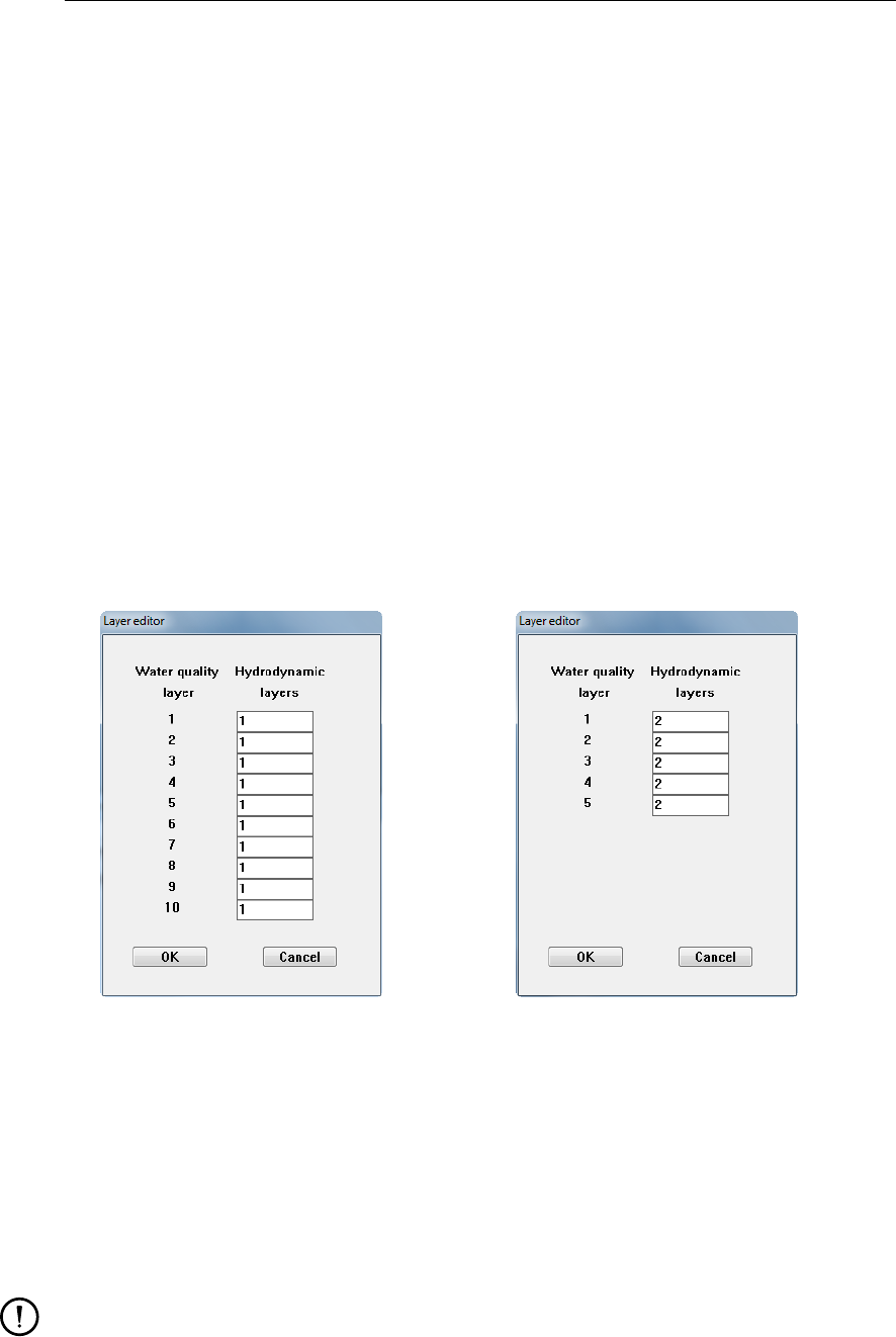
DRAFT
D-Water Quality, User Manual
Horizontal aggregation
The grid can be aggregated in the horizontal within the frame Horizontal aggregation. Select
under Type of either:
No aggregation: no spatial aggregation is used.
Use aggregation file (DIDO): This option requires an administration file (<∗.dwq>) and
can be either created or selected by you. A <∗.dwq>file is created by the grid edi-
tor DIDO. This WAQ tool can be activated from Delft3D-MENU. Consult the DIDO User
Manual for details about the spatial aggregation.
Remove inactive cells: all dry segments are deleted automatically.
In this tutorial the option of Remove inactive cells is chosen (see Figure 7.3).
Vertical aggregation
Layers can be aggregated in the vertical using the layer editor under button Edit layers. This
tutorial case contains 10 (hydrodynamic) layers. If no vertical aggregation is chosen, the num-
ber of water quality layers is equal to the number of hydrodynamic layers. To reduce storage
space and decrease calculation time, the number of water quality layers can be reduced.
Select Edit layers.Figure 7.2 will appear.
Figure 7.2: Vertical aggregation using the Layer editor
On the left part of the Layer editor window, the number of water quality layers is shown. On
the right-hand side, the corresponding number of hydrodynamic layers is shown. By changing
the number in the input boxes (more than one hydrodynamic layer are combined to one water
quality layer), the number of water quality layers decreases.
Create 5 water quality layers by, starting from the top, change the number of hydrodynamic
layers from 1 to 2, see Figure 7.2.
Remark:
The number of hydrodynamic layers remains intact (2+2+2+2+2=10). Many
other aggregations are possible: for example 2−3−3−2(i.e. 4 water quality layers
and 2 + 3 + 3 + 2 = 10) or 3−4−3(i.e. 3 water quality layers and 3 + 4 + 3 = 10).
122 of 382 Deltares
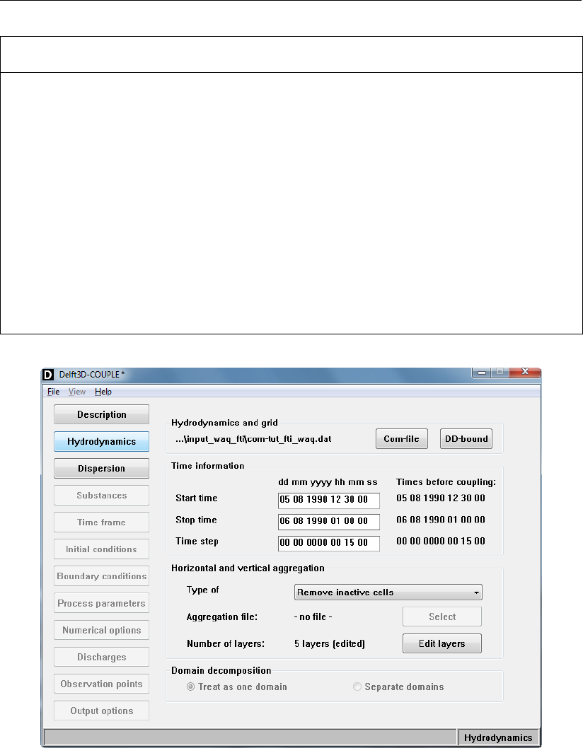
DRAFT
Tutorials
4. SPECIFYING AND AGGREGATION THE HYDRODYNAMIC DATABASE
In the COUP-GUI, click Hydrodynamics.
Click Com-file, and browse to the <. . . /tutorial/waq/friesian_tidal_inlet>directory to
select the <com-tut_fti_waq.dat>file.
Click Open to confirm (note that the details will be displayed in the Time information
frame).
In the Horizontal and vertical aggregation frame, select Remove inactive cells from the
Type of drop-down box.
In the Horizontal and vertical aggregation frame, click Edit layers.
From top to bottom, change in the first 5 entry boxes the “1” into “2”.
Click OK to confirm.
See Figure 7.3.
Figure 7.3: COUP-GUI - Data Group Hydrodynamics
7.1.3.2.3 Dispersion
Within the Data Group Dispersion you can choose to use the vertical diffusion from the hydro-
dynamic simulation. You can specify an interface depth and diffusion coefficients above and
below this interface.
In this tutorial case, the minimum vertical diffusion from the hydrodynamics is not used.
Deltares 123 of 382
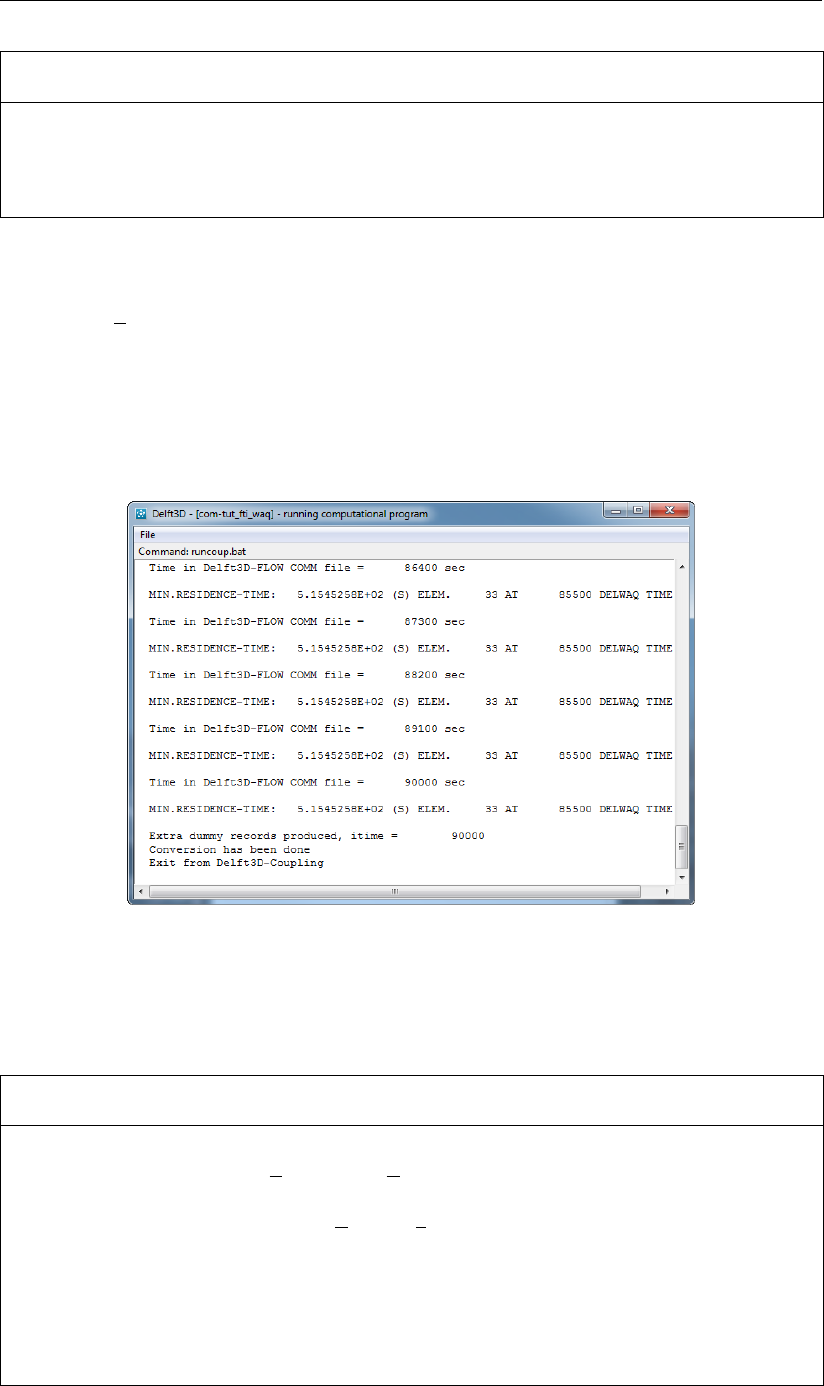
DRAFT
D-Water Quality, User Manual
5. EDITING DISPERSION
In the COUP-GUI, click Dispersion.
Inspect and do not change the (default) values.
7.1.3.3 Saving input and running the coupling module
By selecting File →Save (As) you are requested to save the file. Your current working direc-
tory is the right location. Give the filename <com-tut_fti_waq.hyd>. The extension <hyd>
will be given automatically on Windows platforms. Exit the GUI by selecting File →Exit from
the menubar, returning to the Hydrodynamic coupling window. Select Start and the cou-
pling module will start. A window will be opened in which the coupling of the hydrodynamical
database is carried out (see Figure 7.4). When the window displays ’Conversion has been
done’, you can c lose this window.
Figure 7.4: Screen output of the Coupling program
Result files of the coupling will be available in your current working directory. An interesting
file to inspect is the <couplnef.out>.
6. SAVING INPUT AND RUNNING THE COUPLING
In the COUP-GUI, select File →Save As. . . and save the file as <tut_fti_waq.hyd>in
your current working directory.
Exit the COUP-GUI by selecting File →Exit
Click Start, select the file <tut_fti_waq.hyd>and after pressing OK the coupling will
start in a new window.
As soon as ‘Conversion has been done’ is displayed, close the window.
To inspect the results, first go back pressing the button Return, next click Reports and
subsequently Coupling in the View reports file window.
For a complete overview of the graphical user interface of the Coupling module, see sec-
124 of 382 Deltares
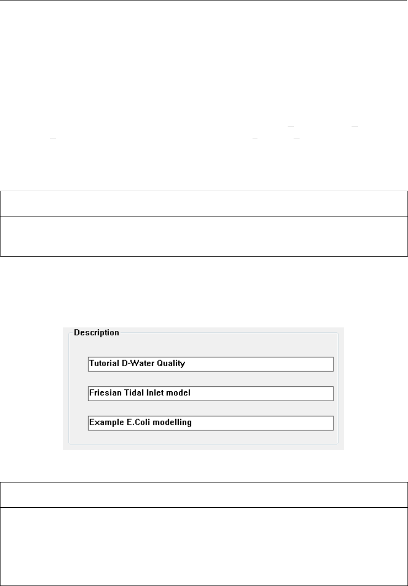
DRAFT
Tutorials
tion 5.2.
7.1.4 Preparing the water quality scenario
By clicking Define input in the Water quality and ecology selection window (Figure 4.3),
the WAQ-GUI is started. The GUI guides you through the various input blocks required in
the water quality modelling (Figure 5.17). After preparing all your water quality input, you
can store your results in a scenario file (<∗.scn>) by selecting Save or Save As. . . in the
menu-item File. You can exit the WAQ-GUI by selecting Exit in the File menu-item.
For every water quality calculation, you need to specify all data groups. For this tutorial case,
this part of the tutorial guides you through these data groups.
7. PREPARING THE WATER QUALITY SCENARIO:START THE WATER QUALITY GUI
In the Water quality (WAQ) selection window, click Define input.
7.1.4.1 Description
Three lines of 39 characters each can be used to specify some meta data. An example of this
meta data is given in Figure 7.5.
Figure 7.5: Meta data displayed in the Description window
8. PREPARING THE WATER QUALITY SCENARIO:DESCRIPTION
In the WAQ-GUI, click Description.
Enter “Tutorial D-Water Quality” in the first line.
Enter “Friesian Tidal Inlet model” in the second line.
Enter “Example E.Coli modelling” in the third line.
An extensive description of the Description Data Group can be found in section 5.3.1.
7.1.4.2 Hydrodynamics
In order to prepare a water quality simulation you must first select the coupled hydrodynamics.
By clicking the Select button, you can browse to the <∗.hyd>file, you just have coupled
<tut_fti_waq.hyd>. By selecting this file and clicking Open, the details of the hydrodynamics
are displayed: time information, horizontal and vertical aggregation. Note that you can only
inspect the results of the hydrodynamic coupling here, no changes can be made. If you want
Deltares 125 of 382
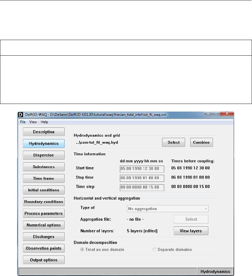
DRAFT
D-Water Quality, User Manual
to, you should close this scenario and return to the coupling module again. Implement your
changes there.
9. PREPARING THE WATER QUALITY SCENARIO:HYDRODYNAMICS
In the WAQ-GUI, click Hydrodynamics.
Click Select, browse to the <tut_fti_waq.hyd>file.
Click Open to confirm.
Inspect the displayed details of the hydrodynamics, see Figure 7.6.
Figure 7.6: Data displayed in the Hydrodynamics window
An extensive description of the Hydrodynamics Data Group can be found in section 5.3.2.
7.1.4.3 Dispersion
Dispersion coefficients are required to solve the advection-dispersion-reaction equation for
water quality modelling. The default values for Uniform dispersion can be adapted. The
Additional vertical diffusion coefficients can not be adapted. These coefficients are extracted
from the hydrodynamic database by the coupling program. These diffusion (or dispersion)
coefficients are called ‘additional’ since they are added to the uniform dispersion coefficients
defined for the horizontal plane. We advise you to set the uniform dispersion coefficient for
the vertical direction to a low value (e.g. 1.0·10−7) if for Additional vertical diffusion,Use
results from hydrodynamics is selected.
For the tutorial case, select the uniform dispersion by leaving the uniform default values un-
touched and specify Use results from hydrodynamics in the drop-down box in the Additional
vertical diffusion frame.
126 of 382 Deltares
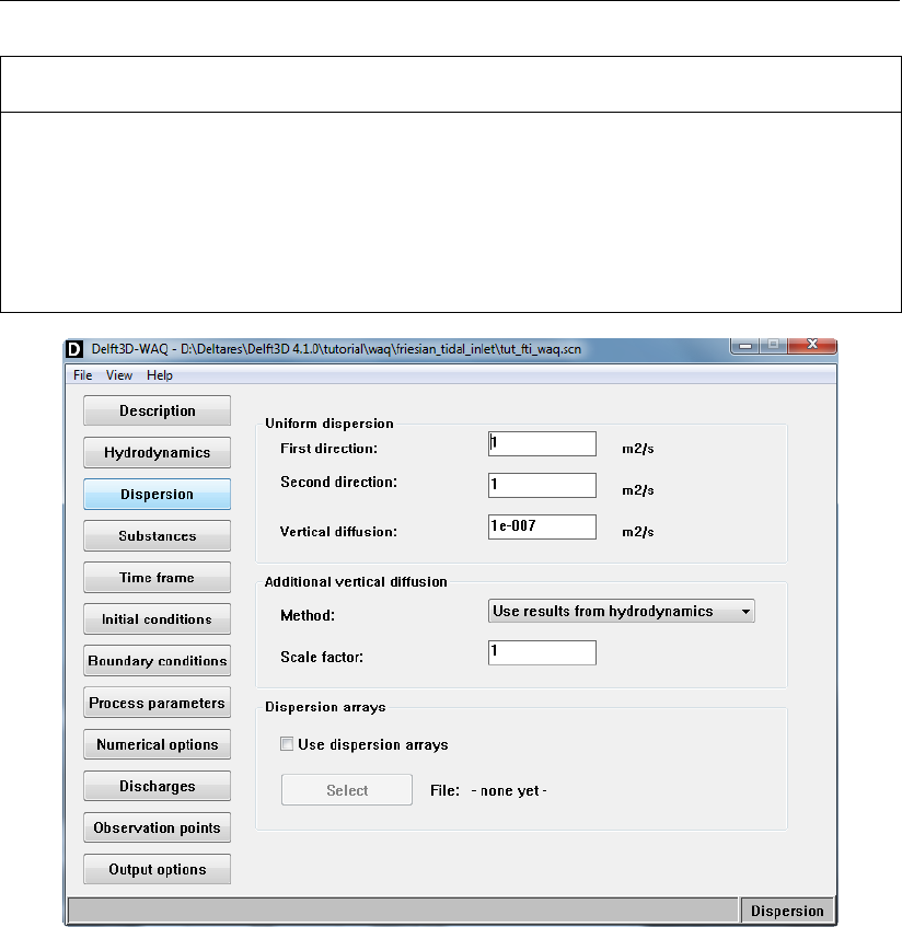
DRAFT
Tutorials
10. PREPARING THE WATER QUALITY SCENARIO:DISPERSION
In the WAQ-GUI, click Dispersion.
Inspect and do not change the (default) uniform dispersion values.
In the Additional vertical diffusion frame select Use results from hydrodynamics.
See Figure 7.7.
Figure 7.7: Datagroup Dispersion window
An extensive description of the Dispersion Data Group can be found in section 5.3.3.
7.1.4.4 Substances
The substances and processes you want to model in your water quality calculation must be
specified here. For the ’tut_fti_waq’ tutorial case, a so-called substance file, describing E.Coli
bacteria, is available. The corresponding filename is <coli_04.sub>. This file can be found
in the <. . . /tutorial/waq/substances>directory. To import this file, click Select and browse
to the mentioned directory, select the <coli_04.sub>file and click Open. The window as
displayed in Figure 7.8 will appear.
Of course, any other substance file created with the PLCT can be imported here. A separate
part of this manual describes the PLCT in detail. More information about this tool can be
found in section 5.1. A descriptive document explaining mortality of E.Coli bacteria can be in
section B.3.
Deltares 127 of 382
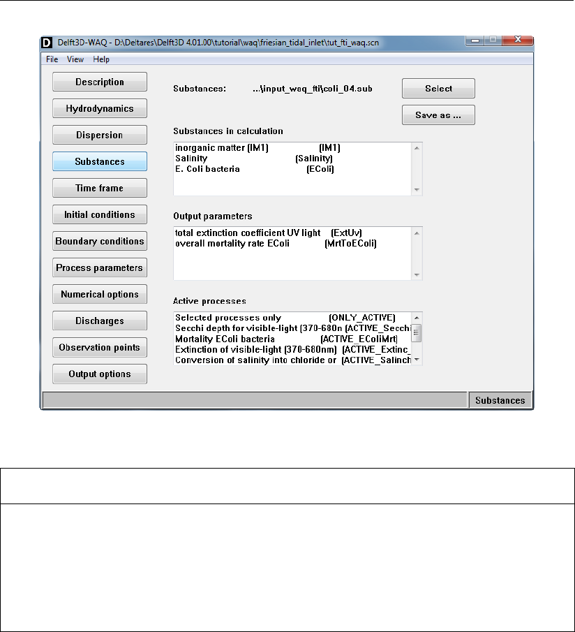
DRAFT
D-Water Quality, User Manual
Figure 7.8: Data Group Substances showing <coli_04.sub>
11. PREPARING THE WATER QUALITY SCENARIO:SUBSTANCES
In the WAQ-GUI, click Substances.
Click Select and browse to the <. . . /tutorial/waq/substances>directory to select the
<coli_04.sub>file.
Click Open to confirm.
Inspect the details which are loaded into the GUI, see Figure 7.8
An extensive description of the Substances Data Group can be found in section 5.3.4.
7.1.4.5 Time frame
In this data group, you should specify the start time, stop time and time step of the water
quality calculation. By default the values of the hydrodynamics are displayed. For the tutorial
case, the start time is the same as for the hydrodynamics (05 08 1990 12 30 00) but the stop
time should be changed to “15 08 1990 12 30 00”, so our calculation lasts for 10 days (the
hydrodynamics will automatically be ‘repeated’ every 12.5 hours). The water quality time step
remains 15 minutes. See Figure 7.9.
128 of 382 Deltares
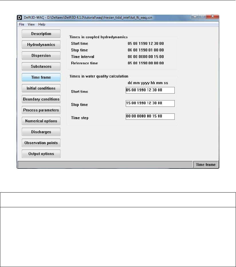
DRAFT
Tutorials
Figure 7.9: Time frame window
12. PREPARING THE WATER QUALITY SCENARIO:TIME FRAME
In the WAQ-GUI, click Time frame.
The content of the Start time entry box should be: “05 08 1990 12 30 00”.
The content of the Stop time entry box should be: “15 08 1990 12 30 00”.
The content of the Timestep entry box should be: “00 00 0000 00 15 00”.
See Figure 7.9.
An extensive description of the Time frame Data Group can be found in section 5.3.5.
7.1.4.6 Initial conditions
In this data group you specify starting (initial) conditions for all substances. Options are: a
constant value (uniform value for the whole model area) or non-uniform values. The list of sub-
stances to be filled in, is automatically generated and originates from the selected <∗.sub>
file.
In our tutorial case, three initial conditions need to be specified: Salinity [g/kg], E.Coli bacteria
[MPN/m3] and inorganic matter [gDM/m3]. We use uniform values for the substances. You
can use the following values, see Table 7.5.
Deltares 129 of 382
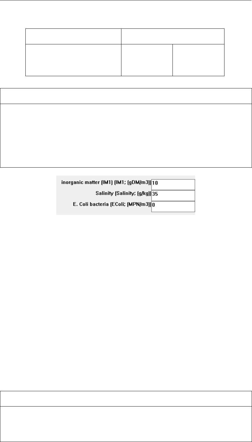
DRAFT
D-Water Quality, User Manual
Table 7.5: Initial Conditions
Substance Initial value [unit]
Salinity 35 [g/kg]
E.Coli bacteria 0 [MPN/m3]
inorganic matter 10 [gDM/m3]
13. PREPARING THE WATER QUALITY SCENARIO:INITIAL CONDITIONS
In the WAQ-GUI, click Initial conditions.
Select the inorganic matter entry box and enter the value: “10”.
Select the Salinity entry box and enter the value: “35”.
Select the E.Coli bacteria entry box and enter the value: “0”.
See Figure 7.10.
Figure 7.10: Initial conditions window
An extensive description of the Initial conditions Data Group can be found in section 5.3.6.
7.1.4.7 Boundary conditions
Boundary conditions are the concentrations of all active substances coming from the ’outside
world’ into the model area. These can vary in time, depth and location. Boundary conditions
may have an important effect on the final model results. Therefore, the model grid schematisa-
tion should be large enough to prevent any unwanted concentration fluctuations resulting from
these boundaries, or from irregularities in the hydrodynamic flows across these boundaries.
In case the boundaries are far away from the area of interest of the modeller (a discharge lo-
cation, an estuary, a harbour, a regional sea etc.) it usually suffices to take constant boundary
conditions (obviously the constants should be chosen carefully). However, for studies over
longer periods of time, time-dependent boundary conditions are often required.
For the tutorial case, in which we will focus on an E.Coli bacteria discharge, the boundary
conditions are the same as the initial conditions, so the values in Table 7.5 can be applied.
Select Boundary conditions and select the Left-right 1 boundary in the list. Click Edit data and
fill in the values from Table 7.5.
14. PREPARING THE WATER QUALITY SCENARIO:BOUNDARY CONDITIONS
In the WAQ-GUI, click Boundary conditions.
Select the Left-right 1 from the list.
130 of 382 Deltares
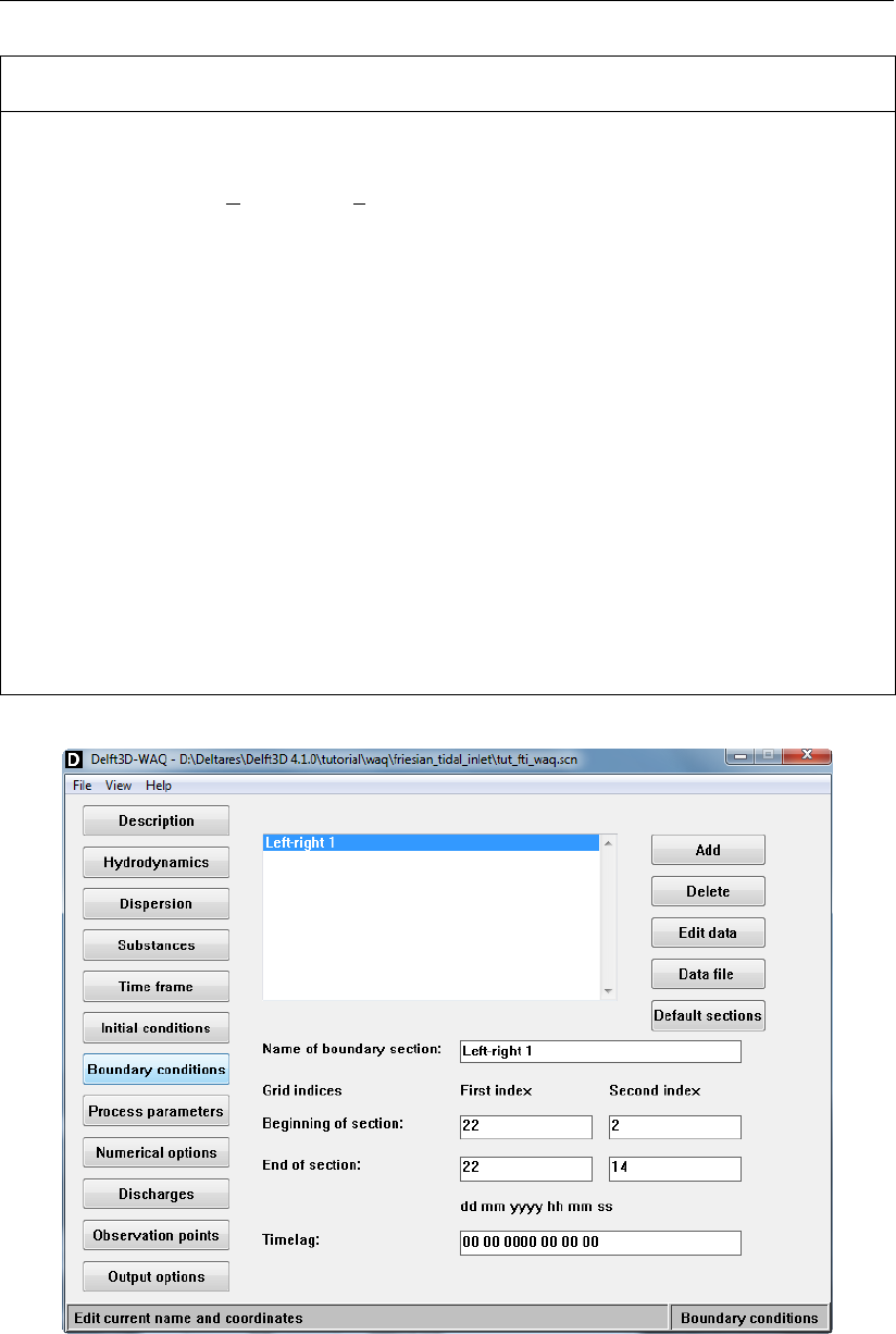
DRAFT
Tutorials
14. PREPARING THE WATER QUALITY SCENARIO:BOUNDARY CONDITIONS
To view the location of the open boundary
Select menu-item View →Visualise area to open the Visualisation Area window.
Select menu-item Edit and select Open boundaries (note that a round curved bold line
will appear in blue or red).
Close this window by selecting menu-item File →Exit.
To edit the Boundary conditions data
Open or go back to the main Boundary conditions window.
Select the Left-right 1 from the list.
Select Edit data.
Select the Salinity entry box and enter the value: “35”.
Select the E.Coli bacteria entry box and enter the value: “0”.
Select the IM1 entry box and enter the value: “10”.
Select menu-option Data →Save and exit to save the data and return to the main
window.
See Figure 7.11 for boundary conditions data.
Figure 7.11: Boundary conditions window
An extensive description of the Boundary conditions Data Group can be found in section 5.3.7.
Deltares 131 of 382
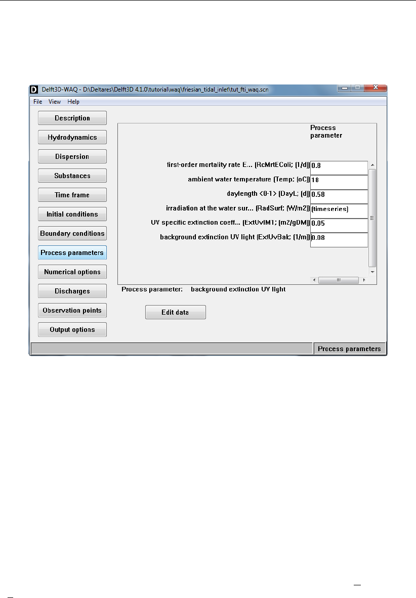
DRAFT
D-Water Quality, User Manual
7.1.4.8 Process parameters
In this data group the editable process parameters as selected within the Processes Library
Configuration Tool will appear. For the tutorial case, you need the following values.
Figure 7.12: Data Group Process parameters
First the irradiation will be discussed (see row 4 in Figure 7.12) and then the other parameters.
Irradiation
Ultraviolet (UV) light increases the mortality of E.Coli bacteria. In summer, more UV light
reaches the water surface so mortality will be higher. A more realistic approach for this pa-
rameter is a time-series. Summer values (during sunny circumstances) can reach up to 250
W/m2(total radiation). For the tutorial case, during a period of 10 days in August, the UV
radiation varies between 190 (lower bound) and 250 W/m2(upper bound). You can create the
time-series as follows:
In the Process parameters Data Group, select the parameter “irradiation at the water surface”
by clicking the entry box behind the parameter. Edit data will be enabled. Clicking this button
will bring up another window where you specify the data. Select menu-option Properties →
Data Properties and check the radio button Timeseries (block function) in the Time frame
(Figure 7.13).
132 of 382 Deltares

DRAFT
Tutorials
Figure 7.13: Specifying Timeseries in the Properties window
After confirming by pressing OK, the start time and stop time will appear in two different rows.
Behind each time breakpoint you can specify a value for irradiation. By default these values
are “-999” (missing values). See Figure 7.14.
Figure 7.14: Time breakpoints in Edit data window after specifying Data Properties
To increase the number of breakpoints, select Edit →Copy row. The selected row will be
copied. Use this option and change the content of the cells in such a way that it looks as in
Figure 7.15. Now every day in the calculation has its own irradiation value. After adding and
editing rows, select menu-option Data →Save and exit. Now the window as in Figure 7.12 will
appear again. The entry box behind irradiation at the water surface will indicate “[timeseries]”.
Deltares 133 of 382
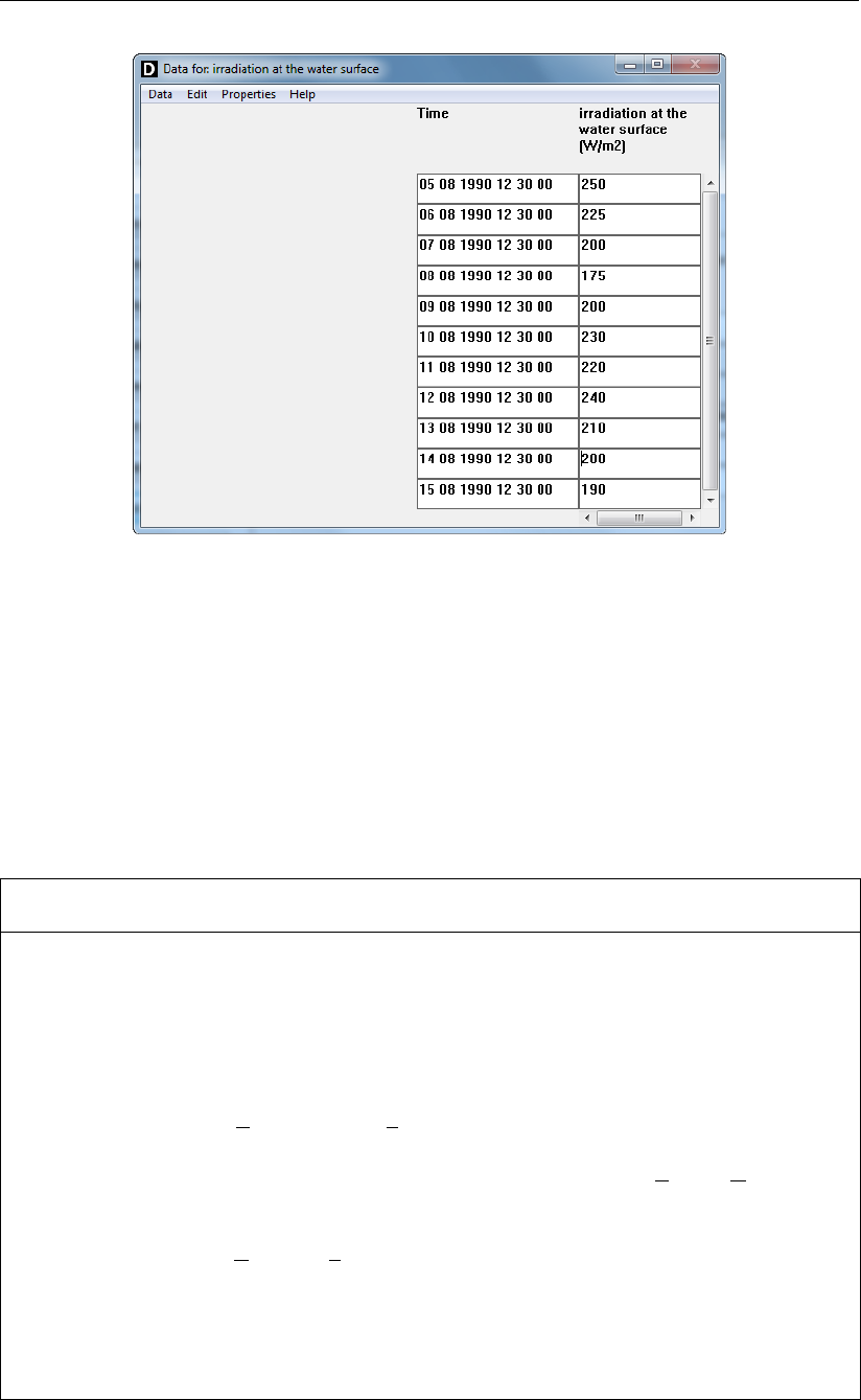
DRAFT
D-Water Quality, User Manual
Figure 7.15: Irradiation values for the 10-day calculation
Other parameters
Specify the other parameters like in Figure 7.12:
first-order mortality rate E.Coli: “0.8”
ambient water temperature: “18”
daylength [0,1]: “0.58”
UV specific extinction coefficient IM1: “0.05”
background extinction UV light: “0.08”
15. PREPARING THE WATER QUALITY SCENARIO:PROCESS PARAMETERS
In the WAQ-GUI, click Process parameters.
Time-series for Irradiation at the water surface
Select the “irradiation at the water surface” entry box.
Click Edit data.
Select menu-option Properties →Data Properties and specify the radio button Time-
series (block function) in the Time frame.
Increase the number of breakpoints to 11 by using menu-option Edit →Copy row or
Ctrl+K several times.
Update the content of the 11-row table according to Figure 7.15.
Select menu-option Data →Save and exit to confirm your time-series.
Other process parameters
Select the other five entry boxes individually and enter the corresponding values dis-
played in Figure 7.12.
An extensive description of the Process parameters Data Group can be found in section 5.3.8.
134 of 382 Deltares

DRAFT
Tutorials
7.1.4.9 Numerical options
In this data group you must specify the integration method (numerical scheme) with which you
want to carry out your water quality calculation. In the tutorial case, please select integration
method 16 from the drop-down box. Check the two checkboxes in the Dispersion frame
and the one in the Transport over boundaries frame. Your window should look like as in
Figure 7.16.
Figure 7.16: Numerical options for tutorial case
16. PREPARING THE WATER QUALITY SCENARIO:NUMERICAL OPTIONS
In the WAQ-GUI, click Numerical options.
Select the “16-Iterative solver, horizontally backward, vertically central” from the Inte-
gration method drop-down box.
In the Dispersion frame, check the “No dispersion if flow rate is zero” check box.
In the Dispersion frame, check the “No dispersion over open boundaries” check box.
In the Transport over boundaries frame, check the “Use first order scheme (certain
high-order methods only)” check box.
See Figure 7.16.
An extensive description of the Numerical options Data Group can be found in section 5.3.9.
Deltares 135 of 382
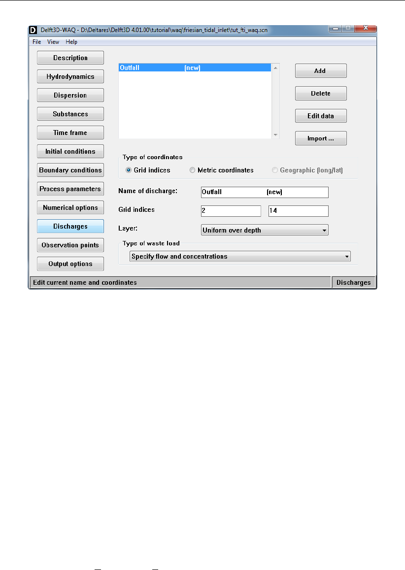
DRAFT
D-Water Quality, User Manual
Figure 7.17: Discharges converted by the Coupling module
7.1.4.10 Discharges
In this data group you will specify the E.Coli discharge in the tutorial case. The location of
a discharge can be pointed by using the Visualisation Area or specifying grid indices. Both
options are explained. Another possibility is that discharges already defined in the hydrody-
namics are imported through the WAQ-GUI. They will be visible in the discharges list when
you select the hydrodynamic results.
Discharges from hydrodynamics
If the hydrodynamic database already contains one or more discharges, these will be con-
verted by the coupling module. If you load these results into the water quality scenario (Data
Group Hydrodynamics) these (pre)defined discharges will be available in the GUI (see Fig-
ure 7.17). The discharge is called “Outfall (new)”.
If you select this name in the list, additional details appear in the lower part of the window.
Select the entry box behind Name of discharge and change it into “E.Coli discharge”.
Create a new discharge by location specification using the Visualisation Area
Use menu-option View →Visualise area to open the Visualisation Area window. In this
window, use the menu-option Edit to check the Discharges menu-item. Use the Edit Mode
menu-option to check Add. In this mode you can select a location in the grid to pinpoint
a discharge location. A red diamond will appear in the selected grid cell. The Discharges
Data Group window will be updated with this discharge. Details can be specified in this
window.
Move your mouse to the opening between the two islands (first and second indices change
at the right-top side of the screen) towards location first index = 8 and second index =
14, click here and a red diamond appears. Go back to the data group window and change
the Name of discharge to “IM1 discharge”.
Create a new discharge by location specification using the Add button and grid indices
136 of 382 Deltares
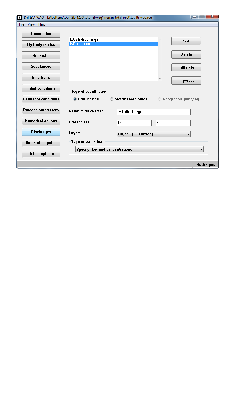
DRAFT
Tutorials
Figure 7.18: Discharges Data Group including the E.Coli discharge and the IM1 dis-
charge
In the Data Group Discharges window you can press Add. A new discharge appears in
the list. Details of this discharge can be specified in the lower half of the window. The Grid
indices needs to be button. Enter “12” in the left box and “8” in the right box. Change the
Name of discharge to “IM1 discharge”.
The results should look like Figure 7.18.
Discharge height The E.Coli discharge is in the surface layer, so the Layer drop- down
box should indicate “Uniform over depth”. For the IM1 discharge
choose “Layer 1 (2-surface)”.
Discharge data Select the E.Coli discharge in the list and click Edit data. Select
menu-option Properties →Data Properties and check the radio but-
ton Timeseries (block function) in the Time frame. Just like in Pro-
cess parameters (Irradiation) you can specify a time-series for the
load of this E.Coli bacteria discharge. For each time breakpoint you
should specify discharge data for each substance (in our case: Salin-
ity, E.Coli and IM1). Flow rates are coming from the hydrodynamic
database and are set constant to 3 m3s−1.
Click in one of the entry boxes of time breakpoint table and use menu-option Edit →Copy
row to increase the number of rows. Repeat this action and change the content until it looks
like Figure 7.19.
Select Data →Save and exit to store your entered discharge rates for the E.Coli discharge.
Select the IM1 discharge in the list and click Edit data. Select menu-option Properties →
Data Properties and check the radio button Constant in time in the lower frame (Time). For
each substance (in our case: Salinity, E.Coli and IM1) you can specify a (constant) value. If
Deltares 137 of 382
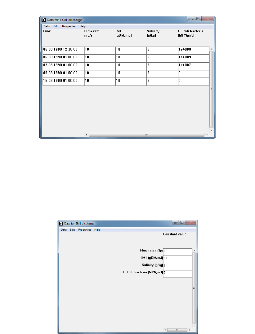
DRAFT
D-Water Quality, User Manual
Figure 7.19: Discharge data of the E.Coli discharge
you leave Flow rate [m3/s] zero, the values will be interpreted as ‘loads’ (mass/time). Use the
values as displayed in Figure 7.20.
Select Data →Save and exit to store your entered discharge rates for the IM1 discharge.
Leave the Type of waste load on the default selection Specify flow and concentrations
Figure 7.20: Discharge data of the IM1 discharge
138 of 382 Deltares

DRAFT
Tutorials
17. PREPARING THE WATER QUALITY SCENARIO:DISCHARGES
In the WAQ-GUI, click Discharges
Editing details of imported discharges (from Coupling module)
The (only) discharge coming from the Coupling module is called: “outfall (new)”.
Click the name in the list;
Select the Name of discharge entry box and change the name into “E.Coli discharge”.
Click Edit data.
Select menu-option Properties →Data Properties and check the radio button Time-
series (block function) in the Time frame.
Increase the number of breakpoints to 5 by using menu-option Edit →Copy row several
times.
Update the content of the 5-row table according to Figure 7.19.
Select menu-option Data →Save and exit to confirm your discharge data.
Adding the discharge by using the Visualisation Area window
Use menu-option View →Visualise area to open the Visualisation Area window.
In the Visualisation Area window, select Discharges from the Edit menu and Add from
the Edit Mode menu.
Move your mouse to the cell with indices first index = 12 and second index = 8
(somewhere in between the two islands) and click your left mouse.
Return to the main Discharges window (and close the Visualisation Area by using
menu-option File →Exit).
or
Adding the discharge by using the Add button/Grid indices
Click Add and enter “12” in the left Grid indices entry box and “8” in the right Grid
indices entry box.
and
Specifying other details
Select the just added discharge from the list.
Enter “IM1 discharge” in the Name of discharge entry box.
Specify Layer 1 (2 - surface) from the Layer drop-down box.
Click Edit data.
Select menu-option Properties →Data Properties and check the radio button Constant
in time in the Time frame.
Update the content of the table according to Figure 7.20.
Select menu-option Data →Save and exit to confirm your discharge data.
Specify Specify flow and concentrations from the Type of waste load drop-down box.
An extensive description of the Discharges Data Group can be found in section 5.3.10.
7.1.4.11 Observation points
To assess the water quality calculation, you need to specify observation points for which output
will be stored. First you have to pinpoint the location of these observation points in the grid.
Deltares 139 of 382

DRAFT
D-Water Quality, User Manual
Table 7.9: Settings for the 4 observation points.
Name Layer first second
index index
left upper Separate per layer 16 6
right upper Separate per layer 16 11
left lower Separate per layer 8 6
right lower Separate per layer 8 11
Like the discharges you can specify the location by either using the Visualisation Area or
using Add and the Grid indices boxes.
Defining observation points using the Visualisation Area
Open the Visualisation Area from the menu-option View →Visualise area. In this win-
dow, use the menu-option Edit →Observation points. Use the Edit Mode menu-option to
check Add. In this mode you can select a location in the grid to pinpoint an observation
point. A red cross will appear in the selected grid cell. The main data group window will
be updated with this new observation point. Details, like name and layer can be specified
here.
Location specification using the Add button and grid indices
In the main data group window you can press Add. A new observation point appears in
the list. Details of this discharge can be specified in the lower half of the window. The Grid
indices need to be specified. Enter “16” in the left box and “6” in the right box. Change
Observation point to “left upper”.
Observation point height
Like discharges, you can specify a layer for an observation point. Use the drop-down box to
select a layer. If you want to have observation points in every layer, please select Separate
per layer. The result is that you will get as many observation points as there are layers. The
tutorial case has 5 water quality layers, so 5 observation points will be created in the selected
grid cell.
Repeat this procedure until you have 4 observation points which comply with the settings in
Table 7.9.
The data group window, including the Visualisation Area looks like displayed in Figure 7.21.
18. PREPARING THE WATER QUALITY SCENARIO:OBSERVATION POINTS
In the WAQ-GUI, click Observation points.
140 of 382 Deltares

DRAFT
Tutorials
18. PREPARING THE WATER QUALITY SCENARIO:OBSERVATION POINTS
Adding 4 observation points by using the Visualisation Area window
Use menu-option View →Visualise area to open the Visualisation Area window.
In the Visualisation Area window, select Observation points from the Edit menu and
Add from the Edit Mode menu.
Move your mouse to the cell with co-ordinates first = 16 and second = 6 and click
your left mouse.
Move your mouse to the cell with co-ordinates first = 16 and second = 11 and click
your left mouse.
Move your mouse to the cell with co-ordinates first = 8 and second = 6 and click your
left mouse.
Move your mouse to the cell with co-ordinates first = 8 and second = 11 and click
your left mouse.
Return to the main Observation points window.
or
Adding 4 observation points by using the Add button/Grid indices
Click Add and enter “16” in the left Grid indices entry box and “6” in the right Grid
indices entry box.
Click Add and enter “16” in the left Grid indices entry box and “11” in the right Grid
indices entry box.
Click Add and enter “8” in the left Grid indices entry box and “6” in the right Grid indices
entry box.
Click Add and enter “8” in the left Grid indices entry box and “11” in the right Grid
indices entry box.
and
Specifying other details
Select the (just added) first observation point from the list.
Enter “left upper” in the Observation point entry box.
Select Separate per layer from the Layer drop-down box.
Select the second observation point from the list.
Enter “right upper” in the Observation point entry box.
Select Separate per layer from the Layer drop-down box.
Select the third observation point from the list.
Enter “left lower” in the Observation point entry box.
Select Separate per layer from the Layer drop-down box.
Select the (just added) first observation point from the list.
Enter “right lower” in the Observation point entry box.
Select Separate per layer from the Layer drop-down box.
Close the Visualisation Area by selecting menu-option File →Exit.
An extensive description of the Observation points Data Group can be found in section 5.3.11.
Deltares 141 of 382
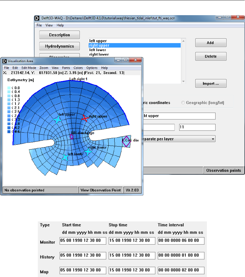
DRAFT
D-Water Quality, User Manual
Figure 7.21: Observation points (crosses), discharge location (diamond) and open
boundary (bold line)
Figure 7.22: Output Options - Timers
7.1.4.12 Output options
In this last data group you can specify the output. You can specify a selection of: output
timers, output parameters, statistics, file types and formats.
Timers
You can specify the start and stop time of the output by changing the corresponding entry
boxes. The time interval can be adjusted as well. You can specify different settings for the
different file types. Change the text boxes according to Figure 7.22.
142 of 382 Deltares
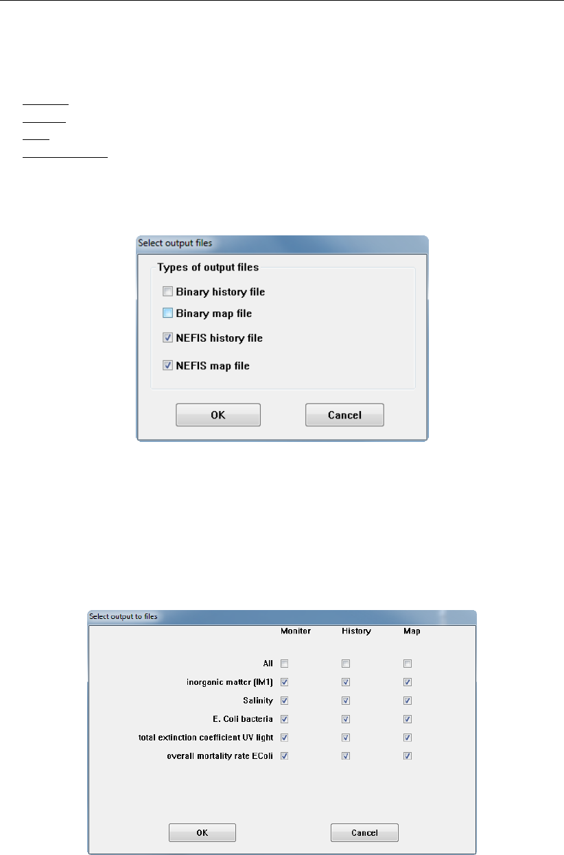
DRAFT
Tutorials
Select output file types and formats
The following file types are available:
Monitor file: ASCII output for the observation points;
History file: time-series output of the observation points;
Map file: geographical plots of concentration contours;
Mass balance file: write a mass balance file.
The available formats are binary (unformatted) and NEFIS, for both windows and LINUX op-
erating systems. Click Files to check the output files and types according to Figure 7.23.
Figure 7.23: Select Output options →Files, showing window Select output files
Select parameters
The output parameters (defined in the PLCT) can be switched on (written to output files) or
off (not written to output files). Click Select to specify this for every substance and file. See
Figure 7.24.
Figure 7.24: Select Output options →Select, showing window Select output to files
Deltares 143 of 382
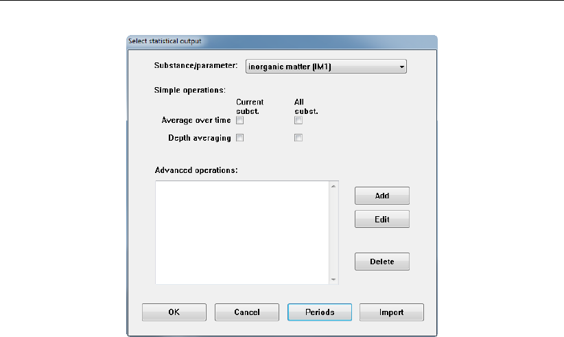
DRAFT
D-Water Quality, User Manual
Figure 7.25: Window Select statistical output
Select statistics
Open the statistics window see Figure 7.25.
Click Statistics.
Select the All checkbox in the Average over time column and
Select the All checkbox in the Depth averaging column.
Select the E.Coli bacteria substance; next click the Periods button.
Click Add.
Enter “whole period” in the Name of period entry box.
Enter “whole” in the Abbreviation entry box.
Enter “05 08 1990 12 30 00” in the Start time entry box.
Enter “15 08 1990 12 30 00” in the Stop time entry box.
Click OK to confirm.
First you need to define the period for which you like to have the statistics. Click the Periods
button and press Add. Specify the “Whole period” as a period and “Whole” as abbreviation
according to the settings in Figure 7.26. Close this window by clicking OK.
144 of 382 Deltares
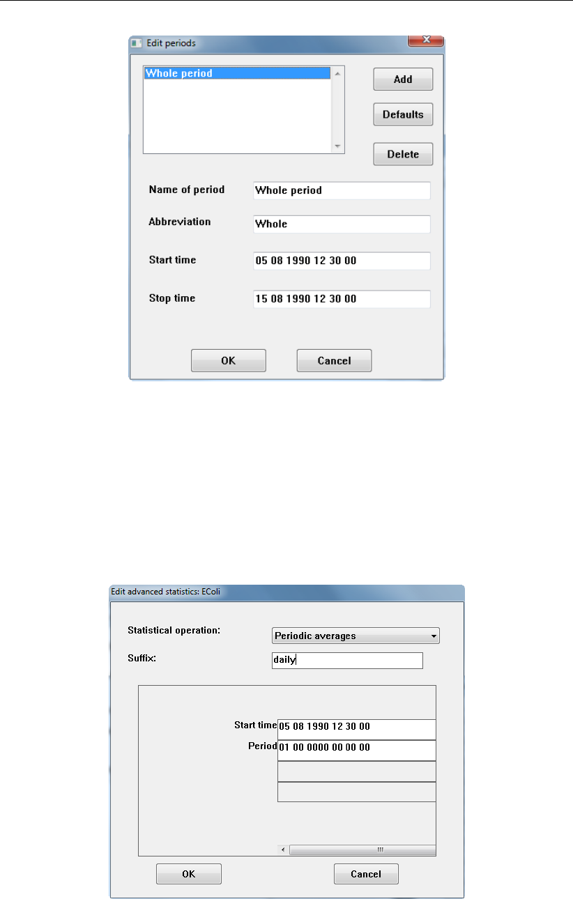
DRAFT
Tutorials
Figure 7.26: Statistics - period definition
Check the All checkbox in the columns for Average over time and Depth averaging to select
all available statistics for the output parameters.
Select Substance/parameter E.Coli bacteria. Click Add in the Advanced operations list box.
Select Periodic averages from the Statistical operation drop-down box. Enter the Suffix “daily”.
Specify the Start time as “05 08 1990 12 30 00” and set Period to 1 day (you will get daily
averages now) by specifying “01 00 0000 00 00 00”. See Figure 7.27 and then press OK.
Figure 7.27: Advanced statistics - Periodic averages
Click Add again. Select Geometric mean from the Statistical operation drop-down box. Enter
the Suffix “geomean”. Specify Threshold as “1” (to prevent zero and negative values to be
Deltares 145 of 382

DRAFT
D-Water Quality, User Manual
Figure 7.28: Advanced statistics - Geometric mean
included in the logarithmical calculations). See Figure 7.28.
Close this window (Figure 7.28) by clicking OK and close the window Select statistical out-
put (Figure 7.25) as well by clicking OK.
Balances
Click the Balances button.
Switch on the Mass balances radio buttons.
Click OK to confirm and close the Balances window.
146 of 382 Deltares

DRAFT
Tutorials
19. PREPARING THE WATER QUALITY SCENARIO:OUTPUT OPTIONS
In the WAQ-GUI, click Output options.
Timers
The content of the 3 Start time entry boxes should be: “05 08 1990 12 30 00”.
The content of the 3 Stop time entry boxes should be: “15 08 1990 12 30 00”.
The content of the 3 Time interval entry boxes should be:
Monitor file: “00 00 0000 06 00 00”
History file: “00 00 0000 01 00 00”
Map file: “00 00 0000 02 00 00”
Files
Click Files.
Switch off both binary files checkboxes.
Switch on both NEFIS files checkboxes.
Click OK to confirm.
Parameters
Click Select.
Select all output parameters for all 3 file types (3 times the all checkbox will ease this
operation).
Click OK
Statistics
Click Statistics
Check the All checkboxes and Substance parameter E.Coli
Click OK
Click Add in the Advanced operations frame.
Select Periodic averages from the Statistical operation drop-down box.
Enter “daily” in the Suffix entry box.
Enter “05 08 1990 12 30 00” in the Start time entry box.
Enter “01 00 0000 00 00 00” in the Period entry box.
Click OK to confirm.
Click Add in the Advanced operations frame.
Select Geometric mean from the Statistical operation drop-down box.
Enter “geomean” in the Suffix entry box.
Click OK to confirm.
Click OK to confirm and close the Statistics window.
Balances
Click the Balances button.
Switch on the Mass balances radio buttons.
Click OK to confirm and close the Balances window.
An extensive description of the Output options Data Group can be found in section 5.3.12.
Deltares 147 of 382
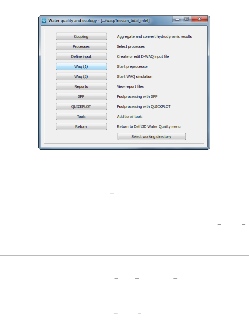
DRAFT
D-Water Quality, User Manual
Figure 7.29: Water quality and ecology selection window
Saving the scenario file
From the WAQ-GUI, select menu-option File →Save or Save As to save your scenario file.
Automatically the extension <∗.scn>will be given. Save your file into the current working
directory. All your results will be stored here as well.
The definition of the ’tut_fti_waq’ tutorial case is ready now. Select menu-option File →Exit
to exit the main window.
20. PREPARING THE WATER QUALITY SCENARIO:SAVING AND EXITING
Saving the scenario file
In the WAQ-GUI, select menu-option File →Save or Save As to save your settings to
a file. Name it <tut_fti_waq.scn>and store it in your current working directory (default
location).
Exiting the WAQ-GUI
In the WAQ-GUI, select menu-option File →Exit to quit.
7.1.5 Running the ’tut_fti_waq’ scenario
The model has been set-up. It is ready to run now. The calculations consists of two parts:
pre-processing and calculation (see Sections 6.1.1 and 6.1.4).
After exiting the WAQ-GUI (previous step) the window from Figure 7.29 appears. Click Waq (1).
Press Select file and browse to the <tut_fti_waq.inp>file. This is the input file generated from
your just saved <tut_fti_waq.scn>file. You can find them in your current working directory.
Click Open to confirm. The window should look as in Figure 7.30.
After selecting OK the pre-processing program (delwaq1) will run to verify and process the
input in a new window, see Figure 7.31. The program will end with a ‘Normal end’.
148 of 382 Deltares
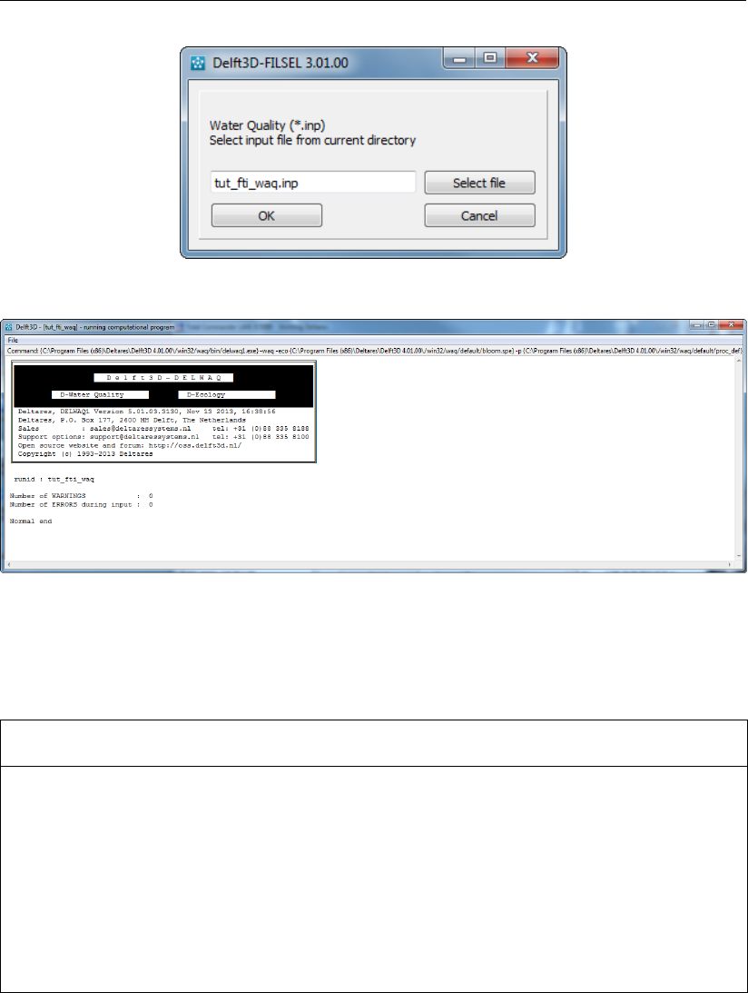
DRAFT
Tutorials
Figure 7.30: Waq (1) - Pre-processing file selection
Figure 7.31: Waq (1) window; pre-processing finished with ’Normal end’
By pressing the Waq (2) button, the water quality calculation starts in a new window, see
Figure 7.32. The progress is monitored by displaying the percentage completed.
21. RUNNING THE WATER QUALITY SCENARIO
Running pre-processors
In the Water quality (WAQ) window, click Waq (1). Click Select file in the next window
to select the <tut_fti_waq.inp>file.
Click OK to confirm.
The pre-processors will run in a new window.
Executing the water quality calculation
Click Waq (2). The calculation will start in a new window.
Close both windows by clicking File →Exit in each window.
Deltares 149 of 382
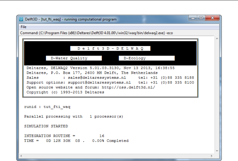
DRAFT
D-Water Quality, User Manual
Figure 7.32: Waq (2) window showing the progress of the calculation.
7.1.6 Visualising results
To view output of a WAQ simulation, the GPP (General Post Processing) program can be
used. By selecting GPP in the Water quality (WAQ) selection window (Figure 7.29), GPP
starts. To open the so-called session file (<∗.ssn>), the data sets and plots of the tutorial
example will be opened. The session file to open is <tut_fti_waq.ssn>and can be found
in the <\delft3d\tutorial\waq\friesian_tidal_inlet>directory. Use the menu-item Session →
Open. . . (select No if you are asked to save changes) to browse to the <tut_fti_waq.ssn>
file, click Open to confirm.
The plots can be found when you click Plots. Select a plot from the list and click the View/Edit
to open it. Figure 7.33 till Figure 7.37 are examples of figures presenting water quality param-
eters from the tutorial case. See the GPP User Manual (GPP UM,2013) for details on how to
use GPP.
150 of 382 Deltares

DRAFT
Tutorials
Figure 7.33: Time-series E.Coli concentration at monitoring stations (note the difference
in scale); LEFT LOWER and LEFT UPPER (upper plot) and RIGHT LOWER
and RIGHT UPPER (lower plot)
Deltares 151 of 382
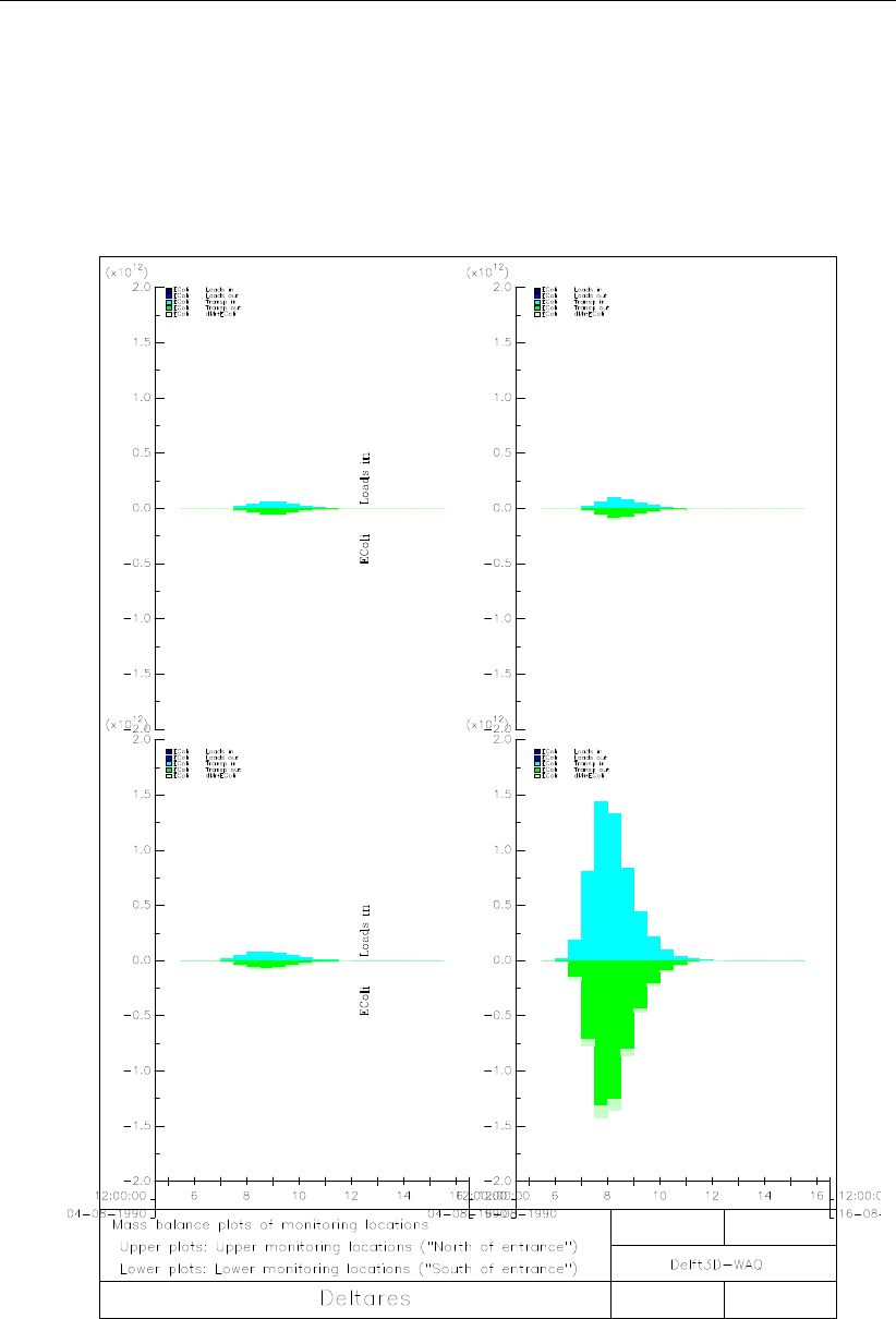
DRAFT
D-Water Quality, User Manual
Figure 7.34: Mass Balances E.Coli; upper plots: monitoring station north of tidal inlet,
lower plots: stations south of inlet
152 of 382 Deltares
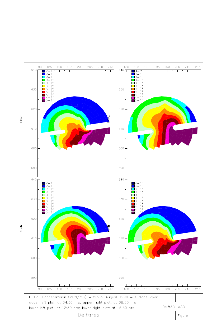
DRAFT
Tutorials
Figure 7.35: Contour plots of E.Coli in the surface layer on 8 August 1990: 03:30 hr (upper
left), 07:30 hr (upper right), 11:30 hr (lower left) and 15:30 hr (lower right)
Deltares 153 of 382
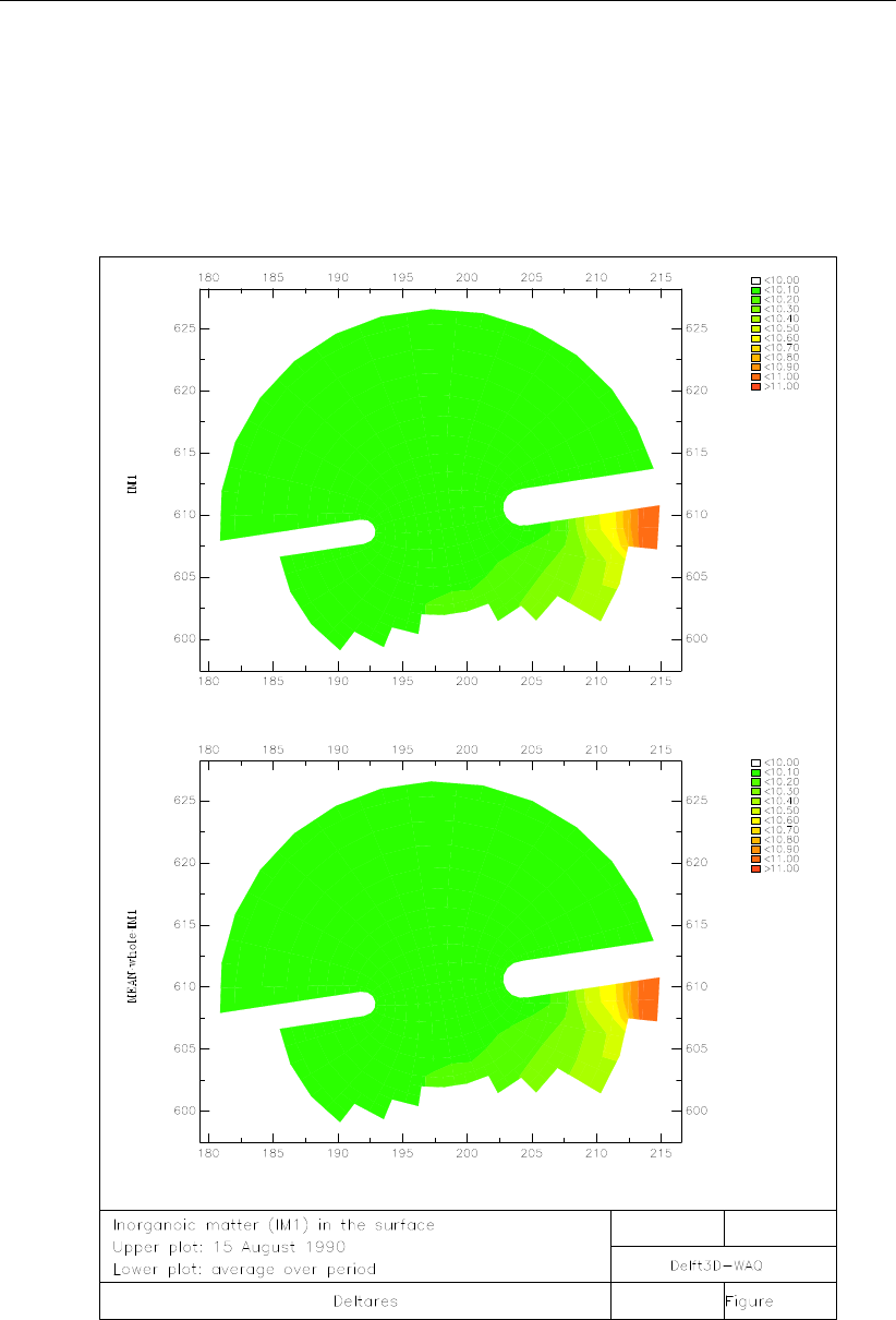
DRAFT
D-Water Quality, User Manual
Figure 7.36: Inorganic matter concentration in the surface layer on 15 August 1990
12:30 hr (upper) and averaged over the simulation period (lower)
154 of 382 Deltares
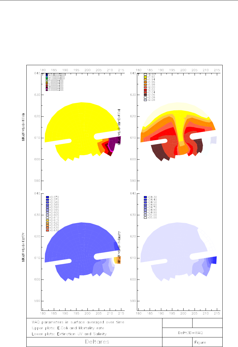
DRAFT
Tutorials
Figure 7.37: Water quality parameters in the surface layer averaged over time; E.Coli
(upper left), extintion UV light (lower left), mortality rate (upper right) and
salinity (lower left)
Deltares 155 of 382

DRAFT
D-Water Quality, User Manual
7.2 Tutorial Water Quality related to sewer overflows (SOBEK-Rural 1DWAQ + 1DFLOW
modules)
7.2.1 How to set up a water quality model
This tutorial describes how to set up a water quality model with SOBEK-Rural 1DWAQ mod-
ule. First a simple model will be set up, for an urban canal with one combined sewer overflow
discharging to it. You will start from scratch and the tutorial guides you step by step through the
schematisation and simulation processes. Once the model is finished you will use it to anal-
yse the water quality problems related to combined sewer overflows. SOBEK-Rural 1DWAQ
contains various options to present and analyse the simulation results. These techniques will
be explained with help of the water quality model that you will set up.
7.2.1.1 Getting started
In this chapter a model will be set up for a single canal with one combined sewer overflow
discharging to it. The schematisation of the water system will be combined with a water
quality model for the simulation of oxygen and biochemical oxygen demand (BOD). At first the
model will be used for the simulation of a period without any overflows.
Click on the Windows Start button.
Select the ’All Programs’ or ’All Apps’ menu.
Select the ’Delft Hydraulics’ menu.
Select the ’SOBEK’ menu item (SOBEK215).
Click on the ’SOBEK’ icon.
Select the menu item ’Options’ - ’SOBEK Options’;
Select the tab ’Background Map’.
Select the file ’Tutorial1.map’.
Press OK button to save and close SOBEK Options.
Click the ’New Project’ button.
Type the name ’T_CSO’.
The program converts all the characters into upper case. If a project with the same name
already exists, the user has to enter a different name here.
Click the OK button.
You have added a new project with the name ’T_CSO’. You are now asked: do you want to
work with this project?
Click the Yes button.
The Case Manager appears, see below:
156 of 382 Deltares
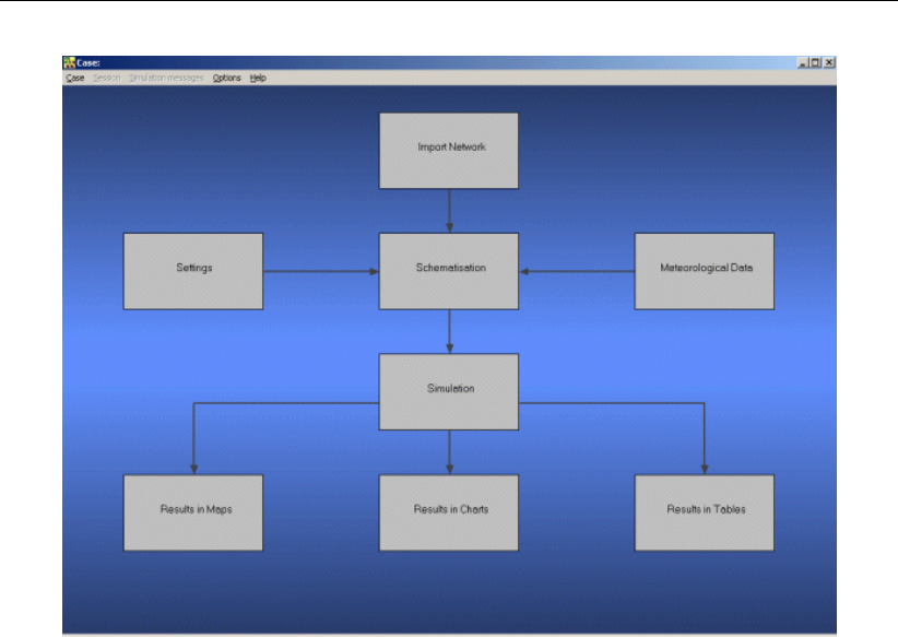
DRAFT
Tutorials
Figure 7.38: The case manager window.
Select the menu ’Case’ - ’Open as new’.
Enter the name “Reference model”.
Click the OK button.
In the Case Manager, the task block Settings, Import Network and Meteorological Data are
yellow, the other task blocks are red. The colour of the task block indicates the actions that
the modeller still has to perform. Yellow indicates that in this task block still some work has to
be done, before one can continue with the red task blocks. Once a task is finished, the colour
of the task block turns into green.
7.2.1.2 Task block: Import network
Double click the task block ’Import Network’ in the case manager.
Choose ’Start from scratch’.
Click the OK button in order to leave the task block ’Import Network’ and return to the
Case Manager.
7.2.1.3 Task block: Settings
Double click the task block ’Settings’ in the Case Manager.
Unselect all the selected modules if any.
Select the module ’1DFLOW (Rural)’.
Select the module ’1DWAQ’.
Click the OK button (The output of the 1DFLOW module(s) is set to mean values!).
Deltares 157 of 382

DRAFT
D-Water Quality, User Manual
Figure 7.39: The Settings window.
Click the Edit... button of the ’1DFLOW (Rural)’ module.
The tab with ’Time settings’ appears.
Figure 7.40: The tab with the time settings for the hydraulic calculation: simulation period
and the time step for calculation.
Make the ’Time step for computation’ 10 minutes.
Select the option ’Simulation period defined as below’.
Change the simulation period, it starts on 1st of January, 2000 00:00:00 and ends on the
7th of January, 2000 00:00:00.
158 of 382 Deltares
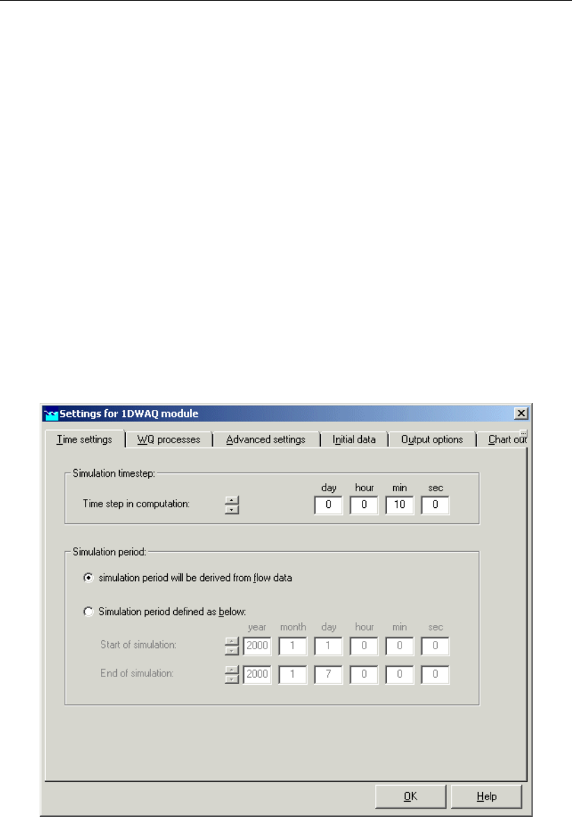
DRAFT
Tutorials
Go to the tab ’Simulation settings’.
In the group box ’Simulation mode:’, select ’unsteady calculation’.
Go to the tab ’Initial data’.
Choose the option ’define global initial values’.
Select the option ’initial depth in channels [m]’.
Enter an initial water depth of “0.5” m.
Go to the tab ’Output options’.
Select a ‘Time step output’ of ’10 minutes’.
The default ’output parameters’ are correct for this simulation.
Click the OK button.
A message appears about the time step of the 1DWAQ module and the output time step of
the 1DFLOW module.
Click the OK button.
Click the OK button.
Click the Edit button of the ’1DWAQ’ module in the Settings window.
The tab with ‘Time step settings’ appears.
Figure 7.41: The tab for the adjustment of the time step in the computation and the sim-
ulation period of the water quality simulation.
Adjust the ’Time step in computation’ to 10 minutes.
Select the option ’Simulation period will be derived from flow data’.
Go to the tab ’WQ processes’.
Select ’Calculate water quality transport’.
Now the transport of substances is activated.
Deltares 159 of 382

DRAFT
D-Water Quality, User Manual
Select ‘active processes’.
Now the water quality processes that act on the substances are activated.
Go to ’Advanced settings’;
Figure 7.42: The tab where the numerical solver can be selected and some dispersion
parameters can be adjusted.
On this tab one can choose a numerical solver from an extended list of different schemes.
These solvers differ from each other in the amount of numerical dispersion that occurs during
the simulation. The selected solver also determines the time that a computation takes. With
some solvers the computing time of a simulation is significantly higher. For instance for urban
canal networks with a number of interconnections, the ‘Fully implicit iterative scheme’ is the
preferred solver. A realistic dispersion coefficient for small, urban water system with low flow
velocities is in the range of 0.1 m2/s to 0.5 m2/s.
Choose for the ’Fully implicit iterative method’ (Numerical scheme 15) from the ’Integration
options’.
Choose ’Use dispersion only if flow is not zero’. The dispersion will be taken into account
only if the flow velocity is not zero.
Enter a dispersion coefficient of “0.1” m2/s.
160 of 382 Deltares
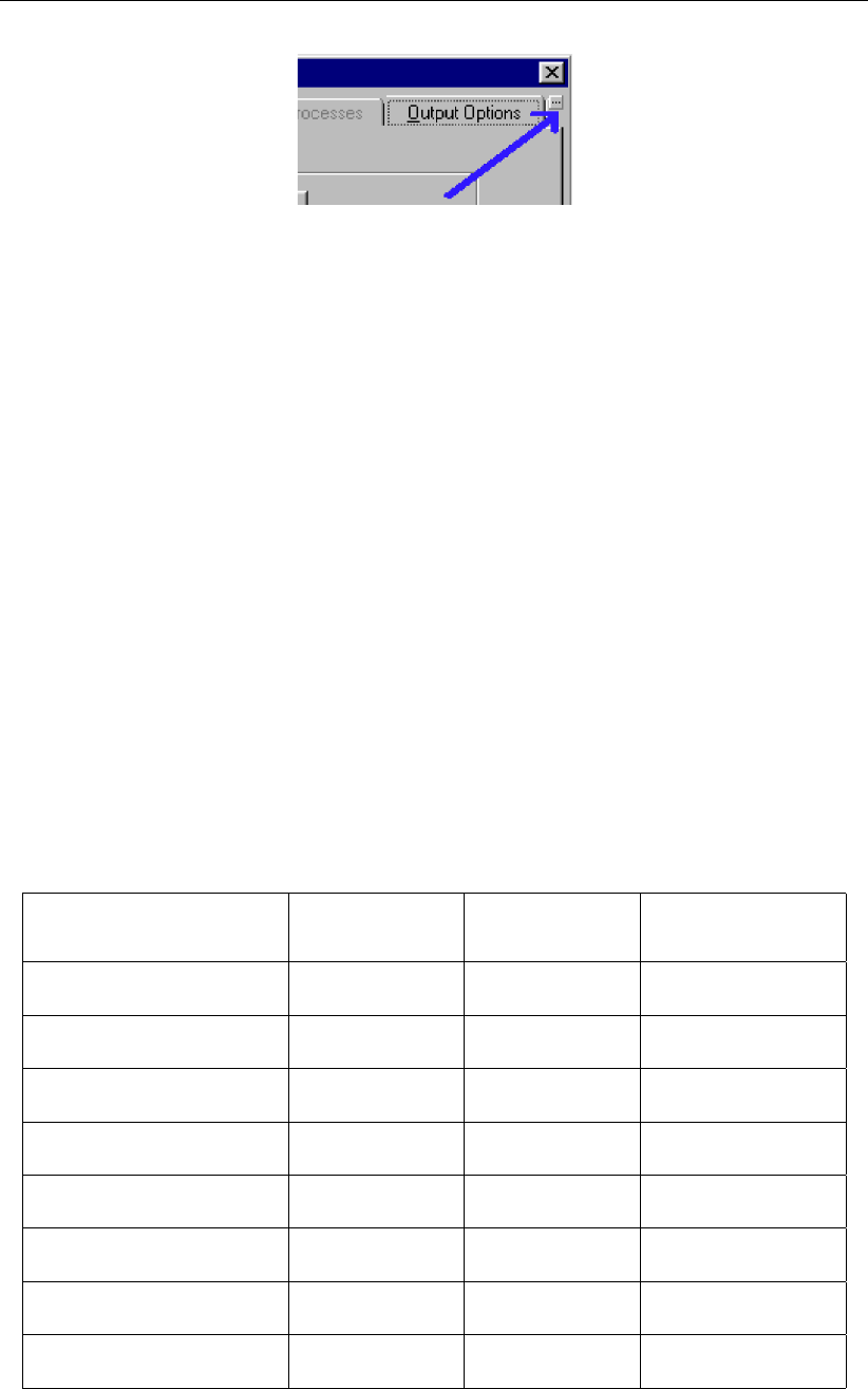
DRAFT
Tutorials
Figure 7.43: Click this button to unveil the tabs "chart output" and "map output"
Go to the tab ’Chart Output’.
Enter “30” minutes.
Go to the tab ’Map Output’.
Enter “30” minutes.
7.2.1.4 The predefined subset
On the tab ’WQ Processes’ the set of processes that are active in the water quality model can
be composed. It is also possible to choose from a number of pre-defined subsets of water
quality processes. In this tutorial a ‘predefined subset’ of water quality processes will be used.
There are three pre-defined subsets available for the simulation of water quality in urban
surface waters:
Tewor+ model for SOBEK (Oxygen).
Tewor+ model for SOBEK (Oxygen and nutrients).
Tewor+ model for SOBEK (Complete).
The subsets are based on the Dutch TEWOR+ model. Table 7.12 summarises the substance
groups in each pre-defined subset.
Table 7.12: Overview of substance used for TEWOR
Subset:
Substance groups:
Tewor+Oxygen Tewor+Oxygen,
Nutrients
Tewor+Complete
Oxygen and BOD X X X
Nitrogen X X X
Phosphorus X X
Suspended Solids X X
Bacteria X
Heavy Metals X
Organic Micro pollutants X
Chloride X
In this tutorial you will use the pre-defined subset Tewor+ model for SOBEK (Oxygen).
Go to the tab WQ Processes.
Deltares 161 of 382

DRAFT
D-Water Quality, User Manual
Choose for the option use predefined process.
Select the pre-defined subset Tewor+ model for Sobek (Oxygen).
Figure 7.44: Selecting a predefined subset.
7.2.1.5 Process coefficients
Click the Edit... button next to ‘Process Coefficients’.
In the table that is shown in Figure 7.45, the process coefficients can be entered. Before
the model is calibrated (the calibration is described further in this tutorial), default parameter
values are used.
162 of 382 Deltares

DRAFT
Tutorials
Figure 7.45: The table of process coefficients.
Set the parameters to default values in the menu ‘File’ - ‘Import’ - ‘File’.
Select the file ‘Tewor+_oxygen.plc’ in the directory ‘\SOBEK215\Fixed\Delwaq\’.
Press the Open button.
Save the parameters via the menu ‘File’ - ‘Save’.
Leave the table with process coefficients via ‘File’ - ‘Exit’.
A warning appears, saying that you should also enter the initial values. We will do that in the
following chapter.
Press the OK button.
7.2.1.6 Initial conditions
Go to the tab ‘Initial data’.
Click the Edit button next to ‘use global initial values’. In the table the initial values can be
entered.
Deltares 163 of 382
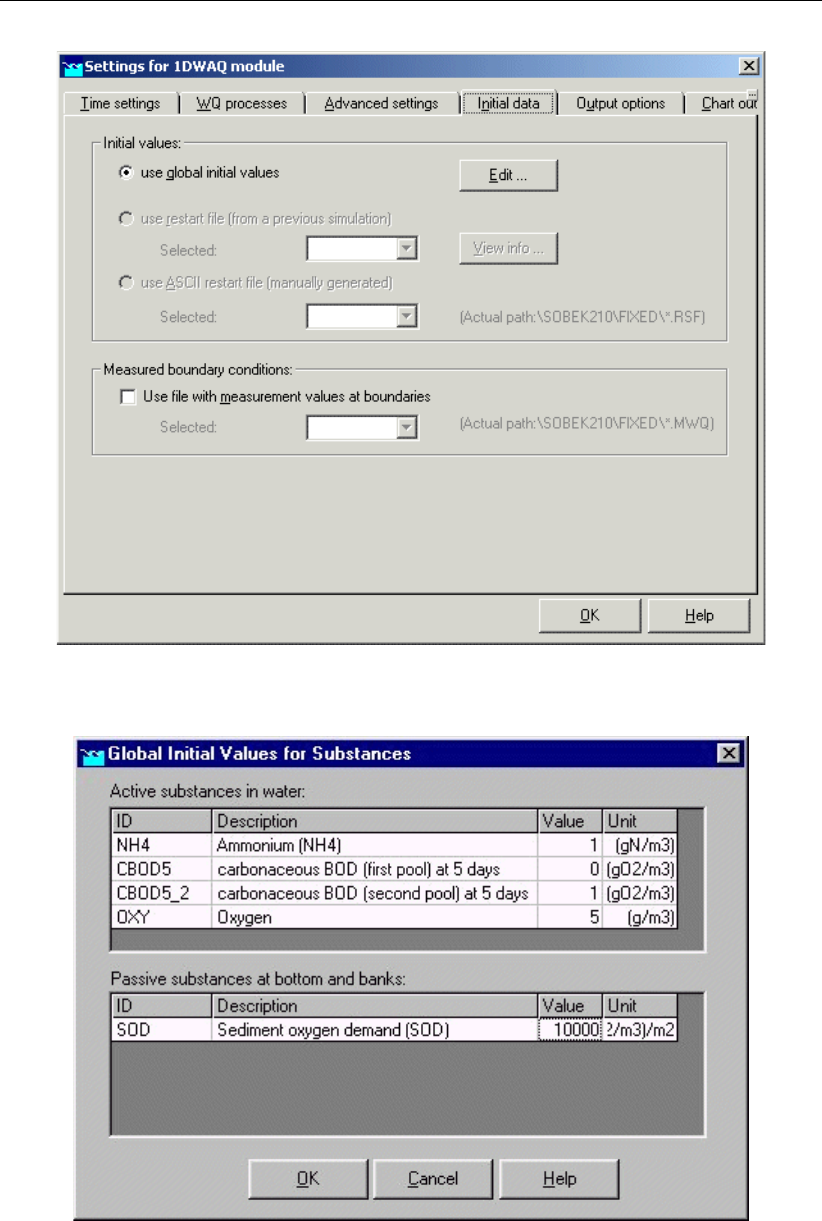
DRAFT
D-Water Quality, User Manual
Figure 7.46: The Initial data tab.
Figure 7.47: Global Initial Values for Substances.
Enter the values as depicted in Figure 7.47.
Click OK to leave the input screen for initial conditions.
Click OK to leave the 1DWAQ Settings.
Click OK to leave Settings and return to the Case Manager.
164 of 382 Deltares
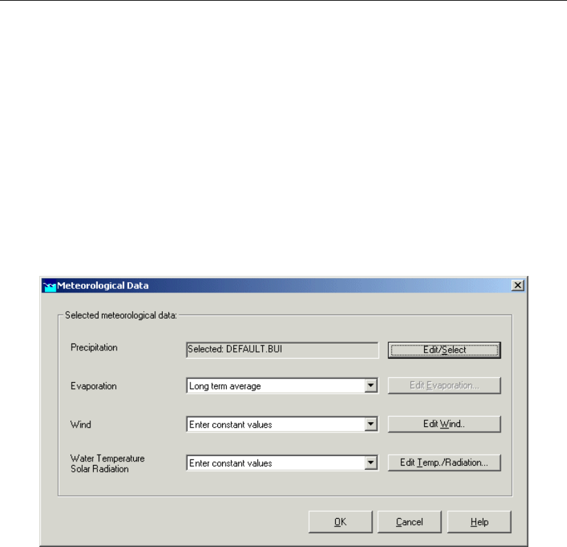
DRAFT
Tutorials
7.2.1.7 Meteorology
SOBEK-Rural simulations require meteorological input data, i.e. precipitation data, evapora-
tion data, wind data, water temperature and solar radiation. The Meteorological data task
block provides precipitation and evaporation data to the RR (Rainfall-Runoff) module, wind
data to the 1DFLOW and Overland Flow (2D) modules and water temperature and solar ra-
diation data to the 1DWAQ and 2DWAQ modules. For simplified rainfall-runoff processes
precipitation data can optionally be provided to the 1DFLOW and Overland Flow (2D) mod-
ules.
Double-click the ’Meteorological Data’ task block of the Case Manager.
The following screen will appear:
Figure 7.48: The Meteorological Data window.
In the dialog that pops up you can see how precipitation, evaporation, wind, water temperature
and solar radiation data are defined.
Click the Edit Wind... button.
Set the wind velocity to 0 m/s.
Press the OK button.
Click the Edit Temp./Radiation... button.
Enter a water temperature of “18.2” ◦C.
Enter a ’Solar Radiation’ of “50” W/m2.
Press the OK button.
Click OK to leave the task block ’Meteorological Data’ and to return to the Case Manager.
Now you have finished defining the meteorological data. Notice that this task block has turned
green too!
Deltares 165 of 382
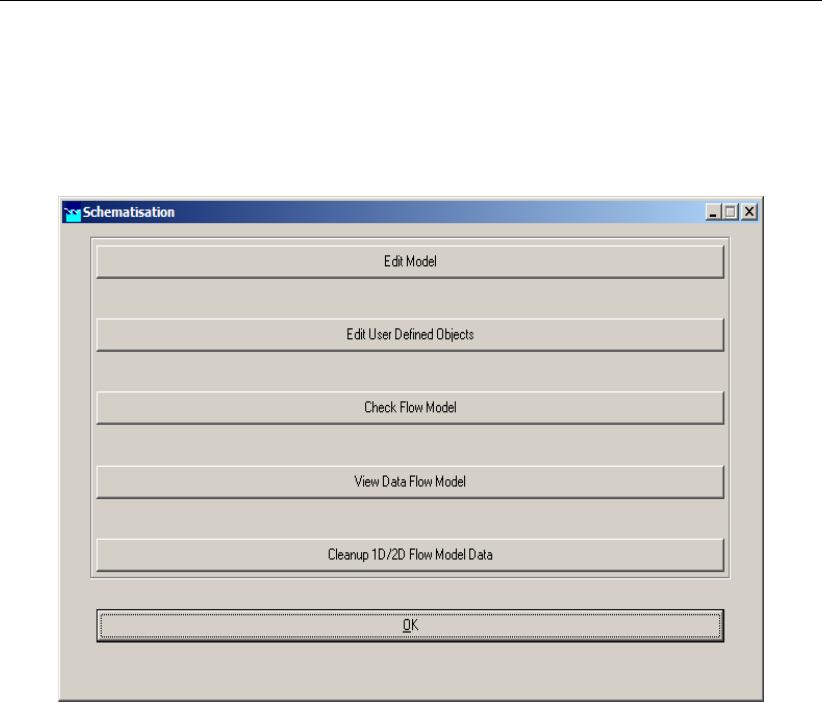
DRAFT
D-Water Quality, User Manual
7.2.1.8 Task block: Schematisation
Double click the task block ‘Schematisation’.
The window below appears:
Figure 7.49: The Schematisation window.
Click the Edit model button.
When the option Edit Model of the ‘Schematisation’ is selected, the network editor starts.
The network editor is called NETTER and is a component of the Delft Hydraulics Decision
Support System (Delft-DSS) tools. NETTER offers the possibility to set-up the schematisation
on top of a background GIS map. NETTER also offers advanced analysis tools to show model
results linked to the schematisation and provide the user with full printing facilities to make high
quality prints.
Within NETTER you can do the following:
1 Interactively and graphically prepare a schematisation;
2 Generate schematisations upon GIS map Layers;
3 Carry out schematisation operations: search for a certain node, show node numbers and
names, show link numbers, etc.;
4 Carry out map operations: zooming in, zooming out, (de)activating map layers, colouring
of map layers, adding title information on the map, etc.;
5 View results of simulation models for schematisations created in NETTER;
6 Print maps or schematisations on one or more pages which fit together.
166 of 382 Deltares
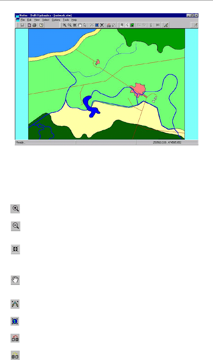
DRAFT
Tutorials
Figure 7.50: The hypothetical town (SOBEK CITY)
In order to focus on a small part of the map, you can use the zoom functionalities.
The View menu contains commands to zoom in, zoom out, centre the window, move the
window and show all schematisation or map layers.
The button allows you to zoom in on any part of the "active main window".
The button allows you to zoom out by shrinking the displayed part of the "active main
window".
The button allows you to centre a schematisation or map GIS object. When choosing
this command and then clicking with the left mouse button on an object NETTER, redraws the
map centring the chosen object to the NETTER window.
The button allows you to shift the view by clicking the mouse anywhere in the NETTER
window and dragging the view to another position.
The button redraws the view fitting all schematisation objects into the NETTER window.
The button redraws the view fitting all GIS map layers into the NETTER window.
The button restores the view of the map before the last zoom command was given.
The button restores the view of the map before the last ‘Show Previous’ command was
given.
Deltares 167 of 382

DRAFT
D-Water Quality, User Manual
Use the button to zoom in on the town and the river.
7.2.1.9 Working with NETTER
Six bars with buttons are available for making schematisations: ‘Node’, ‘Connection’, ‘Reach’,
‘Flow model’, ‘Edit Network’ en ‘Edit Reach Vectors’. The button bars are separate windows
that can be dragged to a convenient place on the screen. In this way you can customise
NETTER.
Go to the menu ‘Edit’ and subsequently ‘Network’.
Click button next to the button ‘No edit action’ in the ‘Edit network’ menu.
A list with menu-options appears:
Figure 7.51: The menu Edit Network.
Move the mouse to ‘Node’.
A window with buttons rolls down, as shown below.
168 of 382 Deltares
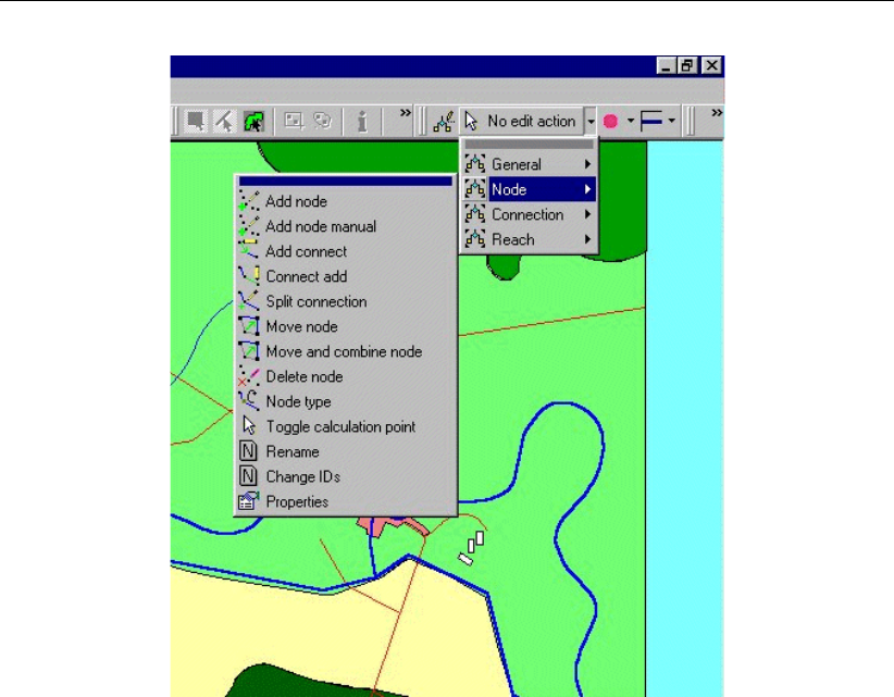
DRAFT
Tutorials
Figure 7.52: The menu Node.
Keep the mouse on the coloured bar;
Keep the left mouse button pressed and drag the button bar ‘Node’ over the window;
Do the same for the button bar ‘Connection’;
Do the same for the button bar ‘Reach’.
Do the same for the button bar ‘Flow model’.
An example of NETTER, with all button bars visible is shown below.
Deltares 169 of 382
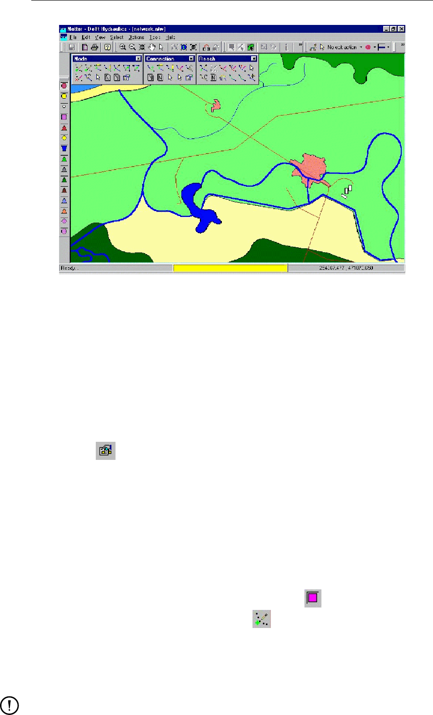
DRAFT
D-Water Quality, User Manual
Figure 7.53: The button bars in NETTER.
7.2.1.10 The schematisation
In this paragraph we are going to make a simple schematisation of a small river, to which one
combined sewer overflow is discharging.
The boundaries of the model are: a constant discharge (east) and a fixed water level (west).
The sewer overflow is modelled as a lateral discharge.
All model components need to have unique identifiers. It is possible to define the identifiers
(or IDs) of the nodes and branches (links) automatically or manually.
Select the button in the ’General’ tool bar, Edit settings, to go to the edit network
options.
Select the tab ’Node’.
In the ’ID’ group box, select the radio button ’Manual’.
In the ’Name’ group box, select the radio button ’Manual’.
Select the tab ’Link’.
Set the ’ID’ and ’Name’ to ’automatic’.
Click the OK button.
During this tutorial we will build a small network as shown in Figure 7.56.
Click the object ‘Flow - boundary’ in the menu Flow-model: .
Click the button ‘Add node’ of the menu ‘Node: .
Enter “Inflow” in both input fields.
Press the OK button.
Place the boundary node east of the town, by clicking on the map with the left mouse
button.
170 of 382 Deltares
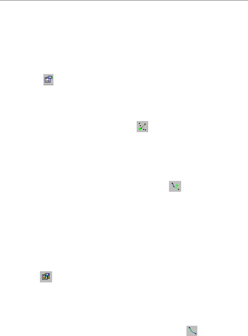
DRAFT
Tutorials
Remark:
Although it is possible to work with object IDs of more than 20 characters in the D-Flow
1D modules, D-WAQ 1D can only work with IDs of 20 characters or less. Because IDs
can be prefixed with an ’n’ when using D-WAQ 1D, any network objects used during a
D-WAQ 1D simulation should have a maximum ID length of 19 characters.
In order to see the identifiers on the map please:
Click on the button in the Active Legend or select the menu item ’Options’ - ’Network
Data...’.
Select the tab ’Node’.
Select the radio button ’Name’.
Press the OK button.
Click the button ‘Add node’ of the menu ‘Node: .
Enter “Outflow” in both input fields.
Press the OK button.
Place a boundary node west of the town, by clicking on the map with the left mouse button.
The river flows from east to west through the town.
Click the button ‘Connect nodes’ of the menu ‘Connection’: .
Connect the two buttons by clicking with the left mouse button on the node ’Inflow’ in the
east and dragging with the left mouse button pressed from the node ’Inflow’ in the east to
the node ’Outflow’ in the west.
The simulation will be more accurate if a calculation grid is used, for instance with a distance
of 50 m between the nodes. Another advantage is the fact that this will make output available
on more locations.
But before we will generate a calculation grid we will change the general edit settings.
Select the button in the ’General’ tool bar, Edit settings, to go to the edit network
options.
Select the tab ’Node’.
In the ’ID’ group box, select the radio button ’Automatic’.
In the ’Name’ group box, select the radio button ’No Names’.
Click the OK button.
Click the button ‘calculation grid all reaches’ of the menu ‘Reach’: .
Select the ‘Split vector’ option in the ’Calculation points’ window.
Enter value “50” for length.
Select ‘Equidistance’.
Then press the OK button.
Deltares 171 of 382

DRAFT
D-Water Quality, User Manual
Figure 7.54: The (provisional) model schematisation in NETTER.
The schematisation is still a straight line crossing town. But we would like to see that the
schematisation follows the river as closely as possible.
Go to the menu ‘Edit’ and subsequently ‘Vector Layer’.
The menu ‘Edit reach vectors’ appears.
Figure 7.55: The menu ’Edit reach vectors’.
172 of 382 Deltares
DRAFT
Tutorials
The reach is shown as a thin black line now. If you point to the reach, the cursor has the form
a thin black arrow.
Click the button ‘Show co-ordinates’: .
Click the reach in order to select it.
Click the button ‘Add co-ordinate’ of the menu ‘Edit reach vectors’: .
Click with the left mouse button on the reach and drag the coordinate to its new location.
Grab the reach with the cursor by repeating the last step at several places and bend the
reach towards the river.
Click the button ‘Edit reach vectors’: and the network will be fixed in this position.
In the following steps we will add a sewer overflow and two cross section profiles as shown in
Figure 7.56.
Figure 7.56: The completed 1DWAQ tutorial schematization.
The sewer overflow is modelled as a lateral discharge to the river.
But before we will add the ’Flow - Lateral Flow’ node we will change the general edit settings.
Select the button in the ’General’ tool bar, Edit settings, to go to the edit network
options.
Select the tab ’Node’.
In the ’ID’ group box, select the radio button ’Manual’.
In the ’Name’ group box, select the radio button ’Manual’.
Click the OK button.
Click the object ‘Flow - Lateral Flow’ of the menu ‘Flow model’: .
Click the button ‘Add node’ of the menu ‘Node: .
Enter “CSO” in both input fields.
Deltares 173 of 382
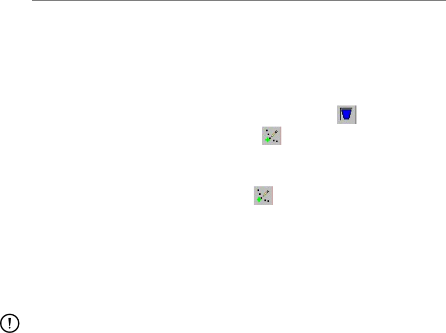
DRAFT
D-Water Quality, User Manual
Press the OK button.
Add the sewer overflow to the network by clicking with the left mouse button on the reach.
The river has two known cross section profiles. It is assumed that between these the profiles
can be calculated by interpolation.
Click the object ‘Flow - Cross section’ of the menu ‘Flow model’: .
Click the button ‘Add node’ of the menu ‘Node’: .
Enter the name “Cross-Section1” in both input fields.
Press the OK button.
Add the cross section to the network by clicking with the left mouse button on the network.
Click the button Add node of the menu Node: .
Enter the name “Cross-Section2” in both input fields.
Press the OK button.
Add the cross section to the network by clicking with the left mouse button on the network.
DELWAQ is the general water quality model of Deltares. DELWAQ can be used stand-alone
and in combination with 1D, 2D and 3D-model schematisations. For that reason DELWAQ
uses its own schematisation, which can be coupled to any hydraulic model.
Remark:
It is essential that a DELWAQ-schematisation is generated!
Perform the following actions
Go to the menu Edit and subsequently Delwaq segments.
Click the button Auto.
Click the menu File →Close.
The DELWAQ-segments are coloured red in the map.
7.2.1.11 Model data
The input data of the model, i.e. the profiles and the boundary conditions, are to be edited in
the menu item ‘Model data’.
Go to the menu ‘Edit’ and subsequently to ‘Model data’.
174 of 382 Deltares
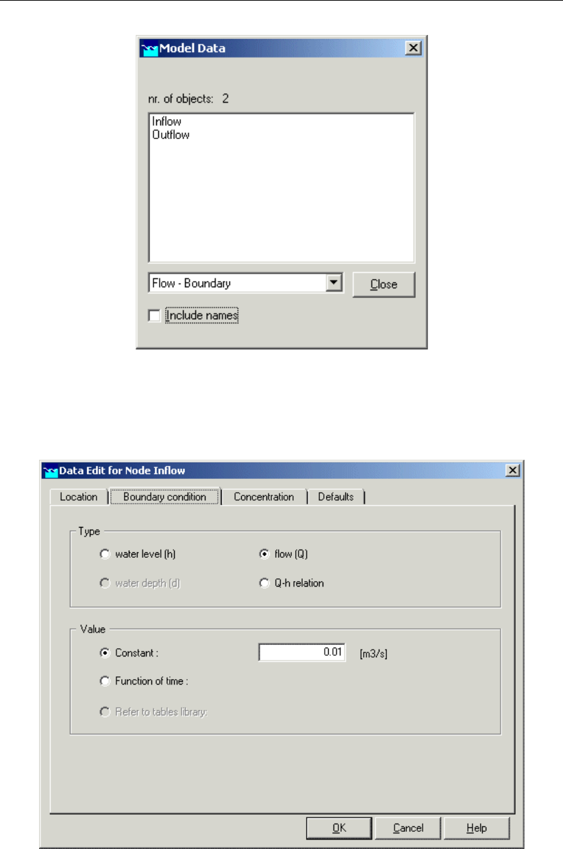
DRAFT
Tutorials
Figure 7.57: The Model Data Window
Select the node with the identifier ’Inflow’.
Click the Edit button that appears in the upper right corner of the ’Model Data’ window.
Figure 7.58: The data editor for hydrological data.
Go to the tab ‘Boundary condition’.
Select ‘flow (Q)’ for this boundary condition.
Select constant option for value and enter value “0.01” m3/s.
Go to the tab ‘Concentration’.
Deltares 175 of 382
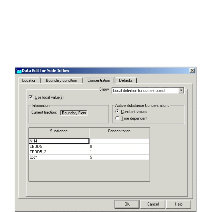
DRAFT
D-Water Quality, User Manual
This ’Data Edit’ window offers the functionality to edit both the local concentration definition
for the current object and the global concentration definition for the current fraction.
Choose the option ‘Use local values’ at the upper left of the window.
Select ‘Show: Local definition for current object’.
Choose the option ‘Constant values’ for ‘Active Substance Concentrations’.
Enter the concentrations (you must double click the cells first) as shown in Figure 7.59.
Figure 7.59: Boundary condition concentrations.
Click the OK button.
Select the boundary node ’Outflow’ in the ’Model Data’ window.
Click the Edit button.
Go to the tab ‘Boundary condition’.
Select ‘water level (h)’ for this boundary condition.
Enter a ‘constant value’ of “9” ‘m. above datum’.
Go to the tab ‘Concentration’.
Tick ‘Use local values’.
Select ‘Show: Local definition for current object’.
Tick ‘Constant values’.
Enter the concentrations in the table as shown in the figure above.
Click the OK button.
Select the node ’CSO’ on the map.
Click the right mouse button and select ’Model data’ - ’Flow Model’.
At this point the boundary condition of the sewer overflow can be provided. At this moment
we enter a discharge of 0 m3/s. The reference model simulates the current situation, without
sewer overflow.
176 of 382 Deltares

DRAFT
Tutorials
Go to the tab ‘Lateral flow’.
Enter a constant discharge of “0” m3/s.
In The Netherlands, the waste load from the sewer system to surface water is calculated as
the product of the discharge of the overflow and a constant concentration. Realistic concen-
trations are:
Substance Concentration
NH4 5.5 mg/l
CBOD5 60 mg/l
CBOD5_2 40 mg/l
OXY 7 mg/l
Go to the tab ‘Concentration’.
Tick ‘Use local values’.
Select ‘Show: Local definition for current object’.
Tick ‘Constant values’.
Enter the concentrations of “NH4”, “CBOD5”, “CBOD5_2” and “OXY” in overflow water in
the table.
Click the OK button.
After the boundary data conditions have been entered, the cross sections are to be defined.
Select ‘Flow - Cross Section’ in the check box in the window ‘Model Data’.
Select ’Cross-Section1’.
Click the ‘Edit’ button that appears in the upper right corner of the Model Data window.
Go to the tab ‘Location’.
Enter a bed level of “8.5” m above datum.
Enter a surface level of “10.5” m above datum.
Go to the tab ‘Cross section’.
Select the trapezium as the general type of cross section to be used.
Enter the name “River profile 1” in the input box next to ‘Cross section :’.
Click Define dimensions, for entering the dimensions of the cross section.
Enter “2” as the slope.
Enter “1.5” meter as the Bottomwidth B.
Enter “7” m as the maximum flow width.
Click Save dimensions. You’ll get a warning message which says " You changed the profile
definition. Do you want to add it as a new definition?".
Click the OK button.
The result is shown below.
Deltares 177 of 382
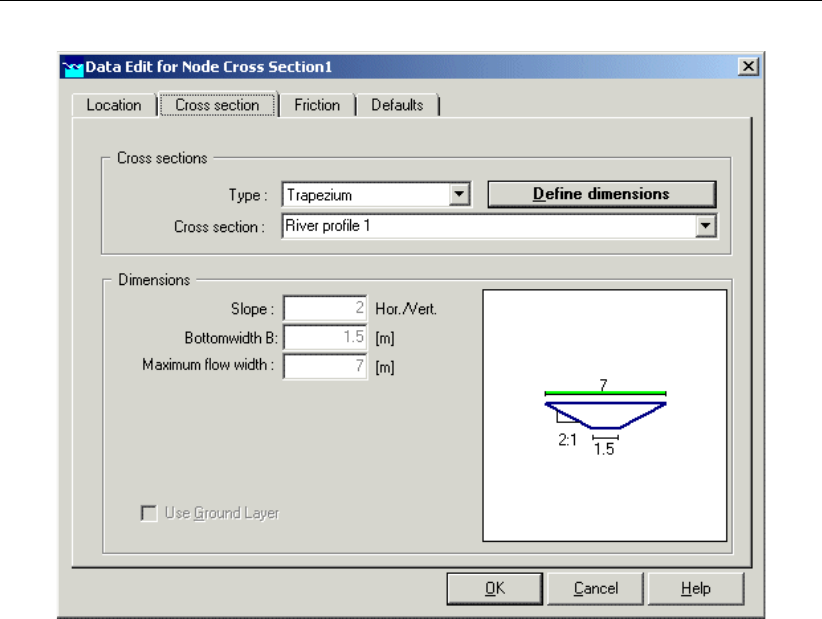
DRAFT
D-Water Quality, User Manual
Figure 7.60: Defining the cross section.
Go to the tab ‘Friction’.
SOBEK offers the functionality to set a global friction value. This value will be used in simula-
tion in case no local friction value has been provided.
In the ’Show’ list button, select ’Global value(s)’.
Select the option ‘Chezy’ for ‘type friction (Bed)’.
Enter “40” for constant value.
Click the OK button.
Select the cross section ’Cross-Section2’ from the list.
Click the Edit button.
Go to the tab ‘Location’.
Enter a bed level of “8” m above datum.
Enter a surface level of “10” m above datum.
Go to the tab ‘Cross section’.
Select the trapezium as the general type of cross section to be used.
Select the ‘River profile 1’ from the list ‘Cross section :’.
Click the OK button.
Click the Close button of Model Data.
Select ‘File’ - ‘Save’ - ‘Network’ to save the network.
Select ‘File’ - ‘Save’ - ‘Map’ to save the map.
Select ‘File’ - ‘Exit’ to leave NETTER and to return to the ’Schematisation’ menu.
178 of 382 Deltares

DRAFT
Tutorials
7.2.1.12 Simulation of the reference model
Click the OK button.
Double click the task block ‘Simulation’ in the Case Manager.
Now SOBEK will start the simulation.
7.2.1.13 Presentation of the simulation results
The simulation results can be presented as a table, a graph, or in a map. The presentation in
a graph is the best method if you want to judge whether or not appropriate values have been
chosen as model parameters.
Results in Charts
Double click the task block ‘Results in Charts’ in the Case Manager.
Select ‘History Results of Water Quality’.
Then click the View button.
Select the parameter ‘OXY’ (oxygen).
Select a segment halfway the schematisation, for instance segment 10.
Click the button All above the right table, to have all output time steps shown in the graph.
See also Figure 7.61, where the selected output options are shown.
Figure 7.61: Selecting output parameters in ‘History Results of Water Quality’.
Click the Graph button.
As can be seen, the oxygen concentration is increasing slowly in time. The increase is due to
re-aeration.
Deltares 179 of 382
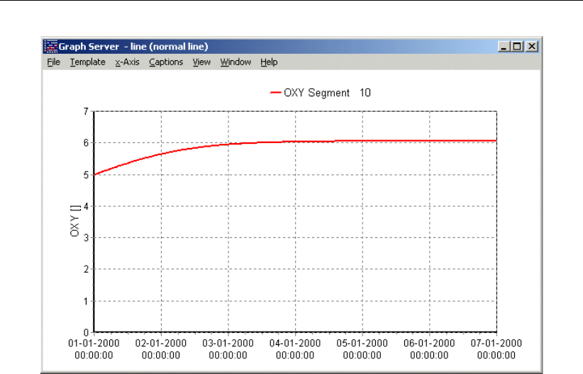
DRAFT
D-Water Quality, User Manual
Figure 7.62: The oxygen concentration for the reference situation. (Graph may differ de-
pending on the segment numbering and length of your schematisation)
Click ’File’ and subsequently ’Exit’ to close the figure.
Press the Exit button.
Click the Exit button to leave the task block ‘Results in Charts’.
Save the model!
Don’t forget to save the model! The model can be saved in the Case Manager.
Go to the menu ‘Case’ and subsequently ‘Save’ to save the case.
7.2.2 Creating cases for several overflow situations
7.2.2.1 The Case manager (I)
In this chapter the reference model for the current situation will be used to create cases for
the simulation of the effects of combined sewer overflows with repeat times of 1, 2, 5 and 10
year. This can be done in the Case Manager.
Note that the case ‘Reference model’ is saved under new names. The copies of the reference
case are used to simulate the effects of sewer overflows with different repeat times.
Please be aware that the Case Manager makes a copy of the model! There is no direct link
with the reference model anymore! A change in the network schematisation (for instance river
discharge) has to be made in all cases, in order to avoid differences between the cases.
Go to the menu ‘Case’ and then ‘Open as new’.
Select the case ‘Reference model’.
Enter the name “T1”.
Press the OK button.
180 of 382 Deltares
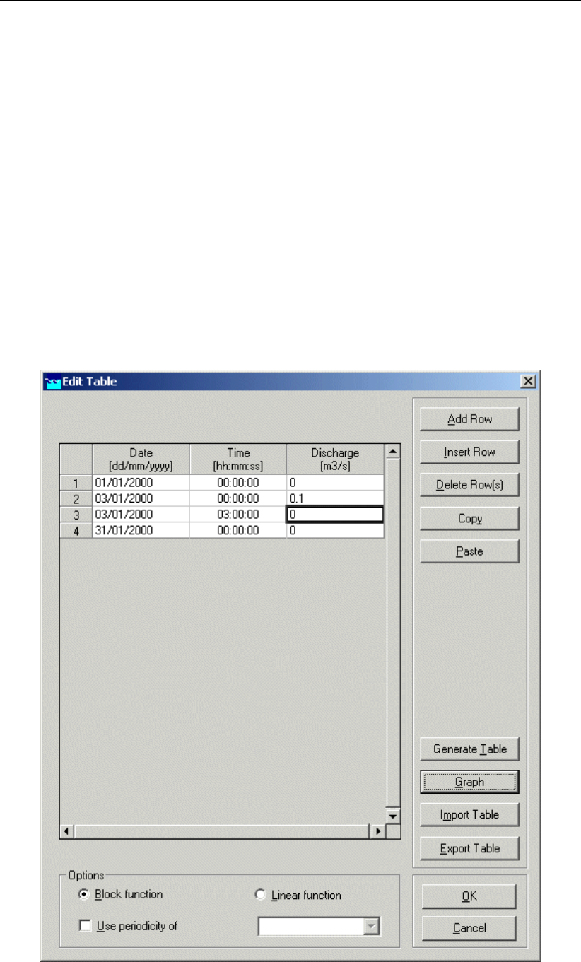
DRAFT
Tutorials
7.2.2.2 Model data
A sewer overflow is in general a peak discharge that lasts for some hours. The sewer overflow
will be modelled as a boundary condition for the node with lateral discharge. In order to give
the model some start-up time, the overflowing happens at the third day.
Double click the task block ‘Schematisation’.
Click Edit model in the ‘Schematisation’ menu.
Select the node ’CSO’ on the map.
Click the right mouse button.
Select ’Model data’ - ’Flow Model’.
Go to the tab ‘Lateral Flow’.
Choose for a ‘Function of time’.
Click the Table... button.
Press the Add Row button.
Enter “3”.
Press the OK button.
Enter the time series as shown below.
Figure 7.63: The time series of the sewer overflow for the case ’T1’.
Deltares 181 of 382

DRAFT
D-Water Quality, User Manual
Tick the option ’Block function’.
Click the OK button to close the ‘Edit Table’.
Press the OK button to close the ‘Data Edit for Node’ window.
Go to the menu ‘File’ and then ‘Save’ and finally ‘Network’ to save the changes.
Go to the menu ‘File’ and then Exit to leave NETTER.
Click the OK button to leave the ‘Schematisation’ and to return to the Case Manager.
The discharge of the sewer overflow with a repeat time of 1 year has been entered now.
7.2.2.3 The Case Manager (II)
The changes in the case ‘T1’ must be saved by the case manager.
Go to ‘Case’ and then ‘Save’ to save the case.
Go to ‘Case’ and then ‘Close’ to close the case.
Now that the case has been saved, you should make copies of the reference case again by
using the Open as New option in the Task Manager, selecting the T1 case and choosing a
new case name for 3 new cases as listed below.
name of the case repeat time CSO discharge duration of the
event
reference model — — —
T1 (T = 1 year) 0.10 m3/s 3 hours
T2 (T = 2 years) 0.20 m3/s 3 hours
T5 (T = 5 years) 0.50 m3/s 3 hours
T10 (T = 10 years) 0.75 m3/s 3 hours
Set up the schematisation of the three remaining cases T2, T5 and T10 in the same way
you modelled the case T1. Each case will have a different discharge value for the ’CSO’
node representing a different repeat time.
Remarks:
The above repeat time is listed for the purpose of clarifying the tutorial data. The repeat
time is not actually a value that the user can enter during this tutorial.
Do not forget to save each case before you make a copy or close them!
7.2.3 Simulations in batch mode
Since there are different cases to be calculated, it would be easy if those simulations were
made in series, without the need for modeller intervention. For this reason, SOBEK offers the
option of simulating in batch mode.
182 of 382 Deltares

DRAFT
Tutorials
7.2.3.1 Simulations
First we have to specify the cases that must be simulated in a batch.
Close the case, if one is loaded at the moment, via the menu Case and subsequently
Close.
Go to the menu Case and then to Define Batch.
In the window shown below the batch can be specified
Figure 7.64: Specifying the batch simulation.
Select the cases ‘T1’, ‘T2’, ‘T5’ and ‘T10’, by clicking while the Ctrl key is kept pressed.
Click the OK button.
Click the grey task block ‘Simulation’. The task block becomes surrounded by an orange
margin.
Go to Case and Run Batch.
The simulations are made and saved one by one now.
7.2.3.2 Special settings
It can happen that the simulations in batch mode are interrupted by the message shown
below:
Deltares 183 of 382
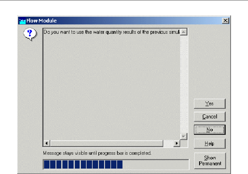
DRAFT
D-Water Quality, User Manual
Figure 7.65: Using the previous simulation results.
A window with such a question would halt the calculation, until an answer is given. For this
reason a timer has been incorporated: after two minutes the window disappears and the
simulation continues. Default the answer is ‘No’. After thirty seconds of waiting a new flow
simulation is started. Of course you can also click ‘No’ yourself. It’s important that the flow
simulation is renewed, because the available flow results stem from the reference model that
has been copied!
By switching on the option ‘use previous flow results in batch mode’ in ‘Settings’, ‘water qual-
ity’, on the tab ‘Simulation options’, the default answer becomes ‘Yes’. This can save calcula-
tion time. However, to avoid confusion, it’s recommended that this option is not used for the
example in this tutorial.
Press the No button four times.
7.2.4 Presentation and analysis of the results
With the Case Analysis Tool the results of several cases can be compared with each other
and shown in one graph or map. This is of great help while analysing several scenarios or
situations. For instance when you want to compare the oxygen concentration in the surface
water after a number of sewer overflow events. Furthermore the Case Analysis Tool (CAT) of-
fers many (statistical) functions, like the derivation of minima and maxima, averages, deviation
from the required water quality etc.
184 of 382 Deltares
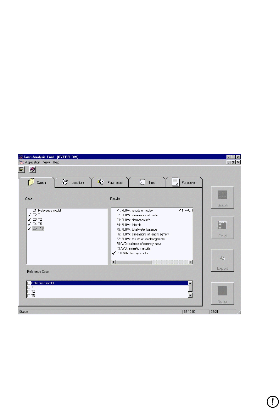
DRAFT
Tutorials
7.2.4.1 Making a graph in the Case Analysis Tool (CAT)
With the sewer overflows in these cases one might expect that more oxygen will be depleted
at events with a higher repeat time. This can be demonstrated with a figure at one location in
which the oxygen concentration is shown for several repeat times. Such a graph can be made
in the Case Analysis Tool.
Leave the Case Manager via ‘Case’ and then ‘Exit’.
Select ’Projects’ - ’Case Analysis Tool’.
Select the project ‘T_CSO’.
Click the OK button.
Go to the tab ‘Cases’.
Select the case T1 in the left panel. Select the function ‘WQ: history results’ in the right
half of the window.
Do the same for the cases ‘T2’, ‘T5’, en ‘T10’: select the name of case an click on the
function ‘WQ history results’ in the right half of the window.
Figure 7.66: The Case Analysis Tool.
Go to the tab ‘Locations’. If the tab names are not visible, increase the width of the window.
Select a segment (for example, segment 33) in the left column and click the button ‘>’.
Go to the tab ‘Parameters’.
Select ‘OXY’ and click ‘>’.
Note: Neither on the tab ‘Time’, nor on the tab ‘Functions’ changes have to be made.
Click the button ‘Graph’, at the right side of the window.
Remark:
The amount of delwaq segments in this network is determined by the distance between
the two boundary nodes we placed earlier in this tutorial. Depending on where exactly
the boundary nodes were placed, both the amount of delwaq segments in this network
may vary, as may the results for any specific delwaq segment.
Deltares 185 of 382
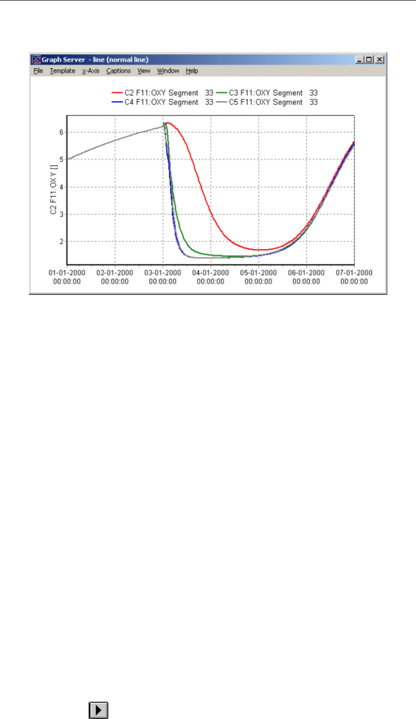
DRAFT
D-Water Quality, User Manual
A graph with simulated oxygen concentration after the four events appears.
Figure 7.67: The simulation results of oxygen after four events with repeat times T1, T2,
T5 and T10.
Close the graph server window via ‘File’ and ‘Exit’.
Leave the Case Analysis Tool via the menu ‘Application’ and ‘Exit’.
Press the No button.
7.2.4.2 Results in maps
The previous paragraph showed that the effects of the sewer overflow are most pronounced
after overflow events with repeat times of 5 and 10 years. In this paragraph the simulation
results of the case T10 will be analysed further.
Click in the main SOBEK menu on ’Open Project’.
Choose the project ’T_CSO’.
Press the OK button.
Select ’Case’ - ’Open’
Select the case ’T10’.
Press the OK button.
Double-click the task ’Results in Maps’ and NETTER will start.
Select ’Map Results of Water Quality’ in the Active Legend.
To get a quick overview of the results data, you can make the nodes change colour and size,
according to their data value.
Choose ’Options’ - ’Network Data...’ in the menu bar.
Click the ’All Data’ tab.
Activate the ’Width’ checkbox for ’Show branch data’.
Click the OK button.
Select ’OXY’ in the View Data list.
Change the ’Play mode’ in the menu ‘play mode’ into ’Play Continuous’
Click the button in ’View Data’ and the oxygen concentration in the canal is shown as
186 of 382 Deltares
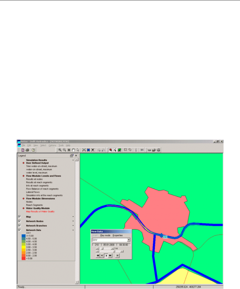
DRAFT
Tutorials
a movie.
A map with the minimum oxygen concentration that is simulated is very illustrative, because it
shows the influence sphere of the sewer overflow.
Go to the menu ’Options’ - ’Data Statistics’ and select ’minimum’.
For presentation purposes it might be useful to customise the scale:
Go to the menu ’Options’ - ’Data value options’
Tick the option ’User’.
Click the button ’Scale’.
In this window you can customise the scale: the number of classes, boundaries of classes
and colours.
Figure 7.68: The simulation results of oxygen after an event with a repeat time of 10
years. The minimum oxygen concentration is shown.
Click the OK button.
Click the OK button.
Select ’File’ - ’Exit’ to leave NETTER.
Select ’Case’ - ’Close’.
Press the Yes button.
7.2.5 Fraction calculations
The option ‘Fraction calculations’ is a useful tool for the analysis of the transport and disper-
sion of water through the water system. The water flowing from each source is labelled, for
instance as River water, Overflow water and Initial water. In this way the origin of the water at
a certain point in the water system can be traced back to the source.
Deltares 187 of 382
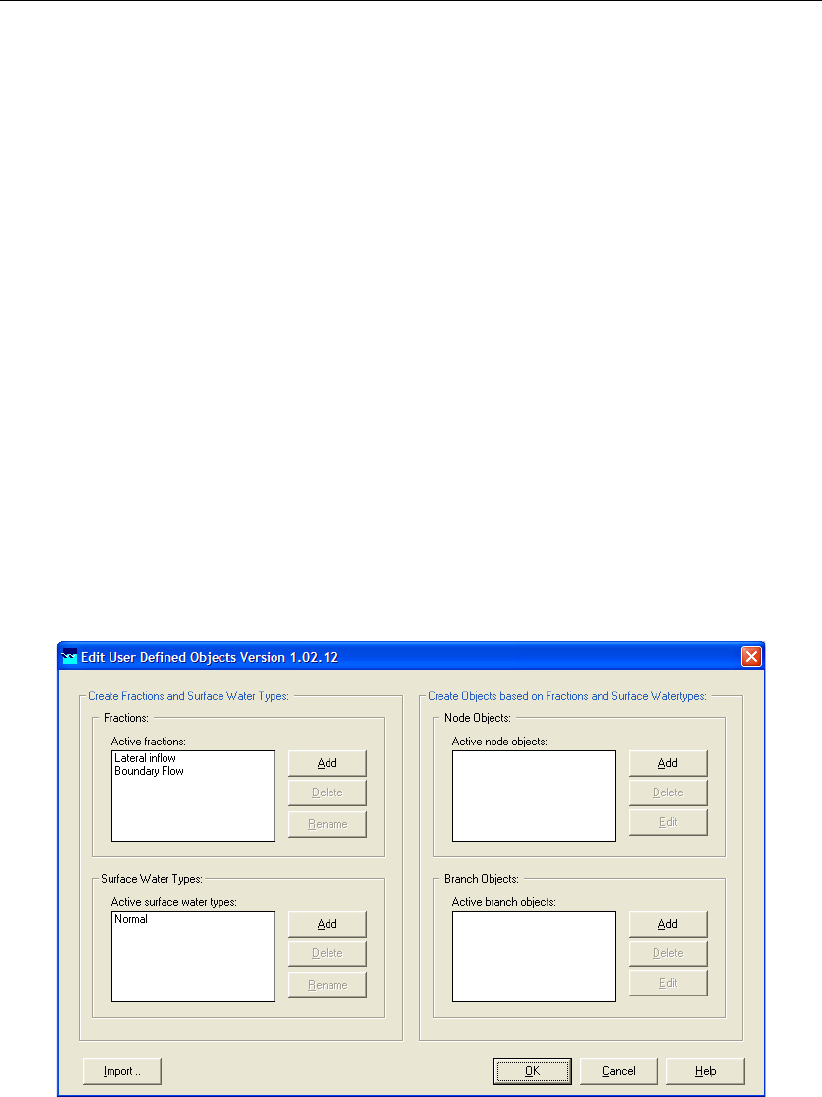
DRAFT
D-Water Quality, User Manual
7.2.5.1 Settings
Select ’Case’ - ’Open as new’.
Select the case ‘T1’.
Enter the name “Fraction T1”.
Press the OK button.
Double click the task block ‘Settings’.
Click the button ‘Edit’ next to ‘1DWAQ’.
Go to the tab ‘WQ Processes’.
Select ‘calculate fractions’.
Click the OK button to leave the 1DWAQ Settings.
Click the OK button to return to the Case Manager.
7.2.5.2 User defined objects
The water fractions enter the water system via so-called user defined objects. The user de-
fined objects are copies of existing object types like ‘Flow-Boundary’ and ‘Flow-Lateral Flow’,
but have a unique water fraction. In this model three water fractions are discerned: River
water, Sewer water and Initial water. The boundary nodes where these fractions enter the
water system will be defined by the modeller.
Double click the task block ‘Schematisation’.
Click the Edit User Defined Objects button.
Figure 7.69: In this window the ‘User Defined Objects’ are created.
The window in Figure 7.69 appears. This window consists of four fields. First the water
fractions will be defined. Then these fractions are coupled to objects. These new, user defined
objects can be applied in the model schematisation. In this specific example two objects will
be added to the list with object types: an object for the upstream boundary and an object for
the sewer overflow.
Click the Add button next to the input block ‘Active fractions’ (upper left input block).
Enter the name of the fraction: “River water”.
Click OK button.
Click the ‘Add’ button once again, to add a second fraction.
188 of 382 Deltares
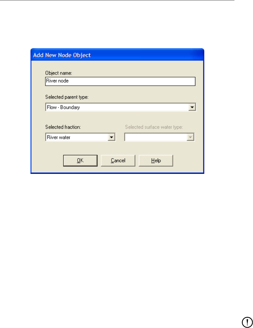
DRAFT
Tutorials
Enter the name of the fraction: “Sewer water”.
Click OK button.
Click Add next to the input block ‘Active node objects’ (upper right block).
Figure 7.70: Defining a new Node object.
The window in Figure 7.70 appears. In this window the new objects are given a name. The
objects are linked with a water fraction. Furthermore one has to specify the type of object that
the new object is derived from.
Enter the ‘Object name’: “River node”.
Select the type of node where the new node is derived from: ‘Flow - Boundary’.
The ‘Selected fraction’ is the fraction ‘River water’.
Click the OK button.
Click Add next to the input block ‘Active node objects’ once again.
Enter the ‘Object name’: “Overflow node”.
Select the type of node where the new object is derived from: ‘Flow - Lateral Flow’.
The ‘Selected fraction’ is the fraction ‘Sewer water’.
Click the OK button.
Click the OK button to return to the ‘Schematisation’ menu.
Click the Edit model button and NETTER will be started.
Remark:
After modifying User-defined objects, the user must always open the network editor and
save the network again. If this step is not performed, the modified user-defined objects
will not be fully updated.
Deltares 189 of 382
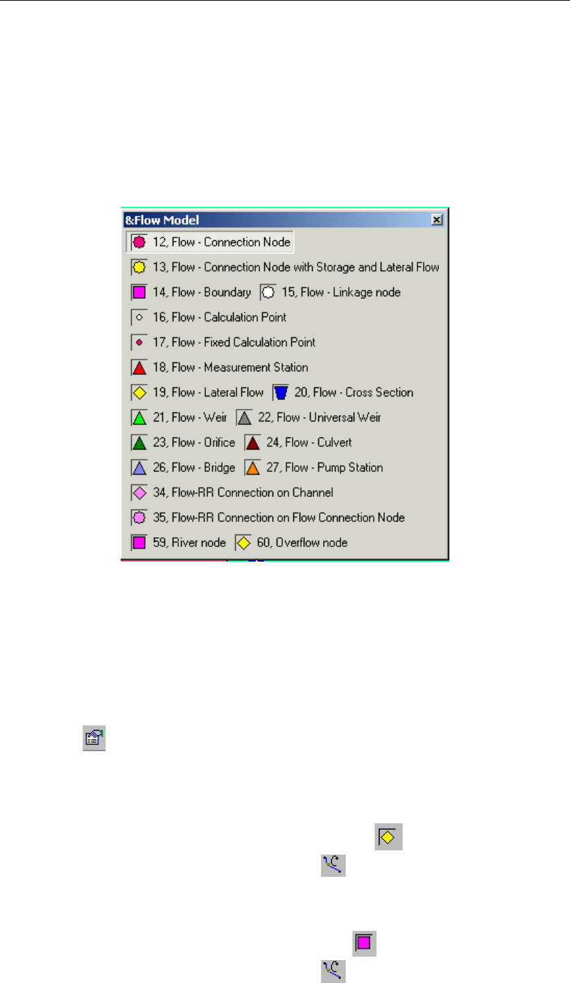
DRAFT
D-Water Quality, User Manual
7.2.5.3 Preparation of the network
The new objects have to be included in the network. In this way two new sources of water are
introduced in the fraction calculations: River water and Sewer water.
Zoom in on the CSO node.
Click the button ‘Edit Network’.
Your Flow Mode node menu will now look similar to Figure 7.71.
Figure 7.71: The available objects. At the bottom are two new user defined objects: ’River
node ’and ’Overflow node’.
From now on two new user defined objects are available: ‘River node’ and ‘Overflow node’. In
the network two existing objects will be replaced by these two new nodes.
In order to see the objects on the map please:
Click the button in the Active Legend or select the menu item ’Options’ - ’Network
Data...’.
Select the tab ’Node’.
Select the radio button ’Netter Type’.
Press the OK button.
Click the object type ’Overflow node’ in the menu ‘Node’: .
Click the button ‘Node type’ of the menu ‘Node’: .
Click the CSO node, that represents the Sewer Overflow. This node is replaced by a node
of the object type ‘Overflow node’.
Zoom in on the ’Inflow’ node.
Click the object type ‘River node’ in the menu ‘Node’: .
Click the button ‘Node type’ of the menu ‘Node’: .
190 of 382 Deltares

DRAFT
Tutorials
Click the ’Inflow’ node that represents the upstream river boundary. This object is replaced
by an object of the type ‘River node’.
Now, we will check if the hydrological data of the replaced nodes is still correct. Please note
that the boundary conditions for water quality (i.e. the concentrations at the boundaries) are
no longer visible. This is because fraction calculations don’t use them.
Go to the menu ‘Edit’ - ‘Model Data’.
Select the ‘Overflow node’ option.
Select the node ‘CSO’.
Click the ‘Edit’ button that appears in the upper right corner of the window.
Have a look at the boundary conditions with regard to the water quantity.
Click the OK button.
Select the ‘River node’ option.
Select the node ‘Inflow’.
Click the ‘Edit’ button that appears in the upper right corner of the window.
Have a look at the boundary conditions with regard to the water quantity. As you can see, the
model data of the original boundary condition has been copied into the user defined object,
"River node".
When you are finished looking at the data:
Click the OK button.
Go to the menu ‘File’ - ‘Save’ - ’Network’.
Go to the menu ‘File’ - Exit’ to leave NETTER.
Click the OK button in the Schematisation menu’ to return to the Case Manager.
7.2.5.4 Simulation and presentation of the results
Double click the task block ‘Simulation’.
Press the No button.
Click the task block ‘Results in Charts’ when the calculation is finished.
Choose for ‘History Results of Water quality’.
Press the View button.
The window shown below appears. In total four fractions, the volume and a check are shown.
Two of them have been added in the previous chapter.
Deltares 191 of 382
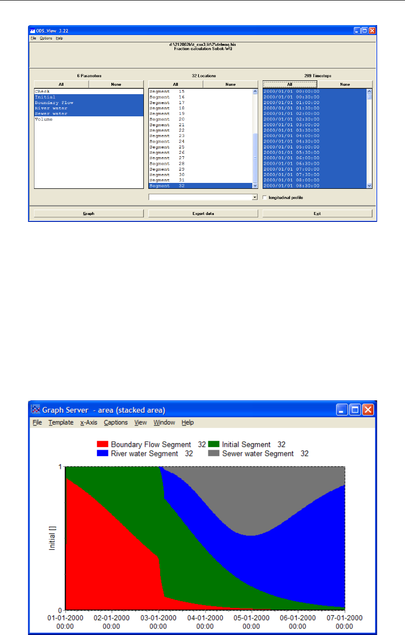
DRAFT
D-Water Quality, User Manual
Figure 7.72: Preparing a graph.
Select the fractions ‘Initial’, ’Boundary Flow’, ‘Sewer water’ and ‘River water’, by clicking
them while the Ctrl key is kept pressed.
Select a segment, for example segment 32.
Click All above the table with the output time steps to select the entire simulation period.
Click the Graph button.
Go to the menu ‘Template’ and choose for ‘area (stacked area)’.
The results of the fraction calculation are shown in Figure 7.73. In the example output, the
influence of the sewer overflow on segment 32 is clearly visible down from day 3. The initial
water is driven out of the initial water by River water and by Sewer water.
Figure 7.73: The results of the fraction calculations.
Go to the menu ‘File’ - ‘Exit’ to close the figure.
Click the Exit button.
Click the Exit button to return to the Case Manager.
192 of 382 Deltares

DRAFT
Tutorials
Go to ‘Case’ and then ‘Save’ to save the case.
Go to ‘Case’ and then ‘Close’ to close the case.
Go to ‘Case’ and then ‘Exit’ to return to the main menu of SOBEK.
7.2.5.5 Epilogue
In this example the fraction calculations were set up after the network was created and several
calculations were made. This approach was chosen for educational reasons. You may save
time if you define the ’user defined objects’ before you start to make a schematisation.
Deltares 193 of 382

DRAFT
D-Water Quality, User Manual
194 of 382 Deltares

DRAFT
8 Conceptual description
8.1 Introduction
D-WAQ solves the equations for transport and physical, (bio)chemical and biological pro-
cesses. You need to define transport and processes and the model does the rest. However,
you should be familiar with the basic concepts in order to understand the functioning of D-
WAQ and to make optimal use of the multiple possibilities of the program.
In this chapter we introduce the mathematical ‘advection-diffusion-reaction equation’ that
forms the basis of D-WAQ. As the model makes use of discrete computational elements and
discrete time steps, this analytical equation can not be applied directly. Therefore, we will
introduce you to the numerical discretisation of D-WAQ and the underlying principles of how
to describe transport and water quality processes.
8.2 Mass balances
D-WAQ administrates the mass balance of selected state variables, such as dissolved oxy-
gen, nitrate or cadmium. It does so for each computational cell. Mass transported by flowing
water from one cell to the next serves as a negative term in the mass balance in the first
computational cell and as a positive term in the second computational cell. The method is
mass-conserving by definition. By combining computational cells in one, two or three dimen-
sions each water system can be represented and substances can be transported through
computational cells and hence through the water system. When we take into account that
within a computational cell substances can be converted to other substances, we have to in-
clude water quality processes. For example, nitrification converts ammonium (NH+
4) to nitrate
(NO−
3), resulting in a negative term in the ammonium mass balance of that computational cell
and a positive term in the nitrate mass balance. Finally, we can add mass to a computational
cell that originates from outside the modelled water system. Waste loads are an example of
this, but also mass may also enter the modelled water system across open model boundaries.
To proceed one step in time (t+ ∆t), D-WAQ solves Eq.(8.1) for each computational cell
and for each state variable. Eq.(8.1) is a simplified representation of the advection-diffusion-
reaction equation which will be discussed in section 8.4.
Mt+∆t
i=Mt
i+ ∆t×∆M
∆tT r
+ ∆t×∆M
∆tP
+ ∆t×∆M
∆tS
(8.1)
The mass balance has the following components:
the mass at the beginning of a time step: Mt
i
the mass at the end of a time step: Mt+∆t
i
changes by transport: ∆M
∆tT r
changes by physical, (bio)chemical or biological processes: ∆M
∆tP
changes by sources (e.g. waste loads, river discharges): ∆M
∆tS
It should be noticed that the basic principles of D-WAQ are the same whether you have one
state variable and only two computational cells, or you have several tens of state variables and
thousands of computational cells. The only differences is the number of times that D-WAQ
has to solve Eq.(8.1).
Changes by transport include both advective and dispersive transport, that is the transport by
flowing water and the transport as a result of concentration differences respectively. The flow
Deltares 195 of 382
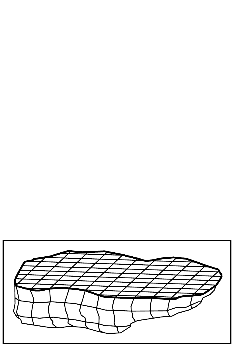
DRAFT
D-Water Quality, User Manual
of water is usually derived from the Delft3D-FLOW hydrodynamic model (Delft3D-FLOW UM,
2013). Dispersion in the vertical direction which is important if the water column is stratified, is
derived from Delft3D-FLOW as well. Dispersion in the horizontal direction is user input (refer
to section 5.3.3). Dispersion, as defined here, differs from the physical concept of molecular
diffusion as it stands for all transport that is not described by the advective transport (there is
sub grid-scale transport of water that is not resolved by Delft3D-FLOW).
Changes by processes include physical processes such as reaeration and settling, (bio)chemical
processes such as adsorption and denitrification and biological processes such as primary
production and predation on phytoplankton. Water quality processes convert one substance
to another (such as the aforementioned nitrification example). A special type of processes
deals with settling in a 3-dimensional situation, as these processes transport particulate mat-
ter from one computational cell to the one below. For a detailed description of the water quality
processes included in D-WAQ refer to chapter 9 and the D-WAQ Technical Reference Manual
(D-WAQ TRM,2013).
Changes by sources include the addition of mass by waste loads and the extraction of mass
by intakes. Mass entering over the model boundaries can be considered a source as well. The
water flowing into or flowing out of the modelled area over the model boundaries is derived
from the Delft3D-FLOW hydrodynamic model.
8.3 Spatial schematisation
To model the transport of substances, a water system is divided in small boxes (Figure 8.1).
The complete ensemble of all the small boxes is called the ‘grid’ or ‘schematisation’. In D-
WAQ each box — from now on called a computational cell — is defined by its volume and
its dimensions in one, two or three directions (∆x,∆y,∆z) depending on the nature of the
schematisation (1D, 2D or 3D). Note that ∆x,∆yand ∆zdo not have to be equal, so that the
computational cell can have any rectangular shape. A computational cell can share surface
areas with other computational cells, the atmosphere and the sediment or coast line.
Figure 8.1: Division of a lake into small boxes with a finite volume; a structured three
dimensional grid is used
In D-WAQ each computational cell has a unique number ranging from 1 to N, where N is
the total number of computational cells. Also, each surface area that is shared with another
computational cell, is identified by a unique number, ranging from 1 to Q, where Q is the total
number of shared surface areas. Over this shared surface area mass can be exchanged be-
tween computational cells. Therefore, the shared surface areas are referred to as exchanges
196 of 382 Deltares
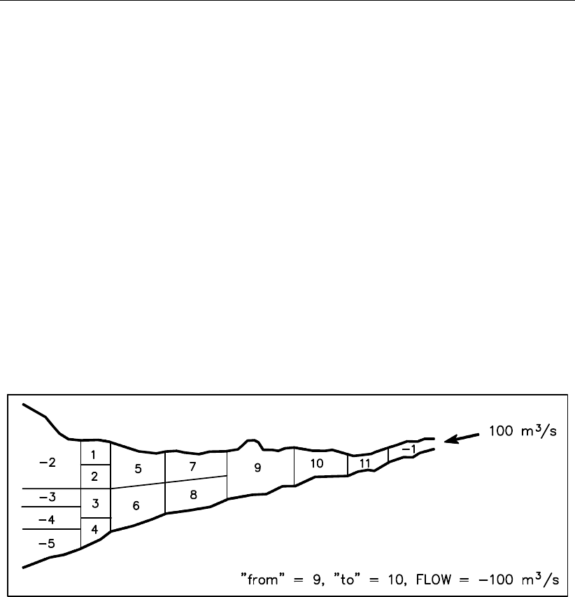
DRAFT
Conceptual description
as well. D-WAQ defines an exchange by the numbers of the two computational cells that
share the surface area.
Recapitulating, for each computational cell we know its:
volume
dimensions
surface area
neighbouring computational cells (i.e. exchanges)
Thus, we describe a water system in individual computational cells and through the exchanges
we know how the individual computational cells are interconnected. Adding to this the flow
of water between the computational cells which is derived from the hydrodynamic model (D-
Flow FM, Delft3D-FLOW, . . . ), and the basis for water quality modelling is there. Substances
and water quality processes can be added.
Because D-WAQ derives flows, volumes and the geometry from the hydrodynamic model, you
do not need to define them yourself. An example of a schematisation for D-WAQ is shown in
Figure 8.2.
Figure 8.2: Schematisation of an estuary with 11 computational cells and 5 boundary
cells indicated with a negative number. The exchange table indicates how the
computational cells are connected to each other and what the flow between
the computational cells is. The “From-1” an “To+1” columns refer to second
order connections which are used in some higher order numerical schemes.
Deltares 197 of 382
DRAFT
D-Water Quality, User Manual
Exchange Number “From” “To” “From - 1” “To + 1” “Flow”
1 -1 11 -1 10 100
2 11 10 -1 9 100
3 9 10 8 11 -100
4 9 8 10 6 75
5 9 7 10 5 25
6 8 7 0 0 5
7 7 5 9 2 30
8 8 6 9 3 70
9 5 6 0 0 0
10 5 2 7 -2 25
11 5 1 7 -2 5
12 1 2 0 3 0
13 2 3 1 4 0
14 3 4 2 0 5
15 6 3 8 -3 60
16 6 4 8 -5 10
17 3 -3 6 -3 50
18 3 -4 6 -4 5
19 4 -4 6 -4 5
20 4 -5 6 -5 10
21 1 -2 5 -2 5
22 2 -2 5 -2 25
Note: that you have to define 11 volumes but 22 flows to define the transport of water through
this estuary completely.
8.4 Advection-diffusion equation
A water quality model is in fact not more than a mass balance for the pollutants or state
variables necessary to describe the problem at hand. D-WAQ makes this mass balance for
you, for so-called segments (i.e. small water volumes):
∂M
∂t =advection +dispersion +source (8.2)
The source term consists for example of direct inputs and/or mortality (for bacteria), decay
(for bod), sedimentation (for solid particles), etc.
8.4.1 Advective transport
The advective transport across an exchange can be given as:
TA
x0=vx0×A×Cx0
with:
TA
x0advective transport at x=x0[g/s]
vx0velocity at x=x0[m/s]
Asurface area at x=x0[m2]
Cx0concentration at x=x0[g/m3]
198 of 382 Deltares

DRAFT
Conceptual description
We assume that velocities and concentrations are an average representative value for the
whole surface. The smaller the cross section, the better this assumption.
8.4.2 Dispersive transport
The dispersive transport across an exchange is assumed to be proportional to the concentra-
tion gradient and to the surface area:
TD
x0=−Dx0×A×∂C
∂x x=x0
with:
TD
x0dispersive transport at x=x0[g/s]
Dx0dispersion coefficient at x=x0[m2/s]
Asurface area at x=x0[m2]
∂C
∂x x=x0concentration gradient at x=x0[g/m4]
Dispersion is done according to Fick’s diffusion law. The proportionality constant Dis called
the dispersion (or diffusion) coefficient. The minus sign originates from the fact that dispersion
causes net transport from higher to lower concentrations, so in the opposite direction of the
concentration gradient.
The concentration gradient is the difference of concentrations per unit length, over a very
small distance across the cross section:
∂C
∂x x
= lim
∆x↓0
Cx+1
2∆x−Cx−1
2∆x
∆x
A numerical expression for this term will be given later on. Dispersion coefficients should be
calibrated or be obtained from calculations with turbulence models.
8.4.3 Transport from sources
The transport of pollutants from sources is given by the following expression, regardless of
the numerical method applied:
Tsrc =Qsrc ×Csrc Qsrc >0(8.3)
If the discharge flow Qsrc is negative (withdrawal), the model uses the following expression:
Tsrc =Qsrc ×CiQsrc <0(8.4)
where Cirepresents the concentration in the receiving Water Quality-segment. Thus, the
model withdraws water with the ambient concentrations. The source concentrations supplied
by the user are therefore neglected if the discharge is negative (withdrawal).
The model mixes the pollutants from the discharge over the receiving Water Quality-segment.
So, some erroneous upstream transport of pollutants can not be avoided. If this is not accept-
able, the only practical solution is to add more calculation points.
Remarks:
There is no dispersive transport related to a discharge.
Deltares 199 of 382

DRAFT
D-Water Quality, User Manual
If a (lateral) discharge is situated exactly on a calculation point (obligatory in SOBEK-
Rural/Urban): SOBEK-River divides the discharge over the grid cells upstream and
downstream of the calculation point;
SOBEK-Rural/Urban puts the discharge in the reach-segment downstream of the cal-
culation point, where the definition of "downstream" is evaluated based on the local and
actual direction of flow.
8.4.4 Mass transport by advection and dispersion
If the advective and dispersive terms are added and the terms at a second surface are in-
cluded (left and right side of a volume), the one dimensional equation results:
Mt+∆t
i=Mt
i+∆t×A× vx0Cx0−vx0+∆xCx0+∆x−Dx0
∂C
∂x x0
+Dx0+∆x
∂C
∂x x0+∆x!
with:
Mt
imass in volume i at time t [g]
∆ttime step [s]
∂C
∂x x0concentration gradient at x=x0[g/m]
Asurface area [m2]
vx0velocity at x=x0[m/s]
Cx0concentration at x=x0[g/m3]
Instead of this equation, D-WAQ uses the following equivalent equation:
Mt+∆t
i=Mt
i+∆t× Qx0Cx0−Qx0+∆xCx0+∆x−Dx0Ax0
∂C
∂x x0
+Dx0+∆xAx0+∆x
∂C
∂x x0+∆x!
with:
Mt
imass in volume iat time t[g]
∆ttime step [s]
∂C
∂x x0concentration gradient at x=x0[g/m]
Ax0surface area at x=x0[m2]
Qx0flow at x=x0[m3/s]
Cx0concentration at x=x0[g/m3]
If the previous equation is divided by the volume V= ∆x∆y∆z1and the time span ∆t,
then the following equation results in one dimension.
Ct+∆t
i−Ct
i
∆t=−vx0+∆xCx0+∆x−vx0Cx0
∆x+Dx0+∆x∂C
∂x x0+∆x−Dx0
∂C
∂x x0
∆x+
Taking the asymptotic limit ∆t→0and ∆x→0, the advection-diffusion equation for one
dimension results:
∂C
∂t +∂
∂x(vC)−∂
∂x D∂C
∂x = 0
Thus, the finite volume method for transport is a computational method to solve the advection-
diffusion equation. The accuracy of the method will be related to the size of ∆x,A(= ∆y×
∆z)and ∆t.
1Hereto it is required that all segments have an equal volume.
200 of 382 Deltares

DRAFT
Conceptual description
By adding terms for transport in the y- and z-direction a 3-dimensional model is obtained.
Taking the asymptotic limit again, will lead to a 3-dimensional advection-diffusion equation:
∂C
∂t +vx
∂C
∂x −Dx
∂2C
∂x2+vy
∂C
∂y −Dy
∂2C
∂y2+vz
∂C
∂z −Dz
∂2C
∂z2= 0 (8.5)
∂C
∂t +vx
∂C
∂x −Dx
∂2C
∂x2+vy
∂C
∂y −Dy
∂2C
∂y2+vz
∂C
∂z −Dz
∂2C
∂z2=S+fR(C, t)
(8.6)
with dispersion coefficients taken for every direction. If functions Sand fare added as
shown in the equation above, the so-called advection-diffusion-reaction equation emerges.
The additional terms are so-called source terms. They stand for:
1 Discharges or ‘waste loads’ (S): these source terms are additional inflows of water or
mass that were not present in the hydrodynamic module (Delft3D-FLOW, SOBEK). They
may be present in the continuity equation, but this is not strictly required. As many source
terms as required may be added by you. They are usually used for small rivers, discharges
of industries, sewage treatment plants, small waste load outfalls, etc.
2 Reaction terms or ‘processes’ (fR).
Processes can be split into physical processes and other processes. Examples of physical
processes are:
settling of suspended particulate matter
water movement not affecting substances, like evaporation
volatilisation of the substance itself at the water surface.
Examples of other processes are:
biochemical conversions like ammonia and oxygen forming nitrite
growth of algae (primary production)
predation by other animals
chemical reactions.
Only processes that can be written in the form of a partial differential equation are considered
∂C1
∂t R
=fRC1, C2, . . . , CN, t
with:
Ciconcentration at a given location for substance ‘i’ (here for Nsubstances)
fRany functional prescription
ttime
The function describes a relation between the concentration variation at a certain location
(x, y, z)and all other concentrations at exactly the same location at that time. Although this
is a very general formulation, some types of processes do not fit. Among them is, as most
important, the equilibrium kinetics of chemistry. Only relatively slow chemical processes can
be described with this equation.
8.5 Boundary conditions
Deltares 201 of 382

DRAFT
D-Water Quality, User Manual
8.5.1 Closed boundaries
Closed boundaries are those boundaries that have zero flow and dispersion for all time steps.
No transport is associated with these exchange surfaces. Sometimes exchanges are de-
fined anyway for these boundaries (e.g. for structured grids) in order to keep the grid layout
completely structured. In such cases the grid has some permanently dry cells. For closed
boundaries no concentrations are required as input.
8.5.2 Open boundaries
Open boundaries are required for solution of the advection-diffusion equation. Without spec-
ification of the open boundaries the model does not know what to do at its borders. Concen-
trations of all substances and dispersion coefficients must be specified at all open boundaries
for all time-steps. Flows are automatically taken from Delft3D-FLOW, SOBEK. As a conse-
quence of the mathematics behind the Water Quality model, downstream boundaries do have
an effect on the solution of the Water Quality model:
If the advection term is computed by a "central method", the concentration at the inter-
face between the last model segment and the downstream boundary is computed as the
average between the concentration in the last segment and the downstream boundary
concentration. Therefore, the downstream boundary concentration affects the advective
transport in this case.
For the computation of the dispersive term, the concentration gradient at the interface
between the last model segment and the downstream boundary is computed as the differ-
ence between the concentration in the last segment and the downstream boundary con-
centration divided by the distance between the two. Therefore, the downstream boundary
concentration affects the dispersive transport.
D-WAQ offers the possibility to avoid this effect of downstream boundary concentrations on
the solution. You can optionally (1) use an upwind advection scheme locally at the model
boundaries, and (2) suppress the dispersive transport locally at the model boundaries.
Remark:
In Figure 8.2 boundaries are segments with negative numbers. These boundary seg-
ments can be considered either as:
inactive computational elements
elements with one cross section but without any volume of water
8.5.3 Time lags and return time
If water crosses a boundary, it may be assumed that the concentration immediately outside
of the model area is influenced by the previous outflows. If the flow changes sign and inflow
takes place again (as in tidal estuaries), it may be assumed that part of the water flowed
out previously, enters again. As inflow proceeds, the boundary conditions as specified by
you, may become more and more effective. D-WAQ enables you to use a cosine shaped
function from the last outflow concentration to the specified boundary condition, according to
Figure 8.3. This so-called Thatcher-Harleman time lag uses the inner concentration if outflow
takes place and starts with the latest outflow concentration to reach the specified boundary
concentration within the user specified time lag.
In mathematical form it is given by:
C(t0+t) = C(t0)0.5+0.5 cos πt
2T+CB(t)0.5−0.5 cos πt
2T (8.7)
202 of 382 Deltares
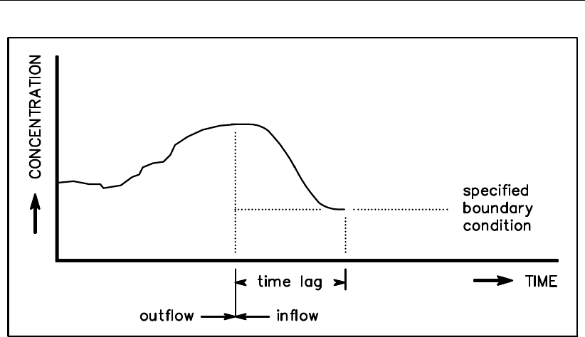
DRAFT
Conceptual description
Figure 8.3: Thatcher-Harleman boundary time lag
with t0< t −t0< t0+T, and:
t0time that outflow changes to inflow
ttime after t0
Csimulated boundary concentration
CBuser-specified boundary concentration (may be time-dependent as well)
TThatcher-Harleman time lag
The Thatcher-Harleman time lag Tmust be specified accurately if the model domain is small
with respect to the boundaries. In such cases, the boundary conditions have a large impact
on the simulation results. For estuaries it is typically in the order of one to six hours and for
polder systems typical values are in the order of five days. For most application the model
boundaries will be far from a region of interest (a beach, an ecological site, a dumping site,
etc.) and the use of constant boundary conditions will then be sufficient.
Deltares 203 of 382

DRAFT
D-Water Quality, User Manual
204 of 382 Deltares
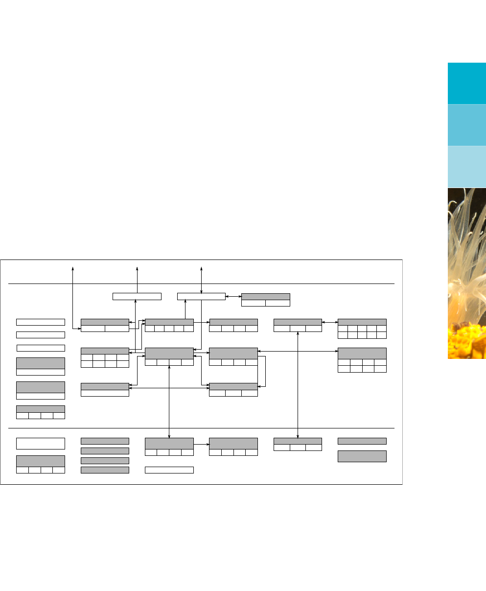
DRAFT
9 Principles of water quality modelling
9.1 Introduction
Water quality deals with the composition of water. In its most limited definition, only the
chemical composition of a water system is included. However, in D-WAQ we include biological
components up to the level of primary producers and some secondary producers as well as
the composition of the sediment in water quality modelling.
In this section we will give a basic outline of water quality in general and a more detailed outline
of how water quality processes are implemented in D-WAQ. The theory of water quality will
not be discussed in detail here as we expect the basic knowledge to be present. However, we
discuss the principles of water quality as needed to link the text book theory to the D-WAQ
model.
TIC Alkalinity
Iron
7 Components
Sulphur
SO4
SUD SUP
NO
NH PO Si
AAP VIVP
APATP
OPAL
Methane
C
P S
NSi
(particulate)
POC PON POP POS
Organic Matter
(dissolved)
DOC DON DOP DOS
Grazers
C N PSi
Dissolved Oxygen
IM2 IM3
IM1
Oxygen Demand
BOD COD
phytobentos
C N PSi
Micro-
As
Cr Hg
Cd Cu
Ni Pb VZn
pollutants
Atr BaP Diu Flu
Organic micro-
HCB HCH PCB OMP
Sediment Oxygen
Demand
EnCoc
EColi FColi TColi
Tracers
Tracers
Continuity
Salinity/Chloride
Temperature
Inorganic Matter
IM2 IM3
IM1
Organic Matter
(particulate)
POC PON POP POS
Heavy Metals
pollutants
Organic micro-
Atmosphere
Water
Sediment
Heavy Metals
Inorganic Matter
Decayable
Conservative
5 Components
5 Components
Bacteria
pH
Nutrients
34 4
Phytoplankton
Organic Matter
Organic Matter
(dissolved)
DOC DON DOP DOS
Nutrients
Oxygen
Sulphur
Iron Methane
Figure 9.1: General overview of substances included in D-WAQ. Substances are organ-
ised in functional groups indicated by a grey header, except for some sub-
stances that form a group of their own. Major links between substances are
indicated by arrows; note that many links are omitted.
In D-WAQ the constituents of a water system are divided in functional groups (Figure 9.1).
A functional group includes one or more substances that display similar physical and/or
(bio)chemical behaviour in a water system. For example, the nutrients nitrate, ammonium,
phosphate and silicon are a functional group as they are required for primary production.
Functional groups can interact with each other directly, as in the previous example, or indi-
rectly as inorganic suspended matter influences the light availability for primary production.
In the remainder of this chapter the functional groups are described separately. To get a
complete description of the water system you intend to simulate, you will have to combine the
separate descriptions of the functional groups. Within the functional group descriptions links
to other functional groups are indicated.
9.2 Salinity, chloride, tracers and continuity
Salinity, chloride and conservative tracers are special substances in D-WAQ as they are not
subject to water quality processes. They are only subject to transport. As insight in transport
Deltares 205 of 382

DRAFT
D-Water Quality, User Manual
is usually essential, these substances are nevertheless useful to water quality modellers. Not
subject to water quality processes themselves, these substances allow you to distinguish
between the effect of transport and processes for other substances, as they can isolate the
effect of transport. Obviously, salinity and chloride indicate the fate of fresh river water mixing
with sea water.
Conservative tracers (conservative meaning ‘not subject to decay’) have a wider range of
application as they can be assigned at choice to sources of water. You might want to use
conservative tracers to indicate where the water entering over the model boundaries is going
to, or to determine the fraction of the water originating from a certain source. D-WAQ allows
you to specify up to five conservative tracers.
A special type of conservative tracer is called ‘Continuity’. It has no physical or chemical
meaning. Instead it is used to establish the numerical correctness and stability of the simula-
tion. By assigning a concentration of 1 g/m3to all water sources (initial condition, boundary
condition and discharges) the Continuity concentration should remain 1 g/m3during the whole
simulation, as there are no processes that dilute or concentrate it and all water has a concen-
tration of 1 g/m3. If the concentration during the simulation significantly deviates from 1 g/m3,
you have either overlooked a source of water or the simulation is numerically unstable. You
should never proceed with including more substances in the water quality simulation if the
latter happens. If for example the Continuity concentration is equal to 1.1 g/m3, the deviation
is +10 %. If you included for example nitrate in the simulation, the nitrate concentration would
have been overestimated by 10 % as well.
Next to conservative tracers D-WAQ has five decayable tracers as well. Decayable tracers
are subject to first order decay (C(t) = C0×e−k×t). Decayable tracers can represent
radioactive elements, when the decay rate kis proportional to the half life (k=ln 2
t1/2). Ignoring
the complex chemical reactions and assuming first order decay, decayable tracers have been
used to simulate the break-down of disinfectants such as chlorine in the natural environment.
In combination with conservative tracers decayable tracers can be used to establish the ‘age’
of water from a specific source. The decaying tracer serves as a timer after it is released
simultaneously with the conservative tracer.
9.3 Water temperature and temperature dependency of rates
The water temperature determines the rate at which water quality processes take place. As
such, it is important that the water temperature is correct in the simulation. The temperature
dependency of reaction rates has a uniform exponential Equation (9.1) that is applied in many
of the processes included in D-WAQ:
k=k20 ×k(T−20)
T(9.1)
with:
krate constant at temperature T[d−1]
k20 rate constant at reference temperature 20 ◦C [d−1]
kTtemperature coefficient [-]
Tambient water temperature [◦C]
The temperature coefficient kTusually ranges between 1.01 and 1.10. With a value of 1.04
the reaction rate at 10 ◦C is 68 % of the rate at 20 ◦C. A value of 1.07 results in a doubling or
halving of a reaction rate every 10 degrees increase or decrease respectively.
206 of 382 Deltares
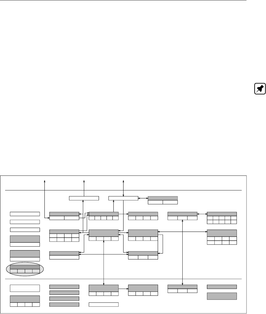
DRAFT
Principles of water quality modelling
D-WAQ allows you to calculate the ambient water temperature as a function of the ambient air
temperature. The heat gain from or loss to the atmosphere takes into account the wind speed.
You can choose to simulate the absolute temperature or the surplus temperature. The latter
is useful when simulating the discharge of cooling water used for example by power plants.
The more elaborate temperature modelling through solar radiation, cloudiness, (back-)scattering,
evaporation, etc. is implemented in D-Flow FM, Delft3D-FLOW (D-Flow FM UM,2015;Delft3D-
FLOW UM,2013).
Note: that if the water temperature was included in the D-Flow FM, Delft3D-FLOW simulation,
it is an option to include this in D-WAQ as a segment (forcing) function.
9.4 Coliform bacteria
9.4.1 Concepts
Coliform bacteria can be modelled as stand-alone substances.
Coliform bacteria originate from human and animal faeces and are often used as indicator for
the presence of disease vectors.
TIC Alkalinity
Iron
7 Components
Sulphur
SO4
SUD SUP
NO
NH PO Si
AAP VIVP
APATP
OPAL
Methane
C
P S
NSi
(particulate)
POC PON POP POS
Organic Matter
(dissolved)
DOC DON DOP DOS
Grazers
C N PSi
Dissolved Oxygen
IM2 IM3
IM1
Oxygen Demand
BOD COD
phytobentos
C N PSi
Micro-
As
Cr Hg
Cd Cu
Ni Pb VZn
pollutants
Atr BaP Diu Flu
Organic micro-
HCB HCH PCB OMP
Sediment Oxygen
Demand
EnCoc
EColi FColi TColi
Tracers
Tracers
Continuity
Salinity/Chloride
Temperature
Inorganic Matter
IM2 IM3
IM1
Organic Matter
(particulate)
POC PON POP POS
Heavy Metals
pollutants
Organic micro-
Atmosphere
Water
Sediment
Heavy Metals
Inorganic Matter
Decayable
Conservative
5 Components
5 Components
Bacteria
pH
Nutrients
34 4
Phytoplankton
Organic Matter
Organic Matter
(dissolved)
DOC DON DOP DOS
Nutrients
Oxygen
Sulphur
Iron Methane
Figure 9.2: Overview of substances. Coliform bacteria
As soon as coliform bacteria are discharged into surface water, they start to die since the
conditions that these bacteria meet are essentially hostile to them. The mortality of coliform
bacteria is enhanced by temperature, salinity and solar radiation. The lethal effect of light is
associated with short wavelengths, ultraviolet radiation in particular.
Deltares 207 of 382

DRAFT
D-Water Quality, User Manual
9.4.2 Modelling framework
The substances that can be modelled in D-WAQ in relation to bacterial pollution are:
Name of
D-WAQ substance
Description Unit
TCOLI Total coliforms MPN/m3
FCOLI Faecal coliforms MPN/m3
ECOLI Escherichia Coli MPN/m3
ENCOC Enterococci MPN/m3
Note: that the unit (MPN/m3, MPN = Most Probable Number) deviates from the unit that is
usually reported for concentrations of coliform bacteria: MPN/100 ml. The conversion factor
between the units is 1 MPN/m3= 1×10⁻⁴MPN/100 ml.
It is assumed that:
1 Coliform bacteria are present in the water column only. They do not accumulate in or
resuspend from sediment.
2 Coliform bacteria do not grow in the water column, although in reality some growth imme-
diately after discharge might occur.
3 Mortality of coliform bacteria is included as a temperature dependent process, formulated
according to first-order kinetics.
4 The mortality rate is enhanced by salinity and UV-radiation in an additive way.
5 The mortality formulation is identical for each of the three coliform substances (ECOLI,
FCOLI, TCOLI, ENCOC). You can define species specific coefficients.
The general mass balance equation for coliform bacteria reads:
∆C
∆t=loads +transport −mortality
with:
C= concentration of coliform bacteria cells [MPN/m3]
t= time [day]
9.4.3 Process equation
Available formulations for the mortality of coliforms are mainly empirical. The formulations as
reported by Mancini (1978) are implemented in D-WAQ. The basic formulations read:
Rmrt =kmrt ×Cx
kmrt = (kmb +kmcl)×ktmrt(T−20) +kmrd
kmcl =kcl ×Ccl
kmrd =krd ×f(I)
with:
Cx concentration of coliform bacteria species [MPN m−3]
Idaily solar UV-radiation at the water surface [W m−2]
kcl chloride related mortality constant [m3g−1d−1]
kmb basic mortality rate [d−1]
kmcl chloride dependent mortality rate [d−1]
208 of 382 Deltares
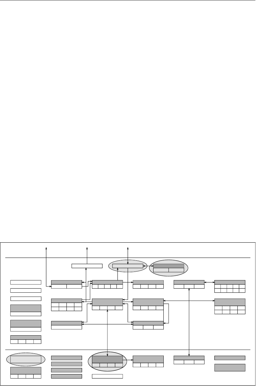
DRAFT
Principles of water quality modelling
kmrd radiation dependent mortality rate [d−1]
kmrt first order mortality rate [d−1]
krd radiation related mortality constant [m2W−1d−1]
ktmrt temperature coefficient of the mortality rate [-]
Rmrt mortality rate of coliform bacteria [MPNm−3d−1]
Ttemperature [◦C]
Ccl chloride concentration [g m−3]
The daily average solar UV-radiation is derived from the total daily radiation of visible light.
Moreover, the model takes into account that no significant mortality may occur at low temper-
atures.
9.5 Dissolved oxygen and BOD
9.5.1 Concepts
The fate of dissolved oxygen is closely linked to the fate of organic matter through:
CO2+H2O→CH2O+O2(9.2)
The equation above is the (simplified) photosynthesis reaction in which organic matter (CH2O)
and dissolved oxygen are formed. For each gram C incorporated into organic matter, 2.67 grams
of O2are formed which is derived from the ratio of the molar masses 32 g O2/ 12 gC. The
reverse reaction in which carbon dioxide and water are formed, is the mineralization or degra-
dation reaction of organic matter. This reaction is microbially mediated. The organic matter
can be autochthonous to the water system when it is produced locally by primary producers,
but can be allochtonous as well when it originates from waste loads such as the sewerage
system. The degradability of organic matter usually decreases as organic matter ages.
TIC Alkalinity
Iron
7 Components
Sulphur
SO4
SUD SUP
NO
NH PO Si
AAP VIVP
APATP
OPAL
Methane
C
P S
NSi
(particulate)
POC PON POP POS
Organic Matter
(dissolved)
DOC DON DOP DOS
Grazers
C N PSi
Dissolved Oxygen
IM2 IM3
IM1
Oxygen Demand
BOD COD
phytobentos
C N PSi
Micro-
As
Cr Hg
Cd Cu
Ni Pb VZn
pollutants
Atr BaP Diu Flu
Organic micro-
HCB HCH PCB OMP
Sediment Oxygen
Demand
EnCoc
EColi FColi TColi
Tracers
Tracers
Continuity
Salinity/Chloride
Temperature
Inorganic Matter
IM2 IM3
IM1
Organic Matter
(particulate)
POC PON POP POS
Heavy Metals
pollutants
Organic micro-
Atmosphere
Water
Sediment
Heavy Metals
Inorganic Matter
Decayable
Conservative
5 Components
5 Components
Bacteria
pH
Nutrients
34 4
Phytoplankton
Organic Matter
Organic Matter
(dissolved)
DOC DON DOP DOS
Nutrients
Oxygen
Sulphur
Iron Methane
Figure 9.3: Overview of substances. Dissolved oxygen and BOD
In 1925 Streeter and Phelps (Streeter and Phelps,1925) calculated the so-called dissolved
oxygen sag that occurs downstream an organic matter discharge into a river. While the river
water flows downstream dissolved oxygen is consumed as organic matter is oxidised. Replen-
ishment from the atmosphere (reaeration) can not match the dissolved oxygen consumption,
until the organic matter amount has been sufficiently reduced. Then the dissolved oxygen
Deltares 209 of 382

DRAFT
D-Water Quality, User Manual
concentration will start to rise again as reaeration becomes larger than the oxygen consump-
tion. The point where the lowest dissolved oxygen concentration occurs is called the dissolved
oxygen sag.
The Streeter-Phelps approach demonstrates that reaeration is an important source of dis-
solved oxygen in the water column. Whether or not reaeration will take place depends on
the deviation of the actual dissolved oxygen concentration from the saturation concentration
at the ambient temperature and salinity. If the actual dissolved oxygen concentration is lower
than the saturation concentration, the water is undersaturated and oxygen will enter the water
column from the atmosphere. If the actual dissolved oxygen concentration is higher than the
saturation concentration, the water is oversaturated and oxygen will escape from the water
column to the atmosphere. If the water column is stratified, the hypolimnion is not in con-
tact with the atmosphere as a result of which it can not be replenished and oxygen depletion
can occur. Decreased dissolved oxygen concentrations are seen as the major water quality
problem arising from stratification.
Finally, dissolved oxygen can be involved in numerous chemical and micro-biological oxidation
reactions. The most important reactions are the oxidation of ammonium to nitrate, iron(II) to
iron(III), sulphides to sulphate and methane to carbon dioxide and water. Of these reactions
only the oxidation of ammonium to nitrate is included in D-WAQ.
Organic matter in natural waters includes a variety of organic compounds usually present
in minute concentrations many of which elude direct isolation and identification. Therefore,
collective parameters such as chemical oxygen demand (COD), biochemical oxygen demand
(BOD), total organic carbon (TOC), particulate organic carbon (POC) or dissolved organic
carbon (DOC) are often used to estimate the quantity of organic matter.
COD is measured using a strong chemical oxidising agent (the Cr-method uses potassium
dichromate; the Mn-method uses potassium permanganate). Although it intends to include
all oxidisable material, the efficiency of the Cr-method is approximately 90% whereas the Mn-
method only yields around 50% of the oxidisable carbon. Ammoniacal and Kjeldahl nitrogen
are included in the COD measurement as well as sulphides, methane and other oxidisable
material.
BOD consists of carbonaceous and nitrogenous oxygen demand. A much used parameter is
BOD5 (in g O2/m3) which represents the amount of oxygen that is consumed when a sample
is stored for 5 days in a dark environment at 20 ◦C. As nitrogenous bacteria show a time lag
in their growth after incubation, during these 5 days only the carbonaceous oxygen demand
is measured.
Discharges of wastes (municipal or industrial) and sewer overflows are principal inputs of
oxygen demanding wastes. These discharges cause a chemical oxygen demand (COD), a
carbonaceous bio-chemical oxygen demand (CBOD) and a nitrogenous biochemical oxygen
demand (NBOD). CBOD represents the oxygen demanding equivalent of the complex car-
bonaceous material present in waste; NBOD represents the oxygen demanding equivalent of
reduced nitrogen species (ammonium or organic nitrogen). Typical values for different waters
are presented in.
210 of 382 Deltares

DRAFT
Principles of water quality modelling
Table 9.1: Typical values for oxygen demanding waste waters (values in g O2/m3, data
from Thomann and Mueller (1987))
Source CBOD5 CBODu NBODu COD
Municipal waste (untreated) 100–400 220 (120–580) 220 -
Combined sewer overflow (untreated) 170 (40–500) 220 - -
Separate urban runoff (untreated) 19 (2–80) - - -
Background natural water (excluding
algae and detritus)
0 - - 2–3
Background of natural water (including
algae and detritus)
2–3 - - 10
9.5.2 Modelling framework
The substances that can be modelled in D-WAQ in relation to dissolved oxygen and dead
organic matter (BOD/COD) are:
Name of
D-WAQ substance
Description Unit
OXY Dissolved oxygen g O2/m3
CBOD5 Carbonaceous Biological Oxygen
Demand after 5 days
g O2/m3
CBODu Ultimate Carbonaceous Biological
Oxygen Demand
g O2/m3
NBOD5 Nitrogenous Biological Oxygen
Demand after 5 days
g O2/m3
NBODu Ultimate Nitrogenous Biological
Oxygen Demand
g O2/m3
COD Chemical Oxygen Demand g O2/m3
SOD Sediment Oxygen Demand g O2
The mass balances for dissolved oxygen, CBOD5 and SOD are given in Equations (9.3),(9.4)
and (9.5) respectively. The mass balance for CBOD5 is the same as the mass balances for
CBODu, NBOD5, NBODu and COD.
∆O2
∆t=loads +transport +reaeration +net primary production (9.3)
−mineralization −nitrification +denitrification
∆CBOD5
∆t=loads +transport −settling −mineralization (9.4)
∆SOD
∆t=loads +settling −mineralization (9.5)
In D-WAQ mineralization of organic matter can be modelled in three ways depending on the
origin of the organic material:
1 Organic matter originating from waste water [g O2/m3]
Deltares 211 of 382

DRAFT
D-Water Quality, User Manual
2 Detritus organic carbon originating from natural sources such as dead phytoplankton
[g C/m3]
3 The combination of both.
In this section we will only discuss the first option. It can be considered as the representation
of the Streeter-Phelps modelling. The second option will be discussed in section 9.7. D-WAQ
allows you to choose both the BOD and the detritus carbon fraction of organic matter (the third
option). It is the users responsibility to make sure that no double counting takes place: each
carbon atom should belong to one fraction only, either BOD or detritus, and never to both. If
this were the case, the oxygen demand would be doubled as both the mineralization of BOD
and the mineralization of detritus will consume dissolved oxygen.
Particulate fractions can settle to the sediment1. The degradation of organic matter continues
there2. In D-WAQ all BOD fractions (CBOD5, CBODu, NBOD5, NBODu, COD) are converted
to the Sediment Oxygen Demand (SOD) pool when they settle. Mineralization of SOD directly
consumes dissolved oxygen in the water column.
Brief description and relevant notes of processes:
Process Substances Comments
Reaeration OXY
The reaeration flux across the air-water inter-
face, which can be positive or negative, is pro-
portional to a reaeration rate constant and the
difference between the actual and saturation DO
concentrations in water.
The reaeration rate constant can be a function
of stream velocity, wind speed and temperature
(10 alternative formulations).
The saturation oxygen concentration is a func-
tion of water temperature and salinity (2 alterna-
tive formulations).
Primary produc-
tion
OXY
(Phytoplankton)
(Nutrients) The production of dissolved oxygen is propor-
tional to the net primary production flux accord-
ing to 2.67 gO2/gC.
Nitrification3OXY
(NH4)
(NO3)
NH+
4+ 2O2→NO−
3+ 2H++H2O
The oxygen consumption is proportional to a ni-
trification rate and a function of the DO and am-
monium concentration.
continued on next page
1For a description of the settling process refer to section 9.6
2For a detailed description of sediment processes refer to section 9.11
3For process equations refer to section 9.7
212 of 382 Deltares

DRAFT
Principles of water quality modelling
continued from previous page
Process Substances Comments
Denitrification7OXY
(NO3)
NO−
3+H+→0.5N2+ 1.25O2+ 0.5H2O
The oxygen production is proportional to a den-
itrification rate and a function of the DO and ni-
trate concentration.
Mineralization in
the water col-
umn
OXY
CBOD5
CBODu
NBOD5
NBODu
COD
The oxygen consumption and the mineralization
of BOD/COD is proportional to a mineralization
rate.
Optionally an age function can be applied to the
mineralization rate of BOD/COD to take into ac-
count the reduced degradability of organic mat-
ter as it ages.
Mineralization in
the sediment
OXY
SOD The oxygen consumption and the mineralization
of SOD is proportional to a mineralization rate.
Settling5CBOD5
CBODu
NBOD5
NBODu
COD
SOD
Settling is proportional to a first order settling ve-
locity (in m/d).
Settling occurs when the actual shear stress is
lower than the user-defined critical shear stress
for sedimentation.
The actual shear stress is a function of flow ve-
locity and waves. Artificial disturbances such as
ships can be added as well.
Each particulate fraction has its own critical
shear stress for sedimentation.
All fractions in the water column are combined
into SOD after settling to the sediment.
Remarks:
All reaction rates are temperature dependent (section 9.3).
A daily variation of algae can be described by constraining the gross primary production
to the daylight period. Algal respiration will take place 24 hours per day. As a result
dissolved oxygen will be produced during daylight and consumed during the night.
In D-WAQ the consumption of dissolved oxygen may lead to a negative dissolved oxy-
gen concentration, i.e. the dissolved oxygen concentration is not restricted to positive
values. The reason for this is that some reduced substances (e.g. sulphides, iron(II),
methane) may not be included in your model, but would oxidise rapidly when coming
into contact with dissolved oxygen. Negative dissolved oxygen concentrations should
Deltares 213 of 382

DRAFT
D-Water Quality, User Manual
therefore be considered as (negative) oxygen equivalents. Optionally, negative oxygen
concentrations can be prevented by letting the mineralization rate depend on dissolved
oxygen concentration (e.g. if DO <0.1mg/l, then mineralization rate = 0 d−1), but this
implies a biased degradation rate.
9.5.3 Process equations
Reaeration
The reaeration rate is a linear function of the difference between the saturation and actual DO
concentration according to:
Rrear =klrear ×(Coxs −Cox)/H
klrear =a×vb
Hc+d×W2
Coxs =f(T, Ccl) = f(T, SAL)
with:
a, b, c, d coefficients with different values for eleven reaeration options
Ccl chloride concentration [gCl m−3]
Cox actual dissolved oxygen concentration [gO2m−3]
Coxs saturation dissolved oxygen concentration [gO2m−3]
Hdepth of the water column [m]
klrear reaeration transfer coefficient in water [d−1]
Rrear reaeration rate [gO2m−3d−1]
SAL salinity [kg m−3]
Twater temperature [◦C]
vflow velocity [m s−1]
Wwind speed at 10 m height [m s−1]
Depending on the reaeration option the transfer coefficient is only dependent on the stream
velocity or the wind speed, or dependent on both. A host of alternative formulations is avail-
able. In addition to the water temperature the saturation concentration is a function of either
the chloride concentration or the salinity (two options available).
Diurnal variation of production
The phytoplankton models implemented in D-WAQ are subjected to daily averaged forcing
functions. However, in reality the gross primary production of phytoplankton is constrained
to daytime, whereas respiration consumes oxygen all day. The resulting diurnal variation
of the dissolved oxygen concentration follows from the production distribution over a day as
displayed in Figure 9.4. The shape of the production curve depends on day length (DL)
and the times (t1) and (t2), which define the period of the maximum production during a day
Rgpmax . The maximal primary production in a day follows from:
Rgpmax =48 ×Rgpa
t2−t1+DL
with:
DL day length [hr]
Rgpadaily average gross primary production rate [gO2m−3d−1]
Rgpmax maximal gross primary production rate during a day [gO2m−3d−1]
t1time at which the maximal production is reached [h]
t2time at which the production starts to decrease [h]
214 of 382 Deltares
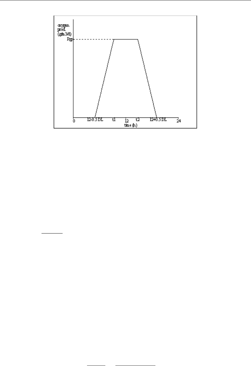
DRAFT
Principles of water quality modelling
Figure 9.4: The distribution of gross primary production over a day
Mineralization
The mineralization rate of all BOD/COD-components depends on the age of the organic mat-
ter, provided that BOD and COD are simulated simultaneously. By default the function of
the age function (fage) is 1.0. The mineralization rate is described with first-order kinetics
according to:
Rmin =fage ×kmin ×Cx (9.6)
fage =fagemin +fagemax −fagemin×ef(AI)(9.7)
AI =COD
BOD5(9.8)
with:
AI index for the age of organic matter [-]
Cx concentration of a BOD/COD-component [gO2m−3]
BOD5concentration of total CBOD5 [gO2m−3]
COD concentration of total COD [gO2m−3]
fage attenuation function for age [-]
kmin first-order kinetic constant [d−1]
Rmin mineralization rate of a BOD/COD-component [gO2m−3d−1]
The Sediment Oxygen Demand (SOD) has been formulated as the sum of a zero-order and a
first-order process, allowing the specification of a background sediment oxygen demand. Two
options are available for the mineralization rate, one of which takes into account the escape of
methane to the atmosphere. The mineralization rate according to option 2 is calculated with:
Rsod = (1 −fch4)×k0sod
H+ksod ×SOD
V
with:
SOD quantity of potential sediment oxygen demand [gO2]
fch4fraction of organic matter escaped as methane [-]
k0sod constant “background” sediment oxygen demand [gO2m−2d−1]
ksod first-order kinetic constant [d−1]
Hdepth of the water column [m]
Rsod sediment oxygen demand [gO2m−3d−1]
Deltares 215 of 382

DRAFT
D-Water Quality, User Manual
Vvolume of the water compartment [m3]
Positive DO
The concentration of dissolved oxygen (DO) may become negative in D-WAQ. Positive pa-
rameter DO is calculated for presentation purposes with:
DO = max (Cox, 0.0)
with:
DO dissolved oxygen concentration [gO2m−3]
Cox equivalent dissolved oxygen concentration, substance, OXY [gO2m−3]
Minimal DO
The minimal DO concentration in a day resulting from the diurnal variation of primary produc-
tion is computed according to:
Coxmin =f(Cox, Rnp, Rrsp, DL)
with:
Cox average dissolved oxygen concentration [gO2m−3]
Coxmin minimal dissolved oxygen concentration in a day [gO2m−3]
DL daylength [hr]
Rnp total net primary production rate [gC m−3d−1]
Rrsp total algae respiration rate [gC m−3d−1]
9.6 Suspended sediment, sedimentation and erosion
9.6.1 Concepts
Sediment is particulate material, formed by the physical and chemical desintegration of rocks
from the earth’s crust (i.e. inorganic) and by various biological processes (i.e. organic). The
sediment carried by natural waters contains a mixture of inorganic and organic components
with can be classified according to the various grain sizes:
1 Gravel : >2 mm
2 Sand : 0.06 mm - 2 mm
3 Silt : 0.004 mm - 0.06 mm
4 Clay : <0.004 mm
5 Organic particles : up to several µm
The very fine organic particles of living and dead algae and the silt and clay fractions can
be carried as colloidal suspension for which electrochemical forces play an predominant role.
Considering the large adsorbing capacities, the fine fraction is characterised as cohesive
sediment. Since flocculation and adsorbing capacities are of minor importance for larger
particles, they are classified as non-cohesive sediment. In principal all particulate components
are subject to settling and resuspension to and from the bed.
Fine grained (cohesive) particulate sediments
All fine grained suspended matter which range in size from several microns up to about 70
microns and are easily brought into suspension. T he behaviour of this fine grained suspended
matter plays an important role in water quality. First, turbidity and its effect on the under-
water light climate is an important environmental condition for algae growth. The presence of
216 of 382 Deltares
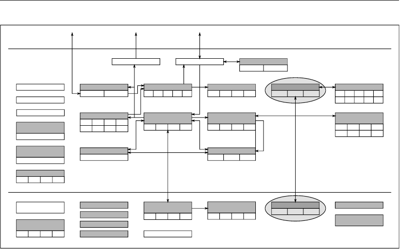
DRAFT
Principles of water quality modelling
TIC Alkalinity
Iron
7 Components
Sulphur
SO4
SUD SUP
NO
NH PO Si
AAP VIVP
APATP
OPAL
Methane
C
P S
NSi
(particulate)
POC PON POP POS
Organic Matter
(dissolved)
DOC DON DOP DOS
Grazers
C N PSi
Dissolved Oxygen
IM2 IM3
IM1
Oxygen Demand
BOD COD
phytobentos
C N PSi
Micro-
As
Cr Hg
Cd Cu
Ni Pb VZn
pollutants
Atr BaP Diu Flu
Organic micro-
HCB HCH PCB OMP
Sediment Oxygen
Demand
EnCoc
EColi FColi TColi
Tracers
Tracers
Continuity
Salinity/Chloride
Temperature
Inorganic Matter
IM2 IM3
IM1
Organic Matter
(particulate)
POC PON POP POS
Heavy Metals
pollutants
Organic micro-
Atmosphere
Water
Sediment
Heavy Metals
Inorganic Matter
Decayable
Conservative
5 Components
5 Components
Bacteria
pH
Nutrients
34 4
Phytoplankton
Organic Matter
Organic Matter
(dissolved)
DOC DON DOP DOS
Nutrients
Oxygen
Sulphur
Iron Methane
Figure 9.5: Overview of substances. Suspended sediment, sedimentation and erosion
suspended sediment increases the attenuation of light in the water column which leads to an
inhibition of photosynthetic activity and hence, a reduction in primary production. Secondly,
the fate of contaminants in waters is closely related to suspended solids due to their large
adsorbing capacities. Like dissolved matter, the sediment is transported by advection and by
turbulent motion. In addition, the fate of the fine grained suspended sediments is determined
by settling and deposition, as well as by bed processes, e.g. consolidation, bioturbation and
resuspension. The sedimentation and erosion processes originate from the Partheniades-
Krone concept (Partheniades,1962;Krone,1962). In this concept, the bottom shear stress
plays an essential role in defining whether or not sedimentation of suspended particles or
erosion of bed material will occur. Deposition takes place when the bottom shear drops below
a critical value. On the other hand erosion occurs when the bottom shear exceeds a critical
value. Suspended matter is subject to settling in the water column and the fractions in the
sediment are subject to erosion. The sediment can also be removed from the modelled part
of the water system by burial. Remobilisation into the modelled system is possible by the
reverse process indicated as ‘digging’.
Coarse grained (non-cohesive) sediment
Particle sizes of non-cohesive material are larger than those of cohesive sediment, and are
in the order of 100 µm and more (sandy). The behaviour of this sandy sediment transport is
of major importance in coastal engineering problems related to morphological changes. The
transport of sediment particles can be in the form of bed-load and suspended load, depending
on the size of the bed material and the local instantaneous flow conditions (Van Rijn,1993).
The transport of particles via rolling, sliding and jumping (saltating) is called bed load transport
and this motion is exclusively determined by the effective bed shear which is assumed to be
dominated by gravity forces. The bed load transport takes places in a thin layer above the
surface of the sediment. The suspended load is that part of the total load that is moving
without continuous contact with the bed as a result of the agitation of fluid turbulence. The
suspended sediment is only affected by the friction of the grains themselves in the water.
Whether there is merely a bed load or a suspended load depends primarily on the intensity
of the water movement. There is a critical velocity below which no movement occurs. If
the velocity increases, bottom transport is initiated to develop ripples and dunes. At higher
Deltares 217 of 382

DRAFT
D-Water Quality, User Manual
velocities, sediment grains come into suspension and suspended loads starts.
The transport rate of non-cohesive sediment is determined by the local instantaneous flow
conditions. This assumption is commonly assumed for bed load transport. For suspended
transport it implies that the time and length scale of the flow variation are much larger than
the adaptation time and adaptation length of the sediment concentration respectively. The
transport of such sediment is not related to the flow field in the same way as for dissolved
substances and hence no dispersion or diffusion is applied.
There are many transport formulation in literature to describe the bed and suspended loads
transport. In D-WAQ the transport formulation for the total load of Engelund and Hansen
(1967) is implemented since this formula is relatively simple and has shown good performance
in numerous field and laboratory experiments.
9.6.2 Modelling framework
The (inorganic) substances that can be modelled in the D-WAQ in relation to particulate matter
are:
Name Description Unit
IM1 suspended inorganic matter fraction 1 g/m3
IM2 suspended inorganic matter fraction 2 g/m3
IM3 suspended inorganic matter fraction 3 g/m3
IM1S1 inorganic matter fraction 1 in bed layer 1 g
IM2S1 inorganic matter fraction 2 in bed layer 1 g
Im3S1 inorganic matter fraction 3 in bed layer 1 g
IM1S2 inorganic matter fraction 1 in bed layer 2 g
IM2S2 inorganic matter fraction 2 in bed layer 2 g
IM3S2 inorganic matter fraction 3 in bed layer 2 g
Remark:
There are (living and dead) particulate organic substances as well (DetC, OOC, POC1,
Algae, etc.). Also adsorbed phosphate can be simulated as a particulate substance.
These substances undergo the same processes for sedimentation, erosion, burial and
digging. However, they are not mentioned explicitly in the remainder of this chapter.
The mass balances for particulate (suspended) matter in the water column (cw) and particu-
late matter in the sediment (cb) is given in Equation (9.9) and Equation (9.10) respectively.
∆cw
∆t=loads +transport −settling +resuspension (9.9)
∆cb
∆t=loads +settling −resuspension −burial +digging (9.10)
Brief description and relevant notes of processes:
218 of 382 Deltares

DRAFT
Principles of water quality modelling
Process Substances Comments
Settling / sedi-
mentation
IM1
IM2
IM3
(all particulates)
Settling is proportional to a first order settling ve-
locity (in m/d).
Settling occurs when the actual shear stress is
lower than the user-defined critical shear stress
for sedimentation.
The actual shear stress is a function of flow ve-
locity and waves. Artificial disturbances such as
ships can be added as well.
Each particulate fraction has its own critical
shear stress for sedimentation.
Resuspension IM1S1/IM1S2
IM2S1/IM2S2
IM3S1/IM3S2
(all particulates)
Resuspension takes places with a zero-order
rate (in g/m2/d) and is proportional to a proba-
bility function.
Resuspension takes place when the actual
shear stress is higher than the critical shear
stress for resuspension.
The sediment layers S1 and S2 each have a crit-
ical shear stress for resuspension. The critical
shear stress for resuspension is valid for all par-
ticulate fractions in the sediment layer.
The resuspension rate of the individual partic-
ulate fractions in the sediment layer is propor-
tional to its weight fraction.
Burial IM1S1/IM1S2
IM2S1/IM2S2
IM3S1/IM3S2
(all particulates)
Burial is the downward movement of particulates
in the sediment. Sediment layers can have ei-
ther a fixed or a variable layer thickness.
When considered independent of the thickness
of a sediment layer, burial can consist of a zero-
order and a first-order term.
When the prescribed layer thickness is ex-
ceeded, exceedance burial can take place.
Combined burial takes places for all particulate
fraction.
The burial rate of the individual particulate frac-
tions in the sediment layer is proportional to its
weight fraction.
continued on next page
Deltares 219 of 382

DRAFT
D-Water Quality, User Manual
continued from previous page
Process Substances Comments
Digging IM1S1/IM1S2
IM2S1/IM2S2
IM3S1/IM3S2
(all particulates)
Digging is the upward movement of particulates
in the sediment. Sediment layers can have ei-
ther a fixed or a variable layer thickness.
When considered independent of the thickness
of a sediment layer, digging can consist of a
zero-order and a first-order term.
When the prescribed layer thickness is not met,
replenishment digging can take place.
Combined digging takes places for all particulate
fraction.
The digging rate of the individual particulate
fractions in the sediment layer is proportional to
its weight fraction.
9.6.3 Processes
Sedimentation of suspended fine-grained particulate matter
A characteristic feature of fine sediments is the ability to form aggregates of flocs that settle
to the bottom. Whether a particle will settle to the bottom depends upon its size and density
and the chemical conditions of the surrounding water system. Sedimentation is the process
describing the settling of particles. This deposition process is described with the formulation
by Krone (1962). Various laboratory and field measurements show that the suspended matter
concentration strongly influences the aggregation process and thereby the settling velocities of
the aggregates. Strong flocs are denser and have larger settling velocities. The aggregation
of flocs strongly depends on the chemical and physical properties of the sediment, salinity
and turbulence. At high sediment concentrations (several g/l) the particles hinder each other,
resulting in a decrease of the settling velocity. Turbulence is an important parameter because
it affects the flocculation and therefore the settling velocity in two opposing ways. On the
one hand an increase in turbulence will increase the collisions between particles, resulting
in larger flocs with high settling velocities. On the other hand, it results in turbulent shear
stresses which can break up the flocs and decrease the settling velocity. At low suspended
concentrations however, flocculation processes are so low, that the floc size, hence settling
velocity does not vary over the depth. So the floc formation and floc break-up processes will
only play a role in the sedimentation process at high-concentrated conditions (Winterwerp,
2002).
The rate of downward mass transport (deposition) is equal to the product of the near-bed
velocity, the concentration and the probability that a settling particle becomes attached to the
sea bed. The deposition (i.e. sedimentation flux) (Krone,1962) is given by:
D=ws·c·1−τb
τc
with:
Ddeposition flux of suspended matter [g m−2d−1]
wssettling velocity of suspended matter [m d−1]
220 of 382 Deltares

DRAFT
Principles of water quality modelling
cconcentration of suspended matter near the bed [g m−3]
τbbottom shear stress [Pa]
τdcritical shear stress for deposition [Pa]
Sedimentation always results in an increase of sediment in the upper sediment bed layer. In
the implemented sedimentation process it is assumed that there is no correlation between the
various sediment components which means that each of the particulate fractions can settle
independently.
Erosion of particulate fine-grained matter
Erosion of bed material occurs when the bed shear forces exceed the resistance of the bed
sediment. The resistance of the bed is characterised by a certain critical erosive strength (bot-
tom shear stress). This critical stress is determined by several factors, such as, the chemical
composition of the bed material, particle size distribution and bioturbation. Erosion of sedi-
ment is induced by the bed stress due to tidal and wind-induced advective flows and surface
waves. The erosion is directly proportional to the excess of the applied shear stress over the
critical erosive bottom shear stress. The formula for erosion of homogeneous beds is based
on Partheniades (1962). The erosion flux is limited by the available amount of sediment on
the sea bed.
The erosion of bed material is given by:
E=Mτb
τc−1
with:
Eerosion rate [g m−2d−1]
Mfirst order erosion rate [g m−2d−1]
τbbed shear stress [Pa]
τecritical shear stress for erosion [Pa]
The values of Mand τstrongly dependent on the sediment properties and environmental
parameters. The amount of eroded dry matter is added to the mass in the water column.
In D-WAQ a variable sediment layer or a fixed sediment layer can be selected. For the
variable-layer option, the erosion flux is limited based on the available amount of sediment
in a sediment layer. The flux is unlimited if the fixed layer option is applied. As long as mass
is available in the upper sediment layer, resuspension takes place from that layer only. If the
upper sediment layer is completely eroded, then resuspension takes place from the lower
sediment layer.
Total Bed shear stress
The bed shear stress is an essential quantity that directly influences the sedimentation and
erosion rates. It depends on the flow (currents) and the wind generated surface waves. For
the sedimentation/erosion processes it is assumed that the bed stresses due to flow (τflow)
and waves (τw) are additive. In addition, a third shear stress component can be defined (τship)
to be representative for the bed shear stresses due to shipping or fishing activities.
τ=τflow +τw+τship (9.11)
Deltares 221 of 382
DRAFT
D-Water Quality, User Manual
1. Bed shear stress to currents (τflow)
The effects of the hydrodynamic forcing on the sediments take place primarily through the
friction they exert on the sea bed shear stress τflow. This shear stress is described by the
following formulae:
In case of depth averaged (2D) flow:
τflow =ρ·g
C2
2D·u2or ρ·u2
∗(9.12)
For hydraulic rough flows, the 2D Chezy coefficient (C2D) can be determined according to
Manning’s formulation or the White Colebrook formulation:
Manning: C2D=6
√h
n
White Colebrook: C2D= 18 10log 12h
ks
In case of three dimensional flow, the logarithmic velocity current profile can be written as:
u(z) = u∗
κln z
z0(9.13)
Averaging over the depth yields:
¯u=u∗
κln H
z0−1(9.14)
where:
u∗=√g¯u
C2D
(9.15)
Substitution of Equation (9.15) in Equation (9.14) results in an expression of z0:
z0=H e−1+ κ·C2D
√g(9.16)
Now, assuming equality of bed stresses for 2D and 3D simulations, the shear stress and the
Chezy coefficient for three-dimensional flows can be written as follows:
τflow =g ρl
C2
3D
~ub|~ub|(9.17)
C3D=√g
κln 1 + hb/2
z0(9.18)
with:
gacceleration of gravity [m/s2]
C3D3D Chézy coefficient [m1/2/s]
C2D2D Chézy coefficient [m1/2/s]
ubvelocity at bed layer [m/s]
u∗bed-shear velocity [m/s]
222 of 382 Deltares

DRAFT
Principles of water quality modelling
udepth averaged horizontal velocity [m/s]
nManning coefficient [m−1/3s1]
Htotal water depth [m]
hbthickness of bed layer [m]
κconstant of Von Kármán (0.4) [-]
ksNikuradse roughness (= 30z0) [m]
z0roughness height of the bed (i.e. zero velocity level) [m]
The Nikuradse roughness ksis related to the roughness length z0by the relationship ks=
30z0for hydrodynamic rough flows. At height z=z0above the bed, the velocity is zero.
Several relationships between ksand grain size have been proposed, with one of the most
widely used being:
ks= 2.5D50
with D50 being the median grain size [m−1].
2. Bed shear stress to waves (τw)
Surface waves are caused by wind stress on the water surface. The magnitude of the waves
depends on the wind conditions, wind duration, water depth and bottom friction. Wave fields
are commonly described by the significant wave height, significant wave period and wave
length. The magnitude of a equilibrium wave field can be estimated with the formulae by
Groen and Dorrestein (1976) for wind-generated waves. The wave growth is limited by the
water depth according to an analysis given by Nelson (1983). The wave-induced bed shear
stress is computed after Soulsby (1997) and Van Rijn (1993), using linear wave theory.
Relevant wave parameters for wave height and period of wind-generated waves are made
non-dimensional with the wind speed at 10 m height U10 and the gravitational acceleration g:
water depth: h∗=gh
U2
10
(9.19)
fetch: F∗=gF
U2
10
(9.20)
wave height: H∗=gH
U2
10
(9.21)
wave period: T∗=gT
U10
(9.22)
Significant wave height and period as a function of water depth and fetch for unlimited wind
duration are given by Groen and Dorrestein (1976):
H∗=k0tanh (k3hm3
∗) tanh k1Fm1
∗
tanh (k3hm3
∗)
T∗=m0tanh (k4hm4
∗) tanh k2Fm2
∗
tanh (k4hm4
∗)
with the coefficients knand mn:
The wave height is limited to 0.55h(Nelson,1983); when the wave height computed with
would exceed this criterion, the wave height is kept constant at H= 0.55h. It is assumed
Deltares 223 of 382

DRAFT
D-Water Quality, User Manual
k0= 0.24 k1= 0.015 k2=
0.0345
k3= 0.710 k4= 0.855
m0= 2π m1= 0.45 m2= 0.37 m3=
0.763
m4=
0.365
that also the wave period stops growing, and Tis kept at the value attained when Hexceeds
0.55h. The wavelength Lfollows from linear wave theory and is given in the following implicit
formula that has to be solved iteratively:
T=s2π
gLcoth 2πh
L
The amplitude of the wave orbital velocity (Uorb) just above the bed follows form linear wave
theory:
Uorb =πH
Tsinh (2πhL)
Waves induce a vertical circular movement (orbital velocity) which decreases with depth. The
waves exert friction forces at the bed during propagation. The magnitude of the time-averaged
wave-induced bed shear stress follows from Van Rijn (1993):
τw=1
4ρ fwU2
orb
where fwis a wave friction factor.
For rough turbulent flows a number of formulae have been proposed for the friction factor. In
D-WAQ two commonly used formulation have been implemented:
1Tamminga (1987)
fw= 0.16 sks
Uorb T /2π
2Swart (1974)
fw=0.3for r≤π/2
0.00251 exp(5.21 r−0.19)for r > π/2
3Soulsby (1997)
fw= 0.237 r−0.52
where:
r=A
ks
rrelative roughness height [-]
Asemi-orbital excursion A=UorbT/2π[m]
ksNikuradse roughness [m]
224 of 382 Deltares

DRAFT
Principles of water quality modelling
Burial and Digging
In addition to the described water-bed exchange processes, particulate components in the
bed layer can be transferred downward from one sediment layer to an underlying layer (i.e.
burial). This process can be defined either by a zero-order or a first order burial rate. The
sediment layer is considered to be homogeneous, therefore the composition of the sediment
being buried is the same as that of the (overlying) sediment layer. Sediment can also be
transferred upward to one sediment layer from an underlying layer in a process known as
’digging’. The composition of the sediment being transported upwards is the same as that of
the (underlying) sediment layer.
Non-cohesive total bed load transport
A sediment transport formula is an algebraic equation relating the sediment rate with the flow
parameters. One of the well known formulae is that of Engelund and Hansen (1967):
S=0.05 u2u3
∗
D g2∆ρ2
∆ρ=ρs−ρ
ρ
where:
Ssediment transport rate [m2/s]
udepth averaged flow velocity [m/s]
u∗bed shear stress velocity [m/s]
Dgrain size of sediment [m]
ggravity [m/s2]
∆ρrelative density of sediment [-]
Non-cohesive sediment is modelled as an inactive substance to prevent the transport algo-
rithms in D-WAQ from acting on this substance. The horizontal transport rate results in a
change of the amount of sediment present in the bed. This change is expressed as a change
in the thickness of the layer of non-cohesive sediment. There is no feed-back of the bed level
change towards the hydrodynamics.
Remark:
The sedimentation process is described with the classical formulation by Krone (1962).
In this formulation the rate of downward mass transport (deposition) is equal to the
product of the near-bed velocity, the concentration and the probability that a settling
particle becomes attached to the sea bed (depending on the critical shear stress of
deposition). A re-analysis of the experiments of Krone by Winterwerp and Van Kesteren
(2004) revealed however that the so-called critical shear stress for deposition does not
exists. In fact, it represents the critical shear stress for erosion of freshly deposited
sediment. Hence, the classical Krone formulation contains both a deposition and an
erosion term. This means that in common engineering practise, in which the water-
bed exchange processes are described with a combination of the Krone’s deposition
formula and Partheniades’ erosion formula is basically wrong. It is therefore proposed
to model the sedimentation flux for applications at low-concentrated cohesive sediment
simply by the deposition flux (D) itself:
D=wsc
Deltares 225 of 382
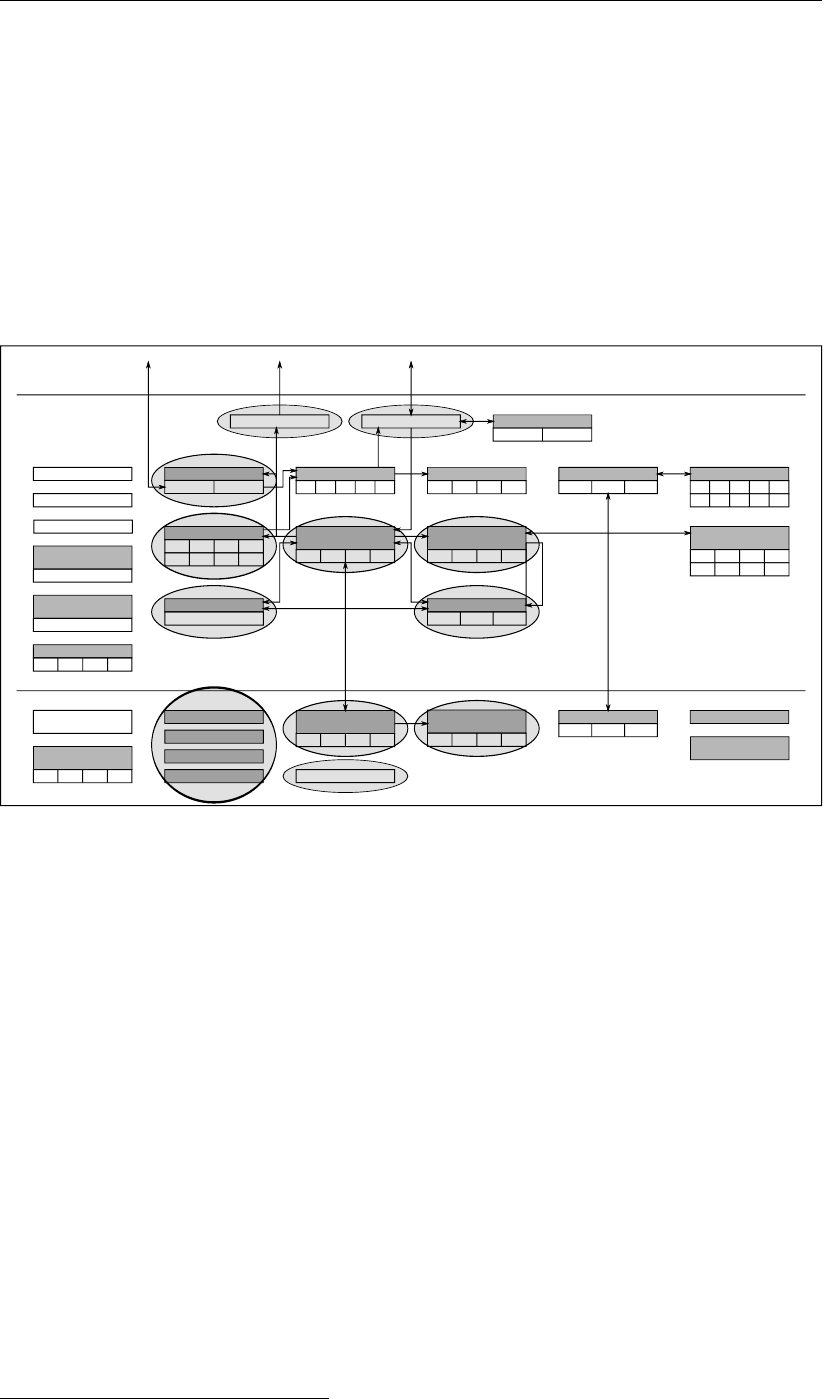
DRAFT
D-Water Quality, User Manual
9.7 Nutrients, detrital organic matter and electron-acceptors
9.7.1 Concepts
The major elements that form organic matter are carbon (C), nitrogen (N), phosphorus (P),
sulphur (S), oxygen (O) and hydrogen (H). Many other elements (Fe, Ca, K, etc.) are incorpo-
rated in minor quantities, but are not included in the D-WAQ modelling framework with respect
to organic components. A special place is reserved for silicon (Si). As certain types of phyto-
plankton use silicon to construct a skeletal structure, silicon is usually considered as a nutrient
as well, although it is not incorporated in organic matter but in silicate minerals, mostly opal
(SiO2).
TIC Alkalinity
Iron
7 Components
Sulphur
SO4
SUD SUP
NO
NH PO Si
AAP VIVP
APATP
OPAL
Methane
C
P S
NSi
(particulate)
POC PON POP POS
Organic Matter
(dissolved)
DOC DON DOP DOS
Grazers
C N PSi
Dissolved Oxygen
IM2 IM3
IM1
Oxygen Demand
BOD COD
phytobentos
C N PSi
Micro-
As
Cr Hg
Cd Cu
Ni Pb VZn
pollutants
Atr BaP Diu Flu
Organic micro-
HCB HCH PCB OMP
Sediment Oxygen
Demand
EnCoc
EColi FColi TColi
Tracers
Tracers
Continuity
Salinity/Chloride
Temperature
Inorganic Matter
IM2 IM3
IM1
Organic Matter
(particulate)
POC PON POP POS
Heavy Metals
pollutants
Organic micro-
Atmosphere
Water
Sediment
Heavy Metals
Inorganic Matter
Decayable
Conservative
5 Components
5 Components
Bacteria
pH
Nutrients
34 4
Phytoplankton
Organic Matter
Organic Matter
(dissolved)
DOC DON DOP DOS
Nutrients
Oxygen
Sulphur
Iron Methane
Figure 9.6: Overview of substances. Nutrients, detrital organic matter and electron-
acceptors
The nutrient cycle has four major pools: dissolved inorganic nutrients, particulate inorganic
nutrients, living organic matter (biomass) and detrital organic matter. Dissolved inorganic
nutrients and carbon dioxide are taken up by primary producers into their biomass4. When
we do not consider the food chain in which biomass can be taken up by ever higher trophic
levels, nutrients become available when primary producers die. Part of the nutrients are
released as dissolved inorganic nutrients again in a process that is called autolysis. The other
part is released as detrital organic matter (or as Opal), which can be dissolved or particulate.
Finally microbial decomposition of detrital organic matter releases the nutrients and carbon
back to their dissolved inorganic form. Electron-acceptors such as oxygen, nitrate, iron(III)
and sulphate are consumed for the decomposition of organic matter. Nitrate and sulphate are
both nutrients and electron-acceptors. Because carbon dioxide and alkalinity are consumed
in primary production and produced at the mineralization of organic matter these processes
affect the pH.
Particulate organic matter can settle to the sediment as a result of which nutrients can be
trapped in the sediment. Decomposition of organic matter and dissolution of opal silicate
will continue there and (eventually) nutrients are released back to the water column. Apart
from carbon dioxide, methane is produced in the degration process. Substantial quantities
4For a detailed description of primary producers refer to section 9.8.
226 of 382 Deltares

DRAFT
Principles of water quality modelling
of the nutrients may be nitrified, denitrified, adsorbed or precipitated in the sediment5. Also,
primary producers living on the sediment (microphytobenthos) fix dissolved inorganic nutrients
in biomass in the sediment.
9.7.2 Modelling framework
The substances that can be modelled in D-WAQ in relation to nutrients and detrital organic
matter in the water column are:
Name of D-WAQ
substance
Description Unit
Inorganic dissolved nutrients
NO3 Nitrate gN/m3
NH4 Ammonium gN/m3
PO4 Ortho-phosphate gP/m3
Si Silicon gSi/m3
SO4 Sulphate gS/m3
TIC Total dissolved inorganic carbon gC/m3
(Alka) Alkalinity, only needed for pH simulation gHCO−
3/m3
Inorganic particulate nutrients
AAP Adsorbed phosphate gP/m3
VIVP Vivianite like P (Fe3(PO4)2) gP/m3
APATP Apatite like P (Ca(CO3)n(PO4)m) gP/m3
Opal Opal silicate (SiO2) gSi/m3
SUP Precipitated sulphide gS/m3
Particulate detrital organic matter
POC1 Particulate Organic Carbon fraction 1 gC/m3
POC2 Particulate Organic Carbon fraction 2 gC/m3
POC3 Particulate Organic Carbon fraction 3 gC/m3
POC4 Particulate Organic Carbon fraction 4 gC/m3
POC5 Particulate Organic Carbon fraction 5 gC/m3
PON1 Particulate Organic Nitrogen fraction 1 gN/m3
PON2 Particulate Organic Nitrogen fraction 2 gN/m3
PON3 Particulate Organic Nitrogen fraction 3 gN/m3
PON4 Particulate Organic Nitrogen fraction 4 gN/m3
PON5 Particulate Organic Nitrogen fraction 5 gN/m3
POP1 Particulate Organic Phosphorus fraction 1 gP/m3
POP2 Particulate Organic Phosphorus fraction 2 gP/m3
POP3 Particulate Organic Phosphorus fraction 3 gP/m3
POP4 Particulate Organic Phosphorus fraction 4 gP/m3
POP5 Particulate Organic Phosphorus fraction 5 gP/m3
POS1 Particulate Organic Sulphur fraction 1 gS/m3
POS2 Particulate Organic Sulphur fraction 2 gS/m3
POS3 Particulate Organic Sulphur fraction 3 gS/m3
POS4 Particulate Organic Sulphur fraction 4 gS/m3
POS5 Particulate Organic Sulphur fraction 5 gS/m3
Dissolved organic matter
DOC Dissolved Organic Carbon gC/m3
DON Dissolved Organic Nitrogen gN/m3
5For a detailed description of sediment processes refer to section 9.11.
Deltares 227 of 382

DRAFT
D-Water Quality, User Manual
Name of D-WAQ
substance
Description Unit
DOP Dissolved Organic Phosphorus gP/m3
DOS Dissolved Organic Sulphur gS/m3
Electron-acceptors and -donors
OXY Dissolved Oxygen gO2/m3
SUD Dissolved sulphide gS/m3
CH4 Methane gC/m3
FeIIId Dissolved Iron(III) gFe/m3
FeIIIpa Amorphous Iron (oxy)hydroxide gFe/m3
FeIIIpc Crystalline Iron (oxy)hydroxide) gFe/m3
FeIId Dissolved Iron(II) gFe/m3
FeS Iron sulphide gFe/m3
FeS2 Pyrite gFe/m3
FeCO3 Iron carbonate gFe/m3
In present D-WAQ organic matter may consist of maximally six fractions: five particulate
fractions (POC1, POC2, POC3, POC4 and POC5) and one dissolved fraction (DOC). For
nitrogen, phosphorus and sulphur corresponding fractions exist. Inactive substance POC5
represents the organic matter in stems, branches and large roots of drowned dead terrestrial
vegetation. In is only used in conjunction with the drowned vegetation module, fully doc-
umented in the Technical Reference Manual, Detailed description of processes (D-WAQ
TRM,2013).
The mass balances for the dissolved nutrients (NO3, NH4, PO4, Si, TIC) the electron-acceptors
(SO4, SUD and FeIIIpa) and detrital organic matter (OM - representing POX) in the water col-
228 of 382 Deltares

DRAFT
Principles of water quality modelling
umn are given in the equations below:
∆NO3
∆t=loads +transport +nitrification −denitrification −primary production
+atmospheric deposition ±sediment exchange flux
(9.23)
∆NH4
∆t=loads +transport −nitrification +mineralization −primary production
+autolysis +atmospheric deposition ±sediment exchange flux
(9.24)
∆P O4
∆t=loads +transport ±sorption +mineralization
±precipitation/dissolution +primary production +autolysis
+atmospheric deposition ±sediment exchange flux
(9.25)
∆Si
∆t=loads +transport +dissolution −primary production
+autolysis ±sediment exchange flux
(9.26)
∆T IC
∆t=loads +transport +mineralization −primary production
±exchange atmosphere flux ±sediment exchange flux
(9.27)
∆SO4
∆t=loads +transport +sulphide oxidation −primary production
−sulphate reduction ±sediment return flux
(9.28)
∆SUD
∆t=loads +transport +sulphate reduction −sulphide oxidation
±sediment return flux
(9.29)
∆F eIIIpa
∆t=loads +transport ±precipitation-dissolution
−iron reduction −settling +resuspension
(9.30)
∆OM
∆t=loads +transport +mortality −mineralization −grazing
−settling +resuspension
(9.31)
Similar mass balances apply to the particulate nutrients (plus settling and resuspension), other
iron components (plus oxidation for dissolved iron), methane (minus primary production), and
DOX components (minus settling).
Nitrogen is not a conservative substance. Nitrate (NO−
3) is subjected to denitrification in
anaerobic zones of the water system: the sediment and deep water in stratified water sys-
tems. This microbial process reduces nitrate into elementary nitrogen, which may escape the
water system as nitrogen gas. The opposite process is also possible by means of the fixa-
tion of nitrogen into ammonium by blue algae and specific bacteria species. Other processes
relevant to nutrient nitrogen are the mineralization of organic nitrogen and the nitrification of
ammonium.
Inorganic phosphorus (phosphate) is formed from organic phosphorus during the microbial
decomposition of natural organic matter. Other important processes that concern phosphorus
are sorption onto (suspended) sediment, its iron containing fraction in particular, and the pre-
cipitation of phosphate minerals. The sorption of phosphate is a physical-chemical process,
Deltares 229 of 382

DRAFT
D-Water Quality, User Manual
among other things dependent on the pH. Primary production may raise the pH substantially,
which leads to the desorption of phosphate from suspended sediment and the direct avail-
ability of this phosphate to primary production. Moreover, phosphate may form vivianite and
apatite like minerals. Vivianite is only stable at chemically reducing conditions.
Silicon is only available to phytoplankton in the form of dissolved silicate. The pool of dissolved
silicate is gradually replenished by slow dissolution of opal silicate, the residue of the silicate
skeletons of diatoms.
Natural detrital organic matter is produced when phytoplankton or other primary producers die.
Live and dead organic matter may be consumed by grazers. The resulting particulate and dis-
solved organic matter in water systems is a continuum of different substances. Fresh natural
organic matter is composed of polysaccharides, proteins, lipids, acids and, when originating
from diatoms, opal silicate. The various substances contain organic forms of the nutrients
nitrogen, phosphorus and sulphur. The production of organic matter (carbon and nutrients) is
clarified in section 9.8.
The original components of detritus are partially transformed into highly decomposition resis-
tant (refractory) humic and fulvic substances during the microbial degradation process. Both
biochemical and chemical processes are involved. A part of the organic matter remains in
a particulate form, a smaller part transforms into dissolved humic and fulvic acids. The big-
ger part of the organic nutrients are converted into inorganic forms during the decomposition
process. However, a smaller part of the nutrients is released at the death of phytoplank-
ton as easily degradable organic substances that are almost instantaneously converted into
inorganic species. This process is called autolysis.
The electron-acceptors needed for the decomposition of detrital organic matter include oxy-
gen, nitrate, manganese(IV), iron(III), sulphate and carbon dioxide. In the oxic water column
only oxygen is used. The other electron-acceptors are consumed in anoxic water or in the sed-
iment. With the exception of manganese all these electron-acceptors can be modelled with
present D-WAQ. Carbon dioxide and hydrogen are considered implicit in methanogenesis.
Oxygen can be simulated stand-alone or combined with any selection of the other electron-
acceptors with D-WAQ.
In view of modelling it is important to be able to relate the model parameters to measured
parameters.
Kjeldahl-N = ammonium + organic nitrogen
Soluble Reactive Phosphorus (SRP) = ortho-phosphate + rapidly desorbing phosphorus
(depends on type of filtration prior to chemical analysis and the pH of the water sample)
Total phosphorus = ortho-phosphate + organic phosphorus + adsorbed phosphorus +
precipitated phosphorus
Total nitrogen = nitrate + ammonium + organic nitrogen
Brief descriptions of processes and specific features in D-WAQ are presented below.
230 of 382 Deltares

DRAFT
Principles of water quality modelling
Process Substances Comments
Nitrification NH4
NO3
(OXY)
(Alka)
NH+
4+ 2O2→NO−
3+ 2H++H2O
There are two alternative process equa-
tions for nitrification. In both alternatives
nitrification proceeds proportional to a ni-
trification rate and to the availability of am-
monium and dissolved oxygen. The alter-
natives differ in their dependency on the
ammonium and dissolved oxygen con-
centration (Michaelis-Menten or linear).
Nitrification can proceed at a (low) back-
ground rate, when the temperature de-
creases below a critically low tempera-
ture. Nitrification can proceed at a con-
stant rate when the oxygen concentra-
tion is below a critically low level. A con-
stant rate may occur in the water column
at zero dissolved oxygen concentration to
take into account, that a water column
compartment in the model may be de-
pleted from dissolved oxygen on the aver-
age, whereas in reality a certain top layer
may still contain dissolved oxygen.
Oxygen
consumption
OXY O2+CH2O→CO2+H2O
The generic approach for oxygen con-
sumption for the degradation of organic
matter in both water and sediment consid-
ers competition with the consumption of
other electron-acceptors such as nitrate,
iron, sulphate and carbon dioxide. The
oxygen consumption flux is proportional
to the mineralization flux. The competi-
tion is formulated according to Michaelis-
Menten kinetics for limitation.
continued on next page
Deltares 231 of 382

DRAFT
D-Water Quality, User Manual
continued from previous page
Process Substances Comments
Denitrification NO3
(OXY)
(Alka)
4NO−
3+5CH2O+4H+→2N2+5CO2+
11H2O
There are two approaches for denitrifica-
tion. The simplified approach considers
denitrification not coupled to the mineral-
ization flux.
The simplified approach for denitrification
in the water column has two alternative
process equations for denitrification. In
both alternatives denitrification proceeds
proportional to a denitrification rate and
to the availability of nitrate (Michaelis-
Menten or linear). The second option also
considers dissolved oxygen concentration
as inhibitor. Denitrification can proceed at
a low background rate, when the tempera-
ture decreases below a critically low tem-
perature. A constant rate may occur in the
water column at positive dissolved oxygen
concentrations to take into account, that a
water column compartment in the model
may contain dissolved oxygen on the av-
erage, whereas in reality a certain bottom
layer may be depleted from oxygen.
In the simplified approach for denitrifica-
tion in the sediment denitrification is only
proportional to the nitrate concentration in
the water column.
The generic approach for denitrification in
both water and sediment considers com-
petition with the consumption of other
electron-acceptors such as oxygen, iron,
sulphate and carbon dioxide. The denitri-
fication flux is proportional to the miner-
alization flux. The competition is formu-
lated according to Michaelis-Menten ki-
netics for limitation and inhibition.
continued on next page
232 of 382 Deltares

DRAFT
Principles of water quality modelling
continued from previous page
Process Substances Comments
Iron reduction SO4
FeIIIpa
(Alka)
4F e(OH)3+CH2O→4F eIId+CO2+
2H2O+ 8OH−
The generic approach for iron reduction in
both water and sediment considers com-
petition with the consumption of other
electron-acceptors such as oxygen, ni-
trate, sulphate and carbon dioxide. The
sulphate reduction flux is proportional to
the mineralization flux. The competi-
tion is formulated according to Michaelis-
Menten kinetics for limitation and inhibi-
tion.
Sulphate reduc-
tion
SO4
SUD
SO2−
4+ 2CH2O→S2−+ 2CO2+ 2H2O
The generic approach for sulphate reduc-
tion in both water and sediment consid-
ers competition with the consumption of
other electron-acceptors such as oxygen,
nitrate, iron and carbon dioxide. The sul-
phate reduction flux is proportional to the
mineralization flux. The competition is for-
mulated according to Michaelis-Menten
kinetics for limitation and inhibition.
Methanogenesis CH4
(POC1-5)
2CH2O→CO2+CH4
The generic approach for methanogen-
esis in both water and sediment con-
siders competition with the consumption
electron-acceptors such as oxygen, ni-
trate, iron and sulphate. The methano-
genesis reduction flux is proportional to
the mineralization flux. The competi-
tion is formulated according to Michaelis-
Menten kinetics for inhibition.
continued on next page
Deltares 233 of 382

DRAFT
D-Water Quality, User Manual
continued from previous page
Process Substances Comments
Oxidation SUD
FeIId
(OXY)
(SO4)
(Alka)
The oxidation of total dissolved sulphide,
methane and dissolved iron(II) is propor-
tional to their concentrations and the con-
centration of dissolved oxygen, or in the
case of methane also proportional to the
concentration of sulphate, or in the case
of iron also proportional to the concentra-
tion of nitrate.
Iron reduction
with sulphides
FeIIIpa
FeIIIpc
SUD
FeS
(Alka)
Both dissolved sulphide and ironsul-
phide reduce amorphous and crystalline
ironoxyhydroxides. All four reduction
rates are proportional to the concentra-
tions of both reactants.
Primary produc-
tion
NH4
NO3
PO4
Si
SO4
(TIC)
(Phytoplankton)
(OXY)
(Alka)
Uptake of nutrients takes place as part
of primary production. The uptake of ni-
trogen, phosphorus and silicon is deter-
mined by C:N:P:Si ratios which can be dif-
ferent for each type of primary producer.
Ammonium is preferred as the nitrogen
nutrient over nitrate.
Atmospheric
deposition
NO3
NH4
PO4
SO4
Atmospheric deposition is a zero-order
term in g/m2/d (both time and space vary-
ing input is possible in D-WAQ)
continued on next page
234 of 382 Deltares

DRAFT
Principles of water quality modelling
continued from previous page
Process Substances Comments
Sediment ex-
change flux
NO3
NH4
PO4
Si
SO4
TIC
OXY
SUD
CH4
FeIII
FeII
(Alka)
Diffusion of dissolved substances be-
tween the water column and the pore wa-
ter in the sediment. If the concentration
in the pore water is higher than in the wa-
ter column, the substances diffuse to the
water column.
The diffusional sediment fluxes are pro-
duced in different ways for the two ap-
proaches for sediment-water interaction.
For the simplified S1-S2 approach the
return fluxes concern only the nutrients
NH4, PO4 and Si. These fluxes are equal
to the mineralization fluxes of the organic
nutrients. For the layered sediment ap-
proach the exchange fluxes result from
diffusion. The dissolved concentrations
on both sides of the sediment-water inter-
face result from the advection-diffusion-
reaction equations (mass balances).
continued on next page
Deltares 235 of 382

DRAFT
D-Water Quality, User Manual
continued from previous page
Process Substances Comments
Mineralization POC1-5
PON1-5
POP1-5
POS1-5
DOC
DON
DOP
DOS
NH4
PO4
SUD
TIC
(OXY)
(NO3)
(FeIIIpa)
(FeIId)
(SO4)
(CH4)
(Alka)
Nutrients produced at the mineralization
of organic matter are released as dis-
solved inorganic nutrients. The mineral-
ization of organic nitrogen leads to the re-
lease of ammonium only (no nitrate).
The POC2-4 fractions are produced from
each other and from POC1 and POC5 (in-
active substance for stems and branches
of from drowned vegetation). DOC is pro-
duced from POC1-4. All substance con-
versions are proportional to the pertinent
mineralization rates.
Optionally, the mineralization rates can be
made dependent on the stoichiometry of
the organic matter. Organic matter with a
low C:N or C:P ratio will have a lower min-
eralization rate than organic matter with a
high C:N or C:P ratio.
Dependent on the difference between ac-
tual nutrient stochiometry of a detritus
fraction and the target stochiometry nu-
trients will be stripped from that fraction.
This implies that the mineralization of N
and P proceeds faster than the mineral-
ization of carbon.
Autolysis NH4
PO4
Si
TIC
(Phytoplankton)
(OXY)
(Alka)
When primary producer die, parts of the
nutrients are instantly released to their in-
organic dissolved equivalents.
The autolysis fraction is different per pri-
mary producer.
continued on next page
236 of 382 Deltares

DRAFT
Principles of water quality modelling
continued from previous page
Process Substances Comments
Sorption PO4
AAP
(IM1-3) Phosphate is reversibly adsorbed to in-
organic matter components IM1-3 (sedi-
ment). The adsorption of phosphate may
either be only proportional to dissolved
phosphate or may saturate according to
the adsorption capacity of the sediment.
Ad- and desorption may be instantaneous
or may slowly proceed towards equilib-
rium. The sorption rate is proportional
to the difference between the actual state
and the equilibrium state.
The actual adsorption capacity of sedi-
ment is dependent on the pH, the iron
content and the presence of dissolved
oxygen concentration (the redox poten-
tial). Under chemically reducing condi-
tions the adsorption capacity is strongly
reduced due to the reduction of phos-
phate adsorbing iron(oxy)hydroxides.
Precipitation
and dissolution
phosphate
PO4
VIVP
APATP Vivianite P is formed in the absence of
dissolved oxygen. The precipitation flux
is proportional to the extent of oversatu-
ration of the solution. Vivianite dissolves
at the presence of dissolved oxygen. The
dissolution flux is proportional to the con-
centrations of vivianite and dissolved oxy-
gen.
Apatite P forms proportionally to the pre-
cipiation of vivianite and the extent of
oversaturation of the solution. The disso-
lution flux is proportional to the concentra-
tion of apatite and the extent of undersat-
uration of the solution.
continued on next page
Deltares 237 of 382

DRAFT
D-Water Quality, User Manual
continued from previous page
Process Substances Comments
Precipitation
and dissolu-
tion electron-
acceptors and
-donors
SUD
SUP
FeIIId
FeIIIpa
FeIIIpc
FeIId
FeS
FeS2
FeCO3
Sulphide precipitates proportional to the
extent of supersaturation of the solution
for the free sulphide ion, the concentra-
tion of which is derived from an addi-
tonal process for the pH dependent spe-
ciation of sulphide. If iron is modelled
SUP should not be modelled, because
sulphide precipitation then coincides with
iron sulphide precipitation.
Dissolved iron (FeIII or FeII) precipitates
or dissolves proportional to the extent of
supersaturation or undersaturation. This
is formulated as the ratio of a ion activ-
ity product and the solubility product mi-
nus 1. The ion activity product is calcu-
lated from the concentration of the free
iron ion that results from an additional pro-
cess that calculates the speciation of iron
in the solution. Additional processes for
the speciation of dissolved sulphide and
carbonate deliver the concentrations of
the cations dependent on the pH.
Crystalline FeIIIpc and pyrite are pro-
duced from amorphous FeIIIpa and FeS
respectively. The aging of FeIIIpa is pro-
portional to its concentration. The forma-
tion of pyrite is proportional to the con-
centrations of FeS and dissolved hydro-
gen sulphide.
Dissolution Si
Opal Opal silicate dissolves in proportion to the
extent of undersaturation. The dissolution
rate is temperature dependent and pro-
portional to the availability of opal silicate.
continued on next page
238 of 382 Deltares

DRAFT
Principles of water quality modelling
continued from previous page
Process Substances Comments
Exchange with
the atmosphere
OXY
TIC
CH4 The exchange of oxygen, carbon dioxide
and methane between water and atmo-
sphere depends on the extent of super- or
undersaturation. The exchange fluxes are
functions of the wind speed and flow ve-
locity according the double layer concept.
The carbon dioxide flux depends on the
concentration of dissolved carbon diox-
ide, which is a function of the pH. The
carbon dioxide concentration is calculated
with an additional process for the carbon-
ate equilibrium.
Methane is also subject to ebullition from
the sediment. Any methane produced in
excess of saturation of the solution in-
stantly escapes to the atmosphere in bub-
bles.
Settling6POC1-4
PON1-4
POP1-4
POS1-4
AAP
VIVP
APATP
OPAL
SUP
FeIIIpa
FeIIIpc
FeS
FeS2
FeCO3
(DetXS1)
(OOXS1)
Settling is proportional to a first order set-
tling velocity (in m/d).
Settling occurs when the actual shear
stress is lower than the user-defined criti-
cal shear stress for settling.
The actual shear stress is a function of
flow velocity and waves. Artificial distur-
bances such as ships can be added as
well.
Each particulate fraction has its own criti-
cal shear stress for settling.
In the case of the S1-S2 approach for the
modelling of sediment water interaction
POX1 settles into DetXS1, POX2-4 set-
tles into OOXS1, AAP into AAPS1, Opal
into DetSiS1.
continued on next page
6For a description of the settling and resuspension process refer to section 9.6.
Deltares 239 of 382

DRAFT
D-Water Quality, User Manual
continued from previous page
Process Substances Comments
Resuspension POC1-4
PON1-4
POP1-4
POS1-4
DetCS1-2
DetNS1-2
DetPS1-2
DetSiS1-2
OOCS1-2
OONS1-2
OOPS1-2
OOSiS1-2
AAP
VIVP
APATP
OPAL
SUP
FeIIIpa
FeIIIpc
FeS
FeS2
FeCO3
Resuspension takes places with a zero-
order rate (in g/m2/d) and is proportional
to a probability function.
Resuspension takes place when the ac-
tual shear stress is higher than the critical
shear stress for resuspension.
The sediment layers S1 and S2 each
have a critical shear stress for resuspen-
sion. The critical shear stress for resus-
pension is valid for all particulate fractions
in the sediment layer.
The resuspension rate of the individual
particulate fractions in the sediment layer
is proportional to its weight fraction.
In the case of the S1-S2 approach for
the modelling of sediment water inter-
action DetXS1-2 resuspends into POX1,
OOXS1-2 into POX2, and DetSiS1-2 and
OOSiS1-2 into Opal.
Mortality POC1-2
PON1-2
POP1-2
POS1-2
POC5
PON5
POP5
POS5
DetCS1-2
DetNS1-2
DetPS1-2
DetSiS1-2
(Phytoplankton)
(Vegetation)
(microphytobenthos;
DiatS1-2)
When phytoplankton or microphytoben-
thos dies its biomass is turned over into
the most rapidly degradable detrital or-
ganic matter fractions. The fractionation
is different per primary producer.
When drowned vegetation dies its leaf,
twig and small roots biomass is turned
over into the most rapidly degradable
detrital organic matter fractions. The
stem, branches and large roots biomass
is turned over into fraction POX5.
Grazing POC1-3
PON1-3
POP1-3
(Primary consumers)
(Phytoplankton)
(TIC)
(OXY)
(Alka)
Primary consumers can derive their nutri-
ents from (living or death) organic matter.
continued on next page
240 of 382 Deltares

DRAFT
Principles of water quality modelling
continued from previous page
Process Substances Comments
pH equilibrium TIC
Alka The pH can be simulated in a simplified
way with process pH_simp.
Buffering by minerals like calcite is not
considered, and the process is therefore
generally not applicable to the sediment
bed. However, the pH can be constrained
to avoid incorrect pH.
Remarks:
All reaction rates are temperature dependent (section 9.3).
Usually, the sediment is an essential pool of nutrients and organic matter. Refer to
section 9.11.
Ammonia (NH3) and nitrite (NO−
2) are not available as substances in D-WAQ. Both
are already toxic at low concentrations, although concentrations are usually below the
toxic levels. In D-WAQ the ammonia concentration can be derived from the ammonium
concentration and the pH.
Nutrients can be recycled for an infinite number of times without any losses other than
those due to transport, denitrification and burial.
9.7.3 Process equations
Nitrification
Ammonium is subjected to nitrification. Nitrification is formulated as the sum of a constant
background rate (zero-order term) and a concentration dependent rate. The latter depends
on dissolved oxygen and ammonium. There are two alternatives for this dependency.
R=k0 + k×fam ×fox
(option 1) fam =Cam
Ks +Cam∧fox =Cox
Ksox +Cox
(option 2) fam =Cam ∧f ox = (1 −foxmin)×Cox −Coxc
Coxo −Coxc10a
+foxmin
with:
Rrate of nitrification [gN m−3d−1]
k0constant background rate [gN m−3d−1]
kkinetic constant [gN m−3d−1]
fam kinetic factor for ammonium [-] or [gN/m3]
fox kinetic factor for dissolved oxygen [-]
Cam dissolved ammonium concentration [gN m−3]
Ks half saturation constant [gN m−3]
Cox dissolved oxygen concentration [gO2m−3]
Ksox half saturation constant for oxygen [gO2m−3]
Deltares 241 of 382

DRAFT
D-Water Quality, User Manual
foxmin minimal value of oxygen limitation function [-]
Coxc critical dissolved oxygen concentration [gO2/m3]
Coxo optimal dissolved oxygen concentration [gO2/m3]
acurvature coefficient [-]
The constant rate k0is made equal to zero when certain criteria with respect to a critically
low temperature and a critically high dissolved oxygen concentration are not met.
Oxidation of sulphide
Sulphides oxidizes when oxygen is available. The oxidation rate is the sum of a zero-order
background rate and a first-order rate, dependent on the concentrations of both dissolved
sulphide and dissolved oxygen:
Roxi =k0oxi +koxi ×Csud ×Cox
with:
Cox dissolved oxygen concentration [gO2m−3]
Csud dissolved sulphide concentration [gS m−3]
k0oxi constant background oxidation rate [gS m−3d−1]
koxi oxidation reaction rate [gO−1
2m3d−1]
Roxi rate of oxidation [gS m−3d−1]
Oxidation of iron
Dissolved iron (FeIId) oxidizes when oxygen and/or nitrate is available. The oxidation rate is
proportional to the concentrations of both dissolved iron and dissolved oxygen or nitrate:
Roxi =koxi ×Cfed ×Cox
with:
Cox dissolved oxygen concentration [gO2m−3]
Cfed dissolved iron(II) concentration [gFe m−3]
koxi oxidation reaction rate [gO−1
2m3d−1]
Roxi rate of oxidation [gFe m−3d−1]
The oxidation reaction rate may be different for the various dissolved iron species.
Reduction of iron by sulphides
Iron(III)oxyhydroxides are reduced by dissolved sulphide and iron(II)sulphide. The reduction
rate is proportional to the concentrations of both reactants:
Rire =kire ×Cfex ×Csux
with:
Cfex amorphous or crystalline iron(III)oxyhydroxide concentration [gFe m−3]
Csux dissolved sulphide or iron(II)sulphide concentration [gS or gFe m−3]
kire reduction reaction rate [gS−1or gFe−1m3d−1]
Rire rate of reduction [gFe m−3d−1]
The reduction reaction rates are different for the four reactions.
242 of 382 Deltares

DRAFT
Principles of water quality modelling
Oxidation of methane
Methane is oxidized when oxygen or sulphate is available. The two oxidation processes
exclude each other. The oxidation rate is the sum of a zero-order background rate and a
Michaelis-Menten rate with two limiting substrates:
Roxi =k0oxi +koxi ×Cch4
Ks +Cch4×Cox
Ksox +Cox
with:
Cch4methane concentration [gC m−3]
Cox dissolved oxygen concentration [gO2m−3]
k0oxi constant background oxidation rate [gC m−3d−1]
koxi oxidation reaction rate [gC m−3d−1]
Roxi rate of oxidation [gC m−3d−1]
In the formulation for the oxidation with sulphate the concentration of dissolved oxygen is
replaced with the concentration of sulphate.
Denitrification, uncoupled
Nitrate is subjected to denitrification. Denitrification is formulated as the sum of a constant
background rate (zero-order term) and a concentration dependent rate. The latter depends
on dissolved oxygen and nitrate. There are two alternatives for this dependency.
R=k0 + k×fni ×fox
(option 1) fni =Cni
Ks +Cni∧fox = 1.0−Cox
Ksox +Cox
(option 2) fni =Cni ∧f ox =Coxc −Cox
Coxc −Coxo
with:
Rrate of denitrification [gN m−3d−1]
k0constant background rate [gN m−3d−1]
kkinetic constant [gN m−3d−1]
fni kinetic factor for ammonium [-] or [gN/m3]
fox kinetic factor for dissolved oxygen [-]
Cni dissolved ammonium concentration [gN m−3]
Ks half saturation constant [gN m−3]
Cox dissolved oxygen concentration [gO2m−3]
Ksox half saturation constant for oxygen [gO2m−3]
foxmin minimal value of oxygen limitation function [-]
Coxc critical dissolved oxygen concentration [gO2/m3]
Coxo optimal dissolved oxygen concentration [gO2/m3]
The constant rate k0is made equal to zero when certain criteria with respect to a critically
low temperature and a critically high dissolved oxygen concentration are not met. Note that
the above formulations imply that denitrification is not coupled to the decomposition of detrital
organic matter.
Deltares 243 of 382
DRAFT
D-Water Quality, User Manual
Sorption of phosphate
Three options are available for the formulation of the sorption of rapidly desorbing phosphate
(AAP). The simplest formulation (option 0) is based on the assumption that the concentration
of adsorbed phosphate is linearly proportional to the concentration of dissolved phosphate
according to a constant distribution coefficient. The equilibrium is reached instantaneously.
Both other options take the Langmuir model for adsorption and the adsorption capacity of
suspended sediment as starting points. Option 1 ignores the pH, temperature and redox
potential dependencies, whereas option 2 takes these into account. The essence of the
formulations can be described with:
Kads =Cpha ×OHa
Cphd ×Cads
Cadst =fcor ×
3
X
i=1
(fFei×Cimi)×1
56 ×103×ϕ
Rsorp =ksorp ×(Cphae −Cpha0)
with:
astoichiometric reaction constant, equal to 0 for option 1 [-]
Cads free adsorbent concentration [mol Fe l−1]
Cadst total molar concentration of adsorption sites [mol Fe l−1]
Cimi concentration of inorganic matter fractions i= 1,2,3[gDW m−3]
Cpha adsorbed phosphate concentration [moleP l−1]
Cpha0adsorbed phosphate concentration after the previous time-step [gP m−3]
Cphae equilibrium adsorbed phosphate concentration [mol P l−1]
Cphd dissolved phosphate concentration [mol P l−1]
fcor correction factor for oxidised iron (III) fraction, equal to 1 for option 1 [-]
fFeifraction reactive iron (III) in inorganic matter fractions i= 1,2,3[gFe gDW−1]
ksor sorption reaction rate [d−1]
Kads adsorption equilibrium constant [mol a−1la−1]
OH adsorption equilibrium constant [mol l−1]
Rsorp rate of adsorption or desorption [gP m−3d−1]
ϕporosity [-]
With fcor the effect on the adsorption capacity of the redox potential represented by the
presence or the absence of dissolved oxygen can be taken into account.
The sorption process can be simulated as a near equilibrium process by assigning high value
to the adsorption and desorption rates ksorp. The equilibrium adsorbed phosphate concen-
tration Cphae can be calculated. The adsorption equilibrium constant Kads is temperature
dependent for option 2.
244 of 382 Deltares

DRAFT
Principles of water quality modelling
Precipitation and dissolution of vivianite and apatite
The precipitation of vivianite and apatite is formulated with first-order kinetics. The difference
between the actual dissolved phosphate concentration and the equilibrium dissolved con-
centration is the driving force. Precipitation of vivianite can not proceed when the dissolved
oxygen concentration is above a critical value. The precipitation rate of apatite is propor-
tional to the rate of vivianite. The dissolution of vivianite depends on the dissolved oxygen
concentration. The formulations are as follows:
Rprc1=kprc1×(Cphd −Cphde1)
Rsol1=ksol1×Cphpr1×Cox
Rprc2=kprc2×(Cphd −Cphde2)
Rsol2=ksol2×Cphpr2×(Cphde −Cphd)
with:
Cox dissolved oxygen concentration [gO2m−3]
Cphd dissolved phosphate concentration [gP m−3]
Cphde equilibrium dissolved phosphate concentration [gP m−3]
Cphpr precipitated phosphate concentration [gP m−3]
kprc precipitation reaction rate [d−1]
ksol dissolution reaction rate [m3w gO2−1d−1]
Rprc rate of precipitation [gP m−3d−1]
Rsol rate of dissolution [gP m−3d−1]
subscript 1 indicates vivianite, 2 indicates apatite
Dissolution of opal silicate
Opal silicate (OPAL) dissolves slowly according to the following (pseudo) second-order kinet-
ics:
Rsol =ksol ×Csip ×Cside −Csid
ϕ
with:
Csid dissolved silicate concentration [gSi m−3]
Cside equilibrium dissolved silicate concentration [gSi m−3]
Csip opal silicate concentration [gSi m−3]
ksol (pseudo) second-order kinetic constant [m3gSi−1d−1]
Rsol rate of opal silicate dissolution [gSi m−3d−1]
ϕporosity [-]
Precipitation and dissolution of iron and sulphur
Dissolved iron (FeIII or FeII) precipitates or dissolves proportional to the extent of supersatu-
ration or undersaturation. This is formulated as follows:
Rprc =kprc ×IAP
SOL −1
Rdis =kdis ×CF eX ×1−IAP
SOL
with:
CF eX concentration of iron mineral X [gFe m−3]
Deltares 245 of 382

DRAFT
D-Water Quality, User Manual
IAP ion activity product [mol L−1]
SOL solubility product [mol L−1]
kprc precipitation reaction rate [gFe m−3d−1]
kdis dissolution reaction rate [d−1]
Rdis rate of dissolution [gFe m−3d−1]
Rprc rate of precipitation [gFe m−3d−1]
The ion activity product is calculated from the concentration of the free iron ion that results
from an additional process that calculates the speciation of iron in the solution. Additional
processes for the speciation of dissolved sulphide and carbonate deliver the concentrations
of the cations dependent on the pH.
The aging of FeIIIpa into FeIIIpc follows from:
Ra =ka ×CF ea
with:
CF ea concentration of amorphous FeIIIpa [gFe m−3]
ka aging reaction rate [d1]
Ra rate of aging [gFe m−3d−1]
The formation of pyrite follows from:
Ra =ka ×CF eS ×H2S
with:
CF eS concentration of FeS [gFe m−3]
H2Sconcentration of H2S [gS m−3]
kpyr formation of FeS2 [gS−1m3d1]
Rpyr rate of pyrite formation [gFe m−3d−1]
If iron is modelled, substance particulate sulphide (SUP) should not be modelled, because
sulphide precipitation then coincides with iron sulphide precipitation. If iron is not modelled
the precipiation and dissolution of SUP is proportional to the extent of supersaturation for the
free sulphide ion as follows from:
Rprc = 32 000 ×kprc ×(Cs −Cse)
Rdis = 32 000 ×kdis ×(Cse−Cs)
with:
Cs concentration of the free sulphide ion [mole L−1]
Cseequilibrium concentration of the free sulphide ion [mole L−1]
kprc precipitation reaction rate [d−1]
kdis dissolution reaction rate [d−1]
Rprc rate of precipitation [gS m−3d−1]
Rdis rate of dissolution [gS m−3d−1]
The concentrations of the sulphide ion are derived from an additional process for the pH
dependent speciation of sulphide.
246 of 382 Deltares
DRAFT
Principles of water quality modelling
Algae C
POC2
POC3
DOC
POC1
+
CO
2
CO
2
DOC
+
CO
2
CO
2
DOC
+
CO
2
CO
2
POC4 CO
2
Decomposition of organic matter (POC1-5/DOC)
The decomposition of detrital organic matter is described as the serial mineralization and
conversion of six fractions. Each mineralization flux has a proportional conversion flux. The
fractions are produced, converted and mineralized according to the following scheme (bold
parameters are actually simulated):
POC1 is the fast decomposing detritus fraction, POC2 the medium slow decomposing fraction,
POC3 the slow decomposing fraction, and POC4 the particulate refractory fraction. DOC
represents dissolved refractory organic matter. POC5 contains the organic matter in stems,
branches and roots of dead vegetation that may be subjected to (very) slow decomposition.
POC5 is not transported in the model. CO2is modelled as TIC (total inorganic carbon). The
scheme represents carbon, but is similarly applicable to nitrogen, phosphorus and sulphur.
The mineralization rate is a function of limiting factors related to the electron acceptor used,
the preferential stripping of nutrients, and the nutrient availability for bacteria. Mineralization
has been formulated as the following first-order kinetic process:
Rmin =fel ×f acc ×kmin ×Cx
kmin =kminmin +fnut ×(kminmax −kminmin)
with:
Cx organic carbon, nitrogen or phosphorus concentration [gC/N/P m−3]
facc acceleration factor for nutrient stripping [-]
fel limiting factor for electron acceptors [-]
fnut limiting factor for nutrient availability [-]
kmin first-order mineralization rate [d−1]
max index for the maximal value, the upper limit
min index for the minimal value, the lower limit
Consumption of electron-acceptors and methanogenesis
The consumption of the electron-acceptors is coupled to the mineralization of organic matter.
The relative contributions of the electron-acceptors oxygen (OXY), nitrate (NO3; denitrifica-
tion), iron (FeIIIpa; iron reduction), sulphate (SO4; sulphate reduction) and carbon dioxide
depend on Michaelis-Menten kinetics for limitation and inhibition. The consumption of car-
bon dioxide and hydrogen is implicit in the production of methane (CH4; methanogenesis), so
that in the model methane is directly produced from organic carbon. The formulations are as
Deltares 247 of 382

DRAFT
D-Water Quality, User Manual
follows:
flii=Cei
Ksli+Cei×(1.0−Cei−1
Ksii−1+Cei−1
)
frlii=f lii
Pn
i=1 flii
Rcnsi=ai×frlii×Rtmin
with:
aistochiometric constant of limiting electron-acceptor i[gEA/gC]
Ceiconcentration of limiting electron-acceptor i[gEA m−3]
Cei−1concentration of inhibiting electron-acceptor i−1[gEA m−3]
fliilimitation-inhibition function for electron-acceptor ior methane [-]
frliifraction of organic matter mineralization connected with the consumption of
electron-acceptor ior the production of methane [-]
Kslihalf-saturation concentration of limitating electron-acceptor i[gEA m−3]
Ksii−1half-saturation concentration of inhibiting electron-acceptor i−1[gEA m−3]
Rcnsiconsumption rate of electron-acceptor i[gEA m−3day−1] or production rate of
methane [gC m−3day−1]
Rtmin total mineralization rate of organic matter [gC m−3day−1]
The reduction of oxygen is only subjected to a limitation function, methanogenesis only to
an inhibition function. Denitrification is inhibited by oxygen, sulphate and iron reduction by
nitrate, and methanogenesis by sulphate. This approach allows the overlap of all reduction
processes in each water or sediment layer. Iron and sulphate are ignored in the formulations
when they are not modelled.
Exchange with the atmosphere
Similar formulations apply to the exchange of oxygen, carbon dioxide and methane between
water and atmosphere as based on the double layer concept with transfer coeffcients. The
exchange of oxygen with the atmosphere (reaeration) is discussed in (section 9.5.3).
Additionally, methane ebullition is included in the Processes Library. The rate of this process is
proportional to the quantity of methane produced, when the dissolved methane concentration
exceeds the pressure and temperature dependent saturation concentration.
9.8 Primary producers: phytoplankton
9.8.1 Concepts
What is primary production?
All organisms require some form of energy for maintenance, growth and reproduction. Basi-
cally there are two sources of energy that are widely used:
1 Light (solar energy) is directly used by so-called primary producers,
2 Organic material resulting from primary production is utilised directly or indirectly by con-
sumers via the food web.
Therefore, it is fair to say that life on earth as we know it would be impossible without pri-
mary production. Primary production occurs both in aquatic and in terrestrial environments.
Although there is a great diversity among primary producers, the basic process is very similar:
248 of 382 Deltares
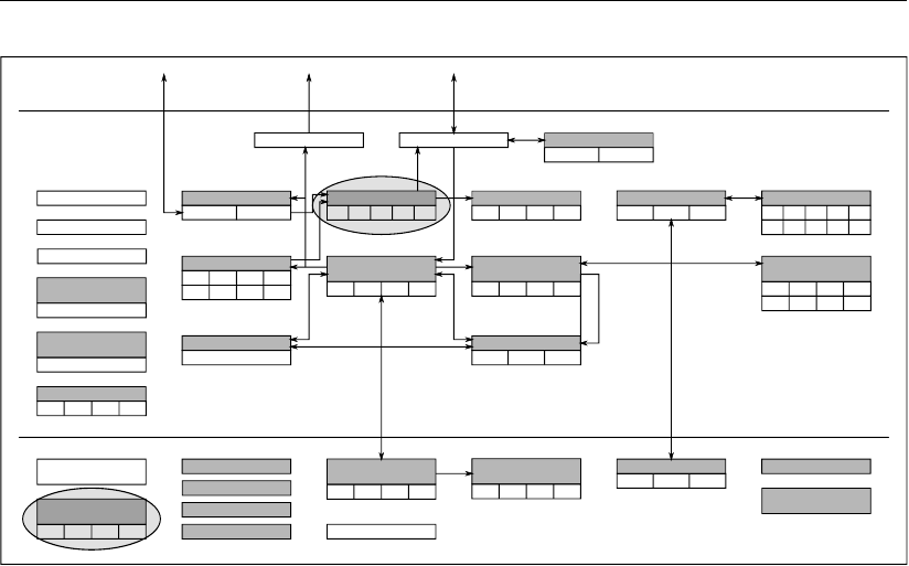
DRAFT
Principles of water quality modelling
TIC Alkalinity
Iron
7 Components
Sulphur
SO4
SUD SUP
NO
NH PO Si
AAP VIVP
APATP
OPAL
Methane
C
P S
NSi
(particulate)
POC PON POP POS
Organic Matter
(dissolved)
DOC DON DOP DOS
Grazers
C N PSi
Dissolved Oxygen
IM2 IM3
IM1
Oxygen Demand
BOD COD
phytobentos
C N PSi
Micro-
As
Cr Hg
Cd Cu
Ni Pb VZn
pollutants
Atr BaP Diu Flu
Organic micro-
HCB HCH PCB OMP
Sediment Oxygen
Demand
EnCoc
EColi FColi TColi
Tracers
Tracers
Continuity
Salinity/Chloride
Temperature
Inorganic Matter
IM2 IM3
IM1
Organic Matter
(particulate)
POC PON POP POS
Heavy Metals
pollutants
Organic micro-
Atmosphere
Water
Sediment
Heavy Metals
Inorganic Matter
Decayable
Conservative
5 Components
5 Components
Bacteria
pH
Nutrients
34 4
Phytoplankton
Organic Matter
Organic Matter
(dissolved)
DOC DON DOP DOS
Nutrients
Oxygen
Sulphur
Iron Methane
Figure 9.7: Overview of substances. Primary producers: phytoplankton
Light + Water + Carbon dioxide →Sugar + Oxygen
The most important primary producers in the aquatic environment are:
Algae, which include relatively large, plant-like organisms (weeds) and planktonic forms.
Cyano-bacteria (often referred to as blue green algae).
Microphytobenthos (mostly benthic diatoms).
Submerged and emerging macrophytes (vascular water plants).
In terms of the total amount of energy that is fixed, planktonic algae and cyano-bacteria are
the most important primary producers.
Environmental requirements
Biologically speaking, phytoplankters are relatively primitive plantlike organisms. They require
considerable amounts of nutrients and solar energy. In theory both of these factors could
become limiting, but the question is where and when. Also the physiological data indicate
that species of phytoplankton differ greatly in nutrient requirements, efficiency of solar energy
fixation (photosynthesis) and (potential) net growth rates.
The sun provides the energy, at a rate per square metre of surface area that depends upon
latitude, season, time of day and cloud cover. The energy must be shared among all the
phytoplankton cells floating in the water column below that square metre of surface area, with
an allowance set aside for reflection from the water surface and absorption by the bulk water
and its contents other than phytoplankton. The absorption (extinction) of light depends on
the concentrations of absorbing substances such as algae biomass, detrital organic matter,
inorganic sediment and water. The extinction of water with dissolved (inorganic) substances
is indicated as the background extinction. The more phytoplankton there is, the less solar
energy is available for each, until the energy per phytoplankton cell is too small to sustain
growth. At that point, solar energy becomes limiting to the phytoplankton biomass.
Plants also require about a dozen chemical elements for a normal development, among which
Deltares 249 of 382

DRAFT
D-Water Quality, User Manual
are nitrogen, phosphorus, sulphur, calcium, potassium, magnesium and iron. The require-
ments for each element vary widely. Three macro-nutrients, which are often reported as
limiting factors (nitrogen, phosphorus, and silicon), are generally considered to be potential
biomass limiting factors for phytoplankton, along with solar energy.
Nitrogen and phosphorus are vital to all phytoplankton species. Nitrogen is an essential com-
ponent of cell proteins such as enzymes, for genetic material, and of light-sensitive pigments
like chlorophyll-a, which are used for fixation of solar energy. Because of its importance
to many vital physiological processes, nitrogen deficiencies cannot be tolerated for long. In
aquatic systems nitrogen is available as ammonium and nitrate. Nitrogen gas (N2) can only
be used by nitrogen fixating algae.
Phosphorus is an important component of proteins, nucleic acids, and lipids (e.g., in the cell
walls). Coupling and uncoupling of ortho-phosphate groups to certain sugars are the main
reactions by which energy is stored or released in the cell. Phytoplankton cells are usually
less sensitive to phosphorus than to nitrogen deficiencies, hence survival at extremely low
internal phosphorus concentrations is often possible for some time.
Silicon is essential to only one phytoplankton group, diatoms. These species use silicon to
build strong skeletons surrounding the cell walls.
Eutrophication
Humans are special among the consumers since man’s activities have strongly affected the
environmental conditions on earth particularly during the the last two centuries. Since then
the amounts of various substances, which are released into the environment, have increased
dramatically. Many of these are seriously toxic, but other chemicals are on the contrary ben-
eficial to certain organisms. Among these are several compounds of the elements nitrogen
and phosphorus which are required by species of phytoplankton, among others.
As a result the concentrations of these plants have increased up to a level where they are
considered a nuisance in many waters. This process, which is called eutrophication, is ac-
companied by several objectionable symptoms: it gives the water a green, turbid appearance;
it can cause bad odours; it may harm other organism because the minimum daily oxygen
level can become extremely low during the night due to phytoplankton respiration; it can even
cause the water to become completely deprived of oxygen (anaerobic) when a bloom de-
clines rapidly, since the biological degradation processes consume large amounts of oxygen;
it may cause clogging of filters in drinking water purification systems. Some species of phyto-
plankton such as cyano bacteria or dinoflagellates may also induce toxic effects in primary or
secondary consumers.
9.8.2 Modelling framework
The substances that can be modelled in D-WAQ in relation to phytoplankton and microphyto-
benthos are:
Name of D-WAQ
substance
Description Unit
Phytoplankton: DYNAMO
Diat Diatoms gC/m3
Green Non-diatoms gC/m3
Phytoplankton: BLOOM
250 of 382 Deltares

DRAFT
Principles of water quality modelling
Name of D-WAQ
substance
Description Unit
FDIATOMS Freshwater diatoms (E- and N-phenotype) gC/m3
FFLAGELA Freshwater flagellates (E-phenotype) gC/m3
GREENS Green algae (E-, N- and P-phenotype) gC/m3
APHANIZO Aphanizomenon (E-, N- and P-phenotype) gC/m3
APHANFIX Nitrogen-fixing Aphanizomenon (E-, N- and P-
phenotype)
gC/m3
MICROCYS Microcystis (E-, N- and P-phenotype) gC/m3
OSCILAT Oscillatoria (E-, N- and P-phenotype) gC/m3
BLUEGRN Blue green algae (E-, N- and P-phenotype) gC/m3
MDIATOMS Marine diatoms (E-, N- and P-phenotype) gC/m3
MFLAGELA Marine flagellates (E-, N- and P-phenotype) gC/m3
DINOFLAG Dinoflagellates (E-, N- and P-phenotype) gC/m3
DINOMIX Mixotrophic dinoflagellates (E-, N- and P-
phenotype)
gC/m3
PHAEOCYS Phaeocystis (E-, N- and P-phenotype) gC/m3
ULVAS Suspended Ulva (E-, N- and P-phenotype) gC/m3
ULVAF Rooted Ulva (E-, N- and P-phenotype) gC
Microphytobenthos: DYNAMO
DiatS1 Benthic diatoms in layer S1 gC/m2
DiatS2 Benthic diatoms in layer S2 gC/m2
Two modules are available for the modelling of phytoplankton, BLOOM and DYNAMO. These
modules are alternatives, that differ strongly with respect to ruling concepts, process formu-
lations and process details. They can not be used simultaneously. However, the modules
share processes with respect to light extinction, settling and resuspension. Both modules in-
clude the same major processes: the production and mortality of algae biomass, the uptake
and excretion of the nutrients and the production and consumption of dissolved oxygen and
carbon dioxide. The modelling of all other processes to which the nutrients are subjected
and the modelling of detrital organic matter partially produced from biomass are described
in section 9.7.section 9.5 provides the description of the modelling of other processes for
dissolved oxygen. BLOOM is also capable of the simulation of Ulva like macro algae that can
attach themselves to the sediment. DYNAMO allows for the modelling of microphytobenthos
by means of an additional process for primary production and mortality in the sediment, when
this is modelling according to the S1-S2 approach.
Deltares 251 of 382

DRAFT
D-Water Quality, User Manual
DYNAMO versus BLOOM
BLOOM is a multi-species algae model, based on an optimisation technique that distributes
the available resources in terms of nutrients and light among the algae species (WL | Delft
Hydraulics,1991a,1992;Los and Brinkman,1988). BLOOM optimises the species composi-
tion to obtain the overall maximum growth rate under the given conditions. A large number of
groups and/or species of algae and even different phenotypes within one species can be con-
sidered. BLOOM distinguishes between three phenotypes: under nitrogen limiting conditions,
under phosphorus limiting conditions and under light limiting conditions. Algae living in the
water column (phytoplankton) and (macro)algae on the sediment can be included with their
specific ecophysiological characteristics (this has been implemented for Ulva). A database for
15 algae groups and species is part of D-WAQ.
DYNAMO is based on a more traditional model of primary production using Monod-kinetics
for the calculation of growth rates (?). Two groups of algae are considered: diatoms and all
non-diatoms (referred to as ‘Green’ algae). The main difference between the types is that
diatoms utilise silica as an essential nutrient, while ‘non-diatoms’ do not.
The selection of the appropriate algae module will often depend on the modelling objective.
However, the availability of data (field observations and model coefficients), model status and
possibly the amount of required computation time can be important too.
DYNAMO is recommended for general reconnaissance studies, in which distinction of different
species and competition between species are not considered of prime importance. Using
DYNAMO the aim should be to calculate overall primary production in terms of the total algal
biomass. DYNAMO may also be selected for eutrophication pre-studies focussing on nutrient
mass balances and the primary effects of the decrease or increase of the nutrient loads.
BLOOM should be selected for phytoplankton simulations, when the prediction of specific al-
gae species and their biomass in a setting of multi-species competition is the primary goal of
the application. BLOOM will include the inter-species competition for resources (light, nutri-
ents). Using BLOOM can for example be of importance, if nuisance algae such as blue green
algae species need to be included in the model.
Before making a choice, you should preferably have a detailed picture of the variables that
need to be simulated and the significance of the quality of the calculations. First of all, both
models can simulate algal growth rates and resulting biomass concentrations. To give a sim-
plified picture of the outcome of these calculations, the DYNAMO approach will generally give
a more linear picture of biomass development, while the BLOOM approach can simulate non-
linear, more dynamic behaviour as well.
In general, the availability and accuracy of the data needed to determine the values of the
model coefficients as well as the data for model validation limit the reliability of modelling re-
sults. Naturally, this is true for algae modelling as well. Since the DYNAMO approach requires
less coefficients, you might be tempted to assume that a scarce data base will automatically
point to the use of DYNAMO. You should note however, that describing complex processes by
simple equations makes it necessary to tune the coefficients for local conditions. Moreover,
DYNAMO-coefficients may be rather hard to determine and the modelling results can be very
sensitive to the values of these coefficients. It is therefore recommended to carefully inspect
the available data before choosing a modelling approach.
Furthermore, it can be wise to investigate whether one of the models has already been val-
idated for a system that is similar to the system that should be modelled. If so, choosing
the model that has proven successful under those conditions can be particularly helpful if the
252 of 382 Deltares

DRAFT
Principles of water quality modelling
available data set is limited. Validation of the model results for a wide range of both fresh-
water and marine systems has resulted in a data base with coefficients for 13 algal groups
and species for which calibration is hardly required. Obviously, this is a special advantage of
BLOOM.
Mass balance
The general mass balance for phytoplankton (in the water column) is given in the equation
below for both DYNAMO and BLOOM:
∆Phytoplankton
∆t=loads +transport −settling +resuspension
+gross primary production −respiration −mortality
(9.32)
Phytoplankton produces oxygen in quantities relative to the gross production of organic matter.
The algae consume dissolved oxygen for respiration.
Dead phytoplankton biomass is converted to the inorganic nutrients (autolysis) and the de-
tritus pool in the water column (see section 9.7). Settled algae biomass only dies in the
sediment, either instantly in the case of the S1-S2 approach, or slowly when sediment-water
interaction is modelled according to the layered sediment approach. The dead biomass is
converted to the sediment detritus pools. Resuspended benthic algae biomass is turned over
instantly in to the detritus pools in the water column.
Grazing is added to the mass balance for algae biomass when one of the availble grazing
modules of D-WAQ is included in a model.
Brief description and relevant notes of processes:
Deltares 253 of 382

DRAFT
D-Water Quality, User Manual
Process Substances Comments
Gross primary
production
All phytoplankton
(NH4)
(NO3)
(PO4)
(Si)
(OXY)
(TIC)
(Alka)
(SO4)
Gross primary production is proportional to the
biomass concentration and a gross primary pro-
duction (growth) rate.
Algae consume inorganic nutrients and produce
dissolved oxygen proportional to net primary
production. Only diatoms consume silicon as
a nutrient. The uptake of nitrogen, phospho-
rus and silicon is determined by C:N:P:Si ratios
which can be different for each type of primary
producer.
The chlorophyll content of algae is species spe-
cific. The total chlorophyll-a concentration is
equal to the sum of the contributions of all algae
species.
(Major) Limiting factors are light availability and
nutrient availability. BLOOM and DYNAMO have
different formulations.
The inclusion of TIC and/or SO4 in a model is
optional for BLOOM. DYNAMO ignores sulphur
components.
Respiration All phytoplankton
(NH4)
(PO4)
(Si)
(OXY)
(TIC)
(Alka)
(SUD)
Respiration is the sum of growth respiration and
maintenance respiration. Growth respiration is
a species specific fraction of gross production,
included in the growth rate for BLOOM. Main-
tenance respiration is proportional to the algal
biomass and a respiration rate.
continued on next page
254 of 382 Deltares

DRAFT
Principles of water quality modelling
continued from previous page
Process Substances Comments
Mortality and
autolysis
All phytoplankton
POX1-2
(Opal)
(NH4)
(PO4)
(Si)
(OXY)
(TIC)
(Alka)
(SUD)
Algal mortality is proportional to the biomass
concentration and an overall mortality rate.
Note that grazing as an additional loss process
is only considered when one of the grazing mod-
ules is included in the model. Otherwise, the
loss due to grazing should be incorporated in the
mortality rate.
Next to temperature dependent mortality, mor-
tality caused by salinity stress can also be in-
cluded. The mortality rate is a combined func-
tion of the temperature and the chloride concen-
tration. Freshwater algae start dying when salin-
ity increases. Marine algae start dying when
salinity drops.
The simulation of POS1-2 and SUD is optional
for BLOOM.
Settling7All phytoplankton
(POX1-2)
(Opal)
DetXS1
Settling only takes place when the bottom shear
stress drops below a critical value. Settling thus
depends on the flow velocity and turbulence in
the water.
Settling is proportional to the biomass concen-
tration and a species specific settling velocity.
Algae biomass settles in DetXS1 in case of the
S1-S2 approach for the sediment.
continued on next page
7For a detailed description of the settling and resuspension process refer to section 9.6.
Deltares 255 of 382

DRAFT
D-Water Quality, User Manual
continued from previous page
Process Substances Comments
Resuspension11 DiatS1
DiatS2
BLOOM algae
(POX1-2)
Resuspension takes places with a zero-order
rate (in g/m2/d) and is proportional to a proba-
bility function.
Resuspension takes place when the actual
shear stress is higher than the critical shear
stress for resuspension.
The sediment layers S1 and S2 each have a crit-
ical shear stress for resuspension. The critical
shear stress for resuspension is valid for all par-
ticulate fractions in the sediment layer.
The resuspension rate of the individual partic-
ulate fractions in the sediment layer is propor-
tional to its weight fraction.
Grazing8All phytoplankton
(Primary con-
sumers)
(POX1-3)
(Opal)
(OXY)
(TIC)
(Alka)
Primary consumers can derive their nutrients
from living and detrital organic matter.
Taking grazing into account requires the inclu-
sion of a grazing module in a model.
Remarks:
The total light extinction in the water column is the sum of background extinction (water
itself and non-modelled substances) and extinction due to phytoplankton, detritus and
inorganic matter.
Process rates are temperature dependent as indicated in section 9.3 (k=kr ×
kt(T−T r)). However, it is important to note that DYNAMO has a reference tempera-
ture of 20 ◦C, whereas BLOOM has a reference temperature of 0 ◦C.
9.8.3 Process equations
Phytoplankton: BLOOM
BLOOM distinguishes species groups like marine diatoms and dinoflagellates. Within a species
group up to three phenotypes can be distinguished: the N-limited phenotype, the P-limited
and the E-limited phenotype. The phenotypes occur under respectively nitrogen limiting con-
ditions, phosphorus limiting conditions and light (energy) limiting conditions. Phenotypes have
distinct growth rates, mortality rates, nutrient-carbon ratios, etc.
The primary production for BLOOM is simulated with an optimisation technique (LP). This
technique delivers the biomass for each (included) algae phenotype at the end of a time step
by means of solving a set of linear equations and inequalities (constraints), thereby maximis-
ing the total net primary production. The principles of the constraints are as follows:
8For a detailed description of grazing refer to section 9.9.
256 of 382 Deltares

DRAFT
Principles of water quality modelling
for nutrients,
Ctnutk=Cnutk+
n
X
i=1
(anutk,i ×Calgi)−Cnutck
for energy (light),
eca =
n
X
i=1
(eci×Calgi)
ecmini≤eca ≤ecmaxi
ecmini=ectmini−ecb
ecmaxi=ectmaxi−ecb
Iai=Itop ×1−e−ectmaxi×Ha
ectmaxi×Ha
Iai=f(Ef ci)
for growth,
Calg2i≤Calg1i×e((kgpi×Efi−krspi)×Dtb)
for mortality,
Calg2i=Calg1i×e(−kmrti×Dtb)
with:
anut stoichiometric constant of nutrient k originating from dissolved inorganic nutrient
over organic carbon in algae biomass [gN/P/Si gC−1]
Calg algae biomass concentration [gC m−3]
Calg1biomass of algae species jat time t1[gC m−3]
Calg2biomass of algae species jat time t2[gC m−3]
Cnut concentration of dissolved inorganic nutrient k [gN/P/Si m−3]
Cnutc threshold concentration of dissolved inorganic nutrient k[gN/P/Si m−3]
Ctnut concentration of total available nutrient k[gN/P/Si m−3]
ec specific extinction coefficient of an algae species type [m2gC−1]
eca total extinction coefficient of all algae [m−1]
ect total extinction coefficient [m−1]
ecmin minimum extinction coefficient of algae due to background extinction [m−1]
ectmin minimum total extinction coefficient due to background extinction [m−1]
ecmax maximum extinction coefficient of algae needed to avoid self shading [m−1]
ectmax maximum total extinction coefficient to avoid self shading of algae i[m−1]
Ef light efficiency factor [-]
Efc critical light efficiency factor [-]
Ha time step average depth of a water compartment or water layer [m]
Ia critical depth average light intensity [W m−2]
Itop light intensity at the top of a water compartment/layer [W m−2]
kgp potential specific gross primary production rate of the E-phenotype of an algae
species [d−1]
kmrt specific mortality rate of an algae species type [d−1]
krsp specific maintenance respiration rate of the E-phenotype of an algae species
[d−1]
zdepth [m]
Deltares 257 of 382

DRAFT
D-Water Quality, User Manual
∆ttime step [d]
iindex for algae species type [-]
kindex for nutrients, 1 = nitrogen, 2 = phosphorus, 3 = silicon [-]
nnumber of algae species types, maximum allowed is 15 [-]
The optimisation technique finds the new biomass of each algal phenotype at the end of a time
step. The rates of growth, production, mortality and autolysis are derived from the change of
the algae biomasses over a time step.
Rgri=(Calg2i−Calg1i)
Dt
Rgpi=Rgri+Rrspi+Rmrti
Rnpi=Rgpi−Rrspi
Rmrti=kmrti×(Calg2i+Calg1i)
2
Rauti=fauti×Rmrti
with:
faut fraction of dead algae biomass autolised [-]
Raut autolysis rate for dead algae biomass [gC m−3d−1]
Rgp gross primary production rate [gC m−3d−1]
Rgr growth rate for organic carbon [gC m−3d−1]
Rmrt mortality rate [gC m−3d−1]
Rnp net primary production rate [gC m−3d−1]
Rrsp respiration rate [gC m−3d−1]
Remarks:
The rates of the effects on the mass balances of dissolved oxygen, nutrients and detritus
are simply derived from the above rates by multiplication with stoichiometric constants.
The nutrient constraints are the minimal value of the quantities of available inorganic
nutrients divided by the relevant algal stoichiometric constant. Only one nutrient at a
time can be limiting to the growth of algae.
Some algae species can satisfy a part of their nutrient demands by the consumption of
organic detritus. Other algae species are capable of the fixation of dissolved elementary
nitrogen. The effects of respectively mixotrophy and nitrogen fixation are included in
the nutrient constraints, respectively by adding the nutrients available in detritus or in
an indefinite stock of elementary nitrogen.
The light limitation function can be based on daily average and depth average condi-
tions. This function is associated with the critical ambient extinction coefficient which
is species specific. The coefficient is derived from imposed tables that relate produc-
tion efficiency to ambient light intensity (irradiation). Growth inhibition if the radiation is
larger than the optimal radiation may be included in these tables. The tables are part of
the BLOOM data base.
The advantage of buoyancy of certain (blue green) algae species can be taken into
account by means of a depth corrected light limitation function.
Macro algae like Ulva attached to the sediment can be simulated as a phytoplankton
species by means of non-transportability and a depth corrected light limitation function.
Growth respiration is included in the potential production rate because of the biomass
maximisation principle. Nutrients released as the consequence of respiration will quickly
be taken up again in order to achieve maximal biomass production.
Autolysis takes care that a certain fraction of the nutrients tied up in biomass is released
as inorganic nutrients at the mortality of algae. The remaining fraction is added to
various detritus pools. The fractionating is species specific.
258 of 382 Deltares

DRAFT
Principles of water quality modelling
The excretion of organic matter (nutrients) by algae is ignored.
BLOOM may also take into account sulphur from SO4, in which case it turns over sul-
phur into POS1-2 at mortality. However, sulphur is not limiting phytoplankton growth.
BLOOM may also be limited by carbon dioxide modelled as (TIC).
Phytoplankton: DYNAMO
The gross primary production for DYNAMO follows from:
Rgpi=fnuti×flti×kgpi×Calgi
with:
Calg algal biomass concentration [gC m−3]
flt light limitation factor [-]
fnut nutrient limitation factor according to Monod [-]
kgp potential gross primary production rate [d−1]
Rgp gross primary production rate [gC m−3d−1]
iindex for species group (Diat or Green) [-]
The nutrient limitation factor for DYNAMO considers only the most limiting nutrient:
fnuti= min Cn
Ksn +Cn,Cph
Ksph +Cph,Csi
Kssi +Csi
with:
Cn ammonium plus nitrate concentration [gN m−3]
Cph phosphate concentration [gP m−3]
Csi dissolved inorganic silicate concentration [gSi m−3]
Ksn half saturation constant for nutrient nitrogen [gN m−3]
Ksph half saturation constant for phosphate [gP m−3]
Kssi half saturation constant for silicate [gSi m−3]
The light limitation function for DYNAMO is a combination of a day length factor and a radiation
limiting factor that saturates for day length and light intensities larger than the optimal day
length and light intensity:
flti=f(Iz, Ioi, DL, DLoi, . . .)
with:
DL day length [d]
DLo optimal day length [d]
flt light limitation factor [-]
Izdepth average light intensity in a water layer [W m−2]
Io optimal light intensity [W m−2]
The depth averaged light intensity is derived according to Lambert-Beer’s Law for light atten-
uation:
Iz=Itop ×e(−ec×z)
with:
ec extinction coefficient of visible light [m−1]
Itop light intensity at the top of a water layer [W m−2]
Deltares 259 of 382

DRAFT
D-Water Quality, User Manual
zwater depth [m]
The extinction coefficient is the sum of contributions of the background (water plus not mod-
elled substances), live algae biomass, particulate and dissolved detritus and inorganic sus-
pended matter. These contributions follow from the multiplication of concentrations and spe-
cific extinction coefficients.
The rates of respiration and mortality in DYNAMO are described with:
Rrspi=krspi×Calgi+frspi×Rgpi
Rmrti=kmrti×Calgi
kmrti=f(Ccl, T )
with:
Ccl chloride concentration [g m−3]
frsp fraction of gross production respired [-]
kmrt total mortality process rate [d−1]
krsp maintenance respiration rate [d−1]
Rmrt total mortality rate [gC m−3d−1]
Rrsp total respiration rate [gC m−3d−1]
Remarks:
There is no growth inhibition if the radiation is larger than the optimal radiation.
Autolysis takes care that a certain fraction of the nutrients tied up in biomass is released
as inorganic nutrients at the mortality of algae. The remaining fraction is added to
various detritus pools. The fractionating is species specific.
The excretion of organic matter (nutrients) by algae is ignored.
9.9 Primary consumption
9.9.1 Concepts
One module (CONSBL) is available for the modelling of primary consumers such as zooplank-
ton and zoobenthos. These primary consumers are also indicated as grazers. CONSBL is
described with respect to organic carbon and nutrients incorporated in the organisms or af-
fected by them. The nutrients concern nitrogen, phosphorus and silicon. The description of
the consumer modules includes the uptake of phytoplankton biomass and detritus for food, the
production, respiration and mortality of biomass, and the excretion of detritus and nutrients.
The effects of consumers on dissolved oxygen by means of respiration are ignored.
260 of 382 Deltares
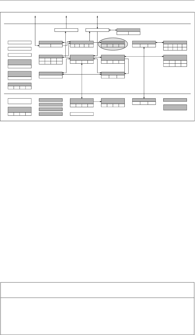
DRAFT
Principles of water quality modelling
TIC Alkalinity
Iron
7 Components
Sulphur
SO4
SUD SUP
NO
NH PO Si
AAP VIVP
APATP
OPAL
Methane
C
P S
NSi
(particulate)
POC PON POP POS
Organic Matter
(dissolved)
DOC DON DOP DOS
Grazers
C N PSi
Dissolved Oxygen
IM2 IM3
IM1
Oxygen Demand
BOD COD
phytobentos
C N PSi
Micro-
As
Cr Hg
Cd Cu
Ni Pb VZn
pollutants
Atr BaP Diu Flu
Organic micro-
HCB HCH PCB OMP
Sediment Oxygen
Demand
EnCoc
EColi FColi TColi
Tracers
Tracers
Continuity
Salinity/Chloride
Temperature
Inorganic Matter
IM2 IM3
IM1
Organic Matter
(particulate)
POC PON POP POS
Heavy Metals
pollutants
Organic micro-
Atmosphere
Water
Sediment
Heavy Metals
Inorganic Matter
Decayable
Conservative
5 Components
5 Components
Bacteria
pH
Nutrients
34 4
Phytoplankton
Organic Matter
Organic Matter
(dissolved)
DOC DON DOP DOS
Nutrients
Oxygen
Sulphur
Iron Methane
Figure 9.8: Overview of substances. Primary consumption
The modelling of all other processes to which the nutrients and detritus are subjected are
described in section 9.7 of this manual. section 9.8 provides the description of the modelling
of phytoplankton processes.
Pelagic and benthic grazing pressure can be imposed on the model as a forcing function
with module CONSBL (WL | Delft Hydraulics,1990). This module can be applied for up to
five types of grazers, which may be species groups or individual species of zooplankton and
zoobenthos. CONSBL requires that biomasses of grazers are imposed to the model as time-
series. Imposed biomasses will be adjusted, if constraints for growth, mortality and available
food are exceeded. Using the grazer biomass time-series as boundary conditions CONSBL
generates the mass fluxes due to grazing with respect to algae biomass, detritus and nutrients
in a consistent and mass conservative way.
The advantage of a forcing function over a dynamic grazing model is that the grazer biomass
is controlled. Even state-of-the-art dynamic simulation of grazers is still subjected to problems
concerning stability and limited accurateness. However, imposing forcing functions demands
for reliable and rather frequently measured grazer biomass data.
9.9.2 Modelling framework
CONSBL imposes the grazing pressure of up to five species (groups) of zooplankton and
zoobenthos. The names of the input parameters for biomass are:
Name of D-WAQ
substance
Description Unit
Zooplank Zooplankton gC/m3
Mussel Mussels gC/m2
Grazer3 Optional user-defined 3rd grazer gC/m3or gC/m2
Grazer4 Optional user-defined 4th grazer gC/m3or gC/m2
Grazer5 Optional user-defined 5th grazer gC/m3or gC/m2
Deltares 261 of 382

DRAFT
D-Water Quality, User Manual
Although input parameter names of the first two groups refer to respectively zooplankton and
mussels (zoobenthos), you still need to define the nature of each of the groups. The grazer
biomass in CONSBL is subjected to growth or mortality, and to growth and maintenance res-
piration. The imposed biomass is corrected in order to obey constraints for growth, mortality
and food availability. The grazer process rates are transformed into the rates of the consump-
tion of detritus and algae, and the production of detritus and inorganic nutrients. According to
the specification a fraction of the produced detritus is added to the sediment detritus pools,
whereas the remainder is allocated to detritus in the water column.
The assumptions for forcing function CONSBL are:
1 Grazers in the water column and at the sediment have essentially the same behaviour in
terms of food consumption, growth, respiration, mortality and detritus production. They
are different in the sense that detritus produced is released into the water column and/or
deposited at the sediment.
2 The existence of distinct physiological types within a grazer species can be ignored.
3 Grazers are not subjected to settling and resuspension.
4 Grazers consume algae species and detritus for food. Grazer species are different with
respect to their preference for these food components.
5 Nutrient-carbon ratios in grazer species are constant and species specific, consequently
nutrients are taken up by grazers in constant ratios. The same holds for the release of
organic nutrients due to mortality.
6 Grazers produce detritus due to egestion of a part of the ingested food as fecal pellets,
and due to mortality. The surplus is determined for every organic nutrient (C, N, P, Si) as
the sum of poorly digestible food fractions and the excess nutrient intakes. The fractions
are specific for both food components and grazer species. Most grazers do not use silicon
at all.
7 Grazers produce inorganic nutrients due to respiration.
8 The change of grazer biomass during a time step can not be larger than constraints for
maximal growth or maximal mortality, and for available food. Growth and mortality do not
necessarily concur. The imposed grazer biomass is adjusted in accordance with these
constraints.
9 Maximal growth is proportional to the biomass concentration and a maximal growth rate.
Maximal mortality is proportional to the biomass concentration and a maximal mortality
rate.
10 Respiration is the sum of growth respiration and maintenance respiration. Growth respira-
tion is a species specific fraction of gross production. Maintenance respiration is propor-
tional to the algal biomass and a respiration rate.
11 Grazer maximal growth, respiration and maximal mortality rates are functions of tempera-
ture with a species specific coefficients.
12 Actual growth is equal to the net increase of grazer biomass over a time step. Net food
assimilation is equal to the net increase of grazer biomass plus respiration.
13 Actual mortality is equal to the net decrease of grazer biomass over a time step plus. Net
detritus production is equal to mortality minus respiration.
14 Grazer consumption is proportional to the biomass concentration and a grazer consump-
tion rate. This rate is either equal to the maximal uptake rate or to a filtration rate. Both
are temperature dependent and grazer species specific. The rate applied depends on the
exceedence of a critical food concentration, which is the concentration for which the rates
are equal. The filtration rate is formulated according to Monod kinetics.
15 The autolysis of grazer biomass at mortality can be ignored.
262 of 382 Deltares

DRAFT
Principles of water quality modelling
9.9.3 Process equations
Grazing: CONSBL
The form of the formulations of forcing function module CONSBL deviates strongly from the
form in dynamic producer and consumer modules because the grazer biomass is imposed
in stead of predicted. The consumption rates for algae and detritus are deduced from the
change of grazer biomasses over a time step. However, this change must be consistent with
maximal growth or maximal mortality, and with the available food. Consequently, the imposed
biomass is adjusted when one of these constraints is not met. The growth, mortality and food
constraints are respectively:
Cgrci=Cgr1i×(1 + kgri×∆t)if Cgr2i≥Cgr1i
Cgr1i×(1 −kmrti×∆t)if Cgr2i< Cgr1i
with:
Cgr1igrazer biomass concentration at t1[gC m−3]
Cgrci grazer biomass concentration constraint at t2[gC m−3]
kgr maximal growth rate [d−1]
kmrt maximal natural mortality rate [d−1]
∆ttime step [d]
iindex for grazer species group 1–5 [-]
kindex for nutients, 1 = carbon, 2 = nitrogen, 3 = phosphorus, 4 = silicon [-]
The available food is equal to the sum of component concentrations multiplied with preference
parameters that can be considered weigth factors:
Cfdi=fdpri×Cdet1+
m
X
j=1
(fapri×Calgj)
with:
Calgjbiomass concentration of algae species group j[gC m−3]
Cfdifood concentration available to grazer species group i[gC m−3]
Cdetidetritus organic carbon concentration [gC m−3]
fdpripreference of a grazer species group ifor detritus [-]
fapri,j preference of a grazer species group ifor algae species group j[-]
mnumber of algae groups [-]
jindex for algae species groups [-]
The consumption rates for detritus and algae biomass of a grazer group are:
Rdcns1k,i =fdpri×kcnsi×Cdetk
Racnsk,i,j =fapri,j ×kcnsi×anutk,j ×Calgj
with:
anutk,j stoichiometric const. of nutrient kover organic carbon in algae j[gC/N/P/Si
gC−1]
Cdetkdetritus concentration for nutrient k[gC/N/P/Si m−3]
fdpripreference of a grazer species group ifor detritus [-]
fapri,j preference of a grazer species group ifor algae species group j[-]
kcnsiconsumption process rate of grazer group i[d−1]
Racnsk,i,j cons. rate of grazer group ifor nutrient kin algae j[gC/N/P/Si m−3d−1]
Rdcns1k,i gross cons. rate of grazer group ifor nutrient kin detritus [gC/N/P/Si m−3d−1]
Deltares 263 of 382

DRAFT
D-Water Quality, User Manual
The consumption process rate is equal to either the maximal uptake rate or a filtration rate
depending on whether the available concentration of food is larger or smaller than a certain
critical amount. This amount is the biomass concentration for which the filtration rate and the
maximal uptake rate are equal.
Consumed food is either assimilated as grazer biomass, respired or egested as detritus (fae-
cal pellets). Depending on the nature of the grazer group a part of the egested detritus is
deposited at the sediment and is therefore added to the sediment detritus pool. The total
rates of food assimilation, net detritus consumption and sediment detritus production caused
by grazing are as follows:
Rask,i = (1 −fdeti)×Rdcnsk,i +
m
X
j=1
((1 −falgi,j )×Racnsk,i,j )
Rdcns2k,i = (1 −fdeti)×Rdcns1k,i +
m
X
j=1
((1 −falgi,j ×(1 −fsedi)) ×Racnsk,i,j )
Rsdprk,i =fdeti×fsedi×Rdcns1k,i +
m
X
j=1
(falgi,j ×fsedi×Racnsk,i,j )
with:
falgi,j egested fraction of algae jconsumed by grazer i, =1-yield [-]
fdetiegested fraction of detritus consumed by grazer i, =1-yield [-]
fsedifraction of detritus egested by grazer iadded to the sediment detritus pool [-]
Rask,i total food assimilation rate for nutrient kfor grazer group I [gC/N/P/Si m−3d−1]
Rdcns2k,i net cons. rate of grazer group ifor nutrient kin detritus [gC/N/P/Si m−3d−1]
Rsdprk,i total nutrient kin detr. prod. at the sediment for all grazers [gC/N/P/Si m−3d−1]
The rates are corrected for nutrient limitation, respiration and the change of grazer biomass
resulting from the food constraint. The nutrient limitation leads to a decrease of Rdcns and
an increase of Rsdpr for those nutrients in the food that are available in excess as calculated
on the basis of grazer biomass stoichiometry. Respiration causes a decrease of both rates
and the release of equivalent amounts of inorganic nutrients. The growth and maintenance
respiration rates are described with:
Rrsp1k,i =bnutk,i ×frsp1i×Ras1,i
Rrsp2k,i =bnutk,i ×krsp2i×Cgr1i
with:
bnutk,i stoichiometric const. of nutrient kover organic carbon in grazer i[gC/N/P/Si
gC−1]
frsp1igrowth respiration fraction [-]
krsp2imaintenance respiration rate [d−1]
Rrsp1k,i growth respiration rate for nutrient kand grazer i[gC/N/P/Si m−3d−1]
Rrsp2k,i maintenance respiration rate for nutrient kand grazer i[gC/N/P/Si m−3d−1]
Finally, in case of mortality the grazer biomass decrease over a time step is allocated to the
detritus production rates.
9.10 Heavy metals and organic micro-pollutants
264 of 382 Deltares
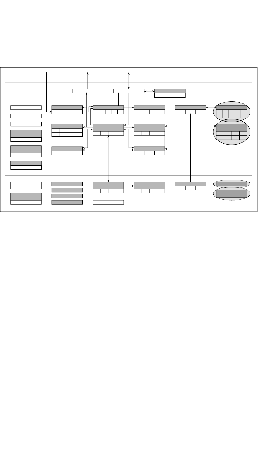
DRAFT
Principles of water quality modelling
9.10.1 Concepts
Two types of micropollutants can be modelled with D-WAQ: heavy metals and organic micro-
pollutants. These types of pollutants show conformities but also many basic differences with
respect to properties and processes. Both conformities and major differences have been
taken into account in D-WAQ.
TIC Alkalinity
Iron
7 Components
Sulphur
SO4
SUD SUP
NO
NH PO Si
AAP VIVP
APATP
OPAL
Methane
C
P S
NSi
(particulate)
POC PON POP POS
Organic Matter
(dissolved)
DOC DON DOP DOS
Grazers
C N PSi
Dissolved Oxygen
IM2 IM3
IM1
Oxygen Demand
BOD COD
phytobentos
C N PSi
Micro-
As
Cr Hg
Cd Cu
Ni Pb VZn
pollutants
Atr BaP Diu Flu
Organic micro-
HCB HCH PCB OMP
Sediment Oxygen
Demand
EnCoc
EColi FColi TColi
Tracers
Tracers
Continuity
Salinity/Chloride
Temperature
Inorganic Matter
IM2 IM3
IM1
Organic Matter
(particulate)
POC PON POP POS
Heavy Metals
pollutants
Organic micro-
Atmosphere
Water
Sediment
Heavy Metals
Inorganic Matter
Decayable
Conservative
5 Components
5 Components
Bacteria
pH
Nutrients
34 4
Phytoplankton
Organic Matter
Organic Matter
(dissolved)
DOC DON DOP DOS
Nutrients
Oxygen
Sulphur
Iron Methane
Figure 9.9: Overview of substances. Heavy metals and organic micro-pollutants
Because the fate of most micropollutants is largely determined by the adsorption to particulate
matter, suspended inorganic and organic matter (including phytoplankton) has to be included
in the model in most cases. It may be necessary to include dissolved organic matter as well.
In D-WAQ the two options available for sediment-water interaction and return fluxes, the lay-
ered sediment approach and the S1-S2 approach, are also applicable for the modelling of
micropollutants.
9.10.2 Modelling framework
Heavy metals
The heavy metals that can be modelled are divided among three subgroups:
Name of D-WAQ
substance
Description Unit
Group 1: sulphide-forming heavy metals
Cd Cadmium g/m3
Cu Copper g/m3
Pb Lead g/m3
Hg Mercury g/m3
Ni Nickel g/m3
Zn Zinc g/m3
Group 2: hydroxide-forming heavy metals
Deltares 265 of 382

DRAFT
D-Water Quality, User Manual
Name of D-WAQ
substance
Description Unit
Cr Chromium g/m3
Group 3: heavy metals occurring as anions
As Arsenic g/m3
Va Vanadium g/m3
Strictly speaking, vanadium and arsenic do not belong to the group of heavy metals. Group
1 encompasses the heavy metals that tend to form poorly soluble sulphides at chemically
reducing conditions. Chromium and arsenic do not form sulphide precipitates under normal
conditions in sediments. However, chromium and vanadium may form (hydr)oxides. Arsenic
and vanadium are present as anions, whereas the other metals form free or complexed cations
in the solution. Referring to their ionic state, some of the metals can possess more than
one valency. Although dependent on the chemical conditions to some extent, one valency
is usually dominant over the other valencies at prevailing natural conditions. The differences
between the groups of metals have important consequences for the partitioning of the metals
among several dissolved and particulate phases.
Metals are conservative substances. The fate of heavy metals in a water system is deter-
mined primarily by partitioning to water and particulate matter (including phytoplankton), and
by transport. The partitioning divides the total amount of a pollutant into a ‘dissolved’ frac-
tion and several ‘adsorbed’ fractions. Adsorbed fractions of a metal are influenced by all the
processes that affect particulate matter, such as settling, resuspension, burial and digging.
Partitioning of metals is described in general by:
1 sorption to particulates;
2 precipitation in minerals; and
3 complexation in solution.
Complexation with inorganic and organic ligands can be considered implicitly in partitioning
by using reprofunctions for the partitioning coefficient. Sorption can be modelled as an equi-
librium process (equilibrium partitioning) or as the resultant of slow adsorption and desorption
reactions (kinetic formulations). In the latter case, partitioning is assumed to proceed at a
finite rate proportional to the difference between the actual state and the equilibrium state. D-
WAQ uses one state variable (substance name) for equilibrium sorption, which represents the
total metal concentration. Alternatively, D-WAQ uses two state variables (substance names
with name additions -Dis and -Par) for slow sorption, one for the dissolved metal concentration
and one for the particulate metal concentration.
To describe the fate of certain heavy metals in reducing environments, such as sediment
layers, the formation of metal sulphides or (hydr)oxides can be modelled. The soluble metal
concentration is determined on the basis of the relevant solubility product. The excess metal
is stored in a precipitated metal fraction.
Notice that sorption and precipitation affect the dissolved metal concentration in different ways.
Both the adsorbed and dissolved fractions increase at increasing total concentration, as long
as no solubility product is exceeded. The dissolved concentration is bounded by precipitation
at the level at which a solubility product is exceeded.
266 of 382 Deltares

DRAFT
Principles of water quality modelling
Mercury is modelled like cadmium. Organic forms (methylated species) are ignored, which
can be justified from the quantitative point of view. The methylated forms of lead and arsenic
have not been taken into consideration for similar reasons.
Metals such as silver, cobalt, antimony, selenium and molybdenum have not been mentioned,
but can be modelled approximately as one of the other metals.
Assumptions for heavy metals:
1 Heavy metals can adsorb to particulate inorganic matter (up to three fractions), to dead
particulate and dissolved organic matter (up to five fractions), and to phytoplankton (sum
of various algae species).
2 The adsorption to particulate matter and dissolved organic matter is described by means
of equilibrium or kinetic partitioning, on the basis of partitioning coefficients. For each par-
ticulate phase, a different partition coefficient is defined. A total of 5 partition coefficients
must be provided if all particulate fractions are present in the model (Kpim1−3,Kppoc
and Kpalg respectively). In case DOC is modelled as well, an additional coefficient is
needed.
3 The partition coefficient is in fact a function of the macrochemical composition of the water
(pH and various ions) and the macrochemical composition of the inorganic matter (binding
capacity). These dependencies can be taken into account in the reprofunction for the
partitioning coefficient.
4 Complexation of metals in solution can be considered implicitly in so-called repro-functions
for the partition coefficient. Complexation is also considered implicitly in precipitation equi-
libria. Relevant ligands are hydroxyl, bicarbonate, chloride and sulphides.
5 All metal is assumed to be available for partitioning.
6 The precipitation of metal sulphides is described as equilibrium process, on the basis of a
solubility product. Precipitation depends on the presence of dissolved oxygen, which has
to be imposed as forcing function, or has to be simulated. The pH and the total dissolved
sulphide concentration have to be provided as well. It is assumed that sulphide is always
present in abundance, so that all particulate metal is in the metal sulphides.
7 The precipitation of metal (hydr)oxides is described as equilibrium process, on the basis of
a solubility product. The pH has to be provided. First the metal is divided among dissolved
and adsorbed species in agreement with the solubility product. Next the remaining metal
is stored in (hydr)oxides.
8 The partitioning processes are different for the sulphide forming metals in reducing and
oxidising environments.
9 Arsenic and vanadium are not subjected to precipitation. Adsorption in the reducing envi-
ronment is described in the same way as in the oxidising environment.
10 Some metals, mercury in particular, are subject to methylation by microbes. Organic
mercury species are important from a bioaccumulation point of view, but little important
in terms of chemical speciation (WL, 1991). Quantification of the processes concerned is
still difficult, so formulations for these processes have not been implemented.
11 Volatization is ignored for all heavy metals, even for mercury, because it is negligible.
Organic micro-pollutants
Principally, all organic micro-pollutants can be modelled with substance OMP, a number of
substances have been defined in D-WAQ allowing for joint simulation.
Name of D-WAQ
substance
Description Unit
OMP (general) Organic Micro-Pollutant g/m3
Deltares 267 of 382

DRAFT
D-Water Quality, User Manual
Name of D-WAQ
substance
Description Unit
HCH Hexachlorohexane (γ-HCH or lindane) g/m3
HCB Hexachlorobenzene g/m3
153 PCB-153 g/m3
BaP Benzo-a-pyrene g/m3
Flu Fluoranthene g/m3
Diu Diuron g/m3
Mef Mevinfos g/m3
Atr Atrazine g/m3
The short term fate of organic micropollutants in a water system is determined primarily by
partitioning to water and particulate and dissolved organic matter (including phytoplankton),
and by transport. Refer to the heavy metals for more details regarding transport and adsorp-
tion, which can be described according to equilibrium partitioning or slow kinetics.
Organic micropollutants are also influenced by additional processes such as volatilisation and
degradation. Various (bio)chemical degradation processes can be distinguished, but present
D-WAQ only considers overall degradation. The rates of these processes are concentration
and temperature dependent.
The presence of a micropollutant in a water system is described by the total concentration
(sum of dissolved and particulate concentrations), the total particulate concentration and the
total dissolved concentration for each water and sediment compartment. The particulate and
dissolved concentrations are derived from the total concentration and the respective fractions.
The latter are calculated from partitioning formulations.
Assumptions for organic micropollutants:
1 Organic substances adsorb to particulate and dissolved detrital organic matter (up to five
fractions), to phytoplankton biomass (sum of the biomass of various algae species).
2 The adsorption to particulate matter is described by means of equilibrium or kinetic par-
titioning, on the basis of a partitioning coefficient (Kppoc and Kpalg respectively). Ad-
sorption to dissolved organic matter (DOC) is described indirectly, by means of the parti-
tioning coefficient for particulate organic carbon (Kppoc) and an efficiency factor (Xdoc).
3 The partition coefficient is in fact a function of the pH when ionic substances are con-
cerned. This dependency has been neglected in the model.
4 All organic micropollutant is available for partitioning.
5 Transport of organic micropollutants across the water-atmosphere interface (e.g. volatili-
sation) is based on the double film theory. Equilibrium is assumed between the concen-
trations of the micropollutant in the gas film and the liquid film according to Henry’s Law.
Only the free dissolved micropollutant is available for volatilisation.
6 Three types of degradation processes can be distinguished: photolysis, hydrolysis and
biodegradation. For all processes the degradation rate is proportional to the micropollutant
concentration, and a function of temperature. The photolysis rate is also dependent on
solar radiation. The hydrolysis rate is dependent on the pH. The biodegradation constants
are dependent on the presence of oxidising or reducing conditions, e.g. the presence of
dissolved oxygen. The formulations for the individual degradation processes have not
(yet) been made operational in standard D-WAQ.
7 The various processes for decomposition of organic micropollutants are integrated in one
overall degradation process. First order temperature dependent kinetics have been used
to formulate this process. Different degradation rate constants can be provided to water
268 of 382 Deltares

DRAFT
Principles of water quality modelling
and sediment compartments.
8 By means of an option parameter the various dissolved fractions or the total concentration
can be subjected to degradation.
General assumptions:
1 For the S1-S2 approach of the sediment-water interaction the substances of the heavy
metals and the organic micro-pollutants in the water column settle in the same substances
in the sediment, but S1 or S2 are added in the names of the substances in the sediment.
2 The rates of settling, resuspension, burial and digging of micropollutants are proportional
to the rates for particulate inorganic matter (sediment).
9.10.3 Process equations
The mass balance equations read:
(for water)
∆Ct
∆t=loads +transport +resuspension −settling −losses
(for sediment)
∆Ct
∆t= +settling −resuspension +digging −burial ±bioturbation
±dispersion(bioirrigation) ±seepage −losses
with:
Ct total concentration of a micropollutant [g m−3]
ttime [day]
The term ‘transport’, representing advection and dispersion, is always present when two or
more water compartments are considered. When a micropollutant partitions among partic-
ulate and dissolved phases, this term affects all phases equally. It is obvious that all other
specifically particle related transport processes disappear from the equation for non-adsorbing
(i.e. dissolved phase) micropollutants.
Whereas D-WAQ simulates total concentration (mass in fact) in compartments, the particulate
and dissolved fractions are needed for this purpose. The rates of transport processes that
affect only the particulate or only the dissolved parts of a micropollutant are corrected with
these fractions. They are also used to produce output on the magnitude of the particulate and
dissolved concentrations.
The fractions are calculated with the following typical equations:
Ct = (fim +fpoc +fdoc +falg +fd)×Ct
fd =φ
φ+Kpim ×Cim +Kppoc ×(Cpoc +Xdoc ×Cdoc) + Kpalg ×Calg
fim = (1 −fd)×Kpim ×Cim
Kpim ×Cim +Kppoc ×(Cpoc +Xdoc ×Cdoc) + Kpalg ×Calg
fpoc = (1 −fd)×Kppoc ×Cpoc
Kpim ×Cim +Kppoc ×(Cpoc +Xdoc ×Cdoc) + Kpalg ×Calg
Deltares 269 of 382
DRAFT
D-Water Quality, User Manual
fdoc = (1 −fd)×Xdoc ×Kppoc ×Cpoc
Kpim ×Cim +Kppoc ×(Cpoc +Xdoc ×Cdoc) + Kpalg ×Calg
falg = (1 −fd −fim −fpoc −fdoc)
with:
Calg/im/poc concentration of algae biomass [gC m−3] inorganic matter, [gDW m−3]
dead particulate organic matter [gC m−3]
Ct total concentration of a micropollutant [mg m−3]
falg/im/poc/doc fraction of a micropollutant adsorbed to algae biomass, inorganic mat-
ter, detrital particulate organic matter, dissolved organic matter [-]
fd dissolved fraction of a micropollutant [-]
Kpalg/im/poc partition coefficient for algae [m3gC−1] inorganic matter [m3gDW−1]
detrital particulate organic matter [m3gC−1]
Xdoc efficiency (attenuation) factor for partition coefficient for dissolved organic mat-
ter [-]
ϕporosity [m3water m−3]
The partitioning coefficient is generally defined as follows:
Kp =Cp0
Cd0=φ×Cp
Cs ×Cd ×106
with:
Kp equilibrium partition coefficient [mg.kg−1DW/mg l−1water]
Cd0dissolved concentration of a micropollutant [mg l−1water]
Cp0particulate concentration of a micropollutant [mg.kg−1DW] or [mg kg−1C]
Cd dissolved concentration of a micropollutant [mg m−3]
Cp particulate concentration of a micropollutant [mg m−3]
Cs concentration of particulate matter [gDW m−3] or [gC m−3]
Differences in the equations for the various types of micropollutants arise in relation to spe-
cific affinities to either inorganic matter and/or organic matter and in relation to speciation in
solution.
Partitioning can be simulated according to the above equilibrium approach (option 1) or ac-
cording to slow sorption kinetics (option 2). Option 1 generates a sorption flux as the differ-
ence between the end concentration of the previous time step and the equilibrium concentra-
tion of the actual time step, divided by the time step ∆t. For option 2 the sorption flux follows
from:
Rsorp =ksorp ×(Cpe −Cp)
with:
Cp actual particulate concentration of a micropollutant [mg m−3]
Cpe equilibrium particulate concentration of a micropollutant [mg m−3]
ksorp first order kinetic constant for adsorption and desorption [d−1]
Rsorp rate of adsorption or desorption [mg m−3d−1]
The equilibrium concentration of the adsorbed micropollutant can be calculated from the
above fractions and the total concentration. Option 2 can be linked up with option 1 by solv-
ing the equation as an exponential equation for time step ∆t, and by feeding the resulting
270 of 382 Deltares

DRAFT
Principles of water quality modelling
concentration into the concentration difference of option 1 instead of the equilibrium concen-
tration.
The mass balance equations are basically similar for all micropollutants except for the loss
processes. Below the differences are illuminated for each group of micropollutants.
Heavy metals
In principal the speciation in solution can be taken into account in adsorption using so-called
repro-functions for the partition coefficients. The repro-functions demand for information on
the cation exchange capacity (CEC) of the inorganic matter, the pH and the concentrations of
various ligands.
The adsorption of arsenic is treated a little differently from that of other metals. Arsenic,
present as AsO3−
4, adsorbs specifically to organic matter and to oxidised iron in inorganic
matter. Consequently, the latter sorption component disappears under reducing conditions.
This could be taken into account in the model by formulating the partition coefficient as a
function of the reactive, oxidized iron content in the inorganic matter. This content would
have to be imposed as forcing function for all water and sediment components. Providing
%F e = 0.0to a sediment compartment would lead to Kpim = 0.0for that compartment.
However, this option has not yet been included in standard D-WAQ.
In order to take precipitation into account partitioning is modified. In case of metal sulphides
precipitation can only occur when dissolved oxygen is not present. So D-WAQ checks the
dissolved oxygen concentration for each compartment, which requires that dissolved oxygen
be imposed, for instance as a forcing function. The algorithm for precipitation is basically as
follows. First the total dissolved metal concentration is calculated from a constant solubility
product and the stability constants of various metal complexes. A solubility product is the
product of the free metal ion concentration and the concentration(s) of the relevant anion(s).
A stability constant provides the ratio between the free metal ion concentration multiplied with
the concentration of a ligand, and the concentration of a metal complex. The pH and the total
dissolved sulphide concentration are inputs for the calculations (forcing functions). The metal
not dissolved is entirely allocated to the sulphide.
For metal hydroxides the metal is adsorbs proportional to the equilibrium dissolved concen-
tration, whereas the remaining part is stored in the precipitated fraction.
Organic micro-pollutants
The adsorption of organic micropollutants is described the same equations as for heavy met-
als. However, organic micropollutants only adsorb to organic matter, including dissolved or-
ganic matter. The fraction adsorbed to dissolved organic matter (DOC) is calculated with
the partition coefficient for particulate detrital organic matter (POC) multiplied with efficiency
(attenuation) factor Xdoc(≤1).
Loss processes for organic micropollutants are volatilization, biodegradation, photolysis and
hydrolysis. The three degradation processes have been lumped into one overall degradation
process in standard D-WAQ. Basically all these processes have been formulated according to
first order kinetics. However, some of the kinetic constants are pseudo first order constants,
since they are in fact functions of other state variables, imposed on the model as forcing
functions.
Volatilization is formulated according to the double film theory. The volatilisation rate is equal
Deltares 271 of 382

DRAFT
D-Water Quality, User Manual
to:
Rvol =−F vol
H=−kvol ×Cd
H
with:
Cd dissolved concentration of a micropollutant [mg m−3water]
F vol volatilisation mass flux [mg m−2d−1]
Hwater depth or thickness of the upper water layer [m]
kvol overall transfer coefficient for volatilization [m d−1]
Rvol volatilisation rate [mg m−3d−1]
This equation is only valid when the atmospheric concentration is negligibly small, which it
always is the case. The overall transfer coefficient is composed of contributions of the transfer
coefficients of the liquid layer and gas layer bordering the water atmosphere interface. It is
also a function of Henry’s constant, defined as the ratio of the atmospheric concentration and
the dissolved concentration in equilibrium. The partial transfer coefficients are calculated from
the wind speed and various properties of water and air. Both Henry’s constant and the transfer
coefficient are functions of the temperature.
All other loss processes are basically described with:
R=−k×Ct
with:
Ct total concentration of a micropollutant [mg m−3]
k(pseudo) first order kinetic constant for overall degradation [d−1]
Rrate of overall degradation [mg m−3d−1]
Overall degradation can be dominated by one the possible degradation processes: biodegra-
dation, photolysis, oxidation, hydrolysis, etc. It can be shown that the degradation kinetics
reduce to the above first-order kinetics assuming that various process parameters are more
or less constant.
9.11 Sediment modelling
9.11.1 Concepts
The sediment is an important part of a water system. Not only is it a living environment for
a whole range of specialised organisms, it can be either a sink for or a source of particulate
and dissolved matter. The exchange of particulate and dissolved matter between the water
column and the sediment can be of great importance for the water quality in the water col-
umn. Sediment-water interaction is usually included in water quality models, although often in
simplified ways. In case of advanced water and sediment quality modelling sediment detailed
simulation of the composition and diagenesis of the sediment may be included.
The principles of exchange of particulate matter between the water column and the sediment
(i.e. settling-sedimentation and resupension-erosion) are described in section 9.6. This sec-
tion focuses on sediment diagenesis and the exchange of dissolved substances between the
water column and the sediment.
272 of 382 Deltares
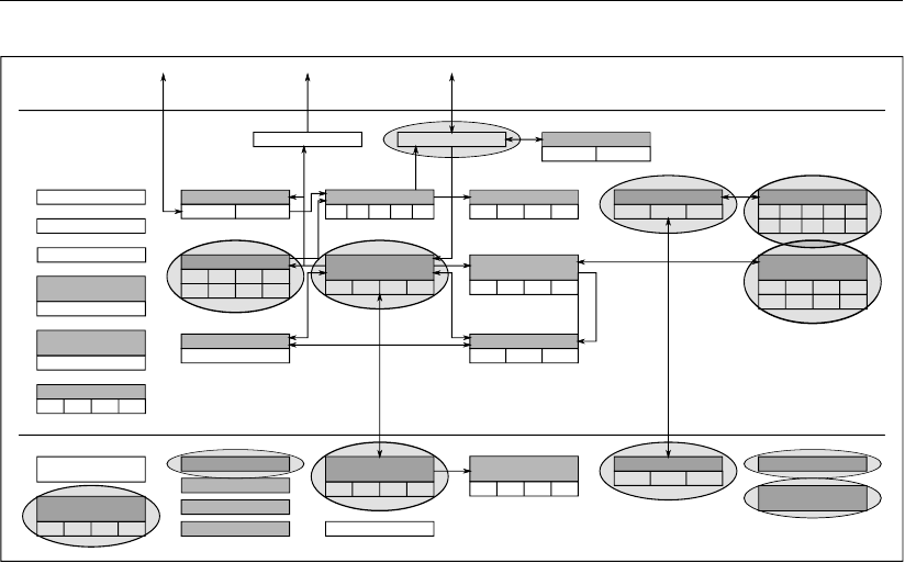
DRAFT
Principles of water quality modelling
TIC Alkalinity
Iron
7 Components
Sulphur
SO4
SUD SUP
NO
NH PO Si
AAP VIVP
APATP
OPAL
Methane
C
P S
NSi
(particulate)
POC PON POP POS
Organic Matter
(dissolved)
DOC DON DOP DOS
Grazers
C N PSi
Dissolved Oxygen
IM2 IM3
IM1
Oxygen Demand
BOD COD
phytobentos
C N PSi
Micro-
As
Cr Hg
Cd Cu
Ni Pb VZn
pollutants
Atr BaP Diu Flu
Organic micro-
HCB HCH PCB OMP
Sediment Oxygen
Demand
EnCoc
EColi FColi TColi
Tracers
Tracers
Continuity
Salinity/Chloride
Temperature
Inorganic Matter
IM2 IM3
IM1
Organic Matter
(particulate)
POC PON POP POS
Heavy Metals
pollutants
Organic micro-
Atmosphere
Water
Sediment
Heavy Metals
Inorganic Matter
Decayable
Conservative
5 Components
5 Components
Bacteria
pH
Nutrients
34 4
Phytoplankton
Organic Matter
Organic Matter
(dissolved)
DOC DON DOP DOS
Nutrients
Oxygen
Sulphur
Iron Methane
Figure 9.10: Overview of substances. Substances that are considered in the S1-S2 ap-
proach for sediment are encircled.
Physical aspects
Physically the sediment is characterised by the particulate fraction: grain size distribution,
sediment strength and porosity. The porosity of freshly settled material can be very high
(>0.9), especially when the material consists of organic matter and clay particles (<63µm).
As more material settles on top, the pore water is gradually squeezed out by the building
overlying pressure and the porosity decreases. Compacted sediment has a typical porosity of
about 0.4.
(Bio)chemical aspects
The major driving force for (bio)chemical processes in the sediment is the mineralization of
organic matter. Organic matter can be produced within the sediment through primary or
secondary production or settled from the water column. The organic matter is worked into
the sediment by bioturbation and burial. Varous electron-acceptors are consumed for the
oxidation of organic matter. Oxygen, nitrate, sulphate, manganese oxides (Mn(IV)), iron oxy-
hydroxides (Fe(III)), sulphate and carbon dioxide are subsequentially consumed by bacteria
as electron-acceptors. The final step when the other electron-acceptors are no longer avail-
able involves fermentation followed by the production of methane from carbon monoxide and
hydrogen. This process is called methanogenesis. The reduced substances that arise from
metal reduction, sulphate reduction and methanogenesis are oxidized with oxygen when dif-
fusing upward to the aerobic top layer. The oxidation and reduction processes result in steep
concentration gradients and chemically distinctive layers in the sediment, each layer having
its dominant electron-acceptor. The aerobic top layer is usually less than a few millimeters
thick. When going deeper in the sediment the aerobic top layer is successively followed by a
denitrifying layer, an iron and sulphate reducing layer and a methanogenic layer. The redox
potential decreases strongly from the sediment-water interface deeper into the sediment. In a
model in view of modelling the composition of large inhomogeneous compartments processes
overlap in the vertical direction. The nutrients nitrogen, phosphorus and silicon interact in dif-
ferent ways to the chemical conditions. The processes affecting the nutrients include nitrifica-
tion, denitrification, adsorption, precipitation and dissolution, see Table 9.11 for an overview.
The stratified development of the composition of the sediment driven by the decompostion
Deltares 273 of 382

DRAFT
D-Water Quality, User Manual
of organic matter is indicated as sediment diagenesis. Diagenesis results in the exchange
of dissolved nutrients, electron-acceptors and reduced substances between sediment and
overlying water. The exchange is established by dispersion (bio-irrigation, flow induced tur-
bulence, diffusion) and often also by advection (seepage). The flux of oxygen from the water
column into the sediment is called the sediment oxygen demand. The nutrient fluxes from the
sediment into the overlying water are indicated as the nutrient return fluxes.
Whereas the adsorption of ammonium is weak and not sensitive for the redox potential this
is totally different for the adsorption of phosphate. Iron oxyhydroxides are the most important
adsorbent for phosphate in the sediment, and usually a large portion of total phosphorus is
adorbed. The iron oxyhydroxides are reduced in the reducing sediment layer implying that they
can no longer adsorb phosphate. The adsorbed phosphate is released and a larger return flux
may occur when the oxic top layer becomes thinner. When the top sediment layer becomes
entirely reducing due to the mineralization of accumulated organic matter and inadequate
transport of oxygen to the sediment, for instance in stratified water, the adsorption capacity
of the sediment collapses and the return flux may increase very strongly. This has a large
impact on water quality if phytoplankton is phophorus limited.
Table 9.11: Major processes for ammonium, nitrate, phosphate and silica as occurring in
sediment layers
Substances Processes Layers
Ammonium
mineralization of organic matter
nitrification
sorption
⇒all layers
⇒aerobic top layer
⇒all layers
Nitrate
nitrification
denitrification ⇒aerobic top layer
⇒denitrifying layer
Phosphate
mineralization of organic matter
sorption
dissolution/precipitation of apatite P
precipitation of vivianite P
dissolution of vivianite P
⇒all layers
⇒strong in oxidizing layer
⇒all layers
⇒strong in reducing layers
⇒aerobic top layer
Silica
dissolution opal ⇒all layers
274 of 382 Deltares

DRAFT
Principles of water quality modelling
Biological aspects
Benthic organisms such as zoobenthos, microphytobenthos and rooted macrophytes may live
at or in the sediment bed. Therefore, these organisms are very much dependent on the
physical and chemical properties of sediments. However, the presence and activity of benthic
organisms can also influence the physical and chemical properties and processes that take
place within the sediment.
Benthic organisms can change the sediment stability and thus have effect on erosion/deposition
processes by their potential effect on both the bed shear stress and the shear strength of the
sediment. The bed shear stress is a combined effect of hydrodynamic conditions near the
sediment and the bottom roughness. Higher plants such as seagrass decrease the current
velocities thereby reducing the local erosion. Other organisms increase the bottom roughness
by creating elevations and depressions at the sediment surface. This greater bottom rough-
ness will increase the shear stress and thus has a negative effect on bottom stability. The
shear strength of the sediment bed is increased by the excretion of polymeric substances by
organisms such as epipellic diatoms, sticking the sediment particles together. The increased
shear strength will stabilise the sediment. Organisms such as Corrophium volutator which
graze on diatoms reduce the effect on sediment stability.
The chemical composition of and processes in the sediment are influenced even more by
benthic organisms. This is the result of their metabolic processes (primary production, primary
consumption and respiration) and their behaviour (sediment capturing, sediment reworking,
tube building, etc.). Suspension feeders remove particles from the overlying water and deposit
them on to the sediment. Deposit feeders ingest organic matter and sediment and return it
to a different location in the sediment. This mixing of sediment by the activity of macrofauna
is termed bioturbation. Zoobenthos transport water and solutes due to motion or ingestion,
which is indicated with bio-irrigation. For instance, tube dwellers pump oxygenated water
through their tubes into the anaerobic sediment. This creates a thin layer of oxidizing sediment
around the tubes. Macrophytes leak oxygen from their roots in the reducing layers. The
transport of substances by organisms may strongly affect chemical processes, composition
and stratification in the sediment.
9.11.2 Modelling framework
D-WAQ has two alternatives to simulate the sediment-water exchange of dissolved sub-
stances:
1 The S1-S2 approach
2 The layered sediment approach
The S1-S2 approach concerns the simplified sediment approach in D-WAQ, which involves
the simulation of so-called inactive substances. Inactive substances are only subjected to
conversion processes and not to mass transport. Only particulate substances can be inactive
in the S1/S2 option in D-WAQ:
Name of D-WAQ
substance
Description Unit
DetCS1/S2 Fast decomposing detrital carbon in layers S1 and S2 gC
DetNS1/S2 Fast decomposing detrital nitrogen in layers S1 and S2 gN
DetPS1/S2 Fast decomposing detrital phosphorus in layers S1 and
S2
gP
DetSiS1/S2 Fast dissolving opal silicon in layers S1 and S2 gSi
OOCS1/S2 Slow decomposing detrital carbon in layers S1 and S2 gC
Deltares 275 of 382

DRAFT
D-Water Quality, User Manual
Name of D-WAQ
substance
Description Unit
OONS1/S2 Slow decomposing detrital nitrogen in layers S1 and S2 gN
OOPS1/S2 Slow decomposing detrital phosphorus in layers S1 and
S2
gP
OOSiS1/S2 Fast dissolving opal silicon in layers S1 and S2 gSi
AAPS1/S2 Adsorbed ortho-phosphate in layers S1 and S2 gP
DiatS1/S2 Diatoms in layers S1 and S2 gC
IM1S1/S2 Inorganic matter fraction 1 in layers S1 and S2 g
IM2S1/S2 Inorganic matter fraction 2 in layers S1 and S2 g
IM3S1/S2 Inorganic matter fraction 3 in layers S1 and S2 g
HMS1/S2 Heavy metal in layers S1 and S2 (cadmium, copper,
lead, mercury, nickel, tin, zinc, chromium, arsenic and
vanadium)
g
OMPS1/S2 Organic micro-pollutant in layers S1 and S2 (OMP, hex-
achlorohexane, hexachlorobenzene, PCB-153, Benzo-
a-pyrene, Fluoranthene, Diuron, Atrazine and Mevin-
fos)
g
Given the generic process formulations, the substances and processes for the layered sedi-
ment option are exactly the same as the substances and the processes for the water column.
Chemical conditions in the sediment such as the concentration of dissolved oxygen determine
how processes turn out in the sediment. See Chapter 9for substances, processes and the
dependency on chemical conditions.
9.11.3 Process equations
In this section we deal with the process formulations for the S1-S2 option, and with mass
transport in the sediment for the layered sediment approach. The generic formulations for
all other processes in the layered sediment approach are discussed in chapter 9. These for-
mulations may turn out differently in the sediment depending on local chemical conditions,
the dissolved oxygen concentration in particular. For the processes and formulations for or-
ganic matter, nutrients and electron-acceptors see section 9.7. For phytoplankton see sec-
tion 9.8. For primary consumers (grazers) see section 9.9. For heavy metals and organic
micro-pollutants see section 9.10. For the inorganic matter fractions see section 9.6. The set-
tling and resuspension of substances and how substances in the water column are allocated
to substances in the sediment and vise versa for the S1-S2 option is also explained in these
sections. Settled phytoplankton biomass dies in the sediment, instantly in the case of the S1-
S2 approach, gradually in the layered sediment approach. Resuspended microphytobenthos
biomass is turned over to the detritus pools in the water column instantly in the case of the
S1-S2 approach.
The mass balance for all substances in the sediment according to the S1-S2 option reads:
∆C
∆t=loads +settling +production −resuspension −losses −burial +digging
Resuspension, settling, burial and digging are described in section 9.6. Loss processes are
mortality of microphytobenthos, mineralization of detritus fractions, dissolution of opal silicate,
desorption of adsorbed phosphate, and degradation of organic micropollutants. Production
only applies to the primary production of microphytobenthos.
276 of 382 Deltares

DRAFT
Principles of water quality modelling
In the S1-S2 approach all loss processes are essentially described by a zero-order term and
a first-order reaction rate:
Rloss =k0loss
H+kloss ×Cx
V
with:
Cx amount of a substance [gC/N/P/Si]
k0loss zero-order loss rate [g m−2d−1]
kloss first-order loss rate [d−1]
Rloss loss rate [gC/N/P/Si m−3d−1]
Hthickness of overlying computational cell [m]
Vvolume of overlying computational cell [m3]
Inorganic nutrients formed by mineralization or desorption are instantaneously released to
the overlying water, as the S1-S2 approach does not include pore water. Particulate nutrients
can be retained in the sediment through burial. The mineralization of organic matter in the
sediment also leads to a sediment oxygen demand. Considering the intentional simplicity
of the S1-S2 approach, this module may be applied in cases in which the sediment-water
exchange is not a dominant or very dynamic feature.
The mass transport in the sediment for the layered sediment approach is taken care of by an
additional process of the Processes Library, described in the additional D-WAQ user manual
‘Sediment Water Interaction’. This process works on the cells of the additional computa-
tional grid for the sediment. It considers the advection and dispersion of both particulate and
dissolved substances. The advection of particulate substances results from settling (as in-
put) and resuspension (as output). The process converts these fluxes into burial and digging
fluxes across the interfaces of the sediment layers and the lower boundary, depending on fixed
porosities. The advection of solutes arises from seepage. Dispersion is described as based
on Fick’s Law. The dispersion coefficient for particulate substances refers to bioturbation, the
dispersion coefficient for solutes to bio-irrigation, flow induced dispersion and diffusion.
9.12 Pre-defined sets, SOBEK only
9.12.1 Simple oxygen model (Streeter Phelps)
9.12.1.1 General
The Simple Oxygen Model is a so-called "pre-defined" set of selected state variables, active
processes, editable input parameters and output parameters. It has been constructed with
the Processes Library Configuration Tool. Experienced users may use the same tool to edit
the predefined set.
9.12.1.2 State variables
The simple oxygen model distinguishes the following 3 state variables:
dissolved oxygen (OXY);
carbonaceous oxygen demand (CBOD5), represented by the 5 day value, expressed in
gO2/m3;
ammonium (NH4), expressed in gN/m3, representing the nitrogeneous oxygen demand.
Deltares 277 of 382

DRAFT
D-Water Quality, User Manual
9.12.1.3 Processes
The model equations for the state variables mentioned above include a number of processes
from the Processes Library, which are described briefly below. For a formal description we
refer to WAQ Technical Reference manual (D-WAQ TRM,2013) for the individual processes
of the Processes Library.
Carbonaceous BOD
The carbonaceous BOD is subject to a linear and temperature dependent decay process:
F lux =−k×CBOD5×θT−20 (9.33)
kfirst order reaction rate (at 20 ◦C) [1/d]
θtemperature dependency constant [−]
Twater temperature [◦C]
CBOD5concentration of BOD5[gO2/m3]
The first order reaction rate (at 20 ◦C) is an input item. The temperature θhas a fixed value
of 1.04. The oxygen consumption rate is computed automatically, taking into account the
transformation of BOD5into ultimate bod.
The mineralisation is supposed to proceed at best under aerobic conditions. Therefore, the
mineralisation process flux depends on the available amount of oxygen. If the oxygen concen-
tration is over 5 mg/l, the process proceeds without limitation. If the oxygen concentration is
below 1 mg/l, the process proceeds at 30 % of its unlimited rate. If the oxygen concentration is
between 1 and 5 mg/l, the limitation factor varies linearly between 0.3 and 1.0. For details we
refer to the BODCOD chapter in the WAQ Technical Reference manual (D-WAQ TRM,2013).
Ammonium
The nitrification process removes ammonium. It is formulated linearly and temperature de-
pendent:
F lux =−k×NH4×θT−20 (9.34)
kfirst order reaction rate (at 20 ◦C) [1/d]
θtemperature dependency constant [−]
Twater temperature [◦C]
NH4concentration of NH4(gN/m3)
The first order reaction rate (at 20 ◦C) is an input item. The temperature θhas a fixed value of
1.07. The mineralisation stops under a certain critical temperature, which is set to 3 ◦C. The
oxygen consumption rate is computed as 4.571 times the nitrogen transformation rate, taking
into account the proper chemical reaction formula and the molar weight of the participating
components.
The nitrification process is supposed to proceed under aerobic conditions only. Therefore, the
process flux depends on the available amount of oxygen. If the oxygen concentration is over 5
mg/l, the process proceeds without limitation. If the oxygen concentration is below 1 mg/l, the
process stops completely. If the oxygen concentration is between 1 and 5 mg/l, the limitation
factor varies linearly between 0 and 1. For details we refer to the NITRIF chapter in the WAQ
Technical Reference manual (D-WAQ TRM,2013).
278 of 382 Deltares

DRAFT
Principles of water quality modelling
Dissolved oxygen
Related to dissolved oxygen, some additional processes are included. The reaeration is for-
mulated as a first order surface related process working on the oxygen deficit:
F lux =k
H(Oxysat −Oxy)×θT−20 (9.35)
kfirst order reaeration rate (at 20 ◦C) [m/d]
Hwater depth [m]
θtemperature dependency constant [−]
Twater temperature [◦C]
Oxy oxygen concentration [g/m3]
Oxysat saturation concentration [g/m3]
The first order reaeration rate in m/d is input to the model. The process is temperature de-
pendent with the θvalue equal to 1.016.
Additionally, there is a sediment oxygen demand process which allows the user to specify
an autonomous oxygen consumption in g/(m2d). This process can proceed under aerobic
conditions in the water column only. If the oxygen concentration is over 2 mg/l, the process
proceeds without limitation. If the oxygen concentration is equal to or below 0 mg/l, the pro-
cess stops completely. If the oxygen concentration is between 0 and 2 mg/l, the limitation
factor varies linearly between 0 and 1. For details we refer to the SEDOX chapter in the WAQ
Technical Reference manual D-WAQ TRM (2013).
Note that the output dissolved oxygen concentration is made non-negative, while the mod-
elled dissolved oxygen concentration can reach negative values if the consumption of oxygen
is intensive enough. Such a negative concentration can be considered as more or less repre-
senting reduced substances.
9.12.1.4 Overview of all processes working on the state variables
State variable Processes acting on it
CBOD5 Mineralisation BOD and COD
NH4 Nitrification of ammonium
OXY Mineralisation BOD and COD
Nitrification of ammonium
Reaeration of oxygen
Sediment oxygen demand (additional)
Deltares 279 of 382

DRAFT
D-Water Quality, User Manual
9.12.1.5 Overview of input items
The input parameters below can be specified through SOBEK’s "Processes Library Coefficient
Editor". A <∗.plc>file with the recommended values is available, so that these values can
be loaded (or reloaded) easily.
Parameter id Description Recommended
value
Unit
RcBOD decay reaction rate BOD (first pool) at 20
◦C
0.7 1/d
RcNit first-order nitrification rate constant 0.1 1/d
KLRear reaeration transfer coefficient 1 m/d
fSOD zeroth-order oxygen demand flux 6 gO2/m2/d
Additionally, the following items can be specified through the Meteorological Task.
Parameter id Description Recommended
value
Unit
Temp Water temperature n.a. ◦C
9.12.1.6 Output items
Apart from the concentrations of the state variables, the following parameters are available as
extra output:
Parameter id Description Unit
Depth depth of segment m
SaturOXY saturation concentration g/m3
SatPercOXY actual saturation percentage O2 %
DO non-negative dissolved oxygen concentration (defined as
max(OXY,0))
g/m3
9.12.2 Simple eutrophication model
9.12.2.1 General
The Simple Eutrophication Model is a so-called "pre-defined" set of selected state variables,
active processes, editable input parameters and output parameters. It has been constructed
with the Processes Library Configuration Tool. Experienced users may use the same tool to
edit the predefined set.
280 of 382 Deltares

DRAFT
Principles of water quality modelling
9.12.2.2 State variables
The simple eutrophication model distinguishes the following 10 state variables:
dissolved oxygen (OXY);
inorganic nutrients: NH4, NO3, PO4 (dissolved), AAP (adsorbed phosphates);
inorganic suspended matter: IM1;
algae ("Green");
detritus: DetC, DetN, DetP.
9.12.2.3 Processes
The model equations for the state variables mentioned above include a number of processes
from the Processes Library, which are described briefly below. For a formal description we
refer to WAQ Technical Reference manual (D-WAQ TRM,2013) for the individual processes
of the Processes Library.
Suspended matter
The state variables representing suspended matter are subject to sedimentation. It concerns
in particular IM1, AAP, DetC, DetN and DetP. The sedimentation process is formulated in
terms of a settling velocity (input) and a sedimentation probability which depends on the local
and momentaneous shear stress and a critical shear stress (input):
F lux =−Vset 1−τ
τcr C
H(9.36)
Vset settling velocity [m/d]
τshear stress [N]
τcr critical shear stress [N]
Cconcentration [g/m3]
Hwater depth [m]
See the SEDCAR chapter in the WAQ Technical Reference manual (D-WAQ TRM,2013) for
more details.
Resuspension is included only for inorganic suspended solids (IM1). It is formulated as a zero
order flux (input) in g/(m2d).
The visual light extinction characteristics of the water are relevant for the growth of algae. The
extinction depends on a background value (input) increased with a contribution of inorganic
suspended matter, living algae and dead organic algae material (detritus):
E=Ebg +X
i
eiCii∈ {algae, detritus, inorganicsusp, solids}(9.37)
Elight extinction [1/m]
Ebg background light extinction [1/m]
especific extinction [m2/g]
Cconcentration [g/m3]
The specific extinction of each contribution to the extinction can be specified as input.
Deltares 281 of 382

DRAFT
D-Water Quality, User Manual
Algae-related processes
The simple eutrophication model includes a relatively simple model for the growth and mor-
tality of algae. The growth process is formulated as a linear process, and can be expressed
as follows:
∂C
∂t =MaxGrowthRate ×NutrientLimitation ×LightLimitation ×DaylengthFactor×
TemperatureFactor ×ActualConcentration (9.38)
The Nutrient, Light and day length factors have a value between 0 and 1. The day length factor
is defined as the quotient of the actual daylight period divided by an optimal value (input). The
nutrient limitation factor is formulated as the product of two Monod type functions, one for
N and one for P. The half saturation values are input items. The light limitation function is
computed based on a linear extinction model and a "saturation value", which expresses the
amount of light needed for optimal growth (input). The growth is not reduced when the light
intensity exceeds the optimal value. The temperature factor is based on a θtype exponential
function:
temperature factor =θT−20 (9.39)
where
θtemperature dependency constant [−]
Twater temperature [◦C]
The value of θis input. For details we refer to the DLALG, NLALG, RADALG and TFALG
chapters of the D-WAQ TRM (2013).
The growth is corrected for respiration, which is composed of a linear or "maintenance" part
and a growth dependent part. The mortality of algae is again formulated as a linear process.
Both respiration and mortality are temperature dependent. The value of J is input. For details
we refer to the PRIPRO chapter of the WAQ Technical Reference manaul (D-WAQ TRM,
2013).
The growth of algae causes an equivalent uptake of nutrients. To this end, the N-C-ratio and
the P-C-ratio in living algae have to be specified as input. Similarly, the mortality of algae
causes an equivalent release of nutrients. The release can be in organic form (detritus) or
inorganic form, controlled by input parameters.
Mineralisation processes
The detritus is subject to a linear and temperature dependent mineralisation process:
F lux =−k×C×φT−20 (9.40)
where
kfirst order reaction rate (at 20 ◦C) [1/d]
φtemperature dependency constant [−]
Twater temperature [◦C]
Cconcentration [g/m3]
The first order reaction rate (at 20 ◦C) as well as the temperature theta are input items. The
mineralisation stops under a certain critical temperature, which is again input to the model.
282 of 382 Deltares

DRAFT
Principles of water quality modelling
Processes related to inorganic nutrients
Inorganic phosphorus occurs in two forms: dissolved (PO4) and sorbed to inorganic sus-
pended matter. The division over both forms is controlled by the adsorption process. A
formulation according to Langmuir was selected. For details we refer to the ADSPO4 chapter
in the WAQ Technical Reference manaul (D-WAQ TRM,2013). The equilibrium constant is
input to the model.
The nitrification process transforms ammonium into nitrates. It is formulated linearly and tem-
perature dependent. The first order reaction rate (at 20 ◦C) as well as the temperature theta
are input items. The mineralisation stops under a certain critical temperature, which is again
input to the model. On top of this, also the oxygen concentration affects the nitrification rate.
For details we refer to the NITRIF chapter in the WAQ Technical Reference manaul (D-WAQ
TRM,2013).
The denitrification process effectively removes nitrates from the water column. It is formulated
as a volumetric process, supposed to take place in the water column, when the oxygen con-
centration is low. It is formulated linearly and temperature dependent. The first order reaction
rate (at 20 ◦C) as well as the temperature theta are input items. The process stops under a
certain critical temperature, which is again input to the model. On top of this, also the oxygen
concentration affects the denitrification rate. For details we refer to the DENWAT chapter in
the WAQ Technical Reference manaul (D-WAQ TRM,2013).
Oxygen
Related to dissolved oxygen, some additional processes are included. The reaeration is for-
mulated as a first order surface related process working on the oxygen deficit:
F lux =k
H(Oxysat −Oxy)×φT−20 (9.41)
where
kfirst order reaeration rate (at 20 ◦C) [m/d]
Hwater depth [m]
φtemperature dependency constant [−]
Twater temperature [◦C]
Oxy oxygen concentration [g/m3]
Oxysat saturation concentration [g/m3]
The first order reaeration rate in m/d is input to the model. The process is temperature de-
pendent with the theta being an input parameter as well.
Additionally, there is a sediment oxygen demand process which allows the user to specify an
autonomous oxygen consumption in g/(m2d). Note that the output dissolved oxygen concen-
tration is made non-negative, while the modelled dissolved oxygen concentration can reach
negative values if the consumption of oxygen is intensive enough. Such a negative concen-
tration can be considered as more or less representing reduced substances.
Remaining processes
Additionally, the model includes a process to specify "diffuse loads" formulated as g/m2/d, for
IM1, NH4, PO4, as well as auxiliary processes to compute the average water depth and the
bottom shear stress from the geometric and hydraulic data passed to the water quality module
by the channel flow module.
Deltares 283 of 382

DRAFT
D-Water Quality, User Manual
9.12.2.4 Overview of all processes working on the state variables
State variable Processes acting on it
OXY Denitrification in water column
Nitrification of ammonium
Reaeration of oxygen
Mineralisation detritus carbon
Sediment oxygen demand (additional)
Net primary production and mortality green algae
NH4 Nitrification of ammonium
Mineralisation detritus nitrogen
Uptake of nutrients by growth of algae
Release (nutrients/detritus) by mortality algae
Diffusive waste NH4
NO3 Denitrification in water column
Nitrification of ammonium
Uptake of nutrients by growth of algae
PO4 Ad(De)Sorption ortho phosphorus to inorg. Matter
Mineralisation detritus phosphorus
Uptake of nutrients by growth of algae
Release (nutrients/detritus) by mortality algae
Diffusive waste PO4
AAP Ad(De)Sorption ortho phosphorus to inorg. Matter
Sedimentation AAP (adsorbed PO4)
IM1 Sedimentation
Resuspension
Diffusive waste IM1
Green Net primary production and mortality green algae
DetC, DetN,
DetP
Mineralisation detritus
Release (nutrients/detritus) by mortality algae
Sedimentation detritus carbon
9.12.2.5 Overview of input items
The input parameters below can be specified through SOBEK’s "Processes Library Coefficient
Editor". A <∗.plc>file with the recommended values is available, so that these values can
be loaded (or reloaded) easily.
Parameter id Description Recommended
value
Unit
SWAdsP switch formulation
<0=Kd|1=Langmuir|2=GEM>
1 -
continued on next page
284 of 382 Deltares

DRAFT
Principles of water quality modelling
continued from previous page
Parameter id Description Recommended
value
Unit
KdPO4AAP partition coefficient PO4-AAP 0.01 m3/gDM
RcDenWat first-order denit. rate constant water 0.09 1/d
TcDenWat temp. coefficient for denitrification 1.045 -
OOXDEN optimum oxygen conc. for denitrification 1 g/m3
COXDEN critical oxygen conc. for denitrification 3 g/m3
RcNit first-order nitrification rate constant 0.09 1/d
TcNit temperature coefficient for nitrification 1.08 -
OOXNIT optimum oxygen conc. for nitrification 5 g/m3
COXNIT critical oxygen conc. for nitrification 1 g/m3
CTNit critical temperature for nitrification 3 ◦C
RcDetN first-order mineralisation rate constant 0.18 1/d
TcDetN temperature coefficient for mineralisa-
tion
1.08 -
CTMin critical temperature for mineralisation 3 ◦C
RcDetP first-order mineralisation rate constant 0.18 1/d
TcDetP temperature coefficient for mineralisa-
tion
1.08 -
NCRatGreen Nitrogen-Carbon ratio in greens 0.1 gN/gC
PCRatGreen Phosphorus-Carbon ratio in greens 0.01 gP/gC
FrAutGreen frac. mort. greens dissolved as nutri-
ents
0 -
FrDetGreen frac. mort. greens to detritus 1 -
RcDetC first-order mineralisation rate constant 0.18 1/d
TcDetC temperature coefficient for mineralisa-
tion
1.08 -
PPMaxGreen maximum primary production green al-
gae
3 1/d
continued on next page
Deltares 285 of 382

DRAFT
D-Water Quality, User Manual
continued from previous page
Parameter id Description Recommended
value
Unit
MRespGreen maintenance respiration green algae 0.03 1/d
GRespGreen growth respiration factor green algae 0.095 -
Mort0Green mortality rc of green algae st. temp 0.2 1/d
VSedDetC sedimentation velocity DetC 0.5 m/d
TauCSDetC critical shear stress sedimentation DetC 0.1 N/m2
VSedIM1 sedimentation velocity IM1 1 m/d
TaucSIM1 critical shear stress sedimentation IM1 0.1 N/m2
fResS1DM resuspension flux dry matter from S1 0 gDM/(m2d)
FrIM1S1 fraction IM1 in sediment S1 1 gDM/gDM
fDfwastIM1 zeroth-order flux IM1 10 gIM1/(m2d)
fDfwastNH4 zeroth-order flux NH4 0.05 gNH4/(m2d)
SWRear switch for oxygen reaeration formulation
<1–11>
1 -
KLRear reaeration transfer coefficient 1 m/d
TCRear reaeration temperature coefficient 1.024 -
Fsod zeroth-order oxygen demand flux 1 gO2/(m2d)
fDfwastPO4 zeroth-order flux PO4 0.005 gPO4/(m2d)
ExtVlGreen Vl specific extinction Greens 0.75 m2/gC
ExtVlDetC Vl specific extinction DetC 0.47 m2/gC
ExtVlIM1 Vl specific extinction coefficent IM1 0.01 m2/gDM
ExtVlBak background extinction visible light 2 1/m
PrfNH4gree ammonium preference over nitrate
green algae
1 -
KMDINgreen half-saturation value N green-algae 0.025 gN/m3
KMPgreen half-saturation value P green-algae 0.005 gP/m3
continued on next page
286 of 382 Deltares

DRAFT
Principles of water quality modelling
continued from previous page
Parameter id Description Recommended
value
Unit
Cl Chloride concentration 200 g/m3
TcGroGreen temp. coeff. for growth processes green
algae
1.06 -
TcDecGreen temp. coeff. for resp./mort. green algae 1.045 -
DayL day length <0-1>0.58 d
OptDLGreen day length for growth saturation green-
algae
0.58 d
RadSatGree total radiation growth saturation greens 80 W/m2
Additionally, the following items can be specified through the Meteorological Task.
Parameter id Description Recommended
value
Unit
Temp Water temperature n.a. ◦C
Rad Solar radiation at the water surface n.a. W/m2
Deltares 287 of 382

DRAFT
D-Water Quality, User Manual
288 of 382 Deltares

DRAFT
10 Numerical aspects
10.1 Dispersion and turbulent diffusion
Diffusion normally refers to molecular diffusion of gases. In transport equation, the dispersion
coefficient stands for all transport that could not be resolved with the finite grid of the Delft3D-
FLOW module (Delft3D-FLOW UM,2013). This implies that dispersion is much larger than
molecular diffusion. First of all, small scale chaotic movement of water parcels (due to density
fluctuations in the water column) will lead to turbulent diffusion. Still this term can be very
small. More dispersion enters the modelling effort by small scale eddies that were not resolved
on the computational grid. These are the terms that we have to deal with in 3D modelling.
Still, in 1D and 2D models diffusion can be much larger and needs serious attention since it
can explain much of the mixing processes in the water column. In water quality modelling this
term is often referred to as ‘dispersion’ as it mixes discharged material. To explain turbulent
diffusion and the dispersion effect, we will demonstrate it for a small estuary that is treated
as a 1-dimensional stretch of elements (the estuary in Figure 10.1). Hereto, we will first
derive the 3-dimensional transport equations and then show the effect of limiting the area to
1-dimension.
For the 1-dimensional model we start from the advection-diffusion equation, neglect the reac-
tion terms and source terms, and integrate over y- and z-direction.
Ty=Zyr
yl
∂
∂y D∂C
∂y −vyCdy =D∂C
∂y −vyC
y=yr
y=yl
= 0 (10.1)
with:
yr=yat right embankment
yl=yat left embankment
Ty=transport at y
Since no transport along the closed boundaries (the embankments in Figure 10.1) occurs the
‘stock terms’ at the right hand side of Equation (10.1) vanish.
For the same reason the ∂/∂z term vanishes after integration over zfrom bottom to surface.
After integrating the 3D advection-diffusion equation over yand z, an equation results with
transport for the x-direction only. It is:
∂
∂t(AC) = ∂
∂x D∂AC
∂x −∂
∂x ZyZz
(vxC)dydz +Af(C, . . . , t) + AS (10.2)
with:
C=average concentration over the cross-section 1
A=cross-sectional surface
D=molecular diffusion
f=cross-sectional averaged water quality processes
S=source terms from discharges
In Equation (10.2) there is one term which will be discussed in more detail here.
Deltares 289 of 382
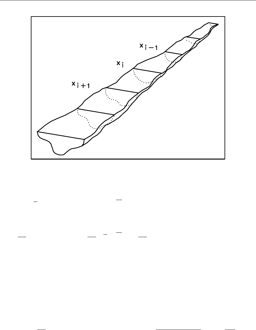
DRAFT
D-Water Quality, User Manual
Figure 10.1: Estuary represented as a 1-dimensional model
With:
vx=vx+ ∆vxand Cx=Cx+ ∆Cx,(10.3)
the advective term of Equation (10.2) is:
∂
∂x ZyZz
(vxC)dydz =∂
∂x vxACx+∂
∂x ZyZz
(∆vx∆Cx)dydz (10.4)
If ∆vxand ∆cx(which are functions of y and z) are not correlated at all, the last term of
Equation (10.4) vanishes. However, there are almost always small turbulences in the water.
They appear as a positive value of ∆vxat some location and a negative value at neighbouring
locations. If the upstream concentration is higher than the downstream concentration, this
small turbulence causes an additional positive transport (Figure 10.2).
A well known approximation is, that this transport is proportional to the concentration differ-
ence over the small turbulence distance:
Tadd =−∂
∂x ZyZz
(∆vx∆Cx)dydz ≈ −∆vx∆xt
(Cx+∆xt−Cx)
∆xt≈ −K∂C
∂x (10.5)
with:
∆xt=length of the turbulence
K=constant of proportionality (= ∆vx∆xt)
This formulation is equivalent with the diffusion formulation Equation (10.5) with diffusion of
magnitude K. This additional term, which is caused by integrating over the distance of turbu-
lences in space, is called turbulent diffusion. It is generally orders of magnitude higher than
the molecular diffusion.
Dispersion
The above given derivation of a turbulent diffusion term K, applies somewhat different if
290 of 382 Deltares
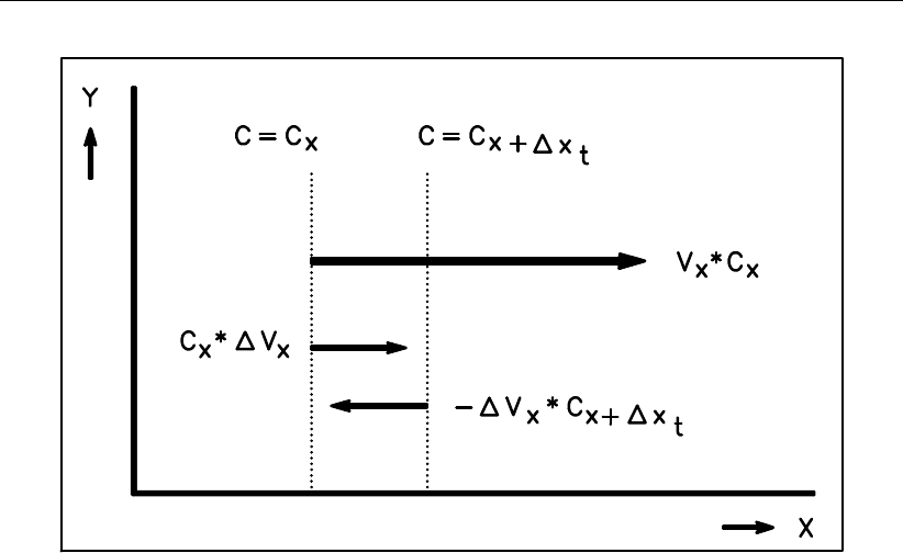
DRAFT
Numerical aspects
Figure 10.2: Effect of turbulent fluctuations ∆vxon the net transport
integration is performed over the whole cross-sectional area of a small estuary instead of only
over the scale of turbulences.
Figure 10.3 shows a one-dimensional estuary with an amount of substance initially distributed
uniformly over the cross-section. After a certain amount of time, the substance is not dis-
tributed uniformly over the cross-section anymore. Because we integrated in our example
over a cross-section however, the resulting cross-sectional average concentration, shows a
pattern along the axis of flow, that is very similar to the pattern obtained by a diffusion process.
The mixing along a cross-section of the system often takes a much longer time than the time
span to generate the picture of Figure 10.3. But the differences over the river width are not
distinguished in the one-dimensional model.
The basis of this phenomenon is again the fact that ∆vxand ∆Cxmay be correlated and
the integral of their product in Equation (10.5) differs from zero. The fact that diffusion type
curves result, like in the river example above, is an empirical fact. Only for some well-defined
very special situations, a precise computation of the effect can be given. Care must be taken,
however.
In e.g. the river situation above, large off-stream parts of the river, called dead zones, cause an
asymmetrical shape of the concentration curve along the x-axis, that cannot fully be explained
with the one-dimensional advection diffusion equation.
The additional diffusion term, that must account as much as possible for these effects, is often
called dispersion. Although experienced modellers have an idea of the magnitude of this term,
it is often subject to calibration in models. This term is again orders of magnitude larger than
the turbulent diffusion mentioned before.
Dispersion is also much higher than turbulent diffusion used in 3D models. The 3-dimensional
models can explain more of the transport in the water column from the hydrodynamics it self
and need much less adjustments for unresolved transport. This is not so for the vertical
direction since transport by vertical velocities (along the sigma-co-ordinates) can be very small
there compared to vertical diffusive transport. Thus, for 3D simulations much attention must
still be put into accurate modelling of vertical transport. Using results from accurate turbulence
Deltares 291 of 382

DRAFT
D-Water Quality, User Manual
Figure 10.3: “Dispersion” by inhomogeneity of flow in a cross-sectionally averaged one-
dimensional model
models (incorporated in Delft3D-FLOW) is therefore strongly recommended.
The dispersion term of a 2-dimensional horizontal application accounts for depth averaging,
but also for horizontal integration over the size of each computational grid cell. If the horizontal
grid cells are larger, this horizontal component will become larger. If the horizontal grid cells
become smaller, more of the heterogeneity of flow and concentration is explicitly incorporated
in the model and consequently the dispersion term becomes smaller. If the horizontal grid
cells become very large, then the grid itself mixes so intensively that the dispersion coefficient
to be added can be taken smaller, or even has to be set at zero because (initial) mixing is
already too large.
Up to now it has been assumed that exact integration over time would take place. Also in
time however discrete steps will be taken and the same type of reasoning applies to fast
fluctuations lumped in cross terms under the integral. A special situation may exist for tidal
areas if a time step of a complete tidal cycle is set and only residual currents are taken into
account. In Table 10.1 some common values for molecular diffusion, turbulent diffusion and
depth integrated (horizontal) dispersion terms are given. Vertical dispersion is usually orders
of magnitude smaller than horizontal dispersion. First of all, this follows from the small length
scales in vertical direction. But, small vertical dispersion is found in particular for stratified
systems where turbulence is dissipated at a pycnocline by buoyancy forces. This leads to
vertical dispersion coefficients of 1.0×10⁻⁵m2/s. Vertical dispersion is accurately calculated
by Delft3D-FLOW’s turbulence model.
292 of 382 Deltares
DRAFT
Numerical aspects
Table 10.1: Common ranges of horizontal dispersion terms in aggregated models with a
finite grid
mixing phenomena D [m2/s]
molecular diffusion 1×10⁻⁹
vertical diffusion (stratified systems) 1×10⁻⁴–1×10⁻⁶
vertical diffusion (non-stratified systems) 1×10⁻¹–1×10⁻³
turbulent diffusion 0.1–1.0
depth integration estuaries and seas 10 –1000
tidal and depth integration estuaries and seas 100 –1000
one dimensional rivers 100 –1000
10.2 Introduction to algorithmic implementation
The multi-dimensional water quality program D-WAQ solves the advection-diffusion-reaction
equation. Solution of the advection-diffusion-reaction equation with computers requires the
use of discrete segments in space with finite mesh sizes ∆x,∆yand ∆zand with a finite
the time-step ∆t. Various options for discretising the partial differential equations in terms
of ∆x,∆y,∆zand ∆tare possible. These options are called ‘numerical discretisation
schemes’. For example, for the space discretisation central discretisations or (first or higher
order) upwind discretisations may be applied. For the time integration you may choose be-
tween explicit,semi-implicit or implicit methods. Having the numerical discretisation different
strategies can be followed to solve the discretised systems of equations. These strategies are
known as ‘solution methods’, and can be divided in iterative solvers or direct solver. This chap-
ter describes the integration schemes in D-WAQ for the advection-diffusion-reaction equation.
A lot of different integration schemes are available in D-WAQ. The numerical discretisations
and applied iterative solution methods will be described.
Important features of numerical schemes are accuracy (determined by the order of the scheme),
robustness (stability and positivity) and efficiency. The choice of the spatial discretisation of
the advective terms has great influence on the accuracy, monotonicity and efficiency of the
computational method. Central differences are second order accurate, but may give rise to
non-physical spurious oscillations, so-called "wiggles" in the solution. These wiggles arise in
the vicinity of steep gradients of the quantity to be resolved. On the other hand, first order
upwinding is unconditionally wiggle-free or monotone, thus promoting the stability of the solu-
tion process, but introduces a truncation error, which has the form of a second-order artificial
viscosity term. In advection-dominated flows, this artificial viscosity dominates the physical
viscosity and the computed solution is much more smooth than the correct one. Higher order
upwinding is not free from numerical oscillations but introduces higher-order artificial viscosity.
This higher order viscosity suppresses the wiggles without smoothing the solution too much.
For explicit methods special considerations for the size of the time step must be taken into
account (stability criteria) in order to get results at all. With respect to 3-dimensional models,
special considerations for stability in vertical direction are required. Some discretisations guar-
antee positive results. Some schemes may lead to spurious oscillations in the concentrations
(although such results may be accurate), and this can make you feel uneasy. Monotonous
Deltares 293 of 382

DRAFT
D-Water Quality, User Manual
or TVD (Total Variation Diminishing) results are usually required. Therefore, positivity and
monotonicity are important items for numerical schemes in water quality modelling. Items of
accuracy, efficiency, and robustness of the various schemes in D-WAQ will be addressed in
this chapter.
10.3 Conceptual description
10.3.1 Partial differential equations
The advection-diffusion-reaction equation in D-WAQ reads:
∂C
∂t =−~u •~
∇C+~
∇•~
~
D•~
∇C+S+fR(c, t)(10.6)
where:
~u = (ux, uy, uz) = flow velocity
~
∇C=∂C
∂x ,∂C
∂y ,∂C
∂z =concentration gradient
~
~
D= Dxx Dyx Dzx
Dxy Dyy Dzy
Dxz Dzy Dzz !=diffusion tensor
~a •~
b=vector dot-product from vector ~a and ~
b
~
~
A•~
b=matrix-vector product from tensor ~
~
Aand vector ~
b
S=sources and sinks
fR(c, t) = biological, bacteriological, ecological, chemical or other reactions
An example of a bacteriological reaction is the following first order decay reaction:
fr(c, t) = −kc (10.7)
For incompressible flow the conservation law of mass, also known as volume balance, is given
by:
~
∇u= 0 (10.8)
The volume balance is computed by Delft3D-FLOW, which is Deltares program for the sim-
ulation of non-steady flow and transport phenomena resulting from tidal and meteorological
forcing. We remark that in its discretised form care must be taken that the equation is exactly
solved. Flow fields should satisfy the volume balance.
10.3.2 Differential equations for computational cells
The finite volume method solves the transport (and reactions) of water and other substances
with computational cells. Exact equation (without any discretisation) can be obtained for flux
transport between these cells. These equations are derived by integrating Equation (10.6)
over the computational cells, and subsequently applying Gauss’ divergence theorem:
Gauss’ theorem:
ZV
~
∇•~
W dV =IA
~
W•~n dA (10.9)
294 of 382 Deltares

DRAFT
Numerical aspects
with ~
Wan arbitrary vector. The resulting equations are the following integro-differential equa-
tions:
ADVECTION-DIFFUSION IN FLUX-FORM:
dM
dt +IA
(~uC)•~n dA =IA~
~
D•~
∇C•~n dA (10.10)
CONTINUITY EQUATION:
dV
dt +IA
~u •~n dA = 0 (10.11)
with
M=mass of the substance in the cell
V=volume
A=face of the volume
dA =infinitesimal face element
~n =unit vector normal to an infinitesimal face element dA
~u =flow velocity
These integro-differential equations are still exact, but contain less detail than the partial dif-
ferential equations. Concentrations inside the cells are no longer used (only concentrations
at the cell face, and concentrations gradients need to be known). By volume averaging also
some geometrical information is lost (only the shape of the cell face and its links to its neigh-
bours matters).
The average concentration in a computational cell is given by:
C=M
V(10.12)
with:
C=average concentration in a cell
M=mass in a cell
V=volume of a cell
Thus, it is assumed that the average concentration value in a segment is representative of the
concentration in the whole volume.
The face integrals represent mass fluxes between the segments. Hydrodynamic packages
only compute the flow of water through a cell face, they do not give a detailed description
of velocities for small face elements. Therefore, we introduce the flow rate in the transport
equation:
IA
(~uC)•~n dA =X
j=1,n ZAi→j
(~uC)•~n dA ≈X
j=1,n
(Q·e
C)i→j(10.13)
Deltares 295 of 382

DRAFT
D-Water Quality, User Manual
with:
Qi→j=ZAi→j
(~u •~n)dA =flow rate
e
C=RAi→jC dA
Ai→j
=cell face averaged concentration
with nthe number of neighbouring cells. The pointer index represents the exchanges between
volumes iand j. A similar flux equation for diffusion fluxes can be given. The resulting volume
averaged equation reads:
d(V C)i
dt +X
j=1,n Qe
Ci→j=X
j=1,n D∂e
C
∂x !i→j
Ai→j(10.14)
Flows and volumes in this equation follow from Delft3D-FLOW. Also exchange faces Acan
be derived from Delft3D-FLOW. To solve the equation for Cand e
Cit is useful to express e
Cin
C. This is what is done in the various numerical schemes. The resulting continuity equation
that follows from Gauss theorem is:
dVi
dt =X
j=1,n
Qi→j(10.15)
This equation can also be derived by substituting a constant number (constant water density)
for concentrations in Equation (10.13).
10.4 Numerical discretisation
10.4.1 Introduction
Important features of numerical schemes are accuracy (determined by the order of the scheme),
robustness (stability and positivity) and efficiency. All numerical schemes can be derived from
the basic equation:
d(V C)i
dt =−X
j=1,n Qe
Ci→j+X
j=1,n D∂e
C
∂x !i→j
Ai→j+fR(Ci, t) + Si(10.16)
with:
C=average concentration in a cell;
e
C=face averaged concentration;
V=volume of a cell;
Q=flow through the face of a cell;
A=face area of a cell
D=diffusion coefficient at the face of a cell;
∂e
C
∂x =concentration gradient at the face of a cell;
fR(Ci, t) = mass derivatives for reactions, as a function of concentrations and time;
S=source or sink terms
n=number of neighbouring cells
296 of 382 Deltares

DRAFT
Numerical aspects
10.4.2 Time discretisation and stability criteria
Time-discretisation is explicit, implicit or semi-implicit. Consider the equation in form:
∂c
∂t =Lc (10.17)
with:
L=differential operator
The general recipe for time-discretisation for D-WAQ is:
ct+∆t−ct
∆t+H.O.T. = (1 −θ)(Lc)t+θ(Lc)t+∆t(10.18)
with the time-splitting factor θ:
1θ= 0.0explicit scheme (Euler’s explicit rule)
2θ= 1.0fully implicit scheme (Euler’s implicit rule)
3θ= 0.5semi-implicit scheme (Trapezoidal rule)
Here H.O.T. stands for Higher-Order-Terms. Some schemes in D-WAQ expand the time-
derivative at the right hand side to second order. Third order terms are not (yet) included in
D-WAQ schemes. The importance of the θ-factor is that schemes with θ≥0.5are uncon-
ditionally stable (robustness). For schemes with θ < 0.5numerical stability is not always
guaranteed. Here, stability criteria should be satisfied. If these criteria are not satisfied, small
round off errors could amplify quickly and completely erroneous results occur (including over-
flow). Another robustness factor is positivity. Without any special measures (e.g. filtering) only
schemes with θ= 0.0or θ= 1.0are positive definite (accuracy and robustness). Schemes
with θ= 0.5(exactly) are unconditionally stable but suffer from serious oscillations and nega-
tive results. Therefore, such schemes are not very popular in water quality modelling, although
they may be computationally efficient (ADI) and accurate.
Numerical stability conditions
For all explicit schemes (θ= 0.0) in D-WAQ the ‘Courant-Friedrichs-Lewy’ (CFL) condition
for stability is:
∆t < Vi
Pj=1,n Qi→j
(10.19)
This criteria must be satisfied for all computational cells simultaneously. This means in words
that:
“The volume of water replaced within any grid cell within one time step must always be
smaller than the volume of the grid cell”
Stability criteria can also be derived for the dispersion term:
∆t < 1
2PDxx(Ayzi→j/Vi)
∆xi+2PDyy (Axzi→j/Vi)
∆yi+2PDzz (Axyi→j/Vi)
∆zi+PiQi→j
Vi(10.20)
From this formula, it can be seen why stability might be a problem in 3D calculations. The term
containing the vertical dispersion can get very large, due to the small mesh sizes in vertical
Deltares 297 of 382
DRAFT
D-Water Quality, User Manual
direction, which will be very large for shallow waters. Thus for 3D-problems, nearly always
implicit factors are required in vertical direction. D-WAQ has such schemes. In D-WAQ it is
also possible to use different numerical schemes (with different θ’s) in horizontal and vertical
direction.
Time discretisation of reaction terms and source terms
Reaction terms and source terms are always treated explicitly in D-WAQ. This allows for
complex and non-linear reactions, but sometimes instabilities may occur. Since usually the
stability criteria for transport is much more stringent this is in practice not a problem. Reaction
terms are calculated every time-step. Reaction terms are treated simply with a first order
discretisation (no H.O.T.), except for the 2nd order Runge Kutta explicit scheme (Scheme 2).
There are a few exceptions to this rule:
1 Intakes from power plants where the rate of intake is "large", that is the volume of water
being taken in per time step is comparable or even larger than the volume of the grid cell
in which the intake is located.
In this situation the general explicit method for evaluating waste loads (which includes
such intakes) implies a limit to the time step. Roughly speaking: the volume taken in per
timestep (so rate time time step size) should not exceed the volume of the cell.
2 Waste loads as function of time where the time scale of variation is comparable or even
shorter than a computational time step. As the waste loads are only evaluated at times
that are multiples of the time, it is possible to miss important information. For instance,
consider the following time series:
Time [hh:mm] Value
0:00 0.0
0:01 1000.0
0:02 0.0
1:00 0.0
1:01 1000.0
1:02 0.0
2:00 0.0
2:01 1000.0
2:02 0.0
... ...
which is interpreted as a block function (so between 0:01 and 0:02 the value is constantly
1 000.0). If the time step is 5 minutes, then this function is evaluated at 0:00, 0:05, 0:10
etc. In other words: it will be constantly zero, whereas if the time step were 1 minute, it
would be 1 000.0 at 0:01, 0 at 0:02, and so on, precisely as intended.
Note: this is true for all timeseries within D-WAQ, so one must take care if the time step
of the computation is not short vis-a-vis the time scales of the input.
10.4.3 Discretisation of transport and numerical diffusion
This section explains the numerical schemes of D-WAQ. D-WAQ calculates mass derivatives
(in time) of:
1 advective transport
2 diffusive transport
3 reaction terms
298 of 382 Deltares

DRAFT
Numerical aspects
4 source terms
D-WAQ uses the following scheme in order to proceed one step in time:
∆Mt+∆t
i= ∆Mt
i+ ∆t∆M
∆tT r
+ ∆t∆M
∆tR
+ ∆t∆M
∆tS
(10.21)
Ct+∆t
i=Mt+∆t
i
Vt+∆t
i
(10.22)
∆M
∆tT r
=mass derivative of advective and diffusive transport
∆M
∆tR
=mass derivative of reactions
∆M
∆tS
=mass derivative of sources
All numerical schemes in D-WAQ (except for scheme 2) use explicit first order schemes for
reaction terms and source terms. The derivatives of mass for these terms are just added to
the derivative obtained for transport.
It is important to realize yourself that the contribution of the extra processes to the model
equations is solved numerically through an explicit integration in time:
Ct+∆t=Ct+ ∆t∂C
∂t t
(10.23)
and
∂C
∂t t
=f(Ct, F F t, MP )(10.24)
where:
ttime [s]
∆ttime step [s]
Cconcentration [g/m3]
F F forcing function[s]
MP model parameters
The new concentration value is computed starting from the old value, using the derivative
of time which is multiplied with the time step. The derivative of time is computed using the
concentrations and forcing functions at the old time level. Such a solution technique is charac-
terized by a stability limit to the time step: if the time step is too large compared to the speed
of the processes involved, the computation becomes unstable or inaccurate. For a process
with a time constant k[1/d], a guideline to obtain a stable and accurate solution would be:
∆t < 1
2|k|(10.25)
Thus, the quicker the process (higher value of k), the smaller the allowed time step.
Deltares 299 of 382

DRAFT
D-Water Quality, User Manual
For dispersive transport, concentration gradients in D-WAQ always follow from a central dis-
cretisation:
∂e
C
∂x ≈Cj−Ci
∆xi→j
(10.26)
with Ciand Cjconcentrations on either side of the face between segments iand j.
The remainder of this section deals with mass derivatives of advective transport.
The basic flux-equation (mass flux) for D-WAQ, with centrally discretised gradients for diffu-
sion, and with a θ-splitting in time is:
Mt+∆t
i−Mt
i
∆t+. . . (H.O.T.) = (1 −θ)"−X
j=1,n
(Qe
C)i→j+X
j=1,n
Di→j
Cj−Ci
∆xAi→j#t
+ (θ)"−X
j=1,n
(Qe
C)i→j+X
j=1,n
Di→j
Cj−Ci
∆xAi→j#t+∆t
+∆M
∆tt
R
+∆M
∆tt
S
(10.27)
The schemes of D-WAQ now differ in the choice for the implicitness of the time integration (θ),
the choice for the face averaged concentration e
Cand the number of H.O.T. that are used to
estimate higher order derivatives in time. For some schemes corrections are used to damp
spurious oscillations. These corrections are not incorporated in this equation, but will be
described for the specific schemes.
10.5 Numerical schemes in D-WAQ
First, we will summarise the numerical schemes in D-WAQ briefly. The subsequent sections
provide detailed information for each numerical scheme.
Overview of numerical schemes in D-WAQ
Numerical schemes
Schemes 1 to 5:
Explicit (stability criterion!)
In practice only applied in 2D simulations as the vertical direction usually results in a
very small time step (notably the influence of dispersion)
scheme 1 is most robust
scheme 5 is most accurate (2nd order scheme)
schemes 2 to 4 should only be used in special cases
Scheme 10:
As scheme 1 but implicit
Uses a direct inversion of the matrix to find the solution at t+ ∆t
Can be applied in 3D simulations, but direct inversion may be very time consuming
Schemes 11 to 14:
Separate solution of horizontal and vertical transport
Horizontal transport explicit either according to scheme 1 or scheme 5 (stability crite-
rion!)
300 of 382 Deltares

DRAFT
Numerical aspects
Vertical transport implicit
Central or Upwind discretisation in the vertical
Upwind schemes may cause numerical mixing which is undesirable when a significant
vertical gradient exists
Scheme 12 (in horizontal as scheme 5 (thus most accurate), in vertical central) is
preferred
Schemes 15 and 16:
Implicit (both in the vertical and in the horizontal)
Iterative solvers of the matrix (may be time efficient)
Upwind (scheme 15) and Central (scheme 16) in the vertical
Numerical mixing of steep gradients occurs
Schemes 19 and 20:
Schemes are also used in Delft3D-FLOW
ADI (Alternating Direction Implicit) used
Aggregation of the hydrodynamic database is not allowed
Remove inactive cells is also not allowed
Very accurate, but iterative solver may require small time step to comply with accuracy
criterion
Scheme 21 and 22:
Improvement on the flux-corrected transport scheme (scheme 5)
Avoids the introduction of local extrema by switching between a local explicit and im-
plicit solution method
Scheme 21 uses the flux limiter of Salezac, while scheme 22 uses the flux limiter of
Boris and Book
Considerations for choice of numerical schemes
Accuracy:
decreases with time step (due to numerical dispersion)
upwind schemes have numerical dispersion
central schemes may produce negative concentrations
implicit schemes smooth gradients
Stability:
explicit schemes require smaller time steps
Positivity:
some schemes may produce negative concentrations
Efficiency:
smaller time step →longer computation time
aggregation not always possible
convergence of solver
Deltares 301 of 382

DRAFT
D-Water Quality, User Manual
Rule of thumb choice of numerical scheme
1 Scheme 19/20 →most accurate, but computation time may be long and grid aggregation
or ’active only’ coupling not allowed
2 Scheme 12 (3D) or scheme 5 (2D) →accurate, but must fulfil stability criterion
3 Scheme 21/22 →fast but accuracy dependent on time step, no stability criterion
4a. Scheme 1 →less accurate than scheme 5, but more robust (larger time step)
4b. Scheme 15/16 →Generally very fast scheme, but numerical dispersion may be large
4c. Scheme 10 →only 2D, less accurate than scheme 5, but no stability criterion
10.5.1 Upwind scheme (Scheme 1)
This scheme uses θ= 0 (explicit) for time. There are no H.O.T. for time discretisation. The
face concentration e
Cis discretised as follows:
e
Ci→j=Cifor Qi→j>0
Cjfor Qi→j<0(10.28)
For the segment adjacent to the cross-section, the concentration is used from one segment
only. This is the segment where the flows comes from (or backward in space). Since usually
the flow comes from the direction where the wind comes from, this method is called ‘upwind
discretisation’.
The discretised equation for scheme 1 reads:
Mt+∆t
i−Mt
i
∆t="−
outflowing
X
j=1,n
Qi→jCi−
inflowing
X
j=1,n
Qi→jCj+X
j=1,n
Di→j
(Cj−Ci)
∆xAi→j#t
+∆M
∆tt
R
+∆M
∆tt
S
(10.29)
The method is:
computationally very efficient if stability criteria can be met easily (for cells with large
residence times, see below). This is not the case for most 3D problems.
positive
conditionally stable, according to the CFL condition.
first order accurate, the second order error is known as numerical dispersion and can be
estimated with the following formulae:
Dnum =1
2(u∆x−u2∆t)(10.30)
E.g.: u= 0.1m/s, ∆x= 1000 m, ∆t= 0.5h⇒Dnum = 41 m2/s
The second order error leads to inaccurate description of steep concentration gradients.
Therefore, this option is not advised for outfall studies, or studies with 2D/3D-dimensional
modelling of sharp concentration fronts (like sediment fronts in coastal zones, salinity fronts
etc.).
302 of 382 Deltares

DRAFT
Numerical aspects
10.5.2 Second order Runge-Kutta (Scheme 2)
This scheme uses θ= 0 (explicit) for time. However, the scheme uses a predictor-corrector
method (see below) for calculation of the time derivative, including transport derivatives,
source terms and reaction derivatives. Therefore, the method is second order accurate in
time. It is the only method in D-WAQ that discretises the reaction terms with higher order
accuracy. Apart from this, all characteristics for scheme 1 are also valid for this method. For
a double time step the method is as efficient as scheme 1.
(or predictor-corrector scheme):
predictor:
ct+∆t/2−ct
∆t/2= (Lc)t
corrector:
ct+∆t−ct
∆t= (Lc)t+∆t/2
(10.31)
The operator Lincludes all processes, e.g. transport and all (including non-linear) water-
quality processes. By using the two step predictor-corrector method, these processes are now
more accurate in time. The use of this scheme is limited since in water-quality modelling most
concentration changes due to processes are relatively slow compared those due to transport,
and thus can be described well by first order schemes. Thus the time step requirements are
more stringent for transport.
10.5.3 Lax Wendroff method (Scheme 3)
This method is second order in time (H.O.T.’s are included) and in space. The face averaged
concentration follows follow from a central discretisation:
e
Ci→j=Ci+Cj
2(10.32)
The method is explicit, it uses θ= 0.
Mt+∆t
i−Mt
i
∆t
="−X
j=1,n
Qi→jCi+Cj
2+X
j=1,n
Q2
i→j∆t(Cj−Ci)
Ai→j∆x+X
j=1,n
Di→j
(Cj−Ci)
∆xAi→j#t
+∆M
∆tt
R
+∆M
∆tt
S
(10.33)
Note that this method can not deal with exchange faces Athat are zero. The interfacing
module of Delft3D is safeguarded by setting Ato 1.0 m2in such a case.
The method is:
computationally very efficient if stability criteria can be met easily (for cells with large
residence times, see below). This is not so for most 3D problems.
Deltares 303 of 382

DRAFT
D-Water Quality, User Manual
not positive. Spurious oscillations and negative concentrations occur at steep concentra-
tion fronts.
conditionally stable, according to the CFL condition.
accurate to second order.
10.5.4 Alternating Direction Implicit (2D) method (Scheme 4)
This method is second order in time and space, and uses a θ= 0.5(semi-implicit) scheme.
The method is unconditionally stable. The method can be applied for 1D systems (it is then
known as the Crank-Nicolson method) and 2D-systems for structured grids (see Chapter 5)
only. The method can not be applied for 3D models. Integration schemes 19 and 20 represent
ADI methods that are suitable for 3D models.
With respect to the space discretisation, method 4 is identical to method 3. Thus, central
discretisations are applied. Owing to its semi-implicit time integration ino stability criteria are
required. However, oscillations may occur. The method becomes less accurate when large
time steps are used, especially in case of irregular model boundaries.
10.5.5 Flux Correct Transport (FCT) Method (Scheme 5)
This method combines the values of positivity of scheme 1, and accuracy of scheme 3. It
works as follows: Scheme 1 is used to get a first estimate of concentrations. Subsequently,
the difference between scheme 1, and scheme 3 is calculated. This difference is an anti-
diffusion term, and therefore may lead to oscillations. Where diffusion smoothens gradients,
anti-diffusion creates gradients.
According to a formula of Boris and Book (Boris and Book,1973), anti-diffusion is applied
only when for a segment no new minimum and maximum occur (i.e. no oscillations). The
condition of Boris and Book uses also the concentrations from neighbouring segments (i−1)
and (j+ 1).
In Delft3D you have the option to aggregate grids. Irregular aggregated grids might cause this
method not to work properly as information on neighbouring grid cells is lost during aggrega-
tion.
The anti-diffusion term is a flux term (whether or not it is applied, mass is conserved). There-
fore, this method is known as a ‘Flux Correct Transport’ method. The method is:
Accurate to second order if the anti-diffusion term is used throughout (in such a case the
method is equivalent to method 3);
Accurate to first order if the anti-diffusion term is never applied (in such a case the method
is equivalent to method 1);
The method is explicit in time. Stability criteria are the same as for method 1 (and 3);
The method may artificially damp existing (true) oscillations (e.g. close to sources)
The method is positive, except for errors in the order of machine precision.
computationally very efficient if stability criteria can be met easily (for cells with large
residence times, see below). This is not so for most 3D models.
10.5.6 Scheme 6
Not available in D-WAQ.
304 of 382 Deltares

DRAFT
Numerical aspects
10.5.7 Scheme 7
Not available in D-WAQ.
10.5.8 Scheme 8
Not available in D-WAQ.
10.5.9 Scheme 9
Not available in D-WAQ.
10.5.10 Implicit Upwind scheme with a direct solver (Scheme 10)
This method is like method 1 but it uses θ= 1.0(fully implicit) for time discretisation. The
following linear system of equations must be solved:
Vt+∆t
iCt+∆t
i
∆t+"outflowing
X
j=1,n
Qi→jCi+
inflowing
X
j=1,n
Qi→jCj+X
j=1,n
Di→j
Ci−Cj
∆xi→j
Ai→j#t+∆t
=Mt
i
∆t+∆Mi
∆tt
R
+∆Mi
∆tt
S
(10.34)
In matrix-notation this equation reads
~
~
A•~c =~
b(10.35)
where
Amatrix
~c concentration vector
~
b‘load vector’
Note: that the diagonal entries of the matrix are always positive.
These diagonal entries of Aare given by:
Aii =Vt+∆t
i
∆t+"outflowing
X
j=1,n
Qi→j+X
j=1,n
Di→j
Ai→j
∆xi→j#t+∆t
(10.36)
Here summation is only over flows that are flowing out of the segment. Note that these
entries never can get zero (even when all flows are flowing in), or negative. This ensures
unconditional numerical stability. Getting the concentrations at t+ ∆trequires the solution
of this system of linear equations. Methods to solve this equation are ‘direct methods’ or
iterative solvers. For scheme 10, D-WAQ uses a direct method. The method is a lower-,
diagonal-, upper-matrix (LDU) decomposition with gauss-elimination (Golub and Van Loan,
1989). LDU decomposition always renders answers, however, the method may be very CPU
expensive and/or may require huge amounts of hard core computer memory (although the
implementation in D-WAQ was optimised for efficiency). The costs of the method, and the
amount of computer memory required depend on the bandwidth of matrix A. The bandwidth
Deltares 305 of 382

DRAFT
D-Water Quality, User Manual
is given by the number of diagonals and co-diagonals in Athat have at least one entry that
is not equal to zero. This costs follows the number of co-diagonals pand the dimension of
the matrix naccording to 1
2np2(Golub and Van Loan,1989), i.e. a number raised to the third
power. For 3D systems the method can not be used due to unfeasible large CPU costs (pwill
be very large then). In such a case iterative solvers (methods 15 and 16) must be used.
An advantage of the method is that when transport for some (say N) substances is exactly
equal (when Qand Dare equal for these substances), the cost for getting Nsolutions is
nearly equal to the cost of one solution. Thus for simulations with hundreds of substances
that all have equal transport this method may be very efficient. The method is:
computationally demanding, especially for most 3D problems;
For simulations with hundreds of substances that all have equal transport the method may
be very efficient (but not in 3D);
positive
there are no stability criteria for transport. Therefore larger times-steps may be used;
first order accurate, the second order error is known as numerical dispersion (see scheme
1).
Very large time steps will lead to loss of accuracy.
Note that this method also works for extremely (or infinite) time-steps in case no reaction terms
are present. In such a case, the so-called steady state solution of the advection-diffusion
equation is obtained. However, for large time-steps reaction terms may start to put stability
requirements on the solution since these are still treated explicitly.
10.5.11 Horizontal Upwind scheme, Vertical: implicit in time and central discretisation
(Scheme 11)
Method 10 is not feasible for most 3D models. However, the use of explicit schemes in 3D
modelling is not advised since stability criteria are, in general, very stringent for vertical dif-
fusive transport. Therefore, implicit schemes should be applied for vertical transport. They
need not be applied for horizontal transport since stability criteria here lead to workable time-
steps. Since mass fluxes can be divided in fluxes for horizontal and vertical direction in D-
WAQ (i.e. transport within layers, and transport between the layers) D-WAQ can solve these
equations independently. In such a case, all equations in vertical direction reduce to simple 1-
dimensional systems over the layers. In vertical direction scheme 4 (Crank-Nicolson method)
is used.
Method 11 also uses a centrally discretised numerical scheme in the vertical direction. There-
fore, it need not be positive, and can lead to spurious oscillations, especially in stratified
systems.
The method is:
computationally very efficient if stability criteria can be met easily for the horizontal direc-
tion (for cells with large residence times).
not positive. Spurious oscillations and negative concentrations may occur for stratified
systems.
condition ally stable in the horizontal direction, according to the CFL condition.
accurate to second order in vertical direction, but to first order in horizontal direction.
An alternative to this method is scheme 15.
306 of 382 Deltares

DRAFT
Numerical aspects
10.5.12 Horizontal: FCT scheme, Vertical: implicit in time and central discretisation (Scheme
12)
This scheme is like scheme 11. However, in horizontal direction scheme 5 (FCT) is applied
instead of scheme 1. This leads to higher order accuracy for horizontal directions. Note that
results for scheme 12 may look like those for scheme 11 in many applications. Firstly, this
will be so for completely unstructured (i.e. irregular aggregated) grids. Secondly, practical
experience showed that this is also true for many simulations on structured grids for stratified
systems or systems with limited vertical dispersion.
If the vertical dispersion is large the concentration difference between the layers will disappear
and all will be reduced to a 2D problem. If the vertical dispersion is small concentration differ-
ences between vertical layers will occur. In such case, the horizontal mixing due to numerical
dispersion may be (much) less than the mixing due to exchange between the vertical layers.
The method is:
Computationally very efficient if stability criteria can be met easily for the horizontal direc-
tion (for cells with large residence times). It less efficient than scheme 11.
Not positive. Spurious oscillations and negative concentrations may occur for stratified
systems.
Condition ally stable in the horizontal direction, according to the CFL condition.
Accurate to second order in vertical direction. The accuracy in horizontal direction is in
principle second order, but may be first order locally.
10.5.13 Horizontal: Upwind scheme, Vertical: implicit in time and upwind discretisation
(Scheme 13)
This scheme is like scheme 11. However, in vertical direction scheme 1 (Upwind) is applied
instead of scheme 4. This will lead to lower order accuracy for vertical directions, but positivity
will be guaranteed.
The method is:
Computationally very efficient if stability criteria can be met easily for the horizontal direc-
tion (for cells with large residence times).
Positive.
Conditionally stable in the horizontal direction, according to the CFL condition.
First order accurate in all directions, in vertical direction it is second order accurate in
time. In case of stratified systems, artificial mixing may result between the layers above
and below the pycnocline.
10.5.14 Horizontal: FCT scheme, Vertical: implicit in time and upwind discretisation (Scheme
14)
This scheme is like scheme 12. However, in vertical direction scheme 1 (Upwind) is applied
instead of scheme 4. This will lead to lower order accuracy for vertical directions, but positivity
will be guaranteed.
The method is:
Computationally very efficient if stability criteria can be met easily for the horizontal direc-
tion (for cells with large residence times).
Positive and monotone.
Conditionally stable in the horizontal direction, according to the CFL condition.
First order accurate in vertical direction for space discretisation, In vertical direction it is
Deltares 307 of 382

DRAFT
D-Water Quality, User Manual
second order accurate in time. The accuracy in horizontal direction is in principle second
order, but may locally be first order. In case of stratified systems, artificial mixing may
result between the layers above and below the pycnocline.
10.5.15 Implicit Upwind scheme with an iterative solver (Scheme 15)
This method deals with exactly the same system of linear equations as scheme 10. However,
the method to solve these equations is different. The method is an iterative solver: it takes a
guess for the concentration vector (if available, this guess is the concentration of the previous
time-step), and subsequently the method checks if this guess was correct or not. The method
is intelligent in such a way, that is will use a next guess that always must be better than the
previous guess, i.e. the squared sum of differences of all concentrations (the residual) will
get less. This method is called the Generalised Minimal RESidual method (GMRES) (Saad
and Schultz,1986). Convergence is always guaranteed. When the (normalised) residual is
small enough (below a convergence threshold to be specified by the user), convergence is
assumed and the iterative process stops. The convergence threshold is by default 10-7 for a
normalised residual, but can be adapted by the user. The maximum number of iterations (one
iterations is one guess) is 100, but can be adapted also.
Although convergence is guaranteed, still many iterations may be required for convergence.
In order to improve the convergence of the method, a pre-conditioner was devised (WL | Delft
Hydraulics,1994a,1996a). This implies that the system of equations is transformed to a
system that can be solved more easily:
M−1A ~c =M−1~
b(10.37)
When Mis easily inverted the method will not become inefficient (contrary to scheme 10
which is based on an expensive method of matrix inversion). When Mresembles A, the
method can be expected to converge must faster, since the matrix product M−1.Ais nearly
the unit matrix. In D-WAQ a Gauss-Seidel pre-conditioner with two sweeps was used. For
the vertical direction a line solver is used, a guess of the solution is made here with a direct
method. The advantage of the line solver is that it also converges fast for stratified systems.
In horizontal direction convergence of the method is generally best when the diagonal entries
are large. Looking at the diagonal entries given in the formulae of scheme 10 (that is also valid
here), this will always be achieved (for all flow conditions) when time-steps are small compared
to the water volume of the cell. Thus, for large time-steps, convergence may be (much)
slower than for small time-steps. It is evident that there is some trade-off for computational
efficiency. When making estimates of this trade-off, one must take into account the computer
time required for calculating the reaction terms. Contrary to scheme 10, the method is applied
to every substance individually. Thus CPU costs are linear with the number of substances.
But by taking large time steps the costs of calculating processes may be reduced a lot.
The method is:
computationally efficient if large time-steps are used, especially most 3D problems;
it may also be used for unstructured grids.
for simulations with hundreds of substances that all have equal transport the method may
get less efficient.
positive.
there are no stability criteria for ∆tfor transport. Therefore large time-steps may be used,
the size being restricted by accuracy and stability criteria for processes.
first order accurate, the second order error is known as numerical dispersion (see scheme
1). Numerical dispersion may lead to artificial mixing over the pycnocline in stratified
308 of 382 Deltares

DRAFT
Numerical aspects
systems.
10.5.16 Implicit Upwind scheme in horizontal, centrally discretised vertically, with an iterative
solver (Scheme 16)
This method is like scheme 15, but a centrally discretised scheme is used for the vertical di-
rection. For scheme 15, numerical dispersion may lead to artificial mixing over the pycnocline
in stratified systems. Due to the use of the pre-conditioner in scheme 15, there is no objection
against the use of centrally discretised systems in vertical direction for this iterative solver
(otherwise convergence might be very slow). For stratified systems it may be required to use
scheme 16 instead of scheme 15. However, positivity is no longer guaranteed for scheme 16.
The method is:
computationally efficient if large time-steps are used, especially most 3D problems;
it may also be used for unstructured grids;
for simulations with hundreds of substances that all have equal transport the method may
get less efficient.
not strictly positive, nor monotone;
there are no stability criteria for ∆tfor transport. Therefore large time-steps may be used,
the size being restricted by accuracy and stability criteria for processes;
first order accurate in the horizontal but second order accurate in vertical direction.
10.5.17 Scheme 17
Not available in D-WAQ.
10.5.18 Scheme 18
Not available in D-WAQ.
10.5.19 ADI scheme for 3D models (horizontal: higher order scheme, vertical: central
discretisation (Scheme 19)
Scheme 4 in D-WAQ represents an ADI-type scheme that in only suitable for 1D or 2D models.
It makes use of central spatial differences, see section 7.1.4.4. Scheme 19 is an ADI-type
scheme that is identical to the scheme used in Delft3D-FLOW for the solution of (conservative)
transport processes. Similarly to scheme 4, scheme 19 can only be applied to structured grids
(aggregation of the hydrodynamic file not allowed).
The ADI methods consists of two stages. At one stage a central discretisation is applied (see
Equation (10.32), whereas at the other stage a higher order upwind method is used:
e
Ci→j=(10Ci−5Ci−1+Ci−2
6for Qi→j>0
10Cj−5Cj+1+Cj+2
6for Qi→j<0(10.38)
We remark that owing to the structured grid we have that j=i+ 1. Discretisation of
Equation (10.38) also requires information at two grid cells away. If such information is not
available, for example near boundaries, dry points and constructions, the discretisation in
Equation (10.38) is simplified to (if possible Equation (10.39)a is applied, otherwise Equa-
Deltares 309 of 382

DRAFT
D-Water Quality, User Manual
tion (10.39)b)
e
Ci→j=3Ci−Ci−1
2for Qi→j>0and Ci−2not available (10.39)a
e
Ci→j=Cifor Qi→j>0and Ci−1not available (10.39)b
For Qi→j<0a similar simplification is applied. In the vertical direction the central discreti-
sation Equation (10.32) is applied.
This scheme is
very accurate and also able to simulate sharp gradients.
unconditionally stable. Thus, large time steps can be applied.
not positive. Spurious oscillations and (small) under- and overshoots may occur at steep
fronts, see remark below.
only available for structured grids.
It is known that Eulerian mesh computations with second or higher order advective difference
methods exhibit non-physical oscillations near steep gradient regions of the solution. Conse-
quently negative concentrations may occur. This is the case for scheme 19 as well. Thus,
positive solutions are not guaranteed. However, in case of negative concentrations an itera-
tive procedure based on local diffusion may be started in order to smooth out negative values.
A non-linear smoothing operator is applied with removes the negative concentrations c.q.
computational noise, without inflicting significant accuracy losses in sharply peaked solutions.
This smoothing technique is the so-called Forester filter (Forester,1979).
Remark:
When the 1 domain WAQ model originates from a multi-domain FLOW simulation,
scheme 19 cannot be used.
10.5.20 ADI scheme for 3D models (horizontal: higher order scheme, vertical: upwind
discretisation (Scheme 20))
Owing to the central discretisation in the vertical for scheme 19, oscillations may occur in the
computations. Therefore, scheme 20 has been made available in D-WAQ that uses the same
discretisations in the horizontal direction, but an upwind discretisation in the vertical direction.
As a result, no oscillations are generated because of the discretisation in the vertical direction.
However, the numerical solution is more diffusive compared to the one of scheme 19.
Remark:
When the 1 domain WAQ model originates from a multi-domain FLOW simulation,
scheme 20 cannot be used.
10.5.21 Local-theta flux-corrected transport scheme (Scheme 21 and 22)
Scheme 5 in D-WAQ represents a flux-corrected transport scheme where horizontal transport
is first treated using central differences (a second-order method), and if local maxima or min-
ima occur just enough numerical dispersion is added to avoid the occurrence of such extrema.
The local-theta method is more or less a refinement of this idea.
The scheme works by solving the equations for a cell with an explicit method first. If the
Courant number for the cell is small enough (the CFL-criterium is met), then no further pro-
310 of 382 Deltares

DRAFT
Numerical aspects
cessing is needed. Otherwise an implicit method is used where just enough numerical disper-
sion is added to avoid local minima or maxima in the complete surroundings of the cell.
Scheme 21 uses the flux limiter of Salezac, while Scheme 22 uses the flux limiter of Boris and
Book. The method of Boris and Book looks in the flow direction only to limit the flux correction
term. Salezac’s method looks around a cell, but that has disadvantages in stratified systems.
For the technical details, see Slingerland et al. (2009).
10.6 Artificial vertical mixing due to σco-ordinates
When the FLOW model used the σ-grid in the vertical, then the WAQ model also uses this
grid in the vertical. The sigma transformation is boundary-fitted in the vertical. The bottom
boundary and free surface are represented smoothly. The water column is divided into the
same number of layers independent of the water depth. In a σ-grid, the vertical resolution
increases automatically in shallow areas.
For steep bottom slopes combined with vertical stratification, sigma transformed grids intro-
duce numerical problems for the accurate approximation of horizontal gradients in the hori-
zontal diffusion term. Due to truncation errors artificial vertical mixing may occur, (Leendertse,
1990) and (Stelling and Van Kester,1994). This artificial vertical transport is sometimes called
“creep”.
Let ζbe the position of the free surface, dthe depth measured downward positive and H
the total water depth. The transformation from Cartesian co-ordinates to σco-ordinates is
defined by:
x=x∗, y =y∗, σ =z−ζ
H(10.40)
For the horizontal diffusion term, the transformation from Cartesian co-ordinates to σco-
ordinates leads to various cross derivatives. For example, the transformation of a simple
second order derivative leads to:
∂2c
∂x2=∂2c∗
∂x∗2+∂σ
∂x 2
−∂2c∗
∂σ2+ 2∂σ
∂x −∂2c∗
∂x∗∂σ +∂2σ
∂x2−∂c∗
∂σ .(10.41)
For such a combination of terms it is difficult to find a numerical approximation that is stable
and positive, see (Huang and Spaulding,1996). Near steep bottom slopes or near tidal flats
where the total depth becomes very small, truncations errors in the approximation of the
horizontal diffusive fluxes in σco-ordinates are likely to become very large, similar to the
horizontal pressure gradient.
Following Delft3D-FLOW the tensor is redefined in the σco-ordinate system assuming that
the horizontal length scale is much larger than the water depth (Blumberg and Mellor,1985)
and that the flow is of boundary-layer type. The horizontal gradients are taken along σ-
planes. This approach guarantees a positive definite operator, also on the numerical grid
(Beckers et al.,1998). For a detailed description we refer to Chapter 9 of the FLOW User
Manual (Delft3D-FLOW UM,2013).
If the same approach is used for the horizontal diffusion operator in the transport equation:
∂2c
∂x2≈∂2c∗
∂x∗2,(10.42)
Deltares 311 of 382
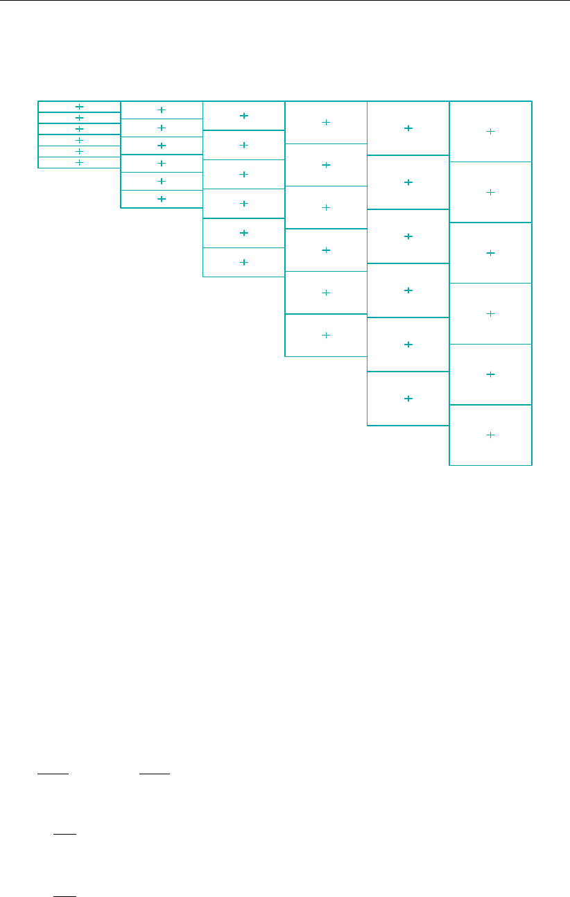
DRAFT
D-Water Quality, User Manual
Horizontal diffusion will lead to vertical transport of matter through vertical stratification in-
terfaces (pycnocline) which is unphysical. A more accurate, strict horizontal discretization is
needed.
Figure 10.4: Finite Volume for diffusive fluxes and pressure gradients
Like in Delft3D-FLOW, in D-WAQ an option is available that minimises artificial vertical dif-
fusion due to truncation errors; see section 5.3.9:Numerical options. A method has been
implemented which gives a consistent, stable and monotonic approximation of the horizontal
diffusion term. This “anti-creep” option is based upon a Finite Volume approach; see Fig-
ure 10.4. The horizontal diffusive fluxes and baroclinic pressure gradients are approximated
in Cartesian co-ordinates by defining rectangular finite volumes around the sigma co-ordinate
grid points. Since these boxes are not nicely connected to each other, see Figure 10.5, an
interpolation in z-co-ordinates is required to compute the fluxes at the interfaces.
Since the centres of the finite volumes on the left-hand side and right-hand side of a vertical
interval are not at the same vertical level, a z-interpolation of the scalar concentration cis
needed to compute strictly horizontal derivatives. The values obtained from this interpolation
are indicated by c∗
1and c∗
2respectively in Figure 10.5.Stelling and Van Kester (1994) apply
a non-linear filter to combine the two consistent approximations of the horizontal gradient,
s1=c∗
2−c1
∆xand s2=c2−c∗
1
∆x:
If s1×s2<0Then (10.43)
∆c
∆x= 0
Else
∆c
∆x=sign(s1)×min(|s1|,|s2|)
Endif
If an interval has only grid boxes at one side, the derivative is directly set to zero. The hor-
izontal fluxes are summed for each control volume to compute the diffusive transport. The
312 of 382 Deltares
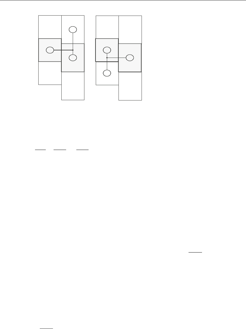
DRAFT
Numerical aspects
+
+
+
+
+
+
+ +
+
+ +
+
c
c
c
c
cc
2
1
1
1
22
*
*
Figure 10.5: Left and right approximation of a strict horizontal gradient
integration of the horizontal diffusion term is explicit with time step limitation:
∆t≤1
DH1
∆x2+1
∆y2−1
.(10.44)
Since this approximation of the horizontal gradient is used for the horizontal diffusion flux, it
is important to ensure that the difference operator is positive definite in order to get physically
realistic solutions. The maximum and minimum of a variable being transported by diffusion do
not increase or decrease (min-max principle). By taking the minimum of the gradients, Stelling
and Van Kester (1994) show that, the min-max principle is fulfilled. Beckers et al. (1998) show
that any nine-point consistent linear discretization of the horizontal diffusion on the σ-grid
does not fulfil the min-max principle. From numerical tests Slørdal (1997) concluded that the
underestimation is reduced by increasing the vertical resolution, but is sometimes enhanced
by increasing the horizontal resolution.
Let s4be a consistent approximation of the horizontal gradient s4=s1+s2
2.Slørdal (1997)
suggested to take s4as approximation of the horizontal gradient. He calls his approach the
“modified Stelling and Van Kester scheme”. It is equivalent to linear interpolation at a certain
z-level before taking the gradient. It is more accurate than taking the minimum of the absolute
value of the two slopes s1and s2but it does not fulfil the min-max principle for the diffusion
operator. It may introduce wiggles and a small persistent artificial vertical diffusion. Due to the
related artificial mixing, stratification may disappear entirely for long term simulations, unless
the flow is dominated by the open boundary conditions.
By introducing an additional approximation of the horizontal gradient in the filter algorithm de-
fined by s3=c2−c1
∆x, the stringent conditions of the minimum operator can be relaxed some-
what. This third gradient s3, which is consistent for min(|s1|,|s2|)< s3<max(|s1|,|s2|),
has point-to-point transfer properties and therefore leads to a positive scheme for sufficiently
small time steps. The following non-linear approach presently available in D-WAQ is both
Deltares 313 of 382

DRAFT
D-Water Quality, User Manual
consistent and assures the min-max principle:
If s1×s2<0Then (10.45)
∆c
∆x= 0
Elseif |s4|<|s3|Then
∆c
∆x=s4
Elseif min(|s1|,|s2|)<|s3|<max(|s1|,|s2|)Then
∆c
∆x=s3
Else
∆c
∆x=sign(s1) min(|s1|,|s2|)
Endif
The method requires a binary search to find the indices of neighbouring grid boxes, which is
time consuming. The increase in computation time is about 30%.
If the streamlines are strictly horizontal, transport of matter discretised on a σ-co-ordinate
grid may still generate some numerical vertical diffusion by the discretization of the advection
terms.
314 of 382 Deltares
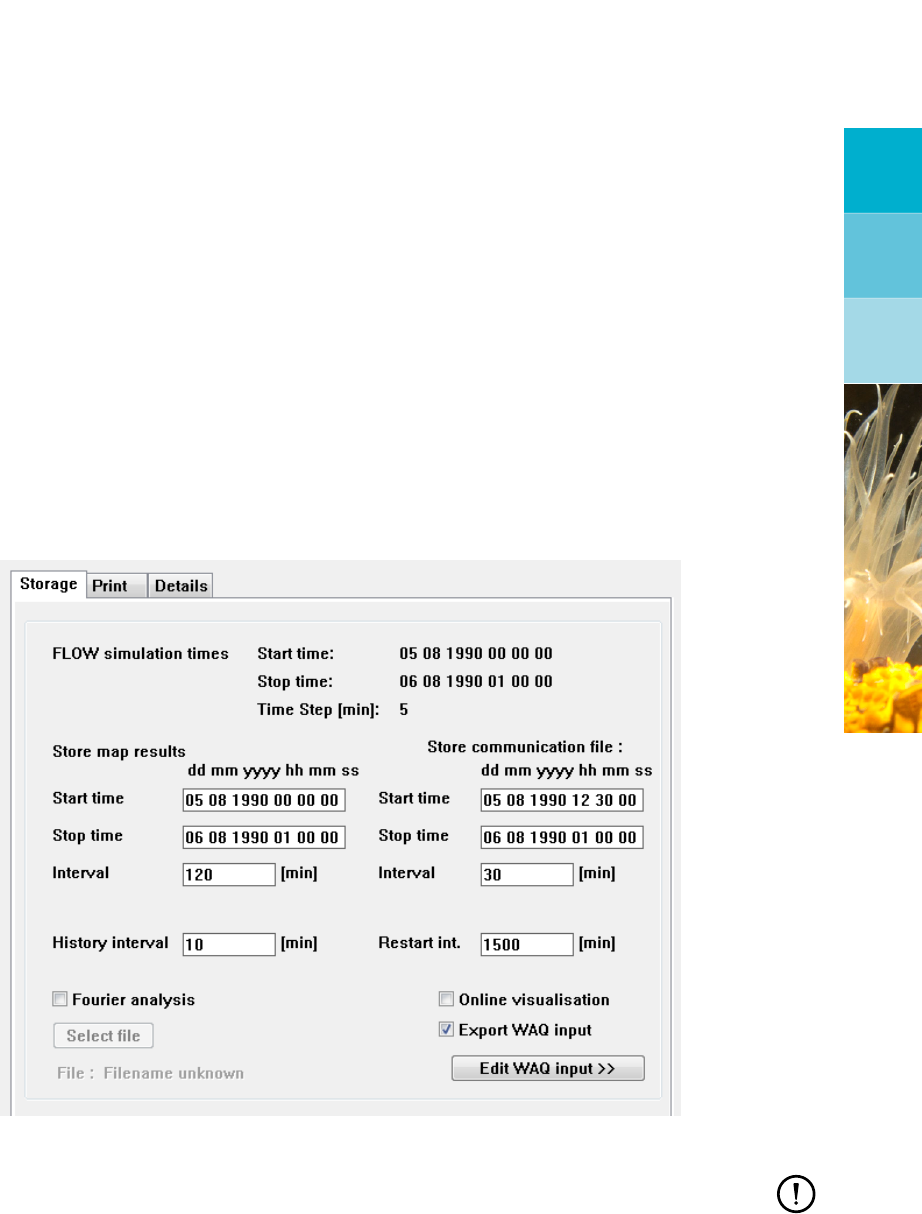
DRAFT
11 Special features
11.1 Built-in coupling with Delft3D-FLOW
Often the communication files resulting from computations with a large hydrodynamic model
(or over a long simulation period) are very large and mostly exclusively used for the coupling
to other modules, such as D-Water Quality. This means that disk space is not used efficiently,
unless you have reasons to experiment with the parameters of the coupling process, such as
aggregating in time or space.
If the conversion to the files used by the water quality modules is fixed, then it is possible to
write directly the hydrodynamic quantities to file, these files can be used by D-Water Quality
without the need of any intermediate program. This option is called built-in coupling with
D-Water Quality and can be switched on in the FLOW-GUI (Delft3D-FLOW UM,2013) data
group Output →Storage by tick off the check box Export WAQ input, see Figure 11.1.
Figure 11.1: Data Group Output →Storage to switch on Export WAQ input
Remark:
The option Online coupling is not available any more.
11.2 Domain decomposition
The current implementation of domain decomposition in Delft3D-FLOW means that for each
domain separate communication files are created. To avoid having to select all these files
separately and to specify the various parameters (start and stop time for instance) in a way that
is consistent for all domains, you simply select the <∗.ddb>file belonging to the computation
as a whole, instead of a communication file.
This file describes how the various domains are connected. It is created automatically while
you define the multiple domains and the corresponding hydrodynamic input. The user-interface
Deltares 315 of 382

DRAFT
D-Water Quality, User Manual
for the coupling program then reads the information contained in this file, so that it can prepare
the conversion of the communication files per domain.
The only locations where you as a user are confronted with the fact that multiple domains are
involved are:
The selection of a <∗.ddb>file, instead of a communication file.
Associating aggregation files (from D-Waq DIDO) with individual domains.
The latter is due to the fact that currently D-Waq DIDO can not handle multiple domains.
Instead you have to specify the spatial aggregation per domain.
11.3 Online coupling between Delft3D-FLOW and SOBEK
In some cases it is advantageous to model a part of the area of interest with a one-dimensional
flow model (like for instance SOBEK) and another part with a multidimensional model. For
instance, if you have a complicated network of rivers and channels that flow into an estuary
and then into the open sea. Modelling such a system with a multidimensional model only can
force you into using a very large detailed grid, just because of the need to include all branches
of the network.
An alternative is to use two simulateneously running computations that interact. While the
technical details of this set-up are quite complex, they are of no particular importance to the
use of such a system. What is important is that this can be done and how it can be done.
The communication (or “online coupling”) between the two computations involves a simple
convention: the names of the boundaries between the two regions must match. That is: if
the one-dimensional model has a boundary “River”, for which the connection with the multidi-
mensional model must be established, then this name must appear in the list of boundaries
for the multidimensional model. This is the strategy for the hydrodynamic models and it is the
strategy for the water-quality models as well.
The user-interface can assist here:
The hydrodynamic description file can be expanded to hold information about these spe-
cial boundaries.
These boundaries become “reserved” in the sense that you can not change the name or
the location of these boundaries (otherwise the communication would go wrong).
If the two models are run simultaneously, so that data can be passed to and fro, any
boundary concentrations you put into the scenario for these boundaries will be ignored.
However, it is still possible to edit the boundary data, as you may wish to run the multidi-
mensional model standalone.
If you run the multidimensional model standalone, there is only one minor limitation: the
concentration data for such boundaries are always uniform over the whole section, but the
same input files can be used for both types of computation. As such boundary sections
are generally short, this is but a minor limitation.
The boundary section designated for the communication are specified as follows in the hyd-
file:
boundaries-coupled-externally
’Name’ xbegin ybegin xend yend
... repeated for each such boundary section ...
end-boundaries-coupled-externally
316 of 382 Deltares

DRAFT
Special features
where:
‘Name’ is the identification of the boundary in question (the string used to recognise the
boundary in both computations).
xbegin and ybegin the indices of the start of the boundary section
xend and yend the indices of the end of the boundary section
11.4 Converting results of a hydrodynamic model using Z-model
The hydrodynamic module in Delft3D can handle both so-called σ-model and z-model (see
Delft3D-FLOW UM (2013)). The latter require a different conversion program, as the concept
is quite different. For the user, however, this should be almost completely transparent. This
section describes the way z-layers are handled in the water quality module.
There is one important aspect to z-layers that differs from σ-layers: the treatment of active
segments:
In a model using σ-layers all segments in the same column are either active or inactive,
depending on the water level. In the water quality module, a threshold is used for most
water quality processes to make sure that in very shallow segments (typically segments
that are dry or are almost dry) the processes that depend on the thickness of the water
layer remain bounded. When the segments are dry, the flow over the interfaces is zero, so
that also the dispersion is turned off.
In a model using z-layers on the other hand, the topmost segment can become dry,
whereas the segments below it still hold water. At a later time the topmost segment can
get wet again or the segment below it can become dry in turn as well. To take care of
this dynamics, a special “water quality process” monitors the thickness of the water layer
and sets the attribute for the segment to inactive once the thickness is below a certain
threshold or to active if it is above the threshold again. In this way, completely analogous
to what happens in the hydrodynamic module, the drying and flooding of segments in a
z-layer model is handled1.
As the hydrodynamic database itself does not allow for a reliable detection of the type of
layers that has been used, the hydrodynamic description file has been extended with two new
keywords, σ-layers and z-layers that can be added after the keyword geometry:
The following lines both define a curvilinear grid with σ-layers (this being the default type of
layers):
geometry curvilinear-grid
geometry curvilinear-grid sigma-layers
To define z-layers, you need to explicitly add the keyword z-layers:
geometry curvilinear-grid z-layers
The effect is that in the water quality computation the process Emersion is turned on with
the specific parameter Zthreshold that determines if the water layer is thick enough for the
segment to be active or not. Note: this is taken care of automatically by the user-interface.
1As all the regular water quality processes are implemented to deal with active and inactive segments, the
z-layer feature is completely transparent to the water quality module in all other respects.
Deltares 317 of 382
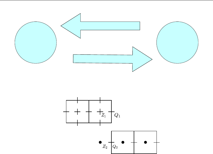
DRAFT
D-Water Quality, User Manual
Delft3D
WAQ
SOBEK-WQ
1D
Concentrations to SOBEK-WQ
Concentrations to Delft3D-WAQ
Figure 11.2: Approach for coupling of 3D and 1D model.
Delft3D-FLOW domain
SOBEK domain
Figure 11.3: Illustration of coupling of D-WAQ and SOBEK-WQ 1D model.
11.5 1D–3D Coupling
11.5.1 Mathematical background
The Deltares System is able to perform joint (on-line coupled) simulations for one 1D do-
main, modelled within the 1D software suite SOBEK, and one 3D domain, modelled within
the Delft3D suite. Both systems simulate time dependent processes for which a time stepping
procedure is applied.
In the coupled 1D–3D model the concentrations of the state variables are exchanged between
both domains at each time step. A so-called explicit coupling is applied. This means that
model quantities are exchanged between the 1D part and the 3D part and that the data from
the other part is stored as input variable of the equations. At every time step, the 1D domain
sends the concentration values in the cells adjacent to the coupling boundary, to the 3D
domain as its boundary conditions, and vice versa. This is illustrated in Figure 11.2.
The 1D and 3D domains optionally use an implicit time integration method, which requires
the solution of a system of equations. For reasons of flexibility, we chose not to apply an
implicit coupling approach. An implicit coupling would require the solving of one large system
of equations, which integrates the systems of equations of the 1D and 3D model domains.
Instead, the explicit approach described above was selected.
The boxes, Figure 11.3, show the control volumes used for setting up the water quality model
in both domains, relative to the water level points (Zi) and velocity points in both domains
(Qi). It is evident that the control volumes in both domains are correctly aligned and allow for
a mass conserving solution.
The implementation of the 1D–3D coupling is such that one SOBEK grid cell corresponds to
318 of 382 Deltares
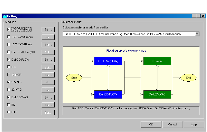
DRAFT
Special features
Figure 11.4: Overview of activated modules.
one open boundary segment in Delft3D-FLOW. If this open boundary segment consists of n
computational cells, each of kvertical layers, then the concentrations of the 1D segment are
transferred as boundary conditions to all nk 3D segments, while the concentrations from all
nk 3D segments are used as boundary conditions for the 1D segment. In the latter case,
the value transferred is the flow-weighted average concentration. It should be noted that it is
common to use an upwind spatial discretisation on the model boundaries. In that case only
the boundary conditions from the “upwind” domain affect the “downwind” domain. The transfer
of boundary conditions from the downwind to the upwind domain is done for administrative
reasons only. Evidently, the definition of “upwind” depends on the local and momentaneous
direction of flow.
The coupling as it is implemented does not allow for a different time step in the coupled
domains: the same time step should be used in the 1D and 3D domains. In practice, 1D
simulations usually run with a larger time step than 3D simulations. Therefore, the time step
synchronisation of the domains means that the time step in the 1D domain is probably smaller
than it would have been in stand alone mode. This will evidently not hamper the accuracy
of the calculations. Since the performance of the joined 1D–3D model is, to a large extent,
determined by the 3D domain, the overall performance is not significantly affected by the
synchronisation.
The fact that the coupling is implemented in an explicit fashion implies that the selection of an
explicit solution method of the governing equations is required to guarantee conservation of
mass. It is not expected however that the use of implicit methods will cause significant errors.
This expectation has been confirmed by test simulations during practical applications.
Deltares 319 of 382

DRAFT
D-Water Quality, User Manual
11.5.2 Software implementation
In general the input for both domains is arranged via the respective User Interfaces of SOBEK
(1D domain) and Delft3D (3D domain). The simulation is started from the SOBEK User In-
terface. To activate this mode of calculation, activate the Settings task in the SOBEK User
Interface, and make the selection as shown in Figure 11.4.
After a successful simulation, the inspection of the output is again arranged via the respective
User Interfaces of SOBEK (1D domain) and Delft3D (3D domain).
The facilities to carry out coupled 1D–3D simulations are available from versions 3.28.06 of
Delft3D and 2.12 of SOBEK.
11.5.3 Tutorial
For making a successful combined 1D–3D water quality simulation, the following requirements
need to be met:
A valid 1D–3D coupled hydrodynamic simulation needs to be available (we refer to the
related Manual).
This hydrodynamic simulation needs to have produced the necessary output files for a
joint water quality simulation (see section 11.5.3.1).
Other input necessary for the 1D and 3D domains of the water quality model needs to
have been prepared (see section 11.5.3.2)
The on-line connection the 1D and 3D domain can then be arranged as described in sec-
tion 11.5.3.3. This section also describes how boundaries, time steps and state variables will
be matched between both domains.
11.5.3.1 Hydrodynamic input files for the water quality simulation
1D domain
To activate the coupling with FLOW in the 1D domain, activate the Settings task in the SOBEK
User Interface. Select Edit for the “1DFLOW(Rural)” module. On the Simulation Settings tab
form, activate “generate output to Water Quality Module” (Figure 11.5). Click OK.
The system may generate a warning, that the output from the 1D FLOW module will be set to
mean values (Figure 11.6). This is required to run WAQ simulations.
To de-activate other coupling options with FLOW in the 3D domain, activate the Settings task
in the SOBEK User Interface and select Edit for the “Delft3D-FLOW” module. On the Time
Settings tab form:
Select the proper <name.mdf>file at Delft3D FLOW Master Definition Flow.
Select the proper <d3d_sobek_conf.ini>file in the same folder (see Manual for 1D–3D
coupled hydrodynamic simulations, (Delft3D-FLOW UM,2013)).
DO NOT activate “On-line coupling to Delft3D WAQ” (Figure 11.7).
320 of 382 Deltares
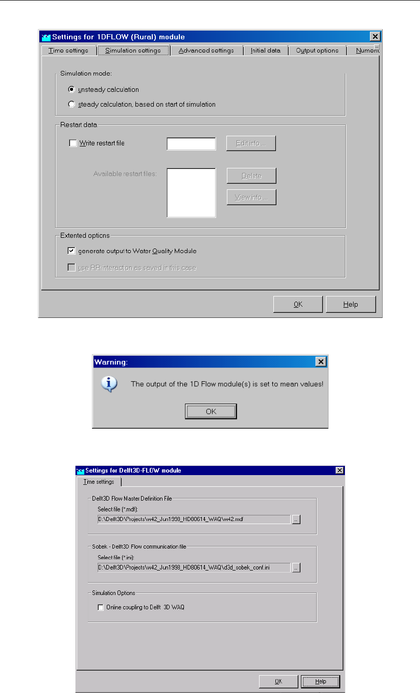
DRAFT
Special features
Figure 11.5: Settings task for “1DFLOW(Rural)” module; Simulation Settings tab form.
Figure 11.6: Warning message.
Figure 11.7: Settings task for “Delft3D-FLOW” module; Time Settings tab form (note that
file names shown have no specific meaning).
Deltares 321 of 382
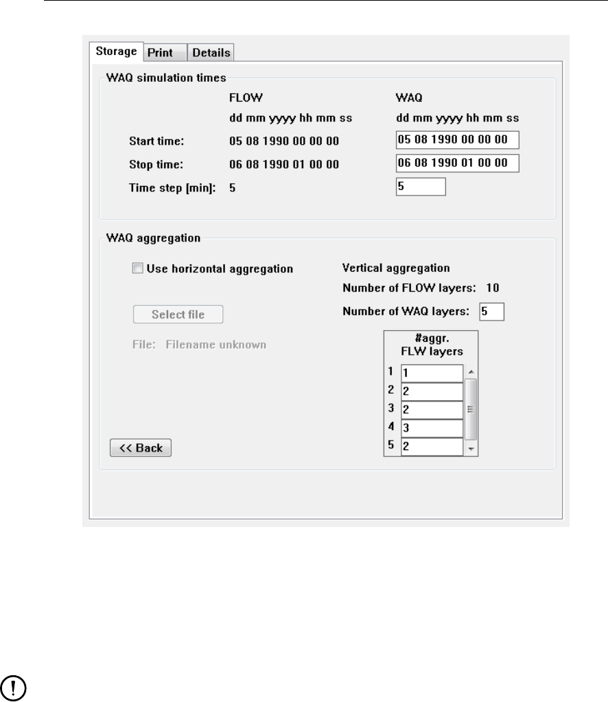
DRAFT
D-Water Quality, User Manual
Figure 11.8: FLOW-GUI: Sub-data group Output →Storage →Export WAQ input.
3D domain
To activate the coupling with FLOW in the 3D domain, activate the Delft3D-FLOW User In-
terface, select Section Output →Storage →Export WAQ input (Delft3D-FLOW UM,2013).
Enter the desired data, for an example see Figure 11.8.
Remark:
Note that minimum values for the vertical dispersion can not be defined at this level. In
stead they can be defined in the D-WAQ user interface, see section 5.2.4.
11.5.3.2 Other input for the water quality simulation
Other input to be provided comprises for both domains:
time frame and time step;
selection of state variables, processes and process parameters;
grid definition (1D domain);
selection of numerical method;
dispersion coefficients;
initial concentrations;
meteorological and other forcing functions;
pollution loadings;
boundary conditions (except for 1D–3D coupling boundaries);
322 of 382 Deltares

DRAFT
Special features
output definition;
definition of observation points.
This should be done via the SOBEK (1D) and Delft3D User Interfaces. We refer to the User
Manuals for further explanations (Delft3D-FLOW UM,2013;SOBEK UM,2013).
11.5.3.3 Arranging the coupling between the 1D and 3D domains
Connecting boundaries in both domains
A coupled 1D–3D WAQ simulation presumes a successfully coupled FLOW simulation. This
requires that there is correspondence between the id’s of:
the boundary nodes in the 1D domain, and
the boundary sections in the 3D domain.
On top of that, a file named <delft3d_sobek_waq.ini>needs to be present in the Delft3D
working directory. This file should look as follows:
boundaries-coupled-externally
’name1’ 175 63 177 63
’name2’ 198 75 198 75
’name3’ 216 80 216 80
...
end-boundaries-coupled-externally
The strings ‘name1’, ‘name2’, etc. are supposed to be equal to the names used for the cou-
pled boundaries in the coupled 1D–3D FLOW model. The four integer numbers following the
strings represent the (m, n)grid co-ordinate ranges of the corresponding boundary sections
in the 3D domain. This file can be derived directly from the <∗.hyd>file produced by the
3D FLOW simulation (if the proper arrangements are made to produce water quality files, see
above).
In the D-WAQ User Interface, the boundaries will be given the name indicated in the
<delft3d_sobek_waq.ini>file, and are indicated as — possibly coupled —, see Figure 11.9.
The boundary conditions supplied for these boundaries will be overruled by the concentrations
in the corresponding branches of the 1D model during a coupled 1D–3D simulation.
Matching substances at coupled boundaries
The selection of state variables may be different in both domains. Boundary conditions how-
ever will only be exchanged at the coupling locations for state variables with the same name.
Matching time steps
The coupling is not able to deal with different time frames in both domains. Therefore, the
user-defined calculation time-step must be the same in both domains, and the simulation
period must be equal in both domains.
Deltares 323 of 382
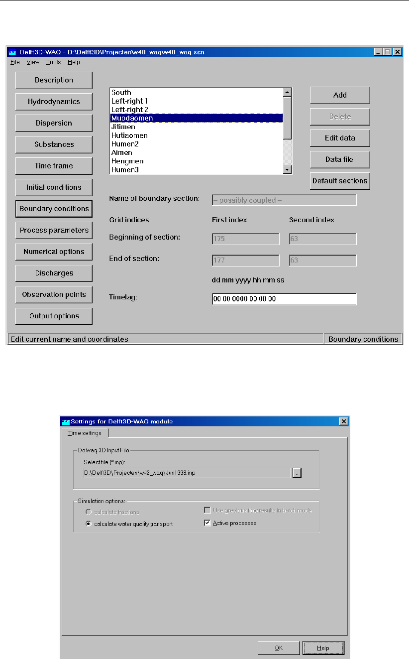
DRAFT
D-Water Quality, User Manual
Figure 11.9: Datagroup Boundary conditions
Figure 11.10: Settings for D-WAQ window (note that file name shown has no specific
meaning).
324 of 382 Deltares
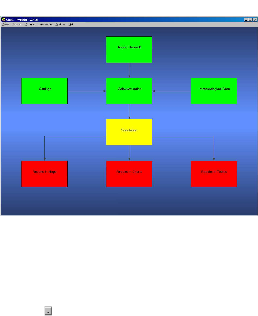
DRAFT
Special features
Figure 11.11: Case manager main window, ready for simulation task.
Running coupled simulations
The coupled simulation is conducted from the SOBEK User Interface. You indicate which 3D
water quality input file you want to use, by activating the Settings task. Select Edit for the “D-
Water Quality” module. The Settings for Delft3D WAQ module now appears (Figure 11.10).
On this window you define the 3D domain input file <∗.inp>, which you prepared. This file
has the same name as the <∗.scn>file, created by the 3D domain D-WAQ GUI.
Click on the button next to the Select file (∗.inp) selection box.
Browse for and open the appropriate <name.inp>file.
Make sure that the rest of this window looks like Figure 11.10.
Select OK to stop editing the “D-Water Quality” module.
Select OK to leave the Settings task box.
To run a simulation, double-click the Simulation task box (see Figure 11.11).
You will be prompted to use the water quantity (FLOW) results from a previous simulation
(Figure 11.12). Click Yes.
You will be warned that existing output for the 3D water quality domain will be overwritten.
Verify that this is not a problem, and click Yes (Figure 11.13).
Deltares 325 of 382
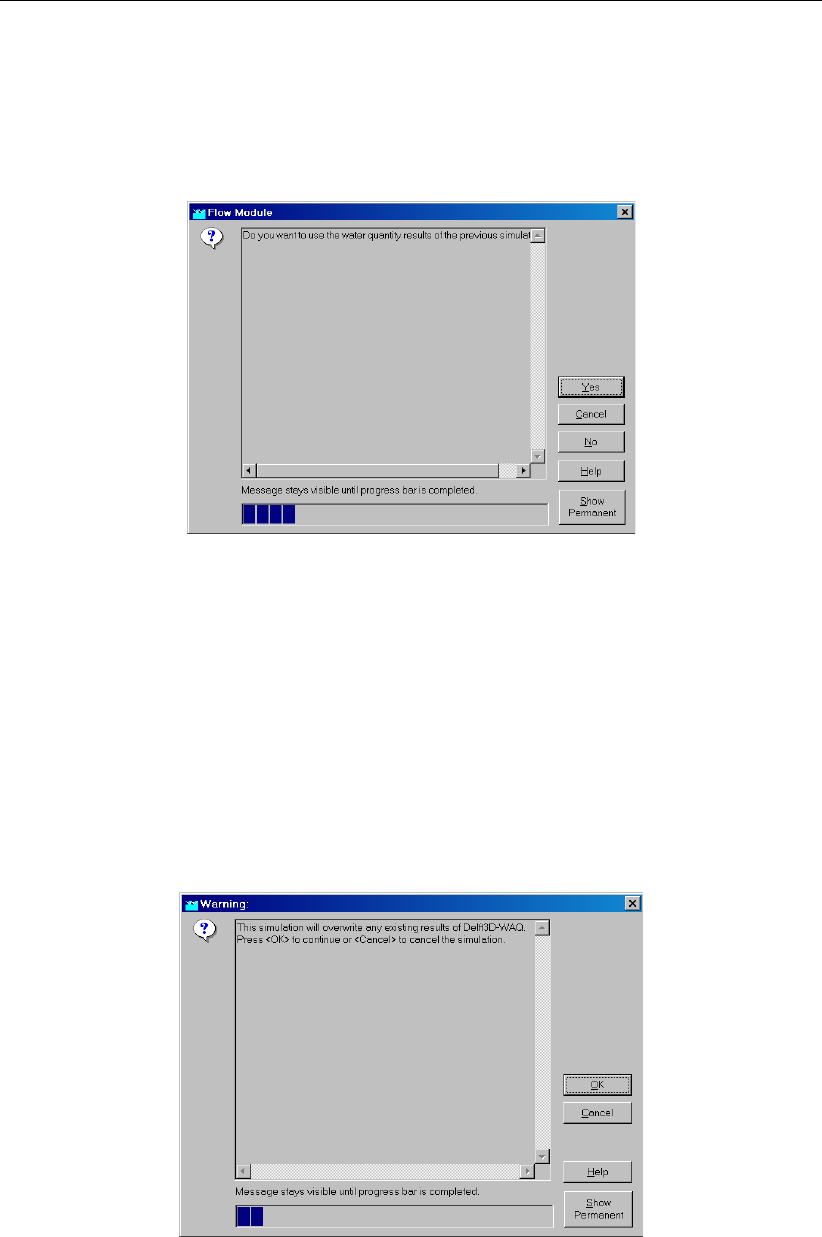
DRAFT
D-Water Quality, User Manual
Figure 11.12: Simulation task Flow Module window.
Figure 11.13: Simulation task; warning for overwriting D-WAQ results.
326 of 382 Deltares
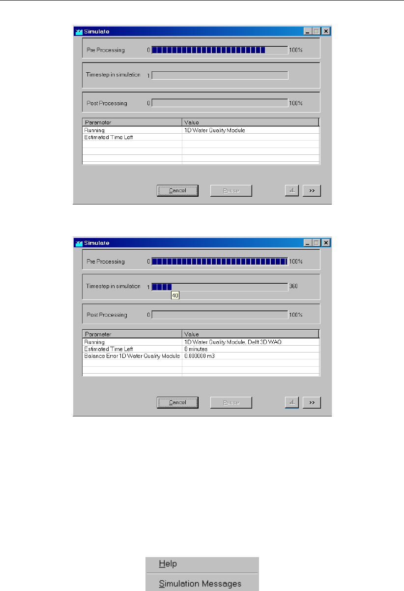
DRAFT
Special features
Figure 11.14: Simulation task progress window; pre-processing.
Figure 11.15: Simulation task progress window; processing.
The simulation task will proceed with pre-processing tasks (Figure 11.14), simulations (Fig-
ure 11.15) and post-processing tasks.
When the simulation is successfully completed, the main window will be like Figure 11.16.
If problems are encountered, move the mouse to the Simulation task box, and use the right
mouse button to access report files:
Figure 11.17: Accessing Help and Simulation messages
The relevant messages files are:
1D domain
input reports: <delwaq.lst>and <delwaq.lsp>
simulation report: <delwaq.mon>
Deltares 327 of 382
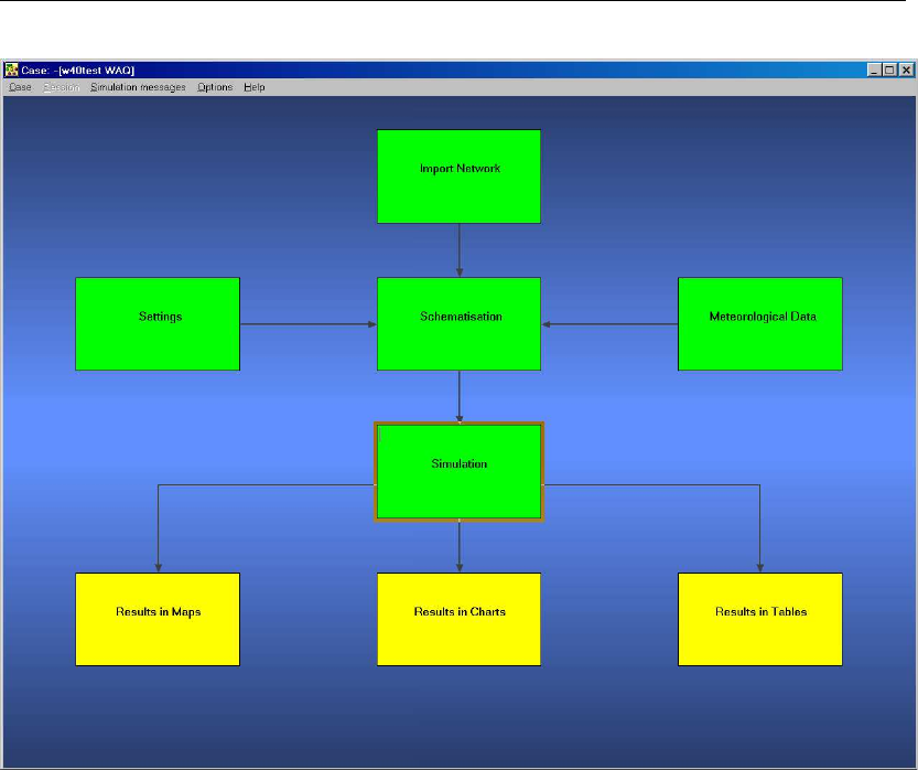
DRAFT
D-Water Quality, User Manual
Figure 11.16: Case manager main window, simulation task successfully completed.
3D domain
input report: <name.lst>and <name.lsp>
simulation report: <name.mon>where name is the name of the ∗.inp used.
11.5.4 Tips & Tricks
The <∗.mon>simulation report file from both domains provides feed back on the successful
matching of boundaries and state variables. In the top section of both files you should find
lines looking like:
Domain decompostion boundary matching for:delwaq_to_xxxx
for boundary 1 (South) no match found
...
for boundary 309 (West) no match found
for boundary nMuodaomen match found with number: 3324
for boundary nMuodaomen match found with number: 3324
for boundary nMuodaomen match found with number: 3324
...
...
Domain decompostion substance matching for:delwaq_to_xxxx
for substance AAP match found with number: 1
for substance DetC match found with number: 2
...
for substance Cbodu no match found
...
Evidently, it is possible that some boundaries and substances show no match. You have to
328 of 382 Deltares

DRAFT
Special features
take care however, that all boundaries and substances which are supposed to match between
both domains, are actually matching.
Deltares 329 of 382

DRAFT
D-Water Quality, User Manual
330 of 382 Deltares

DRAFT
References
List of related publications
General:
Baptist and De Vries (1998)
Bent et al. (1991)
Jenkins et al. (1997)
Salden et al. (1996)
Vatvani and Montazeri (1989)
Vos (1995a)
Vos and Schuttelaar (1995b)
Vos et al. (1998a)
Vos et al. (1998b)
WL | Delft Hydraulics (1994a)
WL | Delft Hydraulics (1996a)
WL | Delft Hydraulics (1997b)
WL | Delft Hydraulics (1999)
Sediment:
Flokstra and Jagers (1999)
Kranenburg and Winterwerp (1997a)
Kranenburg and Winterwerp (1997b)
Mosselman et al. (1999)
?
Vos and Gerritsen (1997)
Vos et al. (1998b)
Winterwerp (1999a)
Winterwerp (1999b)
Winterwerp et al. (1998)
WL | Delft Hydraulics (1996b)
WL | Delft Hydraulics (1997a)
WL | Delft Hydraulics (2000)
Ecology:
Los and Bokhorst (1997)
Van der Molen et al. (1994)
Peeters et al. (1995)
De Vries et al. (1998)
WL | Delft Hydraulics (1991a)
WL | Delft Hydraulics (1994b)
WL | Delft Hydraulics (1996b)
WL | Delft Hydraulics (1997c)
WL | Delft Hydraulics (1997d)
WL | Delft Hydraulics (1998a)
WL | Delft Hydraulics (1998b)
Deltares 331 of 382

DRAFT
D-Water Quality, User Manual
Complete list of references
Baptist, M. and M. de Vries, 1998. Eco Tools, a Technical description of the Delft Hydraulics’
Ecological Toolset for Empirical Modelling. Tech. rep., WL | Delft Hydraulics, Delft, The
Netherlands.
Beckers, J. M., H. Burchard, J. M. Campin, E. Deleersnijder and P. P. Mathieu, 1998. “Another
reason why simple discretizations of rotated diffusion operators cause problems in ocean
models: comments on “isoneutral diffusion in a z co-ordinate ocean model”.” American
Meteorological Society 28: 1552–1559.
Bent, E., L. Postma, A. Roelfzema and R. Stive, 1991. “Hydrodynamic and dispersion mod-
elling of Swansea Bay.” Environmental Hydraulics 1: 865–870.
Blumberg, A. F. and G. L. Mellor, 1985. “Modelling vertical and horizontal diffusivities with the
sigma co-ordinate system.” Monthly Weather Review 113 (8): 1379.
Boris, J. and D. Book, 1973. “Flux corrected transport I. SHASTA, a fluid transport algorithm
that works.” Journal of Computational Physics 11: 38–96.
Chapman, D. e. a., 1996. Water Quality Assessments (A Guide to the Use of Biota, Sediments
and Water in Environmental Monitoring). Chapman & Hall, London, 2nd ed.
Chapra, S. C., 1996. Surface Water Quality Modeling. McGraw-Hill Sci-
ence/Engineering/Math, New York.
D-Flow FM UM, 2015. D-Flow FM Hydro- and Morphodynamics User Manual. Deltares,
1.1.124 ed.
D-WAQ Input file, 2013. D-Water Quality Description of Input file. Deltares, 2.00 ed.
D-WAQ TRM, 2013. D-Water Quality Technical Reference Manual. Deltares, 4.00 ed.
Delft3D-FLOW UM, 2013. Delft3D-FLOW User Manual. Deltares, 3.14 ed.
DIDO UM, 2013. Delft3D-DIDO User Manual. Deltares, Delft, 4.00 ed.
Engelund, F. and E. Hansen, 1967. A monograph on Sediment Transport in Alluvial Streams.
Teknisk Forlag, Copenhagen.
Flokstra, C. and H. Jagers, 1999. Graded sediment in Delft3D.
Forester, C. K., 1979. “Higher Order Monotonic Convective Difference Schemes.” Journal of
Computational Physics 23: 1–22.
Golub, G. H. and C. F. Van Loan, 1989. Matrix computations. Baltimore: John Hopkins
University Press.
GPP UM, 2013. Delft3D-GPP User Manual. Deltares, 2.14 ed.
Groen, P. and R. Dorrestein, 1976. Sea waves. Oceanographic and Maritime Meteorology 11,
Royal Dutch Meteorological Institute. 124 p. (in Dutch).
Huang, W. and M. Spaulding, 1996. “Modelling horizontal diffusion with sigma coordinate
system.” Journal of Hydraulic Engineering 122 (6): 349–352.
Jenkins, A., M. Lahoz, C. de Valk, R. Vos, H. Gerritsen, P. ten Brummelhuis and et al., 1997.
Remote sensing applied to operational models, North Sea. Birkenhead. Tech. Rep. 49,
POL, Bidston Observatory.
332 of 382 Deltares

DRAFT
References
Kranenburg, C. and J. Winterwerp, 1997a. “Erosion of fluid mud layers. I: Entrainment model,
Journal of Hydraulic Engineering.” Journal of Hydraulic Engineering 123 (6): 504–511.
Kranenburg, C. and J. Winterwerp, 1997b. “Erosion of fluid mud layers. II: Experiments
and model validation, Journal of Hydraulic Engineering.” Journal of Hydraulic Engineer-
ing 123 (6): 512–519.
Krone, R., 1962. Flume studies of transport of sediment in estuarial shoaling processes
(Final report). Tech. rep., University of California, Hydraulics Engineering and Sanitary
Engineering Laboratory, Berkeley, USA.
Laws, E. A., 1993. Aquatic Pollution, an Introductory Text. John Wiley & Sons, Inc., New York,
2nd ed.
Leendertse, J. J., 1990. “Turbulence modelling of surface water flow and transport: part IVa.”
Journal of Hydraulic Engineering 114 (4): 603–606.
Los, F. and M. Bokhorst, 1997. “Trend analysis Dutch coastal zone.” In New Challenges for
North Sea Research, pages 161–175. Zentrum for Meeres- und Klimaforschung, University
of Hamburg.
Los, F. and J. Brinkman, 1988. “Phytoplankton modelling by means of optimization; a 10-year
experience with Bloom II.” Verh. Int. Ver. Limnol 23: 790–795.
Mancini, J. L., 1978. “Numerical estimates of coliform mortality rates under various conditions.”
Journal Water Pollution Control Federation -: 2477–2484.
Molen, D. van der, F. Los, L. van Ballegooijen and M. van der Vat, 1994. “Mathematical mod-
elling as a tool for management in eutrophication control of shallow lakes.” Hydrobiologica
275/276: 479–492.
Mosselman, E., A. Sieben, K. Sloff and A. Wolters, 1999. “Effect of spatial grain size variations
on two-dimensional river bed morphology.” In Proceedings IAHR symposium on River,
Coastal and Estuarine Morphology (RCEM), Genoa, pages 499–507.
Nelson, R., 1983. “Wave heights in depth-limited conditions.” In 6th Australian Conference on
Coastal and Ocean Engineering, Gold Coast, Australia.
Partheniades, E., 1962. A study of erosion and deposition of cohesive soils in salt water.
Ph.D. thesis, University of California, Berkeley, USA. 182 p.
Peeters, J., F. Los, R. Jansen, H. Haas, L. Peperzak and I. de Vries, 1995. “The oxygen
dynamics of the Oyster Ground, North Sea. Impact of eutrophication and environmental
conditions.” OPHELIA 42: 257–288.
Poole, H. and W. Atkins, 1929. “Photo-electric measurements of submarine illumination
throughout the year.” Journal of the Marine Biological Association of the United Kingdom
16: 297–324.
QUICKIN UM, 2013. Delft3D-QUICKIN User Manual. Deltares, 4.00 ed.
QUICKPLOT UM, 2013. Delft3D-QUICKPLOT User Manual. Deltares, 2.14 ed.
Rijn, L. C. van, 1993. Principles of Sediment Transport in Rivers, Estuaries and Coastal Seas.
Aqua Publications, The Netherlands.
Saad, Y. and M. H. Schultz, 1986. “GMRES: a generalized minimal residual algorithm for
solving nonsymmetric linear systems.” SIAM J. Sci. Stat. Comput. 7 (3): 856–869. DOI:
http://dx.doi.org/10.1137/0907058, ISSN 0196-5204.
Deltares 333 of 382

DRAFT
D-Water Quality, User Manual
Salden, R., J. de Kok, J. Boon and H. Gerritsen, 1996. NOMADS: NOrth sea Model
Advection-Dispersion Study: the Dutch contribution to the simulations. Tech. Rep.
Z0854/Z0995/T1643, WL | Delft Hydraulics, Delft, The Netherlands. (Rijkswaterstaat, RIKZ,
rapporten en werkdocumenten; nr. 96.010).
Slingerland, v. P., M. Borsboom and C. Vuik, 2009. A local theta scheme for advection prob-
lems with strongly varying meshes and velocity profiles. Tech. Rep. 08-17, Delft University
of Technology.
Slørdal, L. H., 1997. “The pressure gradient force in sigma-co-ordinate ocean models.” Inter-
national Journal Numerical Methods In Fluids 24: 987–1017.
SOBEK UM, 2013. SOBEK User Manual. Deltares, 0.00 ed.
Soulsby, R., 1997. Dynamics of marine sands, a manual for practical applications. Thomas
Telford, London.
Stelling, G. S. and J. A. T. M. van Kester, 1994. “On the approximation of horizontal gradi-
ents in sigma co-ordinates for bathymetry with steep bottom slopes.” International Journal
Numerical Methods In Fluids 18: 915–955.
Streeter, H. and E. Phelps, 1925. Study of the pollution and natural purification of the Ohio
river. III. Factors Concerned in the Phenomena of Oxidation and Reaeration. Tech. Rep.
U.S. Public Health Serv., Pub. Health Bulletin No. 146, U.S. Public Health Service, Wash-
ington D.C. (reprinted 1958).
Swart, 1974. Offshore sediment transport and equilibrium beach profiles. Ph.D. thesis, Delft
University of Technology, Delft, The Netherlands. Delft Hydraulics Publ. 131.
Tamminga, G., 1987. Influence of a constant south-westerly wind on the erosion in Lake
IJssel. Tech. rep., Hydraulics and Discharge-Hydrology Department, Wageningen.
Thomann, R. V. and J. A. Mueller, 1987. Principles of Surface Water Quality Modelling and
Control. Harper & Row publishers, New York.
Vatvani, D. and M. Montazeri, 1989. “Performance of some high accurate semi Lagrangian nu-
merical schemes for the scalar advection equation.” Deutsche Hydrographische Zeitschrift
42: 279–305. (H.3-6, Semi-Lagrangian numerical Schemes).
Vos, R., 1995a. Restwaq : applications of remote sensing to water quality modelling : data
assessment and development of methodology. Tech. Rep. T1083/T1479, WL | Delft Hy-
draulics, Delft, The Netherlands. I.o.v. Rijkswaterstaat, Meetkundige Dienst.
Vos, R., A. Dekker, S. Peters, G. van Rossum and L. Hooijkaas, 1998a. RESTWAQ 2, part
II : comparison of remote sensing data, model results and in-situ data for the southern
Friesian lakes (1998). Tech. Rep. 98-08b, BCRS. I.s.m. WL, IvM-VU, NIOZ, KNMI, K&M en
Waterschap Friesland. - ISBN 90-5411-255-7.
Vos, R. and H. Gerritsen, 1997. Use of NOAA/AVHRR satellite remote sensing data for mod-
elling of suspended sediment transport in the North Sea : approach in the PROMISE
project. Tech. Rep. Z2025, WL | Delft Hydraulics, Delft, The Netherlands. I.o.v. CEC -
DGXII - MAST-3.
Vos, R. and M. Schuttelaar, 1995b. RESTWAQ : data assessment, data-model integration and
application to the Southern North Sea. Tech. Rep. 95-19, BCRS. ISBN 90-5411-168-2.
Vos, R., M. Villars, J. Roozekrans, S. Peters and W. van Raaphorst, 1998b. RESTWAQ 2,
part I: integrated monitoring of total suspended matter in the Dutch coastal zone. Tech.
Rep. 98-08, BCRS. I.s.m. WL, IvM, NIOZ, KNMI, K&M en waterschap Friesland. ISBN
90-5411-245-X.
334 of 382 Deltares

DRAFT
References
Vries, I. de, R. Duin, J. Peeters, F. Los, M. Bokhorst and R. Laane, 1998. “Patterns and trends
in nutrients and phytoplankton in Dutch coastal waters: comparison of time-series analysis,
ecological model simulation, and mesocosm experiments.” ICES Journal of Marine Science
55: 620–635.
WAVE UM, 2013. Delft3D-WAVE User Manual. Deltares, 3.03 ed.
Winterwerp, J., 1999a. “Numerical modelling of harbour siltation.” HANSA International Mar-
itime Journal to be published: –.
Winterwerp, J., 1999b. On the dynamics of high-concentrated mud suspensions. Ph.D. thesis,
Delft University of Technology, Delft, The Netherlands. Also published as Report No 99-3 in
the series “Communications on Hydraulic and Geotechnical Engineering” of Delft University
of Technology, Faculty of Civil Engineering and Geosciences, ISSN 0169-6548.
Winterwerp, J., 2002. “On the flocculation and settling velocity of estuarine mud.” Continental
Shelf Research 22: 1339–1360.
Winterwerp, J. and W. van Kesteren, 2004. “Introduction to the physics of cohesive sediments
in the marine environment.” Developments in Sedimentology 56: –.
Winterwerp, J., R. Uittenbogaard and J. de Kok, 1998. “Rapid siltation from saturated mud
suspensions.” INTERCOH’98 to be published: –.
WL | Delft Hydraulics, 1990. A grazing module for the eutrophication model JSBACH. Re-
search report T462, WL | Delft Hydraulics, Delft, The Netherlands. (in Dutch; W.M. Mooij).
WL | Delft Hydraulics, 1991a. Mathematical simulations of Algae Blooms by the Model
BLOOM II, Version 2. Vol. 1-Documentation Report; Vol.2 - Figures. Documentation re-
port T68, WL | Delft Hydraulics, Delft, The Netherlands. (F.J. Los).
WL | Delft Hydraulics, 1992. Process formulations DBS. Model documentation T542, WL |
Delft Hydraulics, Delft, The Netherlands. (in Dutch; F.J. Los et al.).
WL | Delft Hydraulics, 1994a. DELWAQ fast solvers, iterative solvers for methods 6 and
10. Tech. Rep. T1226, WL | Delft Hydraulics, Delft, The Netherlands. (R.J. Vos and M.
Borsboom).
WL | Delft Hydraulics, 1994b. Model validation study DBS in networks. Tech. Rep. T1210, WL
| Delft Hydraulics, Delft, The Netherlands. (F.J. Los, M.T. Villars and M.R.L. Ouboter).
WL | Delft Hydraulics, 1996a. DELWAQ fast solvers 2, Newton-Krylov methods for solv-
ing linear and non-linear equations. Tech. Rep. T1596, WL | Delft Hydraulics, Delft, The
Netherlands. ( R.J. Vos, M. Borsboom and K.H. Tan).
WL | Delft Hydraulics, 1996b. Flood discharge from Rhine and Meuse during winter
1994/1995: dispersion of fresh water, suspended matter and nutrients through the North
Sea. Tech. Rep. Z2032, WL | Delft Hydraulics, Delft, The Netherlands. J.G. Boon. i.o.v.
Rijkswaterstaat, Directie Noordzee.
WL | Delft Hydraulics, 1997a. Modelling of suspended particulate matter (SPM) in the North
Sea : model set up and first sensitivity analysis. Tech. Rep. Z2025, WL | Delft Hydraulics,
Delft, The Netherlands. (J.G. Boon, T. van der Kaaij, R.J. Vos and H. Gerritsen).
WL | Delft Hydraulics, 1997b. NOMADS: North Sea Model Advection Dispersion Study :
experiment 3: instantaneous releases : intercomparison of 2D and 3D model results. Re-
search report Z2084, WL | Delft Hydraulics, Delft, The Netherlands. (H. Gerritsen, A.C.
Baart and J.G. Boon).
Deltares 335 of 382

DRAFT
D-Water Quality, User Manual
WL | Delft Hydraulics, 1997c. Pilot application of new version of MANS eutrophication model
to the Dutch coastal zone. Tech. Rep. T1629, WL | Delft Hydraulics, Delft, The Netherlands.
(in Dutch; M. Bokhorst and F.J. Los).
WL | Delft Hydraulics, 1997d. Report of the ASMO workshop on eutrophication modelling, The
Hague, The Netherlands, 5-8 November 1996. Tech. Rep. T1608, WL | Delft Hydraulics,
Delft, The Netherlands. (M.T.Villars. I.o.v. RWS, RIKZ).
WL | Delft Hydraulics, 1998a. Report of the ASMO workshop on eutrophication on modelling
of contaminant transport and fate, 4-7 November 1997, The Hague, The Netherlands. Tech.
Rep. Z2264, WL | Delft Hydraulics, Delft, The Netherlands. ( M.T. Villars. I.o.v. RWS, RIKZ).
WL | Delft Hydraulics, 1998b. Scremotox : a screening model for comparative ecotoxicological
risk assessment - North Sea. Tech. Rep. Z2182, WL | Delft Hydraulics, Delft, The Nether-
lands. ( A.C. Baart and J.G. Boon i.o.v. Ministerie van VROM, Directie Drinkwater, Water,
Landbouw).
WL | Delft Hydraulics, 1999. Validation of a 3D temperature model forthe North Sea with
in-situ data and remote sensing data. Tech. Rep. Z2506, WL | Delft Hydraulics, Delft,
The Netherlands. (R.J. Vos, E.J. de Goede and R.E. Uittenbogaard. i.o.v. Rijkswaterstaat,
RIKZ).
WL | Delft Hydraulics, 2000. Analysis Concentration Gradients Delft3D-SED. Tech. Rep.
Z2874.11, WL | Delft Hydraulics, Delft, The Netherlands. (Th. van Kessel).
336 of 382 Deltares
DRAFT
A File descriptions
A.1 Overview of files
Within the process of the setting up a water quality simulation many files are generated and
many files may be used. Table A.1 contains an overview of the files used in some way in
D-Water Quality.
Table A.1: Files in D-Water Quality
File
extension
Description Output from Input for
∗.0 Configuration file for the Processes Library
Configuration Tool (PLCT)
PLCT PLCT
∗.ada Result file with spatial information in NEFIS
format. Always accompanied by <∗.adf>file
WAQ(2) GPP
∗.adf NEFIS definition file of <∗.ada>file WAQ(2) GPP
∗.are Model schematisation file containing the ex-
change areas between computational cells in
[m2]
Couple WAQ(2)
∗.atr Model schematisation file containing the at-
tributes of the computational cells. Attributes
indicate the vertical position of the computa-
tional cell:
0 = 2D simulation
1 = surface layer
2 = intermediate layer
3 = bottom layer
Couple WAQ(2)
∗-bal.his Result file with mass balances per observation
point for each substance
WAQ(2) GPP
∗.cco Model schematisation file containing the co-
ordinates of the computational grid. Always
accompanied by <∗.lga>file
Couple WAQ-GUI
GPP
∗.chz Model schematisation file containing Chézy
values of the computational cells
Couple – 1
∗.did Configuration file for the horizontal aggrega-
tion tool DIDO
DIDO DIDO
∗.dmo File with name and segment numbers of mon-
itoring areas in ASCII format.
DIDO WAQ-GUI
∗.dsp ASCII file with dispersion array that overrules
the uniform dispersions specified
– WAQ-GUI
WAQ (1)
∗.dwq Horizontal aggregation file DIDO Couple
continued on next page
Deltares 337 of 382

DRAFT
D-Water Quality, User Manual
Table A.1 – continued from previous page
File
extension
Description Output from Input for
∗.flo Model schematisation file containing the flows
between computational cells in [m3/s]
Couple WAQ
∗.hda Result file with time-series information at ob-
servation points in NEFIS format. Always ac-
companied by <∗.hdf>file
WAQ(2) GPP
∗.hdf NEFIS definition file of <∗.hda>file WAQ(2) GPP
∗.his Result file with time-series information at ob-
servation points in binary format
WAQ(2) GPP
∗.hyd Coupled hydrodynamics information file Couple WAQ-GUI
∗.ini Initial condition for the water quality simula-
tion. (File size only greater than zero when
spatially varying initial conditions are used.)
WAQ-GUI WAQ(1)
∗.inp Input file for water quality simulation WAQ-GUI WAQ(2)
∗.len Model schematisation file containing the dis-
persion lengths of computational cells in [m]
Couple WAQ(2)
∗.lga Model schematisation file containing number-
ing of computational cells
Couple WAQ-GUI
GPP
∗.lgo (not used) – –
∗.lgt (not used) – –
∗.lsp Report file of the pre-processor for a water
quality simulation containing information on
which water quality processes are selected
(switched on) and the determination of where
to retrieve the parameter input for the pro-
cesses
WAQ(1) –
∗.lst Report file of the pre-processor for a water
quality simulation containing the check on the
correctness of the input
WAQ(1) –
∗.map Result file with spatial information in binary for-
mat
WAQ(2) GPP
∗_res.map Restart file in <∗.map>format containing the
concentration of each substance after the last
computational time step
WAQ(2) WAQ-GUI
GPP
∗-stat.map Result file with spatial information of statistical
output
WAQ(2) GPP
continued on next page
338 of 382 Deltares

DRAFT
File descriptions
Table A.1 – continued from previous page
File
extension
Description Output from Input for
∗.mhy Multiple hydrodynamics file to describe a wa-
ter quality simulation that makes use of more
than one hydrodynamic <∗.hyd>files
WAQ-GUI WAQ-GUI
∗.mon Result file with time-series information and (to-
tal) mass balance information at observation
points in ASCII format. Also contains error
messages that occur during a water quality
simulation.
WAQ(2) –
∗-stat.mon Result file with statistical information at obser-
vation points in ASCII format
WAQ(2) –
∗.obs File with name and location (x, y, z) of obser-
vation points in ASCII format
– WAQ-GUI
∗.par Parameter file containing process parameters
that are spatially varying, but constant in time
WAQ-GUI WAQ(1)
∗.poi Model schematisation file containing the link-
ages (pointers) between the computational
cells
Couple WAQ(2)
∗.q3d QUICKIN 3D data file QUICKIN WAQ-GUI
∗.qin QUICKIN data file QUICKIN WAQ-GUI
∗.res Restart file containing the concentration of
each substance after the last computational
time step
WAQ(2) WAQ(1)
∗.sal Salinity values in [g/kg] derived from the hy-
drodynamic simulation through the <com-
∗.dat>file
Couple – 1
∗.scn Scenario file describing the set-up of a water
quality simulation
WAQ-GUI WAQ-GUI
∗.src Flow rates in [m3/s] for each discharge derived
from the hydrodynamic simulation
Couple WAQ-GUI
∗.srf Model schematisation file containing the hori-
zontal surface areas of the computational cells
in [m2]
Couple WAQ-GUI
∗.stt Input file for specifying statistical output for a
water quality simulation
WAQ-GUI
WAQ(1)
–
∗.sub Substances file containing the state variables
(substances), processes, editable input pa-
rameters and output parameters to be in-
cluded in the water quality simulation
PLCT WAQ-GUI
continued on next page
Deltares 339 of 382

DRAFT
D-Water Quality, User Manual
Table A.1 – continued from previous page
File
extension
Description Output from Input for
∗.tau Shear stress values (Tau) in [N/m2] derived
from the hydrodynamic simulation through the
<com-∗.dat>file
Couple – 1
∗.tem Water temperature values in [◦C] derived
from the hydrodynamic simulation through the
<com-∗.dat>file
Couple – 1
∗.tim Time-series file to import process parameters,
boundary conditions or discharges into the
WAQ-GUI
– WAQ-GUI
∗.vol Model schematisation file containing the vol-
umes of the computational cells in [m3]
Couple WAQ(2)
∗.wrk Temporary work files containing the pre-
processed information for the water quality
simulation
WAQ(1) WAQ(2)
∗.vdf Vertical dispersion values in [m2/s] derived
from the hydrodynamic simulation through the
<com-∗.dat>file
Couple WAQ(2)
∗.wlk Model schematisation file containing informa-
tion on so-called walking discharges. Walk-
ing discharges can change their position if the
computational cell falls dry.
Couple WAQ(2)
breakp.dat (not used) – –
com-∗.dat Communication file. Result file from the hydro-
dynamic (Delft3D-FLOW) simulation in NEFIS
format containing all relevant information such
as model schematisation, flow rates, etc. Al-
ways accompanied by the <com-∗.def>file
Delft3D-FLOW Couple
GPP
com-∗.def NEFIS definition file of <com-∗.dat>file Delft3D-FLOW Couple
GPP
couplnef.out Report file of the coupling containing informa-
tion on model schematisation and aggrega-
tion, minimal residence times and closure er-
rors
Couple –
d3d_waq.log Log file that keeps track of the actions carried
out with the WA- GUI in the current working
directory
WAQ-GUI –
d3d_menu.msg Contains messages from the Delft3D-MENU Delft3D-MENU –
continued on next page
340 of 382 Deltares

DRAFT
File descriptions
Table A.1 – continued from previous page
File
extension
Description Output from Input for
del∗.inp Basic input file for a water quality simulation
using the substance Continuity; based on the
information in the <com-∗.dat>file
Couple –
delw420.dat Framework for the basic input file <del∗.inp>.
Information derived from the <com-∗.dat>
file is filled in
– Couple
delwaq.rtn (not used) – –
matrix.dat (not used) – –
pointer.asc Model schematisation file containing the link-
ages (pointers) between the computational
cells. ASCII version of the <∗.poi>file
Couple –
substate.rtn (not used) – –
waq_gui.err Error messages from the WAQ-GUI – –
1Optionally, these files can be used as segment functions for their respective equivalents in the WAQ-GUI
A.2 Description of file formats
Some files mentioned in Table A.1 can be/have to be generated by you. Most files are dealt
with by the respective programs in D-WAQ and need not be defined here. You will never have
to deal with their formats.
Some files are described elsewhere in the D-WAQ User Manual:
1<∗.lst>Refer to section 6.1.2.
2<∗.lsp>Refer to section 6.1.3.
3<∗.mon>Refer to section 6.2.1.
A.2.1 Observation file <∗.obs>
The observation file <∗.obs>can be used to import observation points in the WAQ-GUI.
Information you need to specify are the name (max 20 characters) of the observation point, its
horizontal position in the co-ordinate system that is used to define the model grid and a layer
number for its vertical position. The file format is prescribed, the order of the columns can not
be changed:
# Structure of an <*.obs> file:
# The file is a comma-separated ASCII-file,
# containing a header and on each line an observation point.
# The format of the header is fixed!
# The header contains: x-co-ordinate, y-co-ordinate, layer, name
# If layer is 0 then it will be "Uniform over depth".
#
#
# Example:
#
Deltares 341 of 382

DRAFT
D-Water Quality, User Manual
# x, y, layer, name
18000, 22625, 1, central obs-point
13373, 11621, 0, south-western obs-point
22462, 23552, 4, north-western obs-point
A.2.2 Observation area file <∗.dmo>
Observation areas are collections of individual computational cells, the concentration in each
cell is averaged and the mass balances, if any, are computed for the cells as a whole. There
can be only one such file and the contents can not be edited. Instead you can use a program
like D-Waq DIDO to generate the file.
Files with observation areas are supposed to have the following layout:
# structure of a <*.dmo> file:
# The file may contain comment lines at the start
# After the comments:
# - The number of observation areas
# - Per observation area:
# - the name (enclosed in single quotes, max 20 characters)
# - the number of grid cells in the observation areas
# - a list of indices of grid cells (separated by spaces)
#
# Example:
2
’Area_1’ 5
12345
’Area_2’ 4
6789
Remark:
Between the last comment line and the line with the number of areas, there may not be
a blank line.
A.2.3 Time-series file <∗.tim>
The general time-series file as supported by the Delft3D system is an ASCII text file containing
keywords and values that are separated by any number of spaces, tabs or commas1. We
distinguish the following keywords:
table-name ‘<table>’2
The keyword indicates the beginning of a new table. It is obligatory if there is more than
one table in the file. If it is missing, the reading program will assume that there is only one
single table. This table will get the name of the file.
Note that names are placed in single quotes (’), so as to allow spaces, tabs and commas.
They can be at most 40 characters long.
contents ‘<contents>’
The contents keyword must follow the table name. The string that is filled in here has
meaning to the interpretation of the table. Within Delft3D only the FLOW module currently
uses this keyword to specify the vertical distribution of the boundary values. The following
options are used:
1uniform
This indicates a vertically uniform boundary condition. The values must be given at
1Important: double tabs or double commas are not assumed to indicate a missing value. Missing values need
to be identified by the special value -999.0.
2Fields that can be filled at liberty are enclosed in triangular brackets (<>). Optional fields are enclosed in
square brackets ([]).
342 of 382 Deltares

DRAFT
File descriptions
both ends of the boundary section.
2linear
A linear profile for the vertical distribution is assumed. Values must be given at the
surface layer for the beginning of the section (end A), for the bottom layer at end A, for
the surface layer at end B and for the bottom layer at end B.
3step
Besides the values at the surface and bottom at both ends (like linear) also the depth
of the discontinuity must be given.
43d-profile
Values must be given at all layers and for both ends. This options is especially useful
when using in conjunction with a model for a larger area (nesting).
location ‘<location>’
The name of the location has no consequences for the interpretation of the table’s contents
and serves as documentation or identification.
geo-coordinates <long> <lat>[depth]
Specifies the geographical co-ordinates of the point in question (in degrees longitude and
latitude). The depth is optional (in metres relative to a reference level). This keyword is
also mainly for documentation and identification.
metric coordinates <x> <y>[depth]
Specifies the metric co-ordinates of the point in question (in metres). The depth is optional
(in metres relative to a reference level). An alternative is:
metric coordinates <x> <y>layer <layer number>
To accommodate for the situation that the model layer has to be specified. Note that
the layer indication should be a negative number counting from the top (being -1 and
then -2 ... till the bottom -number_of_layers).
time-function ‘astronomic’ |‘harmonic’ |‘equidistant’ |‘non-equidistant’
This keyword indicates how to interpret the numbers:
1astronomic
The table contains astronomical tidal components, with the first column containing the
names of these components. For each parameter the amplitude and the phase are to
be given next to each other. The phase is always expressed in degrees.
2harmonic
The table contains harmonic components, with in the first column the angular velocity
or the period of the components. For each parameter both amplitude and phase are
to be given next to each other.
3equidistant
The table contains a time-series with equidistant times. The keyword to specify the
time step must be present. The first column contains the value of the first parameter,
because the time is implicit.
4non-equidistant
The table contains a time-series with arbitrary times. The first column specifies the
time, because in this case the time must be given explicitly. The second column con-
tains the value of the first (real) parameter, and so on. This is the default.
constant
To enter a constant function it is enough to specify this keyword: a single set of values is
expected, one for all parameters.
reference-time <yyyymmdd><hhmmss>|<yyyymmdd>| from model
The time can be specified relatively or absolutely. Sometimes it is convenient to define a
start time and the subsequent times in hours or minutes from that start time. This start
time or reference time can be taken from the model that will use the data or be specified
in the form year-month-day, hour-minute-seconds.
Deltares 343 of 382

DRAFT
D-Water Quality , User Manual
time-unit ‘date’ |‘years’ |‘decades’ |‘days’ |‘hours’ |‘minutes’ |‘seconds’ |‘ddhhmmss’
The unit in which the relative time is expressed can vary widely, hence the various units.
If the time is given absolutely, then this is recognised via the keyword date (date and time
in the form yyyymmdd hhmmss). Should the keyword be absent and no reference time be
given, then the first time is used to identify whether an absolute or a relative time is used.
time-step <value>
The time step needs to be given only for equidistant time-series. The value must be
expressed in the correct unit (if unit of time is date, then the time step must be expressed
as dddhhmmss - months have little importance then).
interpolation ‘linear’ |‘block’
With this keyword the method of interpolation is indicated. It only has meaning for time-
series. Linear means: linear interpolation between the given times, block means that the
value of the last time holds up to the next time.
extrapolation ‘periodic’ |‘constant’ |‘none’
With this keyword the method of extrapolation is indicated: How to determine the value
for times that fall outside the interval of the time-series? It only has consequence for
time-series (not for harmonic or astronomic series). Periodic means: the time-series is
assumed to be periodic. In the case constant the value outside the interval is set equal to
that at the nearest time. The method none causes an error, when the time is outside of
the interval.
parameter ‘<parameter>’ unit ‘<unit>’
This keyword is used both to identify the column and to specify the number of columns:
one such line must appear for each column in the table. This way you are free to specify
the numbers on one or more lines, just as it suits your purposes. Be careful not to add too
many or too few numbers per time, as the reading program may not be able to detect this.
records-in-table <number>
This keyword is mainly used within the Delft3D-FLOW set-up to make reading the file more
simple. It indicates the number of records. If used, it should be placed right before the
actual data.
comments (any text after an asterisk or a hash)
Text that appears after an asterisk (∗) is ignored as well as that after a hash (#). This
allows you to add documentary texts.
Most keywords can appear in any order, except for contents and parameter, as these have a
specific meaning. The skeleton of the table does look like this:
table-name ’table’
contents ’contents’
.... keywords representing options
parameter ...
parameter ...
...
[records-in-table <number>]
<time> <value1> <value2> ...
<time> <value1> <value2> ...
...
table-name ..
...
Examples:
# Time-series file for input parameter
table-name ’Windspeed\_1998’
# Wind data derived from station East
contents ’wind speed 1998’
344 of 382 Deltares

DRAFT
File descriptions
time-unit ’days’
reference-time 19980101 000000
time-function ’non-equidistant’
parameter ’time’ unit ’days’
parameter ’Wind speed’ unit ’m/s’
parameter ’Direction’ unit ’degrees’
0 3 110
0.125 2 80
0.25 1 70
0.375 2 130
0.5 5 120
0.625 6 130
0.75 4 110
0.875 3 110
1 3 110
*Time-series file for multiple discharges
table-name ’River Shiny’
contents ’waste load data’
location ’River Shiny’
metric coordinates 291477 1608157 layer 0
time-unit ’days’
reference-time 19960101 000000
time-function ’non-equidistant’
parameter ’time’ unit ’days’
parameter ’Salinity’ unit ’[-]’
parameter ’IM1’ unit ’[-]’
parameter ’TColi’ unit ’[-]’
parameter ’NH4’ unit ’[-]’
parameter ’NO3’ unit ’[-]’
parameter ’PO4’ unit ’[-]’
parameter ’DetC’ unit ’[-]’
*time Sal. IM1 TColi NH4 NO3 PO4 DetC
0 0.997E+03 0.5781E+03 0.5548E+01 0.6410E+01 0.5707E+02 0.1130E+02 0.5890E+02
1 0.976E+03 0.5660E+03 0.5432E+01 0.6276E+01 0.5588E+02 0.1107E+02 0.5767E+02
2 0.956E+03 0.5542E+03 0.5319E+01 0.6145E+01 0.5471E+02 0.1084E+02 0.5647E+02
3 0.936E+03 0.5427E+03 0.5208E+01 0.6018E+01 0.5358E+02 0.1061E+02 0.5530E+02
4 0.917E+03 0.5315E+03 0.5101E+01 0.5894E+01 0.5247E+02 0.1039E+02 0.5415E+02
5 0.898E+03 0.5206E+03 0.4996E+01 0.5773E+01 0.5140E+02 0.1018E+02 0.5304E+02
table-name ’Discharge Dwarf’
contents ’waste load data’
location ’River Dwarf ’
metric coordinates 295041 1612697 layer 0
time-unit ’days’
reference-time 19960101 000000
time-function ’non-equidistant’
parameter ’time’ unit ’days’
parameter ’Salinity’ unit ’[-]’
parameter ’IM1’ unit ’[-]’
parameter ’TColi’ unit ’[-]’
parameter ’NH4’ unit ’[-]’
parameter ’NO3’ unit ’[-]’
parameter ’PO4’ unit ’[-]’
parameter ’DetC’ unit ’[-]’
*time Sal. IM1 TColi NH4 NO3 PO4 DetC
0 0.596E+02 0.6017E+01 0.3352E+00 0.1120E+01 0.2635E+01 0.6340E+00 0.3036E+01
1 0.581E+02 0.5870E+01 0.3270E+00 0.1092E+01 0.2570E+01 0.6185E+00 0.2961E+01
2 0.570E+02 0.5759E+01 0.3208E+00 0.1072E+01 0.2522E+01 0.6068E+00 0.2905E+01
3 0.556E+02 0.5611E+01 0.3126E+00 0.1044E+01 0.2457E+01 0.5912E+00 0.2831E+01
4 0.545E+02 0.5501E+01 0.3064E+00 0.1023E+01 0.2409E+01 0.5796E+00 0.2775E+01
5 0.537E+02 0.5427E+01 0.3023E+00 0.1010E+01 0.2376E+01 0.5718E+00 0.2738E+01
Deltares 345 of 382

DRAFT
D-Water Quality , User Manual
A.2.4 Dispersion array <∗.dsp>
The dispersion array can be used to apply spatially non-uniform dispersions. A dispersion is
defined for each exchange between computational cells. Within D-WAQ each exchange has
a unique number that identifies it.
If you want to apply non-uniform values you first have to indicate the default value and then
you have to specify for which exchanges you want to use a different value. The major question
is to know the exchange numbers. Follow this procedure:
1 Identify the segment numbers of the computational cells in between which the exchange
is located. You can use GPP for this purpose.
2 Then use the <pointer.asc>file of the hydrodynamic simulation you are using, to find the
exchange number.
For example, we want to use the exchange number between computational cells 111 and 112.
The line in the <pointer.asc>file might look like this:
NO. FROM TO FROM-1 TO+1 FROM-LEN TO-LEN
....
111 111 112 110 113 773.186 760.346
The first column is the exchange number we’re after. The second to fifth column are segment
numbers. For the dispersion array you are only interested in the second and third column,
ignore the fourth and further columns. So we see that exchange number ‘111’ links the com-
putational cells ‘111’ and ‘112’.
The dispersion array file <∗.dsp>then looks like this:
2 ; 2 = option "additional dispersion with default"
1.0 5.0 ; scale factor and default dispersion in the first direction
3 ; number of overridings in the first direction
exchange_#1 new_dispersion_value
exchange_#2 new_dispersion_value
exchange_#3 new_dispersion_value
1.0 5.0 ; scale factor and default dispersion in the second direction
2 ; number of overridings in the second direction
exchange_#4 new_dispersion_value
exchange_#5 new_dispersion_value
1.0 1.e-6 ; scale factor and default dispersion in the third direction
0 ; number of overridings in the third direction
Note: that you have to specify the dispersion in three directions in case of a 3D simulation,
in two direction in case of a 2DH or 2DV simulation and in one direction in case of a 1D
simulation. Further note that the third direction by definition is the vertical direction.
A.2.5 Simple locations/table <∗.∗>
The Simple locations/table file has no prescribed file extension. The file type can be used to
import time-series for process parameters, boundaries or discharges. The comma-separated
file looks like this:
Location, X, Y, Z, Time, "Salinity","NH4","Sups.solids","RcNit"
"g/l", "mg/l", "mg/l","1/d"
1.0,1.0,1.0,1.0
"Location 1", 15000., 20000., 0., 2000/01/01-00:00:00, 30.0, 1.0, 100.0,0.1
346 of 382 Deltares

DRAFT
File descriptions
2000/02/01-00:01:00, 31.0, 1.1, 120.0,0.15
2000/03/04-12:53:00, 28.0, 3.1, 120.0,0.12
"Location 2", 15000., 15000., 1., 2000/01/01-00:00:00, 30.4, 1.0, 100.0,0.25
2000/02/01-00:00:00, 31.4, 1.1, 120.0,0.3
The first three lines and the first 5 columns are fixed:
1 Lines
1.1 line 1: header with column names, sixth column and further must be between double
quotes “”!
1.2 line 2: units, only for the sixth column and further, must be between double quotes
“”
1.3 line 3: scale factors, only for the sixth column and further, must be real values (no
integers)
2 Columns
2.1 column 1: Name of locations, must be between double quotes “”
2.2 column 2: x co-ordinate, must be real value (no integer)
2.3 column 3: y co-ordinate, must be real value (no integer)
2.4 column 4: layer number, must be real value (no integer)
2.5 column 5: absolute timers, format yyyy/mm/dd-hh:mm:ss
If a location has more than one timer, the first to fifth column must be left blank.
A.2.6 Segment function <∗.∗>
A segment function has no prescribed file extension. The <∗.sal>,<∗.tem>and <∗.tau>
files are examples of segment functions. A segment function is a binary file with space and
time varying values for all computational cells. Thus the file is a matrix with dimensions
(number of computational cells) and (number of time steps). Segment function can be written
with small dedicated programs written in any programming language (e.g. Fortran, C).
For Fortran the program can look like this:
PROGRAM WRITE_SEGENT_FUNCTION
PARAMETER (NOSEG=10, NOTIME=5)
c
c NOSEG = Number of segments
c NOTIME = Number of time steps
c
REAL VALUE(NOSEG, NOTIME)
INTEGER TIMER
c
DO 10 I=1, NOTIME
DO 11 J=1, NOSEG
VALUE(I,J)= ??? !! some kind of formula, fill the matrix
11 CONTINUE
10 CONTINUE
c
OPEN (15, FILE=’segmentfunction.bin’,FORM=’BINARY’)
c
DO 20 I=1, NOTIME
TIMER = (I-1) *86400
WRITE (15_} TIMER, (VALUE(I,J), I=1, NOSEG)
20 CONTINUE
CLOSE (15_}
END
Deltares 347 of 382

DRAFT
D-Water Quality , User Manual
Each record contains one time step consisting of a timer (in seconds) and as many parameter
values as there are segments (NOSEG). The number of segment can be found in the input
file <∗.inp>, search for ‘number of segments’ in the <∗.inp>file.
The timer is relative from the reference time in your simulation. So if the reference time is
for example February 1, 2003, then on February 15, 2003 00:00 the timer equals 1209600
seconds. In the example above a time step of one day (86400 seconds) is applied.
A.2.7 QUICKIN data file <∗.qin>
This file applies to 2D models.
Initial conditions for substances or space varying process parameters can be specified using
a QUICKIN file per substance or parameter.
See the FLOW User Manual for a detailed description of the format of this file.
File contents The bathymetry in the model area, represented by depth values (in
metres) for all grid points.
Filetype ASCII
File format Free formatted or unformatted
Filename <name.dep>
Generated FLOW-GUI (only for uniform depth values).
Offline with QUICKIN and data from digitised charts or GIS-database.
Record description:
Filetype Record description
Free formatted Depth values per row, starting at N = 1 to N = Nmax, separated
by one or more blanks. The number of continuation lines is deter-
mined by the number of grid points per row (Mmax) and the maxi-
mum record size of 132.
Unformatted Mmax depth values per row for N = 1 to N = Nmax.
Restrictions:
The file contains one M and N line more than the grid dimension.
The maximum record length in the free formatted file is 132.
Depth values from the file will not be checked against their domain.
The input items are separated by one or more blanks (free formatted file only).
The default missing value is: −999.0
Example:
File containing 16 ∗8data values for a model area with 15 ∗7grid points (free formatted file).
1.0 2.0 3.0 4.0 -5.0 -5.0 -5.0 8.0 9.0 10.0 11.0
12.0 13.0 14.0 -5.0 -999.0
3.0 4.0 5.0 6.0 7.0 -6.0 -6.0 10.0 11.0 12.0 13.0
14.0 15.0 16.0 17.0 -999.0
5.0 6.0 7.0 8.0 9.0 10.0 -7.0 12.0 13.0 14.0 15.0
16.0 17.0 18.0 19.0 -999.0
7.0 8.0 9.0 10.0 11.0 12.0 13.0 14.0 15.0 16.0 17.0
348 of 382 Deltares

DRAFT
File descriptions
18.0 19.0 -7.0 19.0 -999.0
9.0 10.0 11.0 12.0 13.0 14.0 15.0 16.0 17.0 18.0 19.0
20.0 19.0 18.0 17.0 -999.0
-7.0 12.0 13.0 14.0 15.0 16.0 17.0 18.0 19.0 20.0 19.0
18.0 17.0 16.0 15.0 -999.0
-8.0 -8.0 15.0 16.0 17.0 18.0 19.0 20.0 19.0 18.0 17.0
16.0 15.0 14.0 13.0 -999.0
-999.0 -999.0 -999.0 -999.0 -999.0 -999.0 -999.0 -999.0 -999.0 -999.0 -999.0
-999.0 -999.0 -999.0 -999.0 -999.0
Remarks:
Each substance or parameter requires a separate QUICKIN file.
The file generated by QUICKIN is the so-called depth file. If necessary rename the
<∗.dep>file to <∗.qin>.
If you have aggregrated the grid then you prepare the QUICKIN data file using the
(original) un-aggregated grid. The substance value for the aggregated grid cell is then
taken from the first un-aggregated cell in the aggregrated cell.
Warning:
For substances specified in gram/cell you can not use the QUICKIN data files if the grid
is aggregated.
A.2.8 QUICKIN 3D data file <∗.q3d>
This file applies to 3D models.
The format of the 3D QUICKIN file to be used as initial condition (or process parameter) for a
3D WAQ model is:
For each layer you have to specify the initial condition in a block. Theformat of the block is
exactly the format of the QUICKIN depth file.
First layer 1 (surface) then layer 2, etc.
Remark:
The file applies to only 1 substance.
So, first you make the ’depth’ file for layer 1, save it in QUICKIN as subs_lay_1.dep; next for
layer 2, save it as subs_lay_2.dep.; etc.
Then you copy subs_lay_1.dep to subs_1.q3d. Open it and copy the contents of subs_lay_2.dep
AT THE END. Then open subs_lay_3.dep and COPY this one at the end. etc. Finally save the
file subs_1.q3d.
Deltares 349 of 382

DRAFT
D-Water Quality, User Manual
350 of 382 Deltares

DRAFT
B Standard substance files
B.1 Introduction
For the analysis of water quality problems it is often useful to proceed in steps. The starting
point might be substances like salinity (for coastal and estuarine areas) and tracers, as they
give an impression of the transport and residence time in a water system. Just knowing how
fast substances are transported from a source to a target area means you can concentrate
on those processes that have a comparable time scale. For instance: if the time for water to
travel from the source to the target area is one month, then it is very unlikely that bacterial
pollution at that source will be of interest at that target area: bacteria die in a matter of hours,
when released into the environment.
The next step could be to study the effect of organic material on oxygen – if there is an
indication that there are problems with oxygen. Using a simple set-up for such a problem,
with BOD and DO as the only substances, gives you a first impression as to where oxygen
problems may occur and under what circumstances. There would be no need to collect data
on nutrients and algae, as well as organic waste, before you can do a useful calculation.
Of course nutrients may be of importance as well. In that case you have a choice: use a
model set-up that includes algal growth or simply force a particular concentration of algae and
see what effect they have on nutrients.
To help you setting up a water quality model, from very simple to more sophisticated, several
substance files, containing a selection of substances, processes working on these substances
and relevant process parameters are available. The following sections contain a description
of the standardised substance files:
Salinity and tracers (fractions)
A basic coliform model
A basic dissolved oxygen model, and
A basic suspended matter model.
These substance files <∗.sub>can be used as they are but they can also serve as basis
for a more extensive water quality simulation. Use the correspondiing PLCT files <∗.0>to
expand them with more substances and processes.
Note: The files themselves can be found in the directory with tutorial data.
B.2 Salinity and tracers (fractions)
B.2.1 General
The Salinity and Tracers Model is a predefined set of selected state variables, active pro-
cesses, editable input and output parameters. It has been constructed with the Processes
Library Configuration Tool and experienced users may use the same tool to edit the prede-
fined set. This describing document is linked to the files:
Name of PLCT input file <salinity_tracers.0>
Name of substance file <salinity_tracers.sub>
Deltares 351 of 382

DRAFT
D-Water Quality, User Manual
B.2.2 Introduction
This set of substances and processes is meant for a first impression of the dynamics of the
system:
Salinity is a conservative substance and indicates the mixing of seawater with fresh water
inputs. Useful for marine and estuarine environments. For fresh water systems this is not
usually relevant.
Note: Salinity is often included in the hydrodynamic model as well. Ideally the results from
the hydrodynamic model and those from the water quality model should be identical, but
differences in the underlying numerical methods may cause differences.
Conservative tracers 1 and 2 can be associated with specific sources to study how fast
water from these sources is spread by the flow. They can also be used to see how much
water of the source reaches a particular area.
Besides point sources like rivers flowing into a lake or discharges via a pipe into the
sea you can also regard the open boundary of the model area as a source: just set the
concentration to a value like 1 or 100.
When combining with the decayable tracers use the same input (boundary values, waste
loads) for both the conservative and the decayable tracer. The output from the Age pro-
cess will then show how long it takes for the water from the source to reach a particular
area in the model or the residence time for the model region as a whole.
Note: The decay coefficient must be chosen so that the reciprocal is of the same order as
the residence time. For instance: a lake with a residence time (the time in which the water
will be refreshed by incoming rivers and the like) of 2 months requires a decay coefficient
in the order of 1/(2*30) = 0.017/day. That is: 0.005/day would do as well as 0.05/day, but
not 1/day.
B.2.3 Description of processes
The only processes that are selected in this case are the decay of the decayable tracers and
the determination of the "age" for water containing the conservative and decayable tracer from
a particular source.
The first process is implemented as first-order decay:
[dT racei]
dt =−kdecay[dT racei](B.1)
To determine the "age" Tof the water as it has come from the source:
Ti=−1
kdecay
ln([dT racei]/[cT racei]) (B.2)
Input item Description Unit Default value Editable Range
[cT racei]concentration of conserva-
tive tracer i
g.m−3n.a. (state vari-
able)
n.a. –
[dT racei]concentration of decayable
tracer i
g.m−3n.a. (state vari-
able)
n.a. –
kdecay,i decay rate coefficient for de-
cayable tracer i
d−1yes 0.001-0.1 –
Ti"age" (travel time) of tracer i doutput of pro-
cess
– –
352 of 382 Deltares
DRAFT
Standard substance files
B.2.4 Notes
To determine the "age" the conservative tracer and the corresponding decayable tracer
must have the same initial and boundary concentration and have the same concentration
in the discharges. The actual value is typically chosen 1 or 100, but it does not really
matter.
If you are not interested in the "age", then the four tracers can be used independently.
B.2.5 Output items
Apart from the concentration of the state variables, the following parameters are available as
extra output:
Parameter id Description Unit Model name
T1Age as calculated from the first pair of tracers d−1Age1
T2Age as calculated from the second pair of tracers d−1Age2
B.3 Basic coliform model
B.3.1 General
The Basic Coliform Model is a predefined set of selected state variables, active processes,
editable input and output parameters. It has been constructed with the Processes Library
Configuration Tool and experienced users may use the same tool to edit the predefined set.
This describing document is linked to the files:
Name of PLCT input file <coli_04.0>
Name of substance file <coli_04.sub>
Deltares 353 of 382

DRAFT
D-Water Quality, User Manual
B.3.2 Introduction
Coliform bacteria originate from human and animal faeces and are often used as indicator
for the presence of disease factors. The coliform group of bacteria comprises all aerobic
and facultative anaerobic, gram-negative, nonspore-forming, rod-shaped bacteria that ferment
lactose with gas formation within 48 hr at 35 ◦C (Thomann and Mueller,1987). Escherichia
coli is the best known member of this group.
As soon as coliform bacteria have been discharged into surface water, they start to die since
the conditions that these bacteria meet, are essentially hostile to them. The mortality of
coliform bacteria is enhanced by temperature, salinity and solar radiation. The lethal effect of
light is associated with short wavelengths, ultraviolet radiation in particular.
The table below gives an overview of the selected state variables and processes.
Substance Group State variable Model name Processes
Coli-Bacteria Escherichia coli EColi Mortality EColi bacteria
General Salinity Salinity –
Suspended Matter Inorganic matter (cohesive
sediment)
IM1 –
Extra processes
Extinction of ultraviolet light
UV-Radiation at segment upper and lower boundary
Calculation of chloride concentration
B.3.3 Description of processes
For a formal description refer to the Technical Reference Manual (TRM) for the individual
processes of the Processes Library.
The mortality rate of E. Coli depends on the ambient salinity (or chloride concentration),
temperature and the intensity of the UV radiation.
F lux =(Rc0+MrtCl)×ϑT−20 +MrtRad×[E.Coli] = MrtE.Coli ×[E.Coli]
MrtCl =kCl ×[Cl]
MrtRad =RcRad ×DL ×I×fU V ×1−e(−ExtUV ×H)
ExtU V ×H
Input item Description Unit Default
value
Editable Range
[E.Coli]concentration of coliform
bacteria
MPN.m−3n.a. (state
variable)
n.a. –
DL day length d 0.58 yes depends
on latitude
and season
ExtUV total extinction of UV-
radiation
m−1derived
from pro-
cess
n.a. –
354 of 382 Deltares
DRAFT
Standard substance files
Input item Description Unit Default
value
Editable Range
fUV fraction of UV-radiation in
visible light
- 0.12 no –
Hwater depth m derived
from pro-
cess
n.a. –
Isolar radiation at segment
upper boundary
W.m−2derived
from pro-
cess
n.a. –
kCl chloride related mortality
constant
m3.g−1.d−11.1·10−5no –
MrtCl chloride dependent mortality
rate
d−1n.a. n.a. –
MrtRad radiation dependent mortal-
ity rate
d−1n.a. n.a. –
MrtE.Coli total mortality rate of E.Coli d−1n.a. n.a. –
Rc0first order mortality rate d−10.8 yes 0.8 - 5.0
RcRad radiation related mortality
constant
m2.W−1.d−10.086 no –
ϑtemperature coefficient of
the mortality rate
- 1.07 no –
Ttemperature ◦C 15 yes depends
on local
conditions
[Cl]chloride concentration g.m−3derived
from pro-
cess
n.a. –
- 1 0
- 9
- 8
- 7
- 6
- 5
- 4
- 3
- 2
- 1
0
0 1 0 2 0 3 0 4 0 5 0 6 0 7 0 8 0
U V r a d i a t i o n ( W / m 2 )
W a t e r d e p t h ( m )
The chloride concentration is derived from the salinity. The water depth is defined by the
model schematisation. The solar radiation at the upper segment boundary is calculated from
the total surface radiation at the water surface and the extinction in the segments above (see
figure to the right). The extinction of UV-light depends on the suspended matter concentration
and a background extinction according to:
ExtU V =ExtBak +ExtIM1×[IM1]
I=I0×e−ExtU V ×H
Deltares 355 of 382

DRAFT
D-Water Quality, User Manual
Input item Description Unit Default value Editable Range
ExtUV total extinction of
UV-radiation
m−1n.a. n.a. –
ExtBak background extinc-
tion
m−10.08 yes 0.08 - 1.0
ExtIM 1extinction coeffi-
cient of inorganic
suspended matter
m2.g 0.01 yes 0.01 - 0.05
[IM 1] concentration of in-
organic suspended
matter
g.m−3n.a. (state
variable)
n.a. –
I0total radiation at
the water surface
W.m−2160 yes depends on lati-
tude and season
Isolar radiation at
segment upper
boundary
W.m−2n.a. n.a. –
Hwater depth m n.a. n.a. –
B.3.4 Notes
Pure water has an extinction of 0.08 m−1and this is considered the background extinction.
The Basic Coliform Model has only one other constituent that contributes to the extinction,
namely inorganic suspended matter. Other constituents — mainly the organic components
— are ignored. A higher background extinction can be used to compensate this.
Approximately 6 percent of the total solar radiation reaching the earth’s surface is in the
UV range. That is approximately 12 percent of solar radiation measured as visible light,
because visible light is approximately 50 percent of total light. The water quality model
requires input of the total solar radiation at the water surface as the total visible light
intensity, which will be scaled (using the fUV constant) to the UV radiation internally.
Radiation is often available in the units MJ/m2, where the irradiation is accumulated over
a day; the conversion factor between MJ m−2per day and W m−2is 11.57 (= 106/86400).
Settling of the cohesive sediment (IM1) is ignored in the Basic Coliform Model.
B.3.5 Output items
Apart from the concentration of the state variables, the following parameters are available as
extra output:
Parameter id Description Unit Model name
ExtUV total extinction of UV-radiation m−1ExtUV
MrtE.Coli total mortality rate of E.Coli d−1MrtToEColi
356 of 382 Deltares

DRAFT
Standard substance files
B.4 Basic dissolved oxygen model
The Basic Dissolved Oxygen Model is a predefined set of selected state variables, active
processes, editable input and output parameters. It has been constructed with the Processes
Library Configuration Tool and experienced users may use the same tool to edit the predefined
set. This describing document is linked to the files:
Name of PLCT input file <oxy_general_04.0>
Name of substance file <oxy_general_04.sub>
B.4.1 Introduction
Low dissolved oxygen (DO) concentrations are often associated with bad water quality. How-
ever, low dissolved oxygen concentrations can occur due to natural conditions as well, when
stratification isolates the hypolimnion (the part of the water column below the pycnocline) from
the atmosphere. For example, as a result of a permanent stratification the Black Sea has no
dissolved oxygen from a depth of approximately 200 metres down. Consumption of dissolved
oxygen – in general mainly for the decay of organic matter – lowers the concentration, without
the possibility of replenishment from the atmosphere.
The anthropogenic impact on dissolved oxygen can be two-way. The discharge of the efflu-
ent of sewage treatment works or even the discharge of untreated sewerage, brings organic
matter in the environment. If the assimilation capacity of the natural system is exceeded, the
dissolved oxygen concentration may fall to detrimental levels. A second pathway of low dis-
solved concentrations is more indirect. In eutrophic systems where nutrient levels have been
increased considerably, algal blooms can produce large amount of organic matter which in
turn through their decay lower the dissolved oxygen concentration.
The Basic Dissolved Oxygen Model is loosely based on the classic Streeter-Phelps formu-
lation which was derived for a continuous BOD load to a river (Streeter and Phelps,1925).
Apart from dissolved oxygen itself, two state variables are included: organic matter as BOD
and ammonium. The Basic Dissolved Oxygen Model simulates the decay of organic matter,
nitrification of ammonium and replenishment of dissolved oxygen through reaeration. The ta-
ble below gives an overview of the selected state variables and processes. The flow chart on
this page shows the connection between state variables, processes and process parameters.
Substance Group State variable Model name Processes
COxygen-BOD Dissolved oxygen OXY Mineralisation of BOD
BOD5 (carbonaceous) CBOD5 Reaeration
Eutrophication Ammonium NH4 Nitrification
Extra processes
Sediment oxygen demand
Saturation concentration dissolved oxygen
Horizontal stream velocity
Calculation of chloride concentration
Deltares 357 of 382
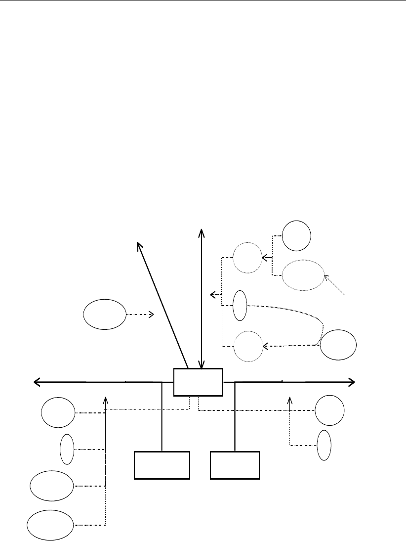
DRAFT
D-Water Quality, User Manual
CBOD5
OXY
NH4
r e a e r a t i o n
nitrificationmineralisation
T
Rc
rear
DOsat Salinity
Velocity
Hydrodynamic
sim ulation
horizontal
stream velocity
Wind
T
Rcnit
T
RcBOD
DOBODCr
DOBODOpt
sediment oxygen demand
fSODaut
saturation
concentration DO
General Dissolved Oxygen Model
358 of 382 Deltares

DRAFT
Standard substance files
B.4.2 Description of processes
For a formal description refer to the Technical Reference Manual (TRM) for the individual
processes of the Processes Library.
Mineralisation of BOD
Carbonaceous BOD is subject to a linear and temperature and oxygen dependent decay
process:
Mineralisation flux =−RcBOD ×[CBOD5 ]×ϑ(T−20 )
BOD ×[O2]−DOCr
BOD
DOOpt
BOD −DOCr
BOD
(B.3)
Input item Description Unit Default
value
Editable Range
[CBOD5] Concentration of carbonaceous
BOD5
gO2.m−3n.a. (state
variable)
n.a. –
RcBOD First order rate constant at 20 ◦C d−10.3 yes 0.1 - 2.0
ϑBOD Temperature coefficient - 1.04 no –
TWater temperature ◦C 15 yes depends
on local
conditions
[O2]Dissolved oxygen concentration gO2.m−3n.a. (state
variable)
n.a. –
DOCr
BOD Critical dissolved oxygen concen-
tration for BOD mineralisation
gO2.m−31 yes 0 - 1
DOOpt
BOD Optimal dissolved oxygen concen-
tration for BOD mineralisation
gO2.m−35 yes 0 - 5
Nitrification
Nitrification is the conversion of ammonium to nitrate. The stoichiometry of the reaction is
(NH+
4:O2:NO−
3=−1 : −4.571 : 1) with concentrations in gN.m−3, gO2.m−3and
gN.m−3respectively.
NH+
4+ 2O2→NO−
3+ 2H++H2O(B.4)
The nitrification process is formulated linearly and temperature and oxygen dependent:
Nitrification flux =−Rcnit ×[NH4]×ϑ(T−20 )
nit ×[O2]−DOCr
nit
DOOpt
nit −DOCr
nit
(B.5)
Input item Description Unit Default
value
Editable Range
[NH4]Concentration of ammonium gN.m−3n.a. (state
variable)
n.a. –
Rcnit First order rate constant for nitrifi-
cation at 20 ◦C
d−10.1 yes
ϑBOD Temperature coefficient - 1.07 no –
TWater temperature ◦C 15 yes depends
on local
conditions
[O2]Dissolved oxygen concentration gO2.m−3n.a. (state
variable)
n.a. –
Deltares 359 of 382

DRAFT
D-Water Quality, User Manual
Input item Description Unit Default
value
Editable Range
DOCr
nit Critical dissolved oxygen concen-
tration for BOD mineralisation
gO2.m−31 no 0 - 1
DOOpt
nit Optimal dissolved oxygen concen-
tration for BOD mineralisation
gO2.m−35 no 0 - 5
Nitrification stops when the water temperature drops below a certain critical level, which is
by default assumed to be 3 ◦C. Also, it is supposed to proceed under aerobic conditions
only. Therefore, the process flux depends on the dissolved oxygen concentration. If the
oxygen concentration is about 5 mg/l (DOOpt
nit ), the process proceeds without limitation. If the
oxygen concentration is below 1 mg/l (DOCr
nit), the process stops completely. If the oxygen
concentration is between 1 and 5 mg/l, the limitation factor varies linearly between 0 and 1.
Reaeration
Reaeration is formulated as a first order process working on the oxygen deficit:
Reaeration flux =Rcrear ×(DOsat −[O2]) ×ϑ(T−20)
rear (B.6)
Rcrear =f(wind speed, stream velocity, water depth) = f(Swrear)(B.7)
DOsat =f(T, salinity)(B.8)
Input item Description Unit Default
value
Editable Range
Rcrear First order reaeration rate constant d−1n.a. (in-
ternal vari-
able)
n.a. –
DOsat Saturation concentration of dis-
solved oxygen
gO2.m−3derived
from pro-
cess
n.a. –
[O2]Dissolved oxygen concentration gO2.m−3n.a. (state
variable)
n.a. –
ϑrear Temperature coefficient for reaera-
tion
- 1.016 no –
Twater temperature ◦C 15 yes depends
on local
conditions
Swrear Switch for reaeration formulation - 1 yes 1-7, 9-11
Wind speed and salinity are input parameters and, obviously, depend on local conditions. The
stream velocity can be derived from the hydrodynamic model using the process ‘Horizontal
stream velocity’. Water depth will be derived from the hydrodynamic model as well.
Reaeration depends on the wind speed, the stream velocity and the water depth. In rivers
the stream velocity usually provides the major contribution to the reaeration rate constant. In
lakes, estuaries and coastal areas stream velocities are generally lower than in rivers and wind
speed takes over as the main contributor. For this reason there are in total 10 formulations for
the reaeration rate constant in D-WAQ, indicated by the Swrear switch. In rivers, you can use
the default formulation. Otherwise, Swrear has to be set to 7 or 9 to include the influence of
wind. Both formulations are equally applicable.
360 of 382 Deltares

DRAFT
Standard substance files
Sediment Oxygen Demand
The ‘Sediment oxygen demand’ process allows you to specify an additional oxygen consump-
tion by the sediment. The input variable is called fSODaut and has the unit of g.m−2.d−1.
This process can proceed under aerobic conditions in the water column only. If the oxygen
concentration is over 2 mg/l, the process proceeds without limitation. If the oxygen concen-
tration is equal to or below 0 mg/l, the process stops completely. If the oxygen concentration
is between 0 and 2 mg/l, the limitation factor varies linearly between 0 and 1.
B.4.3 Notes
It is possible to reach a negative dissolved oxygen concentration in the model, if the consump-
tion of oxygen is allowed to proceed below 0 mg/l. This is only possible if one or more of the
critical dissolved oxygen concentrations is given a negative value. A negative dissolved oxy-
gen concentration can be considered as representing reduced substances such as methane
or sulphides
B.4.4 Output items
Apart from the state variables, the following parameters are available as extra output:
Parameter id Description Unit Model name
Rcrear Reaeration rate constant d−1RCREAR
DO saturation per-
centage
Saturation percentage of dissolved oxygen % SatPercOXY
DO saturation con-
centration
Saturation concentration of dissolved oxygen gO2.m−3SaturOXY
Stream velocity Horizontal stream velocity m.s−1Velocity
B.5 Basic suspended sediment model
B.5.1 General
The Basic Suspended Sediment Model is a predefined set of selected state variables, active
processes, editable input and output parameters. It has been constructed with the Processes
Library Configuration Tool and experienced users may use the same tool to edit the predefined
set. This describing document is linked to the files:
Name of PLCT input file <sed_1fraction_04.0>
Name of substance file <sed_1fraction_04.sub>
Deltares 361 of 382
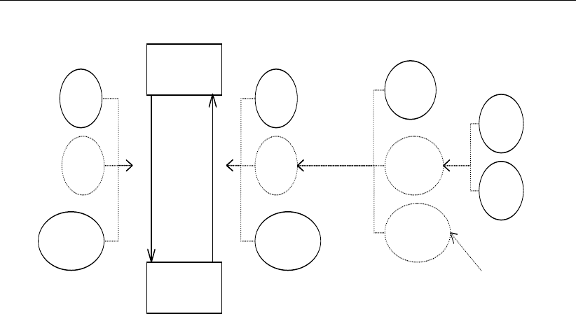
DRAFT
D-Water Quality, User Manual
IM1
IM1S1
s e d i m e n t a t i o n
r e s u s p e n s i o n
V
sed
Tau
Tau
cr
sed
Z
res
Tau
Tau
cr
res
Waves
Velocity
calculation of
shear stress
Chezy
Fetch
Wind
w a v e
c h a r a c t e r i s t i c s
Hydrodynamic
simulation
horizontal
stream velocity
B.5.2 Introduction
Suspended sediment is one of the easiest recognisable water quality parameters and one of
the most important for that matter. Suspended sediment, also often referred to as suspended
(particulate) matter, is generally associated with two major water quality issues:
1 Underwater light climate. Availability of light is essential for primary production. In highly
turbid water primary production is suppressed, while in clear waters lush underwater veg-
etation can develop (if other conditions such as nutrients are met).
2 Sedimentation and erosion. Millions of tons of sediment are dredged each year around
the world to keep seaways and harbours navigable for ships. Obviously, the rate of sed-
imentation in these economically important regions is of interest to authorities. On the
other hand, either at the dredging location or at a dumping site suspended sediment is
released during dredging, which may impact the nearby ecosystem.
The Basic Suspended Sediment Model contains a single suspended sediment fraction called
IM1 which stands for Inorganic Matter 1st fraction. D-WAQ allows you to include up to three
inorganic matter fractions. The Basic Suspended Sediment Model enables you to simulate
the dispersion of suspended sediment taking into account sedimentation and erosion. Ad-
ditionally, the Secchi disk depth is calculated to assess the effect on the underwater light
climate.
The table below gives an overview of the selected state variables and processes. The flow
chart on the top of this page shows the connection between state variables, processes and
process parameters.
362 of 382 Deltares

DRAFT
Standard substance files
Substance Group State variable Model name Processes
Suspended Matter Inorganic Matter (suspended) IM1 Sedimentation
Inorganic Matter in the sediment (settled) IM1S1 Erosion
Extra processes
Total resuspension
Composition of sediment layer S1
Calculation of bottom shear stress (Tau)
Wave characteristics
Horizontal stream velocity
Calculation of Secchi Depth
Extinction of visible light
B.5.3 Description of processes
For a formal description refer to the Technical Reference Manual (D-WAQ TRM,2013) for the
individual processes of the Processes Library.
B.5.4 Inorganic Matter (suspended and settled)
The concentration of suspended sediment in the water column (state variable IM1 ) de-
creases when sedimentation occurs. Erosion, alternatively called resuspension, increases
the suspended sediment concentration in the water column. Obviously, the opposite holds
for the amount settled on the bottom (state variable IM1S1 ). Together, IM1 and IM1S1
form a closed mass balance. The well-known Partheniades-Krone formulations for sedimen-
tation/erosion are implemented in D-WAQ.
The sedimentation of IM1 depends on the ambient shear stress (T au) and a user-defined
critical shear stress for sedimentation (T aused
cr ). Only if the ambient shear stress is lower than
the critical shear stress for sedimentation, sedimentation occurs:
Sedimentation flux =Psed ×Vsed ×[IM1] (B.9)
Psed = max 0,1−T au
T aused
cr (B.10)
Input item Description Unit Default value Editable Range
[IM 1] concentration of Inorganic Mat-
ter 1
g m−3n.a. (state vari-
able)
n.a. –
Psed Probability for sedimentation - n.a. (internal
variable)
n.a. 0 - 1
Vsed Settling velocity m d−10.1 yes 0.1 - 10
T au Ambient shear stress N m−2derived from
process
n.a. –
T aused
cr Critical shear stress for sedi-
mentation
N m−20.1 yes 0.01 - 2.0
Resuspension depends on the ambient shear stress and a user-defined critical shear stress
for resuspension (T aures
cr ). Only if the ambient shear stress is higher than the critical shear
Deltares 363 of 382

DRAFT
D-Water Quality, User Manual
stress for resuspension, resuspension occurs:
Resuspension flux =Pres ×Zres (B.11)
Pres = max 0,T aures
cr
T au −1(B.12)
Input item Description Unit Default value Editable Range
Pres Probability for resuspension - n.a. (internal
variable)
n.a. 0 – 1
Zres Zero-order resuspension rate g m−2d−10 yes 100 –
100,000
T au Ambient shear stress N m−2derived from
process
n.a. -
T aures
cr Critical shear stress for resus-
pension
N m−20.1 yes 0.05 – 2.0
The resuspension flux acts on the total amount of dry matter in the sediment. In the Basic
Suspended Sediment Model the state variable IM1S1 constitutes the total amount as we
have no other particulate components. However, in more extensive applications two more
inorganic matter components and several organic matter components can be included. Then
the resuspension flux of the individual components is proportional to the available fraction in
the sediment (e.g. if the mass fraction of IM1S1 is 10 % and the total resuspension flux is
100 g m−2d−1, then the resuspension flux of IM1S1 is 10 g.m−2.d−1). These fractions are
calculated by the process ‘Composition of sediment layer S1’.
The ambient shear stress, T au, represents the force exerted on the sediment by flowing
water and wave action.
T au =T auveloc +T auwaves (B.13)
T auveloc =f(stream velocity, Chezy)(B.14)
T auwaves =f(wind speed, water depth, Fetch)(B.15)
Input item Description Unit Default value Editable Range
T auveloc Shear stress exerted by stream
velocity
N.m−2n.a. (internal
variable)
n.a. –
T auwaves Shear stress exerted by waves N.m−2n.a. (internal
variable)
n.a. –
Chezy Chézy coefficient m1/2s−1no default yes 40 – 60
F etch Fetch length for the wind m no default yes depends on
area
The stream velocity can be derived from the hydrodynamic model using the process ‘Hori-
zontal stream velocity’. Wind speed, water depth and Fetch are used in the process ‘Wave
characteristics’ to calculate the typical wave height, wave period and wave amplitude, which
in turn determine the shear stress exerted by waves. The wind speed is in input parameter
and is often derived from measurements. Usually, a time series with a frequency of once per
hour or once per day is applied.
364 of 382 Deltares

DRAFT
Standard substance files
The Basic Suspended Sediment Model also calculates the Secchi Depth (in metres).
Secchi Depth =P Aconstant
ExtV l
(B.16)
ExtV l =ExtBak
V l +ExtIM 1
V l ×(IM1) (B.17)
Input item Description Unit Default value Editable Range
ExtV l Total extinction of Visible Light m−1n.a. n.a. –
P Aconstant Poole-Atkins constant - 1.7 no –
ExtBak
V l Background extinction for Visi-
ble light
- 0.08 yes 0.08 – 1.0
ExtIM 1
V l Specific Vl extinction of IM1 m2g−10.01 yes 0.01 – 0.05
[IM 1] Concentration of Inorganic
Matter 1
g m−3n.a. (state vari-
able)
n.a. –
B.5.5 Notes
The settling velocity can be made dependent on salinity, total suspended sediment con-
centration (to account for flocculation) and temperature.
Pure water has an extinction of 0.08 m−1and this is considered the background extinction.
The Basic Suspended Sediment Model has only one other constituent that contributes to
the extinction, namely Inorganic (suspended) Matter. Other constituents — mainly the
organic components — are ignored. A higher background extinction should be used to
compensate this.
B.5.6 Output items
Apart from the concentration of the state variables, the following parameters are available as
extra output:
Parameter id Description Unit Model name
T au Ambient shear stress N m−2Tau
Sedimentation flux Sedimentation flux of IM1 g m−2d−1fSedIM1
Resuspension flux Total resuspension flux g m−2d−1fResS1DM
ExtV l Total extinction of Visible light m−1ExtVL
Secchi Depth Secchi disk depth m SecchiDept
Stream velocity Horizontal stream velocity m s−1Velocity
B.6 References
The references used in this appendix are:
section B.3:Thomann and Mueller (1987)
section B.4:Streeter and Phelps (1925)
section B.5:Krone (1962); Partheniades (1962); Poole and Atkins (1929)
Deltares 365 of 382

DRAFT
D-Water Quality, User Manual
366 of 382 Deltares

DRAFT
C Statistical output functions
D-WAQ offers a number of statistical output facilities as described in Chapter 5. This section
describes the individual functions in more detail and provides some hints as to their use. For
each function the kind of output is described as well as the options that control the output.
Function Output parameters Output files
Stadsc Average (prefix: MEAN_)
Maximum (MAX_)
Minimum (MIN_)
Standard deviation (STDEV_)
Statistical map and monitor files
Stageo Geometrical mean (GEO_) Statistical map and monitor files
Stadpt Depth-averaged values (DPTAVG_)
Minimum over depth (DPTMIN_)
Maximum over depth (DPTMAX_)
Ordinary output files
Staday Periodic mean (TAVG_) Ordinary output files
Staqtl Quantile (QUANT_) Statistical map and monitor files
Staprc Percentage of exceedance (PERC_)
Mean concentration during ex-
ceedance (CMN_)
Statistical map and monitor files
C.1 Descriptive statistical parameters (stadsc)
The basic statistical parameters include:
The average value and the standard deviation over a chosen period.
The maximum and minimum value over that period.
For each water quality parameter these four quantities are computed over all the defined
periods. As by definition there is only one result (per period) for the whole simulation, the
quantities are written to a separate map and to a separate monitor file (both with the suffix
“-stat”). There is no corresponding history output (with only one time this makes very little
sense).
Options:
None
C.2 Geometric mean (stageo)
For quantities whose distribution is very skewed, like the concentration of bacteria or sus-
pended solids, a more useful measure to characterise the values may be the geometrical
mean:
Cgeo = (C1·C2·C3·. . . ·Cn)1/n
The geometrical mean is only defined for positive values (it can be interpreted as the side of
a hypercube with the same volume as the hyperblock with sides C1, C2. . . ). To make sure
Deltares 367 of 382

DRAFT
D-Water Quality, User Manual
very low values do not dominate the outcome, the function as implemented uses a threshold:
any value below the threshold is set equal to that threshold before it enters the computation.
As with the descriptive statistics function the averaging takes place over the defined period
and the output is written to the statistical map and monitor files.
Options:
threshold: Values below the threshold are reset to the threshold value to avoid
run-time errors and too large an influence on the result of very low
values.
C.3 Depth-average mean (stadpt)
Averaging can take place over time, but also over spatial dimensions. The most common
type of spatial averaging is the averaging over depth. The output parameter is written to the
ordinary files. The only difference with the regular output is that the values are repeated over
the layers. Along with the average, the output function also determines the minimum and the
maximum of the parameter over depth.
Options:
None
C.4 Periodical mean (staday)
With the descriptive statistics you get an overview of the water quality parameters for given
periods. It is also possible however to determine the daily mean for such parameters or the
mean for any period that is of interest. This is done with the staday function. The output
behaves as an ordinary time-dependent variable, with the exception that it is only updated at
the end of each period. The output is written to the ordinary output files.
Options:
period: The period over which to average (in seconds).
C.5 Quantiles (staqtl)
Some water quality standards are defined in terms of quantiles: for instance the concentration
of bacteria may exceed some value only 10 % of the time. This can be determined directly
(via the function staprc) or the 90 % quantile (percentage) can be determined: the value that
is exceeded only 10 % of the time.
The computation of this quantity is fairly complicated:
First the probable bounds for the concentrations of the water quality parameter in ques-
tion are determined a priori, that is, they must be set prior to the beginning of the water
quality computation. These bounds together with the number of buckets are used to set
up “buckets” or classes for the concentration.
Then during the computation (taking the period of interest into account) the actual concen-
trations are classified and the number of values in the corresponding bucket is increased.
At the end of the period of interest the histogram that has been calculated in this way is
examined to determine an estimate of the quantile. Suppose for instance that the 75 %
quantile is sought and five buckets are used, with minimum and maximum respectively 1
and 4:
There are 80 observations, so the 75 % quantile occurs within the fourth bucket (we must
368 of 382 Deltares

DRAFT
Statistical output functions
Bucket Number of values Cumulative number
<1 10 10
1–2 20 30
2–3 20 50
3–4 20 70
>4 10 80
determine the threshold below which 60 of the computed values occur). Linear interpola-
tion is used to estimate that threshold: the quantile is approximately 3.5.
The accuracy of these estimates depends greatly on the chosen range, the number of buckets
and the quantile that is looked for:
If the range is chosen wrongly, most values will fall into a few buckets. As there is no
information on the distribution within a bucket, this makes the estimate inaccurate.
The width of the buckets must be small enough to resolve the quantile in question: a 75
% quantile requires less buckets than a 99 % quantile (the bucket containing the latter
quantile should not contain much more than 1 % of the values).
Some rules of thumb:
Specify the minimum and maximum in such a way that typical values fall within the range,
for instance with oxygen, this could be: 4 to 12 mg/l.
Specify the width of the buckets to be at least 2 or 3 times narrower than the quantile:
For a 95 % quantile, the width of the bucket should be at most 2 % of the whole interval,
(2.5 times narrower than the 5 % that is left over). So: the number of buckets would be 50.
For a 10 % quantile (you seek the lower range of values), the bucket width should be at
most 5 %, so 20 buckets, or preferably more.
Options:
minimum: The minimum expected value for the water quality parameter.
maximum: The maximum expected value.
number of buckets: The number of buckets to use
level: The quantile level (in percents).
C.6 Percentage exceedance (staprc)
The staprc function enables you to compute the percentage of the time that a particular critical
level is exceeded (for instance the concentration of bacteria must not exceed some standard)
or the time that the water quality parameter is below that value (for instance oxygen should
be above some standard). Besides the percentage the mean value during the time the critical
level is exceeded is computed.
Options:
ccrit: The critical level that the water quality parameter must not exceed.
above: Indicates whether the time of exceedance is to be determined (“yes”)
or the time that the parameter is below the critical level (“no”).
Deltares 369 of 382

DRAFT
D-Water Quality, User Manual
370 of 382 Deltares

DRAFT
D Command-line arguments
D.1 Command-line arguments for the user-interface
With a few simple command-line arguments it is possible to automate important parts of the
user-interface:
Select a (new) hydrodynamic description file
Select a (new) substances file
Save the imported data into a (new) file
Exit the program automatically
The following options are available:
-coupling -comfile <com-filename>open the given communication file
-hydfile <hyd-filename>open the given hydrodynamic descrip-
tion file
-substances <substances filename>load the given substances file
-saveas <new scenario file>save the data under the given name
-save save the data under the same name
(provided there is one)
-times start, stop and increment
time in the following for-
mat, yyyymmddhhmmss (ex.
"20110101070000 20110102070000
00000000010000" )
-exit exit the user-interface (by itself it
causes no saving of data!)
These have to be handled in a sensible order (-exit last for instance!). For D-WAQ this means:
-scenario is treated first (if given; existing functionality)
-hydfile or -substances can be done then
-save or -saveas are handled thirdly
-exit comes last
D.2 Command-line arguments for the computational core
To run Delft3D-WAQ you need to use one or more command-line arguments. These are
explained below. The basic invocation of the computational core is:
Preprocessing part:
delwaq1 <input file> (one or more standard options ...)
and the computational part:
delwaq2 <input file> (zero or more specific options for the processes library ...)
The options for delwaq1 are:
-p <process definition file>: Specify the exact name of the process
definition file (this is usually the standard file)
Deltares 371 of 382

DRAFT
D-Water Quality, User Manual
-waq, -eco, -chem Enable the water quality processes belonging to a particular module.
The options for delwaq2 are:
-openpb <process definition file>: Specify the exact name of the process
definition file produced via the Open Processes Library Tool.
-nothreads <number>Turn on running in parallel on <number>threads. This will override
any settings in the inp-file. Setting <number>to 0 or omission of
<number>will run delwaq2 on all available threads.
Note that the first argument can be the name of the input file and that normally you do not
need to give any other command-line arguments to the second program, delwaq2.
To accommodate a pecularity that arises in the open processes library (which is compiled and
linked into a DLL or shared object), the routine to retrieve a command-line option (getcom())
also reads from a file called delwaq.options in the current directory. The structure of that
file is simple: each command-line argument must appear on a separate line, even if it is the
value for another one.
Delft3D-WAQ also has a number of specialised options. They are mentioned here, but be
aware that they should be used in a special context only:
-i <name of ini-file>: Use an INI file to specify what kind of submodel
is to be used, the location of the processes definition file and other
options.
-d Turn on domain decomposition mode, that is, get boundary condi-
tions from other D-Water Quality processes
-m <value>Monitoring level - provide more or less output, depending on the
value (defaults to 10)
-a Use only those water quality processes that are explicitly turned on
-np No processes are turned on at all
-conf <configuration>Specify the exact configuration (see also the options -waq, -eco and
-chem above). The argument <configuration>must be a valid con-
figuration.
-imax, -rmax, -cmax
<number>
Reserve a larger array for processing the input – the array of integers
(-imax), the array of reals (-rmax) or the array of strings (-cmax). If
the preprocessor runs into problems with the available memory, it will
report the sizes it requires. Rerunning the preprocessor step with
one or more of these options will enable it to reserve the memory it
requires.
372 of 382 Deltares

DRAFT
E User-defined wasteloads
E.1 Introduction
Occasionally a user of the WAQ water quality module needs to program wasteloads in a
way that is not standard supported by the WAQ system and user interface. Examples are
real-time control applications where a wasteload magnitude is made depending on the ac-
tual concentration values of substances. Another example is the combination of (multiple)
intake(s) and (multiple) outlet(s), as common with power stations. This last application can
then be combined with the first one if legislation would demand the switching off of outlets at
higher ambient temperatures and the start-up of cooling towers.
In very early days ‘user definable routines’ existed that needed to be compiled and linked
together with the WAQ system that came itself as a linkable library. These routines could be
used for that aim. However, for some 10 years that option is not supported any more. That
option is nevertheless used in-house at Deltares to implement the combination of intakes and
outlets that is common for cooling water processing. We feel that we should provide the early
facility again to our users, although now in a more modern way.
This appendix describes how that works and it also provides an example. The example that
we provide is exactly the in-house Deltares implementation of the intake-outlet feature, but
now in this new way. So, if you follow this appendix and compile the example application, then
you get the standard Deltares intake-outlet feature. You may however use this as a starting
point to provide your own algorithms for adjustment of intakes and outlets to run-time model
outcomes.
E.2 IT-background
The background of the new way of implementation is the use of dll files, dynamic link library
files. This means that the WAQ executable calls an external library that is linked at run-time.
This means that the software continues to come as an executable rather than as a linkable
library. It is nevertheless linking to external user routines, but now at run time. There are
currently two ways known at Deltares to do this:
1 Through a C-language interface.
The advantage of this procedure is that if you do not need the feature, the dll also need
not be present. This is the way we have implemented the “Open Processes Library” for
water quality kinetics. The disadvantage is that it is difficult to use Fortran 90 derived types
through the C-language interface, because they are not equivalent to C-structures. That
is why we have not chosen this way for the user wasteload routine interface.
2 Directly by calling the dll from the Fortran executable.
The advantage is that Fortran derived types can be used as a convenient way to group
all properties of a wasteload together and to define an array of those derived types. This
helps you very much to keep your program simple, so this approach is selected for the
user wasteload routine interface. The disadvantage of this procedure is however that the
dll should always be present, because the Fortran launcher checks its presence at start-
up of the executable, whether you use it or not. For this reason a dll is delivered with the
sample application. This dll can always be used in case you furthermore do not use the
user wasteload routine interface. If you need the user wasteload routine interface, you just
replace the default dll with yours.
It may turn out not to be as critical as it seems, but your compiler needs to produce a compat-
ible dll. We are using the Intel Fortran compiler. Many compilers deliver however valid dll’s for
interfacing.
Deltares 373 of 382

DRAFT
D-Water Quality, User Manual
Note: Due to rather technical issues, on Windows, the waste load module will write to a
file called "fort.32", instead of the correct monitoring file. It is possible to solve this, but the
required compile option must be applied to all components, also the components used by
other parts of Delft3D. For the moment, it is necessary to check this other file for any specific
messages.
E.3 The dynamic link library
The dll is called “waq_plugin_wasteload” and should contain a subroutine called “delwaq_user_wasteload”
with a prescribed parameter list. This subroutine can call any subroutine that you want to use
yourself. It is however for simplicity advised that you add the source of your subroutine to
the “module” file that contains “delwaq_user_wasteload” subroutine. See also the example.
All subroutines are contained in one and the same module file to avoid all sorts of interface
statements.
E.4 delwaq_user_wasteload subroutine
It has 8 parameters that will be explained in more detail here:
1nowst
This is an integer that serves input variable that should not be changed, because changing
will make the behaviour of the system unpredictable. It is the number of wasteloads. It
corresponds to the number of wasteloads in the user interface and it is the dimension of
all wasteload-related information.
2wasteloads
This is an array of derived types containing all wasteload information. The array is nowst
long. Its composition will be discussed later in more detail. In this array you will change
values according to your needs.
3notot
This is an integer that serves as input variable that should not be changed, because
changing will make the behaviour of the system unpredictable. It is the total number of
substances in the model. It serves as dimension for all arrays with substance related
properties.
4nosys
This is an integer that serves as input variable that should not be changed, because
changing will make the behaviour of the system unpredictable. It is the number of trans-
portable substances. So nosys is always smaller or equal than notot. The first nosys
substances move with the water. Any other substances do not. They may e.g. contain
sediment that is settled at the water bottom.
5noseg
This is an integer that serves as input variable that should not be changed, because
changing will make the behaviour of the system unpredictable. It is the number of com-
putational elements in the system. Among these elements there will be your wasteload or
withdrawal element number.
6itime
This is an integer that serves as input variable that should not be changed, because
changing will make the behaviour of the system unpredictable. It is the simulation time,
generally in seconds from the reference time. The reference time is given in the user in-
terface. You can use this variable if you want to have different behaviour of your wasteload
for certain time spans. Remind however that time dependent wasteloads are supported
through the normal user interface. Here you are assumed to let wasteloads react on the
actual model outcome of the moment (depending on the elapsed time of simulation if you
wish).
7conc(notot,noseg)
374 of 382 Deltares

DRAFT
User-defined wasteloads
This is a real array giving the concentration values of the substances at simulation time
itime.
It is an input variable and you should not change the value, although probably nothing will
go wrong if you did, because it is a derived variable from the actual simulation variables.
If you want your wasteload to be dependent on the concentration of substance isys in
computational element iseg, you can check the value of conc(isys,iseg) for this.
8syname(notot)
This is a character array giving the reserved names of the substances (the substance IDs).
They should not be changed because changing will make the behaviour of the system
unpredictable. The length of such an ID is 20 characters. If you wonder which substance
number is associated with “Salinity” (e.g. to close a source for agricultural water supply if
salinity is too high) then you check once in the beginning of the simulation
isys=find_substance(‘Salinity’,syname)
and you store this isys value in a local variable with the SAVE attribute. Then you can
use it to obtain conc(isys,iseg) during the simulation. Be aware that the number of
the substance called Salinity may vary from application to application, so do NOT program
a routine that assumes that Salinity is substance 2. You should also allow for a sensible
error message if the substance Salinity is not available at all. If it is not available, then you
have not switched it on.
E.5 “wasteload” derived type
Since Fortran 90 we are allowed to define other types than integers, real, logicals and char-
acters. We defined the type “wasteload”. Once we did so, an array of “wasteloads” can exist
just like an array of reals. Our derived type “wasteload” consists of:
an identification called <id>
This is also a derived type consisting of:
a unique character variable called <id>
This id is comparable with the earlier mentioned substance id. It is also 20 characters
long and you can check whether this is the wasteload that you want to change by
testing its id. The id of a wasteload is also mentioned in the user interface.
a not-necessarily unique character called <name>
This is a meaningful name of at most 40 characters long, which is most useful to print
messages.
a character value giving the <type>Although not supported yet in all user inter-
faces, many wasteloads of the same type can get the same concentration value, which
shortens input procedures. E.g. all “urban run-off” type of wasteloads can have the
same concentrations. This feature is not useful for you on this location.
Because the array of wasteloads is called wasteloads, you can retrieve the name of
wasteload 8 through wasteloads(8)%id%name. Its id string is in wasteloads(8)%id%id.
a location called <loc>
This derived type consists of a single integer called <segnr>containing the segment
number. In the future you may expect to appear also the location in world co-ordinates or
longitude-latitude here and probably also an array of segment numbers if it is a distributed
wasteload covering a larger area than one computational element.
If you want to know the segment number of the wasteload with id “Outfall 7”, then you
loop all wasteloads to check there %id%id string and if you found the wasteload you
looked for say as wasteload number iwst, then you find its computational element in:
wasteloads(iwst)%loc%segnr.
normal real called <flow>
This real contains the flow rate of the wasteloads in m3/s. You may change this value as
part of your programmed wasteload handling. Please be aware that in the current versions
Deltares 375 of 382

DRAFT
D-Water Quality, User Manual
of WAQ:
a flow of exactly 0.0 means something special (it means that the loads are considered
as mass / time rather than as concentrations times the mentioned flow. If you need a
zero flow, but if you do not want to set your concentration values of the wasteload to
zero, then you must specify a very low flow (say 10−10 m3/s).
A negative flow means that water will be withdrawn from the system. If loads (see
below) are exactly zero, water will be withdrawn with the current model concentration,
if not, the specified concentration will be applied for the withdrawal.
an array of normal reals called <loads(nosys)>
If the flow of a wasteload is not exactly zero, this array is interpreted as the concentration
values belonging to the flow. NOTE: this will change in the future. In the future a flag will
be added that indicates whether the values will be used as loads or as concentrations.
If the flow is negative and the values in loads() are not exact zero, then these values will
be interpreted as the withdrawn concentrations. NOTE: this will change in the future. In
the future a flag will be added that indicates whether withdrawals will take place with the
modelled concentrations or with a prescribed concentration.
You will adapt the values in this array for your substances of interest as part of your user-
programmed wasteload. Please look in the section explaining the syname substances
names to see how you can determine which substance number is the substance you are
looking for.
E.6 Utility function find_wasteload
Within the example code a function is available to find a wasteload index number with a given
ID. The function is not sensitive to the case in which the ID is given. The interface of the
routine is given below. The function makes use of the routine zoekns also included in the dll.
function find_wasteload( waste_id, wasteloads) result(iwst)
! function to find a wasteload on id in an array of wasteloads
character(len=*) :: waste_id ! wasteload id to be found
type(wasteload), pointer :: wasteloads(:) ! array of all wasteloads (structure)
integer :: iwst ! on return if found wasteload number,
! otherwise zero
E.7 Utility function find_substance
Within the example code a function is available to find a substance index number with a given
ID. The function is not sensitive to the case in which the ID is given. The interface of the
routine is given below. The function makes use of the routine zoekns also included in the dll.
function find_substance( substance_id, syname) result(isys)
! function to find a substance on id
character(len=*) :: substance_id ! substance id to be found
character(len=20) :: syname(:) ! substance names
integer :: isys ! on return if found substance number,
! otherwise zero
376 of 382 Deltares

DRAFT
User-defined wasteloads
E.8 Recapitulation
concentrations then you add your code to the sample code of the user programmable
wasteload dll.
You will change the wasteloads(mywaste)%flow and the
wasteloads(mywaste)%loads(mysubstance) values.
You will initially find the wasteload number you are looking for by checking the wasteload
id as contained in wasteloads(mywaste)%id%id against the id you are looking for.
You store the found value of mywaste with the ‘save’ attribute in a local variable for further
use.
You will initially find the substance number you are looking for by checking the substance
id as contained in syname(mysubstance) against the id you are looking for. You store
the found value of mysubstance with the ‘save’ attribute in a local variable for further use.
You may also change the value of wasteloads(mywaste)%loc%segnr and thus re-
locate the wasteload to a different location. Please be aware that if the waste flow or waste
withdrawal are substantial and are contained in the hydrodynamics flow database, this flow
is not redirected and inconsistencies may result. If you however redirect a wasteload that
is not contained in the hydrodynamic database and is just only present in the water quality
simulation then you will face no inconsistencies with the redirection.
You are advised NOT to change any of the other variables and only use their information
where you need it, without changing it.
E.9 Example source code delwaq_user_inlet_outlet
This code is added after this manual. It is not discussed per statement, but the general
philosophy is explained. The program:
Checks if a file ‘inlout1.dat’ exists.
If so it reads the combinations of names for inlets and outlets from this file.
If not so it fills a 100 locations array of combinations of names INLETnn and OUTLETnn.
It looks in the wasteload ids whether it can find any of the combinations as provided either
through the file or as filled in the arrays as defaults. NOTE the use of the utility routine
find_wasteload.
Note that all this is done for ‘ifirst’ = 1, so only at first call. Once the table of matches is
filled, it is stored and furthermore used every call.
The final setting of the ‘outlet’ to the values of the ‘inlet’ is done in the tiny piece at the end.
subroutine delwaq_user_inlet_outlet ( nowst , wasteloads, notot , &
nosys , noseg , &
itime , conc , syname)
! routine to set the default inlet-outlet coupling
! global declarations
implicit none
! arguments declarations
integer :: nowst ! number of wasteloads
type(wasteload), pointer :: wasteloads(:) ! array of all wasteloads
! (structure)
integer :: notot ! total number of substances
integer :: nosys ! number of active substances
integer :: noseg ! number of segments
integer :: itime ! system time
real :: conc(notot,noseg) ! concentration array
character(len=*) :: syname(notot) ! substance names
Deltares 377 of 382

DRAFT
D-Water Quality , User Manual
! local declarations
integer, parameter :: mxcomb = 100 ! maximum number of combinations
integer, save :: ifirst = 1 ! initialisation indicator
integer :: lunrep ! report file
logical :: l_exi ! file exists or not
integer :: ncomb ! number of possible inlet outlet
! combinations
integer :: ninout ! actual number of inlet outlet
! combinations
character(len=20) :: c_in ! read buffer name inlet
character(len=20) :: c_out ! read buffer name outlet
character(len=20) :: namin(mxcomb) ! names inlet in the possible
! combinations
character(len=20) :: namout(mxcomb) ! names outlet in the possible
! combinations
integer :: iwin(mxcomb) ! wasteload number inlet of the actual
! combinations
integer :: iwout(mxcomb) ! wasteload number outlet of the actual
! combinations
real :: flow ! inlet flow rate
integer :: ipin ! wasteload number inlet
integer :: ipout ! wasteload number outlet
integer :: iseg ! inlet segment number
integer :: iwst ! loop counter wasteloads
integer :: isys ! loop counter substances
integer :: icomb ! loop counter combinations
integer :: iinout ! loop counter of inlet outlet
! combinations
integer :: i ! loop counter
! Save all local variables
SAVE
! test if there are inlet outlet combinations
lunrep = 32
if ( ifirst == 1 ) then
ifirst = 0
write(lunrep,*)
write(lunrep,2000)
! if availeble read list of possible inlet outlet combinations
inquire (file=’inloutl.dat’,exist=l_exi)
if ( l_exi ) then
write(lunrep,2004)
open ( 83 , file=’inloutl.dat’ )
ncomb = 0
10 continue
read ( 83 , ’(2a20)’ , end = 20 ) c_in, c_out
ncomb = ncomb + 1
if ( ncomb .gt. mxcomb ) then
write(lunrep,2005) mxcomb
call srstop
endif
namin (ncomb) = c_in
namout(ncomb) = c_out
goto 10
20 continue
close
else
! construct the default list of combination INLETxx/OUTLETxx
write(lunrep,2006)
378 of 382 Deltares

DRAFT
User-defined wasteloads
do i = 1 , min(mxcomb,9)
write(namin (i),2007) i
write(namout(i),2008) i
enddo
do i = 10 , min(mxcomb,99)
write(namin (i),2009) i
write(namout(i),2010) i
enddo
do i = 100 , min(mxcomb,999)
write(namin(i),2011) i
write(namout(i),2012) i
enddo
ncomb = mxcomb
endif
! check the actual list of wasteloads with the list of possible combinations
ninout = 0
do icomb = 1 , ncomb
ipin = find_wasteload( namin (icomb), wasteloads)
ipout = find_wasteload( namout(icomb), wasteloads)
if ( ipin .gt. 0 .and. ipout .gt. 0 ) then
! a combination found, print and set administration
write(lunrep,*)
write(lunrep,2001) ipin ,wasteloads(ipin )%id%id
write(lunrep,2002) ipout,wasteloads(ipout)%id%id
write(lunrep,*)
ninout = ninout + 1
iwin(ninout) = ipin
iwout(ninout) = ipout
endif
enddo
if ( ninout == 0 ) write(lunrep,2013)
write(lunrep,2003)
endif
! set outlet equal to inlet flow *concentration at inlet segment for all found
! combinations
do iinout = 1 , ninout
ipin = iwin (iinout)
ipout = iwout(iinout)
iseg = wasteloads(ipin)%loc%segnr
flow = wasteloads(ipin)%flow
wasteloads(ipout)%flow = 0.0
do isys = 1, nosys
wasteloads(ipout)%loads(isys) = -flow*conc(isys,iseg)
enddo
do isys = nosys + 1 , notot
wasteloads(ipout)%loads(isys) = 0.0
enddo
enddo
c
return
2000 format (’ extra functionality INLET/OUTLET’)
2001 format (’ waste number:’,i5,’ name:’,a20,’ (INLET) coupled to’)
2002 format (’ waste number:’,i5,’ name:’,a20,’ (OUTLET)’)
2003 format (’ end extra functionality INLET/OUTLET’)
2004 format (’ possible INLET/OUTLET combinations will be read from ’, &
’file <inloutl.dat>’)
2005 format (’ error : number of combinations exceed maximum:’,i4)
2006 format (’ no file <inloutl.dat> using default combinations names’)
Deltares 379 of 382

DRAFT
D-Water Quality, User Manual
2007 format (’INLET’,i1,14x)
2008 format (’OUTLET’,i1,13x)
2009 format (’INLET’,i2,13x)
2010 format (’OUTLET’,i2,12x)
2011 format (’INLET’,i3,12x)
2012 format (’OUTLET’,i3,11x)
2013 format (’ no INLET/OUTLET combination found’)
end subroutine delwaq_user_inlet_outlet
380 of 382 Deltares
DRAFT
PO Box 177
2600 MH Del
Rotterdamseweg 185
2629 HD Del
The Netherlands
+31 (0)88 335 81 88
sales@deltaressystems.nl
www.deltaressystems.nl
Photo by: Mathilde Matthijsse, www.zeelandonderwater.nl
DRAFT
