D Waves User Manual Waves_User_Manual
User Manual: Pdf D-Waves_User_Manual
Open the PDF directly: View PDF ![]() .
.
Page Count: 136 [warning: Documents this large are best viewed by clicking the View PDF Link!]
- List of Figures
- List of Tables
- 1 A guide to this manual
- 2 Introduction to D-Waves
- 3 Getting started
- 4 Graphical User Interface
- 4.1 Introduction
- 4.2 MDW file, attribute files and file formats
- 4.3 Filenames and coventions
- 4.4 Setting up a D-Waves model
- 4.4.1 General
- 4.4.2 Area
- 4.4.3 Hydrodynamics from flow - currently default tab
- 4.4.4 Spectral resolution (deafult) - currently default tab
- 4.4.5 Domain
- 4.4.6 Time Frame, Hydrodynamics and Wind
- 4.4.7 Boundary Conditions
- 4.4.8 Physical parameters
- 4.4.9 Physical processes
- 4.4.10 Numerical parameters
- 4.4.11 Output parameters
- 4.4.12 Output
- 5 Conceptual description
- References
- A Files of Delft3D-WAVE
- A.1 MDW-file
- A.2 Attribute files of Delft3D-WAVE
- A.2.1 Introduction
- A.2.2 Orthogonal curvilinear grid
- A.2.3 Time-series for wave boundary conditions
- A.2.4 Obstacle file
- A.2.5 Segment file
- A.2.6 Depth file
- A.2.7 Space-varying bottom friction (not yet implemented for Delft3D-WAVE)
- A.2.8 Wave boundary conditions
- A.2.8.1 Time-varying and uniform wave conditions in <wavecon.rid> file
- A.2.8.2 Time-varying and space-varying wave boundary conditions using BCW files
- A.2.8.3 Space-varying wave boudnary conditions using for UNIBEST coupling (<md-vwac>-file)
- A.2.8.4 Time- and space-varying wave boundary conditions: TPAR file
- A.2.9 Spectral input and output files
- A.2.10 Space-varying wind field
- B Definition of SWAN wave variables
- C Example of MDW-file Siu-Lam
Delft3D flexible Mesh suite
1D/2D/3D Modelling suite for integral water solutions
User Manual
D-Waves
DRAFT
DRAFT
DRAFT
D-Waves
Simulation of short-crested waves with SWAN
User Manual
Released for:
Delft3D FM Suite 2018
D-HYDRO Suite 2018
Version: 1.1
SVN Revision: 54363
April 18, 2018
DRAFT
D-Waves, User Manual
Published and printed by:
Deltares
Boussinesqweg 1
2629 HV Delft
P.O. 177
2600 MH Delft
The Netherlands
telephone: +31 88 335 82 73
fax: +31 88 335 85 82
e-mail: info@deltares.nl
www: https://www.deltares.nl
For sales contact:
telephone: +31 88 335 81 88
fax: +31 88 335 81 11
e-mail: software@deltares.nl
www: https://www.deltares.nl/software
For support contact:
telephone: +31 88 335 81 00
fax: +31 88 335 81 11
e-mail: software.support@deltares.nl
www: https://www.deltares.nl/software
Copyright © 2018 Deltares
All rights reserved. No part of this document may be reproduced in any form by print, photo
print, photo copy, microfilm or any other means, without written permission from the publisher:
Deltares.

DRAFT
Contents
Contents
List of Figures vii
List of Tables ix
1 A guide to this manual 1
1.1 Introduction .................................. 1
1.2 Overview ................................... 1
1.3 Manual version and revisions ......................... 2
1.4 Typographical conventions .......................... 2
1.5 Changes with respect to previous versions .................. 2
2 Introduction to D-Waves 3
2.1 SWAN wave model .............................. 3
2.1.1 Introduction .............................. 3
2.1.2 Conceptual design of SWAN: an introduction . . . . . . . . . . . . . 3
2.1.3 Coupling of SWAN with D-Flow Flexible Mesh . . . . . . . . . . . . 3
2.2 Areas of application .............................. 4
2.3 Standard features ............................... 4
2.4 Special features ................................ 4
2.5 Utilities .................................... 4
3 Getting started 5
3.1 Introduction .................................. 5
3.2 Overview of D-Waves plug-in ......................... 5
3.2.1 Project tree .............................. 6
3.2.2 Central (map) window ........................ 7
3.2.3 Map tree ............................... 7
3.2.4 Message window ........................... 8
3.2.5 Time navigator ............................ 8
3.3 Setting up a D-Waves model (basic steps) .................. 8
3.3.1 Add a D-Waves model ........................ 8
3.3.2 Set up a D-Waves model . . . . . . . . . . . . . . . . . . . . . . . 8
3.3.3 Validate D-Waves model . . . . . . . . . . . . . . . . . . . . . . . 9
3.3.4 File tree (to be implemented) . . . . . . . . . . . . . . . . . . . . . 11
3.3.5 Run D-Waves model ......................... 11
3.3.6 Inspect model output ......................... 11
3.3.7 Import/export or delete a D-Waves model . . . . . . . . . . . . . . . 11
3.3.8 Save project ............................. 13
3.3.9 Exit Delta Shell . . . . . . . . . . . . . . . . . . . . . . . . . . . . 13
3.4 Important differences and new features compared to the former GUI (Delft3D-
Waves) .................................... 13
3.4.1 Project vs model ........................... 13
3.4.2 Load/save vs import/export . . . . . . . . . . . . . . . . . . . . . . 14
3.4.3 Working from the map . . . . . . . . . . . . . . . . . . . . . . . . 14
3.4.4 Coordinate conversion . . . . . . . . . . . . . . . . . . . . . . . . 14
3.4.5 Model area .............................. 15
3.4.6 Ribbons (hot keys) . . . . . . . . . . . . . . . . . . . . . . . . . . 15
3.4.7 Context menus (RMB) . . . . . . . . . . . . . . . . . . . . . . . . 16
3.4.8 Scripting ............................... 16
4 Graphical User Interface 17
4.1 Introduction .................................. 17
4.2 MDW file, attribute files and file formats . . . . . . . . . . . . . . . . . . . . 17
Deltares iii

DRAFT
D-Waves, User Manual
4.3 Filenames and coventions . . . . . . . . . . . . . . . . . . . . . . . . . . 18
4.4 Setting up a D-Waves model ......................... 19
4.4.1 General ................................ 19
4.4.2 Area ................................. 21
4.4.2.1 Obstacles ......................... 22
4.4.2.2 Observation Points . . . . . . . . . . . . . . . . . . . . . 24
4.4.2.3 Observation Curves . . . . . . . . . . . . . . . . . . . . 24
4.4.3 Hydrodynamics from flow - currently default tab . . . . . . . . . . . . 25
4.4.4 Spectral resolution (deafult) - currently default tab . . . . . . . . . . . 25
4.4.5 Domain ................................ 27
4.4.5.1 Import and export grids and bathymetries . . . . . . . . . . 27
4.4.5.2 Create and/or edit grids in RGFGRID . . . . . . . . . . . . 28
4.4.5.3 Create and/or edit bathymetries using the spatial editor . . . 28
4.4.5.4 Nest domains ....................... 28
4.4.5.5 Spectral resolution and wind (per domain) . . . . . . . . . 30
4.4.6 Time Frame, Hydrodynamics and Wind . . . . . . . . . . . . . . . . 30
4.4.7 Boundary Conditions ......................... 34
4.4.8 Physical parameters ......................... 39
4.4.8.1 Constants ......................... 39
4.4.9 Physical processes . . . . . . . . . . . . . . . . . . . . . . . . . . 40
4.4.10 Numerical parameters . . . . . . . . . . . . . . . . . . . . . . . . 44
4.4.11 Output parameters . . . . . . . . . . . . . . . . . . . . . . . . . . 45
4.4.12 Output ................................ 48
5 Conceptual description 49
5.1 Introduction .................................. 49
5.2 General background ............................. 49
5.2.1 Units and co-ordinate systems . . . . . . . . . . . . . . . . . . . . 49
5.2.2 Choice of grids and boundary conditions . . . . . . . . . . . . . . . 50
5.2.3 Output grids ............................. 52
5.3 Physical background of SWAN . . . . . . . . . . . . . . . . . . . . . . . . 52
5.3.1 Action balance equation . . . . . . . . . . . . . . . . . . . . . . . 52
5.3.2 Propagation through obstacles . . . . . . . . . . . . . . . . . . . . 56
5.3.3 Wave-induced set-up ......................... 57
5.3.4 Diffraction .............................. 57
5.4 Full expressions for source terms . . . . . . . . . . . . . . . . . . . . . . . 57
5.4.1 Input by wind ............................. 57
5.4.2 Dissipation of wave energy . . . . . . . . . . . . . . . . . . . . . . 58
5.4.3 Nonlinear wave-wave interactions . . . . . . . . . . . . . . . . . . . 60
5.5 Numerical implementation . . . . . . . . . . . . . . . . . . . . . . . . . . 63
5.5.1 Propagation ............................. 64
References 67
A Files of Delft3D-WAVE 73
A.1 MDW-file ................................... 73
A.1.1 General description . . . . . . . . . . . . . . . . . . . . . . . . . . 73
A.1.2 Offline calculation ........................... 77
A.2 Attribute files of Delft3D-WAVE . . . . . . . . . . . . . . . . . . . . . . . . 77
A.2.1 Introduction .............................. 77
A.2.2 Orthogonal curvilinear grid . . . . . . . . . . . . . . . . . . . . . . 77
A.2.3 Time-series for wave boundary conditions . . . . . . . . . . . . . . 79
A.2.4 Obstacle file ............................. 79
A.2.5 Segment file ............................. 81
iv Deltares

DRAFT
Contents
A.2.6 Depth file ............................... 82
A.2.7 Space-varying bottom friction (not yet implemented for Delft3D-WAVE) 83
A.2.8 Wave boundary conditions . . . . . . . . . . . . . . . . . . . . . . 84
A.2.8.1 Time-varying and uniform wave conditions in <wavecon.rid>
file ............................. 84
A.2.8.2 Time-varying and space-varying wave boundary conditions
using BCW files . . . . . . . . . . . . . . . . . . . . . . 85
A.2.8.3 Space-varying wave boudnary conditions using for UNIBEST
coupling (<md-vwac>-file) . . . . . . . . . . . . . . . . . 92
A.2.8.4 Time- and space-varying wave boundary conditions: TPAR
file ............................. 93
A.2.9 Spectral input and output files . . . . . . . . . . . . . . . . . . . . . 93
A.2.10 Space-varying wind field . . . . . . . . . . . . . . . . . . . . . . . 98
A.2.10.1 Space-varying wind on the computational (SWAN) grid . . . 100
A.2.10.2 Space-varying wind on an equistant grid . . . . . . . . . . 104
A.2.10.3 Space-varying wind on a curvilinear grid . . . . . . . . . . 108
A.2.10.4 Space-varying wind on a Spiderweb grid . . . . . . . . . . 111
B Definition of SWAN wave variables 117
C Example of MDW-file Siu-Lam 121
Deltares v

DRAFT
D-Waves, User Manual
vi Deltares
DRAFT
List of Figures
List of Figures
3.1 Start-up lay-out Delta Shell framework .................... 5
3.2 Project tree of D-Waves plugin ........................ 6
3.3 Central map with contents of the D-Waves plug-in . . . . . . . . . . . . . . . 7
3.4 Map tree controlling map contents ...................... 7
3.5 Log of messages, warnings and errors in message window . . . . . . . . . . 8
3.6 Time navigator in Delta Shell ......................... 8
3.7 Adding a new model from the ribbon . . . . . . . . . . . . . . . . . . . . . 8
3.8 Adding a new model using the Right Mouse Button on "project1" in the project
tree ...................................... 9
3.9 Select "Wave model" ............................. 9
3.10 Validate model ................................ 10
3.11 Validation report ............................... 10
3.12 Run model .................................. 11
3.13 Output of wave model in project tree . . . . . . . . . . . . . . . . . . . . . 12
3.14 Import wave model from project tree . . . . . . . . . . . . . . . . . . . . . 12
3.15 Import wave model from file ribbon . . . . . . . . . . . . . . . . . . . . . . 13
3.16 Set map coordinate system using RMB . . . . . . . . . . . . . . . . . . . . 14
3.17 Select a coordinate system using the quick search bar . . . . . . . . . . . . 15
3.18 Perform operations using the hot keys . . . . . . . . . . . . . . . . . . . . . 15
4.1 Overview of the general tab . . . . . . . . . . . . . . . . . . . . . . . . . . 19
4.2 Set the model coordinate system . . . . . . . . . . . . . . . . . . . . . . . 20
4.3 Nautical convention (left panel) and Cartesian convention (right panel) for di-
rection of winds and (incident) waves . . . . . . . . . . . . . . . . . . . . . 21
4.4 Add Area features using the Region ribbon . . . . . . . . . . . . . . . . . . 22
4.5 Area features added to map . . . . . . . . . . . . . . . . . . . . . . . . . . 22
4.6 Edit Area features using the Edit section of the Map ribbon . . . . . . . . . . 22
4.7 Attribute table with properties of obstacles . . . . . . . . . . . . . . . . . . 23
4.8 Select which quantities should be used from FLOW computation . . . . . . . 25
4.9 Import a RGFGRID file from the project tree . . . . . . . . . . . . . . . . . . 27
4.10 Visualize the D-Waves grid on the central map . . . . . . . . . . . . . . . . 27
4.11 Create and/or edit the grid using RGFGRID . . . . . . . . . . . . . . . . . 28
4.12 Create and/or edit the grid using the spatial editor . . . . . . . . . . . . . . . 29
4.13 Create or edit the grid using RGFGRID . . . . . . . . . . . . . . . . . . . . 29
4.14 Create or edit the grid using RGFGRID . . . . . . . . . . . . . . . . . . . . 29
4.15 Create or edit the grid using RGFGRID . . . . . . . . . . . . . . . . . . . . 30
4.16 Specify spectral resolution and wind per domain . . . . . . . . . . . . . . . 30
4.17 Adding time points using the table . . . . . . . . . . . . . . . . . . . . . . . 31
4.18 Pasting time points from another series or program, for example Excel . . . . 31
4.19 Synchronizing the time points with the time points specified for the boundary
conditions ................................... 31
4.20 Specification of constant hydrodynamics . . . . . . . . . . . . . . . . . . . 32
4.21 Specification of hydrodynamics per time point . . . . . . . . . . . . . . . . . 32
4.22 Specification of constant wind ......................... 33
4.23 Specification of wind per time point . . . . . . . . . . . . . . . . . . . . . . 33
4.24 Specification of wind (field) from file . . . . . . . . . . . . . . . . . . . . . . 33
4.25 Add a spiderweb wind field . . . . . . . . . . . . . . . . . . . . . . . . . . 33
4.26 Select Add Boundary from Region ribbon . . . . . . . . . . . . . . . . . . . 34
4.27 Draw the boundary support points on the map . . . . . . . . . . . . . . . . 35
4.30 Overview of the boundary conditions editor . . . . . . . . . . . . . . . . . . 35
4.28 Boundaries are added to the project tree under Boundary Conditions . . . . . 36
4.29 Edit the spatial definition in the attribute table . . . . . . . . . . . . . . . . . 36
Deltares vii

DRAFT
D-Waves, User Manual
4.31 Activate a support point in the boundary condition editor and inspect the loca-
tion of the selected support point in the Geomtery view . . . . . . . . . . . . 36
4.32 Select spectrum shape and set corresponding properties . . . . . . . . . . . 37
4.33 Specify parameterized wave boundary conditions and inspect in graph . . . . 38
4.34 Overview of physical Constants . . . . . . . . . . . . . . . . . . . . . . . . 39
4.35 Overview of physical Processes . . . . . . . . . . . . . . . . . . . . . . . . 40
4.36 Overview of Numerical parameters . . . . . . . . . . . . . . . . . . . . . . 44
4.37 Overview of Output parameters . . . . . . . . . . . . . . . . . . . . . . . . 46
5.1 Nautical convention (left panel) and Cartesian convention (right panel) for di-
rection of winds and (incident) waves . . . . . . . . . . . . . . . . . . . . . 49
5.2 Definition of grids (input, computational and output grids) in Delft3D-WAVE . . 50
5.3 Disturbed regions in the computational grid . . . . . . . . . . . . . . . . . . 51
A.1 Definition wind components for space varying wind . . . . . . . . . . . . . . 103
A.2 Definition sketch of wind direction according to Nautical convention . . . . . . 104
A.3 Illustration of the data to grid conversion for meteo input on a separate curvi-
linear grid . . . . . . . . . . . . . . . . . . . . . . . . . . . . . . . . . . . 110
A.4 Wind definition according to Nautical convention . . . . . . . . . . . . . . . 112
A.5 Spiderweb grid definition . . . . . . . . . . . . . . . . . . . . . . . . . . . 113
viii Deltares

DRAFT
List of Tables
List of Tables
Deltares ix

DRAFT
D-Waves, User Manual
x Deltares

DRAFT
1 A guide to this manual
1.1 Introduction
This User Manual concerns the module D-Waves.
This module is part of several Modelling suites, released by Deltares as Deltares Systems
or Dutch Delta Systems. These modelling suites are based on the Delta Shell framework.
The framework enables to develop a range of modeling suites, each distinguished by the
components and — most significantly — the (numerical) modules, which are plugged in. The
modules which are compliant with the Delta Shell framework are released as D-Name of the
module, for example: D-Flow Flexible Mesh, D-Waves, D-Water Quality, D-Real Time Control,
D-Rainfall Run-off.
Therefore, this user manual is shipped with several modelling suites. In the start-up screen
links are provided to all relevant User Manuals (and Technical Reference Manuals) for that
modelling suite. It will be clear that the Delta Shell User Manual is shipped with all these
modelling suites. Other user manuals can be referenced. In that case, you need to open the
specific user manual from the start-up screen in the central window. Some texts are shared
in different user manuals, in order to improve the readability.
1.2 Overview
In this manual advice is given on how to get started with the SWAN wave model. Furthermore,
the manual gives a description on how to use the SWAN model within D-Waves.
Generally, the following items with respect to the use of the D-Waves module will be described
in this manual.
Chapter 2:Introduction to D-Waves, provides specifications of D-Waves such as required
computer configuration, how to install the software, as well as its main features.
Chapter 3:Getting started, introduces the D-Waves Graphical User Interface (GUI), used to
define the input required for a wave simulation.
Chapter 4:Graphical User Interface, provides practical information on the selection of all
parameters and the tuning of the model.
Chapter 5:Conceptual description, discusses the unit and co-ordinate system, the various
grids, grid-numbering etc. In addition, a brief description is given on the physics and numerics
that have been implemented in D-Waves.
References, provides a list of publications and related material on the D-Waves module.
Appendix A:Files of Delft3D-WAVE, gives a description of all the attribute files that can be
used in the D-Waves input. This information is required for generating certain attribute files
either manually or by means of other utility programs. For other attribute files this description
is just for your information.
Appendix B:Definition of SWAN wave variables, the definition of the integral wave param-
eters is given.
Appendix C:Example of MDW-file Siu-Lam, an example of a Master Definition file for the
Wave <∗.mdw>input file for the WAVE module is given.
Deltares 1 of 124

DRAFT
D-Waves, User Manual
1.3 Manual version and revisions
This manual applies to:
the D-HYDRO Suite, version 2016
the Delft3D Flexible Mesh Suite, version 2016
1.4 Typographical conventions
Throughout this manual, the following conventions help you to distinguish between different
elements of text.
Example Description
Module
Project
Title of a window or a sub-window are in given in bold.
Sub-windows are displayed in the Module window and
cannot be moved.
Windows can be moved independently from the Mod-
ule window, such as the Visualisation Area window.
Save Item from a menu, title of a push button or the name of
a user interface input field.
Upon selecting this item (click or in some cases double
click with the left mouse button on it) a related action
will be executed; in most cases it will result in displaying
some other (sub-)window.
In case of an input field you are supposed to enter input
data of the required format and in the required domain.
<\tutorial\wave\swan-curvi>
<siu.mdw>
Directory names, filenames, and path names are ex-
pressed between angle brackets, <>. For the Linux
and UNIX environment a forward slash (/) is used in-
stead of the backward slash (\) for PCs.
“27 08 1999” Data to be typed by you into the input fields are dis-
played between double quotes.
Selections of menu items, option boxes etc. are de-
scribed as such: for instance ‘select Save and go to
the next window’.
delft3d-menu Commands to be typed by you are given in the font
Courier New, 10 points.
In this User manual, user actions are indicated with this
arrow.
[m s−1] [−] Units are given between square brackets when used
next to the formulae. Leaving them out might result in
misinterpretation.
1.5 Changes with respect to previous versions
This is the first edition which is published.
2 of 124 Deltares

DRAFT
2 Introduction to D-Waves
2.1 SWAN wave model
2.1.1 Introduction
To simulate the evolution of random, short-crested wind-generated waves in estuaries, barrier
islands with tidal inlets, tidal flats, lakes, channels etc., the D-Waves module can be used. D-
Waves is based on the third-generation SWAN model - SWAN is an acronym for Simulating
WAves Nearshore (see e.g. Holthuijsen et al. (1993); Booij et al. (1999); Ris et al. (1999)).
The SWAN model was developed at Delft University of Technology (The Netherlands). It is
specified as the new standard for nearshore wave modelling and coastal protection studies.
The SWAN model has been released under public domain. For more information about SWAN
reference is made to the SWAN home page:
http://www.swan.tudelft.nl/
D-Waves computes wave propagation, wave generation by wind, non-linear wave-wave inter-
actions and dissipation, for a given bottom topography, wind field, water level and current field
in waters of deep, intermediate and finite depth.
2.1.2 Conceptual design of SWAN: an introduction
The SWAN model is based on the discrete spectral action balance equation and is fully spec-
tral (in all directions and frequencies). The latter implies that short-crested random wave fields
propagating simultaneously from widely different directions can be accommodated (e.g. a
wind sea with super-imposed swell). SWAN computes the evolution of random, short-crested
waves in coastal regions with deep, intermediate and shallow water and ambient currents. The
SWAN model accounts for (refractive) propagation due to current and depth and represents
the processes of wave generation by wind, dissipation due to whitecapping, bottom friction
and depth-induced wave breaking and non-linear wave-wave interactions (both quadruplets
and triads) explicitly with state-of-the-art formulations. Wave blocking by currents is also ex-
plicitly represented in the model.
To avoid excessive computing time and to achieve a robust model in practical applications,
fully implicit propagation schemes have been applied. The SWAN model has successfully
been validated and verified in several laboratory and (complex) field cases (see Ris et al.
(1999); WL | Delft Hydraulics (1999,2000)).
2.1.3 Coupling of SWAN with D-Flow Flexible Mesh
This is discussed in the D-Flow Flexible Mesh User Manual.
Deltares 3 of 124
DRAFT
D-Waves, User Manual
2.2 Areas of application
The D-Waves model can be used for coastal development and management related projects
and for harbour and offshore installation design. It can also be used as a wave hindcast
model. Typical areas for the application of the SWAN model may vary of up to more than 50
km ×50 km. Generally, the model can be applied in the following areas:
estuaries
tidal inlets
lakes
barrier islands with tidal flats
channels
coastal regions
2.3 Standard features
The SWAN model accounts for the following physics:
wave refraction over a bottom of variable depth and/or a spatially varying ambient current
depth and current-induced shoaling
wave generation by wind
dissipation by whitecapping
dissipation by depth-induced breaking
dissipation due to bottom friction (three different formulations)
nonlinear wave-wave interactions (both quadruplets and triads)
wave blocking by flow
transmission through, blockage by or reflection against obstacles
diffraction
Note that diffraction and reflections are now available in the present SWAN version under
D-Waves.
2.4 Special features
A special feature is the dynamic interaction with D-Flow Flexible Mesh (i.e. two way wave-
current interaction). By this the effect of waves on current (via forcing, enhanced turbulence
and enhanced bed shear stress) and the effect of flow on waves (via set-up, current refraction
and enhanced bottom friction) are accounted for.
2.5 Utilities
In using D-Waves, the following utilities are important:
module description
RGFGRID for generating grids.
Delft3D-QUICKPLOT for visualising simulation results.
For details on using these utility programs you are referred to the respective User Manuals.
4 of 124 Deltares
DRAFT
3 Getting started
3.1 Introduction
The D-Waves plugin is part of the Delta Shell framework. For an introduction to the general
look-and-feel and functionalities of the DeltaShell framework you are referred to the Delta Shell
framework manual. This Chapter gives an overview of the basic features of the D-Waves
plugin and will guide you through the main steps to set up a D-Waves model. For a more
detailed description of the GUI features you are referred to 4. For technical documentation
you are referred to the D-Waves manual.
3.2 Overview of D-Waves plug-in
Delta Shell is only available for Windows operating systems. You can either install the msi-
version or copy the zip-version. For the msi-version first follow the steps in the installatio
guide. Consequently, open Delta Shell by double-clicking the Delta Shell icon in programs
or the short-cut on your desktop. For the zip-version you don’t have to install anything. First
unpack the zip, consequently go to bin and double-click DeltaShell.Gui.exe to open Delta
Shell.
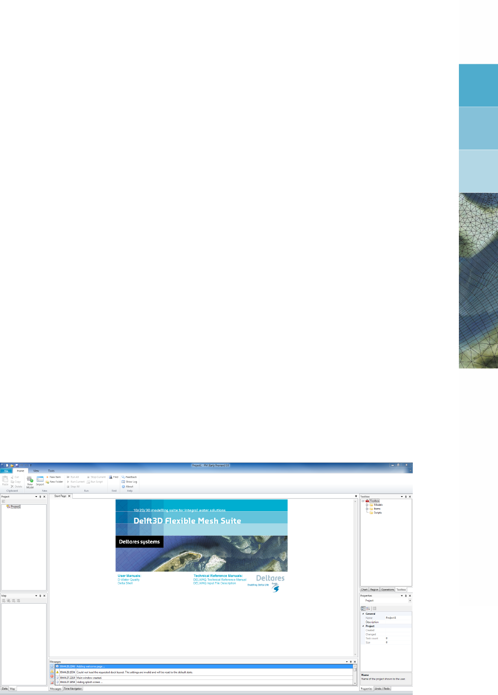
When you open Delta Shell for the first time the lay-out will look like Figure 3.1. The basic
lay-out consists of the following items:
project tree - upper left
map tree and data window - lower left
central (map) window - upper centre
message window and time navigator - lower centre
region and chart window - upper right
properties and undo/redo window - lower right
Figure 3.1: Start-up lay-out Delta Shell framework
All the windows can be customized/hidden according to your own preferences. These set-
tings will be automatically saved for the next time you open Delta Shell. The most important
windows for the D-Waves plugin are the project tree, central (map) window, map tree, the
Deltares 5 of 124
DRAFT
D-Waves, User Manual
message window and time navigator. The contents of these windows are briefly discussed in
the subsections below.
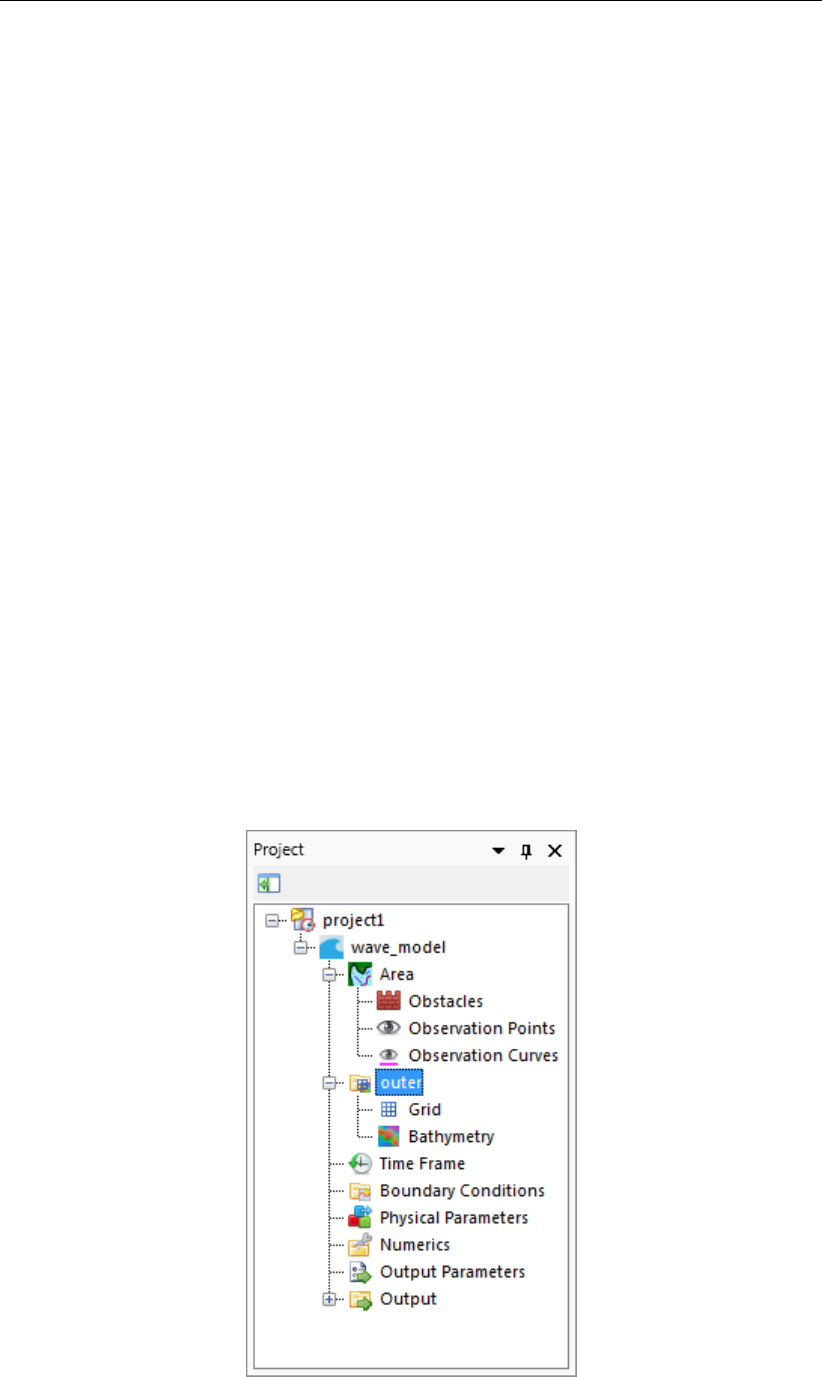
3.2.1 Project tree
After adding or importing a Delft3D-WAVE model (see section . . . ), the project tree will be
extended with wave model specific features (see Figure 3.2). The project tree provides you
with the basic steps to set up a Delft3D-WAVE model.
The project tree consists of the following features:
General general model information such as description, model coordinate
system, simulation mode, directional convention, etc.
Area geographical (GIS based) features, such as observation points and
curves and obstacles
Domain (outer) model grid and bathymetry (multiple in case of nested model)
Hydrodynamics variables to be copied from FLOW model in case of a coupled model
Spectral resolution default spectral settings
Time Frame time points and (time-varying) hydrodynamic and wind conditions
Boundary conditions wave boundary conditions and spectrum specification
Physical parameters physical settings for processes such as setup, wave breaking, refrac-
tion, triads, etc.
Numerical parameters numerical simulation settings
Output parameters output specification
Output output after running the simulation
Upon clicking the items in the project tree the corresponding tab (in case of GIS/map-independent
model settings), attribute table (in case of GIS/map-dependent model settings) or editor view
(in case of advanced editing options) will open. Using the right mouse button (RMB) gives
options such as importing/exporting model data.
Figure 3.2: Project tree of D-Waves plugin
6 of 124 Deltares
DRAFT
Getting started
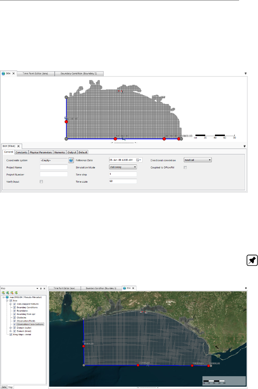
3.2.2 Central (map) window
The central window shows the contents of the main editor you are working with. In most cases
this will be the central map with tabulated input fields (see Figure 3.3). The map is used to edit
GIS dependent model data, the tabulated input fields to edit overall model settings. Moreover,
the contents of the central window can also be a specific editor such as the time point editor
or the boundary condition editor. Each of these editors will open as a separate view.
Figure 3.3: Central map with contents of the D-Waves plug-in
3.2.3 Map tree
The map tree allows the user to control the visibility of the contents of the central map using
checkboxes. Furthermore, the user can add (wms) layers, such as satellite imagery (see
Figure 3.4).
Note: : Please note that the map usually has a different coordinate system than the model. In
rendering the model attributes they are transformed to the map coordinate system (for visual
inspection on the map), but the model will be saved in the model coordinate system.
Figure 3.4: Map tree controlling map contents
Deltares 7 of 124
DRAFT
D-Waves, User Manual
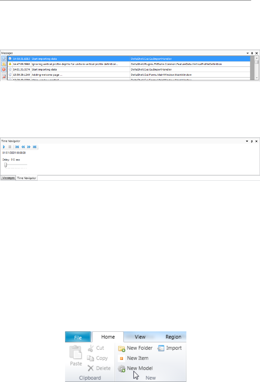
3.2.4 Message window
The message window (Figure 3.5) provides a log of information on the recent activities in
Delta Shell. It also provides warning and error messages.
Figure 3.5: Log of messages, warnings and errors in message window
3.2.5 Time navigator
The time navigator (Figure 3.6) can be used to step through time dependent model output
and other time dependent GIS features on the map.
Figure 3.6: Time navigator in Delta Shell
3.3 Setting up a D-Waves model (basic steps)
This section shows the basic steps to set up a D-Waves model. For a more detailed descrip-
tion of the steps and GUI features you are referred to chapter 4.
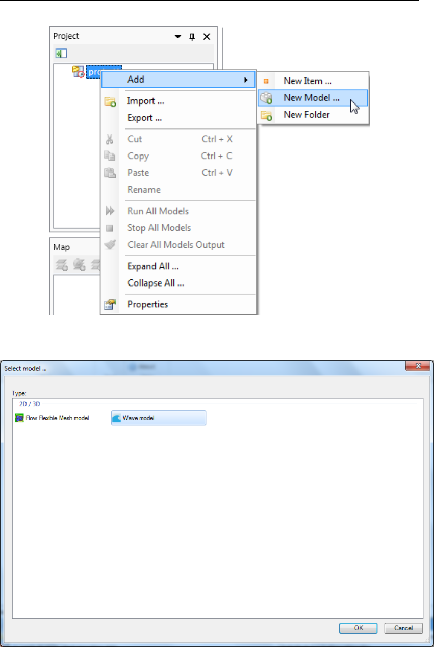
3.3.1 Add a D-Waves model
After starting up Delta Shell, the start page will open with a default project (i.e. ”project1”, see
Figure 3.1). To add a D-Waves model to the project you have the following options:
click ”New Model” in the ”Home”-ribbon (Figure 3.7)
use the Right Mouse Button (RMB) on ”project1” in the project tree, go to ”Add” and ”New
Model’ (Figure 3.8)
From the list of available models (which can vary depending on your installation), select ”Wave
model” (Figure 3.9).
Figure 3.7: Adding a new model from the ribbon
3.3.2 Set up a D-Waves model
To set up the wave model follow the steps in the project tree. For a more detailed description,
see chapter 4.
8 of 124 Deltares
DRAFT
Getting started
Figure 3.8: Adding a new model using the Right Mouse Button on "project1" in the project
tree
Figure 3.9: Select "Wave model"
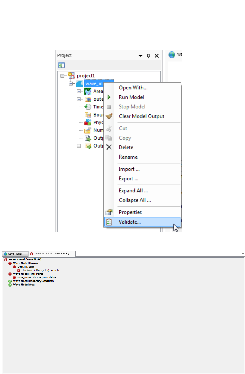
3.3.3 Validate D-Waves model
You can check whether your model setup is valid by using the RMB in the project tree and
Deltares 9 of 124
DRAFT
D-Waves, User Manual
select "Validate" (Figure 3.10). This will produce a validation report (Figure 3.11). Red excla-
mation marks indicate the parts of the model that are still invalid. By clicking the hyperlink you
will be automatically redirected to the invalid step in the model setup, so that you can correct
it.
Figure 3.10: Validate model
Figure 3.11: Validation report
10 of 124 Deltares
DRAFT
Getting started
3.3.4 File tree (to be implemented)
To check the file paths and names of the attribute files which are linked to your model, you
can select "File tree" using the RMB on your model in the project tree.
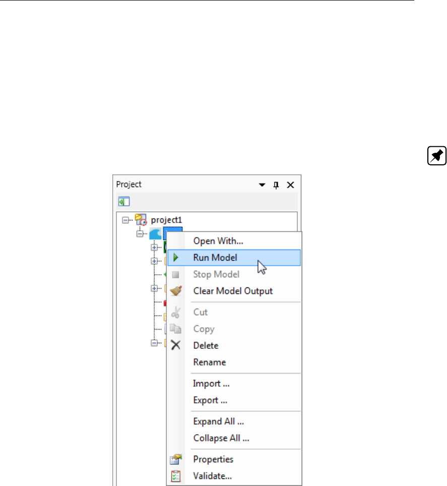
3.3.5 Run D-Waves model
If you are satisfied with the model setup, you can run it from Delta Shell using the RMB on
model and select ”Run model” (Figure 3.12).
Note: it is also possible to run Delft3D-WAVE outside Delta Shell using the command line.
Figure 3.12: Run model
3.3.6 Inspect model output
The simulation will start and the output will be stored in the output folder in the project tree
(Figure 3.13). Delta Shell provides some basic tools to inspect the model output. For more
extensive and advanced options you are referred to Quickplot and Muppet.
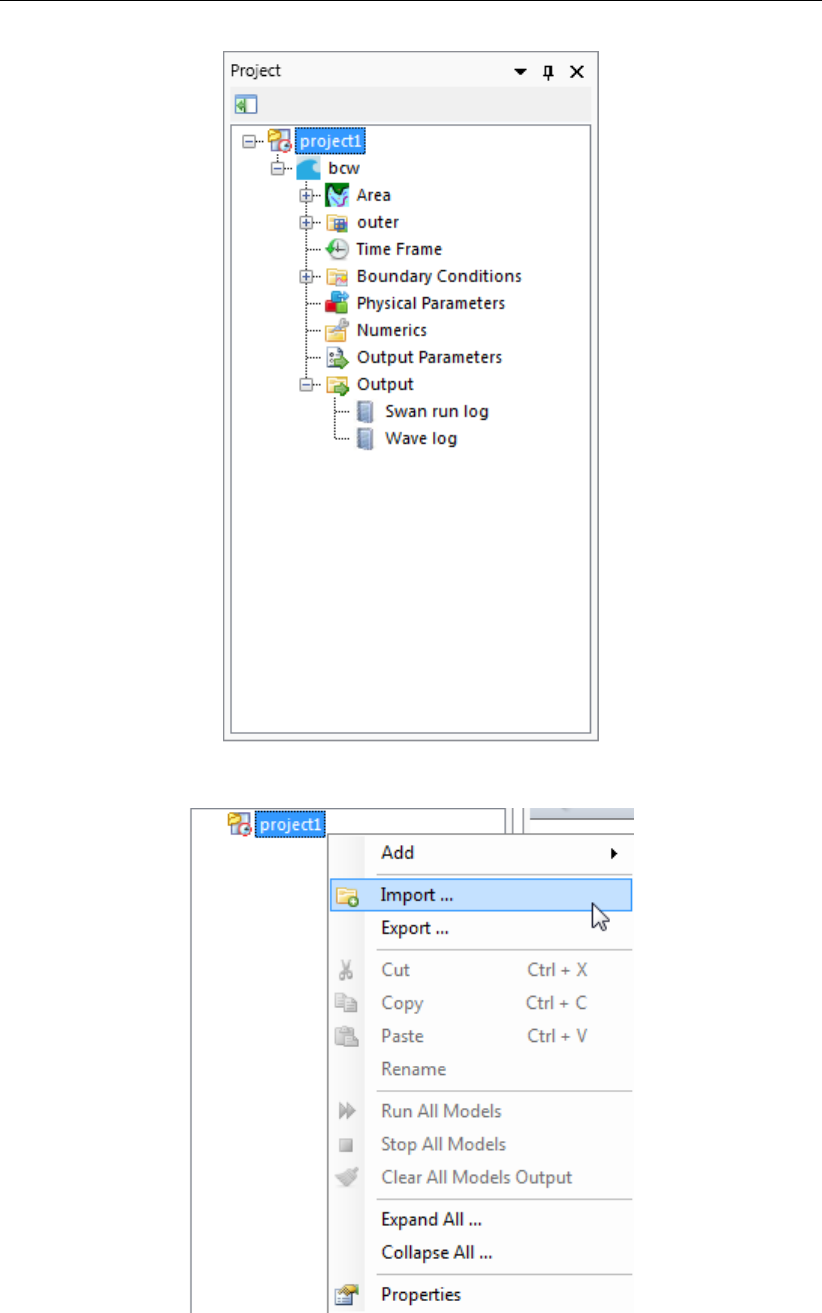
3.3.7 Import/export or delete a D-Waves model
To import an existing Delft3D-WAVE model either use the RMB on the project level in the
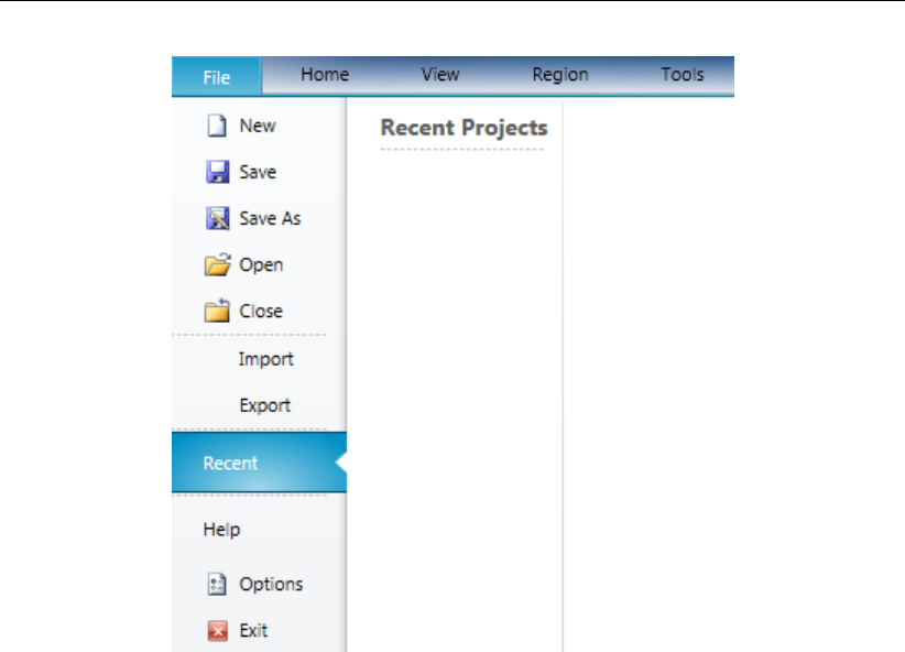
project tree (Figure 3.14) or go to the ”File”-ribbon and press the "Import" (Figure 3.15). Like-
wise you can export a model or delete a model.
For the steps in the project tree that are linked to attribute files (observation points, grid,
bathymetry, etc.) you can use the RMB to import or export these attribute files.
Deltares 11 of 124
DRAFT
D-Waves, User Manual
Figure 3.13: Output of wave model in project tree
Figure 3.14: Import wave model from project tree
12 of 124 Deltares
DRAFT
Getting started
Figure 3.15: Import wave model from file ribbon
3.3.8 Save project
To save the project (and, hence, the model) use the disk-icon on the Quick Access Toolbar
or the "File"-ribbon (Figure 3.15). If you would like to save the project under a different name
use "Save as".
3.3.9 Exit Delta Shell
If you are finished you can exit Delta Shell using the red cross or pressing the "Exit" button in
the "File"-ribbon (Figure 3.15).
3.4 Important differences and new features compared to the former GUI (Delft3D-Waves)
The differences between the former D-Waves GUI and the D-Waves plugin in Delta Shell in
lay-out and functionality are numerous. Here, we address only the most important differences
in the workflow.
3.4.1 Project vs model
The entity "project" is new in the Delta Shell GUI. In the hierarchy the entity "project" is on a
higher level than the entity "model". A project can contain multiple models, which can either
run standalone or coupled. The user can run all models in the project at once (on project
level) or each model separately (on model level). When the user saves the project, the project
settings will be saved in a *.dsproj configuration file and the project data in a *.dsproj_data
folder. The *.dsproj_data folder contains folders with all input and output files for the models
within the project. There is no model intelligence in the *.dsproj configuration file, meaning
that the models can also be run outside the GUI from the *.dsproj_data folder.
Deltares 13 of 124
DRAFT
D-Waves, User Manual
3.4.2 Load/save vs import/export
The user can load an existing Delta Shell project, make changes in the GUI and, consequently,
save all the project data. Loading and saving means working on the original project data, i.e.
the changes made by the user overwrite the original project data. Alternatively, use "save as"
to keep the original project data and save the changes project data at another location (or with
another name).
Import/export functionality can be used to copy data from another location into the project
(import) or, vice versa, to copy data from the project to another location (export). Import/export
is literally copying, e.g.:
import: changes on the imported data will only affect the data in the project and not the
source data (upon saving the project)
export: the model data is copied to another location ”as is”, changes made afterwards will
only affect the data in the project not the exported data (upon saving the project)
3.4.3 Working from the map
One of the most important differences with the former GUI is the central map. The central
map is comparable with the former ”visualization area”, but with much more functionality and
flexibility. The map helps you to see what you’re doing and inspect the model at all times. You
can use the ”Region” and ”Map” ribbons to add/edit model features in the map.
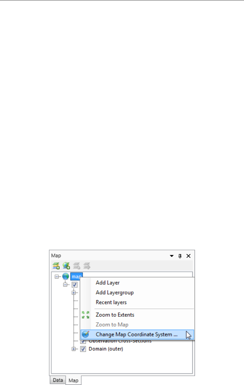
3.4.4 Coordinate conversion
With the map as a central feature, functionality to convert model and map coordinates is an
indispensable feature. In the ”General” tab you can set the model coordinate system. In the
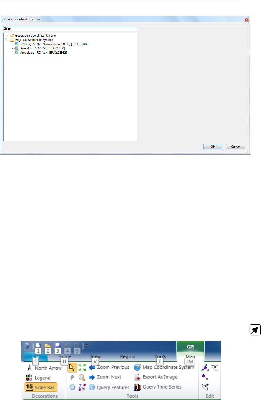
map tree you can set the map coordinate system using the RMB (Figure 3.16). The coordinate
systems are subdivided in geographic and projected systems. Use the quick search bar to
find the coordinate system you need either by name or EPSG code (Figure 3.17).
Figure 3.16: Set map coordinate system using RMB
14 of 124 Deltares
DRAFT
Getting started
Figure 3.17: Select a coordinate system using the quick search bar
3.4.5 Model area
The model area contains geographical (GIS based) features, such as observation points &
curves and obstacles. In contrast to the former GUI, these features can even exist without a
grid or outside the grid and they are not based on grid coordinates, implying that their location
remains the same when the grid is changed (for example by (de-)refining).
Finally, for the computations, the SWAN computational core interpolates the features to the
grid. In the future we would like to show to which grid points the features are snapped before
running the computation. However, this requires some updates in the SWAN computational
core.
3.4.6 Ribbons (hot keys)
Delta Shell makes use of ribbons, just like Microsoft Office. You can use these ribbons for
most of the operations. With the ribbons comes hot key functionality, providing shortcuts to
perform operations. If you press ”ALT”, you will see the letters and numbers to access the
ribbons and the ribbon contents (i.e. operations). For example, ”ALT” + ”H” will lead you to the
”Home”-ribbon (Figure 3.18).
Note: : Implementation of the hot key functionality is still work in progress.
Figure 3.18: Perform operations using the hot keys
Deltares 15 of 124

DRAFT
D-Waves, User Manual
3.4.7 Context menus (RMB)
Context menus are the menus that pop up using the right mouse button (RMB). These context
menus provide you with some handy functionality and shortcuts specific for the selected item.
The functionality is available in all Delta Shell windows and context dependent. You can best
try it yourself to explore the possibilities.
3.4.8 Scripting
Delta Shell has a direct link with scripting in Iron Python (NB: this is not the same as C-Python).
This means that you can get and set data, views and model files by means of scripting instead
of having to do all manually. Scripting can be a very powerful tool to automate certain steps of
your model setup or to add new functionality to the GUI. You can add a new script by adding
a new item, either in the ”Home”-ribbon or through the RMB.
16 of 124 Deltares

DRAFT
4 Graphical User Interface
4.1 Introduction
In order to set up a wave model you must prepare an input file. The input file stores all the
parameters used for a wave computation with D-Waves. The parameters can be divided into
three categories:
1 parameters that define the physical processes being modelled,
2 parameters that define the numerical techniques used to solve the equations that describe
the physical processes,
3 parameters that control the wave computation and store its results.
Within the range of realistic values, it is likely that the solution is sensitive to the selected
parameter values, so a concise description of all parameters is required. The input data
(defined by you) is stored into an input file which is called the Master Definition file for Wave
or MDW-file.
In section 4.2 we discuss some general aspects of the MDW-file and its attribute files. sec-
tion 4.3 discusses shortly the filenames and their extension. In section 4.4 we explain how
to work with the WAVE Graphical User Interface in Delta Shell, including is input parameters,
their restrictions and their valid ranges or domain.
4.2 MDW file, attribute files and file formats
The Master Definition Wave file (MDW-file) is the input file for the wave program. It contains all
the necessary data that is required to define a wave model and run a wave computation. Some
of the parameter values are given directly in the MDW-file. Other parameters are defined in
attribute files, referred to by specific statements in de MDW-file. The latter is particularly the
case when parameters contain a large number of data (e.g. spatially varying data such as
a variable wind or friction field). The user-defined attribute files are listed and described in
Appendix A.
The D-Waves plugin in Delta Shell is a tool that is used to assign values to all the necessary
parameters or to import the names of the attribute files into the MDW-file. When the data
you entered is saved, an mdw-file, containing all the specified data, is created in the selected
working directory.
Although you are not supposed to work directly on the mdw-file (with a text editor) it is useful
to have some idea of what its structure is, as it reflects the idea of the designer on how to
handle large amounts of input data. For an example of an MDW-file, see Appendix C.
The basic characteristics of an MDW-file are:
- It is an ASCII file.
- The file is divided in datagroups.
- It is keyword based.
The mdw-file is an intermediate file between the D-Waves plugin and the D-Waves module
(e.g. the computational core). As it is an ASCII-file, it can be transported to an arbitrary
hardware platform. Consequently, the wave module and the WAVE Graphical User Interface
program do not necessarily have to reside in the same hardware platform.
Deltares 17 of 124

DRAFT
D-Waves, User Manual
As explained before, input parameters that contain a lot of data are defined in attribute files.
How to set up these attribute files is explained elsewhere in this chapter. The mdw-file only
contains permanent input parameters and references to these attribute files. The formats of
all attribute files (and of the mdw-file itself) are described in detail in Appendix A.
The mdw-file and its attribute files form a complete set, defining a simulation. When storing
your simulation input, always make sure you include the complete set of MDW-file and attribute
files.
4.3 Filenames and coventions
The names of the mdw-file and its attribute files have a specific structure, some aspects are
obliged while others are only advised or preferred.
The name of an mdw-file must have the following structure: <run-id.mdw>. The <run-id>
consists of an arbitrary combination of (maximum 252) letters and numbers. This <run-id>
will be part of the result files to safeguard the link between an mdw-file and the result files.
Restriction:
The maximum length of the <run-id>is 252 characters!
The names of the attribute files follow the general file naming conventions, i.e. they have the
following structures: <name>.<extension>. Where:
-<name>is any combination of characters allowed for filenames, except spaces.
- There is no limitation other than the platform dependent limitations; you are referred to
your platform manual for details. We suggest to add some continuation character, for
instance <-number>to the <name>to distinguish between various updates or modifi-
cations of the file.
- The <extension>is mandatory as indicated below.
Quantity Filename and mandatory extension
Bathymetry or water depth <name>.dep
Curvilinear grid <name>.grd
Grid enclosure <name>.enc
Wind field <name>.wnd
Spiderweb wind field <name>.spw
Spectral wave boundary <name>.bnd
Wave boundary conditions <name>.bcw
1D wave spectrum <name>.sp1
2D wave spectrum <name>.sp2
Curves <name>.pol
Output locations <name>.loc
Obstacles <name>.obs
Obstacles locations <name>.pol
18 of 124 Deltares
DRAFT
Graphical User Interface
4.4 Setting up a D-Waves model
In this section, all input parameters in the data groups of the mdw-file will be described in the
order in which they appear in the project tree of D-Waves. We will describe all data groups in
consecutive order. For each input quantity we give:
A short description of its meaning. In many cases we add a more comprehensive discus-
sion to put the quantity and its use in perspective.
The restrictions on its use.
The range of allowed values, called its domain, and its default value.
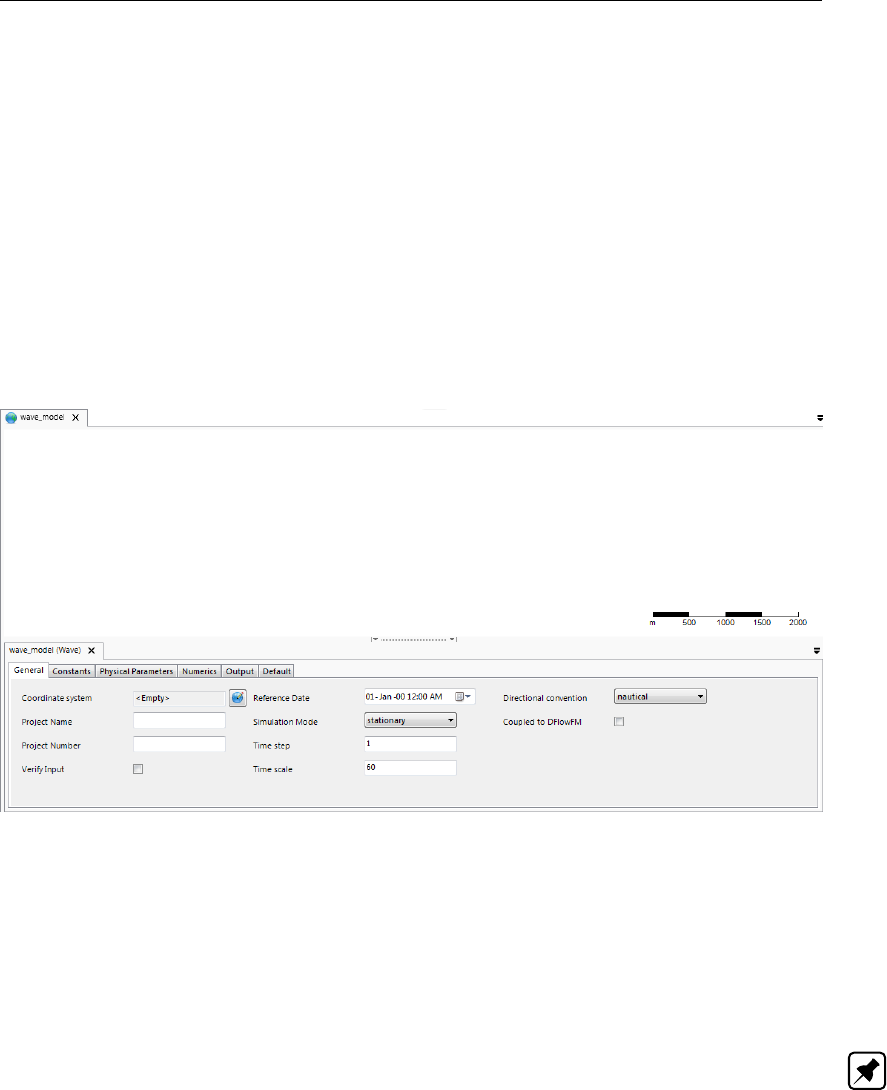
4.4.1 General
In the general tab (Figure 4.1) you can set the basic settings of your model, i.e.:
Figure 4.1: Overview of the general tab
Model coordinate system (default: <Empty>)
By clicking the earth icon, you can select the coordinate system (CS) for your model. Use
the quick search bar to find your CS either by name or EPSG code (Figure 4.2). The list of
CS that you select is limited to those that are supported by SWAN (the computational core of
D-Waves), i.e. only the WGS84 geographic CS and most projected CS.
Note: Please note that the CS is not (yet) a property in the D-Waves import files. At the
moment it is only used to convert geographical model information to the map CS.
Project name (default: <Empty>)
The name of the project may not be longer than 16 characters (restriction of the SWAN com-
putational core).
Project number (default: (default: <Empty>)
The project number may not be longer than 4 characters (restriction of the SWAN computa-
tional core).
Verify input (default: no)
Deltares 19 of 124
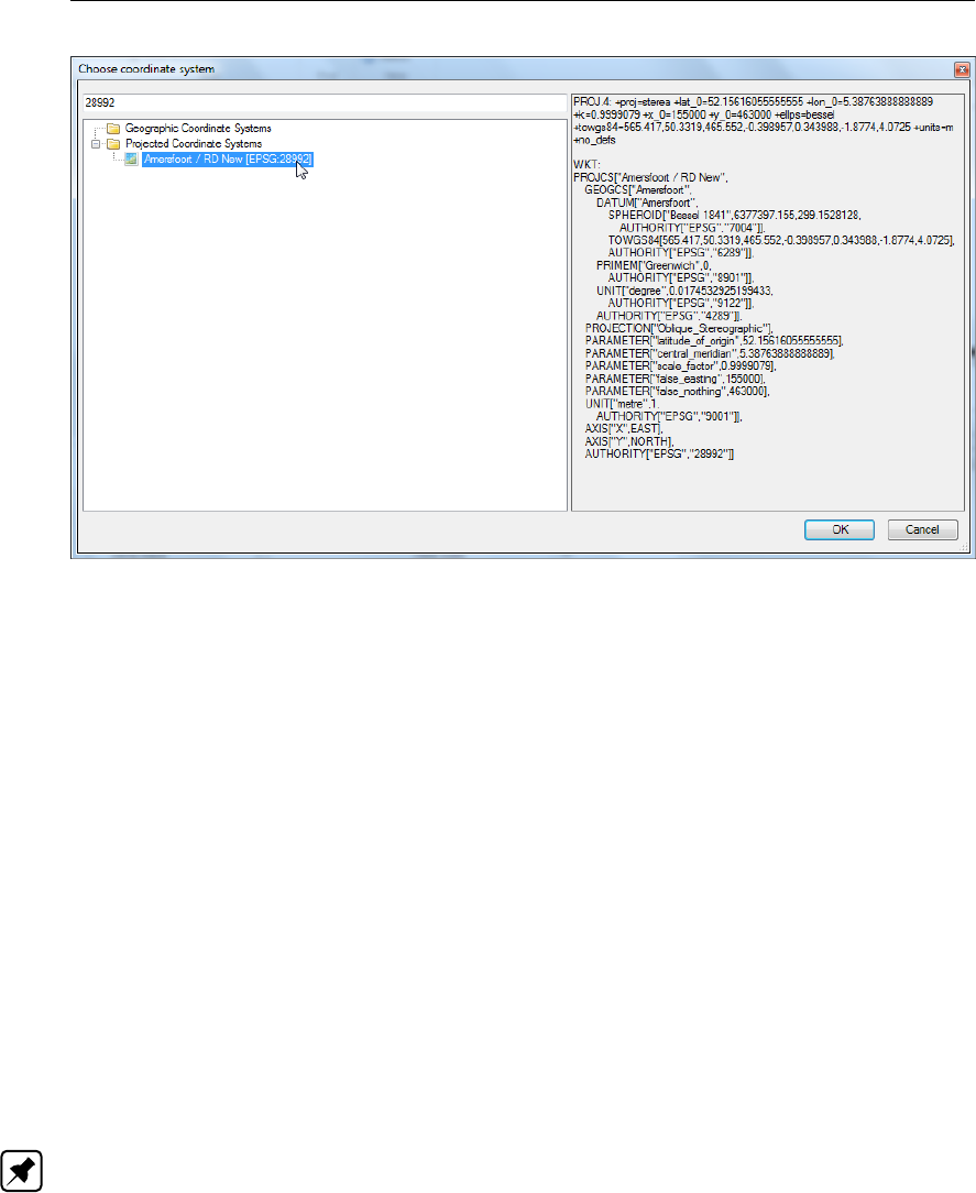
DRAFT
D-Waves, User Manual
Figure 4.2: Set the model coordinate system
During pre-processing SWAN checks the input data. Depending on the severity of the errors
encountered during this pre-processing, SWAN does not start a computation.
Reference date (default: 01-Jan-00 12:00 AM)
This is the reference date relative to which the time points are defined. For accuracy reasons
choose the reference date not too far away from your time points.
Simulation mode (default: stationary)
You can choose between stationary, quasi-stationary and non-stationary. The stationary mode
is considered to be justified when the residence time of the simulated waves – the time that
waves require to travel through the model domain – is small relative to the time scale of
changes in the wave boundary conditions and forcing (e.g. wind and currents). As the model
domain increases or time scale of changes in boundary conditions and forcing decreases,
non-stationary simulations become more appropriate. In case of non-stationary simulations
you have to provide the time step and time interval of the non-stationary simulations.
Note: To do quasi-stationary
Time step (default: 5 minutes)
The time step for non-stationary simulations
Time interval (default: 0 minutes)
The time interval for non-stationary simulations
Time scale (default: 60 minutes)
Unit of time
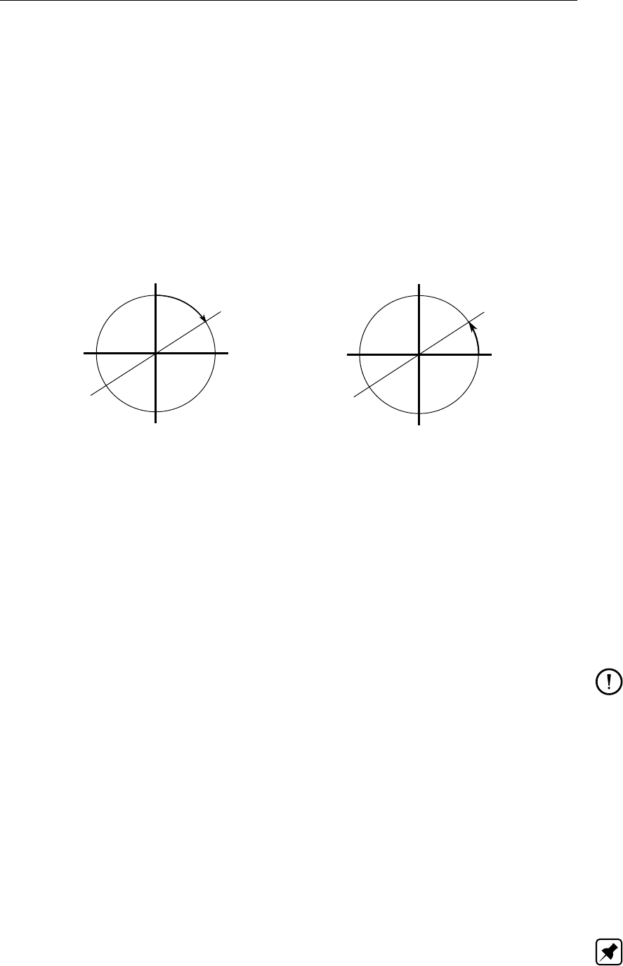
Directional convention (default: nautical)
20 of 124 Deltares
DRAFT
Graphical User Interface
In the input and output of SWAN the direction of wind and waves are defined according to
either the Cartesian convention or the Nautical convention (see Figure 5.1 for definitions).
Cartesian
This option indicates that the Cartesian convention for wind and wave direction (SWAN
input and output) will be used. The direction is the angle between the vector and the
positive x-axis, measured counter-clockwise (the direction where the waves are going to
or where the wind is blowing to).
Nautical
This option indicates that the nautical convention for wind and wave direction will be used.
The direction of the vector from the geographic North measured clockwise + 180◦. This is
the direction where the waves are coming from or where the wind is blowing from.
North
East
South
West
North
East
South
West
Figure 4.3: Nautical convention (left panel) and Cartesian convention (right panel) for di-
rection of winds and (incident) waves
Couple to Delft3D-FM (default: no)
You can specify a FLOW computation from which the results are to be used as input for the
wave computation (so-called offline coupling). If you want to do this, this is the place to define
the FLOW computation to be used.
All needed results are stored in the communication file (com-file) produced by the FLOW
computation Therefore, the FLOW com-file has to be present in your working directory.
Remarks:
When using a FLOW model, make sure that the selected mdf-file and its associated
com-file are located in your working directory, since the two modules will communicate
with each other by this com-file.
During the computations, D-Waves determines the water depth from the bottom level,
the water level and the water level correction. Bottom levels are defined as the level
of the bottom relative to some horizontal datum level (e.g. a still water level), positive
downward. Water levels are defined with respect to the same datum as the bottom; the
water level is positive upward.
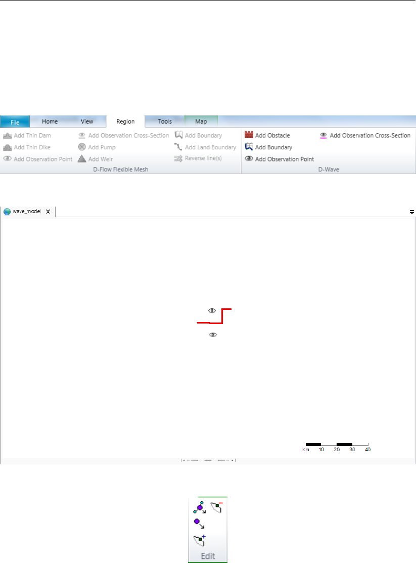
4.4.2 Area
The model area contains geographical (GIS based) features, such as observation points &
curves and obstacles. These features can be added using the "Region"-ribbon (see Fref-
Fig:RegionRibbon and FrefFig:MapAreaFeatures). You can also import and export the at-
tribute files using the RMB in the project tree (Note: NB: still to be implemented). If you
would like to change the locations of the features use the "Edit" section of the "Map"-ribbon
(see FrefFig:EditMapFeatures). You can delete features by selecting them and simply using
Deltares 21 of 124
DRAFT
D-Waves, User Manual
the <delete>button. By selecting a feature from the map and double clicking it, the attribute
table will open with feature specific properties (see Figure 4.7 for obstacles).
All the features defined in Area can exist without a grid and they are not based on grid coor-
dinates, implying that their location remains the same when the grid is changed (for example
by (de-)refining).
Figure 4.4: Add Area features using the Region ribbon
Figure 4.5: Area features added to map
Figure 4.6: Edit Area features using the Edit section of the Map ribbon
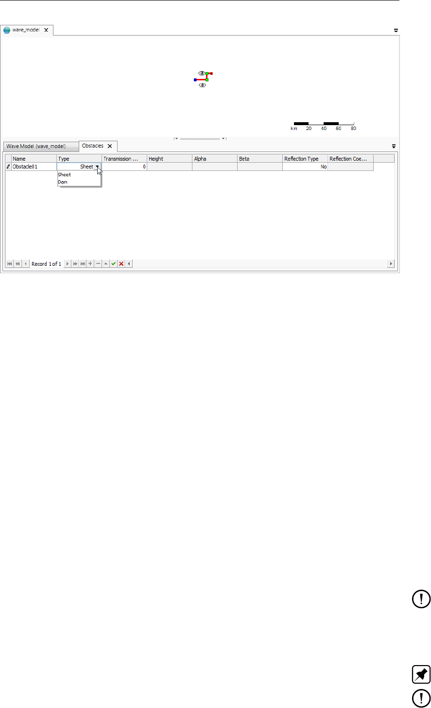
4.4.2.1 Obstacles
Obstacles are sub-grid features through which waves are transmitted or against which waves
are reflected or both at the same time (see FrefFig:ObstaclesProperties). The location of the
obstacle is defined by a sequence of corner points of a polyline. The obstacles interrupt the
propagation of the waves from one grid point to the next wherever this obstacle line is located
between two neighbouring grid points of the computational grid (the resolution of transmission
or blockage is therefore equal to the computational grid spacing).
With respect to the type of the obstacle, the following options are available:
22 of 124 Deltares
DRAFT
Graphical User Interface
Figure 4.7: Attribute table with properties of obstacles
Sheet: With this option you indicate that the transmission coefficient is a constant along
the obstacle.
Dam: With this option you indicate that the transmission coefficient depends on the in-
cident wave conditions at the obstacle and on the obstacle height (which may be sub-
merged).
Reflections: With this option you can specify if the obstacle is reflective (specular or diffu-
sive; possibly in combination with transmission) and the constant reflection coefficient.
Reflection coefficient (default = 0)
The reflection coefficient is formulated in terms of ratio of reflected significant wave height
over incoming significant wave height.
Transmission coefficient (default = 1.0)
is the transmission coefficient for the significant wave height (coefficient = 0.0: no trans-
mission = complete blockage).
Height (default = 0.0)
The elevation of the top of the obstacle above the reference level (same reference level
as for bottom etc.); use a negative value if the top is below that reference level (possibly
in case of submerged obstacles).
Alpha (default = 2.6)
Coefficient determining the transmission coefficient depending on the shape of the dam.
Beta (default = 0.15)
Coefficient determining the transmission coefficient depending on the shape of the dam.
Remark:
When Reflections at obstacles are activated, then for each computational grid the di-
rectional space should be Circle or Sector covering the full circle of 360◦.
When a lot of obstacles have to be defined, the procedure described above can be quite cum-
bersome. Therefore, it also possible to define a number of obstacles by importing a polyline
file in which you defined the corner points of the obstacles. Note: Still to be implemented.
Deltares 23 of 124

DRAFT
D-Waves, User Manual
Remarks:
Reflections will only be computed if the spectral directions cover the full 360◦.
In case of specular reflection the angle of reflection equals the angle of incidence.
In case of diffuse and scattered reflection in which the angle of reflection does not equal
the equal the angle of incidence.
Domain:
Parameter Lower limit Upper limit Default Unit
Reflection No
Reflection coefficient 0.0 1.0 0.0 -
Sheet (max number = 250):
Transmission coefficient 0 1 1.0 -
Dam (max number = 250): .
Height -100. +100. 0. m
Alpha 1.8 2.6 2.6 -
Beta 0.1 0.15 0.15 -
4.4.2.2 Observation Points
With Observation Points you can specify (monitoring) locations at which wave output should
be generated by D-Waves, similar to the observation points in Delft3D FM. The values of
the output quantities at the observation points are interpolated from the computational grid
and written to a Table file. You can add, edit and delete these curves using the ribbons.
Alternatively, you can import the locations from a <∗.loc>file. The format of the <∗.loc>file
should be:
x1y1
x2y2
.
.
..
.
.
xnyn
4.4.2.3 Observation Curves
With Observation Curves you can specify a (curved) output curve at which wave output should
be generated by D-Waves. Actually this curve is a broken line, defined by you in terms of
segments. The values of the output quantities along the curve are interpolated from the
computational grid. You can add, edit and delete these curves using the ribbons.
Remark:
The names of output curves and/or curve segments as displayed in the attribute table,
are not input for SWAN. The names are only displayed for your convenience. Moreover,
the number in the names does not determine the sequence. The first curve in the list
is the first curve specified, the second curve in the list is the second curve specified,
though the name may suggest differently. Reloading this scenario will renumber the
names of curves and segments but not the order.
24 of 124 Deltares
DRAFT
Graphical User Interface
4.4.3 Hydrodynamics from flow - currently default tab
In case FLOW results have been selected to be coupled to D-Waves, the results are read from
the com-file and interpolated from the computational FLOW grid to the computational WAVE
grid. Usually the FLOW grid is chosen smaller than the WAVE grid. Therefore an option is
available to extend the values at the boundary of the FLOW grid to the boundary of the WAVE
grid. Furthermore, you specify which hydrodynamic results should be extended.
When the FLOW computation is performed in 2DH mode, for each of the options Water level,
Current,Bathymetry and Wind the following three options can be chosen, see Figure 4.8:
Don’t use Don’t use the quantity for the wave simulation
Use but don’t extend Use this quantity in the wave simulation but don’t extend
Use and extend Use this quantity in the wave simulation but don’t extend
Figure 4.8: Select which quantities should be used from FLOW computation
If the the FLOW computation is performed in 3D mode then an additional Current type needs
to be specified. This current type can have the following values:
depth averaged Use the depth averaged flow-velocity for the wave simulation.
surface layer Use the flow-velocity in the surface layer for the wave simulation.
wave dependent A weighted flow-velocity will be used, the velocity is dependent on the
orbital velocity of the wave and is especially of interest for stratified flows, see Kirby and
Chen (1989).
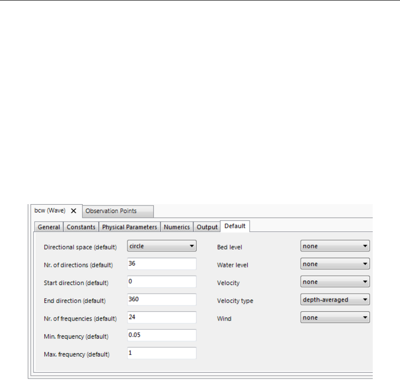
4.4.4 Spectral resolution (deafult) - currently default tab
For each computational grid the spectral resolution in both directional and frequency space
needs to be specified. SWAN only assigns wave energy to the wave directions and wave
frequencies specified in the spectral resolution. In this tab you can set the default setting
for the spectral resolution (see Figure 4.8). By default these settings will be assigned to all
computational grids. However, the spectral resolution can be made domain dependent (see
section 4.4.5.5).
Deltares 25 of 124
DRAFT
D-Waves, User Manual
Directional space
Circle
This option indicates that the spectral directions cover the full circle. This option is default.
Sector
This option means that only spectral wave directions in a limited directional sector are
considered. The range of this sector is given by Start direction and End direction.
Start direction
This is the first direction (in degrees) of the directional sector. It can be defined either in
the Cartesian or the Nautical convention (see Figure 5.1), but this has to be consistent
with the convention adopted for the computation, to be defined in the Data Group Physical
parameters.
End direction
It is the last direction of the sector (required for option Sector; Cartesian or Nautical con-
vention, but in consistency with the convention adopted for the computation).
Remarks:
The Start direction should be smaller than the End direction.
When Reflections at obstacles are activated, then the spectral directions must cover
the full circle of 360◦.
Number of directions
This is the number of bins in the directional space. For Circle this is the number of subdi-
visions of a full circle, so the spectral directional resolution is
∆θ= 360◦/(Number of directions)
In the case a directional sector is used, the spectral directional resolution is
∆θ= (End direction - Start direction)/(Number of directions)
Frequency space
Lowest frequency
This is the lowest discrete frequency that is used in the calculation (in Hz).
Highest frequency
This is the highest discrete frequency that is used in the calculation (in Hz).
Number of frequency bins
The number of bins in frequency space is one less than the number of frequencies. It
defines the resolution in frequency space between the lowest discrete frequency and the
highest discrete frequency. This resolution is not constant, since the frequencies are loga-
rithmically distributed. The number of frequency bins depends on the frequency resolution
∆fthat you require (see SWAN UM (2000), pages 39 and 49).
Domain:
Parameter Lower limit Upper limit Default Unit
Start direction -360 360 0 degree
End direction -360 360 0 degree
Number of directions 4 500 36 -
Lowest frequency 0.0 - 0.05 Hz
Highest frequency 0.0 - 1 Hz
Number of frequency bins 4 - 24 -
26 of 124 Deltares
DRAFT
Graphical User Interface
4.4.5 Domain
Under <domainname>in the project tree you define the geographic location, size and ori-
entation of the computational grids by creating or importing one or more attribute grid files,
which are curvilinear grids generated with RGFGRID (grd-file). The grids can be defined in a
common Cartesian co-ordinate system or in a spherical co-ordinate system.
Remarks:
The computational grid must be much larger than the domain where wave results are
needed, because of the ‘shadow’ zone on both sides of the wave incident direction.
A grid that is created in RGFGRID always has an associated enclosure file (∗.enc). This
file is not imported in the WAVE-GUI, but it will be used in case computational grids are
nested, so it has to be present in the working directory.
4.4.5.1 Import and export grids and bathymetries
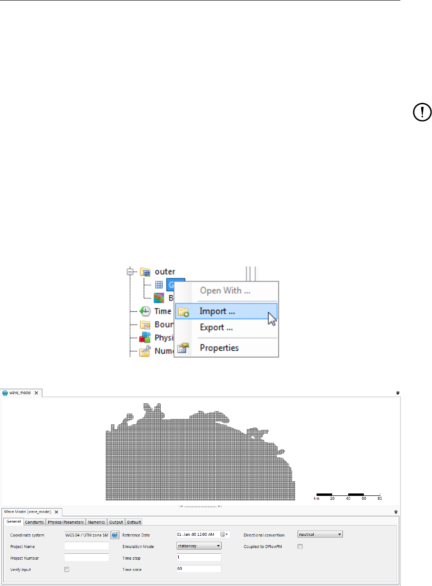
You can import and export a (previously generated) grid using the RMB on the <domainname>
(see Figure 4.9). Likewise, import and export a bathymetry for the domain. The imported
grid/bathymetery can be viewed and inspected in the central map (see Figure 4.10).
Figure 4.9: Import a RGFGRID file from the project tree
Figure 4.10: Visualize the D-Waves grid on the central map
Deltares 27 of 124
DRAFT
D-Waves, User Manual
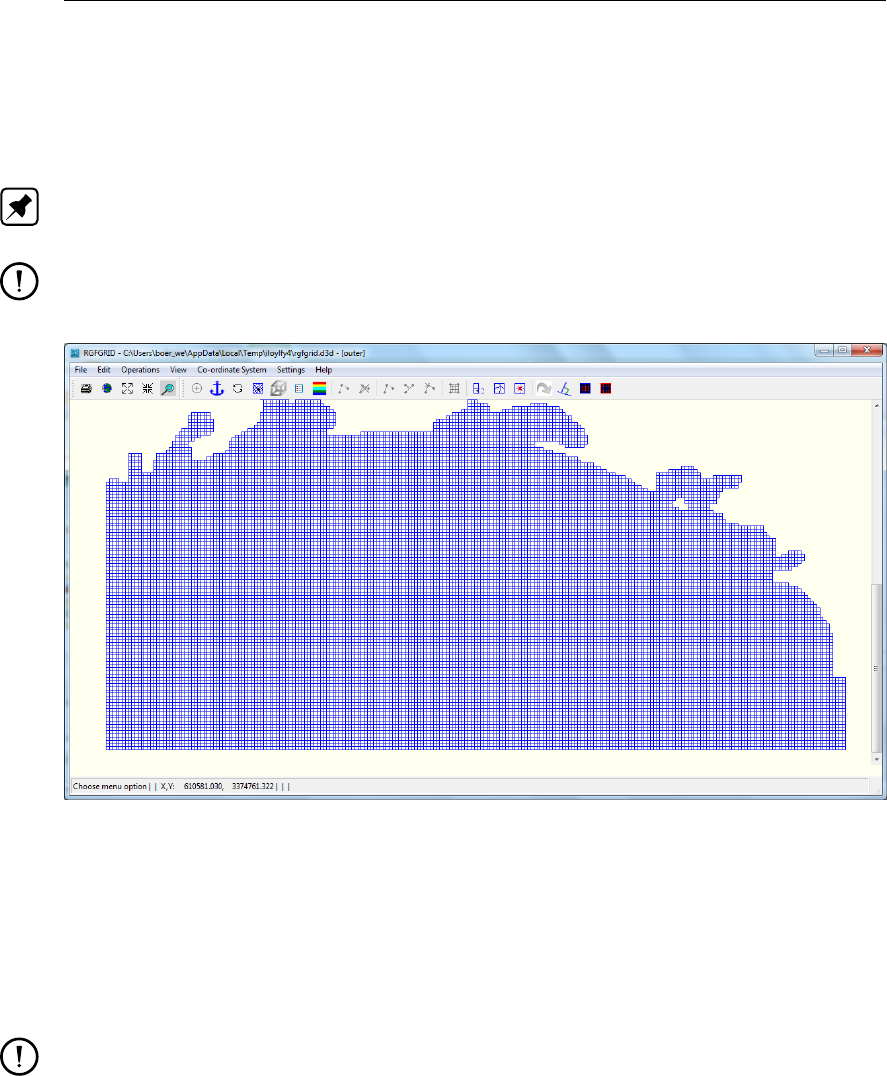
4.4.5.2 Create and/or edit grids in RGFGRID
To generate a grid from scratch or edit an imported grid, double click on "Grid" under <domainname>
in the project tree and RGFGRID will open (see Figure 4.11). You can use RGFGRID to create
and edit the grid. See the RGFGRID manual for more information.
Note: Do not forget to save the RGFGRID project before closing RGFGRID to save the
changes and transfer them to Delta Shell.
Remark:
The formats of the grid files are defined in Appendix A.
Figure 4.11: Create and/or edit the grid using RGFGRID
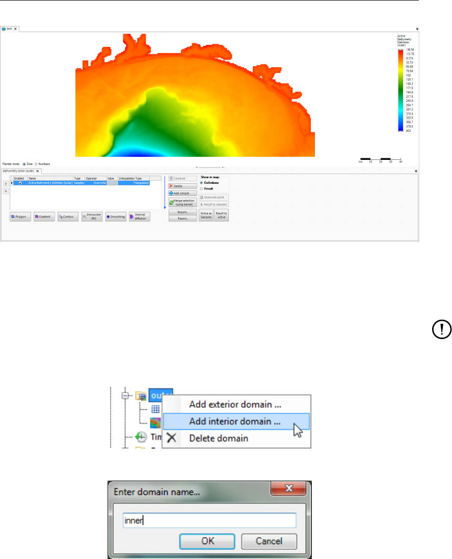
4.4.5.3 Create and/or edit bathymetries using the spatial editor
To generate a bathymetry from scratch or edit an imported bathymetry, double click on "Bathy-
metry" under <domainname>in the project tree and the spatial editor will open (see Fig-
ure 4.12). You can use the spatial editor to create and edit the bathymetry. See the Appendix
.... for more information.
Remark:
The formats of the depth files are defined in Appendix A.
4.4.5.4 Nest domains
D-Waves supports the use of nested computational grids in one wave computation. The idea
of nesting is to have a coarse grid for a large area and one or more finer grids for smaller areas.
The coarse grid computation is executed first and the finer grid computations use these results
to determine their boundary conditions. Nesting can be repeated on ever decreasing scales.
When you want to use the nesting option, you have to create multiple domains. This can be
done using the RMB on the<domainname>in the project tree (see Figure 4.13). You can add
either an interior or exterior domain. A popup will show up in which you can enter the name
of the new domain (Figure 4.14). Consequently, the <domainname>with the corresponding
grid and bathymetry features will show up in the project tree (see Figure 4.15). The grids and
28 of 124 Deltares
DRAFT
Graphical User Interface
Figure 4.12: Create and/or edit the grid using the spatial editor
bathymetries can be added, edited and imported in the same way as described before for one
domain.
Remarks:
The first grid cannot be nested in another one. For this grid, boundary conditions must
be specified in the Data Group Boundaries.
A grid cannot be nested in itself. An error message will pop up if you try this.
Figure 4.13: Create or edit the grid using RGFGRID
Figure 4.14: Create or edit the grid using RGFGRID
Deltares 29 of 124
DRAFT
D-Waves, User Manual
Figure 4.15: Create or edit the grid using RGFGRID
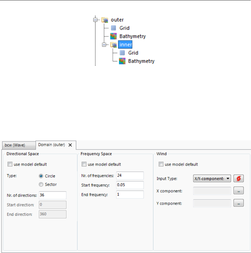
4.4.5.5 Spectral resolution and wind (per domain)
By double clicking the <domainname>in the project tree the domain tab will open. In the
domain tab you can specify whether you would like to use the default settings for the spectral
resolution (section 4.4.4) and wind (section 4.4.6) or set these properties specific for the
domain.
Figure 4.16: Specify spectral resolution and wind per domain
4.4.6 Time Frame, Hydrodynamics and Wind
In the Time frame tab you can specify the time points on which wave computations have to be
carried out, hydrodynamic conditions (water level and currents) and wind conditions.
Time points
There are three options: you want to perform a standalone wave computation, you want to
perform an offline coupling with Delft3D-FM, or you want to perform an online coupling with
Delft3D-FM (in the latter two cases, you specified a FLOW computation in the tab General).
Time steps must be specified for a standalone wave computation. For a coupled flow-wave
(online or offline) computation the time steps (and corresponding hydrodynamics and wind)
are usually copied from the flow computation.
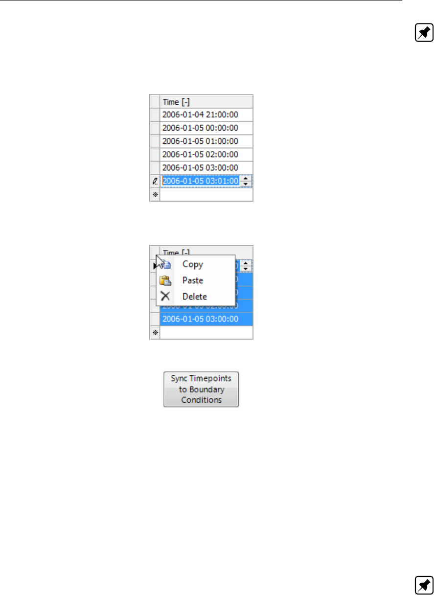
In the time point editor you can add time points in the following ways:
Using the table
Here you can add time points step by step (Figure 4.17)
Pasting copied time series
Using the RMB you can paste copied time series (Figure 4.18)
Using the time series generator
30 of 124 Deltares
DRAFT
Graphical User Interface
Note: Still to be implemented
Synchronizing with the boundary conditions
Using the synchronizing button (Figure 4.19) you can use the time points that are specified
for the boundary conditions.
Figure 4.17: Adding time points using the table
Figure 4.18: Pasting time points from another series or program, for example Excel
Figure 4.19: Synchronizing the time points with the time points specified for the boundary
conditions
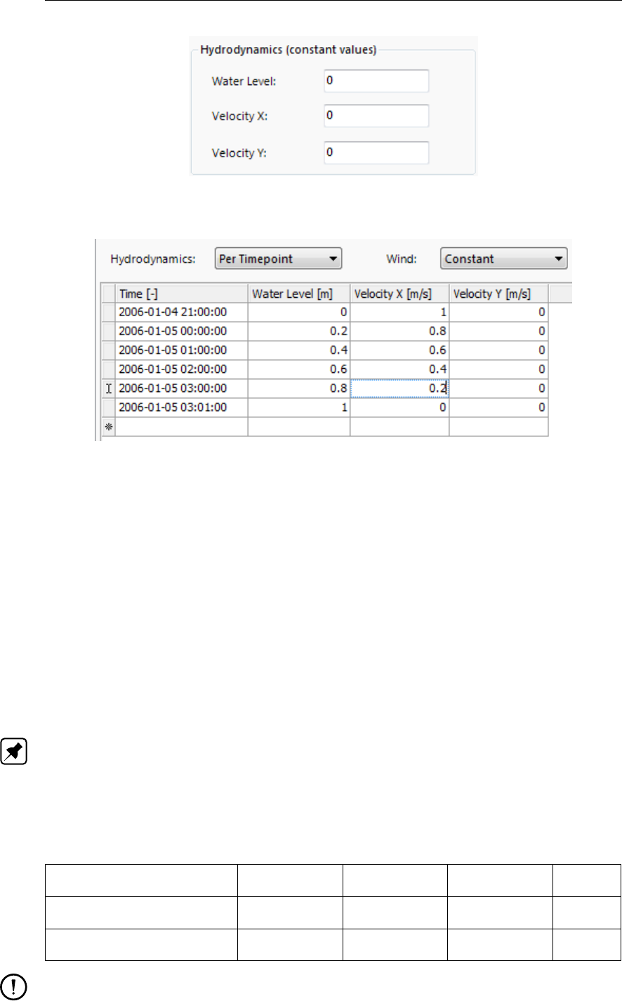
Hydrodynamics
If the hydrodynamics are not copied from a Flow computation, they have to specified here.
You have two options:
Constant
Specify constant hydrodynamics for all time points (Figure 4.20)
Per time point
Specify time point specific hydrodynamics (Figure 4.21)
Note: These are the hydrodynamics for all domains.
Deltares 31 of 124
DRAFT
D-Waves, User Manual
Figure 4.20: Specification of constant hydrodynamics
Figure 4.21: Specification of hydrodynamics per time point
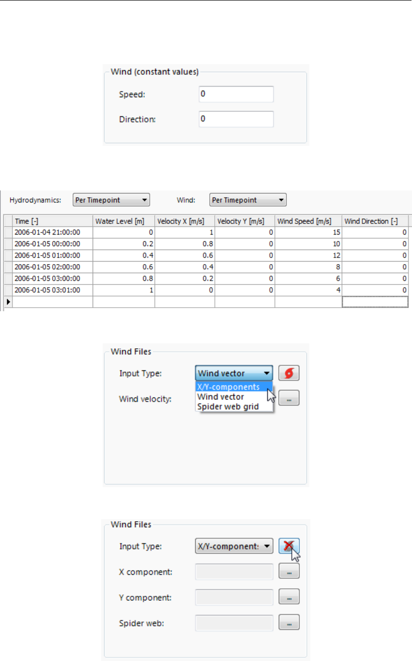
Wind
If the wind conditions are not copied from a Flow computation, they have to specified here.
You have three options:
Constant
Specify constant wind for all time points (Figure 4.22)
Per time point
Specify time point specific wind conditions which are uniform in space (Figure 4.23)
From file
Include wind conditions from a file (Figure 4.24). The wind conditions can be variable
in space and time. Optionally, you can add a spiderweb wind field (usually used for the
specification of cyclone winds) on top of the (background) wind field (Figure 4.25).
Note: These are the default settings for all (nested) domains. Alternatively, these settings
can be made domain dependent (see section 4.4.5.5)
The ranges for the (uniform) wind conditions are as follows:
Domain:
Parameter Lower limit Upper limit Default Unit
Wind speed 0.0 50.0 0.0 m/s
Wind direction -360.0 360.0 0.0 deg
Remark:
32 of 124 Deltares
DRAFT
Graphical User Interface
If the wind speed is larger than zero, and in Physical Parameters the third generation
mode is selected, then the Quadruplets will be activated.
Figure 4.22: Specification of constant wind
Figure 4.23: Specification of wind per time point
Figure 4.24: Specification of wind (field) from file
Figure 4.25: Add a spiderweb wind field
Deltares 33 of 124
DRAFT
D-Waves, User Manual
4.4.7 Boundary Conditions
Under Boundary Conditions in the project tree the incident wave conditions at the boundary
of the first, and only the first, computational grid are prescribed. All other computational grids
(i.e. the nested grids) obtain their boundary information from other grids.
In the D-Waves computations, wave boundary conditions may be specified at different sides.
The general procedure to specify boundary conditions is the following. For each of the bound-
aries:
1 Draw the boundary location(s) in the central map (can be multiple support points).
2 Specify whether the values of the incident wave conditions are Uniform or Spatially varying
along the boundary.
3 Specify whether the values of the incident wave conditions are Parameterized (Constant
in time),Parameterized (Timeseries) or Spectrum based (from file).
4 Activate the support point(s) that you want to put conditions on.
5 Set the spectrum settings (if not loaded from file).
6 Specify the condtions (which may be time series)
Below, each of the six steps described above is explained further.
Remark:
Alternatively, you can select a (pre-processed) 2-dimensional spectrum file that is pro-
viding the spectral data along the boundary directly (optionally varying in time).
Boundary location(s)
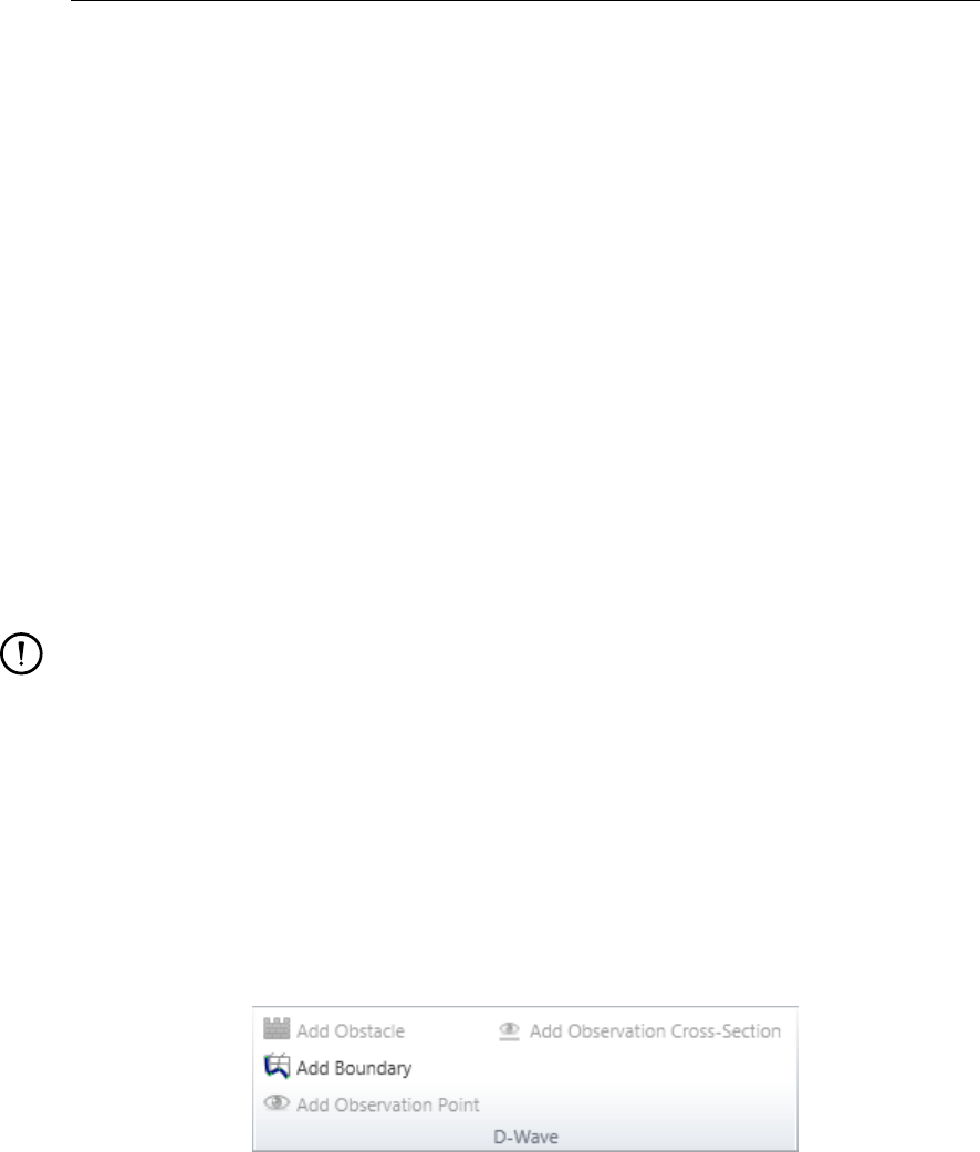
You can specify the boundary locations by selecting Add Boundary from the Region ribbon
(see Figure 4.26) and cosequently drawing the boundary or boundaries on the central map
(see Figure 4.27). In contrast to the previous D-Waves GUI boundaries can only be specified
in terms of xy coordinates, not in grid coordinates or by orientation. After drawing the bound-
aries they will be automatically snapped to the grid. The boundaries are added to the project
tree under Boundary Conditions (Figure 4.28).
Figure 4.26: Select Add Boundary from Region ribbon
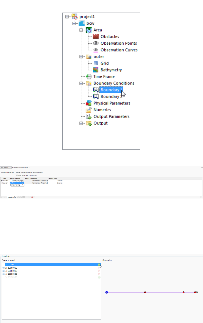
Spatial definition
The spatial definition can be set in the attribute table (see Figure 4.29) of the boundary, which
you can open by double clicking Boundary Conditions in the project tree. Alternatively, you can
set the spatial definition in the boundary condition editor (see Figure 4.30), which is opened
by double clicking the Boundary in the project tree or double clicking the boundary in the
map view. The boundary condition may be Uniform along a boundary, but it may also be
Space-varying:
Uniform
With this option the wave conditions are uniform along a boundary.
Space-varying
34 of 124 Deltares
DRAFT
Graphical User Interface
Figure 4.27: Draw the boundary support points on the map
With this option the wave spectra can vary along the boundary. The incident wave field is
prescribed at a number of support points along the boundary. These points are charac-
terised by their distance from the begin point of the boundary (inidcated by the numbers).
The wave spectra for grid points on the boundary of the computational grid are calculated
by SWAN by spectral interpolation.
Figure 4.30: Overview of the boundary conditions editor
Spectral specification
The boundary conditions in SWAN can be specified in terms of integral wave parameters
(Parameterized (Constant in time or time series)) or they can be read from an external file
(Spectrum based (from file)). You can select this in the boundary condition editor.
Parametric
With this option you define the boundary condition as parametric spectral input.
From file
With this option the boundary condition are read from an external file (bnd-file).
Deltares 35 of 124
DRAFT
D-Waves, User Manual
Figure 4.28: Boundaries are added to the project tree under Boundary Conditions
Figure 4.29: Edit the spatial definition in the attribute table
Activate support points
In order to put conditions on the boundaries you first have to activate one (or multiple) support
point(s) from the list by clicking the green "+"-button (see Figure 4.31). In the geometry panel
next to it you can see which of the points along the boundary is selected (Figure 4.31).
Figure 4.31: Activate a support point in the boundary condition editor and inspect the
location of the selected support point in the Geomtery view
36 of 124 Deltares
DRAFT
Graphical User Interface
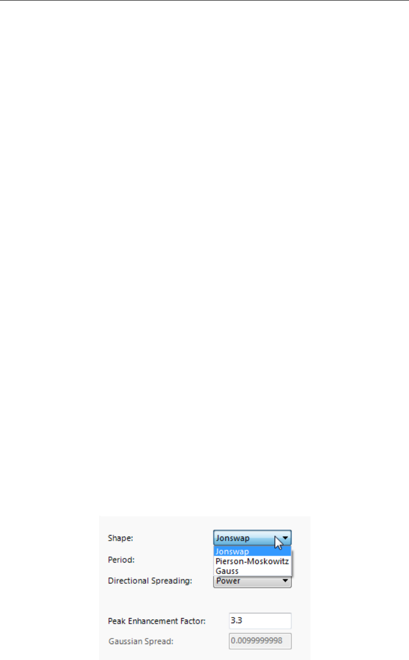
Spectrum settings
In the spectrum panel the spectrum shape and settings can be selected and set (see Fig-
ure 4.32):
Shape: With this option you can define the shape of the input spectra.
JONSWAP (default)
This option indicates that a JONSWAP type spectrum is assumed.
Peak enh. Fact.
This is the peak enhancement parameter of the JONSWAP spectrum. The default value
is 3.3.
Pierson-Moskowitz
This option means that a Pierson-Moskowitz type spectrum will be used.
Gauss
This option indicates that a Gaussian-shaped frequency spectrum will be used. If this
option is used, the width of the spectrum in frequency space has to be specified. Selecting
this option the Spreading box will be enabled.
Spreading
Width of the Gaussian frequency spectrum expressed as a standard deviation in [Hz].
Period: With this input you can specify which wave period parameter (i.e. Peak or Mean
period) will be used as input.
Peak (default)
The peak period Tpis used as characteristic wave period.
Mean
The mean wave period Tm01 is used as characteristic wave period. For the definition see
Appendix B.
Directional spreading: With this input you can specify the width of the directional distribution.
The distribution function itself is: cos(θ−θpeak).
Cosine power (default)
The directional width is expressed with the power m itself.
Degrees (standard deviation)
The directional spreading is expressed in terms of the directional standard deviation of the
[cos(θ−θpeak)] distribution (for a definition see Appendix B).
Figure 4.32: Select spectrum shape and set corresponding properties
Deltares 37 of 124
DRAFT
D-Waves, User Manual
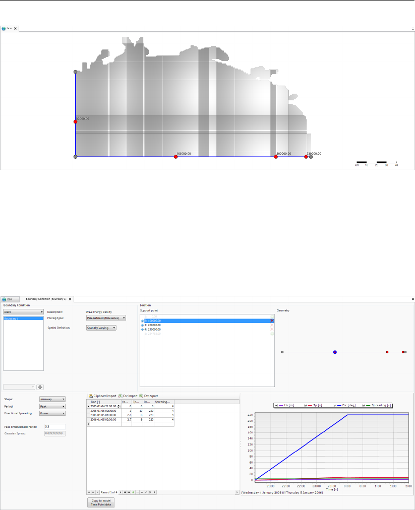
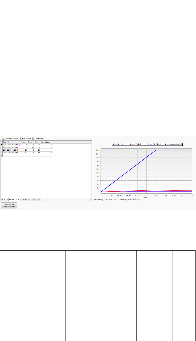
Edit conditions
In case of a parameterized wave spectrum, the (time-dependent) conditions can be set in the
conditions table and inspected in the corresponding graph (Figure 4.33).
The wave conditions are specified in terms of:
Significant wave height
The significant wave height specified in m.
Wave period
The characteristic period of the energy spectrum. It is the value of the peak period (in s)
if option Peak is chosen in the Spectral space sub-window or it is the value of the mean
period if option Mean is chosen in the above same sub-window.
Direction
Mean wave direction (direction of wave vector in degree) according to the Nautical or
Cartesian convention.
Directional spreading
This is the directional standard deviation in degrees if the option Degrees is chosen in the
SWAN Spectral Space window; or it is the power mif the option Cosine power is chosen
in the same window.
Figure 4.33: Specify parameterized wave boundary conditions and inspect in graph
Defaults and ranges
Domain:
Parameter Lower limit Upper limit Default Unit
Number of points to specify
boundary
0 300 0 -
Spectral peak factor 1. 10. 3.3. -
Distance from corner point 0. Y-length 0. m
Significant wave height 0. 25. 0. m
Spectral peak period 0.1 20. 1. s
Wave direction -360 360. 0. ◦
Directional width (m) 1. 100. 4. -
38 of 124 Deltares
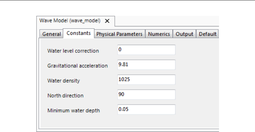
DRAFT
Graphical User Interface
Figure 4.34: Overview of physical Constants
4.4.8 Physical parameters
In the tab Physical parameters you can specify a number of physical parameters. These are:
Constants: Here you can specify constants such as the gravitational constant and the
water density
Processes: With these parameters you can influence some of the physical processes of
SWAN (i.e.type of formulation, dissipation processes, non-linear wave-wave interactions).
4.4.8.1 Constants
In the tab Constants you can specify the following parameters (see Figure 4.34):
Gravity
The gravitational acceleration in m/s2. The default value is 9.81 m/s2.
Water density
The water density ρin kg/m3. The default value is 1025 kg/m3.
North
The direction of North with respect to the x-axis (Cartesian convention). The default value is
90◦i.e. x-axis pointing East.
Minimum depth
The threshold depth in [m]; in the computation any positive depth smaller than this threshold
depth is set to the threshold depth. The default 0.05 m.
Deltares 39 of 124
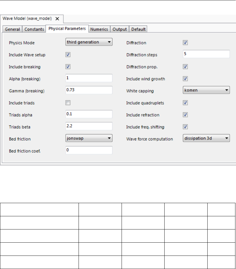
DRAFT
D-Waves, User Manual
Figure 4.35: Overview of physical Processes
Domain:
Parameter Lower limit Upper limit Default Unit
Acceleration of gravity 9.8 10. 9.81 m/s2
Density of water 950. 1050. 1025. kg/m3
North -360. 360. 90. deg
Minimum depth - - 0.05 m
4.4.9 Physical processes
SWAN contains a number of physical processes (see Figure 4.35) that add or withdraw wave
energy to or from the wave field. The processes included are: wave growth by wind, white-
capping, bottom friction, depth induced wave breaking, non-linear wave-wave interactions
(quadruplets and triads). SWAN can run in several modes, indicating the level of parame-
terisation. For initial SWAN runs, it is strongly advised to use the default values as shown
in Figure 4.35. First it should be determined whether or not a certain physical process is
relevant to the result. If this cannot be decided by means of a simple hand computation,
you can perform a SWAN computation without and with the physical process included in the
computations, in the latter case using the standard values chosen in SWAN.
Generation mode for physical formulations:
1st generation
With this option you indicate that SWAN should run in first-generation mode.
2nd generation
With this option you indicate that SWAN should run in second-generation mode (for more
information, reference is made to the SWAN manual).
40 of 124 Deltares

DRAFT
Graphical User Interface
3rd generation
With this option you indicate that SWAN should run in third-generation mode. Activated
are wind input, quadruplet interactions and white-capping. Triads, bottom friction and
depth-induced breaking are not activated by this option.
Remark:
If SWAN runs in third generation mode and the wind speed is larger than zero, then
the Quadruplets in Sub-data Group Various will be activated.
None
With this option you indicate that no deep water physical processes (i.e. wind, white-
capping and quadruplets) are activated.
Wave set-up
If this option is activated, the wave induced set-up is computed and accounted for in the
wave computations (during the computation it is added to the depth that is obtained from
the bottom and the water level). This option should only be used if SWAN is applied as
standalone model or if wave-induced set-up is not accounted for in the flow computations.
Depth-induced breaking
With this option you can influence depth-induced wave breaking in shallow water in the
SWAN model (see section 5.3.1). Ticking off this depth-induced term is usually unwise,
since this leads to unacceptably high wave heights near beaches (the compute wave
heights ‘explode’ due to shoaling effects).
B&J model
This option means that to model the energy dissipation in random waves due to depth-
induced breaking, the bore-based model of Battjes and Janssen (1978) is used. In this
option a constant breaker parameter is to be used.
Alpha
The coefficient for determining the rate of dissipation. Default = 1.0.
Gamma
The value of the breaker parameter defined as Hm/d. Default = 0.73.
Non-linear triad interactions (LTA)
With this option you can activate the triad wave-wave interactions in the SWAN model
(see section 5.3.1). Ticking off this feature means that the non-linear wave-wave inter-
actions due to the triads are not taken into account. LTA means that the Lumped Triad
Approximation (LTA) of Eldeberky and Battjes (1996) is used.
Alpha
The value of the proportionality coefficient αEB. The default value is equal to 0.1.
Beta
This controls the maximum frequency that is considered in the computations. The value
determines the ratio of the maximum frequency over the mean frequency, for which the
interactions are computed. The default value is 2.2.
Bed friction
With this option you can activate bed friction (see section 5.3.1). If this option is not used,
SWAN will not account for bed friction. In SWAN three different formulations are available,
i.e. that of Hasselmann et al. (1973) (JONSWAP), Collins (1972); Madsen et al. (1988)).
The default option is de-activated.
JONSWAP
This indicates that the semi-empirical expression derived from the JONSWAP results for
bottom friction dissipation (Hasselmann et al.,1973) will be activated.
-Coefficient
The coefficient of the JONSWAP formulation. It is equal to 0.067 m2s−3for wind sea
conditions (default value) and equal to 0.038 m2s−3for swell conditions.
Collins
This indicates that the expression of Collins (1972) will be activated.
Deltares 41 of 124
DRAFT
D-Waves, User Manual
-Coefficient
The Collins bottom friction coefficient, default = 0.015.
Madsen et al.
This indicates that the expression of Madsen et al. (1988) is activated.
-Coefficient
The equivalent roughness length scale of the bottom. Default = 0.05 m.
Diffraction
With this option you can activate diffraction in the wave computation. The default option
is de-activated. The diffraction implemented in SWAN is based on a phase-decoupled
refraction-diffraction approximation (Holthuijsen et al.,1993). It is expressed in terms of
the directional turning rate of the individual wave components in the 2D wave spectrum.
The approximation is based on the mild-slope equation for refraction and diffraction, omit-
ting phase information.
Smoothing coefficient
During every smoothing step all grid points exchange [smoothing coefficient] times the
energy with their neighbours. Default = 0.2.
Smoothing steps
Number of smoothing steps. The default value is equal to 5.
Adapt propagation
Switch to turn on or off the adaption of propagation of velocities in geographic space due
to diffraction. The default value is activated (when diffraction is activated).
Remark:
The process diffraction can only be solved accurately when a detailed grid is applied.
Several studies (e.g. Ilic (1994)) have shown that the grid size should be about 1/10
of the wave length; so, dx =L/10. In case of much coarser grids, the SWAN
computation can become unstable and results are not reliable. So, use diffraction
with care!
Wind growth
If this option is activated, wind growth is included in the computation. Note: Only if wind
is included in the computation.
White-capping
For the white capping two model descriptions are possible:
buttonoff (default)
button(Komen et al.,1984)
button(Van der Westhuysen,2007)
Quadruplets
If this option is activated, quadruplets are included in the computation. Note: Only if wind
is included in the computation.
Refraction
If this option is activated, refraction is included in the computation.
Frequency shifting
If this option is activated, frequency shifting is included in the computation
Wave force computation
With the integration of the fully spectral SWAN model under the Delft3D model it is possi-
ble to compute the wave forces on the basis of the energy wave dissipation rate or on the
gradient of the radiation stress tensor (SWAN UM,2000).
42 of 124 Deltares

DRAFT
Graphical User Interface
Domain:
Parameter Lower limit Upper limit Default Unit
Generation mode 3rd genera-
tion
Wave set-up inactive
Depth-induced breaking: B&J model
Alfa 0.1 10 1.0 -
Gamma 0.55 1.2 0.73 -
Non-linear triad interactions inactive
Alfa 0.001 10 0.10 -
Beta 0.001 10 2.2 -
Bottom friction JONSWAP
Bottom friction coefficient 0.067 m2/s3
Diffraction inactive
Smoothing coefficient 0 1.0 0.2 -
Smoothing steps 1 999 5 -
Adapt propation active
Wind growth inactive
White capping Komen et al
Quadruplets inactive
Refraction active
Frequency shift active
Wave forces Radiation
stress
Deltares 43 of 124
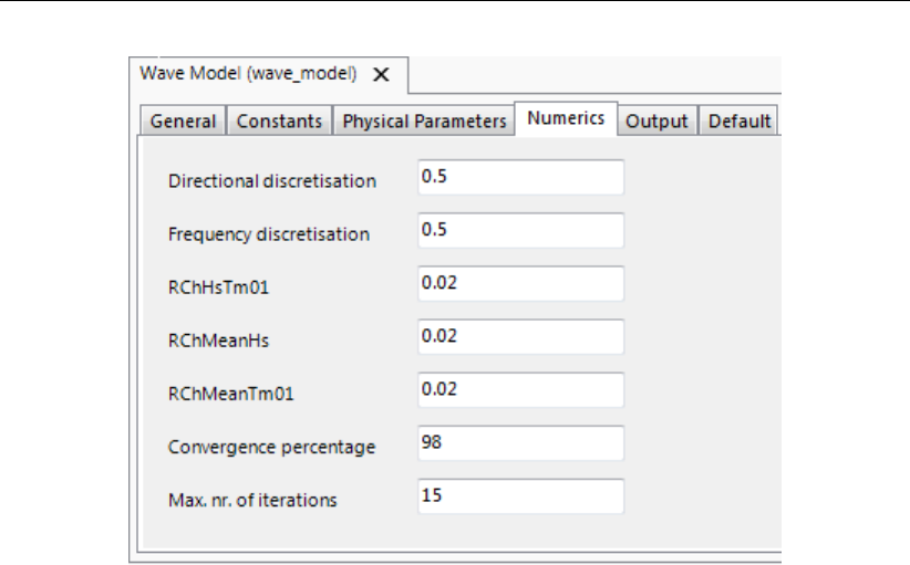
DRAFT
D-Waves, User Manual
Figure 4.36: Overview of Numerical parameters
4.4.10 Numerical parameters
In the Numerical parameters tab you can modify parameters that affect the stability and accu-
racy of the numerical computation (see Figure 4.36). To obtain robust results with acceptable
accuracy, apply the default diffusion parameters.
Spectral space
In this sub-window you can control the amount of diffusion of the implicit scheme in the
directional space through the Directional space (CDD) parameter and frequency space
through the Frequency space (CSS).
Directional space
A value of CDD = 0 corresponds to a central scheme and has the largest accuracy (diffu-
sion ≈0) but the computation may more easily generate spurious fluctuations. A value of
CDD = 1 corresponds to an upwind scheme and it is more diffusive and therefore prefer-
able if (strong) gradients in depth or current are present. The default value is CDD =
0.5.
Frequency space
A value of CSS = 0 corresponds to a central scheme and has the largest accuracy (diffu-
sion ≈0) but the computation may more easily generate spurious fluctuations. A value of
CSS = 1 corresponds to an upwind scheme and it is more diffusive and therefore prefer-
able if (strong) gradients in current are present. The default value is CSS = 0.5.
Accuracy criteria (to terminate the iterative computations)
With these options you can influence the criteria for terminating the iterative procedure
in the SWAN computation (for convergence criteria of SWAN see section 5.5.1). SWAN
stops the iteration if:
a) The change in the local significant wave height (Hs) from one iteration to the next is
less than:
◦fraction Relative change of that wave height or
◦fraction Relative change w.r.t. mean value of the average significant wave height
(averaged over all wet grid points)
b) and if the change in the local mean wave period from one iteration to the next is less
than:
44 of 124 Deltares

DRAFT
Graphical User Interface
◦fraction Relative change of that period or
◦fraction Relative change w.r.t. mean value of the average mean wave period (av-
eraged over all wet grid points)
c) and if the conditions a) and b) are fulfilled in more than fraction Percentage of wet grid
points % of all wet grid points.
Relative change
The default value is 0.02.
Relative change w.r.t. mean value
The default value is 0.02, for both Hsand Tm01.
Percentage of wet grid points
The default value is 98%.
You can also control the terminating procedure by giving the maximum number of itera-
tions Max. number of iterations after which the computation stops.
Max. number of iterations
The default value is 15.
Domain:
Parameter Lower limit Upper limit Default Unit
Diffusion θ-space (directional) 0. 1. 0.5 -
Diffusion σ-space (frequency) 0. 1. 0.5 -
Relative change 0. - 0.02 -
Relative change w.r.t. mean
value (Hsand Tm01 )
0. - 0.02 -
Percentage of wet grid points 0. 100% 98% -
Max. number of iterations 1 - 15 -
4.4.11 Output parameters
In the tab Output parameters (see Figure 4.37) you can determine to which grid (i.e. WAVE
or FLOW grid) output is written and to which extent the computations should be monitored.
The latter option can be used to specify that D-Waves should produce intermediate (model)
results during a SWAN run (test output) if the program produces unexpected results.
There are a couple of options available to monitor the SWAN computation:
Level of test output (Default: 0)
For values up to 50 test output is made that can be interpreted by you. For values above
50, information for the programmer is produced. For values under 100 the amount is usually
reasonable, for values above 200 it can be huge.
Trace subroutine calls (Default: off)
In case an error occurs, the name of the subroutine where the error occurred is written.
Write and use hotstart file (Default: no)
This option can be used to write the entire wave field at the end of a computation to an
initialisation file and use this field as initial condition in a subsequent SWAN run. In many
Deltares 45 of 124
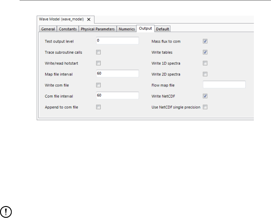
DRAFT
D-Waves, User Manual
Figure 4.37: Overview of Output parameters
cases with a series of wave runs, this option can save significantly amount of computational
time. In case of a FLOW-WAVE coupling with a frequent update, the hydrodynamic conditions
have not changed a lot since a previous wave computation. Therefore SWAN can use the
results of a previous SWAN run as the initial condition for the wave field.
The format of the hotstart file is identical to the format of the files written by the 2D-spectrum
output in the pre-defined locations.
Remarks:
It is recommended to gradually vary the wave directions in the <wavecon>file. When
computing a wave condition using an existing HOT-file, which is generated during a
wave computation with a large different wave direction, the use of a HOT-file can lead
to unrealistic wave fields. Check the wave results carefully.
When applying only one wave condition (e.g. during a flow-wave coupling) it can be wise
to increase the required accuracy (in % of wet points) initially. The subsequent wave
computations may be completed faster in this way, although the first wave computation
will probably need more computational time.
Only verify input files (Default: no)
During pre-processing SWAN checks the input data. Depending on the severity of the errors
encountered during this pre-processing, SWAN does not start a computation. You can influ-
ence the error level above which SWAN will not start computations. The error level is coded
as follows:
Warnings
Errors (possibly automatically repaired or repairable by SWAN)
Severe Errors
D-Waves offers two options to save the results of the calculation: on the communication file
(if available) and on an output file.
Output for FLOW grid (Default: off)
Click in the check box to turn this option on or off. If you select Output for FLOW grid, a
communication file is available and will be updated. The FLOW model (and other modules)
can read and use the wave data directly, since the information is automatically converted
to the curvilinear grid definition by the wave module. In ?? a description of the output
parameters on the communication file is given.
46 of 124 Deltares

DRAFT
Graphical User Interface
A curvilinear grid file (FLOW grid) is required to enable this conversion. In case hydro-
dynamic results from a FLOW simulation are used, the flow input file has been selected.
The grid definition is read from this file. If no hydrodynamic results are used, a Select
grid file button is displayed and a grid file can be selected. If a grid file is selected, still a
communication file is needed. The WAVE simulation will expect that the communication
file <com-name>is available. The communication file can be generated by running a
stand-alone FLOW simulation or a online FLOW/WAVE simulation.
Output for computational grids (Default: off)
If this option is chosen, detailed output is generated on one or more computational grids.
This output is written to a NEFIS file with basename WAVM (waves map file). In ?? a
description of the output parameters on the <wavm-∗.dat>file is given.
Output for specific locations
For the locations defined as observation points you can have three types of output: Table,
1D spectra or 2D spectra.
The parameters written to the Table file are:
XP, YP co-ordinates of output location (with respect to the problem co-
ordinates)
DEPT water depth [m]
HSIG significant wave height [m]
DIR mean wave direction [◦]
Tpeak peak wave period [s]
TM01 mean wave period (Tm01) [s]
DSPR directional spreading of the waves [◦]
UBOT root-mean-square value of the maximum of the orbital motion
near the bottom [m/s]
XWindv, YWindv wind components [m/s]
Xvel, Yvel current velocity components [m/s]
The parameters written in the 1D spectra file are:
absolute frequencies [Hz]
energy densities [J m−2Hz−1]
average nautical direction [degrees]
directional spreading [degrees]
The parameters written in the 2D spectra file are:
absolute frequencies [Hz]
spectral nautical directions [degrees]
energy densities [J m−2Hz−1deg−1]
Remarks:
The Table output for specific locations is stored in files <run-idnit0j>.tab in case of
multiple grids and multiple time points. For the overall computational grid i= 1, for
the first nested grid i= 2, etc. For the first time point j= 1, for the second j= 2,
etc.
The 1D spectra output for specific locations is stored in files <run-idnit0j.sp1>.
Similar for the 2D spectra output in <run-idnit0j.sp2>files.
In case of only one grid and multiple time points the files are <run-idt0j.tab>,<run-
idt0j.sp1>and <run-idt0j.sp2>.
In case of multiple grids and only one time points the files are <run-idni.tab>,<run-
idni.sp1>and <run-idni.sp2>.
In case of only one grid and only one time points the files are <run-id.tab>,<run-
id.sp1>and <run-id.sp2>.
Output curves
Deltares 47 of 124
DRAFT
D-Waves, User Manual
The following output quantities will be generated by D-Waves at the output locations along
a curve.
XP, YP co-ordinates of output location (with respect to the problem co-ordinates)
DIST distance along the output curve in [m]
DEPT depth in [m]
HSIG significant wave height [m]
PER mean wave period (Tm01, [s])
DIR mean wave direction [degrees]
DSPR directional spreading of the waves [degrees]
DISS dissipation rate [J m−2s−1]
WLEN mean wave length [m]
U,V current velocity [m/s]
All the data of each output curve is presented in a table and will be saved in only one file,
named: <curves.run-id>.
4.4.12 Output
Note: Yet to be specified
48 of 124 Deltares
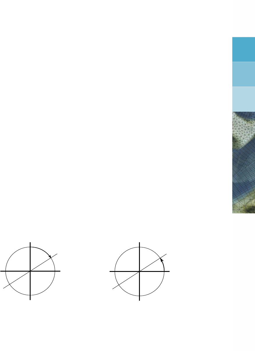
DRAFT
5 Conceptual description
5.1 Introduction
The purpose of this chapter is to give some general background with respect to the unit and
co-ordinate system, the grids (resolution, orientation etc.) and the boundary conditions of the
SWAN model. Advice will be given how to choose the basic input for Delft3D-WAVE for the
SWAN computations.
A brief description is given with respect to the physics (see section 5.3) and numerics (sec-
tion 5.4) that have been implemented in the SWAN model. This description has been copied -
with permission of Delft University of Technology, The Netherlands (personal communication
with dr N. Booij and dr L.H. Holthuijsen, 1999) - from the SWAN manual for SWAN version
40.41. The description given here is indicative only. For a full and proper description reference
is made to SWAN UM (2000).
5.2 General background
5.2.1 Units and co-ordinate systems
Delft3D-WAVE expects all quantities that are input by the user, to be expressed by means of
the S.I. system of units: m, kg, s and composites of these with accepted compounds, such
as Newton [N] and Watt [W]. Consequently the wave height and water depth are in [m], wave
period in [s] etc. Directions and spherical co-ordinates are in degrees [◦] and not in radians.
Delft3D-WAVE can operate in a flat plane and on a spherical earth.
North
East
South
West
North
East
South
West
Figure 5.1: Nautical convention (left panel) and Cartesian convention (right panel) for di-
rection of winds and (incident) waves
In the input for Delft3D-WAVE the directions of winds and (incident) waves are defined relative
to the co-ordinate system according to a Nautical convention or Cartesian convention, see
Figure 5.1 (for definitions reference is made to Appendix B).
In the Cartesian system, all geographic locations and orientations in SWAN, e.g. for the com-
putational grid or for output points, are defined in one common Cartesian co-ordinate system
with origin (0,0) by definition. This geographical origin may be chosen totally arbitrarily by you.
In the spherical system, all geographic locations and orientations in Delft3D-WAVE are de-
fined in geographic longitude and latitude. Both co-ordinate systems are designated in this
manual as the problem co-ordinate system. Figure 5.2 shows how the locations of the various
grids are determined with respect to the problem co-ordinates.
Deltares 49 of 124
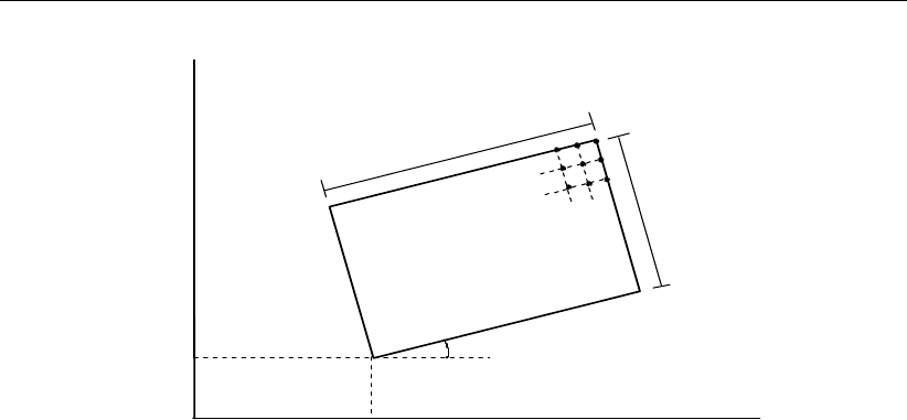
DRAFT
D-Waves, User Manual
MX * DX
MY * DY
α
P0
P0
Y
X
P0
Y
X
Figure 5.2: Definition of grids (input, computational and output grids) in Delft3D-WAVE
5.2.2 Choice of grids and boundary conditions
For your convenience Delft3D-WAVE accepts input and provides output on different grids.
It is not uncommon that a bottom grid is available as an existing data set without any relation
whatsoever to Delft3D-WAVE. You may want output on an entirely different grid (but in the
same region of course), whereas the computations in Delft3D-WAVE may require a different
grid altogether.
For these reasons Delft3D-WAVE operates with different grids (each may have a different
origin, orientation and resolution).
Input grids on which the bathymetry, current field and wind field (if present) are given by
you; one computational grid on which Delft3D-WAVE performs the computations, and one (or
more) output grid(s) on which you require output of Delft3D-WAVE.
During the computations (on the computational grid) Delft3D-WAVE obtains bathymetry and
current information by bilinear interpolation from the input grid. The output on the output
grid is in turn obtained in Delft3D-WAVE by interpolation from the computational grid. These
interpolations will cause some loss of accuracy.
Input grids
Bathymetry and current input need to be provided to Delft3D-WAVE on so-called input grids
(they need not be identical with the computational, the output grids or other input grids). It is
best to make an input grid larger than the computational grid, in fact, so large that it completely
covers the computational grid for every expected situation. In the region outside the input grid
Delft3D-WAVE assumes that the bottom level and friction coefficient are identical to those at
the nearest boundary of the input grid (lateral shift from that boundary). In the regions not
covered by this lateral shift (i.e. in the outside corner quadrants of the input grid), a constant
field equal to the value at the nearest corner point of the input grid is taken.
You should choose the resolution for the input grid such that relevant spatial details in the
bathymetry and in the current pattern are well resolved. Special care is required in cases with
sharp and shallow ridges in the sea bottom. In such cases the shallowest parts are of vital
importance to obtain good Delft3D-WAVE results (during propagation the waves are ‘clipped’
by surf breaking at some maximum value determined by the minimum depth). To represent
50 of 124 Deltares
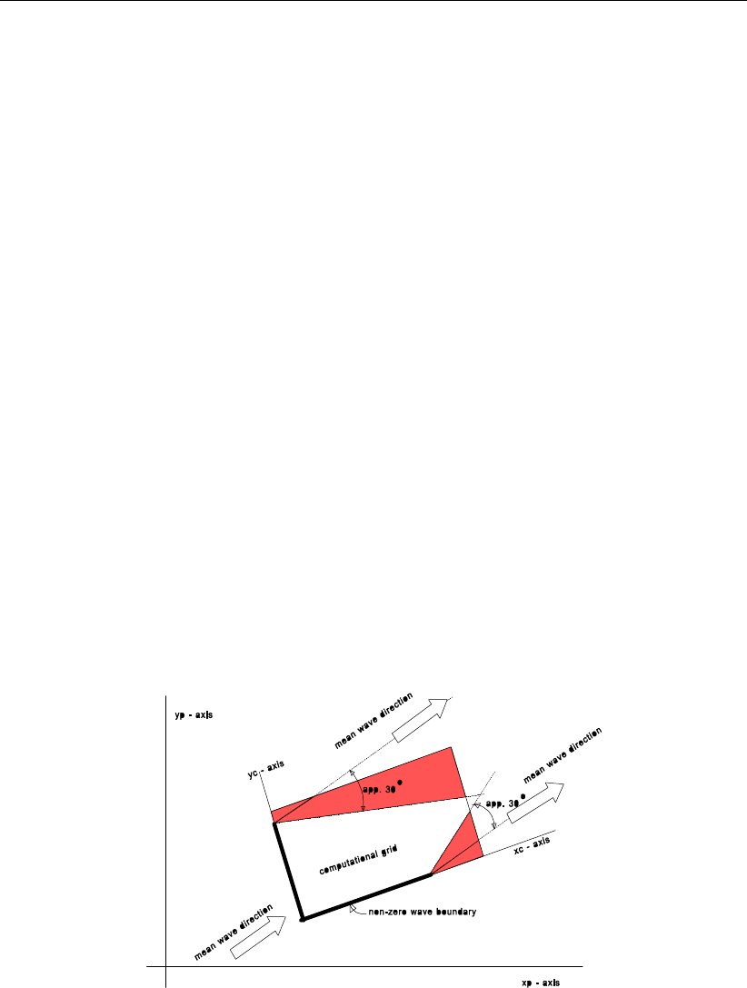
DRAFT
Conceptual description
these shallowest parts in the bottom grid, you may want to have one grid line coincide with
the ridge top (even if this means ”moving” the ridge to the nearest line in the bathymetry grid).
If this is not done, the computed wave height behind the shoal may well be computed higher
than it is in reality, because the ridge is seen deeper in Delft3D-WAVE than it actually is (too
coarse resolution to see shallow peak of the ridge).
Computational grid and boundary conditions
The computational grid is a grid in four dimensions: x-, y- and θ-, σ- space. The computa-
tional grid in x-, y-space must be chosen by you with care. You should choose the location
of the up-wave boundary in water so deep that refraction effects have not (yet) influenced the
wave field. However, a deep water up-wave boundary is not a strict requirement for Delft3D-
WAVE. This advice is not applicable if the incoming waves are provided by a model which
takes refraction into account, for instance Delft3D-WAVE itself (in a nested mode).
The computational grid must be larger than the area where you want to know the wave pa-
rameters. The length (in x-direction) needs not be longer than from the up-wave boundary to
the most down-wave point of interest. The width (in y-direction) must be larger than that of
the area of interest, because along each lateral side of the grid (if there is an open bound-
ary along that side) a region exists where the wave field is disturbed (in Delft3D-WAVE) by
an import of zero energy from the lateral boundaries (see Figure 5.3). This is not the case
if the wave conditions along the lateral boundaries are specified by you or obtained from a
previous Delft3D-WAVE run or if that boundary is closed (e.g. by land). The angle of the line
dividing the disturbed area from the undisturbed area from the up-wave corner points (of the
computational grid) is approximately equal to the half-power width of the directional energy
distribution of the waves (this half-power width is typically 20◦to 40◦for waves generated by
the local wind or 5◦to 10◦for swell).
Figure 5.3: Disturbed regions in the computational grid
The spatial resolution of the computational grid should be sufficient to resolve relevant details
of the wave field. Usually a good choice is to take the resolution of the computational grid
approximately equal to that of the input (bathymetry/current) grid.
The computational spectral grid needs also to be provided by you. In frequency space it is
simply defined by a minimum and maximum frequency and the frequency resolution which
is proportional to the frequency itself (e.g. ∆f= 0.1f). In the frequency domain this low-
est frequency and highest frequency and the number of frequencies must be chosen. The
value of lowest frequency must be slightly smaller than 0.6 times the value of the lowest peak
frequency expected. The value of the highest frequency must be at least 2.5 to 3 times the
highest peak frequency expected; usually it is chosen less than or equal to 1 Hz.
Deltares 51 of 124

DRAFT
D-Waves, User Manual
In directional space the directional range is the full 360◦unless you specify a limited direc-
tional range. This may be convenient (less computer time and/or space) when waves travel
towards a coast within a limited sector of 180◦, say. The directional resolution is determined
by the number of discrete directions that is provided by you. For wind seas with a direc-
tional spreading of typically 30◦on either side of the mean wave direction, a resolution of 10◦
seems enough whereas for swell with a directional spreading of less than 10◦, a resolution of
2◦or less may be required. If you are confident that no energy will occur outside a certain
directional sector (or is willing to ignore this energy), then the computations by SWAN can be
limited to the directional sector that does contain energy. This may often be the case of waves
propagating to shore within a sector of 180◦around some mean wave direction.
Nonstationary situations are simulated with the SWAN model as quasi-stationary with re-
peated model runs. This implies that as e.g. the flow computations progress in time, a (sta-
tionary) wave computation is performed at specified, intermediate time levels. Such stationary
wave computations are usually considered to be acceptable since the travel time of the waves
from the seaward boundary to the coast is mostly relatively small compared to the time scale
of variations in incoming wave field, the wind or tidal induced variations in depth and currents.
5.2.3 Output grids
Delft3D-WAVE can provide output on the computational grids or on grids that are indepen-
dent from the computational grid like the Delft3D-FLOW grid. It must be pointed out that the
information on a flow grid is obtained from the computational grid by spatial interpolation.
Therefore it is wise to choose a resolution that is fine enough to show relevant spatial details.
The spatial interpolation implies that some inaccuracies are introduced. It also implies that
bathymetry or current information on an (output) plot has been obtained by interpolating twice:
once from the input grid to the computational grid and once from the computational grid to the
output grid. If the input, computational and output grids are identical, then no interpolation
errors occur.
In the regions where the output grid does not cover the computational grid Delft3D-WAVE
assumes output values equal to zero.
5.3 Physical background of SWAN
5.3.1 Action balance equation
In SWAN the waves are described with the two-dimensional wave action density spectrum,
even when non-linear phenomena dominate (e.g., in the surf zone). The rational for using the
spectrum in such highly non-linear conditions is that, even in such conditions it seems possible
to predict with reasonable accuracy this spectral distribution of the second order moment of
the waves (although it may not be sufficient to fully describe the waves statistically). The
spectrum that is considered in SWAN is the action density spectrum N(σ, θ)rather than
the energy density spectrum E(σ, θ)since in the presence of currents, action density is
conserved whereas energy density is not (Whitham,1974). The independent variables are
the relative frequency σ(as observed in a frame of reference moving with the current velocity)
and the wave direction θ(the direction normal to the wave crest of each spectral component).
The action density is equal to the energy density divided by the relative frequency: N(σ, θ) =
E(σ, θ)/σ. In SWAN this spectrum may vary in time and space.
In SWAN the evolution of the wave spectrum is described by the spectral action balance
52 of 124 Deltares
DRAFT
Conceptual description
equation which for Cartesian co-ordinates is (e.g., Hasselmann et al. (1973)):
∂
∂tN+∂
∂xcxN+∂
∂y cyN+∂
∂σ cσN+∂
∂θ cθN=S
σ(5.1)
The first term in the left-hand side of this equation represents the local rate of change of ac-
tion density in time, the second and third term represent propagation of action in geographical
space (with propagation velocities cxand cyin x- and y-space, respectively). The fourth term
represents shifting of the relative frequency due to variations in depths and currents (with
propagation velocity cσin σ-space). The fifth term represents depth-induced and current-
induced refraction (with propagation velocity cθin θ-space). The expressions for these prop-
agation speeds are taken from linear wave theory (Whitham,1974;Mei,1983;Dingemans,
1997). The term S(= S(σ, θ)) at the right-hand side of the action balance equation is the
source term in terms of energy density representing the effects of generation, dissipation and
non-linear wave-wave interactions. A brief summary of the formulations that are used for the
various source terms in SWAN is given next.
The following processes are accounted for in SWAN:
generation by wind,
dissipation by whitecapping, bottom friction and depth-induced breaking,
non-linear wave-wave interaction (quadruplets and triads).
In addition wave propagation through obstacles and wave-induced set-up of the mean sea
surface can be computed in SWAN. These phenomena are addressed separately below (see
Sections 5.3.2 and 5.3.3).
Wind input
Transfer of wind energy to the waves is described in SWAN with a resonance mechanism
(Phillips,1957) and a feed-back mechanism (Miles,1957). The corresponding source term
for these mechanisms is commonly described as the sum of linear and exponential growth:
Sin(σ, θ) = A+BE(σ, θ)(5.2)
in which Aand Bdepend on wave frequency and direction, and wind speed and direction.
The effects of currents are accounted for in SWAN by using the apparent local wind speed and
direction. The expression for the term Ais due to Cavaleri and Malanotte-Rizzoli (1981) with
a filter to avoid growth at frequencies lower than the Pierson-Moskowitz frequency (Tolman,
1992a). Two optional expressions for the coefficient B are used in the model. The first is
taken from an early version of the WAM model (known as WAM Cycle 3, the WAMDI group
(1988)). It is due to Snyder et al. (1981), rescaled in terms of friction velocity U∗by Komen
et al. (1984). The drag coefficient to relate U∗to the driving wind speed at 10 m elevation
U10 is taken from Wu (1982). The second expression for Bin SWAN is taken from the most
recent version of the WAM model (known as WAM Cycle 4, Komen et al. (1994)). It is due
to Janssen (1991a) and it accounts explicitly for the interaction between the wind and the
waves by considering atmospheric boundary layer effects and the roughness length of the
sea surface. The corresponding set of equations is solved (as in the WAM model) with the
iterative procedure of Mastenbroek et al. (1993).
Deltares 53 of 124
DRAFT
D-Waves, User Manual
Dissipation
The dissipation term of wave energy is represented by the summation of three different con-
tributions: whitecapping Sds,w(σ, θ), bottom friction Sds,b(σ, θ)and depth-induced breaking
Sds,br(σ, θ).
Whitecapping is primarily controlled by the steepness of the waves. In presently operating
third-generation wave models (including SWAN) the whitecapping formulations are based on
a pulse-based model (Hasselmann,1974), as adapted by the WAMDI group (1988):
Sds,w(σ, θ) = −Γ˜σk
˜
kE(σ, θ)(5.3)
where Γis a steepness dependent coefficient, kis the wave number and ˜
sigma and ˜
k
denote a mean frequency and a mean wave number, respectively (cf. the WAMDI group
(1988)). Komen et al. (1984) estimated the value of Γby closing the energy balance of the
waves in fully developed conditions. This implies that this value depends on the wind input
formulation that is used.
An alternative description for whitecapping in SWAN is given by Van der Westhuysen et al.
(2007) and Van der Westhuysen (2007), which is an adapted form of the expression of Alves
and Banner (2003). The latter is based on the apparent relationship between wave groups and
whitecapping dissipation. This adaption is due to the fact that it can also be applied to mixed
sea-swell conditions and in shallow water. This was done by removing the dependencies on
mean spectral steepness and wavenumber in the original expression, and by applying source
term scaling arguments for its calibration (see below). This led to the following expression for
whitecapping dissipation:
Sds,w(σ, θ) = −C0
ds B(k)
Brp/2
(tanh(kh))(2−p0)/4pgkE(σ, θ)(5.4)
in which the density function B(k) is the azimuthal-integrated spectral saturation, which is
positively correlated with the probability of wave group-induced breaking. It is calculated from
frequency space variables as follows:
B(k) =
2π
Z
0
cgk3E(σ, θ)dθ (5.5)
and Br= 1.75 ×10⁻³is a threshold saturation level. The proportionality coefficient is set
to C0
ds = 5.0×10⁻⁵. When B(k)> Br, waves break and the exponent pis set equal to a
calibration parameter p0. For B(k)≤Brthere is no breaking, but some residual dissipation
proved necessary. This is obtained by setting p= 0.
Depth-induced dissipation may be caused by bottom friction, by bottom motion, by percolation
or by back-scattering on bottom irregularities (Shemdin et al.,1978). For continental shelf
seas with sandy bottoms, the dominant mechanism appears to be bottom friction (e.g., Bertotti
and Cavaleri (1994)) which can generally represented as:
Sds,b(σ, θ) = −Cbottom
σ2
g2sinh2(kd)E(σ, θ)(5.6)
in which Cbottom is a bottom friction coefficient. A large number of models have been pro-
posed since the pioneering paper of Putnam and Johnson (1949). Hasselmann et al. (1973)
54 of 124 Deltares

DRAFT
Conceptual description
suggested to use an empirically obtained constant. It seems to perform well in many dif-
ferent conditions as long as a suitable value is chosen (typically different for swell and wind
sea; Bouws and Komen (1983)). A non-linear formulation based on drag has been proposed
by Hasselmann and Collins (1968) which was later simplified by Collins (1972). More com-
plicated, eddy viscosity models have been developed by Madsen et al. (1988) (see Weber
(1991a)) and by Weber (1989,1991a,b). Considering the large variations in bottom condi-
tions in coastal areas (bottom material, bottom roughness length, ripple height etc.), there
is no field data evidence to give preference to a particular friction model (Luo and Monbaliu,
1994). For this reason, the simplest of each of these types of friction models has been imple-
mented in SWAN: the empirical JONSWAP model of Hasselmann et al. (1973), the drag law
model of Collins (1972) and the eddy-viscosity model of Madsen et al. (1988). The effect of a
mean current on the wave energy dissipation due to bottom friction is not taken into account
in SWAN. The reasons for this are given by Tolman (1992b) who argues that state-of-the-art
expressions vary too widely in their effects to be acceptable. He found that the error in finding
a correct estimate of the bottom roughness length scale has a much larger impact on the
energy dissipation rate than the effect of a mean current.
The process of depth-induced wave-breaking is still poorly understood and little is known
about its spectral modelling. In contrast to this, the total dissipation (i.e., integrated over the
spectrum) due to this type of wave breaking can be well modelled with the dissipation of a
bore applied to the breaking waves in a random field (Battjes and Janssen,1978;Thornton
and Guza,1983). Laboratory observations (e.g., Battjes and Beji (1992), Vincent et al. (1994);
Arcilla et al. (1994) and Eldeberky and Battjes (1996)) show that the shape of initially uni-
modal spectra propagating across simple (barred) beach profiles, is fairly insensitive to depth-
induced breaking. This has led Eldeberky and Battjes (1995) to formulate a spectral version of
the bore model of Battjes and Janssen (1978) which conserves the spectral shape. Expanding
their expression to include directions, the expression that is used in SWAN is:
Sds,br(σ, θ) = −Dtot
Etot
E(σ, θ)(5.7)
in which Etot and Dtot is the rate of dissipation of the total energy due to wave breaking
according to Battjes and Janssen (1978). Adding a quadratic dependency on frequency as
suggested by Mase and Kirby (1992) (supported by Elgar et al. (1997)) seems to have no
noticeable effect on the SWAN results. Chen and Guza (1997) inferred from observations and
simulations with a Boussinesq model that the high-frequency levels are insensitive to such
frequency dependency because an increased dissipation at high frequencies is compensated
approximately by increased non-linear energy transfer (but they did find the frequency depen-
dency to be relevant in time domain). The value of Dtot depends critically on the breaking
parameter γ=Hmax/d (in which Hmax is the maximum possible individual wave height in
the local water depth d). In Delft3D-WAVE a constant value is available equal to γ= 0.73
(the mean value of the data set of Battjes and Stive (1985).
Non-linear wave-wave interactions
In deep water, quadruplet wave-wave interactions dominate the evolution of the spectrum.
They transfer wave energy from the spectral peak to lower frequencies (thus moving the peak
frequency to lower values) and to higher frequencies (where the energy is dissipated by white-
capping). In very shallow water, triad wave-wave interactions transfer energy from lower fre-
quencies to higher frequencies often resulting in higher harmonics (Beji and Battjes,1993)
(low-frequency energy generation by triad wave-wave interactions is not considered here).
A full computation of the quadruplet wave-wave interactions is extremely time consuming and
not convenient in any operational wave model. A number of techniques, based on parametric
methods or other types of approximations have been proposed to improve computational
Deltares 55 of 124

DRAFT
D-Waves, User Manual
speed (see Young and Van Vledder (1993) for a review). In SWAN the computations are
carried out with the Discrete Interaction Approximation (DIA) of Hasselmann et al. (1985).
This DIA has been found quite successful in describing the essential features of a developing
wave spectrum (Komen et al.,1994). For uni-directional waves, this approximation is not valid.
In fact, the quadruplet interaction coefficient for these waves is nearly zero (G.Ph. van Vledder,
personal communication, 1996). For finite-depth applications, Hasselmann and Hasselmann
(1981) have shown that for a JONSWAP-type spectrum the quadruplet wave-wave interactions
can be scaled with a simple expression (it is used in SWAN).
A first attempt to describe triad wave-wave interactions in terms of a spectral energy source
term was made by Abreu et al. (1992). However, their expression is restricted to non-dispersive
shallow water waves and is therefore not suitable in many practical applications of wind waves.
The breakthrough in the development came with the work of Eldeberky and Battjes (1995) who
transformed the amplitude part of the Boussinesq model of Madsen and Sørensen (1993) into
an energy density formulation and who parameterised the biphase of the waves on the basis
of laboratory observations (Battjes and Beji,1992;Arcilla, Roelvink, O’Connor, Reniers and
Jimenez,1994). A discrete triad approximation (DTA) for co-linear waves was subsequently
obtained by considering only the dominant self-self interactions. Their model has been veri-
fied with flume observations of long-crested, random waves breaking over a submerged bar
(Beji and Battjes,1993) and over a barred beach (Arcilla et al.,1994). The model appeared to
be fairly successful in describing the essential features of the energy transfer from the primary
peak of the spectrum to the super harmonics. A slightly different version, the Lumped Triad
Approximation (LTA) was later derived by Eldeberky and Battjes (1996). This LTA is used in
SWAN.
5.3.2 Propagation through obstacles
SWAN can estimate wave transmission through a (line-)structure such as a breakwater (dam).
Such an obstacle will affect the wave field in two ways, first it will reduce the wave height locally
all along its length, and second it will cause diffraction around its end(s). The model is not able
to account for diffraction. In irregular, short-crested wave fields, however, it seems that the
effect of diffraction is small, except in a region less than one or two wavelengths away from the
tip of the obstacle (Booij et al.,1992). Therefore the model can reasonably account for waves
around an obstacle if the directional spectrum of incoming waves is not too narrow. Since
obstacles usually have a transversal area that is too small to be resolved by the bathymetry
grid in SWAN, an obstacle is modelled as a line. If the crest of the breakwater is at a level
where (at least part of the) waves can pass over, the transmission coefficient Kt(defined as
the ratio of the (significant) wave height at the down-wave side of the dam over the (significant)
wave height at the up-wave side) is a function of wave height and the difference in crest level
and water level. The expression is taken from Goda et al. (1967):
Kt= 0.51−sin π
2αF
Hi
+β for −β−α < F
Hi
< α −β(5.8)
where F=h−dis the freeboard of the dam and where Hiis the incident (significant) wave
height at the up-wave side of the obstacle (dam), his the crest level of the dam above the
reference level (same as reference level of the bottom), dthe mean water level relative to the
reference level, and the coefficients α,βdepend on the shape of the dam (Seelig,1979):
Case α β
Vertical thin wall 1.8 0.1
Caisson 2.2 0.4
Dam with slope 1:3/2 2.6 0.15
56 of 124 Deltares
DRAFT
Conceptual description
The above expression is based on experiments in a wave flume, so strictly speaking it is only
valid for normal incidence waves. Since there is no data available on oblique waves it is as-
sumed that the transmission coefficient does not depend on direction. Another phenomenon
that is to be expected is a change in wave frequency since often the process above the dam is
highly non-linear. Again there is little information available, so in the model it is assumed that
the frequencies remain unchanged over an obstacle (only the energy scale of the spectrum is
affected and not the spectral shape).
5.3.3 Wave-induced set-up
In a (geographic) 1D case the computation of the wave induced set-up is based on the ver-
tically integrated momentum balance equation which is a balance between the wave force
(gradient of the wave radiation stress) and the hydrodynamic pressure gradient (no wave-
induced currents exist).
Fx+gd ∂¯η
∂x = 0 (5.9)
where dis the total water depth (including the wave-induced set-up) and ¯ηis the mean surface
elevation (including the wave-induced set-up).
In a 2D case, computations are also based on the vertically integrated momentum balance
equation (in two geographic dimensions), supplemented with the observation of Dingemans
et al. (1987) that the wave-induced currents are mainly driven by the divergence-free part of
the wave forces whereas the set-up is mainly due to the rotation-free part of these forces. To
compute the set-up, it would then be sufficient to compute the set-up as if the currents are
zero, which implies that the divergence of all forces considered would be zero:
∂Fx
∂x +∂Fy
∂y +∂
∂x gd ∂η
∂x+∂
∂y gd∂η
∂y = 0 (5.10)
Note that divergence = 0 is only an approximation of the true divergence. These two equations
have been implemented in SWAN. The 2D set-up module can be activated within Delft3D-
WAVE.
5.3.4 Diffraction
To accommodate diffraction in SWAN simulations, a phase-decoupled refraction-diffraction
approximation is suggested (Holthuijsen et al.,1993). It is expressed in terms of the directional
turning rate of the individual wave components in the 2D wave spectrum. The approximation
is based on the mild-slope equation for refraction and diffraction, omitting phase information.
It does therefore not permit coherent wave fields in the computational domain.
5.4 Full expressions for source terms
The complete expressions for the physical processes of generation, dissipation and non-linear
wave-wave interactions that are available in the SWAN model are given here.
5.4.1 Input by wind
Wave growth by wind is described by:
Sin(σ, θ) = A+BE(σ, θ)(5.11)
Deltares 57 of 124
DRAFT
D-Waves, User Manual
in which Adescribes linear growth and BE exponential growth. It should be noted that the
SWAN model is driven by the wind speed at 10 m elevation U10 whereas the computations
use the friction velocity U∗. For the WAM Cycle 3 formulation the transformation from U10 to
U∗is obtained with:
U2
∗=CDU2
10 (5.12)
in which CDis the drag coefficient from Wu (1982) ?:
CD(U10) = 1.2875 ×10⁻³for U10 <7.5m/s
(0.8+0.065 [s/m]×U10)×10−3for U10 ≥7.5m/s (5.13)
The expression for Bis due to Komen et al. (1984). Their expression is a function of U∗/cph:
B= max 0,0.25 ρa
ρw28 U∗
cph
cos(θ−θw)−1σ(5.14)
in which cph is the phase speed and ρaand ρware the density of air and water, respectively.
This expression is also used in WAM Cycle 3 (cf. the WAMDI group (1988)).
5.4.2 Dissipation of wave energy
Whitecapping
The processes of whitecapping in the SWAN model are represented by the pulse-based model
of Hasselmann (1974). Reformulated in terms of wave number (rather than frequency) so as
to be applicable in finite water depth (cf. the WAMDI group (1988)), this expression is:
Sds,w(σ, θ) = −Γ˜σk
˜
kE(σ, θ)(5.15)
where ˜σand ˜
kdenote the mean frequency and the mean wave number (for expressions
see below) respectively and the coefficient Γdepends on the overall wave steepness. This
steepness dependent coefficient, as given by the WAMDI group (1988), has been adapted by
Günther et al. (1992) based on Janssen (1991a,b):
Γ=ΓKJ =Cds (1 −δ) + δk
˜
k ˜s
˜sP M p
(5.16)
For δ= 0 the expression of Γreduces to the expression as used by the WAMDI group
(1988). The coefficients Cds,δand mare tunable coefficients, ˜sis the overall wave steepness
(defined below), ˜sP M is the value of ˜sfor the Pierson-Moskowitz spectrum (1964; ˜sP M =
(3.02 ×10⁻³)1/2). This overall wave steepness ˜sis defined as:
˜s=˜
kpEtot (5.17)
The mean frequency ˜σ, the mean wave number ˜
kand the total wave energy Etot is defined
as (cf. the WAMDI group (1988)):
˜σ=E−1
tot Z2π
0Z∞
0
1
σE(σ, θ)dσdθ−1
˜
k=E−1
tot Z2π
0Z∞
0
1
√kE(σ, θ)dσdθ−2
(5.18)
Etot =Z2π
0Z∞
0
E(σ, θ)dσdθ
58 of 124 Deltares
DRAFT
Conceptual description
The values of the tunable coefficients Cds and δand exponent pin this model have been
obtained by Komen et al. (1984) by closing the energy balance of the waves in idealised
wave growth conditions (both for growing and fully developed wind seas) for deep water. This
implies that coefficients in the steepness dependent coefficient Γdepend on the wind input
formulation that is used. For the wind input of Komen et al. (1984) (corresponding to WAM
Cycle 3; the WAMDI group (1988)):
Cds = 2.36 ×10⁻⁵,(5.19)
δ= 0 and (5.20)
p= 4.(5.21)
Bottom friction
The bottom friction models that have been selected for SWAN are the empirical model of
JONSWAP (Hasselmann et al.,1973), the drag law model of Collins (1972) and the eddy-
viscosity model of Madsen et al. (1988). The formulations for these bottom friction models
can all be expressed in the following form:
Sds,b(σ, θ) = −Cbottom
σ2
g2sinh2(kd)E(σ, θ)(5.22)
in which Cbottom is a bottom friction coefficient that generally depends on the bottom orbital
motion represented by Urms:
U2
rms =Z2π
0Z∞
0
σ2
sinh2(kd)E(σ, θ)dσdθ (5.23)
Hasselmann et al. (1973) found from the results of the JONSWAP experiment Cbottom =
CJON = 0.038 m2s−3for swell conditions. Bouws and Komen (1983) selected a bottom
friction coefficient of CJON = 0.067 m2s−3for fully developed wave conditions in shallow
water. Both values are available in SWAN.
The expression of Collins (1972) is based on a conventional formulation for periodic waves
with the appropriate parameters adapted to suit a random wave field. The dissipation rate is
calculated with the conventional bottom friction formulation of Eq. (5.22) in which the bottom
friction coefficient is Cbottom =CfgUrms with Cf= 0.015 (Collins,1972). (Note that Collins
(1972) contains an error in the expression due to an erroneous Jacobean transformation; see
page A-16 of Tolman (1990).)
Madsen et al. (1988) derived a formulation similar to that of Hasselmann and Collins (1968)
but in their model the bottom friction factor is a function of the bottom roughness height and
the actual wave conditions. Their bottom friction coefficient is given by:
Cbottom =fw
g
√2Urms (5.24)
in which fwis a non-dimensional friction factor estimated by using the formulation of Jonsson
(1966) (cf. Madsen et al. (1988)):
1
4√fw
+10log 1
4√fw=mf+10log ab
KN(5.25)
in which mf=−0.08 (Jonsson and Carlsen,1976) and abis a representative near-bottom
excursion amplitude:
a2
b= 2 Z2π
0Z∞
0
1
sinh2(kd)E(σ, θ)dσdθ (5.26)
Deltares 59 of 124
DRAFT
D-Waves, User Manual
and KNis the bottom roughness length scale. For values of ab/KN smaller than 1.57 the
friction factor fwis 0.30 (Jonsson,1980).
Depth-induced wave breaking
To model the energy dissipation in random waves due to depth-induced breaking, the bore-
based model of Battjes and Janssen (1978) is used in SWAN. The mean rate of energy
dissipation per unit horizontal area due to wave breaking Dtot is expressed as:
Dtot =−1
4αBJ Qbσ
2πH2
m(5.27)
in which αBJ = 1 in SWAN, Qb[-] is the fraction of breaking waves determined by:
1−Qb
ln Qb
=−8Etot
H2
m
(5.28)
in which Hmis the maximum wave height that can exist at the given depth and ¯σis a mean
frequency defined as:
¯σ=E−1
tot Z2π
0Z∞
0
σE(σ, θ)dσdθ (5.29)
Extending the expression of Eldeberky and Battjes (1995) to include the spectral directions,
the dissipation for a spectral component per unit time is calculated in SWAN with:
Sds,br(σ, θ) = Dtot
E(σ, θ)
Etot
(5.30)
The maximum wave height Hmis determined in SWAN with Hm=γd, in which γis the
breaker parameter and d is the total water depth (including the wave-induced set-up if com-
puted by SWAN). In literature, this breaker parameter γis often a constant or it is expressed
as a function of bottom slope or incident wave steepness (Galvin,1972;Battjes and Janssen,
1978;Battjes and Stive,1985;Arcilla and Lemos,1990;Kaminsky and Kraus,1993;Nelson,
1987,1994). Since SWAN is locally defined, the dependency on incident wave steepness
cannot be used.
In the publication of Battjes and Janssen (1978) in which the dissipation model is described,
a constant breaker parameter, based on Miche’s criterion, of γ= 0.8was used. Battjes
and Stive (1985) re-analysed wave data of a number of laboratory and field experiments and
found values for the breaker parameter varying between 0.6 and 0.83 for different types of
bathymetry (plane, bar-trough and bar) with an average of 0.73. From a compilation of a large
number of experiments Kaminsky and Kraus (1993) have found breaker parameters in the
range of 0.6 to 1.59 with an average of 0.79.
5.4.3 Nonlinear wave-wave interactions
Quadruplet wave-wave interactions
The quadruplet wave-wave interactions are computed with the Discrete Interaction Approxi-
mation (DIA) as proposed by Hasselmann et al. (1985). Their source code (slightly adapted
by Tolman, personal communication, 1993) has been used in the SWAN model. In the Dis-
crete Interaction Approximation two quadruplets of wave numbers are considered, both with
60 of 124 Deltares

DRAFT
Conceptual description
frequencies:
σ1=σ2=σ
σ3=σ(1 + λ) = σ+(5.31)
σ4=σ(1 −λ) = σ−
where λis a constant coefficient set equal to 0.25. To satisfy the resonance conditions for
the first quadruplet, the wave number vectors with frequency σ3and σ4lie at an angle of
θ1=−11.5◦and θ2= 33.6◦to the two identical wave number vectors with frequencies σ1
and σ2. The second quadruplet is the mirror of this first quadruplet (the wave number vectors
with frequency σ3and σ4lie at mirror angles of θ3= 11.5◦and θ4=−33.6◦.
Within this discrete interaction approximation, the source term Snl4(σ, θ)is given by:
Snl4(σ, θ) = S∗
nl4(σ, θ) + S∗∗
nl4(σ, θ)(5.32)
where S∗
nl4(σ, θ)refers to the first quadruplet and S∗∗
nl4(σ, θ)to the second quadruplet (the
expressions for S∗∗
nl4(σ, θ)are identical to those for S∗
nl4(σ, θ)for the mirror directions) and:
S∗
nl4(σ, θ)=2δS∗
nl4(α1, σ, θ)−δS∗
nl4(α2, σ, θ)−δS∗
nl4(α3, σ, θ)(5.33)
in which α1= 1,α2= (1 + λ)and α3= (1 −λ). Each of the contributions (i= 1,2,3) is:
δSnl4(αiσ, θ) = Cnl4(2π)2g−4σ
2π11
E2(αiσ, θ)E2(αiσ+, θ)
(1 + λ)4+E2(αiσ−, θ)
(1 −λ)4−2E2(αiσ, θ)E2(αiσ+, θ)E2(αiσ−, θ)
(1 −λ2)4
(5.34)
The constant Cnl4= 3×10⁷. Following Hasselmann and Hasselmann (1981), the quadruplet
interaction in finite water depth is taken identical to the quadruplet transfer in deep water
multiplied with a scaling factor R:
Snl4,finite depth =R(kpd)Snl4,infinite depth (5.35)
where Ris given by:
R(kpd) = 1 + Csh1
kpd(1 −Csh2kpd) exp(Csh3kpd)(5.36)
in which kpis the peak wave number of the JONSWAP spectrum for which the original com-
putations were carried out. The values of the coefficients are: Csh1= 5.5,Csh2= 6/7
and Csh3=−1.25. In the shallow water limit, i.e., kpd→0the non-linear transfer tends to
infinity. Therefore a lower limit of kpd= 0.5is applied (cf. WAM Cycle 4; Komen et al. (1994),
resulting in a maximum value of R(kpd)=4.43. To increase the model robustness in case
of arbitrarily shaped spectra, the peak wave number kpis replaced by kp= 0.75¯
k(Komen
et al.,1994).
Deltares 61 of 124
DRAFT
D-Waves, User Manual
Triad wave-wave interactions
The Lumped Triad Approximation (LTA) of Eldeberky and Battjes (1996), which is a slightly
adapted version of the Discrete Triad Approximation of Eldeberky and Battjes (1995) is used
in SWAN in each spectral direction:
Snl3(σ, θ) = S−
nl3(σ, θ) + S+
nl3(σ, θ)(5.37)
with
S+
nl3(σ, θ) = max{0, αEB2πccgJ2|sin(β)|{E2(σ/2, θ)−2E(σ/2, θ)E(σ, θ)}} (5.38)
and
S−
nl3(σ, θ) = −2S+
nl3(2σ, θ)(5.39)
in which αEB is a tunable proportionality coefficient. The bi-phase βis approximated with
β=−π
2+π
2tanh 0.2
Ur (5.40)
with Ursell number Ur:
Ur =g
8√2π2
Hs¯
T2
d2(5.41)
with ¯
T= 2π/¯σ. Usually, the triad wave-wave interactions are calculated only for 0.1≤
Ur ≤10. But for stability reasons, it is calculated for the whole range 0≤Ur ≤10.
This means that both quadruplets and triads are computed at the same time. The interaction
coefficient Jis taken from Madsen and Sørensen (1993):
J=k2
σ/2(gd + 2c2
σ/2)
kσdgd +2
15 gd3k2
σ−2
5σ2d2(5.42)
Wave-induced set-up
In a geographic 1D case the computation of the wave induced set-up is based on the vertically
integrated momentum balance equation which is a balance between the wave force (gradient
of the wave radiation stress normal to the coast) and the hydrostatic pressure gradient (note
that the component parallel to the coast causes wave-induced currents but no set-up):
dSxx
dx +ρgH d¯η
dx = 0 (5.43)
where H=d+ ¯ηis the total water depth (including the wave-induced set-up), dis the bottom
level, ¯ηis the mean surface elevation (including the wave-induced set-up) and
Sxx =ρg Zncos2θ+n−1
2E dσdθ (5.44)
is the radiation stress tensor.
Observation and computations based on the vertically integrated momentum balance equa-
tion of Dingemans et al. (1987) show that the wave-induced currents are mainly driven by
the divergence-free part of the wave forces whereas the set-up is mainly due to the rotation-
free part of these forces. To compute the set-up, it would then be sufficient to consider the
divergence of the momentum balance equation. If the divergence of the acceleration in the
resulting equation is ignored, the result is:
∂Fx
∂x +∂Fy
∂y +∂
∂x(ρgH ∂¯η
∂x) + ∂
∂y (ρgH ∂¯η
∂y )=0 (5.45)
62 of 124 Deltares
DRAFT
Conceptual description
Diffraction
In a simplest case, we assume there are no currents. This means that cσ= 0. Let denotes the
propagation velocities in geographic and spectral spaces for the situation without diffraction
as: cx,0,cy,0and cθ,0. These are given by:
cx,0=∂ω
∂k cos(θ), cy,0=∂ω
∂k sin(θ), cθ,0=−1
k
∂ω
∂h
∂h
∂n (5.46)
where kis the wave number and nis perpendicular to the wave ray. We consider the following
eikonal equation:
K2=k2(1 + δ)(5.47)
with δdenoting the diffraction parameter as given by:
δ=∇(ccg∇Hs)
ccgHs
(5.48)
Due to diffraction, the propagation velocities are given by:
cx=cx,0¯
δ, cy=cy,0δ, cθ=cθ,0¯
δ−∂¯
δ
∂xcy,0+∂¯
δ
∂y cx,0(5.49)
where ¯
δ=√1 + δ.
5.5 Numerical implementation
The integration of the action balance equation has been implemented in SWAN with finite
difference schemes in all five dimensions (time, geographic space and spectral space). In
Delft3D-WAVE, SWAN is applied in a stationary mode so that time has been omitted from
the equations. Below the propagation schemes in geographical and spectral space are briefly
described.
The geographic space is discretised with a rectangular grid with constant resolutions ∆x
and ∆yin x- and y-direction respectively (in fact, this rectangular grid is a special case
of the curvi-linear grid that has been programmed in SWAN. The spectrum in the model
is discretised with a constant directional resolution ∆θand a constant relative frequency
resolution ∆σ/σ (logarithmic frequency distribution). For reasons of economy, an option
is available to compute only wave components travelling in a pre-defined directional sector
(θmin < θ < θmax; e.g., those components that travel shorewards within a limited directional
sector). The discrete frequencies are defined between a fixed low-frequency cut-off and a
fixed high-frequency cut-off (the prognostic part of the spectrum). For these frequencies the
spectral density is unconstrained. Below the low-frequency cut-off (typically fmin = 0.04 Hz
for field conditions) the spectral densities are assumed to be zero. Above the high-frequency
cut-off (typically 1 Hz for field conditions) a diagnostic f−mtail is added (this tail is used to
compute non-linear wave-wave interactions at the high frequencies and to compute integral
wave parameters). The reason for using a fixed high-frequency cut-off rather than a dynamic
cut-off frequency that depends on the wind speed or on the mean frequency, as in the WAM
and WAVEWATCH III model, is that in coastal regions mixed sea states with rather different
characteristic frequencies may occur. For instance, a local wind may generate a very young
sea behind an island, totally unrelated to (but superimposed on) a simultaneously occurring
swell. In such cases a dynamic cut-off frequency may be too low to properly account for the
locally generated sea state. Based on physical arguments the value of m(the power in the
above expression of the spectral tail) should be between 4 and 5 (Phillips,1985). In SWAN
m= 4 if the wind input formulation of Komen et al. (1984) is used (cf. WAM Cycle 3) and
m= 5 if the wind input formulation of Janssen (1991a) is used (cf. WAM Cycle 4).
Deltares 63 of 124

DRAFT
D-Waves, User Manual
5.5.1 Propagation
The numerical schemes in SWAN have been chosen on the basis of robustness, accuracy
and economy. Since the nature of the basic equation is such that the state in a grid point
is determined by the state in the up-wave grid points, the most robust scheme would be an
implicit upwind scheme (in both geographic and spectral space). The adjective ”implicit” is
used here to indicate that all derivatives of action density (xor y) are formulated at one com-
putational level, ixor iy, except the derivative in the integration dimension for which also the
previous or up-wave level is used (xor yin stationary mode). For such a scheme the values
of space steps, ∆xand ∆ywould be mutually independent. An implicit scheme would also
be economical in the sense that such a scheme is unconditionally stable. It permits relatively
large time steps in the computations (much larger than for explicit schemes in shallow wa-
ter). Several years of experience in using the second-generation HISWA shallow water wave
model (Holthuijsen et al.,1989) has shown that for coastal regions a first-order upwind differ-
ence scheme in geographic space is usually accurate enough. This experience, together with
test computations with SWAN has also shown that in spectral space a higher accuracy than
that of a first-order upwind scheme is required. This can be achieved by supplementing such a
scheme with a second-order central approximation (more economic than a second-order up-
wind scheme). For SWAN therefore, implicit upwind schemes in both geographic and spectral
space have been chosen, supplemented with a central approximation in spectral space.
The fact that in geographic space, the state in a grid point is determined by the state in the up-
wave grid points (as defined by the direction of propagation), permits a decomposition of the
spectral space into four quadrants. In each of the quadrants the computations can be carried
out independently from the other quadrants except for the interactions between them due
to refraction and non-linear wave-wave interactions (formulated in corresponding boundary
conditions between the quadrants). The wave components in SWAN are correspondingly
propagated in geographic space with the first-order upwind scheme in a sequence of four
forward-marching sweeps (one per quadrant). To properly account for the boundary conditions
between the four quadrants, the computations are carried out iteratively at each time step. The
discretization of the action balance equation is (for positive propagation speeds; including the
computation of the source terms but ignoring their discretisation):
[cxN]ix−[cxN]ix−1
∆xn
iy,iσ,iθ
+[cyN]iy−[cyN]iy−1
∆yn
ix,iσ,iθ
+(1 −ν)[cσN]iσ+1 + 2ν[cσN]iσ−(1 + ν)[cσN]iσ−1
2∆σn
ix,iy,iθ
+(1 −η)[cθN]iθ+1 + 2η[cθN]iθ−(1 + η)[cθN]iθ−1
2∆θn
ix,iy,iσ
=S
σn∗
ix,iy,iσ,iθ
(5.50)
where ix,iy,iσand iθare grid counters and ∆x,∆y,∆σand ∆θare the increments in
geographic space and spectral space respectively. The iterative nature of the computation
is indicated with the iteration index n (the iteration index for the source terms n∗is equal to
nor n−1, depending on the source term, see below). Because of these iterations, the
scheme is also approximately implicit for the source terms. For negative propagation speeds,
appropriate + and - signs are required in Eq. (5.50).
The coefficients νand ηdetermine the degree to which the scheme in spectral space is up-
wind or central. They thus control the numerical diffusion in frequency and directional space,
64 of 124 Deltares

DRAFT
Conceptual description
respectively. A value of ν= 0 or η= 0 corresponds to central schemes which have the
largest accuracy (numerical diffusion 0). Value of ν= 1 or η= 1 correspond to upwind
schemes which are somewhat more diffusive and therefore less accurate but more robust.
If large gradients of the action density in frequency space or directional space are present,
numerical oscillations can arise (especially with the central difference schemes) resulting in
negative values of the action density. In each sweep such negative values are removed from
the two-dimensional spectrum by setting these values equal to zero and re-scaling the remain-
ing positive values such that the frequency-integrated action density per spectral direction is
conserved. The depth derivatives and current derivatives in the expressions of cσand cθ
are calculated with a first-order upwind scheme. For very strong refraction the value of cθis
reduced in each grid point and for each wave component individually with the square of the
fraction of the grid spacing over which kd < 3.0.
The propagation scheme is implicit as the derivatives of action density (in xor y) at the
computational level (ixor iy, respectively) are formulated at that level except in the integration
dimension (xor y; depending on the direction of propagation) where also the up-wave level
is used. The values of ∆xand ∆yare therefore still mutually independent.
The boundary conditions in SWAN, both in geographic space and spectral space are fully
absorbing for wave energy that is leaving the computational domain or crossing a coast line.
The incoming wave energy along open geographic boundaries needs to be prescribed by
you. For coastal regions such incoming energy is usually provided only along the deep-
water boundary and not along the lateral geographic boundaries (i.e., the spectral densities
are assumed to be zero). This implies that such erroneous lateral boundary conditions are
propagated into the computational area. The affected areas are typically triangular regions
with the apex at the corners between the deep-water boundary and the lateral boundaries,
spreading towards shore at an angle of 30◦to 45◦(for wind sea conditions) on either side of
the deep-water mean wave direction (less for swell conditions; this angle is essentially equal
to the one-sided width of the directional distribution of the incoming wave spectrum). For this
reason the lateral boundaries should be sufficiently far away from the area of interest to avoid
the propagation of this error into the area.
Deltares 65 of 124

DRAFT
D-Waves, User Manual
66 of 124 Deltares

DRAFT
References
Abreu, M., A. Larraza and E. Thornton, 1992. “Nonlinear transformation of directional wave
spectra in shallow water.” Journal of Geophysical Research 97: 15579–15589.
Alves, J. and M. Banner, 2003. “Performance of a saturation-based dissipation-rate source
term in modelling the fetch-limited evolution of wind waves.” J. Phys. Oceanogr. 33: 1274–
1298.
Arcilla, A. and C. Lemos, 1990. Surf-Zone Hydrodynamics. Centro Internacional de Métodos
Numéricos en Ingenieria, Barcelona.
Arcilla, A., B. Roelvink, B. O’Connor, A. Reniers and J. Jimenez, 1994. “The Delta flume ’93
experiment.” In Proceedings Coastal Dynamics Conference ’94, pages 488–502.
Battjes, J. and S. Beji, 1992. “Breaking waves propagating over a shoal.” In Proceedings 23rd
International Conference Coastal Engineering, ASCE, pages 42–50.
Battjes, J. and J. Janssen, 1978. “Energy loss and set-up due to breaking of random waves,.”
In Proceedings 16th International Conference Coastal Engineering, ASCE, pages 569–587.
Battjes, J. and M. Stive, 1985. “Calibration and verification of a dissipation model for random
breaking waves.” Journal of Geophysical Research 90 (C5): 9159–9167.
Beji, S. and J. Battjes, 1993. “Experimental investigation of wave propagation over a bar.”
Coastal Engineering 19: 151–162.
Bertotti, L. and L. Cavaleri, 1994. “Accuracy of wind and wave evaluation in coastal regions.”
In Proceedings 24th International Conference Coastal Engineering, ASCE, pages 57–67.
Booij, N., L. H. Holthuijsen and P. H. M. de Lange, 1992. “The penetration of short-crested
waves through a gap.” In Proceedings 23rd International Conference Coastal Engineering,
Venice 4-9 Oct., 1992, New York, 1993, pages 1044–1052.
Booij, N., R. Ris and L. Holthuijsen, 1999. “A third-generation wave model for coastal regions,
Part I, Model description and validation.” Journal of Geophysical Research 104 (C4): 7649–
7666.
Bouws, E. and G. Komen, 1983. “On the balance between growth and dissipation in an
extreme, depth-limited wind-sea in the southern North Sea.” Journal of Physical Oceanog-
raphy 13: 1653–1658.
Cavaleri, L. and P. Malanotte-Rizzoli, 1981. “Wind wave prediction in shallow water: Theory
and applications.” Journal of Geophysical Research 86 (C11): 10 961–10 973.
Chen, Y. and R. Guza, 1997. “Modelling of breaking surface waves in shallow water.” Journal
of Geophysical Research 102 (C11): 25 035–25 046.
Collins, J., 1972. “Prediction of shallow water spectra.” Journal of Geophysical Research
77 (15): 2693–2707.
Delft3D-FLOW UM, 2013. Delft3D-FLOW User Manual. Deltares, 3.14 ed.
Dingemans, M. W., 1997. Water Wave Propagation over Uneven Bottoms, Vol. 1 and 2.
Advanced Series on Ocean Engineering, Vol. 13. World Scientific, London.
Dingemans, M. W., A. C. Radder and H. J. de Vriend, 1987. “Computation of the driving forces
of wave-induced currents.” Coastal Engineering 11: 539–563.
Deltares 67 of 124

DRAFT
D-Waves, User Manual
Eldeberky, Y. and J. Battjes, 1995. “Parameterization of triad interactions in wave energy
models, Gdansk, Poland.” In Proceedings Coastal Dynamics Conference ’95, pages 140–
148.
Eldeberky, Y. and J. A. Battjes, 1996. “Spectral modelling of wave breaking: Application to
Boussinesq equations.” Journal of Geophysical Research 101 (C1): 1253–1264.
Elgar, S., R. Guza, B. Raubenheimer, T. Herbers and E. Gallagher, 1997. “Spectral evolution
of shoaling and breaking waves on a barred beach.” Journal of Geophysical Research
102 (C7): 15797–15805.
Galvin, C., 1972. “Waves on beaches and resulting sediment transport.” In Wave breaking in
shallow water, pages 413–455. Academic Press Inc.
Goda, Y., H. Takeda and Y. Moriya, 1967. Laboratory investigation of wave transmission over
breakwaters. Tech. Rep. 13, Rep. port and Harbour Res. Institution. (from Seelig, 1979).
Günther, H., S. Hasselmann and P. A. E. M. Janssen, 1992. The WAM model Cycle 4 (revised
version). Tech. Rep. 4, Deutsch. Klim. Rechenzentrum, Hamburg, Germany.
Hasselmann, K., 1974. “On the spectral dissipation of ocean waves due to whitecapping.”
Boundary-Layer Meteorology 6 (1-2): 107–127.
Hasselmann, K., T. P. Barnett, E. Bouws, H. Carlson, D. E. Cartwright, K. Enke, J. Ew-
ing, H. Gienapp, D. E. Hasselmann, P. Kruseman, A. Meerburg, P. Müller, D. J. Olbers,
K. Richter, W. Sell and H. Walden, 1973. “Measurements of wind wave growth and swell
decay during the Joint North Sea Wave Project (JONSWAP).” Deutsche Hydrographische
Zeitschrift 8 (12).
Hasselmann, K. and J. Collins, 1968. “Spectral dissipation of finite-depth gravity waves due
to turbulent bottom friction.” Journal of Marine Research 26: 1–12.
Hasselmann, S. and K. Hasselmann, 1981. “A symmetrical method of computing the non-
linear transfer in a gravity-wave spectrum.” Hamburger Geophysikalische Einzelschriften
52 (8): 138p. Serie A.
Hasselmann, S., K. Hasselmann, J. Allender and T. Barnett, 1985. “Computations and pa-
rameterizations of the nonlinear energy transfer in a gravity wave spectrum. Part II: Param-
eterizations of the nonlinear transfer for application in wave models.” Journal of Physical
Oceanography 15 (11): 1378–1391.
Holthuijsen, L., N. Booij and T. Herbers, 1989. “A prediction model for stationary, short-crested
waves in shallow water with ambient currents.” Coastal Engineering 13: 23–54.
Holthuijsen, L., N. Booij and R. Ris, 1993. “A spectral wave model for the coastal zone.” In
Proceedings of 2nd International Symposium on Ocean Wave Measurement and Analysis,
New Orleans, pages 630–641.
Ilic, S., 1994. The role of offshore breakwaters in the coastal defence: comparison of two
measurement systems. Tech. rep., University of Plymouth School of Civil and Structural
Engineering.
Janssen, P., 1991a. “Quasi-linear theory of wind-wave generation applied to wave forecasting.”
Journal of Physical Oceanography 21: 1631–1642.
Janssen, P. A. E. M., 1991b. Consequences of the effect of surface gravity waves on the
mean air flow. Tech. rep., International Union of Theor. and Appl. Mech. (IUTAM), Sydney,
Australia. 193-198.
68 of 124 Deltares

DRAFT
References
Jonsson, I., 1966. “Wave boundary layers and friction factors.” In Proceedings 10th Interna-
tional Conference Coastal Engineering, ASCE, pages 127–148.
Jonsson, I. and N. Carlsen, 1976. “Experimental and theoretical investigations in an oscillatory
turbulent boundary layer.” Journal of Hydraulic Research 14: 45–60.
Jonsson, I. G., 1980. “A new approach to rough turbulent boundary layers.” Ocean Engineer-
ing 7: 109–152.
Kaminsky, G. and N. Kraus, 1993. “Evaluation of depth-limited wave breaking criteria.” In
Proceedings of 2nd International Symposium on Ocean Wave Measurement and Analysis,
pages 180–193. New Orleans.
Kirby, J. T. and T.-M. Chen, 1989. “Surface waves on vertically sheared flows: approximate
dispersion relations.” Journal of Geophysical Research 94: 1013–1027.
Komen, G., L. Cavaleri, M. Donelan, K. Hasselmann, S. Hasselmann and P. Janssen, 1994.
Dynamics and Modelling of Ocean Waves. Camebridge University Press.
Komen, G., S. Hasselmann and K. Hasselmann, 1984. “On the existence of a fully developed
wind-sea spectrum.” Journal of Physical Oceanography 14: 1271–1285.
Kuik, A., G. van Vledder and L. Holthuijsen, 1988. “A method for the routine analysis of
pitch-and-roll buoy wave data.” Journal of Physical Oceanography 18: 1020–1034.
Luo, W. and J. Monbaliu, 1994. “Effects of the bottom friction formulation on the energy
balance for gravity waves in shallow water.” Journal of Geophysical Research 99 (C9):
18501–18511.
Madsen, O., Y.-K. Poon and H. Graber, 1988. “Spectral wave attenuation by bottom friction:
Theory.” In Proceedings 21th International Conference Coastal Engineering, ASCE, pages
492–504.
Madsen, P. and O. Sørensen, 1993. “Bound waves and triad interactions in shallow water.”
Ocean Engineering 20 (4): 359–388.
Mase, H. and J. Kirby, 1992. “Hybrid frequency-domain KdV equation for random wave trans-
formation.” In Proceedings 23th International Conference Coastal Engineering, ASCE,
pages 474–487.
Mastenbroek, C., G. Burger and P. Janssen, 1993. “The dynamical coupling of a wave model
in a storm surge model through the atmospheric boundary layer.” Journal of Physical
Oceanography 23: 1856–1866.
Mei, C., 1983. The applied dynamics of ocean surface waves. Wiley, New York.
Miles, J., 1957. “On the generation of surface waves by shear flows.” Journal of Fluid Me-
chanics 3: 185–204.
Nelson, R., 1987. “Design wave heights on very mild slopes: An experimental study.” Trans-
actions of the Institution of Engineers, Australia, Civil Engineering 29: 157–161.
Nelson, R. C., 1994. “Depth limited wave heights in very flat regions.” Coastal Engineering
23: 43–59.
Phillips, N. A., 1957. “A co-ordinate system having some special advantages for numerical
forecasting.” Journal of Meteorology 14: 184–185.
Phillips, O., 1985. “Spectral and statistical properties of the equilibrium range in wind-
generated gravity waves.” Journal of Fluid Mechanics 156: 505–531.
Deltares 69 of 124

DRAFT
D-Waves, User Manual
Putnam, J. and J. Johnson, 1949. “The dissipation of wave energy by bottom friction.” Trans-
actions - American Geophysical Union 30: 67–74.
Ris, R., N. Booij and L. Holthuijsen, 1999. “A third-generation wave model for coastal regions,
Part II: Verification.” Journal of Geophysical Research 104 (C4): 7649–7666.
Seelig, W., 1979. “Effects of breakwaters on waves: laboratory tests of wave transmission by
overtopping.” In Proceedings Conference Coastal Structures, vol. 79:2, pages 941–961.
Shemdin, P., K. Hasselmann, S. Hsiao and K. Herterich, 1978. “Non linear and linear bottom
interaction effects in shallow water.” In Turbulent Fluxes through the Sea Surface Wave
Dynamics and Prediction, NATO Conference Series, no. 1 in V, pages 347–372.
Snyder, R., F. Dobson, J. Elliot and R. Long, 1981. “Array measurement of atmospheric
pressure fluctuations above surface gravity waves.” Journal of Fluid Mechanics 102: 1–59.
SWAN UM, 2000. SWAN Cycle III version 40.11 User Manual (not the short version). Delft
University of Technology, Delft, The Netherlands, 0.00 ed.
Thornton, E. and R. Guza, 1983. “Transformation of wave height distribution.” Journal of
Geophysical Research 88 (C10): 5925–5938.
Tolman, H., 1990. Wind wave propagation in tidal seas. Ph.D. thesis, Delft University of
Technology, Department of Civil Engineering, The Netherlands.
Tolman, H. L., 1992a. “Effects of numerics on the physics in a third-generation windwave
model.” Journal of Physical Oceanography 22: 1095–1111.
Tolman, H. L., 1992b. “An evaluation of expressions for the wave energy dissipation due to
bottom friction in the presence of currents.” Coastal Engineering 16: 165–179.
Vincent, C., J. Smith and J. Davis, 1994. “Parameterization of wave breaking in models.” In
M. Isaacson and M. Quick, eds., Proceedings of International Symp.: Waves - Physical and
Numerical Modelling, vol. II, pages 753–762. University of British Columbia, Vancouver,
Canada.
WAMDI group, 1988. “The WAM model a third generation ocean wave prediction model.”
Journal of Physical Oceanography 18: 1775–1810.
Weber, S., 1989. Surface gravity waves and turbulent bottom friction. Ph.D. thesis, University
of Utrecht, The Netherlands.
Weber, S. L., 1991a. “Bottom friction for wind sea and swell in extreme depth-limited situa-
tions.” Journal of Physical Oceanography 21: 149–172.
Weber, S. L., 1991b. “Eddy-viscosity and drag-law models for random ocean wave dissipa-
tion.” Journal of Fluid Mechanics 232: 73–98.
Westhuysen, A. J. Van der, 2007. Advances in the spectral modelling of wind waves in the
nearshore. Ph.D. thesis, Delft University of Technology. Fac. of Civil Engineering.
Westhuysen, A. Van der, M. Zijlema and J. Battjes, 2007. Nonlinear saturation-based white-
capping dissipation in SWAN for deep and shallow water. Ph.D. thesis, Delft University of
Technology.
Whitham, G., 1974. Linear and nonlinear waves. Wiley, New York.
WL | Delft Hydraulics, 1999. Modification first-guess SWAN and bench mark tests for SWAN.
Tech. Rep. H3515, WL | Delft Hydraulics, Delft, The Netherlands, Delft.
70 of 124 Deltares

DRAFT
References
WL | Delft Hydraulics, 2000. Physical formulations SWAN and data for validation. Tech. Rep.
H3528, WL | Delft Hydraulics, Delft, The Netherlands, Delft.
Wu, J., 1982. “Wind-stress coefficients over sea surface from breeze to hurricane.” Journal of
Geophysical Research 87 (C12): 9704–9706.
Young, I. R. and G. van Vledder, 1993. “A review of the central role of nonlinear interactions
in wind-wave.” Philosophical transaction of the Royal Society London A 342: 505–524.
Deltares 71 of 124

DRAFT
D-Waves, User Manual
72 of 124 Deltares
DRAFT
A Files of Delft3D-WAVE
A.1 MDW-file
A.1.1 General description
File contents The Master Definition WAVE file (MDW-file) is the input file for the
wave simulation program.
Filetype ASCII
File format Free formatted
Filename <name.mdw>
Generated WAVE-GUI or manually offline
The Master Definition WAVE file (MDW-file) is the input file for the wave simulation program.
It contains all the necessary data required for defining a model and running the simulation
program. In the MDW-file you can define attribute files in which relevant data (for some pa-
rameters) are stored. This is especially useful when parameters contain a large number of
data (e.g. time-dependent or space varying data). The user-definable attribute files are listed
and described in Appendix A.
The MDW-file has the following general characteristics:
Each line contains a maximum of 300 characters.
Each set of input parameter(s) is preceded by a chapter name enclosed in square brackets
(e.g. [WaveFileInformation]).
Each input parameter is preceded by a Keyword.
AKeyword is a combination of numerical and alpha-numerical characters, but starting
with an alpha-numeric character, followed by an equal sign “=”.
The MDW-file is an intermediate file between the WAVE-GUI and the WAVE simulation pro-
gram. As it is an ASCII-file, it can be transported to an arbitrary hardware platform. Conse-
quently, the WAVE simulation program and the WAVE-GUI do not necessarily have to reside
on the same hardware platform.
Generally, you need not to bother about the internal layout or content of the MDW-file. It is,
however, sometimes useful to be able to inspect the file and/or make small changes manually.
Therefore the MDW-file is an ordinary ASCII-file which you can inspect and change with your
favourite ASCII-editor.
The MDW-file is self contained, i.e. it contains all the necessary information about the model
concerned. It can therefore be used as model archive by storing/printing the file.
Here we list all the possible chapters and keywords of the MDW-file:
Record description:
Keyword Format Description
WaveFileInformation
FileVersion string should be 02.00
General
ProjectName C∗16 project name
continued on next page
∗May be specified multiple times
+Not supported by WAVE-GUI
R = Real; I = Integer; L = Logical; C = Character
Deltares 73 of 124

DRAFT
D-Waves, User Manual
continued from previous page
Keyword Format Description
ProjectNr C∗4 project number
Description∗C∗72 description line
OnlyInputVerify 1 L switch for input validation or simulation run: false = simulation run, or true = input validation only
SimMode key-value simulation mode: stationary, quasi-stationary, non-stationary
TimeStep 1 R time step in case of non-stationary simulation
TScale+1 R, optional unit of time, default is 60.0)
FlowFile+string name of mdf-file containing FLOW input. If FlowFile is empty, FLOW is not running online. If FlowFile is
non-empty, FLOW is running online.
FlowMudFile+string name of mdf-file containing FLOW input for the mud phase of a two phased FLOW model. If FlowMudFile is
empty, MUD is not running online. If FlowMudFile is non-empty, MUD is running online.
FlowBedLevel 1 I default usage of bed level from hydrodynamic computation by all domains: 0 = “don’t use”, 1 = “use but don’t
extend”, 2 = “use and extend” if necessary. May be overruled by same keyword in group "domain". Not relevant
when FlowFile is empty; default: 0
FlowWaterLevel 1 I See description of FlowBedLevel above.
FlowVelocity 1 I See description of FlowBedLevel above.
FlowVelocityType key-value method of velocity computation (depth-averaged, surface-layer, wave-dependent; default: depth-averaged)
FlowWind 1 I See description of FlowBedLevel above.
DirConvention key-value direction specification convention: nautical, cartesian
ReferenceDate C∗10 reference date (string format: YYYY-MM-DD)
ObstacleFile string name of file containing obstacles
TSeriesFile string name of file containing time-dependent quantities
TimePntBlock 1 I, optional number of table in TSeriesFile containing time points; only if TSeriesFile has been specified
MeteoFile∗+characters Name of file containing meteo input
DirSpace 1 R, optional default directional space: circle, sector
NDir 1 R, optional default number of directional bins
StartDir 1 R, optional default start direction in case of sector directional space
EndDir 1 R, optional default end direction in case of sector directional space
NFreq 1 R, optional default number of frequencies
FreqMin 1 R, optional default minimum frequency
FreqMax 1 R, optional default maximum frequency
WaterLevel 1 R default water level
XVeloc 1 R default velocity in x-direction
YVeloc 1 R default velocity in y-direction
WindSpeed 1 R default wind speed
WindDir 1 R default wind direction
TimePoint∗TimePoint should be specified if TimePntBlock is not included and not Online with FLOW.
Time 1 R time in minutes since refdate 0:00 hours
WaterLevel 1 R water level at specified time point
XVeloc 1 R velocity in x direction at specified time point
YVeloc 1 R velocity in y direction at specified time point
WindSpeed 1 R wind speed at specified time point
WindDir 1 R wind direction at specified time point
Constants
WaterLevelCorrection1 R Overall water level correction
Gravity 1 R gravitational acceleration (default: 9.81 m/s2)
WaterDensity 1 R density of water (default: 1025 kg/m3)
NorthDir 1 R direction of north relative to x axis (default: 90◦)
MinimumDepth 1 R minimum water depth below which points are excluded from the computation (default: 0.05 m)
Processes
GenModePhys 1 I generation mode of physics: 1 for first-generation, 2 for second-generation, 3 for third-generation
continued on next page
∗May be specified multiple times
+Not supported by WAVE-GUI
R = Real; I = Integer; L = Logical; C = Character
74 of 124 Deltares

DRAFT
Files of Delft3D-WAVE
continued from previous page
Keyword Format Description
WaveSetup 1 L include wave setup (default: false)
Breaking 1 L include wave breaking (default: true)
BreakAlpha 1 R alpha coefficient for wave breaking (default: 1.0)
BreakGamma 1 R gamma coefficient for wave breaking (default: 0.73)
Triads 1 L include triads (default: false)
TriadsAlpha 1 R alpha coefficient for triads (default: 0.1)
TriadsBeta 1 R beta coefficient for triads (default: 2.2)
BedFriction string bed friction type (none, jonswap, collins, madsen et al., default: jonswap)
BedFricCoef 1 R bed friction coefficient (default: 0.067 for jonswap, 0.015 for collins, 0.05 for madsen et al.)
Diffraction 1 L include diffraction (default: true)
DiffracCoef 1 R diffraction coefficient (default: 0.2)
DiffracSteps 1 I number of diffraction smoothing steps (default: 5)
DiffracProp 1 L include adaption of propagation velocities due to diffraction (default: true)
WindGrowth 1 L include wind growth (default: true)
WhiteCapping key-value white capping: (Off, Komen, Westhuysen, default: Komen)
Quadruplets 1 L include quadruplets (default: false)
Refraction 1 L include refraction (default: true)
FreqShift 1 L include frequency shifting in frequency space (default: true)
WaveForces key-value method of wave force computation (dissipation 3d, dissipation, radiation stresses <2013; default: dissipation 3d)
Numerics
DirSpaceCDD 1 R discretisation in directional space: 0 for central, 1 for upwind (default: 0.5)
FreqSpaceCSS 1 R discretisation in frequency space: 0 for central, 1 for upwind (default: 0.5)
RChHsTm01 1 R relative change of wave height or mean wave period with respect to local value (default: 0.02)
RChMeanHs 1 R relative change of wave height with respect to model-wide average wave height (default: 0.02)
RChMeanTm01 1 R relative change of mean wave period with respect to model-wide average mean wave period (default: 0.02)
PercWet 1 R percentage of points included in simulation at which convergence criteria must be satisfied (default: 98%)
MaxIter 1 I maximum number of iterations for convergence (default: 15)
Output
TestOutputLevel 1 I test output level (default: 0)
TraceCalls 1 L trace subroutine calls (default: false)
UseHotFile 1 L write and read hotstart files (default: false)
MapWriteInterval 1 R interval for writing data to map file(s) in minutes
WriteCOM 1 L write results to communication file(s) (default: false)
COMWriteInterval 1 R interval for writing data to communication file(s) in minutes
AppendCOM 1 L upon writing to communication file(s) overwrite the previous data (false) or append to the data series (true) (default:
false)
MassFluxToCOM+1 L, optional write mass fluxes due to wave to communication file(s) (default: true)
LocationFile string, optional file name of output locations
CurveFile string, optional file name of output curves
WriteTable 1 L write tables for output locations (default: false)
WriteSpec1D 1 L write 1D spectra for output locations (default: false)
WriteSpec2D 1 L write 2D spectra for output locations (default: false)
Domain∗
Grid string file name of computational grid
BedLevelGrid string file name of bed level grid (default: equal to computational grid)
BedLevel string file name of bed level data
DirSpace 1 R directional space: circle, sector
NDir 1 R number of directional bins
continued on next page
∗May be specified multiple times
+Not supported by WAVE-GUI
R = Real; I = Integer; L = Logical; C = Character
Deltares 75 of 124

DRAFT
D-Waves, User Manual
continued from previous page
Keyword Format Description
StartDir 1 R start direction in case of sector directional space
EndDir 1 R end direction in case of sector directional space
NFreq 1 R number of frequencies
FreqMin 1 R minimum frequency
FreqMax 1 R maximum frequency
NestedInDomain 1 R number of domain in which current domain is nested (required for domains 2 and following)
FlowBedLevel See description of FlowBedLevel in group [General]
FlowWaterLevel See description of FlowBedLevel in group [General]
FlowVelocity See description of FlowBedLevel in group [General]
FlowVelocityType See description of FlowBedLevel in group [General]
FlowWind See description of FlowBedLevel in group [General]
MeteoFile∗Name of file containing meteo input
Output 1 L write map file for current domain (default: true)
Boundary∗
Name string boundary name
Definition key-value definition type (orientation,grid-coordinates,xy-coordinates)
Orientation key-value boundary orientation in case of boundary definition by means of orientation (north,northwest,west,
southwest,south,southeast,east,northeast)
DistanceDir key-value direction of distance measurements for boundary segments in case of boundary definition by means of orientation
(clockwise,counter-clockwise; default: counter-clockwise)
StartCoordM 1 I start m-coordinate of boundary in case of boundary definition by means of grid-coordinates
EndCoordM 1 I end m-coordinate of boundary in case of boundary definition by means of grid-coordinates
StartCoordN 1 I start n-coordinate of boundary in case of boundary definition by means of grid-coordinates
EndCoordN 1 I end n-coordinate of boundary in case of boundary definition by means of grid-coordinates
StartCoordX 1 R start x-coordinate of boundary in case of boundary definition by means of xy-coordinates
EndCoordX 1 R end x-coordinate of boundary in case of boundary definition by means of xy-coordinates
StartCoordY 1 R start y-coordinate of boundary in case of boundary definition by means of xy-coordinates
EndCoordY 1 R end y-coordinate of boundary in case of boundary definition by means of xy-coordinates
SpectrumSpec key-value spectrum specification type (from file, parametric)
SpShapeType key-value spectrum shape type in case of parametric spectrum specification (jonswap, pierson-moskowitz, gauss)
PeriodType key-value wave period type in case of parametric spectrum specification (peak, mean)
DirSpreadType key-value directional spreading type in case of parametric spectrum specification (power, degrees)
PeakEnhancFac 1 R peak enhancement factor in case of jonswap spectrum
GaussSpread 1 R width of spectral distribution in case of gaussian spectrum
CondSpecAtDist∗1 R distance along boundary at which boundary condition is specified, uniform boundary condition if not specified
WaveHeight∗1 R wave height at specified distance or uniform value in case of parametric spectrum specification
Period∗1 R wave period at specified distance or uniform valuein case of parametric spectrum specification
Direction∗1 R wave direction at specified distance or uniform value in case of parametric spectrum specification
DirSpreading∗1 R directional spreading at specified distance or uniform value in case of parametric spectrum specification
Spectrum∗string file name containing spectrum (string) in case of spectrum specification from file
∗May be specified multiple times
+Not supported by WAVE-GUI
R = Real; I = Integer; L = Logical; C = Character
76 of 124 Deltares

DRAFT
Files of Delft3D-WAVE
A.1.2 Offline calculation
Running WAVE offline using FLOW output is currently not supported by the WAVE-GUI. To
setup such a simulation please create an input file for an online WAVE-FLOW simulation first,
and subsequently adjust the following items in the mdw-file with a text editor:
The keyword FlowFile must be removed from the group [General].
By default WAVE will look for the FLOW output on a pair of <com-name.dat/def>files
where the name part matches the WAVE runid: <name.mdw>. If the FLOW output
should be read from another com-file or from multiple com-files (such as in the case of
a domain decomposition or parallel FLOW simultion) the name of all the runids need to
be specified using the keyword ComFile in the group [General], e.g. ComFile =
rif-001 rif-002 rif-003 for a three partition FLOW simulation.
A time point must be specified for each time for which a calculation must be performed
Example:
[Timepoint]
Time = 1440
[Timepoint]
Time = 1680
The specified time points must correspond with times written on the com-file.
A.2 Attribute files of Delft3D-WAVE
A.2.1 Introduction
In the following sections we describe the attribute files used in the input MDW-file of Delft3D-
WAVE. Most of these files contain the quantities that describe one specific item, such as the
bathymetry or the grid.
Most of the attribute files can be generated by the WAVE-GUI after defining an input scenario.
Some files can only be generated by utility programs such as the curvilinear grid generated
by RGFGRID . Still, we describe both types of files as it might be useful to know how the input
data is structured to be able to generate (large) files.
For each file we give the following information (if relevant):
File content.
File type (free formatted, fix formatted or unformatted).
Filename and extension.
Generated by (i.e. how to generate the file).
Restrictions on the file content.
Example(s).
Remarks:
The access mode of all attribute files is sequential.
In the examples the file contents is printed in font Courier New 10 and comment (not
included in the file) in font Times New Roman 9, unless stated explicitly differently.
A.2.2 Orthogonal curvilinear grid
File contents The co-ordinates of the orthogonal curvilinear grid at the depth points.
Filetype ASCII
Deltares 77 of 124

DRAFT
D-Waves , User Manual
File format Free formatted
Filename <name.grd>
Generated RGFGRID
Record description:
Record Record description
Preceding description records, starting with an asterisk (∗), will be
ignored.
1 Record with Co-ordinate System = Cartesian or value
Spherical
2 Record with
Missing Value = -9.99999000000000024E+02.
If this record is not given 0.0will be assumed as missing value.
3 The number of grid points in m- and n-direction (2 integers).
4 Three real values (not used).
5 to K+5 A label and record number, the x-component of the world co-
ordinates of all points in m-direction, starting with row 1 to row
nmax, with as many continuation records as required by mmax
and the number of co-ordinates per record. The label and record
number are suppressed on the continuation lines. This set of records
is repeated for each row until n=nmax.
K+5 to 2K+4 A similar set of records for the y-component of the world co-
ordinates.
K is the number of records to specify for all grid points a set of x- and y-co-ordinates.
Restrictions:
The grid must be orthogonal.
Input items in a record are separated by one or more blanks.
Example:
*
*Deltares, Delft3D-RGFGRID Version 4.16.01.4531, Sep 30 2008, 23:32:27
*File creation date: 2008-10-01, 23:19:22
*
Coordinate System = Cartesian
9 7
000
Eta= 1 0.00000000000000000E+00 1.00000000000000000E+02 2.000000...
5.00000000000000000E+02 6.00000000000000000E+02 7.000000...
Eta= 2 0.00000000000000000E+00 1.00000000000000000E+02 2.000000...
5.00000000000000000E+02 6.00000000000000000E+02 7.000000...
Eta= 3 0.00000000000000000E+00 1.00000000000000000E+02 2.000000...
5.00000000000000000E+02 6.00000000000000000E+02 7.000000...
Eta= 4 0.00000000000000000E+00 1.00000000000000000E+02 2.000000...
5.00000000000000000E+02 6.00000000000000000E+02 7.000000...
Eta= 5 0.00000000000000000E+00 1.00000000000000000E+02 2.000000...
78 of 124 Deltares

DRAFT
Files of Delft3D-WAVE
5.00000000000000000E+02 6.00000000000000000E+02 7.000000...
Eta= 6 0.00000000000000000E+00 1.00000000000000000E+02 2.000000...
5.00000000000000000E+02 6.00000000000000000E+02 7.000000...
Eta= 7 0.00000000000000000E+00 1.00000000000000000E+02 2.000000...
5.00000000000000000E+02 6.00000000000000000E+02 7.000000...
Eta= 1 1.00000000000000000E+02 1.00000000000000000E+02 1.000000...
1.00000000000000000E+02 1.00000000000000000E+02 1.000000...
Eta= 2 2.00000000000000000E+02 2.00000000000000000E+02 2.000000...
2.00000000000000000E+02 2.00000000000000000E+02 2.000000...
Eta= 3 3.00000000000000000E+02 3.00000000000000000E+02 3.000000...
3.00000000000000000E+02 3.00000000000000000E+02 3.000000...
Eta= 4 4.00000000000000000E+02 4.00000000000000000E+02 4.000000...
4.00000000000000000E+02 4.00000000000000000E+02 4.000000...
Eta= 5 5.00000000000000000E+02 5.00000000000000000E+02 5.000000...
5.00000000000000000E+02 5.00000000000000000E+02 5.000000...
Eta= 6 6.00000000000000000E+02 6.00000000000000000E+02 6.000000...
6.00000000000000000E+02 6.00000000000000000E+02 6.000000...
Eta= 7 7.00000000000000000E+02 7.00000000000000000E+02 7.000000...
7.00000000000000000E+02 7.00000000000000000E+02 7.000000...
A.2.3 Time-series for wave boundary conditions
File contents Time-series for wave boundary conditions.
Filetype ASCII
File format Fix format for header information; free format for time-series data.
Filename <name.bcw>
Generated FLOW-GUI, program Delft3D-NESTHD or manually offline
Record description:
Keyword Description
location location name (quoted string)
time-function time function type (quoted string: "non-equidistant")
reference-time reference time (yyyymmdd integer or quoted string: "from model")
time-unit time unit (quoted string: "decades", "years", "days", "hours", "min-
utes", "seconds", "ddhhmmss", "absolute")
interpolation interpolation type (quoted string: "linear" or "block")
parameter &
unit
parameter name & unit
A.2.4 Obstacle file
File contents Name of the polyline with obstacles.
Filetype ASCII
File format Fix formatted for text variables, free formatted for real and integer
values.
Filename <name.obs>
Generated QUICKIN as land boundary, or manually offline
Record description:
A header block containing information about versions, and the name of the polyline file.
For each observation area the details.
Deltares 79 of 124
DRAFT
D-Waves , User Manual
Keyword Format Description
ObstacleFileInformation
FileVersion string version number of <∗.obs>file
PolylineFilestring name of polyline file with polylines defining obstacles
Obstacle∗
Name string name of obstacle in polyline file
Type key-value type of obstacle (sheet,dam)
TransmCoef 1 real transmission coefficient in case of sheet obstacle
Height 1 real dam height in case of dam obstacle
Alpha 1 real alpha in case of dam obstacle
Beta 1 real beta in case of dam obstacle
Reflections key-value type of reflections (no,specular,diffuse)
ReflecCoef 1 real reflection coefficient if reflections are activated
∗May be specified multiple times
Restriction:
The maximum record length in the file is 132.
Example:
The number of obstacles is 2. They are called ‘Breakwater West’, ’Breakwater East 2’ and
’Breakwater East 1’
[ObstacleFileInformation]
FileVersion = 02.00
PolylineFile = breakwater.pol
[Obstacle]
Name = Breakwater West
Type = dam
Height = 0.0000000e+000
Alpha = 2.5999999e+000
Beta = 1.5000001e-001
Reflections = no
[Obstacle]
Name = Breakwater East 1
Type = dam
Height = 0.0000000e+000
Alpha = 2.5999999e+000
Beta = 1.5000001e-001
Reflections = no
[Obstacle]
Name = Breakwater East 2
Type = dam
Height = 0.0000000e+000
Alpha = 2.5999999e+000
Beta = 1.5000001e-001
Reflections = no
Example polyline file:
Breakwater West
7 2
80 of 124 Deltares

DRAFT
Files of Delft3D-WAVE
1.9174138E+05 6.0961231E+05
1.9190197E+05 6.1048831E+05
1.9242755E+05 6.1140806E+05
1.9321591E+05 6.1228400E+05
1.9422327E+05 6.1301400E+05
1.9536202E+05 6.1358338E+05
1.9655916E+05 6.1394831E+05
Breakwater East 1
2 2
2.0846027E+05 6.0775812E+05
2.0838540E+05 6.0968968E+05
Breakwater East 2
2 2
2.1022712E+05 6.0998915E+05
2.1031696E+05 6.0765331E+05
A.2.5 Segment file
File contents The coordinates of one or more polylines. Each polyline (piecewise
linear) is written in a single block of data.
Filetype ASCII
File format Free formatted
Filename <name.pol>
Generated RGFGRID, QUICKIN, Delta Shell, etc
Record description:
Record Record description
Preceding description records, starting with an asterisk (∗), and will
be ignored.
1 A non blank character string, starting in column one.
2 Two integers Nr, Ncrepresenting the numbers of rows and number
of columns for this block of data.
Two reals representing the x, y or λ, φ-coordinate, followed by re-
maining data values at that location (if Nc>2).
Example:
*
*Polyline L007
*
L007
6 2
132400.0 549045.0
132345.0 549030.0
132165.0 549285.0
131940.0 549550.0
131820.0 549670.0
131585.0 549520.0
*
*Polyline L008
*
L008
4 2
131595.0 549685.0
Deltares 81 of 124
DRAFT
D-Waves , User Manual
131750.0 549865.0
131595.0 550025.0
131415.0 550175.0
*
*Polyline L009
*
L009
6 2
131595.0 549655.0
148975.0 564595.0
150000.0 564935.0
152105.0 565500.0
153150.0 566375.0
154565.0 567735.0
A.2.6 Depth file
File contents The bathymetry in the model area, represented by depth values (in
metres) for all grid points.
Filetype ASCII
File format Free formatted or unformatted
Filename <name.dep>
Generated FLOW-GUI (only for uniform depth values).
Offline with QUICKIN and data from digitised charts or GIS-database.
Record description:
Filetype Record description
Free formatted Depth values per row, starting at N = 1 to N = Nmax, separated
by one or more blanks. The number of continuation lines is deter-
mined by the number of grid points per row (Mmax) and the maxi-
mum record size of 132.
Unformatted Mmax depth values per row for N = 1 to N = Nmax.
Restrictions:
The file contains one M and N line more than the grid dimension.
The maximum record length in the free formatted file is 132.
Depth values from the file will not be checked against their domain.
The input items are separated by one or more blanks (free formatted file only).
The default missing value is: −999.0
Example:
File containing 16 ∗8data values for a model area with 15 ∗7grid points (free formatted file).
1.0 2.0 3.0 4.0 -5.0 -5.0 -5.0 8.0 9.0 10.0 11.0
12.0 13.0 14.0 -5.0 -999.0
3.0 4.0 5.0 6.0 7.0 -6.0 -6.0 10.0 11.0 12.0 13.0
14.0 15.0 16.0 17.0 -999.0
5.0 6.0 7.0 8.0 9.0 10.0 -7.0 12.0 13.0 14.0 15.0
16.0 17.0 18.0 19.0 -999.0
7.0 8.0 9.0 10.0 11.0 12.0 13.0 14.0 15.0 16.0 17.0
18.0 19.0 -7.0 19.0 -999.0
9.0 10.0 11.0 12.0 13.0 14.0 15.0 16.0 17.0 18.0 19.0
20.0 19.0 18.0 17.0 -999.0
82 of 124 Deltares
DRAFT
Files of Delft3D-WAVE
-7.0 12.0 13.0 14.0 15.0 16.0 17.0 18.0 19.0 20.0 19.0
18.0 17.0 16.0 15.0 -999.0
-8.0 -8.0 15.0 16.0 17.0 18.0 19.0 20.0 19.0 18.0 17.0
16.0 15.0 14.0 13.0 -999.0
-999.0 -999.0 -999.0 -999.0 -999.0 -999.0 -999.0 -999.0 -999.0 -999.0 -999.0
-999.0 -999.0 -999.0 -999.0 -999.0
The resulting 2D-matrix for the depth values is then (for simplicity all values are here trans-
formed into integers, in reality this does not occur):
N-direction
↑8 -9 -9 -9 18 19 20 19 18 17 16 15 14 13 12 -9 -9
7 -8 -8 15 16 17 18 19 20 19 18 17 16 15 14 13 -8
6 -7 12 13 14 15 16 17 18 19 20 19 18 17 16 15 14
5 9 10 11 12 13 14 15 16 17 18 19 20 19 18 17 16
4 7 8 9 10 11 12 13 14 15 16 17 18 19 -7 19 18
3 5 6 7 8 9 10 -7 12 13 14 15 16 17 18 19 20
2 3 4 5 6 7 -6 -6 10 11 12 13 14 15 16 17 -6
1 1 2 3 4 -5 -5 -5 8 9 10 11 12 13 14 -5 -5
1 2 3 4 5 6 7 8 9 10 11 12 13 14 15 16
→M-direction
A.2.7 Space-varying bottom friction (not yet implemented for Delft3D-WAVE)
File contents: Bottom friction coefficients values (induced by waves) for all grid
points, starting from row number (y-direction) 1 for all points in the x-
direction (1 to MMAX), until the last row number (NMAX). Note that
for the bottom friction values also a constant value over the entire
computational area can be applied (see ??).
File type: free formatted / unformatted.
Restrictions: maximum record length in the (free) formatted file is 132. Bottom
friction coefficients values from the file will not be checked against
the ranges specified in ?? (domain of input parameters).
Example: (formatted file)
0.01 0.01 0.02 0.03
0.01 0.01 0.02 0.03
0.012 0.012 0.011 0.03
0.013 0.013 0.013 0.03
0.014 0.014 0.013 0.03
The resulting 2D-matrix for the bottom friction coefficients values:
N-direction
↑8
7
6 0.014 0.014 0.013 0.03
50.013 0.013 0.013 0.03
4 0.012 0.012 0.011 0.03
3 0.011 0.011 0.01 0.03
2 0.01 0.01 0.02 0.03
1 0.01 0.01 0.02 0.03
1 2 3 4 5 6 7 8 9 10 11 12 13 14 15 16
→M-direction
Deltares 83 of 124
DRAFT
D-Waves, User Manual
A.2.8 Wave boundary conditions
In Delft3D-WAVE the users could choose different sets of wave boundary conditions and wind
conditions. However not all the features could be specified by the GUI. The functionalities
could be used by adding keywords in <mdw>-file.
In the following subsections, 4 options are described:
1 Time-varying and uniform wave conditions in <wavecon.rid>.
2 Time-varying and space-varying wave boundary conditions using <bcw>-files
3 Space-varying wave boundary conditions using for UNIBEST coupling (<md-vwac>file)
4 Space-varying wave boundary conditions: Spectral input and output files
A.2.8.1 Time-varying and uniform wave conditions in <wavecon.rid>file
In some cases where e.g. the morphology is event-driven or design conditions for a structure
are needed, a set of different wave conditions are to be calculated. These wave conditions
can be specified in an additional file, called <wavecon.rid>(rid=runid of the <mdw>-file).
This file can only be used when constant parametric boundary conditions are prescribed
in the wave model. If other boundary conditions are specified, these will be adjusted into
constant parametric boundary conditions. To use this Wavecon option, just simply add the
<wavecon.rid>file to the working directory and the system will use the file automatically.
A WAVE computation is always performed on a certain time point (based on the reference
date). If a <wavecon.rid>file exists in the working directory, it will get its wave boundary
conditions (including wind and water level) from that file. The boundary condition values in the
default <rid.mdw>file will not be used then. When the time point of the wave computation
lies between two prescribed time points in the <wavecon.rid>file, it will interpolate the wave,
wind and water level conditions between these two time points.
Remarks:
If the wind speed is prescribed as 0 m/s, wind will not be taken into account in the wave
computation.
If the time point of the wave computation lies before the first prescribed time field in the
<wavecon.rid>file, it will use the conditions of this first field.
If a mean period is chosen in the default <rid.mdw>file, this period will be modified
into the peak period (the value of the period will remain the same).
If a variable boundary condition is chosen in the default <rid.mdw>file, this condition
will be modified into a constant condition along the whole boundary.
The defined wave boundary conditions are overruled by the prescribed wave conditions
in the <wavecon.∗>file.
File contents: List of wave and wind conditions
File type: free formatted/unformatted.
Restrictions: maximum record length in the (free) formatted file is 132.
Example: formatted file of a <wavecon.rid >
*Itdate Hs Tp Dir(◦) ms wl windspeed wind dir.(◦)
BL01
3 8 *number of rows number of columns
0 0.01 1.0 270 10 0 0.0 270
60 1.00 7.0 270 4 1.26 10.0 270
240 0.01 10.0 270 10 0.70 5.0 270
Description of parameters:
84 of 124 Deltares

DRAFT
Files of Delft3D-WAVE
Itdate [min] Time point after reference date in minutes; should be given in min-
utes after the reference date (ITDATE), specified in the <rid.mdw>
file.
Hs[m] Significant wave height in metres; this value will be prescribed on all
specified wave boundaries.
Tp[s] Peak period of the energy spectrum. This value will be prescribed
on all specified wave boundaries.
Dir [◦] Mean wave direction according to the Nautical or Cartesian conven-
tion (in degrees). This value will be prescribed on all specified wave
boundaries.
ms [-] or [◦] Width energy distribution. This is the directional standard deviation
in power or in degrees. If the option Degrees is chosen in the sub-
window Spectral space, it is in degree. If the option Cosine power is
chosen in the same above sub-window, it is in the power m.
Water level [m] The additional water level over the entire wave model. The water
level is measured positively upward from the same datum from which
the bottom levels are taken.
Wind speed [m/s] Wind velocity at 10 m elevation.
Wind direction [◦] Wind direction at 10 m elevation according to the convention, speci-
fied in the sub-window Constants.
Remarks:
The defined wave boundary conditions in the mdw file are overruled by the prescribed
wave conditions in the <wavecon.∗>file.
If wavecon or <md-vwac>file is used as wave boundary condition, the width energy
distribution ms is set (overwritten) to be power.
A.2.8.2 Time-varying and space-varying wave boundary conditions using BCW files
In Delft3D-WAVE, time series of wave boundary conditions have been implemented which
are not able to be set in GUI yet. The users can include the keywords TSeriesFile in Data-
group General in MDW-file. The format of BCW-file refer to the section A.2.3. The segments
of boundary conditions could be set using the keywords CondSpecAtDist in Datagroup
Boundary in MDW-file. If the wave computations are carried out at multiple time points, the
time point could be specified in Datagroup Timepoint in MDW-file.
The following examples showed different scenarios of spatial-varying and time-varying wave
boundnary conditions. It is a stand-alone wave model with 2 boundaries, i.e., Boundary West
and Boundary South. The Boundary West is devided into 6 segments and the Boundary
South is devided into 9 segments. For each segments, different parameters such as Wave
Height, Period, Direction, Dirspreading could be defined at different time point in the BCW-file.
The 3 examples show the following 3 scenarios:
1 Multiple time points and spatial uniform wave boundary conditions.
2 One/multiple time points and space-varying wave boundary conditions
3 Multiple time points and space-varying wave boundary conditions, with time-varying but
spatial uniform wind field
Deltares 85 of 124

DRAFT
D-Waves , User Manual
Example 1
If one would like to have a wave model with uniform wave boundary conditions along one
boundary line for multiple time points, one should add them to Datagroup General as follows:
[WaveFileInformation]
FileVersion = 02.00
[General]
ProjectName = Carrara
ProjectNr = 001
Description =
Description = Carrara test run
OnlyInputVerify = false
SimMode = stationary
DirConvention = nautical
ReferenceDate = 2006-01-05
TSeriesFile = timeseries.bcw
WindSpeed = 2.0
WindDir = 2.0
...
In Datagroup TimePoint the following should be added:
...
[TimePoint]
Time = 6.0000000e+001
WaterLevel = 0.0000000e+000
XVeloc = 0.0000000e+000
YVeloc = 0.0000000e+000
[TimePoint]
Time = 1.2000000e+002
WaterLevel = 0.0000000e+000
XVeloc = 0.0000000e+000
YVeloc = 0.0000000e+000
[TimePoint]
Time = 1.8000000e+002
WaterLevel = 0.0000000e+000
XVeloc = 0.0000000e+000
YVeloc = 0.0000000e+000
[TimePoint]
Time = 2.4000000e+002
WaterLevel = 0.0000000e+000
XVeloc = 0.0000000e+000
YVeloc = 0.0000000e+000
...
In Datagroup Boundary the following should be added:
...
[Boundary]
Name = Boundary West
Definition = xy-coordinates
StartCoordX = 5.0000000e+005
EndCoordX = 5.0000000e+005
StartCoordY = 4.9274090e+006
EndCoordY = 4.7885805e+006
SpectrumSpec = parametric
SpShapeType = jonswap
PeriodType = peak
DirSpreadType = power
PeakEnhanceFac = 3.3000000e+000
GaussSpread = 9.9999998e-003
[Boundary]
86 of 124 Deltares

DRAFT
Files of Delft3D-WAVE
Name = Boundary South
Definition = xy-coordinates
StartCoordX = 5.0000000e+005
EndCoordX = 6.2226400e+005
StartCoordY = 4.7608150e+006
EndCoordY = 4.7608150e+006
SpectrumSpec = parametric
SpShapeType = jonswap
PeriodType = peak
DirSpreadType = power
PeakEnhanceFac = 3.3000000e+000
GaussSpread = 9.9999998e-003
...
The <bcw>-file, which is defined in section A.2.3, for the uniform boundaries with multiple
time points should be then:
...
location ’Boundary West ’
time-function ’non-equidistant’
reference-time 20060105
time-unit ’minutes’
interpolation ’linear’
parameter ’time ’ unit ’[min]’
parameter ’WaveHeight’ unit ’[m]’
parameter ’Period’ unit ’[s]’
parameter ’Direction’ unit ’[N^o]’
parameter ’DirSpreading’ unit ’[-]’
0.00 5.5300 8.2400 -171.0700 2.0000
60.00 3.5300 8.2400 -171.0700 2.0000
120.00 1.5300 8.2400 -171.0700 2.0000
180.00 3.5300 8.2400 -171.0700 2.0000
240.00 1.5300 8.2400 -171.0700 2.0000
location ’Boundary South ’
time-function ’non-equidistant’
reference-time 20060105
time-unit ’minutes’
interpolation ’linear’
parameter ’time ’ unit ’[min]’
parameter ’WaveHeight’ unit ’[m]’
parameter ’Period’ unit ’[s]’
parameter ’Direction’ unit ’[N^o]’
parameter ’DirSpreading’ unit ’[-]’
0.00 1.2700 8.4700 -147.8800 2.0000
60.00 3.2700 8.4700 -147.8800 2.0000
120.00 1.2700 8.4700 -147.8800 2.0000
180.00 3.2700 8.4700 -147.8800 2.0000
240.00 3.2700 8.4700 -147.8800 2.0000
Example 2
If one would like to have a wave model with space-varying wave boundary conditions, one
should add them to Datagroup General as follows:
[WaveFileInformation]
FileVersion = 02.00
[General]
ProjectName = Carrara
ProjectNr = 001
Description =
Description = Carrara test run
OnlyInputVerify = false
SimMode = stationary
DirConvention = nautical
Deltares 87 of 124

DRAFT
D-Waves , User Manual
ReferenceDate = 2006-01-05
TSeriesFile = timeseries.bcw
WindSpeed = 2.0
WindDir = 2.0
...
In Datagroup TimePoint the following should be added:
...
[TimePoint]
Time = 6.0000000e+001
WaterLevel = 0.0000000e+000
XVeloc = 0.0000000e+000
YVeloc = 0.0000000e+000
...
In Datagroup Boundary the following should be added:
...
[Boundary]
Name = Boundary West
Definition = xy-coordinates
StartCoordX = 5.0000000e+005
EndCoordX = 5.0000000e+005
StartCoordY = 4.9274090e+006
EndCoordY = 4.7885805e+006
SpectrumSpec = parametric
SpShapeType = jonswap
PeriodType = peak
DirSpreadType = power
PeakEnhanceFac = 3.3000000e+000
GaussSpread = 9.9999998e-003
CondSpecAtDist = 2.7765670e+004
CondSpecAtDist = 5.5531340e+004
CondSpecAtDist = 6.3297008e+004
CondSpecAtDist = 8.3297008e+004
CondSpecAtDist = 1.1106268e+005
CondSpecAtDist = 1.3882834e+005
[Boundary]
Name = Boundary South
Definition = xy-coordinates
StartCoordX = 5.0000000e+005
EndCoordX = 6.2226400e+005
StartCoordY = 4.7608150e+006
EndCoordY = 4.7608150e+006
SpectrumSpec = parametric
SpShapeType = jonswap
PeriodType = peak
DirSpreadType = power
PeakEnhanceFac = 3.3000000e+000
GaussSpread = 9.9999998e-003
CondSpecAtDist = 0.0000000e+000
CondSpecAtDist = 1.0000000e+003
CondSpecAtDist = 1.0000000e+004
CondSpecAtDist = 2.0377330e+004
CondSpecAtDist = 4.0754660e+004
CondSpecAtDist = 6.1131988e+004
CondSpecAtDist = 8.1509320e+004
CondSpecAtDist = 1.0188665e+005
CondSpecAtDist = 1.2226398e+005
...
The <bcw>-file, which is defined in section A.2.3, should be like:
88 of 124 Deltares

DRAFT
Files of Delft3D-WAVE
...
location ’Boundary West ’
time-function ’non-equidistant’
reference-time 20060105
time-unit ’minutes’
interpolation ’linear’
parameter ’time ’ unit ’[min]’
parameter ’WaveHeight’ unit ’[m]’
parameter ’WaveHeight’ unit ’[m]’
parameter ’WaveHeight’ unit ’[m]’
parameter ’WaveHeight’ unit ’[m]’
parameter ’WaveHeight’ unit ’[m]’
parameter ’WaveHeight’ unit ’[m]’
parameter ’Period’ unit ’[s]’
parameter ’Period’ unit ’[s]’
parameter ’Period’ unit ’[s]’
parameter ’Period’ unit ’[s]’
parameter ’Period’ unit ’[s]’
parameter ’Period’ unit ’[s]’
parameter ’Direction’ unit ’[N^o]’
parameter ’Direction’ unit ’[N^o]’
parameter ’Direction’ unit ’[N^o]’
parameter ’Direction’ unit ’[N^o]’
parameter ’Direction’ unit ’[N^o]’
parameter ’Direction’ unit ’[N^o]’
parameter ’DirSpreading’ unit ’[-]’
parameter ’DirSpreading’ unit ’[-]’
parameter ’DirSpreading’ unit ’[-]’
parameter ’DirSpreading’ unit ’[-]’
parameter ’DirSpreading’ unit ’[-]’
parameter ’DirSpreading’ unit ’[-]’
0.00 5.5300 1.8600 1.8600 1.9100 1.8400 1.7100...
8.2400 8.2400 8.2400 8.2400 8.4700 8.4700...
-171.0700 -173.5300 -173.5300 -167.2300 -160.5600 -154.3000...
2.0000 2.0000 2.0000 2.0000 2.0000 2.0000
60.00 3.5300 3.8600 1.8600 3.9100 3.8400 3.7100...
8.2400 8.2400 8.2400 8.2400 8.4700 8.4700...
-171.0700 -173.5300 -173.5300 -167.2300 -160.5600 -154.3000...
2.0000 2.0000 2.0000 2.0000 2.0000 2.0000
location ’Boundary South ’
time-function ’non-equidistant’
reference-time 20060105
time-unit ’minutes’
interpolation ’linear’
parameter ’time ’ unit ’[min]’
parameter ’WaveHeight’ unit ’[m]’
parameter ’WaveHeight’ unit ’[m]’
parameter ’WaveHeight’ unit ’[m]’
parameter ’WaveHeight’ unit ’[m]’
parameter ’WaveHeight’ unit ’[m]’
parameter ’WaveHeight’ unit ’[m]’
parameter ’WaveHeight’ unit ’[m]’
parameter ’WaveHeight’ unit ’[m]’
parameter ’WaveHeight’ unit ’[m]’
parameter ’Period’ unit ’[s]’
parameter ’Period’ unit ’[s]’
parameter ’Period’ unit ’[s]’
parameter ’Period’ unit ’[s]’
parameter ’Period’ unit ’[s]’
parameter ’Period’ unit ’[s]’
parameter ’Period’ unit ’[s]’
parameter ’Period’ unit ’[s]’
parameter ’Period’ unit ’[s]’
parameter ’Direction’ unit ’[N^o]’
parameter ’Direction’ unit ’[N^o]’
parameter ’Direction’ unit ’[N^o]’
Deltares 89 of 124

DRAFT
D-Waves , User Manual
parameter ’Direction’ unit ’[N^o]’
parameter ’Direction’ unit ’[N^o]’
parameter ’Direction’ unit ’[N^o]’
parameter ’Direction’ unit ’[N^o]’
parameter ’Direction’ unit ’[N^o]’
parameter ’Direction’ unit ’[N^o]’
parameter ’DirSpreading’ unit ’[-]’
parameter ’DirSpreading’ unit ’[-]’
parameter ’DirSpreading’ unit ’[-]’
parameter ’DirSpreading’ unit ’[-]’
parameter ’DirSpreading’ unit ’[-]’
parameter ’DirSpreading’ unit ’[-]’
parameter ’DirSpreading’ unit ’[-]’
parameter ’DirSpreading’ unit ’[-]’
parameter ’DirSpreading’ unit ’[-]’
0.00 1.2700 1.2700 1.2700 1.2700 1.3600 1.6000 1.3400 3.3400 3.0500...
8.4700 8.4700 8.4700 8.4700 8.1600 7.3500 7.1200 7.1200 7.0800...
-147.8800 -147.8800 -147.8800 -147.8800 -178.7700 173.9500 175.0400 175.0400 -179.1200...
2.0000 2.0000 2.0000 2.0000 2.0000 2.0000 2.0000 2.0000 2.0000
60.00 3.2700 1.2700 1.2700 3.2700 3.3600 3.6000 3.3400 3.3400 3.0500...
8.4700 8.4700 8.4700 8.4700 8.1600 7.3500 7.1200 7.1200 7.0800...
147.8800 -147.8800 -147.8800 -147.8800 -178.7700 173.9500 175.0400 175.0400 -179.1200...
2.0000 2.0000 2.0000 2.0000 2.0000 2.0000 2.0000 2.0000 2.0000
Example 3
If one would like to have a wave model with space-varying wave boundary conditions, with
time-varying but spatial uniform wind field, one should add them to Datagroup General as
follows:
[WaveFileInformation]
FileVersion = 02.00
[General]
ProjectName = Carrara
ProjectNr = 001
Description =
Description = Carrara test run
OnlyInputVerify = false
SimMode = stationary
DirConvention = nautical
ReferenceDate = 2006-01-05
TSeriesFile = timeseries.bcw
...
In Datagroup TimePoint the following should be added:
...
[TimePoint]
Time = 6.0000000e+001
WaterLevel = 0.0000000e+000
XVeloc = 0.0000000e+000
YVeloc = 0.0000000e+000
WindSpeed = 20.0
WindDir = 20.0
[TimePoint]
Time = 1.2000000e+002
WaterLevel = 0.0000000e+000
XVeloc = 0.0000000e+000
YVeloc = 0.0000000e+000
WindSpeed = 15.0
WindDir = 15.0
[TimePoint]
Time = 1.8000000e+002
WaterLevel = 0.0000000e+000
90 of 124 Deltares

DRAFT
Files of Delft3D-WAVE
XVeloc = 0.0000000e+000
YVeloc = 0.0000000e+000
WindSpeed = 10.0
WindDir = 10.0
[TimePoint]
Time = 2.4000000e+002
WaterLevel = 0.0000000e+000
XVeloc = 0.0000000e+000
YVeloc = 0.0000000e+000
WindSpeed = 2.0
WindDir = 2.0
...
In Datagroup Boundary the following should be added:
...
[Boundary]
Name = Boundary West
Definition = xy-coordinates
StartCoordX = 5.0000000e+005
EndCoordX = 5.0000000e+005
StartCoordY = 4.9274090e+006
EndCoordY = 4.7885805e+006
SpectrumSpec = parametric
SpShapeType = jonswap
PeriodType = peak
DirSpreadType = power
PeakEnhanceFac = 3.3000000e+000
GaussSpread = 9.9999998e-003
CondSpecAtDist = 2.7765670e+004
CondSpecAtDist = 5.5531340e+004
CondSpecAtDist = 6.3297008e+004
CondSpecAtDist = 8.3297008e+004
CondSpecAtDist = 1.1106268e+005
CondSpecAtDist = 1.3882834e+005
[Boundary]
Name = Boundary South
Definition = xy-coordinates
StartCoordX = 5.0000000e+005
EndCoordX = 6.2226400e+005
StartCoordY = 4.7608150e+006
EndCoordY = 4.7608150e+006
SpectrumSpec = parametric
SpShapeType = jonswap
PeriodType = peak
DirSpreadType = power
PeakEnhanceFac = 3.3000000e+000
GaussSpread = 9.9999998e-003
CondSpecAtDist = 0.0000000e+000
CondSpecAtDist = 1.0000000e+003
CondSpecAtDist = 1.0000000e+004
CondSpecAtDist = 2.0377330e+004
CondSpecAtDist = 4.0754660e+004
CondSpecAtDist = 6.1131988e+004
CondSpecAtDist = 8.1509320e+004
CondSpecAtDist = 1.0188665e+005
CondSpecAtDist = 1.2226398e+005
...
The <bcw>-file, which is defined in section A.2.3, should be the same as that in Example 2.
Deltares 91 of 124

DRAFT
D-Waves, User Manual
A.2.8.3 Space-varying wave boudnary conditions using for UNIBEST coupling
(<md-vwac>-file)
For the coastline model UNIBEST, wave computations can be required representing a wave
climate. Such a wave climate is schematized into several wave conditions and corresponding
wind conditions. These wave and wind conditions can be defined all in one file: the so-called
<md-vwac>-file. This file must be added to the working directory of the wave model. Only
when this file is present in the working directory, wave computations will be carried out for all
wave conditions in the <md-vwac>-file. In this way a large number of wave conditions can
be computed in a batch mode.
File contents: List of wave and wind conditions for UNIBEST model with no time
points
File type: free formatted/unformatted.
Restrictions: maximum record length in the (free) formatted file is 132.
Example: formatted file of a <md-vwac.runid>
*Name of main SCO file: NZ_STORM.SCO
UNIBEST *(MORSYS/UNIBEST)
10 *total number of wave conditions
*Hm0 Tp theta ms H0 U10 theta_wind
*(m) (s) (N◦) - (m) (m/s) (N◦)
1.0 5 330 4 0.2 0 0
1.5 5 310 4 0.1 0 0
3.0 8 350 4 0.4 0 0
2.2 7 270 4 0.3 0 0
Description of parameters:
Hm0[m] Significant wave height in metres; this value will be prescribed on all
specified wave boundaries.
Tp[s] Peak period of the energy spectrum. This value will be prescribed
on all specified wave boundaries.
theta [N◦] Mean wave direction according to the Nautical or Cartesian conven-
tion (in degrees). This value will be prescribed on all specified wave
boundaries.
ms [-] Width energy distribution. This is the directional standard deviation in
degrees if the option Degrees is chosen in the sub-window Spectral
space or it is the power mif the option Cosine power is chosen in
the same above sub-window.
H0 [m] The additional water level over the entire wave model. The water
level is measured positively upward from the same datum from which
the bottom levels are taken.
U10 [m/s] Wind velocity at 10 m elevation.
Theta_wind [N◦] Wind direction at 10 m elevation according to the convention, speci-
fied in the sub-window Constants.
Remarks:
On the third line of the md-vwac file the amount of wave conditions is given. In the mdw-
file or in the WAVE-GUI an equal amount of time points must be prescribed matching
with the amount of wave conditions in the md-vwac file.
The defined wave boundary conditions are overruled by the prescribed wave conditions
in the md-vwac file.
92 of 124 Deltares

DRAFT
Files of Delft3D-WAVE
A.2.8.4 Time- and space-varying wave boundary conditions: TPAR file
TPAR files containing non-stationary wave parameters. A TPAR file is for only one section of
the boundaries. For space-varying, the user has to define multiple TPAR files. The TPAR file
has the string TPAR on the first line of the file and a number of lines which each contain 5
numbers:
1 Time (ISO notation),
2 Hs,
3 Period (average or peak period depending on the choice given in the Swan Spectral Space
under Edit Spectral space),
4 Peak Direction (Nautical or Cartesian, depending on the settings in the Physical parame-
ters),
5 Directional spread (in degrees or as power of Cos depending on the choice given in the
Swan Spectral Space under Edit Spectral space).
Example of a TPAR file (for example, the filename is TPAR01.bnd):
TPAR
19920516.1300 4.2 12. -110. 22.
19920516.1800 4.2 12. -110. 22.
19920517.0000 1.2 8. -110. 22.
19920517.1200 1.4 8.5 -80. 26.
19920517.2000 0.9 6.5 -95. 28.
Thus in the mdw file, the corresponding segment is:
...
[Boundary]
Name = Bound1
Definition = grid-coordinates
StartCoordM = 0
EndCoordM = 0
StartCoordN = 0
EndCoordN = 39
SpectrumSpec = from file
Spectrum = TPAR01.bnd
...
The boundary section is defined in MN format.
A.2.9 Spectral input and output files
There are two types of Spectrum files:
files containing stationary or non-stationary 1D spectra (usually from measurements)
files containing stationary or non-stationary 2D spectra (from other computer programs or
other SWAN runs).
The structure of the files containing 1D or 2D spectra is described below (there is no relation
with the definition of the boundary file generated by WAM or WAVEWATCH III). 1D and 2D
files can be used for one or more than one location. The spectral frequencies (and directions
in the case of a 2D spectrum) do not have to coincide with the frequencies and directions used
in the present WAVE (SWAN) run (in a nested run SWAN will interpolate to these frequencies
and directions). The co-ordinates of locations in the 1D and 2D files are ignored when SWAN
reads this.
Deltares 93 of 124

DRAFT
D-Waves , User Manual
This appendix describes the format of the files for spectral input (command BOUNDARY) and
output (commands SPEC and NEST) by SWAN. The files are recognised by SWAN or another
reading program by the presence of the keyword SWAN and a version number on the first line
of the file. This description is valid for version number 1.
These files contain the following information:
co-ordinates of locations
frequencies
directions (if used for 2D)
time (if time-dependent)
spectral energy or variance densities (and aver. dir. and dir. spread if 1D)
Example of a 1D non-stationary spherical co-ordinates file:
SWAN 1 Swan standard spectral file, version
$ Data produced by SWAN version 40.41
$ Project:’projname’ ; run number: ’runnum’
TIME time-dependent data
1 time coding option
LONLAT locations in spherical co-ordinates
2 number of locations
1.00 1.00
1.20 1.00
RFREQ relative frequencies in Hz
25 number of frequencies
0.0418
0.0477
0.0545
0.0622
0.0710
0.0810
0.0924
0.1055
0.1204
0.1375
0.1569
0.1791
0.2045
0.2334
0.2664
0.3040
0.3470
0.3961
0.4522
0.5161
0.5891
0.6724
0.7675
0.8761
1.0000
QUANT
3 number of quantities in table
VaDens variance densities in m2/Hz
m2/Hz unit
-0.9900E+02 exception value
CDIR average Cartesian direction in degr
degr unit
-0.9990E+03 exception value
DSPRDEGR directional spreading
degr unit
-0.9000E+01 exception value
94 of 124 Deltares

DRAFT
Files of Delft3D-WAVE
19680606.030000 date and time
LOCATION 1
0.3772E-03 190.1 6.3
0.1039E-02 190.2 6.5
0.2281E-02 190.3 6.7
0.3812E-02 190.3 6.7
0.4255E-02 190.3 6.6
0.2867E-02 190.1 6.3
0.1177E-02 189.6 5.8
0.3892E-03 192.0 15.2
0.8007E-03 244.5 22.9
0.6016E-02 251.4 11.5
0.1990E-01 251.0 11.0
0.3698E-01 249.9 10.9
0.3874E-01 248.1 12.1
0.2704E-01 246.6 13.0
0.1672E-01 247.0 13.5
0.1066E-01 247.7 13.7
0.5939E-02 247.3 14.0
0.3247E-02 246.5 14.6
0.1697E-02 245.9 14.9
0.8803E-03 245.6 15.1
0.4541E-03 245.5 15.3
0.2339E-03 245.4 15.5
0.1197E-03 245.5 15.6
0.6129E-04 245.5 15.7
0.3062E-04 245.3 15.9
LOCATION 2
0.7129E-02 67.2 25.3
0.3503E-01 67.5 21.7
0.1299E+00 68.2 19.7
0.5623E+00 69.7 18.0
0.1521E+01 71.4 18.0
0.3289E+01 74.0 18.8
0.4983E+01 77.2 20.3
0.4747E+01 79.9 22.0
0.2322E+01 79.4 30.7
0.1899E+01 341.1 56.2
0.1900E+01 314.6 39.4
0.6038E+01 324.3 31.9
0.8575E+01 326.1 31.0
0.4155E+01 325.1 30.5
0.1109E+01 322.8 32.9
0.7494E+00 323.1 33.3
0.4937E+00 323.1 33.3
0.2953E+00 323.3 33.7
0.1661E+00 323.6 34.0
0.9788E-01 323.7 33.8
0.5766E-01 323.8 33.6
0.3397E-01 324.0 33.5
0.2001E-01 324.1 33.4
0.1179E-01 324.2 33.3
0.6944E-02 324.2 33.2
Example of a 2D stationary Cartesian co-ordinates file:
SWAN 1 Swan standard spectral file, version
$ Data produced by SWAN version 40.41
$ Project:’projname’ ; run number:’runnum’
LOCATIONS locations in x-y-space
2 number of locations
0.00 0.00
22222.22 0.00
RFREQ relative frequencies in Hz
25 number of frequencies
Deltares 95 of 124

DRAFT
D-Waves , User Manual
0.0418
0.0477
0.0545
0.0622
0.0710
0.0810
0.0924
0.1055
0.1204
0.1375
0.1569
0.1791
0.2045
0.2334
0.2664
0.3040
0.3470
0.3961
0.4522
0.5161
0.5891
0.6724
0.7675
0.8761
1.0000
CDIR spectral Cartesian directions in degr
24 number of directions
7.5000
22.5000
37.5000
52.5000
67.5000
82.5000
97.5000
112.5000
127.5000
142.5000
157.5000
172.5000
187.5000
202.5000
217.5000
232.5000
247.5000
262.5000
277.5000
292.5000
307.5000
322.5000
337.5000
352.5000
QUANT
1 number of quantities in table
VaDens variance densities in m2/Hz/degr
m2/Hz/degr unit
-0.9900E+02 exception value
FACTOR
0.422574E-11
000000000000 1 00
000000000
000000000000 44 30
000000000
000000000000 817 601
000000000
00000000000080185749
000000000
96 of 124 Deltares

DRAFT
Files of Delft3D-WAVE
0 0 0 0 0 0 0 0 0 0 0 0 39230 2532 38
000000000
0 0 0 0 0 0 0 0 0 0 0 0 92174 4477 68
000000000
0 0 0 0 0 0 0 0 0 0 0 0 99010 1946 29
000000000
000000000000470541312
000000000
00000000000013228 00
000000000
00000000000039417 00
000000000
00000000000061269 00
000000000
00000000000029738 00
000000000
0000000000002161 00
000000000
000000000000 2 00
000000000
000000000000 0 00
000000000
000000000000 0 00
000000000
000000000000 0 00
000000000
000000000000 0 00
000000000
000000000000 0 00
000000000
000000000000 0 00
000000000
000000000000 0 00
000000000
000000000000 0 00
000000000
000000000000 0 00
000000000
000000000000 0 00
000000000
000000000000 0 00
000000000
FACTOR
0.675611E-06
51 242 574 956 1288 1482 1481 1286 957 579 244 51 0 0 0
000000000
129 610 1443 2402 3238 3725 3724 3234 2406 1454 613 128 0 0 0
000000000
273 1287 3054 5084 6846 7872 7869 6837 5091 3076 1295 271 0 0 0
000000000
665 3152 7463 12402 16712 19229 19221 16690 12419 7518 3172 662 0 0 0
000000000
1302 6159 14608 24275 32688 37618 37603 32644 24309 14716 6198 1296 0 0 0
000000000
2328 10989 26020 43341 58358 67109 67080 58281 43401 26213 11058 2317 0 0 0
000000001
3365 15922 37712 62733 84492 97150 97110 84380 62820 37991 16021 3349 0 0 0
000000001
3426 16230 38440 63939 86109 99010 98969 85995 64027 38724 16331 3410 0 0 0
000000000
2027 9612 22730 37790 50909 58529 58505 50841 37843 22898 9672 2018 0 0 0
000000000
672 3178 7538 12535 16892 19440 19432 16870 12552 7594 3198 669 0 0 0
000000000
101 479 1135 1890 2542 2924 2923 2539 1892 1144 482 101 0 0 0
000000000
Deltares 97 of 124

DRAFT
D-Waves , User Manual
2112643576666574326112000
000000000
000111111000000
000000000
000000000000000
000000000
000000000000000
000000000
000000000000000
000000000
000000000000000
000000000
000000000000000
000000000
000000000000000
000000000
000000000000000
000000000
000000000000000
000000000
000000000000000
000000000
000000000000000
000000000
000000000000000
000000000
000000000000000
000000000
Note that the true variance or energy densities are obtained by multiplying each number with
the factor given under the keyword FACTOR.
A.2.10 Space-varying wind field
This feature has been made available as a special feature in Delft3D-WAVE. It can not (yet) be
switched on in the WAVE-GUI. The user can include this functionality by adding the keyword
Meteofile in the MDW-file. The keyword should specify the file containing the space-
varying wind data. If one wishes to specify wind fields that vary in space but are constant
in time, one should simply incorporate the same wind field data block twice in one file. This
generates a wind field that is constant in time.
Remarks:
The keyword Meteofile can be added both in Datagroup General as in Datagroup
Domain. When the keyword is added in Datagroup General, the wind will be incorpo-
rated in all domains. When the keyword is added in Datagroup Domain, the wind will
be incorporated in that domain only.
The Meteofile may occur more than once in the MDW-file to specify multiple sets of
meteorological data (also within a Datagroup).
Example 1
If one would like to add two meteofiles containing an x-component and y-component for space-
varying wind, respectively, and apply the wind to all domains of the WAVE simulation, one
should add them to Datagroup General as follows:
[WaveFileInformation]
FileVersion = 02.00
[General]
ProjectName = Siu-Lam
98 of 124 Deltares

DRAFT
Files of Delft3D-WAVE
ProjectNr = 001
Description = Tutorial Delft3D-WAVE
Description = Siu Lam model
Description = SWAN wave model using a curvilinear grid
OnlyInputVerify = false
SimMode = quasi-stationary
DirConvention = nautical
ReferenceDate = 2005-10-01
ObstacleFile = obst_data_keyw.obs
MeteoFile = xwind.wnd
MeteoFile = ywind.wnd
[TimePoint]
....
Example 2
If one would like to add the same meteorological files, but apply them only in the domain with
grid siu_lam_coarse.grd, one should add them to Datagroup Domain as:
[WaveFileInformation]
FileVersion = 02.00
[General]
ProjectName = Siu-Lam
ProjectNr = 002
Description = Tutorial Delft3D-WAVE
Description = Siu Lam model, 2 domains
Description = SWAN wave model using 2 curvilinear grids
OnlyInputVerify = false
SimMode = quasi-stationary
DirConvention = nautical
ReferenceDate = 2005-10-01
ObstacleFile = obst_data_keyw.obs
[TimePoint]
....
[Domain]
Grid = siu_lam_coarse.grd
BedLevel = siu_lam_coarse.dep
DirSpace = circle
NDir = 36
StartDir = 0.000000000000000000e+000
EndDir = 0.000000000000000000e+000
FreqMin = 5.000000074505806000e-002
FreqMax = 1.000000000000000000e+000
NFreq = 24
Output = true
MeteoFile = xwind.wnd
MeteoFile = ywind.wnd
[Domain]
Grid = siu_lam_fine.grd
BedLevel = siu_lam_fine.dep
DirSpace = circle
NDir = 36
StartDir = 0.000000000000000000e+000
EndDir = 0.000000000000000000e+000
FreqMin = 5.000000074505806000e-002
FreqMax = 1.000000000000000000e+000
NFreq = 24
Output = true
[Boundary]
....
Remark:
When applying space-varying wind in only one or some of the domains, the user should
Deltares 99 of 124

DRAFT
D-Waves, User Manual
be aware of the fact that the transition in wind forcing from one domain to the other may
be not smooth.
In many cases the space varying wind data is provided by a meteorological station. This
data is often defined on a different grid than the computational grid used in Delft3D-WAVE.
Translating these files into files defined on the (curvilinear) grid of the computational engine is
often a lengthy process and can result in huge files. This special feature facilitates the reading
of the meteorological data on its own grid and interpolates the data internally to the grid of
Delft3D-WAVE.
Delft3D-WAVE can handle wind data on several different types of grids:
1 Space-varying wind on the computational (SWAN) grid
2 Space-varying wind on an equistant grid
3 Space-varying wind on a curvilinear grid
4 Space-varying wind on a Spiderweb grid
For these types of meteorological input, fixed formats have been set-up, that completely de-
fine a dataset. This form of meteorological input is also used by Delft3D-FLOW, see (Delft3D-
FLOW UM,2013). In Delft3D-FLOW, also the atmospheric pressure is read from the meteo-
rological files and used in the simulation. This is not (yet) available in Delft3D-WAVE. In the
following sections, generic descriptions of the formats of the meteorological input types are
given. In these descriptions the atmospheric pressure is also considered. This is not rele-
vant for Delft3D-WAVE and may be excluded. For Space-varying wind on the computational
(SWAN) grid, both x_wind,y_wind and air_pressure are given in one file. Similarly, for
Space-varying wind on a Spiderweb grid, both wind_speed,wind_from_direction
and p_drop (atmospheric pressure drop) are specified in one file. This format must also be
used for a Delft3D-WAVE simulation, for which the atmospheric pressure (drop) is then not
used.
A.2.10.1 Space-varying wind on the computational (SWAN) grid
File contents Time-series for space varying wind velocity components (east-west
and south-north) and atmospheric pressure, defined on the compu-
tational grid. The file consists of a header, followed by datablocks
containing the wind and pressure fields at times specified using a
standardised time definition above each datablock. The header spec-
ifies the type of file and the input it contains using a number of key-
words. The keywords are case insensitive and the order of the key-
words is not fixed.
Filetype ASCII or binary.
File format Free formatted or unformatted, keyword based.
Filename <name.wnd>
Generated Some offline program.
100 of 124 Deltares

DRAFT
Files of Delft3D-WAVE
Header description:
Keywords Value Description
FileVersion 1.03 version of file format
Filetype meteo_on_computational_grid meteo input on computa-
tional grid
NODATA_value free value used for input that is
to be neglected
n_quantity 3 number of quantities speci-
fied in the file
quantity1 x_wind wind in x-direction
quantity2 y_wind wind in y-direction
quantity3 air_pressure air pressure
unit1 m s-1 unit of quantity1,
meters/second
unit2 m s-1 unit of quantity2,
meter/second
unit3 Pa or unit of quantity3, Pa or
mbar millibar
Time definition and data block description
Keywords Value Description
Time fixed format described below time definition string
The time definition string has a fixed format, used to completely determine the time at which
a dataset is valid. The time definition string has the following format:
TIME minutes/hours since YYYY-MM-DD HH:MM:SS TIME ZONE, e.g.
360 minutes since 2008-07-28 10:55:00 +01:00
The format of the string is completely fixed. No extra spaces or tabs can be added between
the different parts of the definition. The time definition is followed by the datablock of input
values corresponding to the specified time. The data block consists of three subsequent
blocks containing the velocity component in M-direction, the velocity component in N-direction
and the atmospheric pressure, respectively. All three quantities are given for Nmax by Mmax
points, where the first value in the dataset corresponds to cell (1,1) on the grid. Every next
line in the dataset then corresponds to a row on the grid. The time definition and the data
block — for all three quantities — are repeated for each time instance of the time-series.
Deltares 101 of 124
DRAFT
D-Waves, User Manual
File version and conversion
The current description holds for FileVersion 1.03. The table below shows the latest
modifications in the file format (and version number).
FileVersion Modifications
1.03 No changes for this meteo input type, but for the meteo types me-
teo_on_equidistant_grid and meteo_on_curvilinear_grid
1.02 No changes for this meteo input type, but for the meteo type me-
teo_on_spider_web_grid
1.01 Changed keyword MeteoType to FileType
Changed fixed value of input type (Keyword Filetype) from Svwp to
meteo_on_computational_grid (meteo_on_flow_grid is also allowed)
Restrictions:
Keywords are followed by an equal sign ’=’ and the value of the keyword.
When a keyword has value free the value of this keyword is free to choose by the user.
When only one value is given for a keyword, this keyword has a fixed value and when 2
or more options are shown, the user can choose between those values.
Times must be specified exactly according to the time definition. See the examples
shown in this section.
The contents of the file will not be checked on its domain.
The wind components are specified at the cell centres (water level points) of the com-
putational grid.
Input items in a data block are separated by one or more blanks (free formatted file
only).
Remarks:
The time definition in the meteorological file contains the number of minutes or hours
since a reference data and time in a certain time zone. The reference time and time
zone may differ from those of the simulation. The computational engine will search
in the meteo file for the simulation time and interpolate between neighbouring times if
necessary. Possible differences in time zone will be accounted for by shifting the meteo
input data with the difference. The reference times within the time definition string may
vary in a meteo file, i.e. it is possible to attach new input with a different reference time,
behind the last data block.
Comments can be added after #’s.
Example
Model area of 25 ∗33 grid points (Mmax = 25; Nmax = 33). The input data is printed in
Courier, comments are printed behind #’s.
102 of 124 Deltares
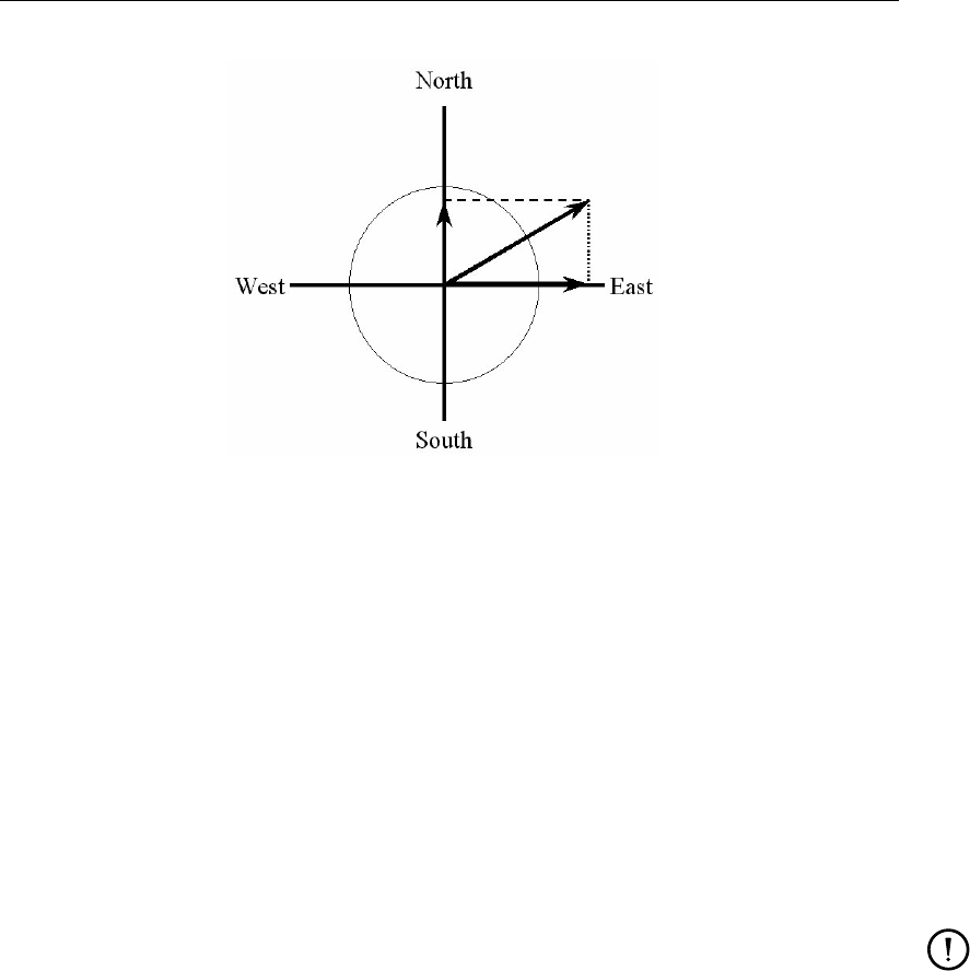
DRAFT
Files of Delft3D-WAVE
Figure A.1: Definition wind components for space varying wind
Time = 0.0 minutes since 2008-09-20 10:30:00 +01:00 # Time definition
{33 records with 25 values each} # Wind component west to east
{33 records with 25 values each} # Wind component south to north
{33 records with 25 values each} # Atmospheric pressure
Time = 340.0 minutes since 2008-09-20 10:30:00 +01:00 # Time definition
{33 records with 25 values each} # Wind component west to east
{33 records with 25 values each} # Wind component south to north
{33 records with 25 values each} # Atmospheric pressure
Time = 600.0 minutes since 2008-09-20 10:30:00 +01:00 # Time definition
{33 records with 25 values each} # Wind component west to east
{33 records with 25 values each} # Wind component south to north
{33 records with 25 values each} # Atmospheric pressure
Time = 1240.0 minutes since 2008-09-20 10:30:00 +01:00 # Time definition
{33 records with 25 values each} # Wind component west to east
{33 records with 25 values each} # Wind component south to north
{33 records with 25 values each} # Atmospheric pressure
Remarks:
To obtain the wind direction according to the nautical convention, the wind direction is
reversed.
The wind is specified in terms of its components along the west-east (x_wind) and
south-north (y_wind) co-ordinate system, see Figure A.1. These definitions differ
from the nautical convention (used for uniform wind), which is specified relative to true
North, see Figure A.2.
Deltares 103 of 124
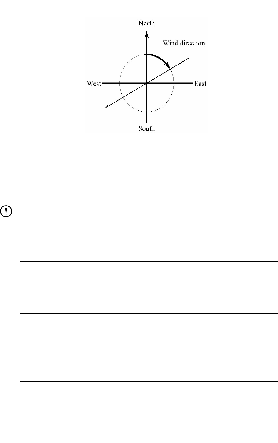
DRAFT
D-Waves, User Manual
Figure A.2: Definition sketch of wind direction according to Nautical convention
A.2.10.2 Space-varying wind on an equistant grid
File contents Time-series of a space varying wind and atmospheric pressure de-
fined on an equidistant (Cartesian or spherical) grid.
File format Free formatted or unformatted, keyword based.
Generated Some offline program.
Remark:
The keywords are case insensitive.
Header description for the wind velocity files:
Keywords Value Description
FileVersion 1.03 version of file format
Filetype meteo_on_equidistant_grid meteo input on equidistant grid
NODATA_value free value used for input that is to be
neglected
n_cols free number of columns used for wind
datafield
n_rows free number of rows used for wind
datafield
grid_unit mor unit of distances on the grid
degree in both x- and y-direction
x_llcorner free x-coordinate of lower left corner
of lower left grid cell (in units
specified in grid_unit
y_llcorner free y-coordinate of lower left corner
of lower left grid cell (in units
specified in grid_unit
104 of 124 Deltares

DRAFT
Files of Delft3D-WAVE
Keywords Value Description
x_llcenter free x-coordinate of centre of lower
left grid cell (in units specified in
grid_unit
y_llcenter free y-coordinate of centre of lower
left grid cell (in units specified in
grid_unit
dx free gridsize in x-direction in units
specified in grid_unit
dy free gridsize in y-direction in units
specified in grid_unit
n_quantity 1 number of quantities specified in
the file
quantity1 x_wind or the velocity component given in
y_wind unit unit1
unit1 m s-1 unit of quantity1:
metre/second
The user must specify the location of the equidistant grid on which the meteorological data
is specified. If one has the location of the lower left corner of the lower left grid cell, one can
specify the starting point of the grid using keywords x_llcorner and y_llcorner. If
one has the location of the cell centre of the lower left grid cell, one should use the keywords
x_llcenter and y_llcenter. Using the first option, the first data value is placed at
(x_llcorner+1
2dx, y_llcorner+1
2dy), which is the cell centre of cell (1,1). Using the latter
option, the first data value is placed at (x_llcenter, y_llcenter), which is again the cell centre
of cell (1,1), i.e. the data values are always placed at the cell centres of the meteorological
grid. Note that the lower left grid cell is defined to be the grid cell with index (1,1). When using
the option of meteorological data on a separate curvilinear grid, the origin and orientation
of the data set can be chosen freely with respect to the grid on which it is specified, see
section A.2.10.3 for details.
Time definition and data block description for the wind velocity files
Keywords Value Description
Time fixed format described below time definition string
The time definition string has a fixed format, used to completely determine the time at which
a dataset is valid. The time definition string has the following format:
TIME minutes/hours since YYYY-MM-DD HH:MM:SS TIME ZONE, e.g.
360 minutes since 2008-07-28 10:55:00 +01:00
The format of the string is completely fixed. No extra spaces or tabs can be added between the
Deltares 105 of 124

DRAFT
D-Waves, User Manual
different parts of the definition. The time definition is followed by the datablock of input values
corresponding to the specified time. The data block contains values for the wind velocity in
x- or y-direction for n_cols by n_rows points, starting at the top left point. The time definition
and the data block are repeated for each time instance of the time-series.
The atmospheric pressure file
The header for the atmospheric pressure is similar to that of the wind velocity files, except for
the following differences.
Keywords Value Description
quantity1 air_pressure air pressure
unit1 Pa or mbar unit of quantity1: Pascal or
millibar
The specification of the time definition and the data block is fully conform the wind velocity
files.
File version and conversion
The current description holds for FileVersion 1.03. The table below shows the latest
modifications in the file format (and version number).
FileVersion Modifications
1.03 Use of keyword Value_pos to indicate the position of the lower left
corner of the grid replaced by use of the combination of keywords:
x_llcorner and y_llcorner or
x_llcenter and y_llcenter
1.02 No changes for this meteo input type, but for the meteo type me-
teo_on_spiderweb_grid
1.01 Changed keyword MeteoType to FileType
Changed fixed value of input type (Keyword Filetype) from ArcInfo
to meteo_on_equidistant_grid
Restrictions:
The contents of the file will not be checked on its domain.
Keywords are followed by an equal sign ’=’ and the value of the keyword.
When a keyword has value free, the value of this keyword is free to choose by the user.
When only one value is given for a keyword, this keyword has a fixed value and when 2
or more options are shown, the user can choose between those values.
Times must be specified exactly according to the time definition. See the examples
shown in this section.
The atmospheric pressure file must use the same grid definition and time frame as the
files for the wind velocity components.
The unit of the meteo grid must be the same as the computational grid, i.e. both with
grid_unit = [m] or both with grid_unit = [degree].
Input items in a data block are separated by one or more blanks.
106 of 124 Deltares

DRAFT
Files of Delft3D-WAVE
The wind components are specified at the cell centres (water level points) of the numer-
ical grid.
The wind components are specified in the west-east (x_wind) and south-north direc-
tions (y_wind).
Remarks:
The time definition in the meteo files contains the number of minutes or hours since
a reference date and time in a certain time zone. The reference time and time zone
may differ from those of the simulation. During a simulation the computational engine
will search in the meteo file for the current simulation time and interpolate between
neighbouring times if necessary. Possible differences in time zone will be accounted for
by shifting the meteo input data. The reference times within the time definition string
may vary in a meteo file, i.e. it is possible to attach new input with a different reference
time, behind the last data block. Consecutive times must always be increasing in the
input file.
Comments can be added after pound signs (#). These are not read.
Example of a file containing wind in x-direction (west-east)
The data blocks in this example are the result of the following FORTRAN statements:
do j = nrows,1,-1
write(out,*) (xwind(i,j),i=1,ncols)
enddo
The x-wind velocity file for a 3 (n_cols) by 4 (n_rows) grid has the following layout:
FileVersion = 1.03
filetype = meteo_on_equidistant_grid
NODATA_value = -999.000
n_cols = 3
n_rows = 4
grid_unit = degree
x_llcenter = -12.000
y_llcenter = 48.000
dx = 0.12500
dy = 0.083333333
n_quantity = 1
quantity1 = x_wind
unit1 = m s-1
TIME = 0.0 hours since 2008-01-15 04:35:00 +00:00
2 3.0 3.6
3 4.5 2
2.2 1 2.3
1.2 0.7 -0.4
TIME = 6.0 hours since 2008-01-15 04:35:00 +00:00
-1.1 -2.3 -3.6
-3.2 0.8 1.1
2.2 -1 -1.6
1.2 -0.7 -0.4
This results in an x-component of wind velocity given - in [m/s] - on a spherical, 3 by 4,
equidistant grid, with grid sizes given by dx and dy (in degrees) and where the centre point
of the lower left cell of the grid lies in (longitude, latitude) (-12.0, 48.0) on the globe. Data is
given at two times: 0 and 6 hours since January 15th, 2008, 4:35 AM, in UTC+0.
Deltares 107 of 124

DRAFT
D-Waves, User Manual
A.2.10.3 Space-varying wind on a curvilinear grid
File contents Time-series of a space varying wind and atmospheric pressure de-
fined on a curvilinear (Cartesian or spherical) grid.
File format Free formatted or unformatted, keyword based.
Generated Some offline program.
Remark:
The keywords are case insensitive.
Header description for the wind velocity files:
Keywords Value Description
FileVersion 1.03 version of file format
Filetype meteo_on_curvilinear_grid meteo input on curvilinear grid
NODATA_value free value used for input that is to be
neglected
grid_file free.grd name of the curvilinear grid file on
which the data is specified
first_data_value grid_llcorner or see example below
grid_ulcorner or
grid_lrcorner or
grid_urcorner
data_row grid_row or see example below
grid_column
n_quantity 1 number of quantities specified in
the file
quantity1 x_wind or the velocity component given in
y_wind unit unit1
unit1 m s-1 unit of quantity1:
metres/second
Time definition and data block description for the wind velocity files
For a description of the time definition and data block see section A.2.10.2.
The atmospheric pressure file
For a description of the atmospheric file see section A.2.10.2.
108 of 124 Deltares
DRAFT
Files of Delft3D-WAVE
File version and conversion
The current description holds for FileVersion 1.03. The table below shows the latest
modifications in the file format (and version number).
FileVersion Modifications
1.03 Fixed bug in interpolation of data from meteo grid to computational grid:
Conversion script mirrored data set erroneously. This was treated cor-
rectly by meteo module. Fixed both the conversion script and the meteo
module together: Required modification in meteo input file:
Change first_data_value = grid_llcorner into grid_ulcorner or
vice versa
or
Change first_data_value = grid_lrcorner into grid_urcorner or
vice versa
1.02 No changes for this meteo input type, but for the meteo type me-
teo_on_spiderweb_grid
1.01 Changed keyword MeteoType to FileType
Changed keyword Curvi_grid_file to Grid_file
Changed fixed value of input type (Keyword Filetype) from Curvi to
meteo_on_curvilinear_grid
Restrictions:
The restrictions for space varying wind and pressure on a separate curvilinear grid are
the same as for space varying wind and pressure on an equidistant grid, described in
section A.2.10.2. A differerence is that the data values on the curvilinear grid are not
specified in the cell centres, but in the grid points (cell corners).
The unit of the meteo grid must be the same as the computational grid, i.e. both with
grid_unit = [m] or both with grid_unit = [degree].
Remark:
The remarks for space varying wind and pressure on a separate curvilinear grid are
the same as for space varying wind and pressure on an equidistant grid, described in
section A.2.10.2.
Deltares 109 of 124
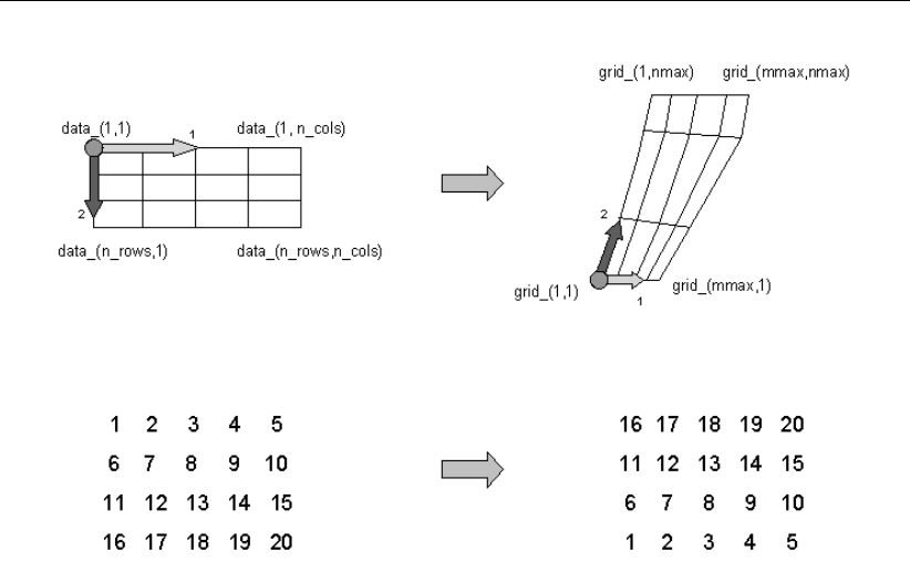
DRAFT
D-Waves, User Manual
Figure A.3: Illustration of the data to grid conversion for meteo input on a separate curvi-
linear grid
Example:
A file for input of x-velocity (in west-east direction) on a 4 (n_rows) by 5 (n_cols) curvilin-
ear grid, where the meteorogical data is mirrored vertically with respect to the grid, has the
following layout:
FileVersion = 1.03
filetype = meteo_on_curvilinear_grid
NODATA_value = -999.000
grid_file = curviwind.grd
first_data_value = grid_llcorner
data_row = grid_row
n_quantity = 1
quantity1 = x_wind
unit1 = m s-1
TIME = 0.0 minutes since 1993-06-28 14:50:00 -02:00
12345
6 7 8 9 10
11 12 13 14 15
16 17 18 19 20
TIME = 600.0 minutes since 1993-06-28 14:50:00 -02:00
12345
6 7 8 9 10
11 12 13 14 15
16 17 18 19 20
This results in an x-component of velocity given - in [m/s] - on the curvilinear grid specified in
file <curviwind.grd>. The data set will be mirrored such that the first value of the data (upper
left corner, in the example ’1’) corresponds to the lower left corner of the grid (point (1,1)) and
a row of data corresponds to a row on the grid, see Figure A.3. Data is given at two times: 0
and 600 minutes since June 28th, 1993, 14:50 PM, in UTC-2.
110 of 124 Deltares

DRAFT
Files of Delft3D-WAVE
A.2.10.4 Space-varying wind on a Spiderweb grid
Cyclone winds are governed by a circular motion, combined with a cyclone track. This type
of wind is generally very difficult to implement on a curvilinear grid. This feature facilitates the
reading of the so-called Spiderweb files and interpolates the wind and pressure data internally
to the computational grid. A special feature of the space varying wind and pressure on the
Spiderweb grid is that it can be combined with one of the other meteorological input options
described in this manual, i.e. to either uniform wind and pressure, or to one of the space
varying wind and pressure options, see section A.2.10.
File contents Time-series of a space varying wind and atmospheric pressure de-
fined on a Spiderweb grid. This grid may be specified in Cartesian
or spherical coordinates.
File format Free formatted or unformatted, keyword based.
Generated Some offline program.
Remarks:
The keywords are case insensitive.
Space varying wind and pressure on a Spiderweb grid is added to other wind input and
the wind fields are interpolated and combined in and around the cyclone.
Header description of the Spiderweb wind and pressure file:
Keywords Value Description
FileVersion 1.03 version of file format
Filetype meteo_on_spiderweb_grid meteo input on Spiderweb grid
NODATA_value free value used for input that is to be
neglected
n_cols free number of gridpoints in angular
direction
n_rows free number of gridpoints in radial
direction
grid_unit mor unit of the Spiderweb grid
degree
spw_radius free radius of the spiderweb given in
units given by spw_rad_unit
spw_rad_unit m unit of the Spiderweb radius
spw_merge_frac [0.0,1.0] fraction of the Spiderweb radius
where merging starts of the back-
ground wind with the Spiderweb
wind. Default is 0.5
air_pressure air_pressure_default_from Both keyword and value are too
_reference _computational_engine long to fit on one line.
Reference value related to
p_drop is the default air pressure
of the computional engine
Deltares 111 of 124
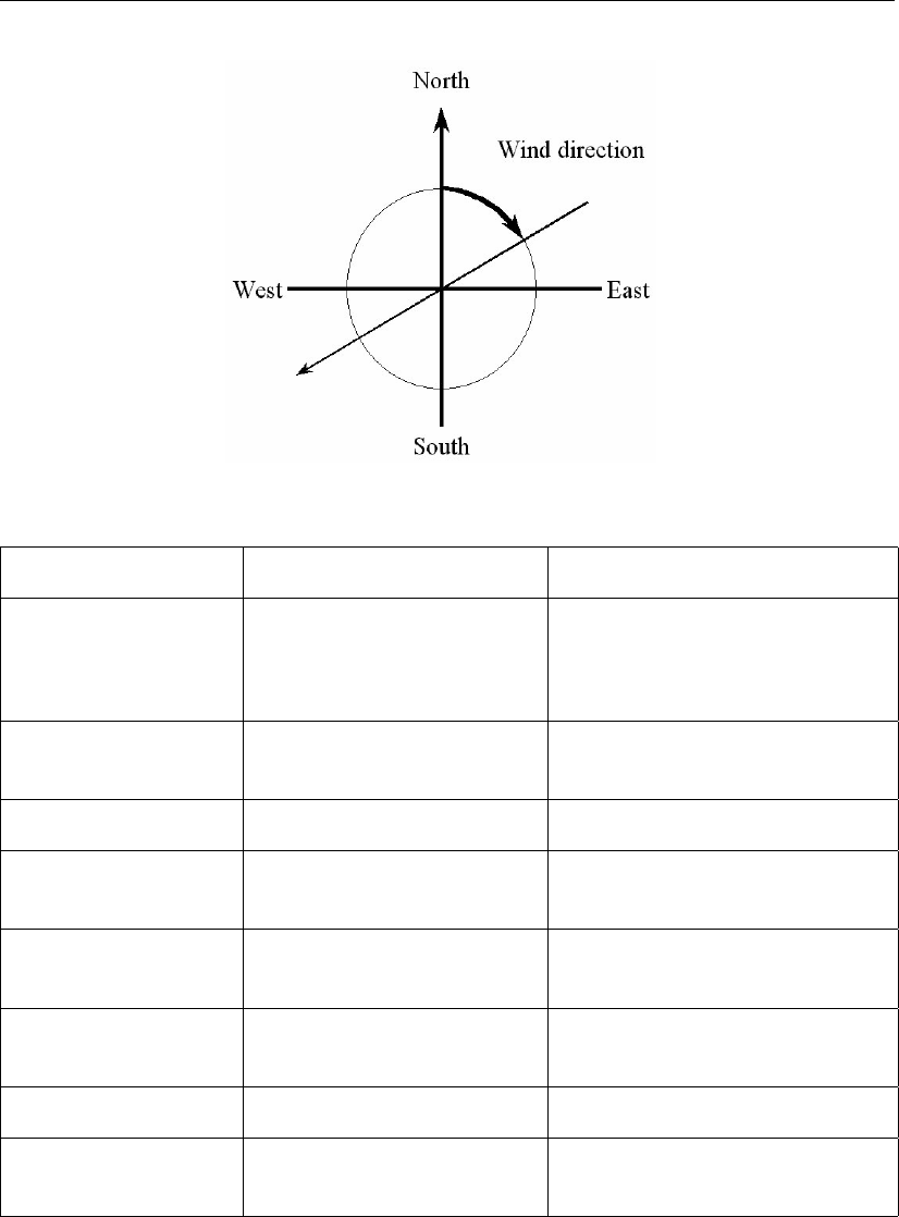
DRAFT
D-Waves, User Manual
Figure A.4: Wind definition according to Nautical convention
Keywords Value Description
or free or the value specified.
If missing, p_drop is extracted
from the actual atmospheric
pressure.
n_quantity 3 number of quantities specified in
the file
quantity1 wind_speed wind speed given in unit unit1
quantity2 wind_from_direction direction where the wind is com-
ing from given in unit unit2
quantity3 p_drop drop in atmospheric pressure
given in unit unit3
unit1 m s-1 unit of quantity1:
metres/second
unit2 degree unit of quantity2: degrees
unit3 Pa or unit of quantity3: Pascal or
mbar millibar
Time definition and data block description
For a description of the time definition see section A.2.10.2.
Cyclone track information:
For each time in the time series of space varying wind and pressure on a Spiderweb grid, the
position of the cyclone eye (and thus also the spiderweb grid) must be given, as well as the
drop of atmospheric pressure in the cyclone eye.
112 of 124 Deltares
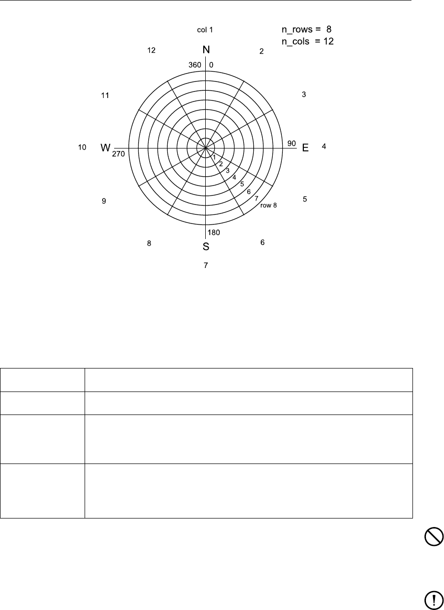
DRAFT
Files of Delft3D-WAVE
Figure A.5: Spiderweb grid definition
File version and conversion
The current description holds for FileVersion 1.03. The table below shows the latest
modifications in the file format (and version number).
FileVersion Modifications
1.03 No changes for this meteo input type
1.02 Changed the use of keyword n_rows and n_cols. The radius of the
cyclone is divided in n_rows rings of width: spw_radius/n_rows [m]
and the circle is divided in n_cols parts of 2π/n_cols [rad].
1.01 Changed keyword MeteoType to FileType
Changed fixed value of input type (Keyword Filetype) from Spider-
web to meteo_on_spiderweb_grid
Restriction:
The restrictions for space varying wind and pressure on a Spiderweb grid are the
same as for space varying wind and pressure on an equidistant grid, described in sec-
tion A.2.10.2.
Remarks:
The remarks for space varying wind and pressure on a separate curvilinear grid are
the same as for space varying wind and pressure on an equidistant grid, described in
section A.2.10.2.
The Spiderweb grid is circular and the definitions of the number of rows n_rows and
the number of columns n_cols is therefore different then for the other meteo input
formats. For the Spiderweb grid, the number of rows determines the grid size in ra-
dial direction. The number of columns defines the grid size in angular direction. See
Figure A.5.
Deltares 113 of 124

DRAFT
D-Waves, User Manual
The wind is specified according to the nautical convention, i.e. wind from the true North
has direction zero and the wind turns clockwise with an increasing angle. See Fig-
ure A.4.
Example:
A file for input of space varying wind and pressure on a 5x3 Spiderweb grid, has the following
layout:
FileVersion = 1.03
filetype = meteo_on_spiderweb_grid
NODATA_value = -999.000
n_cols = 3
n_rows = 5
grid_unit = degree
spw_radius = 600000.0
spw_rad_unit = m
air_pressure_reference = air_pressure_default_from_computational_engine
n_quantity = 3
quantity1 = wind_speed
quantity2 = wind_from_direction
quantity3 = p_drop
unit1 = m s-1
unit2 = degree
unit3 = Pa
TIME = 0.0 hours since 1997-07-14 03:00:00 -06:00
x_spw_eye = 115.1
y_spw_eye = 18.9
p_drop_spw_eye = 5300.0
1.38999 1.38261 1.38315
1.28251 1.34931 1.22571
1.27215 1.31214 1.32451
1.38999 1.86592 2.87732
1.43899 1.24912 2.21519
60.0000 180.0000 270.0000
28.7500 20.0000 31.2500
42.5000 53.7500 65.0000
49.3400 60.2400 81.5200
51.4100 62.0000 43.1200
5301.280 5294.490 5156.240
5043.460 5112.040 5264.020
5140.020 5202.520 5411.210
5294.730 5285.760 5235.250
5242.530 5156.190 5124.240
TIME = 1.0 hours since 1997-07-14 03:00:00 -06:00
x_spw_eye = 114.8
y_spw_eye = 18.8
p_drop_spw_eye = 5250.0
1.35763 1.35763 1.35763
1.35763 1.87273 2.24784
1.92214 2.47836 2.17266
1.87662 2.72116 2.82375
1.26585 2.24146 2.38722
159.0000 346.5200 290.6400
342.3200 282.1400 20.2400
10.7500 25.5300 36.4500
61.8400 81.6200 45.5100
49.5250 56.7500 75.1300
5314.520 5104.490 5287.240
5124.240 5285.760 5252.420
5152.460 5247.040 5222.020
5242.020 5223.520 5475.210
5244.270 5211.210 4998.110
114 of 124 Deltares

DRAFT
Files of Delft3D-WAVE
This results in the following set of meteo data. Velocities given in [m/s] and pressure drops in
[Pa] on a Spiderweb grid which is given in spherical coordinates (grid_unit = degree). The
cyclone and spiderweb grid have a radius of 600 km. The grid is 5x3, which means the radius
is divided in five parts of 120 km and the 360 degrees are divided in 3 parts of 120 degrees
each. Wind speeds, wind directions and pressure drops are given at two times: 0 and 1.0
hour since July 14th, 1997, 03:00 AM, in UTC-6. Between these two times the cyclone eye
moves from (longitude, latitude) (115.1, 18.9) to (114.8, 18.8) on the globe and the pressure
drop in the cylcone eye decreases from 5300.0 [Pa] to 5250.0 [Pa].
Deltares 115 of 124

DRAFT
D-Waves, User Manual
116 of 124 Deltares

DRAFT
B Definition of SWAN wave variables
In SWAN a number of variables, mostly related to waves are used in input and output. The
definitions of these variables are conventional for the most part.
HSIGN significant wave height (Hsin [m]), defined as:
Hs= 4sZZ E(ω, θ)dωdθ
where E(ω, θ)is the variance density spectrum
TM01 mean absolute wave period (in s) of E(ω, θ), defined as:
Tm01 = 2πRRωE(σ, θ)dσdθ
RRE(σ, θ)dσdθ −1
= 2πRRωE(σ, θ)dωdθ
RRE(σ, θ)dωdθ −1
where ωis the absolute radian frequency, determined by the Doppler shifted
dispersion relation.
DIR mean wave direction (in ◦, Cartesian or Nautical convention), as conventionally
defined (Kuik et al.,1988).
[DIR] = arctan Rsin(θ)E(σ, θ)dσdθ
Rcos(θ)E(σ, θ)dσdθ
RTP relative peak period (in s) of E(σ)(equal to absolute peak period in the absence
of currents)
DSPR the one-sided directional width of the spectrum (directional spreading or direc-
tional standard deviation, in 0), defined as:
DSP R2=180
π2Z2π
02 sin θ−¯
θ
22
D(θ)dθ
and computed as conventionally for pitch-and-roll buoy data (Kuik et al. (1988);
this is the standard definition for WAVEC buoys integrated over all frequencies):
DSP R π
1802= 2
1− Zsin(θ)RE(σ, θ)dσ
RE(σ)dσ dθ2
+Zcos(θ)RE(σ, θ)dσ
RE(σ)dσ dθ2!1/2
MS As input to SWAN in the commands BOUNDPAR and BOUNDSPEC the direc-
tional distribution of incident wave energy is: D(θ) = A{cos(θ)}[MS]at all
frequencies. [MS] is not necessarily an integer number.
[MS] is, for this directional distribution, related to the one-sided directional spread
of the waves (DSPR) as follows:
Deltares 117 of 124

DRAFT
D-Waves, User Manual
[MS] dspr (in ◦)
1. 37.5
2. 31.5
3. 27.6
4. 24.9
5. 22.9
6. 21.2
7. 19.9
8. 18.8
9. 17.9
10. 17.1
15. 14.2
20. 12.4
30. 10.2
40. 8.9
50. 8.0
60. 7.3
70. 6.8
80. 6.4
90. 6.0
100. 5.7
200 4.0
400 2.9
800 2.0
DISSIP energy dissipation per unit time due to the sum of bottom friction, whitecapping
and depth induced wave breaking (in W/m2of m2/s, depending on command
SET)
WLEN the mean wavelength,
W LEN = 2πRkpE(σ, θ)dσdθ
Rkp−1E(σ, θ)dσdθ −1
see command QUANTITY (where p= 1 is default)
STEEPNESS wave steepness, computed as:
STEEPNESS =HSIGN
WLEN
Qb fraction of breakers [-] in expression of Battjes and Janssen (1978), see sec-
tion 2.1.
TRANSP energy transport with components Px=RRρgcxE(σ, θ)dσdθ and Py=
RRρgcyE(σ, θ)dσdθ with xand yof the problem co-ordinate system, ex-
cept in the case of output with BLOCK command in combination with command
FRAME, where xand yrelate to the x-axis and y-axis of the output frame.
VEL current velocity with components in x and y direction of the problem co-ordinate
system, except in the case of output with BLOCK command in combination with
command FRAME, where x and y relate to the x-axis and y-axis of the output
frame.
FORCE wave induced force per unit surface area (gradient of the radiation stresses)
with xand yof the problem co-ordinate system, except in the case of output
with BLOCK command in combination with command FRAME, where xand y
118 of 124 Deltares
DRAFT
Definition of SWAN wave variables
relate to the x-axis and y-axis of the output frame.
Fx=−∂Sxx
∂x −∂Sxy
∂y ,and Fy=−∂Syx
∂x −∂Syy
∂y
where Sis the radiation stress tensor:
Sxx =ρg Zncos2θ+n−1
2E dσdθ
Sxy =Syx =ρg Znsin θcos θE dσdθ
Syy =ρg Znsin2θ+n−1
2E dσdθ
and nis the ratio of group velocity over phase velocity.
URMS root-mean-square value of the orbital motion near the bottom
UBOT root-mean-square value of the maximum of the orbital motion near the bottom
Ubot =√2Urms
LEAK numerical loss of energy equal to cθE(ω, θ)across boundaries θ1=[dir1] and
θ2=[dir2] of a directional sector (see command CGRID)
SETUP the elevation of mean water level (relative to still water level) induced by the
gradient of the radiation stresses of the waves
TPS Smoothed Peak wave period. This value is obtained as the maximum of a
parabolic fitting through the highest bin and two bins on either side of the highest
one of the discrete wave spectrum. This ’non-discrete’ or ’smoothed’ value is a
better estimate of the ’real’ peak period compared to the quantity RTP.
Cartesian direction convention: the direction is the angle between the vector and the posi-
tive x-axis, measured counter-clockwise (the direction where the waves are going to or where
the wind is blowing to).
Nautical direction convention: the direction of the vector from geographic North measured
clockwise + 180◦(the direction where the waves are coming from or where the wind is blowing
from).
Deltares 119 of 124

DRAFT
D-Waves, User Manual
120 of 124 Deltares

DRAFT
C Example of MDW-file Siu-Lam
In this appendix the MDW-file for the Siu Lam case is provided <siu.mdw>. Generated by
the WAVE-GUI 4.94.00:
[WaveFileInformation]
FileVersion = 02.00
[General]
ProjectName = Siu-Lam
ProjectNr = 001
Description = Tutorial Delft3D-WAVE
Description = Siu Lam model
Description = SWAN wave model using a curvilinear grid
OnlyInputVerify = false
SimMode = stationary
DirConvention = nautical
ReferenceDate = 2005-10-01
ObstacleFile = siu_lam_obstacles.obs
WindSpeed = 2.0000000e+001
WindDir = 2.5500000e+002
[TimePoint]
Time = 1.0800000e+003
WaterLevel = -1.0000000e+000
XVeloc = 0.0000000e+000
YVeloc = 0.0000000e+000
[TimePoint]
Time = 1.2600000e+003
WaterLevel = 0.0000000e+000
XVeloc = 0.0000000e+000
YVeloc = 0.0000000e+000
[TimePoint]
Time = 1.4400000e+003
WaterLevel = 1.5000000e+000
XVeloc = 0.0000000e+000
YVeloc = 0.0000000e+000
[Constants]
WaterLevelCorrection = 0.0000000e+000
Gravity = 9.8100004e+000
WaterDensity = 1.0250000e+003
NorthDir = 9.0000000e+001
MinimumDepth = 5.0000001e-002
[Processes]
GenModePhys = 3
WaveSetup = false
Breaking = true
BreakAlpha = 1.0000000e+000
BreakGamma = 7.3000002e-001
Triads = false
TriadsAlpha = 1.0000000e-001
TriadsBeta = 2.2000000e+000
BedFriction = jonswap
BedFricCoef = 6.7000002e-002
Diffraction = false
DiffracCoef = 2.0000000e-001
DiffracSteps = 5
DiffracProp = true
WindGrowth = true
WhiteCapping = Komen
Quadruplets = true
Refraction = true
FreqShift = true
WaveForces = dissipation
[Numerics]
DirSpaceCDD = 5.0000000e-001
FreqSpaceCSS = 5.0000000e-001
Deltares 121 of 124

DRAFT
D-Waves, User Manual
RChHsTm01 = 2.0000000e-002
RChMeanHs = 2.0000000e-002
RChMeanTm01 = 2.0000000e-002
PercWet = 9.8000000e+001
MaxIter = 4
[Output]
TestOutputLevel = 0
TraceCalls = false
UseHotFile = false
WriteCOM = false
LocationFile = siu.loc
WriteTable = true
WriteSpec1D = true
WriteSpec2D = true
[Domain]
Grid = siu_lam.grd
BedLevel = siu_lam.dep
DirSpace = circle
NDir = 36
StartDir = 0.0000000e+000
EndDir = 0.0000000e+000
FreqMin = 5.0000001e-002
FreqMax = 1.0000000e+000
NFreq = 24
Output = true
[Boundary]
Name = Boundary 1
Definition = orientation
Orientation = west
SpectrumSpec = parametric
SpShapeType = gauss
PeriodType = peak
DirSpreadType = degrees
PeakEnhanceFac = 3.3000000e+000
GaussSpread = 3.3000000e+000
DistanceDir = counter-clockwise
CondSpecAtDist = 1.5000000e+003
WaveHeight = 0.0000000e+000
Period = 5.0000000e+000
Direction = 2.5500000e+002
DirSpreading = 4.0000000e+000
CondSpecAtDist = 9.0000000e+003
WaveHeight = 1.0000000e+000
Period = 5.0000000e+000
Direction = 2.5500000e+002
DirSpreading = 4.0000000e+000
122 of 124 Deltares
DRAFT
PO Box 177
2600 MH Del
Boussinesqweg 1
2629 VH Del
The Netehrlands
+31 (0)88 335 81 88
sales@deltaressystems.nl
www.deltaressystems.nl
DRAFT
