Data Structures And Algorithm Analysis In C (Second Edition) Solution Manual
Data%20Structures%20and%20Algorithm%20Analysis%20in%20C%20(Second%20Edition)%20Solution%20Manual
Data%20Structures%20and%20Algorithm%20Analysis%20in%20C%20(Second%20Edition)%20Solution%20Manual
Data%20Structures%20and%20Algorithm%20Analysis%20in%20C%20(Second%20Edition)%20Solution%20Manual
Data%20Structures%20and%20Algorithm%20Analysis%20in%20C%20(Second%20Edition)%20Solution%20Manual
Data%20Structures%20and%20Algorithm%20Analysis%20in%20C%20(Second%20Edition)%20Solution%20Manual
User Manual: Pdf
Open the PDF directly: View PDF ![]() .
.
Page Count: 69
Data Structures
and
Algorithm Analysis in C
Second Edition
Solutions Manual
Mark Allen Weiss
Florida International University
Preface
Included in this manual are answers to most of the exercises in the textbook Data Structures and
Algorithm Analysis in C, second edition, published by Addison-Wesley. These answers reflect
the state of the book in the first printing.
Specifically omitted are likely programming assignments and any question whose solu-
tion is pointed to by a reference at the end of the chapter. Solutions vary in degree of complete-
ness; generally, minor details are left to the reader. For clarity, programs are meant to be
pseudo-C rather than completely perfect code.
Errors can be reported to weiss@fiu.edu. Thanks to Grigori Schwarz and Brian Harvey
for pointing out errors in previous incarnations of this manual.
Table of Contents
1. Chapter 1: Introduction ...................................................................................................... 1
2. Chapter 2: Algorithm Analysis .......................................................................................... 4
3. Chapter 3: Lists, Stacks, and Queues ................................................................................. 7
4. Chapter 4: Trees ................................................................................................................. 14
5. Chapter 5: Hashing ............................................................................................................ 25
6. Chapter 6: Priority Queues (Heaps) ................................................................................... 29
7. Chapter 7: Sorting ..............................................................................................................36
8. Chapter 8: The Disjoint Set ADT ....................................................................................... 42
9. Chapter 9: Graph Algorithms ............................................................................................. 45
10. Chapter 10: Algorithm Design Techniques ...................................................................... 54
11. Chapter 11: Amortized Analysis ...................................................................................... 63
12. Chapter 12: Advanced Data Structures and Implementation ............................................ 66
-iii-
Chapter 1: Introduction
1.3 Because of round-off errors, it is customary to specify the number of decimal places that
should be included in the output and round up accordingly. Otherwise, numbers come out
looking strange. We assume error checks have already been performed; the routine
Separate is left to the reader. Code is shown in Fig. 1.1.
1.4 The general way to do this is to write a procedure with heading
void ProcessFile( const char *FileName );
which opens FileName, does whatever processing is needed, and then closes it. If a line of
the form
#include SomeFile
is detected, then the call
ProcessFile( SomeFile );
is made recursively. Self-referential includes can be detected by keeping a list of files for
which a call to ProcessFile has not yet terminated, and checking this list before making a
new call to ProcessFile.
1.5 (a) The proof is by induction. The theorem is clearly true for 0 < X ≤ 1, since it is true for
X = 1, and for X < 1, log X is negative. It is also easy to see that the theorem holds for
1 < X ≤ 2, since it is true for X = 2, and for X < 2, log X is at most 1. Suppose the theorem
is true for p < X ≤ 2p(where pis a positive integer), and consider any 2p < Y ≤ 4p
(p ≥ 1). Then log Y = 1 + log (Y / 2) < 1 + Y / 2 < Y / 2 + Y / 2 ≤ Y , where the first ine-
quality follows by the inductive hypothesis.
(b) Let 2X = A . Then AB = (2X)B = 2XB . Thus log AB = XB . Since X = log A , the
theorem is proved.
1.6 (a) The sum is 4/3 and follows directly from the formula.
(b) S = 4
1
__ + 42
2
___ + 43
3
___ + . . . .4S = 1+4
2
__ + 42
3
___ + . . . . Subtracting the first equation from
the second gives 3S = 1 + 4
1
__ + 42
2
___ + . . . . By part (a), 3S = 4/ 3soS = 4/ 9.
(c) S = 4
1
__ + 42
4
___ + 43
9
___ + . . . .4S = 1 + 4
4
__ + 42
9
___ + 43
16
__ _ + . . . . Subtracting the first equa-
tion from the second gives 3S = 1+4
3
__ + 42
5
___ + 43
7
___ + . . . . Rewriting, we get
3S = 2
i=0
Σ
∞
4i
i
___ +
i=0
Σ
∞
4i
1
___. Thus 3S = 2(4/ 9) + 4/ 3 = 20/ 9. Thus S = 20/ 27.
(d) Let SN =
i=0
Σ
∞
4i
iN
___ . Follow the same method as in parts (a) - (c) to obtain a formula for SN
in terms of SN−1,SN−2, ..., S0and solve the recurrence. Solving the recurrence is very
difficult.
-1-
_______________________________________________________________________________
_______________________________________________________________________________
double RoundUp( double N, int DecPlaces )
{int i;
double AmountToAdd = 0.5;
for( i = 0; i < DecPlaces; i++ )
AmountToAdd /= 10;
return N + AmountToAdd;
}
void PrintFractionPart( double FractionPart, int DecPlaces )
{int i, Adigit;
for( i = 0; i < DecPlaces; i++ )
{FractionPart *= 10;
ADigit = IntPart( FractionPart );
PrintDigit( Adigit );
FractionPart = DecPart( FractionPart );
}
}
void PrintReal( double N, int DecPlaces )
{int IntegerPart;
double FractionPart;
if( N < 0 )
{putchar(’-’);
N = -N;
}
N = RoundUp( N, DecPlaces );
IntegerPart = IntPart( N ); FractionPart = DecPart( N );
PrintOut( IntegerPart ); /* Using routine in text */
if( DecPlaces > 0 )
putchar(’.’);
PrintFractionPart( FractionPart, DecPlaces );
}
Fig. 1.1.
_______________________________________________________________________________
_______________________________________________________________________________
1.7
i=N / 2
Σ
N
i
1
__ =
i=1
Σ
N
i
1
__ −
i=1
Σ
N / 2 − 1
i
1
__ ∼
∼ ln N − ln N / 2 ∼
∼ ln 2.
-2-
1.8 24 = 16 ≡ 1 (mod 5). (24)25 ≡ 125 (mod 5). Thus 2100 ≡ 1 (mod 5).
1.9 (a) Proof is by induction. The statement is clearly true for N = 1 and N = 2. Assume true
for N = 1, 2, ..., k. Then
i=1
Σ
k+1Fi =
i=1
Σ
kFi+Fk+1. By the induction hypothesis, the value of the
sum on the right is Fk+2 − 2 + Fk+1=Fk+3 − 2, where the latter equality follows from the
definition of the Fibonacci numbers. This proves the claim for N = k + 1, and hence for all
N.
(b) As in the text, the proof is by induction. Observe that φ + 1 = φ2. This implies that
φ−1 + φ−2 = 1. For N = 1 and N = 2, the statement is true. Assume the claim is true for
N = 1, 2, ..., k.
Fk+1 = Fk + Fk−1
by the definition and we can use the inductive hypothesis on the right-hand side, obtaining
Fk+1 < φk + φk−1
< φ−1φk+1 + φ−2φk+1
Fk+1 < (φ−1 + φ−2)φk+1 < φk+1
and proving the theorem.
(c) See any of the advanced math references at the end of the chapter. The derivation
involves the use of generating functions.
1.10 (a)
i=1
Σ
N(2i−1) = 2
i=1
Σ
Ni −
i=1
Σ
N1 = N (N+1) − N = N2.
(b) The easiest way to prove this is by induction. The case N = 1 is trivial. Otherwise,
i=1
Σ
N+1i3 = (N+1)3 +
i=1
Σ
Ni3
= (N+1)3 + 4
N2(N+1)2
_________
= (N+1)24
N2
___ + (N+1)
= (N+1)24
N2 + 4N + 4
___________
= 22
(N+1)2(N+2)2
_____________
= 2
(N+1)(N+2)
___________ 2
=
i=1
Σ
N+1i
2
-3-
Chapter 2: Algorithm Analysis
2.1 2/N , 37, √N,N,Nlog log N ,Nlog N ,Nlog (N2), Nlog2N,N1.5,N2,N2log N ,N3,2
N / 2,
2N.Nlog N and Nlog (N2) grow at the same rate.
2.2 (a) True.
(b) False. A counterexample is T1(N) = 2N,T2(N) = N , and f(N) = N .
(c) False. A counterexample is T1(N) = N2,T2(N) = N , and f(N) = N2.
(d) False. The same counterexample as in part (c) applies.
2.3 We claim that Nlog N is the slower growing function. To see this, suppose otherwise.
Then, Nε/ √log N would grow slower than log N . Taking logs of both sides, we find that,
under this assumption, ε/ √log N log N grows slower than log log N . But the first expres-
sion simplifies to ε√log N .IfL = log N , then we are claiming that ε√Lgrows slower than
log L , or equivalently, that ε2Lgrows slower than log2 L . But we know that
log2 L = ο (L), so the original assumption is false, proving the claim.
2.4 Clearly, logk1N = ο(logk2N)ifk1 < k2, so we need to worry only about positive integers.
The claim is clearly true for k = 0 and k = 1. Suppose it is true for k < i . Then, by
L’Hospital’s rule,
N→∞
lim N
logiN
______ = N→∞
lim i N
logi−1N
_______
The second limit is zero by the inductive hypothesis, proving the claim.
2.5 Let f(N) = 1 when Nis even, and Nwhen Nis odd. Likewise, let g(N) = 1 when Nis
odd, and Nwhen Nis even. Then the ratio f(N) / g (N) oscillates between 0 and ∞.
2.6 For all these programs, the following analysis will agree with a simulation:
(I) The running time is O(N).
(II) The running time is O(N2).
(III) The running time is O(N3).
(IV) The running time is O(N2).
(V) jcan be as large as i2, which could be as large as N2.kcan be as large as j, which is
N2. The running time is thus proportional to N.N2.N2, which is O(N5).
(VI) The if statement is executed at most N3times, by previous arguments, but it is true
only O(N2) times (because it is true exactly itimes for each i). Thus the innermost loop is
only executed O(N2) times. Each time through, it takes O(j2) = O (N2) time, for a total of
O(N4). This is an example where multiplying loop sizes can occasionally give an overesti-
mate.
2.7 (a) It should be clear that all algorithms generate only legal permutations. The first two
algorithms have tests to guarantee no duplicates; the third algorithm works by shuffling an
array that initially has no duplicates, so none can occur. It is also clear that the first two
algorithms are completely random, and that each permutation is equally likely. The third
algorithm, due to R. Floyd, is not as obvious; the correctness can be proved by induction.
-4-

See
J. Bentley, "Programming Pearls," Communications of the ACM 30 (1987), 754-757.
Note that if the second line of algorithm 3 is replaced with the statement
Swap( A[i], A[ RandInt( 0, N-1 ) ] );
then not all permutations are equally likely. To see this, notice that for N = 3, there are 27
equally likely ways of performing the three swaps, depending on the three random integers.
Since there are only 6 permutations, and 6 does not evenly divide
27, each permutation cannot possibly be equally represented.
(b) For the first algorithm, the time to decide if a random number to be placed in A[i] has
not been used earlier is O(i). The expected number of random numbers that need to be
tried is N / (N − i ). This is obtained as follows: iof the Nnumbers would be duplicates.
Thus the probability of success is (N − i ) / N . Thus the expected number of independent
trials is N / (N − i ). The time bound is thus
i=0
Σ
N−1
N−i
Ni
____ <
i=0
Σ
N−1
N−i
N2
____ < N2
i=0
Σ
N−1
N−i
1
____ < N2
j=1
Σ
N
j
1
__ = O (N2log N )
The second algorithm saves a factor of ifor each random number, and thus reduces the time
bound to O(Nlog N ) on average. The third algorithm is clearly linear.
(c, d) The running times should agree with the preceding analysis if the machine has enough
memory. If not, the third algorithm will not seem linear because of a drastic increase for
large N.
(e) The worst-case running time of algorithms I and II cannot be bounded because there is
always a finite probability that the program will not terminate by some given time T. The
algorithm does, however, terminate with probability 1. The worst-case running time of the
third algorithm is linear - its running time does not depend on the sequence of random
numbers.
2.8 Algorithm 1 would take about 5 days for N = 10,000, 14.2 years for N = 100,000 and 140
centuries for N = 1,000,000. Algorithm 2 would take about 3 hours for N = 100,000 and
about 2 weeks for N = 1,000,000. Algorithm 3 would use 1 ⁄
12minutes for N = 1,000,000.
These calculations assume a machine with enough memory to hold the array. Algorithm 4
solves a problem of size 1,000,000 in 3 seconds.
2.9 (a) O(N2).
(b) O(Nlog N ).
2.10 (c) The algorithm is linear.
2.11 Use a variation of binary search to get an O(log N ) solution (assuming the array is preread).
2.13 (a) Test to see if Nis an odd number (or 2) and is not divisible by 3, 5, 7, ..., √N.
(b) O(√N), assuming that all divisions count for one unit of time.
(c) B = O (log N ).
(d) O(2B / 2).
(e) If a 20-bit number can be tested in time T, then a 40-bit number would require about T2
time.
(f) Bis the better measure because it more accurately represents the size of the input.
-5-
2.14 The running time is proportional to Ntimes the sum of the reciprocals of the primes less
than N. This is O(Nlog log N ). See Knuth, Volume 2, page 394.
2.15 Compute X2,X4,X8,X10,X20,X40,X60, and X62.
2.16 Maintain an array PowersOfX that can be filled in a for loop. The array will contain X,X2,
X4,uptoX2log N . The binary representation of N(which can be obtained by testing even or
odd and then dividing by 2, until all bits are examined) can be used to multiply the
appropriate entries of the array.
2.17 For N = 0orN = 1, the number of multiplies is zero. If b(N) is the number of ones in the
binary representation of N, then if N > 1, the number of multiplies used is
log N + b (N) − 1
2.18 (a) A.
(b) B.
(c) The information given is not sufficient to determine an answer. We have only worst-
case bounds.
(d) Yes.
2.19 (a) Recursion is unnecessary if there are two or fewer elements.
(b) One way to do this is to note that if the first N−1 elements have a majority, then the last
element cannot change this. Otherwise, the last element could be a majority. Thus if Nis
odd, ignore the last element. Run the algorithm as before. If no majority element emerges,
then return the Nth element as a candidate.
(c) The running time is O(N), and satisfies T(N) = T (N / 2) + O (N).
(d) One copy of the original needs to be saved. After this, the Barray, and indeed the recur-
sion can be avoided by placing each Biin the Aarray. The difference is that the original
recursive strategy implies that O(log N ) arrays are used; this guarantees only two copies.
2.20 Otherwise, we could perform operations in parallel by cleverly encoding several integers
into one. For instance, if A = 001, B = 101, C = 111, D = 100, we could add A and B at the
same time as C and D by adding 00A00C + 00B00D. We could extend this to add Npairs
of numbers at once in unit cost.
2.22 No. If Low = 1, High = 2, then Mid = 1, and the recursive call does not make progress.
2.24 No. As in Exercise 2.22, no progress is made.
-6-
Chapter 3: Lists, Stacks, and Queues
3.2 The comments for Exercise 3.4 regarding the amount of abstractness used apply here. The
running time of the procedure in Fig. 3.1 is O(L + P ).
_______________________________________________________________________________
_______________________________________________________________________________
void
PrintLots( List L, List P )
{int Counter;
Position Lpos, Ppos;
Lpos = First( L );
Ppos = First( P );
Counter = 1;
while( Lpos != NULL && Ppos != NULL )
{if( Ppos->Element == Counter++ )
{printf( "%? ", Lpos->Element );
Ppos = Next( Ppos, P );
}
Lpos = Next( Lpos, L );
}
}
Fig. 3.1.
_______________________________________________________________________________
_______________________________________________________________________________
3.3 (a) For singly linked lists, the code is shown in Fig. 3.2.
-7-
_______________________________________________________________________________
_______________________________________________________________________________
/* BeforeP is the cell before the two adjacent cells that are to be swapped. */
/* Error checks are omitted for clarity. */
void
SwapWithNext( Position BeforeP, List L )
{Position P, AfterP;
P = BeforeP->Next;
AfterP = P->Next; /* Both P and AfterP assumed not NULL. */
P->Next = AfterP->Next;
BeforeP->Next = AfterP;
AfterP->Next = P;
}
Fig. 3.2.
_______________________________________________________________________________
_______________________________________________________________________________
(b) For doubly linked lists, the code is shown in Fig. 3.3.
_______________________________________________________________________________
_______________________________________________________________________________
/* P and AfterP are cells to be switched. Error checks as before. */
void
SwapWithNext( Position P, List L )
{Position BeforeP, AfterP;
BeforeP = P->Prev;
AfterP = P->Next;
P->Next = AfterP->Next;
BeforeP->Next = AfterP;
AfterP->Next = P;
P->Next->Prev = P;
P->Prev = AfterP;
AfterP->Prev = BeforeP;
}
Fig. 3.3.
_______________________________________________________________________________
_______________________________________________________________________________
3.4 Intersect is shown on page 9.
-8-
_______________________________________________________________________________
_______________________________________________________________________________
/* This code can be made more abstract by using operations such as */
/* Retrieve and IsPastEnd to replace L1Pos->Element and L1Pos != NULL. */
/* We have avoided this because these operations were not rigorously defined. */
List
Intersect( List L1, List L2 )
{List Result;
Position L1Pos, L2Pos, ResultPos;
L1Pos = First( L1 ); L2Pos = First( L2 );
Result = MakeEmpty( NULL );
ResultPos = First( Result );
while( L1Pos != NULL && L2Pos != NULL )
{if( L1Pos->Element < L2Pos->Element )
L1Pos = Next( L1Pos, L1 );
else if( L1Pos->Element > L2Pos->Element )
L2Pos = Next( L2Pos, L2 );
else
{Insert( L1Pos->Element, Result, ResultPos );
L1 = Next( L1Pos, L1 ); L2 = Next( L2Pos, L2 );
ResultPos = Next( ResultPos, Result );
}
}
return Result;
}
_______________________________________________________________________________
_______________________________________________________________________________
3.5 Fig. 3.4 contains the code for Union.
3.7 (a) One algorithm is to keep the result in a sorted (by exponent) linked list. Each of the MN
multiplies requires a search of the linked list for duplicates. Since the size of the linked list
is O(MN ), the total running time is O(M2N2).
(b) The bound can be improved by multiplying one term by the entire other polynomial, and
then using the equivalent of the procedure in Exercise 3.2 to insert the entire sequence.
Then each sequence takes O(MN ), but there are only Mof them, giving a time bound of
O(M2N).
(c) An O(MN log MN ) solution is possible by computing all MN pairs and then sorting by
exponent using any algorithm in Chapter 7. It is then easy to merge duplicates afterward.
(d) The choice of algorithm depends on the relative values of Mand N. If they are close,
then the solution in part (c) is better. If one polynomial is very small, then the solution in
part (b) is better.
-9-
_______________________________________________________________________________
_______________________________________________________________________________
List
Union( List L1, List L2 )
{List Result;
ElementType InsertElement;
Position L1Pos, L2Pos, ResultPos;
L1Pos = First( L1 ); L2Pos = First( L2 );
Result = MakeEmpty( NULL );
ResultPos = First( Result );
while ( L1Pos != NULL && L2Pos != NULL ) {
if( L1Pos->Element < L2Pos->Element ) {
InsertElement = L1Pos->Element;
L1Pos = Next( L1Pos, L1 );
}
else if( L1Pos->Element > L2Pos->Element ) {
InsertElement = L2Pos->Element;
L2Pos = Next( L2Pos, L2 );
}
else { InsertElement = L1Pos->Element;
L1Pos = Next( L1Pos, L1 ); L2Pos = Next( L2Pos, L2 );
}
Insert( InsertElement, Result, ResultPos );
ResultPos = Next( ResultPos, Result );
}
/* Flush out remaining list */
while( L1Pos != NULL ) {
Insert( L1Pos->Element, Result, ResultPos );
L1Pos = Next( L1Pos, L1 ); ResultPos = Next( ResultPos, Result );
}
while( L2Pos != NULL ) {
Insert( L2Pos->Element, Result, ResultPos );
L2Pos = Next( L2Pos, L2 ); ResultPos = Next( ResultPos, Result );
}
return Result;
}
Fig. 3.4.
_______________________________________________________________________________
_______________________________________________________________________________
3.8 One can use the Pow function in Chapter 2, adapted for polynomial multiplication. If Pis
small, a standard method that uses O(P) multiplies instead of O(log P ) might be better
because the multiplies would involve a large number with a small number, which is good
for the multiplication routine in part (b).
3.10 This is a standard programming project. The algorithm can be sped up by setting
M' = M mod N , so that the hot potato never goes around the circle more than once, and
-10-
then if M' > N / 2, passing the potato appropriately in the alternative direction. This
requires a doubly linked list. The worst-case running time is clearly O(N min (M, N )),
although when these heuristics are used, and Mand Nare comparable, the algorithm might
be significantly faster. If M = 1, the algorithm is clearly linear. The VAX/VMS C
compiler’s memory management routines do poorly with the particular pattern of free sin
this case, causing O(Nlog N ) behavior.
3.12 Reversal of a singly linked list can be done nonrecursively by using a stack, but this
requires O(N) extra space. The solution in Fig. 3.5 is similar to strategies employed in gar-
bage collection algorithms. At the top of the while loop, the list from the start to Pre-
viousPos is already reversed, whereas the rest of the list, from CurrentPos to the end, is
normal. This algorithm uses only constant extra space.
_______________________________________________________________________________
_______________________________________________________________________________
/* Assuming no header and L is not empty. */
List
ReverseList( List L )
{Position CurrentPos, NextPos, PreviousPos;
PreviousPos = NULL;
CurrentPos = L;
NextPos = L->Next;
while( NextPos != NULL )
{CurrentPos->Next = PreviousPos;
PreviousPos = CurrentPos;
CurrentPos = NextPos;
NextPos = NextPos->Next;
}
CurrentPos->Next = PreviousPos;
return CurrentPos;
}
Fig. 3.5.
_______________________________________________________________________________
_______________________________________________________________________________
3.15 (a) The code is shown in Fig. 3.6.
(b) See Fig. 3.7.
(c) This follows from well-known statistical theorems. See Sleator and Tarjan’s paper in
the Chapter 11 references.
3.16 (c) Delete takes O(N) and is in two nested for loops each of size N, giving an obvious
O(N3) bound. A better bound of O(N2) is obtained by noting that only Nelements can be
deleted from a list of size N, hence O(N2) is spent performing deletes. The remainder of
the routine is O(N2), so the bound follows.
(d) O(N2).
-11-
_______________________________________________________________________________
_______________________________________________________________________________
/* Array implementation, starting at slot 1 */
Position
Find( ElementType X, List L )
{int i, Where;
Where = 0;
for( i = 1; i < L.SizeOfList; i++ )
if( X == L[i].Element )
{Where = i;
break;
}
if( Where ) /* Move to front. */
{for( i = Where; i > 1; i-- )
L[i].Element = L[i-1].Element;
L[1].Element = X;
return 1;
}
else return 0; /* Not found. */
}
Fig. 3.6.
_______________________________________________________________________________
_______________________________________________________________________________
(e) Sort the list, and make a scan to remove duplicates (which must now be adjacent).
3.17 (a) The advantages are that it is simpler to code, and there is a possible savings if deleted
keys are subsequently reinserted (in the same place). The disadvantage is that it uses more
space, because each cell needs an extra bit (which is typically a byte), and unused cells are
not freed.
3.21 Two stacks can be implemented in an array by having one grow from the low end of the
array up, and the other from the high end down.
3.22 (a) Let Ebe our extended stack. We will implement Ewith two stacks. One stack, which
we’ll call S, is used to keep track of the Push and Pop operations, and the other, M, keeps
track of the minimum. To implement Push(X,E), we perform Push(X,S). If Xis smaller
than or equal to the top element in stack M, then we also perform Push(X,M). To imple-
ment Pop(E), we perform Pop(S). If Xis equal to the top element in stack M, then we also
Pop(M). FindMin(E) is performed by examining the top of M. All these operations are
clearly O(1).
(b) This result follows from a theorem in Chapter 7 that shows that sorting must take
Ω(Nlog N ) time. O(N) operations in the repertoire, including DeleteMin , would be
sufficient to sort.
-12-
_______________________________________________________________________________
_______________________________________________________________________________
/* Assuming a header. */
Position
Find( ElementType X, List L )
{Position PrevPos, XPos;
PrevPos = FindPrevious( X, L );
if( PrevPos->Next != NULL ) /* Found. */
{XPos = PrevPos ->Next;
PrevPos->Next = XPos->Next;
XPos->Next = L->Next;
L->Next = XPos;
return XPos;
}
else return NULL;
}
Fig. 3.7.
_______________________________________________________________________________
_______________________________________________________________________________
3.23 Three stacks can be implemented by having one grow from the bottom up, another from the
top down, and a third somewhere in the middle growing in some (arbitrary) direction. If the
third stack collides with either of the other two, it needs to be moved. A reasonable strategy
is to move it so that its center (at the time of the move) is halfway between the tops of the
other two stacks.
3.24 Stack space will not run out because only 49 calls will be stacked. However, the running
time is exponential, as shown in Chapter 2, and thus the routine will not terminate in a rea-
sonable amount of time.
3.25 The queue data structure consists of pointers Q->Front and Q->Rear, which point to the
beginning and end of a linked list. The programming details are left as an exercise because
it is a likely programming assignment.
3.26 (a) This is a straightforward modification of the queue routines. It is also a likely program-
ming assignment, so we do not provide a solution.
-13-
Chapter 4: Trees
4.1 (a) A.
(b) G,H,I,L,M, and K.
4.2 For node B:
(a) A.
(b) Dand E.
(c) C.
(d) 1.
(e) 3.
4.3 4.
4.4 There are Nnodes. Each node has two pointers, so there are 2Npointers. Each node but
the root has one incoming pointer from its parent, which accounts for N−1 pointers. The
rest are NULL.
4.5 Proof is by induction. The theorem is trivially true for H = 0. Assume true for H = 1, 2, ...,
k. A tree of height k+1 can have two subtrees of height at most k. These can have at most
2k+1−1 nodes each by the induction hypothesis. These 2k+2−2 nodes plus the root prove the
theorem for height k+1 and hence for all heights.
4.6 This can be shown by induction. Alternatively, let N= number of nodes, F= number of
full nodes, L= number of leaves, and H= number of half nodes (nodes with one child).
Clearly, N = F + H + L . Further, 2F + H = N − 1 (see Exercise 4.4). Subtracting yields
L − F = 1.
4.7 This can be shown by induction. In a tree with no nodes, the sum is zero, and in a one-node
tree, the root is a leaf at depth zero, so the claim is true. Suppose the theorem is true for all
trees with at most knodes. Consider any tree with k+1 nodes. Such a tree consists of an i
node left subtree and a k − i node right subtree. By the inductive hypothesis, the sum for
the left subtree leaves is at most one with respect to the left tree root. Because all leaves are
one deeper with respect to the original tree than with respect to the subtree, the sum is at
most ⁄
12with respect to the root. Similar logic implies that the sum for leaves in the right
subtree is at most ⁄
12, proving the theorem. The equality is true if and only if there are no
nodes with one child. If there is a node with one child, the equality cannot be true because
adding the second child would increase the sum to higher than 1. If no nodes have one
child, then we can find and remove two sibling leaves, creating a new tree. It is easy to see
that this new tree has the same sum as the old. Applying this step repeatedly, we arrive at a
single node, whose sum is 1. Thus the original tree had sum 1.
4.8 (a) - * * a b + c d e.
(b)((a*b)*(c+d))-e.
(c)ab*cd+*e-.
-14-
4.9
1
2
3
4
5
6
7
9
1
2
4
5
6
7
9
4.11 This problem is not much different from the linked list cursor implementation. We maintain
an array of records consisting of an element field, and two integers, left and right. The free
list can be maintained by linking through the left field. It is easy to write the CursorNew
and CursorDispose routines, and substitute them for malloc and free.
4.12 (a) Keep a bit array B.Ifiis in the tree, then B[i] is true; otherwise, it is false. Repeatedly
generate random integers until an unused one is found. If there are Nelements already in
the tree, then M − N are not, and the probability of finding one of these is (M − N ) / M .
Thus the expected number of trials is M / (M−N) = α / (α − 1).
(b) To find an element that is in the tree, repeatedly generate random integers until an
already-used integer is found. The probability of finding one is N / M , so the expected
number of trials is M / N = α.
(c) The total cost for one insert and one delete is α / (α − 1) + α = 1 + α + 1 / (α − 1). Set-
ting α = 2 minimizes this cost.
4.15 (a) N(0) = 1, N(1) = 2, N(H) = N (H−1) + N (H−2) + 1.
(b) The heights are one less than the Fibonacci numbers.
4.16
1
2
3
4
5
6
7
9
4.17 It is easy to verify by hand that the claim is true for 1 ≤ k ≤ 3. Suppose it is true for k = 1,
2, 3, ... H. Then after the first 2H − 1 insertions, 2H−1is at the root, and the right subtree is
a balanced tree containing 2H−1 + 1 through 2H − 1. Each of the next 2H−1insertions,
namely, 2Hthrough 2H + 2H−1 − 1, insert a new maximum and get placed in the right
-15-
subtree, eventually forming a perfectly balanced right subtree of height H−1. This follows
by the induction hypothesis because the right subtree may be viewed as being formed from
the successive insertion of 2H−1 + 1 through 2H + 2H−1 − 1. The next insertion forces an
imbalance at the root, and thus a single rotation. It is easy to check that this brings 2Hto
the root and creates a perfectly balanced left subtree of height H−1. The new key is
attached to a perfectly balanced right subtree of height H−2 as the last node in the right
path. Thus the right subtree is exactly as if the nodes 2H + 1 through 2H + 2H−1were
inserted in order. By the inductive hypothesis, the subsequent successive insertion of
2H + 2H−1 + 1 through 2H+1 − 1 will create a perfectly balanced right subtree of height
H−1. Thus after the last insertion, both the left and the right subtrees are perfectly bal-
anced, and of the same height, so the entire tree of 2H+1 − 1 nodes is perfectly balanced (and
has height H).
4.18 The two remaining functions are mirror images of the text procedures. Just switch Right
and Left everywhere.
4.20 After applying the standard binary search tree deletion algorithm, nodes on the deletion path
need to have their balance changed, and rotations may need to be performed. Unlike inser-
tion, more than one node may need rotation.
4.21 (a) O(log log N ).
(b) The minimum AVL tree of height 255 (a huge tree).
4.22
_______________________________________________________________________________
_______________________________________________________________________________
Position
DoubleRotateWithLeft( Position K3 )
{Position K1, K2;
K1 = K3->Left;
K2 = K1->Right;
K1->Right = K2->Left;
K3->Left = K2->Right;
K2->Left = K1;
K2->Right = K3;
K1->Height = Max( Height(K1->Left), Height(K1->Right) ) + 1;
K3->Height = Max( Height(K3->Left), Height(K3->Right) ) + 1;
K2->Height = Max( K1->Height, K3->Height ) + 1;
return K3;
}
_______________________________________________________________________________
_______________________________________________________________________________
-16-
4.23 After accessing 3,
1
2
3
4
5
6
7
8
9
10
11
12
13
After accessing 9,
1
2
3
4
5
6
7
8
9
10
11
12
13
-17-
After accessing 1,
1
2
3
4
5
6
7
8
9
10
11
12
13
After accessing 5,
1
2
3
4
5
6
7
8
9
10
11
12
13
-18-
4.24
1
2
3
4
5
7
8
9
10
11
12
13
4.25 (a) 523776.
(b) 262166, 133114, 68216, 36836, 21181, 13873.
(c) After Find (9).
4.26 (a) An easy proof by induction.
4.28 (a-c) All these routines take linear time.
_______________________________________________________________________________
_______________________________________________________________________________
/* These functions use the type BinaryTree, which is the same */
/* as TreeNode *, in Fig 4.16. */
int
CountNodes( BinaryTree T )
{if( T == NULL )
return 0;
return 1 + CountNodes(T->Left) + CountNodes(T->Right);
}
int
CountLeaves( BinaryTree T )
{if( T == NULL )
return 0;
else if( T->Left == NULL && T->Right == NULL )
return 1;
return CountLeaves(T->Left) + CountLeaves(T->Right);
}
_______________________________________________________________________________
_______________________________________________________________________________
-19-
_______________________________________________________________________________
_______________________________________________________________________________
/* An alternative method is to use the results of Exercise 4.6. */
int
CountFull( BinaryTree T )
{if( T == NULL )
return 0;
return ( T->Left != NULL && T->Right != NULL ) +
CountFull(T->Left) + CountFull(T->Right);
}
_______________________________________________________________________________
_______________________________________________________________________________
4.29 We assume the existence of a function RandInt(Lower,Upper), which generates a uniform
random integer in the appropriate closed interval. MakeRandomTree returns NULL if Nis
not positive, or if Nis so large that memory is exhausted.
_______________________________________________________________________________
_______________________________________________________________________________
SearchTree
MakeRandomTree1( int Lower, int Upper )
{SearchTree T;
int RandomValue;
T = NULL;
if( Lower <= Upper )
{T = malloc( sizeof( struct TreeNode ) );
if( T != NULL )
{T->Element = RandomValue = RandInt( Lower, Upper );
T->Left = MakeRandomTree1( Lower, RandomValue - 1 );
T->Right = MakeRandomTree1( RandomValue + 1, Upper );
}
else FatalError( "Out of space!" );
}
return T;
}
SearchTree
MakeRandomTree( int N )
{return MakeRandomTree1( 1, N );
}
_______________________________________________________________________________
_______________________________________________________________________________
-20-
4.30
_______________________________________________________________________________
_______________________________________________________________________________
/* LastNode is the address containing last value that was assigned to a node */
SearchTree
GenTree( int Height, int *LastNode )
{SearchTree T;
if( Height >= 0 )
{T = malloc( sizeof( *T ) ); /* Error checks omitted; see Exercise 4.29. */
T->Left = GenTree( Height - 1, LastNode );
T->Element = ++*LastNode;
T->Right = GenTree( Height - 2, LastNode );
return T;
}
else return NULL;
}
SearchTree
MinAvlTree( int H )
{int LastNodeAssigned = 0;
return GenTree( H, &LastNodeAssigned );
}
_______________________________________________________________________________
_______________________________________________________________________________
4.31 There are two obvious ways of solving this problem. One way mimics Exercise 4.29 by
replacing RandInt(Lower,Upper) with (Lower+Upper) / 2. This requires computing
2H+1−1, which is not that difficult. The other mimics the previous exercise by noting that
the heights of the subtrees are both H−1. The solution follows:
-21-
_______________________________________________________________________________
_______________________________________________________________________________
/* LastNode is the address containing last value that was assigned to a node. */
SearchTree
GenTree( int Height, int *LastNode )
{SearchTree T = NULL;
if( Height >= 0 )
{T = malloc( sizeof( *T ) ); /* Error checks omitted; see Exercise 4.29. */
T->Left = GenTree( Height - 1, LastNode );
T->Element = ++*LastNode;
T->Right = GenTree( Height - 1, LastNode );
}
return T;
}
SearchTree
PerfectTree( int H )
{int LastNodeAssigned = 0;
return GenTree( H, &LastNodeAssigned );
}
_______________________________________________________________________________
_______________________________________________________________________________
4.32 This is known as one-dimensional range searching. The time is O(K) to perform the
inorder traversal, if a significant number of nodes are found, and also proportional to the
depth of the tree, if we get to some leaves (for instance, if no nodes are found). Since the
average depth is O(log N ), this gives an O(K + log N ) average bound.
_______________________________________________________________________________
_______________________________________________________________________________
void
PrintRange( ElementType Lower, ElementType Upper, SearchTree T )
{if( T != NULL )
{if( Lower <= T->Element )
PrintRange( Lower, Upper, T->Left );
if( Lower <= T->Element && T->Element <= Upper )
PrintLine( T->Element );
if( T->Element <= Upper )
PrintRange( Lower, Upper, T->Right );
}
}
_______________________________________________________________________________
_______________________________________________________________________________
-22-
4.33 This exercise and Exercise 4.34 are likely programming assignments, so we do not provide
code here.
4.35 Put the root on an empty queue. Then repeatedly Dequeue a node and Enqueue its left and
right children (if any) until the queue is empty. This is O(N) because each queue operation
is constant time and there are N Enqueue and N Dequeue operations.
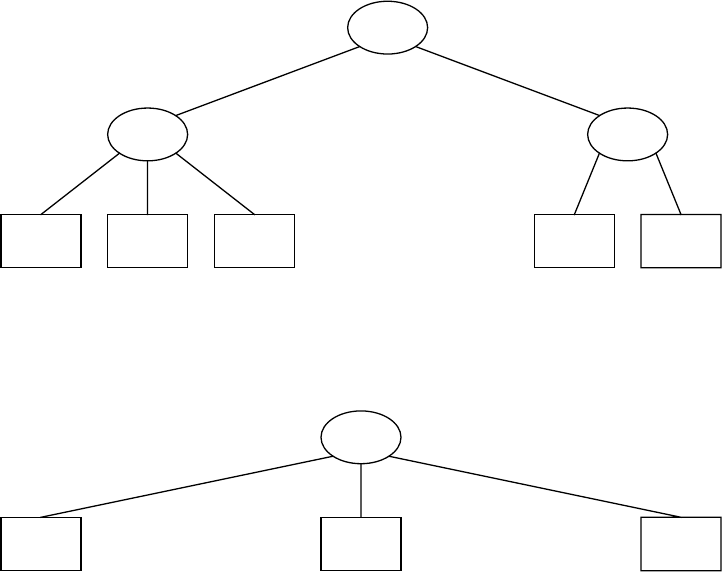
4.36 (a)
0,1
2:4
2, 3
6:-
4, 5
8:-
6, 7 8, 9
(b)
1,2,3
4:6
4, 5 6,7,8
-23-
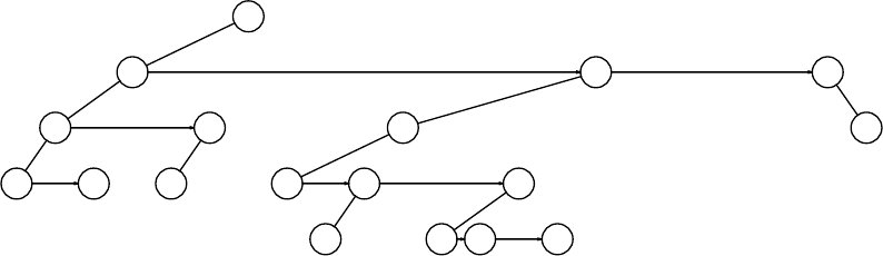
4.39
A
B
D
H I
E
J
C
F
L
O
K M
QP R
G
N
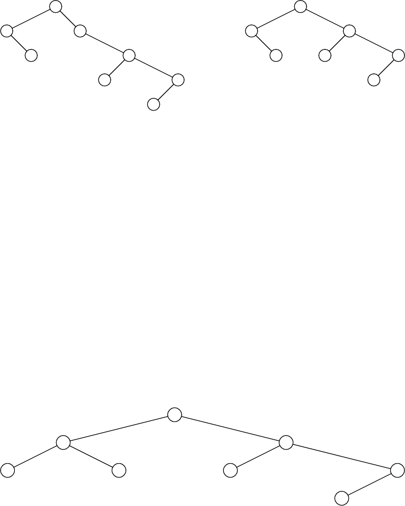
4.41 The function shown here is clearly a linear time routine because in the worst case it does a
traversal on both T1 and T2.
_______________________________________________________________________________
_______________________________________________________________________________
int
Similar( BinaryTree T1, BinaryTree T2 )
{if( T1 == NULL || T2 == NULL )
return T1 == NULL && T2 == NULL;
return Similar( T1->Left, T2->Left ) && Similar( T1->Right, T2->Right );
}
_______________________________________________________________________________
_______________________________________________________________________________
4.43 The easiest solution is to compute, in linear time, the inorder numbers of the nodes in both
trees. If the inorder number of the root of T2 is x, then find xin T1 and rotate it to the root.
Recursively apply this strategy to the left and right subtrees of T1 (by looking at the values
in the root of T2’s left and right subtrees). If dNis the depth of x, then the running time
satisfies T(N) = T (i) + T (N−i−1) + dN, where iis the size of the left subtree. In the worst
case, dNis always O(N), and iis always 0, so the worst-case running time is quadratic.
Under the plausible assumption that all values of iare equally likely, then even if dNis
always O(N), the average value of T(N)isO(Nlog N ). This is a common recurrence that
was already formulated in the chapter and is solved in Chapter 7. Under the more reason-
able assumption that dNis typically logarithmic, then the running time is O(N).
4.44 Add a field to each node indicating the size of the tree it roots. This allows computation of
its inorder traversal number.
4.45 (a) You need an extra bit for each thread.
(c) You can do tree traversals somewhat easier and without recursion. The disadvantage is
that it reeks of old-style hacking.
-24-
Chapter 5: Hashing
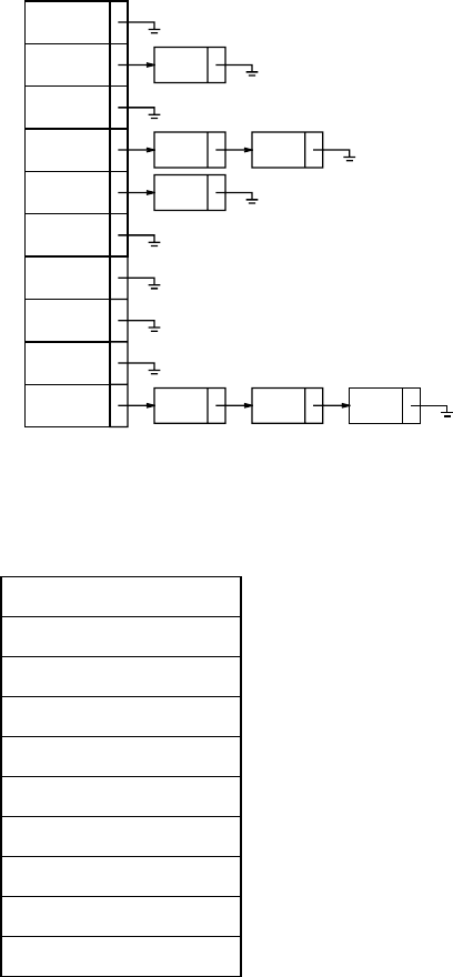
5.1 (a) On the assumption that we add collisions to the end of the list (which is the easier way if
a hash table is being built by hand), the separate chaining hash table that results is shown
here.
4371
1323 6173
4344
4199 9679 1989
0
1
2
3
4
5
6
7
8
9
(b)
9679
4371
1989
1323
6173
4344
4199
0
1
2
3
4
5
6
7
8
9
-25-

(c)
9679
4371
1323
6173
4344
1989
4199
0
1
2
3
4
5
6
7
8
9
(d) 1989 cannot be inserted into the table because hash2(1989) =6, and the alternative locations
5, 1, 7, and 3 are already taken. The table at this point is as follows:
4371
1323
6173
9679
4344
4199
0
1
2
3
4
5
6
7
8
9
5.2 When rehashing, we choose a table size that is roughly twice as large and prime. In our
case, the appropriate new table size is 19, with hash function h(x) = x (mod 19).
(a) Scanning down the separate chaining hash table, the new locations are 4371 in list 1,
1323 in list 12, 6173 in list 17, 4344 in list 12, 4199 in list 0, 9679 in list 8, and 1989 in list
13.
(b) The new locations are 9679 in bucket 8, 4371 in bucket 1, 1989 in bucket 13, 1323 in
bucket 12, 6173 in bucket 17, 4344 in bucket 14 because both 12 and 13 are already occu-
pied, and 4199 in bucket 0.
-26-
(c) The new locations are 9679 in bucket 8, 4371 in bucket 1, 1989 in bucket 13, 1323 in
bucket 12, 6173 in bucket 17, 4344 in bucket 16 because both 12 and 13 are already occu-
pied, and 4199 in bucket 0.
(d) The new locations are 9679 in bucket 8, 4371 in bucket 1, 1989 in bucket 13, 1323 in
bucket 12, 6173 in bucket 17, 4344 in bucket 15 because 12 is already occupied, and 4199
in bucket 0.
5.4 We must be careful not to rehash too often. Let pbe the threshold (fraction of table size) at
which we rehash to a smaller table. Then if the new table has size N, it contains 2pN ele-
ments. This table will require rehashing after either 2N − 2pN insertions or pN deletions.
Balancing these costs suggests that a good choice is p = 2/ 3. For instance, suppose we
have a table of size 300. If we rehash at 200 elements, then the new table size is N = 150,
and we can do either 100 insertions or 100 deletions until a new rehash is required.
If we know that insertions are more frequent than deletions, then we might choose pto be
somewhat larger. If pis too close to 1.0, however, then a sequence of a small number of
deletions followed by insertions can cause frequent rehashing. In the worst case, if p = 1.0,
then alternating deletions and insertions both require rehashing.
5.5 (a) Since each table slot is eventually probed, if the table is not empty, the collision can be
resolved.
(b) This seems to eliminate primary clustering but not secondary clustering because all ele-
ments that hash to some location will try the same collision resolution sequence.
(c, d) The running time is probably similar to quadratic probing. The advantage here is that
the insertion can’t fail unless the table is full.
(e) A method of generating numbers that are not random (or even pseudorandom) is given
in the references. An alternative is to use the method in Exercise 2.7.
5.6 Separate chaining hashing requires the use of pointers, which costs some memory, and the
standard method of implementing calls on memory allocation routines, which typically are
expensive. Linear probing is easily implemented, but performance degrades severely as the
load factor increases because of primary clustering. Quadratic probing is only slightly more
difficult to implement and gives good performance in practice. An insertion can fail if the
table is half empty, but this is not likely. Even if it were, such an insertion would be so
expensive that it wouldn’t matter and would almost certainly point up a weakness in the
hash function. Double hashing eliminates primary and secondary clustering, but the compu-
tation of a second hash function can be costly. Gonnet and Baeza-Yates [8] compare several
hashing strategies; their results suggest that quadratic probing is the fastest method.
5.7 Sorting the MN records and eliminating duplicates would require O(MN log MN ) time
using a standard sorting algorithm. If terms are merged by using a hash function, then the
merging time is constant per term for a total of O(MN ). If the output polynomial is small
and has only O(M + N ) terms, then it is easy to sort it in O((M + N )log (M + N )) time,
which is less than O(MN ). Thus the total is O(MN ). This bound is better because the
model is less restrictive: Hashing is performing operations on the keys rather than just com-
parison between the keys. A similar bound can be obtained by using bucket sort instead of
a standard sorting algorithm. Operations such as hashing are much more expensive than
comparisons in practice, so this bound might not be an improvement. On the other hand, if
the output polynomial is expected to have only O(M + N ) terms, then using a hash table
saves a huge amount of space, since under these conditions, the hash table needs only
-27-
O(M + N ) space.
Another method of implementing these operations is to use a search tree instead of a hash
table; a balanced tree is required because elements are inserted in the tree with too much
order. A splay tree might be particularly well suited for this type of a problem because it
does well with sequential accesses. Comparing the different ways of solving the problem is
a good programming assignment.
5.8 The table size would be roughly 60,000 entries. Each entry holds 8 bytes, for a total of
480,000 bytes.
5.9 (a) This statement is true.
(b) If a word hashes to a location with value 1, there is no guarantee that the word is in the
dictionary. It is possible that it just hashes to the same value as some other word in the dic-
tionary. In our case, the table is approximately 10% full (30,000 words in a table of
300,007), so there is a 10% chance that a word that is not in the dictionary happens to hash
out to a location with value 1.
(c) 300,007 bits is 37,501 bytes on most machines.
(d) As discussed in part (b), the algorithm will fail to detect one in ten misspellings on aver-
age.
(e) A 20-page document would have about 60 misspellings. This algorithm would be
expected to detect 54. A table three times as large would still fit in about 100K bytes and
reduce the expected number of errors to two. This is good enough for many applications,
especially since spelling detection is a very inexact science. Many misspelled words (espe-
cially short ones) are still words. For instance, typing them instead of then is a misspelling
that won’t be detected by any algorithm.
5.10 To each hash table slot, we can add an extra field that we’ll call WhereOnStack, and we can
keep an extra stack. When an insertion is first performed into a slot, we push the address (or
number) of the slot onto the stack and set the WhereOnStack field to point to the top of the
stack. When we access a hash table slot, we check that WhereOnStack points to a valid part
of the stack and that the entry in the (middle of the) stack that is pointed to by the WhereOn-
Stack field has that hash table slot as an address.
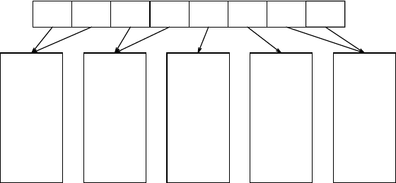
5.14
(2)
00000010
00001011
00101011
(2)
01010001
01100001
01101111
01111111
(3)
10010110
10011011
10011110
(3)
10111101
10111110
(2)
11001111
11011011
11110000
000 001 010 011 100 101 110 111
-28-
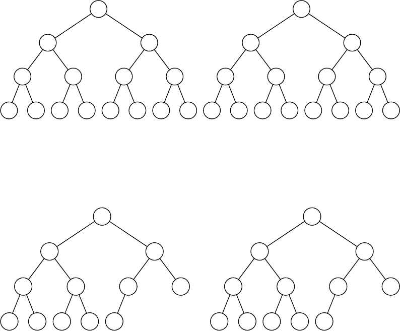
Chapter 6: Priority Queues (Heaps)
6.1 Yes. When an element is inserted, we compare it to the current minimum and change the
minimum if the new element is smaller. DeleteMin operations are expensive in this
scheme.
6.2
1
3 2
6 7 5 4
15 14 12 9 10 11 13 8
1
3 2
12 6 4 8
15 14 9 7 5 11 13 10
6.3 The result of three DeleteMins, starting with both of the heaps in Exercise 6.2, is as fol-
lows:
4
6 5
13 7 10 8
15 14 12 9 11
4
6 5
12 7 10 8
15 14 9 13 11
6.4
6.5 These are simple modifications to the code presented in the text and meant as programming
exercises.
6.6 225. To see this, start with i=1 and position at the root. Follow the path toward the last
node, doubling iwhen taking a left child, and doubling iand adding one when taking a
right child.
-29-
6.7 (a) We show that H(N), which is the sum of the heights of nodes in a complete binary tree
of Nnodes, is N − b (N), where b(N) is the number of ones in the binary representation of
N. Observe that for N = 0 and N = 1, the claim is true. Assume that it is true for values of
kup to and including N−1. Suppose the left and right subtrees have Land Rnodes,
respectively. Since the root has height log N , we have
H(N) = log N + H (L) + H (R)
= log N + L − b (L) + R − b (R)
= N − 1 + ( log N − b (L) − b (R))
The second line follows from the inductive hypothesis, and the third follows because
L + R = N − 1. Now the last node in the tree is in either the left subtree or the right sub-
tree. If it is in the left subtree, then the right subtree is a perfect tree, and
b(R) = log N − 1. Further, the binary representation of Nand Lare identical, with the
exception that the leading 10 in Nbecomes 1 in L. (For instance, if N=37=100101, L=
10101.) It is clear that the second digit of Nmust be zero if the last node is in the left sub-
tree. Thus in this case, b(L) = b (N), and
H(N) = N − b (N)
If the last node is in the right subtree, then b(L) = log N . The binary representation of R
is identical to N, except that the leading 1 is not present. (For instance, if N=27=101011,
L= 01011.) Thus b(R) = b (N) − 1, and again
H(N) = N − b (N)
(b) Run a single-elimination tournament among eight elements. This requires seven com-
parisons and generates ordering information indicated by the binomial tree shown here.
a
bc
d
e
fg
h
The eighth comparison is between band c.Ifcis less than b, then bis made a child of c.
Otherwise, both cand dare made children of b.
(c) A recursive strategy is used. Assume that N = 2k. A binomial tree is built for the N
elements as in part (b). The largest subtree of the root is then recursively converted into a
binary heap of 2k−1elements. The last element in the heap (which is the only one on an
extra level) is then inserted into the binomial queue consisting of the remaining binomial
trees, thus forming another binomial tree of 2k−1elements. At that point, the root has a sub-
tree that is a heap of 2k−1 − 1 elements and another subtree that is a binomial tree of 2k−1
elements. Recursively convert that subtree into a heap; now the whole structure is a binary
heap. The running time for N = 2ksatisfies T(N) = 2T(N / 2) + log N . The base case is
T(8) = 8.
-30-

6.8 Let D1,D2, ..., Dkbe random variables representing the depth of the smallest, second smal-
lest, and kth smallest elements, respectively. We are interested in calculating E(Dk). In
what follows, we assume that the heap size Nis one less than a power of two (that is, the
bottom level is completely filled) but sufficiently large so that terms bounded by O(1 / N )
are negligible. Without loss of generality, we may assume that the kth smallest element is
in the left subheap of the root. Let pj,kbe the probability that this element is the jth smal-
lest element in the subheap.
Lemma: For k >1,E(Dk) =
j=1
Σ
k−1pj,k(E(Dj) + 1).
Proof: An element that is at depth din the left subheap is at depth d + 1 in the entire
subheap. Since E(Dj + 1) = E (Dj) + 1, the theorem follows.
Since by assumption, the bottom level of the heap is full, each of second, third, ..., k−1th
smallest elements are in the left subheap with probability of 0.5. (Technically, the probabil-
ity should be ⁄
12 − 1/(N−1) of being in the right subheap and ⁄
12 + 1/(N−1) of being in the
left, since we have already placed the kth smallest in the right. Recall that we have assumed
that terms of size O(1/N ) can be ignored.) Thus
pj,k = pk−j,k = 2k−2
1
_____ ( j−1
k−2 )
Theorem: E(Dk) ≤ log k .
Proof: The proof is by induction. The theorem clearly holds for k = 1 and k = 2. We then
show that it holds for arbitrary k > 2 on the assumption that it holds for all smaller k. Now,
by the inductive hypothesis, for any 1 ≤ j ≤ k −1,
E(Dj) + E (Dk−j) ≤ log j + log k −j
Since f(x) = log x is convex for x > 0,
log j + log k −j ≤ 2log (k / 2)
Thus
E(Dj) + E (Dk−j) ≤ log (k / 2) + log (k / 2)
Furthermore, since pj,k = pk−j,k,
pj,kE(Dj) + pk−j,kE(Dk−j) ≤pj,klog (k / 2) + pk−j,klog (k / 2)
From the lemma,
E(Dk) =
j=1
Σ
k−1pj,k(E(Dj) + 1)
= 1 +
j=1
Σ
k−1pj,kE(Dj)
Thus
E(Dk) ≤ 1 +
j=1
Σ
k−1pj,klog (k / 2)
-31-
≤ 1 + log (k / 2)
j=1
Σ
k−1pj,k
≤ 1 + log (k / 2)
≤ log k
completing the proof.
It can also be shown that asymptotically, E (Dk) ∼
∼ log (k−1) − 0.273548.
6.9 (a) Perform a preorder traversal of the heap.
(b) Works for leftist and skew heaps. The running time is O(Kd ) for d-heaps.
6.11 Simulations show that the linear time algorithm is the faster, not only on worst-case inputs,
but also on random data.
6.12 (a) If the heap is organized as a (min) heap, then starting at the hole at the root, find a path
down to a leaf by taking the minimum child. The requires roughly log N comparisons. To
find the correct place where to move the hole, perform a binary search on the log N ele-
ments. This takes O(log log N ) comparisons.
(b) Find a path of minimum children, stopping after log N − log log N levels. At this point,
it is easy to determine if the hole should be placed above or below the stopping point. If it
goes below, then continue finding the path, but perform the binary search on only the last
log log N elements on the path, for a total of log N + log log log N comparisons. Other-
wise, perform a binary search on the first log N − log log N elements. The binary search
takes at most log log N comparisons, and the path finding took only log N − log log N ,so
the total in this case is log N . So the worst case is the first case.
(c) The bound can be improved to log N + log*N + O (1), where log*N is the inverse Ack-
erman function (see Chapter 8). This bound can be found in reference [16].
6.13 The parent is at position (i + d − 2)/d . The children are in positions (i − 1)d + 2, ...,
id + 1.
6.14 (a) O((M + dN )logdN).
(b) O((M + N )log N ).
(c) O(M + N2).
(d) d= max (2, M / N ).
(See the related discussion at the end of Section 11.4.)
-32-
6.16
31
18
9
10
4
15
8
5
21
11
6
2
12
11
18
17
6.17
1
2 3
7 6 5 4
8 9 10 11 12 13 14 15
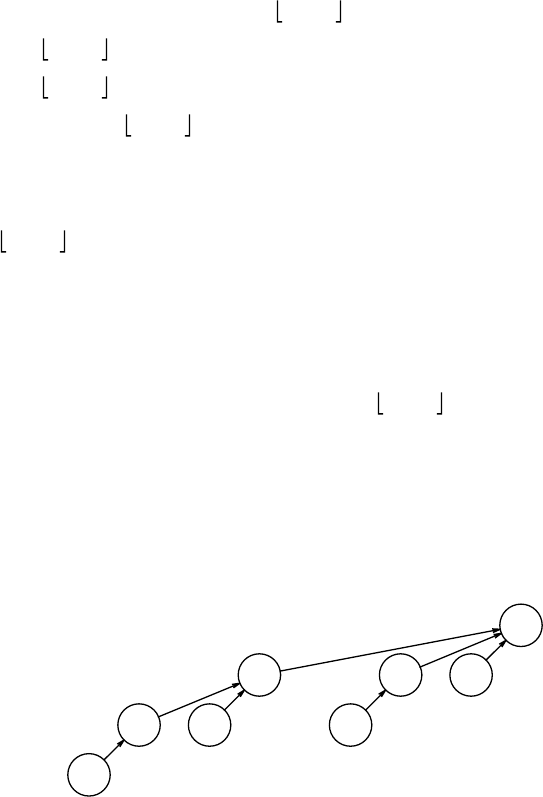
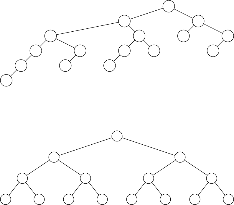
6.18 This theorem is true, and the proof is very much along the same lines as Exercise 4.17.
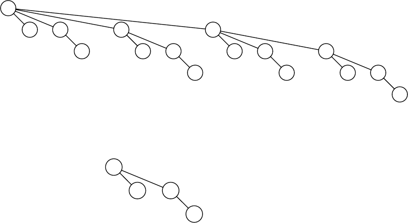
6.19 If elements are inserted in decreasing order, a leftist heap consisting of a chain of left chil-
dren is formed. This is the best because the right path length is minimized.
6.20 (a) If a DecreaseKey is performed on a node that is very deep (very left), the time to per-
colate up would be prohibitive. Thus the obvious solution doesn’t work. However, we can
still do the operation efficiently by a combination of Delete and Insert .ToDelete an arbi-
trary node xin the heap, replace xby the Merge of its left and right subheaps. This might
create an imbalance for nodes on the path from x’s parent to the root that would need to be
fixed by a child swap. However, it is easy to show that at most log N nodes can be affected,
preserving the time bound. This is discussed in Chapter 11.
6.21 Lazy deletion in leftist heaps is discussed in the paper by Cheriton and Tarjan [9]. The gen-
eral idea is that if the root is marked deleted, then a preorder traversal of the heap is formed,
and the frontier of marked nodes is removed, leaving a collection of heaps. These can be
merged two at a time by placing all the heaps on a queue, removing two, merging them, and
placing the result at the end of the queue, terminating when only one heap remains.
6.22 (a) The standard way to do this is to divide the work into passes. A new pass begins when
the first element reappears in a heap that is dequeued. The first pass takes roughly
-33-
2*1*(N / 2) time units because there are N / 2 merges of trees with one node each on the
right path. The next pass takes 2*2*(N / 4) time units because of the roughly N / 4 merges
of trees with no more than two nodes on the right path. The third pass takes 2*3*(N / 8)
time units, and so on. The sum converges to 4N.
(b) It generates heaps that are more leftist.
6.23
31
18
9
10
4
15
8
5
21
11
6
2
12
11
18
17
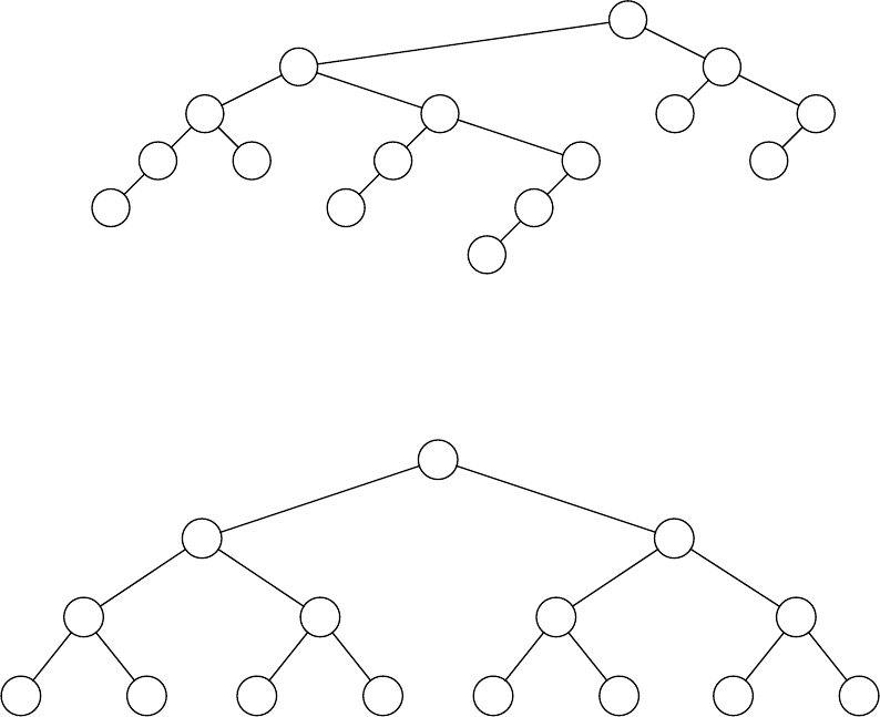
6.24
1
3 2
7564
15 11 13 9 14 10 12 8
6.25 This claim is also true, and the proof is similar in spirit to Exercise 4.17 or 6.18.
6.26 Yes. All the single operation estimates in Exercise 6.22 become amortized instead of
worst-case, but by the definition of amortized analysis, the sum of these estimates is a
worst-case bound for the sequence.
6.27 Clearly the claim is true for k = 1. Suppose it is true for all values i = 1, 2, ..., k.ABk+1
tree is formed by attaching a Bktree to the root of a Bktree. Thus by induction, it contains
aB0through Bk−1tree, as well as the newly attached Bktree, proving the claim.
6.28 Proof is by induction. Clearly the claim is true for k = 1. Assume true for all values i = 1,
2, ..., k.ABk+1tree is formed by attaching a Bktree to the original Bktree. The original
-34-
thus had ( d
k )nodes at depth d. The attached tree had ( d−1
k )nodes at depth d−1,
which are now at depth d. Adding these two terms and using a well-known formula estab-
lishes the theorem.
6.29
4
13 15 23
18 24
65
51
12
21 24
65
14
26 16
18
2
29
55
11
6.30 This is established in Chapter 11.
6.31 The algorithm is to do nothing special −merely Insert them. This is proved in Chapter 11.
6.35 Don’t keep the key values in the heap, but keep only the difference between the value of the
key in a node and the value of the key in its parent.
6.36 O(N + k log N ) is a better bound than O(Nlog k ). The first bound is O(N)if
k = O (N / log N ). The second bound is more than this as soon as kgrows faster than a
constant. For the other values Ω(N / log N ) = k = ο(N), the first bound is better. When
k = Θ(N), the bounds are identical.
-35-
Chapter 7: Sorting
7.1
_______________________________________________
______________________________________________
Original 314159265
______________________________________________
after P=2134159265
after P=3134159265
after P=4113459265
after P=5113459265
after P=6113459265
after P=7112345965
after P=8112345695
after P=9112345569
______________________________________________
_______________________________________________
7.2 O(N) because the while loop terminates immediately. Of course, accidentally changing the
test to include equalities raises the running time to quadratic for this type of input.
7.3 The inversion that existed between A[i] and A[i + k ] is removed. This shows at least one
inversion is removed. For each of the k − 1 elements A[i + 1], A[i + 2], ..., A[i + k − 1],
at most two inversions can be removed by the exchange. This gives a maximum of
2(k − 1) + 1 = 2k − 1.
7.4
________________________________________________
_______________________________________________
Original 987654321
_______________________________________________
after 7-sort 217654398
after 3-sort 214357698
after 1-sort 123456789
_______________________________________________
________________________________________________
7.5 (a) Θ(N2). The 2-sort removes at most only three inversions at a time; hence the algorithm
is Ω(N2). The 2-sort is two insertion sorts of size N / 2, so the cost of that pass is O(N2).
The 1-sort is also O(N2), so the total is O(N2).
7.6 Part (a) is an extension of the theorem proved in the text. Part (b) is fairly complicated; see
reference [11].
7.7 See reference [11].
7.8 Use the input specified in the hint. If the number of inversions is shown to be Ω(N2), then
the bound follows, since no increments are removed until an ht / 2sort. If we consider the
pattern formed hkthrough h2k−1, where k = t / 2 + 1, we find that it has length
N = hk(hk + 1)−1, and the number of inversions is roughly hk4/ 24, which is Ω(N2).
7.9 (a) O(Nlog N ). No exchanges, but each pass takes O(N).
(b) O(Nlog N ). It is easy to show that after an hksort, no element is farther than hkfrom
its rightful position. Thus if the increments satisfy hk+1 ≤ chkfor a constant c, which
implies O(log N ) increments, then the bound is O(Nlog N ).
-36-
7.10 (a) No, because it is still possible for consecutive increments to share a common factor. An
example is the sequence 1, 3, 9, 21, 45, ht+1 = 2ht + 3.
(b) Yes, because consecutive increments are relatively prime. The running time becomes
O(N3/ 2).
7.11 The input is read in as
142, 543, 123, 65, 453, 879, 572, 434, 111, 242, 811, 102
The result of the heapify is
879, 811, 572, 434, 543, 123, 142, 65, 111, 242, 453, 102
879 is removed from the heap and placed at the end. We’ll place it in italics to signal that it
is not part of the heap. 102 is placed in the hole and bubbled down, obtaining
811, 543, 572, 434, 453, 123, 142, 65, 111, 242, 102, 879
Continuing the process, we obtain
572, 543, 142, 434, 453, 123, 102, 65, 111, 242, 811,879
543, 453, 142, 434, 242, 123, 102, 65, 111, 572,811,879
453, 434, 142, 111, 242, 123, 102, 65, 543,572,811,879
434, 242, 142, 111, 65, 123, 102, 453,543,572,811,879
242, 111, 142, 102, 65, 123, 434,453,543,572,811,879
142, 111, 123, 102, 65, 242,434,453,543,572,811,879
123, 111, 65, 102, 142,242,434,453,543,572,811,879
111, 102, 65, 123,142,242,434,453,543,572,811,879
102, 65, 111,123,142,242,434,453,543,572,811,879
65, 102,111,123,142,242,434,453,543,572,811,879
7.12 Heapsort uses at least (roughly) Nlog N comparisons on any input, so there are no particu-
larly good inputs. This bound is tight; see the paper by Schaeffer and Sedgewick [16]. This
result applies for almost all variations of heapsort, which have different rearrangement stra-
tegies. See Y. Ding and M. A. Weiss, "Best Case Lower Bounds for Heapsort," Computing
49 (1992).
7.13 First the sequence {3, 1, 4, 1} is sorted. To do this, the sequence {3, 1} is sorted. This
involves sorting {3} and {1}, which are base cases, and merging the result to obtain {1, 3}.
The sequence {4, 1} is likewise sorted into {1, 4}. Then these two sequences are merged to
obtain {1, 1, 3, 4}. The second half is sorted similarly, eventually obtaining {2, 5, 6, 9}.
The merged result is then easily computed as {1, 1, 2, 3, 4, 5, 6, 9}.
7.14 Mergesort can be implemented nonrecursively by first merging pairs of adjacent elements,
then pairs of two elements, then pairs of four elements, and so on. This is implemented in
Fig. 7.1.
7.15 The merging step always takes Θ(N) time, so the sorting process takes Θ(Nlog N ) time on
all inputs.
7.16 See reference [11] for the exact derivation of the worst case of mergesort.
7.17 The original input is 3, 1, 4, 1, 5, 9, 2, 6, 5, 3, 5
After sorting the first, middle, and last elements, we have
3, 1, 4, 1, 5, 5, 2, 6, 5, 3, 9
Thus the pivot is 5. Hiding it gives
3, 1, 4, 1, 5, 3, 2, 6, 5, 5, 9
The first swap is between two fives. The next swap has iand jcrossing. Thus the pivot is
-37-
_______________________________________________________________________________
_______________________________________________________________________________
void
Mergesort( ElementType A[ ], int N )
{ElementType *TmpArray;
int SubListSize, Part1Start, Part2Start, Part2End;
TmpArray = malloc( sizeof( ElementType ) * N );
for( SubListSize = 1; SubListSize < N; SubListSize *= 2 )
{Part1Start = 0;
while( Part1Start + SubListSize < N - 1 )
{Part2Start = Part1Start + SubListSize;
Part2End = min( N, Part2Start + SubListSize - 1 );
Merge( A, TmpArray, Part1Start, Part2Start, Part2End );
Part1Start = Part2End + 1;
}
}
}
Fig. 7.1.
_______________________________________________________________________________
_______________________________________________________________________________
swapped back with i:3, 1, 4, 1, 5, 3, 2, 5, 5, 6, 9
We now recursively quicksort the first eight elements:
3, 1, 4, 1, 5, 3, 2, 5
Sorting the three appropriate elements gives
1, 1, 4, 3, 5, 3, 2, 5
Thus the pivot is 3, which gets hidden:
1, 1, 4, 2, 5, 3, 3, 5
The first swap is between 4 and 3: 1, 1, 3, 2, 5, 4, 3, 5
The next swap crosses pointers, so is undone; ipoints at 5, and so the pivot is swapped:
1, 1, 3, 2, 3, 4, 5, 5
A recursive call is now made to sort the first four elements. The pivot is 1, and the partition
does not make any changes. The recursive calls are made, but the subfiles are below the
cutoff, so nothing is done. Likewise, the last three elements constitute a base case, so noth-
ing is done. We return to the original call, which now calls quicksort recursively on the
right-hand side, but again, there are only three elements, so nothing is done. The result is
1, 1, 3, 2, 3, 4, 5, 5, 5, 6, 9
which is cleaned up by insertion sort.
7.18 (a) O(Nlog N ) because the pivot will partition perfectly.
(b) Again, O(Nlog N ) because the pivot will partition perfectly.
(c) O(Nlog N ); the performance is slightly better than the analysis suggests because of the
median-of-three partition and cutoff.
-38-

7.19 (a) If the first element is chosen as the pivot, the running time degenerates to quadratic in
the first two cases. It is still O(Nlog N ) for random input.
(b) The same results apply for this pivot choice.
(c) If a random element is chosen, then the running time is O(Nlog N ) expected for all
inputs, although there is an O(N2) worst case if very bad random numbers come up. There
is, however, an essentially negligible chance of this occurring. Chapter 10 discusses the
randomized philosophy.
(d) This is a dangerous road to go; it depends on the distribution of the keys. For many dis-
tributions, such as uniform, the performance is O(Nlog N ) on average. For a skewed distri-
bution, such as with the input {1, 2, 4, 8, 16, 32, 64, ... }, the pivot will be consistently terri-
ble, giving quadratic running time, independent of the ordering of the input.
7.20 (a) O(Nlog N ) because the pivot will partition perfectly.
(b) Sentinels need to be used to guarantee that iand jdon’t run past the end. The running
time will be Θ(N2) since, because iwon’t stop until it hits the sentinel, the partitioning step
will put all but the pivot in S1.
(c) Again a sentinel needs to be used to stop j. This is also Θ(N2) because the partitioning
is unbalanced.
7.21 Yes, but it doesn’t reduce the average running time for random input. Using median-of-
three partitioning reduces the average running time because it makes the partition more bal-
anced on average.
7.22 The strategy used here is to force the worst possible pivot at each stage. This doesn’t neces-
sarily give the maximum amount of work (since there are few exchanges, just lots of com-
parisons), but it does give Ω(N2) comparisons. By working backward, we can arrive at the
following permutation:
20, 3, 5, 7, 9, 11, 13, 15, 17, 19, 4, 10, 2, 12, 6, 14, 1, 16, 8, 18
A method to extend this to larger numbers when Nis even is as follows: The first element is
N, the middle is N − 1, and the last is N − 2. Odd numbers (except 1) are written in
decreasing order starting to the left of center. Even numbers are written in decreasing order
by starting at the rightmost spot, always skipping one available empty slot, and wrapping
around when the center is reached. This method takes O(Nlog N ) time to generate the per-
mutation, but is suitable for a hand calculation. By inverting the actions of quicksort, it is
possible to generate the permutation in linear time.
7.24 This recurrence results from the analysis of the quick selection algorithm. T(N) = O (N).
7.25 Insertion sort and mergesort are stable if coded correctly. Any of the sorts can be made
stable by the addition of a second key, which indicates the original position.
7.26 (d) f(N) can be O(N / log N ). Sort the f(N) elements using mergesort in
O(f(N)log f (N)) time. This is O(N)iff(N) is chosen using the criterion given. Then
merge this sorted list with the already sorted list of Nnumbers in O(N + f (N)) = O (N)
time.
7.27 A decision tree would have Nleaves, so log N comparisons are required.
7.28 log N ! ∼
∼ N log N − N log e .
7.29 (a) ( N
2N ).
-39-
(b) The information-theoretic lower bound is log ( N
2N ). Applying Stirling’s formula, we
can estimate the bound as 2N − ⁄
12log N . A better lower bound is known for this case:
2N−1 comparisons are necessary. Merging two lists of different sizes Mand Nlikewise
requires at least log ( N
M + N )comparisons.
7.30 It takes O(1) to insert each element into a bucket, for a total of O(N). It takes O(1) to
extract each element from a bucket, for O(M). We waste at most O(1) examining each
empty bucket, for a total of O(M). Adding these estimates gives O(M + N ).
7.31 We add a dummy N + 1th element, which we’ll call Maybe .Maybe satisfies
false < Maybe <true . Partition the array around Maybe , using the standard quicksort tech-
niques. Then swap Maybe and the N + 1th element. The first Nelements are then
correctly arranged.
7.32 We add a dummy N + 1th element, which we’ll call ProbablyFalse .ProbablyFalse
satisfies false < ProbablyFalse < Maybe . Partition the array around ProbablyFalse as in
the previous exercise. Suppose that after the partition, ProbablyFalse winds up in position
i. Then place the element that is in the N + 1th slot in position i, place ProbablyTrue
(defined the obvious way) in position N +1 , and partition the subarray from position i
onward. Finally, swap ProbablyTrue with the element in the N + 1th location. The first N
elements are now correctly arranged. These two problems can be done without the assump-
tion of an extra array slot; assuming so simplifies the presentation.
7.33 (a) log 4! =5.
(b) Compare and exchange (if necessary) a1and a2so that a1 ≥ a2, and repeat with a3and
a4. Compare and exchange a1and a3. Compare and exchange a2and a4. Finally, com-
pare and exchange a2and a3.
7.34 (a) log 5! = 7.
(b) Compare and exchange (if necessary) a1and a2so that a1 ≥ a2, and repeat with a3and
a4so that a3 ≥ a4. Compare and exchange (if necessary) the two winners, a1and a3.
Assume without loss of generality that we now have a1 ≥ a3 ≥ a4, and a1 ≥ a2. (The other
case is obviously identical.) Insert a5by binary search in the appropriate place among a1,
a3,a4. This can be done in two comparisons. Finally, insert a2among a3,a4,a5.Ifitis
the largest among those three, then it goes directly after a1since it is already known to be
larger than a1. This takes two more comparisons by a binary search. The total is thus seven
comparisons.
7.38 (a) For the given input, the pivot is 2. It is swapped with the last element. iwill point at
the second element, and jwill be stopped at the first element. Since the pointers have
crossed, the pivot is swapped with the element in position 2. The input is now 1, 2, 4, 5, 6,
..., N − 1, N, 3. The recursive call on the right subarray is thus on an increasing sequence
of numbers, except for the last number, which is the smallest. This is exactly the same form
as the original. Thus each recursive call will have only two fewer elements than the previ-
ous. The running time will be quadratic.
(b) Although the first pivot generates equal partitions, both the left and right halves will
have the same form as part (a). Thus the running time will be quadratic because after the
first partition, the algorithm will grind slowly. This is one of the many interesting tidbits in
reference [20].
-40-
7.39 We show that in a binary tree with Lleaves, the average depth of a leaf is at least log L .
We can prove this by induction. Clearly, the claim is true if L = 1. Suppose it is true for
trees with up to L − 1 leaves. Consider a tree of Lleaves with minimum average leaf
depth. Clearly, the root of such a tree must have non-NULL left and right subtrees. Sup-
pose that the left subtree has LLleaves, and the right subtree has LRleaves. By the induc-
tive hypothesis, the total depth of the leaves (which is their average times their number) in
the left subtree is LL(1 + log LL), and the total depth of the right subtree’s leaves is
LR(1 + log LR) (because the leaves in the subtrees are one deeper with respect to the root of
the tree than with respect to the root of their subtree). Thus the total depth of all the leaves
is L + LLlog LL + LRlog LR. Since f(x) = x log x is convex for x ≥ 1, we know that
f(x) + f (y) ≥ 2f((x+y) / 2). Thus, the total depth of all the leaves is at least
L + 2(L / 2)log (L / 2) ≥ L + L (log L − 1) ≥ L log L . Thus the average leaf depth is at least
log L .
-41-
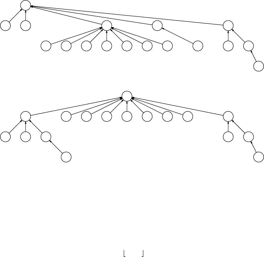
Chapter 8: The Disjoint Set ADT
8.1 We assume that unions operated on the roots of the trees containing the arguments. Also, in
case of ties, the second tree is made a child of the first. Arbitrary union and union by height
give the same answer (shown as the first tree) for this problem. Union by size gives the
second tree.
26
1
4
3
5 7 10 11 12 13
8
9
14
15 16
17
2 6
1 4
3
5 7 10 11 12 13
8
9
14
15 16
17
8.2 In both cases, have nodes 16 and 17 point directly to the root.
8.4 Claim: A tree of height Hhas at least 2Hnodes. The proof is by induction. A tree of
height 0 clearly has at least 1 node, and a tree of height 1 clearly has at least 2. Let Tbe the
tree of height Hwith fewest nodes. Thus at the time of T’s last union, it must have been a
tree of height H−1, since otherwise Twould have been smaller at that time than it is now
and still would have been of height H, which is impossible by assumption of T’s minimal-
ity. Since T’s height was updated, it must have been as a result of a union with another tree
of height H−1. By the induction hypothesis, we know that at the time of the union, Thad
at least 2H−1nodes, as did the tree attached to it, for a total of 2Hnodes, proving the claim.
Thus an N-node tree has depth at most log N .
8.5 All answers are O(M) because in all cases α(M, N ) = 1.
8.6 Assuming that the graph has only nine vertices, then the union/find tree that is formed is
shown here. The edge (4,6) does not result in a union because at the time it is examined, 4
and 6 are already in the same component. The connected components are {1,2,3,4,6} and
-42-
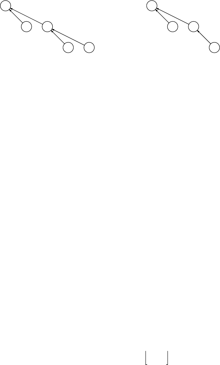
{5,7,8,9}.
1
2 3
4 6
5
7 8
9
8.8 (a) When we perform a union, we push onto a stack the two roots and the old values of their
parents. To implement a Deunion, we only have to pop the stack and restore the values.
This strategy works fine in the absence of path compression.
(b) If path compression is implemented, the strategy described in part (a) does not work
because path compression moves elements out of subtrees. For instance, the sequence
Union(1,2), Union(3,4), Union(1,3), Find(4), Deunion(1,3) will leave 4 in set 1 if path
compression is implemented.
8.9 We assume that the tree is implemented with pointers instead of a simple array. Thus Find
will return a pointer instead of an actual set name. We will keep an array to map set
numbers to their tree nodes. Union and Find are implemented in the standard manner. To
perform Remove(X), first perform a Find(X) with path compression. Then mark the node
containing Xas vacant. Create a new one-node tree with Xand have it pointed to by the
appropriate array entry. The time to perform a Remove is the same as the time to perform a
Find, except that there potentially could be a large number of vacant nodes. To take care of
this, after N Remove s are performed, perform a Find on every node, with path compres-
sion. If a Find (X) returns a vacant root, then place Xin the root node, and make the old
node containing Xvacant. The results of Exercise 8.11 guarantee that this will take linear
time, which can be charged to the N Remove s. At this point, all vacant nodes (indeed all
nonroot nodes) are children of a root, and vacant nodes can be disposed (if an array of
pointers to them has been kept). This also guarantees that there are never more than 2N
nodes in the forest and preserves the Mα(M, N ) asymptotic time bound.
8.11 Suppose there are u Union s and f Find s. Each union costs constant time, for a total of u.
AFind costs one unit per vertex visited. We charge, as in the text, under the following
slightly modified rules:
(A) the vertex is a root or child of the root
(B) otherwise
Essentially, all vertices are in one rank group. During any Find, there can be at most two
rule (A) charges, for a total of 2f. Each vertex can be charged at most once under rule (B)
because after path compression it will be a child of the root. The number of vertices that are
not roots or children of roots is clearly bounded by u, independent of the unioning strategy,
because each Union changes exactly one vertex from root to nonroot status, and this bounds
the number of type (B) nodes. Thus the total rule (B) charges are at most u. Adding all
charges gives a bound of 2f + 2u, which is linear in the number of operations.
8.13 For each vertex v, let the pseudorank Rvbe defined as log Sv, where Svis the number of
descendents (including itself) of vin the final tree, after all Union s are performed, ignoring
-43-
path compression.
Although the pseudorank is not maintained by the algorithm, it is not hard to show that the
pseudorank satisfies the same properties as the ranks do in union-by-rank. Clearly, a vertex
with pseudorank Rvhas at least 2Rvdescendents (by its definition), and the number of ver-
tices of pseudorank Ris at most N / 2R. The union-by-size rule ensures that the parent of a
node has twice as many descendents as the node, so the pseudoranks monotonically increase
on the path toward the root if there is no path compression. The argument in Lemma 8.3
tells us that path compression does not destroy this property.
If we partition the vertices by pseudoranks and assign the charges in the same manner as in
the text proof for union-by-rank, the same steps follow, and the identical bound is obtained.
8.14 This is most conveniently implemented without recursion and is faster because, even if full
path compression is implemented nonrecursively, it requires two passes up the tree. This
requires only one. We leave the coding to the reader since comparing the various Union
and Find strategies is a reasonable programming project. The worst-case running time
remains the same because the properties of the ranks are unchanged. Instead of charging
one unit to each vertex on the path to the root, we can charge two units to alternating ver-
tices (namely, the vertices whose parents are altered by path halving). These vertices get
parents of higher rank, as before, and the same kind of analysis bounds the total charges.
-44-
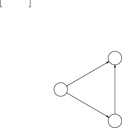
Chapter 9: Graph Algorithms
9.1 The following ordering is arrived at by using a queue and assumes that vertices appear on an
adjacency list alphabetically. The topological order that results is then
s, G, D, H, A, B, E, I, F, C, t
9.2 Assuming the same adjacency list, the topological order produced when a stack is used is
s, G, H, D, A, E, I, F, B, C, t
Because a topological sort processes vertices in the same manner as a breadth-first search, it
tends to produce a more natural ordering.
9.4 The idea is the same as in Exercise 5.10.
9.5 (a) (Unweighted paths) A->B, A->C, A->B->G, A->B->E, A->C->D, A->B->E->F.
(b) (Weighted paths) A->C, A->B, A->B->G, A->B->G->E, A->B->G->E->F, A->B->G-
>E->D.
9.6 We’ll assume that Dijkstra’s algorithm is implemented with a priority queue of vertices that
uses the DecreaseKey operation. Dijkstra’s algorithm uses | E|DecreaseKey operations,
which cost O(logd|V| ) each, and | V|DeleteMin operations, which cost O(dlogd|V| )
each. The running time is thus O(|E| logd|V| + |V|dlogd|V| ). The cost of the
DecreaseKey operations balances the Insert operations when d = |E|/|V| . For a sparse
graph, this might give a value of dthat is less than 2; we can’t allow this, so dis chosen to
be max (2, | E|/|V| ). This gives a running time of O(|E| log2 + |E|/|V||V| ), which is a
slight theoretical improvement. Moret and Shapiro report (indirectly) that d-heaps do not
improve the running time in practice.
9.7 (a) The graph shown here is an example. Dijkstra’s algorithm gives a path from Ato Cof
cost 2, when the path from Ato Bto Chas cost 1.
A
C
B
2
3
-2
(b) We define a pass of the algorithm as follows: Pass 0 consists of marking the start vertex
as known and placing its adjacent vertices on the queue. For j > 0, pass jconsists of mark-
ing as known all vertices on the queue at the end of pass j − 1. Each pass requires linear
time, since during a pass, a vertex is placed on the queue at most once. It is easy to show by
induction that if there is a shortest path from sto vcontaining kedges, then dvwill equal
the length of this path by the beginning of pass k. Thus there are at most | V| passes,
-45-
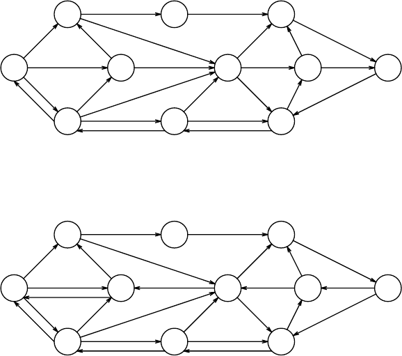
giving an O(|E| | V| ) bound.
9.8 See the comments for Exercise 9.19.
9.10 (a) Use an array Count such that for any vertex u,Count[u] is the number of distinct paths
from sto uknown so far. When a vertex vis marked as known, its adjacency list is
traversed. Let wbe a vertex on the adjacency list.
If dv + cv,w = dw, then increment Count[w] by Count[v] because all shortest paths from s
to vwith last edge (v,w) give a shortest path to w.
If dv + cv,w < dw, then pwand dwget updated. All previously known shortest paths to w
are now invalid, but all shortest paths to vnow lead to shortest paths for w, so set
Count[w] to equal Count[v]. Note: Zero-cost edges mess up this algorithm.
(b) Use an array NumEdges such that for any vertex u,NumEdges[u] is the shortest
number of edges on a path of distance dufrom sto uknown so far. Thus NumEdges is
used as a tiebreaker when selecting the vertex to mark. As before, vis the vertex marked
known, and wis adjacent to v.
If dv + cv,w = dw, then change pwto vand NumEdges[w] to NumEdges[v]+1 if
NumEdges[v]+1 < NumEdges[w].
If dv + cv,w < dw, then update pwand dw, and set NumEdges[w] to NumEdges[v]+1.
9.11 (This solution is not unique).
First send four units of flow along the path s, G, H, I, t. This gives the following residual
graph:
s
A
D
G
B
E
H
C
F
I
t
1
4
2
2
2
3
3
2 1
2
2
2
3
32
2
41
3
1 4
4
4 4
Next, send three units of flow along s, D, E, F, t. The residual graph that results is as fol-
lows:
s
A
D
G
B
E
H
C
F
I
t
1
1
3
2
2
2
3
3
2 1
2
2
2
3
32
2
41
3
1 4
4
4 4
Now two units of flow are sent along the path s, G, D, A, B, C, t, yielding the following
residual graph:
-46-
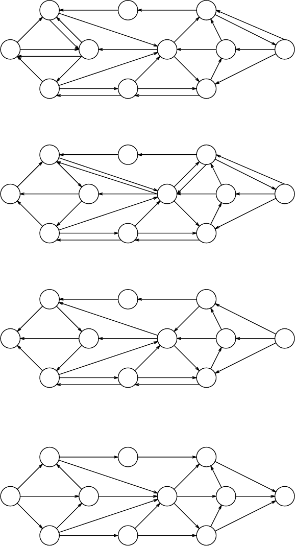
s
A
D
G
B
E
H
C
F
I
t
1
1
3
2
2
3
1
2
2 1
2
2
2
3
32
2
2
2
1
3
1 4
6
4 4
One unit of flow is then sent along s, D, A, E, C, t:
s
A
D
G
B
E
H
C
F
I
t
1
4
2
1
13
3
2 1
2
2
1
13
32
2
1
3
1
3
1 4
6
4 4
Finally, one unit of flow can go along the path s, A, E, C, t:
s
A
D
G
B
E
H
C
F
I
t
1
4
2
2
3
3
2 1
2
2
2
3
32
2
4
1
3
1 4
6
4 4
The preceding residual graph has no path from s to t. Thus the algorithm terminates. The
final flow graph, which carries 11 units, is as follows:
s
A
D
G
B
E
H
C
F
I
t
1
4
6
2
2
3
3
2 0
4
2
2
3
00
4
40
3
0 4
This flow is not unique. For instance, two units of the flow that goes from G to D to A to E
could go by G to H to E.
-47-
9.12 Let Tbe the tree with root r, and children r1,r2, ..., rk, which are the roots of T1,T2, ...,
Tk, which have maximum incoming flow of c1,c2, ..., ck, respectively. By the problem
statement, we may take the maximum incoming flow of rto be infinity. The recursive
function FindMaxFlow( T, IncomingCap ) finds the value of the maximum flow in T
(finding the actual flow is a matter of bookkeeping); the flow is guaranteed not to exceed
IncomingCap .
If Tis a leaf, then FindMaxFlow returns IncomingCap since we have assumed a sink of
infinite capacity. Otherwise, a standard postorder traversal can be used to compute the max-
imum flow in linear time.
_______________________________________________________________________________
_______________________________________________________________________________
FlowType
FindMaxFlow( Tree T, FlowType IncomingCap )
{FlowType ChildFlow, TotalFlow;
if( IsLeaf( T ) )
return IncomingCap;
else
{TotalFlow = 0;
for( each subtree Tiof T )
{ChildFlow = FindMaxFlow( Ti, min( IncomingCap, ci));
TotalFlow += ChildFlow;
IncomingCap -= ChildFlow;
}
return TotalFlow;
}
}
_______________________________________________________________________________
_______________________________________________________________________________
9.13 (a) Assume that the graph is connected and undirected. If it is not connected, then apply the
algorithm to the connected components. Initially, mark all vertices as unknown. Pick any
vertex v, color it red, and perform a depth-first search. When a node is first encountered,
color it blue if the DFS has just come from a red node, and red otherwise. If at any point,
the depth-first search encounters an edge between two identical colors, then the graph is not
bipartite; otherwise, it is. A breadth-first search (that is, using a queue) also works. This
problem, which is essentially two-coloring a graph, is clearly solvable in linear time. This
contrasts with three-coloring, which is NP-complete.
(b) Construct an undirected graph with a vertex for each instructor, a vertex for each course,
and an edge between (v,w) if instructor vis qualified to teach course w. Such a graph is
bipartite; a matching of Medges means that Mcourses can be covered simultaneously.
(c) Give each edge in the bipartite graph a weight of 1, and direct the edge from the instruc-
tor to the course. Add a vertex swith edges of weight 1 from sto all instructor vertices.
Add a vertex twith edges of weight 1 from all course vertices to t. The maximum flow is
equal to the maximum matching.
-48-
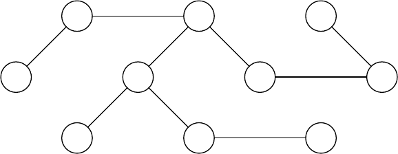
(d) The running time is O(|E| | V|⁄
12) because this is the special case of the network flow
problem mentioned in the text. All edges have unit cost, and every vertex (except sand t)
has either an indegree or outdegree of 1.
9.14 This is a slight modification of Dijkstra’s algorithm. Let fibe the best flow from sto iat
any point in the algorithm. Initially, fi = 0 for all vertices, except s:fs = ∞.
At each stage, we select vsuch that fvis maximum among all unknown vertices. Then for
each wadjacent to v, the cost of the flow to wusing vas an intermediate is min (fv,cv,w).
If this value is higher than the current value of fw, then fwand pware updated.
9.15 One possible minimum spanning tree is shown here. This solution is not unique.
AB C
D E F G
H I J
4
2
3
2
1
3
2
7
1
9.16 Both work correctly. The proof makes no use of the fact that an edge must be nonnegative.
9.17 The proof of this fact can be found in any good graph theory book. A more general theorem
follows:
Theorem: Let G = (V, E ) be an undirected, unweighted graph, and let Abe the adjacency
matrix for G(which contains either 1s or 0s). Let Dbe the matrix such that D[v][v]is
equal to the degree of v; all nondiagonal matrices are 0. Then the number of spanning trees
of Gis equal to the determinant of A + D .
9.19 The obvious solution using elementary methods is to bucket sort the edge weights in linear
time. Then the running time of Kruskal’s algorithm is dominated by the Union/Find opera-
tions and is O(|E|α(|E|,|V| )). The Van-Emde Boas priority queues (see Chapter 6 refer-
ences) give an immediate O(|E| loglog | V| ) running time for Dijkstra’s algorithm, but this
isn’t even as good as a Fibonacci heap implementation.
More sophisticated priority queue methods that combine these ideas have been proposed,
including M. L. Fredman and D. E. Willard, "Trans-dichotomous Algorithms for Minimum
Spanning Trees and Shortest Paths," Proceedings of the Thirty-first Annual IEEE Sympo-
sium on the Foundations of Computer Science (1990), 719-725. The paper presents a
linear-time minimum spanning tree algorithm and an O(|E|+|V| log | V|/ loglog | V| )
implementation of Dijkstra’s algorithm if the edge costs are suitably small.
9.20 Since the minimum spanning tree algorithm works for negative edge costs, an obvious solu-
tion is to replace all the edge costs by their negatives and use the minimum spanning tree
algorithm. Alternatively, change the logic so that < is replaced by >, Min by Max , and vice
versa.
9.21 We start the depth-first search at Aand visit adjacent vertices alphabetically. The articula-
tion points are C,E, and F.Cis an articulation point because Low [B] ≥ Num [C]; Eis an
-49-
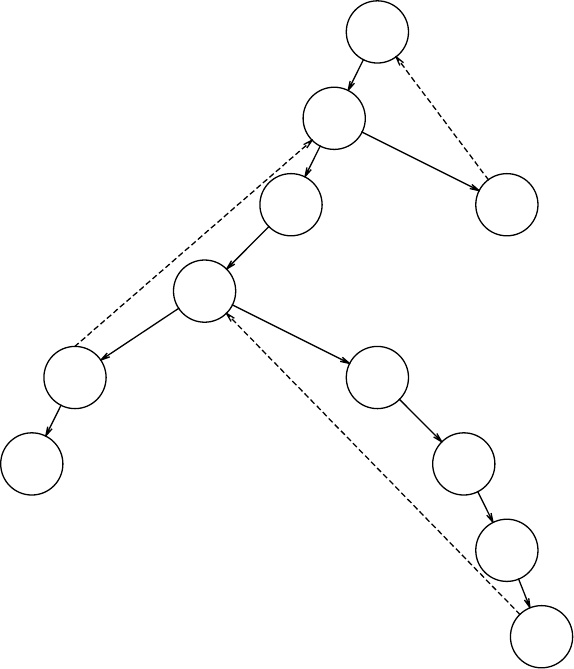
articulation point because Low [H] ≥ Num [E]; and Fis an articulation point because
Low [G] ≥ Num [F]; the depth-first spanning tree is shown in Fig. 9.1.
A 1/1
C 2/1
B 3/2 D 11/1
E 4/2
F 5/2
G 6/6
H 7/4
J 8/4
K 9/4
I 10/4
Fig. 9.1.
9.22 The only difficult part is showing that if some nonroot vertex ais an articulation point, then
there is no back edge between any proper descendent of aand a proper ancestor of ain the
depth-first spanning tree. We prove this by a contradiction.
Let uand vbe two vertices such that every path from uto vgoes through a. At least one
of uand vis a proper descendent of a, since otherwise there is a path from uto vthat
avoids a. Assume without loss of generality that uis a proper descendent of a. Let cbe
the child of athat contains uas a descendent. If there is no back edge between a descen-
dent of cand a proper ancestor of a, then the theorem is true immediately, so suppose for
the sake of contradiction that there is a back edge (s, t ). Then either vis a proper descen-
dent of aor it isn’t. In the second case, by taking a path from uto sto tto v, we can
avoid a, which is a contradiction. In the first case, clearly vcannot be a descendent of c,so
let c' be the child of athat contains vas a descendent. By a similar argument as before, the
only possibility is that there is a back edge (s' , t' ) between a descendent of c' and a proper
ancestor of a. Then there is a path from uto sto tto t' to s' to v; this path avoids a,
which is also a contradiction.
-50-
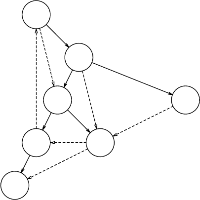
9.23 (a) Do a depth-first search and count the number of back edges.
(b) This is the feedback edge set problem. See reference [1] or [20].
9.24 Let (v,w) be a cross edge. Since at the time wis examined it is already marked, and wis
not a descendent of v(else it would be a forward edge), processing for wis already com-
plete when processing for vcommences. Thus under the convention that trees (and sub-
trees) are placed left to right, the cross edge goes from right to left.
9.25 Suppose the vertices are numbered in preorder and postorder.
If (v,w) is a tree edge, then vmust have a smaller preorder number than w. It is easy to see
that the converse is true.
If (v,w) is a cross edge, then vmust have both a larger preorder and postorder number than
w. The converse is shown as follows: because vhas a larger preorder number, wcannot be
a descendent of v; because it has a larger postorder number, vcannot be a descendent of w;
thus they must be in different trees.
Otherwise, vhas a larger preorder number but is not a cross edge. To test if (v,w) is a back
edge, keep a stack of vertices that are active in the depth-first search call (that is, a stack of
vertices on the path from the current root). By keeping a bit array indicating presence on
the stack, we can easily decide if (v,w) is a back edge or a forward edge.
9.26 The first depth-first spanning tree is
A
B
C
D E
F
G
Gr, with the order in which to perform the second depth-first search, is shown next. The
strongly connected components are {F} and all other vertices.
-51-
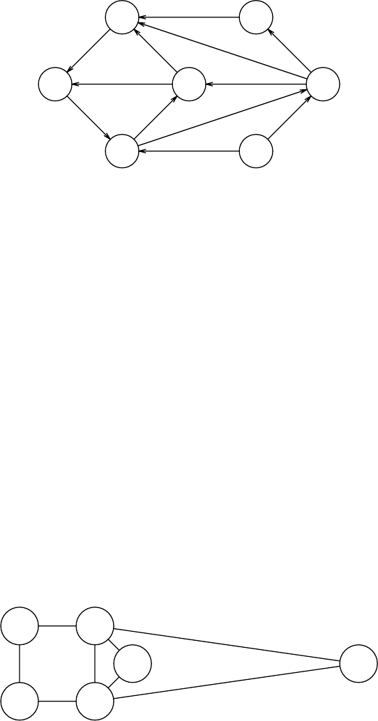
A,7
B,6
C,4
D,2
E,3
F,1
G,5
9.28 This is the algorithm mentioned in the references.
9.29 As an edge (v,w) is implicitly processed, it is placed on a stack. If vis determined to be an
articulation point because Low [w] ≥ Num [v], then the stack is popped until edge (v,w)is
removed: The set of popped edges is a biconnected component. An edge (v,w) is not
placed on the stack if the edge (w,v) was already processed as a back edge.
9.30 Let (u,v) be an edge of the breadth-first spanning tree. (u,v) are connected, thus they must
be in the same tree. Let the root of the tree be r; if the shortest path from rto uis du, then
uis at level du; likewise, vis at level dv.If(u,v) were a back edge, then du > dv, and vis
visited before u. But if there were an edge between uand v, and vis visited first, then
there would be a tree edge (v,u), and not a back edge (u,v). Likewise, if (u,v) were a for-
ward edge, then there is some w, distinct from uand v, on the path from uto v; this con-
tradicts the fact that dv = dw + 1. Thus only tree edges and cross edges are possible.
9.31 Perform a depth-first search. The return from each recursive call implies the edge traversal
in the opposite direction. The time is clearly linear.
9.33 If there is an Euler circuit, then it consists of entering and exiting nodes; the number of
entrances clearly must equal the number of exits. If the graph is not strongly connected,
there cannot be a cycle connecting all the vertices. To prove the converse, an algorithm
similar in spirit to the undirected version can be used.
9.34 Neither of the proposed algorithms works. For example, as shown, a depth-first search of a
biconnected graph that follows A, B, C, D is forced back to A, where it is stranded.
AB
D C
FE
9.35 These are classic graph theory results. Consult any graph theory for a solution to this exer-
cise.
9.36 All the algorithms work without modification for multigraphs.
-52-
9.37 Obviously, Gmust be connected. If each edge of Gcan be converted to a directed edge
and produce a strongly connected graph G' , then Gis convertible.
Then, if the removal of a single edge disconnects G,Gis not convertible since this would
also disconnect G' . This is easy to test by checking to see if there are any single-edge
biconnected components.
Otherwise, perform a depth-first search on Gand direct each tree edge away from the root
and each back edge toward the root. The resulting graph is strongly connected because, for
any vertex v, we can get to a higher level than vby taking some (possibly 0) tree edges and
a back edge. We can apply this until we eventually get to the root, and then follow tree
edges down to any other vertex.
9.38 (b) Define a graph where each stick is represented by a vertex. If stick Siis above Sjand
thus must be removed first, then place an edge from Sito Sj. A legal pick-up ordering is
given by a topological sort; if the graph has a cycle, then the sticks cannot be picked up.
9.39 Given an instance of clique, form the graph G' that is the complement graph of G:(v,w)is
an edge in G' if and only if it is not an edge in G. Then G' has a vertex cover of at most
|V| − K if Ghas a clique of size at least K. (The vertices that form the vertex cover are
exactly those not in the clique.) The details of the proof are left to the reader.
9.40 A proof can be found in Garey and Johnson [20].
9.41 Clearly, the baseball card collector problem (BCCP) is in NP , because it is easy to check if
Kpackets contain all the cards. To show it is NP-complete, we reduce vertex cover to it.
Let G = (V, E ) and Kbe an instance of vertex cover. For each vertex v, place all edges
adjacent to vin packet Pv. The Kpackets will contain all edges (baseball cards) iff Gcan
be covered by Kvertices.
-53-
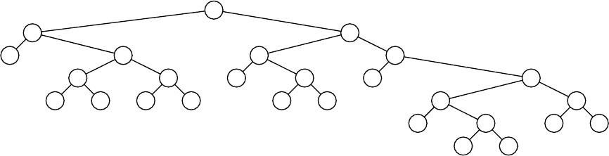
Chapter 10: Algorithm Design Techniques
10.1 First, we show that if Nevenly divides P, then each of j(i−1)P+1through jiP must be
placed as the ith job on some processor. Suppose otherwise. Then in the supposed
optimal ordering, we must be able to find some jobs jxand jysuch that jxis the tth job
on some processor and jyis the t+1th job on some processor but tx > ty. Let jzbe the
job immediately following jx. If we swap jyand jz, it is easy to check that the mean pro-
cessing time is unchanged and thus still optimal. But now jyfollows jx, which is impos-
sible because we know that the jobs on any processor must be in sorted order from the
results of the one processor case.
Let je1,je2, ..., jeM be the extra jobs if Ndoes not evenly divide P. It is easy to see that
the processing time for these jobs depends only on how quickly they can be scheduled,
and that they must be the last scheduled job on some processor. It is easy to see that the
first Mprocessors must have jobs j(i−1)P+1through jiP +M; we leave the details to the
reader.
10.3
,
4 7 8 9
0
1 5
sp
nl
3 :
6 2
10.4 One method is to generate code that can be evaluated by a stack machine. The two opera-
tions are Push (the one node tree corresponding to) a symbol onto a stack and Combine,
which pops two trees off the stack, merges them, and pushes the result back on. For the
example in the text, the stack instructions are Push(s), Push(nl), Combine, Push(t), Com-
bine, Push(a), Combine, Push(e), Combine, Push(i), Push (sp), Combine, Combine.
By encoding a Combine with a 0 and a Push with a 1 followed by the symbol, the total
extra space is 2N − 1 bits if all the symbols are of equal length. Generating the stack
machine code can be done with a simple recursive procedure and is left to the reader.
10.6 Maintain two queues, Q1and Q2.Q1will store single-node trees in sorted order, and Q2
will store multinode trees in sorted order. Place the initial single-node trees on Q1,
enqueueing the smallest weight tree first. Initially, Q2is empty. Examine the first two
entries of each of Q1and Q2, and dequeue the two smallest. (This requires an easily
implemented extension to the ADT.) Merge the tree and place the result at the end of Q2.
Continue this step until Q1is empty and only one tree is left in Q2.
-54-

10.9 To implement first fit, we keep track of bins bi, which have more room than any of the
lower numbered bins. A theoretically easy way to do this is to maintain a splay tree
ordered by empty space. To insert w, we find the smallest of these bins, which has at
least wempty space; after wis added to the bin, if the resulting amount of empty space is
less than the inorder predecessor in the tree, the entry can be removed; otherwise, a
DecreaseKey is performed.
To implement best fit, we need to keep track of the amount of empty space in each bin.
As before, a splay tree can keep track of this. To insert an item of size w, perform an
insert of w. If there is a bin that can fit the item exactly, the insert will detect it and splay
it to the root; the item can be added and the root deleted. Otherwise, the insert has placed
wat the root (which eventually needs to be removed). We find the minimum element M
in the right subtree, which brings Mto the right subtree’s root, attach the left subtree to
M, and delete w. We then perform an easily implemented DecreaseKey on Mto reflect
the fact that the bin is less empty.
10.10 Next fit: 12 bins (.42, .25, .27), (.07, .72), (.86, .09), (.44, .50), (.68), (.73), (.31), (.78,
.17), (.79), (.37), (.73, .23), (.30).
First fit: 10 bins (.42, .25, .27), (.07, .72, .09), (.86), (.44, .50), (.68, .31), (.73, .17), (.78),
(.79), (.37, .23, .30), (.73).
Best fit: 10 bins (.42, .25, .27), (.07, .72, .09), (.86), (.44, .50), (.68, .31), (.73, .23), (.78,
.17), (.79), (.37, .30 ), (.73).
First fit decreasing: 10 bins (.86, .09), (.79, .17), (.78, .07), (.73, .27), (.73, .25), (.72,
.23), (.68, .31), (.50, .44), (.42, .37), (.30).
Best fit decreasing: 10 bins (.86, .09), (.79, .17), (.78), (.73, .27), (.73, .25), (.72, .23),
(.68, .31), (.50, .44), (.42, .37, .07), (.30).
Note that use of 10 bins is optimal.
10.12 We prove the second case, leaving the first and third (which give the same results as
Theorem 10.6) to the reader. Observe that
log pN = log p(bm) = mplog pb
Working this through, Equation (10.9) becomes
T (N) = T (bm) = am
i=0
Σ
m
a
bk
___ i
iplog pb
If a = bk, then
T(N) = amlog pb
i=0
Σ
mip
= O (ammp+1log pb)
Since m = log N /log b , and am = Nk, and bis a constant, we obtain
T(N) = O (Nklog p+1N)
10.13 The easiest way to prove this is by an induction argument.
-55-
10.14 Divide the unit square into N−1 square grids each with side 1/ √N−1. Since there are N
points, some grid must contain two points. Thus the shortest distance is conservatively
given by at most √2/ (N−1).
10.15 The results of the previous exercise imply that the width of the strip is O(1/ √N).
Because the width of the strip is O(1/ √N), and thus covers only O(1/ √N) of the area of
the square, we expect a similar fraction of the points to fall in the strip. Thus only
O(N / √N) points are expected in the strip; this is O(√N).
10.17 The recurrence works out to
T(N) = T (2N / 3) + T (N / 3) + O (N)
This is not linear, because the sum is not less than one. The running time is O(Nlog N ).
10.18 The recurrence for median-of-median-of-seven partitioning is
T(N) = T (5N / 7) + T (N / 7) + O (N)
If all we are concerned about is the linearity, then median-of-median-of-seven can be
used.
10.20 When computing the median-of-median-of-five, 30% of the elements are known to be
smaller than the pivot, and 30% are known to be larger. Thus these elements do not need
to be involved in the partitioning phase. (Extra work would need to be done to imple-
ment this, but since the whole algorithm isn’t practical anyway, we can ignore any extra
work that doesn’t involve element comparisons.) The original paper [9] describes the
exact constants in the worst-case bound, with and without this extra effort.
10.21 We derive the values of sand δ, following the style in the original paper [17]. Let Rt,X
be the rank of element tin some sample X. If a sample S' of elements is chosen ran-
domly from S, and | S' | = s , | S| = N , then we’ve already seen that
E(Rt,S) = s+1
N+1
_____Rt,S'
where Emeans expected value. For instance, if tis the third largest in a sample of 5 ele-
ments, then in a group of 19 elements it is expected to be the tenth largest. We can also
calculate the variance:
V(Rt,S) = √(s+1)2(s+2)
(Rt,S)(s−Rt,S+1)(N+1)(N−s)
_________________________ = O (N / √s)
We choose v1and v2so that
E(Rv1,S) + 2dV (Rv1,S) ∼
∼ k ∼
∼ E (Rv2,S) − 2dV (Rv2,S)
where dindicates how many variances we allow. (The larger dis, the less likely the ele-
ment we are looking for will not be in S' .)
The probability that kis not between v1and v2is
2
d
∫
∞
erf (x) dx = O (e−d2/d )
If d = log1/ 2N, then this probability is ο(1/ N ), specifically O(1/ (Nlog N )). This means
that the expected work in this case is O(log−1N) because O(N) work is performed with
very small probability.
-56-
These mean and variance equations imply
Rv1,S' ≥ k (N+1)
(s+1)
______ − d √s
and
Rv2,S' ≤ k (N+1)
(s+1)
______ + d √s
This gives equation (A):
δ = d √s =√slog 1/ 2N(A)
If we first pivot around v2, the cost is Ncomparisons. If we now partition elements in S
that are less than v2around v1, the cost is Rv2,S, which has expected value k + δs+1
N+1
_____.
Thus the total cost of partitioning is N + k + δs+1
N+1
_____. The cost of the selections to find v1
and v2in the sample S' is O(s). Thus the total expected number of comparisons is
N + k + O (s) + O (Nδ/ s )
The low order term is minimized when
s = N δ/ s (B)
Combining Equations (A) and (B), we see that
s2 = N δ = √s N log 1/ 2N(C)
s3/ 2 = N log 1/ 2N(D)
s = N2/ 3log 1/ 3N(E)
δ = N1/ 3log 2/ 3N(F)
10.22 First, we calculate 12*43. In this case, XL = 1, XR = 2, YL = 4, YR = 3, D1 = −1,
D2 = −1, XLYL = 4, XRYR = 6, D1D2 = 1, D3 = 11, and the result is 516.
Next, we calculate 34*21. In this case, XL = 3, XR = 4, YL = 2, YR = 1, D1 = −1,
D2 = −1, XLYL = 6, XRYR = 4, D1D2 = 1, D3 = 11, and the result is 714.
Third, we calculate 22*22. Here, XL = 2, XR = 2, YL = 2, YR = 2, D1 = 0, D2 = 0,
XLYL = 4, XRYR = 4, D1D2 = 0, D3 = 8, and the result is 484.
Finally, we calculate 1234*4321. XL = 12, XR = 34, YL = 43, YR = 21, D1 = −22,
D2 = −2. By previous calculations, XLYL = 516, XRYR = 714, and D1D2 = 484. Thus
D3 = 1714, and the result is 714 + 171400 + 5160000 = 5332114.
10.23 The multiplication evaluates to (ac − bd ) + (bc + ad )i. Compute ac ,bd , and
(a − b )(d − c ) + ac + bd .
10.24 The algebra is easy to verify. The problem with this method is that if Xand Yare posi-
tive Nbit numbers, their sum might be an N+1 bit number. This causes complications.
10.26 Matrix multiplication is not commutative, so the algorithm couldn’t be used recursively
on matrices if commutativity was used.
-57-
10.27 If the algorithm doesn’t use commutativity (which turns out to be true), then a divide and
conquer algorithm gives a running time of O(Nlog70143640) = O(N2.795).
10.28 1150 scalar multiplications are used if the order of evaluation is
( ( A1A2 ) ( ( ( A3A4 ) A5 ) A6 ) )
10.29 (a) Let the chain be a 1x1 matrix, a 1xA matrix, and an AxB matrix. Multiplication by
using the first two matrices first makes the cost of the chain A + AB . The alternative
method gives a cost of AB + B ,soifA > B , then the algorithm fails. Thus, a counterex-
ample is multiplying a 1x1 matrix by a 1x3 matrix by a 3x2 matrix.
(b, c) A counterexample is multiplying a 1x1 matrix by a 1x2 matrix by a 2x3 matrix.
10.31 The optimal binary search tree is the same one that would be obtained by a greedy stra-
tegy: Iis at the root and has children and and it ;aand or are leaves; the total cost is
2.14.
10.33 This theorem is from F. Yao’s paper, reference [58].
10.34 A recursive procedure is clearly called for; if there is an intermediate vertex, StopOver on
the path from sto t, then we want to print out the path from sto StopOver and then
StopOver to t. We don’t want to print out StopOver twice, however, so the procedure
does not print out the first or last vertex on the path and reserves that for the driver.
_______________________________________________________________________________
_______________________________________________________________________________
/* Print the path between S and T, except do not print */
/* the first or last vertex. Print a trailing " to " only. */
void
PrintPath1( TwoDArray Path, int S, int T )
{int StopOver = Path[ S ][ T ];
if( S != T && StopOver != 0 )
{PrintPath1( Path, S, StopOver );
printf( "%d to ", StopOver );
PrintPath1( Path, StopOver, T );
}
}
/* Assume the existence of a Path of length at least 1 */
void
PrintPath( TwoDArray Path, int S, int T )
{printf( "%d to ", S );
PrintPath1( Path, S, T );
printf( "%d", T ); NewLine( );
}
_______________________________________________________________________________
_______________________________________________________________________________
-58-
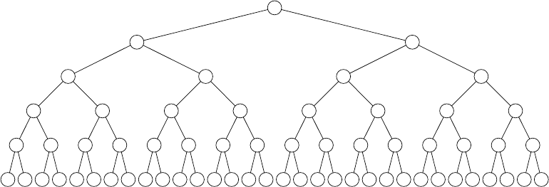
10.35 Many random number generators are poor. The default UNIX random number generator
rand uses a modulus of the form 2b, as does the VAX/VMS random number generator.
UNIX does, however, provide better random number generators in the form of random.
The Turbo random number generators, likewise, are also deficient. The paper by Park
and Miller [44] discusses the random number generators on many machines.
10.38 If the modulus is a power of two, then the least significant bit of the "random" number
oscillates. Thus Flip will always return heads and tails alternately, and the level chosen
for a skip list insertion will always be one or two. Consequently, the performance of the
skip list will be Θ(N) per operation.
10.39 (a) 25 ≡ 32 mod 341, 210 ≡ 1 mod 341. Since 322 ≡ 1 mod 341, this proves that 341 is
not prime. We can also immediately conclude that 2340 ≡ 1 mod 341 by raising the last
equation to the 34th power. The exponentiation would continue as follows:
220 ≡ 1 mod 341, 221 ≡ 2 mod 341, 242 ≡ 4 mod 341, 284 ≡ 16 mod 341, 285 ≡ 32 mod 341,
2170 ≡ 1 mod 341, and 2340 ≡ 1 mod 341.
(b) If A = 2, then although 2560 ≡ 1 mod 561, 2280 ≡ 1 mod 561 proves that 561 is not
prime. If A = 3, then 3561 ≡ 375 mod 561, which proves that 561 is not prime. A = 4
obviously doesn’t fool the algorithm, since 4140 ≡ 1 mod 561. A = 5 fools the algorithm:
51 ≡ 5 mod 561, 52 ≡ 25 mod 561, 54 ≡ 64 mod 561, 58 ≡ 169 mod 561,
516 ≡ 511 mod 561, 517 = 311 mod 561, 534 ≡ 229 mod 561, 535 ≡ 23 mod 561,
570 ≡ 529 mod 561, 5140 ≡ 463 mod 561, 5280 ≡ 67 mod 561, 5560 ≡ 1 mod 561.
10.41 The two point sets are {0, 4, 6, 9, 16, 17} and {0, 5, 7, 13, 16, 17}.
10.42 To find all point sets, we backtrack even if Found == true, and print out information
when line 2 is executed. In the case where there are some duplicate distances, it is possi-
ble that several symmetries will be printed.
10.43
20507950654192598688683959651794
507965928688686594
5065866865
658668
6568
68
Max
Min
Max
Min
Max
10.44 Actually, it implements both; Alpha is lowered for subsequent recursive calls on line 9
when Value is changed at line 12. Beta is used to terminate the while loop when a line
of play leads to a position so good that it is obvious the human player (who has already
seen a more favorable line for himself or herself before making this call) won’t play into
it. To implement the complementary routine, switch the roles of the human and com-
puter. Lines that change are 3 and 4 (obvious changes), 5 (replace Alpha with Beta ), 6
(replace *Value <Beta with *Value >Alpha ), 8 (obvious), 9 (replace
Human . . . *Value ,Beta with Comp . . . Alpha ,*Value ), and 11 (obvious).
-59-
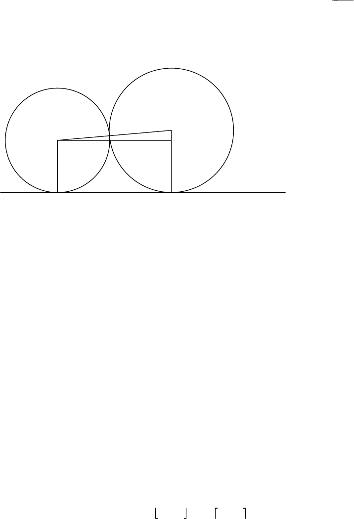
10.46 We place circles in order. Suppose we are trying to place circle j, of radius rj. If some
circle iof radius riis centered at xi, then jis tangent to iif it is placed at xi + 2√rirsj.
To see this, notice that the line connecting the centers has length ri + rj, and the
difference in y-coordinates of the centers is | rj − ri| . The difference in x-coordinates
follows from the Pythagorean theorem.
To place circle j, we compute where it would be placed if it were tangent to each of the
first j−1 circles, selecting the maximum value. If this value is less than rj, then we place
circle jat xj. The running time is O(N2).
10.47 Construct a minimum spanning tree Tof G, pick any vertex in the graph, and then find a
path in Tthat goes through every edge exactly once in each direction. (This is done by a
depth-first search; see Exercise 9.31.) This path has twice the cost of the minimum span-
ning tree, but it is not a simple cycle.
Make it a simple cycle, without increasing the total cost, by bypassing a vertex when it is
seen a second time (except that if the start vertex is seen, close the cycle) and going to the
next unseen vertex on the path, possibly bypassing several vertices in the process. The
cost of this direct route cannot be larger than original because of the triangle inequality.
If there were a tour of cost K, then by removing one edge on the tour, we would have a
minimum spanning tree of cost less than K(assuming that edge weights are positive).
Thus the minimum spanning tree is a lower bound on the optimal traveling salesman tour.
This implies that the algorithm is within a factor of 2 of optimal.
10.48 If there are two players, then the problem is easy, so assume k >1. If the players are num-
bered 1 through N, then divide them into two groups: 1 through N / 2 and N / 2+1
though N. On the ith day, for 1 ≤ i ≤ N / 2, player pin the second group plays players
((p + i ) mod N / 2) + 1 in the first group. Thus after N / 2 days, everyone in group 1 has
played everyone in group 2. In the last N / 2−1 days, recursively conduct round-robin
tournaments for the two groups of players.
10.49 Divide the players into two groups of size N / 2 and N / 2 , respectively, and recur-
sively arrange the players in any order. Then merge the two lists (declare that px > pyif
xhas defeated y, and py > pxif yhas defeated x−exactly one is possible) in linear time
as is done in mergesort.
10.50
10.51 Divide and conquer algorithms (among others) can be used for both problems, but neither
is trivial to implement. See the computational geometry references for more information.
-60-
10.52 (a) Use dynamic programming. Let Sk=the best setting of words wk,wk+1, ... wN,Uk=
the ugliness of this setting, and lk=for this setting, (a pointer to) the word that starts the
second line.
To compute Sk−1, try putting wk−1,wk, ..., wMall on the first line for k < M and
i=k−1
Σ
Mwi< L . Compute the ugliness of each of these possibilities by, for each M, comput-
ing the ugliness of setting the first line and adding Um+1. Let M' be the value of Mthat
yields the minimum ugliness. Then Uk−1 =this value, and lk−1 = M' + 1. Compute
values of Uand lstarting with the last word and working back to the first. The
minimum ugliness of the paragraph is U1; the actual setting can be found by starting at l1
and following the pointers in lsince this will yield the first word on each line.
(b) The running time is quadratic in the case where the number of words that can fit on a
line is consistently Θ(N). The space is linear to keep the arrays Uand l. If the line
length is restricted to some constant, then the running time is linear because only O(1)
words can go on a line.
(c) Put as many words on a line as can fit. This clearly minimizes the number of lines,
and hence the ugliness, as can be shown by a simple calculation.
10.53 An obvious O(N2) solution to construct a graph with vertices 1, 2, ..., Nand place an
edge (v,w)inGiff av < aw. This graph must be acyclic, thus its longest path can be
found in time linear in the number of edges; the whole computation thus takes O(N2)
time.
Let BEST (k) be the increasing subsequence of exactly kelements that has the minimum
last element. Let tbe the length of the maximum increasing subsequence. We show how
to update BEST (k) as we scan the input array. Let LAST (k) be the last element in
BEST (k). It is easy to show that if i<j,LAST (i) < LAST (j). When scanning aM, find
the largest ksuch that LAST (k) < aM. This scan takes O(log t ) time because it can be
performed by a binary search. If k = t , then xMextends the longest subsequence, so
increase t, and set BEST (t) and LAST (t) (the new value of tis the argument). If kis 0
(that is, there is no k), then xMis the smallest element in the list so far, so set BEST (1)
and LAST (1), appropriately. Otherwise, we extend BEST (k) with xM, forming a new and
improved sequence of length k+1. Thus we adjust BEST (k+1) and LAST (k+1).
Processing each element takes logarithmic time, so the total is O(Nlog N ).
10.54 Let LCS (A, M , B , N ) be the longest common subsequence of A1,A2, ..., AMand B1,
B2, ..., BN. If either Mor Nis zero, then the longest common subsequence is the empty
string. If xM = yN, then LCS (A, M , B , N ) = LCS (A, M −1, B , N −1),AM. Otherwise,
LCS (A, M , B , N ) is either LCS (A, M , B , N −1) or LCS (A, M −1, B , N ), whichever is
longer. This yields a standard dynamic programming solution.
10.56 (a) A dynamic programming solution resolves part (a). Let FITS (i, s ) be 1 if a subset of
the first iitems sums to exactly s;FITS (i, 0) is always 1. Then FITS (x, t ) is 1 if either
FITS (x − 1, t − ax)orFITS (x − 1, t ) is 1, and 0 otherwise.
(b) This doesn’t show that P = NP because the size of the problem is a function of N
and log K . Only log K bits are needed to represent K; thus an O(NK ) solution is
exponential in the input size.
-61-
10.57 (a) Let the minimum number of coins required to give xcents in change be COIN (x);
COIN (0) = 0. Then COIN (x) is one more than the minimum value of COIN (x − ci),
giving a dynamic programming solution.
(b) Let WAYS (x, i ) be the number of ways to make xcents in change without using the
first icoin types. If there are Ntypes of coins, then WAYS (x, N ) = 0ifx ≠ 0, and
WAYS (0, i ) = 1. Then WAYS (x, i − 1) is equal to the sum of WAYS (x − pci, i ), for
integer values of pno larger than x /ci(but including 0).
10.58 (a) Place eight queens randomly on the board, making sure that no two are on the same
row or column. This is done by generating a random permutation of 1..8. There are only
5040 such permutations, and 92 of these give a solution.
10.59 (a) Since the knight leaves every square once, it makes B2moves. If the squares are
alternately colored black and white like a checkerboard, then a knight always moves to a
different colored square. If Bis odd, then so is B2, which means that at the end of the
tour the knight will be on a different colored square than at the start of the tour. Thus the
knight cannot be at the original square.
10.60 (a) If the graph has a cycle, then the recursion does not always make progress toward a
base case, and thus an infinite loop will result.
(b) If the graph is acyclic, the recursive call makes progress, and the algorithm ter-
minates. This could be proved formally by induction.
(c) This algorithm is exponential.
-62-
Chapter 11: Amortized Analysis
11.1 When the number of trees after the insertions is more than the number before.
11.2 Although each insertion takes roughly log N , and each DeleteMin takes 2log N actual
time, our accounting system is charging these particular operations as 2 for the insertion
and 3log N −2 for the DeleteMin. The total time is still the same; this is an accounting
gimmick. If the number of insertions and DeleteMins are roughly equivalent, then it
really is just a gimmick and not very meaningful; the bound has more significance if, for
instance, there are Ninsertions and O(N / log N )DeleteMins (in which case, the total
time is linear).
11.3 Insert the sequence N,N + 1, N − 1, N + 2, N − 2, N + 3, ..., 1, 2Ninto an initially
empty skew heap. The right path has Nnodes, so any operation could take Ω(N) time.
11.5 We implement DecreaseKey(X, H) as follows: If lowering the value of Xcreates a heap
order violation, then cut Xfrom its parent, which creates a new skew heap H1with the
new value of Xas a root, and also makes the old skew heap Hsmaller. This operation
might also increase the potential of H, but only by at most log N . We now merge Hand
H1. The total amortized time of the Merge is O(log N ), so the total time of the
DecreaseKey operation is O(log N ).
11.8 For the zig −zig case, the actual cost is 2, and the potential change is
Rf( X ) + Rf( P ) + Rf( G ) − Ri( X ) − Ri( P ) − Ri( G ). This gives an amortized
time bound of
ATzig −zig = 2 + Rf( X ) + Rf( P ) + Rf( G ) − Ri( X ) − Ri( P ) − Ri( G )
Since Rf( X ) = Ri( G ), this reduces to
= 2 + Rf( P ) + Rf( G ) − Ri( X ) − Ri( P )
Also, Rf( X ) > Rf( P ) and Ri( X ) < Ri( P ), so
ATzig −zig < 2 + Rf( X ) + Rf( G ) − 2Ri( X )
Since Si( X ) + Sf( G ) < Sf( X ), it follows that Ri( X ) + Rf( G ) < 2Rf( X ) − 2.
Thus
ATzig −zig < 3Rf( X ) − 3Ri( X )
11.9 (a) Choose W(i) = 1/ N for each item. Then for any access of node X,Rf( X ) = 0, and
Ri( X ) ≥ −log N , so the amortized access for each item is at most 3 log N + 1, and the
net potential drop over the sequence is at most N log N , giving a bound of
O(Mlog N + M + N log N ), as claimed.
(b) Assign a weight of qi/M to items i. Then Rf( X ) = 0, Ri( X ) ≥ log(qi/M ), so the
amortized cost of accessing item iis at most 3 log(M /qi) + 1, and the theorem follows
immediately.
11.10 (a) To merge two splay trees T1and T2, we access each node in the smaller tree and
insert it into the larger tree. Each time a node is accessed, it joins a tree that is at least
-63-
twice as large; thus a node can be inserted log N times. This tells us that in any sequence
of N−1 merges, there are at most Nlog N inserts, giving a time bound of O(Nlog2N).
This presumes that we keep track of the tree sizes. Philosophically, this is ugly since it
defeats the purpose of self-adjustment.
(b) Port and Moffet [6] suggest the following algorithm: If T2is the smaller tree, insert its
root into T1. Then recursively merge the left subtrees of T1and T2, and recursively
merge their right subtrees. This algorithm is not analyzed; a variant in which the median
of T2is splayed to the root first is with a claim of O(Nlog N ) for the sequence of
merges.
11.11 The potential function is ctimes the number of insertions since the last rehashing step,
where cis a constant. For an insertion that doesn’t require rehashing, the actual time is
1, and the potential increases by c, for a cost of 1 + c .
If an insertion causes a table to be rehashed from size Sto 2S, then the actual cost is
1 + dS , where dS represents the cost of initializing the new table and copying the old
table back. A table that is rehashed when it reaches size Swas last rehashed at size S / 2,
so S / 2 insertions had taken place prior to the rehash, and the initial potential was cS / 2.
The new potential is 0, so the potential change is −cS / 2, giving an amortized bound of
(d − c / 2)S + 1. We choose c = 2d, and obtain an O(1) amortized bound in both cases.
11.12 We show that the amortized number of node splits is 1 per insertion. The potential func-
tion is the number of three-child nodes in T. If the actual number of nodes splits for an
insertion is s, then the change in the potential function is at most 1 − s , because each
split converts a three-child node to two two-child nodes, but the parent of the last node
split gains a third child (unless it is the root). Thus an insertion costs 1 node split, amor-
tized. An Nnode tree has Nunits of potential that might be converted to actual time, so
the total cost is O(M + N ). (If we start from an initially empty tree, then the bound is
O(M).)
11.13 (a) This problem is similar to Exercise 3.22. The first four operations are easy to imple-
ment by placing two stacks, SLand SR, next to each other (with bottoms touching). We
can implement the fifth operation by using two more stacks, MLand MR(which hold
minimums).
If both SLand SRnever empty, then the operations can be implemented as follows:
Push(X,D): push Xonto SL;ifXis smaller than or equal to the top of ML, push Xonto
MLas well.
Inject(X,D): same operation as Push , except use SRand MR.
Pop(D): pop SL; if the popped item is equal to the top of ML, then pop MLas well.
Eject(D): same operation as Pop , except use SRand MR.
FindMin(D): return the minimum of the top of MLand MR.
These operations don’t work if either SLor SRis empty. If a Pop or Eject is attempted
on an empty stack, then we clear MLand MR. We then redistribute the elements so that
half are in SLand the rest in SR, and adjust MLand MRto reflect what the state would be.
We can then perform the Pop or Eject in the normal fashion. Fig. 11.1 shows a transfor-
mation.
Define the potential function to be the absolute value of the number of elements in SL
minus the number of elements in SR. Any operation that doesn’t empty SLor SRcan
-64-
3, 1, 4, 6, 5, 9, 2, 6
1, 2, 6
3, 1, 4, 6 5, 9, 2, 6
1, 4, 6 5, 2
SLSR
MLMR
SLSR
MLMR
Fig. 11.1.
increase the potential by only 1; since the actual time for these operations is constant, so
is the amortized time.
To complete the proof, we show that the cost of a reorganization is O(1) amortized time.
Without loss of generality, if SRis empty, then the actual cost of the reorganization is
|SL| units. The potential before the reorganization is | SL| ; afterward, it is at most 1.
Thus the potential change is 1−|SL| , and the amortized bound follows.
-65-
Chapter 12: Advanced Data Structures
and Implementation
12.3 Incorporate an additional field for each node that indicates the size of its subtree. These
fields are easy to update during a splay. This is difficult to do in a skip list.
12.6 If there are Bblack nodes on the path from the root to all leaves, it is easy to show by
induction that there are at most 2Bleaves. Consequently, the number of black nodes on a
path is at most log N . Since there can’t be two consecutive red nodes, the height is
bounded by 2log N .
12.7 Color nonroot nodes red if their height is even and their parents height is odd, and black
otherwise. Not all red black trees are AVL trees (since the deepest red black tree is
deeper than the deepest AVL tree).
12.19 See H. N. Gabow, J. L. Bentley, and R. E. Tarjan, "Scaling and Related Techniques for
Computational Geometry," Proceedings of the Sixteenth Annual ACM Symposium on
Theory of Computing (1984), 135-143, or C. Levcopoulos and O. Petersson, "Heapsort
Adapted for Presorted Files," Journal of Algorithms 14 (1993), 395-413.
12.29 Pointers are unnecessary; we can store everything in an array. This is discussed in refer-
ence [12]. The bounds become O(klog N ) for insertion, O(k2log N ) for deletion of a
minimum, O(k2N) for creation (an improvement over the bound in [12]).
12.35 Consider the pairing heap with 1 as the root and children 2, 3, ... N.ADeleteMin
removes 1, and the resulting pairing heap is 2 as the root with children 3, 4, ... N; the cost
of this operation is Nunits. A subsequent DeleteMin sequence of 2, 3, 4, ... will take
total time Ω(N2).
-66-
