GPP User Manual Delft3D GPP_User_Manual
User Manual: Pdf Delft3D-GPP_User_Manual
Open the PDF directly: View PDF ![]() .
.
Page Count: 202 [warning: Documents this large are best viewed by clicking the View PDF Link!]
- List of Figures
- List of Tables
- 1 Guide to this manual
- 2 Getting started
- 3 Graphical User Interface
- 4 Data sets and presentations
- 5 Files and filetypes
- 6 Layouts and plots
- 7 Customising GPP
- 8 Advanced features
- 9 Installation
- 10 Glossary
- A Command-line arguments
- B ODS error codes
- C Description of files used by GPP
- C.1 Description of the file <devices gpp>
- C.2 Description of the file <filetype.gpp>
- C.3 Description of the file <layouts.gpp>
- C.4 Description of the file <routines.gpp>
- C.5 Description of the file <setting.gpp>
- C.6 Description of the file <gppstate.0>
- C.7 Description of the GPP description file
- C.8 Description of the X resources used in GPP
- C.9 Description of the script library
- D Creating animations
- E Example of using AWK to edit the state/session file
- F Printers, plotters and pictures
- G Frequently asked questions
- H Trouble shooting
- I Overview of data sets
- J Models and filetypes
- K Plot routines
- K.1 Plot routines
- K.1.1 Plot Timeseries
- K.1.2 Plot Limiting Factors
- K.1.3 Plot Error Margins
- K.1.4 Plot curvilinear grid
- K.1.5 Plot finite elements grid
- K.1.6 Plot contour map
- K.1.7 Plot isolines
- K.1.8 Plot thin dams
- K.1.9 Plot XY graph
- K.1.10 Plot vertical profile
- K.1.11 Polar contourplot
- K.1.12 Polar isoline plot
- K.1.13 Plot isolines (FEM)
- K.1.14 Plot finite element grid
- K.1.15 Plot vector field
- K.1.16 Plot balances
- K.1.17 Plot histogram
- K.1.18 Plot pie chart
- K.1.19 Plot land boundaries
- K.1.20 Plot drogue tracks
- K.1.21 Plot time bar
- K.1.22 Samples plot
- K.1.23 Add text to drawing
- K.1.24 Add a simple annotation
- K.1.25 Plot text at position
- K.1.26 Plot via a simple script
- K.2 Selection routines
- K.3 Operation routines
- K.4 Binary operations
- K.5 Export routines
- K.5.1 Write Timeseries to Annotated File
- K.5.2 Write Timeseries to TSV File
- K.5.3 Write Timeseries to Text File
- K.5.4 Write MAP2D to Text File
- K.5.5 Write XY data to Text File
- K.5.6 Write data sets (finite element grid) to Text File
- K.5.7 Write grid to ArcView/Info import file
- K.5.8 Write results to ArcView/Info import file
- K.5.9 Write via a simple script
- K.1 Plot routines
Delft3D
3D/2D modelling suite for integral water solutions
User Manual
GPP
DRAFT
DRAFT
DRAFT
GPP
Visualisation of Delft3D simulation results and mea-
surement data
User Manual
Hydro-Morphodynamics & Water Quality
Version: 4.00
SVN Revision: 52614
April 18, 2018
DRAFT
GPP, User Manual
Published and printed by:
Deltares
Boussinesqweg 1
2629 HV Delft
P.O. 177
2600 MH Delft
The Netherlands
telephone: +31 88 335 82 73
fax: +31 88 335 85 82
e-mail: info@deltares.nl
www: https://www.deltares.nl
For sales contact:
telephone: +31 88 335 81 88
fax: +31 88 335 81 11
e-mail: software@deltares.nl
www: https://www.deltares.nl/software
For support contact:
telephone: +31 88 335 81 00
fax: +31 88 335 81 11
e-mail: software.support@deltares.nl
www: https://www.deltares.nl/software
Copyright © 2018 Deltares
All rights reserved. No part of this document may be reproduced in any form by print, photo
print, photo copy, microfilm or any other means, without written permission from the publisher:
Deltares.
DRAFT
Contents
Contents
List of Figures vii
List of Tables ix
1 Guide to this manual 1
1.1 Introduction .................................. 1
1.2 Changes with respect to previous versions .................. 2
1.3 What’s new? ................................. 3
2 Getting started 5
3 Graphical User Interface 17
3.1 Starting the program ............................. 17
3.2 Main window ................................. 17
3.2.1 Menubar ............................... 20
3.2.2 Data group Description . . . . . . . . . . . . . . . . . . . . . . . . 22
3.2.3 Data group Datasets ......................... 22
3.2.4 Data group Plots ........................... 25
3.3 Graphical windows .............................. 26
3.3.1 Usage of the menubar . . . . . . . . . . . . . . . . . . . . . . . . 27
3.3.2 Composing a plot ........................... 27
3.3.3 Buttons in the graphical window . . . . . . . . . . . . . . . . . . . . 29
3.3.4 Using double-clicks . . . . . . . . . . . . . . . . . . . . . . . . . . 29
3.4 Error handling ................................. 35
4 Data sets and presentations 37
4.1 Data sets in general .............................. 37
4.2 Presentations and selections ......................... 39
4.3 Importing the data set ............................. 40
4.4 Available presentations . . . . . . . . . . . . . . . . . . . . . . . . . . . . 40
4.4.1 Types of presentations . . . . . . . . . . . . . . . . . . . . . . . . 41
5 Files and filetypes 43
5.1 Data files in the user-interface ......................... 43
5.2 Representing date and time . . . . . . . . . . . . . . . . . . . . . . . . . . 43
5.3 Formatted data files .............................. 43
5.3.1 TEKAL files (general) ......................... 44
5.3.2 Samples files ............................. 46
5.3.3 TEKAL time-series files . . . . . . . . . . . . . . . . . . . . . . . . 47
5.4 Other properties of the filetypes . . . . . . . . . . . . . . . . . . . . . . . . 48
6 Layouts and plots 49
6.1 Layouts .................................... 49
6.2 How presentation routines co-operate . . . . . . . . . . . . . . . . . . . . . 49
7 Customising GPP 53
7.1 Printing and plotting .............................. 53
7.1.1 Defining printers and plotters . . . . . . . . . . . . . . . . . . . . . 53
7.1.2 Configuring printers for GPP . . . . . . . . . . . . . . . . . . . . . 54
7.1.3 Procedure for configuring a new printer or plotter . . . . . . . . . . . 55
7.2 Anatomy of a layout .............................. 56
7.3 Default options for plot routines . . . . . . . . . . . . . . . . . . . . . . . . 57
7.4 Graphical settings ............................... 58
7.5 Working environment ............................. 60
Deltares iii

DRAFT
GPP, User Manual
7.5.1 Directories and files for GPP . . . . . . . . . . . . . . . . . . . . . 60
7.5.2 File types and file names ....................... 61
7.5.3 Description files ........................... 61
8 Advanced features 63
8.1 Standardising pictures . . . . . . . . . . . . . . . . . . . . . . . . . . . . 63
8.1.1 Batch processing ........................... 63
8.1.2 Editing the session file . . . . . . . . . . . . . . . . . . . . . . . . 63
8.1.3 Using dedicated layouts . . . . . . . . . . . . . . . . . . . . . . . 66
8.2 Creating animations .............................. 67
8.3 Facilities for making animations . . . . . . . . . . . . . . . . . . . . . . . . 68
8.4 Automatically exporting data sets . . . . . . . . . . . . . . . . . . . . . . . 69
8.5 Automating tasks ............................... 70
8.6 Defining your own plot and export routines . . . . . . . . . . . . . . . . . . 70
8.6.1 Script commands ........................... 73
9 Installation 75
9.1 Installing on the PC .............................. 75
9.2 Installing under Linux ............................. 75
10 Glossary 77
A Command-line arguments 81
B ODS error codes 83
C Description of files used by GPP 85
C.1 Description of the file <devices gpp>..................... 85
C.2 Description of the file <filetype.gpp>..................... 87
C.3 Description of the file <layouts.gpp>..................... 88
C.4 Description of the file <routines.gpp>. . . . . . . . . . . . . . . . . . . . 91
C.5 Description of the file <setting.gpp>..................... 92
C.6 Description of the file <gppstate.0>. . . . . . . . . . . . . . . . . . . . . 100
C.7 Description of the GPP description file . . . . . . . . . . . . . . . . . . . . 107
C.8 Description of the X resources used in GPP . . . . . . . . . . . . . . . . . . 108
C.9 Description of the script library . . . . . . . . . . . . . . . . . . . . . . . . 109
D Creating animations 111
E Example of using AWK to edit the state/session file 113
F Printers, plotters and pictures 115
F.1 Storing pictures ................................115
F.2 Support of printers and plotters . . . . . . . . . . . . . . . . . . . . . . . . 115
F.2.1 Printing on MS Windows systems . . . . . . . . . . . . . . . . . . . 115
F.2.2 Printing on Linux systems . . . . . . . . . . . . . . . . . . . . . . . 116
F.2.3 Supported printers and plotters . . . . . . . . . . . . . . . . . . . . 116
G Frequently asked questions 119
G.1 Installation ..................................120
G.2 Printing ....................................121
G.3 Plotting ....................................123
G.4 Customising . . . . . . . . . . . . . . . . . . . . . . . . . . . . . . . . . 125
G.5 Animations ..................................127
G.6 Files and data . . . . . . . . . . . . . . . . . . . . . . . . . . . . . . . . . 128
iv Deltares

DRAFT
Contents
H Trouble shooting 131
H.1 Checklist . . . . . . . . . . . . . . . . . . . . . . . . . . . . . . . . . . . 131
H.2 Errors that may occur . . . . . . . . . . . . . . . . . . . . . . . . . . . . . 132
H.3 Problems involving files and directories . . . . . . . . . . . . . . . . . . . . 141
H.3.1 NEFIS files ..............................141
H.3.2 Map files from D-Water Quality (DELWAQ) . . . . . . . . . . . . . . 142
H.3.3 Binary and unformatted files . . . . . . . . . . . . . . . . . . . . . 142
H.3.4 Navigating over directories . . . . . . . . . . . . . . . . . . . . . . 142
I Overview of data sets 145
J Models and filetypes 151
K Plot routines 163
K.1 Plot routines . . . . . . . . . . . . . . . . . . . . . . . . . . . . . . . . . 163
K.1.1 Plot Timeseries . . . . . . . . . . . . . . . . . . . . . . . . . . . . 163
K.1.2 Plot Limiting Factors . . . . . . . . . . . . . . . . . . . . . . . . . 164
K.1.3 Plot Error Margins . . . . . . . . . . . . . . . . . . . . . . . . . . 164
K.1.4 Plot curvilinear grid . . . . . . . . . . . . . . . . . . . . . . . . . . 165
K.1.5 Plot finite elements grid . . . . . . . . . . . . . . . . . . . . . . . . 165
K.1.6 Plot contour map . . . . . . . . . . . . . . . . . . . . . . . . . . . 166
K.1.7 Plot isolines . . . . . . . . . . . . . . . . . . . . . . . . . . . . . 166
K.1.8 Plot thin dams . . . . . . . . . . . . . . . . . . . . . . . . . . . . 167
K.1.9 Plot XY graph . . . . . . . . . . . . . . . . . . . . . . . . . . . . . 168
K.1.10 Plot vertical profile . . . . . . . . . . . . . . . . . . . . . . . . . . 168
K.1.11 Polar contourplot . . . . . . . . . . . . . . . . . . . . . . . . . . . 169
K.1.12 Polar isoline plot . . . . . . . . . . . . . . . . . . . . . . . . . . . 169
K.1.13 Plot isolines (FEM) . . . . . . . . . . . . . . . . . . . . . . . . . . 169
K.1.14 Plot finite element grid . . . . . . . . . . . . . . . . . . . . . . . . 170
K.1.15 Plot vector field . . . . . . . . . . . . . . . . . . . . . . . . . . . . 170
K.1.16 Plot balances . . . . . . . . . . . . . . . . . . . . . . . . . . . . . 171
K.1.17 Plot histogram . . . . . . . . . . . . . . . . . . . . . . . . . . . . 172
K.1.18 Plot pie chart . . . . . . . . . . . . . . . . . . . . . . . . . . . . . 173
K.1.19 Plot land boundaries . . . . . . . . . . . . . . . . . . . . . . . . . 173
K.1.20 Plot drogue tracks . . . . . . . . . . . . . . . . . . . . . . . . . . 174
K.1.21 Plot time bar . . . . . . . . . . . . . . . . . . . . . . . . . . . . . 174
K.1.22 Samples plot . . . . . . . . . . . . . . . . . . . . . . . . . . . . . 174
K.1.23 Add text to drawing . . . . . . . . . . . . . . . . . . . . . . . . . . 175
K.1.24 Add a simple annotation . . . . . . . . . . . . . . . . . . . . . . . 176
K.1.25 Plot text at position . . . . . . . . . . . . . . . . . . . . . . . . . . 176
K.1.26 Plot via a simple script . . . . . . . . . . . . . . . . . . . . . . . . 176
K.2 Selection routines . . . . . . . . . . . . . . . . . . . . . . . . . . . . . . . 177
K.2.1 Select a parameter . . . . . . . . . . . . . . . . . . . . . . . . . . 177
K.2.2 Select a time . . . . . . . . . . . . . . . . . . . . . . . . . . . . . 177
K.2.3 Select a location . . . . . . . . . . . . . . . . . . . . . . . . . . . 178
K.2.4 Select a layer . . . . . . . . . . . . . . . . . . . . . . . . . . . . . 178
K.2.5 Select a grid line (M) . . . . . . . . . . . . . . . . . . . . . . . . . 178
K.2.6 Select a grid line (N) . . . . . . . . . . . . . . . . . . . . . . . . . 179
K.2.7 Select a vertical profile . . . . . . . . . . . . . . . . . . . . . . . . 179
K.2.8 Select an arbitrary transect . . . . . . . . . . . . . . . . . . . . . . 180
K.3 Operation routines ..............................180
K.3.1 Average over a fixed layer . . . . . . . . . . . . . . . . . . . . . . 180
K.3.2 Average squared vector (fixed layer) . . . . . . . . . . . . . . . . . 181
K.3.3 Root-mean-square vector (fixed layer) . . . . . . . . . . . . . . . . 181
Deltares v

DRAFT
GPP, User Manual
K.3.4 Calculate length . . . . . . . . . . . . . . . . . . . . . . . . . . . 182
K.4 Binary operations . . . . . . . . . . . . . . . . . . . . . . . . . . . . . . . 182
K.4.1 A−B................................182
K.4.2 A+B................................183
K.4.3 A∗B................................183
K.4.4 A/B .................................183
K.4.5 min(A, B)..............................183
K.4.6 max(A, B). . . . . . . . . . . . . . . . . . . . . . . . . . . . . 184
K.4.7 f(A, B). . . . . . . . . . . . . . . . . . . . . . . . . . . . . . . 184
K.4.8 f(A).................................185
K.5 Export routines ................................185
K.5.1 Write Timeseries to Annotated File . . . . . . . . . . . . . . . . . . 185
K.5.2 Write Timeseries to TSV File . . . . . . . . . . . . . . . . . . . . . 185
K.5.3 Write Timeseries to Text File . . . . . . . . . . . . . . . . . . . . . 186
K.5.4 Write MAP2D to Text File . . . . . . . . . . . . . . . . . . . . . . . 186
K.5.5 Write XY data to Text File . . . . . . . . . . . . . . . . . . . . . . . 186
K.5.6 Write data sets (finite element grid) to Text File . . . . . . . . . . . . 187
K.5.7 Write grid to ArcView/Info import file . . . . . . . . . . . . . . . . . 187
K.5.8 Write results to ArcView/Info import file . . . . . . . . . . . . . . . . 187
K.5.9 Write via a simple script . . . . . . . . . . . . . . . . . . . . . . . 187
vi Deltares

DRAFT
List of Figures
List of Figures
2.1 GPP main window .............................. 6
2.2 Data Group Datasets ............................. 6
2.3 Add dataset window ............................. 7
2.4 File Selection window ............................ 8
2.5 List of parameters and locations, after selecting a file and a parameter from
that file .................................... 9
2.6 Graphical window with a time series plot . . . . . . . . . . . . . . . . . . . 10
2.7 Data Group Plots ............................... 11
2.8 Create Plot window . . . . . . . . . . . . . . . . . . . . . . . . . . . . . . 12
2.9 Assigning data sets to the plot areas . . . . . . . . . . . . . . . . . . . . . 13
2.10 Graphical window with empty plot . . . . . . . . . . . . . . . . . . . . . . . 14
2.11 Area Attributes dialogue window . . . . . . . . . . . . . . . . . . . . . . . 14
3.1 Main window of GPP ............................. 18
3.2 Data Group Datasets window ......................... 19
3.3 Data Group Plots window ........................... 19
3.4 Main window menu options . . . . . . . . . . . . . . . . . . . . . . . . . . 20
3.5 Sub-menu option Edit links to data files . . . . . . . . . . . . . . . . . . . . 21
3.6 Sub-menu option Replace text in frames . . . . . . . . . . . . . . . . . . . 21
3.7 Sub-menu option Replace text near axes . . . . . . . . . . . . . . . . . . . 21
3.8 Make Job dialogue . . . . . . . . . . . . . . . . . . . . . . . . . . . . . . 22
3.9 Data Group Description ............................ 23
3.10 Data Group Datasets ............................. 23
3.11 Combine datasets dialogue ......................... 24
3.12 Export datasets dialogue . . . . . . . . . . . . . . . . . . . . . . . . . . 24
3.13 Data Group Plots ............................... 25
3.14 Layout of the graphical Plot window ..................... 26
3.15 Assign data dialogue ............................. 28
3.16 Data sets currently assigned to a plot area . . . . . . . . . . . . . . . . . . 28
3.17 Quickscan facility allows for temporary selection of other locations or times . . 30
3.18 Point selection ................................ 30
3.19 Axes Attributes dialogue ........................... 31
3.20 Axis Labels dialogue ............................. 31
3.21 Axis options dialogue . . . . . . . . . . . . . . . . . . . . . . . . . . . . 31
3.22 Frame Texts dialogue . . . . . . . . . . . . . . . . . . . . . . . . . . . . 32
3.23 Text Attributes dialogue ........................... 32
3.24 Frame attributes dialogue . . . . . . . . . . . . . . . . . . . . . . . . . . 32
3.25 Change Plot area attributes window . . . . . . . . . . . . . . . . . . . . . 33
3.26 Change Plot Options window . . . . . . . . . . . . . . . . . . . . . . . . 34
3.27 Interpolate contour classes dialogue . . . . . . . . . . . . . . . . . . . . 34
3.28 Change Area Text window . . . . . . . . . . . . . . . . . . . . . . . . . . 35
4.1 Example of particular data set. Missing values are represented by discontinu-
ities in the line ................................ 38
4.2 Plot of water level (filled contours) and flow velocity (vectors) . . . . . . . . . 39
5.1 Specifying time column of a TEKAL file . . . . . . . . . . . . . . . . . . . . 48
6.1 Empty layout ................................. 50
6.2 Filled-in layout: the plot . . . . . . . . . . . . . . . . . . . . . . . . . . . . 51
7.1 Print setup dialogue .............................. 53
Deltares vii

DRAFT
GPP, User Manual
viii Deltares

DRAFT
List of Tables
List of Tables
4.1 Measured data of BOD5 (mg/l) in two locations. (Note: these data are fictional) 37
4.2 Presentation forms for various types of data sets . . . . . . . . . . . . . . . 41
A.2 Environment variables used by GPP . . . . . . . . . . . . . . . . . . . . . 82
C.1 Symbols in Toolmaster/agX . . . . . . . . . . . . . . . . . . . . . . . . . . 98
C.2 Line types in Toolmaster/agX ......................... 98
Deltares ix

DRAFT
GPP, User Manual
x Deltares

DRAFT
1 Guide to this manual
1.1 Introduction
The name GPP has been derived from "general postprocessing program". It is meant for
applications developed by Deltares. It can read most of the result files produced by the Delft3D
modules and handles various other types as well.
Key terms for GPP are:
data sets collections of data to be visualised, recognised by a unique name
presentations ways of presenting the data, such as contour maps or xy-graphs
models the source of the data files, this identifies what types of files can be
used
file types the structure of a data file is important when selecting the data set
and reading the actual data. The interface to the file is, however,
uniform.
layouts before presenting the data, you specify the general set-up of the pic-
ture by selecting the appropriate layout: size of the graph or graphs
(called plot areas), their position, additional text etc.
plots a plot contains one or more plot areas; data sets are presented
within a plot area according to some plotting method. One or more
data sets may be added. Together with the axes and additional text,
they make up the plot.
This manual describes the use of GPP. It is divided into two parts, the first will give you a
short introduction and moves on to a detailed description of the user-interface:
chapter 2:Getting started, describes how to get started with the program.
chapter 3:Graphical User Interface, explains most of the menus and dialogues contained
in GPP.
The second part explains the concepts and documents what external files are used, how you
can customise the program and so on. It is intended for the experienced users:
chapter 4:Data sets and presentations, describes the concepts of data sets and presenta-
tions in more detail.
chapter 5:Files and filetypes, presents some details on the currently supported file types.
chapter 6:Layouts and plots, describes the function of layouts and plots.
chapter 7:Customising GPP, discusses customising the program.
chapter 8:Advanced features, presents advanced options within GPP, such as animations.
chapter 9:Installation, describes how to install GPP.
chapter 10:Glossary, is a glossary of the most important terms in GPP.
More details can be found in the appendices:
Appendix A:Command-line arguments, lists the command-line options and the environ-
Deltares 1 of 190

DRAFT
GPP, User Manual
ment variables that may be used.
Appendix B:ODS error codes, lists the possible errors that can be unconnected and their
codes.
Appendix C:Description of files used by GPP, presents the contents of the configuration
files in detail.
Appendix D:Creating animations, describes how to use the auxiliary script gpp_anim for
creating and displaying animations.
Appendix E:Example of using AWK to edit the state/session file, gives an example of
batch editing facilities that can be added to GPP.
Appendix F:Printers, plotters and pictures, contains information about supported printers,
plotters and storing pictures under Linux and MS Windows.
Appendix G:Frequently asked questions, has the frequently asked questions and their
answers.
Appendix H:Trouble shooting, describes the known problems and their work arounds.
Should you experience problems.
Appendix I:Overview of data sets, provides an overview of the data set types supported
by GPP.
Appendix J:Models and filetypes, gives an overview of the file types that are supported by
GPP.
Appendix K:Plot routines, contains an overview of the plot routines and other routines.
1.2 Changes with respect to previous versions
2 of 190 Deltares
DRAFT
Guide to this manual
Version Description
2.14 section 8.4, in description Separator should be ‘Separator’.
section K.4, new operations f(A, B)and f(A)described.
In the Tutorial folder files <trih-k05.∗>replaced by <trih-f44-tutorial.∗>.
Headers in Appendices D,Iand Kcorrected.
2.12 section 8.3, Facilities for making animations, inserted.
section 8.4, Automatically exporting data sets, inserted.
Old Section 8.3 is now section 8.5, old Section 8.4 is now section 8.6.
Section 1.3 What’s new added.
2.11 Updated terminology in some places
Added the new features concerning the scripting interface (Sections 8.3 and
8.4)
Appendix I added: an overview of data set types
Appendix K: updated the list of available plot routines and other action routines
Name changed to “GPP”
2.10 Enhancements to the user-interface:
The Edit menu in the main window, which allows the user to replace data files
and text strings
The Quick Scan button in the plot window
The Showbutton in the Assign data window
The Interpolate button in the Plot options window
The changes to the printing facility under Windows documented
Several details updated and corrected
1.3 What’s new?
This chapter intends to give a concise overview of new features and changes in GPP and the
manual.
Enhancements dd. november 2005 (version 2.11.07):
Replacement of the old reading routines for certain NEFIS files. The new ones have a
different approach, making it much easier to extend the supported parameters.
Replacement of the underlying plot library. As a consequence you can send pictures
directly to PostScript files for further use.
Introduced a scripting language, Tcl, enabling you to create your own plot routines and
export routines. Also useful to automate certain tasks.
Documentation of the export functionality via the session file.
Facilities for making animations.
Deltares 3 of 190

DRAFT
GPP, User Manual
4 of 190 Deltares
DRAFT
2 Getting started
If you are anxious to start working with GPP and loath reading fat manuals, like most of us,
then read at least this chapter: we describe a simple recipe for getting pictures from your data
files. As GPP is fully window-oriented with a graphical user-interface, it should not be difficult
to get around in the program. But, nevertheless, it is good to have some guideline.
We will concentrate on a few files from the tutorial directory, but please note that GPP can use
all kinds of data files. As long as you have files in one of the supported formats, you have no
need to convert your files (the supported formats are described in a separate appendix).
GPP is normally installed as part of the Delft3D system (cf. WL |Delft Hydraulics, 1999), but
it can be used independently as well.
To start GPP on:
Linux type gpp or delft3d-menu on the command line. If you use the Delft3D
menu program (via delft3d-menu) then select the Utilities →GPP option.
PC start the program Delft3D from its icon and select the Utilities →GPP option.
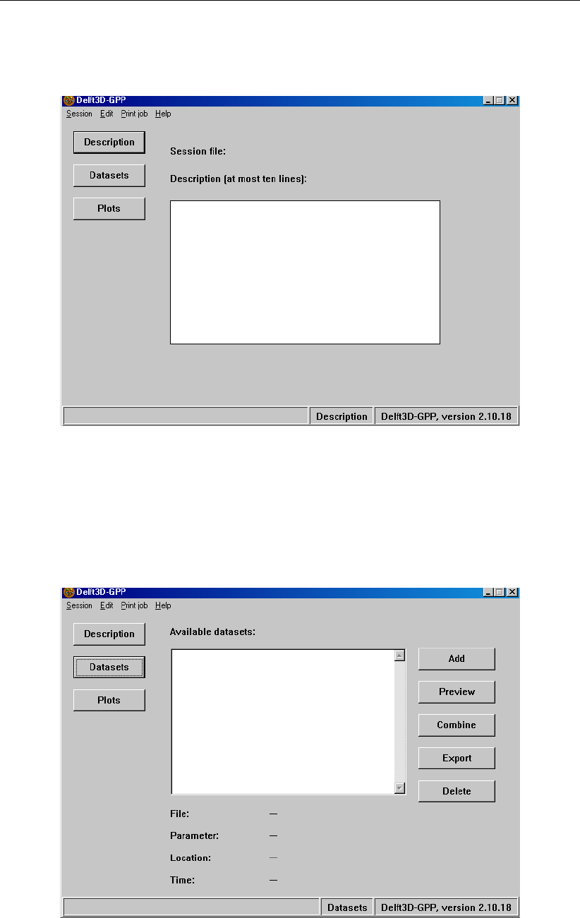
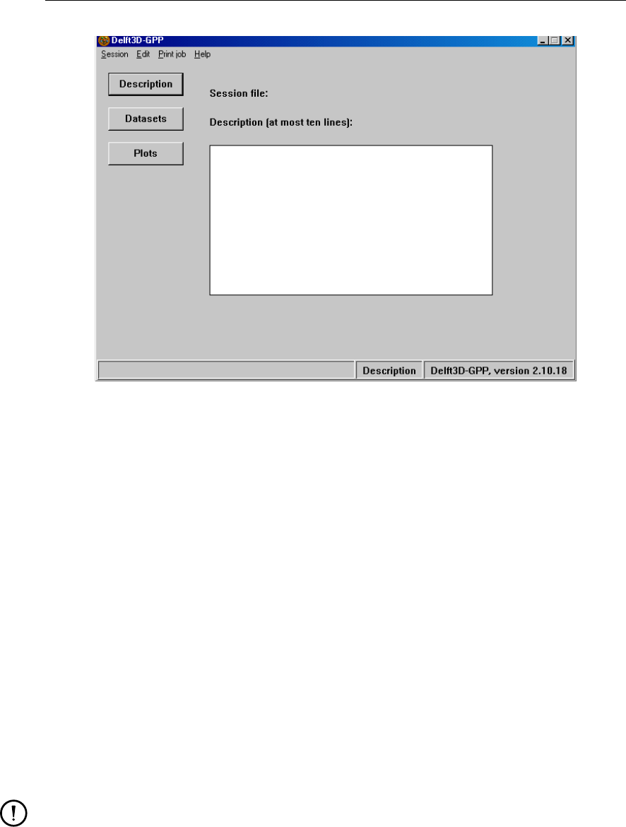
You will get the main window, which initially shows the description (Figure 2.1). It has a simple
menubar with the menus Session, Edit, Print job and Help, three push buttons (Description,
Datasets and Plots) and a status bar, showing the current version of GPP.
Description allows you to type or edit several lines of text that are meant to describe the set
of data sets and plots you will create. The combination of data sets and plots is called a
sessionand it can be saved in a so-called session file. You can save such files, open existing
ones and create new session files via the Sessionmenu.1
The other buttons in the main window bring up the subwindows for defining and manipulating
data sets and plots.
The basic steps toward pictures are:
prepare a sub-set of all data sets you might have and from which you are going to make
graphs
select or define the layout of the pictures you want to make
combine layout and data.
First we need to select the data we want to present.
Click Datasets (see Figure 2.2).
The list box will show the already defined data sets and will be empty if you start a new. The
buttons to handle data sets are shown on the right hand side.
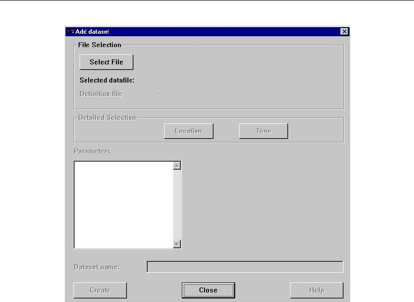
Click Add.
A dialogue appears, which shows from top to bottom (Figure 2.3):
a button Select File
two additional buttons which are greyed out
an empty list box
1The menu has not been called File, because this might give confusion with the data files you will use.
Deltares 5 of 190
DRAFT
GPP, User Manual
Figure 2.1: GPP main window
Figure 2.2: Data Group Datasets
6 of 190 Deltares
DRAFT
Getting started
Figure 2.3: Add dataset window
a text entry field (greyed)
three buttons, Create (greyed), Close and Help
We need to get the data from some file. So:
Click Select File.
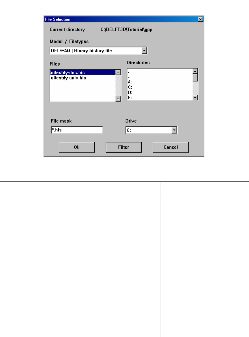
Again a dialogue appears (Figure 2.4). This time a list button, to select the type of data file,
two list boxes (left for files of the selected type, right for the sub-directories under the current),
an input field for setting the mask for matching filenames and three buttons (OK,Filter and
Cancel):
The list boxes are filled with the subdirectories and files in the current directory that match
the first file type.
You will need to select the correct type of file, say a history file from D-Water Quality. This
will bring up the appropriate filter, in this case "∗.his" and a list of files that match this filter.
Select a different directory if necessary by double-clicking on the directories (".." is the
parent directory).
Select the file you want: click once and press OK (or double-click).
In this tutorial we will use the file <uitestdy-dos.his>, a DELWAQ (binary) history to illustrate
the use of GPP. We have supplied several other files in the tutorial directory:
Deltares 7 of 190
DRAFT
GPP, User Manual
Figure 2.4: File Selection window
File Type Remarks
<table31.tek>TEKAL time-series file Used to generate the picture in
chapter 4 of the manual
<trim-edw.dat> <trim-
edw.def>
Delft3D-FLOW map file The calculation has to do with
current-wave interaction.
<trih-f44-tutorial.dat>
<trih-f44-tutorial.def>
Delft3D-FLOW history file The area of interest is a small
inlet in the Dutch Wadden sea.
<del011.hda>
<del011.hdf>
D-Water Quality history file No particular area, just some
eutrophication calculation.
<manukau.ldb>TEKAL landboundary file
(GIS)
Land contours of Manukau
harbour in New Zealand
<texts.ann>TEKAL annotation file File, showing how to include
geographic text
<samples.obs>Samples observations file Example of defining measure-
ment data
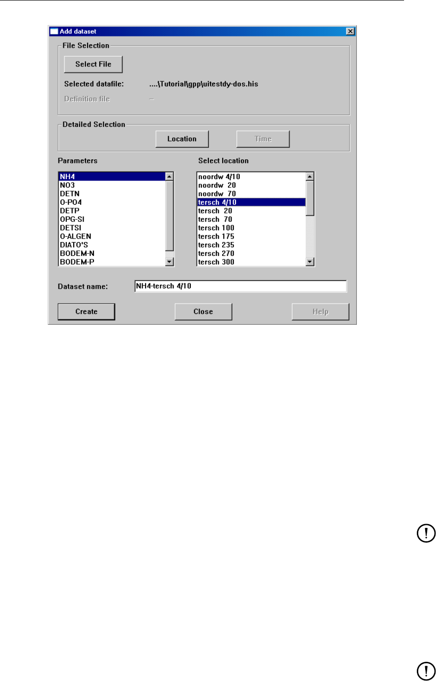
The file selection dialogue disappears and the list of parameters is shown (see Figure 2.5).
Then you can select a data set from this file. To do that:
Select the parameter NH4 (ammonia).
As a consequence the right-hand list box is filled with either locations or times (depending
on the type of data file)
Select one of the possible locations or times, in this case: tersch 4/10.
Click Create (otherwise it will not create the data set).
Click Close to close the dialogue (or go to the first step to define other data sets).
These actions have created the data set containing one parameter, NH4, one location, ter-
8 of 190 Deltares
DRAFT
Getting started
Figure 2.5: List of parameters and locations, after selecting a file and a parameter from
that file
sch 4/10 and a series of times. The data set is therefore a time-series and we can make a
graph of the parameter versus time at that location.
The next step is to plot the data set. To do this,
Select the data set and click Preview. This action has the following result.
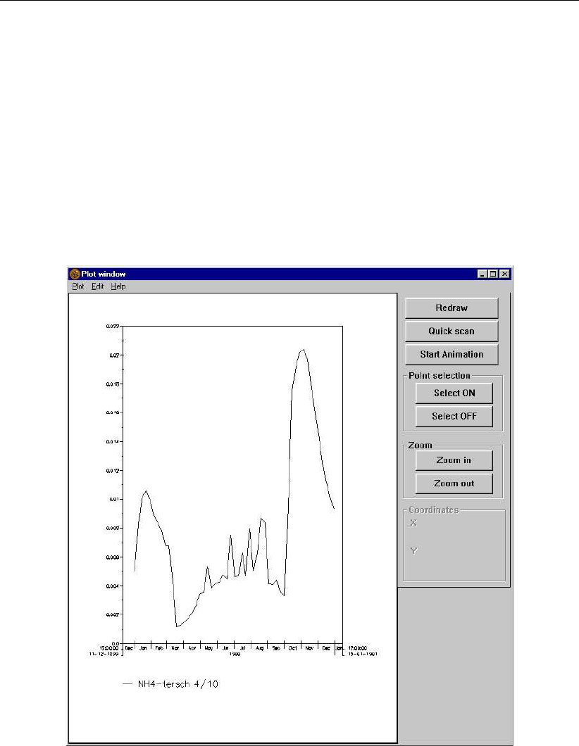
A graphical window comes up (Figure 2.6). This displays the chosen data set, using:
the first layout
the first suitable presentation form for this type of data set
Remarks:
Presentation forms and layouts are described in the chapter 4 and chapter 6.
It may be that you selected a data set that has no (direct) presentation forms, such as
a three-dimensional data set. In that case the Assign data window is shown and you
first have to create a subset (for instance select a layer) which can be plotted.
You may postpone the choice of a location or a time. That way the data set will contain
more information and when you try to display it, you can select the location or time you
want to see.
The plot window allows all kinds of manipulations, as described below.
Remark:
The quick-and-dirty approach offered by the Preview button is not the only way to make
a picture, it is simply the quickest. If you change to the Plots Data Group, the procedure
Deltares 9 of 190
DRAFT
GPP, User Manual
Figure 2.6: Graphical window with a time series plot
10 of 190 Deltares
DRAFT
Getting started
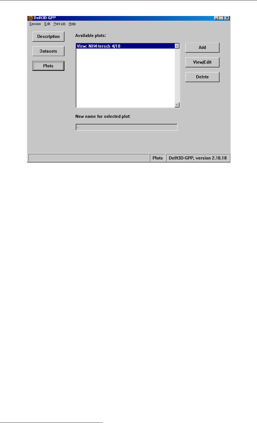
Figure 2.7: Data Group Plots
will be somewhat more elaborate but it offers quite a bit of flexibility.
To do this, click Plots on the left.2(see Figure 2.7):
The main window is now filled in with a list box containing the names of any plots you may
have defined, including the ones creating via the Preview button. Again there is a series of
buttons on the right-hand side:
Add Add a new plot
View/Edit View or edit the first selected plot
Delete Delete all selected plots
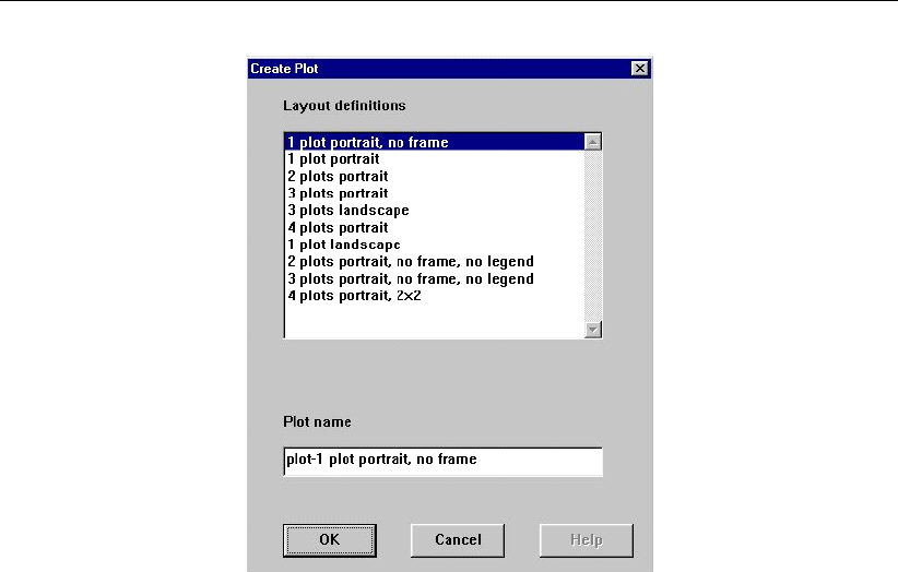
Now click Add. This action has the following result, see Figure 2.8:
A selection dialogue appears which allows you to select a layout for the new plot.
Select the first layout (actually, any one will do).
Normally you will change the name of the plot to a meaningful name reflecting the contents of
the plot. In this tutorial we will use the default name “plot-1 plot portrait, no frame”.
Click OK to enter the Assign data dialogue.
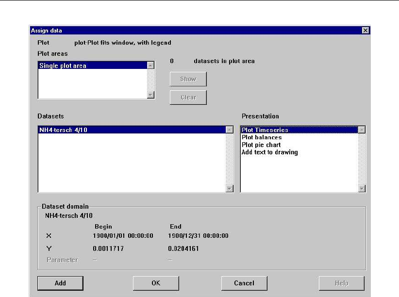
The dialogue Assign data sets lets you assign one or more data sets with their presentations
to the plot (Figure 2.9). Now:
Select a plot area from the list box Plot areas.
Select a data set from the Datasets list box. (The program will then fill in the right-hand
list box: names of possible presentation methods for the selected data set or selection
procedures to derive a sub-set. For this: see the next chapters.)
2On Windows (in all its guises) you will need to click Plots twice if the focus is currently within the visible data
group. This is no design of ours, but apparently part of the window management system. It makes it necessary to
be a bit careful, when switching between data groups.
Deltares 11 of 190
DRAFT
GPP, User Manual
Figure 2.8: Create Plot window
If we use the previous data set, NH4 - tersch 4/10, the possibilities include:
Plot time series
Plot balances
Plot pie chart
Add text to drawing
Select a presentation method, f.i. "Plot Timeseries", from the right-hand list.
Click Add.
Click OK (or go to the first step to add more data sets).
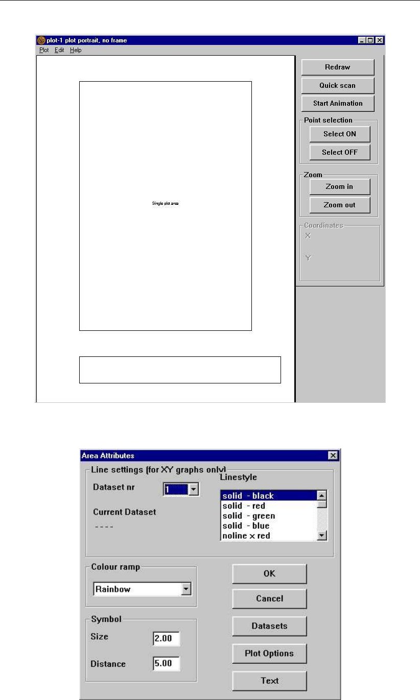
If you simply click OK without assigning a data set, the graphical window will be filled in with
the chosen layout (see Figure 2.10): possibly a frame with some text, one or more so-called
plot areas: rectangles in the picture to which data sets can be assigned.
The graphical window has a menu, like the main window, and a sub-window on the right-hand
side with buttons. You can use the menu item Edit →Assign data, to invoke the dialogue
Assign Data for an existing plot.
You can also double-click on different parts of the graphical window: legend frame, axes of
each graph, or graph itself. Then a dialogue appears that enables you to modify either the
presentation of legend, axes or graphs.
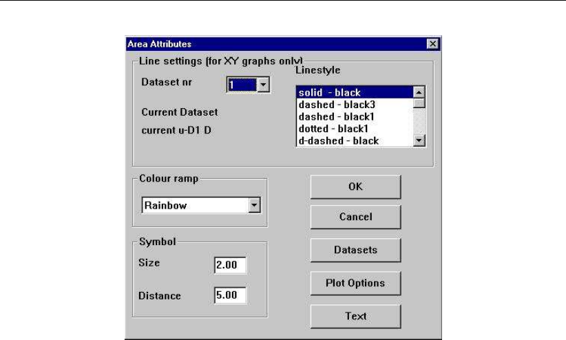
Perhaps this last action requires some explanation. The dialogue box concerning a graph,
named Area Attributes (see Figure 2.11) contains four parts:
Line settings:
Select the line settings per data set in the plot area. If your graph contains a number of
time series, then each set of data is drawn in a different way: the first line may be solid
and black, the second a red dotted line, the third green crosses etc.
Colour ramp:
Select the sequence of colours to be used in a contour map or a histogram or, in fact, any
graph consisting of filled areas.
12 of 190 Deltares
DRAFT
Getting started
Figure 2.9: Assigning data sets to the plot areas
Symbols:
Adjust the size and mutual distance of the symbols (plusses, circles, crosses etc.) in xy
graphs.
The following buttons:
OK, Cancel end the dialogue
Data sets invoke the Assign data sets dialogue for the selected plot area.
Plot options edit the options for the plot routines
Text features of text used in the graph (other than text near the axis)
You may want to print the graph.
Select Plot →Print from the window’s menu.
On Linux, a dialogue will appear to select the printer. You can also specify whether you want
to save the print file. The default printer is the printer defined in the environment variable
PRINTER or LPDEST (unless this printer is not known to GPP).
Also on MS Windows, a dialogue will appear to select the printer, but there is one special
printer: the default printer. You can set that printer via the menu item Plot/Printer set-up.Only
this printer will actually print, all others create a print file with the picture. This is especially
useful if you want to save the pictures in, say, a PostScript file for incorporating them in a
document.
Close the graphical window by selecting Plot →Close when you are done.
The definitions of the data sets and the plots you made will be saved in a so-called state file,
when you leave the program. This file is read the next time you start GPP, so that you can
Deltares 13 of 190
DRAFT
GPP, User Manual
Figure 2.10: Graphical window with empty plot
Figure 2.11: Area Attributes dialogue window
14 of 190 Deltares

DRAFT
Getting started
continue your previous session. The definitions can also be saved in a session file, this is
essentially the same type of file, but it allows more explicit manipulation (see chapter 6 for
more details).
Many settings of GPP are defined in external files (default layouts, properties of the plot rou-
tines, file types, graphical settings and printers). These files can be edited to suit your own
preferences. We refer to chapter 7 and the appendices for a detailed description.
Deltares 15 of 190

DRAFT
GPP, User Manual
16 of 190 Deltares

DRAFT
3 Graphical User Interface
3.1 Starting the program
We need to distinguish between a workstation running X Window and a PC running some
version of Microsoft Windows. Also, as GPP is part of the Delft3D system, you may prefer to
use it from within Delft3D:
On a Linux workstation:
After installation (see chapter 9), the program can be started standalone by typing:
> gpp
or from the Delft3D user-interface:
> delft3d-menu
(and selecting a module or the Utilities option, and next GPP).
As the installation procedure has added the home directory for GPP to the PATH variable,
this command can be issued from any directory.
On a PC:
Double-click on the GPP (or Delft3D) icon in the desktop or start the program via the Start
menu (this depends on how the installation was done and how you have organised your
PC).
To start GPP, go either to the Utilities or to one of the modules; next select GPP.
When starting, GPP will bring up the main window (see Figure 3.1). It will also read a number
of configuration files and the so-called state file (if it exists), which contains the definitions of
data sets and plots from a previous session (see Appendix C).
Read section 7.5,Working environment, for more information on which files from which direc-
tory are used.
GPP may be passed a sequence of command-line arguments as well. Such arguments are
used to:
Determine a session file to read instead of the default state file, so that you can continue
previous work.
Let GPP work in batch mode, which means that any pictures defined in the given session
file are printed without interaction from the user.
Specify the so-called system directory (see chapter 7) which determines where the con-
figuration files are coming from.
In Appendix A these command-line arguments are explained in detail.
3.2 Main window
The main window initially shows three buttons on the left-hand side, a simple menubar and
the description of the session file. When you click on any of these buttons, the main window
changes to present a list box of existing data sets or plots and push buttons that allow you to
create new data sets or to view the plots and other functions. The buttons on the left represent
data groups and clicking them brings up the corresponding dedicated subwindow.
The status bar is used to display various messages, but only those that do not require imme-
diate attention from the user.
The buttons are:
Deltares 17 of 190
DRAFT
GPP, User Manual
Figure 3.1: Main window of GPP
Description, see Figure 3.1
This allows you to document the session file with a few lines of text. Rather than simply
relying on file names or the actual data sets and plots in the session file, you can use this
facility to document its purpose and contents.
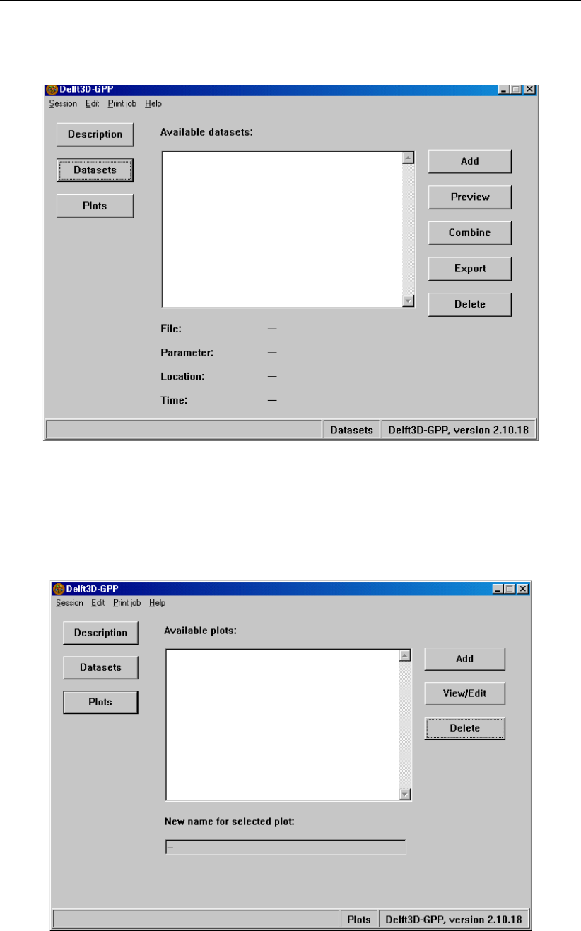
Datasets, see Figure 3.2
When you select this data group, the main window displays a list of the data sets. The
buttons on the right-hand side allow manipulation of the data sets:
Add Add one or more new data sets
Preview Create a simple plot to show the selected data set
Combine Combine two data sets via an arithmetic calculation
Export Export the contents of data sets to an external file
Delete Delete the selected data set or data sets
The button Preview is a function that allows you to view a selected data set. It will create a
plot containing that data set based on:
the first layout in the list of layouts
the first plot routine in the list of plot routines for that type of data sets.
Remark:
If the data set is a 3D data set or some other type that has no direct plot routine, then
the Assign data dialogue appears and you have to do the necessary selections first.
Plots, see Figure 3.3
Selecting the Plots Data Group brings up the list of existing plots and a set of three buttons:
Add Add a new plot
View/Edit View and/or edit the selected plot
Delete Delete the selected plot or plots
18 of 190 Deltares
DRAFT
Graphical User Interface
Figure 3.2: Data Group Datasets window
Figure 3.3: Data Group Plots window
Deltares 19 of 190

DRAFT
GPP, User Manual
Figure 3.4: Main window menu options
The intention is that the next release will allow you to rename the plot. This facility is visible in
the user-interface but not fully implemented yet.
The main window has a simple menubar with the following menus:
Session
This menu allows you to manipulate the current session, such as:
Start from scratch
Open an existing session file
Leave the program
Edit
This menu allows you to manipulate filenames and texts in a global way:
Edit links to data files
Replace text in a frame
Replace text near axes
Print job
This menu allows you to create a so-called print job and to set the characteristics of the
(default) printer.
Help
This menu can be used to bring up the online help information. Pressing function key F1
has a similar effect.
The functions associated with the data groups and the menubar will be explained in more
detail below.
3.2.1 Menubar
The main window has a menubar with three menus, see Figure 3.4.
The Session menu has the following items, which are equivalent in function to the more
usual File menu (the name however refers to session files, and was chosen to avoid
confusion with the data files that you will use):
New Remove all data sets and plots from the current session and start a new
Open Read an existing session file
Save Save the data sets and plots in the current session file (if any)
Save as . . . Save the data sets and plots in a new session file
Exit Exit the program (save the state file, while doing this)
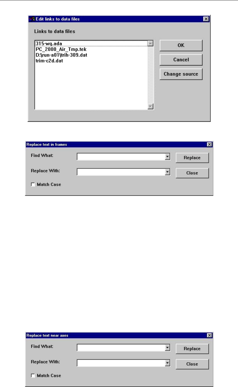
The Edit menu contains three items:
Links
A dialogue will appear that presents all selected data files (see Figure 3.5). By select-
ing a data file and next Change source, the data file can be replaced by another (but
similar) data file.
Frame texts
This option allows you to replace texts in the frames of a plot.
Axis texts
20 of 190 Deltares
DRAFT
Graphical User Interface
Figure 3.5: Sub-menu option Edit links to data files
Figure 3.6: Sub-menu option Replace text in frames
This option allows you to replace texts near axes in a plot.
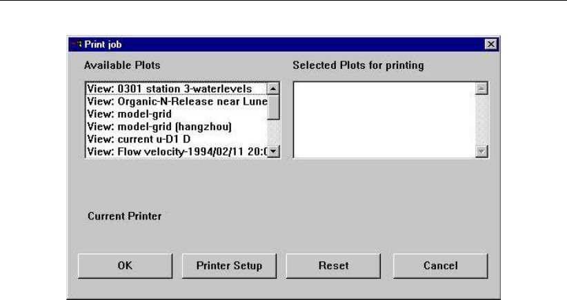
The Print Job menu contains two items:
Make job
A dialogue will appear that presents all existing plots (see Figure 3.8). By selecting
one or more plots you indicate that these plots should be sent to the printer without
showing them on the screen or any actions from you.
Printer setup
Select the printer and set its properties.
The Help menu should require no specific explanation: it will bring up the online help
information. The text is an abbreviated version of this manual, so the manual is the most
comprehensive reference to GPP.
Figure 3.7: Sub-menu option Replace text near axes
Deltares 21 of 190
DRAFT
GPP, User Manual
Figure 3.8: Make Job dialogue
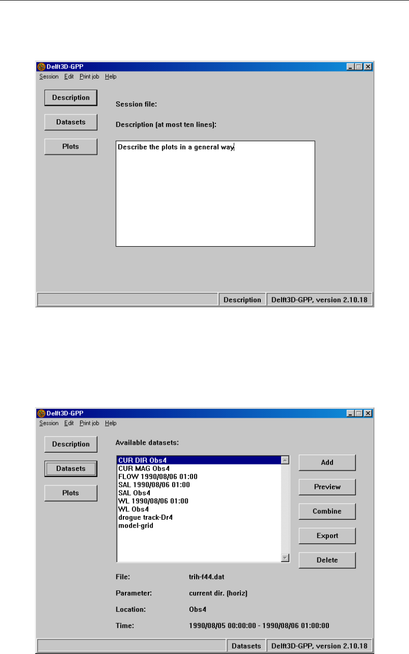
3.2.2 Data group Description
We can be short about this data group (see Figure 3.9):
It shows the name of the session file that was imported (if any) and which will be written
again if you select the Save item from the Session menu.
It also displays a short description of the session, which consists maximally of some ten
lines. You can edit this description and it will be stored in the session file. Whether you
want to use this facility or not, is entirely up to you, but it is quite convenient if you have a
lot of such files.
3.2.3 Data group Datasets
The data group Datasets presents a list of existing data sets and a set of push buttons to
manipulate the data sets (see Figure 3.10). Its functions as follows:
When you select a data set, several properties will be shown below the list box.
Click Add to bring up a dialogue to add new data sets (see the explanation in chapter 3).
When you click Preview, the data set will be put in a new plot and this plot is then shown
in a new plot window (see section 3.3). This fails, if there is no presentation available for
that particular type of data set and you will have to use other means in stead (see the
description of the Data Group Plots).
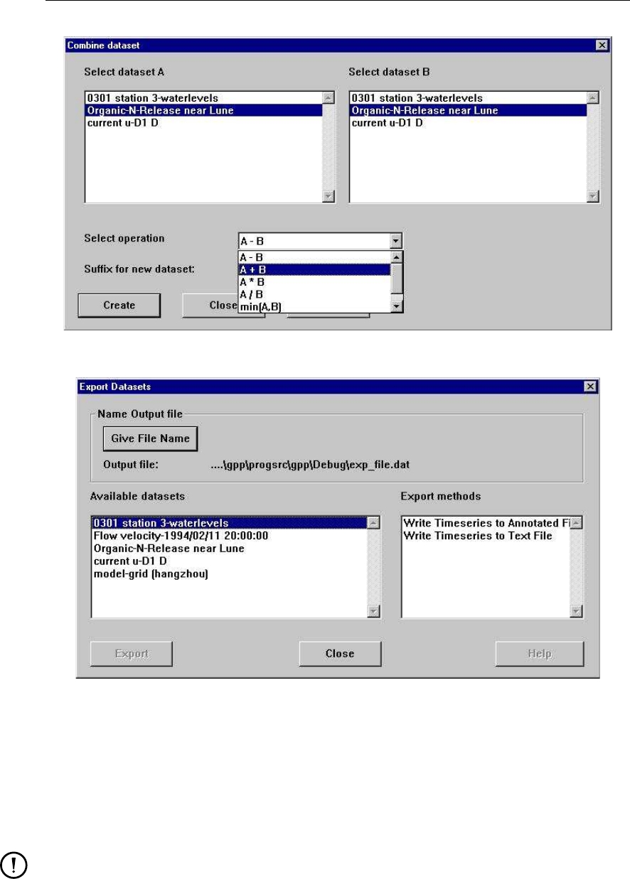
Click Combine to bring up a dialogue to combine two data sets via arithmetic operations
(addition, maximisation etc.) This should be fairly straightforward (see Figure 3.11):
The list box labelled Dataset A only contains data sets for which one or more opera-
tions (like addition) are available.
The list box labelled Dataset B is filled with the same list.
Selecting a data set from both list boxes brings up the list of possible operations (the
first operation is chosen by default).
By clicking Create you create the new data set. If you type a string in the Suffix field,
this string will be appended to the name of the new data set. This makes it easier to
distinguish it.
Click Export to bring up yet another dialogue (see Figure 3.12). This one allows you to
export the data contained in the data set to an external file. (Not all data sets can be
exported, because currently only a limited number of methods is available).
22 of 190 Deltares
DRAFT
Graphical User Interface
Figure 3.9: Data Group Description
Figure 3.10: Data Group Datasets
Deltares 23 of 190
DRAFT
GPP, User Manual
Figure 3.11: Combine datasets dialogue
Figure 3.12: Export datasets dialogue
Most methods export to a text file of some kind as these are best suited for the purpose.
When you have selected one or more data sets and click Delete, the selected data sets
will be removed from the session (which includes removing them from the plots as well).
In some cases, data sets are required by other data sets and because of this relationship,
such data sets will not be removed (but you get a message about that).
Remark:
The x,yco-ordinates in exported 2D map data sets refer to the grid cell corners. The
x,yco-ordinates of the grid cell centre are also added.
24 of 190 Deltares
DRAFT
Graphical User Interface
Figure 3.13: Data Group Plots
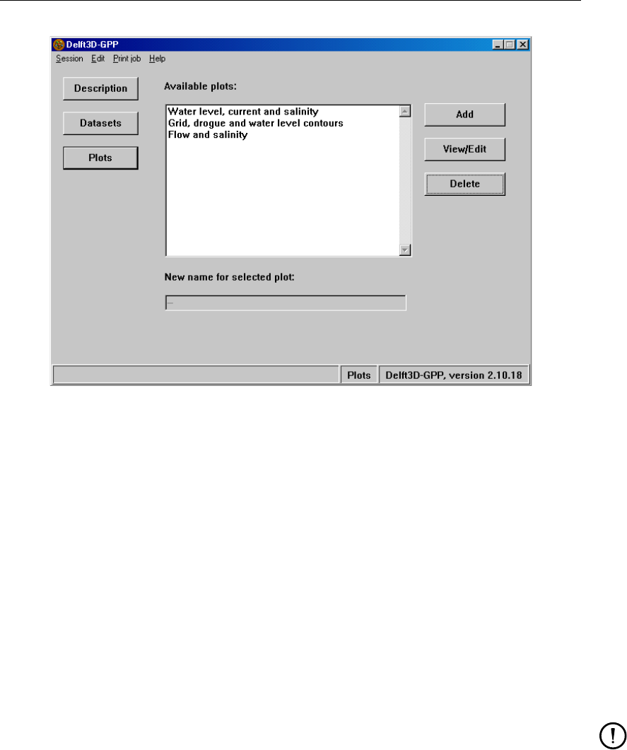
3.2.4 Data group Plots
The data group Plots allows you to define new plots or to view and edit existing plots (see
Figure 3.13). The window contains a list of all existing plots and a set of three buttons:
Select a plot and click View/edit, the plot is shown in a (new) graphical window.
When you have selected one or more plots and click Delete, the selected plots will be
removed from the session. This has no effect on the data sets that were used in the plots.
Click Add to bring up:
A new graphical window
A list of available layouts from which you should select one
A dialogue allowing you to assign data sets to the various plot areas within the new
plot
This procedure is explained in section 3.3.2.
Remark:
In a next release, the data group will allow you to rename the plot, as it is often difficult
to think of a good name beforehand. In version 2.10 this has not been implemented yet.
Deltares 25 of 190
DRAFT
GPP, User Manual
Figure 3.14: Layout of the graphical Plot window
3.3 Graphical windows
When you use the Preview button in the Datasets data group or the Add or View/Edit buttons
in the Plots data group, you get a new window, called a graphical window. This window has a
separate menubar and a number of buttons and other functions that will be explained in this
section (see Figure 3.14).
Remark:
If you select the Preview option, the data set will be displayed in the graphical window
directly only if the data set needs no further selections. If the data set needs further
user selections (layer, time point, etc.) the Assign data dialogue (Figure 3.15) comes
up.
26 of 190 Deltares

DRAFT
Graphical User Interface
3.3.1 Usage of the menubar
The menubar consists of the following menus:
Plot
This menu takes care of several overall functions. It has five items:
Create Create a new plot, by selecting a layout and setting a unique
name for the plot
Select Select a plot from the list of existing plots
Printer setup Select the printer and set its properties
Print Print the plot that is shown
Close Close the graphical plot window
Edit
This menu may be used to change the contents of the plot or to copy it to the clipboard:
Assign data Open the dialogue to assign the data sets to the plot areas or to
clean up the plot.
Attributes (not implemented)
Add text Open the dialogue to add or modify text in the plot.
Copy to clipboard Copy the plot as a bitmap to the clipboard.
Copying the picture to the clipboard is useful, if you want to include it in some document.
Be aware though that the resolution is that of the screen and this can be too coarse for a
printed document. A better alternative might be to print it in a PostScript file, as this will
preserve the resolution much better.
Help
You can get the online information via this menu.
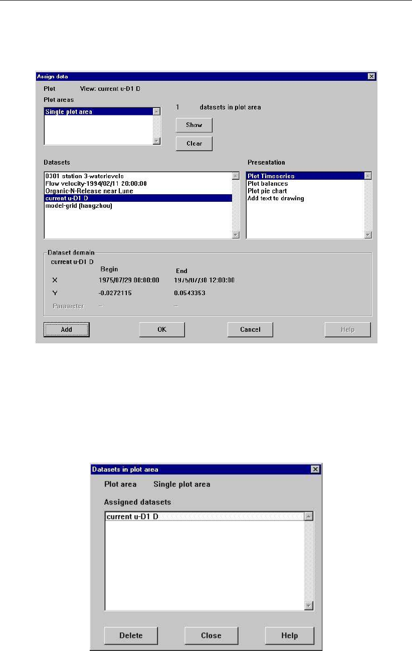
3.3.2 Composing a plot
When you want to fill the plot with data sets, you can do so by selecting the item Assign data
from the Edit menu (see Figure 3.14 and Figure 3.15). The procedure is fairly simple:
First select the plot area.
Then select the data set you want to visualise. The third list, the possible presentations, is
then filled. Sometimes you can use a so-called selection procedure to make a subset out
of the data set, for instance to display a single layer from a three-dimensional data set.
Select the appropriate presentation or selection procedure (if the latter, a new list appears,
allowing you to select a layer or a location and thus to create a subset. This new data set
will be automatically highlighted and a list of available presentations will appear).
Then click Add to add the data set and its presentation to the list for that one plot area.
You can repeat this procedure as often as you want. After clicking OK, the plot will be
drawn.
To delete 1 or more data sets from a plotarea:
First select the plotarea then select Show in the Assign data window. Figure 3.16 will
appear and you can view and delete separate data sets.
Deltares 27 of 190
DRAFT
GPP, User Manual
Figure 3.15: Assign data dialogue
Figure 3.16: Data sets currently assigned to a plot area
28 of 190 Deltares

DRAFT
Graphical User Interface
3.3.3 Buttons in the graphical window
The buttons on the right in the graphical window have the following meaning:
Redraw:
Redraws the graph. Use this if parts remain blank. (This might happen in some weird
circumstances when the screen is not properly refreshed.)
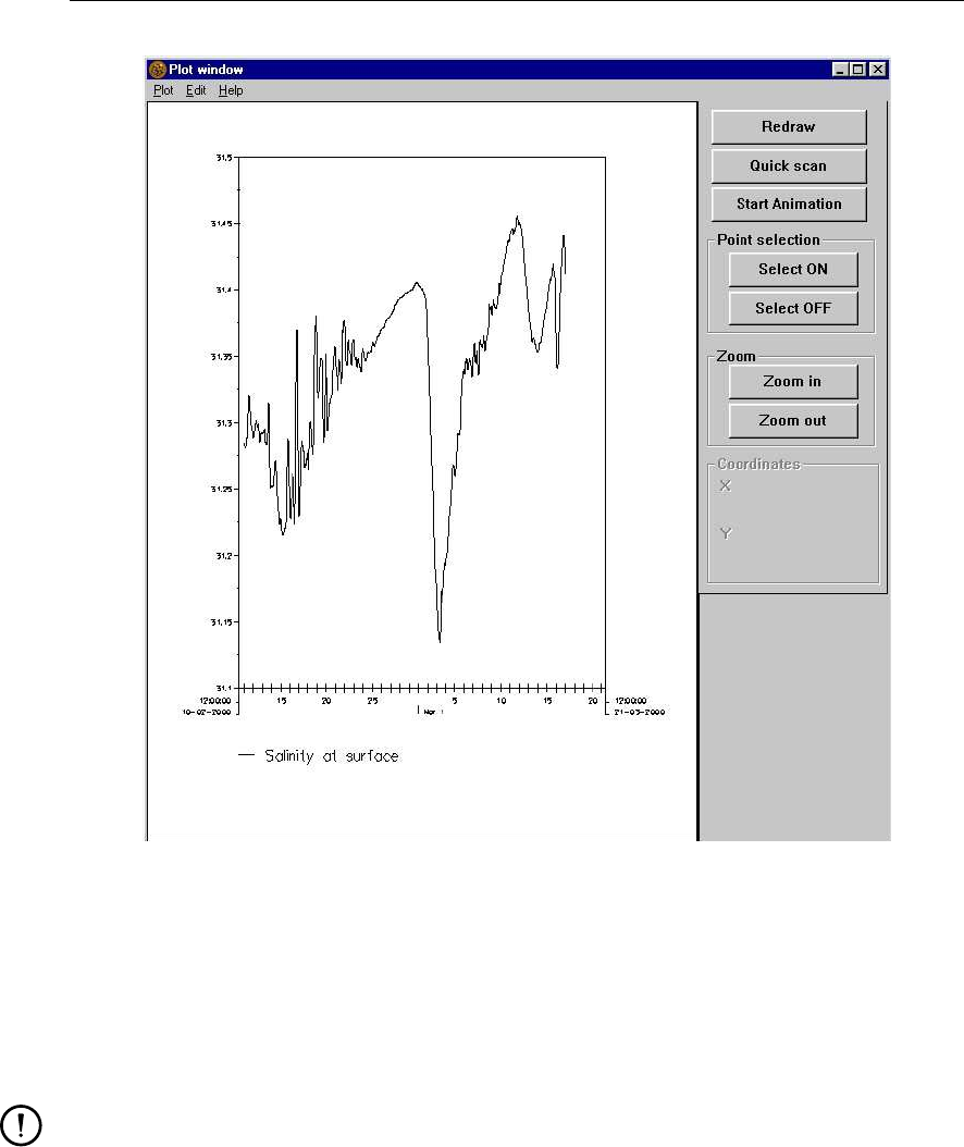
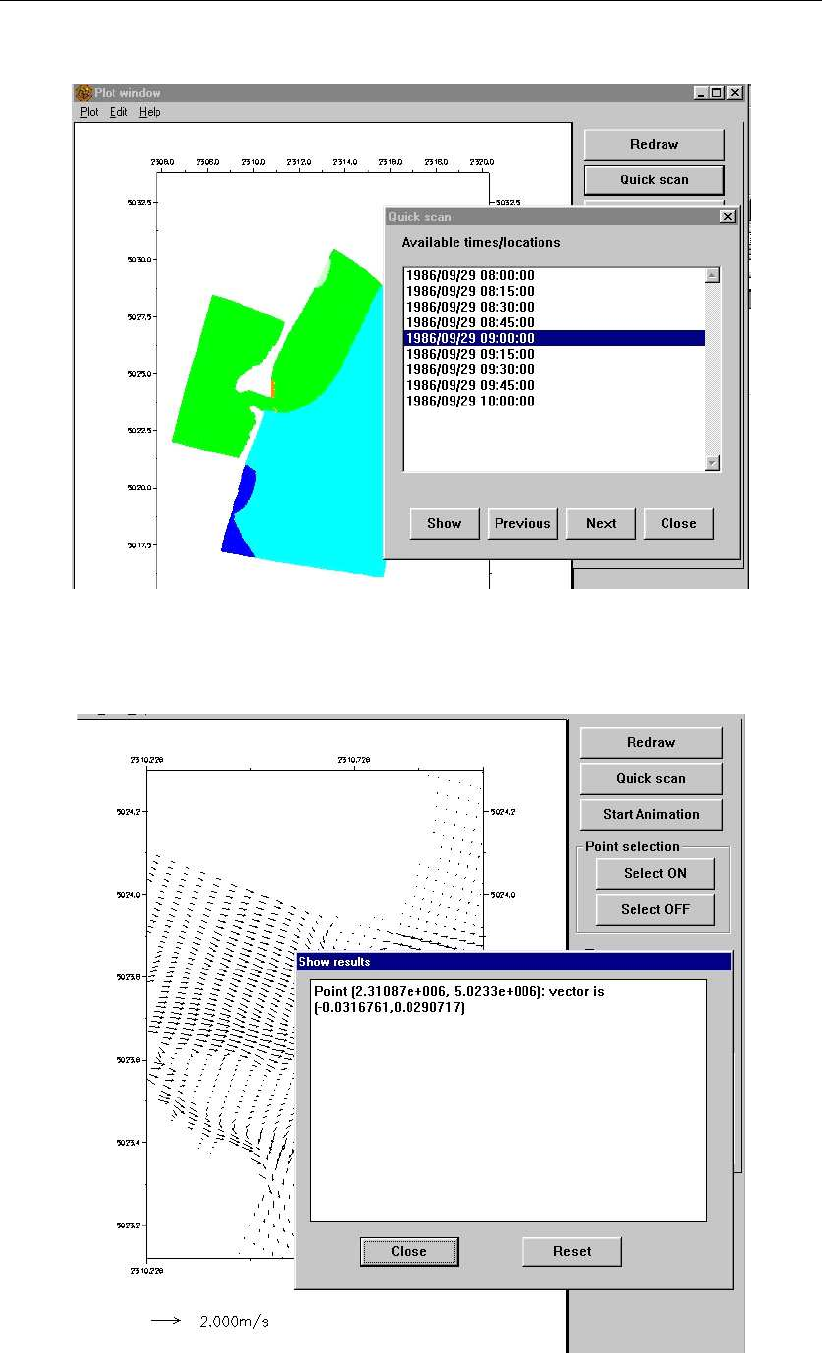
Quick scan:
If the plot contains but one data set, this button brings up a list of locations or times that are
contained in the same data file, so that you can have a quick look at these other locations
or times without having to define new data sets (see Figure 3.17). To keep the facility easy
to use, this works only if there is a single data set.
Start animation:
Start a simple animation. Its use is a bit complicated: you must create a data set with a
spatial distribution and one or more time steps (typically one parameter from a so-called
map file). Create a subset by selecting one time step and present it in the plot. If you then
click this button, GPP will draw all time steps in the original data set one by one. Then its
saves the picture in a bitmap file.1
Point selection: Select ON, Select OFF
You can choose a point in one of the plot areas. It will show the value at that point or other
relevant information (such as the grid cell indices; see Figure 3.18).
The co-ordinates are shown in the two text fields below the buttons.
Zoom: Zoom in, Zoom out
Zoom in on a smaller area:
First select Zoom in
Click the left mouse button at one of the corners of the area you want to select
Keep it pressed and move the mouse. If you release the button, the area will have
been selected and the graph will zoom in.
You can repeat this again and again. By clicking Zoom out you will return to the original
area (for all plot areas).
Note: Depending on the kind of axis type, the zoom size is adapted in that way the aspect
ratio is not changed.
3.3.4 Using double-clicks
You can use a double-click of the left mouse button:
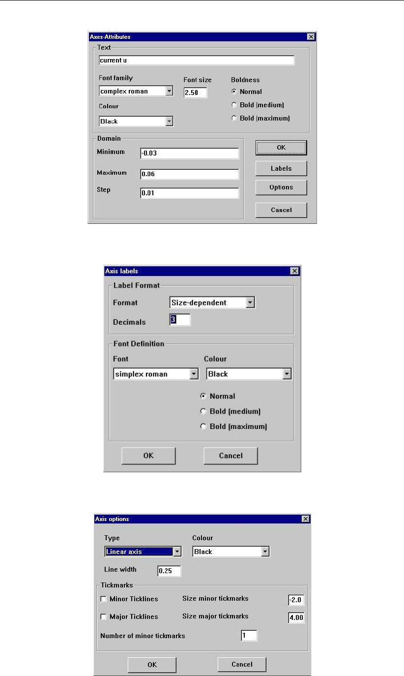
Double-click on or near an axis brings up a dialogue in which you can change the attributes
to the axis, colour text, font, number of tickmarks, scaling (see Figure 3.19,Figure 3.20
and Figure 3.21).
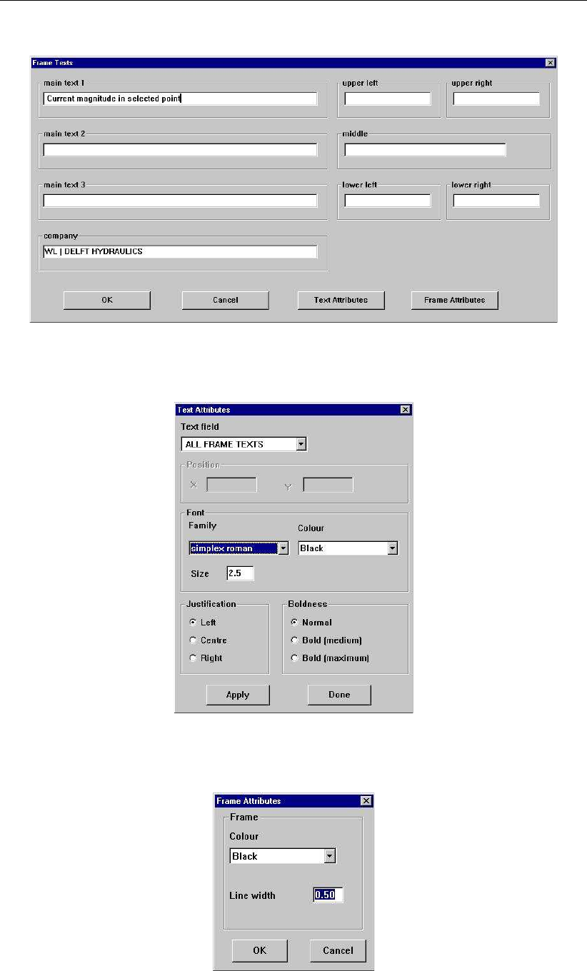
Double-click in the frame (if a frame is visible); this allows you to fill in the text that appears
in the frame (see Figure 3.22,Figure 3.23 and Figure 3.24). The buttons Text Attributes
and Frame Attributes are used to change the detailed appearance of the text and the
frame.
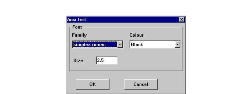
Double-click in a plot area to give you the opportunity to change (see Figure 3.25,Figure 3.26
and Figure 3.28):
series settings appearance of individual time-series in line graphs.
colour ramp which sequence of colours to use for a contour map or pie-chart
1On the UNIX workstation it will save each picture in an XWD file, on PC it will save each picture as a BMP file.
See also chapter 8 for more information.
Deltares 29 of 190
DRAFT
GPP, User Manual
Figure 3.17: Quickscan facility allows for temporary selection of other locations or times
Figure 3.18: Point selection
30 of 190 Deltares
DRAFT
Graphical User Interface
Figure 3.19: Axes Attributes dialogue
Figure 3.20: Axis Labels dialogue
Figure 3.21: Axis options dialogue
Deltares 31 of 190
DRAFT
GPP, User Manual
Figure 3.22: Frame Texts dialogue
Figure 3.23: Text Attributes dialogue
Figure 3.24: Frame attributes dialogue
32 of 190 Deltares
DRAFT
Graphical User Interface
Figure 3.25: Change Plot area attributes window
datasets which data sets are shown in the area
plot options the options used in drawing the data sets.
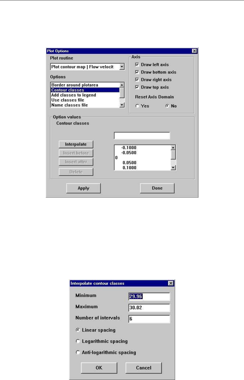
The dialogue for changing the plot options requires some further explanation. Each presen-
tation form can have one or more specific options. These are for instance whether to use a
right vertical axis or a left axis or a list of concentration levels for making a contour map.
The idea is that each combination of a data set and a presentation form can have its own
values for these options. This way you are very flexible in making the plot. Defaults for these
options are read from the configuration files.
A second purpose of the dialogue is that you control whether the axes are visible or that the
axes have to be determined again. This may be necessary if the plot options involve a change
in axis type or if you have added new data sets for which the previous scaling is not effective.
For Contour classes you can either modify the classes or Use classes file. Via Interpolate you
get a dialogue that allows easy manipulation of the contour classes (see Figure 3.27):
Enter a minimum and a maximum value for the class limits as well as the number of
intervals.
Select the method of interpolation:
Linear spacing gives equal steps
Logarithmic spacing gives steps that are small near the maximum and large near the
minimum
Anti-logarithmic spacing gives steps that are small near the minimum and large near
the maximum (so the reverse)
Depending on the character of the quantity to be shown, any of these methods may be useful.
For instance, if you show the salinity in open sea, then you probably want to emphasize slight
deviations from the maximum (i.e. fine scales in the range 33–35 promilles), whereas below
33 promilles the steps can be larger. With logarithmic spacing you can achieve this effect.
Deltares 33 of 190
DRAFT
GPP, User Manual
Figure 3.26: Change Plot Options window
Figure 3.27: Interpolate contour classes dialogue
34 of 190 Deltares
DRAFT
Graphical User Interface
Figure 3.28: Change Area Text window
To import a user-defined classes file:
Set the option Use classes file to true.
Set the option Name classes file to the name of your classes file.
A classes file has a very simple format: any line may contain one single number, the numbers
must be in ascending order and for documentation purposes you can add comments by using
a hash (#) or an asterisk (∗) in the first column.
Example of a classes file:
*
*Water levels: fixed contour classes
*
-2.0
-1.5
-1.0
-0.5
0.0
0.5
1.0
1.5
2.0
3.4 Error handling
If an error occurs while reading any of these files, you will see a message box with a descrip-
tion of this error. Three types of errors are possible:
The program cannot find the file, which is a serious error for all but the session state file,
as things are not defined then.
The program can not read the file because of some syntax error. The reading routines will
indicate the line on which the syntax error occurred and the offending word or character.
The program complains about the version number in the configuration files. As these files
are extended and adjusted with new releases it is important to use the correct versions.
We try to keep them compatible, so that some things are simply not available, but occa-
sionally major changes do happen.
The message is therefore: if an error occurs with any of the configuration files, please find out
what is the matter before continuing. If an error occurs with the state file, you may ignore it,
though some data sets or plots from the previous session are not available.
Deltares 35 of 190

DRAFT
GPP, User Manual
36 of 190 Deltares

DRAFT
4 Data sets and presentations
4.1 Data sets in general
Sets of data, the results of a numerical model or of a measurement campaign, are commonly
characterised by some quantity or quantities (a hydraulic parameter, an ecological parameter
or whatever), by locations (we are dealing with the real world and models of that world) and
by a range of times. This summarises the idea of the Open Data Structure (or ODS for
short): these three things are characteristic for all data sets we usually deal with. Within this
data model you can have many variations: time-series, scalar data on a 2D grid, a three-
dimensional flow field and so on.
To elaborate on this: a data set can be a time-series of water quality data - measurements of
the concentration of BOD at a fixed location in time. The most natural form of presentation of
such a data set is, of course, a plot of the concentration versus time. This is certainly one of
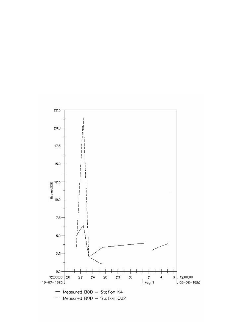
the presentation forms contained in GPP. But what if the data set contains the data for two or
more locations (see Table 4.1 and Figure 4.1)? Or for two or more parameters (temperature,
salinity and oxygen concentration, for instance, as measured by a probe)?
Although we try to abstract from the actual format of the data file via this general data model,
there remains a relationship between the data set and the file it comes from. In general, the
files you import in GPP can be considered to contain one or a limited number of such data
sets. In some cases, such as map files from D-Water Quality, all the information in the file can
be arranged into one single data set according to the ODS data model. In other cases more
than one data set can be distinguished: a history file from Delft3D-FLOW is an example. It
contains results for monitoring stations (single points) and for cross-sections. For the stations
different parameters are available than for cross-sections. So, we may say that the data in
such files constitute two disjoint data sets.
Some files actually require a second or even a third file to be read. If this is the case, the
primary file will be selected and the names of the others are derived from that, if possible.
It is not necessary to import the whole data set at once. In fact, GPP suggests that you select
at least a parameter from the list of available quantities.
So, GPP is a framework which allows you to import certain data sets (from external files) or to
create data sets from others, and to present them in any way possible and suitable.1To keep
track of these data sets, they are given unique names. The user-interface constructs a default
1We refer to the detailed documentation on GPP for the algorithms used, how to extend the set of presentations
etc.
Table 4.1: Measured data of BOD5 (mg/l) in two locations. (Note: these data are fictional)
Time of measurement Station K4 Station QU2
21 July 1985, 8:00 5.0 3.5
22 July 1985, 10:35 6.5 21.5
23 July 1985, 8:10 2.0 2.0
25 July 1985, 13:43 3.4 1.0
1 August 1985, 12:20 4.0 < 1.0
2 August 1985, 11:55 (not measured) 3.0
5 August 1985, 7:22 11.2 4.5
Deltares 37 of 190
DRAFT
GPP, User Manual
Figure 4.1: Example of particular data set. Missing values are represented by disconti-
nuities in the line
38 of 190 Deltares
DRAFT
Data sets and presentations
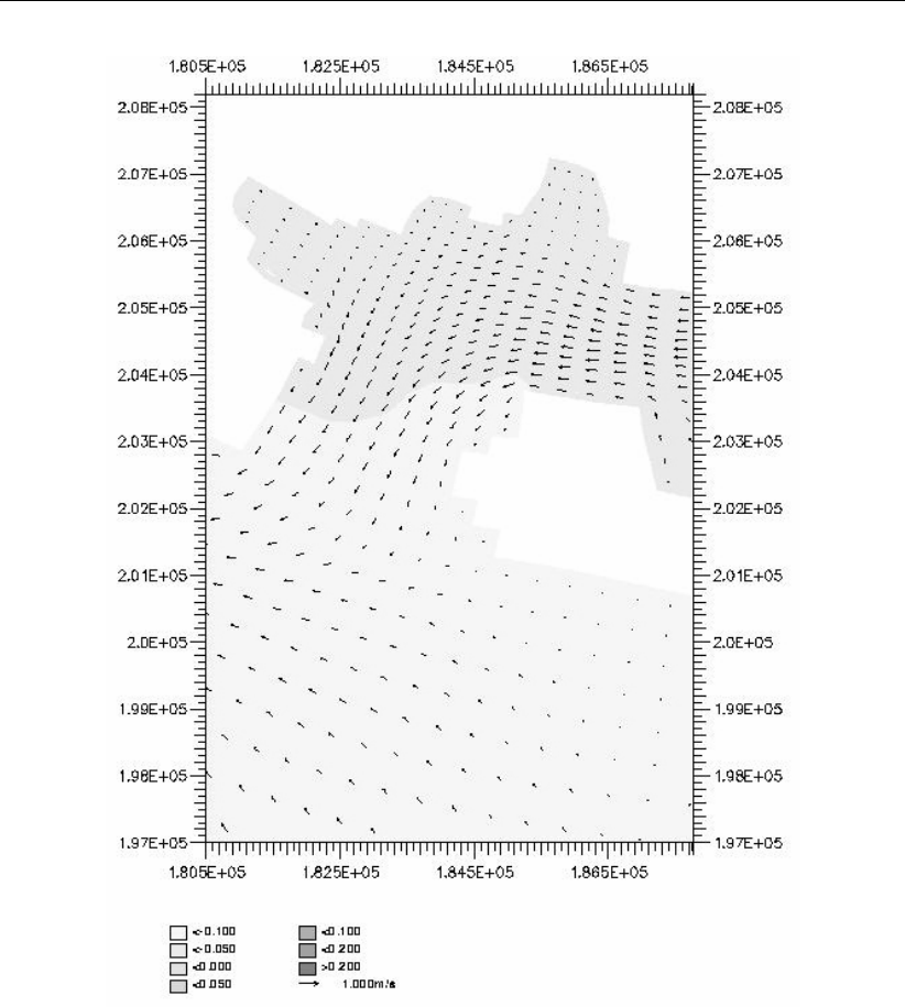
Figure 4.2: Plot of water level (filled contours) and flow velocity (vectors)
name, but you are free to select a different name.
4.2 Presentations and selections
Internally, the data sets have a type and a subtype. These two properties among others allow
GPP to construct a list of suitable presentation forms and selection methods. They are set
automatically from all available information. The type indicates the dimensions of the data
set: time-series, two-dimensional data sets, three-dimensional data sets etc. The subtype is
usually ’SINGLE’, indicating a single component. In some cases, the subtype is ’VECTOR’,
indicating two components (a vector quantity), others are used as well. Both the type and the
subtype determine which subroutines for plotting a data set are suitable (see Figure 3.15).
Sometimes, selecting the file from which the data set should come and selecting parameter,
location or time is enough. An example: selecting the water level at a single monitoring
station from a result file from Delft3D-FLOW. In other cases, we need the underlying grid as
well. This may mean that another file has to be selected which contains information about
the grid. As an example we may look at D-Water Quality map files. D-Water Quality does not
Deltares 39 of 190

DRAFT
GPP, User Manual
know anything about the grid (the underlying computational program, called DELWAQ, does
not use the co-ordinates of the grid points, but only derived quantities), hence its output files
do not possess any information about the geographical layout. You need to import an extra
file (two actually). At present, only curvilinear grids can be imported. The order in which you
do that is not important, but it is important to get the right files, as otherwise the data set can
not be plotted: its proper type is not recognised.
4.3 Importing the data set
The basic procedure to create a data set from a file has been described in chapter 2. But
there are in fact several possibilities after you have selected the parameter:
If the file contains named locations, it is known as a history file. You can:
select a single location. The result is a time-series (or possibly a set of time-series, if
the location has more than one layer).
select several locations, in which case the data set is a combination of several time-
series.
postpone the choice. GPP automatically selects all locations into the data set.
If the file does not contain named locations, it is considered a map file or a grid file. In the
first case, you can:
select a single time to get a data set that is defined on some grid.
postpone the choice. GPP automatically selects all times into the data set.
(It is not possible to select several times for technical reasons.)
In the second case, there is no time to select. The parameter has uniquely identified the
data that should be imported from the file.
The data set will be known by a unique name: it is up to you to accept the name constructed
by default or to type in one yourself. The name is important because whenever you need to
chose a data set, this name is presented.
4.4 Available presentations
Depending on the type of data several presentation forms will be available. Table 4.2 provides
some examples (a more elaborate overview is given in Appendix K):
During the creation of the data set you may want to postpone the choice of, say, a location.
When you select such a data set in the plot dialogue, one of the possible "presentations" will
be: Select a location.
Besides selections you can also do some operations on data sets. Examples of selections
and operations are:
Select a single parameter (if the data set contains more than one parameter).
Select a single time (used when creating animations, see chapter 7).
Select a single layer (if the data set is three-dimensional).
Select a fixed M or N grid line.
Select an arbitrary transect.
Select a vertical profile.
Instead of a picture, a dialogue appears which shows the possible choices for the selection
or details for the operation. By selecting an item you create a new data set, which is actually
40 of 190 Deltares
DRAFT
Data sets and presentations
Table 4.2: Presentation forms for various types of data sets
Data set Presentation form
Time-series Plot of values versus time
Cumulative histogram of values (so-called
balances)
Plot limiting factors
XY series Plot of y-value versus x-value
Scalar data on a two-dimensional grid2Plot contour map
Plot iso-lines
Plot thin dams
Plot time bar
Scalar data on a three-dimensional grid No direct presentation possible, reduce to
some form of 2D data first
Vector data on a two-dimensional grid Vector plot
Plot time bar
Grid itself Plot of the grid layout
a subset of the original one. This new data set is automatically selected and the possible
presentation forms are presented.
Besides the above mentioned selections you can do also some operations on appropriate
data sets:
Calculate the magnitude of a vector parameter.
Average over a fixed layer (from the surface) (3D data sets only).
Averaged squared vector (m2/s2) over a fixed layer (3D data sets only).
RMS vector (m/s) over a fixed layer (3D data sets only).
4.4.1 Types of presentations
Presentation forms may roughly be divided in three categories:
line graphs (like a time-series)
surface graphs (like a contour map)
all others (like a grid).
This is not to be taken too strict: drawing a grid as a collection of short lines outlining the grid
cells could be called a line graph and iso-lines belong to the category of contour maps. The
main reason for this distinction is that the resources used by the two categories are different.
In the first category we are dealing with one or more series of data points in a graph. Each
series needs to be distinguished from the others. This can be achieved with:
different line styles and line thicknesses
different colours
different symbols
Symbols are especially useful if you want to show the individual data, whereas colours and
line styles are very handy to distinguish more or less continuous series. In order to make the
Deltares 41 of 190

DRAFT
GPP, User Manual
presentation routines work together, they take these settings from a common source.
Presentations which belong to the second category are different altogether: there different
colours will be used to indicate a continuous distribution. For example: the colours used in a
contour map will follow a rainbow-like sequence or perhaps a range of blue shades, not only
to please the eye, but also to better present this continuity. To aid the presentation routines in
achieving this aim GPP uses so-called colour ramps and contour classes:
Colour ramps are sequences of colours which can be selected by selecting the name of
that colour ramp.
Contour classes are sequences of numbers which can be edited in a dialogue box (see
chapter 3) and are used in the order they are given.
The third category consists of various unrelated presentation forms which do not use either
type of resources. They are independent from other presentations.
42 of 190 Deltares

DRAFT
5 Files and filetypes
This chapter focuses on some general features of the data files. For specific information on
the models and filetypes that are supported and what special considerations may apply, we
refer to the appendices.
5.1 Data files in the user-interface
To read the data from the data files GPP uses a simple concept, such that the details of the
file structure are irrelevant to you. To be able to read the files properly, it does have to know
the structure, or put in another way, the filetype. In the user-interface, this is characterised by
the model and by the filetype within such a model.
To facilitate the selection of files, GPP uses a file mask. This is a pattern like "∗.hda" that is
used to select only those file names that are likely to be of the right type. The asterisk (∗)
matches any sequence of characters. You may change this mask when selecting a file or you
may supply a different default mask for files of a certain type.
To summarise the properties of a data file that are important to the user-interface:
model The numerical model or other source that created the file
filetype Indication of the file’s structure
file mask A pattern to be used to pre-select the file names, usually fixed by the
conventions used by the model.
These properties are defined in the file <filetype.gpp>. Only filetypes listed in this file are
available in GPP (see Appendix C.2).
5.2 Representing date and time
Time in GPP is always a date and time of day. The routines that read the files are supposed
to retrieve such a date and time. Some models do not use an absolute time. Instead, the
routines may use the following convention (check the addendum on filetypes):
A reference date and time may be given via comments. This will be used to reconstruct
the actual date and time for the model results. The layout of such a line is:
t0= 1993.12.31 12:59:59 (scu= 1 )
....+....1....+....2....+....3....+....4 (column numbers)
The first part is the date and time to which the relative time 0 in the calculation refers, the
second is the unit of the system clock in seconds.
Note:
It is important that the time units are given consistently, otherwise a distorted picture will
be drawn!
If the files do not contain a reference date (or the date is not of the correct format), the
reference date is set to January 1, 1900.
5.3 Formatted data files
Measurement data are often stored in text files or databases of various kinds. GPP offers
several filetypes to import such data: the so-called TEKAL and Samples files.
Deltares 43 of 190

DRAFT
GPP, User Manual
5.3.1 TEKAL files (general)
Essentially, all TEKAL filetypes share that structure:
The file may contain one or more tables of data, which are independent. They are some-
times referred to as blocks.
A short string (the block name) identifies the "block" or table of data.
A line should follow to indicate the number of rows and columns. In the case of data on a
two-dimensional grid, a third number indicates the number of cells in the first direction.
Each line after that contains the data for one row.
Comments can be added before the block name, via an asterisk (∗) in the first column.
(Examples appear in the various subsections.)
Thus, the structure is (almost) always as described briefly above. It is a very flexible and easy-
to-handle format. This is partly because it lacks additional information, such as the quantities
that are given in these columns, the meaning of the table and so on. This information must be
added by the program or the user.
Within GPP, this lacking information is added in three different ways:
By selecting the filetype from the list defined in the <filetype.gpp>file.
By using the comments to supply names to the columns.
For the one-dimensional variant, an extra dialogue will appear.
The files can be used for the following purposes:
Time-series or data as function of an arbitrary co-ordinate
This is a one-dimensional TEKAL file (meaning that the line after the block name has only
two numbers, the number of rows and the number of columns. This type of file is handled
in a special way in the user-interface (see section 5.3.3).
Co-ordinates for land boundaries:
This is also a one-dimensional TEKAL file, but it should have two columns, the first for the
x-co-ordinate, the second for the y-co-ordinate. All blocks are read at once, though they
define individual poly-lines or polygons. Furthermore:
The missing value 999.999 for a co-ordinate indicates a break in the line.
Polygons are recognised by the fact that the first pair of co-ordinates is identical to the
last pair.
Scalar quantities on a curvilinear grid:
Files that are used for this purpose require at least three columns, the first two being the
x- and y-co-ordinates of the vertex of the grid cell, the others quantities that are given on
these vertices. Special features:
To make the subtype correspond to values defined on the vertex (VALUE_AT_VERTEX ),
the quantities are called "value 1", "value 2" etc. and they are read as extra parame-
ters.
You can associate a particular date and time to a block of data by using a comment
line before the block:
*Use the keyword to set the time to
*1 January 1990, 10:00:
*
*time : 19900101 100000
*
BLOCK (will be ignored)
...
44 of 190 Deltares

DRAFT
Files and filetypes
The time string must be given exactly as above, with a space before and after the
colon. If no such comment is present or recognised, then a default time is used (start-
ing at 1 January 1900, to make clear that actual date time information are missing).
The grid information, that is, which cells are active, is defined implicitly, by the value
of the first quantity. If this value is equal to the missing value, then the grid cell is
considered inactive. Otherwise it is active. A consequence of this is: all quantities in
all tables (blocks) must be defined on this same grid. In general, this condition will be
satisfied, but it does mean that you can not combine such files arbitrarily.
Vector quantities on a curvilinear grid:
The same format can be used to import vector quantities, such as the transport of matter
or flow velocity. The difference is only, that the columns appearing after the co-ordinates
are grouped in pairs and the vectors are called "vector 1", "vector 2" and so on. All other
remarks hold just as in the case of scalar quantities.
Text at geographic locations:
It is also possible to apply the TEKAL file format, if you want to read in text strings that
should appear at a particular geographic location. The current implementation expects
three columns, the first two the geographic co-ordinates, the last a string:
*
*Just some text to appear in the plot
*
BLOCK (will be ignored)
3 5
1000.0 2000.0 " Text 1"
999.999 999.999 " is continued"
2200.0 3000.0 Somewhere in the plot
700.0 1000.0 Text 3
3300.0 2020.0 / Text 4 /
This type of data is called geographic text (by lack of a more suitable name) and it will
be drawn at the location indicated. The plot routine that does this has several options for
positioning the strings relative to the location and selecting the angle and text height.
We must make a number of remarks about this filetype:
Lines can be up to 80 characters long.
The strings are read without leading blanks, unless a delimiting character is used: any
character that is not a letter or a digit and is repeated within the string (in the example
above: the quotation marks (") and the slashes (/)).
Only the first block is read from the file.
The co-ordinates are grouped together and appear as one parameter, texts, whereas
the strings appear as location names.
Because of ODS conventions, the location names can be up to 19 characters long.
If the string is longer, then it will be split into two, three or more locations. The co-
ordinates associated with these extra locations are so-called missing values (the value
999.999). You may use this internal convention to join text strings (it might come in
handy, in special cases).
Some caution must be observed: if the file contains empty lines or uncommented lines outside
the tables, the reading routines may recognise extra blocks and give somewhat strange lists.
So: whenever possible, follow the above format exactly.
Deltares 45 of 190

DRAFT
GPP, User Manual
5.3.2 Samples files
Yet two other filetypes are supported that share some of the characteristics of TEKAL files, in
that the structure is very simple and you can edit them manually: the so-called samples files.
Samples files are available in two types:
Observation points in a geographical area
These file have the following format:
Lines can be up to 80 characters long
Comments can be added at the beginning of the file by starting a line with an asterisk
(∗) or a pound sign (#)
After the comments a line with the names of the columns may appear (they should
be enclosed in quotation marks ("). Names for the first two columns will be ignored
though, for technical reasons.
Unfortunately, no time information can be given yet.
Each line after these should have at least three numbers. The first two are the co-
ordinates of the observation point, the rest are the values that were observed.
Values are separated by spaces, tabs or commas. Missing values can not be indicated
by two consecutive tabs or commas though, a dot (.) or a question mark (?) is called
for, to make the missing value visible.
A small example:
<------- up to 1000 columns ------->
*Lines with *in the first column are comments
*Observation points: X,Y, Salinity, Temperature
*
’’X’’ ’’Y’’ ’’Salinity’’ ’’Temperature’’
1000. 1000. 30.0 14.3
1200. 1540. 31.2 14.5
5210. 522. 25.62 17.5
3111. 354. 22.62 18.9
Remarks:
Lines that contain one single value, before the lines with actual data (always at least
two numbers) are treated specially: the number on the last line is regarded as a
scale value for the third column (this was introduced for the SHIPMA model).
A line with the names of the columns may appear only once in the file.
Data as function of some independent variable:
This filetype is very similar to the corresponding one-dimensional TEKAL file, except that
it has no header stating the number of columns and rows and the first column is by con-
vention the independent variable. This makes it unnecessary to pose another question to
the user.
All remarks for the observations points hold for this filetype as well, except that now, only
the first column is special.
If you want to represent a missing value, use a period (.) or a question mark (?) to indicate
that an actual value is missing.
The following is an example of such a file:
<------- up to 1000 columns ------->
*Lines with *in the first column are comments
*Data as function of distance
*A question mark is a missing value
"Distance" "Oxygen" "pH" "Ammonia (mg/l)"
21. 8.8 7.1 0.01
54. 8.0 7.8 0.21
77. 6.8 6.4 0.4
113. ? 6.4 0.4
202. 4.5 6.0 1.2
Data as function of date/time:
46 of 190 Deltares

DRAFT
Files and filetypes
For this filetype the first two columns are interpreted as date and time, all others are
interpreted as the value of some parameter at that date/time. You can use two different
formats for the date and time columns, as shown in the example:
"DATE" "TIME" "salinity" "temperature"
19990101 200000 30.0 12.0
20010201 210000 31.0 12.3
1991/03/02 21:20:00 29.0 ?
1998/02/01 11:12:11 29.1 11.32
Remark:
To enable a smooth transition between the “old” TEKAL format and the “new” obser-
vations files, you can include the two lines that distinguish old-style TEKAL formats
(without comments for identifying the columns), that is, the block name and the number
of rows and columns. These lines are simply ignored. There is one condition though:
in order to detect these extra lines, the program assumes that such a line starts with a
letter in the first column. As this is typically true for the majority of such files, this was a
simple criterion.
5.3.3 TEKAL time-series files
As stated above, TEKAL time-series files are treated somewhat special by the user-interface.
As this format does not include information about what these numbers are, the ODS routines
that read these files use the following conventions:
The blocks are supposed to refer to one parameter. The various columns refer to different
locations.
In case of a "time block" the first column contains the date in the so-called yyyymmdd
format and the second column in the hhmmss format (see example).
The block name may be up to 19 characters. The block name serves as the name of the
parameter.
Each block may be described by lines starting with an asterisk (∗). If they contain the
keyword "column" and a column number in the right position, the text on these lines is
used for the names of the locations. (Important: this information is read with a fixed
format, see next example.)
The user-interface of GPP will ask for the two columns that contain the date and time or it
asks for the start time and the increment, depending on the actual type that was chosen (see
Figure 5.1).
As an example, Table 4.1 has been converted to a TEKAL file:
....+....1....+....2....+....3....+....4 (column numbers)
*
*column 1 : Date and time
*column 3 : Station\_K4
*column 4 : Station\_QU2
*
b001 Measurements of bod
7 4\]
19850721 80000 5.0 3.5
19850722 103500 6.5 21.5
19850723 81000 2.0 2.0
19850725 134300 3.4 1.0
19850801 122000 4.0 999.999
19850802 115500 999.999 3.0
Deltares 47 of 190
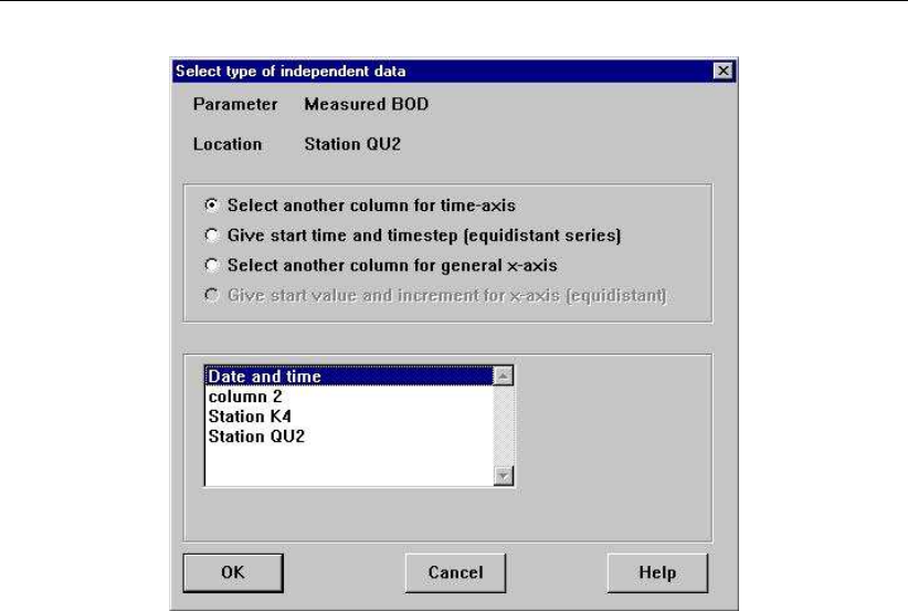
DRAFT
GPP, User Manual
Figure 5.1: Specifying time column of a TEKAL file
19850805 72200 11.2 4.0
The table has seven rows and four columns. The date (given as yyyymmdd) and time
(hhmmss) are distributed over two consecutive columns. The third and fourth columns con-
tain the BOD concentration at stations K4 and QU2 respectively. The two entries in Table 4.1
that do not contain valid data are replaced by the special value 999.999, the so-called missing
value. This value is skipped in all drawing routines. The graph is shown in Figure 4.1.
5.4 Other properties of the filetypes
As mentioned GPP uses the file <filetype.gpp>for defining the properties of the filetypes.
Each filetype is defined by three sets of properties:
Presentation options
This set of properties has to do with the way data sets read from these files are plotted.
If a database contains measurement data only, it is likely that you want these data to be
drawn as symbols, rather than as connected lines, or, on the other hand you may prefer
model data always to be represented as lines without symbols. For this a separate section
may be included which sets these properties.
Properties for the user-interface
This set has been explained in the first section. It is the most "visible" one.
Special parameters
This set of properties has to do with the meaning of the parameters in the file. For instance,
vector quantities are defined in this way. The technical documentation contains more
details. In general, it is enough to know that this can be done arbitrarily.
If you want to change this configuration file, you are free to do so. We suggest that you
change things like the description of the filetype or the order in which the filetypes appear,
so that they suit your system better: if you never use a model like PHAROS, why have the
filetypes associated with that model appear in the list?
48 of 190 Deltares

DRAFT
6 Layouts and plots
6.1 Layouts
In GPP you must select a layout to create a plot. By selecting a layout the following items are
defined:
the size and position of a graph
the size and position of a legend to the graph
an optional frame around the whole plot
the orientation (portrait or landscape) of the plot
These items can not be changed from within the user-interface. They can be changed by
editing the session file, though.
All layouts are defined in the file <layouts.gpp>which can be adapted to include user-defined
layouts. Note that existing plots are not affected by such changes.
A layout is empty: it only defines where items will appear and what size they have (see
Figure 6.1).
To show a data set you need to define a plot. A plot, you might say, is a filled-in layout (see
Figure 6.2).
Because a layout may contain more than one area designated for graphical presentations,
so-called plot areas, a data set must be assigned to a plot area, together with the appropriate
presentation type. It is quite possible to combine more than one presentation type in a single
plot area, to show, for instance, a model grid, a contour map and a vector field. What is
important, however, is that the order in which the data sets are shown, is the order in which
they were assigned to the plot area. So, if you select a contour map after a model grid, you
will not see the grid, as the (filled) colour map is drawn on top.
There is currently no way to change the layout of a plot interactively and layouts that you
define may not always be suitable for all types of plots, for instance because the legend and
the text to a time axis overlap.
chapter 7, Customising GPP, describes what the layouts are made up of and how to make
new layouts yourself.
6.2 How presentation routines co-operate
As explained in the introduction, you have to assign data sets together with the appropriate
presentation forms to a plot area. You can combine all kinds of data sets in one single plot
area, but there are certain restrictions. The routines responsible for the actual plotting are
assumed to co-operate:
The colours, symbols and so on they use for line graphs are chosen in a consistent way:
the user must be able to influence these settings.
If two or more data sets are drawn, they are drawn using the same type of axes with the
same scaling.
If a legend should be drawn, the legend area is used, as determined by the layout.
You might say, that the plot routines share the somewhat limited resources (see Figure 6.2):
Deltares 49 of 190
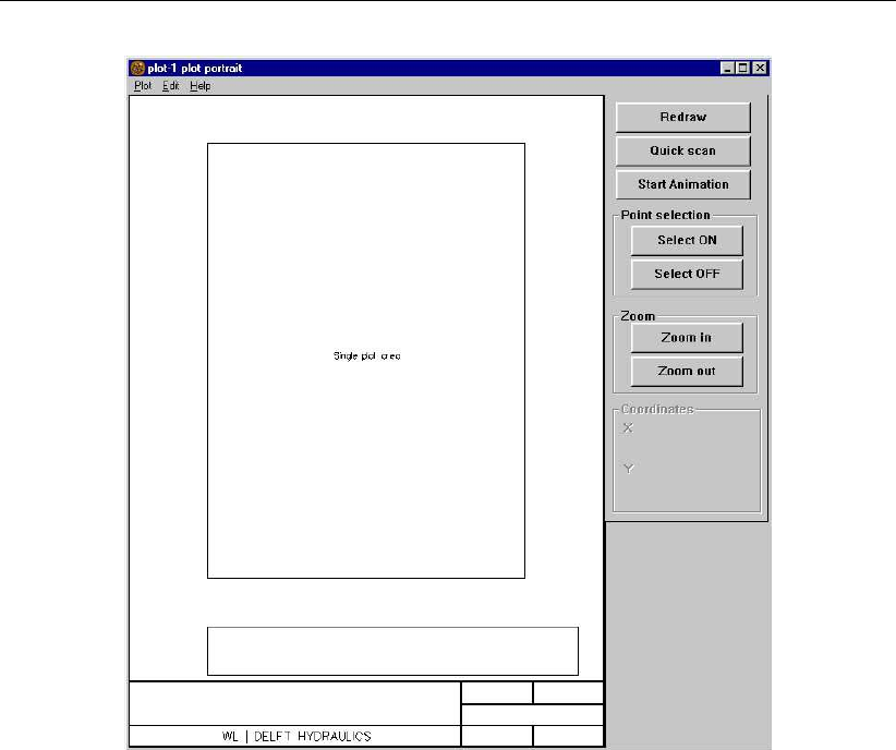
DRAFT
GPP, User Manual
Figure 6.1: Empty layout
four axes, one on each side of the plot area
a legend area (if there is one)
one single colour ramp
one single set of line-styles, line colours and so on
The implementation is as follows:
First, each plot routine will specify the axes (which axes, what type and the scaling) on the
basis of the associated data set. This information is combined into a common specification
for all axes.
Then each plot routine draws the data set:
it uses the set of line settings (as defined for that plot area!)
it uses the colour ramp (as chosen for that plotarea)
it specifies the legend entries
When all this is completed, the general routines in GPP plot the axes and plot the legend
(if there is one).
The actual plotting may be influenced by specific options other than the ones mentioned
above. For instance: the routine to plot time-series has an option to use the right axis instead
the left. The options to each routine are described in the separate appendices.
Note that GPP distinguishes the following types of axes:
Linear and logarithmic axis
50 of 190 Deltares
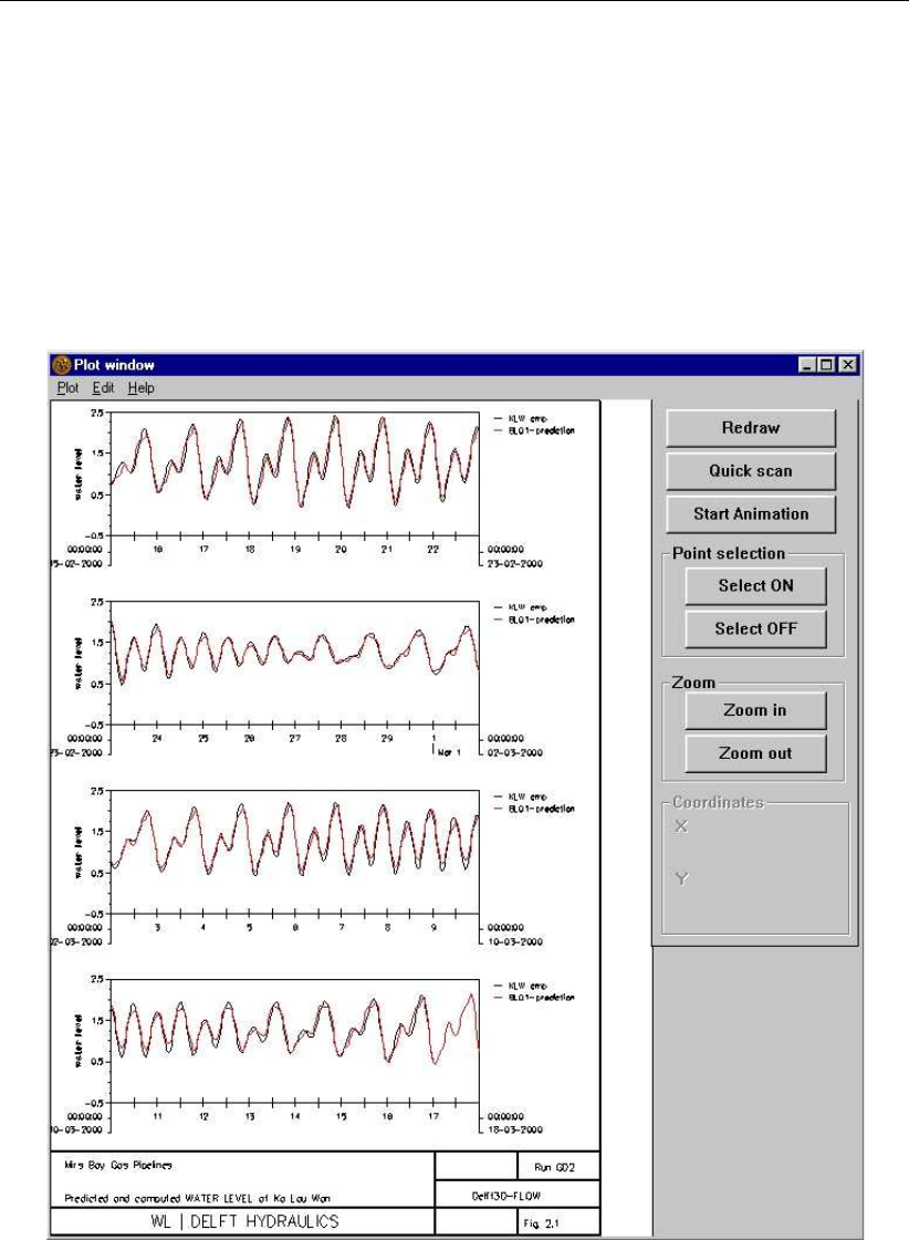
DRAFT
Layouts and plots
Figure 6.2: Filled-in layout: the plot
Deltares 51 of 190

DRAFT
GPP, User Manual
These types are used in xy-graphs and for the vertical axis in time-series plots.
Time axis
This type of axis is used in time-series plots (it can only be horizontal, at the bottom of the
plot area).
Geographic axes
If a plot routine uses this type of axis, then a vertical and a horizontal axis have the same
aspect ratio as the plot area. Specifying co-ordinates yourself (after double-clicking on an
axis) will lead to unexpected results. Instead use the zoom functionally to achieve this.
Polar axes
Some plot routines will use a polar co-ordinate system instead of a Cartesian (for instance
to draw a spectrum of directions and frequencies).
Special axes
For instance for plotting so-called limiting factors, a numerical axis is combined with an
axis with textual labels.
Which type of axis is used is determined by the first plot routine in the plot area. As the axes
are very characteristic of the plot, they should be properly taken care of. Some plot routines
provide an option to set the type of axis, others always use the same type.
A plot routine like the one for plotting time-series, defines the bottom and left axis or the bottom
and right axis, depending on an option. Therefore you can combine left and right vertical axes
with different scaling (but with the same bottom axis).
The final scaling is the result of a combination of all data sets in the plot that use this particular
axis.
52 of 190 Deltares
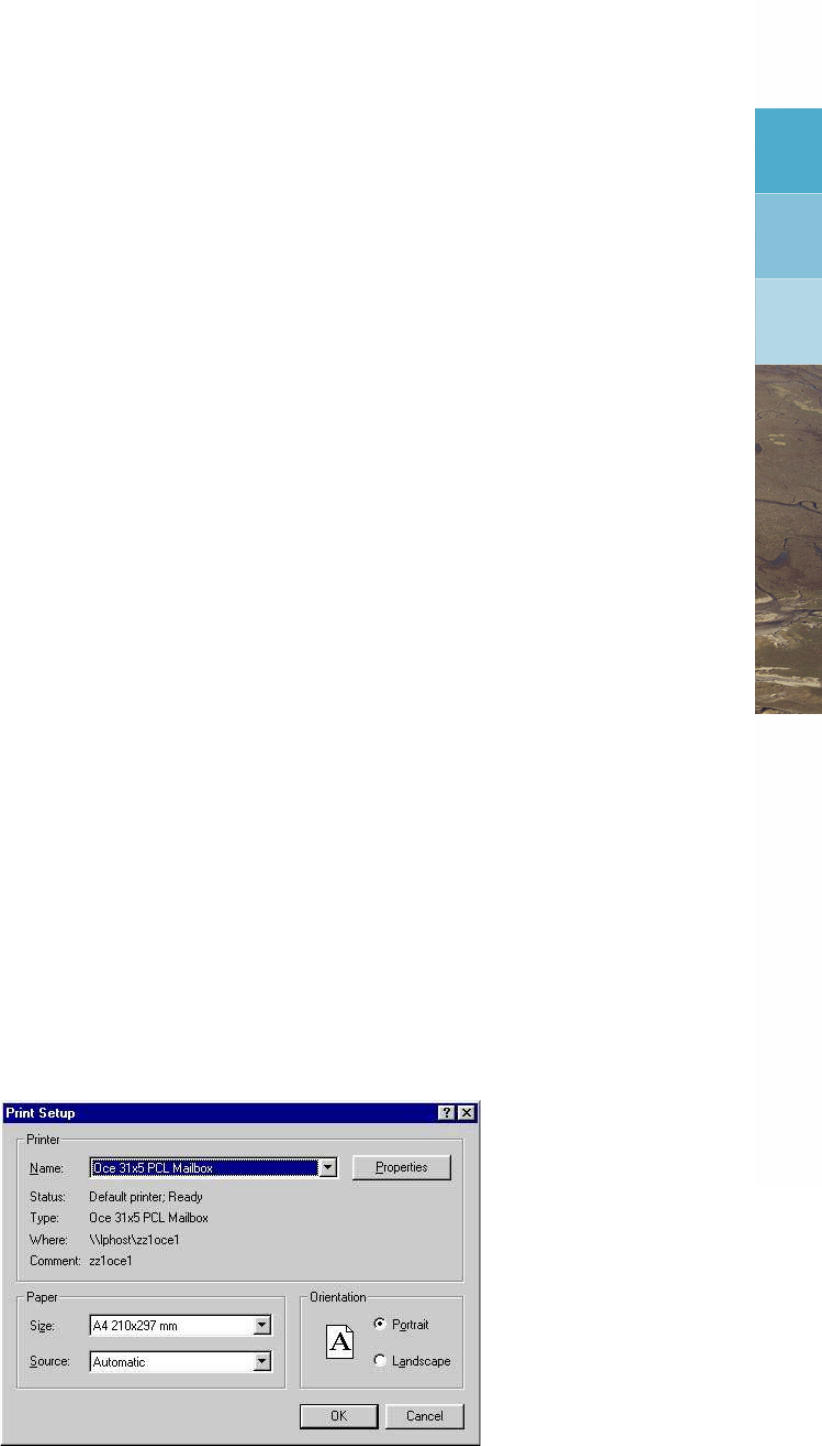
DRAFT
7 Customising GPP
This chapter describes the use of the GPP configuration files and some other points:
How to define printers and plotters (including some platform-dependent details).
How to define layouts.
How to set the default options for plot routines.
How to change colours, line styles and so on.
How to use GPP in an integrated environment and fine-tuning by command-line argu-
ments.
7.1 Printing and plotting
7.1.1 Defining printers and plotters
Under MS Windows the selection and definition of printers is handled directly by the operating
system. You can define new printers via MS Windows utilities.
Linux workstations on the other hand do not provide such utilities, at least not for ordinary
users. Such workstations have no way of knowing what the capabilities are of the printers
that are attached and therefore the programs that use the printers or plotters are to a certain
extent themselves responsible.
For this reason the set-up dialogue for the printers and plotters differs on both platforms. For
MS Windows, you can set the standard or default printer via Windows’ standard dialogue. For
Linux workstations the default printer is identified via the environment variables LPDEST and
PRINTER (see Appendix A).
When actually printing, the following dialogue comes up (Figure 7.1):
The list of printers and plotters in this dialogue, is taken from the configuration file <devices.gpp>
(see section C.1 for details). It contains a list of printers and plotters and their properties.
Important, but somewhat awkward properties are the paper size and the margins (see the ex-
ample below). They differ for each printer type, unfortunately, and for the printer/plotter driver
as well. To get correct values for a printer type not included in the installed list, you will have
to experiment.
Figure 7.1: Print setup dialogue
Deltares 53 of 190

DRAFT
GPP, User Manual
#
# \DGPP: definition of printers and plotters (what are their
# properties)
#
# Note: the margins depend on the device driver used. The margins
# in this file have been set correctly for the following drivers:
# - HP LaserJet III (HP/GL): GHPL300
# - PostScript (A paper size): HPOSTA
#
device ’print1 (HP LaserJet III (300dpi) )’
type black-white # alternative: colour
uniras-driver ’GHPL300’
orientation portrait # alternative: landscape
hardcopy-size 270.0 180.0 # long, short side (in mm)
left-margin 5.0
right-margin 2.0
top-margin 26.0
bottom-margin 1.0
print-command ’lp -dprint1 -oraw -onb’ # option: -onb = no banner
end-device
#
# PostScript printer
#
device ’ps2 (Postscript HP laserjet III)’
type black-white # alternative: colour
uniras-driver ’HPOSTA’
orientation portrait # alternative: landscape
hardcopy-size 297.0 210.0 # width, height in mm
left-margin 0.0
right-margin 0.0
top-margin 0.0
bottom-margin 0.0
print-command ’lp -dps2 -opostscript -onb’
end-device
For both workstations and PCs you can save the plot in an external file by using the right
“printer”. (Note that the “Delete” option for the print file is inoperative under Windows - if you
select another printer than the default one, the print file is always saved whereas for the default
printer there is ordinarily no print file.
Using this mechanism, you can create PostScript files containing the drawing and use them
in reports later on.
7.1.2 Configuring printers for GPP
GPP uses a configuration file, called <devices.gpp>, that describes the properties of the
printers and plotters that are available to GPP. This file is used under Windows, mainly to
define output to PostScript files.
The reason for using such a file is simple: Linux systems provide no way, or at least no simple
way, for an application to find out which printers and plotters are available and what their
properties are. Thus, the configuration file contains the following information per printer:
a descriptive string for the user
the type of printer or plotter, colour or black-white
the UNIRAS driver, which is a string identifying the software driver to be used, e.g. HPOSTA4
for black-white printers using A4-sized paper with postscript.
the orientation of the paper (portrait or landscape)
the size of the paper
the margins to be respected
54 of 190 Deltares

DRAFT
Customising GPP
the actual print command
All this information is necessary:
The descriptive string should contain the logical name of the printer, so that GPP can link
the printer to the default printer (LPDEST or PRINTER variable).
The software driver creates the print file. If there is a mismatch between the printer’s
capability and the print file, this will result in a large stack of useless paper.
The orientation of the paper is important as this is sometimes an option in the print com-
mand. This must match the orientation of the layout. Hence make two descriptions for the
printer: one for each orientation.
The actual print command and its options differs from system to system. Sometimes, a
small correction to the print file is needed, because the offset is wrong.
7.1.3 Procedure for configuring a new printer or plotter
To configure a new printer or plotter:
Find the description of a printer or plotter that resembles this new device.
Copy the set of lines describing it and change the descriptive string so that the logical
name (the one used in the environment variable LPDEST or PRINTER is contained in it).
Change the print command so that the correct device is used. You can use “%s” to sub-
stitute the name of the print file (otherwise it is simply appended to the command string).
If the printer is of the same type, you are done. Otherwise it is necessary to experiment
with the margins (they correct for the bizarre and completely obscure relation between the
printer’s logical co-ordinate system and the actual position on paper).
If there is no matching description, try the most reliable printer command languages, PostScript
and HPGL (the print files are ordinary text files). If your printer or plotter do not support either
of these, then filters like GhostScript might be used.
Remark:
The easiest way to get the margins right is to print an empty plot with a standard frame
via GPP: on an A4 paper the frame lines should be positioned 2 cm from the left and 1
cm from the other sides. Then measuring the actual position of the lines on paper and
calculating the diference should give you a fair indication of the correct margins.
Sometimes however, the useable area simply is not large enough. Then you will have set the
margins to whatever values will make the lines visible.
Some PostScript printers, especially those that use the HTPIIA4S driver, require a correction
of the origin. Check the script files “slpl” and others in the ./gpp directory on how this is done.
Deltares 55 of 190

DRAFT
GPP, User Manual
7.2 Anatomy of a layout
This section describes in some detail what a layout is made up of. Together with the descrip-
tion in Appendix C, you should be able to make new layouts yourself. (In future releases it
may be possible to interactively make layouts.)
In the frame below a simple example is given of one particular layout. The details are ex-
plained afterwards.
Layouts have four general attributes:
The units in which all positions and sizes are given: centimetres, inches or "stretch".
The latter unit requires some explanation. Layouts with this attribute always fit the window
or the paper in which they appear. Layouts with centimetres or inches as the unit attribute
will keep the same form and thus are not always able to fill the region.
Whether or not a frame is present:
If there is a standard frame it can be used to add descriptive text to the plot. The frame
has a fixed layout which can not be changed (see Figure 7.1). An alternative is the simple
frame that consists of a rectangle only.
The size:
All layouts have a width and height, given in the appropriate units. These are used mainly
to determine the aspect ratio. The actual size depends on the medium. For stretch units
the width and height determine the scale of the co-ordinates and sizes (the relative mea-
sure).
The orientation: portrait or landscape
The orientation on the screen, that is what is the long side and what is the short side is
determined by this parameter. Complications arise because this is unfortunately indepen-
dent of the actual orientation when printing or plotting on paper (that is determined by the
printer or plotter driver). Be careful to choose a consistent combination.
#
# GPP configuration: layouts
#
layout ’portrait-legend’ ’One plot area with legend’
units stretch
size 18 27
orientation portrait
standard frame
frame
’company’ ’DELFT HYDRAULICS’ font ’simplex roman’ 3.5 medium
’Black’
’main text 1’ ’ ’ default-font
’main text 2’ ’ ’ default-font
’main text 3’ ’ ’ default-font
’upper left’ ’ ’ default-font
’upper right’ ’ ’ default-font
’middle’ ’ ’ default-font
’lower left’ ’ ’ default-font
’lower right’ ’ ’ default-font
end-frame
plot-area ’single-area’ ’Single plot area’
position 3 7
size 12 19
legend
use datasetname
position 2 3
size 14 2
end-legend
end-plot area
end-layout
56 of 190 Deltares

DRAFT
Customising GPP
Within a layout you may define plot areas, text areas and groups, these being convenient
collections of other elements:
Plot areas:
These determine rectangles in the layout that can be used for plotting. The definition
may contain a rectangle reserved for the legend as well. Note that legends are logically
associated with a plot area, but they may be positioned anywhere.
Text areas:
Rectangles for putting extra text in the plot.
Groups:
Collections of layout elements that have the purpose of defining a new origin. All elements
belonging to a group are positioned relative to the origin of the group. This allows you to
move elements in the layout by changing the position of the group only.
There is no limit to the number of layout elements or the layouts (except memory), but in
practice the available space becomes limiting quite fast. As a consequence, certain layouts
are more suited for xy-graphs than others. Some are more suited for printing and others are
more suited for display on the screen.
7.3 Default options for plot routines
All plot routines use one or more options that influence the appearance of the actual plot.
These options can be set for each instance independently. Moreover the defaults can be set
for your personal preferences as well. You can not define new options, but you can define
"new" plot routines.
Suppose you often need plots of time-series with a right vertical axis. You can copy the
definition of the plot routine in the file <routines.gpp>, edit the default value of the "new" plot
routine and give it a unique description (see frame below). The name of the plot routine must
remain the same, because this is the link to the actual subroutine that does the work.
You are quite free to do this, just as with the defaults. Note that you should not change the
types of data sets that can be handled, as GPP might crash because of this. The routines
expect certain types of data sets and are not always capable of determine whether a data set
of the correct type has been supplied.
#
# Original plot routine "Plot Time series" has been copied
# - use right axis by default
#
# (name is the same) (description is unique)
plot-routine ’PlotTimeseries’ ’Plot Time series (right)’
no-topography
accepts-data sets
’TIMESERIES’ ’SINGLE’
’TIMESERIES’ ’MULTIPLE’
end-data sets
options \# Changed default
logical ’UseAxisRight’ ’Use right axis’ TRUE
.... (other options)
end-options
end-routine
Deltares 57 of 190

DRAFT
GPP , User Manual
7.4 Graphical settings
The file <setting.gpp>, which is explained in detail in Appendix C.5, contains the graphical
settings. As with all the other configuration files, you can adjust it according to your wishes. It
contains quite some information, but the following items may be of most interest:
Colours:
The colours section contains the name and the definition (for instance in RGB values from
0 to 255) of the colours to be used. You should not define too many colours, say more
than 50, as the internal colour table has only 220 free entries and you need space for the
colour ramps as well.
Colour ramps:
Colour ramps are sequences of colours used by any plot routine that needs such se-
quences. You can define any number of colour ramps, but the total number of colours in
the colour ramps plus the colours from the colours section must not exceed 220 say. If
there are too many, the list is truncated.
Line-styles:
Line-styles are used when a time-series or a similar interconnected series of points is
drawn. Each line style can have:
a line type (one of the predefined types)
a thickness (in mm)
a colour (one of the colours defined in the colours section)
a symbol (one of the symbols defined in the symbols section)
Global parameters:
There is a collection of “global” parameters that allow you to set values for such things as:
the colour-ramp to be used with contour maps and isolines
the unit for geographic axes (either meters or kilometers)
the orientation of polar axes (either clockwise or counter-clockwise, or a nautical ver-
sus mathematical orientation)
the language for month names
what “escape” characters to use for superscripts and subscripts in text
the relative sizes for a customised frame
Some can be changed via the user-interface, some can not
You are free to define or change any of these, but you must be aware that changing the
settings may affect the existing plots in the state file.
An example of the above mentioned sections is shown below. Apart from these settings
themselves, you can control the occurrence of lines, colours and symbols in two other ways:
for each type of device (screen, black-white printer or plotter, colour printer or plotter)
for each set of filetypes (the presentation section in the definition of the models and their
filetypes)
The first is meant to help optimise the appearance of the picture on any output device. The
latter is meant to help distinguish, for instance, data sets from measurements (typically pre-
sented as symbols) and data sets from numerical models (typically presented as lines).
#
# Colours section - the names are used in the other sections!
#
colours
’Black’ 0 0 0
58 of 190 Deltares

DRAFT
Customising GPP
’Red’ 255 0 0
’Darkred’ 127 0 0
’Green’ 0 255 0
’Lightgreen’ 200 255 200
’Darkblue’ 0 0 127
’Blue’ 0 0 255
’Cyan’ 0 255 255
’Magenta’ 255 0 211
’White’ 255 255 255
...
end-colours
... (sections for fonts, linetypes)
colour-ramps
colour-ramp ’Rainbow’
’Darkblue’
’Blue’
’Cyan’
’Green’
’Lightgreen’
’Yellow’
’Orange’
’Red’
’Magenta’
end-colour-ramp
...
end-colour-ramps
... (several sections left out)
default-settings
... (several options left out)
colour-ramp ’Rainbow’
#
# Unit for geographical axes:
# either meters or kilometers
#
geographic-axis-unit kilometers # Alternatives:
# kilometers or meters
#
# Orientation for polar axes:
# either clockwise or counter-clockwise
#
orientation-polar-axis clockwise
# Alternatives: clock-wise or counter-clockwise
#
# Language for months on the time axis
# either dutch or english
#
language-for-months english
# Alternatives: dutch or english
#
# Escape characters:
# When used in a text string, the next character
# will be subscripted or superscripted.
# Choose the characters with care - they can
# not be used in the text
#
subscript-escape ’‘’
superscript-escape ’\^{}’
#
# Custom frames (text boxes):
# Modelled after the standard frame,
# but with variable width and height
#
custom-frame-width 10.0 # <cm>
custom-frame-height 3.0 # <cm>
custom-frame-side right # Alternatives: left, right
custom-frame-part1 70 # Percentage of total
Deltares 59 of 190

DRAFT
GPP, User Manual
custom-frame-part2 30 # Percentage of total
custom-frame-part3 0 # Percentage of total
#
# For MS Windows we offer a crude method to influence the
# margins used for printing plots with a frame
# (as "devices.gpp" is not used for the system printer)
#
mswindows-margin-left 0.0 # mm
mswindows-margin-right 0.0 # mm
mswindows-margin-top 0.0 # mm
mswindows-margin-bottom 0.0 # mm
end-default-settings
series # line thickness (mm)
’solid - black’ ’Black’ ’no symbol’ ’solid’ 0.1
’solid - red’ ’Red’ ’no symbol’ ’solid’ 0.1
’noline x black’ ’Black’ ’cross’ ’no line’ 0.1
’noline + black’ ’Black’ ’plus’ ’no line’ 0.1
’dotted - black’ ’Black’ ’no symbol’ ’dotted’ 0.1
’dashed - green’ ’Green’ ’no symbol’ ’dashed’ 0.1
end-series
7.5 Working environment
7.5.1 Directories and files for GPP
GPP uses a number of so-called configuration files and they have to be located in some known
directory. GPP reads data files and stores the session files. Quite often you can just rely on
the defaults. But if you want to use specific configuration files, then you can do so by starting
GPP with one or more command line arguments like -workdir <directory>(see Appendix A).
The idea is:
The configuration files are found in some fixed directory: the directory where you installed
the program. It is called the system directory.
You start the program in some arbitrary directory and you want to use the files in that
directory.
This directory may not be a directory where you can write files (because you are not the
owner). So GPP distinguishes a working directory as well.
Thus:
At start-up the configuration files are read from the system directory.
The state file is read from and written to the work directory.
Files that you import are found in the current directory, which may change as you move
through the directory structure.
The current directory is not well-defined under MS Windows or else it is always the Windows
system directory, unless you explicitly specify a different location. So you need to specify it
yourself, for instance by setting it in the properties of an item in the Start menu.
60 of 190 Deltares

DRAFT
Customising GPP
7.5.2 File types and file names
The files that GPP can read come in roughly three categories:
Ordinary “text” files, that is, files that you can read and write using an ordinary editor like
notepad on Windows or vi on Linux.
Binary files with a platform-independent structure or
a structure that in practice is platform-independent.
This means that in practice GPP on Linux can read all files produced on Windows and vice
versa.1
File names and their exact location are a different matter:
Linux uses case-sensitive names for both files and directories. The full directory name
starts with /
Windows uses case-preserving names and the full directory name starts with “c:\” (or
some other drive).
To make sure that the proper files are read, GPP stores the full name (file name and the
directory that contains it) internally and in the session files. If you move the files to a
different location (a different computer for instance), you may have to edit the session file
– GPP does, however, accept relative names, like “..\..\data\myresult.dat”.
7.5.3 Description files
Apart from a stand-alone program, GPP offers the facility to work in a so-called integrated
environment. In such an environment, you are not confronted with the peculiarities of the un-
derlying operating system, but is shown a user-interface from which you operate the programs
without having to know precisely which files to edit and which programs to run. In such an
environment, you do not know the names of the files or their location.
The assumption made by GPP is that the integrated environment organises the files in some
sort of hierarchy. For example: the environment supports a simple scenario or case man-
agement, keeping track of data files for different models and different cases. One possible
classification can be:
Files from different models, but belonging to the same case, are recognised by a short
description of the case.
Files should also be grouped for the different models as not everybody is interested in all
model output all of the time.
Hence, some hierarchy is used, which appears "natural" to the user of the system. This
hierarchy can be made clear to GPP by passing it the name of a so-called description file:
gpp -descfile exmpl.dsc
Instead of showing the raw file names, it will show you the files listed in the description file
only. A simple example is shown below.
#
# Example description file
#
1Currently, the Solaris and SGI platforms ares not supported anymore. On these platforms it is possible to
produce files with an incompatible internal structure, due to the different byte ordering. The different line endings
in Linux and Windows do not matter however
Deltares 61 of 190

DRAFT
GPP, User Manual
begin ’Water quality results’
"del01.his" ’case 1: basic situation’
"del02.his" ’case 2: 10\% growth of waste loads’
"del03.his" ’case 3: realisation of all policies’
end
begin ’Waste loads’
"../waste/inp01.tek" ’case 1: basic situation’
"../waste/inp5a.tek" ’case 3: realisation of all policies’
"../data/meas\_r2.tek" ’measured waste loads (1993)’
end
...
62 of 190 Deltares

DRAFT
8 Advanced features
This chapter describes a number of features that are useful when you want to:
standardise the pictures or use batch editing, in general, create large numbers of pictures
with as little actions as possible
create animation files that are useful for presentations
8.1 Standardising pictures
In many cases, certainly when evaluating the results of several model calculations, or prepar-
ing a report with a large number of plots, you will want to minimise the effort to produce these
pictures. Another requirement is that they be uniform - use the same plot layout, graphical
settings etc. GPP has several features that can be employed. We will discuss them one by
one.
8.1.1 Batch processing
Within GPP, batch processing is loosely defined as printing without you having to select the
plots manually. This can be achieved by the command-line option -batch, followed by the
name of a session file. If this is specified, GPP will read the session file, print all pictures it
contains to the default printer and terminate when this is done. You need do nothing, except
wait for it finish.
We must make some remarks about the usage of this option:
On Linux the printer or plotter can be specified by a second option: -printer, followed by
a printer name defined in the <devices.gpp>file. Unfortunately, this can not be done on
PC: the printer that will be used is the default printer.
Though you can not do anything, for technical reasons, the program will still come up with
the start-up screen and the main window.
If, under Linux, the window manager asks you to place windows interactively, then the
appearance of the main window necessitates at least this action from you. The cause
is the policy of the window manager. If you want to use this facility, make sure the win-
dows appear on screen without interaction. (Under the Motif window manager, this is the
InteractivePlacement property which should be false.)
8.1.2 Editing the session file
A second step in reducing the effort to produce pictures is editing a state/session file outside
the user-interface of GPP. To understand this, note the following:
The state/session file is a text file which is divided in blocks. Each block contains other
blocks defining parts of a data set or a plot.
By manipulating these blocks you can create a new session file that contains different data
sets from different files in different plots.
Because the session file is made up of blocks, an edit program could manipulate individual
lines as well as blocks of lines. For example: replace the list of class values for contours
by a standard list or add the lines defining a land boundary data set to each plot area of
interest, so that each plot will contain the land boundary.
We will list a number of possible edit actions in detail:
If you have prepared plots from one data file and you want to get the same sort of plots for
another file (of the same type), then you can replace the name of the file(s) in the definition
Deltares 63 of 190

DRAFT
GPP , User Manual
of the data sets.
For instance:
The original data set is defined as (results from calculation 1):
dataset-def ’NH4’
model ’DELWAQ’
filetype ’ODS_DELWAQ_HIS_BIN’
file "scen1.his" "" "" end-files
parameter ’NH4’
all-times
location ’noordw 4/10’
end-dataset-def
You can simply change the file name and read the new session file:
dataset-def ’NH4’
model ’DELWAQ’
filetype ’ODS_DELWAQ_HIS_BIN’
file "scen2.his" "" "" end-files
parameter ’NH4’
all-times
location ’noordw 4/10’
end-dataset-def
Warnings:
This can only be done with files of the same type. GPP will not verify this, nor in some
cases would be able to do so.
If a parameter is asked for that does not exist in the new file, then the data set can not
be defined. Similarly, locations have to match. Times are matched by looking for the
one equal or just later than the one asked for.
If you have data from one location, parameter, layer or time and you want to see the data
for another location, parameter, layer or time. One way to proceed is:
Create a data set that contains all locations, parameters, layers or times that you might
be interested in:
◦For locations and times, this is simple: do not select a single location or time, but
click Create directly.
◦For parameters, this will depend on the file type: some file types can produce so-
called hierarchical parameters, such as the D-Water Quality balances file and the
PHAROS files.
◦For layers you need not do anything special.
Insert a block for creating a resultant dataset.
For instance:
resultant-dataset ’NH4 (tersch 4/10)’
selection ’SelectLocation’
operand ’NH4’
options
logical ’Interactive’ false
string ’SelectedString1’ ’tersch 4/10’
end-options
end-resultant-dataset
Another way is:
Copy the definition of a data set and change the name of the parameter, the location
or the time value.
Adjust the name of the data set (as they must be unique)
For example:
dataset-def ’NO3’
model ’DELWAQ’
64 of 190 Deltares

DRAFT
Advanced features
filetype ’ODS_DELWAQ_HIS_BIN’
file "scen1.his" "" "" end-files
parameter ’NO3’
all-times
location ’noordw 4/10’
end-dataset-def
Warning:
You need to give the new data set a unique name and use that whenever you use it in
a plot.
If you want to use a different data set in a plot, but with the same plot routine and the same
options, then you can simply replace the name of the old data set with the new one.
Warning:
The new data set must be of the same type and subtype as the previous one. GPP
will assume that is the case. Difficulties arise, from strange plots to program crashes,
should this not be the case.1
If you use a different data set, the axes may not have an appropriate scaling or the contour
classes may not match the values:
By setting the axis type of any axis to unknown-axis, rather than to linear-axis and so
on, you force a re-scaling of the axis.
By replacing the list of values for contour classes by the single keyword automatic-
scaling, you force re-evaluation of the contour classes.
If you require a uniform zoom area for contour plots and such, you can copy the axis
definitions for a plot area that is to your liking to any others using similar type axes.
Warnings:
The sizes of the plot area are important, as the limits for the horizontal and vertical
geographic axes are coupled. Use this only for plot areas with the same aspect ratio.
If the aspect ratio is slightly off, you may change the type of the axes into linear in
stead of geographic. By doing so you break the connection (the risk is that the picture
gets distorted a bit). It may be safer to try and resize the plot area itself.
An alternative method is to create a dedicated layout. The layout will then contain the axes
definitions and they will be copied in directly by the user-interface (see the next section).
If you want to add a set of standard data sets (like land boundaries) to each plot area,
you can do so by copying the lines dataset ... to end-dataset that put such a data set with
the associated plot routine into the plot. The order in which such blocks appear in the plot
definition is the order in which they will be drawn.
Warning:
When you edit a session file yourself, you must make sure that the syntax is correct. GPP
will warn about syntax errors and stop reading the file. Something GPP will not do is
check whether data sets are indeed compatible:
When a link to a topographical data set (better known as a grid data set) is encountered
in the definition of a data set, there is no check if this is indeed compatible with the data
set itself.
When a binary operation, like addition, is specified, again there is no check whether the
two data sets are indeed compatible.
1Actually, the condition is a bit more relaxed than this. The given condition is the simplest and the safest. To
check the type and subtype: see the definition of the data set in the state/session file. Unfortunately, this does not
work with the resultant data sets.
Deltares 65 of 190

DRAFT
GPP , User Manual
There is, in general, no way to make sure that the data files are of the same type as stated
in the definition.
These checks should be built in to make the editing of session files safer. Right now, these
are the caveats you must deal with. Especially the last one is of importance!
8.1.3 Using dedicated layouts
A layout defines the position of plot areas, the (default) contents of the frame and so on. In-
ternally, the data structure for a layout is also used for keeping information about the plots. As
the plots need to retain information about the extreme axis co-ordinates and other parameters
for the plot area, this information is actually part of the data structure for the layout. In other
words, layouts may now also define the default axis settings: colours, visibility, but also the
extreme co-ordinates, in fact anything there is to tell about plot areas and the associated axes
except for the data sets and plot routines.
Using this new feature, the layouts may be specialised in such a way that you can zoom in
on a fixed area, if you specify default axis settings via the layout. Simply copy the lines that
define the axis settings from a plot definition into a (new) layout and any data set that is drawn
in that particular plot area will be plotted using these very same co-ordinates. This works not
only with geographical axes, but in fact with any axes.
It does have one drawback: the layout becomes dedicated to a particular type of plot, and you
will be forced to be careful about the sort of presentations you use in it. (Currently, there is no
fully operational auxiliary program that helps you with the editing.2)
Below is an example of a filled-in layout:
layout ’portrait-filledin’ ’Partly filled in, with legend’
units stretch
size 18 27
orientation portrait
no frame
plotarea ’single-area’ ’Single plot area’
position 3 7
size 12 19
legend
position 2 3
size 14 2
end-legend
#
# Define the default axes
#
default-area-settings
axis bottom
type time-axis
visible yes
text ’’
start 1997/02/05 12:00:00
stop 1997/02/11 12:00:00
stepsize 1:00:00:00
default-axis-settings
end-axis
axis left
type linear-axis
2You can use scripting languages like AWK or Perl to achieve the automated editing via small dedicated pro-
grams. This is the most practical solution, but thus require some programming skill. An example is shown in
Appendix E.
66 of 190 Deltares

DRAFT
Advanced features
visible yes
text ’’
start 7100
stop 7350
stepsize 25
default-axis-settings
end-axis
end-plotarea
end-layout
Note that this is simply an example and has no particular meaning.
This makes a layout more specific. The reverse situation occurs with the definition of plots.
These specify precisely what numbers to use on the axes. It would be nice, to allow some
automatic scaling, when putting in a different data set than the one(s) used to define the plot.
This can now be done: by replacing the type of the axis in question by the keyword “unknown-
axis”. This triggers the scaling algorithm to use the actual scaling information from the data
sets in the plot area, rather than rely on the values from the definition.
The last remark about layouts concerns the positioning of the legend. Normally, the position is
given with respect to the lower-left corner of the whole plot, as is the position of the plot area
to which it belongs. By using the keyword relative-position instead of position you can place it
with respect to the lower left corner of the plot area. Thus it is easier to vary the layout:
plotarea ’single-area’ ’Single plot area’
position 3 7
size 12 19
legend
relative-position -1 -4
size 14 2
end-legend
8.2 Creating animations
Creating animation files is relatively simple, but the procedure is a bit special and there are
some pitfalls some of which are platform dependent. This section will clarify both the proce-
dure and the pitfalls.
The procedure can be divided in three steps:
create data sets that contain several time steps so that the results can be drawn for these
times
prepare individual pictures (or frames) for each time
create the animation file from the individual frames
Suppose you have a file that contains the salinity over a whole model grid and several times.
Rather than selecting the parameter and a time in the dialogue to add new data sets (click
Add in the Data Group Datasets), you simply select the parameter and do not select a time.
This will result in a data set defined over the grid with more than one time. Such a data set
can not be drawn directly, instead you are asked to select a time when adding the data set to
a plot.
Select a time (this needs not be the first time), prepare the whole plot, by adding a land
boundary, changing the plot options etc. When you are satisfied (see the pitfalls), then click
Start animation (Step 2). The result of this action is that the data for the first time are drawn
and the picture is stored in a bitmap file, then the data for the next time are retrieved and
Deltares 67 of 190

DRAFT
GPP, User Manual
drawn. The new picture is stored in another file and so on. When the hourglass disappears,
all times will have been treated this way and a series of picture files results.
These files are called <anim0001.xwd>,<anim0002.xwd>,<...>(on Linux) and <anim0001.bmp>,
<anim0002.bmp>,<...>(on MS Windows). They are found in the work directory. The files
are either in XWD-format or in the Windows bitmap format. Specialised programs, such as
ImageMagick’s convert can be used to create a very compact animation file (Step 3)3Other
programs create AVI-files, a file format popular with Windows multimedia applications. The
drawback is that the file seems to be about as large as the sum of the original bitmaps.
It is beyond the intentions of this manual to discuss further the advantages and disadvantages
of the various programs. Many freeware and shareware programs exist, but the tools from
ImageMagick give very good results.
It is more important at the moment to know the pitfalls of the procedure within GPP:
Once started, the animation can not be stopped in an elegant way. You can stop it, though,
by closing the window from the system menu.
Data sets that are used in an animation do not, currently, retain the original time, but rather
refer to the last time. When preparing a different plot, you should keep this in mind.
Automatic scaling of, for instance, contour classes is based on the first time step shown,
not on the data in the whole time frame. So either choose a representative time or change
the contour levels manually.
Existing animation files will not be overwritten, rather the count is increased until a gap is
found. GPP does not give any warnings about it.
When making an animation of different data sets in the same plotarea, the various data
sets should have the same time information (i.e. start and stop time, and time interval).
When making an animation of a plot with more than one plotarea, all plotareas should be
filled-in.
8.3 Facilities for making animations
It has long been possible within GPP to create picture files for each timestep in a data set.
However, converting these picture files into a single animation file, such as an AVI file or an
MPEG file was not supported via GPP. The reason for this is that there are many programs
available that can do this conversion and every user was supposed to find an appropriate so-
lution for themselves. For the Linux platform, a popular choice for such a conversion program
is ImageMagick’s convert (http://www.imagemagick.org). For MS Windows there are many
free and commercial products available. Unfortunately most come with a GUI that helps you
select and order the individual frames but they do not allow you to specify them via a batch
file.
The solution described below does make it possible to automate the conversion process on
MS Windows. It relies on a program called VideoMach. As this is a commercial product, you
will have to get a trial version yourself and decide if this is something you want to continue to
use (http://www.gromada.com/videomach.html). But it at least gives a smooth procedure to
turn the frames into an AVI file.
The procedure is simple:4
Create a session file with the data sets you want to show
Prepare the picture that is to be animated as the first plot
3The procedure for creating an animation is described in more detail in Appendix D.
4By courtey of S. Luger, CSIR South Africa.
68 of 190 Deltares

DRAFT
Advanced features
Store the data sets and the plot in a session file
Then run the batch file "gpp_animate.bat" with the name of the session file as its argument
(you will find this batch file in the directory ...\delft3d\w32\gpp\bin\):
C:\> gpp-animate.bat filename.ssn
This will start GPP with a number of command-line options:
-animate to start the animation for the first plot
-plotsize to set the width and height of the plot window to convenient values
When the animation is completed, one or more frames remain on disk and the conversion
program is started. The end result is an AVI file.
8.4 Automatically exporting data sets
It is possible to automate the export of data sets. This is especially useful if you need the
data from several data sets in a different format for further analysis. The method for doing this
consists of the following steps:
Define the data sets and store the definitions in a session file
Insert blocks like the one below into the session file (by using an ordinary text editor),
these blocks should come after the data set they refer to:
export
dataset ’name of dataset’
to-file ’filename’
export-routine ’WriteTimeseries’
options
# If needed
end-options
end-export
Load the session file into GPP. During the loading process, the export functions will be
executed as indicated by the export blocks. (You can of course do this via the batch option
too.)
The format of the export blocks is straightforward:
A block starts with the keyword export and ends with the keyword end-export.
Within the block you need to indicate what data set to export, what export routine to use
and to what file to write the data.
Because several export routines have options that control their operation, you need to
specify a block of options too.
The names of the export routines (not the descriptions) and the corresponding options can be
found in the routines.gpp file. For completeness, here are a few examples:
Exporting a timeseries to a file which uses spaces to separate the values:
export
dataset ’name of dataset’
to-file ’filename’
export-routine ’WriteTimeseries’
options
end-options
end-export
Deltares 69 of 190

DRAFT
GPP, User Manual
Exporting a time-series to a file which uses tabs to separate the values (a format com-
monly used by such programs as MicroSoft Excel):
export
dataset ’name of dataset’
to-file ’filename’
export-routine ’WriteTimeseries’
options
list ‘SeparatorType’ ’tab’
end-options
end-export
(If you want a comma instead, use ‘comma’ as the value to the option ‘SeparatorType’.)
Exporting a time-series to a “TEKAL” file (one with a simple tabular structure):
export
dataset ’name of dataset’
to-file ’filename’
export-routine ’WriteTSTekal’
options
end-options
end-export
(If you want a comma instead, use ‘comma’ as the value to the option ‘SeparatorType’.)
Exporting a 2D data set to a “TEKAL” file:
export
dataset ’name of dataset’
to-file ’filename’
export-routine ’WriteMAP2DTekal’
options
end-options
end-export
(In most cases, there is no option required.)
Though the list above is not exhaustive, it does include the most common types of output.
8.5 Automating tasks
As of version 2.11 GPP provides several so-called scripting interfaces, which enable sophis-
ticated automation and customisation of tasks. For this it uses the Tool Command Language
or Tcl, which is a very simple yet flexible and powerful language.
Scripts are interpreted rather than compiled programs or routines and this makes it possible
to extend the program without having to recompile and link. Instead the program reads the
source code at start-up and executes it when asked. Another advantage of scripting is that
it can hide many of the tedious details from the casual programmer, making the source code
more concise and easier to read and write.
You can distinguish two sets of scripting capabilities. The first set is more or less an alternative
to the user-interface: rather than interactively define data sets and plot, you can use the
scripting interface to programmatically define them and thereby automate the tasks. This has
not been implemented to its full potential yet and we mention it pro memorie.
The other set allows you to define your own routines for presenting and exporting the data
sets. This is the subject of the next section.
8.6 Defining your own plot and export routines
Via the scripting interface you can define a routine to plot a particular data set or to export the
contents to a file. For instance: GPP does not contain a plot routine that draws a truncated
Fourier series (that is: the time-series is fitted to a Fourier series with only a few terms and
70 of 190 Deltares

DRAFT
Advanced features
that series is then drawn). With the scripting interface, you can define such a routine yourself
and add it to GPP.
When you use the scripting interface to define new plotting or exporting routines, you need to
follow a simple protocol:
For plotting routines, there are two steps:
Specify the co-ordinates for the axes and what kind of axes should be used
Draw the data set
The reason for these two steps is simple: the axes are a common resource, they are
shared by all the data sets that are plotted within the plot area – this way you can combine
two or more time series for instance in one graph. The first step allows GPP to make a
common scaling and the second step allows the individual routines to use this scaling.
For exporting routines, there is only one step:
Write the data in the form you want to the external file
The file to which the data should be written is managed by GPP, so there is no need to
open or close it.
The routines must be registered within GPP. For this, there is a simple mechanism:
Use the plot-routine command to register a new plotting routine
Use the export-routine command to register a new export routine
Both commands have the same interface (modelled after the blocks in <routines.gpp>
– see section C.4):
◦A formal name (for recognition in the session file, this must be unique)
◦A title (for display in the user-interface)
◦A list of acceptable types for topographical data sets
◦A list of acceptable types for ordinary data sets
◦A list of options
◦The code for the routine
Here is an example:
plot-routine PlotTest "Plot Cumulative Distribution" {} \
{TIMESERIES SINGLE} {} {
PlotTest $mode
}
Let us examine a simple example: a routine to draw the (estimated) cumulative distribution for
a time-series:
First step (mode “specify”):
We need to determine the range for the horizontal axis. So we get the values from the
data set via the command “dataset data” and examine them in the “foreach” loop.
We take the range for the vertical axis to be 0 to number of values.
Second step (mode “draw”):
We need to determine the rank of each value in the time-series – get the values and sort
them in ascending order (via the lsort command).
We then loop over the sorted values and draw the line segments, where the vertical co-
ordinate is the index in the list. This way we get a raw estimate of the cumulative distribu-
tion.
Deltares 71 of 190

DRAFT
GPP , User Manual
Here is the code:
proc PlotCumulativeDistribution {mode} {
#
# Determine the extremes
#
if { mode == "specify" } {
set vmin 1.0e20
set vmax -1.0e20
set count 0
foreach value [dataset data] {
if { $vmin > $value } {
set $vmin $value
}
if { $vmax < $value } {
set $vmax $value
}
incr count
}
#
# Define the axes that we want to use
#
setaxis bottom linear vmin vmax
setaxis left linear 0 count
}
#
# The actual drawing part
#
if { \mode == "draw" } {
#
# Select the axes, so that we can use ’’natural’’ coordinates
#
useaxes bottom left;# in that order
set count 0
set sorted [lsort --real [dataset data]]
foreach value $sorted {
if { count == 0 } {
set xend $value
set yend $count
} else {
set xbgn $xend
set ybgn $yend
set xend $value
set yend $count
plotline $xbgn $ybgn $xend $yend
}
incr count
}
}
}
If we want to export this distribution to an external file, then we could do this via the following
routine (its one argument is the handle to the output file):
proc WriteCumulativeDistribution {outfile} {
set count 0
set sorted [lsort --real [dataset data]]
foreach value $sorted {
puts outfile ’’$count\t$value’’
incr count
72 of 190 Deltares

DRAFT
Advanced features
}
}
Note that we use a tab (\t) to separate the two values. The routine could be enhanced by also
writing information about the data set in question and so on.
8.6.1 Script commands
For plotting the following commands are available, besides the general commands of the
scripting language:
plotline x1 y1 x2 y2
Plot a straight line segment from (x1,y1) to (x2,y2)
plottext x y string
Plot the text string at position (x,y)
setcolour colour
Set the colour for drawing or filling. The colour argument can be a name or an index as
returned for colour options.
setthickness thickn
Set the line thickness (in mm).
getarea
Returns a list of four numbers: the minimum x and y co-ordinates of the plot area and the
width and height (all in mm).
getworldcoords
Returns a list of four numbers: the minimum and maximum x co-ordinates and the mini-
mum and maximum y co-ordinates of the current world co-ordinate system.
setaxis which type min max step
Let the axis at which side (bottom, left, right or top) from min to max (at least) with op-
tionally a stepsize of step. The type of axis is type (linear, logarithmic, time, geographic or
polar).
useaxes horiz vert
Select which axes to use when drawing (where horiz is either “bottom” or “top” and vert is
either “left” or “right”)
dataset subcommand
Get information about the data set to be drawn. The subcommand determines what infor-
mation is returned:
name: return the name of the data set
parameters: return the names of the parameters it contains (as a list)
locations: return the names of the locations it contains (if any, as a list)
times: return the times it contains (as a list)
data: return the data it contains (as a list)
getoption name
Return the value of the named option. If there is no such option, an error is raised.
For exporting only the dataset and the getoption commands are available (as they have noth-
ing to do with plotting).
Deltares 73 of 190

DRAFT
GPP, User Manual
74 of 190 Deltares
DRAFT
9 Installation
Installing GPP is simple: most of it is taken care when you install the Delft3D package. A few
items remain and they are described separately for each platform.
9.1 Installing on the PC
The first step in the installation is taken care of by the Delft3D installation procedure. You will
find that the GPP executable is stored in a directory under Delft3D (the name is . . . \w32\gpp\bin)
and the configuration files can be found in . . . \w32\gpp\lib.
There remain these two issues:
You may want to run GPP outside Delft3D.
In that case, making a short-cut in the standard MS Windows way will suffice. Note that
the start-up directory for the short-cut will be the system and working directory for GPP,
unless you give the proper command-line options.
You may want to customise the configuration files.
As explained in chapter 7, the configuration files are read from the GPP system directory.
Simply create a separate directory and copy the files (*.gpp) in the lib directory to this new
one. You can then set the start-up directory for the short-cut to that same directory. Or
you can use the command-line options to make GPP read the customised versions.
Remark:
When you use GPP via the Delft3D menu system, it will read the set of configuration
files found in the ..\w32\gpp\lib directory, as no special system directory will be specified.
9.2 Installing under Linux
The first step in the installation is taken care of by the Delft3D installation procedure. You will
find that the GPP executable is stored in a directory under Delft3D (the name is $D3D_HOME/$ARCH/gpp/bin)
and the configuration files can be found in $D3D_HOME/$ARCH/gpp/lib.1
There remain these two issues:
You may want to run GPP outside Delft3D.
Simply start the program via:
> gpp
(with or without additional command-line arguments)
You may want to customise the configuration files.
The script gpp_install will create a directory ˜
/gpp if it does not already exist and copy the
default configuration files to that directory. The script will make a backup of any existing
configuration files. Simply type:
> gpp_install
Of course, if you want to use specific configuration files, you can do so by copying these
configuration files to a separate directory and edit them. Then run GPP via:
> gpp -sysdir some directory
Remark:
Under Linux GPP is started via a shell script, even in the Delft3D menu system. This
means that it will read the set of configuration files found in the directory $HOME/gpp,
1The environment variables are set by the Delft3D login script or profile.
Deltares 75 of 190

DRAFT
GPP, User Manual
if you have such a directory (run gpp_install for this) or from the central directory if you
do not.
76 of 190 Deltares

DRAFT
10 Glossary
Below is a list of terms commonly used in the context of GPP:
absolute time Time given in the form of calendar date and time
action routine Routine in GPP designed to perform a certain task using data sets, such
as plotting or exporting the data to an external file
colour ramp Sequence of colours that are used for instance in contour maps
command-line
argument
Options that can be specified at start-up
configuration
file
File that contains certain information important to the working of Delft3D-
gpp
contour classes Sequence of numbers that are used to create contour maps and such
data set Collection of data, identified by a unique name
Delft3D Comprehensive user-interface for multi-dimensional models
devices.gpp Configuration file, contains definition of printers and plotters
dialogue User-interface element, an area on the screen meant to enter data in
some way or other. It can be moved, but in most cases it can not be
resized
export routine Subroutine to export the data in a data set to an external file. May have
options
file Output file from a model, containing results, or a database
filetype ods type of an output file
filetype.gpp Configuration file, contains models and associated filetypes
gppstate.0 File containing previous data set and plot definitions (the last state is
saved in it)
gregorian date Representation of date and time in year, month, day of the month etc.
history file File containing time-series for quantities at separate locations
julian date Internal representation of date and time, as the number of days since a
reference date and time.
layout Specification of the position and size of plot areas, legends additional
texts etc.
Linux Operating system that resembles UNIX
list box User-interface element that allows selection from a list
list button User-interface element that allows selection from a list, but the list has
to be opened first
layouts.gpp Configuration file, contains definitions of layouts
location Location in the area that is studied, such as a monitoring station
map file File containing information on the value of a quantity in the whole model
area, such as the concentration distribution at several times.
menu User-interface element, represents one or more tasks that can be se-
lected with the left mouse button
menubar User-interface element, collections of pull-down menus. Selecting an
item shows the pull-down menu
model Computer program which produces the output files (or any other source
of datafiles)
model-grid Special parameter, handles the grid used by models but can also contain
geographical data
MS Windows Windowing system commonly used on PC’s. In this manual the term
covers Windows 95, 98, NT and XP
ODS Open Data Structure, a set of concepts and subroutine definitions to
deal with a wide variety of filetypes
Deltares 77 of 190

DRAFT
GPP, User Manual
operation Operation on the data in one or more data sets, like adding two param-
eters or calculating the average over time. This will result in a new data
set
operation rou-
tine
Subroutine that takes care of a particular operation
options Options for action routines (defined in file routines.gpp)
parameter Quantity for which data can be imported
plot Layout plus data sets and associated presentation forms
plot area Area in a layout or plot designated for plotting data sets
plotroutine Subroutine that plots the data set in some form. May have several op-
tions to customise the appearance of the plot.
presentation Form of graphical presentation of a data set
push button User-interface element to make an action start (or finish)
relative time Time given as the number of time units since a reference time
routines.gpp Configuration file, contains the definitions of action routines with their
options
selection Method of creating a subset of a particular data set
selection rou-
tine
Subroutine that takes care of the selection (including the necessary di-
alogue)
session file File containing the definitions of data sets and plots
setting.gpp Configuration file, contains graphical settings
TEKAL Name of a general plot package that defines one particular file format
text field User-interface element to enter a text string (in the case of GPP only
single-line texts can be entered)
time Time (date and time) for which the imported value holds
window User-interface element, area on the screen that acts as a unit. Can be
moved and resized.
78 of 190 Deltares

DRAFT
Glossary
Deltares, 2016. “BIBTEX key with no entry, needed if no citations are made in the document.”
Deltares 79 of 190

DRAFT
GPP, User Manual
80 of 190 Deltares
DRAFT
A Command-line arguments
GPP recognises the following command-line arguments (see below for some examples):
-display <display>This indicates which X-terminal or console to use. It is a
standard X command line argument and hence has no
meaning under MS Windows. (Other X arguments are
recognised as well, but they are much less common.)1
-sysdir <directory>Specify the directory where the configuration files can
be found (different from the default directory).
-workdir <directory>Specify the directory where the state file (gppstate.0)
can be found and will be written to. Any other files pro-
duced by GPP will also be written to this directory, un-
less the name explicitly refers to a different location.
-descfile <description file>Specify a so-called description file. This allows GPP to
link to integrated model systems where you do not deal
with files directly but with scenario names and such.
The actual data files are hidden from you and therefore
they should not appear in GPP either (see chapter 7)
-session <session file>Specify the session file to read instead of the default
state file <gppstate.0>
-batch <session file>Specify the session file to read and print all the plots it
contains. After that, the program will finish.
-animate <session file>Specify the session file for which to automatically start
the animation. Note only the first plot is animated in
this way. The program will automatically stop when the
animation is completed.
-convertto <extension>Convert the raw bitmap file to a file of the type
indicated by the extension (like: gif). This op-
tion relies on ImageMagick and for valid extensions
we refer to the ImageMagick documentation (see
<www.imagemagick.org>).
-printer <printer name>Specify the name of the default printer. This makes
sense under Linux only, as on PC a different method
is used. This option overrides the values from the
LPDEST and PRINTER environment variables.
-plotsize <widthxheight>Specify the initial size of plot windows as width and
height in pixels. For instance: -plotsize 600x400.
Useful for controlling the result of an animation.
-noprint Do not send the print files to the printer. This is useful
in combination with the -batch and -savefile op-
tions. Printing will be suppressed and instead the print
files are saved. This is useful under Linux only.
1Sometimes it is useful to specify a foreground and background colour, if the display can not allocate the
colours from the resource database. This would look like: gpp -fg black -bg white. Such arguments
are not taken care of by GPP explicitly and cause it to complain about unknown arguments. Simply ignore these
messages.
Deltares 81 of 190

DRAFT
GPP, User Manual
-savefile When printing, save the print file (that is do not delete
it after the print command has finished). This is useful
under Linux only.
-scriptfile <file name>Instruct GPP to run a script file after initialisation. This
enables you to automate certain tasks, like opening a
plot window.
-verbose Instruct GPP to print additional information on the
screen, such which command-line options are used and
where all the files come from. This should help you to
identify possible problems with the configuration.
Note that the arguments are evaluated from left to right and that they take immediate effect. If
you rely on relative directory names, you must be aware of this.
Examples:
gpp -display foo:0.0 -workdir . -sysdir $HOME/gpp
This is used under Linux to make GPP use the X-terminal called "foo", get the statefile (if any)
from the current directory and use the configuration files from the directory $HOME/gpp.
gpp -printer laser1 -savefile -noprint -batch scen1.ssn
Select the "laser1" printer from the <devices.gpp>file as the printer to prepare print files for,
leave the print files, do not send them to the printer. Use the session file <scen1.ssn> and
process this in batch mode, so that we get all the pictures in it in a bunch of print files.
GPP uses a small number of environment variables. They are listed in Table A.2. You do not
need to define them, as appropriate defaults are supplied.
Remark:
On PC, GPP uses a number of dlls, notably the XVT dlls. When loading the program,
MS Windows will search for any such libraries and uses the PATH variable for this. It is
safest, however, to install these libraries in the same directory as the executable.
Table A.2: Environment variables used by GPP
Environment vari-
able
Platform Meaning
DISPLAY Linux Name of X-terminal to be used
GPPHOME Linux Directory where GPP has been installed
LD_LIBRARY_PATH Linux Path for locating the shared objects
LM_LICENSE_FILE Both Full name of the license file
LPDEST Linux Name of the standard printer
PATH MSWindows Used for locating the DLLs
PRINTER Linux Also name of the standard printer
UIDPATH Linux Path for Motif UID file
82 of 190 Deltares
DRAFT
B ODS error codes
The table below gives the meaning of the ODS error codes. Sometimes the code is displayed
instead of an explanatory text:
Error code Description Name
0 Okay IEOK
1 Unable to determine filetype IEUNDE
2 File type not implemented in this version IEUNKN
3 File is not of indicated type IETYPE
10 File does not exist IENOFI
11 No free handle (too many open files) IENOHA
12 File already open IEFIAO
13 File locked by other program IEFLCK
14 Access denied/file is read-only IEFIRO
15 Record locked by other program IERLCK
16 Cannot lock file/record/share not installed IENLCK
17 File not new IEFNNW
20 File does not contain wanted information IEINFO
21 Unexpected end of file IEUEOF
30 Too many parameters found for array space IEPMNY
31 Too many locations found for array space IELMNY
32 Too many times found for array space IETMNY
35 No. of parameters <1 IEPLOW
36 No. of locations <1 IELLOW
37 No. of times <1 IETLOW
40 Bad date/time format IETIME
41 RunId not equal IERUNI
42 Par. not equal IEPARI
43 Loc. not equal IELOCI
44 Time not equal IETIMI
45 Time-step too small (time can not be represented) IESTEP
91 Buffer space too small (warn WL technical support) IEBUFF
92 No space left on device IEDISK
99 Other error IEOTHR
Deltares 83 of 190

DRAFT
GPP, User Manual
84 of 190 Deltares

DRAFT
C Description of files used by GPP
GPP uses the following configuration files:
<devices.gpp>Which printers and plotters are defined for the system (used only on
workstations)
<filetype.gpp>Description of the filetypes and the models or information sources in
general they belong to
<layouts.gpp>Layouts of the plots that can be used
<routines.gpp>Plot routines and such and their properties
<scripts.gpp>Script library
<setting.gpp>Graphical settings for (new) plots
It also uses a so-called state file, <gppstate.0>, which contains the data sets and the plot
routines that were defined during the last session and session files which serve the same
purposes. They can be explicitly selected via the user-interface.
In this appendix the format of these configuration files is explained, as well as that of the state
or session file. All these files are simple text files (or ASCII files) so that if you want to, you
can edit them via a standard text editor.
This appendix also describes the X resources files for GPP that are used under Linux.
C.1 Description of the file <devices gpp>
GPP uses a device definition file to define the properties of the printers and plotters. This file
is used only under UNIX/X Window, as X Window or indeed the UNIX operating system itself
provides no way to identify the printers, plotters and their capabilities.
Under MS Windows the operating system itself is responsible for the printer and its capabili-
ties.
Under Linux the method of printing and plotting is simply this:
produce a file which can be printed or plotted (taken care of by agX/UNIRAS ROUTINES
and device drivers)
issue a command to send the file to the printer or plotter.
As the workstation itself provides no method to check the capabilities of the device, you must
yourself take some care: a PostScript file on an ordinary printer simply produces a large stack
of paper with a lot of print commands. The above way of working allows you to save the
plot file, something which can only be achieved in MS Windows or Windows NT with screen
grabbers (we will work on it, it is not that hard).
The following is a description of the format of the file containing these definitions:
Any text following and including a hash (#) is considered comment and is ignored up to the
end of the line. Any number of blanks can appear between keywords and values. They
are used as separators.
The file starts with a version string in the following format:
version 2 minor 00
Each printer or plotter is defined by a separate block. The order of the blocks is irrelevant,
though the order of the statements within the block is fixed.
Each block starts with a descriptive string, which will be shown to the user. The string
Deltares 85 of 190

DRAFT
GPP, User Manual
includes the name of the printer or plotter as it is known by the system as the first word.
For instance, if the system has a fast printer called "prt1" and you would print to it via a
command like: lp -dprt1 file, then the description might look like:
device ’prt1 (fast printer)’
Other useful information may include: the type of printer or its location. The printer’s name
is used to determine the default printer (LPDEST or PRINTER) in the list of devices.
The following properties are important:
can it print or plot colours?
what paper size and orientation?
what print command?
In the file:
device ’<name>’ # Description useful for user
type black-whitetextbar colour # Either black/white or colour
uniras-driver ’<drivername>’ # Consult uniras documentation!
orientation portraittextbar landscape
hardcopy-size <height> <width> # in mm, note the order
left-margin <mm> # the actual paper size may
right-margin <mm> # require correction: seldom
top-margin <mm> # the whole sheet is useable
bottom-margin <mm>
print-command ’<command>’ # how to put the print file
# on the printer/plotter
end-device
This block may be repeated as often as necessary.
The following is an example, defining a typical HP LaserJet printer, capable of PostScript:
device ’in2las4-P Portrait (HP Laserjet 4M; PS)’
type black-white # alternative: colour
uniras-driver ’HPOSTA4’
orientation portrait # alternative: landscape
hardcopy-size 0.0 0.0 # long, short side (in mm)
left-margin 9.0
right-margin 1.0
top-margin 3.0
bottom-margin 2.5
print-command ’lp -c -din2las4 -onb -opostscript’
end-device
Remarks:
The margins are used to make sure that the size and origin of the plot correspond to
the definition. This depends, unfortunately, on the specific properties of the printer.
Also, they depend on the orientation. So create two entries, one for portrait and one for
landscape orientation.
The option -c in the print command makes sure that the print file is copied rather than
linked to, so that when GPP removes the print file, the print command will not fail.
The <devices.gpp>file distributed with GPP contains several examples that you can
use as a template.
86 of 190 Deltares

DRAFT
Description of files used by GPP
C.2 Description of the file <filetype.gpp>
GPP uses a configuration file for the supported filetypes. This file provides the user-interface
with a means to use the ODS-routines and to select the files containing the data. Whether
such files can actually be read is determined by the ODS library.
The following is a description of this file:
Any text following and including a hash (#) is considered comment and is ignored up to the
end of the line. Any number of blanks can appear between keywords and values. They
are used as separators.
The file starts with a version string in the following format:
version 2 minor 10
Each filetype is assigned to a model: a model is in general the source of information or
data (in many cases a numerical model, hence the name). A model may contain several
filetypes. It is a means of grouping the filetypes.
In the file:
model ’<name>’ ’<description>’
presentation
no | use colours # Whether or not to use these
no | use linetypes # features. Default: use all
no | use lines # No required order or keyword
no | use symbols
end-presentation
filetype ... # any number of file types allowed
... # though zero is not useful
end-filetype
filetype ...
...
end-filetype
...
end-model
You can repeat this block for all the models you want to specify. The block with presentation
options may be empty or may be left out.
With these options you can make sure for instance that measurement data are presented by
symbols only.
The name of the model is used to identify the type of file, the description is shown to the user.
Each file type is defined by a block of the following type:
filetype ’<ODS-name>’ ’<description>’
mask ’<filemask>’
containstextbar no topography
[default-subtype ’<subtype>’] # statement may be left out
implicit-components # block may be left out
parameter ’<parameter name>’
...
end-implicit-components
hidden-parameters # block may be left out
parameter ’<parameter name>’
Deltares 87 of 190

DRAFT
GPP , User Manual
...
end-hidden-parameters
extra-parameter ’<name>’ ’<description>’
subtype ’<new subtype>’
component ’<parameter name>’
...
end-extra-parameter
... # more than one extra parameter
# may be defined
end-filetype
This block requires some explanation:
The name of the filetype is a description of the ods filetype (a string indicating the model
and the meaning of the filetype). The description is a more elaborate version of this, which
is presented to the user.
A file is recognised as being of the specified type by means of the file mask: a string like
∗.his that the filename should match. The string can contain several asterisks, both on
workstation and PC, so that a string like ∗admin∗is also accepted.
A file may contain the definition of the model grid or other so-called topographical infor-
mation. Topographical data sets are supposed to contain the parameter model-grid.
The meaning of the keyword contains topography is, that the files of this type contain not
only co-ordinate data, but also an administration array to describe the actual grid.
GPP normally defines a data set to be of subtype SINGLE, that is, the quantities are scalar.
To import vector quantities and discern them from other data sets, you can define an extra
parameter: this may contain more than one component (e.g. the x- and y-components of
the flow velocity) and it may have a distinct subtype. It is also possible to set the subtype
explicitly. This can be useful if all parameters require a subtype different from SINGLE.
Some data sets and plot routines require an extra component, an example is the attribute
for a grid cell in FLOW files that indicates the status of the cell. This attribute may be used
by the plot routine to indicate dry cells and such. To prevent you from having to select that
parameter yourself, the filetype may be defined to require an implicit parameter. GPP will
create an implicit component to the data set for the same time and location.
In a similar way, some parameters are meaningless for you. Hence they may be hidden.
Remark:
You can define any number of models and any number of filetypes per model, as long
as within a model block the ODS-type is unique.
C.3 Description of the file <layouts.gpp>
GPP uses a configuration file for layouts: the organisation of plots into separate areas. The
following is a description of this file:
Any text following and including a hash (#) is considered comment and is ignored up to the
end of the line. Any number of blanks can appear between keywords and values. They
are used as separators.
The file starts with a version string in the following format:
version 2 minor 10
Each layout is defined by a block of the following type:
layout ’<name>’ ’<description>’
units cm | inches | stretch
size <width> <height> # in units
orientation portrait | landscape
suppress | simple | standard | custom frame
88 of 190 Deltares

DRAFT
Description of files used by GPP
frame # only if "contains frame"
’<name>’ ’<text>’ ’<fontname>’ <fontsize> <boldness> ’<colour>’
’<name>’ ’<text>’ ’<fontname>’ <fontsize> <boldness> ’<colour>’
’<name>’ ’<text>’ ’<fontname>’ <fontsize> <boldness> ’<colour>’
... (nine such lines in total!)
end-frame
(alternatively a line like:
’<name>’ ’<text>’ default-font
can be specified. The default font is the text font in the settings file.)
After this, one or more of the following sub-blocks which all define a layout element, follow:
plotarea ’<name>’ ’<description>’
position <x> <y>
size <width> <height>
legend
position <x> <y> # relative to same point as
# plot area!
size <width> <height>
font ’<fontname>’ <font-size> <boldness> ’<colour>’
# size in mm!
end-legend
(or: "no legend" or leave it out.
Note: <boldness>= normal, medium or bold)
end-plotarea
text ’<name>’ ’<description>’
position <x> <y>
size <width> <height>
font ’<fontname>’ <font-size> <boldness> <colour>
# size in mm!
justify lefttextbar righttextbar centred
end-text
group ’<name>’
position <x> <y>
size <width> <height>
...
(other blocks defining elements)
end-group
Close the layout definition with:
end-layout
Remarks:
You can define any number of layouts.
A layout has both a name and a description. The name uniquely identifies the layout,
whereas the description is shown to the user.
The units keyword specifies how to interpret the sizes of the layout and the sizes and
positions of layout elements. The stretch option means that the plot will always fill up
the window or the paper and that the actual sizes will be relative to the given layout size.
There are four options for plotting or not plotting a frame around the plot:
suppress: do not draw a frame at all
simple: draw a simple rectangle
standard: draw a standard frame containing nine texts
custom: draw a line around the plot and use the custom-frame settings from the set-
tings file to position the part with the text
The first option is especially useful if you want to draw your own frame, for instance via a
land boundary data set (this is the easiest way to get arbitrary lines in the plot).
Deltares 89 of 190

DRAFT
GPP, User Manual
If you use the custom frame, you can:
Set the total width and height of the part with the text.
Set the relative width of the three sections.
Position it either to the left- or to the right-hand side.
The custom frame text is oriented in the same way as the plot, instead of always along the
short side.
The description for a text element is the text to be shown.
Sizes are always given in the unit defined for the layout, except for font sizes which are
expressed in mm.
A plot area is a viewport within the rectangle on screen or paper, which is designated to
contain data sets. You can have any number of plot areas and you may group them in
every way you want, the main restriction is readability.
Axes are drawn on the four sides of the plot area, the axis labels and text are usually
drawn outside the area. This restricts the useful width of the plot area.
A legend is logically connected to a plot area, even though the physical position may
suggest otherwise. In other words, this particular legend area is used by any plot routines
in that plot area.
The position of the legend can also be given via:
relative-position <x> <y>
in which case the x- and y-co-ordinates are relative to the plot area, not to the same whole
plot (or the group in which it is contained).
Below is an example, taken from the standard <layouts.gpp>file:
layout ’portrait-legend’ ’1 plot portrait’
units stretch
size 18 27
orientation portrait
standard frame
frame
’company’ ’WL | Delft Hydraulics’ font ’simplex roman’ 3.5
normal ’Black’
’main text 1’ ’ ’ default-font
’main text 2’ ’ ’ default-font
’main text 3’ ’ ’ default-font
’upper left’ ’ ’ default-font
’upper right’ ’ ’ default-font
’middle’ ’ ’ default-font
’lower left’ ’ ’ default-font
’lower right’ ’ ’ default-font
end-frame
plotarea ’single-area’ ’Single plot area’
position 3 7
size 12 18
legend
position 3 3
size 14 2
font ’simplex roman’ 1.3 normal ’Black’
end-legend
end-plotarea
end-layout
It defines a single plot area (with a size of 12 cm wide and 18 cm high). This plot area has a
legend just below it. The frame is a standard frame, with one text, the company name, filled
in. A font is specified to make it appear in a convenient way. For all other texts, a blank is
given and the default font is used.
90 of 190 Deltares

DRAFT
Description of files used by GPP
C.4 Description of the file <routines.gpp>
GPP uses a definition file for the supported action routines. This file provides the user-
interface with a means to select the relevant plot, selection and transformation routines for
a given data set.
The following is a description of this file:
Any text following and including a hash (#) is considered comment and is ignored up to the
end of the line. Any number of blanks can appear between keywords and values. They
are used as separators.
The file starts with a version string in the following format:
version 2 minor 10
Each routine is defined by a block of the following type:
<type-of-routine> ’<name>’ ’<description>’
accepts-topography # or: no-topography
’<type>’ ’<subtype>’
...
end-topography
accepts-data sets
’<type>’ ’<subtype>’
...
end-data sets
options # or: no-options
<type> ’<name>’ ’<description>’ <default>
...
end-options
end-routine
The type of routine is one of:
plot-routine Routine to actually plot a data set
export-routine Routine to write the data to an external file
selection-routine Routine to create a new data set by selecting a subset (selecting
a single layer for instance)
operation-routine Routine to create a new data set by manipulating a data set
(such as calculating the magnitude of a vector)
binary-operation Routine to combine two data sets into a new one (such as cal-
culating the sum of two data sets)
The blocks "accepts-topography" and "accept-data sets" contain lists of data set types that
are accepted by the routine.
The block "options" contains one or more options of the following types:
integer: an integer number
real: a real number
logical: a logical option, with the value TRUE or FALSE
string: a text string
colour: a colour from the list of colours defined in <setting.gpp>
symbol: similarly a symbol from the list of symbols
line style: a line style from the list of line styles
Two further option types are available, but they are more complicated:
list: specify a user-defined list
Definition:
list ’<name>’ ’<description>’ ’<default item>’
from ’<item>’ ... end-values
classes-list: specify a list of reals
Definition:
Deltares 91 of 190

DRAFT
GPP, User Manual
classes-list ’<name>’ ’<description>’
values ’<item>’ ... end-values
or:
classes-list ’<name>’ ’<description>’ automatic-scaling
Each routine is known internally by the routine name. The description is shown to you.
You may copy the block to define a "new" routine with different default settings.
Each option is known internally by the option name. The description is shown to you. You
may change the default value or delete the option. You can also add new options if you
like, but they will not have any effect, unless you change the implementation of the routine.
Below is an example from the standard <routines.gpp>file:
plot-routine ’PlotContours’ ’Plot contour map’
no-topography
accepts-data sets
’MAP2D’ ’SINGLE’
’MAP2D’ ’VALUE_AT_VERTEX’
end-data sets
options
logical ’PlotAreaBord’ ’Border around plotarea’ FALSE
classes-list ’ContourClasses’ ’Contour classes’ automatic-scaling
logical ’UseClassesFile’ ’Use classes file’ FALSE
string ’ClassesFile’ ’Name classes file’ ’default.cls’
real ’ExtraMissVal’ ’Extra missing value’ -999.0
list ’TypeAxes’ ’Axis type’ ’Geographic axes’
from
’Geographic axes’
’Linear axes’
’Polar axes’
end-values
end-options
end-routine
C.5 Description of the file <setting.gpp>
GPP uses a settings file to define the graphical settings by default. It should be noted that
the actual usage of these settings is taken care of by the agX/UNIRAS graphics library, so
that it may be necessary to consult the agX/UNIRAS manuals. The standard <setting.gpp>
file which is distributed with GPP can be edited to better fit your purposes. For examples, we
refer to that file.
Note that not all keywords are described in detail, but their purpose should be clear from their
names.
The following is a description of the format of this file:
Any text following and including a hash (#) is considered comment and is ignored up to the
end of the line. Any number of blanks can appear between keywords and values. They
are used as separators.
The file starts with a version string in the following format:
version 2 minor 10
The file is divided in a number of parts which should come in the given order (some blocks
need information that is defined in another block):
1 A block defining the colours that can be used
2 A block defining the fonts that can be used
3 A block defining line types
92 of 190 Deltares

DRAFT
Description of files used by GPP
4 A block defining colour ramps
5 A block defining symbols
6 A block defining the names of the months (∗)
7 A block defining the names of the various types of axis (∗)
8 A block defining the names of the various types of label formats (∗)
9 A block defining preferences for printer/plotter and screen
10 A block defining certain defaults
11 A block defining the combinations of colour, line type and symbol for individual data
sets
(∗) These blocks are meant for internationalisation.
Each block starts with a line like series, which identifies the block and ends with a line to close
the block, end-series. It should be noted that each of the above blocks can be defined only
once and in this order.
The philosophy behind the file is, that it is much easier to use meaningful names than en-
coding. So, all items that can appear in lists are represented by names that you may give
yourself. If the item (a colour or a line type for instance) needs to be referred to it is always by
this name.
Note that this does not mean that you should never consult the agX/UNIRAS manuals for
certain things. We refer to the listing at the end of this document for some information about
fonts, line types and symbols that are standard available from agX/UNIRAS.
Detailed description
1. Block for colours:
This block contains lines that define the colour by name and by RGB, CMY or HLS compo-
nents. The default is RGB with values ranging from 0 to 255, the three numbers after the
colour name then represent the amount of red, green and blue in the colour. Alternatively, you
may specify all colours via the CMY method, that is the amounts of cyan, magenta and yellow
are given (also ranging from 0 to 255). The last method utilises the hue (from 0 to 360◦),
lightness (0 to 100 %) and saturation (from 0 to 100 %) of the colours on a colour cone.
In the file:
colours [RGB | CMY | HLS]
’name’ <value> <value> <value>
’name’ <value> <value> <value>
...
end-colours
2. Block for fonts:
This block contains lines that define the font in the graphs by name. Each font has a user-
defined name, a UNIRAS code and the code 1 or 0 (meaning whether to use a software or
hardware font; this can best be set to 1).
In the file:
fonts
’font-name’ ’UNIRAS-code’ 1
’font-name’ ’UNIRAS-code’ 1
...
end-fonts
Deltares 93 of 190

DRAFT
GPP, User Manual
3. Block for line types
This block contains lines that define the line type by name and its UNIRAS code. We have
chosen to support only the predefined line types in the graphics library, as some hardware
seems to have trouble with other line types (see the agX/UNIRAS manuals). So you have 20
line types at your disposal.
A special line type (not defined by agX/UNIRAS) is the type no line, the code for this is -1. You
may want to use it for plotting measurement data.
In the file:
linetypes
’name’ <code>
’name’ <code>
...
end-linetypes
4. Block for colour ramps
This block contains zero or more sub-blocks which each define sets of colours to be used
(in the given order) in contour plots, histograms and such: in some cases you might prefer
continuous ramps, rainbow-like or grey-scales. In others you may want to see different colours.
That is why you can define more than one colour ramp.
Note:
In principle there is no limit to the number of colour ramps you can define nor to the number
of colours that they can contain. However, we had to make some compromises with the
implementation of these settings in GPP and decided that it is unlikely that you want more
than 20 classes or data sets in a drawing. So, in practice:
Legends will contain no more than 20 items, which means that you should not define more
than 20 colours per colour ramp.
The sum of the number of colour names (from the first section) and the total number of
colours referred in the colour ramps must not exceed 220.
In the file:
colour-ramps
colour-ramp ’name’
’colourname’
’colourname’
...
end-colour-ramp
colour-ramp ’name’
’colourname’
’colourname’
...
end-colour-ramp
...
end-colour-ramps
5. Block for symbols
This block contains lines that define the symbols or markers by name and UNIRAS code. We
have chosen to support only the predefined symbols in the graphics library, as defining new
symbols is troublesome. So you have 22 symbols at your disposal.
94 of 190 Deltares

DRAFT
Description of files used by GPP
A special symbol (not defined by agX/UNIRAS) is the symbol no symbol, the code for this
is -1. You may want to use it for plotting lines only.
In the file:
symbols
’name’ <code>
’name’ <code>
...
end-symbols
6. Block for names of months
This block contains lines that define the months of the year: both the full name and the three-
characters abbreviation that is used as a shorthand notation with axes and dates. It is not
currently used, but it is expected to be present in the file.
As there are twelve months in the Gregorian calendar, you are assumed to specify twelve
months in this block.
In the file:
months
’<full name>’ ’<abb>’ \# Example: ’janvier’ ’jan’
’<full name>’ ’<abb>’ \# Example: ’fevrier’ ’fev’
...
end-months
7. Block with the names of axis types
The plot routines in GPP use different sorts of axes for different purposes. In some case
you can interactively change the axis type, so that it is convenient to have a list of names for
these types. This list is read from the settings file, as this allows later translation to other user
languages.
In the file:
axis-types # To be given in this order!
’Unknown axis’
’No axis’
’Special axis’
’Linear axis’
’Logarithmic axis’
’Time axis’
’Geographical axis’
end-axis-types
8. Block with the names of label formats
The axes may be plotted using different label formats, so it is convenient to have a list of
names for these formats. This list is read from the settings file, as this allows later translation
to other user languages.
In the file:
label-formats # To be given in this order!
’Exponential’
’Floating’
Deltares 95 of 190

DRAFT
GPP , User Manual
’Size-dependent’
end-label-formats
9. Block for preferences for plotter/printer and screen
This block contains lines in a fixed order that indicate which abilities lack in the graphics
device:
Black-and-white printers will use dithering or grey-scales to represent colours. In many a
case the quality is not satisfactory.
Screens have limited resolution, so that text should not appear too small and line types
(certainly intricate ones, with lots of dashes and dots) are not easily recognised.
To overcome these problems to some extent, you may specify whether a colour printer/plotter,
a black-and-white printer/plotter or a screen should use such features at all.
In the file:
general-settings
bw-printer: no colours # or: use colours
bw-printer: no linetypes # or: use linetypes
bw-printer: no symbols # or: use symbols
bw-printer: minimum-text-size <mm>
colour-printer: no colours # or: use colours
colour-printer: no linetypes # or: use linetypes
colour-printer: no symbols # or: use symbols
colour-printer: minimum-text-size <mm>
screen no colours # or: use colours
screen no linetypes # or: use linetypes
screen no symbols # or: use symbols
screen minimum-text-size <mm>
end-general-settings
10. Block for defaults for plot areas
This block contains lines in a fixed order that indicate which defaults to use with plot areas.
Most of these names are quite descriptive, so that it is not necessary to describe them in
detail.
In the file:
default-settings
symbol-size <mm>
symbol-distance <mm>
text-size <mm>
text-font ’<fontname>’
text-colour ’<colourname>’
axis-text-size <mm>
axis-text-font ’<fontname>’
axis-text-colour ’<colourname>’
# Note: label size can not be set independently from
# axis text size (limitation of agx/uniras)
#
axis-label-font ’<fontname>’
axis-label-colour ’<colourname>’
axis-numeric-format floating\textbar exponential\textbar size-dependent
axis-decimals <number>
major-tick-size <mm>
major-tick-orientation in\textbar out
96 of 190 Deltares

DRAFT
Description of files used by GPP
major-tick-lines yes\textbar no
minor-tick-number <number>
minor-tick-size <mm>
minor-tick-orientation in\textbar out
minor-tick-lines yes\textbar no
axis-line-thickness <mm>
axis-line-colour ’<colour>’
colour-ramp ’<colourrampname>’
geographic-axis-unit kilometers\textbar meters
orientation-polar-axis clockwise\textbar counter-clockwise
language-for-months english\textbar dutch
#
# Escape characters:
# When used in a text string, the next character will
# be subscripted or superscripted.
# Choose the characters with care - they can not be
# used in the text
#
subscript-escape ’‘’
superscript-escape ’\^{}’
#
# Custom frames (text boxes):
# Modelled after the standard frame, but with variable
# width and height
#
custom-frame-width 10.0 # <cm>
custom-frame-height 3.0 # <cm>
#custom-frame-side right # Alternatives: left, right
custom-frame-side left # Alternatives: left, right
custom-frame-part1 70 # Percentage of total
custom-frame-part2 20 # Percentage of total
custom-frame-part3 10 # Percentage of total
#
# For MS Windows we offer a crude method to influence the
# margins used for printing plots with a frame
# (as "devices.gpp" is not used on these platforms)
#
mswindows-margin-left 0.0 # mm
mswindows-margin-right 0.0 # mm
mswindows-margin-top 0.0 # mm
mswindows-margin-bottom 0.0 # mm
end-default-settings
The last three options can not be changed via the user-interface, so they act as global set-
tings.
11. Block for the combinations of colour, line type and symbol
This block contains lines that define for each series to be shown in a line graph (or a presen-
tation form much like that) what colour, line type and symbol to use, even what the width of the
line must be. You can specify up to 20 of these combinations. The order in which you specify
them is the default order of usage. Later you can specify the order in which they should be
used in detail, for each plot area individually.
In the file:
series
’<name>’ ’<colourname>’ ’<symbolname>’ ’<linetype>’ <mm>
Deltares 97 of 190

DRAFT
GPP, User Manual
’<name>’ ’<colourname>’ ’<symbolname>’ ’<linetype>’ <mm>
...
end-series
Additional: Symbols, line types and fonts in Toolmaster/agX
Symbols are defined in Toolmaster/agX by numbers. This is a listing of the symbols and the
corresponding numbers:
Table C.1: Symbols in Toolmaster/agX
Symbol Code
Hollow square 1
Hollow octagon 2
Hollow triangle (up) 3
Plus sign 4
Cross 5
Hollow square (point up) 6
Wide arrow (up) 7
"Picknick table" 8
Hollow hexagon 9
Capital-Y 10
Four-pointed star 11
Star 12
Double triangle 13
Vertical line 14
David’s star 15
Dot 16
Small circle 17
Medium circle 18
Large circle 19
Filled circle 20
Filled square 21
Filled triangle (down) 22
If you do not want a symbol to be plotted, use the code -1.
Line styles are also defined by numbers. 21 line styles are predefined in agX/UNIRAS and
more could be defined. Because defining new line styles may give problems with some hard-
ware devices, GPP uses only those predefined line styles. The following list indicates these
line styles:
Table C.2: Line types in Toolmaster/agX
Line style Code Example
Solid 0 _________________
Dot 1 .................
Dot, medium-spaced 2 . . . . . . . . .
continued on next page
98 of 190 Deltares
DRAFT
Description of files used by GPP
Table C.2 – continued from previous page
Line style Code Example
Dot, wide-spaced 3 . . . . . .
Short dash 4 —————–
Medium dash 5 —————–
Longer dash 6 —————–
Very long dash 7 —————–
Longer-medium dash 8 —————–
Very long-medium dash 9 —————–
Very long dash - dot 10 —.—.—.—.-
Dot, medium-spaced 11 . . . . . . . . . (seems identical to 2)
Dot, widest-spaced 12 . . . . .
Medium dash, medium-
spaced
13 ---------
Longer dash, wide-spaced 14 – – – – -
Medium dash, two spaces 15 - - - - - - -
Longest dash, medium-
spaced
16 —- —- —- –
Longest dash, dot 17 —-.—-.—-.–
Longest dash, two dots 18 —-..—-..—-.
Longest dash, three dots 19 —-...—-...—
Longest dash, four dots 20 —-....—-....-
If you do not want a line to be plotted, use the code -1.
Fonts are defined in agX/UNIRAS by a code of four characters. Below is a list of font codes
and a description of the fonts. We refer to the agX/UNIRAS manuals for examples of the fonts:
the agX User’s Guide (volume 2) provides tables of the fonts.
SIMP Simplex Roman
COMP Complex Roman
ITAL Italic Complex
DUPL Duplex Roman
TRIP Triplex Roman
CART Cartographic
SMAL Small Complex
SCRI Script Complex
SIMS Script Simplex
TRII Italic Triplex
SMAI Small Italic Complex
GREE Greek Complex
SIMG Greek Simplex
CARG Greek Cartographic
SMAG Greek Small Complex
CYRI Cyrillic Complex
GOTG Gothic German
GOTE Gothic English
GOTI Gothic Italian
VSIM Vector Simplex
PSIM Polygon Simplex
FUTU Futura
Deltares 99 of 190
DRAFT
GPP , User Manual
CENB Century Bold
SWIL Swiss Light
SWIM Swiss Medium
SWIB Swiss Bold
Remarks:
The symbol size and distance have as yet no effect, nor have the names of the months.
There is no way to define what to do with contour maps on a black/white device. Even
though it is easier to represent coloured patches than coloured lines in grey tones, it is
not possible to guarantee that the contours will indeed look different on paper. Currently,
the most effective way to solve this is to use a colour ramp consisting of greys.
C.6 Description of the file <gppstate.0>
GPP uses a so-called state file to store and retrieve the latest information on data sets and
plots. It contains all the information needed to restore the last session, except any command-
line arguments that were given:
A list of the data sets that were defined when the session was finished.
A list of so-called resultant data sets (the results of operations, but also of selections, if
appropriate).
A list of the defined plots.
The state file has the name <gppstate.0>and is always written to the directory that was
current at start-up or the work directory specified by the command-line argument -workdir.
Session files are essentially the same as the state file, except that a more concise format is
used. The reason for this is that this allows you to change the session files and define new
data sets based on the same things you would select via the user-interface. For some file
types, this concise format is not suitable for technical reasons. This will be indicated in the
discussion.
Remark:
Though, normally, the definitions of the data sets appear separately from the definitions
of the plots, this is not necessary: the only condition is that a data set be defined before
it is referenced (in the definition of a resultant data set or in a plot).
The following is a description of the format of the state files:
Any text following and including a hash (#) is considered comment and is ignored up to the
end of the line. Any number of blanks can appear between keywords and values. They
are used as separators.
The file starts with a version string in the following format:
version 2 minor 10
Each data set is defined by the following block (the text after the hash indicates the mean-
ing of the item):
dataset-def ’<name>’
defining ’<name>’ # normally ’NONE’ - no parent dataset
type ’<type>’ # type of dataset - note: from list!
subtype ’<subtype>’ # subtype of dataset - note: normally
# ’SINGLE’
topography ’<dataset>’ # name of topographical dataset or
# ’NONE’
model ’<model>’ # name of the model/data source
filetype ’<filetype>’ # ODS type of file containing the data
files # names of the files: at most three
100 of 190 Deltares

DRAFT
Description of files used by GPP
"<file1>" # NOTE: double quotes distinguish file
"<file2>" # names from ordinary strings
"<file3>"
end-files
parameters # names of the parameters, code is
’<parameter>’ <parcode> # the ID given to the parameter by
’<parameter>’ <parcode> # the ODS routines
...
end-parameters
times
number <number> # number of time steps
start-time <time> # date and time: yyyy/mm/dd hh:mm:ss
stop-time <time> # ditto
timestep <time step> # expressed as: dd:hh:mm:ss
end-times
location-names # names and codes of locations
’<location>’ <loccode>
’<location>’ <loccode>
...
end-location-names
location-matrix # matrix for grid-like location structure
start <start1> <start2> <start3>
stop <stop1> <stop2> <stop3>
stepsize <step1> <step2> <step3>
end-location-matrix
end-dataset-def
Such blocks are repeated until all data sets have been defined. They come after the
configuration files and before the definitions of plots.
Each plot is defined by a block of the following type:
plot ’<name>’
layout ’<name>’ ’<description>’
units cm | inches | stretch
size <width> <height> # in units
orientation portrait\textbar landscape
no\textbar contains frame
frame # only if "contains frame"
’<name>’ ’<text>’ ’<fontname>’ <size> <boldness> ’<colour>’
’<name>’ ’<text>’ ’<fontname>’ <size> <boldness> ’<colour>’
’<name>’ ’<text>’ ’<fontname>’ <size> <boldness> ’<colour>’
... (nine such lines!)
end-frame
(alternatively a line like:
’<name>’ ’<text>’ default-font
can be specified. The default font is the text font in the settings file.)
After this, one or more of the following sub-blocks which all define a layout element, follow:
plotarea ’<name>’ ’<description>’
position <x> <y>
size <width> <height>
legend
position <x> <y> # relative to same point as
# plot area!
size <width> <height>
font ’<fontname>’ <font-size> <boldness> ’<colour>’
# size in mm!
end-legend
(or: no legend or leave it out. Note: <boldness>= normal, medium or bold)
area-settings
font <font> # font for text inside area
symbol-size <size> # size of symbols
symbol-distance <dist> # minimum distance between symbols
colour-ramp ’<rampname>’ # colour ramp to be used
series-settings
<setting-name> # order in which settings
Deltares 101 of 190

DRAFT
GPP , User Manual
<setting-name> # for line presentations
... # should be used
end-series-settings
end-area-settings
(or: the keyword default-area-settings instead of this block)
axis left | top | bottom | right
type <string> # string: type of axis
visible yes | no # axis visible yes or no
text <string> # text to the axis
start <value> # start values for axis
stop <value> # stop values for axis
stepsize <value> # stepsize values for axis
axis-settings # data on axes
axis-colour <colour> # colour for labels
thickness <thickness> # thickness for axis lines
text-font <font-parameters>
label-font <font-parameters>
major-tick-size <size> # size of major tickmarks
major-tick-orientation in | out # orientation major
# tickmarks
major-ticklines yes | no # yes or no major ticklines
minor-ticks <number> # no. of minor tickmarks
minor-tick-size <size> # size of minor tickmarks
minor-tick-orientation in | out # orientation minor
# tickmarks
minor-ticklines yes | no # yes or no minor ticklines
numeric-format <format> # exponential or floating
decimals <number> # number of decimals in
# labels
end-axis-settings
(or: the keyword default-axis-settings instead of this block)
end-axis
...
Note: the block may be repeated for other axes. You can also use the keyword default-
axes to explicitly indicate that you want default axes.
dataset ’<name>’
plotroutine ’<plotroutine>’
options
integer | real | logical | list | string | classes-list option
’<name>’ <value>
# (depends on option! see description of routines.gpp)
...
end-options
end-dataset
dataset ’<name>’
plotroutine ’<plotroutine>’
options
integer option ’<name>’ <value> # (depends on option!)
...
end-options
end-dataset
...
end-plot area
text ’<name>’ ’<description>’
position <x> <y>
size <width> <height>
font ’<fontname>’ <font-size> <boldness> <colour>
# size in mm!
justify left | right | centred
end-text
102 of 190 Deltares

DRAFT
Description of files used by GPP
group ’<name>’
position <x> <y>
size <width> <height>
...
(other blocks defining elements)
end-group
Close the plot definition with:
end-layout
end-plot
The usage of the state and session files as described above has several subtle issues:
1 The existence of so-called hierarchical parameters
2 Data sets that are the result of an operation like the addition of two separate data sets (via
the Combine dialogue)
3 The format above contains too much information
ad 1.
A hierarchical parameter is a parameter that represents a list of other parameters. There are
essentially no data for the hierarchical parameter. It serves as a convenient name for the
group. ODS routines that support these parameters are responsible for retrieving consistent
lists of names and arrays of data.1
GPP stores the parameters that belong to the hierarchical parameter in a list along with the
ODS codes. However, the parameter code that is passed to the ODS routines is stored in a
separate field. The situation used to be this: the code field (in the data set structure) had the
correct value when the data set is interactively defined, but not when its definition is read back
from the state/session file. In that case, the code for the first parameter is used.
The changes that have been made to the state file are fairly subtle and limited:
Explicitly store the name and the code of the hierarchical parameter, if the parameter is
hierarchical
Do not add this information if the parameter is an ordinary parameter.
The state file will then contain the following information:
parameter ’Name’ <code>
parameters
...
end-parameters
The one plot routine that currently is able to handle such data sets properly is the Plot balances
routine.
ad 2.
The difficulty with combined data sets was that the data for these data sets can not be re-
trieved from a file, but instead have to be calculated. Similarly, calculations are required for
vertical cross-sections. By extending the syntax of the state/session files it has become pos-
1The abbreviation ODS stands for Open Data Structure and is the term for the library of reading routines. The
information that follows is rather technical and you can ignore it, if you are not involved in developing such routines.
Deltares 103 of 190

DRAFT
GPP, User Manual
sible to include the operations involved. This can also be used with selection routines (see
also the discussion on batch editing).
The complete definition of such a resultant data set is as follows:
resultant-dataset ’<Name of new dataset>’
selection\textbar operation ’<Name routine>’
operand ’<Existing dataset name>’
options
logical ’Interactive’ false
string ’SelectedString1’ ’<Name from list>’
string ’SelectedString2’ ’<Possible second name>’
end-options
end-resultant-dataset
And in case of a binary operation, like adding two data sets:
resultant-dataset ’<Name of new dataset>’
binary-operation ’<Name routine>’
first-operand ’<Existing dataset name>’
second-operand ’<Second dataset name>’
# There are currently no options to these routines
end-resultant-dataset
The meaning is “simple” (much like the way data sets and plot routines are incorporated in a
plot):
The result of the operation (or selection) is a data set that needs some name
There are one or two operands to the operation or selection, which are indicated by the
name (they should have been defined earlier in the file)
An operation or selection is in turn identified by the name found in the <routines.gpp>
file.
This file also presents the list of options. For the routines that select a parameter, a
location or a time, two are important:
Interactive: whether you want to select the parameter, location or time from a dialogue
or not
SelectedString1: if the interactive option is false, then the parameter, location, layer
or time must come from a different source, the value of this option. It is this name or
string and no code or index that determines the contents of this new data set.
SelectedString2: some selection or operation routines use a second list. In that case,
this option indicates the string value of the second choice.
The routines that select a vertical cross-section or a vertical profile work in a similar way (and
to make things easier, they use the same names for these general options).
Note that the string value is not interpreted in any way. You should use the same strings
(including embedded spaces) as appear in the user-interface. This is especially important
with layers (the first layer is called layer 1(surface) for instance) and times (if the strings do not
match exactly, the program will not use the next one or the one closest).
When you create new data sets via operations, GPP keeps track of the actual definitions and
later stores them in the state/session file. This does not happen for selections, as these can
be handled in the classical way. You may edit the session file and use this facility, however, if
you want to define such new data sets outside the user-interface of GPP.
104 of 190 Deltares

DRAFT
Description of files used by GPP
ad 3.
The state/session file can in principle be edited to define new data sets. However, in the
current definition of this file there are a number of difficulties to be reckoned with:
The parameter or parameters in the data set are defined by both the name and the ODS
code. It is the latter that is actually used to retrieve the data
The same holds for the locations if defined by name
The number of times is reported in the data set definition and is used to determine the
size of several arrays. If by specifying a different file, this number should change, the new
value must be included.
For the actual retrieval of the data, the so-called location-index matrix is used. Again,
there is a strong and arcane relationship with the internals of the file from which the data
should be retrieved.
All this means that you have to know too much about the internals of GPP and ODS to use
these definitions as freely as desired.
There is a further difficulty: TEKAL 1D files contain so little information that a special trick is
used to identify the time or xcolumn. This involves the third filename: a string like “COLUMN1”
is copied into the name and when the data are retrieved, column 1 is interpreted as the column
containing time.
To improve the possibilities for batch editing and processing we have extended the procedure
by which the data set definitions are read:
The parameter names can be used to retrieve the ODS parameter codes directly, that is,
the file is read and the returned list is compared to the list from the definition.
The location names can be used to retrieve the ODS location codes, in the same way as
the parameter names
The times can now also be specified as follows:
A single time, which is used if present in the file or, if there is no exact match, is
changed into the next time that is present.
All times, that is, the times are retrieved directly from the file and the data set is defined
for all of them
If no location names are given, the data set uses some kind of grid. The dimensions are
retrieved directly from file, except for the layer information that may be present.
As the state/session file should be clear and understandable, we introduced a number of new
keywords. The overall effect is that you need to do little more than you would do via the
user-interface:
To select a parameter you can use:
parameter ’Name’
This is enough to select any valid parameter from the file. (Hierarchical parameters are
automatically taken care of.)
To specify a specific time use:
time 1990/01/01 12:00:00
Alternatively,
all-times
will create a data set for all times in the file.
To select a single location, use:
Deltares 105 of 190

DRAFT
GPP , User Manual
location ’Name’
To select all named locations:
all-locations
If the data are defined on a grid, rather than separate locations, use the keyword:
whole-grid
(The reason is that it turned out to be difficult to identify the two types of locations, named
and within a grid, automatically. So, in order to get started, we chose the easiest way out
of the problem.)
To specify the layer (important for 3D data sets for instance), use:
layer 1
To specify all layers (so a three-dimensional data set results), use:
all-layers
Note that the layer numbering starts at 1, the surface layer. If you leave out the layer
keyword, then all layers will be selected.
Most of the existing keywords have become optional:
The keywords parent and topography default to ’NONE’, which means that the data set
will have no parent (if it has one time, the data will not change during animations). For the
topographical data set, GPP will simply apply the standard procedure.
The keywords type and subtype were used for debugging purposes only and can be left
out. When present, the information is ignored.
The keywords model,filetype and files are required, because they identify the data file.
The order in which the keywords appear, if they appear, is the same as before, as some
information needs to be present before other information can be retrieved. So, the data set
definition:
dataset-def ’NH4’
parent ’NONE’
type ’STACKED_DIAGRAM’
subtype ’SINGLE’
topography ’NONE’
model ’DELWAQ’
filetype ’ODS_DELWAQ_HIS_BIN’
files
"uitestdy.his"
""
""
end-files
parameters
’NH4’ 1
end-parameters
times
number 53
start-time 1900/01/01 00:00:00
stop-time 1900/12/31 00:00:00
timestep 7:00:00:00
end-times
location-names
’noordw 4/10’ 0
end-location-names
location-matrix
start 0 0 0
stop 0 0 0
stepsize 1 1 1
106 of 190 Deltares
DRAFT
Description of files used by GPP
end-location-matrix
end-dataset-def
can be stripped down to:
dataset-def ’NH4’
model ’DELWAQ’
filetype ’ODS_DELWAQ_HIS_BIN’
file "uitestdy.his" "" "" end-files
parameter ’NH4’
all-times
location ’noordw 4/10’
end-dataset-def
Remarks:
You have to use double quotes with the file names. The NEFIS file types require two
files: the data file and the definition file.
The above specification is incomplete as far as TEKAL 1D data files are concerned.
There is no solution yet, you will have to use the third file name.
For debugging, interpretation purposes and performance, the old format will still be used
when storing the data set definitions, but some comments will be added, regarding the
obsolete nature of things. It will remain possible to read the old-style session files.
Remarks:
The plot only has a name. Since it is up to you to enter that name, it is assumed to be
clear enough. The name uniquely identifies the plot.
The description for a text element is the text to be shown.
Sizes are always given in the unit defined for the layout, except for font sizes which are
expressed in mm.
Plot options depend on the plot routines that are used.
When saving the state file, a back-up is created, called <gppstate.0>.
C.7 Description of the GPP description file
GPP has three ways of selecting files:
1 use the file system directly
2 use a description file as produced by Delft3D or SOBEK
3 use the cases defined by the Case Management Tool
ad 1.
If you do not specify the option -descfile <description file> when starting GPP, it will use the
files and directories as they are found on the disks. The disadvantage of this is that you have
to know yourself what these files mean. They are distinguished by their name and position
only.
ad 2 and 3.
Many integrated model systems have some sort of case management, that is, you work with
scenarios or calculations, identified by descriptive strings, instead of filenames. You do not
need to know where the files are located, what they are called, how you use them. This
administrative information must be transferred to GPP in some way: via a description file.
Examples of such systems are:
Deltares 107 of 190

DRAFT
GPP, User Manual
Delft3D: model system for two-dimensional and three-dimensional model applications
SOBEK: model system for rivers, canal and other one-dimensional (branched) water sys-
tems
These systems have their own way of administrating the calculations. A more general, but
simpler, system, which mainly takes care of the administration, is CMT (the case manage-
ment tool). This tool provides a library of subroutines to get hold of the filenames and the
descriptions of the cases and so on. Therefore GPP uses two methods:
The library routines from CMT, if the name of the description file is <caselist.cmt>. That
is, GPP needs to know the name of the file containing the cases.2
Its own routines, if the name is anything else.
The following is a description of these files (though, not of the files produced by CMT):
Any text following and including a hash (#) is considered comment and is ignored up to the
end of the line. Any number of blanks can appear between keywords and values. They
are used as separators.
The file consists of one or more blocks that define a scenario or case:
begin ’<description of scenario>’
"<filename>" ’<description of file>’
...
end
begin ...
...
end
Inside each scenario you may define other scenarios with similar blocks. Scenarios inside
another scenario block are supposed to be sub-scenarios. There is no limit to the number
of hierarchical levels that is created in this way.
There is no fixed order for files and scenario blocks inside a block.
If you want to use GPP in such an integrated environment, it may be advantageous to edit the
file with file type definitions so that it reflects the tasks that you are familiar with. For instance,
instead of using the model name FLOW, specify Hydrodynamics.
C.8 Description of the X resources used in GPP
For Linux the following resources are defined which are used to control such things as the font
and the window colours (for an explanation of X resources, consult the relevant literature):
gpp*background: <X colour>Background colour for windows and dialogues
gpp*foreground: <X colour>Text colour in windows and dialogues
gpp*fontList: <X fonts>List of fonts to be used (only one needed)
gpp*highlightColor: <X colour>Colour for highlighted text
gpp*selectColor: <X colour>Colour for selected items in lists
These resources will normally be contained in a file called "Gpp" located in the system direc-
tory. They can be loaded into the resource database by the command:
xrdb -merge Gpp (or whatever file you are using)
This is normally taken care of by the Delft3D profile script or the start-up script.
2This is not yet operational.
108 of 190 Deltares

DRAFT
Description of files used by GPP
C.9 Description of the script library
Pro memorie
Deltares 109 of 190

DRAFT
GPP, User Manual
110 of 190 Deltares

DRAFT
D Creating animations
GPP has the ability to draw plots for successive times from a contour or vector data set that
has several time steps. The details about how to do this can be found in Section 8.2. If you
choose this option, the plots will be stored as so-called XWD-files under Linux or BMP-files
under MS Windows. To create an animation file you need to run a set of auxiliary programs
that convert these individual picture files into, for instance, an animated GIF-file.
The procedure described below assumes you are using the ImageMagick tools:
Start GPP and create the series of plots according to Section 8.2.
As the picture files are stored in the working directory, change to this directory.
Run the command (make sure the convert program is the one from ImageMagick):
convert anim*movie.gif
or, if you want MPEG files:
convert anim*movie.mpg
(The convert command determines the output format by means of the extension of its
second argument, but we advise you to look at the manual for details).
You can use several command-line options to make it easier to create such animations:
The option –plotsize controls the initial size of the plot window. You can use this to create
animations of the desired width and height.
The option –animate allows you to create the individual pictures automatically, much like
the –batch option does for printing.
The option –convertto specifies that you want to create output as, say, GIF files instead of
XWD or BMP files. GIF files are usually much smaller and thus you can save a lot of disk
space.
Deltares 111 of 190

DRAFT
GPP, User Manual
112 of 190 Deltares

DRAFT
E Example of using AWK to edit the state/session file
This appendix describes a small, dedicated AWK script as an example of how you can use
scripts to create new session files or change existing ones. The AWK scripting language is
standardly available on Linux systems and PC versions are available as well.
The reason for building this script was simple: we had to check all layouts, because some plot
areas were defined in such a way that text to the axes would be outside the frame. Hence we
built a script that transforms the layouts into plots (which requires adding a unique name to
each layout) and defines four axes for each plot area (no data sets required though).
The script looks like this:
#
# AWK-script to transform the layouts to pictures with axes
#
BEGIN {
plot = 0 ;
cont = getline < "axes.lay"
i = 0
while ( cont == 1 )
{
array[i] = $0
i ++
cont = getline < "axes.lay"
}
nolines = i
}
#
# Extract the lines:
# layout ’...’ - Beginning of layout
# end-layout - End of layout
# end-plotarea - End of plot area (insert axes)
$1 == "layout" { plot ++ ;
print "plot ", "’", plot, "’"
}
$1 == "end-layout" {
print "end-layout"
print "end-plot"
next \# Skip handling of all lines
}
$1 == "end-plotarea" {
for(i=0;i<nolines;i++)
{
print array[i]
}# Any line
# print $0}
The block of statements after BEGIN (enclosed in braces) is used to initialise the plot number
and to read a file containing the lines that define the axes (just an excerpt from one suitable
plot in an existing session file). These lines are stored in an array so that they can be used
over and over again.
Before the line that starts a new layout (layout ’name’), we have to add a line like "plot ’1’".
And after the line ’end-layout’ we have to add the line "end-plot". Using the pattern recognition
facilities of AWK, this is really easy: $1 is the first word of the current line. So if this is equal
to one of the keywords we need to look at, we have to take action. In almost all cases we can
simply print the line that was read the last block).
Deltares 113 of 190

DRAFT
GPP, User Manual
Then using the command:
awk -f tstlay.awk layouts.gpp > tstlay.ssn
we created the new session file and using the command:
gpp -batch tstlay.ssn
we sent all these plots to the default printer.
As for the file <axes.lay>: it is included before lines containing the keyword end-plotarea
and it contained the following:
axis bottom
type linear-axis
visible yes
text ’Bottom’
start 101468
stop 134994
stepsize 999.999
default-axis-settings
end-axis
axis left
type linear-axis
visible yes
text ’Left’
start 555091
stop 603705
stepsize 999.999
default-axis-settings
end-axis
axis right
type linear-axis
visible yes
text ’Right’
start 555091
stop 603705
stepsize 999.999
default-axis-settings
end-axis
axis top
type linear-axis
visible yes
text ’Top’
start 101468
stop 134994
stepsize 999.999
default-axis-settings
end-axis
This is simply an abstract from a session file created via the user-interface. It contains all the
information required to draw some axes. Originally they were geographical axes, but in order
to avoid possible trouble with different aspect ratios, we changed the type to linear.
114 of 190 Deltares

DRAFT
F Printers, plotters and pictures
F.1 Storing pictures
Under MS Windows, the easiest way to store the plots as picture files is to use the clipboard:
Select the menu item Edit - Copy to clipboard.
Use an MS Windows word processor, Paint Brush or other graphical applications to get it
from the clipboard.
An alternative way is to use Start Animation: this will store the picture in a bitmap file, even if
there is only one time to show.
Under Linux a "clipboard" exists but is not as accessible as under MS Windows.
The freely available tools by ImageMagick (convert, mogrify and so on) can be used to manip-
ulate the bitmap files. These tools are available for both Linux and Windows (cf. http://www.imagemagick.org)
F.2 Support of printers and plotters
The post-processing tool GPP relies on the PLplot graphical library for plotting on screen
and printing to printers and plotters. This library supports a number of different printers and
plotters, but on Linux we mainly use PostScript output. This section describes some important
aspects of printing support by GPP.
F.2.1 Printing on MS Windows systems
On PCs running MS Windows 95 or Windows NT/XP/. . . (in various versions) the philosophy
for printing is simple enough in principle: it is the operating system that takes full responsi-
bility. Via the user-interface of either the operating system itself or of GPP you can select a
printer (and perhaps change the properties for the current print jobs, like the paper format).
Then GPP will draw on the printer device that is supplied by Windows. Once the drawing is
complete, the print manager takes care of the rest.
The advantage is that the program does not have to “know” anything about the printer (whether
it is a laser printer using a vendor-specific printer command language or a pen plotter using
PostScript.) The disadvantage is, that if an old version of the printer driver has been installed
on the system, the results may not be optimal. And GPP or any other application has no
control over that.
So, because the operating system is in charge, anything that goes wrong has to be solved
at that level. An example of what can go wrong: with some old printer drivers contour maps
contain fine lines surrounding the underlying grid cells.
Also, if you want to store the print file (for example, store the plot as a PostScript file to
incorporate it later on in a report), you will have to arrange for this in the printer properties.
The printer driver then determines when you will be asked to select a file name. Some require
a file name to be specified in the printer set-up dialogue, others will ask you when you actually
print something.
To be independent of the properties of the printer driver, over which you have no control, select
a printer from the list of printers other than the one described as “Windows - print directly via
printing system”. This will result in a print file on disk, but it is not sent to the printer.
Deltares 115 of 190

DRAFT
GPP, User Manual
F.2.2 Printing on Linux systems
On Linux printing can be taken care of in numerous ways, but as far as you (or applications
like GPP) is concerned, everything is simple - unless there are problems. Let us start with
the ordinary situation: all printers that you want to use are online and working as they are
supposed to. Then the print command (usually lp) with zero, one or several options is enough
to print a file, whether it is a simple text file, a PostScript file or a binary file containing plot
instructions.
Unfortunately, problems may arise in any of the following situations:
The options for the print command are unknown:
No where on the system the properties of the printers are described in an easily use-
able form. You need to consult the system manager to find out what the options are for
printing a PostScript file as a real PostScript file, rather than as plain text consisting of
PostScript commands. As a user you ought not to be aware of the various printer models
that are used by the printer system, but you may be confronted with them searching for
the capabilities of the installed printers.
Incomplete set-up of the printing system:
In a number of cases we have come across, print jobs were redirected to a different
system and the protocol was not meant for binary files or anything else than simple text
files. As a consequence, there was no way to tell the printer system on the Linux machine
that the files were actually PostScript files and that they should be treated as such. The
workaround we found, was that we added a prologue and an epilogue to the print file
before printing. This way the control characters could be added that instruct the printer on
the other end of the whole network to do its job properly. Such solutions require a lot of
work to find out and make work smoothly.
Unsupported printer types:
Problems can also occur because the printers use a different command language or dif-
ferent dialects of these languages than supported by the graphical library (to give an im-
pression: the library supports several hundreds of printer types by tens of vendors, but
still we run into printers or plotters unknown to the library).
The printing system does have a few advantages:
An application like GPP has quite some control over the way the printing is done (this is
what the <devices.gpp>file is used for).
You can choose to save the print file for later use in a report: GPP produces an external
file that is later sent to the printer or plotter.
F.2.3 Supported printers and plotters
Within GPP we have ample experience with the following types of printers:
HP LaserJets (black and white):
The graphical library supports HPGL, PCL and PostScript. In most cases we use either
PCL or PostScript.
HP DeskJet’s and Paintjets (colour):
The graphical library supports both Colour PCL and Colour PostScript. However, the
various “dialects” of Colour PCL have presented quite a few problems in the past:
The colour map for newer models is different from older ones.
The specific properties of the language have changed.
As a result, the Colour PCL driver can be used without a problem on an HP DeskJet
500C, but not on an HP DeskJet 600C and later.
116 of 190 Deltares

DRAFT
Printers, plotters and pictures
We prefer using the PostScript driver for this, even though here we have found the need
to change the origin of plotting sometimes (this is handled by a simple sed command).
PostScript printers in general:
Whenever a printer supports PostScript, we tend to use that, as it presents the least
problems and has the advantage of producing a file that can be used in word processors
as well.
HPGL and HPGL2 for plotters:
For pen plotters the driver of choice is any of the HPGL drivers, at least we have some
experience with these. The variety in properties for plotter types is probably the reason for
the existence of several different drivers.
Deltares 117 of 190

DRAFT
GPP, User Manual
118 of 190 Deltares
DRAFT
G Frequently asked questions
This chapter aims to help you with common questions that may arise while using GPP. (Many
issues are covered in the User Manual as well and perhaps in greater detail). Some questions
have a simple answer, others require some discussions or are covered in separate documents.
To make finding the questions and possibly their answers a bit easier, the questions have been
grouped:
Installation: any questions that arise around installing the program on a particular system
or for a particular user.
Printing: plotting the data sets is one thing, printing can be quite an other.
Plotting: the precise meaning of some common options, manipulating the plot
Customising: setting the options for the plot routines, making new layouts.
Animations: how to prepare animations, what happens and so on.
Files and data: types of files that are supported, their contents, configuration files.
Note: errors like when there is a crash of the program or the program does not start at all are
covered in a separate chapter: Appendix H.
The table below summarises the questions:
Installation
Where are the configuration files?
What happens when I re-install GPP for my user-ID?
Printing
How to install a new printer?
Can I print all pictures at once?
How to save the plot file under Windows?
How can I save a picture as a bitmap?
On paper the picture is shifted or it does not fit
Plotting
What is the scaling factor for vectors?
How can I set the extremes for axes?
Why does GPP refuse to use the new values for the axes?
How do I get GIS data in my pictures?
What happens when I click Clear in the selection of data sets for a plot?
I want to zoom in on the same area each time
I want to return to automatic scaling in a contour plot
I want to add "dry" cells to my plot
I want to plot a vertical cross-section and all I get is a rectangular block
I want to calculate the average over a fixed thickness and I get an error message
I want to plot measured vectors
I want to compare two data sets
How can I get numbers in the isoline plots?
Customising
Deltares 119 of 190
DRAFT
GPP, User Manual
I want a different layout
How can I use the same contour classes for my data sets?
How can I change the colours/line styles/symbols
Animations
How do I create an animation?
Why is my data set changed after an animation?
How can I set up my pictures for an animation?
How can I display the time?
How can I stop an animation?
I want to make an animation and it does not work.
Files and data
I want a different extension for my . . . files
I get an extra dialogue when I use simple text files
How do I get my measurements into a plot?
What is the difference between a state file and a session file?
Where do the plot files go?
What is the current directory?
I see data sets that I did not create myself.
G.1 Installation
Question: Where are the configuration files?
Answer: When you start GPP, you can give it a number of command-line options, one being
-sysdir. This option sets the (preferred) directory containing the configuration files. If
the program can not find them there, it will try the <lib>directory parallel to the directory
containing the program itself and finally that directory.
Under Linux, the script that is usually used, as part of the installation, calls the actual program
with the option -sysdir ˜
/gpp, that is a directory with personal copies under your home-
directory. (This default option can be overwritten though.)
On PC, the command connected to the icon (Windows 3.x and Windows NT 3.x) or the short-
cut (Windows 95 and Windows NT 4.0) contains a very similar option.
So, unless the wrong directory is given or files are missing, GPP uses your personal copies
of the configuration files. For more information: see the appendix in the User Manual.
You can find out what files are being used with the command-line option -verbose. This
will print the names of the files and the directories.
Question: What happens when I re-install GPP for my user-ID?
Answer: The installation procedure will copy the new configuration files into the designated
directory. On Linux it is able to save the existing files (with a second extension), on PC this,
unfortunately, does not happen. If you want to save the old files, then you must copy them
yourself, before re-installing GPP in your user-ID.
120 of 190 Deltares

DRAFT
Frequently asked questions
In most updates, the files that are changed are: <filetype.gpp>and <routines.gpp>, as
extensions to the capabilities of GPP concern mostly new filetypes or new plot- and selection
routines.
G.2 Printing
Question: How to install a new printer?
Answer: The installation procedure for a new printer depends on the platform:
On PC:
Use the Windows system’s utilities to correctly install a new printer. Then select it as
the default printer. GPP will recognise it as the system or default printer and print to this
device.
Under Linux:
GPP uses a configuration file <devices.gpp>to define the printers that are available on
a particular system. Unfortunately, the Linux system itself can not provide the information,
such as the capabilities of the printers. See Appendix C.1 for a detailed description of this
file.
You can add a new printer by adding a new block of lines to this configuration file. Be sure
to use the correct device driver. Some experimentation will be necessary with regard to the
margins - there is no system to these, we found them by trial and error - as the relationship
between the lower-left corner of the paper and the origin of the plot co-ordinate system is
something of a black art. In many cases it is best to copy the block that defines a similar
printer. To illustrate the difficulties involved, let us quote from a book by Charles Geschke:1
Every output device has a built-in co-ordinate system by which it addresses points on a page.
We call this built-in co-ordinate system, idiosyncratic to each device, device space. Device
space varies widely from printer to printer; there is no uniformity in the placement of co-
ordinate origins or in horizontal and vertical scaling.
Effectively, this means that for each type of printer trial and error is the only way to find the
correct margins as there is no automatically determinable relationship between the plot origin
and its actual position on paper.
Question: Can I print all pictures at once?
Answer: Yes, you can. There are in fact several ways of achieving this:
Use the Make Job menu item (in the Print job menu from the main window). This allows
you to interactively select the plots you want to print
Use the batch option. This will print all plots at once
The batch option (on the command-line: -batch <session file>) will instruct GPP to
print all pictures contained in the session file and then exit.
It prints to the current printer or, under Linux, if you add the option -printer <printer name>, to
the designated printer. (See the appendix on the command-line options).
1Charles Geschke (Adobe Systems Incorporated): PostScript language, Tutorial and Cookbook Addison Wes-
ley, 1990
Deltares 121 of 190

DRAFT
GPP, User Manual
Two additional options (also working under Linux only) further control the activities:
-savefile will suppress the removal of the files, so that the print files remain on disk.
-noprint will suppress printing (and exiting) and is useful in combination with the -savefile
option.
The reason that the latter two options are available on UNIX only is that the printing method
works via external files, whereas under MS Windows the printer driver takes care of all de-
tails.2
Question: How to save the plot file under Windows?
Answer: The simplest way is to use a different printer than the default one, select the appro-
priate one in the printing dialogue.
Question: How can I save a picture as a bitmap?
Answer: Depending on the platform:
On PC:
You can use a screen capture program or the key combination Alt-PrtSc. However, the
most direct way is to select the menu option Edit/Copy to clipboard.
Under Linux:
There are several possibilities here as well. One approach that is likely to work on most
systems is to use the X Window dump program, xwd. Consult the man-pages for details
about this utility and its companions xwud ("undump" the picture) and xpr (print a X
Windows dump file). As Linux does not use a “clipboard”, the menu option Edit/Copy to
clipboard has no function under Linux.
Other very useful programs include: convert and display by ImageMagick, which are
part of a series of public-domain programs for manipulating images.
Question: On paper the picture is shifted or it does not fit
Answer: This has to do with the size of the paper, its orientation and the settings in the
program. The program may think that the orientation is landscape, but actually it is portrait (or
vice versa).
Other reasons may be that the margins are incorrect. You should check the margins in the
configuration file <devices.gpp>. (On PC, the <setting.gpp>file has options to set the
margins of the frame, see the appendix on the configuration files.)
2Our experiments with defining printer drivers that print to a file rather than to a printer have been limited and
rather ambiguous. This has nothing to do with GPP, though. sometimes the file was correctly created, sometimes
it was not - which is why we never used it much.
122 of 190 Deltares

DRAFT
Frequently asked questions
G.3 Plotting
Question: What is the scaling factor for vectors?
Answer: In vector plots use is made of a so-called unit vector. It is a vector that has length
unity (1) in whatever units the vector quantity is expressed. The length of such a vector
converted to millimetres on the paper or the screen is used as the scaling factor for all vectors
in the plot.
When you set its value to zero or negative in the (Plot Options dialogue), the plot routine will
determine an automatic scaling factor (as it will do at first). The philosophy is that the vectors
should not overlap too much, so the mean size of the grid cells is used as well as the size on
paper or screen of the area that is visible.
Question: How can I set the extremes for axes?
Answer: By double clicking on an axis you get a dialogue that enables you to set the minimum
and maximum of the axis. (see next question).
Question: Why does GPP refuse to use the new values for the axes?
Answer: GPP distinguishes a variety of axes, one of them being geographic axes. Such axes
are meant to show a square expressed in the axis co-ordinates as a square on the screen,
no matter how you zoom in. This causes some confusion when you try and set new extremes
for such axes: the vertical and the horizontal axes are connected via the condition explained
above. Hence you can not set the extremes arbitrarily. (The dialogue probably should be
adapted to reflect this limitation.)
Question: How do I get GIS data in my pictures?
Answer: GPP supports a number of filetypes that may contain GIS co-ordinate information,
such as DXF files (commonly produced by ArcInfo or AutoCad) and BNA files (produced by
Atlas-GIS). A very simple format is that of the TEKAL land boundary files. Such files are
simple tables of x- and y-co-ordinates with a header consisting of a "block name" and two
numbers, the number of rows and columns in the tables (see chapter 5).
The plot routine offers a number of options to plot such data:
The colour in which to display the lines
Fill the polygons (closed polylines) or not
The thickness of the lines
By adding the same data set with co-ordinate information one, two or in fact any number of
times to the plot and setting the right plot options for each instance, you can get a full-colour
map, similar to the layers in a GIS.
Question: What happens when I click Clear in the selection of data sets for a plot?
Answer: Clear resets the whole plot area, that is, it removes all data sets from the plot area,
it resets the properties of the axes to their default values and similarly the properties of the
plot area itself. Use Show →Delete to selectively remove data sets.
Question: I want to zoom in on the same area each time
Deltares 123 of 190

DRAFT
GPP, User Manual
Answer: If you want to zoom in to the same area each time, currently, you will have to edit
the session or state file and change the axes’ extremes This can simply be done by replacing
a block of lines describing the axes for some plot area by the block of lines that describe the
precise co-ordinates you want to zoom to. Be aware of one thing: the height/width ratio of
each plot area that you treat that way, must be the same as the one containing the zoom
co-ordinates. Otherwise the picture will be distorted.
An alternative way is that you use a specialised or filled-in layout, which is a layout that already
contains the axes’ extremes for one or plot areas.
Question: I want to return to automatic scaling in a contour plot
Answer: If you have edited the contour classes, and you are not satisfied with them, you can
start from scratch, that is, have the plot routine figure out what classes to use by removing all
classes from the list of classes. This will instruct the routine to apply automatic scaling again.
Question: I want to add "dry" cells to my plot
Answer: Computational models like Delft3D-FLOW calculate the drying and flooding of grid
cells. This information is stored in a special way and is in fact automatically retrieved by GPP.
The plot routine that will show this information is described as Plot thin dams. You do not have
to define a special data set for it, as it is part of any data set derived from Delft3D-FLOW map
files. Because of limitations in the recognition algorithm, the user-interface allows you to plot
thin dams for any data set defined on a two-dimensional grid. However, only Delft3D-FLOW
map files contain the information in the correct form.
Remark:
You can not use data sets from Delft3D communication files for this, due to limitations
in the reading routine.
Question: I want to plot a vertical cross-section and all I get is a rectangular block
Answer: You can plot vertical cross-sections (the selection is described as Select a grid line).
This requires information on the vertical co-ordinate and this may or may not be available from
the data file.
The selection routine uses either of two parameters for this: z-co-ordinate and LocalDepth.
(The reasons for using two different parameters are highly arcane and beyond the scope of
this document.) If no such parameters are found (as part of the data set), it decides to use the
layer index as vertical co-ordinate, which is evident from the seemingly uniform depth along
the cross-section.
Question: I want to calculate the average over a fixed thickness and I get an error
message
Answer: You can only calculate the average over a fixed thickness if the vertical co-ordinate
is known. Some data files do not contain this information and data sets defined via such
data files can not actually be used in the averaging operation. Such data files are notably the
Delft3D communication files.
Question: I want to plot measured vectors
Answer: The plot routine for vector plots accepts both vector fields defined on a regular grid
124 of 190 Deltares

DRAFT
Frequently asked questions
and vector data in arbitrary points. There is only one issue: upon reading the data, the two
components of the vector must be known. This is achieved by automatically matching the
parameter names (via the so-called extra parameters defined in the file <filetype.gpp>.
The two components of vector data sets are either:
cartesian, subtype “VECTOR” or “VECTOR_AT_VERTEX”
polar (that is magnitude and direction in degrees from positive x-axis, counter-clockwise),
subtype “POLAR_COMPONENTS”
nautical (magnitude and direction in degrees from north, clockwise)
Question: I want to compare two data sets
Answer: You can combine two data sets in the same plot, either the same plot area or two
different plot areas. There is another possibility and that is that you calculate the difference
between the two data sets first and then plot the resulting data set.
Plotting the two data sets is the best way to proceed if they are of a different nature, one a
calculated time-series, the other measurements for instance. You can use symbols to explicitly
show the data points.
Calculating the difference is done via the Combine dialogue available in the Datasets Data
Group. Note that it is only possible if the two data sets have the same dimensions. (The
algorithm simply consists of a loop in which the difference between two arrays is calculated,
there is nothing sophisticated about it). Despite this restriction, it may be a very useful method
because it highlights the differences.
Question: How can I get numbers in the isoline plots?
Answer: Currently, you can not. The reason for this is that the iso-lines are drawn on a per
cell basis so that the lines are not recognised as continuous lines.
In principle it is possible, but that would require a different set-up of the iso-lines routine. The
original use of the routine was to emphasise the borders between contour classes and the
exact handling of the plotting near internal and external boundaries (cells that do not contain
information or cells whose sides are "dry") makes it awfully difficult to use the alternative
approach of a whole grid instead of individual cells.
G.4 Customising
Question: I want a different layout
Answer: If you are not satisfied with the layouts that are provided by the installation, then
you can edit your personal copy of the configuration file that contains the layout definitions
<layouts.gpp>. The format has been described in detail in Section C.3.
Remark:
It is also possible to use specialised layouts. In the User Manual such layouts have been
called filled-in layouts, as they predefine the axes’ properties and other characteristics of the
plot areas. This is a means to zoom in on a particular area for instance. The easiest way to
create such a layout is:
Prepare the picture with the co-ordinates as you want them
Deltares 125 of 190

DRAFT
GPP, User Manual
Save the session in a session file
Remove the definition of any data sets and plots that you do not want
Remove the lines containing "plot ’<plot name>" and :"end-plot" that surround the plot
definition
Remove the blocks of lines beginning with "dataset ’<dataset name>’" and ending with
"end-dataset" from all plot areas.
The result is a complete layout definition which includes the axes’ properties a priori.
Put the layout in the file <layouts.gpp>and give the layout a unique name.
Question: How can I use the same contour classes for my data sets?
Answer: Unfortunately the user interface does not readily help you to set the same list of
contour classes. You can however use three different methods outside the user-interface:
Edit the session file.
Create a new routine description in <routines.gpp>.
Use a classes file in the contour plotting routine.
The first method requires that you save the session (or simply leave GPP, which will then write
the data to the file <gppstate.0>). Then edit the file:
Look for the plots (lines like plot ’Some plot’) that indicate the start of a plot definition
Change the values listed in the plot-option "ContourClasses" to whatever you like (you can
put them on the same line. Be sure to add the keyword end-values). For instance:
classes-list ’ContourClasses’
values 0 1 21 5 10 20 50 100 end-values
If you then load this session file again, the new values will be used for displaying the data
sets. Or use the -batch option to print all the plots you defined.
The second method is more permanent. You can copy the block defining a routine in the file
<routines.gpp>, give it a new description (the name, the first string is fixed!) and change the
default options. The changes are very similar to the first method:
classes-list ’ContourClasses’ ’Contour classes’
values 0 1 21 5 10 20 50 100 end-values
instead of the word automatic.
The third method requires you to set two plot options, but is the most flexible:
Set the option Use classes file to true
Set the option Name classes file to the name of a classes file of choice.
Currently, these files are located in the system directory (unless you specify the name with
a directory). They have a very simple format: any line may contain one single number, the
numbers must be in ascending order and for documentation purposes you can add comments
by using a hash (#) or an asterisk (∗) in the first column.
Question: How can I change the colours/line styles/symbols
Answer: You have several options:
Changes per plot area:
126 of 190 Deltares

DRAFT
Frequently asked questions
Double-click in the plot area to get a dialogue that allows you to change the order in which
the line types are used or to change the colour ramp (for contour maps etc.)
Changes that hold for all new plots:
You can modify your copy of the appropriate configuration file.
The configuration file <setting.gpp>contains all the colours, line styles and symbols that
GPP will use. You can change your personal copy any way you want to define new colour
ramps (sequences of colours to be used in contour plots), single colours, line styles and so
on. The file is described in detail in the appendix to the manual.
Warning:
When you change this file and load a session file that contains references to things you
eliminated, GPP will give warnings that it can not find a certain colour or line style by name.
It will instead use a default. Other than that, the changes should present no problem.
G.5 Animations
Question: How do I create an animation?
Answer: Creating an animation is discussed in considerable detail in the Appendix D in the
User-Manual. We refer to this text for more information. However, some comments will be
made here:
It is important to realise that during the animation GPP will change only the underlying
data and will keep all plot options as defined before Start Animation was clicked. So,
the basic problem then is to get all data sets you need into the picture (together with the
presentation type), set the plot options to whatever you want and then press the button.
This is particularly important for contour maps, as the classes will be determined from the
time originally shown.
During animation, GPP reads the data from file, plots the data and then writes the picture
as a bitmap file to disk for later reuse.
The actual animation files (like FLI/FLC files) are created after the pictures have been
written.
Question: Why is my data set changed after an animation?
Answer: When preparing the animation, GPP changes some settings in the data set definition
and then retrieves the data. This means that at the end of the animation procedure the data
set definition may have changed! It is a shortcoming of the program.
Question: How can I set up my pictures for an animation?
Answer: As explained in the first question of this section, you should set up the pictures
before you start the animation. Some special features exist that are particularly useful for
animations:
Showing a time bar can be very useful to indicate the progress of time, especially if you
combine that with a time-series for the flow rate or a water level. For this you probably
need a separate plot area.
The time can also be shown as a date/time string, via the plot routine Add text to drawing.
This routine draws a string for the data set it is used with, by default, the time in the data
set. But it can also draw an analogue clock.
Deltares 127 of 190

DRAFT
GPP, User Manual
Question: How can I display the time?
Answer: See the previous question, which lists some of the plot routines that allow the visu-
alisation of time.
Question: How can I stop an animation?
Answer: When you start the animation, it can take a long time to finish, as with each time
step the data are read and redrawn. Unfortunately, the user-interface will not listen to button
clicks (this is due to some mysterious limitation in the user-interface library). The best way,
as non-interruptive, is to close the window in which the animation is running. Do this via the
system menu button (upper-left corner) or the square with X in the upper-right corner. It is a
crude method, but it does work!
Question: I want to make an animation and it does not work
Answer: For animation to work you need at least one data set in the picture that is a child of
a data set with more than one time. The easiest way to do that is to create a data set from a
map file by selecting only the parameter and not a time. Then try and put this data set into a
plot. You will be asked to select a single time.
If the data set is three-dimensional, however, you will have two or more choices: to select a
time and to select a layer (or a grid line and so on). Now you should select a layer first, thereby
creating a new data set and for that data set you select the time. Otherwise the parent of the
data set you plot will have one time only (the grandparent is not taken into account for this).
See also the explanation at the first question: How do I create an animation?
G.6 Files and data
Question: I want a different extension for my . . . files
Answer: The file selection dialogue allows you to set the filter for displaying the file names,
but this is set for the current selection only. The dialogue always starts with the default filter.
This default filter (the file extension, or better, the mask for the file names), is set in the file
<filetype.gpp>. If your files typically have a different extension than the one given there, you
can change it in your personal copy of that file. The user-interface will then come up with the
new mask the next time you start GPP.
Question: I get an extra dialogue when I use simple text files
Answer: In some cases, an extra dialogue will be displayed after you click Create. The reason
is that the file you selected belongs to a type that does not contain enough information for the
data set definition to be completed. Typically this is a so-called TEKAL time-series file. Such
files can be barren of any textual information and at the time we implemented the support
for these files, it was decided that we solve this lack of information by displaying the extra
dialogue, rather than requiring that the information be put into the file in one way or another.
The extra dialogue allows you to refine the filetype and to select a column from the table to
serve as date/time or as an x-co-ordinate. (see The description of data set and data files).
Question: How do I get my measurements into a plot?
Answer: GPP supports a number of filetypes that can be used to input measurement data:
128 of 190 Deltares
DRAFT
Frequently asked questions
2D observation data:
This filetype has been designed for the case that you have observation data at a set of
arbitrary points. The file must contain the x- and y-co-ordinates of the points and the
values that were observed.
Tabular data:
Data as a function of some independent parameter.
Time-series or XY series file:
Tables of data that may be a function of date and time (or of an arbitrary parameter).
Details can be found in the User Manual.
Remark:
If you want, then the configuration file <filetype.gpp>can be used to automatically
emphasise the fact that they are measurements. Each model chapter may begin with
a section presentation that contains for instance the sentence no lines. This instructs
GPP to suppress the drawing of lines regardless of the line type. (If you want to see
something though, the line type must include a symbol!) Appendix C.2 contains more
information.
Question: What is the difference between a state file and a session file?
Answer: There is in fact no difference in contents. GPP makes this distinction only at start-up
and at the end of the session. At start-up it reads a file called <gppstate.0>, which is the
state file, unless an option -session <file> has been given. Similarly, at the end of the program
it will write the file <gppstate.0>. To save the data sets and plots in a file that you can name
yourself, use the Session menu. The default extension for session files is <∗.ssn>>.
Question: Where do the plot files go?
Answer: When GPP saves a plot file, it puts it in the working directory, which is either the
directory at start-up or the one given via the option -workdir <directory>. This also holds for
the bitmap files created when animating the plots.
Question: What is the current directory?
Answer: The current directory is either the directory at start-up or, the last selected directory
when you have selected a file via the Select File dialogue when defining data sets. The current
directory is not set by GPP. It simply is the directory from which the program was started or
the directory that is selected during the selection of an input file.
Remark:
Under MS Windows programs are often started via an icon or Start Menu and then the
current directory is the working directory, as set in the properties of the icon.
Question: I see data sets that I did not create myself
Answer: Especially when selecting a grid-line from a three-dimensional data set, you will
see new data sets being created. The reason is that these data sets represent the new grid
on which the selected data should be displayed. These data sets are made public, because
it may be advantageous to look at the grid thus created - to inspect the layer thickness for
instance or the depth.
Deltares 129 of 190

DRAFT
GPP, User Manual
130 of 190 Deltares

DRAFT
H Trouble shooting
Though we have tried to make GPP as robust a program as possible, it is known to crash
or behave oddly in a number of situations: Most are due to external influences and some
are due to bugs in the program itself. This chapter is meant to help identifying the most
common causes of trouble. It contains a checklist and a detailed list of problems that have
been encountered in the past and their possible solutions. Please use the checklist to find the
causes of the problem and handle accordingly.
As the program consists of several well-defined parts and working with it involves a number
of well-defined steps, one step in identifying a problem is determining which category of mis-
behaviour it belongs to. A second refinement is the operating system you are working on,
because especially problems caused by external influences are connected to details of the
operating environment.
H.1 Checklist
First we define the terms by which a problem can be pinned down:
Operating systems:
The following platforms (operating systems) are distinguished:
1Linux: Any workstation running Linux
2Windows: Any PC or workstation running MS Windows 95/98 or MS Windows NT
Symptoms:
The misbehaviour that GPP can exhibit is defined by the following terms:
1Crash:
The program simply stops, on Linux mostly after writing a core file, on Windows after
displaying an error message like General Protection Fault: ...
2Message boxes with errors:
The program displays one or more message boxes and then continues or stops.
3Messages on the screen:
The program writes text to the screen. The text describes - sometimes cryptically - what
went wrong.1
4No picture:
If something goes wrong with drawing a data set, often the result is a (partly) empty
graphical window.
5Incorrect graphical result (Graph):
The result of drawing a data set is not what you expected: some parts of the window are
not drawn, axes are missing, and so on.
6Wrong contents for files (Files):
GPP does not allow you to select a certain parameter that you know to be in the file or the
data set can not be drawn ("No presentations available").
7Misbehaviour of user-interface (UI):
Anything that appears to be directly connected to the user-interface, like dialogues not
coming up, not being able to select a directory and so on.
1Under Windows, GPP will write messages to two files, rather than to a terminal window or DOS-box. The
reason is, that such a separate window is not always available. The files to check are: <gppdebug.out>and
<gppmess.out>in the working directory (the directory that was the current directory when the program was
started).
Deltares 131 of 190
DRAFT
GPP, User Manual
It is important to realise that a misbehaviour of the program is not always a crash. To solve the
problem you need to be precise in defining what goes wrong and, especially, what you tried
to do.
Occurrence:
1 At start-up: no window appears, some messages in the terminal window.
2 After the start-up screen has disappeared (initialisation phase): initialisation messages,
either in the terminal window or via message boxes.
3 After the start-up screen has disappeared: core dump or a general protection fault (failure
to initialise).
4Selecting or defining data sets: not being able to find the files you want, errors reading the
files, the data sets can not be plotted at all or not in the way you want.
5Errors when plotting: the result of plotting data sets is unexpected (nothing appears, the
picture seems mangled, etc.).
6User-interface errors: any misbehaviour that occurs while working with dialogues or menu
bars.
H.2 Errors that may occur
Below are tables describing the known problems. The tables are organised by the type of
occurrence.
At start-up (1) or failure to initialise (2):
No. System Symptom Details
1.1 Linux Message "Could not open file gen.uid - MrmNOT_FOUND"2
1.2 Linux Message “Could not open display”
1.3 Linux Message "Can not connect to :0.0"
1.4 Linux Message "Connection to server refused"
1.5 Linux Message "Could not allocate colour map entry"
1.6 Linux Message "Could not convert String to Font"
1.7 Linux Message "Warning: ..." (other than above)
2.1 Linux Message "can not fork: too many processes"
In the initialisation phase (3):
No. System Symptom Details
3.1 Linux UI Unexpected colours or fonts (text may not be read-
able)
3.2 all Message-box "Error reading file routines.gpp"
3.3 all Message "Data set could not be created: . . . " (mostly a file
is missing)
3.5 all Message "Syntax error at or near line 15"
3.7 all Message "Unknown option: . . . "
3.8 all Message-box "There seems to be a newer version . . . "
3.9 all Message-box "Serious differences between versions . . . "
3.10 all Message-box "Version of GPP newer than configuration files"
When selecting or defining data sets (4):
132 of 190 Deltares
DRAFT
Trouble shooting
No. System Symptom Details
4.2 all Message box "No write permission for NEFIS file"
4.3 all Crash/UI-errors Data set or plot from previous session does not
work any more
4.4 all UI-errors Data set appears to be of type “XY-graph”
4.5 all Crash (no further details)
4.6 all Message-box Errors concerning ODS-routines (extra information
is displayed)
4.8 all Crash After selecting a binary file
4.9 all UI-errors Defining a data set fails: the run that produced the
data file failed and you want to find out why
4.10 Windows Message-box "Error in ODS-routine getdim: File not found"
Errors that occur when plotting (5):
No. System Symptom Details
5.5 all No picture For no apparent reason, nothing is drawn
5.7 all Graph Axes are missing from plot
5.8 all Graph Data from a text file (like a samples file) appear to
be wrongly read, hence totally different scale for
co-ordinates etc.
5.10 all Graph Contour map of a data set displays a checker pat-
tern
5.11 Linux Message "lp: can’t access file plot0001.plt"
5.13 Linux Crash After deleting a plot and manipulating some win-
dows, the program crashes
5.14 all No picture Redisplaying pictures from previous sessions fails
5.15 all No picture Displaying data sets from files that are being writ-
ten, fails (online visualisation)
5.17 all Missing line Some data line is missing from the plot
User-interface errors (6):
No. System Symptom Details
6.1 Linux UI-errors "Unable to change directory"
6.2 all Message box Errors concerning SLISTs, wrong window or con-
trol types
6.4 Linux Message box "Current printer ... is not defined in ..."
6.5 Windows Message box "No printer defined"
6.6 all Message box "Error in selection/operation routine"
6.7 all Graph No effect of plot option (especially changing axes)
6.8 all UI-errors Parameters that are displayed for a file are not cor-
rect or the parameters result in a wrong data set
(the data set is 2D, where you expected 3D), and
so on
6.9 Linux Message box "Unable to access file ..."
The above list of errors and odd behaviour is not complete. Therefore some advice is in order
Deltares 133 of 190

DRAFT
GPP, User Manual
about what to do if something happens that can not be fit in the above tables:
1 Should the program crash under Linux, then most probably a core dump is produced. It
would be interesting to find out what caused the crash. For this the core file is available.
The procedure is:3
1.1 Start the appropriate debugger (xdb, dbx or if all else fails, adb).
1.2 Retrieve the list of subroutines that are called (the stack trace).
1.3 Send this list with additional information to the GPP Support team.
2 Should the program crash under Windows, then there is very little you can do with the
debugging facilities that Windows provides (such as the Developer Studio): it requires a
debugging database which has to be located in precisely the same directory as on the
machine the executable was created on. The assembly code that may be shown is not
very informative, as no trace is provided.
3 Document the problem via the above terms and provide information about the files and
data sets you were using at the time - if at all possible.
Notes on version 2.00:
The following errors listed in the tables above have been solved or should have been solved.
Their description is retained both for documentation purposes and to make sure that they do
not reoccur:
Error 5.2: bars in histograms (balance plots) no longer filled (this has not been seen in
version 2.00, though there is no report of the cause being solved).
Error 5.4: printed contour maps showing the underlying grid.
Error 5.6: uniform values in contour maps caused crash or hanging program
Error 5.9: large arrow heads.
Error 5.11: disappearing print files.
Error 5.12: crash when clicking Start animation.
Error 6.3: missing data window (showing the results of point selections)
The release notes contain more detailed information about these and other corrections.
Explanation of the errors:
Error Explanation Remedy
1.1 Under Linux the environment variable
UIDPATH is used to find the so-called
UID file. This variable should have
been exported. It is set by the pro-
file and by the scripts via which GPP
is run.
Check if the variable has a proper value;
consult the maintenance team.
1.2 The environment variable DISPLAY
identifies the workstation or X-terminal
to use for displaying the windows. If
not set, then no screen is available.
Check if the variable is properly set. You
may use a command-line option instead
of the variable.
continued on next page
3The precise commands differ from program to program. Consult the appendix for details.
134 of 190 Deltares

DRAFT
Trouble shooting
Table H.1 – continued from previous page
Error Explanation Remedy
1.3 If the workstation or X-terminal uses
an authorisation scheme, you must be
allowed to connect to it.
Use the command xhost to ask for
connection.
1.4 Two possible causes for errors regard-
ing colours:
1 The colour name is unknown.
2 The colour table is filled up.
Check the X-resources via xrdb
-query: the name might contain a
space.
1.5 The font, as specified via the X-
resources, is not available on the X-
server or an error was made in the
string value for this resource.
Check the available fonts (via xlsfonts).
1.6,
1.7
Warnings concerning “translations”
and other obscure messages occur
sometimes.
Ignore them, if everything seems to
work. Otherwise consult the system
manager.
2.1 GPP is actually started via a script. If
you have no permission to run the ex-
ecutable itself or the executable is not
found, then the script is started recur-
sively.
Check the file permissions for the exe-
cutable of GPP.
3.1 Under the CDE environment a lot of re-
sources (colours, fonts and so on) are
provided directly by the window man-
ager. These may conflict with the ones
contained in the GPP resources file
($HOME/gpp/gpp). We have not found
the proper solution for this yet.
Rename the file <gpp>to <gpp.org>
and restart the window manager.
3.2 When GPP starts, a number of config-
uration files are read. Errors opening
these files or (syntax) errors reading
them are reported via message boxes.
Details are reported on screen.
Check the mentioned configuration file
for possible errors.
3.3 At start-up the file <gppstate.0>or a
session file is read. This defines the
initial data sets and plots. If the file that
is used to retrieve data for a data set
does not exist any longer or can not be
found (see below), the data set can not
be created.
Check if the file still exists. (Note: Plots
may be missing as a consequence.)
continued on next page
Deltares 135 of 190
DRAFT
GPP, User Manual
Table H.1 – continued from previous page
Error Explanation Remedy
3.5 While reading a configuration or ses-
sion file a syntax error was found. The
message tells you what line and which
word. It should also tell the name of
the file.
Correct the error by editing the file.
3.7 If the program reports that some (plot)
option is unknown in the session file,
you probably created it with a differ-
ent set of configuration files, specifi-
cally the file <routines.gpp>.
Check if the file <routines.gpp>con-
tains the same list of options for the plot
routine in question.
3.8 If GPP reads a configuration file with
a higher version number than is regis-
tered in the program, it will display this
message. It probably means that you
are using an old executable.
Check if you are using the correct ex-
ecutable. Use the -verbose to find out
where the configuration files come from.
3.9 If the major number of the version of
a configuration file is different from the
program, you may have an incompati-
bility. To warn against this, it displays
this message.
Re-install the configuration files, via the
gpp_install script, for instance.
3.10 If the minor number of the version of a
configuration file is lower than that of
the program, no incompatibility should
exist, but you may be using less func-
tionality than is available.
Re-install the configuration files, via the
gpp_install script, for instance.
4.2 NEFIS files actually consist of two files,
a definition file (extension often .def )
and a data file (.dat). Both need to be
opened read-write in the current set-up
of the NEFIS library.
Make sure you that you can write to the
files, even though the files will not actu-
ally be written to.
4.3 GPP stores information about the data
set in the session file for quick access.
This information should match the in-
formation that is actually in the file. If
the file has been overwritten (for in-
stance, another run is done with a dif-
ferent number of time steps), there will
be a mismatch between the session
file and the actual data file.
Avoid overwriting existing files or choose
Session/New to start without any data
sets or plots.
continued on next page
136 of 190 Deltares
DRAFT
Trouble shooting
Table H.1 – continued from previous page
Error Explanation Remedy
4.4 Some models (notably D-Water Qual-
ity or DELWAQ) do not put co-ordinate
data in their output files. This means
that the model grid must be selected
separately. Only then does the pro-
gram have the relevant grid informa-
tion.
Select the appropriate grid file before
defining a data set from a DELWAQ/D-
Water Quality map file.
4.5 Some filetypes offer little or no infor-
mation that the program can check.
So, if the program tries to read an arbi-
trary file assuming the wrong filetype,
it may fail in this attempt.
Be careful when selecting files: use the
correct filetype whenever possible.
4.6 Errors that occur while reading the
files are presented via a message box.
In many cases the text is descriptive
enough to identify the problem. But
see also 4.10.
Handle according to the message.
4.8 If you try to read a binary file that
was written for a different platform,
then GPP will fail in most circum-
stances, because it is almost impossi-
ble to recognise that it was not meant
for the current platform. This is espe-
cially true for files written on PC and
read on Linux and vice versa. For the
various Linux workstations there is no
such problem.
Never use binary files written on a PC
under Linux and vice versa.
4.9 If a program fails to complete, the re-
sulting data files may or may not be
readable by GPP. This depends on the
type of file, on the implementation of
the reading routines and on the type of
failure.
Use different methods to inspect the run.
4.10 The current versions of MS Windows
make it very easy to create directories
that contain embedded spaces (like
"My Documents"). Some reading rou-
tines do not expect this and use the
space as the end of the filename. Con-
sequently, some types of files can not
be read, if one of the directories con-
tains an embedded space.
Move the file or files to a directory path
that does not contain spaces.
continued on next page
Deltares 137 of 190
DRAFT
GPP, User Manual
Table H.1 – continued from previous page
Error Explanation Remedy
5.5 If a conflict arises in the co-ordinate
systems that the various plot routines
want, for instance, a time axis and si-
multaneously an ordinary axis, noth-
ing can be drawn. A similar situation
occurs, when a data set could not be
properly read. For technical reasons,
no message box can be displayed.
Try to redraw the picture with one data
set at a time. Check the types of axes
the data sets and plot routines use.
5.7 If the axes use a lot of labels or are
defined with minimum and maximum
reversed (but no suitable sign for the
step-size), the graphics library decides
it can not plot the axes.
Double-click in the plot area and reset
the axes domain (via Plot options).
5.8 The data in a data set from a TEKAL
data file or another text file were spec-
ified using the D-format, e.g. 1.0D+00.
This format is not recognised by the C
reading routines. (Fortran90 does not
write it anymore). As a consequence
the exponent is not read properly.
Change the D-format to the equivalent
but more widely supported E-format.
(1.0E+00).
5.10 Checker patterns in contour maps may
arise in the following situations:
1 The contour value is equal to the
initial value in a calculation. Very
small deviations may be positive
and negative in a checker-like pat-
tern.
2 The calculation is in fact diverging,
resulting in positive and negative
errors that propagate and grow.
3 The underlying grid has a differ-
ent numbering, as might be when a
grid from Delft3D-FLOW is present
when a map file from D-Water
Quality is read.
Check which of these situations apply.
In the last case: make sure no model
grids or data sets from Delft3D-FLOW
in general are present in the current
session.
5.11 On some Linux systems the lp com-
mand does not make a copy of the
file to be printed. As the lp command
finishes, GPP continues with the next
step: deleting the plot file. Hence
when the printer spooler tries to ac-
cess the file, it is not there anymore.
In the file <devices.gpp>use the option
-c (for copy) in the printer command: lp
-c -dprinter
continued on next page
138 of 190 Deltares
DRAFT
Trouble shooting
Table H.1 – continued from previous page
Error Explanation Remedy
5.13 The plot that was deleted was still in
use by some window. This received
a message to redraw the picture and
then tried to access freed memory.
(The real solution is that GPP keep
track of windows and plots.)
Be careful when iconising plot windows
- the most common circumstance in
which this occurs.
5.14 Redisplaying data sets may fail if the
underlying data files have changed. A
typical example is: you have run a pro-
gram, looked at the results, changed
the input and have run the program
again. The definitions of the data sets
in the state file are now inconsistent
with the actual contents.
If you rewrite data files, be sure to rede-
fine the data sets. One easy way: select
File/New , to remove all data sets and
plots and start again.
5.15 You can use GPP as a somewhat cum-
bersome on-line visualisation tool, but
it was not actually designed for this.
Thus, the user-interface may show a
time to be available, but the data for
that time need not be in the file yet.
If you want to use GPP in that way, do
not import data sets for times near the
end of the available list.
5.17 There are a couple of reasons why a
data line might be missing from a plot:
1 The data fall outside the range of
axes.
2 The data set was not added to the
plot (Add was not clicked properly).
3 The line is too thin to be displayed
visibly on the screen.
4 The data set belongs to a model
that suppresses the drawing of
lines.
Use the plot options dialogue to reset
the axes’ domain or select a different
line type, especially one that uses a
symbol.4
continued on next page
4Some extra remarks are relevant here:
The thickness of the lines and the occurrence of symbols is controlled by the file <setting.gpp>, one of the
configuration files. Very thin dotted lines may actually be invisible. Making the line thicker helps.
In <filetype.gpp>the presentation section for each model may be used to exclude certain attributes for plotting
lines - which is especially useful for measurements. You may want to check that not too much is excluded though.
If it contains the keywords no lines and no symbols, then nothing will be displayed!
Deltares 139 of 190
DRAFT
GPP, User Manual
Table H.1 – continued from previous page
Error Explanation Remedy
6.1 In very rare circumstances changing a
directory may be impossible:
1 The network is very busy and a
timeout is encountered
2 The directory contains an invalid
subdirectory (this is a very rare sit-
uation which has occurred once in
the four years’ time we have been
working on GPP)
Either try again or have the system man-
ager look at the contents of the directory.
6.2 Error messages about SLISTs or in-
valid handles and the like should not
occur. If they do, they represent un-
solved program errors.
Make as detailed a report as possible
and send it to the maintenance team.
6.4 The default printer is determined by
the command-line option -printer, the
environment variable LPDEST or by
the environment variable PRINTER, in
that order. If neither is defined or it is
set to a value that does not correspond
to a printer in the file <devices.gpp>,
GPP will complain about it.
Set the environment variable LPDEST
via your login file (this is also very con-
venient for printing in general).
6.5 At present, the Windows system does
not define a default printer.
You should set a printer via the Print set-
up dialogue.
6.6 When you select a selection routine to
create a new data set, but later click
Cancel in one of the dialogues, the
program displays this message. (The
text should be less intimidating.)
Ignore the message - the text should be
changed.
6.7 In some cases, changing the plot op-
tions only takes effect if you also ask
for a resetting of the axes (in the Plot
options dialogue). Changes in the op-
tions only take effect if Apply is clicked.
Be sure to click Apply when you change
an option and to use Reset axes domain
if you change an option connected to
axes.
continued on next page
140 of 190 Deltares
DRAFT
Trouble shooting
Table H.1 – continued from previous page
Error Explanation Remedy
6.8 If you expect a data set to be of a par-
ticular type (for instance 3D), hence
you can select certain plot routines or
selection routines, and it is not, then
the following causes may apply:
1 The file does not contain 3D data
2 You have no corresponding grid (cf.
5.10)
3 The reading routine contains a bug
Try to detect which applies, by examin-
ing the data file with different means or
by importing other data sets from that
file. Sometimes you need to explicitly
load a model grid (see below).
6.9 When moving to a directory like "/", you
get this message. The reason is quite
unclear, but may have to do with the
so-called auto-mounter. After clicking
OK -the directory list is empty.
You can do nothing else than restart
GPP. Try starting it in the directory you
wanted in the first place - this avoids a
repetition of the error.
H.3 Problems involving files and directories
There are a few problems that require a more extensive explanation than can be given in the
above tables:
1 Dealing with so-called NEFIS files (all platforms)
2 Dealing with map files from D-Water Quality (or DELWAQ; all platforms)
3 Dealing with binary files (all platforms)
4 Directories under Linux
H.3.1 NEFIS files
GPP can read numerous different NEFIS files, as this file format is used by a large number of
computational models of WL |Delft Hydraulics. The things you should be aware of are:
1 The NEFIS files are portable among platforms (one of the reasons this format was devel-
oped).
2 They consist of a data file (usually with the extension .dat) and an accompanying definition
file (extension, usually, .def ). You need both files to read the data.
3 To avoid the selection of both files, GPP always assumes that the files have names that
only differ by the extension and that they are located in the same directory. This does not
normally present any problem. It is just that when copying the files you must be aware of
the fact that there are physically two files.
4 Due to the way the NEFIS subroutine library has been set up, the files must be read-write
for anyone trying to read them. This can be a problem, especially if you want to look at
the files that some one else created. As a consequence, the user-interface will warn you
about the fact that the files are not read-write and will refuse to read them.
5 Some NEFIS files are written in such a way that the information that constitutes a complete
time step (time and data) is dispersed. On failure, part of the information is present and
can be read, other parts are not available or accessing them causes an error. Depending
on the way the information is retrieved, GPP may or may not be capable of handling such
files.
Deltares 141 of 190

DRAFT
GPP, User Manual
H.3.2 Map files from D-Water Quality (DELWAQ)
One of the computational models supported by GPP is D-Water Quality (also known as DEL-
WAQ). This water quality model is extremely flexible in the kind of geometry it uses for rep-
resenting the water body. Because of this, it does not actually uses a grid, rather it uses a
pointer table. Unfortunately, this means that you must import the model grid separately.
The algorithm used by GPP to match the data sets from the D-Water Quality map files to the
grid files may get confused. The criteria for matching are:
1 The sizes of the matrices are equal, or
2 The number of active grid cells (per layer) are equal
3 The first one in the (alphabetic) list that matches will do
Model grids from Delft3D-FLOW map files use a different numbering technique than those
involved in the water quality calculations. As a consequence, you should not try to mix them,
as then checkerboard patterns will occur. The workaround is easy:
1 First import the grid underlying the water quality files (a DELWAQ curvilinear grid file in
most cases)
2 Then import the water quality model results or the flow model results. This will make sure
that the appropriate grid is used for any water quality data set you create.
H.3.3 Binary and unformatted files
In general binary or unformatted files can be used only on the same platform as they were
created. That is:
1 Binary or unformatted files created on a PC can only be used on a PC, though the version
of MS Windows does not matter.
2 Files created on a Linux workstation can be used on any other UINX workstation that uses
the same number formatting. You can safely exchange such files among HP, SUN Solaris,
IBM RS6000 and Silicon Graphics workstations. (The list may include other vendors as
well, but we have mainly experience with the ones mentioned.)
The reason is that the files contain raw bytes that should be correctly interpreted by the pro-
gram. It is however next to impossible to detect whether the contents of a binary or unformat-
ted file is indeed appropriate for the platform you are working on. This means that the checks
should be made by you as a user!
H.3.4 Navigating over directories
Under Linux files and directories may actually be links.5They serve as an alias for the actual
name of the directory or the file for that matter. Some Linux environments, such as the Korn
shell are able to maintain the logic of these links as if they were regular files and directories,
others (e.g. the C shell) are not. Unfortunately, this logic has to be implemented explicitly by
each program that wants to behave in the same way.
An example will help to show the problem. Suppose that the physical directory where your
home-directory is located is:
/disk4.users32/dep1/smith on the workstation workdep1
5Links are similar to but not the same as shortcuts known from the Windows platform. They are more flexible
than that, as they can represent entire directories.
142 of 190 Deltares

DRAFT
Trouble shooting
To enable you work conveniently, the system manager has made links, such that any machine
you work on knows about the directory /u/smith:
On workdep1 the directory /u/smith is linked to /disk4/.users32/dep1/smith
On calc2 the directory /u/smith is linked to a NFS mount to the workstation workdep1,
such that your logical home-directory is the same. The actual name of this mount is
/workdep1/disk4/dep1/smith.
If you use the Korn shell, and you are in the directory /u/smith the command cd .. changes
the work directory to /u, on any machine. This is because the Korn shell keeps track of the
logical path. However, the C shell follows the physical path and will come up with this:
workdep1 the new directory becomes /disk4/.users32/dep1
calc2 the new directory becomes /workdep1/disk4/dep1
This also happens in any program, like GPP, that asks for the current directory: the physical
rather than the logical path is returned.
Deltares 143 of 190

DRAFT
GPP, User Manual
144 of 190 Deltares

DRAFT
I Overview of data sets
GPP supports a wide range of data set types. The purpose of this appendix is to provide an
overview of these types and some of their properties. Data sets in Delf3D-GPP are classified
according to their structure and their purpose. The structure (whether it is a time-series for
instance) is indicated by the type and the purpose and further properties are recognisable via
the subtype. Here are two examples:
A time-series for some quantity where also error parameters are available (so that the error
margin around each point can be drawn) is characterised as TIMESERIES/ERROR_MARGINS.
This way the correct plot routine can be chosen automatically.
The flow velocity as computed for a coastal area with a three-dimensional model is defined
on a three-dimensional grid. The flow velocity at each point of this grid consists of three
components: one for each co-ordinate direction. In GPP such a data set (assuming there
is only one time) is called MAP3D/VECTOR3D. Again these two keywords are used to
identify what can be done with such data sets.
The type of the data set is completely determined by the number of spatial dimensions and
whether there is one or more than one time involved. One complication is that not all data
sets are defined on a computational grid, but rather on separate locations recognised by a
name. Another complication is that there are several types of computational grids possible,
structured and non-structured. These complications are taken care of within the program in
such a way that the user does not have to worry about them.
In the table below the most important types are described (an asterisk - ∗- in the column for
the spatial dimension means that the data set is defined on separate named locations).
Type Number of
times
Spatial
dimension
Remarks
TIMESERIES >10 Mostly defined on one
named location
XY_GRAPH 1 1 Requires an array with x co-
ordinates
MAP2D 1 2 Assumes a two-
dimensional grid
MAP3D 1 3 Vertical dimension is a set
of layers
TOPOGRAPHY 1 >0Keyword for any kind of grid
data set or data set holding
co-ordinates in general
DIAGRAM 1 ∗Data defined on two or
more named locations - e.g.
data for a histogram
ANIMATED_MAP2D >12 Like a MAP2D data set, but
with two or more times
Notes:
Deltares 145 of 190

DRAFT
GPP, User Manual
There are more data set types than the above, in fact GPP defines a type for each combi-
nation of dimensions.
There are also data sets defined on a “named” location that have yet another spatial
dimension, such as wave spectra.
The subtype of the data set is used to distinguish scalar data from vector data, to select
special plot routines and so on. In the table below the most important subtypes are explained:
Time-series Description
SINGLE Ordinary time-series of one parameter
MULTIPLE Time-series with more than one component
X_APPENDED Time-series with an x co-ordinate appended, so that the
data set can also be used for plotting the parameter as
function of the travelled distance
LIMITING_FACTORS Time-series with several indicator parameters attached.
This kind of data set arises in the ecological model Delft3D-
ECO for algae and the limits on growth.
ERROR_MARGINS Time-series with minimum and maximum values attached,
so that an interval can be drawn.
XY_COORDINATES Time-series consisting of x and y co-ordinates of for in-
stance a drogue or a particle as function of time. This kind
of data set is used for the trajectory of such drogues and
particles.
146 of 190 Deltares
DRAFT
Overview of data sets
Map2D/Map3D Description
SINGLE Scalar quantity, such as salinity or water level, defined in
the centre of the grid cell
VALUE_AT_VERTEX Scalar quantity defined at the corner (vertex) of a grid cell
VECTOR Vector quantity (two directions) defined in the centre of the
grid cell
VECTOR_AT_VERTEX Vector quantity (two directions) defined at the corner (ver-
tex) of a grid cell
VECTOR3D Vector quantity (in three directions) defined in the centre of
the grid cell
POLAR_COMPONENTS Vector quantity whose components are given as magni-
tude and direction (counter-clockwise, the mathematical
convention)
NAUTIC_COMPONENTS Vector quantity whose components are given as magnitude
and direction, but according to the nautical (clockwise) con-
vention, where “north” is zero degrees
FINITE ELEMENTS 3 Scalar quantity defined on a finite elements grid (type 1,
used by the SHYFEM model)
FINITE ELEMENTS 3P Scalar quantity defined on a finite elements grid (type 2,
used by the PHAROS model)
GRID_POLAR_LOCAL Vector quantity whose components are given as magnitude
and direction but with respect to the local grid orientation
Deltares 147 of 190
DRAFT
GPP, User Manual
XY-graph Description
SINGLE Scalar quantity, such as salinity or water level, defined
along some co-ordinate
MULTIPLE Several scalar quantities defined along some co-ordinate
SAMPLES Scalar quantity defined on one or more locations in the hor-
izontal plane (x and y co-ordinates appended)
VECTOR Vector quantity defined on one or more locations in the hor-
izontal plane (x and y co-ordinates appended)
POLAR_COMPONENTS Vector quantity whose components are given as magnitude
and direction (counter-clockwise, the mathematical con-
vention) - also on one or more locations
NAUTIC_COMPONENTS Vector quantity whose components are given as magnitude
and direction, but according to the nautical (clockwise) con-
vention, where “north” is zero degrees- also on one or more
locations
VERTPROFILE Scalar quantity defined on a vertical co-ordinate (this sub-
type is used mainly to select a specific plotroutine)
Diagram Description
SINGLE Scalar quantity, defined on a set of named locations (dis-
played as a histogram)
XY_TEXT Text defined at some xy co-ordinate, the text itself is dis-
played in the user-interface as the names of locations. (Yes,
this is a somewhat peculiar workaround)
Topography Description
CURVILINEAR GRID Curvilinear grid (a structured grid) where each grid cell is
characterised by an index number and the co-ordinates of
one corner
FINITE ELEMENTS 3 Finite elements grid of the type used by the SHYFEM
model
FINITE ELEMENTS 3P Finite elements grid of the type used by the PHAROS
model
LANDCONTOURS Set of xy co-ordinates forming a land boundary (the
boundary itself can consist of one or more polylines and
polygons)
Further notes:
148 of 190 Deltares

DRAFT
Overview of data sets
A parameter with the name model-grid is always assumed to be a topographical data set
and is thus handled in a specific way.
Two other parameter names exist which are handled in a special way: z-coordinate and
LocalDepth. Both have to do with the need to determine the vertical co-ordinate for three-
dimensional data sets. As these parameters are not very useful for any other purpose,
they are not shown in the user-interface (see also the description of the file filetype.gpp).
Deltares 149 of 190

DRAFT
GPP, User Manual
150 of 190 Deltares

DRAFT
J Models and filetypes
GPP organises filetypes in groups called models. The name comes from the computational
models that produce the files that are visualised using GPP.
For simplicity, any data source is termed a model, but as long as the files are correctly struc-
tured according to the format, they may be produced by any program, including text editors.
In some cases an extra parameter model-grid is defined. This parameter is special within
GPP as it represents the co-ordinates at which the data are defined. It is used for both two-
or three-dimensional data sets defined on some computational grid, but also if the data set is
a function of some independent parameter.
Remarks for version 2.00
This version contains several incompatibilities with the previous releases (versions 1.18 and
1.19), because we needed to handle things in a better way:
Most parameters from the Delft3D communication filetype now have regular names, rather
than encoding like "S1" or "DP". This means old session files that refer to the old names
will cause complaints from GPP.
The Samples filetype has been enhanced: now you can specify names for the data
columns and the subtype is specified via the default-subtype keyword. This means that
the old, somewhat clumsy names "Parameter 1", etc. will not be recognised in old session
files.
For the TEKAL 2D data files the default-subtype keyword is also used. The values are
supposed to be defined on the corner of a grid cell, indicated by VALUE_AT_VERTEX.
(See also the FAQ).
GPP will warn you about the possible incompatibility, because the major version numbers will
be different.
A new subtype has been introduced: VECTOR_AT_VERTEX. This makes it possible to plot
vectors starting in the corner of a grid cell. It is used for the TEKAL 2D vector files. Actually,
two versions are supplied: vectors defined in the centre and vectors defined in the corner.
(See also the Appendix G)
Some models are no longer supported:
The hydrodynamic model TRISULA has been fully incorporated in the Delft3D package,
as Delft3D-FLOW, and therefore the model TRISULA has been removed.
This is only partly true for the water quality model DELWAQ, hence this model definition
has been retained. The binary versions of the output files are used in other contexts.
The wave model PHIDIAS has become obsolete. The model definition is still contained
within this file, but only as comments.
Deltares 151 of 190
DRAFT
GPP, User Manual
Model/origin: Delft3D
The Delft3D system consists of a large number of modules, such as Delft3D-FLOW and D-
Water Quality, that produce various types of output files.
Three general categories exist:
History files
Such files contain detailed information on the results of a calculation for selected monitor-
ing points.
Map files
Files that contain the results for the whole grid. Because of the size of the files the number
of times is generally smaller than for history files.
To visualise data sets from these files, it is necessary to have a matching grid. In most
cases this is automatically taken care of (via the keyword contains topography and the
special parameter model-grid), but for map files from D-Water Quality, the water quality
module, you need to explicitly import a grid file.
Grid files
For the general water quality module (D-Water Quality) separate files are used that only
contain the grid information.
Remark:
The water quality modules within Delft3D use a so-called T0 string to store the date/time
information. This is automatically taken care of by the user-interfaces. For an explana-
tion of this convention we refer to the User Manual, as it is also used in other cases.
For your convenience the following table describes the naming conventions for the data files
that you would select in GPP and their accompanying files that are automatically selected (the
name is the same, except they have a different extension).
Data file Secondary file Comments
∗.dat ∗.def Common extension, the name, not the extension de-
termines the type of file. The files are independent of
the platform.
∗.ada ∗.adf Map file (WAQ; independent of the platform)
∗.had ∗.hdf History file (WAQ; independent of the platform)
∗.lga ∗.cco Grid file (WAQ). As the file is binary it must be used
on the platform it was created on.
∗.bal (none) Balances file (also binary, used by WAQ)
152 of 190 Deltares
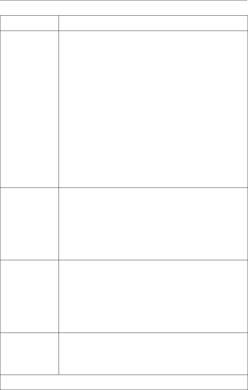
DRAFT
Models and filetypes
Filetype Description
Communication file The communication file is used for transferring information between
different modules of Delft3D, notably the hydrodynamic data calcu-
lated by Delft3D-FLOW. The map files from the Delft3D-MOR Bot-
tom module can be handled as this type as well. The appropriate file
mask is: botm*.dat. (We will introduce them as a separate file type
in a future version).
Note: Though it is possible to read communication files that con-
tain the results for a three-dimensional model, GPP does not support
vertical cross-sections yet, as the essential information, the vertical
co-ordinate, can not be read from this type of file. Special parame-
ter(s):
model-grid
Wave vector
Wave forces
Wave volume flux
Av.Bed Load Transp
Av.Susp. Transp
Flow velocity
Hydrodynamic his-
tory file
This type of file is produced by Delft3D-FLOW and contains de-
tailed results for selected monitoring points. If the model is three-
dimensional, some parameters will be defined on layers, making it
necessary to select a single layer before you can plot a time-series.
Special parameter(s):
Tidal ellipsis
Tidal ellipsis (av.)
Hydrodynamic
map file
This type of file is produced by Delft3D-FLOW and contains the re-
sults for the whole computational grid. Via the special (or extra) pa-
rameters you can view the flow velocity as a vector. Special parame-
ter(s):
model-grid
Flow velocity
Flow velocity (3D)
Hydrodynamic
drogues file
This type of file is produced by Delft3D-FLOW and contains the tra-
jectory of drogues calculated within the runs. Special parameter(s):
drogue track
continued on next page
Deltares 153 of 190
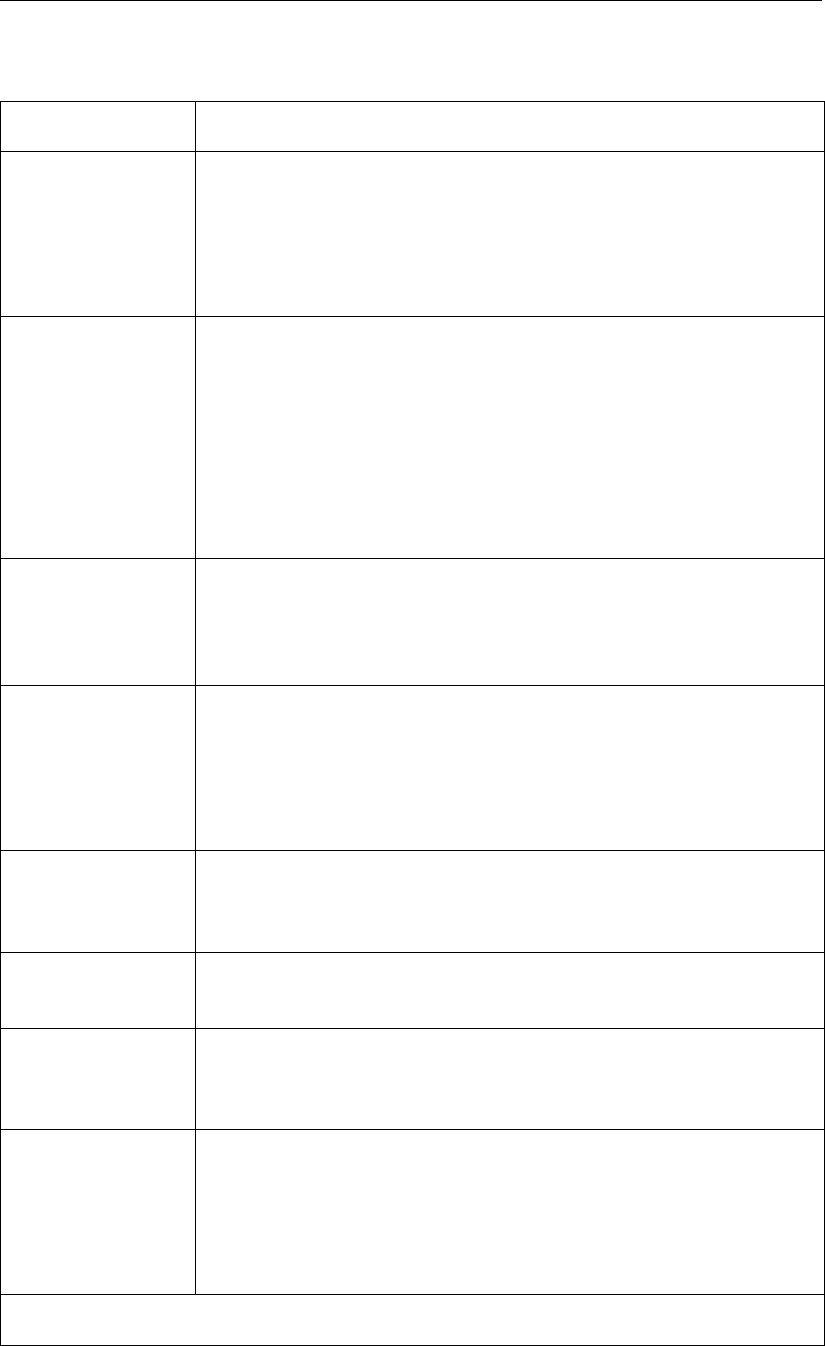
DRAFT
GPP, User Manual
continued from previous page
Filetype Description
Fourier vector file File produced by Delft3D-FLOW and contains computed amplitudes
and phases of selected parameters. Special parameter(s):
Vectors-AMPL
Vectors-PHAS
Water quality his-
tory file
This type of file is produced by D-Water Quality and the more spe-
cialised versions, Delft3D-ECO, Delft3D-SED and Delft3D-CHEM.
The file contains detailed information on selected monitoring points.
If all components are present, it can also return the so-called limit-
ing factors that show details about algae growth processes. Special
parameter(s):
Limiting factors
Water quality map
file
This type of file is produced by D-Water Quality and the more spe-
cialised versions, Delft3D-ECO, Delft3D-SED and Delft3D-CHEM.
The file contains information on the whole grid. You will need to im-
port a corresponding grid file for displaying contour maps.
Water quality grid
file
This type of file contains the grid used in D-Water Quality and D-
Waq PART calculations. (It is accompanied by a file with extension
<*.cco>). Special parameter(s):
model-grid
Mass balances file This type of file contains the detailed water quality process terms,
including the transport, for selected monitoring points. The contribu-
tions to the mass balance are automatically grouped per substance.
Mid field history file This type of file is produced by D-Waq PART. The file contains de-
tailed information on selected monitoring points.
Mid field map file This type of file is produced by D-Waq PART. The file contains infor-
mation on the whole grid. You will need to import a corresponding
grid file for displaying contour maps.
Mid field plot grid
file
This type of file is produced by D-Waq PART. The file contains infor-
mation on the specified counting grid. (It contains the grid data itself)
Special parameter(s):
model-grid
continued on next page
154 of 190 Deltares
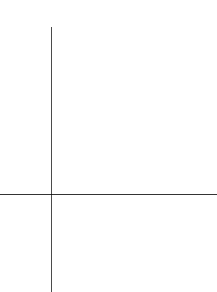
DRAFT
Models and filetypes
continued from previous page
Filetype Description
Mid field particles
track file
This type of file is produced by D-Waq PART. The file contains de-
tailed information on the trajectories of particles. Special parame-
ter(s): particle track
Waves map file The Delft3D-WAVE model uses this type of files to store the model
results on the selected output grid. Special parameter(s):
model-grid
Flow velocity
Wave vector
Energy transport
Sediment transport
map files
The output from the TRSTOT and TRSSUS sub modules from
Delft3D-MOR is stored in these files. They contain the sediment
transport on the whole (hydrodynamic) grid. Special parameter(s):
model-grid
Bedload tr. (frac)
Bedload tr. (all)
Susp.sed.tr. (frac)
Susp.sed.tr. (all)
Sediment transport
history files
The type of file is produced by Delft3D-MOR and contains de-
tailed results for selected monitoring points. If the model is three-
dimensional, some parameters will be defined on layers, making it
necssary to select a single layer before you can plot a time-series.
Dredging results
file
The dredging sub-module from Delft3D-MOR uses this type of files
to store its results. Special parameter(s):
Reference depth
Cumulative dredging
Depth with dredging
Depth (no dredging)
model-grid
Deltares 155 of 190

DRAFT
GPP, User Manual
Model/origin: DELWAQ
DELWAQ is the old name for D-Water Quality, it is still used, when the computational model
is used stand-alone. The output files defined here are all in FORTRAN unformatted or binary
form.
As the format is very simple, other programs have adopted the file formats for storing their
output.
Remark:
The original file format does not include an absolute time and date. To incorporate it,
you can use a so-called T0 string as the fourth string in the header. This will define the
reference time. (The User Manual explains this convention in detail.)
Filetype Description
Binary history file This type of file contains detailed results for selected monitoring
points. If produced within the Delft3D context, the file contains the
same information as the NEFIS files. Special parameter(s):
Limiting factors
Binary map file This type of file contains the results for the whole computational grid.
As DELWAQ does not "know" the grid co-ordinates, you should im-
port the grid separately. Otherwise the data sets will get the type
XY_GRAPH, an unstructured set of data. If the model grid is three-
dimensional, the output parameter LocalDepth represents the depth
in the cell centres. This implicit parameter is used by some action
routines to create the vertical co-ordinate.
Curvilinear grid
files
This type of file contains the grid used in D-Water Quality and D-Waq
PART calculations. (It is accompanied by a file with extension .cco).
Special parameter(s):
model-grid
Mass balances file This type of file contains the detailed water quality process terms,
including the transport, for selected monitoring points. The contribu-
tions to the mass balance are automatically grouped per substance.
Model/origin: DELWAQ-SHYF
When DELWAQ is used for computations based on the finite elements model SHYFEM, the
grid is contained in a different kind of file than for most other applications.
156 of 190 Deltares
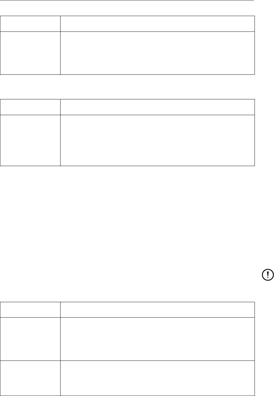
DRAFT
Models and filetypes
Filetype Description
Finite ele-
ments grid files
(SHYFEM)
This type of file contains the grid according to the SHYFEM model.
Special parameter(s):
model-grid
Model/origin: DELPAR
Filetype Description
Binary plot grid file This type of file is produced by DELPAR. The file contains information
on the specified counting grid. (It contains the grid data itself) Special
parameter(s):
model-grid
Model/origin: PHAROS
PHAROS is a wave prediction model that works in the frequency domain. Much of the re-
sults are therefore expressed as spectra, which can best be visualised in a polar co-ordinate
system. Two kinds of data are stored in the output files:
Wave characteristics in chosen locations
Wave characteristics over the whole model grid
Because of the limitations in the interface definition for data files, the same output file can be
read in two ways, each one corresponding to one of the above data types.
Remark:
This model uses a finite elements approach, rather than a finite differences. As a con-
sequence separate plot routines have been developed to support this model.
Filetype Description
Administration file Special parameter(s):
model-grid
Vector
Amplifications file Special parameter(s):
model-grid
Deltares 157 of 190
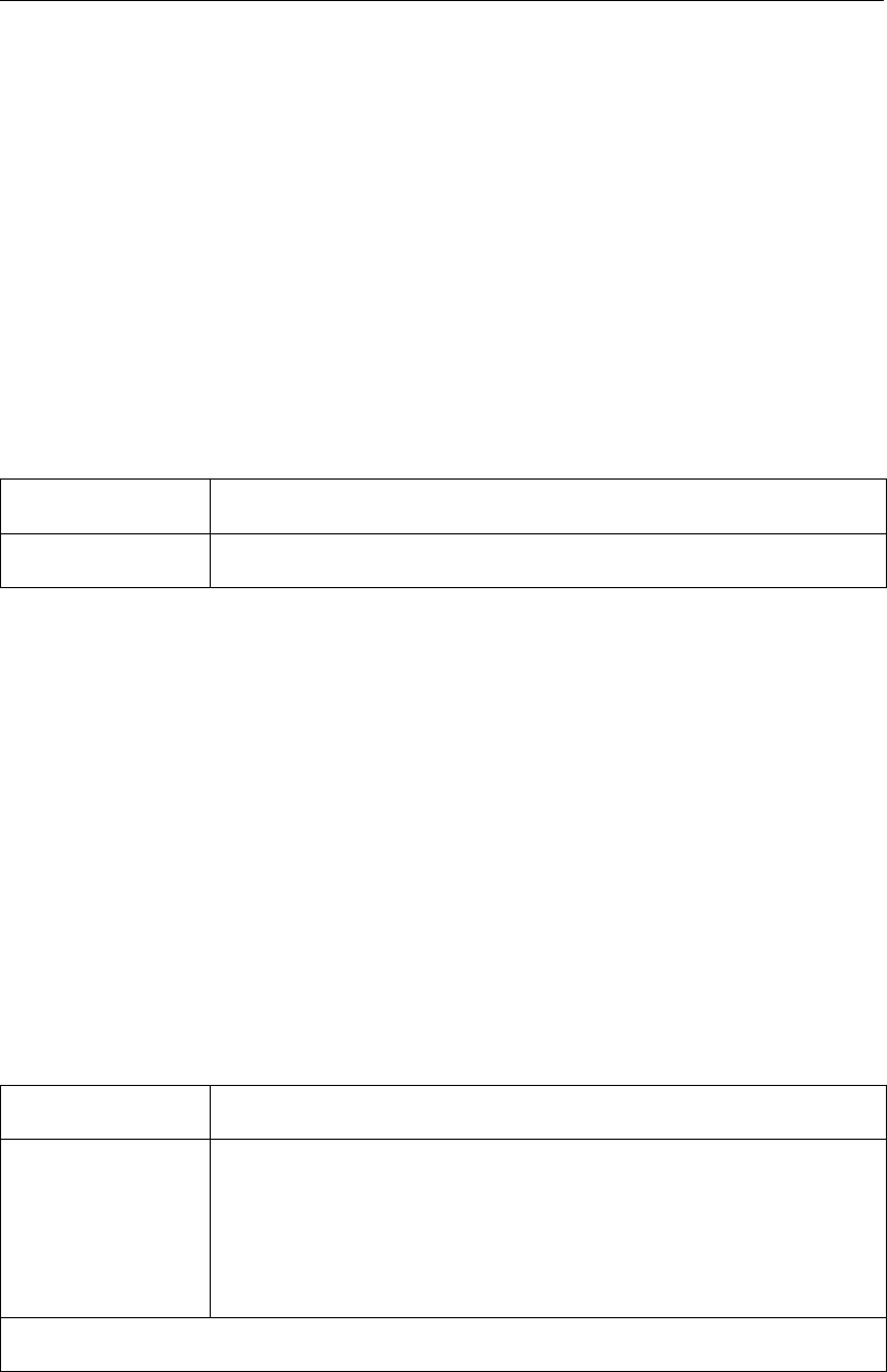
DRAFT
GPP, User Manual
Model/origin: JSPOST
JSPOST is the name of a predecessor of GPP. The file format it used is still used by some
programs, especially utilities for manipulating the output from DELWAQ. The binary PST is
accompanied by a text file with the extension .STU. This file contains the names of the pa-
rameters, but also the times stored in the binary file.
Note: When using this type of file, take care that the scale factor for time, as represented by
the value of SCU in the T0 string (if present) is in accordance with the unit of time (a string
like "day") appearing in the fifth line. Because the utilities ask one to supply the time string,
there is no guarantee that these two pieces of information are consistent.
To be precise: the value of SCU is read, but used only if the time string is not recognised.
The reading routines recognise: sec, min, hour, day and their Dutch equivalents (all in lower
case).
Filetype Description
JSPost files See the above description.
Model/origin: Samples
Samples files are files in a specific text format that is suitable for incorporating measurement
data with very little inherent structure. The format was designed to be as self-contained as
possible (so the reading routines derive the number of parameters and data points from the
file, there is no need to add this information to the file itself).
Because there is no need to count anything, a dump from a spreadsheet is (almost) enough
to create this type of files.
There are two types:
Data for a single moment in time, but for various locations
Data depending on some x-co-ordinate
The structure of these files is described in Section 5.3.2.
Filetype Description
2D observation
data
This filetype is suited for observed field data that can be said to rep-
resent one single time. Special parameter(s):
Vector
Vector UV
continued on next page
158 of 190 Deltares
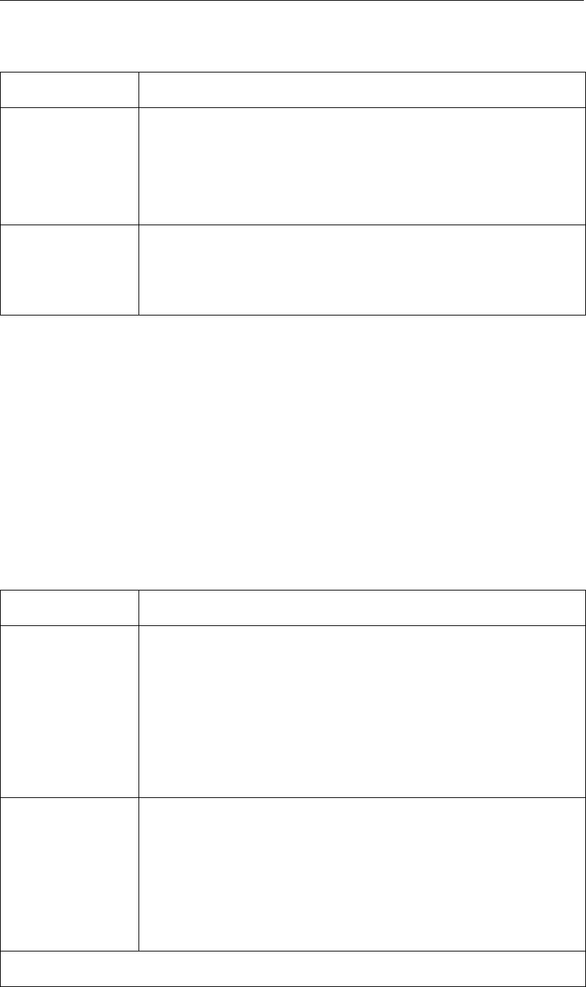
DRAFT
Models and filetypes
continued from previous page
Filetype Description
Tabular data This filetype is defined as a simple table of data. The first column is
the independent co-ordinate. All other columns contain parameters
that depend on that co-ordinate. Special parameter(s):
model-grid
Time-dependent
data
This file type is defined as a simple table of data with the first two
columns the date and time in the yyyymmdd and hhmmss format
respectively. All other columns contain parameters that are given for
that date/time.
Model/origin: TEKAL
TEKAL files are files in a specific, but very flexible text format. You can use them to incorporate
measured time-series, but also to store the results of calculations on a grid. This might be a
solution if the other file formats that are supported by GPP are not suitable.
From the point of view of the user and the user-interface, the file format contains too little infor-
mation that can be guaranteed to be present (see the User Manual for a detailed discussion.)
To solve this and still be almost as flexible as possible with this type of files, the user-interface
presents an extra dialogue in certain cases, to get the missing information from the user.
The structure of these files and possible usage is described in Section 5.3.1.
Filetype Description
Time-series or XY
series file
Time-series files can contain more than one table of data, some-
what uncomfortably regarded as parameters. The columns of each
table are therefore shown as locations. XY series files are actually
the same as time-series files, the user has to tell the GPP program
whether the independent co-ordinate is a time/date co-ordinate or an
ordinary co-ordinate. Special parameter(s):
model-grid
2D data file This filetype can be used to import data defined on a regular grid.
The missing value "999.999" is used to inactivate certain grid cells.
The values are supposed to be defined in the upper right corner of
the cells (defined by the x and y co-ordinates in the first and second
columns). Special parameter(s):
model-grid
continued on next page
Deltares 159 of 190
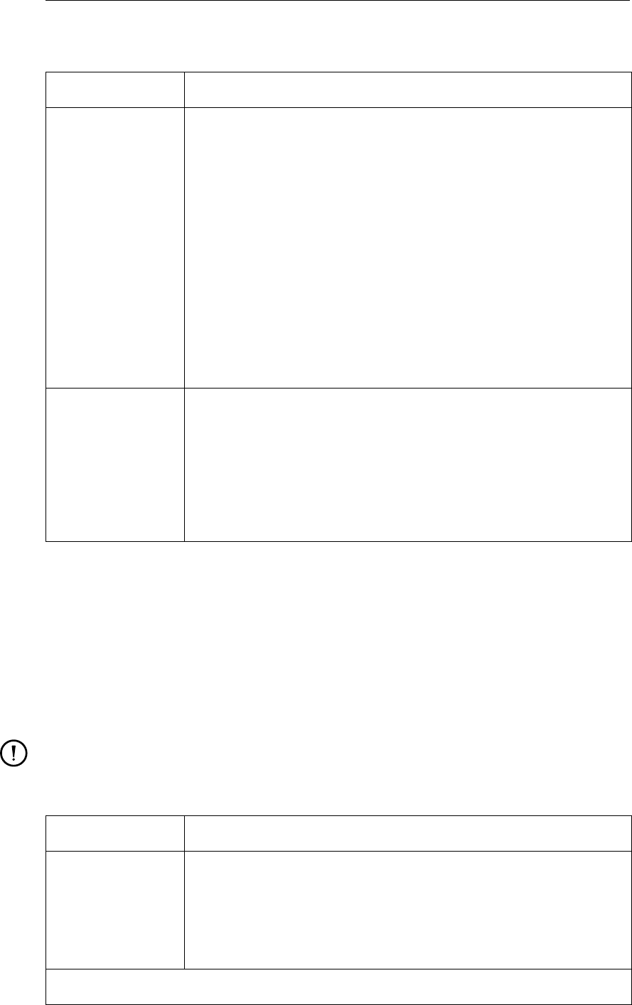
DRAFT
GPP, User Manual
continued from previous page
Filetype Description
Vector data file This filetype is actually the same as the previous, however the read-
ing routines will recognise that two consecutive columns together
form a vector. Note: The present implementation assumes there
is one vector quantity only but it can be defined in the centre of the
grid cell or in the corner. The latter type is especially useful with
measured vectors. Furthermore, the columns should not be given
an explicit name. Otherwise they will not be recognised as belonging
to the extra parameters. The program also assumes that the vector
components are Cartesian, so there is no rotation necessary. Spe-
cial parameter(s):
model-grid
Vector field 1
Vector (at vertex) 1
Annotation file If you need text in a geographical map, then this is the sort of file that
allows you to define a data set with text strings at xy-co-ordinates.
There are some limitations: There can only one table of strings Only
the whole table can be used, so do not select any locations in the
user-interface. Special parameter(s):
texts
Model/origin: GIS
GPP supports several file formats that are suitable for geographical maps. Within the context
of for instance Delft3D, they are typically used to show land boundaries, but you can also use
them for other purposes, such as incorporating a logo (see Appendix G on frequently asked
questions).
The plot routine will treat each data set derived from these files as one chart layer. But of
course, you can combine several data sets in one plot.
Remark:
Currently, the types are limited to some popular textual formats. These are relatively
easy to read and to create.
Filetype Description
BNA file BNA files are typically produced by CAD and DTM packages or by
GIS’s like Arc/Info and Atlas-GIS. They contain named polylines and
polygons, the labels are not used by GPP. Special parameter(s):
model-grid
continued on next page
160 of 190 Deltares
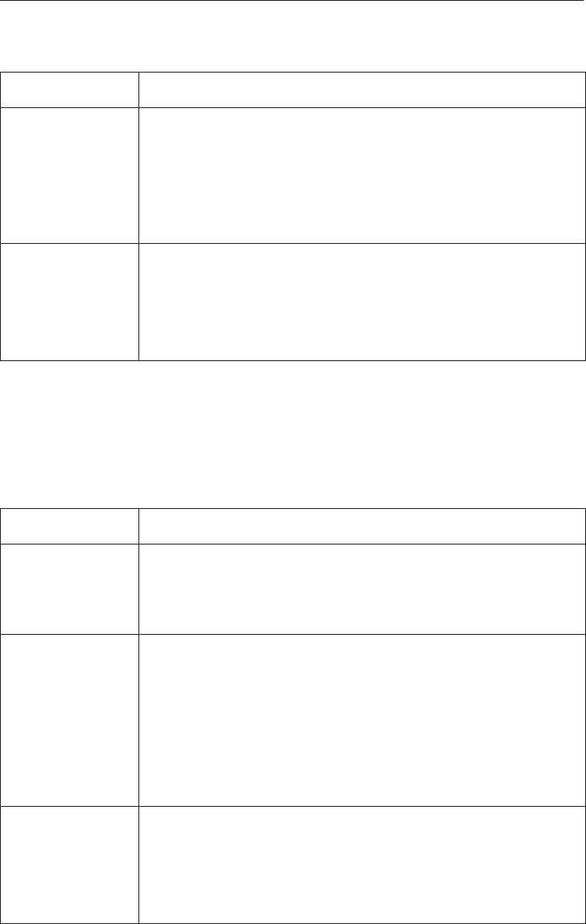
DRAFT
Models and filetypes
continued from previous page
Filetype Description
DXF file DXF files originated from AutoCAD (tm). The implementation in GPP
of the reading routines simply extracts the co-ordinate information
and thus produces polylines and polygons. No information about line
styles, text strings or other items is used. Special parameter(s):
model-grid
TEKAL land
boundary file
TEKAL land boundary files are yet another form of TEKAL files,
but the use is limited to defining polylines and polygons. See sec-
tion 5.3.1 for more information. Special parameter(s):
model-grid
Model/origin: SHIPMA
SHIPMA is a model for predicting the path (track) of a ship in the flow field around a harbour
or other constructions. The file types that GPP supports are derived from others, with some
special details. As these files are created within the SHIPMA user-interface, the user will
never be obliged to create them him/herself.
Filetype Description
Data plot file This type of file contains detailed results for the ship manoeuvring
parameters along the track of the ship. To make it possible to plot
the data as function of distance along the track, a special subtype is
used (X_APPENDED)
Environmental
data file
This file type is used for storing the environmental data, such depth
and flow velocities. Use Parameter 1 for scalar data (depth) and
Vector for vector data such as the flow velocity or the wind speed.
For vector data the nautical convention is used (the first component
is the magnitude, the second is the clockwise angle to the north)
Special parameter(s):
Vector
Track plot file Track plot files contain the realised or requested ship track as (a se-
ries of) polygons. The parameter that represents this information is
called model-grid. Special parameter(s):
model-grid
Deltares 161 of 190
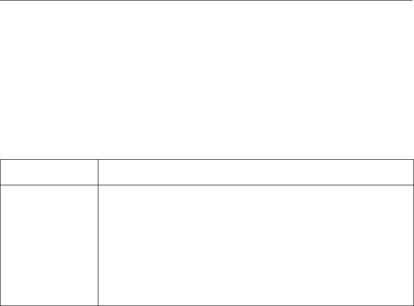
DRAFT
GPP, User Manual
Other models/origins
When you have special requirements, or want to experiment with certain features, you can
define your own model section in the filetype.gpp file. The only condition is that you use a file
type that is already present. Several such models and corresponding filetypes may be present
in the official installation to show you how particular functionality can be used.
For example the SPECDATA model:
The "model" SPECDATA is introduced mainly for supporting files with a special contents.
Filetype Description
Error margins file This file type is defined as a simple table of data with the first two
columns the date and time in the yyyymmdd and hhmmss format
respectively. All other columns contain parameters that are given for
that date/time.
The file should contain three columns to define error margin data
labelled "Mean", "Minimum", "Maximum". Special parameter(s):
Time-series 1
162 of 190 Deltares
DRAFT
K Plot routines
GPP recognises several groups of routines that manipulate the data sets:
Plot routines: they plot the data according to some predefined method.
Export routines: to store the data in some convenient external format.
Selection routines: to create subsets of data sets (for instance the data in a single layer.
Operation routines: to create new data sets containing data that have been processed in
one way or another.
Binary operations: to create a new data set that is some (arithmetic) combination of two
other data sets.
The properties of all these routines are stored in the file <routines.gpp>, which allows you to
customise certain defaults or to create specialised routines.
K.1 Plot routines
K.1.1 Plot Timeseries
Routine to plot time-series, using a date/time axis. The options allow the appearance to be
changed. For instance: a vertical axis on the right is used if the option "Use right axis" is set
to true.
You can plot data sets with this or other routines in one and the same area, but the axes are
shared resources. Sometimes it is convenient to use two independent scales. For this you
can use the option mentioned above.
Option Default value
Use right axis FALSE
Logarithmic axis FALSE
Border around plotarea TRUE
American time notation FALSE
Text in legend Dataset name
User-defined string in legend “?”
Date string at ends time-axis Date and time
Horizontal line at 0.0 FALSE
Months as digits FALSE
Character between date digits :
Start at zero (remove offset) FALSE
Deltares 163 of 190
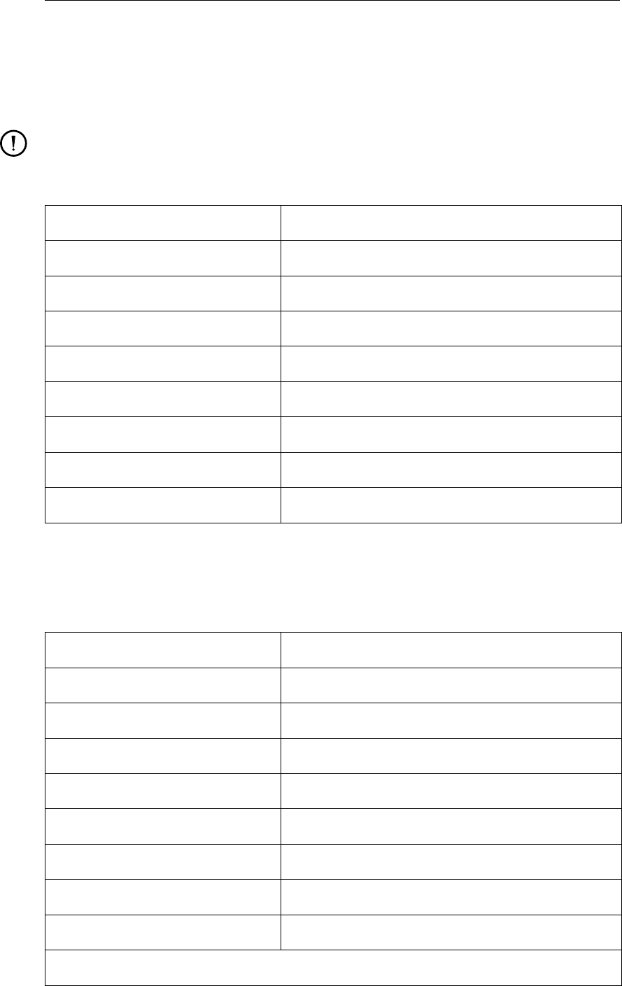
DRAFT
GPP, User Manual
K.1.2 Plot Limiting Factors
This routine plots a graph of chlorophyll and the so-called limiting factors for algae growth.
The type of presentation is somewhat specialised, but if it is suitable for your needs, then it is
almost as general as the time-series routine "Plot Timeseries".
Remark:
Logarithmic axes are not currently supported (as the negative vertical axis is reserved
for plotting the limiting factors).
Option Default value
Use right axis FALSE
Border around plotarea TRUE
American time notation FALSE
Text in legend Parameter and location
Date string at ends time-axis Date and time
Horizontal line at 0.0 TRUE
Months as digits FALSE
Character between date digits :
K.1.3 Plot Error Margins
Routine to plot time-series that have error margin information. The data points appear as
intervals, rather than a single dot.
Option Default value
Use right axis FALSE
Logarithmic axis FALSE
Border around plotarea TRUE
American time notation FALSE
Text in legend Parameter and location
User-defined string in legend “?”
Date string at ends time-axis Date and time
Horizontal line at 0.0 FALSE
continued on next page
164 of 190 Deltares
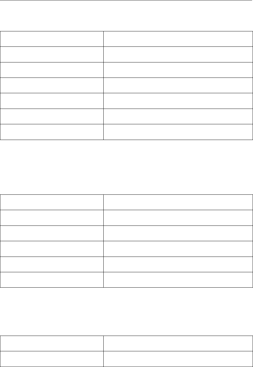
DRAFT
Plot routines
continued from previous page
Option Default value
Months as digits FALSE
Character between date digits :
Start at zero (remove offset) FALSE
Width of horizontal bars (mm) 1.5
Radius of margin disk (mm) 1.0
Colour for drawing error margin Black
K.1.4 Plot curvilinear grid
This routine plots the cells in a curvilinear grid. As an option, it may limit plotting to those sides
of the active cells that are shared with inactive cells, thereby creating a primitive boundary
outline.
Option Default value
Border around plotarea FALSE
Draw outline only FALSE
Axis type Geographic axes
Colour of grid lines Black
Line thickness (mm) 0.15
K.1.5 Plot finite elements grid
This routine plots the grid used by finite elements models. The grid cells have triangular
shapes.
Option Default value
Border around plotarea FALSE
Deltares 165 of 190
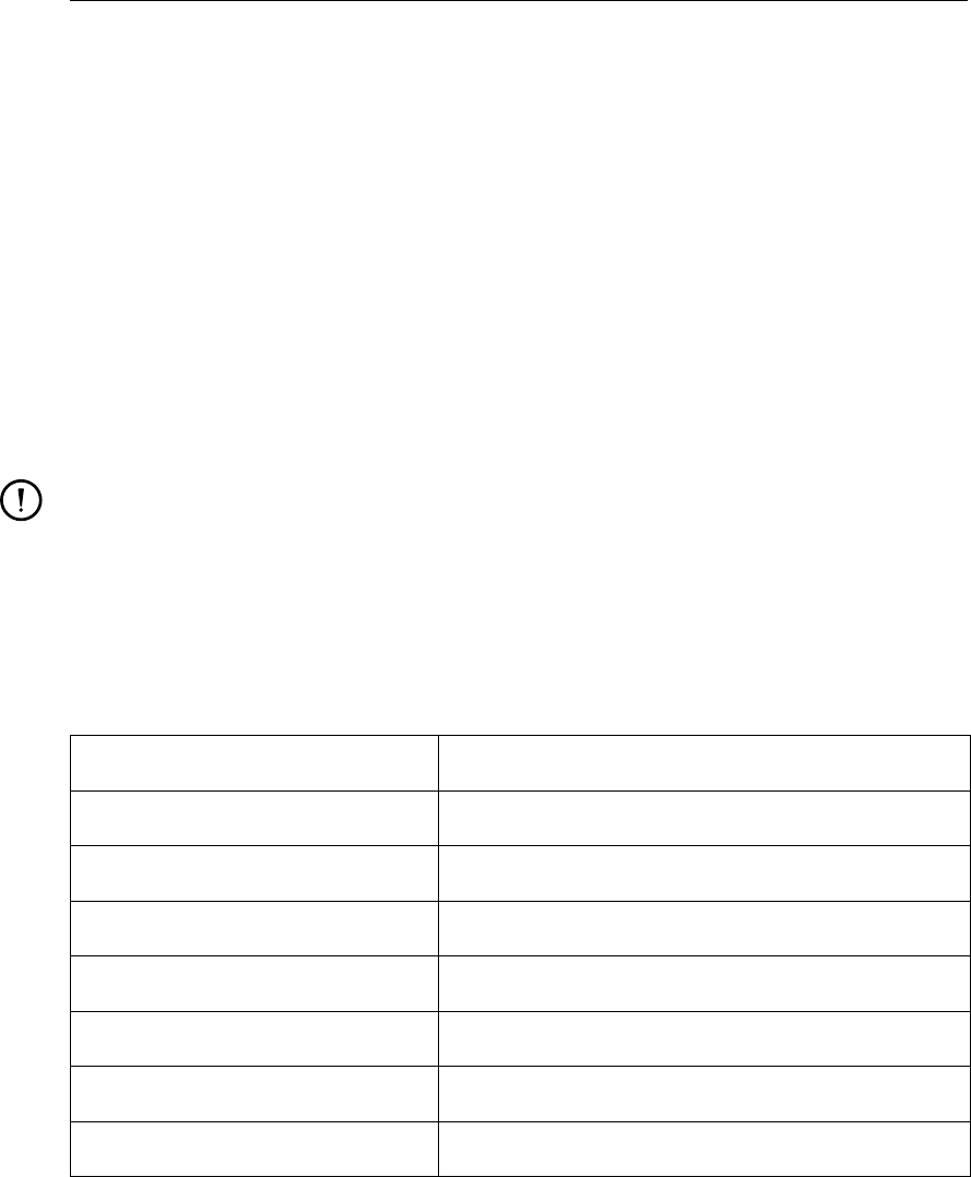
DRAFT
GPP, User Manual
K.1.6 Plot contour map
This routine plots contour maps based on a curvilinear grid. The contour classes are initially
determined automatically, and can later be changed via the plot options dialogue.
To use predefined classes you can:
Change the keyword automatic-scaling into a list of class values, like:
values 0 0.1 0.2 0.5 1.0 2.0 5.0 end-values
Use a so-called classes file. This file is expected to reside in the system directory as if it
were a configuration file. The format of these files is very simple indeed:
An asterisk or a hash in the first column means comment.
All other lines should contain a single number that is taken to be a class limit.
Remark:
To resume automatic scaling, it suffices to delete all classes via the plot options dia-
logue. (Make sure not to leave empty lines, though).
The routine may use linear axes in stead of geographic axes if the aspect ratio of the bounding
box that encloses all grid points is lower than 0.01 or greater than 100.0. This normally
happens with vertical cross-sections (after selecting a grid line in a 3D data set): the depth is
in general much smaller than the horizontal extent.
Option Default value
Border around plotarea FALSE
Contour classes automatic-scaling
Add classes to legend TRUE
Use classes file FALSE
Name classes file default.cls
Extra missing value -999
Axis type Geographic axes
K.1.7 Plot isolines
This routine plots iso-lines based on a curvilinear grid. It has the same capabilities as the
contour routine (PlotContours). We refer to this routine for further details.
The iso-lines can be black or they can be coloured:
Use black lines, if you want to emphasise contour maps (use the same contour classes
then)
Use black lines, if you want to overlay e.g. the depth on a contour map of another param-
eter.
Use coloured, if you want a true iso-lines plot.
166 of 190 Deltares
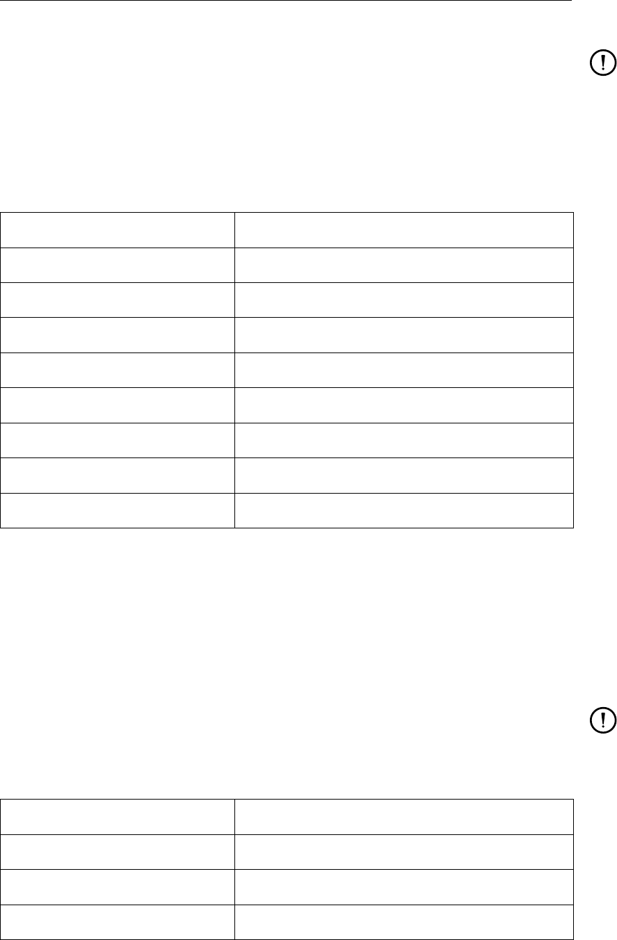
DRAFT
Plot routines
Remark:
Unfortunately, the plot technique that is used does not allow the lines to be dashed: the
lines in each grid cell are drawn separately, so there is no continuity. This is also the
reason why the iso-lines can not be annotated with class values.
An alternative technique that could be used is that first the data set is interpolated to a regular
grid and then the iso-lines are drawn. However, doing so would give slight but annoying
differences in the precise shape of the iso-lines versus the contour maps.
Option Default value
Border around plotarea FALSE
Coloured iso-lines FALSE
Contour classes automatic-scaling
Add classes to legend TRUE
Use classes file FALSE
Name classes file default.cls
Extra missing value -999
Axis type Geographic axes
K.1.8 Plot thin dams
This routine plots the sides of the grid cells that are considered dry. The sides can be:
Adjacent to inactive cells (permanently dry cells, indicating land)
Temporarily dry due to the water level (drying and flooding of tidal flat).
(cf. Documentation on Delft3D-FLOW for the meaning of dry grid cells and sides of grid cells).
Remark:
The data set must contain a component called "UVDAMS" for this routine to work prop-
erly. Otherwise nothing will be drawn (see the file with definitions for the filetypes,
<filetype.gpp>).
Option Default value
Border around plotarea FALSE
Draw outline only FALSE
Axis type Geographic axes
Deltares 167 of 190
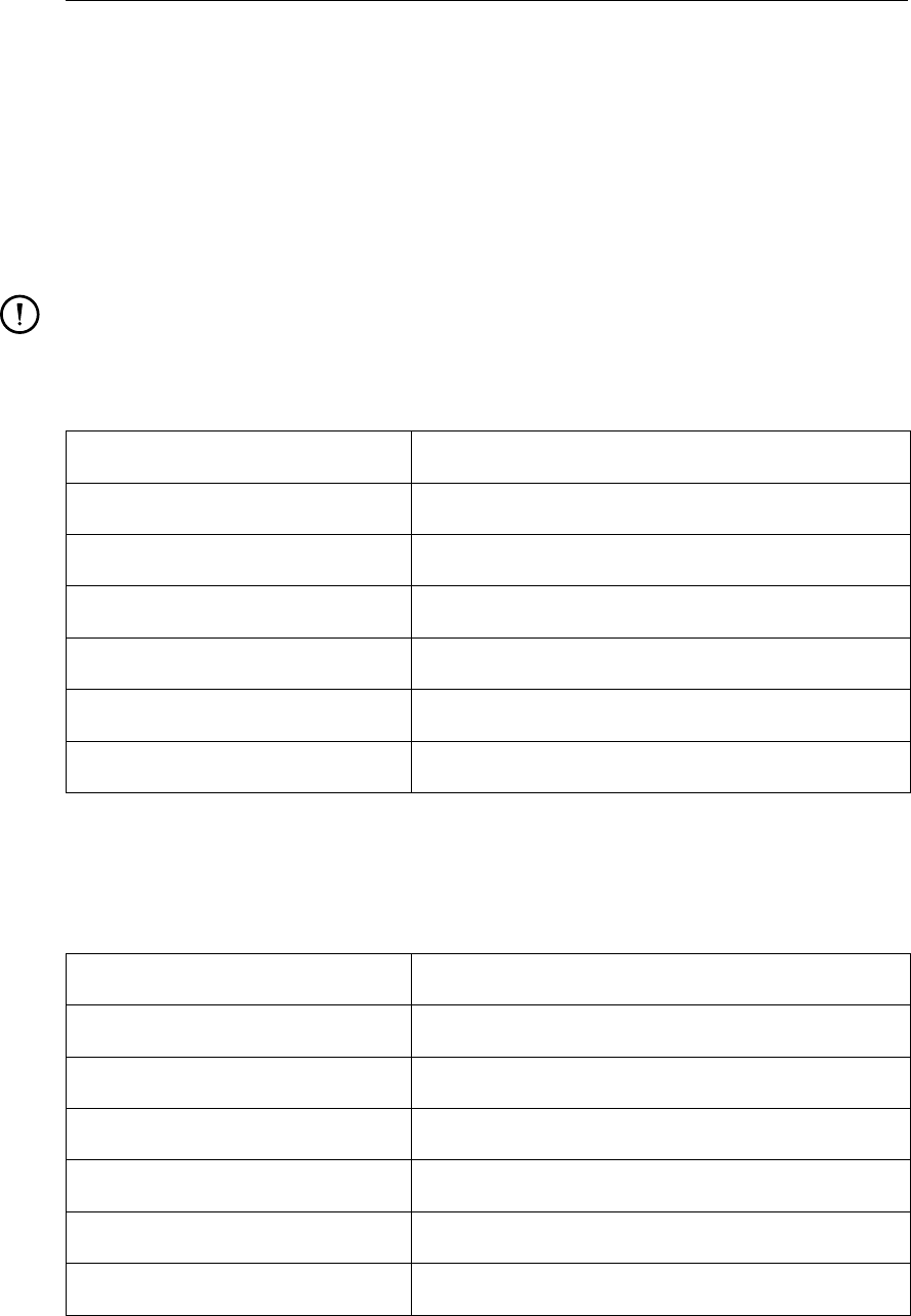
DRAFT
GPP, User Manual
K.1.9 Plot XY graph
This routine plots simple XY-graphs. It expects an x-co-ordinate to be present either in the
data set or in the topographical data set that is associated with the data set. If neither is the
case, it will use the index of the data as the x-co-ordinate.
If you exchange the x- and y-axis via the plot options, for instance when the data represent a
vertical profile, be sure to reset the axes, as otherwise the plot routine will continue to use the
old co-ordinate system.
Remark:
You can use this routine on data sets that were derived as a single grid line from a 2D
data set (via Select N/M grid-line). The x-co-ordinate will then be the chord co-ordinate
along the grid line.
Option Default value
Use right axis FALSE
Logarithmic axis FALSE
Border around plotarea FALSE
Exchange x/y axes FALSE
Text in legend Dataset name
Horizontal line at 0.0 FALSE
K.1.10 Plot vertical profile
This routine plots simple XY-graphs with the axes exchanged, so that the presentation is more
suitable for vertical profiles.
Option Default value
Use right axis FALSE
Logarithmic axis FALSE
Border around plotarea FALSE
Exchange x/y axes TRUE
Text in legend Parameter
Horizontal line at 0.0 FALSE
168 of 190 Deltares
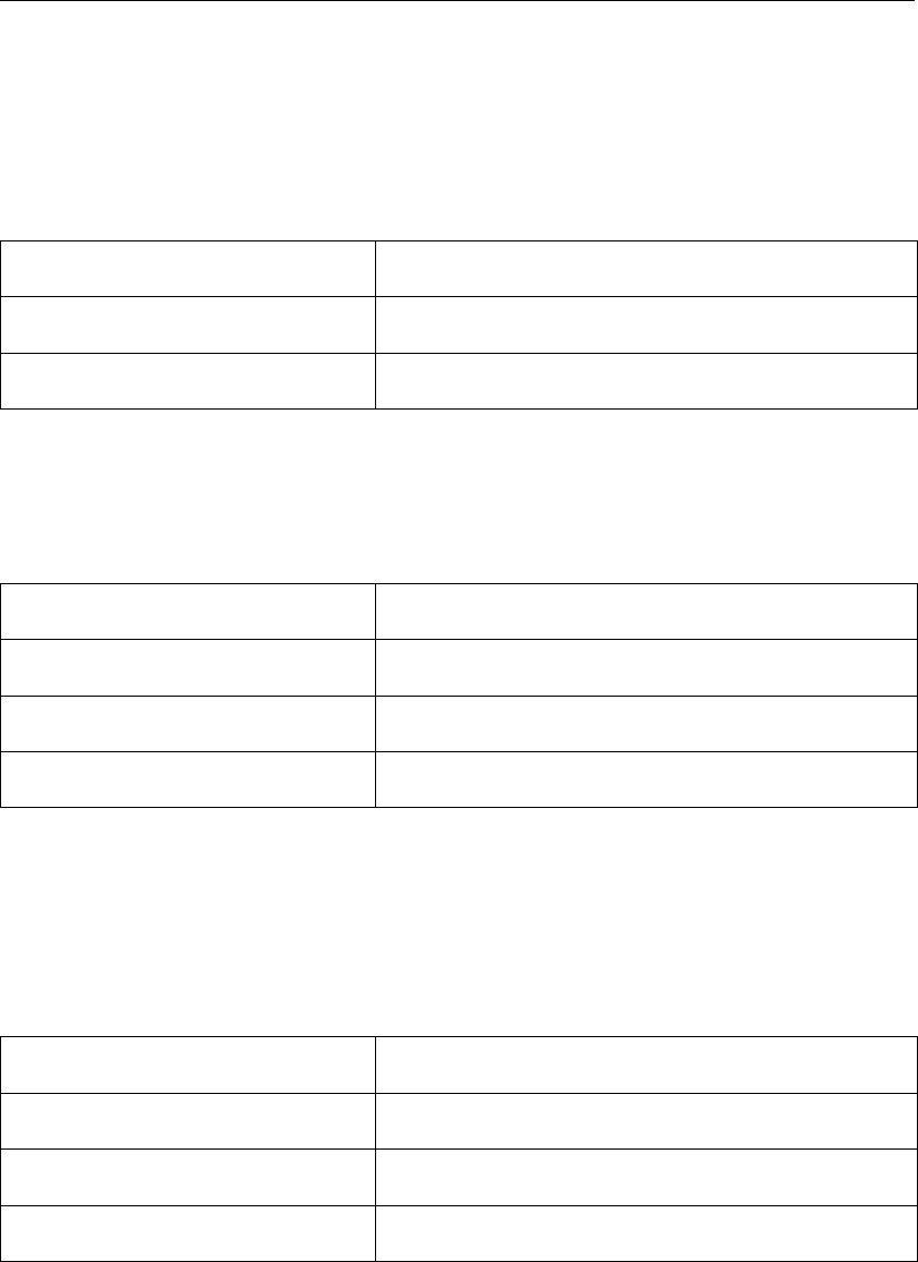
DRAFT
Plot routines
K.1.11 Polar contourplot
This routine plots contour maps based on a polar co-ordinate system, that is, the x- and
y-co-ordinates of the grid are interpreted as being the radial and tangential (in degrees) co-
ordinates. It has similar capabilities as the ordinary contour routine (PlotContours), except
that it does not support the use of classes files yet.
Option Default value
Border around plotarea FALSE
Contour classes automatic-scaling
K.1.12 Polar isoline plot
This routine plots iso-lines based on a polar co-ordinate system (cf the routines PlotContours
and PlotPolarContours for details).
Option Default value
Border around plotarea FALSE
Coloured iso-lines FALSE
Contour classes automatic-scaling
%—————————————————————————— subsectionPlot contour map (FEM)
This routine plots contours for data sets based on a finite elements grid. The elements must
be triangular. It is similar in function to PlotContours, though it is less flexible (it does not allow
a classes file to be used or different types of co-ordinate axes).
Option Default value
Border around plotarea FALSE
Contour classes automatic-scaling
Extra missing value -999
K.1.13 Plot isolines (FEM)
This routine plots iso-lines for data sets based on a finite elements grid. The elements must
be triangular. It is similar in function to PlotIsolines, though it is less flexible (it does not allow
a classes file to be used or different types of co-ordinate axes).
The iso-lines can be coloured or all in black, to emphasise the bounds between contours.
Deltares 169 of 190
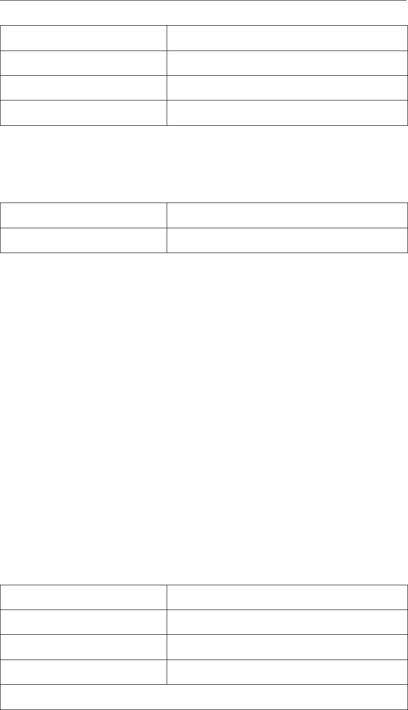
DRAFT
GPP, User Manual
Option Default value
Border around plotarea FALSE
Coloured iso-lines FALSE
Contour classes automatic-scaling
K.1.14 Plot finite element grid
This routine plots the grid used by a finite elements model, The grid cells have triangular
shapes.
Option Default value
Border around plotarea FALSE
K.1.15 Plot vector field
The purpose of this routine is to draw a vector field. It can plot the vectors in various ways:
Uniformly coloured: each individual vector has the same colour and the vectors are scaled
with the same factor.
Coloured according to the length: just like in contour plots you can specify a set of classes.
The vectors will be coloured according to the class the length of the vector.
Thin out the vectors so that the underlying grid is no longer apparent or the thickening due
to locally small grid sizes is reduced. The thinning is done by constructing a set of arrows
whose starting points are at least a certain minimum distance from each other. Using a
value of zero or less for this distance disables the thinning.
Non-uniformly scaled: if you have a vertical cut-out from a 3D data set it may be advanta-
geous to accentuate the vertical vector component. You do this by applying a scale factor
larger than 1 to the y-component.
The arrow head and shaft can be controlled in detail. By combining the correct options,
you can make the arrow head always display the direction, even though the shaft itself is
too short.
The routine tries to determine the default scaling in such a way that the mean vector length
is roughly of the order of a single grid cell. The scale factor is reported as the length in mm
of the arrow on the screen or paper that represents a vector of length 1 in the data set. (for
instance, a flow velocity of 1 m/s and a scale factor of 10 mm would result in a arrow of 10
mm on screen.)
Option Default value
Border around plotarea FALSE
Colour of the vectors Black
Unit of vector quantity m/s
continued on next page
170 of 190 Deltares
DRAFT
Plot routines
continued from previous page
Option Default value
Length unit vector (mm) 0
Separate scaling y-component FALSE
Scale factor y-component 1.0
Minimum distance arrows (mm) 0.0
Vector length for colour FALSE
Minimum arrow head (mm) 0.0
Maximum arrow head (mm) 1000.0
Add vectors to legend TRUE
Classes for vector length automatic scaling
Relative size head (%) 25
Angle of arrow head 45.0
Line thickness (mm) 0.15
Axis type Geographic axes
K.1.16 Plot balances
The balances that this routine draws are especially mass balances, as they occur in water
quality and biochemical modelling. They are represented as a histogram that accumulates
the positive and negative values of the balance terms.
The various options allow the appearance of the plot to be changed:
The number of data per bar is used to average the values of several consecutive times. If
the value is very large (larger than the number of times available, the mean contributions
of each balance term is displayed.
The drawing can be a histogram or a piecewise linear function, this depends on what you
want to see.
(The threshold option has not been implemented yet).
The plot routine is quite flexible, even though the type of presentation is especially suitable
for mass balances, any time-series can be used. There is one restriction because of the
accumulation that needs to be done: the times for the data are taken from the first time-series.
You must take care to combine data sets that are based on the same times only.
Deltares 171 of 190
DRAFT
GPP, User Manual
Option Default value
Number of data per bar 2
Threshold (%) 10.0
Draw as histogram TRUE
Text in legend Parameter
K.1.17 Plot histogram
This routine will plot a histogram of one or more data series. The data need to be defined on
various named locations (see the note below).
If more than one data series is used, the histogram will be accumulated, using different colours
to indicate the contribution.
The options allow the plot to be enhanced with:
Totals expressed as numbers above each bar.
Horizontal lines to indicate critical or special values.
There is also an option that influences the relative thickness of the bars.
Remark:
The user-interface does not easily allow data sets to be construed that are suitable for
this plot routine. The procedure for D-Water Quality history files is:
Select a parameter, but do not select a location. This creates a data set with several times
and (named) locations.
Then try adding the data set to a plot. You must then select either a location or a time.
Choose Select a time.
The new data set contains the data for one parameter, one time and one or several
(named) locations. This is the type of data set that can be used.
Unfortunately, not all reading routines can handle requests for such data sets. The routines
for D-Water Quality files have been adapted for this.
Option Default value
Relative width of bars (%) 60
Show totals FALSE
Show horizontal lines FALSE
First horizontal line 0
Second horizontal line 0.0
172 of 190 Deltares
DRAFT
Plot routines
K.1.18 Plot pie chart
This routine will plot a pie chart. It should be revised, however. If you need this sort of
functionality, please let us know.
Option Default value
Border around plotarea FALSE
K.1.19 Plot land boundaries
Land boundaries and other geographic information can be plotted using this routine. The data
sets (essentially xy-co-ordinates that together form a coast line or the contours of islands,
areas of interest and other features) can come from various files, such as DXF-files or BNA-
files.
The plot routine has a large number of options and by combining several data set/plot rou-
tines with the correct plot options in one picture, you can essentially do similar things as a
geographical presentation or information system does with chart layers.
You can choose to:
Draw the boundaries in solid black.
Draw the boundaries in the colour of choice (only one colour per data set, but you can
combine data sets in one picture of course).
Fill any closed polygons with the plot colour (if you selected to draw the boundaries in
black, the polygons will have a border.
Draw with a thick or thin line.
Option Default value
Border around plotarea FALSE
Text in legend land boundaries
Show text in legend FALSE
Axis type Geographic axes
Draw the boundaries in black FALSE
Fill closed polygons FALSE
Colour for drawing/filling Black
Line thickness (mm) 0.15
Deltares 173 of 190
DRAFT
GPP, User Manual
K.1.20 Plot drogue tracks
Often, the trajectory of drogues is observed to get insight in the flow pattern in an area. This
plot routine will visualise this trajectory or track.
It requires a composite data set: the time-series of x-co-ordinates and the time-series of y-
co-ordinates. This way it can plot the track and annotate it at regular intervals with dots, to
indicate the progress.
Option Default value
Time between circles (h) 1
Radius of circles (mm) 1
Colour for drawing Black
Line thickness (mm) 0.15
K.1.21 Plot time bar
In animations it is often advantageous to compare a contour plot that is being animated with
the phase of the tide or whatever other time-dependent phenomenon. This plot routine allows
you to do just that, by drawing a simple vertical line in the plot of a time-series.
To use it, put the data set for which you want to show the time in a plot area with a time-series.
The time bar will be drawn at the time contained in the associated data set. In an animation it
will move along the time axis.
Option Default value
Colour for drawing Black
K.1.22 Samples plot
Measurements of any parameter in a collection of sample points can be shown as coloured
dots via this plot routine. You can combine it with a contour map for instance so that spatial
comparison between model results and measurements is possible.
If you do so, be careful to use the same contour classes for both presentations, otherwise the
colouring may be misleading. There is no automatic way to ensure the equality.
You can however suppress the set of contour classes showing up in the legend, once you
have the same sets.
Option Default value
Border around plotarea FALSE
continued on next page
174 of 190 Deltares
DRAFT
Plot routines
continued from previous page
Option Default value
Contour classes automatic-scaling
Axis type Geographic axes
Plot contour map Circles only
Radius of circles (mm) 1
Extra missing value 999.999
Add classes to legend TRUE
Frames around circles FALSE
K.1.23 Add text to drawing
To add an arbitrary text to a plot, use this routine. As it is also meant to indicate time in
animations, it can automatically contain the time of the associated data set.
To keep the interface simple, the position of the text is related to the top or bottom sides of
the plot area. The position of the text is not related to the co-ordinate system. (If you want
text that has a particular geographical position, such as place names, use the plot routine
PlotGeoText.
As it requires very little information from the data set, it can be used with all kinds of data sets.
Option Default value
String to plot (as prefix) Time:
Add date and time to string TRUE
Position of the string Upper-right
Distance from border (cm) 3.0
Draw an analogue clock FALSE
Clock size (cm) 3.0
Deltares 175 of 190
DRAFT
GPP, User Manual
K.1.24 Add a simple annotation
Annotations like a North arrow are very useful, though unrelated to a particular data set.
Currently, he plot routine allows the following symbols or annotations:
a north arrow
an incident wave
The position is related to the top-right corner, as this is the usual position for such picture
elements.
It can be used with any kind of data sets, but is for reasons of usefulness restricted to data
sets with a two-dimensional co-ordinate system.
Option Default value
Type of annotation North arrow
Angle of arrow to north (east=90) 0
Length of the arrow (mm) 10
Distance from right border (mm) 25.0
Distance from top border (mm) 25.0
K.1.25 Plot text at position
Pictures displaying a map of some kind can be enhanced with text at the right positions. Such
text can represent the name of some feature, a landmark or a town for instance. The plot
routine PlotGeoText takes care of drawing the associated data sets.
The routine has several options, such as the colour and the angle, but they will be applied to
all text defined by the data set.
Option Default value
Height of text (in mm) 2.5
Default text angle (degrees) 0
Colour of text Black
Text justification Left
Axis type Geographic axes
K.1.26 Plot via a simple script
Plot routine that serves as a place holder. This definition is used when you register “scripted”
plot routines.
176 of 190 Deltares

DRAFT
Plot routines
Option Default value
Name of script PlotTest
K.2 Selection routines
GPP allows you to create subsets of data sets. This may be necessary, as in the case of 3D
data sets, to plot the data (or a part of the data).
All routines have a similar interface: they present a list of possibilities and when you have
selected one, they create the new data set (or data sets).
K.2.1 Select a parameter
This routine allows you to select a particular parameter from a data set with more than one
parameter. Like all other selection routines, it will show the available parameters in a list box
and after confirmation by you create a new data set with the desired parameter.
The options are for private use only, and have been introduced to allow batch processing.
Option Default value
Interactive - private TRUE
SelectedString1 - private (–)
SelectedString2 - private (–)
K.2.2 Select a time
This routine allows you to select a particular time from a data set with more than one time. Like
all other selection routines, it will show the available times in a list box and after confirmation
by you create a new data set with the desired time.
The options are for private use only, and have been introduced to allow batch processing.
Option Default value
Interactive - private TRUE
SelectedString1 - private (–)
SelectedString2 - private (–)
Deltares 177 of 190
DRAFT
GPP, User Manual
K.2.3 Select a location
This routine allows you to select a particular location from a data set with more than one
(named) location. Like all other selection routines, it will show the available locations in a list
box and after confirmation by you create a new data set with the desired location.
The options are for private use only, and have been introduced to allow batch processing.
Option Default value
Interactive - private TRUE
SelectedString1 - private (–)
SelectedString2 - private (–)
K.2.4 Select a layer
This routine allows you to select a particular layer from a 3D data set. It will show the available
layers in a list box and after confirmation by you create a new data set. This will be a 2D data
set, so that it can be plotted as a contour map and so on.
The options are for private use only, and have been introduced to allow batch processing.
Option Default value
Interactive - private TRUE
SelectedString1 - private (–)
SelectedString2 - private (–)
K.2.5 Select a grid line (M)
This routine allows you to select a particular grid line from a 3D data set. It will show the
available grid lines and create a new data set. This will be a 2D data set but the two co-
ordinates are the distance along the grid line and the z-co-ordinate in each grid cell. In other
words, the new data set is a vertical cut-out.
To be able to do this properly, the 3D data set must contain the z-co-ordinate in the grid points
or the local depth, the depth in the cell centres. Unfortunately, the general matching procedure
can not distinguish this, so if such data are not available, the routine uses the layer number to
generate a z-co-ordinate.
The routine also creates a grid data set for this new data set and you can view this in its own
right.
The options are for private use only, and have been introduced to allow batch processing.
178 of 190 Deltares
DRAFT
Plot routines
Option Default value
Interactive - private TRUE
SelectedString1 - private (–)
SelectedString2 - private (–)
Selected direction 1
Default indices .. , .. ; .. , ..
K.2.6 Select a grid line (N)
The routine SelectGridLine displays the grid lines along one particular grid direction. This is
controlled by the option SelectedDirection. See the first occurrence for a detailed discussion.
Option Default value
Interactive - private TRUE
SelectedString1 - private (–)
SelectedString2 - private (–)
Selected direction 2
Default indices .. , .. ; .. , ..
K.2.7 Select a vertical profile
The routine allows you to select a single grid point and creates a new data set that contains
the data at this point along the vertical, this way you can create a vertical profile.
Remark:
The routine has similar restrictions as the routine SelectGridLine.
Option Default value
Interactive - private TRUE
SelectedString1 - private (–)
SelectedString2 - private (–)
Selected direction 3
Default indices .. , .. ; .. , ..
Deltares 179 of 190
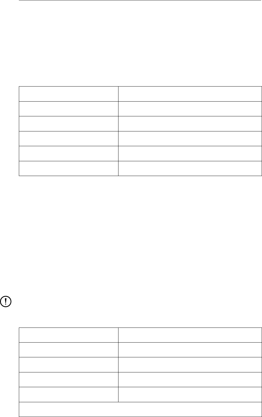
DRAFT
GPP, User Manual
K.2.8 Select an arbitrary transect
The routine SelectGridLine allows you not only to select a grid line, but also to specify an
arbitrary transect. The transect is given as pairs of indices in a format like:
10,10;20,10;20,20 (semicolons separate the pairs)
The newly created data set contains the values of grid cells as closely as possible to the lines
defined in the above way.
Option Default value
Interactive - private TRUE
SelectedString1 - private (–)
SelectedString2 - private (–)
Selected direction 4
Default indices .. , .. ; .. , ..
K.3 Operation routines
Operation routines within GPP create a new data set by performing some kind of operation,
like averaging. They may or may not display dialogues to ask for specific information.
K.3.1 Average over a fixed layer
This operation will calculate the average of a scalar or vector data set over a layer of fixed
physical thickness. The layer starts at a user-specified distance (in meter) from the surface.
The resulting data set is two-dimensional and also represents a scalar or a vector.
In interactive mode it will ask for the distance from the surface the layer starts, and the thick-
ness of this layer, both in (in principle) meters. If the layer is thicker than the depth, the result
is averaged over the whole water column.
Remark:
The option "Squared average (vector)" applies to vector data sets only and is not set
interactively.
Option Default value
Interactive - private TRUE
Start of layer (from surface) 0.0
Thickness of layer 1
Squared average (vector) FALSE
continued on next page
180 of 190 Deltares
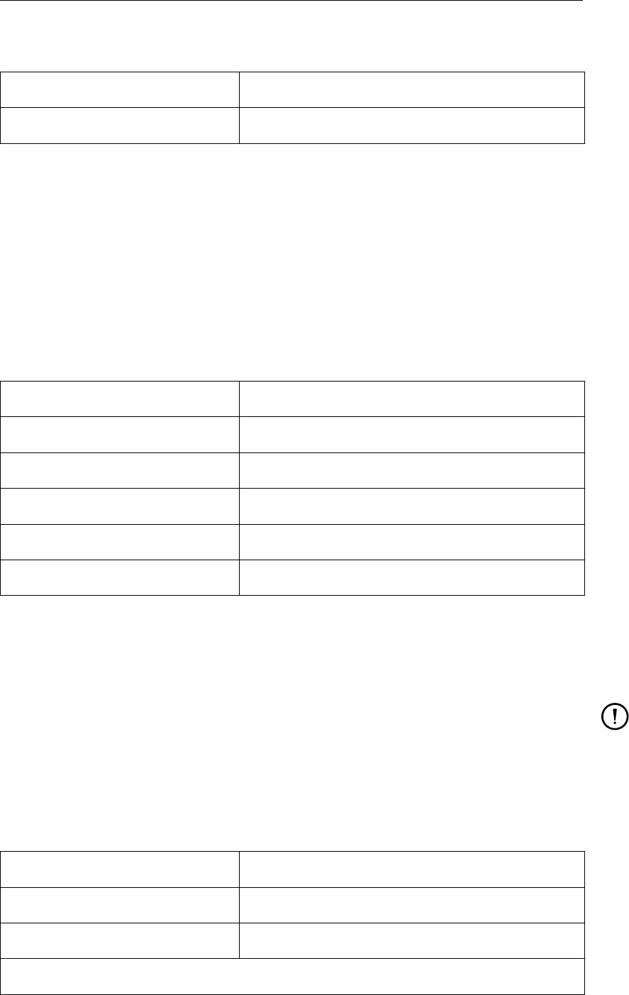
DRAFT
Plot routines
continued from previous page
Option Default value
Return the RMS value FALSE
K.3.2 Average squared vector (fixed layer)
This operation will calculate the average of the square of a vector data set over a layer of fixed
physical thickness. The idea is that by calculating the average of the squared vector, you get
a measure for the force the flow field is exercising.
If the vector field is a flow velocity with m/s as the unit, then the result is a vector field with the
unit m2/s2. If you need a root mean square value, use a different routine.
It is the same routine as "Average over fixed layer", except for the option, which instructs it to
use another algorithm.
Option Default value
Interactive - private TRUE
Start of layer (from surface; m) 0.0
Thickness of layer 1
Squared average (vector) TRUE
Return the RMS value FALSE
K.3.3 Root-mean-square vector (fixed layer)
This operation will calculate the root mean square of a vector data set over a layer of fixed
physical thickness. (cf. its companions).
Remark:
If the vector field is a flow velocity with m/s as the unit, then the result is again a vector
field with the unit m/s. If you need the average of the squared vector, use a different
routine.
Internally, it is the same routine as "Average over fixed layer", except for the options, which
instruct it to use another algorithm.
Option Default value
Interactive - private TRUE
Start of layer (from surface; m) 0.0
continued on next page
Deltares 181 of 190
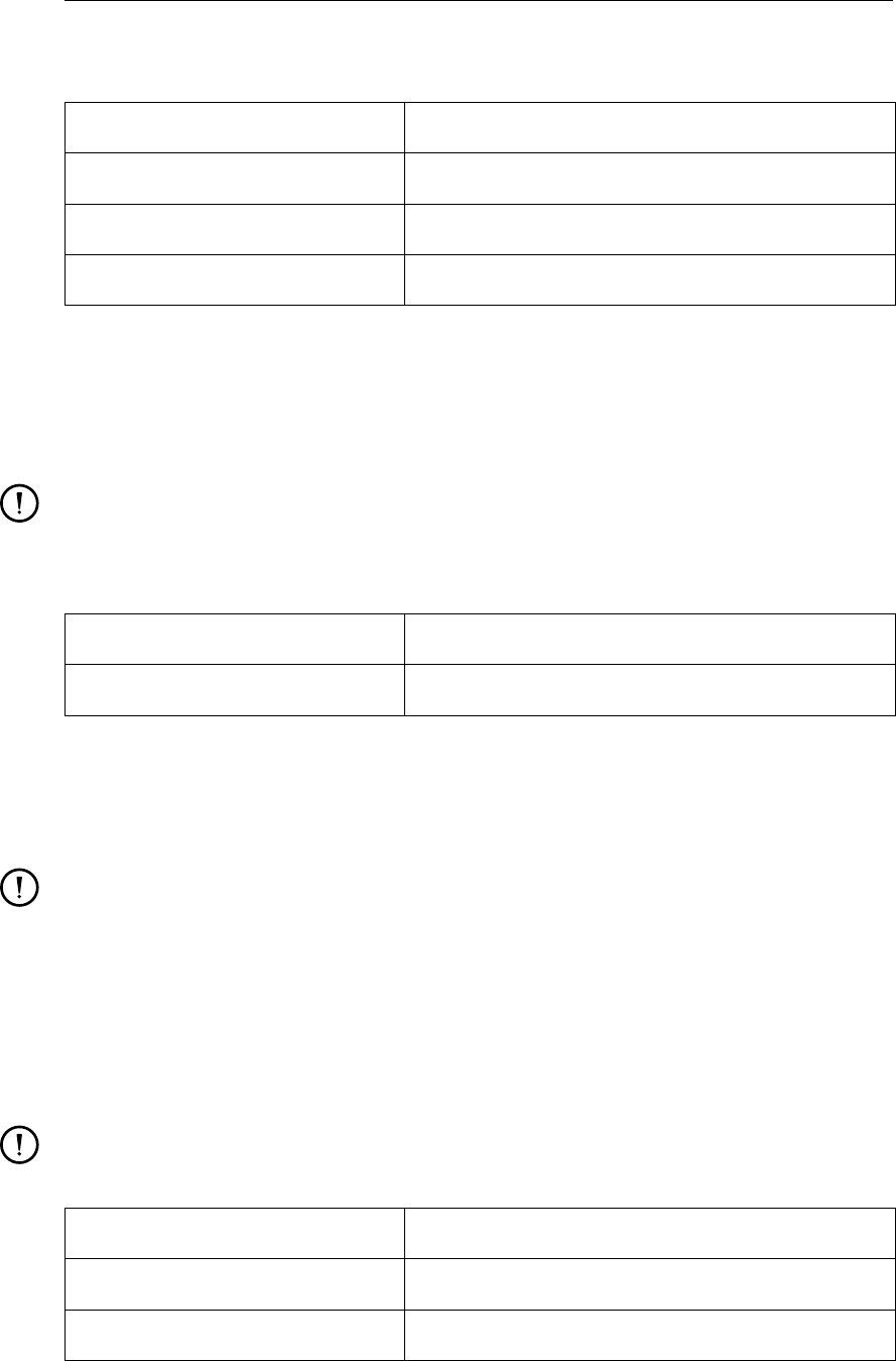
DRAFT
GPP, User Manual
continued from previous page
Option Default value
Thickness of layer 1
Squared average (vector) TRUE
Return the RMS value TRUE
K.3.4 Calculate length
This operation will calculate the length of vectors in a vector data set and store them in a
new (scalar) data set. This resulting data set can then be displayed using a contour map or
iso-lines.
Remark:
The operation will work on 3D data sets as well, but this gives rise to conflicts when
storing and reloading the data sets in a session file. For this reason the operation is
limited to 2D data sets.
Option Default value
Interactive - private TRUE
K.4 Binary operations
GPP currently supports six arithmetic operations on two selected data sets. Such binary
operations are available via the Combine menu item in the Data menu in the main window.
Remark:
Data sets can only be combined if they are of the same type and have the same number
of data. Missing values within the data arrays cause the data in the resulting data sets
to be missing as well. All operations are done using pairs of corresponding data from
the data sets.
K.4.1 A−B
This operation will calculate the difference between the corresponding values in two data sets.
Remark:
The operation has not been implemented for vector data sets yet.
Option Default value
Interactive - private TRUE
Suffix - private (–)
182 of 190 Deltares
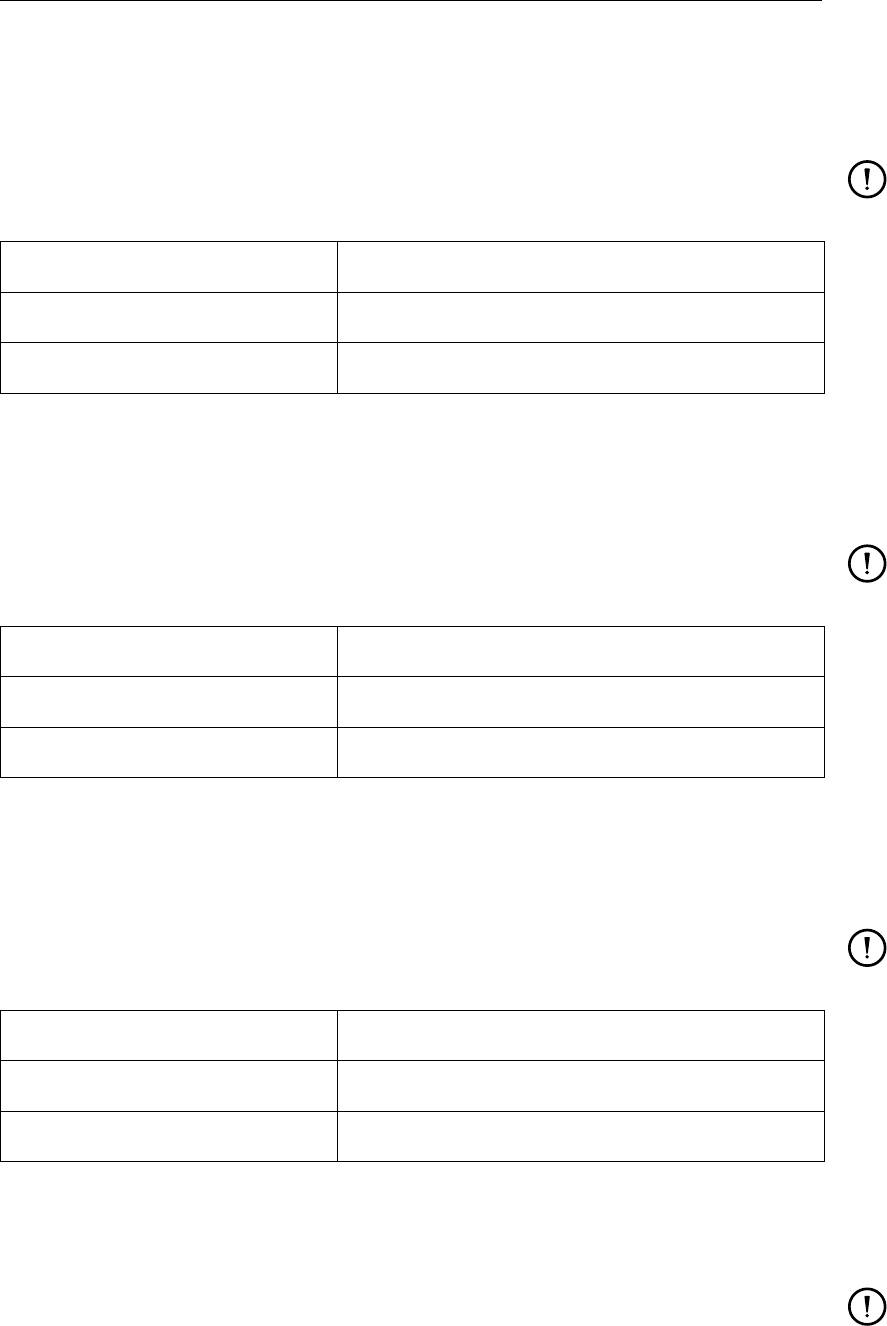
DRAFT
Plot routines
K.4.2 A+B
This operation will calculate the sum of corresponding values in two data sets. Such binary
operations are available via the Combine menu item in the Data menu in the main window.
Remark:
The operation has not been implemented for vector data sets yet.
Option Default value
Interactive - private TRUE
Suffix - private (–)
K.4.3 A∗B
This operation will calculate the product of two data sets. Such binary operations are available
via the Combine menu item in the Datasets menu in the main window.
Remark:
There is no obvious way to extend this operation to vector data sets.
Option Default value
Interactive - private TRUE
Suffix - private (–)
K.4.4 A/B
This operation will calculate the quotient of two data sets. Should a value in the second data
set be zero, then a missing value is inserted.
Remark:
There is no obvious way to extend this operation to vector data sets.
Option Default value
Interactive - private TRUE
Suffix - private (–)
K.4.5 min(A, B)
This operation will calculate the minimum of the corresponding values in two data sets.
Remark:
The operation has not been implemented for vector data sets yet.
Deltares 183 of 190
DRAFT
GPP, User Manual
Option Default value
Interactive - private TRUE
Suffix - private (–)
K.4.6 max(A, B)
This operation will calculate the maximum of the corresponding values in two data sets.
Remark:
The operation has not been implemented for vector data sets yet.
Option Default value
Interactive - private TRUE
Suffix – private (–)
K.4.7 f(A, B)
This operation will calculate the mathematical expression given by you using the correspond-
ing values in two data sets. You can specify a formula with variables A and B as placeholders
for the data sets. For example: if the expression is “A+B∗B”, then the values in the new
data set are computed by substituting the values of the first data set wherever “A” is found
and the values of the second data set wherever “B” is found.
Neither “A” nor “B” need to occur in the formula, but these are the only variables allowed.
All usual mathematical operations are allowed, except exponentiation, that is done via the
pow() function.
If you need minimum and maximum function, you will need to use a ternary operator:
A>B?(A:B)
(This is an emulation of the maximum function – if A>B, then the first expression after
the question mark results, otherwise the second one is used, after the colon.)
The following functions are supported:
abs(), acos(), asin(), atan(), atan2(), ceil(), cos(), cosh(), exp(), floor(), fmod(), hypot(),
log(), log10(), pow(), rand(), round(), sin(), sinh(), sqrt(), tan(), tanh().
The function pow() takes two arguments: pow(x, y)yields xy.
The function rand() takes no arguments
Some care should be taken: 1/3∗Awill not yield the correct values, as 1/3 is computed
using integer arithmetic. You should always use a decimal point with numerical constants.
Remark:
The operation has not been implemented for vector data sets yet.
Option Default value
Interactive - private TRUE
continued on next page
184 of 190 Deltares
DRAFT
Plot routines
continued from previous page
Option Default value
Suffix – private (–)
Function of A and B “A+B”
K.4.8 f(A)
This operation will calculate the mathematical expression given by you using the values in
a single data set. You can specify a formula with the variables A as a placeholder. For
example: if the expression is “A+A∗A’, then the values in the new data set are computed
by substituting the values of the first data set wherever “A” is found.
See the description of the previous operation for more details.
Remark:
The operation has not been implemented for vector data sets yet.
Option Default value
Interactive - private TRUE
Suffix – private (–)
Function of A “1.0∗A”
K.5 Export routines
GPP currently supports the following routines to export the contents of data sets to external
files. These routines are invoked via the Export Dataset dialogue.
K.5.1 Write Timeseries to Annotated File
This routine exports time-series data to a text file with some simple annotations. The routine
is suitable for any data set that consists of one or more time-series.
Option Default value
Default filename data.out
K.5.2 Write Timeseries to TSV File
This routine exports time-series data to a so-called tab-separated-values file with some simple
annotations. This type of files can easily be imported in spreadsheets.
The routine is suitable for any data set that consists of one or more time-series.
Deltares 185 of 190
DRAFT
GPP, User Manual
Option Default value
Default filename data.out
Separator to be used tab
K.5.3 Write Timeseries to Text File
This routine exports time-series data to a text file in TEKAL format. The file can be read again
by GPP, as a TEKAL time-series file. The routine is suitable for any data set that consists of
one or more time-series.
Option Default value
Default filename data.out
K.5.4 Write MAP2D to Text File
This routine exports a data set defined on a two-dimensional grid to a text file in TEKAL
format. The file can be read again by GPP, as a TEKAL 2D data file.
The output includes the co-ordinates as the first and second columns. If there are several pa-
rameters in the data set (such as with vector quantities), they will appear as multiple columns.
Option Default value
Default filename data.out
K.5.5 Write XY data to Text File
This routine exports a data set that contains data as a function of a single (X) co-ordinate to a
text file in TEKAL format. The file can be read again by GPP, as a TEKAL Timeseries or XY
series file.
The output includes the X co-ordinate as the first and second columns. If there are sev-
eral parameters in the data set (such as with vector quantities), they will appear as multiple
columns.
Option Default value
Default filename data.out
186 of 190 Deltares
DRAFT
Plot routines
K.5.6 Write data sets (finite element grid) to Text File
This routine exports a data set defined on a finite element grid to a text file in TEKAL format.
The file can be read again by GPP, as a samples file (the FEM structure is not preserved).
The output includes the co-ordinates of the FEM nodes as the first and second columns. If
there are several parameters in the data set (such as with vector quantities), they will appear
as multiple columns.
Option Default value
Default filename data.out
K.5.7 Write grid to ArcView/Info import file
This routine exports a grid data set to an import file for ArcView/ArcInfo.
Option Default value
Default filename data.out
K.5.8 Write results to ArcView/Info import file
This routine exports a MAP2D data set to an import file for ArcView/ArcInfo.
Option Default value
Default filename data.out
K.5.9 Write via a simple script
Export routine that serves as a place holder. This definition is used when you register
“scripted” export routines.
Option Default value
Name of script WriteTest
Deltares 187 of 190

DRAFT
GPP, User Manual
188 of 190 Deltares
DRAFT
PO Box 177
2600 MH Del
Rotterdamseweg 185
2629 HD Del
The Netherlands
+31 (0)88 335 81 88
sales@deltaressystems.nl
www.deltaressystems.nl
DRAFT
