Delft3D QUICKPLOT User Manual QUICKPLOT_User_Manual
User Manual: Pdf Delft3D-QUICKPLOT_User_Manual
Open the PDF directly: View PDF ![]() .
.
Page Count: 106 [warning: Documents this large are best viewed by clicking the View PDF Link!]
- List of Figures
- List of Tables
- 1 Introduction
- 2 Getting started
- 3 Plotting options
- 3.1 Data units
- 3.2 Component
- 3.3 Axes type
- 3.4 Plot coordinate
- 3.5 Vector style
- 3.6 Vector scaling
- 3.7 Vertical scaling
- 3.8 Presentation type
- 3.9 Formatting of texts
- 3.10 Colouring vectors
- 3.11 Colouring dams
- 3.12 Thresholds for contours
- 3.13 Colour
- 3.14 Fill polygons
- 3.15 Text box
- 3.16 Line style
- 3.17 Line width
- 3.18 Marker settings
- 3.19 Colour limits
- 3.20 Colour map
- 3.21 Colour bar
- 3.22 Field thinning
- 3.23 Clipping data values
- 3.24 Clipping coordinate values
- 4 Export and printing options
- 5 Digging deeper
- A Supported file formats
- A.1 Delft3D-FLOW map file
- A.2 Delft3D-FLOW history file
- A.3 Delft3D-FLOW drogues file
- A.4 Delft3D communication file
- A.5 Delft3D-WAVE map file
- A.6 Delft3D-MOR transport map file
- A.7 Delft3D-MOR transport history file
- A.8 Delft3D-MOR bottom map file
- A.9 Delft3D-MOR bottom history file
- A.10 Delft3D-MOR dredging option 1 map file
- A.11 D-Water Quality, ECO, SED and PART map file
- A.12 D-Water Quality, ECO, SED and PART history file
- A.13 JS Post file
- A.14 D-Water Quality, ECO, SED balance file
- A.15 D-Waq PART plot file
- A.16 D-Waq PART particle track file
- A.17 D-Water Quality grid file
- A.18 Delft3D grid file
- A.19 QUICKIN depth file
- A.20 SIMONA box file
- A.21 Delft3D-FLOW restart file
- A.22 Delft3D-FLOW thin dam file
- A.23 SIMONA/Baseline thin dam file
- A.24 Delft3D-FLOW 2d weir file
- A.25 SIMONA/Baseline 2d weir file
- A.26 Delft3D-FLOW observation point file
- A.27 Delft3D-FLOW discharge station file
- A.28 Delft3D-FLOW dry point file
- A.29 Delft3D-FLOW cross-section file
- A.30 Delft3D-FLOW trachytope area file
- A.31 Delft3D-MOR dredging option 2 map files
- A.32 Delft3D-MOR dredging option 2 depot file
- A.33 Delft3D-MOR tree file
- A.34 Delft3D-FLOW boundary condition files
- A.35 D-Water Quality tim files
- A.36 QUICKIN samples file
- A.37 Simona SDS file
- A.38 BIL/HDR files
- A.39 ArcInfo grid files
- A.40 Delft-FLS or SOBEK incremental file
- A.41 Delft-FLS point history file
- A.42 Delft-FLS cross-section history file
- A.43 Tekal annotation file
- A.44 Tekal data files
- A.45 QUICKIN and Tekal land boundary file
- A.46 BNA file (as land boundary file)
- A.47 ArcInfo (un)generate file (as land boundary file)
- A.48 ESRI shape file
- A.49 Bitmap files
- A.50 UNIBEST output
- A.51 SOBEK network data
- A.52 SKYLLA file
- A.53 PHAROS file
- A.54 MATLAB files (exported from Delft3D-QUICKPLOT)
- A.55 TRITON file
- A.56 NetCDF file
- A.57 PC-Raster file
- A.58 Auke/PC file
- A.59 Telemac file
- A.60 Mike zero files

Delft3D
3D/2D modelling suite for integral water solutions
User Manual
QUICKPLOT
DRAFT
DRAFT
DRAFT
Delft3D-QUICKPLOT
Visualisation and animation program for analysis of
simulation results
User Manual
Hydro-Morphodynamics & Water Quality
Version: 2.30
SVN Revision: 54816
April 18, 2018
DRAFT
Delft3D-QUICKPLOT, User Manual
Published and printed by:
Deltares
Boussinesqweg 1
2629 HV Delft
P.O. 177
2600 MH Delft
The Netherlands
telephone: +31 88 335 82 73
fax: +31 88 335 85 82
e-mail: info@deltares.nl
www: https://www.deltares.nl
For sales contact:
telephone: +31 88 335 81 88
fax: +31 88 335 81 11
e-mail: software@deltares.nl
www: https://www.deltares.nl/software
For support contact:
telephone: +31 88 335 81 00
fax: +31 88 335 81 11
e-mail: software.support@deltares.nl
www: https://www.deltares.nl/software
Copyright © 2018 Deltares
All rights reserved. No part of this document may be reproduced in any form by print, photo
print, photo copy, microfilm or any other means, without written permission from the publisher:
Deltares.
DRAFT
Contents
Contents
List of Figures vii
List of Tables xi
1 Introduction 1
1.1 Version information .............................. 1
1.2 Known issues ................................. 1
2 Getting started 3
2.1 Starting the program ............................. 3
2.2 Selecting a data file .............................. 3
2.3 Selecting a data field ............................. 7
2.4 Selecting time and location .......................... 9
2.5 Creating a plot ................................ 11
3 Plotting options 13
3.1 Data units ................................... 13
3.2 Component .................................. 14
3.3 Axes type ................................... 15
3.4 Plot coordinate ................................ 15
3.5 Vector style .................................. 15
3.6 Vector scaling ................................. 15
3.7 Vertical scaling ................................ 17
3.8 Presentation type ............................... 17
3.9 Formatting of texts .............................. 19
3.10 Colouring vectors ............................... 20
3.11 Colouring dams ................................ 20
3.12 Thresholds for contours . . . . . . . . . . . . . . . . . . . . . . . . . . . . 20
3.13 Colour .................................... 21
3.14 Fill polygons ................................. 21
3.15 Text box .................................... 21
3.16 Line style ................................... 21
3.17 Line width ................................... 21
3.18 Marker settings ................................ 22
3.19 Colour limits ................................. 22
3.20 Colour map .................................. 22
3.21 Colour bar .................................. 22
3.22 Field thinning ................................. 24
3.23 Clipping data values ............................. 24
3.24 Clipping coordinate values . . . . . . . . . . . . . . . . . . . . . . . . . . 25
4 Export and printing options 27
4.1 Exporting data ................................ 27
4.2 Exporting and printing figures ......................... 28
5 Digging deeper 31
5.1 Setting preferences .............................. 31
5.1.1 General preferences ......................... 31
5.1.2 Quick View preferences . . . . . . . . . . . . . . . . . . . . . . . . 31
5.1.3 Grid View preferences . . . . . . . . . . . . . . . . . . . . . . . . 31
5.2 Combining multiple data sets in one plot . . . . . . . . . . . . . . . . . . . 35
5.3 Difference of Files ............................... 36
5.4 Plot Manager ................................. 38
Deltares iii

DRAFT
Delft3D-QUICKPLOT, User Manual
5.5 Interacting with plots ............................. 39
5.6 Animating results ............................... 45
5.7 Defining and combining variables . . . . . . . . . . . . . . . . . . . . . . . 46
5.8 Define your own colour maps ......................... 51
5.9 Using the Grid selection window . . . . . . . . . . . . . . . . . . . . . . . 52
5.10 Using log files as macros ........................... 54
A Supported file formats 59
A.1 Delft3D-FLOW map file . . . . . . . . . . . . . . . . . . . . . . . . . . . . 59
A.2 Delft3D-FLOW history file ........................... 61
A.3 Delft3D-FLOW drogues file . . . . . . . . . . . . . . . . . . . . . . . . . . 63
A.4 Delft3D communication file . . . . . . . . . . . . . . . . . . . . . . . . . . 63
A.5 Delft3D-WAVE map file . . . . . . . . . . . . . . . . . . . . . . . . . . . . 66
A.6 Delft3D-MOR transport map file . . . . . . . . . . . . . . . . . . . . . . . . 66
A.7 Delft3D-MOR transport history file . . . . . . . . . . . . . . . . . . . . . . 67
A.8 Delft3D-MOR bottom map file ......................... 68
A.9 Delft3D-MOR bottom history file . . . . . . . . . . . . . . . . . . . . . . . . 68
A.10 Delft3D-MOR dredging option 1 map file . . . . . . . . . . . . . . . . . . . 69
A.11 D-Water Quality, ECO, SED and PART map file . . . . . . . . . . . . . . . . 69
A.12 D-Water Quality, ECO, SED and PART history file . . . . . . . . . . . . . . . 70
A.13 JS Post file .................................. 71
A.14 D-Water Quality, ECO, SED balance file . . . . . . . . . . . . . . . . . . . 72
A.15 D-Waq PART plot file ............................. 73
A.16 D-Waq PART particle track file . . . . . . . . . . . . . . . . . . . . . . . . 74
A.17 D-Water Quality grid file . . . . . . . . . . . . . . . . . . . . . . . . . . . . 74
A.18 Delft3D grid file ................................ 75
A.19 QUICKIN depth file .............................. 75
A.20 SIMONA box file ............................... 75
A.21 Delft3D-FLOW restart file ........................... 76
A.22 Delft3D-FLOW thin dam file . . . . . . . . . . . . . . . . . . . . . . . . . . 77
A.23 SIMONA/Baseline thin dam file . . . . . . . . . . . . . . . . . . . . . . . . 77
A.24 Delft3D-FLOW 2d weir file . . . . . . . . . . . . . . . . . . . . . . . . . . 77
A.25 SIMONA/Baseline 2d weir file ......................... 77
A.26 Delft3D-FLOW observation point file . . . . . . . . . . . . . . . . . . . . . 78
A.27 Delft3D-FLOW discharge station file . . . . . . . . . . . . . . . . . . . . . 78
A.28 Delft3D-FLOW dry point file . . . . . . . . . . . . . . . . . . . . . . . . . . 78
A.29 Delft3D-FLOW cross-section file . . . . . . . . . . . . . . . . . . . . . . . 78
A.30 Delft3D-FLOW trachytope area file . . . . . . . . . . . . . . . . . . . . . . 78
A.31 Delft3D-MOR dredging option 2 map files . . . . . . . . . . . . . . . . . . . 79
A.32 Delft3D-MOR dredging option 2 depot file . . . . . . . . . . . . . . . . . . . 79
A.33 Delft3D-MOR tree file ............................. 79
A.34 Delft3D-FLOW boundary condition files . . . . . . . . . . . . . . . . . . . . 79
A.35 D-Water Quality tim files ........................... 80
A.36 QUICKIN samples file ............................. 80
A.37 Simona SDS file ............................... 80
A.38 BIL/HDR files ................................. 81
A.39 ArcInfo grid files ................................ 81
A.40 Delft-FLS or SOBEK incremental file . . . . . . . . . . . . . . . . . . . . . 82
A.41 Delft-FLS point history file ........................... 82
A.42 Delft-FLS cross-section history file . . . . . . . . . . . . . . . . . . . . . . 82
A.43 Tekal annotation file .............................. 82
A.44 Tekal data files ................................ 83
A.45 QUICKIN and Tekal land boundary file . . . . . . . . . . . . . . . . . . . . 83
A.46 BNA file (as land boundary file) . . . . . . . . . . . . . . . . . . . . . . . . 83
iv Deltares

DRAFT
Contents
A.47 ArcInfo (un)generate file (as land boundary file) . . . . . . . . . . . . . . . . 83
A.48 ESRI shape file ................................ 83
A.49 Bitmap files .................................. 84
A.50 UNIBEST output ............................... 84
A.51 SOBEK network data ............................. 84
A.52 SKYLLA file .................................. 84
A.53 PHAROS file ................................. 85
A.54 MATLAB files (exported from Delft3D-QUICKPLOT) . . . . . . . . . . . . . . 86
A.55 TRITON file .................................. 86
A.56 NetCDF file .................................. 87
A.57 PC-Raster file ................................. 87
A.58 Auke/PC file ................................. 88
A.59 Telemac file .................................. 88
A.60 Mike zero files ................................ 89
Deltares v

DRAFT
Delft3D-QUICKPLOT, User Manual
vi Deltares

DRAFT
List of Figures
List of Figures
2.1 Delft3D-QUICKPLOT main window ...................... 4
2.2 The ‘File Open’ command can be selected in two ways: from the File menu
and from the toolbar ............................. 4
2.3 The File menu contains a list of the most recently opened files . . . . . . . . 5
2.4 The leftmost buttons on the toolbar of the main window are used for file oper-
ations. .................................... 5
2.5 User interface after opening a Delft3D-FLOW map file. . . . . . . . . . . . . 6
2.6 List of data fields in the Delft3D-FLOW map file. . . . . . . . . . . . . . . . . 7
2.7 The list of plot options is changed after selection of the water level from the
dropdown list. ................................. 8
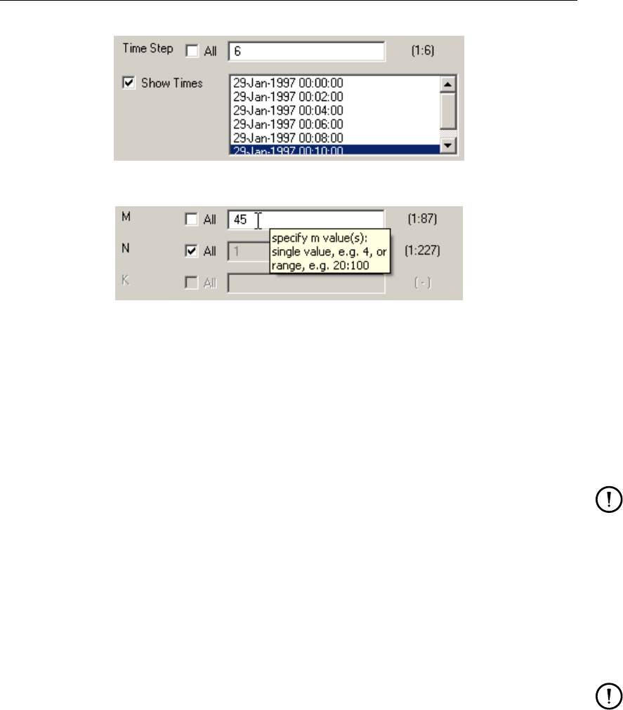
2.8 Optional listing of the times associated with the various time steps. . . . . . . 9
2.9 Selection of a cross-section along a grid line in M direction: one M value, all N
values. .................................... 9
2.10 Selection of a cross-section piecewise along a grid lines. . . . . . . . . . . . 10
2.11 Selection of an arbitrary cross-section using (x,y) co-ordinates. . . . . . . . . 10
2.12 Example of the station list in case of a history file. . . . . . . . . . . . . . . . 10
2.13 2D Plot of the water levels. . . . . . . . . . . . . . . . . . . . . . . . . . . 11
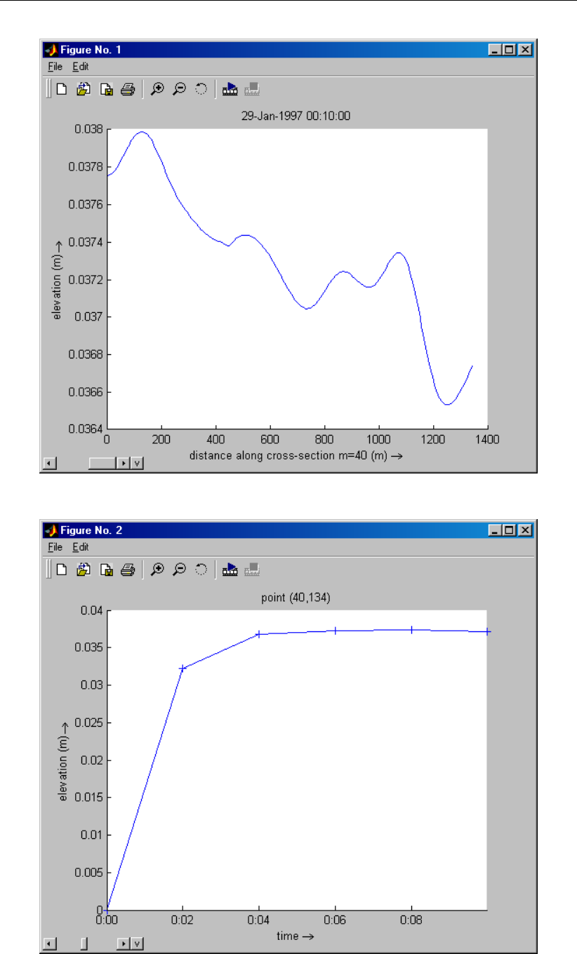
2.14 Plot of the water levels along a grid line of constant M. . . . . . . . . . . . . 12
2.15 Time-series plot of the convergence of the water levels at point M=40, N=134
to a stationary solution. Markers added for clarity (see section 3.18).. . . . . . 12
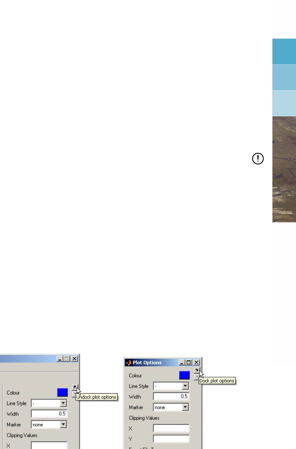
3.1 Undocking and docking of the plot options. . . . . . . . . . . . . . . . . . . 13
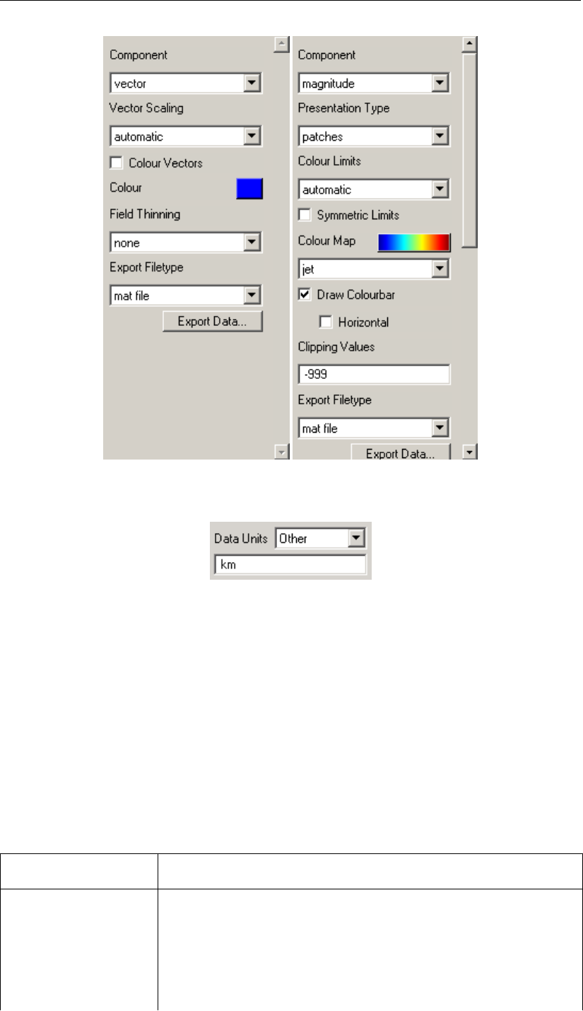
3.2 List of plot options depending on the plot type: (a, left) vector and (b, right)
scalar. .................................... 14
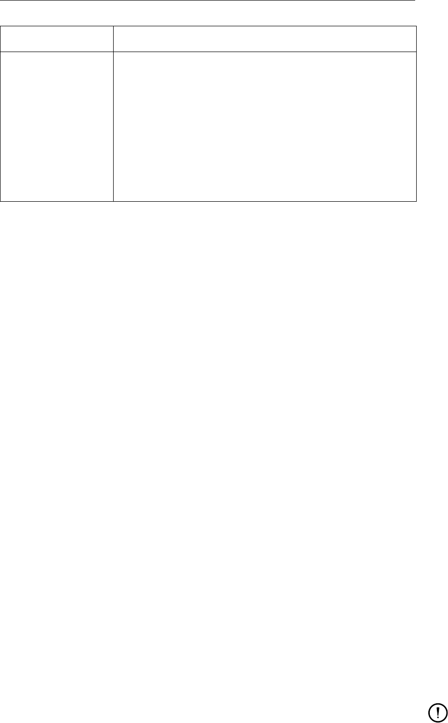
3.3 Data unit set to user specified unit. . . . . . . . . . . . . . . . . . . . . . . 14
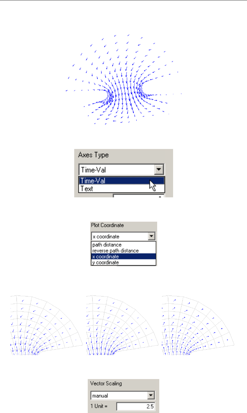
3.4 Standard vector plot. ............................. 16
3.5 Selecting axes type. ............................. 16
3.6 Selecting plot coordinate. ........................... 16
3.7 Example plots of the vector styles. . . . . . . . . . . . . . . . . . . . . . . 16
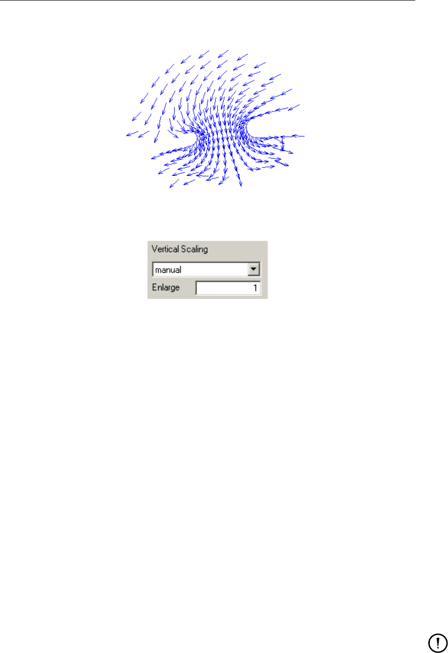
3.8 Vector scaling set to manual. ......................... 16
3.9 Normalised vector plot (same field as in Figure 3.4) . . . . . . . . . . . . . . 17
3.10 Vertical scaling set equal to horizontal scaling. . . . . . . . . . . . . . . . . 17
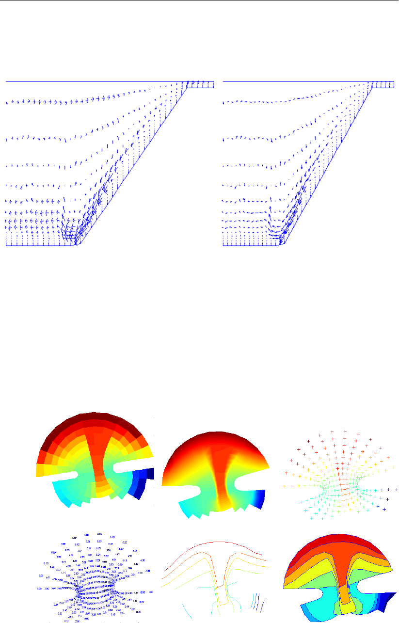
3.11 Unrestricted vertical scaling on the left (skewed arrows), vertical scaling factor
of 100 used on the right (non-skewed arrows: arrows corrected for vertical
scaling). ................................... 18
3.12 Examples of the presentation types. . . . . . . . . . . . . . . . . . . . . . . 18
3.13 Effect of the ‘Extend to Domain Edge’ option. . . . . . . . . . . . . . . . . . 19
3.14 Options available for the formatting of the numerical values. . . . . . . . . . . 19
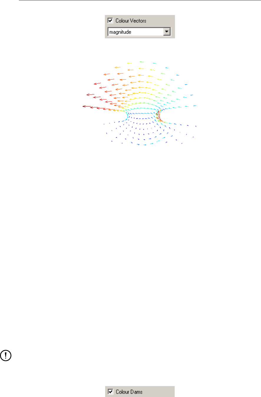
3.15 Option to colour the vectors with their magnitude. . . . . . . . . . . . . . . . 20
3.16 Vector colour dependent on the velocity magnitude (vector length). . . . . . . 20
3.17 Checkbox to indicate optional colouring of thin dam like structures such as weirs. 20
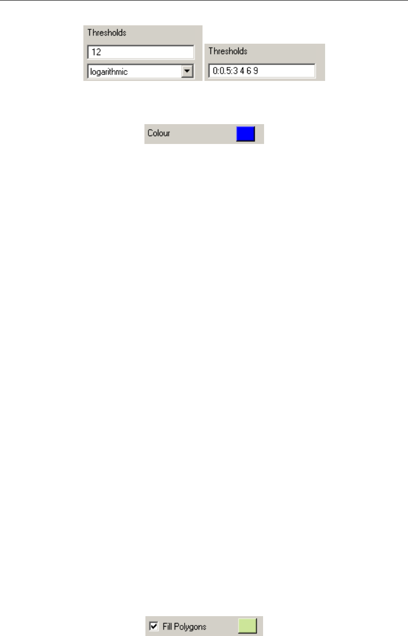
3.18 Contouring threshold options: 12 automatic thresholds logarithmically dis-
tributed or 10 user-specified thresholds. . . . . . . . . . . . . . . . . . . . . 21
3.19 Default colour setting. ............................. 21
3.20 Default colour setting for filled polygons. . . . . . . . . . . . . . . . . . . . 21
3.21 Default colour setting for text boxes. . . . . . . . . . . . . . . . . . . . . . . 22
3.22 Dropdown list for line style selection. . . . . . . . . . . . . . . . . . . . . . 22
3.23 Edit box for the line width. ........................... 22
3.24 Marker option selecting circles with a blue border and fill colour dependent on
the local value. ................................ 23
3.25 The colour limits have been set manually to 5 and 30, respectively. . . . . . . 23
3.26 List of colour maps available to the Delft3D-QUICKPLOT user. . . . . . . . . 23
Deltares vii

DRAFT
Delft3D-QUICKPLOT, User Manual
3.27 A colour map can be selected from the dropdown list. The colour map preview
will update when another colour map has been selected. . . . . . . . . . . . 23
3.28 Checkboxes for plotting a vertical (or optionally horizontal) colour bar. . . . . . 23
3.29 Optional field thinning based on grid numbers (uniform thinning) or distance. . 24
3.30 Example of a marker plot without thinning (left), uniform thinning (factor 2) and
distance thinning (right). ........................... 24
3.31 This setting will clip the values equal to -999, or larger than 0 and less than or
equal to 4, or larger than 7. . . . . . . . . . . . . . . . . . . . . . . . . . . 24
4.1 Fields for exporting the data. ......................... 27
4.2 Select the printing and exporting option from the File menu of a figure. . . . . 28
4.3 Dialog for printing and exporting figures. . . . . . . . . . . . . . . . . . . . 28
5.1 Start the preferences dialog. ......................... 32
5.2 General section of the preferences dialog. . . . . . . . . . . . . . . . . . . 32
5.3 Quick View section of the preferences dialog. . . . . . . . . . . . . . . . . . 33
5.4 Grid View section of the preferences dialog. . . . . . . . . . . . . . . . . . . 34
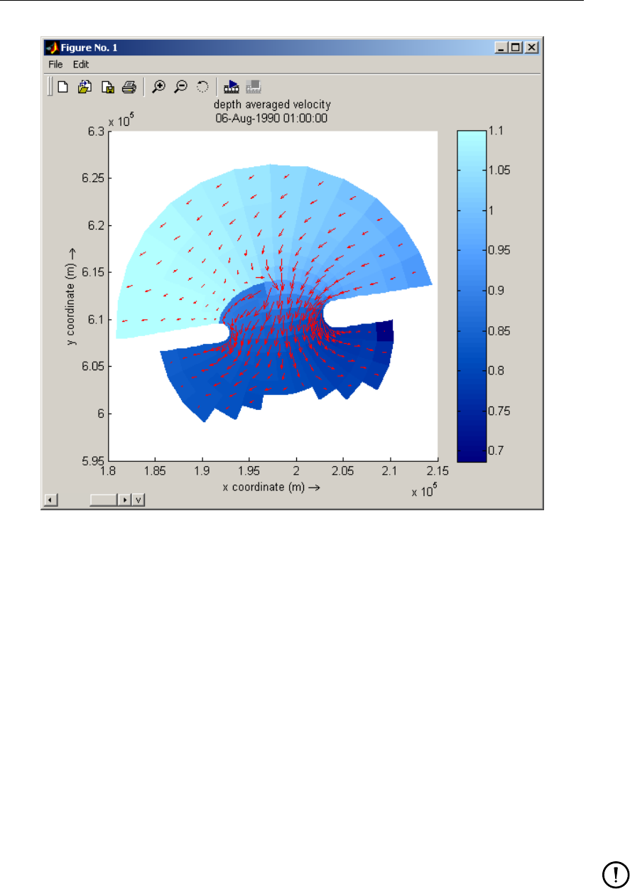
5.5 Overlay plot of the water level using patches and the depth averaged velocity
using red vectors. ............................... 35
5.6 Diff Files dialog. ................................ 36
5.7 Diff Files dialog. ................................ 37
5.8 Activation of the Plot Manager from the Window menu of the main program
window. .................................... 38
5.9 Interface of the Plot Manager. ......................... 38
5.10 A couple of standard figure layouts created using the new figure button of the
Plot Manager: 1 plot – portrait, 2 plots, vertical – portrait, 4 plots, 2x2 – portrait,
2 plots, horizontal – landscape. . . . . . . . . . . . . . . . . . . . . . . . . 40
5.11 Select Edit Border from the Edit menu to edit the border texts. . . . . . . . . . 41
5.12 The layout of the editor for the border texts matches the layout of the boxes. . . 41
5.13 Dialog for defining five ‘user selected subplots’ based on a regular grid of 3
plots on a row and 2 plots above each other. All plots are created except plot
number 5 (see Figure 5.14). . . . . . . . . . . . . . . . . . . . . . . . . . . 41
5.14 Five ‘user defined subplots’ with an indication of their row-wise numbering. . . 42
5.15 Example of the interactive positioning of a ‘user positioned subplot’. . . . . . . 43
5.16 Toolbar buttons of a Delft3D-QUICKPLOT figure. . . . . . . . . . . . . . . . 43
5.17 Rotating a 3D topography. ........................... 44
5.18 Slider and object/dimension selection button marked with the character v. . . . 45
5.19 Dialog for the animation settings. . . . . . . . . . . . . . . . . . . . . . . . 46
5.20 Clicking Define Var. will lead to the definition of a variable representing the last
water level field in the selected Delft3D communication file. . . . . . . . . . . 47
5.21 Dialog window requesting a unique name for the variable. . . . . . . . . . . . 48
5.22 Virtual file labelled <user defined variables>in the list of data files. . . . . . 48
5.23 The data field list contains the variables. . . . . . . . . . . . . . . . . . . . 48
5.24 File options dialog window for <user defined variables>while defining a new
conditional variable. .............................. 49
5.25 Main program window showing the newly defined variable ‘Froude’. . . . . . . 50
5.26 Open the colour map editor by clicking on the colour map preview. . . . . . . 51
5.27 The colour map editor. . . . . . . . . . . . . . . . . . . . . . . . . . . . . 51
5.28 Right click on the colour bar to add a colour. . . . . . . . . . . . . . . . . . 52
5.29 Grid selection window after the selection of a Grid Range. . . . . . . . . . . 53
5.30 Grid selection window while selecting an Arbitrary Line. . . . . . . . . . . . . 54
5.31 Logfile icons in the main program interface. . . . . . . . . . . . . . . . . . . 55
5.32 End result of the example log file and MATLAB script. . . . . . . . . . . . . . 56
viii Deltares

DRAFT
List of Figures
A.1 File options dialog for Delft3D-FLOW map file. . . . . . . . . . . . . . . . . 65
A.2 File options dialog for Delft3D-FLOW history file. . . . . . . . . . . . . . . . 65
A.3 File options dialog for Delft3D communication file. . . . . . . . . . . . . . . . 66
A.4 Example of a limiting factors plot. . . . . . . . . . . . . . . . . . . . . . . . 71
A.5 File options dialog for D-Water Quality or PART history file. . . . . . . . . . . 72
A.6 Example of a balance plot. . . . . . . . . . . . . . . . . . . . . . . . . . . 73
A.7 File options dialog for D-Water Quality balance file. . . . . . . . . . . . . . . 74
A.8 File options dialog for Delft3D grid file. . . . . . . . . . . . . . . . . . . . . 76
A.9 File options dialog for a bitmap file. . . . . . . . . . . . . . . . . . . . . . . 84
A.10 Example of a frequency plot. ......................... 86
A.11 Example of a drainage plot. . . . . . . . . . . . . . . . . . . . . . . . . . . 88
Deltares ix

DRAFT
Delft3D-QUICKPLOT, User Manual
x Deltares


DRAFT
Delft3D-QUICKPLOT, User Manual
xii Deltares

DRAFT
1 Introduction
This manual describes the features of Delft3D-QUICKPLOT. The program can be used to
visualise and animate numerical results produced by the Delft3D modules and some other
programs (a.o. UNIBEST, SOBEK, PHAROS). The program has been developed using MAT-
LAB. The Delft3D-MATLAB interface contains a version of Delft3D-QUICKPLOT that inte-
grates seamlessly with the MATLAB environment.
Delft3D-QUICKPLOT has been developed to be a user-friendly, flexible and robust tool for
interactive data visualisation and animation. For instance, all active buttons and edit fields
have tool tips that provide online help. Therefore, Chapter 2 contains only a short tutorial to
get you familiar with the main program window for creating basic plots. Chapter 3 describes
all plot options. Chapter 4 explains how to export and print figures. Chapter 5 addresses the
more advanced features of Delft3D-QUICKPLOT.
1.1 Version information
This manual describes the functionality of Delft3D-QUICKPLOT version 2.30 and later ver-
sions with minor revisions.
Delft3D-QUICKPLOT was created using MATLAB and the MATLAB Compiler by The Math-
Works, Inc.. This program requires technology of The MathWorks to run, a.o. the MATLAB
Compiler Runtime (MCR) Libraries. These MCR Libraries version 8.2 (MATLAB Release
2013b) have been installed as a separate step during the installation. This technology is gov-
erned by additional license conditions; please read the The MathWorks license agreement for
details (this agreement is included in license.txt in the MCR Installation directory).
1.2 Known issues
Plotting 3D results for Delft3D Flexible Mesh Suite components is not yet supported.
Deltares 1 of 92

DRAFT
Delft3D-QUICKPLOT, User Manual
2 of 92 Deltares

DRAFT
2 Getting started
Basically there are just four or five steps to get your first plots using Delft3D-QUICKPLOT:
start the program, select the file, select the data field, select the time and location, and press
plot. The following text will show you how to get your first plots of some Delft3D-FLOW map
and history files (other files can be processed in exactly the same way).
2.1 Starting the program
If Delft3D-QUICKPLOT is installed as part of the Delft3D 4 system, it can be started from
the Delft3D-MENU by selecting Utilities -QUICKPLOT. If you installed Delft3D-QUICKPLOT
for use with Delft3D Flexible Mesh Suite then you should run the program d3d_qp.exe from
the win64/quickplot/bin subdirectory under the directory in which you unpacked the Delft3D-
QUICKPLOT zip-file.
While the program is starting and the MATLAB runtime environment is loading, a splash
screen is shown. This may take a while. Subsequently, the main program window should
appear and the splash screen will disappear. The main program window will initially look as
shown in Figure 2.1. The left part of the window contains the fields for opening and closing
files, selecting data sets, time steps and plotting locations, and the buttons for creating the
actual plots. The right part of the window (now empty) will contain all options for the selected
data set (plot and export options).
2.2 Selecting a data file
The first step in creating a plot is opening a data file. This can be accomplished by clicking on
the Open a data file toolbar button or by selecting Open File from the File menu.
From the standard file selection window that appears select the data file you want to process.
The selection window contains a number of pre-configured filename filters, such as Delft3D
output file <∗.dat>and Delft3D grid file <∗.grd;*.rgf>.
Remarks:
If the file is located on a server that supports OPeNDAP, you may also select the appro-
priate website using the Open URL... menu option. Specify for example:
http://iridl.ldeo.columbia.edu/SOURCES/.WORLDBATH432/.bath/dods
Although the selection interface lists for the Delft3D output files only the data files
<∗.dat>, the accompanying definition files <∗.def>are always required for reading
the data files. Similarly, D-Water Quality aggregated grid files consist of pairs of grid
<∗.cco>and aggregation <∗.lga>files. Furthermore, shape files require in general
shape description <∗.shp>, index <∗.shx>and attribute date <∗.dbf>files. So, in
general one has to realise that the file you select in Delft3D-QUICKPLOT may not be
the only file needed to read the data contained in it. Have a look at Appendix A for an
overview of the files associated with all supported file types.
The filename filter does not influence the automatic recognition procedure that follows
the selection procedure, so any file may be selected with any filename filter active.
Once you have opened one or more files, the File menu contains a list of the most
recently opened files (upto 9) for quick access (see Figure 2.3). This list is persistent
between Delft3D-QUICKPLOT sessions.
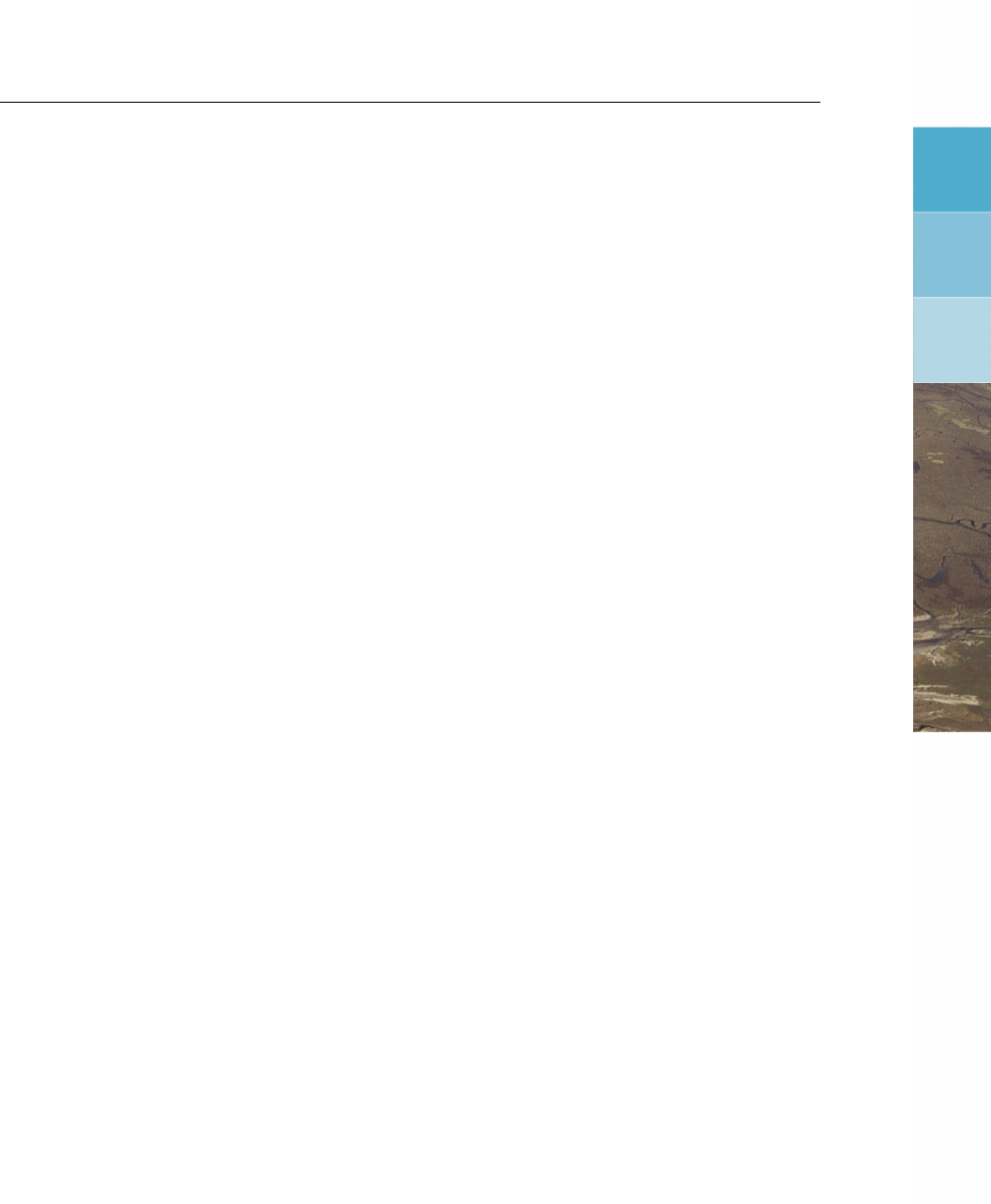
After opening a Delft3D-FLOW map-file, the Delft3D-QUICKPLOT interface will activate a
larger part of its interface. It will look as shown in Figure 2.5. The filename is indicated as the
active file in the dropdown list just below the Open a data file button. Below the filename, the
data fields available from the selected file are shown. The Quick View button for plotting the
Deltares 3 of 92

DRAFT
Delft3D-QUICKPLOT, User Manual
Figure 2.1: Delft3D-QUICKPLOT main window
Figure 2.2: The ‘File Open’ command can be selected in two ways: from the File menu
and from the toolbar
4 of 92 Deltares

DRAFT
Getting started
Figure 2.3: The File menu contains a list of the most recently opened files
Figure 2.4: The leftmost buttons on the toolbar of the main window are used for file oper-
ations.
result is activated, and some plotting and export options are available from the right part of
the window. This basically indicates that you can already create your first plot now, but let us
first inspect the other parts of the interface.
The toolbar buttons shown above have the following meaning:
The button to the left of the Open a data file button is the File reload button. If the opened
file has been changed, you can press this button to update the information initially read
from the data file (e.g. number of time steps stored in the file). This has the basically same
result as re-opening the file. However, file option settings (see below) are persistent when
reloading, but they are reset upon re-opening the file.
Pressing the Close file button to the right of the Open a data file button removes the active
file (i.e. the file selected in the dropdown list of opened files below) from the list of open
files.
Pressing the File options button to the right of the Close file button opens another window
containing some extra commands available for the selected file. For instance, in case of
a Delft3D grid file there will be buttons for opening spatial input files defined on the grid
(such as bathymetry, restart files, and thin dams). The file options dialog is an extension to
the main window, i.e. all changes made in the file options dialog will immediately affect the
main window and vice versa. If you leave it open; it will update automatically if you switch
between files in the main program window. Check out the relevant section in section 5.7
to see what functionality the file options dialog provides for your file format.
Finally, the last button on the right after the separator can be used to open a previously
saved figure (stored MATLAB format).
The purpose of the other toolbar buttons further to the right is explained in Chapter 5.
Deltares 5 of 92
DRAFT
Delft3D-QUICKPLOT, User Manual
Figure 2.5: User interface after opening a Delft3D-FLOW map file.
6 of 92 Deltares
DRAFT
Getting started
Figure 2.6: List of data fields in the Delft3D-FLOW map file.
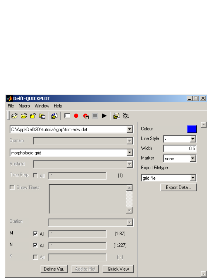
2.3 Selecting a data field
The next step in creating a plot is selecting the quantity or data field from the file to be plotted.
The data fields available from the active file are shown in a dropdown list below the name of
the file. Click on the selected field (in the example: ‘morphologic grid’) to expand the list and
to select another data field as shown in Figure 2.6. The supported file formats and the data
fields that may be contained in them are listed in Appendix A.
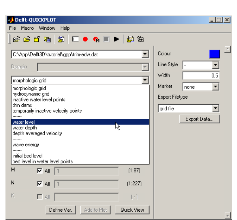
Different quantities allow for different types of plots and, therefore, the lists of plot and export
options in the right part of the window will adapt to your selection. Figure 2.7 shows the list
of options if the water level (or any other scalar 2D quantity) is selected; the options will be
discussed in Chapter 3. Furthermore, the number of time steps depends on the selected data
field; the example file contains 6 time steps for the water level as indicated by the edit box
below the datafield list box.
The domain selection box between the file selection box and the datafield selection box is
only active when the file may contain multiple domains. Similarly, the subfield selection box
immediately below the datafield selection box is only active when the datafield contains multi-
ple subfields (e.g. the datafield ‘sediment transport’ may have subfields for sediment fractions
1, 2, etc.)
Deltares 7 of 92
DRAFT
Delft3D-QUICKPLOT, User Manual
Figure 2.7: The list of plot options is changed after selection of the water level from the
dropdown list.
8 of 92 Deltares
DRAFT
Getting started
Figure 2.8: Optional listing of the times associated with the various time steps.
Figure 2.9: Selection of a cross-section along a grid line in M direction: one M value, all
N values.
2.4 Selecting time and location
After the selection of the data file and the data field, you must select which time step and
which location to plot. The default setting is to plot the last time step in the file and the whole
domain. In the case of Figure 2.7, this is indicated by the selection of time step 6 and all M
and N co-ordinates.
Remark:
If you want to see the times associated with the time steps stored in the file, check
the Show Times checkbox (see Figure 2.8). Reading and displaying a large number
of times can be very time consuming and you should be careful when opening data
files (generally history files) containing a large number of time steps: uncheck the Show
Times checkbox first.
If instead of a 2D plot of the whole domain, you want a plot of a cross-section along an M grid
line uncheck the All checkbox associated with M and specify the M-value of the desired grid
line as shown in Figure 2.9.
Remarks:
The valid range of grid and time step numbers is indicated to the right of the M/N/K
and time step edit boxes, respectively. The indicated range of grid points includes the
extra row of points added due to staggering of the variables on the computational grid.
Depending on the selected data field, the first and last grid lines may or may not have
data defined on it.
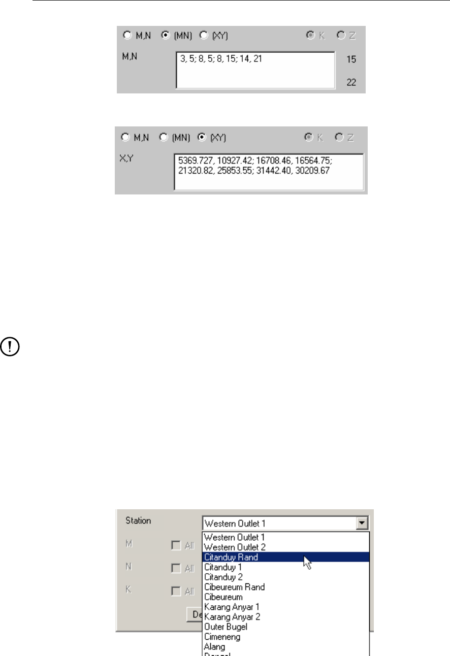
Instead of selecting a block of M and N indices, you may want to select a generic
cross-section that runs piecewise along grid lines (or diagonal lines). This can be ac-
complished by selecting the (MN) option as shown in Figure 2.10. The M and N pairs
should be separated using spaces, commas or semi-colons. Once the input has been
parsed Delft3D-QUICKPLOT will separate to co-ordinate pairs by semi-colons and the
co-ordinate indices by commas as shown in the figure. See also section 5.9 on selecting
such cross-sections interactively.
Another option is to select an arbitrary cross-section using (x,y) co-ordinates. This
feature is activated using the (XY) option as shown in Figure 2.11. The x and y co-
ordinates should be separated using spaces, commas or semi-colons. Once the input
has been parsed Delft3D-QUICKPLOT will separate to co-ordinate pairs by semi-colons
Deltares 9 of 92
DRAFT
Delft3D-QUICKPLOT, User Manual
Figure 2.10: Selection of a cross-section piecewise along a grid lines.
Figure 2.11: Selection of an arbitrary cross-section using (x,y) co-ordinates.
and the co-ordinate indices by commas as shown in the figure. See also section 5.9 on
selecting such cross-sections interactively.
It is currently not yet possible to make generic horizontal slices (such as along Z-planes
instead of K-planes).
If you want a time-series plot at any computational point of the grid, select All (or multiple)
time steps and one M and one N (and optionally one K) co-ordinate.
Remarks:
Multiple time steps can be selected by typing the time steps in the Time Step edit box.
This is particularly useful if the data file contains many time steps; type for instance
1:10:301 if you want to plot every 10th time step of a series of 301 time steps.
The extraction of a time-series from a map-file is carried out by reading for each selected
time step the whole domain and selecting only the requested point. This procedure is
more flexible yet also slower than selecting history points in the Delft3D input.
If you have opened a history file, for instance a Delft3D-FLOW trih-file, the spatial dimensions
m and n will not be available. Instead you can select the observation point or cross-section
name from the station list as shown in Figure 2.12.
Figure 2.12: Example of the station list in case of a history file.
10 of 92 Deltares
DRAFT
Getting started
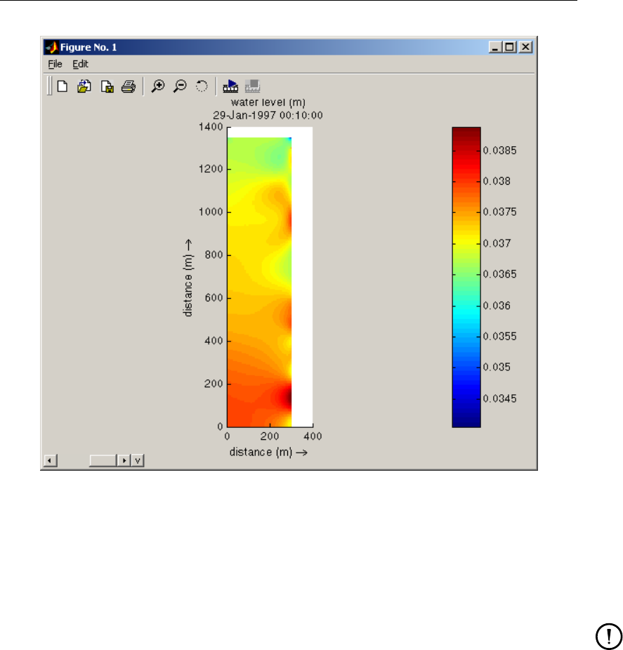
Figure 2.13: 2D Plot of the water levels.
2.5 Creating a plot
You can now plot the data by pressing the Quick View button. Depending on the data field
selected, the selected time step and the selected spatial extent, you will get a 2D plot, a
cross-sectional plot or a time-series plot. Figure 2.13 until Figure 2.15 show some results.
Remarks:
If you have selected multiple time steps and a spatially extended plot domain (i.e., all or
multiple M, N or K co-ordinates), the Quick View button will have changed into a Quick
Animate button. Pressing the button will cause the program to animate the selected
plot by looping over the selected time steps. The same result can also be obtained by
selecting one time step initially and using the Animation menu in the plot.
It is currently not possible to plot data sets on a 3D domain (i.e. all or multiple M, N
and K co-ordinates selected). Always specify a single M, N or K co-ordinate for 3D data
sets.
If there are multiple time steps and if you have selected only one, or if you have selected
only one M, N or K co-ordinate, the plot will contain an active slider in the lower left corner
of the plot. You can select other time steps and other spatial co-ordinates using that slider.
See Chapter 5.7 for information on how to use the slider, how to create animations, how to
combine plots, and how to define your own variables.
Deltares 11 of 92
DRAFT
3 Plotting options
As already indicated in the ‘Getting started’ chapter, the plot options available in the right
part of the window are constantly adjusting to the selections that you make in the left part
of the window (different data fields from the data file, different selections of space and time
co-ordinates). Note that the list of options, which is by default docked into the right part of the
main window, can also be undocked to a separate window using the undock/dock button at
the top right corner of the option list, just above the scroll bar.
This chapter describes all available options. We will use a 2D vector field (for instance the
depth averaged velocity) as the main example since most options apply to it. Initially the list
of options will look as shown in Figure 3.2a: the plot will result in a field of blue automatically
scaled vectors.
Remarks:
The export option is discussed in Chapter 5.
Changing an option will only affect the options below it. The best way to work through
the list is from top to bottom.
The options interface has been programmed to be “lazy”, that is, the options retain their
setting when switching between data files and data fields. This helps to make consistent
plots of different datasets.
If there are more options available than fit on the screen, the slider just to the right of
the list of options becomes active and it allows you to scroll through all relevant options
(as shown in Figure 3.2b).
3.1 Data units
Whenever Delft3D-QUICKPLOT knows the unit of the quantity that you have selected, the
data unit conversion option will appear. The listbox allows you to select the unit system that
you want to use for plotting and exporting. The following options are available: As in file (no
conversion carried out), SI (base units: m, kg, s), CGS (base units: cm, g, s), FPS (base
units: ft, lb, s), IPS (base units: in, lb, s), NMM (base units: mm, g, s), Other (user speci-
fied unit consistent with the original unit), and finally Hide (no units shown in plot). On start
Delft3D-QUICKPLOT reads the unit definitions from the units.ini file stored in the executable
directory. That file contains both long and short names, all names will be recognized as well
as combinations with prefixes such as kilo (or k) and milli (or m). Figure 3.3 shows the Data
unit option in the mode in which you can specify your own unit from simple units such as yd
or km (as shown) or more complex equivalents thereof such as in3/yd2, i.e. cubic inch per
Figure 3.1: Undocking and docking of the plot options.
Deltares 13 of 92
DRAFT
Delft3D-QUICKPLOT, User Manual
Figure 3.2: List of plot options depending on the plot type: (a, left) vector and (b, right)
scalar.
Figure 3.3: Data unit set to user specified unit.
square yard (typed as inˆ3/ydˆ2).
3.2 Component
This option is only available for vector quantities. Basically, it allows you to select between
different types of derived quantities. A vector quantity may be plotted as a vector, but you can
also plot its magnitude, direction (according to nautical definition) or one of its components
in computational space (M, N) or physical space (X, Y, Z, in plotting plane or perpendicular).
These derived quantities are all scalar quantities, which results in the adjustment of the op-
tions below as shown in Figure 3.2b. Plotting a scalar quantity, such as the water level, gives
the same options as the plotting of a derived quantity such as the velocity magnitude.
Component Description
vector vector
vector (split x, y) vector plot showing decomposition of vector quantity in xand y
components
vector (split m, n) vector plot showing decomposition of vector quantity in compo-
nents in mand ndirection
magnitude magnitude of the vector quantity: (u2
x+u2
y+u2
z)1/2
14 of 92 Deltares
DRAFT
Plotting options
Component Description
magnitude in plane magnitude of the vector quantity in the selected plane: (u2
m+
u2
z)1/2in case of a vertical plane along an m grid line
normal component vector component perpendicular to plane: equals n component in
case of a vertical plane along an m grid line
angle (...) angle of vector in horizontal plane in degrees or radians clockwise
from North (nautical convention)
x component vector component in xdirection
y component vector component in ydirection
z component vector component in zdirection (corresponds to kdirection)
m component vector component in local direction of mgrid line
n component vector component in local direction of ngrid line
3.3 Axes type
Some data sets may be plotted in different ways. The axes type selection option allows you
the select the type of axes you want to plot the data in. Currently, this option is only available
if you have selected a single value from a data set with multiple time steps. You can select the
value to be plotted as a Text (which was the only option in previous releases) or as a vertical
line in a Time-Val(ue) plot with a text indicating the value. This option can be used to create a
moving time line in an animation.
3.4 Plot coordinate
In the case of a variable defined along a line (or a data slice out of a 3D data set along such a
line) you may select any of four coordinates: path distance (distance measured along the line
plotted on the horizontal axis), reverse path distance (same as previous option, but measured
from the other end), xcoordinate and ycoordinate.
3.5 Vector style
If the plot type is set such that a vector field is to be plotted (in a horizontal or vertical plane)
the vector style can be set. There are currently three choices: rooted arrow (base of vector
located at point at which vector quantity is defined), centred arrow (vector extends in both
directions relative to the location at which it is defined), rooted line (combination of point and
line, i.e. no arrow head). Figure 3.7 shows all three vector styles in action.
3.6 Vector scaling
If the plot type is set such that a vector field is to be plotted (in a horizontal or vertical plane)
the vector scaling option can be set. There are four choices: automatic (default), manual,
automatic normalised and manual normalised. If the vector scaling is set to automatic, the
vectors in the field are scaled such that the maximum vector length is of the order of the
distance between points. When such a field is animated, the scaling will differ between frames.
If either one of the normalised options is selected all vectors plotted will have the same length
(see Figure 3.9).
If either one of the options with manual scaling is selected, you are requested to enter a
scaling value: a value of 2.5 indicates that a unit vector (e.g. 1 m/s) is plotted as a vector of
2.5 m length (see Figure 3.8).
Remark:
Deltares 15 of 92
DRAFT
Delft3D-QUICKPLOT, User Manual
Figure 3.4: Standard vector plot.
Figure 3.5: Selecting axes type.
Figure 3.6: Selecting plot coordinate.
Figure 3.7: Example plots of the vector styles.
Figure 3.8: Vector scaling set to manual.
16 of 92 Deltares
DRAFT
Plotting options
Figure 3.9: Normalised vector plot (same field as in Figure 3.4)
Figure 3.10: Vertical scaling set equal to horizontal scaling.
It is not yet possible to get a legend or unit vector in the plot for reference.
3.7 Vertical scaling
Because most numerical models of natural open waters cover in general a larger domain in
the horizontal plane (X, Y distance) than in the vertical plane (Z distance), the vertical scale
of a cross-sectional plot is generally exaggerated. Special care must be taken when plotting
vector quantities in such cases. The default setting of the Vertical Scaling is unrestricted
scaling, which means that the vertical scale of the plot automatically adjusts to the vertical
space available in the plot; arrows may come out skewed in this case. If the Vertical Scaling
is set to automatic, the vertical scaling is adjusted such that the maximum vertical dimensions
are 1/10 of the maximum horizontal dimensions. If it is set to manual, you can fix the vertical
scale relatively to the horizontal scale by setting the enlargement factor. An enlargement
factor of 1 implies an undistorted scale, a factor of 30 indicates a thirty times exaggerated
vertical scale.
3.8 Presentation type
Depending on the storage of the data field in the data file, there may be several presentation
types for 2D plots, such as patches, continuous shades, markers, values, contour lines and
contour patches. Examples are shown in Figure 3.12. The default setting (if available) is
patches.
Remarks:
In the case of a patches plot, the uniformly coloured grid cells have their corner points
at depth points of the staggered Delft3D grid. This implies that variables not defined
at the water level point (such as the bed levels in their traditional location) have to
be transformed in some way. The bed level data in the Delft3D-FLOW map file and
the Delft3D communication file are processed in accordance with the selected drying-
Deltares 17 of 92
DRAFT
Delft3D-QUICKPLOT, User Manual
Figure 3.11: Unrestricted vertical scaling on the left (skewed arrows), vertical scaling fac-
tor of 100 used on the right (non-skewed arrows: arrows corrected for verti-
cal scaling).
Figure 3.12: Examples of the presentation types.
18 of 92 Deltares

DRAFT
Plotting options
Figure 3.13: Effect of the ‘Extend to Domain Edge’ option.
Figure 3.14: Options available for the formatting of the numerical values.
flooding criterion. Other variables and bed levels stored in files without information on
the drying-flooding procedure are averaged to the water level points.
In the case of a continuous shades plot or a contour (lines or patches) plot data is lin-
early interpolated between the points at which the values are defined. The interpolation
is carried out across any thin dams that may exist. Furthermore, if the values are de-
fined at the water level points in the centre of the grid cells, there will be half of a grid cell
missing along the outer rim of the plot area. Since version 2.15, the option ‘Extend to
Domain Edge’ is available to fill in these gaps along the boundaries (see Figure 3.13).
The continuous shades plot is not a 2D plot, but basically a 3D plot. The values (or when
available z-data) is used to generate a 3D surface. Combining continuous shades plots
with other plot types is therefore generally not possible.
3.9 Formatting of texts
If the presentation type is set to values, you can specify the size of the font used for displaying
the values and the format of the values. The unit of the font size (default 6) is points. This is
the normal font unit used in most word processors. The size of the font does not scale with
the size of the plot: a cluttered plot on the screen may come out fine on paper. The main
part of the format string for the values is a C-style value format indicator. This can be %.df
for a floating point value with d decimals behind the decimal point, %.de for an exponential
notation with d+1 decimal places, or %g for an automatic selection of the display format per
value. Optionally, you can add some text to each value, e.g. ‘depth = %.2f’ although this often
increases the cluttering. Furthermore, the alignment of the values can be set to left, centre, or
right (horizontal) and top, cap, middle, baseline, or bottom (vertical). Non-central alignment is
useful when combining different quantities in one plot or when combining markers and values
in one plot.
Deltares 19 of 92
DRAFT
Delft3D-QUICKPLOT, User Manual
Figure 3.15: Option to colour the vectors with their magnitude.
Figure 3.16: Vector colour dependent on the velocity magnitude (vector length).
3.10 Colouring vectors
Besides uniformly coloured vectors, it is also possible to have the vectors coloured based on
some derived quantity. If you want this, check the Colour Vectors checkbox and select the
quantity from the dropdown list that appears below it. The derived quantities are the same as
those listed in the component field except for the M and N components which are not available.
3.11 Colouring dams
There are some cases in which thin dams have certain properties (e.g. weir heights). In such
cases, you can check the Colour Dams checkbox to colour them based on that value.
3.12 Thresholds for contours
If the presentation type is set to any of the contouring options, the program will by default plot
10 contours which are automatically selected uniformly between the minimum and maximum
value in the plot (or between the limits set in the edit fields of the colour limit option, see
section 3.19). The number of contours can be changed by typing a positive integer number
in the edit field below the Thresholds label. The thresholds can be distributed linearly or
logarithmic. If you want even more control over the thresholds, you can specify them in the
Thresholds edit box. You can use the MATLAB colon-notation (minimum : step : maximum
or minimum : maximum which uses the default step 1) as a shorthand notation for multiple
linearly spaced contour levels, e.g. 0:0.5:3 is a shorthand for the list 0 0.5 1 1.5 2 2.5 3.
Remarks:
If you want only one contour line at an integer value, say 12, you will have to shift it
a little (say, 12.001) to distinguish it from a number indicating the number of automatic
Figure 3.17: Checkbox to indicate optional colouring of thin dam like structures such as
weirs.
20 of 92 Deltares
DRAFT
Plotting options
Figure 3.18: Contouring threshold options: 12 automatic thresholds logarithmically dis-
tributed or 10 user-specified thresholds.
Figure 3.19: Default colour setting.
contours.
Areas below the lowest threshold will be clipped. Add a big negative value to prevent
this.
3.13 Colour
You can change the colour used for line graphs, vector fields, values and uniformly coloured
contour lines by clicking on the coloured rectangle of the colour option and selecting the colour
from the standard colour interface. This colour option sets also the colour of the lines if the
presentation type is set to patches with lines or contour patches with lines.
3.14 Fill polygons
If the data contains line data (for instance a land boundary file) you can select the option to
Fill Polygons. When this option is activated, you can set the colour separately.
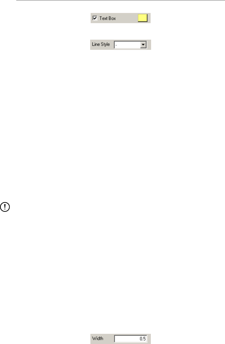
3.15 Text box
When plotting text labels (for instance when the presentation type is set to values) you can
add a box around each text. When this option is activated, you can set the fill colour of the
box separately. The boundary of the box will have the same colour as the text.
3.16 Line style
In case of a line plot, you can make selection of four line styles: - (continuous line, default),
– (dashed line), : (dotted line) and -. (dash dotted line) combined with an optional marker or
switch off the line completely and use a marker only (for marker settings, see section 3.18).
The width of the line can also be changed (see section 3.17).
3.17 Line width
Besides the line style you can also set the line width. The default line width is 0.5 point.
Figure 3.20: Default colour setting for filled polygons.
Deltares 21 of 92
DRAFT
Delft3D-QUICKPLOT, User Manual
Figure 3.21: Default colour setting for text boxes.
Figure 3.22: Dropdown list for line style selection.
3.18 Marker settings
If the presentation type is set to marker or if a line plot is created, you have to select the
marker type. There are thirteen markers: + (plus symbol), o (circle), * (star), . (dot), x (times
symbol), square, diamond, v (triangle pointing down), ∧(triangle pointing up), >(triangle
pointing right), <(triangle pointing left), pentagram and hexagram. In case of a line plot,
there is the additional option of no marker (none). By default, the markers are coloured based
on the local values in a 2D plot, whereas they are transparent (no filling) and marker colour
equals line colour for line graphs. Optionally, you can set a uniform colour for the marker edge
and/or filling. The markers +, *, . and x do not have a filled area, so you can set only their
(edge) colour.
3.19 Colour limits
By default the colour limits are determined automatically based on the selected data. Com-
parison of results of different simulations and animations require a fixed colour scaling for all
plots. Therefore, an option has been provided to set the colour scaling manually. In that case
change the Colour Limits option from automatic into manual and specify the upper and lower
limit of the colour range. If the colour limits are set automatically, you can force symmetric
limits around 0 (i.e., max=+x and min=-x) by checking the Symmetric Limits option.
Remark:
The colour limits influence the automatic selection of contouring thresholds (see sec-
tion 3.12).
3.20 Colour map
There are currently 25 colour maps to choose from: autumn, avs, bluemap, bone, cool, cop-
per, depth, earth1, earth2, earthsurface, flag, gray, hot, hsv, jet, jet (5% white band), pastel,
pink, qncmap, reversed bluemap, sedconc, spring, summer, winter, xhsv. All colour maps are
shown in Figure 3.26 from left to right. The colour map must be selected from the dropdown
list below the colour map label. The colour maps are stored in ASCII files in a subdirectory
‘colormaps’. Additional colour maps can be defined and added interactively; how to do this is
explained in Section 5.7.
3.21 Colour bar
If the plot uses a colour map for colouring the data, the colour map can be drawn as a legend to
the right (default) or below the plot. You can set this by checking the concerning checkboxes.
Figure 3.23: Edit box for the line width.
22 of 92 Deltares

DRAFT
Plotting options
Figure 3.24: Marker option selecting circles with a blue border and fill colour dependent
on the local value.
Figure 3.25: The colour limits have been set manually to 5 and 30, respectively.
Figure 3.26: List of colour maps available to the Delft3D-QUICKPLOT user.
Figure 3.27: A colour map can be selected from the dropdown list. The colour map pre-
view will update when another colour map has been selected.
Figure 3.28: Checkboxes for plotting a vertical (or optionally horizontal) colour bar.
Deltares 23 of 92
DRAFT
Delft3D-QUICKPLOT, User Manual
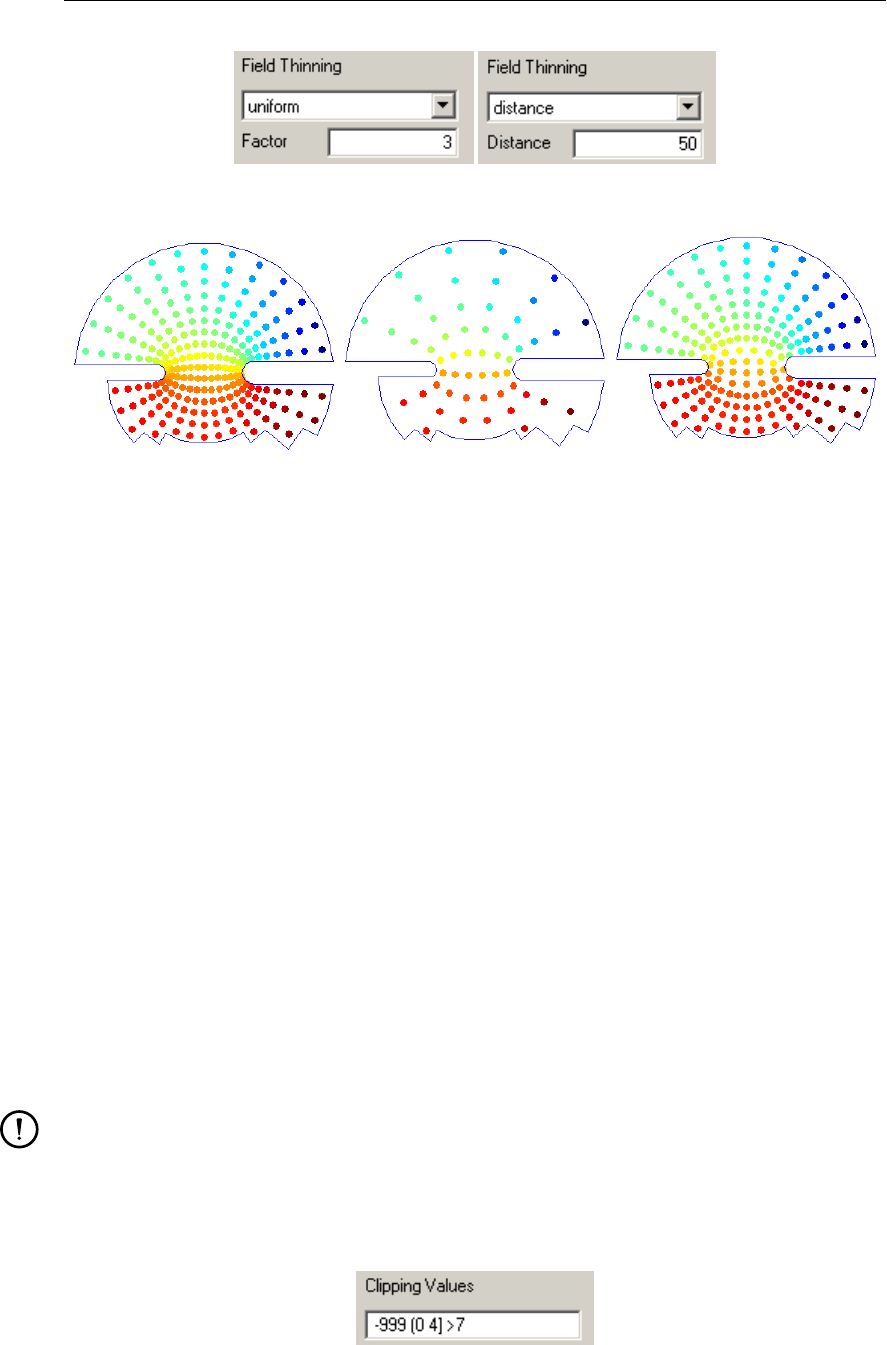
Figure 3.29: Optional field thinning based on grid numbers (uniform thinning) or distance.
Figure 3.30: Example of a marker plot without thinning (left), uniform thinning (factor 2)
and distance thinning (right).
3.22 Field thinning
A vector field, a field of values or markers can become cluttered when a lot of items are
plotted. Therefore, it is possible to selectively remove some of these items (vectors, values
or markers). There are three settings: none (default), uniform and distance. If the setting is
none, no thinning will be applied. If the setting is uniform and the factor is set to 3, every 3rd
vector/value in M, N and K direction is plotted. If the setting is distance and the distance is set
to 50, the plot locations are spaced at least 50 m.
3.23 Clipping data values
One of the most powerful plotting options is the clipping functionality. It allows you to clip/remove
certain values from the plot. Default it clips data points equal to -999, but you can clip almost
any value or range that you can think of. Examples:
<0Clip all values less than 0.
<= 0 Clip all values less than or equal to 0.
[0 4] Clip all values larger than or equal to 0 and smaller than or equal to 4.
(0 4) Clip all values larger than 0 and smaller than 4.
Furthermore, it allows you to have any combination of such ranges as shown in Figure 3.31.
Remark:
If you clip values in a certain range, for instance between 0 and 4, and two neighbouring
data points have values at either side outside the range, say -1 and 5, then a continuous
shades plot may still contain some interpolated values in the clipped range.
Figure 3.31: This setting will clip the values equal to -999, or larger than 0 and less than
or equal to 4, or larger than 7.
24 of 92 Deltares

DRAFT
Plotting options
3.24 Clipping coordinate values
Besides clipping data based on the values, it may be useful to clip the data based on xand
ycoordinates. This is in particular useful if the coordinate data contains dummy values that
have not automatically been detected and removed. Although this feature can also be used
to clip the plotted domain to a certain x,yregion, it should be mentioned here that it is more
memory efficient to use the M,Nindex space for such clipping.
Deltares 25 of 92

DRAFT
Delft3D-QUICKPLOT, User Manual
26 of 92 Deltares
DRAFT
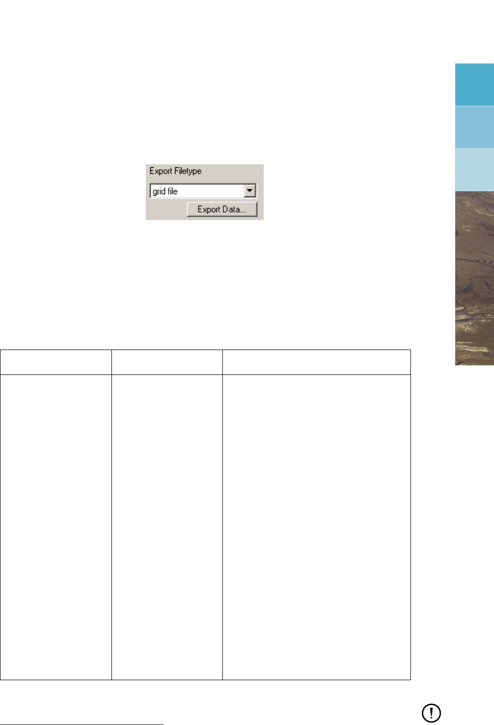
4 Export and printing options
At the end of the list of plotting options, there will always be one field that allows you to export
data to a number of file formats (see Figure 4.1). The first section of this chapter lists what
kind of file types are available under which conditions. The second section addresses the
exporting of figures for further processing.
Figure 4.1: Fields for exporting the data.
4.1 Exporting data
Data can be exported to a number of different file formats using the dropdown list and button
shown in Figure 4.1. The following table lists the formats and the conditions under which the
data can be exported to the indicated file format.
Table 4.1: Overview of the data export options
Format Condition Comments
grid file 2DH field, single time
step
grid depends on definition of selected
data field: hydrodynamic or morphologic
grid
grid file (old format) 2DH field, single time
step
the old grid format with limited precision
co-ordinates
spline one grid line, single
time step
spline format used by RGFGRID
QUICKIN file 2DH field standard format for Delft3D fields
Delft3D-MOR field file 2DH field, scalar val-
ues
obsolete file format, use QUICKIN for-
mat instead
SIMONA box file 2DH field, scalar val-
ues
3rd party file format, use QUICKIN for-
mat instead
ARCview shape 2DH field, (not contin-
uous shades), single
time step
standard GIS format
landboundary file polygonal data sets landboundary format used Delft3D
TEKAL file at most 10 time steps largely self-describing ASCII file format
Tecplot file at most 10 time steps ASCII or BINARY file format used by the
visualisation program Tecplot
CSV file 1 point, multiple time
steps
time-value ASCII file
sample file 1 time step x-y-value or x-y-z-value ASCII file
mat file always MATLAB binary format1
Remarks:
1The stand-alone version of Delft3D-QUICKPLOT writes the data in mat files compatible with MATLAB version
6. QUICKPLOT versions running within MATLAB as part of the Delft3D-MATLAB toolbox can also export to mat
files native to versions 7 and up.
Deltares 27 of 92
DRAFT
Delft3D-QUICKPLOT, User Manual
Figure 4.2: Select the printing and exporting option from the File menu of a figure.
Figure 4.3: Dialog for printing and exporting figures.
Exporting large datasets to mat files may exhaust system resources. Use Delft3D-
MATLAB interface instead.
Exported data may depend on selected component and presentation type.
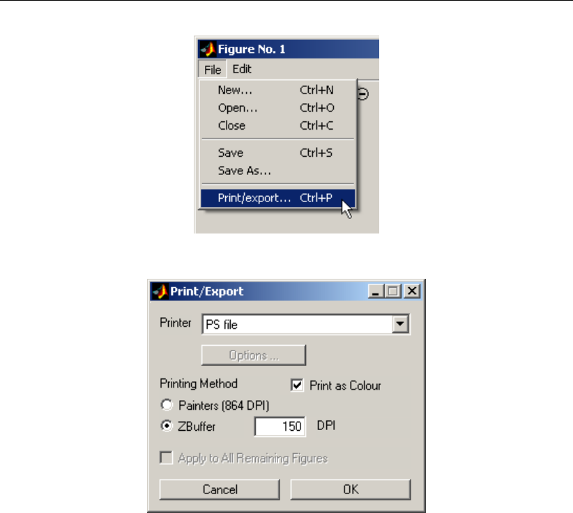
4.2 Exporting and printing figures
Every Delft3D-QUICKPLOT figure contains a File menu (see Figure 4.2). The menu allows
you to create new figures, load figures from file, close the figure, save the figure to file and,
most importantly for this section, it offers you the possibility to print and export the figure.
If you select the Print/Export option from the File menu (or if you press Ctrl+P), the print/export
dialog appears as shown in Figure 4.3. Currently, you can export your figures to the following
file types: PostScript (PS), Encapsulated PostScript (EPS), TIFF, PNG and JPEG files. On
Windows PCs you have the additional option of exporting to Windows’ EMF (Enhanced Meta
File) format, sending the figure to the clipboard as bitmap or metafile, and you can send the
figure to any of the installed Windows printers (selectable using the Options... button).
The dialog also allows you to select multiple figures to print or export. By default only the
figure from which you activated the Print/Export process is selected for printing or exporting.
If you select multiple figures, you will be asked to give a name for each figure separately.
If you are exporting or printing to a medium that supports vector graphics (such as, PostScript
files) set the printing method to painters for the best quality. The zbuffer method will always re-
sult in a bitmap representation of the image and, therefore, it is only advantageous if the image
28 of 92 Deltares
DRAFT
Export and printing options
is so complex that the painters method fails. For the current version of Delft3D-QUICKPLOT,
this applies probably only to 3D plots with continuous shades.
Remark:
Exporting or printing a series of pictures is possible using the animation functionality as
described in section 5.6. Selecting export/print as output option in the animation dialog
brings up the same dialog for exporting and printing files as shown in Figure 4.3.
Deltares 29 of 92

DRAFT
Delft3D-QUICKPLOT, User Manual
30 of 92 Deltares

DRAFT
5 Digging deeper
At the end of the ‘Getting started’ chapter, we shortly introduced the slider in the lower left
corner of each plot and indicated that it can be used to select other time steps and other
spatial co-ordinates. This chapter describes how to
combine plots (section 5.2),
looking at result differences (section 5.3),
use the Plot Manager (section 5.4),
use the slider (section 5.5),
create animations (section 5.6),
define your own derived variables (section 5.7),
define your own colour maps (section 5.8),
use the Grid selection window (section 5.9), and
use command logging to create macros (section 5.10).
5.1 Setting preferences
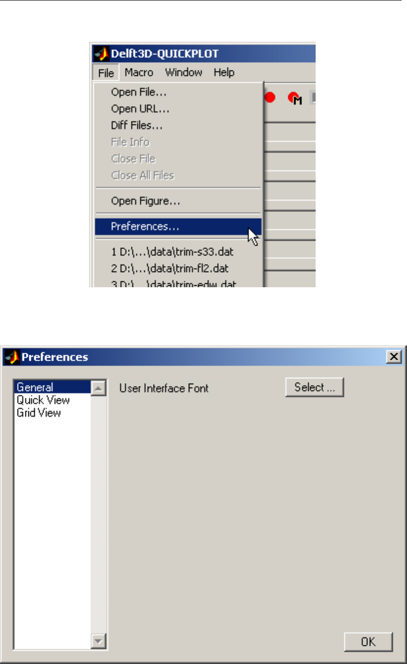
From the File menu of the main Delft3D-QUICKPLOT window, select the option Preferences... .
This will open the preferences dialog which has three sections.
5.1.1 General preferences
Currently there is only one setting that can be changed in this section, namely the characteris-
tics of the font used in all dialogs (excluding menus) of Delft3D-QUICKPLOT. This functionality
is mainly intended for cases in which the default system font selection is unsuitable.
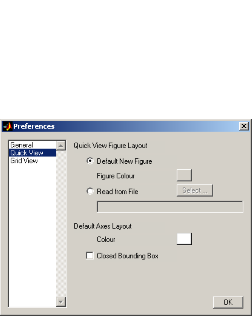
5.1.2 Quick View preferences
The Quick View section allows you to personalize a number of figure and axes settings. It
allows you to change the figure and axes colours and you can switch whether the bounding
box of the axes are closed or that, as is the default, only the left and bottom axes are drawn.
Instead of the simple default figure, it is also possible to point to a previously saved figure
file. Delft3D-QUICKPLOT will use the layout of the selected figure each time you press Quick
View. If the figure file contains multiple axes, the Quick View plot action will use the front axes.
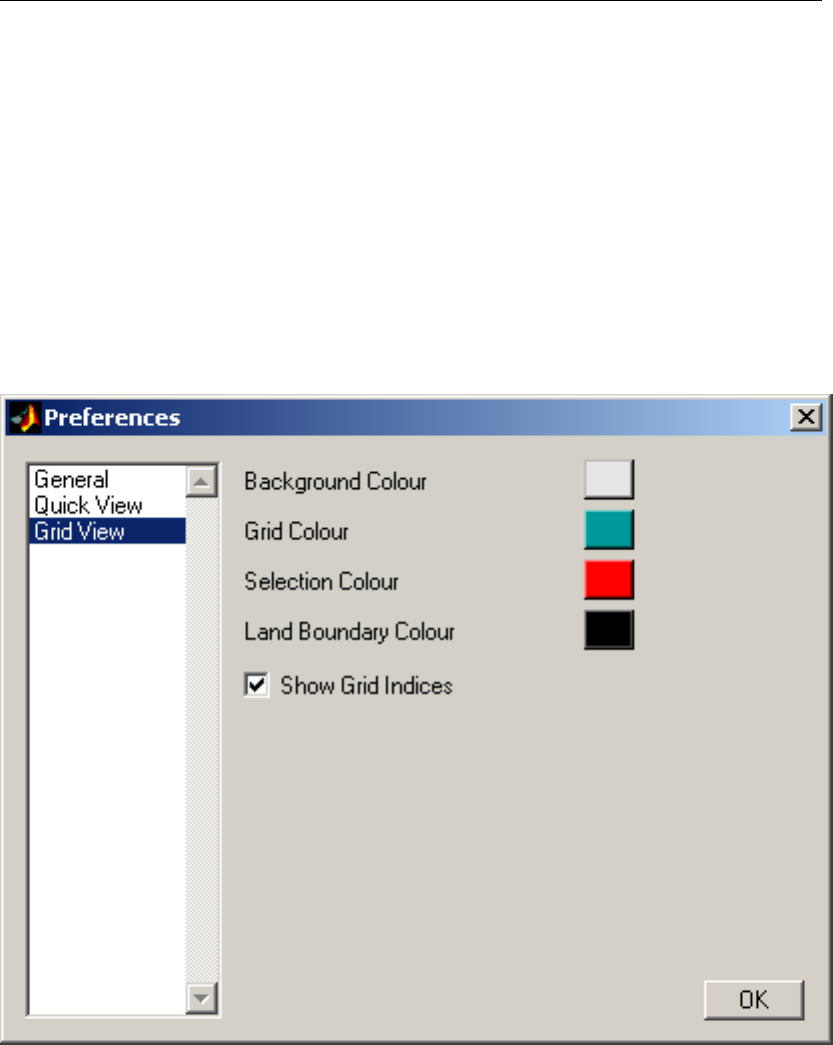
5.1.3 Grid View preferences
The Grid View section allows you to change the colours used by the Grid View interface (see
section 5.9) and to select whether grid indices should be drawn for curvilinear grids by the
Grid View interface. Switching of the drawing of grid indices may speed up the Grid View
interface in case of large models.
Deltares 31 of 92
DRAFT
Delft3D-QUICKPLOT, User Manual
Figure 5.1: Start the preferences dialog.
Figure 5.2: General section of the preferences dialog.
32 of 92 Deltares
DRAFT
Digging deeper
Figure 5.3: Quick View section of the preferences dialog.
Deltares 33 of 92
DRAFT
Delft3D-QUICKPLOT, User Manual
Figure 5.4: Grid View section of the preferences dialog.
34 of 92 Deltares
DRAFT
Digging deeper
Figure 5.5: Overlay plot of the water level using patches and the depth averaged velocity
using red vectors.
5.2 Combining multiple data sets in one plot
In most cases it will be sufficient to plot only one quantity in a plot. However, under certain
circumstances you may want to combine two different variables or variables from different files
in one plot. Therefore, an Add to Plot button has been added next to the Quick View button.
By default the Add to Plot function adds the plot of the selected variable to the last created
figure/axes using Quick View. If you want to add a variable to another axes, you should use
the Plot Manager to select the desired axes (see section 5.4).
The text on the Add to Plot button will turn red if the program detects some incompatibilities
in the plot settings. These checks currently include a check on dimensionality of the data set
(e.g. trying to add a 2D spatial data set to a time-series plot) and a check on units (e.g. a
velocity magnitude [m/s] cannot be added to a water level [m] plot, nor should a water level in
[m] be added to a plot of water levels in [ft]). Although the text turns red to warn you of such
conflicts, the button will still works such that you can still combine data sets in one plot.
Remarks:
It is not possible to combine two plots with different colour maps in one figure.
It is not possible to combine two plots with different colour scaling in one axes.
It is not possible to combine plots with the presentation type set to continuous shades
with other plot types, such as contours and vectors.
Deltares 35 of 92
DRAFT
Delft3D-QUICKPLOT, User Manual
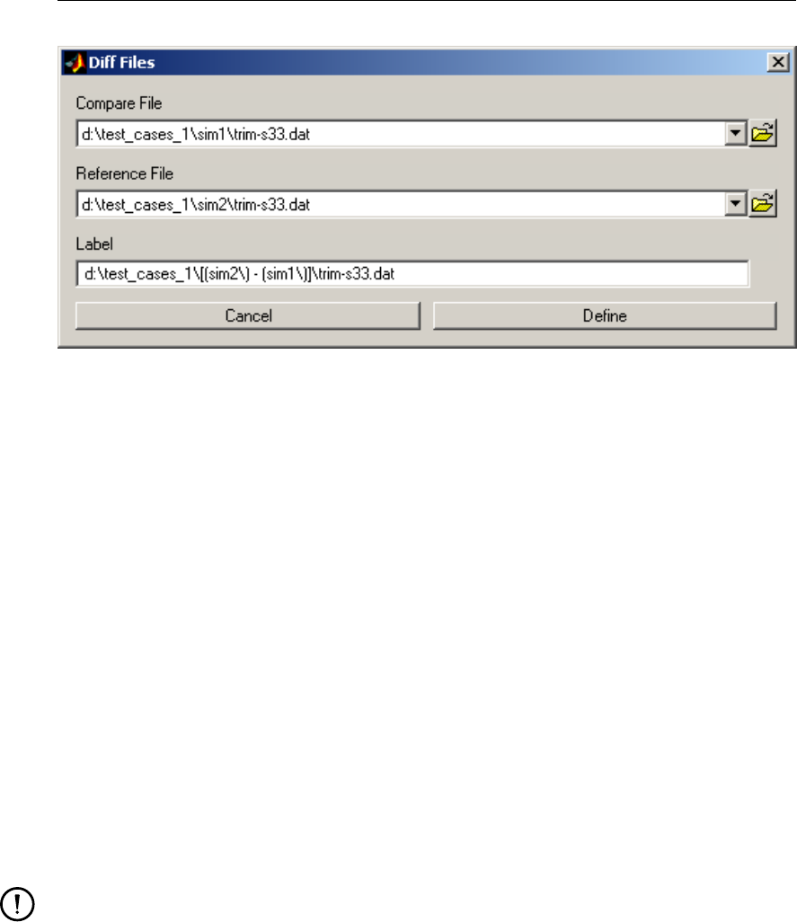
Figure 5.6: Diff Files dialog.
5.3 Difference of Files
Often you will run multiple simulations to study the effect of certain parameter settings, change
in forcing conditions or minor geometry changes. If the effect is (initially) small, it may some-
times be difficult to spot the essence of the differences between two simulations. The option
to define and combine variables (described in section 5.7) allows you to define and subtract
individual variables to look at the net effect of a model input change. However, this method
is quite laborous and error prone if you want to look at the differences of multiple quantities
(possibly in multiple files). The option to use logfiles (see section 5.10) to repeat some steps
helps but is not always straightforward to use. For this reason we have added a new feature
called ‘Diff Files’ to quickly subtract the contents of two data files. The new option is available
from the File menu. When you select the menu item, you will see the dialog shown in Fig-
ure 5.6. The list boxes are automatically populated with the files already opened in the main
dialog, but you can open additional files if needed (note: these additional files won’t show up
in the main dialog). The algorithm will look for all quantities with identical names and identical
time and space dimensions and subtract (on demand) the values in the second file from the
values in the first file. The last line of the dialog allows you to specify the name that should
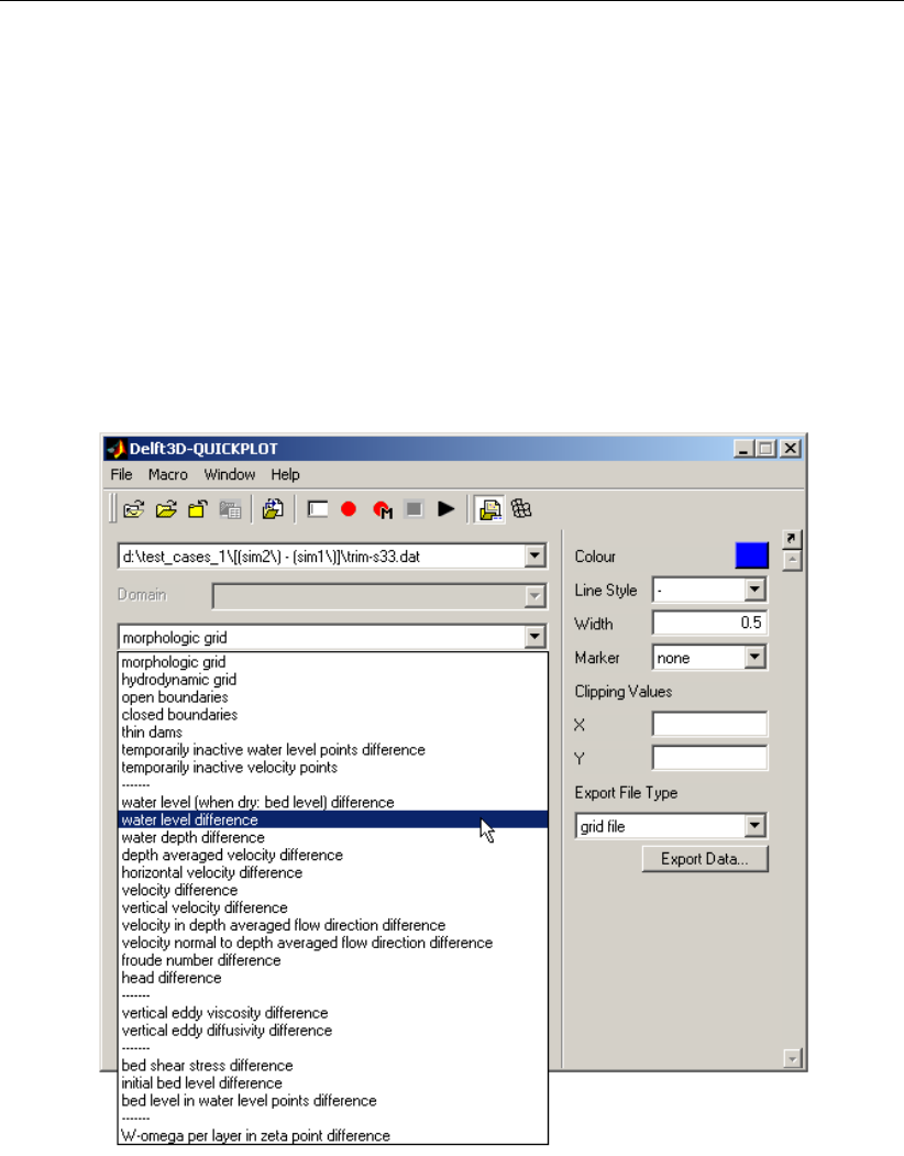
identify the difference of the files in the listbox in the main dialog. In the main dialog you
will subsequently be able to select of which quantity you would like to see the differences as
shown in Figure 5.7.
Remarks:
When looking at differences, please check the limits of vertical axes and color bars care-
fully. If the differences are small and irregular they may very well result from numerical
noise in the computations.
Since the algorithm checks for identical time and space dimensions, the differencing will
fail if you change the number of output stations or the number of time steps. Supporting
such changes is considered for a future release.
The algorithm doesn’t check for location or time changes, i.e. if you change grid, output
times, or output stations (or reorder them) while keeping the grid dimensions, number of
time steps and number of output stations identical then the ‘Diff Files’ option will allow
you to subtract the data from the original simulation. The graphs will show you the
location and times of the original (top) simulation.
36 of 92 Deltares
DRAFT
Digging deeper
Figure 5.7: Diff Files dialog.
Deltares 37 of 92
DRAFT
Delft3D-QUICKPLOT, User Manual
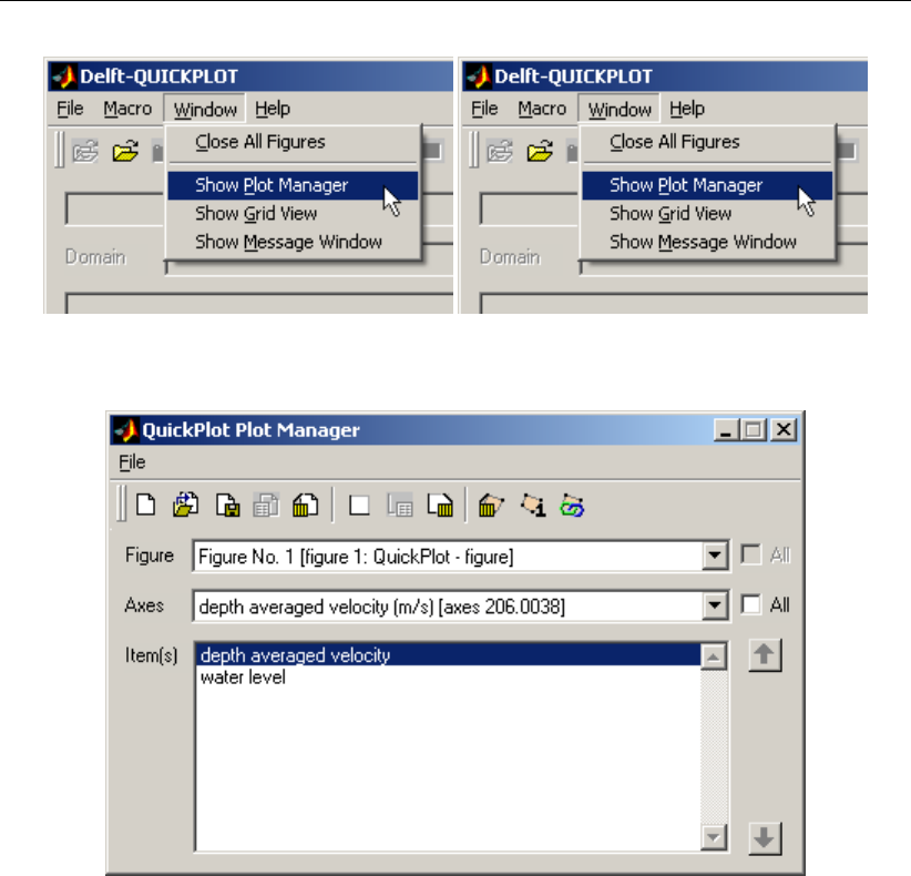
Figure 5.8: Activation of the Plot Manager from the Window menu of the main program
window.
Figure 5.9: Interface of the Plot Manager.
5.4 Plot Manager
If you want to add a variable to another plot than the last one created or if you want to delete
a quantity from a plot, you should use the Plot Manager. The Plot Manager can be opened
from the Window menu in the main program window or by clicking on the button in the toolbar.
The Plot Manager has a toolbar with buttons for
creating new figures (some standard paper layouts are provided) and opening previously
saved figures, saving figures, setting figure options (not yet available), deleting figures;
creating new axes, setting axes options (not yet available) and deleting axes;
deleting items (in axes), requesting information on items, and linking items for animations.
The selection boxes for figures and axes allow you to select all figures and axes. The list
box shows the names of the items in the selected axes (which may be located in multiple
figures). If the bare names of the items are the same, the names are automatically extended
with the name of the file, selected time steps and M, N or K indices, and plot type if one or
more of these labels will help to distinguish between the items. More detailed information
(in particular plot characteristics) for the selected item can be obtained by clicking the item
information button in the toolbar. Multiple items across multiple axes or even figures can be
linked to animate or to scroll through at once.
38 of 92 Deltares

DRAFT
Digging deeper
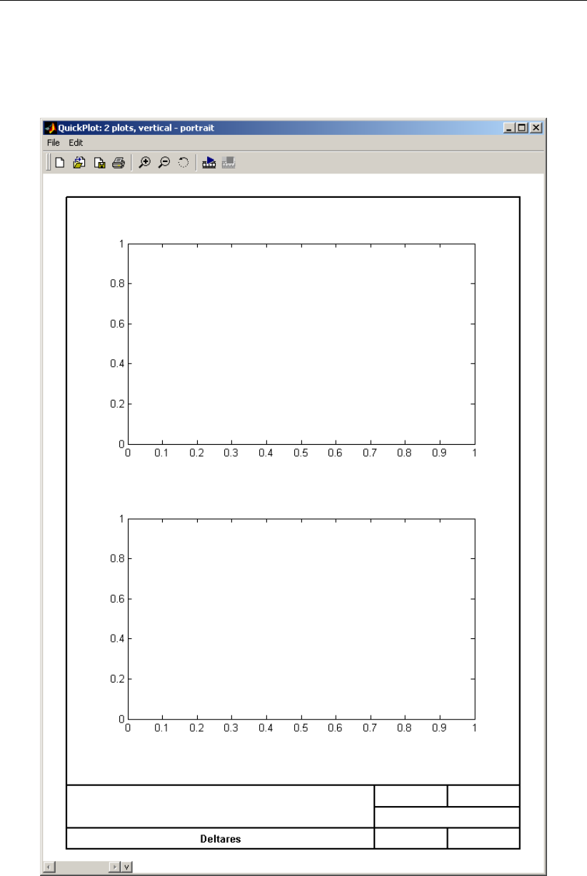
The new figure button allows you to create a new figure with a standard layout. Figure 5.10
shows a couple of standard layouts available. All plots except for the free format figure contain
the standard Deltares border. You can edit all texts in the border by selecting the Edit Border
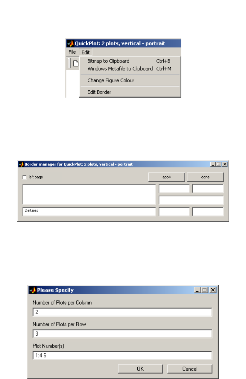
option from the Edit menu in the figure (see Figures 5.11 and 5.12). More flexibility in figure
layouts can be achieved making your own set of standard plot layouts and by using the load
figure option instead of the new figure option. Because stand-alone Delft3D-QUICKPLOT
saves figures in the figure file format of MATLAB 6.5, you can also open any figure created in
MATLAB 6.5.
Furthermore, you can add axes to and remove axes from the selected figure using the next
row of buttons. There are three options for adding axes:
one plot. In this case one big axes is created (identical to the default axes that appears
when pressing Quick View).
user selected subplot. In this case a number of plots can be created based on a regular
grid as illustrated by Figures 5.13 and 5.14. Note that the plots are numbered row-wise
starting in the upper-left corner.
user positioned subplot. In this case, you are asked to interactively draw the location of
the axes in the figure. The axes labels extend outside the indicated area.
If you want to add a plot to a certain axes, select the figure to which the axes belong from the
list of figures and, subsequently, select the axes from the list of axes. Now, the desired axes
are active and you can use the Add to Plot option to add a dataset to the active axes. The
lower listbox in the Plot Manager lists all items/quantities plotted in the axes (or if you check
the ‘all’ checkbox to the right of the axes listbox, all items in the current figure are listed). You
can select and delete some of them and you can link them for an animation (see also Sections
5.5 (interacting with plots) and 5.6 (animating results).
5.5 Interacting with plots
Each figure contains a toolbar with seven buttons as shown in Figure 5.16. From left to right
they provide the following functionality: create a new figure, load a figure from file, save a
figure to file, print a figure (Windows only), zooming in, zooming out and rotating the plot.
A zoom action should always start inside the plot area of the axes. It works by dragging a
zoom area with the left mouse button pressed down. When the zoom-in mode is activated,
you can zoom out with a right click. When the zoom-out mode is activated, you can zoom
out with the left button (single click) and zoom in with the right button (drag zoom area). It is
only possible to zoom out up to the dimensions of the original plot. The rotation option is not
relevant for most plots. Only a plot for plots created using Presentation Type set to continuous
value, 3D particle tracks from D-Waq PART and vector plots of the 3D velocity fields, the
rotation functionality can be useful. Rotate the axes by pressing and holding down the left
mouse button. Preliminary the vertical exaggeration factor is kept fixed at 30, which is enough
to visualise 3D topography. When zooming in on a rotated plot, use single clicks only; do not
drag a zoom window.
A slider is drawn in the lower left corner of the plot window. The slider can be used to change
the time step, station or M, N, K co-ordinate of one or more of the objects in the plot. The
currently selected time step, station or M, N, K co-ordinate is shown in the tooltip of the slider.
To the right of the slider, there is a small button marked with the character v; that button,
allows you to select the object and dimension (i.e., time step, station, M, N, or K co-ordinate)
to be varied (see Figure 5.18). Left click on the button and select from the menu that appears
the object and dimension that you want to vary: the current selection is marked with a check
Deltares 39 of 92
DRAFT
Delft3D-QUICKPLOT, User Manual
Figure 5.10: A couple of standard figure layouts created using the new figure button of
the Plot Manager: 1 plot – portrait, 2 plots, vertical – portrait, 4 plots, 2x2 –
portrait, 2 plots, horizontal – landscape.
40 of 92 Deltares
DRAFT
Digging deeper
Figure 5.11: Select Edit Border from the Edit menu to edit the border texts.
Figure 5.12: The layout of the editor for the border texts matches the layout of the boxes.
Figure 5.13: Dialog for defining five ‘user selected subplots’ based on a regular grid of 3
plots on a row and 2 plots above each other. All plots are created except
plot number 5 (see Figure 5.14).
Deltares 41 of 92
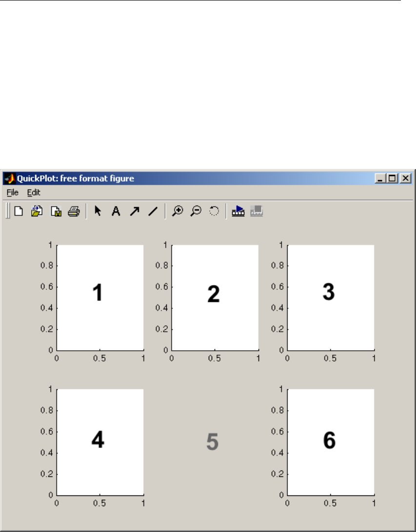
DRAFT
Delft3D-QUICKPLOT, User Manual
Figure 5.14: Five ‘user defined subplots’ with an indication of their row-wise numbering.
42 of 92 Deltares
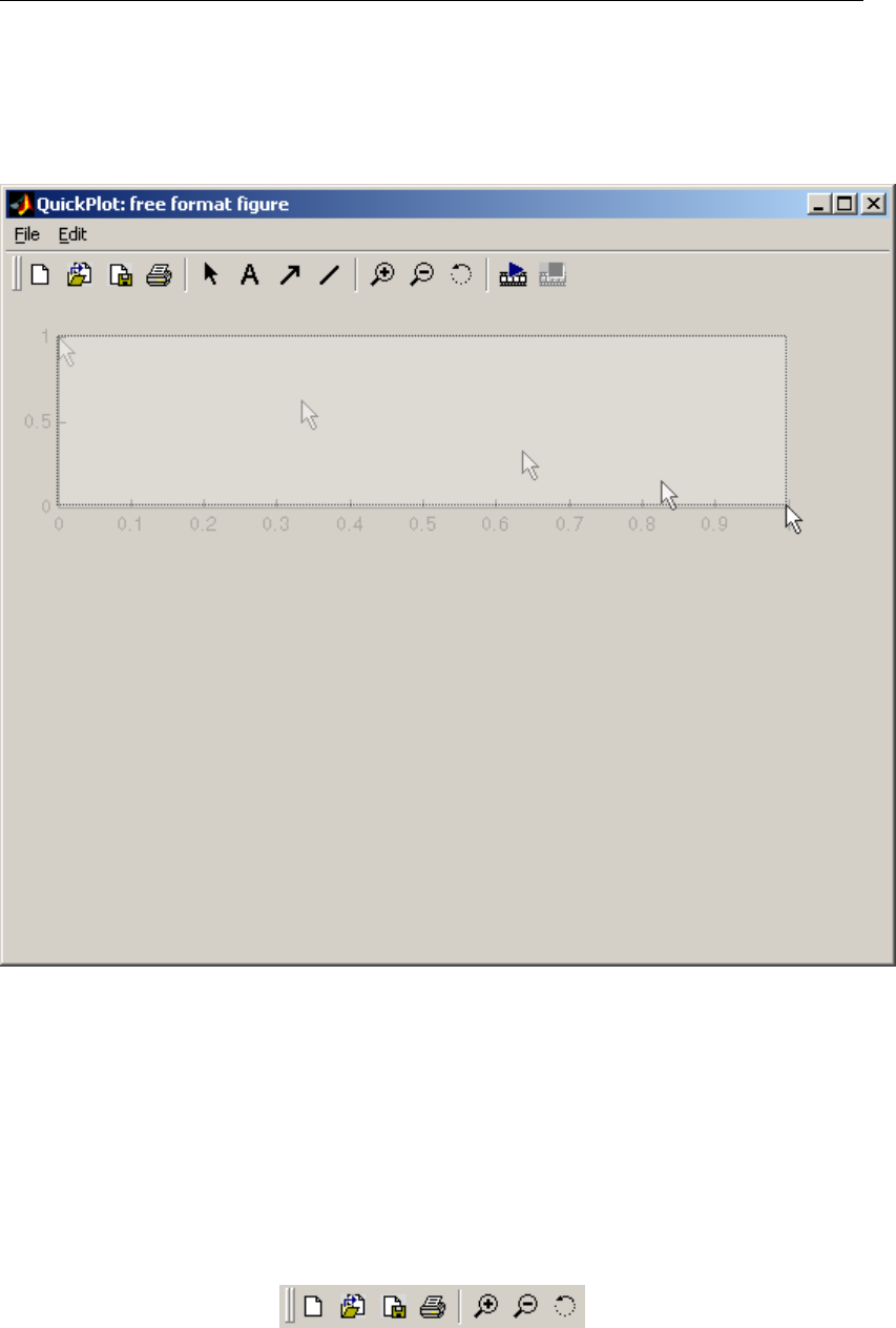
DRAFT
Digging deeper
Figure 5.15: Example of the interactive positioning of a ‘user positioned subplot’.
Figure 5.16: Toolbar buttons of a Delft3D-QUICKPLOT figure.
Deltares 43 of 92
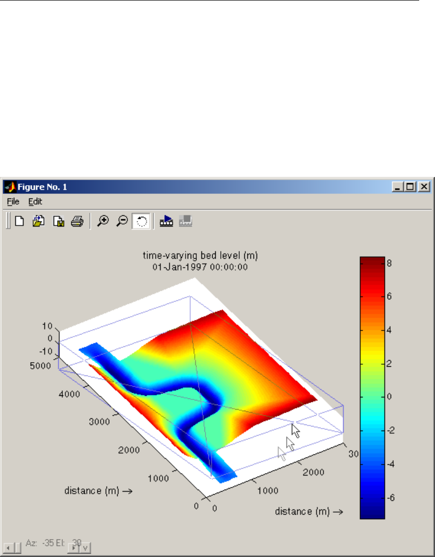
DRAFT
Delft3D-QUICKPLOT, User Manual
Figure 5.17: Rotating a 3D topography.
44 of 92 Deltares
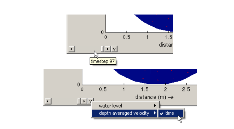
DRAFT
Digging deeper
Figure 5.18: Slider and object/dimension selection button marked with the character v.
mark (see the right part of Figure 5.18). If the dimension of the newly selected object matches
your previous selection (i.e., same number of time steps or same number of grid points) the
program will ask whether you would like to link the parameter changes of the selected object
with those of the previous object(s). If you answer this question confirmatively, both the newly
selected object and the previously selected ones will be affected by the state of the slider.
To unlink the objects, select any of the objects again. The same functionality can also be
accessed by using the link items button in the Plot Manager; if you want to link a large number
of items that approach will be faster.
5.6 Animating results
The slider allows you to interactively change between time steps, stations or grid lines. If you
combine these plots together you have an animation. For this purpose each figure contains an
Animation menu; select Start from this menu (or press Ctrl+A). If there is anything to animate
in the figure, a dialog appears as shown in Figure 5.19. The animation will vary the same
objects and dimensions as the slider does at the moment that the animation dialog opens.
Therefore, the creation of an animation starts by selecting the object(s) and dimension to
animate using the procedure described in the previous section.
The dialog contains six fields.
output: The first field allows you to indicate whether you want each picture of the animation
written to be stored. You may select one of the supported bitmap formats (TIF, JPG, PNG
or BMP), output via the print/export option (automatically send a series of figures to the
printer) or create an AVI file (Windows only).
render in background: When creating output (other than to the screen), you can select the
option to render in background. This accelerates the image generation. This option is not
available for BMP files which are created from screen grabs.
steps: The second field allows you to select the time steps and spatial co-ordinates that
should be part of the animation. You can walk through the steps in any order you like, e.g.
backwards (97:-1:1) or more detailed in one range (1:19 20:5:95).
loop until stopped: The last field enables you to animate the selected steps repeatedly
until the animation is explicitly stopped. This option only available if the output option is
set to no output.
maximum frame rate: Because animations on small datasets and fast hardware may be
Deltares 45 of 92
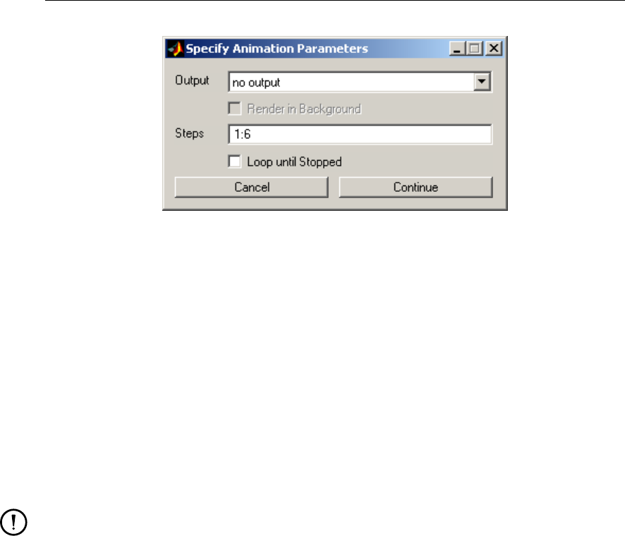
DRAFT
Delft3D-QUICKPLOT, User Manual
Figure 5.19: Dialog for the animation settings.
too fast to follow, you can set a maximum display frame rate. This frame rate is also used
when creating an AVI animation as the frame rate of the animation.
script: When you run QUICKPLOT as part of the Delft3D-MATLAB interface from within
MATLAB, you may optionally specify an m-file script to run after each plot update. This
allows you to make final adjustments to the plot using MATLAB features. This option is not
available in the standalone Delft3D-QUICKPLOT version.
The default setting is to animate the results for the full range of the dimension to be varied (for
instance all time steps or all N co-ordinates) without storing the pictures. Instead of storing
the pictures on disk, the program can also copy the files to the clipboard (useful if you have
another program that can collect them automatically) or send them to a printer. The animation
can be stopped by pressing Ctrl+H or selecting Stop from the Animation menu.
Remarks:
If you are using the animation option for the purpose of creating files (i.e. not for imme-
diate viewing), you may generally cover or minimise the figure that is being animated (or
select Render in Background). However, there is one exception: BMP files are created
using a screen capture process which will produce undesired effects when the figure
playing the animation is not on top.
When creating an animation it is generally best to use consistent colouring and scaling
for all pictures/frames of the animation. Set vector scaling, colour thresholds and colour
limits manually as indicated in Sections 3.6,3.12 and 3.19. For 1D and 2DV plots, use
the zoom option explained in section 5.5 to keep the plot ranges fixed.
5.7 Defining and combining variables
Sometimes it is useful to determine derived quantities, like minimum, mean or maximum val-
ues of some quantities over a (rectangular) part of the domain (e.g. a cross-section) or to
determine the Froude number in each point. For these purposes, the program includes basic
functionality for defining variables and combining those using simple expressions.
The first step is defining the variables. The main program window contains one button that has
not yet been explained, namely Define Var., and it does as you probably have guessed, lead
to the definition of a variable. The variable will represent the data selection at the moment that
the variable was defined. For instance, in the case shown in Figure 5.20, defining a variable
now will cause it to represent the last water level in the selected Delft3D communication file.
However, if you check the Time Step – All checkbox first, the variable will represent the water
level field at all 97 time steps. Careful data selection before defining the variables is important.
Clicking the Define Var. button will open a small dialog window requesting a name for the
46 of 92 Deltares
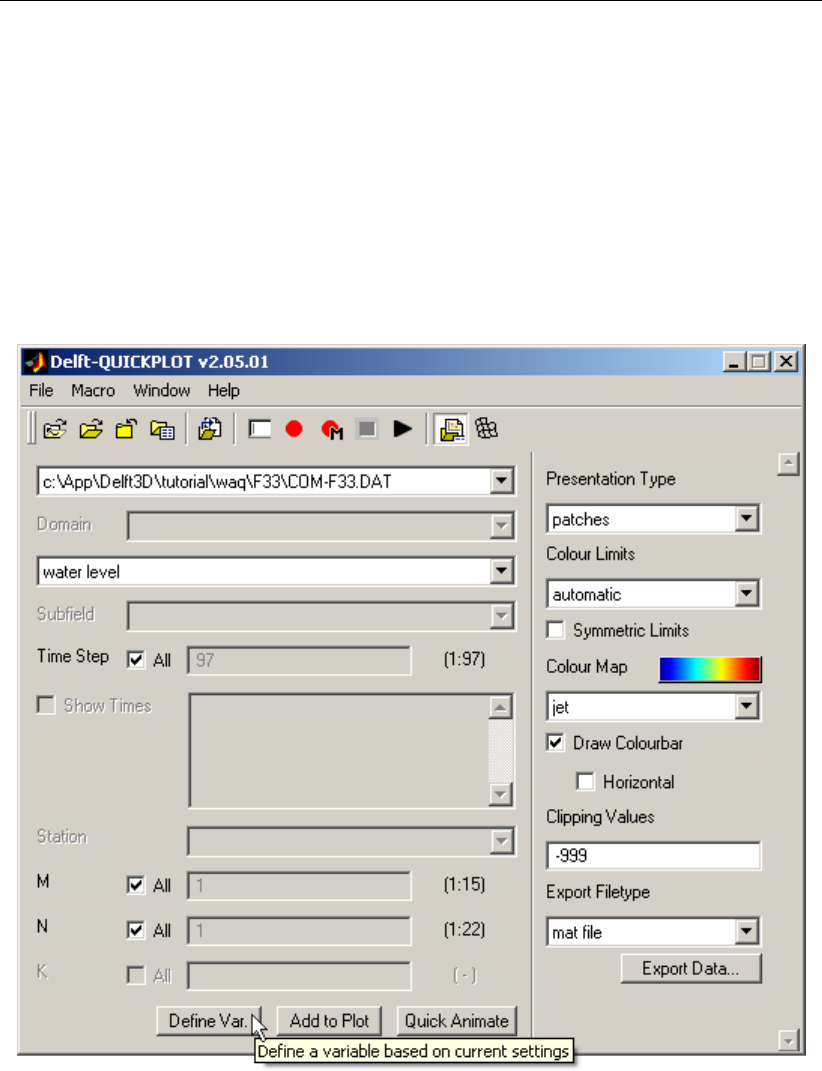
DRAFT
Digging deeper
Figure 5.20: Clicking Define Var. will lead to the definition of a variable representing the
last water level field in the selected Delft3D communication file.
Deltares 47 of 92
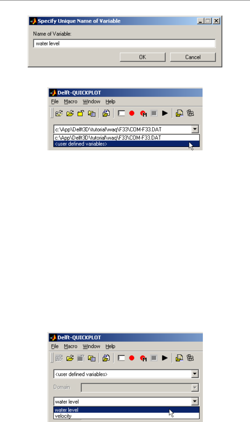
DRAFT
Delft3D-QUICKPLOT, User Manual
Figure 5.21: Dialog window requesting a unique name for the variable.
Figure 5.22: Virtual file labelled <user defined variables>in the list of data files.
variable (see Figure 5.21). The dialog will persist until you have specified a unique variable
name. Suppose that we define two variables: ‘water level’ and ‘velocity’ representing all 97
water levels and depth averaged velocity fields in the Delft3D communication file used above.
Once you have defined variables, the label <user defined variables>will be available in the
list of data files as shown by Figure 5.22. If we select it, the list of data fields will contain the
two variables that we had defined: ‘water level’ and ‘velocity’ (see Figure 5.23). It is possible
to make plots using these two variables in exactly the same way as the original data fields and
all plot and export options still apply.
The variables can be manipulated by clicking on the File options button. The file options
dialog for the virtual file <user defined variables>allows you to define new variables based
on functional relationships of one or two existing variables. The dialog window is shown in
Figure 5.24. The following operators are available:
A+B, A-B, A/B, A*B, max(A,B), min(A,B): combine two data sets of compatible size
+ constant, * constant, ˆ
constant, max(A,constant), min(A,constant): combine a data set
with a constant
10log, abs: compute logarithm or absolute value of data set
Figure 5.23: The data field list contains the variables.
48 of 92 Deltares
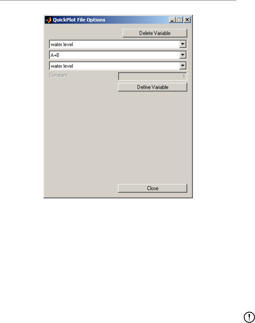
DRAFT
Digging deeper
Figure 5.24: File options dialog window for <user defined variables>while defining a
new conditional variable.
magnitude: compute magnitude of vector field
series: A,B: treat second variables as a continuation of the first variable (e.g. combine
data sets from separate files into one large virtual time-series)
A under condition B: use the value of the first variable when the second variable is in a
certain range of values. Acceptable condition statements include a value, e.g. 3, a range,
e.g. [2 3], or all values larger or smaller than a certain value, e.g. >3. See also section 5.7
on clipping data values.
max, alg. mean, min, sum of M, N, K: compute maximum, algebraic mean, minimum
and sum of a field variable in the indicated grid direction. The spatial co-ordinates are
averaged along the indicated direction.
Remarks:
Two variables have compatible dimensions if all dimensions (time and space) match for
the two variables or if dimensions that do not match are equal to 1 for either one of the
variables.
The alg. mean M, N, K operators compute the algebraic mean and not the weighted
average. For instance, the ‘alg. mean K’ operator merely sums all variables in the K
direction and divides the sum by the number of points in the vertical, so the computed
value does not correspond to the depth averaged value.
Given the operators listed above and the two variables, the Froude number can be defined in
five steps assuming a horizontal bed level at 5 m below the reference level:
1 select the variable ‘velocity’, select operator ‘magnitude’, define a new variable called
Deltares 49 of 92
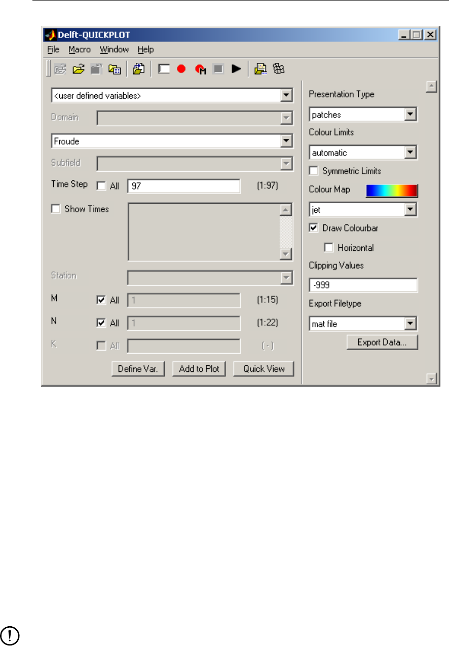
DRAFT
Delft3D-QUICKPLOT, User Manual
Figure 5.25: Main program window showing the newly defined variable ‘Froude’.
‘magnitude(velocity)’
2 select the variable ‘water level’, select operator ‘+ constant’, specify constant ‘5’, define a
new variable ‘water depth’
3 select the variable ‘water depth’, select operator ‘* constant’, specify constant ‘9.8’, define
a new variable ‘water depth * 9.8’
4 select the variable ‘water depth * 9.8’, select operator ‘ˆ
constant’, specify constant ‘0.5’,
define a new variable ‘sqrt(gh)’
5 select the variable ‘magnitude(velocity)’, select operator ‘A/B’, select the variable ‘sqrt(gh)’,
define a new variable ‘Froude’
Switch back to the main program window. The variable ‘Froude’ and all other intermediate
variables are now available for plotting. Since the original variables, called ‘water level’ and
‘velocity’, were both defined for the whole domain and for all time steps, so is the variable
‘Froude’. All plot and export options still apply.
Remark:
The variables are currently self-containing, that is the internal definition of the variable
‘Froude’ contains all information on the intermediate steps and information on the orig-
inal variables ‘water level’ and ‘velocity’. If all other variables are deleted (using the
Delete Variable button in the file options dialog) and all files are closed, the ‘Froude’
variable will still be able to plot as long as the files are still in their original location
and contain valid data. Because of reasons of memory efficiency and flexibility, this
50 of 92 Deltares
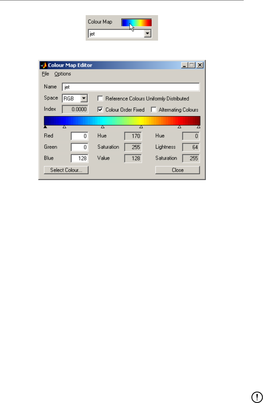
DRAFT
Digging deeper
Figure 5.26: Open the colour map editor by clicking on the colour map preview.
Figure 5.27: The colour map editor.
behaviour is likely to change in a future release.
5.8 Define your own colour maps
The number of colour maps can be extended interactively by clicking on the preview colour
map in the list of plot options as indicated in Figure 5.26.
A colour map editor window will open as shown in Figure 5.27. It will initially show the colour
map selected in the plot options. The colours that form the basis of the colour map are indi-
cated by little triangles below the colour bar. The active colour is indicated by a black triangle
whereas the other colours are indicated by white triangles. Left clicking on the colour bar
selects the nearest colour. Right clicking on the colour map adds a colour at the selected
location; the colour will initially match the colour in the original colour map (see Figure 5.28).
The colour can be changed by specifying the red, green and blue components (or the resepec-
tive components in case of another colour space) or by selecting the colour from a standard
colour selection interface (accessible by clicking the Select Colour button in the lower left cor-
ner). The location of the colour on the colour map can be changed by left click and dragging
the colour. Colours can be removed from the colour map by left clicking on them and dragging
them away from colour bar.
When you are satisfied with the new colour map, specify a new name, save it in the colormaps
directory as a file with an extension ‘.clrmap’ and close the colour map editor; the new colour
will be selected in the main window. If you don’t like the changes don’t save the colour map,
just press the Close button or open another colour map.
Remark:
Make sure that the colour map has a unique name. The program will behave incorrectly
if there are multiple colour maps with the same name. Note: the name of the colour
map used by Delft3D-QUICKPLOT is the name you specify in the user interface; not
Deltares 51 of 92

DRAFT
Delft3D-QUICKPLOT, User Manual
Figure 5.28: Right click on the colour bar to add a colour.
the name of the file.
5.9 Using the Grid selection window
Besides the Plot Manager described in section 5.4, you can also start the Grid selection
window from the Window menu of the main program window (command: Open grid view) or
from the icon on the toolbar in the same window. This will open a new window showing a plot
of the grid (optionally with grid numbers) in cyan and the selection of the spatial co-ordinates
in red as shown in Figure 5.29 (some of these settings can be changed in the preferences
dialog described in section 5.1.3).
The interface can be used as an alternative way of selecting a grid line or area to be plotted.
The selection procedure should be started from the Select menu of the Grid selection window
or the associated toolbar button. There are ten selection options: Grid Point, (whole) Grid
Line, Grid Line Segment, Piecewise Grid Line, Shortest Path, Arbitrary (x,y) Line, Grid Range,
Whole Grid, Arbitrary Rectangle, and Arbitrary Area. Figure 5.29 shows a selected Grid
Range; Figure 5.30 shows a General Line while being drawn (toolbar buttons and menus
disabled). A Grid Point is selected using a single click. A Grid Line is selected using one click
to select one point and a second click to select the grid line direction. A Grid Line Segment
is selected by subsequently clicking on the start and end point. The selection process of
Piecewise Grid Line, Shortest Path, Arbitrary Line and Arbitrary Area start and continue with
left mouse clicks and finish with a right mouse click. A Grid Range and Arbitrary Rectangle
require two clicks indicating two opposite corners of the range to be selected. The Whole Grid
option does not require any clicks. The number of options accessible depends on the data set
chosen. During the selection process the mouse co-ordinates are indicated in the lower left
corner: both X, Y and M, N co-ordinates. When the selection process is switched off, you can
zoom in by dragging a zoom area while keeping the left mouse button pressed and zoom out
by pressing the right mouse button.
Remarks:
The grid selection window switches between the hydrodynamic and morphologic grid
depending on the location of definition of the selected data field in the main program
interface.
For large models (re)drawing the Grid selection window may require a significant amount
of time, therefore, it is advised to keep the window closed in general.
52 of 92 Deltares
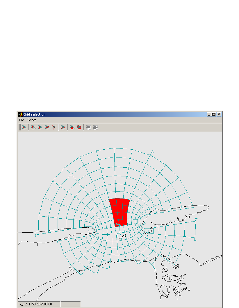
DRAFT
Digging deeper
Figure 5.29: Grid selection window after the selection of a Grid Range.
Deltares 53 of 92
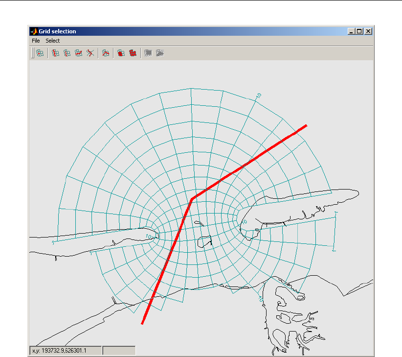
DRAFT
Delft3D-QUICKPLOT, User Manual
Figure 5.30: Grid selection window while selecting an Arbitrary Line.
For reference one can load one or more land boundary files from the File, Show Land
Boundary menu in the Grid View window. These land boundaries will remain to be
displayed until you select the File, Show Land Boundary menu item and cancel the
selection of a new land boundary file. Acceptable file formats are Tekal two column
landboundary files, BNA files, ArcInfo generate files and polyline Esri shape files.
5.10 Using log files as macros
Delft3D-QUICKPLOT has log file functionality for all actions of the main program window and
some secondary interfaces, such as the file options dialog. This functionality can be accessed
from the Macro menu and the macro icons on the toolbar of the main program interface as
shown in Figure 5.31.
The icons have (from left to right) the follow purpose:
Open the Delft3D-QUICKPLOT command line interface (menu item: Show Command
Line). In general you will not need this, it is used for testing out new functionality.
Record commands to a log file (menu item: Record Log File).
Record commands to a MATLAB script file (menu item: Record MATLAB Script).
Stop recording the commands (menu item: Stop Recording)
Play/re-run a log file (menu item: Run Log File).
When the recording of commands is started all commands will be written in ASCII format to
a file (extension .qplog) specified by you until you stop the recording. The commands stored
54 of 92 Deltares
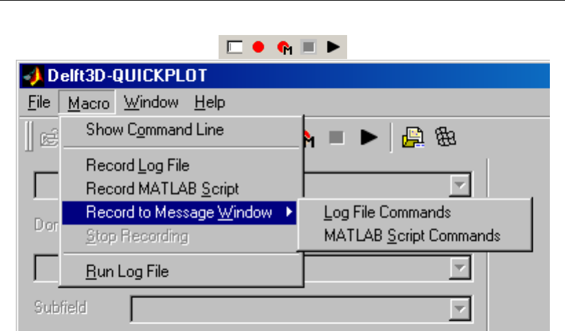
DRAFT
Digging deeper
Figure 5.31: Logfile icons in the main program interface.
in a log file can be played back, that is, log files can be used as macros. To repeat the list of
commands stored in a log file, select the Run Log File option and select the file. The MATLAB
script file is intended for use with the Delft3D-MATLAB interface, but can be re-run using the
Run Log File option as well.
In addition to writing the commands to a log or script file, it is possible to echo the commands
to the Delft3D-QUICKPLOT Message Window.
This manual does not explain the commands in the log file. Below you find an example of the
log file of the procedure to define the Froude variable in section 5.7 from the opening of the
file until the first plot.
openfile ’d:\Delft3D\tutorial\waq\f34\com-f34-waq.dat’
selectfield ’water level’
allt 1
defvariable ’water level’
selectfield ’depth averaged velocity’
defvariable ’velocity’
selectfile ’<user defined variables>’
fileoptions ’selectvar’ ’velocity’
fileoptions ’selectoperator’ ’magnitude’
fileoptions ’defvariable’ ’magnitude(velocity)’
fileoptions ’selectvar’ ’water level’
fileoptions ’selectoperator’ ’+ constant’
fileoptions ’const’ 5
fileoptions ’defvariable’ ’water depth’
fileoptions ’selectoperator’ ’*constant’
fileoptions ’const’ 9.8
fileoptions ’defvariable’ ’water depth *9.8’
fileoptions ’selectoperator’ ’^ constant’
fileoptions ’const’ 0.5
fileoptions ’defvariable’ ’sqrt(gh)’
fileoptions ’selectvar’ ’magnitude(velocity)’
fileoptions ’selectoperator’ ’A/B’
fileoptions ’selectvar2’ ’sqrt(gh)’
fileoptions ’defvariable’ ’Froude’
selectfield ’Froude’
allt 0
Deltares 55 of 92
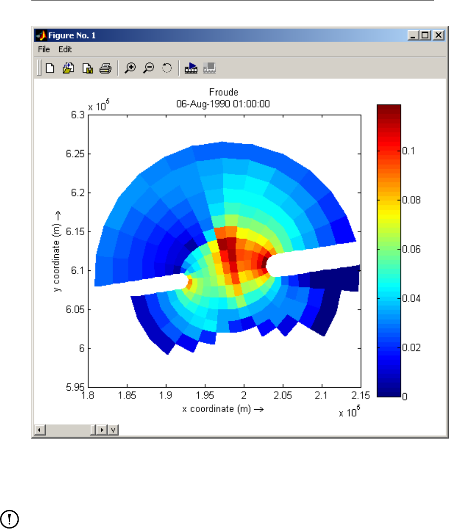
DRAFT
Delft3D-QUICKPLOT , User Manual
Figure 5.32: End result of the example log file and MATLAB script.
quickview
Remarks:
Interactive commands (manipulation of plots) are not recorded.
As an alternative to a log file, you can write a MATLAB script file. Its basic syntax is the
same, but it consists of valid MATLAB commands to be used in combination with the
Delft3D-MATLAB interface that allows for integration of Delft3D-QUICKPLOT features
and the tools of the MATLAB environment. The equivalent MATLAB script reads:
d3d_qp(’openfile’,’d:\Delft3D\tutorial\waq\f34\com-f34-waq.dat’)
d3d_qp(’selectfield’,’water level’)
d3d_qp(’allt’,1)
d3d_qp(’defvariable’,’water level’)
d3d_qp(’selectfield’,’depth averaged velocity’)
d3d_qp(’defvariable’,’velocity’)
d3d_qp(’selectfile’,’<user defined variables>’)
d3d_qp(’fileoptions’,’selectvar’,’velocity’)
d3d_qp(’fileoptions’,’selectoperator’,’magnitude’)
56 of 92 Deltares

DRAFT
Digging deeper
d3d_qp(’fileoptions’,’defvariable’,’magnitude(velocity)’)
d3d_qp(’fileoptions’,’selectvar’,’water level’)
d3d_qp(’fileoptions’,’selectoperator’,’+ constant’)
d3d_qp(’fileoptions’,’const’,5)
d3d_qp(’fileoptions’,’defvariable’,’water depth’)
d3d_qp(’fileoptions’,’selectoperator’,’*constant’)
d3d_qp(’fileoptions’,’const’,9.8)
d3d_qp(’fileoptions’,’defvariable’,’water depth *9.8’)
d3d_qp(’fileoptions’,’selectoperator’,’^ constant’)
d3d_qp(’fileoptions’,’const’,0.5)
d3d_qp(’fileoptions’,’defvariable’,’sqrt(gh)’)
d3d_qp(’fileoptions’,’selectvar’,’magnitude(velocity)’)
d3d_qp(’fileoptions’,’selectoperator’,’A/B’)
d3d_qp(’fileoptions’,’selectvar2’,’sqrt(gh)’)
d3d_qp(’fileoptions’,’defvariable’,’Froude’)
d3d_qp(’selectfield’,’Froude’)
d3d_qp(’allt’,0)
d3d_qp(’quickview’)
Deltares 57 of 92

DRAFT
Delft3D-QUICKPLOT, User Manual
Deltares, 2016. “BIBTEX key with no entry, needed if no citations are made in the document.”
58 of 92 Deltares

DRAFT
A Supported file formats
The following sections list for each supported file format the quantities that may be read from
the indicated file. Often the file will not contain all the data sets specified. The following
abbreviations are used to indicate the location:
Abbreviation Meaning
D depth points, corners of grid cells
Z water level points, cell centres of grid
UV velocity points
Z (UV) data averaged to water level points (data on file defined at velocity points)
c defined at cell centres in vertical direction
i defined at cell interfaces in vertical direction
A.1 Delft3D-FLOW map file
File <trim-runid.dat>and <trim-runid.def>
File format NEFIS
Quantity Unit Location
morphologic grid D
hydrodynamic grid Z(1)
domain decomposition boundaries UV
open boundaries UV
closed boundaries UV
thin dams UV
temporarily inactive water level points Z
temporarily inactive velocity points UV
air temperature ◦C Z
cloud coverage % Z
relative air humidity % Z
wind speed m/s Z
wave height m Z
wave vector m Z
orbital velocity amplitude m/s Z
wave period s Z
wave length m Z
short-wave energy J/m2Z
roller energy J/m2Z
transport velocity of roller energy m/s Z (UV)
transport velocity of wave energy m/s Z (UV)
wave force N/m2Z (UV)
roller force N/m2Z (UV)
water level (when dry: bed level) m Z
water level m Z
water depth m Z
depth averaged velocity m/s Z (UV)
horizontal velocity m/s Z (UV), c
velocity m/s Z (UV), c
vertical velocity m/s Z, c
velocity in depth averaged flow direction m/s Z (UV), c
Deltares 59 of 92
DRAFT
Delft3D-QUICKPLOT, User Manual
Quantity Unit Location
velocity normal to depth averaged flow direction m/s Z (UV), c
filtered depth averaged velocity m/s Z (UV), c
d.a. velocity fluctuations m/s Z (UV), c
froude number - Z
head m Z
density kg/m3Z, c
non-hydrostatic pressure Pa Z, c
constituents(2) (2) Z, c
constituents flux(2) (2)*m3/s Z (UV), c
constituents cumulative flux(2) (2)*m3Z (UV), c
turbulent quantities(2) (2) Z, i
vertical eddy viscosity m2/s Z, i
vertical eddy diffusivity m2/s Z, i
horizontal viscosity m2/s Z,i
Richardson number - Z, i
vorticity 1/s Z, c
enstrophy 1/s2Z, c
characteristic velocity m/s Z
characteristic velocity magnitude m/s Z
height above bed for characteristic velocity m Z
bed shear velocity magnitude m/s Z
settling velocity m/s Z, i
equilibrium concentration kg/m3Z, c
bed load transport due to currents (zeta point) (4) Z
bed load transport due to currents (4) Z (UV)
bed load transport due to waves (zeta point) (4) Z
bed load transport due to waves (4) Z (UV)
suspended load transport due to waves (zeta point) (4) Z
suspended load transport due to waves (4) Z (UV)
bed load transport (4) Z (UV)
d.a. suspended transport (4) Z (UV)
total transport (4) Z (UV)
mean bed load transport (4) Z (UV)
mean d.a. suspended transport (4) Z (UV)
mean total transport (4) Z (UV)
concentration kg/m3Z, c (gen.sig.)
settling velocity m/s Z, i (gen.sig.)
bed shear stress N/m2Z (UV)
maximum bed shear stress N/m2Z
excess bed shear ratio - Z
initial bed level m D (3)
bed level in water level points m Z(3)
bed slope - Z (UV)
cum. erosion/sedimentation m Z(3)
morphological acceleration factor - -
available mass of sediment kg/m2Z
sediment fraction in top layer - Z
mud fraction in top layer - Z
sediment fraction - Z, c (bed)
60 of 92 Deltares

DRAFT
Supported file formats
Quantity Unit Location
cumulative mass error m Z
arithmic mean sediment diameter m Z
geometric mean sediment diameter m Z
hiding and exposure - Z
reduction factor due to limited sediment thickness - Z
other fields (5) Z(4)
(1) In the current version of the program, the hydrodynamic grid connects the 3D co-ordinates
of the cell centres of the computation grid points. This may change in a future release to
represent the bounding boxes of the grid cells.
(2) These fields are expanded depending on the contents of the data file. Units: temperature in
◦C, salinity in ppt, secondary flow in m/s, sediment concentrations in kg/m3, turbulent kinetic
energy in m2/s2, energy dissipation in m2/s3. The user defined tracer concentrations are in
unknown units.
(3) These locations are only valid if the correct drying/flooding setting is selected in the file
options dialog.
(4) Units depend on the model input. By default the units are (m3/m)/s where the volume
represents m3stone. It can also be switched to (m3/m)/s where the volume represents m3
bed volume, or kg/(ms).
(5) New 2D and 3D fields of the same dimension as the grid are automatically detected. They
are assumed to be located at water level points.
The file options dialog for a Delft3D-FLOW map file allows you to (see Figure A.1):
1 select dpsopt for old output files that do not yet contain that information
2 select a time step and export the data to a binary Delft3D-FLOW restart file (hydrody-
namics only) or to a one time step Delft3D-FLOW map file (for restarting morphological
simulations)
3 select a time step and perform a time step analysis using the data of that time step
4 export bed stratigraphy (sediment fraction) to Golder ASCII file format for further analysis
in Petrel software
5 switch between hydrodynamic time and morphological time
A.2 Delft3D-FLOW history file
File <trih-runid.dat>and <trih-runid.def>
File format NEFIS
Quantity Unit Location
water level m station (Z)
depth averaged velocity m/s station (Z)
horizontal velocity m/s station (Z), c
vertical velocity m/s station (Z), c
depth averaged discharge m3/s station (Z)
discharge m3/s station (Z), c
density kg/m3station (Z), c
Deltares 61 of 92

DRAFT
Delft3D-QUICKPLOT, User Manual
Quantity Unit Location
non-hydrostatic pressure Pa station (Z), c
constituents(1) (1) station (Z), c
turbulent quantities(1) (1) station (Z), i
vertical eddy viscosity m2/s station (Z), i
vertical eddy diffusivity m2/s station (Z), i
Richardson number - station (Z), i
significant wave height m station (Z)
peak wave period s station (Z)
wave direction deg station (Z)
wave length m station (Z)
peak near-bed orbital velocity m/s station (Z)
settling velocity m/s station (Z), i
equilibrium concentration kg/m3station (Z), c
available mass of sediment kg/m2station (Z)
bed load transport (m3/m)/s station (Z)
d.a. suspended transport (m3/m)/s station (Z)
total transport (m3/m)/s station (Z)
bed shear stress N/m2station (Z)
bed level at station m station (Z)
cum. erosion/sedimentation m station (Z)
morphological acceleration factor - -
instantaneous discharge m3/s cross-s, culverts
cumulative discharge m3/s cross-s, culverts
concentration(1) (1) culverts
cum. advective transport(1) (1)*m3cross-sections
cum. dispersive transport(1) (1)*m3cross-sections
instantaneous bed load transport (2)/s station (Z)
instantaneous suspended transport (2)/s station (Z)
instantaneous total transport (2)/s station (Z)
cumulative bed load transport (2) station (Z)
cumulative suspended transport (2) station (Z)
cumulative total transport (2) station (Z)
dimensionless sediment diameter - station (Z)
current-related bed roughness height m station (Z)
wave-related bed roughness height m station (Z)
critical bed shear stress N/m2station (Z)
current-related bed shear stress N/m2station (Z)
wave-related bed shear stress N/m2station (Z)
efficiency factor - current - station (Z)
efficiency factor - waves - station (Z)
thickness of near-bed sediment mixing layer m station (Z)
sediment reference height m station (Z)
dimensionless sediment suspension parameter - station (Z)
near-bed reference concentration of sediment kg/m3station (Z)
suspended sediment particle size m station (Z)
vertical sediment diffusion coefficient m2/s station (Z), i
wave orbital velocity in onshore direction m/s station (Z)
wave orbital velocity in offshore direction m/s station (Z)
magnitude of (unadjusted) bedload transport vector (m3/m)/s station (Z), i
magnitude of current-related bedload transport vector (m3/m)/s station (Z), i
62 of 92 Deltares

DRAFT
Supported file formats
Quantity Unit Location
magnitude of wave-related bedload transport vector (m3/m)/s station (Z), i
magnitude of wave-related near-bed transport vector (m3/m)/s station (Z), i
cumulative dredged material m3station (Z), i
(1) These fields are expanded depending on the contents of the data file. Units: temperature
in ◦C, salinity in ppt, secondary flow in m/s, sediment concentrations in kg/m3, turbulent kinetic
energy in m2/s2, energy dissipation in m2/s3. The user defined tracer concentrations are in
unknown units.
(2) Units depend on the model input. By default the units are (m3/m)/s where the volume
represents m3stone. It can also be switched to (m3/m)/s where the volume represents m3
bed volume, or kg/sm.
The file options dialog for a Delft3D-FLOW history file allows you to (see Figure A.2):
1 switch between hydrodynamic time and morphological time
A.3 Delft3D-FLOW drogues file
File <trid-runid.dat>and <trid-runid.def>
File format NEFIS
Quantity Unit Location
drogue track -
A.4 Delft3D communication file
File <com-runid.dat>and <com-runid.def>
File format NEFIS
Quantity Unit Location
morphologic grid D(1)
hydrodynamic grid Z
inactive water level points Z
thin dams UV
temporarily inactive velocity points UV
wind velocity m/s Z
hrms wave height m Z
hrms wave vector m Z
tp wave period s Z
wave dissipation W/m2Z
wave force N/m2Z (UV)
mass flux (m3/m)/s Z (UV)
water level m Z
velocity (horizontal) m/s Z (UV), c
velocity in depth averaged flow direction m/s Z (UV), c
velocity normal to depth averaged flow direction m/s Z (UV), c
Deltares 63 of 92
DRAFT
Delft3D-QUICKPLOT, User Manual
Quantity Unit Location
depth averaged velocity m/s Z (UV)
unit discharge (horizontal) m2/s Z (UV), c
depth averaged unit discharge m2/s Z (UV)
discharge potential m3/s D
spiral flow intensity m/s Z
u roughness parameter(2) (2) Z (U)
v roughness parameter(2) (2) Z (V)
max. bottom friction N/m2Z
salinity ppt Z, c
temperature ◦C Z, c
vertical eddy diffusivity m2/s Z, c
initial bedload transport m3/m Z
avg bedload transport (m3/m)/s Z
initial susp. transport m3/m Z
avg susp. transport (m3/m)/s Z
initial bed level m D
fixed layer m D
sed. layer above fixed bed m D
time-varying bed level m D
cum. erosion/sedimentation m D
transport layer thickness m D
transp. l. thickness (wlvl) m Z
median grainsize m Z
transport layer - D
transport layer (wlvl) - Z
exchange layer - D
GUU grid distance m Z (U)
GVU grid distance m Z (U)
GVV grid distance m Z (V)
GUV grid distance m Z (V)
cell area water level point m2Z
cell area bottom point m2D
other fields(3) Z(3)
(1) In the current version of the program, the hydrodynamic grid connects the 3D co-ordinates
of the cell centres of the computation grid points. This may change in a future release to
represent the bounding boxes of the grid cells.
(2) The names and units of these fields are adjusted according to the roughness formulation
used in the simulation. Units: Manning n in s/m1/3, White-Colebrook/Nikuradse k in m, Chézy
in m1/2/s, z0 in m.
(3) New 2D and 3D fields of the same dimension as the grid are automatically detected. They
are assume to be located at water level points.
The file options dialog for a Delft3D communication file allows you to (see Figure A.3):
1 perform a time step analysis using the data of the last flow time step on the communication
file (requires also the Delft3D-FLOW map file)
64 of 92 Deltares

DRAFT
Supported file formats
Figure A.1: File options dialog for Delft3D-FLOW map file.
Figure A.2: File options dialog for Delft3D-FLOW history file.
Deltares 65 of 92

DRAFT
Delft3D-QUICKPLOT, User Manual
Figure A.3: File options dialog for Delft3D communication file.
A.5 Delft3D-WAVE map file
File <hwgxyrunid.dat>and <hwgxyrunid.def>, or
<wavm-runid.dat>and <wavm-runid.def>
File format NEFIS
Quantity Unit Location
wave grid D
wind velocity m/s D
water depth m D
current velocity m/s D
hsig wave height m D
hsig wave vector (mean direction) m D
hsig wave vector (peak direction) m D
mean wave period s D
relative peak wave period s D
mean wave steepness - D
mean wave length m D
directional spreading deg D
dissipation N/ms D
leakage J/m2s D
fraction breaking - D
energy transport W/m D
orbital velocity near bottom m/s D
other fields(1) D(1)
(1) New 2D and 3D fields of the same dimension as the grid are automatically detected. They
are assume to be located at wave points (i.e. depth points).
A.6 Delft3D-MOR transport map file
File <tram-runid.dat>and <tram-runid.def>
File format NEFIS
Quantity Unit Location
morphologic grid D
hydrodynamic grid Z(1)
water level m Z
water depth m Z
velocity (horizontal) m/s Z (UV), c
velocity in depth averaged flow direction m/s Z (UV), c
velocity normal to depth averaged flow direction m/s Z (UV), c
depth averaged velocity m/s Z (UV)
spiral flow intensity m/s Z
u roughness Chezy C m1/2/s Z (U)
v roughness Chezy C m1/2/s Z (V)
initial bedload transport m3/m Z
avg bedload transport (m3/m)/s Z
bedload transport per frac (m3/m)/s Z
total bedload transport (m3/m)/s Z
66 of 92 Deltares
DRAFT
Supported file formats
Quantity Unit Location
initial susp. transport m3/m Z
avg susp. transport (m3/m)/s Z
susp. transport per frac (m3/m)/s Z
total susp. transport (m3/m)/s Z
concentration m3/m3Z
bed exchange contribution m3/m3D
bed level increment m D
time-varying bed level m D
D50 (char. diam. 1) m D
D90 (char. diam. 2) m D
transport layer thickness m D
median grainsize m D
D10 m D
D50 m D
D90 m D
transport layer - D
exchange layer - D
GUU grid distance m Z (U)
GVU grid distance m Z (U)
GVV grid distance m Z (V)
GUV grid distance m Z (V)
cell area water level point m2Z
cell area bottom point m2D
other fields(2) Z(2)
(1) In the current version of the program, the hydrodynamic grid connects the 3D co-ordinates
of the cell centres of the computation grid points. This may change in a future release to
represent the bounding boxes of the grid cells.
(2) New 2D and 3D fields of the same dimension as the grid are automatically detected. They
are assume to be located at water level points.
A.7 Delft3D-MOR transport history file
File <trah-runid.dat>and <trah-runid.def>
File format NEFIS
Quantity Unit Location
water level m station (Z)
velocity m/s station (Z), c
u roughness Chezy C m1/2/s station (Z)
v roughness Chezy C m1/2/s station (Z)
sediment transport of a fraction (m3/m)/s station (Z)
sediment transport magnitude of a fraction (m3/m)/s station (Z)
sediment transport (m3/m)/s station (Z)
transport magnitude (m3/m)/s station (Z)
concentration m3/m3station (Z), c
bed level m station (Z)
source term m3/m3s station (Z)
Deltares 67 of 92
DRAFT
Delft3D-QUICKPLOT, User Manual
Quantity Unit Location
transport layer - station (Z)
exchange layer - station (Z)
underlayer - station (Z)
transport layer thickness m station (Z)
D10 m station (Z)
D50 m station (Z)
D90 m station (Z)
median diameter m station (Z)
U cross-sec. sed. transport of a fraction m3/s U cross-sections
U cross-sec. sed. transport m3/s U cross-sections
V cross-sec. sed. transport of a fraction m3/s V cross-sections
V cross-sec. sed. transport m3/s V cross-sections
A.8 Delft3D-MOR bottom map file
File <botm-runid.dat>and <botm-runid.def>
File format NEFIS
Quantity Unit Location
morphologic grid D
bedload transport m3/m Z
entrainment m3/m3D
bed level m D
cumulative erosion/sedimentation m D
GUU grid distance m Z (U)
GVU grid distance m Z (U)
GVV grid distance m Z (V)
GUV grid distance m Z (V)
cell area water level point m2Z
cell area bottom point m2D
other fields(1) Z(1)
(1) New 2D and 3D fields of the same dimension as the grid are automatically detected. They
are assume to be located at water level points.
A.9 Delft3D-MOR bottom history file
File <both-runid.dat>and <both-runid.def>
File format NEFIS
Quantity Unit Location
bedload sediment transport m3/m station
entrainment m3/m3station
bed level m station
68 of 92 Deltares
DRAFT
Supported file formats
A.10 Delft3D-MOR dredging option 1 map file
File <bagr-runid.dat>and <bagr-runid.def>
File format NEFIS
Quantity Unit Location
morphologic grid D
contract dredging depth m Z
cumulative dredging depth m D
bed level m D
GUU grid distance m Z (U)
GVU grid distance m Z (U)
GVV grid distance m Z (V)
GUV grid distance m Z (V)
cell area water level point m2Z
cell area bottom point m2D
A.11 D-Water Quality, ECO, SED and PART map file
File <∗.map>
File format Binary or unformatted
File <runid.ada>and <runid.adf>
<map-runid.dat>and <map-runid.def>
File format NEFIS
Required extra files: D-Water Quality grid file (<name.lga>and <name.cco>) otherwise the
files are treated as D-Water Quality and PART history files.
Deltares 69 of 92

DRAFT
Delft3D-QUICKPLOT, User Manual
Quantity Unit Location
aggregated grid D
segment number centres
constituents(1) (1) centres
(1) These fields are expanded depending on the contents of the data file.
A.12 D-Water Quality, ECO, SED and PART history file
File <∗.his>
File format Binary or unformatted
File <runid.hda>and <runid.hdf>
<his-runid.dat>and <his-runid.def>
File format NEFIS
Quantity Unit Location
total chlorophyll in algae (limiting factors) (1) station
constituents(2) (2) station
constituents (bed layer)(2)(3) (2) station
70 of 92 Deltares
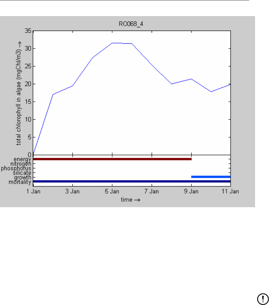
DRAFT
Supported file formats
Figure A.4: Example of a limiting factors plot.
(1) The total chlorophyll quantity results in a special plot showing the development of the
chlorophyll concentration over time and the factors that limit its growth. See Figure A.4.
(2) These fields are expanded depending on the contents of the data file.
(3) The bed layer quantities will only occur for output files of a D-Waq PART simulation with
sedimentation process switched on.
Remarks:
It is currently only possible to create limiting factors plots for the whole simulation period.
It is currently not possible to change the colour settings of the limiting factors plot.
The file options dialog for a D-Water Quality or PART history file allows you to (see Figure A.5):
1 switch between station based data selection (default) or to treat all stations as lying on
one line as a 1D model
2 switch to D-Water Quality balance file handling (see section A.14)
A.13 JS Post file
File <runid.stu>and <runid.pst>
File format <runid.stu>: Ascii file
<runid.pst>: Binary file
Deltares 71 of 92
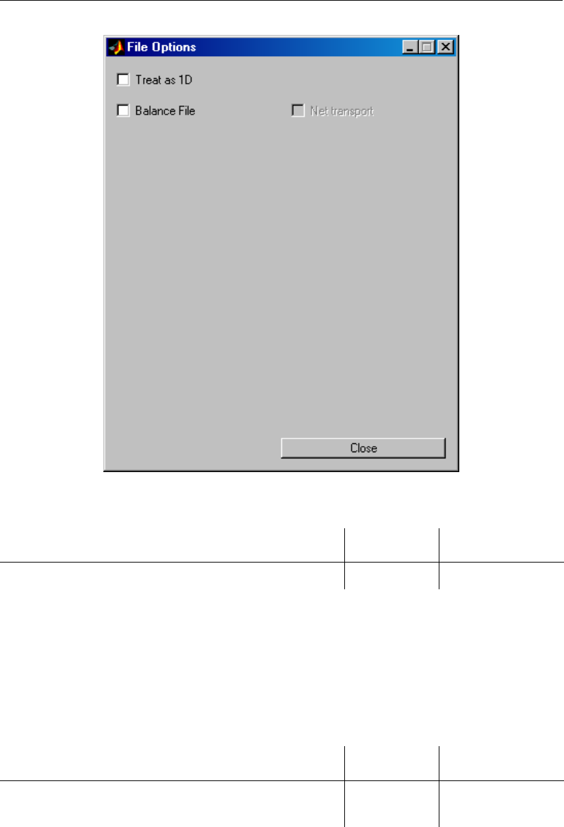
DRAFT
Delft3D-QUICKPLOT, User Manual
Figure A.5: File options dialog for D-Water Quality or PART history file.
Quantity Unit Location
constituents(1) station
(1) These fields are expanded depending on the contents of the data file.
A.14 D-Water Quality, ECO, SED balance file
File <∗.bal>
File format Binary or unformatted
Quantity Unit Location
constituents(1) (1) station
balances(1)(2) (1) station
(1) These fields are expanded depending on the contents of the data file.
(2) The balances result in special plots showing the contribution of all relevant processes in
the mass balance of the constituent considered over time. See Figure A.6 for an example.
72 of 92 Deltares
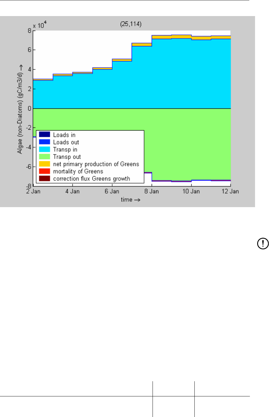
DRAFT
Supported file formats
Figure A.6: Example of a balance plot.
Remarks:
It is currently only possible to create balance plots for the whole simulation period.
It is currently not possible to change the colour settings of the balance plot
The file options dialog for a D-Water Quality balance file allows you to (see Figure A.7):
1 switch to D-Water Quality history file handling
2 plot net transports instead of both in and out transports
A.15 D-Waq PART plot file
File <∗.plo>;<∗.psf>
File format Binary or unformatted
File <plo-runid.dat>and <plo-runid.def>
<psf-runid.dat>and <psf-runid.def>
File format NEFIS
Quantity Unit Location
constituents(1) (1) centres
constituents (bed layer)(1)(2) (1) centres
Deltares 73 of 92
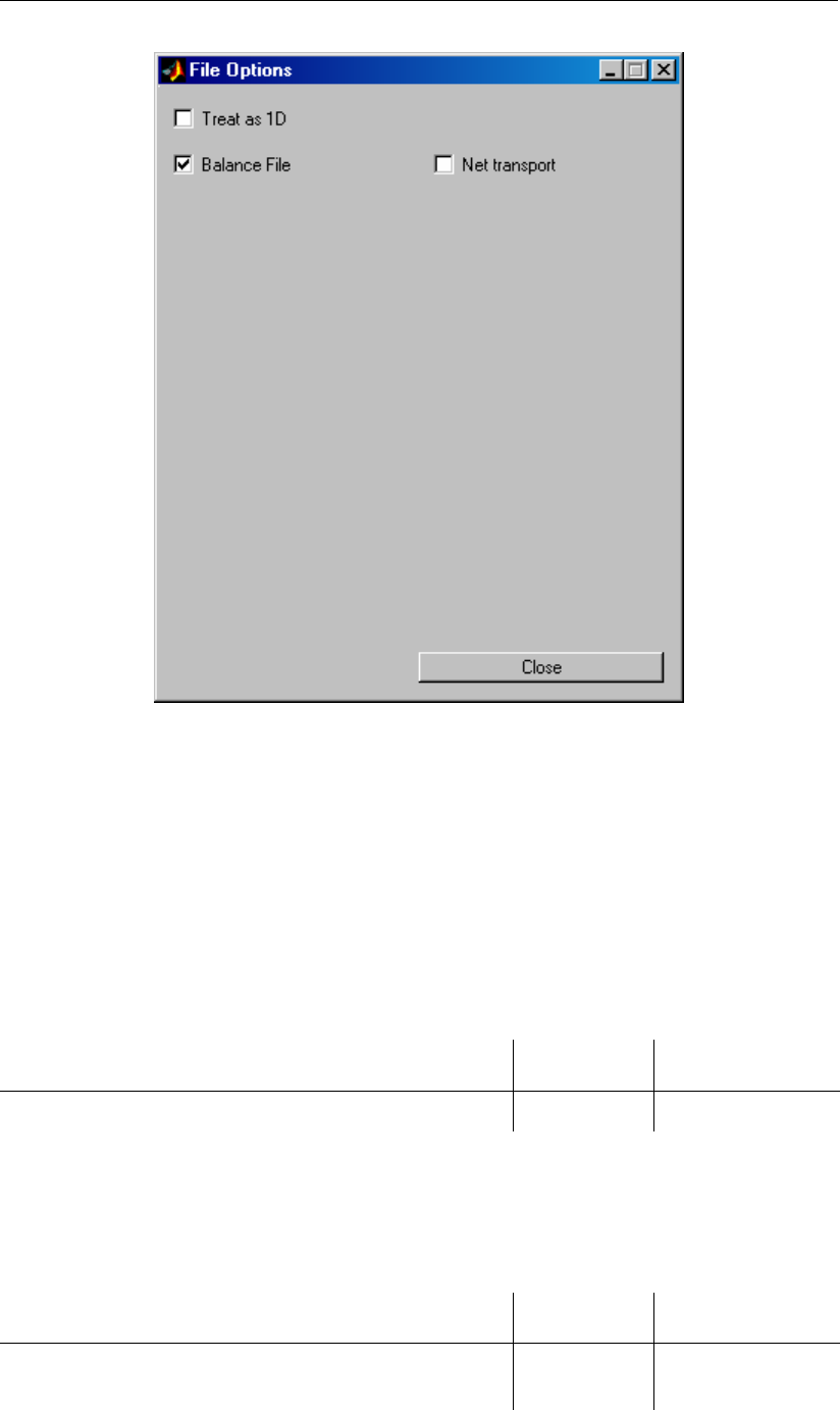
DRAFT
Delft3D-QUICKPLOT, User Manual
Figure A.7: File options dialog for D-Water Quality balance file.
(1) These fields are expanded depending on the contents of the data file.
(2) The bed layer quantities will only occur for output files of a D-Waq PART simulation with
sedimentation process switched on.
A.16 D-Waq PART particle track file
File <trk-runid.dat>and <trkrunid.def>
File format NEFIS
Quantity Unit Location
particle track -
A.17 D-Water Quality grid file
File <name.lga>and <name.cco>
File format Binary or unformatted
Quantity Unit Location
aggregated grid D
segment number centres
74 of 92 Deltares

DRAFT
Supported file formats
A.18 Delft3D grid file
File <∗.grd>
File format Ascii file
Quantity Unit Location
morphologic grid D
hydrodynamic grid Z(1)
(1) In the current version of the program, the hydrodynamic grid connects the co-ordinates
of the cell centres of the computation grid points. This may change in a future release to
represent the bounding boxes of the grid cells (i.e. equal to morphologic grid in plan).
The file options dialog for a Delft3D grid file allows you to (see Figure A.8):
1 load additional attribute files (QUICKIN depth file, Delft3D-FLOW restart file, Delft3D-
FLOW enclosure file, Delft3D-FLOW thin dam file, Delft3D-FLOW dry points file, Delft3D-
FLOW observation point file, Delft3D-FLOW cross-section file, Delft3D-FLOW discharge
station file, Delft3D-FLOW 2D weir file, Delft3D-MOR dredge map output file, Incremental
file, Delft3D-MOR field file, SIMONA box file, SIMONA/Baseline 2d weir file, SIMONA/Baseline
thin dam file, Delft3D-FLOW trachytope area file) onto the grid
2 in case of a Delft3D-FLOW restart file: select the number of layers, substances, and
turbulent quantities.
3 in case of a Delft3D-FLOW restart file: convert between PC and UNIX platforms (and
optionally change the number of layers)
4 in case of a QUICKIN depth file: select the data location, data ordering and Delft3D-FLOW
dpsopt option for interpolation to cell centres.
A.19 QUICKIN depth file
File <∗.dep>
File format Ascii file
Plotted as added dataset on Delft3D grid file (see section A.18).
Quantity Unit Location
data field(1) D / user defined
(1) These fields are expanded depending on the contents of the data file.
A.20 SIMONA box file
File <∗.dep>
File format Ascii file
Plotted as added dataset on Delft3D grid file (see section A.18). The SIMONA system itself
does not have a strict definition of a depth file. The box file currently supported should start
with the BOX record and it should contain all records below that level.
Deltares 75 of 92
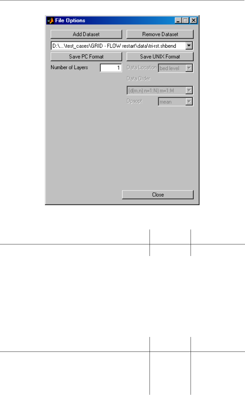
DRAFT
Delft3D-QUICKPLOT, User Manual
Figure A.8: File options dialog for Delft3D grid file.
Quantity Unit Location
data field(1) D
(1) These fields are expanded depending on the contents of the data file.
A.21 Delft3D-FLOW restart file
File <tri-rst.runid>
File format Unformatted file
Plotted as added dataset on Delft3D grid file (see section A.18).
Quantity Unit Location
water level m Z
(horizontal) velocity m/s Z (UV), c
substance Z, c
turb. quantity Z, i
data field(1) Z
76 of 92 Deltares
DRAFT
Supported file formats
(1) These fields are expanded depending on the contents of the data file.
A.22 Delft3D-FLOW thin dam file
File <∗.thd>
File format Ascii file
Plotted as added dataset on Delft3D grid file (see section A.18).
Quantity Unit Location
thindams UV
A.23 SIMONA/Baseline thin dam file
File <schot-u.*>or <schot-v.*>
File format Ascii file
Plotted as added dataset on Delft3D grid file (see section A.18). The SIMONA system itself
does not have a strict definition of a thin dam file. The thin dam ("schotjes") files generated by
the Baseline preprocessing system are currently supported.
Quantity Unit Location
thindams UV
A.24 Delft3D-FLOW 2d weir file
File <∗.2dw>
File format Ascii file
Plotted as added dataset on Delft3D grid file (see section A.18).
Quantity Unit Location
weirs m UV
A.25 SIMONA/Baseline 2d weir file
File <overlaat.*>
File format Ascii file
Plotted as added dataset on Delft3D grid file (see section A.18). The SIMONA system itself
does not have a strict definition of a 2d weir file. The 2d weir ("overlaten") files generated by
the Baseline preprocessing system are currently supported.
Quantity Unit Location
weirs m UV
Deltares 77 of 92
DRAFT
Delft3D-QUICKPLOT, User Manual
A.26 Delft3D-FLOW observation point file
File <∗.obs>
File format Ascii file
Plotted as added dataset on Delft3D grid file (see section A.18).
Quantity Unit Location
observation points station
A.27 Delft3D-FLOW discharge station file
File <∗.src>
File format Ascii file
Plotted as added dataset on Delft3D grid file (see section A.18).
Quantity Unit Location
discharge stations station
A.28 Delft3D-FLOW dry point file
File <∗.dry>
File format Ascii file
Plotted as added dataset on Delft3D grid file (see section A.18).
Quantity Unit Location
dry points Z
A.29 Delft3D-FLOW cross-section file
File <∗.crs>
File format Ascii file
Plotted as added dataset on Delft3D grid file (see section A.18).
Quantity Unit Location
cross-sections UV
A.30 Delft3D-FLOW trachytope area file
File <∗.aru>or <∗.arv>
File format Ascii file
Plotted as added dataset on Delft3D grid file (see section A.18). This file format is equivalent
to the SIMONA Nikuradse area files generated by the Baseline preprocessing system.
78 of 92 Deltares

DRAFT
Supported file formats
Quantity Unit Location
area fraction(1) Z
(1) Subfields based on roughness codes encountered in the data file.
A.31 Delft3D-MOR dredging option 2 map files
File <bagbgv*.runid>;<bagbgc*.runid>;<bagdzi*.runid>
File format Ascii file
Plotted as added dataset on Delft3D grid file (see section A.18).
Quantity Unit Location
dredged volume m3D
dumped volume m3D
cumulative dredged volume m3D
cumulative dumped volume m3D
bed level increment m D
A.32 Delft3D-MOR dredging option 2 depot file
File <bagdpt*.runid>
File format Ascii file
Quantity Unit Location
volume in depot m3
dredged volume m3
dumped volume m3
A.33 Delft3D-MOR tree file
File <morf.runid>
File format Ascii file
Quantity Unit Location
morf tree
morf tree with time management
A.34 Delft3D-FLOW boundary condition files
File <∗.bct>;<∗.bcc>;<∗.dis>
File format Ascii file
Quantity Unit Location
location - quantity(1) station
Deltares 79 of 92
DRAFT
Delft3D-QUICKPLOT, User Manual
(1) These fields are expanded depending on the contents of the data file.
A.35 D-Water Quality tim files
File <∗.tim>
File format Ascii file
Quantity Unit Location
location - quantity(1) station
(1) These fields are expanded depending on the contents of the data file.
A.36 QUICKIN samples file
File <∗.xyz>
File format Ascii file
Quantity Unit Location
samples xy
A.37 Simona SDS file
File <SDSrunid>
File format Binary SIMONA file
Quantity Unit Location
depth grid D
hydrodynamic grid Z(1)
thin dams UV
temporarily inactive velocity points UV
weirs UV
wave height m Z
wave vector m Z
wave period s Z
wave number - Z
wave force N/m2Z
stokes drift velocity m/s Z
water level m Z
water depth m Z
horizontal velocity m/s Z (UV), c
velocity m/s Z (UV), c
unit discharge m2/s Z (UV)
discharge potential m3/s D
roughness Chezy C m1/2/s UV
head m Z
non-hydrostatic pressure Pa Z, c
substances(2) Z, c
turbulent kinetic energy m2/s2Z, i
80 of 92 Deltares
DRAFT
Supported file formats
Quantity Unit Location
energy dissipation m2/s3Z, i
classified water depth - Z
classified water level - Z
classified u velocity - Z
classified v velocity - Z
classified velocity magnitude - Z
classified velocity angle - Z
minimum/maximum(3) Z
bed shear stress N/m2Z
bed level m D
stations xy
water level (station) m station (Z)
horizontal velocity (station) m/s station (Z),c
vertical velocity (station) m/s station (Z), c
substances(2) station (Z), c
instantaneous discharges (transect) m3/s cross-section
cumulative discharges (transect) m3cross-section
(1) In the current version of the program, the hydrodynamic grid connects the 3D co-ordinates
of the cell centres of the computation grid points. This may change in a future release to
represent the bounding boxes of the grid cells.
(2) These fields are expanded depending on the contents of the data file.
(3) The minimum/maximum field is expanded depending on the contents of the data file into
quantities named ‘<variable1>at <minimum|maximum> <variable2>’, e.g. ‘water level at
maximum velocity magnitude’. The name is abbreviated to ‘<minimum|maximum> <variable2>’
if <variable1>equals <variable2>, e.g. ‘minimum velocity in m-direction’.
A.38 BIL/HDR files
File <name.hdr>and <name.bil>,<name.bip>or <name.bsq>
File format <∗.hdr>: Ascii file
<∗.bil>,<∗.bip>,<∗.bsq>: Binary file
Quantity Unit Location
datafield cell centres
A.39 ArcInfo grid files
File <∗.asc>
File format Ascii file
Special support for extensions used by Delft-FLS and SOBEK Overland Flow module: <∗.adp>,
<∗.amu>,<∗.amv>,<∗.amh>,<∗.amz>,<∗.amc>,<∗.aht>,<∗.afb>,<∗.afw>,
<∗.acx>,<∗.ahx>
Quantity Unit Location
datafield cell centres
Deltares 81 of 92

DRAFT
Delft3D-QUICKPLOT, User Manual
A.40 Delft-FLS or SOBEK incremental file
File <∗.inc>
File format Ascii file
Optionally plotted as added dataset on Delft3D grid file (see section A.18).
Quantity Unit Location
classified waterdepth Z
classified velocity Z
classified waterlevel Z
classified u-velocity Z
classified v-velocity Z
A.41 Delft-FLS point history file
File <∗.bin>
File format Binary file
File <∗.his>
File format Ascii file
Quantity Unit Location
waterdepth m station
waterlevel m station
velocity m/s station
A.42 Delft-FLS cross-section history file
File <∗.crs>
File format Ascii file
Quantity Unit Location
discharge m3/s cross-section
A.43 Tekal annotation file
File <∗.ann>
File format Ascii file
Quantity Unit Location
data fields(1) xy
(1) These fields are expanded depending on the contents of the data file.
82 of 92 Deltares
DRAFT
Supported file formats
A.44 Tekal data files
File <∗.tek>;<∗.map>
File format Ascii file
Quantity Unit Location
data fields(1) (2)
(1) These fields are expanded depending on the contents of the data file.
(2) Location depends on file contents: time-series or 1D/2D/3D spatial data.
A.45 QUICKIN and Tekal land boundary file
File <∗.ldb>
File format Ascii file
Quantity Unit Location
line xy
A.46 BNA file (as land boundary file)
File <∗.bna>
File format Ascii file
Quantity Unit Location
line xy
A.47 ArcInfo (un)generate file (as land boundary file)
File <∗.gen>
File format Ascii file
Quantity Unit Location
line xy
A.48 ESRI shape file
File <name.shp>and <name.shx>and <name.dbf>
File format Binary file
Quantity Unit Location
line xy
Deltares 83 of 92
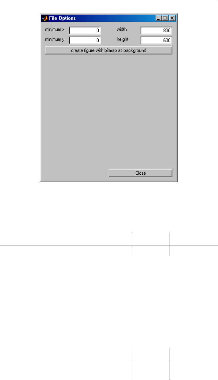
DRAFT
Delft3D-QUICKPLOT, User Manual
Figure A.9: File options dialog for a bitmap file.
A.49 Bitmap files
File <∗.bmp>;<∗.jpg>;<∗.tif>;<∗.png>
File format Binary file
Quantity Unit Location
bitmap user specified
The file options dialog for a bitmap file allows you to:
1 specify the lower-left co-ordinates of the bitmap as well as the width for georeferencing.
These data are used when plotting the bitmap.
2 create a figure containing an axes object such that the plotted bitmap exactly fits the figure.
A.50 UNIBEST output
File <name.daf>and <name.fun>
File format <∗.fun>: Ascii file
<∗.daf>: Binary file
Quantity Unit Location
grid
data fields(1)
(1) These fields are expanded depending on the contents of the data file.
A.51 SOBEK network data
File <deftop.1>(SOBEK-RE) or <network.ntw>(SOBEK-River/Rural/Urban) De-
pending on network characteristics other files also required.
File format Ascii files and optional binary data files
Quantity Unit Location
network xy
datafields(1) xy
(1) These fields are expanded depending on the contents of the flowmap.his, minmax.his,
gsedmap.his, kafhmap.his, kafpmap.his, kafrmap.his, kaphmap.his, kappmap.his, saltmap.his,
sedtmap.his, morpmap.his, sobekwq.map, calcpnt.his and reachseg.his files in the same di-
rectory.
A.52 SKYLLA file
File <animrunid.dat>and <animrunid.def>
File format NEFIS
84 of 92 Deltares
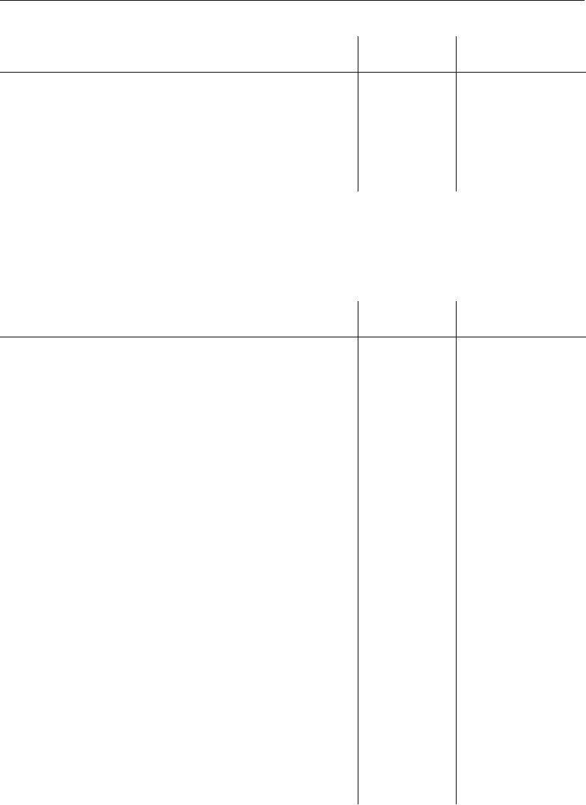
DRAFT
Supported file formats
Quantity Unit Location
cell fill rate
pressure/density m2/m2
rotation 1/s
velocity m/s
pressure at station Pa station
velocity at station m/s station
A.53 PHAROS file
File <name1adminname2.dat>and <name1adminname2.def>
File format NEFIS
Quantity Unit Location
grid vertices
water level m vertices
bed level m vertices
water depth m vertices
velocity m/s vertices
breaking coefficient gamma vertices
weighted mean wave height dir. m vertices
wave height m vertices
wave phase vertices
wave image m vertices
maximum velocity m/s vertices
maximum velocity direction radians vertices
minimum velocity m/s vertices
wave number vertices
phase velocity m/s vertices
group velocity m/s vertices
potential (real part) vertices
potential (imag part) vertices
seiches potential (real part) vertices
seiches potential (imag part) vertices
weighted period Tm-1,0 s vertices
wave number based on Tm-1,0 vertices
radial frequency based on Tm-1,0 vertices
data fields(1) vertices
data fields (frequency graph)(1)(2) stations
(1) These fields are expanded depending on the contents of the data file.
(2) These quantities result in special frequency graphs.
Deltares 85 of 92
DRAFT
Delft3D-QUICKPLOT, User Manual
Figure A.10: Example of a frequency plot.
A.54 MATLAB files (exported from Delft3D-QUICKPLOT)
File <∗.mat>containing a structure ’data’ as exported from Delft3D-QUICKPLOT.
File format Binary file
The stand-alone version of Delft3D-QUICKPLOT accepts only MATLAB files created by the
standalone version itself or created from within MATLAB 6. When saving data from within a
more recent MATLAB releases, use the version 6 compatible MAT-file format.
Quantity Unit Location
data field(1) (1) (1)
(1) Field name, unit and location are determined from the contents of the data file.
A.55 TRITON file
File <runid.dat>and <runid.def>
File format NEFIS
86 of 92 Deltares
DRAFT
Supported file formats
Quantity Unit Location
grid grid points
coarse grid coarse grid points
points observation points
ray slice(1) ray points
water level m (2)
velocity m/s (2)
bed level m (3)
H1/3 m (2)
Hrms m (2)
H1% m (2)
H2% m (2)
Tm s (2)
T1/3 s (2)
Hm0 m (2)
Tm-1,0 s (2)
Tm0,1 s (2)
Svar m2/Hz (2)
(1) The list of cross-sectional rays will be automatically expanded based on file contents.
(2) Variable defined on coarse grid, points, or rays.
(3) Variable defined on grid, coarse grid, points, rays.
A.56 NetCDF file
File <∗.nc>
File format NetCDF 3.6
Remark:
The implementation supports CF conventions
Quantity Unit Location
data fields(1) (1) (1)
(1) The list of data fields will be automatically expanded based on file contents.
A.57 PC-Raster file
File <∗.map>
File format Binary file
Quantity Unit Location
drainage plot(1)
data field(2)
Deltares 87 of 92

DRAFT
Delft3D-QUICKPLOT, User Manual
Figure A.11: Example of a drainage plot.
(1) The drainage plot results in special plot as shown in Figure A.11.
(2) The name of the quantity will be automatically determined from the file contents.
A.58 Auke/PC file
File <name.seq>and <name.dat>
File format <∗.seq>: Ascii file
<∗.dat>: Binary file
Quantity Unit Location
data fields(1) data channel
(1) The list of data fields will be automatically expanded based on file contents.
A.59 Telemac file
File <∗.slf>
File format Binary file
88 of 92 Deltares
DRAFT
Supported file formats
Quantity Unit Location
grid vertices
data fields(1) vertices
(1) The list of data fields will be automatically expanded based on file contents.
A.60 Mike zero files
File <∗.dt0>;<∗.dt1>;<∗.dt2>;<∗.dfs0>;<∗.dfs1>;<∗.dfs2>;<∗.dfs3>;<∗.dfsu>
File format Binary file
Quantity Unit Location
data fields(1) grid points
(1) The list of data fields will be automatically expanded based on file contents.
Deltares 89 of 92

DRAFT
Delft3D-QUICKPLOT, User Manual
90 of 92 Deltares
DRAFT
PO Box 177
2600 MH Del
Rotterdamseweg 185
2629 HD Del
The Netherlands
+31 (0)88 335 81 88
sales@deltaressystems.nl
www.deltaressystems.nl
DRAFT
