Dymola Dynamic Ing Laboratory User Manual Volume 2
User Manual: Pdf
Open the PDF directly: View PDF ![]() .
.
Page Count: 476 [warning: Documents this large are best viewed by clicking the View PDF Link!]
- 1 Model Experimentation
- 2 Model Calibration
- 3 Design Optimization
- 4 Model Management
- 4.1 Version management
- 4.1.1 Short guide with new features included
- 4.1.2 The context of version management
- 4.1.3 Introduction to version management
- 4.1.4 Scope of implementation
- 4.1.5 Supported features
- 4.1.6 Selecting version management system
- 4.1.7 Version management using CVS
- 4.1.8 An example of file management using CVS
- 4.1.9 Version management using SVN
- 4.1.10 An example of file management using SVN
- 4.1.11 Version management using Git
- 4.1.12 Short guide to version management with new features included
- 4.1.13 References
- 4.2 Model dependencies
- 4.3 Encryption in Dymola
- 4.4 Model and library checking
- 4.5 Model comparison
- 4.6 Model structure
- 4.1 Version management
- 5 Visualize 3D
- 6 Other Simulation Environments
- 7 User-defined GUI
- 8 Advanced Modelica Support
- 8.1 Declaring functions
- 8.2 User-defined derivatives
- 8.3 External functions in other languages
- 8.4 Means to control the selection of states
- 8.5 Using noEvent
- 8.6 Equality comparison of real values
- 8.7 Some supported features of the Modelica language
- 8.7.1 Support for Modelica Language version 3.4
- 8.7.2 Synchronous Modelica
- 8.7.3 State Machines
- 8.7.4 Operator overloading
- 8.7.5 Homotopy operator
- 8.7.6 Arrays
- 8.7.7 Enumerations
- 8.7.8 Support of String variables in models
- 8.7.9 Support of inner/outer components
- 8.7.10 Functions as formal input to functions
- 8.7.11 Assert
- 8.7.12 Identifiers starting with underscore and vendor-specific annotations
- 8.7.13 Quoted identifiers containing dot supported
- 8.7.14 Running a function before check/translation/simulation
- 8.7.15 Forcing translation of functions
- 8.7.16 Deprecation warnings
- 8.7.17 Licensing
- 8.8 Symbolic Processing of Modelica Models
- 8.9 Symbolic solution of nonlinear equationsin Dymola
- 8.9.1 Introduction
- 8.9.2 Solving a nonlinear equation with single appearance of the unknown by applying function inverses
- 8.9.3 Solving a nonlinear equation with special patterns for the unknown
- 8.9.4 Partitioning of a system of equations into a linear and nonlinear (one variable) part
- 8.9.5 Using min and max values to evaluate if-conditions
- 9 Appendix — Migration
- 10 Index
Dymola
Dynamic Modeling Laboratory
User Manual
Volume 2
March 2017 (Dymola 2018)

The information in this document is subject to change without notice.
Document version: 22. Important additions/corrections compared with the previous Dymola documentation
“September 2016 (Dymola 2017 FD01)” (doc. version 21) are marked in the margin.
© Copyright 1992-2017 by Dassault Systèmes AB. All rights reserved.
Dymola® is a registered trademark of Dassault Systèmes AB.
Modelica® is a registered trademark of the Modelica Association.
Other product or brand names are trademarks or registered trademarks of their respective holders.
Dassault Systèmes AB
Ideon Gateway
Scheelevägen 27 – Floor 9
SE-223 63 Lund
Sweden
E-mail: http://www.3ds.com/support
URL: http://www.Dymola.com
Phone: +46 46 270 67 00

3
Contents
1 Model Experimentation ........................................................................................................ 11
1.1 Introduction .................................................................................................................................................... 11
1.2 Varying parameters of a model ...................................................................................................................... 11
1.2.1 Case Study: CoupledClutches model .................................................................................................... 12
1.2.2 Response to parameter perturbations - perturbParameters ................................................................... 13
1.2.3 Sweep one parameter – two variants .................................................................................................... 19
1.2.4 Sweep two parameters - sweepTwoParameters .................................................................................... 24
1.2.5 Monte Carlo Analysis ........................................................................................................................... 26
2 Model Calibration ................................................................................................................. 37
2.1 Introduction .................................................................................................................................................... 37
2.2 The basics of setting up and executing a calibration task .............................................................................. 39
2.2.1 Vehicle data .......................................................................................................................................... 40
2.2.2 Vehicle model ....................................................................................................................................... 42
2.2.3 Validation of the nominal model .......................................................................................................... 44
2.2.4 Measurement file formats ..................................................................................................................... 50
2.2.5 Calibration ............................................................................................................................................ 53
2.2.6 Free start values .................................................................................................................................... 55
2.2.7 Tune the parameters ............................................................................................................................. 56
2.2.8 Validation using measurements from first gear .................................................................................... 57
2.2.9 The setup as Modelica code .................................................................................................................. 59
2.3 Saving the setup for reuse .............................................................................................................................. 60
2.4 Reusing a setup for a similar operation .......................................................................................................... 61
2.5 Analysing parameter sensitivities and dependencies ..................................................................................... 62
2.5.1 Sweep one parameter – sweepParameter .............................................................................................. 62
2.5.2 Sweep two parameters – sweepTwoParameters ................................................................................... 69

4
2.5.3 Response to parameter perturbations - perturbParameters ................................................................... 71
2.5.4 Check if tuners can be calibrated – checkCalibrationSensitivity .......................................................... 73
2.6 Data Preprocessing ......................................................................................................................................... 75
2.6.1 Setting up for preprocessing ................................................................................................................. 76
2.6.2 Limiting and detrending signals ........................................................................................................... 79
2.6.3 Analyzing Signals: is there any noise? ................................................................................................. 82
2.6.4 Filtering signals .................................................................................................................................... 84
2.7 Static calibration ............................................................................................................................................ 86
2.7.1 The staticCalibrate function .................................................................................................................. 86
2.7.2 The calibrateSteadyState function ........................................................................................................ 98
3 Design Optimization ............................................................................................................ 101
3.1 Introduction .................................................................................................................................................. 101
3.2 First optimization setup ................................................................................................................................ 103
3.2.1 Specifying tuners ................................................................................................................................ 107
3.2.2 Specification of the criteria ................................................................................................................. 109
3.2.3 The result of the optimization ............................................................................................................. 112
3.2.4 Adding more tuners ............................................................................................................................ 115
3.3 Multi-criteria experimenting ........................................................................................................................ 116
3.4 Multi-case optimization ............................................................................................................................... 118
4 Model Management ............................................................................................................. 125
4.1 Version management .................................................................................................................................... 126
4.1.1 Short guide with new features included .............................................................................................. 126
4.1.2 The context of version management ................................................................................................... 126
4.1.3 Introduction to version management .................................................................................................. 127
4.1.4 Scope of implementation .................................................................................................................... 129
4.1.5 Supported features .............................................................................................................................. 130
4.1.6 Selecting version management system ............................................................................................... 133
4.1.7 Version management using CVS ........................................................................................................ 134
4.1.8 An example of file management using CVS ...................................................................................... 136
4.1.9 Version management using SVN........................................................................................................ 142
4.1.10 An example of file management using SVN ...................................................................................... 144
4.1.11 Version management using Git .......................................................................................................... 148
4.1.12 Short guide to version management with new features included ........................................................ 149
4.1.13 References .......................................................................................................................................... 151
4.2 Model dependencies ..................................................................................................................................... 151
4.2.1 Cross-reference options ...................................................................................................................... 153
4.3 Encryption in Dymola .................................................................................................................................. 153
4.3.1 Introduction ........................................................................................................................................ 153
4.3.2 Visible and concealed classes ............................................................................................................. 154
4.3.3 Developing encrypted libraries ........................................................................................................... 155
4.3.4 Using encrypted components .............................................................................................................. 155
4.3.5 Examples ............................................................................................................................................ 156
4.3.6 Special annotations for concealment .................................................................................................. 165
4.3.7 Licensing libraries .............................................................................................................................. 167
4.3.8 Scrambling in Dymola ........................................................................................................................ 169
4.4 Model and library checking ......................................................................................................................... 172
4.4.1 Overview ............................................................................................................................................ 172

5
4.4.2 Regression testing ............................................................................................................................... 173
4.4.3 Class coverage .................................................................................................................................... 180
4.4.4 Condition coverage ............................................................................................................................. 181
4.4.5 Style checking .................................................................................................................................... 182
4.5 Model comparison........................................................................................................................................ 185
4.5.1 Overview ............................................................................................................................................ 185
4.5.2 Getting started .................................................................................................................................... 185
4.5.3 Comparison report .............................................................................................................................. 187
4.6 Model structure ............................................................................................................................................ 194
4.6.1 Introduction ........................................................................................................................................ 194
4.6.2 Traversing models before translation ................................................................................................. 194
4.6.3 Interface to semantics not only to syntax ........................................................................................... 196
4.6.4 Extracting information before translation ........................................................................................... 197
4.6.5 Traversing translated models .............................................................................................................. 200
5 Visualize 3D.......................................................................................................................... 203
5.1 Introduction .................................................................................................................................................. 203
5.2 Inserting and removing graphical objects .................................................................................................... 206
5.3 Basic primitives ........................................................................................................................................... 217
5.4 Surface Plots ................................................................................................................................................ 219
6 Other Simulation Environments ........................................................................................ 235
6.1 Introduction .................................................................................................................................................. 235
6.2 Dymola – Matlab interface........................................................................................................................... 236
6.2.1 Using the Dymola-Simulink interface ................................................................................................ 236
6.2.2 Other Matlab utilities .......................................................................................................................... 246
6.3 Real-time Simulation ................................................................................................................................... 247
6.3.1 dSPACE systems ................................................................................................................................ 249
6.3.2 Simulink Real-Time (formerly Matlab xPC Target) .......................................................................... 254
6.3.3 Advanced Options for Real-Time Simulation .................................................................................... 258
6.4 DDE Communication ................................................................................................................................... 261
6.4.1 DDE interface for Dymola ................................................................................................................. 261
6.4.2 Explorer file type associations ............................................................................................................ 263
6.4.3 DDE Server support in Dymosim simulator ....................................................................................... 264
6.5 OPC Communication ................................................................................................................................... 268
6.5.1 OPC Server support in Dymosim simulator ....................................................................................... 268
6.6 Java Interface for Dymola ............................................................................................................................ 273
6.7 Python Interface for Dymola ........................................................................................................................ 288
6.8 JavaScript interface for Dymola ................................................................................................................... 298
6.9 Report generator ........................................................................................................................................... 299
6.9.1 Fundamentals ...................................................................................................................................... 299
6.9.2 JavaScript functions ............................................................................................................................ 299
6.9.3 Example of HTML report sections ..................................................................................................... 302
6.9.4 Mouse and keyboard commands available for animation in reports .................................................. 305
6.10 FMI Support in Dymola .......................................................................................................................... 306
6.10.1 Introduction ........................................................................................................................................ 306
6.10.2 Exporting FMUs from Dymola .......................................................................................................... 307
6.10.3 Importing FMUs in Dymola ............................................................................................................... 319
6.10.4 Validating FMUs from Dymola ......................................................................................................... 330

6
6.10.5 FMU Export from Simulink/FMU Import into Simulink: The FMI Kit for Simulink ....................... 332
6.11 Code and Model Export .......................................................................................................................... 347
6.11.1 Introduction ........................................................................................................................................ 347
6.11.2 Binary Model Export .......................................................................................................................... 349
6.11.3 Source Code Generation ..................................................................................................................... 352
6.11.4 The StandAloneDymosim project ...................................................................................................... 353
7 User-defined GUI ................................................................................................................ 361
7.1 Building user-defined dialogs ...................................................................................................................... 361
7.1.1 Ways of working with annotations ..................................................................................................... 361
7.1.2 Records and dialogs ............................................................................................................................ 362
7.2 Extendable user interface – menus, toolbars and favorites .......................................................................... 391
7.2.1 Defining content of menus and toolbars ............................................................................................. 391
7.2.2 Displaying library-specific menus and toolbars in Dymola (commercial library developers) ........... 393
7.2.3 Defining packages with users own collection of favorite models ...................................................... 394
8 Advanced Modelica Support .............................................................................................. 397
8.1 Declaring functions ...................................................................................................................................... 397
8.2 User-defined derivatives .............................................................................................................................. 397
8.2.1 Analytic Jacobians .............................................................................................................................. 398
8.2.2 How to declare a derivative ................................................................................................................ 399
8.3 External functions in other languages .......................................................................................................... 403
8.3.1 C ......................................................................................................................................................... 403
8.3.2 Java ..................................................................................................................................................... 408
8.3.3 C++ ..................................................................................................................................................... 413
8.3.4 FORTRAN ......................................................................................................................................... 413
8.4 Means to control the selection of states ....................................................................................................... 414
8.4.1 Motivation .......................................................................................................................................... 414
8.4.2 The state select attribute ..................................................................................................................... 415
8.5 Using noEvent .............................................................................................................................................. 417
8.5.1 Background: How events are generated ............................................................................................. 417
8.5.2 Guarding expressions against evaluation ............................................................................................ 417
8.5.3 How to use noEvent to improve performance .................................................................................... 418
8.5.4 Combined example for noEvent ......................................................................................................... 419
8.5.5 Constructing anti-symmetric expressions ........................................................................................... 419
8.5.6 Mixing noEvent and events in one equation ....................................................................................... 421
8.6 Equality comparison of real values .............................................................................................................. 423
8.6.1 Type of variables ................................................................................................................................ 423
8.6.2 Trigger events for equality ................................................................................................................. 423
8.6.3 Locking when equal ........................................................................................................................... 423
8.6.4 Guarding against division by zero ...................................................................................................... 424
8.7 Some supported features of the Modelica language ..................................................................................... 425
8.7.1 Support for Modelica Language version 3.4 ...................................................................................... 425
8.7.2 Synchronous Modelica ....................................................................................................................... 425
8.7.3 State Machines.................................................................................................................................... 425
8.7.4 Operator overloading .......................................................................................................................... 425
8.7.5 Homotopy operator ............................................................................................................................. 426
8.7.6 Arrays ................................................................................................................................................. 426
8.7.7 Enumerations ...................................................................................................................................... 427

7
8.7.8 Support of String variables in models ................................................................................................ 429
8.7.9 Support of inner/outer components .................................................................................................... 429
8.7.10 Functions as formal input to functions ............................................................................................... 429
8.7.11 Assert .................................................................................................................................................. 429
8.7.12 Identifiers starting with underscore and vendor-specific annotations................................................. 430
8.7.13 Quoted identifiers containing dot supported ....................................................................................... 430
8.7.14 Running a function before check/translation/simulation .................................................................... 430
8.7.15 Forcing translation of functions .......................................................................................................... 431
8.7.16 Deprecation warnings ......................................................................................................................... 431
8.7.17 Licensing ............................................................................................................................................ 431
8.8 Symbolic Processing of Modelica Models ................................................................................................... 431
8.8.1 Sorting and algebraic loops ................................................................................................................ 432
8.8.2 Reduction of size and complexity ...................................................................................................... 432
8.8.3 Index reduction ................................................................................................................................... 434
8.8.4 Example .............................................................................................................................................. 436
8.8.5 References .......................................................................................................................................... 439
8.9 Symbolic solution of nonlinear equations in Dymola .................................................................................. 440
8.9.1 Introduction ........................................................................................................................................ 440
8.9.2 Solving a nonlinear equation with single appearance of the unknown by applying function inverses
440
8.9.3 Solving a nonlinear equation with special patterns for the unknown ................................................. 443
8.9.4 Partitioning of a system of equations into a linear and nonlinear (one variable) part ......................... 443
8.9.5 Using min and max values to evaluate if-conditions .......................................................................... 445
9 Appendix — Migration ....................................................................................................... 449
9.1 Migrating to newer libraries ......................................................................................................................... 449
9.1.1 How to migrate ................................................................................................................................... 449
9.1.2 Basic commands to specify translation ............................................................................................... 450
9.1.3 How to build a convert script ............................................................................................................. 456
9.2 Upgrading to new version of Modelica Standard Library ............................................................................ 458
9.2.1 Introduction ........................................................................................................................................ 458
9.2.2 Basics ................................................................................................................................................. 458
9.2.3 Upgrading to a new Modelica version ................................................................................................ 460
9.2.4 Using old models after upgrading to the latest Modelica version ....................................................... 463
9.2.5 Determining what libraries a model use ............................................................................................. 463
9.2.6 Specifying the version of a package ................................................................................................... 464
9.2.7 Upgrading models and libraries to a new library version ................................................................... 465
9.3 Preparing libraries for migration .................................................................................................................. 467
9.4 Updating Modelica annotations ................................................................................................................... 467
10 Index ................................................................................................................................ 469

8
1 MODEL
EXPERIMENTATION

1 MODEL EXPERIMENTATION 11
1 Model Experimentation
1.1 Introduction
Dymola provides the Experimentation package as a feature of the Design package. The
main purpose of this package is to allow the user to vary parameters of the system to get an
intuitive knowledge of the behavior of the model. Some of the functionalities of this
package are related to other functions of the Calibration package. Please see chapter “Model
calibration”.
The main difference is that those are coupled to the calibration setup, while the functions in
Experimentation are independent and can be used to illustrate phenomena of the system.
One of the functionalities of Experimentation package is essentially different: Monte Carlo
simulation.
1.2 Varying parameters of a model
The Experimentation package provides several ways of analyzing the behavior of a model.
The main functions are perturbParameters, sweepParameter, sweepOneParameter,
sweepTwoParameters and MonteCarloAnalysis.
12
The functions perturbParameters, sweepParameter and sweepTwoParameters have
corresponding functions in the Calibration package and can be used for more general
parameter studies. The main difference in this package compared to Calibration is that the
resulting output is the response of the model. We give a short overview of these functions
now.
The functions sweepOneParameter and MonteCarloAnalysis complete the set, giving the
possibility of plotting the response at the end of the integration interval and random draws
of numbers for the parameters in Monte Carlo simulations. The example studied for this
package is the model Design.Experimentation.Examples.CoupledClutches. This example is
an extension of Modelica.Mechanics.Rotational.Examples.CoupledClutches.
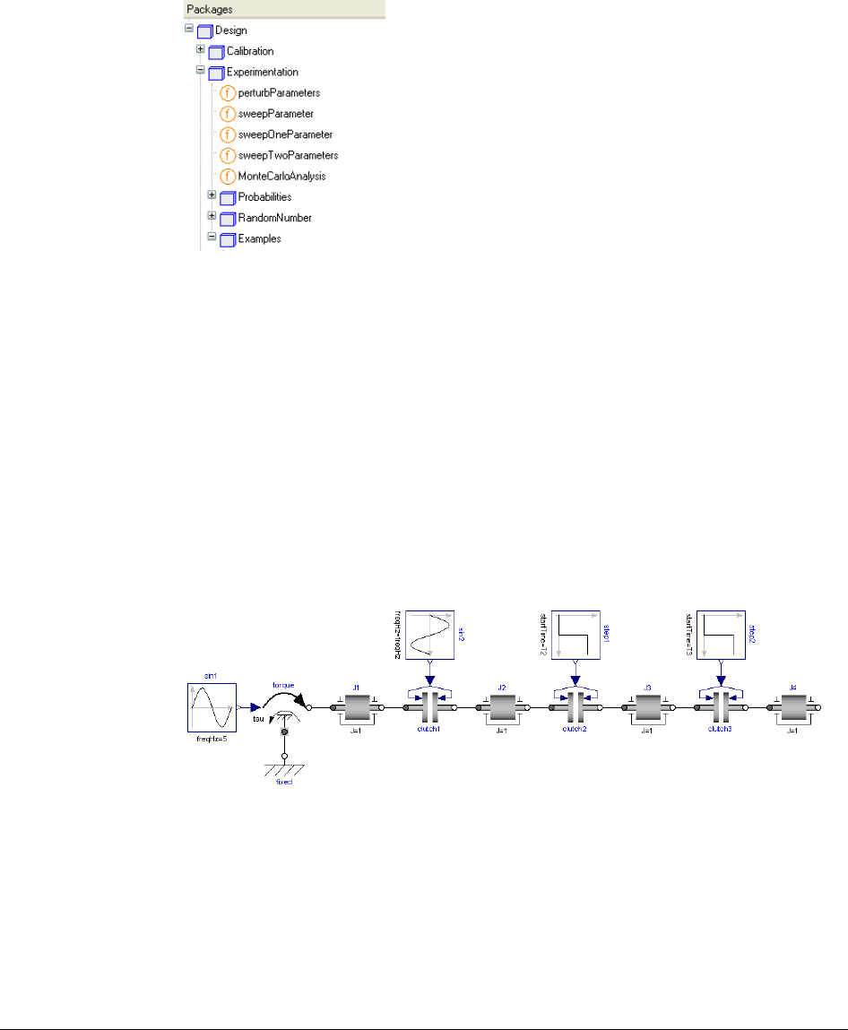
1.2.1 Case Study: CoupledClutches model
The model CoupledClutches is composed by four rotating inertias J1, J2, J3 and J4 coupled
by three clutches that make them interact. The diagram looks as follows.
The parameters of the model to explore are the inertia values J1.J, J2.J, J3.J and J4.J. The
observed variables are the rotational speeds J1.w, J2.w, J3.w and J4.w. The setups of the
functions are very similar and their description will therefore be brief.
The demo CoupledClutches can be reached either in Modelica Standard Library, as
Modelica.Mechanics.Rotational.Examples.CoupledClutches or in the Design library, as
Design.Experimentation.Examples.CoupledClutches. It is really the same demo, but
opening it using the last path will also give access to a number of commands that
corresponds of some of the cases below.
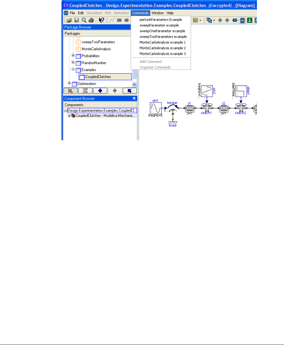
1 MODEL EXPERIMENTATION 13
Selecting any of these commands will pop up the relevant function with variables etc
already selected. The only thing to do then is to click the button Execute to see the result.
Please note that all cases are not handled by the commands, and not some minor adapting of
e.g. curve legends after executing the command. More curves than needed might also be
shown.
It is a good idea to open the CoupledClutches example from the Design package before
continuing.
1.2.2 Response to parameter perturbations -
perturbParameters
Let us check the behavior of the model if we perturb the nominal values of the parameters.
(Shortcut: Use the command perturbParmeters Example as described in the beginning of
this chapter.)
The function perturbParameters must be visible in the package browser. If not, expand
Design and then Experimentation by clicking on the + in front of them. Now you can right-
click on perturbParameters and select Call Function …. The following menu pops
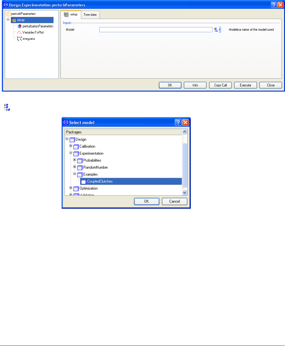
14
Now, to specify the model to use, click on Edit icon to the right of the input field. A
package browser pops up. Use it to select the model.
Click OK. The model is now translated in order to gather information needed to build
browsers and selectors to support the remaining setting up. If Dymola already has a
translated model, then this model appears as the default model.
1 MODEL EXPERIMENTATION 15
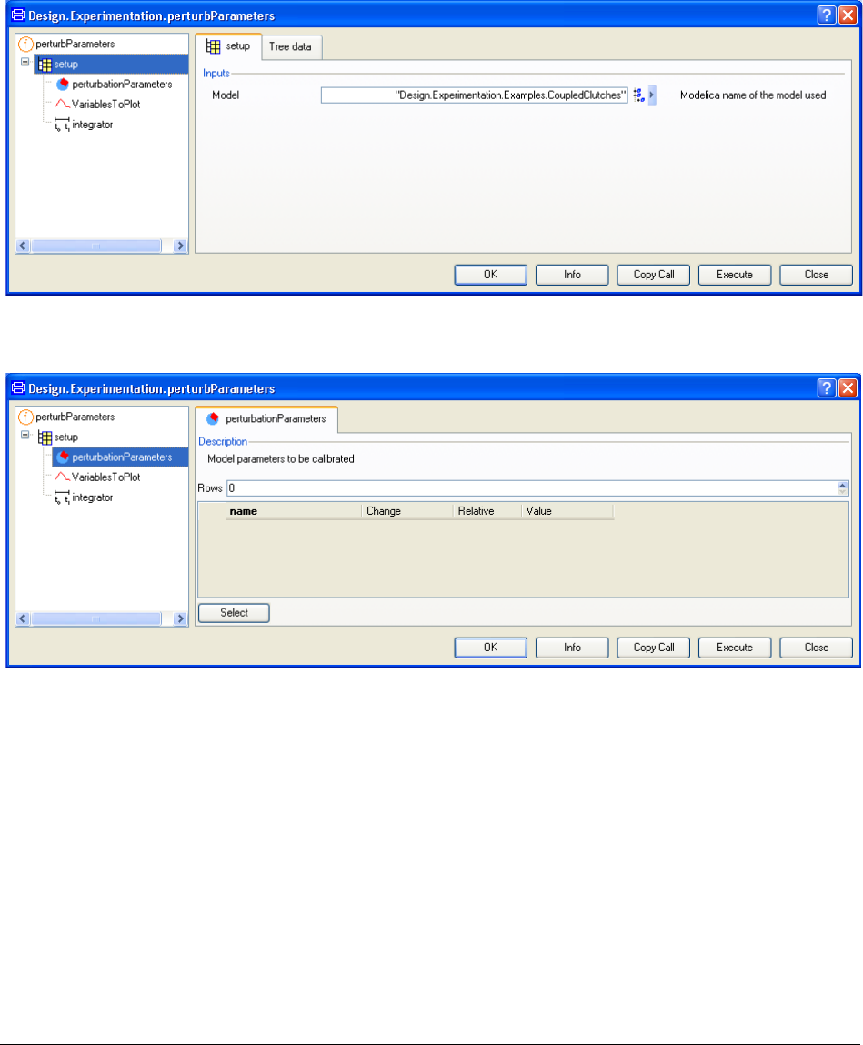
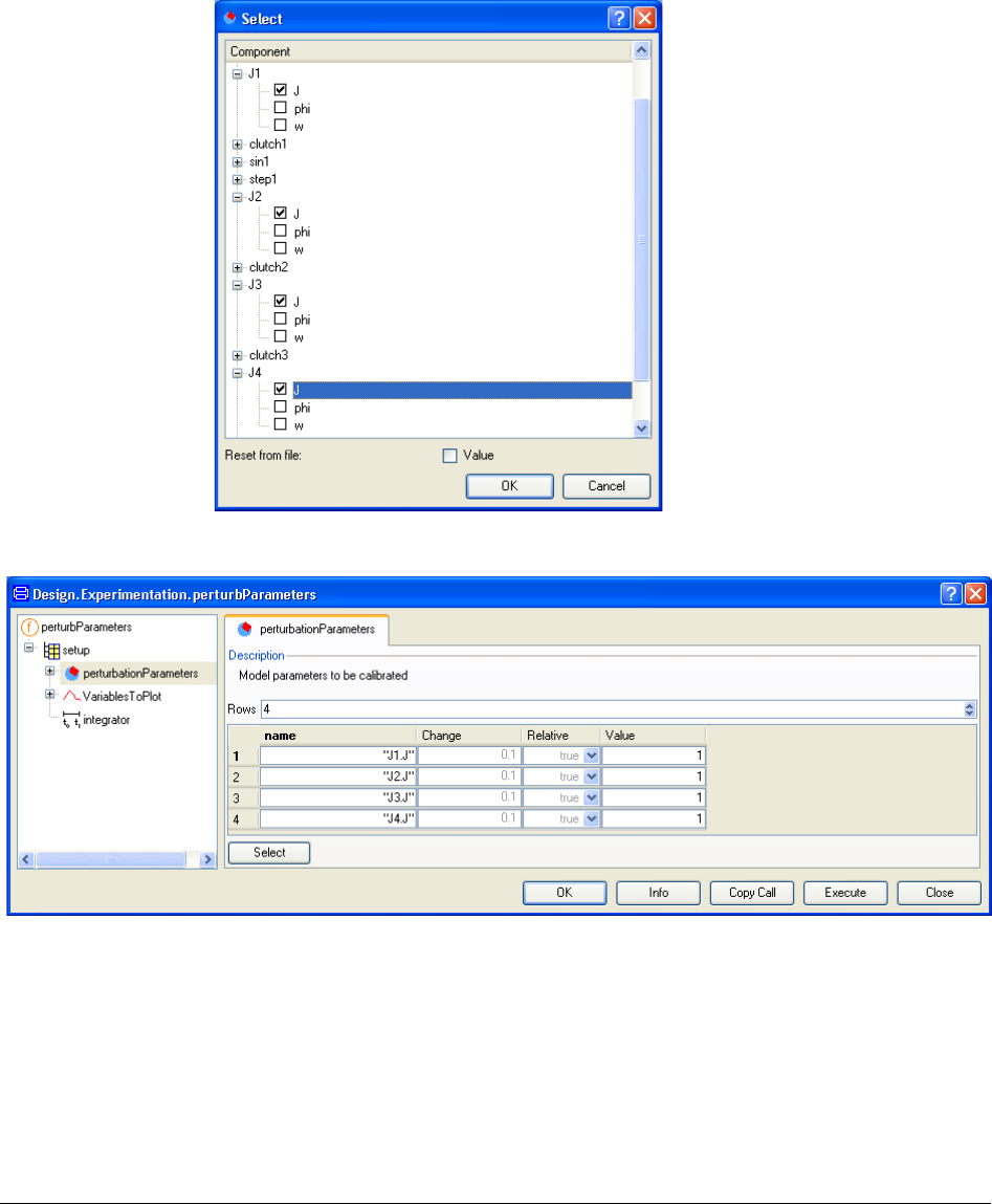
The next task is to select the parameters to perturb and the variables to observe and plot.
Click on perturbationParameters. The following menu pops up.
Click on the Select button. The following browser pops and the parameters J1.J, J2.J, J3.J
and J4.J can be selected as perturbation parameters. Their nominal value is 1 for all of them.
The perturbation is by default 10 percent.
16
Click OK.
We can select a percent change of absolute change if we like. In the setup presented, the
parameters are perturbed 10 percent from their nominal value.
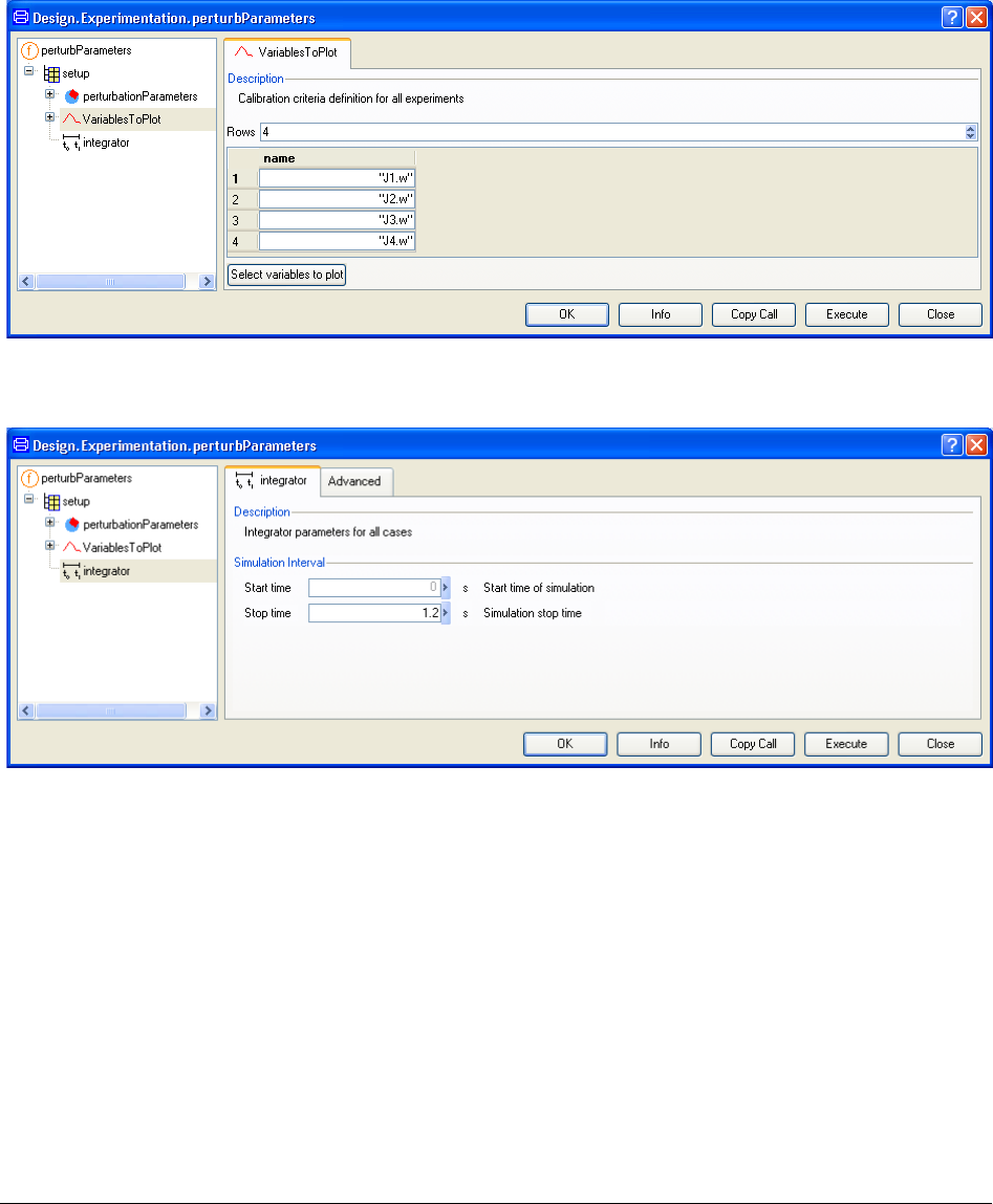
Now, let us select the variables to plot. Click on VariablesToPlot and then clicking on
Select variables to plot button we get a variable browser where the selection of J1.w, J2.w,
J3.w and J4.w is possible. The resulting menu looks as following.
1 MODEL EXPERIMENTATION 17
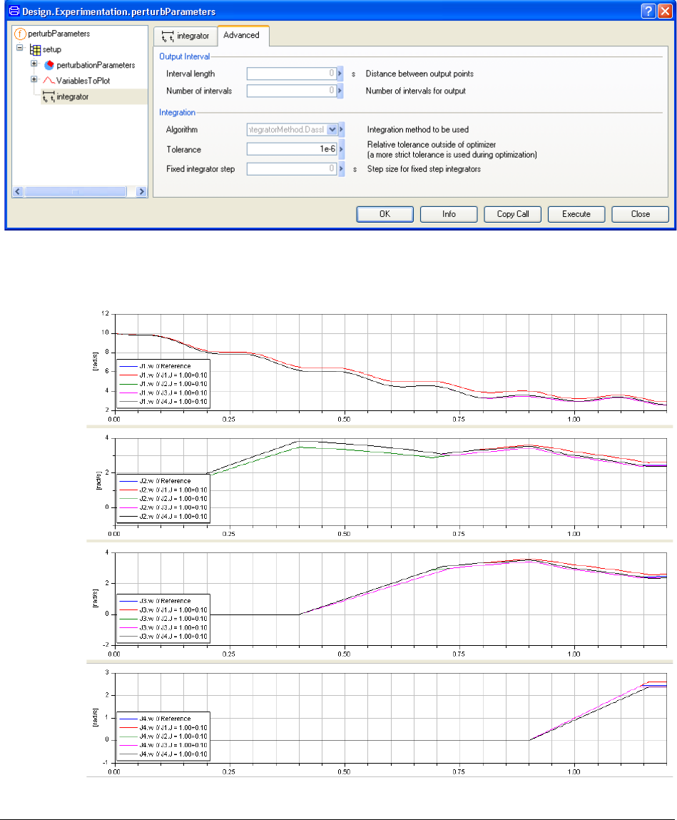
Finally, the setup for the integrator is to be done. Click on integrator in the left pane and set
the stop time to 1.2.
Click on the Advanced tab and select the default tolerance for the integrator lowered to
1e-6.
18
Now we can run the command. Click on Execute. After the simulations, and moving the
curves and legends to the appropriate place (some curves are on top of each other), we get
the following sequence of images.
1 MODEL EXPERIMENTATION 19
The plots show the variation of every variable when varying the parameters J1.J, J2.J, J3.J
and J4.J 10 percent, one at a time. We observe, for instance, in the first plot that only the
variation of J1.J affects the response on J1.w.
1.2.3 Sweep one parameter – two variants
The phenomenon described before can be observed in another fashion. We can sweep one
parameter and observe the result along the whole interval form 0 to 1.2, or just at the final
time of 1.2 seconds. These variants are implemented in two functions; sweepParameter and
sweepOneParameter.
sweepParameter
The setup of this function is very similar to perturbParameters.
(Shortcut: Use the command sweepParameter example as described in the beginning of
this chapter.)
If the previous example has been executed, go back to Modeling mode and right-click on
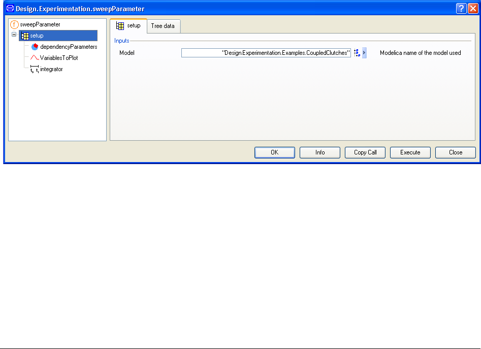
the function sweepParameter in the Experimentation package. Select Call Function…. The
model is already filled in (if not it has to be selected as in previous example).
We have to select the dependency parameter and the variable to plot. The way is the same as
in the previous example.
The first thing to do is to specify dependencyParameters (click on dependencyParameters
in the left of the menu). The Select button can be used to select J1.J. The result will be:

20
The Edit icon to the right of the Sweeping Values column can be used to select five
equidistant values between 0.9 and 1.3 for J1.J.
Click OK. The result will be
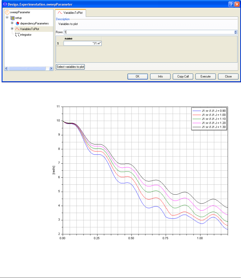
1 MODEL EXPERIMENTATION 21
Use VariablesToPlot to select the variable to plot (like in previous example) in this case the
variable should be J1.w
Don’t forget to set the Stop Time to 1.2 in the integrator setup and the tolerance to 1e-6
(like in the previous example)! Press Execute and the result follows.
Let us observe now J1.w and vary J2.J. Exchange in the setup J1.J with J2.J, in
dependencyParameters setup. Don’t forget that the Sweeping Values has to be set again.

22
Press Execute again. (This example is not included in the demo commands in the beginning
of this chapter.)
The response J1.w is less sensitive at the beginning of the interval to variations of J2.w. At
the end, when all inertias are coupled, the variation is larger.
sweepOneParameter
If our interest is just the response at end point of the interval, we use sweepOneParameter.
This setup is the same as for sweepParameter.
(Shortcut: Use the command sweepOneParameter example as described in the beginning
of this chapter.)
Just choose J1.J as dependency variable in the same way, take 51 values between 0.9 and
1.3 and use J1.w as variable to plot. The following curve is obtained when the command is
executed. Once more, don’t forget to set the Stop Time to 1.2 in the integrator setup and the
tolerance to 1e-6.
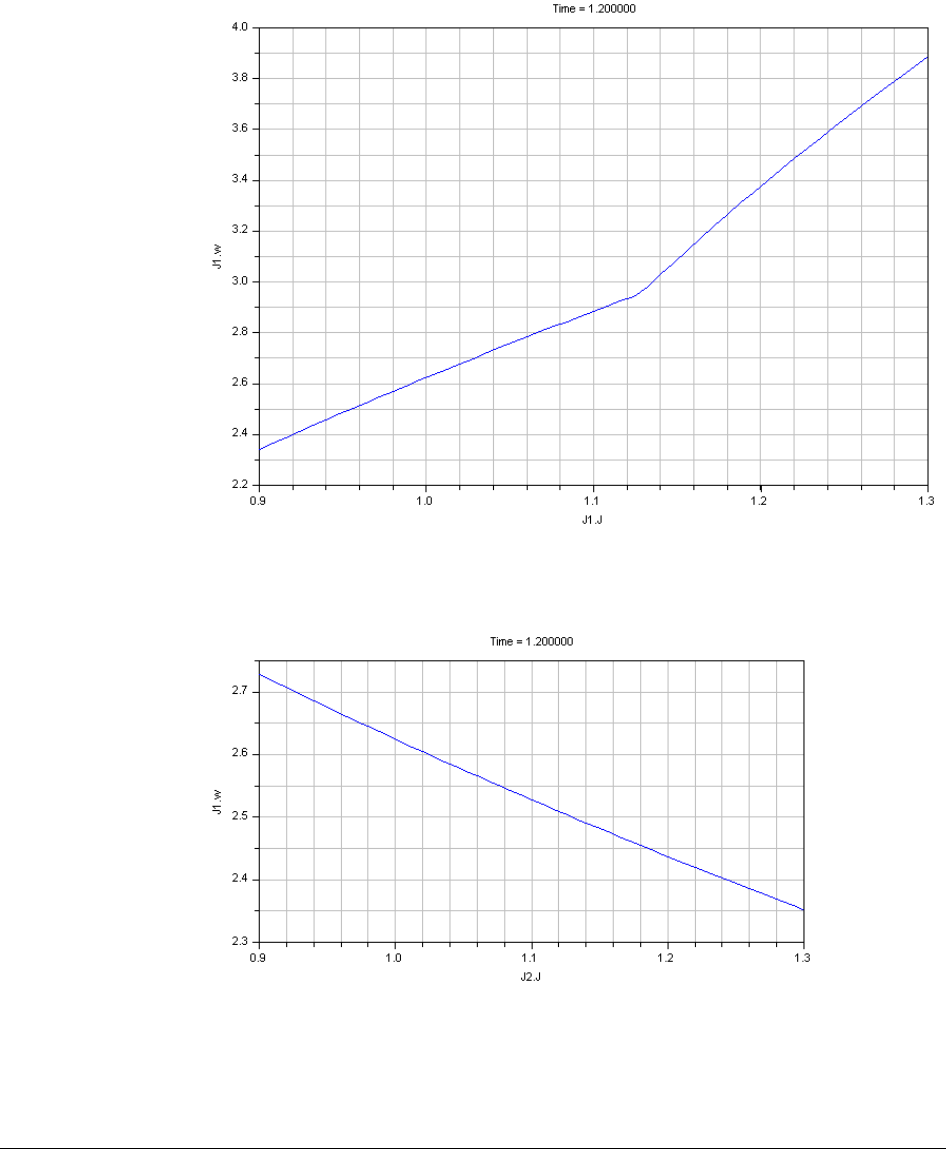
1 MODEL EXPERIMENTATION 23
This curve relates at t=1.2 the parameter J1.J and the response J1.w. The same situation can
be depicted for J2.J as parameter and J1.w as response. (This case is not covered by any
command in the beginning of this chapter.)
24
1.2.4 Sweep two parameters -
sweepTwoParameters
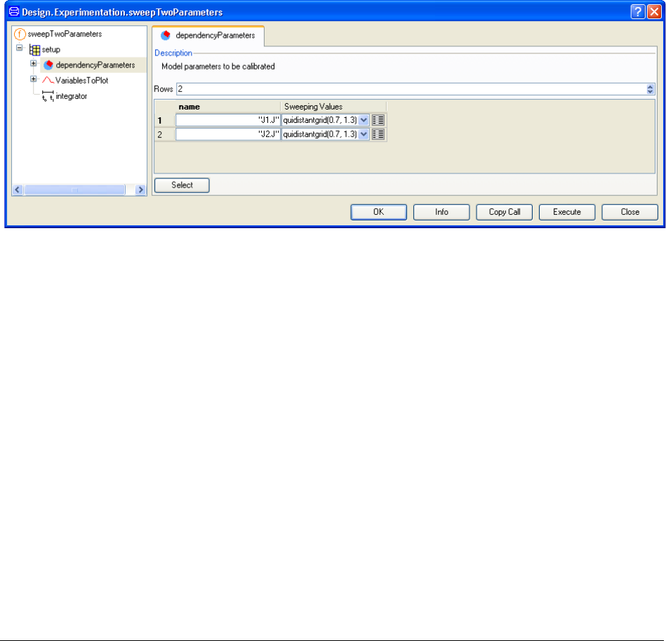
To study the dependence of one response with respect to two parameters at the end of the
integration interval, the function sweepTwoParameters is to be used. The setup is almost
identical to sweepParameter and sweepOneParameter. The only difference is that two
dependency variables are to be selected instead.
(Shortcut: Use the command sweepTwoParmeter example as described in the beginning of
this chapter.)
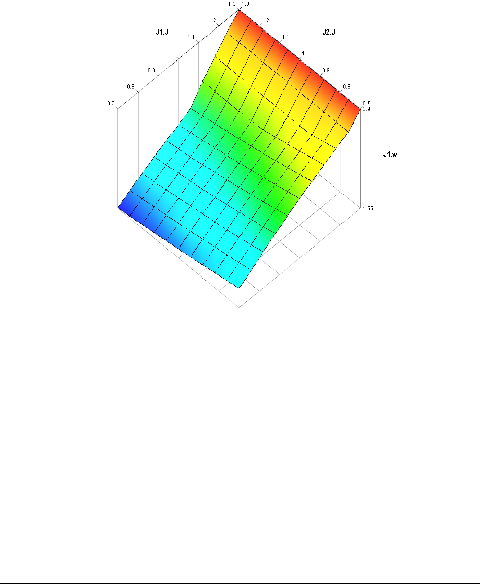
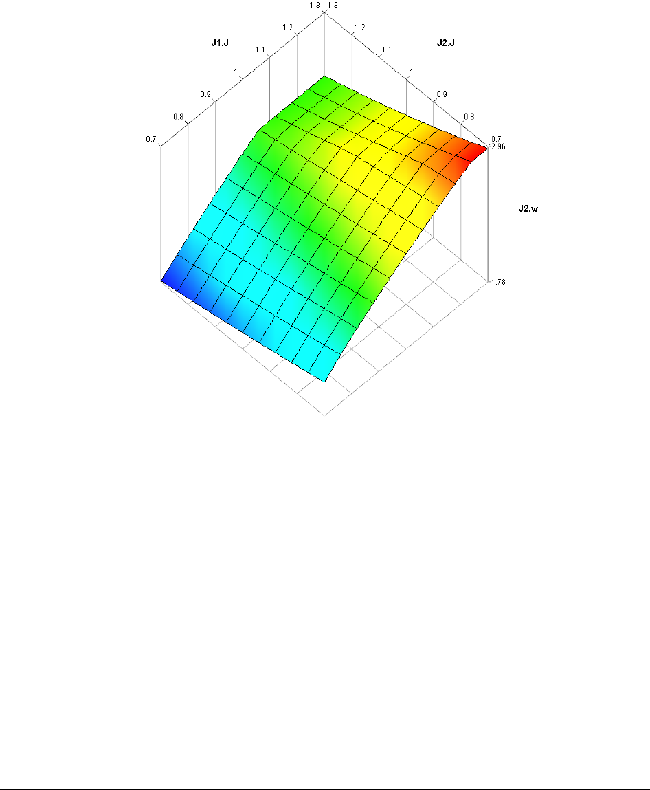
We observe now J1.w against J1.J and J2.J. The values chosen for J1.J and J2.J are eleven
values between 0.7 and 1.3 for both variables. Even for this case, the Stop time is 1.2 and
the tolerance is 1e-6 in the integrator tab.
(Please note that this case is not covered by the demo command in the beginning in this
chapter, the next case is however covered.)
1 MODEL EXPERIMENTATION 25
Observing J2.w gives the following result.
26
1.2.5 Monte Carlo Analysis
Monte Carlo Analysis is widely used to explore the behavior of a model when the input
parameters are multidimensional. We will set up now the command MonteCarloAnalysis to
observe the model response when varying J1.J, J2.J, J3.J and J4.J at the same time.
(Shortcut: Use the command MonteCarloAnalysis example 1, as described in the
beginning of this chapter.)
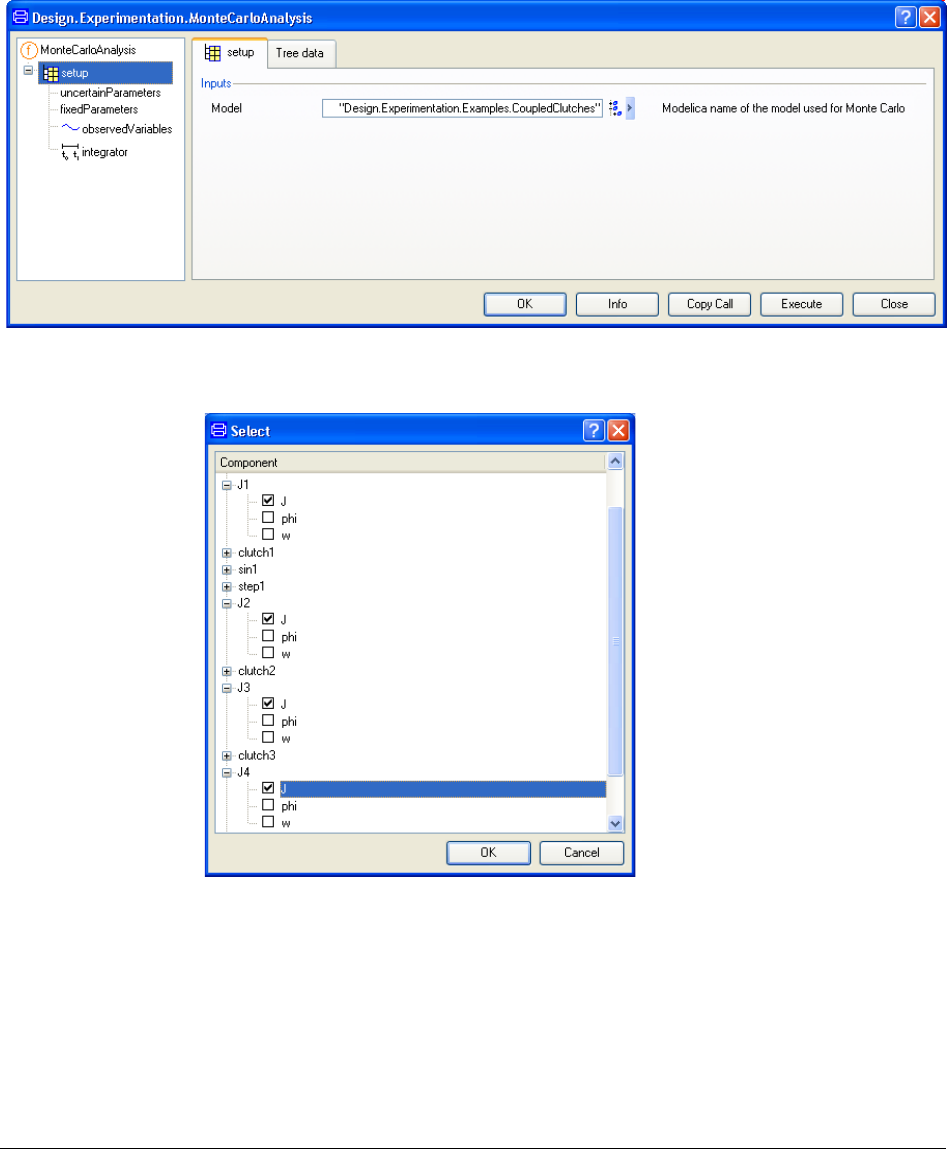
Right-click on the function MonteCarloAnalysis in the Experimentation package and select
Call Function…. A menu pops up. Since we so far started by defining the setup, please
click on setup in the browser to the left. Select the model (if not preselected) like in
previous examples. The result will be:
1 MODEL EXPERIMENTATION 27
The task now, as before, is to select the uncertain parameters. Click on
uncertainParameters and click on the Select button. Select the browser J1.J to J4.J.
Click OK. The next step is to select a random distribution for every inertia.

28
Click on the arrow of the combo box and select randomNormal for J1.J. Another menu
pops up asking for values for Mean Value and Standard Deviation. Those values
characterize the normal distribution to be used. Set mean to 1 and standard deviation to 0.1.
Click OK. Repeat the same process for J2.J to J4.J.
The setup for fixedParameters is used if we want to specify other simulation situations than
the nominal values written in the model. For instance, if the initial angle J1.phi is specified
1 MODEL EXPERIMENTATION 29
and different from zero, we should add it there. In our case, we don’t have such fixed
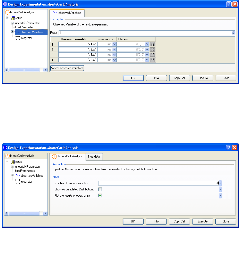
parameters so we just go directly to observed variables. Click on observedVariables and
press the button Select observed variables. Mark in the browser J1.w, J2.w, J3.w and J4.w.
The flag automaticBins set to true allows the algorithm to choose automatically an
appropriate set of bins, according to the maximum and minimum values observed in the
result. It takes also into account the total number of samples to set the appropriate resolution.
Set the integrator stop time once more to 1.2. To set up the type of desired result, click on
MonteCarloAnalysis in the browser in the left pane of the window.
We set the number of draws in the field Number of random samples. As we want to plot
the result of every draw, only twenty draws are needed. Check also Plot the results of
every draw to obtain the plot of the responses and the density of probability.
Click on Execute. The result will be a number of plot windows. The first (that is, you have
to minimize the ones on top to see it) plot will look similar to the following:

30
In this graph we observe the variation of slope and behavior produced by random sampling
of the values of J1.J, J2.J J3.J and J4.J in time.
If the plots of the density of probability or accumulated probability are important, we
change the setup to plot those with more samples. To plot the densities, we take five
thousand samples and uncheck the flag Plot results of every draw. Press Execute to obtain
the plots (this corresponds to using the command MonteCarloAnalysis example 2 as
described in the beginning of this chapter). Please note that making 1000 draws takes some
time.
0.00 0.25 0.50 0.75 1.00
0
1
2
3
4
5
6
7
8
9
10

1 MODEL EXPERIMENTATION 31
To plot the accumulated distributions, check the flag Show Accumulated Distributions.
Click on Execute. (This corresponds to using the command MonteCarloAnalysis example
3 as described in the beginning of this chapter.) The result plots follow.
2 3 4
0.0
0.4
0.8
1.2
Expected Value = 2.6403
Standard Deviation = 0.328018
Probability Density
J1.w
2.0 2.5 3.0
0.0
0.4
0.8
1.2
Expected Value = 2.44334
Standard Deviation = 0.18562
Probability Density
J2.w
32
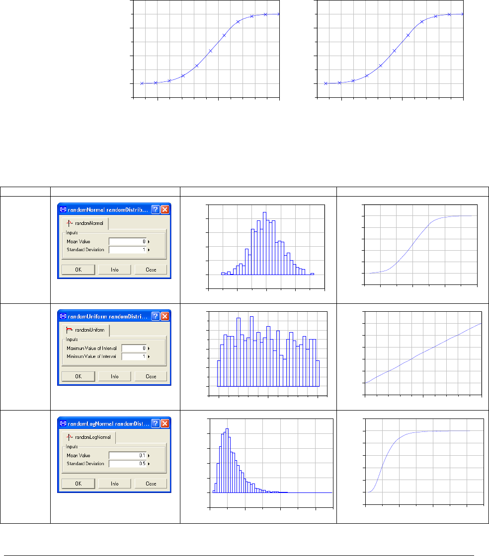
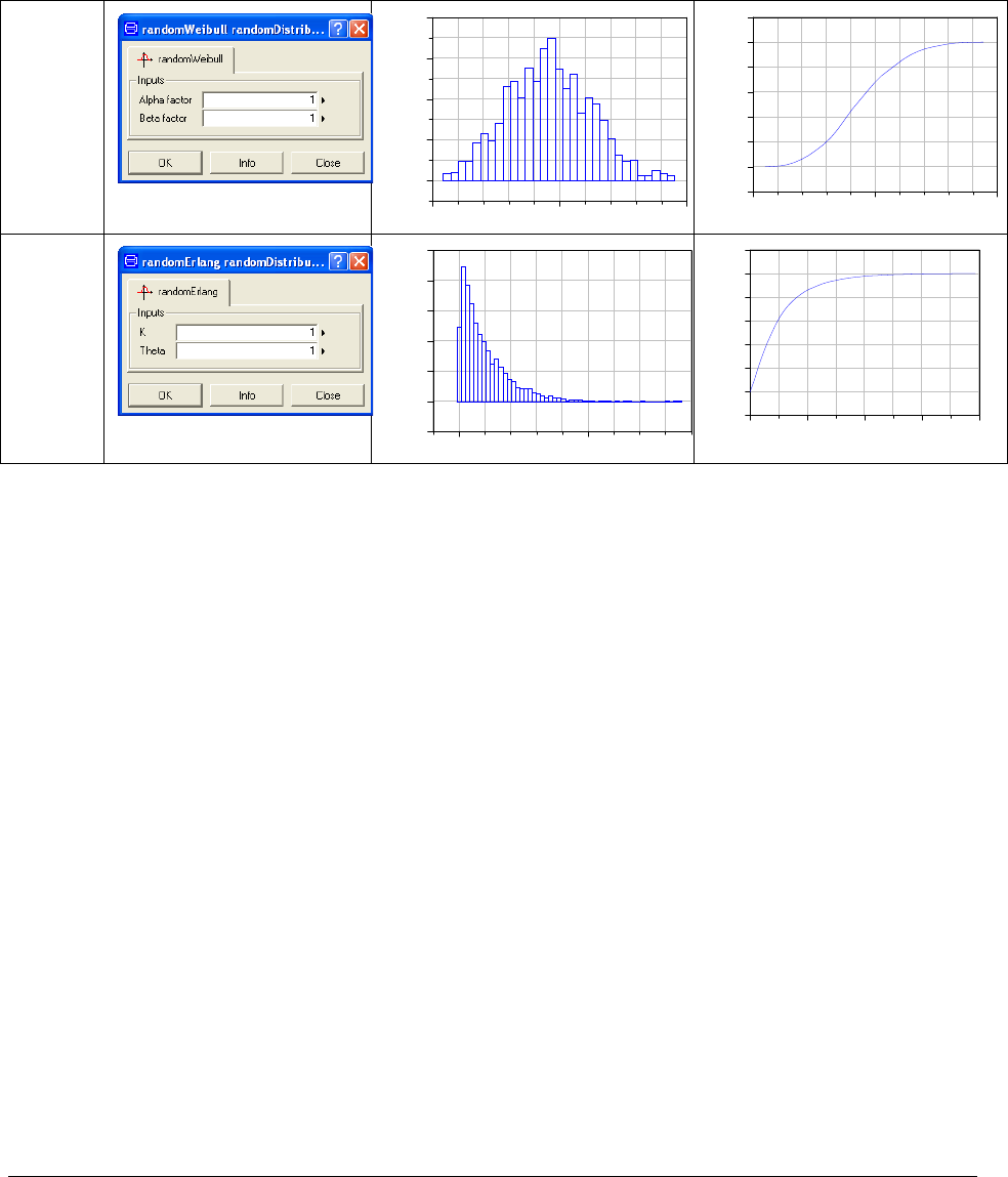
Random Distributions available and their parameters
The following table reviews briefly the random distributions in Experimentation package
that can be used together with MonteCarloAnalysis.
Distribution Parameters Probability density Accumulated probability
Normal
Uniform
Logarithmic
Normal
2.0 2.5 3.0
0.0
0.4
0.8
1.2
Expected Value = 2.44334
Standard Deviation = 0.18562
Probability Density
J3.w
2.0 2.5 3.0
0.0
0.4
0.8
1.2
Expected Value = 2.44232
Standard Deviation = 0.185749
Probability Density
J4.w
-4 -2 0 2 4
-0.1
0.0
0.1
0.2
0.3
0.4
0.5
Probability Density
x
-2 0 24
-0.2
0.0
0.2
0.4
0.6
0.8
1.0
1.2
Accumulated Probability
x
0.0 0.5 1.0
0.0
0.4
0.8
1.2
1.6
Probability Density
x
0.0 0.5 1.0
-0.2
0.0
0.2
0.4
0.6
0.8
1.0
1.2
Accumulated Probability
x
0246
-0.2
0.0
0.2
0.4
0.6
0.8
1.0
Probability Density
x
0 2 4 6
-0.2
0.0
0.2
0.4
0.6
0.8
1.0
1.2
Accumulated Probability
x

1 MODEL EXPERIMENTATION 33
Pareto
Exponential
Circular
Uniform
Beta
1.0 1.5 2.0
0
2
4
6
8
Probability Density
x
1.0 1.5 2.0
-0.2
0.0
0.2
0.4
0.6
0.8
1.0
1.2
Accumulated Probability
x
05
0.0
0.2
0.4
0.6
0.8
Probability Density
x
0 5 10
-0.2
0.0
0.2
0.4
0.6
0.8
1.0
1.2
Accumulated Probability
x
0 1 2 3
-0.1
0.0
0.1
0.2
0.3
0.4
0.5
Probability Density
x
0 1 2 3
-0.2
0.0
0.2
0.4
0.6
0.8
1.0
1.2
Accumulated Probability
x
0.0 0.5 1.0
-0.5
0.0
0.5
1.0
1.5
2.0
2.5
3.0
Probability Density
x
0.0 0.5 1.0
-0.2
0.0
0.2
0.4
0.6
0.8
1.0
1.2
Accumulated Probability
x
34
Weibull
Erlang
0 1 2
0.0
0.4
0.8
1.2
1.6
Probability Density
x
0 1 2
-0.2
0.0
0.2
0.4
0.6
0.8
1.0
1.2
Accumulated Probability
x
0 5
-0.2
0.0
0.2
0.4
0.6
0.8
1.0
Probability Density
x
0 2 4 6 8
-0.2
0.0
0.2
0.4
0.6
0.8
1.0
1.2
Accumulated Probability
x
2 MODEL CALIBRATION

2 MODEL CALIBRATION 37
2 Model Calibration
2.1 Introduction
Dymola includes features to perform integrated computer experiments with Modelica
models. This document describes the features to calibrate and to assess models. The
functions described in this document are parts of the Design.Calibration package. There is
no licensing for Model Calibration.
Consider a Modelica model describing a physical system. Such a model includes typically
many parameters, which have to be set. Some parameter values can be found from design
sheets. Some parameters such as physical dimensions may be easy to measure on the system.
Direct measurements of the weights of the parts are more difficult since it requires the
system to be dismounted. Moreover, it is for example not simple to measure the inertia of a
part. Friction and loss parameters are good examples of parameters that often are unknown.
Model calibration (parameter estimation) is the process where measured data from a real
device is used to tune parameters such that the simulation results are in good agreement with
the measured data. The parameters that we tune are often referred to as tuners. Dymola
varies the tuners and simulates when it searches for satisfactory solutions. Mathematically,
the tuning procedure is an optimization procedure to minimize the error between the
simulation results and the measurements.
38
When tuning parameters from measurements, a basic question is “Which parameters can be
estimated from the measurements available?” Changing a parameter to be estimated must of
course influence the output. However, this is not enough. Two or several parameters may
influence the result in a similar way such that it is not possible to estimate them individually.
Dymola includes function to analyze and to plot parameter sensitivities. When a set of
parameters have been tuned, it is recommendable to validate the model and the tuned
parameters against other measured data to check that there is a good agreement between the
simulation result and the new measurements. For a specific series of measured data it is
possible to get good fits by increasing the model complexity and the number of tuned
parameters. However, this does not guarantee that the result is that good for other operating
conditions.
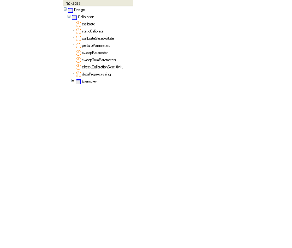
To load the package Design.Calibration, select File > Libraries and select Design. When
the library is opened, expand Design and then Calibration by clicking on the + in front of
them. The result in the package browser will be:
The function Design.Calibration.calibrate is the main function for calibration and validation
of models1. There is also a set of functions for analyzing parameter sensitivities and
dependencies of calibration tasks. For parameter studies in general see chapter “Model
Experimentation”. The function Design.Calibration.calibrate supports easy setup of
calibration to tune static characteristics.
The content of this chapter is the following:
In section 2.2 starting on page 39 the basics of setting up and executing a basic calibration
task is described with a number of examples based on a simple car model describing
translational motion available in the Design library.
Section 2.3 starting on page 60 describes how to store a setup for later reuse.
Section 2.4 starting on page 61 describes how to reuse a setup for a similar operation.
1 The optimization method used by the function is a least-square fit with regularization to ensure that it does not get
stuck due to redundant tuners.
The functions of
Design.Calibration.
2 MODEL CALIBRATION 39
Section 2.5 starting on page 62 describes a number of functions to analyze parameter
sensitivities and dependencies. The functions sweepParameter, sweepTwoParameters,
perturbParameters and checkCalibrationSensitivity are described in this section.
Section 2.6 starting on page 75 describes data preprocessing, the process of adjust the data
eliminating noise, zones where the model is not valid and erroneous or not representative
measurements. The function used is dataPreprocessing.
Section 2.7 starting on page 86 describes static calibration. Two cases are described. One
case is the calibration of completely static models (to tune static characteristics of
components such as pipes, valves, throttles etc). Such models are always in steady-state.
The function to use is staticCalibrate. The other case is steady-state calibration to tune
steady-state cases for which either dynamics is ignored or each case is simulated until
steady-state is obtained. The function used is calibrateSteadyState.
2.2 The basics of setting up and executing a
calibration task
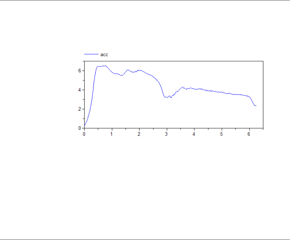
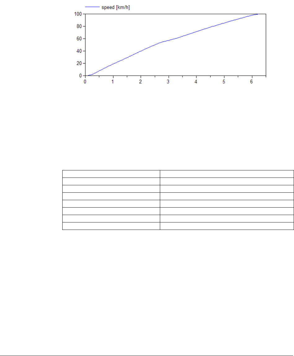
We have acceleration and speed measurements from a BMW 645i at full throttle as shown
in the plot below. For further information we refer to Auto Mobil, Issue 1, 2005.
Acceleration and speed
measurements from a
BMW 645i at full
throttle.
Gear shift
Anti spin control
40
Anti spin control and gear shifting make the acceleration curve complex. Here we will focus
on the time interval 3.8-6 seconds when the second gear is engaged.
We need to describe how the generated torque makes the car move. Thus we need to make a
simple power train model including gearbox and rotating elements which make the wheels
rotate.
2.2.1 Vehicle data
By searching on the web we can find the following data for the car
Engine torque at 3600 rpm [Nm]
450
Engine inertia [kgm2]
0.4
Gearbox and cardan inertia [kgm2]
0.01
Wheel inertia [kgm2]
4* 1
Wheel radius [m]
0.34
Car mass [kg]
1690
Automatic gear ratios I-VI
{4.17, 2.34, 1.52, 1.14, 0.87, 0.69}
Gear ratio of final gear
3.46
The wheel radius is calculated for 245/45 R18 W saying that the radius is 18”/2 + 0.45*245
= 0.338 m.
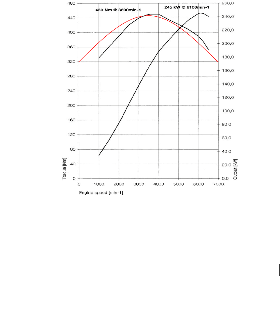
Engine characteristics at full throttle for a BMW 545i were found at
http://www.e60.net/information/options/engines/my2004_545i
Data for a BMW 645i.
2 MODEL CALIBRATION 41
BMW 545i and BMW 645i have the same 4.4-liter V8 engine. The black lines in the plot
above show the torque and power characteristics.
As a first approximation we fit a quadratic characteristic:
tau = tau_0 +(tau_max-tau_0)*(1-((w-w_max)/w_max)^2);
The parameter w_max is 3600*2π/60 rad/s and tau_max is 450 Nm. Choosing tau_0 to 320
gives the red curve in the plot above.
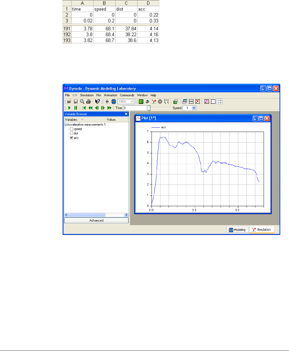
The velocity and acceleration measurements are stored simply as a csv file in
Program Files (x86)\Dymola 2018\Modelica\Library\Design
1.0.6\Acceleration measurements.csv
Engine characteristics
at full throttle for a
BMW 545i.
42
The first row of the file includes the column headings and then the data follow. Dymola
supports plotting of such a csv file. Select Plot > Open Result… and a file browser pops.
Use it to select the csv file. The file and its variables appear in the variable browser and can
be plotted in the usual way.
2.2.2 Vehicle model
The model we are going to build is available as:
Design.Calibration.Examples.SimpleCar
Useful modeling components are found in
Modelica.Mechanics.Rotational
Modelica.Mechanics.Translational
The measurements
stored as a csv file.
Plotting the measured
data in Dymola.
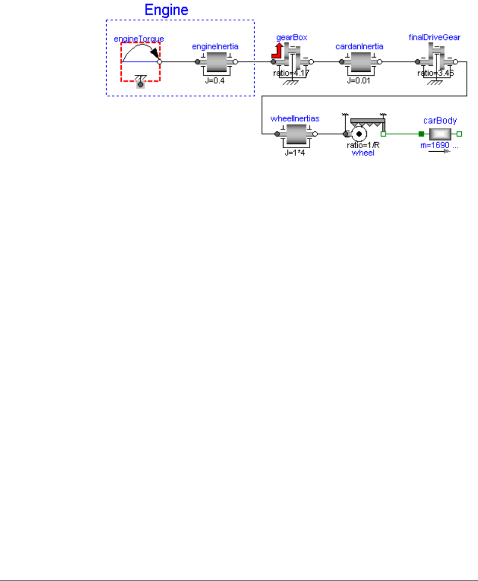
2 MODEL CALIBRATION 43
To the left there is the engine driving the gearbox, which is connected to the cardan system
giving a final drive to the four wheels. The rotational motion of the wheels results in a
translational motion of the car. Let R be the wheel radius then 1/R gives the ratio between
the driving rotational motion and the resulting translational motion where R is the wheel
radius. The model defines
parameter Real R=0.34;
and binds the parameter wheel.ratio = 1/R. Setting of parameters are indicated by the
diagram. Additionally the mass of the car, carBody.m is set to 1690+70+50 kg to include
the weight of the driver and measurement equipment.
The quadratic torque characteristics at full throttle is modeled by extending from
Modelica.Mechanics.Rotational.Interfaces.PartialSpeedDependentT
orque
and adding the quadratic torque characteristics and the definitions of its parameters
model Engine
extends
Modelica.Mechanics.Rotational.Interfaces.PartialSpeedDependentT
orque;
parameter Modelica.SIunits.Torque tau_0;
parameter Modelica.SIunits.Torque tau_max;
parameter Modelica.SIunits.AngularVelocity w_max;
equation
tau = - (tau_0 + (tau_max-tau_0)*(1-((w-w_max)/w_max)^2));
end Engine;
Please, note minus sign for the torque to specify that the torque is a driving torque and not a
reaction torque.
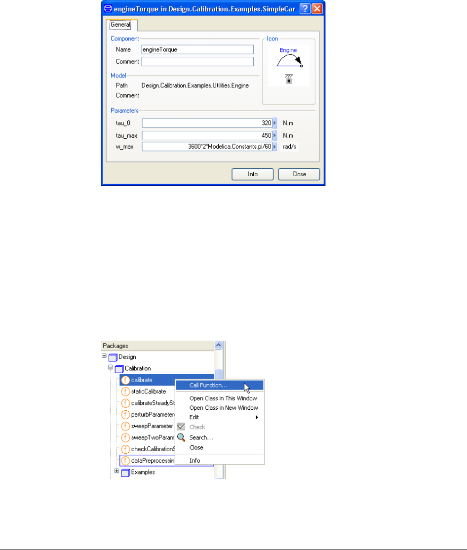
The parameters of the component engineTorque are then set as shown by its parameter
dialog (double-click on the component):
The vehicle model.
44
2.2.3 Validation of the nominal model
Let us first check how the model with nominal parameters compares with measured data.
Validation is set up very similar to calibration. A basic difference is of course that no
tunable parameters need to be specified for the validation. The functions described in this
document are parts of the Design package. If you have not loaded the Design package by
now, please see the section “Introduction” above on how to do it.
The following section corresponds to using the command Commands > Validation of
original model.
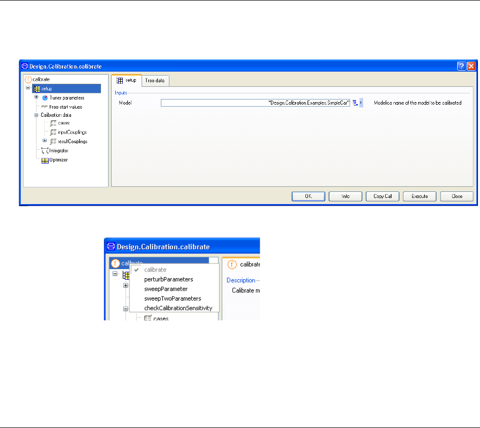
To set up the calibration, select Design.Calibration.calibrate in the package browser. Right-
click and select the command Call function…
The following menu pops up:
The parameter
settings for
engineTorque.
Selecting calibrate and
right-clicking.
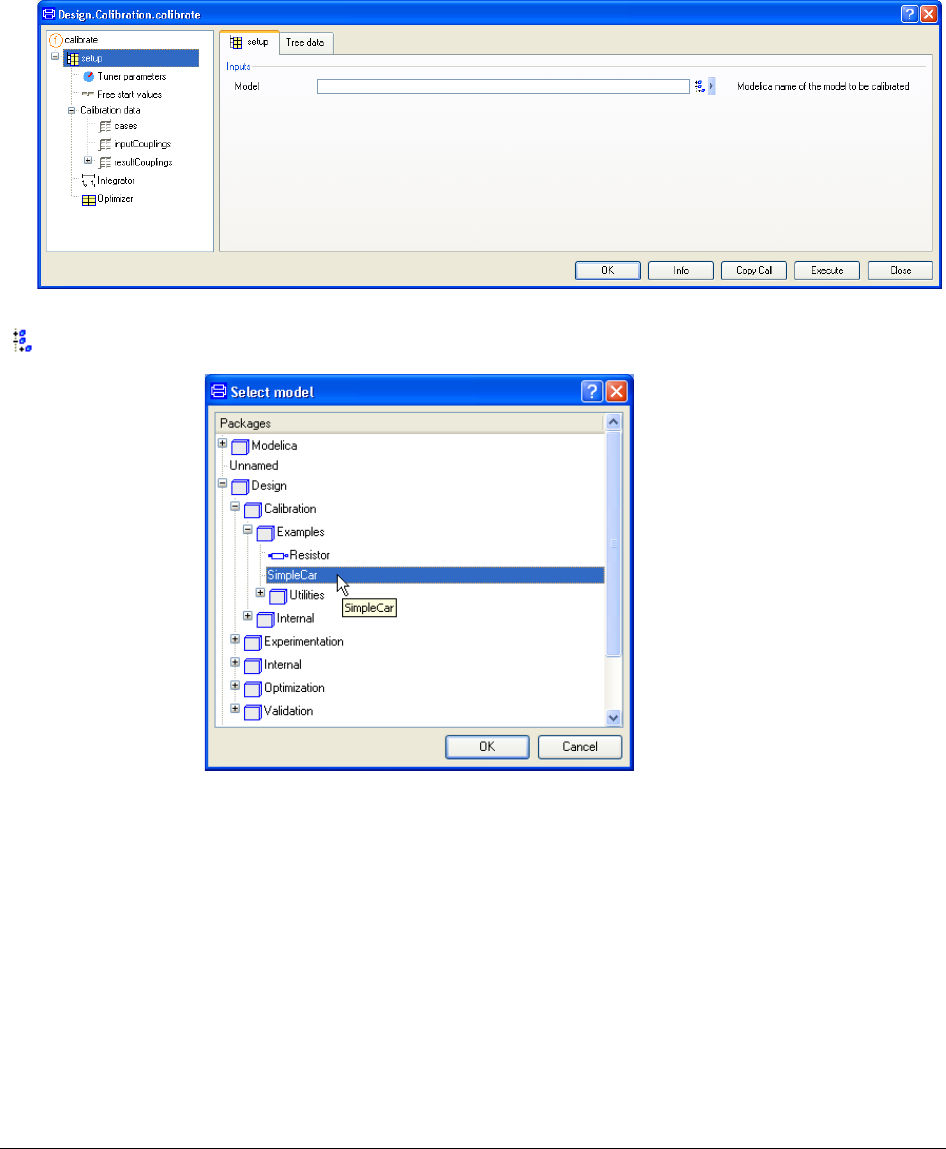
2 MODEL CALIBRATION 45
To specify the model to be calibrated, click on the Browser icon to the right of the input
field. A package browser pops up. Use it to select the model.
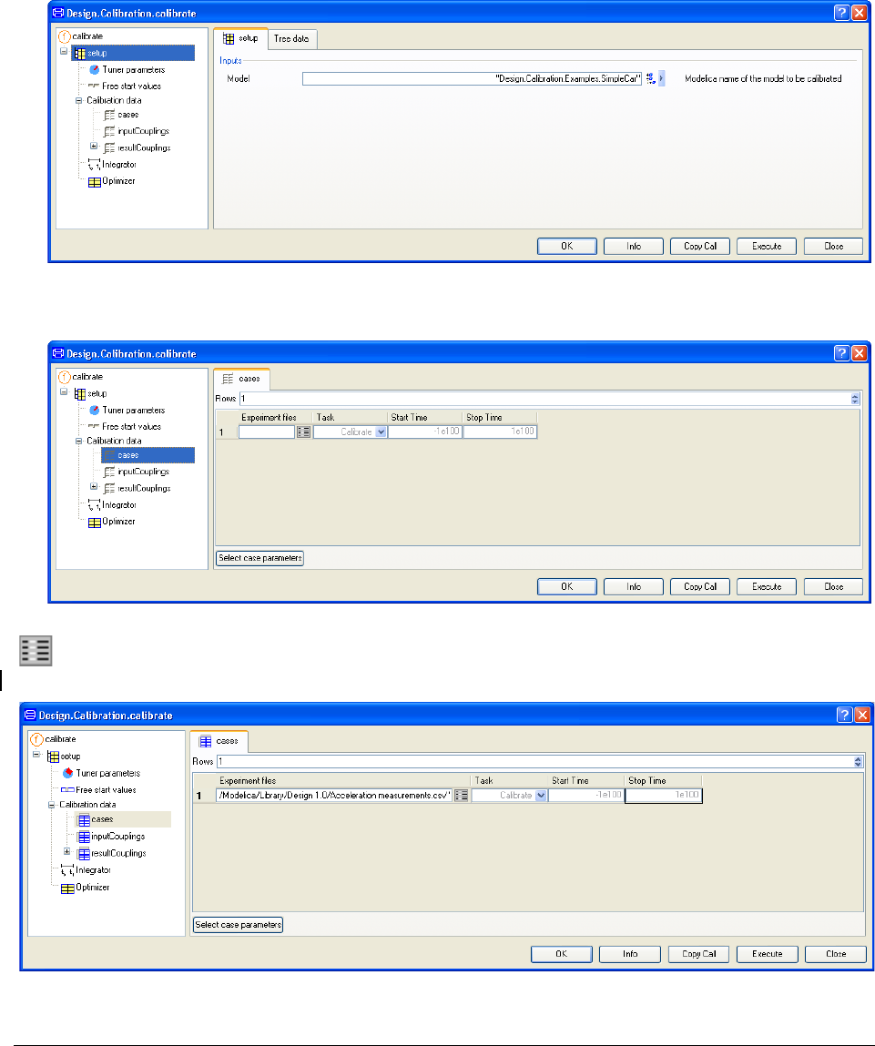
Click OK. The model is now translated in order to gather information needed to build
browsers and selectors to support the remaining setting up of the calibration task. If Dymola
already has a translated model, then this model appears as the default model.
Selecting model to
calibrate.
46
The next task is to specify the measurements and how they are stored. Consider the tree
browser to the left. Select cases under Calibration data.
To introduce an experiment file, click on the Edit icon of the first element in the
Experiment files column. A file browser pops up. Use it to select the file Program Files
(x86)\Dymola 2018\Modelica\Library\Design 1.0.6\Acceleration measurements.csv.

2 MODEL CALIBRATION 47
If we had had more measurement files we had increased the number of rows and selected
more measurement files. In this case the measurements are stored in a csv file as described
above. Dymola supports some common ways of storing measurements, see further below.
An advanced user can replace the calibration data input with a routine accessing data in
different formats, without having to change the underlying calibration routines.
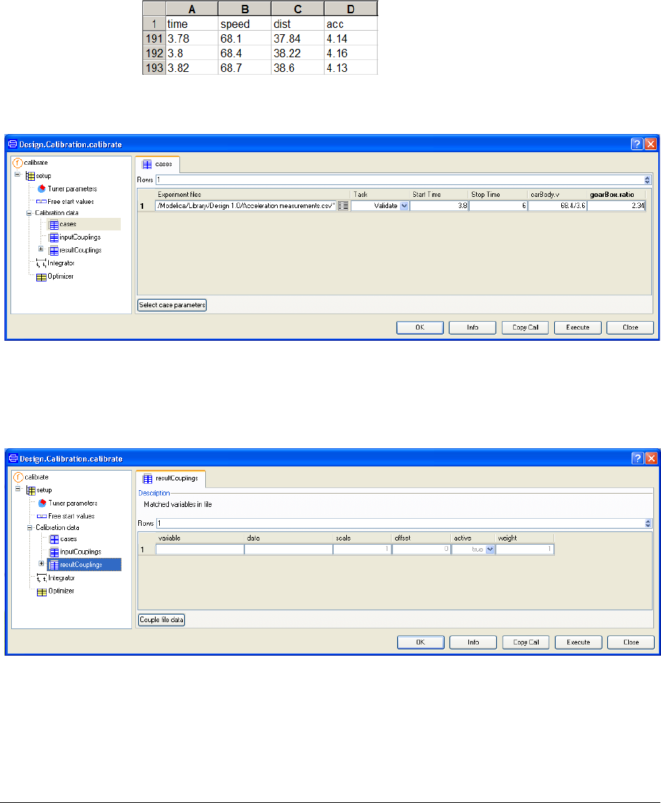
The different cases may need individual parameter settings or individual initial values for
some of the states. Recall that we are to use the measurements from the time interval 3.8-6
seconds when second gear is engaged. Thus we need to use the gear ratio of the second gear
and an initial velocity. To enter this information, click on Select case parameters. Use the
browser to select carBody.v and gearBox.ratio.
Click OK. The default values appear in the new columns.
From the measurement file we can find that the velocity at time 3.8s is 68.4 km/hour =
68.4/3.6 m/s.
Specifying case
dependent parameters.
48
Enter this value for carBody.v and set gearBox.ratio to have the value of the second gear,
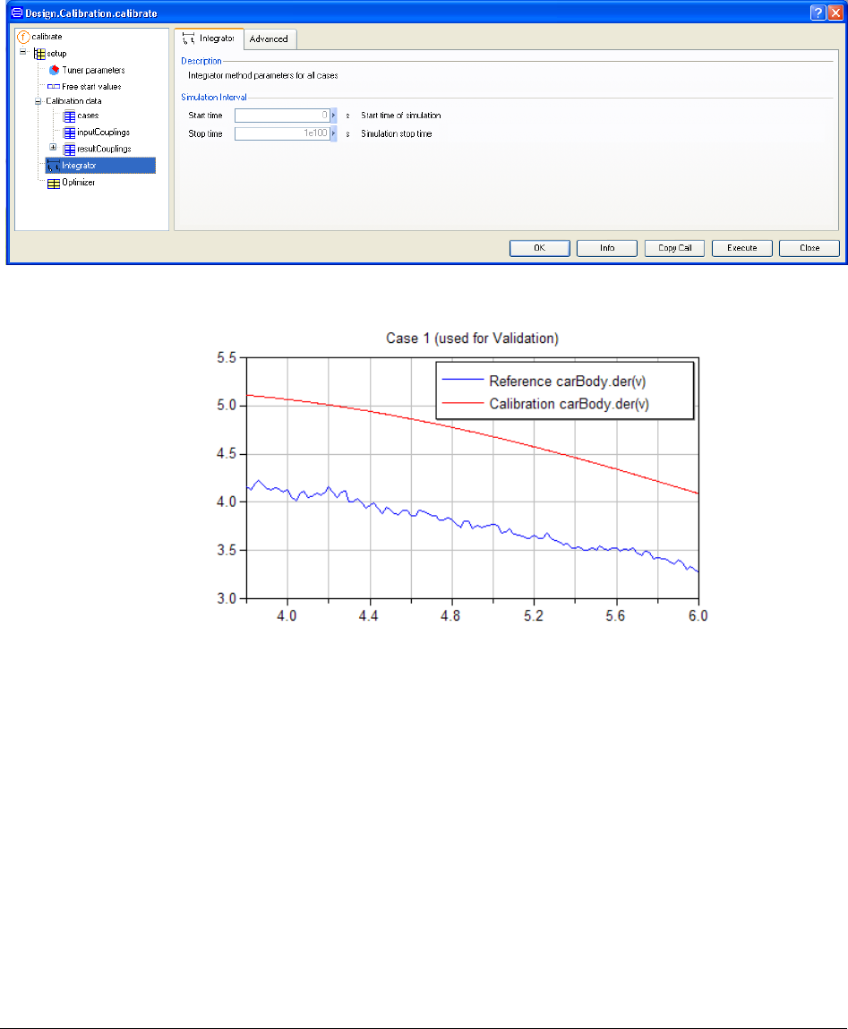
namely 2.34. Enter also start time (3.8) and stop time (6) and set Task to Validate.
The files may include input signals to drive the model, parameter values to be used and
measured data that the model shall reproduce. In this case the file includes measured speed,
distance and acceleration for each 20 ms in the time interval 0-6.24 seconds. The
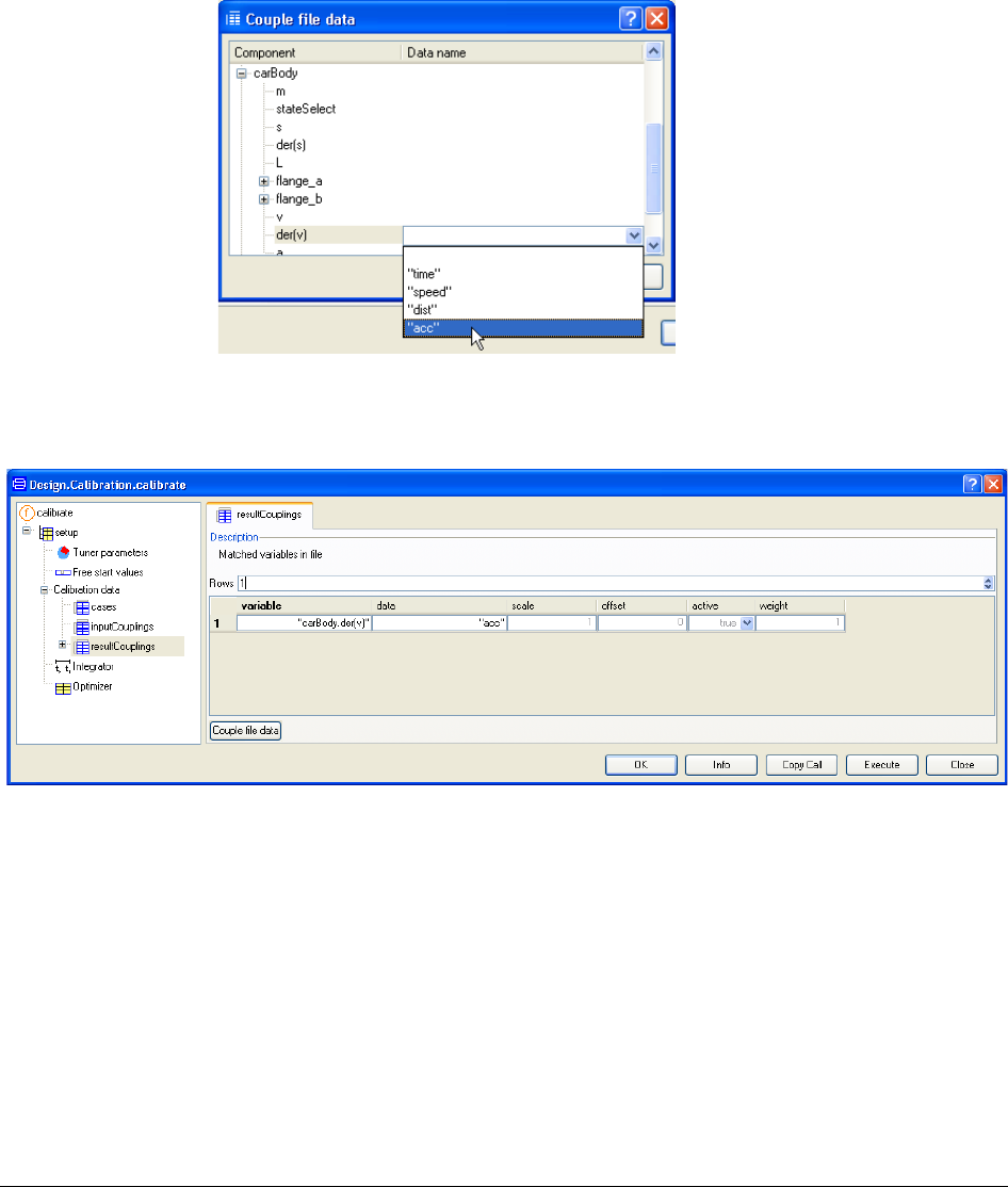
acceleration measurements will be used for the calibration criterion. To specify that click on
resultCouplings in the browser to the left
Click on Couple file data.
A part of the csv file
with the
measurements.
2 MODEL CALIBRATION 49
Use the browser to select the car acceleration, carBody.der(v), and then right-click click to
the right to see the names of the data series in the input files. Select “acc”. We could also
have chosen carBody.a, because carBody.a = carBody.der(v). Click OK.
We have now specified that the difference between carBody.der(v) and the data column
“acc” shall be used as the criterion for calibration. If the measured data are given in some
unit different than that used in the model, the Scale column allows scaling of the
measurements: variable = data * scale + offset
In case the deviations of several variables shall be used to specify the criterion, the Weight
column allows the user to give them different weights.
The model SimpleCar has no inputs. In case the model has inputs, click on inputCouplings
and couple them to the file data in a similar way as done for the outputs.
The Integrator element allows specification of a global simulation interval.
Couple the accelerator
variable carBody.der(v)
with measured
acceleration “acc”.
50
To perform the validation, click Execute.
The result is plotted above. The curves have similar shapes, but there is an offset. The model
gives a higher acceleration than measured. This may make you think of losses not being
modeled. Soon we will discuss calibration – please do not shut down any window, the next
section “Measurement file formats” describes how working with a Matlab file differs from
working with a csv file. If you want to continue with calibration etc directly please jump the
next section.
(If you by mistake have shut down the window, please see the tip to get back in section
“Saving the setup for reuse” on page 60.)
2.2.4 Measurement file formats
In the example above the measurements are stored in a csv file as described. Dymola
supports some common ways of storing measurements and allows users to specify their own
storage formats. The measurement files must have the same format.
Comparing measured
acceleration with
simulated acceleration
before calibration.
2 MODEL CALIBRATION 51
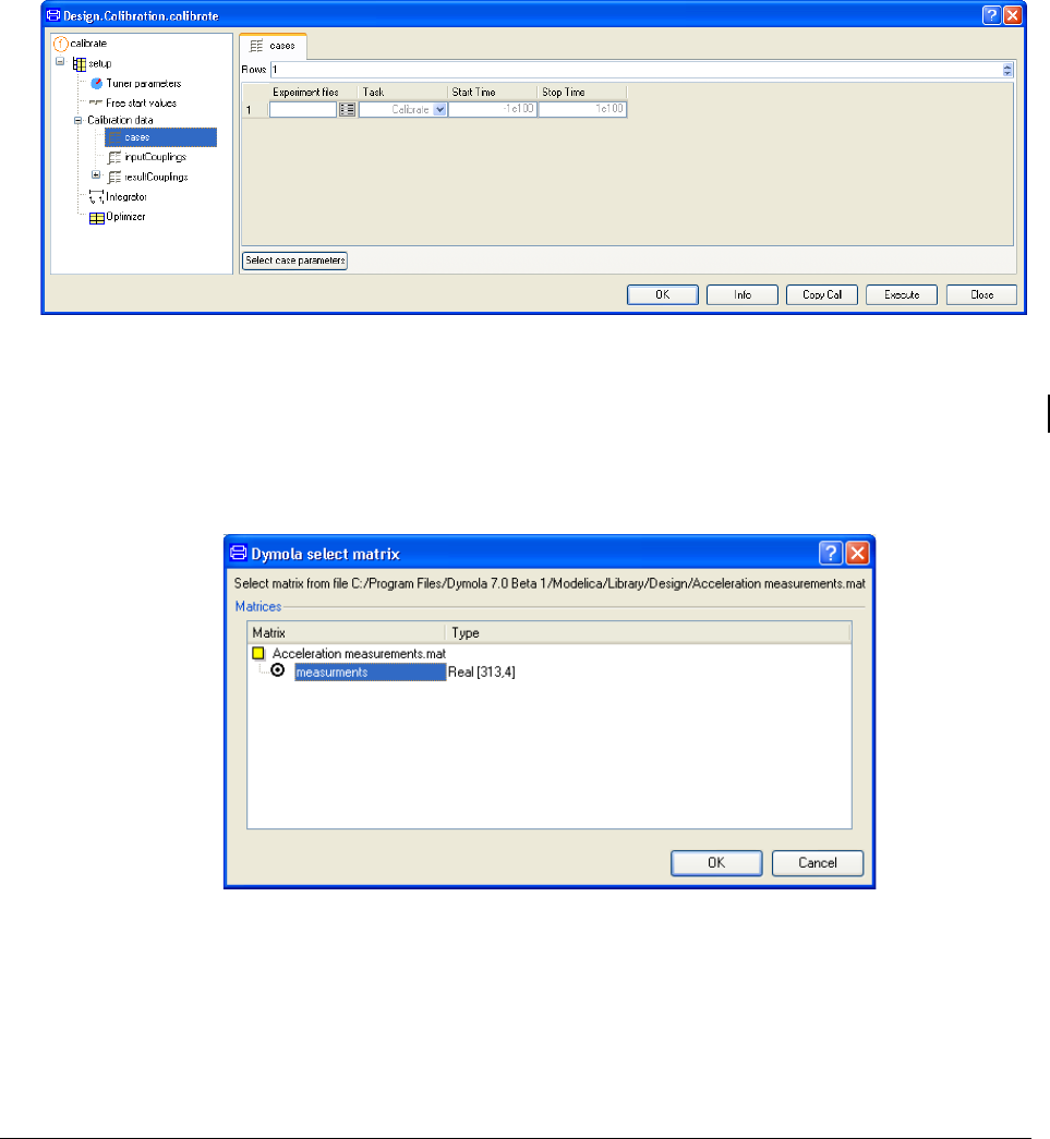
In case the measurement data are stored in (Matlab 4) mat files, we need to specify the name
of the matrix containing the measurement data to be used and the data are referred by
column number. The acceleration measurements are also available as a .mat file. Let us use
this file instead.
As previously, click on cases. Click on the Edit icon of the first element in the Experiment
files column. A file browser pops up. Use it to select the file
Program Files (x86)\Dymola 2018\Modelica\Library\Design 1.0.6\Acceleration
measurements.mat
Dymola then pops a menu to select the appropriate matrix. After selection (in this case no
alternative is possible) it will look:
Click OK.
Selecting matrix.
52
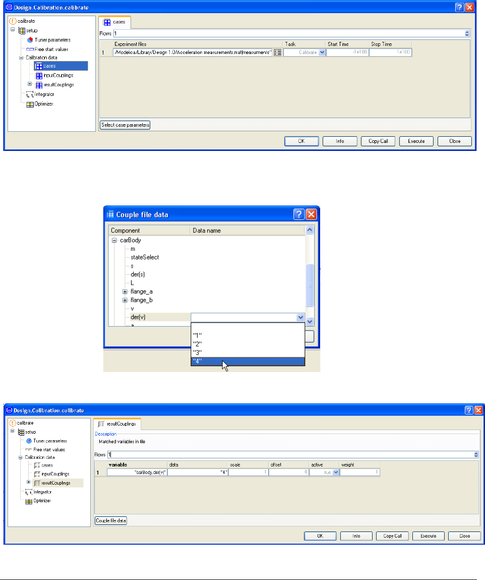
Proceed as previously to select case parameters, setting their values and start and stop time.
The specification of result couplings is slightly different, because the data is referenced by
column number. The acceleration measurements is column 4.
The result of the coupling now becomes
Couple model variable
and data.

2 MODEL CALIBRATION 53
The data field has “4” instead of “acc”.
The simulation results of Dymola are stored as .mat files, which includes information on the
name of the variables. If such trajectory files are used as measurement files then the
information on variable names are used. The user will not be prompted for matrix name.
When coupling inputs or results, the browser will display variable names.
2.2.5 Calibration
The task of a calibration is to tune some parameters to obtain a better agreement between
measured behavior and behavior predicted by the model. Thus, we need to address the
question, which parameters to tune. When deciding which parameters to tune, it is good to
consider the question: Which parameter values are most uncertain? In the model above,
friction and losses in the gearbox elements have been neglected. Frictions and other losses
are good examples where calibration is useful. There are for instance losses in both gearBox
and finalDriveGear, however, having only measurements of the translational motion of the
car, it is not possible to decide the individual losses of these two elements. Thus, it is
necessary to aggregate all losses to one element and gearBox is selected, since it has
provisions to model efficiency. The efficiency is given by gearBox.lossTable[1,2], see the
documentation of Modelica.Mechanics.Rotational.Components.LossyGear.
The parameter tau_0 was manually selected to 320, so it is a good candidate for tuning.
Dymola supports an interactive explorative approach to this problem. Dymola has powerful
functions to perform parameter sweeps and to analyze parameter sensitivities and possible
couplings between parameters with respect to the result variables to eliminate irrelevant
parameters and to diagnose over- parameterization. However, let us come back to these later
and first try tuning the two parameters.
We continue with the initial example where a .csv file was used as measurement file. If you
happen to have shut down the window below, you can use the command Commands >
Validation of original model to get back the needed setup
The final result of this section (“Calibration”) and the section “Validation using
measurements from first gear” below can also be obtained using the command Commands
> Calibration with validation.
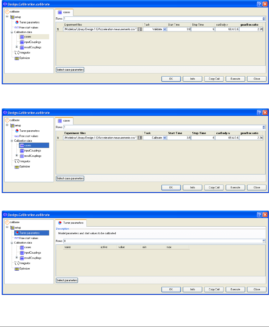
Clicking on cases in the browser of that window should give:
54
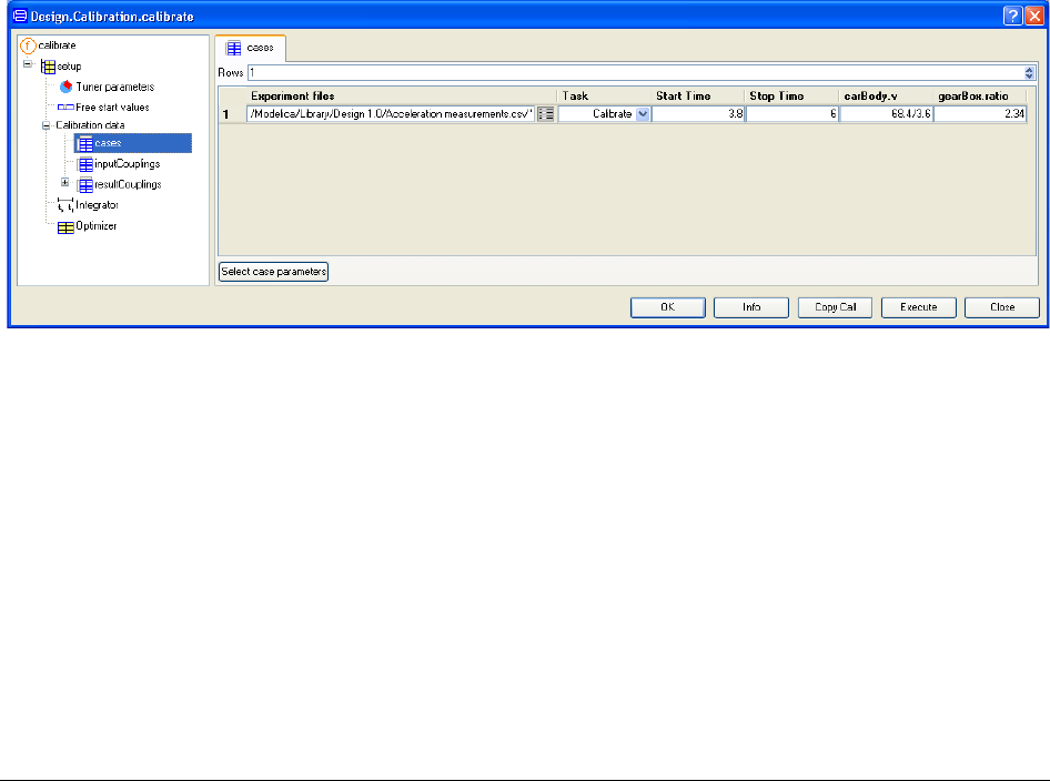
First we have to set the task to Calibrate. Click on cases (if not done already) in the tree
browser to the left and then set the column Task to Calibrate.
Select Tuner parameters in the browser.
Click Select parameters. A menu pops. Select
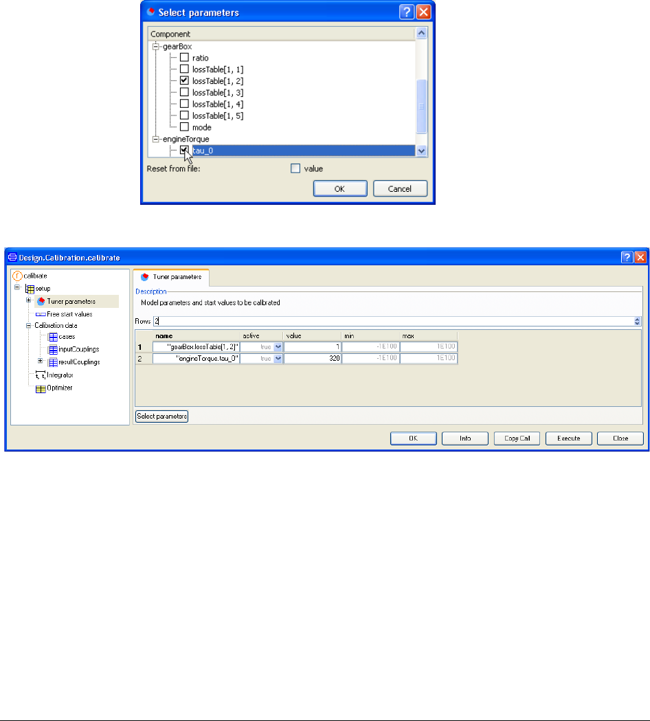
2 MODEL CALIBRATION 55
gearBox.lossTable[1, 2]
and
engineTorque.tau_0
Click OK. The result will be
Please do not close any window, continue to the next section.
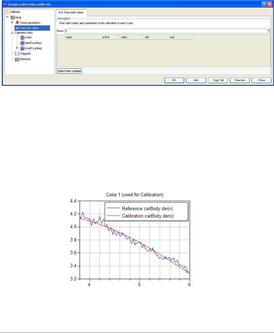
2.2.6 Free start values
The start value of a state may be unknown. By including the state as a tuner, the start value
is estimated automatically. However, in case we have several measurement series, it may be
necessary to tune or estimate these initial values individually for each calibration case.
Dymola supports individual tuning of parameters and start values of states and they are
specified as freeStartValues. Clicking on Free start values in the browser of the window
will give:
Selecting parameters
to tune.
56
Such parameters or states are selected by clicking Select free variables button which pops
a variable selector as when selecting case parameters or tuners. The variable selector
includes parameters and states. These values are also tuned for cases having Task = Validate.
2.2.7 Tune the parameters
It is time to do the first calibration. Click Execute. During the calibration, results are plotted.
After 25 fast iterations, we obtain the result.
gearBox.lossTable[1, 2]
0.794
engineTorque.tau_0.
260.7
criterion
0.218
The tuning result.
Comparing measured
and simulated
acceleration after
tuning.
2 MODEL CALIBRATION 57
A passenger car has normally an efficiency of 0.90 at high gears in normal operation. The
measurements are made at full throttle to give maximum acceleration. It means for example
that the tires are slipping say 4%, which of course is increasing the losses.
It is very easy to add new tuners. Just select Tuner parameters, click Select parameters
and select new parameters. By changing active from true to false or vise versa it is easy to
experiment with different set of tuners. Having a parameter as an inactive turner is a good
way to set a parameter to have a value different from the value given by the model.
2.2.8 Validation using measurements from first
gear
The result of the above section “Calibration” and this section is also available using the
command Commands > Calibration with validation.
It is recommended to validate against other measuremnts. Unfortunately, we do not have
another measurement series in this case, but for validation we can use the data from the time
interval where first gear is used.
We do this by specifying another case. Click on cases.
Put the cursor in the input field for Rows and press the arrow up key on the keyboard once
to increase the value by one. You may also use the arrow up of Rows to increase Rows to 2.
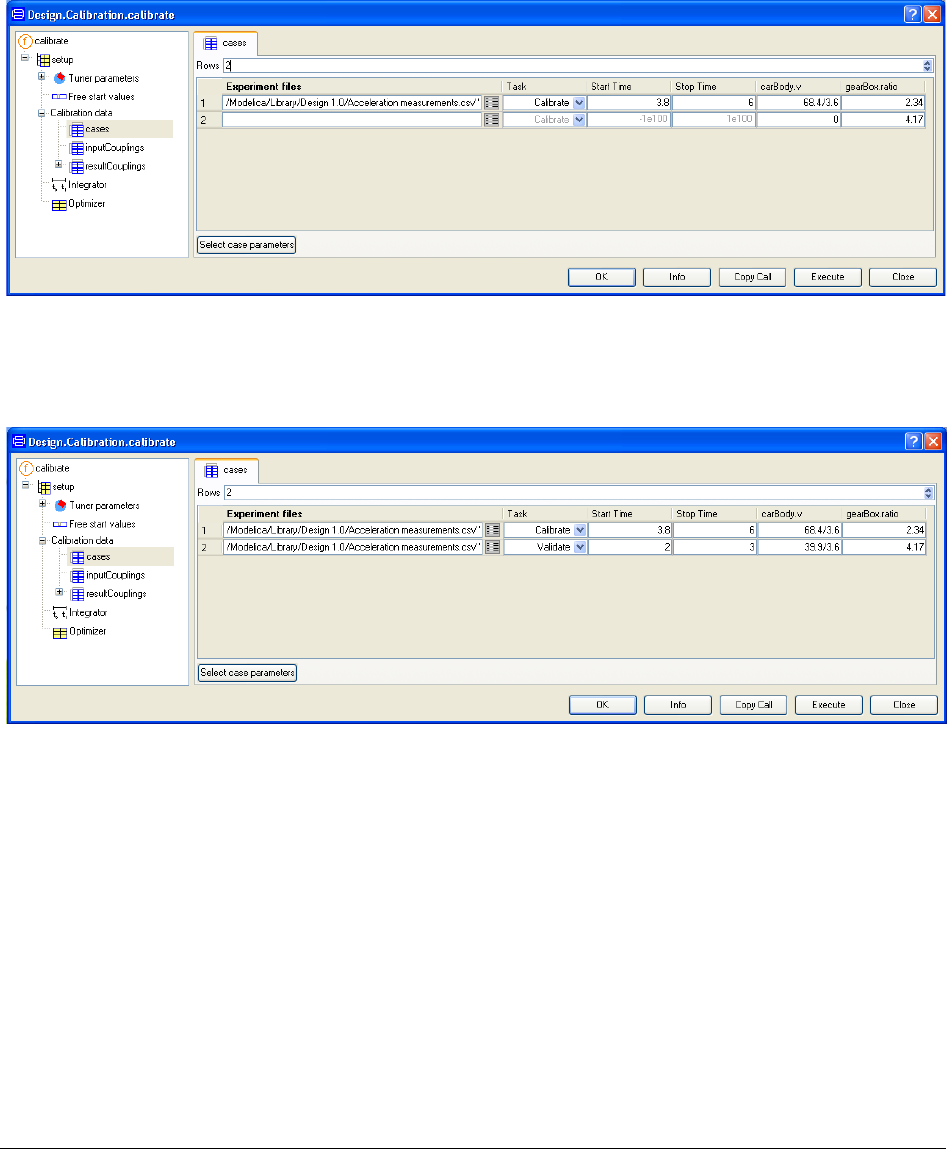
58
As previosly, use the Edit button of Experiment files to select experiment file. You can also
copy and paste the file name (using Ctrl + C and Ctrl + V). Enter the values for start time
(2.0), stop time (3.0), carBody.v (39.9/3.6) and gearBox.ratio (4.17) as illustrated below. Do
not forget to set Task to Validate.
Click Execute. The calibration starts and gives the same results as previously, but also the
plot below for the validation case (the criterion is 13.88).

2 MODEL CALIBRATION 59
The agreement for the interval 2.0-2.7 s is very good. If we rerun the validation having set
the stop time of the second case to 2.7, the criterion is 0.44. As indicated above the tires are
slipping when the car is run to accelarate as fast as possible. If the wheels slip too much, the
anti spin control system gets active and the result is reduced acceleration after 2.7 seconds
as shown by the measured data.
As illustrated, Dymola supports a flexible and incremental way of working. We need not
define this total setup in one step. First we made the model and validated the nominal model
against the measured data, then selected turners and calibrated. Finally we validated the
calibrated model. Dymola also provides support for sentivity analysis (see below).
2.2.9 The setup as Modelica code
The calibration setup is represented in Modelica in the following way. It is a function call,
where nested record constructors build the needed input arguments.
Design.Calibration.calibrate(Design.Internal.Records.ModelCalibrationSetup(
Model="Design.Calibration.Examples.SimpleCar",
tunerParameters={
Design.Internal.Records.TunerParameter(name= "gearBox.lossTable[1, 2]", Value=1),
Design.Internal.Records.TunerParameter(name="engineTorque.tau_0", Value=320)},
calibrationData=Design.Calibration.Internal.Dynamic_common(
Design.Internal.Records.DynamicCommonCalibrationCases(
experimentNames={"Acceleration measurements.csv",
"Acceleration measurements.csv"},
task={1,2},
startTime={3.8,2},
stopTime={6.0,3},
parameterNames={"carBody.v","gearBox.i"},
parameterValues=[68.4/3.6,2.34; 39.9/3.6,4.17]),
resultCouplings={Design.Internal.Records.DynamicCalibrationResultCoupling(
variable="carBody.der(v)", data="acc")}),
integrator=Design.Internal.Records.CalibrationIntegrator(stopTime=6.2),
optimizer=Design.Internal.Records.Optimizer()))
Comparing
measurement and
simulated acceleration
to validate mode.
60
2.3 Saving the setup for reuse
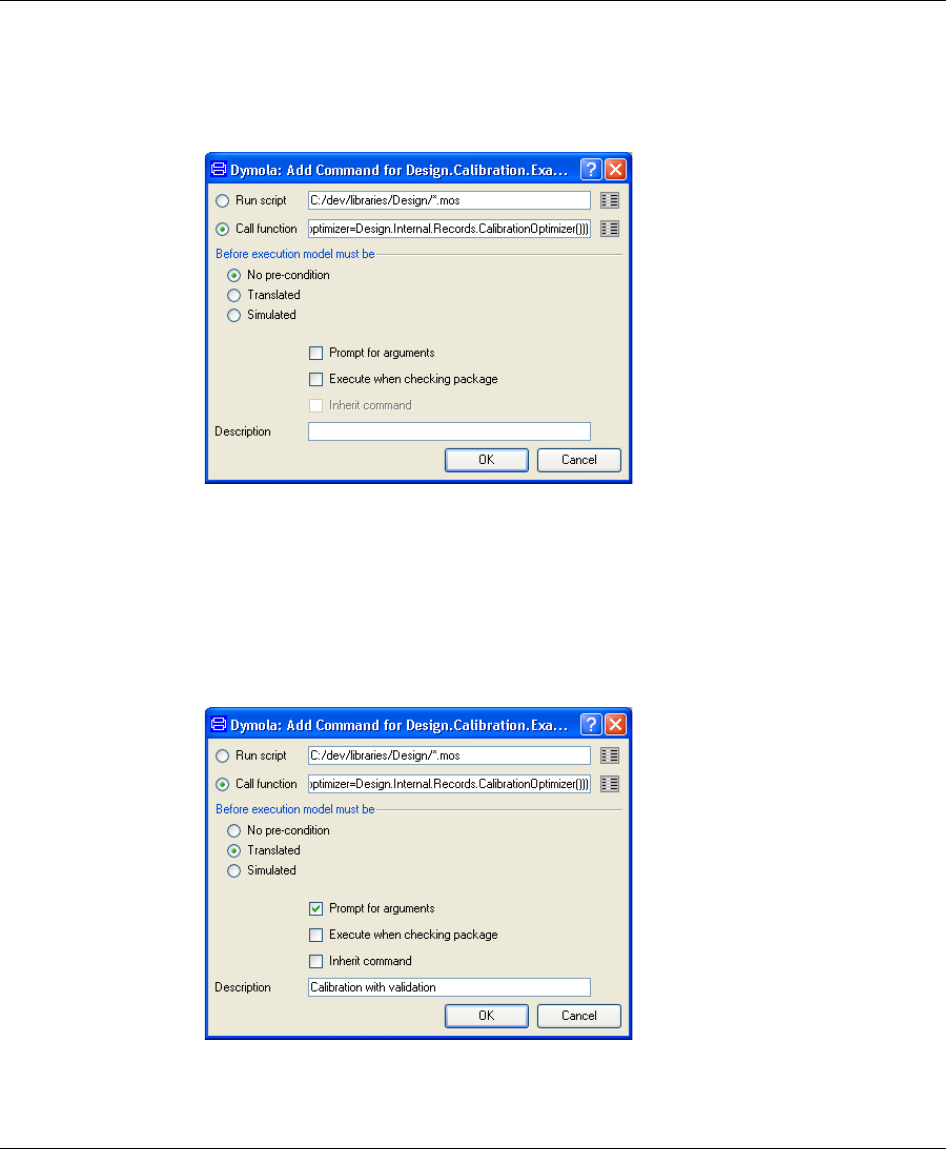
After an execution of a command we can save it in the model for later reuse. Select
Commands > Add command. A menu pops up:
Tick Prompt for arguments and enter a description, which will be used in the commands
menu. Since the model needs to be translated in order to get the select browsers we tick that
model shall be Translated. This is not critical, only a matter of convenience. If we do not
tick Translated, then when a browser needs to be popped, Dymola will give a prompt
pointing out that the model needs to be translated. If we just select the command and then
click Execute there will be no prompt, but function is executed as expected. The model is
translated when needed. The Edit button next to the function call allows you browse or edit
the function call once more.
Note: This cannot be
done for SimpleCar,
because it is read-only.
Saving the calibration
setup.
2 MODEL CALIBRATION 61
Click OK. (More about this menu can be read in “Dymola User Manual Volume 1”, chapter
“Developing a model”, section “Editor command reference – Modeling mode”, sub-section
“Main window: Commands menu”.)
A function call menu as for calibrate has an Execute button. Clicking this button start an
execution of the function and the menu stays popped. If we click Close, the menu is closed
without any execution. If we click OK, the function is executed and the menu is closed. You
click OK by mistake when you meant Execute, you can fix the situation. Click in the
command input line. Press the arrow up once to scroll back in the commands given. Click
right mouse button and select Edit Function Call and the function call menu pops. This can
be done for any function call in the command log.
2.4 Reusing a setup for a similar operation
A setup can be reused for a similar operation. Assume that we just have made a calibration.
The menu is then (if clicking on setup in the browser).
Select calibrate (at the top in the tree browser) and right-click to get the context menu.
The menu offers a selection of analysis and plotting functions that can exploit the
calibration setup. We will describe these functions further below.
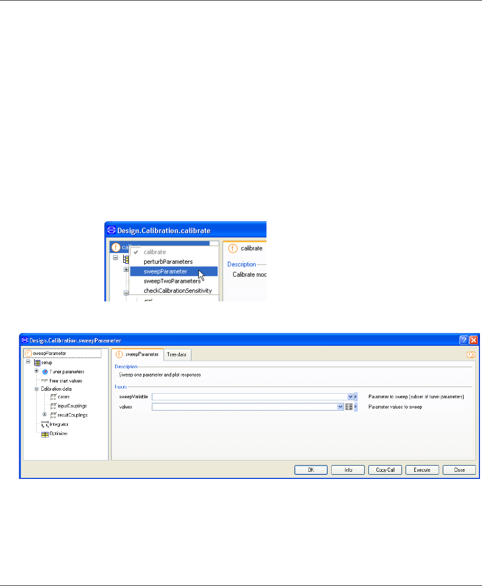
62
2.5 Analysing parameter sensitivities and
dependencies
Dymola provides a set of functions to analyze parameter sensitivities and dependencies.
Below the functions perturbParameters, sweepParameter, sweepTwoParameters and
checkCalibrationSensitivity will be described.
2.5.1 Sweep one parameter – sweepParameter
The function sweepParameter sweeps a tuner and plots the responses.
As an example open the model (if not already open) Design.Calibration.Examples.
SimpleCar by using the command File > Libraries > Design and then using the package
browser to open Examples.SimpleCar
Now select the command Commands > Calibration with validation. When the calibrate
window has opened, select calibrate (at the top in the tree browser in that window), right-
click and select sweepParameter.
The sweepParameter menu changes since additional parameters needs to be provided.
Select gearBox.lossTable[1,2] in the combobox of sweepVariable and select Equidistant
grid for values. When doing the last selection, a new menu pops up:
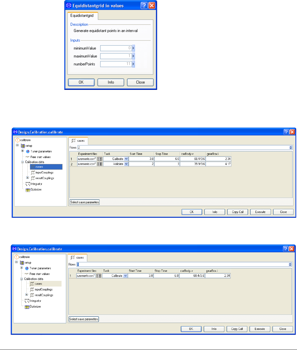
2 MODEL CALIBRATION 63
Enter minimum and maximum values and number of points (0.5 for the minimum value and
6 for the number of points is used for the plot below) and click OK.
Click on cases in the browser. It will show that we sweeps two cases.
The Validate case is not interesting now, so decrease the number of rows to 1. The result
will be:
Selecting grid for
parameter sweep.
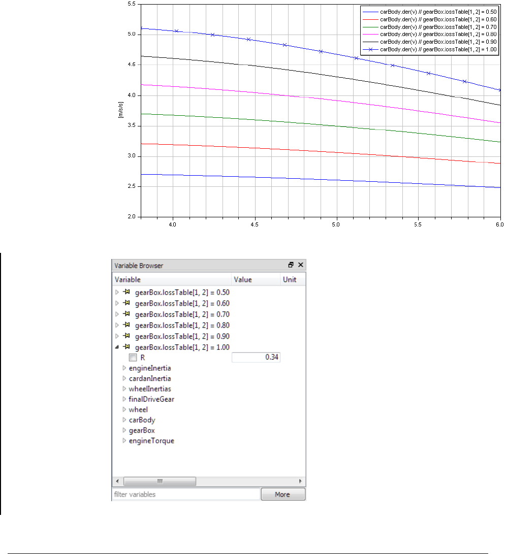
64
Click Execute. The result is plots of the result variables, which in this case is the
acceleration. As expected, higher efficiency gives higher acceleration.
All results of the simulations are available for access in the variable browser.
Simulated acceleration
when sweeping
gearbox loss (x-axis is
time, y-axis is
acceleation).
The results from the
parameter is available
in the variable browser.
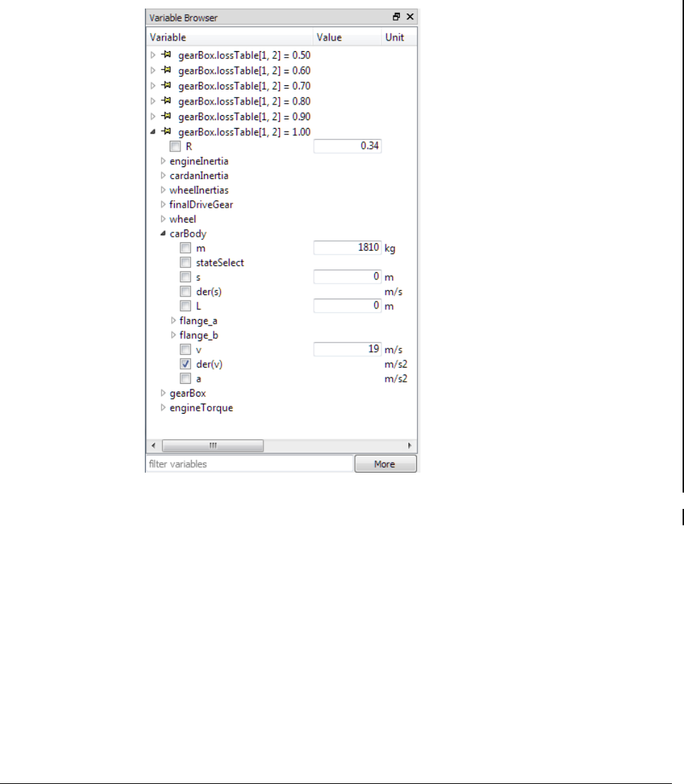
2 MODEL CALIBRATION 65
To look what signal is plotted, carBody can be expanded by clicking on the + before it. The
result in the variable browser will be:
All Dymola’s plotting facilities can be used to produce other plots from the sweep. It is e.g.
easy to get a similar plot with the velocity of the car. Click on More and tick Compare
results. Then select carBody.v – and deselect carBody.der(v) to not get too many curves.
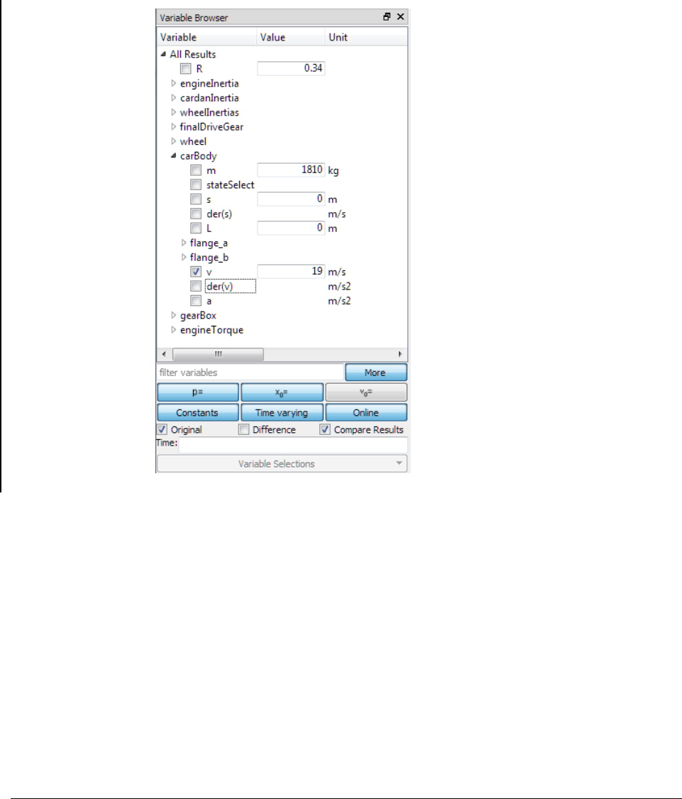
66
and the plot becomes (after having moved the legend square to the bottom left, see later):
Setting plot to
compare results.
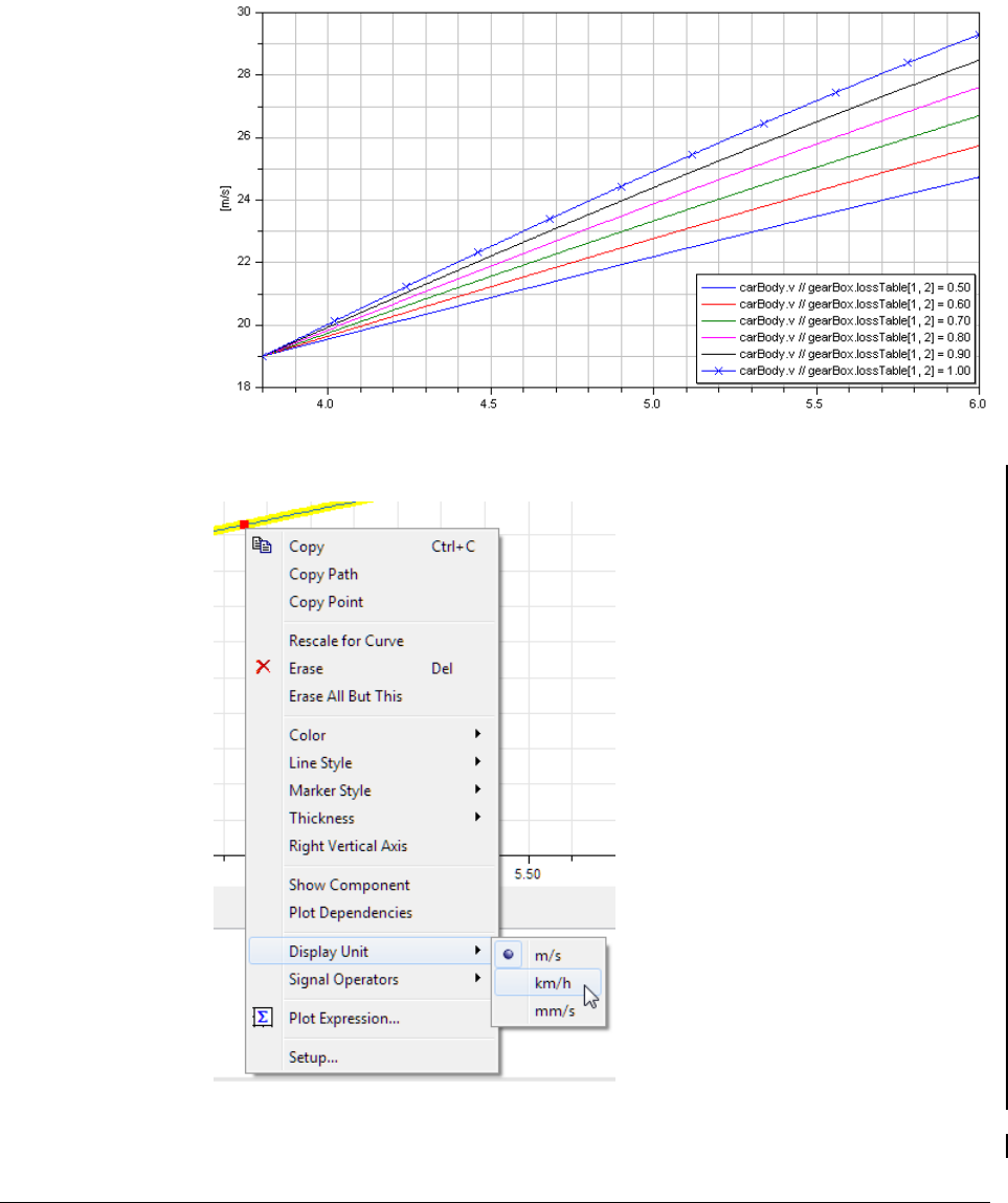
2 MODEL CALIBRATION 67
The velocites are in m/s, but it is easy to get them in km/h. The easiest way is to right-click
on a curve and use the context menu command Display Unit to select km/h.
Another way is to use Setup… in the above context menu (or using Plot > Setup…) and use
the Display unit drop-down menu in the Variables tab.
Plotting the velocites
from the sweep.
Using context menu to
select display unit.

68
Whatever method used, the plot becomes now
Changing display result.
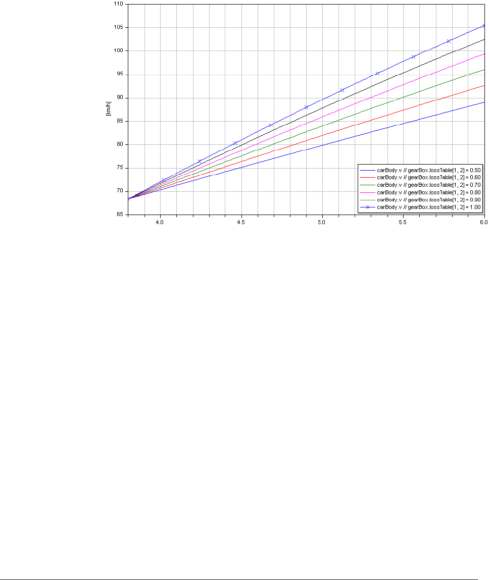
2 MODEL CALIBRATION 69
The plot window has a lot of other possibilities, e.g. zooming, displaying values etc., please
see Dymola User Manual Volume 1, chapter “Simulating a model”, section “Model
simulation”, sub-section “Plot window interaction”. (The Setup menu above can be used for
many things as well, e.g. to change the placement of the curve legend using the Legend
tab.)
In the beginning of this example we de-selected one of the two cases available in the demo,
the validation case. If both cases have been selected, two plots would have been the result,
and the corresponding signals should also have been visible in the variable browser.
2.5.2 Sweep two parameters –
sweepTwoParameters
The function sweepTwoParameters sweeps two tuners and produces a 3D plot of the
criterion.
As an example open the model (if not already open) Design.Calibration.Examples.
SimpleCar by using the command File > Libraries > Design and then using the package
browser to open Examples.SimpleCar
Now select the command Commands > Calibration with validation. When the
sweepParameter window has opened, select calibrate (at the top in the tree browser in that
window), right-click and select sweepTwoParameters.
Plotting velocities in
[km/h]. The x-axis is
time.
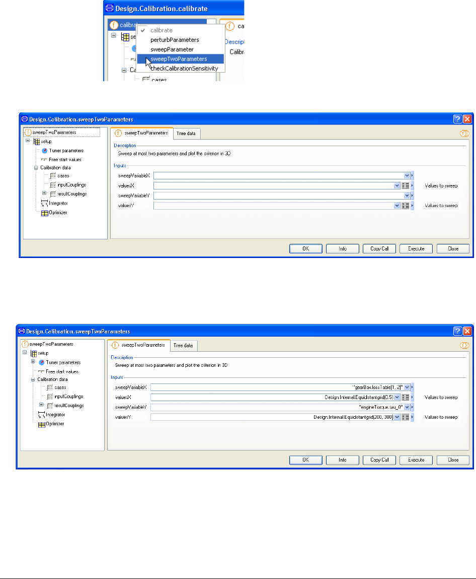
70
The menu changes
Since we have just two tuners, we select the efficieny as sweepVariableX and 11 values in
the interval 0.5-1. We select tau_0 as sweepVariableY and 11 values in the interval 200-300.
The result of this will be (for a more detailed description on how to select start values etc
please see previous section if needed).
Click Execute and Dymola produces the plot below:
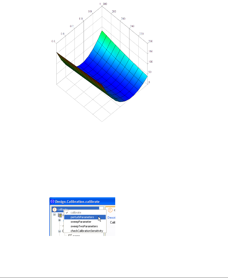
2 MODEL CALIBRATION 71
2.5.3 Response to parameter perturbations -
perturbParameters
The function perturbParameters plots the responses to perturbations in the tuners.
As an example open the model (if not already open) Design.Calibration.Examples.
SimpleCar by using the command File > Libraries > Design and then using the package
browser to open Examples.SimpleCar
Now select the command Commands > Calibration with validation. When the
sweepParameter window has opened, select calibrate (at the top in the tree browser in that
window), right-click and select perturbParameters.
The menu changes. The function exploits the setup of calibration, but needs some additional
input, perturbationParameters, which by default are the same as the tuner parameters of
setup. When executing the function it perturbs the parameters in turn. The default
pertubation is 10%. Note that the efficiency has a nominal value of 1 meaning a default
The criterion for
different values of the
tuners.
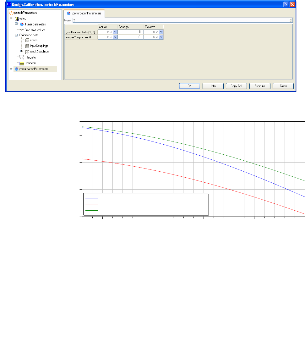
72
perturbation to 1.1, which is not a physical value. Thus, we change it to –10% to get an
efficiency of 0.9. The menu after the change look like:
Click on Execute. The results are plots of the result variables as shown below (the legends
have been moved also).
Both tuners influence the acceleration. The responses for the validation case are also plotted
(the legends have also been moved)
4.0 4.5 5.0 5.5 6.0
3.8
4.0
4.2
4.4
4.6
4.8
5.0
5.2
[m/s/s]
carBody.der(v) // Reference1
carBody.der(v) // gearBox.lossTable[1, 2] = 1.00-0.10
carBody.der(v) // engineTorque.tau_0 = 320.00+32.00
The acceleration when
perturbating the
tuners.

2 MODEL CALIBRATION 73
2.5.4 Check if tuners can be calibrated –
checkCalibrationSensitivity
When tuning parameters from measurements, a basic question is “Which parameters can be
estimated from the measurements available?” Changing a parameter to be estimated must of
course influence the output. However, this is not enough. Two or several parameters may
influence the result in a similar way such that it is not possible to estimate them individually.
Assume that our nominal model is the correct model and we had used it to produce a
“measurement” file. If we make small perturbations of the values of some parameters and
use the “measurement” file for calibration, we would like the result of the calibration
procedure to be that the perturbed parameters are tuned to their original values. The function
checkCalibrationSensitivity checks if this is the case. If not, it lists tuners that do not
influence the criterion and linear combinations of parameters where changes of the
appearing parameters do not influence the criterion, if the linear expression remains constant.
As an example open the model (if not already open) Design.Calibration.Examples.
SimpleCar by using the command File > Libraries > Design and then using the package
browser to open Examples.SimpleCar
2.0 2.5 3.0
5.2
5.6
6.0
6.4
6.8
7.2
7.6
[m/s/s]
carBody.der(v) // Reference2
carBody.der(v) // gearBox.lossTable[1, 2] = 1.00-0.10
carBody.der(v) // engineTorque.tau_0 = 320.00+32.00
The acceleration for
the validation case
when perturbing the
tuners.
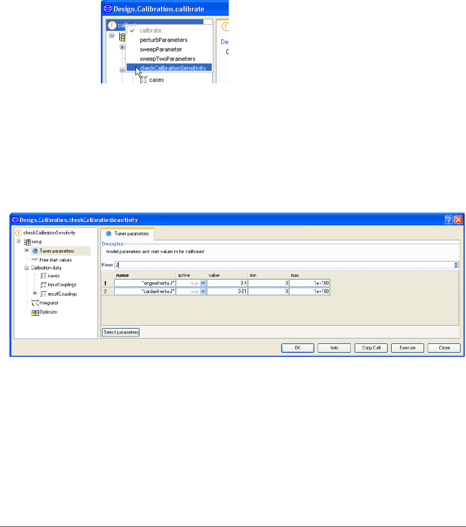
74
Now select the command Commands > Calibration with validation. When the
sweepParameter window has opened, select calibrate (at the top in the tree browser in that
window), right-click and select checkCalibrationSensitivity.
The menu changes. Click Execute. Dymola outputs a positive message in the Command
window:
The calibration criteria are sensitive for small variations
around the nominal values in all tuner parameters and in all
their linear combinations.
Let us try some other tuners. Can we tune the engine and cardan inertia? Click on Tuner
parameters in the browser in the checkCalibration window. Select them as tuners by
remowing the present tuners by setting the Rows to 0, then use Select parameters to select
the new tuners. The result in the menu will be:
Click Execute. Dymola outputs the message
The calibration criteria are insensitive for small variations
around the nominal values in the following linear parameter
combinations:
-engineInertia.J-0.1826*cardanInertia.J
The message says that if we change the two values, but keep
-engineInertia.J-0.1826*cardanInertia.J
The result of checking
calibration sensitvity.
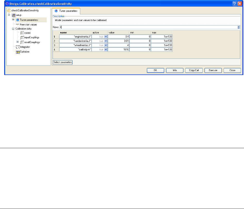
2 MODEL CALIBRATION 75
constant, then the criterion does not change. In other words we cannot tune the inertias
individually, but we can tune the combination given. The engine and the cardan are rigidly
coupled. It means that the inertia for those to bodies sensed from the engine is
2
/iJJ
ce
+
where Je is the inertia of the engine and Jc is the inertia of the cardan and is i is the gear ratio.
Using i = 2.34, we get
cece
JJiJJ 1826.0/
2
+=+
This is consistent with what Dymola told us. In fact the engine, cardan, wheels and the car
body are rigidly connected. It means that we can only estimate a total inertia for example
reduced to the engine side or a mass equivalent reduced to car body. Let us specify the
inertias and the car mass as tuners.
Clicking Execute gives the expected answer
The calibration criteria are insensitive for small variations
around the nominal values in the following linear parameter
combinations:
-engineInertia.J-0.0018*carBody.m-0.1826*cardanInertia.J-
0.0153*wheelInertias.J
If we multiply by –1, this is the total inertia reduced to the engine side.
2.6 Data Preprocessing
The quality of the calibration process is directly related to the quality of the measured data
used as input to the calibration tool. Any factor that perturbs the data will cause directly
distortion of the final result of the calibration tool. It is important then to preprocess the data,
that is, to adjust the data eliminating noise, zones where the model is not valid and
erroneous or not representative measurements.
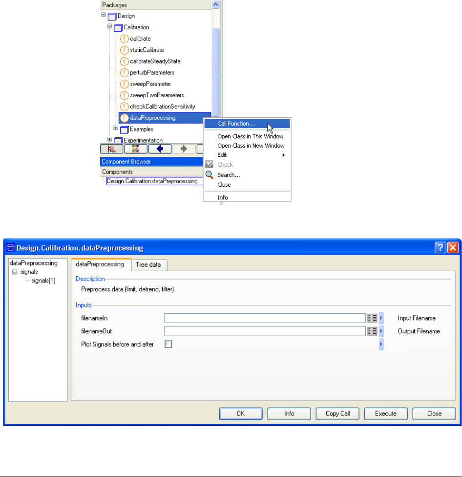
76
The Design.Calibration package incorporates the function dataPreprocessing with this
objective: preprocess data for calibration.
2.6.1 Setting up for preprocessing
Select dataPreprocessing in the package browser under Design.Calibration. Right-
click and select the command Call function…
The dialog of dataPreprocessing pops. We select now the file we want to process and the
file that will contain the output.
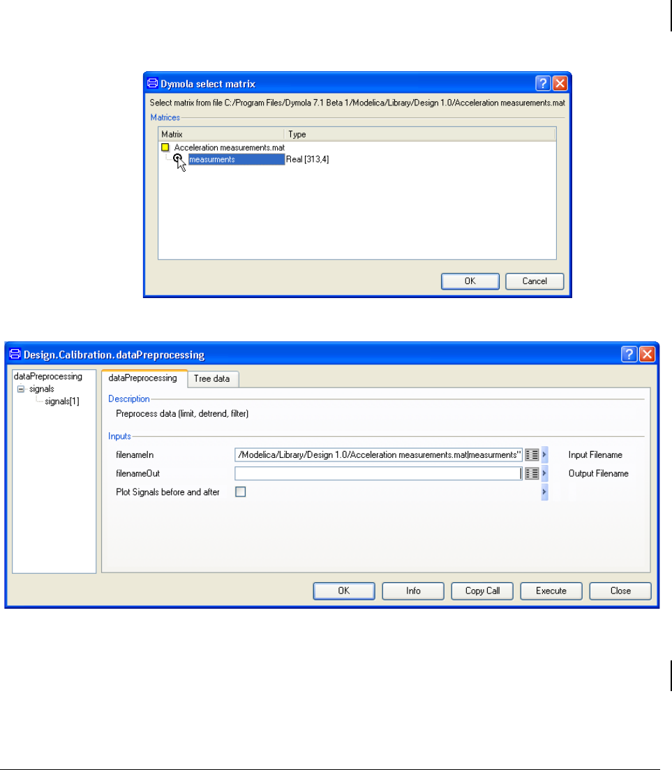
2 MODEL CALIBRATION 77
To introduce an experiment file, click on the Edit icon in the Input Filename. A file
browser pops up. Use it to select the file
…/Design 1.0.6/Acceleration measurements.mat.
A menu for selection of appropriate matrix will pop up. In this case there is only one
selection possible:
After clicking OK the window will look like:
The same procedure has to be repeated to select an output file. In this case, the file does not
exist. We choose as name for this example
…/Design 1.0.6/Acceleration measurementsfiltered.mat.
and check the field Plot Signals before and after to obtain a plot of the original signal and
the result of the preprocessing.

78
It is possible to overwrite the original file; there is no restriction for that. This means that the
original data is gone, and no possibility of recovery is possible. A good practice is always to
change the name slightly, since we might want to adjust later on the preprocessing
parameters.
We select now a signal from the file. Since the input filename is a .mat file, we don’t have
access to the name of the variables, but we know the position of the acceleration signal, that
is, number four in the matrix. Choose 4 from the combo box in Signal Name.
The dataPreprocessing tool assumes for .mat files that time is in the first column always.
This is a cornerstone of the function, since all functionalities are relying on time. This is
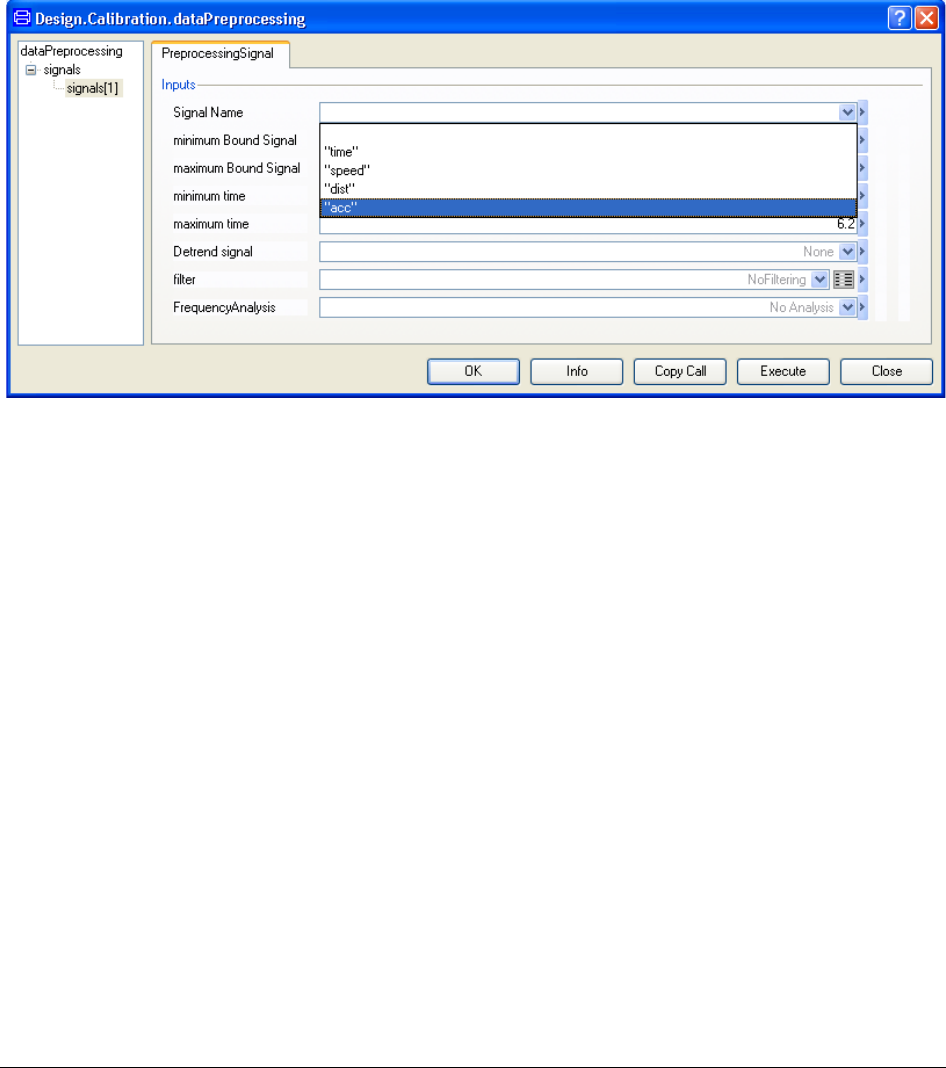
2 MODEL CALIBRATION 79
very important. If we instead choose to process a .csv file, we get the names in the combo
box. We can simply then select “acc”. And dataPreprocessing will seek the keyword “time”
and “Time”.
We are ready now to run the preprocessor function. We start limiting and detrending
functions.
2.6.2 Limiting and detrending signals
Limiting and detrending the signals is also very important. To limit a signal in time and
amplitude it is enough to write the desired values in the fields minimum Bound Signal and
maximum Bound of Signal for the amplitude and minimum time and maximum time for
time axis. The data outside of these limits is taken away and interpolated or extrapolated
linearly.
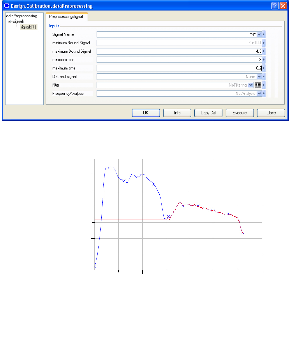
80
Just to demonstrate this feature, take as limits the interval [-1e100,4.3] for the amplitude and
[3,6.2] for time. Press Execute and the result is presented.
All values outside of the range have been substituted by linear interpolation. Now, we
choose Line(y=a*x+b) in the combo box Detrend signal. This will fit in least squares sense
a straight line and subtract it form the data.
0 2 4 6
0
2
4
6
4
Time
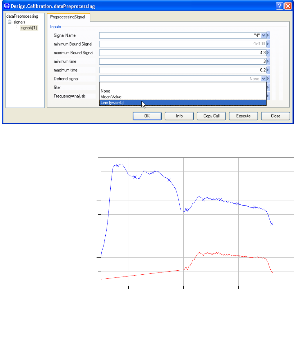
2 MODEL CALIBRATION 81
Press Execute and the result follows.
We observe the resulting curve. The other possibility for detrending is Mean Value, which
subtracts the mean value of the function. Reset the values of the limits and set detrending to
None. We are now into frequency analysis and filtering of signals.
0 2 4 6
-2
0
2
4
6
4
Time
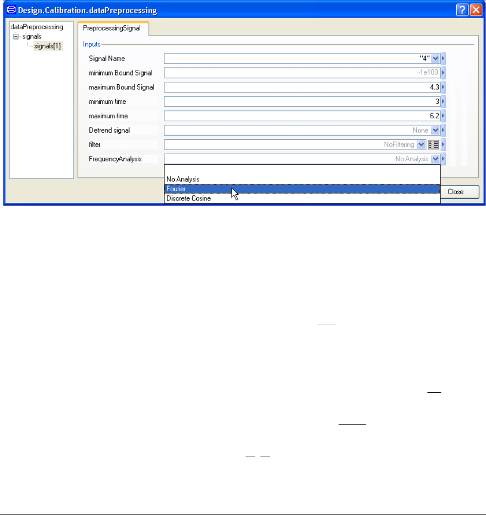
82
2.6.3 Analyzing Signals: is there any noise?
Let us analyze the function in the frequency domain. The point now is to filter out noise.
Such a noisy perturbation is normally easy to get in the measured data and complicates later
on the calibration process unnecessary. Select Fourier from the combo box of
FrequencyAnalysis.
We are about to perform the discrete Fourier transform (DFT) of the acceleration signal.
The DFT is defined as follows. Assume we have N samples of a function
()
nn
x xt=
at
ns
t nT=
, where
s
T
is the sampling time. The DFT is a set of complex numbers
k
c
such that
( )
1
exp i
N
n k ks
k
x c nT
ω
=
=∑
for all sampling
n
x
points and frequencies
2
k
s
k
NT
π
ω
=
, and
i
the imaginary unit. The
coefficients
k
c
can be calculated explicitly by matrix-vector multiplication or by more
effective algorithms in case of large amounts of data.
The frequencies are discrete equidistant points distributed in the interval
2
0,
s
T
π
. Since
the complex exponential function
( )
i2
exp i exp
ks
kn
nT N
π
ω
=
is periodic, we choose a
representation in the interval
,
ss
TT
ππ
−
, to have the highest frequencies farther at the
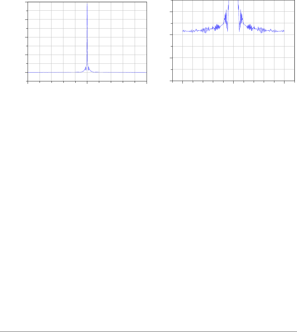
2 MODEL CALIBRATION 83
boundary, instead of in the middle of the graph. Now, we press Execute and obtain the
graph at the left side. The right side graph is a zooming.
Since the coefficients are complex numbers, we present their modulus. In the log of the
command window we observe also the following report
Processing signal 4
Signal 4 has the 99.5341% of its power under 2.21519 Hz
This is an important piece of information. The tool detected that the energy of the signal is
almost condensed in the interval
[ ]
2.2159,2.2159−
. In the graphs before (right) we observe
the behavior of the coefficients, and it is less smooth and more erratic outside of the interval
reported by the tool.
We can therefore suspect that additive noise is present in this range of frequencies. We can
now design a filter and get rid of these noisy oscillations.
-25 025
0
20
40
60
80
Frequency Analysis
Fourier Transform
4 (Amplitude)
Frequency (Hz)
-25 025
-0.8
-0.4
0.0
0.4
Frequency Analysis
Fourier Transform
4 (Amplitude)
Frequency (Hz)
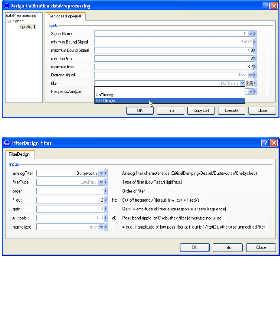
84
2.6.4 Filtering signals
Back to the GUI, click on filter combo box and choose FilterDesign.
The GUI for filter Design from the LinearSystems library pops up now.
We choose a Butterworth filter in analogFilter and as cut frequency we choose 2 Hz. It is
enough to choose 2 Hz and not exactly 2.2159 since the filter is not ideal and we will
smooth out the spectrum of the signal around those frequencies too. The type of the filter
has to be low pass since the signal is clustered around zero frequency. Press OK. Then
Execute in the main GUI. The resultant spectra are presented.

2 MODEL CALIBRATION 85
We observe how high oscillatory modes are smoothed out. This means that the signal in
time is also smoother. The result is presented in the next picture.
The filtered signal (red) has less noise than the original one (blue). This makes the
calibration process easier. The filters are constructed using the Linear Systems library
(opening “Types” and then “AnalogFilter”). These are discretised versions of continuous
systems, with a discretisation in such a way that the ramp response is exact. The possible
filters are four: Critically damped, Bessel, Butterworth and Chebyshev.
-25 025
0
20
40
60
80
Frequency Analysis
Fourier Transform
4 (Amplitude)
Frequency (Hz)
-25 025
-0.4
0.0
0.4
0.8
Frequency Analysis
Fourier Transform
4 (Amplitude)
Frequency (Hz)
0 2 4 6
0
2
4
6
4
Time

86
2.7 Static calibration
Two cases of static calibration exist.
A typical purpose of a static calibration is to tune static characteristics of components such
pipes, valve, throttles, pumps, nonlinear resistors, frictions etc. Such models are completely
static (always in steady-state). The function staticCalibration should be used in this case.
The other purpose of static calibration is to handle models in steady-state, either by giving
steady-state initial conditions or by specifying a suitable stop time (where the user is
assumed to guarantee that the solution has reached steady-state). The function
calibrateSteadyState should be used in this case.
Dymola’s GUI supports setting up such calibrations without building a corresponding test
rig model. The GUI allows simple redefinition of a variable to be an input. The measured
data for such an input and of course also for an original input can then be specified to have a
common value for all cases or to have a case dependent value read from a file.
Assume that we want to find a static relation from the variable v to w of the model and that
we have measurements for v and w and all inputs of the model. First we need to decide a
parameterized shape or in other words we need to come up with a function w = f(p, v) where
p is a parameter vector. In many cases we can use polynomials. In general it is nontrivial to
come up with a good function that fits the data well. However, in this case it is possible to
use the model and the measured data to back calculate w for each case. Dymola supports the
setup of such a calculation is in a straightforward way very similar to the setup of the
transient calibration. Having w makes the relation much more explicit and easier to
visualize and inspect. Just by plotting w against v, we can get a good estimate of the chances
to get a good result. If the plot shows that the points seem to be lying on a line, the chance is
much better than when the plot looks like a random scatter. Such a plot may also give us
good insight in what kind of functional relation we should use. Classic pen and paper
approaches as plotting in lin-log or log-log diagrams can be used to find out if exponential
or potential relations could be useful.
This document uses calibration of a resistor model to illustrate how a static calibration task
is setup. More advanced uses are described in H.Olsson, J. Eborn, S.E. Mattsson and
H.Elmqvist: Calibration of Static of Static Models using Dymola. Proceedings of the 5th
International Modelica Conference, Vienna, Austria, 2006, vol 2, pp. 615-620 (available for
download from www.Modelica.org).
2.7.1 The staticCalibrate function
The staticCalibrate function should be used for completely state-less (static) models. For
steady-state models, please see the function calibrateSteadyState.
To load Design.Calibration, select File > Libraries and click Design.
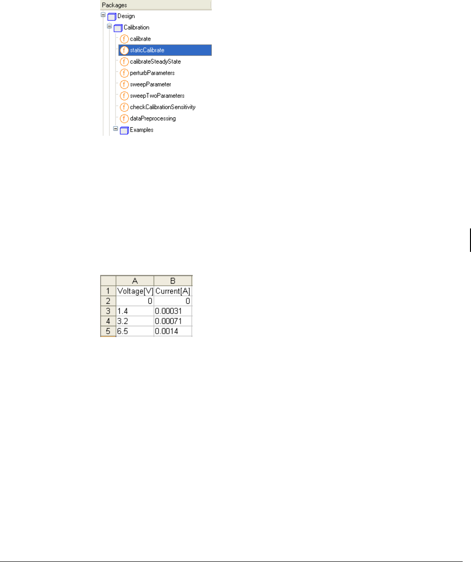
2 MODEL CALIBRATION 87
Example
(The first example below corresponds to the command Commands > Resistor example 1
in the package Design.Calibration.Examples.Resistor. However, you have to select
Calibration data in the browser in the pane to the left in the window that pops and browse
yourself for the Resistor measurements.csv file; see just below for the path.)
Assume that we have measurements of the voltage across and the current through a resistor.
The file Program Files (x86)\Dymola 2018\Modelica\Library\Design
1.0.6\Resistor measurements.csv contains the measurement data.
The first row of the file includes the column headings and then the data follow.
We now want to estimate the resistance. Thus we need a resistor model. There is one in the
Modelica Standard Library: Modelica.Electrical.Analog.Basic.Resistor
Since it is a model from the Modelica Standard Library, it is a read-only model. To allow us
to store the calibration setup in connection with the model, we make a copy of it. It can be
done in the following way: Select the resistor model of the Modelica Standard Library in the
package browser. Right-click and select New > Duplicate Class…. Let us call the model
Resistor as proposed by the menu. Click OK.
The staticCalibrate
function.
Data for a session.
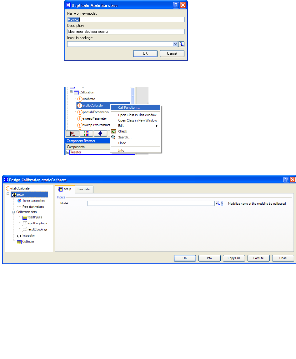
88
We now have a resistor model. To set up the calibration, select staticCalibrate in the
package browser. Right-click and select Call Function….
A menu pops up.
To specify the model to be calibrated, click on the Edit icon to the right of the Model input
field. A package browser pops up. Use it to select the model.
Making a resistor
model for calibration.
Start the setup.
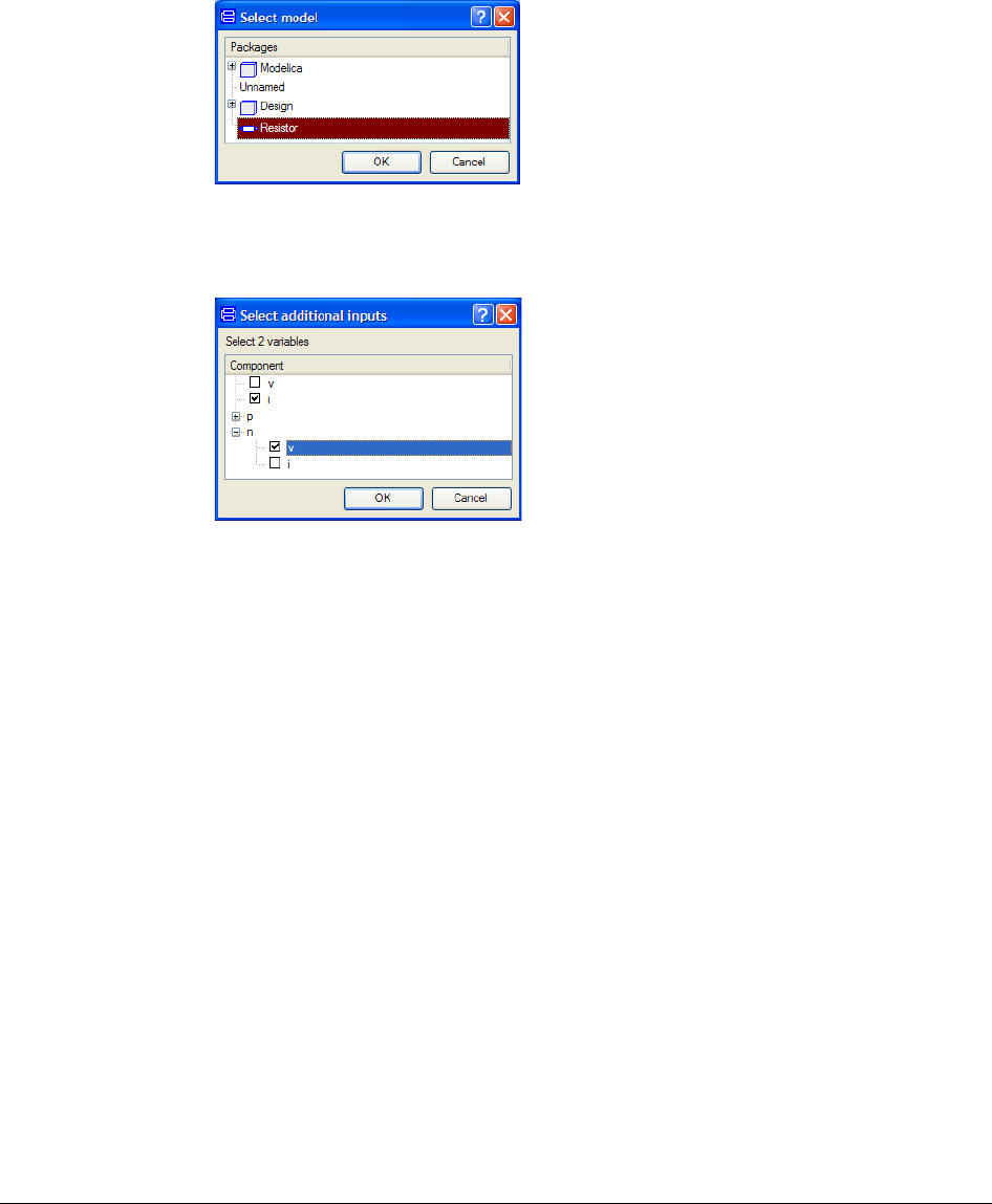
2 MODEL CALIBRATION 89
Click OK. The model is now translated in order to gather information to support the further
setup of the calibration task. Dymola finds that the resistor model is incomplete (the model
has two more variables than equations) and pops a variable browser.
The resistor model cannot be simulated as it is. We need to provide sources driving the
component. In real life we need a test bench or a rig. We could have built such a rig model
in Dymola using the GUI for model building. We then would have to define a new model,
drag in the resistor component and source components and connect them. The availability of
appropriate source elements with compatible connectors may be a problem. In this case we
could have constructed a test-circuit with a current source driving the resistor being
grounded at the n-pin and measuring the resulting voltage across the resistor. The static
calibration feature of Dymola provides a powerful solution to this problem. The translate
procedure determines which variables that are not uniquely defined and displays them in a
browser and asks us to turn 2 variables of them to inputs in order to make the problem well-
posed. In this simple way it is specified which variables that are to be driven from external
source. In this case we tick the current, i, through the resistor and the voltage n.v to be given.
When clicking OK, the model is translated assuming the specified variables to be inputs in
addition to other possible inputs of the model component. This rigging is found to be OK.
(There will be a warning that a parameter does not have a value, but this is not important
here.)
The next task is to specify how the measurements are stored. Click on Calibration data in
the tree browser to the left.
Selecting the model to
calibrate.
Add inputs to the
model.
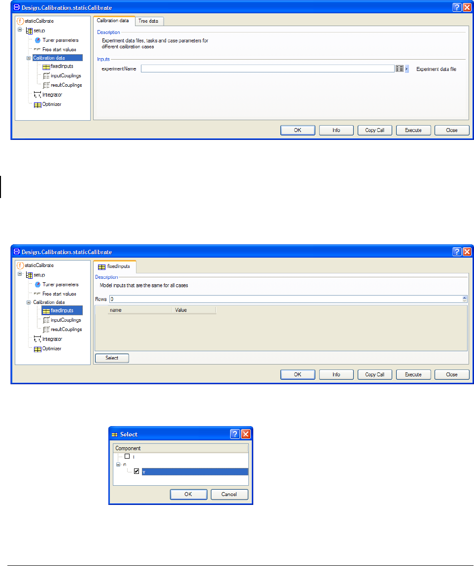
90
For static calibration it is assumed that all measurements are stored in one file. Click on the
Edit icon of experimentName. A file browser pops up. Use it to select the file
Program Files (x86)\Dymola 2018\Modelica\Library\Design
1.0.6\Resistor measurements.csv.
Fixed Inputs
We now need to specify those inputs that have the same value for all cases.
Click on fixedInputs in the tree browser. For the resistor calibration we have the grounding
of the n-pin to specify. Click on Select and a browser including all inputs are popped.
Tick n.v. Click OK. (Since the value should be 0, no input of value is needed here.)
Specify grounding.
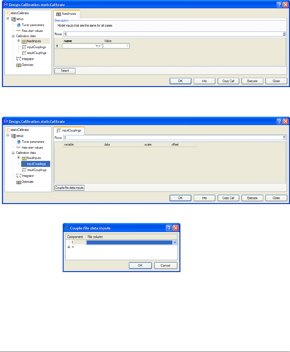
2 MODEL CALIBRATION 91
Input Couplings
To couple case dependent sources to the inputs, click on inputCouplings in the tree browser.
Click Couple file data inputs and a browser including all inputs is popped.
The right column allows us to specify where to find the source of the inputs in the
measurement file. Here we should specify the input to i. Click on i or in the right column. A
selector appears in the right column. Select “Current [A]” as it is called in the csv file.
Menu to couple inputs.
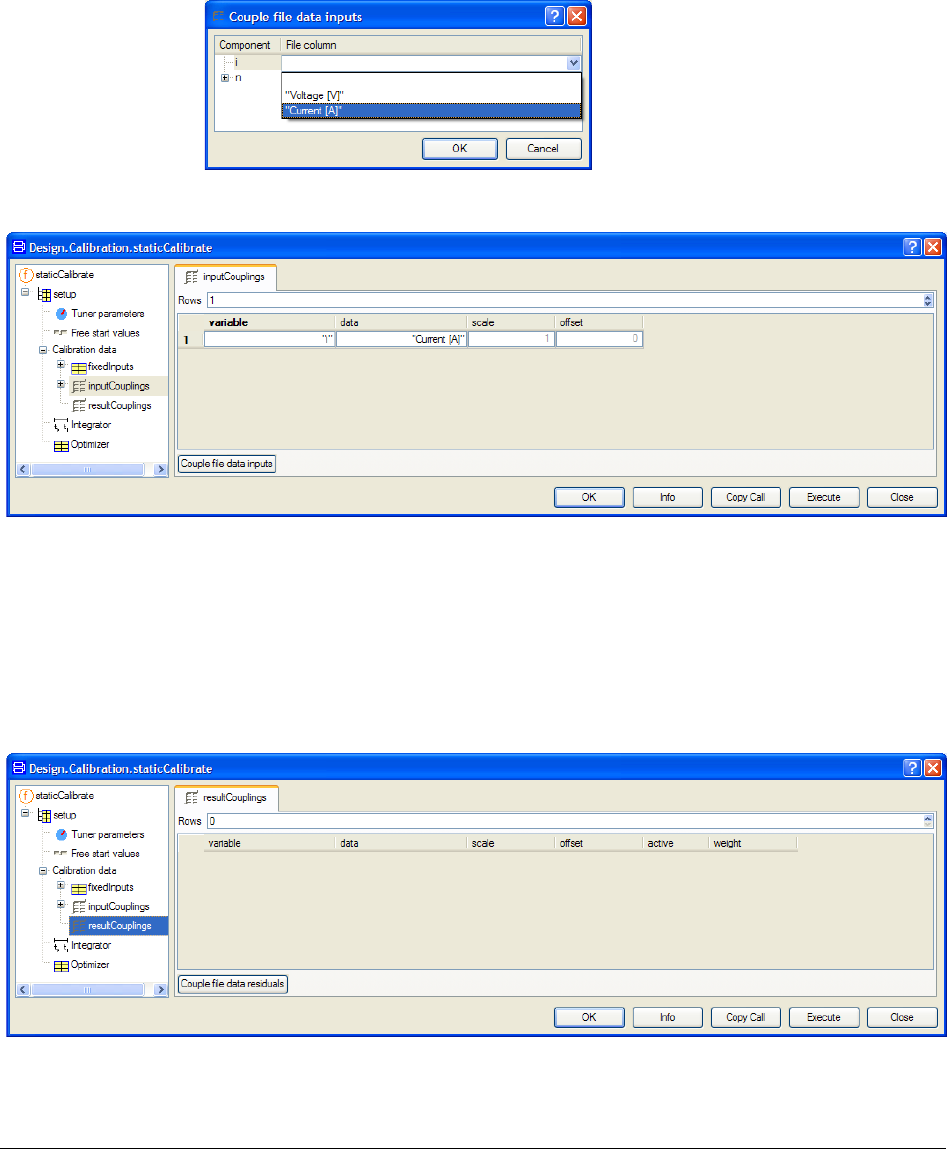
92
Click OK. The result of coupling file data to the inputs is displayed as
The input of the model as well as the measured current are given in the SI unit, A, so there
is no need for scaling. In case of different units being used, the menu supports rescaling
(variable = data*scale + offset). For example if the measurements of the current had been
given in mA, we had needed to downscale them by a factor of 1000 by setting scale to 0.001.
Result Couplings
The measurements of the voltage across the resistor are to be used for the calibration
criterion. To specify this, click on resultCouplings in the tree browser.
Couple current as
input.
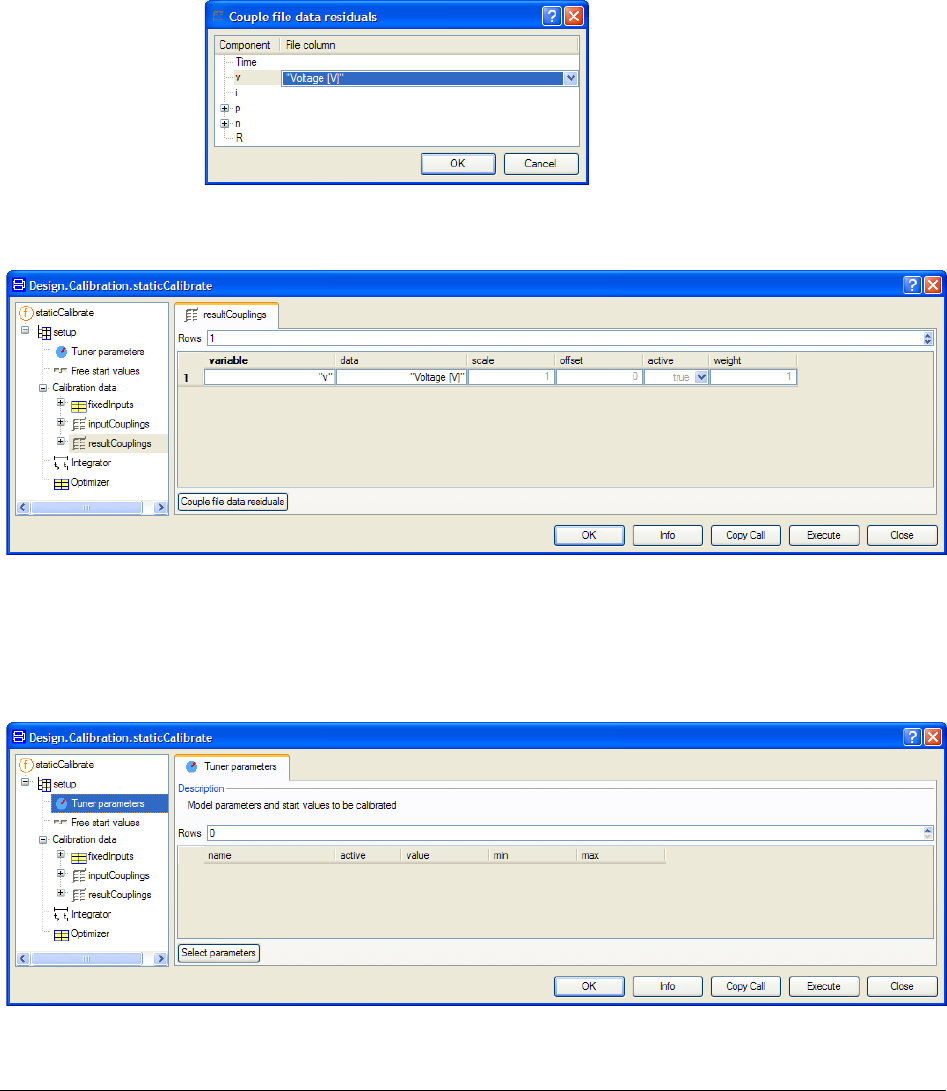
2 MODEL CALIBRATION 93
Click Couple file data residuals. A browser similar to that for connecting file data inputs is
popped.
Select v to be compared with “Voltage [V]” in the csv file. Click OK. These measurement
data are given V so no need for scaling.
We have now specified the instrumentation or the rigging of the experiments.
Tuner parameters
For the calibration task we need to specify which paramers to tune. Click on Tuner
parameters in the tree browser.
Couple output and
data.
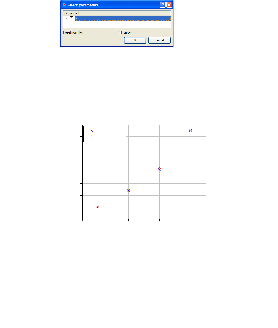
94
Click Select parameters.
The model has a only one parameter, namely R representing the resistance. Tick it and click
OK.
It is time to do the first calibration. Click Execute. After 13 fast iterations we obtain the
result.
R = 4611.4,
with the error being 0.0083 and a plot comparing measured reference and simulated voltage
from tuned model for the different cases (the legend of the plot has to be moved to see the
last point).
The fit is rather good. To get better insight, it may be of interest to plot versus current. In the
variable browser we find two results; the Reference and the simulation result Case. For
these two results v is plotted. Put the cursor on either i, right-click and select i as
independent variable.
1234
-1
0
1
2
3
4
5
6
7
Reference v
Calibration v
Select resistance for
tuning.
Tuning result.
Comparing measured
and calculated voltage
drop after tuning.
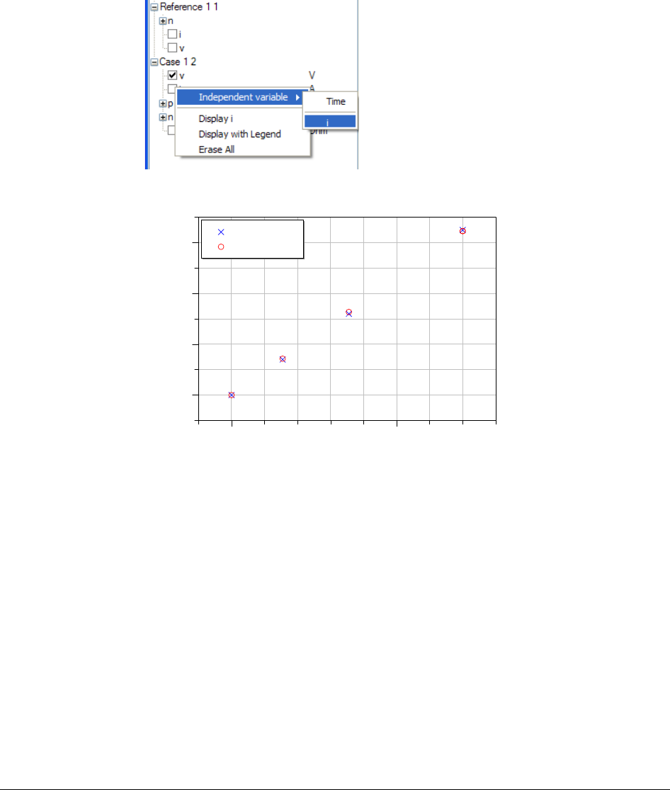
2 MODEL CALIBRATION 95
This plot now becomes
Saving the setup for reuse
After an execution of a command we can save it in the model for later reuse as described
above. Select Commands > Add command. A menu pops up
0.000 0.001
0
2
4
6
i
Reference v
Calibration v
The results are easily
accessible in the
variable browser.
Current v s voltage
drop.
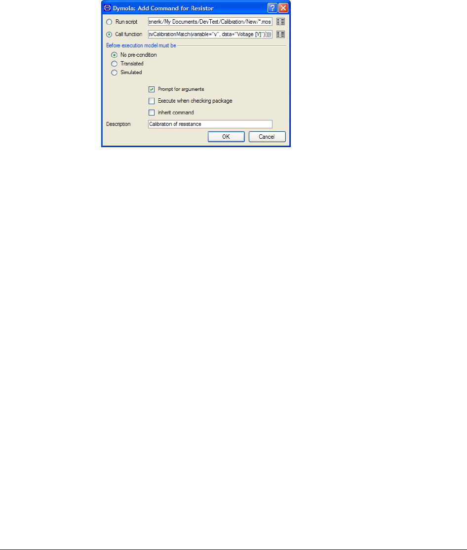
96
Tick Prompt for arguments and enter a description, which will be used in the commands
menu. Do not tick that the model must be translated before execution, because this would
mean translation of the model Resistor without the additional inputs and consequently
Dymola would generate error messages that the model is singular. (More about this menu
can be read in “Dymola User Manual Volume 1”, chapter “Developing a model”, section
“Editor command reference – Modeling mode”, sub-section “Main window: Commands
menu”.)
Direct calculation of R from the measurements
There is another way to get insight. The measurements can be used to uniquely back
calculate R for each case. Make a copy of
Modelica.Electrical.Analog.Basic.Resistor
as described above. Call it ResistorBase. We need to free R; change the declaration of R
parameter Modelica.SIunits.Resistance R(start=1) "Resistance";
to
Modelica.SIunits.Resistance R "Resistance";
Take ResistorBase and set up a calibration task as done above,
• Select staticCalibrate in the package browser, right-click and select Call function…
• Select the model to be ResistorBase.
• Select the additional inputs as previously, but also select v (v, i and p.v should be
selected).
• Select Calibration data and specify experimentName as previously.
• Specify fixedInputs and give their values as previously.
• Specify inputCouplings and scaling as previously, but couple also v to “Voltage [V]”
(no scaling)
Menu for saving the
setup.
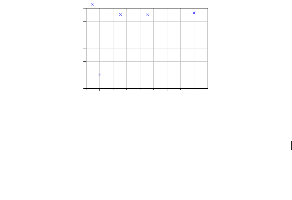
2 MODEL CALIBRATION 97
• Do not specify any resultCouplings.
• Do not specify any tuners.
Clicking Execute produces a result file. Plot R and select i as independent variable. It gives
the plot below.
You can also define the setup by starting from the setup of the previous calibration.
• Select the model to be ResistorBase.
• Select the additional inputs as previously, but select also v (v, i and p.v should be
selected).
• Select inputCouplings and select v and couple it to “Voltage [V]”. Click OK. Scaling is
OK.
• Select resultCouplings. We want to deselect v. Decrease the number of rows to zero
and click OK.
• Deselect tuners by decreasing the number of rows to zero (or by clicking Select
parameters – no parameter is yet selected – and click OK).
Clicking Execute produces two results Reference and Case 1. Plot R and select i as
independent variable. It gives the plot.
First, we realize that it is not possible to get a unique R when the current is zero. The
measurements indicates that the resistance is independent of current. If they had indicated
dependencies, this kind of plot can give us hint about useful parameterizations for the
relation between voltage and current for our component.
0.000 0.001
-1000
0
1000
2000
3000
4000
5000
[Ohm]
i
R
Obtained resistance
values from direct
calculation using the
measurements.
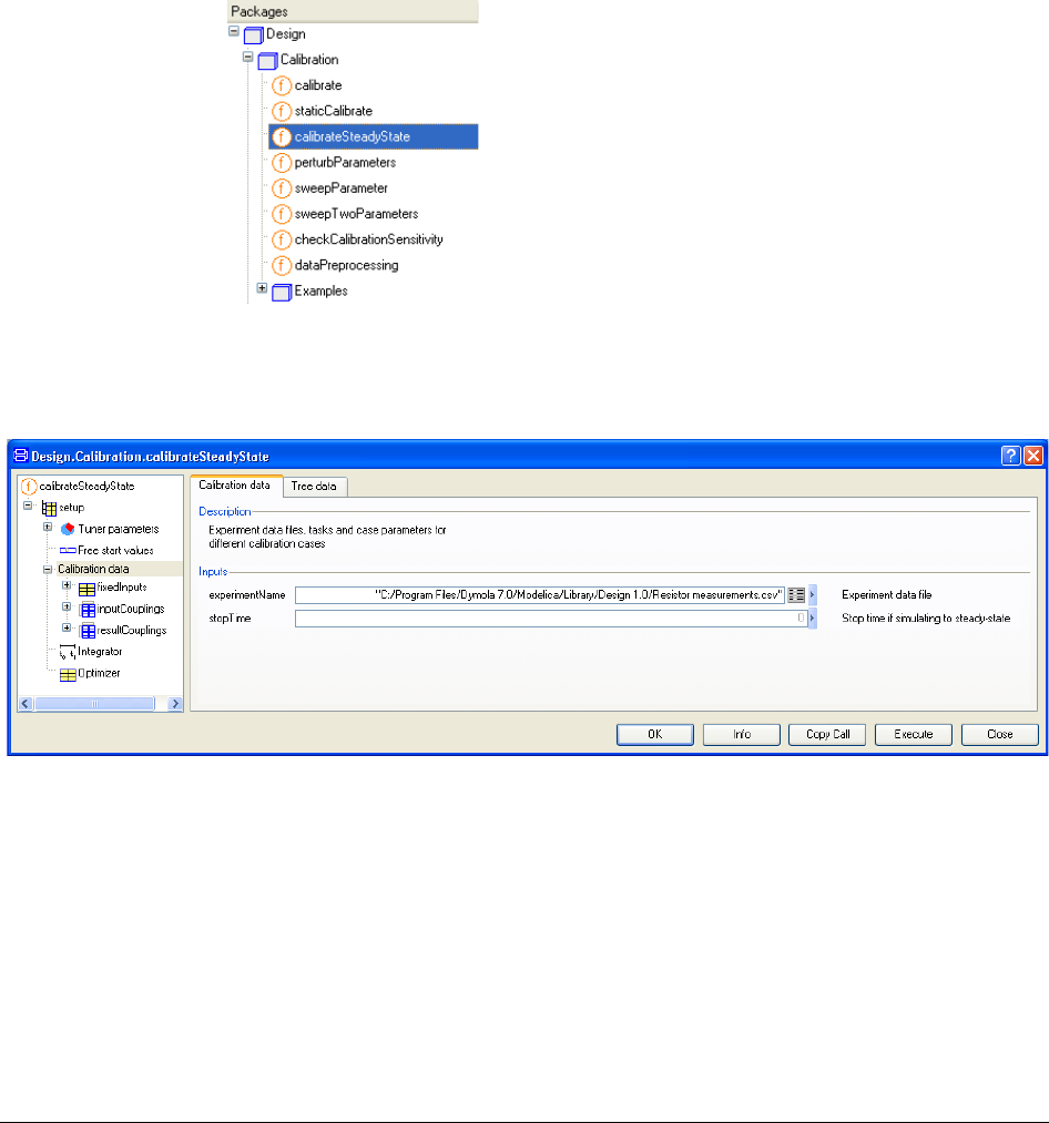
98
2.7.2 The calibrateSteadyState function
The calibrateSteadyState function should be used for steady-state models. For completely
state-less (static) models, please see the function staticCalibrate.
To load Design.Calibration, select File > Libraries and click Design.
Example
The resistor example above can be solved using calibrateSteadyState as well; the only
difference in the menus compared with the above example is the Calibration data menu:
Here also stopTime can be specified if a steady-state model should be treated. The time
should be specified by the user when a model is not initially in steady-state. The time should
be stated in such a way that steady-state conditions can be guaranteed at that time.
The
calibrateSteadyState
function.
3 DESIGN OPTIMIZATION

3 DESIGN OPTIMIZATION 101
3 Design Optimization
Please note that a new library, Optimization 2.x, is now available. Optimization 2.x has
largely been re-implemented and improved and is not backwards compatible with the
Design.Optimization package (“Optimization 1.0”) described here.
Both libraries are available and can be used at the same time; existing optimization setups
work without changes.
However, wanting to take advantage of the new features, Optimization 2.x has to be used.
Please see separate documentation for this free-standing library.
3.1 Introduction
Dymola includes features to perform integrated computer experiments with Modelica
models. This document describes the features to determine improved values of model
parameters by multi-criteria optimization based on simulation runs. The functions and
models described in this document are parts of the Design.Optimization package. The
DesignOptimization option is required. However, the optimization examples given below
can be run without the DesignOptimization option.
Consider a Modelica model describing a technical system that shall be improved. Such a
model includes typically many parameters that can still be changed, for example the spring
constants of a car, the gear ratio of a gear box, or parameters of a controller. Some
parameters might be determined by using heuristic design rules, by adjusting them by “trial
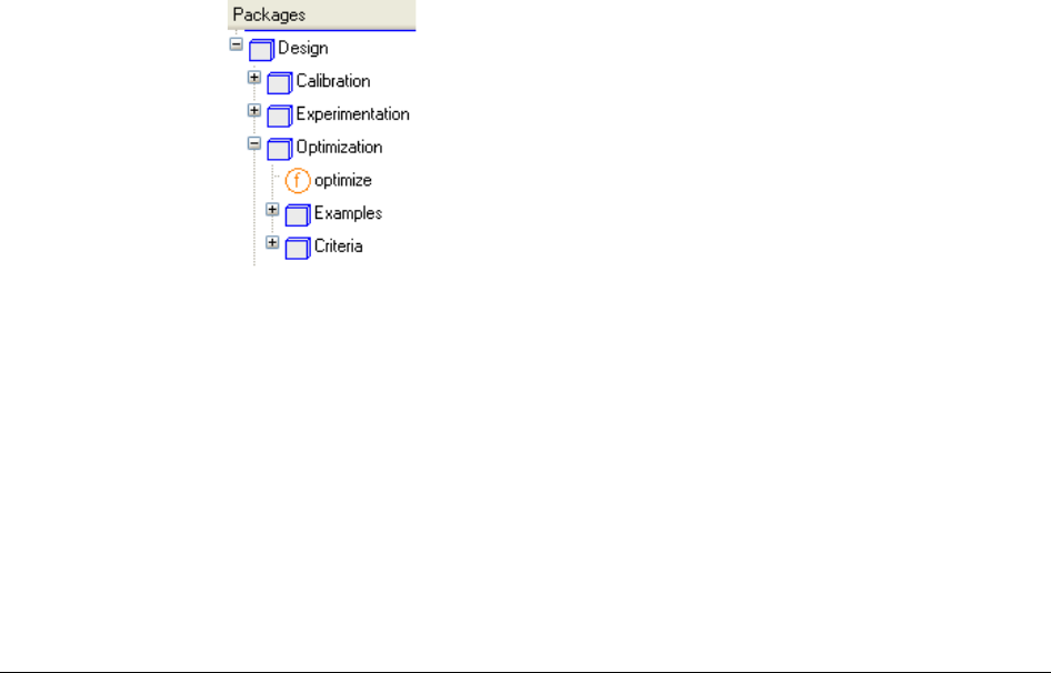
102
and error” using simulation runs or by using simplified linear models and apply the well
established synthesis procedures for linear systems.
Design optimization is an approach to tune parameters such that the system behavior is
improved. The parameters that are tuned are often referred to as tuners. Mathematically, the
tuning procedure is formulated as multi-criteria parameter optimization: Parameters are
calculated to minimize criteria which express in mathematical terms what “improvement”
shall mean. Criteria values are usually derived from simulation results, e.g., the overshoot or
rise time of a response, but they can also be derived by other analysis procedures, such as
frequency responses or eigenvalue analysis.
The typical setup described below consists in defining the most important operating points
of a model, and to define criteria for every operating point. This means that usually several
simulation runs are needed to compute the criteria values. This setup is called multi-criteria,
multi-case optimization. The different operating points are the “cases” under consideration.
The major goal is to minimize all criteria and/or to keep them below required bounds. Other
types of demands, e.g., criteria that shall be maximized, have to be reformulated.
Since several criteria shall be minimized there is usually no unique mathematical solution.
Instead, the criteria have to be weighted with respect to each other and the goal is to find the
best compromise solution that minimizes all criteria in the “designer’s sense”. The
“weighting” technique described in the next sections is a proven technology developed by
DLR and it has been applied in many industrial projects in the last 10 years.
To load Design.Optimization, select File > Libraries and click Design.
The function Design.Optimization.optimize is the main function for design optimization via
multi-criteria, multi-case parameter optimization. There is also a set of functions and of
models to define criteria. For parameter studies in general, see chapter “Model
Experimentation”. To determine model parameters using measurement data, see chapter
“Model calibration”.
This document uses the design of a control system for a very simple model of an F14
aircraft (see figure below) to illustrate how a basic design optimization task is set up and
executed, and how the setup is stored for later reuse.
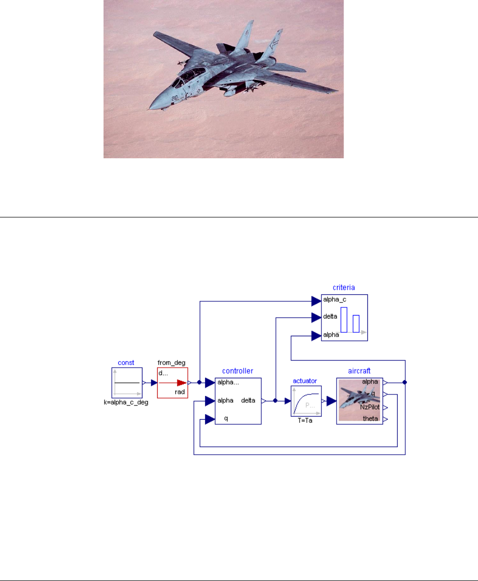
3 DESIGN OPTIMIZATION 103
3.2 First optimization setup
In this section the first setup of the design optimization of the F14 controllers is shown.
Open model Design.Optimization.Examples.ControllerDesign_F14.
Component “aircraft” contains the dynamic equations of the aircraft. Component “controller”
is the control system for the longitudinal motion, and component “criteria” contains the
criteria computation.
This model is used for simulation and analysis of the closed loop step response of the
longitudinal motion of a very simple F14 aircraft model. A linear controller with fixed
controller parameters is used for tracking the reference motion of the angle of attack, alpha.
F14 aircraft used as
example.
Model used in the
design example.
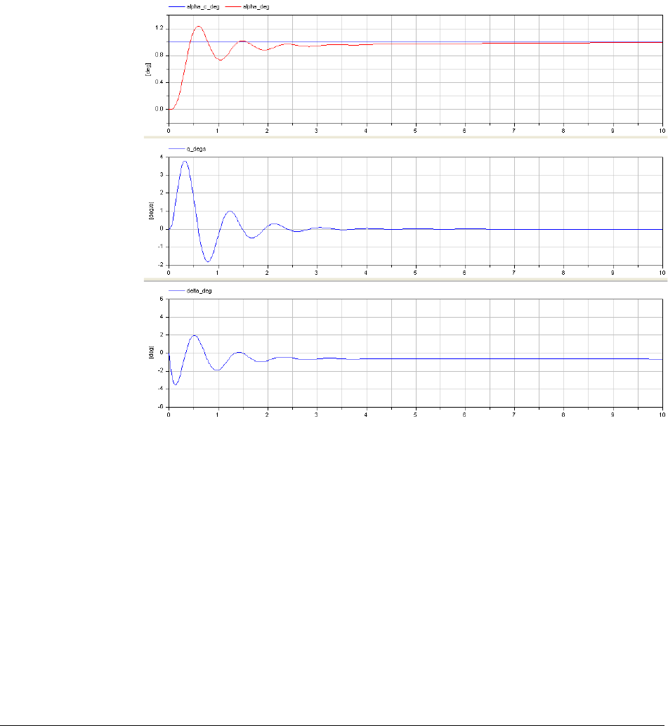
104
The goal is to determine the controller parameters such that the step response is reasonable
in the operation region of the aircraft.
Simulate this model for 10 s and plot alpha_c_deg (= commanded angle of attack),
alpha_deg (angle of attack), q_degs (pitch rate) and delta_deg (elevator deflection):
The controller is shown in the next figure:
Response to step
change in alpha_deg
before tuning.

3 DESIGN OPTIMIZATION 105
The values of the controller parameters are Kf = -6, Ki = -2, Kq = 0.5. The desired reference
value for alpha is alpha_c_deg = 1°. The initial value for alpha(t) is alpha(0) = 0. This
arbitrarily chosen stabilizing set of controller parameters leads to a large overshoot of alpha
and a significant maximum elevator deflection. The design objectives will be to reduce
overshoot of alpha below 1 % and to reduce the maximum elevator deflection below 2°.
The design problem is now translated into a setup for optimization based parameter tuning.
In the Commands menu in the toolbar you can find all setups described in this tutorial. We
will perform now the setups manually. Right-click on function optimize in the package
browser and select Call Function …:
The controller.
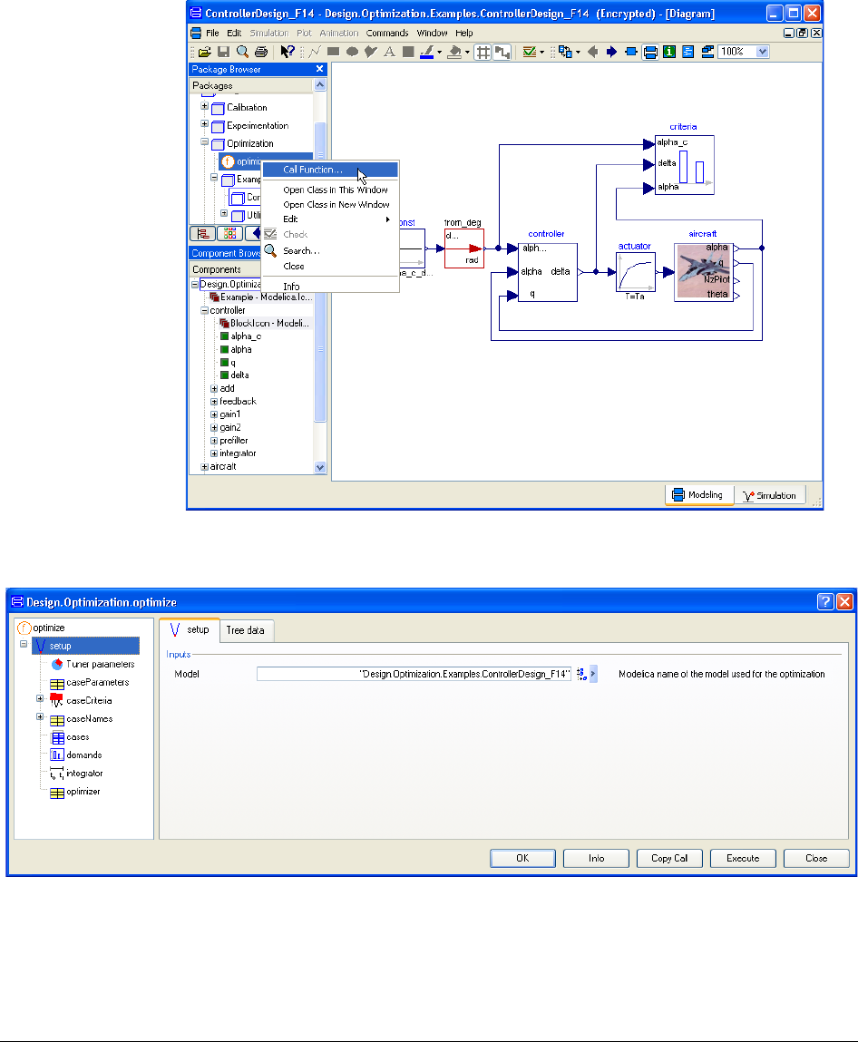
106
In the appearing dialog window, the model name of the last translated model is
automatically inserted (there is also a browser for selecting the model):
Start setting up the
optimizator.
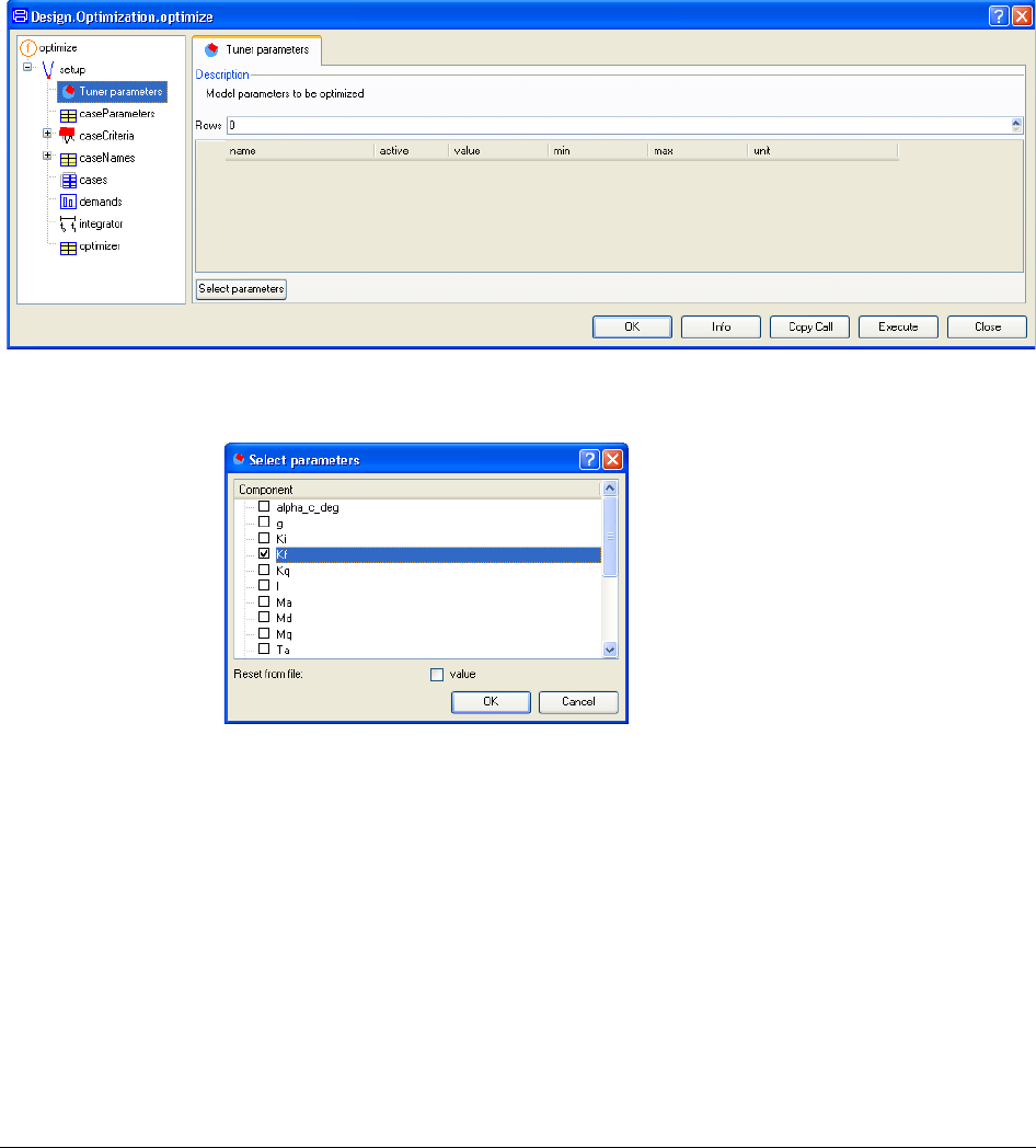
3 DESIGN OPTIMIZATION 107
3.2.1 Specifying tuners
Select Tuner parameters in the left part of the window in order to define the model
parameters that shall be determined by the optimizer.
By clicking on the Select parameters button a variable tree browser of the selected models
opens. Select the controller parameter Kf as a tuner that is being optimized:
The actual tuner value and the corresponding minimum and maximum values as well as the
unit (if defined in the model) are read from the last simulation run.
Selecting Kf for tuning.

108
Note that minimum and maximum values should always be defined for tuner parameters in
order to ease the task for the optimizer.
Optionally, case parameters can be specified to define the “operating conditions”. Here,
parameter “alpha_c_deg” is selected from the tree browser via caseParameters and the
button Select:
The value of “alpha_c_deg = 1” of this operating condition has to be given under cases:
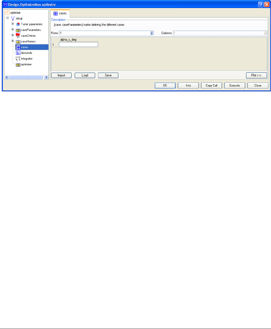
3 DESIGN OPTIMIZATION 109
(The buttons Import, Load and Save makes it possible to save the matrix of cases which
might be interesting e.g. if the matrix should be treated separately. Concerning Load and
Save they work the same as in the matrix editor (please see “Dymola User Manual Volume
1”; search the index for “Matrix editor”). Import makes it possible to load a file of name
cases.csv from the current working directory directly. If such a file is not present an error
message will be displayed.)
3.2.2 Specification of the criteria
In the model ControllerDesign_F14, criteria blocks from the Design.Criteria sub-library are
used to compute how well the controller works (see next figure). In the F14 model, for
example the criteria block “Criteria.MaximumDeviation” is used with the component name
“maximum” (see figure below). Since in the F14 model the “maximum” block is in a block
called “criteria”, and the criterion is always the output y from a criteria block, the criterion
of the maximum deviation is accessed as “criteria.maximum.y”.
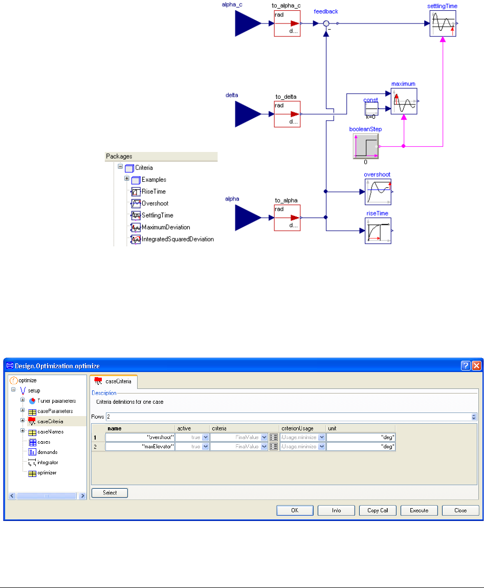
110
In order to access this variable a bit easier, in the top level text layer of the F14 example an
alias variable “maxElevator” is defined as:
output NonSI.Angle_deg maxElevator = criteria.maximum.y
"maximum elevator deflection";
In other words, “maxElevator” is the maximum deviation of the elevator signal from zero.
In the variable tree browser of caseCriteria the used criteria might be defined by selecting
again variables (here: “overshoot” and “maxElevator”):
The default value in column “criteria” of the above menu is “FinalValue”, i.e., the final
value of a variable in the model is used as criterion. Alternatively, this pop up menu also
Specification of the
criteria.
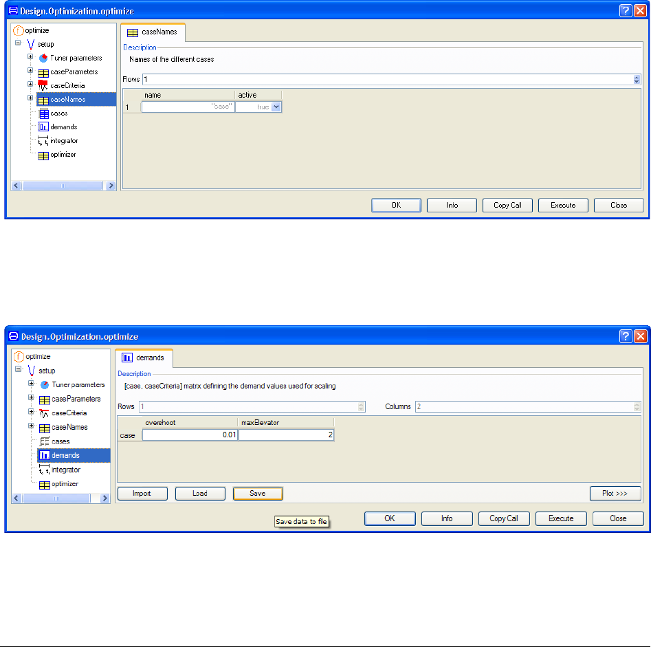
3 DESIGN OPTIMIZATION 111
allows selecting other criteria that are not defined in the model but are deduced from
simulation results. In some cases this is more convenient. Criteria based on linearization of
the model around an operating point (e.g., maximum real part of all eigenvalues) can only
be selected from this menu and cannot be defined in the model (this function criterion is not
yet supported). Column “criteriaUsage” remains unchanged for the moment.
As already mentioned, it is possible to define multiple cases representing, e.g., different
working conditions. We could provide different names for them using caseNames, but for
our first optimization run we simply use the default name.
Since we are using several criteria, they have to be weighted with regards to each other. In
optimize(), the value “criterion / demand” is minimized, i.e., “demand” is used as scaling
factor of “criterion”. A demand value has the same unit as the corresponding criterion. For
this first setup in demands, we use a demand value of 0.01o for the overshoot (=1 %
overshoot) and 2° for the maximum absolute elevator deflection:
(Concerning the buttons Import, Load and Save they work the same as for “cases”; please
see above. The name of the file that Import works with is demands.csv.)
Finally, a simulation time of 10 s has to be defined under integrator:

112
The optimization problem defined and to be solved by the Design package optimizer is now:
min( max( overshoot(Kf)/(0.01°), maxElevator(Kf)/(2°) ), Kf in [-10;0]
By clicking on the Execute button, the optimization is started.
The same setup could be obtained by selecting the first command in the Commands menu:
After Execute is pressed, the optimization is started.
3.2.3 The result of the optimization
The Dymola command log shows the iterations and the final output.
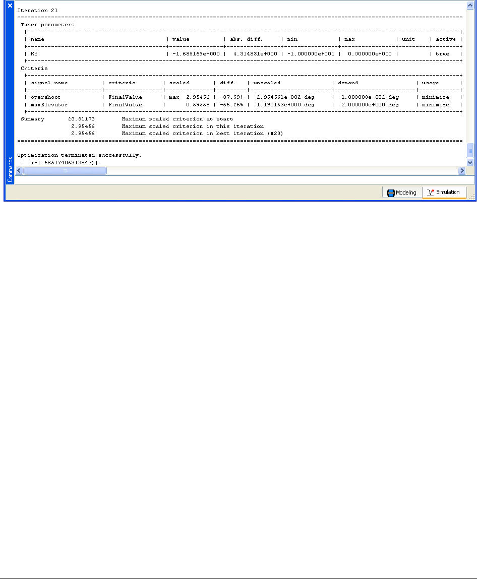
3 DESIGN OPTIMIZATION 113
All iterations that are better than all previous ones are shown in the log. The following
information is given in the log for iteration 21:
Tuner “Kf” is active (see last column in the figure above) and has the value “-1.68517”.
This is a change of +4.31 with regards to the value of Kf before the optimization started.
The search interval for the optimizer for this tuner is [-10 ... 0] (see min/max columns).
There is only one simulation case defined and therefore no additional information is given
for the cases.
The scaled criteria “overshoot” is currently the largest of the scaled criteria (due to the “max”
in front of the scaled value) and has a scaled value overshoot/demand = 2.95456. This is a
change of -87.59 % with regards to the initial value. The actual value of overshoot =
0.0295456 (= 2.95 % overshoot). This criterion is minimized due to “minimize” and has a
demand value of 0.01 (see column “demand”).
The best values of all tuners are also given in the log as last output. The best value of Kf is
-1.68517406313843. It can be seen, that the overshoot is reduced by 87.59 % and the
control activity by 66.26 % (see column “diff”). However, by tuning only Kf, the overshoot
could not be reduced below the requested demand value of 1 %. Note, the scaled criterion is
below 1, if the demand value is fulfilled. Therefore in the next steps the controller
parameters Ki and Kq will be also optimized.
After the optimization is finalized, the Design.optimize() menu remains open (when using
Execute; using OK will close the menu). Nothing in the setup has changed. In order that the
result of the last optimization run is included in the setup, it is necessary to apply Reset
from file. To do that, select the Select parameters button of tunerParameters,
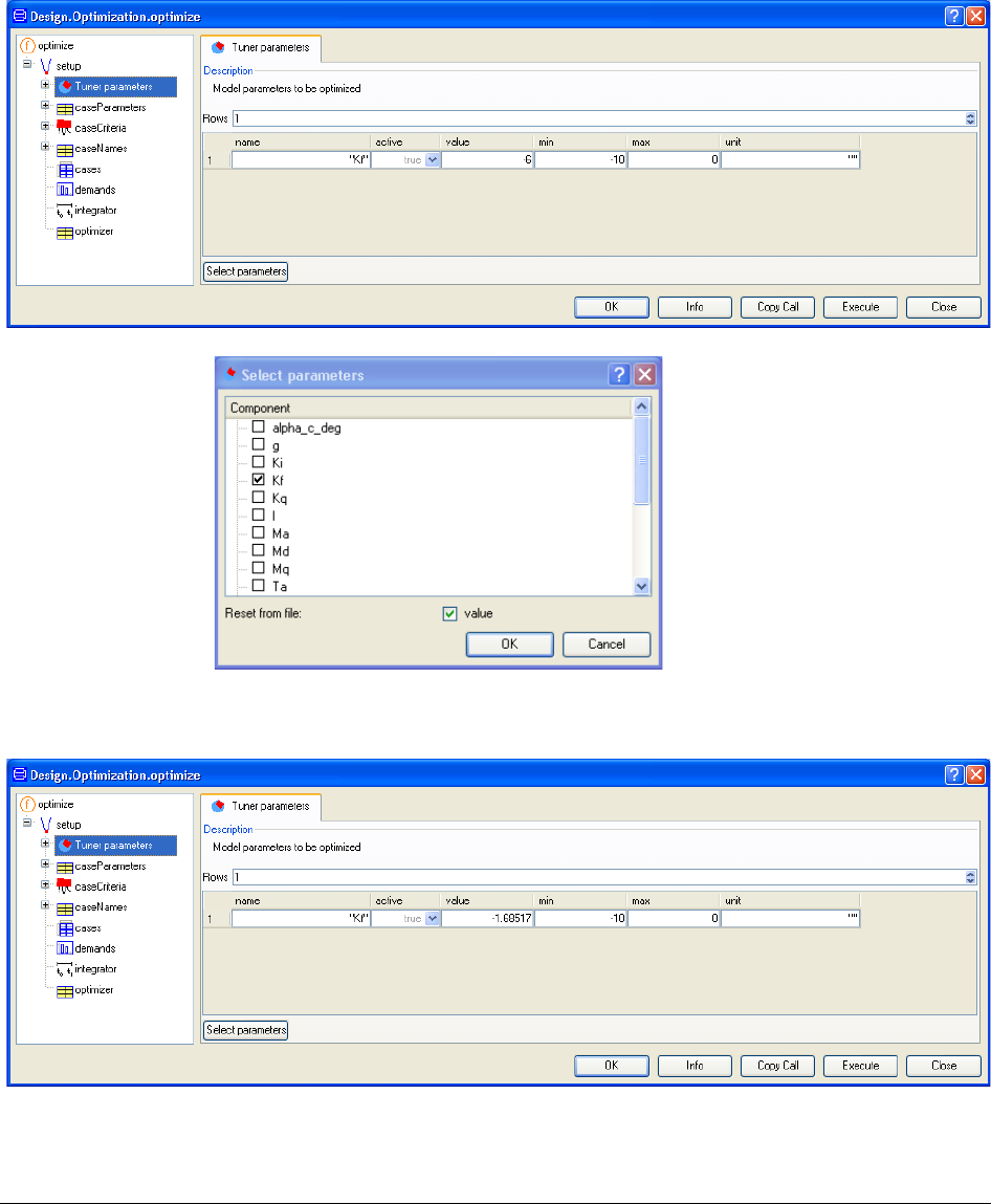
114
tick value to apply Reset from file and click on OK. This will load the values of all tuners
from the last simulation run:

3 DESIGN OPTIMIZATION 115
Since the optimizer performs a last simulation run with the best tuner values, these tuner
values are the ones from the best iteration of the last optimization.
3.2.4 Adding more tuners
The setup is changed such that all controller parameters Kf, Ki, Kq are defined as tuners.
Furthermore rise time and settling time are introduced as further criteria. These criteria are
introduced to counteract the effect that the reduction of control activity and overshoot may
lead to very long rise and settling times in the alpha step response.
The controller parameters Kf and Kq are defined with active = true (default value in the
second column of the Tuner parameters table). In turn, we set active = false for Ki. This
means that the value of Ki is not changed by the optimizer. By increasing Kq it should be
possible to reduce the overshoot.
In a first step we set active = false for the riseTime and settlingTime criteria (via the second
column of the caseCriteria). Therefore, these criteria are shown in the log output, but are not
utilized in the optimization.
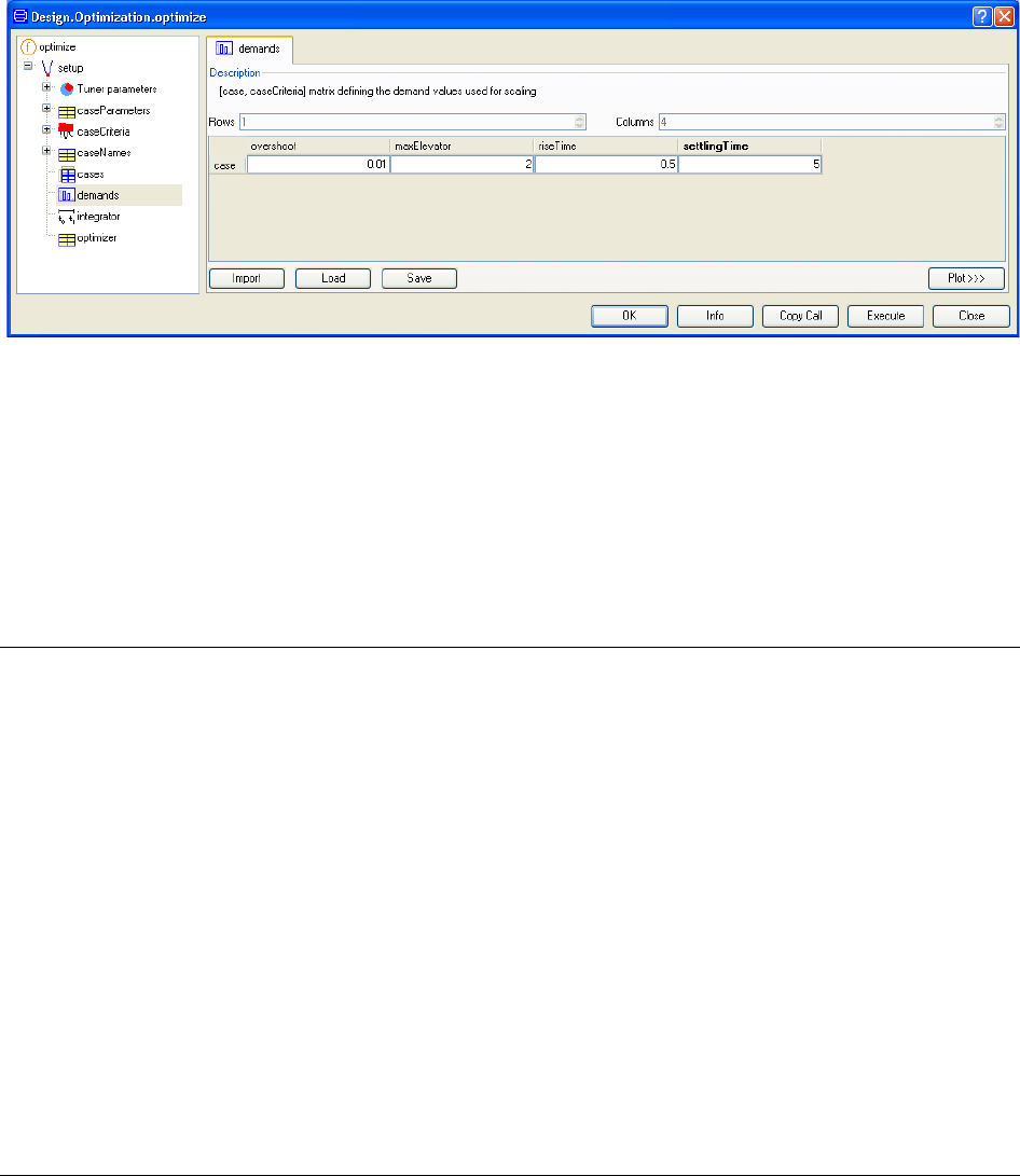
116
Although the riseTime and the settlingTime criteria are not used in the optimization itself,
we have to provide demand values for them (0.5 and 5).
After the optimization run (same as Commands > Run 2), Kq has been increased to
0.725384879534943 and Kf has been increased to -1.33686682932122. As a consequence,
the overshoot is now below the demand value of 1 %. However due to the high value of Kq
the rise time increased.
Finally we update the tuner values again (with the values from the previous optimization
run), set the riseTime and settlingTime criteria active and make the controller parameter Ki
a tuner as well, i.e., set active = true as done in Commands > Run 3 After the optimization
is finished, all demand values are fulfilled.
3.3 Multi-criteria experimenting
The Design optimize function provides features for criteria weighting and scaling by
demand values as well as the possibility to use criteria as a value to be minimized or to use
them as constraints.
During an optimization run, the optimization criteria are scaled with their demand values, i.e.
the value delivered to the optimization method is criterion_value/demand_value. By
changing the demand value of a criterion, a differently weighted optimization task is defined
and therefore normally a different solution is obtained. In the following, the effect of
demand value variation on the multi-criteria controller parameter optimization for the F14
aircraft is shown. Furthermore, the effect of using an optimization criterion as inequality
constraint is demonstrated.
The controller parameters Kf, Ki, Kq are defined as tuners (using the best values of the last
run by Reset from file; you may also execute Commands > Run 4 to achieve this result)
and the final values of overshoot, riseTime, settlingTime and maxElevator as optimization
criteria (c1(Kf,Kq,Ki)..c4(Kf,Ki,Kq)) with their new demand values di = {0.01, 0.5, 2.5, 3}.
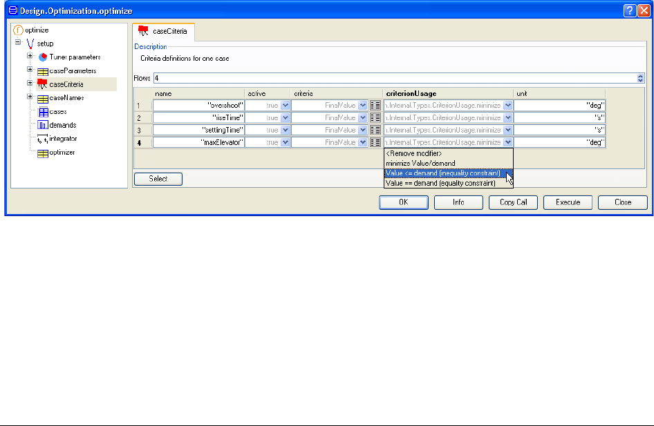
3 DESIGN OPTIMIZATION 117
For a first optimization of the controller parameters all criteria are defined as minimum
(default), i.e. the optimization task is to solve the min-max problem:
min( max( c1/d1, c2/d2, c3/d3, c4/d4 ) ) over Kf, Ki, Kq
A solution for the controller parameters Kf, Ki, Kq was found (-4.25114383886458,
-4.23376396990245, 1.00353017925373) such that all criteria are reduced below their
demand values. The scaled criteria all have nearly the same value (within computational
accuracy): 0.7829. This result indicates that the solution is a Pareto-optimal solution, where
no criterion can be further minimized without degrading at least one other criterion
(provided this is not a local minimum).
As a first variation, we will change the demand value for the overshoot criterion from 1 %
to 10 %. This means that more overshoot in the alpha step response is allowed and we
expect that the other criteria improve. After updating the tuner values by Reset from file,
we start the optimization (you can get this result also by executing Commands > Run 5).
In the command log output of this optimization run you can see that the overshoot increased
with the effect that all the other criteria could be improved. We obtain again a Pareto-
optimal solution among all criteria as their scaled criterion values are nearly identical: 0.73.
This demonstrates how different compromise solutions can be found by variation of the
demand values.
As a next modification of the optimization task we change the type of the maxElevator
criterion (c4) from minimum to inequality:
This means, that this criterion is not minimized any more but taken as inequality constraint.
The new problem to solve is
min( max( c1/d1, c2/d2, c3/d3 ) ), subject to c4/d4 <= 1 over Kf, Ki, Kq
After updating the tuners (Reset from file) and starting the optimization, the result is (this
result can also be obtained with Commands > Run 6):
{Kf, Ki, Kq} = {-5.52323683463408, -5.30428567387681, 0.992903708042067}.
The change of the type of the maxElevator criterion from minimum to inequality yields a
new controller parameter set. You can see from the simulation results that due to the new

118
criterion formulation the elevator is now deflected to the maximum allowed value of 3°
during the step response. This is an increase of 37.18 % in the maximum elevator deflection
compared to the solution of the previous optimization (see the command log output).
However due to the increased maximum elevator deflection other criteria could be
decreased.
3.4 Multi-case optimization
In this section, we start a new optimization task in order to extend the controller parameter
synthesis to a multi-case optimization. As all aerodynamic parameters Ma, Mq, Md, Za, Zd
of the F14 aircraft may vary within ± 10 % of their nominal value,
{Ma, Md, Mq, Za, Zd}nominal = {-5, -7.5, -0.7, -0.67, -0.2},
known worst-case scenarios are simultaneously considered in addition to the nominal case.
A controller parameter set stabilizing all these cases shall be found.
First, a simulation with the current controller parameters Ki = -2, Kf = -1.72 and Kq = 0.5
for the nominal case is performed. (You have to enter all figures manually in the variable
browser, and please note that Advanced is activated, with the Time 10 entered.)
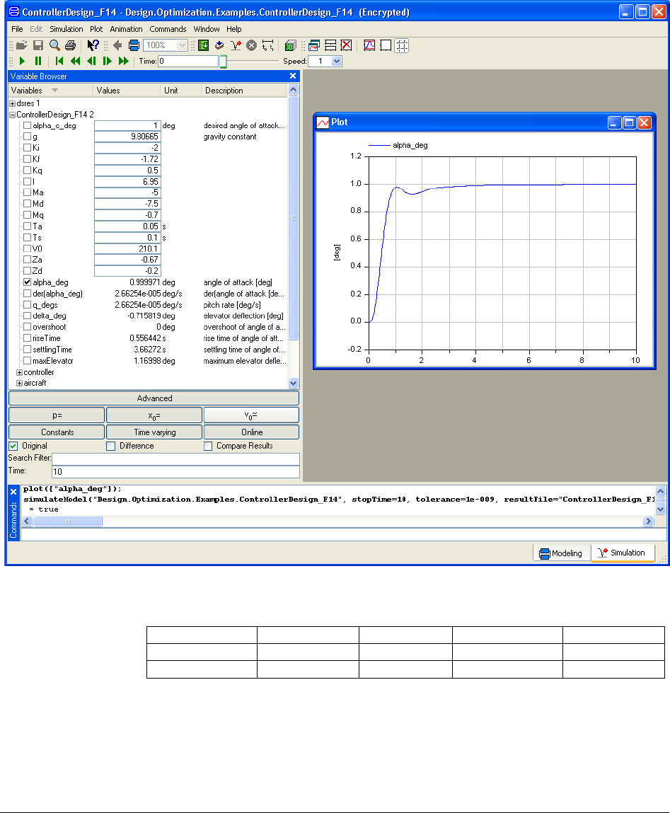
3 DESIGN OPTIMIZATION 119
The variable browser shows the corresponding criteria values:
overshoot
riseTime
settlingTime
maxElevator
demand value
0.01
0.5
4
2
current value
0
0.56
3.7
1.2
You see that the riseTime criterion is not yet satisfied. Therefore a new optimization task
will be defined (you may use Commands > Run 7 instead). In this particular step we only
consider the nominal case.
It should be straightforward to define the tuners {Kf, Ki, Kq} and the criteria {overshoot,
riseTime, settlingTime, maxElevator} with the demand values given in the above table.
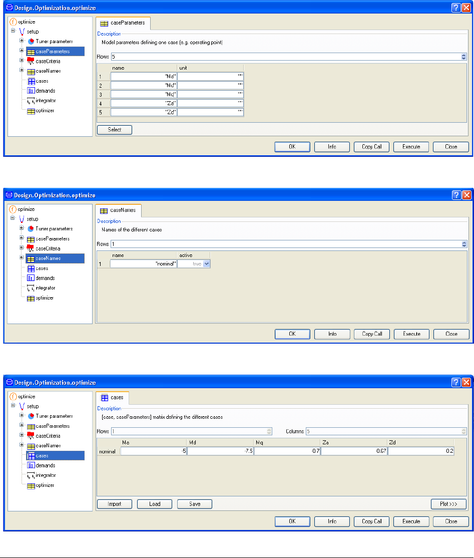
120
Further we define the aerodynamics parameters as case parameters.
An appropriate name is assigned to the currently considered case.
We provide the case parameters’ values for the nominal case.
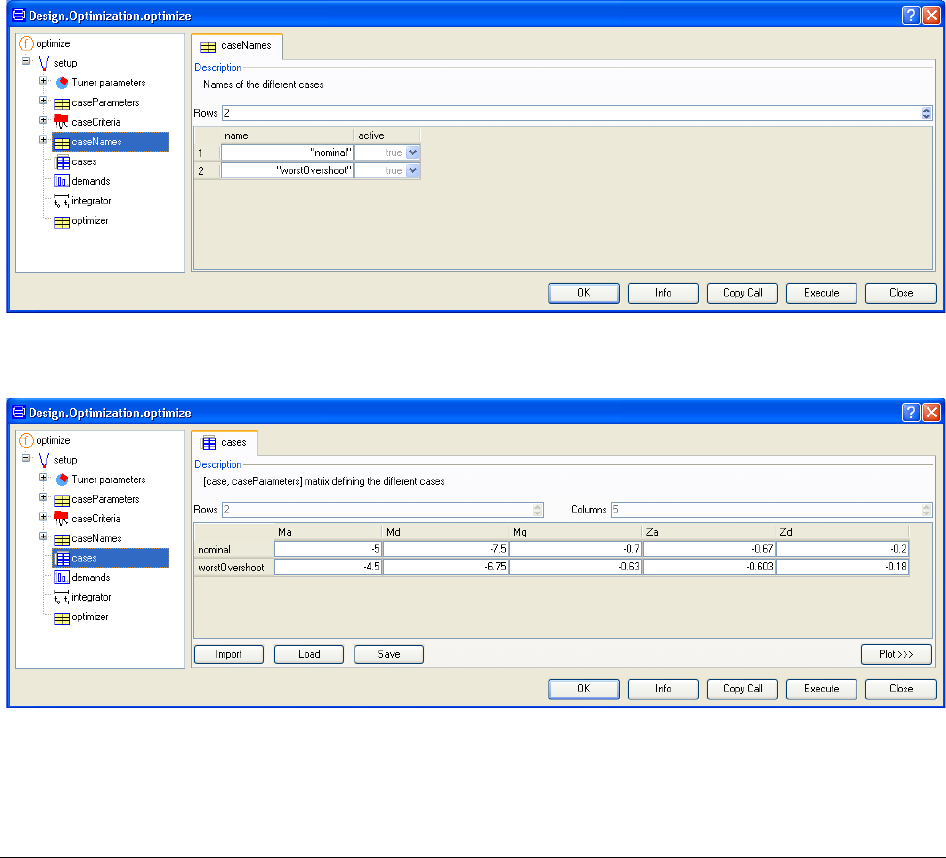
3 DESIGN OPTIMIZATION 121
Finally, we set the simulation time (integrator) to 10 seconds.
The obtained optimization result satisfies all criteria and gives the following tuner values:
{Kf, Ki, Kq} = {-2.76447041008657, -2.73348741868026, 0.618294701540142}
From a different analysis, it is known, that the obtained controller set does not satisfy the
criteria in the case
{Ma, Md, Mq, Za, Zd}worstOvershoot = {-4.5, -6.75, -0.63, -0.603, -0.18}
This set of aerodynamic parameters will be used to define a case “worstOvershoot” besides
the “nominal” case.
In caseNames we define the additional case:
The different values for the parameters defining the new case are given in the
cases [case,caseParameters] matrix:
We have to provide demand values for the new case.

122
An optimization will be performed now (i.e., after having updated the tuner values using
Reset from file) for this multi-case scenario. The objective is to find controller parameter
values for Ki, Kf, Kq such that all criteria are satisfied simultaneously for both cases
"nominal" and "worstOvershoot" (you may execute this optimization task by Commands >
Run 8).
You can see that for both cases a controller parameter set could be determined that satisfies
all criteria:
{Kf, Ki, Kq} = {-2.95319084159519), -2.71504062005572, 0.700519234697927}
Again, it can be shown, that a controller using these parameters is not robust against the
uncertainties in the aerodynamic parameters. The settling time criterion is not satisfied for
the aerodynamic parameters
{Ma, Md, Mq, Za, Zd}worstSettlingTime = {-5.5, -6.75, -0.63, -0.737, -0.18}
This set enters the setup as new case “worstSettlingTime”. Another optimization step will
be performed (do not forget to update the tuner values and to provide demand values for the
new case) to determine controller parameter values to simultaneously satisfy all criteria for
the three cases “nominal”, “worstOvershoot”, “worstSettlingTime” (you may execute this
optimization task by Commands > Run 9). The optimizer is able to find a controller
parameter set that satisfies all demands in all three operating points:
{Kf, Ki, Kq} = {-3.15272724951542, -3.05878110656018, 0.764835089447917}
By further analysis, it could be shown, that this controller parameter set stabilizes the
aircraft robustly to the aerodynamics parameters.
Although the F14 example is very simple, many essential ingredients have been shown.
They can all be applied also to much more complicated cases.
4 MODEL MANAGEMENT

4 MODEL MANAGEMENT 125
4 Model Management
The model management package includes version management, automatic documentation of
model dependencies, encryption of models, model and library checking, model comparison,
and functions for accessing the model structure. There is no licensing for Model
Management.
In Dymola 2017 FD01, the Model Management product (MOC) was integrated into the
Dymola standard configuration, meaning that Model Management is from that version
available without licensing.
Because of this, the checkbox to control if Model Management should be disabled was
removed, in the menu Help > License… > Details. The default value was that Model
Management was disabled. That setting was stored in the setup file.
As a general rule, we never override customer settings, which meant that the stored setting
may then block opening the Model Management library in Dymola 2017 FD01 and later
versions.
To correct this, check what value the flag Advanced.EnableModelManagement has by
executing it in the command input line of the command window. If the value is false,
execute Advanced.EnableModelManagement=true; to reenable the feature. This only
has to be done once, the updated value is now stored when for example closing Dymola.
The setting is saved between sessions.
If again starting Dymola 2017 or earlier, the value of the setting is still false; the change of
the value is only performed in the new settings file used by Dymola 2017 FD01 and later.
Note!

126
4.1 Version management
4.1.1 Short guide with new features included
If you are familiar with version management, and just want a short guide to use the latest
features (Dymola 2017 and later) please go to section “Short guide to version management
with new features included” starting on page 149.
4.1.2 The context of version management
In developing model components for a complex system such as a vehicle, many different
kinds of competence are needed. Experts in engines, transmissions and chassis etc. are
needed to develop a drive train. Because several people are involved in the process, it
becomes essential to break up or decompose the overall problem into modular units during
development.
As more people are involved in the process, the development is geographically and
chronologically distributed because it is natural to have centers with specific core-
competencies. This implies that the modular units developed must be seamlessly integrated
to solve the overall problem, and the partitioning should be able to reflect the organizational
structure of the model development teams.
In order to increase quality and reduce development time, tools should be made available to
• Provide a structure for organizing, storing and retrieving information (models,
simulation results, documentation, and experiment data).
• Support the exchange of information and simplify reuse of models throughout the
organization.
• Ensure that correct information is available to each user (versions of libraries,
corresponding experiments).
A version control system provides means to track changes to a set of files. A “commit”
operation associates a developer and documentation with each change to the common
storage of files. The Modelica text of two versions can be compared, and it is possible to
back up to any previous version.
The underlying version control system must be able to support multiple concurrent
developers working on the same set of models. Extensive locking of files is undesirable in a
collaborative environment, and more recent tools also support concurrent development of
closely related parts (with appropriate safety nets). A single physical person may have
multiple roles in the development or use of the library; one role as a developer for new
features of the library, and one role fixing bugs in a release version of the library.
Traceability is essential for maintaining quality over time. Tool enforcement to document
modifications before they become publicly available gives the opportunity to review
changes and improves quality. The development history (documentation of changes) may
also be needed for tracing model incompatibilities, for example.

4 MODEL MANAGEMENT 127
Model testing should be integrated with model development, which implies that the version
control system must be able to handle test scripts, support utilities and binary test data.
Regression testing, where models are simulated and compared with known good simulation
results, is very powerful in detecting involuntary changes to model libraries. A failed
regression test may cause either a change of a model, or the revision of the test itself.
Multiple libraries are often used together. In this case, version compatibility across libraries
becomes essential. It must be possible to “tag” releases of multiple libraries to indicate
compatibility at the project level.
Dymola supports storing, retrieving, etc. of models in version control systems such as CVS
(Concurrent Versions System), SVN (subversion) or Git. We have deliberately chosen to
build on existing version control systems, which offers greater flexibility and better
integration than a proprietary system. Because of the textual representation of models in the
Modelica language, existing text-based tools can be used, for example, to compare versions.
To browse changes in large systems, support in the graphical environment of Dymola would
be needed.
The use of public libraries has increased in industry over several years. More recent is “open
source development”, which can be described as the loosely organized development
(typically of software) by several geographically separated parties. Public websites, such as
SourceForge, support Open Source development with web-based tools and CVS/SVN. The
Modelica Standard Library is maintained as a project on a server.
4.1.3 Introduction to version management
If you are familiar with version management, skip this section. This section describes the
principles, for details please see later detailed description.
General principles
If a version management system is in place (including a suitable local directory structure),
the user will always work with a local copy of the files in the repository (with one
exception). Some typical work flows will be:
Making changes to an existing file that the user has not worked with before
Typically, a user intends to add some code to a file that is included in the version
management system. If the user has not worked with this file before, the following will be
the work flow:
1. The user checks out the appropriate file by using a command in the version management
system. What will happen is that the version management system will create a local copy
of the appropriate file on the user’s local hard disk.
2. The user makes changes in this file copy. When the user saves the changes, the changes
are however only saved locally, that is, on the user’s own local directory.
3. When the user finds it appropriate the changes can be made available to all users of the
version management system. This is done by a commit command in the version
management system. The basic idea of a commit is to save the changed file in the

128
repository (that can be located in another computer, e.g. a server). However, since many
users can work on the same file the operation must be done in two steps. The first step
will be that the version management system compares the version of the file initially
checked out (copied) to the hard disk of the user and the present version on the
repository. Two alternatives occur:
a. The file version is the same. That means that no changes have been made in the file
on the repository since the user checked out the local copy. The second step is easy –
the local copy will now be saved in the repository (with an updated version number).
The old file on the repository will not be overwritten – it will always be possible to
revert to an older version if necessary.
b. If the versions are not the same it means that some other user already has updated
that file in the repository. The user gets at warning and can compare the file in the
repository and the local file and take proper actions, e.g. merge the changes. The
resulting file can then be saved in the repository (with an updated version number).
The old file on the repository will not be overwritten – it should always be possible
to revert to an older version if necessary.
Making changes to existing files that the user has been working with before
Being on vacation a couple of weeks, the user is now requested to make another change in a
file that the user has been working with before. In this case the user already has the local
copy on the hard disk and need not to (can’t) check it out, but since other users might have
changed files during the vacation, the user updates the files using commands in the version
management system. An updating command for a certain file means that the version
management system compares the version of the local file to the version of the
corresponding file in the repository. If the repository holds a file that is newer, the local file
is deleted and a new (updated) local file is created. Now the user can start working with that
file. The user continues to work like in point 2 and 3 above. Please see those.
Creating new files that should be included in the version management system
(available for other users)
Sometimes the user wants to create a new file that should be available to all users of the
version management system. What the user has to do is the following:
1. The file cannot be created in “empty space”; it must be created in a directory that has
been checked out by a command in the version management system. In most cases such
a directory is already available (when creating a new model in Dymola it can be stored
where other models are already present that are handled by the version management
system). In other words the user has to create a local file in a directory that has been
previously defined to hold local copies of files from the repository. Please be cautious –
you must not try to create any file directly in the repository!
2. The existence of the file must be made recognized by the version management system –
otherwise it cannot handle it. This is done using a command in the version management
system (Dymola uses the command Add Model). Please note that yet no such file is in
the repository, but now it is possible to create such a file.

4 MODEL MANAGEMENT 129
3. Now a commit command can be done for this file, which in this case will mean that the
file is copied to the repository. Now everything is set, and the user can continue to work
as if the file existed in the repository from the very beginning. (This was by the way the
exception to the rule to only work with a local copy; in this case the copy was made
before making the “original”…)
These are the principles; of course there is more to it. Comments can (should) be made
when committing files, files can be compared without committing; version history can be
reviewed etc etc. See the following sections for details.
Please note that an ordinary user never works directly with the files in the repository! That
is the job of the version management system – the user only works with the local copies –
and the version management system.
Deploying a version management system
If the version management system is not in place, the user must install one. The following
will just give the basics; the details are described in later sections. Only basic principles are
described (local repository), not e.g. the handling of (distributed) remote servers etc. The
idea is to give an idea of what might be done.
• External software might have to be installed. This is the case for SVN and Git, but not
for CVS.
• A repository has to be set up, that is, the directory structure that should be used by the
management system as the repository must be defined. This is done by certain
commands. Definition of environment variables might be included.
• A local copy of the repository structure has to be checked out. This will be where the
local files will be modified – the “working directory”.
4.1.4 Scope of implementation
This is a description of minimal support for version management in Dymola. The strategy is
to provide a relatively thin layer on top of an existing version management system, such as,
CVS (Concurrent Versions System) SVN (Subversion), or Git.
The added value for the user, compared to using existing graphical user interfaces e.g.
WinCVS or TortoiseSVN, is:
• Commands are integrated in the Dymola environment. No need to swap between
different applications. Some information is easily accessible in Dymola, e.g. version
number and date.
• Some steps have been automated. For example, Dymola knows the filename of the
current class, knows if there are files which have been modified, etc.
• Files are automatically reloaded into Dymola after updates from the repository.
However, there is no need to provide a comprehensive version management environment in
Dymola. More complex tasks are better performed in specialized tool such as WinCVS,
TortoiseCVS, TortoiseSVN or RapidSVN.
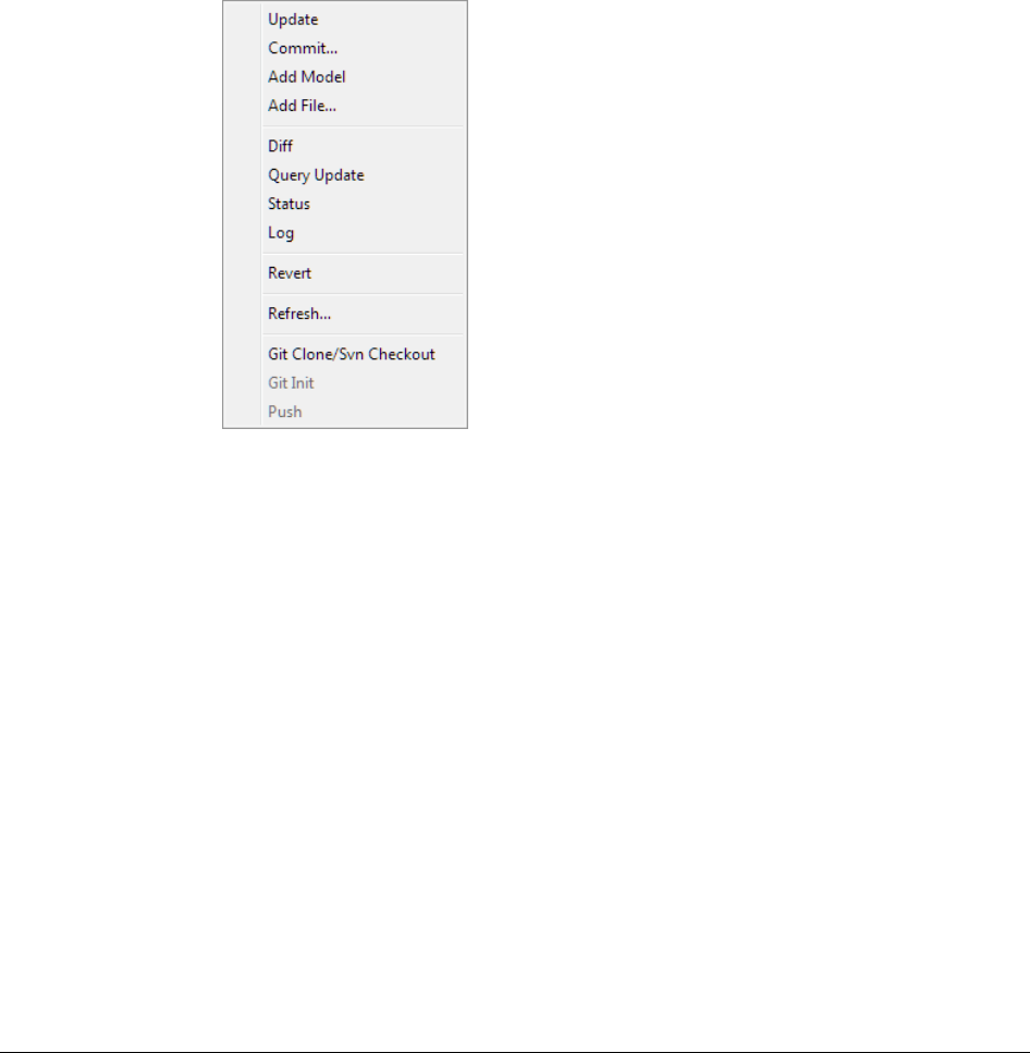
130
4.1.5 Supported features
Dymola provides a graphical user interface to the most basic CVS, SVN, and Git commands,
where the principal automatic step is to provide the correct file name in which the model the
user is located.
The primary commands which can be reached using File > Version are (in CVS
terminology):
Update
Updates your local copy of the file with changes from the repository. If your file has been
changed since it was last updated, your changes are merged with the changes made to the
repository. After a successful update the file is reloaded into Dymola.
If conflicts arise during the merge, this is noted in the message window, and the file is not
reloaded into Dymola.
See section “Query Update” on page 131 for an explanation of the status code displayed in
the message window.
For Git the Update command works as the Git command Pull.
Commit...
Updates the repository with changes you have made in your local file. Your file is first
checked to make sure that you have an up-to-date copy. You are then asked to enter a
description of the changes, which is later available through the Log command.
Note that for Dymola 2017 and later, SVN and Git commits the entire directory, not specific
files.

4 MODEL MANAGEMENT 131
Add Model
Makes a new model’s file known to the underlying version management system. The user
must then perform a Commit on the model.
Add File...
Makes an arbitrary file known to the version management system. The user must select the
file using a file browser.
Diff
Displays the textual differences between your local file and the corresponding version in the
repository.
Query Update
Displays which files in the model's directory are
• Locally modified compared to the corresponding version in the repository (marked by
“M” before the filename).
• Changed in the repository compared to the version that was checked out (“U” or “P”).
• Caused a conflict during an Update operation, or which could potentially create a
conflict because it is both locally modified and changed in the repository (“C”).
• Added but not yet committed (“A”).
• Unknown to the version management system (“?”).
Local files are not updated. The repository is not changed.
Status
Displays version status of the file. The information includes:
• If the file is up-to-date, needs an Update, or has been locally changed.
• Revision of your local file and the repository file.
• A list of all symbolic tags and which revisions they refer to.
Log
Displays log messages which were entered every time the file was committed, and a list of
all symbolic tags and which revisions they refer to
Revert
Deletes your local file and retrieves the latest version from the repository. All changes to
your local file are lost.
All version management systems operate on files. An environment which would allow
version management of individual models even when several models are stored in the same
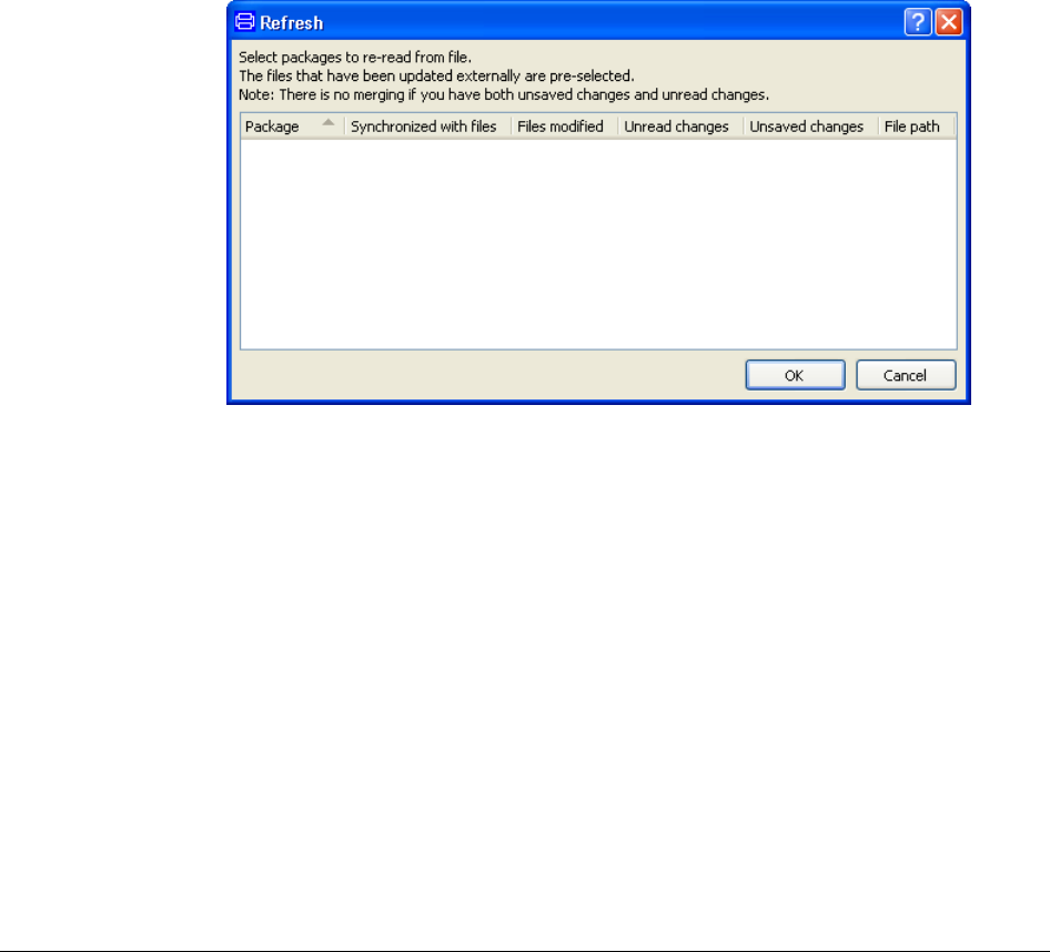
132
file could be implemented on top of external tools, but would be quite complex. However,
Dymola can easily map from model to the corresponding filename, and also knows when a
model is part of a larger package comprising several files (in which case updates probably
should be made on all files).
Also note that CVS can update special “keywords” in the Modelica text, which can be used
to automatically insert information in the model documentation. They include version
number, date of last change, and a log describing all changes. An example of this is given
below.
Refresh…
The command can be used to refresh selected files. A menu is displayed:
Git Clone/Svn Checkout
See section “Short guide to version management with new features included” starting on
page 149.
Git Init
See section “Short guide to version management with new features included” starting on
page 149.
Push
Git command, commits to remote Git repository. For Git Pull, see the Update command
above.
Conflict handling after update
If several users have modified the file, the “update” command will attempt to merge the
changes. If they have modified the same lines of code, CVS will detect a conflict. After a
conflict the original modified file is kept as backup, and the merged file contains both sets

4 MODEL MANAGEMENT 133
of changes marked by special indicators inserted into the text. It is then up to the user to
resolve the conflicts.
An important issue here is that Dymola cannot use the file until conflicts have been resolved.
Initially we do nothing, i.e., require that the user edits the Modelica file with some external
text editor to delete conflicting lines and their indicators. At some future point in time
Dymola could be extended to parse Modelica text with CVS conflict indicators, and the
resolution could be handled from within Dymola (which of course has better support for
analyzing the conflicts). An intermediate step is to rename the file with conflicts and restore
the backup; this will at least maintain consistency between the Dymola environment
internally and the corresponding file externally.
It should be noted that merge conflicts arise from a people management problem, and are
rare in practice. Normally people working on a project do not edit the same code.
Version management of non-model files
The discussion of version management is naturally focused on Modelica code, but the
facilities also handle parameter sets, experiments and trajectories in large projects.
Parameter sets and experiments can be represented by Modelica models. In this case the
experiment extends from the top-level model and provides experiment-specific parameters
through modifiers of the extends clause. An alternative is to set up the experiment with a
Modelica script file (extension .mos). Trajectories are represented by binary files
(extension .mat).
Files which are not Modelica text can be stored in hierarchical Modelica packages. These
files are added to the repository using the Add File... command. Operations performed on
the package will then also operate on the contained .mos and .mat files. Operations
supported include Update, Commit and Status.
4.1.6 Selecting version management system
Dymola supports three version control systems, CVS, SVN, and Git, and generates the
appropriate external commands to perform operations on the version control system. Which
system is used is set in Edit > Options… > Version.
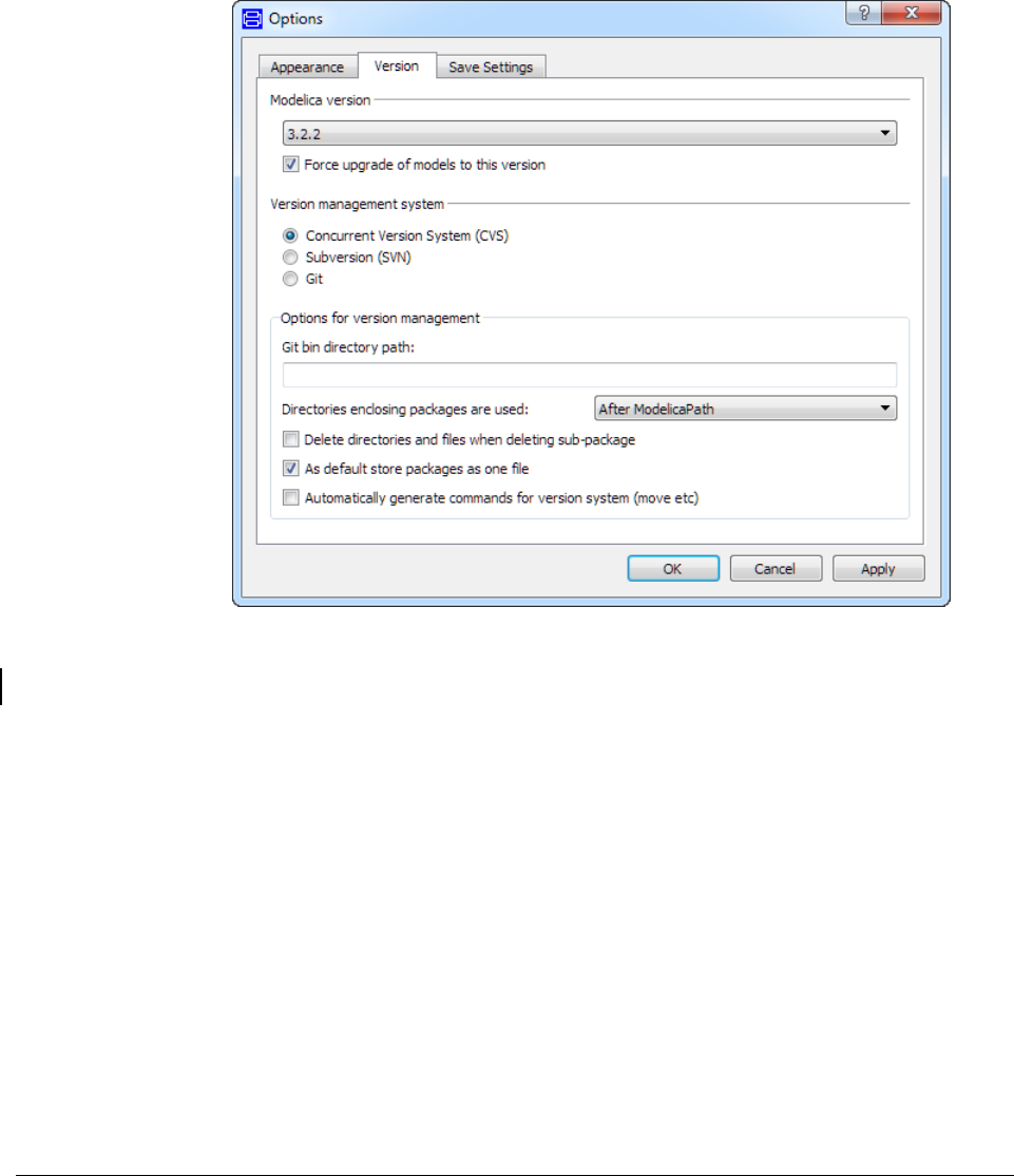
134
For options for versions management, see section “Short guide to version management with
new features included” starting on page 149.
The settings for version management system are stored between sessions.
4.1.7 Version management using CVS
Version management support in Dymola assumes that there exists a functional CVS
environment. In its simplest form there exists a CVS repository on a local disk. More
advanced installations maintain a CVS server on a separate UNIX system; one such setup is
the use of the SourceForge server to maintain the Modelica standard library. Two examples
are given below.
It is worth pointing out that Dymola and the underlying CVS system supports development
of libraries maintained at several different servers concurrently. For example, the Modelica
standard library may be maintained at SourceForge, other libraries proprietary to the
company, and still others by the user on a local disk. In this fashion version management
also facilitates effective distribution of updates as they become available from the vendor.
Setting version
management system.

4 MODEL MANAGEMENT 135
Location of the CVS command
Note: in several places the user is asked to execute the CVS command. The file cvs.exe is
located in the Dymola distribution, typically \dymola <version>\bin. A command for
initialization of a repository directory CVS_Repository with the full path written might be
e.g.
"C:\Program Files (x86)\Dymola 2018\bin\cvs" –d \CVS_Repository
init
In order to avoid long paths the path to cvs.exe (in this case C:\Program Files
(x86)\Dymola 2018\bin) can be added to the environment variable PATH. This is done
the following way:
• Use the Windows Start Button, select Control Panel and then System.
• Select the Advanced tab, click on the Environment Variables button.
• In the System Variables pane, select the variable Path. Click on Edit.
• Enter a ; to separate from the previous path, and then C:\Program Files
(x86)\Dymola 2018\bin
• Click OK in three consecutive menus.
Please note that a new DOS command window has to be opened after changing the
environment variable!
Now the path can be omitted in the commands. For conciseness we will use that form in the
following; the command above will now be cvs –d \CVS_Repository init.
Local CVS repository
To set up a local CVS repository, first choose the machine and disk on which you want to
store the revision history of the source files. CPU and memory requirements are modest, so
most machines should be adequate.
To create a repository with a set of configuration files, run the “cvs init” DOS command to
set up an empty repository in the designated directory.
mkdir \CVS_Repository
cvs -d \CVS_Repository init
These steps complete the initialization of the CVS repository. The “init” command is careful
to never overwrite any existing files in the repository, so no harm is done if you run cvs init
on an already set-up repository.
Note that if you use a Windows drive letter, you must write a slightly longer repository
specification because the “cvs” command interprets the colon after the drive letter:
cvs -d ":local:c:\CVS_Repository" init
The CVS repository is initially empty. It is necessary to create one or more directories
which act as top-level directories for further development. For example, we may create a
“models” directory:
mkdir \CVS_Repository\models
Location of the CVS
command.

136
To use a CVS repository it is necessary to initially perform a “checkout” operation:
cvs -d \CVS_Repository checkout models
This command creates a “models” sub-directory with all models currently stored in the
corresponding top-level directory in the CVS repository. It also creates extra directories
called “CVS” at each level, which are used to maintain CVS status information. The files
inside the “CVS” directories should never be manipulated by hand.
Access to servers via CVS
Projects maintained at SourceForge (http://www.sourceforge.net) or other servers can be
accessed via CVS. To access a Modelica area via CVS, you set up your CVSROOT when
the files are initially checked out, and do a “cvs login” with an empty password. After that
the usual CVS commands work as expected.
If you work against a single CVS repository it may be convenient to set the CVSROOT
environment variable to the value below, as an alternative to using the -d command line
switch:
:pserver:anonymous@myproject.sourceforge.net:/cvsroot/modelica
To use it you must first login and then check out using these DOS commands:
cvs login // enter password
cvs checkout models // check out models library
These will checkout a Modelica library in the current directory.
4.1.8 An example of file management using CVS
In this example we will demonstrate the basic version management operations provided by
Dymola. It is divided into several different steps to setup a local CVS repository, to create a
new model, and to make changes to an existing model.
Setting up the CVS repository
A local CVS repository is set up (we choose to start from the directory C:\MyWorkspace
in this example and we assume Dymola 2018\bin to be located according to the path used
below), and then a new top-level directory called “models” is created. Finally the new top-
level directory needs to be checked out in the current working directory.
Execute these DOS commands in the directory C:\MyWorkspace:
mkdir \CVS_Repository
"C:\Program Files (x86)\Dymola 2018\bin\cvs" –d \CVS_Repository
init
mkdir \CVS_Repository\models
"C:\Program Files (x86)\Dymola 2018\bin\cvs" –d \CVS_Repository
checkout
models
The first command creates an empty folder CVS_Repository at the root level
(C:\CVS_Repository).
DOS commands.

4 MODEL MANAGEMENT 137
The second command declares the folder CVS_Repository as a CVS repository and
creates a folder CVSROOT inside it. (Inside that folder a number of files are created that are
used by the cvs system.).
The third command creates an empty folder models in the folder CVS_Repository – the
resulting folder is C:\CVS_Repository\models. (This is one of the few cases when the
user tampers with the CVS_Repository folder - when the folder system for the cvs handling
is created.)
The forth command will give the answer cvs checkout: Updating models. The
command creates a (very specific) copy of the folder models in the folder MyWorkspace
(the result is C:\MyWorkspace\models). Please note that inside this folder a new folder
CVS is created. This folder is part of the cvs handling – each folder that contains files that
should be handled by the cvs system will contain such a folder! This folder should never be
tampered with.
The result of these commands is that we have a folder C:\MyWorkspace\models where
we should put the Dymola models that we create. This folder is handled by the cvs system,
so cvs commands can be applied to the files inside it.
(Shorter paths in the commands above can be used if the environment variable PATH has
been modified; please see above.)
Creating a new model
We can start by creating a model in Dymola and saving it in the
C:\MyWorkspace\models folder (not in C:\CVS_Repository\models!). For our
example we will use the simple model:
model Decay
Real x(start=2);
equation
der(x) = -x;
end Decay;
Initially the model is unknown to the version management system. For example, using the
command File > Version > Status returns this information in the message window:
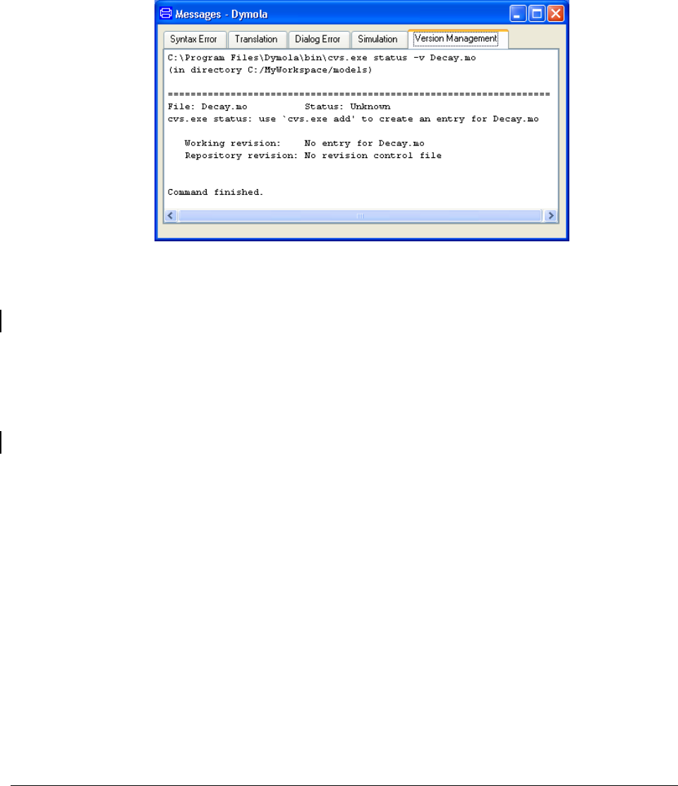
138
Next we perform the command File > Version > Add Model to make the model’s file
known to the version management system. The message in the Message window will be the
following:
C:\Program Files (x86)\Dymola 2018\bin\cvs.exe add Decay.mo
(in directory C:/MyWorkspace/models)
cvs.exe add: scheduling file `Decay.mo' for addition
cvs.exe add: use 'cvs.exe commit' to add this file permanently
Command finished.
The information from the command File > Version > Status is now different, but there is no
file in the repository yet (not until we commit the file).
C:\Program Files (x86)\Dymola 2018\bin\cvs.exe status -v
Decay.mo
(in directory C:/MyWorkspace/models)
============================================================
File: Decay.mo Status: Locally Added
Working revision: New file!
Repository revision: No revision control file
Sticky Tag: (none)
Sticky Date: (none)
Sticky Options: (none)
Command finished.
When we perform File > Version > Commit..., the user is asked to enter a log message
describing what changes are committed. The lines beginning with CVS are generated to
help us remember the nature of the commit.
This is the first version of our test example.
CVS: -------------------------------------------------------
CVS: Enter Log. Lines beginning with `CVS:' are removed
automatically
CVS: Added Files:
Information in the
Message window.
Informaton in the
Message window.
Informaton in the
Message window.
Informaton in the
Message window.

4 MODEL MANAGEMENT 139
CVS: Decay.mo
CVS: -------------------------------------------------------
When having entered the log message, save the changes using File > Save or Ctrl + S, then
close the window.
The message after the commit operation has finished looks like this:
C:\Program Files (x86)\Dymola 2018\bin\cvs.exe commit Decay.mo
(in directory C:/MyWorkspace/models)
RCS file: \CVS_Repository/models/Decay.mo,v
done
Checking in Decay.mo;
\CVS_Repository/models/Decay.mo,v <-- Decay.mo
initial revision: 1.1
done
Command finished.
The output from File > Version > Status now contains more information, in particular the
version number of the file and the date it was last changed in the repository.
C:\Program Files (x86)\Dymola 2018\bin\cvs.exe status -v
Decay.mo
(in directory C:/MyWorkspace/models)
============================================================
File: Decay.mo Status: Up-to-date
Working revision: 1.1 Fri Oct 04 09:34:02 2005
Repository revision: 1.1 \CVS_Repository/models/Decay.mo,v
Sticky Tag: (none)
Sticky Date: (none)
Sticky Options: (none)
Existing Tags:
No Tags Exist
Command finished.
It is also possible to view the change log with File > Version > Log. The change log
contains all messages entered during commit operations.
C:\Program Files (x86)\Dymola 2018\bin\cvs.exe log Decay.mo
(in directory C:/MyWorkspace/models)
RCS file: \CVS_Repository/models/Decay.mo,v
Working file: Decay.mo
head: 1.1
branch:
locks: strict
access list:
symbolic names:
keyword substitution: kv
total revisions: 1; selected revisions: 1
description:
----------------------------
revision 1.1
date: 2005/10/04 09:34:02; author: Dag; state: Exp;
This is the first version of our test example.
============================================================
Command finished.

140
The output from both File > Version > Status and File > Version > Log contain
information specific to the underlying CVS system, which is beyond the scope of this report.
For non-expert users it would be beneficial to filter the raw output.
Changing an existing model
Starting with the model created above, we now modify it by adding a time constant Ti. The
revised Modelica text looks like this:
model Decay
Real x(start=2);
parameter Real Ti=1;
equation
der(x) = -x/Ti;
end Decay;
After changing the model it must be saved using File > Save.
The File > Version > Diff command will display the differences between the model stored in
the repository and the current model. Changed lines are indicated by “!”, added lines by “+”
and any removed lines by “-” (this is the so-called “context diff” format).
C:\Program Files (x86)\Dymola 2018\bin\cvs.exe diff -c Decay.mo
(in directory C:/MyWorkspace/models)
Index: Decay.mo
============================================================
RCS file: \CVS_Repository/models/Decay.mo,v
retrieving revision 1.1
diff -c -w -r1.1 Decay.mo
*** Decay.mo 2005/10/04 09:34:02 1.1
--- Decay.mo 2005/10/04 09:43:12
***************
*** 1,6 ****
within ;
model Decay
Real x(start=2);
equation
! der(x) = -x;
end Decay;
--- 1,7 ----
within ;
model Decay
Real x(start=2);
+ parameter Real Ti=1;
equation
! der(x) = -x/Ti;
end Decay;
Command finished.
The File > Version > Query Update command is used to quickly list which files have been
locally modified (indicated by “M”) or need to be updated from the repository (“U”). Files
that are not included in the version handling will be marked with “?”.
C:\Program Files (x86)\Dymola 2018\bin\cvs.exe -qn update
(in directory C:/MyWorkspace/models)

4 MODEL MANAGEMENT 141
M Decay.mo
? dsin.txt
Command finished.
The File > Version > Query Update command does not operate only on the file of the
model. Instead it operates on the entire directory and all sub-directories; this makes it
particularly useful to concisely review the status of all files in a complex model hierarchy.
The model is then committed to the repository with File > Version > Commit, as shown
above. If we review the log with File > Version > Log, we see that the new revision
comment is also listed. The listing also shows the number of changed Modelica text lines.
C:\Program Files (x86)\Dymola 2018\bin\cvs.exe log Decay.mo
(in directory C:/MyWorkspace/models)
RCS file: \CVS_Repository/models/Decay.mo,v
Working file: Decay.mo
head: 1.2
branch:
locks: strict
access list:
symbolic names:
keyword substitution: kv
total revisions: 2; selected revisions: 2
description:
----------------------------
revision 1.2
date: 2005/10/04 09:44:57; author: Dag; state: Exp; lines:
+2 -1
Added time constant Ti.
----------------------------
revision 1.1
date: 2005/10/04 09:34:02; author: Dag; state: Exp;
This is the first version of our test example.
============================================================
Command finished.
This concludes the demonstration of how models are edited in co-operation with the version
management facilities in Dymola.
Use of revision information
The underlying CVS system supports expansion of particular keywords, for example to
automatically document the revision or commit date of the model. We could for example
enter this text in the revision part of the documentation layer of our model:
<PRE>
Model revision: $Revision$
Last changed: $Date$
Change log:
$Log$
</PRE>
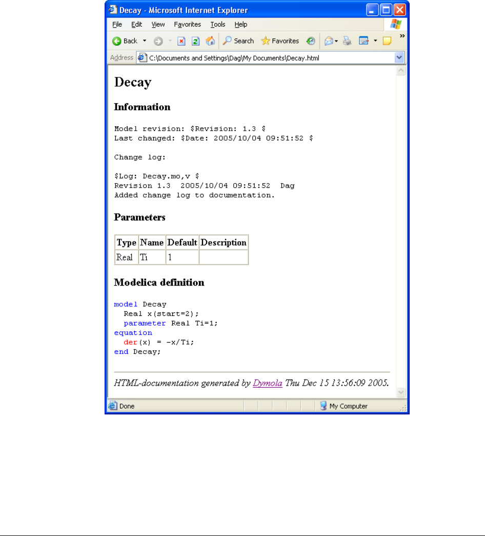
142
The keywords indicated by $ will be expanded at the next commit operation. Since this
means that the committed file actually will be changed due to the expansion of the keywords,
the local copy needs to be updated after the commit. The result after an update is shown in
the following example of HTML documentation:
4.1.9 Version management using SVN
Version management support in Dymola assumes that there exists a functional SVN
(subversion) environment. In its simplest form there exists a SVN repository on a local disk.
More advanced installations maintain a SVN server on a separate UNIX system.

4 MODEL MANAGEMENT 143
It is worth pointing out that Dymola and the underlying SVN system supports development
of libraries maintained at several different servers concurrently. For example, the Modelica
standard library may be maintained at svn.modelica.org, other libraries proprietary to the
company, and still others by the user on a local disk. In this fashion version management
also facilitates effective distribution of updates as they become available from the vendor.
Some SVN operations require input from the user, for example a log message when a file is
committed. To enable this feature the user must set either of the environment variables
SVN_SETUP, EDITOR or VISUAL to the name of a text editor. Windows “notepad” will
be sufficient for most uses.
Note: in several places the user is asked to execute SVN commands. The files svn.exe and
svnadmin.exe should be available from the Windows Command Prompt or Dymola
command input line if you have performed the default installation of SVN (see section
“References” on page 151). Please also see the example below.
Local SVN repository
To set up a local SVN repository, first choose the machine and disk on which you want to
store the revision history of the source files. CPU and memory requirements are modest, so
most machines should be adequate.
To create a repository with a set of configuration files, run the “svnadmin create” DOS
command to set up an empty repository in the designated directory. For example,
svnadmin create \SVN_Repository
The SVN documentation suggests that you populate the repository with three directories
called ”branches”, ”tags” and ”trunks”. The easiest way to do that is to create these
directories locally and then import them:
mkdir models
cd models
mkdir branches
mkdir tags
mkdir trunk
cd ..
svn import models file:///SVN_Repository/models -m "Initial
import"
A user name might be requested after the last command. An empty one might be sufficient.
SVN will report that it has imported the directories as revision 1. It is worth noting that
SVN manages directories as well as files, whereas CVS only manages files directly and
implicitly creates directories as needed.
These steps complete the initialization of the SVN repository. Remove the local “models”
directory to start over.
rmdir /s models
To use a SVN repository it is necessary to initially perform a “checkout” operation to create
a local copy with files that can be modified
svn checkout file:///SVN_Repository/models/trunk models
SVN editor setup.
Location of the SVN
command.
DOS command.
DOS commands.
DOS command.
DOS commands.

144
This command creates a “models” sub-directory with all models currently stored in the
corresponding top-level directory in the SVN repository. It also creates extra directories
called “.svn” at each level, which are used to maintain SVN status information. The files
inside the “.svn” directories should never be manipulated by hand.
4.1.10 An example of file management using SVN
In this example we will demonstrate the basic version management operations provided by
Dymola. The example shows the first steps from the CVS-based example above.
Please note that a SVN client must be downloaded and installed first. We assume that this is
done. Dymola must be restarted afterwards since the environment variable PATH is
modified by the installation. The same goes for any Windows Command Prompt. (If the
DOS commands do not work check that the path to svn.exe has been added to the
environment variable PATH. For handling of the environment variable PATH, please see
section “Location of the CVS command” on page 135. The handling is analogue but this
path is of course different.
Please note that the location when executing the DOS commands should be the directory
C:\MyWorkspace if the example should be the same as the CVS example above. We use a
directory “testmodels” instead of “models” in this example.
Of course SVN must be selected in Dymola as the system to use, please see section
“Selecting version management system” on page 133.
We must define an environment variable that defines the text editor to use. We choose to
use notepad, and choose to define this in the EDITOR environment variable. Please see the
section “Location of the CVS command” on page 135 for a description how to edit
environment variables in MS Windows.
Now setup the SVN repository with initial directories, remove the initial local models
directory and check it out. In this example the DOS commands (we assume being in the
directory C:\MyWorkspace) would be (please note that the svn import command is so long
that two lines are needed in the print below):
svnadmin create \SVN_Repository
mkdir testmodels
cd testmodels
mkdir branches
mkdir tags
mkdir trunk
cd ..
svn import testmodels file:///SVN_Repository/testmodels -m
"Initial import"
rmdir /s testmodels
svn checkout file:///SVN_Repository/testmodels/trunk testmodels
The first command creates a folder SVN_Repository at the root level
(C:\SVN_Repository). The folder contains a number of folders and files and will work as
the repository. This folder should not be manipulated directly by the user.
The second command creates an empty folder testmodels at the MyWorkspace level. The
resulting folder will be C:\MyWorkspace\testmodels.
DOS commands.

4 MODEL MANAGEMENT 145
The third command changes the directory of where the commands are given in the DOS
window (the location) to C:\MyWorkspace\testmodels.
The fourth, fifth and sixth command creates three empty folders (branches, tags and
trunks) at this level – as example the first command will create the folder
C:\MyWorkspace\testmodels\branches.
The seventh command changes the directory of where the commands are given in the DOS
window (the location) to C:\MyWorkspace.
The eight command (occupying two lines above) imports the directory structure consisting
of the folder testmodels and the folders inside it to the SVN repository (please note that
there has to be a space before “Initial import”). The visible result of the command will be an
answer that folders have been added and that the first version is archived. (The folder
structure inside C:\SVN_Repository will however not be changed, the folder structure is
handled differently in SVN compared to CVS.)
The ninth command removes the folder testmodels and including folders from the
directory C:\MyWorkspace. The structure was imported into the SVN system and is not
needed anymore. (Please compare with the next command.) You have to answer Y to
acknowledge that the command should be executed.
The last command checks out the folder testmodels and including folders. The folder
C:\MyWorkspace\testmodels will be recreated (however without the three previous
folders inside). This folder is now included in the SVN version handling! This might be
seen looking at the folder using explorer – the folder has a sign on it. Looking inside the
folder a folder .svn is present. This folder should not be tampered with.
The result of these commands is that we have a folder C:\MyWorkspace\testmodels
where we should put the Dymola models that we create. This folder is handled by the svn
system, so svn commands can be applied to the files and folders inside it.
Let us assume that we entered username “Dag” when importing the folder testmodels in
one of the commands above.
Creating a new model
We can start by creating a model in Dymola and saving it in the testmodels directory. For
our example we will use the simple model:
model Decay
Real x(start=2);
equation
der(x) = -x;
end Decay;
Store the model in C:\MyWorkspace\testmodels. Initially the model is unknown to the
version management system. For example, a File > Version > Status command returns this
information in the message window:
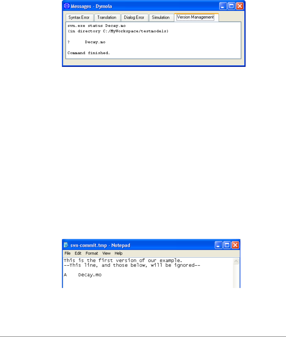
146
Next we perform the File > Version > Add Model command to make the model’s file
known to the version management system. The system will respond with the message:
svn.exe add Decay.mo
(in directory C:/MyWorkspace/testmodels)
A Decay.mo
Command finished.
We can now perform a File > Version > Query Update command to get some more
information. The system will respond with the message:
svn.exe status –verbose --show-updates
(in directory C:/MyWorkspace/testmodels)
A 0 ? ? Decay.mo
1 1 Dag .
Status against revision: 1
Command finished.
“Dag” is the name user name entered when executing the DOS commands above.
When we perform File > Version > Commit..., the user is asked to enter a log message
describing what changes are committed. Since we use notepad, the window after entering
the comment might look like:
The lines at the end (starting with “--This line”) are generated by SVN to help us remember
which file is committed. After the text has been entered (e.g. like the first line in the window
above) save the changes using File > Save or Ctrl + S, then close the window.
The message after the commit operation has finished looks like this:
Information in
Message window.
Inserting a commit
comment.

4 MODEL MANAGEMENT 147
svn.exe commit Decay.mo
(in directory C:/MyWorkspace/testmodels)
Adding Decay.mo
Transmitting file data .
Committed revision 2.
Command finished.
It is also possible to view the change log with File > Version > Log. The change log
contains all messages entered during commit operations.
svn.exe log Decay.mo
(in directory C:/MyWorkspace/testmodels)
------------------------------------------------------------
r2 | Dag | 2005-12-15 11:59:22 (Thu, 15 Dec 2005) | 2 lines
This is the first version of our example.
------------------------------------------------------------
Command finished.
The output from both File > Version > Status and File > Version > Log contain
information specific to the underlying SVN system, which is beyond the scope of this report.
For non-expert users it would be beneficial to filter the raw output.
Changing an existing model
Changing the model follows the same pattern as for the CVS-based example above. The
main difference is that SVN log message are different from those produced by CVS.
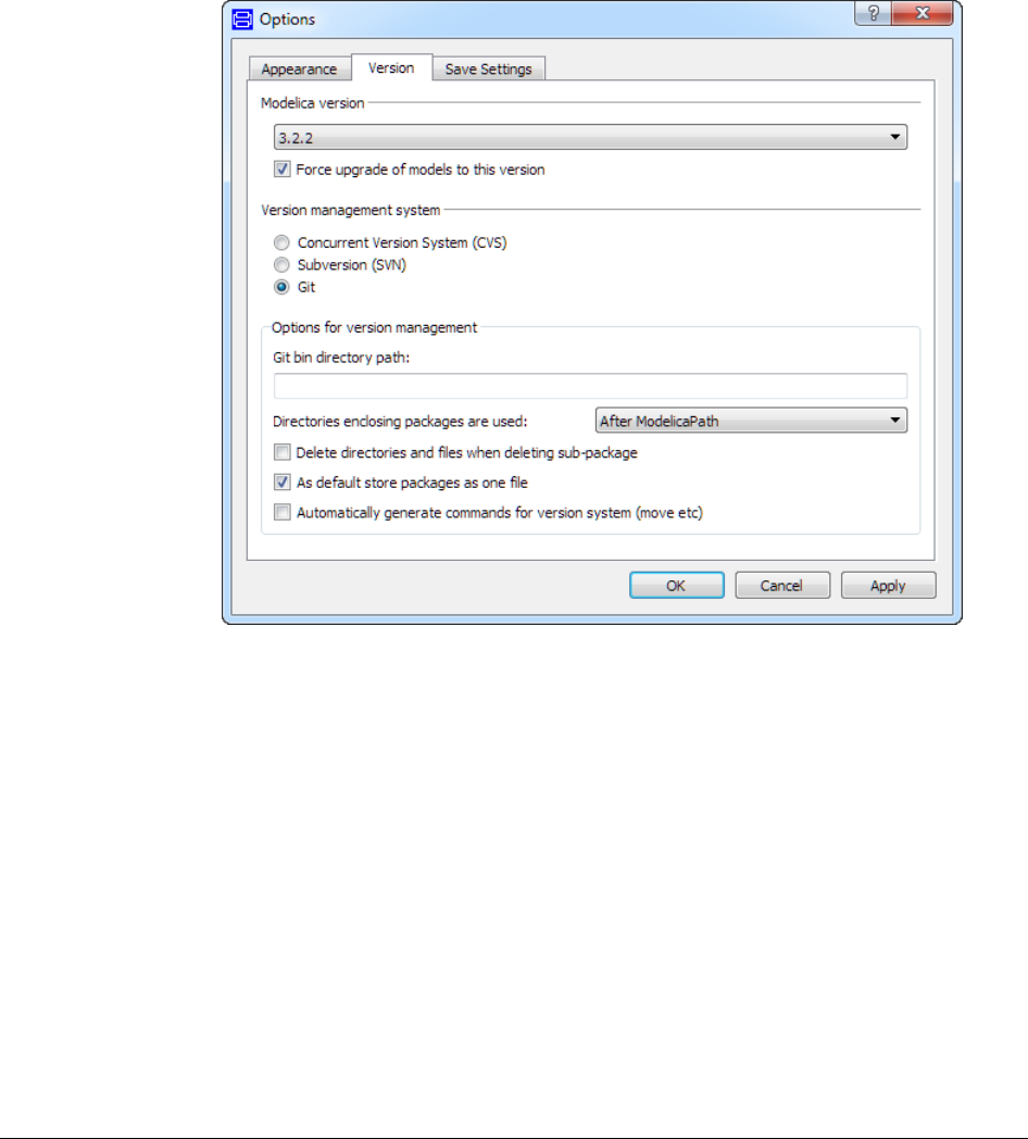
148
4.1.11 Version management using Git
Dymola 2017 and later supports Git. Git can be selected as version management system by
ticking Git in the Version tab reached by the command Edit > Options…
The command File > Version displays the available Git commands:
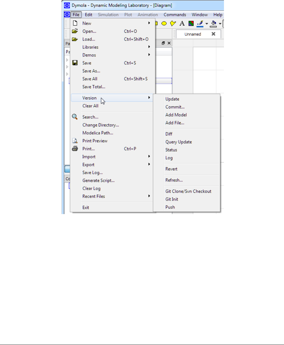
4 MODEL MANAGEMENT 149
4.1.12 Short guide to version management with
new features included
To sum up the improvements in version management for Dymola 2017 and later, the
following is a short guide to get started with version management in Dymola; in order to
keep track of changes during development.
The guide assumes that you are already familiar with the basics of version management.
Note that the terminology differs between different systems.
The steps are:
1. Figure out which version management you already are using – or going to use (in
the latter case we do not recommend CVS). Select this in Edit > Options >
Version. For Git you also have to provide the path to the bin-directory. In case you
use an unsupported system or do not want to use the support in Dymola go to step
3.

150
2. Now you need a local copy of a repository of changes. If you do not already have
one:
a. In most cases there is an existing repository for changes stored on a server
(or you create one first) – use File > Version > Git Clone/Svn Checkout
to connect to it. The first line is the URL – for example
https://github.com/HansOlsson/GitModelicaTest.git for git or
https://svn.modelica.org/projects/Modelica/trunk for svn. The second line
is only needed if you want to give the local copy a different name.
b. To experiment you can create a local repository – but you should move to
a server later on. For svn follow the instructions in
https://tortoisesvn.net/docs/nightly/TortoiseSVN_en/tsvn-qs-guide.html –
and use a file-url. For git just use File > Version > Git Init.
c. If you are starting a new project: plan ahead – e.g. have a directory
containing your library even if there is initially only one; and do not use
the version number in the path (so name your directory ”MyLibrary” not
“MyLibary 1.2.0” – and use a better name than “MyLibrary”).
3. We now recommend some important changes of settings in Edit > Options >
Version: The first three options below can also be used without using a version
management system in Dymola.
a. If you use version management for more than one related package they
are normally versioned and stored together. A simple alternative is to just
open one of them and rely on Edit > Options > Directories enclosing
packages are used: “Before ModelicaPath”. The default “After
ModelicaPath” also works, except if you are developing a library already
present in Dymola (such as Modelica Standard Library). Another
alternative would be to add the directory containing those libraries to
ModelicaPath using File > Modelica Path; and store the setting using Edit
> Options > Save Settings > Modelica Path; the benefit is that you can
add entries in File > Libraries.
b. Dymola normally creates backup files for deleted mo-files. With a version
management system that is not needed, so: enable Edit > Options >
Version > Delete …
c. For version management it is usually preferable to have a finer granularity
so that each model is stored in its own file. Disable Edit > Options > As
default store packages as one file. (Note: Some classes cannot be stored
in a separate file, and this only controls the default for each package you
create later on.)
d. For version management you want to keep track of files being added,
moved, and deleted automatically. Enable Edit > Options > Version >
Automatically… This applies both to model-files and images added for
equations in the documentation layer. Note: This option does not work for
CVS, and must be enabled already when you add/rename/delete the class
and is executed when you save your library. This also changes save to
always saving entire libraries, not just individual files. If you rename a

4 MODEL MANAGEMENT 151
package (stored as directory) – please save before renaming any classes
inside it. You can also add files manually using File > Version > Add file.
4. You can either use Dymola’s commands in File > Version or an external tool for
seeing your changes.
4.1.13 References
The primary reference to the CVS version management system is
• Per Cederqvist et al. (1993): “Version Management with CVS”.
CVS binaries for several platforms and documentation (including Cederqvist et al.) are
available for downloading from the official CVS homepage:
http://www.cvshome.org/
The primary source on Subversion is the homepage. The SVN command line tools used by
Dymola are available here.
http://subversion.tigris.org/
Graphical user interfaces to SVN are available for downloading. Two of the more popular
are TortoiseSVN (an extension to Windows Explorer)
http://tortoisesvn.tigris.org/
and RapidSVN
http://rapidsvn.tigris.org/
which is a free-standing application.
4.2 Model dependencies
Dymola can export documentation of models and packages in HTML format. The HTML
documentation contains information extracted from Modelica classes. For example, model
parameters and functions inputs and outputs are tabulated for easy reading without any need
to understand the Modelica text.
Dymola can also make tables of cross-references in HTML. Such a table clearly shows
dependencies to other packages, and in some cases incorrect references can be found. The
following is an example from the package Modelica.Blocks.Examples:
152
These classes have been referenced in this package.
Class
Referenced From
Modelica.Blocks.Continuous.CriticalDamping
InverseModel
Modelica.Blocks.Continuous.FirstOrder
InverseModel
Modelica.Blocks.Continuous.Integrator
PID_Controller
Modelica.Blocks.Continuous.LimPID
PID_Controller
Modelica.Blocks.Examples.BusUsage_Utilities.Part
BusUsage
Modelica.Blocks.Examples.BusUsage_Utilities.Interfaces.ControlBus
BusUsage
Modelica.Blocks.Logical.And
LogicalNetwork1
Modelica.Blocks.Logical.Not
LogicalNetwork1
Modelica.Blocks.Logical.Or
LogicalNetwork1
Modelica.Blocks.Logical.Pre
LogicalNetwork1
Modelica.Blocks.Math.Feedback
InverseModel
Modelica.Blocks.Math.Gain
BusUsage
Modelica.Blocks.Math.InverseBlockConstraints
InverseModel
Modelica.Blocks.Sources.BooleanConstant
ShowLogicalSources
Modelica.Blocks.Sources.BooleanExpression
ShowLogicalSources
Modelica.Blocks.Sources.BooleanPulse
ShowLogicalSources
Modelica.Blocks.Sources.BooleanStep
BusUsage, ShowLogicalSources
Modelica.Blocks.Sources.BooleanTable
LogicalNetwork1,
ShowLogicalSources
Modelica.Blocks.Sources.IntegerStep
BusUsage
Modelica.Blocks.Sources.KinematicPTP
PID_Controller
Modelica.Blocks.Sources.SampleTrigger
ShowLogicalSources
Modelica.Blocks.Sources.Sine
BusUsage, InverseModel
Modelica.Mechanics.Rotational.Components.Inertia
PID_Controller
Modelica.Mechanics.Rotational.Components.SpringDamper
PID_Controller
Modelica.Mechanics.Rotational.Sensors.SpeedSensor
PID_Controller
Modelica.Mechanics.Rotational.Sources.ConstantTorque
PID_Controller
Modelica.Mechanics.Rotational.Sources.Torque
PID_Controller
Modelica.SIunits.Angle
PID_Controller
extends Modelica.Icons.Example
BusUsage, InverseModel,
LogicalNetwork1, PID_Controller,
ShowLogicalSources
The column to the left shows all classes that have been referenced, for example in import
statements or as the type of a component; extends clauses are specially marked. The column

4 MODEL MANAGEMENT 153
to the right shows the class in this package which contains some kind of reference. To see
what the reference is, click on the link and view the Modelica text.
4.2.1 Cross-reference options
The generation of cross-references is controlled by options in File > Export > HTML..., the
Advanced tab. To be able to select the Advanced tab, Custom must first be selected in the
General tab.
Per file
Generate cross-references to classes in HTML documentation in each HTML-file. This is
typically a sub package in a larger library.
Top level
Generate cross-references to classes in HTML documentation for top-level package.
Because this often is quite large, the cross-references are stored in a separate file which is
liked from the top-level HTML file (near the end).
Full name
Generate HTML cross-references to classes using full name (the default). When checking
consistency of referencing to classes, it may be useful to disable this option, because
inconsistent naming will show up as multiple cross-reference entries.
4.3 Encryption in Dymola
4.3.1 Introduction
There are a number of closed simulation packages on the market where you are not able to
see the details of the models. Modeling is an art in the sense of describing the relevant
aspects of the object under observation. It is thus very important to be able to see what
assumptions and approximation the author of a model made.
Dymola is open to view all and possibly modify the details of models by showing graphical
representations and, if all details are wanted, the Modelica code itself. However, Dymola
also supports concealment of model details, if, for example, a supplier wants to protect
proprietary information when shipping models.
A classical way of protecting software is to distribute only executable programs or object
code and no source code. This approach is not useful for Modelica models. To achieve
robust and efficient simulation, it is important that Dymola can make a global analysis and
manipulation of all equations. It is thus highly desirable to give Dymola access to the
equations in their original form. Encryption of the textual Modelica representation of the
model supports concealment of internal parts such as the equations, while still allowing
Dymola internally to access the equations as if the model was not encrypted.

154
There are also other aspects of protecting models and model libraries. Prevention of
unauthorized modification of models, but still having unrestricted viewing and use is
supported by including checksums. Another aspect of library protection is to ensure
authorized use. In this case, any use of the library is controlled by options in a license file.
4.3.2 Visible and concealed classes
The basic idea of the protection of models is to hide some information while making it
possible to use the model components.
A protected library typically consists of parts that are open, and other parts that are
protected.
Protected parts may require different degree of information hiding, e.g.:
• The model is regarded as a “black box”. The icon, its connectors and parameters as well
as documentation are available to the user to allow use of the model as a component, but
model structure and equations are concealed.
• The model is completely concealed from external use.
Dymola supports concealment by encrypting models or libraries and the use of protected
code sections, and special annotations to allow more information to be revealed. The special
annotations are grouped in “Protection” group (similar to e.g. “Diagram”).
There are several kinds of classes in an encrypted library starting from the most open:
• Example classes that are completely open, such that a user can duplicate it and use it as a
basis for their own work. They can still refer to concealed classes.
• Classes that that can be viewed completely (including the entire Modelica text), but
cannot be copied.
• Classes where the diagram is visible (but not the text).
• Classes where only the interface is visible. (This is the normal case).
• Concealed classes are completely hidden for the users, who shall not be aware of the
existence of such components at all. They are not shown in the package browser and
they cannot be inspected.
A class or a component is defined as concealed if one of these conditions is fulfilled:
• It is declared in the protected section of an encrypted class.
• Its lexically enclosing scope is concealed.
• It has the Protection annotation: hideFromBrowser=true.
Dymola supports encryption on file basis, which means that all parts of an encrypted
package must be stored in one file. Storing an encrypted package in several files or in
subdirectories would reveal structural information. Instead it is possible to reveal the
contents of encrypted packages.

4 MODEL MANAGEMENT 155
4.3.3 Developing encrypted libraries
To allow visible components to be used in the normal way to compose models, set
parameters and initial values, the developer of such components must make a careful design.
The public part must provide all necessary parameters, necessary control of initialization
and variables to inspect and plot. Nested modifiers cannot be used to modify concealed
parameters.
Instead new parameters have to be declared and propagated down the hierarchy. Parameters
for initial conditions need to be introduced and propagated to start values or used in “initial
sections”.
The procedure for developing an encrypted library is:
• The developer maintains an unencrypted library, which is easy to modify and easy to
maintain in a version control system. All parts which should be concealed in the finished
library must be declared as protected or using the protection annotation.
• When the unencrypted library has been finished for release, double-click on the package
to show it in Dymola.
• Select File > Export > Encrypted File… which produces the encrypted file
myPackage.moe.
• The encrypted file, i.e., the .moe file, is distributed. The original .mo files for the
encrypted parts are never distributed outside of the development group.
It is worth pointing out that external decrypting of a .moe file is not supported by Dymola,
but all development work must be performed in the original unencrypted .mo file. In
Dymola all encrypted files are by definition read-only.
4.3.4 Using encrypted components
Dymola must not reveal any concealed information when encrypted components are used to
compose a model and as well as at simulation (unless the library developers has decided
otherwise). It means that some commands or operations are disabled or have modified
effects or results. Also some diagnostics and error messages must be less informative.
Let us first discuss the use of encrypted components in Modeling mode.
File menu
An important and basic restriction is that encrypted components are read-only and cannot be
modified. The File commands Save, Save All, Save As…, and Save Total… are not
available for encrypted components. The Edit > Duplicate command is only available if
duplication is explicitly enabled.
The commands File > Print, File > Export > Image… and File > Export > Animation… are
not changed in the meaning that they output what is visible on the screen.
The command File > Open… reads encrypted files in the usual way, when the file type
“Encrypted Modelica files (*.moe)” is selected. This file-type is visible for all users – not
only the ones who can encrypt models.

156
Package and component browsers
Concealed classes are never shown in the package browser. The component browser does
not show components or extends of a concealed class.
Editor (graphics and text)
Encrypted models are read-only and concealed models are never visible in the editor.
Dymola implements the following restrictions on what is shown in the graphical and textual
layers of the editor.
• The icon layer is empty for concealed classes. Also, it does not show protected
connectors (regardless of encryption). Note that these rules for the icon layer also apply
to icons as they are shown in the diagram layer of some other class.
• The diagram layer is as default empty for encrypted classes (not even public ones).
However, models enclosed in a package called “Examples” or “Tutorial” are shown as
default.
• Modelica text (declarations and equations) is as default empty if the class is encrypted.
• The documentation layer is empty for concealed classes, but is otherwise shown.
The window title says Encrypted instead of Read-Only for all encrypted classes.
Simulation mode
The aim of translating a model is to perform consistency checks and analyze and manipulate
the equations to generate efficient code for simulation. This procedure is not affected by the
fact that components are encrypted or concealed with the following natural modifications:
• Diagnostics and error messages during translation and simulation do as default not
reveal concealed information. Warnings and error messages are issued as for non-
encrypted models, but they may be less informative. An extreme is “Error in
ConcealedEquation”.
• The generated simulation code as default prohibits storing, plotting or other access to
simulation results for concealed variables by the use of their names.
4.3.5 Examples
Encrypted transfer function
To illustrate the basics of using and encrypted model component and how encryption
changes error messages, let us develop a simple encrypted model and use it in some simple
contexts.
The model Modelica.Blocks.Continuous.TransferFunction defines the transfer function
between a scalar input, u, and a scalar output, y. Transfer functions may be realized in
different ways. Assume that we have invented a new good way to realize transfer functions
and that we have developed a new model MyTransferFunction that exploits our ideas. We
have also decided to protect our intellectual property by encrypting the model
MyTransferFunction before making it available to others.
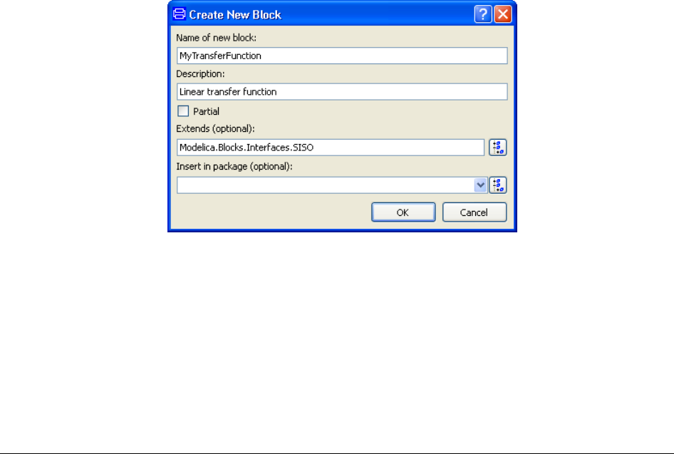
4 MODEL MANAGEMENT 157
The model MyTransferFunction may look like
block MyTransferFunction "Linear transfer function"
extends Modelica.Blocks.Interfaces.SISO;
parameter Real b[:]={1} "Numerator coefficients.";
parameter Real a[:]={1,1} "Denominator coefficients.";
protected
Real x[size(a, 1) - 1] "State";
parameter Integer na=size(a, 1);
parameter Integer nb=size(b, 1);
parameter Integer nx=size(a, 1) - 1;
Real x1dot;
Real xn;
equation
[der(x); xn] = [x1dot; x];
[u] = transpose([a])*[x1dot; x];
[y] = transpose([zeros(na - nb, 1); b])*[x1dot; x];
end MyTransferFunction;
(The easiest way to create such a model for testing is:
1. Create a block using File > New > Block... Extend Modelica.Blocks.Interfaces.SISO.
The dialog will look the following (please note that in order to encrypt this block only it
has to be top level, that is, not inserted into any package – if not the whole package
should be encrypted):
2. (optionally) Copy relevant graphics from the icon layer of
Modelica.Blocks.Continuous.TransferFunction.
3. Enter the code in the Modelica Text layer.
4. Use File > Export > Encrypted File… to encrypt the block.
5. Depending what should be tested below; either MyTransferFunction.mo (not encrypted)
or MyTransferFunction.moe (encrypted) should be opened. Please remember that if
encrypted models should be opened the Files of type must be changed in the file
dialog.)
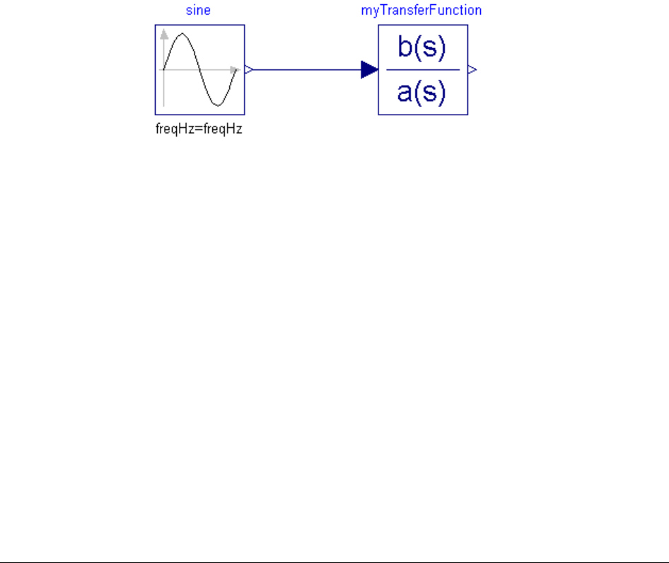
158
The code part is smaller that the corresponding code in the Modelica Standard Library (the
initialization is simplified etc.). However, the important difference for us is that the output.
The model in the Modelica Standard Library, declares the state x in the public sections as
output Real x[size(a, 1) - 1](start=x_start) "State of transfer
function from controller canonical form";
If it is possible to store the time trajectories of x, it is possible to find out how we realize the
transfer function by simulating different transfer functions. In our MyTransferFunction the
state is protected, to prevent users to store, plot or otherwise inspect the simulation results
for the state.
Let us test the model by creating a package MyPackage, and connecting the input to the
source to the sine signal generator of the type Modelica.Block.Sources.Sine. Do not forget
that the encrypted version of MyTransferFunction should be used.
Such a model is built in the usual way by dragging and dropping components and
connecting them together. The encrypted model MyTransferFunction is available in the
package browser for dragging but it cannot be displayed or inspected in the editor. The
connectors are public and thus available for connection. Selecting the component and right-
clicking pops the context menu in the usual way and selecting the alternative Parameters…
displays the parameter window.
Example of use of
encrypted model (TF).
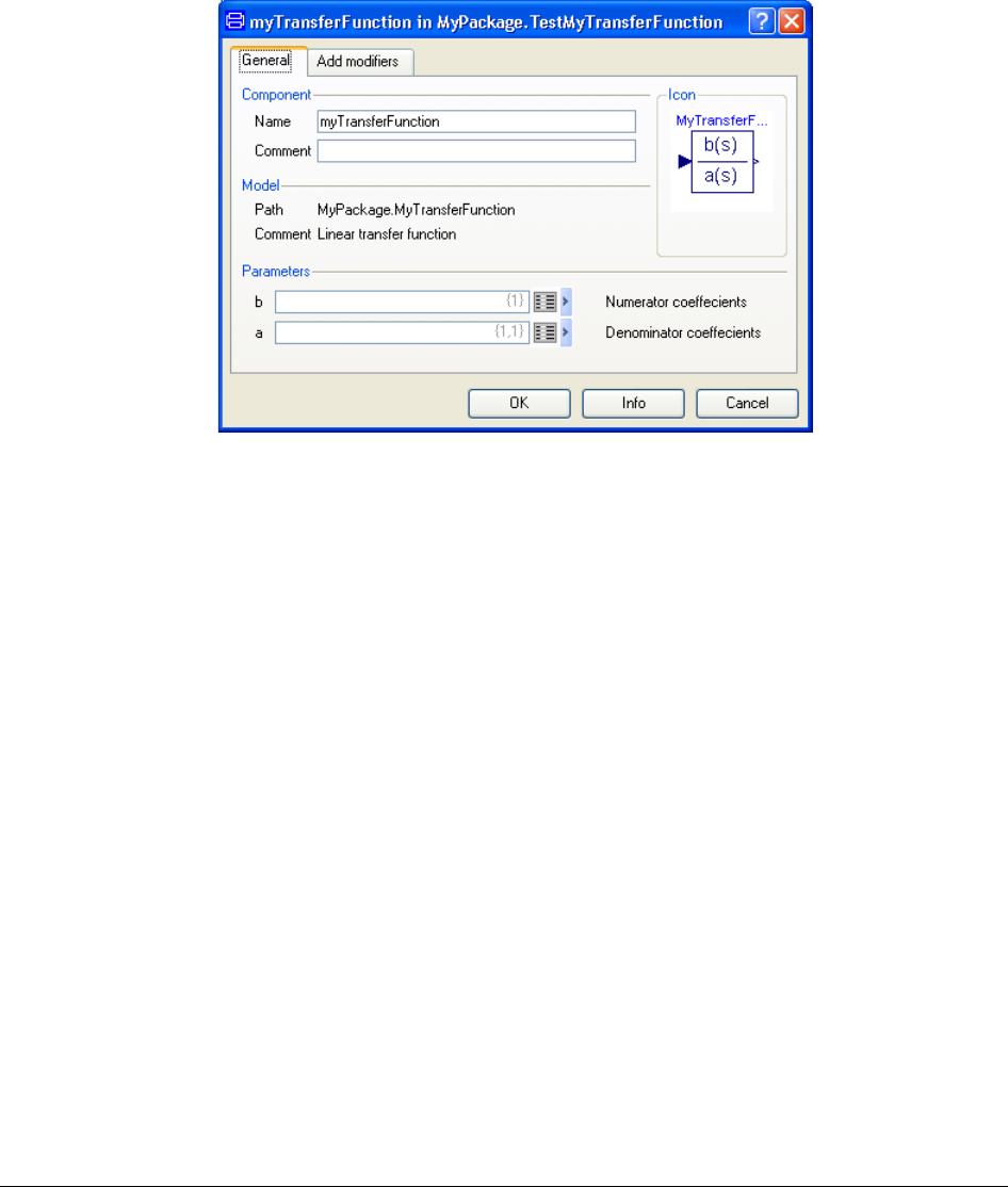
4 MODEL MANAGEMENT 159
and it is possible to enter values for the coefficient parameters. (The parameter dialog looks
the same for the encrypted and un-encrypted model – parameters protected are not shown in
either case.)
The result of a simulation is shown below. Please note that the state x components are not
available in the variable browser (that is the case also for the unencrypted model since the
variables are protected, but for the unencrypted model also protected variables can be shown
in the variable browser by the setting Simulation > Setup… > Output > (Store) Protected
Variables).
Parameters for
component of
encrypted model.
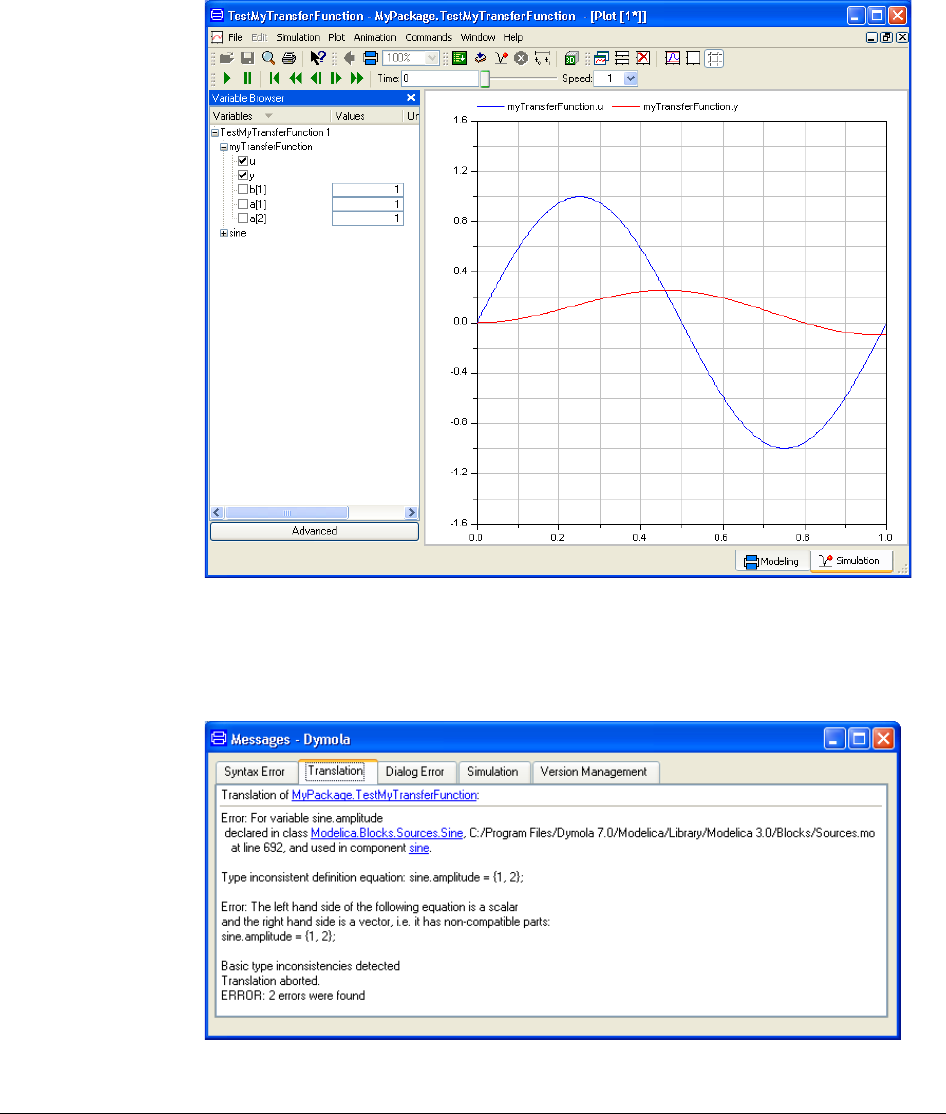
160
The sine generator may produce multiple output signals, while the transfer function assumes
a scalar input. Let us see what happens if we let the sine generator produce two signals. This
can be achieved by setting the value of its parameter amplitude to {1, 2}.
Translation gives the error message
Plot for encrypted
model – concealed
variables are not
selectable.
Error message
containing no sensitive
information.

4 MODEL MANAGEMENT 161
This error message does not reveal any concealed information. In fact the same error
message is given also when MytransferFunction is not encrypted.
MyTransferFunction assumes that the transfer function is proper, i.e. the degree of the
nominator polynomial is equal to or less than the degree of the denominator polynomial. As
shown above the parameter a = {1, 1}. If we set b = {1, 1, 1} and translate, Dymola issues
the error message for the encrypted block:
For a non-encrypted MyTransferFunction the error message is more informative
However, such an error message cannot be output for the encrypted version, because its
reveals concealed information.
Coupled clutches
We will use the example Modelica.Mechanics.Rotational.Examples.CoupledClutches and
exchange components to illustrate various possibilities to provide or conceal information.
Let us make a package ConcealedMechanics where we put the components developed. We
can use the command File > New > Package….
Error message for
encrypted block.
Corresponding error
message for non-
encrypted block.
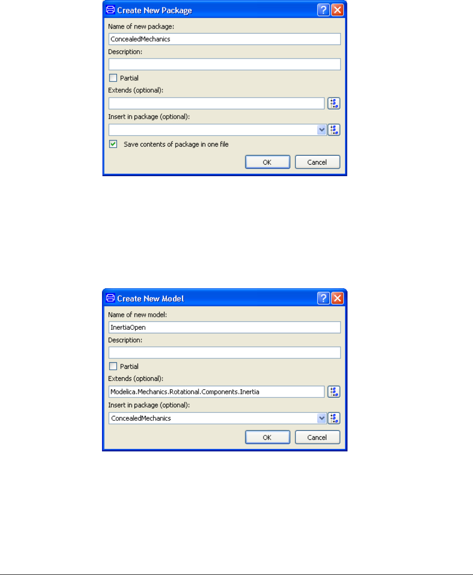
162
The package will later be encrypted.
Now, let us just make an identical copy of Modelica.Mechanics.Rotational.
Components.Inertia, call it InertiaOpen.
It is most simply done right-clicking on the ConcealedMechanics package in the package
browser, and then selecting New > Model… to insert it into ConcealedMechanics and
extending from Modelica.Mechanics.Rotational.Components.Inertia. The dialog will look
like:
The resulting code when looking at the Modelica Text layer will be:
model InertiaOpen
extends Modelica.Mechanics.Rotational.Components.Inertia;
end InertiaOpen;
This model will reveal all public components (by right-clicking on the extended class in the
Modelica Text layer) and select the command Selected Class > Open in New Window)
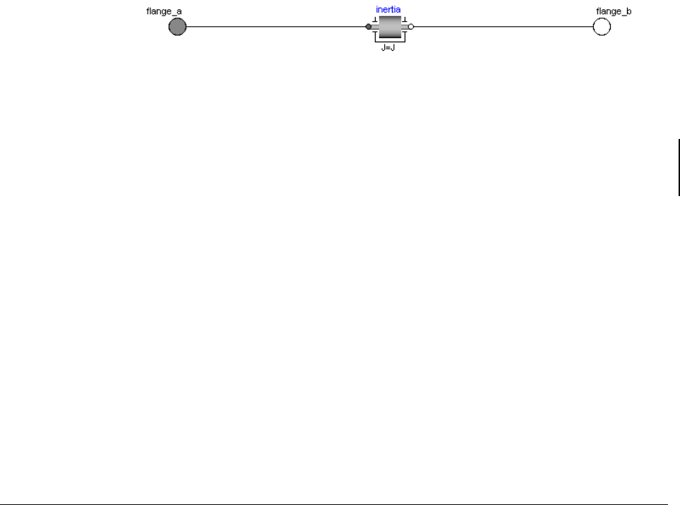
4 MODEL MANAGEMENT 163
model Inertia "1D-rotational component with inertia"
import SI = Modelica.SIUnits;
parameter SI.Inertia J(min=0, start=1) "Moment of inertia";
parameter StateSelect stateSelect=StateSelect.default
"Priority to use phi and w as states";
SI.Angle phi(stateSelect=stateSelect)
"Absolute rotation angle of component";
SI.AngularVelocity w(stateSelect=stateSelect)
"Absolute angular velocity of component (=der(w))";
SI.AngularAcceleration a
"Absolute angular acceleration of component (=der(w))";
We could restrict this by putting phi, w and a in a protected section. If doing so, the name of
the component also should be changed to e.g. InertiaProtected to reflect the change.
Another approach is to design a new interface and hide the internals of the model. In
Dymola we make a new model InertiaHidden extending from
Modelica.Mechanics.Rotational.Interfaces.PartialTwoFlanges.
We drag in a component of class Modelica.Mechanics.Rotational.Components.Inertia and
connect it.
To declare a parameter J we first right-click on inertia (that will pop the context menu of the
component) and then select the Parameters alternative and set its parameter J to J. To
propagate the parameter, right-click in the input field where J was entered (or click the
triangle after the field) and select Propagate…, then click OK button two times.
To make the component inertia protected, we once again right-click on inertia and select the
Parameters alternative. This time we select the Attributes tab and, in the Properties group,
activate Protected. Click OK to validate. The resulting Modelica model is
model InertiaHidden
extends
Modelica.Mechanics.Rotational.Interfaces.PartialTwoFlanges;
protected
Modelica.Mechanics.Rotational.Components.Inertia
inertia(J=J);
public
parameter Modelica.SIUnits.Inertia J "Moment of inertia";
equation
connect(inertia.flange_a, flange_a);
connect(inertia.flange_b, flange_b);
end InertiaHidden;
Save the package ConcealedMechanics and then encrypt it using the command File >
Export > Encrypted File...
The demo model Modelica.Mechanics.Rotational.Examples.CoupledClutches is read-only
but we can copy it. In the package browser, right-click on the demo and use the command
Model to be encrypted.
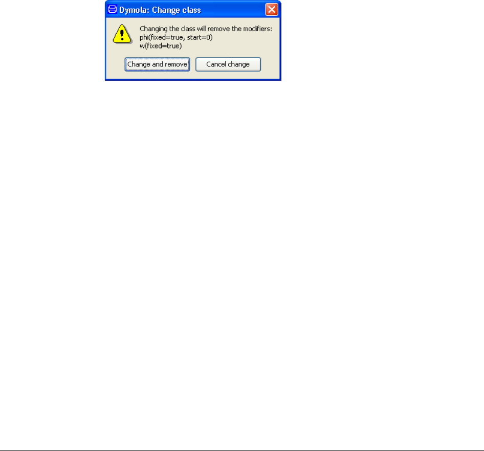
164
New > Duplicate class…. A suitable name for the model is MyCoupledClutches. Since this
is just a test, we can accept the model being a top-level model (not inserted in any package).
When changing MyCoupledClutches the encrypted version of the package
ConcealedMechanics should be used; the non-encrypted package is now present in the
package browser. Right-click on the package, select Unload, and accept it. Now the
encrypted package can be opened (please remember that if encrypted models should be
opened the Files of type must be changed in the file dialog).
Now please right-click on J1 and select Change Class… Select
ConcealedMechanics.InertiaOpen. In the same way, change the class of J2 to
ConcealedMechanics.InertiaHidden. When doing that, an error message appears:
The reason for this warning message is that since now a number of variables are not public
anymore; it is not possible to e.g. select start values of them. Use Change and remove to
accept this.
Now the simulation of the model CoupledClutches gives the following variable browser:
Warning message
when changing class to
a protected one.
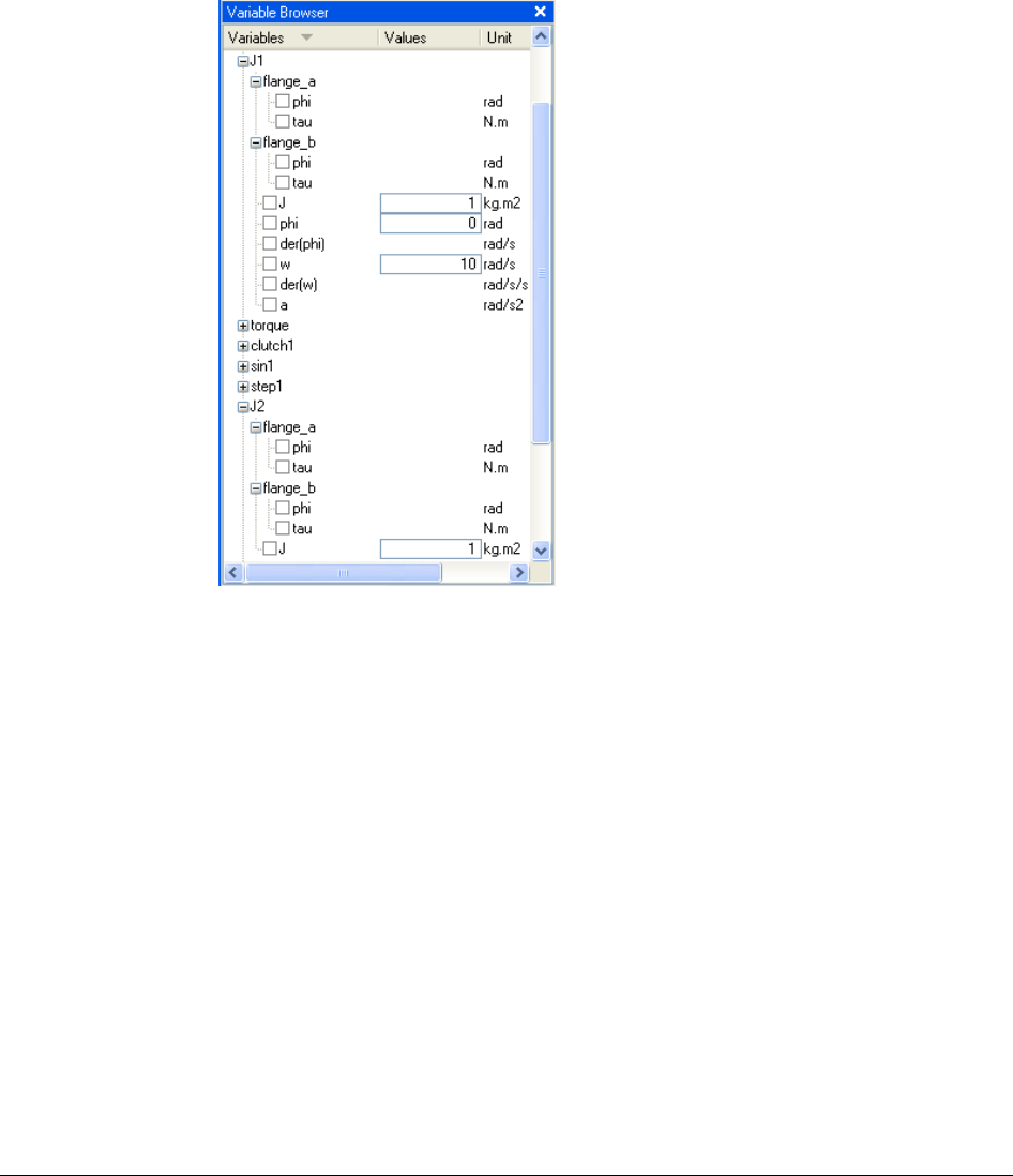
4 MODEL MANAGEMENT 165
For J1and J2 it is possible to plot the connector variables and set the moment of inertia J.
However, for J1 it is also possible to plot velocity and acceleration. What to do if we would
like to plot the velocity of J2? The velocity can be made available by connecting a Speed-
Sensor.
For J1 it is possible to set an initial value for w. For J2 the situation is more complex. By
just looking at it we cannot tell whether there is some internal initialization. When
translating the model Dymola issues a warning that initial conditions are not fully specified.
The documentation of InertiaHidden needs thus to include documentation on initial
conditions. In this case we know that there are no initial conditions stated for J2, so we may
introduce an initial equation section in the CoupledClutches model containing for example
initial equation
J2.flange_a.phi = ... "start angle";
der(J2.flange_a.phi) = ... "start velocity";
to specify the initial position and velocity of J2.
4.3.6 Special annotations for concealment
These special annotations are all grouped inside:
Concealed variables:
J1 is public (non-
encrypted).
J2 is concealed
(encrypted).
This gives different
plot possibilities.
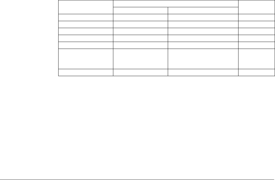
166
annotation(__Dymola_Protection(…));
The annotations are designed based on the following basic principles:
• Security by default – the default is to not reveal information for encrypted packages.
You as the library developer have to enable each of these flags.
• It is more important to protect an entire package than individual classes in the package.
The annotation “nested” is used for this purpose, setting e.g. nestedAllowDuplicate
= true in a certain package means that a single non-package class in that package can
be duplicated but not the whole package. This is useful when e.g. a large amount of
examples should have a certain extent of protection, although a specific example should
be possible to look at.
• Easy-to-use.
• Simple logic to make it easy to verify the behavior. Thus you can enable duplication, but
hide diagrams even though this does not make sense.
• Only applied after encryption – thus they can be present in the original library.
The behavior can be summarized in the following table (the missing entries are not
implemented):
Show/allow
Annotation
Default
All classes
Non-packages
Duplicate (1)
allowDuplicate
nestedAllowDuplicate
false
Diagram
showDiagram
nestedShowDiagram
false (2)
Text (3)
showText
nestedShowText
false
Icon
true
Documentation (4)
showDocumentation
nestedShowDocumentation
true
In package browser/
choices all matching
(4,5)
hideFromBrowser
N/A
false
License check (6)
Library
None
The annotation applies hierarchically to all classes (unless overridden by a similar
annotation).
The idea is to use either an all-classes or a non-packages annotation for a certain package,
they should be considered as alternatives depending on the functionality wanted. Note that
if single class(es) in a package should be protected, the top-level package itself should be
annotated using non-package annotation, e. g. nestedShowText=true to allow all non-
package text to be visible unless overridden locally. If using All classes annotation to
annotate the top-level package, e. g. showText=true, the classes inside it cannot be
protected, they will be visible by inspecting/duplicating the top-level package.
Notes:
Annotation for making
encrypted classes
visible.

4 MODEL MANAGEMENT 167
1. Please note that any class being allowed to duplicate is also not protected anymore; any
protection annotations in that class is useless since the source code is revealed anyway
when looking at the copy of the class.
2. However, the default for Examples and Tutorial-packages is showDiagram=true.
3. The text window has copying disabled (unless duplicate is allowed), but there are ways
of circumventing this.
4. If a class is hidden from browser or not shown in documentation layer it is treated as a
protected class for HTML-generation. It is thus not possible to export to HTML unless a
specific setting is applied (that is valid also before encryption).
5. The logic for the browser is reversed (“hide” contrary to the others “show”).
6. License check of libraries: see next section.
In addition there are several top level settings (also inside __Dymola_Protection) as follows:
Show/allow
Annotation
Default
Plotting of protected variables
showVariables
false
Diagnostics with variable
showDiagnostics
false
Statistics (e.g. #states)
showStatistics
false
Flat-modelica
showFlat
false
Note that if several encrypted packages are used they must all enable e.g. statistics for the
statistics to be shown.
4.3.7 Licensing libraries
Introduction
A licensing mechanism is available for “external” Modelica libraries, i.e. libraries which are
not sold and licensed through the Dassault Systèmes channels.
Note that below describes third party licensing for node-locked licenses. Licensing of third
party libraries is also supported for sharable licenses, however currently only on Windows.
Third party library vendors, please contact your support channel/sales representative for
additional information, and examples.
The licensing mechanism provides a number of functions:
• The library developer can create/administrate licenses without the help of tool vendor.
• It is possible to update the licensing information without updating the library, and to
update the library without changing licensing information.
• It is possible to tie the library license to specified users, identified by license number or
computer host-id. For sharable licenses, see note above.

168
• Start and expiration dates on licenses can be defined.
The licensing scheme is implemented on top of the encryption mechanism in Dymola that
prevents the user from inspecting all source code. This is how the licensing mechanism
works:
• In the library that will be protected, the developer adds an annotation with an arbitrary
key. This key is used to associate the library with a separate authorization file, and will
not be visible to the user after library encryption.
• The developer then makes a separate authorization Modelica file which contains the
library key, some identification of the user that should be able to read the library (the
licensed systems), and possibly start and expiration dates. This file is also encrypted in
Dymola and distributed as needed. Note:
o The encrypted authorization file must be located in the same folder as the
encrypted corresponding library.
o Dymola allows extension .moe or .mo_lic for the encrypted
authorization file, 3DEXPERIENCE Dymola Behavior Modeling app
only allows extension .mo_lic for the encrypted authorization file.
• When Dymola opens the library and sees the key, it also opens the corresponding
authorization file, and checks if the user is permitted to open the library. The
authorization file is never shown to the user, only used internally by the tool.
The full details of the licensing mechanism can be found in “Modelica Language
Specification, Version 3.2”, section 17.8.2 “Licensing”. The specification can be
downloaded from the Modelica website, http://www.Modelica.org.
Some comments to the detailed description above:
• The content of the library key string is unspecified, but must match the key of the
library.
• The license id currently supported is the Dymola license number or the computer host-id
(as shown by Dymola using the command Help > License…, the Details tab).
A license id (e.g. 1234) can be specified as "1234" as well as "lic:1234", a host id
(e.g. 0019d2c9bfe7) can be specified as "0019d2c9bfe7" as well as
"mac:0019d2c9bfe7".
• In some cases there are multiple host id´s (docking stations etc.). In such case you
should authorize all such host id’s.
Note that a hideFromBrowser annotation is advised to prevent the authorization file from
being shown in the Dymola package browser. See example below.
It is important however to note that you cannot use the Dymola annotation
__Dymola_Protection() together with the the general Modelica annotation
Protection() in the same file; the solution is to embed the wanted Dymola annotation
components in the Modelica one, for example
annotation(Protection(License=…., Access=…., __Dymola_showFlat=true,
__Dymola_showVariable=true, …));
Important

4 MODEL MANAGEMENT 169
Example (before encryption)
The authorization file and the library are created independently in Dymola, at top level. The
command File > Export… > Encrypted File… is then used to create encrypted versions of
the authorization file and the library. When used, they must be located in the same folder in
order for the library to find the authorization file.
The library contains these annotations to specify the library key and the authorization file.
// File MyLibrary\package.mo
// (library file before encryption)
package MyLibrary
…
annotation(Protection(License(
libraryKey="15783-A39323-498222-444ckk4ll",licenseFile=
"MyLibraryAuthorization_Dymola.moe")));
end MyLibrary;
The authorization file contains annotations that allow execution on three different licensed
systems. (The first one uses Dymola license number, the second also has an expiration date
and the third uses mac address/host id.):
// File MyLibraryAuthorization_Dymola.mo
// (authorization file before encryption)
package MyLibraryAuthorization_Dymola
annotation(
__Dymola_Protection(hideFromBrowser=true),
Authorization(
libraryKey="15783-A39323-498222-444ckk4ll",
licensor="Organization A\nRoad, Country",
license={License(licensee="Organization B, Mr. X",
id={"lic:1269"}),
License(licensee="Organization C, Mr. Y",
id={"lic:511"}, expirationDate="2011-06-30"),
License(licensee="Organization D, Mr. Z",
id={"mac:0019d2c9bfe7","mac:0026c6b26950"})
}));
end MyLibraryAuthorization_Dymola;
4.3.8 Scrambling in Dymola
Encryption of a package/model is a useful way of making a package useable without
revealing information. However, in certain scenarios it is not the ideal choice when sending
one (or a few) component models that shall only be used directly.
In such cases the most important information to conceal is data and internal structure, and
there is no need to keep “replaceable” components or classes.
The ideal choice would in that case be to send something that:
• Does not contain internal structure and original data.
• Automatically hides all internal components.
• Can be used as any other model in Dymola (including differentiation for state-selection).

170
• Allows you to see exactly what is sent.
This is accomplished using File > Export… > Encrypted total model… and can be done
either on a model/block or for a package, where each public non-partial model/block is
scrambled individually and then placed together in a package.
Each individual model is scrambled as explained in the next to remove unnecessary
information and the resulting file is then encrypted as an additional safety precaution.
Note that the protection annotation for license check is preserved during scrambling, i.e. you
can specify this in the model/package before scrambling. However, license checks from
enclosing packages are not copied, i.e. if you want to protect a model you should add the
annotation on the particular model.
Example of scrambling
We continue with the inertia example, but now rewrite the Inertia model by replacing the
parameter ‘J’ by two variables ‘r’ and ‘m’ and computing the inertia based on these.
Create the model below as a top-level model (to be able to encrypt it) and extend
Modelica.Mechanics.Rotational.Interfaces.PartialTwoFlanges.
model InertiaAlternative
annotation (uses(Modelica(version="3.0")),
Documentation(info="<html> An inertia of a certain shape with
settable radius.
<html>"));
extends Modelica.Mechanics.Rotational.Interfaces.
PartialTwoFlanges;
parameter Modelica.SIunits.Length r=1 "Radius";
protected
constant Modelica.SIunits.Mass m=0.5 "Mass";
Modelica.SIunits.Angle phi "Absolute rotation angle of
component (= flange_a.phi = flange_b.phi)";
Modelica.SIunits.AngularVelocity w "Angular velocity";
equation
flange_a.phi=phi;
flange_b.phi=phi;
w = der(phi);
m*r^2/12*der(w) = flange_a.tau + flange_b.tau;
end InertiaAlternative;
The mass and the shape should be hidden from the user of the model. By selecting File >
Export… > Encrypted total model… the model is first scrambled and then encrypted.
The procedure gives the messages:
Will encrypt to file C:/MyExperiment/InertiaAlternative.moe.
First scrambling to file
C:/MyExperiment/InertiaAlternative.tmp.moe
Scrambling InertiaAlternative.
The scrambling should preserve the following top-level
variables:
connector flange_a
connector flange_b

4 MODEL MANAGEMENT 171
parameter r
Scrambling complete, verifying it.
Encrypting.
Encryption complete, file can be found in
C:/MyExperiment/InertiaAlternative.moe.
The scrambling indicate which variables should be kept, and include a tag before the
variable to explain why.
Users can examine the Inertia3.tmp.mo file to verify that the no vital information is present
(if the file is to be loaded in Dymola, do not forget to first close the present file with the
same name by right-clicking on it in the package browser and select Unload, otherwise
there will be a name conflict):
model InertiaAlternative
encapsulated connector r0
Real phi(unit = "rad", displayUnit = "deg") "Absolute rotation
angle of flange";
flow Real tau(unit = "N.m") "Cut torque in the flange";
annotation(Hide=true,
Icon(coordinateSystem(preserveAspectRatio=true, extent={{-100,-
100},{100,100}}, grid={2,2}),
graphics={Ellipse(
extent={{-100,100},{100,-100}},
lineColor={0,0,0},
fillColor={95,95,95},
fillPattern=FillPattern.Solid)}));
end r0;
r0 flange_a annotation (Placement(transformation(extent={{-
110,-10},{-90,10}}, rotation=0)));
encapsulated connector r1
Real phi(unit = "rad", displayUnit = "deg") "Absolute rotation
angle of flange";
flow Real tau(unit = "N.m") "Cut torque in the flange";
annotation(Hide=true,
Icon(coordinateSystem(preserveAspectRatio=true, extent={{-100,-
100},{100,100}}, grid={2,2}),
graphics={Ellipse(
extent={{-98,100},{102,-100}},
lineColor={0,0,0}, fillColor={255,255,255},
fillPattern=FillPattern.Solid)}));
end r1;
r1 flange_b annotation (Placement(transformation(extent={{90,-
10},{110,10}}, rotation=0)));
parameter Real r(unit = "m") = 1 "Radius";
protected
Real z2;
Real z1;
annotation(Settings(NewStateSelection=true),
Documentation(info="<html>
An inertia of a certain shape with settable radius.
</html>"));
protected equation
flange_a.phi = z2;

172
flange_b.phi = z2;
z1 = der(z2);
0.0416666666666667*r^2*der(z1) = flange_a.tau+flange_b.tau;
end InertiaAlternative;
As can be seen the mass and shape have been constant-evaluated making it impossible to
determine their individual values. In addition the names of all internal variables are replaced
by scrambled names (if the variable is preserved at all).
The encrypted file only contains this information, but is in addition encrypted. Encryption
prevents disclosure of even the scrambled information and also makes the model read-only.
4.4 Model and library checking
4.4.1 Overview
This section is an overview of the functionality in the Check package.
Regression testing
Sometimes, model code modification can cause unintended changes in the model behavior.
To catch this type of error regression testing can be used. By simulating and comparing the
state variables of a model against a reference data file, changes in the behavior can be
detected. With this new feature, a test suite can easily be constructed and the process of
regression testing can be automated.
Class coverage
To determine how well the test suite for regression testing covers (uses) the classes in the
library under test, class coverage analysis is used.
Condition coverage
For conditional expressions and Boolean variables, condition coverage analysis can be
performed to investigate which branches of conditional equations in the test cases that are
ever executed. This can be used to detect “untested code”.
Style checking
For model development, style checking is introduced to assure that models and libraries are
well documented etc.
Translation statistics
The translation statistics option is an extension to the normal regression testing of state
variables to make testing more powerful and to catch differences that could otherwise be
hard to see. Using this option, the statistics of the translated model can be included in the

4 MODEL MANAGEMENT 173
regression testing to detect changes in, for example; the number and sizes of linear and
nonlinear system of equations and the number of state variables.
4.4.2 Regression testing
It will be shown how to use checkLibrary to set up a test suite for regression testing of a
library, and how to use the checking utilities included in the package.
Regression testing is the utility for library and model developers to assist with regression
testing of libraries. Regression testing is performed to detect unintended changes in the
behavior of models due to updates and rewriting of model code.
The package collects all test cases specified by the user, i.e. the models in the library that
have the annotation experiment(StopTime=…) set and additional test cases from a test
package (if available). After simulating a test case, the results are compared to the reference
file. The package takes as comparison signals the possible continuous and discrete state
variables of the model.
Setting up reference files
We will start by setting up reference files for the regression testing.
• Right-click on the function checkLibrary in the package Check and select Call
function... in the context menu. Please keep the default settings with exception of the
ones that are changed below.
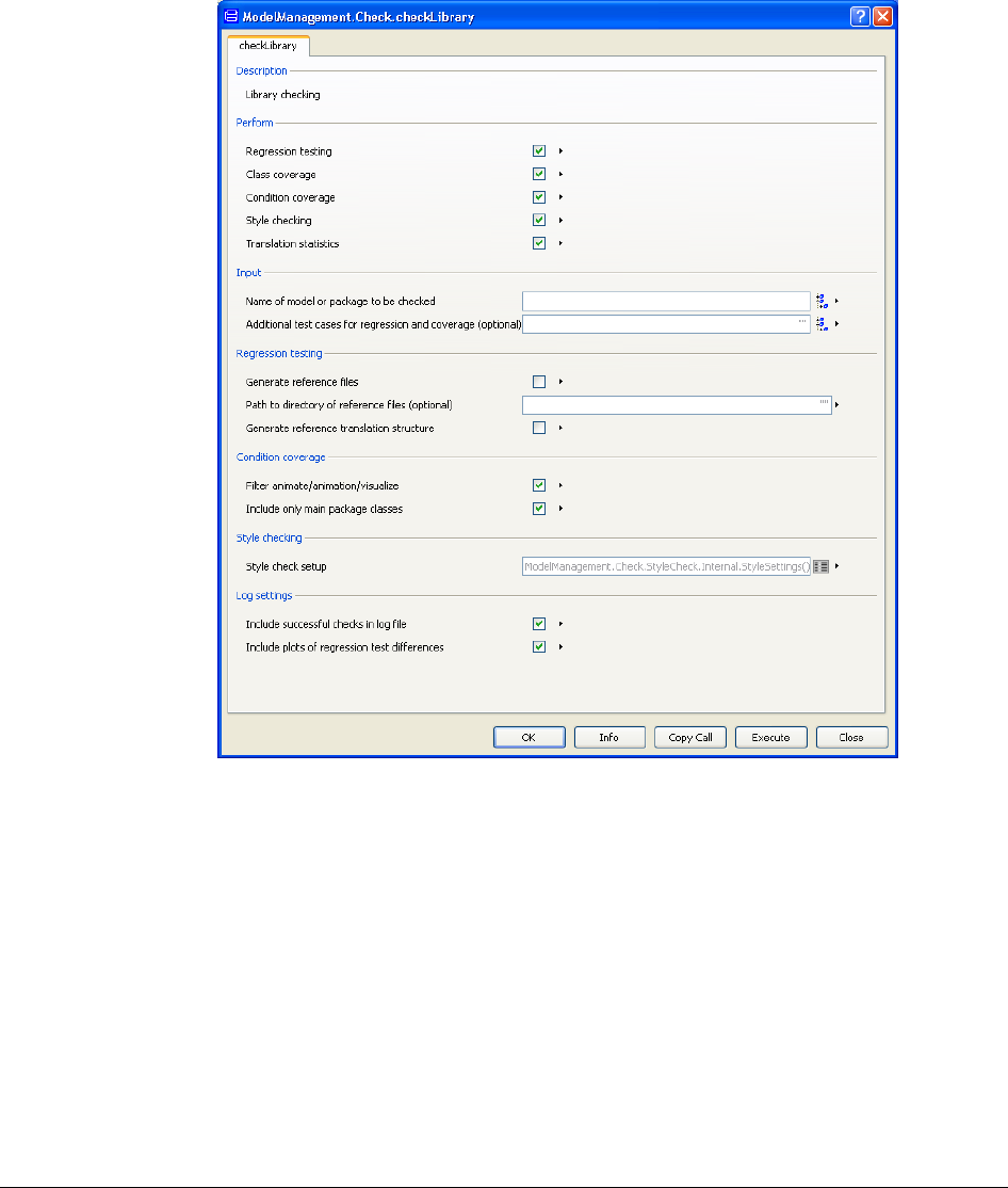
174
• Select the library or model you want to check by using the browser for Name of model
or package to be checked in the menu above.
Dialog of checkLibrary.
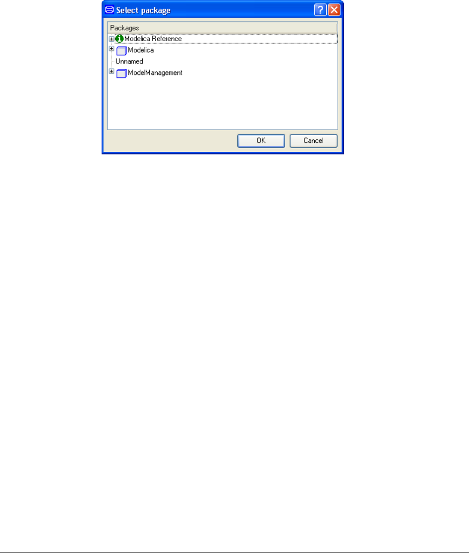
4 MODEL MANAGEMENT 175
• Check the boxes for Generate reference files and Generate reference translation
structure.
• Use the browser to select additional test cases by using the entry Additional test cases
for regression and coverage (optional), if there are any.
• Optionally, specify the path a directory where the reference files should be stored by
entering the complete path under Path to directory of reference files (optional). If not
specified, the files will be stored in workdir\ReferenceData\Libraryname.
• Execute by clicking OK or Execute.
The package will now generate a set of reference files for the selected library and optional
test suite.
In some cases one would like to expand the test suite by adding additional reference files
without re-generating the entire test suite reference. This can easily be done by selecting that
particular model as the package to generate reference files for, and then specify the old
directory of reference files under Regression testing.
The new reference file will now end up in the same folder as the old files and the new test
case can be included in the test package. The same procedure can be used to replace specific
reference files if intended changes in the behavior of a model require a new reference file.
Performing regression testing
In order to perform regression testing, right-click on checkLibrary function to pop a dialog
box with the default settings for checking and regression testing. By default, all checks are
active.
As before, when generating reference files, choose your library, additional test cases (if any)
and specify a path to your directory of reference files, if you are not using the default
directory.
Execute the test by clicking OK or Execute.
Package selector.

176
The testing will now start and an html log file will be generated in your working directory.
A message in the commands window will tell the name and path of the log file generated.
Output
As an example of the output generated from regression testing consider a simple model,
model Test
annotation (experiment(StopTime=1));
Real x(start=1);
parameter Real a = 10;
equation
der(x)= -a*x;
end Test;
Note that the annotation experiment(StopTime=1) have been set to define this model as a
test case.
Start by generating a reference file as described previously. (Since this simple example
covers only regression testing of one model, please uncheck all items in the group Perform
except Regression testing and Translation statistics.) Click OK. (By selecting Execute
the dialog window will be kept displayed after performing the call.)
A log named Test_Reference_Log will be generated in the working directory:
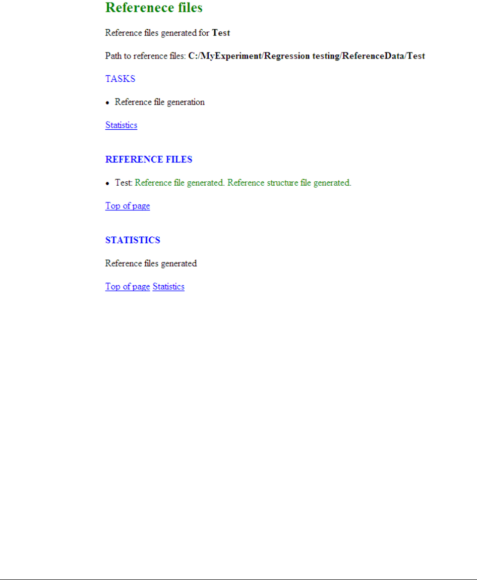
4 MODEL MANAGEMENT 177
Then perform a regression test by right-clicking the checkLibray function again. Select the
model, uncheck everything in the Perform group except Regression testing and
Translation statistics and click OK. A log named Test_HTML_log will be generated in the
working directory:
Log of reference file
generation.
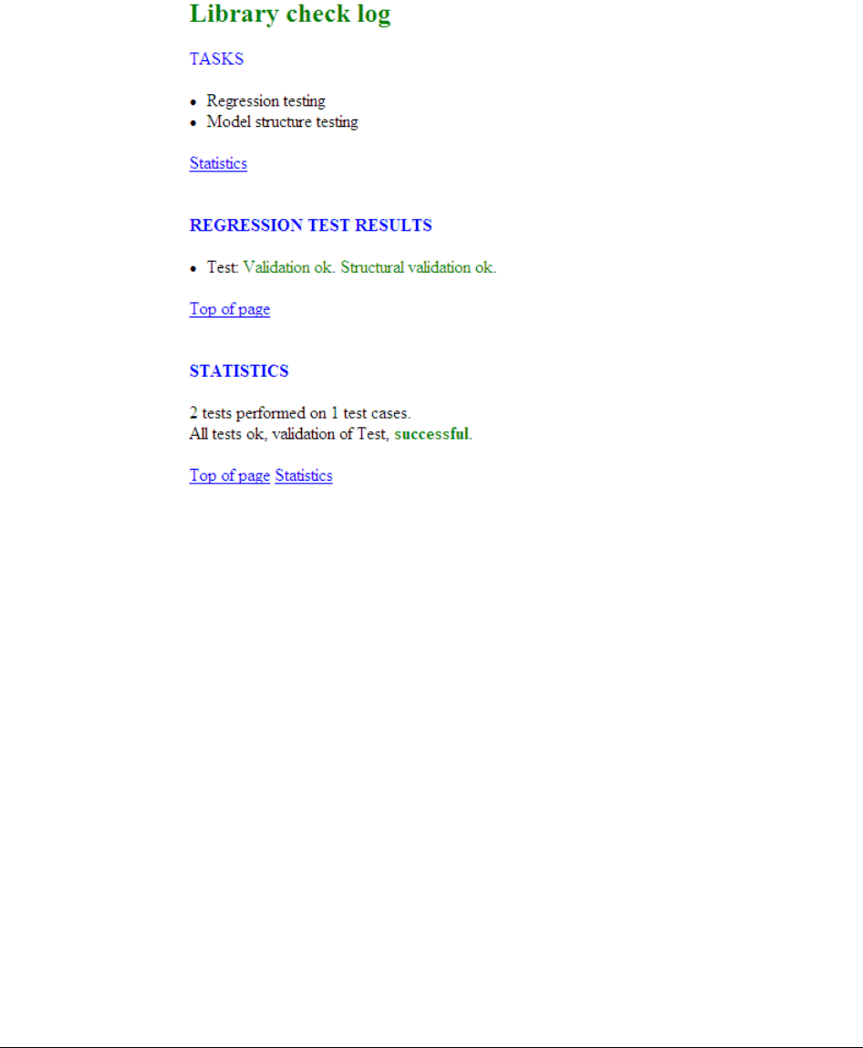
178
The regression tests (regression and model structure) are successful and this is expected
since there should be no differences in the model since nothing has changed in the model
code.
Changing the value of the parameter a to a=15 causes the regression testing to fail. The
results can be seen below.
Log of successful test.
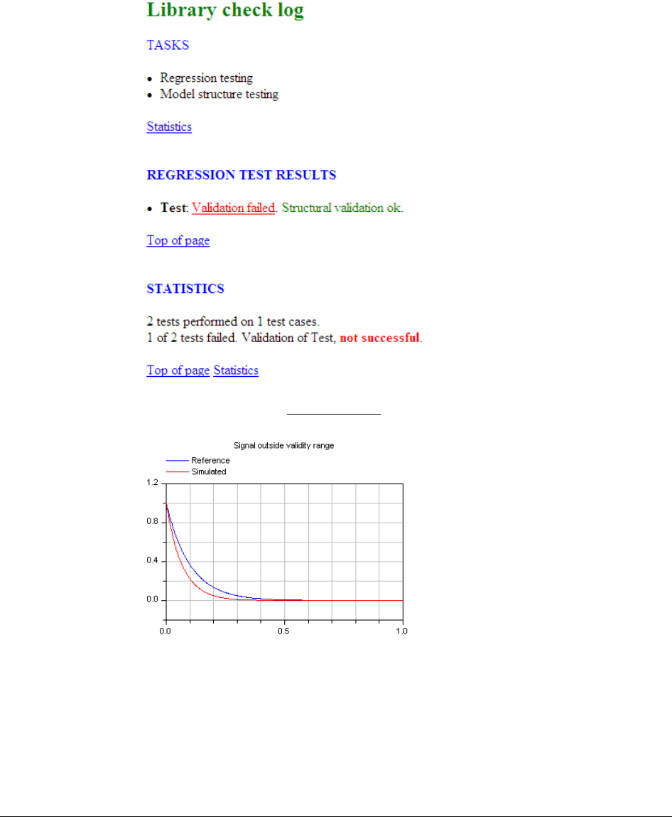
4 MODEL MANAGEMENT 179
Clicking the link for the validation failed shows the specific log for this test case. A plot is
generated to show the difference in the state variable (compared to the reference).
Log of failed test.
Failed validation plot.
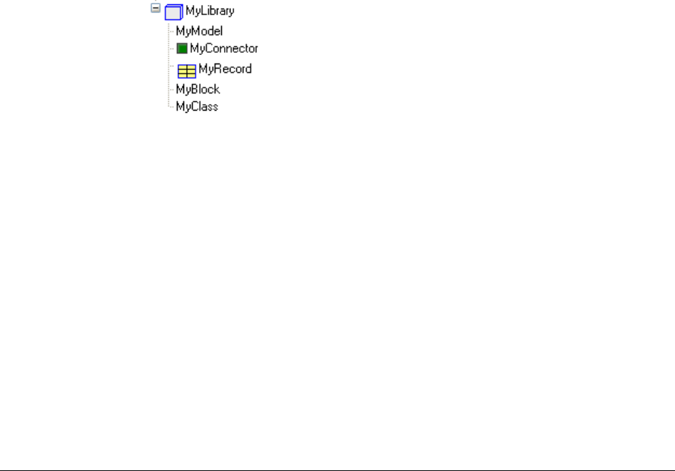
180
4.4.3 Class coverage
The class coverage analysis is performed by default to show how well the test cases cover
the classes in a library. A class is considered covered if it is used in a test case, or if a class
used in a test case extends from it. The analysis is performed for models, blocks and
connectors, (type, record, function and class are considered covered by default).
The result of the class coverage analysis is reported in the log file under Class coverage.
There are two ways to present the results:
• List all classes and how many times they are used.
• Only list classes that are never used.
The output is by default the first option and it can be changed by unchecking the checkbox
in the dialog box for checkLibrary under Log settings.
NOTE: The class coverage does not give any result for encrypted libraries.
Output
As an example, consider the following library, MyLibrary, containing 5 classes, depicted
below. The library is available under ModelManagement.Check.Examples.
The library contains 5 classes, 3 of which are considered in the class coverage analysis. The
classes that are not included in the analysis are MyRecord and MyClass since only blocks,
models and connectors are considered as explained above.
Since the package ModelManagement is encrypted, please duplicate the package MyLibrary
to be able to run class coverage test on it. (Right-click on MyLibrary, select New >
Duplicate Class…. Click OK. Finally save the library; now it can be tested.)
Running regression testing with the option class coverage on the library copy will generate
the following section in the log MyLibrary_HTML_log:
Library example.
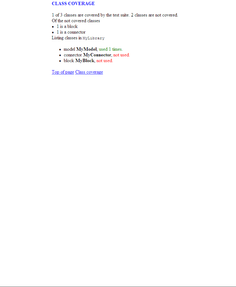
4 MODEL MANAGEMENT 181
The log indicates that the only class that was used in the test suite is MyModel. This is
correct since MyLibrary only contains one test case (MyModel is the only model in
MyLibrary with experiment.StopTime set). To get complete class coverage one could
define a test case, or multiple ones, that uses the classes that are not covered. This can be
done either by creating new models in the library or by creating a new TestLibrary
containing only test cases. The TestLibrary can then be coupled to the regression as
Additional test cases.
4.4.4 Condition coverage
Condition coverage analysis is performed to ensure that all conditional parts in model
equations are tested. A global merge is performed for the entire test suite so that a condition
is considered to be covered if it has been both true and false in a test case or if it has been
true in one test case and false in another test case in the test suite.
Condition coverage analysis considers:
• Boolean variables
• if conditions in all equations and expressions
NOTE: For encrypted libraries the condition coverage analysis may neglect classes
depending on the level of encryption.
Output
Consider a model, MyModel, containing a Boolean variable, low,
low = x < min;
Running regression testing with the option Condition coverage on this model will generate
the following section in the log file. (Please work with the copy of the library MyLibrary
that was made in the previous section to avoid working with the encrypted MyModel.)
Class coverage log.

182
This indicates that there is a parameter or variable, low, which always has the value false.
Acknowledgement
The Check package is based on earlier implementations used for several years for testing
libraries and Dymola itself.
The condition coverage feature is inspired by Mike Tiller’s work described in
Tiller, Michael M. and Burit Kittirungsi: “UnitTesting: A Library for Modelica Unit
Testing”, Proc. 5th International Modelica Conference 2006, pp. 695—704, Vienna, Austria.
See http://www.modelica.org.
4.4.5 Style checking
Style Checking is a utility for checking of libraries and classes according to the guidelines
in the style guide. The intention is to assist a model developer with quality control of the
library and to warn when issues regarding the specified quality constraints are not fulfilled.
Settings
To change the default settings for library checking, check Style check setup in the group
Style checking, when calling the main function checkLibrary.
It is then possible to edit the setup according to your own requirements. The checks are
divided in to three categories; Class checks, Component checks and General. Below is a
screenshot of the available settings in the setup menu.
Condition coverage log.
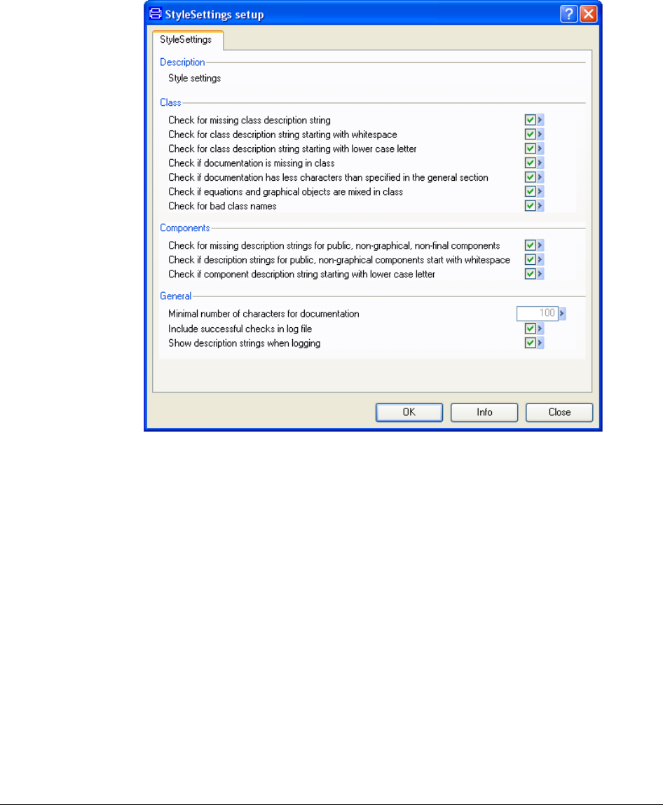
4 MODEL MANAGEMENT 183
The styleCheck can be customized by selecting appropriate checks in the checkboxes.
The rules for the option Check for bad class names are:
• Class name shall start with capital letter except for functions that shall start with lower
case letter.
• Class name shall not contain “_”. Use names like “IdealDiode” instead of “Ideal_diode”
Documentation and description strings are not required for type.
Output
Again, consider MyLibrary. The first class, MyModel, intentionally contains style errors.
Below is the Modelica text of that class and to the right, the parameter dialog. In the
parameter part of the window one can see that the description strings are missing for
parameter b and c, and that the description strings for the class and parameter a starts with a
lower case character. These are style errors that will be detected by the style checking
feature. The other classes in MyLibrary are implemented with correct style.
Stylecheck setup
dialog.
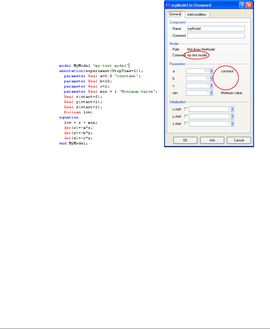
184
Changing the default settings of the style check by specifying that 5 characters is enough for
the documentation, the following style check log is generated when applying the Style
Checking to the copy of MyLibrary (in order not to check an encrypted library, see previous
sections).
Parameter dialog of
MyModel.
Example model.
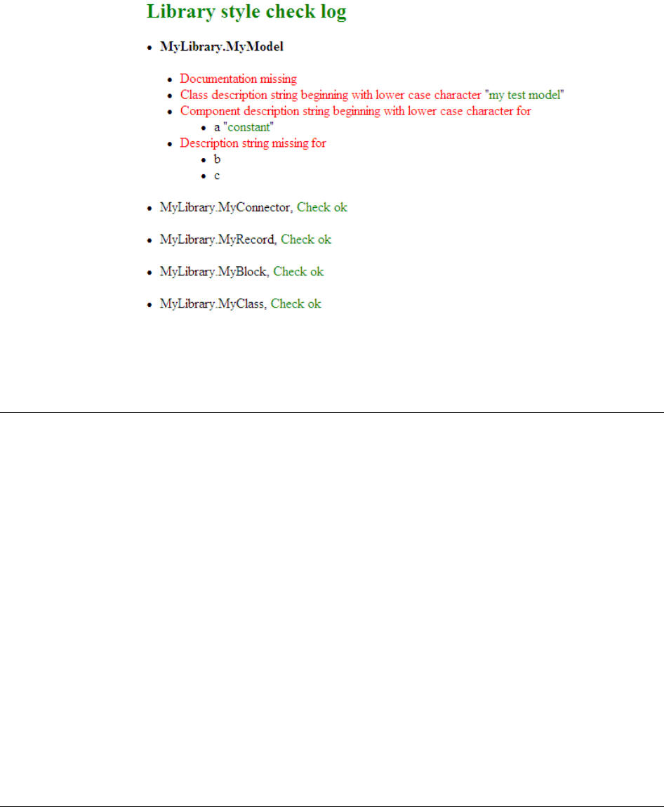
4 MODEL MANAGEMENT 185
The log reports 5 errors for MyModel. In addition to the errors described above it also
reports that no HTML documentation exists for the class.
4.5 Model comparison
4.5.1 Overview
The aim of this package is to create a report with the differences between two classes. The
package consists of a main function called compareModels.
To establish the comparison, the function compareModels needs as input parameters the
name of the classes to be compared, together with corresponding pseudonyms (the names to
be used in the report). The pseudonyms are by default Version 1 and Version 2. Another
two input parameters are the check options Compare equations and Compare documentation.
The differences between the two classes are presented in a HTML file whose name can be
specified.
4.5.2 Getting started
This is a short getting started tutorial. It will demonstrate how to use compareModels to
report differences in different versions of Modelica models or libraries.
• Make sure that the packages/models to be compared are available in the Package
Browser. If not, load them by the File > Open… command. To load two different
versions of the same package, open the first one, and rename to e.g. name_a. Then load
Style check log.
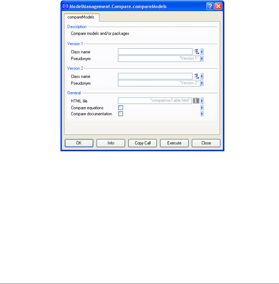
186
the second package and rename to e.g. name_b. Both packages should now be visible in
the Package Browser.
Note: It is not possible to rename read-only packages; instead you can duplicate and
unload the original. The reason the second package is renamed is that there is an issue if
the second name is a prefix of the first name.
• Right click the main function compareModels and choose Call function... to pop the
dialog box depicted below.
• Now select your models/packages to be compared using the browsers under Version 1
and Version 2.
• Enter the version names to display in the report by entering those names as pseudonyms
under Version 1 and Version 2.
• Use the browser to specify or select the output HTML file for the report.
• Optionally check the boxes for Compare equations and Compare documentation to
include these features.
• Finally, press Execute

4 MODEL MANAGEMENT 187
4.5.3 Comparison report
The comparison report consists of a number of possible tables for each class (in the case of
comparing two packages, the classes with the same names are the ones to be compared as
follows).
The first table appears when the attributes of the classes differ (for example, if one class is a
model and the other one is an encapsulated model) or when components of the classes differ.
The components are first compared by their names. For the components that share names,
the comparison is based on all possible attributes (input, output, protected, graphical,
modifiers, extent annotation, etc). The keywords are shown in the table with bold face. If
there is a component which is present in only one of the classes it is expressed in the table
as well as its position (extent annotation) in case of being graphical.
The second table presents the differences between the equations and it is created if the
option Compare equations is checked.
The next table presents the differences between the documentation and it is created if the
option Compare documentation is checked.
The comparisons between the equations of two classes and between their documentations
are done using the same algorithm, based only on text comparison and the results of the
comparison are also presented in the same fashion. In the tables appear mostly the
differences between the texts, given a few common lines as references. The algorithm will
recognize added/removed text or strings that have been changed. Moved text is not
recognized as such.
In the case of comparing two packages, a last table may be created, containing the classes
that only appear in one of the packages (see the last example).
To illustrate how the function compareModels works and the way in which the tables in
the HTML file should be interpreted we present here some examples.
Class Attributes
We call the function compareModels with the setup as shown below.
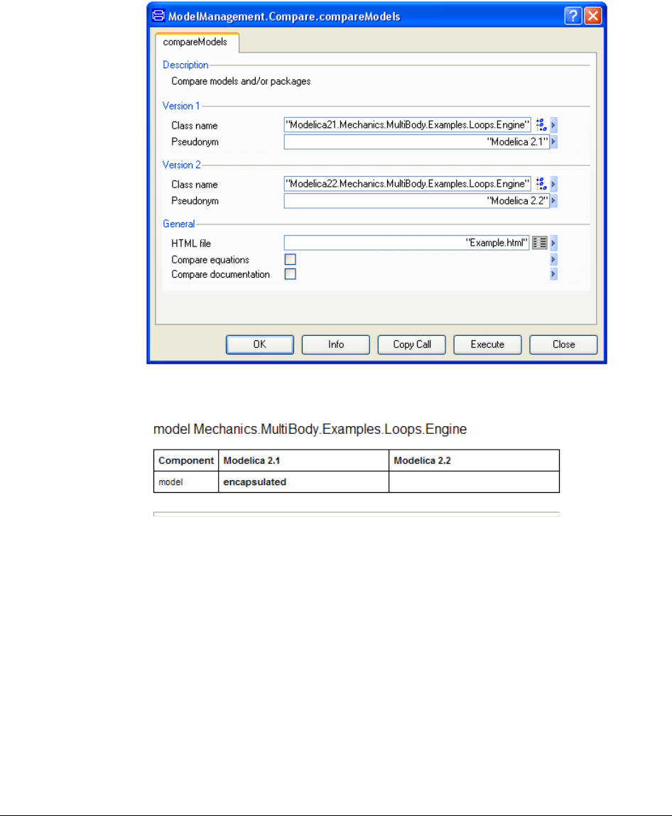
188
The report is then in Example.html:
This means that in Modelica 2.1 the model is encapsulated, but not in Modelica 2.2, and this
is the only difference that they have (disregarding equations and documentation).
Components
We call the function compareModels as follows.
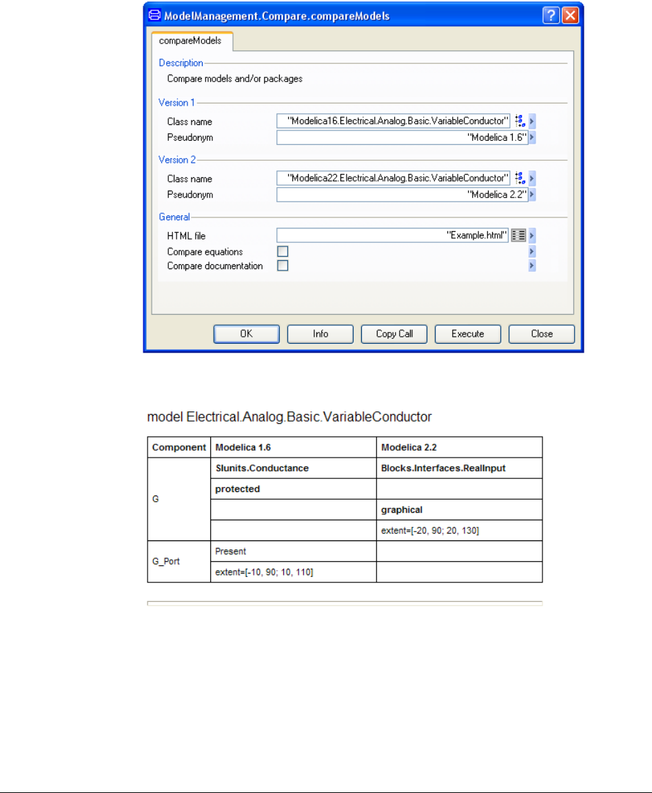
4 MODEL MANAGEMENT 189
The report is then in Example.html:
The component G is present in both models.
• In Modelica 1.6 it is defined Modelica16.SIunits.Conductance G among the
protected members.
• In Modelica 2.2 it is defined as the public connector component
Modelica22.Blocks.Interfaces.RealInput G. In addition in this version it
is graphical and its position is indicated with extent.
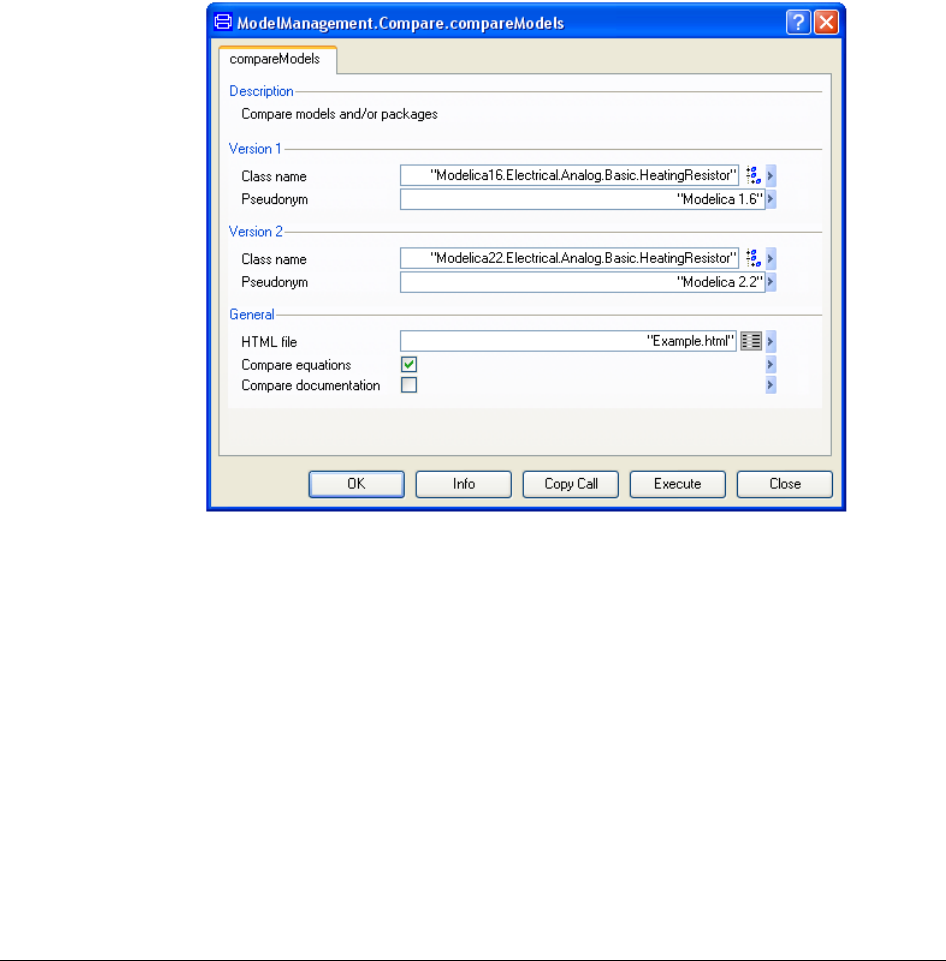
190
The component G_Port is present only in Modelica 1.6. In Modelica 2.2 the simplification
of the blocks library allowed G to be used both as input connector and directly in the
equations.
Equations
We call the function compareModels to compare the HeatingResistor including its
equations.
The report is then in Example.html:
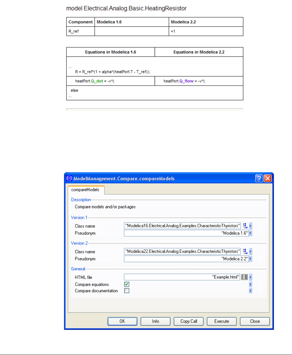
4 MODEL MANAGEMENT 191
If two equations have differences they are marked in boldface and with different colors. The
one-column rows are common equations of the models. A default value has been added and
the heat-flow variable was renamed to make it clear that it is not a time-derivative.
Connections
We call the function compareModels for CharacteristicThyristors.

192
The report is then in Example.html:
When the connections between the components of the models are different they are
presented as equations. The differences are due to the simplification of the blocks library in
Modelica 2.
Documentation
We call the function compareModels with “Compare Documentation” enabled.
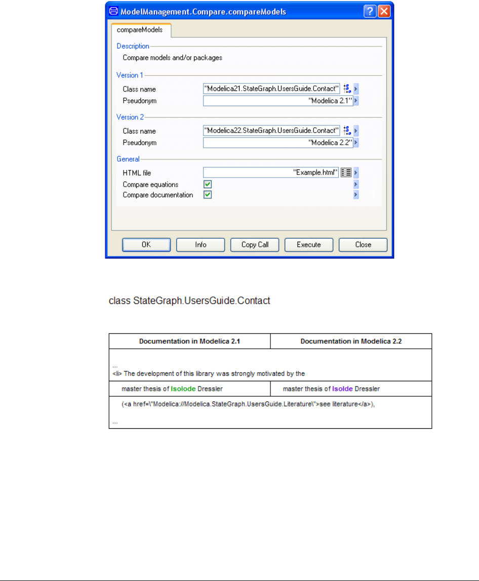
4 MODEL MANAGEMENT 193
The report is then in Example.html:
The differences in the documentation are presented in analogous way to the equation
differences.

194
4.6 Model structure
4.6.1 Introduction
This defines an Application Programmers Interface for traversing Modelica models,
extracting information, and some limited forms of modifications of the structure as well.
The API is defined in Modelica and to access it from non-Modelica code it relies on
Dymola’s interface to other languages.
The basics of the API are routines for accessing information for particular elements, giving
the complete list of sub-elements. This allows extraction of the entire model information by
recursively traversing the elements. The functions are stateless (i.e. there are no getNext-
calls) corresponding to the functional style in Modelica.
There is no mapping from the structure to a complete structure in Modelica. Mapping the
entire structure of a model to class-structure would not be possible in current Modelica
because the class structure is inherently recursive. However, even if it were possible to
replicate the entire class structure as a set of nested records it would not provide an efficient
interface to the class structure for simple queries or modifications.
4.6.2 Traversing models before translation
In order to provide a useful interface to the classes and components three sets of routines are
provided as follows in package ModelManagement.Structure.AST. The common basis is a
set comprised of two functions and one record,
The three sets of routines are for classes, extends-clauses and components. In each set there
is a routine for obtaining the elements (as an array), a record defining the “attributes”
(protected, inner, full class name, …) and a routine for getting the attributes for a specific
element.
These interfaces assume that one can use the name of elements in the queries, which is
possible in the cases above (technically excluding the obscure case of repeated identical
extends-statements which is legal Modelica, but without any reasonable use). Note that
Dymola enforces this semantic restriction in Modelica already during parsing of classes, and
thus it is safe to base the API-routines on this assumption.
The requirements also include access to the import-statements in the class. For import-
clauses it is hard to define which name to use as a key (when considering both the qualified
and the unqualified import-statements, thus a combined routine has been added that returns
an array of records defining the import-statements.
This routine is also present for the other cases and provides an easy to use interface. Such
functions are trivial to implement based on the primary routines, and we give a full example
below (excluding its documentation):

4 MODEL MANAGEMENT 195
function ComponentsInClassAttributes
"Get components of a class"
input String className;
output ComponentAttributes res[:]=
GetComponentAttributes(className,
ComponentsInClass(className));
algorithm
end ComponentsInClassAttributes;
Here the names of the components are constructed by ComponentsInClass and this is then
used in a vectorized call (as defined in Modelica) of GetComponentAttributes to get the
attributes of all components.
Thus functions exist for all elements of table given on the below (where “elements in class”
has a class/package as input and get attributes also exist in a form that returns an array
containing the attributes of all elements).
Record of attributes
Elements in class
Get attributes
Classes
ClassAttributes
ClassesInPackage
GetClassAttributes
Extends
ExtendsAttributes
ExtendsInClass
GetExtendsAttributes
Components
ComponentAttributes
ComponentsInClass
GetComponentAttributes
Import
ImportAttributes
ImportsInClassAttributes
The row headings are the element types and the column headings the different functions
(and records)
To make it possible to traverse all classes it is also possible to list all top-level classes
(optionally limited to the ones defined in a specific Modelica file).
Example
The functions in ModelManagement.Structure.AST are documented online with description,
and example of use. There is furthermore a small set of examples, and one example is
extracting statistics for packages, an example of use is ModelManagement.Structure.
AST.Examples.countModelsInPackage(“Modelica”); which find all restricted classes and
can be used to provide e.g. the following list of accessible classes (excluding protected and
partial ones):
Modelica 1.6
Modelica 2.1
Modelica 2.2
Model
222
429
494
Block
71
147
147
Function
41
199
472
Type
485
513
513
Package
50
130
1447
The growth of the standard library in 2.1 is in part due to the fact that ModelicaAdditions
libraries were completed and after (in some cases major) revisions included in the Modelica
Overview of basic
interface to class
structure
Statistics for Modelica
Standard Library

196
Standard Library. The increase in Modelica 2.2 is to a large extent due to the
Modelica.Media library.
4.6.3 Interface to semantics not only to syntax
The API above defines basic routines that can be used directly. They also provide the basis
for writing functions intended to answer higher-level questions, e.g. to search in a hierarchy
for all components declared of a certain class.
Programming such queries require that the API answers questions related to the semantics
of the declarations instead of questions based on their syntax (i.e. Dymola must not only
parse the Modelica classes to answer the question, but also implement e.g. the semantics of
look-up in Modelica).
To clarify this, consider the declaration of T2 in the coupled clutches demo:
parameter SI.Time T2;
To obtain information about this declaration we can use the following:
ModelManagement.Structure.AST.GetComponentAttributes(
"Modelica.Mechanics.Rotational.Examples.CoupledClutches", "T2")
this gives the result:
ModelManagement.Structure.AST.ComponentAttributes(
name = "T2",
fullTypeName="Modelica.SIunits.Time",
isProtected = false,
sizes = {},
variability = "parameter",
isInput = false,
isOutput = false,
isInner = false,
isOuter = false,
isReplaceable = false,
isRedeclared = false,
isGraphical = false)
By returning the full name of the type ("Modelica.SIunits.Time") and not the type-name part
of the declaration ("SI.Time") it is straightforward to program this kind of queries and this
also made it easier to program the calling interface in other languages.
Obviously advanced users would like to also have access to the exact declaration (including
modifiers and annotations), and this is described in the next section.
Basing the API on the semantics is also important for API-routines that modify the classes,
since e.g. copying (or moving) a class from one Modelica package to another might require
changes to its declarations in order to ensure that the declarations refer to the same classes
after the change. This is done automatically by Dymola’s GUI and hidden from the user.

4 MODEL MANAGEMENT 197
4.6.4 Extracting information before translation
The ModelManagement.Structure.AST contains routines for extracting information before
translation. All of the routines are documented with information including description and
examples. Thus examine the information layer of the functions for further information.
Classes
For classes it is possible to list classes in a package (ClassesInPackage), get attributes
(GetClassAttributes), get a list with attributes (ClassesInPackageAttributes) and get the
complete text of a class (GetClassText – with or without annotations).
One can thus e.g. extract all classes in package:
ModelManagement.Structure.AST.ClassesInPackage(
"ModelManagement.Structure.AST.Examples");
= {"countModelsInPackage", "givePackagesInPackage",
"attributeModelsInPackage"}
and extract the complete text (in this case without annotations) of an individual class:
ModelManagement.Structure.AST.GetClassText(
"ModelManagement.Structure.AST.GetClassText")
= "function GetClassText
input String fullName;
input Boolean includeAnnotations=false;
output String prettyPrinted;
external \"C\"
prettyPrinted=Dymola_AST_ClassText(fullName,includeAnnotations)
;
end GetClassText;
"
Components
For components it is possible to list components in a class (ComponentsInClass), get the
component attributes (GetComponentAttributes), get a list with component attributes
(ComponentsInClassAttributes), get modifiers (ComponentModifiers) and the entire text of
a component (GetComponentText – with or without annotations).
The modifiers are returned as an array of modifiers:
ModelManagement.Structure.AST.ComponentModifiers(
"Modelica.Mechanics.Rotational.Examples.CoupledClutches","J1");
Returns
= {"J=1", "phi(start=0)", "w(start=10)"}
Modifiers for the value are indicated with a leading ‘=’:
ModelManagement.Structure.AST.ComponentModifiers(
"Modelica.Mechanics.Rotational.Examples.CoupledClutches","T2");
= {"=0.4"}

198
Equations and connections
For models it is important to not only examine components, but also equations
(EquationBlocks) – in particular connection-equations (Connections).
Both of these routines return a list of strings as follows:
ModelManagement.Structure.AST.EquationBlocks(
"Modelica.Mechanics.Rotational.Examples.CoupledClutches");
returns
= {" connect(sin1.y, torque.tau);", "
connect(torque.flange_b, J1.flange_a);",
" connect(J1.flange_b, clutch1.flange_a);", "
connect(clutch1.flange_b, J2.flange_a);",
" connect(J2.flange_b, clutch2.flange_a);", "
connect(clutch2.flange_b, J3.flange_a);",
" connect(J3.flange_b, clutch3.flange_a);", "
connect(clutch3.flange_b, J4.flange_a);",
" connect(step2.y, clutch3.f_normalized);", "
connect(step1.y, clutch2.f_normalized);",
" connect(sin2.y, clutch1.f_normalized);"}
The difference between EquationBlocks and Connections is that Connections only return
the connection-equations. It is optional to include the annotations as well.
Annotations
Extracting information is useful, e.g. to get default simulation stop-time, documentation,
and placement of components.
To extract the default stop-time for the r3-robot:
ModelManagement.Structure.AST.GetAnnotation(
"Modelica.Mechanics.MultiBody"+
".Examples.Systems.RobotR3.fullRobot","experiment.StopTime");
returns
= "=3"
Since many of the annotations are strings there is direct support for extracting the string
itself:
ModelManagement.Structure.AST.GetAnnotationString(
"Modelica.Mechanics.MultiBody"+
".Examples.Systems.RobotR3.fullRobot","Documentation.info");
returns
= "<HTML>
<p>
…

4 MODEL MANAGEMENT 199
Extends and import
Only the basic routines as presented in section “Traversing models before translation” are
present.
Modifying models
In order to modify models it is possible to copy or move a class.
These correspond to the package-browser context menu entries New > Duplicate Class…
and Rename….
As an example consider making a copy of the Inertia-model:
ModelManagement.Structure.AST.CopyClass("Modelica.Mechanics.Rot
ational.Inertia",
"Inertia");
= true
Looking at the angular velocity(w) in the original component we note that it uses an import-
statement from the package:
ModelManagement.Structure.AST.GetComponentText(
"Modelica.Mechanics.Rotational.Inertia", "w");
= " SI.AngularVelocity w \"Absolute angular velocity of
component\";"
Since the new declaration is not in the same package the declaration is modified to preserve
the reference:
ModelManagement.Structure.AST.GetComponentText(
"Inertia", "w");
= " Modelica.SIunits.AngularVelocity w \"Absolute angular
velocity of component\";"
The class Inertia can then be moved to a new location I2 (if not already present):
if not ModelManagement.Structure.AST.ClassExists("I2") then
ModelManagement.Structure.AST.MoveClass("Inertia","I2");
end if;
Internal references are also updated when moving (in the same way as copying), but
references to the old class will not automatically refer to the new name.
File-system interface
In order to modify and manage models it is necessary to read it from a file
(ReadModelicaFile), erase it from memory (EraseClasses), save the model (SaveModel), or
save a total model (SaveTotalModel). An example of saving and reading model is:
ModelManagement.Structure.AST.SaveModel("U2.mo","Unnamed");
ModelManagement.Structure.AST.EraseClasses({"Unnamed"});
ModelManagement.Structure.AST.ReadModelicaFile("U2.mo");
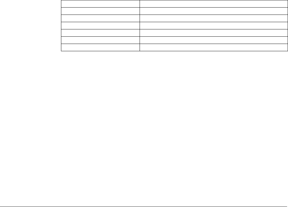
200
This saves Unnamed in a file, erases it from memory, and reads it back in (i.e. it is back as
before).
EraseClasses takes vector of classes in order to be able remove interdependent classes at the
same time without having any dangling references.
4.6.5 Traversing translated models
During translation (and check) the model is instantiated, i.e. the abstract syntax tree is
transformed into a specific structure for the model. To answer questions related to this the
package ModelManagement.Structure.Instantiated provides several API-routines. Note that
the instantiation can be time-consuming in order to get the complete result, and thus these
routines can be slower than the AST-routines.
These routines are used to implement the check in ModelManagement.Check, and can
answer questions such as number of equations and unknowns, what are the possible states
(discrete and continuous), and which models are used for components (useful for e.g. test-
coverage). The content is:
Name
Description
NrEquations
Get the number of equations of a model
NrUnknowns
Get the number of unknowns of a model
ListPossibleContinuousStates
Get possible continuous states
ListPossibleDiscreteStates
Get possible discrete states
UsedModels
Get classes that are used as components in a model
CountUsedModels
Get the number of instances of components in a model
The number of equations and unknowns is counted as for check, and not as for translate.
The numbers differ slightly, since during check an external environment for physical
connectors is assumed (in order to allow check of models that cannot be translated on their
own).
The continuous (and discrete) states are important to verify results. The term possible is
used, since for dynamic state-selection all possible states are not active at all points in time.
The counting of used models is split into two routines: one that returns the used models and
another that returns the count for specific models.
Content of
ModelManagement.-
Structure.Instantiated.
5 VISUALIZE 3D

5 VISUALIZE 3D 203
5 Visualize 3D
5.1 Introduction
Data visualization in 3D is an important way of representation, and it is adequate for
understanding and comprehending model behavior. Dymola includes a 3D graphical tool:
Visualize 3D.
Visualize 3D renders 3D scenes and has an associated Modelica package named Plot3D.
This package manipulates and sends the graphical data representation of the scene to
Visualize 3D. This guide describes how to use Plot3D to obtain graphs and figures with the
Visualize 3D tool in Dymola.
To open the Plot3D package, use the command File > Libraries > Plot 3D:
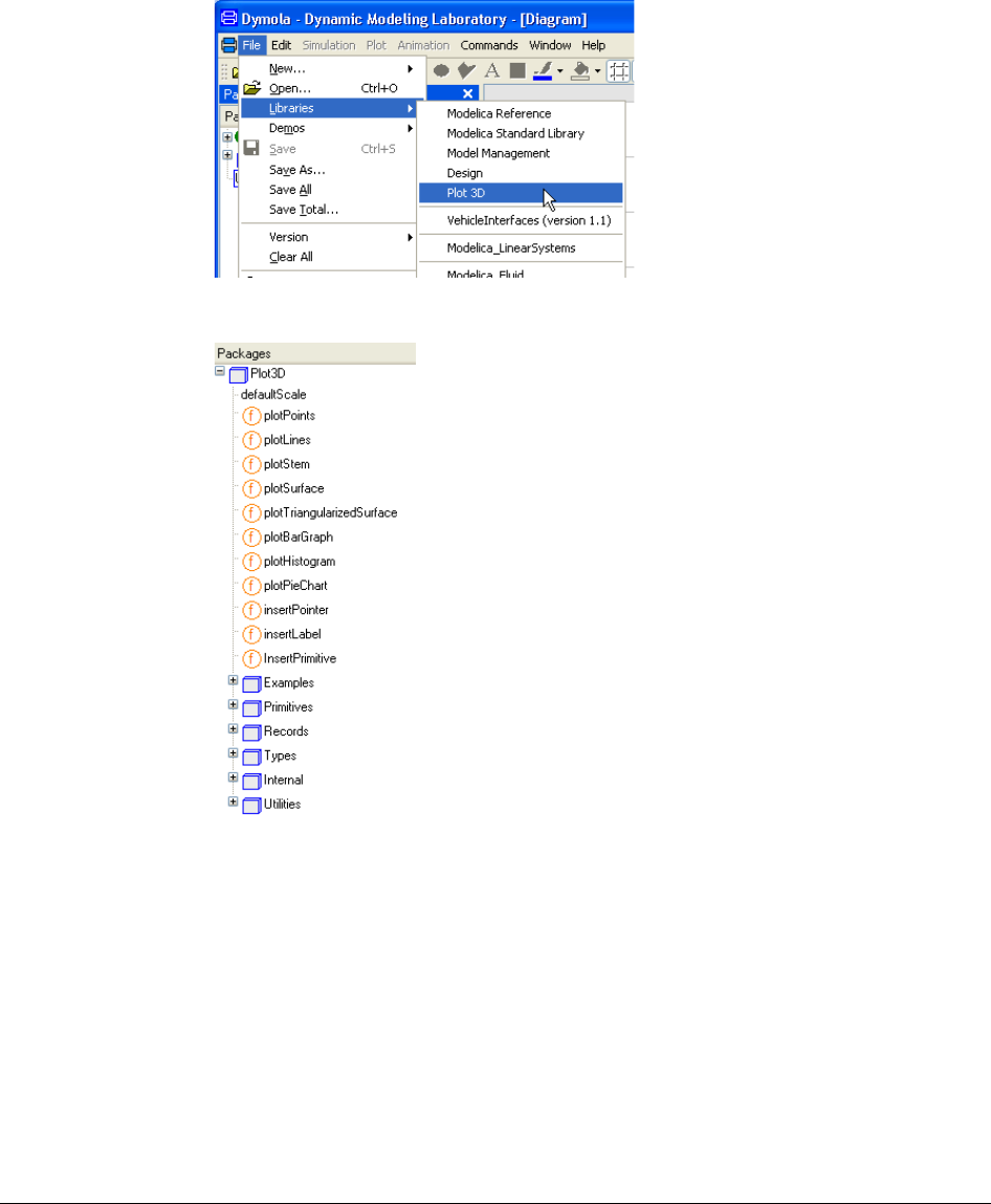
204
The package browser of Plot3D will look the following:
The main functions are at top level of the package: plotPoints, plotLines, plotStem,
plotSurface, plotTriangularizedSurface, plotBarGraph, plotHistogram, plotPieChart,
insertPointer, insertLabel and insertPrimitive. We recommend strongly using these high-
level functions instead of trying to use the low-level ones in Plot3D.Internal.
The sub-package Plot3D.Primitives contains the basic primitives preset. The sub-packages
Records and Types also contain information about the internal representation of a 3D scene.
The sub-package Examples contains in its turn some of the examples presented here and we
will refer to them later on.
Visualize 3D supports several different types of plots and can be presented separately in
their own windows if desired, all integrated in the Simulation tab.
Opening the Plot3D
package.
Plot3D packages.
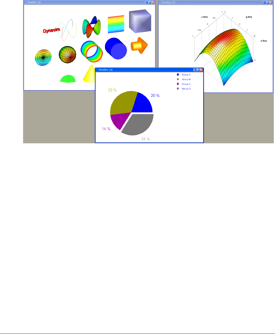
5 VISUALIZE 3D 205
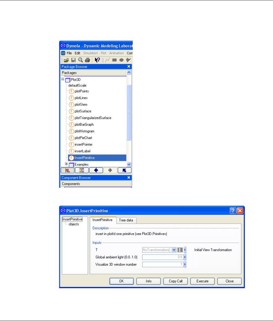
206
5.2 Inserting and removing graphical objects
Visualize 3D has several basic primitives that can be combined to construct more
complicated scenes. We will start by constructing a simple solid cylinder by combining a
cylinder shell with two disks. We start by using the function Plot3D.InsertPrimitive
Right-click on it and select Call Function. The following dialog will pop up:
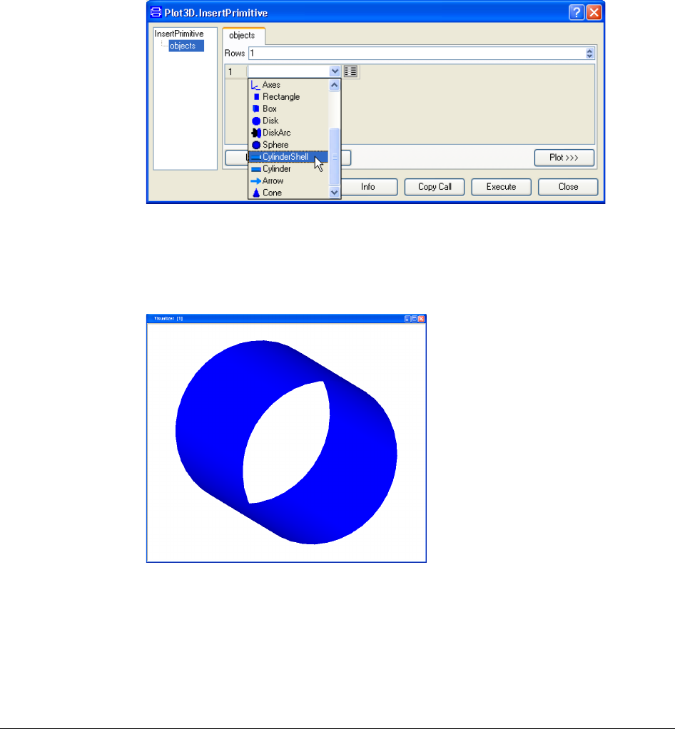
5 VISUALIZE 3D 207
The first elements we observe are the View transform matrix T, the global ambient light and
Visualize 3D window number. This number identifies the window we want to add some
primitive to. We keep the default values now and click on objects field in the tree. There
we are to select the primitive forms to be added. Click on the arrow of the combo box and
scroll down until CylinderShell.
We have now selected a cylinder shell and we can plot it with default values. Press Execute.
At first sight there is just an empty Visualize 3D window. Actually, we are looking at the
shell with zero thickness along its main axis. In order to see the figure, press the Ctrl key
and move the mouse to rotate along the axes x and y. The figure below shows one possible
view of the new created cylinder shell.
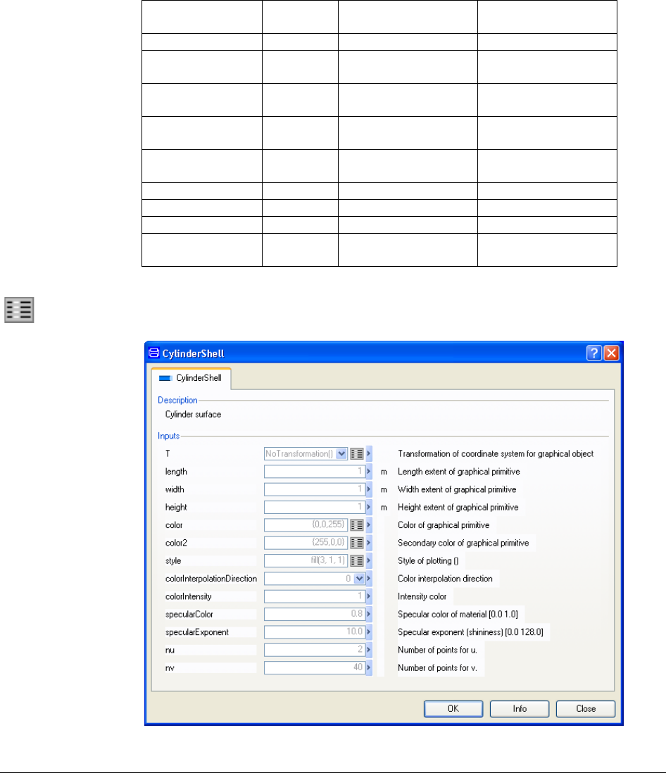
208
The operation of Visualize 3D can be summarized in the following table:
Operation
Meta key
Mouse move
(dragging)
Arrow keys
Selecting object
Alt+Select
Moving
up/down/left/right
none
Up/Down/Left/Right
Up/Down/Left/Right
Tilt (Rotate
around x-axis)
Ctrl
Up/Down
Up/Down
Pan (Rotate
around y-axis)
Ctrl
Left/Right
Left/Right
Roll (rotate
around z-axis)
Ctrl+Shift
Clockwise/Counter-
clockwise
Right/Left
Zoom in/out
Shift
Up/Down
Up/Down
Zoom in/out
none
Wheel
Zoom in/out
Ctrl
Wheel
Zoom in/out
Ctrl
Right mouse button
Up/Down
We can also perform other operations on the cylinder shell. Going back to the dialog
window and clicking on the Edit icon, we get the following dialog window.
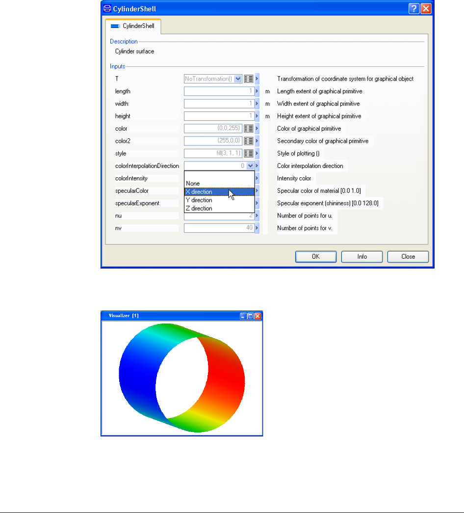
5 VISUALIZE 3D 209
We observe different graphical properties of the cylinder shell primitive. We are now
interested in a few: matrix T, length, color, style, colorInterpolationDirection and
colorIntensity. Change colorInterpolationDirection to “x direction”, press OK in the edit
menu and press Execute once more.
Press the Ctrl key and move the mouse. The change is that Visualize3D interpolates the
color using the range of the x coordinate of the primitive.
Changing the colorIntensity parameter it is possible to set the brightness of the color scheme
applied. This factor is to be in the interval [0,1]. Below we find depicted the cylinder shell
for intensityColor=0, 0.5 and 1.
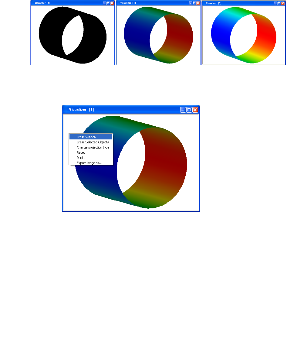
210
Remember that we are adding primitives; this means that if the intention is to change and
paint again, the Visualize 3D window has to be erased. This can be done by right-clicking in
the window and selecting Erase window in the context menu, as below. This operation will
clean the window object list.
The matrix T is used to perform transforms on just the associated graphical object.
Operations like translation, scaling and rotation of the body respect to the global coordinate
system are described with this T matrix. These transforms are independent of the global
view, and are used to construct the 3D scene. Clicking on the combo box arrow shows the
predefined possibilities.
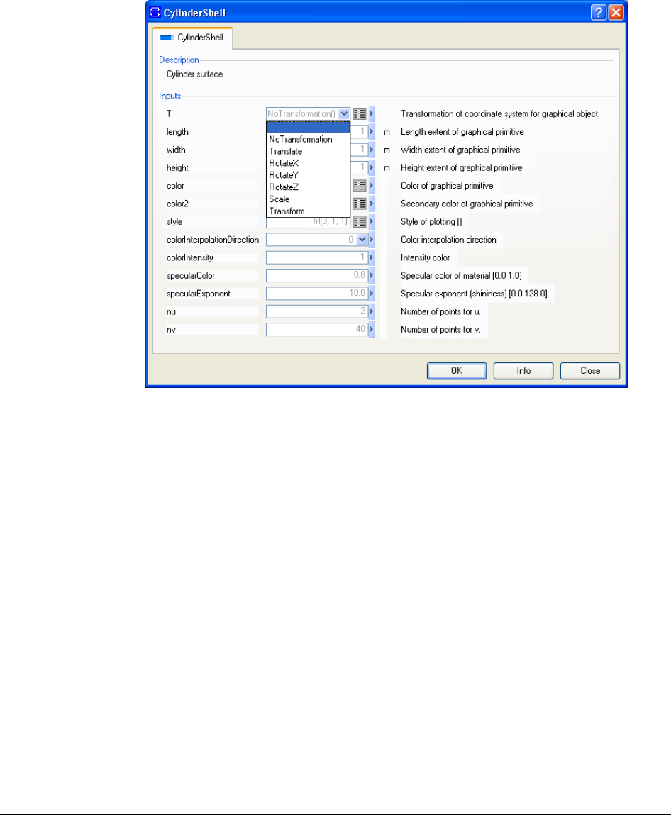
5 VISUALIZE 3D 211
We can select NoTransform, Translate, RotateX, RotateY, RotateZ, Scale and Transform.
The most general of the operations is Transform that involves a combination of all the
others.
The dialog window for “Transform” is the following:

212
Here we can describe what we want to do with the graphical object. The order is important,
since all these operations are not commutative, for instance, it is not the same to rotate and
translate as to translate and then rotate. The order preset is scale first, rotate around Z, rotate
around Y, rotate around X and then translate.
Let us now add the top and bottom of the cylinder. Again in the dialog window, we change
the “CylinderShell” primitive to the “Disk” primitive.
Click on the Edit button to pop the menu for the disk.
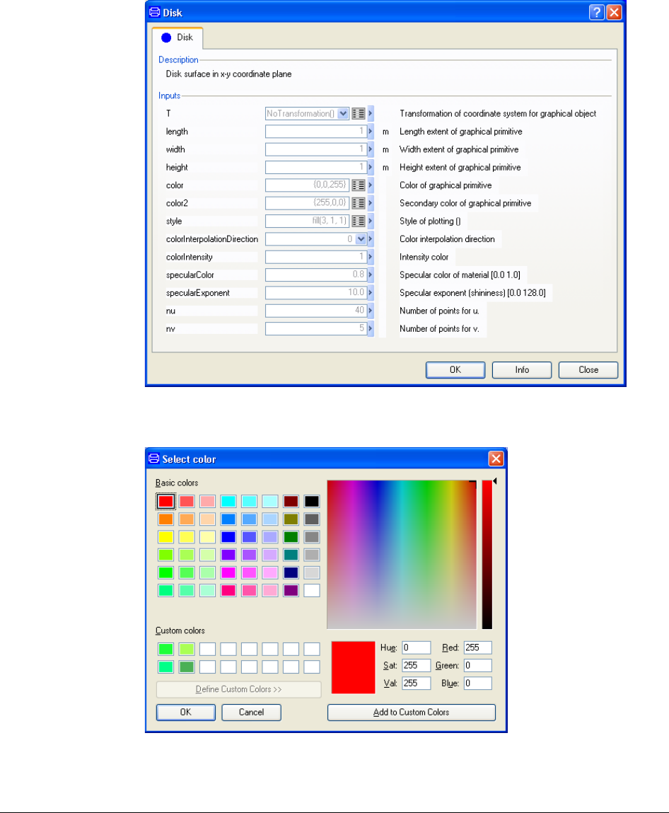
5 VISUALIZE 3D 213
Change the color of the “Disk” by pressing the Edit icon of the field “color”. We choose in
this case the red color to get a good contrast.
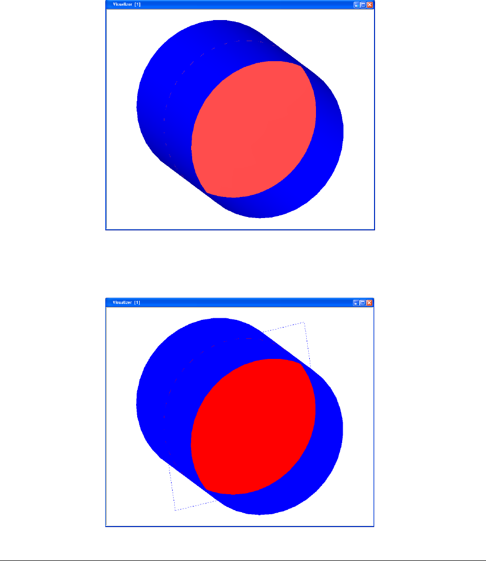
214
Click OK in the color window, click OK in the edit window and press Execute and finally
rotate once more using the Ctrl key and moving the mouse. We observe the following result:
The disk is in the middle by default. We want to place the disks on top and bottom of the
cylinder shell. We will therefore erase the disk and place it correctly using the translate
transform. To erase a graphical object, we have to select it first by clicking on it while
pressing the Alt key. The selected object will then be delimited by a dotted box.
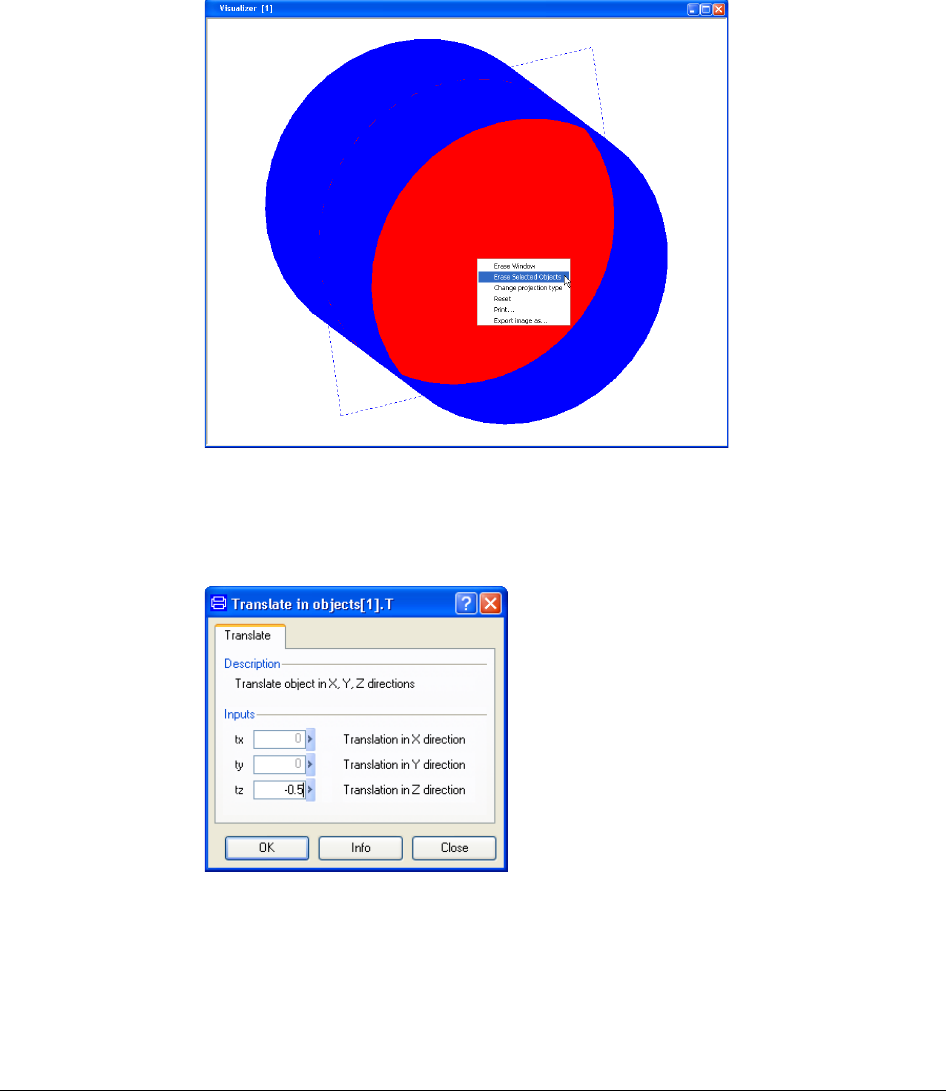
5 VISUALIZE 3D 215
Now we select from the context menu Erase Selected Objects, and the disk is erased from
the actual view.
To close the cylinder shell, we have then to set the bottom disk at the point
(0, 0, 0.5)−
and
the top disk at
(0, 0,0.5)
, since the cylinder has length 1. In the window “Disk”, click on the
edit icon of “T” and change “NoTransformation” to “Translate” using the arrow in the
combo box. A menu will appear. Set “tz” to -0.5 in this menu.
Press OK in this menu. It will disappear. Press Execute. A bottom disk will appear on the
cylinder.
To create a top disk for the cylinder, go back to the “Disk” window; change the color to
yellow (to be able to see all components clearly). Then click on the edit icon of “T” change
tz to 0.5 and press OK and Execute again. We obtain now a closed cylinder as below.
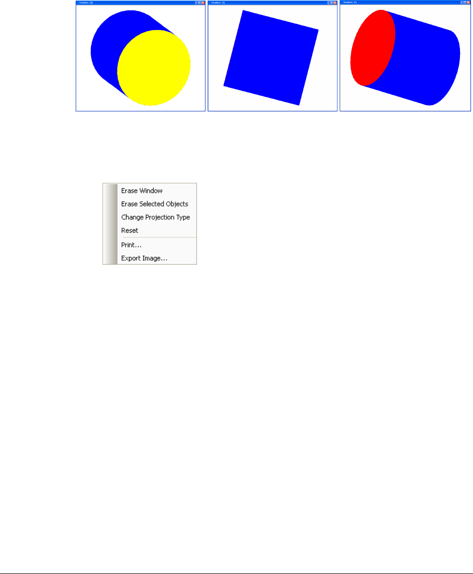
216
Here we see top, side and bottom of the newly created cylinder. The primitive
Plot3D.Primitives.Cylinder is constructed with this technique, encapsulating all necessary
steps to get a uniform color, size and other properties.
The context menu of the visualizer window can be summarized as:
Erase Window will erase all objects in the window.
Erase Selected Objects will erase the selected objects.
Change projection type will toggle between orthogonal projection (angles are preserved)
and perspective projection.
Reset will reset the objects in the window.
Print… will print the window.
Export Image… saves an image of the contents of the visualizer window (without window
borders) as a .png, .xpm or .jpg file. The user is prompted for a file name.
The image is identical to the image shown in the window, so the size and representation can
be changed by first resizing the window.
Exported images are included in the command log.
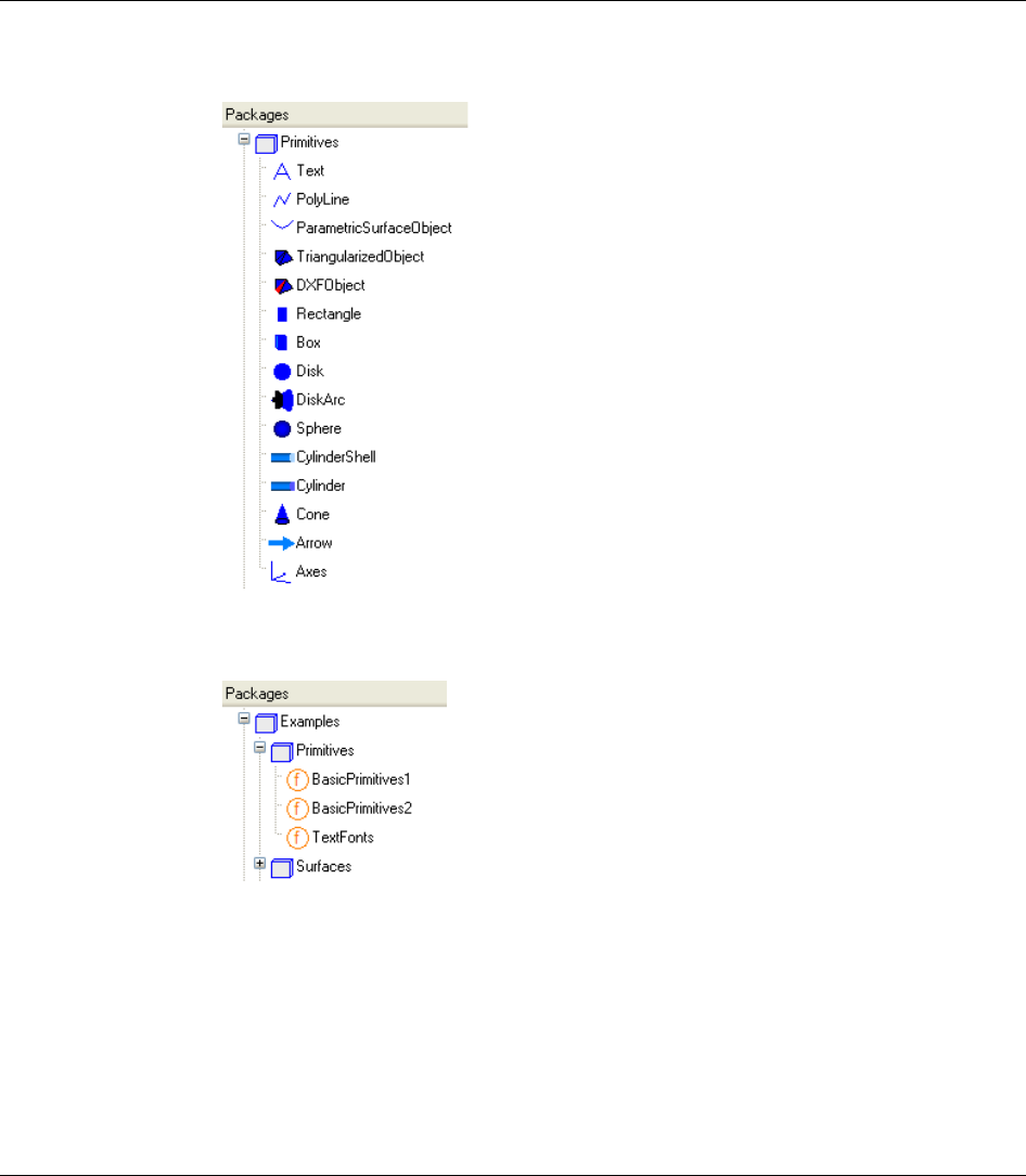
5 VISUALIZE 3D 217
5.3 Basic primitives
The basic predefined primitives included in Plot3D are presented in the figure below.
In the package Plot3D.Examples.Primitives, the functions BasicPrimitives1 and
BasicPrimitives2 produce 3D scenes with the primitives.
Click right on BasicPrimitives1 and then Call Function.... Then, press Execute. The
resulting 3D scene is the following.
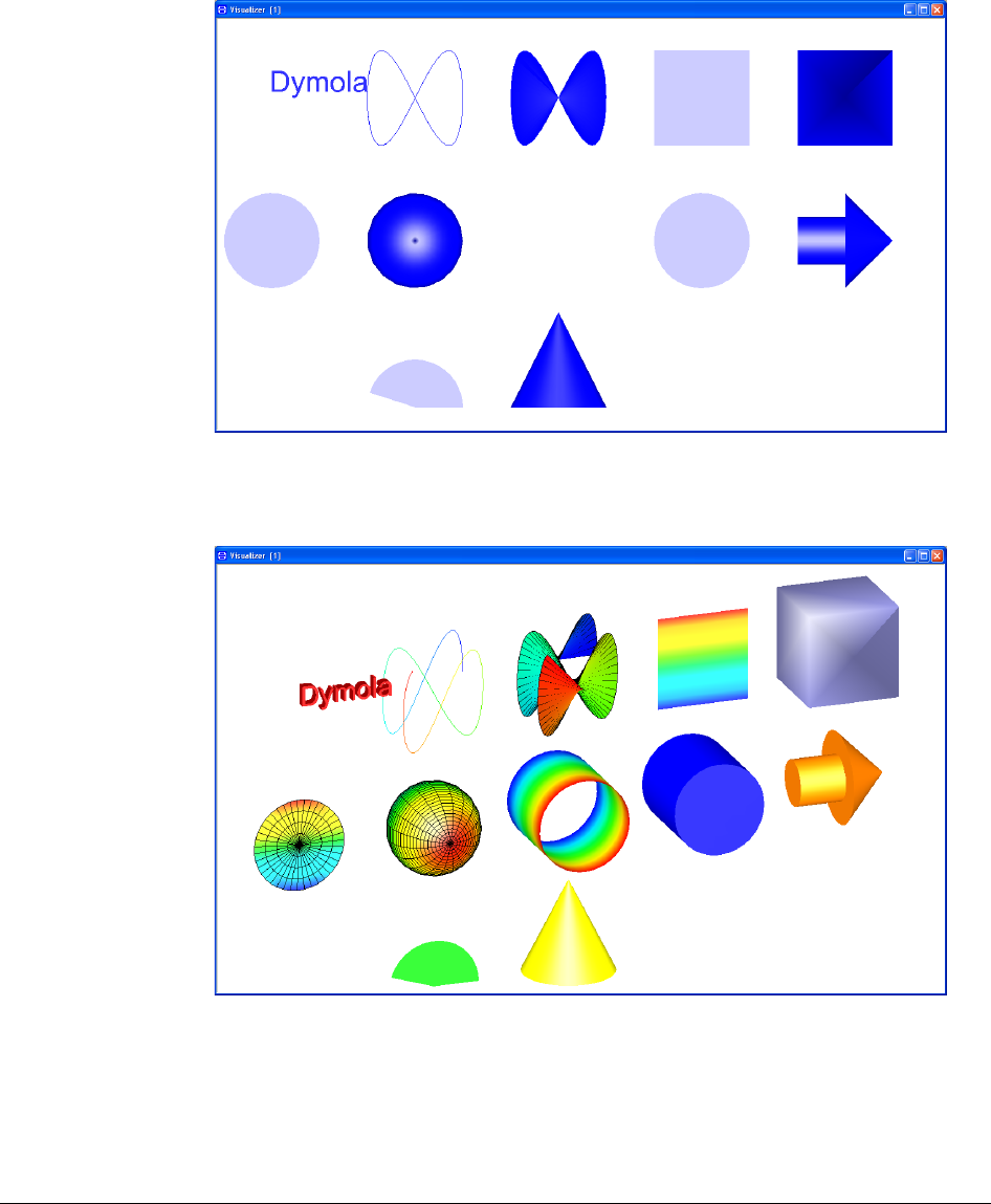
218
Notice that the cylinder shell has no thickness. BasicPrimitives2 is another example
showing some of the features of Visualize 3D. Repeat for BasicPrimitives2 as before to get
the following 3D scene.
In particular, the third curve at the top line is a Lissajous curve, typically used in electronics
and electrotechnique to find frequency and phase of an unknown sine curve, using a known
one as reference. If we observe now this curve along its z-axis, the result is the following.
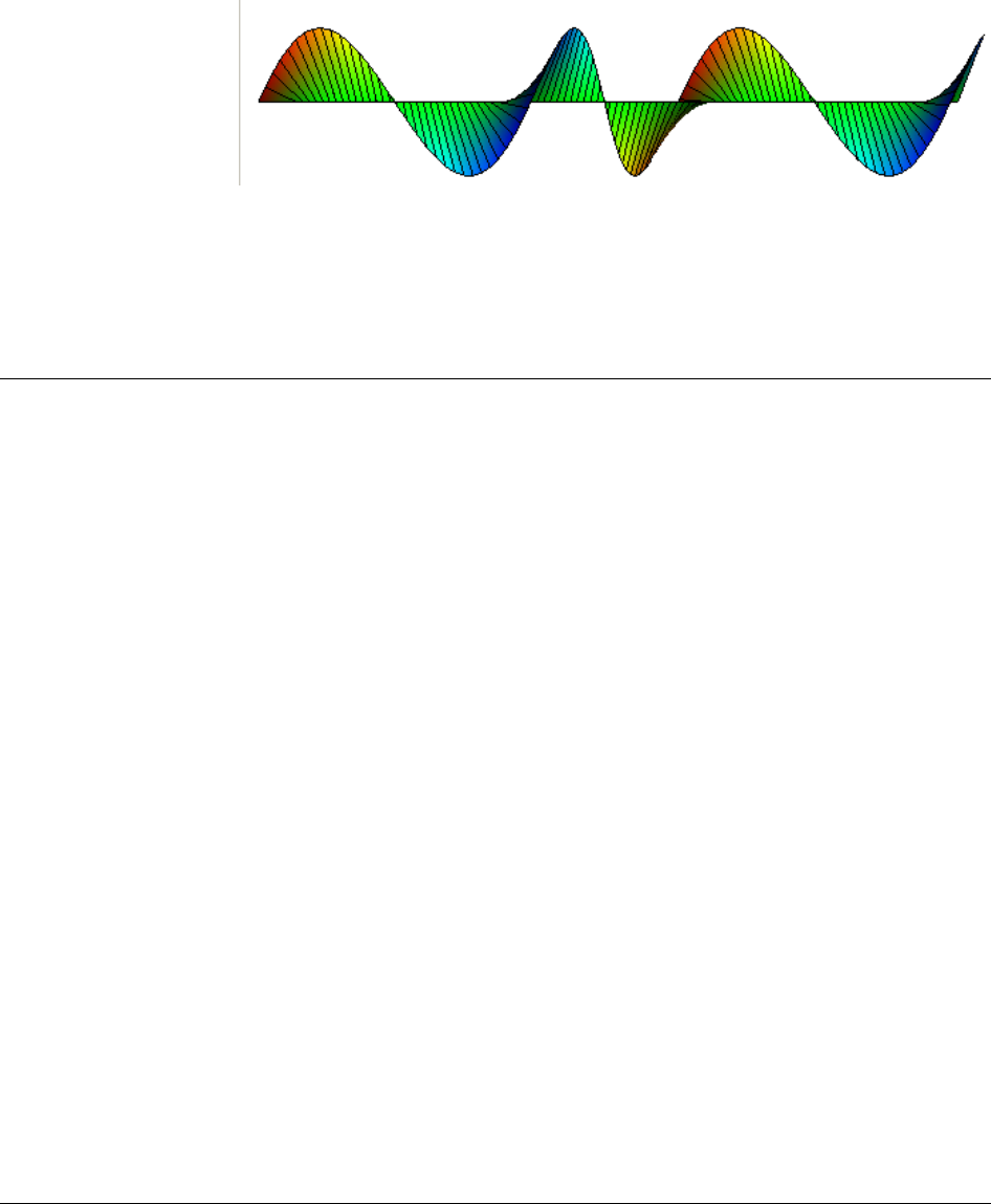
5 VISUALIZE 3D 219
The dialog windows of all primitives are very similar. Each one of them have inherent fields,
for instance, Plot3D.Primitives.Text has a String field called textString. In this case, the
label we want to render. The primitive Plot3D.Primtives.Axes is a very particular one, since
it produces a reference coordinate system. We will use it in the next section.
5.4 Surface Plots
Other important feature of Plot3D is the easy user interface and the inclusion of high level
help functions that will render surfaces, contour lines, water fall plots and bar graphs from
matrix data. In the following, the notation we use is as follows
1. The matrices x,y,z describing a parametric surface of the form
(,), (,), (,)x f ts y gts z hts= = =
.
2. The matrices nx,ny,nz describing a vector field
(,,)
xyz
ηηη
on the point
(,,)xyz
.
We will consider three test cases with their respective plots:

220
• parabolic function
22
1z xy=−−
on the interval
[1,1] [2,2]− ×−
• hyperbolic function
22z x xy= +
on the interval
[ 3, 3] [ 3, 3]− ×−
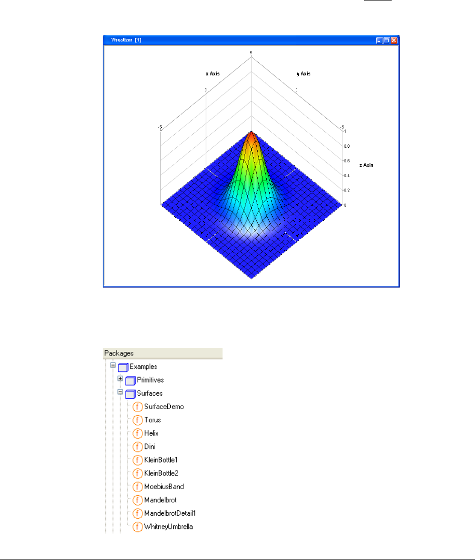
5 VISUALIZE 3D 221
• bivariate non-normalized Gaussian distribution
22
2
e
xy
z
+
−
=
on the interval
[ 5,5] [ 5,5]− ×−
.
The function Plot3D.Examples.Surfaces.surfaceDemo runs all test cases. We will consider
two of them here and just show the rest.
There are a number of more functions available, as can be seen in the package browser.

222
Let us plot the first test function. Enter the following command (followed by Return) in the
command input line to create the matrices x,y,z,nx,ny and nz
(x,y,z,nx,ny,nz):=Plot3D.Utilities.SurfaceTest1(25);
(You can get the command window and command input line displayed in Modeling mode
by using the command Window > Tools > Commands.)
Now, right-click on the function Plot3D.plotSurface. Select Call Function… . The
following dialog window appears
In this dialog we can set whether we want the axes automatically constructed or not.
Furthermore, we can indicate a Visualize window number in “plotId”. Click now on
plotSurfaces in the tree to the left. The following dialog pops
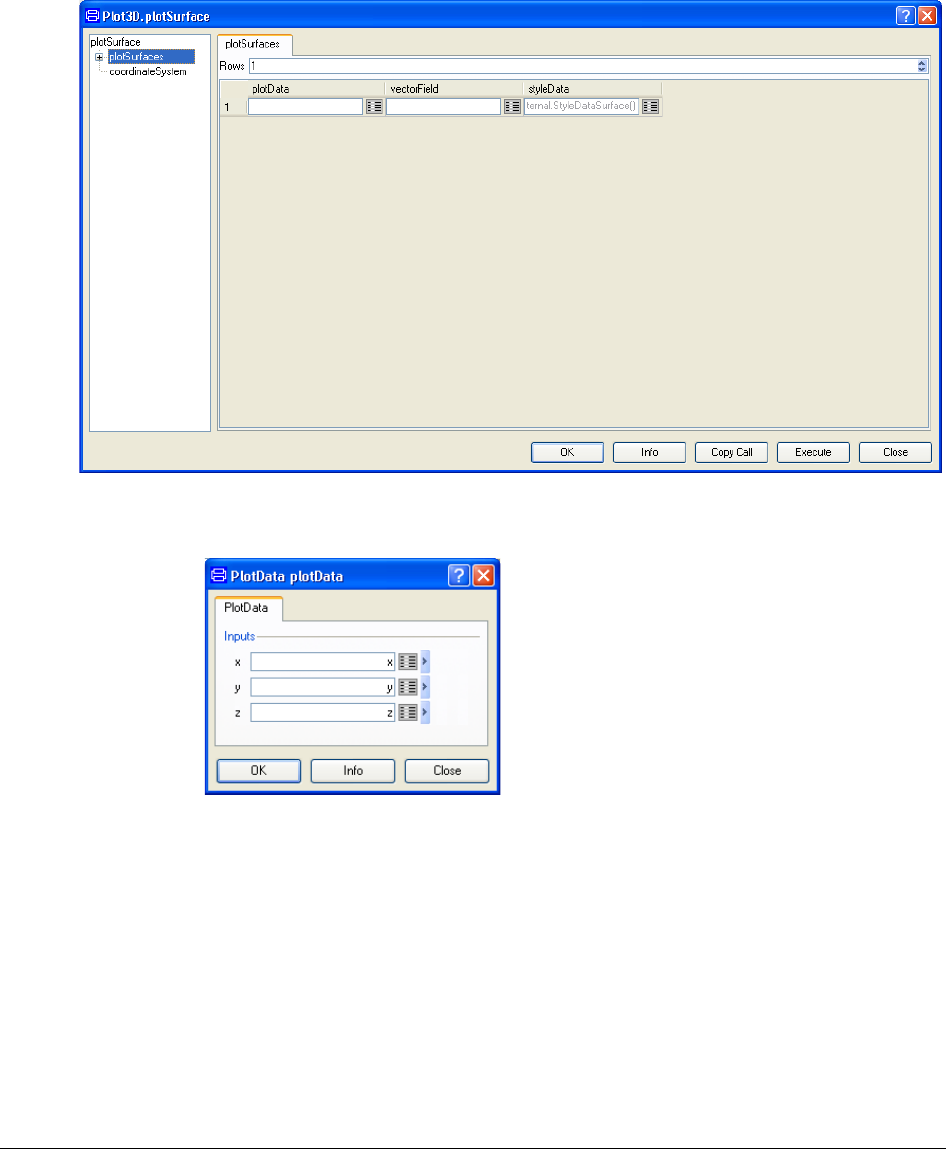
5 VISUALIZE 3D 223
To set the parametric surface matrices x, y and z we click on the edit icon of “plotData”.
The following window pops
The only information needed to create a plot is to fill in the matrices. We write x, y and z in
their corresponding places and click OK. Then, back in the main Dialog, we click on
Execute and obtain the following plot:
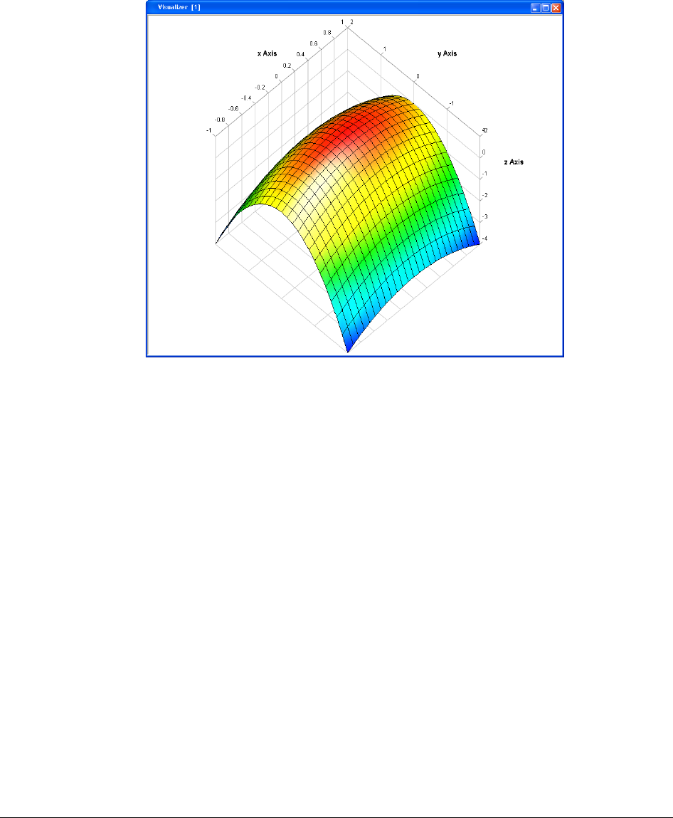
224
This is the default plot style (Filled with Mesh), and with default names for the X, Y and Z
axes. If we want to change the style of the plots, the data has to be filled in the “styleData”
field, using its Edit icon. The dialog follows
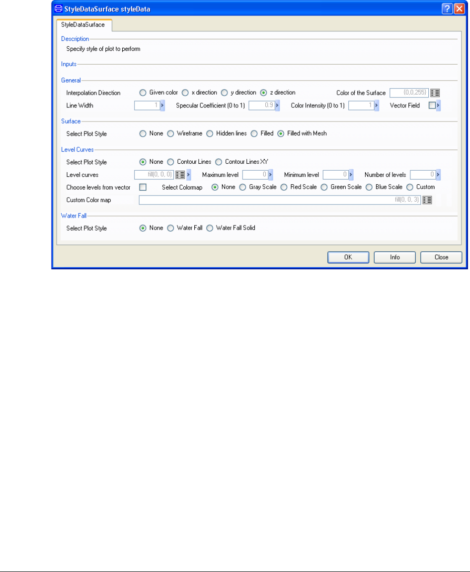
5 VISUALIZE 3D 225
We observe the different styleData alternatives. We can combine independently four groups
of data: Surface (Wireframe, Hidden Lines, Filled and Filled with Mesh), Level Curves
(Contour Lines and Contour lines XY), Water Fall (Normal and Solid disks) and Vector
Field (check box in General group).
To change the axes properties, we click on “coordinateSystem” in the tree to the left in the
Plot3D.plotSurface window. The following dialog window pops up:
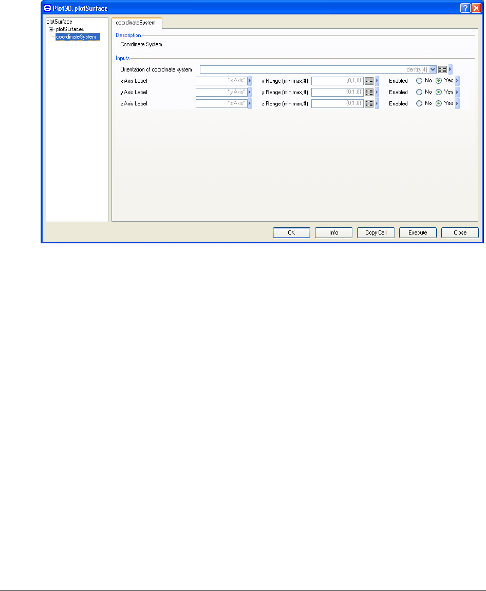
226
We observe here the fields “Axis label”, “Range” and “Enabled” for X, Y and Z axis.
Using the functions plotPoints, plotLines, plotStem, plotSurface and plotBarGraph follows
the same lines, with particular variations.
We want to emphasize the combination of contour plots with Wireframe. This combination
is particularly interesting to show features of a surface. For instance, the contour lines of the
hyperbolic function
22z x xy= +
for
0z=
yield two straight lines and constitute a
degenerated transition case between the hyperbolic lines in two quadrants (above of
0z=
)
and hyperbolic lines in the other two quadrants (below of
0z=
). The resulting plot follows
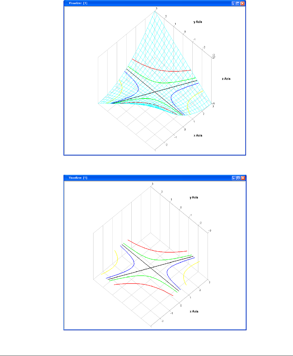
5 VISUALIZE 3D 227
Or easily viewed, projected on the XY plane without Z axis ticks

228
The black lines are the asymptotes of both sets of hyperbolic contour lines (red means
4z=
,
green
1z=
, blue
1z= −
and yellow
4z=
).
Other combinations can be useful to explain features too. For instance, when considering the
Gaussian bivariate probability distribution. If we integrate one of the variables (let us
integrate the y variable in this case) the resulting univariate function is also a Gaussian
distributed variable. Combining the “Rectangle on Top” with the “Rectangle” plots of
Plot3D.plotBarGraph function we can illustrate just that. The result follows.
The intersection of surfaces using Plot3D.plotSurface is also possible. The only thing we
have to do is to increment the number of elements to plot in the dialog. We can also set
color and style to identify easily the functions and delimit the intersection area.
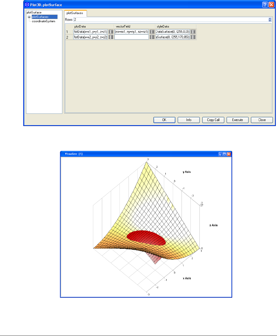
5 VISUALIZE 3D 229
One possibility is to have different colors for the surfaces. The intersection of the parabolic
surface and the hyperbolic surface with different colors will look as follows.
Combining different styles, we can obtain the following graph.
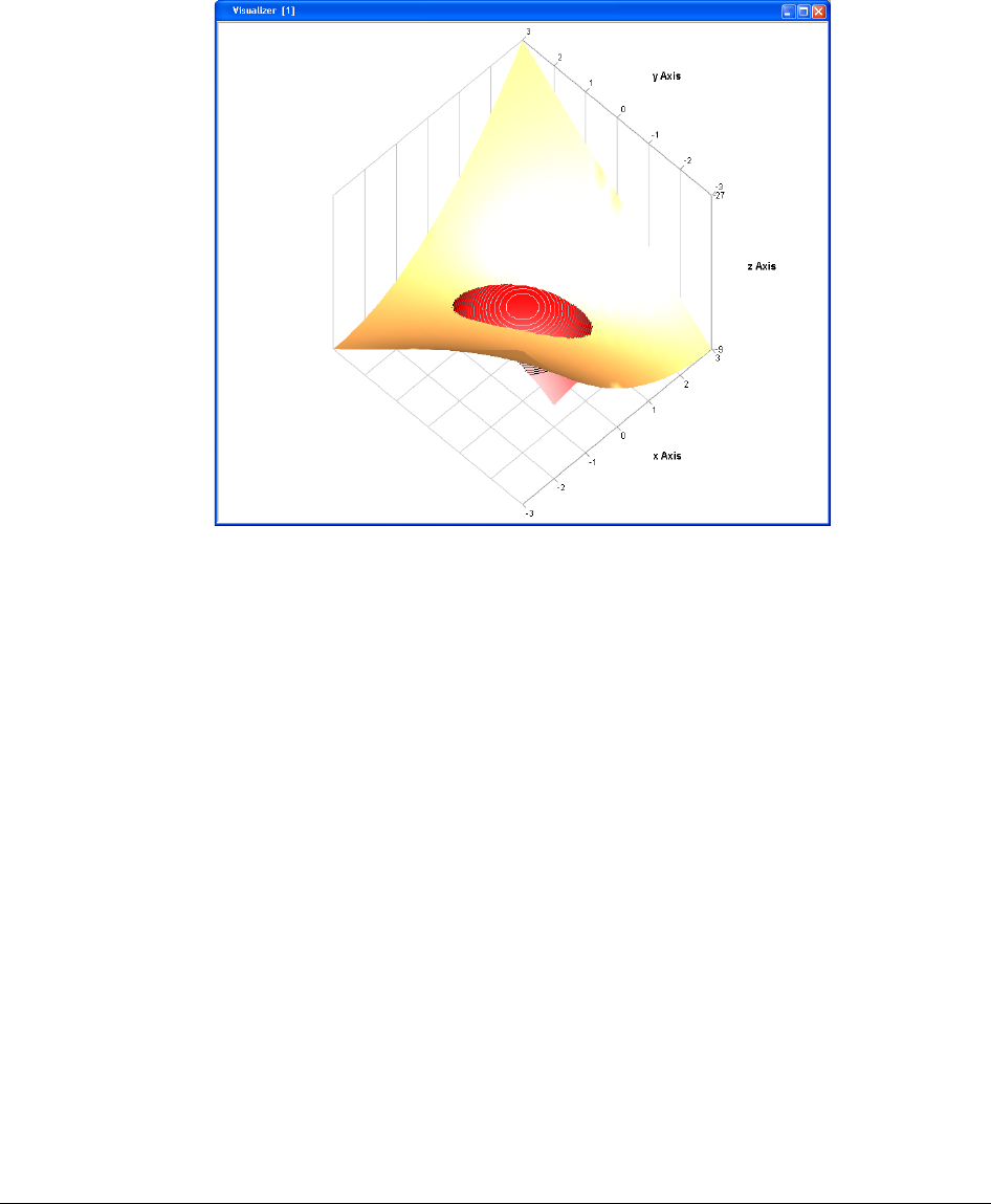
230
The contour lines in the parabolic surface (red) are used to illustrate that the intersection
does not happen on a plane. The black color corresponds to the level z=-1.5 and the white
color corresponds to the level z=1.
We can add a pointer to show where the maximum of the red surface occurs. Using the
function Plot3D.insertPointer directly on the last image we can add text and an arrow. The
resulting figure follows.
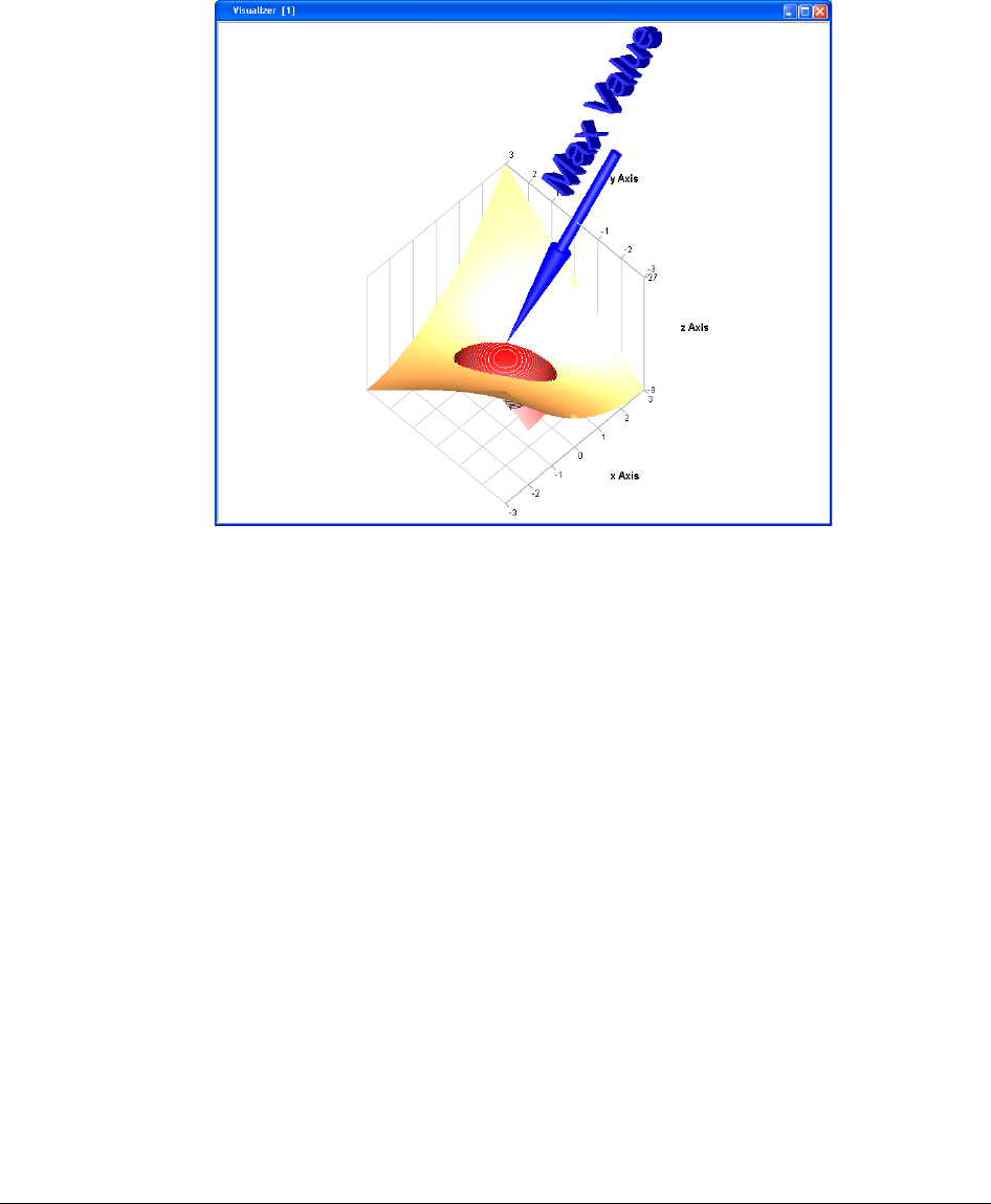
5 VISUALIZE 3D 231
To plot discrete data, the alternative is to use plotStem function. This function considers
each point by itself and puts a triangle, square or circle at the data point and adds a line from
the point to the plane XY. The following example shows the amplitude or absolute value of
the discrete Fourier Transform of a pulse. Putting the values in the unit circle of the complex
plane relates the Z-transform to the discrete Fourier transform. The color is interpolated in
the x direction.
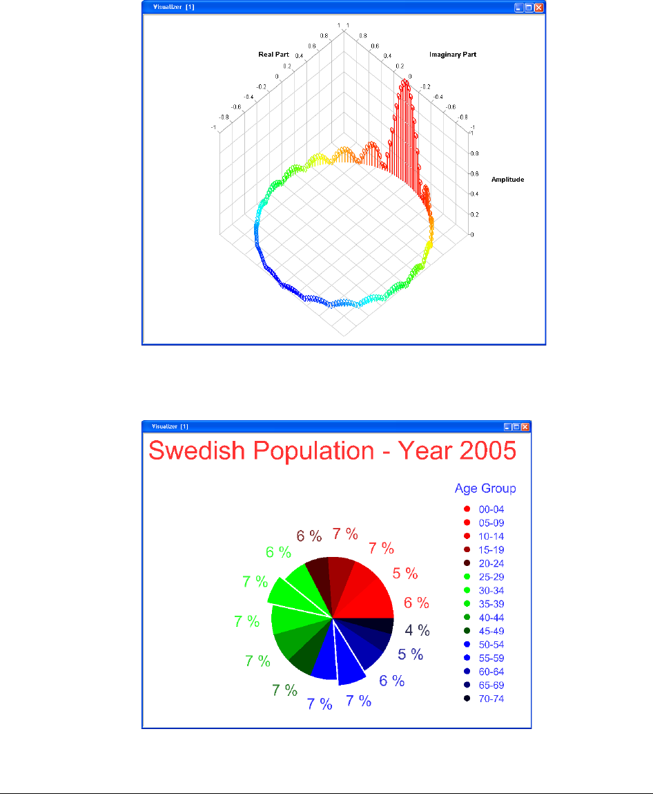
232
Other alternative that Plot3D provides is to make pie charts. Statistiska Centralbyrån
(Central statistics office) in Sweden reports the following population distribution by age in
2005. Two age groups are separated (30-34 and 55-59) to distinguish them.
6 OTHER SIMULATION
ENVIRONMENTS

6 OTHER SIMULATION ENVIRONMENTS 235
6 Other Simulation Environments
6.1 Introduction
This chapter describes how to interface models created in Dymola to other simulation
environments, or applications. The following external interfaces are detailed:
• Dymola interface to Matlab and Simulink (page 236).
• Real-time simulation on dSPACE and Matlab Simulink Real-Time (formerly xPC
Target) hardware (page 247).
• DDE communication (page 261).
o DDE interface for Dymola.
o DDE server support in the Dymosim simulator.
• OPC server support in the Dymosim simulator (page 268).
• Java interface for Dymola (page 273).
• Python interface for Dymola (page 288).
• JavaScript interface for Dymola (page 298).
• The Dymola report generator (page 299).

236
• Support for the Functional Mockup Interface (FMI) (page 306):
o Import and export of FMI models in Dymola.
o Validating FMI models from Dymola (page 330).
o FMI Kit for Simulink
Export of FMI models from Matlab/Simulink (page 332 and
335).
Import of FMI models into Matlab/Simulink (page 334 and 341).
• Building of stand-alone executables from source code or binary export models exported
from Dymola (page 352).
Note that information about external functions in other languages (C, Java, C++, and
FORTRAN 77) is available in the chapter “Advanced Modelica Support”.
6.2 Dymola – Matlab interface
The connection between Dymola and Matlab consists of an interface to Simulink
(DymolaBlock) and a set of Matlab m-file utilities. The paths below are for Windows, for
Linux the path to the Mfiles will be different.
In order to use the Matlab interface and all available m-files, please include
• Program Files (x86)\Dymola 2018\Mfiles
• Program Files (x86)\Dymola 2018\Mfiles\dymtools
• Program Files (x86)\Dymola 2018\Mfiles\traj
in the Matlab path. The first path must be present every time you want to use blocks
constructed with Dymola; the others are optional, if all m-files should be available. A good
idea is to do it once and then store the paths in Matlab.
Make sure that you have a Visual Studio C++ compiler installed on your computer. Make
sure that the Matlab mex utility has been configured to use that compiler (type mex –setup
in Matlab to configure). Finally, test by trying to compile and link an example mex file, e.g.,
matlab\extern\examples\mex\yprime.c
The Dymola – Simulink interface of Dymola 2018 supports Matlab releases from R2012a
(version 7.14) up to R2016b (version 9.1). Only Visual Studio C++ compilers are supported
to generate the DymolaBlock S-function on Windows. For Linux the gcc compiler is
supported. The LCC compiler is not supported, neither on Windows nor Linux.
6.2.1 Using the Dymola-Simulink interface
Note that you need a Dymola-Simulink license to use the Dymola-Simulink interface.
The following describes the Simulink interface for Windows, for Linux please see section
“Using the Simulink interface on Linux” on page 243.
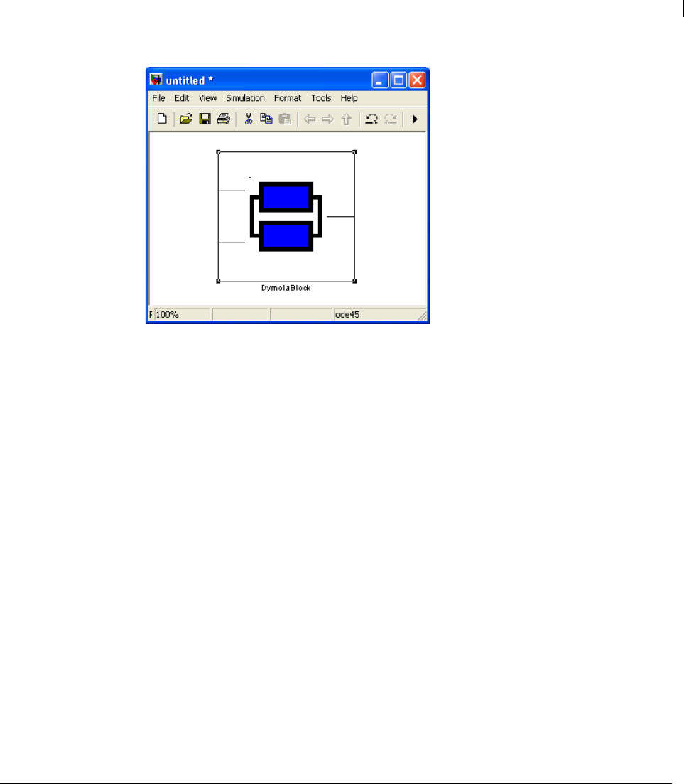
6 OTHER SIMULATION ENVIRONMENTS 237
The Dymola interface to Simulink is located in the Simulink library browser as Dymola
Block/DymolaBlock (if it does not appear you have probably not included the directory
Program Files (x86)\Dymola 2018\Mfiles in your Matlab-path; please see above).
You click once to open the library and you then drag the DymolaBlock to other models.
The DymolaBlock block, with the Dymola logo, represents the Modelica model. It can be
connected to other Simulink blocks, and also to other DymolaBlocks. Input and output ports
are added after compiling the model. The DymolaBlock is a shield around an S-function
MEX block, i.e., the interface to the C-code generated by Dymola for the Modelica model.
The DymolaBlock GUI
By double-clicking the DymolaBlock you open a GUI used to configure the block (see
figure on the next page). Configuration involves specifying the Modelica model, selecting
compiler options, compiling the Modelica model into a Simulink MEX file, setting and
resetting parameters and start values of the block, etc.
In the DymolaBlock GUI, you can set the name of the model and optionally the file name.
A simple way of setting the model name is to start Dymola, open the correct model, and
then press Select from Dymola>. This automatically gives the model name. Note that the
model name may contain a dotted name, e.g., Modelica.Blocks.Sources.ExpSine.
The file name is optional, but is used both to find the model and to ensure that the Simulink
model is up-to-date (for example, if the Modelica model is more recent than the MEX file
you are prompted to re-compile the DymolaBlock).
When associating a Modelica model with a DymolaBlock for the first time or when you
need to edit the Modelica model, you may click Edit model (after selecting the correct
current directory at the Matlab prompt). This launches Dymola, changes directory to the
correct directory in Dymola and opens a window with the model. Edit the model in Dymola
and verify it by making a test simulation in Dymola. After that, click on Compile model.
Dymola block before
compiling.

238
Two tree views are used to display parameters and start values of states (depending on the
model). After compilation, the tree views are populated and the first level is expanded.
Selecting a variable will display its name, size (for matrix variables), and description string.
The variable may be edited by entering a new value in the text field. Matrix variables may
also be edited using a matrix editor, which is launched by the button to the right of the text
field. While editing using the matrix editor, the rest of the DymolaBlock GUI is disabled.
The parameter settings are kept even if you press Compile model (assuming they match).
To reset parameters and start values to the default in Dymola press Reset Parameters.
Model dialog for a
DymolaBlock in
Simulink.

6 OTHER SIMULATION ENVIRONMENTS 239
Advanced configuration options
Hierarchical connectors as buses
Sometimes it is desirable to use buses for signals in Simulink and it is possible to map
hierarchical connectors in Modelica to buses in Simulink. This is accomplished by checking
Hierarchical Connector as Bus and re-compiling. In order to get an understanding of the
structure, an easy way is to construct hierarchical output connectors in Modelica and
examine the corresponding bus signals in Simulink. The rules for the buses are:
• All hierarchical input/outputs components are transformed into buses, except the signal-
element of block-connectors.
• Connector members of simple types (Real/Integer/Boolean) are mapped to real signals in
Simulink with the same name as in Dymola. Non-scalar elements are mapped into non-
scalar signals in Simulink.
• Connector members that are scalar records/connectors are mapped to buses in Simulink
with the same name as in Dymola.
• For connector members that are arrays of records/connectors, each element is mapped to
buses in Simulink with the same name as in Dymola (except that Simulink requires that
any “,” for matrix elements is replaced by “;”).
The mapping is fully hierarchical (i.e. connectors can contain sub-connectors that contain
sub-connectors etc), and applied to all input/outputs.
Using multiple DymolaBlocks
A Simulink model may contain several DymolaBlocks as long as they all use different
underlying MEX files. Using the same MEX file for several blocks in the same model will
give incorrect results or runtime errors. For this reason, copying of the DymolaBlock takes
special care to create a unique identification <tag> for the block such that all blocks in the
model use different MEX files even if they are multiple copies of the same Dymola model.
Unchecking Allow multiple copies of block will disable the generation of unique tags
when DymolaBlocks are copied. Unchecking it should only be done if you have dSPACE
multi-processor hardware, since the build command of dSPACE internally makes copies of
the model that should share the original MEX file name.
Compiling large models, /bigobj
When compiling large models, you may need to check the box Compiler flag /bigobj. This
will supplement COMPFLAGS with the /bigobj option to increase the number of
addressable sections of the produced object file. It should be noted that object files produced
with /bigobj can only be consumed by linkers shipped with Visual C++ 2005 or later.

240
Export for use with Dymola runtime concept
Checking the box Runtime export enables the compiled model to be distributed and
executed on a different computer by using a runtime concept. This box should never be
checked in any other case.
Omitting description strings
For models with big input files, you can select to omit description strings for parameters and
start values by selecting Omit description strings. This will avoid problems with Matlab
memory limitations (especially for 32-bit installation).
Result files
Sometimes it is useful to generate result files in the Dymola standard format when running
in Matlab/Simulink, e.g., to:
• Animate 3D-objects
• Investigate intermediate variables in the model
• Generate an input file for further simulation studies in Dymola (this requires an extra
step: to export the generated result file (using the context menu in the variable browser
in Dymola) as ‘dsu.txt’).
All of this is accomplished by selecting Generate result. If you also want the result file to
be automatically loaded in Dymola select Auto-load. If the result files become very large it
might be useful to reduce the size by introducing a Minimum Dt, which is a minimal output
interval length, e.g., 0.1 (similar, but not identical to “Interval length” in Dymola). Any
modifications of these choices require a new compilation of the DymolaBlock.
The generated result file will get the name specified in the Result name text field. By
default the text field is empty and if not specified the result name will be populated with the
same name as the generated S-function MEX file after compilation. This is an automatically
generated name (on the form <modelname>_dy<tag>) that ensures uniqueness between
DymolaBlocks and result files also when generated from the same original Modelica model.
Import mode
The functionality of the Select from Dymola>, Edit model, and Compile model as
described above relies on communication between Matlab and Dymola using a DDE
connection. This mode is only supported on Windows and is therefore called Dymola-on-
Windows mode.
The DymolaBlock also supports a generic import mode, to be used on non-Windows
computers or on computers without a full Dymola installation. This mode does not require a
DDE connection to Dymola and is intended for import of compiled DymolaBlock S-
functions or code that have been exported from Dymola for use in Simulink. One dedicated
use of this new functionality is to import S-functions or code that has been generated on a
different computer using the binary model export feature.
The button at the bottom right corner of the DymolaBlock GUI is used to toggle between
the Dymola-on-Windows (using DDE) mode and the Import mode.
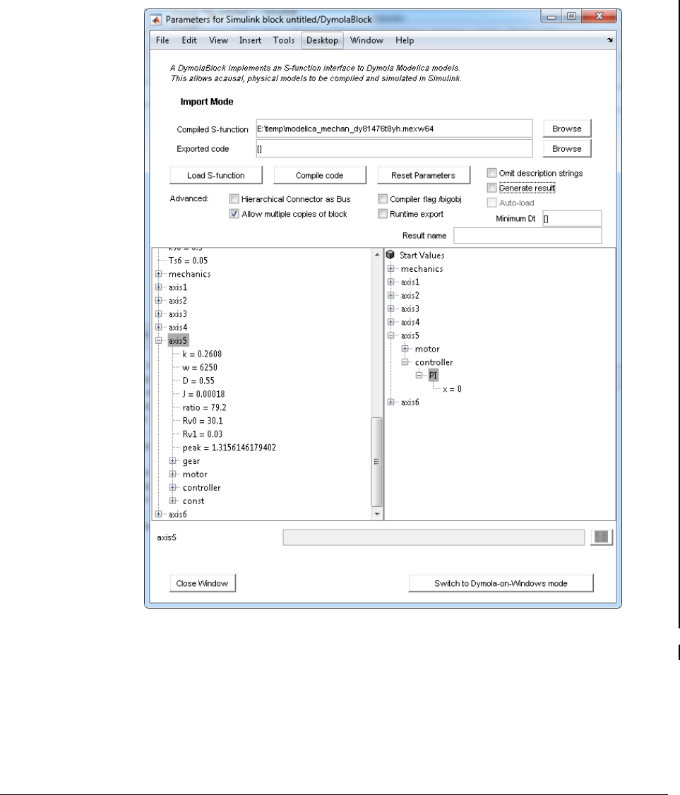
6 OTHER SIMULATION ENVIRONMENTS 241
In import mode, it is possible to either import pre-compiled DymolaBlock S-functions
(.mexw32, .mexw64, .mexglx or .mexa64 files) or C code that has been exported to
Simulink from Dymola.
For an example on how to export code to Simulink, see section “Using the Simulink
interface on Linux” on page 243 ; the export is applicable to Windows as well.
GUI of DymolaBlock in
import mode.

242
Compiled S-function import
To import a pre-compiled DymolaBlock S-function, press the Browse to the right of the
Compiled S-function input field. This opens a file selector that allows you to browse for
the desired S-function to load. The selected S-function is then loaded to the DymolaBlock
by pressing the Load S-function button. This will also create the tree views of parameters
and start values and create the input and output ports of the block.
This import functionality allows a DymolaBlock to be compiled at one computer with a full
Dymola installation and then sent in binary form to another computer where it can be loaded
and simulated.
Importing compiled S-functions requires having a copy of the Program Files
(x86)\Dymola 2018\Mfiles folder available. The location of this folder should be
added to the Matlab-path as described above.
The following files created during compilation of a DymolaBlock need to be distributed to
allow this type of import
1. Compiled S-function
2. dsin.txt or model-specific input file (<modelname>_dy<tag>.txt)
Note that the names of S-functions generated by the DymolaBlock are machine-generated,
on the form <modelname>_dy<tag>.<mexext>, where <tag> is a unique tag for the
DymolaBlock.
C code import
To import code that has been exported for Simulink, press the Browse to the right of the
Exported code input field. This opens a directory selector that allows you to browse for the
folder containing the exported code. The code is compiled into a DymolaBlock S-function
by pressing the Compile code button. This will also create the tree views of parameters and
start values and create the input and output ports of the block.
This import functionality allows a Modelica model to be exported at one computer and then
the code generated during compilation can be distributed to another computer where it can
be compiled, simulated, and also downloaded to real-time platforms.
Use of the C code import requires a full Dymola installation. The location of the Mfiles
folder should be added to the Matlab-path as described above.
The following files created during compilation of a DymolaBlock need to be distributed to
allow this type of import
1. dsmodel.c
2. dsin.txt
3. dymModelInfo.m
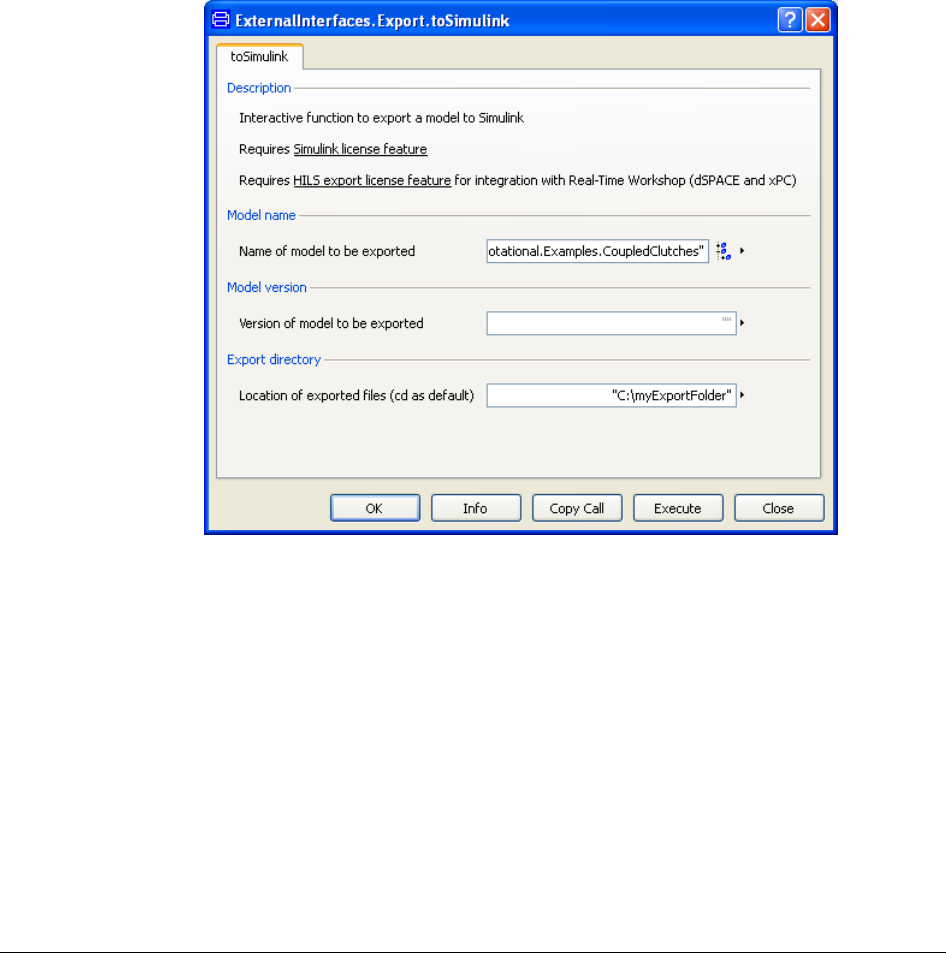
6 OTHER SIMULATION ENVIRONMENTS 243
Using the Simulink interface on Linux
The Simulink interface on Linux uses a two-step export/import procedure. The import step
relies on the C code import of the DymolaBlock GUI as described in the previous section.
To export the needed files from Dymola, open the package ExternalInterfaces (located
in the Modelica/Library subdirectory of the Dymola installation) and execute the function
ExternalInterfaces.Export.toSimulink:
Select the name of the model to be exported and the export directory, the model version
field can be left unchanged. The C code and .m file required by the import will then be
generated in the selected export directory. Then browse to this directory in the Exported
code input field of the DymolaBlock GUI and press the Compile code button.
Example model from Dymola – Coupled clutches
As an example of using the Dymola-Simulink interface, we will use the Dymola demo
model Coupled Clutches shown in the figure below. The coupled clutches demo is opened
in Dymola using the command File > Demos.
Function dialog for
export of model code
to Simulink.
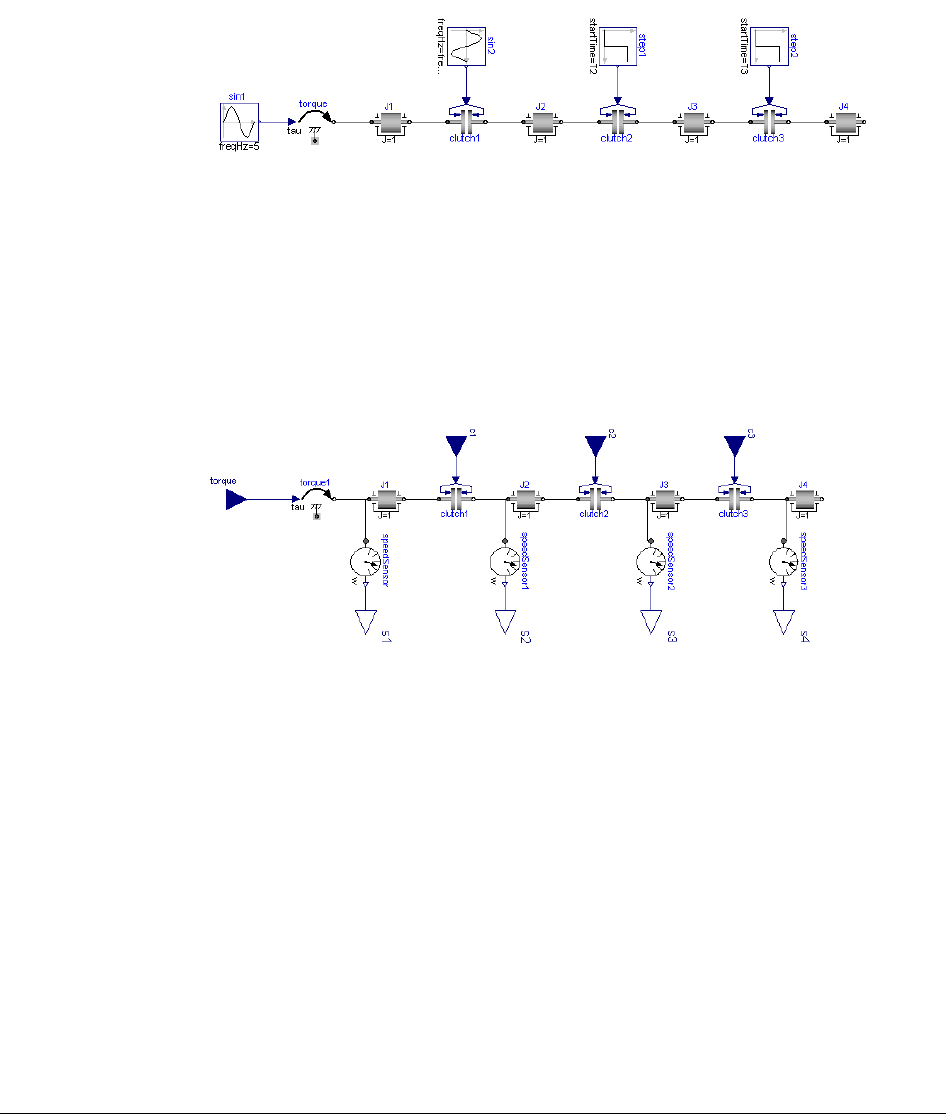
244
In order to make the Dymola model useful as a block in Simulink, you first need to define
external inputs and outputs to and from the Dymola block. You change this in your model in
Dymola, and it may either be accomplished by declaring variables as input or output in the
top-level model or graphically by adding input (filled) and output (non-filled) connectors,
e.g., from Modelica.Blocks.Interfaces.
The latter option is used for the coupled clutches example and shown in the figure below.
The sine wave and step inputs are replaced by input connectors, and speed sensors are
connected to the inertias and used as outputs.
The next step is to create a new Simulink model and drag a DymolaBlock from the
Simulink library browser to the model. To compile the model, double-click the
DymolaBlock and press the Select from Dymola> button followed by Compile model. The
compilation process creates a C-style S-function with a machine-generated name, in this
case coupledclutches_dy<tag>.c, where <tag> is unique for the DymolaBlock.
After compiling the model, input and output ports are added to the DymolaBlock,
corresponding to the input and output connectors in Dymola. The names of the ports are the
names of the Modelica input/output variables. The order of the graphical inputs and outputs
correspond to the order in which they were added to the model. Note: Dymola may convert
output variables to states, in which case the outputs will disappear from the DymolaBlock.
Apply the der()-operator to an intermediate variable to avoid this problem.
Coupled clutches
example in Dymola.
Model with external
inputs and outputs for
use in Simulink.
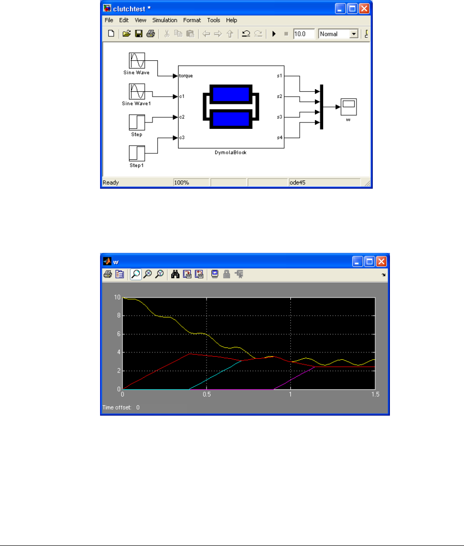
6 OTHER SIMULATION ENVIRONMENTS 245
The input ports are connected to external signal sources and a scope is connected to the
output ports for plotting the rotational speed of the inertias. After configuring the signal
sources according to the Dymola model (amplitude, frequency, phase, and step times), a
1.5-second simulation in Simulink produces the following output.
To recreate the corresponding Dymola simulation you should be aware that the
parameterizations differ between the Modelica Standard Library models and Simulink
blocks, e.g., the frequency of the Simulink Sine-block is measured in rad/s, which is
commonly known as angular frequency and should thus be 2*pi times the frequency in the
corresponding source in Modelica.
Simulink model of the
coupled clutches
example.
Simulink simulation
output.

246
Implementation notes
The DymolaBlock relies on a number of callbacks and tags in order to allow copying,
renaming, etc. This allows storing of settings for model name, parameters, and initial values
in the Simulink format. However, manually editing mdl-files containing DymolaBlocks is
not supported neither is changing the tag of the DymolaBlock or any of the callbacks asso-
ciated with the DymolaBlock.
DymolaBlock is found in DymolaBlockMaster.mdl, and you can also get DymolaBlock by
running DymolaBlockMaster. In this case you must copy DymolaBlock to another model.
The library annotation for external functions is automatically used also in Simulink. For
those who have worked around this in other ways it can be turned off using
Advanced.IncludeLibrariesForSimulink=false;
Using DymolaBlock GUI on a computer without Dymola installation
It is possible to use the DymolaBlock GUI on a computer without a Dymola installation by
copying some files to that computer. This in needed when distributing DymolaBlock S-
functions using the binary export option, or for use with a runtime concept. Files to copy
are:
• newDymolaGui.p
• newDymolaGuiJava.p
These files should be copied from a computer having the same Dymola version as was used
for creating the model. The files are located in the Mfiles directory (e.g. Program Files
(x86)\Dymola 2018\Mfiles). They could be copied to any directory on the target
computer. In order to be found by Matlab the path to that directory should be added to the
Matlab paths.
6.2.2 Other Matlab utilities
The directory Program Files (x86)\Dymola 2018\Mfiles and the sub-directories
dymtools and traj contain a number of useful Matlab m-files that can be used to, e.g., run
dymosim, load and save tables, and manipulate parameters and start values interactively
from the command prompt or from Matlab scripts. The m-files concerning the use of
dymosim are described in “Dymola User Manual Volume 1”, chapter “Simulating a model”,
section “Dynamic Model Simulator”, sub-section “Dymosim reference”. For additional
descriptions use the Matlab help command on the functions below.
The handling of tables is facilitated by Matlab routines for easier construction of 2- and n-
dimensional tables. The n-dimensional routines below work in combination with an n-
dimensional table lookup model, TableND. Please see “Dymola User Manual Volume 1”,
chapter “Developing a model”, section “Advanced model editing”, sub-section “Using data
from files” for more information about TableND.

6 OTHER SIMULATION ENVIRONMENTS 247
Tables:
load2DTable
Load a 2-dimensional table in the format suitable for 2D-table
interpolation in Dymola using the model
ModelicaAdditions.Tables.CombiTable2D
loadNDTable
Load the N-dimensional table in the format suitable for ND-table
interpolation in Dymola
save2DTable
Saves the 2-dimensional table in a format suitable for 2D-table
interpolation in Dymola using the model
ModelicaAdditions.Tables.CombiTable2D
saveNDTable
Saves the N-dimensional table in a format suitable for ND-table
interpolation in Dymola
The following commands are used to change parameters and start values of a simulation
without using the DymolaBlock GUI. These commands are useful in constructing batch
simulations, in which a series of simulations are run from a script (using the sim command)
with parameter changes in between each simulation. You need to close and re-open the
DymolaBlock GUI to display the new values set using setParametersFDsin.
Loading and changing parameters and start values:
loaddsin
Loads values from dsin.txt (or <modelname> .txt file)
setParameterByName
Set parameters and start values using the name of the
corresponding Modelica variable.
setParametersFDsin
Modifies the parameters and start values of a DymolaBlock.
setfromdsin
Sets parameters and initial conditions from values in dsin.txt (the
same as Reset Parameters in the DymolaBlock GUI). Calls
loaddsin followed by setParametersFDsin
The following is an example of using the functions for the robot demo model:
>> [p,x0,pnames,x0names]=loaddsin('fullRobot.txt');
>> p=setParameterByName(pnames,p,'mLoad',25);
>> p=setParameterByName(pnames,p,'mechanics.world.mue',4.5320e14);
>> x0=setParameterByName(x0names,x0,'axis1.gear.spring.phi_rel',10);
>> setParametersFDsin('untitled/DymolaBlock',pnames,p,x0names,x0);
6.3 Real-time Simulation
Dymola provides support for real-time simulation (e.g., Hardware-In-the-Loop) on dSPACE
and xPC Target platforms. This is accomplished using the Dymola-Simulink interface in
connection with Matlab Coder. Real-time simulation also requires the Dymola RealtimeSim
or SourceCodeGeneration license options. Models used for real-time simulation can contain
more than one DymolaBlock, enabling use of the Simulink multi-tasking feature for more
efficient utilization of computational resources in real-time simulations.

248
In this section we will describe the needed configurations for each of the supported
platforms. The description will focus on the Dymola-specific setup and we refer to the
documentation for each platform for more complete instructions. Setup and real-time
simulation results for the coupled clutches Simulink model described in the previous section
will be shown for the supported real-time platforms.
Restrictions
Real-time Simulation only allows export of models that use inline integration, i.e., that have
embedded fixed-step integrators. Inline integration is configured in Dymola by choosing
Simulation > Setup and selecting the Realtime tab. The model can still be used in normal
Simulink without inline integration, and a warning is issued that the model cannot be used
for real-time simulation. Advanced options for inline integration are documented at the end
of this section. The inline integration restriction for real-time simulation is not imposed for
users having the Source Code Generation export option.
The model code exported for real-time simulation does not include the most advanced
runtime routines that are normally included from binary libraries when building simulation
executables from Dymola. Most notably, models with dynamic state selection cannot be
used in real-time simulations2. For this reason, the exported C-code is used only when
compiling for real-time targets. For normal simulation in Simulink, the S-function is linked
with the binary libraries, thus, allowing use of the advanced runtime routines.
Disabling real-time simulation
To generate code for real-time simulation when compiling models for Simulink, the
RealtimeSim or SourceCodeGeneration options must be available. The option RealtimeSim
is by default available.
In a few cases a user might want to disable checking out the RealtimeSim option. Such a
case is if a user wants to work with Simulink but don´t intend to use the models on real-time
simulation platforms. By not checking out the RealtimeSim or the SorceCodeGeneration
option, the result files will be smaller.
To disable checking out the option RealtimeSim, you can set the following flag on the
command line
Advanced.EnableRealtimeSim = false
This setting is used to avoid unintentionally checking out real-time simulation options from
a sharable license when compiling for Simulink. The flag is by default true.
The setting to disable real-time simulation is remembered between Dymola sessions.
2 For more information about state selection, please see chapter “Advanced Modelica Support”, section “Means to
control the selection of states”.

6 OTHER SIMULATION ENVIRONMENTS 249
Checking out the SorceCodeGeneration option is by default disabled. Concerning the
handling of the export option SourceCodeGeneration, please see section “Enabling Export”
on page 349.
6.3.1 dSPACE systems
Compatibility
Dymola 2018 officially supports the DS1005, DS1006, MicroLabBox, and SCALEXIO
systems for HIL applications. For these systems, Dymola 2018 generated code has been
verified for compatibility with the following combinations of dSPACE and Matlab releases.
• dSPACE Release 7.3 with Matlab R2012a
• dSPACE Release 7.4 with Matlab R2012b
• dSPACE Release 2013-A with Matlab R2013a
• dSPACE Release 2013-B with Matlab R2013b
• dSPACE Release 2014-A with Matlab R2014a
• dSPACE Release 2014-B with Matlab R2014b
• dSPACE Release 2015-A with Matlab R2015a
• dSPACE Release 2015-B with Matlab R2015b
• dSPACE Release 2016-A with Matlab R2015b and R2016a
• dSPACE Release 2016-B with Matlab R2015b, R2016a, and R2016b
The selection of supported dSPACE releases focuses on releases that introduce support for a
new Matlab release and releases that introduce a new version of a cross-compiler tool. In
addition, Dymola always supports the three latest dSPACE releases with the three latest
Matlab releases. Although not officially supported, it is likely that other combinations
should work as well.
Configuration
The appearance of the dialogs presented in the following description may differ slightly
depending on the configuration of Matlab and dSPACE releases. Also note that for dSPACE
SCALEXIO, the selection of system target file and the configuration of tasks is performed
from dSPACE ConfigurationDesk (see the dSPACE documentation for details).
Open the Configurations Parameters dialog (in the Simulation menu of the Simulink model)
and select Solver. Set the start time to 0 and the stop time to inf. The solver needs to be a
fixed-step solver and the fixed-step size is configurable by the user. Make sure that the
check box “Higher priority value indicates higher task priority” is unchecked.
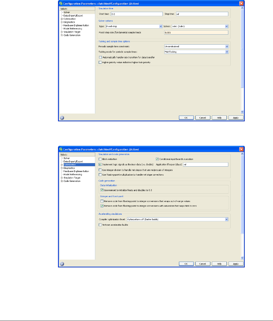
250
Next, select the Optimization tab and make sure that the check boxes “Block reduction” and
“Signal storage reuse” (for older Simulink versions) are unchecked.
The remaining settings are made for the code generation. Select Code Generation and
expand the tree. First, click Browse to select the appropriate RTW target. In our case, we
have chosen the rti1006.tlc target file for the dSPACE DS1006 platform. For the
Configuring solver
settings.
Configuring
optimization settings.
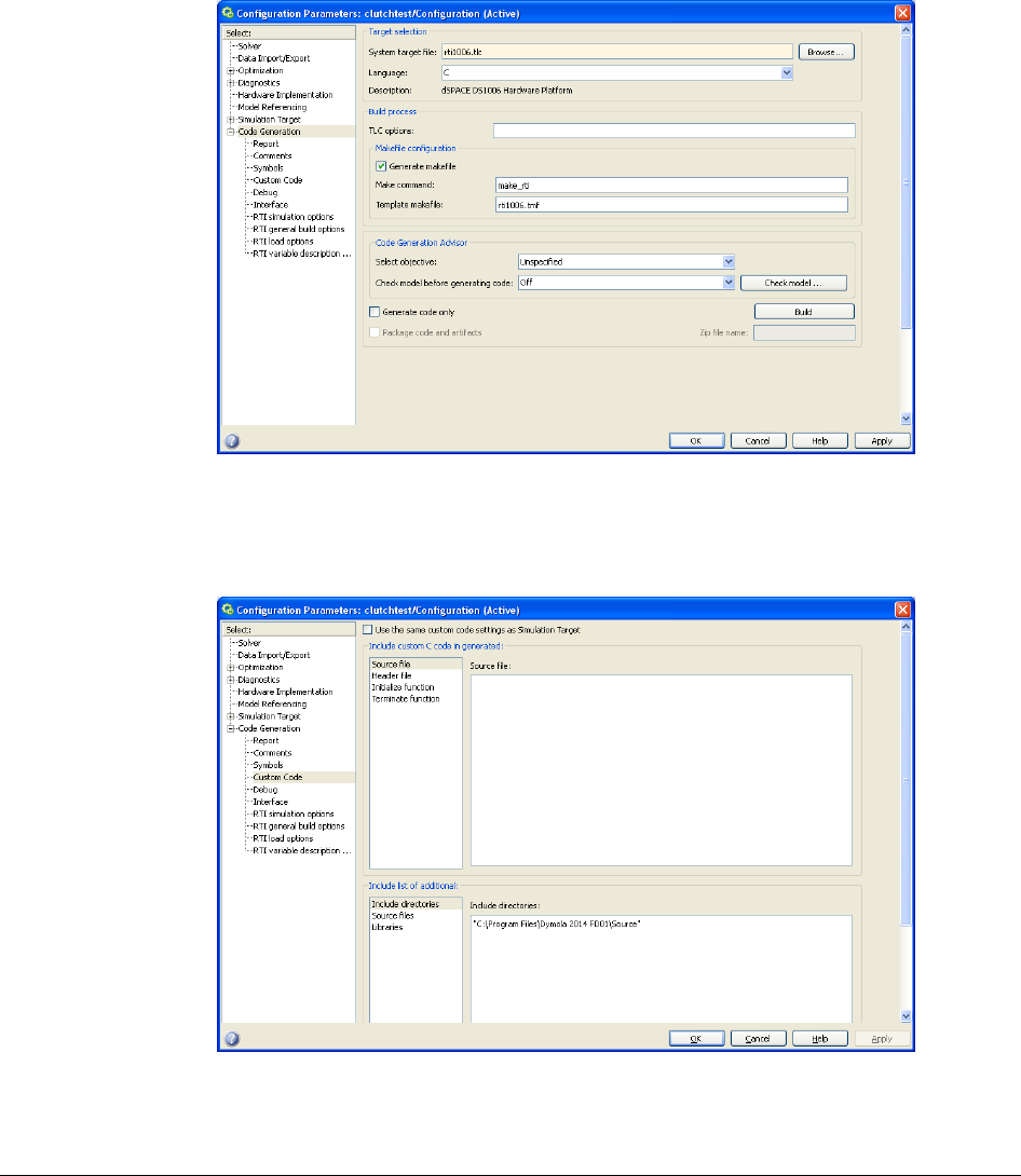
6 OTHER SIMULATION ENVIRONMENTS 251
DS1005 platform, choose rti1005.tlc. The default build process can be used without
change.
Second, the include directory for custom code should be configured. This is the directory
where additional C source and header files needed to compile Dymola models are found.
The default should be the Source subdirectory of the Dymola distribution. Note that the
path must be surrounded by quotes if it contains spaces.
Configuring Simulink
Coder.
Configuring Custom
Code.
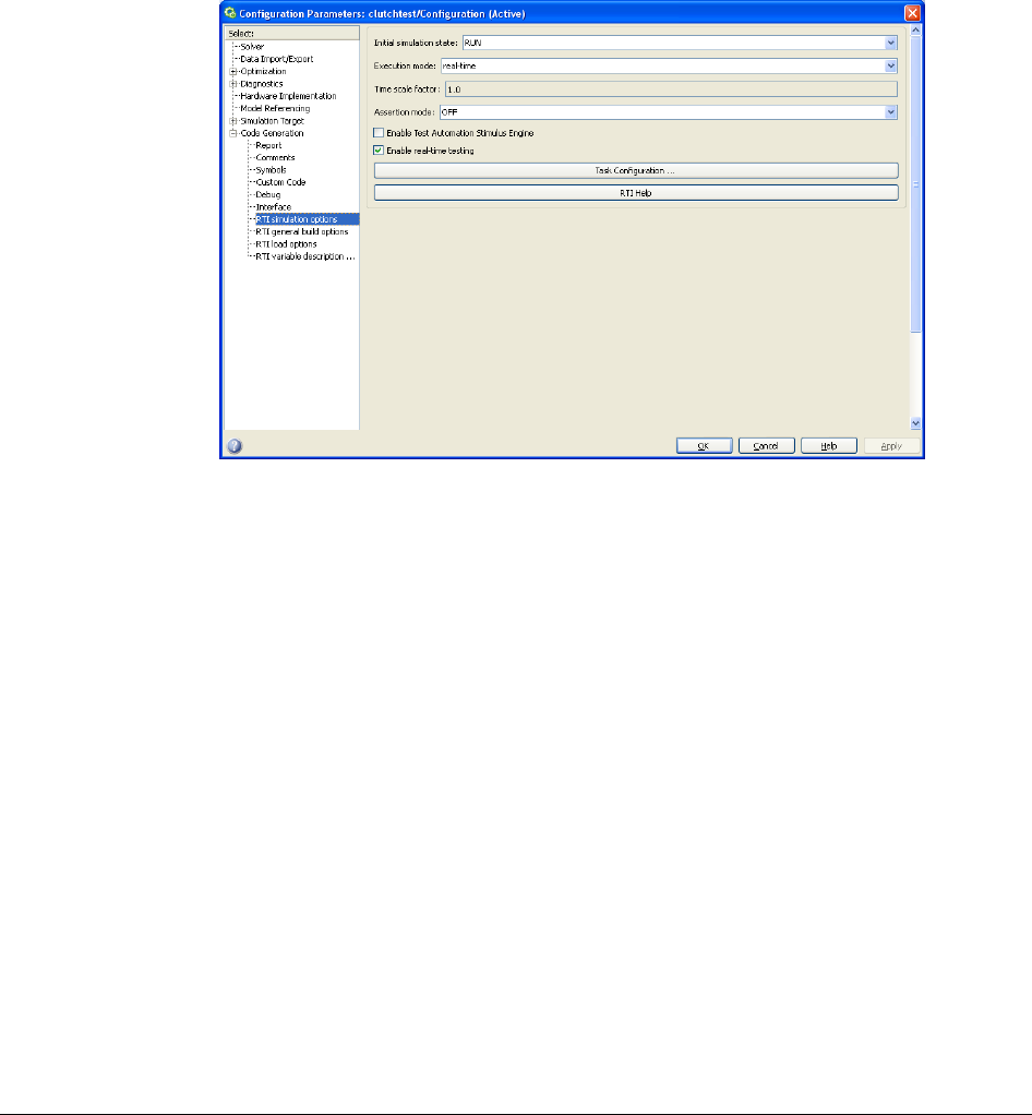
252
The final configurations are related to the dSPACE real-time interface (RTI). Under RTI
simulation options, it is, e.g., possible to set the initial simulation state and execution mode.
The dSPACE system can run in different execution modes, for example in real-time or as
fast as possible. To configure RTI real-time tasks (including the overrun strategy, which will
be described below), press the “Task Configuration” button.
Overruns
An overrun situation may arise for several reasons, as documented in the dSPACE manual.
For Dymola models, event iteration in the model may also require additional CPU resources.
In these cases it is usually helpful to plot the turnaround time (model calculation time plus
overhead in every sample), a signal provided by the dSPACE system. The turnaround time
will show when additional resources are needed. In many cases occasional overrun
situations are harmless.
The RTI task configuration enables you to specify the number of instances of a task that
may be queued before the real-time kernel issues an overrun error. The appropriate setting
can be determined by trial-and-error. The dSPACE ControlDesk also allows plotting of
important real-time system variables, such as, the model turnaround time and the number of
overruns.
Configuring the
dSPACE RTI.
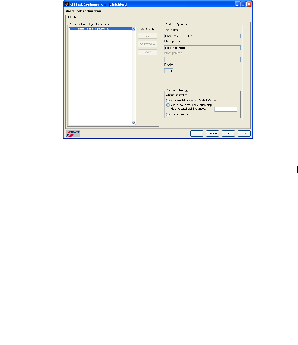
6 OTHER SIMULATION ENVIRONMENTS 253
Building and loading the model,
dym_rti_build
and
dym_rtimp_build
Dymola provides a Matlab function dym_rti_build (located in Program Files
(x86)\Dymola 2018\Mfiles) to build real-time models containing DymolaBlocks for
dSPACE. This command will invoke Simulink Coder to generate code, compile, link, and
download the application. The function will also generate a variable description file for
improved presentation of Dymola variables (outputs, parameters, and start values) in
dSPACE ControlDesk. It is also possible to build and download the model without
generating the Dymola-specific variable description file by choosing Tools -> Simulink
Coder -> Build Model (or by pressing Ctrl+B).
The inputs to the dym_rti_build function are the model name and a build command (‘C’
to generate code only, ‘M’ to compile and link, ‘L’ to load application, ‘CM’ to generate
code, compile and link, etc). Type help dym_rti_build in Matlab for complete
instructions. Note that the name of your DymolaBlock must start with the string
DymolaBlock in order to generate a correct variable description file.
Dymola also provides the function dym_rtimp_build, which combines the dSPACE
rtimp_build command and dym_rti_build to build dSPACE multi-processor systems
for models containing DymolaBlocks. Again, use the Matlab help command (help
dym_rtimp_build) for complete instructions.
The dSPACE ControlDesk is used to start and stop the simulation, changing parameters,
and plotting signals from the simulation. If the model has been built using
dym_rti_build, the outputs, parameters, and start values of the DymolaBlock are found
under User Variables in the ControlDesk variable browser.
RTI task configuration
(overrun strategy).

254
Note that for dSPACE SCALEXIO, the build process is configured and started from
dSPACE ConfigurationDesk. However, it is still possible to use dym_rti_build to
construct the variable description file by entering the string ‘trc’ as build command.
6.3.2 Simulink Real-Time (formerly Matlab xPC
Target)
The Simulink Real-Time (formerly xPC Target) environment allows Simulink models to be
compiled at a host computer using Visual Studio or Watcom C compilers and then
downloaded and executed in real-time on a target computer. The target computer can be any
standard desktop PC booted with the Simulink real-time kernel. Communication between
the host and target is performed either using TCP/IP or using a direct RS-232 serial
connection. The xPC environment is controlled from the xPC Target explorer, which is
started by the command xpcexplr.
Compatibility
Compatibility of Dymola 2018 real-time simulation with Matlab Simulink Real-Time/xPC
Target has been verified for all Matlab releases that are supported by the Dymola –
Simulink interface, which means R2012a (xPC Target version 5.2) to R2016b (Simulink
Real-Time version 6.5). Only Microsoft VisualC compilers have been tested.
Simulation of the
coupled clutches demo
example using dSPACE
ControlDesk.
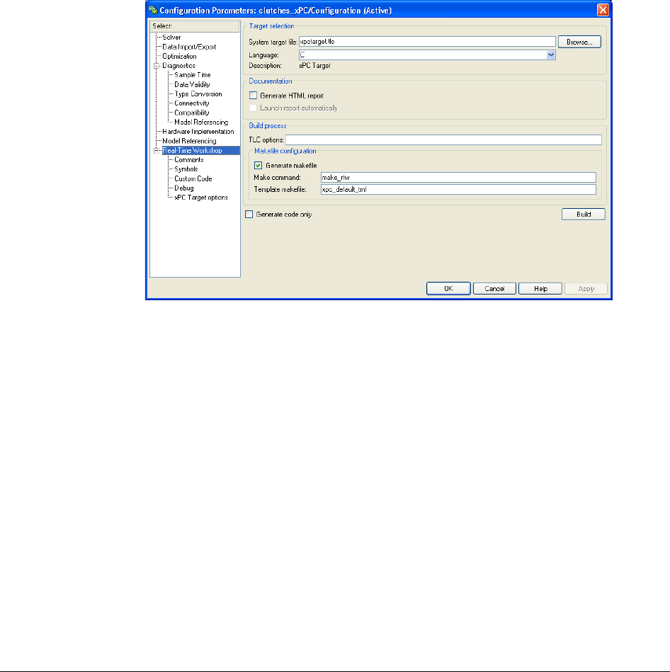
6 OTHER SIMULATION ENVIRONMENTS 255
Configuration
A fixed-step solver is required, which is configured by opening the Configuration
Parameters dialog in Simulink and selecting the Solver tab. Also set the start time to 0 and
the stop time to the desired value (usually inf for real-time simulation).
Next select Simulink Coder to configure the target language compiler for xPC Target. Select
xpctarget.tlc (slrt.tlc in Matlab R2014a and later) as ‘System target file’. Use the
default settings without change.
Next select the Custom Code tab to configure the additional include directory to point to the
directory where additional C source and header files needed to compile Dymola models are
found. The default should be the source subdirectory of the Dymola distribution (see
below).
Configuring the target
language compiler for
xPC.
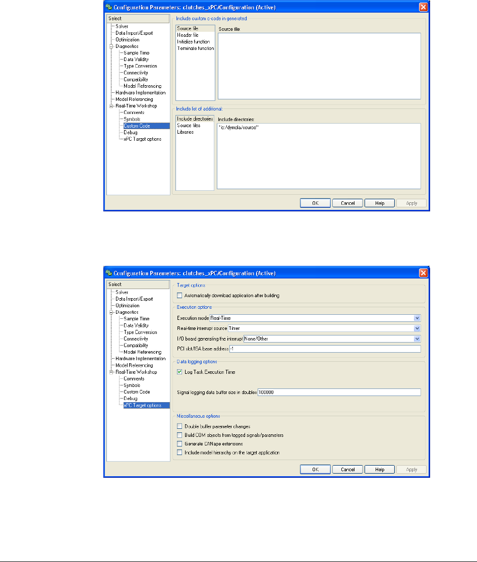
256
Finally, select the xPC Target options tab to configure some options specific for xPC Target.
Here it is, for example, possible to choose between real-time and free-running (as fast as
possible) execution modes and to select data logging parameters.
Building and loading a model
To be able to monitor signals from the simulation on the target node, an xPC Target Scope
is added to the coupled clutches Simulink model before code generation and compilation.
Configuring Custom
Code.
Configuring xPC Target
options.
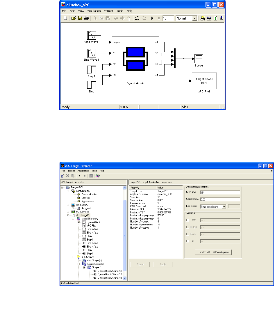
6 OTHER SIMULATION ENVIRONMENTS 257
After this modification of the model, the real-time application is built by choosing Tools ->
Simulink Coder -> Build Model (or by pressing Ctrl+B). This will create an executable
(.dlm file) that then is downloaded to the target node (either automatically during the build
process or manually from the xPC target explorer). The real-time simulation is then
conducted either from the xPC Target explorer (see below) or directly from the Simulink
model by running in External mode.
Results from a real-time simulation on xPC Target of the coupled clutches example are
shown below. The range of the x-axis can be changed by modifying the value of ‘Number
of samples’ in the xPC Target Scope.
CoupledClutches
model with an xPC
Target Scope.
Monitoring the real-
time simulation using
the xPC Target
explorer.
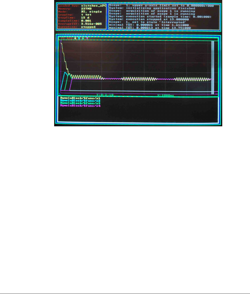
258
6.3.3 Advanced Options for Real-Time Simulation
The section describes a number of options specifically designed for inline integration and to
improve performance for real-time simulation.
Inline integration in Dymola in general is also documented in the manual “Dymola User
Manual Volume 1”, chapter “Simulating a model”, section “Improving simulation
efficiency”, sub-section “Inline integration”.
To get a small improvement of the simulation performance, you can activate the global
optimization in the compiler, by setting the flag
Advanced.Define.GlobalOptimizations = 2;
before generating code. (The default value of the flag is 0.)
This flag works the same for all Visual Studio compilers. Note that although the simulation
performance is somewhat improved by setting the flag, but the compilation of the code
might take substantially longer for large models. The setting corresponds to the compiler
command /Og.
General options
The following options are available from the Realtime tab in Simulation > Setup menu of
Dymola:
Real-time simulation of
coupled clutches on
xPC Target.

6 OTHER SIMULATION ENVIRONMENTS 259
The first three selections (Realtime simulation group) are described in Dymola User Manual
Volume 1, click on entry “real-time simulation – options” in the chapter “Index” in that
manual to navigate to the description.
The next three selections that can be made for Inline integration in the menu above
corresponds to three flags that can be set from the command input line in Dymola or from
scripts.
The inline integration method corresponds to the flag
Advanced.InlineMethod = 1; // 0-7
The order for the higher-order Runge-Kutta methods (including Rosenbrock) corresponds to
the flag
Advanced.InlineOrder = 2; // 2-4
The step size that the code is optimized for corresponds to the flag
Advanced.InlineFixedStep = 0.001;
Two other general flags that can be set from the command input line are
Advanced.Define.AutoRemoveAuxiliaries = true;
Removes code for auxiliary variables that neither influences the simulation state nor the
outputs. This improves performance a bit. If the auxiliary code is used to assert correct
behavior or to generate external outputs that code will not be run.
Evaluate = true;
Evaluates the code based on the given parameter values (excluding top-level parameters)
preventing further modifications. This used to be very important for multi-body models,
since axis of rotations are often along a co-ordinate axis. That is, however, already taken
care of with specific Evaluate annotations for those variables, and thus Evaluate=true
should be less important now.

260
Options for nonlinear solver
Advanced.Define.NewJacobian = false;
This avoids recomputing the Jacobian from scratch every step. The problem with keeping
the Jacobian from the previous step is that at certain points major updates of the Jacobian
are needed. Thus even if keeping the Jacobian is on average better it is not clear that it will
improve real-time performance.
Advanced.Define.AimForHighAccuracy = false;
Normally the non-linear systems of equations are solved with additional accuracy. That
additional accuracy not only improves the accuracy of the solution in itself, but also avoids
spurious events. Setting the flag to false can thus cause loss of accuracy and spurious events.
Advanced.Define.NonLinearIterations = 2; // or 3, 4 or 5
Limit the number of non-linear iterations of the non-linear systems of equations. In
combination with Advanced.Define.NewJacobian = false this improves
performance substantially, but manual verification of the result is needed. The default of
zero ensures that iterations are until convergence. Values 0, 2-8 are supported, but values 6-
8 are not recommended; the result will be better using value 0 (default) in such cases.
Options for implicit inline integration
Advanced.InterpolateStatesForInline = true;
In case of an event we will take a smaller step to step just past the event point. This shorter
step would normally slow down the non-linear solver, but this flags changes it so that we
first compute as for a normal step and then only scale the states. This avoids the loss of
efficiency. This flag is important to set for implicit inline integration.
Advanced.InlineIntegrationJacobian = false;
This is only useful if Advanced.Define.NewJacobian is false, and basically avoids
generating the large amount of code needed for a Jacobian that is only needed at the initial
step.
Simulink option
Advanced.InlineAsDiscrete = true;
Normally the inlined block is run based on the sampling time. With this setting the sampling
time for this block is given by the fixed step-size setting of the Realtime tab
(Advanced.InlineFixedStep as described above). If Advanced.InlineAsDiscrete
is set and the fixed step-size is set at the default zero the block will have inherited sampling
time in Simulink.
Break delay loops
Advanced.BreakDelayLoops = true;
Use this flag to break loops involving the delay operator. The delay operator is normally
treated as if there were a direct coupling between the input and the output. Be aware that
setting of this flag may lead to wrong simulation results if the delay times are too short.

6 OTHER SIMULATION ENVIRONMENTS 261
Profiling of execution time
Advanced.DymosimRealTimePriority = true;
Use this flag to enable profiling of execution time for a simulation. This will set the priority
class of the dymosim process to REALTIME_ PRIORITY_CLASS. Be aware that
processes of this class may interrupt system threads managing mouse or keyboard and that
they may also be difficult to terminate.
Advanced.Define.PrecisionTiming = true;
Set this flag to enable precision timing. This functionality uses the frequency counter of the
processor to provide high-resolution time measurements.
Advanced.Define.UseRDTSCFrequency = 0.0;
This variable is used to specify the frequency (in Hz) of the processor. It is recommended to
keep it at the default value of 0.0 (auto detection), which means that the frequency is
automatically read from the text description of the processor.
6.4 DDE Communication
Two types of DDE communication are provided:
• An interface for Dymola for commands etc., (An additional feature is to associate new
commands with the .mo file type in Windows Explorer.)
• DDE server support in Dymosim simulator.
6.4.1 DDE interface for Dymola
DDE commands can be sent to Dymola just to be executed, or with special DDE-request to
allow the caller to collect the result from Dymola (since a normal execute does not allow
more advanced return codes.)
Executing
Dymola accepts commands through a Windows DDE connection. The DDE connection
should be opened with an application name of "dymola"; the topic name is not used. (You
can use e.g. ’model’ as topic.)
The following commands are recognized:
• All Dymola commands as entered in the command input or read from a script file
(including the command for running a script file).
• The command open filename that corresponds to the command File > Open in the
graphical editor.
All Modelica script features are also supported.

262
Fetching results
The special DDE-requests are: “ModelicaString:expression” and
“MatlabString:expression”, in both cases the result of the expression (usually a function
call) is returned as a string, containing a literal expression in one of the syntaxes (of
Modelica or Matlab).
Example (the example is explained in more detail below):
>> ch=ddeinit(’dymola’,’model’);
>> res=eval(ddereq(ch,’Matlabstring:Modelica.Math.Matrices.
solve([1,2;3,4],{1,5})’,[1,1]))
Note 1: Multiple outputs are supported.
Note 2: You should adjust the timeout in the calling program (e.g. Matlab) to allow for the
command to complete.
Note 3: When using scripting, please note the usefulness of some examples in “Dymola
User Manual Volume 2”, chapter “Simulating a model”, section “Scripting”. In particular
note the use of the function SimulateExtendedModel.
Note 4: In Matlab, additional information about ddereq can be obtained by typing
help ddereq in the Matlab command window.
Example: Solving a real system of linear equations (Matlab)
The function Modelica.Math.Matrices.solve is used for solving a real system of
linear equations A*x=b where A is a matrix and x and b are vectors.
This function can be used from Matlab using DDE connection, executing the function in
Dymola and fetching the resulting value to Matlab.
Dymola must be running.
In the Matlab command window the following command can be executed:
>> ch=ddeinit(’dymola’,’model’);
>> res=eval(ddereq(ch,’Matlabstring:Modelica.Math.Matrices.
solve([1,2;3,4],{1,5})’,[1,1]))
The format [1,1] means that the clipboard format CF_TEXT is used for the request and that
the result is returned as a string. eval is used to make Matlab to execute that resulting string
as an expression or statement.
The result will be output in the Matlab command window:
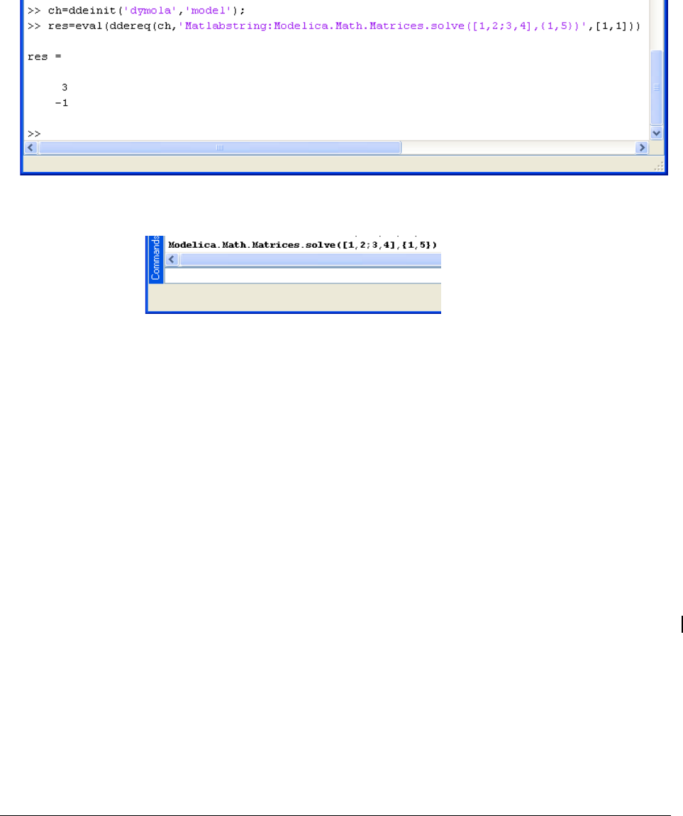
6 OTHER SIMULATION ENVIRONMENTS 263
Please note that the corresponding call (the resulting command in Dymola) will also be
shown in Dymola command window (this makes it easier to e.g. trace errors):
The timeout of the ddereq command is by default 3000 ms. If some other value should be
used it can be specified in the command. If e.g. the timeout should be 4000 ms in the
example above, the last line would be:
>> res=eval(ddereq(ch,’Matlabstring:Modelica.Math.Matrices.
solve([1,2;3,4],{1,5})’,[1,1],4000))
6.4.2 Explorer file type associations
It is possible to associate new commands with the “.mo” file type. These commands are ac-
cessible through the right-mouse button menu in Explorer. We suggest this setup (the setup
varies somewhat with version of MS Windows):
1. Start Windows Explorer and select View/Options. Select the File Type tab.
2. Associate new menu commands with the file type. Click on "New...", then enter:
a. Action: Open
b. Application used to perform action: browse for the Dymola program, typically
C:\Program Files (x86)\Dymola 2018\bin\dymola.exe.
c. Use DDE: check
d. DDE message: open %1
e. Application: dymola
f. Leave the remaining fields empty.
In a similar way you can associate several commands with the extensions .mo and .mos:

264
Action
Application to perform action
DDE message
File extension
Edit
C:\windows\notepad.exe%1
or
C:\winnt\notepad.exe%1
all
Open
C:\Program Files (x86)\Dymola
2018\bin\dymola.exe
open%1
*.mo
Run
C:\Program Files (x86)\Dymola
2018\bin\dymola.exe
@%1
*.mos
6.4.3 DDE Server support in Dymosim simulator
Dymosim can be compiled as a Windows application with built-in DDE server with
realtime capability. To be able to perform such a compilation, DDE must be selected as
embedded server in the Compiler tab in the simulation setup menu (reached by the
command Simulation > Setup…).
For more information about Dymosim in general, please see “Dymola User Manual Volume
1”, chapter “Simulating a model”, section “Dynamic Model Simulator”. Note in particular
the flag Advanced.CompileWith64 that can be used in a 64-bit version of Dymola to
select if dymosim with DDE server should be compiled as 32-bit or 64-bit application
Without any action from the user, Dymosim will be built and executed in the usual way, i.e.,
without real-time synchronization. The noticeable differences are that the current simulation
time is shown in the minimized Dymosim window, and that the dymosim application has a
graphical user interface (see below).
Real-time simulation
If the environment variable DYMOSIMREALTIME is defined, Dymosim will start in real-
time mode, where the simulation time is synchronized with real (or wall-clock) time. The
time display will also include the time the simulation is delayed at each accepted output
point, relative real-time. A negative value indicates that the simulation is faster than real-
time, i.e., that there is spare time for additional computations. (In this case the simulation is
actually delayed by the system in order not to accumulate the time difference.)
Dymosim DDE server
Dymosim compiled as a Windows application will act as a DDE server, allowing some oth-
er application to retrieve data values or set parameters. Dymosim must be started before it
can accept DDE operations; Matlab's ddeinit will not start Dymosim automatically, for
example.
A DDE connection is established by sending a WM_DDE_INITIATE messages with the
application name "dymosim" (any topic can be used).
Matlab example: channel=ddeinit('dymosim','xxx')
After a Stop command or at the end of simulation, Dymosim will send a
WM_DDE_TERMINATE message.
Matlab example: ddeterm(channel)

6 OTHER SIMULATION ENVIRONMENTS 265
Note that in addition to running Dymosim with DDE server from Dymola, it can also be
called directly by the user. To enable this, the environment variable PATH needs to be
complemented with the path to the Dymola installation directory bin.
Note that all transactions between the Dymosim DDE server and the DDE client are logged
in the Dymosim window. They can also be logged on file (see later).
Simulator commands
The following commands can be sent to Dymosim using WM_DDE_EXECUTE messages:
“run”
Start simulation (if simulation is not started automatically), or resume
simulation after a pause command.
“stop”
Stop simulation.
“pause”
Pause simulation. The simulation is temporarily halted until a “run”
command is given. Note that DDE requests are handled while pausing.
“logon”
Enables logging to file, if logging is off.
“logoff”
Disables logging to file, if logging is on.
Matlab example: ddeexec(channel,'run')
Setting parameters
Parameters may be set by sending a WM_DDE_POKE message with the name of the pa-
rameter and its new value (the string representation of a number).
There are four special variables:
realtime_
Set to “1” to enable realtime mode, or to “0” to disable realtime mode.
tscale_
The scale factor between simulated time and real time. In real-time mode
the simulator will maintain the relationship
real-time = tscale_ * simulated-time
abstol_
Absolute tolerance for hot linked variables (default 0).
reltol_
Relative tolerance for hot linked variables (default 0).
Matlab example: ddepoke(channel,'tscale_','2.0')
When simulation is started, also simulation parameters, auxiliary variables and states may
be set. However, these are not set immediately (but almost) but only at certain points in the
simulation that allows for updates. Hence, when a client requests a certain e.g. variable, an
update for another or the same client may be pending. Any such pending update value will
be reported in the response.
Requesting variables
When simulation is started, the values of simulation parameters/variables/states etc. at the
last accepted output point are available by sending a WM_DDE_REQUEST message with
the name of the variable. Dymosim will then return a message with a current value of the
variable etc. (the string representation of the number), or zero if no such variable exists.

266
It is also possible to request the value of special variables. In addition to the four special
variables mentioned in the table in the previous section, the following special variables can
also be requested:
delayed_
Returns the time the simulation was delayed at the last accepted output
point.
status_
Returns the state of the DDE server. The state is composed as the sum of
the following parts:
1 Simulation started (running)
10 Simulation paused
100 Current simulation time = 0
E.g. 11 means that the simulation is started but paused at a simulation time
greater than 0.
time_
Returns the current simulation time in seconds.
Matlab example: ddereq(channel, 'time_')
Hot linking variables
Variables can be "hot linked" using message WM_DDE_ADVISE. The linked variables
will be sent to the client at output points when a significant change has occurred. A
significant change of a variable is determined from absolute and relative tolerances (settable
by the DDE client) as follows (x0 = value last sent to client, x = current value):
absmax = max(abs(x0), abs(x));
absdiff = abs(x - x0);
changed = absmax < 1 ? absdiff > abstol_
: absdiff/absmax > reltol_;
The variable is sent to the client when "changed" is true. The variable is also sent at the first
output point following the hot-link operation.
Matlab example: ddeadv(channel, 'time_', 't=[t x];', 'x')
Dymosim counts the number of links to a variable, and any corresponding "unlink" messag-
es. Updates for the variable are sent while the link count is greater than zero.
Graphical user interface
By clicking on the minimized Dymosim window a graphical user interface for the Dymosim
application will be displayed:
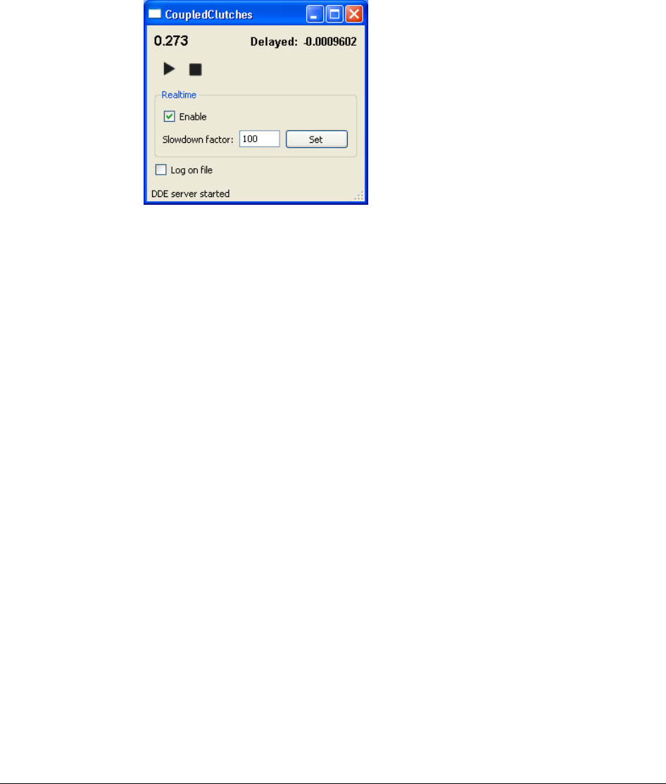
6 OTHER SIMULATION ENVIRONMENTS 267
The example above shows the GUI for the model CoupledClutches, simulated with real-
time (synchronization) using a slowdown factor of 100. The slowdown factor can be
modified anytime. The simulation has been paused at 0.273 seconds by the user. The time
the simulation is delayed at the accepted output point, relative to real time is displayed.
The simulation can be resumed by clicking on the “play” button or using the short key
Ctrl+P. (When the simulation is running, a “pause” button is shown instead of the “play”
button.) Logging of DDE events to file is not activated. The status bar shows in this
example the Dymola request to Dymosim.
If the environment variable DYMOSIMGUI is defined, simulation will not start
automatically when the program is executed; instead the user must give a Run command.
Logging of transactions
If the environment variable DYMOSIMLOGDDE is defined, all DDE communication
to/from the simulator will be logged to a file ddelog.txt in the current directory. The file is
created when the program starts, if not existing. Once Dymosim has started the setting in
Dymosim GUI take precedence over DYMOSIMLOGDDE.
For each new execution of Dymosim, the logs are appended to the file, i.e. old messages are
kept.
Limitations
There are some limitations of the feature:
• Currently only the solvers Lsodar, Dassl, Euler, Rkfix2, Rkfix3 and Rkfix4 are supported.
• When clients request data from the DDE server they specify the desired data format.
Dymosim currently only support the following formats:
o Plain text, used by e.g. Matlab.
o XITable, used by e.g. Microsoft Office Excel.
• DDE Server cannot be combined with Export model as DLL.
Example of Dymosim
interface.

268
6.5 OPC Communication
Compared to DDE (previous section), OPC communication only consists of the OPC Server
support in Dymola.
6.5.1 OPC Server support in Dymosim simulator
Dymosim can be compiled as a Windows application with built-in OPC server with real-
time capability. To be able to perform such a compilation, OPC must be selected as
embedded server in the Compiler tab in the simulation setup menu (reached by the
command Simulation > Setup…).
For more information about Dymosim in general, please see “Dymola User Manual Volume
1”, chapter “Simulating a model”, section “Dynamic Model Simulator”. Note in particular
that dymosim as OPC server only can be compiled as 32-bit, setting the flag
Advanced.CompileWith64=2 is not supported when compiling dymosim as OPC server.
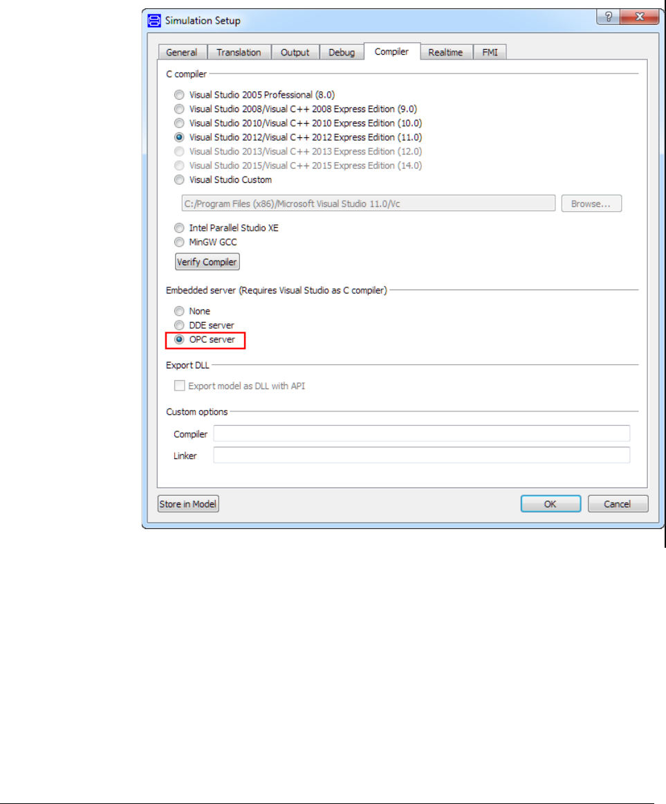
6 OTHER SIMULATION ENVIRONMENTS 269
Prerequisites
In addition to running Dymosim with OPC server from Dymola, or called directly by the
user, it is also possible to start it from an OPC client. To enable this, the environment
variable PATH needs to be complemented with the path to the Dymola installation
directories bin and bin\lib.
The Dymosim OPC server is registered automatically each time a new model translation is
performed in Dymola. The reason for repeating the registration (and unregister the
previous), is that each translation may occur in a new working directory and hence the path
to the executable may change. For each translation or change in the simulation setup, e.g.
new stop time, it is also necessary to run the simulation once from Dymola to propagate the
settings to dsin.txt. If this is omitted, the default stop time 0 will prevent any useful
simulation.

270
The server registration requires administrator rights. In Windows 7, where administrator
rights are not automatically transferred to the started program, you must explicitly run
Dymola “as administrator”.
Dymosim OPC server
Although it can be started from Dymola or called directly by the user, the normal procedure
is to start it from an OPC client, in which Dymosim will show up as
Dymosim.OPCServer.1. When connecting, the below tags become available, where the
leading SimControl has been omitted.
OPC tags
The first group below configures the simulation and can be set any time.
Realtime
Whether real-time mode shall be enabled (True, default) or not (False).
tScale
The scale factor between simulated time and real time. In real-time mode
the simulator will maintain the relationship
real-time = tScale * simulated-time
The next group controls the simulation. The values of these tags are insignificant; setting
any value has the effect of performing the corresponding action. Before any useful
interaction can be commenced, the tag Initialize must be written. An exception is the Run
tag that will cause the model to be initialized before it is run. Writing the tag Initialize after
a completed run will reset the simulation and enable a new run.
Initialize
Initialize simulation.
Pause
Pause simulation. The simulation is temporarily halted until a run
command is given. Note that OPC requests are handled while pausing.
Run
Start simulation (if simulation is not started automatically), or resume
simulation after a pause command.
Stop
Stop simulation.
The remaining of the non-model specific tags are for reading.
Delay
The time the simulation was delayed at the last accepted output point.
Initialized
Whether simulation is initialized.
Time
The current simulation time in seconds.
Once the Initialize tag has been written, model specific tags that correspond to the model
parameters and variables become available for writing/reading respectively under the
leading tag modelVariables.
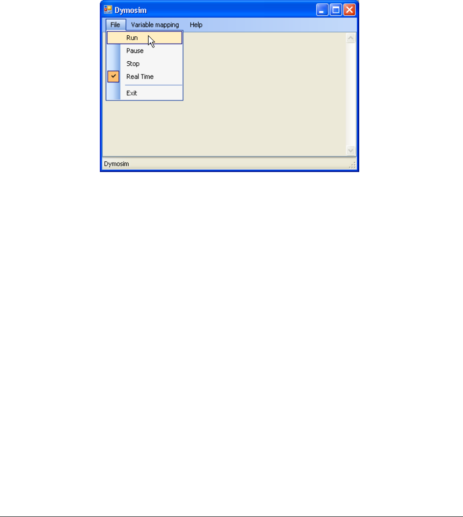
6 OTHER SIMULATION ENVIRONMENTS 271
Graphical user interface
By clicking on the minimized Dymosim window a graphical user interface for the Dymosim
application will be displayed:
This GUI provides some possibilities for setup and interaction with the simulation, but no
simulation data is accessible.
Mapping OPC tags to Dymola variable names
There is a possibility to assign aliases to the model variables. These should be specified in
an xml file. If e.g. the variable “J1.w” in the model CoupledClutches should be accessed
through a tag named “DB500.DB1.0”, the xml file should read:
<mappings><mapping tag="DB500.DB1.0" variable="J1.w" /></mappings>
By clicking Variable mapping > Generate mapping file in the Dymosim window a file
containing the variable names but no tags is generated. This file must be edited manually to
specify the tags. The check-boxes in Variable mapping > Include can be used to select
which of model parameters, inputs, outputs etc. that should be included in the file.
If new variables are added to a model, an existing mapping file can be extended with the
new variables by choosing this file in the dialog box for Variable mapping > Generate
mapping file. The new variables will be added to the end of the file, but the existing
mappings will be left unmodified.
A mapping file is loaded by clicking Variable mapping > Open mapping file. The check-
boxes in Variable mapping > Include are used in the same way as when generating a file.
If the file specifies a mapping to a variable that is not present in the model, a warning
message will be displayed, and the tag will not be added.
Opening or generating a mapping file will initialize the model and make the modelVariables
and the alias tags available in the server.
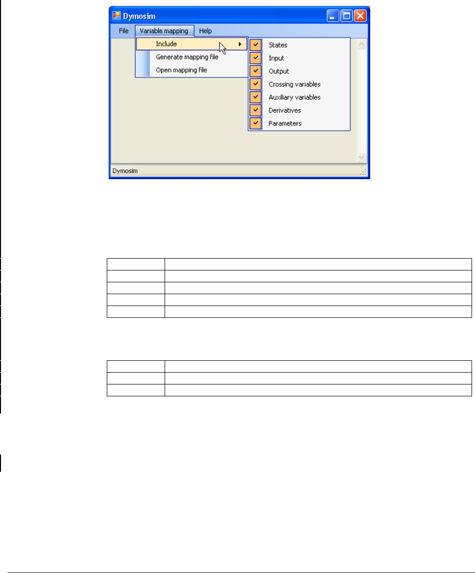
272
Logging
By default events are logged in the GUI provided by the OPC server and optionally to a file.
To alter the behavior, two environment variables can be set:
DYMOSIM_OPC_LOG_LEVEL
Value
What is logged
0 (default)
All
1
Warnings and errors
2
Errors
3
Nothing
DYMOSIM_OPC_LOG_TO_FILE
Value
File written
0 (default)
None
1
opclog.txt
The file opclog.txt is created in the current simulation directory.
Limitations
There are some limitations of the feature:
• You must run Dymola with administrator rights to be able to run the OPC server.
• Currently only the solvers Lsodar, Dassl, Euler, Rkfix2, Rkfix3 and Rkfix4 are
supported.
• Only Visual Studio 2008, 2010, and 2012 compilers are supported.
• Dymosim with OPC server is always built as a 32-bit application.
• OPC Server cannot be combined with Export model as DLL.

6 OTHER SIMULATION ENVIRONMENTS 273
6.6 Java Interface for Dymola
The Java interface is an API for executing commands in Dymola using a Java program. It
contains a number of functions to perform operations such as simulating, setting variables,
plotting, and exporting data.
The Java interface is included in the Dymola distribution. Go to the installation folder for
Dymola, then to the subfolder Modelica\Library\java_interface. The following
files and folders are included:
• dymola_interface.jar
The Java archive that contains the Java interface for Dymola.
• json-simple-1.1.1.jar
A required third party library. JSON Simple is copyrighted under Apache License 2.0
and may be freely distributed. The license is found at: licenses/LICENSE-2.0.txt.
• examples
A folder that contains examples that illustrate how to use the Java interface. Feel free to
copy and modify the examples.
• doc
This folder contains the documentation for the Java interface in Javadoc format. Double-
click on the file index.html to view the documentation in your favourite web browser.
To quickly get started using the Java interface, you can build and run the examples that
come with the Dymola distribution. You find step-by-step instructions below.
The Java interface is supported on both Windows and Linux.
Getting Started with an Example on Windows
1. Install Java Development Kit (JDK). It can be downloaded for free at
http://www.oracle.com/technetwork/java/javase/downloads/index.html
The Java interface was built with Java 6. You find JDK 6 under “Previous Releases” and
then “Java SE 6”. Note that you need to login in order to download Java 6 platforms.
2. Open a Command Prompt (cmd.exe).
3. Update your PATH environment variable to include the Java tools, for example:
set PATH=C:\Program Files\Java\jdk1.6.0_43\bin;%PATH%
4. Update your Java CLASSPATH to include the library for the Java interface, i.e.,
dymola_interface.jar. An example of this could be the following:
set CLASSPATH=%CLASSPATH%;C:\Program Files (x86)\Dymola
2018\Modelica\Library\java_interface\dymola_interface.jar
Also make sure that the current directory is included in the class path. If not, then
include it:
set CLASSPATH=.;%CLASSPATH%
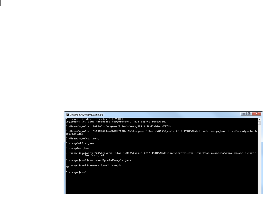
274
5. Copy the example DymolaExample.java to another folder. You find the example in
the subfolder examples. The reason that the example should be copied is that Windows
might not allow you to create files in the distribution directory. Change current directory
to the folder that contains DymolaExample.java.
The Java interface will automatically find Dymola if you install it in the default location.
Otherwise you need to edit the example to point to the path of the Dymola executable.
Open DymolaExample.java and edit the line
dymola = DymolaWrapper.getInstance();
to take the full path to the Dymola executable as argument. For example:
dymola = DymolaWrapper.getInstance("C:\\Dymola
2018\\bin64\\Dymola.exe");
Remember to use double backslashes \\ in the path.
6. Build the example:
javac.exe DymolaExample.java
A file DymolaExample.class should be generated in the same folder as
DymolaExample.java.
7. Run the example:
java.exe DymolaExample
If the example ran successfully then OK should be displayed after a few seconds. If you
get an error that the Dymola installation could not be found, you need to specify the path
to Dymola.exe yourself. See step 5 above for how to edit the example.
Here is an example of a successful run of the commands above:

6 OTHER SIMULATION ENVIRONMENTS 275
See the Javadoc documentation for the Java interface for available functions and how to use
them.
The example is reproduced below. It is also available in the Dymola distribution. You find it
in the folder Modelica\Library\java_interface\examples as
DymolaExample.java.
import com.dassault_systemes.dymola.DymolaException;
import com.dassault_systemes.dymola.DymolaInterface;
import com.dassault_systemes.dymola.DymolaWrapper;
public class DymolaExample
{
public static void main(String[] args)
{
DymolaInterface dymola = null;
try {
// Set this flag to false if you want Dymola to be visible.
// By default Dymola is hidden.
//DymolaWrapper.nowindow = false;
// Instantiate the Dymola interface and start Dymola
dymola = DymolaWrapper.getInstance();
// Call a function in Dymola and check its return value
boolean result =
dymola.translateModel("Modelica.Mechanics.Rotational.Examples.CoupledClutches");
if (!result) {
System.err.println("Translation failed.");
// Get the translation log and print it
String log = dymola.getLastError();
System.err.println(log);
return;
}
// Simulate the model
result = dymola.simulateModel("", 0, 1.2);
if (!result) {
System.err.println("Simulation failed.");
// Get the simulation log and print it
String log = dymola.getLastError();
System.err.println(log);
return;
}
// Plot a few variables
result = dymola.plot(new String[]{"J1.w", "J2.w", "J3.w", "J4.w"});
if (!result) {
System.err.println("Plot failed.");
return;
}
// Save the plot as a PNG file
result = dymola.ExportPlotAsImage("C:/temp/plot.png");

276
if (!result) {
System.err.println("Failed to save the plot.");
return;
}
System.out.println("OK");
} catch (DymolaException e) {
System.err.println("Connection to Dymola failed. " + e.getMessage());
} finally {
// The connection to Dymola is closed and Dymola is terminated
dymola = null;
}
}
}
Getting Started with an Example on Linux
Performing the above example on Linux, there are some differences:
• Installation on Linux depends on the particular Linux variant. To check which Java
compiler and Java runtime environment is currently installed, do:
o For compiler version: javac -version
o For runtime environment: java -version
• public static DymolaWrapper getInstance() on Linux won´t necessarily
return the 64-bit version of Dymola, but the one located in /usr/local/bin/dymola.
This is normally the latest installed Dymola version.
The above example on Linux (without color indication of the text):
import com.dassault_systemes.dymola.DymolaException;
import com.dassault_systemes.dymola.DymolaInterface;
import com.dassault_systemes.dymola.DymolaWrapper;
public class DymolaExample
{
public static void main(String[] args)
{
// determine OS
String osName = System.getProperty("os.name");
Boolean isWindows = osName.substring(0,3).equals("Win");
DymolaInterface dymola = null;
try {
// Set this flag to false if you want Dymola to be visible.
// By default Dymola is hidden.
//DymolaWrapper.nowindow = false;
// Instantiate the Dymola interface and start Dymola
dymola = DymolaWrapper.getInstance();
// Call a function in Dymola and check its return value

6 OTHER SIMULATION ENVIRONMENTS 277
boolean result =
dymola.translateModel("Modelica.Mechanics.Rotational.Examples.CoupledClutches");
if (!result) {
System.err.println("Translation failed.");
// Get the translation log and print it
String log = dymola.getLastError();
System.err.println(log);
return;
}
// Simulate the model
result = dymola.simulateModel("", 0, 1.2);
if (!result) {
System.err.println("Simulation failed.");
// Get the simulation log and print it
String log = dymola.getLastError();
System.err.println(log);
return;
}
// Plot a few variables
result = dymola.plot(new String[]{"J1.w", "J2.w", "J3.w", "J4.w"});
if (!result) {
System.err.println("Plot failed.");
return;
}
// Save the plot as a PNG file
String plotPath;
if (isWindows) {
plotPath = "C:/temp/plot.png";
} else {
plotPath = "/tmp/plot.png";
}
result = dymola.ExportPlotAsImage(plotPath);
if (!result) {
System.err.println("Failed to save the plot.");
return;
}
System.out.println("OK");
} catch (DymolaException e) {
System.err.println("Connection to Dymola failed. " + e.getMessage());
} finally {
// The connection to Dymola is closed and Dymola is terminated
dymola = null;
}
}
}
The Java Interface
To illustrate the Java interface, consider the function simulateModel. Its description in
Dymola is:
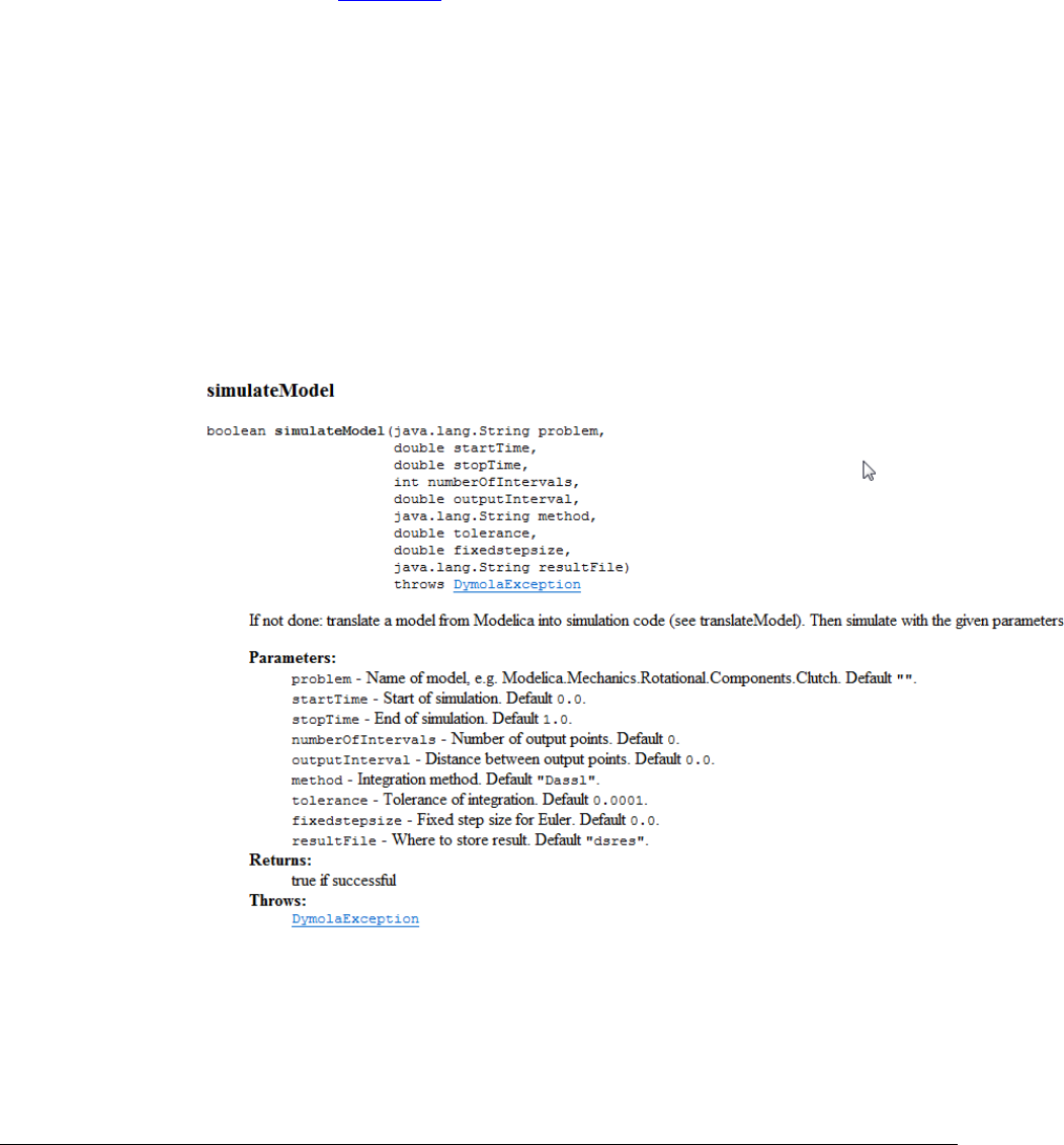
278
Function simulateModel "simulate a Modelica model"
input String problem := "" "Name of model, e.g. Modelica.Mechanics
.Rotational.Components.Clutch";
input Real startTime := 0.0 "Start of simulation";
input Real stopTime := 1.0 "End of simulation";
input Integer numberOfIntervals := 0 "Number of output points";
input Real outputInterval := 0.0 "Distance between output points";
input String method := "Dassl" "Integration method";
input Real tolerance := 0.0001 "Tolerance of integration";
input Real fixedstepsize := 0.0 "Fixed step size for Euler";
input String resultFile := "dsres" "Where to store result";
output Boolean result "true if successful";
external "builtin";
annotation(Documentation(info="If not done: translate a model from
Modelica into simulation code (see translateModel).
Then simulate with the given parameters"));
end simulateModel;
The corresponding function in the Java interface is:
There is a one-to-one correspondence between the parameters in the Dymola command and
the parameters in the Java method. If a parameter has a default value, it is shown in the
documentation for that parameter. Commands that have default parameters are overloaded
in the Java interface. The overloaded methods use the default parameter values. In the
example above, simulateModel is called with three parameters:
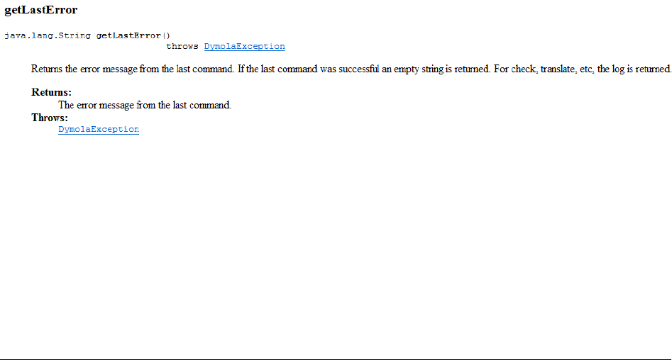
6 OTHER SIMULATION ENVIRONMENTS 279
result = dymola.simulateModel("", 0, 1.2);
This means that for the other six parameters, the default values are used. Note that the
Javadoc documentation only contains the base method and not the overloaded methods,
even though they exist in the interface. Also note that Java does not support named
parameters.
For a complete list of available commands, see the Javadoc documentation for the Java
interface. You find it in the subfolder Modelica\Library\java_interface\doc in the
Dymola distribution. Double-click on the file index.html to view the documentation in
your favourite web browser.
ExecuteCommand
If a command that is not a part of the Java interface should be executed, the method
ExecuteCommand can be used. It takes a string parameter that can contain any command or
expression. For example:
dymola.ExecuteCommand("a=1");
The command is not type checked so you are responsible for making sure the command is
valid. It is not possible to retrieve the output from the command.
getLastError
The translation and simulation log is available through the function getLastError. Call it
after a translate, and/or simulate, command to retrieve the log in text format. The function
can also be used to retrieve other error messages. Note that getLastError is cleared if a
new command is issued, so it should be called directly after the check/translate/simulate
command. getLastError is defined as follows:
An example of usage is:
boolean result =
dymola.translateModel("Modelica.Mechanics.Rotational.Examples.Couple
dClutches");
if (!result) {
System.err.println("Translation failed.");
// Get the translation log and print it
String log = dymola.getLastError();
System.err.println(log);
return;
}

280
Getting an Instance of Dymola
You get an instance of the Dymola interface by calling the method
DymolaWrapper.getInstance. This method has a number of overloads.
public static DymolaWrapper getInstance()
throws DymolaException
public static DymolaWrapper getInstance(boolean use_64bit)
throws DymolaException
public static DymolaWrapper getInstance(boolean use_64bit, int port)
throws DymolaException
public static DymolaWrapper
getInstance(java.lang.String dymolaExePath)
throws DymolaException
public static DymolaWrapper
getInstance(java.lang.String dymolaExePath, int port)
throws DymolaException
By default, the 64-bit Dymola version is used, and the port number used for communication
between Dymola and the Java interface is 8082.
The first three overloads above assume that Dymola is installed in the default location. If
you installed Dymola in another location, you need to use one of the two last overloads and
specify the path to Dymola.exe. Please remember to use double backslashes \\ in the path.
For more details about the instantiation methods and their parameters, see the Javadoc
documentation.
Exiting Dymola
Dymola will automatically exit when the Java program exits. It is good practice to enclose
the interface method calls in a try/catch block and set the DymolaWrapper object to null in
the finally block.
DymolaInterface dymola = null;
try {
dymola = DymolaWrapper.getInstance();
...
} catch (DymolaException e) {
System.err.println("Connection to Dymola failed. " + e.getMessage());
} finally {
dymola = null;
}
Alternatively you can exit Dymola yourself by using the method close. It will wait until
Dymola is closed before returning. The close command is useful, for example, if you want
to start another instance of Dymola.
dymola.close();
dymola = null;

6 OTHER SIMULATION ENVIRONMENTS 281
Commands with Two Output Parameters
The commands simulateExtendedModel and simulateMultiExtendedModel each
have two output parameters. Since a Java function can have only one output parameter, the
values are returned as an array of type Object[].
simulateExtendedModel
Here is an example of a call to simulateExtendedModel in Dymola:
simulateExtendedModel("Modelica.Mechanics.Rotational.Examples.C
oupledClutches", initialNames={"J1.J","J2.J"},
initialValues={2,3}, finalNames={"J1.w","J4.w"});
= true, {6.213412958654296, 1.000000000000004}
The function returns two values, a Boolean status flag and a vector of values. The
corresponding call in the Java interface is shown below. The output parameters are available
as elements in the Object[] array.
Object[] output =
dymola.simulateExtendedModel("Modelica.Mechanics.Rotational.Exa
mples.CoupledClutches", 0.0, 1.0, 0, 0.0, "Dassl", 0.0001, 0.0,
"test", new String[]{"J1.J","J2.J"}, new double[]{2,3}, new
String[]{"J1.w","J4.w"}, true);
boolean status = (Boolean) output[0];
double[] values = (double[]) output[1];
double J1_w = values[0];
double J4_w = values[1];
simulateMultiExtendedModel
Here is an example of a call to simulateMultiExtendedModel in Dymola:
simulateMultiExtendedModel("Modelica.Mechanics.Rotational.Examp
les.CoupledClutches", initialNames={"J1.J","J2.J"},
initialValues=[2,3;3,4;4,5], finalNames={"J1.w","J4.w"});
= true,
[6.213412958654296, 1.000000000000004;
7.483558191010655, 1.000000000000003;
8.107446379737779, 0.9999999999999931]
The function returns two values, a Boolean status flag and a two-dimensional array of
values. The corresponding call in the Java interface is shown below:
double[][] initialValues = {{2,3},{3,4},{4,5}};
Object[] output =
dymola.simulateMultiExtendedModel("Modelica.Mechanics.Rotationa
l.Examples.CoupledClutches", 0.0, 1.0, 0, 0.0, "Dassl", 0.0001,
0.0, "dsres", new String[]{"J1.J","J2.J"}, initialValues, new
String[]{"J1.w","J4.w"});
boolean status = (Boolean) output[0];

282
double[][] values = (double[][]) output[1];
double[] result1 = values[0];
double J1_w1 = result1[0];
double J4_w1 = result1[1];
double[] result2 = values[1];
double J1_w2 = result2[0];
double J4_w2 = result2[1];
double[] result3 = values[2];
double J1_w3 = result3[0];
double J4_w3 = result3[1];
Extended versions of both examples are available in the file
SimulateExtendedExample.java in the folder
Modelica\Library\java_interface\examples.
Multithreading
The Java interface supports multithreading. It is possible to instantiate more than one
Dymola and run them in parallel.
Each Dymola instance needs to have a unique port number. You can either assign a port
number yourself, or let the Java interface find an available port. To set the port, call one of
the overloaded DymolaWrapper.getInstance methods that take a port as argument. To
automatically find a free port, simply call a DymolaWrapper.getInstance method that
does not take a port.
Two Dymola instances that are run simultaneously cannot share the same working directory.
You need to assign a unique working directory to each instance. Use the interface method
cd to set the working directory.
The Java interface is not thread-safe. The only exception is
DymolaWrapper.getInstance. Each thread should run its own instance of Dymola.
Below is an example that illustrates how to use multithreading in the Java interface (one
example on Windows, one on Linux). The example on Windows is available as
MultithreadingExample.java in the folder
Modelica\Library\java_interface\examples.
Example on Windows:
import java.io.File;
import com.dassault_systemes.dymola.DymolaException;
import com.dassault_systemes.dymola.DymolaInterface;
import com.dassault_systemes.dymola.DymolaWrapper;
public class MultithreadingExample
{
public static class CoupledClutchesThread implements Runnable
{

6 OTHER SIMULATION ENVIRONMENTS 283
@Override
public void run()
{
DymolaInterface dymola = null;
try {
System.out.println("1: Starting Dymola instance");
dymola = DymolaWrapper.getInstance();
System.out.println("1: Using port " + ((DymolaWrapper)
dymola).portnumber);
String path = "C:/temp/Dymola/CoupledClutches";
System.out.println("1: Change working directory to " + path);
File folder = new File(path);
if (!folder.exists()) {
folder.mkdirs();
}
boolean result = dymola.cd(path);
if (!result) {
System.err.println("1: Failed to change working
directory");
}
System.out.println("1: Simulating model");
result =
dymola.simulateModel("Modelica.Mechanics.Rotational.Examples.CoupledClutches");
if (!result) {
System.err.println("1: Simulation failed");
String log = dymola.getLastError();
System.err.println(log);
}
System.out.println("1: Plotting");
result = dymola.plot(new String[] { "J1.w", "J2.w", "J3.w",
"J4.w" });
if (!result) {
System.err.println("1: Plot failed");
}
System.out.println("1: Saving the plot");
result = dymola.ExportPlotAsImage(path + "/plot.png");
if (!result) {
System.err.println("1: Failed to save the plot");
}
System.out.println("1: Saving log");
dymola.savelog(path + "/log.txt");
System.out.println("1: OK");
} catch (DymolaException e) {
System.err.println("Connection to Dymola failed. " +
e.getMessage());
} finally {
dymola = null;
}

284
}
}
public static class FullRobotThread implements Runnable
{
@Override
public void run()
{
DymolaInterface dymola = null;
try {
System.out.println("2: Starting Dymola instance");
dymola = DymolaWrapper.getInstance();
System.out.println("2: Using port " + ((DymolaWrapper)
dymola).portnumber);
String path = "C:/temp/Dymola/fullRobot";
System.out.println("2: Change working directory to " + path);
File folder = new File(path);
if (!folder.exists()) {
folder.mkdirs();
}
boolean result = dymola.cd(path);
if (!result) {
System.err.println("2: Failed to change working
directory");
}
System.out.println("2: Simulating model");
result =
dymola.simulateModel("Modelica.Mechanics.MultiBody.Examples.Systems.RobotR3.fullRobot");
if (!result) {
System.err.println("2: Simulation failed");
String log = dymola.getLastError();
System.err.println(log);
}
System.out.println("2: Plotting");
result = dymola.plot(new String[] { "mechanics.q[1]",
"mechanics.q[2]" });
if (!result) {
System.err.println("2: Plot failed");
}
System.out.println("2: Saving the plot");
result = dymola.ExportPlotAsImage(path + "/plot.png");
if (!result) {
System.err.println("2: Failed to save the plot");
}
System.out.println("2: Saving log");
dymola.savelog(path + "/log.txt");
System.out.println("2: OK");
} catch (DymolaException e) {

6 OTHER SIMULATION ENVIRONMENTS 285
System.err.println("Connection to Dymola failed. " +
e.getMessage());
} finally {
dymola = null;
}
}
}
public static void main(String[] args)
{
// Set this flag to false if you want Dymola to be visible.
// By default Dymola is hidden.
//DymolaWrapper.nowindow = false;
Thread coupledClutchesThread = new Thread(new CoupledClutchesThread());
Thread fullRobotThread = new Thread(new FullRobotThread());
coupledClutchesThread.start();
fullRobotThread.start();
}
}
Example on Linux (without color indication of text):
import java.io.File;
import com.dassault_systemes.dymola.DymolaException;
import com.dassault_systemes.dymola.DymolaInterface;
import com.dassault_systemes.dymola.DymolaWrapper;
public class MultithreadingExample
{
static String basePath;
public static class CoupledClutchesThread implements Runnable
{
@Override
public void run()
{
DymolaInterface dymola = null;
try {
System.out.println("1: Starting Dymola instance");
dymola = DymolaWrapper.getInstance();
System.out.println("1: Using port " + ((DymolaWrapper)
dymola).portnumber);
String path = basePath + "/CoupledClutches";
System.out.println("1: Change working directory to " +
path);
File folder = new File(path);
if (!folder.exists()) {
folder.mkdirs();
}

286
boolean result = dymola.cd(path);
if (!result) {
System.err.println("1: Failed to change working
directory");
}
System.out.println("1: Simulating model");
result =
dymola.simulateModel("Modelica.Mechanics.Rotational.Examples.CoupledClutches");
if (!result) {
System.err.println("1: Simulation failed");
String log = dymola.getLastError();
System.err.println(log);
}
System.out.println("1: Plotting");
result = dymola.plot(new String[] { "J1.w", "J2.w", "J3.w",
"J4.w" });
if (!result) {
System.err.println("1: Plot failed");
}
System.out.println("1: Saving the plot");
result = dymola.ExportPlotAsImage(path + "/plot.png");
if (!result) {
System.err.println("1: Failed to save the plot");
}
System.out.println("1: Saving log");
dymola.savelog(path + "/log.txt");
System.out.println("1: OK");
} catch (DymolaException e) {
System.err.println("Connection to Dymola failed. " +
e.getMessage());
} finally {
dymola = null;
}
}
}
public static class FullRobotThread implements Runnable
{
@Override
public void run()
{
DymolaInterface dymola = null;
try {
System.out.println("2: Starting Dymola instance");
dymola = DymolaWrapper.getInstance();
System.out.println("2: Using port " + ((DymolaWrapper)
dymola).portnumber);
String path = basePath + "/fullRobot";

6 OTHER SIMULATION ENVIRONMENTS 287
System.out.println("2: Change working directory to " +
path);
File folder = new File(path);
if (!folder.exists()) {
folder.mkdirs();
}
boolean result = dymola.cd(path);
if (!result) {
System.err.println("2: Failed to change working
directory");
}
System.out.println("2: Simulating model");
result =
dymola.simulateModel("Modelica.Mechanics.MultiBody.Examples.Systems.RobotR3.fullRobot"
);
if (!result) {
System.err.println("2: Simulation failed");
String log = dymola.getLastError();
System.err.println(log);
}
System.out.println("2: Plotting");
result = dymola.plot(new String[] { "mechanics.q[1]",
"mechanics.q[2]" });
if (!result) {
System.err.println("2: Plot failed");
}
System.out.println("2: Saving the plot");
result = dymola.ExportPlotAsImage(path + "/plot.png");
if (!result) {
System.err.println("2: Failed to save the plot");
}
System.out.println("2: Saving log");
dymola.savelog(path + "/log.txt");
System.out.println("2: OK");
} catch (DymolaException e) {
System.err.println("Connection to Dymola failed. " +
e.getMessage());
} finally {
dymola = null;
}
}
}
public static void main(String[] args)
{
// Set this flag to false if you want Dymola to be visible.
// By default Dymola is hidden.
//DymolaWrapper.nowindow = false;

288
// determine proper base path
String osName = System.getProperty("os.name");
if (osName.substring(0,3).equals("Win")) {
basePath = "C:/temp/Dymola";
} else {
basePath = "/tmp/Dymola";
}
Thread coupledClutchesThread = new Thread(new CoupledClutchesThread());
Thread fullRobotThread = new Thread(new FullRobotThread());
coupledClutchesThread.start();
fullRobotThread.start();
}
}
6.7 Python Interface for Dymola
The Python interface is an API for executing commands in Dymola using a Python
program. It contains a number of functions to perform operations such as simulating, setting
variables, plotting, and exporting data.
The Python interface is included in the Dymola distribution. Go to the installation folder for
Dymola, then to the subfolder Modelica\Library\python_interface. The following
files and folders are included:
• dymola.egg
The Python package that contains the Python interface for Dymola. The package is
tested with Python 2.7 and Python 3.5.
• examples
A folder that contains examples that illustrate how to use the Python interface. Feel free
to copy and modify the examples.
• doc
This folder contains the documentation for the Python interface in Sphinx format.
Double-click on the file index.html to view the documentation in your favourite web
browser.
To quickly get started using the Python interface, you can build and run the examples that
come with the Dymola distribution. You find step-by-step instructions below.
The Python interface by default uses 64-bit Dymola. To change it to 32-bit Dymola, see
section “Getting an Instance of Dymola” on page 292.
The Python interface is supported on Windows and Linux. The instructions for Windows in
this section apply to Linux as well, with adjustments for the Linux structure. For example:
• The Dymola binary is supposed to be located as /usr/local/bin/dymola if the path
is omitted when using the interface.

6 OTHER SIMULATION ENVIRONMENTS 289
• The PYTHONPATH should for the 64-bit Linux version of this release be set according
to:
PYTHONPATH=$PYTHONPATH:/opt/Dymola-2018-
x86_64/Modelica/Library/python_interface/dymola.egg
Getting Started with an Example
1. Install Python 2.7. It can be downloaded for free at http://www.python.org/download/.
2. Open a Command Prompt (cmd.exe).
3. Update your PATH environment variable to include the Python environment, for
example:
set PATH=C:\Python27;C:\Python27\Scripts;C:\Python27\Tools\
Scripts;%PATH%
4. Update your PYTHONPATH to include the package with the Python interface, i.e.,
dymola.egg. An example of this could be the following:
set PYTHONPATH=%PYTHONPATH%;C:\Program Files (x86)\Dymola
2018\Modelica\Library\python_interface\dymola.egg
Note that the path to dymola.egg should not be surrounded by double-quotes.
5. Copy the example DymolaExample.py to another folder. You find the example in the
subfolder examples. The reason that the example should be copied is that Windows might
not allow you to create files in the distribution directory. Change current directory to the
folder that contains DymolaExample.py.
The Python interface will automatically find Dymola if you install it in the default location.
Otherwise you need to edit the example to point to the path of the Dymola executable. Open
DymolaExample.py and edit the line
dymola = DymolaInterface()
to take the full path to the Dymola executable as argument. For example:
dymola = DymolaInterface("C:\\Dymola 2018\\bin64\\Dymola.exe")
Remember to use double backslashes \\ in the path.
6. Run the example:
python.exe DymolaExample.py
If the example ran successfully then OK should be displayed after a few seconds. If you
get an error that the Dymola installation could not be found, you need to specify the path
to Dymola.exe yourself. See step 5 above for how to edit the example.
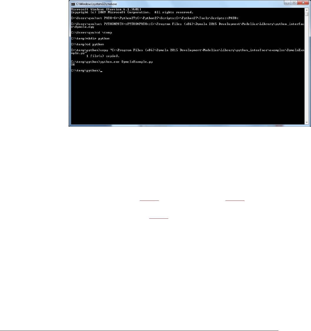
290
Here is an example of a successful run of the commands above:
See the documentation for the Python interface for available functions and how to use them.
The example is reproduced below. It is also available in the Dymola distribution. You find it
in the folder Modelica\Library\python_interface\examples as
DymolaExample.py.
from dymola.dymola_interface import DymolaInterface
from dymola.dymola_exception import DymolaException
dymola = None
try:
# Instantiate the Dymola interface and start Dymola
dymola = DymolaInterface()
# Call a function in Dymola and check its return value
result =
dymola.simulateModel("Modelica.Mechanics.Rotational.Examples.Coupl
edClutches")
if not result:
print("Simulation failed. Below is the translation log.")
log = dymola.getLastError()
print(log)
exit(1)
dymola.plot(["J1.w", "J2.w", "J3.w", "J4.w"])
dymola.ExportPlotAsImage("C:/temp/plot.png")
print("OK")
except DymolaException as ex:
print("Error: " + str(ex))
finally:
if dymola is not None:
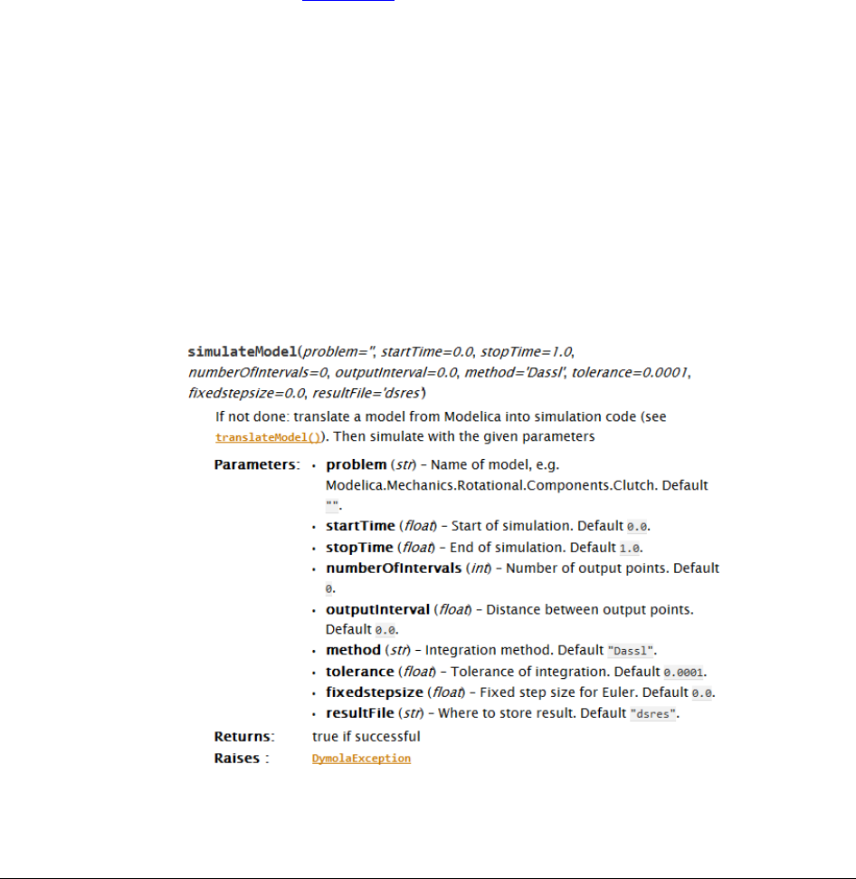
6 OTHER SIMULATION ENVIRONMENTS 291
dymola.close()
dymola = None
The Python Interface
To illustrate the Python interface, consider the function simulateModel. Its description in
Dymola is:
Function simulateModel "simulate a Modelica model"
input String problem := "" "Name of model, e.g. Modelica.Mechanics
.Rotational.Components.Clutch";
input Real startTime := 0.0 "Start of simulation";
input Real stopTime := 1.0 "End of simulation";
input Integer numberOfIntervals := 0 "Number of output points";
input Real outputInterval := 0.0 "Distance between output points";
input String method := "Dassl" "Integration method";
input Real tolerance := 0.0001 "Tolerance of integration";
input Real fixedstepsize := 0.0 "Fixed step size for Euler";
input String resultFile := "dsres" "Where to store result";
output Boolean result "true if successful";
external "builtin";
annotation(Documentation(info="If not done: translate a model from
Modelica into simulation code (see translateModel).
Then simulate with the given parameters"));
end simulateModel;
The corresponding function in the Python interface is:
There is a one-to-one correspondence between the parameters in the Dymola command and
the parameters in the Python method. If a parameter has a default value, it is shown in the
292
documentation for that parameter. Note that in the Python interface documentation, default
values and array dimensions are formatted as in Modelica. An example of a call to
simulateModel is:
result = dymola.simulateModel("MotorDriveTest", 0, 1.2,
resultFile="MotorDriveTest")
For a complete list of available commands, see the documentation for the Python interface.
You find it in the subfolder Modelica\Library\python_interface\doc in the Dymola
distribution. Double-click on the file index.html to view the documentation in your favourite
web browser.
ExecuteCommand
If a command that is not a part of the Python interface should be executed, the method
ExecuteCommand can be used. It takes a string parameter that can contain any command or
expression. For example:
dymola.ExecuteCommand("a=1")
The command is not type checked so you are responsible for making sure the command is
valid. It is not possible to retrieve the output from the command.
getLastError
The translation and simulation log is available through the function getLastError. Call it
after a translate, and/or simulate, command to retrieve the log in text format. The function
can also be used to retrieve other error messages. Note that getLastError is cleared if a
new command is issued, so it should be called directly after the check/translate/simulate
command. getLastError is defined as follows:
An example of usage is:
result =
dymola.translateModel("Modelica.Mechanics.Rotational.Examples.C
oupledClutches")
if not result:
print("Translation failed.")
log = dymola.getLastError()
print(log)
Getting an Instance of Dymola
You get an instance of the Dymola interface by initializing DymolaInterface.

6 OTHER SIMULATION ENVIRONMENTS 293
dymola.dymola_interface.DymolaInterface(dymolapath="",
use64bit=True, port=-1, showwindow=False, debug=False,
allowremote=False, nolibraryscripts=False)
By default, the 64-bit Dymola version is used, and the port number used for communication
between Dymola and the Python interface is 8082. (If 32-bit Dymola should be used, set
use64bit= False.)
For more details about the instantiation methods and their parameters, see the
documentation.
Exiting Dymola
You exit Dymola by calling the method DymolaInterface.close().
It is good practice to enclose the interface calls in a try/except block and close Dymola in
the finally block.
dymola = None
try:
dymola = DymolaInterface()
...
except DymolaException as ex:
print("Error: " + str(ex))
finally:
if dymola is not None:
dymola.close()
dymola = None
Commands with Two Output Parameters
The commands simulateExtendedModel and simulateMultiExtendedModel each
have two output parameters.
simulateExtendedModel
Here is an example of a call to simulateExtendedModel in Dymola:
simulateExtendedModel("Modelica.Mechanics.Rotational.Examples.C
oupledClutches", initialNames={"J1.J","J2.J"},
initialValues={2,3}, finalNames={"J1.w","J4.w"});
= true, {6.213412958654296, 1.000000000000004}
The function returns two values, a Boolean status flag and a vector of values. The
corresponding call in the Python interface is shown below. The output parameters are
available as elements in a list.
output =
dymola.simulateExtendedModel("Modelica.Mechanics.Rotational.Exa
mples.CoupledClutches", 0.0, 1.0, 0, 0.0, "Dassl", 0.0001, 0.0,
"test3", ["J1.J", "J2.J"], [2, 3], ["J1.w", "J4.w" ], True)
status = output[0]
values = output[1]

294
J1_w = values[0]
J4_w = values[1]
simulateMultiExtendedModel
Here is an example of a call to simulateMultiExtendedModel in Dymola:
simulateMultiExtendedModel("Modelica.Mechanics.Rotational.Examp
les.CoupledClutches", initialNames={"J1.J","J2.J"},
initialValues=[2,3;3,4;4,5], finalNames={"J1.w","J4.w"});
= true,
[6.213412958654296, 1.000000000000004;
7.483558191010655, 1.000000000000003;
8.107446379737779, 0.9999999999999931]
The function returns two values, a Boolean status flag and a two-dimensional array of
values. The corresponding call in the Python interface is shown below:
initialValues = [[2, 3], [3, 4], [4, 5]]
output =
dymola.simulateMultiExtendedModel("Modelica.Mechanics.Rotationa
l.Examples.CoupledClutches", 0.0, 1.0, 0, 0.0, "Dassl", 0.0001,
0.0, "dsres", ["J1.J", "J2.J"], initialValues, ["J1.w",
"J4.w"])
status = output[0]
values = output[1]
result1 = values[0]
J1_w = result1[0]
J4_w = result1[1]
result2 = values[1]
J1_w = result2[0]
J4_w = result2[1]
result3 = values[2]
J1_w = result3[0]
J4_w = result3[1]
Extended versions of both examples are available in the file
SimulateExtendedExample.py in the folder
Modelica\Library\python_interface\examples.
Multithreading
The Python interface supports multithreading. It is possible to instantiate more than one
Dymola and run them in parallel.
Each Dymola instance needs to have a unique port number. You can either assign a port
number yourself, or let the Python interface find an available port. To set the port,
instantiate DymolaInterface with the port argument. To automatically find a free port,
instantiate DymolaInterface either without the port argument, or set port to -1.

6 OTHER SIMULATION ENVIRONMENTS 295
Two Dymola instances that are run simultaneously cannot share the same working directory.
You need to assign a unique working directory to each instance. Use the interface method
cd to set the working directory.
The Python interface is not thread-safe. The only exception is the instantiation method for
DymolaInterface. Each thread should run its own instance of Dymola.
Below is an example that illustrates how to use multithreading in the Python interface. The
example is available as MultithreadingExample.py in the folder
Modelica\Library\python_interface\examples.
import os
import threading
from dymola.dymola_interface import DymolaInterface
from dymola.dymola_exception import DymolaException
def CoupledClutchesThread():
dymola = None
try:
print("1: Starting Dymola instance")
dymola = DymolaInterface()
print("1: Using Dymola port " + str(dymola._portnumber))
path = "C:/temp/Dymola/CoupledClutches"
print("1: Change working directory to " + path)
try:
os.makedirs(path)
except OSError as ex:
print("1: " + str(ex))
result = dymola.cd(path)
if not result:
print("1: Failed to change working directory")
print("1: Simulating model")
result =
dymola.simulateModel("Modelica.Mechanics.Rotational.Examples.CoupledClutches")
if not result:
print("1: Simulation failed")
log = dymola.getLastError()
print(log)
print("1: Plotting")
result = dymola.plot(["J1.w", "J2.w", "J3.w", "J4.w"])
if not result:
print("1: Plot failed")
print("1: Saving the plot")
result = dymola.ExportPlotAsImage(path + "/plot.png")
if not result:
print("1: Failed to save the plot")

296
print("1: Saving log")
dymola.savelog(path + "/log.txt")
print("1: OK")
except DymolaException as ex:
print("1: Error: " + str(ex))
finally:
if dymola is not None:
dymola.close()
dymola = None
def FullRobotThread():
dymola = None
try:
print("2: Starting Dymola instance")
dymola = DymolaInterface()
print("2: Using Dymola port " + str(dymola._portnumber))
path = "C:/temp/Dymola/fullRobot"
print("2: Change working directory to " + path)
try:
os.makedirs(path)
except OSError as ex:
print("2: " + str(ex))
result = dymola.cd(path)
if not result:
print("2: Failed to change working directory")
print("2: Simulating model")
result =
dymola.simulateModel("Modelica.Mechanics.MultiBody.Examples.Systems.RobotR3.fullRobot")
if not result:
print("2: Simulation failed")
log = dymola.getLastError()
print(log)
print("2: Plotting")
result = dymola.plot(["mechanics.q[1]", "mechanics.q[2]"])
if not result:
print("2: Plot failed")
print("2: Saving the plot")
result = dymola.ExportPlotAsImage(path + "/plot.png")
if not result:
print("2: Failed to save the plot")
print("2: Saving log")
dymola.savelog(path + "/log.txt")
print("2: OK")
except DymolaException as ex:
print("2: Error: " + str(ex))
finally:
if dymola is not None:

6 OTHER SIMULATION ENVIRONMENTS 297
dymola.close()
dymola = None
if __name__ == '__main__':
coupled_clutches_thread = threading.Thread(target=CoupledClutchesThread)
coupled_clutches_thread.daemon = True
coupled_clutches_thread.start()
full_robot_thread = threading.Thread(target=FullRobotThread)
full_robot_thread.daemon = True
full_robot_thread.start()
coupled_clutches_thread.join()
full_robot_thread.join()

298
6.8 JavaScript interface for Dymola
The class DymolaInterface provides a JavaScript API for accessing the most useful built-in
functions in Dymola.
To use the JavaScript interface, Dymola must be started specifying server port 8082, for
example by adding this port as the last part of Target in a shortcut for starting Dymola:
…\Dymola.exe" –serverport 8082
There is a one-to-one correspondence between the parameters in a Dymola command and
the parameters in the corresponding JavaScript method. Note that JavaScript does not
support named parameters.
If you want to execute a command that is not part of the Java interface, you can use the
method ExecuteCommand. It takes a string parameter that can contain any command or
expression. For example:
dymola.ExecuteCommand("a=1");
The command is not type checked so you are responsible for making sure that the command
is valid. It is not possible to retrieve the output from the command.
The JavaScript interface is supported on Windows and Linux. The instructions for
Windows in this section apply to Linux as well, with adjustments for the Linux structure.
The JavaScript interface has been tested on Firefox, Google Chrome, and Internet Explorer
11.
Below an example of how to use the JavaScript interface:
try {
var dymola = new DymolaInterface();
var result =
dymola.simulateModel("Modelica.Mechanics.Rotational.Examples.CoupledClutches");
if (result) {
result = dymola.plot(["J1.w", "J2.w", "J3.w", "J4.w"]);
if (result) {
result = dymola.ExportPlotAsImage("C:/temp/plot.png");
}
} else {
alert("Simulation failed.");
var log = dymola.getLastError();
alert(log);
}
} catch (e) {
alert("Exception: " + e);
}
For more information about the JavaScript interface, open the file
DymolaInterface.html, located in
Program Files (x86)\Dymola 2018\Modelica\Library\
javascript_interface\doc
with your favorite browser.

6 OTHER SIMULATION ENVIRONMENTS 299
6.9 Report generator
6.9.1 Fundamentals
In Dymola a report generator is available. It is based on Dymola running as a server. It
enables a HTML page loaded in a browser to call Modelica functions using JavaScript. It is
possible to insert a model diagram, change parameters, simulate a model, show plots, show
animations, etc. It can be used as a “notebook” since it´s possible to re-execute function
calls, for example to make a simulation with changed parameters and observe the changed
plots. The resulting report can then be stored and sent to anyone (the reader does not need
Dymola to read the report).
XHTML can be used, as well as HTML5, SVG, WebGL, MathML and X3D (successor
standard for VRML). For example, 3D animations can be made directly in a browser using
X3DOM which renders 3D animations represented as X3D. It is written in JavaScript and
uses WebGL. For animation commands available in the animation, see section “Mouse and
keyboard commands available for animation in reports” on page 305 below.
In order to allow calling Modelica functions from HTML, a web server version of Dymola
has been developed. All functions available in the package DymolaCommands are possible
to call from JavaScript in the client web browser. An automatic JavaScript generator has
been developed. It creates the code for the parameter exchange.
To support the report generator, Dymola must be started specifying server port 8082, for
example by adding this port as the last part of Target in a shortcut for starting Dymola:
…\Dymola.exe" –serverport 8082
Note! The report generator is currently only supported on Windows.
The report generator has been tested on Firefox, Google Chrome, and Internet Explorer 11.
6.9.2 JavaScript functions
A set of special report JavaScript functions has been developed which are suitable to include
in the HTML code. When the HTML page is opened, the browser communicates with
Dymola to retrieve various information, such as model diagrams, plots, and animations.
This information is inserted in the HTML page. It is possible to save the HTML code
including this information for use without having Dymola running. It is also possible to re-
execute a function call, for example to re-run a simulation after changing parameters.
The functions add content (innerHTML) of HTML div-blocks. The structure of the
functions is:
insertXXX(result_block, model, ...);
The id of the div-block is a parameter block-_id. The model path is given as the
parameter model. A typical structure of a HTML page is thus:
<p>Text</p>
<div id="diagram"></div>
<script type="text/javascript">insertDiagram(diagram, "MyModel", "svg");
Important.

300
</script>
The functions are:
insertDiagram(result_block, model, format, width, height)
Inserts a Modelica diagram.
The format is either "PNG" or "SVG". The dimensions in pixels are given by width and
height.
insertIcon(result_block, model, format, width, height)
Inserts a Modelica icon.
The format is either "PNG" or "SVG". The dimensions in pixels are given by width and
height.
insertText(result_block, model)
Inserts pretty printed Modelica text.
The annotations are omitted from the Modelica text.
insertClass(result_block, model, width, height)
Inserts a Modelica text editor for a given model.
The text of the model can be edited and submitted to Dymola. If the model is read-only, the
editor is disabled and the model is not possible to edit.
The dimensions in pixels are given by width and height.
insertEquations(result_block, model, format)
Inserts the equations and algorithms of a Modelica model.
The format is either "PNG" or "MathML".
insertDocumentation(result_block, model, width, height)
Inserts the formatted documentation of a Modelica model.
The dimensions in pixels are given by width and height.
insertParameterDialog(result_block, model)
Inserts an editor for the top-level parameters in a model.
The parameter values can be changed and submitted to Dymola.
insertCommand(result_block, width, height)
Inserts a command window.

6 OTHER SIMULATION ENVIRONMENTS 301
The bottom part is a command-line where any command may be entered. The top part
shows the result.
The dimensions in pixels are given by width and height.
insertPlot(result_block, model, variables, format, width, height)
Inserts a plot.
The array of variables to plot is given by variables.
The format is either "PNG" or "SVG". The dimensions in pixels are given by width and
height.
insertVariableValue(model, variable, time)
Inserts a variable value. The value is read from the result file.
The variable path is given by variable. The time in seconds is given by time.
insertSignalOperatorValue(model, variable, signalOperator)
Inserts a signal operator value.
The variable path is given by variable. The signalOperator is an enumeration value.
Here is a list of available signal operators:
SignalOperator.Min
SignalOperator.Max
SignalOperator.ArithmeticMean
SignalOperator.RectifiedMean
SignalOperator.RMS
SignalOperator.ACCoupledRMS
SignalOperator.SlewRate
SignalOperator.THD
SignalOperator.FirstHarmonic
insertAnimation(result_block, model, format, width, height)
Inserts an animation.
The animation is automatically running. You can rotate the animation object by pressing left
button and moving the mouse. Pan by also pressing Ctrl. Zoom by pressing Alt.
The format supported is "X3D". The dimensions in pixels are given by width and height.
The following utility function is also available:
setClassText(package_path, Modelica_text);
Creates or changes a Modelica class.
The complete text definition of a Modelica class is given. It can be inserted in a package. If
the package_path is an empty string, a top level class is created.

302
6.9.3 Example of HTML report sections
Below a small example of how a HTML report can look like:
<?xml version="1.0" encoding="UTF-8" ?>
<!DOCTYPE html PUBLIC "-//W3C//DTD XHTML 1.1//EN"
"http://www.w3.org/TR/xhtml11/DTD/xhtml11.dtd">
<html xmlns="http://www.w3.org/1999/xhtml" xml:lang="en">
<head>
<meta http-equiv="Content-Type" content="application/xhtml+xml; charset=utf-8"/>
<title>Dymola Report</title>
<link rel="stylesheet" type="text/css" href="dymola_report.css"/>
<script type="text/javascript" src="utils.js"></script>
<script type="text/javascript" src="dymola_interface.js"></script>
<script type="text/javascript" src="dymola_report.js"></script>
<script type="text/javascript"
src="http://cdn.mathjax.org/mathjax/latest/MathJax.js?config=TeX-AMS-
MML_HTMLorMML"></script>
</head>
<body>
<h1>Dymola Report</h1>
<p>This is a sample report to demonstrate the Dymola Report features.</p>
<h2>Diagram</h2>
<p>The model diagram for the Modelica.Blocks.Examples.PID_Controller is shown
below:</p>
<div id="dymola_example_diagram"></div>
<script
type="text/javascript">insertDiagram(document.getElementById("dymola_example_diagram
"), "Modelica.Blocks.Examples.PID_Controller", "svg");</script>
<h2>Plot</h2>
<p>The angular velocities of
Modelica.Mechanics.Rotational.Examples.CoupledClutches are shown below:</p>
<div id="dymola_example_plot"></div>
<script
type="text/javascript">insertPlot(document.getElementById("dymola_example_plot"),
"Modelica.Mechanics.Rotational.Examples.CoupledClutches", ["J1.w", "J2.w", "J3.w",
"J4.w"], "svg", 600, 350);</script>
<h2>Animation</h2>
<p>The animation view of
Modelica.Mechanics.MultiBody.Examples.Systems.RobotR3.fullRobot is shown below:</p>
<div id="dymola_example_animation"></div>
<script
type="text/javascript">insertAnimation(document.getElementById("dymola_example_anima
tion"), "Modelica.Mechanics.MultiBody.Examples.Systems.RobotR3.fullRobot", "xhtml",
600, 300);</script>
<div id="dymola_report_created"></div>
</body>
</html>

6 OTHER SIMULATION ENVIRONMENTS 303
This example only includes a model diagram, a plot and an animation. For an example with
more features, please open the file dymola_report_example.xhtml in the folder
Modelica\Library\javascript_interface in the distribution. Note that this file also
displays the resulting report.
For more information about the report generator, open the file global.html, located in
Program Files (x86)\Dymola 2018\Modelica\Library\
java_interface\doc_report
with your favorite browser.
An example of how a report could look like when generated is:

304

6 OTHER SIMULATION ENVIRONMENTS 305
6.9.4 Mouse and keyboard commands available for
animation in reports
The implementation of X3DOM for animation in reports provides some generic interaction
and navigation methods. Navigation is controlled by specific predefined modes.
Examine mode (activate with key “e”)
Function
Button
Rotate
Left Button / Left Button + Shift
Pan
Mid Button / Left Button + Ctrl
Zoom
Right Button / Wheel / Left Button + Alt
Set center of rotation
Left Button double-click
Walk mode (activate with key “w”)
Function
Button
Move forward
Left Button
Move backward
Right Button
Fly mode (activate with key “f”)
Function
Button
Move forward
Left Button
Move backward
Right Button
Look at mode (activate with key “l”)
Function
Button
Move closer
Left Button
Move back
Right Button
Non-interactive movement
Function
Button
Reset view
r
Show all
a
Upright
u

306
6.10 FMI Support in Dymola
6.10.1 Introduction
FMI
The FMI (“Functional Mock-up Interface”) standard allows any modeling tool to generate C
code or binaries representing a dynamic system model which may then be seamlessly
integrated in another modeling and simulation environment.
FMI started as a key development effort within the MODELISAR project, see
https://itea3.org/project/modelisar.html
The FMI standard is today maintained and developed as a long-term project within the
Modelica Association.
Three official FMI specifications have been released. The ‘FMI for Model Exchange’
specification version 1.0 was released on January 28, 2010, and the ‘FMI for Co-
Simulation’ specification version 1.0 was released on October 12, 2010. FMI 2.0 which
merges the model exchange and co-simulation specifications into one document was
published on July 25, 2014.
The model exchange specifications focus on the model ODE interface, whereas the co-
simulation specifications deal with models with built-in solvers and coupling of simulation
tools. A model package implementing the FMI standard is called a Functional Mockup Unit
(FMU). For further details visit:
http://www.fmi-standard.org/
The specification documents are also available in Dymola using the command Help >
Documentation. The specifications are separated into an execution part (C header files) and
a model description part (XML schema). A separate model description is used in order to
keep the executable footprint small. Both FMI 1.0 specifications use essentially the same
XML schema (a couple of capability flags are introduced for FMI for Co-Simulation).
In summary, an FMU (Functional Mock-up Unit) implementing an FMI specification
consists of
• The XML model description.
• Implementation of the C function interface in binary and/or source code format.
• Resources such as input data.
• Image and documentation of the model.
FMI support in Dymola
The Dymola FMI support consists of the two built-in functions described below for FMU
export and import, respectively. Commands are also available in the Dymola user interface
to execute these functions.

6 OTHER SIMULATION ENVIRONMENTS 307
The first three items in the list above are currently supported by Dymola. FMI (both Model
Exchange and Co-Simulation) is supported for Windows and Linux.
Unless otherwise stated, features are available both for FMI version 1.0 and version 2.0.
For the latest information about limitations and supported features of FMI, please visit
www.Dymola.com/FMI.
Online tunable parameters
Online tunable parameters are supported in FMI version 2.0 (tunable parameters were not
allowed in FMI version 1.0).
6.10.2 Exporting FMUs from Dymola
FMU export by the built-in function translateModelFMU
Exporting FMU models from Dymola is achieved by the function
translateModelFMU(modelToOpen, storeResult, modelName,
fmiVersion, fmiType, includeSource)
The input string modelToOpen defines the model to open in the same way as the traditional
translateModel command in Dymola.
The Boolean input storeResult is used to specify if the FMU should generate a result file
(dsres.mat). If storeResult is true, the result is saved in <model id>.mat when the
FMU is imported and simulated, where <model id> is given at FMU initialization. (If
empty, “dsres” is used instead.) This is useful when importing FMUs with parameter
allVariables = false, since it provides a way to still obtain the result for all variables.
Simultaneous use of result storing and source code inclusion (see below) is not supported.
The input string modelName is used to select the FMU model identifier. If the string is
empty, the model identifier will be the name of the model, adapted to the syntax of the
model identifier (e.g. dots will be exchanged with underscores).The name must only contain
letters, digits and underscores. It must not begin with a digit.
The input string fmiVersion controls the FMI version ("1" or "2") of the FMU. The
default is "1".
The input string fmiType defines whether the model should be exported as
• Model exchange (fmiType="me")
• Co-simulation using Cvode (fmiType="cs"),
• Both model exchange, and Co-simulation using Cvode (fmiType="all")
• Co-simulation using Dymola solvers (fmiType="csSolver").
The default setting is fmiType="all". This parameter primarily affects
modelDescription.xml. For the three first choices binary and source code always contains
both model exchange and Co-simulation. For the last choice the binary code only contains
Co-simulation; the solver and tolerance that are selected in Dymola in the general tab in the

308
simulation setup are also used by the exported FMU. Note that co-simulation using Dymola
solvers requires the Binary Model Export license. Please see also “Notes on Co-Simulation”
on page 316 concerning Co-simulation
The Boolean input includeSource is used to specify if source code should be included in
the FMU. The default setting is that it is not included (includeSource=false).
Simultaneous use of result storing (see above) and source code inclusion is not supported.
Note that source code generation is not supported for Co-simulations using Dymola solvers.
Note also that general source code documentation is available in the Documentation folder
inside the generated FMU folder.
The function outputs a string FMUName containing the FMU model identifier on success,
otherwise an empty string.
As an example, translating the Modelica CoupledClutches demo model to an FMU with
result file generation, is accomplished by the function call
translateModelFMU("Modelica.Mechanics.Rotational.Examples.
CoupledClutches", true);
After successful translation, the generated FMU (with file extension .fmu) will be located in
the current directory. The user can select if 32-bit and/or 64-bit FMU binaries should be
generated – see the FMI tab description below.
The generated FMU contains information about if it has been generated without export
options. In the corresponding XML file of such an FMU, the following is seen:
generationTool="Dymola Version 2015 (64-bit), 2014-02-21
(requires license to execute)"
FMUs exported from Dymola support intermediate results for event update
(fmiEventUpdate) for Model Exchange for FMI version 1.0.
Commands in Dymola for FMU export
An alternative to executing the translateModelFMU function from the command line is to
use the FMU option of the Translate button as illustrated below.
The above is also available as the command Simulate > Translate > FMU.
The settings that will be used when using any of the above commands is specified in a
dialog that appears when the command has been given:
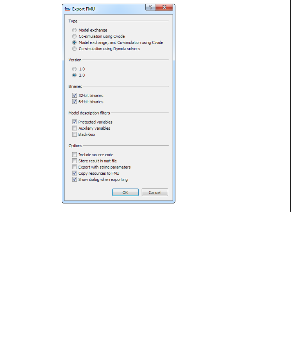
6 OTHER SIMULATION ENVIRONMENTS 309
This dialog corresponds to the export part of the FMI tab of the simulation setup, reached by
the command Simulate > Setup…, the FMI tab:
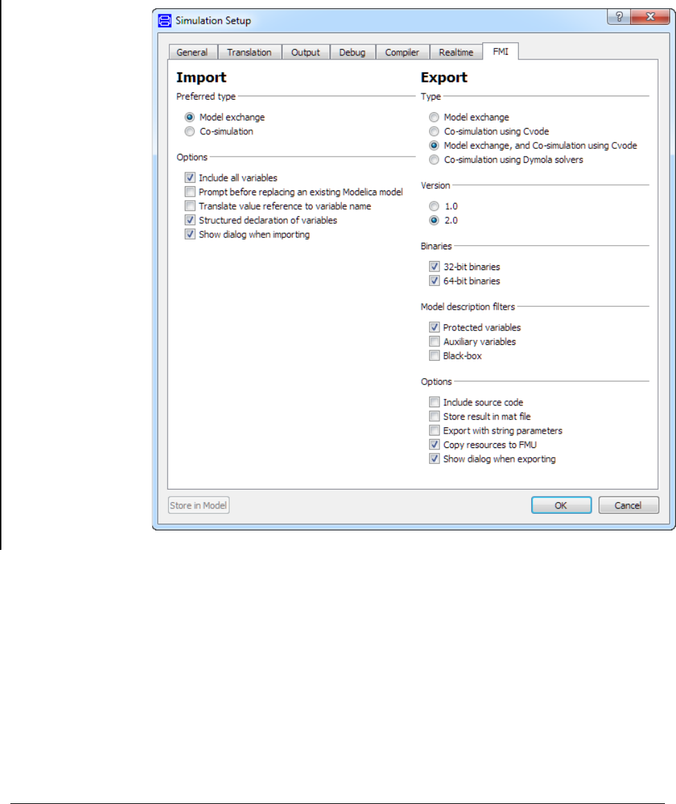
310
Changing settings when exporting will impact also this menu. Changed settings are
remembered in the session, but not between sessions.
Type group
FMI type can be selected as Model exchange, Co-simulation using Cvode, Model
exchange, and Co-simulation using Cvode or Co-simulation using Dymola solvers; this
setting corresponds to the parameter fmiType in translateModelFMU (see description
above of this setting for more information).
Version group
The FMI version can be selected as "1" or "2", the default being "1".
Binaries group

6 OTHER SIMULATION ENVIRONMENTS 311
The user can select whether 32- and/or 64-bit FMU binaries should be generated. This
option is not available in translateModelFMU.
Model description filters group
You can control the filtering of the modelDescription.xml file with these settings:
• Protected variables (by default activated) filters away protected Modelica variables.
This setting corresponds to the flag Advanced.FMI.xmlIgnoreProtected =
true;.
• Auxiliary variables (by default not activated) works differently in FMI version 2.0 and
FMI version 1.0:
o For FMI version 2.0 activating this setting means filtering away all
variables of causality local, except states and derivatives of states.
o For FMI version 1.0 activating this setting means all variables of causality
internal except the ones with variability parameters are filtered away.
This setting corresponds to the flag Advanced.FMI.xmlIgnoreLocal = false;.
• Black-box (by default not activated) works differently in FMI version 2.0 and FMI
version 1.0:
o For FMI version 2.0 activating this setting means filtering away all
variables except the following:
Variables of causality inputs and outputs
Variables needed for the model structure. The names are
however hidden (concealed).
o For FMI version 1.0 activating this setting means filtering away all
variables except variables of causality inputs and outputs.
This setting corresponds to the flag Advanced.FMI.BlackBoxModelDescription =
false;.
Black-box export can be used to export sensitive models without exposing the names of
parameters and internal variables.
Note that if you activate Black-box, the settings Protected variables and Auxiliary
variables are dimmed; they are not relevant is this case.
Options group
Five general options are available; see the description above of the corresponding
parameters for more information concerning the first two. Note that the two first ones
cannot be ticked simultaneously.
• Include source code – corresponds to the parameter includeSource in
translateModelFMU. If ticked (includeSource=true) source code is included, if
unticked the source code is not included. Note that for Co-simulation, source code
export is currently only supported for the CVODE solver. Note also that general source

312
code documentation is available in the Documentation folder inside the generated FMU
folder.
• Store result in mat file – corresponds to the parameter storeResult in
translateModelFMU. If ticked (storeResult=true) a result file is generated and
stored as a .mat file <model id>.mat, if unticked no result file is generated.
• Export with string parameters – enables using string parameters when exporting
FMUs. All types of FMUs are supported. Note:
o The default value is false, since you would normally not want the
regular simulation to use string parameters as this makes the code slightly
less efficient.
o The default setting corresponds to the flag
Advanced.AllowStringParametersForFMU = false.
o String variables are currently not supported.
• Copy resources to FMU – external resources using the functions
ModelicaServices.ExternalReferences.loadResource or
Modelica.Utilities.Files.loadResource are by default copied to the FMU. The
resulting FMU will be larger due to this. If this is not wanted, de-selecting the setting
will not copy the resources to FMU, but the resource-paths using Windows-shares will
be changed to UNC-paths when possible. This makes the FMU usable within a company
– without increasing its size. An example of using the resource copying is given below,
the extended example in the “String parameter support - examples” section.
• Show dialog when exporting – this option is by default ticked. If unticked, the Export
FMU dialog is not displayed when exporting FMUs.
Including settings in the exported FMU
Note the possibility to include settings in the exported FMU by ticking Settings included
in translated model, reachable by the command Simulation > Setup…, the Debug tab. (If
such settings are included in a Dymola-generated FMU, they can be logged by activating
fmi_loggingOn in the FMI tab of the parameter dialog of the imported and instantiated
FMU.)
String parameter support - examples
String parameters are supported in FMUs if the option Export with string parameters is
selected (see the setting above)..
Basic example
String parameter support can be illustrated by a simple example of changing tables for an
FMU; consider creating a simple model for linearization.
Create a model; drag an instance of Modelica.Blocks.Tables.CombiTable2D into the
model. Connect the two inputs and the output and create the corresponding connectors. The
result is:
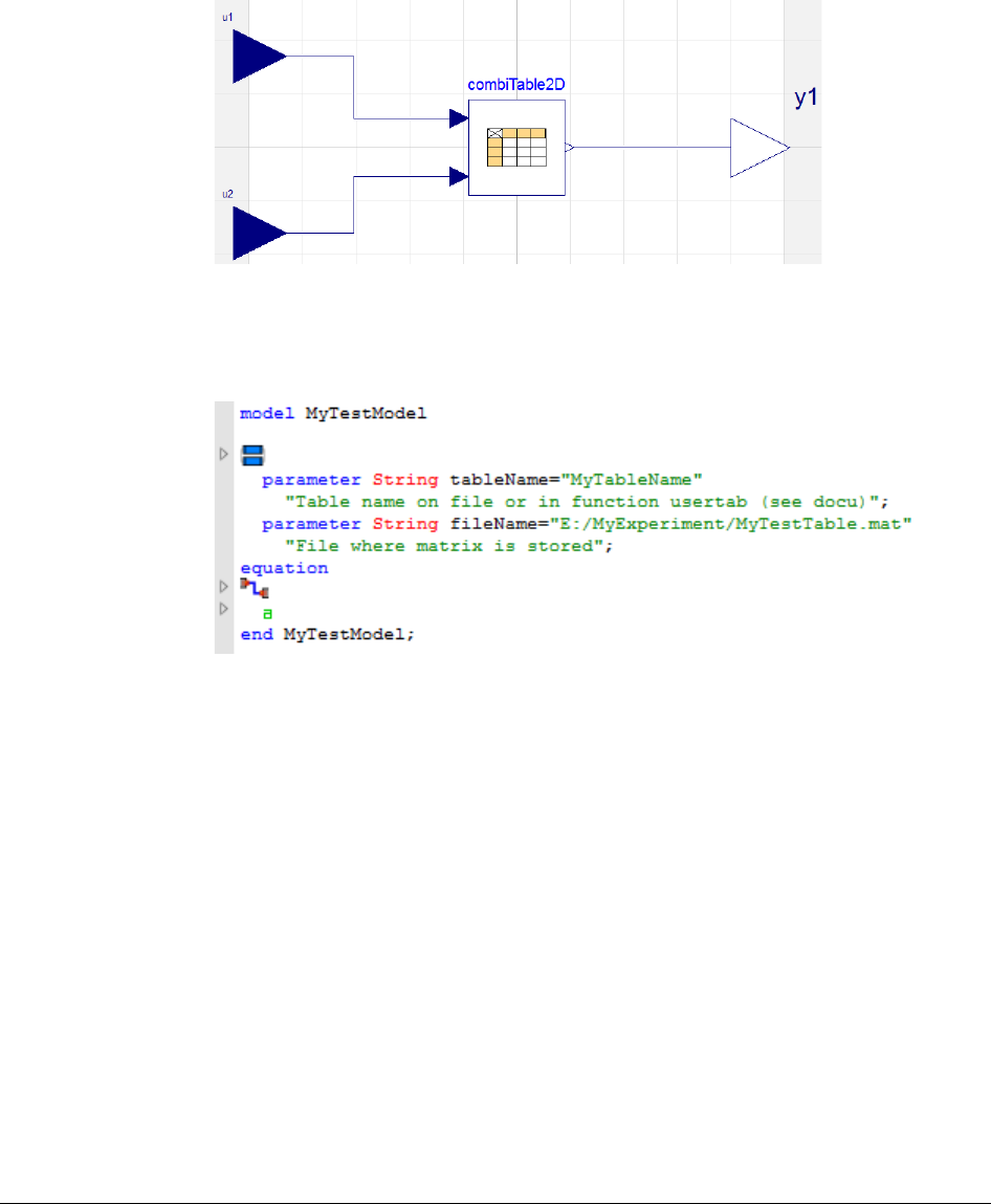
6 OTHER SIMULATION ENVIRONMENTS 313
In the parameter dialog of combiTable2D, select tableOnFile to true, and propagate
tableName and fileName. Give relevant default values for them. As an example, looking at
the resulting Modelica code when having specified a table name and file name as default
value, we find:
Saving the model, and then generating an FMU from it (do not forget to set the flag above),
we can import this FMU and look at the resulting parameter dialog of an instance of that
FMU:
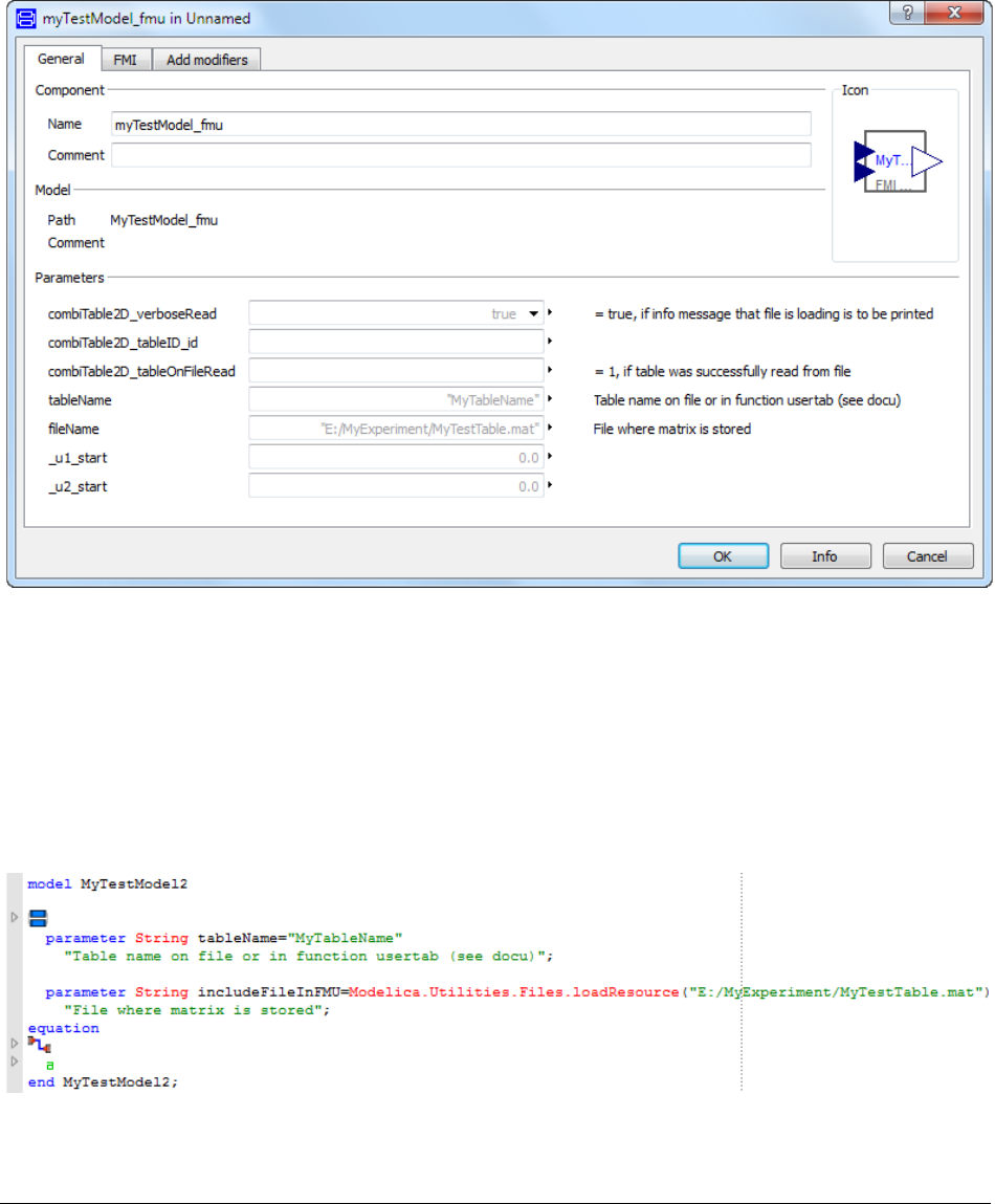
314
This FMU supports changing the table name and file name as string parameters.
Extended example (resource handling)
If the FMU should contain the table as a resource, the following can be done:
Rename the parameter fileName to includeFileInFMU (really not needed, but for clarity).
Use, in the variable definition dialog of includeFileInFMU, in the default value input field,
the context command Insert Function Call… to access
Modelica.Utilities.Files.loadResources, and specify the file name. The resulting
code is (given a new model MyTestModel2 is created):
Save the model. Before generating the FMU, check:
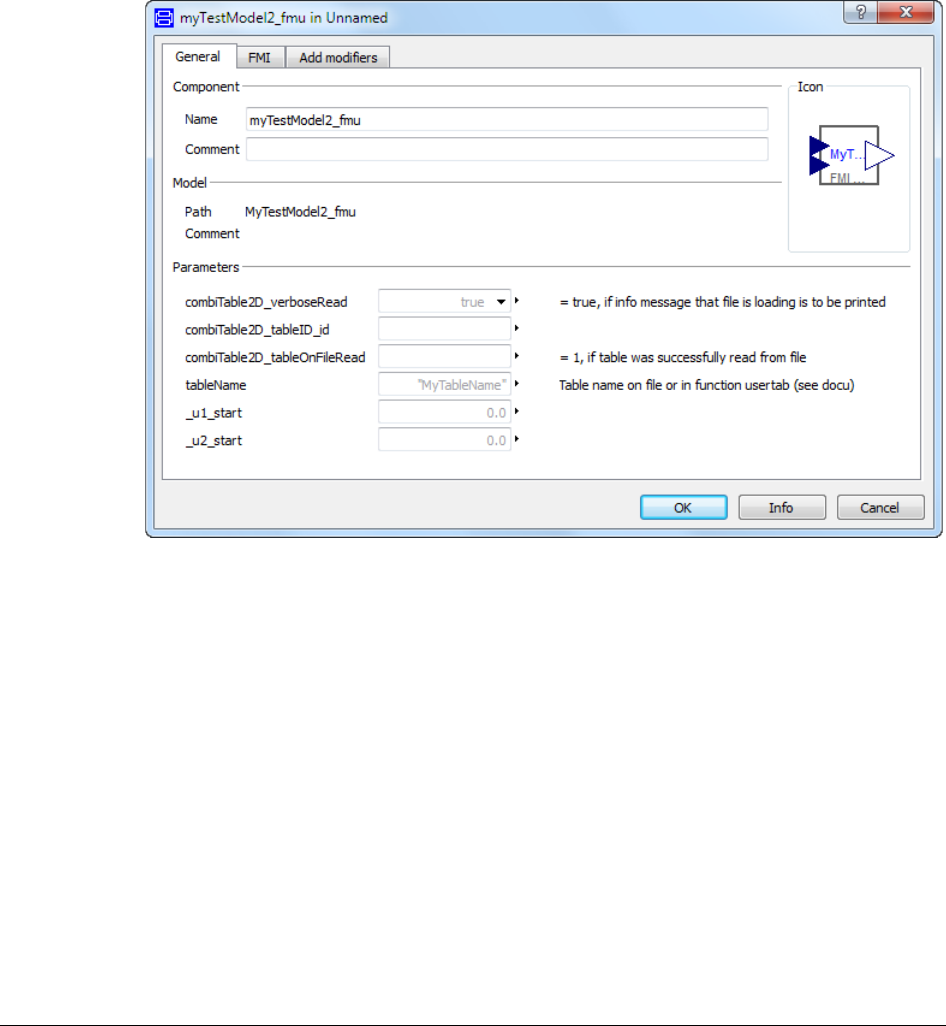
6 OTHER SIMULATION ENVIRONMENTS 315
• that Advanced.AllowStringParameters=true.
• that Copy resources to FMU is ticked in the FMI tab of the simulation setup.
We can import the generated FMU and look at the resulting parameter dialog of an instance
of that FMU:
The includeFileInFMU parameter is not displayed, it is evaluated, and the corresponding file
has been copied to the Resources directory of the FMU.
Handling multiple FMUs
An extra source code file all.c is provided; it includes all other C files. This file is needed
to compile all FMUs source code as one unit, which in turn is required because the demand
that all internal functions and symbols needs to be static to be able to combine several
source code FMUs.
The only disadvantage compiling this file instead of the separate C files, is that any
modification in any source code file requires re-compilation of everything.
Multiple instantiation of the same FMU
FMUs generated by Dymola 2016 and later support multiple instantiation. This means that
the same FMU can be used several times in the same model.
The generated XML file indicates that the model can be instantiated multiple times.

316
Restrictions:
• Multiple instances are currently only supported for Co-simulation with Cvode, see next
section.
• The support for multiple instances has a runtime cost, you can for this reason disable the
support for multiple instances by setting the flag
Advanced.AllowMultipleInstances=false. (This flag is by default true.)
• The old table handling, corresponding to tables in previous versions for Modelica
Standard Library (3.2 or older) is not supported. If you have user models with such old
table handling, those must be updated to use this feature.
Notes on Co-Simulation
Note that all Dymola solvers are supported for FMU Co-simulation export (if the Binary
Model Export license is available); however, the CVODE solver can be selected as a
particular solver by any export type selection containing Co-simulation using Cvode. The
support for features is currently larger when selecting CVODE as a particular solver this
way than when selecting Co-simulation using Dymola solvers:
• Including source code is currently only supported when selecting Co-simulation using
Cvode.
• Multiple instances are currently only supported when selecting Co-simulation using
Cvode.
CVODE solver
The SUNDIALS suite of numerical solvers (version 2.6.2) can be used in the co-simulation
FMUs. The SUNDIALS CVODE solver with Backward Differentiation Formula (BDF) and
Newton iteration can be used as solver in the exported co-simulation FMUs. For further
details, visit
https://computation.llnl.gov/casc/sundials/main.html
Fixed-step embedded (inline) solvers for FMU Co-Simulation export
The Dymola inline integration solvers are supported also for FMU Co-Simulation export.
Note that the fixed step-size used for the inline integration should also be used as step-size
when calling the fmiDoStep routine of the generated FMU.
For source code export it is also required to set the flag
#define ONLY_INCLUDE_INLINE_INTEGRATION
in the header file conf.h.

6 OTHER SIMULATION ENVIRONMENTS 317
Support for optional FMI Export options
Support for optional FMI Export options in FMI 2.0
The following tables list Dymola support for optional export options in FMI 2.0. Since both
“True” and “False” can be a limitation, the cells are color coded: green means “underlying
feature supported in Dymola”, yellow means “underlying feature not supported in Dymola”.
Furthermore, capital letters are used for “underlying feature supported”.
The order of the features is the order they appear in the specification. See next page; the
tables are on the same page for comparison reasons.
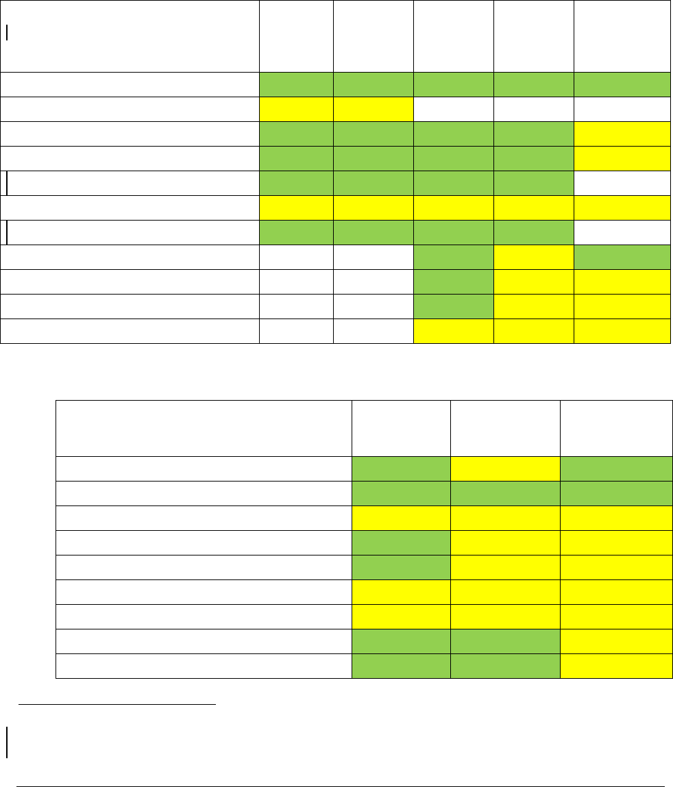
318
Optional FMI 2.0 features Model
Exchange Model
Exchange
with inline
integration
Co-
simulation
using
Cvode
Co-
simulation
with inline
integration
Co-
simulation
using Dymola
solvers
needsExecutionTool
FALSE
FALSE
FALSE
FALSE
FALSE
completedIntegratorStepNotNeeded
false
false
NA
NA
NA
canBeInstantiatedOnlyOncePerProcess
FALSE
FALSE
FALSE
FALSE
true
canNotUseMemoryManagementFunctions
FALSE
FALSE
FALSE
FALSE
true
canGetAndSetFMUState
TRUE
TRUE
TRUE
TRUE
Partly
3
canSerializeFMUState
false
false
false
false
false
providesDirectionalDerivative
TRUE
TRUE
TRUE
TRUE
Partly
4
canHandleVariableCommunicationStepSize NA NA TRUE false TRUE
canInterpolateInputs NA NA TRUE false false
maxOutputDerivativeOrder NA NA 1 0 0
canRunAsynchronuously NA NA false false false
Support for optional FMI Export options in FMI 1.0
Optional FMI 1.0 Co-simulation features Co-simulation
using Cvode Co-simulation
with inline
integration
Co-simulation
using Dymola
solvers
canHandleVariableCommunicationStepSize YES false YES
canHandleEvents YES YES YES
canRejectSteps false false false
canInterpolateInputs YES false false
maxOutputDerivativeOrder 1 0 0
canRunAsynchronuously false false false
canSignalEvents false false false
canBeInstantiatedOnlyOncePerProcess FALSE FALSE true
canNotUseMemoryManagementFunctions FALSE FALSE true
3 Supported except for the solvers Lsodar, Dassl, Cvode, Euler, Rkfix2, Rkfix3, and Rkfix4.
4 Supported except for the solvers Lsodar, Dassl, Euler, Rkfix2, Rkfix3, and Rkfix4.

6 OTHER SIMULATION ENVIRONMENTS 319
Propagating annotations from Modelica variables to the FMI model
description
Dymola supports propagating annotations from Modelica variables to the fmi2Annotation
node “Annotations” in the corresponding scalar variables in an FMI 2.0
modelDescription.xml document.
To activate this feature, set the flag
Advanced.FMI2.OutputVariableAnnotationsInXML = true;
The flag is by default false.
FMU export on Linux
The FMU export on Linux requires the Linux utility “zip”. If not already installed, please
install using your packaging manager (e. g. apt-get) or see e.g. http://www.info-zip.org.
Limitations
• The value meUndefinedValueReference is never returned when value references are
requested. As a consequence, some value references returned may not be present in the
model description file.
• The result file generation is currently only fully supported for the traditional solvers
(Lsodar, Dassl, Euler, Rkfix2, Rkfix3, and Rkfix4) when importing the FMU in Dymola.
For the other solvers, the number of result points stored will typically be too low.
However, the values are accurate for the time-points at which they are computed.
• String variables cannot be used in models which are exported as FMUs. String
parameters are however supported.
6.10.3 Importing FMUs in Dymola
The Dymola FMU import consists of (1) unzipping the .fmu archive, (2) transforming the
XML model description into Modelica, and (3) opening the resulting Modelica model in
Dymola.
Importing FMU models to Dymola is achieved by the function
importFMU(fileName, includeAllVariables, integrate,
promptReplacement, packageName)
The input string fileName is the FMU file (with the .fmu extension).
By setting the variable includeAllVariables to false, only inputs, outputs and
parameters from the model description are included when generating the Modelica model.
Such black-box import can be used as separate compilation of models to substantially
reduce translation times. For large model this is recommended since the generated .mo file
otherwise becomes huge and will take long time for Dymola to parse and instantiate.
The parameter integrate controls if integration is done centralized or in the FMU, i.e.
integrate=true means import the Model Exchange part of the FMU and
integrate=false means use the Co-Simulation part of the FMU. By default this

320
parameter is true. This setting is only relevant if the FMU to import supports both types.
Otherwise this setting is silently ignored. If the Co-Simulation part is used, the macro step-
size can be set as the parameter fmi_CommunicationStepSize in the FMI tab of the
parameter dialog of the imported FMU. See also section “Settings of the imported FMU” on
page 324.
The parameter promptReplacement can be set to true to generate prompting before
replacement of any existing Modelica model being the result of a previous import. Having
no prompting is useful when repeatedly importing FMUs using scripting. By default this
parameter is false.
The string parameter packageName can be set to the package to where the FMU should be
imported. The package must be open in Dymola when importing.
The function outputs true if successful, false otherwise.
The generated Modelica file will get the name model_fmu.mo or
model_fmu_black_box.mo, depending on the value of includeAllVariables.
ASCII characters of values larger than 32 are supported in the xml file of the imported FMU.
Also UTF characters are supported, but not recommended.
Note: The binary library files from any previous import are replaced when calling
importFMU and thus translations of previously imported models are not guaranteed to work
any longer (in the unlikely event of a name clash).
Commands in Dymola for FMU import
An alternative to executing the importFMU function from the command line is to use the
command File > Import > FMU....
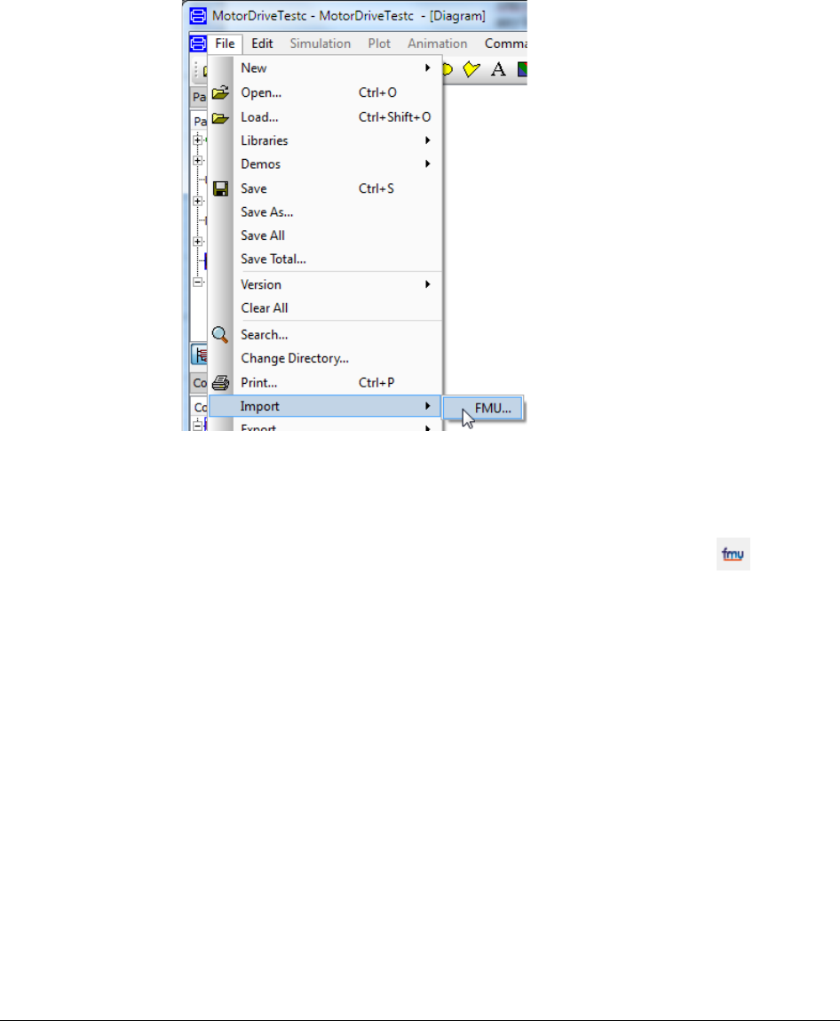
6 OTHER SIMULATION ENVIRONMENTS 321
Notes:
• This command also will be automatically applied on an .fmu file by dragging it into the
Dymola main window.
• The command can also be given by clicking the button Import FMU in the Files
toolbar.
What settings will be used when using any of the above commands is specified in a dialog
that appears when applying any of the commands:
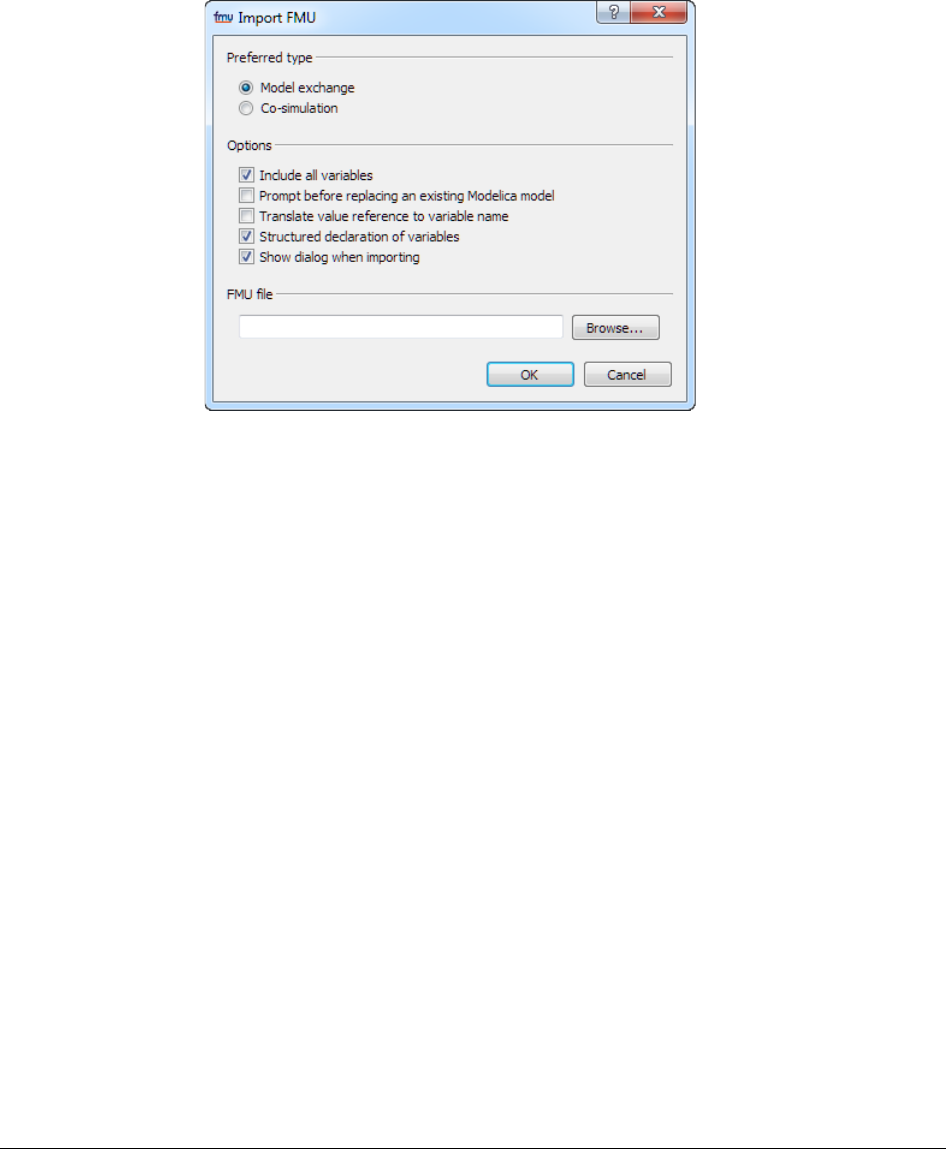
322
Except the FMU file section, this dialog corresponds to the import part of the FMI tab of the
simulation setup, reached by the command Simulate > Setup…, the FMI tab:

6 OTHER SIMULATION ENVIRONMENTS 323
Changing settings when exporting will impact also this menu. Changed settings are
remembered in the session, but not between sessions.
The FMU file part of the dialog that appears when applying a command can be used to
browse for the FMU. When the FMU is dragged into Dymola, the path is prefilled.
Preferred type can be selected as Model exchange or Co-simulation. This setting is only
relevant if the FMU to import supports both types. Otherwise this setting is silently ignored.
This setting corresponds to the parameter integrate in importFMU (see above for
description).
Five options are available:
• Include all variables – corresponds to the function parameter includeAllVariables
(see above).

324
• Prompt before replacing an existing Modelica model – corresponds to the function
parameter promptReplacement (see above).
• Translate value reference to variable name – this option is not present in importFMU.
If ticked, the imported FMU will contain a translation from value references to variable
names. This is useful for debugging, however will decrease the performance.
• Structured declaration of variables – this option is not present in importFMU. If
ticked, (the default value) the variables of the imported FMU will be presented in a
hierarchical structure, that is, as records. This is useful when e.g. wanting to change
variable values. To be able to use this option, the attribute
variableNamingConvention in the model description file of the FMU to be imported
must be set to variableNamingConvention="structured".
• Show dialog when importing – this option is by default ticked. If unticked, the Import
FMU dialog is not displayed when importing FMUs.
Settings of the imported FMU
The parameter dialog of the imported and instantiated FMU contains an Input Start Values
tab and an FMI tab.
Input Start Values tab
For FMI Model Exchange in FMI version 2.0, input start values can be set before
initialization. This should however only be necessary if your FMU is constructed in such a
way that the default start values for an input is illegal in the FMU, e.g. division with an
input variable having a default value of zero. For such an input variable you can set the
input start value to some value not being zero; sources of the FMU will then be handled
properly in the initializationMode.
Such start values are collected in the Input Start Values tab:

6 OTHER SIMULATION ENVIRONMENTS 325
For FMUs of FMI version 1.0, you should avoid a design where input values affect
initialization, since the FMI 1.0 interface lacks proper support to iterate during initialization.
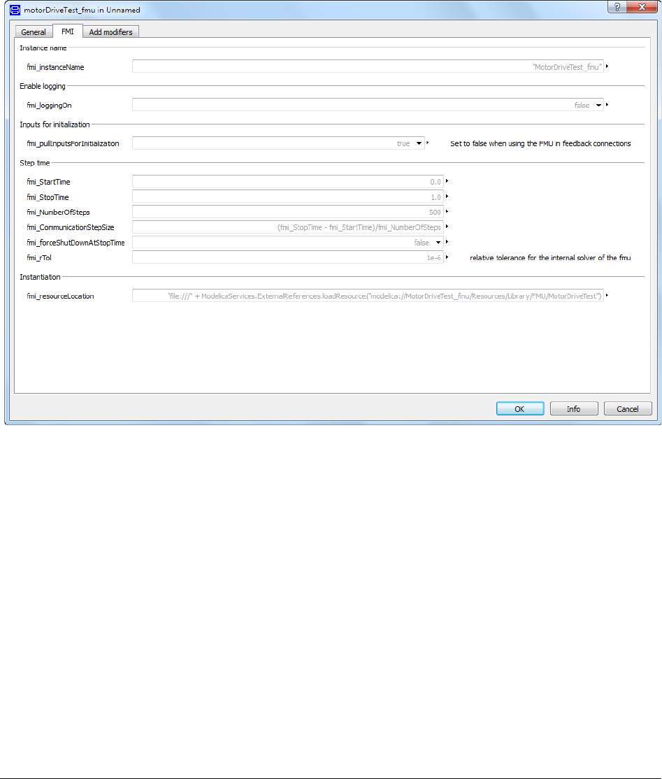
326
FMI tab
The available settings depend on the FMU type.
fmi_resourceLocation might be needed when importing FMUs from other vendors, to
specify the location of external resources. (For FMI version 1.0 Co-simulation the name is
fmi_fmuLocation.) By default the parameter displays the location where the FMU is
unpacked, which is usually the location of external resources (dlls, tables, etc,) as well.
Importing FMUs with many inputs/outputs
When importing FMUs with many inputs/outputs, the input and output connectors of the
imported FMU are automatically stacked at the same location, one location for each type
(Integer, Real, and Boolean) of input and output connectors (the image to the right below).
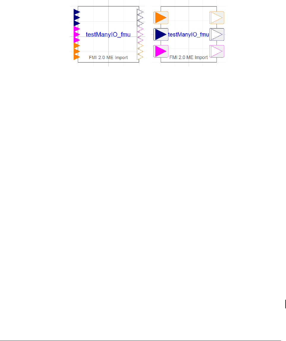
6 OTHER SIMULATION ENVIRONMENTS 327
The limit of the number of connectors when stacking should be applied is defined by the
flag
Advanced.FMI.OverlappingIOThreshold
The default value of the flag is 10 (so for creating the figure above, the value was set to 4).
Dragging a connection from/to a stacked connector displays a dialog to conveniently select
what connectors to connect. See previous chapter for details.
Import of FMUs of FMI version 1.0 and version 2.0 to the same model
Import of both FMUs of FMI version 1.0 and version 2.0 to the same model, is supported.
Input handling for co-simulation FMU import
Input time point
You can now choose the time point used as input when calling doStep with a co-simulation
FMU from time t0->t1.
Your choices are input at time t0 input at time t1 or pre on input at time t1 (default and
behavior of Dymola 2017).
Input time can be chosen with the parameter fmi_Input time, and if StepEnd is chosen
fmi_UsePreOnInputSignals can be used to disable pre operator on the input signal.
Be aware that using StepStart at for fmi_inputTime will introduce delays in output if
you have direct dependencies on the input.
Using StepEnd and disabling pre can introduce algebraic loops when connecting with
feedback which cannot be solved by co-simulation FMUs.
Using pre on inputs at StepEnd will break these loops if you create them with connections
by introducing an infinite small delay.
Input derivatives
Dymola 2018 supports interpolation of input and to set the input derivatives of real inputs if
the FMU has the capability flag canInterpolateInputs.

328
The interpolation is a first order interpolation. This can be activated by setting the flag
Advanced.FMI.SetInputDerivatives = true before importing an FMU that supports
this feature.
Since we only supports interpolation and not extrapolation, similar restrictions exists as
when using StepEnd as input time and disabling pre, i.e. all FMUs in a feedback loop
cannot have this feature at the same time.
Improved fmi2 initialization for co-simulation
FMI 2.0 co-simulation supports initialization with algebraic loops (but not solving algebraic
loops at simulation time).
Improvement has been made to make this more robust at Dymola import, this has also
removed the need for the parameter fmi_pullInputsForInitialization and thus it
been removed, (it is still needed for some cases in FMI 1.0 co-simulation as you cannot
solve initialization of multiple FMUs there).
Translation of underscore
The default (in Dymola 2017 and later) is to translate underscore “_” without any changes
when importing an FMU. If you want underscore “_” to be translated to “_0” when you
import an FMU, you can set the flag
Advanced.FMI.UseTrueVariableNames = false;
Previously the default value was to always translate underscore “_” to “_0” because of
possible conflicting names (the period “.” in Modelica paths is always translated to
underscore when importing an FMU). Now, when structured variables are used by default
when importing an FMU, the likeliness for conflicting names is very small, hence the
changed default behavior, and the flag to revert to the old behavior.
Note! If you have a model that contains an FMU as a connected component, you might get
errors if you want to reimport the FMU to the model, due to the changed translation of
underscore. You need in such a case to either redo your connections or set the above flag to
false to have the old naming convention when reimporting the FMU:
Display of information for an imported FMU
Information from the modelDescription.xml file of an imported FMU is displayed in the
information layer of the imported FMU.
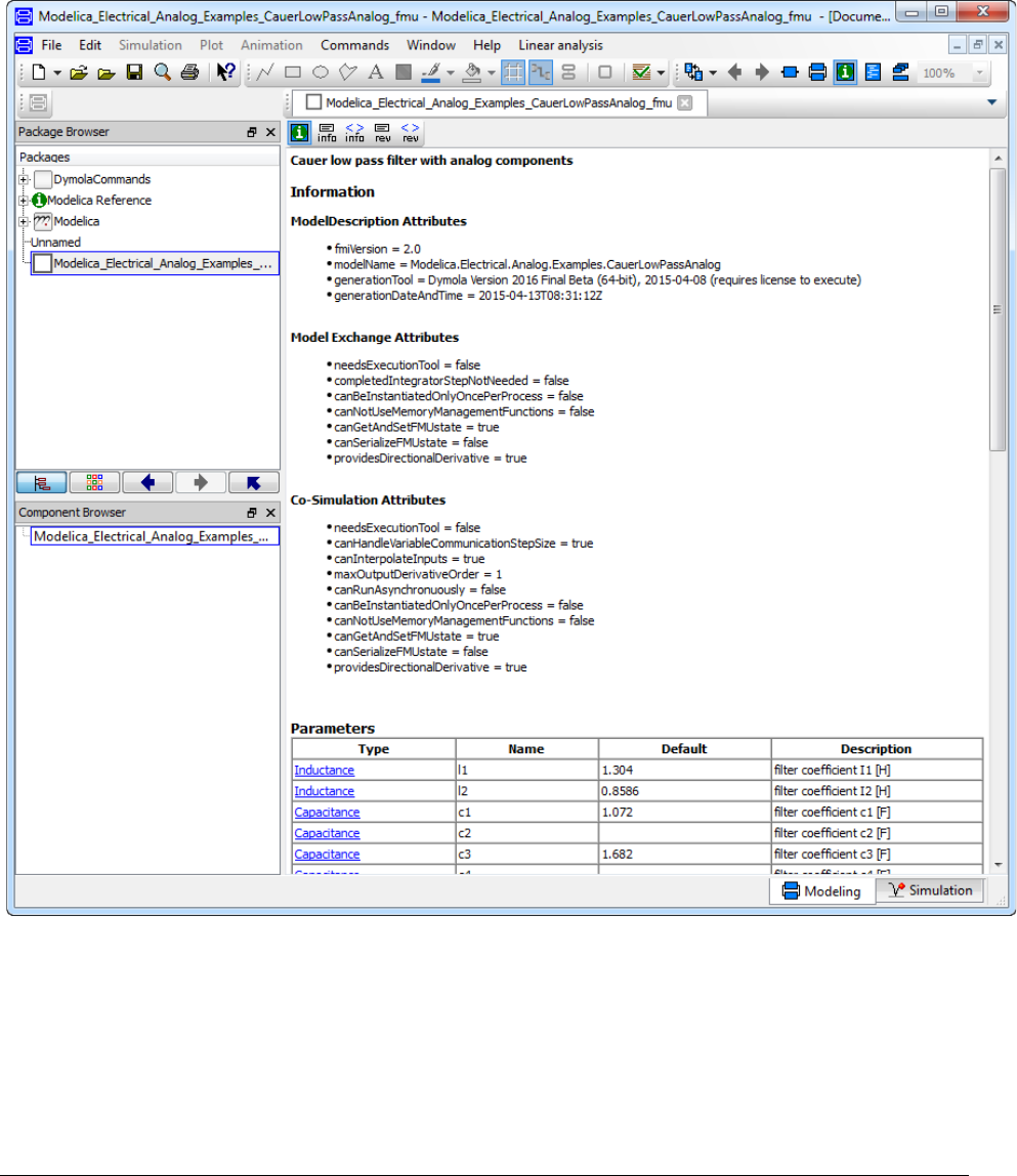
6 OTHER SIMULATION ENVIRONMENTS 329
Unit handling
FMI version 2.0 supports unit handling where an FMU exporter can define any unit for
inputs and outputs as long as conversion to base units according to the FMI standard is
available. This allows for proper unit checking for inputs and outputs between FMUs.
Dymola supports this; units are automatically converted to base units for inputs and outputs
of imported FMUs. Such unit handling for parameters in FMUs is also supported.

330
The unit conversion can be disabled by setting the flag
Advanced.FMI.DoNotDeclareUnits = true;
Setting this flag means ignoring the unit declarations completely. The flag is by default false.
FMU import on Linux
The FMU import on Linux requires the Linux utility “unzip”. If not already installed, please
install using your packaging manager (e. g. apt-get) or see e.g. http://www.info-zip.org.
Limitations
• For FMI version 1.0, the attribute nominal for scalar variables is not supported when
importing FMUs with Model Exchange. (For FMI version 2.0, this is supported.)
6.10.4 Validating FMUs from Dymola
Once the dynamic behavior of a model is verified and it is ready to be exported as FMU,
one would like to verify that this behavior can be repeated on the targeted simulation
environment. For model exchange, which is dependent on the solver of the target, this is
naturally less straight-forward than for co-simulation, where the solver is built into the
FMU. We focus this discussion on the co-simulation case, although all is possible for model
exchange as well.
Normally, the FMU contains inputs that need to be connected to signal generators (sources)
before this validation can be commenced. Since this is model and test dependent and hard to
automate, we will assume the model inputs have been connected to necessary sources
beforehand. The result is a test model with no disconnected inputs. After the validation,
these sources are of course removed before the final FMU is created.
Since Dymola supports FMU import, it becomes natural to re-import the FMU in Dymola
and compare its simulation with the original model. We demonstrate this for the demo
model CoupledClutches. For brevity, we use a scripting perspective. First, export as FMU
with, say, both model exchange and co-simulation support:
translateModelFMU(
"Modelica.Mechanics.Rotational.Examples.CoupledClutches",
false, "", "1", "all");
Re-import, in a non-interactive mode, the FMU for co-simulation:
importFMU(
"Modelica_Mechanics_Rotational_Examples_CoupledClutches.fmu",
true, false, false);
Simulate the model being the result of the import:
simulateModel(
"Modelica_Mechanics_Rotational_Examples_CoupledClutches_fmu",
stopTime=1.5, method="dassl");
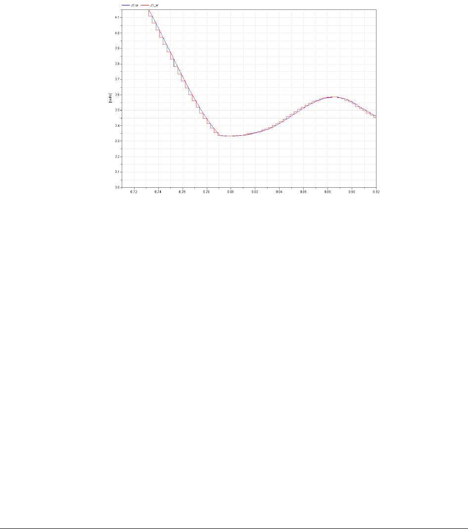
6 OTHER SIMULATION ENVIRONMENTS 331
Finally, the resulting trajectories can be plotted and compared visually with the original
(non-FMU) simulation. Note that, since the imported model is flattened, the trajectory
names are somewhat different; e.g. J1.w becomes J1_w:
The blue trajectory is from the reference simulation and the red is from the co-simulation.
Note that the latter is rendered as constant between the sample points.
While this validation is ok for sample testing of a single model, this clearly becomes
infeasible for systematic validation of several trajectories.
The remedy is a new function validateModelAsFMU, which automates the following
steps:
• Generation of reference trajectories.
• Exporting of the FMU.
• Importing of the FMU.
• Mapping of trajectories names to those of the original model.
• Numeric comparison of trajectories.
• Graphical HTML presentation of deviating trajectories in fashion similar to the plot
above.
Main features include:
• Using a default set of trajectories to compare or specifying it explicitly. The default it
the set of all state candidates.
• Choosing tolerance for the comparison.
• Optional generation of reference trajectories which is typically only needed once.
• Optional FMU export which might not be needed each time.
• Test of co-simulation or model exchange.
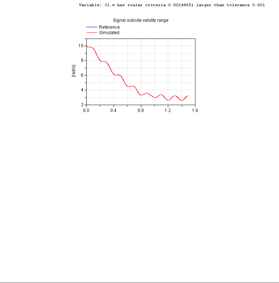
332
• Test of FMI version 1.0 or 2.0.
It is available in Modelica\Library under the Dymola installation.
Below call validates CoupledClutches as a co-simulation FMU for FMI 1.0:
validateModelAsFMU(
"Modelica.Mechanics.Rotational.Examples.CoupledClutches");
An excerpt from the log file is given below:
In this case we may argue that the comparison tolerance should be increased to avoid the
report of this trajectory.
6.10.5 FMU Export from Simulink/FMU Import into
Simulink: The FMI Kit for Simulink
FMI Kit for Simulink support export of FMUs from Matlab/Simulink as well as import of
FMUs into Matlab/Simulink.
Introduction
FMU Export from Simulink
FMI Kit for Simulink provides a Simulink Coder Target (rtwsfcnfmi) to support export of
FMUs from Matlab/Simulink. The FMU export package contains implementations of the
FMI standards on top of model code generated by Simulink Coder (formerly Real-Time
Workshop). The Matlab Target Language Compiler (TLC) is used to construct the XML
model description.
The package for FMU export from Simulink together with the Dymola support for FMU
import facilitates simulation of Simulink models in Dymola.

6 OTHER SIMULATION ENVIRONMENTS 333
The utility builds on the Simulink Coder 'S-function Target' configuration that is available
in Matlab. In fact, the same model C code is generated by the 'S-function target with FMI' as
for the Simulink Coder S-function target. In addition, the FMI target performs the following
• Constructs the model description interface, modelDescription.xml, from the
<modelname>.rtw model description
• Compiles the generated model code and the S-function FMI wrapper, and links with
required libraries
• Copies resources, such as images and MEX files, to the FMU resources folder
• Constructs the FMI zip archive (.fmu) according to the FMI distribution structure
Release History:
Note: The FMU Export from Simulink package is independent of Dymola and updates are
sometimes released in between the official Dymola releases. Information about new
released versions can be found at www.dymola.com/FMI.
• Version 1.0, February 10, 2010
o First version
• Version 1.1, August 20, 2010
o Supporting MATLAB R2010a
o Support for S-function blocks written in C
• Version 1.2, June 1, 2012
o MATLAB support up to R2011b
o Support for Visual Studio 2010
o 64-bit support
• Version 1.2.1, March 4, 2013
o Compliant to FMU Checker ver. 1.0.2
• Version 2.0, March 31, 2015 (included with Dymola 2016)
o FMI 1.0 and 2.0 support
o Model Exchange and Co-Simulation
o Support for all Simulink built-in data types
o MATLAB support for R2010a - R2014b (32- and 64-bit)
o Support for Visual Studio 2008 and later compilers
• Version 2.1, May 29, 2015
o Loading of binary MEX S-functions
o C++ source S-functions

334
o Simulink I/O buses with structured naming
o Black-box FMU generation
o Block hierarchy in variable names
• Version 2.1.1, June 24, 2015 (a maintenance version)
• Version 2.1.2, October 9, 2015 (included with Dymola 2016 FD01)
o Support for Matlab R2015a and R2015b
• Version 2.2.0, April 15, 2016 (included with Dymola 2017)
o Released as part of FMI Kit for Simulink (export and import)
o Support for global tunable workspace parameters
o Full support for Matlab R2015b code generation, especially support for
parameter references to workspace or mask variables
• Version 2.3.0, October 7, 2016 (included with Dymola 2017 FD01)
o Support for Matlab R2016a
o Improved input handling and support for input interpolation
o Support for FMU export on Linux
• Version 2.4.0, April 7, 2017 (included with Dymola 2018)
o Support for Matlab R2016b
FMU Import into Simulink
FMI Kit for Simulink contains a Simulink FMU block, which enables embedding of FMUs
into Simulink models. With source code FMUs exported with Dymola 2016 or later it is
also possible to use FMUs in Rapid Accelerator mode and create target code for RSIM,
GRT, and dSPACE ds1005, ds1006, and SCALEXIO platforms.
The package for FMU import into Simulink together with the Dymola support for FMU
export facilitates simulation of Dymola models in Simulink. In particular, this enables use
of Dymola solvers in Simulink through the FMI Co-Simulation interface.
Support and Usage
FMI Kit for Simulink has full support for both export and import, which means that both
versions 1.0 and 2.0 of the FMI standard are supported for both Model Exchange and Co-
Simulation. Supported Matlab releases are R2010a to R2016b (32- and 64-bit). FMU export
supports both Windows and Linux. FMU import is currently only supported on Windows.
FMI Kit for Simulink can be used for free without any license key.
Support and maintenance is offered to Dymola customers through the regular support
channel at www.3ds.com/support.

6 OTHER SIMULATION ENVIRONMENTS 335
FMI Kit for Simulink is independent of Dymola and updates are sometimes released in
between the official Dymola releases. Information about new released versions can be found
at www.dymola.com/FMI.
Installation
FMI Kit for Simulink is located in the $DYMOLA/Mfiles/FMIKit_for_Simulink
directory of the Dymola distribution or may be also be downloaded as a zip archive through
DS FileTransfer after contacting your DS support channel. Since the package is independent
of Dymola it may be extracted or copied to any location.
Follow these steps to set up the environment in Matlab:
• Add the FMIKit_for_Simulink directory to your Matlab path and then execute the
script FMIKit.initialize().
• Optionally, you may add the following to your Matlab startup script to automatically
perform the setup for each new session:
addpath('C:\Program Files\FMIKit_for_Simulink');
FMIKit.initialize()
(the addpath command should be changed to match your system)
Exporting FMUs from Simulink
This section describes the procedure to export an FMU from Simulink and the associated
settings / configurations.
Adding input and output ports
If the Simulink model to be exported as an FMU should be possible to connect to other
components, you need to add external input and/or output ports to your model. These can be
found in the Sinks and Sources categories of the Simulink browser. Hierarchical Simulink
buses are supported as input and output port types.
Selecting system target file
In the Simulink Configuration Parameters dialog, choose the Code Generation tab and
click Browse to select a different System Target File. Select rtwsfcnfmi.tlc in the list:
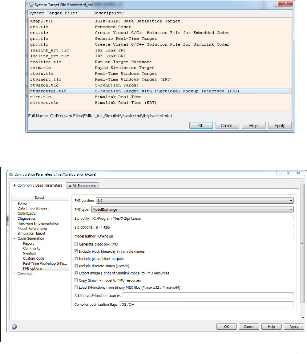
336
Options for FMU export
After selecting the rtwsfcnfmi.tlc target, the tab FMI options becomes available in the
Code Generation tab. A description of each option follows below.

6 OTHER SIMULATION ENVIRONMENTS 337
• FMI version
o Selects FMI version for the export (1.0 or 2.0)
• FMI type
o Specifies FMI type (ModelExchange or CoSimulation)
• Zip utility
o Path to Zip utility used to build the FMU archive (the default on Windows
is 7-zip, which can be downloaded from www.7-zip.org.)
• Zip options
o Command line options passed to the Zip utility
• Model author
o Specifies the model author for the FMU XML file
• Generate black-box FMU
o Selects if the FMU should be generated as a black box (only inputs and
outputs exposed).
• Include block hierarchy in variable names
o Selects if variable names in the FMU XML file should be generated in a
structured view using block hierarchy notation. Read more about variable
naming below.
• Include global block outputs
o Selects if block outputs should be included in the FMU XML file. Has no
effect if black-box export has been selected.
• Include discrete states (DWork)
o Selects if discrete states and modes should be included in the FMU XML
file. Has no effect if black-box export has been selected.
• Export image (.png) of Simulink model to FMU resources
o Selects if an image of the top-level Simulink model should be exported
with the FMU. The exported image will be located in the subfolder
SimulinkModel of the FMU resources.
• Copy Simulink model to FMU resources
o Selects if the whole Simulink model should be copied to the FMU. The
model will be located in the subfolder SimulinkModel of the FMU
resources.
• Load S-functions from binary MEX files
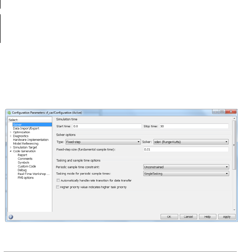
338
o Selects that S-functions in the model will be loaded from pre-compiled
binary MEX files instead of using stand-alone compilation of S-function
sources (more details on S-functions below). Note: This checkbox should
only be used if your model has S-function blocks.
• Additional S-function sources
o List of additional user source files for stand-alone S-function compilation.
Should be used instead of Custom Code > Source Files to ensure that the
correct compiler options are used.
• Compiler optimization flags
o User-defined optimization flags to be used by the compiler (default /O2
/Oy- for Visual Studio on Windows and –O2 for GCC on Linux).
Solver settings
These are the recommended settings for Configuration Parameters -> Solver
• Model Exchange export: Both Variable-step and Fixed-step solvers supported
(recommended to use Variable-step when possible to support accurate event detection
using non-sampled zero crossings).
• Co-Simulation export: Requires a Fixed-step solver (the selected solver is compiled
into the FMU).
• It is also recommended to explicitly set the Tasking mode to SingleTasking.

6 OTHER SIMULATION ENVIRONMENTS 339
Including S-functions in the exported FMU
Models containing S-functions can be exported and the S-functions can be included in the
FMU either from C/C++ sources or as binary MEX files. Note that the S-functions are not
allowed to call into the Matlab environment, e.g., using mexCallMATLAB or
mexEvalString.
Including S-functions from C/C++ sources
Source compilation of S-functions is default and is used if the option Load S-functions from
binary MEX files is not selected.
The S-function sources (C or C++) should be available and located in the same directory as
the Simulink model. The S-function sources are then automatically compiled and linked to
the FMU and no further configuration is needed in the Simulink model.
Note that source compilation of S-functions defines the flag NRT, which is used to indicate
that the S-function is generated by Simulink Coder (or user-written) for non-real-time
applications using a variable-step (or fixed-step) solver. For S-functions that should be built
as MEX files for use in Simulink, it is recommended to use the binary MEX file inclusion as
described below.
Including S-functions from binary MEX files
If the option Load S-functions from binary MEX files is selected, no compilation of S-
function sources is performed. Instead, the S-function MEX files are copied to the FMU (to
resources\SFunctions) and code is added to dynamically load and call the MEX files
when the FMU is instantiated. This option will also create dependencies on Matlab binaries
(which will not be copied to the FMU).
On Windows, the FMU will by default try to load the Matlab binaries from the bin directory
of the exporting MATLAB installation, which means that export / import on the same
computer should work seamlessly. The environment variable SFCN_FMI_MATLAB_BIN can
be used to specify a different directory from where to load the Matlab DLLs (for example a
Matlab runtime installation on a different computer).
On Linux, it is required to use the environment variable LD_LIBRARY_PATH to specify the
path to the Matlab binaries.
With logging enabled the FMU outputs information about the loading of binaries and MEX
files during instantiation. The following is an example of importing a 64-bit FMU with
MEX file dependencies into Dymola on Windows:
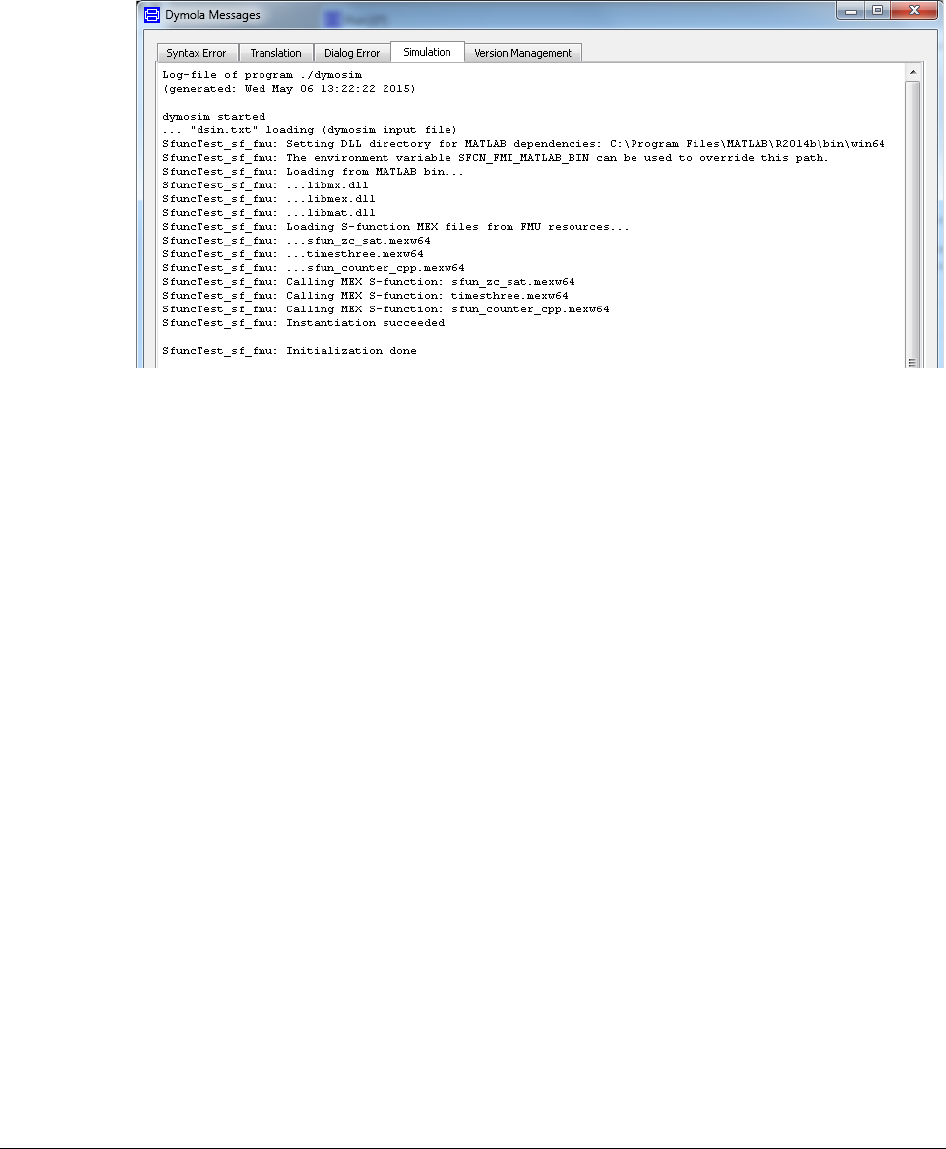
340
Configuring Visual Studio Compiler
The FMI binary is built using the same version of compiler as used when building MEX
files in Matlab. The compiler is configured in Matlab using the command
>> mex –setup
Variable naming
Two options are available for naming of variables in the FMU XML file. With the option
Include block hierarchy in variable names selected, variable names are generated with
block-hierarchical notation and the XML model description specifies the attribute
variableNamingConvention="structured". Alternatively, with the box de-selected,
the Simulink Coder C code identifiers (not traceable back to model) are used as variable
names and the XML specifies variableNamingConvention="flat".
The variable names for continuous-time states, discrete states, parameters, and block outputs
are separated into the top-level categories ContStates, DiscStates, Parameters, and
BlockOutputs in the structured view (see example from Dymola structured FMU import
below). This is to ensure unique variable names in the FMU XML file, since variable names
from different categories are not guaranteed to be unique within a block. In the flat view, the
variable names are appended with _xc, _xd, _pm, and _wb, respectively.
The flat view is guaranteed to generate unique variable names in all cases, whereas the
structured view in some rare cases could produce name conflicts (on limitations, see section
“Limitations and Trouble-Shooting” below).
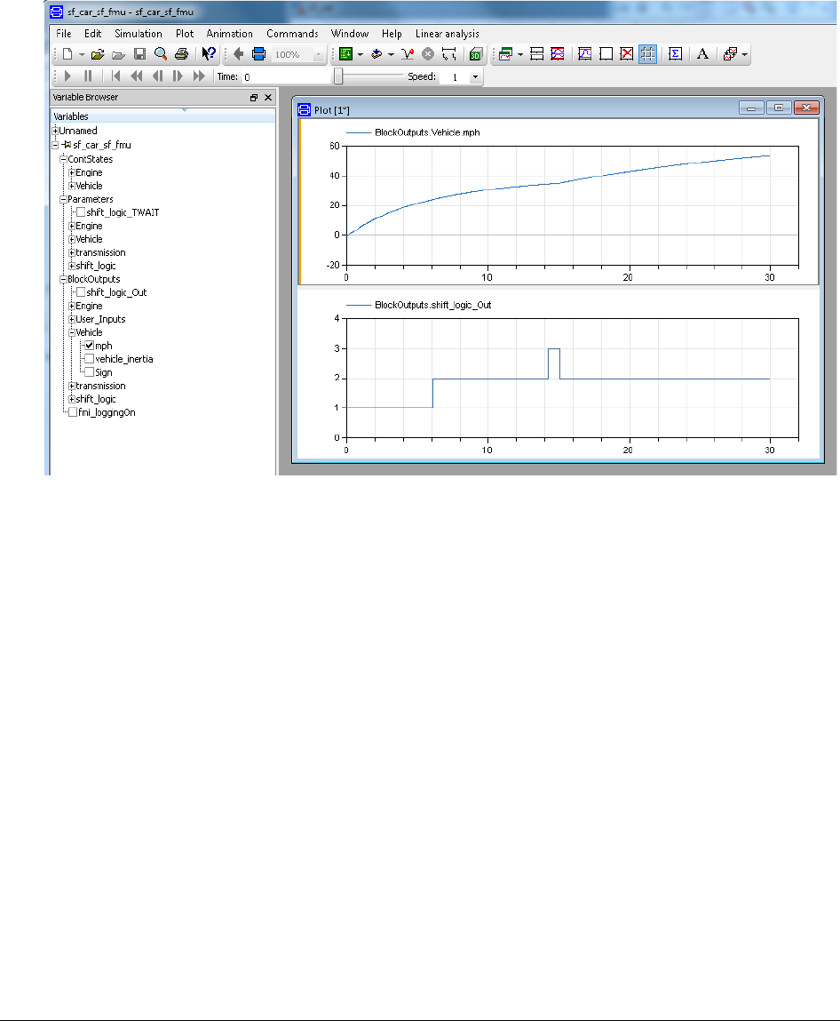
6 OTHER SIMULATION ENVIRONMENTS 341
Building the FMU
Start the build process by pressing Ctrl-B (or through the Simulink Code menu).
The build process will compile the generated model code using the FMI Simulink wrapper
and link with the required Matlab and system libraries to create the FMU binaries. The build
process will also create the FMI XML model description, modelDescription.xml, and
construct the FMI archive, <modelname>_sf.fmu in the current working directory.
Importing FMUs into Simulink
This section describes the procedure to import an FMU into Simulink and the associated
settings / configurations in the user interface. There is also a set of Matlab commands to
interact with the FMI Kit import. These are described more in detail in the HTML
documentation accessed through FMIKit_for_Simulink/html/fmikit.html
Adding FMUs to a model
• Open the Simulink library browser (View > Library Browser) and drag the FMU block
from the FMI Kit library into your model.
• Double-click the FMU block, select Load and choose the FMU.
• Click OK.
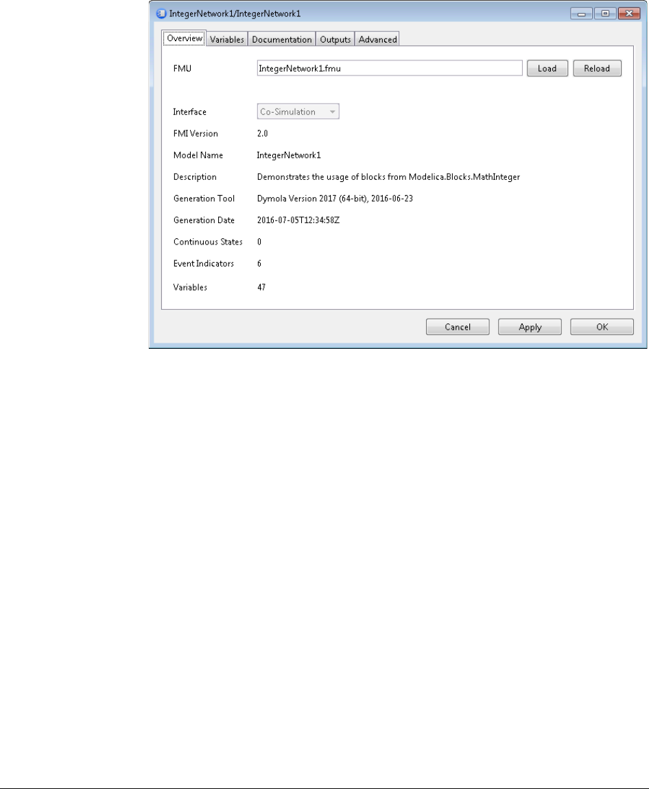
342
The FMU is automatically extracted to the directory specified under Advanced > Upzip
Directory. This directory must remain in the same relative path when the model is moved to
a different directory or machine.
For FMI 2.0 FMUs that support both model exchange and co-simulation the interface kind
can be selected.
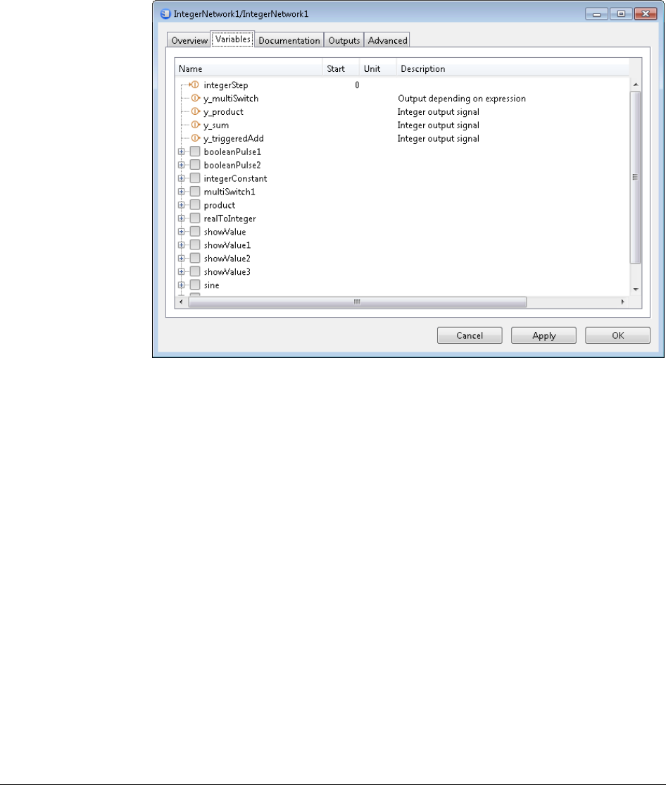
6 OTHER SIMULATION ENVIRONMENTS 343
Variables and start values
The Variables tab shows all variables of the FMU. Input variables are marked with an
arrow on the left, output variables with an arrow on the right of the icon.
The start value, unit, and description of the variable (if provided) are displayed in the Start,
Unit, and Description columns. Start values that were explicitly set are displayed as bold
text.
To change the start value of a variable, click in the respective field in the “Start” column
and enter an expression that evaluates to the respective type of the variable. Changed start
values are indicated by bold text. To reset the start value to its default, clear the “Start” field.
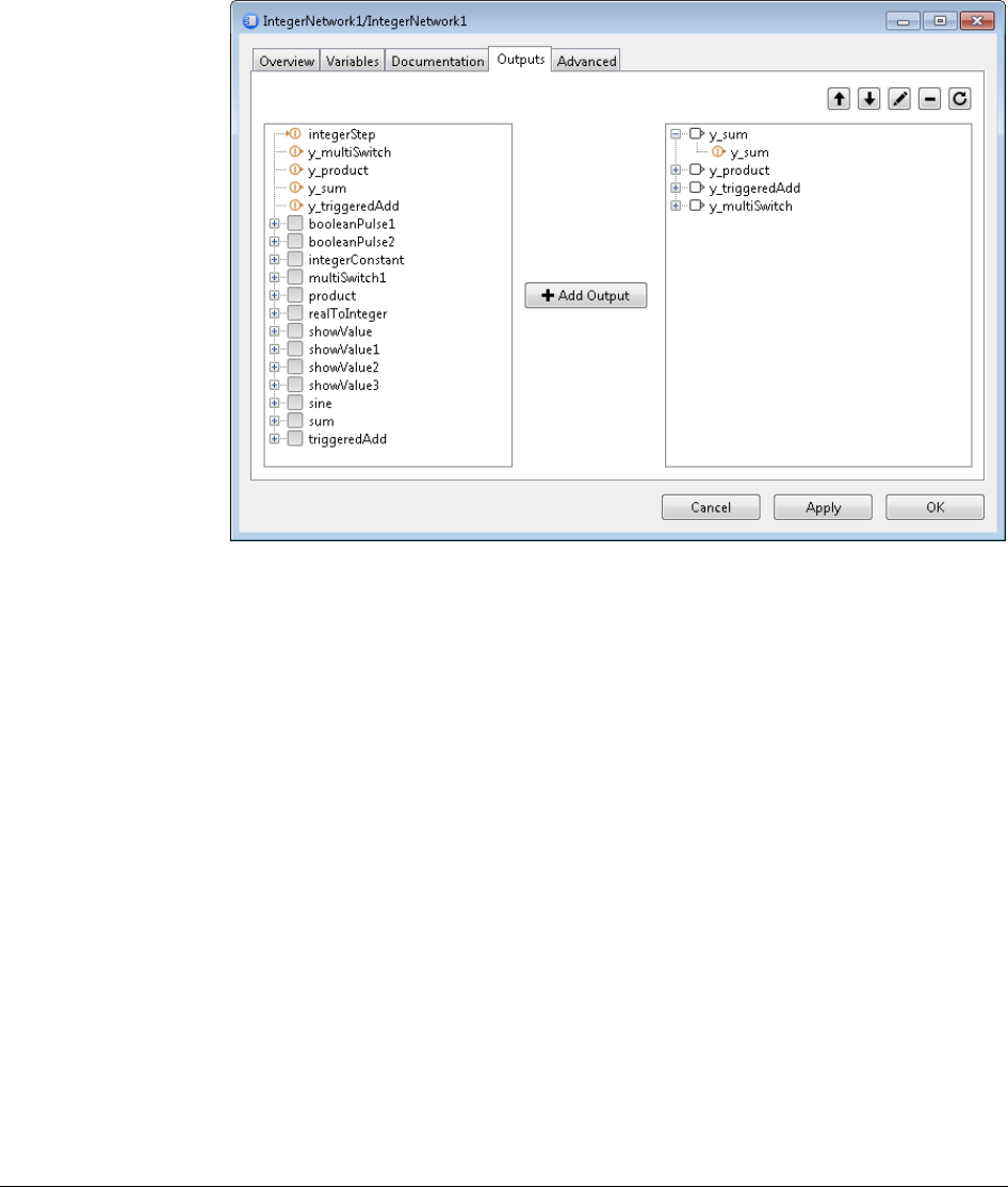
344
Output ports
By default the block has the output ports defined by the FMU.
• To add output ports, select one or more variables in the left view and click “Add Output”
• To remove output ports select the ports in the right view and click “-“
• To move an item in the right view, select it and use the up and down buttons
• To restore the default output ports click the reset button.
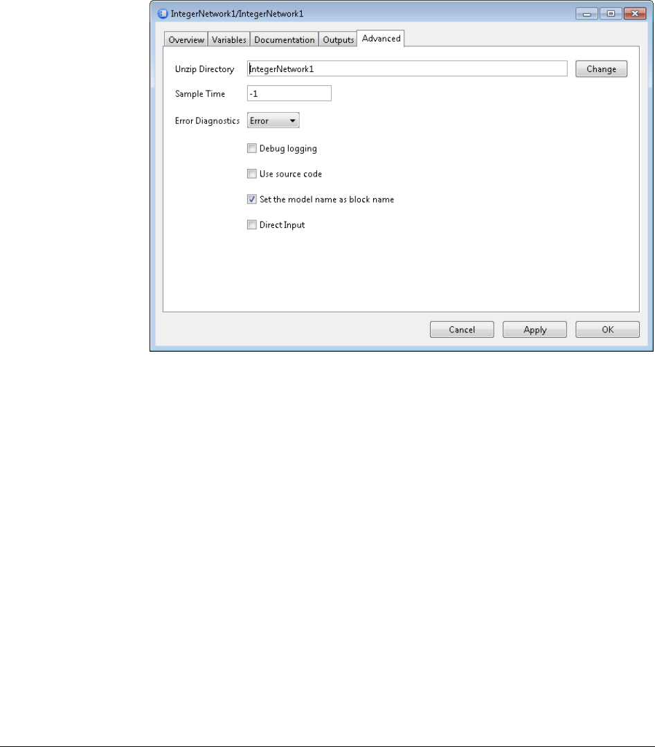
6 OTHER SIMULATION ENVIRONMENTS 345
Advanced settings
On the Advanced tab you can change additional settings for the FMU block:
• Unzip Directory
o The folder where the FMU is extracted. The path can be absolute or
relative to the model file. To use a custom path, change this field before
loading the FMU.
• Sample Time
o The sample time for the block (use -1 for inherited)
• Error Diagnostics
o Determines how to handle errors reported by the FMU
• Debug Logging
o Enables the debug logging to the Matlab console
• Use Source Code
o If checked, a source S-function sfun_<model_name>.c is generated
from the FMU source code which gets automatically compiled when
Apply or OK button is clicked. For FMI 1.0 this feature is only available
for FMUs generated with Dymola 2016 and later.

346
• Set Model Name
o Use the model name of the FMU as block name
• Direct Input
o If checked, ssSetInputPortDirectFeedThrough(true) is set for all
input ports of the FMU and the value of the block´s inputs u and t+1 is
applied to the input variables of the FMU at time t. This gives better
result for FMUs that contain direct terms and do not support input
interpolation.
If not checked, ssSetInputPortDirectFeedThrough(true) is only
set for input ports whose input variables have output variables with a
direct dependency. The derivative der_u for these input variables is set
such that u(t)+der_u(t)*step_size=u(t+1) if the FMU supports
input interpolation. Variables that are manually added to the block´s
output ports are assumed to depend on all input variables.
Source code FMUs
With source code FMUs you can use advanced simulation targets that require code
generation.
To use FMU source code, open the block dialog and on the “Advanced” tab select “Use
source code”. After clicking OK, FMI Kit generates a source S-function .c and builds S-
function MEX file mexw32 (or mexw64 on a 64-bit platform). You can now use the
following additional simulation targets: Rapid Accelerator, RSIM, GRT, ds1005, ds1006.
Limitations and Trouble-Shooting
FMU Export
The following relates to version 2.4.0 of the rtwsfcnfmi target:
On Windows, the export supports Visual Studio 2008 (9.0) and later compilers as supported
with the respective MATLAB releases.
On Linux, the package should support the versions of gcc supported with the respective
Matlab releases. The object files shipped in the package have all been compiled using gcc
4.3.4.
The FMU is compiled with dynamic loading of the C run-time on Windows. This may
require installation of the corresponding Visual Studio redistributables on the target
platform.
The option Include block hierarchy in variable names could in very rare cases give rise to
name conflicts in the XML variable names. For example, any special characters in Simulink
block names will be converted to underscore which may lead to name conflicts. It is
recommended to avoid using special characters in block names with this option (carriage
return and space are safe to use).

6 OTHER SIMULATION ENVIRONMENTS 347
For multiple instances of conditionally executed nonvirtual subsystems or Stateflow charts,
it is required to select “Treat as atomic unit” and set “Functions packaging” to “Inline” for
the subsystems/charts.
S-functions in the exported model are not allowed to call into the MATLAB environment,
e.g., using mexCallMATLAB or mexEvalString.
The FMU export target is not model reference compliant.
The package is subject to the same limitations as the standard S-Function Target.
File Structure
The rtwsfcnfmi target folder (FMIKit_for_Simulink\rtwsfcnfmi) consists of six
sub-directories and the included files are described briefly below.
bin
Pre-compiled Visual Studio and GCC binaries of the FMI implementation for the supported
Visual Studio compilers and MATLAB releases.
c
This directory holds C source files to include and compile the Simulink Coder-generated
model code. The standard FMI header files are located in the sub-directory fmi.
m
This directory contains MATLAB help files called from the TLC scripts. These are used to
construct the date, GUID, and value reference attributes used in the XML model
description.
rtwsfcnfmi\spec
This folder contains the official specification documents for FMI 1.0 and 2.0 as a reference.
tlc
The TLC scripts used for code generation and for constructing FMI-specific files are
included in this directory. The template makefiles and compiler-dependent settings can also
be found here.
6.11 Code and Model Export
6.11.1 Introduction
When a model is translated in Dymola, model C-code is produced in the file dsmodel.c. In
the normal case, this file does not contain simulation runtime code, i.e., the code needed to
solve the model equations in order to compute outputs and derivatives of state variables.

348
Instead, this simulation runtime code is included in binary link libraries (compiled using
Microsoft C compilers), which are used when building dymosim.exe in Dymola or
building a Simulink S-function. The code in the binary libraries also contains license checks
that are performed when the model is executed.
To facilitate export of models from Dymola, e.g., to be able to compile the C-code for non-
Windows platforms or to run the model on another computer without license check, certain
export licenses are provided. These export options are Real-time Simulation (see Section
“Real-time Simulation” starting on page 247), Binary Model Export, and Source Code
Generation. Depending on the export option available, Dymola will generate special
extended versions of dsmodel.c during model translation.
The Binary Model Export option allows the model to be exported to other Windows
computers without requiring a Dymola license at the target system. The simulation
functionality of the exported model is the same as on a computer having a Dymola license.
The Source Code Generation is intended for advanced model-based development including,
e.g., rapid prototyping of control systems. The code exported with this option can be used
on any platform without the need of a Dymola license at the target system. A special
translation command should be used with Source Code Generation and a number of built-in
flags are available that can be used to modify the contents of the generated model code. The
Source Code Generation option includes the functionality provided by Real-time Simulation
(without restrictions) and Binary Model Export when models are translated in Dymola or
Simulink.
Dassault Systèmes provides a template project on how to interface the models exported with
Binary Model Export and Source Code Generation to standard integration routines to build
stand-alone applications. This package is called StandAloneDymosim, and is described in
detail in section “The StandAloneDymosim project” starting on page 353. The simulation
code provided in the StandAloneDymosim project makes use of the dsmodel.c model API,
which is described in detail in the section “Interfacing to dsmodel.c” starting on page 355.
Note that for large models, additional files are created to dsmodel.c (dsmodelext1.c,
dsmodelext2.c, etc.). To prevent this, instead generating a larger dsmodel.c, the following
flag can be set:
Advanced.SeparateFilesCcode=false;
The default value of the flag is true.
Note that some compilers may have problems with compiling large files.
Required License Options
The following license features are required for the export options
• Dymola Real-Time Simulation
• Dymola Binary Model Export
• Dymola Source Code Generation
Models developed by users that lack export options can still be run at other computers using
a runtime concept. Dymola runtime concept requires the user of the model to have a
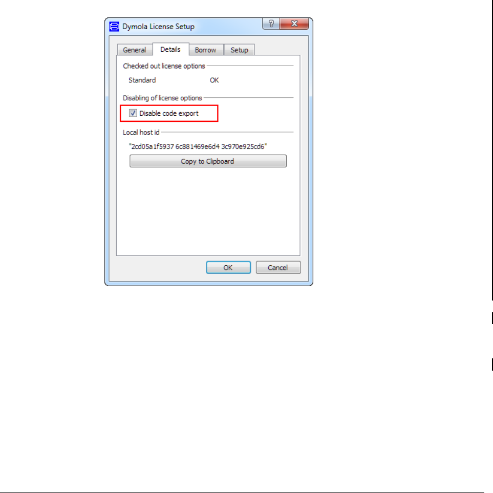
6 OTHER SIMULATION ENVIRONMENTS 349
Dymola license. The license file should be defined by the environment variable
DYMOLA_RUNTIME_LICENSE, for example
set DYMOLA_RUNTIME_LICENSE=C:\My Documents\dymola.lic
Enabling Export
In the Details tab of the Dymola License Setup (reached through the command Help >
License…), it is possible to enable the code export (BinaryModelExport and
SourceCodeGeneration). Code export is by default disabled:
This setting is used to avoid unintentionally checking out export options from a sharable
license. The code export can also be enabled by the following corresponding flag on the
command line
Advanced.EnableCodeExport = true
The flag is by default false.
The setting to enable code export is remembered between Dymola sessions.
6.11.2 Binary Model Export
No additional simulation runtime code is added to dsmodel.c for Binary Model Export and
the simulation applications are built by linking with Visual Studio compatible binary
libraries. Instead, the main functionality provided by Binary Model Export is to disable the
runtime license checking during execution of the model.

350
Binary Model Export allows a developer to create stand-alone applications for the following
purposes:
• to generate a dymosim.exe application that can be executed on other Windows computers
without a license.
• to generate a dymosim DLL with an extended co-simulation API (the DLL includes the
Dymola DAE solvers and routines to run a simulation for a given time and to load/save
simulation setups (snapshots)).
• to generate Matlab/Simulink models including DymolaBlocks to be run in other Matlab
environments without requiring a license.
• to interface the model code (dsmodel.c) to custom integration routines and compile
stand-alone applications by linking with binary libraries for the runtime routines.
For the last alternative Dassault Systèmes provides a template project,
StandAloneDymosimBinary (see section “The StandAloneDymosim project” starting on
page 353), which shows how to interface standard solvers to the model code exported by
Binary Model Export.
Running the dymosim executable with the command line option -h will print if binary
model export is activated or if a Dymola license is required for execution. It is also
displayed which libraries that the executable uses.
XML Interface
Binary Model Export and Source Code Generation (see below) supports export of symbol
table information, e.g., model structure, variable names, types, and units as an XML file.
The feature is enabled by setting the flag
Advanced.GenerateXMLInterface = true
At translation an XML file with the same name as the model is generated. It contains a
description of each variable on scalar level. An actual variable description may look as
<Variable>
<Name>J1.phi</Name>
<Description>Absolute rotation angle of
component</Description>
<DataType>Real</DataType>
<Category>State</Category>
<Quantity>Angle</Quantity>
<Unit>rad</Unit>
<ValueInterpretation>
<UnitConversion>
<DisplayUnit>deg</DisplayUnit>
<Gain>57.2957795130823</Gain>
<Offset>0.0</Offset>
</UnitConversion>
</ValueInterpretation>
</Variable>
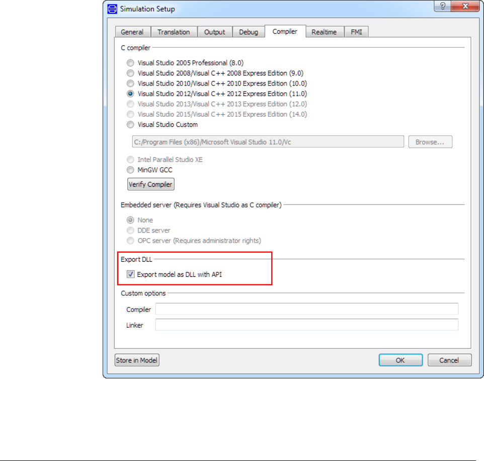
6 OTHER SIMULATION ENVIRONMENTS 351
A description includes only the attributes that have been defined for the variable in the
Modelica model. The description may include min and max value, but values for these
attributes have not been specified for J1.phi in the example above.
Generating a dymosim DLL
With the Binary Model Export (or Source Code Generation) option it is possible to generate
a dynamic link library (dymosim.dll) from a model. To enable the DLL export, mark the
checkbox Export model as DLL with API in the Compiler tab of the Simulation Setup,
(reached by the command Simulation > Setup…).
The API of the DLL is given by the header file $DYMOLA/source/dymosim.h. For
examples on how to use the API (dynamically loading a model, using the snapshot solver,
etc.), see the file dymosim.c in the same directory.

352
Note that Export model as DLL cannot be combined with any embedded server (DDE or
OPC).
Important. Any new development of this functionality will be to use FMI instead since the
FMI supports Co-simulation using Dymola solvers. This also means that the possibility to
generate a dymosim DLL in the way it is done today will be removed in some future version
of Dymola.
6.11.3 Source Code Generation
Source code generation by export
The Source Code Generation contains the functionality provided by Real-time Simulation
and Binary Model Export. However, the restriction concerning inline integration for Real-
time Simulation is not imposed if the user has the Source Code Generation option.
Furthermore, Source Code Generation allows export of readable and well-documented code
facilitating inspection, debugging, profiling, etc. This makes this export option suitable for
advanced model-based applications, such as rapid prototyping.
Dymola has a special built-in function that should be used with Source Code Generation.
The function is called
translateModelExport
and takes the model name as input.
When a model is translated using this function, the required simulation runtime code is
automatically added to the generated dsmodel.c c-file in the same way as for Real-time
Simulation. This removes the need to link with binary libraries. Furthermore, during
translation using the translateModelExport function, the following three built-in
Dymola flags are enabled
Advanced.UseModelicaNamesForC
To keep the original variable names in the generated C-code to make it readable (default
value true).
Advanced.OutputEquationTrace
To generate comments in the generated C-code about original equation and component
origin for increased traceability (default value true).
Advanced.SubstituteVariablesUsedOnce
If an intermediate variable is used only once, the right-hand side expression is substituted to
remove the need to store the intermediate variable (default value false).
Using these flags allows for more readable, traceable, and efficient code that can be used for
debug purposes. It is, however, also possible to generate standard dsmodel.c code by
setting all flags to false. This can be used if it is desired to distribute the code in obscured
form. Source Code Generation also enables the XML export described above.
If compilation and producing an executable is not of interest, the compilation can be
disabled by setting the flag

6 OTHER SIMULATION ENVIRONMENTS 353
Advanced.CompileAfterTranslation=false
This will save some time. However, note that the compilation can detect some potential
errors.
As for real-time simulation, it should be noted that the simulation runtime code does not
contain the most advanced routines from the binary link libraries. It is, e.g., not possible to
export models with dynamic state selection. For models with dynamic state selection,
translateModelExport gives an error during translation.
A template project, StandAloneDymosim, is provided to describe how to interface standard
integrators to the model code exported by Source Code Generation or Binary Model Export.
Source code generation features for normal translation
A flag is available to be able to obtain the same features for normal translation as for source
code generation when it comes to creating more readable, traceable, and efficient code that
can be used for debug purposes.
These features correspond to the flags
Advanced.UseModelicaNamesForC
Advanced.OutputEquationTrace
Advanced.SubstituteVariablesUsedOnce
To be able to activate the corresponding features for normal translation, set
Advanced.SourceCodeExportNormal=true
The flag is by default false.
Note. To be able to use this flag:
• You must have the SourceCodeGeneration license option.
• Code export must not be disabled in Help > License…, the Details tab.
6.11.4 The StandAloneDymosim project
The StandAloneDymosim project is intended to show how to build stand-alone simulation
applications by interfacing to dsmodel.c, the model code generated by Dymola. As
described above, building general stand-alone applications for arbitrary platforms requires
the Source Code Generation license feature to have Dymola include all necessary source
code in dsmodel.c. The model should be translated using the command
translateModelExport which takes the model name as input.
The project also shows how to create stand-alone applications from the dsmodel.c code
generated with Binary Model Export by linking with the Visual Studio-compatible binary
libraries included in the Dymola distribution. The Binary Model Export option will make
sure that runtime license checking is disabled in the executable. This option is only possible
on Windows platforms that are link-compatible with Visual Studio.
The example template in the project describes two options, standard Euler integration and
an interface to Daskr (a successor of Dassl/Dassrt).

354
Included Files
The zip-archive StandAloneDymosim.zip (located in Program Files (x86)\Dymola
2018\bin\external) contains two directories, proj and source. Below follows a short
description of the files.
proj
• readme.txt : The instructions contained in this section in a condensed format.
• StandAloneDymosim.vcproj: Project file for Visual Studio 2005 (8.0).
• Assumes that Dymola is installed in C:\Program Files\Dymola
• Assumes that the StandAloneDymosim source files are located in
C:\dev\source\dymosim\standalone
• You have to modify the project if this is not the case (see compilation and
linking below).
• You should use the configuration: Win32 Release
• The project can be imported to newer versions of Visual Studio.
• StandAloneDymosimBinary.vcproj: Project file to link application with binary libraries
for the runtime routines.
• StandAloneDymosim.sln: Visual Studio 2005 (8.0) solution file.
source
• StandAloneDymosim.c: Main program. Contains interface, call of Euler, and call of
Daskr integration.
• inline_Int.h, inline_Int.c: Interface to dassl-routines.
• daux.c, ddaskr.h, ddaskr.c: f2c converted files for ddaskr (successor of ddasrt). Separate
License file provided. Available in Fortran form from www.netlib.org
The main program, StandAloneDymosim.c, contains documentation of the routines
exported by dsmodel.c and shows how to use these routines to simulate the model using
standard Euler integration. This documentation is also given in section “Interfacing to
dsmodel.c” starting on page 355 in this document.
The main program is intended as an example, and all sections marked CHANGE in
StandAloneDymosim.c indicate places where it might be a good idea to change
something or, e.g., add code for external I/O.
Compilation and Linking
You should follow the steps below in order to compile and link the example code. Note that
you will need to adapt the include paths and location of the libraries if you use the project
file StandAloneDymosim.vcproj.
• Adjust the line (at the end of StandAloneDymosim.c)

6 OTHER SIMULATION ENVIRONMENTS 355
#include "c:/my documents/dymola/dsmodel.c"
to refer to the correct model. Note that for big models, additional files (dsmodelext1.c,
dsmodelext2.c etc.) are created; those have to be included as well.
• Add C:\Program Files\Dymola\source to the include path.
• Add C:\dev\source\dymosim\standalone\daskr\solver to the include path.
• For models exported with Binary Model Export also link with
• libds.lib
• ModelicaExternalC.lib (only required for some models)
• Define INCLUDE_EULER or INCLUDE_DASSL to use the different solvers.
• Define INCLUDE_MAIN if you want to have a main-loop with calls to the solvers.
• If you want to generate a result file usable in Dymola you can also define:
• GenerateResultInNonDymosim=1 (generates dsres.mat)
• GenerateResultInNonDymosim_DT=0.01 (minimum distance in result
file)
The needed libraries are located in C:\Program Files\Dymola\bin\lib.
Interfacing to dsmodel.c
This section contains documentation of the routines exported by dsmodel.c that are used
by the simple Euler integration routines in StandAloneDymosim.c.
dsblock
The main routine used to compute outputs, derivatives, etc is called dsblock_ and has the
following interface:
long dsblock_(long *idemand_, long *icall_,
double *time, double x_[], double xd_[], double u_[],
double dp_[], long ip_[], Dymola_bool lp_[],
double f_[], double y_[], double w_[], double qz_[],
double duser_[], long iuser_[], Dymola_bool luser_[],
long *ierr_);
The inputs to the function are
• idemand_:
• 0: start of integration, initial equations are solved
• 1: compute outputs (y_)
• 2: compute derivatives (f_)
• 3: compute auxiliary variables (w_)
• 4: compute crossing functions (qz_)

356
• 5: event handling
• 7: ‘terminal()’ is true
Note that, e.g., for *idemand_==1 some derivatives may be computed. Thus it is not legal
to pass f_ as nil-pointer in that case.
• icall_: should normally be set to 0 before each call to dsblock. If you set *icall_
> 0 it indicates that the previous call had the same inputs, except that idemand has
increased. This can be used internally to skip redundant computations.
• time: time in simulation
• x_: state variables (input/output when *idemand_ is 0 or 5)
• u_: inputs (input/output when *idemand_ is 0)
• dp_: parameters (input)
• f_: derivatives (output / must be kept between calls)
• y_: outputs (output / must be kept between calls)
• w_: auxiliary variables (output / must be kept between calls)
• qz_: crossing functions (output / must be kept between calls)
• duser_: pointer to struct of real-valued simulation flags (struct
BasicDDymosimStruct)
• iuser_: pointer to struct of integer-valued simulation flags (struct
BasicIDymosimStruct)
• *ierr_: Output: start with *ierr_=0
• 0 indicates success
• -999 terminate integration successfully (call of terminate in model)
• otherwise error
GetDimensions
void GetDimensions(long*nStates, long*nx2, long*nInputs,
long*nOutputs, long*nAuxiliary, long*nParameters,
long*nRelations,long*ncons,long*dae);
• *nStates: number of states
• *nInputs: number of inputs
• *nOutputs: number of outputs
• *nAuxiliary: number of additional variables
• *nParameters: number of parameters
• *nRelations: number of relations

6 OTHER SIMULATION ENVIRONMENTS 357
The number of crossing functions is 2*nRelations (+1 if simple handling of timed events).
The inputs and outputs correspond to top-level inputs/outputs of the model. The parameters
correspond to parameters that can be changed after compilation (they must be bound to a
literal value and not evaluated).
declare_
void declare_(double* states, double* parameters,
void* cuser_[], long* QiErr);
This function is used to get default literal values of states and parameters (cuser_ can be
set to 0). The states and parameter vectors may be uninitialized, and must be at least as long
as indicated by GetDimensions.
*QiErr is set to non-zero to indicate failure.
FindEvent_
getBasicIDymosimStruct()->mFindEvent;
Keep at 0 as default.
Set this flag to 1 to indicate that the solver is a fixed-step solver, and a high resolution of
state events is required (higher than the step size). This causes the derivatives to be rescaled
next to events, such that the states exactly hit the event point.
NextTimeEvent
getBasicDDymosimStruct()->mNextTimeEvent;
Set to 1e37 before call with *idemand_ 0, 4, or 5.
If the returned value is smaller it indicates the time of the next time-event and the simulation
should stop at that point and trigger an event (unless there is a state event or end of
integration before).
Logging functionality
The functions below are examples of available routines for generation of log messages from
the compiled models. More routines are available in Program Files (x86)\Dymola
2018\Source\dsutil.h
void DymosimMessage(const char* message);
Prints a message string.
void DymosimMessageDouble(const char* message, double d);
Prints a message string followed by a double value.
void DymosimMessageLong(const char* message, long i);
Prints a message string followed by a long integer.

358
void VariableChanged(char* var, double val, double t);
Used to print the name and value of a variable at a given time point.
Trouble-shooting
• When building an application at one computer and executing it at another, it is essential
that the target machine has the required redistributable runtime libraries. These depend
on the compiler used to build the application. Check the Visual Studio documentation
for further details. As an example, the Visual Studio 2005 distribution contains an
installer program, vcredist_x86.exe, for redistributable libraries.
• If you use the StandAloneDymosim.vcproj project make sure to use the corresponding
Win32 Release configuration. Debug builds may contain libraries that are not
redistributable.
• Make sure to adapt the include paths and locations of libraries.
• Your license must include Source Code Generation or Binary Model Export
(DymolaSourceCodeGeneration or DymolaBinaryModelExport).
• If you have the Source Code Generation feature, you should use the command
translateModelExport to have Dymola generate model code that includes the
simulation runtime routines.
7 USER-DEFINED GUI

7 USER-DEFINED GUI 361
7 User-defined GUI
This chapter has two main sections. The first describes building user-defined input dialogs
for models and functions that corresponds to records and arrays. The second describes the
extendable user interface of Dymola, that is, extending the user interface by introducing
own menus and toolbars from which Modelica functions can be called, and the possibility to
define packages with users own collection of favorite models.
7.1 Building user-defined dialogs
In addition to primitive data types, Real, Integer, Boolean and String and from them derived
types, Modelica has records and arrays. We will in this section show how to build graphical
user interfaces for models and functions that correspond to these data structuring
mechanisms, by using annotations
7.1.1 Ways of working with annotations
When it comes to working with annotations for variables, there are two ways of working:
• By direct typing in the Modelica Text layer.
• By using the Declare variable dialog.
Depending on what should be done, one way might be more convenient to use than the
other. As an example consider the case when variables should be divided in tabs and groups

362
in a parameter dialog. The Declare variable dialog gives, in the Annotations tab, a very
convenient way to use input fields to handle this.
On the other hand, all annotations are not available as settings in the Declare variable dialog.
In that case it might be as easy to use the Modelica Text layer directly, even though it of
course still is possible to work with the Declare variable dialog (typing in the annotations;
the full Modelica text for that variable is visible and editable in the dialog).
Certain annotations are not at all connected to variables; in that case there is no alternative
than the Modelica Text layer.
Please note that to see the annotations in the Modelica Text layer of the Edit window, right-
click in the window and use the context command Expand > Show entire text.
How to work with the Declare variable dialog is introduced in section “Tabs and Groups”
starting on page 365 below.
For a full description of the Declare variable dialog, please see the manual “Dymola User
Manual Volume 1”, chapter “Developing a model”, section “Advanced model editing”, sub-
section “Parameters, variables and constants”.
7.1.2 Records and dialogs
As an introductory example, we will consider making a small data base of personal data.
Assume that each person is described by the following information:
record Person
String firstName;
String middleInitial;
String lastName;
Integer number;
String street;
Integer zipCode;
String city;
end Person;
(The record can be created by directly typing in the Modelica Text layer of the Edit window,
or by using the command File > New… > Record. The variables in it can be typed in
directly or can be added using Edit > Variables > New Variable….)
The corresponding automatically constructed GUI dialog for entering data is accessed by
right-clicking on the record in the package browser, taking up the context menu and
selecting Create Record…:
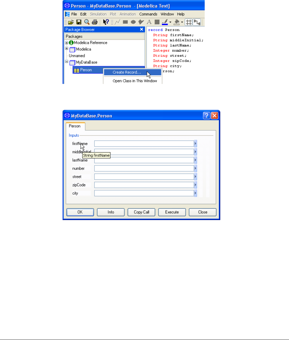
7 USER-DEFINED GUI 363
(In this example the record has been created in a package MyDataBase.) The menu for
entering data that pops looks as follows:
The tool tip shows the data type of the input field.
Entering the following data:
Accessing the menu
for entering data.
Automatically
constructed dialog.
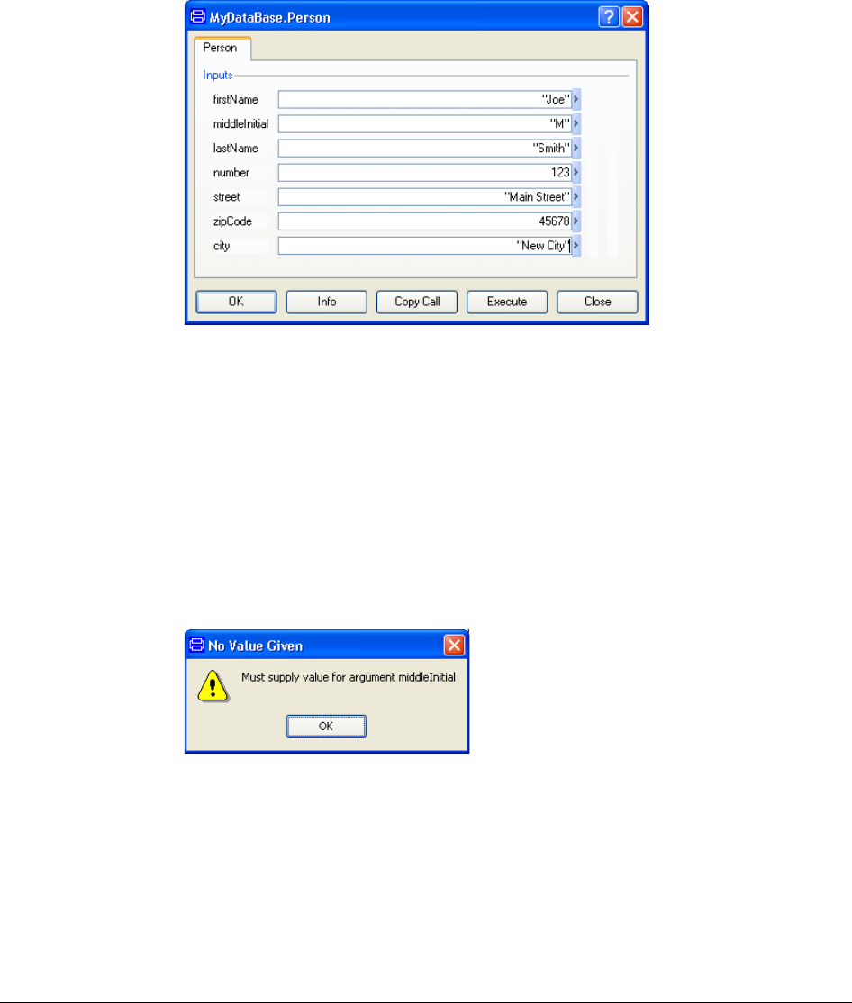
364
and pressing the OK or Execute buttons gives the result in the log window as a call to the
record constructor Records.Person with the name-value pairs for the entered data.
= MyDataBase.Person(
firstName = "Joe",
middleInitial = "M",
lastName = "Smith",
number = 123,
street = "Main Street",
zipCode = 45678,
city = "New City"
)
If we would not fill in any value for middleInitial, the following error message would be
generated:
To avoid having to give such data, a default value can be given in the declaration:
String middleInitial = "";
Modelica allows you to add description strings to all variables. We alter the record to:
Filled-in dialog.
Missing data error.
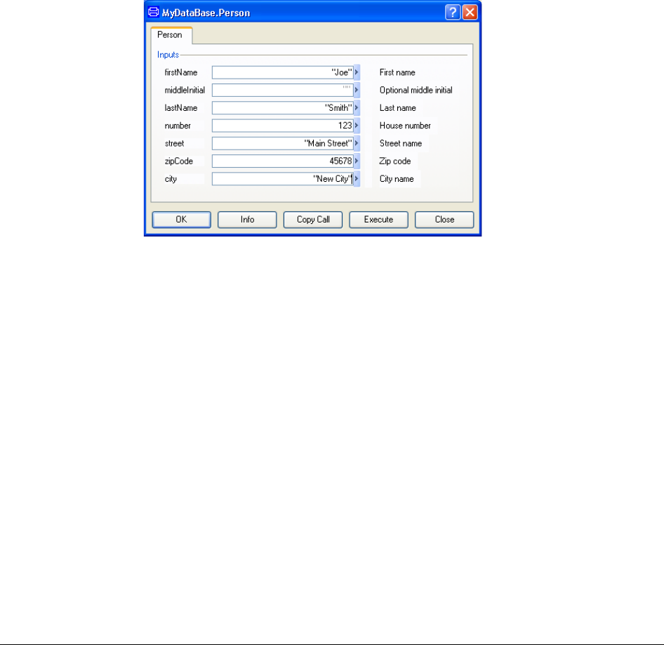
7 USER-DEFINED GUI 365
record Person
String firstName "First name";
String middleInitial="" "Optional middle initial";
String lastName "Last name";
Integer number "House number";
String street "Street name";
Integer zipCode "Zip code";
String city "City name";
end Person;
These are used to annotate the dialog as shown below.
Tabs and Groups
It is possible to annotate input fields in various ways in order to simplify for the user to
enter data.
It is, for example, possible to group record fields together and introduce tabs in the dialog
by means of annotations. This is very conveniently done for each variable using the Declare
Variable dialog, please see below.
Dialog with description
strings.
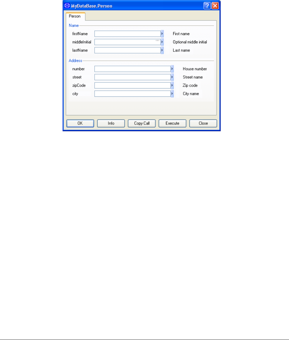
366
These changes are made by adding the following annotations and extending the record with
field married.
record Person
String firstName "First name"
annotation (Dialog(group="Name"));
String middleInitial="" "Optional middle initial"
annotation (Dialog(group="Name"));
String lastName "Last name"
annotation (Dialog(group="Name"));
Integer number "House number"
annotation (Dialog(group="Address"));
String street "Street name"
annotation (Dialog(group="Address"));
Integer zipCode "Zip code"
annotation (Dialog(group="Address"));
String city "City name"
annotation (Dialog(group="Address"));
Boolean married "Marital status"
annotation (Dialog(tab="Properties", group="Marital
status"));
end Person;
Note that for the Boolean field married the combobox with choices false and true appear
automatically.
The changes above can be done by direct typing in the Modelica Text layer, but a
convenient alternative way to work with the variables (and annotations) is to use the Declare
variable dialog.
Dialog with groups and
tabs.

7 USER-DEFINED GUI 367
There are two to access the dialog when a variable has been declared:
• Use the command Edit > Variables.
• If non-graphical components are enabled in the component browser (by right-clicking in
the component browser and selecting Settings > Include non-graphical) variables will
be shown. In that case a variable can be right-clicked; selecting Parameters… will
display the Declare variable dialog.
Say we want to add the annotations of firstName using the first alternative above. By using
the command Edit > Variables we get:
(It is also possible to right-click in the Modelica Text layer and select Variables >
firstName.)
By popping the menu, selecting the Annotations tab, entering Name in the Group field we
will get:
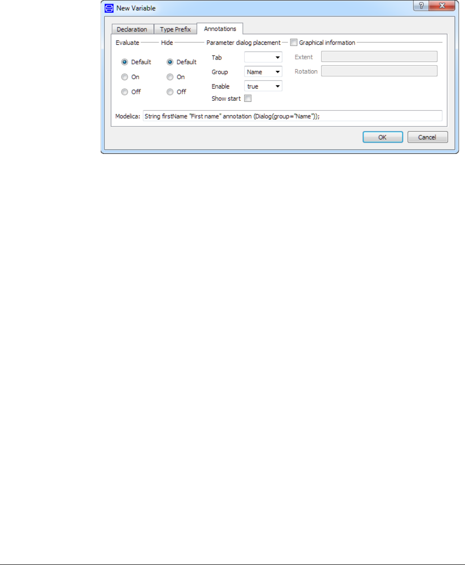
368
When clicking OK we have created the completed the annotations for the variable firstName.
In the same the way the other variables could be given annotations. New variables can be
introduced using the New variable… alternative. This way the new variable married can
be added, and corresponding annotations specified.
Hiding variables
A variable that should be internal (only accessible inside the model) should be declared as
protected. This can be done using the Type Prefix tab of the Declare variable dialog, ticking
protected. This variable will neither be seen in any parameter dialog, nor in the variable
browser.
It is also possible to prevent the variable from being presented in the variable browser by
declaring it as hidden using the Annotations tab of the Declare variable dialog (see
previous picture), ticking On in the Hide group. However, it will still be available in the
parameter dialog. Usually the alternative to declare it as protected is better.
For more information about this, please see the manual “Dymola User Manual Volume 1”,
chapter “Developing a model”, section “Advanced model editing”, sub-section “Parameters,
variables and constants”.
Activation of the dialog entry for start values
The annotation for activating the dialog entry for start values can be set in the variable
declaration dialog, in the Annotations tab. See the above figure; here it is also described
how to display this tab.
As an example, enabling this option Show start for an integer variable MyTest in the
dialog gives the result:
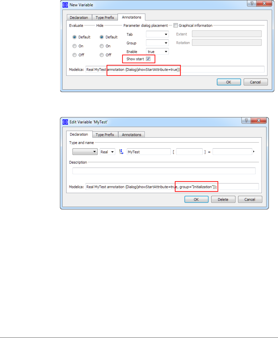
7 USER-DEFINED GUI 369
Clicking OK will also add the annotation to display this start value in an “Initialization”
group, taking up the menu again after having clicked OK will display:
The result of using the model containing this variable is, looking at the parameter dialog:
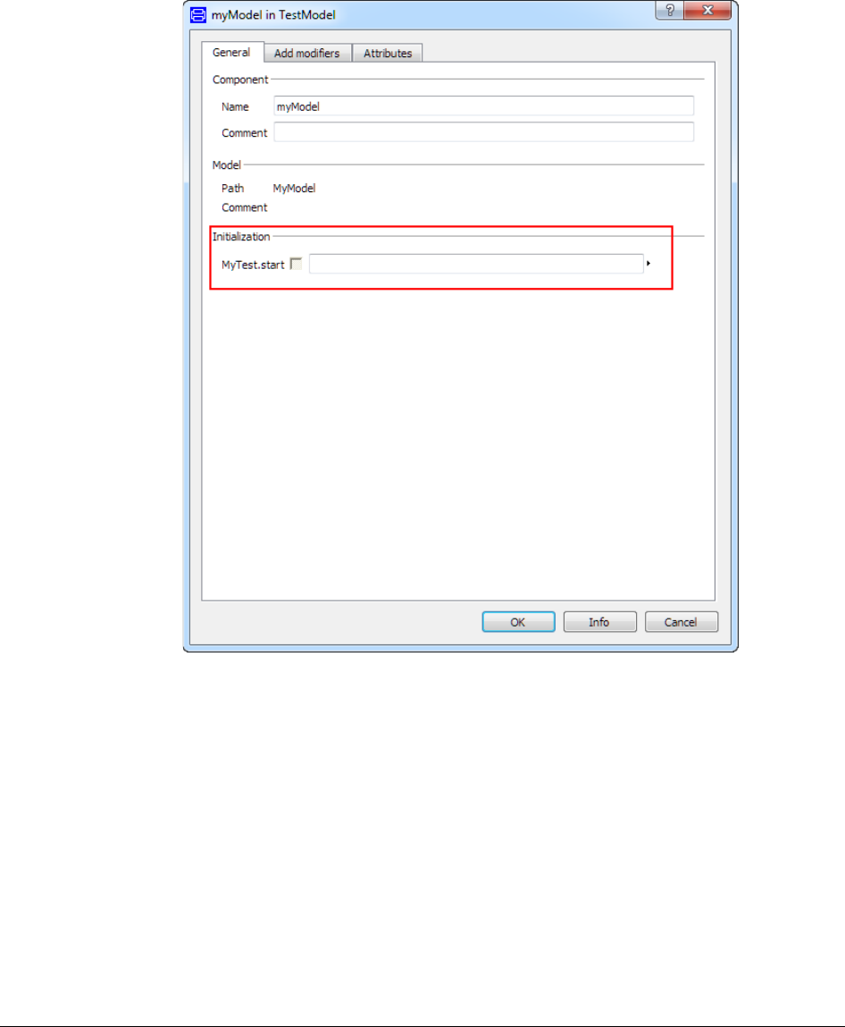
370
Labels and layout
By annotating a field, such as firstName, with the attribute __Dymola_joinNext=true, the
next field, middleInitial, is put on the same horizontal line as firstLine.
Instead of having the variable name in front of the input field, the description string is used
if the Dialog annotation: __Dymola_descriptionLabel=true is given. The description string
is then not shown after the input field. A label with free text can be given by
__Dymola_label="free-text". The free text label has precedence over the description
label.
The width of the inputs fields can be specified as, for example, __Dymola_naturalWidth=10.
The width is given in the unit "en", the width of character '0'. The width can also be
specified as __Dymola_absoluteWidth=10. The difference is that fields with
__Dymola_absoluteWidth keep their size when the entire dialog is made wider. The fields
with __Dymola_naturalWidth specification are made wider.
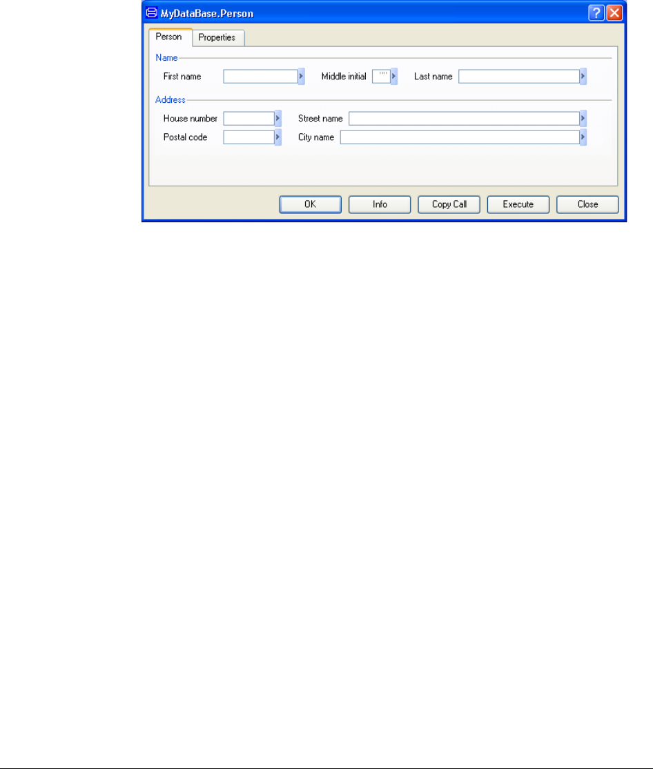
7 USER-DEFINED GUI 371
By use of these annotations we can make the dialog much nicer.
The details of the record declaration are given below:
record Person
String firstName "First name"
annotation (Dialog(group="Name", __Dymola_joinNext=true,
__Dymola_naturalWidth=15, __Dymola_descriptionLabel=true));
String middleInitial="" "Middle initial"
annotation (Dialog(group="Name", __Dymola_joinNext=true,
__Dymola_absoluteWidth=3, __Dymola_descriptionLabel =
true));
String lastName "Last name"
annotation (Dialog(group="Name", __Dymola_naturalWidth=25,
__Dymola_descriptionLabel = true));
Integer number "Number"
annotation (Dialog(group="Address", __Dymola_joinNext=true,
__Dymola_absoluteWidth = 10, __Dymola_descriptionLabel =
true));
String street "Street name"
annotation
(Dialog(group="Address",__Dymola_descriptionLabel
= true));
Integer zipCode "Zip code or postal code"
annotation (Dialog(group="Address", __Dymola_joinNext=true,
__Dymola_absoluteWidth = 10, __Dymola_descriptionLabel =
true, __Dymola_label="Postal code"));
String city "City name"
annotation (Dialog(group="Address",
__Dymola_descriptionLabel = true));
Boolean married "Marital status"
annotation (Dialog(tab="Properties",
group="Marital status", __Dymola_absoluteWidth=10));
end Person;
Flexible labeling and
layout of input fields.
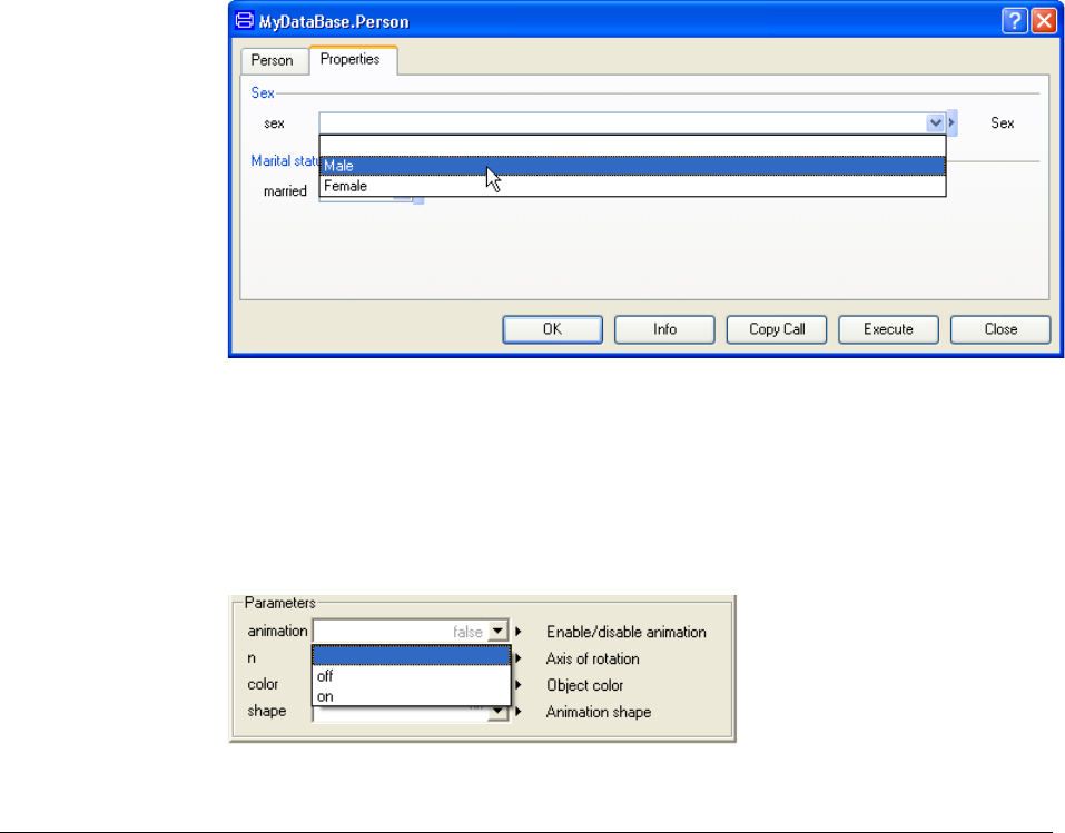
372
The annotations used above are not available as settings in the Declare variable dialog; it
can however be entered in that dialog.
Alternative forms for input fields
Using combo boxes
Sometimes there is a set of frequent input values (enumerations) and in addition free text
should be possible. For such cases, it is possible to add a combo box for the frequent choices.
This would, for example, be convenient for a sex field:
Integer sex "Sex"
annotation (Dialog(tab="Properties", group="Sex"),
choices(choice=1 "Male", choice=2 "Female"));
Associated with each value (1, 2), it’s possible to give a description string (“Male”,
“Female”).
The Properties tab has the following layout after this addition.
It should be noted that it’s possible to enter any value without using the pull-down menu.
This enables the use of expressions, for example.
Some additional examples
It is possible to annotate parameters or parameter types in order that it's possible to make a
selection from a set of values from a pull down menu. For example, setting a parameter true
or false can be made by selecting on or off as shown below.
Input field with combo
box.
Drop-down menu in
parameter dialog.

7 USER-DEFINED GUI 373
The needed declarations for this appearance are:
type OnOff = Boolean annotation (choices(
choice=false "off",
choice=true "on"));
parameter OnOff animation=false
"Enable/disable animation";
The following examples show similar choices from a set of predefined vectors representing
different common directional axes or commonly used colors. In the example to the right, a
selection has been among a set of strings.
The corresponding declarations are:
type Axis = Real[3] annotation (choices(
choice={1,0,0} "{1,0,0} - x axis",
choice={0,1,0} "{0,1,0} - y axis",
choice={0,0,1} "{0,0,1} - z axis",
choice={0,0,0} "any axis"));
parameter Axis n={1,0,0} "Axis of rotation";
type Color = Real[3] annotation (choices(
choice={1,0,0} "red",
choice={0,1,0} "green",
choice={0,0,1} "blue"));
parameter Color color={1,0,0} "Object color";
type Shape = String annotation (choices(
choice="" "none",
choice="box" "box",
choice="cylinder" "cylinder"));
parameter Shape shape="" "Animation shape";
It should be noted that it's possible to enter any value without using the pull down menu.
This enables the use of expressions, for example.
Using radio buttons
In the case of only a set of fixed choices, radio buttons are more appropriate. Specification
of sex can, for example, be made by radio buttons by adding
__Dymola_radioButtons=true, i.e. if the following declaration is given (__Dymola_
means that the annotation is Dymola vendor specific):
Integer sex "Sex"
annotation (Dialog(tab="Properties", group="Sex"),
choices(__Dymola_radioButtons=true, choice=1 "Male",
choice=2 "Female"));
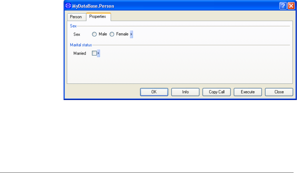
374
Boolean variables such as
Boolean married "Marital status"
annotation (Dialog(tab="Properties",
group="Marital status"));
give by default a combo box with choices false and true. However, in many cases a check
box is more convenient. This is achieved by adding __Dymola_checkBox=true, i.e. be
giving the declaration
Boolean married "Marital status"
annotation (Dialog(tab="Properties",
group="Marital status"), choices(__Dymola_checkBox=true));
By adding these declarations for sex and married
Integer sex "Sex"
annotation (Dialog(tab="Properties", group="Sex",
__Dymola_compact=true, __Dymola_descriptionLabel = true),
choices(choice=1 "Male", choice=2 "Female",
__Dymola_radioButtons=true));
Boolean married "Married"
annotation (Dialog(tab="Properties",
group="Marital status",
__Dymola_compact=true, __Dymola_descriptionLabel = true),
choices(__Dymola_checkBox=true));
including __Dymola_compact=true to move triangle closer to the input field, we obtain
the following dialog layout:
The annotations used above are not available as settings in the Declare variable dialog; it
can however be entered in that dialog.
Input field with radio
buttons and check box.
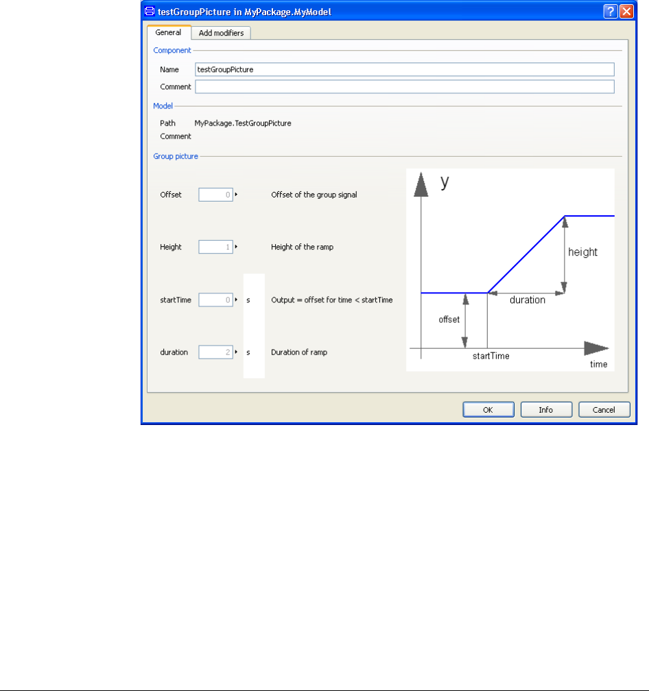
7 USER-DEFINED GUI 375
Illustrations and formatting in dialogs
Adding images to groups
To make it easier to understand the meaning of input data, it’s possible to associate a picture
with a Group:
The record declaration including the annotation to specify the file name of the picture is
shown below. The last annotation creates the image. It is recommended to put pictures used
in Dymola documentation in a folder “Images” in the same folder as the top package. It is
also recommended to use the Modelica URI ‘modelica://’ scheme. If the top package is
MyPackage, and an image “ramp.png” is located in a folder “Images” in the same folder as
MyPackage, the annotation will be as below.
Parameter dialog with
illustrations.
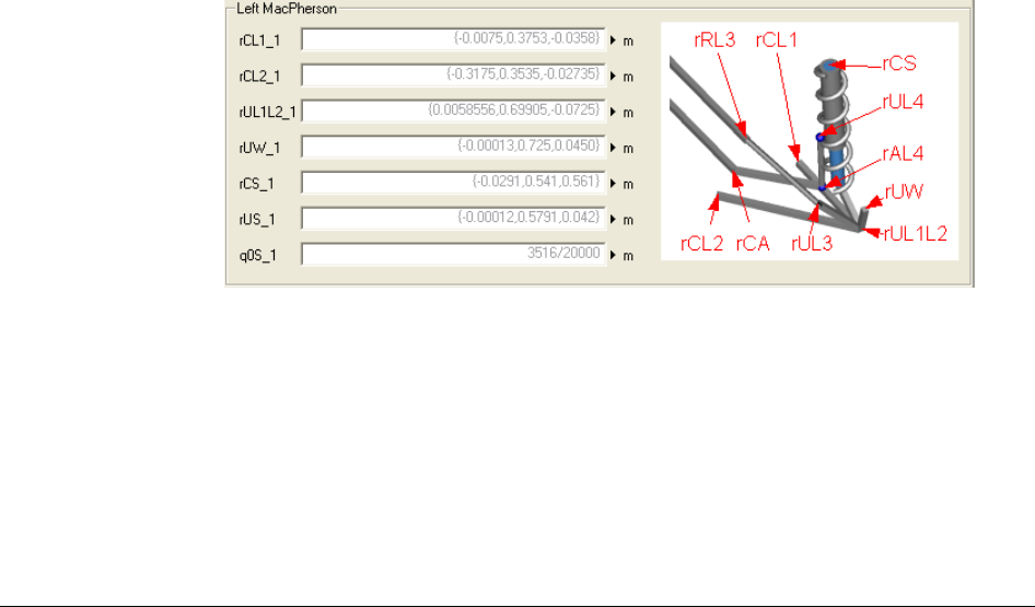
376
record TestGroupPicture
Real offset=0 "Offset of output signal"
annotation(Dialog(group="Group picture"));
Real height=1 "Height of ramps"
annotation(Dialog(group="Group picture"));
Modelica.SIunits.Time startTime=0
"Output = offset for time < startTime"
annotation(Dialog(group="Group picture"));
Modelica.SIunits.Time
duration(min=Modelica.Constants.small) = 2
"Duration of ramp"
annotation(Dialog(group="Group picture"));
annotation (__Dymola_Images(Parameters(group="Group picture",
source="modelica://MyPackage/Images/ramp.png")));
end TestGroupPicture;
To test this functionality, please drag an instance of the record into the diagram layer and
double-click it to access the parameter dialog (the picture will not be shown if clicking on
the record and selecting Create Record…).
The annotations used above are not available as settings in the Declare variable dialog; it
can however be entered in that dialog.
An additional example
In this example for the Tab “Geometry” and the Group “Left MacPherson” we wanted to
add an illustration showing the meaning of parameters.
The syntax for adding the image to this group in the parameter dialog is:
annotation (__Dymola_Images(Parameters(tab="Geometry",
group="Left MacPherson",
source="modelica://MyPackage/Images/MacPherson_text.png")));
Images in parameter
dialog.
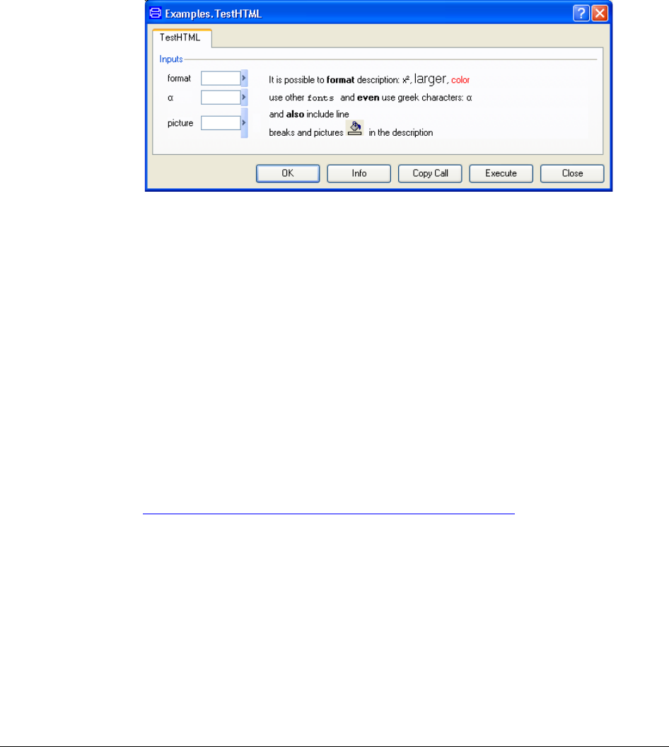
7 USER-DEFINED GUI 377
HTML formatting
The description texts and labels may contain HTML formatting tags if the text string is
enclosed in <html> … </html>. The example below shows some of the possibilities.
The corresponding record declaration is given below:
record TestHTML
Real format
"<html>It is possible to <b>format</b> description:
x<sup>2</sup>, <font size=\"+2\">larger</font>,
<font color=\"#ff0000\">color</font> </html>";
Real alpha
"<html>use other <font face=\"Courier New, Courier,
monospace\">fonts </font> and <b>even</b>
use Greek characters: α</html>"
annotation(Dialog(__Dymola_label="<html>α</html>"));
Real picture
"<html>and <b>also</b> include line <br> breaks and
pictures
<img src=\"C:/Dymola/work/colorfill.png\" /> in
the description</html>";
end TestHTML;
Greek symbols can, for example, be found at:
http://www.htmlhelp.com/reference/html40/entities/symbols.html
The annotations used above are not available as settings in the Declare variable dialog; it
can however be entered in that dialog.
Dialog with flexible
formatting.
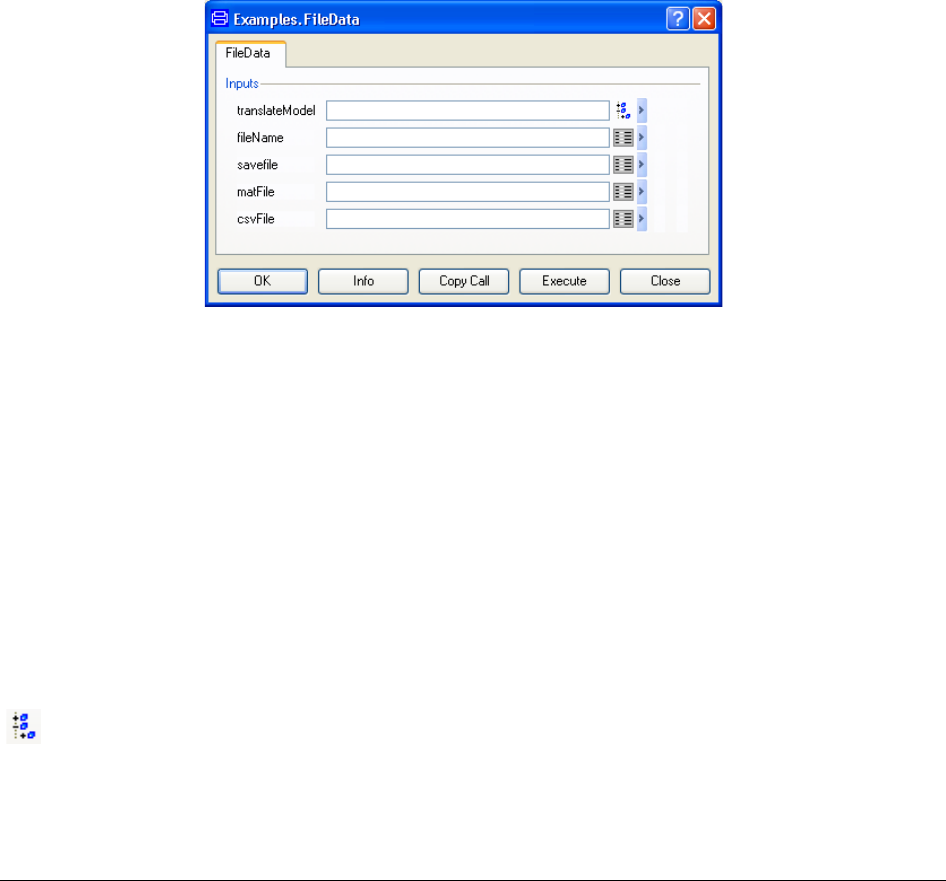
378
Specialized GUI widgets
Declarations of variables can be annotated to provide a convenient user interface, for
example to select models, open files, input data in matrices or select color. These
annotations are typically used to give inputs to functions or for creating records. The dialog
is annotated with edit buttons (except when browsing files, then a browser symbol is
automatically inserted).
File handling
The following dialog shows five examples of handling files. (The dialog pops when right-
clicking on the record in the package browser and selecting Create Record…):
Given the appropriate type definitions (see below), such a record is very easy to declare.
record FileData
Examples.TranslatedModel translateModel;
Examples.FileName fileName;
Examples.FileNameOut savefile;
Examples.MatFileName matFile;
Examples.CsvFileName csvFile;
end FileData;
The first example makes it possible to select a model. The type is declared as follows:
type TranslatedModel=String
annotation(Dialog(__Dymola_translatedModel(
translate=true,caption="Model selection")));
If the selected model is not translated, it will be translated automatically. (Actually,
translate=true can be omitted since it is true by default.). The caption will specify the header
of the window that will pop. If omitted, the text will be “Select model”.
Pressing the Edit button for such function argument displays this dialog:
Input fields with
associated specialized
GUI widgets for file
handling.
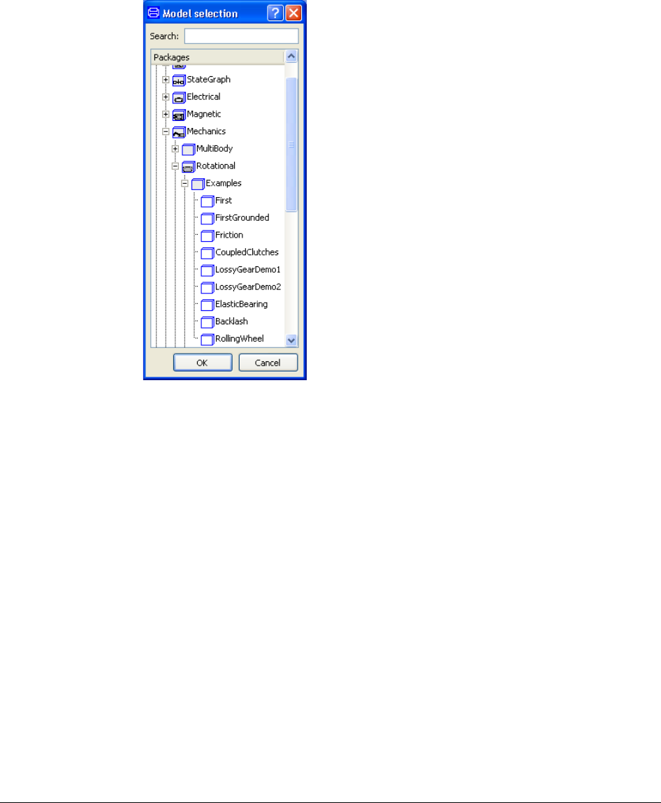
7 USER-DEFINED GUI 379
The second example is a GUI widget for directory handling. It creates a button for selecting
a directory:
type FileDirectory=String
annotation(Dialog(__Dymola_directorySelector(caption"Select
Directory")));
The following declarations use annotations to display different kinds of file dialogs. The
third example gets a filename for reading a file:
type FileName=String
annotation(Dialog(__Dymola_loadSelector(filter="Matlab files
(*.mat);;CSV files (*.csv)",caption="Open experiment data
file")));
The fourth one gets a filename for writing a file:
type FileNameOut = String
annotation(Dialog(__Dymola_saveSelector(filter="Matlab files
(*.mat);;CSV files (*.csv)",caption="Save experiment data
file")));
The fifth one makes it possible to first select a .mat file, and then selecting a matrix in that
file.
type MatFileName=String
annotation(Dialog(__Dymola_loadSelector(matrixAfter="|",filter=
"Matlab files (*.mat)",caption="Open experiment data file")));
Translated model
dialog.
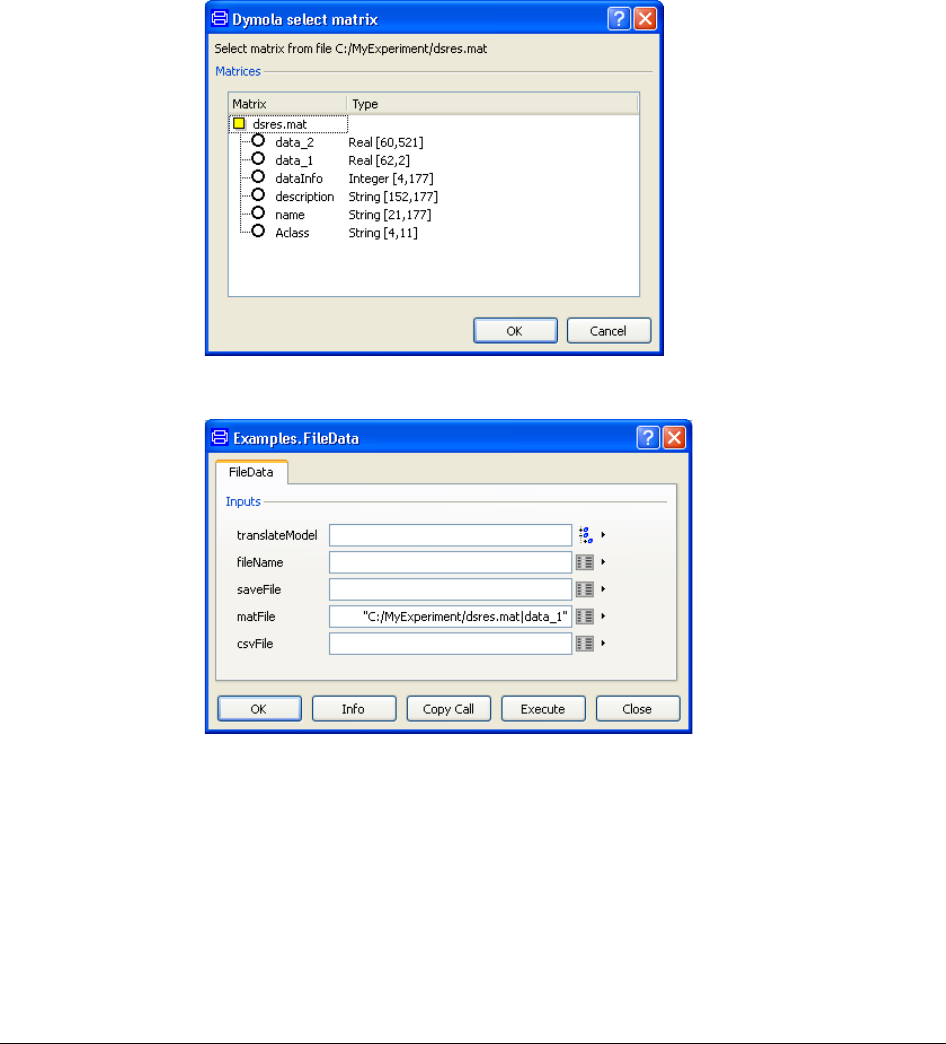
380
As an example just to show how the annotation works a user might want to read a matrix in
the file dsres.mat, which was created when simulating the CoupledClutches demo (after
having selected C:/MyExperiment as working directory). Using the widget above to select
the resulting dsres.mat, the following dialog for selection of matrix in that file will pop:
Selecting the alternative data_1 and clicking OK will result in:
The sixth example makes it possible to read a csv file or a txt file (it is actually of the same
type as the first one above).
type CsvFileName=String
annotation(Dialog(__Dymola_loadSelector(filter="CSV files
(*.csv);;Text csv files (*.txt)",caption="Open experiment data
file")));
Selection of matrix in
a .mat file.
Selection of a matrix
in a .mat file – the
result.

7 USER-DEFINED GUI 381
Data input and color handling
The following shows a dialog for data input in a matrix and color selection (with default
value of the color):
The corresponding record is:
record DataAndColor
Examples.MatrixData Input;
Examples.Color Color={85,255,85};
end DataAndColor;
A type for entering the data of a 3 x 3 real matrix can look the following:
type MatrixData = Real[3,3];
Pressing the corresponding Edit button will display:
And the last type for color selection:
type Color=Real[3] annotation(Dialog(
__Dymola_colorSelector=true));
Pressing the corresponding Edit button will give (note that default values have been given in
the record definition):
Input fields with
associated specialized
GUI widgets for data
input and color.
Input of matrix data.
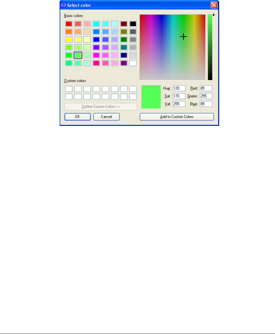
382
Import of model data in functions
The annotation __Dymola_importDsin makes it possible to define a function that enables
the user to import selected data from a model.
The wanted result might look like the figure below; by right-clicking on the function
Function in the package browser and then selecting Call Function… and then selecting
Model parameters a button Import is displayed.
(In the example below the model selected to import from is
Modelica.Blocks.Examples.PID_Controller.)
Color selection.
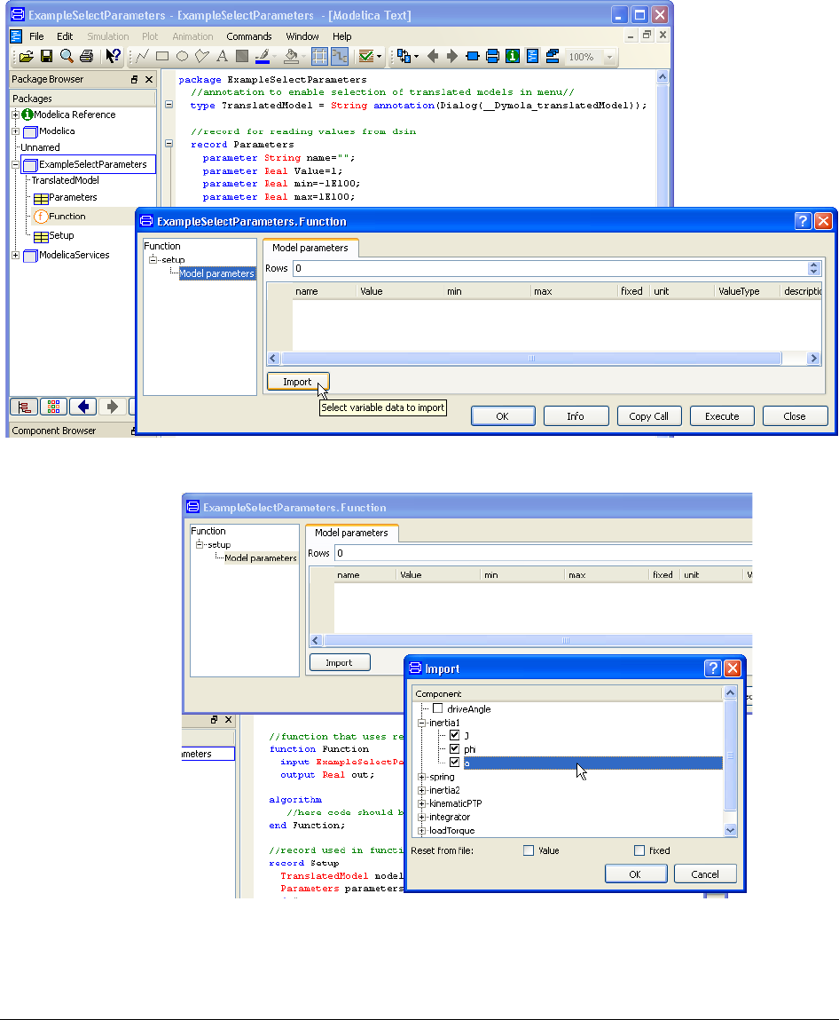
7 USER-DEFINED GUI 383
Clicking on that button pops a tree of variables to select from.
When clicking OK, the imported data will be shown in the dialog (the columns have been
somewhat adapted for nicer presentation):
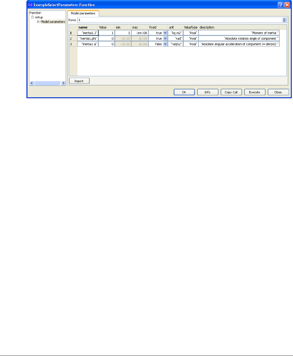
384
It is possible to change e.g. the value of inertia1.J before importing the data into the function
by clicking OK.
This feature is used in several menus in e.g. the Calibration package; please see chapter
“Model Calibration” in this manual for more examples of such menus and the use of those.
The code behind this example looks the following (compare also with the package browser
in the figure above when it comes to the structure of the code):
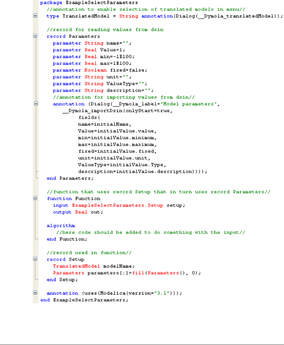
7 USER-DEFINED GUI 385

386
The code is shown with all annotations expanded. The annotation in the middle of the code
is the one that makes it possible to import data from models. Extracting only the
__Dymola_importDsin part of the annotation from the example we find:
__Dymola_importDsin(onlyStart=true,
fields(
name=initialName,
Value=initialValue.value,
min=initialValue.minimum,
max=initialValue.maximum,
fixed=initialValue.fixed,
unit=initialValue.unit,
ValueType=initialValue.Type,
Description=initialValue.description))
(For a full list of what can be handled in the annotation, see notes below.) In this example
all possible attributes from a signal is being imported. The corresponding attributes are
shown as headers when importing (please see previous figures in this example). If less
attributes are needed, just omit that attribute when writing the code (e.g. to not import the
data type of the signal in this example, remove ValueType=initialValue.Type, from
the annotation – and don’t forget to also remove parameter String ValueType=""
from the Parameter record definition).
It is possible to select what kind of signals that should be selectable.
In this example initial values of parameters and states are selectable because of using
onlyStart=true in the annotation. Please note that this means the parameter values that
are used when starting the simulation of the model; if a parameter has a start value of 2 but
the user has input 14 before simulation, it will be the value 14 that will be imported.
The default text of the button and the tooltip is used in the example. It other texts are
wanted; the annotation in the example can be changed to e.g.
…__Dymola_importDsin(button="Mytext" "My tooltip",onlyStart=…
Some notes about the example:
• This example only shows how to import different data to a function and nothing more,
that is, the function in this example is meaningless; the imported data has to be used
also, by adding code in the algorithm part of the function to e.g. specify the output of the
function.
• To be able to create the function dialog, the record Setup is created. That record is used
as input for the function, and supplies the model that data should be selected from, and
the data that is imported from that model using the record Parameters.
• __Dymola_translatedModel that is used in the record Setup is a type that has an
annotation that makes it possible to select from translated models from a tree structure;
this annotation has been used in a previous example also.
• dsin is a file where data of a model is stored.

7 USER-DEFINED GUI 387
• The full annotation is:
__Dymola_importDsin(
button=String "comment",
onlyStart=Boolean,
onlyInput=Boolean,
onlyTimeVarying=Boolean,
nonStaticMessage=String
fields(
name=initialName,
Value=initialValue.value,
min=initialValue.minimum,
max=initialValue.maximum,
fixed=initialValue.fixed,
unit=initialValue.unit,
ValueType=initialValue.Type,
Description=initialValue.description))
Not mentioned in the example above were onlyInput, onlyTimeVarying and
nonStaticMessage. If onlyInput is set to true, only inputs are imported, if
onlyTimeVarying is set to true, only time varying variables are imported.
nonStaticMessage will display the specified string as message when a model is time
dependent.
Conditional input of data
It is possible to control whether data input is possible or not for a variable using the
annotation annotation(Dialog(enable=expression)).
The annotation is easily applied using the Declare variable dialog; the Annotation tab. The
Parameter dialog placement group contains an Enable input field. Here the condition can be
entered.
As an example, assume the capital to have zip code 11111, having a number of sub-codes.
The field for entering sub-codes should only be possible to access if the zip code is entered
as 11111. When an instance of Person is dragged into the diagram layer of the edit window
and double-clicked it might look the following:
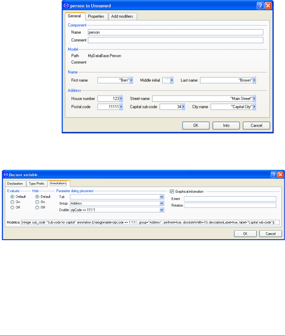
388
In this case the field for the sub-code is accessible.
The corresponding Annotation tab for the variable sub_code is (the window is made longer
to show the complete Modelica text line):
Parameter dialog for
an instance of Person.
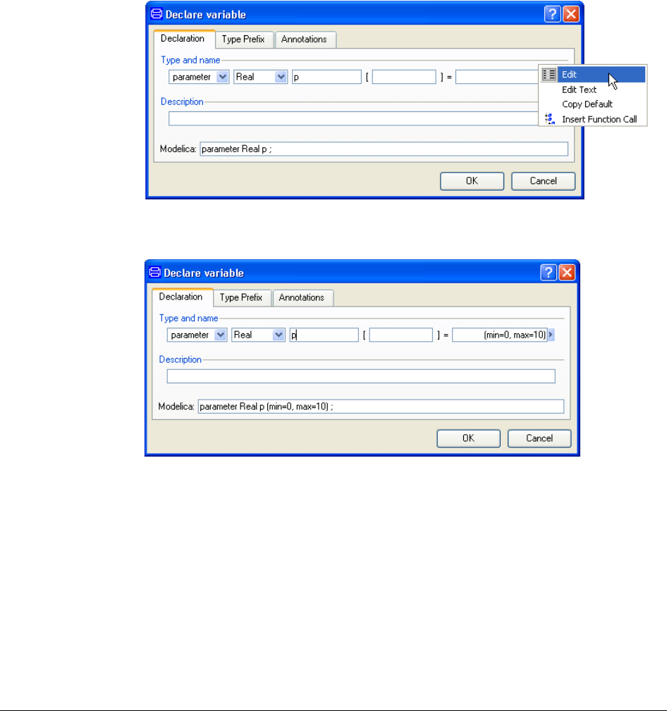
7 USER-DEFINED GUI 389
Checking of input data
It is possible to declare parameters with minimum and maximum values, which are then
checked by Dymola when the user sets a parameter value. The variable is declared with type
and name as usual using the command Edit > Variables > New variable….. Then press the
edit button (right-arrow) and the end of the value field to present a menu.
Select Edit from the menu and enter the min and max values for the parameter. Assuming
that we have specified the range to be [0, 10], the variable dialog shows
If we have a model with such a parameter and try to set a value outside of the valid range,
Dymola will display an error message. The parameter dialog cannot be closed until the
invalid modifier value has been corrected.
Editing attributes of
variables.
Variable dialog with
min and max attributes.
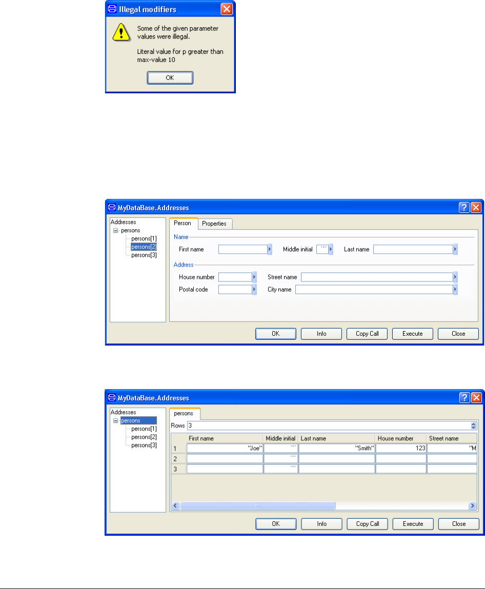
390
Arrays of records
A simple address book can be created as an array of Person records as follows:
record Addresses
Person persons[:];
end Addresses;
The corresponding dialog for one record in such an array is:
It is also possible to view all person records at the same time by selecting the array “persons”
in the left tree browser:
Out of bound error
message.
Dialog for one record
in an array.
Dialog for an entire
array of records.
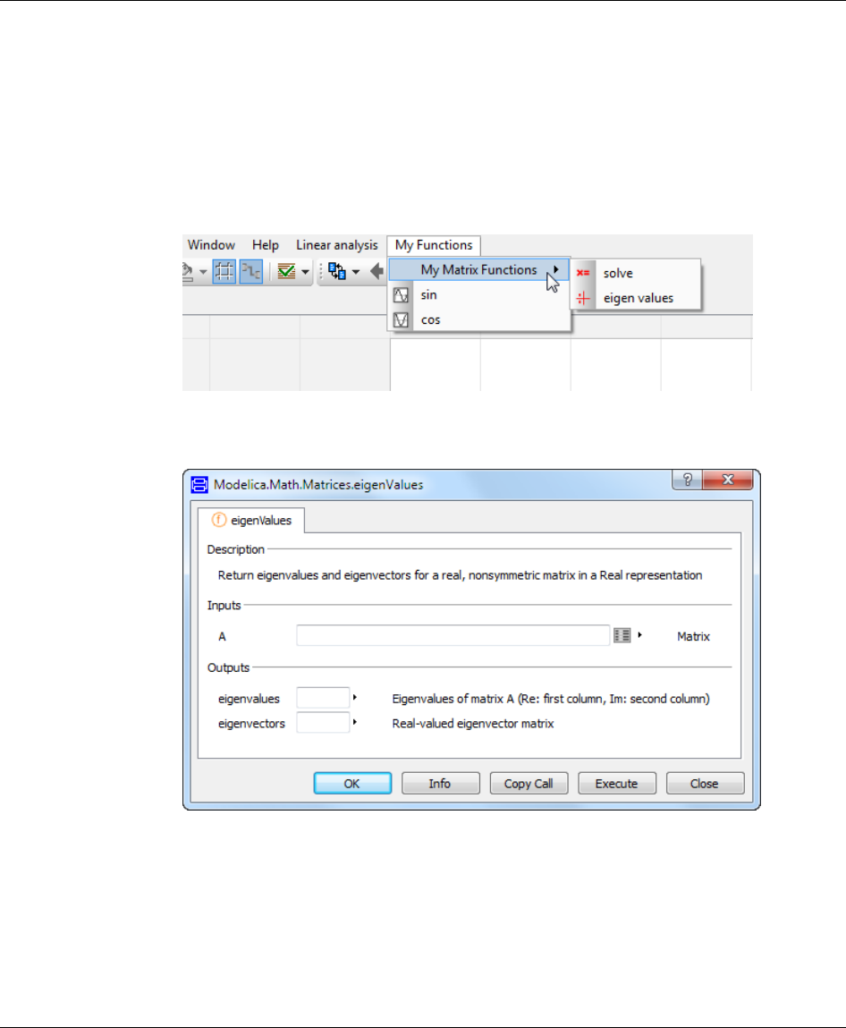
7 USER-DEFINED GUI 391
7.2 Extendable user interface – menus, toolbars and
favorites
7.2.1 Defining content of menus and toolbars
It is possible to extend the graphical user interface of Dymola by introducing own menus
and toolbars from which Modelica functions can be called.
The following image shows a new menu My Functions. It contains a submenu My Matrix
Functions with two menu items; sin and cos.
When selecting eigen values, the dialog of Modelica.Math.Matrices.eigenValues
function is shown:
The definition of menus and toolbars are done by defining a package structure with short
extends definitions to the functions to be called.
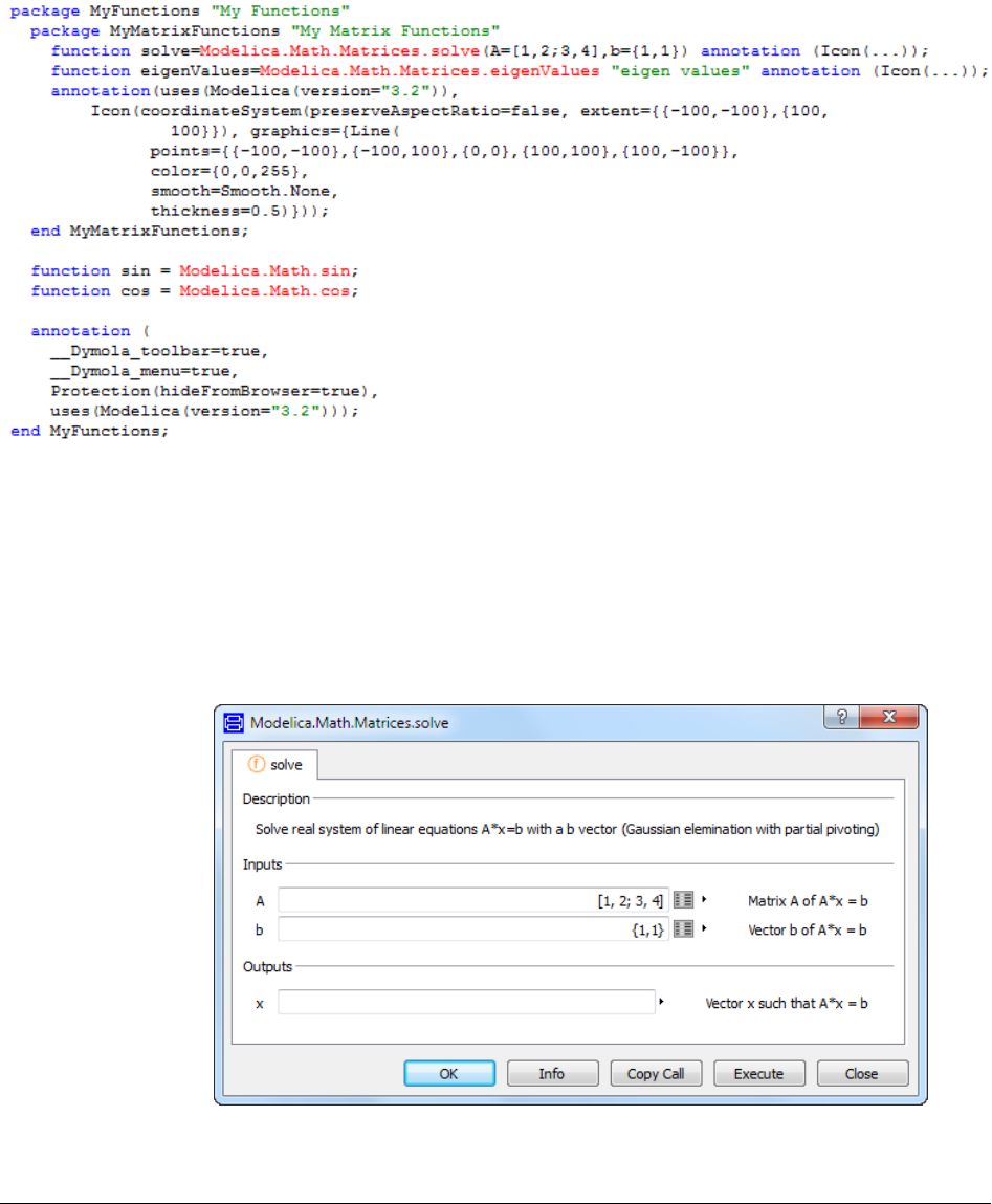
392
Note that icon annotations have been given for solve, eigenValues and MyMatrixFunctions
and that these are used in the menus. To increase the readability of the code above, the icon
annotations for the two first has been expressed as (Icon(…)) in the figure above.
If a description string is given, for example “My Functions”, “My Matrix Functions” and
“eigen values” in the example above, those strings are used for the menu, otherwise the
defined name.
It is possible to give values to inputs which then becomes prefilled in the dialog; in the
example above the command My Functions > My Matrix Functions > solve will display:
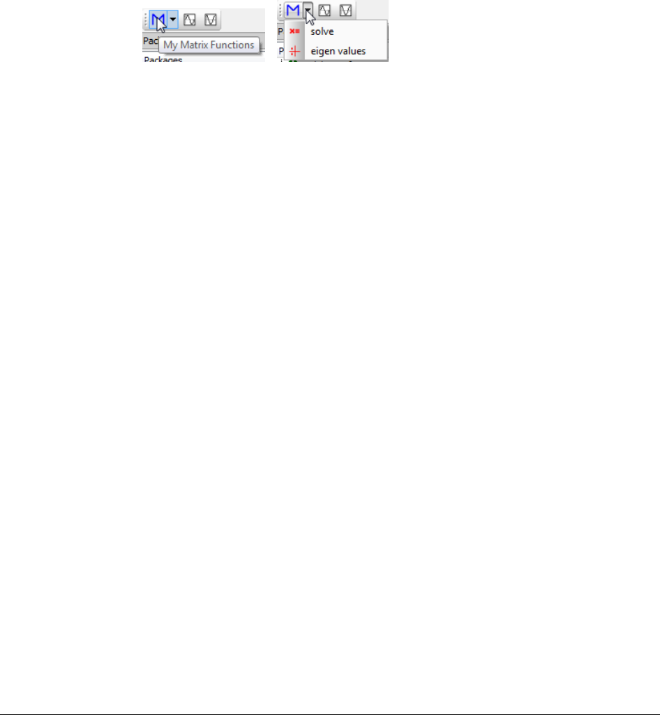
7 USER-DEFINED GUI 393
The package structure is made into a menu by providing (as in the example above) the
annotation
annotation(__Dymola_menu=true);
It is also possible to define a toolbar, tooltip included:
Toolbars are created by giving (as in the example above) the annotation:
annotation(__Dymola_toolbar=true);
It is possible to hide such a package from the package browser by (as in the example above)
using the annotation:
annotation(Protection(hideFromBrowser=true));
such a package can be automatically loaded by using a libraryinfo.mos file with
category="persistent":
LibraryInfoMenuCommand(
Category="persistent",
Reference="<Class to preload>",
Text="dummy")
It is then not removed when the File > Clear All command is given.
The annotation __Dymola_hideGraphics=true can be used to hide the graphics coming
from such a class. This also means that the base class is only loaded when needed to build
the parameter dialog and call the function.
7.2.2 Displaying library-specific menus and
toolbars in Dymola (commercial library
developers)
Commercial library developers can in their libraries include menus and toolbars that will be
displayed in Dymola when opening the libraries. To do this, the annotation
annotation(__Dymola_containsMenu=true);
must be present in the top level of the library (e.g. in package.mo). This causes all classes in
the library to be searched for menu and toolbar annotations.
The package containing the menu and toolbar annotations described in previous section
must be located inside the library.
An example of a menu created this way is the menu that will be displayed when opening the
Optimization library:
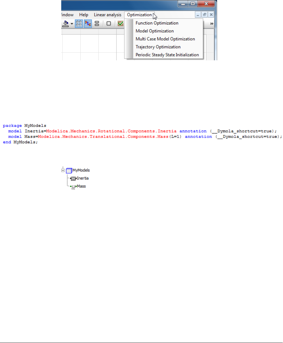
394
The menu will disappear when performing File > Clear All or unloading the library.
7.2.3 Defining packages with users own collection
of favorite models
It is possible to define packages with your own collection of favorite models by introducting
shortcut to models:
The models appear in the package browser the usual way:
When dragging from such a shortcut, an instance of the original model is created, possible
with prefilled parameter values if a modifier has been used in the short class definition.
Note that a simpler way of creating favorite packages is available, however with no
possibility to have prefilled parameter values. For more information, see “Dymola User
Manual Volume 1”, chapter “Developing a model”, section “Basic model editing,
subsection “Packages, models, and other classes”.
8 ADVANCED MODELICA
SUPPORT

8 ADVANCED MODELICA SUPPORT 397
8 Advanced Modelica Support
8.1 Declaring functions
In Modelica it is possible to define and use functions, and the functions can be used in
equations of a model, in defining parameters, and called interactively from the command
line.
Functions inherently reduce the possibility for symbolic manipulations, and should thus not
be used unless necessary. In particular index reduction requires that all functions are differ-
entiated, which cannot be done in a straightforward way without help. This “help” is pro-
vided in form of an annotation giving the derivative of the function.
The functions themselves can either be written in Modelica or as external functions in C,
Java, C++ or FORTRAN 77. In most cases the external function is provided in a binary
library with a corresponding header defining the function.
8.2 User-defined derivatives
In order to reduce the index it is necessary to differentiate arbitrary expressions with respect
to time. This derivative must be very accurate in order to not introduce unnecessary numer-

398
ical errors. The functions are seldom simple scalar functions from one scalar input, but in-
stead have vectors and/or records as input, in many case the functions also have several
inputs and/or outputs. Often second order differentials are also needed.
For solving non-linear system of equations derivatives can also increase performance, by
allowing us to compute an analytical Jacobian.
The first choice is of course to rely on the automatic differentiation of functions in Dymola.
If this is not sufficient, there is an annotation available for the user to explicitly define the
derivative of a function, and Dymola can use this both to reduce the index and to compute
Jacobians for non-linear system of equations.
The annotation declaring the derivative function can be given both for functions written in
Modelica as well as for external functions.
8.2.1 Analytic Jacobians
For non-linear systems of equations it is possible to avoid numeric Jacobians and instead
rely on Dymola to automatically differentiate the functions. Compared to writing derivative
functions this is much easier for the modeler, easier to understand for the user, and also
considerably less error-prone.
In order to enable Dymola’s automatic differentiation feature, the modeler writing functions
must declare the smoothness of the function by providing a smoothOrder annotation
corresponding to the smooth operator in Modelica. A basic limitation of automatic
differentiation is that it can provide a derivative even at points where the function does not
have a derivative. Verifying that a function with branches (if-statements, if-expressions, or
while-statements) is continuous is a difficult problem. The person providing the
smoothOrder annotation is guaranteeing that the function is at least that smooth. When
using the function, its derivative is only constructed if it is found to be needed because of
index reduction or to generate an analytic Jacobian.
The basics of automatic differentiation and the implementation choices in Dymola are
discussed in H. Olsson, H. Tummescheit and H. Elmqvist: “Using automatic differentiation
for partial derivatives in Modelica”, Proceedings of the 4th International Modelica
Conference, Hamburg-Harburg, Germany, 2005, pp. 105-112.
Example
We will use a simple function that just inverts a strictly positive number for illustration:
function MyDivision
input Real x;
output Real y;
annotation (smoothOrder=1000);
algorithm
assert(x>0, "x should be positive");
y:=1/x;
end MyDivision;
We then write a simple model where this function must be differentiated in order to solve a
non-linear equation:

8 ADVANCED MODELICA SUPPORT 399
model TestDivision3
Real x;
equation
MyDivision(x)=1+time;
end TestDivision3;
Translating this example gives a translation log with:
…
Sizes of nonlinear systems of equations: {1}
Sizes after manipulation of the nonlinear systems: {1}
Number of numerical Jacobians: 0
An analytic Jacobian is automatically constructed and used since needed. The derivative
function is:
function P.TestDivision3.MyDivision:derf
input Real x;
protected
Real y;
public
input Real x_der2;
output Real y_der2;
algorithm
assert(x > 0, "x should be positive");
y_der2 := -x_der2/x^2;
annotation (smoothOrder=999);
end P.TestDivision3.MyDivision:derf;
Removing the smoothOrder annotation instead gives:
…
Sizes of nonlinear systems of equations: {1}
Sizes after manipulation of the nonlinear systems: {1}
Number of numerical Jacobians: 1
8.2.2 How to declare a derivative
The following define how to declare the derivative to a function, and finally how to verify
that the derivative is consistent with the function. It is strongly influenced by forward mode
automatic differentiation and well suited for differentiation with respect to one variable, as
in index reduction.
It can furthermore be used to efficiently compute all interesting derivatives in a straightfor-
ward way as will be explained later.
A function declaration can have an annotation derivative specifying the derivative function
with an optional order attribute indicating the order of the derivative (default 1), e.g.:
function f0 annotation(derivative=f1); end f0;
function f1 annotation(derivative(order=2)=f2); end f1;
function f2 end f2;
It is also necessary to write the derivative function for a given function, this is described in a
procedural form below, and with examples that make it clearer.

400
The lookup for the derivative annotation follow the normal lookup rules of Modelica.
First order derivative
The inputs to the derivative function of order 1 are constructed as follows:
• First are all inputs to the original function listed and after them, in order, one derivative
for each input containing Real variables is appended.
• The outputs are constructed by starting with an empty list and then in order appending
one derivative for each output containing Real variables.
As an example consider the following:
function foo0
input Real x;
input Boolean linear;
input Real z;
output Real y;
algorithm
if linear then
y:=z+x;
else
y:=z+sin(x);
end if;
annotation(derivative=foo1);
end foo0;
function foo1
input Real x;
input Boolean linear;
input Real z;
input Real der_x;
input Real der_z;
output Real der_y;
annotation(derivative(order=2)=foo2);
algorithm
der_y:=der_z+(if linear then der_x else cos(x)*der_x);
end foo1;
This implies that given the following equation
( ) ( ) ( )
( )
y t foo0 x t ,b,z t=
we know that
( ) ( ) ( ) ( ) ( )
( )
y t foo1 x t ,b,z t , x t ,z t=
A more complex example involving records and matrices is

8 ADVANCED MODELICA SUPPORT 401
record R
Real M[2,2];
Real x[2];
end R;
function recordFunction
input R x;
output Real y[2];
algorithm
y:=x.M*x.x;
annotation(derivative=recordFunction_d);
end recordFunction;
function recordFunction_d
input R x;
input R der_x;
output Real der_y[2];
algorithm
der_y:=x.M*der_x.x+der_x.M*x.x;
// Since (A*B)'=A'*B+A*B' for matrices.
end recordFunction_d;
Thus if
y(t)=recordFunction(x(t));
we have
der(y(t))=recordFunction_d(x(t),der(x(t)));
Second and higher order derivatives
If the Modelica function is a nth derivative (n>=1) the derivative annotation indicates the
(n+1):th derivative, and order=n+1.
The input arguments are amended by the (n+1):th derivatives, which are constructed in
order from the nth order derivatives.
The output arguments are similar to the output argument for the n:th derivative, but each
output is one higher in derivative order.
Continue the example above with:

402
function foo1
...
annotation(derivative(order=2)=foo2);
...
end foo1;
function foo2
input Real x;
input Boolean linear;
input Real z;
input Real der_x;
input Real der_z;
input Real der_2_x;
input Real der_2_z;
output Real der_2_y;
algorithm
der_2_y:=der_2_z+(if linear then der_2_x else
cos(x)*der_2_x-sin(x)*der_x^2);
end foo1;
This allows us to conclude that
( ) ( ) ( ) ( ) ( ) ( ) ( )
( )
foo2 , , , , , ,yt xtbztxtztxtzt=
Restrictions
An input or output to the function may be any predefined type (Real, Boolean, Integer or
String) or a record, provided the record does not contain both real and non-real predefined
types. Allowing mixed records would require that we automatically constructed a new
record from the parts containing real types, which would be difficult to describe.
The function must have at least one input containing a real type, since we must have
something to take the derivative with respect to.
The output list of the derivative function may not be empty, since we otherwise have no de-
rivative. This can occur if the function e.g. returns a Boolean value.
Verifying Derivatives
In order to verify that a derivative is consistent with the function it is recommended to fol-
low the following test procedure. The basic idea is to compare the integral of the derivative
with the original function.
Assume one has a model using foo0:
model B
Real x;
equation
x=foo0(time, false, -0.1*time);
end B;
and we want to verify that the derivative of foo0 is correct. We do that by extending B as
follows:

8 ADVANCED MODELICA SUPPORT 403
model VerifyFirstDerivative
extends B;
Real y;
equation
der(y)=der(x);
initial equation
y=x;
end VerifyFirstDerivative;
That the derivative is correct can be verified by comparing x (which is computed directly)
and y (which is computed as an integral of the derivate). By setting second derivatives equal
one can verify the second derivative as well. Note that this procedure does not modify the
original model and can therefore be used even when the input arguments to the function are
given internally.
8.3 External functions in other languages
8.3.1 C
In addition to functions written in Modelica, Dymola also allows external functions written
in ANSI/ISO C. For each external function it is necessary to declare a Modelica interface.
This declaration provides the required information needed to call the function from a Mod-
elica model, and in some simple cases provide argument conversion.
External functions are declared as Modelica functions, but with a body that defined the in-
terface. The Modelica specification defines the details of how function arguments in
Modelica are mapped to similar data types in C, and how values returned from the functions
are mapped back to Modelica types. When the interface of the external function does not
match the Modelica specification, a wrapper function must be written in C to perform the
required conversions.
In most cases the external function is provided in a binary library with a corresponding
header file declaring the function. In order to support this one can specify a header, overrid-
ing the usual definition of the function, and a library that will automatically be linked with.
Note – when using external functions in parallel code, it is assumed that the functions are
not thread-safe. For handling the case that they are, see “Dymola User Manual Volume 1”,
chapter “Simulating a model”, section “Improving simulation efficiency”, subsection
“Simulation speed-up” (or use index entry “thread-safe: external functions” in that manual).
Including external functions
In simple cases it is possible to translate the C code of the function with the model itself.
The main advantage of this approach is that it does not require any additional effort to build
a library. The disadvantage is that definitions in the implementation of the C function may
interfere with the generated model code and cause the compilation to fail.
As an example we will use the following trivial function that returns the sum of two real
numbers. Its implementation in ANSI/ISO C is called add2.c.
Existing libraries may
require wrapper func-
tions.

404
#ifndef ADD2_C
#define ADD2_C
double add2(double x, double y)
{
return x + y;
}
#endif
This function requires a declaration that provides a mapping between Modelica and C, and
also specifies the name of the file containing the implementation.
function add2 "Sum of two numbers"
input Real x, y;
output Real sum;
external "C";
annotation(Include="#include <add2.c>");
end add2;
The first two declarations define the input and output arguments and their types in the
Modelica context. The external declaration identifies this as an external function. The
types of the parameters in the external function must be compatible with the Modelica
specification.
The Include annotation is a string which in this case includes the implementation of the
function. The contents of the Include string is inserted into the generated C code, hence it
should contain valid C code. It can even contain header line breaks in order to include
several files or even preprocessor macros. There is no guarantee that the header will only be
included once, and thus necessary to guard against multiple inclusion with #ifndef and
#endif wrapping.
The code (add2.c) should be located either in the current directory, in a relative location
(#include <../source/add2.c>), or in directory dymola/source. However, using
Modelica Standard Library version 3.2 and later the annotation IncludeDirectory can be
used to define where the code is located. Please also see example below.
Linking with external library
For most application it is best to build a library with function definitions using software de-
velopment tools outside of the Dymola environment, and then compile the model linking
with the library. In this way libraries are easily shared between various applications.
A major benefit compared to including function definitions is that the risk of interference
between the code generated by Dymola and the code of the external functions is greatly re-
duced. The only parts included in the compilation of the model are header files declaring the
external functions in C, and the implementation is compiled separately.
DLLs are handled by linking with their wrapper libraries, or directly. Please see section
“Linking with DLLs” below.
This section refers
only to the Windows
version of Dymola.

8 ADVANCED MODELICA SUPPORT 405
Building an external library
Using an external library the C code consists of two parts: a header file declaring the func-
tion, and an implementation. It is common to use a single header file to declare a group of
related functions. The header file for the example above would be:
#ifndef ADD2_H
#define ADD2_H
extern double add2(double x, double y);
#endif
The implementation is very similar to the code used for inclusion in the model code, but the
header file should be included to ensure compatibility in the event of changes in the inter-
face. The #ifndef and #endif wrappers are not needed.
#include <add2.h>
double add2(double x, double y)
{
return x + y;
}
Library annotation
The Modelica interface uses two special annotations, Include and Library, to specify the
header file and the name of the library:
function add2 "Sum of two numbers"
input Real x, y;
output Real sum;
external "C";
annotation(Include="#include <add2.h>", Library="ext");
end add2;
Note that the library name is “ext”; the “lib” prefix is added by the linker, and the extension
depends on the used compiler (.lib for Microsoft C). This ensures portability of the
Modelica interface to different platforms and compilers.Note that the syntax in the Include
annotation for linking with multiple static libraries is Library={"lib1","lib2","lib3"}
As a more complex example consider an interface to National Instruments AI_VRead in its
Ni-Daq library. A protected variable is used to pick up the status code returned from the
function.
function AI_VRead "Analog in"
annotation (
Include="#include <nidaqex.h>",
Library={"nidaq32"});
input Integer iDevice=1;
input Integer iChannel=1;
input Integer iGain=1;
output Real dVoltage;
protected
Integer iStatus;
external "C" iStatus = AI_VRead(iDevice, iChannel, iGain,
dVoltage);
end AI_VRead;
Prefix and extension
are not given.
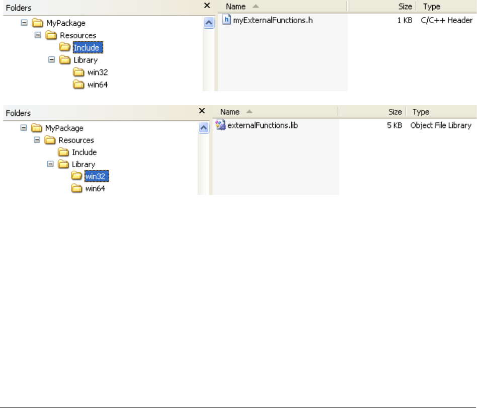
406
The Library annotation is either a single string or a vector or strings that name several bina-
ry libraries and the compiler will link with all listed libraries.
Note that for this example to work the header and library files must be in the search path of
the compiler. This could be accomplished by placing the header in %DYMOLA%/source and
the library in the correct sub-directory of %DYMOLA%/bin or by placing both of them in the
current directory. However, using Modelica Standard Library version 3.2 and later the
annotations IncludeDirectory and LibraryDirectory can be used to define where the
header and library files are located; as in the next example.
Using annotations for location of external library and include files, and recommended
file locations
Wanting to distribute a package MyPackage with external C functions, a recommended way
of locating the header and implementation files is:
(The win64 folder is analogous to the win32 one.)
To specify these locations the annotations IncludeDirectory and LibraryDirectory
can be used.
A package MyPackage with a model MyModel calling a function myFunction that uses an
external C function can be written:
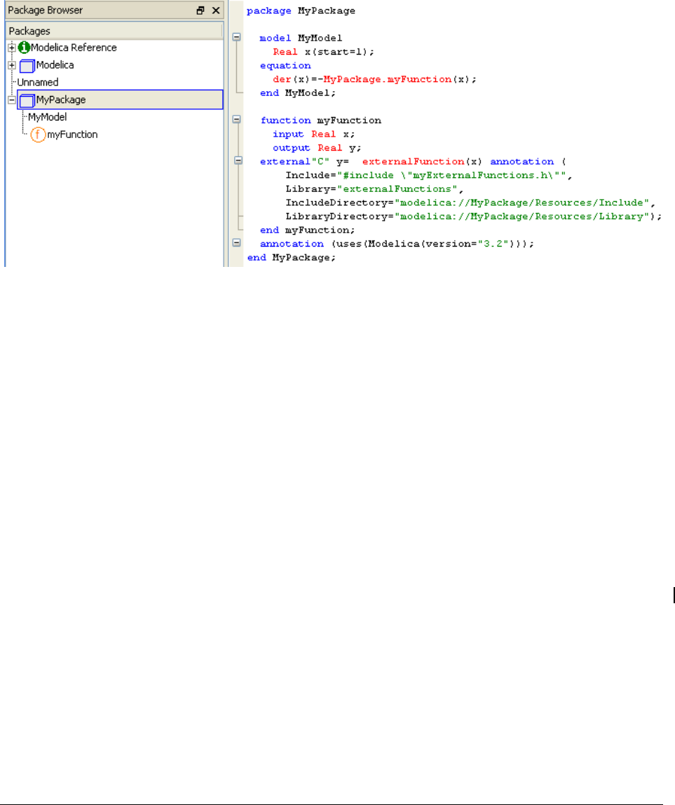
8 ADVANCED MODELICA SUPPORT 407
For more information (an examples) please see “Modelica Language Specification”, version
3.2, section 12.9.4. This document is available using the command Help > Documentation
in Dymola.
Improved support for different C++ library versions
Dymola has improved support for different C++ library versions for different version of the
Visual Studio compiler. This eases the use of some commercial libraries.
This support is standardized in Modelica – by automatically switching from win32 (or
win64) to the relevant subdirectory, e.g. vs2012 (for Microsoft Visual Studio 2012). Note
that this is specific for external C++ code, since there is normally no need to have multiple
versions of C libraries.
A warning appears if mismatch occurs.
Linking with DLLs
Linking with DLLs by linking with their wrapper libraries
DLLs can be handled by linking with their wrapper libraries. The library must be
multithreaded and with DLL-linking with the I/O (/DLL switch).
The library specified using annotation(Library="MyLib") is on Windows normally a
.lib file (i.e. “MyLib.lib”) in a directory specified by the annotation LibraryDirectory,
its default value, or in the win32/win64 subfolder.
If the LibraryDirectory contains “MyLib.dll” file Dymola will automatically delay-load
the corresponding DLL file (using “-delay...”). This ensures that the DLL is not loaded
when generating the default parameter settings.

408
Linking with DLLs by direct linking
Direct linking with a DLL (without import-library) is supported when all the following is
fulfilled:
• The specified lib-file does not exist.
• A corresponding dll-file exists.
• There is an external function call.
• There is no include-annotation.
8.3.2 Java
Note – the below implementation of Java is intended for calling Java functions from
Modelica, or Modelica functions from Java functions. A newer Java interface is available
for accessing Dymola remotely, please see chapter “Other Simulation Environments”,
section “Java interface for Dymola”.
Dymola can call functions written in Java - either interactively or from models. This
requires that you:
• Install either Java Development Kit or J2SE Software Development Kit. It is not
sufficient to install the Java Runtime Environment.
• Ensure that the environment variable JAVA_HOME points to this directory.
• For each function written in Java that you want to call from Modelica you add an
external declaration in Modelica.
Note! The above Java implementation currently only supported on Windows 32-bit. (The
newer Java interface supports both Windows and Linux, 32-bit and 64-bit.)
Calling Java functions from Modelica
The functions must be static member functions and the syntax in Modelica is:
function f
input Real u;
output Real y;
external "Java" y='MyPackage.MyClass.Myfunction'(u);
end f;
In Java this function can be implemented as:
package MyPackage;
public class MyClass
{
// A simple function in Java
public static double Myfunction(double d)
{
return d * 2;
}
}

8 ADVANCED MODELICA SUPPORT 409
Note: Dymola just performs a normal function call, and thus have user interaction from
functions written in Java dialogs must use modal dialogs (i.e. they only return once the
action is complete).
Mapping of data structures
Simple types in Modelica (e.g. Real) are normally mapped to corresponding simple types in
Java. Strings are non-simple objects in Java, the mapping is still direct, and the character
mapping is made simpler by the fact that Java Virtual Machine and Dymola internally use
the same UCS-8 implementation of Unicode strings.
Note: The UCS-8 mapping is the result of applying the UTF-8 mapping to UTF-16 strings,
and the recommendation is that even though it can be used internally in programs it should
not be used for interfaces. In this case we make an exception in order to be compatible with
the pre-existing C interface of the Java Virtual Machine.
Arrays in Modelica correspond to (possibly nested) arrays in Java. Heterogeneous arrays in
Java cannot be sent to Modelica. Zero-sized matrices sent from Java should be avoided (if
possible) since the non-zero dimensions cannot always be completely determined.
Records in Modelica are mapped to a class implementing a map interface in Java. This
ensures that the semantics of Modelica records (named based type equivalence) is preserved.
To summarize we first present how arguments are mapped when calling a function written
in Java from Modelica.
The record class, com.dynasim.record implements the map interface, and the content is
mapped as above (the difference is for simple data types, since the simple data types are not
Modelica Java
normal case for record contents
Real double java.lang.Double
Integer int java.lang.Integer
Boolean boolean java.lang.Boolean
String java.lang.String java.lang.String
record com.dynasim.record com.dynasim.record
Real[] double[] double[]
Integer[] int[] int[]
Boolean[] boolean[] boolean[]
String[] java.lang.String[] java.lang.String[]
record[] com.dynasim.record[] com.dynasim.record[]

410
objects in Java). However, for easy access to simple variables there are also special
functions, getDouble, getInt, and getBoolean.
The map for records is straightforward to use and by being name based avoid issues with
declaration order and future extensions of the records in Modelica.
Mapping of errors
Exceptions thrown from Java functions called from Modelica are automatically mapped to
assertions, which is the normal error handling primitive in Modelica. Currently an assertion
stop Dymola’s interpreter as there is no way of catching the error inside Modelica.
Calling Modelica functions from Java functions
For interactive calls to Modelica functions it is possible to call Dymola's interpreter from
Java, by using the function com.dynasim.dymola.interpretMainStatic. Calls of Modelica
functions (and Dymola’s API functions callable as Modelica functions) from Java go
through one function accessible in Java as com.dynasim.dymola.interpretMainStatic, found
in Program Files\Dymola 2015\Modelica\Library\java. The exact details are
explained later. For other Modelica functions a wrapper in Java can be constructed in a
mechanical way that maps arguments, calls this bridge function, and maps the result.
Having one entry point to Modelica from Java makes it straightforward to transparently
redirect all calls to a remote instance of Dymola, i.e. remote method invocation.
Dymola’s interface for Java functions is found in Program Files\Dymola
2015\Modelica\Library\java, this directory should be included in the class path when
compiling Java programs that use the Dymola interface, e.g.:
javac –classpath
".;c:\Program Files\Dymola 2015\Modelica\Library\java" *.java
This has to be adapted depending on where Dymola is installed. There are also other
settings in the Java compilers for making this easier to use, but we will not consider these
here. The quotes around the path are used to ensure that the string is one command line
argument.
Thus as examples we will implement additional functions using standard Modelica
functions:

8 ADVANCED MODELICA SUPPORT 411
package MyPackage;
public class CallDymola
{
// A function calling Dymola:
public static double Norm(double[][] m, double p)
{
// Construct argument list.
Object objs[] = new Object[2];
objs[0] = m;
objs[1] = new Double(p);
// Call function
Object res = com.dynasim.dymola.interpretMainStatic(
"Modelica.Math.Matrices.norm", objs);
// Go back
double returnValue = ((Double)(res)).doubleValue();
// Additional computations
return returnValue;
}
// A matrix to test the norm
public static double[][] Test()
{
double[][] d=new double[2][];
d[0] = new double[2];
d[1] = new double[2];
d[0][0] = 1;
d[0][1] = 2;
d[1][0] = 3;
d[1][1] = 4;
return d;
}
// Using records.
//
// The functions getDouble, getInt, getBoolean
// are also useful
public static double[][] Rotate90()
{
Object objs[] = new Object[3];
objs[0] = new Integer(1);
objs[1] = new Double(1.57);
objs[2] = new Double(0);
com.dynasim.record res = (com.dynasim.record)(
com.dynasim.dymola.interpretMainStatic(
"Modelica.Mechanics.MultiBody.Frames.axisRotation",
objs));
return (double[][])(res.get("T"));
}
}
412
To test all of these functions in Dymola we need:
package TestJava
function f
input Real u;
output Real y;
external "Java" y='MyPackage.MyClass.Myfunction'(u);
end f;
function Rotate90
output Real y[3,3];
external "Java" y='MyPackage.CallDymola.Rotate90'();
end Rotate90;
function Test
output Real y[:,:];
external "Java" y='MyPackage.CallDymola.Test'();
end Test;
function Norm
input Real u[:,:];
input Real p;
output Real y;
external "Java" y='MyPackage.CallDymola.Norm'(u,p);
end Norm;
end TestJava;
Mapping of data structure
The mapping when a function in Java calls interpretMainStatic is identical to the mapping
of record contents when calling functions written in Java. This is necessary since the simple
types such as double are not objects and thus cannot be part of the generic argument list of
interpretMainStatic.
Modelica
Java
Real
java.lang.Double
Integer
java.lang.Integer
Boolean
java.lang.Boolean
String
java.lang.String
record
com.dynasim.record
Real[]
double[]
Integer[]
int[]
Boolean[]
Boolean[]
String[]
java.lang.String[]
record[]
com.dynasim.record[]
The contents of records are also mapped in this way, and this mapping is identical to the
contents of records when calling functions written in Java.

8 ADVANCED MODELICA SUPPORT 413
Mapping of errors
When an assertion (or other error) is trigged in Modelica originating from a call to
interpretMainStatic this is mapped to an exception in Java as follows:
• com.dynasim.DymolaException base-class of the other exception – introduced in order
to make it easy to catch all exceptions.
• com.dynasim.DymolaNoSuchFunction(<name of function>) when the function is not
found by interpretMainStatic.
• com.dynasim.DymolaIllegalArgumentException for problems with transforming results
or argument between Java and Dymola, and incorrect type of arguments to function.
• com.dynasim.DymolaEvaluationException when evaluation fails – e.g. assertions and
division by zero.
These exception classes all inherit from java.lang.RunTimeException, this ensures that no
‘throws’ clause is needed for routines calling Dymola functions.
This corresponds to the Modelica environment where a function does not have to declare
whether it may fail (e.g. using assert).
Accessing Dymola remotely
A newer interface for accessing Dymola remotely is available, please see chapter “Other
Simulation Environments”, section “Java Interface for Dymola”.
8.3.3 C++
Functions written in C++ are supported provided the C compiler supports cross-linkage with
C++. When using languages other than C, provisions must be made to ensure that the
required runtime libraries are linked.
Functions written in C++ must declared as extern "C" to be linkage compatible with C.
Wrapper functions are needed for example to use virtual functions or other C++ features
that are not present in C.
8.3.4 FORTRAN
Functions written in FORTRAN 77 are supported provided the C compiler supports cross-
linkage with FORTRAN. When using languages other than C, provisions must be made to
ensure that the required runtime libraries are linked.
FORTRAN code can be linked in two ways. Perhaps the most straight-forward approach is
to convert the FORTRAN code to C using a tool called f2c. This tool translates the code
into portable C code, and also includes libraries for common FORTRAN runtime routines.
The alternative is to use a link compatible FORTRAN compiler.
In either case, wrapper functions are most likely required to map argument types.

414
8.4 Means to control the selection of states
Dymola supports automatic state selection according to the specification of Modelica.
Variables being subtypes of Real has an attribute, stateSelect, to give hints or even impera-
tively control the selection of variables to use as continuous time state variables.
Note that Modelica allows the state selection to be separated from the specification of initial
conditions. The fixed attribute should exclusively be used for specifying start conditions and
it should not influence the selection of states at all.
8.4.1 Motivation
The general view is that selection of states ought to be done automatically. This is also pos-
sible and unproblematic in most models, and we thus clearly understand that manual state
selection can easily be overused. However, there are several reasons for allowing model li-
brary developers as well as users to influence or control the state selection:
• Accuracy: There are often many sets of state variables that will work from a pure math-
ematical point of view. However, they may have drastically different numerical proper-
ties. For mechanical systems it is favourable to use relative positions as state variables.
If absolute coordinates are used then accuracy is lost when taking differences to
calculate relative positions. The effect is drastic in rotating machinery systems and
power systems where angular positions are increasing with time, but relative positions
are rather constant, at least in normal operation. Say that two rotating bodies are
connected by a spring such that the relative distance between them is 1 and that their
angular speed is 1000. If the positions are calculated with a relative accuracy of 0.001,
after one second there is hardly any accuracy in calculating the distance by taking the
difference. The difference behaves irregularly and gives an irregular torque. The
simulation stops. It is very difficult for a tool to find this out without actually doing
simulation runs. Model developers for mechanical systems and power systems know it
very well. It would be easy for them to indicate that absolute positions are bad choices
when selecting states.
• Efficiency by avoiding inverting functions: The relations between possible sets of
state variables may be non-linear. For some choices it may be necessary to invert non-
linear functions, while for another set it is straightforward to calculate others. A typical
example is thermodynamic problems, where you have property functions. They often
assume two variables to be inputs (for example pressure and enthalpy) and calculate
other properties (such as temperature, density etc). Thus, if such variables are selected as
state variables it is “simply” calling property functions to calculate other need variables.
If not it is necessary to solve equation systems to calculate the input variables. A model
library developer knows this and it is straightforward to him to indicate good choices
when selecting dynamic states.
• Selecting a less nonlinear representation: Different sets, x, of states gives an ODE,
der(x) = f(x) where the right hand side f have different properties. In general, the
problem is simpler to solve if f is a less nonlinear problem. The Park transformation for
three-phase power systems is a classical way of transforming a nonlinear time-varying
ODE into a time-invariant linear ODE. For control design it is very favourable to have

8 ADVANCED MODELICA SUPPORT 415
linear time-invariant models, because there are lot of analysis and design methods and
tools for such models. When using linearized versions of Modelica models it is
important that the set of state variables is insensitive to minor changes in the model.
• Avoiding dynamic state selection: When selecting states the problem consists of a set
of algebraic state constraints that relate dynamic variables. It may be remarked that these
constraints are equations that are differentiated by Pantelides's algorithm. The task when
selecting states is actually to use the algebraic constraints to solve for some of the vari-
ables, which thus are deselected as states and the remaining dynamic variables become
state variables. A subset of dynamic variables can be deselected locally if its Jacobian is
non-singular. In the general case the state selection must be made dynamic, but in many
real applications it is possible to make a static selection of states. If the Jacobian has
constant elements it is straightforward to make it automatically. However, for non-linear
problems such as closed kinematics loops it is difficult to establish that a time-varying
Jacobian always is non-singular. For reasons of efficiency it would be favourable to
avoid the overhead of dynamic state selection and allow a user to inform that a certain
selection of states will always work. Tools can support such an explicit control. Using
dynamic state selection and making off-line simulations one can find a fixed choice that
will work for real-time simulation, where efficiency is really needed. Note: models with
dynamic state selection cannot be used in real-time simulation.
• The reinit construct: The construct reinit(x) requires that x is state.
• Use auxiliary variables as states: To avoid unnecessary differentiation, it is useful to
consider only variables appearing differentiated in a model as candidates when selecting
states. It means that if a user would like to see an auxiliary variable, v, as a state
variable, he has today to introduce another variable, say derv and an equation derv =
der(v) to make the derivative der(v) appear in the model. It would be convenient to have
a simpler way to introduce a variable as a state candidate.
• Sensors: A sensor for measuring speed, v, makes a variable differentiated, v = der(r)
and in most cases it is not desirable to have the variable of the sensor model as a state
variable. Introduction of variable for just plotting should not influence the state
selection.
8.4.2 The state select attribute
A variable being subtype of Real variable has an attribute stateSelect to indicate its possible
use as state variable. Its value can be:
never
Do not use as a state at all.
avoid
Avoid it as state in favour of those having the default value.
default
If the variable does not appear differentiated in the model this means no.
prefer
Prefer it as state over those having the default value.
always
Do use it as a state.
The values of the stateSelect attribute are to be given as

416
Real y(stateSelect = StateSelect.never);
Real y(stateSelect = StateSelect.avoid);
Real y(stateSelect = StateSelect.default);
Real y(stateSelect = StateSelect.prefer);
Real y(stateSelect = StateSelect.always);
The two extreme values never and always have clear and context independent meanings. If
stateSelect is always, the variable will be a state. If such a variable does not appear differen-
tiated in the model, the index reduction procedure will differentiate equations in order to be
able to calculate the derivative. A model with two variables, x and y, with attribute stateSe-
lect being always and being algebraically constrained, is thus erroneous. It is compulsory
for variables appearing as arguments in reinit expressions. It supports explicit control of the
selection of states and gives the user full control. It eliminates use of dynamic state selec-
tion. A dynamic state selection problem should only include variables having stateSelect
being prefer, default or avoid.
The value never forbids the variable to be used as a state and it solves the sensor problem:
Real r(stateSelect = StateStateSelect.never);
Real v = der(r);
The value prefer indicates that the variable should be used as a state when possible. The am-
biguity lies in that there may be several candidates with prefer when selecting states. It
solves the problem of giving preference to relative positions in mechanical problems. It is
also useful for thermodynamic problems to avoid nonlinear equation systems. However,
here the value never may be useful to rule out other candidates as well.
The value default means never for algebraic variables of the model. The index reduction
procedure may introduce derivatives of algebraic variables when differentiating equations.
However, this should not make them candidates for being state variables. Neither should
higher order derivatives make derivatives candidates for being state variables. For example
in mechanics we have
der(r) = v;
m*der(v) = F;
The index procedure may introduce the second order derivative of r, but we should then not
consider der(r) as candidate for being state variable.
The priorities for state selection are thus always, prefer, default and avoid for variables ap-
pearing differentiated.

8 ADVANCED MODELICA SUPPORT 417
8.5 Using noEvent
Note that this is an advanced section, and in most cases one should not use noEvent. This
section describes the exceptions, and how to correctly use noEvent.
8.5.1 Background: How events are generated
By default Dymola generates events for the relational operators (>,>=,<,<=) and certain
built-in functions: ceil, floor, div, mod, rem and integer. A simple optimization ensures that
events are only generated if the arguments are varying continuously. Events are generated
after the Boolean expression have changed value, and it is thus necessary that expressions
involving relations are valid and smooth a certain amount past the actual event.
Events are generated for code for equations and algorithms outside of functions. For algo-
rithms there are currently some minor limitations for events in for-loops and severe limita-
tions inside while-loops.
The problem of using events for all relations is that one cannot use an expression to guard
against errors, e.g. square root of a negative number, since the Boolean guard would keep
the value from the previous event. Furthermore, the events can lead to undesirable
degrading of performance, if the derivatives are sufficiently smooth. On the other hand, if
the derivatives are not smooth removing events would degrade performance even more.
8.5.2 Guarding expressions against evaluation
Certain numerical operations have a limited range of allowed input values, e.g. one cannot
divide by zero and one cannot take the square root of a negative number. To guard against
this one must use noEvent surrounding the guard condition.
As an example consider guarding against taking the square root of a negative number. An
idealized model of a tank that is emptied through a hole in the bottom is:
c h, if h 0
h0, otherwise
−≥
=
The model is best written as
Real h "Height of water in tank";
equation
der(h)=if noEvent(h>=0) then -c*sqrt(h) else 0;
As an alternative we could in this particular case rewrite it using the max function resulting
in equations that are more compact, but less readable.
Real h "Height of water in tank";
equation
der(h)=-c*sqrt(max({0,h}));
Note that we guard against h being negative even if the exact solution to the differential
equation has h(t)>=0. The reason is that the numerical solution generates an approximate

418
h(t) which will be slightly negative. In general one must not only guard against the possible
values for the exact solution, but also for all nearby approximate values.
Another example concern guarding against division by zero:
Real x;
Real sinc_x;
equation
sinc_x=
if noEvent(abs(x)<=Modelica.Constants.eps) then
1
else
sin(x)/x;
In these two examples the noEvent is necessary in order to make it possible to evaluate the
model for all values. Note that in the second example we do not compare abs(x) with 0 but
with the slightly larger Modelica.Constants.eps. This provides a guard against roundoff er-
rors. The extra error is insignificant since the error in the sinc approximation it is propor-
tional to the square of x, and thus lost in round-off.
8.5.3 How to use noEvent to improve performance
In some cases the derivatives are sufficiently smooth that events need not be generated, as
an example we have piece-wise interpolation polynomials.
parameter Real cpos,cneg;
Real x,y;
equation
der(x)=noEvent(if x>0 then cpos*x else cneg*x)
+if time>=1 then y else 0;
For this to be useful the right hand side must be a sufficiently smooth function of x. In this
case we note that the switch between the branches occurs for x=0 in which case both
branches are zero. Note that as for all performance optimizations one should measure the
performance to verify that the optimization is beneficial.
Additionally noEvent only surrounds the expression involving x and not the second term,
which will generate a time event exactly at the time 1.
A note on style
When using the noEvent operator to improve performance we are implicitly stating that the
expression is sufficiently ‘smooth’. Dynasim initiated work in the Modelica design process
to introduce an operator ‘smooth’ for this purpose, and this thinking explains why noEvent
is used surrounding the entire expression in the examples above and not only the actual
relational operator. When viewing it as smooth it only makes sense to view a real-valued
expression as smooth. This also guards against accidentally introducing events in one of the
sub-expressions. The smooth-operator is now available and should be used in most cases.

8 ADVANCED MODELICA SUPPORT 419
8.5.4 Combined example for noEvent
A more subtle example is if the noEvent is necessary in order to guarantee that we can solve
for all algebraic variables. This is more complex than merely being able to evaluate the
model. A simple example occurs for the turbulent flow equation
loss
P cm m∆=
Real mdot,Ploss;
parameter Real c;
equation
Ploss = c* mdot*noEvent(abs(mdot));
Remember that abs(mdot) is expanded into an if-expression, in this case leading to:
Ploss = c* mdot*noEvent(if mdot>=0 then mdot else -mdot);
The noEvent allows us to use this equation to implicitly solve mdot from Ploss. Without the
noEvent it would not be possible to solve the equation past the point where mdot changes
sign (since it would be tantamount to taking the square root of a negative number).
We can also manually solve this equation for Ploss resulting in
Real mdot,Ploss;
parameter Real c;
equation
mdot = noEvent(if Ploss/c>=0 then sqrt(Ploss/c) else -sqrt(-
Ploss/c));
// Or: mdot = noEvent(sign(Ploss/c)*sqrt(abs(Ploss/c)));
We have here not considered the possibility that c might be zero.
The right hand side is here continuous when Ploss passes through zero, and thus noEvent
can be seen as a performance improvement. Additionally we guard against taking the square
of a negative number by using noEvent.
An additional note on style
In this example we note an additional reason for using noEvent around the entire expres-
sion: if one of the branches of the if-expression contain any relations these relations should
also be inside noEvent.
Consider the out-commented part of the previous example where we use abs and sign for
Ploss/c. When using that form it is easy to forget that not only abs but also sign generates
events and only have noEvent surrounding sqrt. Although it does generate errors, we
unnecessarily lose performance due to the sign events. By having noEvent around the entire
expression this is automatically handled.
8.5.5 Constructing anti-symmetric expressions
Quite a few expressions are naturally anti-symmetric in some variable. In most cases this
requires no extra thought, and only requires one to write the expression in the natural form,
and it will be anti-symmetric.

420
However, in some cases it is known that a formula is anti-symmetric, and it straightforward
to give a formula for positive values, but more difficult to give a simple formula valid for
both positive and negative values. The natural idea in these cases is to extend the expression
for positive values to an anti-symmetric formula valid for all values.
As a generic example consider
( )
( )
g x,p , x 0
xg x,p , x 0
≥
=−− ≤
As a model this is written as:
Real x;
parameter Real p;
equation
der(x)=noEvent(if x>=0 then g(x,p) else -g(-x,p));
assert(noEvent(abs(g(0,p))<=1e-10),
"Formula requires g(0,p)=0");
In most cases the assert-statement would be removed for efficiency reasons, and the func-
tion g replaced by an expression involving x, p, and perhaps other variables.
There are several details worth explaining in this example.
First and foremost neither abs nor sign are used; the reason is that by having only one test
for the sign of x we guarantee that Dymola can correctly differentiate the expression (pro-
vided g(0,p)=0), and use it to reduce the index and to compute Jacobians for non-linear sys-
tem of equations involving this equation.
Second noEvent is used. The reason is that we assumed that g(x,p) was not valid for nega-
tive x, either because it cannot be evaluated or because it generated incorrect results. Thus
using noEvent guarantees that g(x,p) is only evaluated for positive values of x.
Thirdly, the formula is only valid if g(0,p)=0. There are anti-symmetric expressions that do
not obey this, such as friction force depending on relative velocity. In those cases one
should introduce an extra locked state, as described in the friction logic models, and under
no circumstances use noEvent. Using the above formula without thinking would for friction
lead to a sliding mode, and many unnecessary events.
Although one has to be careful one can construct a variant of this model, where we intro-
duce an auxiliary variable for the sign. In this form it is also possible to have expressions
generating events in the expanded form of g(x,p), provided they do not depend on x.
Real x,sign_x;
parameter Real p;
equation
sign_x=noEvent(if x>=0 then 1 else -1);
der(x)=sign_x*g(sign_x*x,p);
assert(noEvent(abs(g(0,p))<=1e-10),
"Formula requires g(0,p)=0");
Similar remarks as for the first example apply to this example.

8 ADVANCED MODELICA SUPPORT 421
8.5.6 Mixing noEvent and events in one equation
There are no restrictions on using variables computed using noEvent to trigger events in
other equations, or to applying noEvent to expressions involving variables computed using
events. This allows a modeller to combine models independently of whether they internally
use events or have turned them off using noEvent.
Sometimes it makes sense to mix noEvent and events in one equation. This is, however,
only allowed under certain restrictions since the number of active relations generating
events can only change at events. We would otherwise not be able to determine if the ex-
pression had changed value or not and thus would be unable to correctly determine when to
trigger the event.
Thus if the condition of an if-expression, if-clause, while-clause, or the indices of a for-loop
is a relation where events have been turned off by using noEvent the bodies should not con-
tain relations generating events. They can, of course, depend on variables that are computed
using events. As a concrete example consider the following:
1, if x 1
x x, if x 0 x 1
2x, if x 0
−≥
=− ≥∧≤
≤
Assuming that we do not want events when x passes through 1 an illegal example would be:
model ILLEGAL
Real x(start=2);
equation
der(x)=
if noEvent(x<1) then
if x>0 then -x else 2*x
else -1;
end ILLEGAL;
In order to explain why this is illegal consider what happens after one second when x be-
comes less than one and x>0 is evaluated for the first time (without triggering an event be-
cause of the noEvent). The next if-expression should trigger an event if x>0 does not have
the value from the last event. However, we did not evaluate it at the previous event and thus
we do not know if it has changed value or not and thus we do not know when to trigger an
event.
We are not allowed to evaluate the relations inside the wrong branch of the if-expression
since that might involve unsafe operations, such as square roots of negative number, index-
ing outside of bounds, etc.
To solve this problem we can either surround the entire right-hand side by noEvent or intro-
duce an auxiliary variable for ‘if x>0 then -x else 2*x’.
Conditional use of events
An extreme example of mixing noEvent and events is to have one variable control whether
events should be generated or not. This is only applicable if noEvent is introduced for per-
formance reasons.

422
We revisit the interpolation example from “How to use noEvent to improve performance”
on page 418, and let a Boolean parameter control whether we generate events or not.
Real x;
parameter Boolean generateEvents;
parameter Real cpos,cneg;
equation
der(x)=
(if (if generateEvents then x>0 else noEvent(x>0))
then cpos*x
else cneg*x)
+if time>=1 then y else 0;
If generateEvents is not a boolean parameter, but changes continuously we have to be more
careful.
Real x;
Real level;
parameter Real eventLimit;
parameter Real cpos,cneg;
equation
level=noEvent(abs(der(x-time))*2+abs(x-time));
der(x)=
(if (if level>eventLimit then x>0 else noEvent(x>0))
then cpos*x
else cneg*x)
+if time>=1 then y else 0;
Here level must be computed using noEvent since we do not want to introduce extra events
every time der(x) or x changes sign, but level is used without any noEvent in the if-expres-
sion since the number of relations generating events would otherwise change between
events.
It is not possible to store the expression in parenthesis in the if-expression in a Boolean vari-
able, since it can change its value between events. To re-use it introduce an extra Real vari-
able as follows.
Real x;
Real level;
parameter Real eventLimit;
Real xIsPositive;
parameter Real cpos,cneg;
equation
level=noEvent(abs(der(x-time))*2+abs(x-time));
xIsPositive=if
(if level>eventLimit then x>0 else noEvent(x>0)) then
1
else
-1;
der(x)=(if noEvent(xIsPositive>0) then cpos*x else cneg*x)
+if time>=1 then y else 0;
Note the noEvent on the last line. Without it we would always have an event when x
changed sign. If level>eventLimit the expression x>0 will introduce events and thus xIsPos-
itive need not introduce an additional event.

8 ADVANCED MODELICA SUPPORT 423
8.6 Equality comparison of real values
Following the Modelica specification Dymola does not allow you to compare two real val-
ues for equality. The reason is not that it would be difficult to allow it, but that the desired
result depends on circumstances and there is not one correct way of re-writing it as legal
code. Instead of automatically generating a result that would only work for some cases, you
are required to manually select the desired result.
8.6.1 Type of variables
In many cases it does not matter whether variables are declared as Integer or Real. However,
only integers may be used as indices and compared for equality. Thus some equality
comparisons between real expressions can be removed by replacing Real variables by Inte-
ger variables (and perhaps a fixed scaling).
In some cases all variables and constants appearing in the expression are integers, but some
operations generate a real valued result, e.g. division. If the result is known to be an integer
one can replace these by integer division (div) or use integer to convert a real-valued ex-
pression to an integer-valued one.
8.6.2 Trigger events for equality
In some cases one want to perform some special action triggered when two real expressions
have the same value. This is not possible, but it is for continuous varying variables equiva-
lent to triggering the condition as follows, which is a part of car model where we want to
terminate the simulation when the velocity is equal to 100km/h.
Modelica.SIunits.Velocity velocity;
constant Modelica.SIunits.Velocity stopAt=100/3.6;
equation
when {velocity>=stopAt,velocity<=stopAt} then
if not initial() then
terminate("Velocity is 100km/h");
end if;
end when;
Assuming this is a normal test of accelerating to 100km/h it is possible to remove the sec-
ond triggering condition velocity<=stopAt, because we know that the original velocity is
less than 100km/h. This also allows us to remove if-statement. Similar reasoning applies to
many similar cases.
8.6.3 Locking when equal
In some models, e.g. bouncing balls it is natural to enter another state when the relative ve-
locity is zero in order to avoid chattering. By necessity this should not occur when the rela-
tive velocity is exactly zero, but when it is small enough. The first challenge is thus to
guarantee that the ball stops bouncing in this case, the second is that if we apply a relative
force it should start bouncing anew. A model demonstrating this is given below.

424
model BouncingBall
import Modelica.SIunits;
SIunits.Height x(start=1);
SIunits.Velocity v;
SIunits.Force f;
parameter SIunits.Mass m=2;
parameter Real ebounce=0.5;
parameter SIunits.Velocity vsmall=1e-4;
Real fext=if time<10 then 0 else 350*sin(time)/(1+time);
Boolean locked(start=false);
equation
der(x)=v;
m*der(v)=if locked then 0 else f;
f=-m*Modelica.Constants.g_n+fext;
when {x<=0,locked} then
reinit(x,0);
reinit(v,if locked then 0 else -ebounce*v);
end when;
locked=if pre(locked) then f<=0 else x<=0 and
abs(v)<=vsmall and f<=0;
end BouncingBall;
Note that the logic here is more complex due to the fact that we have an external force in
addition to the inherent bouncing of the ball. When writing such state machine logic it is vi-
tal that the expression used to enter the locked state is still true in the state (in order to avoid
chattering), and to be safer one can rewrite it as
locked = f<=0 and if pre(locked) then true else
x<=0 and abs(v)<=vsmall;
A more advanced model would have these as relative quantities and allow both the ball and
the surface to move.
8.6.4 Guarding against division by zero
The sole exception where comparison of two real expressions would make sense is when it
is used to guard against a single exceptional value, e.g. division by zero. By careful analysis
it is in general possible to show that the guard can and should be applied to slightly larger
values, and use the technique in “Guarding expressions against evaluation” on page 417.
In some cases only one exact value is exceptional, and it is not possible to apply the guard
for other values. In those rare cases one can use the same technique without any extra epsi-
lon, i.e. ‘noEvent(abs(x)<=0)’.

8 ADVANCED MODELICA SUPPORT 425
8.7 Some supported features of the Modelica
language
Dymola’s support for the Modelica language is extensive. Some of the supported features
are dealt with below.
8.7.1 Support for Modelica Language version 3.4
Dymola is compliant with the Modelica Language Specification version 3.4. Support for the
following features is added in Dymola 2018:
• Explicitly casting a model record, provided you set the flag
Advanced.RecordModelConstructor=true; (the default value of the flag is
false).
• Differentiation of functions handles records mixing Real and non-Reals.
• Conversion from Integer to enumeration, e.g. Modelica.Blocks.Types.Smoothness(2)
gives Modelica.Blocks.Types.Smoothness.ContinuousDerivative.
• Ellipse segments can set whether to also draw arc, chord, or nothing.
Note that the other major features added in Modelica 3.4 were already supported in previous
releases of Dymola – e.g. automatic conversion of models.
8.7.2 Synchronous Modelica
The synchronous features of Modelica are supported. References to papers describing these
features are available using the command Help > Documentation. A tutorial is also
available using the command Help > Demos > Synchronous Tutorial. The tutorial relates
to the papers and presentations mentioned.
8.7.3 State Machines
The State Machines of Modelica are supported. References to papers describing these
features are available using the command Help > Documentation. A tutorial is also
available using the command Help > Demos > Synchronous Tutorial. The tutorial relates
to the papers and presentations mentioned.
8.7.4 Operator overloading
Dymola supports operator overloading.
• The special class operator record is supported. Overloaded operators can only be
defined inside such a class.
• This allows user-defined specification of operations such as +, -, /, *.
• Overloaded element “0” is supported. This element enables operator record classes to be
used as flow variables in connectors.
• Inheritance of operator record is allowed if defined via a short class definition.

426
8.7.5 Homotopy operator
The Modelica homotopy operator homotopy is supported.
The operator is a powerful tool in improving the convergence of iterative solvers by
providing an alternative, simplified version of the model that is not so dependent of accurate
initial guess values for the unknown variables, and then continuously transforming that
simplified model to the original more complicated model.
In other words, the operator allows the user to make it easier to solve the initialization
problem by formulating a simpler initialization problem. This is handled by symbolically
processing the system of equations, resulting in e. g. replacing non-linear flow-
characteristics by a linear approximation valid at the operating point. The simpler
initialization problem is first solved, and then continuously changed to finally solve the
actual initialization problem.
The step-size is chosen adaptively allowing the initialization to converge for more
complicated problems.
The homotopy method is activated automatically if an initialization problem cannot be
solved and the homotopy operator is used.
For more information about homotopy, please see the papers
• Robust Initialization of Differential-Algebraic Equations Using Homotopy.
• Steady-state initialization of object-oriented thermo-fluid models by homotopy methods.
These papers are available at www.Modelica.org. Note that the first paper includes
application examples from different physical domains.
8.7.6 Arrays
The support for array of records makes it possible to check the entire Modelica library.
• The size of arrays of records can depend on the inputs.
• Arrays in functions declared using the size : can be resized by assigning to the entire
array. (This applies to both arrays of records and arrays of simple types.):
function f
input Integer n;
output Real x[:];
algorithm
for j in 1:n loop
x:=cat(1, x, {j});
end for;
end f;
Array of records (with literal size) is supported in compiled functions, and in all cases for
non-compiled functions.

8 ADVANCED MODELICA SUPPORT 427
Flexible array sizes and resizing of arrays in functions
Dymola fully supports functions with variable sized arrays (declared using [:]) in compiled
functions, described in section 12.4.5 in Modelica Language Specification, Version 3.3.,
Revision 1.
Note that changing the size of such arrays uses more memory and time.
For efficiency a hint is to first assign zeros(maxSize) to the array, assign elements using an
auxiliary size-indicator, and then shrink the array at the end to the auxiliary size-indicator.
As example, consider the following function:
function
…
protected Real x[:];
algorithm
for i in 1:n
if (…) then
x:=cat(1,x,{f(i)});
end if;
end ..;
This function can be rewritten, to be more efficient, as (changes in italics):
function
…
protected Real x[:];
Integer x_size;
algorithm
x:=zeros(n);
x_size:=0;
for i in 1:n
if (…) then
x_size:=x_size+1;
x[x_size]:=f(i);
end if;
end for ..;
x:=x[1:x_size];
Note that dynamic sizing of arrays in models is not supported.
8.7.7 Enumerations
General
Enumerations are supported. You can:
• Declare enumeration types – with description for each member. The enumeration types
will automatically get proper choices in the parameter dialog (using the description).
• Declare variables of enumeration types (the min and max attribute is automatically set to
first and last enumeration members).
• Have algorithms, equations and bindings for enumerations.
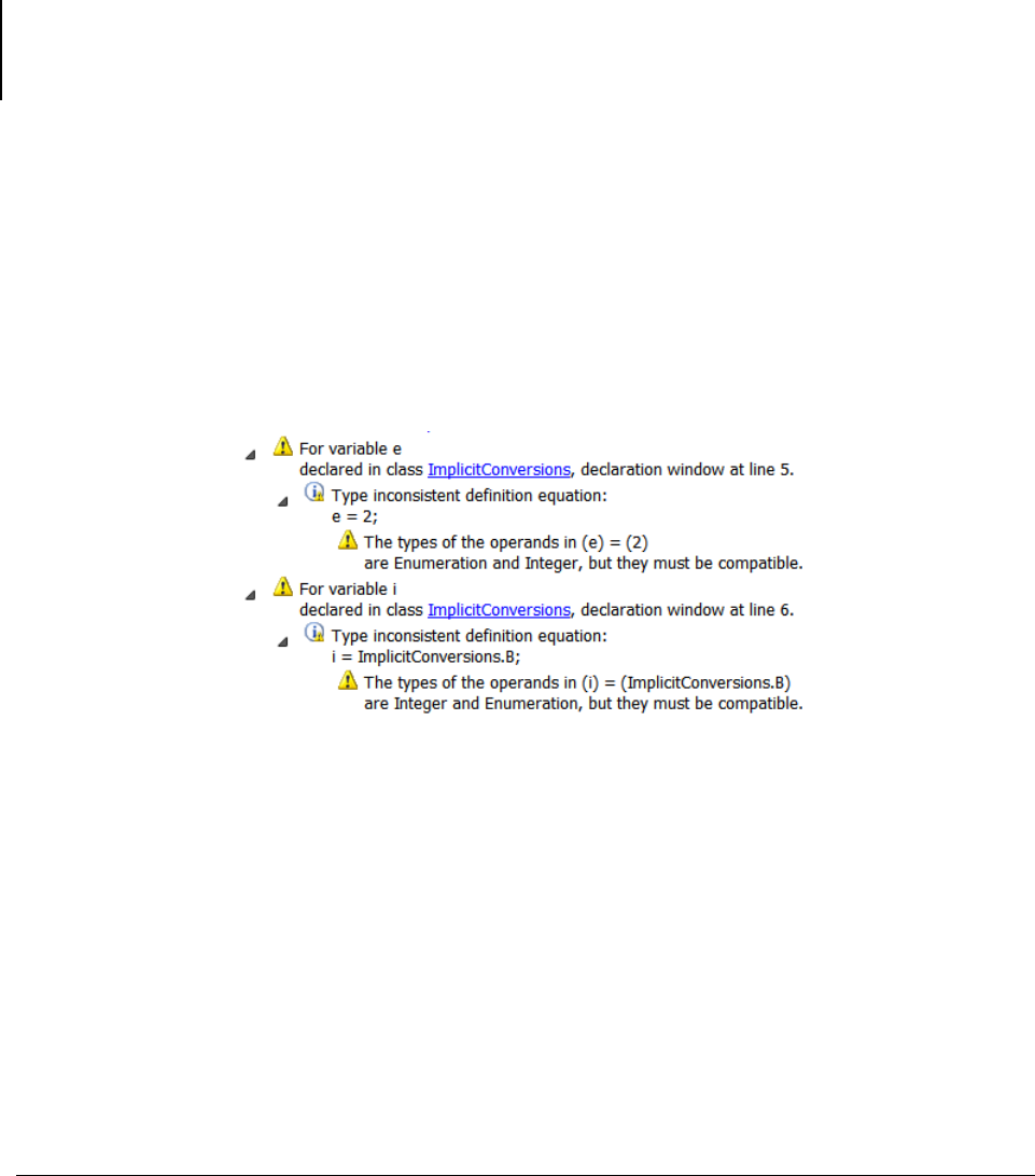
428
• Use enumeration literals.
• Declare arrays indexed by enumeration types.
• Convert enumeration values to strings.
• Convert from Integer to enumeration, e.g. Modelica.Blocks.Types.Smoothness(2) gives
Modelica.Blocks.Types.Smoothness.ContinuousDerivative.
Enumeration value conversion
Implicit conversion of integers to enumeration values and vice-versa are unsafe. For
example, the following model will result in translation warnings:
model ImplicitConversions
type E = enumeration(
A,
B);
output E e = 2;
output Integer i = E.B
end ImplicitConversions;
The warnings:
To safely convert an enumeration value to an integer or vice-versa, the integer or respective
enumeration type constructors can be used:
model ExplicitConversions
type E = enumeration(
A,
B);
output E e = E(2);
output Integer i = Integer(E.B)
end ExplicitConversions;
The usage of enumeration constructors to avoid warnings is highly recommended. In future
Dymola versions implicit integer to enumeration values might be errors, not just warnings.

8 ADVANCED MODELICA SUPPORT 429
8.7.8 Support of String variables in models
String variables can be used in models, not only in functions used in models and for
scripting. String variables in models are allocated with a maximum string length. It is
defined by the scripting variable Advanced.MaxStringLength with default=500. If
assignment to a model string variable fails due to too short string length, truncation is done
and a warning is given in the simulation log window.
8.7.9 Support of inner/outer components
In order to support inner/outer components some new annotations are supported (can also be
useful for other cases):
annotation (
defaultComponentName="world",
defaultComponentPrefixes="inner replaceable",
missingInnerMessage="No \"world\" component is defined. A
default world
component with the default gravity field will be used
(g=9.81 in negative y-axis). If this is not desired,
drag MultiBody.World into the top level of your model.",
8.7.10 Functions as formal input to functions
Functional input arguments to functions in order to e.g. pass criteria functions to generic
optimization functions are supported. This is useful for e.g. Design Optimization.
The following functionality is currently supported:
• Sending a function as an input argument to another function, e.g. function sin() as
argument.
• Calls through a functional input argument, e.g. integrand(x).
• Propagating a functional input argument, either directly, e.g. function
integrand(x), or with partial binding, e.g. function integrand(x=1).
• Partial interface functions.
• Functional input arguments to functions can be used interactive or in models.
8.7.11 Assert
In Modelica, an assertion that in short looks the following (for more information, see the
Modelica Language Specification version 3.3, section 8.3.7):
assert(condition, message, level=AssertionLevel.error);
where condition is a Boolean expression, message is a string expression and level is a
built-in enumeration with a default value. It can be used in equations or algorithms.
If the condition is true, message is not evaluated and the procedure call is ignored. If
condition evaluates to false, different actions is taken depending on the level input:

430
• Level=AssertionLevel.error. The current evaluation is aborted; message indicates
the cause of the error.
• Level=AssertionLevel.warning: The current evaluation is not aborted; message
indicates the cause of the warning.
8.7.12 Identifiers starting with underscore and
vendor-specific annotations
In general identifiers can start with underscore (although not recommended if not vendor-
specific annotations).
Modelica allows vendor-specific annotations. All Dymola specific annotations can be
preceded by __Dymola_ as specified in the Modelica language specification. The next
sections are examples of this.
8.7.13 Quoted identifiers containing dot supported
Quoted identifiers containing dot are now supported, including
• Class and component names
• Hierarchical modifiers
• Variable browser
• Import
• Derivative names
It is recommended to avoid quoted identifiers (with or without dot) for top-level classes; the
file names will not be nice.
8.7.14 Running a function before
check/translation/simulation
A model may specify that a function should be run before a component of the model is
checked, translated or simulated. This could be used to verify structural parameters or
external data before using them. The function to be called is specified in an annotation in
the following form:
model M
parameter String s="";
annotation(__Dymola_preInstantiate=MyPackage.foo(s));
end M;
Notes:
• This is only intended as a help and there is no absolute guarantee that this function will
be called. It is not intended for e.g. license-checking.
• Any parameters used must be possible to evaluate to literals.

8 ADVANCED MODELICA SUPPORT 431
• Any parameters used must be top-level parameters in the model, e.g. you cannot use
component.s.
• Conditional components first have their condition evaluated. If the condition is false the
component is not present and the __Dymola_preInstantiate function is not called.
8.7.15 Forcing translation of functions
By applying the annotation annotation(__Dymola_translate=true) to a function, a
translation for that function is forced. This speeds up the translation. The annotation can be
applied to both external and non-external functions.
8.7.16 Deprecation warnings
In Dymola 2018 the following language constructs generate warnings indicating future
deprecation:
• The usage of extends to constrain replaceable components; constrainedby should
be used instead.
• The usage of operator as an identifier name; since Modelica 3, operator is a keyword.
• The usage of the flow and stream prefix within short class definitions.
Note that Modelica 2 contains the above: using Modelica 2 will generate warnings when
used, due to this.
The warnings are displayed in the messages window, in the Syntax Error tab.
8.7.17 Licensing
Licensing of packages is supported. Please see chapter “Model Management”, section
“Encryption in Dymola”, sub-section “Licensing Libraries” for more information.
8.8 Symbolic Processing of Modelica Models
(This section, except “Handling of implicit constraints between dynamic variables”, is a
reprint from Handbook of Dynamic System Modeling 2007, chapter 36.4, by M. Otter, H.
Elmqvist and S. E. Mattson - courtesy of Taylor & Francis Group LCC – Books.)
The Modelica Language Specification (Modelica 2005) defines how a Modelica model shall
be mapped into a mathematical description as a mixed system of differential-algebraic
equations (DAE) and discrete equations with Real, Integer and Boolean variables as
unknowns. There are no general-purpose solvers for such problems. There are numerical
DAE solvers, which could be used to solve the continuous part. However, if a DAE solver is
used directly to solve the original model equations, the simulation will be very slow and
initialization might be not possible for higher index systems (see below). It is therefore
assumed that Modelica models are first symbolically transformed into a form that is better
suited for numerical solvers. In this section, the transformation techniques are sketched that

432
have been initially designed for the Dymola modeling language (Elmqvist 1978), further
developed in Omsim for the Omola language (Mattsson and Söderlind 1993) and in the
commercial Modelica simulation environment Dymola (Mattsson et. al. 2000, Dynasim
2006):
Dymola converts the differential-algebraic system of equations symbolically to ordinary
differential equations in state-space form, i.e. solves for the derivatives. Efficient graph-
theoretical algorithms are used to determine which variables to solve for in each equation
and to find minimal systems of equations to be solved simultaneously (algebraic loops). The
equations are then, if possible, solved symbolically or code for efficient numeric solution is
generated. Discontinuous equations are properly handled by translation to state or time
events as required by numerical integration routines.
8.8.1 Sorting and algebraic loops
The behavior of a Modelica model is defined in terms of genuine equations and a Modelica
translator must assign an equation for each variable as part of the sorting procedure, which
also identifies algebraic loops. To be able to process problems with hundred thousand
unknowns, the idea is to focus on the structural properties, i.e., which variables that appear
in each equation rather than how they appear. This information can be represented by a
“structure” Jacobian, where for a system of equations, h(x) = 0, each element i, j, is zero if
xj does not appear in the expression hi, otherwise it is one. The sorting procedure is to order
unknowns and equations to make the structure Jacobian become Block Lower Triangular,
BLT. A BLT partitioning reveals the structure of a problem. It decomposes a problem into
sub-problems, which can be solved in sequence. There are efficient algorithms, see, e.g.,
(Duff et.al. 1986), for constructing BLT partitions with diagonal blocks of minimum size
(with respect to permutation of equations and variables). Each non-scalar block on the
diagonal constitutes an algebraic loop. This sorting procedure identifies all algebraic loops
in their minimal form that is unique. The sorting procedure is done in two steps. The first
step is to assign each variable, xj, to a unique equation, hi = 0 such that xj appears in this
equation. It can be viewed as permuting the equations to make all diagonal elements of the
structure Jacobian non-zero. If it is impossible to pair variables and equations in this way
then the problem is structurally singular. The second step of the BLT partition procedure is
to find the loops in a directed graph that has the variable/equation pairs of the first step as
nodes. The basic algorithm was given by Tarjan (Tarjan 1972).
8.8.2 Reduction of size and complexity
A Modelica model has typically many simple equations, v1 = v2 or v1 = -v2 being the result
of connections. These are easy to exploit for elimination.
From the BLT partition it is rather straightforward to find unknowns that actually are
constant and can be calculated and substituted at translation. This may have considerable
impact on the complexity of the problem that has to be solved numerically. For example, a
multi-body component is developed for free motion in a 3-dimensional space. When using it
we connect it to other components and set parameters implying restrictions on its motion.
For example, it may be restricted to move in a plane. It means that coefficients in the
equations become zero and terms disappear. This in turn may make algebraic loops to
decompose into smaller loops or even disappear.

8 ADVANCED MODELICA SUPPORT 433
A linear small algebraic loop is solved symbolically. Otherwise code for efficient numeric
solution is generated. In order to obtain efficient simulation, it is very important to reduce
the size of the problem sent to a numerical solver. The work to solve a system of equations
increases rapidly with the number of unknowns, because the number of operations is
proportional to the cube of n, i.e. O(n3), where n is the number of unknowns. One approach
to reduce size is called tearing (Elmqvist and Otter 1994). Let z represent the unknowns to
be solved from the system of equations. Let z be partitioned as z1 and z2 such that
1 12
212
()
(, )
⋅=
=
Lz f z
0 fzz
where L is lower triangular with non-zero diagonal elements. A numerical solver needs then
only consider z2 as unknown. A numerical solver provides guesses for z2 and would like to
have the f2 residuals calculated for these guesses. When having a value for z2, it is simple to
calculate z1 from the first set of equations. Note, that it is very important to avoid divisions
by zero. The assumption that the diagonal elements are non-zero guarantees this. It is then
straightforward to calculate the f2 residuals. The z1 variables are in fact hidden from the
numerical solver. The general idea of tearing is to decompose a problem into two sets,
where it is easy to solve for the first set when the solution to the second set is known and to
iterate over the second set. The aim is of course to make the number of components of z2 as
small as possible. It is a hard (NP-complete) problem to find the minimum. However, there
are fast heuristic approaches to find good partitions of z. If the equations are linear, they can
be written as
1 21
1 22
= +
=++
Lz Az b
0 Bz Cz b
and it is possible to eliminate z1 to get Jz2 = b, where
1
1
21
−
−
J = C+ BL A
b = b +BL b
This may be interpreted as Gauss elimination of z1. The procedure may be iterated. Note,
since L is a lower triangular matrix, the determination of J and b is at most O(n2).
When solving a linear equation system, a major effort is to calculate an LU or QR
factorization of the Jacobian, J. Back substitutions are much less computationally
demanding. In some cases the elements of the Jacobian does not vary continuously with
time. The Jacobian may for example only change at events and it is then only necessary to
calculate and factorize it during event iterations and not during continuous simulation. In
other cases, it may depend only on parameters and constants and then it needs only to be
calculated once, at the start of a simulation.
When using Newton methods for non-linear equation systems, it is necessary to calculate
the Jacobian. If this is made numerically from residuals, then n residual calculations are
needed. Dymola provides analytic Jacobians. These are more accurate and much less
computationally demanding, because there are many common subexpressions to exploit.
Modelica provides facilities to provide derivatives also for external functions.

434
8.8.3 Index reduction
When solving an ordinary differential equation (ODE) the problem is to integrate, i.e. to
calculate the states when the derivatives are given. Solving a DAE may also include
differentiation, i.e. to calculate the derivatives of given variables. Such a DAE is said to
have high index. It means that the number of states needed for a model is less than the
number of variables appearing differentiated. The number of states is equal to the number of
independent initial conditions that can be imposed. Higher index DAEs are typically
obtained because of constraints between models. To support reuse, model components are
developed to be “general”. Their behavior is restricted when they are used to build a model
and connected to other components. Take as a very simple example two rotating bodies with
inertia J1 and J2 connected rigidly to each other. The angles and the velocities of the two
bodies should be equal. Not all four differentiated variables can be state variables with their
own independent start values. The connection equation for the angles, ϕ1 = ϕ2, must be
differentiated twice to get a relation for the accelerations to allow calculation of the reaction
torque.
The reliability of a direct numerical solution is related to the number of differentiations
needed to transform the system algebraically into ODE form. Modern numerical integration
algorithms for DAEs, such as used by most simulators, can handle systems where equations
needed to be at most differentiated once. However, reliable direct numerical solutions for
non-linear systems are not known if two or more differentiations are required. Furthermore,
if mixed continuous and discrete systems are solved, the hybrid DAE must be initialized at
every event instant. In this case, it is in general not sufficient to just fulfill the original DAE.
Instead, also some differentiated equations have to be fulfilled, in order that the
initialization is consistent. Direct numerical methods have problems at events to determine
consistent restart conditions of higher index systems.
Higher index DAEs can be avoided by restricting how components may be connected
together and/or include manually differentiated equations in the components for the most
common connection structures. The drawback is (1) physically meaningful component
connections may no longer be allowed in the model or (2) unnecessary “stiff” elements have
to be introduced in order that a connection becomes possible. For example, if a stiff spring
is introduced between the two rotating bodies discussed above, the problem has no longer a
higher index.
Since most Modelica libraries are designed in a truly object-oriented way, i.e., every
meaningful physical connection can also be performed with the corresponding Modelica
components, this leads often to higher index systems, especially in the mechanical and
thermo-fluid field. Also modern controllers based on non-linear inverse plant models lead to
higher index DAEs (Looye et.al. 2005) and can be conveniently treated with Dymola.
Dymola transforms higher index problems by differentiating equations analytically. The
standard algorithm by Pantelides (Pandelides 1988) is used to determine how many times
each equation has to be differentiated. The algorithm by Pantelides is based on the structure
of the equations. It means that there are examples where it does not give the optimal result
(Reissig, Martinsson and Barton, 1999). However, the practical experience is very good.
Moreover, for large problems a structural analysis is the only feasible approach. Selection of
which variables to use as state variables is done statically during translation or in more
complicated cases during simulation with the dummy derivative method (Mattsson and
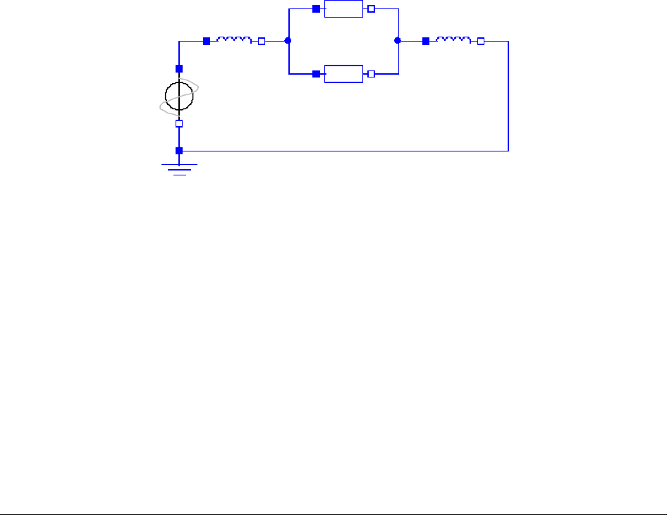
8 ADVANCED MODELICA SUPPORT 435
Söderlind 1993, Mattsson et.al. 2000). Let us make the example above a bit more realistic
and put a gearbox with fixed gear ratio n between the two bodies. Dymola differentiates the
position constraint twice to calculate the reaction torque in the coupling, and it is sufficient
to select the angle and velocity of either body as state variables. The constraint leads to a
linear system of simultaneous equations involving angular accelerations and torques. The
symbolic solution contains a determinant of the form “J1 + n2J2”. Dymola thus automatically
deduces how inertia is transformed through a gearbox.
Handling of implicit constraints between potential state variables
(This section is not included in the original article; it is later improvement in Dymola 7.1
and later.)
The index reduction algorithm basically focuses on the structure of the equations. The
practical experience of this approach is good. However, there are examples were the results
is not satisfactory. Such examples appear typically in models of electrical circuits.
Consider the example
The model has two potential state variables, namely the currents through the inductors: L1.i
and L2.i. However, they cannot be selected as states simultaneously because these currents
must be equal, L1.i = L2.i. In this example it is easy to see for a human being. Unfortunately,
the original Pantelides’s algorithm will not detect this constraint, because it is too implicit in
the model equations. After alias elimination of the connector variables, the zero sum current
equations for the connections between the inductors and the resistors are
L1.i = R1.i + R2.i
L2.i = -R1.i – R2.i
Assuming L1.i and L2.i to be states, the structural analysis of Pantelides’s algorithm
indicates that R1.i and R2.i can be solved from these two equations. However, this is not
true and the simulation will fail because the system actually is singular from that respect. It
is easy to see by just adding the two equations giving L1.i = L2.i.
The improved support of index reduction looks for such kinds of implicit constraints
between potential state variables and manipulates the equations to make them explicit.
sineVoltage
+ -
R=R
R1
R=R
R2
ground
L=L
L1
L=L
L2
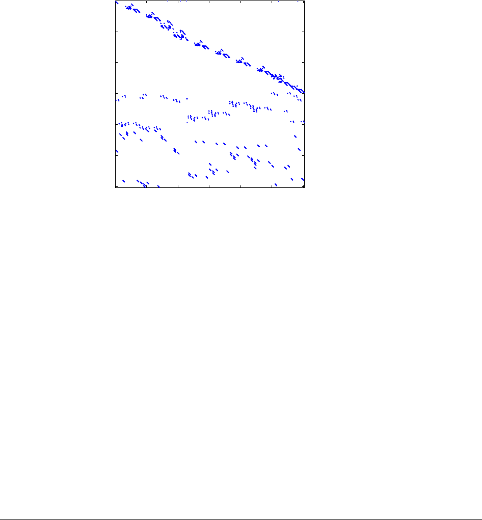
436
8.8.4 Example
To illustrate how Dymola’s symbolic processing reduces the size and complexity we will
show the structure Jacobian at different stages when translating a mechanical model with a
kinematic loop.
0200 400 600 800 1000 1200
0
200
400
600
800
1000
1200
nz = 3995
The structure Jacobian
of the original model.
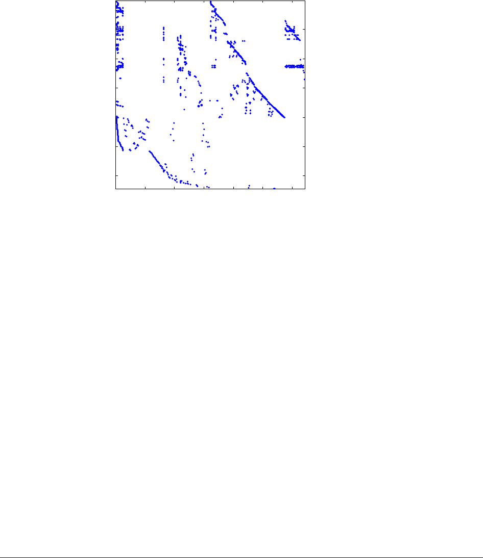
8 ADVANCED MODELICA SUPPORT 437
The upper figure above shows the structure Jacobian of the original model. There are about
1200 unknown variables and equations. Each row corresponds to an equation and each
column corresponds to a variable. A blue marker indicates that the variable appears in the
equation. There are 3995 markers. The upper half of the matrix has a banded structure.
These equations are the equations appearing in the component models and such equations
refer typically only to the local variables of the component. The equations in the lower part
are equations deduced from the connections, which includes references to variables of two
or more components.
The lower figure above shows the structure of the problem after exploitation of simple
equations to eliminate alias variables and utilizing zero constants. The number of unknowns
is reduced from about 1200 to 330.
050 100 150 200 250 300
0
50
100
150
200
250
300
nz = 1017
The structure Jacobian
after elimination of
alias variables.
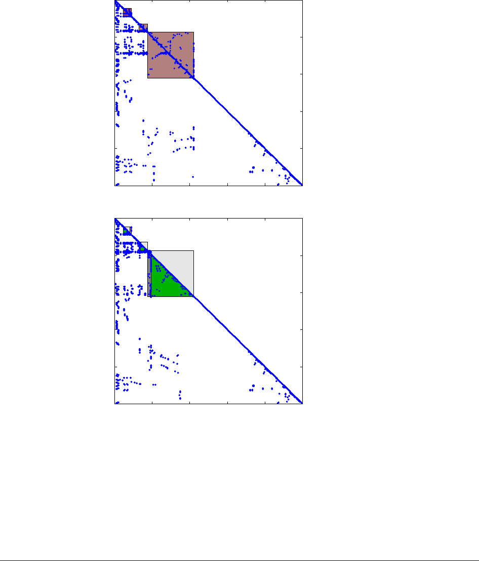
438
Then equations are differentiated to reduce the DAE index and states are selected. After
some further simplifications the number of unknowns is reduced to 250. A BLT partitioning
reveals that there are 3 algebraic loops as indicated by the upper figure above.
The lower figure above shows the structure after tearing. The first algebraic loop is a
nonlinear loop with 12 unknowns. This loop includes the positional constraints of the
kinematics loop. The tearing procedure reduces the number of iteration variables to 2. This
is illustrated by turning the eliminated part from grey to green. The second loop includes the
velocity constraints due to the kinematic loop. It means that this loop includes the equations
050 100 150 200 250
0
50
100
150
200
250
nz = 895
050 100 150 200 250
0
50
100
150
200
250
nz = 916
The BLT partitioning.
The structure after
tearing.

8 ADVANCED MODELICA SUPPORT 439
of the positional constraints differentiated. This loop has also 11 unknowns, but it is linear.
The remaining two by two system can be solved symbolically or numerically. The third
loop includes acceleration and force/torque as unknown variables. The loop is linear and has
62 unknowns and the tearing procedure eliminates 57 so a linear 5 by 5 system remains to
be solved numerically.
8.8.5 References
Duff, I.S, A.M. Erisman, and J.K. Reid. 1986. Direct Methods for Sparse Matrices,
Clarendon Press, Oxford.
Dynasim. 2006. Dymola Version 6.0. Dynasim AB, Lund, Sweden. Homepage:
http://www.dynasim.se/.
Elmqvist Hilding. 1978. A Structured Model Language for Large Continuous Systems.
Dissertation. Report CODEN:LUTFD2/(TFRT--1015), Department of Automatic Control,
Lund Institute of Technology, Lund, Sweden, 1978.
Elmqvist, H., and M. Otter. 1994. Methods for Tearing Systems of Equations in Object-
Oriented Modeling. Proceedings ESM'94, European Simulation Multiconference, Barcelona,
Spain, June 1-3, pp.326--332.
Elmqvist, H., S. E. Mattsson, and M. Otter. 2001. Object-Oriented and Hybrid Modeling in
Modelica. Journal Europeen des Systemes Automatises, 35, pp. 1 a X.
Looye, G., M. Thümmel, M. Kurze, M. Otter, and J. Bals. 2005. Nonlinear Inverse Models
for Control. Proceedings of the 4th International Modelica Conference, Hamburg, ed. G.
Schmitz,.
http://www.modelica.org/events/Conference2005/online_proceedings/Session3/Session3c3.
pdf
Mattsson, S. E., and G. Söderlind. 1993. Index reduction in differential-algebraic equations
using dummy derivatives. SIAM Journal of Scientific and Statistical Computing, Vol. 14 pp.
677-692.
Mattsson, S. E., H. Olsson and H. Elmqvist. 2000. Dynamic Selection of States in Dymola.
Proceedings of the Modelica Workshop 2000. pp. 61-67.
http://www.modelica.org/Workshop2000/papers/Mattsson.pdf.
Modelica. 2005. Modelica® - A Unified Object-Oriented Language for Physical Systems
Modeling - Language Specification, Version 2.2.
http://www.Modelica.org/Documents/ModelicaSpec22.pdf.
Pantelides C.. 1988. The consistent initialization of differential-algebraic systems. SIAM
Journal of Scientific and Statistical Computing, pp. 213-231.
Reissig, G., W. S. Martinsson, and P. I. Barton . 1999. Differential-Algebraic equations of
index 1 may have an arbitrarily high structural index. SIAM J. Sci. Comp.
Tarjan, R.E. 1972. Depth First Search and Linear Graph Algorithms, SIAM J. Comput. 1,
pp. 146-160.

440
8.9 Symbolic solution of nonlinear equations
in Dymola
8.9.1 Introduction
In the general case it is not possible to solve a nonlinear equation analytically. However,
Dymola supports some special cases:
1. Solving a nonlinear equation with single appearance of the unknown by applying
function inverses
2. Solving a nonlinear equation with special patterns for the unknown such as abs(w)*w
3. Partitioning of a system of equations into a linear and a nonlinear (one variable) part
4. Using min and max values to evaluate if-conditions
These items will be discussed in turn.
8.9.2 Solving a nonlinear equation with single
appearance of the unknown by applying
function inverses
A single appearance of the unknown allows the technique of successive inverses to be
applied. It requires the inverses of the appearing functions to be known. The basic idea is
simple. However, the issues of nonexistent or multiple solutions need to be considered.
When translating a model, Dymola sorts the equations to determine which variable to solve
for in each equation. The result of the sorting procedure of the initialization problem and the
simulation problem is a sequence of sub-problems which can be solved in turn. The feature
to solve a nonlinear equation symbolically is useful when such a sub-problem has one
unknown, x, that appears nonlinearly in the equation. You may say that the computational
causality of the initialization or simulation problem requires “inversion” of the equation.
The feature to solve a nonlinear equation symbolically is activated when Dymola finds that
solving a sub-problem with one unknown is a nonlinear problem. If Dymola is not able to
solve the equation symbolically, then code is generated for numerical solution as previously.
Solving nested functions
Consider the equation
f1(f2(x,v), v) = f3(v);
Let x denote the scalar real variable to be solved for and let the vector v denote the
remaining appearing variables which are considered to be known variables. When solving
nested functions, the approach is to introduce an auxiliary variable, w, to decompose the
problem as
f1(w, v) = f3(v);
f2(x, v) = w;

8 ADVANCED MODELICA SUPPORT 441
where the first equation is used to solve for w and if successful, then the solution procedure
is applied recursively on the second equation to solve for x. This includes also the functions
+, -, * and /. For example, let f1 in the example above be +, implying the problem
f2(x,v) + v = f3(v);
The decomposition becomes
w + v = f3(v)
f2(x, v) = w;
Below we will focus on solving f(x) = v.
No solution exists
When solving an equation
f(x) = v;
it is important to check that the equation has a solution. It is easy to produce false solutions.
Consider the equation
sqrt(x) = v;
It has the unique solution x = v*v when v ≥ 0. However, when v < 0, there is no solution.
Note, that the right hand side of the equation x = v*v is well-defined also for v < 0, but the
result is not a solution to the original equation. Thus Dymola transforms the equation as
assert(v >= 0, "Cannot solve sqrt(x)=v when v < 0");
x = v*v;
If f(x) is not onto the real axis (the range of f(x) is not the whole real axis), it is necessary to
add asserts to check if v belongs to the range of f. However, sometimes the check can be
deferred, because calculating the “inverse” will fail. Consider the equation
exp(x) = v;
It has the unique solution x = ln(v) when v > 0, but no solution when v ≤ 0, so Dymola
solves it as
x = ln(v)
If v <= 0, the failure to calculate ln(v) will trig an assertion and stop the simulation.
Multiple solutions
The equation
f(x) = v;
may have multiple solutions. As an example, consider the equation
abs(x) = v;
First, it has no solution if v < 0, so it is necessary to generate an assert for that. Second,
when v > 0, there are two solutions:
x = v;
x = -v;

442
A numerical solver needs a start or guess value and it then hopefully returns the solution
closest to the guess value. This is most critical during initialization and during event
iteration, because v may then jump. During continuous time integration, v shall change
continuously and the resulting solution x shall be smooth. Dymola’s approach is to mimic
this behavior. The solution looks as
assert(v >= 0, "Cannot solve abs(x)=v when v < 0");
x := if x>= 0 then v else –v;
Supported functions
Modelica and Modelica.Math functions
Dymola currently support symbolic inversion of the following Modelica functions
• abs
• noEvent, smooth
• x^a, a^x, sqrt
and the following Modelica.Math functions
• sin, cos, tan
• exp, ln, log10
• asin, acos, atan
Annotations
Functions may have an additional annotation to define an inverse of the function:
function f1
input Real x;
input Real y;
input Boolean b[4,3];
output Real z;
annotation(__Dymola_inverse(y=f2(z,x,b));
algorithm
..
end f1;
The meaning is that function "f2" is an inverse to the function "f1" where the previous
output "z" is now an input and the previous input "y" is now an output.
The inverse requires that for all valid values of the input arguments of f2(z,x,b) and y being
calculated as y := f2(z,x,b) implies the equality z = f1(x,y,b).
Function "f1" can have any number and types of arguments. The current restriction is that
both "f1" and "f2" must have exactly one scalar Real output argument and that "f2" must
have exactly the same arguments as "f1", but the order of the arguments may be permuted.
Deactivation of supported functions
The feature is by default activated. It can be disabled by setting the flag
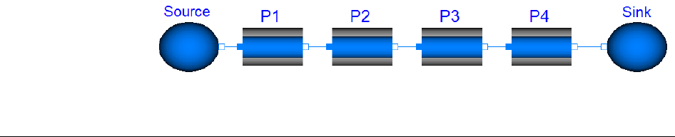
8 ADVANCED MODELICA SUPPORT 443
Advanced.SolveNonlinearEquationSymbolically = false;
8.9.3 Solving a nonlinear equation with special
patterns for the unknown
Above it was assumed that the unknown variable to solve for only appeared once. However,
the feature to solve nonlinear equations also supports some special patterns
x*x = v;
x*abs(x) = v; abs(x)*x = v
sign(x)*sqrt(abs(x)) = v; sqrt(abs(x))*sign(x)
The two last equations may appear in modeling of the pressure drop, dp, characteristics with
respect to the mass flow rate w:
dp = c*w*abs(w);
w = sign(dp/c)*sqrt(abs(dp/c);
The recursive scheme discussed above also supports the case when the unknown parts are
expressions depending on x, for example
f(x, v)*f(x, v) = v;
as long as Dymola can establish that the two factors are equal expressions.
The equation x*x = v; is solved in a similar way as abs(x) = v:
assert(v>=0);
x = if x >= 0 then sqrt(v) else –sqrt(v)
The equations x*abs(x) = v; and abs(x)*x = v have the solution
x = sign(v)*sqrt(abs(v))
The equations sign(x)*sqrt(abs(x)) = v; and sqrt(abs(x))*sign(x) = v have the solution
x = v*abs(v)
8.9.4 Partitioning of a system of equations into a
linear and nonlinear (one variable) part
When modeling flow systems with a number of flow elements (pipes, ducts, valves etc.) in
series there will typically be a nonlinear system of equations to solve for flow rate.
Introduction of storage elements will break such loops. However, there is the cost of extra
dynamics. Moreover, making the volumes small makes the problem stiff.
Consider the example below with four flow elements connected in series between a source
and a sink with given pressures.

444
The pressure drop, dp, of a flow element is modeled by quadratic characteristics with
respect to the mass flow rate m_flow as
dp = noEvent(c*m_flow*abs(m_flow));
where c is independent of dp and m_flow, but it may depend on physical dimensions of the
component. After elimination of simple equations the simulation problem includes a
nonlinear system of equations with 8 unknowns
P1.dp, P1.m_flow, P2.dp, P2.port_a.p, P3.dp, P3.port_a.p, P4.dp,
P4.port_a.p
and the equations
P4.dp = P4.c*P1.m_flow*abs(P1.m_flow);
P4.dp = P4.port_a.p-Sink.port.p;
P3.dp = P3.port_a.p-P4.port_a.p;
P2.dp = P2.c*P1.m_flow*abs(P1.m_flow);
P2.dp = P2.port_a.p-P3.port_a.p;
P1.dp = Source.port.p-P2.port_a.p;
P1.dp = P1.c*P1.m_flow*abs(P1.m_flow);
P3.dp = P3.c*P1.m_flow*abs(P1.m_flow);
The algebraic loop is nonlinear only because of the expression
P1.m_flow*abs(P1.m_flow);
Moreover, P1.m_flow appears in no other ways in the equations of the algebraic loops. By
substituting all appearances of the expression P1.m_flow*abs(P1.m_flow) by w_expr, the
problem decomposes into two sub-problems
• A linear system of equations that is independent of P1.m_flow.
P4.dp = P4.c* w_expr;
P4.dp = P4.port_a.p-Sink.port.p;
P3.dp = P3.port_a.p-P4.port_a.p;
P2.dp = P2.c* w_expr;
P2.dp = P2.port_a.p-P3.port_a.p;
P1.dp = Source.port.p-P2.port_a.p;
P1.dp = P1.c*P1 w_expr;
P3.dp = P3.c* w_expr
• A nonlinear equation for P1.m_flow
P1.m_flow*abs(P1.m_flow) = w_expr;
This decomposition is valuable, because the nonlinearity has been reduced to one equation;
to solve a scalar nonlinear equation. Dymola manipulates the two subsystems in the usual
way and solves the linear system symbolically.
The feature to solve nonlinear equations also supports support solving a nonlinear equation
with single appearance of the unknown by applying function inverses. It is also able to
handle some special patterns
x*x = v;
x*abs(x) = v; abs(x)*x = v
sign(x)*sqrt(abs(x)) = v; sqrt(abs(x))*sign(x)

8 ADVANCED MODELICA SUPPORT 445
The scheme discussed supports the case when the unknown parts are expressions depending
on x, for example
f(x, v)*f(x, v) = v;
as long as Dymola can establish that the two factors are equal expressions.
The nonlinear equation for P1.m_flow
P1.m_flow*abs(P1.m_flow) = w_expr;
is solved symbolically as
P1.m_flow :=
noEvent(sign(w_expr)*sqrt(abs(w_expr)));
8.9.5 Using min and max values to evaluate if-
conditions
An if-then-else expression may cause the appearances of algebraic loops. A typical case is
flow systems. The model components are built to handle either flow direction as well as
reversing flows. It means that the equations include if-then-else expressions depending on
the actual flow direction:
d = if m_flow >= 0 then medium_a.d else medium_b.d;
H_flow = semiLinear(m_flow, medium_a.h, medium_b.h);
According to definition of the Modelica function semiLinear, the last equation means
H_flow = if m_flow >= 0 then m_flow*medium_a.h
else m_flow*medium_b.h;
If we are simulating a flow system at normal operation, the flow direction shall not change
and it is known, say m_flow >= 0. By using this information it is possible to significantly
simplify the equations to
d = medium_a.d;
H_flow = m_flow*medium_a.h;
Please, note that neither medium_b.d nor medium_b.h appear in the resulting equations. The
elimination of them may make an algebraic loop decrease in size or even disappear.
At translation Dymola of course evaluates all constant conditions and simplifies the
equations accordingly. In this case Dymola is dealing with relations where the expressions
of the relations may be time varying to see if it nevertheless is possible to evaluate the
condition by exploiting the values of the min and max attributes of variables. To specify that
the flow direction is known, m_flow >= 0, is done by setting the min value of m_flow to 0,
i.e., m_flow(min=0).
If the assumption that m_flow >= 0 turned out to be false, the normal assert that the value
must not be less than min will be triggered.
This feature may be disabled by setting the flag
Advanced.UseMinMaxToSimplify = false

446
9 APPENDIX - MIGRATION

9 APPENDIX - MIGRATION 449
9 Appendix — Migration
9.1 Migrating to newer libraries
Dymola supports migration of models using one set of model libraries to another set of
model libraries with model components of similar structure, but for example having other
class names or different connector names or parameter names. Dymola has commands to
build up internal translation tables which will take effect when a model library or a model
component is loaded. These commands can be collected in a script allowing all models that
use a specific library to upgrade to the new one.
The feature was originally designed to convert models to the Modelica Standard Library,
and it has been updated to handle conversion from version 1 and 2 of the Modelica Standard
Library (primarily vectorization of blocks-library), and version 2 and 3 (primarily removing
SignalType and replacing some modifier equations by normal equations).
Dymola supports multiple upgrade of libraries, see section “Upgrading models and libraries
to a new library version” starting on page 465.
9.1.1 How to migrate
Assume that we would like to migrate myModel that uses a package OldLibrary to exploit a
NewLibray. In many cases, in particular when releasing a new version of a library, the

450
library developer will provide a conversion script, which specifies the translation from the
old version to the new version of the library.
Assume that the model is stored in a file named myModel.mo. It is advisable to also have a
backup copy of the file. Assume also that a specification of the translation when migrating
from using OldLibrary to using NewLibrary is specified in the script file Convert.mos.
To migrate myModel proceed as follows.
1. Start with a fresh Dymola.
2. Use the command File > Open… to open the file NewLibrary.
3. In the Dymola main window, in Simulation mode, use the Run Script button to run
the script Convert.mos.
4. Use the command File > Open… to open the file myModel.mo
5. Perform a check using the command Edit > Check.
6. Hopefully there is no error message and the model can be saved. The conversion is done.
7. In case of error message consult the next two subsections on specifying translation and
building a script file.
8. After a migration, the model shall of course be tested and it shall be checked that it gives
the same simulation result as the old one.
9.1.2 Basic commands to specify translation
The command to build the translation tables are
convertClass("oldClass", "newClass");
convertClassIf("OldClassName","para","val","NewClassName");
convertElement("oldClass", "oldElement", "newElement");
convertModifiers("oldClass", oldParameterBindings,
newParameterBindings);
convertClear();
convertClass
The command
convertClass("oldClass", "newClass");
builds conversion tables to be applied on extends clauses and type declarations. As an ex-
ample consider:
convertClass("DriveTwoCut",
"Modelica.Mechanics.Rotational.Interface.Compliant");
All components of type DriveTwoCut or classes that contain extends DriveTwoCut will be
converted such that they refer to class Modelica.Mechanics.Rotational.Interface.Compliant
instead.
Conversion is also applied on hierarchical names. For example

9 APPENDIX - MIGRATION 451
convertClass("Modelica.Rotational1D","Modelica.Rotational")
will take effect on Modelica.Rotational1D.Clutch and give Modelica.Rotational.Clutch.
Modelica’s normal vectorization applies for convertClass, which means that it is possible to
let the arguments be vectors of Strings. For example,
convertClass({"oldClass1", "oldClass2"},
{"newClass1", "newClass2"});
is equivalent to
convertClass("oldClass1", "newClass1");
convertClass("oldClass2", "newClass2");
Using convertClass for converting emulated enumerations
The convertClass can be used for converting an emulated enumeration (using package
constants) to a proper enumeration. As an example consider the following emulated
enumeration in Modelica Standard Library version 2:
package RotationTypes
extends Modelica.Icons.Enumeration;
constant Integer RotationAxis=1;
constant Integer TwoAxesVectors=2;
constant Integer PlanarRotationSequence=3;
type Temp “Temporary type of RotationTypes"
extends Modelica.Icons.TypeInteger;
end Temp;
end RotationTypes;
This can now be replaced by a proper enumeration:
type RotationTypes = enumeration(
RotationAxis,
TwoAxesVectors,
PlanarRotationSequence);
The enumeration automatically handles the constants, and to also convert the Temp-part it is
only necessary to add:
convertClass("…RotationTypes.Temp","…RotationTypes");
The “…” shall be replaced by the proper path to RotationTypes.
Using convertClass for adding component prefixes
In some cases elements of one class should be converted to inner elements of another class,
as when converting InertialSystem of ModelicaAdditions to World in Modelica Standard
Library version 2. This is done by prefixing the new class-name by “inner“, followed by a
space and then the new class-name:
convertClass("ModelicaAdditions.MultiBody.Parts.InertialSystem,
"inner Modelica.Mechanics.MultiBody.World world");
Other allowed prefixes are “outer “, “parameter”, and “constant”.

452
convertClassIf
It is possible to optionally convert components to a different class using
convertClassIf("OldClassName","para","val","NewClassName");
If the parameter has the given value the component will be converted to this class, and the
modifier will be removed. The modifier will otherwise be kept (thus the safe option for a
Boolean parameter is give one conversion for true and another for false). Another variant is
to base it on whether a connector is connected:
convertClassIf("OldClassName","connector","connect",
"NewClassName");
The normal conversion will be used if these conditions are not satisfied and all conversion
of elements, modifiers is common for these cases.
convertElement
The command
convertElement("oldClass", "oldElement", "newElement");
converts references to elements (connectors, parameters and local variables of classes) in
equations, connections, modifier lists etc. The class name of the component is still convert-
ed according to convertClass.
The conversion uses the model structure after conversion, thus it correctly detects base-
classes among the models you convert. However, only the new library is used, thus any in-
heritance used in the old library is lost. It means, for example, if a connector was renamed in
base-class conversion of that connector name must be specified for all models in the old
library extending from base-class. By using vector arguments to the conversion functions it
is only necessary to list the classes once for each renamed element.
Let us illustrate by an example. Assume that we have a drive train library, where there is a
partial class DriveTwoCut specifying two connectors pDrive and nDrive. The new library
has a similar class TwoFlanges defining two connectors flange_a and flange_b. We thus
give the commands
convertClass("DriveTwoCut", "TwoFlanges");
convertElement("DriveTwoCut", "pDrive", "flange_a");
convertElement("DriveTwoCut", "nDrive", "flange_b");
Assume that the old library contains the models Shaft and Gear, which are to be converted
as Inertia and IdealGear, respectively:
convertClass("Shaft", "Inertia");
convertClass("Gear", "IdealGear");
Assume that Shaft and Gear extend from DriveTwoCut. Unfortunately, there will be no
translation of references in, for example, connect statements to their connectors pDrive and
nDrive, since the conversion uses the model structure after conversion. To have a proper
translation, we need also to specify
convertElement({"Shaft", "Gear"}, "pDrive", "flange_a");
convertElement({"Shaft", "Gear"}, "nDrive", "flange_b");

9 APPENDIX - MIGRATION 453
where the vectorization allows a compact definition.
The convertElement command can also be used when a parameter is renamed. For more
complex reparameterizations the command convertModifiers is useful.
convertModifiers
The command
convertModifiers("oldClass", oldParameterBindings,
newParameterBindings);
specifies how parameter bindings given in modifiers are to be converted. The argument old-
ParameterBindings is a vector of strings of the form “oldParameter=defaultValue”, and the
argument newParameterBindings is a vector of strings of the type “newParameter=expres-
sion”. To use the value of an old parameter in the new expression use %oldParameter%
As an example, assume that in the old model Clutch that the viscous friction coefficient mue
is given as
mue = mueV0 + mueV1*abs(wrel)
where mueV0 and mueV1 are parameters declared in Clutch as
parameter Real mueV0 = 0.6;
parameter Real mueV1 = 0;
The model Clutch of the new model library uses linear interpolation with respect to the rel-
ative velocity, wrel, with a parameter mue_pos to define the interpolation table
parameter Real mue_pos[:, :] = [0, 0.5];
The original mue-equation is linear and one way of specifying a linear interpolation table is
to compute its value for two arbitrary velocities. The model requires that the first velocity is
zero, with mue=mueV, and for the other value velocity we use velocity one, with
mue=mueV0 + mueV1. Thus at translation we would like to obtain a new modifier
mue_pos = [0, value-of-mueV0;
1, value-of-mueV0 + value-of-mueV1];
This is obtained by
convertModifiers("Clutch",{"mueV0=0.6","mueV1=0"},
{"mue_pos=[0,%mueV0%;1,%mueV0%+%mueV1%]}");
Example, the declarations in the old model
Clutch c1(mueV0=0.4,mueV1=0.1)
Clutch c2(mueV0=2*p);
are converted to
Modelica.Mechanics.Rotational.Clutch
c1(mue_pos = [0,(0.4); 1,(0.4)+(0.1)]);
Modelica.Mechanics.Rotational.Clutch
c2(mue_pos=[0,(2*p); 1,(2*p)+(0)]);

454
Note that since c2 did not specify a value for mueV1 the conversion used the default value.
The substitution automatically adds parenthesis for the substituted arguments, thus avoiding
the need for parenthesis in macros that are familiar to a C programmer. The parentheses are
sometimes redundant and can be removed by going to the parameter dialogs of the corre-
sponding components.
Prefer convertElement over convertModifiers even for parameters, and only use convert-
Modifiers when there is a need for more than a one-to-one conversion of parameters.
Using convertModifiers for replacing modifiers by equations
A special case is converting modifier-equations (for BaseProperties-members) to normal
equations when converting to Modelica 3. This is handled by:
convertModifiers("…BaseProperties",{"p", "T" ,…},
{"equation"});
Using convertModifiers for removing vectorization
The special case of removing vectorization of a block (as was done between version 1 and 2
of Modelica) has two cases, either the size is explicitly given as a size-parameter or
implicitly by the size of a number of a vector-parameters. The first case is handled by
conversion of the size-parameter to the special value “size” – where a value different from
one indicates that the conversion will replace the block by an array of appropriate size:
convertModifiers("Modelica.Blocks.Math.Sin",{"n=1"},
{"size=%n%"});
convertElement({"Modelica.Blocks.Math.Sin", "outPort ", "y");
convertElement({"Modelica.Blocks.Math.Sin", "inPort ", "u");
The other case is handled by converting each vector-parameter to a scalar, and in case any
of them is a vector of length different from one the block is replaced by a vector of blocks.
convertModifiers("Modelica.Blocks.Math.Gain",
{"k={1}"},
{"k=scalar(%k%)"});
convertElement({"Modelica.Blocks.Math.Sin",
"outPort.signal", "{y}");
convertElement({"Modelica.Blocks.Math.Gain", "outPort", "y");
convertElement({"Modelica.Blocks.Math.Gain", "inPort", "u");
convertElement({"Modelica.Blocks.Math.Gain", "outPort.signal",
"{y}");
The conversion of outPort.signal is used in case anyone used this hierarchical name.
This will convert
Modelica.Blocks.Math.Sin sin1(n=1);
Modelica.Blocks.Math.Sin sin2(n=2);
Modelica.Blocks.Math.Gain gain1(k={4});
Modelica.Blocks.Math.Gain gain2(k={2,3});
To

9 APPENDIX - MIGRATION 455
Modelica.Blocks.Math.Sin sin1;
Modelica.Blocks.Math.Sin sin2[2];
Modelica.Blocks.Math.Gain gain1(k=4);
Modelica.Blocks.Math.Gain gain2[2](k={2,3});
Simplifying the result of convertModifiers
In some cases the result of conversion will be a large expression involving several package
constants/enumerations. This can be simplifying by adding a fourth argument with value
true to convertModifiers. An example will be converting initType for the rotational inertia
of Modelica Standard Library version 2.1 to fixed-modifiers for the attributes (and replacing
the phi_start by a start-value modifier):
convertModifiers("…Inertia",{"initType"}, {"phi.fixed=
if(%initType%==…InitialState or %initType%==
…InitialAngle or +%initType%==…InitialAngleAcceleration or
%initType%==…InitialAngleSpeedAcceleration) then true else
false",
"w.fixed=if (%initType%==…SteadyState or
%initType%==…InitialState or %initType%==…InitialSpeed or
%initType%==…InitialSpeedAcceleration or
%initType%==…InitialAngleSpeedAcceleration) then true else
false",
"a.fixed=if (%initType%==…SteadyState or
%initType%==…InitialState or
%initType%==…InitialAcceleration or
%initType%==…InitialAngleAcceleration or
%initType%==…InitialSpeedAcceleration or
%initType%==…InitialAngleSpeedAcceleration) then true else
false"}, true);
convertModifiers("…Inertia",{"phi_start"},{"phi.start=%phi_star
t%"});
The additional true-argument ensures that the result of the conversion of
Inertia inertia(
initType=Modelica.Mechanics.Rotational.Types.Init.SteadyState,
phi_start=1);
is just
Inertia inertia(
a(fixed=true),
phi(fixed=false, start=1),
w(fixed=true));
Note that the simplification applies both to the expressions that are part of convertModifiers,
and also to the original expression. This explains why the conversion is not the default, but
it is advisable for large expressions.
Removing modifiers with convertModifiers
In some cases the modifier is just removed. This can be handled by converting the modifier
to an empty list of modifiers. In some cases this applies to a common class where it would
be tedious to explicitly list all conversion where the class is used, and in those cases one can

456
use a fourth argument to convertModifiers to force the conversion to be applied in other
cases.
convertModifiers("…RealInput",
{"SignalType"}, fill("",0), true);
In this case all SignalType modifiers for RealInput components are removed.
convertClear
The command convertClear() clears the translation tables.
9.1.3 How to build a convert script
In order to convert a model using one library to another it is recommended to begin con-
structing a conversion script for the library. Even if the script is not complete after
converting one model it can be reused for the next model, and only amend it with additional
lines for the additional library components in that model. If a library developer restructures
a Modelica library, it is recommendable to construct such a script.
Below it is explained how to construct a convert script and how to amend it for additional
models. For clarity assume that we would like to convert a drive train model, myOldModel,
that uses components in the model library "Drive Trains" to a model, myNewModel that in-
stead uses the components in the library Modelica.Mechanics.Rotational.
1. Copy myOldModel.mo to myNewModel.mo.
2. Make a local conversion script, say Convert.mos. Depending on what you are converting
start as follows:
a. If you have a script for converting similar models: Use that as starting point, and at
the end add the following lines (and remove similar ones):
openModel("myNewModel.mo");
checkModel("myModel");
b. If you are starting from scratch, use the following as a template:
clear
// Start
//
// End
openModel("myNewModel.mo");
checkModel("myModel");
3. Converting class names.
a. In the Dymola main window select File > Clear Log and then use the command
button Run Script to run the script file Convert.mos.
b. There will be error messages such as Error: Component type specifier
Shaft not found. Go through these entire messages and list all model types that
are missing.

9 APPENDIX - MIGRATION 457
c. For each missing type find the new one in Modelica.Mechanics.Rotational. You can
do that by opening both libraries and comparing icons and reading documentation.
For component Shaft, we select Modelica.Mechanics.Rotational.Inertia.
d. Use a text editor to edit Convert.mos with a contents as
clear
// Conversion of not found Component type specifiers
convertClass("Shaft",
"Modelica.Mechanics.Rotational.Inertia");
convertClass("Clutch",
"Modelica.Mechanics.Rotational.Clutch");
convertClass("Gear",
"Modelica.Mechanics.Rotational.IdealGear");
//
openModel("myNewModel.mo");
checkModel("myModel");
4. In the Dymola main window select File > Clear Log and then use the command button
Run Script to run the script file Convert.mos.
5. Error messages saying
Use of undeclared variable shaft1.pDrive
Use of undeclared variable shaft1.nDrive
indicate that the connectors of typical components have changed name. To fix that we
include in Convert.mos before openModel("myNewModel.mo");
convertElement({"Clutch", "Shaft", "Gear"},
"pDrive", "flange_a");
convertElement({"Clutch", "Shaft","Gear"},
"nDrive", "flange_b");
6. Error messages of the type
Error: Modifier 'fnMax' not found in Clutch.
indicate that a parameter has changed name. In simple cases when a simple renaming
works use convertElement. Otherwise use convertModifiers.
7. Run the updated Convert.mos file (when asked if update myModel in the file myNew-
Model, answer No)
8. Keep a copy of the conversion script, Convert.mos, since it can be useful for converting
similar models.
9. Now save the model.
In some rare cases it might be necessary to edit the model by hand or it is necessary develop
model wrappers or a new model component.
Note, that default values for parameters are not translated. For example, if there is a model
component m1 that has a parameter p declared as
parameter Real p = 1.0;
and the new model component also has a parameter p declared as
parameter Real p = 0;

458
then the old default value of 1.0 is lost and the new one being zero is used. If it is important
to preserve the old parameter default values, this can be done by making a new model com-
ponent that extends the new “m1” and modifies its parameter values according to the old
m1.
9.2 Upgrading to new version of Modelica Standard
Library
9.2.1 Introduction
This user guide describes how to upgrade your own models and libraries to use the new
version of Modelica Standard Library.
The upgrading of a model or a library to use a new version of Modelica means renaming of
classes and components. Dymola provides an automatic procedure based on scripts
specifying the name conversion rules. When upgrading your model library, Dymola also
automatically creates such a conversion script which in turn will be used when you convert
models or other libraries building upon your library. The automatic conversion feature
supported by Dymola allows a user to have automatic conversion if for example names of
classes or components are changed.
9.2.2 Basics
Before describing the conversion procedure we need to describe some basic issues
• Naming of versions of libraries
• Which versions of other libraries to use in a model or a library
• Specifying default version of the Modelica Standard library
Naming of versions of libraries
The upgrading and handling of versions of libraries builds on the standardized Modelica
annotation “version” specifying a version name for each Modelica package. The version
names are hierarchical and not decimal, thus the order is e.g. “1.0”, “1.1”, “1.1.1”, “1.2”, ...,
“2.2”, “2.2.1”, “2.2.2”, “3.0”, …,”3.2.2”). For non-default versions the directory name is
given by appending space and the version name to the library, e.g. version 0.5 of MyLibrary
is stored in the directory “MyLibrary 0.5”.
Modifying this is described in “Specifying the version of a package” on page 464, and it
also modified every time you upgrade the library, “Upgrading to a new Modelica version”
on page 460.
Which versions of other libraries to use in a model or a library
To ensure that the automatic loading feature of Dymola loads consistent libraries, each
package has an annotation “uses” to specify which versions of referenced libraries it builds
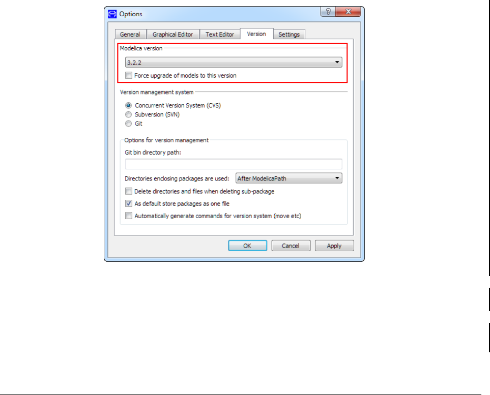
9 APPENDIX - MIGRATION 459
on. This information is also exploited when upgrading models from using one version of a
library to another.
The version information is handled automatically by Dymola in most cases. The design has
been chosen to make it easy to maintain in a simple way. Version numbers respectively
uses-information is only stored once per package and apply to the entire package.
Specifying default version of the Modelica standard library
The specification of which version of the Modelica standard library to use influences the
loading of all other libraries since they should be consistent with the Modelica library. It can
be specified according to the following rules
1. The basic rule is that the loading of the first model or library using the Modelica library
specifies which version of Modelica to use.
2. There is a possibility to force an automatic upgrading of a model or library to a certain
version by using the Versions tab in Edit > Options…
to specify the version. Ticking Force upgrade of models to this version means that
loading e.g. a library that uses Modelica 2.2.2 will force that library to be upgraded to use
Modelica 3.2.2. If another version of the Modelica library is already loaded, you will be
asked to use the command File > Clear All, which unloads all libraries.
If you modify the version, click OK. The setting will be saved for the next time you run
Dymola.
Conditional use of
Modelica 3.2.2
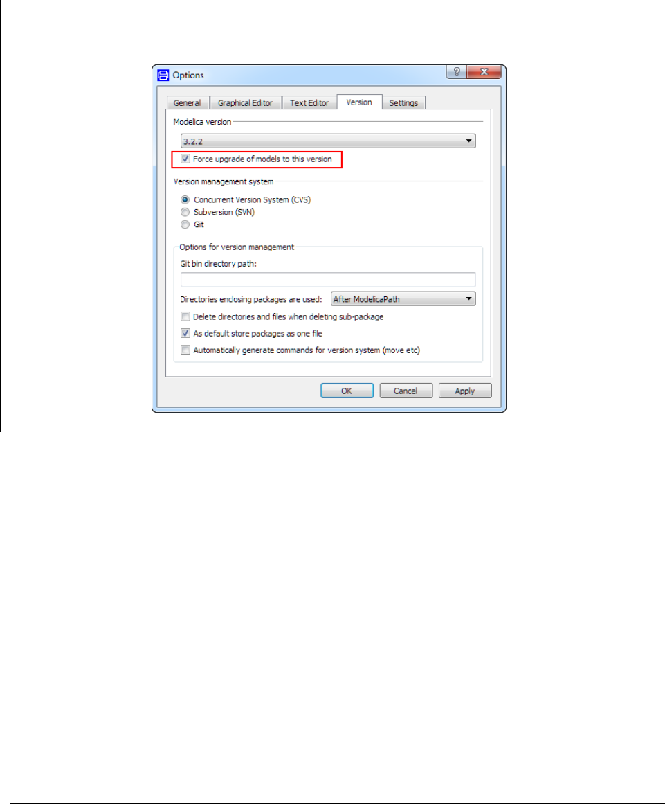
460
3. Setting the default version to a certain version and ticking Force upgrade of models to
this version will also prevent automatic conversion to another version. The following
setting will lead to an unconditional use of Modelica 3.2.2:
Your models will then automatically open the correct Modelica library and related libraries.
In case you later start to upgrade some of your libraries to a later version of Modelica they
will continue to use the old version provided you follow the following rule:
• Use default names for libraries (i.e. the ones suggested by Save).
This rule also ensures easy handling of the library in general.
9.2.3 Upgrading to a new Modelica version
The procedure to upgrade models to a new Modelica version is in principle simple to
perform provided some conditions are fulfilled. In order to have smooth upgrading, it may
be useful to first consider the following issues
1. Perform Check on the library before conversion, and verify that test-examples are
consistent.
2. Save the library after Check. This automatically updates the uses-information.
3. Install updated versions of all libraries used by this library. For commercial libraries,
please, contact your distributor for a new release. For non-commercial and in-house
libraries please contact the maintainer.
Unconditional use of
Modelica 3.2.2
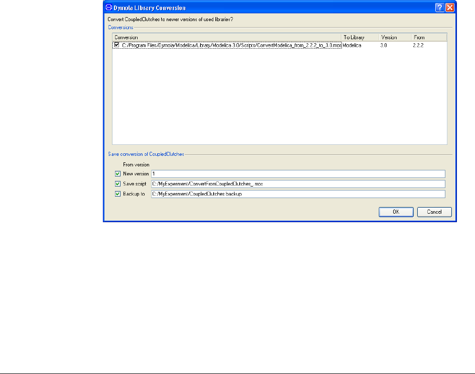
9 APPENDIX - MIGRATION 461
4. The conversion procedure is easiest performed and most reliable if the models are stored
in the standard way. Packages may be stored in one file having the same name as the
package and .mo extension. Packages may also be stored using hierarchical directories.
It is not advisable to upgrade files produced by the File > Save Total… command,
because they include typically several packages and a model. This is discussed further
below in the section “Using old models after upgrading to the latest Modelica version”
on page 463.
The conversion procedure is as follows (we will here assume that version 3.0 should be
used):
1. Start Dymola
2. You should ensure that either you have loaded Modelica 3.0 (normally by selecting
Modelica Standard Library version 3.0 in the library), or that the default Modelica
version is 3.0 and Force upgrade of models to this version is ticked.
3. You open the model or library you would like to upgrade. Dymola will prompt you
about the upgrading.
During the conversion Dymola prompts
a. for a version number of the converted library
b. if and where to store the conversion script which contains information relevant for users
of your library, e.g. if the renaming of library components caused a change in the name of
any component in your library
c. about storing backup of the original
We recommend that you accept the defaults proposed by Dymola. You may of course give
another version number. The applied conversions are written to the Syntax Error log. It may
Conversion including
version information

462
happen that you do not get any prompt for conversion when you open the package. This is
typically the case when there is no uses annotation for the Modelica library in your package.
Dymola then does not detect uses of the Modelica library in sub-packages.
After conversion
1. Re-check the model or the library, and verify that test-examples are consistent.
2. Update documentation to take into account the new structure.
3. Distribute the library (including conversions) to other users and convert other libraries.
You should also consider distributing the automatically generated backup for users who
want to continue using the older version.
Conversion of mutually dependent libraries
You should in general first convert a library and verify this library in itself and then convert
libraries and models using this library. In some cases this is not possible.
The most problematic case for conversion is if you have two (or more) mutually dependent
top-level libraries, neither of which specifies any version or uses-information.
To handle this case we recommend the following procedure:
1. Update the libraries with version and uses-information. (There will otherwise be an
unnecessary conversion step.) For giving version number see section “Specifying the
version of a package” on page 464. Additionally save all libraries to ensure that the uses-
information is correct.
2. Ensure that all libraries are stored with default names without version number, e.g. for
MyLibrary either as a file MyLibrary.mo or as a directory MyLibrary with a file
packge.mo inside. This enables demand-loading of the libraries which is needed for the
next step.
3. Trigger conversion of one of the libraries, by opening it. This will read the other
libraries, and you will be prompted to save new versions of all of them.
Potential problems with conversion
The conversion procedure has been tested with several libraries and the conversion handles
large and advanced libraries. However, in some advanced cases the command Check might
detect incompatibilities. This is either because the conversion of some library is incomplete
or because the required conversion is too complex. In some cases it is easy to determine the
problem and correct the partially converted model. If not, please contact Dassault Systèmes
AB and/or the distributor of the used libraries.
An example of too complex a conversion is a block-source that can be either scalar or vector
(conversions assume this is a scalar). Later hierarchical modifiers can then turn this into a
vector-source. For this case the block-source should have been automatically converted into
a vector of blocks.

9 APPENDIX - MIGRATION 463
Reverting to old versions
In case you want to revert to the backup of the original library and are not using a version
handling system you can copy all of the files from the backup directory to the original
directory (overwriting the new files).
Another possibility is to remove the converted files and then rename the backup directory
by removing everything in the directory name starting from the first space, e.g. “MyLibrary
0.8” or “MyLibrary backup” is renamed to “MyLibrary”.
Updates of conversions
This user guide centers on the handling of the upgrade from Modelica library version 2.2.2
to version 3.0. However, this conversion procedure is not unique to this conversion of
Modelica but also works for other conversions, e.g. MyLibrary 0.8 to 0.9 and for any
conversions of your own libraries. For changes that are not directly caused by upgrades of
other libraries it requires that the library maintainer also provides a conversion script.
When upgrading a library that already has conversion scripts, the existing scripts will also
automatically be updated (by appending the new script to the old one), and none-
conversions handled in an appropriate way. The updated conversion scripts should be seen
as a fall-back strategy and the recommended procedure is always to keep all libraries and
models consistent with the latest version of libraries.
9.2.4 Using old models after upgrading to the
latest Modelica version
Dymola can only have one version of each library loaded at the time. It allows you to use
old, non-upgraded models. You have the following possibilities
1. Manually load an old version of Modelica before loading the model.
2. Load the model directly in Dymola, i.e. before you open the Modelica library, and
ensure that Force upgrade of models to this version (as explained above) either is un-
ticked or is ticked for the version you want to use.
3. Use the command File > Save Total… of the model before using either of the
approaches 1 and 2 above. A save total model using components from the Modelica
Standard library includes a shortened version of the Modelica library including the
components needed. Loading a save total model means an explicit loading of the
Modelica library as in alternative 1.
9.2.5 Determining what libraries a model use
In most cases the uses-information is automatically updated by Dymola, when you use
models of library in another library:
• Drag’n’drop a component from one library to a model in another.
• Extend from a class in one library and place it another library.
• Duplicate a class.
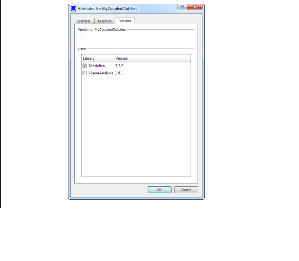
464
This handles the graphical uses, and if you write models textually there are number of
alternatives:
• Edit the version and uses-information using the Version tab in the command Edit > Edit
Attributes... This is described in the next section.
• Write the uses-annotation textually.
• Save the model or library, since Dymola automatically adds uses-information (provided
the used library has a version number, and is opened in Dymola).
9.2.6 Specifying the version of a package
For a top-level package or model you can edit the version information from Edit > Edit
Attributes… in the Version tab.
This dialog also allows you to edit the uses-information by selecting which libraries a
package uses. All existing uses-annotations are included and checked, and all loaded non-
used packages with version information are included as non-checked.
If the uses-annotation specifies a package that is not loaded you can also edit which version
is used.
Version tab

9 APPENDIX - MIGRATION 465
For models and/or packages inside another package the version information is read-only.
The version information is also shown in the Documentation layer.
9.2.7 Upgrading models and libraries to a new
library version
We are here providing a reference for what happens at conversion, including some of the
minor details of the conversion.
If you want to force to a specific library you should start by loading that version of the
library. You then load the model(s) or library you want to upgrade and will be prompted to
upgrade them. The applied conversions will be written to the Syntax Error log.
In some cases there will be warnings for conversions that are too complex or the converted
library does not pass through check, please consult the library documentation in that case.
In addition to converting you will be asked for a new version number, to save the
conversion script for users of the library, and create a backup of the original. The conversion
script contains information relevant for users of your library, e.g. if the renaming of library
components caused a change in the name of any component in your library.
Thus models using your library will automatically upgrade to the new version.
You can also add your own conversions to this script.
In some cases the automatically generated conversion script will be empty - in this case the
reference to the script will be replaced by a none-conversion, and the conversion script will
contain a comment saying that it is not used.
Conversion including
version information

466
The default for the new version is that the least significant version number is increased by
one. Dymola will also store the old version as backup and after backing up the files save the
converted library at the original place. To avoid problems it is verified that the backup
directory is non-existent, empty, or already contains a backup of the Modelica files and
scripts.
If the model is read-only and no conversion is needed Dymola will silently accept the model
as being compatible with the library.
The dialog contains information about what scripts are used for which conversion. De-
selecting a conversion script should only be done if you the conversion have already been
performed (and for some reasons the uses-information was not updated).
If the need for upgrading is found during the translation of a model the translation will be
interrupted, you will be prompted to convert, and the translation will then re-start.
If you have loaded one of several mutually dependent libraries, you will be asked to convert
all of them at the same time and there will be several ‘Save conversion’ groups (but only
one set of conversions).
Note that pressing Cancel cancels all conversions and until you exit Dymola or use the
command File > Clear All and re-open the files, and you should perform one of these
actions after pressing Cancel.
Note also that Dymola supports multiple conversions of libraries. A typical case is that a
customer does not upgrade to each new Dymola version, but “jumps” a certain version.
When upgrading to the present Dymola version in this case, certain libraries may demand to
be upgrading to the “jumped” version before upgrading to the present version. Dymola
handles this by executing more than one upgrading script in the same operation.
As an example, consider MyLib that should be converted from 1.2. to 1.6. That can be done
the following, considering the corresponding scripts exist and work:
annotation(conversion(
from(version="1.2", to="1.3", script="modelica://MyLib/scripts/
Convert_from_1.2_to_1.3.mos"),
from(version="1.3", to="1.4", script="modelica://MyLib/scripts/
Convert_from_1.3_to_1.4.mos"),
from(version="1.4", to="1.5", script="modelica://MyLib/scripts/
Convert_from_1.4_to_1.5.mos"),
from(version="1.5",script="modelica://MyLib/scripts/
Convert_from_1.5_to_1.6.mos")));
What will happen (which differs from just having multiple scripts) is that these conversions
will be run in sequence as completely separate conversions, i.e. 1.2->1.3, 1.3->1.4, 1.4->1.5,
1.5->1.6; thus if you change the name of a class between 1.2 and 1.3 and then rename
parameters between 1.3 to 1.4, and then rename both the parameter and the class between
1.5 to 1.6 it should work. (Each conversion script may have renaming of classes and
parameters in arbitrary order.)
An exception is if any intermediate library version requires manual conversion; which is
handled by converting models to a deprecated library. This deprecated library may be
missing in, or may be incompatible with, the newer Dymola version.

9 APPENDIX - MIGRATION 467
9.3 Preparing libraries for migration
If libraries are to be distributed (e.g. commercial libraries), they should be prepared for
migration when e.g. a new version of Modelica Standard Library is released.
Dymola supports the Modelica annotations for version handling, including the use of the
Modelica URI scheme ‘modelica://’ for specifying the location of conversion script files in
the conversion annotation.
Please see Modelica Language Specification for further details concerning this. The
specification can be found in the Modelica site; www.Modelica.org.
9.4 Updating Modelica annotations
The built-in function updateModelicaAnnotations can be used to update Modelica
annotations, in particular to remove deprecated annotations for text-primitives. The function
is defined as:
function updateModelicaAnnotations "update Modelica annotations
To follow the standard and preserve behavior"
input String className;
input Boolean changeLinePattern := true
"Linepattern.none->LinePattern.Solid";
input Boolean orderBitMapExtent := true
"Order Bitmap extent";
input Boolean removeTextDeprecated := true
"Remove deprecated textannotations";
input Boolean renameTextColor := false
"Text.lineColor->Text.textColor";
output Boolean ok;
end updateModelicaAnnotations;
Some comments about some inputs:
The input orderBitmapExtent is used to allow images to be created as flipped.
The input removeTextDeprecated removes the following annotations for text-primitives:
fillColor, pattern, fillPattern, and lineThickness.
The input renameTextColor is intended for future use.
As an example, annotations can be updated (with default settings) for a library MyLibrary
by executing updateModelicaAnnotations("MyLibrary");. The library must be
loaded before giving the command.

468

469
10 Index
A
adaptive
homotopy, 426
algebraic loops, 432
analogFilter, 84
analytic Jacobians, 433
annotation
protection, 165
annotations, 361
update Modelica annotations, 467
vendor-specific, 430
API, 194
model structure, 194
array of records in dialog, 390
arrays, 426
assert, 429
automatic differentiation, 398
B
basic primitives, 204, 217
Bessel filter, 85
binary model export, 348, 349
dymosim DLL, 350
license, 348
XML interface, 350
black-box import using FMI, 319
BLT partitioning, 432
Butterworth filter, 85
C
calibrate, 38
calibrateSteadyState, 98
calibration, 37, 53
detrending signals, 79
free start values, 55
limiting signals, 79
measurement file formats, 50
model validation against measurement, 57
parameter. See parameter tuning
preprocess data, 75
sensitivity, 73
setting up/executing task, 39
static, 86
steady-state. See static calibration
validation of nominal model, 44
Calibration package. See packages : Calibration
Chebyshev filter, 85
check box in dialog, 374
check of input data in dialog, 389

470
checkCalibrationSensitivity, 73
checkLibrary, 173
class
coverage, 180
code
export. See code and model export
code and model export
disabling export, 349
license options, 348
color, 209, 213
combo box in dialog, 372
commands
convertClass, 450
convertClear, 456
convertElement, 452
convertModifiers, 453
compareModels, 185
component
inner/outer, 429
conceal. See encryption
condition coverage, 181
contour lines, 226
ControlDesk, 252
conversion
multiple conversion of libraries, 466
conversion script, 456
coordinate system
creatinga reference coordinate system, 219
coordinateSystem, 225
Co-simulation
FMI for Co-simulation, 316
critically damped filter, 85
CVS, 134
CVS commands, 130
CVS selection, 133
D
DAE, 431
high index, 434
data preprocessing for calibration, 75
dataPreprocessing, 75
DDE
Dymola commands, 261
Dymosim DDE server, 264
extended GUI, 267
GUI, 266
hot linking variables, 266
requesting variables, 265
setting parameters, 265
simulator commands, 265
DDE interface for Dymola, 261
declaration
derivative, 399
delay-load, 407
dependencies
model, 151
deprecation
warnings, 431
derivative, 397
derivatives
partial, 398
design optimization, 102
Design package. See packages : Design
Design.Calibration, 37
Design.Experimentation, 11
detrending signals, 79
DFT. See discrete Fourier transform
dialog
array of records, 390
automatically constructed, 362
check box, 374
check of input data, 389
combo box, 372
edit buttons in dialog, 378
entry for start values, 368
formatting, 377
groups, 365
illustrations, 375
labels, 370
layout, 370
open files, 378
radio buttons, 373
select model, 378
tabs, 365
differential-algebraic equations, 431
high index, 434
differentiation
automatic, 398
discrete Fourier transform. See Fourier transform
DLL
dymosim, 350
dsmodel.c, 347
interfacing, 353
dSPACE
ControlDesk, 252
DS1005, 250
DS1006, 251
dym_rti_build, 253
overrun situation, 252
turnaround time, 252

471
dummy derivative method, 434
DymolaBlock, 237
Dymosim
DDE server, 264
dymosim DLL, 350
API, 351
dynamic state selection. See state selection : dynamic
E
edit buttons in specialized GUI widget, 378
encrypted file, 155
Encrypted total model, 170
encryption, 153
Modelica files, 155
enumeratons, 427
environment variables
CLASSPATH, 273
CVSROOT, 136
DYMOLA_RUNTIME_LICENSE, 349
DYMOSIMGUI, 267
DYMOSIMLOGDDE, 267
DYMOSIMREALTIME, 264
EDITOR, 143
JAVA_HOME, 408
PATH, 135, 144, 273, 289
PYTHONPATH, 289
SVN_SETUP, 143
VISUAL, 143
equality comparison, 423
Erase Selected Objects, 215
Erase window, 210
EraseClasses, 199
erasing graphical object, 206, 214
event
noEvent operator, 417
examples
automatic differentiation, 398
calibration - setting up/executing task, 39
check if tuners can be calibrated, 73
combining basic primitives, 206
CVS file management, 136
encrypted transfer function, 156
experimentation case study - CoupledClutches, 12
filtering signals, 84
limiting and detrending signals, 79
model validation, 44, 57
Monte Carlo Analysis, 26
multi-criteria optimization design, 102
noise analysis, 82
perturb parameters (calibration), 71
perturb parameters (experimentation), 13
preprocess data for calibration, 75
providing/concealing information, 161
scrambling, 170
SVN file management, 144
sweep one parameter (calibration), 62
sweep one parameter (experimentation) - two variants,
19
sweep two parameters (calibration), 69
sweep two parameters (experimentation), 24
experiment.StopTime, 173
Experimentation package. See packages :
Experimentation
export. See code and model export
visualizer image, 216
export options. See code and model export - license
options
exporting models using FMI, 307
exporting models with built-in numerical solvers, 316
Extendable user interface
menus, toolbars and favorites, 391
external function, 403
annotations, 405
including, 403
link with library, 404
F
file extensions
.csv, 50, 79
.mat, 51, 78
.mo, 263
.moe, 155
.mos, 264
.png, 216
jpg, 216
xpm, 216
file type associations, 263
filter
Bessel, 85
Butterworth, 85
Chebyshev, 85
critical damped, 85
filtering signals, 84
FMI, 306
exporting models, 307
FMI Kit for Simulink, 332
for Co-simulation, 316
importing black-box models, 319
importing models, 319
model exchange, 306

472
specification for Co-simulation, 306
specification for model exchange, 306
validating FMUs, 330
XML model description, 306
FMU, 306
black-box export, 311
exporting FMU´s with settings, 312
exporting FMU’s, 307
FMU export form Simulink, 335
FMU export from Simulink, 332
FMU import into Simulink, 334, 341
generate Dymola result file (dsres.mat), 307
importing FMU’s, 319
importing FMUs with many inputs/outputs, 326
multiple FMU´s, 315
multiple instantiation of the same FMU, 315
online tunable parameters, 307
string parameters, 312
validating FMUs, 330
formatting of dialog, 377
Fourier transform, 82
freeStartValues, 55
frequency analysis, 82
function
derivative, 397
external, 403
preInstantiate, 430
Functional Mock-up Unit. See FMU
functions
calibrate, 38
calibrateSteadyState, 98
checkCalibrationSensitivity, 73
dataPreprocessing, 75
functional input argument to, 429
perturbParameters (calibration), 71
perturbParameters (experimentation), 13
staticCalibrate, 86
sweepOneParameter (experimentation), 22
sweepParameter (calibration), 62
sweepParameter (experimentation), 19
sweepTwoParameters (calibration), 69
sweepTwoParameters (experimentation), 24
G
Git, 148
Git commands, 130
Git selection, 133
global ambient light, 207
graphical properties, 209
graphics. See also plot and Plot3D
basic primitives, 204, 217
color, 209, 213
contour lines, 226
creating a reference coordinate system, 219
erasing graphical object, 206, 214
inserting graphical object, 206
pie chart, 232
Plot3D. See Plot3D
rotation, 210
scaling, 210
surface plots, 219
translation, 210
Visualize 3D, 203
grouping of record fields in dialog, 365
GUI
user-defined, favorite models, 394
user-defined, for data structures, 361
user-defined, library-specific menus and toolbars, 393
user-defined, menus and toolbars, 391
GUI widgets
in general. See dialog
specialized, 378
H
hardware-in-the-loop simulation, 247
hiding variables, 368
high oscillatory modes, 85
homotopy, 426
adaptive, 426
operator, 426
I
identifiability. See parameter : identifiability
if-then-else expression, 445
illustrations in dialog, 375
importing models using FMI, 319
black-box models, 319
index reduction, 434
inline integration, 248
advanced options, 258
insert
graphical object, 206
interpretMainStatic, 412
J
Jacobian, 432
Java interface, 273

473
calling Java functions from Modelica, 408
calling Modelica functions from Java functions, 410
interpretMainStatic, 412
Java interface (older version), 408
JavaScript interface, 298
L
labels in dialog, 370
layout of dialog, 370
least squares, 80
library
annotation, 405
checking, 172
licensing, 167
migration, 449
multiple conversion, 466
license
binary model export, 348
real-time simulation, 348
source code generation, 348
licensing
of library, 167
limiting signals, 79
line (y = a*x+b), 80
Linear Systems library, 85
Lissajous curve, 218
M
Matlab, 236, See also Simulink
mex, 236
m-file utilities, 236
path, 236
matrix T, 209, 210
mean value, 81
m-file
load2DTable, 247
loaddsin, 247
loadNDTable, 247
save2DTable, 247
saveNDTable, 247
setfromdsin, 247
setParametersFDsin, 247
migration to a new library, 449
model
calibration. See calibration
comparison, 185
dependencies, 151
export. See code and model export
management. See model management
packages. See packages
structure, 194
model description
XML model description for FMI, 306
model exchange using FMI, 306
model management, 172
check package, 172
encryption, 153
model structure, 194
Modelica
Synchronous, 425
MODELISAR, 306
ModelManagement.Structure.AST, 195
ModelManagement.Structure.Instantiated, 200
Monte Carlo analysis, 11, 26
accumulated probability, 30
automatic selection of set of bins, 29
density of probability, 30
fixed parameters, 28
number of draws, 29
observed variables, 29
random distributions available, 32
uncertain parameters, 27
moving
visualizer view, 208
multi-case optimization, 118
multi-criteria optimization
multi-criteria, 101
N
noEvent(...) operator, 417
noise analysis, 82
nonlinear equations, 440
O
ODE, 434
OPC
Dymosim OPC server, 270
Dymosim OPC Server, 268
GUI, 271
Limitations, 272
Logging, 272
mapping OPC tags to Dymola variable names, 271
OPC tags, 270
prerequisites, 269
opening of files in specialized GUI widget, 378
operator overloading, 425

474
optimization
design, 102
inequality contraint, 116
multi-case, 118
multi-criteria, 101
ordinary differential equations, 434
overloading, 425
P
package
Plot3D. See Plot3D
packages
Calibration, 11, 37
Design, 11
Experimentation, 11
pan
visualizer window, 208
Pantelides´ algorithm, 434
parameter
calibration. See parameter tuning
dependency, 62
estimation. See parameter tuning
identifiability, 73
MonteCarloAnalysis. See Monte Carlo analysis
perturb (calibration), 71
perturb (experimentation), 13
sensitivity, 38, 62
sweep (calibration), 62
sweep (experimentation), 19
sweepOneParameter (experimentation), 22
sweepTwoParameters (calibration), 69
sweepTwoParameters (experimentation), 24
tuners, 102
tuning. See parameter tuning
varying of, 11
parameter tuning, 53, See also calibration
direct calculation, 96
tuners, 37, 55, 57
parametric surface, 219
partial derivatives, 398
Path system variable, 135
perturbParameters
calibration, 71
experimentation, 13
pie chart, 232
platforms
non-Windows, 353
plot. See also graphics
add a pointer, 230
default plot style, 224
intersection of surfaces, 228
Plot3D. See Plot3D
projected on the xy plane, 227
surface, 219
Plot3D, 203
insertLabel, 204
insertPointer, 204, 230
insertPrimitive, 204
plotBarGraph, 204, 226
plotData, 223
plotHistogram, 204
plotLines, 204, 226
plotPieChart, 204
plotPoints, 204, 226
plotStem, 204, 226, 231
plotSurface, 204, 226
plotTriangularizedSurface, 204
styleData. See styleData
Plot3D.Examples.Surfaces.surfaceDemo, 221
preprocess data for calibration, 75
protecting variables, 368
protection group, 154
Python interface, 288
R
radio buttons in dialog, 373
ReadModelicaFile, 199
read-only
encrypted models, 156
real-time simulation, 247
export restrictions, 248
license, 348
reference files, 173
regression testing, 173, 175
removing graphical object. See erasing graphical
object
report generator, 299
roll
visualizer window, 208
rotate
visualizer view, 208
rotation, 210
S
SaveModel, 199
SaveTotalModel, 199, See also Save Total… (in GUI)
scaling, 210
scrambling, 169

475
scroll
visualizer view, 208
selecting object
in visualizer window, 208
selection of model in dialog, 378
semiLinear, 445
S-function MEX block, 237
signal
detrending, 79
filtering, 84
limiting, 79
Simlink Real-Time, 254
Simulink
DymolaBlock, 237
external input and output, 244
FMI Kit for Simulink, 332
FMU export form Simulink, 335
FMU export from Simulink, 332
FMU import into Simulink, 334, 341
Generate Result, 240
graphical interface, 237
implementation notes, 246
parameters and initial values, 238
parameters and initial values, 247
setting up environment for FMU export from/import into
Simulink, 335
smoothOrder, 398
solution of nonlinear equations, 440
source code generation, 348, 352
license, 348
source code generation features for normal translation,
353
translateModelExport, 352
specification
FMI for Co-simulation, 306
FMI for model exchange, 306
stand-alone application, 348, 350, See also
StandAloneDymosim
StandAloneDymosim, 348, 353
compiling and linking, 354
declare_, 357
dsblock, 355
FindEvent_, 357
GetDimensions, 357
NextTimeEvent, 357
trouble-shooting, 358
start values
free start values, 55
state event, 417
state machines, 425
state selection, 414
dynamic, 415
StateSelect, 414
static calibration, 86
staticCalibrate, 86
steady-state calibration. See static calibration
string variables in models, 429
structurally singular, 432
style, 209
style checking, 182
styleData, 224, 225
Level Curves, 225
Surface, 225
Vector Field, 225
Water Fall, 225
SUNDIALS suite of numerical solvers, 316
surface plots, 219
SVN, 142
SVN commands, 130
SVN selection, 133
sweepOneParameter
experimentation, 22
sweepParameter
calibration, 62
experimentation, 19
sweepTwoParameters
calibration, 69
experimentation, 24
symbolic processing, 431
Synchronous Modelica, 425
system variable
Path, 135
T
T matrix, 209, 210
table handling
Matlab routines, 246, 247
n-dimensional, 246, 247
TableND package, 246, 247
tabs in dialog, 365
tearing, 433
test
case, 173
suite, 173
textString, 219
tilt
visualizer view, 208
transform matrix
view, 207

476
translateModelExport, 352
translation, 210
translation statistics, 172
traversing
models before translation, 194
translated models, 200
trouble-shooting
stand-alone application, 358
tuners, 102, See parameter tuning : tuners
tuning. See parameter tuning
U
update
Modelica annotations, 467
user-defined GUI. See GUI
V
variable
hidden, 368
protected, 368
vector
field, 219
vendor-specific annotations, 430
version management, 126
view
transform matrix, 207
Visualize 3D, 203
window number, 207
visualizer window, 204
moving view, 208
pan, 208
roll, 208
rotate view, 208
scroll view, 208
selecting object, 208
tilt view, 208
zooming, 208
W
widgets. See GUI widgets
window
number (Visualize 3D), 207
visualizer, 204
Wireframe, 226
X
XML
model description for FMI, 306
XML interface, 350
xPC Target, 254
Z
zooming
visualizer window, 208
