DynaNet User's Guide V3.3
User Manual: Pdf
Open the PDF directly: View PDF ![]() .
.
Page Count: 234 [warning: Documents this large are best viewed by clicking the View PDF Link!]

1
x
y
z
DynaNet User’s Guide
Version 3.3
Editors:
Roger Fraser, Frank Leahy, Philip Collier
July 2017

DynaNet User’s Guide
Dynamic Network Adjustment Software
July 2017
©Commonwealth of Australia (Geoscience Australia) 2017.
With the exception of the Commonwealth Coat of Arms and where otherwise noted, this product is provided
under a Creative Commons Attribution 4.0 International Licence.
(http://creativecommons.org/licenses/by/4.0/legalcode)
For all technical and software related matters, please contact:
Dr. Roger Fraser
Manager, Geodetic Survey
Office of Surveyor-General Victoria
Department of Environment, Land, Water and Planning
Level 17/570 Bourke St, Melbourne, Victoria, 3000
roger.fraser@delwp.vic.gov.au
ii
DynaNet User’s Guide
Version 3.3
Dr. Roger Fraser
Manager, Geodetic Survey
Office of Surveyor–General Victoria
Melbourne
Dr. Frank Leahy
Associate Professor
University of Melbourne
Melbourne
Dr. Phil Collier
Research Director
Cooperative Research Centre for Spatial Information
Melbourne
iii
iv
Acknowledgements
The development of this software and user guide has benefited from the assistance provided by
several individuals and organisations. In particular, the authors gratefully acknowledge the following
people for their advice, support, feedback, supply of sample data files and contribution at various
levels: Gary Johnston, John Dawson, Nick Brown, Craig Harrison and Ted Zhou from Geoscience
Australia (Commonwealth); Ben Menadue and Dale Roberts from the National Computational
Infrastructure (Commonwealth); John Tulloch (retired), David Boyle, Alex Woods, Dave Collett, Bob
Ross (retired) and Peter Growse (retired) from the Department of Environment, Land, Water and
Planning (Victoria); Matt Higgins, Steve Tarbit, Mike Cowie, Darren Burns and Peter Todd (retired)
from the Department of Natural Resources and Mines (Queensland); Simon McElroy, Joel Haasdyk
and Nic Gowans from the Department of Finance, Services and Innovation (New South Wales); Linda
Morgan (retired), Irek Baran and Kent Wheeler from Landgate (Western Australia); Graeme Blick,
Nic Donnelly and Chris Crook from Land Information New Zealand (New Zealand); Scott Strong from
the Department of Primary Industries, Parks, Water and Environment (Tasmania); Stephen Latham
and Peter Stolz from the Department of Planning, Transport and Infrastructure (South Australia);
Gavin Evans from the Department of Environment and Sustainable Development (ACT); Rob Sarib
and Amy Peterson from the Department of Lands and Planning (Northern Territory); Simon Fuller
of ThinkSpatial (Victoria); Peter Teunissen of Curtin University; Chris Rizos of the University of New
South Wales; and Rod Deakin (retired) and Don Grant of Royal Melbourne Institute of Technology.
Freely ye have received, freely give
(Matthew 10:8)
Remember the words of the Lord Jesus, how He said, “It is more blessed to give than to receive”
(Acts 20:35)
v
vi
Contents
Acknowledgements ...................................... v
Contents............................................ vii
ListofFigures......................................... xiii
ListofTables ......................................... xvii
ListofAbbreviations ..................................... xix
ListofSymbols ........................................ xxi
1 Introduction 1
1.1 Brief history of phased adjustment and DynaNet . . . . . . . . . . . . . . . . . . . 1
1.1.1 Preamble to Version 3.3 . . . . . . . . . . . . . . . . . . . . . . . . . . . . 3
1.2 Conventions used in this document . . . . . . . . . . . . . . . . . . . . . . . . . . . 3
1.3 Programoverview.................................... 4
1.3.1 Software architecture and information flow . . . . . . . . . . . . . . . . . . 4
1.3.2 Program execution and command line options . . . . . . . . . . . . . . . . 6
1.3.3 Program execution sequence . . . . . . . . . . . . . . . . . . . . . . . . . . 7
1.4 Two–minute quick start tutorial . . . . . . . . . . . . . . . . . . . . . . . . . . . . 9
2 Creating, editing and processing projects 13
2.1 Introduction....................................... 13
2.2 Conventions used in DynaNet . . . . . . . . . . . . . . . . . . . . . . . . . . . . . 13
2.2.1 Filenaming................................... 13
2.2.2 Filetypes.................................... 14
2.2.3 Directories ................................... 15
2.3 Project setup and processing . . . . . . . . . . . . . . . . . . . . . . . . . . . . . . 15
2.3.1 Prepare station and measurement files . . . . . . . . . . . . . . . . . . . . 15
2.3.2 Create DynaNet project file . . . . . . . . . . . . . . . . . . . . . . . . . . 15
2.3.3 Automated project processing . . . . . . . . . . . . . . . . . . . . . . . . . 15
3 Import and export of geodetic network information 17
3.1 Introduction....................................... 17
3.2 Importing station and measurement information . . . . . . . . . . . . . . . . . . . . 17
3.2.1 Station coordinate information . . . . . . . . . . . . . . . . . . . . . . . . . 18
3.2.2 Supported measurement types . . . . . . . . . . . . . . . . . . . . . . . . . 19
3.2.3 Networkconstraints .............................. 19
3.2.4 Geoidinformation ............................... 21
3.2.5 File name argument conventions . . . . . . . . . . . . . . . . . . . . . . . . 21
3.2.6 Progress reporting and import log . . . . . . . . . . . . . . . . . . . . . . . 21
3.2.7 Verification and error checking . . . . . . . . . . . . . . . . . . . . . . . . . 23
3.3 Configuring import options . . . . . . . . . . . . . . . . . . . . . . . . . . . . . . . 24
3.3.1 Referenceframe ................................ 24
3.3.2 Datascreening ................................. 25
3.3.3 GNSS variance matrix scaling . . . . . . . . . . . . . . . . . . . . . . . . . 31
vii
3.4 Network measurement simulation . . . . . . . . . . . . . . . . . . . . . . . . . . . 33
3.5 Dataexport....................................... 35
3.5.1 Station and measurement files . . . . . . . . . . . . . . . . . . . . . . . . . 35
3.5.2 Association lists and station map . . . . . . . . . . . . . . . . . . . . . . . 35
4 Transformation of coordinates and measurements 37
4.1 Introduction....................................... 37
4.2 Reference frame fundamentals . . . . . . . . . . . . . . . . . . . . . . . . . . . . . 38
4.2.1 Cartesian reference frame . . . . . . . . . . . . . . . . . . . . . . . . . . . 38
4.2.2 Geographic reference frame . . . . . . . . . . . . . . . . . . . . . . . . . . 38
4.2.3 Local reference frame . . . . . . . . . . . . . . . . . . . . . . . . . . . . . 39
4.2.4 Polar reference frame . . . . . . . . . . . . . . . . . . . . . . . . . . . . . . 40
4.3 Transformation between cartesian reference frames . . . . . . . . . . . . . . . . . . 42
4.4 Propagation of variances between reference frames . . . . . . . . . . . . . . . . . . 43
4.4.1 Local reference frame . . . . . . . . . . . . . . . . . . . . . . . . . . . . . 43
4.4.2 Polar reference frame . . . . . . . . . . . . . . . . . . . . . . . . . . . . . . 43
4.4.3 Geographic reference frame . . . . . . . . . . . . . . . . . . . . . . . . . . 44
4.5 Conversion of projection coordinates . . . . . . . . . . . . . . . . . . . . . . . . . 44
4.6 Transformation of coordinates and measurements . . . . . . . . . . . . . . . . . . . 47
4.6.1 Supported reference frames and geodetic datums . . . . . . . . . . . . . . . 47
4.6.2 Relationship between ITRF, IGS and WGS84 reference frames . . . . . . . . 49
4.6.3 Transforming station coordinates and measurements . . . . . . . . . . . . . 50
4.7 Dataexport....................................... 51
5 Import and export of geoid information 53
5.1 Introduction....................................... 53
5.2 Fundamentalconcepts ................................. 53
5.2.1 Geoidmodels.................................. 55
5.2.2 Conventions used in DynaNet . . . . . . . . . . . . . . . . . . . . . . . . . 56
5.3 Gridfileinterpolation.................................. 56
5.3.1 Bilinear interpolation . . . . . . . . . . . . . . . . . . . . . . . . . . . . . . 56
5.3.2 Bicubicinterpolation.............................. 58
5.4 Import of geoid information . . . . . . . . . . . . . . . . . . . . . . . . . . . . . . 59
5.5 Arbitrary interpolation and height transformation . . . . . . . . . . . . . . . . . . . 61
5.5.1 Interactivemode ................................ 61
5.5.2 Textfilemode ................................. 62
5.6 Exporting interpolated information . . . . . . . . . . . . . . . . . . . . . . . . . . . 63
5.7 Working with NTv2 geoid grid files . . . . . . . . . . . . . . . . . . . . . . . . . . . 64
5.7.1 Reporting NTv2 geoid grid file metadata . . . . . . . . . . . . . . . . . . . 64
5.7.2 Importing WINTER DAT geoid grid files . . . . . . . . . . . . . . . . . . . 65
5.7.3 Grid file interpolation errors . . . . . . . . . . . . . . . . . . . . . . . . . . 67
6 Network segmentation 69
6.1 Introduction....................................... 69
6.2 The concept of network segmentation . . . . . . . . . . . . . . . . . . . . . . . . . 69
6.3 Segmentationalgorithm................................. 71
6.4 Accommodating variations in network design, size, user preferences and computer
performance ...................................... 72
6.4.1 Optimum block size and maximum adjustment efficiency . . . . . . . . . . 73
6.4.2 Inevitable influences on the generated block sizes . . . . . . . . . . . . . . . 74
6.4.3 Factors influencing the segmentation rate . . . . . . . . . . . . . . . . . . . 76
viii
6.4.4 Generating coordinate estimates and full variance matrix for a user–defined
setofstations ................................. 77
6.4.5 Datum deficient blocks . . . . . . . . . . . . . . . . . . . . . . . . . . . . . 77
6.4.6 Non–contiguous networks . . . . . . . . . . . . . . . . . . . . . . . . . . . 78
6.5 Segmentinganetwork ................................. 78
6.5.1 Configuring segmentation behaviour . . . . . . . . . . . . . . . . . . . . . . 79
6.5.1.1 Specifying stations to appear in the first block . . . . . . . . . . . . 79
6.5.1.2 Achieving optimum block sizes . . . . . . . . . . . . . . . . . . . . 80
6.5.1.3 Isolated networks . . . . . . . . . . . . . . . . . . . . . . . . . . . 81
7 Mathematical models for dynamic network adjustment 83
7.1 Introduction....................................... 83
7.2 Observationequations ................................. 83
7.2.1 Slopedistances(S)............................... 84
7.2.2 Ellipsoid arc (E) and ellipsoid chord (C) distances . . . . . . . . . . . . . . 84
7.2.3 Mean sea level (MSL) arc distances (M) . . . . . . . . . . . . . . . . . . . 85
7.2.4 Ellipsoid heights (R) and height differences . . . . . . . . . . . . . . . . . . 86
7.2.5 Orthometric heights (H) and height differences (L) . . . . . . . . . . . . . . 87
7.2.6 Cartesian coordinates and GNSS point clusters (Y) . . . . . . . . . . . . . . 88
7.2.7 GNSS baselines (G) and GNSS baseline clusters (X) . . . . . . . . . . . . . 88
7.2.8 2D position via geodetic latitude (P) and longitude (Q) . . . . . . . . . . . 89
7.2.9 Geodetic azimuths and horizontal bearings (B) . . . . . . . . . . . . . . . . 90
7.2.10 Horizontal angles (A) . . . . . . . . . . . . . . . . . . . . . . . . . . . . . 91
7.2.11 Horizontal direction sets (D) . . . . . . . . . . . . . . . . . . . . . . . . . . 91
7.2.12 Zenith distances (V) . . . . . . . . . . . . . . . . . . . . . . . . . . . . . . 92
7.2.13 Verticalangles(Z)............................... 93
7.2.14 Astronomic latitude (I) and longitude (J) . . . . . . . . . . . . . . . . . . . 94
7.2.15 Astronomic (or Laplace) azimuth (K) . . . . . . . . . . . . . . . . . . . . . 95
7.3 Stochastic modelling and reporting . . . . . . . . . . . . . . . . . . . . . . . . . . . 95
7.3.1 Probability distributions used in DynaNetfor testing . . . . . . . . . . . . . 95
7.3.1.1 Normal distribution . . . . . . . . . . . . . . . . . . . . . . . . . . 95
7.3.1.2 Chi–square distribution . . . . . . . . . . . . . . . . . . . . . . . . 96
7.3.1.3 Student’s t distribution . . . . . . . . . . . . . . . . . . . . . . . . 98
7.3.2 Preparation of measurement precisions and variance matrices . . . . . . . . 99
7.3.2.1 Scaling GNSS variance matrices . . . . . . . . . . . . . . . . . . . 100
7.3.3 Expressing estimates of quality and reliability . . . . . . . . . . . . . . . . . 101
7.3.3.1Errorellipses.............................. 101
7.3.3.2 Positional uncertainty . . . . . . . . . . . . . . . . . . . . . . . . . 103
7.3.3.3 Measurement reliability and network reliability . . . . . . . . . . . . 103
8 Estimation of station parameters 105
8.1 Introduction....................................... 105
8.2 Overview of least squares estimation . . . . . . . . . . . . . . . . . . . . . . . . . . 105
8.3 Adjustinganetwork................................... 108
8.3.1 Simultaneousmode .............................. 108
8.3.2 Phased adjustment mode . . . . . . . . . . . . . . . . . . . . . . . . . . . 111
8.3.2.1 Single–thread mode . . . . . . . . . . . . . . . . . . . . . . . . . . 113
8.3.2.2 Multi–thread mode . . . . . . . . . . . . . . . . . . . . . . . . . . 114
8.3.2.3 Block–1 only mode . . . . . . . . . . . . . . . . . . . . . . . . . . 115
8.3.2.4 Staged adjustment mode . . . . . . . . . . . . . . . . . . . . . . . 115
8.3.2.5 Report results mode . . . . . . . . . . . . . . . . . . . . . . . . . . 116
8.3.3 Adjustment configuration options . . . . . . . . . . . . . . . . . . . . . . . 116
ix
8.3.4 Output configuration options . . . . . . . . . . . . . . . . . . . . . . . . . 118
8.3.5 Export configuration options . . . . . . . . . . . . . . . . . . . . . . . . . . 121
9 Estimating uncertainty and testing least squares adjustments 125
9.1 Introduction....................................... 125
9.2 Algorithms for estimating uncertainty . . . . . . . . . . . . . . . . . . . . . . . . . 125
9.2.1 Precision of the estimated parameters . . . . . . . . . . . . . . . . . . . . . 125
9.2.2 Precision of the adjusted measurements . . . . . . . . . . . . . . . . . . . . 126
9.3 Testing least squares adjustments . . . . . . . . . . . . . . . . . . . . . . . . . . . 126
9.3.1 Testing the least squares adjustment as a whole . . . . . . . . . . . . . . . 127
9.3.1.1 Rectifying over–optimistic variance matrices of the same type . . . . 129
9.3.2 Testing for the presence of outliers . . . . . . . . . . . . . . . . . . . . . . 131
9.3.2.1 Testing measurements with reliable estimates of precision . . . . . . 131
9.3.2.2 Testing measurements with doubtful estimates of precision . . . . . 135
9.3.3 Hints on addressing measurement failures . . . . . . . . . . . . . . . . . . . 141
Bibliography 143
Index of subjects 147
A Command line reference 151
A.1 dynanet ......................................... 151
A.2 import.......................................... 152
A.3 reftran.......................................... 156
A.4 geoid........................................... 157
A.5 segment......................................... 160
A.6 adjust .......................................... 162
A.7 plot ........................................... 166
B File format specification 171
B.1 Dynamic Network Adjustment (DNA) format . . . . . . . . . . . . . . . . . . . . . 171
B.1.1 Changes from Version 1 to Version 3 . . . . . . . . . . . . . . . . . . . . . 171
B.1.2 Headerline................................... 171
B.1.3 Stationinformation............................... 172
B.1.4 Measurement information . . . . . . . . . . . . . . . . . . . . . . . . . . . 174
B.1.5 Geoidinformation ............................... 182
B.2 Comma Separated Values (CSV) format . . . . . . . . . . . . . . . . . . . . . . . . 183
B.3 Dynamic Network Adjustment Project (DNAPROJ) format . . . . . . . . . . . . . . 184
B.4 DynaNet Markup Language (DynaML) format . . . . . . . . . . . . . . . . . . . . . 188
B.4.1 Stationinformation............................... 188
B.4.2 Measurement information . . . . . . . . . . . . . . . . . . . . . . . . . . . 190
B.5 GeodesyMLformat ................................... 193
B.6 SINEXformat...................................... 193
B.7 Geoid input text file format . . . . . . . . . . . . . . . . . . . . . . . . . . . . . . . 193
C Output file format specification 195
C.1 Headerblock ...................................... 195
C.2 Importlogfile(IMP) .................................. 195
C.3 Measurement to station output file (M2S) . . . . . . . . . . . . . . . . . . . . . . 196
C.4 Segmentation output file (SEG) . . . . . . . . . . . . . . . . . . . . . . . . . . . . 198
C.5 Coordinate output file (XYZ) . . . . . . . . . . . . . . . . . . . . . . . . . . . . . 200
C.6 Adjustment output file (ADJ) . . . . . . . . . . . . . . . . . . . . . . . . . . . . . 203
C.6.1 Adjustment statistics . . . . . . . . . . . . . . . . . . . . . . . . . . . . . . 203
x
C.6.2 Measurement to station connections . . . . . . . . . . . . . . . . . . . . . 203
C.6.3 Adjusted measurements . . . . . . . . . . . . . . . . . . . . . . . . . . . . 203
C.6.4 Estimated station coordinates . . . . . . . . . . . . . . . . . . . . . . . . . 206
C.6.5 Output of results on each iteration . . . . . . . . . . . . . . . . . . . . . . 206
C.7 Station coordinate corrections file (COR) . . . . . . . . . . . . . . . . . . . . . . . 207
C.8 Adjusted positional uncertainty file (APU) . . . . . . . . . . . . . . . . . . . . . . 209
C.9 SINEX output warning file (SNX.ERR) . . . . . . . . . . . . . . . . . . . . . . . . 212
xi
xii
List of Figures
1.1 Coordination of DynaNet program execution . . . . . . . . . . . . . . . . . . . . . . 5
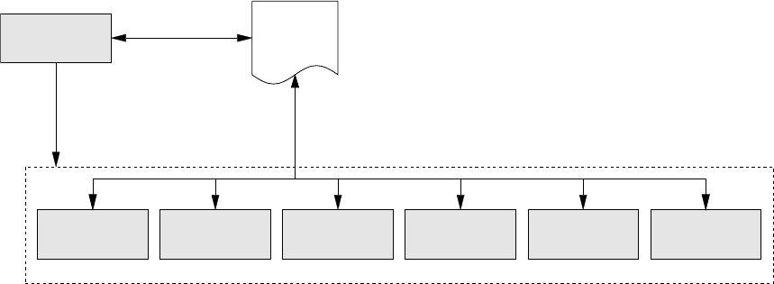
1.2 Flow of information between various DynaNet programs and input and output files . 6
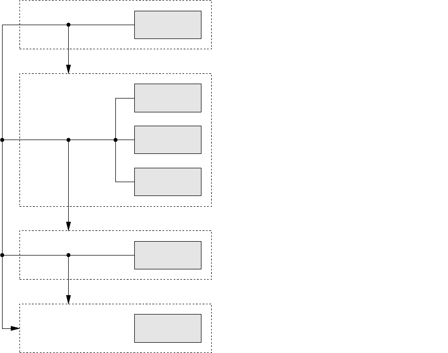
1.3 DynaNet program execution sequence . . . . . . . . . . . . . . . . . . . . . . . . . 8
1.4 Stations and measurements in the skye network.................... 9
3.1 import progress reporting of data import, conversion and processing . . . . . . . . . 22
3.2 Stations and measurements in the skye network filtered by the --bounding-box option. 26
3.3 Stationrenamingfile .................................. 28
3.4 Baselinescalarfile.................................... 33
3.5 Example simulation measurements list . . . . . . . . . . . . . . . . . . . . . . . . . 34
4.1 The ellipsoid–centred cartesian reference frame . . . . . . . . . . . . . . . . . . . . 38
4.2 The local reference frame . . . . . . . . . . . . . . . . . . . . . . . . . . . . . . . . 40
4.3 Orthogonal reference frames displaced by geodetic azimuth, vertical angle and distance 41
4.4 reftran progress reporting of station and measurement transformations . . . . . . . 51
5.1 The relationships between the natural terrain, ellipsoid, geoid, mean sea level, and
seasurface. ....................................... 54
5.2 The relationship between the geoid and quasigeoid, and between ellipsoid height (h)
and normal orthometric height (HNO)......................... 55
5.3 Bilinear interpolation concept . . . . . . . . . . . . . . . . . . . . . . . . . . . . . . 57
5.4 geoid progress reporting of geoid grid file interpolation . . . . . . . . . . . . . . . . 61
5.5 Interactive geoid grid file interpolation . . . . . . . . . . . . . . . . . . . . . . . . . 62
5.6 geoid progress reporting of geoid interpolation and text file transformation . . . . . 63
5.7 Example NTv2 grid file summary . . . . . . . . . . . . . . . . . . . . . . . . . . . . 64
5.8 Progress of NTv2 grid file creation . . . . . . . . . . . . . . . . . . . . . . . . . . . 66
6.1 Network segmentation concept . . . . . . . . . . . . . . . . . . . . . . . . . . . . . 70
6.2 A trivial GNSS network segmented into two blocks . . . . . . . . . . . . . . . . . . 70
6.3 Network segmentation concept involving four blocks . . . . . . . . . . . . . . . . . . 72
6.4 Segmentation of a geodetic network having stations with large numbers of measurements. 74
6.5 GNSS, direction set and distance measurements in the Victorian geodetic network
associated with MORANG PM 48. . . . . . . . . . . . . . . . . . . . . . . . . . . . 75
6.6 Segmentation of a spirit levelling network having stations with a low measurement
count. .......................................... 76
6.7 segment progressreporting............................... 79
6.8 Segmentation summary for uni_sqr with a block threshold of 45 . . . . . . . . . . . 80
6.9 Segmentation summary for uni_sqr with a block threshold of 45 and minimum inner
stationcountof35 ................................... 81
7.1 Slope, ellipsoid arc and ellipsoid chord distances . . . . . . . . . . . . . . . . . . . . 84
7.2 Mean sea level arc distances . . . . . . . . . . . . . . . . . . . . . . . . . . . . . . 85
xiii
7.3 Relationships between slope distance, MSL arc distance, ellipsoid arc distance and
ellipsoid chord distance measurements . . . . . . . . . . . . . . . . . . . . . . . . . 86
7.4 Heights and height differences . . . . . . . . . . . . . . . . . . . . . . . . . . . . . 87
7.5 Bearings and horizontal angles . . . . . . . . . . . . . . . . . . . . . . . . . . . . . 90
7.6 Cluster of horizontal directions . . . . . . . . . . . . . . . . . . . . . . . . . . . . . 92
7.7 Zenithdistances..................................... 93
7.8 Verticalangles...................................... 94
7.9 TheNormaldistribution................................. 96
7.10 Chi–square (χ2) distributions for 4, 6, 10 and 20 degrees of freedom . . . . . . . . . 97
7.11 Student’s t distributions for 2, 5, 10 and 50 degrees of freedom . . . . . . . . . . . . 98
7.12 The error ellipse and its dependence on coverage factor k............... 102
8.1 adjust progressreporting ................................ 109
8.2 Single–threadmode................................... 111
8.3 Multi–thread mode on four cores . . . . . . . . . . . . . . . . . . . . . . . . . . . . 112
8.4 Thread switching on a single core . . . . . . . . . . . . . . . . . . . . . . . . . . . . 112
8.5 Block–1onlymode ................................... 113
8.6 Progress reporting using single–thread adjustment mode . . . . . . . . . . . . . . . 114
8.7 Progress reporting using multi–thread adjustment mode . . . . . . . . . . . . . . . . 114
8.8 Progress reporting using Block–1 only adjustment mode . . . . . . . . . . . . . . . 115
9.1 Adjustment summary from a sample GNSS network . . . . . . . . . . . . . . . . . . 136
9.2 Adjusted measurements table from a sample GNSS network — without a–priori
variancematrixscaling ................................. 137
9.3 Adjusted measurements table from a sample GNSS network — with a–priori variance
matrixscaling ...................................... 138
9.4 (a) Level run adjustment with all original measurements, and (b) Repeat level run
adjustment with the suspect measurement removed . . . . . . . . . . . . . . . . . . 140
B.1 Exampleheaderlines .................................. 172
B.2 Example station file with coordinates in UTM,LLH and XYZ formats . . . . . . . . . . 173
B.3 Example angle measurements . . . . . . . . . . . . . . . . . . . . . . . . . . . . . . 174
B.4 Example geodetic azimuths, astronomic azimuths, zenith distances and vertical angles 175
B.5 Exampledirectionsets.................................. 176
B.6 Example ellipsoid chords, ellipsoid arcs, Mean Sea Level arcs, slope distances and
heightdifferences .................................... 177
B.7 Example GNSS baseline measurement . . . . . . . . . . . . . . . . . . . . . . . . . 179
B.8 Example GNSS baseline clusters. . . . . . . . . . . . . . . . . . . . . . . . . . . . . 180
B.9 Example GNSS point clusters. . . . . . . . . . . . . . . . . . . . . . . . . . . . . . 180
B.10 Example orthometric height and ellipsoid height measurements. . . . . . . . . . . . . 181
B.11 Example geodetic latitude and longitude, and astronomic latitude and longitude
measurements....................................... 181
B.12 Example geoid information records . . . . . . . . . . . . . . . . . . . . . . . . . . . 182
B.13 Example general options. . . . . . . . . . . . . . . . . . . . . . . . . . . . . . . . . 184
B.14 Example import options. ................................ 185
B.15 Example reftran options. ................................ 185
B.16 Example geoid options.................................. 185
B.17 Example segment options. ............................... 186
B.18 Example adjust options. ................................ 186
B.19 Example output options. . . . . . . . . . . . . . . . . . . . . . . . . . . . . . . . . 187
B.20 DnaXMLFormat schemadefinition ............................ 188
B.21 DnaStation schemadefinition.............................. 189
xiv
B.22 Sample station file encoded in DynaML format . . . . . . . . . . . . . . . . . . . . 189
B.23 DnaMeasurement schemadefinition ........................... 190
B.24 Clusterpoint and GPSBaseline schema definition . . . . . . . . . . . . . . . . . . . 191
B.25 Directions and GPSCovariance schema definition . . . . . . . . . . . . . . . . . . . 191
B.26 Sample measurements encoded in DynaML format . . . . . . . . . . . . . . . . . . 192
B.27 Example formatted text file . . . . . . . . . . . . . . . . . . . . . . . . . . . . . . . 194
B.28 Example comma separated values file . . . . . . . . . . . . . . . . . . . . . . . . . . 194
xv
xvi
List of Tables
3.1 Station coordinate types handled by the supported file formats . . . . . . . . . . . . 18
3.2 Supported measurement types and measurement codes . . . . . . . . . . . . . . . . 19
3.3 GNSS variance matrix scaling options . . . . . . . . . . . . . . . . . . . . . . . . . 32
3.4 StationMapfields.................................... 36
3.5 Associated Stations List fields . . . . . . . . . . . . . . . . . . . . . . . . . . . . . . 36
3.6 Associated Measurements List fields . . . . . . . . . . . . . . . . . . . . . . . . . . 36
4.1 EPSG codes and reference frames . . . . . . . . . . . . . . . . . . . . . . . . . . . 48
4.2 Supported transformation parameters . . . . . . . . . . . . . . . . . . . . . . . . . . 48
4.3 Alignment of IGS precise orbit product reference frames with ITRF updates over time
(source: http://acc.igs.org/igs-frames.html) ................. 49
4.4 Alignment of WGS84 realisations with ITRF updates over time (source: https:
//confluence.qps.nl/pages/viewpage.action?pageId=29855173)....... 50
5.1 NTv2 grid file overview fields . . . . . . . . . . . . . . . . . . . . . . . . . . . . . . 65
5.2 NTv2 grid file sub grid fields . . . . . . . . . . . . . . . . . . . . . . . . . . . . . . 65
5.3 Grid file interpolation error codes and descriptions . . . . . . . . . . . . . . . . . . . 67
6.1 Distribution of parameters and measurements of a network segmented into two blocks 71
7.1 Confidence intervals for ±1σto ±4σ. ......................... 96
9.1 Student’s t confidence intervals for α= 95%,r= 2 . . . 1000 ............. 135
A.1 dynanet standardoptions................................ 151
A.2 dynanet genericoptions ................................ 152
A.3 import standardoptions ................................ 153
A.4 import referenceframeoptions............................. 153
A.5 import datascreeningoptions ............................. 154
A.6 import GNSS variance matrix scaling options . . . . . . . . . . . . . . . . . . . . . 155
A.7 import network simulation options . . . . . . . . . . . . . . . . . . . . . . . . . . . 155
A.8 import exportoptions.................................. 156
A.9 reftran standardoptions ................................ 156
A.10 reftran transformationoptions ............................. 157
A.11 reftran exportoptions ................................. 157
A.12 geoid standardoptions ................................. 158
A.13 geoid interpolationoptions............................... 158
A.14 geoid NTv2creationoptions .............................. 159
A.15 geoid interactive interpolation options . . . . . . . . . . . . . . . . . . . . . . . . . 159
A.16 geoid file interpolation options . . . . . . . . . . . . . . . . . . . . . . . . . . . . . 160
A.17 geoid exportoptions .................................. 160
A.18 segment standardoptions ............................... 161
A.19 segment configurationoptions............................. 161
xvii
A.20 adjust standardoptions................................. 162
A.21 adjust adjustment mode options . . . . . . . . . . . . . . . . . . . . . . . . . . . . 163
A.22 adjust phased adjustment options . . . . . . . . . . . . . . . . . . . . . . . . . . . 163
A.23 adjust adjustment configuration options . . . . . . . . . . . . . . . . . . . . . . . . 163
A.24 adjust staged adjustment options . . . . . . . . . . . . . . . . . . . . . . . . . . . 164
A.25 adjust adjustment output options . . . . . . . . . . . . . . . . . . . . . . . . . . . 164
A.26 adjust exportoptions.................................. 166
A.27 plot standardoptions .................................. 167
A.28 plot data configuration options . . . . . . . . . . . . . . . . . . . . . . . . . . . . . 167
A.29 plot mappingoptions .................................. 168
A.30 plot PDFvieweroptions ................................ 169
B.1 Header line column locations and field widths . . . . . . . . . . . . . . . . . . . . . 172
B.2 Station information column locations and field widths . . . . . . . . . . . . . . . . . 173
B.3 General measurement information column locations and field widths . . . . . . . . . 174
B.4 Column locations and field widths for horizontal angles . . . . . . . . . . . . . . . . 174
B.5 Column locations and field widths for geodetic azimuths, astronomic azimuths, zenith
distances and vertical angles. . . . . . . . . . . . . . . . . . . . . . . . . . . . . . . 175
B.6 Column locations and field widths for direction sets. . . . . . . . . . . . . . . . . . . 176
B.7 Column locations and field widths for ellipsoid chords, ellipsoid arcs, Mean Sea Level
arcs, slope distances and height differences. . . . . . . . . . . . . . . . . . . . . . . 176
B.8 Column locations and field widths for a GNSS baseline (single or cluster) header record.177
B.9 Column locations and field widths for a GNSS point cluster header record. . . . . . . 178
B.10 Column locations and field widths for GNSS baseline and point measurements. . . . 178
B.11 Column locations and field widths for a GNSS cluster covariance block. . . . . . . . 179
B.12 Column locations and field widths for orthometric and ellipsoid height measurements. 181
B.13 Column locations and field widths for geodetic latitudes and longitudes, and astronomic
latitudesandlongitudes. ................................ 181
B.14 Geoid information column locations and field widths . . . . . . . . . . . . . . . . . . 182
B.15 DynaNet program options formatting. . . . . . . . . . . . . . . . . . . . . . . . . . 184
B.16 Formatted text file fields . . . . . . . . . . . . . . . . . . . . . . . . . . . . . . . . 193
B.17 Comma separated values file fields . . . . . . . . . . . . . . . . . . . . . . . . . . . 194
C.1 Measurement to station connections table . . . . . . . . . . . . . . . . . . . . . . . 198
C.2 Segmentation summary table . . . . . . . . . . . . . . . . . . . . . . . . . . . . . . 200
C.3 Individual block data table . . . . . . . . . . . . . . . . . . . . . . . . . . . . . . . 200
C.4 Adjusted station coordinates . . . . . . . . . . . . . . . . . . . . . . . . . . . . . . 201
C.5 Adjustment statistics summary table . . . . . . . . . . . . . . . . . . . . . . . . . . 203
C.6 Adjusted measurements and associated statistics table . . . . . . . . . . . . . . . . 204
C.7 Computed measurements (a–priori) on each iteration . . . . . . . . . . . . . . . . . 206
C.8 Coordinate corrections table . . . . . . . . . . . . . . . . . . . . . . . . . . . . . . . 207
C.9 Adjusted positional uncertainty table . . . . . . . . . . . . . . . . . . . . . . . . . . 209
C.10 Positional uncertainty covariance block . . . . . . . . . . . . . . . . . . . . . . . . . 210
xviii
List of Abbreviations
AGD66 Australian Geodetic Datum 1966
AGD84 Australian Geodetic Datum 1984
AHD Australian Height Datum. Commonly used in reference to Australian Height Datum
1971 (AHD71) and Australian Height Datum (Tasmania) 1983 (AHD–TAS83).
AHD–TAS83 The Australian Height Datum (Tasmania) 1983 is the normal–orthometric height
datum for mainland Tasmania.
AHD71 The Australian Height Datum 1971 is the normal–orthometric height datum for
mainland Australia.
CSV Comma Separated Values
DNA Dynamic Network Adjustment
DynaML DynaNet Markup Language. XML format defined according to the DynaNet 2.0 XML
schema.
EPSG European Petroleum Survey Group
GDA2020 Geocentric Datum of Australia 2020. Realised by continuous analysis of over 400
Asia Pacific Reference Frame sites, referenced to the GRS80 ellipsoid and determined
with respect to ITRF2014 at epoch 2020.0.
GDA94 Geocentric Datum of Australia 1994. Realised by the derived coordinates of the
Australian Fiducial Network (AFN) geodetic stations, referenced to the GRS80 ellipsoid
and determined with respect to ITRF92 at epoch 1994.0.
GLONASS GLObal NAvigation Satellite System
GMA Geodetic Model of Australia. Implemented via the adjustments termed GMA73,
GMA80, GMA82 and GMA84.
GNSS Global Navigation Satellite System
GPS Global Positioning System
GRS80 Geodetic Reference System 1980 reference ellipsoid, where a = 6378137.0 m, f =
1/298.257222101
ICSM Intergovernmental Committee on Surveying and Mapping
IGS International GNSS Service
ITRF International Terrestrial Reference Frame — a realisation of the International Terrestrial
Reference System (ITRS) produced by the International Earth Rotation and Reference
Systems Service (IERS).
MGA94 Map Grid of Australia 1994. Universal Transverse Mercator projection of the Geocentric
Datum of Australia 1994.
MSL Mean sea level
PDF Probability Density Function
xix
RHEL RedHat Enterprise Linux
SINEX Solution INdependent EXchange format.
TM Transverse Mercator
UTM Universal Transverse Mercator
WGS84 World Geodetic System of 1994
XML eXtensible Markup Language
xx
List of Symbols
φGeodetic latitude.
λGeodetic longitude.
ΦAstronomic latitude.
ΛAstronomic longitude.
AAstronomic azimuth.
θ12 Geodetic azimuth between points 1and 2.
α123 Horizontal angle at point 1, between points 2and 3.
s12 Slope or direct distance between points 1and 2.
c12 Ellipsoid chord distance between points 1and 2.
e12 Ellipsoid arc distance between points 1and 2.
m12 Mean sea level arc distance between points 1and 2.
ζ12 Zenith distance from point 1 to 2.
ϑ12 Vertical angle from point 1 to 2.
νRadius of curvature in the prime vertical.
ρRadius of curvature in the prime meridian.
aSemi–major axis of the reference ellipsoid.
bSemi–minor axis of the reference ellipsoid.
e2First eccentricity of the reference ellipsoid.
x, y, z X, Y and Z coordinates in the cartesian reference frame.
φ, λ, h Geodetic latitude, geodetic longitude and ellipsoid height in the geographic reference
frame.
e, n, up East, north and up coordinates in the local reference frame.
θ, ϑ, s Geodetic azimuth, vertical angle and direct distance in the polar reference frame.
E, N, Zo Easting, Northing and zone of a Universal Transverse Mercator (UTM) projection.
k0UTM central scale factor.
λ0Longitude of the central meridian of a UTM zone.
zwUTM zone width.
ξDeflection of the vertical in the prime meridian (north–south component).
ηDeflection of the vertical in the prime vertical (east–west component).
Combined deflection of the vertical calculated from north–south and east–west components.
Nor ζGeoid–ellipsoid separation or height anomaly.
HHeight of point pabove an orthometric height surface.
xxi
hHeight of point pabove the ellipsoid.
µThe mean.
σStandard deviation of an estimated quantity.
σ2Variance or precision of an estimated quantity.
σ2
0Variance factor or sigma zero.
αProbability or significance level, expressed as a percentage or value from 0 to 1.0.
kCoverage factor corresponding to the level of significance.
χ2
rChi–square statistic with rdegrees of freedom.
wSum of the squares of the weighted corrections minimised in the solution of the least
squares normal equations.
τPelzer’s measurement reliability criterion.
TPelzer’s global network reliability criterion.
xxii
Chapter 1
Introduction
DynaNet is a rigorous, high performance least squares adjustment application. It has been designed
to estimate 3D station coordinates and uncertainties for both small and extremely large geodetic
networks, and can be used for the adjustment of a large array of Global Navigation Satellite System
(GNSS) and conventional terrestrial survey measurement types. On account of the phased adjustment
approach used by DynaNet, the maximum network size which can be adjusted is effectively unlimited,
other than by the limitations imposed by a computer’s processor, physical memory and operating
system memory model. Example projects where DynaNet can and has been used include the
adjustment of small survey control networks, engineering surveys, deformation monitoring surveys,
national and state geodetic networks and digital cadastral database upgrade initiatives.
DynaNet provides the following capabilities:
•Import of data in geographic, cartesian and/or projection (UTM) coordinates contained in
DNA, CSV, DynaML and SINEX data formats;
•Input of a diverse range of measurement types;
•Transformation of station coordinates and measurements between several static and dynamic
reference frames;
•Rigorous application of geoid–ellipsoid separations and deflections of the vertical;
•Simultaneous (traditional) and phased adjustment modes;
•Automatic segmentation and adjustment of extremely large networks in an efficient manner;
•Rigorous estimation of positional uncertainty for all points in a network;
•Detailed statistical analysis of adjusted measurements and station corrections;
•Production of high quality network plots;
•Automated processing and analysis with minimal user interaction.
1.1 Brief history of phased adjustment and DynaNet
Since Gauss published his treatment of the method of least squares in 1809, Tienstra [1956] was
the first to develop the concept and principles of phased adjustment. In his work, Tienstra defines
the principle property of phased adjustment as — “Least squares problems may be divided into
an arbitrary number of phases, provided that in each following phase(s), cofactors resulting from
preceding phases are used.” Using the method of condition equations and Ricci calculus, Tienstra
demonstrated that rigorous parameter estimates for all stations could be derived in a step–wise
fashion by treating the parameters estimated in one phase as quasi–measurements in the next phase.
1

Since the time of his publication, Tienstra’s concept of phased adjustment has been studied by
several authors, and has been extended and implemented in various forms. Initially, Professor
Dr. Ir. Willem Baarda of the Computing Centre of the Delft Technological University (where Tienstra
was Professor until his death in 1951) led the implementation of Tienstra’s phased adjustment
algorithm for the 1959 adjustment of the United European levelling network [Alberda, 1963]. A
few years later, Lambeck [1963] studied phased adjustment and demonstrated that Krüger’s [1905]
method of stacking normal equations was mathematically equivalent to Tienstra’s phased adjustment
technique. Schmid and Schmid [1965], in their discussion of the generalised approach to least squares,
include an algorithm which solves least squares problems “sequentially” in steps. Their algorithm is
essentially the same as Tienstra’s phased adjustment algorithm, although it is designed to provide for
the addition and removal of measurements after all parameters in the network have been estimated,
rather than to provide a mechanism for handling the adjustment of a large network in stages.
Kouba [1970, 1972] studied the phased adjustment method and demonstrated that the sequential
least squares technique developed by Schmid and Schmid [1965] was mathematically equivalent to
that of Tienstra’s. In his work, Kouba made an important contribution to the study of phased
adjustment by demonstrating that all junction parameter estimates and variances must be carried
between phases if rigorous results are to be achieved. Ying Chung–Chi [1970] summarised Tienstra’s
work using matrix algebra and extended the concept to adjustment by observation equations. Ying
Chung–Chi also demonstrated mathematical equivalence between Tienstra’s method and Krüger’s
method. Although Ying Chung–Chi [1970] does not formally prove that Tienstra’s phased adjustment
method will give the same estimates as a simultaneous adjustment, he demonstrates that it does so
numerically for a simple level network.
The next major application of Tienstra’s concept of phased adjustment was the Canadian Section
Method, developed by Pinch and Peterson [1974]. In this development, Pinch and Peterson formally
prove that where two sections of a network are adjusted independently in a first stage adjustment,
and the estimates of the parameters common to the two sections (with their variance matrices)
are integrated in a second stage adjustment, the second stage estimates will be identical to those
produced from a simultaneous adjustment. Whilst their method produces rigorous estimates for the
junction station parameters and variance matrices, Gagnon [1976] notes that in the final phase of the
process, rigorous variance matrix estimates are not produced for the inner1stations of each block.
The Canadian Section Method has been used widely in Australia for adjustments of the national
network subsequent to the Australian Geodetic Datum 19662(AGD66). These are referred to as
various versions of the Geodetic Model of Australia (GMA) and include the adjustments termed
GMA73, GMA80, GMA82 and GMA84, the latter of which led to the development of the Australian
Geodetic Datum 1984 (AGD84) [Allman, 1983, Allman and Steed, 1984]. The establishment of the
North American Datum 1983 (NAD83) and the European Datum of 1987 (ED87) also made use of
the Canadian Section Method, although they varied from Tienstra’s approach in that they employed
Helmert Blocking for the solution of the normal equations.
Around the time of the development of the early GMA adjustments, Leahy [1983] revisited the
application of Tienstra’s phased adjustment method to the adjustment of large geodetic networks.
This led to further research [Leahy et al., 1986] and the development of VicNet — a two–dimensional
1. Repeated mention of inner and junction stations will be made throughout this user guide. By way of preliminary
definition, inner stations are the stations which are connected only by measurements in a single section, whereas
junction stations are those which are connected by measurements from two or more sections. See §6.2 for more
information.
2. Whilst the establishment of AGD66 was conducted in phases using the process of segmenting the network into
smaller sections, the approach undertaken for the adjustment and integration of the respective sections didn’t
employ Tienstra’s rigorous phased adjustment technique. This was largely driven by the challenges and complexities
associated with undertaking a large scale adjustment on 1960’s computational infrastructure.
2
package designed to undertake phased adjustments of geodetic networks comprised of conventional
terrestrial measurements. This software package was refined by Collier [1991] to accommodate
three–dimensional adjustments and the integration of GPS baseline measurements. With these
enhancements and other new capabilities and bug fixes, the software became known as MetNet and
was used extensively for the adjustment of the Melbourne survey control network. Further research
by Leahy [1999] led to the development of a fully automated network segmentation procedure which
can handle networks of any size and configuration, and a rigorous approach for the extension and
integration of networks.
Continued research on the automatic segmentation and phased adjustment of large geodetic networks
gave rise to further refinements in the algorithm and the development of a new 32–bit Windows
package (developed in Visual Basic 6) known as Dynamic Network Adjustment (DNA). The initial
development of DNA was undertaken by Leahy and Collier [1998] at the University of Melbourne and
was made possible through funding provided by the Australian Research Council (ARC) and industry
support from the Office of Surveyor–General Victoria, AUSLIG Geodesy and WBCM Surveys Pty Ltd.
Following numerous enhancements and refinements in subsequent years, DNA was repackaged and
released as DynaNet version 1.0. In turn, version 2.0 was developed to cater for new measurement
types, and to provide several user enhancements.
1.1.1 Preamble to Version 3.3
DynaNet Version 3.0 is a completely revised version developed by the authors of this user guide. It
has been re–written in C
++ to provide cross–platform support (e.g. Windows, Linux, Mac OS X),
and to take advantage of multi–core processors so as to achieve optimum adjustment performance.
The main specifications of DynaNet and the environments in which it has been compiled and tested
include:
•Developed using C
++11 and the C
++ Standard Library, Boost [Schäling, 2014], CodeSynthesis
XSD [Kolpackov, 2017] and Apache’s Xerces C
++ XML parser [Apache, 2017];
•The modular architecture design and comprehensive API allows for implementation via custom
software development;
•Developed for Windows, Linux and Mac OS X platforms, and runs on 32–bit and 64–bit
operating systems;
•Compiled using Microsoft C
++ 2010 and 2017, Intel C
++ 2014 and 2017, and gcc 4.8.2;
•Tested on Windows XP, Windows 7, Windows 2003 Server. RedHat Enterprise Linux (RHEL)
7, Fedora 23 and OpenSUSE 10.
DynaNet Version 3.3 contains new features and user options, numerous code enhancements, and
various bug fixes.
1.2 Conventions used in this document
The following typographical and mathematical conventions have been adopted throughout this
document:
•DynaNet program names are indicated by bold sans serif font. For example, the program
import is the main program for importing data into DynaNet.
•Program execution on the command line usage is denoted by fixed–width typewriter font.
Examples of program execution at the command prompt are encapsulated by a grey box. If
different syntax is required for Windows and UNIX/Linux platforms, syntax for both environments
3

will be provided. Program options may be either inline with the text or placed within a grey
box. For example, basic command line usage of import is given by:
> import -n network_name network.stn network.msr
and the program option for specifying the input directory is --input-folder.
•File names and file contents are denoted by fixed–width typewriter font. File contents are
encapsulated by a grey box with column positions shown in a separate box:
1234567890123456789012345678901234567890123456789012345678901234567890123456789
!#=DNA 3.00 STN 28.08.2013 GDA94 43
•Math symbols are given in serif font. Variables are denoted by upper or lower case letters in
italics, as in bor B. Matrices are denoted by upper case letters in bold font, as in A, and vectors
are denoted by lower case letters in bold font, as in m. The identity matrix is denoted by I,
and the context in which it is used determines its dimensions. The term variance matrix is used
to refer to the covariance matrix or variance–covariance matrix and is denoted by V. Indexing
of matrix and vector elements is denoted by Cij or cij. Superscripts Tand −1denote the
transpose and inverse respectively. For a random variable x, the notation E(x)∼Nµ, σ2
means that xfollows a Normal distribution with a mean or expected value of µand variance
σ2.
1.3 Program overview
This section provides an overview of the DynaNet software architecture and a summary of the various
DynaNet programs. The general philosophy of program execution and configuration via program
options and arguments is also explained.
1.3.1 Software architecture and information flow
DynaNet consists of several programs, the functionality of which is distributed across a number of
executables and Dynamic Link Libraries (DLL) using a modular, service–oriented architecture. The
modular architecture of DynaNet affords several advantages, such as:
•Individual programs can be executed to perform a specific function relating to the processing
and adjustment of geodetic networks;
•One or more programs can be chained together in a customised sequence to satisfy a specific
user requirement;
•A sequence of program calls can be invoked via scripts at will, at scheduled times or as part
of a larger automated datum maintenance environment;
•Routine and conventional processing of geodetic control surveys can be handled in a single
step.
To assist with conventional end–to–end processing, the main program dynanet serves as a wrapper
application which can be used to coordinate the execution of one or more DynaNet programs in a
single step. The coordination of the various programs is illustrated in Figure 1.1.
4
dynanet
import adjust
segment
reftran geoid plot
.dnaproj
Figure 1.1: Coordination of DynaNet program execution
A brief description of the various DynaNet programs is given below:
import To create and process projects in DynaNet, this program must be run first to define
the network name, and to convert geodetic station coordinates and measurements from
external file formats into the required binary and text file formats (see §2.2.2). Note that
import only needs to be run once in order to import geodetic station coordinates and
measurements into DynaNet. Accordingly, import does not need to be run for repeated
calls to other programs unless there is a change to the stations or measurements, or if
some form of manipulation to the import process is required. Chapter 3 provides detailed
information on how to use and configure import.
reftran This program performs reference frame transformations to align all imported stations
and measurements to a common reference frame and epoch. See Chapter 4 for more
information on using reftran.
geoid This program introduces geoid–ellipsoid separations and deflections of the vertical into a
project from either an NTv2 formatted geoid model or ASCII text file. This program can
optionally export interpolated geoid information to a DNA geoid text file. geoid also
provides a capability to generate NTv2 formatted files from the legacy AUSGeoid DAT
file format. See Chapter 5 for more information on using geoid.
segment This program segments a network into a series of inter–connected blocks for use by adjust
in phased adjustment mode. See Chapter 6 for more information on using segment.
adjust This is the main parameter estimation program in DynaNet. adjust can be executed in
simultaneous or phased adjustment mode. When attempting to adjust large networks
using phased adjustment, adjust may be executed in single–thread or multi–thread mode.
For the former, users may opt to use staged mode if physical memory limits prevent
normal program execution. A reverse, Block–1 only adjustment may also be undertaken
if the desired outcome is a full variance matrix for a specific cluster of stations. See
Chapter 8 for more information on using adjust.
plot This program generates PDF images of a network from the imported information and
graphs relating to network segmentation and adjustment statistics. More information on
plot and its use will be given in a subsequent version of this guide.
As is hinted by Figure 1.1, the coordination of DynaNet programs is handled via a .dnaproj (DynaNet
project) file. The use of the project file will be discussed in more detail in Chapter 2.
5
The programs import,reftran,geoid,segment,adjust and plot read and write a range of formatted
files in a way which permits the structured flow of information. Figure 1.2 illustrates the flow of
information amongst the various programs and files.
import
adjust
segment
reftran
geoid
plot
.adj
.xyz
.snx
.snx
.mtx
.xml
.stn
.msr
.net
.apu
.cor
.bst
.bms
.eps
.pdf
.seg
.map
.asl
.aml
Figure 1.2: Flow of information between various DynaNet programs and input and output files
As shown in Figure 1.2, information exported from one program often serves as input to other
programs. This concept affords the user an ability to examine the output from one program before
executing another program, and to re–run certain programs with different user options and to examine
the variation in results. A brief description of the various file types is discussed in Chapter 2.
1.3.2 Program execution and command line options
DynaNet programs can only be executed from the system command prompt (or shell or terminal
emulator), via Windows batch files (.bat and .cmd) and UNIX/Linux shell scripts (.sh), or from
system calls made within custom–developed programs. Hence, DynaNet Version 3.3 does not provide
a windows–based graphical user interface (GUI).
The convention for executing DynaNet programs is to enter a program name, followed by one or
more options that modify its behaviour and, if required, an argument upon which the program will
act. The convention is as follows:
> program --option argument
6

The complete command line reference for all DynaNet programs is provided in Chapter A. To display
the command line reference for a DynaNet program, type in the program name at the command
prompt, followed by --help and press Enter:
> dynanet --help
Alternatively, if no program options are provided upon program execution, the program’s version
information and command line reference will be displayed on the screen.
There are over 140 program options which can be used to configure the way in which DynaNet
programs process geodetic network information. Each DynaNet program will require certain options
specific to its operation and depending on which option has been provided, additional arguments may
be required. Several options, such as --quiet,--version and --help are common to all programs.
If an option requires an argument, the command line reference will use the term arg.
All options are case–sensitive and must be preceded by two hyphens. Spaces must not be entered
between the hyphen and the option text, however spaces are required between options. Options can
be provided in any order whatsoever. Some options may be specified using an abbreviated form.
For example, to display the version of a DynaNet program, the abbreviated form -v may be used.
In addition, all DynaNet programs permit the use of partial option text, provided that the partial
option text contains a sufficient number of characters to uniquely distinguish the required option
from all other options. For example, the program import will export newly imported stations and
measurements in DNA format if the option --export-dna-files is provided. This function can
also be executed by providing --export-d. However, import will return an error if just --export is
provided since there are five export options that commence with the text export.
When a program option requires an argument, input may require alpha–numeric entry and/or the
selection of a multiple–choice option. If an argument must include spaces, such as a station name,
enclose the argument with double quotes, such as:
> program --option "arguments with spaces"
For multiple choice options, DynaNet will adopt the default value (denoted in the command line
reference) unless the user overrides it by supplying an alternative argument value. For example,
import provides an ability to specify the default reference frame for all stations and measurements
contained in the user–supplied input files via the option --reference-frame (or -r in brief). As this
option provides a multiple choice, only predefined reference frames are allowed. If this option is not
provided, import will adopt the Geocentric Datum of Australia 1994 (GDA94) as the default value.
Several options adopt this convention.
Following chapters will explain in detail the function of each program and how to configure program
behaviour using the program options.
1.3.3 Program execution sequence
Figure 1.3 shows the program execution sequence employed by dynanet when performing end–to–end
processing. For the most part, this sequence will be adequate for conventional geodetic network
processing and adjustment.
7
import
adjust
segment
reftran
geoid
plot
Project creation stage
Pre–processing stage
Parameter estimation stage
Network plotting and
statistics graphing
Specify network name, reference frame and epoch, import data
into DynaNet format, apply data screening, specify GNSS scaling,
and export data into other formats.
Transform station coordinates and measurements onto the
specified reference frame and epoch.
Interpolate geoid–ellipsoid separations and deflections of the
vertical from geoid model.
Segment the network into a series of blocks.
Estimate station coordinates and uncertainties, calculate network
statistics, adjusted measurements and statistics, output corrections
and export adjustment results.
Plot network map, graph segmentation results and graph
adjustment statistics.
Figure 1.3: DynaNet program execution sequence
There are two circumstances, however, where this sequence may not be appropriate or will need to
be varied. Firstly, depending on the desired outcome, only some stages will be necessary. For this
purpose, dynanet provides the user with an ability to choose which DynaNet programs to execute.
The following examples explain some basic scenarios in which the user will require the execution of
only a subset of the DynaNet programs:
Ellipsoid–only adjustment To estimate coordinates on the ellipsoid from a small geodetic control
survey of GNSS measurements which are aligned to a common reference frame, only import
and adjust are required.
Multiple reference frames If the GNSS measurements in this survey are aligned to different reference
frames, then the sequence import,reftran and adjust will be required.
Terrestrial measurements If terrestrial measurements (e.g. angles, distances and orthometric
height differences) form part of this survey, then the sequence will change to import,reftran,
geoid and adjust. Here, geoid is added to the sequence to obtain geoid–ellipsoid separations
and deflections of the vertical which are used by DynaNet to cater for the influence of gravity
on the terrestrial measurements.
Generate basic network plot If only a plot of all stations and measurements in a network is
required, then only import and plot are required.
Generate plot of error ellipses, uncertainties and corrections If the network plot should also
include estimated error ellipses, circular confidence regions and a–priori station corrections
derived from a least squares adjustment, then the sequence will be import,adjust and plot.
8

Secondly, network processing and adjustment may require data concatenation, screening (or filtering),
scaling and multiple transformations between different reference frames before the network is suitable
for processing by adjust. For these tasks, it is recommended that a script file be used to string
together the needed program calls to achieve the required program execution sequence.
In either case, knowing which programs to execute will require a knowledge of the data and an
elementary knowledge of geodetic measurement, reference frames and adjustment theory.
1.4 Two–minute quick start tutorial
This section provides a quick start tutorial to processing geodetic network information in DynaNet.
The example used in this tutorial is a network comprised of six stations and nine GNSS baseline
measurements. The the project is named skye, and the stations and measurements are contained
in 2009-10-20-skye.stn and 2009-10-20-skye.msr respectively. Figure 1.4 shows the stations and
measurements in the skye network. The station file contains a mixture of ellipsoid heights and
orthometric heights on the Australian Height Datum (AHD). The GNSS baseline measurements and
variance matrices have been derived from conventional GNSS processing software and have been
estimated according to the Geocentric Datum of Australia 1994 (GDA94). No scaling has been
applied to the variance matrices.
145˚11'0.0"
145˚11'0.0"
145˚11'30.0"
145˚11'30.0"
145˚12'0.0"
145˚12'0.0"
−38˚07'0.0" −38˚07'0.0"
−38˚06'30.0" −38˚06'30.0"
−38˚06'0.0" −38˚06'0.0"
0 1
Kilometres
302502400
302513650
302508300
302509800
302513640
261907650
Figure 1.4: Stations and measurements in the skye network
9

Step 1 — Prepare the script
For this and many other examples provided in this user guide, it is assumed that users will want
to make use of a script file to string together several DynaNet program calls. Apart from some
basic differences, calls to DynaNet programs will be identical for both Windows and UNIX/Linux
platforms and can therefore be copied directly to a Windows batch file or a UNIX/Linux shell script
respectively.
For Windows platforms, prepare a file called run_skye.bat as follows:
echo off
rem Script to automate processing of skye geodetic network
For UNIX/Linux platforms, prepare a file called run_skye.sh as follows:
#!/bin/bash
# Script to automate processing of skye geodetic network
To execute this script using the UNIX/Linux shell, the execute permission for run_skye.sh will need
to be granted to the current user (or group or all users). The file execute permission can be set by:
$ chmod +x ./run_skye.sh
Alternatively, this script can be executed from the command line using bash:
$ bash ./run_skye.sh
Step 2 — Import the data
The next step to be undertaken is to create a project named skye. In this step, a call to import
is required to name the project and to introduce the station and measurement files. Setting the
network name and importing files into DynaNet is achieved by:
import -n skye 2009-10-20-skye.stn 2009-10-20-skye.msr
Upon running this command, the project skye is created and several files will be written to disk:
skye.bst,skye.bms,skye.map,skye.asl,skye.aml and skye.imp. See Chapter 2 for an explanation
of these file types.
Step 3 — Introduce geoid–ellipsoid separations
Since DynaNet requires all station heights to be reduced to the ellipsoid prior to adjustment, the next
step is to convert the orthometric station heights to ellipsoid heights. For this purpose, interpolation
of geoid–ellipsoid separations from a geoid model is needed. To this end, the script would be expanded
as follows:
10

import -n skye 2009-10-20-skye.stn 2009-10-20-skye.msr
geoid skye -g ./ausgeoid09.gsb --convert-stn-hts
Here, geoid–ellipsoid separations will be interpolated from ausgeoid09.gsb, which is a geoid grid
file structured according to the National Transformation version 2.0 (NTv2) format. The option
--convert-stn-hts informs geoid that all orthometric station heights should be converted to ellipsoid
heights. After this command is executed, all stations in the binary station file skye.bst will contain
geoid–ellipsoid separations and deflections of the vertical, and any orthometric heights will be reduced
to ellipsoid heights.
Step 4 — Adjust the network
DynaNet offers the flexibility to undertake constrained and minimally constrained (or free) least
squares adjustments in a number of ways. Adjustments may also be performed in a single pass via
simultaneous mode or sequentially in phases using phased adjustment mode. For this tutorial, the
skye network will be adjusted using no constraints and, given the relatively small size of this control
survey, via simultaneous mode. Assuming that station constraints have not been introduced into
either station or measurement files, the script would be expanded as follows:
import -n 2009-10-20-skye.stn 2009-10-20-skye.msr
geoid skye -g ./ausgeoid09.gsb --convert-stn-hts
adjust skye --output-adj-msr
From this call to adjust, the resulting adjustment output file will be called skye.simult.adj. The
option --output-adj-msr was added so as to print a table of adjusted measurements and statistics
to the .adj file.
If it is decided that a station should be constrained, users can choose one of three options to apply
station constraints — (1) set the station constraint flag within the station file, (2) add a station
position measurement to the measurement file, including the measurement precision by which to
constrain the station, or (3) specify the station and how it is to be constrained via the call to adjust.
The third option, which in effect replicates the first option, can be achieved by the following change
to the call to adjust (using station 302513640 as an example):
adjust skye --output-adj-msr --constraints 302513640,CCC
This section has provided a simple tutorial on using DynaNet to perform a straightforward network
adjustment of GNSS observations. Detailed help on program usage for numerous other processing
tasks will be provided throughout the remainder of this user guide.
11
12
Chapter 2
Creating, editing and processing
projects
2.1 Introduction
DynaNet uses the concept of a project to manage the input, processing and output of geodetic
network information. For each project, DynaNet uses a project file to store default and user specified
options. The user options contained in a project file configure the way in which the respective
DynaNet programs handle the geodetic network information relating to a project. At execution
time, each program can be configured by providing a project file path as a program argument, or by
specifying the respective options as program arguments. Since DynaNet Version 3.3 can be executed
from the system command prompt or from custom–developed programs, project files can be used to
completely automate the processing of geodetic networks, and to capture the options used during
program operation.
This chapter explains the various conventions used by DynaNet for managing projects, how to prepare
input files, and provides an overview of the basic program operation. More information about the
various options for each program will be explained in subsequent chapters.
2.2 Conventions used in DynaNet
2.2.1 File naming
Central to the management of projects is the network name. DynaNet uses the network name
to form the file names for all generated output files, and to determine which file to open when
information generated from one program must be read as input by another program. The basic file
naming convention is represented by network_name.ext where network_name is the user–supplied
network name and ext is the file extension. In some cases, DynaNet generates files in the form of
network_name.mode.ext where mode represents either a mode in which a program has been executed
or a user–specified program option.
To permit the input of files with a different file name to that which is expected from the default
naming convention, the file name for certain input files may be overridden by providing the relevant
command line argument. This feature will be covered in more detail in subsequent chapters describing
the input and output options of the various programs.
The network name is a mandatory argument required by all DynaNet programs except import. If
a network name is not specified when running import, DynaNet adopts the name ’network#’ where
’#’ represents the next available integer that yields a unique (or unused) file name in the folder of
13
program execution.
The primary exceptions to the file naming convention are station and measurement files (e.g. *.snx,
*.stn,*.msr,*.xml) provided as input to import, and the raw data files and formatted grid files
(e.g. *.dat,*.csv,*.gsb) provided as input to geoid. No restrictions are imposed upon the
naming of these files other than that the file extension corresponds with the file format. The file
extension restriction is imposed only for certain file types which prevent DynaNet from automatically
interpreting file content.
2.2.2 File types
As shown in Figure 1.2 on page 6, DynaNet creates and/or updates a number of binary and text
files, which are treated as either output and/or input files. The following is a list of file types
created by DynaNet in accordance with the file naming convention (assuming the network name is
network_name):
Binary formatted file types
network_name.aml Associated Measurements List. This file contains a list of measurements that
a station appears in.
.asl Associated Stations List. This file contains a count of the measurements
connected to a station and the index of this station in the AML file.
.bms Binary Measurements file. This file contains information about the
measurements in a network. The BMS file is a binary formatted file created
using an efficient file structure to provide maximum efficiency for retrieving
measurement information.
.bst Binary Stations file. This file contains information about the stations in a
network. The BST file is a binary formatted file created using an efficient file
structure to provide maximum efficiency for retrieving station information.
.map Station Map. This file maintains the relationship between the supplied
alphanumeric name and a unique (numerical) station identifier.
.mtx Matrix file. This file stores matrices in a structured file format designed for
efficient data storage.
.dbid Database ID list. This file contains the user–supplied database IDs for
measurements contained in DNA formatted measurement files.
ASCII text file types
network_name.imp import log. This file is a log of the station and measurement import
process.
.seg segment output. This file contains the station and measurement indices
for the respective blocks created from network segmentation.
.adj adjust output. This file contains the adjusted station coordinates and
measurements and associated statistics.
.xyz Adjusted Station Coordinates produced by adjust.
.cor Station Coordinate Corrections produced by adjust. This file contains
the corrections to the initial station coordinates.
.apu Adjusted Positional Uncertainty produced by adjust. This file contains
the positional uncertainties of the adjusted station coordinates.
14
.dbg Debug output. This file contains detailed program output information
to help assist with isolating network adjustment problems.
.dst Duplicate Stations list. This file contains a list of stations that were
identified as duplicates by import.
.dms Duplicate Measurements list. This file contains a list of measurements
that were identified as duplicates by import.
.log dynanet log. This file provides a time–stamped record of the progress
of the individual programs that have been coordinated by dynanet.
2.2.3 Directories
By default, all DynaNet programs expect input files to exist in the directory in which the programs
are run. DynaNet will also generate output files in this directory. Optionally, an input folder and
an output may be specified to inform the DynaNet programs where to find input files and where to
store output files. This feature will be covered in more detail in subsequent chapters.
2.3 Project setup and processing
2.3.1 Prepare station and measurement files
The first step in creating a project is to prepare the station and measurement files. DynaNet
supports a small range of file types. Appendix B provides a list of supported file types and the format
specification for selected file types. Stations and measurements may be provided in one or more files,
each of which may be encoded in any one of the supported file formats. DynaNet does not impose
any restrictions on how this information should be structured and so the user is left to decide which
file type is chosen and how station and measurement information will be stored.
2.3.2 Create DynaNet project file
In order to process projects in a single step using the main program dynanet, a project file must be
created. Note that a project file does not need to be created if the various DynaNet programs will be
executed manually, or executed via Windows batch files or UNIX/Linux shell scripts. In these cases
however, a project file will be created and updated automatically as each program is executed.
There are two options for creating a DynaNet project file — users may create this file manually or
use import to create this file automatically. The file format for the project file is described in §B.3.
Each time import is executed, a new project file will be created using the network name and the
default or user–specified output folder path. If this file exists, it will be re–created using the options
and arguments supplied. Options which have not been provided will assume default values. All other
options and arguments supplied to import, such as network name and station and measurement
files, will be printed to project file. Users not familiar with the project file format are encouraged
to use import to create the project file, and to use a text editor to modify the project file with the
desired options and arguments.
2.3.3 Automated project processing
Upon creating a project file, projects can be processed in a single step using the main program
dynanet. Using the project file shown in §B.3 for the skye project (see §1.4), the following command
illustrates how end–to–end processing can be performed in a single step using dynanet.
15

dynanet -p skye.dnaproj --import --geoid --adjust
The first option (-p) and argument (skye.dnaproj) inform dynanet where to find the project file.
Since the folder path was not provided on the command line, DynaNet will assume the project file
is located in the folder from which dynanet is executed. As shown by the general section in Figure
B.13, §B.3, this folder is C:\Data\proj.
The second, third and fourth options tell dynanet to execute import,geoid and adjust respectively
using the options specified in the project file. The order of these options is not important since
dynanet will adopt the program execution sequence shown in Figure 1.3. With respect to import,
the mandatory network name and input files are entered into the project file using --network-name
(under #general) and --stn-msr-input-file (under #import) respectively. All other options use
default arguments. For geoid, the NTv2 geoid grid file path and conversion of orthometric heights to
ellipsoid heights are handled by --ntv2-filepath and --convert-stn-hts (under #geoid). Finally,
configuring adjust to perform a simultaneous adjustment, holding station 302513640 fixed, and
to produce a table of adjusted measurements and statistics in the adjustment output (.adj) file is
managed by --adjustment-mode and --constraints (under #adjust), and --output-adj-msr (under
#output). Note that the options and arguments under #reftran and #segment are ignored since the
dynanet argument to execute reftran (–reftran) was not provided, and adjust was configured to
run a simultaneous adjustment.
As dynanet runs, it will load the options contained in the project file and pass them to the
respective programs. Upon execution, a log file named dynanet.log will be created and will contain
a time–stamped record of the progress of the individual programs that have been executed. A sample
of the log file is shown below.
1234567890123456789012345678901234567890123456789012345678901234567890123456789012345
+---------------------------------------------------------------------------
+ Title: dynanet
+ Description: Geodetic network adjustment software
+ Version: 3.2.6, Release (64-bit)
+ Build: Sep 22 2016, 16:23:21 (MSVC++ 10.0)
+ Copyright: (C) 2016 F.J.Leahy, P.A.Collier, R.W.Fraser.
This software is released under a restricted license.
+ Contact: dynanet.mail@gmail.com
+ +61 407 062 507
+---------------------------------------------------------------------------
+ Executable Start date and time End date and time Exit status
------------------------------------------------------------------------------------------
+ import 11-04-2014 6:04:06 PM 11-04-2014 6:04:07 PM Ended successfully.
+ geoid 11-04-2014 6:04:07 PM 11-04-2014 6:04:08 PM Ended successfully.
+ adjust 11-04-2014 6:04:08 PM 11-04-2014 6:04:09 PM Ended successfully.
+ DynaNet finished successfully.
16
Chapter 3
Import and export of geodetic network
information
3.1 Introduction
DynaNet supports a number of file formats for the exchange of geodetic network information. The
primary file formats supported by DynaNet, Version 3.3 for the import and export of stations,
measurements and adjustment solutions include:
CSV (Comma/Character Separated Values format) for the exchange of stations, measurements
and geoid information without concern for aligning data in specific positions
DNA (Dynamic Network Adjustment format) for the exchange of stations, measurements and
geoid information in a simple, human–readable format. Versions 1 and 3 are supported.
DynaML (DynaNet Markup Language format) for the exchange of stations and measurements in
XML format defined according to the DynaNet 2.0 XML schema
GeodesyML (Geodesy Markup Language format) for the exchange of station, measurement, solution
and covariance information in XML format defined according to ICSM’s eGeodesy GML
application schema
SINEX (Solution-INdependent EXchange format) for the exchange of solutions and covariance
information
Appendix B provides the file format specification for the CSV, DNA and DynaML file types. The
specification for GeodesyML can be found at http://geodesyml.org. The specification for the
SINEX file format can be found at
http://www.iers.org/IERS/EN/Organization/AnalysisCoordinator/SinexFormat/
sinex.html
DynaNet also reads and writes a number of binary and ASCII file formats for the exchange of geodetic
network adjustment information. These will be described throughout this section as the need arises.
3.2 Importing station and measurement information
The primary program for importing and converting geodetic network stations and measurements into
the format required by DynaNet is import. To import station and measurement information into
DynaNet, type import at the command prompt, followed by one or more options and arguments. The
17

complete command line reference for import is given in §A.2. If no program options are provided
upon program execution, the command line reference for import will be displayed.
If a DynaNet Project File (c.f. Chapter 2) is to be used, provide --project-file (or its shortcut -p)
followed by the full path for the project file:
import -p uni_sqr.dnaproj
No other options are required, as import will be invoked using the options and arguments contained
in the project file uni_sqr.dnaproj.
Alternatively, if all options and arguments are to be entered via the command line, type import, then
--network-name (or its shortcut -n) followed by the network name and the names of the files that
contain the station and measurement information:
import -n uni_sqr uni_sqrstn.xml uni_sqrmsr.xml
If the --network-name option and argument are omitted, import will use the default “network1”
name. If there is evidence in the current directory that “network1” has already been created, then
“network2” will be used. The integer appended to “network” increases until the first available
network name is found.
Whether using a project file or not, additional options and arguments can be supplied to configure
the way in which this information is imported. When using a project file, any additional options and
arguments provided on the command line will overwrite the values contained in the project file.
3.2.1 Station coordinate information
import accepts station coordinate information in three commonly accepted coordinate systems,
namely, Geographic coordinates, Universal Transverse Mercator (UTM) projection coordinates, and
Earth–centred cartesian coordinates. Geographic coordinates are expressed as latitude,longitude and
height, where height may be ellipsoidal height or orthometric height. UTM projection coordinates are
expressed as Easting,Northing,zone and height. Earth–centred cartesian coordinates are expressed
as X,Yand Z. These coordinate systems and the methods by which DynaNet handles transformations
between them are explained in Chapter 4. With reference to the supported file formats described in
the introduction, Table 3.1 lists the coordinate types handled by the respective file formats.
Table 3.1: Station coordinate types handled by the supported file formats
Format CSV DNA DynaML GeodesyML SINEX
Geographic (d.mmss) • • • • •
Geographic (d.dddd) •
UTM Projection • • • •
Cartesian • • • • •
Appendix B explains the formatting of station coordinate information for each of the supported file
18

formats. §3.2.3 explains the concept of station constraints and how they are interpreted by DynaNet.
Configuring the default reference frame for stations is described in §3.3.1.
3.2.2 Supported measurement types
DynaNet supports a wide range of GNSS and terrestrial measurement types. To facilitate the efficient
management of these types, DynaNet uses the concept of a measurement code. The measurement
types and corresponding codes supported by DynaNet are listed in Table 3.2.
Table 3.2: Supported measurement types and measurement codes
Code Measurement type
A Horizontal angles (uncorrelated)
B Geodetic azimuth (or bearing)
C Ellipsoid chord distance
D Direction set
E Ellipsoid arc distance
G Single GNSS baseline (∆x∆y∆z)
H Orthometric height
I Astronomic latitude
J Astronomic longitude
K Astronomic (Laplace) azimuth
L Orthometric height difference
M Mean sea level (MSL) arc distance
P Geodetic latitude
Q Geodetic longitude
R Ellipsoid height
S Slope (direct) distance
V Zenith distance
X GNSS baseline cluster (full correlations)
Y GNSS point cluster (full correlations)
Z Vertical angle
A brief description of these measurement types, including the observation equations implemented
within DynaNet for relating them to the unknown parameters are described in §7.2. Appendix B
explains the formatting of measurement information for each of the supported file formats.
3.2.3 Network constraints
DynaNet permits networks to be constrained using two different forms — via station constraints and
position measurement constraints. Multiple constraints of both forms may be applied to a network.
19
Station constraints
Station constraints can be imposed on a network as either free (‘F’) or constrained (‘C’), and either
constraint may be applied to one, two or three station cardinals (hereafter referred to as parameters).
Station constraints may be provided in CSV, DNA, DynaML and GeodesyML formats (see Appendix
B for help on formatting for the respective file formats).
Station parameters which the user considers fixed can be constrained, so that they will not be
subject to variation by least squares adjustment. Station parameters held free are those in which
the user expects variation according to network geometry, measurements and their uncertainties, and
other station parameter constraints. Stations held constrained in three dimensions define the datum
(position, rotation and scale) for other stations held free in the network. Care should be exercised
when applying multiple station constraints, as constraining multiple stations with poor coordinate
estimates can lead to network distortions and/or cause several measurements to fail (c.f. §9.3.2).
By default, free stations are assigned an uncertainty of 10.0 m, and constrained an uncertainty of
0.001 mm. To alter these values, refer to the paragraph on default constraint values in § 8.3.3 on
page 117.
When all unknown parameters in a network are held free, the solution of the parameters is undertaken
as a free network adjustment. Accordingly, the estimation of parameters derives solely from the
measurements. When the minimum number of parameters required to estimate all dimensions of
the network are constrained, the solution is undertaken as a minimally constrained adjustment. In
this case, poor coordinate estimates for the fixed station will not distort the network nor cause
measurement failures. The exception to this of course is if position measurements are supplied
for the constrained station and there is a significant difference between the constrained station
coordinates and the position measurements. In the absence of these inconsistencies, both free
network adjustments and minimally constrained adjustments may be used to test the least squares
adjustment and the reliability of the measurements and their uncertainties (see §9.3).
DynaNet supports the application of any combination of free and constrained parameter constraints
to any number of stations in a network. The advantage of combining Free and Constrained parameter
constraints is illustrated as follows. At times, there may be a single parameter (e.g. a station height)
which cannot be estimated from the available measurements. At other times, a particular plane or
axis may contain no measurements and as such, a one–dimensional or two–dimensional adjustment
is necessary. In either case, station constraints may be applied to fix parameters for which estimation
is not required without compromising the least squares adjustment.
Position measurement constraints
Like constrained stations, position measurement constraints provide a means for defining the geodetic
datum for all stations in a network. However, position measurement constraints are somewhat
different in that they permit the least squares adjustment to vary the parameter estimates in
accordance with network geometry, measurements and their uncertainties, and any other station
parameters held constrained. Providing a position measurement with an extremely small value of
uncertainty is identical to holding a station constrained (or fixed), whereas providing a position
measurement with an extremely large value of uncertainty is identical holding a station free.
The measurement types which act as positional constraints include GNSS point cluster (Y), geodetic
latitude (P), geodetic longitude (Q), astronomic latitude (I) astronomic longitude (J), orthometric
height (H) and ellipsoid height (R). Hence, to constrain a network horizontally, provide P and Q
measurements for the station to be constrained together with appropriate standard deviations to
reflect the amount by which the station should be constrained. Similarly, H or R measurements with
appropriate standard deviations may be supplied to constrain a network in the vertical direction.
20

A GNSS point cluster with full variance matrix (e.g. obtained from a GNSS Continuously Operating
Reference Station (CORS) network, made available via a SINEX file) is the most rigorous approach
for constraining a network in three dimensions, and for defining a datum for the stations of a network.
As with station constraints, care should be exercised when supplying position measurements as poor
measurement estimates or over–optimistic values of uncertainty can lead to network distortions
and/or cause several measurements to fail.
3.2.4 Geoid information
In order to rigorously combine measurements subject to the influence of the anomalous gravity field
with GNSS measurements within a single adjustment, geoid–ellipsoid separations and deflections of
the vertical are required. For this purpose, geoid facilitates the interpolation of the required geoid
information from a structured geoid grid file (see Chapter 5).
import also provides a capability for importing geoid information into DynaNet for two primary
purposes. Firstly, there may be instances where more accurate and higher resolution geoid information
has been observed over an area but is not yet available within a geoid grid file. In this case, all
information about a geodetic network can be imported in a single step. Secondly, import offers
an option to simulate measurements observed in the local reference frame which contain realistic
measures of geoid–ellipsoid separations and deflections of the vertical (see §3.4).
To introduce geoid information into DynaNet, add --geo-file to the list of options for import,
followed by the geoid file name:
import -n uni_sqr uni_sqrstn.xml uni_sqrmsr.xml --geo-file uni_sqr.geo
See §B.1.5 for help on formatting geoid information using the DNA geoid file format.
3.2.5 File name argument conventions
When supplying import with options and arguments relating to input station and measurement files,
DynaNet offers a few conventions to simplify the process of entering file names. Firstly, supplying
a file name does not require the --stn-msr-input-file option (or its shortcut -f). Secondly, any
number of station and measurement files may be supplied, whether of the same or different file
formats. Thirdly, input files can be supplied in any order. The following hypothetical example shows
how a number of files and file formats may be used:
import -n my_net constraints.snx gps_bsl.xml level.msr level.stn
This example creates a new network called “my_net”, which is comprised of station constraints
in constraints.snx, GNSS baselines and associated stations in gps_bsl.xml, and spirit levelling
measurements in level.msr and stations in level.stn.
3.2.6 Progress reporting and import log
Once import has been executed with the relevant options and arguments, import will report to
the screen a number of items relevant to the project (e.g. name, location of input and output
files); the progress of file reading; summary of loaded station and measurement information; progress
21

of various processing tasks; and final exit status (i.e. success or failure). Figure 3.1 shows the
information reported to the screen upon program execution.
+ Options:
Network name: uni_sqr
Input folder: .
Output folder: .
Associated station file: ./uni_sqr.asl
Associated measurement file: ./uni_sqr.aml
Binary station output file: ./uni_sqr.bst
Binary measurement output file: ./uni_sqr.bms
Default reference frame GDA94
+ Parsing:
uni_sqrstn.xml... Done. Loaded 149 stations in 0.035s
uni_sqrmsr.xml... Done. Loaded 1199 measurements in 0.04s
+ Reducing stations... Done.
+ File parsing summary:
Read 149 stations:
-------------------------------------------
(CCC) 3D constrained: 1
(FFF) 3D free: 145
(CCF) 2D constrained, 1D free: 1
(FFC) 2D free, 1D constrained: 1
(CFF) custom 2D constraints: 1
-------------------------------------------
Total 149
Read 1199 measurements:
-------------------------------------------
(A) Horizontal angle: 251
(B) Geodetic azimuth: 1
(C) Chord dist: 0
(D) Directions: 0
(E) Ellipsoid arc: 0
(G) GPS baseline: 114
(H) Orthometric height: 1
(I) Astronomic latitude: 0
(J) Astronomic longitude: 0
(K) Astronomic azimuth: 1
(L) Level difference: 89
(M) Mean sea level arc: 1
(P) Geodetic latitude: 0
(Q) Geodetic longitude: 0
(R) Ellipsoidal height: 0
(S) Slope distance: 428
(V) Zenith angle: 300
(X) GPS baseline cluster: 0
(Y) GPS point cluster: 12
(Z) Vertical angle: 1
-------------------------------------------
Total 1199*
* Includes 17 ignored measurements
+ Testing for duplicate stations... Done.
+ Sorting stations... Done.
+ Serialising station map... Done.
+ Mapping measurements to stations... Done.
+ Creating association lists... Done.
+ Serialising association lists... Done.
+ Serialising binary station file uni_sqr.bst... Done.
+ Serialising binary measurement file uni_sqr.bms... Done.
+ Total file handling process took 0.697s.
+ Binary station and measurement files are now ready for processing.
Figure 3.1: import progress reporting of data import, conversion and processing
22
The amount of information will vary depending on the options and arguments supplied to import,
such as folder locations, input files, file contents, reference frame, data screening, GNSS measurement
scaling and export. This information is also logged to a file named uni_sqr.imp. Any errors
encountered during the various tasks will result in premature program termination and a description
of the error.
3.2.7 Verification and error checking
When import is executed, a number of verification and error checking tasks are undertaken upon
loading the information into DynaNet. These tasks are briefly summarised below.
Empty strings
As data is loaded from the input files, import will verify that non–empty strings exist for mandatory
fields and elements. The fields and elements which are mandatory will depend upon which station
coordinate type and measurement is being supplied. For instance, zone is not required when supplying
station coordinates in geographic format. Instrument and target heights are only required for slope
distances, vertical angles and zenith angles. Refer to the file format specification in Appendix B for
a list of mandatory fields and elements for the respective station coordinate types and measurement
types.
Testing for duplicate stations and measurements
When supplying import with station and measurement information either in one file or in a number
of files, import will identify and remove duplicate station information. Although input file arguments
may be supplied in any order, import processes input files sequentially in the order they have been
entered on the command line. If a station contained in an earlier input file is found in a subsequent
file, the latter station will be regarded as a duplicate station and thereby ignored. All duplicate
stations are printed to a file with a .dst extension. If it is essential that duplicate station information
be maintained across multiple files, then the user must ensure that the file which contains the desired
station information (e.g. station name, coordinates and constraints) is loaded first.
When concatenating networks contained in different files, the same station can sometimes appear
in the station and measurement files twice with different station names. To assist users with the
detection of two differently named stations which are intended to represent the same station, import
provides the --search-nearby-stn option. See §3.3.2 for more information on using this option.
As for measurements, it is quite normal for several repeated measurements to be observed over the
same set of stations. Sometimes, measurement files can contain two independent measurements
with equal values. For this reason, import does not attempt to remove measurements which appear
to be identical and so the responsibility for checking for duplicate measurements falls to the user.
import affords the ability to test for duplicates via the --search-similar-msr option. See §3.3.2
for more information on using this option to search for duplicate measurements.
Station and measurement connectivity
Two tests are performed to ensure that the supplied station and measurement information is valid
in the context of network connectivity. Firstly, a test is performed to verify that the station file(s)
contain information about all stations connected to the measurements. For this test to pass, the
station names referenced in each measurement must exist in the station file exactly as they appear
23

in the measurements. This test is case sensitive and includes whitespace. Any stations which are not
found in the station file will cause import to terminate prematurely with an error message. Secondly,
any stations which are not connected to any measurements will be noted as unused and marked for
exclusion from segmentation and adjustment processes. See the section on Flagging unused stations
on page 31 for configuring the way in which unused stations are handled.
3.3 Configuring import options
3.3.1 Reference frame
DynaNet provides a capability to transform station coordinates and GNSS measurements between
several static and dynamic reference frames via reftran (see Chapter 4). The purpose of this
functionality is to align stations and GNSS measurements on multiple reference frames to a common
reference frame prior to least squares adjustment. To this end, reftran expects all stations and
measurements to be tagged with a recognised reference frame abbreviation. The reference frames
and abbreviations supported by DynaNet are listed in Table 4.1 of Chapter 4. If the reference frame
is dynamic, reftran will also require an epoch.
Since reference frame information is not always present in CSV, DNA, DynaML, GeodesyML and
SINEX input files1,import provides two options to efficiently associate a reference frame to stations
and measurements upon loading the input files.
Default Reference frame
Before any input files are loaded, import by default assumes that the reference frame for all incoming
stations and measurements is GDA94. If an input file does not contain reference frame information,
this default reference frame option will be adopted. However, if an input file contains reference
frame information, this information will be retained. To specify a different default reference frame
to be used for all stations and GNSS measurements contained in the input files, add the option
--reference-frame (or its shortcut -r) followed by the reference frame abbreviation to the list of
import options. For example, to assign the International Terrestrial Reference Frame 2008, run the
following command:
import -n igs_net constraints.snx gps_bsl.xml level.stn level.msr -r ITRF2008
In this example, import will set ITRF2008 as the default reference frame for the GNSS Point
cluster measurement loaded from constraints.snx, all GNSS baseline measurements loaded from
gps_bsl.xml, and for all stations from gps_bsl.xml and level.stn. This is effected by setting the
default reference frame abbreviation in the binary station (.bst) and binary measurement (.bms)
files. Any GNSS measurement which does not have a reference frame abbreviation assigned to it will
adopt this default abbreviation. The default epoch assigned to the GNSS baselines in gps_bsl.xml
will be the reference epoch of the user–supplied frame. The reference epoch contained in the SINEX
file constraints.snx is not altered by this option. Similarly, any GNSS measurements loaded from
a measurement file that have already been assigned a reference frame will not be altered.
1. According to the SINEX 2.02 specification, a SINEX file must contain a reference epoch for the solution, however
there is no provision for storing the reference frame. Both DynaML and GeodesyML contain elements for managing
reference frame and epoch, although this information is not mandatory. CSV and DNA Version 3 provides the
ability for reference frame and epoch to be stored, but again this information is optional. See Appendix B for more
information.
24

Override input reference frame name
The option --reference-frame sets the default reference frame and thereby only comes into effect if
a GNSS measurement has not already been assigned a reference frame (see, for example, Table B.8
in Appendix B). To override the assigned measurement reference frame with the default reference
frame, provide the option --override-input-ref-frame.
Handling multiple different reference frames
Note that option --reference-frame will set the default reference frame for all input files in a
single step. If a project is based upon multiple input files aligned to different reference frames,
a blanket application of a single reference frame to all stations and measurements may lead to
non–rigorous results. To ensure the correct reference frame is associated with the imported stations
and measurements, a number of processing steps may be required. For instance, some or all of the
following may be required:
•Where file format specification allows (e.g. CSV, DNA and DynaML formats. See B.1), set the
default and measurement–specific reference frame of the stations and measurements within in
the input file;
•Where file formats do not make provision for setting the default reference frame, use a two–step
approach:
1. Group files together which are aligned to a common reference frame. Set the default
reference frame upon loading the input files with import.
2. Execute reftran with the desired reference frame and export to the desired file format
(see Chapter 4).
3. Repeat steps 1. and 2. until the appropriate reference frame and epoch have been assigned
to all stations and measurements.
Further details on performing reference frame transformations will be provided in Chapter 4.
3.3.2 Data screening
When undertaking network maintenance tasks, it is often necessary to screen or filter input data
using some specialised criteria to produce a thinned or optimal subset of the network. At other
times, it may be necessary to search input data for inconsistent, incorrect or duplicate information.
The data screening helps provided by import include extracting stations and measurements based on
geographical region, network connectivity, network segmentation, and measurement type. Helps for
searching for inconsistent, incorrect or duplicate information include station nearness, measurement
similarity and flagging and ignoring station and measurement information.
Geographical region
To import stations and measurements within a rectangular geographical region, pass the option
--bounding-box to import followed by a comma delimited string in the form of latitude and longitude
pairs defining the upper left and lower right corners of the bounding box. For example, considering
the skye network shown in Figure 1.4 on page 9, the command:
import -n skye skye.stn skye.msr --bounding-box -38.0630,145.1130,-38.07,145.12
25
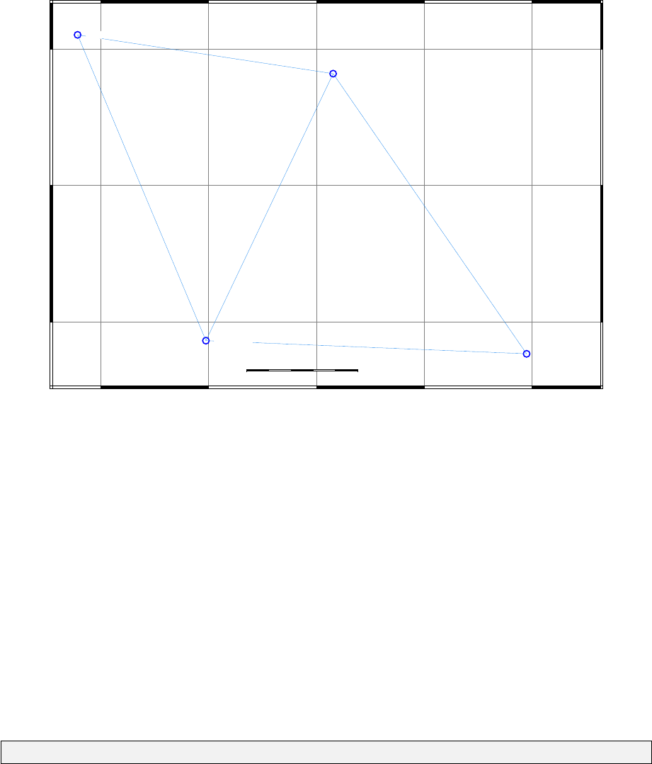
will import stations 302513640,302513650,302509800 and 302502400, and all connected GNSS
baselines wholly within the bounding box. The stations and measurements that are imported using
this command are shown in Figure 3.2.
145˚11'44.0"
145˚11'44.0"
145˚11'48.0"
145˚11'48.0"
145˚11'52.0"
145˚11'52.0"
145˚11'56.0"
145˚11'56.0"
145˚12'0.0"
145˚12'0.0"
−38˚06'48.0" −38˚06'48.0"
−38˚06'44.0" −38˚06'44.0"
−38˚06'40.0" −38˚06'40.0"
0 0.1
Kilometres
302502400
302513650
302509800
302513640
Figure 3.2: Stations and measurements in the skye network filtered by the --bounding-box option.
Note that only the stations and measurements which lie wholly within the limits of the bounding
box will be imported. To include measurements which transcend the bounding box, add the option
--get-msrs-transcending-box. By default, GNSS baseline clusters and GNSS point clusters which
transcend a bounding box will not be split and as a consequence, will be ignored from the import
process. If option --bounding-box is intended to be used to obtain a subset of a GNSS baseline or
point cluster, add the option --split-gnss-cluster-msrs.
Including or excluding stations and measurements
To import only a set of specific stations and associated measurements, pass to import the option
--include-stns-assoc-msrs followed by a comma delimited string defining the stations to be
imported. This option will also import any stations connected to the associated measurements.
For example, the command:
import -n skye skye.stn skye.msr --include-stns-assoc-msrs 302502400
will import station 302502400, all measurements associated with 302502400, and stations 302513650
and 302509800 which happen to be connected to the associated measurements. Any measurements
between stations 302513650 and 302509800 will not be imported. For these measurements to be
included, add 302513650 or 302509800 to the argument string. As with the bounding box function,
if --include-stns-assoc-msrs is intended to be used to obtain a subset of a GNSS point or baseline
26

cluster, add the option --split-gnss-cluster-msrs.
Conversely, to import all stations except a set of specific stations, pass to import the option
--exclude-stns-assoc-msrs followed by a comma delimited string defining the stations to be
excluded from the import process. This option will also exclude all measurements associated with
that station, but not other stations. For example, the command:
import -n skye skye.stn skye.msr --exclude-stns-assoc-msrs 302513650
will import all stations except station 302513650 and all measurements associated with it. If the
intention is to exclude one or more stations from a GNSS point or baseline cluster, add the option
--split-gnss-cluster-msrs.
Segmented network block
DynaNet provides a capability to segment a network into a series of connected blocks via segment
(see Chapter 6). The purpose of this functionality is support phased adjustment. Once a network
has been segmented, stations and measurements within a segmented block can be imported using
the option --import-block-stn-msr and the desired block number as an argument:
import -n uni_sqr uni_sqrstn.xml uni_sqrmsr.xml --import-block-stn-msr 3
Using this command sequence, only the stations and measurements in block 3 will be imported. For
this command sequence to work as intended, a segmentation file named uni_sqr.seg must exist
in the folder from which import was executed, and this file must contain at least three blocks
(see Chapter 6 for more information on the creation of segmentation files). To use an alternative
segmentation file, pass to import the option --seg-file followed by the name of the segmentation
file. If the segmentation file is located in another directory, the file name must include the full folder
path.
Measurement type
For networks of mixed measurement types, options --import-msr-types and --exclude-msr-types
can be used to include or exclude certain measurements from the import process. Both options take
for their argument a non–delimited string defining the measurement types to be included or excluded.
For example, the following command will only import GNSS measurements:
import -n uni_sqr uni_sqrstn.xml uni_sqrmsr.xml --import-msr GXY
Conversely, the following command will import all measurements except astronomic latitude and
longitude:
import -n uni_sqr uni_sqrstn.xml uni_sqrmsr.xml --exclude-msr IJ
An additional option under the category of measurement type is --prefer-single-x-as-g. This
option will convert all GNSS baseline cluster (X) measurements containing a single baseline into
GNSS baseline (G) measurements.
27

Station renaming
At times it will be necessary to rename multiple stations throughout a network, such as to correct
stations which have been wrongly named in the field or during data processing, or to change from
a well-known alias to another preferred name (or alias). To rename one or more stations upon
importing stations and measurements, pass the option --stn-renaming-file to import followed by
the name of the station renaming file:
import -n skye skye.stn skye.msr --stn-renaming-file skye.renaming
The structure and format of the station renaming file is shown in Figure 3.3. The first column is the
preferred name to which all occurrences of the names listed in columns 1, 2, . . . , n will be changed.
The number of characters reserved for each station name field will be defined according to the DNA
STN file format version. For DNA version 3.0 onward, this width is 20. Rows beginning with an
asterisk are treated as comments and are ignored.
12345678901234567890123456789012345678901234567890123456789012345678901234567890
!#=DNA 3.01 REN
* Station renaming file
* List the preferred name first, and then all other aliases a mark may have
* NEWNAME (20 chrs) ALIAS (20 chars) ALIAS (20 chars) ALIAS (20 chars) ALIAS (20 chars)
302513640 1364
302509800 980
302508300 830
261907650 765
Figure 3.3: Station renaming file
Station nearness
When concatenating networks contained in different files, the same physical station can sometimes
appear in the station and measurement files with different station names. To assist with identifying
stations with different names, pass the option --search-nearby-stn to import and, if required, pass
the option --nearby-stn-buffer followed by a distance in metres by which to search for nearby
stations. For example, to search for stations in uni_sqrstn.xml within 1.5 metres of each other, run
the following command:
import -n uni_sqr uni_sqrstn.xml --search-nearby-stn --nearby-stn-buffer 1.5
This command will produce the following output:
+ Testing for duplicate and nearby stations... Done.
- Error: 1 station was found to be separated by less than 1.5m.
See ./unisqr.dst for details.
If the names in each pair refer to the same station, then update the
station and measurement files with the correct station name and re-run import.
Alternatively, if the names in each pair are unique, either call import
without the --search-nearby-stn option, or decrease the radial search
distance using --nearby-stn-buffer.
Having identified one or more nearby stations, import will create a file called uni_sqr.dst in which
will be printed a list of stations that are separated by less than 1.5 metres. The contents of this file
28

are as follows:
--------------------------------------------------------------------------------
DUPLICATE STATION FILE
Version 3.1.2
Build May 26 2014, 22:27:14 (MSVC++ 10.0)
File created Monday, 26 May 2014, 10:30:35 PM
File name C:\Data\unisqr.dst
Command line arguments import -n unisqr uni_sqrstn.xml --search-nearby-stn --nearby-stn-buf 1.5
Network name unisqr
Stations file C:\Data\unisqr.bst
Measurements file C:\Data\unisqr.bms
Associated station file C:\Data\unisqr.asl
Associated measurement file C:\Data\unisqr.aml
Duplicate stations output file C:\Data\unisqr.dst
Similar measurement output file C:\Data\unisqr.dms
Input files uni_sqrstn.xml
Default reference frame GDA94
Search for nearby stations tolerance = 1.5m
--------------------------------------------------------------------------------
Nearby station search results:
1 station was found to be separated by less than 1.5m:
First station Nearby station Separation (m)
2120 NEWP 0.531
Once import has identified the stations that satisfy the search criteria, it is up to the user to verify
if the stations listed in the .dst file are the same physical station or not. If a single station has
been inadvertently given different names in the station and measurement files, redundant station
information can be harmonised by:
1. Amalgamate the station information record(s) to form a single station with the preferred station
name, coordinates and constraints.
2. Search and replace in the measurement file all instances of the redundant station name with
the preferred station name
It is anticipated that a future version of DynaNet will provide an automated approach for harmonising
redundant station information.
Measurement similarity
As in the case for stations, concatenating networks contained in different files can easily result
in duplicate measurements in the measurement files. Duplicate measurements can be difficult to
detect as it is normal and legitimate for redundant measurements to exist. To assist with identifying
duplicate measurements, pass the option --search-similar-msr to import:
import -n uni_sqr uni_sqrmsr.xml --search-similar-msr
This sequence of commands will produce the following output:
29

+ Searching for similar measurements...
- Error: 3 measurements were found to be very similar (if not identical)
to other measurements. See ./uni_sqr.dms for details.
If the listed measurements are true duplicates, either remove each duplicate
from the measurement file and re-run import, or re-run import with the
--ignore-similar-msr option. Alternatively, if each measurement
is unique, then call import without the --search-similar-msr option.
As shown in the above output, import will create a file called unisqr.dms in which will be printed
a list of measurements that appear to be similar or identical to other measurements. The format of
the similar measurements is DynaML as follows:
- 3 measurements were found to be very similar (if not identical)
to other measurements.
<!--Type L Level difference-->
<DnaMeasurement>
<Type>L</Type>
<Ignore/>
<First>2214</First>
<Second>2213</Second>
<Value>0.0010</Value>
<StdDev>0.0020</StdDev>
</DnaMeasurement>
<!--Type S Slope distance-->
<DnaMeasurement>
<Type>S</Type>
<Ignore/>
<First>2205</First>
<Second>2213</Second>
<Value>13.3010</Value>
<StdDev>0.0050</StdDev>
<InstHeight>0.000</InstHeight>
<TargHeight>0.000</TargHeight>
</DnaMeasurement>
<!--Type S Slope distance-->
<DnaMeasurement>
<Type>S</Type>
<Ignore/>
<First>6002</First>
<Second>1049</Second>
<Value>136.4290</Value>
<StdDev>0.0100</StdDev>
<InstHeight>1.601</InstHeight>
<TargHeight>1.337</TargHeight>
</DnaMeasurement>
As with stations, the second and subsequent appearances of a measurement with similar attributes
will be regarded as a duplicate. Once import has identified the measurements that satisfy the test
for similarity, it is up to the user to verify if the measurements listed in the .dms file are the same
measurement or different measurements. Measurements which are duplicates can either be removed
from the measurement file, or set as an ignored measurement. For example, measurements can be
ignored in DNA files by providing an asterisk (*) for the ignore flag (see Table B.3, §B.1.4).
For very large networks which have been derived from hundreds of GNSS survey projects, it is possible
for a single GNSS data set to be inadvertently processed twice, resulting in unique but similar GNSS
baselines and GNSS baseline clusters. At times, these similar measurements can be difficult to
detect due to slight variations in the generated GNSS vector and variance matrix components. To
search for single GNSS baselines which may be similar to a GNSS baseline cluster, pass the option
--search-similar-gnss-msr to import. This option will cause import to identify every single GNSS
baseline where both terminal stations are contained within a GNSS baseline cluster and where both
30

measurements the same reference frame and epoch.
Ignoring similar measurements
Upon verifying whether the measurements listed in the .dms file are duplicate measurements, the
user may opt to remove the duplicate measurements or flag them as ignored for further verification.
To automatically ignore all measurements identified as similar. add --ignore-similar-msr to the
list of options for import:
import -n uni_sqr uni_sqrstn.xml uni_sqrmsr.xml --ignore-similar-msr
Executing this command will automatically flag any measurements deemed to be similar as other
measurements in the network as ignored and thereby exclude them from all subsequent processing.
Removing ignored measurements
Measurements which are flagged as ignored, whether in the measurement file or by supplying the
--ignore-similar-msr option, can be automatically removed from all subsequent processing as
follows:
import -n uni_sqr uni_sqrstn.xml uni_sqrmsr.xml --remove-ignored-msr
This option can be combined with option --ignore-similar-msr in a single command:
import -n uni_sqr uni_sqrstn.xml uni_sqrmsr.xml --ignore-similst-msr --remove-ignored-msr
Executing this command will automatically flag similar measurements and, together with any other
measurements already marked as ignored, will not be written to the binary measurement file.
Flagging unused stations
Upon loading the station and measurement information from the input files, any stations not
connected to any measurements will be noted as unused and thereby marked for exclusion from
segmentation and adjustment processes. However, import will retain these stations within the
binary station file. Accordingly, functions such as data export (see §3.5) will include these stations.
To prevent unused stations from being used in any further processing, pass to import the option
--flag-unused-stations:
import -n uni_sqr uni_sqrstn.xml uni_sqrmsr.xml --flag-unused-stations
3.3.3 GNSS variance matrix scaling
For the most part, GNSS measurement and variance matrix information will be sourced from files
generated by a GNSS processing package. Depending on the processing strategy, it is possible
that the variance matrices accompanying the GNSS measurements will need some form of scaling
such that a more realistic estimate of the GNSS measurement precision is incorporated within an
31

adjustment. GNSS measurement variance matrices may be scaled using the appropriate scalar fields
within the input files (e.g. Table B.8 on page 177 for DNA file format, or Figure B.23 on page 190
for DynaML file format). In addition, import provides a capacity to scale GNSS variance matrices
via five different scaling options. Table 3.3 lists the lists the various GNSS variance matrix scaling
options (c.f. Table A.6 on page 155 in the Command line reference).
Table 3.3: GNSS variance matrix scaling options
Option All msrs Clusters Matrix North–south East–west Up
--v-scale • • •
--p-scale • • •
--l-scale • • •
--h-scale • • •
--baseline-scalar-file • • • •
As shown in Table 3.3, GNSS variance matrix scaling can be applied to all GNSS measurements
contained in all measurement files passed to import, or to individual GNSS baselines. Individual
baseline scaling is based upon the contents of a baseline scalar file and does not apply to GNSS point
or baseline clusters. Whether scaling all or individual GNSS variance matrices, scaling can be applied
in two different ways — via a single matrix multiplier (or variance factor) or via individual scalars
corresponding to the three dimensions of the local reference frame. One or more scaling options in
any combination can be passed to import.
To scale all GNSS variance matrices by a single multiplier, pass to import the option --v-scale
followed by a scalar value. For example, to scale all variance matrices in the skye project by a factor
of 10.0, run the following command:
import -n skye skye.stn skye.msr --v-scale 10
To scale all GNSS variance matrices by partial scalars in the north–south, east–west or vertical
directions, pass to import the options --p-scale,--l-scale or --h-scale respectively, followed by
the relevant scalar value. For example, to scale all variance matrices in the skye project by a factor
of 2.0 in the horizontal direction and 5.0 in the vertical direction, run the following command:
import -n skye skye.stn skye.msr --p-scale 2 --l-scale 2 --h-scale 5
To scale specific GNSS baseline variance matrices, pass to import the option --v-scale followed by
the name of the baseline scalar file:
import -n skye skye.stn skye.msr --baseline-scalar-file skye.scalars
The structure and format of the baseline scalar file is shown in Figure 3.4. 20 characters are reserved
for the two station names, and 10 characters are reserved for v-scale,p-scale,l-scale and h-scale.
32

12345678901234567890123456789012345678901234567890123456789012345678901234567890
--------------------------------------------------------------------------------
GNSS BASELINE VARIANCE MATRIX SCALAR FILE
SCALARS
Station 1 Station 2 v-scale p-scale l-scale h-scale
--------------------------------------------------------------------------------
409601230 409601240 100.0 1 1 1
409601230 409601250 10 2 2 5
409601230 409601260 1 3 3 10
Figure 3.4: Baseline scalar file
For all scaling options, §7.3.2.1 describes the procedure implemented by DynaNet for scaling GNSS
variance matrices.
3.4 Network measurement simulation
import provides a capability to simulate a network of GNSS and terrestrial measurements through
the --simulate-msr-file option. In order to simulate measurements, two files are required — a
station file and a measurement simulation control file. Upon execution, measurements are simulated
for all measurement types and station names listed in the measurement simulation control file.
Measurement values are calculated using the coordinates provided in the station file. The following
command demonstrates the use of import to simulate measurements:
import -n simnet simnet.stn simnet-list.msr --simulate
Running this command will create a DNA measurements file named simnet.simulated.msr which
will contain measurements generated from the station coordinates in simnet.stn and the types and
station names in simnet-list.msr. The input station file simnet.stn must conform to the DNA
station file format (c.f. §B.1.3). The input measurement simulation control file simnet-list.msr
must conform to the DNA measurement file format (c.f. §B.1.4) in principle, the exceptions being
that only measurement types, station names and cluster counts need to be present. Figure 3.5 shows
a sample simulation control file.
The measurement values in the simulated measurements file are calculated exactly from the station
coordinates. All other information is generated as follows:
•Standard deviations for measurement types C, E, L, M and S will be calculated from
3.0×p(L/1000.0)/100.0
where Lis the calculated distance in metres;
•Standard deviations for measurement types H and R will be set to 0.024 metres.
•Variance matrices for G, X and Y measurement types will be set to:
4.022000e-05 −1.369000e-05 3.975000e-05
−1.369000e-05 1.487000e-05 −2.035000e-05
3.975000e-05 −2.035000e-05 6.803000e-05
33

•Station and target heights for measurements which require these heights (e.g. S, V, Z) will be
set to 1.650 and 1.651 metres respectively.
•Standard deviations for measurement types A, B, D, K, V and Z will be set to 0.01 seconds.
•Standard deviations for measurement types I, J, P and Q will be set to 0.021 seconds.
123456789012345678901234567890123456789012345678901234567890123456789
!#=DNA 3.00 MSR 16.06.2014 GDA94 01.01.1994 20
* Measurement simulation control file
A 503 304 307
B 909 1010
C 501 309
D 602 302 2
501
503
E 503 307
G 604 606
H 105
I 106
J 106
K 101 202
L 910 1010
M 604 706
P 105
Q 105
R 106
S 602 302
V 109 207
X 406 501 2
109 501
Y 406 XYZ 3
203
509
Z 503 307
Figure 3.5: Example simulation measurements list
If orthometric heights are supplied in the station file, or if simulated terrestrial measurements are
intended to contain a realistic measure of the influence of the gravity field, geoid–ellipsoid separations
and deflections of the vertical can be added to the measurements through the use of a DNA geoid
file. To this end, add the --geo-file option (c.f. §3.2.4), followed by the geoid file name:
import -n simnet simnet.stn simnet-list.msr --simulate --geo-file simnet.geo
If a DNA geoid file has not been created, geoid may be called to interpolate and export the
geoid–ellipsoid separations and deflections of the vertical to a DNA geoid file. For this purpose,
a binary station file for simnet is required. The steps are as follows:
1. Import the simulation station file to create the binary station file simnet.bst.
2. Interpolate the geoid information (from simnet.bst) and export to a DNA geoid file.
3. Simulate using the station file, simulation control file and the newly created geoid file.
The command line sequence for these steps is as follows:
import -n simnet simnet.stn
geoid simnet --ntv2-file ausgeoid09.gsb --export-dna-geo
import -n simnet simnet.stn simnet-list.msr --simulate --geo-file simnet.geo
34

See Chapter 5 for more help on interpolating geoid information from a geoid grid file.
3.5 Data export
In addition to translating the external file formats into the binary formats required by DynaNet,
import provides a capacity to export geodetic network information into a number of different file
formats. The options for exporting information include:
•Export of station and measurement information to CSV, DNA, DynaML, GeodesyML and
SINEX file formats
•Export of geodetic network binary files (MAP, AML, ASL) to equivalent plain text variants
Export options can be passed to import together with any other option. Hence, the residual station
and measurement information generated through the various configuration options can be stored for
subsequent import, filtering and processing.
3.5.1 Station and measurement files
To export station and measurement information into CSV or DNA format, pass to import the
option --export-dna-files or --export-csv-files respectively. Similarly, to export station and
measurement information into DynaML format, pass the option --export-xml-files. For example,
the following command will export DNA station and measurement files comprised of only GNSS
measurements found within the uni_sqr project, with the default reference frame set to ITRF2005
and all GNSS variance matrices scaled by 100.0:
import -n us_bsl uni_sqrstn.xml uni_sqrmsr.xml --v-sc 100 --ref itrf2005 --import-m GXY --export-dna --flag
Running this command will produce two files named us_bsl.stn and us_bsl.msr corresponding
to the station and measurement files respectively. Since --flag-unused-stations was passed to
import, stations which become disconnected from removed measurements (as a result of importing
only GNSS measurements) will not be written to the station file.
The option --export-xml-files will produce two XML files named <network_name>stn.xml and
<network_name>msr.xml corresponding to the station and measurement files respectively. To produce
a single DynaML file, pass to import the option --single-xml-file with --export-xml-files.
Note that if the network name supplied in the above command matched the name of the input files
according to the file naming convention described in §2.2.1 (i.e. uni_sqr), and data is exported to
the same file format as the input files, then the original input files will be overwritten.
3.5.2 Association lists and station map
As discussed in §2.2.2, DynaNet reads and writes a number of binary files. The Station Map
(MAP), Associated Stations List (ASL) and Associated Measurements List (AML) may be exported
to plain text to assist with detailed analysis of the network’s geometry, measurement connectivity
and measurement frequency. To export the ASL, AML and MAP to their plain text counterparts,
run the following command:
import -n us_bsl us_bsl.stn us_bsl.msr --export-map --export-asl --export-aml
35

This command will produce three files named us_bsl.map.txt,us_bsl.asl.txt and us_bsl.aml.txt.
The fields contained in the exported files are described in Tables 3.4, 3.5 and 3.6.
Table 3.4: Station Map fields
Field Description
Station name The station name as given in the input station and measurement files. The column
header contains the number of stations detected in the input files.
Station index The (zero–based) index of the station name in an alpha–numeric sorted list of all station
names. DynaNet uses this index when referring to stations during all internal processing.
Table 3.5: Associated Stations List fields
Field Description
Station name The station name as given in the input station and measurement files. The
column header contains the number of stations detected in the input files.
No. connected msrs The number of measurements connected to this station.
AML index The (zero–based) index of the first record of this station’s appearance in the
Associated Measurements List.
Unused? If an asterisk is present, this station is not connected to any measurements.
Table 3.6: Associated Measurements List fields
Field Description
Station name The station name as given in the input station and measurement files. The column
header contains the number of records in the file.
Msr index The (zero–based) index of this measurement in the binary measurements file.
Msr type The type of measurement (c.f. Table 3.2) and which measurement station this station
refers to (first, second or third)
Cluster If this measurement is part of a cluster, this number represents the index of the cluster
in a list of all detected clusters.
Ignored msr? If an asterisk is present, this measurement has been marked as ignored.
36
Chapter 4
Transformation of coordinates and
measurements
4.1 Introduction
Recognising that GNSS surveying is the most highly utilised measurement technique for geodetic
network establishment and maintenance, DynaNet has been designed around the use of pre–processed
GNSS measurements for the estimation of network station parameters. DynaNet has also been
designed to integrate measurements taken in the local reference frame with GNSS measurements in
an earth–centred, cartesian reference frame.
But since the reference frame of GNSS measurements is directly related to the reference frame of the
satellite orbit information used during GNSS processing, it is inevitable that GNSS measurements
taken over several successive years will be based upon different reference frames and epochs. This is
primarily due to the fact that since the launch of the first GNSS satellites, several reference frames
(and versions) have been adopted for broadcast and precise ephemeris. The reference frames that
may be relevant in this context can include:
•The PZ-90 coordinate system. Used for the Russian GLObal NAvigation Satellite System
(GLONASS).
•The International Terrestrial Reference Frame (ITRF). Adopted by the International GNSS
Service (IGS) for their precise orbit products.
•The World Geodetic System of 1994 (WGS84). Used for the Global Positioning System (GPS).
Since its establishment, WGS84 has been aligned (and re–aligned) to several versions of ITRF.
In all cases, these frames can undergo several iterations (or revisions), such as ITRF1988, ITRF1992,
ITRF2008, etc. WGS84 is regularly updated and aligned to ITRF. It follows that each frame
realisation will have a different reference epoch. Accordingly, there is a fundamental need to handle
transformations of GNSS measurements between these reference frames if the combination and
adjustment of multiple GNSS measurements in a single solution is to be free from reference frame
bias. To this end, reftran has been developed to transform stations and GNSS measurements between
a selection of commonly used reference frames.
The first part of this chapter (§4.2 – §4.5) presents the theory of reference frames and coordinate
systems, conversions between coordinate systems, transformation of coordinates and measurements
between static and dynamic reference frames, and propagation of variances. The remainder of the
chapter describes the use of reftran and its options.
37
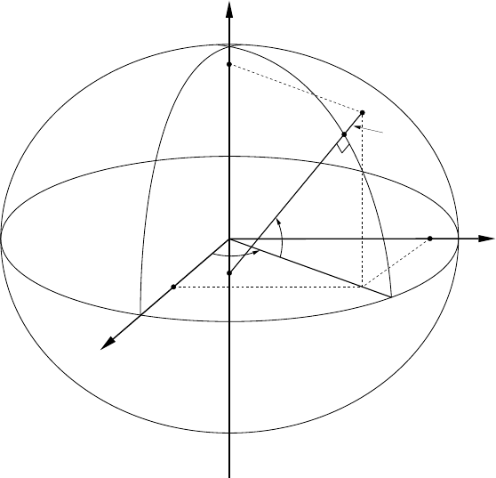
4.2 Reference frame fundamentals
4.2.1 Cartesian reference frame
The cartesian reference frame is a three–dimensional system, the origin oof which is coincident
with the centre of the reference ellipsoid. The referencing of point pis by means of orthogonal
displacements parallel to the x,yand zaxes. Figure 4.1 illustrates point pin relation to the axes
of the cartesian reference frame, and the relationship between cartesian coordinates and geodetic
latitude φ, geodetic longitude λand ellipsoid height h.
x
y
z
o
xp
yp
zp
p
p′
φ
λ
ν
q
h
Figure 4.1: The ellipsoid–centred cartesian reference frame
A vector xcbetween two points in the cartesian reference frame will have the elements:
xc=
∆x
∆y
∆z
(4.1)
As shown by Figure 4.1, geodetic latitude is the angle between the equatorial (x–y) plane and the
normal to the ellipsoid through p, and geodetic longitude is the angle between the zero meridian and
the meridian through p. Ellipsoid height is the distance of pabove p0, which is a point projected onto
the reference ellipsoid along the ellipsoid normal. As Figure 4.1 indicates, the coordinates defining
the location of pare dependent upon the size, shape and location of the reference ellipsoid.
4.2.2 Geographic reference frame
With respect to Figure 4.1, geographic reference frame (or geodetic) coordinates φ,λand hare
related to the corresponding cartesian coordinates by the following expressions:
38

x= (ν+h) cos φcos λ
y= (ν+h) cos φsin λ(4.2)
z=ν(1 −e2) + hsin φ
where νis the radius of curvature in the prime vertical, given by:
ν=a
q1−e2sin2φ(4.3)
ais the quantity representing the semi–major axis of the reference ellipsoid and e2is the first
eccentricity obtained from:
e2=a2−b2
a2(4.4)
and bis the semi–minor axis of the ellipsoid (coincident with the zaxis).
As will be required for later developments, the radius of curvature in the prime meridian ρat φis
given by:
ρ=a1−e2
1−e2sin2φ3
2
(4.5)
and the distance oq which provides for the zcoordinate of the point q— being at the intersection
of the normal at pwith the polar axis of the ellipsoid — is given by:
oq =e2νsin φ(4.6)
4.2.3 Local reference frame
The local reference frame is a three–dimensional orthogonal system that has its origin on or above
any point on the ellipsoid, and is oriented with respect to the local geodetic meridian. Figure 4.2
illustrates the axes of the local reference frame in relation to the cartesian reference frame. The
vector displacement up is coincident with the ellipsoid normal. The orientation of the local reference
frame varies with respect to latitude φand longitude λ.
Vectors in the cartesian reference frame can be represented in the local reference frame as xl:
xl=
∆e
∆n
∆up
(4.7)
A vector xlin the local reference frame is related to the cartesian reference frame by:
xc=Rlxl(4.8)
where Rlis the rotation matrix with origin at latitude φand longitude λ:
Rl=
−sin λ−sin φcos λcos φcos λ
cos λ−sin φsin λcos φsin λ
0 cos φsin φ
(4.9)
39
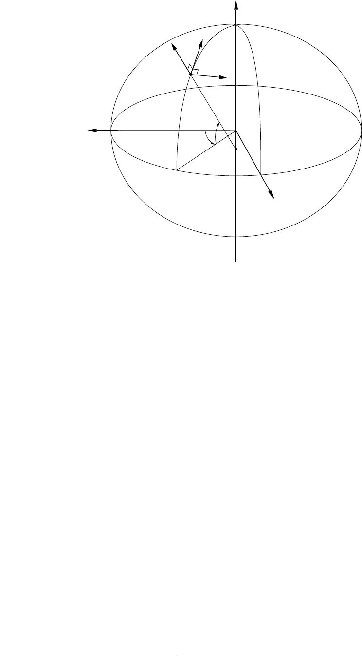
x
y
z
o
q
e
n
up
p′
φ
λ
Figure 4.2: The local reference frame
Equation 4.8 can be written in expanded form as:
∆x
∆y
∆z
=
−sin λ(∆e)−sin φcos λ(∆n) + cos φcos λ(∆up)
cos λ(∆e)−sin φsin λ(∆n) + cos φsin λ(∆up)
cos φ(∆n) + sin φ(∆up)
(4.10)
Since Rlis orthogonal1, a vector xcin the cartesian reference frame is related to the local reference
frame by:
xl=RT
lxc(4.11)
which can be written in expanded form as:
∆e
∆n
∆up
=
−sin λ(∆x) + cos λ(∆y)
−sin φcos λ(∆x)−sin φsin λ(∆y) + cos φ(∆z)
cos φcos λ(∆x) + cos φsin λ(∆y) + sin φ(∆z)
(4.12)
4.2.4 Polar reference frame
At times it is necessary to transform vectors in a local reference frame into a displaced orthogonal
polar reference frame. Figure 4.3 illustrates the displacement of a local reference frame at point
p2in relation to the polar frame at point p1by geodetic azimuth (θ), vertical angle (ϑ) and direct
distance (s).
1. A matrix is orthogonal if the inverse of that matrix is equal to its transpose, i.e. RT=R−1.
40
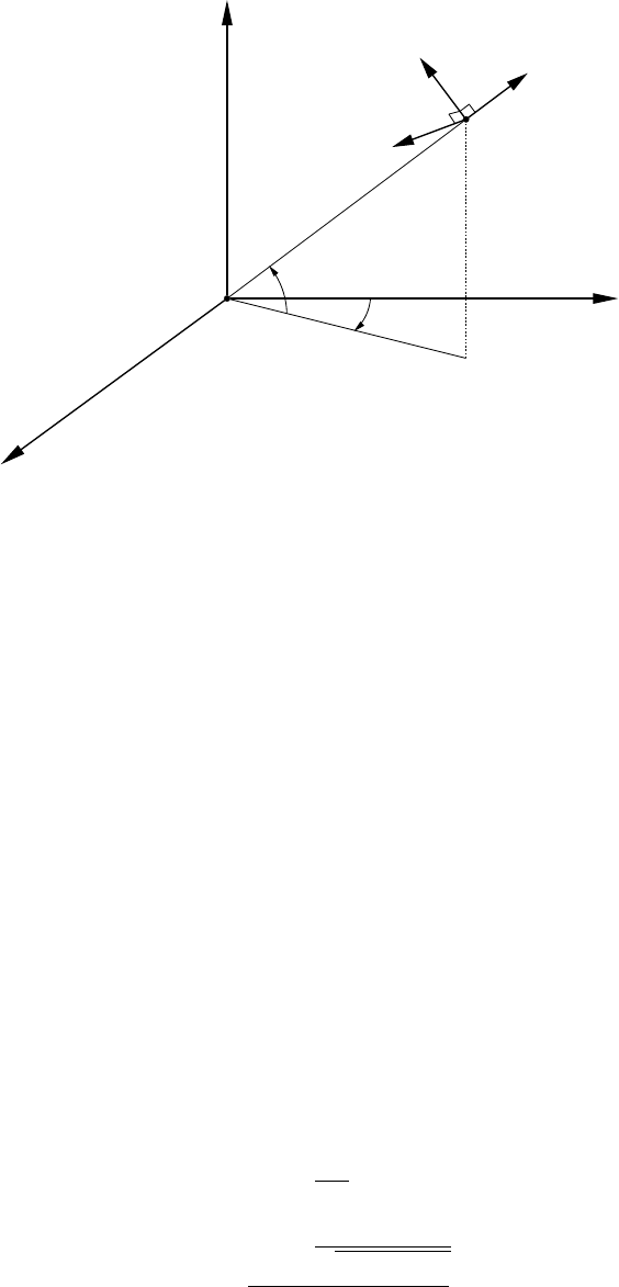
e
n
up
p1
p2
ϑ
θ
s
∆ϑ
∆θ
∆s
v
a
s
Figure 4.3: Orthogonal reference frames displaced by geodetic azimuth, vertical angle and distance
With respect to Figure 4.3, a,vand sare unit vectors defining the displaced polar reference frame.
Vectors vand sare in the vertical plane, whereas ais in the horizontal plane. A vector xpin the
polar reference frame has the elements:
xp=
a
v
s
(4.13)
A vector in the local reference frame is transformed to the displaced polar reference frame by:
xp=Rpxl(4.14)
where Rpis an orthogonal rotation matrix at origin p2:
Rp=
−cos θ−sin ϑsin θcos ϑsin θ
−sin θ−sin ϑcos θcos ϑcos θ
0 cos ϑsin ϑ
(4.15)
Polar coordinates of θ,ϑand sare related to vectors in the local reference frame by:
θ= arctan ∆e
∆n
ϑ= arctan ∆up
√∆e2+ ∆n2(4.16)
s=p∆e2+ ∆n2+ ∆up2
Equation 4.14 can be written in expanded form as:
a
v
s
=
−cos θ(∆e)−sin ϑsin θ(∆n) + cos ϑsin θ(∆up)
−sin θ(∆e)−sin ϑcos θ(∆n) + cos ϑcos θ(∆up)
cos ϑ(∆n) + sin ϑ(∆up)
(4.17)
41
Since Rpis orthogonal, a vector xpin the displaced polar reference frame can be rotated into the
local reference frame by:
xl=RT
pxp(4.18)
which can be written in expanded form as:
∆e
∆n
∆up
=
−cos θ(a)−sin θ(v)
−sin ϑsin θ(a)−sin ϑcos θ(v) + cos ϑ(s)
cos ϑsin θ(a) + cos ϑcos θ(v) + sin ϑ(s)
(4.19)
4.3 Transformation between cartesian reference frames
Several methods are available for transforming coordinates and vectors from one cartesian reference
frame to another. DynaNet supports (conformal 3D) 7–parameter and 14–parameter similarity
transformations using the Bursa–Wolf model.
Conformal transformations between two cartesian reference frames on the same epoch are managed
by a 7–parameter similarity relationship. The relationship involves a three–dimensional shift, rotation
and scale of the cartesian coordinate axes and is given by:
x2
y2
z2
=
∆x12
∆y12
∆z12
+ (1 + δ)
1rz−ry
−rz1rx
ry−rx1
x1
y1
z1
(4.20)
where ∆x12,∆y12 and ∆z12 are the origin shifts, rx,ryand rzare the coordinate axis rotations (in
radians) and δis the scale factor between the two systems. Where rotation of axes exceeds 10” of
arc, the rotation matrix in equation 4.20 is replaced with the following:
R=
cos rzsin rz0
−sin rzcos rz0
0 0 1
cos ry0−sin ry
0 1 0
sin ry0 cos ry
1 0 0
0 cos rxsin rx
0−sin rxcos rx
Conformal transformations between two cartesian reference frames on different epochs are managed
by a 14–parameter similarity relationship. The relationship is identical to that given in equation 4.20,
with the exception of introducing terms for the first order derivatives of origin shift, rotation and
scale as follows:
x2
y2
z2
=
∆x12 + ˙x(t2−t1)
∆y12 + ˙y(t2−t1)
∆z12 + ˙z(t2−t1)
+1 + δ+˙
δ(t2−t1)×(4.21)
1rz+ ˙rz(t2−t1)−ry−˙ry(t2−t1)
−rz−˙rz(t2−t1) 1 rx+ ˙rx(t2−t1)
ry+ ˙ry(t2−t1)−rx−˙rx(t2−t1) 1
x1
y1
z1
Here, [˙x˙y˙z],[˙rx˙ry˙rz]and ˙
δare the rates of change in origin shift, axis rotation and
scale respectively, t1is the reference epoch of the reference frame for x1,y1and z1, and t2is the
epoch of the reference frame for x2,y2and z2.
42

4.4 Propagation of variances between reference frames
4.4.1 Local reference frame
Variances in the local reference frame can be expressed in the cartesian reference frame by the law
of propagation of variances:
Vxc=RlVxlRT
l(4.22)
where Vxlis a variance matrix in the local reference frame, Vxcis a variance matrix in the cartesian
reference frame, and Rlis the rotation matrix given in equation 4.9. Conversely, propagation of
variances from the cartesian system into the local reference frame is obtained by:
Vxl=R−1
lVxcR−1
lT(4.23)
Since Rlis orthogonal, Vxlmay be expressed as:
Vxl=RT
lVxcRl(4.24)
4.4.2 Polar reference frame
The precision of polar coordinates can be derived from precisions in either cartesian reference frame
or the local reference frame. For precisions in the cartesian system, propagation of variances is
evaluated by a two step process, by (1) propagation into the local system as described above, and
then (2) propagation into the polar form.
To transform a variance matrix Vxlin the local reference frame into the polar form Vxp, propagation
of variances is evaluated as:
Vxp=PVxlPT(4.25)
where Pis the Jacobian transformation matrix formed by linearising equations 4.16:
P=
∂θ
∂e
∂θ
∂n
∂θ
∂up
∂ϑ
∂e
∂ϑ
∂n
∂ϑ
∂up
∂s
∂e
∂s
∂n
∂s
∂up
(4.26)
To transform a variance matrix directly from the cartesian system to the polar reference frame,
propagation is computed by combining equations 4.24 and 4.25:
Vxp=PRT
lVxcRlPT(4.27)
43

4.4.3 Geographic reference frame
To transform a variance matrix Vxgfor geographic coordinates into the cartesian system, propagation
of variances takes the familiar form:
Vxc=TVxgTT(4.28)
Tis the Jacobian transformation matrix formed by linearising equations 4.2:
T=
∂x
∂φ
∂x
∂λ
∂x
∂h
∂y
∂φ
∂y
∂λ
∂y
∂h
∂z
∂φ
∂z
∂λ
∂z
∂h
(4.29)
For the reverse solution, propagation of variances into the geographic coordinate system is via:
Vxg=T−1VxcT−1T(4.30)
4.5 Conversion of projection coordinates
It is often necessary to work with geographic information defined in terms of projection2coordinates.
DynaNet supports Universal Transverse Mercator (UTM) and Transverse Mercator (TM) projections3.
UTM and TM projection coordinates are expressed in terms of Easting E, Northing Nand Zone
Zo. For UTM projections, the earth is divided into 60 zones. Each zone is 6◦wide in longitude,
extends from −80◦latitude to +80◦latitude, and is numbered consecutively beginning from zone 1
at −180◦to −174◦longitude and extending eastwards to zone 60 (+174◦to +180◦longitude). The
origin of each zone is the point of intersection between the equator and the meridian central to the
zone, and the central scale factor of the projected zones is 0.9996. To alleviate negative coordinate
values in the southern hemisphere, the origin is assigned a false Northing of 10,000,000m and a false
Easting of 500,000m. Since two points located in different zones can have equal values for Easting
and Northing, projection coordinates are unique only when accompanied by the zone number.
2. As the reference ellipsoid is by nature a three–dimensional curved surface, projecting figures on the ellipsoid onto
a flat, two–dimensional surface requires distortion in some form or another. Accordingly, different map projections
have been designed to preserve one or more of the following geometric properties: shape (conformal), direction
(azimuthal),distance (gnomic) and area (equal area). To this end, several map projections are available —
Transverse Mercator (conformal), Lambert Conic (conformal), Polar Stereographic (azimuthal, conformal) and
Albers Conic (equal area) [Snyder, 1997].
3. A UTM projection is a TM projection with standardised values for zone width, origin, scale factor and false Easting
and Northings.
44

The relationship between UTM and TM projection coordinates E,Nand Zo and geographic
coordinates φ,λand his given by [Redfearn, 1948]:
E= 500,000 + k0nνω cos φ+νω3
6cos3φψ−t2
+νω5
120 cos5φ4ψ31−6t2+ψ21+8t2−ψ2t2+t4
+νω7
5040 cos7φ61 −479t2+ 179t4−t6(4.31)
N= 10,000,000 + k0m+νsin φω2
2cos φ
+νsin φω4
24 cos3φ4ψ3+ψ−t2
+νsin φω6
720 cos5φ8ψ411 −24t2+ 28ψ31−6t2
+ψ21−32t2−ψ2t2+t4
+νsin φω8
40320 cos7φ1385 −3111t2+ 543t4−t6(4.32)
Zo =ω
zw
(4.33)
where:
ω=λ−λ0(4.34)
zw= zone width (in units of λ)(4.35)
ψ=ν
ρ(4.36)
t= tan φ(4.37)
m=a(A0φ−A2sin 2φ+A4sin 4φ−A6sin 6φ)(4.38)
A0= 1 −e2
4−3e4
64 −5e2
256(4.39)
A2=3
8e2+e4
4−15e6
128 (4.40)
A4=15
256 e4+3e6
4(4.41)
A6=35e6
3072 (4.42)
k0is the central scale factor, λ0is the longitude of the central meridian, zwis the projection zone
width, and ρis the radii of curvature in the meridian at φ.
45

Conversely, the relationship between geographic coordinates and UTM and TM projection coordinates
is given by [Redfearn, 1948]:
φ=φ0−t0
k0ρ0xE0
2+t0
k0ρ0x3E0
24 −4ψ02+ 9ψ01−t02+ 12t02
−t0
k0ρ0x5E0
720 8ψ0411 −24t02−12ψ0321 −71t02
+ 15ψ0215 −98t02+ 15t04+ 180ψ05t02−3t04+ 360t04
+t0
k0ρ0x7E0
403201385 + 3633t02+ 4095t04+ 1575t06(4.43)
λ=λ0+ sec φ0x−x3
6sec φ0ψ0+ 2t02
+x5
120sec φ0−4ψ031−6t02+ψ029−68t02+ 72ψ0t02+ 24t04
−x7
5040sec φ061 + 662t02+ 1320t04+ 720t06(4.44)
where:
E0=E−Ef(4.45)
N0=N−Nf(southern hemisphere only) (4.46)
x=E0
k0ν0(4.47)
ψ0=ν0
ρ0(4.48)
λ0=zozw+λ1−zw(4.49)
φ0=σ+3η
2−27η3
32 sin 2σ+21η2
16 −55η3
32 sin 4σ
+151η3
96 sin 6σ+1097η4
512 sin 8σ(4.50)
η=f
2−f(4.51)
G=a(1 −η)1−η21 + 9
4η+225
64 ηπ
180 (4.52)
σ=πm
180G(4.53)
m=N0
k0
(4.54)
Efand Nfare the false Easting and Northing values, λ1is the longitude of the central meridian of
zone 1. ν0and ρ0are the radii of curvature evaluated at the foot–point latitude φ0(via equations
4.3 and 4.5), which is the latitude for which the meridian distance mequals N0/k0.
46

4.6 Transformation of coordinates and measurements
The least squares adjustment model implemented within DynaNet is based upon the cartesian
reference frame. After loading station information from the input files, import converts all station
coordinates in geographic and projection systems to their cartesian counterparts. Upon preparing for
least squares adjustment, adjust forms observation equations in terms of the cartesian reference frame
using the principles outlined in §4.2 and if required, performs propagation of variances of a–priori
GNSS measurement variance matrices (c.f. §4.4). When reporting the adjustment results, adjust
converts the estimated station coordinates to the user–specified coordinate systems (e.g. geographic
and/or projection). If required, adjust undertakes propagation of variances of estimated station and
GNSS measurement variance matrices to the user–specified system (e.g. cartesian, geographic, local
or polar).
The primary purpose of reftran is to align all station coordinates and GNSS measurements to
a common reference frame and epoch prior to least squares adjustment. reftran performs this
task using the reference frame information supplied to import (either in the input files or via the
--reference-frame option. c.f. §3.3.1), and the reference frame passed to reftran.
4.6.1 Supported reference frames and geodetic datums
DynaNet supports several commonly used reference frames. To simplify the process of uniquely
identifying each frame, DynaNet adopts the naming convention, abbreviations and system of codes
defined in the EPSG Geodetic Parameter Dataset4(version 7.9.0). Table 4.1 lists the EPSG codes
and reference frames supported by DynaNet.
Table 4.2 shows the various reference frame transformation combinations supported by DynaNet and
the respective references from which the transformation parameters have been sourced.
In addition to supporting transformations between a variety of reference frames, DynaNet also
supports the projection of coordinates between epochs on a single frame using a plate motion model.
In Version 3.3.0, only the Australian plate motion model is supported. Hence, DynaNet cannot be
used to project coordinates between epochs on a frame if the coordinates lie outside the Australian
tectonic plate.
4. The EPSG Geodetic Parameter Dataset, or EPSG dataset, is maintained by the Geodesy Subcommittee of the
Surveying and Positioning Committee of the International Association of Oil and Gas Producers (OGP). See
http://www.epsg.org
47

Table 4.1: EPSG codes and reference frames
Code Reference frame name Abbreviated name
4939 Geocentric Datum of Australia 1994 (geographic) GDA94
4347 Geocentric Datum of Australia 1994 (cartesian) GDA94
7843 Geocentric Datum of Australia 2020 (geographic) GDA2020
7842 Geocentric Datum of Australia 2020 (cartesian) GDA2020
7789 International Terrestrial Reference Frame, 2014 ITRF2014
5332 International Terrestrial Reference Frame, 2008 ITRF2008
4896 International Terrestrial Reference Frame, 2005 ITRF2005
4919 International Terrestrial Reference Frame, 2000 ITRF2000
4918 International Terrestrial Reference Frame, 1997 ITRF1997
4917 International Terrestrial Reference Frame, 1996 ITRF1996
4916 International Terrestrial Reference Frame, 1994 ITRF1994
4915 International Terrestrial Reference Frame, 1993 ITRF1993
4914 International Terrestrial Reference Frame, 1992 ITRF1992
4913 International Terrestrial Reference Frame, 1991 ITRF1991
4912 International Terrestrial Reference Frame, 1990 ITRF1990
4911 International Terrestrial Reference Frame, 1989 ITRF1989
4910 International Terrestrial Reference Frame, 1988 ITRF1988
4978 World Geodetic System, 1984 WGS84
Table 4.2: Supported transformation parameters
From reference frame To reference frame Transformation Parameters
GDA2020 ITRF2014, GDA94 ICSM [2017]
GDA94 ITRF1996, ITRF1997, ITRF2000,
ITRF2005, ITRF2008
Dawson and Woods [2010]
ITRF1988, ITRF1989, ITRF1990,
ITRF1991, ITRF1992, ITRF1993,
ITRF1994
ITRF2000, ITRF2008 ITRF [2000], ITRF [2008]
ITRF1996, ITRF1997 ITRF2000, ITRF2008, GDA94 ITRF [2000], ITRF [2008],
Dawson and Woods [2010]
ITRF2000 ITRF1988, ITRF1989, ITRF1990,
ITRF1991, ITRF1992, ITRF1993,
ITRF1994, ITRF1996, ITRF1997,
ITRF2005, ITRF2008, GDA94
ITRF [2000], ITRF [2005],
ITRF [2008], Dawson and
Woods [2010]
ITRF2005 ITRF2000, GDA94 ITRF [2005], Dawson and
Woods [2010]
ITRF2008 ITRF1988, ITRF1989, ITRF1990,
ITRF1991, ITRF1992, ITRF1993,
ITRF1994, ITRF1996, ITRF1997,
ITRF2000, ITRF2005, GDA94
ITRF [2008], Dawson and
Woods [2010]
48

4.6.2 Relationship between ITRF, IGS and WGS84 reference frames
When post–processing GNSS data to produce high–precision GNSS baselines or point clusters, a
common prerequisite is the availability of precise GNSS satellite orbit information. IGS and its
participating analysis centres (see http://www.igs.org/) are amongst the most reliable and well
respected producers of precise GNSS orbits. Over the course of its history, IGS has aligned the
reference frame for its satellite orbit products to a variety of ITRF reference frames. Table 4.3 lists
the respective ITRF frames to which the orbit products are aligned and the periods in which those
frames apply.
Table 4.3: Alignment of IGS precise orbit product reference frames with ITRF updates over time
(source: http://acc.igs.org/igs-frames.html)
ITRF versions IGS frame Start date End date GPS weeks
ITRF 1992 ITRF92 02.01.1994 31.12.1994 0730 – 0781
ITRF 1993 ITRF93 01.01.1995 29.06.1996 0782 – 0859
ITRF 1994 ITRF94 30.06.1996 28.02.1998 0860 – 0946
ITRF 1994 retained ITRF96 01.03.1998 31.07.1999 0947 – 1020
ITRF 1994 retained ITRF97 01.08.1999 03.06.2000 1021 – 1064
ITRF 1997 IGS97 04.06.2000 01.12.2001 1065 – 1142
ITRF 2000 IGS00 02.12.2001 10.01.2004 1143 – 1252
ITRF 2000 retained IGb00 11.01.2004 04.11.2006 1253 – 1399
ITRF 2005 IGS05 05.11.2006 16.04.2011 1400 – 1631
ITRF 2008 IGS08 17.04.2011 06.10.2012 1632 – 1708
ITRF 2008 retained IGb08 07.10.2012 28.01.2017 1709 – 1933
ITRF 2014 IGS14 29.01.2017 . . . 1934 –
Upon processing GNSS data, the reference frame in which the baselines or points will be produced will
be the reference frame of the satellite orbit coordinates used in the GNSS processing. This is of course
the case if the processed GNSS baselines or points have not been transformed to a user–specified
frame by the GNSS processing package. If the GNSS processing software is able to transform the
GNSS data to the desired reference frame of the adjustment, no further steps are required. However,
to ensure the correct reference frame is selected upon importing GNSS measurements into DynaNet,
Table 4.3 should be used to identify the ITRF frame corresponding to the frame of the orbit products.
For example, if a GNSS campaign was undertaken on 5 May 2005 and precise satellite orbits from IGS
were used to produce a set of GNSS baselines and station coordinate estimates, the corresponding
IGS frame of those satellite orbits would be IGb00. As the IGb00 frame was aligned to ITRF 2000,
the reference frame and epoch of the GNSS baseline measurements should be set to ITRF 2000 and
05.05.2005 within the measurement input file. The following sample shows a GNSS baseline encoded
in DNA format (c.f. Table B.8 in Appendix B.1.4 for DNA measurement files).
G N-2234 N-6200 1.00 1.00 1.00 1.00 ITRF2005 05.05.2005
11675.0160 1.3617930e-04
-20144.2370 5.0458000e-09 7.1068070e-05
-26611.5240 8.5190970e-05-2.7839720e-05 7.6459650e-05
Of course, the user is free to select an alternative frame to which the input data should be transformed
prior to adjustment.
49

In cases where broadcast ephemeris has been adopted (rather than precise satellite orbits), the
processed data will be in the frame of the GNSS constellation transmitting the broadcast signals. In
the case of GPS, the reference frame of the broadcast ephemerides is WGS84. Despite its name,
WGS84 is a dynamic frame which is continuously realised from routine analysis of the control centre
stations over time. In order to maintain compatibility with international reference frames, WGS84
has been aligned to various versions of ITRF throughout its 30+ year history. Table 4.4 tabulates the
different versions of WGS84, the ITRF version and epoch to which each WGS84 version has been
aligned, and the date at which the alignment was adopted.
Table 4.4: Alignment of WGS84 realisations with ITRF updates over time (source: https:
//confluence.qps.nl/pages/viewpage.action?pageId=29855173)
WGS84 version Epoch ITRF version and epoch Offset (m) Adopted GPS weeks
WGS84 1984.0 First realisation (DOPPLER) 1987 0001 – 0729
WGS84 (G730) 1994.0 ITRF 1991 0.7 29.06.1994 0730 – 0872
WGS84 (G873) 1997.0 ITRF 1994 0.2 29.01.1997 0873 – 1149
WGS84 (G1150) 2001.0 ITRF 2000 0.06 20.01.2002 1150 – 1673
WGS84 (G1674) 2005.0 ITRF 2008 0.01 08.02.2012 1164 – 1761
WGS84 (G1762) 2005.0 ITRF 2008 retained 0.01 16.10.2013 1762 –
To avoid misrepresentation of the appropriate frame to which stations and measurements are aligned,
DynaNet prevents the user from using WGS84. Hence, where WGS84 coordinates and/or GPS
baselines are to be introduced into an adjustment, the user should substitute the corresponding
ITRF version from Table 4.4 for the input GNSS measurements based on the date of that data.
Although not provided here, the same will need to be applied for the other GNSS constellations (e.g.
Beidou, Galileo, GLONASS, etc.).
4.6.3 Transforming station coordinates and measurements
To transform station coordinates and measurements, type reftran on the command line followed by
the network name, and then --reference-frame (or its shortcut -r) followed by the desired reference
frame to which all imported stations and GNSS measurements should be aligned:
reftran skye -r GDA94
If a DynaNet Project File (c.f. Chapter 2) is to be used, type dynanet on the command line, then
--project-file (or its shortcut -p) followed by the full path for the project file, and then the option
to invoke reftran:
dynanet -p skye.dnaproj --reftran
No other options are required, as reftran will be invoked using the options and arguments contained
in the project file uni_sqr.dnaproj.
Upon executing reftran, the binary station and measurement files skye.bst and skye.bms will be
loaded into memory. For each station and GNSS measurement found in the binary files, reftran
will verify whether the associated reference frame abbreviation is one of the supported reference
50

frames (c.f. Table 4.1). If the user–specified reference frame is not supported, reftran will terminate
prematurely with an error message. If the frame is in the list of supported frames, the appropriate
reference frame parameters will be selected. As it is possible for the input stations and measurements
to be aligned to multiple reference frames, reftran performs this test for every station and measurement.
Then, depending on whether one or more dynamic frames are involved, either equation 4.20 or 4.21
will be applied. Once all stations and measurements have been transformed, the binary station and
measurement files are updated.
At this point it should be noted that in order to achieve a rigorous transformation between reference
frames, the correct reference frame of the input stations and measurements must be set within the
input files or via the call to import (c.f. §3.3.1). Mis–identification of the input reference frame will
lead to incorrect results.
Using the command above, reftran will undertake a transformation using the default reference frame
epoch. To transform station coordinates and measurements to a different epoch, add --epoch (or
its shortcut -e) followed by the desired epoch in the form of dd.mm.yyyy:
reftran skye -r itrf2005 -e 05.05.2005
If a transformation using an epoch corresponding with today’s date is required, simply type today:
reftran skye -r itrf2005 -e today
When complete, reftran will report the number of stations and measurements transformed or, in the
case of failure, an error message corresponding to the type of failure. Using the skye project, Figure
4.4 shows the information reported to the screen upon normal program execution.
+ Options:
Network name: skye
Input folder: .
Output folder: .
Binary station file: ./skye.bst
Binary measurement file: ./skye.bms
Target reference frame: ITRF2005
+ Transforming stations and measurements... done.
+ Transformed 6 stations.
+ Transformed 27 measurements.
Figure 4.4: reftran progress reporting of station and measurement transformations
4.7 Data export
Upon transforming stations and measurements to an alternative reference frame, reftran provides
a capacity to export the transformed data into a number of different file formats, including CSV,
DNA, DynaML and GeodesyML file formats.
To export transformed station and measurement information into CSV or DNA format, pass to
reftran the option --export-dna-files or --export-csv-files respectively. Similarly, to export
station and measurement information into DynaML format, pass the option --export-xml-files.
For example, the following command will export the stations and measurements in the skye project
to DNA format in GDA94:
51

reftran skye -r GDA94 --export-dna
Running this command will produce two files named skye.GDA94.stn and skye.GDA94.msr, which
correspond to the station and measurement files respectively.
Similarly, the option --export-xml-files will produce two XML files named skyestn.GDA94.xml and
skyemsr.GDA94.xml corresponding to the station and measurement files respectively. To produce a
single DynaML file, pass to reftran the option --single-xml-file with --export-xml-files.
52
Chapter 5
Import and export of geoid information
5.1 Introduction
In recognition of the inescapable influence of the anomalous gravity field upon terrestrial geodetic
measurements, and the difference that exists between ellipsoidal and gravity–based height systems,
DynaNet provides an efficient means for incorporating geoid information within an adjustment project.
Introducing this information into a project permits the rigorous combination of GNSS measurements
and terrestrial measurements within a single adjustment, the efficient transformation of heights from
one height system to another, and the rigorous estimation of parameters in cartesian, geodetic and
local reference frames.
The task of introducing geoid information into a DynaNet project can be performed using a geoid file
as described in §3.2.4, or via automatic interpolation from a geoid model using geoid. The purpose of
this chapter is to explain the latter. This chapter also explains how to interpolate geoid information in
interactive and text file modes, how to transform between ellipsoid heights and orthometric heights,
how to convert geoid models in the legacy WINTER file format to binary grid files in National
Transformation version 2.0 (NTv2) grid file format [Junkins and Farley, 1995], and how to display
the metadata contained in an existing NTv2 binary grid file. The application of geoid information to
the observation equations for terrestrial geodetic measurements is dealt with in Chapter 7.
5.2 Fundamental concepts
Height determination demands a reasonable level of care due to the number of systems to which a
height can be related. To minimise the error that may be introduced into an adjustment through
incorrectly defined station heights and/or height measurements, users should be aware of the intrinsic
differences between these systems. This section provides a basic overview of height systems and geoid
models, and will define the terms used throughout this document. For further information of height
systems and geoid modelling, the reader is encouraged to refer to Heiskanen and Moritz [1993],
Hofmann–Wellenhof and Moritz [2006], Vaniček and Krakiwsky [1986], Bomford [1980], Rapp [1961]
and Featherstone and Kuhn [2006].
Consider the surfaces labelled natural terrain, ellipsoid, geoid, mean sea level and sea surface shown
in Figure 5.1. The terrain is the well understood ground surface upon which features of interest
and survey control marks are located. The ellipsoid is the mathematical surface chosen to best
represent the geometric size and shape of the Earth — either as a whole, or in a particular region. It
serves as the fundamental basis upon which positioning and navigation, map projections and geodetic
calculations can be based. It is also the surface to which GNSS measurements on the terrain are
related (c.f. Figure 4.1). As shown in Figure 5.1, ellipsoid height hrepresents the height of point p
above the ellipsoid, measured along the normal to the ellipsoid at point p0.
53
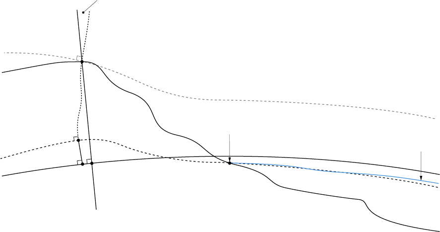
p′
p′′
p
NO
HOh
ν
plumb–line (direction of gravity)
ellipsoid normal
deflection of the vertical (ǫ)
terrain
geoid (W0)
gravity potential (Wp)
ellipsoid
sea surface
mean sea level
ocean
ocean floor
Figure 5.1: The relationships between the natural terrain, ellipsoid, geoid, mean sea level, and sea
surface.
Mean sea level (MSL) is an observed tidal datum and is used as the conventional reference surface
to which heights on the terrain (e.g. contours, heights of mountains, flood plains, etc.) and other
tidal datums are related. The geoid is the surface of constant gravity potential (or equipotential)
chosen to best approximate MSL. It is often shown in the literature as W0in order to distinguish it
as the reference equipotential surface to which other gravity potentials (such as the potential Wpat
point p) are related. Being a gravity potential surface (as opposed to a geometrical surface like the
ellipsoid), the geoid is consistently perpendicular to the direction of gravity (i.e. the plumb–line). In
this sense, it represents the “spirit–level” surface at which fluids stabilise.
As suggested by the curved plumb–line, the direction of gravity varies along the path of the plumb–line
on account of variations in land (or subsurface) mass–density and other gravity anomalies. The
deflection of the vertical is the angle between the direction of the plumb–line and the normal to
the ellipsoid and is generally expressed in two dimensions, as a north–south component (deflection
in the prime meridian, ξ) and an east–west component (deflection in the prime vertical, η). The sea
surface varies from the geoid due to the dynamic topography of the ocean caused by variations in
temperature, regional currents, gravitational effects, and salinity, for example. For similar reasons,
MSL also varies from the geoid.
As shown in Figure 5.1, true orthometric height HOis the length of the curved plumb–line between
point pand the geoid. The geoid–ellipsoid separation NOis the length of the normal to the ellipsoid,
from p00 to the geoid. In practice, it is not a simple matter to compute the true orthometric height
since the integral mean of gravity between pand the geoid is a rather complex and practically
challenging phenomenon to quantify. For this reason, several approximations of HOhave been
proposed, such as Helmert orthometric (HH), normal (HN) and normal orthometric (HN O). It is
not necessary to explain all approximations for HO, although brief comments will be made on the
normal orthometric height system due to its frequent use in establishing national vertical datums.
Consider Figure 5.2. Normal orthometric height HN O is the length of the curved normal gravity
plumb–line between point pand the quasigeoid. It is based on a theoretical (ellipsoidal) normal gravity
field and can be readily computed without knowing the nature of the subsurface mass–density or
54

needing to take gravity observations. As a result of approximating the Earth’s gravity field with a
normal gravity field, propagation of normal orthometric heights through spirit levelling requires a
relatively simple correction (known as the normal orthometric correction) to account for the change
in gravity according to the change in latitude along the levelling run.
p′
p′′
p
NNO (ζ)
HNO
h
normal gravity plumb–line
ellipsoid normal
terrain
geoid
mean sea level
quasigeoid(W0)
ellipsoid
Figure 5.2: The relationship between the geoid and quasigeoid, and between ellipsoid height (h) and
normal orthometric height (HNO)
The height of the quasigeoid above the ellipsoid is labelled NNO and is often cited in the literature
as the height anomaly ζ. The quasigeoid is given its name since it is not an equipotential surface
and thereby does not properly describe the flow of fluids. The geoid and quasigeoid are coincident
at MSL, but diverge, more or less, over land with respect to elevation. According to Featherstone
and Kuhn [2006], this divergence may reach up to 3.4 metres in the Himalayas and 0.15 metres in
Australia. The point to note is that the quasigeoid, being an approximation, does not represent true
gravity and hence, does not provide for estimating true orthometric heights and height differences.
5.2.1 Geoid models
There are numerous geoid and quasigeoid models (so called) in use throughout the world. A
comprehensive review of all such models is beyond the scope of this document. However, it is
worthwhile noting the subtle differences that may be found between such models.
Firstly, reflecting on the concepts discussed in the previous section, a gravimetric geoid model provides
NOvalues, whereas a gravimetric quasigeoid model generally provides approximations of it, such as
NNO or NH. Secondly, the adopted reference ellipsoid for each model is not unique. Although
international practice shows a global trend towards the use of the Geodetic Reference System 1980
(GRS80), some older models may be based upon the World Geodetic System 1984 (WGS84). Thirdly,
a geoid or quasigeoid model can be derived from a global equipotential model alone, such as EGM96
or EGM2008, or a combination of gravimetric data sourced from a global model, regional gravity
observations and other gravity modelling.
55

Another point to note is that there are models which also include a geometric component to
account for known distortions in a particular vertical datum. In the Australian context, AHD
was established using a normal–orthometric height system. Due to various reasons, AHD contains
numerous distortions of various magnitudes and does not coincide uniformly with the quasigeoid.
Of the four national geoid models published since 1990 for use over the Australian continent1, only
AUSGeoid09 includes a geometric component that models the difference between the gravimetric
quasigeoid and the zero surface of the AHD [Featherstone et al., 2011]. Hence, AUSGeoid09 provides
for converting between the GRS80 ellipsoid heights and AHD heights, not heights relative to the
gravimetric quasigeoid.
Therefore, when selecting a geoid model from which to interpolate geoid/quasigeoid–ellipsoid values
and deflections of the vertical, it is imperative that the model supplied to geoid is compatible with
the adjustment project reference frame (and ellipsoid), and the supplied station heights and height
measurements.
5.2.2 Conventions used in DynaNet
Although there is a tangible difference between the geoid and the quasigeoid (and other approximations
of the geoid), the term geoid will be used throughout this document to refer to gravimetric geoid
and quasigeoid models generally. Similarly, the term geoid–ellipsoid separation (N) will be used to
refer to both the separation between the geoid and the ellipsoid (NO) and the separation between
the quasigeoid (and other geoid approximations) and the ellipsoid (NN, ζ). Likewise, orthometric
height (H) will be used to refer to true orthometric (HO), Helmert (HH), normal (HN) and normal
orthometric (HNO) height. The practical implication is that whenever these terms are cited, the
user is responsible for interpreting them according to the context of the adjustment project.
5.3 Grid file interpolation
By far, the most simple, convenient, efficient and repeatable means for retrieving geoid information
from a geoid model is to use interpolation from a structured grid file defined by regularly–spaced
grid nodes. Using a regular grid file, geoid information can be interpolated at will for arbitrarily
located points via one of several interpolation methods. The information that can be incorporated
within a DynaNet adjustment includes values for geoid–ellipsoid separation N, the north–south and
east–west deflections of the vertical ξand η, and the respective uncertainties σN,σξand ση. When
attempting to interpolate this information from a gridded geoid model, geoid provides an ability to
derive the unknown parameter values using bilinear interpolation and bicubic interpolation. These
methods are briefly described in the following sections.
5.3.1 Bilinear interpolation
The method of bilinear interpolation uses a quadratic form to calculate the desired parameter values
for an arbitrary point from a two–dimensional array of grid nodes. Bilinear interpolation is well suited
to the task of interpolating from grids having a relatively high resolution with respect to variability
in the grid node parameter values, or where higher order curve (or polynomial) fitting offers minimal
improvement in accuracy. In this method, only the four surrounding grid nodes are required. Figure
5.3 illustrates the concept of interpolating an unknown geoid–ellipsoid separation Nat point pfrom
the surrounding grid nodes using bilinear interpolation. The same concept applies to interpolating ξ
and η.
1. AUSGeoid90, AUSGeoid93, AUSGeoid98 and AUSGeoid09
56
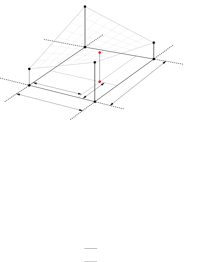
N1
N2
N3
N4
Np
φ1
φ2
φ3
φ4
λ1
λ2
λ3
λ4
∆φinterval
∆λinterval
∆φp
∆λp
Figure 5.3: Bilinear interpolation concept
The formula to compute Nat point pusing bilinear interpolation is given by [Press et al., 2002]:
Np=α00 +α10t+α01u+α11tu (5.1)
=
1
X
i=0
1
X
j=0
αijtiuj(5.2)
where:
a00 =N1(5.3)
a10 =N2−N1(5.4)
a01 =N4−N1(5.5)
a11 =N1+N3−N2−N4(5.6)
t=∆λp
∆λint
(5.7)
u=∆φp
∆φint
(5.8)
∆λp=λp−λ1(5.9)
∆φp=φp−φ1(5.10)
Here, N1,N2,N3and N4are retrieved from the grid file. ∆λint and ∆φint are the grid node
intervals in the east–west and north–south directions respectively. Since the majority of grid files are
orthogonal with regularly spaced grid nodes, ∆λint and ∆φint will be constant for throughout each
grid. The exception to this convention is when a geoid grid file contains one or more sub–grids which
have a higher resolution than the parent grid. However, in these instances, the values for ∆λint
and ∆φint will most likely be constant for each sub–grid. To interpolate ξpand ηp, the Nterms in
57
equations 5.3, 5.4, 5.5 and 5.6 are replaced with the corresponding ξand ηvalues for grid nodes 1
to 4.
5.3.2 Bicubic interpolation
Bicubic interpolation uses a third degree polynomial, in two dimensions, to approximate a continuous
(or smooth) surface from which to calculate the unknown quantities. For this purpose, bicubic
interpolation requires the parameter values at sixteen grid nodes surrounding the arbitrary point. It
is computationally less efficient, but may be necessary where the grid node spacing is large or there
is high variability in the grid node parameter values.
Conceptually, the method of bicubic interpolation involves two steps. Firstly, a two–dimensional
polynomial is fitted to the sixteen grid node parameter values and, secondly, the value at the arbitrary
point is evaluated. To fit the third order polynomial to the surrounding parameter values, sixteen
values must be evaluated for the four grid nodes — four parameter values, four east–west gradients,
four north–south gradients, and four cross–product gradients. All gradients (i.e. partial derivatives)
are computed using numerical differentiation from the sixteen parameter values N1...16.
The formula to compute Nat point pusing bicubic interpolation is given by [Press et al., 2002]:
Np=
3
X
i=0
3
X
j=0
αijtiuj(5.11)
Evaluating αinvolves a linear transformation of a vector xrepresenting the four parameter values
and twelve derivatives using a coefficient matrix Cand is given by:
α=C−1x
where C−1is the inverse of the coefficient matrix:
C−1=
1000000000000000
0000000010000000
−30030000−2 0 0 −10000
200−2000010010000
0000100000000000
0000000000001000
0000−30030000−2 0 0 −1
0000200−200001001
−3 3 0 0 −2−10000000000
00000000−3 3 0 0 −2−1 0 0
9−9 9 −9 6 3 −3−6 6 −6−334212
−6 6 −6 6 −4−2 2 4 −3 3 3 −3−2−1−1−2
2−200110000000000
000000002−2001100
−6 6 −6 6 −3−3 3 3 −4 4 2 −2−2−2−1−1
4−4 4 −4 2 2 −2−2 2 −2−221111
58

The elements of xare calculated as follows:
x1=N1x5=∂N1
∂x ∆λint x9=∂N1
∂y ∆φint x13 =∂2N1
∂x∂y ∆λint∆φint
x2=N2x6=∂N2
∂x ∆λint x10 =∂N2
∂y ∆φint x14 =∂2N2
∂x∂y ∆λint∆φint
x3=N3x7=∂N3
∂x ∆λint x11 =∂N3
∂y ∆φint x15 =∂2N3
∂x∂y ∆λint∆φint
x4=N4x8=∂N4
∂x ∆λint x12 =∂N4
∂y ∆φint x16 =∂2N4
∂x∂y ∆λint∆φint
The twelve gradient values ∂Ni/∂x,∂Ni/∂y and ∂2Ni/∂x∂y (i= 1,...,4) are evaluated as follows:
∂N1
∂x =N2−N16
2∆λint
∂N2
∂x =N9−N1
2∆λint
∂N3
∂x =N10 −N4
2∆λint
∂N4
∂x =N3−N15
2∆λint
∂N1
∂y =N4−N6
2∆φint
∂N2
∂y =N3−N7
2∆φint
∂N3
∂y =N12 −N2
2∆φint
∂N4
∂y =N13 −N1
2∆φint
∂2N1
∂x∂y =N3−N7−N15 +N5
4∆λint∆φint
∂2N2
∂x∂y =N10 −N8−N4+N6
4∆λint∆φint
∂2N3
∂x∂y =N11 −N9−N13 +N1
4∆λint∆φint
∂2N4
∂x∂y =N12 −N2−N14 +N16
4∆λint∆φint
Values for t,u,∆λpand ∆φpare evaluated from equations 5.7, 5.8, 5.9 and 5.10, and ∆λint and
∆φint are the grid node intervals. Finally, Nis evaluated at point pfrom equation 5.11 using the
following pseudocode:
Np= 0
for i= 0 to 4do
Np=Np∗t+ai,4∗u+ai,3∗u+ai,2∗u+ai,1equation 5.11
end for
5.4 Import of geoid information
To introduce geoid information into a project, type geoid at the command prompt, followed by one
or more options and arguments. The complete command line reference for geoid is given in §A.4.
If no program options are provided upon program execution, the command line reference for geoid
will be displayed.
If a DynaNet Project File (c.f. Chapter 2) is to be used, provide --project-file (or its shortcut -p)
followed by the full path for the project file:
geoid -p skye.dnaproj
No other options are required, as geoid will be invoked using the options and arguments contained
in the project file skye.dnaproj.
59

To import geoid information using command line options and arguments, type geoid followed by the
network name2, and then --ntv2-file (or its shortcut -g) followed by the full path for the NTv2
binary geoid file:
geoid skye -g ausgeoid09.gsb
Upon executing geoid, the binary station file skye.bst and the header records from the NTv2 geoid
grid file ausgeoid09.gsb will be loaded into memory. For each station found in the binary station file,
geoid will attempt to interpolate the geoid–ellipsoid separations and the north–south and east–west
deflections of the vertical from the surrounding grid nodes. If the station lies outside the limits of
the geoid grid file, no information will be retrieved for that station. Once the information for all
stations has been interpolated, the binary station file and corresponding DynaNet project file will be
updated.
By default, bicubic interpolation (c.f. §5.3.2) is used to interpolate values from the surrounding grid
nodes. To interpolate geoid information using bilinear interpolation (c.f. §5.3.1), add to the geoid
command the option --interpolation-method (or its shortcut -m) followed by a zero (0):
geoid skye -g ausgeoid09.gsb -m 0
Since the least squares adjustment model implemented within DynaNet is based upon the cartesian
reference frame, all orthometric heights contained in the station file must be transformed to ellipsoid
heights. This can be achieved by adding the option --convert-stn-hts:
geoid skye -g ausgeoid09.gsb --convert-stn-hts
When the option --convert-stn-heights is provided, geoid will determine whether or not to
transform a station’s height by examining the coordinate type (c.f. §B.1.3, §B.4.1). If the coordinate
type is LLH or UTM,geoid will treat the supplied height as an orthometric height and transform it to
an ellipsoidal height using the interpolated Nvalue. If the coordinate type is LLh,geoid will treat
the station height as ellipsoidal, leaving it as–is. The application of interpolated geoid information
to terrestrial geodetic measurements prior to running an adjustment will be explained in Chapter 7.
When complete, geoid will report the number of stations for which geoid information was interpolated
or, in the case of failure, an error message corresponding to the type of failure. Using the geoid
project, Figure 5.4 shows the information reported to the screen upon normal program execution.
2. Note that the option --network-name is the default option to geoid and as such, the network name may be
passed to geoid without the option text.
60

+ Options:
Network name: skye
Input folder: .
Output folder: .
Binary station file: ./skye.bst
Convert orthometric heights: Yes
Geoid grid file: ausgeoid09.gsb
Interpolation method: Bi-cubic
Input coordinate format: Degrees minutes seconds
+ Binary station file interpolation mode.
+ Opening grid file... done.
+ Interpolating geoid components and reducing
heights to the ellipsoid... done.
+ Interpolated data for 6 points.
+ Geoid file interpolation took 0.007s
Figure 5.4: geoid progress reporting of geoid grid file interpolation
5.5 Arbitrary interpolation and height transformation
In addition to introducing geoid information into an adjustment project, geoid offers two modes for
interpolating geoid information from a geoid grid file — interactive mode and text file mode. With
the latter, it is also possible to transform a file of heights from one height system (or vertical datum)
to another.
5.5.1 Interactive mode
Interpolating geoid information in interactive mode involves using the command line to specify
arbitrary interpolation points one at a time. For instance, to retrieve information for an arbitrary
location of -33°24’ 36” latitude and 149°39’ 06” longitude (provided in degrees, minutes and
seconds), type geoid, the NTv2 grid file option and file path, then --interactive (or its shortcut
-e) to indicate that coordinates will be entered via the command line, followed by options and
arguments for latitude and longitude:
geoid -g ausgeoid09.gsb -e --latitude -33.2436 --longitude 149.3906
When complete, geoid will report the Nvalue and the north–south and east–west deflections of the
vertical ξand ηinterpolated for the supplied coordinates. In the case of failure, an error message
corresponding to the type of failure will be displayed. Figure 5.5 shows the information reported to
the screen upon normal program execution.
61

+ Options:
Geoid grid file: ausgeoid09.gsb
Interpolation method: Bi-cubic
Input coordinate format: Degrees minutes seconds
+ Opening grid file... done.
+ Interpolation results for -33.2436, 149.3906 (ddd.mmssss):
N value = 25.4 metres
Deflections:
- Prime meridian = -4.41 seconds
- Prime vertical = -6.48 seconds
Figure 5.5: Interactive geoid grid file interpolation
By default, interactive input requires coordinates to be supplied in degrees, minutes and seconds
format. To interpolate geoid information using decimal degrees, simply add the --decimal-degrees
option:
geoid -g ausgeoid09.gsb -e --latitude -33.4100 --longitude 149.6517 --decimal-degrees
Note that latitudes and longitudes, whether in decimal degrees or degrees, minutes and seconds, must
be supplied in HP notation (i.e. dd.dddddddd or dd.mmssssss). Spaces between degrees, minutes
and seconds will cause geoid to treat values following the spaces as independent option arguments.
Since geoid does not check or correct latitude values for sign, positive and negative latitude values
will be treated as being in the northern and southern hemispheres respectively. Similarly, positive and
negative longitude values will be treated as being east or west of the zero meridian (i.e. Greenwich
meridian) respectively.
To interpolate geoid information using bilinear interpolation (c.f. §5.3.1), add --interpolation-method
(or its shortcut -m) followed by a zero (0).
5.5.2 Text file mode
Text file mode has been designed to provide an efficient means for (1) interpolating geoid information
for a list of coordinates and (2) transforming heights from one system to another using simple ASCII
text file formats. For these purposes, geoid supports Formatted Text files (e.g. *.dat,*.prn,*.txt)
and Comma Separated Values files (*.csv). Appendix B.7 provides the file format specification for
these file types.
To interpolate geoid information and transform a file of heights, type geoid on the command line,
followed by the NTv2 grid file option and file path, then --text-file (or its shortcut -t) with the
input text file path and, if required, options and arguments for interpolation method, coordinate
format and conversion direction. For example, to transform a file of heights in a file named
pipeline.txt from orthometric to ellipsoidal, where the desired interpolation method is bilinear
and the input coordinates are in decimal degrees, type:
geoid -g ausgeoid09.gsb -t pipeline.txt -m 0 --decimal -r 0
Upon transforming a text file of heights, geoid will report to the screen the items relevant to the
text file transformation, the progress of interpolation and transformation of heights, and any errors or
warnings related to the file transformation. Figure 5.6 shows the information reported to the screen
upon normal program execution.
62

+ Options:
Input folder: .
Output folder: .
ASCII file: pipeline.txt
Output file: pipeline_out.txt
Geoid grid file: ausgeoid09.gsb
Interpolation method: Bi-linear
Input coordinate format: Decimal degrees
+ ASCII file interpolation mode.
+ Opening grid file... done.
+ Interpolating geoid components... done.
+ Interpolated data for 17 points.
+ Warning: data for 1 point could not be interpolated.
See pipeline_out.txt for more information.
+ Geoid file interpolation took 0.012s
Figure 5.6: geoid progress reporting of geoid interpolation and text file transformation
During this process, geoid will attempt to determine the file type from the file extension and contents
of the input file. Any problems encountered with opening the input file will be reported to the screen.
The name of the output file will be the same as the input file name, but with a “_out” inserted
between the file name and the file extension. During the transformation process, geoid information
will be interpolated using the default or user–specified interpolation method, and the height supplied
on each line will be transformed according to the transformation direction. The original height,
transformed height, interpolated Nvalue and deflections of the vertical ξand ηfor each point in
the file will be appended to the original record from the input file, which is in turn printed to the
output file. Since geoid is only concerned with heights, the input latitude and longitude are written
directly to the output file without any alteration.
In the case of an error, the input record prefixed by the string ’ERROR (#)’, where ’#’ is a number
indicating the type of error, will be printed to the output file. Typical examples of error include
instances when the coordinates cannot be read from the input file (possibly due to an incorrect
coordinate type or file record format), or if the coordinates lie outside the extents of the geoid grid
file. Table 5.3 in §5.7.3 lists the possible range of error codes and their meanings.
5.6 Exporting interpolated information
During the process of interpolating geoid information from a geoid grid file, geoid can export this
information to a DNA geoid file. Generating a DNA geoid file is only necessary when it is desirable to
introduce geoid information into a DynaNet project via import (c.f. §3.2.4). To export interpolated
geoid information to a DNA geoid file, simply add the --export-dna-geo-file option when executing
geoid. The following examples show how to export geoid information during the process of (1)
introducing geoid information into a project (c.f. §5.4) and (2) interpolating in text file mode (c.f.
§5.5.2):
geoid skye -g ausgeoid09.gsb --export-dna-geo-file
geoid -g ausgeoid09.gsb -t pipeline.txt --export-dna-geo-file
63
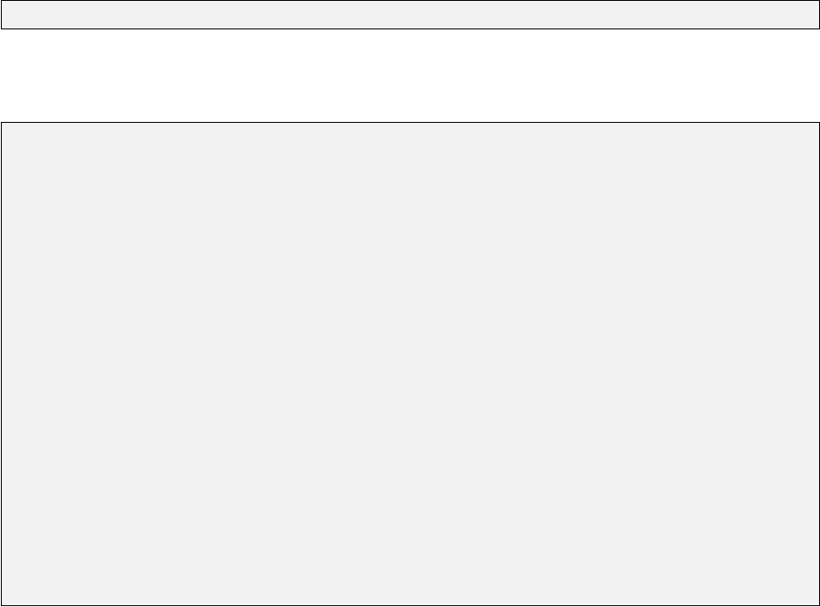
5.7 Working with NTv2 geoid grid files
5.7.1 Reporting NTv2 geoid grid file metadata
At times, it may be necessary to view a summary of the metadata contained within an NTv2 geoid
grid file. NTv2 grid file metadata is contained within an array of block header records, and provides
specific information relating to, for example, geoid grid file version, geoid and ellipsoid parameters,
grid file extents and grid node interval. To display the header information for a grid file, type geoid
on the command line, followed by the NTv2 grid file option and file path, then --summary (or its
shortcut -u) :
geoid -g ausgeoid09.gsb -u
Running this command will produce a summary similar to that which is shown in Figure 5.7.
+ Options:
Geoid grid file: ausgeoid09.gsb
Input coordinate format: Degrees minutes seconds
Grid properties for "ausgeoid09.gsb":
+ GS_TYPE = SECONDS
+ VERSION = 1.0.0.0
+ SYSTEM_F = GDA94
+ SYSTEM_T = AHD_1971
+ MAJOR_F = 6378137.000
+ MAJOR_T = 6378137.000
+ MINOR_F = 6356752.314
+ MINOR_T = 6356752.314
+ NUM_OREC = 11
+ NUM_SREC = 11
+ NUM_FILE = 1
+ SUBGRID 0:
SUB_NAME = AUSGEOID
PARENT = NONE
CREATED = 01012010
UPDATED = 01012010
S_LAT = -165540.000
N_LAT = -28800.000
E_LONG = -575940.000
W_LONG = -388800.000
LAT_INC = 60.000
LONG_INC = 60.000
GS_COUNT = 7113600
Figure 5.7: Example NTv2 grid file summary
In relation to Figure 5.7, Tables 5.1 and 5.2 describe the NTv2 grid file header fields and the individual
sub grid header fields.
64

Table 5.1: NTv2 grid file overview fields
Field Description
NUM_OREC Number of header records in the overview block.
NUM_SREC Number of header records in each sub grid block.
NUM_FILE Number of sub grids contained in the geoid grid file. A grid file may contain several sub
grids of different densities. The limits of these sub grids will all be contained within the
parent grid. If there is only one sub grid, then it is the parent grid.
GS_TYPE The units of the grid nodes.
VERSION The geoid grid file version.
SYSTEM_F The “from” reference ellipsoid (or geodetic datum with well known ellipsoid)
SYSTEM_T The “to” height system or vertical datum.
MAJOR_F The ellipsoid semi–major axis of the “from” system.
MAJOR_T The ellipsoid semi–major axis of the “to” system.
MINOR_F The ellipsoid semi–minor axis of the “from” system.
MINOR_T The ellipsoid semi–minor axis of the “to” system.
Table 5.2: NTv2 grid file sub grid fields
Field Description
SUB_NAME The name of this particular sub grid.
PARENT The parent sub grid name. ’NONE’ if this is the parent grid.
CREATED Grid file creation date
UPDATED Grid file modification date
S_LAT Lower latitude extent
N_LAT Upper latitude extent
E_LONG Lower longitude extent
W_LONG Upper longitude extent
LAT_INC Latitude interval
LONG_INC Longitude interval
GS_COUNT Grid node count
5.7.2 Importing WINTER DAT geoid grid files
AUSGeoid09 has been publicly released in the form of ASCII text files using the legacy WINTER
DAT file format. Whilst serving as a simple, human–readable format, the WINTER DAT file format
is not designed to provide an efficient means for instantaneous interpolation. Accordingly, DynaNet
requires the geoid information contained in these files to be converted into a structured binary format.
DynaNet uses the NTv2 format for structuring, storing and interpolating geoid model information.
To convert geoid information in the WINTER DAT file format to the NTv2 binary format, type
geoid at the command prompt, then --create-ntv2 (or its shortcut -c), followed by the options
and arguments relating to the input and output files and the geoid model parameters. For example,
65

to create a new NTv2 binary grid file named geoid_model.gsb from geoid information stored in a
WINTER DAT file named geoid_model.dat using the default options, run the following command:
geoid -c -g ./geoid_model.gsb -d geoid_model.dat
When converting geoid files to the NTv2 binary format, geoid will determine from the raw data the
upper and lower grid extents and the north–south and east–west grid node intervals. Checks are
also performed to ensure the data contains a sufficient number of nodes to construct an orthogonal
grid file. The parameters derived from the raw data will be written to the grid file header records
(c.f. Tables 5.1 and 5.2). Since the WINTER DAT file format contains data for a single grid, the
resultant NTv2 grid file will contain a single sub–grid which will be the parent grid.
To facilitate the capture of other metadata relating to the geoid grid file, geoid provides options
to specify the units for the deflections of the vertical (in radians or seconds), the grid file version,
the name of the ellipsoid system, the name of the height system or vertical datum, the semi–major
and semi–minor ellipsoid parameters of the two systems, the name of the sub–grid, and the dates of
creation and update. For example, to specify a version of 2.5.0.0, the name MYGEOID, ellipsoid and
height system names GDA94 and AHD71, a creation date of 18 March 2015 and an update date of 5
May 2015, run the following command:
geoid -c -g ./geoid_model.gsb -d geoid_model.dat --VERSION 2.5.0.0 --SUB_NAME MYGEOID --SYSTEM_F GDA94
--SYSTEM_T AHD71 --CREATED 18032015 --UPDATED 05052015
The option --grid-shift-type followed by either seconds or radians can be used to specify the
units in which the grid extents and the deflections of the vertical will be stored. The options
--semi-major-from,--semi-major-to,--semi-minor-from and --semi-minor-to are not used during
grid file interpolation and can be provided for metadata purposes only.
Figure 5.8 shows the information reported to the screen upon normal program execution. Once the
NTv2 binary grid file has been created, a summary of the grid file parameters (c.f. Figure 5.7) will
be displayed.
+ Options:
Input folder: .
Output folder: .
Geoid grid file: geoid_model.gsb
WINTER DAT file: geoid_model.dat
+ Creating NTv2 file from WINTER DAT file format:
+ Reading contents of WINTER DAT file... done.
+ WINTER DAT file structure appears OK.
+ Creating NTv2 gsb file... done.
+ Grid properties for geoid_model.gsb:
- GS_TYPE = SECONDS
- VERSION = 2.5.0.0
- SYSTEM_F = GDA94
- SYSTEM_T = AHD71
- ...
- ...
Figure 5.8: Progress of NTv2 grid file creation
66

5.7.3 Grid file interpolation errors
If an error occurs at any time during the geoid interpolation process, a non-zero value is printed to
the output file to indicate the type of error. Table 5.3 lists the errors that may be encountered upon
geoid grid file interpolation.
Table 5.3: Grid file interpolation error codes and descriptions
Code Description
-6 The NTv2 version of the specified grid file is not supported.
-5 The parameters for the specified grid file do not match the number of records.
-4 Could not allocate the required memory.
-3 A grid file has not been opened.
-2 Cannot locate the required sub grid.
1 The specified grid file could not be opened.
2 Cannot read this type of grid file.
3 or 14 Found an unrecoverable error in the specified grid file: <grid–file–name>
It is likely that this file was downloaded or produced incorrectly.
4 Could not read from the specified input file.
5 Could not write to the specified output file.
6 Cannot read this type of input file.
7 Cannot produce this type of output file.
8 No data was contained within the last input record.
9 The record <data–record> is too short to contain valid data.
10 The record <data–record> does not contain valid numeric input.
11 The required data could not be extracted from the record <data–record>.
12 The specified zone is invalid.
13 or -1 The point <data–record> lies outside the extents of the specified grid file.
15 The interpolation shifts could not be retrieved from the ASCII grid file.
16 The interpolation shifts could not be retrieved from the Binary grid file.
17 The csv record <data–record> does not contain sufficient records.
67
68
Chapter 6
Network segmentation
6.1 Introduction
For relatively small survey control networks, the task of estimating unknown station coordinates and
their uncertainties can be readily achieved in a matter of seconds using a modern computer. In
these circumstances, network segmentation can be omitted, and least squares adjustments can be
undertaken in a conventional, simultaneous fashion. When dealing with extremely large networks
however, network adjustment becomes computationally intensive and time consuming, taking up to
several hours, if not days to complete. This is primarily due to the number of floating point operations
that must be undertaken when computing the inverse of the least squares normal equation matrix
— an essential step for the full analysis of the precision of the estimated parameters. Invariably, the
sheer size of state, national and continental scale geodetic networks (i.e. those which have tens of
thousands of stations and hundreds of thousands of measurements) presents a substantial obstacle
to performing regular re–adjustment as demanded by datum maintenance. In such circumstances, it
becomes more efficient to segment and adjust the network using phased least squares adjustment.
DynaNet has been specifically designed to make the phased adjustment process as simple and
efficient as possible. This is achieved by the use of an automated network segmentation algorithm
which eliminates the need for the user to manually subdivide a network into blocks. The first part
of this chapter (§6.2 – §6.3) describes the concept of network segmentation and the automated
segmentation algorithm employed by DynaNet. The second part describes how to use segment and
its options to segment networks and to constrain the way in which networks are segmented.
6.2 The concept of network segmentation
The concept of network segmentation involves partitioning a network into smaller–sized blocks.
Figure 6.1 illustrates the concept of a geodetic network segmented into two blocks. In Figure 6.1,
Block A is defined by the set of measurements mawith variance matrix Va, and Block B is defined
by the set of measurements mbwith variance matrix Vb. The parameters to be estimated in the
entire network are represented by xp,xqand xr, of which xpand xqappear in Block A, and xq
and xrappear in Block B. Thus, xqrepresents the set of junction stations which link Blocks A and
B through measurements maand mb, and xprepresents the set of inner stations relating to Block
A. Since all stations represented by xqare connected to measurements in Block B, both xqand xr
represent the inner stations relating to Block B. xp,xqand xreach represent a cluster of stations
which can be of any size. Likewise, maand mbeach represent clusters of measurements of any size.
With this concept in mind, Figure 6.2 shows a trivial GNSS network segmented into two blocks.
69
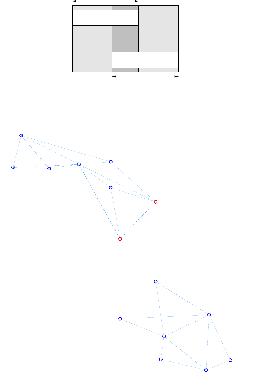
Block A
Block B
xpxqxr
maVa
mbVb
Figure 6.1: Network segmentation concept
310211240
236300210
365300060
309100090
409704930
409600170
360100260
335800500
(a) First block (Block A)
212000820
409700110
269100210
299000080
230900140
360100260
335800500
(b) Second block (Block B)
Figure 6.2: A trivial GNSS network segmented into two blocks
70

In Figures 6.2a and 6.2b, the stations with a blue circle are inner stations. The stations with a
red circle are the junction stations which link the two blocks. With reference to Figure 6.1 and the
network shown in Figure 6.2, Table 6.1 summarises the distribution of the stations and measurements
amongst the two blocks. An important note worth emphasising is that whilst a particular station
can appear as a junction station in both Blocks A and B, each measurement in a network must only
ever appear once — either in Block A or in Block B.
Table 6.1: Distribution of parameters and measurements of a network segmented into two blocks
Block Parameters and stations Measurements
Axp236300210, 309100090, 310211240,
365300060, 409600170, 409704930 ma
xq335800500, 360100260
Bxq335800500, 360100260 mb
xr212000820, 230900140, 269100210,
299000080, 409700110
Although the preceding text has outlined the concept of network segmentation using two blocks,
a geodetic network can be segmented into an almost unlimited number of blocks. It follows that
the phased adjustment technique can be applied to geodetic networks of almost any number of
stations and measurements. The primary factors which define the way in which a geodetic network
is segmented are (a) the desired maximum number of stations each block should contain (i.e. the
maximum block size), and (b) the level of connectivity in a network (i.e. the number of other stations
each station is connected to by the set of measurements). Concerning the latter, networks with few
measurements per station can be segmented in a far more flexible manner than highly connected
networks, whereas networks having a high level of connectivity cannot always be segmented into the
desired number of stations. In any case, to achieve a rigorous solution for the unknown parameters,
the network must be correctly segmented so that:
•each block contains the total number of measurements that exist between all inner stations in
that block, and
•junction station estimates and variances can be passed between successive blocks.
segment takes care of these concerns using a fully automated procedure, and offers the flexibility
for users to nominate (a) the maximum number of stations each block should contain and (b)
which stations should appear in the first block. Nominating the maximum block size is essential
to optimising network adjustment performance according to network size and computer hardware
capability. The ability to nominate which stations should appear in the first block affords the ability
to derive the relative uncertainties between any two or more stations in the network. These options
will be described in §6.5.1.
6.3 Segmentation algorithm
At the most fundamental level, the segmentation algorithm partitions a large network into a series
of blocks with the characteristics of the two adjacent blocks as shown in Figure 6.1. To help
conceptualise a network segmented into multiple blocks, Figure 6.3 illustrates the concept of a
network segmented into four blocks.
71
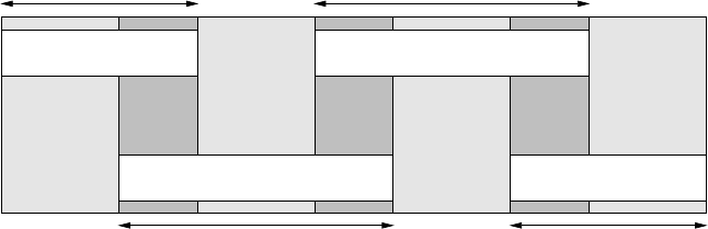
Block 1
Block 2
Block 3
Block 4
x1x2x3x4
x12 x23 x34
m1V1
m2V2
m3V3
m4V4
Figure 6.3: Network segmentation concept involving four blocks
In summary, each block is made up of inner stations (xi), for which all their associated measurements
(mi) make up the measurement–set, and junction stations (xij, j=i+1), which are connected by
measurements to the inner stations but are also associated with other measurements to stations in
other blocks. The segmentation algorithm moves forward (e.g. block i, block i+ 1, . . . , block n−1,
block n) by selecting the inner stations for the next block from the junction stations of the last block.
The total process of selecting stations and measurements for the series of connected blocks can be
summarised as:
1. Select the inner stations for the first block.
2. Select all measurements associated with inner stations.
3. Select as junction stations, all stations connected by measurements to the inner stations.
4. The structure of the block is now complete and is made up of inner stations, junction stations
and associated measurements.
5. Move to the next block by selecting its inner stations from the previous block’s junction stations.
6. Repeat steps 2, 3 and 4 until all measurements have been selected for one of the blocks.
The result of this process is to segment a large network into a series of smaller blocks which can be
adjusted sequentially. After each block is adjusted, the estimates of the parameters associated with
the junction stations are passed as pseudo measurements to the next block for further processing,
and the parameters associated with the inner stations drop from the procedure.
The stations selected as inner stations of the first block do not have to be in a close spatial proximity
or connected by direct measurement, and may indeed be on opposite sides of a continent. In many
applications of DynaNet, the selection of the inner stations of the first block is critical as it provides
a mechanism for placing a particular set of stations in one block. If these are the only stations for
which a rigorous estimate and the full variance matrix is required, it makes for great efficiency in
adjustment as only one pass through the full series of blocks is required (see §6.4.4). The efficiency
of the adjustment process is aided by having a high ratio of inner to junction stations and various
strategies are available at step 5 to enhance this (see §6.4.2).
6.4 Accommodating variations in network design, size, user
preferences and computer performance
In general, conventional survey control networks used for land development are those which have
been developed over several decades with an almost random pattern of extension, reinforcement
and re–measurement. They are not structures that are characterised by uniform network design
72

and homogeneous station–to–measurement ratios, such as is found in a regular lattice, a honeycomb
pattern, or triangulated terrain model. Rather, survey control networks vary considerably in geometry,
station count, measurement count, types of measurements, the number of measurements per station,
the number of stations which are connected by a single measurement, and so on. In order to permit
phased adjustment to be performed on any network, the automated segmentation algorithm has
been designed to be extremely flexible so as to handle a virtually innumerable number of network
designs and sizes whilst at the same time, permitting the user to influence the way in which a
network is segmented. To achieve this flexibility, the segmentation algorithm takes several aspects
into consideration, including:
•Optimum block size;
•Inevitable influences on block size;
•Factors influencing the rate of segmentation;
•Datum deficient blocks;
•Non–contiguous networks, and;
•The need for coordinate estimates and full variance matrix for a particular set of stations.
The aspects are explained in the sections that follow.
6.4.1 Optimum block size and maximum adjustment efficiency
Considering that the linear CPU time taken to adjust a network is a factor of n3, where nis the
number of parameters to be estimated, logic would suggest that adopting smaller block sizes would
lead to greater phased adjustment efficiency. However, this notion is true only to a certain degree.
Experience shows that for each network and computer there is an optimum block size limit, beyond
which phased adjustment efficiency decreases. Three primary influences (positive and negative) on
the optimum block size are noted:
1. Smaller than optimum block sizes can lead to a larger number of parameters to
estimate. Two things need to be noted in this context. Firstly, as smaller block sizes lead to
larger numbers of blocks to adjust, the total aggregate time to perform a phased adjustment on
the set of segmented blocks may be more than the time taken to adjust fewer blocks. Secondly,
smaller block sizes increase the likelihood that the same station will appear as a junction station
in several blocks. Inevitably, multiple occurrences of a junction station increases the number of
total parameters to be estimated in a phased adjustment and thereby, increases the adjustment
time. Generally speaking, networks which are partitioned using less than the optimal number
of stations per block will take additional CPU time to adjust.
2. Adjustment times improve with higher performing processor (CPU) architectures and
frequencies. Intuitively, the time taken to adjust a network varies, more or less, according to
the CPU frequency of the computer on which an adjustment is run. As faster CPU frequencies
lead to faster adjustment times, it follows that the optimum block size will also increase.
With the widespread availability of multiple CPUs, hyper–threading and multi–core CPUs1,
adjustment times can be reduced significantly by the use of multi–threaded phased adjustments
(c.f. §8.3.2.2). Accordingly, the optimum block size will be different again. In almost every
case, the optimum block size varies according to computer capability.
3. Measurement connectivity. Networks having a high number of measurements per station will
take more time to adjust than networks with lower ratios, particularly if larger than expected
blocks are generated (c.f. §6.4.2). Accordingly, the optimum block size for the former case
1. In some cases, CPUs with a large number of cores have a lower frequency per core than those with fewer cores.
Hence, a quad–core CPU will not always lead to faster adjustment times than a dual–core.
73
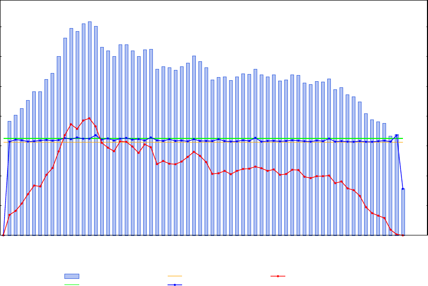
may be lower than the latter case, despite the two networks having a similar number of stations
and (total) measurements.
It is for these reasons that the optimum block size will vary from one project to another, and from one
computer to another. To achieve the maximum phased adjustment efficiency for any one network
on any given computer, the segmentation algorithm affords a capacity for users to nominate the
maximum block size by which the network is segmented.
6.4.2 Inevitable influences on the generated block sizes
Despite careful efforts to determine the optimum block size for segmenting a network, there are
some inevitable influences which cause the segmentation algorithm to generate blocks which exceed
the user–specified block size. Two primary influences are (1) the amount of station–to–station
connectivity created from the set of measurements and (2) the presence of large clusters of correlated
GNSS baselines or GNSS points. Left unmanaged, these influences have the potential to create
excessively large block sizes.
In the first instance, large numbers of measurements from a single station can cause the algorithm to
introduce large numbers of stations into a block. In some cases, the number of stations introduced
to a block may exceed the user–specified block size. An example of this scenario is shown in Figure
6.4, whereby the total block size regularly exceeds the Max station limit (650) because many of the
stations in this network are connected to large numbers of measurements. Figure 6.5 shows a typical
station with a high level of connectivity (MORANG PM 48, associated with over 770 GNSS baseline,
distance and direction set measurements). Conversely, Figure 6.6 shows the segmentation results
from a spirit levelling network. In this case, all stations in the network are connected to less than
five measurements and as such, the total block size closely follows the Max station limit (385).
0
200
400
600
800
1000
1200
1400
5 10 15 20 25 30 35 40 45 50 55 60 65 70
2
765
806
851
905
965964
1046
1087
1202
1324
1390
1370
1418
1433
1403
1263
1238
1200
1278
1280
1238
1199
1246
1247
1115
1132
1125
1110
1131
1156
1205
1166
1124
1044
1061
1064
1039
1062
1083
1080
1115
1078
1065
1076
1036
1044
1078
1073
1024
1012
1033
1028
1050
978993
943930
896
816
776763751
666677
312
1
628642638629631636640635639652645656648648672642650636648653642646636656637633645633636630645633633632645632629630638633654628633634630633638635631628636631649628632628627632627627631635628
671
312
1
137164
213
276
334328
406
452
563
672
745714
770785
731
621588564
630627596
553
610591
478499480477495526
560533
491
412416432410432445447461450432442
406411440438
393384397397401
350361
315303
264
189
149132116
38 60
Segmented Network Blocks (Total 66)
Station Count (Total 41151)
Total block size
Max station limit (650)
Min inner stns (625)
Inner stns
Junction stns
Figure 6.4: Segmentation of a geodetic network having stations with large numbers of measurements.
74
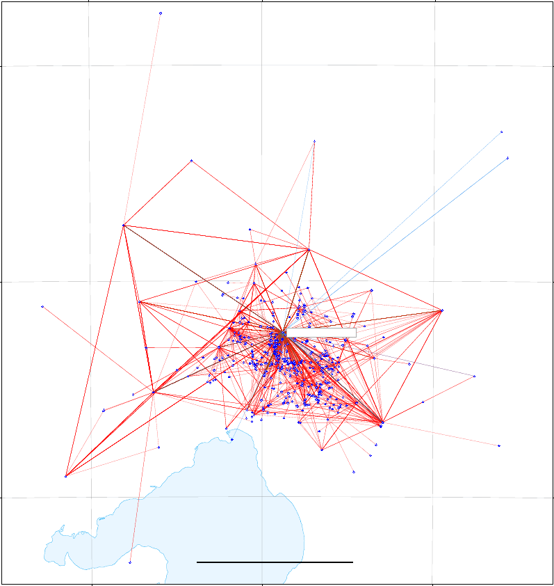
144˚30'
144˚30'
145˚00'
145˚00'
145˚30'
145˚30'
−38˚00'
−38˚00'
−37˚30'
−37˚30'
−37˚00'
−37˚00'
0 20 40
Kilometres
MORANG PM 48
Figure 6.5: GNSS, direction set and distance measurements in the Victorian geodetic network
associated with MORANG PM 48.
Secondly, owing to the fact that GNSS clusters are correlated sets of measurements with a fully
populated variance matrix, each GNSS cluster is introduced to a block as a single group. Hence,
GNSS clusters cannot be “split” and spread across multiple blocks without compromising the rigour
of the adjustment. When the segmentation algorithm adds a large GNSS baseline or point cluster
to a block (such as a national GNSS CORS network solution), it is not unusual for the aggregate
number of stations introduced by the cluster to exceed the user–specified block size.
75
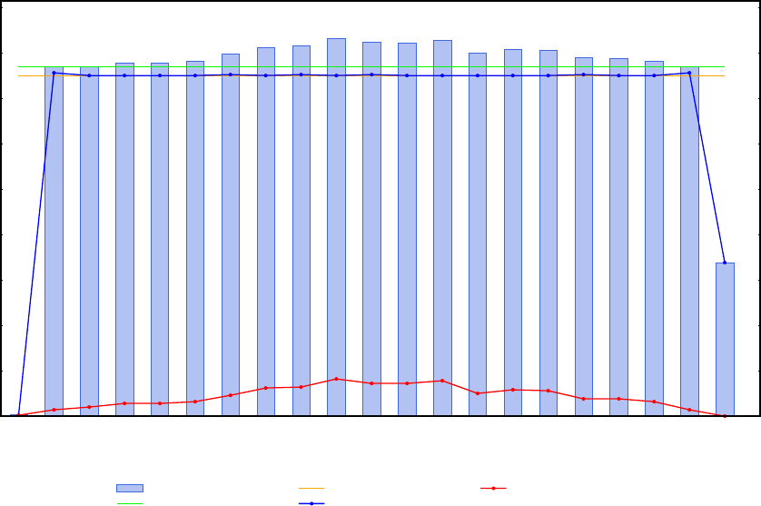
0
50
100
150
200
250
300
350
400
450
1 2 3 4 5 6 7 8 9 10 11 12 13 14 15 16 17 18 19 20 21 22
2
385 385 389 389 391 399 406 408 416 412 411 414
400 404 403 395 394 391 385
169
1
378 375 375 375 375 376 375 376 375 376 375 375 375 375 375 376 375 375 378
169
1710 14 14 16 23 31 32 41 36 36 39
25 29 28 19 19 16 70
Segmented Network Blocks (Total 21)
Station Count (Total 7667)
Total block size
Max station limit (385)
Min inner stns (375)
Inner stns
Junction stns
Figure 6.6: Segmentation of a spirit levelling network having stations with a low measurement count.
Although these influences are for the most part inevitable, the segmentation algorithm includes
a strategy to minimise the influence of stations having excessive numbers of measurements, and
those which form part of a large correlated cluster of measurements. When forming new blocks,
the algorithm introduces stations in order by taking the next available station which has the least
number of associated measurements. By delaying the introduction of large groups of measurements
in this way, the segmentation algorithm has a greater opportunity to advance through the network
at rapid rates. In addition, the segmentation algorithm examines each junction station prior to its
introduction to verify whether its associated measurements will result in an excessively large block
size. In this case, the algorithm advances to alternative junction stations which can maximise the
rate of segmentation and thereby, minimise the resulting block size.
6.4.3 Factors influencing the segmentation rate
When the segmentation algorithm is forced to introduce a large set of measurements to a block,
which in turn results in the insertion of a large number of junction stations to that block, the rate at
which the segmentation advances through the network will slow down considerably if there is little
flexibility in permitting measurements associated with those junction stations from being added.
Whilst this is somewhat counter–intuitive to maintaining block size thresholds, failure to provide
flexibility in this regard will result in the creation of an excessive number of blocks due to the way in
which junction stations are carried from one block to the next.
For example, if a block is created with 400 inner stations and 200 junction stations, the segmentation
algorithm will commence building the next block with 200 junction stations. That all junction stations
are carried to the next block is an essential criteria for rigorous phased adjustment. However, if a
block size limit of 200 stations has been imposed, a dead–end situation (or stalemate) immediately
arises if there is no flexibility to permit the introduction of new measurements and in turn, more
76
stations. To circumvent the algorithm from reaching stalemate, the segmentation algorithm affords a
capacity for the user to specify the minimum number of inner stations that each block must contain.
6.4.4 Generating coordinate estimates and full variance matrix for a user–defined
set of stations
At different times and for various reasons, the need for the coordinates and full variance matrix for a
particular set of stations in a geodetic network will arise — whether for those that surround a certain
project, or those which lie within or along the extent a defined area. Whilst this may seem to be a
rather trivial objective to fulfil, three obstacles to achieving this objective must be borne in mind.
Firstly, it is highly unlikely that the full variance matrix for extremely large networks (i.e. state,
national or continental scale networks of which a small portion survey control is needed) has been
produced and archived in an easily accessible form. Secondly, some or all of the stations selected for
a project may have never been directly connected by measurement. Thirdly, the only plausible way
to obtain a rigorous variance matrix for the defined set of stations is to incorporate the contribution
from all measurements in the network.
Recognising the reality of these issues, the segmentation algorithm has been designed to offer a
capacity to meet the requirement for producing, at will, coordinate estimates and the full variance
matrix for randomly selected stations. This is achieved by permitting users to nominate the stations
which must appear together in a single block. Upon running a phased adjustment of the entire
network with these stations all appearing in the last block to be adjusted, rigorous coordinates and
the full variance matrix will be available. If the latest, most rigorous station coordinates have been
used as the a–priori estimates, a single pass in Block–1 only mode (c.f. §8.3.2.3) is all that will be
required to generate a rigorous variance matrix.
6.4.5 Datum deficient blocks
During segmentation, it is quite common for one or more segmented blocks to be generated without
a sufficient number of measurements to connect the inner and/or junction stations to datum. In
addition, it is equally common for a block to not contain a sufficient number of measurements to
solve all parameter estimates. This particular case arises when the user has nominated a specific set
of stations to be contained in the first block and those stations are not connected by the associated
measurements. The absence of a sufficient number of measurements is a characteristic feature of
many blocks generated by the segmentation algorithm. The consequential outcome of forming blocks
with insufficient measurements is that the normal equation matrix will be singular and therefore,
non–invertible. This is despite the fact that the coordinate estimates and uncertainties for the
junction stations are carried forward from the previous block.
DynaNet accommodates for the problem of singularity during phased adjustment using the following
approach. Prior to running a phased adjustment, all stations which have an insufficient number of
measurements or connections to datum are identified and considered to be known with a (default)
variance matrix of 10 metres2. This ensures the non–singularity of the normal matrix for each block
and that the solution can be taken. Thus, in the early stages of the sequence of phased adjustments,
the variances of the adjusted coordinates will be of the order of 10 metres2if no connection to datum
has yet been found in any of the blocks so far adjusted. Eventually however, the influence of datum
will arise through the remaining measurements and the variance of the estimated coordinates will
reduce to the appropriate values.
77

6.4.6 Non–contiguous networks
Experience with several large geodetic networks developed over long periods of time shows that,
despite the best intentions of those who have managed them, geodetic networks are not always
contiguous. That is, geodetic networks inevitably contain isolated networks comprised of stations
and measurements which are not connected to other parts of the network. At times, these isolated
networks are not connected to datum. DynaNet has been developed to handle multiple isolated
networks in a contiguous fashion and to deal with the associated implications during segmentation
and phased adjustment.
6.5 Segmenting a network
Once import has created the binary station (.bst) and measurement (.bms) files, and the associated
station (.asl) and measurement (.aml) lists from the input station and measurement files, the
network is ready for segmentation. To segment a network using all default settings, type segment on
the command line followed by the network name:
segment uni_sqr
Upon running this command, a segmentation output file (uni_sqr.seg) will be created. This file
contains the station and measurement indices for the respective blocks. Appendix C.4 describes
the structure and format of the segmentation output file. The content of the segmentation output
file is structured in a way to provide for the efficient loading of network segmentation information.
In particular, adjust relies on the formatting of this file to obtain metrics relating to block count,
individual block sizes, and block station and measurement counts. These values are needed for the
creation and management of several lists and matrices used in the phased adjustment process. As
this file is automatically generated by segment, any changes to this file will be lost if segment is
executed after those changes have been made.
If a DynaNet Project File (c.f. Chapter 2) is to be used, type dynanet on the command line, then
--project-file (or its shortcut -p) followed by the full path for the project file, and then the option
to invoke segment:
dynanet -p uni_sqr.dnaproj --segment
No other options are required, as segment will be invoked using the options and arguments contained
in the project file uni_sqr.dnaproj.
When complete, segment will report to the screen a number of items relevant to the project
(e.g. name, location of input and output files); user–specified options; the progress of network
segmentation; brief statistical summary of the formed blocks; and final exit status (i.e. success or
failure). Using the uni_sqr project, Figure 6.7 shows the information reported to the screen upon
program execution.
Note that each time a project has been created using import,segment must be executed before
adjust can be called to perform phased adjustment. The importance of this program execution
sequence (c.f. Figure 1.3) is illustrated as follows. Consider a situation where a network project has
been created using import, and then segment has been executed to divide the network into several
blocks. If at a later stage new measurements and/or stations are added to the original station and
measurement files and import is again executed to reload the network, the BST, BMS, ASL and
78

AML elements and the relationships between them will be different to what was previously created.
Consequently, the original segmentation file (.seg) will be deficient, failing to take into account the
new measurements and/or stations. For this reason, adjust performs a test on the SEG file to ensure
that it has been created subsequent to the creation of the BST, BMS, ASL and AML files.
+ Options:
Network name: uni_sqr
Input folder: .
Output folder: .
Associated station file: ./uni_sqr.asl
Associated measurement file: ./uni_sqr.aml
Binary station file: ./uni_sqr.bst
Binary measurement file: ./uni_sqr.bms
Segmentation output file: ./uni_sqr.seg
Minimum inner stations: 5
Block size threshold: 65
No initial station specified. The first station will be used.
+ Loading binary files... done.
+ Adopting 1018 as the initial station in the first block.
+ Creating blocks... done.
+ Segmentation statistics:
No. blocks Max size Min size Average Total size
-------------------------------------------------------------------------
4 65 3 45.75 183
+ Verifying station connections... done.
+ Printing blocks to uni_sqr.seg... done.
+ Network segmentation took 0.001s
+ uni_sqr is now ready for sequential phased adjustment.
Figure 6.7: segment progress reporting
6.5.1 Configuring segmentation behaviour
Recognising the need to accommodate variations in network size, station–to–measurement connectivity
and computer performance, and to produce coordinate estimates and their variance matrix for a
particular set of stations, the following sections describe how to configure the behaviour of segment
to achieve the optimal phased adjustment outcome.
6.5.1.1 Specifying stations to appear in the first block
To specify the stations that should be contained in the first block, provide the list of stations in a
text file and/or via the command line interface. To specify the stations using a text file, add the
option --net-file:
segment uni_sqr --net-file
In this case, segment will look for a file named uni_sqr.net. This file must be formatted as a .net
file. To specify starting stations on the command line, add the option --starting-stns followed
by a comma delimited string of station names. For example, to ensure stations 2202 and 2203 are
contained in the first block, execute the following (remembering that station names with spaces will
require double quotes, c.f. §1.3.2):
79

segment uni_sqr --starting-stns 2202,2203
Both --net-file and --starting-stns options can be used at the same time.
6.5.1.2 Achieving optimum block sizes
To achieve the optimum segmentation block size, add the option --max-block-stns followed by the
block size threshold (i.e. the number of stations by which to limit the block sizes). For example, to
specify a block size threshold of 45, execute the following:
segment uni_sqr --starting-stns 2202,2203 --max-block-stns 45
Upon running this command, seven blocks will be created. Figure 6.8 shows the segmentation
summary from uni_sqr.seg.
SEGMENTATION SUMMARY
No. blocks produced 7
------------------------------------------------------------------------------------------
Block Network ID Junction stns Inner stns Measurements Total stns
1 0 14 2 90 16
2 0 17 28 187 45
3 0 23 23 152 46
4 0 27 18 120 45
5 0 25 20 119 45
6 0 8 37 183 45
7 0 0 21 243 21
------------------------------------------------------------------------------------------
Figure 6.8: Segmentation summary for uni_sqr with a block threshold of 45
As shown in Figure 6.8, each row summarises the station and measurement counts for a block.
The block number is given in the first column. If the option to form separate blocks for isolated
networks has been provided (c.f. §6.5.1.3), the values in the Network ID column will increment.
Otherwise, a 0 (zero) will be given for all blocks. Based on the above command, the first block will
include stations 2202 and 2203, and all associated measurements and stations connected to those
measurements. Due to the connectivity of the network, fourteen junction stations were introduced
to the first block — this is an inevitable result of the connectivity of the network as was explained
in §6.4.2.
To increase the number of inner stations per block, add the option --min-inner-stns followed by
the minimum number of inner stations to be included in each block. For example, to specify a block
size threshold of 45 with a minimum inner station count of 35, execute the following:
segment uni_sqr --starting-stns 2202,2203 --max-block-stns 45 --min-inner-stns 35
Upon running this command, six blocks will be created. Figure 6.9 shows the revised segmentation
summary. Note that each block (except the first) now has at least 35 inner stations. There is also a
decrease in the total number of blocks, which, in turn, has resulted in a decrease in the total number
of parameters to be estimated (c.f. Total stns).
80

Whilst increasing the minimum number of inner stations from 5 to 35 yielded negligible improvements
for the uni_sqr network, increasing the minimum inner station count can offer substantial performance
gains on large networks. Hence, the user should examine the output from a range of alternative block
size threshold and minimum inner station values to achieve the optimum block size.
SEGMENTATION SUMMARY
No. blocks produced 5
------------------------------------------------------------------------------------------
Block Network ID Junction stns Inner stns Measurements Total stns
1 0 14 2 90 16
2 0 19 37 248 56
3 0 30 35 249 65
4 0 17 38 179 55
5 0 0 37 328 37
------------------------------------------------------------------------------------------
Figure 6.9: Segmentation summary for uni_sqr with a block threshold of 45 and minimum inner
station count of 35
To assist with this analysis, segment provides an option to specify the segmentation output file
name, so that various segmentation options and their results can be stored in different files. By
maintaining several segmentation output files, different phased adjustments can be run by providing
each segmentation file to the input segmentation file option in adjust. To specify the output
segmentation file, simply add the option --seg-file followed by the desired file name to the list of
segment options. For example, to force the segmentation output of two different segmentation runs
to uni_sqr_test1.seg and uni_sqr_test2.seg, run the following command:
segment uni_sqr --max-block-stns 20 --min-inner-stns 20 --seg-file uni_sqr_test1.seg
segment uni_sqr --max-block-stns 80 --min-inner-stns 80 --seg-file uni_sqr_test2.seg
6.5.1.3 Isolated networks
As discussed in §6.4.6, DynaNet automatically caters for isolated networks and provides a capacity
to estimate parameters for all stations in a network, despite the fact that the network may not
be contiguous. In this context, segment permits the option to integrate isolated networks with
other parts of the network, or to keep those isolated networks as individual blocks. The default
option is the former. To form individual blocks for isolated networks, provide a 0 (zero) to the
--contiguous-blocks option as follows:
segment uni_sqr --contiguous-blocks 0
If there are isolated networks, the values in the Network ID column in the SEGMENTATION SUMMARY
section of the segmentation output file (e.g. Figure 6.9 — discussed in more detail in Appendix C.4)
will increment.
The option to separate isolated networks is particularly useful when attempting to identify which
stations and measurements are disconnected from the rest of the network. To achieve this outcome,
run the following sequence of commands:
81

import -n uni_sqr uni_sqrstn.xml uni_sqrmsr.xml
segment uni_sqr --contiguous-blocks 0
import -n uni_sqr_block_# uni_sqrstn.xml uni_sqrmsr.xml --seg-file uni_sqr.seg --import-block-stn-msr #
--export-xml-files
According to this sequence of commands, the first and second commands will import and segment
the entire network into blocks, separating isolated networks (if any) into individual blocks. If there
are any stations and measurements which are disconnected from the rest of the network, the values
in the Network ID column will increment. In this circumstance, record the block number(s) for every
change in the Network ID column. If the call to segment above causes an isolated network to be split
into two or more blocks, increase the maximum block size until a unique Network ID value appears
on a single row and hence, is associated with a unique number in the Block column. Using the block
number of the isolated network, the second import command with the --seg-file option (using the
segmentation output file generated from the previous command), and the --import-block-stn-msr
option (where #equals the isolated block number) will export the isolated network to a set of DynaML
files named uni_sqr_block_#stn.xml and uni_sqr_block_#msr.xml.
82
Chapter 7
Mathematical models for dynamic
network adjustment
7.1 Introduction
The purpose of this chapter is to describe the functional models implemented within DynaNet for
the formulation of the least squares normal equations. Since proper testing of measurements and
estimated results is of fundamental importance to the verification of least squares adjustments, a
summary of relevant probability distributions is provided. The stochastic models for scaling a–priori
variance matrices and expressing quality and reliability are also described.
7.2 Observation equations
The measurement types handled by DynaNet are listed in Table 3.2 on page 19. DynaNet recognises
that certain measurements may be aligned with the direction of the plumb–line rather than the
ellipsoid normal, and that certain measurements may be related to the astronomic meridian rather
than local meridian. In addition, measurements may be related to a different ellipsoid, reference
frame and/or epoch than that chosen for the adjustment. In any case, a correction will need to be
made prior to adjustment to ensure all measurements are aligned with the adopted datum. To this
end, DynaNet makes the following assumptions and pre–adjustment corrections upon loading each
of the supported measurement types:
•Horizontal angles (A), directions (D), astronomic latitude (I) and longitude (J), astronomic
azimuths (K), zenith distances (V) and vertical angles (Z) have not been corrected for deflection
of the vertical. Hence, corrections for the deflection of the vertical are applied using the
east–west and north–south deflection components contained within the station file. The
algorithms used to cater for the deflection of the vertical will be developed in related subsections.
•Geodetic azimuths (B) relate to the local meridian and are thereby not subject to the deflection
of the vertical. Since all observation equations have been developed in the cartesian reference
frame using vector geometry rather than on the surface of the ellipsoid, skew normal corrections
are not required for azimuths.
•Ellipsoid chord (C) and arc (E) distances, MSL arc distances (M), slope distances (S), zenith
distances (V) and vertical angles (Z) have already been corrected for coefficient of refraction.
•GNSS baselines (G) and baseline clusters (X), GNSS point clusters (Y), geodetic latitude (P)
and longitude (Q) and ellipsoid height (R) are aligned with the adjustment ellipsoid, reference
frame and epoch. If a different ellipsoid, reference frame and/or epoch has been provided with
such measurements, DynaNet applies a transformation (as per §4.3) to align each measurement
to the adjustment reference frame.
83

7.2.1 Slope distances (S)
Figure 7.1 shows a typical slope (or direct) distance measurement s12 in the local reference frame
from p1to p2.
x
y
z
s12
e12
c12
p1
p′
1
p2
p′
2
q1
q2
ν1ν2
h1
h2
Figure 7.1: Slope, ellipsoid arc and ellipsoid chord distances
The slope distance measurement s12 is related to the coordinates of p1and p2in the cartesian
reference frame by:
s12 =q(x2−x1)2+ (y2−y1)2+ (z2−z1)2(7.1)
Slope distances are observed either between instrument and target or directly between stations.
Accordingly, the cartesian elements in 7.1 reflect the coordinates of the instrument and target or
stations p1and p2. The coordinates relating to the former are derived from supplied instrument and
target heights. Direct distances between stations are dealt with by supplying a zero height for the
instrument and target.
Note that for all slope distances, it is assumed that first and second velocity corrections have already
been applied to the observed distance.
7.2.2 Ellipsoid arc (E) and ellipsoid chord (C) distances
Figure 7.1 shows typical ellipsoid arc and ellipsoid chord distance measurements e12 and c12 from p0
1
to p0
2. The formation of observation equations for ellipsoid arc measurements is handled by reducing
each measurement to its chord counterpart first. An ellipsoid arc e12 is related to the corresponding
chord c12 by:
c12 = 2rsin e12
2r(7.2)
84

where ris the radius of curvature of the ellipsoid in the direction of the chord, given by:
r=ρν
νcos2θ12 +ρsin2θ12
(7.3)
and θ12 is the bearing from p0
1to p0
2. Therefore, using equation 7.1, the ellipsoid chord distance
measurement c12 can be related to the coordinates of p0
1and p0
2in the cartesian reference frame by:
c12 =q(x0
2−x0
1)2+ (y0
2−y0
1)2+ (z0
2−z0
1)2(7.4)
The coordinates of points p0
1and p0
2in the cartesian reference frame are obtained as follows:
for i = 1,2
x0
i=xi
νi
νi+hi
(7.5)
y0
i=yi
νi
νi+hi
(7.6)
z0
i= (zi+qzi)νi
νi+hi−qzi(7.7)
where qziis the zcoordinate element of the point qievaluated from equation 4.6, νiis the radius of
curvature in the prime vertical at pi, and xi,yiand ziare the cartesian coordinates of pi.
7.2.3 Mean sea level (MSL) arc distances (M)
Figure 7.2 shows a typical MSL arc distance measurement m12 and the corresponding MSL chord
mc12 from p1to p2. As indicated by Figure 7.2, MSL arcs are assumed to be coincident with the
geoid, where N1,2are the geoid–ellipsoid separations at p1,2respectively.
m12
mc12
c12
p1
p′
1
p2
p′
2
h1
h2
N1N2
ν1ν2
terrain
geoid
ellipsoid
Figure 7.2: Mean sea level arc distances
Similar to the procedure for handling ellipsoid arcs, the task of forming observation equations for
MSL arc distances is handled by firstly reducing each MSL arc m12 to its chord counterpart mc12
and secondly reducing the MSL chord to an ellipsoid chord distance c12. A MSL arc m12 is related
to the corresponding MSL chord mc12 using equation 7.2, repeated here as:
mc12 = 2rsin m12
2r(7.8)
85
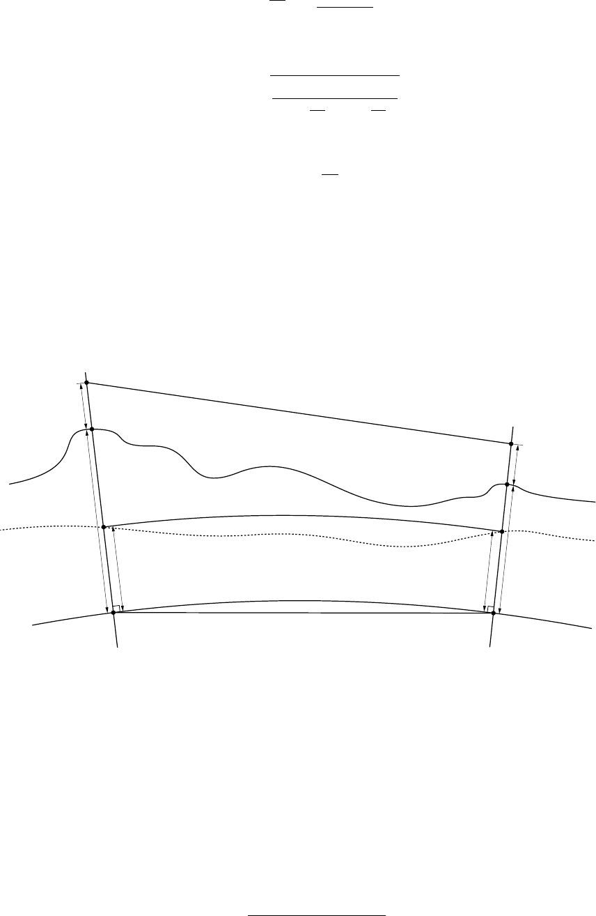
Here, ris the radius of curvature at MSL and is approximated by:
r=√ρν +N1+N2
2(7.9)
Then, the ellipsoid chord c12 is obtained from:
c12 =smc2
12 −(N2−N1)2
1 + N1
R1 + N2
R(7.10)
where Ris the average radius of curvature approximated from the two principle radii of curvature:
R+√ρν (7.11)
As explained in §7.2.2, the ellipsoid chord distance measurement c12 can be related to the coordinates
of p0
1and p0
2in the cartesian reference frame using equation 7.4.
For the sake of clarity, Figure 7.3 is provided to show the relationships between slope distance, MSL
arc distance, ellipsoid arc distance and ellipsoid chord distance measurements.
c12 Ellipsoid chord (C)
e12 Ellipsoid arc (E)
m12 Mean sea level arc (M)
s12 Slope distance (S)
c12
e12
m12
s12
p1
p′
1
p2
p′
2
hinst.
htarg.
h1h2
N1N2
ν1ν2
terrain
geoid
ellipsoid
Figure 7.3: Relationships between slope distance, MSL arc distance, ellipsoid arc distance and ellipsoid
chord distance measurements
7.2.4 Ellipsoid heights (R) and height differences
Figure 7.4 illustrates typical height measurements h1and h2observed above the ellipsoid at p1and
p2.
An ellipsoid height measurement h1is related to the coordinates of p1in the cartesian reference
frame by:
h1= (q1p1−ν1)
=qx2
1+y2
1+ (z1+qz1)2−ν1(7.12)
86
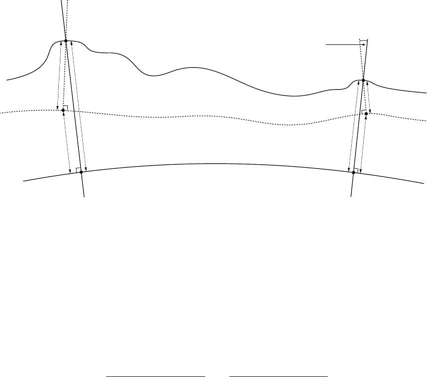
p′
1
p1
p2
p′
2
N1N2
H1
H2
h1
h2
ν1ν2
plumb–lineellipsoid normal
deflection of the vertical (ǫ)
terrain
geoid
ellipsoid
Figure 7.4: Heights and height differences
where q1is the intersection of the normal at p1with the polar axis of the ellipsoid (see Figure 7.1),
qz1is the zcoordinate element of the point q1evaluated from equation 4.6, and ν1is the radius of
curvature in the prime vertical at p1. Hence, q1p1is the total distance from q1to p1.
An ellipsoid height difference ∆h12 is related to the coordinates of p1and p2in the cartesian reference
frame by:
∆h12 =h2−h1
= (q2p2−ν2)−(q1p1−ν1)(7.13)
=qx2
2+y2
2+ (z2+qz2)2−qx2
1+y2
1+ (z1+qz1)2−ν2+ν1
Here, q2,qz2and ν2relate to p2as per p1in equation 7.12.
7.2.5 Orthometric heights (H) and height differences (L)
Figure 7.4 illustrates typical orthometric height measurements H1and H2observed above the geoid
at p1and p2. The development of observation equations for orthometric height measurements
is handled by reducing them to their ellipsoid counterparts first. With respect to Figure 7.4, an
orthometric height measurement H1is related to the corresponding ellipsoid height h1by:
h1=H1cos 1+N1(7.14)
where 1is the deflection in the direction of gravity from the ellipsoid normal (or deflection of the
vertical) at p1. However, since cos always very close to unity, the correction to h1is generally at
the 1/100 millimetre level and can be safely ignored. Accordingly, h1can be derived rigorously by:
h1=H1+N1(7.15)
Thus, h1can be related to the coordinates of p1using equation 7.12.
A height difference ∆H12 observed by spirit levelling can be reduced to an ellipsoidal difference by:
∆h12 = ∆H12 + (N2−N1)(7.16)
87

Note that the observation equations developed in this section assume the geoid to be coincident with
the orthometric height datum to which spirit levelling observations (i.e. H1,H2and ∆H12) refer.
In practice, however, orthometric height datums derived from spirit levelling observations1are rarely
coincident with the geoid, especially those developed over large regions. To cater for the separation
between an established orthometric height datum and the geoid, separations N1and N2in equations
7.15 and 7.16 should incorporate both a geoid–ellipsoid separation component and a geoid–ortho
separation component.
7.2.6 Cartesian coordinates and GNSS point clusters (Y)
For direct cartesian coordinate measurements, derived either by GNSS or resulting from a previously
adjusted network, the relationship between the measured coordinates xm,ymand zmand the
coordinates x1,y1and z1of p1is:
xm=x1
ym=y1(7.17)
zm=z1
If GNSS point cluster measurements are provided in terms of latitude φ, longitude λand orthometric
height H, the equivalent cartesian coordinates x,yand zare obtained by transformation using
equation 4.2, repeated here as:
x= (ν+h) cos φcos λ
y= (ν+h) cos φsin λ(7.18)
z=ν(1 −e2) + hsin φ
where hhas been derived from Husing equation 7.15. In these instances, the point cluster variance
matrix Vxg(supplied in units of radians2
φ,radians2
λand metres2
H) is propagated into the cartesian
reference frame using equation 4.28.
When multiple GNSS points are processed simultaneously, correlations will exist between all the points
in the cluster. Similarly, correlations will exist for coordinates resulting from network adjustment.
In such cases where a fully correlated variance matrix is available, DynaNet takes these correlations
into account within the a–priori variance matrix so as to rigorously propagate the quality of the
measurement set into the solution.
7.2.7 GNSS baselines (G) and GNSS baseline clusters (X)
A direct cartesian vector (or GNSS baseline) measurement [∆x12 ∆y12 ∆z12]is related to the
coordinates of p1and p2in the cartesian reference frame by:
∆x12 =x2−x1
∆y12 =y2−y1(7.19)
∆z12 =z2−z1
As with a cluster of simultaneously processed GNSS points, DynaNet takes into account the correlations
between simultaneously processed GNSS vectors when forming the a–priori variance matrix.
1. For example, the Australian Height Datum of 1971 (AHD71) and the North American Vertical Datum of 1988
(NAVD88).
88
7.2.8 2D position via geodetic latitude (P) and longitude (Q)
§7.2.6 provides a rigorous way for dealing with a full set of geographic coordinates (φ,λand H). In
practice however, it is often the case that the full set of geographical coordinates for a single point
is not available. This is due primarily to the way in which the horizontal and vertical components of
geodetic networks have been maintained as separate networks. On some occasions, only latitude and
longitude will be available for a single station within a horizontal network. On other occasions only
height will be available where the station forms part of the vertical network. For these circumstances,
the observation equations for the estimates of the horizontal and vertical components are developed
as follows.
If ∆x,∆yand ∆zrepresent small changes in the cartesian coordinates of a station due to small
changes ∆φ,∆λand ∆hin the geographical coordinates, which are represented as:
xc=
∆x
∆y
∆z
xg=
∆φ
∆λ
∆h
(7.20)
then:
xc=Txg(7.21)
xg=T−1xc(7.22)
where Tis the Jacobian matrix given by equation 4.29. In expanded form, equation 7.22 can be
written as:
xg=
t11 t12 t13
t21 t22 t23
t31 t32 t33
xc
Here, tij are the individual elements of T−1. In this form, observation equations can be formed for
any one of ∆φ,∆λor∆h. Thus, the observation equations for measured latitude φmand longitude
λmcoordinates and can be written as:
φm−φc=t11∆x+t12∆y+t13∆z(7.23)
λm−λc=t21∆x+t22∆y+t23∆z(7.24)
hm−hc=t31∆x+t32∆y+t33∆z(7.25)
where φc,λcand hcare the latitude, longitude and ellipsoid height coordinates computed from the
most recent estimates of x,yand z, and t11,t12, . . . , t33 are the differentiations corresponding to
x,yand z. If φmand λmhave been derived from a previous adjustment, then a full variance matrix
for xccan be developed from the variance matrix relating to φmand λm.
Incidentally, observations of this kind provide a convenient, yet rigorous way to constrain a network
with respect to the local reference frame in a single horizontal direction. By virtue of providing
φmor λmas a unique measurement, a network can be horizontally constrained in the nor e
dimension without the up dimension being influenced by the correlations that would normally be
introduced through equation 4.28. The same also applies to constraining a network in the up
dimension using equation 7.25, however it is computationally more efficient to do so using ellipsoid
height (R) measurements (see §7.2.4). This is due to the necessity for the inversion of Tbefore t31,
t32 and t33 can be obtained.
89
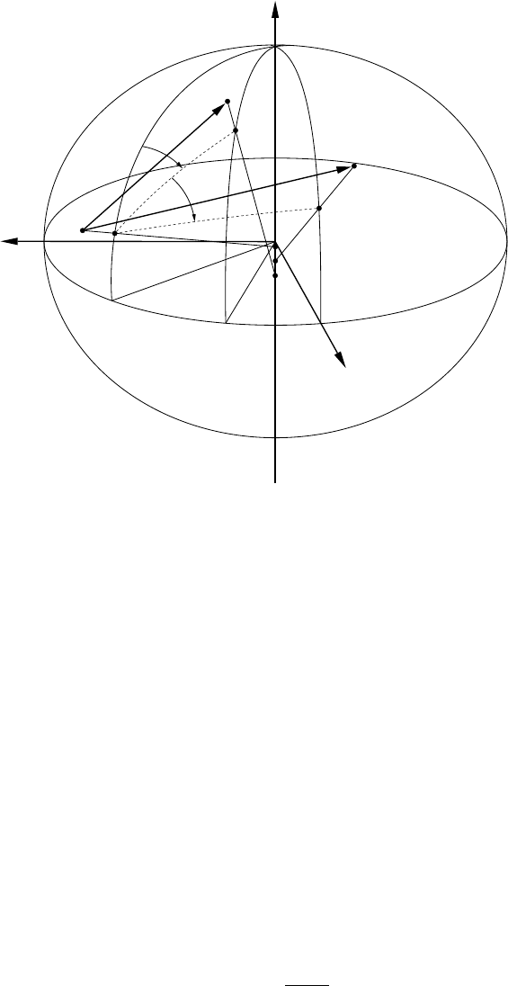
7.2.9 Geodetic azimuths and horizontal bearings (B)
Figure 7.5 shows a typical geodetic azimuth (or bearing corrected for the deflection of the vertical)
measurement θ12 in the local reference frame from p1to p2.
x
y
z
α123
θ12
q1
q2
q3
p1
p′
1
p2
p′
2
p3
p′
3
p12
p13
Figure 7.5: Bearings and horizontal angles
The azimuth between p1and p2is represented by vector p12. The elements of p12 are related to
the cartesian reference frame via equation 4.11:
p12 =
∆e12
∆n12
∆up12
=RT
1
∆x12
∆y12
∆z12
(7.26)
where R1is the rotation matrix defined by equation 4.9 evaluated at φ1, λ1. From equation 4.12,
this can be written in expanded form as:
∆e12
∆n12
∆up12
=
−sin λ(x2−x1) + cos λ(y2−y1)
−sin φcos λ(x2−x1)−sin φsin λ(y2−y1) + cos φ(z2−z1)
cos φcos λ(x2−x1) + cos φsin λ(y2−y1) + sin φ(z2−z1)
Hence, the azimuth θ12 between stations p1and p2is related to the vector elements with:
θ12 = arctan ∆e12
∆n12 (7.27)
Traditionally, skew normal corrections are applied to azimuth measurements as part of the process of
reducing such measurements from the terrain to the ellipsoid. The correction takes account of the
fact that the normal section through the instrument station and containing the target station does
90

not contain the normal through the target station. In DynaNet, skew normal corrections are not
required because the observation equation for an azimuth measurement (equation 7.27) is developed
in the cartesian reference frame using vector geometry rather than on the surface of the ellipsoid.
7.2.10 Horizontal angles (A)
Figure 7.5 shows a typical angle measurement αat p1in the local reference frame between two
directions (or bearings) from p1to p2and p3. The local vectors between p1and p2, and p1and p3
are given in short as p12 and p13 respectively. As per equation 7.26, the local vector elements of
p13 can be related to the cartesian reference frame via equation 4.11.
The horizontal angle α123 at station p1is related to the local vector elements with:
α123 = arctan ∆e13
∆n13 −arctan ∆e12
∆n12 (7.28)
Prior to evaluating the design matrix elements for horizontal angles, DynaNet corrects observed
angles for the deflection of the vertical. If mα123 is an observed angle, the influence of the deflection
of the vertical 1at p1is corrected by:
α123 =mα123 −1(7.29)
where 1is the deflection of the vertical at p1given by [Hofmann–Wellenhof and Moritz, 2006]:
1= (ξ1sin θ13 −η1cos θ13) cot ζ13 −(ξ1sin θ12 −η1cos θ12) cot ζ12 (7.30)
Here, φ1and λ1are the geodetic latitude and longitude at p1,ξ1is the deflection in the prime
meridian and η1is the deflection in the prime vertical evaluated at p1, and ζ12 and ζ13 are the zenith
angles (corrected for the deflection of the vertical) at p1to p2and p3respectively.
As will be gathered from equation 7.30, if the zenith angles ζ12 and ζ13 are equal, such as would be
the case for angles in the horizontal plane, 1will be negligible and can be safely ignored.
7.2.11 Horizontal direction sets (D)
Figure 7.6 shows a typical cluster of direction measurements θ12,θ13,θ14 and θ15 in the local reference
frame from p1to p2,p3,p4and p5.
The estimation of parameters from direction sets is handled by reducing the respective directions
to angles α123,α134 and α145. The relationship between a cluster of directions and corresponding
angles can be written as:
α=Ad (7.31)
which can be written in expanded form as:
α123
α134
α145
=
−1 1 0 0
0−110
0 0 −1 1
θ12
θ13
θ14
θ15
(7.32)
91

α123
α134
α145
θ12
θ13
θ14
θ15
p1
p2
p3
p4
p5
Figure 7.6: Cluster of horizontal directions
In this way, the observation equations which relate α123,α134 and α145 to the x,yand zelements
of p1,p2,p3,p4and p5have the same form as those developed for angles in §7.2.10.
As it is common practice to observe a cluster of directions at the same time, correlations will exist
between the derived angles α123,α134,α145. Accordingly, the a–priori variance matrix must take
these correlations into account. Given standard deviations σθ12 ,σθ13 ,σθ14 and σθ5for the cluster of
directions, the full variance matrix Vαfor the derived angles is obtained by propagation of variances:
Vα=AVθAT(7.33)
where Ais the functional model relating the derived angles to the observed directions given in
equation 7.32 and Vθis the (diagonal) variance matrix of the directions, given by:
Vθ=
σ2
θ12 0 0 0
0σ2
θ13 0 0
0 0 σ2
θ14 0
0 0 0 σ2
θ15
(7.34)
The zero terms in Vθreflect the fact that the observed directions are independent measurements.
Whilst the directions are uncorrelated, however, Vαwill be a non–diagonal matrix containing
non–zero off-diagonal terms which represent the correlations between adjacent angles.
7.2.12 Zenith distances (V)
Figure 7.7 shows a typical zenith distance measurement ζ12 from p1to p2. The vector between p1
and p2is represented by p12.
The elements of p12 are related to the cartesian reference frame via equation 7.35:
ζ12 = arctan p∆e2
12 + ∆n2
12
∆up12 !(7.35)
92

x
y
z
ζ12
q1
q2
p1
p′
1p2
p′
2
p12
Figure 7.7: Zenith distances
Since zenith distances are observed between instrument and target, the elements in 7.35 relate to
the vector formed between the instrument and target. These elements are derived by incorporating
instrument and target heights into the computation of ∆e,∆nand ∆up.
Prior to evaluating the design matrix elements for zenith distances, DynaNet corrects observed zenith
distances for the deflection of the vertical. If mζ12 is an observed zenith distance, the influence of
the deflection of the vertical is corrected by:
ζ12 =mζ12 −1(7.36)
where 1is the deflection of the vertical at p1given by [Hofmann–Wellenhof and Moritz, 2006]:
1=ξ1cos θ12 +η1sin θ12 (7.37)
Here, ξ1is the deflection in the prime meridian and η1is the deflection in the prime vertical evaluated
at p1, and θ12 is the azimuth (corrected for the deflection of the vertical) of the line from p1to p2.
7.2.13 Vertical angles (Z)
Figure 7.8 shows a typical vertical angle measurement ϑ12 in the local reference frame from p1to
p2. The vector between p1and p2is represented by p12, the elements of which are related to the
cartesian reference frame via equation 7.26.
The vertical angle ϑ12 between stations p1and p2is related to the vector elements with:
ϑ12 = arctan ∆up12
p∆e2
12 + ∆n2
12 !(7.38)
93
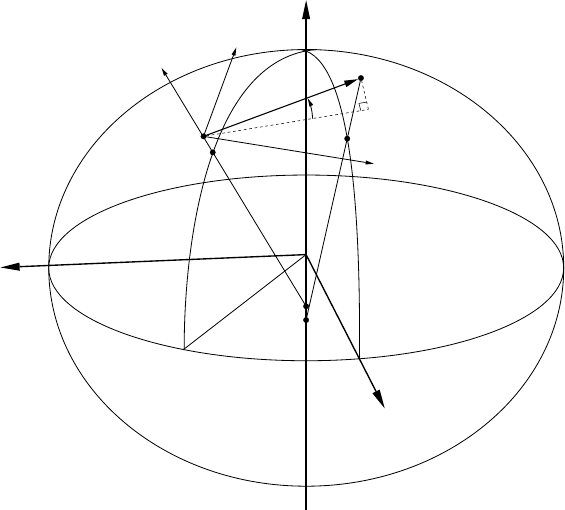
x
y
z
e
n
up
ϑ12
q1
q2
p1
p′
1
p2
p′
2
p12
Figure 7.8: Vertical angles
As with zenith distances, vertical angles are observed between instrument and target. Hence, the
elements in 7.38 relate to the vector formed between the instrument and target. These elements are
derived by incorporating instrument and target heights into the computation of ∆e,∆nand ∆up.
Prior to evaluating the design matrix elements for vertical angles, DynaNet corrects observed vertical
angles for the deflection of the vertical using equation 7.29, which is repeated here for vertical angles
as:
ϑ12 =mϑ12 −1(7.39)
where 1is the deflection of the vertical at p1given by equation 7.37.
7.2.14 Astronomic latitude (I) and longitude (J)
The treatment of astronomic latitude Φand longitude Λmeasurements at point pis handled by
reducing the values for Φand Λto their geodetic counterparts φand λ. Astronomic latitude and
longitude are related to geodetic latitude and longitude by [Hofmann–Wellenhof and Moritz, 2006]:
φ= Φ −ξ
λ= Λ −ηsec φ(7.40)
where ξis the deflection in the prime meridian and ηis the deflection in the prime vertical at p.
As explained in §7.2.8, the reduced φand λcan be related to the coordinates of pin the cartesian
reference frame using equations 7.23 and 7.24 respectively.
94

7.2.15 Astronomic (or Laplace) azimuth (K)
The treatment of astronomic azimuth measurement A12 from point p1to p2is handled by reducing
A12 to a geodetic azimuth θ12 prior to adjustment. Astronomic azimuths are related to geodetic
azimuths via:
θ12 =A12 −∆α1(7.41)
where ∆α1is the Laplace correction at p1given by [Hofmann–Wellenhof and Moritz, 2006]:
∆α1=ηtan φ1+ (ξ1sin θ12 −η1cos θ12) cot ζ12 (7.42)
Here, φ1and λ1are the geodetic latitude and longitude at p1,ξ1is the deflection in the prime
meridian and η1is the deflection in the prime vertical evaluated at p1, and ζ12 is the zenith angle
(corrected for the deflection of the vertical) at p1.
As explained in §7.2.9, θ12 can be related to the coordinates of p1and p2using equation 7.27.
7.3 Stochastic modelling and reporting
7.3.1 Probability distributions used in DynaNetfor testing
7.3.1.1 Normal distribution
Survey measurements, free of blunders and systematic error, are assumed to be random variables
which are Normally distributed about a mean of µwith a variance of σ2. It follows that the
errors resulting in random measurement variations can also be considered as random variables with
a mean of zero. Likewise, estimates which are based on those measurements are assumed to
possess the same random characteristics. For these reasons, DynaNet uses the Normal or Gaussian
distribution as the basic model for quantifying and testing the statistical behaviour of measurements,
measurement corrections and parameter estimates. The probability density function (PDF ) of the
Normal distribution is given by:
f(x) = 1
σx√2πexp −(x−µx)2
2σ2
x,−∞ <x<∞(7.43)
Equation 7.43 is used to estimate the probability of a measurement correction or estimated coordinate
coinciding with the mean or falling within a certain interval (e.g. µx−σx≤ˆx≤µx+σx). Figure
7.9 shows the typical bell shaped curve of the Normal PDF.
The probability that a measurement correction or estimated coordinate will fall within a certain
confidence interval µ−σand µ+σis given by:
P[µ−σ≤¯x≤µ+σ]≈Z+∞
−∞
f(x)dx ≈α(7.44)
where αis a value ranging from 0 to 1 commonly expressed as a percentage. The statistical inference
is that Pis the level of uncertainty that the estimated parameter will fall within the interval ±σabout
the mean µ. When expressing the level of probability as a specific multiple of ±σ,k(or coverage
factor) is used. For example, for k= 1,α= 0.683 (or 68.3%). Common confidence intervals based
upon multiples of σand their respective probabilities are given in Table 7.1.
95
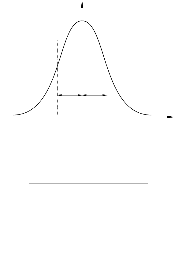
f(x)
x
+σx
−σx
µx
Figure 7.9: The Normal distribution
Table 7.1: Confidence intervals for ±1σto ±4σ.
k P [µ−kσ ≤x≤µ+kσ ]
1.00 68.3 %
1.96 95.0 %
2.00 95.4 %
2.58 99.0 %
3.00 99.73 %
3.29 99.9 %
4.00 99.994 %
By default, DynaNet adopts the 95% confidence interval for all statistical reporting and testing. See
§8.3.3 on page 116 for selecting an alternative confidence interval by which to quantify and test
measurements, their assumed variances and the parameters estimated from an adjustment. The use
of the Normal distribution to test the quality of supplied measurements will be discussed in §9.3.2.
7.3.1.2 Chi–square distribution
DynaNet uses the Chi–square (χ2) distribution to test the reliability of a least squares adjustment.
By definition, the quantity wobtained from the sum of the squares of a set of Normally distributed
random variables is a χ2random variable and is given by:
wχ2=vTv=x1x2··· xu
x1
x2
.
.
.
xu
(7.45)
96
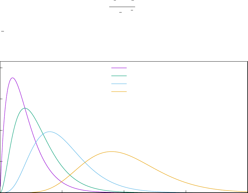
Aχ2random variable may also be obtained from the weighted sum of the squares:
wχ2=vTV−1v=x1x2··· xu
σ2
x1σx1x2··· σx1xn
σx2x1σ2
x2
.
.
.
.
.
....
σxnx1··· σ2
xu
−1
x1
x2
.
.
.
xu
(7.46)
where Vis the variance matrix which weights the respective contribution of each variable x1, x2, ..., xu
to wχ2. The PDF of χ2random variables is given by:
f(x) =xr
2−1e−x
2
Γr
22r
2
(7.47)
where Γ1
2ris a gamma function and ris the degrees of freedom in the model. The χ2PDFs for
random variables having 4, 6, 10 and 18 degrees of freedom respectively are shown in Figure 7.10.
0
Probability density f(x)
x
0.00s
0.05
0.10
0.15
0.20
10 20 30 40
r= 4
r= 6
r= 10
r= 20
Figure 7.10: Chi–square (χ2) distributions for 4, 6, 10 and 20 degrees of freedom
As shown in Figure 7.10, as rincreases to ∞, the χ2distribution will take the form of the Normal
distribution. The expected value of a χ2random variable wis defined by the degrees of freedom:
Ewχ2
r=r(7.48)
and its variance is given by:
σ2wχ2
r= 2r(7.49)
Therefore, as r→ ∞,µ=rand σ2= 2r. The probability of a χ2random variable being greater
than a particular critical value cis denoted as αand is given by:
α=Pwχ2
r> c=Z∞
c
f(x)dy (7.50)
97
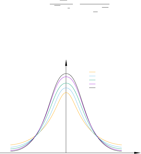
where αis the level of significance. The use of this distribution to test the quality of a least squares
adjustment will be explained in §9.3.1.
7.3.1.3 Student’s t distribution
When a network contains a large set of measurements having reliable estimates of precision, the
Normal distribution offers a reliable means for testing measurement quality. However, when a network
is comprised of a limited number of measurements, or the assumed measurement precisions are
doubtful, the level of confidence that can be gained from testing against the Normal distribution
decreases. To obtain a higher level of confidence from a solution in such circumstances, DynaNet
can optionally compute statistics according to the Student’s t (t) distribution which provides for
more stringent testing on the supplied measurements.
The PDF of the tdistribution is given by:
f(x) = Γr+1
2
√rπΓr
2·1
1 + x2
rr+1
2
(7.51)
where Γ (. . .)is the gamma function and ris the degrees of freedom. Four tPDFs having 2, 5, 10
and 50 degrees of freedom respectively are shown in Figure 7.11.
f(x)
x
µx
r= 2
r= 5
r= 10
r= 50
Normal distribution
Figure 7.11: Student’s t distributions for 2, 5, 10 and 50 degrees of freedom
As indicated by Figure 7.11, as rincreases, the tdistribution approaches the Normal distribution.
What is distinctly different however, is that for low values of r, the tdistribution has the characteristic
of causing variations from the mean to disperse quickly beyond the confidence intervals giving a lower
tendency to mark variations as outliers.
The Expected value of a trandom variable is:
E[wtr] = 0 (r > 1) (7.52)
98

and its variance is given by:
σ2(wtr) = r
r−2(r≥2) (7.53)
The probability that a measurement correction will fall within a certain confidence interval −σand
+σis given by:
α=P[wtr> c] = Z∞
c
f(x)dy (7.54)
The use of this distribution to analyse small networks with measurements having doubtful precisions
will be explained in §9.3.2.2.
7.3.2 Preparation of measurement precisions and variance matrices
Since a least squares adjustment of a geodetic network depends upon a reliable stochastic model,
it is imperative that realistic estimates of precision are assigned to the measurements. Whilst some
may argue that the use of least squares to estimate the precision of measurements is theoretically
legitimate, the practical limitation of this argument is that the true statistical behaviour of a
measurement and its contribution to the estimation of station coordinates will be biased.
In the absence of having a rigorous instrument calibration uncertainty2, sound geodetic practice
for achieving reliable measurement precisions involves estimating the standard deviation from a
large sample of measurements. Traditionally, the procedure employed by many geodetic agencies
was, for each instrument type, to (i) take a large sample of measurements under normal operating
conditions (and over different parts of the year); (ii) estimate the standard deviation from those
measurements; and (iii) scale and/or add additional terms to the estimated standard deviation
to account for external influences not discernible from the sample (such as errors which have a
systematic effect and need to be estimated from experience). The quantity derived from (ii) is
sometimes termed Type A uncertainty or internal precision, whereas the quantity obtained during
(iii) is termed Type B uncertainty or external precision. Using elementary statistical principles, the
precision for a measurement at (ii) may be obtained by:
σ2=1
(n−1)
n
X
1
(m1−m)2(7.55)
where nis the sample size, mirelates to each measurement in the sample and mis the theoretical
mean of the sample. Following the procedure outlined above, any measurement taken from an
instrument thereafter would be assigned the total (one–sigma) uncertainty estimate.
Nowadays however, this procedure is almost totally forgotten or regarded as being unimportant with
the availability of high precision equipment. Instead, the practice of taking an adjustment and scaling
the supplied variances by the estimated variance factor (c.f. §9.3.1.1) has become a favourable option
due to the relative ease and efficiency with which it can be computed. Whilst this may be true for
several modern digital surveying instruments, the same cannot be said for all instruments or GNSS
baselines and point clusters which have been derived from GNSS analysis.
Experience shows that GNSS variance matrices derived from GNSS analysis software are almost
always over optimistic, giving only an estimate of the internal precision. More often than not, the
uncertainties from all collatoral measurement sources (e.g. carrier phase measurement precision;
2. A rigorous uncertainty computed by instrument calibration and expanded to include uncertainties for all known
collatoral measurement sources and unmodelled systematic error.
99

receiver clock estimates; antenna phase centre models; satellite orbit and clock estimates) and
systematic models (e.g. effect of double–difference decorrelation; troposphere and ionosphere models;
ocean loading models) are not taken into account. From another perspective, variance matrices
derived from short occupation periods almost always fail to convey the imprecision in the resulting
measurements. Failing to take the uncertainties of all of these factors results in variance matrices
which are, on the whole, over–optimistic. Ultimately, this problem causes a number of down–stream
difficulties when attempting to combine measurements taken over the same stations under different
circumstances, different observation techniques, different equipment and over different times of the
year.
DynaNet cannot generate realistic matrices, but can be used to assist with attaining more reliable
estimates of measurement precision. Two such tools include GNSS variance matrix scaling (discussed
in the next section) and local testing via the Student’s t distribution (c.f. §7.3.1.3 and §9.3.2.2).
7.3.2.1 Scaling GNSS variance matrices
As described in §3.3.3, DynaNet offers a capacity for a–priori GNSS variance matrices to be scaled
prior to adjustment. The options for scaling a variance matrix include a total variance matrix scalar
and individual (or partial) variance matrix scalars. A total variance matrix scalar is in the form of a
single multiplier or variance factor. Partial matrix scalars are given in terms of east–west, north–south
and up scalars. Both forms of scaling are stored within the binary measurement file and applied upon
executing an adjustment. Hence, the original input files are not modified.
Variance matrix scaling using a single multiplier is often carried out once the quality of the solution
has been determined. Scaling a variance matrix by a single multiplier is performed automatically
prior to the least squares adjustment as:
Vscaled
m=s2Vm(7.56)
where Vmis the a–priori variance matrix and sis the variance matrix scalar.
In the case of partial matrix scaling, it may be desirable to, for example, scale a variance matrix by
a greater magnitude in the vertical axis than in the horizontal plane. To effect this outcome, three
operations are performed. Firstly, the a–priori variance matrix is propagated into the local reference
frame from either the cartesian or geographic reference frame such that the variance matrix terms
are in units of east, north and up. This is achieved by applying both equations 4.28 and 4.24 if the
input variance matrix is in the geographic reference frame or equation 4.24 alone if the input variance
matrix is in the cartesian reference frame.
Secondly, partial variance matrix scalars are applied via propagation of variances:
Vscaled
xl=SenuVxlST
enu (7.57)
where the functional model is expressed as:
Senu =
√seast 0 0
0√snorth 0
0 0 √sup
(7.58)
If Vxlis larger than a (3x3) matrix — that is, it applies to a GNSS cluster rather than a single
baseline or position — the same procedure as described above is used except the Senu matrix is
100
constructed so as to match the dimensions of the variance matrix that is to be scaled. The scaling
matrix will be block–diagonal, with each (3x3) sub-matrix on the leading diagonal being as shown
in equation 7.58 and all off–diagonal terms will be zero. If a single multiplier scalar is supplied with
partial matrix scalars, the partial scalar values are multiplied by the single multiplier first prior to
propagation of variances.
Thirdly, the scaled variance matrix is propagated into the cartesian reference frame using equation
4.8, such that it is in a ready state for the development of the normal equation matrix.
7.3.3 Expressing estimates of quality and reliability
As will be seen in §8.2, a by–product of least squares adjustment is an estimate of the precision
of the estimated parameters and adjusted measurements. To assist with analysing the quality and
reliability of a network, DynaNet performs additional computations to quantify and express the
following indicators:
•Quality of a least squares adjustment
•Quality of the estimated station coordinates (in one, two or three dimensions)
•Quality of supplied and adjusted measurements
•Reliability of the supplied measurements
•Reliability of the whole network
As discussed in the previous section, DynaNet uses the Chi–square statistic to quantify the quality
of the solution of a network. To express the quality of estimated station coordinates, standard
deviations directly obtained from the estimated variance matrix are used by default. Optionally,
station coordinate quality in the horizontal plane can be quantified in terms of the standard error
ellipse and a circular 95% confidence region, known as Positional Uncertainty. On reporting the
quality of measurements, residuals normalised (or standardised) to certain confidence intervals of the
unit Normal distribution and unit Student’s t distribution may be computed. Measurement reliability
and network reliability are expressed using quantities based on supplied and adjusted measurement
precisions. The formula used by DynaNet to compute these indicators are described in the following
sections.
7.3.3.1 Error ellipses
The error ellipse of constant probability is the locus of points (x, y)described by the intersection
between a horizontal plane at a height kabove the xy plane and the continuous PDF surface. Figure
7.12a illustrates the error ellipse at height k. Figure 7.12b shows the relevant parameters of the error
ellipse.
The size, shape and orientation (i.e. the complete spatial behaviour) of the ellipse is obtained when
the exponent term in the PDF of the Normal distribution is set to a specific value k2:
(m−µm)TV−1
m(m−µm) = k2(7.59)
The centre of the ellipse coincides with the most probable values for xand y, being µxand µy
respectively. The semi–major aand semi–minor baxes are defined by the square roots of the
101
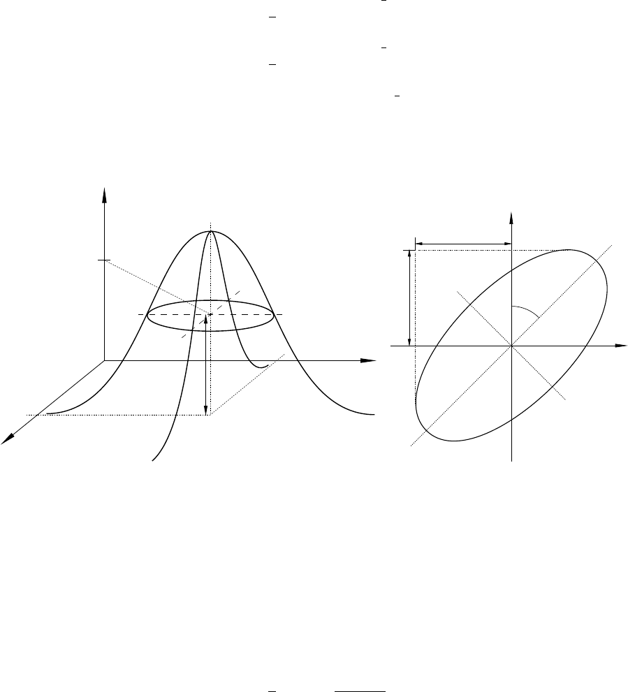
relevant eigenvalues of Vm[Mikhail, 1976]:
a=1
2σ2
x+σ2
y+z1
2
(7.60)
b=1
2σ2
x+σ2
y−z1
2
(7.61)
z=hσ2
x−σ2
y2+ 4σ2
xyi1
2
f(x, y)
f(x, y) = k
kx
y
µx
µy
(a) The intersection of a horizontal plane at height k
σx
σy
φ
µx
µy
a
b
(b) The error ellipse of constant probability
Figure 7.12: The error ellipse and its dependence on coverage factor k
The estimated variances σ2
xand σ2
yare dimensioned along the xand yaxes of the two–dimensional
reference frame. When the estimates of xand yare uncorrelated, the axes of the ellipse will be
coincident with the xand yaxes. When ρ6= 0, the ellipse axes are rotated relative to the xand y
axes by the angle φ. The orientation φof the error ellipse is a function of the estimated variances
and covariance of xand y, and is given by:
φ=1
2arctan 2σxy
σ2
x−σ2
y(7.62)
When the correlation between Normal random variables under the same probability distribution is
equal to zero, the orientation φis equal to zero.
At any time, users may opt to present these quantities in higher confidence intervals than the standard.
For example, if users wish to express standard deviations for one dimensional components (such as
height) at the 95% confidence level, the uncertainty value is computed by scaling the estimated (1
sigma) standard deviation by coverage factor k= 1.960. To express the standard two–dimensional
error ellipse at the 95% confidence level, the axes of the 95% error ellipse are obtained by scaling
the (1 sigma) axes by coverage factor k= 2.448. Similarly, the axes of the 95% three dimensional
error ellipsoid are obtained by scaling the (1 sigma) axes by coverage factor k= 2.796.
102

7.3.3.2 Positional uncertainty
According to the Guideline for the Adjustment and Evaluation of Survey Control [ICSM, 2014],
Positional Uncertainty (PU) is the uncertainty of the horizontal and/or vertical coordinates of a
survey control mark with respect to the defined datum and represents the combined uncertainty of
the existing datum realisation and the new control survey. PU is expressed in SI units at the 95%
confidence level.
For the horizontal circular confidence region, the 95% uncertainty value is calculated from the
standard (1 sigma) error ellipse and is expressed as a single quantity, being the radius of the circular
confidence region. The radius rof the circular confidence region is computed by:
r=a×K(7.63)
K=q0+q1C+q2C2+q3C3(7.64)
C=b
a(7.65)
where:
ais the semi–major axis of the standard error ellipse computed from equation 7.60
bis the semi–minor axis of the standard error ellipse computed from equation 7.61
q0= 1.960790
q1= 0.004071
q2= 0.114276
q3= 0.371625
Values for aand bare derived from the full a–posteriori variance matrix (or precision of the estimated
coordinates) obtained from least squares adjustment (discussed in §8.2 and evaluated by equation
8.16).
7.3.3.3 Measurement reliability and network reliability
Amongst the reliability factors which may be used to determine measurement reliability, a common
and relatively simple indicator is Pelzer’s measurement reliability criterion [Prószynski, 1994]. Pelzer’s
criterion is computed as:
τ=σ2
i
σ2
i−ˆσ2
i
(7.66)
where σ2
iis the a–priori measurement precision and ˆσ2
iis the a–posteriori measurement precision
arising from least squares adjustment. Based on this formula, τwill vary between unity and infinity.
The larger the value for τ, the poorer the reliability. For instance, as measurement redundancy
increases, ˆσ2
iwill decrease and cause τto tend towards unity.
Once the reliability criterion has been computed for each measurement via equation 7.66, the global
(or whole) network reliability can be computed as:
T2=P1
n(τ2−1) (7.67)
103
104
Chapter 8
Estimation of station parameters
8.1 Introduction
DynaNet estimates unknown station parameters using the technique of least squares via the traditional
observation equations method. The parameters which may be estimated include station coordinates
and their uncertainties, adjusted measurements and the precision of adjusted measurements. DynaNet
also computes a small range of statistics to aid in the validation of the supplied measurements and
their precisions, and in the analysis and verification of the estimated parameters. The program which
performs all adjustment operations is adjust.
The objectives of this chapter are twofold — firstly, to provide a basic overview of the least squares
algorithm employed by adjust and secondly, to describe how adjust may be configured to achieve
maximum computational efficiency and to produce the desired output. Chapter 9 explains how the
statistics computed by adjust can be used to validate the precision of the measurements and the
reliability of the least squares solution as a whole.
8.2 Overview of least squares estimation
According to the least squares observation equations method, the solution of unknown parameters
is achieved using linearised observation equations (or measurement functions) without any need for
condition or constraint equations. For each measurement, the observation equation is developed as:
m=f(x1, x2, . . . , xu)(8.1)
where x1, x2, . . . , xuare the parameters to be estimated and fis the function that expresses the
deterministic relationship between a measurement and the unknown parameters. The observation
equations presented in §7.2 have been developed in the form of equation 8.1. In matrix form, a
system of nlinearised observation equations can be related to a set of uunknown parameters by the
functional model:
m=Ax (8.2)
where:
xis a vector of unknown parameters (size u×1)
mis a vector of measurements (size n×1)
Ais the matrix of coefficients, or design matrix (size n×u)
105

When the number nof functionally independent measurements exceeds the number uof unknown
parameters, the redundancy r(or degrees of freedom) will be defined as:
r=n−u(8.3)
If n<u, the solution is indeterminate. If n=u, there is only one possible solution for the unknown
parameters. If n>u, an inconsistency in m=Ax will arise. This inconsistency arises from the
fact that some form of error will exist in a set of measurements which, in turn, leads to a range of
possible parameter values that could satisfy the system of observation equations.
To arrive at a unique set of values for the parameters, the least squares algorithm adjusts the system
of measurements mby a set of estimated corrections (or residuals)ˆ
vsuch that the functional model
is satisfied. In matrix form, the adjusted measurements ˆm are related to the original measurements
m, residuals ˆv and estimated parameters ˆx as follows:
ˆm =m−ˆ
v(8.4)
=Aˆx (8.5)
This allows equation 8.2 to be expressed as:
m−ˆv =Aˆx with E(m) = µ=Ax and E (ˆv) = 0(8.6)
The expectation E(ˆv) = 0 is based on the hypothesis that the measurements mare Normally
distributed random variables with an expected mean of µ=Ax, and that vrepresents random error
in m. The subject of dealing with larger than expected values for vwill be taken up in §9.3.2.
For the observation equations in the functional model which are non–linear with respect to the
parameters, the linear form of functions f1,f2,f3, . . . , fnin Aare approximated by the zero and
first–order terms of a Taylor series expansion:
m1−ˆv1=f1(x0
1, x0
2, ... , x0
u) + ∂f1
∂x1
∆x1+∂f1
∂x2
∆x2+··· +∂f1
∂xu
∆xu
m2−ˆv2=f2(x0
1, x0
2, ... , x0
u) + ∂f2
∂x1
∆x1+∂f2
∂x2
∆x2+··· +∂f2
∂xu
∆xu
.
.
.
mn−ˆvn=fn(x0
1, x0
2, ... , x0
u) + ∂fn
∂x1
∆x1+∂fn
∂x2
∆x2+··· +∂fn
∂xu
∆xu
(8.7)
where x0
1, x0
2, ... , x0
uare the starting values used to compute m. Hence, xi=x0
i+ ∆xu. Simplified
in matrix form, equation 8.7 is written as:
m−ˆv =m0+Aˆx (8.8)
where m0denotes the vector of measurements computed from the starting values and Ais the full
Jacobian (or design) matrix of partial derivatives of fwith respect to the parameters x1,x2, . . . , xu.
Since the linearised functional model is approximated using a first order Taylor series, the solution
will require iteration. In steps, the vector of reduced measurements mris computed with an initial
approximate for ˆ
m, denoted by ˆ
m0:
mr=m−ˆ
m0(8.9)
106

and then the most probable values are evaluated by:
ˆm =mr+Aˆx (8.10)
The solution is iterated (i.e. ˆ
mis substituted for ˆ
m0) until ∆x1,∆x0
2, ... , ∆x0
uin equation 8.7
converge to zero (i.e. when mr= 0). Assuming that the measurements are Normally distributed,
the least squares algorithm estimates values for ˆv1,ˆv2, ... , ˆvnso that the values for ˆx will have a
maximum probability under the Normal distribution. This is achieved by minimising the exponent of
the normal distribution PDF (c.f. equation 7.43) for m:
w= (m−Ax)TV−1
m(m−Ax)(8.11)
where Vmis a symmetric positive definite variance matrix (size n×n) representing the stochastic
behaviour of the measurements , and wis the weighted sum of the squares of the corrections. After
substituting m−Ax with v(from equation 8.6), wcan be rewritten in the familiar form:
w=vTV−1
mv(8.12)
The minimum value for wis achieved by minimising equation 8.11 as:
∂w
∂x= 0 (8.13)
which after expansion and differentiation of equation 8.11 leads to the least squares normal equations:
ATV−1
mAx=ATV−1
mm(8.14)
Solving for xenables the least squares solution of the unknown parameters and corresponding variance
matrix to be written as:
ˆ
x=ATV−1
mA−1ATV−1
mm(8.15)
Vˆ
x=ATV−1
mA−1(8.16)
Here, distinction is made between xand ˆ
xin that the latter represents the estimates of the former —
the most probable values according to the functional model Aand stochastic model Vm. Explanation
of Vˆx is left until Chapter 9. If the functional model is non–linear, equation 8.15 will need to be
iterated to arrive at the final coordinate and precision estimates.
107

8.3 Adjusting a network
Once import has created the binary station (.bst) and measurement (.bms) files, and the associated
station (.asl) and measurement (.aml) lists from the input station and measurement files, the
network is ready for adjustment. This assumes that all necessary reference frame transformations
(c.f. Chapter 4) and geoid file interpolations (c.f. Chapter 5) have been undertaken. For phased
adjustments, the only additional precondition apart from running import is that segment has been
run to create a segmentation file (c.f. Chapter 6).
With adjust, users may undertake adjustments in either simultaneous mode or phased adjustment
mode. By default, adjust will perform network adjustments in simultaneous mode. In phased
adjustment mode, several options are provided so as to maximise computational efficiency based upon
the computer’s available processor, physical memory and hard disk resources. For both modes, several
options are provided to configure the adjustment behaviour and output. If there is a requirement
to re–print the results from a previous adjustment using different configuration options, adjust may
be executed in report results mode. In this mode, no adjustment is undertaken but rather, the
output files are regenerated. The complete command line reference for adjust is given in §A.6. If no
program options are provided upon program execution, the command line reference will be displayed.
If a DynaNet Project File (c.f. Chapter 2) is to be used, type dynanet on the command line, then
--project-file (or its shortcut -p) followed by the full path for the project file, and then the option
to invoke adjust:
dynanet -p uni_sqr.dnaproj --adjust
No other options are required, as adjust will be invoked using the options and arguments contained
in the project file uni_sqr.dnaproj.
8.3.1 Simultaneous mode
As described in previous sections, simultaneous adjustment mode is ideally suited to smaller–sized
networks. To adjust a network in simultaneous mode using all default settings, type adjust on the
command line followed by the network name:
adjust uni_sqr
Upon running this command, adjust will report to the screen a number of items relevant to the
project (e.g. name, location of input and output files); user–specified options; the progress of network
adjustment including adjustment iterations; brief statistical summary of the adjustment; and final
exit status (i.e. success or failure). Using the uni_sqr project, Figure 8.1 shows the information
reported to the screen upon program execution. By and large, the screen output shown in Figure
8.1 will be similar to the output for all other adjustment modes.
Upon invoking adjust, a variety of matrices will be formed such that the station parameter estimates
(c.f. 8.15) and uncertainties (c.f. equation 8.16) can be solved. This stage of the adjustment process
is reported to the screen as “+ Preparing for adjustment... ” and can take anywhere from
milliseconds to several minutes depending on the size of the network, the number of computations
that need to be undertaken to form the normals matrix, and the amount of data that needs to be
held in physical memory. If there is insufficient memory to load the network in memory, DynaNet
will report an error, in which case, users may need to revert to the use of phased adjustment mode
108

in either single-thread mode or staged adjustment mode (c.f. §8.3.2).
+ Options:
Network name: uni_sqr
Input folder: .
Output folder: .
Associated station file: ./uni_sqr.asl
Associated measurement file: ./uni_sqr.aml
Binary station file: ./uni_sqr.bst
Binary measurement file: ./uni_sqr.bms
Adjustment output file: ./uni_sqr.simult.adj
Coordinate output file: ./uni_sqr.simult.xyz
Reference frame: GDA94
Epoch: 01.01.1994
Geoid model: ./ausgeoid09.gsb
+ Simultaneous adjustment mode
+ Preparing for adjustment... done.
+ Adjusting network...
Iteration 1, max station corr: -0.5850 e
Iteration 2, max station corr: -0.0023 e
Iteration 3, max station corr: 0.0000 n
+ Done.
+ Solution: converged after 3 iterations.
+ Network adjustment took 0.06s.
+ Generating statistics... done.
+ Adjustment results:
+-------------------------------------------------------------------------------
Number of unknown parameters 440
Number of measurements 1182 (72 potential outliers)
Degrees of freedom 742
Chi squared 627.01
Rigorous sigma zero 0.845
Global (Pelzer) Reliability 4.008 (excludes non redundant measurements)
Chi-Square test (95.0%) 0.901 < 0.845 < 1.104 *** WARNING ***
+--------------------------------------------------------------------------------
+ Serialising adjustment matrices... done.
+ Printing adjusted station coordinates... done.
+ Updating binary station and measurment files... done.
+ Open uni_sqr.simult.adj to view the adjustment details.
Figure 8.1: adjust progress reporting
Following the preparation of adjustment matrices, adjust will commence adjusting the network,
iterating as many times as necessary until the iteration threshold (or convergence criteria) is met or
the maximum number of iterations has been reached. If either of these conditions fail, adjust will
report to the screen an error message describing the reason for failure.
The time each iteration will take will vary according to the network size and the computer’s
computational power, including its processor (type, CPU frequency and architecture), physical
memory and operating system memory model (32–bit or 64–bit). For these reasons, it is not possible
to provide an estimate of computation progress or time to completion. Only experience with running
several network adjustments will give the user a sense for how long an adjustment iteration may take.
Upon the completion of each iteration, the largest difference between the previously estimated station
coordinates and the newly estimated station coordinates (denoted as “max station corr”) will be
displayed. These values will be particularly helpful in understanding the agreement between the
starting estimates and the measurement system, and may be used to help diagnose problematic
adjustments. For instance, a well configured and appropriately weighted measurement system will
result in a rapid convergence (e.g. three or less iterations), despite the quality of the initial station
109
coordinate estimates. However, a system with poorly configured station constraints, measurement
blunders, insufficient measurements, inappropriate measurement uncertainties and/or wrongly named
stations may cause unexpected convergence rates (i.e. very small or large, erratic changes to the
maximum station correction values) or a failure to converge at all.
When the largest correction becomes less than the iteration threshold, adjust will deem the solution
to have converged. Once the solution has converged, adjust will compute a range of values and
statistics for the output files. This task may take anywhere from milliseconds to several minutes
depending on the size of the network and the user–specified options for configuring the output of
adjusted measurements and statistics (c.f. §8.3.4).
Provided there are no significant errors, the next block of information will be a summary of statistics.
Referring to Figure 8.1, the reported statistics include:
Number of unknown parameters In DynaNet, every station is treated by default as having three
unknown parameters (i.e. x,y,z). Any one or more cardinals may be fixed by the use of
station constraints. The number of unknown parameters therefore corresponds to the number
(u) of parameters to be estimated, excluding those station coordinates which have been held
fixed in the station file. See §3.2.3 for more information on the concept of station constraints
and how they are interpreted by DynaNet.
Number of measurements This value reports the number (n) of measurement components. All
measurements except GNSS measurement types are treated as having a single measurement
component. Each GNSS baseline and GNSS point is regarded as having three measurement
components (i.e. x,y,z). The number of measurement components in a cluster of GNSS
baselines or GNSS points will be equal to three times the number of GNSS baselines or points in
the cluster. If a measurement correction exceeds the specified confidence interval and thereby
fails the local test, the measurement will be flagged as a potential outlier (c.f. Figure 8.1 where
72 measurements have been flagged as potential outliers). In such cases, the adjustment output
file should be inspected to identify whether the potential outlier is a genuine failure and to
rectify the cause of that failure. Details on the local test are given in §9.3.2.
Degrees of freedom This value (r) is calculated directly from uand n(c.f. equation 8.3), and
is the parameter against which the global rigorous sigma zero value is tested. As described
earlier, uexcludes all fixed station coordinates.
Chi squared This quantity (w) is calculated directly from the supplied measurement precisions and
the measurement residuals of the least squares adjustment (c.f. equation 8.12). With a
well–configured measurement system, wwill approach r.
Rigorous sigma zero This value (ˆσ2) is derived from wand r(c.f. equation 9.7) and is used to
test the least squares solution as a whole (c.f. §9.3.1).
Global (Pelzer) Reliability This quantity (T2) is calculated using equation 7.67 according to Pelzer’s
measurement reliability criterion. It is intended to give an assessment of the reliability of the
measurement system as a whole.
Chi–Square test (95.0%) This statement reports the result of the global test of ˆσ2using the
default or–user specified confidence interval (c.f. §8.3.3, page 116). This test will be explained
in §9.3.1. Note that it is possible for a least squares adjustment to have passed this global test
and at the same time, one of the measurements in the set to have failed the local test. For
this reason, the adjustment output file should be inspected in conjunction with this statistic.
Users should become acquainted with the statistical indicators presented in this summary and how
they are calculated in order to make an informed decision about the quality of the solution and any
measurements flagged as outliers.
110
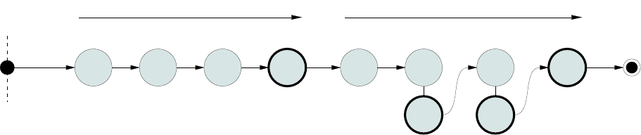
The final statements reported in the screen output include references to various binary and text
files that are created or updated with the latest adjustment results. The primary output file which
contains the adjustment results is the adjustment output file. This file will be named using the
convention <network-name>.<adjustment-mode>.adj (e.g. uni_sqr.simult.adj). The file content,
format and structure of the adjustment output file is described in Appendix C.6. Hints on interpreting
the adjusted measurements and associated statistics contained in this file will be given in Chapter 9.
By default, the adjustment output file contains the global adjustment statistics (as shown in the
screen output) and estimated station coordinates. Further information on configuring the information
printed to this file is given in §8.3.4.
8.3.2 Phased adjustment mode
When adjusting large adjustments in phased adjustment mode, the total network adjustment task is
broken up into several smaller adjustments which are undertaken in an ordered sequence. The only
pre–requisite for phased adjustment mode is that the network has been segmented (c.f. Chapter 6).
There are three primary ways in which phased adjustment mode can be executed — single–thread
mode, multi–thread mode and Block–1 only mode. In addition, when running an adjustment in
single–thread mode, staged adjustment mode may be used. Brief mention is made of these modes
to help determine which mode is appropriate for the network and the computer on which it is being
adjusted.
The processing of single–threaded phased adjustments is illustrated in Figure 8.2. In single–thread
mode, all adjustment operations are executed in a sequential (or procedural) fashion on one thread
managed by a single core. If a computer’s CPU has two cores, only 50% of the computer’s processing
power will be utilised. Similarly, if the CPU has four cores, only 25% will be used.
Block 1Block 1 Block 2Block 2 Block 3Block 3 Block 4 Block 4
Thread 1 FFFF RRRR
CC
Rigorous
Rigorous Rigorous
Rigorous
Forward pass Reverse pass
Figure 8.2: Single–thread mode
Information pertaining to the entire network is managed in physical memory (RAM). If there is
insufficient RAM to retain the entire network in memory, staged adjustment mode should be used.
In this mode, DynaNet uses memory mapping — a technique which treats the hard disk as if it
were physical memory. Due to the I/O operations that must be performed to exchange information
between the hard disk and memory, this mode may take longer than single–thread mode, however it
permits the adjustment of extremely large networks on computers with small amounts of RAM.
The processing of multi–threaded phased adjustments is illustrated in Figure 8.3. In this mode,
the forward and reverse pass adjustments are executed on two separate threads concurrently. If a
computer’s CPU has at least two cores, these threads will be executed in parallel by the operating
system on two cores. When a block has been adjusted by both forward and reverse adjustments, a
new thread will be invoked to undertake the combination adjustment of that block. This new thread
will remain active for as long as it takes to adjust that block.
111
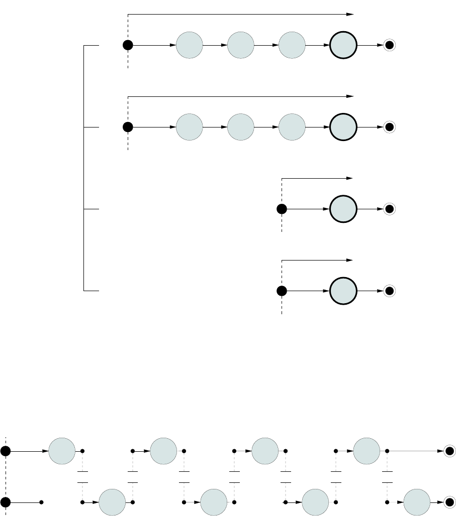
If a computer has at least four cores, all concurrent threads will be executed in parallel which will
achieve the fastest adjustment time. Hence, running adjustments in multi–thread mode on a quad
core CPU will result in 100% utilisation of the computer’s processing capability. With hyper–threading
technology (now almost a standard commodity in all modern computers), extreme performance gains
can be achieved in this mode.
Block 1
Block 1
Block 2
Block 2
Block 2
Block 3
Block 3
Block 3 Block 4
Block 4
Thread 1
Thread 2
Thread 3
Thread 4
Core 1
Core 2
Core 3
Core 4
Quad core CPU
FFFF
RRRR
C
C
Rigorous
Rigorous
Rigorous
Rigorous
Forward pass
Reverse pass
Combination pass
Combination pass
Figure 8.3: Multi–thread mode on four cores
If the number of concurrent threads exceeds the number of cores available on a CPU, the processing
of individual tasks by those threads will be interleaved (or time–sliced) on the available core(s) such
that all tasks appear to advance in parallel. The concept of interleaving between two threads on a
single core is shown in Figure 8.4.
Thread 1
Thread 2
Context switchContext switch
Context switchContext switch
Context switch
Context switchContext switch
F
F
FF
R
R
RR
C
Figure 8.4: Thread switching on a single core
When interleaving from one task to the other, the CPU must perform a context switch, which involves
storing and recalling the state of each process. Depending on the size of the blocks, these operations
can be computationally intensive. Therefore, running multi–thread adjustments on a single core CPU
may take longer than the time required for a simultaneous or single–threaded phased adjustment due
112
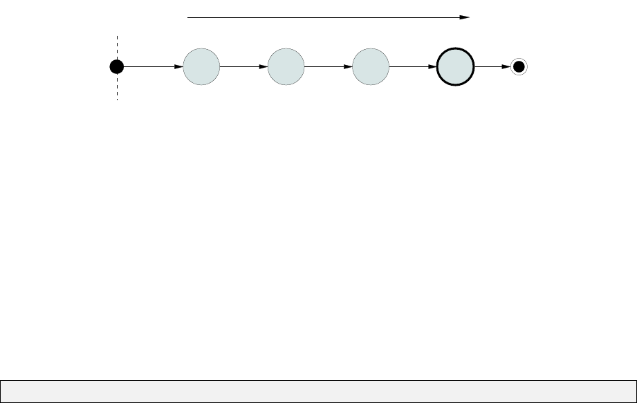
to the additional time that is needed to switch from the adjustment of one block to another. Note
that since the adjustment of a single block involves numerous sub–tasks, context switching can occur
at any stage of the adjustment.
The concept of a Block–1 only phased adjustment is illustrated in Figure 8.5. In this case, all blocks
are adjusted once in a sequential fashion on a single thread. Since rigorous coordinates are required
for the first block only, forward and combination passes are not required. Therefore, only block 1
will contain rigorous coordinates as it will be the only block that will take contribution from all other
blocks in the network.
Block 1
Block 2
Block 3
Block 4
Thread 1 RRRR
Rigorous
Reverse pass
Figure 8.5: Block–1 only mode
Block–1 only phased adjustment mode is by far the most efficient if only a subset of the station
coordinate estimates (i.e. those which have been selected to appear in the first block) are required.
However, care must be taken to ensure that the most rigorous coordinates are available for all stations
in the network prior to running an adjustment. The reason for this is because only a single reverse
pass is performed and no further iterations will be undertaken if the solution has not converged.
8.3.2.1 Single–thread mode
To adjust a network using phased adjustment in single–thread mode, type adjust on the command
line followed by the network name, and then --phased-adjustment:
adjust uni_sqr --phased-adjustment
Figure 8.6 shows the information reported to the screen pertinent to executing an adjustment in
single–thread mode (omitting information common to the output from a simultaneous adjustment).
As shown in the screen output, an adjustment output file named uni_sqr.phased.adj will be created,
the contents of which will be very similar to the simultaneous adjustment output.
The main difference in the behaviour of this mode over that of simultaneous mode is that the progress
(“+ Adjusting network...”) will indicate which block is being adjusted and thereby, provide a more
realistic indicator of the rate at which the adjustment is progressing. Since each block size will vary
according to the behaviour of the network segmentation, it is not possible to give an estimate of
time to completion.
113

+ Options:
...
Adjustment output file: ./uni_sqr.phased.adj
Coordinate output file: ./uni_sqr.phased.xyz
...
+ Rigorous sequential phased adjustment mode
+ Preparing for a 5 block adjustment... done.
+ Adjusting network...
...
+ Done.
+ Successfully adjusted 5 blocks.
...
+ Open uni_sqr.phased.adj to view the adjustment details.
Figure 8.6: Progress reporting using single–thread adjustment mode
8.3.2.2 Multi–thread mode
To adjust a network using phased adjustment in multi–thread mode, type adjust on the command
line followed by the network name, and then --multi-thread:
adjust uni_sqr --multi-thread
Figure 8.7 shows the information reported to the screen pertinent to executing an adjustment in
multi–thread mode.
+ Options:
...
Adjustment output file: ./uni_sqr.phased-mt.adj
Coordinate output file: ./uni_sqr.phased-mt.xyz
...
+ Rigorous sequential phased adjustment mode
+ Optimised for concurrent processing via multi-threading.
+ The active CPU supports the execution of 8 concurrent threads.
+ Preparing for a 5 block adjustment... done.
+ Adjusting network...
...
+ Done.
+ Successfully adjusted 5 blocks.
...
+ Open uni_sqr.phased-mt.adj to view the adjustment details.
Figure 8.7: Progress reporting using multi–thread adjustment mode
When reporting the progress of the adjustment, information on iterations following (“+ Adjusting
network...”) will indicate which block is being adjusted by the combination pass, not the forward
and reverse passes. Since a combination pass on a block is invoked only once both forward and
reverse passes have completed their adjustments of that block, the order of blocks adjusted by the
combination passes will appear to be random. The exact order is subject to the order in which
114

forward and reverse adjustments are completed and the way in which the operating system marshals
a list of threads waiting in a queue.
8.3.2.3 Block–1 only mode
To adjust a network using phased adjustment in Block–1 only mode, type adjust on the command
line followed by the network name, and then --block1-phased:
adjust uni_sqr --block1-phased
Figure 8.8 shows the information reported to the screen pertinent to executing an adjustment in
Block–1 only mode. As described earlier, this mode is ideally suited to the situation where final
coordinate estimates for all stations in the network have already been produced, and there is a
requirement for the full variance matrix for a subset of stations in the network.
+ Options:
...
Adjustment output file: ./uni_sqr.phased-block1.adj
Coordinate output file: ./uni_sqr.phased-block1.xyz
...
+ Sequential phased adjustment resulting in rigorous estimates for Block 1 only
+ Preparing for a 5 block adjustment... done.
...
+ Solution: estimates solved for Block 1 only.
- Warning: Depending on the quality of the apriori station estimates, further
iterations may be needed. --block1-phased mode should only be used once
rigorous estimates have been produced for the entire network.
...
+ Open uni_sqr.phased-block1.adj to view the adjustment details.
Figure 8.8: Progress reporting using Block–1 only adjustment mode
8.3.2.4 Staged adjustment mode
In staged adjustment mode, adjust relies upon the hard disk, rather than RAM, to store the
adjustment matrices and estimated results for the entire network. Only the block being adjusted is
loaded into memory. To this end, it is necessary to inform adjust whether to create a set of binary
matrix files or to read from existing matrix files created from a previous adjustment. To adjust
a network for the first time using phased adjustment in staged mode whereby new binary matrix
files must be created, type adjust on the command line followed by the network name, and then
--staged-adjustment and --create-stage-files:
adjust uni_sqr --staged --create-stage-files
Upon running the command above, adjust will serialise all matrix and vector information required
to execute an adjustment in files with a .mtx extension. All the necessary information to re–run the
adjustment will be contained within the .mtx files. If a repeat adjustment is to be executed using
115

the information serialised from a previous staged adjustment, the option --create-stage-files is
not required. For example, the following command:
adjust uni_sqr --staged
will cause adjust to look for and open files named uni_sqr-*.mtx. Any failure associated with
opening or reading these files will cause adjust to terminate prematurely.
8.3.2.5 Report results mode
To simply regenerate the results of a previous adjustment, type adjust on the command line followed
by the network name, and then --report-results and the mode in which the previous adjustment
was run (e.g. --phased-adjustment). If the mode is not supplied, adjust will assume simultaneous
by default:
adjust uni_sqr --report-results
During this mode, the results can be re–produced at any time and using different output options.
Refer to §8.3.4 for details on configuring the output of the results of an adjustment. The critical
thing to remember when running report results mode is to supply the adjustment mode in which the
last adjustment was run.
8.3.3 Adjustment configuration options
adjust permits the configuration of certain parameters which effect the behaviour of an adjustment
independent of the adjustment mode. These include the confidence interval for testing the global
statistic and measurement corrections; the least squares convergence threshold to test whether further
iterations are required; the maximum number of iterations; additional station constraints; the level of
precision by which fixed and free stations are constrained; and an option to scale the normal matrix
prior to computing its inverse. The full command line reference for configuring adjustment behaviour
is given in Table A.23.
Confidence interval
Confidence intervals represent the range of probability within which a parameter will equal the true
value (c.f. §7.3.1 and §7.3.3.1). Based upon the assumption that a set of measurements will be
Normally distributed random variables, and that the corrections represent the random error in those
measurements (c.f. equation 8.6), assessments of the quality of a measurement set can be undertaken
using the Normal distribution. The criteria by which a measurement is regarded as having passed
or failed, is whether or not the measurement correction is within a probabilistic confidence interval.
Hence, it is imperative that an appropriate confidence interval be chosen if assertions are to be made
about the reliability of measurements and estimated quantities. The theoretical basis and application
of statistical testing of measurements is given in more detail in Chapter 9.
116

The default interval used by adjust for all testing is the 95% confidence interval. To change the
confidence interval to another value, such as 68.3% (or one sigma), pass the option --conf-interval
followed by the interval as a percentage:
adjust uni_sqr --conf-interval 68.3
Note that reducing the confidence interval implies a more stringent testing criteria is required. It
means decreasing the probability that measurements will fall within an acceptable range of uncertainty
and thereby, less probability that measurements will be deemed reliable. For example, testing the
uni_sqr network with a 68.3% confidence interval leads to the identification of 220 potential outliers,
whereas a 99.73% (or three sigma) identifies only 22 potential outliers. As shown from these two
intervals, the number of outliers that exist in an adjustment largely depends on how stringent a
probability test is imposed.
Iteration threshold and maximum number of iterations
Since the functional model adopted for the least squares solution is a linearised model (approximated
using a first order Taylor series), a solution will often require iteration until the parameter estimates
converge to the most probable values. Or, more accurately, until the least squares normal equations
are satisfied (c.f. equation 8.14). Depending on the quality of the initial station coordinates and the
quality of the measurements (both as to their accuracy and their stated precision), the solution may
require several iterations before equality is reached. One way of limiting excessive or unnecessary
iterations from being undertaken is to impose a threshold by which the normal equations are deemed
to have been satisfied.
The default iteration threshold used by adjust is 0.5mm. This means that the solution will keep
iterating while corrections to the station coordinates exceed this amount, and until the maximum
number of iterations has been reached. To change the convergence threshold to another value, such
as 1mm, pass the option --iteration-threshold followed by the value in metes:
adjust uni_sqr --iteration-threshold 0.001
Care should be exercised when increasing this amount as too large a value may mean that incorrect
(or less than acceptable) estimates will be derived.
The default maximum number of iterations adjust will undertake before terminating is 10. Under
normal circumstances where the measurements are of good quality and the starting coordinates
are close to their most probable values, this number will be more than adequate. However, in
circumstances where a system is defective and troubleshooting is required, this iteration count can
be set to, for example, 1 (one) to force an early termination. To change the maximum iteration
limit, pass to adjust the option --max-iterations followed by the desired value:
adjust uni_sqr --max-iterations 3
Additional station constraints and default constraint values
adjust affords a capacity to introduce station constraints to an adjustment in addition to those
which were obtained from the input station file(s). If it is decided that a station constraint should
be added, modified or removed, users can specify the station and how it is to be constrained via the
117

option --constraints. Using station 5000 as an example, the following call to adjust demonstrates
how to constrain this station in the horizontal axis:
adjust uni_sqr --constraints 302513640,CCF
This option replicates the functionality to apply station constraints supplied in the input station file
(c.f. §3.2.3) . Therefore, the order of the three characters in the user–supplied constraint string
corresponds to the cardinals of the supplied station coordinate. Since station 5000 was supplied in
the form of UTM coordinates, the constraints CCF correspond to Easting, Northing and height up
respectively.
Whilst this method of imposing constraints is not the recommended means for constraining a network
to a datum, it does provide a useful mechanism for the detection of outliers and analysis of problematic
adjustments.
By default, values of 10.0 m and 0.001 mm are adopted for free (‘F’) and constrained (‘C’)
station constraints respectively. To alter these values, pass the options --free-stn-sd and/or
--fixed-stn-sd to adjust:
adjust uni_sqr --free-stn-sd 5.0 --fixed-stn-sd 0.003
Scaling the normal matrix to unity
At times, computing the inverse of the normal matrix will be problematic if there is a very large
numerical difference across the normal matrix elements, or if the matrix tends towards singularity
due to very small quantities. This difference can arise from large variations in measurement precisions
and/or linearisations which generate very large and very small quantities. These characteristics can
cause numerical instability and/or loss of precision at the time of computing the inverse of the
normal matrix. A method of overcoming such problems is to scale the normal matrix to unity prior
to computing the inverse. To cause the normal matrix to be scaled to unity prior to computing the
inverse, pass the option --scale-normals-to-unity to adjust:
adjust uni_sqr --scale-normals-to-unity
Note that this action is only to avoid instability in inverting the various variance matrices. The effect
is reversed after matrix inversion so that the computed values are as if no scaling has taken place.
This option will most likely only be required for cases where there is a very large variation in the
precisions supplied for the set of measurements.
8.3.4 Output configuration options
By default, the adjustment output file (*.adj) contains basic adjustment statistics and adjusted
coordinates using all default settings. Optionally, users can activate and configure the output and
format of results that adjust generates from an adjustment. The full command line reference for
configuring the adjustment output is given in Table A.25.
118

Measurements to station summary
To output a table of measurements connected to each station, add --output-msr-to-stn to the
command line arguments for adjust:
adjust uni_sqr --output-msr-to-stn
This command will produce a table commencing with the title block Measurements to Station that
shows the frequency of each measurement type and the total number of measurements associated
with each station. The table will be sorted row–wise by the station name, and column–wise by the
measurement type (c.f. Table 3.2). Appendix C.6.2 mentions the output of the measurements to
stations table to the adjustment output file. For details on the content, structure and format of the
table, refer to Table C.1 in Appendix C.3. Generating this table can be quite useful when attempting
to identify measurement conflicts, or the presence of unnecessary measurements, measurement
constraints or station constraints.
Printing and configuring adjusted measurements
To output a table showing the adjusted measurements and their associated statistics, add the option
--output-adj-msr to the command line arguments. The table will commence with the title block
Adjusted Measurements and will contain several columns containing information derived from the
adjustment. Appendix C.6.3 provides further details on the content, structure and format of the
adjusted measurements table.
Upon supplying this command, several options are available for configuring the adjusted measurement
table. These include changing the units (Cartesian, local, polar) in which adjusted GNSS baselines
are printed (via --output-adj–gnss-units); printing the tstatistic (via --output-tstat-adj-msr);
printing the optional database IDs (via --output-database-ids); sorting the adjusted measurements
(via --sort-adj-msr-field); printing the adjusted measurements according to the segmented blocks
(via --output-msr-blocks, for phased adjustments only); changing the precision to which linear and
angular measurements are printed (via --precision-msr-linear and --precision-msr-angular);
and altering the type and format in which angular measurements are printed (via --angular-msr-type
and --dms-msr-format).
For each of these options, the --output-adj-msr option must be provided (either before or after the
additional options). The configuration options can be supplied in any order.
For example, the following records show adjusted output information for a GNSS baseline in the
default cartesian reference frame (station information excluded):
12345678901234567890123456789012345678901234567890123456789012345678901234567890123456789012345678901234567890123456789012345678901234567890
Adjusted Measurements
------------------------------------------
... C Measured Adjusted Correction Meas. SD Adj. SD Residual N-stat Pelzer Rel Pre Adj Corr
... ---------------------------------------------------------------------------------------------------------------------------------
... X -10325.4980 -10325.5078 -0.0098 0.0661 0.0494 0.0440 -0.22 1.50 0.0000
... Y 39327.8660 39327.8795 0.0135 0.0487 0.0365 0.0322 0.42 1.51 0.0000
... Z 44763.3780 44763.3639 -0.0141 0.0593 0.0447 0.0389 -0.36 1.52 0.0000
119

The following records show the corresponding adjustment information in the local reference frame
via the --output-adj–gnss-units option:
12345678901234567890123456789012345678901234567890123456789012345678901234567890123456789012345678901234567890123456789012345678901234567890
Adjusted Measurements
------------------------------------------
... C Measured Adjusted Correction Meas. SD Adj. SD Residual N-stat Pelzer Rel Pre Adj Corr
... ---------------------------------------------------------------------------------------------------------------------------------
... e -25623.1954 -25623.2005 -0.0051 0.0112 0.0084 0.0073 -0.70 1.53 0.0000
... n 54776.0622 54776.0599 -0.0022 0.0130 0.0099 0.0085 -0.26 1.54 0.0000
... u -303.0373 -303.0162 0.0211 0.0998 0.0748 0.0660 0.32 1.51 0.0000
The following records show the output information having also passed the --precision-msr-linear
option with a value of 3 to adjust:
12345678901234567890123456789012345678901234567890123456789012345678901234567890123456789012345678901234567890123456789012345678901234567890
Adjusted Measurements
------------------------------------------
... C Measured Adjusted Correction Meas. SD Adj. SD Residual N-stat Pelzer Rel Pre Adj Corr
... ---------------------------------------------------------------------------------------------------------------------------------
... e -25623.195 -25623.201 -0.005 0.011 0.008 0.007 -0.70 1.53 0.0000
... n 54776.062 54776.060 -0.002 0.013 0.010 0.008 -0.26 1.54 0.0000
... u -303.037 -303.016 0.021 0.100 0.075 0.066 0.32 1.51 0.0000
Information on interpreting the adjusted measurement statistics is provided in §9.3.2.
Configuring adjusted coordinates
By default, adjust prints the adjusted coordinates to the adjustment output file. The options
available for configuring the coordinate output include printing the adjusted station coordinates
in sections according to the segmented blocks (via --output-stn-blocks, for phased adjustments
only); sorting the stations on the sort order found in the input file (via --sort-stn-order-orig);
selecting which coordinate types should be printed (via --stn-coord-types); printing the optional
corrections to the original station coordinates (via --stn-corrections); and changing the precision
in which linear and angular station coordinate values are printed (via --precision-stn-linear and
--precision-stn-angular).
The following sample records show adjusted station coordinate output information having also passed
to adjust the --precision-stn-linear option with a value of 3, the --stn-coord-types option
followed by ENzH, and the --stn-corrections option (omitting station names and descriptions):
12345678901234567890123456789012345678901234567890123456789012345678901234567890123456789012345678901234567890123456789012345678901234567890
Adjusted Coordinates
------------------------------------------
... Const Easting Northing Zone H(Ortho) SD(e) SD(n) SD(up) Corr(e) Corr(n) Corr(up) ...
... ---------------------------------------------------------------------------------------------------------------------------------
... FFF 751542.610 6066631.957 54 88.056 2.774 2.774 2.775 -0.027 0.009 0.056 ...
... FFF 668103.768 6069681.066 54 56.127 2.774 2.774 2.774 -0.021 0.020 0.043 ...
... FFF 609169.911 6181529.819 54 62.476 2.774 2.774 2.774 -0.012 -0.004 -0.009 ...
... FFF 722194.458 6055677.636 54 123.898 2.774 2.774 2.774 -0.024 0.016 0.036 ...
Appendix C.6.4 mentions the output of the adjusted station coordinates to the adjustment output
file. For details on the content, structure and format of this information, refer to Table C.4 in
Appendix C.5.
120

Adjustment results at each iteration
Various adjustment results can be generated upon each iteration to help identify and solve adjustment
failure, such as excessive measurement corrections or a failure to converge. The results that can
be printed to the output file upon each iteration include the adjusted station coordinates (via
--output-iter-adj-stn); the summary of adjustment statistics (via --output-iter-adj-stat); the
measurements computed prior to an adjustment (via --output-iter-cmp-msr); and the adjusted
measurements (via --output-iter-adj-msr). Refer to Appendix C.6.5 for further information on
the behaviour of this output.
8.3.5 Export configuration options
adjust provides a capacity to export the results of an adjustment into a variety of different files and
formats. These include the adjusted positional uncertainty (*.apu) file; the station corrections file
(*.cor); and the DNA (*.stn and *.msr), DynaML (*.xml) and SINEX (*.snx) file formats.
Full uncertainty information
To produce a file containing the rigorous uncertainties of the estimated parameters, pass the option
--output-pos-uncertainty to adjust:
adjust uni_sqr --output-pos-uncertainty
Running this command will produce a file named uni_sqr.simult.apu. Similar files will be produced
for the various phased adjustment modes. By default, this file will contain the adjusted coordinates;
horizontal PU; vertical PU; error ellipse semi–major (a), semi–minor (b) and orientation (φ); and the
upper–triangular component of the (3x3) variance matrix for each station. To output the covariances
for all stations, add the option --output-all-covariances:
adjust uni_sqr --output-pos-uncertainty --output-all-covariances
If the above command is executed in phased adjustment mode, the uncertainty information will be
printed in sections according to the segmented blocks. By default, the variance matrix is in the
cartesian reference frame. To output the covariances in the local reference frame, pass the option
--output-apu-vcv-units followed by 1:
adjust uni_sqr --output-pos-uncertainty --output-apu-vcv-units 1
Appendix C.8 provides further details on the content, structure and format of this file.
At times, there may be a need for the latest station coordinate estimates and a full variance matrix for
a specific subset of stations from a large geodetic network, which, owing to the size of the network,
must be adjusted in phased adjustment mode. This need can be met via the Block–1 only phased
adjustment mode, whereby adjust is supplied the uncertainty output options described above. For
example, the following command:
adjust uni_sqr --block1-phased --output-pos-uncertainty --output-all-covariances
121

will write the latest station coordinate estimates to uni_sqr.phased-block1.adj and the full variance
matrix to uni_sqr.phased-block1.apu.
Station corrections
To produce a file containing the corrections to the original station coordinates, pass the option
--output-corrections-file to adjust:
adjust uni_sqr --output-corrections-file
Running this command will produce a file named uni_sqr.simult.cor. Similar files will be produced
for the various phased adjustment modes. This file will contain the adjusted station coordinate
corrections in terms of horizontal azimuth; vertical angle; slope distance; horizontal distance; and
the three-dimensional shifts in the local reference frame (east, north and up). Appendix C.7 provides
further details on the content, structure and format of the station coordinate corrections file.
To restrict the information printed to the corrections file to those corrections which exceed a
horizontal and/or vertical threshold, pass the --hz-corr-threshold and/or --vt-corr-threshold
options followed by the respective thresholds. For example, to restrict the output of corrections to
those which are larger than 25 mm horizontally and 25 mm vertically, run the following command:
adjust uni_sqr --output-corrections-file --hz-corr 0.025 --vt-corr 0.025
Exporting adjusted station coordinates to DynaML, DNA and SINEX
Adjusted station coordinates can be exported to DynaNet XML (DynaML), DNA and/or SINEX
formats. These export functions are invoked by adjust upon adding the command line options
--export-xml-stn-file,--export-dna-stn-file and/or --export-sinex-stn-file respectively. All
three may be passed at the same time, as:
adjust uni_sqr --export-xml-stn-file --export-dna-stn-file --export-sinex-stn-file
Appendix B provides the file format specification for the DynaML, DNA and SINEX file types.
Adjusted station coordinates exported from adjust can be imported in subsequent adjustments as
a–priori coordinate information. Importing adjusted station coordinates into an adjustment offers the
advantage of reducing the number of iterations. The reason DynaNet does not support the export
of adjusted measurement information is that properly configured network adjustments should not be
based upon adjusted measurements and adjusted measurement precisions, but rather, reduced (or
processed) and appropriately weighted measurements.
When exporting adjustment results to SINEX format from a phased adjustment, an independent
SINEX file will be created for each block using the convention <network-name>-block<n>.<frame>.snx.
Independent files are created for each block of a phased adjustment since the SINEX standard does
not permit multiple blocks of data in a single file. For each file created, <n> corresponds to the block
number and <frame> corresponds to the adjustment reference frame. Each file will contain the full
variance matrix for the subject block. To assist with managing the information contained in separate
SINEX files, brief comments are provided in the FILE/REFERENCE and FILE/COMMENT sections. The
122

following example shows the preliminary sections from the first of two SINEX files produced for the
trivial GNSS network shown in Figure 6.2.
12345678901234567890123456789012345678901234567890123456789012345678901234567890123456789012345678901234567890123456789012345678901234567890
%=SNX 2.00 DNA 16:320:28126 DNA 94:001:00000 94:001:00000 P 00039 0 S
*-------------------------------------------------------------------------------
+FILE/REFERENCE
*INFO_TYPE_________ INFO________________________________________________________
DESCRIPTION Network 50kex
OUTPUT Phased adjustment results. Block 1 of 2
SOFTWARE dynanet, Geodetic network adjustment software
SOFTWARE Version: 3.2.6, Release (64-bit)
SOFTWARE Build: Nov 2 2016, 17:41:32 (MSVC++ 10.0)
HARDWARE Win 64
INPUT 50k_exgpsmsr.xml
INPUT 50k_exgpsstn.xml
-FILE/REFERENCE
*-------------------------------------------------------------------------------
+FILE/COMMENT
This file contains the rigorous estimates for block 1 of a segmented
network comprised of 2 blocks. Due to the way in which junction stations
are carried through successive blocks, stations appearing in this file
may also be found in other SINEX files relating to this network, such as
50kex-block1.snx, 50kex-block2.snx, etc.
-FILE/COMMENT
*-------------------------------------------------------------------------------
+SITE/ID
*CODE PT __DOMES__ T _STATION DESCRIPTION__ APPROX_LON_ APPROX_LAT_ _APP_H_
2120 A 212000820 P TUTCHEWOP 143 46 25.0 -35 30 43.4 94.9
2691 A 269100210 P POLA 143 27 11.9 -35 37 03.8 130.1
4097 A 409700110 P GENOE 143 29 34.3 -35 01 04.8 79.3
-SITE/ID
*-------------------------------------------------------------------------------
+SOLUTION/STATISTICS
*_STATISTICAL PARAMETER________ __VALUE(S)____________
NUMBER OF OBSERVATIONS 90
NUMBER OF UNKNOWNS 39
NUMBER OF DEGREES OF FREEDOM 51
VARIANCE FACTOR 0.141551
-SOLUTION/STATISTICS
...
If the adjustment contains a station name exceeding the maximum four–character code limit imposed
by the SINEX standard, a new file with the extension .snx.err will be created. This file will contain
an error statement for every station exceeding four characters in length. For example, the following
shows the .snx.err file corresponding to the (block 1) SINEX file shown above.
12345678901234567890123456789012345678901234567890123456789012345678901234567890123456789012345678901234567890123456789012345678901234567890
--------------------------------------------------------------------------------
DYNANET SINEX OUTPUT WARNINGS FILE
Version: 3.2.6, Release (64-bit)
Build: Nov 2 2016, 17:41:32 (MSVC++ 10.0)
File created: Tuesday, 15 November 2016, 7:48:46 AM
File name: c:\Data\dist\50kex-block1.GDA94.snx.err
--------------------------------------------------------------------------------
Station name 212000820 exceeds four characters.
Station name 269100210 exceeds four characters.
Station name 409700110 exceeds four characters.
To overcome this problem, users should consider the use of a renaming file (c.f. §3.3.2, page 28)
when executing import to properly handle station names greater than four characters.
123
124
Chapter 9
Estimating uncertainty and testing least
squares adjustments
9.1 Introduction
The previous chapter summarised the least squares estimation theory implemented within adjust
and the various modes of its execution to determine rigorous station coordinates for all stations in a
network. The purpose of this chapter is to elaborate on two secondary, yet equally important functions
of adjust — (1) estimating the precision of the estimated coordinates and adjusted measurements
and (2) the computation of statistical indicators for the verification of least squares adjustments and
adjustment results.
The first part of this chapter presents the theory for determining the precision of estimated coordinates
and statistical indicators generated by adjust. The remainder of the chapter explains the meaning
of these values, where they appear in the adjustment output file, and how they can be used to
identify erroneous measurements, less–than–optimal (i.e. over– or under–optimistic) measurement
precisions, invalid constraints and other inconsistencies in the measurement system.
9.2 Algorithms for estimating uncertainty
9.2.1 Precision of the estimated parameters
The precision of the estimated parameters expresses the quality (or uncertainty) of the adjusted
station coordinates. For many applications, determining the uncertainty of the adjusted station
coordinates is of vital importance and forms the basis for making decisions about the location of
real–world objects and their movement over time. So that a high–level of confidence can be placed
upon the computed values, it is imperative that the computation of the precision of the estimated
parameters is completely rigorous.
The precision of the estimated parameters is directly obtainable from the least squares solution via
equation 8.16, repeated here as:
Vˆx = (ATV−1
mA)−1(9.1)
For simultaneous adjustments, Vˆx will contain the precisions for the entire network and will be
derived in a single step upon the solution of the normal equations. For phased adjustments, a separate
variance matrix will be produced for the parameters in each block (Vˆxi,i= 1..n). Owing to the
way in which the phased adjustment algorithm carries the precision of the junction station estimates
125
through to the solution of successive blocks (in forward, reverse and combination adjustments), these
variance matrices will be completely rigorous.
The variance matrix Vˆx is a square, symmetric positive definite matrix. The square dimension of Vˆx
is equal to the number uof parameters being estimated. Since the system of observation equations
for the linear functional model Ais required to have functional independence in order to achieve
non–singularity in the normal equation matrix, it follows from the evaluation of (ATV−1
mA)−1that
the elements of Vˆx will also have functional independence. Therefore, Vˆx will be non–singular.
Note that Vˆx may appear in some texts and least squares adjustment programs as Qˆx and termed the
a–posteriori variance–covariance matrix or cofactor matrix which is multiplied by a single variance
factor to obtain a more realistic variance matrix Vˆx. The scaling of cofactor matrices will be
explained in §9.3.1.1.
Spatial correlation between the diagonal precision elements (i.e. the respective uncertainties of the
estimated parameters) is held by the off–diagonal elements. Where there is no correlation between
the estimated parameters, the off–diagonal elements will be zero.
By default, Vˆx will be expressed in the cartesian reference frame. When the precision of the estimated
parameters is to be expressed in another reference frame (i.e. geographic, local or polar), the law of
propagation of variances is applied as described in §4.4.
9.2.2 Precision of the adjusted measurements
The precision of the adjusted measurements Vˆm is derived by applying the law of propagation of
variances to the precision of estimated parameters:
Vˆ
m=AVˆ
xAT(9.2)
Vˆm is a square matrix, the dimensions of which are equal to the number nof measurements in the
system. Where Vˆm holds values for the precision of estimated parameters of different types (e.g.
angular and linear quantities), the corresponding elements will be in the respective units of measure
(the square of radians or metres).
Once the precision of the adjusted measurements has been computed, the precision of the corrections
to the measurements can be computed as:
Vˆ
v=Vm−Vˆ
m(9.3)
where Vmrepresents the a–priori precision of the measurements.
9.3 Testing least squares adjustments
Following the tasks of estimating unknown station coordinates and their uncertainties, it is of primary
importance to test the estimated results to validate the measurements, the assumed precision of those
measurements, and the reliability of the network as a whole. There are three primary reasons for
which testing is essential for the proper management of geodetic networks:
1. It is quite common for the a–priori precision assumed for a measurement to not be realistic,
whether over– or under–optimistic, giving the impression that the measurements are better
or worse than reality (c.f. §7.3.2). This situation frequently arises during the processing of
126
raw GNSS data to produce GNSS baselines and/or positions and their accompanying variance
matrices. In this context, GNSS variance matrices typically represent the internal precision of
the GNSS processing and fail to take into account the external influences that degrade the
solution. Similarly, manufacturer–stated precisions for distance and angle measuring equipment
which have been derived from laboratory–like conditions are not always representative of the
performance that is achieved from equipment operating under real–world conditions.
2. It is possible that erroneous, sub–standard measurements (or outliers) have been introduced
to the system — despite every care being undertaken during observation and measurement
reduction. Examples of this are numerous, including an erroneous instrument or GNSS antenna
height, an incorrectly transcribed measurement value and station mis–identification. Estimated
parameters influenced by outlier measurements will not only be biased as to their physical
location, but also as to their estimated quality.
3. When there is a shortcoming in the functional model adopted for the observation equations. A
well–known example of this is movement of the station mark which occurs between successive
(or repeat) observation campaigns. Movements of this nature yield in an inconsistency in the
solution, the inevitable result of which will be measurement failure and error in the station
coordinates if the change in the mark’s physical location is not taken into account. Failing to
deal with such influences in a rigorous way can lead to the false assumption that the precision
of older measurements (to the marks which have moved) are no longer representative and
therefore need some tweaking or scaling.
DynaNet cannot provide an automated means for fixing these issues. Rather, it has been designed
to assist the user in identifying and resolving the cause of inconsistencies. The following sections
outline the statistical indicators calculated by adjust to assist the user in these processes.
9.3.1 Testing the least squares adjustment as a whole
Recall from equation 8.12 that the sum of the squares of the weighted corrections that is minimised
in the solution of the least squares normal equations is:
w=vTV−1
mv
The minimised quantity wis a Chi–square random variable with rdegrees of freedom — written as
χ2
r(c.f. §7.3.1.2). In the context of network adjustment, ris equal to the number of redundant
measurements:
E[w] = r(9.4)
w∼χ2
r(9.5)
To assist the user with validating the reliability of the least squares solution, adjust performs a
test to quantify how significantly different wis to r. This test is referred to as the global test
(or goodness–of–fit test), since it tests the least squares solution as a whole. The global test is
undertaken immediately following the solution of the normal equations and calculation of the set
of corrections v. Whilst equality between wand ris the desired outcome, the estimation can be
considered statistically reliable if wis within the upper and lower limits (or critical values) of the
confidence interval at significance level α. The test for reliability is usually written as:
Phχ2
1−α/2, r ≤ˆσ2
0≤χ2
α/2, r i≈α(9.6)
127

where ˆσ2
0is the estimated variance factor (or variance of unit weight, or sigma zero) obtained from:
ˆσ2
0=w
r(9.7)
This quantity is particularly useful in estimating the precision of measurements of the same type and
will be elaborated on in §9.3.2.
The outcome of the global test, together with the upper and lower limits of the confidence interval
to which ˆσ2
0is compared, is reported in the last line of the statistical summary printed to the screen
and the adjustment output file (*.adj) at the completion of an adjustment (c.f. §8.3.1, page 110).
For example, the following shows the results of an adjustment where ris 1482,wis 823.99,ˆσ2
0is
0.556, and the lower (χ2
1−α/2, r) and upper (χ2
α/2, r) critical values of the 95% confidence interval are
0.929 and 1.073 respectively. A warning is issued from the global test since the estimated variance
factor is less than the lower limit of the confidence interval:
+--------------------------------------------------------------------------------
Number of unknown parameters 495
Number of measurements 1977 (22 potential outliers)
Degrees of freedom 1482
Chi squared 823.99
Rigorous Sigma Zero 0.556
Global (Pelzer) Reliability 12.886 (excludes non redundant measurements)
Chi-Square test (95.0%) 0.929 < 0.556 < 1.073 *** WARNING ***
+--------------------------------------------------------------------------------
There are three possible outcomes from the global test undertaken by adjust:
PASSED In this case, the estimated value ˆσ2
0is within the lower and upper limits of the confidence
interval at probability α. Whilst unity is desirable, any value within the lower and upper
limits can be regarded as statistically reliable. Users should be aware that it is possible
for a least squares adjustment to pass the global test despite the presence of one or
more measurements which have failed the local test. For this reason, the number of
measurement corrections which exceed the specified confidence interval (in the local test)
will be noted in the record which provides the measurement count (e.g. (22 potential
outliers)).
FAILED This means that the calculated quantity for wis significantly greater than the expected
value. That is, ˆσ2
0has exceeded the confidence interval upper limit of the probability α
that wis equal to r. When this test fails, it is clear that an unacceptable number of
measurement corrections have failed.
WARNING When the estimated value ˆσ2
0is less than the lower limit, a warning is issued. In some
cases, it means that the set of measurements was better than indicated by the supplied
precisions. In this context, it may be implied that the global test has not failed, despite
wbeing significantly different to r. However, a warning is issued to indicate that some
of the measurements in the set and their variance matrix require attention. In particular,
it indicates that the variances allocated could be too large and as a result, the estimates
of the precision of the parameters would suffer.
Elaboration of all possible reasons for which wdiffers significantly from rwill not be given here.
However, as discussed earlier, three common reasons for which a failure is most likely to occur are an
incorrect a–priori variance matrix Vm, outlier measurements and/or shortcomings in the functional
model. Another three reasons why an adjustment might fail include inappropriate station constraints,
128

an incorrect choice of measurement type in the measurement file and/or failure to apply an essential
reference frame transformation or geoid correction. It is the responsibility of the user to discern
which of these reasons has caused a failure to occur and how to resolve it.
9.3.1.1 Rectifying over–optimistic variance matrices of the same type
As described earlier, it is quite common for a set of GNSS variance matrices to be over–optimistic,
giving the false impression that the measurement set is of a higher quality than reality. In this
context, it is not that there is a measurement blunder or that there is a bias unaccounted for in the
processing, but that the GNSS processing has simply failed to produce a reliable estimate of the true
measurement precision. Upon performing an adjustment of newly–processed GNSS baselines with
over–optimistic variance matrices, under minimal constraints without any other modification, it is
not uncommon for the adjustment to fail the global test.
For this reason, the a–priori measurement variance matrix is often referred to as a cofactor matrix
Qm, implying that the true variance matrix Vmis never really known. Based on the fact that
vTV−1
mvis a Chi–square random variable, the expected value for vTQ−1
mvcan be written as:
EvTQ−1
mv=Eσ2
0vTV−1
mv(9.8)
=σ2
0r(9.9)
From this relationship, it can be assumed that an unbiased estimate of variance matrix Vmfor
measurement sets of the same type can be estimated after the least squares solution by a global
matrix scalar operation:
Vm= ˆσ2
0Qm(9.10)
where ˆσ2
0is the variance factor estimated from the adjustment with an a–priori variance matrix Qm.
From this, the unbiased variance for each measurement can be determined by:
ˆσ2
i= ˆσ2
0σ2
i(9.11)
where σ2
iis the a–priori variance of the original measurement mi.
To produce an unbiased variance matrix for a new set of GNSS measurements, the following sequence
of steps may be applied. For this example, the skye network shown in Figure 1.4 will be used. As a
general rule for all other networks to which this procedure is to be applied, all stations in the station
file should be held free (no constraints). In addition, all measurements in the measurement file should
be captured under similar measurement conditions and a similar observation methodology, produced
from the same processing strategy, and be of the same category (i.e. baselines only, baseline clusters
only, or point clusters only).
Step 1 — Import the data
Using import, create a project introducing the required station and measurement files:
import -n skye skye.stn skye.msr
129

Step 2 — adjust the network
Call adjust using the default settings, effecting the condition of minimum constraints:
adjust skye --output-adj-msr
Inspect the adjustment output file to ensure the measurement set is free from significant blunders.
Make a note of the estimated rigorous sigma zero ˆσ2
0value reported in the adjustment statistics
summary. For the skye network shown in Figure 1.4, the estimated rigorous sigma zero (ˆσ2
0) shown
in the adjustment statistics summary is 2.648, as follows:
+--------------------------------------------------------------------------------
Number of unknown parameters 18
Number of measurements 27 (3 potential outliers)
Degrees of freedom 9
Chi squared 23.84
Rigorous sigma zero 2.648
Global (Pelzer) Reliability 1.204 (excludes non redundant measurements)
Chi-Square test (95.0%) 0.300 < 2.648 < 2.114 *** FAILED ***
+--------------------------------------------------------------------------------
Step 3 — re–import the data and scale all measurement variance matrices
Using import again, create a new project (e.g. skye-scaled) introducing the original station and
measurement files, with the option --v-scale (c.f. §3.3.3) followed by the rigorous sigma zero value
obtained from Step 2. At this step, the variance matrix scaling can be exported to new station and
measurement files (e.g. via --export-dna):
import -n skye-scaled skye.stn skye.msr --v-scale 2.648 --export-dna
At this point, the value 2.648 will be assigned to the v-scale element in the binary measurement file
for every GNSS baseline in the network. Hence, the original variance matrices are retained. Then,
when adjust is executed again using the command:
adjust skye-scaled --output-adj-msr
equation 9.10 will be applied to all variance matrices prior to adjustment. The net result from
this sequence of steps is a set of a–priori measurement variance matrices which can be considered
unbiased, and a new rigorous sigma zero closer to unity:
+--------------------------------------------------------------------------------
Number of unknown parameters 18
Number of measurements 27 (1 potential outlier)
Degrees of freedom 9
Chi squared 9.00
Rigorous sigma zero 1.000
Global (Pelzer) Reliability 1.204 (excludes non redundant measurements)
Chi-Square test (95.0%) 0.300 < 1.000 < 2.114 *** PASSED ***
+--------------------------------------------------------------------------------
130
This action is generally only performed once and, to maintain the highest rigour in the measurement
precisions, should only be used for scaling variance matrices of measurements of the same type,
measurement characteristics, category and processing strategy.
9.3.2 Testing for the presence of outliers
Following the global test, adjust also undertakes a local test on each measurement correction to
help detect the presence of individual outliers. There are two general cases which provide adequate
justification for testing every measurement. Firstly, if there is a blunder in the set of measurements,
it is possible that the measurement correction will be so large that it will, on its own, cause the
adjustment to fail the global test and several other reliable measurements to fail the local test. For
this reason, all measurements which have failed the local test are denoted potential outliers. The
user will need to take steps to distinguish the true outliers which require attention (e.g. removal,
reprocessing, or variance matrix scaling) from the measurements (marked as potential outliers) which
are indeed reliable. Secondly, it is equally possible for an outlier to exist amongst the measurements
despite the solution passing the global test. In certain situations where there is a high degree of
redundancy in the measurement system, the confidence interval may become so small that marginal
inconsistencies between the measurement precisions and the corrections will cause a higher likelihood
of local test failures. In this context, it may be entirely acceptable to ignore such failures as any
modification to the measurement system to achieve a unanimous pass may have a negligible effect
on the estimated parameters. In any case, it is the responsibility of the user to understand the nature
of the outlier, to identify the cause of failure and thereupon, take steps to address it.
Drawing from equation 8.6, the set of measurement corrections ˆv is evaluated from the original
measurements m, estimated parameters ˆx and design matrix Avia the expression:
ˆv =m−Aˆx (9.12)
Being estimated quantities, the corrections ˆv1,ˆv2, ... , ˆviare considered in DynaNet as Normally
distributed random variables, having an expected value of zero:
E[v] = 0 (9.13)
v∼N(0, σv)(9.14)
adjust uses two distributions to assist with testing each correction — the Normal distribution (c.f.
§7.3.1.1) and the Student’s tdistribution (c.f. §7.3.1.3). By default, adjust performs all local
testing using the Normal distribution at the 95% confidence interval. Optionally, the confidence
interval for all statistical testing may be changed by providing the option --conf-interval followed
by the desired level of significance in the command line call to adjust. The user may also undertake
local testing using the Student’s t distribution upon providing the option --output-tstat-adj-msr
to adjust. These distributions have been selected to help the user in addressing outliers with reliable
(or well–known, trusted) and doubtful (or suspect) measurement variances respectively.
9.3.2.1 Testing measurements with reliable estimates of precision
If the a–priori variance matrix Vmis known or considered to be reliable, the magnitude of the
corrections can be satisfactorily tested using the Normal distribution (c.f. §7.3.1.1). The test to
verify whether a correction vifalls within the upper and lower limits of the confidence interval at
significance αcan be written as:
P−z(1−α)/2×σvi≤vi≤+z(1−α)/2×σvi≈α(9.15)
131

Here, the confidence interval for each correction viis centred upon an expected zero mean with a
standard deviation σvi. The quantity σviis the standard deviation of the correction calculated from
equation 9.3. The upper and lower limits are calculated from the correction standard deviation and
the (Normal) zcoefficient which is evaluated from the inverse of the Normal cumulative distribution
function (CDF) at significance α. For example, when α= 95%,z(1−0.95)/2= 1.96. The test
is two–tailed since the corrections may be either positive or negative. Since the PDF will vary
according to σvi, the upper and lower limits must be calculated for each correction.
To reduce the time taken to perform this test for every measurement in the network, DynaNet
simplifies the testing of corrections by computing a standardised Normal statistic (N–statistic, or
normalised residual) for each correction:
v0
i=vi
σvi
(9.16)
This permits adjust to test all measurement corrections using the standard (or unit) Normal
distribution. The test interval for v0
iis expressed as:
P−k≤v0
i≤+k≈αk(9.17)
The upper and lower critical values will be the coverage factor kcorresponding to the level of
significance (c.f. Table 7.1). For example, the critical value of the unit Normal distribution for the
default 95% confidence interval is ±1.96:
P−1.96 ≤v0
i≤+1.96 ≈0.95 (9.18)
To examine the local testing undertaken by adjust, add the option --–output-adj-msr to the list of
options on the command line:
adjust uni_sqr --output-adj-msr --sort-adj-msr-field 7
Adding this option will cause adjust to print to the adjustment output file a table showing the
adjusted measurements (c.f. §8.3.4 on page 119) and their associated statistics. The additional
option and argument --sort-adj-msr-field 7 sorts the list of adjusted measurements according to
the N–statistic. Appendix C.6.3 provides further details on the content, structure and format of the
adjusted measurements table.
The example on page 134 shows the adjustment statistics summary and some of the adjusted
measurements arising from a simultaneous adjustment of the uni_sqr network. Note in this case,
the rigorous sigma zero is less than the lower limit of the χ2confidence interval. At first glance, this
might suggest that the solution is performing better than expected (leading to a warning). However,
there are 72 measurements which have a correction that exceeds the critical value of the unit Normal
distribution and therefore, are noted as potential outliers. For a concise summary of each of the
columns in the Adjusted measurements table, please refer to Appendix C.6.3.
As shown by the example on page 134, measurements which have been identified as potential outliers
are flagged using an asterisk in the column labelled Outlier?. This occurs when the N–statistic v0
i
exceeds ±1.96, which is the critical value for the 95% confidence interval. The N–statistic for
each measurement is in the column labelled N-stat and is calculated from Correction/Residual
(c.f. equation 9.16). For example, the N–statistic for the first measurement in the list — a zenith
132
distance (c.f. §7.2.12) — is calculated as:
v0=v/σv
7.09 = 124.165500/17.506300
Knowing that the critical value for the 95% confidence interval is ±1.96, the values in the Outlier?
and N-stat columns can be quickly scanned to determine which measurements have failed the local
test and how significant the failure is. At this point, the user should follow well–defined standards
and practices for identifying the nature and cause of the failure using the values contained in the
columns labelled Correction,Meas. SD,Adj. SD,Residual and Pelzer Rel.
133

123456789012345678901234567890123456789012345678901234567890123456789012345678901234567890123456789012345678901234567890123456789012345678901234567890123456789012345678901234567890123456789012345678901234567890123456789
--------------------------------------------------------------------------------
SOLUTION Converged
Total time 00:00:00.052000
Number of unknown parameters 440
Number of measurements 1182 (72 potential outliers)
Degrees of freedom 742
Chi squared 627.00
Rigorous Sigma Zero 0.845
Global (Pelzer) Reliability 4.008 (excludes non redundant measurements)
Chi-Square test (95.0%) 0.901 < 0.845 < 1.104 *** WARNING ***
Adjusted Measurements
-----------------------------------------
M Station 1 Station 2 Station 3 * C Measured Adjusted Correction Meas. SD Adj. SD Residual N-stat Pelzer Rel Pre Adj Corr Outlier?
----------------------------------------------------------------------------------------------------------------------------------------------------------------------------------------------------------------
V PELH NEWP 90 01 47.5000 90 03 51.7413 124.1655 20.0000 9.6711 17.5063 7.09 1.14 -0.0758 *
V 1044 2024 91 22 57.5000 91 21 28.9924 -80.8657 20.0000 14.5085 13.7660 -5.87 1.45 7.6419 *
S 1016 1014 58.4800 58.4955 0.0155 0.0050 0.0041 0.0029 5.39 1.74 0.0000 *
V 1033 1034 89 37 39.0000 89 38 33.0618 56.9413 20.0000 16.6592 11.0666 5.15 1.81 2.8795 *
V 2029 2028 91 56 47.0000 91 56 16.6740 -27.3081 20.0000 19.0357 6.1352 -4.45 3.26 3.0180 *
V 2029 2030 88 28 38.5000 88 29 12.7387 31.1717 20.0000 18.7277 7.0194 4.44 2.85 -3.0669 *
...
S 1015 1014 73.9910 73.9791 -0.0119 0.0050 0.0041 0.0029 -4.16 1.75 0.0000 *
V 2024 2016 90 34 22.0000 90 33 43.7114 -43.7058 20.0000 16.9095 10.6804 -4.09 1.87 -5.4173 *
S 1002 1034 46.5210 46.5155 -0.0055 0.0050 0.0048 0.0014 -3.92 3.54 0.0000 *
V NEWP PELH 90 14 44.2000 90 15 51.1019 66.9760 20.0000 9.6706 17.5065 3.83 1.14 0.0741 *
G HOSP 5000 X -528.4051 -528.4158 -0.0107 0.0058 0.0021 0.0054 -2.00 1.07 0.0000 *
G HOSP 5000 Y -571.8662 -571.8585 0.0077 0.0051 0.0020 0.0047 1.65 1.09 0.0000
G HOSP 5000 Z 168.7984 168.7830 -0.0154 0.0060 0.0021 0.0057 -2.73 1.07 0.0000 *
V BOWL 2106 89 39 50.8000 89 40 50.9127 53.9767 20.0000 13.7470 14.5265 3.72 1.38 -6.1361 *
V BOWL 2106 90 31 18.3000 90 30 31.3701 -53.0660 20.0000 13.7419 14.5313 -3.65 1.38 -6.1361 *
G HOSP 2215 X -187.7390 -187.7434 -0.0044 0.0032 0.0020 0.0025 -1.79 1.29 0.0000
G HOSP 2215 Y -416.2030 -416.1971 0.0059 0.0032 0.0021 0.0024 2.47 1.32 0.0000 *
G HOSP 2215 Z -66.1290 -66.1338 -0.0048 0.0032 0.0021 0.0024 -2.00 1.32 0.0000 *
S 1033 1034 60.5550 60.5473 -0.0077 0.0050 0.0045 0.0021 -3.60 2.33 0.0000 *
V 1044 2011 90 33 54.5000 90 34 55.6139 59.5189 20.0000 11.0894 16.6441 3.58 1.20 -1.5949 *
V 1002 1034 93 02 12.3000 93 01 34.0019 -34.4605 20.0000 17.4263 9.8144 -3.51 2.04 3.8376 *
S 1050 1011 84.5670 84.5609 -0.0061 0.0050 0.0047 0.0017 -3.49 2.87 0.0000 *
S 1011 1012 61.5440 61.5376 -0.0064 0.0050 0.0046 0.0019 -3.35 2.61 0.0000 *
A BARR NEWP 2118 330 59 16.7000 330 58 24.6325 -52.0901 20.0000 12.5594 15.5647 -3.35 1.28 -0.0227 *
V 2028 1030 91 41 25.5000 91 40 31.3886 -51.0524 20.0000 12.9284 15.2597 -3.35 1.31 3.0590 *
G 6004 6003 X 138.3607 138.4002 0.0395 0.0241 0.0066 0.0232 1.70 1.04 0.0000
G 6004 6003 Y 226.0200 225.9922 -0.0278 0.0142 0.0051 0.0132 -2.10 1.07 0.0000 *
G 6004 6003 Z 32.1482 32.1860 0.0378 0.0216 0.0060 0.0207 1.82 1.04 0.0000
...
S 4024 4023 167.2120 167.2120 0.0000 0.0100 0.0054 0.0084 0.00 1.19 0.0000
S 4019 1040 240.2420 240.2420 0.0000 0.0100 0.0055 0.0084 0.00 1.20 0.0000
S 2024 2023 49.0460 49.0460 0.0000 0.0050 0.0034 0.0037 0.00 1.36 0.0000
A 4015 4013 1019 74 15 30.0000 74 15 30.2309 0.0225 20.0000 13.9325 14.3487 0.00 1.39 -0.2083
A 2214 5000 2239 130 53 36.0000 130 53 35.9631 -0.0161 20.0000 13.7392 14.5339 0.00 1.38 0.0208
V 1015 1018 89 51 16.0000 89 51 23.0383 0.0000 20.0000 20.0000 0.0044 0.00 999.99 -7.0383
S 2007 2021 33.6070 33.6070 0.0000 0.0050 0.0034 0.0037 0.00 1.35 0.0000
A 1015 1007 1018 258 50 05.0000 258 50 04.7316 0.0000 20.0000 20.0000 0.0044 0.00 999.99 0.2684
A 2108 2120 2102 254 51 23.0000 254 51 23.3363 -0.0031 20.0000 10.3436 17.1175 0.00 1.17 -0.3395
V 1029 1030 91 04 55.0000 91 04 47.5012 0.0000 20.0000 20.0000 0.0106 0.00 999.99 7.4988
S 1015 1018 22.5200 22.5200 0.0000 0.0050 0.0050 0.0000 0.00 999.99 0.0000
A 1030 1029 1010 91 29 15.0000 91 29 15.2429 0.0000 20.0000 20.0000 0.0106 0.00 999.99 -0.2429
S 1029 1025 130.6050 130.6050 0.0000 0.0100 0.0100 0.0000 0.00 999.99 0.0000
134

9.3.2.2 Testing measurements with doubtful estimates of precision
When testing newly observed or processed measurements for the first time, or when the processed
variance matrix Vmis in doubt or in any way suspect, the magnitude of the corrections v1, v2, ... , vi
can be reliably validated using a Student’s t test. The test to verify whether a correction vifalls
within the upper and lower limits of the confidence interval at significance αcan be written as:
P−t(α,r−1) ×σvi≤vi≤+t(α,r−1) ×σvi≈α(9.19)
The upper and lower limits are calculated from the correction standard deviation and the Student’s
t coefficient, evaluated from the inverse of the Student’s t CDF at significance αand degrees
of freedom r. As was introduced in §7.3.1.3, as the redundancy in a network increases, the critical
values approach those of the Normal distribution. Table 9.1 lists the critical values for r= 2 . . . 1000
computed at the 95% confidence interval.
Table 9.1: Student’s t confidence intervals for α= 95%,r= 2 . . . 1000
r tα=95%,r
2 4.303
5 2.571
10 2.228
20 2.086
50 2.009
100 1.984
200 1.972
500 1.965
1000 1.962
Since the Student’s t distribution approaches a Normal distribution once the rapproaches 100 or so,
local testing using Student’s t is ideally suited to smaller sets of measurements.
As with testing corrections against the Normal distribution, DynaNet simplifies tests against the
Student’s t distribution by computing a standardised Student’s t statistic (T–statistic):
v00
i=v0
i
ˆσ0
=vi
ˆσ0σvi
(9.20)
By definition, the quantity v00
iis a Student’s t random variable and can be tested against the standard
(or unit) Student’s t distribution. This quantity is similar to the N–statistic v0
i(c.f. equation 9.16),
the only difference is that the quotient σviis scaled by the square root of the variance factor ˆσ2
0
estimated from equation 9.7 — a computation undertaken to produce an unbiased estimate of the
uncertainty (c.f. §9.3.1.1).
To illustrate how the T–statistic may assist in validating the quality of measurements and measurement
precisions, consider the adjustment summary in Figure 9.1 on the following page and the adjusted
measurements table in Figure 9.2 on page 137. These results have been produced from a minimally
constrained simultaneous adjustment of a network of 10 stations and 19 GNSS baselines. The
135

a–priori variance matrix (obtained directly from the GNSS processing software) was not scaled, and
the option --output-tstat-adj-msr was provided to adjust so that the T–statistic would be printed
to the adjusted measurements table.
--------------------------------------------------------------------------------
SOLUTION Converged
Total time 00:00:00
Number of unknown parameters 30
Number of measurements 57 (34 potential outliers)
Degrees of freedom 27
Chi squared 391.33
Rigorous Sigma Zero 14.494
Global (Pelzer) Reliability 1.027 (excludes non redundant measurements)
Chi-Square test (95.0%) 0.540 < 14.494 < 1.600 *** FAILED ***
Figure 9.1: Adjustment summary from a sample GNSS network
From these results, the following points are noted:
•The adjustment fails the global test significantly.
•Over one half of the measurements in the set fail the local test using the Normal distribution.
These measurements are marked as potential outliers since the N–statistic (column N-stat)
has exceeded the critical value of the unit Normal distribution for the default 95% confidence
interval, being ±1.96.
•Around two thirds of the GNSS baselines have corrections larger than their a–priori standard
deviation. Of those baselines, many have X, Y and/or Z corrections which are significantly
larger than the corresponding standard deviations.
•All measurements pass the local test using the Student’s t distribution
Clearly something is amiss, but as to whether there are blunders, over–optimistic precisions, or both,
remains to be answered. The T–statistic for each measurement is in the column labelled T-stat
and is calculated from N-stat/ˆσ0(c.f. equation 9.20). For example, the T–statistic for the first
measurement in the list — the X component of a GNSS baseline — is calculated as:
v00 =v0/ˆσ0
−0.97 = −3.69/√14.494
Here it can be seen that the Student’s t distribution is more forgiving in that, whereas the N–statistic
value of −3.69 exceeded the critical value of −1.96, the T–statistic value of −0.97 did not. This
is the case for all measurements, which suggests that the issue is not necessarily confined to one or
a small number of measurements. Rather, the results seem to indicate that there is an underlying
issue affecting all measurements.
Considering the form of equation 9.20, it can be seen from the measurement statistics in Figure
9.2 that the T–statistic is equivalent to what would result for the N–statistic if the variance factor
was used to scale the a–priori variance matrix prior to adjustment. That is, by scaling the a–priori
variance matrix by ˆσ2
0= 14.494 prior to adjustment, the new a–posteriori ˆσ2
0would become 1.0
and the N–statistic would become equal to the T–statistic. By following the procedure outlined in
§9.3.1.1, the adjusted measurements table in Figure 9.3 on page 138 shows the net effect of scaling
the a–priori variance matrix by ˆσ2
0= 14.494. Since all measurements now pass the local test using the
Normal distribution, it may be inferred — in this case — that the issue lay solely with the reliability
of the variance matrix produced by the GNSS processing package. In particular, the variance matrix
was over–optimistic.
136

123456789012345678901234567890123456789012345678901234567890123456789012345678901234567890123456789012345678901234567890123456789012345678901234567890123456789012345678901234567890123456789012345678901234567890123456789
M Station 1 Station 2 Station 3 * C Measured Adjusted Correction Meas. SD Adj. SD Residual N-stat T-stat Pelzer Rel Pre Adj Corr Outlier?
-----------------------------------------------------------------------------------------------------------------------------------------------------------------------------------------------------------------------------
G 409700110 299000080 X 44663.6990 44663.6813 -0.0177 0.0062 0.0039 0.0048 -3.69 -0.97 1.29 0.0000 *
G 409700110 299000080 Y 34616.4430 34616.4636 0.0206 0.0048 0.0030 0.0037 5.57 1.46 1.29 0.0000 *
G 409700110 299000080 Z -21377.6470 -21377.6702 -0.0232 0.0055 0.0035 0.0043 -5.41 -1.42 1.29 0.0000 *
G 310211240 360100260 X -11412.3870 -11412.3644 0.0226 0.0067 0.0039 0.0054 4.19 1.10 1.24 0.0000 *
G 310211240 360100260 Y -59911.3030 -59911.3220 -0.0190 0.0050 0.0030 0.0040 -4.69 -1.23 1.25 0.0000 *
G 310211240 360100260 Z -40068.0740 -40068.0528 0.0212 0.0060 0.0035 0.0049 4.37 1.15 1.23 0.0000 *
G 310211240 236300210 X 14084.5430 14084.5358 -0.0072 0.0033 0.0028 0.0018 -4.02 -1.06 1.85 0.0000 *
G 310211240 236300210 Y -10691.6250 -10691.6185 0.0065 0.0025 0.0021 0.0013 4.78 1.26 1.86 0.0000 *
G 310211240 236300210 Z -25853.7910 -25853.7963 -0.0053 0.0029 0.0025 0.0016 -3.31 -0.87 1.84 0.0000 *
G 212000820 269100210 X 22694.2880 22694.2983 0.0103 0.0062 0.0049 0.0039 2.65 0.70 1.60 0.0000 *
G 212000820 269100210 Y 19348.4820 19348.4690 -0.0130 0.0046 0.0036 0.0029 -4.53 -1.19 1.60 0.0000 *
G 212000820 269100210 Z -9559.1510 -9559.1364 0.0146 0.0058 0.0045 0.0037 3.98 1.05 1.57 0.0000 *
G 212000820 409700110 X -10325.4980 -10325.5079 -0.0099 0.0066 0.0050 0.0044 -2.27 -0.60 1.51 0.0000 *
G 212000820 409700110 Y 39327.8660 39327.8792 0.0132 0.0049 0.0037 0.0032 4.14 1.09 1.52 0.0000 *
G 212000820 409700110 Z 44763.3780 44763.3636 -0.0144 0.0059 0.0045 0.0039 -3.71 -0.98 1.53 0.0000 *
G 269100210 299000080 X 11643.8660 11643.8751 0.0091 0.0056 0.0035 0.0044 2.06 0.54 1.28 0.0000 *
G 269100210 299000080 Y 54595.8870 54595.8739 -0.0131 0.0044 0.0027 0.0035 -3.79 -1.00 1.27 0.0000 *
G 269100210 299000080 Z 32944.8150 32944.8299 0.0149 0.0050 0.0031 0.0039 3.81 1.00 1.28 0.0000 *
G 269100210 230900140 X 26690.7580 26690.7616 0.0036 0.0036 0.0031 0.0017 2.09 0.55 2.05 0.0000 *
G 269100210 230900140 Y 47953.9560 47953.9509 -0.0051 0.0028 0.0024 0.0014 -3.76 -0.99 2.03 0.0000 *
G 269100210 230900140 Z 10466.4910 10466.4965 0.0055 0.0032 0.0028 0.0016 3.46 0.91 2.02 0.0000 *
G 335800500 360100260 X -46576.9390 -46576.9589 -0.0199 0.0062 0.0032 0.0053 -3.75 -0.99 1.16 0.0000 *
G 335800500 360100260 Y -18603.6710 -18603.6595 0.0115 0.0047 0.0024 0.0040 2.86 0.75 1.17 0.0000 *
G 335800500 360100260 Z 36786.5760 36786.5669 -0.0091 0.0055 0.0028 0.0047 -1.93 -0.51 1.16 0.0000
G 230900140 299000080 X -15046.8920 -15046.8865 0.0055 0.0046 0.0036 0.0030 1.85 0.49 1.57 0.0000
G 230900140 299000080 Y 6641.9310 6641.9230 -0.0080 0.0036 0.0028 0.0023 -3.45 -0.91 1.57 0.0000 *
G 230900140 299000080 Z 22478.3250 22478.3333 0.0083 0.0041 0.0032 0.0026 3.19 0.84 1.58 0.0000 *
G 335800500 236300210 X -21080.0670 -21080.0586 0.0084 0.0048 0.0033 0.0034 2.45 0.64 1.40 0.0000 *
G 335800500 236300210 Y 30616.0510 30616.0439 -0.0071 0.0037 0.0026 0.0026 -2.71 -0.71 1.40 0.0000 *
G 335800500 236300210 Z 51000.8130 51000.8234 0.0104 0.0042 0.0030 0.0030 3.43 0.90 1.40 0.0000 *
G 269100210 409700110 X -33019.8010 -33019.8062 -0.0052 0.0056 0.0038 0.0041 -1.28 -0.34 1.37 0.0000
G 269100210 409700110 Y 19979.4010 19979.4103 0.0093 0.0041 0.0029 0.0030 3.12 0.82 1.39 0.0000 *
G 269100210 409700110 Z 54322.5110 54322.5000 -0.0110 0.0050 0.0034 0.0037 -2.97 -0.78 1.36 0.0000 *
G 409700110 360100260 X 20600.9200 20600.9186 -0.0014 0.0075 0.0047 0.0058 -0.25 -0.07 1.29 0.0000
G 409700110 360100260 Y 65606.4490 65606.4602 0.0112 0.0058 0.0037 0.0045 2.49 0.65 1.29 0.0000 *
G 409700110 360100260 Z 32812.8170 32812.8063 -0.0107 0.0065 0.0042 0.0050 -2.12 -0.56 1.30 0.0000 *
G 236300210 360100260 X -25496.8870 -25496.9003 -0.0133 0.0064 0.0036 0.0052 -2.54 -0.67 1.22 0.0000 *
G 236300210 360100260 Y -49219.7100 -49219.7034 0.0066 0.0048 0.0028 0.0039 1.67 0.44 1.22 0.0000
G 236300210 360100260 Z -14214.2510 -14214.2565 -0.0055 0.0056 0.0032 0.0046 -1.18 -0.31 1.22 0.0000
G 299000080 360100260 X -24062.7700 -24062.7628 0.0072 0.0057 0.0038 0.0042 1.73 0.45 1.36 0.0000
G 299000080 360100260 Y 30990.0030 30989.9965 -0.0065 0.0044 0.0030 0.0032 -2.00 -0.53 1.36 0.0000 *
G 299000080 360100260 Z 54190.4720 54190.4765 0.0045 0.0050 0.0034 0.0037 1.23 0.32 1.36 0.0000
G 310211240 365300060 X 25366.5730 25366.5783 0.0053 0.0051 0.0035 0.0037 1.43 0.38 1.38 0.0000
G 310211240 365300060 Y 29789.3220 29789.3168 -0.0052 0.0039 0.0027 0.0029 -1.83 -0.48 1.38 0.0000
G 310211240 365300060 Z -2397.0210 -2397.0195 0.0015 0.0045 0.0031 0.0033 0.48 0.12 1.38 0.0000
G 236300210 365300060 X 11282.0440 11282.0424 -0.0016 0.0047 0.0033 0.0033 -0.48 -0.13 1.41 0.0000
G 236300210 365300060 Y 40480.9310 40480.9353 0.0043 0.0036 0.0025 0.0026 1.67 0.44 1.41 0.0000
G 236300210 365300060 Z 23456.7760 23456.7768 0.0008 0.0041 0.0029 0.0029 0.29 0.07 1.41 0.0000
G 299000080 335800500 X 22514.2000 22514.1961 -0.0039 0.0055 0.0040 0.0037 -1.04 -0.27 1.47 0.0000
G 299000080 335800500 Y 49593.6580 49593.6561 -0.0019 0.0043 0.0031 0.0030 -0.65 -0.17 1.45 0.0000
G 299000080 335800500 Z 17403.9060 17403.9096 0.0036 0.0049 0.0036 0.0033 1.08 0.28 1.46 0.0000
G 335800500 360100260 X -46576.9660 -46576.9589 0.0071 0.0061 0.0032 0.0052 1.36 0.36 1.17 0.0000
G 335800500 360100260 Y -18603.6570 -18603.6595 -0.0025 0.0047 0.0024 0.0040 -0.62 -0.16 1.17 0.0000
G 335800500 360100260 Z 36786.5680 36786.5669 -0.0011 0.0053 0.0028 0.0045 -0.24 -0.06 1.18 0.0000
G 335800500 365300060 X -9798.0120 -9798.0162 -0.0042 0.0060 0.0039 0.0045 -0.93 -0.24 1.32 0.0000
G 335800500 365300060 Y 71096.9790 71096.9792 0.0002 0.0047 0.0030 0.0036 0.07 0.02 1.31 0.0000
G 335800500 365300060 Z 74457.6030 74457.6002 -0.0028 0.0053 0.0034 0.0040 -0.70 -0.18 1.32 0.0000
Figure 9.2: Adjusted measurements table from a sample GNSS network — without a–priori variance matrix scaling
137

123456789012345678901234567890123456789012345678901234567890123456789012345678901234567890123456789012345678901234567890123456789012345678901234567890123456789012345678901234567890123456789012345678901234567890123456789
M Station 1 Station 2 Station 3 * C Measured Adjusted Correction Meas. SD Adj. SD Residual N-stat T-stat Pelzer Rel Pre Adj Corr Outlier?
-----------------------------------------------------------------------------------------------------------------------------------------------------------------------------------------------------------------------------
G 409700110 299000080 X 44663.6990 44663.6813 -0.0177 0.0235 0.0149 0.0182 -0.97 -0.97 1.29 0.0000
G 409700110 299000080 Y 34616.4430 34616.4636 0.0206 0.0181 0.0114 0.0141 1.46 1.46 1.29 0.0000
G 409700110 299000080 Z -21377.6470 -21377.6702 -0.0232 0.0210 0.0133 0.0163 -1.42 -1.42 1.29 0.0000
G 310211240 360100260 X -11412.3870 -11412.3644 0.0226 0.0254 0.0150 0.0205 1.10 1.10 1.24 0.0000
G 310211240 360100260 Y -59911.3030 -59911.3220 -0.0190 0.0192 0.0115 0.0154 -1.23 -1.23 1.25 0.0000
G 310211240 360100260 Z -40068.0740 -40068.0528 0.0212 0.0228 0.0134 0.0185 1.15 1.15 1.23 0.0000
G 310211240 236300210 X 14084.5430 14084.5358 -0.0072 0.0125 0.0105 0.0068 -1.06 -1.06 1.85 0.0000
G 310211240 236300210 Y -10691.6250 -10691.6185 0.0065 0.0096 0.0081 0.0051 1.26 1.26 1.86 0.0000
G 310211240 236300210 Z -25853.7910 -25853.7963 -0.0053 0.0112 0.0094 0.0061 -0.87 -0.87 1.84 0.0000
G 212000820 269100210 X 22694.2880 22694.2983 0.0103 0.0237 0.0185 0.0148 0.70 0.70 1.60 0.0000
G 212000820 269100210 Y 19348.4820 19348.4690 -0.0130 0.0176 0.0137 0.0110 -1.19 -1.19 1.60 0.0000
G 212000820 269100210 Z -9559.1510 -9559.1364 0.0146 0.0220 0.0170 0.0140 1.05 1.05 1.57 0.0000
G 212000820 409700110 X -10325.4980 -10325.5079 -0.0099 0.0252 0.0189 0.0166 -0.60 -0.60 1.51 0.0000
G 212000820 409700110 Y 39327.8660 39327.8792 0.0132 0.0185 0.0140 0.0122 1.09 1.09 1.52 0.0000
G 212000820 409700110 Z 44763.3780 44763.3636 -0.0144 0.0226 0.0171 0.0147 -0.98 -0.98 1.53 0.0000
G 269100210 299000080 X 11643.8660 11643.8751 0.0091 0.0214 0.0133 0.0168 0.54 0.54 1.28 0.0000
G 269100210 299000080 Y 54595.8870 54595.8739 -0.0131 0.0167 0.0103 0.0132 -1.00 -1.00 1.27 0.0000
G 269100210 299000080 Z 32944.8150 32944.8299 0.0149 0.0190 0.0119 0.0148 1.00 1.00 1.28 0.0000
G 269100210 230900140 X 26690.7580 26690.7616 0.0036 0.0135 0.0118 0.0066 0.55 0.55 2.05 0.0000
G 269100210 230900140 Y 47953.9560 47953.9509 -0.0051 0.0106 0.0092 0.0052 -0.99 -0.99 2.03 0.0000
G 269100210 230900140 Z 10466.4910 10466.4965 0.0055 0.0123 0.0107 0.0061 0.91 0.91 2.02 0.0000
G 335800500 360100260 X -46576.9390 -46576.9589 -0.0199 0.0235 0.0121 0.0202 -0.99 -0.99 1.16 0.0000
G 335800500 360100260 Y -18603.6710 -18603.6595 0.0115 0.0179 0.0093 0.0153 0.75 0.75 1.17 0.0000
G 335800500 360100260 Z 36786.5760 36786.5669 -0.0091 0.0209 0.0107 0.0180 -0.51 -0.51 1.16 0.0000
G 230900140 299000080 X -15046.8920 -15046.8865 0.0055 0.0177 0.0136 0.0113 0.49 0.49 1.57 0.0000
G 230900140 299000080 Y 6641.9310 6641.9230 -0.0080 0.0137 0.0106 0.0088 -0.91 -0.91 1.57 0.0000
G 230900140 299000080 Z 22478.3250 22478.3333 0.0083 0.0157 0.0121 0.0099 0.84 0.84 1.58 0.0000
G 335800500 236300210 X -21080.0670 -21080.0586 0.0084 0.0182 0.0127 0.0130 0.64 0.64 1.40 0.0000
G 335800500 236300210 Y 30616.0510 30616.0439 -0.0071 0.0139 0.0098 0.0099 -0.71 -0.71 1.40 0.0000
G 335800500 236300210 Z 51000.8130 51000.8234 0.0104 0.0161 0.0113 0.0115 0.90 0.90 1.40 0.0000
G 269100210 409700110 X -33019.8010 -33019.8062 -0.0052 0.0212 0.0145 0.0155 -0.34 -0.34 1.37 0.0000
G 269100210 409700110 Y 19979.4010 19979.4103 0.0093 0.0157 0.0109 0.0113 0.82 0.82 1.39 0.0000
G 269100210 409700110 Z 54322.5110 54322.5000 -0.0110 0.0192 0.0131 0.0141 -0.78 -0.78 1.36 0.0000
G 409700110 360100260 X 20600.9200 20600.9186 -0.0014 0.0286 0.0181 0.0221 -0.07 -0.07 1.29 0.0000
G 409700110 360100260 Y 65606.4490 65606.4602 0.0112 0.0221 0.0139 0.0171 0.65 0.65 1.29 0.0000
G 409700110 360100260 Z 32812.8170 32812.8063 -0.0107 0.0249 0.0159 0.0192 -0.56 -0.56 1.30 0.0000
G 236300210 360100260 X -25496.8870 -25496.9003 -0.0133 0.0242 0.0138 0.0199 -0.67 -0.67 1.22 0.0000
G 236300210 360100260 Y -49219.7100 -49219.7034 0.0066 0.0182 0.0105 0.0149 0.44 0.44 1.22 0.0000
G 236300210 360100260 Z -14214.2510 -14214.2565 -0.0055 0.0215 0.0122 0.0176 -0.31 -0.31 1.22 0.0000
G 299000080 360100260 X -24062.7700 -24062.7628 0.0072 0.0216 0.0146 0.0159 0.45 0.45 1.36 0.0000
G 299000080 360100260 Y 30990.0030 30989.9965 -0.0065 0.0167 0.0113 0.0123 -0.53 -0.53 1.36 0.0000
G 299000080 360100260 Z 54190.4720 54190.4765 0.0045 0.0189 0.0129 0.0139 0.32 0.32 1.36 0.0000
G 310211240 365300060 X 25366.5730 25366.5783 0.0053 0.0193 0.0133 0.0140 0.38 0.38 1.38 0.0000
G 310211240 365300060 Y 29789.3220 29789.3168 -0.0052 0.0150 0.0103 0.0109 -0.48 -0.48 1.38 0.0000
G 310211240 365300060 Z -2397.0210 -2397.0195 0.0015 0.0171 0.0118 0.0124 0.12 0.12 1.38 0.0000
G 236300210 365300060 X 11282.0440 11282.0424 -0.0016 0.0177 0.0125 0.0126 -0.13 -0.13 1.41 0.0000
G 236300210 365300060 Y 40480.9310 40480.9353 0.0043 0.0138 0.0097 0.0098 0.44 0.44 1.41 0.0000
G 236300210 365300060 Z 23456.7760 23456.7768 0.0008 0.0157 0.0111 0.0111 0.07 0.07 1.41 0.0000
G 299000080 335800500 X 22514.2000 22514.1961 -0.0039 0.0208 0.0153 0.0141 -0.27 -0.27 1.47 0.0000
G 299000080 335800500 Y 49593.6580 49593.6561 -0.0019 0.0165 0.0119 0.0114 -0.17 -0.17 1.45 0.0000
G 299000080 335800500 Z 17403.9060 17403.9096 0.0036 0.0185 0.0135 0.0127 0.28 0.28 1.46 0.0000
G 335800500 360100260 X -46576.9660 -46576.9589 0.0071 0.0232 0.0121 0.0198 0.36 0.36 1.17 0.0000
G 335800500 360100260 Y -18603.6570 -18603.6595 -0.0025 0.0180 0.0093 0.0154 -0.16 -0.16 1.17 0.0000
G 335800500 360100260 Z 36786.5680 36786.5669 -0.0011 0.0202 0.0107 0.0171 -0.06 -0.06 1.18 0.0000
G 335800500 365300060 X -9798.0120 -9798.0162 -0.0042 0.0227 0.0148 0.0173 -0.24 -0.24 1.32 0.0000
G 335800500 365300060 Y 71096.9790 71096.9792 0.0002 0.0179 0.0115 0.0137 0.02 0.02 1.31 0.0000
G 335800500 365300060 Z 74457.6030 74457.6002 -0.0028 0.0201 0.0131 0.0153 -0.18 -0.18 1.32 0.0000
Figure 9.3: Adjusted measurements table from a sample GNSS network — with a–priori variance matrix scaling
138

In the context of identifying outliers, consider the adjustment summary and adjusted measurements
table shown in Figure 9.4 (a) on the next page. These results are from a simultaneous adjustment
of a small spirit levelling network of 5 stations and 8 orthometric height difference measurements.
Two Permanent Marks with published reduced level (RL) values were held constrained (‘C’). The
a–priori measurement standard deviations have been evaluated by scaling the manufacturer–stated
instrument precisions by a factor of 12√k, where kis the distance in kilometres of each level run.
The height differences were reduced from two–way levelling and as such, the measurement standard
deviations are considered reliable. The geoid–ellipsoid separations were interpolated for all points
using geoid, the effect of which on each height difference is tabulated in the column Pre Adj Corr.
The option --output-tstat-adj-msr was provided to adjust so that the T–statistic would be printed
to the adjusted measurements table.
From the results in Figure 9.4 (a), the following points are noted:
•The adjustment fails the global test significantly.
•Three of the eight measurements fail the local test using the Normal distribution. These
measurements are marked as potential outliers since the N–statistic has exceeded ±1.96, being
the critical value of the unit Normal distribution for the default 95% confidence interval. All
three measurements have corrections larger than the corresponding standard deviation.
•Of the measurements which are marked as potential outliers, one measurement (2to BM-3)
has a correction which is significantly larger than the corresponding standard deviation. This
measurement is the only measurement which fails the local test using the Student’s t distribution.
From this elementary analysis, it would appear that the measurement 2to BM-3 is suspect. To prove
whether this is indeed the case, a repeat adjustment will be run with this measurement removed
from the set. As a general rule, only one change to a measurement set should be undertaken at a
time so as to not adversely affect other measurements which might be of reasonable quality. The
results from this adjustment are shown in Figure 9.4 (b) on the following page.
From the repeat adjustment, the following points are noted:
•The global test has produced a warning, indicating that the measurement set performed better
than assumed by the standard deviations.
•No measurements fail the local test using the Normal distribution or the Student’s t distribution.
From this analysis, it can be safely assumed that measurement 2to BM-3 is indeed a blunder. Whilst
the estimated heights would vary marginally from scaling the a–priori standard deviations by the
variance factor (c.f. §9.3.1.1), doing so is recommended if (a) more reliable estimates of uncertainty
are required on those heights or (b) if these levelling measurements are to be integrated with other
measurement sets in a larger network adjustment.
139

123456789012345678901234567890123456789012345678901234567890123456789012345678901234567890123456789012345678901234567890123456789012345678901234567890123456789012345678901234567890123456789012345678901234567890123456789
--------------------------------------------------------------------------------
SOLUTION Converged
Total time 00:00:00
Number of unknown parameters 3
Number of measurements 8 (3 potential outliers)
Degrees of freedom 5
Chi squared 38.23
Rigorous Sigma Zero 7.646
Global (Pelzer) Reliability 0.833 (excludes non redundant measurements)
Chi-Square test (95.0%) 0.166 < 7.646 < 2.567 *** FAILED ***
Adjusted Measurements
-----------------------------------------
M Station 1 Station 2 Station 3 * C Measured Adjusted Correction Meas. SD Adj. SD Residual N-stat T-stat Pelzer Rel Pre Adj Corr Outlier?
-----------------------------------------------------------------------------------------------------------------------------------------------------------------------------------------------------------------------------
L 2 BM-3 -5.180 -5.115 0.065 0.012 0.006 0.011 6.18 2.23 1.14 0.0069 *
L BM-1 2 16.164 16.183 0.019 0.010 0.006 0.008 2.28 0.82 1.22 0.0074 *
L 2 3 -8.119 -8.129 -0.010 0.008 0.006 0.005 -2.08 -0.75 1.58 -0.0061 *
L 1 2 10.756 10.766 0.010 0.010 0.007 0.007 1.54 0.56 1.51 -0.0059
L 3 BM-3 3.024 3.015 -0.009 0.009 0.006 0.007 -1.36 -0.49 1.33 0.0130
L 1 BM-3 5.662 5.651 -0.011 0.012 0.007 0.009 -1.11 -0.40 1.26 0.0011
L BM-1 3 8.046 8.053 0.007 0.012 0.006 0.010 0.69 0.25 1.15 0.0013
L BM-1 1 5.410 5.417 0.007 0.015 0.007 0.013 0.50 0.18 1.15 0.0132
123456789012345678901234567890123456789012345678901234567890123456789012345678901234567890123456789012345678901234567890123456789012345678901234567890123456789012345678901234567890123456789012345678901234567890123456789
--------------------------------------------------------------------------------
SOLUTION Converged
Total time 00:00:00
Number of unknown parameters 3
Number of measurements 7
Degrees of freedom 4
Chi squared 0.06
Rigorous Sigma Zero 0.015
Global (Pelzer) Reliability 0.934 (excludes non redundant measurements)
Chi-Square test (95.0%) 0.121 < 0.015 < 2.786 *** WARNING ***
Adjusted Measurements
-----------------------------------------
M Station 1 Station 2 Station 3 * C Measured Adjusted Correction Meas. SD Adj. SD Residual N-stat T-stat Pelzer Rel Pre Adj Corr Outlier?
-----------------------------------------------------------------------------------------------------------------------------------------------------------------------------------------------------------------------------
L BM-1 1 5.410 5.408 -0.002 0.015 0.007 0.013 -0.18 -1.44 1.15 0.0132
L 1 BM-3 5.662 5.660 -0.002 0.012 0.007 0.009 -0.18 -1.43 1.28 0.0011
L BM-1 3 8.046 8.045 -0.001 0.012 0.006 0.010 -0.12 -0.97 1.16 0.0013
L 3 BM-3 3.024 3.023 -0.001 0.009 0.006 0.007 -0.11 -0.92 1.36 0.0130
L BM-1 2 16.164 16.164 0.000 0.010 0.006 0.008 -0.03 -0.21 1.31 0.0074
L 1 2 10.756 10.756 0.000 0.010 0.008 0.006 0.02 0.16 1.55 -0.0059
L 2 3 -8.119 -8.119 0.000 0.008 0.006 0.005 -0.01 -0.08 1.68 -0.0061
Figure 9.4: (a) Level run adjustment with all original measurements, and (b) Repeat level run adjustment with the suspect measurement removed
140
9.3.3 Hints on addressing measurement failures
There is no single recipe or prescription that may be applied to each adjustment to identify and address
inconsistencies in the measurement system. As stated earlier, the user should follow well–defined
standards and practices for identifying the nature and cause of such inconsistencies using the values
contained in the columns labelled Correction,Meas. SD,Adj. SD,Residual and Pelzer Rel.
As a general guide however, the following hints may be of some practical value:
1. Attempt to identify measurement blunders and defective variance matrices as soon as possible
after measurement processing and/or reduction.
2. The process of detecting outliers and manipulating measurement variance matrices should be
undertaken on measurement sets of the same type, measurement characteristics, category and
processing strategy.
3. It is easier to identify anomalies in smaller–sized measurement sets, and to rectify inconsistencies
prior to aggregating different measurement sets into a larger network.
4. If a GNSS baseline variance matrix produced from GNSS processing software is over–optimistic,
it is likely that many other variance matrices from the same campaign will also bear the same
optimism. Therefore, it will be advantageous to consider the measurement set as a whole, and
to verify whether the problem may be rectified by scaling the a–priori variance matrix.
5. Attempt to distinguish from the list of measurements which have failed the measurements
which are blunders and those which may be reliable. Blunder measurements are those which
are characterised by a very high N–statistic value or a very large correction, the failure of which
is usually significantly different to the other measurements. Reliable measurements connected
to a station (to which a blunder is also connected) can often appear to be a blunder. Therefore,
when ignoring or deleting suspected blunders from the input measurement file, measurement
removal and re–adjustment should be undertaken one measurement at a time. This procedure
will minimise the effect on correlated measurements which are of satisfactory quality.
6. Repeat the adjustment and note the differences in the global test and local testing of each
measurement.
7. Repeat steps 4– 6 until there are no unsatisfactory measurement failures.
141
142
Bibliography
Alberda, J. E. (1963). Report on the Adjustment of the United European Levelling Net and Related
Computations. In Publications on Geodesy — New Series, Volume 1. Netherlands Geodetic
Commission, Delft.
Allman, J. (1983). Final Technical Report to the National mapping CounGeodetic Model of Australia
1982. University of New South Wales.
Allman, J. and Steed, J. (1984). Geodetic Model of Australia 1980. Technical Report 29. Division
of National Mapping, Canberra.
Allman, J. and Veenstra, C. (1984). Geodetic Model of Australia 1982. Technical Report 33. Division
of National Mapping, Canberra.
Altamimi, Z., Collilieux, X., and Métivier, L. (2011). ITRF2008: an improved solution of the
international terrestrial reference frame. Journal of Geodesy 85, 457–473.
Altamimi, Z., Rebischung, P., Métivier, L., and Collilieux, X. (2016). ITRF2014: A new release of
the International Terrestrial Reference Frame modeling nonlinear station motions. J. Geophys.
Res. Solid Earth 121(8).
Apache (2017). Apache Xerces XML parser (compiler software). Version 3.1. Available online:
http://xerces.apache.org/.
Blewitt, G. (1996). GPS Data Processing Methodology. In GPS for Geodesy, Kleusberg, A. and
Teunissen, P. (Eds.), pp. 231–270. Springer–Verlag, Berlin.
Bomford, A. (1967). The geodetic adjustment of Australia. Survey Review 19(144), 52–71.
Bomford, G. (1980). Geodesy (4th ed.). Clarendon Press, London.
Bowditch, N. (1939). The American Practical Navigator: An Epitome of Navigation — Originally by
Nathaniel Bowditch (1938 ed.). Pub. No. 9, [First published in 1802] United States Government
Printing Office, Washington.
Bowring, B. (1985). The accuracy of geodetic latitude and height equations. Survey Review 28(218),
202–206.
Collier, P. (1991). Status Report on the Re–adjustment of the MMBW Horizontal Survey Control
Network. MMBW Survey and Mapping Group — Internal Report.
Collier, P. and Leahy, F. (1992). Readjustment of Melbourne’s Survey Control Network. Australian
Surveyor 37(4), 275–288.
Collier, P., Leahy, F., and Argeseanu, V. (1996). Transition to the Geocentric Datum of Australia.
Consultants Report to the Office of Surveyor General, Victoria. Department of Geomatics, The
University of Melbourne.
143
Collier, P. A. (1988). Integrated Geodesy Applied to Precise Engineering Surveys. Ph. D. thesis,
University of Melbourne.
Cooper, M. (1974). Aspects of Modern Land Surveying — Fundamentals of Survey Measurement
and Analysis. Crosby Lockwood Staples, London.
Cooper, M. (1987). Control Surveys in Civil Engineering. Collins Professional and Technical Books,
London.
Cooper, M. and Leahy, F. (1977). Phased adjustment of engineering control surveys. XV International
Congress of Surveyors, Stockholm.
Cross, P. A. (1990). Advanced Least Squares Applied to Position–Fixing, Working paper No. 6 (1st
ed.). Polytechnic of East London, Department of Land Surveying. Reprinted with corrections.
Dawson, J., Deo, M., Jia, M., Hu, G., and Ruddick, R. (2012). Asia Pacific Reference Frame
(APREF): Densification of the ITRF in the Asia Pacific. In EGU General Assembly Conference
Abstracts, Abbasi, A. and Giesen, N. (Eds.), Volume 14 of EGU General Assembly Conference
Abstracts, pp. 3940.
Dawson, J. and Woods, A. (2010). ITRF to GDA94 coordinate transformations. Journal of Applied
Geodesy 4, 189–199.
Featherstone, W., Kirby, J., Hirt, C., Filmer, M., Claessens, S., Brown, N., Hu, G., and Johnston, G.
(2011). The AUSGeoid09 model of the Australian Height Datum. Journal of Geodesy 85(3),
133–150.
Featherstone, W. and Kuhn, M. (2006). Height systems and vertical datums: a review in the
Australian context. Journal of Spatial Science 51(1), 21–42.
Fraser, R., Leahy, F., and Collier, P. (2016). Phased adjustment: efficient, elegant and exact.
Unpublished, 1–16.
Gagnon, P. (1976). Step by Step Adjustment Procedures for Large Horizontal Geodetic Networks.
Technical Report No. 38. University of New Brunswick, Frederickton.
Gauss, C. F. (1809). Theoria Motus Corporum Coelestium in Sectionibus Conicis Solem Ambientium.
[English Translation (1857) by C. H. Davis, Little, Brown & Co., Boston.], Hamburg.
Hayes, B. (2002). Science on the farther shore. American Scientist 90(6), 499–502.
Heiskanen, W. A. and Moritz, H. (1993). Physical Geodesy. W.H.Freeman an Company San
Francisco, Reprint, Institute of Physical Geodesy, Technical University, Graz, Austria.
Hofmann–Wellenhof, B., Lichtenegger, H., and Collins, J. (2001). Global Positioning System —
Theory and Practice (5th ed.). Springer–Verlag/Wien, New York.
Hofmann–Wellenhof, B. and Moritz, H. (2006). Physical Geodesy (2nd ed.). Springer–Verlag/Wien,
New York.
ICSM (2002). Geocentric Datum of Australia Technical Manual. Intergovernmental Committee on
Surveying and Mapping, Canberra, Australia. Version 2.2.
ICSM (2014). Guideline for the Adjustment and Evaluation of Survey Control. Special Publication
No. 1. Intergovernmental Committee on Surveying and Mapping (ICSM), Version 2.1.
ICSM (2017). Geocentric Datum of Australia 2020 Interim Release Note. Intergovernmental
Committee on Surveying and Mapping (ICSM), Version 1.01.
144
IGS (2005). IGS Products Website. International GPS Service for Geodynamics. Available online:
http://igscb.jpl.nasa.gov/components/prods.html.
ISO (1995). Guide to the Expression of Uncertainty in Measurement. International Standards
Organisation, Geneva, Switzerland.
ITRF (2000). ITRF2000 transformation parameters. Available online: http://itrf.ensg.ign.
fr/doc_ITRF/Transfo-ITRF2000_ITRFs.txt.
ITRF (2005). ITRF2005 transformation parameters. Available online: http://itrf.ensg.ign.
fr/doc_ITRF/Transfo-ITRF2005_ITRF2000.txt.
ITRF (2008). ITRF2008 transformation parameters. Available online: http://itrf.ensg.ign.
fr/doc_ITRF/Transfo-ITRF2008_ITRFs.txt.
ITRF (2016). ITRF2014 transformation parameters. Available online: http://itrf.ensg.ign.
fr/ITRF_solutions/2014/tp_14-08.php.
Junkins, D. R. and Farley, S. A. (1995). NTv2 Developer’s Guide. Geodetic Survey Division,
Geomatics Canada.
Kolpackov, B. (2017). Codesynthesis XSD — XML data binding for C
++ (compiler software). Version
4.0. Code Synthesis. Available online: http://codesynthesis.com/products/xsd/.
Kouba, J. (1970). Generalized Sequential Least Squares Expressions and Matlan Programming. M.
sc. thesis, University of New Bunswick, Fredericton.
Kouba, J. (1972). Principle property and least squares adjustment. The Canadian Surveyor 26(2),
136–145.
Krüger, L. (1905). Über die ausgleichung von bedingten beobachtungen in zwei gruppen. Potsdam.
Lambeck, K. (1963). The Adjustment of Triangulation with Particular Reference to Subdivision into
Phases. B. sc. thesis, University of New South Wales, Sydney.
Langley, R. (1996). Propagation of the GPS Signals. In GPS for Geodesy, Kleusberg, A. and
Teunissen, P. (Eds.). Springer–Verlag, Berlin.
Larson, R., Hostetler, R., and Edwards, B. (1994). Calculus with Analytic Geometry (5th ed.). D.
C. Heath & Company, Lexington, MA.
Leahy, F. (1983). Phased Adjustment of Large Networks. Research Paper. Department of Surveying,
University of Melbourne.
Leahy, F. (1996). Kalman Filtering — An Introduction. Lecture Notes. Department of Geomatics,
University of Melbourne.
Leahy, F. and Collier, P. (1998). Dynamic network adjustment and the transition to GDA94.
Australian Surveyor 43(4), 261–272.
Leahy, F., Fuansumruat, W., and Norton, T. (1986). VICNET — geodetic adjustment software.
Australian Surveyor 33(2), 86–91.
Leahy, F. J. (1999). The Automatic Segmenting and Sequential Phased Adjustment of Large Geodetic
Networks. Ph. D. thesis, University of Melbourne.
Leick, A. (1995). GPS Satellite Surveying (2nd ed.). John Wiley & Sons, New York.
145
Lin, K.-C. and Wang, J. (1995). Transformation from geocentric to geodetic coordinates using
newton”s iteration. Bulletin Géodésique 69(4), 300–303.
Merriman, M. (1884). A Text Book on the Method of Least Squares. John Wiley & Sons, New York.
Mikhail, E. (1976). Observations and Least Squares. IEP — A Dun-Donnelley Publisher, New York.
Mikhail, E. and Gracie, G. (1987). Analysis and Adjustment of Survey Observations. Van Nostrand
Reinhold, New York.
Pinch, M. and Peterson, A. (1974). Adjustment of survey networks by sections. The Canadian
Surveyor 28(1), 3–24.
Press, W., Teukolsky, S., Vetterling, W., and Flannery, B. (2002). Numerical Recipes in C: The Art
of Scientific Computing (2nd ed.). Cambridge University Press, Cambridge.
Prószynski, W. (1994). Criteria for internal reliability of linear least squares models. Bulletin
Géodésique 68(3), 162–167.
Rainsford, H. F. (1957). Survey Adjustment and Least Squares. Constable & Company Ltd.
Rapp, R. H. (1961). The orthometric height. M.s. thesis, Ohio State University, Columbus, USA.
Rebischung, P., Griffiths, J., Ray, J., Schmid, R., Collilieux, X., and Garayt, B. (2012). IGS08: the
IGS realization of ITRF2008. GPS Solutions 16(4), 483–494.
Redfearn, J. (1948). Transverse Mercator formulae. The Empire Survey Review 69, 218–322.
Schäling, B. (2014). The Boost C
++ libraries. XML Press. Available online: http://boost.org.
Schmid, H. and Schmid, E. (1965). Estimation of geodetic network station coordinates via phased
least squares adjustment — an overview. Canadian Surveyor 19(1), 27–41.
Snyder, J. (1997). Map Projections: A Working Manual. United States Government Printing.
Strang, G. and Borre, K. (1997). Linear Algebra, Geodesy, and GPS. Wellesley–Cambridge Press,
MA.
Teunissen, P. J. G. (2003). Adjustment theory. VSSD.
Teunissen, P. J. G. (2006). Testing theory (2nd ed.). VSSD.
Tienstra, J. M. (1956). Theory of Adjustment of Normally Distributed Observations. Argus,
Amsterdam.
Vaniček, P. and Krakiwsky, K. (1986). Geodesy: The Concepts. North Holland, Amsterdam.
Vincenty, T. (1975). Direct and inverse solutions of geodesics on the ellipsoid with application of
nested equations. Survey Review 12(176).
Ying Chung–Chi (1970). On phased adjustment. Survey Review 20(156, 157), 282–288, 298–309.
146
Index of subjects
A
adjust .............11, 108, 162
Angles .......................91
a–posteriori
Variance matrix . . . . . . . . . . 103
a–priori
Coordinates . . . . . . . . . 122, 207
Variance matrices . . 47, 88, 92,
100, 126, 128, 131
Astronomic latitude . . . . . . . . . . 94
Astronomic longitude . . . . . . . . .94
Azimuths
Astronomic . . . . . . . . . . . . . . . . 95
General treatment of . . . . . . . 83
Geodetic . . . . . . . . . . . . . . . . . . 90
B
Bearing . . . . . . . . . . . . . . . . . . 85, 90
Beidou ......................50
Block–1 only adjustment . . . 113,
115, 121
Block threshold, maximum . . . 80
C
Canadian Section Method . . . . . 2
Chi–square distribution . . . . . . . 96
Chi–square, estimated . . 110, 127
Cofactor matrices . . . . . . . . . . . 126
Command line conventions . . . . 6
Command line options . . . . . . . . . 6
adjust ...................162
dynanet .................151
geoid ....................157
import ...................152
plot .....................166
reftran .................. 156
segment .................160
Confidence interval . . . . . . . . . . . 95
Default and user defined . . 116
Error ellipse . . . . . . . . . . . . . . 101
Global test . . . . . . . . . . . . . . . 128
Adjustment summary . . . . 110
Local test . . . . . . . . . . . . . . . . 131
For known precisions . . . . .131
For unknown precisions . . 135
Constraining parameters
Additional station constraints
117, 163
Modifying default values . .118,
164
Position measurement and
variance . . . . . . . . . . . . . . . . .20
Station coordinates . . . 20, 173
Contiguous (non) networks 78, 81
Convergence criteria see Iteration
threshold, 117
Coordinate systems
Cartesian coordinates . . . . . . 38
Geodetic coordinates . . . . . . . 38
Local coordinates . . . . . . . . . . 39
Polar coordinates . . . . . . . . . . 40
Projection coordinates . . . . . 44
Coordinates
Configuring output . . . . . . . 120
Constraining 20, 117, 118, 163,
164, 173, 189
Corrections to a–priori . . . .120,
122, 207
Estimated . . . . . . . . . . . 200, 206
Exporting adjusted . . . . . . . .122
To CSV .................183
To DNA . . . . . . . . . . . . . . . . 172
To DynaML . . . . . . . . . . . . . 188
To GeodesyML . . . . . . . . . . 193
To SINEX . . . . . . . . . . . . . . . 212
Uncertainty and error ellipse
121, 209
D
Datum ......................20
Development . . . . . . . . . . . . . . . 2
Distortion in vertical . . . . . . . 56
List of supported . . . . . . . 47, 48
Relationship between ITRF,
WGS84 and IGS frames . . 49
Tidal (MSL) . . . . . . . . . . . . . . . 54
Vertical . . . . . . . . . . . . . . . . . . . 54
Datum deficient blocks . . . 73, 77
Decimal degrees . . . . 62, 119, 165
Decimal places . . . . 119, 120, 165
Deflection of the vertical . . . . . 54
Interpolation . . . . . . . . . . . . . . 56
Degrees of freedom . . . . 110, 127
Degrees, minutes and seconds 62,
119, 165
Design matrix . . . . . 105, 106, 131
Direction sets . . . . . . . . . . . . . . . . 91
Duplicate stations . . . . . . . . . . . . 23
dynanet ................15, 151
E
Ellipsoid arc distance . . . . . . . . . 84
Ellipsoid chord distance . . . . . . .84
Ellipsoid height . . . . . . . . . . . . . . 86
Ellipsoid height difference . . . . .86
Ephemeris
Broadcast . . . . . . . . . . . . . . . . . 50
Precise satellite orbits . . . . . . 49
Error ellipse . . . . . . . . . . . . . . . . 101
European Petroleum Survey
Group (EPSG) . . . . . . . . . . 47
F
File format
ADJ .....................203
APU .....................209
COR .....................207
CSV .....................183
DNA .....................171
DNAPROJ . . . . . . . . . . . . . . . 184
DynaML . . . . . . . . . . . . . . . . . 188
GeodesyML . . . . . . . . . . . . . . 193
Geoid input file . . . . . . . . . . . 193
IMP ..................... 195
M2S .....................196
SEG .....................198
SINEX ...................193
SNX.ERR . . . . . . . . . . . . . . . . 212
XYZ .....................200
File naming conventions . . . . . . 13
File types . . . . . . . . . . . . . . . . . . . . 14
Flags
Similar measurements as
ignored . . . . . . . . . . . . . . . . . 31
Unused stations as ignored . 31
147
G
Galileo ...................... 50
Geodetic azimuth . . . . . . . . . . . . 90
Geodetic datums . . . . . . . . . . . . . 47
Geoid ....................... 53
geoid ...............10, 59, 157
Geoid–ellipsoid separation . . . . 54
Geoid grid file . . . . . . . . . . . . . . . .56
Convert WINTER to NTv2 file
format ..................65
Interpolation
Bicubic .................. 58
Bilinear . . . . . . . . . . . . . . . . . . 56
NTv2 file format 59, 61, 62, 64
NTv2 metadata report . . . . . 64
WINTER file format . . . . . . . 65
Geoid information
Arbitrary interpolation
Interactive mode . . . . . . . . . .61
Text file mode . . . . . . . . . . . . 62
Data Export . . . . . . . . . . . . . . 160
Data export . . . . . . . . . . . . . . . 63
Import
Using geoid ..............59
Using import .............21
Geoid model
Gravimetric geoid . . . . . . . . . . 55
Gravimetric quasigeoid . . . . . 55
Gravimetric quasigeoid with
known vertical datum
distortions . . . . . . . . . . . . . . 56
GLONASS . . . . . . . . . . . . . . . . . . . 50
GNSS
Baseline clusters . . . . . . . . . . . 88
Baselines . . . . . . . . . . . . . . . . . . 88
Point clusters . . . . . . . . . . . . . . 88
Reference frame . . . . . . . . . . . 24
Reference frame transformation
50
Variance matrix scaling 31, 155
GPS .........................50
H
Height
Ellipsoid . . . . . . . . . . . . . . . . . . .55
Heighting systems . . . . . . . . . 53
Instrument and target (Slope
distances) . . . . . . . . . . . . . . . 84
Instrument and target (Vertical
angles) . . . . . . . . . . . . . . . . . .93
Instrument and target (Zenith
distances) . . . . . . . . . . . . . . . 92
Mean sea level . . . . . . . . . . . . . 54
Measurement
Ellipsoid height . . . . . . . . . . . 86
Ellipsoid height difference . 86
GNSS point cluster . . . . . . . 88
Orthometric height . . . . . . . 87
Orthometric height difference
87
Normal orthometric . . . . . . . . 54
Transformation to other frames
38
Helmert Blocking . . . . . . . . . . . . . 2
Horizontal angles . . . . . . . . . . . . 91
Horizontal bearings . . . . . . . . . . .90
I
Ignoring measurements . . 30, 174
import .............10, 17, 152
Inner station, minimum . . . . . . .80
International GNSS Service . . . 49
International Terrestrial Reference
Frame (ITRF) . . . .37, 48, 49
Isolated networks . . . . . . . . . . . . .81
Iteration threshold . . . . . . . . . . 117
L
Laplace correction . . . . . . . . . . . .95
Least squares
Adjustment
Measurement corrections .131
Station corrections . . . . . . 107
Adjustment configuration
options . . . . . . . . . . . . . . . . 116
Adjustment output . . . . . . . 121
Adjusted measurements . . 119
Export station coordinates 122
Station corrections . . . . . . 122
Uncertainties . . . . . . . . . . . . 121
Expected value . . . . . . . . . . . 127
Overview . . . . . . . . . . . . . . . . . 105
Phased adjustment . . . . . . . 111
Block–1 only . . 113, 115, 121
Multi thread . . . . . . . .111, 114
Single thread . . . . . . . 111, 113
Staged . . . . . . . . . . . . . 111, 115
Probability . . . . . . . . . . . . . . . 107
Report results only . . . . . . . .116
Simultaneous adjustment . .108
Solution . . . . . . . . . . . . . . . . . . 107
Testing
Outlier detection . . . . . . . . 131
Whole solution . . . . . . . . . . 127
Variance factor . . . . . . . . . . . 127
M
Maximum block size . . . . . . . . . 80
Maximum iterations . . . . . . . . . 117
Mean sea level arc distance . . . 85
Measurement information
Adjustment output . . . . . . . 118
Adjusted measurements . . 119
Command line specification
164
Configuration options . . . . 119
Corrections at each iteration
121
Measurements to station . 119
Statistics . . . . . . 119, 121, 132
Constraints . . . . . . . . . . . . . . . . 20
Data export
From import .............35
From adjust ............121
Ignore flag . . . . . . . 30, 174, 190
Import screening
By geographical region . . . . 25
Ignoring similar measurements
31
Include or exclude stations 26
Measurement similarity . . . 29
Measurement type . . . . . . . . 27
Removing ignored
measurements . . . . . . . . . . . 31
Renaming stations . . . . . . . . 28
Network simulation . . . . . . . . 33
Observation equations
Astronomic azimuth . . . . . . 95
Astronomic latitude . . . . . . . 94
Astronomic longitude . . . . . 94
Cartesian coordinates . . . . . 88
Direction sets . . . . . . . . . . . . 91
Ellipsoid arc distance . . . . . .84
Ellipsoid chord distance . . . 84
Ellipsoid height . . . . . . . . . . . 86
Ellipsoid height difference . 86
Geodetic azimuths . . . . . . . . 90
GNSS baseline clusters . . . . 88
GNSS baselines . . . . . . . . . . . 88
Horizontal angles . . . . . . . . . 91
Horizontal bearings . . . . . . . 90
Latitude . . . . . . . . . . . . . . . . . .89
Longitude . . . . . . . . . . . . . . . . 89
Mean sea level arc distance 85
Orthometric height . . . . . . . 87
Orthometric height difference
87
Slope distance . . . . . . . . . . . . 84
Vertical angles . . . . . . . . . . . .93
Zenith distances . . . . . . . . . . 92
Reference frame . . . . . . . . . . . 24
Default .................. 24
Overriding . . . . . . . . . . . . . . . .25
Supported types . . . . . . . . . . . 19
Transforming measurements 50
Verification . . . . . . . . . . . . . . . . 23
Station and measurement
connectivity . . . . . . . . . . . . . 23
Testing for duplicates . . . . . 23
Minimal constraint . . . . . . . . . . . 20
148
Minimum inner station count . 80
N
Network simulation . . . . . . 33, 155
Normal distribution . . . . . . . . . . 95
Unit Normal distribution . . 132
Normal equations
System of . . . . . . . . . . . . . . . . 107
Normal matrix scaling . . . . . . . 118
Normalised residual . . . . . . . . . 132
N–statistic . . . . . . . . . . . . . . . 132
T–statistic . . . . . . . . . . . . . . . 135
O
Observation equations . . . . . . . . 83
Optimum block size . . . . . . . . . . 73
Orthometric height . . . . . . . . . . . 87
Orthometric height difference . 87
P
Pelzer global reliability . 103, 110
Phased adjustment
Brief history . . . . . . . . . . . . . . . . 1
Cofactors ...................1
Different methods of . . . . . . . . 1
plot ........................166
Polar coordinates . . . . . . . . . . . . 40
Positional uncertainty . . 103, 121,
209
Positive definite variance matrix
107
Precision . . . 99, see also Decimal
places
Adjusted measurements . . 119,
126, 203
Estimated parameters 107, 121,
125, 206, 209
Managing large variation in 118
Prime meridian
Deflection of . . . . . . . . . . . . . . 54
Prime vertical . . . . . . . . . . . . . . . . 39
Deflection of . . . . . . . . . . . . . . 54
Probability
Adjustment results . . . . . . . . 128
Specifying level of . . . . . . . . 116
Probability distributions . . . . . . 95
Chi–square . . . . . . . . . . . . . . . . 96
Normal ....................95
Student’s t . . . . . . . . . . . . . . . . 98
Program execution . . . . . . . . . . . . 6
Recommended sequence . . . . . 7
Project
Automated processing . . . . . .15
Create a project . . . . . . . . . . . 15
Project file . . . . . . . . . . . . . . . 184
Q
Quasigeoid . . . . . . . . . . . . . . . 54, 55
Gravimetic only . . . . . . . . . . . . 55
Gravimetic plus geometric . . 56
R
Reference frame . . . . . . . . . . 24, 38
Coordinate systems
Cartesian . . . . . . . . . . . . . . . . . 38
Geographic . . . . . . . . . . . . . . . 38
Local ....................39
Polar .....................40
EPSG codes . . . . . . . . . . . . . . . 48
In station and measurement
input file . . . . . . . . . . . 24, 171
International GNSS Service . 49
Project
Default .................. 24
Overriding default . . . . . . . . 25
Propagation of variances . . 43,
119
Supported frames . . . . . . . . . . 47
Transformation between frames
42
Supported parameters . . . . .48
World Geodetic System 1984
50
reftran .................47, 156
Reliability
Measurement . . . . . . . . . . . . . 103
Network . . . . . . . . . . . . . 103, 110
Renaming stations . . . . . . . . . . . 28
Residuals . . . . . . . . . . . . . . . . . . . 131
S
segment ...............78, 160
Segmentation
Handling isolated networks .81,
161
Maximum block size threshold
80, 161
Minimum inner station count
80, 161
Optimum block size . . . . . . . .73
Output file . . . . . . . . . . . 78, 198
Performance . . . . . . . . . . . . . . . 72
Specifying stations in the first
block . . . . . . . . . . . . . . 79, 161
Segmented block
Import stations and
measurements from . . . . .154
Segmented blocks
Adjusted measurements . . . 165
Rigorous estimates . . . . . . . .165
Sigma zero . . . 110, 128, 130, 132
Simulation . . . . . . . . . . . . . . 33, 155
Singularity, prevention during
phased adjustment . . . . . . 77
Skew normal corrections . . . . . . 83
Slope distance . . . . . . . . . . . . . . . 84
Standard deviation . 99, 101, 132,
135
Station information
Adjustment output . . . . . . . 118
Adjusted measurements . . 119
Configuring station format
120
Corrections at each iteration
121
Measurements to station . 119
Baseline scalar file . . . . . . . . . 32
Configuring segmentation . . 79
Constraints
Adding to an adjustment .117
Configuring default values 118
Input file . . . . . . . . . . . . . . . . . 20
Coordinate systems . . . . . . . . 18
Data export
From import . . . . . . . . 35, 155
From reftran . . . . . . . . 51, 157
From adjust . . . . . . . .121, 166
File format
CSV ....................183
DNA ....................172
DNAPROJ . . . . . . . . . . . . . . 185
DynaML . . . . . . . . . . . . . . . . 188
GeodesyML . . . . . . . . . . . . . 193
Geoid input file . . . . . . . . . . 193
SINEX ..................193
Import log file . . . . . . . . . . . . 195
Import screening
By geographical region . . . . 25
Command line options . . . 153
Flagging unused . . . . . . . . . . 31
Identifying multiple names 28
Include or exclude stations 26
Renaming stations . . . . . . . . 28
Input file . . . . . . . . . . . . . . . . . . 15
Measurement to station table
196
Network simulation . . . 33, 155
Reference frame . . . . . . . . . . . 24
Default .................. 24
Overriding . . . . . . . . . . . 25, 153
Transforming coordinates . . .50
Verification
Station and measurement
connectivity . . . . . . . . . . . . . 23
Testing for duplicates . . . . . 23
Student’s t distribution . . . . . . . 98
Unit Student’s t distribution
135
149
T
Testing .....................126
Outlier detection . . . . . . . . . 131
Normal test . . . . . . . . . 95, 131
Student’s t test . . . . . . 98, 135
Whole solution . . . . . . . . . . . 127
Chi–square test . . . . . . . . . . . 96
Transformation
Coordinates and Measurements
47
Reference frames . . . . . . . . . . 42
Variance matrices . . . . . . . . . . 43
Transformation parameters . . . 48
Tutorial (two–minute) . . . . . . . . . 9
U
Uncertainty . . . . . . . . . . . . . . . . . 125
Universal Transverse Mercator
(UTM) ................. 44
V
Variance . . . . . . . 95, see Precision
Variance factor .32, 99, 100, 126,
127
Variance matrices
Adjusted measurement
corrections . . . . . . . . . . . . . 126
Adjusted measurements . . . 126
a–posteriori estimate . . . . . . 107
Preparation of . . . . . . . . . . . . . 99
Scaling using estimated
variance factor . . . . . .31, 129
Scaling using partial scalars 32
Simulated . . . . . . . . . . . . . . . . . 33
Symmetric positive definite 126
Variance matrix transformation 43
Variance of unit weight . . . . . .128
Vertical angles . . . . . . . . . . . . . . . 93
W
Weighted sum of the squares of
the corrections . . . . 107, 127
World Geodetic System 1984 . 50
Z
Zenith distances . . . . . . . . . . . . . 92
150

Appendix A
Command line reference
A.1 dynanet
Basic usage
To automate the processing of a geodetic network adjustment in a single step using a project file,
type dynanet at the command prompt, followed by one or more options and, if required, option
arguments:
> dynanet [options]
The options available to dynanet are described below. The term arg denotes a required argument.
Standard options
Table A.1 lists the standard options.
Table A.1: dynanet standard options
Option Comments and Result
--project-file arg arg is the full path to the DynaNet project file. This file contains all user
options for import, segment, geoid, reftran, adjust and plot.
--network-name arg arg is the network name for the DynaNet project and is used to form the
name of all input and output files. If no name is provided, a default name
of “network#” will be adopted, where #is incremented until the first
available network is reached.
--import Causes dynanet to invoke Import – DynaNet file exchange software.
--geoid Causes dynanet to invoke geoid – geoid model interpolation software to
determine geoid–ellipsoid separation and deflection values.
--reftran Causes dynanet to invoke reftran – reference frame transformation
software to transform stations and measurements.
--segment Causes dynanet to invoke segment – automated segmentation software
to partition a geodetic network into smaller sized blocks.
--adjust Causes dynanet to invoke adjust – geodetic network adjustment software.
151

Generic options
Table A.2 lists the generic options for dynanet. These options are common to all DynaNet programs
and as such, reference will be made to this section from the command line reference for other
programs.
Table A.2: dynanet generic options
Option Comments and Result
--verbose-level arg Give detailed information about what dynanet is doing, where arg produces
the following results:
0. No information (default)
1. Helpful information
2. Extended information
3. Debug level information
--quiet Suppress all explanation of what dynanet is doing unless an error occurs.
--version Display the version information for dynanet.
--help Show the dynanet command line reference.
--help-module Provide help for a specific help category.
A.2 import
Basic usage
To import station and measurement information into DynaNet using import, type import at the
command prompt, followed by one or more options and, if required, option arguments:
> import [options] [files]...
The options available to import are described below. The term arg denotes a required argument.
Standard options
Table A.3 lists the standard options. At least one option is mandatory, either --project-file or
--network-name.
152

Table A.3: import standard options
Option Comments and Result
--project-file arg arg is the full path to the DynaNet project file. Using this option alone,
import will configure all other options using the values contained in the
DynaNet project file. If no file is specified, a new file is created using
default and user–specified options.
--network-name arg arg is the network name for the DynaNet project and is used to form the
name of all input and output files. If no name is provided, a default name
of “network#” will be adopted, where #is incremented until the first
available network is reached.
--stn-msr-file arg arg is a station or measurement file name. Any number of station and
measurement files can be passed to import in any order. This is the
default option to import and as such, files may be passed to import
without the option text --stn-msr-file.
--geo-file arg arg is a geoid file formatted according to the DNA Version 1.0 file format.
--input-folder arg arg is the path containing all input files. If not specified, import assumes
all input files are located in the folder from which import is executed.
--output-folder arg arg is the path for the creation of all output files. If not specified, import
will create all output files in the folder from which import is executed.
--binary-stn-file arg arg is the binary station output file name. arg overrides the default file
name formed from the argument to --network-name.
--binary-msr-file arg arg is the binary measurement output file name. arg overrides the default
file name formed from the argument to --network-name.
Reference frame options
Table A.4 lists the reference frame options.
Table A.4: import reference frame options
Option Comments and Result
--reference-frame arg When input files do not specify a reference frame, arg is the default
reference frame to be assigned to all imported stations and
measurements, and to be used for preliminary reductions on the
ellipsoid. The default reference frame is GDA94.
--override-input-ref-frame Replace the reference frame specified in the input files with the
reference frame specified by arg in --reference-frame .
Data screening options
Table A.5 lists the data screening options.
153

Table A.5: import data screening options
Option Comments and Result
--bounding-box arg arg is a comma delimited string in the form
lat1,lon1,lat2,lon2 (i.e. latitude, longitude pairs in
dd.mmss) defining the upper–left and lower–right limits of a
bounding box within which to extract stations and
measurements from the input files. A measurement must be
wholly located within the bounding box for its successful
inclusion.
--get-msrs-transcending-box Include measurements which transcend the bounding box,
including the associated stations which lie outside the bounding
box.
--include-stns-assoc-msrs arg arg is a comma delimited string stn1,stn2,stn3,stn4
defining the stations and all associated measurements to include
from the input files. All other stations are excluded.
--exclude-stns-assoc-msrs arg arg is a comma delimited string stn1,stn2,stn3,stn4
defining the stations and all associated measurements to exclude
from the input files. All other stations are included.
--split-gnss-cluster-msrs Split GNSS point and baseline cluster measurements, causing
import to ignore points or baselines within the cluster which lie
outside the user defined bounding box, or are not associated
with the list of stations specified by
--include-stns-assoc-msrs arg.
--import-block-stn-msr arg arg is the segmented network block number from which to
extract stations and all associated measurements. A
corresponding .seg file must exist for this option.
--seg-file arg arg is the name of the segmentation file from which to
determine the segmentation information. arg overrides default
file name formed from the argument to --network-name.
--prefer-single-x-as-g Convert baseline cluster measurements (X) with only one
baseline to a single baseline measurement (G).
--include-msr-types arg arg is a non-delimited string (eg GXY) defining the list of
measurement types to be included. All other measurement types
will be excluded.
--exclude-msr-types arg arg is a non-delimited string (eg IJK) defining the list of
measurement types to be excluded. All other measurement
types will be included.
--stn-renaming-file arg is the name of the station renaming file containing the
preferred station name and the aliases to be replaced.
--search-nearby-stn Invoke a search for nearby stations that are within a radius of
--nearby-stn-buffer arg.
--nearby-stn-buffer arg arg is the radius of the circle within which to search for nearby
stations. Default is 0.3m.
--search-similar-msr Invoke a search and provide warnings for similar measurements.
--search-similar-gnss-msr Invoke a search and provide warnings for GNSS baselines which
appear to be similar to GNSS baseline clusters
--ignore-similar-msr Ignore similar measurements.
--remove-ignored-msr Exclude ignored measurements from the import process.
154

Option Comments and Result
--flag-unused-stations Mark unused stations in binary file. Stations marked will be
excluded from any further processing.
--test-integrity Test the integrity of the association lists and binary files.
GNSS variance matrix scaling options
Table A.6 lists the GNSS variance matrix scaling options.
Table A.6: import GNSS variance matrix scaling options
Option Comments and Result
--v-scale arg arg is a global variance matrix scalar for all GNSS measurements.
Replaces existing scalar. Default is 1.
--p-scale arg arg is a latitude variance matrix scalar for all GNSS measurements.
Replaces existing scalar. Default is 1.
--l-scale arg arg is a longitude variance matrix scalar for all GNSS
measurements. Replaces existing scalar. Default is 1.
--h-scale arg arg is a height variance matrix scalar for all GNSS measurements.
Replaces existing scalar. Default is 1.
--baseline-scalar-file arg arg is a file containing global, latitude, longitude and height
variance matrix scalars for GNSS baseline measurements between
specific station pairs. Scalar file values do not apply to GNSS point
or baseline clusters.
Network simulation options
Table A.7 lists the network simulation options.
Table A.7: import network simulation options
Option Comments and Result
--simulate-msr-file Simulate measurements corresponding to the input measurements using the
coordinates in the station file. If a geoid file was imported using --geo-file,
import will apply the geoid–ellipsoid separations and deflections of the
vertical to the simulated measurements.
Export options
Table A.8 lists the file export options.
155

Table A.8: import export options
Option Comments and Result
--export-xml-files Export stations and measurements to DynaML (DynaNet XML) format.
--single-xml-file Create a single DynaML file containing all stations and measurements.
--export-dna-files Export stations and measurements to DNA STN and MSR format.
--export-asl-file Export the ASL file as raw text.
--export-aml-file Export the AML file as raw text.
--export-map-file Export the MAP file as raw text.
Generic options
Please refer to the Generic options for dynanet on page 152 for a list of generic options for import.
A.3 reftran
Basic usage
To transform imported station coordinates and GNSS measurement into a common reference frame
using reftran, type reftran at the command prompt, followed by one or more options and, if
required, option arguments:
> reftran network-name [options]
The options available to reftran are described below. The term arg denotes a required argument.
Standard options
Table A.9 lists the standard options.
Table A.9: reftran standard options
Option Comments and Result
--project-file arg arg is the full path to the DynaNet project file. Using this option alone,
reftran will configure all other options using the values contained in the
DynaNet project file. If no file is specified, a new file is created using default
and user–specified options.
--network-name arg arg is the network name for the DynaNet project and is used to form the
name of all input and output files. If no name is provided, a default name of
“network#” will be adopted, where #is incremented until the first available
network is reached.
--input-folder arg arg is the path containing all input files. If not specified, reftran assumes
all input files are located in the folder from which reftran is executed.
--output-folder arg arg is the path for the creation of all output files. If not specified, reftran
will create all output files in the folder from which reftran is executed.
--binary-stn-file arg arg is the binary station output file name. arg overrides the default file
name formed from the argument to --network-name.
156

Option Comments and Result
--binary-msr-file arg arg is the binary measurement output file name. arg overrides the default
file name formed from the argument to --network-name.
Transformation options
Table A.10 lists the reference frame transformation options.
Table A.10: reftran transformation options
Option Comments and Result
--reference-frame arg arg is the target reference frame for all stations and datum-dependent
measurements.
--epoch arg is a dot delimited string in the form of dd.mm.yyyy defining the
projected date for the transformed stations and measurements. If today’s
date is required, type today. If no date is supplied, the reference epoch of
the supplied reference frame will be used.
Export options
Table A.11 lists the file export options.
Table A.11: reftran export options
Option Comments and Result
--export-xml-files Export stations and measurements to DynaML (DynaNet XML) format.
--single-xml-file Create a single DynaML file containing all stations and measurements.
--export-dna-files Export stations and measurements to DNA STN and MSR format.
Generic options
Please refer to the Generic options for dynanet on page 152 for a list of generic options for reftran.
A.4 geoid
Basic usage
To introduce geoid–ellipsoid separations and deflections of the vertical into a project from either an
NTv2 formatted geoid model or ASCII text file using geoid, type geoid at the command prompt,
followed by one or more options and, if required, option arguments:
> geoid [options]
157

The options available to geoid are described below. The term arg denotes a required argument.
Standard options
Table A.12 lists the standard options.
Table A.12: geoid standard options
Option Comments and Result
--project-file arg arg is the full path to the DynaNet project file. Using this option alone, geoid
will configure all other options using the values contained in the DynaNet
project file. If no file is specified, a new file is created using default and
user–specified options.
--network-name arg arg is the network name for the DynaNet project and is used to form the name
of all input and output files. If no name is provided, a default name of
“network#” will be adopted, where #is incremented until the first available
network is reached.
--input-folder arg arg is the path containing all input files. If not specified, geoid assumes all
input files are located in the folder from which geoid is executed.
--output-folder arg arg is the path for the creation of all output files. If not specified, geoid will
create all output files in the folder from which geoid is executed.
Interpolation options
Table A.13 lists the geoid grid file interpolation options.
Table A.13: geoid interpolation options
Option Comments and Result
--interactive Perform geoid interpolation from coordinates entered via the
command line.
--text-file arg Perform geoid interpolation from coordinates contained in a text file.
arg is the full path to the text file to be transformed.
--interpolation-method arg arg is an integer informing geoid which interpolation method to use:
0. Bi–linear
1. Bi–cubic (default)
--decimal-degrees Informs geoid that all input coordinates are in decimal degrees.
Default coordinate format is degrees, minutes and seconds.
--create-ntv2 Create an NTv2 binary grid file from the legacy Winter DAT file
format.
--ntv2-file arg arg is the full path to the NTv2 grid file.
--summary Print a summary of the grid file.
158

NTv2 creation options
Table A.14 lists the National Transformation version 2.0 (NTv2) file creation options.
Table A.14: geoid NTv2 creation options
Option Comments and Result
--dat-file arg arg is the full path to the WINTER DAT grid file.
--grid-shift-type arg arg is the grid shift type. Valid values include SECONDS or RADIANS.
--grid-version arg arg is the grid file version.
--system-from arg arg is the ’from’ reference system (e.g. GDA94).
--system-to arg arg is the ’to’ reference system (e.g. AHD_1971).
--semi-major-from arg arg is the semi major axis of the ’from’ reference system.
--semi-major-to arg arg is the semi major axis of the ’to’ reference system.
--semi-minor-from arg arg is the semi minor axis of the ’from’ reference system.
--semi-minor-to arg arg is the semi minor axis of the ’to’ reference system.
--sub-grid-name arg arg is the name of the subgrid.
--creation-date arg arg is a dot delimited string in the form of dd.mm.yyyy defining the date of file
creation. Default is today’s date if no value is supplied.
--update-date arg arg is a dot delimited string in the form of dd.mm.yyyy defining the date of the last
file update. Default is today’s date if no value is supplied.
Interactive interpolation options
Table A.15 lists the interactive interpolation options.
Table A.15: geoid interactive interpolation options
Option Comments and Result
--latitude arg arg is the latitude of the interpolant. Default is degrees, minutes and seconds in
the form dd.mmssss.
--longitude arg arg is the longitude of the interpolant. Default is degrees, minutes and seconds in
the form dd.mmssss.
File interpolation options
Table A.16 lists the file interpolation options.
159

Table A.16: geoid file interpolation options
Option Comments and Result
--direction arg arg is an integer informing geoid which direction the conversion of
user–supplied heights should be:
0. Orthometric to ellipsoid
1. Ellipsoid to orthometric (default)
--convert-station-hts Informs geoid to convert orthometric heights in the binary station file to
ellipsoidal heights.
Export options
Table A.17 lists the export options.
Table A.17: geoid export options
Option Comments and Result
--export-dna-geo-file Creates a DynaNet version 1.0 geoid file from interpolated geoid information.
Generic options
Please refer to the Generic options for dynanet on page 152 for a list of generic options for geoid.
A.5 segment
Basic usage
To segment a network into a series of blocks for use by adjust in phased adjustment mode, type
segment at the command prompt, followed by one or more options and, if required, option arguments:
> segment network-name [options]
The options available to segment are described below. The term arg denotes a required argument.
Standard options
Table A.18 lists the standard options.
160

Table A.18: segment standard options
Option Comments and Result
--project-file arg arg is the full path to the DynaNet project file. Using this option alone,
segment will configure all other options using the values contained in the
DynaNet project file. If no file is specified, a new file is created using default
and user–specified options.
--network-name arg arg is the network name for the DynaNet project and is used to form the
name of all input and output files. If no name is provided, a default name of
“network#” will be adopted, where #is incremented until the first available
network is reached.
--input-folder arg arg is the path containing all input files. If not specified, segment assumes
all input files are located in the folder from which segment is executed.
--output-folder arg arg is the path for the creation of all output files. If not specified, segment
will create all output files in the folder from which segment is executed.
--binary-stn-file arg arg is the binary station output file name. arg overrides the default file name
formed from the argument to --network-name.
--binary-msr-file arg arg is the binary measurement output file name. arg overrides the default file
name formed from the argument to --network-name.
--seg-file arg arg is the segmentation output file name. arg overrides the default file name
formed from the argument to --network-name.
Configuration options
Table A.19 lists the segmentation configuration options.
Table A.19: segment configuration options
Option Comments and Result
--net-file Look for a file named network-name.net, which contains the list of
stations to be incorporated within the first block.
--starting-stns arg arg is a comma delimited string in the form of “stn1, stn 2,stn3 ,
stn 4”, which defines a list of additional stations to be incorporated
within the first block.
--min-inner-stns arg arg is the minimum number of inner stations that must appear within
each block. Default is 5.
--max-block-stns arg arg is the threshold defining the maximum number of stations per block.
Default is 65.
--contiguous-blocks arg arg is an integer which informs segment how to treat isolated networks:
0. Isolated networks as individual blocks
1. Force production of contiguous blocks (default)
--search-level arg arg is the level to which searches should be conducted to find stations
with the lowest measurement count. Default is 0.
--test-integrity Test the integrity of the segmentation output file.
161

Generic options
Please refer to the Generic options for dynanet on page 152 for a list of generic options for segment.
A.6 adjust
Basic usage
To perform a least squares adjustment using adjust, type adjust at the command prompt, followed
by one or more options and, if required, option arguments:
> adjust network-name [options]
The options available to adjust are described below. The term arg denotes a required argument.
Standard options
Table A.27 lists the standard options.
Table A.20: adjust standard options
Option Comments and Result
--project-file arg arg is the full path to the DynaNet project file. Using this option alone,
adjust will configure all other options using the values contained in the
DynaNet project file. If no file is specified, a new file is created using default
and user–specified options.
--network-name arg arg is the network name for the DynaNet project and is used to form the
name of all input and output files. If no name is provided, a default name of
“network#” will be adopted, where #is incremented until the first available
network is reached.
--input-folder arg arg is the path containing all input files. If not specified, adjust assumes all
input files are located in the folder from which adjust is executed.
--output-folder arg arg is the path for the creation of all output files. If not specified, adjust
will create all output files in the folder from which adjust is executed.
--binary-stn-file arg arg is the binary station output file name. arg overrides the default file
name formed from the argument to --network-name.
--binary-msr-file arg arg is the binary measurement output file name. arg overrides the default
file name formed from the argument to --network-name.
--seg-file arg arg is the name of an alternative segmentation file. arg overrides the
default file name formed from the argument to --network-name.
--comments arg arg is a string of comments to be associated with this adjustment. If arg
contains whitespace, ensure that arg is enclosed with double quotes, e.g.
“Constraints assumed from GNSS CORS network.”.
Adjustment mode options
Table A.21 lists the adjustment mode options.
162

Table A.21: adjust adjustment mode options
Option Comments and Result
--simultaneous-adjustment Adjust the network in simultaneous adjustment mode. The default
mode.
--phased-adjustment Adjust the network in sequential phased adjustment mode. Refer to
Phased adjustment options for additional options.
--block1-phased Adjust the network in sequential phased adjustment mode, resulting in
rigorous estimates for block 1 only.
--simulation Perform a simulation adjustment, resulting in rigorous variance
matrices for station coordinates and adjusted measurements. Rigorous
station coordinates are not produced.
--report-results Reproduce the adjustment output files without performing an
adjustment.
Phased adjustment options
Table A.22 lists the phased adjustment mode options.
Table A.22: adjust phased adjustment options
Option Comments and Result
--staged-adjustment Store adjustment matrices in memory mapped files instead of retaining data in
memory. This option decreases efficiency but may be required if there is
insufficient RAM to hold an adjustment in memory. Refer to Staged
adjustment options for additional options.
--multi-thread Process forward, reverse and combination adjustments concurrently using all
available CPU cores. This option yields maximum efficiency but requires a
RAM footprint twice the size of a phased adjustment.
Adjustment configuration options
Table A.23 lists the adjustment configuration options.
Table A.23: adjust adjustment configuration options
Option Comments and Result
--conf-interval arg arg is the confidence interval to be used for testing the least squares
solution and measurement corrections. Default is 95.0%.
--iteration-threshold arg arg is the least squares iteration threshold. Default is 0.0005m.
--max-iterations arg arg is the maximum number of iterations. Default is 10.
--constraints arg arg is a comma delimited string in the form of station,constraint
pairs (e.g. “stn 1,CCC,stn 2,CCF”) defining specific station
constraints. These values override those contained in the station file.
163

Option Comments and Result
--free-stn-sd arg arg is the a–priori standard deviation for free stations. Default is 10m.
--fixed-stn-sd arg arg is the a–priori standard deviation for fixed stations. Default is
0.000001m.
--inversion-method arg arg is an integer which informs adjust which inversion method to use
for the solution of the normal equations:
0. Cholesky (default)
1. Gaussian
2. Sweep
--scale-normals-to-unity Scale the normal matrices to unity prior to computing the inverse to
minimise loss of precision caused by tight variances placed on
constraint stations.
Staged adjustment options
Table A.24 lists the staged adjustment options.
Table A.24: adjust staged adjustment options
Option Comments and Result
--create-stage-files Recreate memory mapped files. If not specified, adjust will attempt to
load all information from existing files.
--purge-stage-files Purge memory mapped files from disk upon completing the adjustment.
Output options
Table A.25 lists the adjustment output options. All output options affect the .adj file only.
Table A.25: adjust adjustment output options
Option Comments and Result
--output-msr-to-stn Print a summary of the measurements connected to each station.
--output-iter-adj-stn Print the adjusted station coordinates on each iteration.
--output-iter-adj-stat Print a statistical summary on each iteration.
--output-iter-adj-msr Print the adjusted measurements on each iteration.
--output-iter-cmp-msr Print the computed measurements on each iteration.
--output-adj-msr Print the final adjusted measurements.
--output-adj-gnss-units arg arg is an integer defining the units for the adjusted GNSS
measurements:
0. As measured (default)
1. Local [east, north, up]
2. Polar [azimuth, vert. angle, slope dist]
3. Polar [azimuth, slope dist, up]
164

Option Comments and Result
--output-tstat-adj-msr Print Student t statistics for adjusted measurements.
--output-database-ids Print measurement ID and cluster ID for database mapping.
--sort-adj-msr-field arg arg is an integer defining the sort order for the adjusted
measurements:
0. Original input file order (default)
1. Measurement type
2. Station 1
3. Station 2
4. Measurement value
5. Correction
6. Adjusted std. dev.
7. N-statistic
8. Suspected outlier
--output-stn-blocks For phased adjustments, print the adjusted coordinates according to
each block.
--output-msr-blocks For phased adjustments, print the adjusted measurements according
to each block.
--sort-stn-orig-order Print station information using the station order in the original
station file. By default, stations are output in alpha–numeric order.
--stn-coord-types arg arg is a case–sensitive string in the form of “ENzPLHhXYZ”, defining
the specific types and order for the output of adjusted station
coordinates. Default is “PLHhXYZ”.
--stn-corrections Print the corrections (in the form of e, n, up) to the initial station
coordinates with the adjusted station coordinates.
--precision-stn-linear arg arg is an integer defining the precision for linear station
coordinates. Default is 4.
--precision-stn-angular arg arg is an integer defining the precision for angular station
coordinates. For values in degrees, minutes and seconds, arg
relates to seconds. For values in decimal degrees, arg relates to
degrees. Default is 5.
--precision-msr-linear arg arg is an integer defining the precision for linear measurements.
Default is 4.
--precision-msr-angular arg arg is an integer defining the precision for angular measurements.
For values in degrees, minutes and seconds, arg relates to seconds.
For values in decimal degrees, arg relates to degrees. Default is 4.
--angular-msr-type arg arg is an integer defining the output type for adjusted angular
measurements:
0. Degrees, minutes and seconds (default)
1. Decimal degrees
--dms-msr-format arg arg is an integer defining the output format for adjusted angular
measurements in degrees, minutes and seconds:
0. Separated fields (default)
1. Separated fields with symbols
2. HP notation
165

Export options
Table A.26 lists the adjustment export options.
Table A.26: adjust export options
Option Comments and Result
--output-pos-uncertainty Print positional uncertainty and variances of the adjusted station
coordinates to the .apu file.
--output-all-covariances Print covariances between adjusted station coordinates to the .apu
file.
--output-apu-vcv-units arg arg is an integer defining the variance matrix units in the .apu file:
0. Cartesian [X,Y,Z] (default)
1. Local [e,n,up]
--output-corrections-file Print the corrections (in the form of azimuth, distance, e, n, up) to
the initial station coordinates to the .cor file.
--hz-corr-threshold arg arg is the minimum horizontal threshold by which to restrict output
of station corrections to .cor file. Default is 0.0m.
--vt-corr-threshold arg arg is the minimum vertical threshold by which to restrict output of
station corrections to .cor file. Default is 0.0m.
--export-xml-stn-file Export the estimated station coordinates to a DynaML (DynaNet
XML) station file.
--export-dna-stn-file Export the estimated station coordinates to a DNA STN file.
--export-sinex-file Export the estimated station cooridnates and full variance matrix to a
SINEX file.
Generic options
Please refer to the Generic options for dynanet on page 152 for a list of generic options for adjust.
A.7 plot
Basic usage
To generate a PDF image of the network using plot, type plot at the command prompt, followed
by one or more options and, if required, option arguments:
> plot network-name [options]
The options available to plot are described below. The term arg denotes a required argument.
Standard options
Table A.27 lists the standard options.
166

Table A.27: plot standard options
Option Comments and Result
--project-file arg arg is the full path to the DynaNet project file. Using this option alone,
plot will configure all other options using the values contained in the
DynaNet project file. If no file is specified, a new file is created using
default and user–specified options.
--network-name arg arg is the network name for the DynaNet project and is used to form the
name of all input and output files. If no name is provided, a default name
of “network#” will be adopted, where #is incremented until the first
available network is reached.
--input-folder arg arg is the path containing all input files. If not specified, plot assumes all
input files are located in the folder from which plot is executed.
--output-folder arg arg is the path for the creation of all output files. If not specified, plot
will create all output files in the folder from which plot is executed.
--binary-stn-file arg arg is the binary station output file name. arg overrides the default file
name formed from the argument to --network-name.
--binary-msr-file arg arg is the binary measurement output file name. arg overrides the default
file name formed from the argument to --network-name.
Data configuration options
Table A.28 lists the data configuration options.
Table A.28: plot data configuration options
Option Comments and Result
--plot-msr-types arg arg is a non-delimited string (eg "GXY") defining the specific measurement
types to be printed.
--plot-ignored-msrs Plot ignored measurements.
--phased-block-view Plot the blocks of a segmented network in individual sheets. A
corresponding .seg file must exist for this option.
--seg-file arg arg is the name of an alternative segmentation file. arg overrides the
default file name formed from the argument to --network-name.
--block-number arg When plotting phased adjustments, arg is the number of the block to be
printed. A value of zero (default) causes all blocks to be plotted. A
corresponding .seg file must exist for this option.
--label-stations Label each station with the station name.
--alternate-name When station labels are required, label each station with the station
description string, rather than the station name.
--label-constraints Appends each station label with the station constraints. Applies to the
--label-stations option.
--correction-arrows Plot arrows representing the direction and magnitude of corrections to the
original station coordinates.
--label-corrections Plot correction labels.
167

Option Comments and Result
--omit-measurements Prevent measurements from being printed.
--compute-corrections Compute the corrections to the original station coordinates from binary
station file. Default is to use the values contained in the .cor file.
--error-ellipses Plot error ellipses for all stations.
--positional-uncertainty Plot positional uncertainties for all stations.
--scale-arrows arg arg is the amount by which to scale the size of the correction arrows.
--scale-ellipse-circles arg arg is the amount by which to scale the size of error ellipses positional
uncertainty circles.
--bounding-box arg arg is a comma delimited string in the form lat1,lon1,lat2,lon2 (i.e.
latitude, longitude pairs in dd.mmss) defining the upper–left and
lower–right limits of the desired plot extents.
--centre-latitude arg arg is the latitude, in the form of ±dd.mmsssss, upon which to centre
the plot. The plot area is circumscribed by --area-radius.
--centre-longitude arg arg is the longitude, in the form of ±ddd.mmsssss, upon which to centre
the plot. The plot area is circumscribed by --area-radius.
--centre-station arg arg is the station name upon which to centre the plot. The plot area is
circumscribed by --area-radius.
--area-radius arg arg is the radius (in metres) of a circular perimeter by which to limit plots
that are to be centered upon a station or latitude/longitude pair. Default
is 5000m.
--graph-stn-blocks Plot a graph of the block stations resulting from network segmentation.
--graph-msr-blocks Plot a graph of the block measurements resulting from network
segmentation.
--keep-gen-files Keep command and data files used to generate EPS and PDF plots.
Default behaviour is to delete these files once the PDF has been generated.
Mapping options
Table A.29 lists the mapping options.
Table A.29: plot mapping options
Option Comments and Result
--map-projection arg arg is an integer defining the map projection to use for the display of the
network:
0. Let plot choose best projection (default)
1. World plot
2. Orthographic
3. Mercator
4. Transverse Mercator
5. Albers equal-area conic
6. Lambert conformal conic
7. General stereographic
168

Option Comments and Result
--label-font-size arg arg is an integer defining the font size for station name and constraint
labels. Default is 5.
--msr-line-width arg arg is an integer defining the measurement line width. Default is 0.15.
--omit-title-block Prevent plot from printing a title block and measurements legend to the
network map.
--pdflatex Use PdfL
A
T
E
X to create the PDF (available only if a suitable T
EX
implementation is installed). Default pdf creation uses ps2pdf (invokes
Ghostscript). PdfL
A
T
EX may help resolve problems associated with creating
large landscape plots.
--supress-pdf-creation Don’t create a pdf, just the command files.
PDF viewer options
Table A.30 lists the Postscript Document Format (PDF) viewer options.
Table A.30: plot PDF viewer options
Option Comments and Result
--pdf-viewer arg arg is the application to use when displaying PDF files. Default is Adobe
Acrobat.
--acrobat-ddename arg arg is the DDE message to use when viewing PDF files with Adobe
Acrobat Reader. Default is AcroViewR10
Generic options
Please refer to the Generic options for dynanet on page 152 for a list of generic options for plot.
169
170
Appendix B
File format specification
B.1 Dynamic Network Adjustment (DNA) format
The DNA format provides information about geodetic network stations, measurements, and geoid–ellipsoid
separations and deflections of the vertical. This information is contained in three separate files —
the station file has a stn file extension, the measurement file has a msr extension and the geoid
file has a geo extension. All three files must contain a single header line at the beginning of the
file. As required, these files can contain one or more comment lines throughout the file. Comment
lines must begin with an asterisk (*). Every record in the station, measurement and geoid files must
contain data fields located in particular file positions (or columns).
Version 1.0 of the DNA format was originally defined for the first version of DynaNet, formerly known
as DNA. The following specifications relate to version 3.01.
B.1.1 Changes from Version 1 to Version 3
DNA Version 3 introduces the following changes:
•Version control information within the header record;
•Various changes in field locations and widths to support larger station names (up to 20
characters), and extra precision for GNSS measurements;
•A new coordinate format identifier to enable ellipsoid and orthometric heights in the station
file to be distinguished;
•GNSS measurement variance matrix scalars, and;
•GNSS measurement reference frame and epoch.
B.1.2 Header line
DNA Version 3 introduces formatting to the header line to distinguish which DNA version a file has
been formatted in, and to provide basic metadata relevant to the file and its contents. A single
header line must be present at the beginning of every station file, measurement file and geoid file.
The relevant fields and corresponding file positions for the header line are shown in Table B.1.
The reference frame/geoid model and epoch/version fields are non–mandatory and are used to
indicate the default parameters for the file. The epoch field relates to the reference frame, and
the version field relates to the geoid model. If this information is absent, DynaNet will set the
default reference frame for stations and measurements to GDA94 and the default geoid model for
geoid–ellipsoid separations and deflections of the vertical to AusGeoid09. For measurement files, the
171

default reference frame and epoch will be overridden by the reference frame and epoch provided for
each GNSS measurement. The measurement count specified in columns 58 – 67 relates to the number
of measurement sets. Hence, a GNSS point cluster of four points is regarded as one measurement,
not four points or twelve measurement components. The same applies to GNSS baseline clusters
and direction sets.
Table B.1: Header line column locations and field widths
Field Columns Width Examples
File format 1 – 6 6 !#=DNA
Version 7 – 12 6 3.01
File type 13 – 15 3 STN,MSR,GEO,REN
Creation date 16 – 29 14 01.03.2013
Default reference frame or geoid model 30 – 43 14 GDA94,ITRF2005,AUSGEOID09
Default epoch or version 44 – 57 14 01.01.2010,1.0.0.0
Number of stations or measurements 58 – 67 10 100
Figure B.1 shows some example header lines in DNA format for a station file, a measurement file
and a geoid file. Note that all values can be positioned anywhere within the respective fields without
the need for right or left justification.
12345678901234567890123456789012345678901234567890123456789012345678901234567890
!#=DNA 3.00 STN 28.08.2013 GDA94 43
!#=DNA 3.00 MSR 28.08.2013 ITRF2005 01.01.2010 121
!#=DNA 3.00 GEO 28.08.2013 AUSGEOID09 1.0.0.0 16
!#=DNA 3.01 REN 16
Figure B.1: Example header lines
B.1.3 Station information
All information for a single station is formatted on one line. DynaNet allows station coordinate
information in a DNA station file to be stored in one of three different coordinate types:
LLH/LLh Geographic coordinates. Expected values are latitude,longitude and height. Latitude
and longitude must be expressed in degrees, minutes and seconds using HP notation
(e.g. dd.mmssssss). Height must be expressed in metres and can be provided as either
an ellipsoidal or orthometric height. LLH is case sensitive — specify LLH for orthometric
height and LLh for ellipsoidal height.
UTM Universal Transverse Mercator coordinates. Expected values are Easting,Northing, zone
and height. Easting and Northing values must be expressed in metres. Zone is an integer
value. Height is assumed to be orthometric.
XYZ Earth–centred cartesian coordinates. Expected values are x,y,z. All elements must be
expressed in metres.
172

Information in a station file can be formatted using multiple coordinate types. That is, there is no
requirement for all stations in a file to be formatted according to one coordinate type. The relevant
fields and corresponding file positions for station information are shown in Table B.2.
Table B.2: Station information column locations and field widths
Field Columns Width Comments
Station name 1 – 20 20 Alphanumeric string. Can contain spaces.
Constraints 21 – 23 3 Constraints must be supplied according to the
coordinate order, where F= free and C= constrained,
e.g. FFC.
Blank 24 1 Ignored.
Coordinate type 25 – 27 3 LLH/LLh,UTM or XYZ.
Latitude / Easting / x 28 – 47 20 Latitude is represented as dd.mmssss. Easting and x is
in metres.
Longitude / northing / y 48 – 67 20 Longitude is represented as ddd.mmssss. Northing and
y are in metres.
Height / z 68 – 87 20 Height and z are in metres.
Hemisphere and zone 88 – 90 3 Hemisphere (Nor S) and zone (e.g. S55). This field is
compulsory for UTM coordinates only. Hemisphere is
optional (Sis the default if left blank).
Blank 91 1 Ignored.
Description 92 128 Alphanumeric string. Not compulsory.
Figure B.2 shows some example stations in DNA format. Again, the values can be positioned
anywhere within the respective fields without the need for right or left justification.
12345678901234567890123456789012345678901234567890123456789012345678901234567890123456789
!#=DNA 3.01 STN 16.10.2012 GDA94 14
* Created 02 August 2013.
* Sample stations in UTM
* Level section 103
103-E CCF UTM 554222.559 5760821.962 5.013 54 PTL
* Level section 748
748-16 CCF UTM 635671.48 5945852.24 137.515 54 BM 16
748-15 CCF UTM 634398.61 5945979.47 136.821 54 BM 15
* Level section 1002
1002-7 CCF UTM 340477.173 5913039.786 166.790 55 BM 7
1002-9 CCF UTM 343140. 5914120. 151.693 55 BM 9
1002-26 CCF UTM 372772.813 5931491.145 175.668 55 BM 26
1002-28 CCF UTM 350360. 5919700. 177.278 55 BM 28
* Sample stations in LLH
HOSP CCF LLH-37.4801765569144.5717295509 83.9000 HOSP
PELH FFF LLH-37.4813731558144.5734312921 31.0810 PELH
RMH-FP CCC LLH-37.4801998629144.5717239117 100.0000 55 RMH Flag Pole
ramp FFF LLH -37.47053445 144.57103055 41.669 55 Zoo ramp
* Sample stations in XYZ
Zoo3 FFF XYZ -4131942.8194 2898817.3761 -3886309.6280 Zoo point 3
AAAAC CCC XYZ -4373792.5877 3074983.9818 -3466230.4471
AAAAD FFF XYZ -3227491.9637 4780697.6162 -2712698.5913
Figure B.2: Example station file with coordinates in UTM,LLH and XYZ formats
173

B.1.4 Measurement information
Depending on the type of measurement, information for a measurement (or cluster of measurements)
can be contained on one or multiple lines. The measurement types supported by DynaNet, Version
3.3 are listed in Table 3.2, on page 19.
The required information and formatting for a measurement will vary according to the type of
measurement. However, there are certain fields which are common to all measurement types. Table
B.3 shows the fields and file formatting common to all measurements.
Table B.3: General measurement information column locations and field widths
Field Columns Width Comments
Measurement type 1 1 Alpha character.
Ignore flag 2 1 If a measurement is to be ignored, supply an asterisk (*).
First station name 3 – 22 20 Alphanumeric string. Can contain spaces. Must correspond
to a station name in the Station file.
Measurement ID 143 – 152 10 Integer. Represents a unique database identifier.
Cluster ID 153 – 162 10 Integer. Represents a unique database identifier.
The following sections describe the additional fields and corresponding file formatting for the various
measurement types.
Horizontal angles (A)
Table B.4 shows the information and file formatting that applies to horizontal angle measurements,
and Figure B.3 shows some formatted examples.
Table B.4: Column locations and field widths for horizontal angles
Field Columns Width Comments
Second station name 23 – 42 20 As per first station name in Table B.3.
Third station name 43 – 62 20 As per first station name in Table B.3.
Horizontal angle:
Degrees 77 – 80 4 Integer (0 – 359).
Minutes 81 – 82 2 Integer (0 – 59).
Seconds 83 – 90 8 Decimal (0 < s< 60).
Standard deviation 91 – 99 9 Decimal value in units of seconds.
12345678901234567890123456789012345678901234567890123456789012345678901234567890123456789012345678901234567890123456789
A 102 103 104 47 32 31.716 0.010
A 104 102 103 8 34 49.259 0.010
Figure B.3: Example angle measurements
174
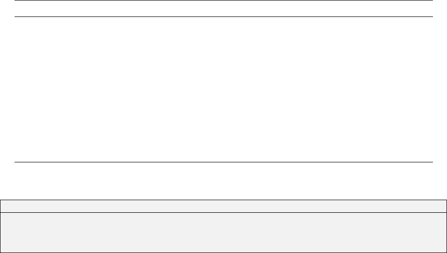
Geodetic (B) and astronomic (K) azimuths, zenith distances (V) and vertical angles (Z)
Table B.5 shows the information and file formatting that applies to geodetic azimuths, astronomic
azimuths, zenith distances and vertical angles. Note that instrument and target heights are not
required for geodetic or astronomic azimuths. Figure B.4 shows some formatted examples.
Table B.5: Column locations and field widths for geodetic azimuths, astronomic azimuths, zenith
distances and vertical angles.
Field Columns Width Comments
Second station name 23 – 42 20 As per first station name in Table B.3.
Azimuth / zenith distance / angle:
Degrees 77 – 80 4 Integer (0 – 359 for azimuths, 0 – 179 for zenith
distances and -89 – 89 for vertical angles).
Minutes 81 – 82 2 Integer (0 – 59).
Seconds 83 – 90 8 Decimal (0 < s< 60).
Standard deviation 91 – 99 9 Decimal value in units of seconds.
Instrument height 100 – 106 7 )Compulsory for zenith distances and
vertical angles only.
Target height 107 – 113 7
12345678901234567890123456789012345678901234567890123456789012345678901234567890123456789012345678901234567890123456789
B 101 202 137 42 08.500 0.010
K 301 502 17 39 24.920 0.010
V 503 304 89 32 59.147 0.010 1.591 1.438
Z 309 410 -0 20 10.331 0.010 1.623 1.345
Z 503 307 1 01 47.654 0.010 1.623 1.345
Figure B.4: Example geodetic azimuths, astronomic azimuths, zenith distances and vertical angles
Direction sets (D)
Information for direction sets is contained on at least two lines. The first record provides information
relating to the reference direction and the number of directions in the set, and the remaining records
provide information about each direction. Each direction must be provided in a clockwise fashion
from the reference direction.
Table B.6 shows the information and file formatting that applies to direction sets, and Figure B.5
shows some formatted examples.
175

Table B.6: Column locations and field widths for direction sets.
Field Columns Width Comments
Reference station name 23 – 42 20 As per first station name in Table B.3.
Reference direction:
Number of directions 43 – 62 20 The number of directions that follow the
reference direction.
Degrees 77 – 80 4 Integer (0 – 359).
Minutes 81 – 82 2 Integer (0 – 59).
Seconds 83 – 90 8 Decimal (0 < s< 60).
Standard deviation 91 – 99 9 Decimal value in units of seconds.
Directions (one per line):
Station name 43 – 62 20 As per first station name in Table B.3.
Degrees 77 – 80 4 Integer (0 – 359).
Minutes 81 – 82 2 Integer (0 – 59).
Seconds 83 – 90 8 Decimal (0 < s< 60).
Standard deviation 91 – 99 9 Decimal value in units of seconds.
12345678901234567890123456789012345678901234567890123456789012345678901234567890123456789012345678901234567890123456789
D 322600020 322600010 2 0 00 00.000 1.769
D 213000050 161 16 41.400 1.769
D 322600030 342 09 25.400 1.769
D 322600010 305700010 4 0 00 00.000 1.769
D 213000040 14 09 21.100 1.769
D 322600050 76 21 16.600 1.769
D 409600180 152 20 05.300 1.769
D 265600050 170 48 53.400 1.769
Figure B.5: Example direction sets
Ellipsoid chords (C), ellipsoid arcs (E), Mean Sea Level arcs (M), slope distances (S) and
height differences (L)
For ellipsoid chords, ellipsoid arcs, Mean Sea Level arcs, slope distances and height differences, the
information and file formatting shown in Table B.7 applies. Note that instrument and target heights
are only required for slope distances. Figure B.6 shows some formatted examples.
Table B.7: Column locations and field widths for ellipsoid chords, ellipsoid arcs, Mean Sea Level arcs,
slope distances and height differences.
Field Columns Width Comments
Second station name 23 – 42 20 As per first station name in Table B.3.
Distance / height difference 63 – 76 14 Decimal value in metres.
Standard deviation 91 – 99 9 Decimal value in metres.
Instrument height 100 – 106 7 Compulsory only for slope distances.
Target height 107 – 113 7 Compulsory only for slope distances.
176

12345678901234567890123456789012345678901234567890123456789012345678901234567890123456789012345678901234567890123456789
C 501 309 5476.1616 0.031
E 503 307 8807.1030 0.054
M 4000 13 53.9380 0.005
S 4000 2012 76.9140 0.005 1.6060 1.3370
L 108 1034 -0.2220 0.010
Figure B.6: Example ellipsoid chords, ellipsoid arcs, Mean Sea Level arcs, slope distances and height
differences
Single GNSS baselines (G), GNSS baseline clusters (X) and GNSS point clusters (Y)
Information for single GNSS baselines, GNSS baseline clusters, and GNSS point clusters is contained
in multiple lines. Depending on the GNSS measurement, certain fields are compulsory whilst
others are ignored. The first record for GNSS measurements is a general header record containing
information about stations, variance matrix scaling, reference frame and epoch. This record varies
depending on whether GNSS baselines or GNSS points are supplied. Table B.8 shows the required
information and file formatting for the header record of a GNSS baseline (single or cluster) measurement.
Table B.8: Column locations and field widths for a GNSS baseline (single or cluster) header record.
Field Columns Width Comments
Second station name 23 – 42 20 As per first station name in Table B.3.
Cluster count 43 – 62 20 Not required for single GNSS baselines.
Variance matrix scaling:
V–scale 63 – 72 10 Whole of matrix scalar.
P–scale 73 – 82 10 North–south scalar.
L–scale 83 – 92 10 East–west scalar.
H–scale 93 – 102 10 Vertical scalar.
Reference frame 103 – 122 20 Abbreviated name (c.f. Table 4.1), e.g. ITRF2008
Epoch 123 – 142 20 Date in the form ’dd.mm.yyyy’, e.g. 01.03.2010
GNSS point clusters have a slightly different header record. The only differences are the omission of
the second station name and the inclusion of a coordinate type, whereby GNSS point clusters may
be supplied in XYZ or LLH format as described in §B.1.3. GNSS measurements in XYZ format are
not supported. Table B.9 shows the different header information and file formatting for GNSS point
cluster measurements.
177

Table B.9: Column locations and field widths for a GNSS point cluster header record.
Field Columns Width Comments
Coordinate type 23 – 42 20 XYZ or LLH.UTM is not supported.
Cluster count 43 – 62 20 Integer.
. . .
Variance matrix scaling, reference frame and epoch as per Table B.8
. . .
For all GNSS measurements, the next three lines provide the three GNSS measurement components
and the lower/upper–triangular elements of the accompanying variance matrix Vm. For GNSS
baselines, this information must be supplied in metres. For GNSS points, the coordinate format of
this information must correspond to the coordinate type specified in the header record (c.f. Table
B.9). Hence, the measurement and variance components can be provided in metres (corresponding
to XYZ) or in latitude,longitude and height (corresponding to XYZ). Latitude and longitude values
must be expressed in degrees, minutes and seconds using HP notation (e.g. dd.mmssssss), and
variance components for latitude and longitude must be in radians. Table B.10 shows the required
information and file formatting for the GNSS measurement and variance components. Figure B.7
shows an example GNSS baseline (G) measurement. In this example, note that the reference frame
and epoch have not been provided. In this case DynaNet will adopt the reference frame and epoch
supplied in the header line (c.f. Table B.1).
Table B.10: Column locations and field widths for GNSS baseline and point measurements.
Field Columns Width Comments
x–component:
For XYZ, measurement and variance in metres.
For LLH, measurement in dd.mmssss and
variance in units of radians.
∆xor x63 – 82 20
Vm11 (σxσx) 83 – 102 20
y–component:
∆yor y63 – 82 20
Vm21 (σyσx) 83 – 102 20
Vm22 (σyσy) 103 – 122 20
z–component:
Measurement variances in metres for both
XYZ and LLH.
∆zor z63 – 82 20
Vm31 (σzσx) 83 – 102 20
Vm32 (σzσy) 103 – 122 20
Vm33 (σzσz) 123 – 142 20
178

1234567890123456789012345678901234567890123456789012345678901234567890123456789012345678901234567890123456789012345678901234567890123456789012
G 202 304 1.000 1.000 1.000 1.000
-53817.2076 4.0220e-05
-88430.4791 -1.3690e-05 1.4870e-05
-50031.4264 3.9750e-05 -2.0350e-05 6.8030e-05
Figure B.7: Example GNSS baseline measurement
For GNSS baseline and point clusters, the measurement information shown in Table B.10 is repeated
for the total number nof measurement vectors (m1, m2, . . . , mn) in the cluster. Immediately after
each vector, the row–wise covariance blocks (Cm1m2,Cm1m3,...,Cm1mn) between the respective
GNSS measurement variance blocks (Vm1,Vm2,...,Vmn) must be provided such that a rigorous
upper variance matrix V1...n can be formed for the whole cluster, as per equation B.1.
V1...n =
σxσxσxσyσxσz
σyσyσyσz
σzσz
Cm1m2··· Cm1mn
σxσxσxσyσxσz
σyσyσyσz
σzσz··· Cm2mn
....
.
.
σxσxσxσyσxσz
σyσyσyσz
σzσz
(B.1)
The information for a single covariance block Ccontains nine elements which are provided over three
records. Table B.11 shows the required information and file formatting for the nine cluster covariance
components.
Table B.11: Column locations and field widths for a GNSS cluster covariance block.
Field Columns Width Comments
C11 83 – 102 20
First record
C12 103 – 122 20
C13 123 – 142 20
C21 83 – 102 20
Second record
C22 103 – 122 20
C23 123 – 142 20
C31 83 – 102 20
Third record
C32 103 – 122 20
C33 123 – 142 20
These blocks are repeated for as many covariance blocks required to complete each row of the
upper–triangular matrix V1...n. As with the variance matrix information supplied for the individual
GNSS measurements, the covariance units must correspond to the coordinate type specified in the
cluster header record.
179

As an example, Figure B.8 shows a GNSS baseline cluster comprised of three baselines. Note that
there are two covariance blocks associated with the first GNSS baseline (HOI_ –MEI_). These blocks
represent the row–wise covariances between the first baseline and the second and third baselines
(HOI_ –MSI_ and HOI_ –SBI_) respectively. Similarly, the covariance block associated with the
second GNSS baseline corresponds to the covariance between the second and third baselines. Figure
B.9 shows an example of two GNSS point clusters — the first is comprised of three correlated points
in XYZ format and the second has two points in LLH format.
1234567890123456789012345678901234567890123456789012345678901234567890123456789012345678901234567890123456789012345678901234567890123456789012
X HOI_ MEI_ 3 1.000 1.000 1.000 1.000 itrf2005 17.09.2008
-125691.6314 2.034048e-06
-145519.2865 -6.968547e-07 1.474554e-06
73663.5870 3.962077e-07 -2.984549e-07 1.537337e-07
5.871788e-07 -2.839605e-07 1.247021e-07
-2.808181e-07 4.298451e-07 -1.016602e-07
1.242805e-07 -1.025933e-07 5.222703e-08
7.646870e-07 -2.856280e-07 1.465497e-07
-2.926789e-07 5.238148e-07 -1.193196e-07
1.550035e-07 -1.182915e-07 6.196860e-08
X HOI_ MSI_
-86797.3963 1.876158e-06
-87459.1959 -7.301331e-07 1.217260e-06
91306.3628 3.423311e-07 -2.596589e-07 1.278370e-07
5.709494e-07 -2.902187e-07 1.189632e-07
-2.869810e-07 4.243482e-07 -1.022121e-07
1.239490e-07 -1.010039e-07 5.159684e-08
X HOI_ SBI_
-39640.6285 2.385609e-06
-13533.0128 -6.219224e-07 1.637419e-06
131721.2044 4.633211e-07 -2.878135e-07 1.732844e-07
Figure B.8: Example GNSS baseline clusters.
1234567890123456789012345678901234567890123456789012345678901234567890123456789012345678901234567890123456789012345678901234567890123456789012
Y YIEL XYZ 3 1.00 1.00 1.00 1.00 IGb08 01.06.2013
-4247834.5782 1.288543e-05
2948383.3671 -5.037133e-06 1.040270e-05
-3721788.4927 3.642770e-06 -2.406477e-06 9.898976e-06
1.065777e-05 -3.701601e-06 2.041076e-06
-3.579744e-06 9.246168e-06 -1.254975e-06
2.174192e-06 -1.449455e-06 8.465730e-06
8.159775e-06 -2.180570e-06 1.558934e-06
-1.892996e-06 7.311562e-06 -1.455025e-06
1.484222e-06 -4.435524e-07 5.804253e-06
Y YRRM
-4172492.9321 1.269096e-05
2743402.2911 -4.907058e-06 1.027008e-05
-3954709.8313 3.570733e-06 -2.329364e-06 9.936777e-06
8.167171e-06 -2.118313e-06 1.598938e-06
-1.942259e-06 7.291434e-06 -1.513716e-06
1.394181e-06 -3.230191e-07 5.780071e-06
Y YSSK
-3465321.0856 9.840133e-06
2638269.2861 -2.482731e-06 8.405404e-06
4644085.3490 2.303389e-06 -1.473060e-06 7.531223e-06
Y 1004 LLH 2 10.000 1.000 1.000 1.500 GDA94
-37.480000000 9.402e-09
144.573400000 5.876e-10 9.402e-09
42.195 5.876e-10 5.876e-10 2.500e-01
5.876e-12 5.876e-12 5.876e-12
5.876e-12 5.876e-12 5.876e-12
5.876e-12 5.876e-12 5.876e-12
Y 9004
-37.474800000 9.402e-09
144.573600000 5.876e-10 9.402e-09
44.324 5.876e-10 5.876e-10 2.500e-01
Figure B.9: Example GNSS point clusters.
Orthometric height (H) and ellipsoid height (R)
For orthometric height and ellipsoid height measurements, the information and file formatting shown
in Table B.12 applies. Figure B.10 shows some formatted examples.
180

Table B.12: Column locations and field widths for orthometric and ellipsoid height measurements.
Field Columns Width Comments
Height 63 – 76 14 Decimal value in metres.
Standard deviation 91 – 99 9 Decimal value in metres.
12345678901234567890123456789012345678901234567890123456789012345678901234567890123456789012345678901234567890123456789
H 387800830 283.8600 0.090
R 701219 130.161 0.0001
Figure B.10: Example orthometric height and ellipsoid height measurements.
Geodetic latitudes (P), geodetic longitudes (Q), astronomic latitudes (I) and astronomic
longitudes (J)
For geodetic latitudes, geodetic longitudes, astronomic latitudes and astronomic longitudes, the
information and file formatting shown in Table B.13 applies. Figure B.11 shows some formatted
examples.
Table B.13: Column locations and field widths for geodetic latitudes and longitudes, and astronomic
latitudes and longitudes.
Field Columns Width Comments
Latitude / longitude 63 – 76 14 Decimal value in ddd.mmssss.
Standard deviation 91 – 99 9 Decimal value in units of seconds.
12345678901234567890123456789012345678901234567890123456789012345678901234567890123456789012345678901234567890123456789
P 105 -24.2958384014 0.0001
Q 105 136.3000088022 0.0001
I 106 -24.2957481018 0.02
J 106 137.0003182747 0.02
Figure B.11: Example geodetic latitude and longitude, and astronomic latitude and longitude
measurements.
181

B.1.5 Geoid information
Following the single header line, all geoid information that can be introduced to an adjustment for
a station is formatted on one line. The relevant fields and corresponding file positions for geoid
information are shown in Table B.14.
Table B.14: Geoid information column locations and field widths
Field Columns Width Comments
Station name 1 – 20 20 Alphanumeric string. Can contain spaces.
N–value 41 – 50 10 Geoid–ellipsoid separation (N). Decimal value in units
of metres.
N–S deflection 60–69 10 Deflection in prime meridian (ξ). Decimal value in
units of seconds.
E–W deflection 70 – 79 10 Deflection in prime vertical (η). Decimal value in
units of seconds.
Figure B.12 shows some example geoid records in DNA format. As with station and measurement
information, geoid information can be positioned anywhere within the respective fields without the
need for right or left justification.
12345678901234567890123456789012345678901234567890123456789012345678901234567890123456789
!#=DNA 3.01 GEO 16.10.2012 GDA94 12
* Created 06 November 2016.
* Geoid information for level section 1596
1596-3H 3.177 -9.267 -0.816
1596-4 3.205 -9.354 -1.035
1596-7 2.897 -8.991 -1.351
1596-8 2.810 -8.669 -1.672
1596-9 2.728 -8.334 -1.316
1596-10 2.573 -8.112 -1.119
1596-11H 2.501 -7.819 -0.767
1596-12 2.430 -7.462 -0.606
1596-13 2.382 -7.189 -0.423
1596-14 2.289 -6.919 -0.269
1596-15H 2.232 -7.035 -0.365
1596-16H 2.184 -7.154 -0.457
Figure B.12: Example geoid information records
Note that whilst the header record can simply be in the form of a comment, it is helpful to record
metadata pertaining to the records, including the date, geodetic datum (and hence, ellipsoid) to
which the geoid–ellipsoid separations relate and the number of records. Any number of comments
may be dispersed throughout the file.
182
B.2 Comma Separated Values (CSV) format
The CSV format (still under development) provides information about geodetic network stations,
measurements, and geoid–ellipsoid separations and deflections of the vertical. This information is
contained in three separate files — the station file has a stn file extension, the measurement file
has a msr extension and the geoid file has a geo extension. All three files must contain a single
header line at the beginning of the file. As required, these files can contain one or more comment
lines throughout the file. Comment lines must begin with an asterisk (*). Every record in the
station, measurement and geoid files must contain data fields located in particular fields separated
by commas.
183

B.3 Dynamic Network Adjustment Project (DNAPROJ) format
The DynaNet project file is designed to capture default and user–specified program options and
arguments. The first line in the project file is reserved for comments and commences with the hash
character (#). The remainder of the file consists of sections which correspond directly to the various
DynaNet programs. The formatting used to capture the options for each program is given in Table
B.15.
Table B.15: DynaNet program options formatting.
Field Columns Width Comments
Element 1 – 35 35 Program option
Value 36 – Unlimited Default or user–specified value
Using this formatting, each section contains a header record commencing with a hash character, a
line of dashes, then one or more options and their corresponding values. Each section is separated by
a blank line. The first section is a general section and contains the list of options which are common
to all programs. The following sections contain the default and user–specified options corresponding
to import,reftran,geoid,segment,adjust and the options for the output of information. Figure
B.13 shows a formatted example for the skye project (see §1.4), including the comment line and the
list of general options.
12345678901234567890123456789012345678901234567890123456789012345678901234567890
# skye project file. Created by: import, DynaNet file exchange software.
#general (35) VALUE
--------------------------------------------------------------------------------
network-name skye
input-folder C:\Data\proj
output-folder C:\Data\proj
verbose-level 0
quiet no
project-file C:\Data\proj\skye.dnaproj
dynanet-log-file C:\Data\proj\dynanet.log
Figure B.13: Example general options.
Note that the general section commences with #general. As a project file is loaded, DynaNet will
look for these section headings before attempting to load the options and values which follow. In
addition to #general, the valid section headings are #import,#reftran,#geoid,#segment,#adjust,
#output and #display. Using the skye project (see §1.4), Figures B.14, B.15, B.16, B.17 and B.18
list the options and example arguments for import,reftran,geoid,segment and adjust. B.19 lists
an example of the options and arguments for the output of information from DynaNet.
184

12345678901234567890123456789012345678901234567890123456789012345678901234567890
#import (35) VALUE
--------------------------------------------------------------------------------
stn-msr-file skye.stn
stn-msr-file skye.msr
geo-file
bounding-box
get-msrs-transcending-box no
include-stns-assoc-msrs no
exclude-stns-assoc-msrs no
split-gnss-cluster-msrs no
import-block-stn-msr no
seg-file
prefer-single-x-as-g no
import-msr-types
exclude-msr-types
stn-renaming-file
search-nearby-stn no
nearby-stn-buffer 0.3
search-similar-msr no
ignore-similar-msr no
remove-ignored-msr no
flag-unused-stations no
test-integrity no
v-scale 1
p-scale 1
l-scale 1
h-scale 1
baseline-scalar-file
export-xml-files no
single-xml-file no
export-dna-files no
export-asl-file no
export-aml-file no
export-map-file no
simulate-msr-file no
Figure B.14: Example import options.
12345678901234567890123456789012345678901234567890123456789012345678901234567890
#reftran (35) VALUE
--------------------------------------------------------------------------------
reference-frame GDA94
epoch
Figure B.15: Example reftran options.
12345678901234567890123456789012345678901234567890123456789012345678901234567890
#geoid (35) VALUE
--------------------------------------------------------------------------------
ntv2-file C:\Data\geoid\ausgeoid09.gsb
interpolation-method 1
decimal-degrees 0
direction 0
convert-stn-hts yes
export-dna-geo-file no
Figure B.16: Example geoid options.
185

12345678901234567890123456789012345678901234567890123456789012345678901234567890
#segment (35) VALUE
-------------------------------------------------------------------------------
net-file
seg-file
min-inner-stns 5
max-block-stns 65
contiguous-blocks yes
starting-stns
Figure B.17: Example segment options.
12345678901234567890123456789012345678901234567890123456789012345678901234567890
#adjust (35) VALUE
--------------------------------------------------------------------------------
seg-file
comments
adjustment-mode simultaneous-adjustment
multi-thread no
staged-adjustment no
conf-interval 95
iteration-threshold 0.0005
max-iterations 10
constraints 302513640,CCC
free-stn-sd 10.000
fixed-stn-sd 1.0000e-06
inversion-method 0
scale-normals-to-unity no
create-stage-files no
purge-stage-files no
Figure B.18: Example adjust options.
186

12345678901234567890123456789012345678901234567890123456789012345678901234567890
#output (35) VALUE
--------------------------------------------------------------------------------
output-msr-to-stn no
output-iter-adj-stn no
output-iter-adj-stat no
output-iter-adj-msr no
output-iter-cmp-msr no
output-adj-msr yes
output-adj-gnss-units 0
output-tstat-adj-msr no
sort-adj-msr-field 0
output-database-ids no
output-msr-blocks no
sort-stn-orig-order no
stn-coord-types PLHhXYZ
stn-corrections no
precision-stn-linear 4
precision-stn-angular 5
precision-msr-linear 4
precision-msr-angular 4
angular-msr-type 0
dms-msr-format 0
output-pos-uncertainty yes
output-all-covariances no
output-apu-vcv-units 0
output-corrections-file yes
hz-corr-threshold 0.000
vt-corr-threshold 0.000
export-xml-stn-file no
export-dna-stn-file no
export-sinex-file no
Figure B.19: Example output options.
187

B.4 DynaNet Markup Language (DynaML) format
The DynaML format provides for the exchange of stations and measurements in eXtensible Markup
Language (XML) using the DynaNet 2.0 XML (DynaML) schema. The scope of information includes
the station and measurement information handled by the DNA and CSV formats (see §B.1 and §B.2).
The DynaML schema definition permits this information to be stored in two files, corresponding to
station and measurement files, or a single stations and measurements file. All DynaML files have an
xml file extension. For convenience, DynaNet names station files as *stn.xml, and measurement
files as *msr.xml. DynaML files must be encoded using well–formed XML, and conform to the XML
schema definition.
As required, these files can contain one or more comment lines throughout the file. Comment lines
must conform with conventional XML encoding as follows.
<!-- Comments can appear on one line. -->
<!-- Alternatively, comments can be
spread over many lines.
-->
DynaML files must contain a root element named DnaXmlFormat. The DynaML schema definition
for DnaXmlFormat is given in Figure B.20.
<?xml version="1.0" encoding="UTF-8" standalone="yes"?>
<!--W3C Schema definition for DynaML -->
<xs:schema xmlns:xs="http://www.w3.org/2001/XMLSchema" elementFormDefault="qualified">
<xs:element name="DnaXmlFormat">
<xs:complexType>
<xs:choice maxOccurs="unbounded">
<xs:element ref="DnaStation"/>
<xs:element ref="DnaMeasurement"/>
</xs:choice>
<xs:attribute name="type" use="required">
<xs:simpleType>
<xs:restriction base="xs:string">
<xs:enumeration value="Measurement␣File"/>
<xs:enumeration value="Station␣File"/>
<xs:enumeration value="Combined␣File"/>
</xs:restriction>
</xs:simpleType>
</xs:attribute>
</xs:complexType>
</xs:element>
...
...
</xs:schema>
Figure B.20: DnaXMLFormat schema definition
As shown above, the root element can be one of three types — "Measurement File","Station
File" and "Combined File". These types inform the parser whether the elements contained in the
file station information, measurement information or both. Accordingly, the root element can contain
an unlimited number of DnaStation elements, DnaMeasurement elements or both.
B.4.1 Station information
All station information is recorded in the DnaStation element. This element contains a sub–element
StationCoord which is a xs:complexType containing the coordinates for the station. The DynaML
188

schema definition is given in Figure B.21.
<xs:element name="DnaStation">
<xs:complexType>
<xs:sequence>
<xs:element ref="Name"/>
<xs:element ref="Constraints"/>
<xs:element ref="Type"/>
<xs:element ref="StationCoord"/>
<xs:element ref="Description"
minOccurs="0"/>
</xs:sequence>
</xs:complexType>
</xs:element>
(a) DnaStation element
<xs:element name="StationCoord">
<xs:complexType>
<xs:sequence>
<xs:element ref="Name" minOccurs="0"/>
<xs:element ref="XAxis"/>
<xs:element ref="YAxis"/>
<xs:element ref="Height"/>
<xs:element ref="HemisphereZone"
minOccurs="0"/>
</xs:sequence>
</xs:complexType>
</xs:element>
(b) StationCoord element
Figure B.21: DnaStation schema definition
With respect to DnaStation and StationCoord, elements Name,Constraints,Type,Description,
XAxis,YAxis,Height and HemisphereZone are of type xs:string. All elements correspond to the
station information fields shown in Table B.2.
By way of example, Figure B.22 shows a station file encoded in XML according to the DynaML
schema definition. In this example, the coordinates for HOSP are provided in terms of type LLH and
1002-26 in terms of UTM.
<?xml version="1.0"?>
<DnaXmlFormat type="Station␣File"
xmlns:xsi="http://www.w3.org/2001/XMLSchema-instance"
xsi:noNamespaceSchemaLocation="DynaML.xsd">
<!-- Station file. -->
<DnaStation>
<Name>HOSP</Name>
<Constraints>FFF</Constraints>
<Type>LLH</Type>
<StationCoord>
<XAxis>-37.4801765569</XAxis>
<YAxis>144.5717295509</YAxis>
<Height>83.9</Height>
</StationCoord>
<Description>HOSP</Description>
</DnaStation>
<DnaStation>
<Name>1002-26</Name>
<Constraints>CCF</Constraints>
<Type>UTM</Type>
<StationCoord>
<XAxis>372772.813</XAxis>
<YAxis>5931491.145</YAxis>
<Height>175.668</Height>
<HemisphereZone>S55</HemisphereZone>
</StationCoord>
<Description>BM 26</Description>
</DnaStation>
</DnaXmlFormat>
Figure B.22: Sample station file encoded in DynaML format
In relation to the expected format of coordinates corresponding to the value in the Type element,
§B.1.3 can be used as a guide. However, note that latitude and longitude values must be expressed
189

in degrees, minutes and seconds using HP notation (e.g. dd.mmssssss). Since there is no restriction
on column formatting, values can be provided to any level of precision.
B.4.2 Measurement information
All measurement information is recorded in the DnaMeasurement element. The DynaML schema
definition is given in Figure B.23.
<xs:element name="DnaMeasurement">
<xs:complexType>
<xs:choice maxOccurs="unbounded">
<xs:element ref="Clusterpoint"/>
<xs:element ref="Coords"/>
<xs:element ref="Directions"/>
<xs:element ref="First"/>
<xs:element ref="Epoch" minOccurs="0"/>
<xs:element ref="GPSBaseline"/>
<xs:element ref="Hscale" minOccurs="0"/>
<xs:element ref="Ignore" minOccurs="0"/>
<xs:element ref="InstHeight"/>
<xs:element ref="Lscale" minOccurs="0"/>
<xs:element ref="Pscale" minOccurs="0"/>
<xs:element ref="ReferenceFrame" minOccurs="0"/>
<xs:element ref="Second"/>
<xs:element ref="Source"/>
<xs:element ref="StdDev"/>
<xs:element ref="TargHeight"/>
<xs:element ref="Third"/>
<xs:element ref="Total"/>
<xs:element ref="Type"/>
<xs:element ref="Value"/>
<xs:element ref="Vscale" minOccurs="0"/>
</xs:choice>
</xs:complexType>
</xs:element>
Figure B.23: DnaMeasurement schema definition
Elements Type,Ignore,First,Second,Third,Value,StdDev,InstHeight,TargHeight,Total,
Vscale,Hscale,Lscale,Pscale,Coords and Source are of type xs:string. Not all elements are
mandatory for each measurement. The mandatory elements and required format for the respective
measurement types (c.f. Type) follow the definitions contained in the DNA format specification (see
§B.1.4). To flag a measurement as ignored so that DynaNet will exclude the measurement from all
processing, provide an asterisk (*) for the Ignore element’s value:
<DnaMeasurement>
...
<Ignore>*</Ignore>
...
</DnaMeasurement>
Elements Clusterpoint and GPSBaseline are of type xs:complexType and are given in Figure B.24.
Directions is also of type xs:complexType and is given in Figure B.25.
190

<xs:element name="Clusterpoint">
<xs:complexType>
<xs:sequence>
<xs:element ref="X"/>
<xs:element ref="Y"/>
<xs:element ref="Z"/>
<xs:element ref="SigmaXX"/>
<xs:element ref="SigmaXY"/>
<xs:element ref="SigmaXZ"/>
<xs:element ref="SigmaYY"/>
<xs:element ref="SigmaYZ"/>
<xs:element ref="SigmaZZ"/>
<xs:element ref="PointCovariance"
minOccurs="0" maxOccurs="unbounded"/>
</xs:sequence>
</xs:complexType>
</xs:element>
(a) Clusterpoint element
<xs:element name="GPSBaseline">
<xs:complexType>
<xs:sequence>
<xs:element ref="X"/>
<xs:element ref="Y"/>
<xs:element ref="Z"/>
<xs:element ref="SigmaXX"/>
<xs:element ref="SigmaXY"/>
<xs:element ref="SigmaXZ"/>
<xs:element ref="SigmaYY"/>
<xs:element ref="SigmaYZ"/>
<xs:element ref="SigmaZZ"/>
<xs:element ref="GPSCovariance"
minOccurs="0" maxOccurs="unbounded"/>
</xs:sequence>
</xs:complexType>
</xs:element>
(b) GPSBaseline element
Figure B.24: Clusterpoint and GPSBaseline schema definition
Elements GPSCovariance (for GPSBaseline) and PointCovariance (for Clusterpoint) are of xs:complexType
and relate to the covariance information between GNSS baseline and GNSS point variance matrices.
The schema definition for GPSCovariance is given in Figure B.25. The element PointCovariance
contains an identical set of elements to those in GPSCovariance and as such is not shown here.
<xs:element name="Directions">
<xs:complexType>
<xs:sequence>
<xs:element ref="Ignore"/>
<xs:element ref="Target"/>
<xs:element ref="Value"/>
<xs:element ref="StdDev"/>
</xs:sequence>
</xs:complexType>
</xs:element>
(a) Directions element
<xs:element name="GPSCovariance">
<xs:complexType>
<xs:sequence>
<xs:element ref="m11"/>
<xs:element ref="m12"/>
<xs:element ref="m13"/>
<xs:element ref="m21"/>
<xs:element ref="m22"/>
<xs:element ref="m23"/>
<xs:element ref="m31"/>
<xs:element ref="m32"/>
<xs:element ref="m33"/>
</xs:sequence>
</xs:complexType>
</xs:element>
(b) GPSCovariance element
Figure B.25: Directions and GPSCovariance schema definition
Elements Target,X,Y,Z,SigmaXX through to SigmaZZ and m11 through to m33 are of type xs:string.
Figure B.26 provides some sample measurements presented in §B.1.4 encoded in XML according to
the DynaML schema definition.
As with station information, §B.1.4 can be used as a guide for the expected format and precision
of angular and linear measurement values. However, with angular measurements (such as latitude,
angles, etc.), all measurement values must be expressed in degrees, minutes and seconds using HP
notation (e.g. dd.mmssssss) with their precision in seconds.
191

<?xml version="1.0"?>
<DnaXmlFormat type="Measurement␣File"
xmlns:xsi="http://www.w3.org/2001/XMLSchema-instance"
xsi:noNamespaceSchemaLocation="DynaML.xsd">
<!-- Sample measurements file -->
<!-- Type G GPS Baseline -->
<DnaMeasurement>
<Type>G</Type>
<ReferenceFrame>ITRF2008</ReferenceFrame>
<Epoch>01.01.2010</Epoch>
<Vscale>1.000</Vscale>
<Pscale>1.000</Pscale>
<Lscale>1.000</Lscale>
<Hscale>1.000</Hscale>
<First>202</First>
<Second>304</Second>
<GPSBaseline>
<X>-53817.2076</X>
<Y>-88430.4791</Y>
<Z>-50031.4264</Z>
<SigmaXX>4.0220e-05</SigmaXX>
<SigmaXY>-1.3690e-05</SigmaXY>
<SigmaXZ>3.9750e-05</SigmaXZ>
<SigmaYY>1.4870e-05</SigmaYY>
<SigmaYZ>-2.0350e-05</SigmaYZ>
<SigmaZZ>6.8030e-05</SigmaZZ>
</GPSBaseline>
</DnaMeasurement>
<!-- Orthometric Height -->
<DnaMeasurement>
<Type>H</Type>
<Ignore>*</Ignore>
<First>202</First>
<Value>43.086</Value>
<StdDev>0.065</StdDev>
</DnaMeasurement>
<!-- Zenith Angle -->
<!-- Instrument and target heights -->
<DnaMeasurement>
<Type>V</Type>
<First>1013</First>
<Second>1014</Second>
<Value>90.243</Value>
<StdDev>20</StdDev>
<InstHeight>1.545</InstHeight>
<TargHeight>0.125</TargHeight>
</DnaMeasurement>
<!-- Horizontal Angle -->
<DnaMeasurement>
<Type>A</Type>
<First>2012</First>
<Second>4000</Second>
<Third>2013</Third>
<Value>266.281</Value>
<StdDev>20</StdDev>
</DnaMeasurement>
<!-- Geodetic Azimuth -->
<DnaMeasurement>
<Type>B</Type>
<First>1046</First>
<Second>4010</Second>
<Value>91.2031</Value>
<StdDev>20</StdDev>
</DnaMeasurement>
...
...
<!-- Slope Distance -->
<!-- Instrument and target heights -->
<DnaMeasurement>
<Type>S</Type>
<First>1037</First>
<Second>4006</Second>
<Value>44.06</Value>
<StdDev>0.005</StdDev>
<InstHeight>1.542</InstHeight>
<TargHeight>1.559</TargHeight>
</DnaMeasurement>
<!-- Astronomic Azimuth -->
<DnaMeasurement>
<Type>K</Type>
<First>1046</First>
<Second>4010</Second>
<Value>91.2001</Value>
<StdDev>20</StdDev>
</DnaMeasurement>
<!-- Direction set -->
<DnaMeasurement>
<Type>D</Type>
<First>365200180</First>
<Second>TS5137</Second>
<Value>52.025209</Value>
<StdDev>0.707</StdDev>
<Total>3</Total>
<Directions>
<Target>409700260</Target>
<Value>238.545977</Value>
<StdDev>0.707</StdDev>
</Directions>
<Directions>
<Target>TS2761</Target>
<Value>264.344190</Value>
<StdDev>0.707</StdDev>
</Directions>
<Directions>
<Target>TS3568</Target>
<Value>305.285959</Value>
<StdDev>0.707</StdDev>
</Directions>
</DnaMeasurement>
<!-- Vertical Angle -->
<!-- Instrument and target heights -->
<DnaMeasurement>
<Type>Z</Type>
<First>4000</First>
<Second>1050</Second>
<Value>0.3711</Value>
<StdDev>20</StdDev>
<InstHeight>1.606</InstHeight>
<TargHeight>1.715</TargHeight>
</DnaMeasurement>
<!-- Level Difference -->
<DnaMeasurement>
<Type>L</Type>
<First>2217</First>
<Second>2218</Second>
<Value>0.018</Value>
<StdDev>0.002</StdDev>
</DnaMeasurement>
...
</DnaXmlFormat>
Figure B.26: Sample measurements encoded in DynaML format
192

B.5 GeodesyML format
GeodesyML is a comprehensive Geography Markup Language (GML) application schema defined by
the Intergovernmental Committee on Surveying and Mapping (ICSM). GeodesyML provides both
XML schema definition and XML format. The specification for GeodesyML can be found at http:
//geodesyml.org. The version of GeodesyML supported by DynaNet is 0.1.1.
B.6 SINEX format
The Solution (software/technique) INdependent EXchange (SINEX) file format is maintained by the
International Earth Rotation Service (IERS) and provides for the management of station coordinates,
velocities and earth rotation parameters. The SINEX file format specification is beyond the scope of
this user guide, however interested readers are referred to the following site for more information:
http://www.iers.org/IERS/EN/Organization/AnalysisCoordinator/SinexFormat/
sinex.html
The version of SINEX supported by DynaNet is 2.02.
B.7 Geoid input text file format
To provide an efficient means for converting spot heights contained in both small and extremely
large files from one height system to another, geoid supports Formatted Text files (e.g. *.dat,
*.prn,*.txt) and Comma Separated Values files (*.csv). geoid expects all input coordinates in
both file formats to be geographic coordinates in degrees, minutes and seconds or decimal degrees.
In both cases, coordinates must be in HP Notation (i.e. dd.dddddddd or dd.mmssssss). In this form,
the latitude and longitude fields should each contain only one numeric value. When working with
formatted text files, the maximum number of significant digits the values can have is 15 significant
figures1. For latitudes in the southern hemisphere and longitudes west of the zero meridian, the
number of significant figures is further reduced by 1 to cater for the minus sign.
Formatted text files
Every line in a formatted text file must contain data fields in particular file positions (or columns).
Certain fields may be omitted depending on what they are. Table B.16 lists the compulsory and
non-compulsory fields in the required order. Figure B.27 shows an example formatted text file and
illustrates the use of the non–compulsory fields. Column numbers shown for reference only.
Table B.16: Formatted text file fields
Field Columns Width Compulsory?
Point ID 1 – 11 11 No
Latitude 12 –27 16 Yes
Longitude 28 – 43 16 Yes
Height 44 – 52 9 No
1. Since the maximum field width for both latitude and longitude is 16 characters, excluding the decimal point leaves
a maximum of 15 characters.
193

123456789012345678901234567890123456789012345678901234567890
----------><--------------><--------------><-------><
Point (11) Latitude (16) Longitude (16) Hght (9)
MT HIGH -27.498408428 153.001072611
-27.498421786 150.001124192
-29.086179181 151.966654878
-29.073486997 151.805272886 4.23
62 / 54 -29.000294436 151.457723186
GBM16 -28.636707072 151.970252700
GBM34 -28.619868617 151.650131492
-28.235994419 151.990397797 36.281
Figure B.27: Example formatted text file
Comma separated values files
Every line in a CSV file must contain data fields separated by commas. Non-compulsory fields may
be empty, however a sufficient number of commas must be present to delineate the presence of
compulsory fields. Table B.17 lists the compulsory and non-compulsory fields in the required order.
Table B.17: Comma separated values file fields
Field Compulsory?
Point ID No
Latitude Yes
Longitude Yes
Height No
According to Table B.17, a minimum of two commas is sufficient to delineate Point ID, Latitude and
Longitude. Figure B.28 shows an example CSV file. Note that a header line is not required.
MT HIGH,-10.498408428,153.001072611
,-20.498421786,140.001124192
,-40.086179181,121.966654878,
1596-4 , -37.593644101, 144.204321339
1596-5 , -37.593616320, 144.204318245
62 / 54,-40.000294436,141.457723186, 4.23
GBM16,-30.636707072,151.970252700,
GBM34,-20.619868617,141.650131492
4,-20.235994419,121.99039779,36.281
Figure B.28: Example comma separated values file
194

Appendix C
Output file format specification
C.1 Header block
For each of the output files that DynaNet generates, a standard header block is printed to the file.
The information printed in the header block will commence and end with a dashed line, and will
contain basic to detailed information depending on the file type. As a minimum, the header block
contains the file type, information about the version and build of the program that created the file,
and the file’s creation date and location. Following this, additional information relevant to the file
type is printed. The following example shows the header block of a coordinate output file.
12345678901234567890123456789012345678901234567890123456789012345678901234567890123456789012345678901234567890123456789
--------------------------------------------------------------------------------
DYNANET COORDINATE OUTPUT FILE
Version: 3.2.6, Release (64-bit)
Build: Oct 18 2016, 16:48:34 (MSVC++ 10.0)
File created: Tuesday, 18 October 2016, 4:53:59 PM
File name: c:\Data\uni_sqr.phased.xyz
Reference frame: GDA94
Epoch: 01.01.1994
Geoid model: c:\Data\ausgeoid09.gsb
Stations printed in blocks: No
--------------------------------------------------------------------------------
The width of the field names in the header block will always be 35 characters wide.
C.2 Import log file (IMP)
The import log (.imp) file is generated by import and contains information closely matching the
information printed to the screen (c.f. Figure 3.1). In addition to the program version and log file
metadata printed in the header block, the import log header will contain the command line arguments
supplied to import, the file paths to the binary and ASCII files created by import, the input station
and measurement files, and the options that have been supplied import. Apart from the default
reference frame, only the options which have been modified on calling import (c.f. §3.3) will be
printed to the header. The following example shows the information printed to the import log file
upon calling import using the default options.
Any failures in the import of stations and measurements will be reported to this file and must be
rectified before proceeding to other steps in the adjustment.
195

12345678901234567890123456789012345678901234567890123456789012345678901234567890123456789012345678901234567890123456789
--------------------------------------------------------------------------------
DYNANET IMPORT LOG FILE
Version: 3.2.6, Release (64-bit)
Build: Oct 19 2016, 07:30:53 (MSVC++ 10.0)
File created: Wednesday, 19 October 2016, 7:31:30 AM
File name: c:\Data\uni_sqr.imp
Command line arguments: import -n uni_sqr uni_sqrstn.xml uni_sqrmsr.xml
Network name: uni_sqr
Input folder: c:\Data\
Output folder: c:\Data\
Stations file: c:\Data\uni_sqr.bst
Measurements file: c:\Data\uni_sqr.bms
Associated station file: c:\Data\uni_sqr.asl
Associated measurement file: c:\Data\uni_sqr.aml
Duplicate stations output file: c:\Data\uni_sqr.dst
Similar measurement output file: c:\Data\uni_sqr.dms
Input files: uni_sqrstn.xml
uni_sqrmsr.xml
Default reference frame: GDA94
--------------------------------------------------------------------------------
+ Parsing
uni_sqrstn.xml... Done. Loaded 149 stations in 0.035s
uni_sqrmsr.xml... Done. Loaded 1199 measurements in 0.04s
+ Reducing stations... Done.
+ File parsing summary:
Read 149 stations:
-------------------------------------------
(CCC) 3D constrained: 1
(FFF) 3D free: 145
(CCF) 2D constrained, 1D free: 1
(FFC) 2D free, 1D constrained: 1
(CFF) custom 2D constraints: 1
-------------------------------------------
Total 149
Read 1199 measurements:
-------------------------------------------
(A) Horizontal angle: 251
(B) Geodetic azimuth: 1
(C) Chord dist: 0
(D) Directions: 0
(E) Ellipsoid arc: 0
(G) GPS baseline: 114
(H) Orthometric height: 1
(I) Astronomic latitude: 0
(J) Astronomic longitude: 0
(K) Astronomic azimuth: 1
(L) Level difference: 89
(M) Mean sea level arc: 1
(P) Geodetic latitude: 0
(Q) Geodetic longitude: 0
(R) Ellipsoidal height: 0
(S) Slope distance: 428
(V) Zenith angle: 300
(X) GPS baseline cluster: 0
(Y) GPS point cluster: 12
(Z) Vertical angle: 1
-------------------------------------------
Total 1199*
* Includes 17 ignored measurements
+ Testing for duplicate stations... Done.
+ Sorting stations... Done.
+ Serialising station map... Done.
+ Mapping measurements to stations... Done. Mapped 1199 measurements to 149 stations.
+ Creating association lists... Done.
+ Serialising association lists... Done.
+ Serialising binary station file uni_sqr.bst... Done.
+ Serialising binary measurement file uni_sqr.bms... Done.
+ Total file handling process took 0.182s.
+ Binary station and measurement files are now ready for processing.
C.3 Measurement to station output file (M2S)
The measurement to station (.m2s) file is generated by import when the option --output-msr-to-stn
has been provided. The following example shows the information printed to the measurement to
station file (several records have been omitted).
196

12345678901234567890123456789012345678901234567890123456789012345678901234567890123456789012345678901234567890123456789012345678901234567890123456789012345678901234567890123456789012345678901234567890
--------------------------------------------------------------------------------
DYNANET MEASUREMENT TO STATION OUTPUT FILE
Version: 3.2.6, Release (64-bit)
Build: Oct 19 2016, 07:30:17 (MSVC++ 10.0)
File created: Wednesday, 19 October 2016, 7:51:13 AM
File name: c:\Data\uni_sqr.m2s
Associated measurement file: c:\Data\uni_sqr.aml
Stations file: c:\Data\uni_sqr.bst
Measurements file: c:\Data\uni_sqr.bms
No. stations: 149
--------------------------------------------------------------------------------
MEASUREMENT TO STATIONS
------------------------------------------
Station A B C D E G H I J K L M P Q R S V X Y Z Total
-----------------------------------------------------------------------------------------------------------------------------------------------------------------------------------------------
0102 2 4 4 10
1002 9 2 5 4 20
1003 10 1 2 3 16
1004 11 2 5 5 1 24
1005 6 4 4 14
1006 3 2 2 7
... ...
1042 12 1 3 3 1 20
1044 10 4 3 17
1046 5 1 1 5 4 16
1047 5 7 5 17
1049 6 5 6 17
1050 6 7 6 1 20
1051 4 3 4 11
1052 3 6 4 13
108 5 2 1 8
13 5 1 4 3 13
... ...
9003 20 2 10 7 39
9004 4 4 4 4 1 17
BARR 3 4 2 4 4 17
BOWL 3 3 2 8 8 24
CLUB 3 3
HOSP 7 7
NEWP 6 4 13 12 35
PELH 3 8 2 10 9 32
RMH-FP 12 12
-----------------------------------------------------------------------------------------------------------------------------------------------------------------------------------------------
Totals 251 1 114 1 1 89 1 428 300 12 1 1199
WARNING: 1 station was found to have GNSS measurements and absolute terrestrial measurements:
Station Measurement types Count
------------------------------------------------------------
1042 AHSVY 20
197

Table C.1 shows the formatting of measurement to station table printed to the .m2s file. The table
will be sorted row–wise by the station name, and column–wise by the measurement type (c.f. §7.2).
In addition to the row–wise measurement count for each station, total counts for each measurement
type are provided at the bottom of the table (column–wise), with a final count at the end of the
table.
Table C.1: Measurement to station connections table
Heading Columns Width Comments
Station name 1–20 20 Alphanumeric string. Can contain spaces. Corresponds to the
station names in the Station file.
A ... Z 21–180 20 x 8 20 columns (8 characters wide) with header fields representing
the supported measurement types.
Total 181–191 11 Integer. Represents the total number of measurements
connected to the station in this row.
If a station has been observed by GNSS, and that station is also connected by terrestrial measurements
of an absolute nature (e.g. latitude, longitude and/or height), conflicts between those measurements
may arise. In some scenarios, such conflicts can cause bias in the estimation of coordinates and
uncertainties. To assist with identifying the stations which may be the result of such conflicts, a
warning summary will be printed at the end of the file. In the example shown above, a warning is
produced for station 1042 because it is connected to a height measurement (H) and a GNSS point
cluster (Y).
C.4 Segmentation output file (SEG)
The segmentation output (.seg) file is generated by segment and contains block–wise information
about a segmented network. Following the header block, there are two primary sections in the file.
Firstly, there is a segmentation summary section, titled ’SEGMENTATION SUMMARY’, and secondly, there
is a section for all the individual block data, titled ’INDIVIDUAL BLOCK DATA’. The example on the
facing page shows the segmentation output file for the trivial GNSS network shown in Figure 6.2.
Table C.2 shows the formatting of the segmentation summary table. In the summary table, each
row summarises the station and measurement counts for a block (sequentially numbered in the
Block column). If the network contains isolated networks, the values in the Network ID column will
increment if the --contiguous-blocks switch has been passed to segment.
The INDIVIDUAL BLOCK DATA section contains sub–sections for each block, entitled ’Block #’ where
#is the respective block number. Following the sub–section heading is a re–iteration of the summary
statistics for the subject block, including the junction station count, inner station count, measurement
count and total station count. After this comes the block data. Table C.3 shows the formatting of
the individual block data. Note that the data in this table is presented column–wise.
198

123456789012345678901234567890123456789012345678901234567890123456789012345678901234567890123456789012345678901234567890
--------------------------------------------------------------------------------
DYNANET SEGMENTATION OUTPUT FILE
Version: 3.2.1, Release (64-bit)
Build: Mar 2 2016, 10:55:54 (MSVC++ 10.0)
File created Wednesday, 02 March 2016, 10:56:44 AM
File name c:\data\gnss_example.seg
Command line arguments segment gnss_example --min 2 --max 5 --start 409704930
Stations file c:\Data\gnss_example.bst
Measurements file c:\Data\gnss_example.bms
Minimum inner stations 2
Block size threshold 5
Starting stations 409704930
--------------------------------------------------------------------------------
SEGMENTATION SUMMARY
No. blocks produced 2
------------------------------------------------------------------------------------------
Block Network ID Junction stns Inner stns Measurements Total stns
1 0 2 5 13 7
2 0 0 8 17 8
------------------------------------------------------------------------------------------
INDIVIDUAL BLOCK DATA
------------------------------------------------------------------------------------------
Block 1
-----------------------------------------------------
Junction stns: 2
Inner stns: 5
Measurements: 13
Total stns: 7
Inner stns Junction stns Measurements Type
-----------------------------------------------------
0 7 0 G
1 8 3 G
3 6 G
4 9 G
11 12 G
15 G
18 G
21 G
24 G
27 G
30 G
33 G
36 G
-----------------------------------------------------
Block 2
-----------------------------------------------------
Junction stns: 0
Inner stns: 8
Measurements: 17
Total stns: 8
Inner stns Junction stns Measurements Type
-----------------------------------------------------
2 39 G
5 42 G
6 45 G
7 48 G
8 51 G
9 54 G
10 57 G
12 60 G
63 G
66 G
69 G
72 G
75 G
78 G
81 G
84 G
87 G
-----------------------------------------------------
199

Table C.2: Segmentation summary table
Heading Columns Width Comments
Block 2–14 12 Unique block number.
Network ID 14–27 14 Unique network number. By default, all non–contiguous
networks will be incorporated within a single network unless
the --contiguous-blocks is passed to segment with a
value of 0, in which case the values in this column will
increment.
Junction stns 28–43 16 The number of junction stations in the block.
Inner stns 44–59 16 The number of inner stations in the block.
Measurements 60–75 16 The number of measurements in the block.
Total stns 76–89 14 Total number of stations (i.e. inner + junction).
Table C.3: Individual block data table
Heading Columns Width Comments
Inner stns 1–15 16 Index of the inner station in the binary station file.
Junction stns 16–31 16 Index of the junction station in the binary station file.
Measurements 32–47 11 Index of the measurement in the binary measurement file.
Type 48–52 5 Measurement type.
C.5 Coordinate output file (XYZ)
The coordinate output (.xyz) file is produced by adjust after an adjustment and contains a list of the
rigorous station coordinate estimates and uncertainties. The coordinate information will commence
after the section ’Adjusted Coordinates’ and dashed line following it. Table C.4 describes the
structure and formatting of the coordinate information printed to this file.
Since the user may select the type(s) and order of the coordinates to be printed, and whether or not
station corrections in east, north and up should be printed (c.f. §8.3.4, page 120), Table C.4 lists
the formatting for all possible data types. Hence, the columns to which each heading and value are
printed may vary, however the width will remain as shown in the Table. The default precision for
units in metres is 4. The default format for angular units is degrees, minutes and seconds using HP
notation (e.g. dd.mmssssss) with a precision of 4 decimal places of a second.
If a phased adjustment has been undertaken and the option --output-stn-blocks has been provided
to adjust to print station coordinates in sections according to the segmented blocks, the header field
Stations printed in blocks will be set to Yes and the coordinates will be separated into sections
beginning with the heading ’Block #’ where #is the respective block number.
200

Table C.4: Adjusted station coordinates
Heading Columns Width Comments
Station name 1–20 20 Alphanumeric string. Can contain spaces. Corresponds to the
station names in the Station file.
Const 21–25 5 Three character string representing the station constraints
loaded from the station file, including any additional constraints
applied upon executing adjust.
X26–40 15 X coordinate
Y41–55 15 Y coordinate
Z56–70 15 Z coordinate
Latitude 71–84 14 Latitude
Longitude 85–99 14 Longitude
H(Ortho) 100–110 11 Orthometric height
h(Ellipse) 111–121 11 Ellipsoid height
Easting 122–135 14 UTM Easting
Northing 136–150 15 UTM Northing
Zone 151–158 8 UTM zone
SD(e) 161–170 10 Standard deviation (1 sigma, k= 0.683) in east–west direction
SD(n) 171–180 10 Standard deviation (1 sigma, k= 0.683) in north–south direction
SD(up) 181–190 10 Standard deviation (1 sigma, k= 0.683) in up direction
Corr(e) 193–203 11 Correction (m) in east–west direction. Optional output.
Corr(n) 204–214 11 Correction (m) in north–south direction. Optional output.
Corr(up) 215–225 11 Correction (m) in up direction. Optional output.
Description 228–283 56 Description obtained from the input station file
The example on the next page shows a coordinate output file for a ten–station GNSS point cluster
produced from the following command:
adjust auscope --stn-coord PLhHENz --stn-cor
201

12345678901234567890123456789012345678901234567890123456789012345678901234567890123456789012345678901234567890123456789012345678901234567890123456789012345678901234567890123456789012345678901234567890
--------------------------------------------------------------------------------
DYNANET COORDINATE OUTPUT FILE
Version: 3.2.6, Release (64-bit)
Build: Oct 18 2016, 21:15:12 (MSVC++ 10.0)
File created: Thursday, 20 October 2016, 8:44:59 PM
File name: c:\Data\auscope.2016.281.simult.adj
Reference frame: GDA94
Epoch: 01.01.1994
Geoid model: c:\Data\ausgeoid09.gsb
Station coordinate types: PLHhXYZ
Stations printed in blocks: No
Station coordinate corrections: Yes
--------------------------------------------------------------------------------
Adjusted Coordinates
------------------------------------------
Station Const Latitude Longitude h(Ellipse) H(Ortho) Easting Northing Zone SD(e) SD(n) SD(up) Corr(e) Corr(n) Corr(up) Description
---------------------------------------------------------------------------------------------------------------------------------------------------------------------------------------------------------------------
BDLE FFF -37.453101249 147.392168354 126.0462 117.5732 557785.6828 5820764.0674 55 0.0004 0.0004 0.0015 -0.0000 -0.0000 0.0000 Bairnsdale
BEEC FFF -36.204720955 146.392785392 443.0460 431.7983 469288.0989 5977570.0200 55 0.0003 0.0004 0.0014 0.0000 0.0000 0.0000 Beechworth
BROC FFF -36.015307858 144.121443042 131.5443 124.8616 248072.8417 6008950.1585 55 0.0002 0.0003 0.0009 0.0000 0.0000 0.0000 Bald Rock
GABO FFF -37.340528406 149.545470658 24.0108 14.2482 757468.8589 5838104.0853 55 0.0004 0.0004 0.0015 0.0000 -0.0000 0.0000 Gabo Island
MNGO FFF -38.464726709 143.390618768 62.6922 62.7174 730344.8964 5704319.3171 54 0.0004 0.0005 0.0020 0.0000 0.0000 0.0000 Marengo
MOBS FFF -37.494589896 144.583120660 40.6783 35.9030 321819.5907 5811180.0342 55 0.0002 0.0003 0.0009 0.0000 0.0000 0.0000 Melbourne Observatory
MTEM FFF -37.351546510 143.265604555 518.0798 514.4954 716222.3846 5837117.2130 54 0.0003 0.0004 0.0015 0.0000 0.0000 0.0000 Mt Emu
NHIL FFF -36.183034611 141.384561955 139.0387 136.8019 557995.7461 5981647.7258 54 0.0003 0.0004 0.0013 0.0000 0.0000 0.0000 Nhil
PTLD FFF -38.203985552 141.364848580 0.9651 4.4363 553608.2465 5755793.4327 54 0.0003 0.0004 0.0013 0.0000 -0.0000 -0.0000 Portland
STNY FFF -38.223067510 145.125052090 29.3115 25.7223 343993.3077 5751046.0773 55 0.0003 0.0003 0.0010 0.0000 0.0000 0.0000 Stony Point
YANK FFF -38.484419898 146.122480626 29.8992 26.6257 431141.6910 5703756.1314 55 0.0005 0.0007 0.0024 0.0000 0.0000 0.0000 Yanakie
202
C.6 Adjustment output file (ADJ)
The adjustment output (.adj) file is produced by adjust and, depending on which options have been
provided, may contain basic or detailed information relating to an adjustment. Again, depending on
what options have been provided, a high amount of variability may exist in the formatting of the
results.
C.6.1 Adjustment statistics
By default, adjust will print to the adjustment output file a summary of the adjustment statistics
and a listing of the estimated station coordinates. The adjustment statistics summary commences
with a dashed line, then the following information:
Table C.5: Adjustment statistics summary table
SOLUTION Converged or Failed
Total time The total wall time to undertake the adjustment (not including the
time taken to load the input files or to print the output files).
Number of unknown
parameters
This value corresponds to the number (u) of parameters to be
estimated, excluding those station coordinates which have been
fixed. A station is comprised of three parameters (i.e. x,y,z).
Number of measurements This value reports the number (n) of measurement components.
Note, that each GNSS baseline and GNSS point is regarded as
having three measurement components (i.e. x,y,z).
Degrees of freedom This value (r) is calculated directly from uand n(c.f. equation
8.3), excluding all fixed station coordinates, and is the parameter
against which the global rigorous sigma zero value is tested.
Chi squared This quantity (w) is calculated from the least squares adjustment
using equation 8.12.
Rigorous sigma zero This value (ˆσ2) is derived from wand rand is used to test the least
squares solution as a whole (c.f. §9.3.1).
Global (Pelzer) Reliability This quantity (T2) estimates the global measurement reliability
criterion using equation 7.67.
Chi–Square test (95.0%) This statement reports the result of the global test of ˆσ2using the
default or–user specified confidence interval (c.f. §8.3.3, page 116).
Full details on this test will be explained in §9.3.1.
C.6.2 Measurement to station connections
The table of measurement to station connections commences with the section heading ’Measurements
to Station’ and shows the frequency of each measurement type and the total number of measurements
associated with each station. This table is identical to that which is in the measurement to station
.m2s file produced by import (c.f. §C.3). Table C.1 shows the formatting of this table.
C.6.3 Adjusted measurements
The table of adjusted measurements and their associated statistics commences with the section
heading ’Adjusted Measurements’ and, when the full range of options are selected, will contain the
columns shown in §C.6.
203

Table C.6: Adjusted measurements and associated statistics table
Heading Columns Width Comments
M1–2 2 Alpha character corresponding to the measurement type.
Station 1 3 – 22 20 Alphanumeric string. Can contain spaces. Must correspond to a
station name in the Station file.
Station 2 23 – 42 20 As per first station name.
Station 3 43 – 62 20 As per first station name.
*63–65 3 This column reports whether the measurement was ignored or not.
C66–67 2 Coordinate cardinal (e.g. e,n,u;P,L,H;X,Y,Z).
Measured 68–86 19 The original measurement obtained from the input file.
Adjusted 87–105 19 The adjusted measurement.
Correction 106–117 12 The estimated random error (or residual) vin the original
measurement. Linear corrections are in metres, whereas angular
corrections are in seconds.
Meas. SD 118–130 13 The standard deviation of the original measurement. Linear values
are in metres, whereas angular values are in seconds.
Adj. SD 131–143 13 The standard deviation of the adjusted measurement. Linear values
are in metres, whereas angular values are in seconds.
Residual 144–156 13 The standard deviation of the measurement corrections, computed
as the difference between the precisions of the original and adjusted
measurements. Linear / angular units apply.
N-stat 157–167 11 The standardised Normal statistic, calculated relative to the unit
Normal distribution.
T-stat 168–178 11 The standardised Student’s t statistic, calculated relative to the unit
Student’s t distribution. Optional output and is disabled by default.
To enable, add the --output-tstat-adj-msr option to the list of
adjust commands.
Pelzer Rel 179–190 12 Pelzer’s reliability criterion.
Pre Adj Corr 191–204 14 The total (systematic) correction applicable to this measurement
applied prior to least squares adjustment, such as geoid–ellipsoid
separation (N), deflection of the vertical (c.f. equations 7.30 and
7.37) or Laplace correction (c.f. equation 7.42).
Outlier? 205–216 12 An asterisk denoting whether this measurement has failed the local
test.
Msr ID 217–226 10 The original measurement id obtained from the input file. Optional
output and is disabled by default. To enable, add the
--output-database-ids option to the list of adjust commands.
Cluster ID 227–236 10 Integer. Represents a unique database identifier.
The example on the facing page shows some of the adjusted measurements arising from a simultaneous
adjustment of the uni_sqr network with the --output-tstat-adj-msr option set. See §8.3.4 on
page 119 for a range of options for configuring the output of adjusted measurements, such as GNSS
baseline units, sort order and output precision.
204

12345678901234567890123456789012345678901234567890123456789012345678901234567890123456789012345678901234567890123456789012345678901234567890
Adjusted Measurements
------------------------------------------
M Station 1 Station 2 Station 3 * C Measured Adjusted Correction Meas. SD Adj. SD Residual N-stat T-stat Pelzer Rel Pre Adj Corr Outlier?
------------------------------------------------------------------------------------------------------------------------------------------------------------------------------------------------------------------------
H 1042 43.0859 43.0869 0.0010 0.0650 0.0062 0.0647 0.02 0.02 1.00 4.8659
Y 1042 P -37 47 52.0000 -37 47 52.4755 -0.4755 20.0003 0.0002 20.0003 -0.02 0.01 1.00 0.0000
Y 1042 L 144 57 37.0000 144 57 37.2520 0.2520 20.0003 0.0002 20.0003 0.01 -0.03 1.00 0.0000
Y 1042 H 43.1640 43.0869 -0.0771 0.5000 0.0053 0.5000 -0.15 -0.03 1.00 4.8659
Y 2215 P -37 48 01.0000 -37 48 05.1554 -4.1554 20.0003 0.0000 20.0003 -0.21 0.03 1.00 0.0000
Y 2215 L 144 57 32.0000 144 57 35.6306 3.6306 20.0003 0.0001 20.0003 0.18 -0.29 1.00 0.0000
Y 2215 H 57.0640 57.0650 0.0010 0.5000 0.0015 0.5000 0.00 -0.23 1.00 4.8521
Y 1004 P -37 48 00.0000 -37 48 00.5702 -0.5702 20.0003 0.0001 20.0003 -0.03 0.02 1.00 0.0000
Y 1004 L 144 57 34.0000 144 57 34.0939 0.0939 20.0003 0.0001 20.0003 0.00 -0.02 1.00 0.0000
Y 1004 H 42.1950 42.2181 0.0231 0.5000 0.0034 0.5000 0.05 -0.03 1.00 4.8561
Y 9004 P -37 47 48.0000 -37 47 48.6456 -0.6456 20.0003 0.0001 20.0003 -0.03 0.01 1.00 0.0000
Y 9004 L 144 57 36.0000 144 57 36.3873 0.3873 20.0003 0.0001 20.0003 0.02 -0.04 1.00 0.0000
Y 9004 H 44.3240 44.3168 -0.0072 0.5000 0.0028 0.5000 -0.01 -0.04 1.00 4.8694
A 2013 2012 1032 91 41 49.5000 91 41 49.5075 0.0011 20.0000 20.0000 0.0148 0.07 0.08 999.99 -0.0064
G 2206 1039 X -217.5180 -217.5272 -0.0092 0.0316 0.0076 0.0307 -0.30 -0.33 1.03 0.0000
G 2206 1039 Y -166.5620 -166.5477 0.0143 0.0316 0.0077 0.0307 0.47 0.51 1.03 0.0000
G 2206 1039 Z 129.7860 129.7739 -0.0121 0.0316 0.0087 0.0304 -0.40 -0.43 1.04 0.0000
G 2215 BARR X 242.0880 242.0793 -0.0087 0.0063 0.0025 0.0058 -1.49 -1.62 1.08 0.0000
G 2215 BARR Y 28.7460 28.7462 0.0002 0.0039 0.0019 0.0034 0.06 0.06 1.15 0.0000
G 2215 BARR Z -192.4643 -192.4677 -0.0034 0.0082 0.0028 0.0078 -0.44 -0.48 1.06 0.0000
K 1046 4010 91 20 01.0000 91 20 10.7885 12.7820 20.0000 10.0371 17.2990 0.74 0.80 1.16 2.9935
B 1046 4010 91 20 31.0000 91 20 10.7885 -20.2115 20.0000 10.0371 17.2990 -1.17 -1.27 1.16 0.0000
V 1013 1014 90 24 31.0000 90 24 35.6599 -0.6425 20.0000 18.8328 6.7324 -0.10 -0.10 2.97 -5.3024
V 1013 1017 91 47 53.0000 91 47 47.7279 -1.0274 20.0000 19.6744 3.5944 -0.29 -0.31 5.56 4.2447
M 4000 13 53.9380 53.9307 -0.0073 0.0050 0.0028 0.0041 -1.77 -1.92 1.21 0.0000
A 4000 1050 13 84 10 09.5000 84 10 04.9638 -4.5990 20.0000 15.7313 12.3502 -0.37 -0.41 1.62 -0.0628
A 4000 1050 2012 171 55 24.5000 171 55 19.6089 -4.7430 20.0000 14.9844 13.2464 -0.36 -0.39 1.51 0.1481
...
S 4000 13 53.9280 53.9311 0.0031 0.0050 0.0028 0.0041 0.76 0.82 1.21 0.0000
S 4000 2012 76.9140 76.9145 0.0005 0.0050 0.0031 0.0039 0.12 0.13 1.27 0.0000
S 2012 4000 76.9080 76.9088 0.0008 0.0050 0.0031 0.0039 0.20 0.22 1.27 0.0000
S 2012 2014 62.9750 62.9759 0.0009 0.0050 0.0046 0.0019 0.49 0.53 2.66 0.0000
S 2012 2013 28.4890 28.4901 0.0011 0.0050 0.0034 0.0037 0.30 0.33 1.37 0.0000
...
Z 4000 1050 0 37 11.0000 0 37 08.3998 -0.9140 20.0000 10.6038 16.9575 -0.05 -0.06 1.18 1.6862
V 4000 1050 89 22 59.0000 89 22 51.6002 -5.7135 20.0000 10.6038 16.9575 -0.34 -0.37 1.18 1.6862
V 4000 13 89 51 51.0000 89 52 08.6295 9.8936 20.0000 13.3083 14.9294 0.66 0.72 1.34 -7.7359
V 4000 2012 91 50 46.5000 91 50 42.4656 -6.8202 20.0000 12.0257 15.9807 -0.43 -0.46 1.25 -2.7858
...
L 108 1034 -0.2220 -0.2126 0.0094 0.0100 0.0073 0.0068 1.38 1.50 1.47 0.0017
L 108 1002 2.2700 2.2620 -0.0080 0.0100 0.0073 0.0068 -1.18 -1.28 1.47 0.0025
L 1002 1003 0.3420 0.3417 -0.0003 0.0100 0.0044 0.0090 -0.03 -0.04 1.11 -0.0027
L PELH NEWP 0.0790 0.0890 0.0100 0.0100 0.0015 0.0099 1.01 1.10 1.01 0.0000
...
G BARR PELH X -74.0779 -74.0646 0.0133 0.0125 0.0026 0.0122 1.09 1.19 1.02 0.0000
G BARR PELH Y -107.1686 -107.1708 -0.0022 0.0076 0.0022 0.0072 -0.30 -0.33 1.05 0.0000
G BARR PELH Z -0.5302 -0.5201 0.0101 0.0079 0.0026 0.0074 1.36 1.48 1.06 0.0000
G BARR BOWL X -102.6500 -102.6460 0.0040 0.0079 0.0024 0.0075 0.53 0.57 1.05 0.0000
G BARR BOWL Y 27.3013 27.2897 -0.0116 0.0072 0.0024 0.0068 -1.70 -1.85 1.06 0.0000
G BARR BOWL Z 121.3314 121.3360 0.0046 0.0106 0.0027 0.0102 0.45 0.49 1.03 0.0000
G BOWL PELH X 28.5858 28.5814 -0.0044 0.0075 0.0025 0.0070 -0.62 -0.68 1.06 0.0000
G BOWL PELH Y -134.4629 -134.4605 0.0024 0.0066 0.0023 0.0062 0.39 0.42 1.06 0.0000
G BOWL PELH Z -121.8631 -121.8561 0.0070 0.0060 0.0021 0.0056 1.25 1.36 1.07 0.0000
...
205

C.6.4 Estimated station coordinates
The output of the estimated station coordinates commences with the heading ’Adjusted Coordinates’
and is identical to the output contained in the coordinate output .xyz file. Table C.4 shows the
formatting of the coordinate listing.
The format and structure of the information in this section will vary depending on the options
provided to adjust. For instance, by default, all estimated station coordinates will appear in a single
block, sorted alphabetically, with coordinate types latitude, longitude, orthometric height, ellipsoidal
height, X, Y, Z. Latitude and longitude values will be presented with a precision of 5 decimal places
of a second, and values in metres will be shown to 4 decimal places. As discussed in §C.5, the
order of the station coordinates can be sorted to the original order as found in the input station
file using --sort-stn-orig-order; station coordinates produced from phased adjustment can be
presented in blocks by --output-stn-blocks; the type of station coordinates can be altered by
--stn-coord-types; and the precision of the coordinates can be altered by --precision-stn-linear
and --precision-stn-angular.
C.6.5 Output of results on each iteration
Optionally, adjust is able to print upon each iteration the current station coordinate estimates, the
summary of adjustment statistics, the measurements computed prior to adjustment and the adjusted
measurements (c.f. §8.3.4, page 121). If any of these options are provided to adjust, the adjustment
output file will contain section headings titled ’ITERATION #’ where #refers to the subject iteration.
The output of adjustment statistics, adjusted measurements and adjusted station coordinates will
follow the same format as described in §§C.6.1, C.6.3 and C.6.4 respectively. The a–priori computed
measurements will be preceded with the heading ’Computed Measurements (a-priori)’ and will
follow a similar format and structure to the adjusted measurements section. Table C.7 shows the
structure and format of the computed measurements table.
Table C.7: Computed measurements (a–priori) on each iteration
Heading Columns Width Comments
M1–2 2 Alpha character corresponding to the measurement type.
Station 1 3 – 22 20 Alphanumeric string. Can contain spaces. Corresponds to a
station name in the Station file.
Station 2 23 – 42 20 As per first station name.
Station 3 43 – 62 20 As per first station name.
*63–65 3 Indicates whether a measurement is ignored or not.
C66–67 2 Coordinate cardinal (e.g. e,n,u;P,L,H;X,Y,Z).
Measured 68–86 19 The original measurement obtained from the input file.
Computed 87–105 19 The measurement computed from the latest station coordinate
estimates.
Difference 106–117 12 The difference between the original and computed measurement.
Linear corrections are in metres, whereas angular corrections are in
seconds.
Meas. SD 118–130 13 The standard deviation of the original measurement. Linear values
are in metres, whereas angular values are in seconds.
206

Heading Columns Width Comments
Pre Adj Corr 131–144 14 The total (systematic) correction applicable to this measurement
applied prior to least squares adjustment.
C.7 Station coordinate corrections file (COR)
The coordinate corrections output (.cor) file is produced by adjust and lists the three–dimensional
shifts to the a–priori coordinates supplied in the input station file. Table C.8 shows the structure and
format of the coordinate corrections table.
Table C.8: Coordinate corrections table
Heading Columns Width Comments
Station 1 – 20 20 Station name (corresponding to the input station file)
Azimuth 23–41 19 Horizontal azimuth (from true north)
V. Angle 42–60 19 Vertical azimuth (from the horizontal plane)
S. Distance 61–79 19 Slope distance correction
H. Distance 80–98 19 Horizontal distance correction
east 99–109 11 East–ward correction (in the local reference frame)
north 110–120 11 North–ward correction
up 121–131 11 Up–ward correction
If either --hz-corr-threshold or --vt-corr-threshold options are supplied upon executing adjust
(c.f. §8.3.5, page 122), the coordinate corrections will be limited to those corrections which exceed
the respective horizontal and vertical thresholds.
The example on the following page shows a sample of the coordinate corrections output for the
uni_sqr network.
207

12345678901234567890123456789012345678901234567890123456789012345678901234567890123456789012345678901234567890123456789012345678901234567890
--------------------------------------------------------------------------------
DYNANET CORRECTIONS OUTPUT FILE
Version: 3.2.6, Release (64-bit)
Build: Oct 18 2016, 21:15:12 (MSVC++ 10.0)
File created: Thursday, 20 October 2016, 5:55:49 PM
File name: c:\Data\dist\uni_sqr.simult.cor
Stations printed in blocks No
--------------------------------------------------------------------------------
Corrections to stations
------------------------------------------
Station Azimuth V. Angle S. Distance H. Distance east north up
-----------------------------------------------------------------------------------------------------------------------------------
0102 159 37 11 -82 20 18 0.0380 0.0051 0.0018 -0.0047 -0.0377
1002 78 33 17 -26 13 15 0.0186 0.0167 0.0163 0.0033 -0.0082
1003 70 48 05 -10 55 44 0.0396 0.0388 0.0367 0.0128 -0.0075
1004 134 10 10 -20 12 05 0.0084 0.0078 0.0056 -0.0055 -0.0029
1005 190 16 02 -85 41 35 0.0078 0.0006 -0.0001 -0.0006 -0.0078
1006 146 34 51 -52 38 46 0.0089 0.0054 0.0030 -0.0045 -0.0070
1007 141 12 57 -12 07 46 0.0094 0.0092 0.0058 -0.0072 -0.0020
1008 135 53 54 -6 16 32 0.0345 0.0343 0.0239 -0.0246 -0.0038
101 152 04 35 -2 56 37 0.2509 0.2506 0.1174 -0.2214 -0.0129
1010 239 36 08 -2 00 57 0.0801 0.0801 -0.0691 -0.0405 -0.0028
1011 143 29 55 9 41 38 0.0466 0.0460 0.0273 -0.0369 0.0079
1012 144 17 17 20 19 55 0.0316 0.0296 0.0173 -0.0240 0.0110
1013 130 34 02 20 43 20 0.0274 0.0257 0.0195 -0.0167 0.0097
1014 138 08 53 18 25 01 0.0238 0.0225 0.0150 -0.0168 0.0075
1015 124 56 37 7 29 55 0.0110 0.0109 0.0090 -0.0063 0.0014
1016 171 11 57 -0 44 58 0.0182 0.0182 0.0028 -0.0180 -0.0002
1017 147 35 40 29 42 37 0.0233 0.0202 0.0108 -0.0171 0.0115
1018 123 23 53 0 52 43 0.0112 0.0112 0.0094 -0.0062 0.0002
1019 128 12 06 0 35 33 0.0092 0.0092 0.0072 -0.0057 0.0001
1022 117 53 03 44 50 07 0.0138 0.0098 0.0086 -0.0046 0.0097
1023 77 30 02 -37 39 23 0.0163 0.0129 0.0126 0.0028 -0.0099
1025 125 20 52 51 29 01 0.0175 0.0109 0.0089 -0.0063 0.0137
1027 123 45 14 44 13 43 0.0161 0.0115 0.0096 -0.0064 0.0112
1029 268 16 47 -43 55 10 0.0485 0.0350 -0.0349 -0.0010 -0.0337
1030 266 39 57 -29 32 12 0.0511 0.0445 -0.0444 -0.0026 -0.0252
1032 195 55 06 -1 11 37 0.4920 0.4919 -0.1349 -0.4730 -0.0102
1033 22 46 24 0 15 14 0.0560 0.0560 0.0217 0.0516 0.0002
1034 68 10 37 10 23 21 0.0232 0.0228 0.0212 0.0085 0.0042
1037 91 09 34 -55 10 05 0.0139 0.0079 0.0079 -0.0002 -0.0114
1039 119 16 32 -25 26 12 0.0104 0.0094 0.0082 -0.0046 -0.0045
...
208

C.8 Adjusted positional uncertainty file (APU)
The adjusted positional uncertainty output (.apu) file is produced by adjust and lists the rigorous
positional uncertainty (horizontal and vertical), standard error ellipse elements and upper–triangular
variance matrix elements for each station arising from the least squares adjustment. Table C.9 shows
the structure and format of the adjusted positional uncertainty table.
Table C.9: Adjusted positional uncertainty table
Heading Columns Width Comments
Station 1 – 20 20 Station name (corresponding to the input station file)
Latitude 23–36 14 Estimated latitude
Longitude 37–51 15 Estimated longitude
Hz PosU 52–62 11 Horizontal radius (95% confidence interval)
Vt PosU 63–73 11 Vertical uncertainty (95% confidence interval)
Semi-major 74–86 13 Semi–major axis of the standard error ellipse
Semi-minor 87–99 13 Semi–minor axis of the standard error ellipse
Orientation 100–112 13 Orientation of the standard error ellipse
Variance (X/e) 113–131 19 Vs11 (σxσxor σeσe)
Variance (Y/n) 132–150 19 Vs12 (σxσyor σeσn)
Vs22 (σyσyor σnσn)
Variance (Z/up) 151–169 19 Vs13 (σxσzor σeσup)
Vs23 (σyσzor σnσup)
Vs33 (σzσzor σupσup)
In accordance with the Guideline for the Adjustment and Evaluation of Survey Control [ICSM,
2014], the positional uncertainty elements are computed at 95% (c.f. §7.3.3.2) irrespective of the
chosen confidence interval. The error ellipse terms and variance matrix elements are expressed as
one–sigma. This enables the output variance matrix elements to be used directly as input constraints
for subsequent (or subsidiary) survey control projects.
By default, all variance matrix elements are expressed in the cartesian coordinate system. If the
--output-apu-vcv-units option is provided to adjust with an argument of 1, all variance matrix
elements will be propagated to the local reference frame and expressed in terms of e,nand up. In
this case, the header field Variance matrix units will be set to ENU, and the column headers for
the variance matrix elements will be Variance (e),Variance (n) and Variance (up).
If a phased adjustment has been undertaken and the option --output-stn-blocks has been provided
to adjust, the header field Stations printed in blocks will be set to Yes and the variances will be
separated into sections beginning with the heading ’Block #’ where #is the respective block number.
If the --output-all-covariances option is provided to adjust, covariances for the upper–triangular
component of the full variance matrix will be printed in rows between the variances for the respective
stations. Information for a single covariance block Csisj(between stations siand sj) contains nine
elements positioned over three records. These blocks are repeated for as many covariance blocks
required to complete each row of the upper–triangular matrix Vsij . When this option is selected,
the header field Full covariance matrix will be set to Yes. Table C.10 shows the structure and
format of the covariance blocks.
209

Table C.10: Positional uncertainty covariance block
Heading Columns Width Comments
Variance (X/e) 113–131 19 C11 (first row)
C21 (second row)
C31 (third row)
Variance (Y/n) 132–150 19 C12 (first row)
C22 (second row)
C32 (third row)
Variance (Z/up) 151–169 19 C13 (first row)
C23 (second row)
C33 (third row)
The example on the next page shows the formatting of the positional uncertainty output for five
GNSS CORS sites (MTEM,NHIL,PTLD,STNY and YANK), with variance matrix elements printed in the
(default) cartesian system, and with all covariance blocks.
210

12345678901234567890123456789012345678901234567890123456789012345678901234567890123456789012345678901234567890123456789012345678901234567890
--------------------------------------------------------------------------------
DYNANET POSITIONAL UNCERTAINTY OUTPUT FILE
Version: 3.2.6, Release (64-bit)
Build: Oct 21 2016, 08:21:55 (MSVC++ 10.0)
File created: Wednesday, 02 November 2016, 1:23:13 PM
File name: C:\Data\dist\2016_GDA2020\auscope.2016.281.simult.apu
PU confidence interval 95.0%
Stations printed in blocks No
Variance matrix units XYZ
Full covariance matrix Yes
--------------------------------------------------------------------------------
Positional uncertainty of adjusted station coordinates
------------------------------------------------------
Station Latitude Longitude Hz PosU Vt PosU Semi-major Semi-minor Orientation Variance(X) Variance(Y) Variance(Z)
-------------------------------------------------------------------------------------------------------------------------------------------------------------------------
MTEM -37.351543592 143.265605967 0.0211 0.0616 0.0094 0.0077 179.1009 4.846809052e-04 -3.054932865e-04 3.432502058e-04
2.784526132e-04 -2.443643972e-04
3.712110788e-04
NHIL 1.978086552e-05 -6.652906981e-06 7.108005259e-06
-6.417476502e-06 1.590022835e-05 -4.826451197e-06
7.240680472e-06 -5.175665729e-06 1.779002888e-05
PTLD 1.423033977e-05 -2.914252624e-06 3.310305848e-06
-2.828090458e-06 1.250344141e-05 -2.151283789e-06
3.187831757e-06 -2.133807649e-06 1.362578436e-05
STNY 3.982497312e-05 -1.809900497e-05 2.193434324e-05
-1.857501340e-05 2.559121232e-05 -1.480062889e-05
2.160627581e-05 -1.416263970e-05 3.331940004e-05
YANK 1.186492250e-05 -1.294983466e-06 1.532820860e-06
-1.572900826e-06 1.128156818e-05 -1.115428788e-06
1.455995371e-06 -7.386412641e-07 1.176504605e-05
NHIL -36.183031660 141.384563456 0.0119 0.0286 0.0052 0.0045 174.1112 1.033775111e-04 -6.539928097e-05 6.836658670e-05
7.237999713e-05 -5.309352587e-05
8.437149226e-05
PTLD 8.477705259e-06 9.252335698e-07 -9.143204033e-07
9.199795153e-07 9.203596111e-06 8.732055712e-07
-1.035811291e-06 1.000480253e-06 9.300828583e-06
STNY 1.595900972e-05 -3.818155445e-06 4.567432495e-06
-4.202071526e-06 1.364772566e-05 -3.301540864e-06
4.379726299e-06 -2.766092178e-06 1.512126315e-05
YANK 1.158084155e-05 -1.063747954e-06 1.366753222e-06
-1.499979436e-06 1.115547005e-05 -1.087739799e-06
1.202427044e-06 -5.073664549e-07 1.151681076e-05
PTLD -38.203982588 141.364850004 0.0302 0.0929 0.0136 0.0109 179.3113 1.034536689e-03 -7.095825589e-04 7.704937836e-04
6.669820273e-04 -5.927929204e-04
8.465184087e-04
STNY 1.899834165e-05 -5.542236095e-06 6.558160273e-06
-5.852001001e-06 1.482967563e-05 -4.445744643e-06
6.639141911e-06 -4.208603650e-06 1.702382773e-05
YANK 1.256279844e-05 -1.626720489e-06 1.861596484e-06
-2.047692692e-06 1.161458709e-05 -1.393744103e-06
1.999596373e-06 -1.004998101e-06 1.218399481e-05
STNY -38.223064609 145.125053409 0.0136 0.0340 0.0060 0.0050 175.1517 1.487928854e-04 -8.641608728e-05 1.043654831e-04
8.600511767e-05 -7.183574891e-05
1.280843718e-04
YANK 1.180914377e-05 -1.338168295e-06 1.523055571e-06
-1.433162306e-06 1.122194317e-05 -9.833189549e-07
1.435418279e-06 -8.103754064e-07 1.176084216e-05
YANK -38.484417008 146.122481907 0.0384 0.0975 0.0168 0.0145 173.2844 1.225903848e-03 -7.196501509e-04 8.562354669e-04
7.213269628e-04 -6.006868514e-04
1.021421363e-03
211
C.9 SINEX output warning file (SNX.ERR)
Upon running adjust, users may export the adjustment results to a SINEX file. Since the SINEX
specification has strict formatting rules which may not accommodate the data that DynaNet supports,
warnings may be produced at the time of SINEX export. One such inconsistency is the four–character
station name restriction on station names enforced by the SINEX standard. In this context, each
time a station is found with more than four characters, a warning file named *.snx.err will be
produced. Each warning file will contain a record ‘Station name ##### exceeds four characters’,
where ‘#####’ refers to the station in question. If a phased adjustment has been undertaken, warning
files will be produced for each block and each file will be named according to the block number.
212
