FID A Manual
User Manual: Pdf
Open the PDF directly: View PDF ![]() .
.
Page Count: 106 [warning: Documents this large are best viewed by clicking the View PDF Link!]

FID-A: The FID Appliance
Version 1.1
User Manual
Jamie Near
06 February 2018
Acknowledgements:
I would like to thank the following people for their
contributions to developing the FID-A toolkit:
Robin Simpson
Peter Jezzard
Philip Cowen
Gabriel Devenyi
Philip Ehses
Martyn Klassen
Richard Edden
Ashley Harris
Kimberly Chan
Mark Mikkelsen
Chathura Kumaragamage
Jay Hennessy
Elvisha Dhamala
Franck Lamberton
Esin Ozturk
Table of Contents:
1. Introduction ............................................... 7
1.1. Simulation Toolbox ........................................... 8
1.2. RF Pulse Toolbox ............................................ 10
1.3. Input-Output Toolbox ........................................ 11
1.4. Processing Toolbox .......................................... 11
1.5. Example Run Scripts ......................................... 12
1.6. Data structure formatting ................................... 13
1.7. Example Data ................................................ 16
2. Simulation Tools .......................................... 17
2.1. sim_Hamiltonian.m ........................................... 17
2.2. sim_evolve.m ................................................ 17
2.3. sim_excite.m ................................................ 17
2.4. sim_excite_arbPh.m .......................................... 18
2.5. sim_gradSpoil.m ............................................. 18
2.6. sim_laser.m ................................................. 19
2.7. sim_lcmrawbasis.m ........................................... 19
2.8. sim_make2DSimPlot.m ......................................... 20
2.9. sim_megapress.m ............................................. 21
2.10. sim_megapress_shaped.m ...................................... 21
2.11. sim_megapress_shapedEdit.m .................................. 22
2.12. sim_megapress_shapedRefoc.m ................................. 23
2.13. sim_megaspecial_shaped.m .................................... 24
2.14. sim_onepulse.m .............................................. 25
2.15. sim_onepulse_arbPh.m ........................................ 26
2.16. sim_onepulse_shaped.m ....................................... 26
2.17. sim_press.m ................................................. 27
2.18. sim_press_shaped.m .......................................... 27
2.19. sim_readout.m ............................................... 28
2.20. sim_rotate.m ................................................ 29
2.21. sim_rotate_arbPh.m .......................................... 29
2.22. sim_shapedRF.m .............................................. 29
2.23. sim_spinecho.m .............................................. 30
2.24. sim_spinecho_shaped.m ....................................... 31
2.25. sim_spinecho_xN.m ........................................... 31
2.26. sim_spoil.m ................................................. 32
2.27. sim_steam.m ................................................. 32
2.28. sim_steam_gradSim.m ......................................... 32
3. RF Pulse Tools ............................................ 33
3.1. rf_blochSim.m ............................................... 33
3.2. rf_dualBand.m ............................................... 33
3.3. rf_freqshift.m .............................................. 34
3.4. rf_gauss.m .................................................. 34
3.5. rf_hs.m ..................................................... 35
3.6. rf_refocusedComponent.m ..................................... 35
3.7. rf_resample.m ............................................... 36
3.8. rf_sinc.m ................................................... 36
4. Input-Output Tools ........................................ 36
4.1. io_loadRFwaveform.m ......................................... 36
4.2. io_loadjmrui.m .............................................. 37
4.3. io_loadlcmdetail.m .......................................... 37
4.4. io_loadspec_GE.m ............................................ 37
4.5. io_loadspec_IMA.m ........................................... 38
4.6. io_loadspec_bruk.m .......................................... 38
4.7. io_loadspec_data.m .......................................... 39
4.8. io_loadspec_irBruk.m ........................................ 39
4.9. io_loadspec_sdat.m .......................................... 40
4.10. io_loadspec_twix.m .......................................... 40
4.11. io_loadspec_varian.m ........................................ 41
4.12. io_readRF.m ................................................. 41
4.13. io_readRFBruk.m ............................................. 41
4.14. io_readRFtxt.m .............................................. 42
4.15. io_readjmrui.m .............................................. 42
4.16. io_readlcmcoord.m ........................................... 42
4.17. io_readlcmcoord_getBackground.m ............................. 43
4.18. io_readlcmraw.m ............................................. 43
4.19. io_readlcmraw_basis.m ....................................... 43
4.20. io_readlcmraw_dotraw.m ...................................... 44
4.21. io_readlcmtab.m ............................................. 44
4.22. io_readpta.m ................................................ 44
4.23. io_writeRF.m ................................................ 45
4.24. io_writejmrui.m ............................................. 45
4.25. io_writelcm.m ............................................... 45
4.26. io_writelcmraw.m ............................................ 46
4.27. io_writepta.m ............................................... 46
5. Processing Tools .......................................... 46
5.1. addphase.m .................................................. 46
5.2. addphase1.m ................................................. 47
5.3. op_ISIScombine.m ............................................ 47
5.4. op_addNoise.m ............................................... 48
5.5. op_addScans.m ............................................... 48
5.6. op_addphase.m ............................................... 48
5.7. op_addphaseSubspec.m ........................................ 49
5.8. op_addrcvrs.m ............................................... 49
5.9. op_alignAllScans.m .......................................... 50
5.10. op_alignAllScans_fd.m ....................................... 50
5.11. op_alignAverages.m .......................................... 51
5.12. op_alignAverages_fd.m ....................................... 51
5.13. op_alignISIS.m .............................................. 52
5.14. op_alignMPSubspecs.m ........................................ 52
5.15. op_alignMPSubspecs_fd.m ..................................... 52
5.16. op_alignScans.m ............................................. 53
5.17. op_alignScans_fd.m .......................................... 53
5.18. op_alignrcvrs.m ............................................. 54
5.19. op_ampScale.m ............................................... 54
5.20. op_arsos.m .................................................. 55
5.21. op_autophase.m .............................................. 55
5.22. op_averaging.m .............................................. 55
5.23. op_combineRcvrs.m ........................................... 56
5.24. op_combinesubspecs.m ........................................ 56
5.25. op_complexConj.m ............................................ 56
5.26. op_concatAverages.m ......................................... 57
5.27. op_concatSubspecs.m ......................................... 57
5.28. op_creFit.m ................................................. 57
5.29. op_dccorr.m ................................................. 58
5.30. op_downsamp.m ............................................... 58
5.31. op_ecc.m .................................................... 58
5.32. op_fddccorr.m ............................................... 59
5.33. op_filter.m ................................................. 59
5.34. op_freqAlignAverages.m ...................................... 59
5.35. op_freqAlignAverages_fd.m ................................... 60
5.36. op_freqrange.m .............................................. 60
5.37. op_freqshift.m .............................................. 61
5.38. op_freqshiftSubspec.m ....................................... 61
5.39. op_gaussianPeak.m ........................................... 61
5.40. op_getLW.m .................................................. 62
5.41. op_getPeakHeight.m .......................................... 62
5.42. op_getSNR.m ................................................. 62
5.43. op_getcoilcombos.m .......................................... 63
5.44. op_getcoilcombos_specReg.m .................................. 63
5.45. op_integrate.m .............................................. 64
5.46. op_leftshift.m .............................................. 64
5.47. op_lorentz.m ................................................ 65
5.48. op_lorentz_linbas.m ......................................... 65
5.49. op_lorentzianPeak.m ......................................... 66
5.50. op_makeFreqDrift.m .......................................... 66
5.51. op_makePhaseDrift.m ......................................... 66
5.52. op_median.m ................................................. 67
5.53. op_movef0.m ................................................. 67
5.54. op_peakFit.m ................................................ 67
5.55. op_phaseAlignAverages.m ..................................... 68
5.56. op_phaseAlignAverages_fd.m .................................. 68
5.57. op_plotfid.m ................................................ 69
5.58. op_plotspec.m ............................................... 69
5.59. op_ppmref.m ................................................. 69
5.60. op_relyTest.m ............................................... 70
5.61. op_removeWater.m ............................................ 70
5.62. op_rmNworstaverages.m ....................................... 71
5.63. op_rmbadaverages.m .......................................... 71
5.64. op_rmworstaverage.m ......................................... 72
5.65. op_subtractScans.m .......................................... 72
5.66. op_takeaverages.m ........................................... 72
5.67. op_takesubspec.m ............................................ 73
5.68. op_timerange.m .............................................. 73
5.69. op_unfilter.m ............................................... 73
5.70. op_zeropad.m ................................................ 73
5.71. op_zerotrim.m ............................................... 74
6. Example Run Scripts ....................................... 74
6.1. run_getLWandSNR.m ........................................... 75
6.2. run_make2DSimPlot.m ......................................... 75
6.3. run_megapressproc.m ......................................... 76
6.4. run_megapressproc_GEauto.m .................................. 77
6.5. run_megapressproc_auto.m .................................... 78
6.6. run_pressproc.m ............................................. 78
6.7. run_pressproc_brukAuto.m .................................... 79
6.8. run pressproc_GEauto.m ...................................... 80
6.9. run_pressproc_auto.m ........................................ 80
6.10. run_simExampleBasisSet.m .................................... 81
6.11. run_simMegaExTEShaped.m ..................................... 82
6.12. run_simMegaPressShaped.m .................................... 83
6.13. run_simMegaPressShapedEdit.m ................................ 84
6.14. run_simMegaPressShapedRefoc.m ............................... 85
6.15. run_simMegaSpecialShaped.m .................................. 86
6.16. run_simPressShaped.m ........................................ 87
6.17. run_simSpinEchoShaped.m ..................................... 88
6.18. run_specialproc.m ........................................... 88
6.19. run_specialproc_auto.m ...................................... 89
6.20. run_specialproc_fmrs.m ...................................... 89
6.21. run_specialproc_fmrs_slidingWindow.m ........................ 90
7. Graphical User Interfaces (GUIs) .......................... 91
7.1. DiffTool .................................................... 91
7.2. SpecTool .................................................... 92
7.3. subSpecTool ................................................. 93
8. Processing the Example Data ............................... 94
8.1. Processing GE PRESS data .................................... 95
8.2. Processing GE MEGA-PRESS data ............................... 97
8.3. Processing Siemens MEGA-PRESS data .......................... 99
8.4. Processing Siemens SPECIAL data ............................ 102
8.5. Processing Bruker PRESS data ............................... 104
1. Introduction
The FID Appliance (FID-A) is an open-source software package for
simulation of MRS experiments, design and analysis of
radiofrequency (RF) pulses, and processing of MRS data. The
software is freely available for download (www.github.com/CIC-
methods/FID-A).
The FID-A software package consists of four separate toolboxes:
• The Simulation Toolbox for simulation of
in vivo
MRS
experiments,
• The RF-pulse Toolbox, for designing and simulating
radiofrequency pulse waveforms,
• The Input-output Toolbox, for reading and writing data
between MATLAB and other useful data formats,
• and The Processing toolbox, for processing of
in vivo
MRS
data.
In addition to the toolboxes listed above, FID-A also comes with
a library of Example Run Scripts, which provide examples of
useful “pipelines” for NMR simulation and data processing. The
example run scripts each make use of combinations of the various
functions within the FID-A toolboxes. A library of Example
Data, consisting of actual
in vivo
and
in vitro
MRS data in a
few different vendor formats, is also provided with the FID-A
toolkit, and can be used to test the functionality of some of
the Example Run Scripts. Finally, although the FID-A toolbox is
primarily MATLAB command-line based, a few graphical user
interfaces are also provided to assist with processing tasks in
which visual feedback is required, such as manual phasing of
spectra, and visual alignment of spectra or sub-spectra prior to
subtraction.
The FID-A toolboxes are each described briefly below:
1.1. Simulation Toolbox
The FID-A NMR simulation toolbox is based on an implementation
of the density matrix formalism, where the evolution of the spin
system in a given NMR experiment is described by successive
evolutions of the density matrix by time-independent Hamiltonian
operators.
The simulation toolbox contains built-in functions for
simulating the basic components of an MRS pulse sequence,
including excitation (sim_excite.m), delays (sim_evolve.m),
rotation using ideal (sim_rotate.m) and shaped (sim_shapedRF.m)
radiofrequency pulses, and signal readout (sim_readout.m).
Using these basic pulse sequence elements, common
in vivo
MRS
pulse sequences are also implemented, including the FID
(sim_onepulse.m), PRESS (sim_press.m), STEAM (sim_steam.m) and
spin-echo (sim_spinecho.m) sequences.
Simulation is performed on a given spin-system by specifying the
pulse timings and the chemical shifts and coupling constants of
the spin-system of interest. A full set of common metabolite
spin-system definitions is provided based on values previously
published by Govindaraju et al (NMR Biomed 2000, 13:129-153),
Near et al (Magn Reson Med 2013, 70(5):1183-1191 (GABA)) and
Choi et al (Magn Reson Med 2014, 72(2):316-323 (Citrate)). Spin
system definitions can be found in {FID-
A_path}/simulationTools/metabolites/, where {FID-A_path} is the
path to the root folder of the FID-A software package. Each
metabolite’s spin system definition is contained within a
structure with two fields: “shifts” and “J”. Shifts is a
vector of length N, which contains the chemical shift value (in
ppm) for each of the N spins in the spin system. J is an N x N
matrix specifying the coupling constant (in Hz) between each
spin and every other spin in the system. For spin systems with
more than 6 or 7 spins, the spin system is sometimes broken down
in to multiple independent (uncoupled) sub-groupings with fewer
spins. This is because the computation time increases more than
linearly with increasing number of spins, and so it is much more
computationally efficient to simulate, say two groups of spins
with 6 protons each rather than simulating one group of 12
protons. Finally, some spin systems have been reduced in size
due to redundancy. For example, scyllo inositol consists of
nine magnetically equivalent protons, and is therefore most
easily simulated as a single proton. However, the user must
then remember to scale the intensity of Scyllo Inositol
Simulations by a factor of 9. Such an amplitude scaling can
easily be done using one of the tools from the FID-A processing
toolbox. The example below shows how one can easily generate
and display a scyllo inositol spectrum using just four lines of
code:
load Scyllo; %Load the spin system
scyllo = sim_onepulse(2048,2000,3,6,sysScyllo); %Simulate
scyllo_scaled = op_ampScale(scyllo,9); %Do amplitude scaling
op_plotspec({scyllo,scyllo_scaled}); %Plot
This example highlights one of the nice features of the FID-A
software package; namely that the operations in the processing
toolbox can be applied to both simulated data as well as real
experimental data.
In FID-A simulations, excitation and refocusing RF pulses can be
modeled as ideal (instantaneous) rotations, or fully shaped RF
waveforms, depending on the user requirements. In the case of
shaped RF pulses, phase cycling can be performed to remove
unwanted coherences. Furthermore, in the case of a shaped slice
selective pulse, a single simulation corresponds to one point in
space, which must be specified relative to the centre of the
slice selective pulse. In order to simulate the result of a
full
in vivo
MRS experiment involving shaped localization
pulses, it is necessary to run the simulation over many points
in space (with phase cycling), and then combine the results.
Function names in the simulation toolbox begin with the prefix
“sim_”.
1.2. RF Pulse Toolbox
The FID-A RF toolbox enables the creation of basic RF pulse
waveforms, and Bloch simulation to determine the resulting
excitation/refocusing/inversion profiles, as well as frequency
shifting and resampling of rf waveforms. RF pulses are stored
in MATLAB structure format, with fields corresponding to the RF
waveform, the type of rf pulse (excitation, inversion,
refocusing), the time-bandwidth product of the rf pulse, and the
time-B1 product. The time-bandwidth product and time-b1 product
of the rf pulse are calculated automatically when the rf pulse
is initialized using the io_loadRFwaveform.m function. These
values can then be used to calculate the required B1 amplitude
to achieve a certain flip angle in bloch simulations (see
rf_blochSim.m) or to calculate the required gradient strength
for slice selection (see run_simMegaPressShaped.m). Function
names in the RF-pulse toolbox begin with the prefix ”rf_”.
1.3. Input-Output Toolbox
The FID-A Input-Output toolbox contains “load” functions to
accept MRS data in MRI vendor data formats (Siemens, Agilent,
Philips, Bruker, GE), and store them in MATLAB. It also
contains “load” functions to accept MRS data from other data
processing or analysis software packages (LCModel, jMRUI), and
“write” functions to export MRS data back into those formats.
Finally, the Input-Output toolbox also contains “load” functions
to accept radiofrequency pulse waveforms in MRI vendor data
formats (Siemens, Agilent), and “write” functions to export
newly designed RF pulses back into vendor formats for use on the
scanner. All of the functions in the Input-Output toolbox begin
with the prefix “io_”.
1.4. Processing Toolbox
Once data has been loaded into MATLAB using the FID-A Input-
Output toolbox, the data can then be operated on using any of
the over 50 different processing operations, including (but not
limited to) filtering (op_filter.m), zeropadding (op_zeropad.m),
time domain truncation (op_leftshift.m and op_zerotrim.m),
frequency domain truncation (op_freqrange.m), eddy current
correction (op_ecc.m), removal motion corrupted averages
(op_rmbadaverages.m), retrospective frequency and phase drift
correction (op_alignAverages.m and op_alignAverages_fd.m, Near
et al, Magn Reson Med 2014, DOI: 10.1002/mrm.25094), combination
of multi-element RF coil data (op_addrcvrs.m and
op_combineRcvrs.m), and zero- and first-order phase corrections
(op_addphase.m).
These functions can be nested within one another. For example,
to load a spectrum, combine the receivers, combine the averages
and then filter the result, can be done using the following
single line of code:
out=
op_filter(op_averaging(op_addrcvrs(op_loadspec_twix(‘filename.dat’),1,’w’),5)
;
where the argument “5” represents a 5 Hz exponential filter,
the argument “‘w’” specifies that a weighted coil
recombination should be performed, and the argument “1”
specifies that the phases and amplitudes of the rf coil
channels should be determined using the first point in the
time domain.
Function names in the processing toolbox begin with the prefix
“op_”, which stands for operator.
1.5. Example Run Scripts
The {FID-A_dir}/exampleRunScripts directory contains a few
examples of full MRS data processing pipelines. These include:
run_specialproc.m, run_pressproc.m, and run_megapressproc.m.
These “pipeline” operations begin with raw MRS data in Siemens
.dat format and then process the data in a logical step-by-step
fashion to generate fully processed data that is ready to be
analyzed using one of the leading MRS analysis software packages
(LCModel, jMRUI or Tarquin). Processing steps performed in
these pipelines include combination of receive channels
(op_addrcvrs.m), removal of motion corrupted averages
(op_rmbadaverages.m), spectral registration of averages
(op_alignAverages.m), and combination of averages
(op_averaging.m). Sample MRS data for testing these data
processing pipelines are provided with the FID-A toolkit and can
be found in the {FID-A_dir}/exampleData directory (see Section
1.7 below).
In addition to processing pipelines, the {FID-
A_dir}/exampleRunScripts directory contains some examples of how
to run complicated simulations involving pulse sequences with
shaped rf pulses (run_simMegaPressShaped.m,
run_simMegaPressShapedEdit.m, run_simMegaPressShapedRefoc.m,
run_simMegaSpecialShaped.m, run_simSpinEchoShaped.m). Finally,
the {FID-A_dir}/exampleRunScripts directory contains an example
script showing how to generate all of the .RAW files necessary
to create a basic LCModel basis set (run_simExampleBasisSet.m).
1.6. Data structure formatting
The FID-A software package is implemented in MATLAB (Natick MA,
USA). Within FID-A, simulated or experimental MRS datasets are
stored in uniquely formatted data structures that encapsulate
all of the data, (in both the time-domain and frequency-domain)
as well as the relevant header information in the fields of the
structure. By encapsulating data and header information in this
way, processing operations have access to all relevant
information and thus require as few input arguments as possible.
FID-A is unique among MRS processing software tools in that it
enables the user to easily and efficiently manage MRS datasets
with higher dimensionality (datasets with multiple averages,
multiple coils, and multiple subspectra). When multiple
averages, coil channels, or subspectra of data are present, they
are stored in separate dimensions of a data arrays, and indexed
within the header. The FID-A processing operations are designed
to automatically recognize the dimensionality of the data based
on the header information and perform their operations
accordingly. The fields of the MRS data structure are listed
and briefly described below:
fids - time domain MRS data.
specs - frequency domain MRS data.
t - vector of time values for plotting in the time domain [s]
ppm - vector of frequency values for plotting in the frequency domain
[ppm]
sz - size of the fids and specs arrays
date - date that the data was acquired or simulated
averages - number of averages in the dataset (possibly altered by
processing)
rawAverages - number of averages in the original dataset (not altered by
processing).
subspecs - number of subspectra (ISIS, edit on/off, etc) in the dataset
(possibly altered by processing).
rawSubspecs - number of subspectra (ISIS, edit on/off, etc) in the original
dataset (not altered by processing).
Bo - magnetic field strength [Tesla]
txfrq - Centre frequnecy [MHz];
linewidth - linewidth of data (only used for simulated data) [Hz]
n - number of spectral points
dwelltime - dwell time of the data in the time domain [s] (dwelltime =
1/spectralwidth)
sim - type of simulation (ideal vs. shaped pulses), only used for
simulated data.
te - echo time of acquisition [ms], only used for simulated data
seq - type of sequence used (only used for simulated data).
dims - structure specifying which data dimensions are stored along
which dimensions of the fids/specs arrays. Fields include:
t - time/frequency dimension (usually this is 1, the first
dimension of the fids/specs array).
coils - for multiple receiver array, this is the dimension of
the arrayed receiver data (can be 2, 3 or 4).
averages - for multiple averages, this is the dimension of the
averages (can be 2, 3 or 4).
subSpecs - in the case of subtraction data (ISIS, MEGA-PRESS), this
is the dimension of the subSpectra (can be 2, 3 or 4).
flags - structure specifying what processing operations have already
been done on the data. fields include:
writtentostruct - Has the dataset been written to a structure (1 or
0)
gotparams - Have the parameters been retrieved from the
dataset (1 or 0)
filtered - Has the dataset been filtered (1 or 0)
zeropadded - Has the dataset been zeropadded (1 or 0)
freqcorrected - Has the dataset been frequency corrected (1 or 0)
phasecorrected - Has the dataset been phase corrected (1 or 0)
averaged - Have the averages been combined (1 or 0)
addedrcvrs - Have the rcvr channels been combined (1 or 0).
Subtracted - Have the subspecs been subtracted (1 or 0)
Writtentotext - Has the data been written to text file (1 or 0)
Downsampled - has the data been resampled to a different
spectral resolution (1 or 0)
avgNormalized - Has the data been amplitude scaled following
combination of the averages (1 or 0)
isISIS - Does the dataset contain ISIS subspectra (1 or 0)
RF pulses are also stored in uniquely formatted data structures.
Each RF pulse structure stores the rf waveform as well as
information about the rf pulse type (excitation, refocusing or
inversion), the time-bandwidth product, and the time-B1 product.

The fields of the RF pulse structure are listed and briefly
described below:
waveform – an n x 3 array, where n is the number of points in the rf
pulse, the first column (:,1) contains the rf pulse phase, the
second column (:,2) contains the absolute rf amplitude, and the
third column (:,3) contains the duration of each time step
(normally this is a vector of ones, but not necessarily).
type - The type of RF pulse. Options are ‘exc’ for an excitation
pulse, ‘inv’ for an inversion pulse, and ‘ref’ for a refocusing
pulse.
tw1 - The product of the duration of the rf pulse [s] and the w1max
of the rf pulse [Hz].
tbw - The product of the duration of the rf pulse [s] and the
bandwidth of the rf pulse [Hz]
1.7. Example Data
The FID-A toolkit comes with examples of raw MRS data from a few
different scanner vendors (Bruker, GE and Siemens), and a few
different pulse sequences (PRESS, MEGA-PRESS and SPECIAL).
These datasets can be processed using some of scripts provided
in the {FID-A_dir}/exampleRunScripts directory. These are
relatively large files that could not be stored normally in the
GitHub repository due to GitHub’s native file size limitations.
Therefore, in order to download these data, you must first
download and install the “Large File Storage” (LFS) extension to
GitHub, which can be found here: (https://git-lfs.github.com).
Without this extension, a clone or download of the FID-A
repository will result in a {FID-A_dir}/exampleData directory
that is empty. However, after you’ve downloaded and installed
the LFS extension, then re-cloning or downloading the FID-A
repository should result in a {FID-A_dir}/exampleData folder
that correctly contains the required example data. For more
information on how to use the exampleRunScripts to test this
example data, please see Chapter 8.
Below is a brief summary of all of the functions in the FID-A
Software package. The same information can be obtained by
typing ‘help functionName” at the MATLAB command line:
2. Simulation Tools
2.1. sim_Hamiltonian.m
USAGE:
[H,d] = sim_Hamiltonian(sys,Bfield);
DESCRIPTION:
Creates the nxn Hamiltonian matrix for a spin system which can then be used
in other functions to simulate NMR experiments.
INPUTS:
sys = spin system definition structure.
Bfield = magnetic field strength (Tesla).
OUTPUTS:
H = n x n Hamiltonian matrix for spin system.
d = Equilibrium density matrix.
2.2. sim_evolve.m
USAGE:
d_out = sim_evolve(d_in,H,t)
DESCRIPTION:
This function simulates free evolution of the spin system under the effects
of chemical shift and scalar coupling.
INPUTS:
d_in = input density matrix structure.
H = Hamiltonian operator structure.
t = duration of evolution (s)
OUTPUTS:
d_out = output density matrix following free evolution.
2.3. sim_excite.m
USAGE:
d_out = sim_excite(H,axis,angle)
DESCRIPTION:
This function simulates the effect of an ideal (instantaneous) excitation
pulse on the density matrix. Used in simulation tools.
INPUTS:
d_in = input density matrix structure.
H = Hamiltonian operator structure.
axis = Axis of rotation ('x' or 'y');
angle = Flip angle of excitation (degrees). Optional. Default=90.
If angle is a scalar, then the same flip angle is applied to all
spins in the spin system. If angle is a vector, then the
elements of the vector specify the flip angles to apply to each
spin in the system. In this case, the length of the vector must
be the same as the number of spins in the spin system.
OUTPUTS:
d_out = output density matrix following excitation pulse.
2.4. sim_excite_arbPh.m
USAGE:
d_out = sim_excite_arbPh(H,phase,angle)
DESCRIPTION:
This function simulates the effect of an ideal (instantaneous) excitation
pulse on the density matrix. Used in simulation tools. The phase of the
excitation pulse can be arbitrarily chosen. To achieve an arbitrary phase,
this code executes a rotation about z by an angle of -phi (the rf pulse
phase), then executes a rotation about x by an angle of "angle" the flip
angle of the excitation pulse), and then executes a rotation back about z by
an angle of phi.
INPUTS:
d_in = input density matrix structure.
H = Hamiltonian operator structure.
phase = Phase of rotation in degrees (ie. 0='x', 90='y', etc);
angle = Flip angle of excitation (degrees). Optional. Default=90.
If angle is a scalar, then the same flip angle is applied to all
spins in the spin system. If angle is a vector, then the
elements of the vector specify the flip angles to apply to each
spin in the system. In this case, the length of the vector must
be the same as the number of spins in the spin system.
OUTPUTS:
d_out = output density matrix following excitation pulse.
2.5. sim_gradSpoil.m
USAGE:
d_out = sim_gradSpoil(d_in,H,gradVect,posVect,dur)
DESCRIPTION:
This function simulates the effect of a rectangular spoiler gradient with a
given amplitude, direction and duration.
INPUTS:
d_in = input density matrix structure.
H = Hamiltonian operator structure.
gradVect = Vector of spoiler gradient amplitudes [Gx Gy Gz] in G/cm.
posVect = Position vector of spins of interest [x y z] in cm.
dur = Duration of the gradient pulse in ms.
OUTPUTS:
d_out = output density matrix following spoiler gradient.
2.6. sim_laser.m
USAGE:
out = sim_laser(n,sw,Bfield,linewidth,sys,TE)
DESCRIPTION:
This function simulates an ideal LASER experiment with total echo time "TE",
and six equally spaced echoes. The function calls the function
'sim_Hamiltonian.m' which produces the free evolution Hamiltonian and
rotation Hamiltonians for the specified spin system.
INPUTS:
n = number of points in fid/spectrum
sw = desired spectral width in [Hz]
Bfield = main magnetic field strength in [T]
linewidth = linewidth in [Hz]
sys = spin system definition structure
TE = Echo time in [s]
OUTPUTS:
out = simulated spectrum, in FID-A structure format, using LASER
sequence.
2.7. sim_lcmrawbasis.m
USAGE:
[RF,out]=sim_lcmrawbasis(n,sw,Bfield,linewidth,metab,tau1,tau2,addref,makeraW
,seq)
DESCRIPTION:
Generate an LCModel .RAW file to be used as an individual metabolite basis
spectrum in an LCModel basis set. The relevant characteristics of the
acquisition can be specified (pulse sequence, number of points, spectral
width, etc)
INPUTS:
n = number of points in fid/spectrum
sw = desired spectral width in [Hz]
Bfield = main magnetic field strength in [T]
linewidth = linewidth in [Hz]
tau1 = first echo time in [s] (if seq='st' or 'l', tau1 = TE)
tau2 = second echo time in [s]. (Used in Press, but not used in SE or
LASER. If seq='st', tau2=TM).
addref = add reference at 0ppm (for use in LCModel makebasis) ['y' or 'n']
makeraw = make output file for lcmodel ['y' or 'n']
seq = pulse sequence ['se' for Spin Echo, 'p' for Press, 'st' for
Steam, or 'l' for LASER]
metab = one of the following choices
'H2O' = Water
'Ala' = Alanine
'Asp' = Aspartate
'PCh' = PhosphoCholine
'Cr' = Creatine
'PCr' = PhosphoCreatine
'GABA' = Gamma-aminobutyric acid (kaiser)
'GABA3' = Gamma-aminobutyric acid (de Graaf)
'Gln' = Glutamine
'Glu' = Glutamate
'GSH' = Glutathione
'Gly' = Glycine
'Ins' = Myo-inositol
'Lac' = Lactate
'NAA' = N-acetyl aspartate
'Scyllo' = Scyllo-inositol
'Tau' = Taurine
'Asc' = Ascorbate (Vitamin C)
'bHB' = beta-Hydroxybutyrate
'bHG' = beta-Hydroxyglutarate
'Glc' = Glucose
'NAAG' = N-acetyl aspartyl glutamate
'GPC' = Glycero-phosphocholine
'PE' = Phosphoryl ethanolamine
'Ser' = Serine
OUTPUTS:
RF = not used.
out = Simulated basis spectrum in FID-A structure format.
2.8. sim_make2DSimPlot.m
USAGE:
sim_make2DSimPlot(in,ppmmin,ppmmax)
DESCRIPTION:
This function takes the output of a spatially resolved simulation, and plots
the array of spectra on a single figure. The input should be a cell array
where each element of the cell array is a simulated spectrum from one spatial
position in the spatially resolved simulation. Each element of the array is
also in FID-A data structure format. By including the optional input
argument ppmmin and ppmmax, only a the corresponding range of each spectrum
will be plotted.
INPUTS:
in = input cell array of simulated spectra from a spatially resolved
simulation
ppmmin = lower limit of ppm range to plot [ppm]
ppmmax = upper limit of ppm range to plot [ppm]
OUTPUTS:
none
2.9. sim_megapress.m
USAGE:
out=sim_megapress(n,sw,Bfield,linewidth,sys,taus,refoc1Flip,refoc2Flip,editFl
ip)
DESCRIPTION:
Simulate the MEGA-PRESS sequence with instantaneous localization and editing
pulses. Provides the ability to specify the flip angle of each refocusing
pulse and editing pulse on each spin in the spin system.
INPUTS:
n = number of points in fid/spectrum
sw = desired spectral width in [Hz]
Bfield = main magnetic field strength in [T]
linewidth = linewidth in [Hz]
sys = spin system definition structure
taus = pulse sequence timing vector:
taus(1) = time in [ms] from 90 to 1st 180
taus(2) = time in [ms] from 1st 180 to 1st edit pulse
taus(3) = time in [ms] from 1st edit pulse to 2nd 180
taus(4) = time in [ms] from 2nd 180 to 2nd edit pulse
taus(5) = time in [ms] from 2nd edit pulse to ADC
refoc1Flip= array of refoc1 flip angles for each spin in system
refoc2Flip= array of refoc2 flip angles for each spin in system
editFlip = array of editing flip angles for each spin in system
OUTPUTS:
out = simulated spectrum, in FID-A structure format, using MEGA-PRESS
sequence.
2.10. sim_megapress_shaped.m
USAGE:
sim_megapress_shaped(n,sw,Bfield,linewidth,taus,sys,editPulse,editTp,editPh1,
editPh2,refPulse,refTp,Gx,Gy,dx,dy,refPh1,refPh2)
DESCRIPTION:
This function simulates the MEGA-PRESS sequence with shaped localization
pulses and shaped editing pulses. Enables choice of the timings of all of
the rf pulses as well as the choice of the phase of both the editing pulse
and the refocusing pulses. This allows phase cycling of the editing and
refocusing pulses by repeating simulations with different editing pulse
phases, which is necessary to remove phase artefacts from the editing pulses.
For the editing pulses, an eight step phase cycling scheme is typically
sufficient, where by the first editing pulse is cycled by 0 and 90 degrees,
and the second editing pulse is cycled by 0,90,180, and 270 degrees, and all
phase cycles should be added together to remove unwanted coherences. For the
refocusing pulses, a four step phase cycling scheme is typically sufficient,
where both refocusing pulses are phase cycled by 0 and 90 degrees, and the
phase are combined in the following way:
signal = ([0 90] - [0 0]) + ([90 0] - [90 90]);
where, in [X Y], X is the phase of the first refocusing pulse and Y is the
phase of the second refocusing pulse
Note that this code only simulates one subspectrum at a time (edit-on or
edit-off). The difference spectrum can be obtained by simulating one of
each, and then subtracting.
INPUTS:
n = number of points in fid/spectrum
sw = desired spectral width in [Hz]
Bfield = main magnetic field strength in [T]
linewidth = linewidth in [Hz]
taus(1) = time in [ms] from 90 to 1st 180
taus(2) = time in [ms] from 1st 180 to 1st edit pulse
taus(3) = time in [ms] from 1st edit pulse to 2nd 180
taus(4) = time in [ms] from 2nd 180 to 2nd edit pulse
taus(5) = time in [ms] from 2nd edit pulse to ADC
FOR MEGA-PRESS on SIEMENS SYSTEM:
taus=[4.545,12.7025,21.7975,12.7025,17.2526];
sys = Metabolite spin system definition structure;
editPulse = RF pulse definition structure for editing pulses (obtain using
'io_loadRFwaveform.m')
editTp = duration of editing pulse in [ms];
editPh1 = the phase of the first editing pulse in [degrees];
editPh2 = the phase of the second editing pulse in [degrees];
refPulse = RF pulse definition structure for refoc pulses (obtain using
'io_loadRFwaveform.m')
refTp = duration of refocusing pulse in [ms]
Gx = gradient strength for first selective refocusing pulse [G/cm]
Gy = gradient strength for second selective refocusing pulse [G/cm]
dx = position offset in x-direction (corresponding to first
refocusing pulse) [cm]
dy = position offset in y-direction (corresponding to second
refocusing pulse) [cm]
refPh1 = the phase of the first refocusing pulse in [degrees];
refPh2 = the phase of the second refocusing pulse in [degrees];
OUTPUTS:
out = simulated spectrum, in FID-A structure format, using MEGA-PRESS
sequence.
2.11. sim_megapress_shapedEdit.m
USAGE:
sim_megapress_shapedEdit(n,sw,Bfield,linewidth,taus,sys,editPulse,editTp,edit
Ph1,editPh2,centreFreq)
DESCRIPTION:
This function simulates the MEGA-PRESS sequence with instantaneous
localization pulses and shaped editing pulses. Enables choice of the timings
of all of the rf pulses as well as the choice of the phase of the editing
pulse. This allows phase cycling of the editing pulses by repeating
simulations with different editing pulse phases, which is necessary to remove
phase artefacts from the editing pulses. For the editing pulses, an eight
step phase cycling scheme is typically sufficient, where by the first editing
pulse is cycled by 0 and 90 degrees, and the second editing pulse is cycled
by 0,90,180, and 270 degrees, and all phase cycles should be added together
to remove unwanted coherences.
Note that this code only simulates one subspectrum at a time (edit-on or
edit-off). The difference spectrum can be obtained by simulating one of
each, and then subtracting.
INPUTS:
n = number of points in fid/spectrum
sw = desired spectral width in [Hz]
Bfield = main magnetic field strength in [T]
linewidth = linewidth in [Hz]
taus(1) = time in [ms] from 90 to 1st 180
taus(2) = time in [ms] from 1st 180 to 1st edit pulse
taus(3) = time in [ms] from 1st edit pulse to 2nd 180
taus(4) = time in [ms] from 2nd 180 to 2nd edit pulse
taus(5) = time in [ms] from 2nd edit pulse to ADC
FOR MEGA-PRESS on SIEMENS SYSTEM:
taus=[4.545,12.7025,21.7975,12.7025,17.2526];
sys = Metabolite spin system definition structure;
editPulse = RF pulse definition structure for editing pulses (obtain using
'io_loadRFwaveform.m')
editTp = duration of editing pulse in [ms];
editPh1 = the phase of the first editing pulse in [degrees];
editPh2 = the phase of the second editing pulse in [degrees];
centreFreq = the centre frequency of the experiment in [ppm];
OUTPUTS:
out = simulated spectrum, in FID-A structure format, using MEGA-PRESS
sequence.
2.12. sim_megapress_shapedRefoc.m
USAGE:
sim_megapress_shapedRefoc(n,sw,Bfield,linewidth,taus,sys,editFlip,refPulse,re
fTp,Gx,Gy,dx,dy,refPh1,refPh2)
DESCRIPTION:
This function simulates the MEGA-PRESS sequence with shaped localization
pulses and instantaneous editing pulses. Enables choice of the timings of
all of the rf pulses as well as the choice of the phase of both the editing
pulse and the refocusing pulses. This allows phase cycling of the editing
and refocusing pulses by repeating simulations with different editing pulse
phases, which is necessary to remove phase artefacts from the editing pulses.
For the editing pulses, an eight step phase cycling scheme is typically
sufficient, where by the first editing pulse is cycled by 0 and 90 degrees,
and the second editing pulse is cycled by 0,90,180, and 270 degrees, and all
phase cycles should be added together to remove unwanted coherences. For the
refocusing pulses, a four step phase cycling scheme is typically sufficient,
where both refocusing pulses are phase cycled by 0 and 90 degrees, and the
phase are combined in the following way:
signal = ([0 90] - [0 0]) + ([90 0] - [90 90]);
where, in [X Y], X is the phase of the first refocusing pulse and Y is the
phase of the second refocusing pulse
Note that this code only simulates one subspectrum at a time (edit-on or
edit-off). The difference spectrum can be obtained by simulating one of
each, and then subtracting.
INPUTS:
n = number of points in fid/spectrum
sw = desired spectral width in [Hz]
Bfield = main magnetic field strength in [T]
linewidth = linewidth in [Hz]
taus(1) = time in [ms] from 90 to 1st 180
taus(2) = time in [ms] from 1st 180 to 1st edit pulse
taus(3) = time in [ms] from 1st edit pulse to 2nd 180
taus(4) = time in [ms] from 2nd 180 to 2nd edit pulse
taus(5) = time in [ms] from 2nd edit pulse to ADC
FOR MEGA-PRESS on SIEMENS SYSTEM:
taus=[4.545,12.7025,21.7975,12.7025,17.2526];
sys = Metabolite spin system definition structure;
editFlip = vector of editing flip angles in [degrees] at chemical shifts
corresponding to 'shifts'.
refPulse = RF pulse definition structure for refoc pulses (obtain using
'io_loadRFwaveform.m')
refTp = duration of refocusing pulse in [ms]
Gx = gradient strength for first selective refocusing pulse [G/cm]
Gy = gradient strength for second selective refocusing pulse [G/cm]
dx = position offset in x-direction (corresponding to first
refocusing pulse) [cm]
dy = position offset in y-direction (corresponding to second
refocusing pulse) [cm]
refPh1 = the phase of the first refocusing pulse in [degrees];
refPh2 = the phase of the second refocusing pulse in [degrees];
OUTPUTS:
out = simulated spectrum, in FID-A structure format, using MEGA-PRESS
sequence.
2.13. sim_megaspecial_shaped.m
USAGE:
sim_megaspecial_shaped(n,sw,Bfield,linewidth,taus,sys,editPulse,editTp,editPh
1,editPh2,refPulse,refTp,Gx,dx,refPh)
DESCRIPTION:
This function simulates the MEGA-SPECIAL sequence with a shaped localization
pulse and shaped editing pulses. Enables choice of the timings of all of the
rf pulses as well as the choice of the phase of both the editing pulses and
the refocusing pulse. This allows phase cycling of the editing and
refocusing pulses by repeating simulations with different editing pulse
phases, which is necessary to remove phase artefacts from the editing pulses.
For the editing pulses, an eight step phase cycling scheme is typically
sufficient, where by the first editing pulse is cycled by 0 and 90 degrees,
and the second editing pulse is cycled by 0,90,180, and 270 degrees, and all
phase cycles should be added together to remove unwanted coherences. For the
refocusing pulse, a two step phase cycling scheme is typically sufficient,
where the refocusing pulses is phase cycled by 0 and 90 degrees, and the two
phase cycles are subtracted from each other.
Note that this code only simulates one subspectrum at a time (edit-on or
edit-off). The difference spectrum can be obtained by simulating one of
each, and then subtracting.
INPUTS:
n = number of points in fid/spectrum
sw = desired spectral width in [Hz]
Bfield = main magnetic field strength in [T]
linewidth = linewidth in [Hz]
taus(1) = time in [ms] from 90 to 1st edit pulse
taus(2) = time in [ms] from 1st edit pulse to the 180
taus(3) = time in [ms] from the 180 pulse to 2nd edit pulse
taus(4) = time in [ms] from 2nd edit pulse to ADC
sys = Metabolite spin system definition structure;
editPulse = Editing pulse shape structure
editTp = duration of editing pulse in [ms];
editPh1 = the phase of the first editing pulse in [degrees];
editPh2 = the phase of the second editing pulse in [degrees];
refPulse = RF pulse definition structure for refoc pulse (obtain using
'io_loadRFwaveform.m')
refTp = duration of refocusing pulse in [ms]
Gx = gradient strength for selective refocusing pulse [G/cm]
dx = position offset in x-direction (corresponding to refocusing
pulse) [cm]
refPh = the phase of the refocusing pulse in [degrees];
OUTPUTS:
out = simulated spectrum, in FID-A structure format, using MEGA-SPECIAL
sequence.
2.14. sim_onepulse.m
USAGE:
out=sim_onepulse(n,sw,Bfield,linewidth,sys)
DESCRIPTION:
This function simulates a pulse-acquire experiment with an ideal
(instantaneous) excitation pulse and an assumed lorentzian lineshape. The
function calls the function 'sim_Hamiltonian' which produces the free
evolution Hamiltonian for the specified number of spins, J and shifts.
INPUTS:
n = number of points in fid/spectrum
sw = desired spectral width in [Hz]
Bfield = main magnetic field strength in [T]
linewidth = linewidth in [Hz]
sys = spin system definition structure
OUTPUTS:
out = simulated spectrum, in FID-A structure format, using pulse-
acquire sequence.
2.15. sim_onepulse_arbPh.m
USAGE:
out=sim_onepulse_arbPh(n,sw,Bfield,linewidth,sys,ph)
DESCRIPTION:
This function simulates a pulse-acquire experiment with an ideal
(instantaneous) excitation pulse and an assumed lorentzian lineshape. The
function calls the function 'sim_Hamiltonian' which produces the free
evolution Hamiltonian for the specified number of spins, J and shifts. This
function enables an excitation pulse with an arbitrary phase.
INPUTS:
n = number of points in fid/spectrum
sw = desired spectral width in [Hz]
Bfield = main magnetic field strength in [T]
linewidth = linewidth in [Hz]
sys = spin system definition structure
ph = excitation pulse phase (in degrees)
OUTPUTS:
out = simulated spectrum, in FID-A structure format, using
pulse-acquire sequence.
2.16. sim_onepulse_shaped.m
USAGE:
out = sim_onepulse_shaped(n,sw,Bfield,linewidth,sys,RF,tp,phCyc,dfdx,G)
DESCRIPTION:
This function simulates the effect of a frequency selective or slice
selective excitation, followed immediately by the acquisition window. This is
mainly an exercise to see if I can get slice selective excitation working.
Note that when simulating a frequency selective pulse, it is okay to specify
only 8 arguments (no gradient needs to be specified). If the 9th argument,
G, is specified and is non-zero, then a slice selective pulse is assumed.
INPUTS:
n = number of points in fid/spectrum
sw = desired spectral width in [Hz]
Bfield = main magnetic field strength in [T]
linewidth = linewidth in [Hz]
sys = spin system definition structure
RF = RF pulse definition structure (obtain using
'io_loadRFwaveform.m')
tp = RF pulse duration in [ms]
phCyc = Phase of excitation rf pulse in [degrees].
dfdx = if simulating a frequency selective pulse, this argument should
be the frequency offset [Hz]. If simulating a slice selective
pulse, this argument should be the position offset [cm].
G = gradient strength for slice-selective pulse [G/cm];
OUTPUTS:
out = simulated spectrum, in FID-A structure format, using pulse-
acquire sequence.
2.17. sim_press.m
USAGE:
out = sim_press(n,sw,Bfield,linewidth,sys,tau1,tau2)
DESCRIPTION:
This function simulates an ideal PRESS experiment with first echo time "tau1"
and a second echo time of "tau2". The function calls the function
'sim_Hamiltonian.m' which produces the free evolution Hamiltonian and
rotation Hamiltonians for the specified spin system.
INPUTS:
n = number of points in fid/spectrum
sw = desired spectral width in [Hz]
Bfield = main magnetic field strength in [T]
linewidth = linewidth in [Hz]
sys = spin system definition structure
tau1 = Echo time in [s] of first press Spin Echo
tau2 = Echo time in [s] of second press Spin Echo
OUTPUTS:
out = simulated spectrum, in FID-A structure format, using PRESS
sequence.
2.18. sim_press_shaped.m
USAGE:
out = sim_press_shaped(n,sw,Bfield,linewidth,sys,tau1,tau2,RF,tp,dx,dy,Gx,
Gy,phCyc1,phCyc2,flipAngle)
DESCRIPTION:
This function simulates the PRESS experiment. The excitation is simulated as
an instantaneous rotation, and the refocusing pulse is simulated as a shaped
rotation.
This code enables the choice of the phase of the refocusing pulses. This
enables phase cycling of the refocusing pulses by repeating simulations with
different editing pulse phases, which is necessary to remove phase artefacts
from the editing pulses. A four step phase cycling scheme is typically
sufficient, where both refocusing pulses are phase cycled by 0 and 90
degrees, and the phase are combined in the following way:
signal = ([0 90] - [0 0]) + ([90 0] - [90 90]);
where, in [X Y], X is the phase of the first refocusing pulse and Y is the
phase of the second refocusing pulse
Finally, this code simulates the spectrum at a given point in space (x,y),
given the values of the slice selection gradients (Gx, and Gy). The pulse
waveform is assumed to be the same for both refocusing pulses. In order to
fully simulate the MEGA-PRESS experiment, you have to run this simulation
many times at various points in space (x,y), and then add
together the resulting spectra.
INPUTS:
n = number of points in fid/spectrum
sw = desired spectral width in [Hz]
Bfield = main magnetic field strength in [T]
linewidth = linewidth in [Hz]
sys = spin system definition structure
tau1 = echo time 1 in [ms].
tau2 = echo time 2 in [ms].
RF = RF pulse definition structure for refoc pulses (obtain using
'io_loadRFwaveform.m')
tp = RF pulse duration in [ms]
dx = position offset in x-direction (corresponding to first refocusing
pulse) [cm]
dy = position offset in y-direction (corresponding to second
refocusing pulse) [cm]
Gx = gradient strength for first selective refocusing pulse [G/cm]
Gy = gradient strength for second selective refocusing pulse [G/cm]
phCycl = initial phase of the first refocusing pulse in [degrees];
phCycl2 = initial phase of the second refocusing pulse in [degrees];
flipAngle = flip angle of refocusing pulses [degrees] (Optional. Default =
180 deg)
OUTPUTS:
out = simulated spectrum, in FID-A structure format, using PRESS
sequence.
2.19. sim_readout.m
USAGE:
[out,d_out] = sim_readout(d_in,H,n,sw,linewidth,rcvPhase,shape)
DESCRIPTION:
This function simulates an ADC readout of the transverse magnetization during
the free evolution of the spin system under the effects of chemical shift and
scalar coupling.
INPUTS:
d_in = input density matrix structure.
H = Hamiltonian operator structure.
n = number of readout points
sw = spectral width [Hz]
linewidth = full width at half maximum of spectral peaks [Hz]
rcvPhase = receiver phase [degrees]. Optional. Default = 0 (corresponds to
x'-axis readout);
shape = line broadening function. Optional,
'L' = lorentzian (default)
'G' = gaussian
'LG' = Lorentz-Gauss (50% mixture)
OUTPUTS:
out = simulated spectrum resulting from readout.
d_out = output density matrix following readout.
2.20. sim_rotate.m
USAGE:
d_out = sim_rotate(d_in,H,angle,axis)
DESCRIPTION:
This function simulates the effect of an ideal (instantaneous) rotation on
the density matrix. Used in simulation tools.
INPUTS:
d_in = input density matrix structure.
H = Hamiltonian operator structure.
angle = RF pulse flip angle (degrees). If this value is a scalar,
then the same flip angle will be applied to all spins in
the system. To apply a different flip angle to the
different spins in the system, the angle variable can be a
vector of flip angles with length equal to the H.nspins.
axis = Axis of rotation ('x', 'y' or 'z'); (A z-rotation technically
doesn't correspond to an rf pulse rotation, but it is included
here anyway).
OUTPUTS:
d_out = output density matrix following rf rotation.
2.21. sim_rotate_arbPh.m
USAGE:
d_out = sim_rotate_arbPh(d_in,H,angle,ph)
DESCRIPTION:
This function simulates the effect of an ideal (instantaneous) rotation on
the density matrix. Used in simulation tools. The phase of the rf pulse can
be arbitrarily chosen. To achieve an arbitrary phase, this code executes a
rotation about z by an angle of -phi (the rf pulse phase), then executes a
rotation about x by an angle of "angle" (the flip angle of the pulse), and
then executes a rotation back about z by an angle of phi.
INPUTS:
d_in = input density matrix structure.
H = Hamiltonian operator structure.
angle = RF pulse flip angle (degrees). If this value is a scalar,
then the same flip angle will be applied to all spins in
the system. To apply a different flip angle to the
different spins in the system, the angle variable can be a
vector of flip angles with length equal to the H.nspins.
ph = Phase of rotation (in degrees; ie. 0='x', 90='y');
OUTPUTS:
d_out = output density matrix following rf rotation.
2.22. sim_shapedRF.m
USAGE:
d_out = sim_shapedRF(d_in,H,RFstruct,flipAngle,phase,dfdx,grad)
DESCRIPTION:
This function simulates the effect of a shaped rf pulse on the density
matrix. The temporal shape of the refocusing pulses is modelled as a series
of N instantaneous rotations about the effective RF field, where N is the
number of time points in the RF waveform. The instantaneous effective RF
field can be an arbitrary vector, and can be represented in polar coordinates
as B(Beff,alpha,zeta), where Beff is the magnitude field, alpha is the polar
angle (the angle between the transverse plane and the effective B field), and
zeta is the azimuthal angle, which is given by the phase of the RF).
Rotation about the effective B-field is achieved by a composite rotation:
Rotate about Y by -alpha, rotate about Z by -zeta, then rotate about X by
2*pi*gamma*Beff*dt, then rotate back about Z by zeta and back about Y by
alpha.
INPUTS:
d_in = input density matrix structure.
H = Hamiltonian operator structure.
RF = Radiofrequency pulse. This can be the filename of a Siemens .pta
file, or an RF pulse definition structure (obtained using
io_loadRFwaveform.m)
Tp = Pulse duration in [ms];
flipAngle = RF pulse flip angle [degrees].
phase = Phase of RF pulse [degrees]. Optional. Default = 0 (x'-axis.
90 degress corresponds to +y' axis)
dfdx = if simulating a frequency selective pulse, this argument
should be the frequency offset [Hz] (Optional. Default = 0 Hz).
If simulating a slice selective pulse, this argument should
be the position offset [cm].
grad = Gradient strength [G/cm]. Optional (for slice selective pulses
only).
OUTPUTS:
d_out = output density matrix following shaped RF pulse.
2.23. sim_spinecho.m
USAGE:
out = sim_spinecho(n,sw,Bfield,linewidth,sys,tau)
DESCRIPTION:
This function simulates a spin-echo experiment with instantaneous RF pulses.
INPUTS:
n = number of points in fid/spectrum
sw = desired spectral width in [Hz]
Bfield = main magnetic field strength in [T]
linewidth = linewidth in [Hz]
sys = spin system definition structure
tau = echo time in [s]
OUTPUTS:
out = simulated spectrum, in FID-A structure format, using spin-echo
sequence.
2.24. sim_spinecho_shaped.m
USAGE:
sim_spinecho_shaped(n,sw,Bfield,linewidth,sys,TE,RF,Tp,grad,pos,ph)
DESCRIPTION:
This function simulates a localized spin-echo sequence with a shaped
refocusing pulse. It enables choice of the echo-time as well as the choice
of the phase refocusing pulse. This allows phase cycling of the refocusing
pulses by repeating simulations with different pulse phases, which is
necessary to remove unwanted coherences from outside the volume of interest.
For the refocusing pulse, a two step phase cycling scheme is typically
sufficient, where the refocusing pulse is phase cycled by 0 and 90 degrees
the phase are combined by subtraction.
INPUTS:
n = number of points in fid/spectrum
sw = desired spectral width in [Hz]
Bfield = main magnetic field strength in [T]
linewidth = linewidth in [Hz]
sys = Metabolite spin system definition structure;
TE = Echo time in [ms]
RF = RF pulse definition structure for refoc pulse (obtain using
'io_loadRFwaveform.m');
Tp = duration of refocusing pulse in [ms]
grad = gradient strength for the selective refocusing pulse [G/cm]
pos = position offset in the direction corresponding to the refocusing
pulse [cm]
ph = the phase of the refocusing pulse in [degrees];
OUTPUTS:
out = simulated spectrum, in FID-A structure format, using spin-echo
sequence.
2.25. sim_spinecho_xN.m
USAGE:
out = sim_spinecho(n,sw,Bfield,linewidth,sys,tau,Nechoes)
DESCRIPTION:
This function simulates a multi-echo spin-echo experiment with 'Nechoes’
instantaneous RF pulses.
INPUTS:
n = number of points in fid/spectrum
sw = desired spectral width in [Hz]
Bfield = main magnetic field strength in [T]
linewidth = linewidth in [Hz]
sys = spin system definition structure
tau = echo time in [s]
Nechoes = number of spin echoes (optional. Default = 10);
OUTPUTS:
out = simulated spectrum, in FID-A structure format, using multi-echo
spin-echo sequence.
2.26. sim_spoil.m
USAGE:
d_out = sim_spoil(d_in,H,angle)
DESCRIPTION:
This function simulates the effect of a rotation about the z-axis.
INPUTS:
d_in = input density matrix structure.
H = Hamiltonian operator structure.
angle = Spoil angle (degrees).
OUTPUTS:
d_out = output density matrix following z-rotation.
2.27. sim_steam.m
USAGE:
out = sim_steam(n,sw,Bfield,linewidth,sys,te,tm)
DESCRIPTION:
Simulate the STEAM sequence using ideal (instantaneous) RF pulses. To remove
unwanted coherences, a 4 step phase cycle is automatically performed, with
the first and third rf pulses being cycled by 0, 90 180, and 270 degrees.
THIS CODE IS NOT TESTED. RESULTS MAY NOT BE ACCURATE!!
INPUTS:
n = number of points in fid/spectrum
sw = desired spectral width in [Hz]
Bfield = main magnetic field strength in [T]
linewidth = linewidth in [Hz]
sys = spin system definition structure
te = echo time in [s]
tm = mixing time in [s]
OUTPUTS:
out = simulated spectrum, in FID-A structure format, using steam
sequence.
2.28. sim_steam_gradSim.m
USAGE:
Script can be run by pressing "run".
DESCRIPTION:
This function runs the sim_steam_spoil function multiple times with different
spoiler gradient intensities. The result is a spoiled STEAM sequence.
INPUTS:
Initialize the following variables and then click "run":
spinsys = Spin system.
TE = Echo time [s].
TM = Mixing time [s].
N = Number of 'phase cycles'
OUTPUTS:
steam = simulated spectrum, in FID-A structure format, using STEAM
sequence.
press = simulated spectrum, in FID-A structure format, using PRESS
sequence (for comparison).
3. RF Pulse Tools
3.1. rf_blochSim.m
USAGE:
[mv,sc]=rf_blochSim(RF,tp,fspan,f0,peakB1,ph,M0);
DESCRIPTION:
Perform a bloch simulation of an RF pulse. This code simply runs Martyn
Klassen's excellent bloch equation simulator. For more information, see help
file for bes.m. (~FID-A/rfPulseTools/mklassenTools/bes.m).
INPUTS:
RF = RF pulse definition structure
tp = pulse duration in [ms]
fspan = Frequency span in [kHz] (optional. Default=10kHz)
f0 = Centre of frequency span [kHz] (optional. Default=0)
peakB1 = Peak B1 amplitude in [kHz] (optional. Default=RF.tw1/tp)
ph = Starting phase of the rf pulse [degrees] (optional. Default=0)
M0 = Starting magnetization [units of M0] (optional. Default=[0,0,1])
OUTPUTS:
mv = Simulated magnetization vector in three columns (x,y,z) as a
function of frequency.
sc = Frequency scale (in kHz) corresponding to the simulated mv
vectors.
3.2. rf_dualBand.m
USAGE:
[rf,AMPINT]=rf_dualBand(tp,df,n,bw,ph,shft)
DESCRIPTION:
Creates an n-point dual banded gaussian inversion RF pulse with duration
tp(ms). The first band will be at f=0Hz and the second band will be at df
Hz. Bw is the bandwidth of the two selection bands in Hz.
INPUTS:
tp = pulse duration in ms.
df = frequency of 2nd gaussian band [Hz].
n = number of points in rf waveform.
bw = bandwidth of both selection bands [Hz].
ph = phase of the second gaussian.
shft = frequency shift applied to both bands.
OUTPUTS:
rf = Output rf waveform for a dual banded rf pulse, in FID-A rf
pulse structure format.
AMPINT = Calculated amplitude integral (for use in Siemens .pta files).
3.3. rf_freqshift.m
USAGE:
RF_shift=rf_freqshift(RF,Tp,F);
DESCRIPTION:
Apply a frequency shift to an RF pulse.
INPUTS:
RF = RF pulse definition structure.
Tp = duration of the rf pulse in [ms].
F = amount that you would like to frequency shift the rf pulse in
[Hz].
OUTPUTS:
RF_shift = Output rf pulse following frequency shift.
3.4. rf_gauss.m
USAGE:
[rf,AMPINT]=rf_gauss(tp,df,n,bw);
DESCRIPTION:
Create an n point gaussian rf waveform. Waveform can be converted in to
siemens pta file using rf_writepta.m or into varian/agilent rf file using
io_writeRF.m.
INPUTS:
tp = duration of rf pulse in ms.
df = frequency of gaussian pulse in Hz. 0 frequency will
correspond to the reference frequency of the rf transmitter.
n = number of points in the rf waveform.
bw = FWHM of the gaussian inversion profile in the frequency
domain (Hz).
OUTPUTS:
rf = Output rf waveform for gaussian rf pulse, in FID-A rf
pulse structure format.
AMPINT = Calculated amplitude integral (for use in Siemens .pta files).
3.5. rf_hs.m
USAGE:
[RF,FM,mv,sc]=rf_hs(outfile,N,n,tbw,Tp,trunc,thk)
DESCRIPTION:
This function creates any desired HS pulse. N is the number of steps, n is
the order of the HS pulse, tbw is the time bandwidth product of the pulse, Tp
is the duration of the pulse and thk is the desired thickness of the pulse.
INPUTS:
outfile = name of output rf file.
N = Number of points in RF waveform.
n = order of the HS pulse.
tbw = Time bandwidth product.
Tp = Duration of the RF pulse (ms).
trunc = Truncation of the amplitude modulation function.
thk = thickness of the slice selective pulse (optional).
OUTPUTS:
rf = Output rf waveform for a HS pulse, in FID-A rf pulse
structure format.
FM = Frequency modulation waveform (in Hz).
mv = Simulated magnetization vector in three columns (x,y,z)
as a function of frequency.
sc = Frequency scale (in kHz) corresponding to the simulated
mv vectors.
3.6. rf_refocusedComponent.m
USAGE:
[I,ph]=rf_refocusedComponent(RF,tp ,flipAngle,fspan);
DESCRIPTION:
Calculates the refocused component and refocused phase of an rf pulse. This
is done according to the description in Section 5.7.3 of "In vivo NMR
Spectroscopy - Principles and Techniques" by Robin A de Graaf. Specifically,
the RF pulse is simulated twice: once with the starting magnetization along
Mx, and once with the starting magnetization along My. From these, fxx, fxy,
fyy and fyx are calculated and fed into the equations for refocused component
magnitude (I) and phase (ph). For a plane rotation pulse, the refocused
component should be 1 across the slice profile, and the phase should be
uniform (or linearly varying) across the slice profile.
INPUTS:
RF = RF pulse definition structure
tp = pulse duration in [ms] (optional. Default = 5ms).
flipAngle = flip angle of pulse [degrees] (optional. Default = 180 deg).
fspan = frequency span in [kHz] (optional. Default = 10kHz).
OUTPUTS:
I = Refocused component magnitude.
ph = Refocused component phase.
3.7. rf_resample.m
USAGE:
RF_out=rf_resample(RF_in,N);
DESCRIPTION:
Resample the input RF pulse into a new waveform with N discrete points.
INPUTS:
RF_in = Input RF pulse definition structure
N = Number of points in new RF waveform
OUTPUTS:
RF_out = Output rf waveform following resampling.
3.8. rf_sinc.m
USAGE:
[rf,AMPINT]=rf_sinc(lobes,n,type);
DESCRIPTION:
Create an n point sinc rf waveform. Waveform can be converted in to siemens
pta file using rf_writepta.m or into varian/agilent rf file using
io_writeRF.m.
INPUTS:
lobes = Number of lobes in the sinc pulse.
n = number of points in the rf waveform.
type = Type of pulse:
Refocusing = 'ref'
Inversion = 'inv'
Excitation = 'exc'
OUTPUTS:
rf = Output rf waveform for sinc shaped rf pulse, in FID-A rf
pulse structure format.
AMPINT = Calculated amplitude integral (for use in Siemens .pta files).
4. Input-Output Tools
4.1. io_loadRFwaveform.m
USAGE:
[RF_struct]=io_loadRFwaveform(filename,type,f0);
DESCRIPTION:
Initialize an RF pulse structure to contain an RF Pulse waveform as well as
its accompanying header information. This function finds the time-bandwidth
product (tbw) and the time-w1 product (tw1) of the pulse, and stores this
information in the header fields of the output RF structure.
INPUTS:
filename = filename of RF pulse waveform text file. Can be in Siemens
format (.pta), Varian/Agilent format (.RF), Bruker format
(.inv, .ref or .exc) or a plain text file (.txt, with two columns
(amplitude and phase). Filename can also be the name of a
three column matlab vector specifing the phase, amplitude and
time vectors of an RF pulse waveform.
type = Excitation ('exc'), Refocusing ('ref') or Inversion ('inv')
f0 = centre frequency of the rf pulse [Hz]. Optional. Default=0.
OUTPUTS:
RF_struct = RF pulse waveform in FID-A rf pulse structure format.
4.2. io_loadjmrui.m
USAGE:
out=io_loadjmrui(filename);
DESCRIPTION:
Load a jMRUI text file into matlab structure format.
INPUTS:
filename = filename of the jMRUI txt file.
OUTPUTS:
out = Input dataset in FID-A structure format.
4.3. io_loadlcmdetail.m
USAGE:
[metabs,corrMatrix]=io_loadlcmdetail(filename);
DESCRIPTION:
This function loads in the "detailed output" of LCModel and returns the
matrix of metabolite correlation coefficients.
INPUTS:
filename = Filename of the lcmodel detailed output file.
OUTPUTS:
metabs = A listing of the metabolites included in the correlation
coefficients table.
corrMatrix = A matrix of correlation coefficients between metabolites,
with indices specified by the 'metabs' variable.
4.4. io_loadspec_GE.m
USAGE:
[out,out_w]=io_loadspec_GE(filename,sw,Larmor,subspecs,te,tr);
DESCRIPTION:
Reads in GE P file (.dat file) using code adapted from GERead.m, provided as
part of the Gannet software package by Richard Edden (gabamrs.blogspot.com).
op_loadspec_GE outputs the data in structure format, with fields
corresponding to timescale, fids, frequency scale, spectra, and header fields
containing information about the acquisition. The resulting matlab structure
can be operated on by the other functions in this MRS toolbox. NOTE: Since
the Gannet code is geared towards edited GABA MRS data, this code may not be
general enough to handle all types of MRS data. Suggestions are most
welcome.
INPUTS:
filename = filename of GE P file to be loaded.
sw = spectral width (Hz)
Larmor = Larmor frequency (Hz/ppm, ie. 127 for 3T)
subspecs = number of subspectra in the data (from spectral editing, ISIS,
etc.)
te = Echo time (ms). Optional. Default is [].
tr = Repetition time (ms). Optional. Default is [].
OUTPUTS:
out = Input water suppressed dataset in FID-A structure format.
out_w = Input water reference dataset in FID-A structure format.
4.5. io_loadspec_IMA.m
USAGE:
out=io_loadspec_IMA(filename,Bo,spectralwidth,te,tr);
DESCRIPTION:
Loads a siemens .IMA file into matlab structure format.
INPUTS:
filename = Filename of Siemens .IMA file to load.
Bo = Field strength (Tesla).
spectralwidth = spectral width of the input spectrum (Hz).
te = Echo time (ms). Optional. Defulat is [].
tr = Repetition time (ms). Optional. Default is [].
OUTPUTS:
out = Input dataset in FID-A structure format.
4.6. io_loadspec_bruk.m
USAGE:
[out,ref]=io_loadspec_bruk(filename);
DESCRIPTION:
Reads in Bruker MRS data (fid.raw, fid.ref).
op_loadspec_bruk outputs the data in structure format, with fields
corresponding to time scale, fids, frequency scale, spectra, and header
fields containing information about the acquisition. The resulting matlab
structure can be operated on by the other functions in this MRS toolbox.
INPUTS:
inDir = Path to the scan number directory that contains the 'pdata' folder.
OUTPUTS:
out = Input dataset in FID-A structure format.
ref = The Reference scan data (navigator echoes) in FID-A structure
format, if applicable.
4.7. io_loadspec_data.m
USAGE:
[out,out_w]=io_loadspec_data(filename,sw,Larmor,subspecs,te,tr);
DESCRIPTION:
Reads in philips MRS data (.data and .list files) using code adapted from
PhilipsRead_data.m, provided as part of the Gannet software package by
Richard Edden (gabamrs.blogspot.com).
op_loadspec_data outputs the data in structure format, with fields
corresponding to time scale, fids, frequency scale, spectra, and header
fields containing information about the acquisition. The resulting matlab
structure can be operated on by the other functions in this MRS toolbox.
NOTE: Since the Gannet code is geared towards edited GABA MRS data, this
code may not be general enough to handle all types of MRS data. Suggestions
are most welcome.
INPUTS:
filename = filename of Philips .data file to be loaded.
sw = spectral width (Hz)
Larmor = Larmor frequency (Hz/ppm, ie. 127 for 3T)
subspecs = number of subspectra in the data (from spectral editing, ISIS,
etc.)
te = echo time (ms). Optional, default is [].
tr = repetition time (ms). Optional, default is [].
OUTPUTS:
out = Input water suppressed dataset in FID-A structure format.
out_w = Input water reference dataset in FID-A structure format.
4.8. io_loadspec_irBruk.m
USAGE:
out=io_loadspec_irBruk(inDir);
DESCRIPTION:
Reads in Bruker MRS data (1i and 1r files). Generally with this data, the
averages and coil channels have already been combined.
op_loadspec_irBruk outputs the data in structure format, with fields
corresponding to time scale, fids, frequency scale, spectra, and header
fields containing information about the acquisition. The resulting matlab
structure can be operated on by the other functions in this MRS toolbox.
INPUTS:
inDir = Path to the scan directory that contains the 'pdata' folder.
OUTPUTS:
out = Input dataset in FID-A structure format.
4.9. io_loadspec_sdat.m
USAGE:
out=io_loadspec_sdat(filename,subspecs);
DESCRIPTION:
Reads in Philpis MRS data (.spar and .sdat files) using code adapted from
PhilipsRead.m, provided as part of the Gannet software package by Richard
Edden (gabamrs.blogspot.com).
op_loadspec_sdat outputs the data in structure format, with fields
corresponding to time scale, fids, frequency scale, spectra, and header
fields containing information about the acquisition. The resulting matlab
structure can be operated on by the other functions in this MRS toolbox.
NOTE: Since the Gannet code is geared towards edited GABA MRS data, this
code may not be general enough to handle all types of MRS data. Suggestions
are most welcome.
ALSO: This code is not currently smart enough to parse out all of the
relevant information from the header file, such as the number of subspectra.
So for now, these details must be passed to the function as input arguments.
Help implementing these improvements are most welcome!!
INPUTS:
filename = filename of Philips sdat file to be loaded.
subspecs = number of subspectra in the data (from spectral editing, ISIS,
etc.)
OUTPUTS:
out = Input dataset in FID-A structure format.
4.10. io_loadspec_twix.m
USAGE:
out=io_loadspec_twix(filename);
DESCRIPTION:
Reads in siemens twix raw data (.dat file) using the mapVBVD.m and
twix_map_obj.m functions from Philipp Ehses (philipp.ehses@tuebingen.mpg.de).
op_loadspec_twix outputs the data in structure format, with fields
corresponding to time scale, fids, frequency scale, spectra, and header
fields containing information about the acquisition. The resulting matlab
structure can be operated on by the other functions in this MRS toolbox.
INPUTS:
filename = filename of Siemens twix data to load.
OUTPUTS:
out = Input dataset in FID-A structure format.
4.11. io_loadspec_varian.m
USAGE:
out=io_loadspec_varian(filename);
DESCRIPTION:
Reads in varian .fid data using the readfid.m and readprocpar.m functions
from Martyn Klassen (mklassen@robarts.ca).
io_loadspec_varian outputs the data in structure format, with fields
corresponding to time scale, fids, frequency scale, spectra, and header
fields containing information about the acquisition. The resulting matlab
structure can be operated on by the other functions in this MRS toolbox.
INPUTS:
filename = filename of Varian .fid data to load.
OUTPUTS:
out = Input dataset in FID-A structure format.
4.12. io_readRF.m
USAGE:
[rf]=io_readRF(filename)
DESCRIPTION:
Read a Varian/Agilent .RF file into matlab. The resulting RF matrix will
have 3 columns specifying magnitude, phase, and duration. This function
simply calls Martyn Klassen's readrfvnmr.m function.
INPUTS:
filename = filename of the .RF file to read in.
OUTPUTS:
rf = Input rf pulse waveform saved as a matlab array with 3 columns
(magnitude, phase, duration).
4.13. io_readRFBruk.m
USAGE:
rf=io_readRFBruk(filename);
DESCRIPTION:
Read a Bruker RF pulse file into matlab. The resulting RF matrix will have 2
columns specifying magnitude and phase.
INPUTS:
filename = filename of the .pta file to read in.
OUTPUTS:
rf = Input rf pulse waveform saved as a matlab array with 2
columns (magnitude and phase).
4.14. io_readRFtxt.m
USAGE:
[rf,info]=io_readRFtxt(filename)
DESCRIPTION:
Read an RF pulse in basic .txt format into matlab. The text file should
contain two columns of data, with the first column specifying the magnitude
(arbitrary units) and the second column specifying the phase (in degrees) of
the RF waveform. If a third column exists, it will be the timestep waveform.
The resulting RF matrix will have 3 columns specifying phase, magnitude and
timestep.
INPUTS:
filename = filename of the .txt file to read in.
OUTPUTS:
rf = Input rf pulse waveform saved as a matlab array with 3
columns (phase, magnitude, duration).
info = Empty. Not required.
4.15. io_readjmrui.m
USAGE:
out=io_readjmrui(filename);
DESCRIPTION:
Reads jMRUI .txt format into the FID-A data structure format in MATLAB.
INPUTS:
filename = filename of jMRUI .txt file.
OUTPUTS:
out = Input dataset in FID-A structure format.
4.16. io_readlcmcoord.m
USAGE:
out = io_readlcmcoord(filename,metab)
DESCRIPTION:
Reads a LCModel .coord file and extracts the desired part.
INPUTS:
filename = filename of the LCModel .coord file.
part = Which metabolite fit to extract from the .coord file -
The abbreviated metabolite name should be given (ie.
'Cr','PCr','Glu','GABA',etc.)
OUTPUTS:
out = Desired metabolite component in simplified FID-A structure
format.
4.17. io_readlcmcoord_getBackground.m
USAGE:
out = io_readlcmcoord_getBackground(filename,part)
DESCRIPTION:
Reads a LCModel .coord file and extracts the desired part.
INPUTS:
filename = filename of the LCModel .coord file.
part = Which part of the .coord file to extract - 'bg' extracts the
LCModel baseline signal, 'sp' extracts the spectrum, and
'fit' extracts the fit.
OUTPUTS:
out = Desired background component in simplified FID-A structure
format.
4.18. io_readlcmraw.m
USAGE:
out=io_readlcmraw(filename,type);
DESCRIPTION:
Reads LCModel raw data format into the FID-A data structure format in MATLAB.
INPUTS:
filename = filename of LCModel raw file.
type = type of LCModel raw file:
'rda' - .raw file generated from Siemens RDA file
'dat' - .raw file generated by FID-A using io_writelcm.
'sim' - .raw file generated from FID-A simulated data.
'raw' - not sure about this one.
OUTPUTS:
out = Input dataset in FID-A structure format.
4.19. io_readlcmraw_basis.m
USAGE:
out=io_readlcmraw_basis(filename);
DESCRIPTION:
Reads entire LCModel .basis file into multiple FID-A data structures in
MATLAB.
INPUTS:
filename = filename of LCModel .basis file.
OUTPUTS:
out = Input basis set saved as a structure in which each field is
an individual metabolite basis spectrum in FID-A structure
format.
4.20. io_readlcmraw_dotraw.m
USAGE:
out=io_readlcmraw_dotraw(filename);
DESCRIPTION:
Reads LCModel .RAW model spectrum file into the FID-A data structure format
in MATLAB.
INPUTS:
filename = filename of LCModel raw file.
OUTPUTS:
out = Input metabolite basis spectrum in FID-A structure format.
4.21. io_readlcmtab.m
USAGE:
out = io_readlcmtab(filename)
DESCRIPTION:
Reads a LCModel .table output file and stores the metabolite concentrations
into a matlab structure array.
INPUTS:
filename = filename of the LCModel .table file.
OUTPUTS:
out = A structure containing the LCmodel concentration estimates
and CRLB values for each metabolite.
4.22. io_readpta.m
USAGE:
[rf,info]=io_readpta(filename)
DESCRIPTION:
Read a Siemens .pta file into matlab. The resulting RF matrix will have 2
columns specifying magnitude and phase.
INPUTS:
filename = filename of the .pta file to read in.
OUTPUTS:
rf = Input rf pulse waveform saved as a matlab array with 2
columns (magnitude and phase).
info = Not used.
4.23. io_writeRF.m
USAGE:
RF=io_writeRF(rf,outfile);
DESCRIPTION:
Write a matlab RF pulse structure (containing 3 x N waveform array field with
rf.waveform(1,:)= phase, rf.waveform(2,:)=amplitude, and
rf.waveform(3,:)=timestep), to a varian/agilent format .RF file.
INPUTS:
rf = matlab RF pulse.
outfile = name of the output .RF file to be written.
OUTPUTS:
RF = Same as input. Not used. The primary output of this
function is a text file in Varian/Agilent .RF format.
4.24. io_writejmrui.m
USAGE:
RF=io_writejmrui(in,outfile);
DESCRIPTION:
Takes MRS data in matlab structure format and writes it to a text file that
can be read by jMRUI.
INPUTS:
in = input data in matlab structure format.
outfile = Desired filename of output text file.
OUTPUTS:
RF = Same as input. Not used. The primary output of this
function is a text file in jMRUI txt format.
4.25. io_writelcm.m
USAGE:
RF=io_writelcm(in,outfile,te);
DESCRIPTION:
Takes MRS data in matlab structure format and writes it to a text file that
can be read by LCModel.
INPUTS:
in = input data in matlab structure format.
outfile = Desired filename of output text file.
te = Echo time of acquisition (in ms).
OUTPUTS:
RF = Same as input. Not used. The primary output of this function
is a text file in LCModel raw format.
4.26. io_writelcmraw.m
USAGE:
RF=io_writelcmraw(data_struct,outfile,metab);
DESCRIPTION:
Take a simulated metabolite basis spectrum in matlab structure format, and
output it into LCModel RAW format to be used in an LCModel basis spectrum.
INPUTS:
data_struct = simulated metabolite basis spectrum in matlab structure
format.
outfile = name of the output .RAW file.
metab = Abbreviated name of the metabolite (ie. 'Cr', 'Glu',
etc.)
OUTPUTS:
RF = Same as input. Not used. The primary output of this
function is a text file in LCModel raw format.
4.27. io_writepta.m
USAGE:
RF=io_writepta(rf,outfile);
DESCRIPTION:
Write a matlab RF pulse structure (containing N x 3 waveform array field
with rf.waveform(:,1)= phase, rf.waveform(:,2)=amplitude, and
rf.waveform(:,3)=timestep), to a siemens format .pta file.
INPUTS:
rf = matlab RF pulse.
outfile = name of the output .pta file to be written.
OUTPUTS:
RF = Same as input. Not used. The primary output of this
function is a text file in Siemens .pta format.
5. Processing Tools
5.1. addphase.m
USAGE:
PhasedSpecs=addphase(specs,AddedPhase);
DESCRIPTION:
Add equal amount of complex phase to each point of a vector. This function
operates on a vector (fid or spectrum), not on a FID-A data structure. For a
phase shifting function that operates on a FID-A data structure, see
'op_addphase.m'.
INPUTS:
specs = Input vector.
AddedPhase = Amount of phase (degrees) to add.
OUTPUTS:
PhasedSpecs = Output vector (0th order phased version of the input).
5.2. addphase1.m
USAGE:
PhasedSpecs=addphase1(specs,ppm,timeShift,ppm0,B0);
DESCRIPTION:
Add first order phase to a spectrum (added phase is linearly dependent on
frequency). This function operates on a vector (fid or spectrum), not on a
FID-A data structure. For a phase shifting function that operates on a FID-A
data structure, see 'op_addphase.m'.
INPUTS:
specs = input vector
ppm = frequency scale (ppm) corresponding to the specs vector
timeShift = This defines the amount of 1st order phase shift by
specifying the equivalent horizontal shift (in seconds) in the
time domain.
ppm0 = The frequency "origin" (ppm) of the 1st order phase shift.
(this frequency will undergo 0 phase shift).
B0 = The main magnetic field strength (needed since ppm depends on
B0)
OUTPUTS:
PhasedSpecs = Output vector (1st order phased version of the input).
5.3. op_ISIScombine.m
USAGE:
out=op_ISIScombine(in,addInd);
DESCRIPTION:
Combine dimensions corresponding to ISIS on/off acquisitions to produce fully
localized MRS volumes. Mostly used for MEGA-SPECIAL data to combine the ISIS
subspectra but not the Edit-on/edit-off subspectra.
INPUTS:
in = input data in matlab structure format.
addInd = (optional) If add==1, then row indices [1 2] and [3 4]
will be added. Otherwise, row indices [1 2] and [3 4] will
be subtracted.
OUTPUTS:
out = Output following combination of ISIS subspectra.
5.4. op_addNoise.m
USAGE:
[out,noise]=op_addNoise(in,sdnoise,noise);
DESCRIPTION:
Add noise to a spectrum (useful for generating simulated data). Normally
distributed random noise is added to both the real and imaginary parts of the
data. Real and imaginary noise parts are uncorrelated.
INPUTS:
in = Input data in matlab structure format.
sdnoise = Standard deviation of the random noise to be added in the time
domain.
noise = (optional) Specific noise kernel to be added (if specified,
sdnoise variable is ignored).
OUTPUTS:
out = Output dataset with noise added.
noise = The noise vector that was added.
5.5. op_addScans.m
USAGE:
out=op_addScans(in1,in2,subtract);
DESCRIPTION:
Add or subtract two scans together.
INPUTS:
in1 = First spectrum to add (in matlab structure format)
in2 = Second spectrum to add (also in matlab structure format).
subtract = (optional). Add or subtract? (0 = add, 1=subtract).
Default=0;
OUTPUTS:
out = Result of adding inputs in1 and in2.
5.6. op_addphase.m
USAGE:
out=op_addphase(in,ph0,ph1,ppm0,suppressPlot);
DESCRIPTION:
add zero and first order phase to a spectrum.
INPUTS:
in = input spectrum in matlab structure format
ph0 = zero order phase to add (degrees)
ph1 = 1st order phase to add (in seconds);
ppm0 = (optional) frequency reference point. Default = 4.65;
suppressPlot = (optional) Boolian to suppress plots. Default = 0;
OUTPUTS:
out = Phase adjusted output spectrum.
5.7. op_addphaseSubspec.m
USAGE:
out=op_addphaseSubspec(in,ph);
DESCRIPTION:
Add zero order phase to one of the subspectra in a dataset. For example, the
edit-on spectrum of a mega-press acquisition.
INPUTS:
in = Input spectrum in matlab structure format.
ph = Phase (in degrees) to add to the second subspectrum.
OUTPUTS:
out = Output dataset with phase adjusted subspectrum.
5.8. op_addrcvrs.m
USAGE:
[out,fids_presum,specs_presum,ph,sig]=op_addrcvrs(in,point,mode,coilcombos);
DESCRIPTION:
Perform weighted coil recombination for MRS data acquired with a receiver
coil array.
INPUTS:
in = input spectrum in matlab structure format.
point = point of fid to use for phase estimation (optional. Default =
1);
mode = Method for estimating the coil weights and phases (optional.
Default = 'w').
-'w' performs amplitude weighting of channels based on the
maximum signal of each coil channel.
-'h' performs amplitude weighting of channels based on the
maximum signal of each coil channel divided by the square of
the noise in each coil channel (as described by Hall et al.
Neuroimage 2014).
coilcombos = The predetermined coil weights and phases and amplitudes as
generated by the op_getcoilcombos.m function. If this
argument is provided, the 'point', and 'mode', argument
will be ignored. (optional. Default = []).
OUTPUTS:
out = Output dataset with coil channels combined.
fids_presum = Input data with coil channels in phase (time domain).
specs_presum = Input data with coil channels in phase (frequency domain).
ph = Vector of applied coil phases (in degrees).
sig = Vector of coil weights.
5.9. op_alignAllScans.m
USAGE:
[out,ph,frq]=op_alignAllScans(in,tmax,ref,mode);
DESCRIPTION:
Use spectral registration to align many separate scans;
INPUTS:
in = cell array of inputs (spectra all to be registered)
tmax = Maximum time (s) in time domain to use for registration.
ref = Align to what? (optional)
'f' - Align to the first input? (default)
'a' - Align to average of inputs.
mode = (optional)'f' - Frequency align only
'p' - Phase align only
'fp or pf' - Frequency and phase align (default)
OUTPUTS:
out = Cell array of multiple datasets after alignment.
ph = Vector of phase shifts (in degrees) used for alignment.
frq = Vector of frequency shifts (in Hz) used for alignment.
5.10. op_alignAllScans_fd.m
USAGE:
[out,ph,frq]=op_alignAllScans_fd(in,fmin,fmax,tmax,ref,mode);
DESCRIPTION:
Use spectral registration to align many separate scans. In this version only
a limited frequncy range is used for fitting;
INPUTS:
in = cell array of inputs (spectra all to be registered)
fmin = Minimum frequency for spectral alignment (ppm).
fmax = Maximum frequency for spectral alignment (ppm).
tmax = Maximum time (s) in time domain to use for registration.
ref = Align to what? (optional)
'f' - Align to the first input? (default)
'a' - Align to average of inputs.
mode = (optional)'f' - Frequency align only
'p' - Phase align only
'fp or pf' - Frequency and phase align (default)
OUTPUTS:
out = Cell array of multiple datasets after alignment.
ph = Vector of phase shifts (in degrees) used for alignment.
frq = Vector of frequency shifts (in Hz) used for alignment.
5.11. op_alignAverages.m
USAGE:
[out,fs,phs]=op_alignAverages(in,tmax,avg,initPars);
DESCRIPTION:
Perform spectral registration in the time domain to correct frequency and
phase drifts. As described in Near et al. Frequency and phase drift
correction of magnetic resonance spectroscopy data by spectral registration
in the time domain. Magn Reson Med. 2014 Jan 16.
doi: 10.1002/mrm.25094. [Epub ahead of print]
June 15th 2017: Made the tmax and avg arguments optional. If tmax is
not specified, the value is determined automatically by finding the time
at which the SNR of the FID drops permanently below 5. This idea
was suggested by Mark Mikkelsen. Thanks Mark!!
INPUTS:
in = Input data structure.
tmax = Maximum time (s) in time domain to use for alignment.
(Optional. Default is the time at which SNR drops below 3)
avg = Align averages to the average of the averages? (y or n)
(Optional. Default = 'n')
initPars = (Optional) Initial fit parameters [freq(Hz), phase(degrees)].
Default=[0,0];
OUTPUTS:
out = Output following alignment of averages.
fs = Vector of frequency shifts (in Hz) used for alignment.
phs = Vector of phase shifts (in degrees) used for alignment.
5.12. op_alignAverages_fd.m
USAGE:
[out,fs,phs]=op_alignAverages_fd(in,minppm,maxppm,tmax,avg,initPars);
DESCRIPTION:
Perform time-domain spectral registration using a limited range of
frequencies to correct frequency and phase drifts. As described in Near et
al. Frequency and phase drift correction of magnetic resonance spectroscopy
data by spectral registration in the time domain. Magn Reson Med. 2014 Jan
16. doi: 10.1002/mrm.25094. [Epub ahead of print]
INPUTS:
in = Input data structure.
minppm = Minimum of frequency range (ppm).
maxppm = Maximum of frequency range (ppm).
tmax = Maximum time (s) in time domain to use for alignment.
avg = Align averages to the average of the averages? (y or n)
initPars = (Optional) Initial fit parameters [freq(Hz), phase(degrees)].
Default=[0,0];
OUTPUTS:
out = Output following alignment of averages.
fs = Vector of frequency shifts (in Hz) used for alignment.
phs = Vector of phase shifts (in degrees) used for alignment.
5.13. op_alignISIS.m
USAGE:
[out,fs,phs]=op_alignISIS(in,tmax,initPars);
DESCRIPTION:
Apply spectral registration to align ISIS subspectra prior to subtraction.
This is intended to be used prior to averaging, so that the alignment can be
performed independently for each average.
INPUTS:
in = Input data structure.
tmax = Maximum time (s) in time domain to use for alignment.
initPars = (Optional) Initial fit parameters [freq(Hz), phase(degrees)].
Default=[0,0];
OUTPUTS:
out = Output following alignment of ISIS subspectra.
fs = Vector of frequency shifts (in Hz) used for alignment.
phs = Vector of phase shifts (in degrees) used for alignment.
5.14. op_alignMPSubspecs.m
USAGE:
[out,fs,phs]=op_alignMPSubspecs(in,initPars);
DESCRIPTION:
Apply spectral registration to align MEGA-PRESS subspectra prior to
subtraction. This function is designed to minimize subtraction artefacts
from choline, and residual water. This is intended to be used after
averaging.
INPUTS:
in = Input data structure.
initPars = (Optional) Initial fit parameters [freq(Hz), phase(degrees)].
Default=[0,0];
OUTPUTS:
out = Output following alignment of MEGA-PRESS subspectra.
fs = Vector of frequency shifts (in Hz) used for alignment.
phs = Vector of phase shifts (in degrees) used for alignment.
5.15. op_alignMPSubspecs_fd.m
USAGE:
[out,fs,phs]=op_alignMPSubspecs_fd(in,minppm,maxppm,initPars);
DESCRIPTION:
Apply spectral registration to align MEGA-PRESS subspectra prior to
subtraction. This function is designed to minimize subtraction artefacts
from choline, and residual water. This is intended to be used after
averaging.
INPUTS:
in = Input data structure.
minppm = Minimum of frequency range (ppm).
maxppm = Maximum of frequency range (ppm).
initPars = (Optional) Initial fit parameters [freq(Hz), phase(degrees)].
Default=[0,0];
OUTPUTS:
out = Output following alignment of MEGA-PRESS subspectra.
fs = Vector of frequency shifts (in Hz) used for alignment.
phs = Vector of phase shifts (in degrees) used for alignment.
5.16. op_alignScans.m
USAGE:
[out,ph,frq]=op_alignScans(in,in1,tmax,mode);
DESCRIPTION:
Use spectral registration to align two separate scans (align in to in1);
INPUTS:
in = input (spectrum to be registered)
in1 = base (spectrum that the input is to be registered to).
tmax = Maximum time (s) in time domain to use for registration.
mode = (optional)'f' - Frequency align only
'p' - Phase align only
'fp or pf' - Frequency and phase align (default)
OUTPUTS:
out = Output following alignment of input (in) to the base spectrum.
ph = Phase shift (in degrees) used for alignment.
frq = Frequency shift (in Hz) used for alignment.
5.17. op_alignScans_fd.m
USAGE:
[out,ph,frq]=op_alignScans_fd(in,in1,fmin,fmax,tmax,mode);
DESCRIPTION:
Use spectral registration on a limited frequency range to align two separate
MRS datasets (align in to in1);
INPUTS:
in = input (spectrum to be registered to the base)
in1 = base (spectrum that the input is to be registered to).
fmin = Minimum frequency for spectral alignment (ppm).
fmax = Maximum frequency for spectral alignment (ppm).
tmax = Maximum time (s) in time domain to use for registration.
mode = (optional)'f' - Frequency align only
'p' - Phase align only
'fp or pf' - Frequency and phase align (default)
OUTPUTS:
out = Output following alignment of input (in1) to base.
ph = Phase shift (in degrees) used for alignment.
frq = Frequency shift (in Hz) used for alignment.
5.18. op_alignrcvrs.m
USAGE:
[out,ph,sig]=op_alignrcvrs(in,point,mode,coilcombos);
DESCRIPTION:
phase align the receiver channels without combining them.
INPUTS:
in = input spectrum in matlab structure format.
point = Index of point in time domain to use for phase reference.
(optional. Default = 1);
mode = Method for estimating the coil weights and phases (optional.
Default = 'w').
-'w' performs amplitude weighting of channels based on the
maximum signal of each coil channel.
-'h' performs amplitude weighting of channels based on the
maximum signal of each coil channel divided by the square of
the noise in each coil channel (as described by Hall et al.
Neuroimage 2014).
coilcombos = (optional) The predetermined coil phases and amplitudes as
generated by the op_getcoilcombos.m function. If this
argument is provided, the 'point', and 'mode', arguments
will be ignored.
OUTPUTS:
out = Output following alignment of rf channels.
ph = Vector of coil phases (in degrees) used for alignment.
sig = Vector of coil weights.
5.19. op_ampScale.m
USAGE:
out=op_ampScale(in,A);
DESCRIPTION:
Scale the amplitude of a spectrum by factor A.
INPUTS:
in = input data in matlab structure format
A = Amplitude scaling factor.
OUTPUTS:
out = Output following amplitude scaling.
5.20. op_arsos.m
USAGE:
out=op_arsos(in,domain);
DESCRIPTION:
Perform all rank statistic order filter (see Slotboom J et al, Meas Sci
Technol. 20 (2009)). This effectively rank-orders the data along the
averages dimension. This can be done in either the time domain (default) or
the frequency domain.
INPUTS:
in = input data in matlab structure format.
domain = time domain ('t', (default)) or frequency domain ('f').
OUTPUTS:
out = Output following arsos filtering.
5.21. op_autophase.m
USAGE:
[out,phaseShift]=op_autophase(in,ppmmin,ppmmax,ph,dimNum);
DESCRIPTION:
Search for the peak located between ppmmin and ppmmax, and then phase the
spectrum so that that peak reaches the desired phase.
INPUTS:
in = input data in matlab structure format.
ppmmin = minimum of ppm search range.
ppmmax = maximum of ppm search range.
ph = desired phase value in degrees [optional. Default=0].
dimNum = which subSpec dimension to use for phasing? [Only for use in
data with multiple subSpectra].
OUTPUTS:
out = Output following automatic phasing.
phaseShift = The phase shift (in degrees) that was applied.
5.22. op_averaging.m
USAGE:
out=op_averaging(in);
DESCRIPTION:
Combine the averages in a scan by adding the averages together and then
dividing by the number of averages.
INPUTS:
in = input data in matlab structure format.
OUTPUTS:
out = Output following averaging.
5.23. op_combineRcvrs.m
USAGE:
[out,outw,out_presum,outw_presum,weights]=op_combineRcvrs(in,inw);
DESCRIPTION:
Perform weighted coil recombination on both water suppressed and water
unsuppressed MRS data acquired with a receiver coil array.
INPUTS:
in = Water suppressed input spectrum in matlab structure format.
inw = Water unsuppressed input spectrum in matlab structure format.
OUTPUTS:
out = Water suppressed output following combination of RF channels.
outw = Water unsuppressed output following combination of RF
channels.
out_presum = Water suppressed output with RF channels aligned but not
combined.
outw_presum = Water unsuppressed output with RF channels aligned but not
combined.
weights = Structure containing the coil weights and phases that were
applied.
5.24. op_combinesubspecs.m
USAGE:
out=op_combinesubspecs(in,mode);
DESCRIPTION:
Combine the subspectra in an acquisition either by addition or
subtraction.
INPUTS:
in = input data in matlab structure format.
mode = -"diff" adds the subspectra together (this is counter intuitive,
but the reason is that many "difference editing" sequences use
phase cycling of the readout ADC to achieve "subtraction by
addition".
-"summ" performs a subtraction of the subspectra.
OUTPUTS:
out = Output following combination of subspectra.
5.25. op_complexConj.m
USAGE:
out=op_complexConj(in)
DESCRIPTION:
take the complex conjugate of the data;
INPUTS:
in = Input data in matlab structure format.
OUTPUTS:
out = Output following conjugation.
5.26. op_concatAverages.m
USAGE:
out=op_concatAverages(in1,in2);
DESCRIPTION:
Concatenate two scans along the averages dimension. Two scans with 50
averages each will now look like a single scan with 100 averages.
INPUTS:
in1 = first input in matlab structure format.
in2 = second input in matlab structure format.
OUTPUTS:
out = Output following concatenation of inputs along the averages
dimension.
5.27. op_concatSubspecs.m
USAGE:
out=op_concatSubspecs(in1,in2);
DESCRIPTION:
Concatenate two scans along the subspecs dimension. Two scans with 50
averages each will now look like a single scan with 100 averages.
INPUTS:
in1 = first input in matlab structure format.
in2 = second input in matlab structure format.
OUTPUTS:
out = Output following concatenation along the subspecs dimension.
5.28. op_creFit.m
USAGE:
parsFit=op_creFit(in,ph0,ph1);
DESCRIPTION:
Perform a Lorentzian lineshape fit to the creatine resonance in a brain
proton MRS dataset.
INPUTS:
in = input data in matlab structure format.
ph0 = zero order phase to add to the input data.
ph1 = 1st order phase to add to the input data.
OUTPUTS:
parsFit = Fit parameters for the Creatine peak fit.
parsFit(1) = Amplitude (in arbitrary units);
parsFit(2) = Linewidth (in Hz);
parsFit(3) = Frequency (in ppm);
parsFit(4) = Baseline slope;
parsFit(5) = Baseline DC Offset;
5.29. op_dccorr.m
USAGE:
out=op_dccorr(in,mode,var1);
DESCRIPTION:
Do a DC Correction on the data. This method is a frequency domain operation.
INPUTS:
in = input data in matlab structure format.
mode = Point('p') or Value('v'). In point mode, the DC offset is calculated
automatically at a specific point in the spectrum. In value mode,
the user has to provide the value of the desired DC offset.
var1 = If mode is 'p', then 'var' is the index of the spectral point that
you wish to use to calculate the DC offset. If mode is 'v', then
'var' is the value of the dc offset correction that you wish to
employ.
OUTPUTS:
out = Output following DC correction.
5.30. op_downsamp.m
USAGE:
out=op_downsamp(in,dsFactor);
DESCRIPTION: Change the time domain sampling rate of a spectrum by a
factor of 'dsFactor'. Nearest neighbour interpolation is performed by
default.
INPUTS:
in = input data in matlab structure format.
dsFactor = factor by which to divide the sampling rate of the fid.
OUTPUTS:
5.31. op_ecc.m
USAGE:
[out,outw]=op_ecc(in,inw);
DESCRIPTION:
Perform an eddy current correction by estimating any non-linearity in the
phase of the water unsuppressed data in the time domain and applying the
appropriate correction to both the water suppressed and water unsuppressed
data.
INPUTS:
in = water suppressed input data in matlab structure format.
inw = water unsuppressed input data in matlab structure format.
OUTPUTS:
out = Water suppressed output following eddy current correction
outw = Water unsuppressed output following eddy current correction
5.32. op_fddccorr.m
USAGE:
out=op_fddccorr(in,npts);
DESCRIPTION:
Correct and DC offset in the frequency domain. This is equivalent to a
vertical shift in the frequency domain. The required vertical shift is
calculated by taking the average of the first and last "NPTS" points in the
frequency domain. This requires that those points are in the noise floor.
INPUTS:
in = input data in matlab structure format.
npts = number of points at both edges of the freqeuncy domain that will
be used for estimation of the DC offset of the spectrum.
OUTPUTS:
out = Output following time-domain DC offset correction.
5.33. op_filter.m
USAGE:
[out,lor]=op_filter(in,lb);
DESCRIPTION:
Perform line broadening by multiplying the time domain signal by an
exponential decay function.
INPUTS:
in = input data in matlab structure format.
lb = line broadening factor in Hz.
OUTPUTS:
out = Output following alignment of averages.
lor = Exponential (time domain) filter envelope that was applied.
5.34. op_freqAlignAverages.m
USAGE:
[out,fs]=op_freqAlignAverages(in,tmax,avg,initPars);
DESCRIPTION:
Perform spectral registration in the time domain using only frequency
adjustment (no phase adjustment).
INPUTS:
in = Input data structure.
tmax = Maximum time (s) in time domain to use for alignment.
avg = Align averages to the average of the averages? (y or n)
initPars = (Optional) Initial fit parameters [freq(Hz), phase(degrees)].
Default=[0,0];
OUTPUTS:
out = Output following alignment of averages.
fs = Vector of frequencies (in Hz) used for alignment.
5.35. op_freqAlignAverages_fd.m
USAGE:
[out,fs]=op_freqAlignAverages_fd(in,minppm,maxppm,tmax,avg,initPars);
DESCRIPTION:
Perform time-domain spectral registration using a limited range of
frequencies and using only frequency adjustment (no phase adjustment).
INPUTS:
in = Input data structure.
minppm = Minimum of frequency range (ppm).
maxppm = Maximum of frequency range (ppm).
tmax = Maximum time (s) in time domain to use for alignment.
avg = Align averages to the average of the averages? (y or n)
initPars = (Optional) Initial fit parameters [freq(Hz), phase(degrees)].
Default=[0,0];
OUTPUTS:
out = Output following alignment of averages.
fs = Vector of frequencies (in Hz) used for alignment.
5.36. op_freqrange.m
USAGE:
out=op_freqrange(in,ppmmin,ppmmax);
DESCRIPTION:
Output only a specified frequency range of the input spectrum.
INPUTS:
in = input data in matlab structure format.
ppmmin = minimum extent of frequency range in ppm.
ppmmax = maximum extent of frequency range in ppm.
OUTPUTS:
out = Output following frequency range selection.
5.37. op_freqshift.m
USAGE:
out=op_freqshift(in,f);
DESCRIPTION:
Apply a frequency shift to the input spectrum by 'f' Hz.
INPUTS:
in = input data in matlab structure format.
f = frequency shift to apply (in Hz).
OUTPUTS:
out = Output following frequency shift.
5.38. op_freqshiftSubspec.m
USAGE:
out=op_freqshiftSubspec(in,f);
DESCRIPTION:
Apply a frequency shift to only one of the sub-spectra in a dataset. This is
used to minimize subtraction artefacts from MEGA_PRESS data, for instance.
INPUTS:
in = input data in matlab structure format.
f = frequency shift to apply to subspectrum (in Hz).
OUTPUTS:
out = Output following frequency shifting of subspectrum.
5.39. op_gaussianPeak.m
USAGE:
out=op_gaussianPeak(n,sw,Bo,lw,ppm0,amp);
DESCRIPTION:
Generate a noiseless spectrum containing a single gaussian peak with desired
parameters (frequency, amplitude, linewidth, etc.).
INPUTS:
n = Number of points in spectrum.
sw = spectral width of spectrum (Hz).
Bo = Magnetic field strength (Tesla).
lw = Linewidth of gaussian peak (Hz).
ppm0 = Frequency of gaussian peak (ppm).
amp = Amplitude of gaussian peak.
OUTPUTS:
out = Gaussian lineshape peak in FID-A structure format
5.40. op_getLW.m
USAGE:
[FWHM]=op_getLW(in,Refppmmin,Refppmmax,zpfactor);
DESCRIPTION:
Estimates the linewidth of a reference peak in the spectrum. By default, the
reference peak is water, between 4.4 and 5.0 ppm. Two methods are used to
estimate the linewidth: 1. FWHM is measured by simply taking the full width
at half max of the reference peak. 2. The FWHM is measured by fitting the
reference peak to a lorentzian lineshape and determine the FWHM of the best
fit. The output FWHM is given by the average of these two measures.
INPUTS:
in = input spectrum in structure format.
Refppmmin = Min of frequency range (ppm) in which to search for reference
peak. (Optional. Default = 4.4 ppm);
Refppmmax = Max of frequency range to (ppm) in which search for reference
peak (Optional. Default = 5/3 ppm per Tesla B0);
zpfactor = zero-padding factor (used for method 1.) (Optional. Default =
8);
OUTPUTS:
FWHM = Estimated linewidth of the input spectrum (in Hz).
5.41. op_getPeakHeight.m
USAGE:
[h]=op_getPeakHeight(in,NAAppmmin,NAAppmmax);
DESCRIPTION:
Find the height of a peak in a spectrum.
INPUTS:
in = input data in matlab structure format
NAAppmmin = min of frequency range in which to search for peak.
(Optional. Default = 1.8 ppm (for NAA));
NAAppmmax = max of frequency range in which to search for peak.
(Optional. Default = 2.2 ppm (for NAA));
OUTPUTS:
h = Peak amplitude of the desired peak.
5.42. op_getSNR.m
USAGE:
[SNR]=op_getSNR(in,NAAppmmin,NAAppmmax,noiseppmmin,noiseppmmax);
DESCRIPTION:
Find the SNR of the NAA peak in a spectrum.
INPUTS:
in = input data in matlab structure format
NAAppmmin = min of frequency range in which to search for NAA peak.
(Optional. Default = 1.8 ppm);
NAAppmmax = max of frequency range in which to search for NAA peak.
(Optional. Default = 2.2 ppm);
noiseppmmin = min of frequency range in which to measure noise.
(Optional. Default = -2 ppm);
noiseppmmax = max of frequency range in which to measure noise.
(Optional. Default = 0 ppm);
OUTPUTS:
SNR = Estimated SNR of the input spectrum.
5.43. op_getcoilcombos.m
USAGE:
coilcombos=op_getcoilcombos(file_or_struct,point,mode);
DESCRIPTION:
This function finds the relative coil phases and amplitudes. Coil phases are
found by determining the phase and amplitude of the “pointth” point in the
time domain.
INPUTS:
file_or_struct = this function will accept either a string filename or
the name of a structure. If the input is a string,
the program will read in the data corresponding to
that filename. If the input is a structure, it will
operate on that structure.
point = The index of the datapoint in the fid that is used
for determination of signal intensity and phase.
(Optional. Default = 1).
mode = Method for estimating the coil weights and phases
(optional. Default = 'w').
-'w' performs amplitude weighting of channels based on
the maximum signal of each coil channel.
-'h' performs amplitude weighting of channels based on
the maximum signal of each coil channel divided by the
square of the noise in each coil channel (as described by
Hall et al. Neuroimage 2014).
OUTPUTS:
coilcombos = Structure containing the calculated coil weights and
phases.
5.44. op_getcoilcombos_specReg.m
USAGE:
coilcombos=op_getcoilcombos_specReg(file_or_struct,tmin,tmax,point);
DESCRIPTION:
This funciton finds the relative coil phases and amplitudes. Coil phases
are found by fitting in the time domain. (In the original op_getcoilcombos,
the phases were determined simply by observation of the pointth point in the
time domain). The "Base" receiver channel is Determined as the one with the
highest signal (all other coil channels will be registered to that channel.
INPUTS:
file_or_struct = this function will accept either a string filename or
the name of a structure. If the input is a string, the
program will read in the data corresponding to that
filename. If the input is a structure, it will operate on
that structure.
tmin = The earliest timepoint in the fid to be used for
spectral registration. (Optional. Default=0 sec);
tmax = The latest timepoint in the fid to be used for
spectral registration. (Optional. Default=0.2 sec);
point = The index of the datapoint in the fid that is used
for determination of Signal intensity. (Optional. Default
= 1);
OUTPUTS:
coilcombos = Structure containing the calculated coil weights and
phases.
5.45. op_integrate.m
USAGE:
[int]=op_integrate(in,ppmmin,ppmmax,mode);
DESCRIPTION:
Basic peak integration over a specified frequency range. By default, this
function integrates under the real part of the curve, but it can also be made
to integrate the imaginary part or the magnitude part by changing the "mode"
parameter.
INPUTS:
in = input data in matlab structure format
ppmmin = min of frequncy range (in ppm) in which to calculate integral.
ppmmax = max of frequncy range (in ppm) in which to calculate integral.
mode = mode (optional):
-'re' (integral performed on real part (default)).
-'im' (integral performed on imaginary part).
-'mag' (integral performed on magnitude part).
OUTPUTS:
int = Estimated area under the curve for the desired frequency range.
5.46. op_leftshift.m
USAGE:
out=op_leftshift(in,ls);
DESCRIPTION:
Remove leading data points from the fid to get rid of 1st order phase errors.
INPUTS:
in = input data in matlab strucure format.
ls = number of points to remove from the beginning of the fid.
OUTPUTS:
out = Output following left shifting.
5.47. op_lorentz.m
USAGE:
y=op_lorentz(pars,ppm);
DESCRIPTION:
Generate a parametrized lorentzian peak.
This function is fed into fitting tools to enable fitting of peaks using
lorentzian lineshapes.
INPUTS:
pars = The parameters of the Lorentizan function. This is a five
element vector consisting of the following fields:
[ Amplitude,
FWHM, (In Hz)
Centre Freq, (In ppm)
baseline offset, (in Amplitude units)
Phase shift]; (in degrees)
ppm = frequency axis vector (in ppm);
OUTPUTS:
y = Output vector specifying a lorentzian lineshape.
5.48. op_lorentz_linbas.m
USAGE:
y=op_lorentz_linbas(pars,ppm);
DESCRIPTION:
Generate a parametrized lorentzian peak with a linearly sloping baseline.
This function is fed into fitting tools to enable fitting of peaks using
lorentzian lineshapes.
INPUTS:
pars = The parameters of the Lorentizan function. This is a six
element vector consisting of the following fields:
[ Amplitude,
FWHM, (In Hz)
Centre Freq, (In ppm)
baseline slope, (in Amplitude units per ppm)
baseline offset, (in Amplitude units)
Phase shift]; (in degrees)
ppm = frequency axis vector (in ppm);
OUTPUTS:
y = Output vector specifying a lorentzian lineshape.
5.49. op_lorentzianPeak.m
USAGE:
out=op_lorentzianPeak(n,sw,Bo,lw,ppm0,amp);
DESCRIPTION:
Generate a noiseless spectrum containing a single lorentzian peak with
desired parameters (frequency, amplitude, linewidth, etc.).
INPUTS:
n = Number of points in spectrum.
sw = spectral width of spectrum (Hz).
Bo = Magnetic field strength (Tesla).
lw = Linewidth of gaussian peak (Hz).
ppm0 = Frequency of gaussian peak (ppm).
amp = Amplitude of gaussian peak.
OUTPUTS:
out = Lorentzian lineshape peak in FID-A structure format.
5.50. op_makeFreqDrift.m
USAGE:
[out,fDrift]=op_makeFreqDrift(in,totalDrift,noise);
DESCRIPTION:
Add frequency drift to a dataset containing multiple averages. This is
generally used to generate simulated datasets with phase drift.
INPUTS:
in = input data in matlab structure format.
totalDrift = total amount of frequency drift (in Hz) to add over the whole
scan. If totalDrift is a scalar, then a constant slope of drift
will be added. If totalDrift is a vector or matrix with
dimensions equal to the dimensions of the input data, then this
vector specifies the drift applied to each average.
noise = the standard deviation of noise to add to the frequency drift
function.
OUTPUTS:
out = Output dataset with frequency drift added.
fDrift = Vector of frequency drift values that were added (in Hz).
5.51. op_makePhaseDrift.m
USAGE:
[out,phDrift]=op_makePhaseDrift(in,totalDrift,noise);
DESCRIPTION:
Add phase drift to a dataset containing multiple averages. This is generally
used to generate simulated datasets with phase drift.
INPUTS:
in = input data in matlab structure format.
totalDrift = total amount of phase drift (in degrees) to add over the whole
scan. If totalDrift is a scalar, then a constant slope of drift
will be added. If totalDrift is a vector or matrix with
dimensions equal to the dimensions of the input data, then this
vector specifies the drift applied to each average.
noise = the standard deviation of noise to add to the phase drift
function.
OUTPUTS:
out = Output dataset with phase drift added.
phDrift = Vector of phase drift values that were added (in degrees).
5.52. op_median.m
USAGE:
out=op_median(in);
DESCRIPTION:
Combine the averages in a scan by calculating the median of all averages.
INPUTS:
in = input data in matlab structure format.
OUTPUTS:
out = Output dataset following median calculation.
5.53. op_movef0.m
USAGE:
out=op_movef0(in,f);
DESCRIPTION:
Change the centre frequency of the input spectrum by 'f' Hz.
INPUTS:
in = input data in matlab structure format.
f = frequency shift to apply (in Hz).
OUTPUTS:
out = Output dataset following f0 shift.
5.54. op_peakFit.m
USAGE:
[fit,parsFit,residual]=op_peakFit(in,ppmmin,ppmmax,parsGuess);
DESCRIPTION:
Perform a Voigt lineshape fit to a prominent singlet resonance within the
provided ppm window of a proton MRS dataset.
INPUTS:
in = input data in matlab stucture format.
ppmmin = lower frequency limit for fitting.
ppmmax = upper frequency limit for fitting.
parsGuess = Initial parameter guesses:
(Amplutide [arb units]
linewidth [Hz]
frequency [ppm]
phase [degrees])
OUTPUTS:
fit = Voigt lineshape fit in simplified FID-A structure format.
parsFit = Fit parameters (same format as parsGuess).
residual = The fit residual in simplified FID-A structure format.
5.55. op_phaseAlignAverages.m
USAGE:
[out,phs]=op_phaseAlignAverages(in,Npts,avg,weighting)
DESCRIPTION:
Perform time-domain spectral registration using only phase adjustment (no
frequency adjustment). This is rarely used.
INPUTS:
in = Input data structure.
Npts = Number of points in time domain to use for alignment.
avg = Align averages to the average of the averages ('y'), or the
first average in the series ('n');
weighting = (Optional) Apply less weight to the later points of the fid?
OUTPUTS:
out = Output following alignment of averages.
phs = Vector of phases (in Degrees) used for alignment.
5.56. op_phaseAlignAverages_fd.m
USAGE:
[out,phs]=op_phaseAlignAverages_fd(in,minppm,maxppm,Npts,avg,weighting)
DESCRIPTION:
Perform time-domain spectral registration using a limited range of
frequencies and using only phase adjustment (no frequency adjustment).
This is rarely used.
INPUTS:
in = Input data structure.
minppm = Minimum of frequency range (ppm).
maxppm = Maximum of frequnecy range (ppm).
Npts = Number of points in time domain to use for alignment.
avg = Align averages to the average of the averages ('y'), or the
first average in the series ('n');
weighting = (Optional) Apply less weight to the later points of the fid?
OUTPUTS:
out = Output following alignment of averages.
phs = Vector of phases (in degrees) used for alignment.
5.57. op_plotfid.m
USAGE:
out=op_plotfid(in,tmax,xlab,ylab,tit);
DESCRIPTION:
Plot the spectrum in the time domain.
INPUTS:
in = input data in matlab structure format. This argument can be a
MATLAB structure (formatted according to the FID-A structure
format), or it can be a cell array, where the elements of each cell
are FID-A structures. In the latter case, each spectrum in the
structure will be plotted, with the option of a vertical offset.
tmax = upper limit of time scale to plot in seconds (optional. Default =
max(in.t)).
xlab = Label for the x-axis (optional. Default = 'Time (sec)');
ylab = label for the y-axis (optional. Default = 'FID Amplitude (arb
units)');
tit = label for the title of the plot (optional. Default = '');
OUTPUTS:
out = Figure handle.
5.58. op_plotspec.m
USAGE:
out=op_plotspec(in,ppmmin,ppmmax,xlab,ylab,tit);
DESCRIPTION:
Plot the MR spectrum in the frequency domain.
INPUTS:
in = input data in matlab structure format. This argument can be a
MATLAB structure (formatted according to the FID-A structure
format), or it can be a cell array, where the elements of each cell
are FID-A structures. In the latter case, each spectrum in the
structure will be plotted, with the option of a vertical offset.
ppmmin = lower limit of ppm scale to plot (optional. Default = 0.2 ppm).
ppmmax = upper limit of ppm scale to plot (optional. Default = 5.2 ppm).
xlab = Label for the x-axis (optional. Default = 'Frequency (ppm)');
ylab = label for the y-axis (optional. Default = '');
tit = label for the title of the plot (optional. Default = '');
OUTPUTS:
out = Figure handle.
5.59. op_ppmref.m
USAGE:
[out,frqshift]=op_ppmref(in,ppmmin,ppmmax,ppmrefval,dimNum);
DESCRIPTION:
Search for the peak located between ppmmin and ppmmax, and then give that
peak a new ppm reference value.
INPUTS:
in = input data in matlab structure format.
ppmmin = minimum of ppm search range.
ppmmax = maximum of ppm search range.
ppmrefval = new reference ppm value.
dimNum = which subspectrum to used for referencing (optional).
OUTPUTS:
out = Output dataset following frequency shift.
frqshift = Frequency shift applied (in Hz).
5.60. op_relyTest.m
USAGE:
out = op_relyTest(in);
DESCRIPTION:
Perform reliability testing on a dataset with multiple averages, as described
in Slotboom J et al, Meas Sci Technol 20 (2009). This involves calculating
the skewness (3rd standard moment) and kurtosis (4th standard moment) of any
dataset along the "averages" dimension. The output structure contains
skewness and kurtosis vectors (as a function of t), as well as the mean of
the absolute values skewness and kurtosis for all timepoints where the
average FID SNR is greater than 2.
INPUTS:
in = input data in matlab structure format.
OUTPUTS:
out = Structure containing skewness and kurtosis indices for reliability
testing.
5.61. op_removeWater.m
USAGE:
out=op_removeWater(out,wlim,Kinit,M,plot_bool);
DESCRIPTION:
This function removes the water signal from MRS data using HSVD method
described by H. BARKHUIJSEN et al. 1987.
INPUTS:
in = MRS data structure used by FID-a toolkit. Data should be
pre-processed, for example by out = run_pressproc(filename)
wlim = This is the frequency limits of the water peak to be fitted in
ppm. (default = [4.4 5]
Kinit = The number of frequency components in the data model This
parameter might have to be played with. (default is 20).
M = M is the integer number of columns in the henkel matrix. Note: L
is the number of rows and L+M=N where N is the number of data
points. For best results 0.5<=L/M<=2. (default M= .75*length.
plot_bool = if 1, water fit is plotted (default =1)
OUTPUTS:
out = New spectrum without the water peak in the as a FID-A structure
K = The number of frequency components used to fit the data.
5.62. op_rmNworstaverages.m
USAGE:
[out,metric,badAverages]=op_rmNworstaverages(in,n);
DESCRIPTION:
Removes motion corrupted averages from a dataset containing multiple
averages. The N most badly motion corrupted averages are discarded.
INPUTS:
in = input data in matlab structure format
n = number of bad averages to remove
OUTPUTS:
out = Output dataset following removal of motion corrupted averages.
metric = Vector of unlikeness metrics corresponding to all input
averages.
badAverages = Indices of the averages that were removed.
5.63. op_rmbadaverages.m
USAGE:
[out,metric,badAverages]=op_rmbadaverages(in,nsd,domain);
DESCRIPTION:
Removes motion corrupted averages from a dataset containing multiple
averages. Bad averages are identified by calculating a 'likeness' metric for
each average. This is done by subtracting each average from the average of
the averages, and then calculating the root mean squared of this difference
spectrum. Averages whose likeness metrics are greater than 'nsd' above the
mean are discarded.
INPUTS:
in = input data in matlab structure format
nsd = number of standard deviations to use a rejection threshold
domain = domain in which to perform calculations ('t' or 'f')
OUTPUTS:
out = Output dataset following removal of motion corrupted averages.
metric = Vector of unlikeness metrics corresponding to all input
averages.
badAverages = Indices of the averages that were removed.
5.64. op_rmworstaverage.m
USAGE:
[out,metric,badAverages]=op_rmworstaverage(in);
DESCRIPTION:
Removes motion corrupted averages from a dataset containing multiple
averages. The most badly motion corrupted average is discarded.
INPUTS:
in = input data in matlab structure format
OUTPUTS:
out = Output dataset following removal of the most motion corrupted
average.
metric = Vector of unlikeness metrics corresponding to all input
averages.
badAverages = Indices of the averages that were removed.
5.65. op_subtractScans.m
USAGE:
out=op_subtractScans(in1,in2);
DESCRIPTION:
Subtract input 2 from input 1;
INPUTS:
in1 = 1st input data in matlab structure format.
in2 = 2nd input data in matlab structure format.
OUTPUTS:
out = Output dataset following subtraction of in2 from in1.
5.66. op_takeaverages.m
USAGE:
out=op_takeaverages(in,index);
DESCRIPTION:
Extract the averages with indices corresponding to the 'index' input array.
INPUTS:
in = input data in matlab structure format.
index = vector indicating the indices of the averages you would like to
extract.
OUTPUTS:
out = Output dataset consisting of averages extracted from the input.
5.67. op_takesubspec.m
USAGE:
out=op_takesubspec(in,index);
DESCRIPTION:
Extract the subspectra with indices corresponding to the 'index' input array.
INPUTS:
in = input data in matlab structure format.
index = vector indicating the indices of the subspectra you would like to
extract.
OUTPUTS:
out = Output dataset consisting of subspectra indices extracted from the
input.
5.68. op_timerange.m
USAGE:
out=op_timerange(in,tmin,tmax);
DESCRIPTION:
Output only a specified frequency range of the input spectrum.
INPUTS:
in = input data in matlab structure format.
tmin = minimum extent of frequency range in ppm.
tmax = maximum extent of frequency range in ppm.
OUTPUTS:
out = Output dataset following truncation in the time domain.
5.69. op_unfilter.m
USAGE:
out=op_unfilter(in,lb);
DESCRIPTION:
Multiply the fid by an inverted exponential decay function to undo the
effects of filtering.
INPUTS:
in = input data in matlab structure format.
lb = line narrowing factor (Hz).
OUTPUTS:
out = Output dataset following application of inverted exponential filter.
5.70. op_zeropad.m
USAGE:
out=op_zeropad(in,zpFactor);
DESCRIPTION:
Apply zeropadding (a.k.a. zero-filling) to MRS data.
INPUTS:
in = input data in matlab structure format.
zpFactor = the factor by which the number of points in the fid will be
increased. ie. if zpFactor =2, then the number of zeros added
to the end of the fid will be equal to the number of points in
the original spectrum.
OUTPUTS:
out = Output dataset following zeropadding.
5.71. op_zerotrim.m
USAGE:
out=op_zerotrim(in,numPointsToTrim);
DESCRIPTION:
Remove zeros (or even non-zero data points) from the end of the fid.
INPUTS:
in = input data in matlab structure format.
numPointsToTrim = The number of points to trim from the end of the fid.
OUTPUTS:
out = Output dataset following truncation in time domain.
6. Example Run Scripts
The FID—A software package contains a library of example run
scripts which are located in the {FID-A_DIR}/exampleRunScripts
directory. These are intended to provide the user with examples
of useful “pipelines” for NMR simulation and data processing.
In the case of NMR simulation pipelines, the provided example
run scripts involve spatially resolved simulations for
experiments with shaped localization pulses, or examples of how
to generate a simple LCModel basis set. In the case of MRS data
processing, the provided example run scripts demonstrate all of
the necessary steps for a full processing pipeline, from
importing the raw data into matlab, combining RF coil channels,
removing motion corrupted averages, spectral registration to
remove frequency and phase drift, signal averaging and phase
correction, and exporting the final processed data into a format
that is readable by one of the leading analysis software
packages. Some of these example processing scripts may be
useable in their existing form for routine data processing of
MRS data. Others may need to be modified to suit the user’s
specific needs. All of the example run scripts make use of the
various functions in within the FID-A toolboxes.
6.1. run_getLWandSNR.m
USAGE:
[ FWHM,SNR ] = run_getLWandSNR(in);
DESCRIPTION:
Calculate the linewidth and SNR of a spectrum. This function calculates the
Linewidth by measuring the FWHM of the unsuppressed water peak. SNR is
calculated by measuring the height of the NAA peak and comparing this to the
standard deviation of the noise in a signal-free region of the spectrum. SNR
is measured four separate times using four different noise regions and the
average of those four measurements is reported.
INPUTS:
in = input data in matlab structure format
OUTPUTS:
FWHM = Linewidth (full width at half maximum, in [Hz]) of the water peak.
SNR = Signal to noise ratio of the NAA peak.
6.2. run_make2DSimPlot.m
USAGE:
[]=run_make2DSimPlot(in,ppmmin,ppmmax,plotDiff)
DESCRIPTION:
This function takes the output of a spatially resolved simulation, and plots
the array of spectra on a single figure. The input should be a cell array
where the grid of elements of the cell array are simulated spectra from a
corresponding grid of spatial positions in the spatially resolved simulation.
Each element of the cell array is also in FID-A data struture format. By
including the optional input arguement ppmmin and ppmmax, only a the
corresponding range of each spectrum will be plotted.
INPUTS:
in = input cell array of simulated spectra from a spatially resolved
simulation
ppmmin = lower limit of ppm range to plot [ppm]
ppmmax = upper limit of ppm range to plot [ppm]
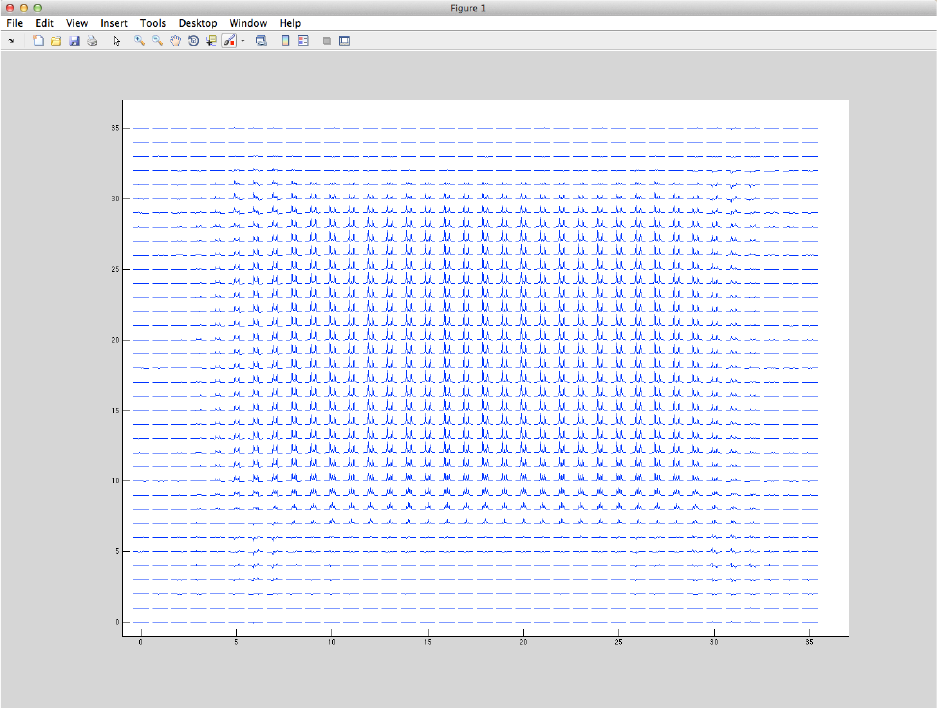
Figure 1: The output of run_make2DSimPlot, which shows simulated, spatially
resolved MEGA-PRESS difference spectra of the GABA spin system. This
simulation was generated using run_simMegaPressShaped, and it incorporates
the shaped editing and refocusing pulses. Only the 3ppm GABA resonance is
shown.
6.3. run_megapressproc.m
USAGE:
[out1_diff,out1_sum,out1,outw,coilcombos]=run_megapressproc(filestring,coilco
mbos,avgAlignDomain,alignSS);
DESCRIPTION:
Processing script for Siemens MEGA-PRESS MRS data in .dat format (twix raw
data). Includes combination of reciever channels, removal of bad averages,
freqeuncy drift correction, manual alignment of edit-on and edit-off spectra,
and leftshifting.
INPUTS:
filestring = String variable for the name of the directory containing
the water suppressed .dat file. Water unsuppressed .dat
file should be contained in [filestring '_w/'];
coilcombos = (Optional). A structure obtained by running the
op_getcoilcombos function. This allows the user to
specify the coil phases and amplitudes as an input,
rather calculating these from the input data by
default.
avgAlignDomain = (Optional) Perform the spectral registration (drift
correction) using the full spectrum ('t'), or only a
limited frequency range ('f'). Default is 'f'.
alignSS = (Optional)
0 - Do not align the edit-on and edit-off subspectra
(default).
2 - Perform manual alignment of edit-on and edit-off
subspectra.
OUTPUTS:
out1_diff = Fully processed difference spectrum.
out1_sum = Fully processed sum spectrum.
out1 = Fully processed edit-on and edit-off subspectra.
outw = Fully processed water unsuppressed spectrum.
coilcombos = Estimated coil weights and phases.
6.4. run_megapressproc_GEauto.m
USAGE:
[diffSpec,sumSpec,subSpec1,subSpec2,outw]=run_megapressproc_GEauto(filestring
,coilcombos,avgAlignDomain,alignSS);
DESCRIPTION:
Fully automated processing script for GE MEGA-PRESS MRS data in P-file format
(GE raw data). Includes combination of reciever channels, removal of bad
averages, freqeuncy drift correction, manual alignment of edit-on and edit-
off spectra, and leftshifting. This pipeline requires no user interaction.
This function automatically generates an html report to describe the results
of each processing step.
INPUTS:
filestring = String variable for the name of the P file.
coilcombos = (Optional). A structure obtained by running the
op_getcoilcombos function. This allows the user to
specify the coil phases and amplitudes as an input,
rather calculating these from the input data by default.
avgAlignDomain = (Optional) Perform the spectral registration (drift
correction) using the full spectrum ('t'), or only a
limited frequency range ('f'). Default is 'f'.
alignSS = (Optional)
0 - Do not align the edit-on and edit-off subspectra
(default).
2 - Perform manual alignment of edit-on and edit-off
subspectra.
OUTPUTS:
diffSpec = Fully processed difference spectrum.
sumSpec = Fully processed sum spectrum.
subSpec1 = Fully processed MEGA-PRESS subspectrum #1.
subSpec2 = Fully processed MEGA-PRESS subspectrum #2.
outw = Fully processed water unsuppressed spectrum.
6.5. run_megapressproc_auto.m
USAGE:
[diffSpec,sumSpec,subSpec1,subSpec2]=run_megapressproc_auto(filestring,coilco
mbos,avgAlignDomain,alignSS);
DESCRIPTION:
Fully automated processing script for Siemens MEGA-PRESS MRS data in .dat
format (twix raw data). Includes combination of reciever channels, removal
of bad averages, freqeuncy drift correction, manual alignment of edit-on and
edit-off spectra, and leftshifting. This pipeline requires no user
interaction. This function automatically generates an html report to describe
the results of each processing step.
INPUTS:
filestring = String variable for the name of the directory containing
the water suppressed .dat file. Water unsuppressed .dat
file should be contained in [filestring '_w/'];
coilcombos = (Optional). A structure obtained by running the
op_getcoilcombos function. This allows the user to
specify the coil phases and amplitudes as an input,
rather calculating these from the input data by
default.
avgAlignDomain = (Optional) Perform the spectral registration (drift
correction) using the full spectrum ('t'), or only a
limited frequency range ('f'). Default is 'f'.
alignSS = (Optional)
0 - Do not align the edit-on and edit-off subspectra
(default).
2 - Perform manual alignment of edit-on and edit-off
subspectra.
OUTPUTS:
diffSpec = Fully processed difference spectrum.
sumSpec = Fully processed sum spectrum.
subSpec1 = Fully processed MEGA-PRESS subspectrum #1.
subSpec2 = Fully processed MEGA-PRESS subspectrum #2.
6.6. run_pressproc.m
USAGE:
[out,out_w,out_noproc,out_w_noproc]=run_pressproc(filestring,aaDomain,tmaxin,
iterin);
DESCRIPTION:
Processing script for Siemens PRESS MRS data in .dat format (twix raw data).
Includes combination of reciever channels, removal of bad averages, freqeuncy
drift correction, and leftshifting.
INPUTS:
filestring = String variable for the name of the directory containing the
water suppressed .dat file. Water unsuppressed .dat file
should be contained in [filestring '_w/'];
aaDomain = (Optional) Perform the spectral registration (drift
correction) using the full spectrum ('t'), or only a limited
frequency range ('f'). Default is 'f'.
tmaxin = (Optional). Duration (in sec.) of the time domain signal
used in the spectral registration (drift correction).
Default is 0.2 sec.
iterin = (Optional). Maximum number of allowed iterations for the
spectral registration to converge. Default is 20.
OUTPUTS:
out = Fully processed, water suppressed output spectrum.
out_w = Fully processed, water unsuppressed output spectrum.
out_noproc = Water suppressed output spectrum without pre-processing (No
bad-averages removal, no frequency drift correction).
out_w_noproc = Water unsuppressed output spectrum without pre-
processing.
6.7. run_pressproc_brukAuto.m
USAGE:
[out,out_w,out_noproc,out_w_noproc]=run_pressproc_brukAuto(filestring,
filestringw,aaDomain,tmaxin,iterin);
DESCRIPTION:
Fully automated processing script for Bruker PRESS MRS data in fid.raw
format (raw data). Processing steps include removal of bad averages,
frequency drift correction, leftshifting and auto-phasing. This pipeline
requires no user interaction. This function automatically generates an
html report to describe the results of each processing step.
INPUTS:
filestring = String variable for the name of the directory containing
the water suppressed fid.raw file.
filestringw = String variable for the name of the directory containing
the water unsuppressed fid.raw file.
aaDomain = (Optional) Perform the spectral registration (drift
correction) using the full spectrum ('t'), or only a limited
frequency range ('f'). Default is 'f'.
tmaxin = (Optional). Duration (in sec.) of the time domain signal
used in the spectral registration (drift correction).
Default is 0.2 sec.
iterin = (Optional). Maximum number of allowed iterations for the
spectral registration to converge. Default is 20.
OUTPUTS:
out = Fully processed, water suppressed output spectrum.
out_w = Fully processed, water unsuppressed output spectrum.
out_noproc = Water suppressed output spectrum without pre-
processing (No bad-averages removal, no frequency drift
correction).
out_w_noproc = Water unsuppressed output spectrum without pre-
processing.
6.8. run pressproc_GEauto.m
USAGE:
[out,out_w,out_noproc,out_w_noproc]=run_pressproc_GEauto(filestring,aaDomain,
tmaxin,iterin);
DESCRIPTION:
Fully automated processing script for GE PRESS MRS data in p-file format (GE
raw data). Includes combination of reciever channels, removal of bad
averages, freqeuncy drift correction, and leftshifting. This pipeline
requires no user interaction. This function automatically generates an html
report to describe the results of each processing step.
INPUTS:
filestring = String variable for the name of the p-file the water
suppressed data;
aaDomain = (Optional) Perform the spectral registration (drift
correction) using the full spectrum ('t'), or only a limited
frequency range ('f'). Default is 'f'.
tmaxin = (Optional). Duration (in sec.) of the time domain signal
used in the spectral registration (drift correction).
Default is 0.2 sec.
iterin = (Optional). Maximum number of allowed iterations for the
spectral registration to converge. Default is 20.
OUTPUTS:
out = Fully processed, water suppressed output spectrum.
out_w = Fully processed, water unsuppressed output spectrum.
out_noproc = Water suppressed output spectrum without pre-processing (No
bad-averages removal, no frequency drift correction).
out_w_noproc = Water unsuppressed output spectrum without pre-processing.
6.9. run_pressproc_auto.m
USAGE:
[out,out_w,out_noproc,out_w_noproc]=run_pressproc_auto(filestring,aaDomain,tm
axin,iterin);
DESCRIPTION:
Fully automated processing script for Siemens PRESS MRS data in .dat format
(twix raw data). Includes combination of reciever channels, removal of bad
averages, freqeuncy drift correction, and leftshifting. This pipeline
requires no user interaction. This function automatically generates an html
report to describe the results of each processing step.
INPUTS:
filestring = String variable for the name of the directory containing
the water suppressed .dat file. Water unsuppressed .dat file
should be contained in [filestring '_w/'];
aaDomain = (Optional) Perform the spectral registration (drift
correction) using the full spectrum ('t'), or only a limited
frequency range ('f'). Default is 'f'.
tmaxin = (Optional). Duration (in sec.) of the time domain signal
used in the spectral registration (drift correction).
Default is 0.2 sec.
iterin = (Optional). Maximum number of allowed iterations for the
spectral registration to converge. Default is 20.
OUTPUTS:
out = Fully processed, water suppressed output spectrum.
out_w = Fully processed, water unsuppressed output spectrum.
out_noproc = Water suppressed output spectrum without pre-processing (No
bad-averages removal, no frequency drift correction).
out_w_noproc = Water unsuppressed output spectrum without pre-processing.
6.10. run_simExampleBasisSet.m
USAGE:
This script is run simply by editing the input parameters and then clicking
"Run".
DESCRIPTION:
Script to generate simulated basis spectra for all metabolites of interest in
the human brain. The script will generate an LCModel format .RAW file for
each metabolite basis spectrum, which can then be passed into LCModel's
"makebasis" function to generate a complete LCModel basis set.
INPUTS:
To run this script, edit the following parameters as desired and then click
run:
lb = linewidth (Hz)
np = Spectral points
sw = Spectral width (Hz)
Bo = Magnetic Field Strength (Tesla)
te1 = First PRESS echo time, or SPECIAL echo time (s)
te2 = Second PRESS echo time (if applicable) (s).
seq = Pulse sequence ('se'= SPECIAL, 'p'=press, 'st'=steam);
ref = Add reference peak at 0ppm (used in LCModel, y or n);
OUTPUTS:
H2O = Simulated water spectrum
Ala = Simulated alanine spectrum
Asp = Simulated aspartate spectrum
PCh = Simulated phosphocholine spectrum
Cr = Simulated creatine spectrum
PCr = Simulated phosphochreatine spectrum
GABA = Simulated GABA spectrum
Gln = Simulated glutamine spectrum
Glu = Simulated glutamate spectrum
GSH = Simulated glutathione spectrum
Gly = Simulated glycine spectrum
Ins = Simulated myo-inositol spectrum
Lac = Simulated Lactate spectrum
NAA = Simulated NAA spectrum
Scyllo = Simulated scyllo-inositol spectrum
Tau = Simulated taurine spectrum
Asc = Simulated ascorbate spectrum
bHB = Simulated beta-hydroxybutyrate spectrum
bHG = Simulated 2-hydroxyglutyrate spectrum
Glc = Simulated glucose spectrum
NAAG = Simulated N-acetylaspartylglutamate spectrum
GPC = Simulated glycerophosphocholine spectrum
PE = Simulated phosphoethanolamine spectrum
Ser = Simulated serine spectrum
************INPUT PARAMETERS**********************************
6.11. run_simMegaExTEShaped.m
USAGE:
This script is run simply by editing the input parameters and then clicking
"Run".
DESCRIPTION:
This script simulates an ExTE-MEGA-PRESS experiment with fully shaped editing
and refocusing pulses. Phase cycling of both the editing and refocusing
pulses is performed. Simulations are run at various locations in space to
account for the within-voxel spatial variation of the GABA signal. Summation
across phase cycles and spatial positions is performed. As a result of the
phase cycling and spatially resolved simulations, this code takes a long time
to run. Therefore, the MATLAB parallel computing toolbox (parfor loop) was
used to accelerate the siumulations. Accelration is currently performed in
the direction of the slice selective pulse along the x-direction, but this
can be changed. Up to a factor of 12 acceleration can be achieved using this
approach. To enable the use of the MATLAB parallel computing toolbox,
initialize the multiple worked nodes using "matlabpool size X" where "X" is
the number of available processing nodes. If the parallel processing toolbox
is not available, then replace the "parfor" loop with a "for" loop.
INPUTS:
To run this script, edit the parameters below as desired and then click
"run":
refocWaveform = name of refocusing pulse waveform.
editWaveform = name of editing pulse waveform.
editOnFreq = freqeucny of edit on pulse[ppm]
editOffFreq = frequency of edit off pulse[ppm]
refTp = duration of refocusing pulses[ms]
editTp = duration of editing pulses[ms]
Bfield = Magnetic field strength in [T]
Npts = number of spectral points
sw = spectral width [Hz]
Bfield = magnetic field strength [Tesla]
lw = linewidth of the output spectrum [Hz]
thkX = slice thickness of x refocusing pulse [cm]
thkY = slice thickness of y refocusing pulse [cm]
x = vector of X positions to simulate [cm]
y = vector of y positions to simulate [cm]
taus = vector of pulse sequence timings [ms]
spinSys = spin system to simulate
editPhCyc1 = vector of phase cycling steps for 1st editing pulse
[degrees]
editPhCyc2 = vector of phase cycling steps for 2nd editing pulse
[degrees]
refPhCyc1 = vector of phase cycling steps for 1st refocusing pulse
[degrees]
refPhCyc2 = vector of phase cycling steps for 2nd refocusing pulse
[degrees]
OUTPUTS:
outON_posxy = Simulated ExTE-MEGA-PRESS edit-ON spectrum, spatially
resolved.
outOFF_posxy = Simulated ExTE-MEGA-PRESS edit-OFF spectrum, spatially
resolved.
outDIFF_posxy = Simulated ExTE-MEGA-PRESS difference spectrum, spatially
resolved.
outON = Simulated ExTE-MEGA-PRESS edit-ON spectrum, summed over
all positions.
outOFF = Simulated ExTE-MEGA-PRESS edit-OFF spectrum, summed over
all positions.
outDIFF = Simulated ExTE-MEGA-PRESS difference spectrum, summed
over all positions.
6.12. run_simMegaPressShaped.m
USAGE:
This script is run simply by editing the input parameters and then clicking
"Run".
DESCRIPTION:
This script simulates a MEGA-PRESS experiment with fully shaped editing and
refocusing pulses. Phase cycling of both the editing and refocusing pulses
is performed. Simulations are run at various locations in space to account
for the within-voxel spatial variation of the GABA signal. Summation across
phase cycles and spatial positions is performed. As a result of the phase
cycling and spatially resolved simulations, this code takes a long time to
run. Therefore, the MATLAB parallel computing toolbox (parfor loop) was used
to accelerate the siumulations. Accelration is currently performed in the
direction of the slice selective pulse along the x-direction, but this can be
changed. Up to a factor of 12 acceleration can be achieved using this
approach. To enable the use of the MATLAB parallel computing toolbox,
initialize the multiple worked nodes using "matlabpool size X" where "X" is
the number of available processing nodes. If the parallel processing toolbox
is not available, then replace the "parfor" loop with a "for" loop.
INPUTS:
To run this script, edit the parameters below as desired and then click
"run":
refocWaveform = name of refocusing pulse waveform.
editWaveform = name of editing pulse waveform.
editOnFreq = freqeucny of edit on pulse[ppm]
editOffFreq = frequency of edit off pulse[ppm]
refTp = duration of refocusing pulses[ms]
editTp = duration of editing pulses[ms]
Bfield = Magnetic field strength in [T]
Npts = number of spectral points
sw = spectral width [Hz]
Bfield = magnetic field strength [Tesla]
lw = linewidth of the output spectrum [Hz]
thkX = slice thickness of x refocusing pulse [cm]
thkY = slice thickness of y refocusing pulse [cm]
x = vector of X positions to simulate [cm]
y = vector of y positions to simulate [cm]
taus = vector of pulse sequence timings [ms]
spinSys = spin system to simulate
editPhCyc1 = vector of phase cycling steps for 1st editing pulse
[degrees]
editPhCyc2 = vector of phase cycling steps for 2nd editing pulse
[degrees]
refPhCyc1 = vector of phase cycling steps for 1st refocusing pulse
[degrees]
refPhCyc2 = vector of phase cycling steps for 2nd refocusing pulse
[degrees]
OUTPUTS:
outON_posxy = Simulated MEGA-PRESS edit-ON spectrum, spatially
resolved.
outOFF_posxy = Simulated MEGA-PRESS edit-OFF spectrum, spatially
resolved.
outDIFF_posxy = Simulated MEGA-PRESS difference spectrum, spatially
resolved.
outON = Simulated MEGA-PRESS edit-ON spectrum, summed over
all positions.
outOFF = Simulated MEGA-PRESS edit-OFF spectrum, summed over
all positions.
outDIFF = Simulated MEGA-PRESS difference spectrum, summed over
all positions.
6.13. run_simMegaPressShapedEdit.m
USAGE:
This script is run simply by editing the input parameters and then clicking
"Run".
DESCRIPTION:
This script simulates a MEGA-PRESS experiment with fully shaped editing
pulses. Phase cycling of editing pulses is performed, and summation across
phase cycles is performed.
INPUTS:
To run this script, edit the parameters below as desired and then click
"run":
editWaveform = name of editing pulse waveform.
editOnFreq = freqeucny of edit on pulse[ppm]
editOffFreq = frequency of edit off pulse[ppm]
editTp = duration of editing pulses[ms]
Npts = number of spectral points
sw = spectral width [Hz]
Bfield = magnetic field strength [Tesla]
lw = linewidth of the output spectrum [Hz]
taus = vector of pulse sequence timings [ms]
spinSys = spin system to simulate
editPhCyc1 = vector of phase cycling steps for 1st editing pulse
[degrees]
editPhCyc2 = vector of phase cycling steps for 2nd editing pulse
[degrees]
OUTPUTS:
outON = Simulated MEGA-PRESS edit-ON spectrum.
outOFF = Simulated ExTE-MEGA-PRESS edit-OFF spectrum.
outDIFF = Simulated ExTE-MEGA-PRESS difference spectrum.
6.14. run_simMegaPressShapedRefoc.m
USAGE:
This script is run simply by editing the input parameters and then clicking
"Run".
DESCRIPTION:
This script simulates a MEGA-PRESS experiment with fully shaped refocusing
pulses. Phase cycling of the refocusing pulses is performed and simulations
are run at various locations in space to account for the within-voxel spatial
variation of the GABA signal. Summation across spatial positions is
performed. As a result of the phase cycling and spatially resolved
simulations, this code takes a long time to run. Therefore, the MATLAB
parallel computing toolbox (parfor loop) is used to accelerate the
siumulations. Acceleration is currently performed in the direction of the
slice selective pulse along the x-direction, but this can be changed. Up to
a factor of 12 acceleration can be achieved using this approach. To enable
the use of the MATLAB parallel computing toolbox, initialize the multiple
worked nodes using "matlabpool size X" where "X" is the number of available
processing nodes. If the parallel processing toolbox is not available, then
replace the "parfor" loop with a "for" loop.
INPUTS:
To run this script, edit the parameters below as desired and then click
"run":
refocWaveform = name of refocusing pulse waveform.
refTp = duration of refocusing pulses[ms]
Npts = number of spectral points
sw = spectral width [Hz]
Bfield = magnetic field strength [Tesla]
lw = linewidth of the output spectrum [Hz]
thkX = slice thickness of x refocusing pulse [cm]
thkY = slice thickness of y refocusing pulse [cm]
x = vector of X positions to simulate [cm]
y = vector of y positions to simulate [cm]
taus = vector of pulse sequence timings [ms]
spinSys = spin system to simulate
editFlipON = vector of edit-ON pulse flip angles for each spin in
spin system.
editFlipOFF = vector of edit-OFF pulse flip angles for each spin in
spin system.
refPhCyc1 = vector of phase cycling steps for 1st refocusing
pulse [degrees]
refPhCyc2 = vector of phase cycling steps for 2nd refocusing
pulse [degrees]
OUTPUTS:
outON_posxy = Simulated MEGA-PRESS edit-ON spectrum, spatially
resolved.
outOFF_posxy = Simulated MEGA-PRESS edit-OFF spectrum, spatially
resolved.
outDIFF_posxy = Simulated MEGA-PRESS difference spectrum, spatially
resolved.
outON = Simulated MEGA-PRESS edit-ON spectrum, summed over
all positions.
outOFF = Simulated MEGA-PRESS edit-OFF spectrum, summed over
all positions.
outDIFF = Simulated MEGA-PRESS difference spectrum, summed over
all positions.
6.15. run_simMegaSpecialShaped.m
USAGE:
This script is run simply by editing the input parameters and then clicking
"Run".
DESCRIPTION:
This script simulates a MEGA-SPECIAL experiment with fully shaped editing and
refocusing pulses. Phase cycling of both the editing and refocusing pulses
is performed. Furthermore, simulations are run at various locations in space
to account for the within-voxel spatial variation of the GABA signal.
Summation across phase cycles and spatial positions is performed. As a
result of the phase cycling and spatially resolved simulations, this code
takes a long time to run. Therefore, the MATLAB parallel computing toolbox
(parfor loop) was used to accelerate the siumulations. Accelration is
performed in the direction of the slice selective pulse (along the x-
direction). Up to a factor of 12 acceleration can be achieved using this
approach. To enable the use of the MATLAB parallel computing toolbox,
initialize the multiple worked nodes using "matlabpool size X" where "X" is
the number of available processing nodes. If the parallel processing toolbox
is not available, then replace the "parfor" loop with a "for" loop.
INPUTS:
To run this script, edit the parameters below as desired and then click
"run":
refocWaveform = name of refocusing pulse waveform.
editWaveform = name of editing pulse waveform.
editOnFreq = freqeucny of edit on pulse[ppm]
editOffFreq = frequency of edit off pulse[ppm]
refTp = duration of refocusing pulses[ms]
editTp = duration of editing pulses[ms]
Bfield = Magnetic field strength in [T]
Npts = number of spectral points
sw = spectral width [Hz]
Bfield = magnetic field strength [Tesla]
lw = linewidth of the output spectrum [Hz]
thkX = slice thickness of x refocusing pulse [cm]
x = vector of X positions to simulate [cm]
taus = vector of pulse sequence timings [ms]
spinSys = spin system to simulate
editPhCyc1 = vector of phase cycling steps for 1st editing pulse
[degrees]
editPhCyc2 = vector of phase cycling steps for 2nd editing pulse
[degrees]
refPhCyc = vector of phase cycling steps for 1st refocusing pulse
[degrees]
OUTPUTS:
outON_posx = Simulated MEGA-SPECIAL edit-ON spectrum, spatially
resolved.
outOFF_posx = Simulated MEGA-SPECIAL edit-OFF spectrum, spatially
resolved.
outDIFF_posx = Simulated MEGA-SPECIAL difference spectrum, spatially
resolved.
outON = Simulated MEGA-SPECIAL edit-ON spectrum, summed over
all positions.
outOFF = Simulated MEGA-SPECIAL edit-OFF spectrum, summed over
all positions.
outDIFF = Simulated MEGA-SPECIAL difference spectrum, summed over
all positions.
6.16. run_simPressShaped.m
USAGE:
This script is run simply by editing the input parameters and then clicking
"Run".
DESCRIPTION:
This script simulates a PRESS experiment with fully shaped refocusing pulses.
Phase cycling of refocusing pulses is performed. Furthermore, simulations
are run at various locations in space to account for the within-voxel spatial
variation of the metabolite signal. Summation across phase cycles and
spatial positions is performed. As a result of the phase cycling and
spatially resolved simulations, this code takes a long time to run.
Therefore, the MATLAB parallel computing toolbox (parfor loop) was used to
accelerate the siumulations. Acceleration is currently performed in the
direction of the slice selective pulse along the x-direction, but this can be
changed. Up to a factor of 12 acceleration can be achieved using this
approach. To enable the use of the MATLAB parallel computing toolbox,
initialize the multiple worked nodes using "matlabpool size X" where "X" is
the number of available processing nodes. If the parallel processing toolbox
is not available, then replace the "parfor" loop with a "for" loop.
INPUTS:
To run this script, edit the parameters below as desired and then click
"run":
refocWaveform = name of refocusing pulse waveform.
refTp = duration of refocusing pulses[ms]
Bfield = Magnetic field strength in [T]
Npts = number of spectral points
sw = spectral width [Hz]
Bfield = magnetic field strength [Tesla]
lw = linewidth of the output spectrum [Hz]
thkX = slice thickness of x refocusing pulse [cm]
thkY = slice thickness of y refocusing pulse [cm]
x = vector of X positions to simulate [cm]
y = vector of y positions to simulate [cm]
taus = vector of pulse sequence timings [ms]
spinSys = spin system to simulate
refPhCyc1 = vector of phase cycling steps for 1st refocusing pulse
[degrees]
refPhCyc2 = vector of phase cycling steps for 2nd refocusing pulse
[degrees]
OUTPUTS:
out_posxy = Simulation results, spatially resolved.
out = Simulation results, summed over all space.
6.17. run_simSpinEchoShaped.m
USAGE:
This script is run simply by editing the input parameters and then clicking
"Run".
DESCRIPTION:
This script simulates a localized spin-echo experiment with a fully shaped
refocusing pulse. Phase cycling of the refocusing pulse is performed.
Furthermore, simulations are run at various locations in space (1-D) to
account for the within-voxel spatial variation of the metabolite signal due
to J-evolution. Summation across phase cycles and spatial positions is
performed. As a result of the phase cycling and spatially resolved
simulations, this code takes a long time to run. Therefore, the MATLAB
parallel computing toolbox (parfor loop) was used to accelerate the
siumulations. Accelration is performed in the direction of the slice
selective refocusing pulse. Up to a factor of 12 acceleration can be achieved
using this approach. To enable the use of the MATLAB parallel computing
toolbox, initialize the multiple worked nodes using "matlabpool size X" where
"X" is the number of available processing nodes. If the parallel processing
toolbox is not available, then replace the "parfor" loop with a "for" loop.
INPUTS:
To run this script, edit the parameters below as desired and then click
"run":
RFWaveform = name of refocusing pulse waveform.
Tp = duration of refocusing pulses[ms]
Bfield = Magnetic field strength in [T]
Npts = number of spectral points
sw = spectral width [Hz]
lw = linewidth of the output spectrum [Hz]
thk = slice thickness of refocusing pulse [cm]
pos = vector of positions to simulate [cm]
TE = Echo-Time [ms]
spinSys = spin system to simulate
PhCyc = vector of phase cycling steps for refocusing pulse
[degrees]
OUTPUTS:
out_pos = Simulation results, spatially resolved.
out = Simulation results, summed over all space.
6.18. run_specialproc.m
USAGE:
[out,out_w,out_noproc,out_w_noproc]=run_specialproc(filestring,aaDomain,tmaxi
n,iterin);
DESCRIPTION:
Processing script for Siemens SPECIAL MRS data in .dat format (twix raw
data). Includes combination of reciever channels, removal of bad averages,
freqeuncy drift correction, and leftshifting.
INPUTS:
filestring = String variable for the name of the directory containing the
water suppressed .dat file. Water unsuppressed .dat file
should be contained in [filestring '_w/'];
aaDomain = (Optional) Perform the spectral registration (drift
correction) using the full spectrum ('t'), or only a limited
frequency range ('f'). Default is 'f'.
tmaxin = (Optional). Duration (in sec.) of the time domain signal
used in the spectral registration (drift correction).
Default is 0.2 sec.
iterin = (Optional). Maximum number of allowed iterations for the
spectral registration to converge. Default is 20.
OUTPUTS:
out = Fully processed, water suppressed output spectrum.
out_w = Fully processed, water unsuppressed output spectrum.
out_noproc = Water suppressed output spectrum without pre-processing (No
bad-averages removal, no frequency drift correction).
out_w_noproc = Water unsuppressed output spectrum without pre-processing.
6.19. run_specialproc_auto.m
USAGE:
[out,out_w,out_noproc,out_w_noproc]=run_specialproc_auto(filestring,aaDomain,
tmaxin,iterin);
DESCRIPTION:
Processing script for Siemens SPECIAL MRS data in .dat format (twix raw
data). Includes combination of reciever channels, removal of bad averages,
freqeuncy drift correction, and leftshifting.
INPUTS:
filestring = String variable for the name of the directory containing
the water suppressed .dat file. Water unsuppressed.dat file
should be contained in [filestring '_w/'];
aaDomain = (Optional) Perform the spectral registration (drift
correction) using the full spectrum ('t'), or only a limited
frequency range ('f'). Default is 'f'.
tmaxin = (Optional). Duration (in sec.) of the time domain signal
used in the spectral registration (drift correction).
Default is 0.2 sec.
iterin = (Optional). Maximum number of allowed iterations for the
spectral registration to converge. Default is 20.
OUTPUTS:
out = Fully processed, water suppressed output spectrum.
out_w = Fully processed, water unsuppressed output spectrum.
out_noproc = Water suppressed output spectrum without pre-processing (No
bad-averages removal, no frequency drift correction).
out_w_noproc = Water unsuppressed output spectrum without pre-processing.
6.20. run_specialproc_fmrs.m
USAGE:
[out_stimOFF,out_stimON,out_w]=run_specialproc_fmrs(filestring,blockDesign,le
adingAvgsToRmv);
DESCRIPTION:
Processing script for functional MRS data acquired using the SPECIAL MRS
sequence. This script accepts data in Siemens .dat format (twix raw data).
Processing steps include combination of reciever channels, removal of bad
averages, freqeuncy drift correction, and leftshifting. Also includes prior
knowledge of the stimulation paradigm (given by the 'blockDesign’ vector) and
returns the averaged stimulus OFF and simulus ON spectra.
INPUTS:
filestring = String variable for the name of the directory containing
the water suppressed .dat file. Water unsuppressed .dat
file should be contained in [filestring '_w/'];
blockDesign = This is a vector of positive and negative even integers
that make up the ON/OFF block design. Each integer
represents the number of sequential averages in a block.
Positive integers refer to ON blocks, and negative
integers refer to OFF blocks. For example, for a block
design consisting of 30 OFF averages followed by 20 ON
averages followed by 10 OFF averages, the blockDesign
vector would be: [-30 20 -10];
leadingAvgsToRmv = The number of averages to omit from the beginning of
each block. This is done to account for a lag in the
neurochemical response to stimulus. Must be an even
integer. (optional. Default=0);
OUTPUTS:
out_stimOFF = Fully processed water suppressed spectrum from the sum
of the stimulus OFF periods.
out_stimON = Fully processed water suppressed spectrum from the sum
of the stimulus ON periods.
out_w = Fully processed, water unsuppressed output spectrum.
6.21. run_specialproc_fmrs_slidingWindow.m
USAGE:
[out1,out_w]=run_specialproc_fmrs_slidingWindow(filestring,windowSize);
DESCRIPTION:
Processing script for functional MRS data acquired using the SPECIAL MRS
sequence. This script accepts data in Siemens .dat format (twix raw data).
Processing steps include combination of reciever channels, removal of bad
averages, freqeuncy drift correction, and leftshifting. This code generates
a 'sliding window timecourse' of MR spectra by combining the averages within
a small window given by the windowSize argument, and then sliding the window
by 1 average and combining again. Each summed window is output as an LCModel
text file to be analyzed in LCModel. As a result, this function generates
many text output files.
INPUTS:
filestring = String variable for the name of the directory containing
the water suppressed .dat file. Water unsuppressed .dat
file should be contained in [filestring '_w/'];
windowSize = This is an integer that specifies the number of averages
that are stored within the sliding window. It is
recommended to choose a window size that is divisible by
the number of phase cycles so that the window does not
contain any partial phase cycles.
OUTPUTS:
out1 = The first sliding window spectrum (the others are written
to LCModel format).
out_w = Fully processed, water unsuppressed output spectrum.
7. Graphical User Interfaces (GUIs)
Although the FID-A software package is primarily a MATLAB
command-line software application, it does contain a three GUI
based tools to enable visual manipulation of MR spectra. The
three GUI based tools are called DiffTool, SpecTool and
subSpecTool, and they can be found in the {FID-
A_DIR}/processingTools/SpecTool/ Directory. A brief description
of each tool is given below:
7.1. DiffTool
The DiffTool Gui is used to visualize at the difference between
two spectra, while interactively controlling the relative
frequency, phase (0th and 1st order), amplitude, and DC offset
between them. This tool is useful to enable subtraction of two
spectra whilst minimizing subtraction errors due to frequency
and phase shifts, etc. The DiffTool GUI is called in the
following way:
DiffTool(in1,in2,ppmmin,ppmmax);
Where in1 and in2 are the two spectra to be subtracted, and
ppmmin and ppmmax are the minimum and maximum frequencies over
which to display the result. The DiffTool GUI is shown in Figure
2, below.
Figure 2: The DiffTool GUI.
7.2. SpecTool
The SpecTool GUI is enables adjustment of the 0th and 1st order
phase of the spectrum, while providing real-time visual feedback
of both the time-domain and frequency-domain signals. The
SpecTool GUI is called in the following way:
SpecTool(in,tmax,ppmmin,ppmmax);
Where in is the input spectrum, tmax is the maximum time over
which to display the result in the time domain, and ppmmin and
ppmmax are the minimum and maximum frequencies over which to
display the result in the frequency domain. The SpecTool GUI is
shown in Figure 3 below.
Figure 3: The SpecTool GUI.
7.3. subSpecTool
The subSpecTool GUI is used to visualize at the difference
between two subspectra of an edited MRS scan, while
interactively controlling the relative frequency and phase (0th
order only), between them. This tool is useful to enable
subtraction of two subspectra whilst minimizing subtraction
errors due to frequency and phase shifts, etc. The subSpecTool
GUI is called in the following way:
subSpecTool(in,ppmmin,ppmmax);
Where in is the input spectrum, and ppmmin and ppmmax are the
minimum and maximum frequencies over which to display the result
in the frequency domain. The subSpecTool GUI is shown in Figure 4
below.
Figure 4: The subSpecTool GUI.
8. Processing the Example Data
As mentioned above, the FID-A toolkit comes with examples of raw
MRS data (both
in vivo
and
in vitro
) from a few different
scanner vendors (Bruker, GE and Siemens), and a few different
pulse sequences (PRESS, MEGA-PRESS and SPECIAL). These datasets
can be processed using some of scripts provided in the {FID-
A_dir}/exampleRunScripts directory. Please note that the
Example Data are contained in relatively large files that could
not be stored normally in the GitHub repository due to GitHub’s
native file size limitations. Therefore, in order to download
these data, you must first download and install the “Large File

Storage” (LFS) extension to GitHub, which can be found here:
(https://git-lfs.github.com). Without this extension, a clone
or download of the FID-A repository will result in a {FID-
A_dir}/exampleData directory that is empty. However, after
you’ve downloaded and installed the LFS extension, then re-
cloning or downloading the FID-A repository should result in a
{FID-A_dir}/exampleData folder that correctly contains the
required example data. Below are some quick examples of how to
use the ExampleRunScripts to process the Example Data provided.
8.1. Processing GE PRESS data
The {FID-A_dir}/exampleData/GE/sample01_press directory contains
a P file from a PRESS MRS scan in a brain tissue mimicking
phantom on a 3 Tesla GE MRI scanner. As is commonplace with GE
datasets, both the water suppressed and water unsuppressed data
are contained within the same file. This dataset can be
processed using the ‘run_pressproc_GEauto.m’ script as follows:
1. Open MATLAB and add the FID-A repository to your path
using:
addpath(genpath(‘Enter full path to FID_A directory’));
2. Inside MATLAB, navigate to the {FID-
A_dir}/exampleData/GE/sample01_press/press directory. Note
that this folder contains the desired P file, which is
called ‘P17920.7’.
3. Run the example Run script ‘run_pressproc_GEauto.m’ by
typing the following:
[out,out_w]=run_pressproc_GEauto(‘P17920.7’);
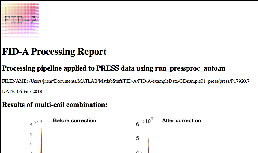
The script should run to completion within about 10 seconds
with no user input, and two new structures (out and out_w)
should appear in your workspace. These are the fully processed
water suppressed (out) and water unsuppressed datasets (out_w).
You can plot the resulting spectra using:
op_plotspec(out);
and
op_plotspec(out_w);
In addition to these outputs, the script should also
generate a new folder called “report” in which you will find an
HTML file (report.html, Figure 5) that summarizes the results of
the various stages of the processing pipeline. This should be
viewable using any standard HTML viewer or internet browser.
Figure 5: The report file generated by run_pressproc_GEauto.
Finally, you will also notice that in the working
directory, two new files are generated: “P17920.7_lcm” and
“P17920.7_w_lcm”. These are the processed water suppressed and
water unsuppressed data files, respectively, in LCModel raw
format. These files can be imported immediately for analysis in
LCModel or Tarquin.
8.2. Processing GE MEGA-PRESS data
The {FID-A_dir}/exampleData/GE/sample02_megapress directory
contains a P file from a GABA-edited MEGA-PRESS MRS scan in a
brain tissue mimicking phantom on a 3 Tesla GE MRI scanner.
Once again, both the water suppressed and water unsuppressed
data are contained within the same file. This dataset can be
processed using the ‘run_megapressproc_GEauto.m’ script as
follows (this time assuming that MATLAB is already open and that
FID-A is already on your path):
1. Navigate into the {FID-
A_dir}/exampleData/GE/sample02_megapress/megapress
directory. Note that this directory contains a GE P file
called ‘21504.7’.
2. Run the example Run script ‘run_megapressproc_GEauto.m’ by
typing the following:
[diff,sum,on,off,out_w]=run_megapressproc_GEauto(‘P21504.7’);
Again, the script should run to completion within about 10
seconds with no user input. This time, five new structures
(diff, sum, on, off and out_w) should appear in your workspace.
These are the fully processed difference spectrum (diff) sum
spectrum (sum), edit-on spectrum (on), edit-off spectrum (off)
and water unsuppressed spectrum (out_w). You can plot the
resulting spectra using:
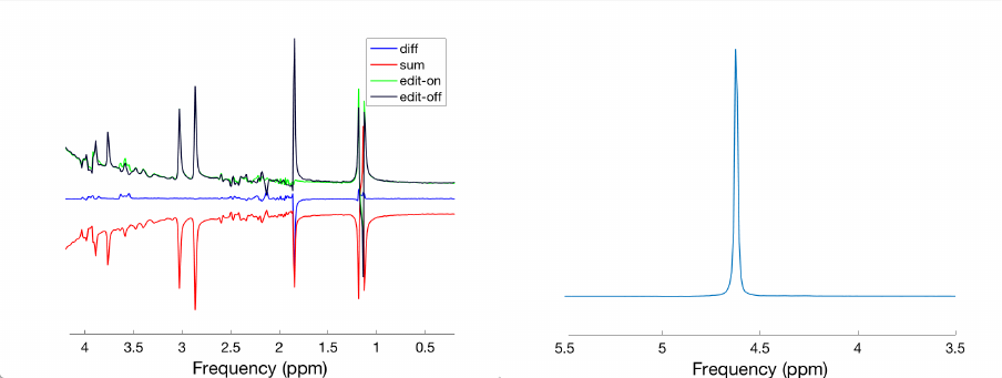
op_plotspec({diff,sum,on,off},0.2,4.2);
legend(‘diff’,’sum’,’on’,’off’);
and
op_plotspec(out_w,3.5,5.5);
Note that there is no edited peak in the difference
spectrum at 3.0 ppm, because the phantom that we used does not
contain GABA (See Figure 6. oops!!). Also note that the ‘sum’
spectrum is out of phase. This can be fixed with a simple
phasing operation such as ‘op_autophase.m’ or ‘op_addphase.m’.
Like before, this script also generates a new folder called
“report” in which you will find an HTML file (report.html) that
summarizes the results of the various stages of the processing
pipeline. This should be viewable using any standard HTML
viewer or internet browser.
Figure 6: Example GE MEGA-PRESS data, processed using
‘run_megapressproc_GEauto.m’.
Finally, you will again notice that in the working directory,
four new files are generated: “P21504.7_diff_lcm”,
“P21504.7_editON_lcm”, “P21504.7_editOFF_lcm” and
“P17920.7_w_lcm”. These are the processed spectra in LCModel
raw format, which can be imported immediately for analysis in
LCModel or Tarquin.
8.3. Processing Siemens MEGA-PRESS data
The {FID-A_dir}/exampleData/Siemens/sample01_megapress directory
contains two subfolders: one called “megapress”, which contains
an
in vivo
GABA-edited MEGA-PRESS MRS scan, and one called
“megapress_w”, which contains corresponding water unsuppressed
data acquired from the same region of interest. Both are from
the dorsolateral prefrontal cortex of a healthy human volunteer
3 Tesla Siemens MRI scanner. This dataset can be processed
using the ‘run_megapressproc_auto.m’ script as follows (this
time assuming that you have already opened MATLAB and that {FID-
A_dir} is already on your path):
1. Inside MATLAB, navigate to the {FID-
A_dir}/exampleData/Siemens/sample01_megapress directory.
Note that this folder contains two directories: one called
“megapress” and one called “megapress_w”. The former
contains the Siemens raw twix file (in .dat format)
corresponding to the water suppressed MEGA-PRESS scan,
while the latter contains the corresponding water
unsuppressed data in the same format. In order for
“run_megapressproc_auto.m” to work properly, the water
suppressed and water unsuppressed .dat files must be stored
in separate folders, and the folder names must differ only
by the ‘_w’ extension at the end of the water unsuppressed
folder name.
2. From the sample01_megapress directory, run the example Run
script ‘run_megapressproc_auto.m’ by typing the following:
[diff,sum,on,off]=run_megapressproc_auto(‘megapress’);
Note that the argument to the ‘run_megapressproc_auto’
function, ‘megapress’, is the name of the directory where the
water suppressed data is kept. Now, the script should run to
completion within about one minute with no user input. This
time, four new structures (diff, sum, on, and off) should appear
in your workspace. These are the fully processed difference
spectrum (diff) sum spectrum (sum), edit-on spectrum (on), and
edit-off spectrum (off). You can plot the resulting spectra
using:
op_plotspec({diff,sum,on,off},0.2,4.2);
This time note the presence of the GABA peak in the
difference spectrum at 3.0 ppm, since this data was collected in
a healthy human brain (See Figure 7). Like before, this script
also generates a new folder called “report” in which you will
find an HTML file (report.html) that summarizes the results of
the various stages of the processing pipeline. This should be
viewable using any standard HTML viewer or internet browser.
Finally, you will again notice that in the ‘megapress’
directory, three new files are generated: “megapress_diff_lcm”,
“megapress_editON_lcm”, and “megapress_editOFF_lcm”, while in
the ‘megapress_w’ directory, one new file (“megapress_w_lcm”) is
generated. These are the processed spectra in LCModel raw
format, which can be imported immediately for analysis in
LCModel or Tarquin.
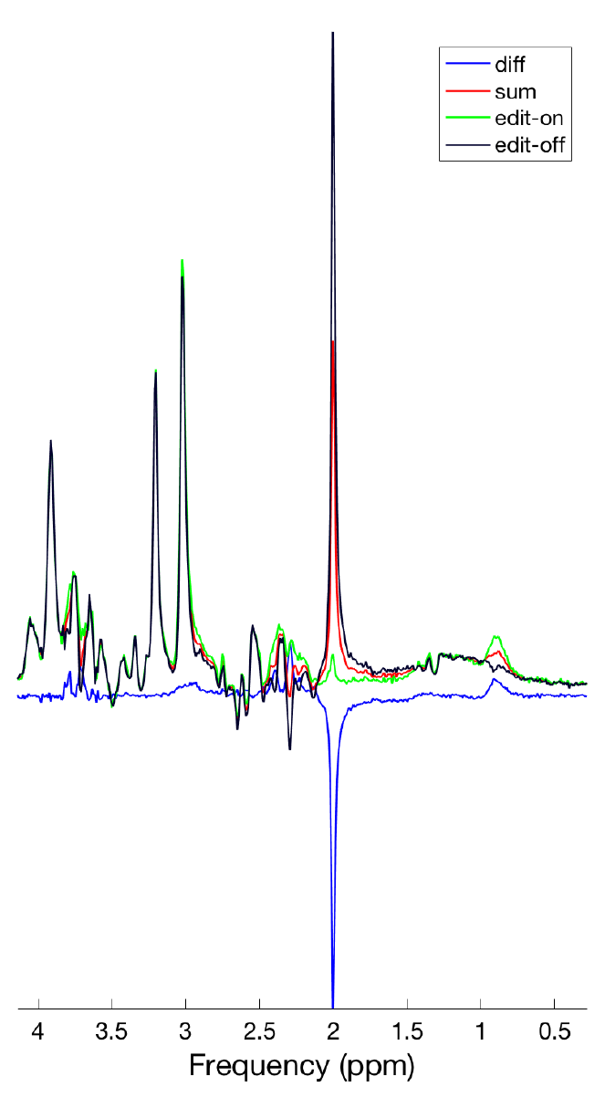
Figure 7: Example Siemens MEGA-PRESS data, processed using
run_megapressproc_auto.m .
8.4. Processing Siemens SPECIAL data
The {FID-A_dir}/exampleData/Siemens/sample02_special directory
contains two subfolders: one called “special”, which contains
an
in vivo
short-TE SPECIAL MRS scan, and one called
“special_w”, which contains corresponding water unsuppressed
data acquired from the same region of interest. Both are from
the dorsolateral prefrontal cortex of a healthy human volunteer
3 Tesla Siemens MRI scanner. This dataset can be processed
using the ‘run_specialproc_auto.m’ script as follows (this time
assuming that you have already opened MATLAB and that {FID-
A_dir} is already on your path):
1. Inside MATLAB, navigate to the {FID-
A_dir}/exampleData/Siemens/sample02_special directory.
Note that this folder contains two directories: one called
“special” and one called “special_w”. The former contains
the Siemens raw twix file (in .dat format) corresponding to
the water suppressed SPECIAL scan, while the latter
contains the corresponding water unsuppressed data in the
same format. In order for “run_specialproc_auto.m” to work
properly, the water suppressed and water unsuppressed .dat
files must be stored in separate folders, and the folder
names must differ only by the ‘_w’ extension at the end of
the water unsuppressed folder name.
2. From the sample01_special directory, run the example Run
script ‘run_specialproc_auto.m’ by typing the following:
[out,out_w]=run_specialproc_auto(‘special’);
Note that the argument to the ‘run_special_auto’ function,
‘special’, is the name of the directory where the water
suppressed data is kept. Now, the script should run to
completion within about one minute with no user input. This
time, two new structures (out, and out_w) should appear in your
workspace. These are the fully processed water suppressed
spectrum (out), and water unsuppressed spectrum (out_w). You
can plot the resulting spectra using:
op_plotspec(out,0.2,4.2);
and
op_plotspec(out_w,3.5,5.5);
Figure 8 shows the results of the above plot commands. The
plot of the water suppressed data shows the metabolite peaks,
while the plot of the water unsuppressed data shows the water
peak. Like before, this script also generates a new folder
called “report” in which you will find an HTML file
(report.html) that summarizes the results of the various stages
of the processing pipeline. This should be viewable using any
standard HTML viewer or internet browser.
Finally, you will again notice that in the ‘special’
directory, one new file is generated (“special_lcm”), while in
the ‘special_w’ directory, one new file (“special_w_lcm”) is
generated. These are the processed spectra in LCModel raw
format, which can be imported immediately for analysis in
LCModel or Tarquin.
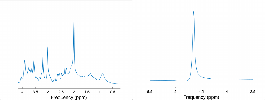
Figure 8: Example Siemens SPECIAL data, processed using
run_specialproc_auto.m .
8.5. Processing Bruker PRESS data
The {FID-A_dir}/exampleData/Bruker/sample01_press directory
contains two subfolders: one called “press”, which contains an
in vivo
short-TE PRESS MRS scan, and one called “press_w”, which
contains corresponding water unsuppressed data acquired from the
same region of interest. Both are from the dorsal hippocampus
of a healthy rat on a 7 Tesla Bruker 70/30 MRI scanner. This
dataset can be processed using the ‘run_pressproc_brukAuto.m’
script as follows (this time assuming that you have already
opened MATLAB and that {FID-A_dir} is already on your path):
1. Inside MATLAB, navigate to the {FID-
A_dir}/exampleData/Bruker/sample01_press directory. Note
that this folder contains two directories: one called
“press” and one called “press_w”. The former contains the
Bruker raw data files corresponding to the water suppressed
PRESS scan, while the latter contains the corresponding
water unsuppressed data in the same format. In order for
“run_pressproc_brukAuto.m” to work properly, the water
suppressed and water unsuppressed data must be stored in
separate folders, and the folder names must differ only by
the ‘_w’ extension at the end of the water unsuppressed
folder name. A couple extra things to note here: A) The
Bruker PRESS acquisition was set up so that the individual
averages were stored separately (not the default setting).
B) After scanning, the Bruker scanner saves each scan by
default in a numbered directory whose number corresponds to
the order of the scans in a given study. Here, we have
taken the numbered directories corresponding to the water
suppressed and water unsuppressed PRESS data and re-named
them ‘press’ and ‘press_w’, respectively.
2. From the sample01_press directory, run the example Run
script ‘run_press_brukAuto.m’ by typing the following:
[out,out_w]=run_press_brukAuto(‘press’,’press_w’);
Note that the arguments to the ‘run_pressproc_brukAuto’
function, ‘press’, and ‘press_w’, are the names of the
directories where the water suppressed data are kept. Now, the
script should run to completion within about one minute with no
user input. This time, two new structures (out, and out_w)
should appear in your workspace. These are the fully processed
water suppressed spectrum (out), and water unsuppressed spectrum
(out_w). You can plot the resulting spectra using:
op_plotspec(out,0.2,4.2,’Frequency’,’Signal Amplitude’);
and
op_plotspec(out_w,3.5,5.5,’Frequency’,’Signal Amplitude’);
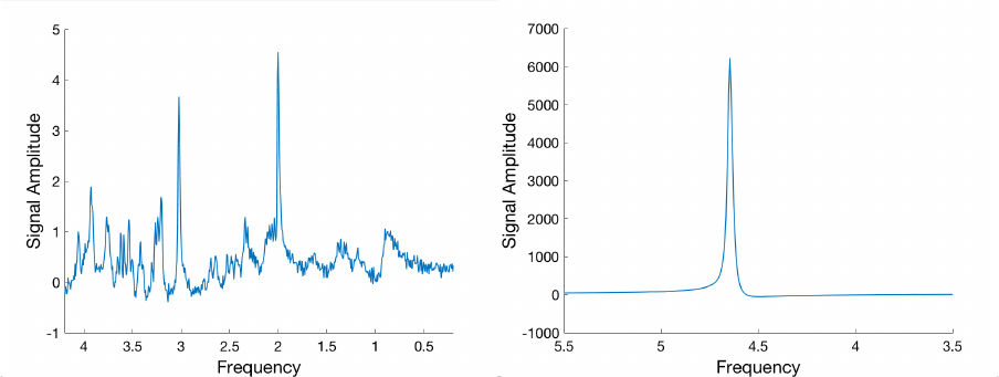
Figure 9 shows the results of the above plot commands. The
plot of the water suppressed data shows the metabolite peaks,
while the plot of the water unsuppressed data shows the water
peak. Note this time that by specifying the y- axis labels in
op_plotspec (5th argument), we are now shown the signal
intensity values on the y-axis. Like before, this script also
generates a new folder called “report” in which you will find an
HTML file (report.html) that summarizes the results of the
various stages of the processing pipeline. This should be
viewable using any standard HTML viewer or internet browser.
Finally, you will again notice that in the ‘press’
directory, two new directories are generated (“press” and
“press_w”). These directories contain the processed water
suppressed (“press_lcm”) and water unsuppressed (“press_w_lcm”)
spectra, respectively, in LCModel raw format, which can be
imported immediately for analysis in LCModel or Tarquin.
Figure 9: Example Bruker PRESS data, processed using
run_pressproc_brukAuto.m .
