Grokking Algorithms An Illustrated Guide For Programmers And Other Curious People

Grokking%20Algorithms%20-%20An%20illustrated%20guide%20for%20programmers%20and%20other%20curious%20people

Grokking%20Algorithms%20-%20An%20illustrated%20guide%20for%20programmers%20and%20other%20curious%20people

Grokking%20Algorithms%20-%20An%20illustrated%20guide%20for%20programmers%20and%20other%20curious%20people

Grokking%20Algorithms%20-%20An%20illustrated%20guide%20for%20programmers%20and%20other%20curious%20people

Grokking%20Algorithms%20-%20An%20illustrated%20guide%20for%20programmers%20and%20other%20curious%20people

User Manual: Pdf

Open the PDF directly: View PDF .
Page Count: 1

grokking

algorithms

grokking

algorithms

An illustrated guide for

programmers and other curious people

Aditya Y. Bhargava

MANNING

Shelter IS l an d

For online information and ordering of this and other Manning books, please visit

www.manning.com. e publisher oers discounts on this book when ordered in

quantity. For more information, please contact

Special Sales Department

Manning Publications Co.

20 Baldwin Road, PO Box 761

Shelter Island, NY 11964

Email: orders@manning.com

©2016 by Manning Publications Co. All rights reserved.

No part of this publication may be reproduced, stored in a retrieval system, or

transmitted, in any form or by means electronic, mechanical, photocopying, or

otherwise, without prior written permission of the publisher.

Many of the designations used by manufacturers and sellers to distinguish their

products are claimed as trademarks. Where those designations appear in the book,

and Manning Publications was aware of a trademark claim, the designations have

been printed in initial caps or all caps.

∞ Recognizing the importance of preserving what has been written, it is Manning’s

policy to have the books we publish printed on acid-free paper, and we exert our best

eorts to that end. Recognizing also our responsibility to conserve the resources of

our planet, Manning books are printed on paper that is at least 15 percent recycled

and processed without the use of elemental chlorine.

Manning Publications Co. Development editor: Jennifer Stout

20 Baldwin Road Technical development editor: Damien White

Shelter Island, NY 11964 Project manager: Tiany Taylor

Copyeditor: Tiany Taylor

Technical proofreader: Jean-François Morin

Typesetter: Leslie Haimes

Cover and interior design: Leslie Haimes

Illustrations by the author

ISBN: 9781617292231

Printed in the United States of America

1 2 3 4 5 6 7 8 9 10 – EBM – 21 20 19 18 17 16

For my parents, Sangeeta and Yogesh

vii

contents

preface xiii

acknowledgments xiv

about this book xv

1 Introduction to algorithms 1

Introduction 1

What you’ll learn about performance 2

What you’ll learn about solving problems 2

Binary search 3

A better way to search 5

Running time 10

Big O notation 10

Algorithm running times grow at different rates 11

Visualizing different Big O run times 13

Big O establishes a worst-case run time 15

Some common Big O run times 15

The traveling salesperson 17

Recap 19

2 Selection sort 21

How memory works 22

Arrays and linked lists 24

Linked lists 25

Arrays 26

Terminology 27

Inserting into the middle of a list 29

Deletions 30

viii contents

Selection sort 32

Recap 36

3 Recursion 37

Recursion 38

Base case and recursive case 40

The stack 42

The call stack 43

The call stack with recursion 45

Recap 50

4 Quicksort 51

Divide & conquer 52

Quicksort 60

Big O notation revisited 66

Merge sort vs. quicksort 67

Average case vs. worst case 68

Recap 72

5 Hash tables 73

Hash functions 76

Use cases 79

Using hash tables for lookups 79

Preventing duplicate entries 81

Using hash tables as a cache 83

Recap 86

Collisions 86

Performance 88

Load factor 90

A good hash function 92

Recap 93

6 Breadth-first search 95

Introduction to graphs 96

What is a graph? 98

Breadth-first search 99

Finding the shortest path 102

ixcontents

Queues 103

Implementing the graph 105

Implementing the algorithm 107

Running time 111

Recap 114

7 Dijkstra’s algorithm 115

Working with Dijkstra’s algorithm 116

Terminology 120

Trading for a piano 122

Negative-weight edges 128

Implementation 131

Recap 140

8 Greedy algorithms 141

The classroom scheduling problem 142

The knapsack problem 144

The set-covering problem 146

Approximation algorithms 147

NP-complete problems 152

Traveling salesperson, step by step 153

How do you tell if a problem is NP-complete? 158

Recap 160

9 Dynamic programming 161

The knapsack problem 161

The simple solution 162

Dynamic programming 163

Knapsack problem FAQ 171

What happens if you add an item? 171

What happens if you change the order of the rows? 174

Can you fill in the grid column-wise instead

of row-wise? 174

What happens if you add a smaller item? 174

Can you steal fractions of an item? 175

Optimizing your travel itinerary 175

Handling items that depend on each other 177

xcontents

Is it possible that the solution will require

more than two sub-knapsacks? 177

Is it possible that the best solution doesn’t fill

the knapsack completely? 178

Longest common substring 178

Making the grid 179

Filling in the grid 180

The solution 182

Longest common subsequence 183

Longest common subsequence—solution 184

Recap 186

10 K-nearest neighbors 187

Classifying oranges vs. grapefruit 187

Building a recommendations system 189

Feature extraction 191

Regression 195

Picking good features 198

Introduction to machine learning 199

OCR 199

Building a spam filter 200

Predicting the stock market 201

Recap 201

11 Where to go next 203

Trees 203

Inverted indexes 206

The Fourier transform 207

Parallel algorithms 208

MapReduce 209

Why are distributed algorithms useful? 209

The map function 209

The reduce function 210

Bloom filters and HyperLogLog 211

Bloom filters 212

xi

HyperLogLog 213

The SHA algorithms 213

Comparing files 214

Checking passwords 215

Locality-sensitive hashing 216

Diffie-Hellman key exchange 217

Linear programming 218

Epilogue 219

answers to exercises 221

index 235

contents

xiii

preface

I rst got into programming as a hobby. Visual Basic 6 for Dummies

taught me the basics, and I kept reading books to learn more. But the

subject of algorithms was impenetrable for me. I remember savoring

the table of contents of my rst algorithms book, thinking “I’m nally

going to understand these topics!” But it was dense stu, and I gave

up aer a few weeks. It wasn’t until I had my rst good algorithms

professor that I realized how simple and elegant these ideas were.

A few years ago, I wrote my rst illustrated blog post. I’m a visual

learner, and I really liked the illustrated style. Since then, I’ve written

a few illustrated posts on functional programming, Git, machine

learning, and concurrency. By the way: I was a mediocre writer when

I started out. Explaining technical concepts is hard. Coming up with

good examples takes time, and explaining a dicult concept takes time.

So it’s easiest to gloss over the hard stu. I thought I was doing a pretty

good job, until aer one of my posts got popular, a coworker came up

to me and said, “I read your post and I still don’t understand this.” I still

had a lot to learn about writing.

Somewhere in the middle of writing these blog posts, Manning reached

out to me and asked if I wanted to write an illustrated book. Well, it

turns out that Manning editors know a lot about explaining technical

concepts, and they taught me how to teach. I wrote this book to scratch

a particular itch: I wanted to write a book that explained hard technical

topics well, and I wanted an easy-to-read algorithms book. My writing

has come a long way since that rst blog post, and I hope you nd this

book an easy and informative read.

xiv

acknowledgments

Kudos to Manning for giving me the chance to write this book and

letting me have a lot of creative freedom with it. anks to publisher

Marjan Bace, Mike Stephens for getting me on board, Bert Bates for

teaching me how to write, and Jennifer Stout for being an incredibly

responsive and helpful editor. anks also to the people on Manning’s

production team: Kevin Sullivan, Mary Piergies, Tiany Taylor,

Leslie Haimes, and all the others behind the scenes. In addition, I

want to thank the many people who read the manuscript and oered

suggestions: Karen Bensdon, Rob Green, Michael Hamrah, Ozren

Harlovic, Colin Hastie, Christopher Haupt, Chuck Henderson, Pawel

Kozlowski, Amit Lamba, Jean-François Morin, Robert Morrison,

Sankar Ramanathan, Sander Rossel, Doug Sparling, and Damien White.

anks to the people who helped me reach this point: the folks on the

Flaskhit game board, for teaching me how to code; the many friends

who helped by reviewing chapters, giving advice, and letting me try

out dierent explanations, including Ben Vinegar, Karl Puzon, Alex

Manning, Esther Chan, Anish Bhatt, Michael Glass, Nikrad Mahdi,

Charles Lee, Jared Friedman, Hema Manickavasagam, Hari Raja, Murali

Gudipati, Srinivas Varadan, and others; and Gerry Brady, for teaching

me algorithms. Another big thank you to algorithms academics like

CLRS, Knuth, and Strang. I’m truly standing on the shoulders of giants.

Dad, Mom, Priyanka, and the rest of the family: thank you for your

constant support. And a big thank you to my wife Maggie. ere are

many adventures ahead of us, and some of them don’t involve staying

inside on a Friday night rewriting paragraphs.

Finally, a big thank you to all the readers who took a chance on this

book, and the readers who gave me feedback in the book’s forum.

You really helped make this book better.

xv

about this book

is book is designed to be easy to follow. I avoid big leaps of thought.

Any time a new concept is introduced, I explain it right away or tell

you when I’ll explain it. Core concepts are reinforced with exercises

and multiple explanations so that you can check your assumptions and

make sure you’re following along.

I lead with examples. Instead of writing symbol soup, my goal is to

make it easy for you to visualize these concepts. I also think we learn

best by being able to recall something we already know, and examples

make recall easier. So when you’re trying to remember the dierence

between arrays and linked lists (explained in chapter 2), you can just

think about getting seated for a movie. Also, at the risk of stating the

obvious, I’m a visual learner. is book is chock-full of images.

e contents of the book are carefully curated. ere’s no need to

write a book that covers every sorting algorithm—that’s why we have

Wikipedia and Khan Academy. All the algorithms I’ve included are

practical. I’ve found them useful in my job as a soware engineer,

and they provide a good foundation for more complex topics.

Happy reading!

Roadmap

e rst three chapters of this book lay the foundations:

• Chapter 1—You’ll learn your rst practical algorithm: binary search.

You also learn to analyze the speed of an algorithm using Big O

notation. Big O notation is used throughout the book to analyze how

slow or fast an algorithm is.

xvi about this book

• Chapter 2—You’ll learn about two fundamental data structures:

arrays and linked lists. ese data structures are used throughout the

book, and they’re used to make more advanced data structures like

hash tables (chapter 5).

• Chapter 3—You’ll learn about recursion, a handy technique used by

many algorithms (such as quicksort, covered in chapter 4).

In my experience, Big O notation and recursion are challenging topics

for beginners. So I’ve slowed down and spent extra time on these

sections.

e rest of the book presents algorithms with broad applications:

• Problem-solving techniques—Covered in chapters 4, 8, and 9. If you

come across a problem and aren’t sure how to solve it eciently, try

divide and conquer (chapter 4) or dynamic programming (chapter

9). Or you may realize there’s no ecient solution, and get an

approximate answer using a greedy algorithm instead (chapter 8).

• Hash tables—Covered in chapter 5. A hash table is a very useful data

structure. It contains sets of key and value pairs, like a person’s name

and their email address, or a username and the associated password.

It’s hard to overstate hash tables’ usefulness. When I want to solve

a problem, the two plans of attack I start with are “Can I use a hash

table?” and “Can I model this as a graph?”

• Graph algorithms—Covered in chapters 6 and 7. Graphs are a way to

model a network: a social network, or a network of roads, or neurons,

or any other set of connections. Breadth-rst search (chapter 6) and

Dijkstra’s algorithm (chapter 7) are ways to nd the shortest distance

between two points in a network: you can use this approach to

calculate the degrees of separation between two people or the shortest

route to a destination.

• K-nearest neighbors (KNN)—Covered in chapter 10. is is a

simple machine-learning algorithm. You can use KNN to build a

recommendations system, an OCR engine, a system to predict stock

values—anything that involves predicting a value (“We think Adit will

rate this movie 4 stars”) or classifying an object (“at letter is a Q”).

• Next steps—Chapter 11 goes over 10 algorithms that would make

good further reading.

xvii

How to use this book

e order and contents of this book have been carefully designed. If

you’re interested in a topic, feel free to jump ahead. Otherwise, read the

chapters in order—they build on each other.

I strongly recommend executing the code for the examples yourself. I

can’t stress this part enough. Just type out my code samples verbatim

(or download them from www.manning.com/books/grokking-

algorithms or https://github.com/egonschiele/grokking_algorithms),

and execute them. You’ll retain a lot more if you do.

I also recommend doing the exercises in this book. e exercises are

short—usually just a minute or two, sometimes 5 to 10 minutes. ey

will help you check your thinking, so you’ll know when you’re o track

before you’ve gone too far.

Who should read this book

is book is aimed at anyone who knows the basics of coding and

wants to understand algorithms. Maybe you already have a coding

problem and are trying to nd an algorithmic solution. Or maybe

you want to understand what algorithms are useful for. Here’s a short,

incomplete list of people who will probably nd this book useful:

• Hobbyist coders

• Coding boot camp students

• Computer science grads looking for a refresher

• Physics/math/other grads who are interested in programming

Code conventions and downloads

All the code examples in this book use Python 2.7. All code in the

book is presented in a

fixed-width font like this

to separate it

from ordinary text. Code annotations accompany some of the listings,

highlighting important concepts.

You can download the code for the examples in the book from the

publisher’s website at www.manning.com/books/grokking-algorithms

or from https://github.com/egonschiele/grokking_algorithms.

I believe you learn best when you really enjoy learning—so have fun,

and run the code samples!

about this book

xviii

About the author

Aditya Bhargava is a soware engineer at Etsy, an online marketplace

for handmade goods. He has a master’s degree in computer science

from the University of Chicago. He also runs a popular illustrated

tech blog at adit.io.

Author Online

Purchase of Grokking Algorithms includes free access to a private web

forum run by Manning Publications where you can make comments

about the book, ask technical questions, and receive help from the

author and from other users. To access the forum and subscribe to

it, point your web browser to www.manning.com/books/grokking-

algorithms. is page provides information on how to get on the forum

once you are registered, what kind of help is available, and the rules of

conduct on the forum.

Manning’s commitment to our readers is to provide a venue where a

meaningful dialog between individual readers and between readers and

the author can take place. It isn’t a commitment to any specic amount

of participation on the part of the author, whose contribution to Author

Online remains voluntary (and unpaid). We suggest you try asking the

author some challenging questions lest his interest stray! e Author

Online forum and the archives of previous discussions will be accessible

from the publisher’s website as long as the book is in print.

about this book

1

1

In this chapter

• You get a foundation for the rest of the book.

• You write your rst search algorithm (binary

search).

• You learn how to talk about the running time

of an algorithm (Big O notation).

• You’re introduced to a common technique for

designing algorithms (recursion).

introduction

to algorithms

Introduction

An algorithm is a set of instructions for accomplishing a task. Every

piece of code could be called an algorithm, but this book covers the

more interesting bits. I chose the algorithms in this book for inclusion

because they’re fast, or they solve interesting problems, or both. Here

are some highlights:

• Chapter 1 talks about binary search and shows how an algorithm can

speed up your code. In one example, the number of steps needed goes

from 4 billion down to 32!

2Chapter 1

I

Introduction to algorithms

• A GPS device uses graph algorithms (as you’ll learn in chapters 6, 7,

and 8) to calculate the shortest route to your destination.

• You can use dynamic programming (discussed in chapter 9) to write

an AI algorithm that plays checkers.

In each case, I’ll describe the algorithm and give you an example. en

I’ll talk about the running time of the algorithm in Big O notation.

Finally, I’ll explore what other types of problems could be solved by the

same algorithm.

What you’ll learn about performance

e good news is, an implementation of every algorithm in this book is

probably available in your favorite language, so you don’t have to write

each algorithm yourself! But those implementations are useless if you

don’t understand the trade-os. In this book, you’ll learn to compare

trade-os between dierent algorithms: Should you use merge sort or

quicksort? Should you use an array or a list? Just using a dierent data

structure can make a big dierence.

What you’ll learn about solving problems

You’ll learn techniques for solving problems that might have been out of

your grasp until now. For example:

• If you like making video games, you can write an AI system that

follows the user around using graph algorithms.

• You’ll learn to make a recommendations system using k-nearest

neighbors.

• Some problems aren’t solvable in a timely manner! e part of this

book that talks about NP-complete problems shows you how to

identify those problems and come up with an algorithm that gives

you an approximate answer.

More generally, by the end of this book, you’ll know some of the most

widely applicable algorithms. You can then use your new knowledge to

learn about more specic algorithms for AI, databases, and so on. Or

you can take on bigger challenges at work.

3Binary search

Binary search

Suppose you’re searching for a person in the phone book (what an old-

fashioned sentence!). eir name starts with K. You could start at the

beginning and keep ipping pages until you get to the Ks. But you’re

more likely to start at a page in the middle, because you know the Ks

are going to be near the middle of the phone book.

Or suppose you’re searching for a word in a dictionary, and it

starts with O. Again, you’ll start near the middle.

Now suppose you log on to Facebook. When you do, Facebook

has to verify that you have an account on the site. So, it needs to

search for your username in its database. Suppose your username is

karlmageddon. Facebook could start from the As and search for your

name—but it makes more sense for it to begin somewhere in the

middle.

is is a search problem. And all these cases use the same algorithm

to solve the problem: binary search.

Binary search is an algorithm; its input is a sorted list of elements

(I’ll explain later why it needs to be sorted). If an element you’re

looking for is in that list, binary search returns the position

where it’s located. Otherwise, binary search returns

null

.

What you need to know

You’ll need to know basic algebra before starting this book. In parti-

cular, take this function: f(x) = x × 2. What is f(5)? If you answered 10,

you’re set.

Additionally, this chapter (and this book) will be easier to follow if

you’re familiar with one programming language. All the examples in

this book are in Python. If you don’t know any programming languages

and want to learn one, choose Python—it’s great for beginners. If you

know another language, like Ruby, you’ll be ne.

Chapter 1

I

Introduction to algorithms

4

For example:

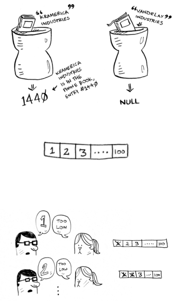
Here’s an example of how binary search works. I’m thinking of a

number between 1 and 100.

You have to try to guess my number in the fewest tries possible. With

every guess, I’ll tell you if your guess is too low, too high, or correct.

Suppose you start guessing like this: 1, 2, 3, 4 …. Here’s how it would

go.

Looking for companies

in a phone book with

binary search

5Binary search

is is simple search (maybe stupid search would be a better term). With

each guess, you’re eliminating only one number. If my number was 99,

it could take you 99 guesses to get there!

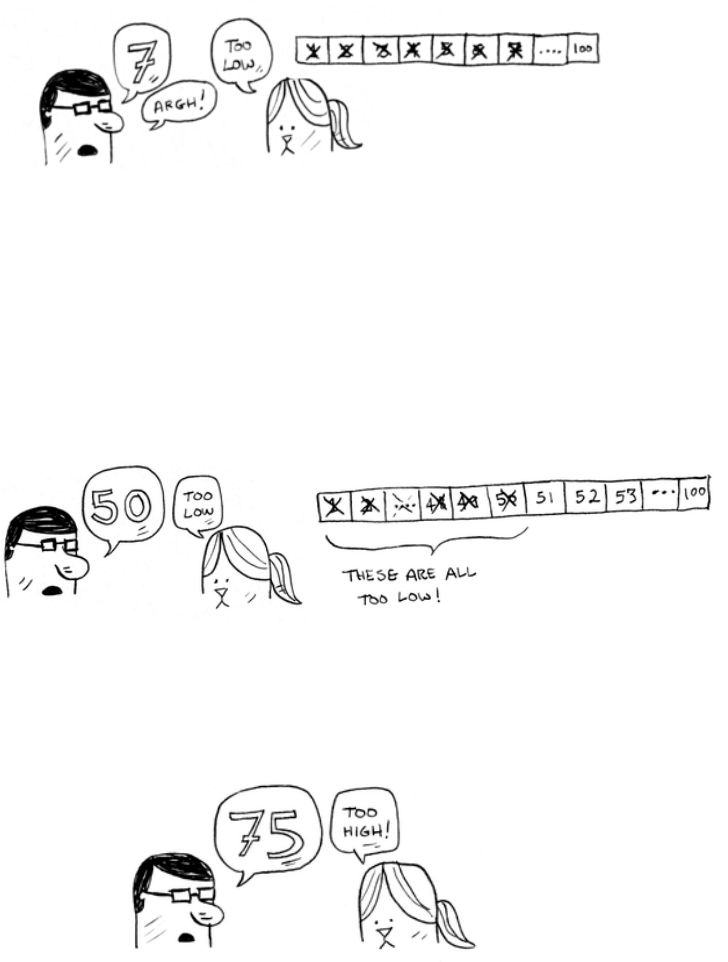
A better way to search

Here’s a better technique. Start with 50.

Too low, but you just eliminated half the numbers! Now you know that

1–50 are all too low. Next guess: 75.

A bad approach to

number guessing

Chapter 1

I

Introduction to algorithms

6

Too high, but again you cut down half the remaining numbers! With

binary search, you guess the middle number and eliminate half the

remaining numbers every time. Next is 63 (halfway between 50 and 75).

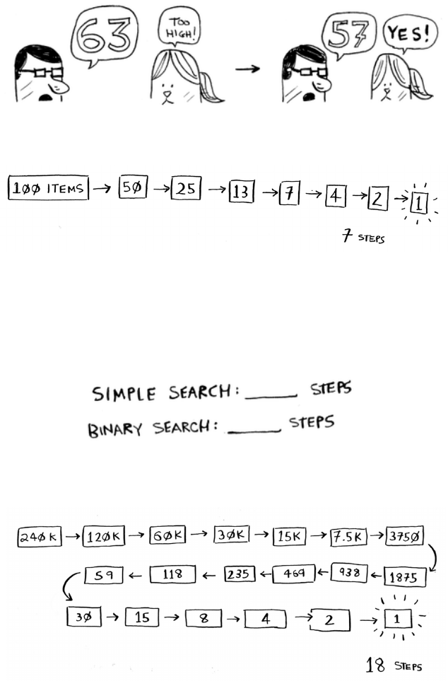
is is binary search. You just learned your rst algorithm! Here’s how

many numbers you can eliminate every time.

Whatever number I’m thinking of, you can guess in a maximum of

seven guesses—because you eliminate so many numbers with every

guess!

Suppose you’re looking for a word in the dictionary. e dictionary has

240,000 words. In the worst case, how many steps do you think each

search will take?

Simple search could take 240,000 steps if the word you’re looking for is

the very last one in the book. With each step of binary search, you cut

the number of words in half until you’re le with only one word.

Eliminate half the

numbers every time

with binary search.

7Binary search

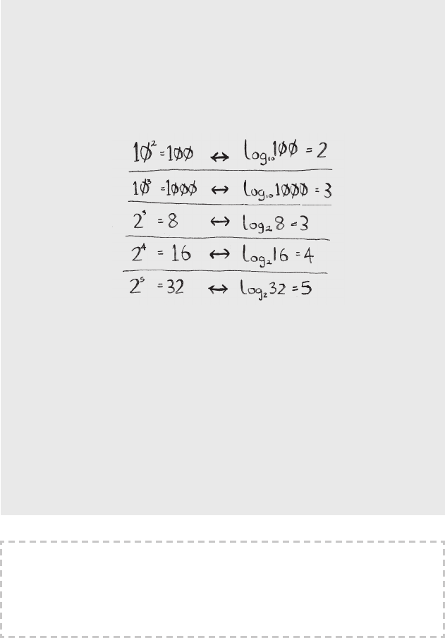
Logarithms

You may not remember what logarithms are, but you probably know what

exponentials are. log10 100 is like asking, “How many 10s do we multiply

together to get 100?” e answer is 2: 10 × 10. So log10 100 = 2. Logs are the

ip of exponentials.

Logs are the flip of exponentials.

In this book, when I talk about running time in Big O notation (explained

a little later), log always means log2. When you search for an element using

simple search, in the worst case you might have to look at every single

element. So for a list of 8 numbers, you’d have to check 8 numbers at most.

For binary search, you have to check log n elements in the worst case. For

a list of 8 elements, log 8 == 3, because 23 == 8. So for a list of 8 numbers,

you would have to check 3 numbers at most. For a list of 1,024 elements,

log 1,024 = 10, because 210 == 1,024. So for a list of 1,024 numbers, you’d

have to check 10 numbers at most.

Note

I’ll talk about log time a lot in this book, so you should understand the con-

cept of logarithms. If you don’t, Khan Academy (khanacademy.org) has a

nice video that makes it clear.

So binary search will take 18 steps—a big dierence! In general, for any

list of n, binary search will take log2 n steps to run in the worst case,

whereas simple search will take n steps.

Chapter 1

I

Introduction to algorithms

8

Note

Binary search only works when your list is in sorted order. For example,

the names in a phone book are sorted in alphabetical order, so you can

use binary search to look for a name. What would happen if the names

weren’t sorted?

Let’s see how to write binary search in Python. e code sample here

uses arrays. If you don’t know how arrays work, don’t worry; they’re

covered in the next chapter. You just need to know that you can store

a sequence of elements in a row of consecutive buckets called an array.

e buckets are numbered starting with 0: the rst bucket is at position

#0, the second is #1, the third is #2, and so on.

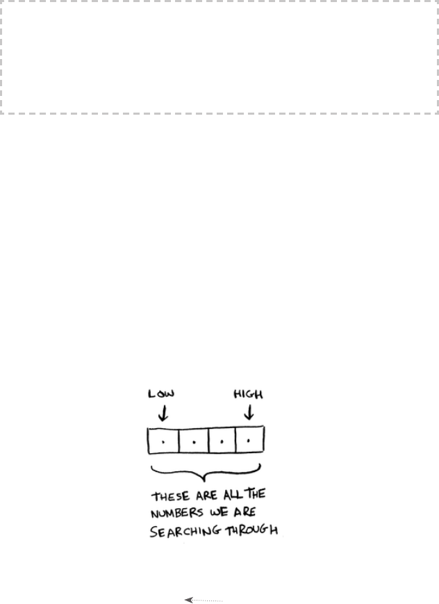
e

binary_search

function takes a sorted array and an item. If the

item is in the array, the function returns its position. You’ll keep track

of what part of the array you have to search through. At the beginning,

this is the entire array:

low = 0

high = len(list) - 1

Each time, you check the middle element:

mid = (low + high) / 2

guess = list[mid]

If the guess is too low, you update

low

accordingly:

if guess < item:

low = mid + 1

mid is rounded down by Python

automatically if (low + high) isn’t

an even number.

9

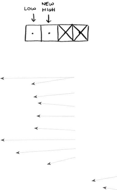
And if the guess is too high, you update

high

. Here’s the full code:

def binary_search(list, item):

low = 0

high = len(list)—1

while low <= high:

mid = (low + high)

guess = list[mid]

if guess == item:

return mid

if guess > item:

high = mid - 1

else:

low = mid + 1

return None

my_list = [1, 3, 5, 7, 9]

print binary_search(my_list, 3) # => 1

print binary_search(my_list, -1) # => None

EXERCISES

1.1 Suppose you have a sorted list of 128 names, and you’re searching

through it using binary search. What’s the maximum number of

steps it would take?

1.2 Suppose you double the size of the list. What’s the maximum

number of steps now?

Binary search

low and high keep track of which

part of the list you’ll search in.

While you haven’t narrowed it down

to one element …

… check the middle element.

Found the item.

The guess was too high.

The guess was too low.

The item doesn’t exist.

Let’s test it!

Remember, lists start at 0.

The second slot has index 1.

“None” means nil in Python. It

indicates that the item wasn’t found.

Chapter 1

I

Introduction to algorithms

10

Running time

Any time I talk about an algorithm, I’ll discuss its running time.

Generally you want to choose the most ecient algorithm—

whether you’re trying to optimize for time or space.

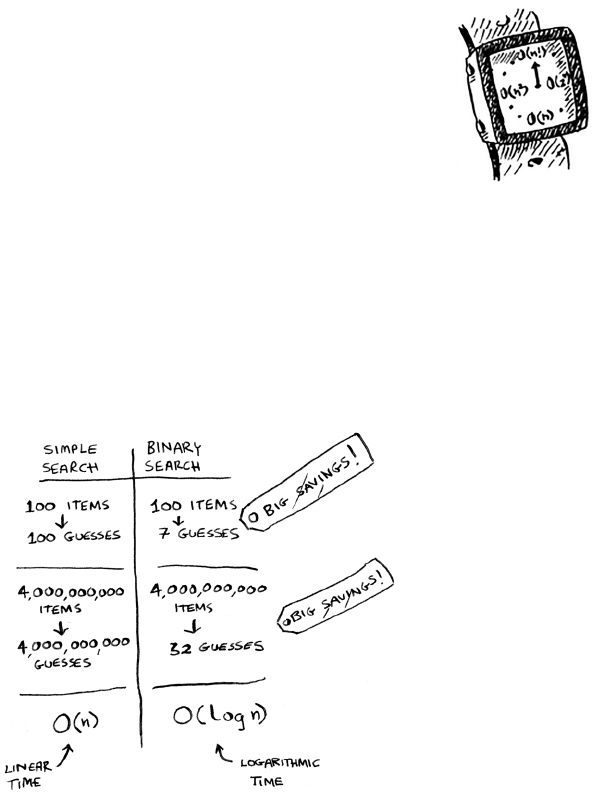
Back to binary search. How much time do you save by using

it? Well, the rst approach was to check each number, one by

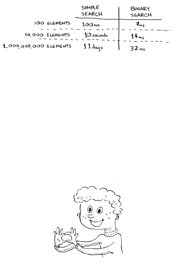
one. If this is a list of 100 numbers, it takes up to 100 guesses.

If it’s a list of 4 billion numbers, it takes up to 4 billion guesses. So the

maximum number of guesses is the same as the size of the list. is is

called linear time.

Binary search is dierent. If the list is 100 items long, it takes at most

7 guesses. If the list is 4 billion items, it takes at most 32 guesses.

Powerful, eh? Binary search runs in logarithmic time (or log time, as

the natives call it). Here’s a table summarizing our ndings today.

Big O notation

Big O notation is special notation that tells you how fast an algorithm is.

Who cares? Well, it turns out that you’ll use other people’s algorithms

oen—and when you do, it’s nice to understand how fast or slow they

are. In this section, I’ll explain what Big O notation is and give you a list

of the most common running times for algorithms using it.

Run times for

search algorithms

11Big O notation

Running time for

simple search vs.

binary search,

with a list of 100

elements

Algorithm running times grow at dierent rates

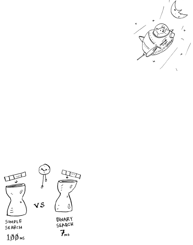
Bob is writing a search algorithm for NASA. His algorithm will kick in

when a rocket is about to land on the Moon, and it will help calculate

where to land.

is is an example of how the run time of two algorithms can grow

at dierent rates. Bob is trying to decide between simple search and

binary search. e algorithm needs to be both fast and correct. On one

hand, binary search is faster. And Bob has only 10 seconds to gure out

where to land—otherwise, the rocket will be o course. On the other

hand, simple search is easier to write, and there is less chance of bugs

being introduced. And Bob really doesn’t want bugs in the code to land

a rocket! To be extra careful, Bob decides to time both algorithms with

a list of 100 elements.

Let’s assume it takes 1 millisecond to check one element. With simple

search, Bob has to check 100 elements, so the search takes 100 ms to

run. On the other hand, he only has to check 7 elements with binary

search (log2 100 is roughly 7), so that search takes 7 ms to run. But

realistically, the list will have more like a billion elements. If it does,

how long will simple search take? How long will binary search take?

Make sure you have an answer for each question before reading on.

Bob runs binary search with 1 billion elements, and it takes 30 ms

(log2 1,000,000,000 is roughly 30). “32 ms!” he thinks. “Binary search

is about 15 times faster than simple search, because simple search took

100 ms with 100 elements, and binary search took 7 ms. So simple

search will take 30 × 15 = 450 ms, right? Way under my threshold of

10 seconds.” Bob decides to go with simple search. Is that the right

choice?

Chapter 1

I

Introduction to algorithms

12

No. Turns out, Bob is wrong. Dead wrong. e run time for simple

search with 1 billion items will be 1 billion ms, which is 11 days! e

problem is, the run times for binary search and simple search don’t

grow at the same rate.

at is, as the number of items increases, binary search takes a little

more time to run. But simple search takes a lot more time to run. So

as the list of numbers gets bigger, binary search suddenly becomes a

lot faster than simple search. Bob thought binary search was 15 times

faster than simple search, but that’s not correct. If the list has 1 billion

items, it’s more like 33 million times faster. at’s why it’s not enough

to know how long an algorithm takes to run—you need to know how

the running time increases as the list size increases. at’s where Big O

notation comes in.

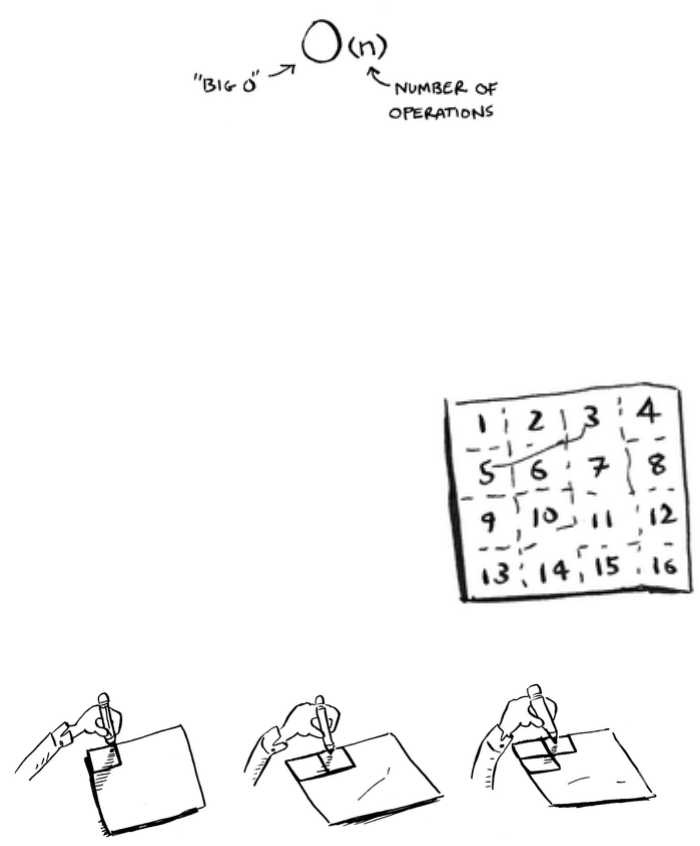
Big O notation tells you how fast an algorithm is. For example, suppose

you have a list of size n. Simple search needs to check each element, so

it will take n operations. e run time in Big O notation is O(n). Where

are the seconds? ere are none—Big O doesn’t tell you the speed in

seconds. Big O notation lets you compare the number of operations. It

tells you how fast the algorithm grows.

Run times grow at

very different speeds!

13Big O notation

Here’s another example. Binary search needs log n operations to check

a list of size n. What’s the running time in Big O notation? It’s O(log n).

In general, Big O notation is written as follows.

is tells you the number of operations an algorithm will make. It’s

called Big O notation because you put a “big O” in front of the number

of operations (it sounds like a joke, but it’s true!).

Now let’s look at some examples. See if you can gure out the run time

for these algorithms.

Visualizing dierent Big O run times

Here’s a practical example you can follow at

home with a few pieces of paper and a pencil.

Suppose you have to draw a grid of 16 boxes.

Algorithm 1

One way to do it is to draw 16 boxes, one at

a time. Remember, Big O notation counts

the number of operations. In this example,

drawing one box is one operation. You have

to draw 16 boxes. How many operations will

it take, drawing one box at a time?

It takes 16 steps to draw 16 boxes. What’s the running time for this

algorithm?

What Big O

notation looks like

What’s a good

algorithm to

draw this grid?

Drawing a grid

one box at a time

Chapter 1

I

Introduction to algorithms

14

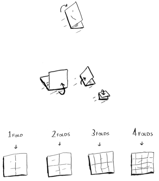
Algorithm 2

Try this algorithm instead. Fold the paper.

In this example, folding the paper once is an operation. You just made

two boxes with that operation!

Fold the paper again, and again, and again.

Unfold it aer four folds, and you’ll have a beautiful grid! Every fold

doubles the number of boxes. You made 16 boxes with 4 operations!

You can “draw” twice as many boxes with every fold, so you can draw

16 boxes in 4 steps. What’s the running time for this algorithm? Come

up with running times for both algorithms before moving on.

Answers: Algorithm 1 takes O(n) time, and algorithm 2 takes

O(log n) time.

Drawing a grid

in four folds

15Big O notation

Big O establishes a worst-case run time

Suppose you’re using simple search to look for a person in the phone

book. You know that simple search takes O(n) time to run, which

means in the worst case, you’ll have to look through every single entry

in your phone book. In this case, you’re looking for Adit. is guy is

the rst entry in your phone book. So you didn’t have to look at every

entry—you found it on the rst try. Did this algorithm take O(n) time?

Or did it take O(1) time because you found the person on the rst try?

Simple search still takes O(n) time. In this case, you found what you

were looking for instantly. at’s the best-case scenario. But Big O

notation is about the worst-case scenario. So you can say that, in the

worst case, you’ll have to look at every entry in the phone book once.

at’s O(n) time. It’s a reassurance—you know that simple search will

never be slower than O(n) time.

Some common Big O run times

Here are ve Big O run times that you’ll encounter a lot, sorted from

fastest to slowest:

• O(log n), also known as log time. Example: Binary search.

• O(n), also known as linear time. Example: Simple search.

• O(n * log n). Example: A fast sorting algorithm, like quicksort

(coming up in chapter 4).

• O(n2). Example: A slow sorting algorithm, like selection sort

(coming up in chapter 2).

• O(n!). Example: A really slow algorithm, like the traveling

salesperson (coming up next!).

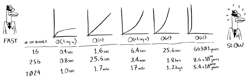
Suppose you’re drawing a grid of 16 boxes again, and you can choose

from 5 dierent algorithms to do so. If you use the rst algorithm, it

will take you O(log n) time to draw the grid. You can do 10 operations

Note

Along with the worst-case run time, it’s also important to look at the

average-case run time. Worst case versus average case is discussed in

chapter 4.

Chapter 1

I

Introduction to algorithms

16

per second. With O(log n) time, it will take you 4 operations to draw a

grid of 16 boxes (log 16 is 4). So it will take you 0.4 seconds to draw

the grid. What if you have to draw 1,024 boxes? It will take you

log 1,024 = 10 operations, or 1 second to draw a grid of 1,024 boxes.

ese numbers are using the rst algorithm.

e second algorithm is slower: it takes O(n) time. It will take 16

operations to draw 16 boxes, and it will take 1,024 operations to draw

1,024 boxes. How much time is that in seconds?

Here’s how long it would take to draw a grid for the rest of the

algorithms, from fastest to slowest:

ere are other run times, too, but these are the ve most common.

is is a simplication. In reality you can’t convert from a Big O run

time to a number of operations this neatly, but this is good enough

for now. We’ll come back to Big O notation in chapter 4, aer you’ve

learned a few more algorithms. For now, the main takeaways are as

follows:

• Algorithm speed isn’t measured in seconds, but in growth of the

number of operations.

• Instead, we talk about how quickly the run time of an algorithm

increases as the size of the input increases.

• Run time of algorithms is expressed in Big O notation.

• O(log n) is faster than O(n), but it gets a lot faster as the list of items

you’re searching grows.

17Big O notation

EXERCISES

Give the run time for each of these scenarios in terms of Big O.

1.3 You have a name, and you want to nd the person’s phone number

in the phone book.

1.4 You have a phone number, and you want to nd the person’s name

in the phone book. (Hint: You’ll have to search through the whole

book!)

1.5 You want to read the numbers of every person in the phone book.

1.6 You want to read the numbers of just the As. (is is a tricky one!

It involves concepts that are covered more in chapter 4. Read the

answer—you may be surprised!)

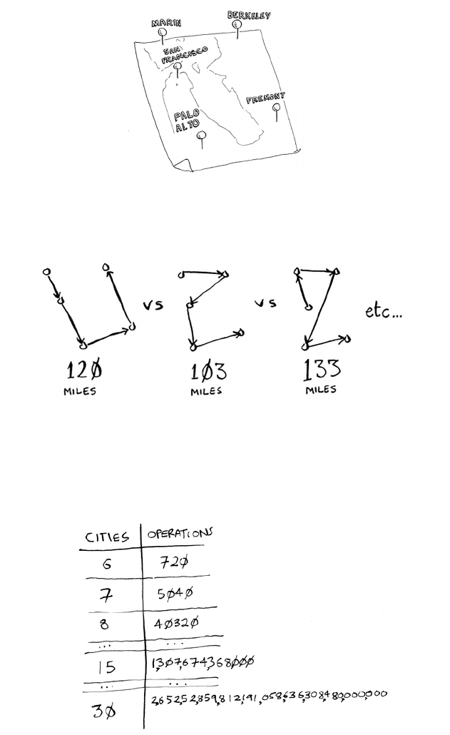
The traveling salesperson

You might have read that last section and thought, “ere’s no way I’ll

ever run into an algorithm that takes O(n!) time.” Well, let me try to

prove you wrong! Here’s an example of an algorithm with a really bad

running time. is is a famous problem in computer science, because

its growth is appalling and some very smart people think it can’t be

improved. It’s called the traveling salesperson problem.

You have a salesperson.

Chapter 1

I

Introduction to algorithms

18

e salesperson has to go to ve cities.

is salesperson, whom I’ll call Opus, wants to hit all ve cities while

traveling the minimum distance. Here’s one way to do that: look

at every possible order in which he could travel to the cities.

He adds up the total distance and then picks the path with the

lowest distance. ere are 120 permutations with 5 cities, so it will

take 120 operations to solve the problem for 5 cities. For 6 cities, it

will take 720 operations (there are 720 permutations). For 7 cities,

it will take 5,040 operations!

The number of

operations

increases drastically.

19Recap

In general, for n items, it will take n! (n factorial) operations to

compute the result. So this is O(n!) time, or factorial time. It takes a

lot of operations for everything except the smallest numbers. Once

you’re dealing with 100+ cities, it’s impossible to calculate the answer in

time—the Sun will collapse rst.

is is a terrible algorithm! Opus should use a dierent one, right? But

he can’t. is is one of the unsolved problems in computer science.

ere’s no fast known algorithm for it, and smart people think it’s

impossible to have a smart algorithm for this problem. e best we can

do is come up with an approximate solution; see chapter 10 for more.

One nal note: if you’re an advanced reader, check out binary search

trees! ere’s a brief description of them in the last chapter.

Recap

• Binary search is a lot faster than simple search.

• O(log n) is faster than O(n), but it gets a lot faster once the list of

items you’re searching through grows.

• Algorithm speed isn’t measured in seconds.

• Algorithm times are measured in terms of growth of an algorithm.

• Algorithm times are written in Big O notation.

2

In this chapter

• You learn about arrays and linked lists—two of the

most basic data structures. They’re used absolutely

everywhere. You already used arrays in chapter 1,

and you’ll use them in almost every chapter in this

book. Arrays are a crucial topic, so pay attention!

But sometimes it’s better to use a linked list instead

of an array. This chapter explains the pros and cons

of both so you can decide which one is right for

your algorithm.

• You learn your rst sorting algorithm. A lot of algo-

rithms only work if your data is sorted. Remember

binary search? You can run binary search only

on a sorted list of elements. This chapter teaches

you selection sort. Most languages have a sorting

algorithm built in, so you’ll rarely need to write

your own version from scratch. But selection sort is

a stepping stone to quicksort, which I’ll cover in the

next chapter. Quicksort is an important algorithm,

and it will be easier to understand if you know one

sorting algorithm already.

selection

sort

21

22 Chapter 2

I

Selection sort

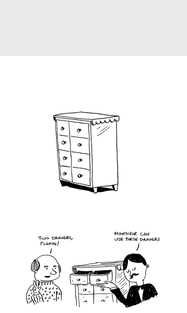
How memory works

Imagine you go to a show and need to check your things. A chest of

drawers is available.

Each drawer can hold one element. You want to store two things, so you

ask for two drawers.

What you need to know

To understand the performance analysis bits in this chapter, you need to

know Big O notation and logarithms. If you don’t know those, I suggest

you go back and read chapter 1. Big O notation will be used throughout

the rest of the book.

23How memory works

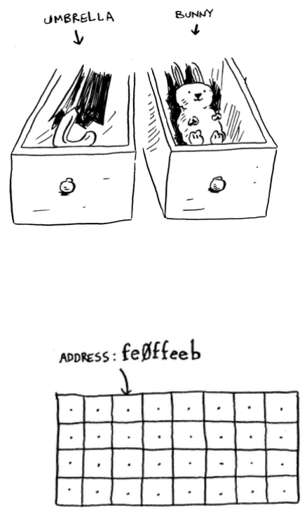
You store your two things here.

And you’re ready for the show! is is basically how your computer’s

memory works. Your computer looks like a giant set of drawers, and

each drawer has an address.

fe /

0eeb is the address of a slot in memory.

Each time you want to store an item in memory, you ask the computer

for some space, and it gives you an address where you can store your

item. If you want to store multiple items, there are two basic ways to

do so: arrays and lists. I’ll talk about arrays and lists next, as well as the

pros and cons of each. ere isn’t one right way to store items for every

use case, so it’s important to know the dierences.

24

Arrays and linked lists

Sometimes you need to store a list of elements in memory. Suppose

you’re writing an app to manage your todos. You’ll want to store the

todos as a list in memory.

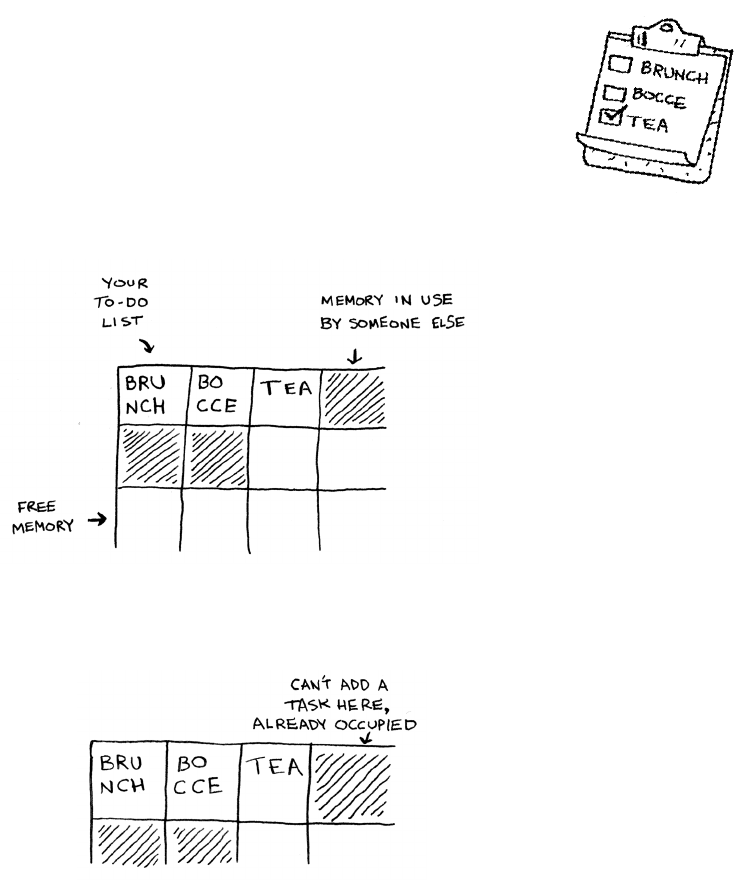
Should you use an array, or a linked list? Let’s store the todos in an

array rst, because it’s easier to grasp. Using an array means all your

tasks are stored contiguously (right next to each other) in memory.

Now suppose you want to add a fourth task. But the next drawer is

taken up by someone else’s stu!

It’s like going to a movie with your friends and nding a place to sit—

but another friend joins you, and there’s no place for them. You have to

move to a new spot where you all t. In this case, you need to ask your

computer for a dierent chunk of memory that can t four tasks. en

you need to move all your tasks there.

Chapter 2

I

Selection sort

25Arrays and linked lists

If another friend comes by, you’re out of room again—and you all have

to move a second time! What a pain. Similarly, adding new items to

an array can be a big pain. If you’re out of space and need to move to a

new spot in memory every time, adding a new item will be really slow.

One easy x is to “hold seats”: even if you have only 3 items in your task

list, you can ask the computer for 10 slots, just in case. en you can

add 10 items to your task list without having to move. is is a good

workaround, but you should be aware of a couple of downsides:

• You may not need the extra slots that you asked for, and then that

memory will be wasted. You aren’t using it, but no one else can use

it either.

• You may add more than 10 items to your task list and have to

move anyway.

So it’s a good workaround, but it’s not a perfect solution. Linked lists

solve this problem of adding items.

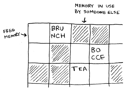
Linked lists

With linked lists, your items can be anywhere in memory.

Each item stores the address of the next item in the list. A bunch of

random memory addresses are linked together.

26

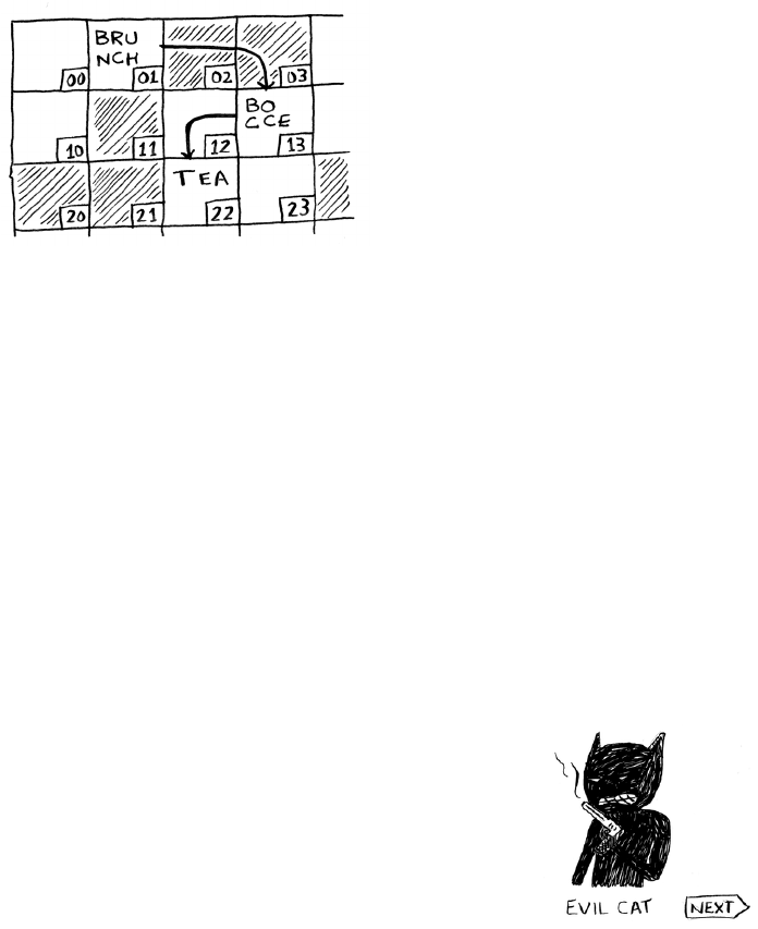
It’s like a treasure hunt. You go to the rst address, and it says, “e next

item can be found at address 123.” So you go to address 123, and it says,

“e next item can be found at address 847,” and so on. Adding an item

to a linked list is easy: you stick it anywhere in memory and store the

address with the previous item.

With linked lists, you never have to move your items. You also avoid

another problem. Let’s say you go to a popular movie with ve of your

friends. e six of you are trying to nd a place to sit, but the theater

is packed. ere aren’t six seats together. Well, sometimes this happens

with arrays. Let’s say you’re trying to nd 10,000 slots for an array. Your

memory has 10,000 slots, but it doesn’t have 10,000 slots together. You

can’t get space for your array! A linked list is like saying, “Let’s split up

and watch the movie.” If there’s space in memory, you have space for

your linked list.

If linked lists are so much better at inserts, what are arrays good for?

Arrays

Websites with top-10 lists use a scummy tactic to get more page views.

Instead of showing you the list on one page, they put one item on each

page and make you click Next to get to the next item in the list. For

example, Top 10 Best TV Villains won’t show you the entire list on one

page. Instead, you start at #10 (Newman), and you have to click Next on

each page to reach #1 (Gustavo Fring). is technique gives the websites

10 whole pages on which to show you ads, but it’s boring to click Next 9

times to get to #1. It would be much better if the whole list was on one

page and you could click each person’s name for more info.

Linked lists have a similar problem. Suppose you want to read the last

item in a linked list. You can’t just read it, because you don’t know what

address it’s at. Instead, you have to go to item #1 to get the address for

Chapter 2

I

Selection sort

Linked memory

addresses

27Arrays and linked lists

item #2. en you have to go to item #2 to get the address for item #3.

And so on, until you get to the last item. Linked lists are great if you’re

going to read all the items one at a time: you can read one item, follow

the address to the next item, and so on. But if you’re going to keep

jumping around, linked lists are terrible.

Arrays are dierent. You know the address for every item in your array.

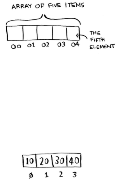
For example, suppose your array contains ve items, and you know it

starts at address 00. What is the address of item #5?

Simple math tells you: it’s 04. Arrays are great if you want to read

random elements, because you can look up any element in your array

instantly. With a linked list, the elements aren’t next to each other,

so you can’t instantly calculate the position of the h element in

memory—you have to go to the rst element to get the address to the

second element, then go to the second element to get the address of

the third element, and so on until you get to the h element.

Terminology

e elements in an array are numbered. is numbering starts from 0,

not 1. For example, in this array, 20 is at position 1.

And 10 is at position 0. is usually throws new programmers for a

spin. Starting at 0 makes all kinds of array-based code easier to write,

so programmers have stuck with it. Almost every programming

language you use will number array elements starting at 0. You’ll

soon get used to it.

28

e position of an element is called its index. So instead of saying, “20 is

at position 1,” the correct terminology is, “20 is at index 1.” I’ll use index

to mean position throughout this book.

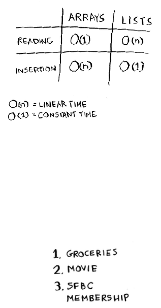
Here are the run times for common operations on arrays and lists.

Question: Why does it take O(n) time to insert an element into an

array? Suppose you wanted to insert an element at the beginning of an

array. How would you do it? How long would it take? Find the answers

to these questions in the next section!

EXERCISE

2.1 Suppose you’re building an app to keep track of your nances.

Every day, you write down everything you spent money on. At the

end of the month, you review your expenses and sum up how much

you spent. So, you have lots of inserts and a few reads. Should you

use an array or a list?

Chapter 2

I

Selection sort

29Arrays and linked lists

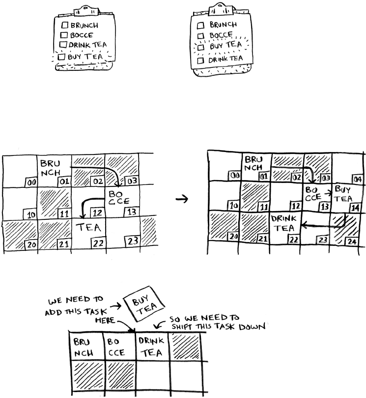
Inserting into the middle of a list

Suppose you want your todo list to work more like a calendar. Earlier,

you were adding things to the end of the list.

Now you want to add them in the order in which they should

be done.

What’s better if you want to insert elements in the middle: arrays or

lists? With lists, it’s as easy as changing what the previous element

points to.

But for arrays, you have to shi all the rest of the elements down.

And if there’s no space, you might have to copy everything to a new

location! Lists are better if you want to insert elements into the middle.

Unordered Ordered

30 Chapter 2

I

Selection sort

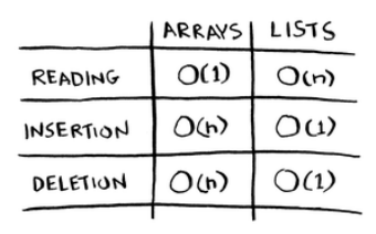
Deletions

What if you want to delete an element? Again, lists are better, because

you just need to change what the previous element points to. With

arrays, everything needs to be moved up when you delete an element.

Unlike insertions, deletions will always work. Insertions can fail

sometimes when there’s no space le in memory. But you can always

delete an element.

Here are the run times for common operations on arrays and

linked lists.

It’s worth mentioning that insertions and deletions are O(1) time only

if you can instantly access the element to be deleted. It’s a common

practice to keep track of the rst and last items in a linked list, so it

would take only O(1) time to delete those.

Which are used more: arrays or lists? Obviously, it depends on the use

case. But arrays see a lot of use because they allow random access. ere

are two dierent types of access: random access and sequential access.

Sequential access means reading the elements one by one, starting

at the rst element. Linked lists can only do sequential access. If you

want to read the 10th element of a linked list, you have to read the rst

9 elements and follow the links to the 10th element. Random access

means you can jump directly to the 10th element. You’ll frequently

hear me say that arrays are faster at reads. is is because they provide

random access. A lot of use cases require random access, so arrays are

used a lot. Arrays and lists are used to implement other data structures,

too (coming up later in the book).

31Arrays and linked lists

EXERCISES

2.2 Suppose you’re building an app for restaurants to take customer

orders. Your app needs to store a list of orders. Servers keep adding

orders to this list, and chefs take orders o the list and make them.

It’s an order queue: servers add orders to the back of the queue, and

the chef takes the rst order o the queue and cooks it.

Would you use an array or a linked list to implement this queue?

(Hint: Linked lists are good for inserts/deletes, and arrays are good

for random access. Which one are you going to be doing here?)

2.3 Let’s run a thought experiment. Suppose Facebook keeps a list of

usernames. When someone tries to log in to Facebook, a search is

done for their username. If their name is in the list of usernames,

they can log in. People log in to Facebook pretty oen, so there are

a lot of searches through this list of usernames. Suppose Facebook

uses binary search to search the list. Binary search needs random

access—you need to be able to get to the middle of the list of

usernames instantly. Knowing this, would you implement the list

as an array or a linked list?

2.4 People sign up for Facebook pretty oen, too. Suppose you decided

to use an array to store the list of users. What are the downsides

of an array for inserts? In particular, suppose you’re using binary

search to search for logins. What happens when you add new users

to an array?

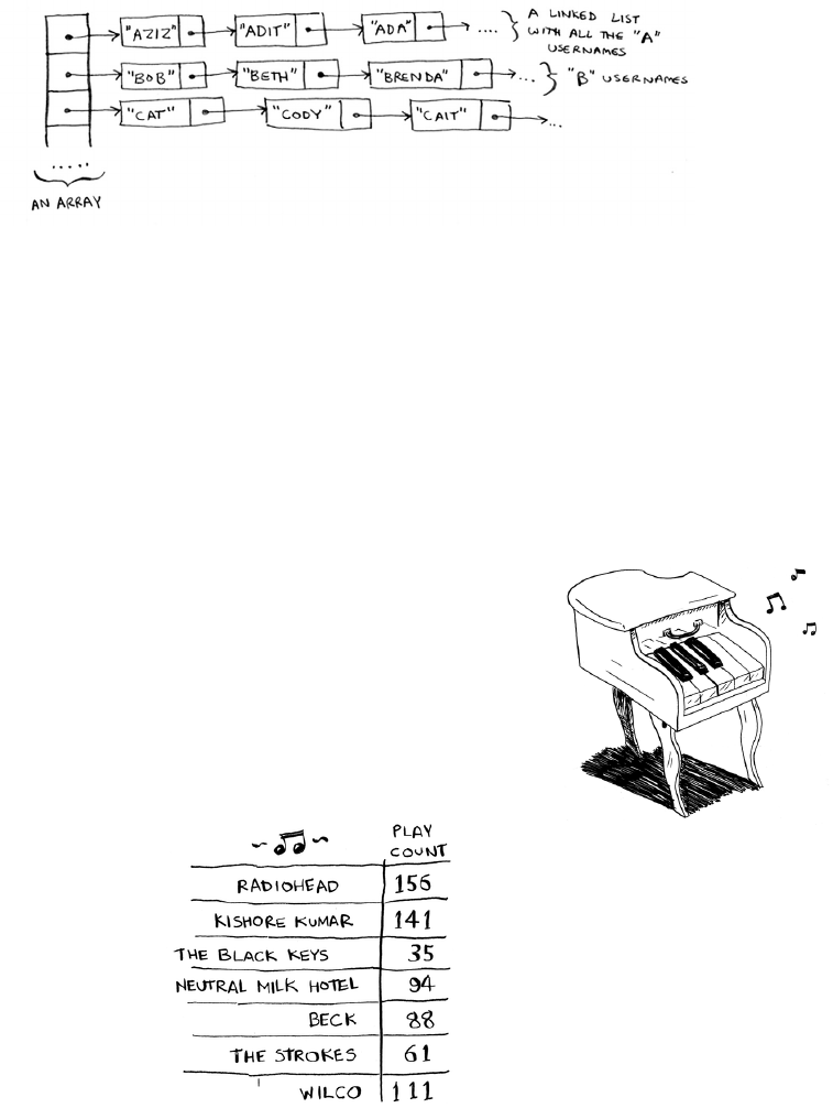
2.5 In reality, Facebook uses neither an array nor a linked list to store

user information. Let’s consider a hybrid data structure: an array

of linked lists. You have an array with 26 slots. Each slot points to a

linked list. For example, the first slot in the array points to a linked

list containing all the usernames starting with a. The second slot

points to a linked list containing all the usernames starting with b,

and so on.

32 Chapter 2

I

Selection sort

Suppose Adit B signs up for Facebook, and you want to add them

to the list. You go to slot 1 in the array, go to the linked list for slot

1, and add Adit B at the end. Now, suppose you want to search for

Zakhir H. You go to slot 26, which points to a linked list of all the

Z names. en you search through that list to nd Zakhir H.

Compare this hybrid data structure to arrays and linked lists. Is it

slower or faster than each for searching and inserting? You don’t

have to give Big O run times, just whether the new data structure

would be faster or slower.

Selection sort

Let’s put it all together to learn your second algorithm:

selection sort. To follow this section, you need to

understand arrays and lists, as well as Big O notation.

Suppose you have a bunch of music on your computer.

For each artist, you have a play count.

You want to sort this list from most to least played, so that you can rank

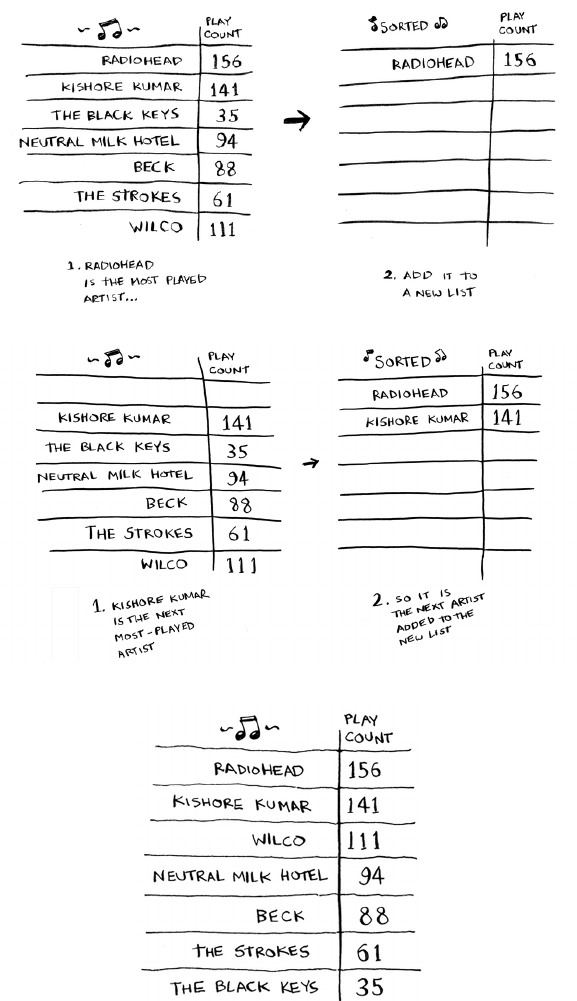
your favorite artists. How can you do it?

33Selection sort

One way is to go through the list and nd the most-played artist. Add

that artist to a new list.

Do it again to nd the next-most-played artist.

Keep doing this, and you’ll end up with a sorted list.

34 Chapter 2

I

Selection sort

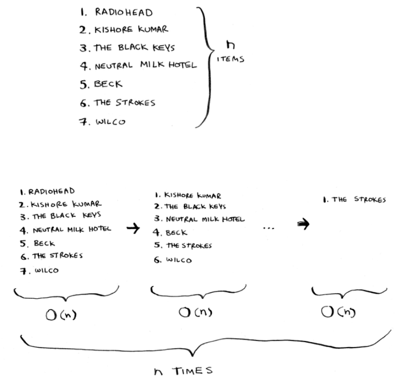
Let’s put on our computer science hats and see how long this will take to

run. Remember that O(n) time means you touch every element in a list

once. For example, running simple search over the list of artists means

looking at each artist once.

To nd the artist with the highest play count, you have to check each

item in the list. is takes O(n) time, as you just saw. So you have an

operation that takes O(n) time, and you have to do that n times:

is takes O(n × n) time or O(n2) time.

Sorting algorithms are very useful. Now you can sort

• Names in a phone book

• Travel dates

• Emails (newest to oldest)

35

Selection sort is a neat algorithm, but it’s not very fast. Quicksort is a

faster sorting algorithm that only takes O(n log n) time. It’s coming up

in the next chapter!

EXAMPLE CODE LISTING

We didn’t show you the code to sort the music list, but following is

some code that will do something very similar: sort an array from

smallest to largest. Let’s write a function to nd the smallest element

in an array:

def fi n d S m a l l e s t(a r r):

smallest = arr[0] Stores the smallest value

smallest_index = 0 Stores the index of the smallest value

for i in range(1, len(arr)):

if arr[i] < smallest:

smallest = arr[i]

smallest_index = i

return smallest_index

Now you can use this function to write selection sort:

def selectionSort(arr): Sorts an array

newArr = []

for i in range(len(arr)):

smallest = findSmallest(arr)

newArr.append(arr.pop(smallest))

return newArr

print selectionSort([5, 3, 6, 2, 10])

Selection sort

Checking fewer elements each time

Maybe you’re wondering: as you go through the operations, the number

of elements you have to check keeps decreasing. Eventually, you’re down

to having to check just one element. So how can the run time still be

O(n2)? at’s a good question, and the answer has to do with constants

in Big O notation. I’ll get into this more in chapter 4, but here’s the gist.

You’re right that you don’t have to check a list of n elements each time.

You check n elements, then n – 1, n - 2 … 2, 1. On average, you check a

list that has 1/2 × n elements. e runtime is O(n × 1/2 × n). But constants

like 1/2 are ignored in Big O notation (again, see chapter 4 for the full

discussion), so you just write O(n × n) or O(n2).

Finds the smallest element in the

array, and adds it to the new array

36

Recap

• Your computer’s memory is like a giant set of drawers.

• When you want to store multiple elements, use an array or a list.

• With an array, all your elements are stored right next to each other.

• With a list, elements are strewn all over, and one element stores

the address of the next one.

• Arrays allow fast reads.

• Linked lists allow fast inserts and deletes.

• All elements in the array should be the same type (all ints,

all doubles, and so on).

Chapter 2

I

Selection sort

37

3

In this chapter

• You learn about recursion. Recursion is a coding

technique used in many algorithms. It’s a building

block for understanding later chapters in this book.

• You learn how to break a problem down into a

base case and a recursive case. The divide-and-

conquer strategy (chapter 4) uses this simple

concept to solve hard problems.

recursion

I’m excited about this chapter because it covers recursion, an

elegant way to solve problems. Recursion is one of my favorite

topics, but it’s divisive. People either love it or hate it, or hate it until

they learn to love it a few years later. I personally was in that third

camp. To make things easier for you, I have some advice:

• is chapter has a lot of code examples. Run the code for yourself

to see how it works.

• I’ll talk about recursive functions. At least once, step through a

recursive function with pen and paper: something like, “Let’s see,

I pass 5 into

factorial

, and then I return 5 times passing 4 into

factorial

, which is …,” and so on. Walking through a function

like this will teach you how a recursive function works.

38 Chapter 3

I

Recursion

is chapter also includes a lot of pseudocode. Pseudocode is a

high-level description of the problem you’re trying to solve, in code.

It’s written like code, but it’s meant to be closer to human speech.

Recursion

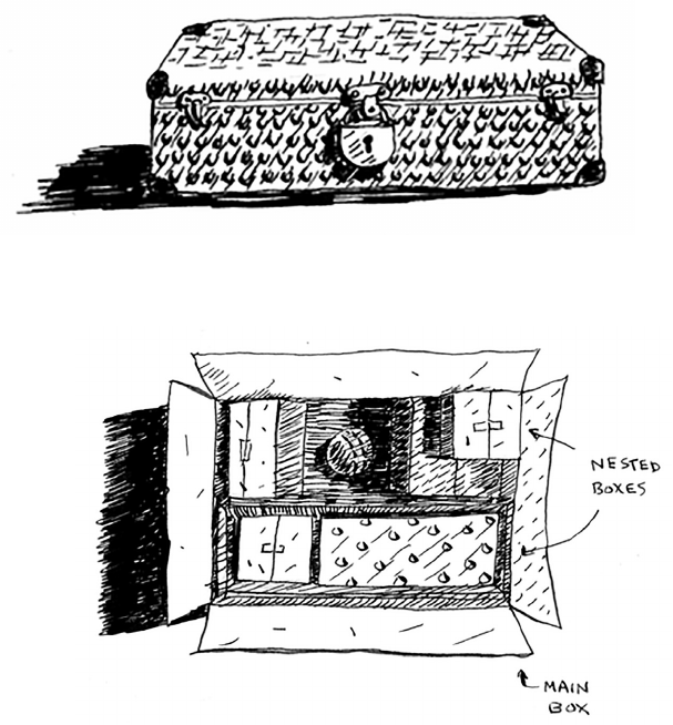
Suppose you’re digging through your grandma’s attic and come across a

mysterious locked suitcase.

Grandma tells you that the key for the suitcase is probably in this

other box.

is box contains more boxes, with more boxes inside those boxes. e

key is in a box somewhere. What’s your algorithm to search for the key?

ink of an algorithm before you read on.

39Recursion

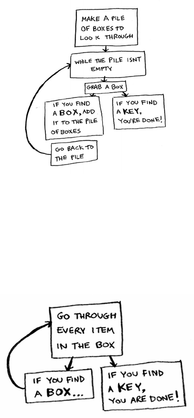
Here’s one approach.

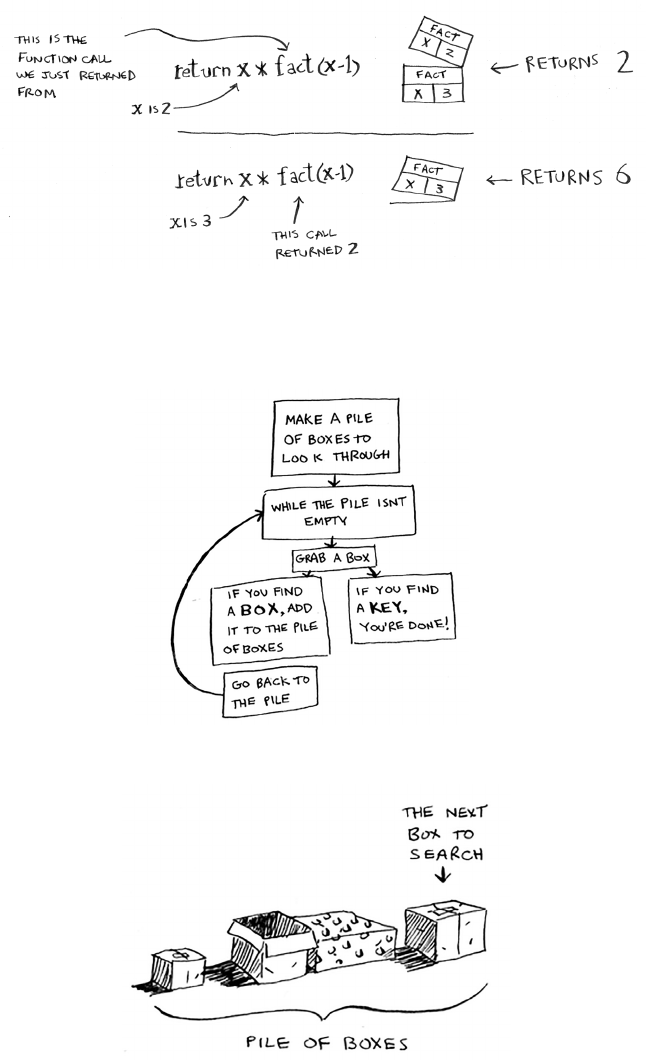
1. Make a pile of boxes to look through.

2. Grab a box, and look through it.

3. If you nd a box, add it to the pile to look through later.

4. If you nd a key, you’re done!

5. Repeat.

Here’s an alternate approach.

1. Look through the box.

2. If you nd a box, go to step 1.

3. If you nd a key, you’re done!

40 Chapter 3

I

Recursion

Which approach seems easier to you? e rst approach uses a

while

loop. While the pile isn’t empty, grab a box and look through it:

def look_for_key(main_box):

pile = main_box.make_a_pile_to_look_through()

while pile is not empty:

box = pile.grab_a_box()

for item in box:

if item.is_a_box():

pile.a p p e n d(ite m)

elif item.is_a_key():

print “found the key!”

e second way uses recursion. Recursion is where a function calls itself.

Here’s the second way in pseudocode:

def lo o k _ f o r _ k e y( b o x ):

for item in box:

if item.is_a_box():

look_for_key(item) Recursion!

elif item.is_a_key():

print “found the key!”

Both approaches accomplish the same thing, but the second approach

is clearer to me. Recursion is used when it makes the solution clearer.

ere’s no performance benet to using recursion; in fact, loops are

sometimes better for performance. I like this quote by Leigh Caldwell

on Stack Overow: “Loops may achieve a performance gain for

your program. Recursion may achieve a performance gain for your

programmer. Choose which is more important in your situation!”1

Many important algorithms use recursion, so it’s important to

understand the concept.

Base case and recursive case

Because a recursive function calls itself, it’s easy to write a

function incorrectly that ends up in an innite loop. For

example, suppose you want to write a function that prints a countdown,

like this:

> 3...2...1

1 http://stackoverow.com/a/72694/139117.

41Base case and recursive case

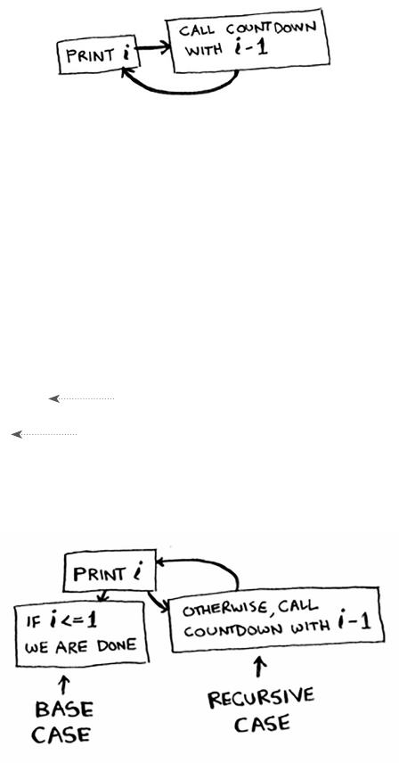
You can write it recursively, like so:

def countdown(i):

print i

c o u n t d o w n(i-1)

Write out this code and run it. You’ll notice a problem: this function

will run forever!

> 3...2...1...0...-1...-2...

(Press Ctrl-C to kill your script.)

When you write a recursive function, you have to tell it when to stop

recursing. at’s why every recursive function has two parts: the base

case, and the recursive case. e recursive case is when the function calls

itself. e base case is when the function doesn’t call itself again … so it

doesn’t go into an innite loop.

Let’s add a base case to the countdown function:

def c o u n t d o w n(i):

print i

if i <= 0: Base case

return

else: Recursive case

c o u n t d o w n(i-1)

Now the function works as expected. It goes something like this.

Infinite loop

42 Chapter 3

I

Recursion

The stack

is section covers the call stack. It’s an important concept

in programming. e call stack is an important concept in

general programming, and it’s also important to understand

when using recursion.

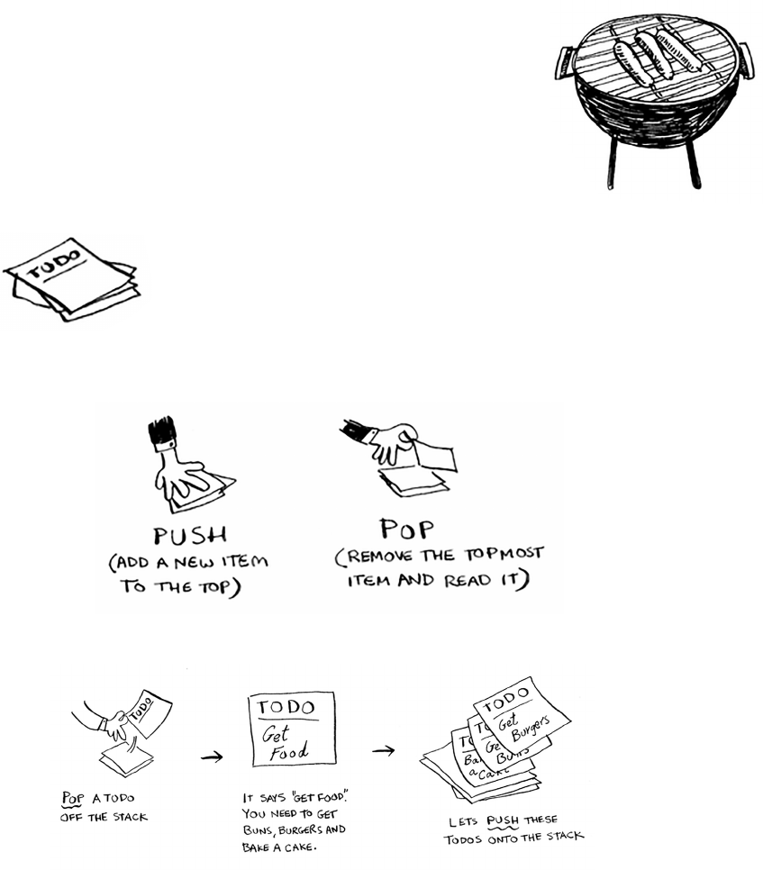
Suppose you’re throwing a barbecue. You keep a todo list for the

barbecue, in the form of a stack of sticky notes.

Remember back when we talked about arrays and lists,

and you had a todo list? You could add todo items

anywhere to the list or delete random items. e stack of

sticky notes is much simpler. When you insert an item,

it gets added to the top of the list. When you read an item,

you only read the topmost item, and it’s taken o the list. So your todo

list has only two actions: push (insert) and pop (remove and read).

Let’s see the todo list in action.

is data structure is called a stack. e stack is a simple data structure.

You’ve been using a stack this whole time without realizing it!

43The stack

The call stack

Your computer uses a stack internally called the call stack. Let’s see it in

action. Here’s a simple function:

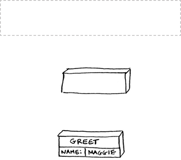
def greet(name):

print “hello, “ + name + “!”

greet2(name)

print “getting ready to say bye...”

b ye()

is function greets you and then calls two other functions. Here are

those two functions:

def greet2(name):

print “how are you, “ + name + “?”

def b y e ():

print “ok bye!”

Let’s walk through what happens when you call a function.

Suppose you call

g r e e t(“ m a g g i e”)

. First, your computer allocates a box

of memory for that function call.

Now let’s use the memory. e variable

name

is set to “maggie”. at

needs to be saved in memory.

Note

print

is a function in Python, but to make things easier for this example,

we’re pretending it isn’t. Just play along.

44 Chapter 3

I

Recursion

Every time you make a function call, your computer saves the values

for all the variables for that call in memory like this. Next, you print

hello, m aggie!

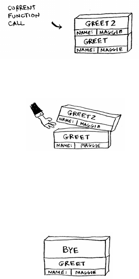
en you call

g r e e t 2(“ m a g g i e ”).

Again, your

computer allocates a box of memory for this function call.

Your computer is using a stack for these boxes. e second box is added

on top of the rst one. You print

how are you, maggie?

en you

return from the function call. When this happens, the box on top of the

stack gets popped o.

Now the topmost box on the stack is for the

greet

function, which

means you returned back to the

greet

function. When you called the

greet2

function, the

greet

function was partially completed. is is

the big idea behind this section: when you call a function from another

function, the calling function is paused in a partially completed state. All

the values of the variables for that function are still stored in memory.

Now that you’re done with the

greet2

function, you’re back to the

greet

function, and you pick up where you le o. First you print

getting ready to say bye…

. You call the

bye

function.

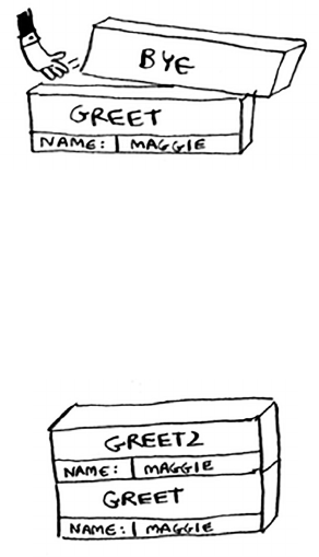
45The stack

A box for that function is added to the top of the stack. en you print

ok bye!

and return from the function call.

And you’re back to the

greet

function. ere’s nothing else to be done,

so you return from the

greet

function too. is stack, used to save the

variables for multiple functions, is called the call stack.

EXERCISE

3.1 Suppose I show you a call stack like this.

What information can you give me, just based on this call stack?

Now let’s see the call stack in action with a recursive function.

The call stack with recursion

Recursive functions use the call stack too! Let’s look at this in action

with the

factorial

function.

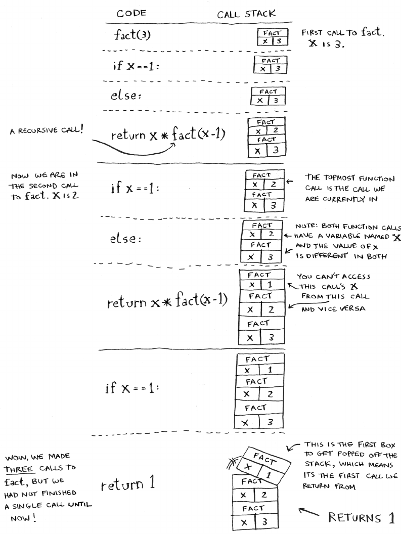
factorial(5)

is written as 5!, and it’s

dened like this: 5! = 5 * 4 * 3 * 2 * 1. Similarly,

factorial(3)

is

3 * 2 * 1. Here’s a recursive function to calculate the factorial of a

number:

def f a c t( x):

if x == 1:

return 1

else:

return x * fact(x-1)

Now you call

f ac t(3)

. Let’s step through this call line by line and see

how the stack changes. Remember, the topmost box in the stack tells

you what call to

fact

you’re currently on.

46 Chapter 3

I

Recursion

47The stack

Notice that each call to

fact

has its own copy of

x

. You can’t access a

dierent function’s copy of

x

.

e stack plays a big part in recursion. In the opening example, there

were two approaches to nd the key. Here’s the rst way again.

is way, you make a pile of boxes to search through, so you always

know what boxes you still need to search.

48 Chapter 3

I

Recursion

But in the recursive approach, there’s no pile.

If there’s no pile, how does your algorithm know what boxes you still

have to look through? Here’s an example.

49The stack

At this point, the call stack looks like this.

e “pile of boxes” is saved on the stack! is is a stack of half-

completed function calls, each with its own half-complete list of boxes

to look through. Using the stack is convenient because you don’t have to

keep track of a pile of boxes yourself—the stack does it for you.

Using the stack is convenient, but there’s a cost: saving all that info can

take up a lot of memory. Each of those function calls takes up some

memory, and when your stack is too tall, that means your computer is

saving information for many function calls. At that point, you have two

options:

• You can rewrite your code to use a loop instead.

• You can use something called tail recursion. at’s an advanced

recursion topic that is out of the scope of this book. It’s also only

supported by some languages, not all.

EXERCISE

3.2 Suppose you accidentally write a recursive function that runs

forever. As you saw, your computer allocates memory on the

stack for each function call. What happens to the stack when your

recursive function runs forever?

50 Chapter 3

I

Recursion

Recap

• Recursion is when a function calls itself.

• Every recursive function has two cases: the base case

and the recursive case.

• A stack has two operations: push and pop.

• All function calls go onto the call stack.

• e call stack can get very large, which takes up a lot of memory.

4

In this chapter

• You learn about divide-and-conquer. Sometimes

you’ll come across a problem that can’t be solved

by any algorithm you’ve learned. When a good

algorithmist comes across such a problem, they

don’t just give up. They have a toolbox full of

techniques they use on the problem, trying to

come up with a solution. Divide-and-conquer

is the rst general technique you learn.

• You learn about quicksort, an elegant sorting

algorithm that’s often used in practice. Quicksort

uses divide-and-conquer.

51

quicksort

You learned all about recursion in the last chapter. is chapter

focuses on using your new skill to solve problems. We’ll explore

divide and conquer (D&C), a well-known recursive technique for

solving problems.

is chapter really gets into the meat of algorithms. Aer all,

an algorithm isn’t very useful if it can only solve one type of

problem. Instead, D&C gives you a new way to think about solving

52 Chapter 4

I

Quicksort

problems. D&C is another tool in your toolbox. When you get a new

problem, you don’t have to be stumped. Instead, you can ask, “Can I

solve this if I use divide and conquer?”

At the end of the chapter, you’ll learn your rst major D&C algorithm:

quicksort. Quicksort is a sorting algorithm, and a much faster one than

selection sort (which you learned in chapter 2). It’s a good example of

elegant code.

Divide & conquer

D&C can take some time to grasp. So, we’ll do three

examples. First I’ll show you a visual example. en

I’ll do a code example that is less pretty but maybe

easier. Finally, we’ll go through quicksort, a sorting

algorithm that uses D&C.

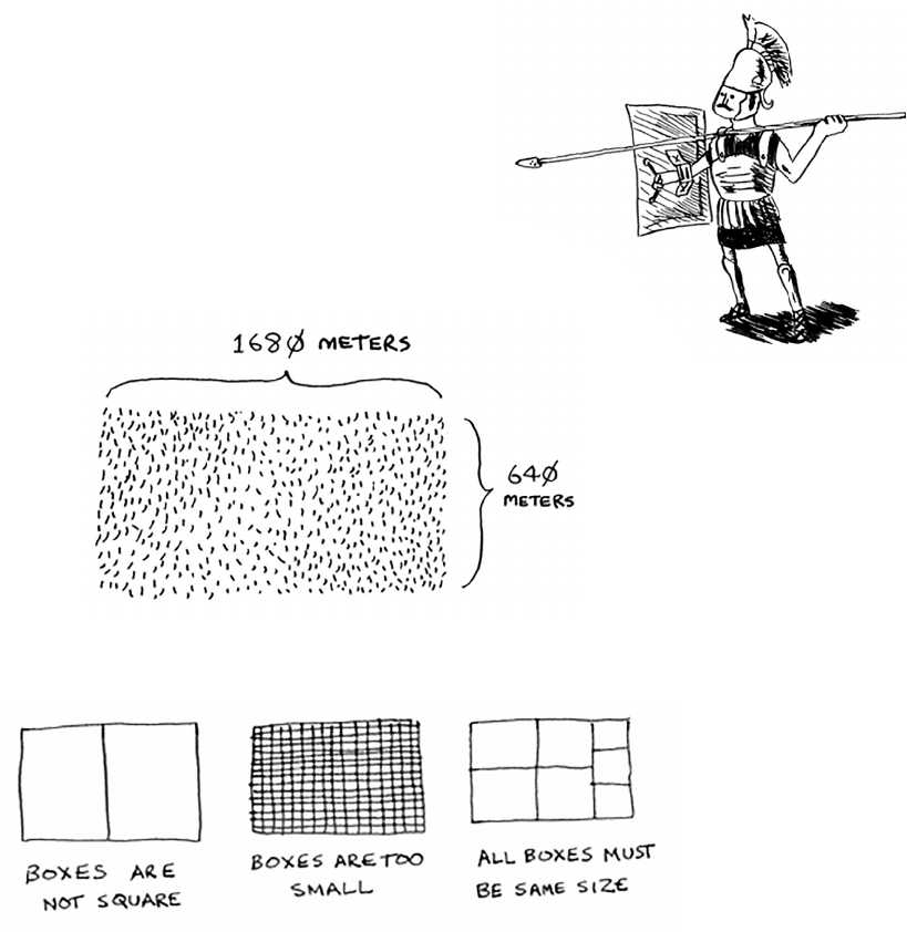
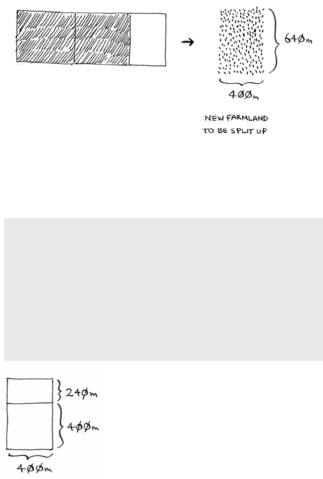
Suppose you’re a farmer with a plot of land.

You want to divide this farm evenly into square plots. You want the plots

to be as big as possible. So none of these will work.

53Divide & conquer

How do you gure out the largest square size you can use for a plot of

land? Use the D&C strategy! D&C algorithms are recursive algorithms.

To solve a problem using D&C, there are two steps:

1. Figure out the base case. is should be the simplest possible case.

2. Divide or decrease your problem until it becomes the base case.

Let’s use D&C to nd the solution to this problem. What is the largest

square size you can use?

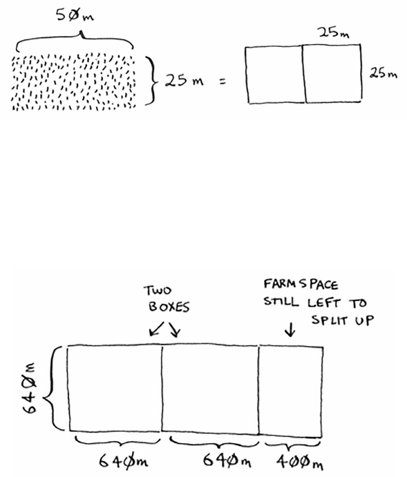
First, gure out the base case. e easiest case would be if one side was

a multiple of the other side.

Suppose one side is 25 meters (m) and the other side is 50 m. en the

largest box you can use is 25 m × 25 m. You need two of those boxes to

divide up the land.

Now you need to gure out the recursive case. is is where D&C

comes in. According to D&C, with every recursive call, you have to

reduce your problem. How do you reduce the problem here? Let’s start

by marking out the biggest boxes you can use.

54 Chapter 4

I

Quicksort

You can t two 640 × 640 boxes in there, and there’s some land still

le to be divided. Now here comes the “Aha!” moment. ere’s a

farm segment le to divide. Why don’t you apply the same algorithm

to this segment?

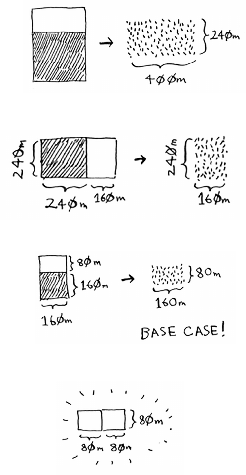
So you started out with a 1680 × 640 farm that needed to be split up.

But now you need to split up a smaller segment, 640 × 400. If you nd

the biggest box that will work for this size, that will be the biggest box

that will work for the entire farm. You just reduced the problem from

a 1680 × 640 farm to a 640 × 400 farm!

Let’s apply the same algorithm again. Starting

with a 640 × 400m farm, the biggest box you

can create is 400 × 400 m.

Euclid’s algorithm

“If you nd the biggest box that will work for this size, that will be the

biggest box that will work for the entire farm.” If it’s not obvious to you

why this statement is true, don’t worry. It isn’t obvious. Unfortunately, the

proof for why it works is a little too long to include in this book, so you’ll

just have to believe me that it works. If you want to understand the proof,

look up Euclid’s algorithm. e Khan academy has a good explanation

here: https://www.khanacademy.org/computing/computer-science/

cryptography/modarithmetic/a/the-euclidean-algorithm.

55Divide & conquer

And that leaves you with a smaller segment, 400 × 240 m.

And you can draw a box on that to get an even smaller segment,

240 × 160 m.

And then you draw a box on that to get an even smaller segment.

Hey, you’re at the base case: 80 is a factor of 160. If you split up this

segment using boxes, you don’t have anything le over!

56 Chapter 4

I

Quicksort

So, for the original farm, the biggest plot size you can use is 80 × 80 m.

To recap, here’s how D&C works:

1. Figure out a simple case as the base case.

2. Figure out how to reduce your problem and get to the base case.

D&C isn’t a simple algorithm that you can apply to a problem. Instead,

it’s a way to think about a problem. Let’s do one more example.

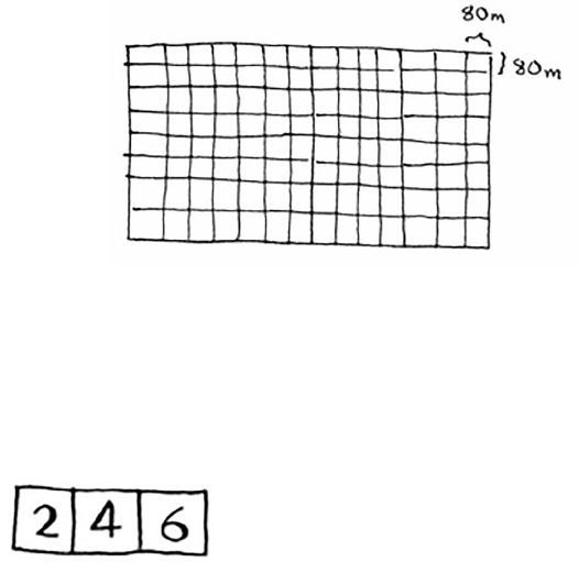
You’re given an array of numbers.

You have to add up all the numbers and return the total. It’s pretty easy

to do this with a loop:

def s u m ( a r r):

total = 0

for x in arr:

total += x

return total

print sum([1, 2, 3, 4])

But how would you do this with a recursive function?

Step 1: Figure out the base case. What’s the simplest array you could

get? ink about the simplest case, and then read on. If you get an array

with 0 or 1 element, that’s pretty easy to sum up.

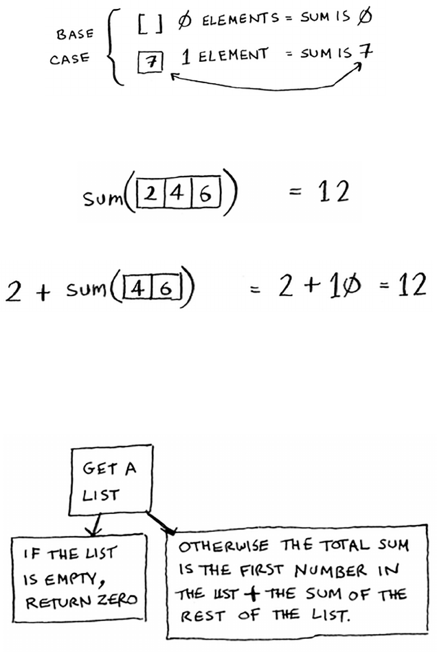
57Divide & conquer

So that will be the base case.

Step 2: You need to move closer to an empty array with every recursive

call. How do you reduce your problem size? Here’s one way.

It’s the same as this.

In either case, the result is 12. But in the second version, you’re passing

a smaller array into the

sum

function. at is, you decreased the size of

your problem!

Your

sum

function could work like this.

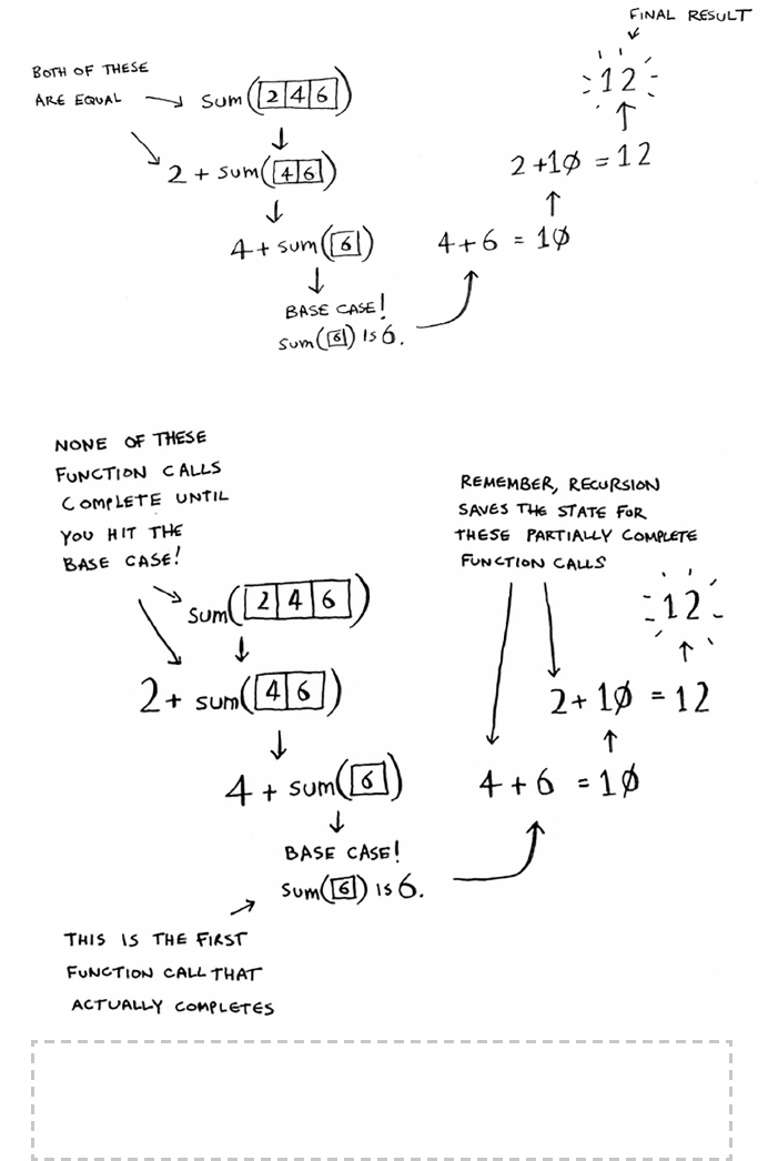
58 Chapter 4

I

Quicksort

Here it is in action.

Tip

When you’re writing a recursive function involving an array, the base case is

often an empty array or an array with one element. If you’re stuck, try that rst.

Remember, recursion keeps track of the state.

59Divide & conquer

EXERCISES

4.1 Write out the code for the earlier

sum

function.

4.2 Write a recursive function to count the number of items in a list.

4.3 Find the maximum number in a list.

4.4 Remember binary search from chapter 1? It’s a divide-and-conquer

algorithm, too. Can you come up with the base case and recursive

case for binary search?

Sneak peak at functional programming

“Why would I do this recursively if I can do it easily with a loop?” you

may be thinking. Well, this is a sneak peek into functional programming!

Functional programming languages like Haskell don’t have loops, so

you have to use recursion to write functions like this. If you have a good

understanding of recursion, functional languages will be easier to learn.

For example, here’s how you’d write a

sum

function in Haskell:

sum [] = 0 Base case

sum (x:xs) = x + (sum xs) Recursive case

Notice that it looks like you have two denitions for the function. e rst

denition is run when you hit the base case. e second denition runs

at the recursive case. You can also write this function in Haskell using an

if statement:

sum arr = if arr == []

then 0

else (head arr) + (sum (tail arr))

But the rst denition is easier to read. Because Haskell makes heavy use

of recursion, it includes all kinds of niceties like this to make recursion

easy. If you like recursion, or you’re interested in learning a new language,

check out Haskell.

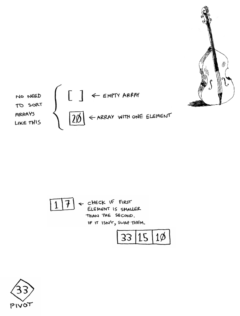
60 Chapter 4

I

Quicksort

Quicksort

Quicksort is a sorting algorithm. It’s much faster than selection sort

and is frequently used in real life. For example, the C standard library

has a function called

qsort

, which is its implementation of quicksort.

Quicksort also uses D&C.

Let’s use quicksort to sort an array. What’s the simplest array that a

sorting algorithm can handle (remember my tip from the previous

section)? Well, some arrays don’t need to be sorted at all.

Empty arrays and arrays with just one element will be the base case. You

can just return those arrays as is—there’s nothing to sort:

def q u i c k s o r t(a r r a y):

if len(array) < 2:

return array

Let’s look at bigger arrays. An array with two elements is pretty easy to

sort, too.

What about an array of three elements?

Remember, you’re using D&C. So you want to break down this array

until you’re at the base case. Here’s how quicksort works. First, pick an

element from the array. is element is called the pivot.

We’ll talk about how to pick a good pivot later. For now,

let’s say the rst item in the array is the pivot.

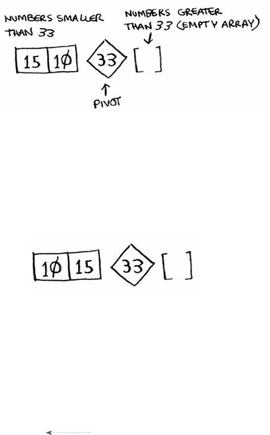
61Quicksort

Now nd the elements smaller than the pivot and the elements larger

than the pivot.

is is called partitioning. Now you have

• A sub-array of all the numbers less than the pivot

• e pivot

• A sub-array of all the numbers greater than the pivot

e two sub-arrays aren’t sorted. ey’re just partitioned. But if they

were sorted, then sorting the whole array would be pretty easy.

If the sub-arrays are sorted, then you can combine the whole thing like

this—

left array + pivot + right array

—and you get a sorted

array. In this case, it’s

[10, 15] + [33] + [] =

[10, 15, 33]

, which is a sorted array.

How do you sort the sub-arrays? Well, the quicksort base case already

knows how to sort arrays of two elements (the le sub-array) and

empty arrays (the right sub-array). So if you call quicksort on the two

sub-arrays and then combine the results, you get a sorted array!

quicksort([15, 10]) + [33] + quicksort([])

> [10, 15, 33] A sorted array

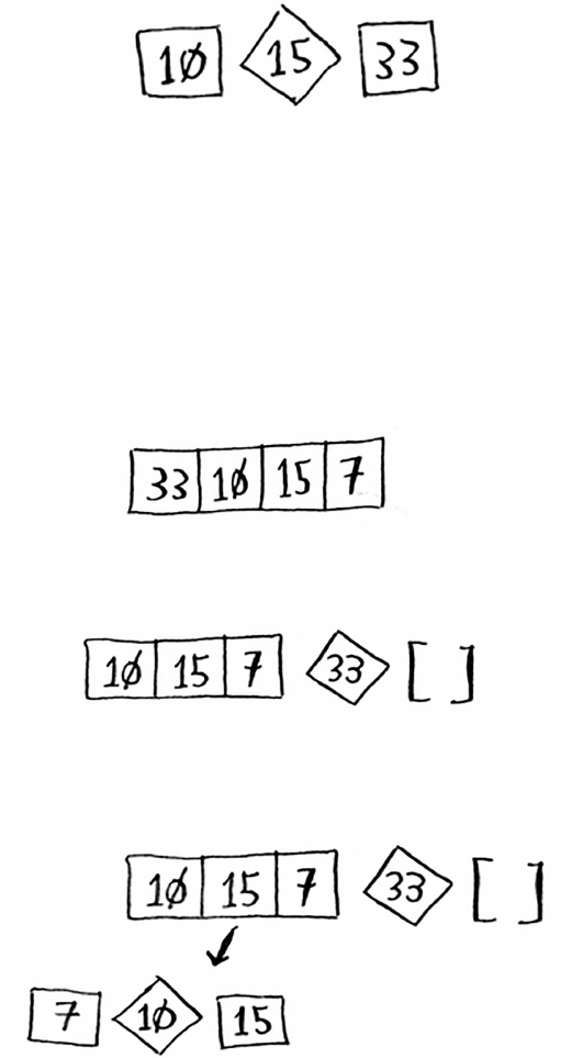
62 Chapter 4

I

Quicksort

is will work with any pivot. Suppose you choose 15 as the

pivot instead.

Both sub-arrays have only one element, and you know how to sort

those. So now you know how to sort an array of three elements. Here

are the steps:

1. Pick a pivot.

2. Partition the array into two sub-arrays: elements less than the pivot

and elements greater than the pivot.

3. Call quicksort recursively on the two sub-arrays.

What about an array of four elements?

Suppose you choose 33 as the pivot again.

e array on the le has three elements. You already know how to sort

an array of three elements: call quicksort on it recursively.

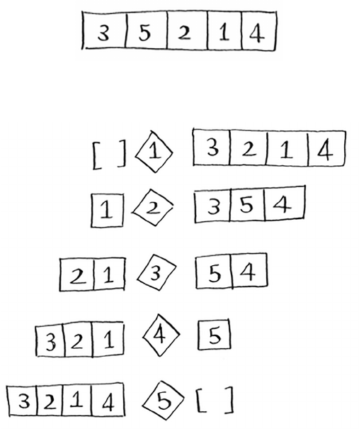
63Quicksort

So you can sort an array of four elements. And if you can sort an array

of four elements, you can sort an array of ve elements. Why is that?

Suppose you have this array of ve elements.

Here are all the ways you can partition this array, depending on what

pivot you choose.

Notice that all of these sub-arrays have somewhere between 0 and 4

elements. And you already know how to sort an array of 0 to 4 elements

using quicksort! So no matter what pivot you pick, you can call

quicksort recursively on the two sub-arrays.

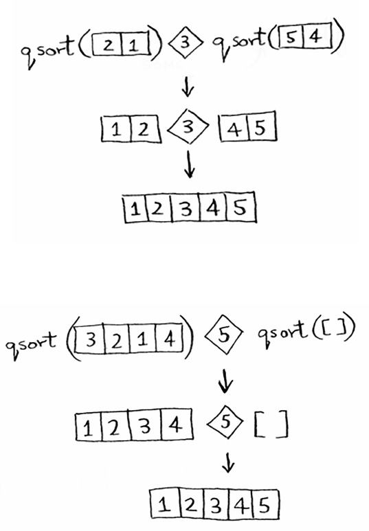
64 Chapter 4

I

Quicksort

For example, suppose you pick 3 as the pivot. You call quicksort on the

sub-arrays.

e sub-arrays get sorted, and then you combine the whole thing to get

a sorted array. is works even if you choose 5 as the pivot.

is works with any element as the pivot. So you can sort an array

of ve elements. Using the same logic, you can sort an array of six

elements, and so on.

65Quicksort

Here’s the code for quicksort:

def q u i c k s o r t(a r r a y):

if len(array) < 2:

return array Base case: arrays with 0 or 1 element are already “sorted.”

else:

pivot = array[0] Recursive case

less = [i for i in array[1:] if i <= pivot] Sub-array of all the elements

less than the pivot

greater = [i for i in array[1:] if i > pivot] Sub-array of all the elements

greater than the pivot

return quicksort(less) + [pivot] + quicksort(greater)

print quicksort([10, 5, 2, 3])

Inductive proofs

You just got a sneak peak into inductive proofs! Inductive proofs are one

way to prove that your algorithm works. Each inductive proof has two

steps: the base case and the inductive case. Sound familiar? For example,

suppose I want to prove that I can climb to the top of a ladder. In the

inductive case, if my legs are on a rung, I can put my legs on the next rung.

So if I’m on rung 2, I can climb to rung 3. at’s the inductive case. For

the base case, I’ll say that my legs are on rung 1. erefore, I can climb the

entire ladder, going up one rung at a time.

You use similar reasoning for quicksort. In the base case, I showed that the

algorithm works for the base case: arrays of size 0 and 1. In the inductive

case, I showed that if quicksort works for an array of size 1, it will work

for an array of size 2. And if it works for arrays of size 2, it will work for

arrays of size 3, and so on. en I can say that quicksort will work for all

arrays of any size. I won’t go deeper into inductive proofs here, but they’re

fun and go hand-in-hand with D&C.

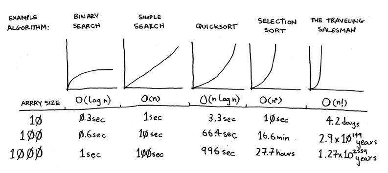
66 Chapter 4

I

Quicksort

Big O notation revisited

Quicksort is unique because its speed depends on the pivot you choose.

Before I talk about quicksort, let’s look at the most common Big O run

times again.

e example times in this chart are estimates if you perform 10

operations per second. ese graphs aren’t precise—they’re just there

to give you a sense of how dierent these run times are. In reality, your

computer can do way more than 10 operations per second.

Each run time also has an example algorithm attached. Check out

selection sort, which you learned in chapter 2. It’s O(n2). at’s a pretty

slow algorithm.

ere’s another sorting algorithm called merge sort, which is

O(n log n). Much faster! Quicksort is a tricky case. In the worst case,

quicksort takes O(n2) time.

It’s as slow as selection sort! But that’s the worst case. In the average

case, quicksort takes O(n log n) time. So you might be wondering:

• What do worst case and average case mean here?

• If quicksort is O(n log n) on average, but merge sort is O(n log n)

always, why not use merge sort? Isn’t it faster?

Estimates based on a slow computer that performs 10 operations per second

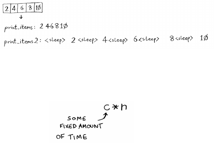
67Big O notation revisited

Merge sort vs. quicksort

Suppose you have this simple function to print every item in a list:

def print_items(list):

for item in list:

print item

is function goes through every item in the list and prints it out.

Because it loops over the whole list once, this function runs in O(n)

time. Now, suppose you change this function so it sleeps for 1 second

before it prints out an item:

from time import sleep

def print_items2(list):

for item in list:

sle e p(1)

print item

Before it prints out an item, it will pause for 1 second. Suppose you

print a list of ve items using both functions.

Both functions loop through the list once, so they’re both O(n) time.

Which one do you think will be faster in practice? I think

print_items

will be much faster because it doesn’t pause for 1 second before printing

an item. So even though both functions are the same speed in Big O

notation,

print_items

is faster in practice. When you write Big O

notation like O(n), it really means this.

c

is some xed amount of time that your algorithm takes. It’s called the

constant. For example, it might be

10 milliseconds *

n

for

print_

ite ms

versus

1 second

*

n

for

print_items2

.

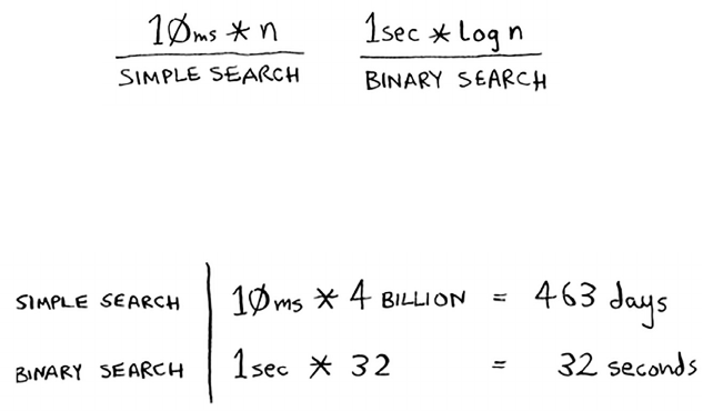
68 Chapter 4

I

Quicksort

You usually ignore that constant, because if two algorithms have

dierent Big O times, the constant doesn’t matter. Take binary search

and simple search, for example. Suppose both algorithms had these

constants.

You might say, “Wow! Simple search has a constant of 10 milliseconds,

but binary search has a constant of 1 second. Simple search is way

faster!” Now suppose you’re searching a list of 4 billion elements. Here

are the times.

As you can see, binary search is still way faster. at constant didn’t

make a dierence at all.

But sometimes the constant can make a dierence. Quicksort versus

merge sort is one example. Quicksort has a smaller constant than

merge sort. So if they’re both O(n log n) time, quicksort is faster. And

quicksort is faster in practice because it hits the average case way more

oen than the worst case.

So now you’re wondering: what’s the average case versus the worst case?

Average case vs. worst case

e performance of quicksort heavily depends on the pivot you choose.

Suppose you always choose the rst element as the pivot. And you

call quicksort with an array that is already sorted. Quicksort doesn’t

check to see whether the input array is already sorted. So it will still try

to sort it.

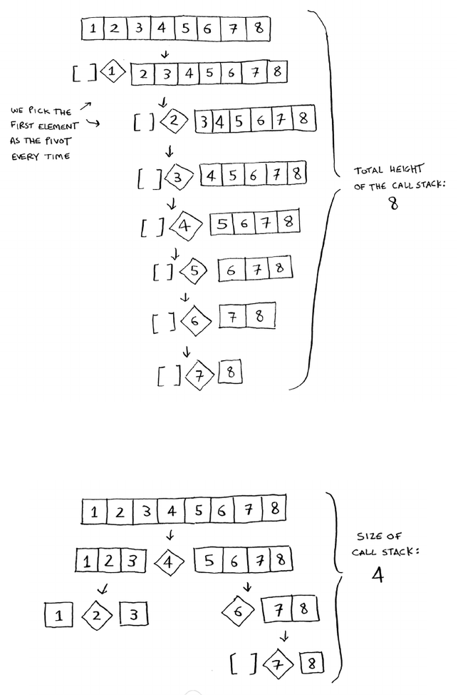
69Big O notation revisited

Notice how you’re not splitting the array into two halves. Instead, one

of the sub-arrays is always empty. So the call stack is really long. Now

instead, suppose you always picked the middle element as the pivot.

Look at the call stack now.

It’s so short! Because you divide the array in half every time, you don’t

need to make as many recursive calls. You hit the base case sooner, and

the call stack is much shorter.

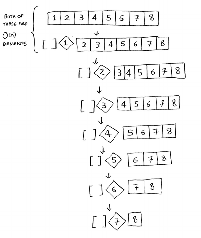
70 Chapter 4

I

Quicksort

e rst example you saw is the worst-case scenario, and the second

example is the best-case scenario. In the worst case, the stack size is

O(n). In the best case, the stack size is O(log n).

Now look at the rst level in the stack. You pick one element as the

pivot, and the rest of the elements are divided into sub-arrays. You

touch all eight elements in the array. So this rst operation takes O(n)

time. You touched all eight elements on this level of the call stack. But

actually, you touch O(n) elements on every level of the call stack.

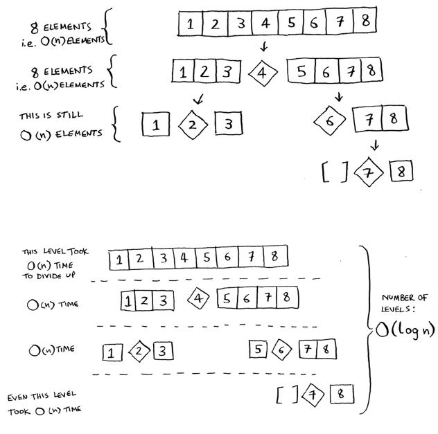
71Big O notation revisited

Even if you partition the array dierently, you’re still touching O(n)

elements every time.

So each level takes O(n) time to complete.

In this example, there are O(log n) levels (the technical way to say

that is, “e height of the call stack is O(log n)”). And each level takes

O(n) time. e entire algorithm will take O(n) * O(log n) = O(n log n)

time. is is the best-case scenario.

In the worst case, there are O(n) levels, so the algorithm will take

O(n) * O(n) = O(n2) time.

Well, guess what? I’m here to tell you that the best case is also the

average case. If you always choose a random element in the array as the

pivot, quicksort will complete in O(n log n) time on average. Quicksort

is one of the fastest sorting algorithms out there, and it’s a very good

example of D&C.

72 Chapter 4

I

Quicksort

EXERCISES

How long would each of these operations take in Big O notation?

4.5 Printing the value of each element in an array.

4.6 Doubling the value of each element in an array.

4.7 Doubling the value of just the rst element in an array.

4.8 Creating a multiplication table with all the elements in the array. So

if your array is [2, 3, 7, 8, 10], you rst multiply every element by 2,

then multiply every element by 3, then by 7, and so on.

Recap

• D&C works by breaking a problem down into smaller and smaller

pieces. If you’re using D&C on a list, the base case is probably an

empty array or an array with one element.

• If you’re implementing quicksort, choose a random element as the

pivot. e average runtime of quicksort is O(n log n)!

• e constant in Big O notation can matter sometimes. at’s why

quicksort is faster than merge sort.

• e constant almost never matters for simple search versus binary

search, because O(log n) is so much faster than O(n) when your list

gets big.

73

In this chapter

• You learn about hash tables, one of the most

useful basic data structures. Hash tables have many

uses; this chapter covers the common use cases.

• You learn about the internals of hash tables:

implementation, collisions, and hash functions.

This will help you understand how to analyze a

hash table’s performance.

hash tables 5

Suppose you work at a grocery store. When a customer

buys produce, you have to look up the price in a book. If

the book is unalphabetized, it can take you a long time to

look through every single line for apple. You’d be doing

simple search from chapter 1, where you have to look at

every line. Do you remember how long that would take?

O(n) time. If the book is alphabetized, you could run

binary search to nd the price of an apple. at would

only take O(log n) time.

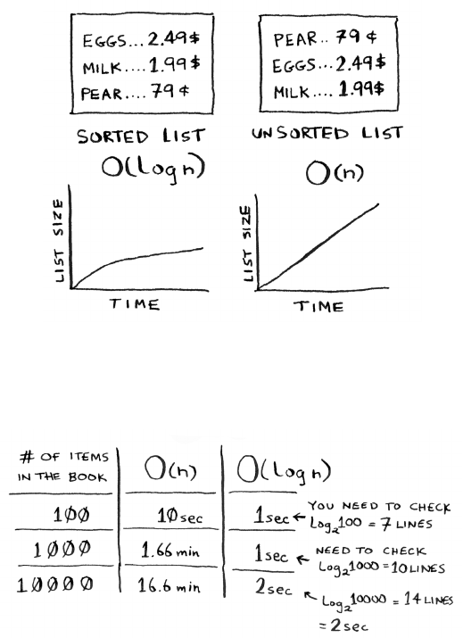
74 Chapter 5

I

Hash tables

As a reminder, there’s a big dierence between O(n) and O(log n) time!

Suppose you could look through 10 lines of the book per second. Here’s

how long simple search and binary search would take you.

You already know that binary search is darn fast. But as a cashier,

looking things up in a book is a pain, even if the book is sorted. You can

feel the customer steaming up as you search for items in the book. What

you really need is a buddy who has all the names and prices memorized.

en you don’t need to look up anything: you ask her, and she tells you

the answer instantly.

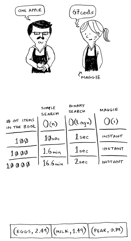
75Hash tables

Your buddy Maggie can give you the price in O(1) time for any item, no

matter how big the book is. She’s even faster than binary search.

What a wonderful person! How do you get a “Maggie”?

Let’s put on our data structure hats. You know two data structures so

far: arrays and lists (I won’t talk about stacks because you can’t really

“search” for something in a stack). You could implement this book as

an array.

Each item in the array is really two items: one is the name of a kind of

produce, and the other is the price. If you sort this array by name, you

can run binary search on it to nd the price of an item. So you can nd

items in O(log n) time. But you want to nd items in O(1) time. at is,

you want to make a “Maggie.” at’s where hash functions come in.

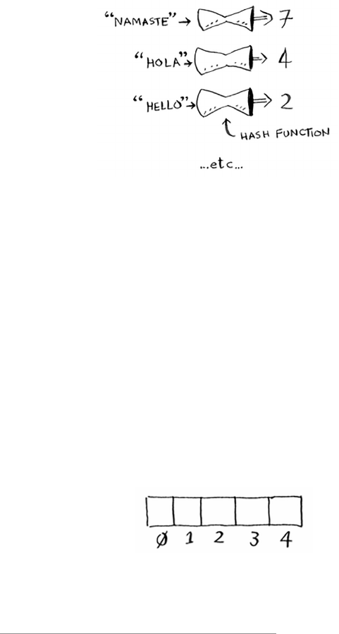
76 Chapter 5

I

Hash tables

Hash functions

A hash function is a function where you put in a string1 and you get

back a number.

In technical terminology, we’d say that a hash function “maps strings

to numbers.” You might think there’s no discernable pattern to what

number you get out when you put a string in. But there are some

requirements for a hash function:

• It needs to be consistent. For example, suppose you put in “apple” and

get back “4”. Every time you put in “apple”, you should get “4” back.

Without this, your hash table won’t work.

• It should map dierent words to dierent numbers. For example, a

hash function is no good if it always returns “1” for any word you put

in. In the best case, every dierent word should map to a dierent

number.

So a hash function maps strings to numbers. What is that good for?

Well, you can use it to make your “Maggie”!

Start with an empty array:

You’ll store all of your prices in this array. Let’s add the price of an apple.

Feed “apple” into the hash function.

1 String here means any kind of data—a sequence of bytes.

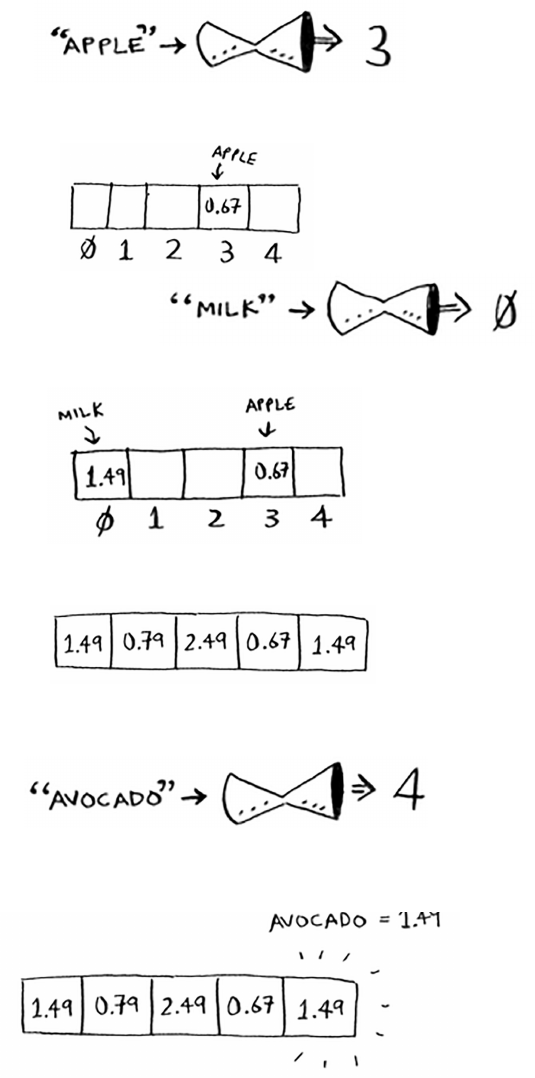
77Hash functions

e hash function outputs “3”. So let’s store the price of an apple at

index 3 in the array.

Let’s add milk. Feed “milk”

into the hash function.

e hash function says “0”. Let’s store the price of milk at index 0.

Keep going, and eventually the whole array will be full of prices.

Now you ask, “Hey, what’s the price of an avocado?” You don’t need to

search for it in the array. Just feed “avocado” into the hash function.

It tells you that the price is stored at index 4. And sure enough,

there it is.

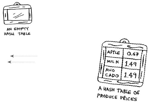
78 Chapter 5

I

Hash tables

e hash function tells you exactly where the price is stored, so you

don’t have to search at all! is works because

• e hash function consistently maps a name to the same index. Every

time you put in “avocado”, you’ll get the same number back. So you

can use it the rst time to nd where to store the price of an avocado,

and then you can use it to nd where you stored that price.

• e hash function maps dierent strings to dierent indexes.

“Avocado” maps to index 4. “Milk” maps to index 0. Everything maps

to a dierent slot in the array where you can store its price.

• e hash function knows how big your array is and only returns valid

indexes. So if your array is 5 items, the hash function doesn’t return

100 … that wouldn’t be a valid index in the array.

You just built a “Maggie”! Put a hash function and an array together,

and you get a data structure called a hash table. A hash table is the rst

data structure you’ll learn that has some extra logic behind it. Arrays

and lists map straight to memory, but hash tables are smarter. ey use

a hash function to intelligently gure out where to store elements.

Hash tables are probably the most useful complex data structure

you’ll learn. ey’re also known as hash maps, maps, dictionaries, and

associative arrays. And hash tables are fast! Remember our discussion

of arrays and linked lists back in chapter 2? You can get an item from an

array instantly. And hash tables use an array to store the data, so they’re

equally fast.

You’ll probably never have to implement hash tables yourself. Any good

language will have an implementation for hash tables. Python has hash

tables; they’re called dictionaries. You can make a new hash table using

the

dict

function:

>>> book = dict()

book

is a new hash table. Let’s add some prices to

book

:

>>> book[“apple”] = 0.67 An apple costs 67 cents.

>>> book[“milk”] = 1.49 Milk costs $1.49.

>>> book[“avocado”] = 1.49

>>> print book

{‘avocado’: 1.49, ‘apple’: 0.67, ‘milk’: 1.49}

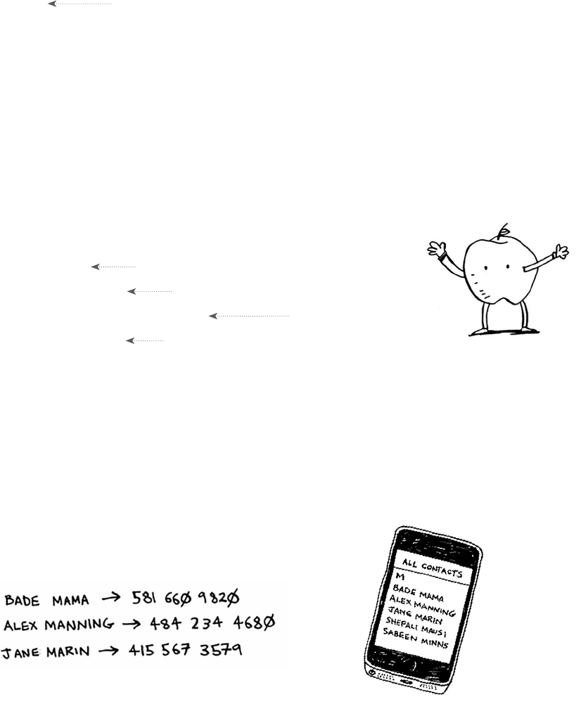
79Use cases

Pretty easy! Now let’s ask for the price of an avocado:

>>> p r i n t b o ok[“av o c ad o”]

1.49 The price of an avocado

A hash table has keys and values. In the

book

hash, the names of

produce are the keys, and their prices are the values. A hash table maps

keys to values.

In the next section, you’ll see some examples where hash tables are

really useful.

EXERCISES

It’s important for hash functions to consistently return the same output

for the same input. If they don’t, you won’t be able to nd your item

aer you put it in the hash table!

Which of these hash functions are consistent?

5.1

f(x) = 1

Returns “1” for all input

5.2

f(x) = rand()

Returns a random number every time

5.3

f(x) = next_empty_slot()

5.4

f(x) = len(x)

Use cases

Hash tables are used everywhere. is section will show you a few

use cases.

Using hash tables for lookups

Your phone has a handy phonebook built in.

Each name has a phone number associated with it.

Returns the index of the next

empty slot in the hash table

Uses the length of the

string as the index

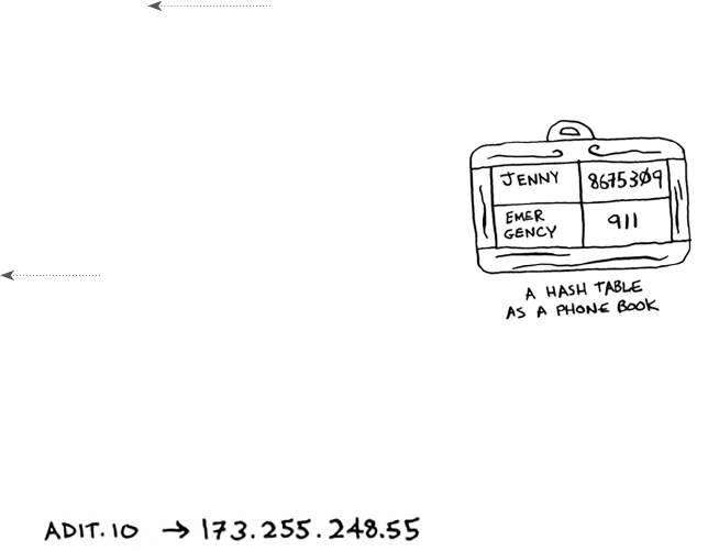
80 Chapter 5

I

Hash tables

Suppose you want to build a phone book like this. You’re mapping

people’s names to phone numbers. Your phone book needs to have this

functionality:

• Add a person’s name and the phone number associated

with that person.

• Enter a person’s name, and get the phone number associated

with that name.

is is a perfect use case for hash tables! Hash tables are

great when you want to

• Create a mapping from one thing to another thing

• Look something up

Building a phone book is pretty easy. First, make a new hash table:

>>> phone_book = dict()

By the way, Python has a shortcut for making a new hash table. You can

use two curly braces:

>>> phone_book = {} Same as phone_book = dict()

Let’s add the phone numbers of some people into this phone book:

>>> phone_book[“jenny”] = 8675309

>>> phone_book[“emergency”] = 911

at’s all there is to it! Now, suppose you want to nd

Jenny’s phone number. Just pass the key in to the hash:

>>> print phone_book[“jenny”]

8675309 Jenny’s phone number

Imagine if you had to do this using an array instead.

How would you do it? Hash tables make it easy to model a relationship

from one item to another.

Hash tables are used for lookups on a much larger scale. For example,

suppose you go to a website like http://adit.io. Your computer has to

translate adit.io to an IP address.

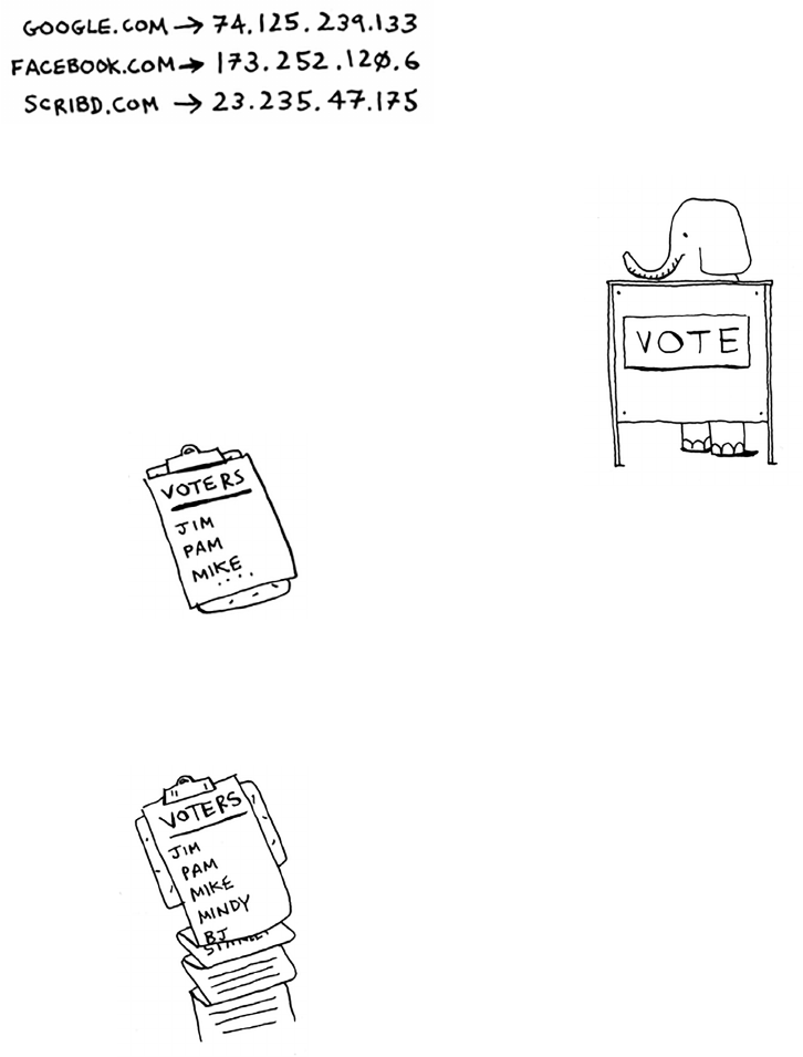
81Use cases

For any website you go to, the address has to be translated to an IP

address.

Wow, mapping a web address to an IP address? Sounds like a perfect

use case for hash tables! is process is called DNS resolution. Hash

tables are one way to provide this functionality.

Preventing duplicate entries

Suppose you’re running a voting booth. Naturally, every person can

vote just once. How do you make sure they haven’t voted before? When

someone comes in to vote, you ask for their full name. en you check

it against the list of people who have voted.

If their name is on the list, this person has already voted—kick them

out! Otherwise, you add their name to the list and let them vote. Now

suppose a lot of people have come in to vote, and the list of people who

have voted is really long.

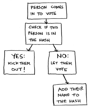
82 Chapter 5

I

Hash tables

Each time someone new comes in to vote, you have to scan this giant

list to see if they’ve already voted. But there’s a better way: use a hash!

First, make a hash to keep track of the people who have voted:

>>> voted = {}

When someone new comes in to vote, check if they’re already in

the hash:

>>> value = voted.get(“tom”)

e

get

function returns the value if “tom” is in the hash table.

Otherwise, it returns

None

. You can use this to check if someone

has already voted!

Here’s the code:

voted = {}

def check_voter(name):

if voted.get(name):

print “kick them out!”

else:

voted[name] = True

print “let them vote!”

Let’s test it a few times:

>>> check_voter(“tom”)

let them vote!

>>> check_voter(“mike”)

let them vote!

>>> check_voter(“mike”)

kick them out!

e rst time Tom goes in, this will print, “let them vote!” en Mike

goes in, and it prints, “let them vote!” en Mike tries to go a second

time, and it prints, “kick them out!”

83Use cases

Remember, if you were storing these names in a list of people who have

voted, this function would eventually become really slow, because it

would have to run a simple search over the entire list. But you’re storing

their names in a hash table instead, and a hash table instantly tells you

whether this person’s name is in the hash table or not. Checking for

duplicates is very fast with a hash table.

Using hash tables as a cache

One nal use case: caching. If you work on a website, you

may have heard of caching before as a good thing to do.

Here’s the idea. Suppose you visit facebook.com:

1. You make a request to Facebook’s server.

2. e server thinks for a second and comes up with

the web page to send to you.

3. You get a web page.

For example, on Facebook, the server may be collecting all of your

friends’ activity to show you. It takes a couple of seconds to collect all

that activity and shows it to you. at couple of seconds can feel like a

long time as a user. You might think, “Why is Facebook being so slow?”

On the other hand, Facebook’s servers have to serve millions of people,

and that couple of seconds adds up for them. Facebook’s servers are

really working hard to serve all of those websites. Is there a way to make

Facebook faster and have its servers do less work at the same time?

Suppose you have a niece who keeps asking you about planets. “How far

is Mars from Earth?” “How far is the Moon?” “How far is Jupiter?” Each

time, you have to do a Google search and give her an answer. It takes

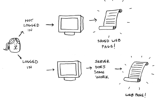
84 Chapter 5

I

Hash tables

a couple of minutes. Now, suppose she always asked, “How far is the

Moon?” Pretty soon, you’d memorize that the Moon is 238,900 miles

away. You wouldn’t have to look it up on Google … you’d just remember

and answer. is is how caching works: websites remember the data

instead of recalculating it.

If you’re logged in to Facebook, all the content you see is tailored just

for you. Each time you go to facebook.com, its servers have to think

about what content you’re interested in. But if you’re not logged in to

Facebook, you see the login page. Everyone sees the same login page.

Facebook is asked the same thing over and over: “Give me the home

page when I’m logged out.” So it stops making the server do work to

gure out what the home page looks like. Instead, it memorizes what

the home page looks like and sends it to you.

is is called caching. It has two advantages:

• You get the web page a lot faster, just like when you memorized the

distance from Earth to the Moon. e next time your niece asks you,

you won’t have to Google it. You can answer instantly.

• Facebook has to do less work.

Caching is a common way to make things faster. All big websites use

caching. And that data is cached in a hash!

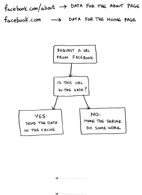
85Use cases

Facebook isn’t just caching the home page. It’s also caching the About

page, the Contact page, the Terms and Conditions page, and a lot more.

So it needs a mapping from page URL to page data.

When you visit a page on Facebook, it rst checks whether the page is

stored in the hash.

Here it is in code:

cache = {}

def get_page(url):

if cache.get(url):

return cache[url] Returns cached data

else:

data = get_data_from_server(url)

cache[url] = data Saves this data in your cache first

return data

Here, you make the server do work only if the URL isn’t in the cache.

Before you return the data, though, you save it in the cache. e next

time someone requests this URL, you can send the data from the cache

instead of making the server do the work.

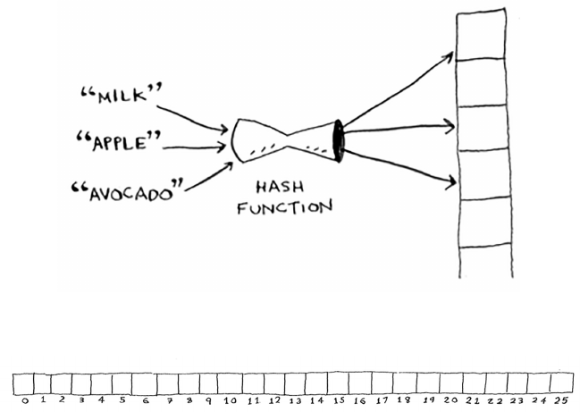
86 Chapter 5

I

Hash tables

Recap

To recap, hashes are good for

• Modeling relationships from one thing to another thing

• Filtering out duplicates

• Caching/memorizing data instead of making your server do work

Collisions

Like I said earlier, most languages have hash tables. You don’t need to

know how to write your own. So, I won’t talk about the internals of hash

tables too much. But you still care about performance! To understand

the performance of hash tables, you rst need to understand what

collisions are. e next two sections cover collisions and performance.

First, I’ve been telling you a white lie. I told you that a hash function

always maps dierent keys to dierent slots in the array.

In reality, it’s almost impossible to write a hash function that does this.

Let’s take a simple example. Suppose your array contains 26 slots.

And your hash function is really simple: it assigns a spot in the array

alphabetically.

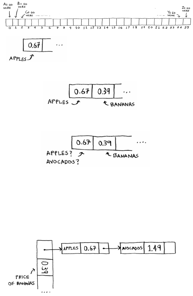
87Collisions

Maybe you can already see the problem. You

want to put the price of apples in your hash.

You get assigned the rst slot.

en you want to put the price of bananas in the hash. You get assigned

the second slot.

Everything is going so well! But now you want to put the price of

avocados in your hash. You get assigned the rst slot again.

Oh no! Apples have that slot already! What to do? is is called a

collision: two keys have been assigned the same slot. is is a problem.

If you store the price of avocados at that slot, you’ll overwrite the price

of apples. en the next time someone asks for the price of apples,

they will get the price of avocados instead! Collisions are bad, and you

need to work around them. ere are many dierent ways to deal with

collisions. e simplest one is this: if multiple keys map to the same

slot, start a linked list at that slot.

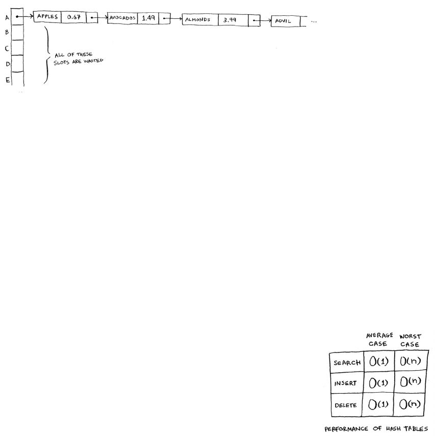
88 Chapter 5

I

Hash tables

In this example, both “apple” and “avocado” map to the same slot.

So you start a linked list at that slot. If you need to know the price of

bananas, it’s still quick. If you need to know the price of apples, it’s a

little slower. You have to search through this linked list to nd “apple”. If

the linked list is small, no big deal—you have to search through three or

four elements. But suppose you work at a grocery store where you only

sell produce that starts with the letter A.

Hey, wait a minute! e entire hash table is totally empty except for one

slot. And that slot has a giant linked list! Every single element in this

hash table is in the linked list. at’s as bad as putting everything in a

linked list to begin with. It’s going to slow down your hash table.

ere are two lessons here:

• Your hash function is really important. Your hash function mapped

all the keys to a single slot. Ideally, your hash function would map

keys evenly all over the hash.

• If those linked lists get long, it slows down your hash table a lot. But

they won’t get long if you use a good hash function!

Hash functions are important. A good hash function will give you very

few collisions. So how do you pick a good hash function? at’s coming

up in the next section!

Performance

You started this chapter at the grocery store. You wanted to build

something that would give you the prices for produce instantly. Well,

hash tables are really fast.

In the average case, hash tables take O(1) for everything. O(1) is called

constant time. You haven’t seen constant time before. It doesn’t mean

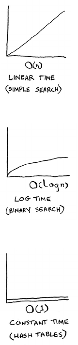
89Performance

instant. It means the time taken will stay the same, regardless of how

big the hash table is. For example, you know that simple search takes

linear time.

Binary search is faster—it takes log time:

Looking something up in a hash table takes constant time.

See how it’s a at line? at means it doesn’t matter whether your hash

table has 1 element or 1 billion elements—getting something out of

a hash table will take the same amount of time. Actually, you’ve seen

constant time before. Getting an item out of an array takes constant

time. It doesn’t matter how big your array is; it takes the same amount

of time to get an element. In the average case, hash tables are really fast.

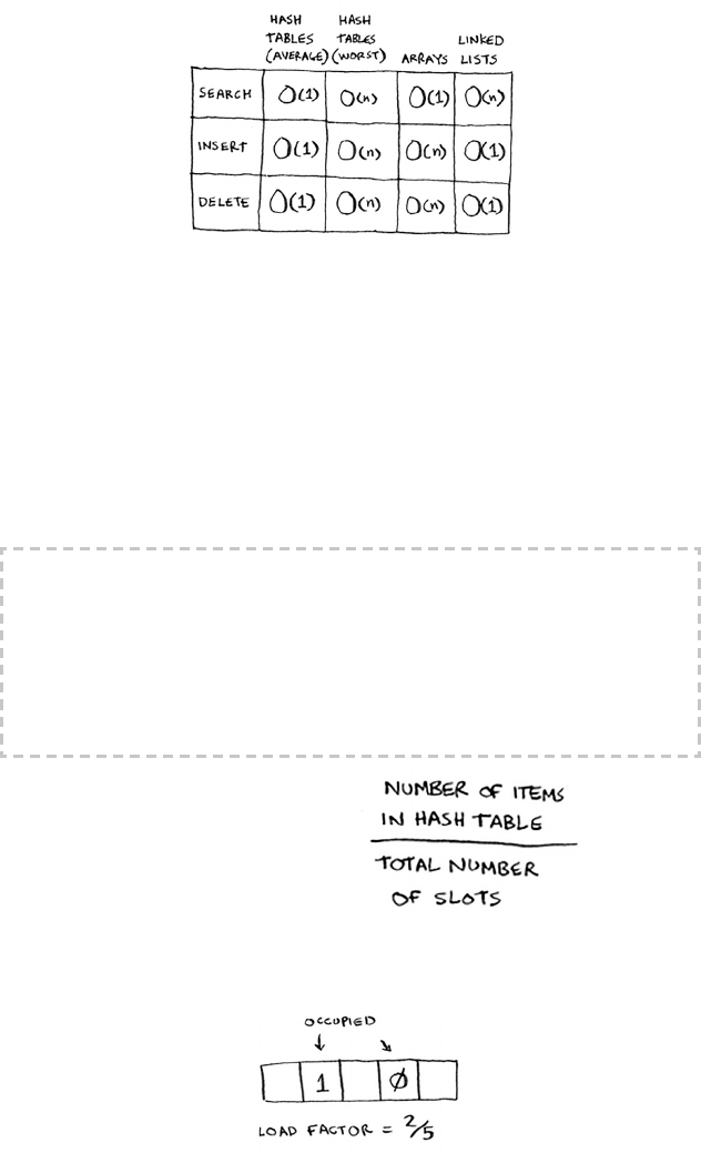
90 Chapter 5

I

Hash tables

In the worst case, a hash table takes O(n)—linear time—for everything,

which is really slow. Let’s compare hash tables to arrays and lists.

Look at the average case for hash tables. Hash tables are as fast as arrays

at searching (getting a value at an index). And they’re as fast as linked

lists at inserts and deletes. It’s the best of both worlds! But in the worst

case, hash tables are slow at all of those. So it’s important that you don’t

hit worst-case performance with hash tables. And to do that, you need

to avoid collisions. To avoid collisions, you need

• A low load factor

• A good hash function

Load factor

e load factor of a hash table

is easy to calculate.

Hash tables use an array for storage, so you count the number of

occupied slots in an array. For example, this hash table has a load factor

of 2

/5, or 0.4.

Note

Before you start this next section, know that this isn’t required reading. I’m

going to talk about how to implement a hash table, but you’ll never have

to do that yourself. Whatever programming language you use will have an

implementation of hash tables built in. You can use the built-in hash table

and assume it will have good performance. The next section gives you a

peek under the hood.

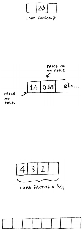
91Performance

What’s the load factor of this hash table?

If you said 1

/3, you’re right. Load factor measures how many empty slots

remain in your hash table.

Suppose you need to store the price of 100 produce items in your hash

table, and your hash table has 100 slots. In the best case, each item will

get its own slot.

is hash table has a load factor of 1. What if your hash table has only

50 slots? en it has a load factor of 2. ere’s no way each item will

get its own slot, because there aren’t enough slots! Having a load factor

greater than 1 means you have more items than slots in your array.

Once the load factor starts to grow, you need to add more slots to your

hash table. is is called resizing. For example, suppose you have this

hash table that is getting pretty full.

You need to resize this hash table. First you create a new array that’s

bigger. e rule of thumb is to make an array that is twice the size.

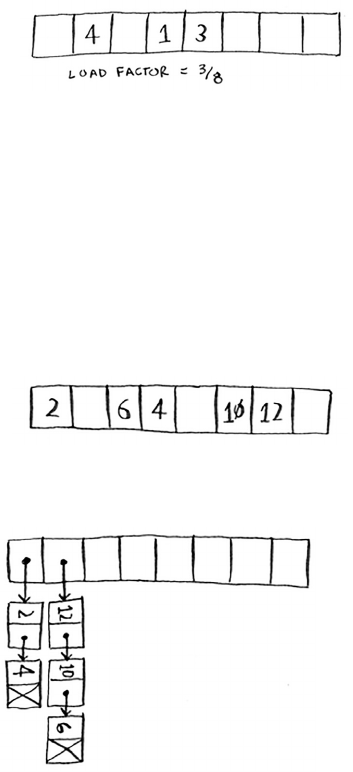
92 Chapter 5

I

Hash tables

Now you need to re-insert all of those items into this new hash table

using the

hash

function:

is new table has a load factor of 3

/8. Much better! With a lower load

factor, you’ll have fewer collisions, and your table will perform better. A

good rule of thumb is, resize when your load factor is greater than 0.7.

You might be thinking, “is resizing business takes a lot of time!” And

you’re right. Resizing is expensive, and you don’t want to resize too

oen. But averaged out, hash tables take O(1) even with resizing.

A good hash function

A good hash function distributes values in the array evenly.

A bad hash function groups values together and produces a lot of

collisions.

What is a good hash function? at’s something you’ll never have to

worry about—old men (and women) with big beards sit in dark rooms

and worry about that. If you’re really curious, look up the SHA function

(there’s a short description of it in the last chapter). You could use that

as your hash function.

93Recap

EXERCISES

It’s important for hash functions to have a good distribution. ey

should map items as broadly as possible. e worst case is a hash

function that maps all items to the same slot in the hash table.

Suppose you have these four hash functions that work with strings:

. Return “1” for all input.

. Use the length of the string as the index.

. Use the rst character of the string as the index. So, all strings

starting with a are hashed together, and so on.

. Map every letter to a prime number: a = 2, b = 3, c = 5, d = 7,

e = 11, and so on. For a string, the hash function is the sum of all

the characters modulo the size of the hash. For example, if your

hash size is 10, and the string is “bag”, the index is 3 + 2 + 17 %

10 = 22 % 10 = 2.

For each of these examples, which hash functions would provide a good

distribution? Assume a hash table size of 10 slots.

5.5 A phonebook where the keys are names and values are phone

numbers. e names are as follows: Esther, Ben, Bob, and Dan.

5.6 A mapping from battery size to power. e sizes are A, AA, AAA,

and AAAA.

5.7 A mapping from book titles to authors. e titles are Maus, Fun

Home, and Watchmen.

Recap

You’ll almost never have to implement a hash table yourself. e

programming language you use should provide an implementation for

you. You can use Python’s hash tables and assume that you’ll get the

average case performance: constant time.

Hash tables are a powerful data structure because they’re so fast and

they let you model data in a dierent way. You might soon nd that

you’re using them all the time:

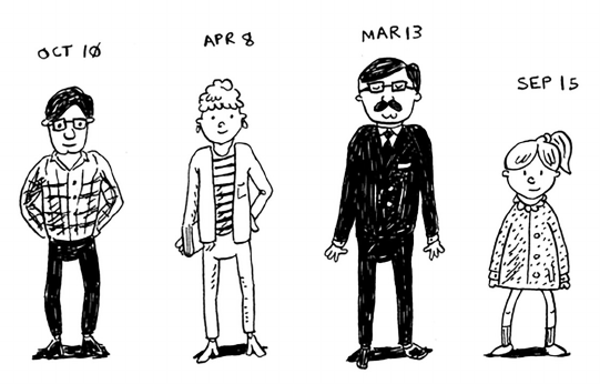
94 Chapter 5

I

Hash tables

• You can make a hash table by combining a hash function

with an array.

• Collisions are bad. You need a hash function that

minimizes collisions.

• Hash tables have really fast search, insert, and delete.

• Hash tables are good for modeling relationships from one

item to another item.

• Once your load factor is greater than .07, it’s time to resize

your hash table.

• Hash tables are used for caching data (for example, with

a web server).

• Hash tables are great for catching duplicates.

95

In this chapter

• You learn how to model a network using a new,

abstract data structure: graphs.

• You learn breadth-rst search, an algorithm you

can run on graphs to answer questions like,

“What’s the shortest path to go to X?”

• You learn about directed versus undirected graphs.

• You learn topological sort, a dierent kind of

sorting algorithm that exposes dependencies

between nodes.

6

breadth-first

search

is chapter introduces graphs. First, I’ll talk about what graphs

are (they don’t involve an X or Y axis). en I’ll show you your rst

graph algorithm. It’s called breadth-rst search (BFS).

Breadth-rst search allows you to nd the shortest distance

between two things. But shortest distance can mean a lot of things!

You can use breadth-rst search to

• Write a checkers AI that calculates the fewest moves to victory

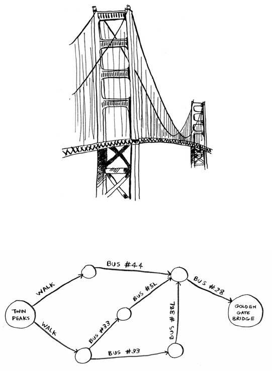
96 Chapter 6

I

Breadth-rst search

• Write a spell checker (fewest edits from your misspelling to a real

word—for example, READED -> READER is one edit)

• Find the doctor closest to you in your network

Graph algorithms are some of the most useful algorithms I know. Make

sure you read the next few chapters carefully—these are algorithms

you’ll be able to apply again and again.

Introduction to graphs

Suppose you’re in San Francisco, and you want to go from Twin Peaks

to the Golden Gate Bridge. You want to get there by bus, with the

minimum number of transfers. Here are your options.

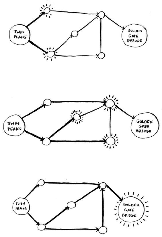
97Introduction to graphs

What’s your algorithm to nd the path with the fewest steps?

Well, can you get there in one step? Here are all the places you can get

to in one step.

e bridge isn’t highlighted; you can’t get there in one step. Can you get

there in two steps?

Again, the bridge isn’t there, so you can’t get to the bridge in two steps.

What about three steps?

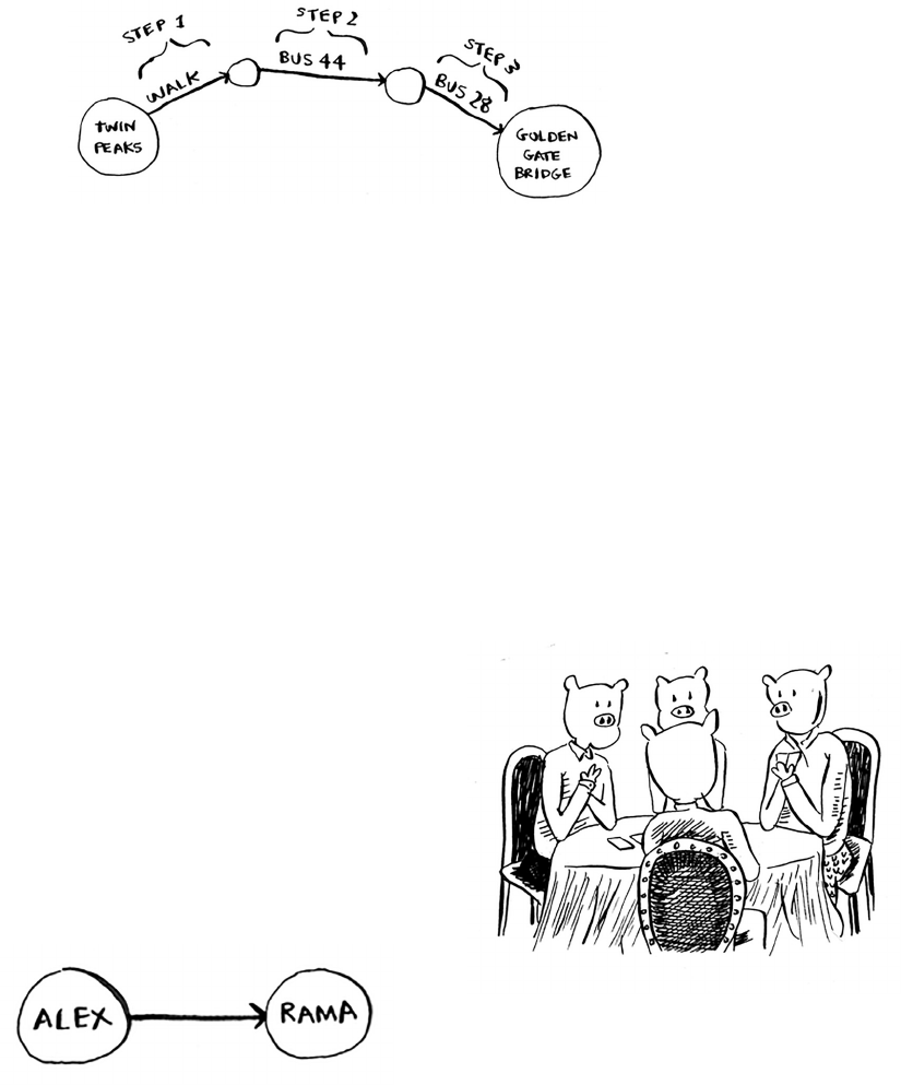
98 Chapter 6

I

Breadth-rst search

Aha! Now the Golden Gate Bridge shows up. So it takes three steps to

get from Twin Peaks to the bridge using this route.

ere are other routes that will get you to the bridge too, but they’re

longer (four steps). e algorithm found that the shortest route to the

bridge is three steps long. is type of problem is called a shortest-path

problem. You’re always trying to nd the shortest something. It could

be the shortest route to your friend’s house. It could be the smallest

number of moves to checkmate in a game of chess. e algorithm to

solve a shortest-path problem is called breadth-rst search.

To gure out how to get from Twin Peaks to the Golden Gate Bridge,

there are two steps:

1. Model the problem as a graph.

2. Solve the problem using breadth-rst search.

Next I’ll cover what graphs are. en I’ll go into breadth-rst search in

more detail.

What is a graph?

A graph models a set of connections. For

example, suppose you and your friends are

playing poker, and you want to model who owes

whom money. Here’s how you could say, “Alex

owes Rama money.”

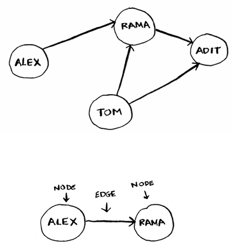
99Breadth-rst search

e full graph could look something like this.

Alex owes Rama money, Tom owes Adit money, and so on. Each graph

is made up of nodes and edges.

at’s all there is to it! Graphs are made up of nodes and edges. A node

can be directly connected to many other nodes. ose nodes are called

its neighbors. In this graph, Rama is Alex’s neighbor. Adit isn’t Alex’s

neighbor, because they aren’t directly connected. But Adit is Rama’s and

Tom’s neighbor.

Graphs are a way to model how dierent things are connected to one

another. Now let’s see breadth-rst search in action.

Breadth-rst search

We looked at a search algorithm in chapter 1: binary search. Breadth-

rst search is a dierent kind of search algorithm: one that runs on

graphs. It can help answer two types of questions:

• Question type 1: Is there a path from node A to node B?

• Question type 2: What is the shortest path from node A to node B?

Graph of people who owe

other people poker money

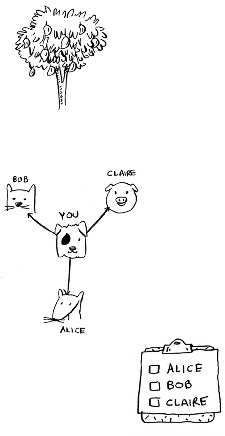
100 Chapter 6

I

Breadth-rst search

You already saw breadth-rst search once, when you calculated the

shortest route from Twin Peaks to the Golden Gate Bridge. at was

a question of type 2: “What is the shortest path?” Now let’s look at the

algorithm in more detail. You’ll ask a question of type 1: “Is there a

path?”

Suppose you’re the proud owner of a mango farm. You’re looking for a

mango seller who can sell your mangoes. Are you connected to a mango

seller on Facebook? Well, you can search through your friends.

is search is pretty straightforward.

First, make a list of friends to search.

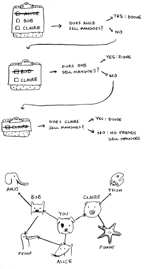
101Breadth-rst search

Now, go to each person in the list and check whether that person sells

mangoes.

Suppose none of your friends are mango sellers. Now you have to

search through your friends’ friends.

Each time you search for someone from the list, add all of their friends

to the list.

102 Chapter 6

I

Breadth-rst search

is way, you not only search your friends, but you search their friends,

too. Remember, the goal is to nd one mango seller in your network.

So if Alice isn’t a mango seller, you add her friends to the list, too. at

means you’ll eventually search her friends—and then their friends, and

so on. With this algorithm, you’ll search your entire network until you

come across a mango seller. is algorithm is breadth-rst search.

Finding the shortest path

As a recap, these are the two questions that breadth-rst search can

answer for you:

• Question type 1: Is there a path from node A to node B? (Is there a

mango seller in your network?)

• Question type 2: What is the shortest path from node A to node B?

(Who is the closest mango seller?)

You saw how to answer question 1; now let’s try to answer question

2. Can you nd the closest mango seller? For example, your friends

are rst-degree connections, and their friends are second-degree

connections.

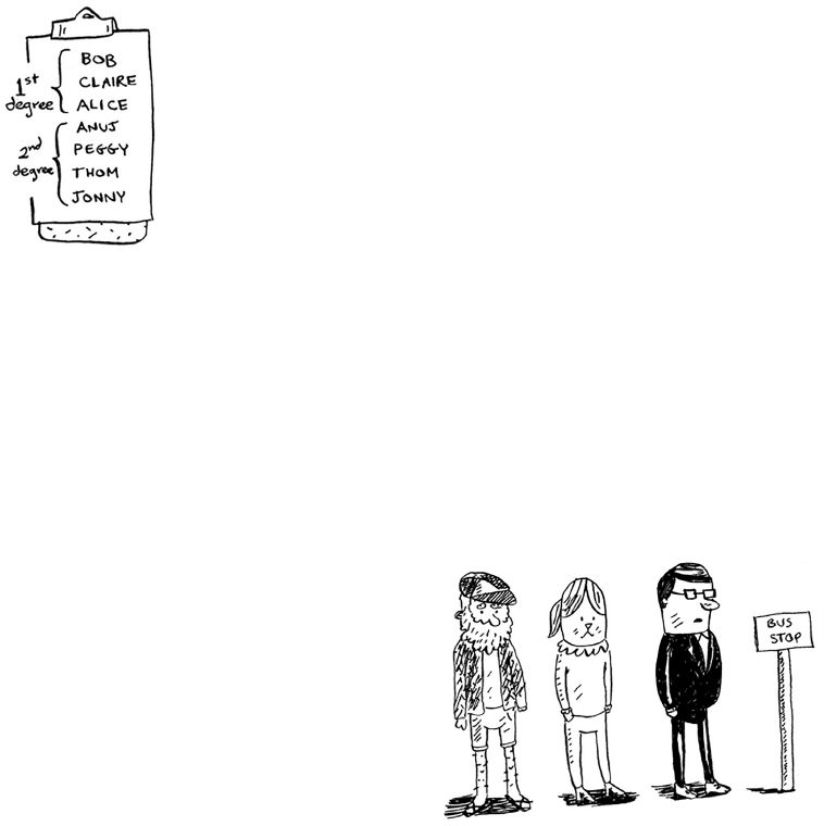
103Breadth-rst search

You’d prefer a rst-degree connection to a second-degree connection,

and a second-degree connection to a third-degree connection, and so

on. So you shouldn’t search any second-degree connections before you

make sure you don’t have a rst-degree connection who is a mango

seller. Well, breadth-rst search already does this! e way breadth-rst

search works, the search radiates out from the starting point. So you’ll

check rst-degree connections before second-degree connections. Pop

quiz: who will be checked rst, Claire or Anuj? Answer: Claire is a rst-

degree connection, and Anuj is a second-degree connection. So Claire

will be checked before Anuj.

Another way to see this is, rst-degree connections

are added to the search list before second-degree

connections.

You just go down the list and check people to see

whether each one is a mango seller. e rst-degree

connections will be searched before the second-

degree connections, so you’ll nd the mango seller

closest to you. Breadth-rst search not only nds a

path from A to B, it also nds the shortest path.

Notice that this only works if you search people in the same order in

which they’re added. at is, if Claire was added to the list before Anuj,

Claire needs to be searched before Anuj. What happens if you search

Anuj before Claire, and they’re both mango sellers? Well, Anuj is a

second-degree contact, and Claire is a rst-degree contact. You end up

with a mango seller who isn’t the closest to you in your network. So

you need to search people in the order that they’re added. ere’s a data

structure for this: it’s called a queue.

Queues

A queue works exactly like it does in

real life. Suppose you and your friend

are queueing up at the bus stop. If you’re

before him in the queue, you get on the

bus rst. A queue works the same way.

Queues are similar to stacks. You can’t

access random elements in the queue.

Instead, there are two only operations,

enqueue and dequeue.

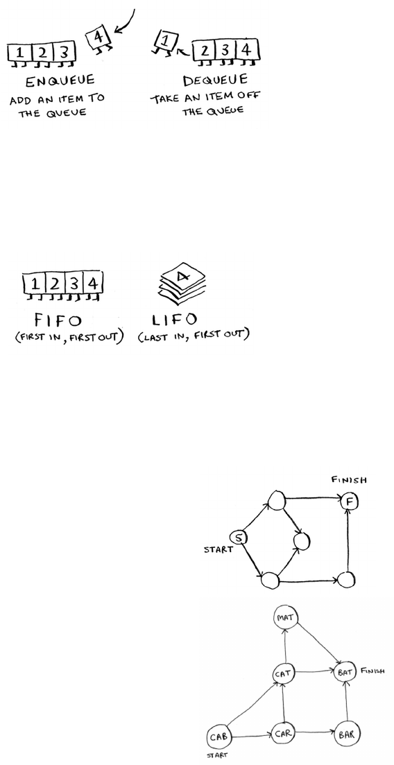
104 Chapter 6

I

Breadth-rst search

If you enqueue two items to the list, the rst item you added will be

dequeued before the second item. You can use this for your search list!

People who are added to the list rst will be dequeued and searched

rst.

e queue is called a FIFO data structure: First In, First Out. In

contrast, a stack is a LIFO data structure: Last In, First Out.

Now that you know how a queue works, let’s implement breadth-rst

search!

EXERCISES

Run the breadth-rst search algorithm on each of these graphs to nd

the solution.

6.1 Find the length of the shortest path

from start to nish.

6.2 Find the length of the shortest path

from “cab” to “bat”.

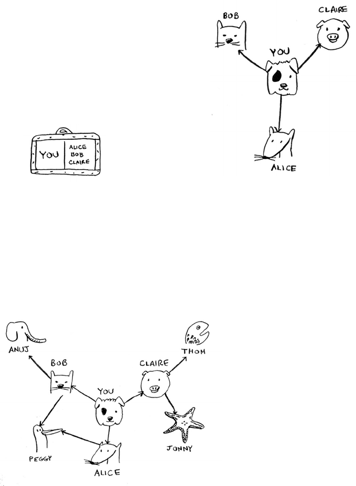
105Implementing the graph

Implementing the graph

First, you need to implement the graph in code. A graph

consists of several nodes.

And each node is connected to neighboring nodes.

How do you express a relationship like “you -> bob”?

Luckily, you know a data structure that lets you express

relationships: a hash table!

Remember, a hash table allows you to map a key to a

value. In this case, you want to map a node to all of its

neighbors.

Here’s how you’d write it in Python:

graph = {}

graph[“you”] = [“alice”, “bob”, “claire”]

Notice that “you” is mapped to an array. So

g r a p h[“ y o u”]

will give you

an array of all the neighbors of “you”.

A graph is just a bunch of nodes and edges, so this is all you need to

have a graph in Python. What about a bigger graph, like this one?

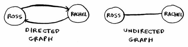
106 Chapter 6

I

Breadth-rst search

Here it is as Python code:

graph = {}

graph[“you”] = [“alice”, “bob”, “claire”]

g r a ph[“b o b”] = [“a nuj”, “p e g g y”]

g r a ph[“a lic e”] = [“p e g g y”]

g r a ph[“cl a i r e”] = [“t h o m”, “jo n n y”]

graph[“anuj”] = []

graph[“peggy”] = []

graph[“thom”] = []

graph[“jonny”] = []

Pop quiz: does it matter what order you add the key/value pairs in?

Does it matter if you write

g r a ph[“cl a i r e”] = [“t h o m”, “jo n n y”]

graph[“anuj”] = []

instead of

graph[“anuj”] = []

g r a ph[“cl a i r e”] = [“t h o m”, “jo n n y”]

ink back to the previous chapter. Answer: It doesn’t matter. Hash

tables have no ordering, so it doesn’t matter what order you add

key/value pairs in.

Anuj, Peggy, om, and Jonny don’t have any neighbors. ey have

arrows pointing to them, but no arrows from them to someone else.

is is called a directed graph—the relationship is only one way. So Anuj

is Bob’s neighbor, but Bob isn’t Anuj’s neighbor. An undirected graph

doesn’t have any arrows, and both nodes are each other’s neighbors. For

example, both of these graphs are equal.

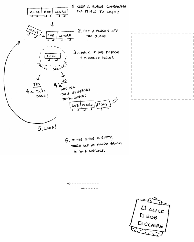
107Implementing the algorithm

Implementing the algorithm

To recap, here’s how the implementation will work.

Make a queue to start. In Python, you use the double-ended queue

(

deque

) function for this:

from collections import deque

search_queue = deque()

search_queue += graph[“you”]

Remember,

graph

[

“you”

] will give you a list of all your

neighbors, like [

“ a l i c e ”, “ b o b ”, “ c l a i r e ”

]. ose all get

added to the search queue.

Creates a new queue

Adds all of your neighbors to the search queue

Note

When updating queues, I

use the terms enqueue and

dequeue. You’ll also encoun-

ter the terms push and pop.

Push is almost always the

same thing as enqueue, and

pop is almost always the

same thing as dequeue.

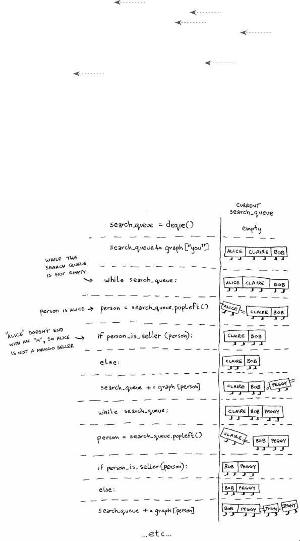
108 Chapter 6

I

Breadth-rst search

Let’s see the rest:

while search_queue:

person = search_queue.popleft()

if person_is_seller(person):

print person + “ is a mango seller!”

return True

else:

search_queue += graph[person]

return False

One nal thing: you still need a

person_is_seller

function to tell you

when someone is a mango seller. Here’s one:

def person_is_seller(name):

return name[-1] == ‘m’

is function checks whether the person’s name ends with the letter m.

If it does, they’re a mango seller. Kind of a silly way to do it, but it’ll do

for this example. Now let’s see the breadth-rst search in action.

While the queue isn’t empty …

… grabs the first person off the queue

Checks whether the person is a mango seller

Yes, they’re a mango seller.

No, they aren’t. Add all of this

person’s friends to the search queue.

If you reached here, no one in

the queue was a mango seller.

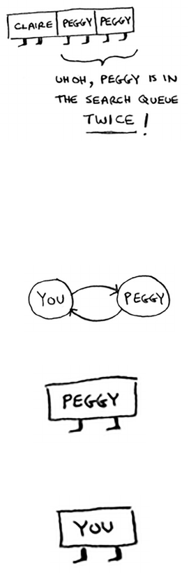
109Implementing the algorithm

And so on. e algorithm will keep going until either

• A mango seller is found, or

• e queue becomes empty, in which case there is no mango seller.

Alice and Bob share a friend: Peggy. So Peggy will be added to the

queue twice: once when you add Alice’s friends, and again when you

add Bob’s friends. You’ll end up with two Peggys in the search queue.

But you only need to check Peggy once to see whether she’s a mango

seller. If you check her twice, you’re doing unnecessary, extra work. So

once you search a person, you should mark that person as searched and

not search them again.

If you don’t do this, you could also end up in an innite loop. Suppose

the mango seller graph looked like this.

To start, the search queue contains all of your neighbors.

Now you check Peggy. She isn’t a mango seller, so you add all of her

neighbors to the search queue.

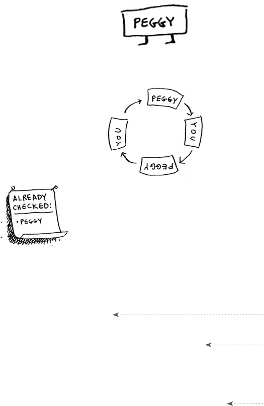
110 Chapter 6

I

Breadth-rst search

Next, you check yourself. You’re not a mango seller, so you add all of

your neighbors to the search queue.

And so on. is will be an innite loop, because the search queue will

keep going from you to Peggy.

Before checking a person, it’s important to make sure

they haven’t been checked already. To do that, you’ll

keep a list of people you’ve already checked.

Here’s the nal code for breadth-rst search, taking that into account:

def search(name):

search_queue = deque()

search_queue += graph[name]

searched = []

while search_queue:

person = search_queue.popleft()

if not person in searched:

if person_is_seller(person):

print person + “ is a mango seller!”

return True

else:

search_queue += graph[person]

searched.append(person)

return False

search(“you”)

This array is how you keep track of

which people you’ve searched before.

Only search this person if you

haven’t already searched them.

Marks this person as searched

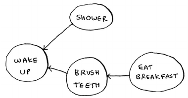
111Implementing the algorithm

Try running this code yourself. Maybe try changing the

person_is_

seller

function to something more meaningful, and see if it prints

what you expect.

Running time

If you search your entire network for a mango seller, that means you’ll

follow each edge (remember, an edge is the arrow or connection from

one person to another). So the running time is at least O(number of

edges).

You also keep a queue of every person to search. Adding one person to

the queue takes constant time: O(1). Doing this for every person will

take O(number of people) total. Breadth-rst search takes O(number of

people + number of edges), and it’s more commonly written as O(V+E)

(V for number of vertices, E for number of edges).

EXERCISE

Here’s a small graph of my morning routine.

It tells you that I can’t eat breakfast until I’ve brushed my teeth. So “eat

breakfast” depends on “brush teeth”.

On the other hand, showering doesn’t depend on brushing my teeth,

because I can shower before I brush my teeth. From this graph, you can

make a list of the order in which I need to do my morning routine:

1. Wake up.

2. Shower.

3. Brush teeth.

4. Eat breakfast.

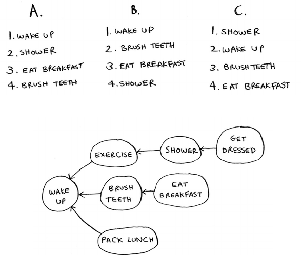
112 Chapter 6

I

Breadth-rst search

Note that “shower” can be moved around, so this list is also valid:

1. Wake up.

2. Brush teeth.

3. Shower.

4. Eat breakfast.

6.3 For these three lists, mark whether each one is valid or invalid.

6.4 Here’s a larger graph. Make a valid list for this graph.

You could say that this list is sorted, in a way. If task A depends on

task B, task A shows up later in the list. is is called a topological sort,

and it’s a way to make an ordered list out of a graph. Suppose you’re

planning a wedding and have a large graph full of tasks to do—and

you’re not sure where to start. You could topologically sort the graph

and get a list of tasks to do, in order.

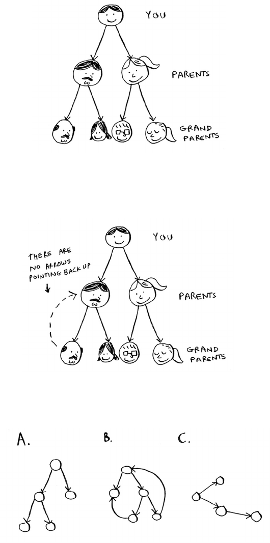
113Implementing the algorithm

Suppose you have a family tree.

is is a graph, because you have nodes (the people) and edges.

e edges point to the nodes’ parents. But all the edges go down—it

wouldn’t make sense for a family tree to have an edge pointing back up!

at would be meaningless—your dad can’t be your grandfather’s dad!

is is called a tree. A tree is a special type of graph, where no edges

ever point back.

6.5 Which of the following graphs are also trees?

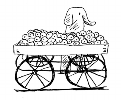
114 Chapter 6

I

Breadth-rst search

Recap

• Breadth-rst search tells you if there’s a path from A to B.

• If there’s a path, breadth-rst search will nd the shortest path.

• If you have a problem like “nd the shortest X,” try modeling your

problem as a graph, and use breadth-rst search to solve.

• A directed graph has arrows, and the relationship follows the

direction of the arrow (rama -> adit means “rama owes adit money”).

• Undirected graphs don’t have arrows, and the relationship goes both

ways (ross - rachel means “ross dated rachel and rachel dated ross”).

• Queues are FIFO (First In, First Out).

• Stacks are LIFO (Last In, First Out).

• You need to check people in the order they were added to the search

list, so the search list needs to be a queue. Otherwise, you won’t get

the shortest path.

• Once you check someone, make sure you don’t check them again.

Otherwise, you might end up in an innite loop.

115

In this chapter

• We continue the discussion of graphs, and you

learn about weighted graphs: a way to assign

more or less weight to some edges.

• You learn Dijkstra’s algorithm, which lets you

answer “What’s the shortest path to X?” for

weighted graphs.

• You learn about cycles in graphs, where

Dijkstra’s algorithm doesn’t work.

7

Dijkstra’s

algorithm

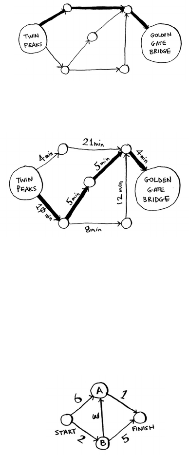
116 Chapter 7

I

Dijkstra’s algorithm

In the last chapter, you gured out a way to get from point A to point B.

It’s not necessarily the fastest path. It’s the shortest path, because it has

the least number of segments (three segments). But suppose you add

travel times to those segments. Now you see that there’s a faster path.

You used breadth-rst search in the last chapter. Breadth-rst search

will nd you the path with the fewest segments (the rst graph shown

here). What if you want the fastest path instead (the second graph)? You

can do that fastest with a dierent algorithm called Dijkstra’s algorithm.

Working with Dijkstra’s algorithm

Let’s see how it works with this graph.

Each segment has a travel time in minutes. You’ll use Dijkstra’s

algorithm to go from start to nish in the shortest possible time.

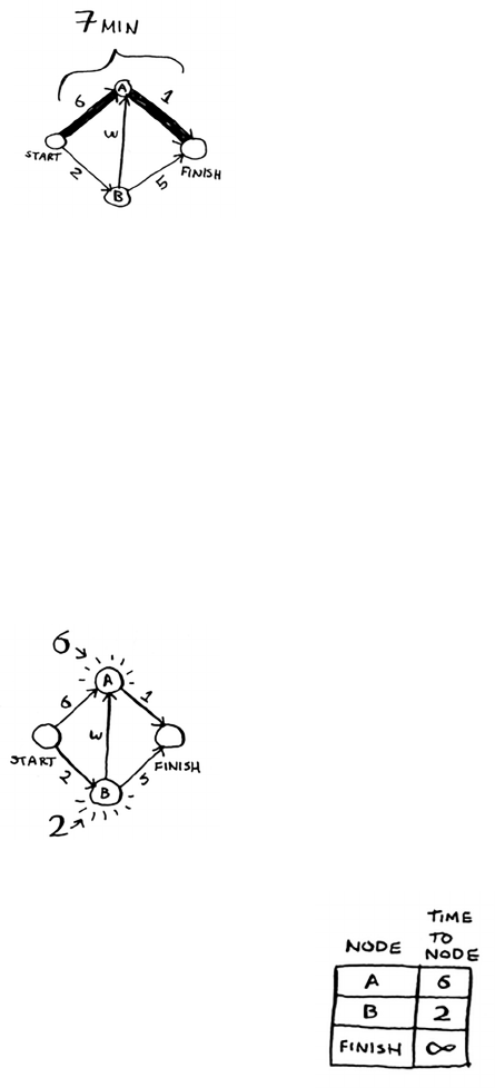
117Working with Dijkstra’s algorithm

If you ran breadth-rst search on this graph, you’d get this

shortest path.

But that path takes 7 minutes. Let’s see if you can nd a path that takes

less time! ere are four steps to Dijkstra’s algorithm:

1. Find the “cheapest” node. is is the node you can get to in the least

amount of time.

2. Update the costs of the neighbors of this node. I’ll explain what I

mean by this shortly.

3. Repeat until you’ve done this for every node in the graph.

4. Calculate the nal path.

Step 1: Find the cheapest node. You’re standing at the start, wondering

if you should go to node A or node B. How long does it take to get to

each node?

It takes 6 minutes to get to node A and 2 minutes to get to node B.

e rest of the nodes, you don’t know yet.

Because you don’t know how long it takes to get

to the nish yet, you put down innity (you’ll see

why soon). Node B is the closest node … it’s 2

minutes away.

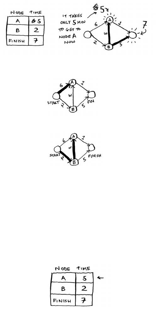
118 Chapter 7

I

Dijkstra’s algorithm

Step 2: Calculate how long it takes to get to all of node B’s neighbors by

following an edge from B.

Hey, you just found a shorter path to node A! It used to take 6 minutes

to get to node A.

But if you go through node B, there’s a path that only takes 5 minutes!

When you nd a shorter path for a neighbor of B, update its cost. In this

case, you found

• A shorter path to A (down from 6 minutes to 5 minutes)

• A shorter path to the nish (down from innity to 7 minutes)

Step 3: Repeat!

Step 1 again: Find the node that takes the least amount of time

to get to. You’re done with node B, so node A has the next smallest

time estimate.

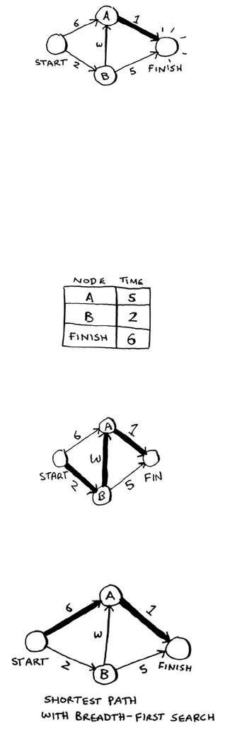
119Working with Dijkstra’s algorithm

Step 2 again: Update the costs for node A’s neighbors.

Woo, it takes 6 minutes to get to the nish now!

You’ve run Dijkstra’s algorithm for every node (you don’t need to run it

for the nish node). At this point, you know

• It takes 2 minutes to get to node B.

• It takes 5 minutes to get to node A.

• It takes 6 minutes to get to the nish.

I’ll save the last step, calculating the nal path, for the next section. For

now, I’ll just show you what the nal path is.

Breadth-rst search wouldn’t have found this as the shortest path,

because it has three segments. And there’s a way to get from the start to

the nish in two segments.

120 Chapter 7

I

Dijkstra’s algorithm

In the last chapter, you used breadth-rst search to nd the shortest

path between two points. Back then, “shortest path” meant the path

with the fewest segments. But in Dijkstra’s algorithm, you assign a

number or weight to each segment. en Dijkstra’s algorithm nds the

path with the smallest total weight.

To recap, Dijkstra’s algorithm has four steps:

1. Find the cheapest node. is is the node you can get to in the least

amount of time.

2. Check whether there’s a cheaper path to the neighbors of this node.

If so, update their costs.

3. Repeat until you’ve done this for every node in the graph.

4. Calculate the nal path. (Coming up in the next section!)

Terminology

I want to show you some more examples of Dijkstra’s algorithm in

action. But rst let me clarify some terminology.

When you work with Dijkstra’s algorithm, each edge in the graph has a

number associated with it. ese are called weights.

A graph with weights is called a weighted graph. A graph without

weights is called an unweighted graph.

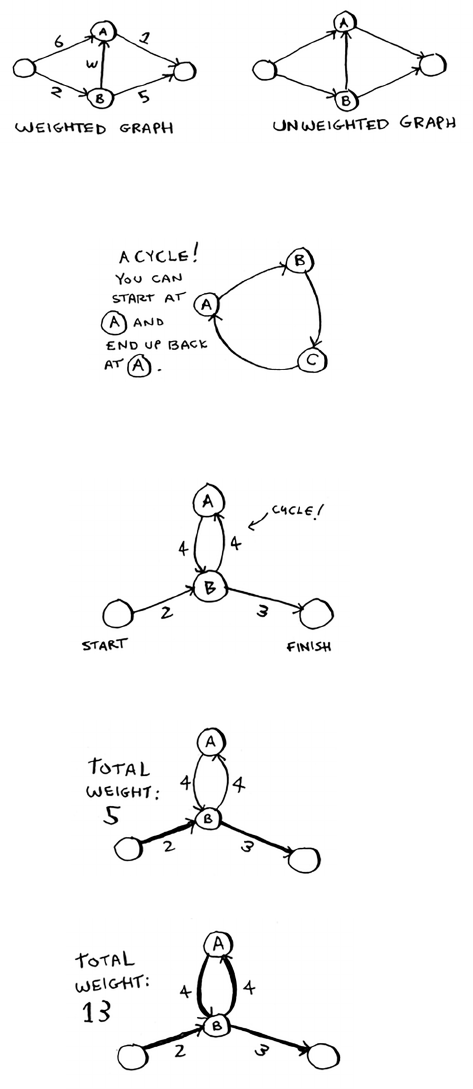
121Terminology

To calculate the shortest path in an unweighted graph, use breadth-rst

search. To calculate the shortest path in a weighted graph, use Dijkstra’s

algorithm. Graphs can also have cycles. A cycle looks like this.

It means you can start at a node, travel around, and end up at the same

node. Suppose you’re trying to nd the shortest path in this graph that

has a cycle.

Would it make sense to follow the cycle? Well, you can use the path that

avoids the cycle.

Or you can follow the cycle.

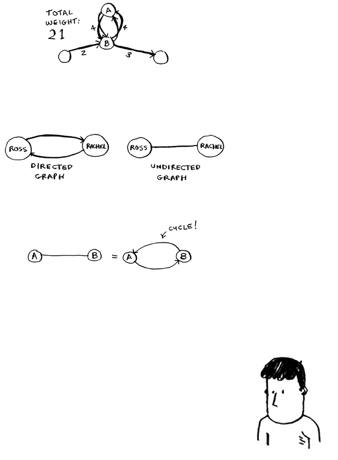
122 Chapter 7

I

Dijkstra’s algorithm

You end up at node A either way, but the cycle adds more weight. You

could even follow the cycle twice if you wanted.

But every time you follow the cycle, you’re just adding 8 to the total

weight. So following the cycle will never give you the shortest path.

Finally, remember our conversation about directed versus undirected

graphs from chapter 6?

An undirected graph means that both nodes point to each other. at’s

a cycle!

With an undirected graph, each edge adds another cycle.

Dijkstra’s algorithm only works with directed acyclic graphs,

called DAGs for short.

Trading for a piano

Enough terminology, let’s look at another example! is is Rama.

Rama is trying to trade a music book for a piano.

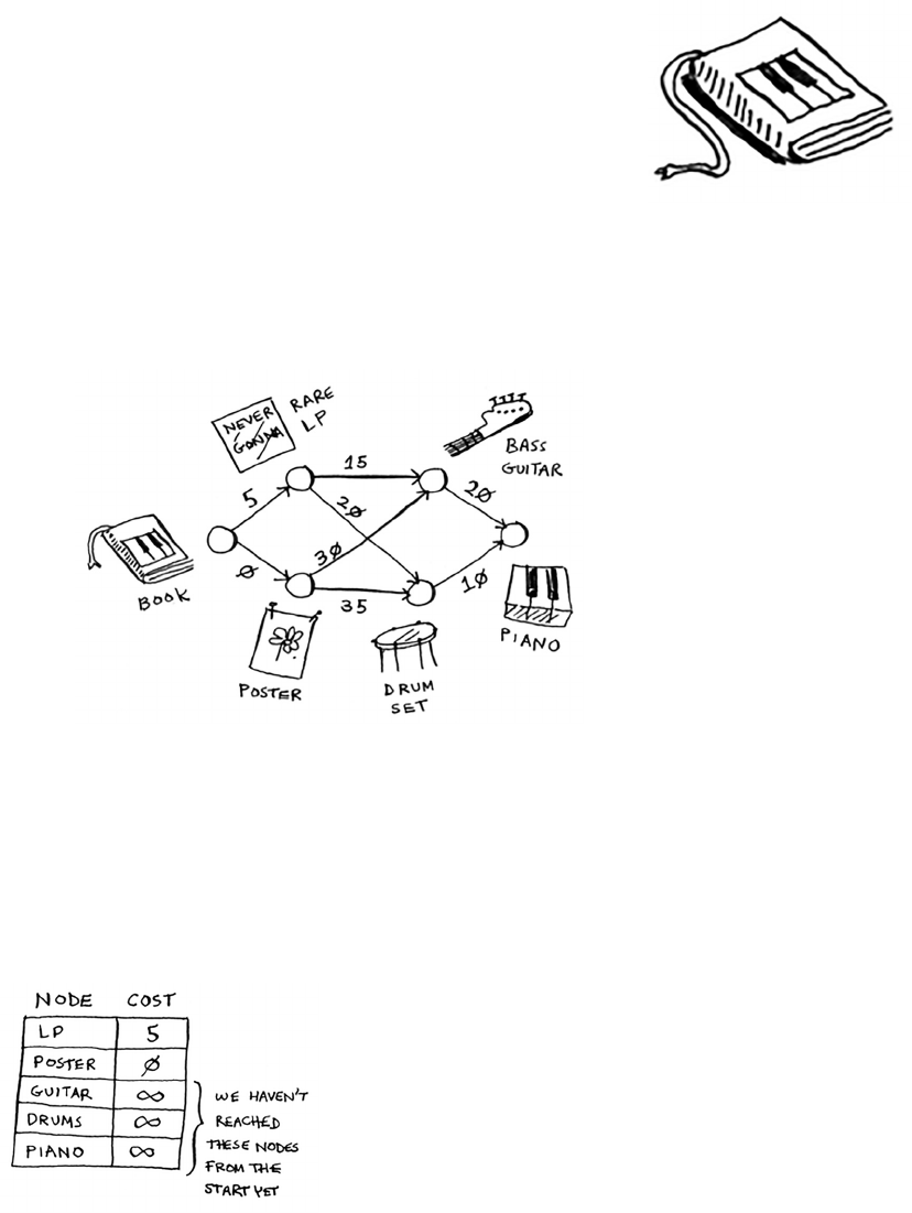
123Trading for a piano

“I’ll give you this poster for your book,” says Alex. “It’s a poster of

my favorite band, Destroyer. Or I’ll give you this rare LP of Rick

Astley for your book and $5 more.” “Ooh, I’ve heard that LP has a

really great song,” says Amy. “I’ll trade you my guitar or drum set

for the poster or the LP.”

“I’ve been meaning to get into guitar!” exclaims Beethoven. “Hey,

I’ll trade you my piano for either of Amy’s things.”

Perfect! With a little bit of money, Rama can trade his way from a piano

book to a real piano. Now he just needs to gure out how to spend the

least amount of money to make those trades. Let’s graph out what he’s

been oered.

In this graph, the nodes are all the items Rama can trade for. e

weights on the edges are the amount of money he would have to pay

to make the trade. So he can trade the poster for the guitar for $30, or

trade the LP for the guitar for $15. How is Rama going to gure out

the path from the book to the piano where he spends the least dough?

Dijkstra’s algorithm to the rescue! Remember, Dijkstra’s algorithm has

four steps. In this example, you’ll do all four steps, so you’ll calculate

the nal path at the end, too.

Before you start, you need some

setup. Make a table of the cost for

each node. e cost of a node is how

expensive it is to get to.

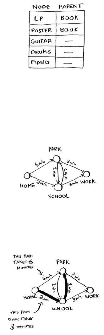
124 Chapter 7

I

Dijkstra’s algorithm

You’ll keep updating this table as the algorithm goes on. To calculate the

nal path, you also need a parent column on this table.

I’ll show you how this column works soon. Let’s start the algorithm.

Step 1: Find the cheapest node. In this case, the poster is the cheapest

trade, at $0. Is there a cheaper way to trade for the poster? is is a

really important point, so think about it. Can you see a series of trades

that will get Rama the poster for less than $0? Read on when you’re

ready. Answer: No. Because the poster is the cheapest node Rama can get

to, there’s no way to make it any cheaper. Here’s a dierent way to look at

it. Suppose you’re traveling from home to work.

If you take the path toward the school, that takes 2 minutes. If you take

the path toward the park, that takes 6 minutes. Is there any way you can

take the path toward the park, and end up at the school, in less than

2 minutes? It’s impossible, because it takes longer than 2 minutes just

to get to the park. On the other hand, can you nd a faster path to the

park? Yup.

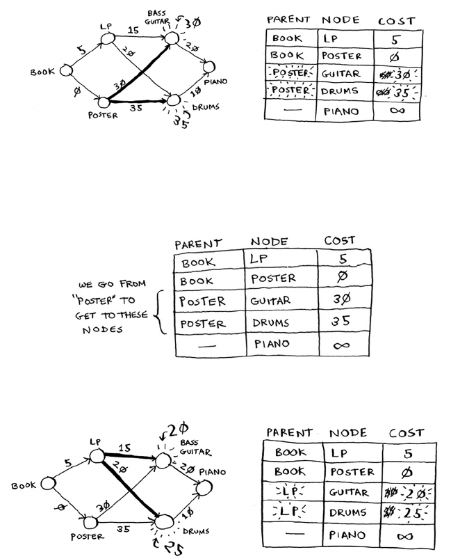
125Trading for a piano

is is the key idea behind Dijkstra’s algorithm: Look at the cheapest

node on your graph. ere is no cheaper way to get to this node!

Back to the music example. e poster is the cheapest trade.

Step 2: Figure out how long it takes to get to its neighbors (the cost).

You have prices for the bass guitar and the drum set in the table. eir

value was set when you went through the poster, so the poster gets set

as their parent. at means, to get to the bass guitar, you follow the edge

from the poster, and the same for the drums.

Step 1 again: e LP is the next cheapest node at $5.

Step 2 again: Update the values of all of its neighbors.

Hey, you updated the price of both the drums and the guitar! at

means it’s cheaper to get to the drums and guitar by following the edge

from the LP. So you set the LP as the new parent for both instruments.

126 Chapter 7

I

Dijkstra’s algorithm

e bass guitar is the next cheapest item. Update its neighbors.

Ok, you nally have a price for the piano, by trading the guitar for the

piano. So you set the guitar as the parent. Finally, the last node, the

drum set.

Rama can get the piano even cheaper by trading the drum set for the

piano instead. So the cheapest set of trades will cost Rama $35.

Now, as I promised, you need to gure out the path. So far, you know

that the shortest path costs $35, but how do you gure out the path? To

start with, look at the parent for piano.

e piano has drums as its parent. at means Rama trades the drums

for the piano. So you follow this edge.

127Trading for a piano

Let’s see how you’d follow the edges. Piano has drums as its parent.

And drums has the LP as its parent.

So Rama will trade the LP for the drums. And of course, he’ll trade the

book for the LP. By following the parents backward, you now have the

complete path.

Here’s the series of trades Rama needs to make.

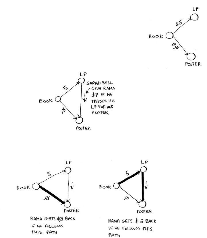
128 Chapter 7

I

Dijkstra’s algorithm

So far, I’ve been using the term shortest path pretty literally: calculating

the shortest path between two locations or between two people. I

hope this example showed you that the shortest path doesn’t have to

be about physical distance. It can be about minimizing something. In

this case, Rama wanted to minimize the amount of money he spent.

anks, Dijkstra!

Negative-weight edges

In the trading example, Alex oered to trade the book for

two items.

Suppose Sarah oers to trade the LP for the poster, and

she’ll give Rama an additional $7. It doesn’t cost Rama

anything to make this trade; instead, he gets $7 back.

How would you show this on the graph?

e edge from the LP to the poster has a negative weight! Rama

gets $7 back if he makes that trade. Now Rama has two ways to get

to the poster.

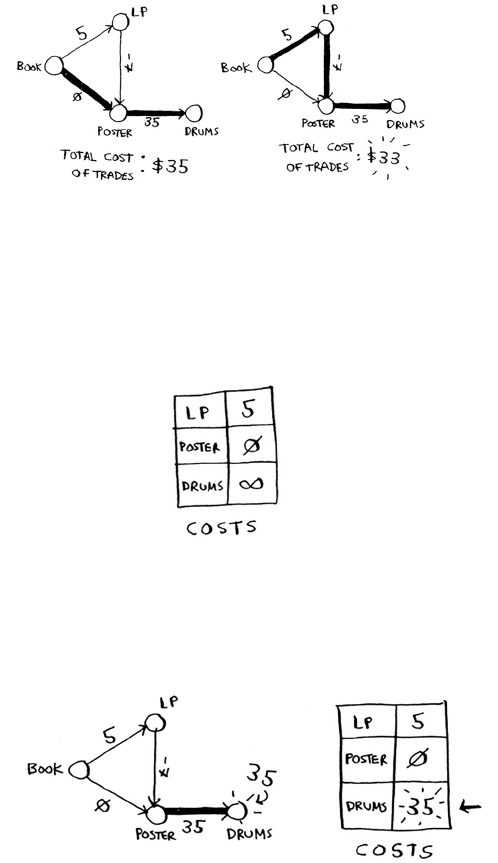
129Negative-weight edges

So it makes sense to do the second trade—Rama gets $2 back that way!

Now, if you remember, Rama can trade the poster for the drums. ere

are two paths he could take.

e second path costs him $2 less, so he should take that path, right?

Well, guess what? If you run Dijkstra’s algorithm on this graph, Rama

will take the wrong path. He’ll take the longer path. You can’t use

Dijkstra’s algorithm if you have negative-weight edges. Negative-weight

edges break the algorithm. Let’s see what happens when you run

Dijkstra’s algorithm on this. First, make the table of costs.

Next, nd the lowest-cost node, and update the costs for its neighbors.

In this case, the poster is the lowest-cost node. So, according to

Dijkstra’s algorithm, there is no cheaper way to get to the poster than

paying $0 (you know that’s wrong!). Anyway, let’s update the costs for

its neighbors.

Ok, the drums have a cost of $35 now.

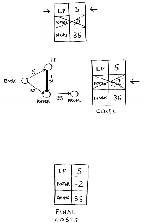
130 Chapter 7

I

Dijkstra’s algorithm

Let’s get the next-cheapest node that hasn’t already been processed.

Update the costs for its neighbors.

You already processed the poster node, but you’re updating the cost for

it. is is a big red ag. Once you process a node, it means there’s no

cheaper way to get to that node. But you just found a cheaper way to

the poster! Drums doesn’t have any neighbors, so that’s the end of the

algorithm. Here are the nal costs.

It costs $35 to get to the drums. You know that there’s a path that costs

only $33, but Dijkstra’s algorithm didn’t nd it. Dijkstra’s algorithm

assumed that because you were processing the poster node, there was

no faster way to get to that node. at assumption only works if you

have no negative-weight edges. So you can’t use negative-weight edges

with Dijkstra’s algorithm. If you want to nd the shortest path in a graph

that has negative-weight edges, there’s an algorithm for that! It’s called

the Bellman-Ford algorithm. Bellman-Ford is out of the scope of this

book, but you can nd some great explanations online.

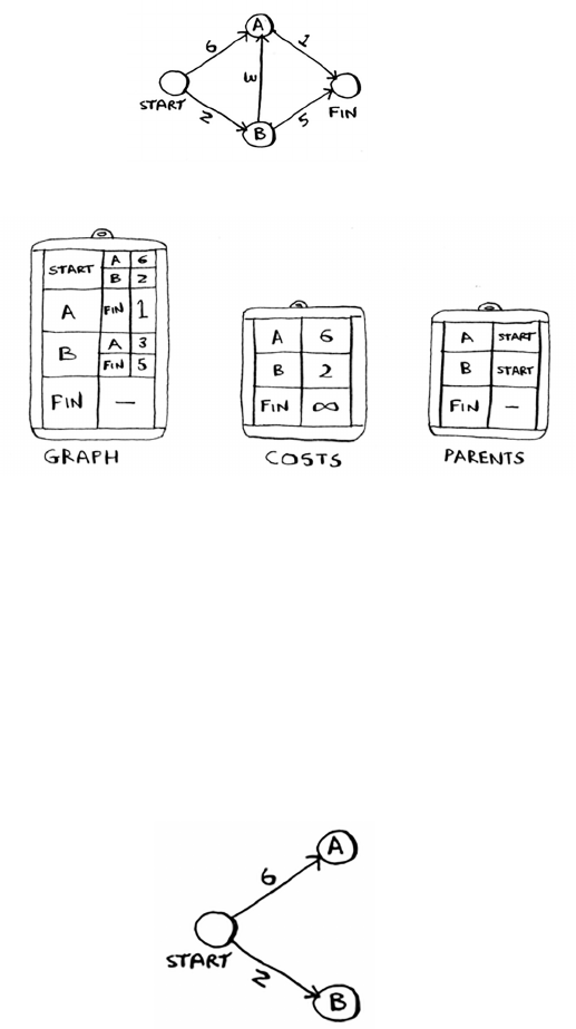
131Implementation

Implementation

Let’s see how to implement Dijkstra’s algorithm in code. Here’s the

graph I’ll use for the example.

To code this example, you’ll need three hash tables.

You’ll update the costs and parents hash tables as the algorithm

progresses. First, you need to implement the graph. You’ll use a hash

table like you did in chapter 6:

graph = {}

In the last chapter, you stored all the neighbors of a node in the hash

table, like this:

graph[“you”] = [“alice”, “bob”, “claire”]

But this time, you need to store the neighbors and the cost for getting to

that neighbor. For example, Start has two neighbors, A and B.

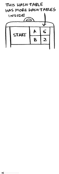
132 Chapter 7

I

Dijkstra’s algorithm

How do you represent the weights of those edges? Why not just use

another hash table?

graph[“start”] = {}

g r a ph[“st a r t”][“a”] = 6

g r a ph[“st a r t”][“b”] = 2

So

g r a p h[“s t a r t”]

is a hash table. You can get all the neighbors for

Start like this:

>>> print graph[“start”].keys()

[“a”, “b”]

ere’s an edge from Start to A and an edge from Start to B. What if you

want to nd the weights of those edges?

>>> p r i n t g ra p h[“st a r t”][“a”]

2

>>> p r i n t g ra p h[“st a r t”][“b”]

6

Let’s add the rest of the nodes and their neighbors to the graph:

graph[“a”] = {}

g r a ph[“a”][“fi n”] = 1

graph[“b”] = {}

g r a ph[“b”][“a”] = 3

g r a ph[“b”][“fi n”] = 5

graph[“fin”] = {} The finish node doesn’t have any neighbors.

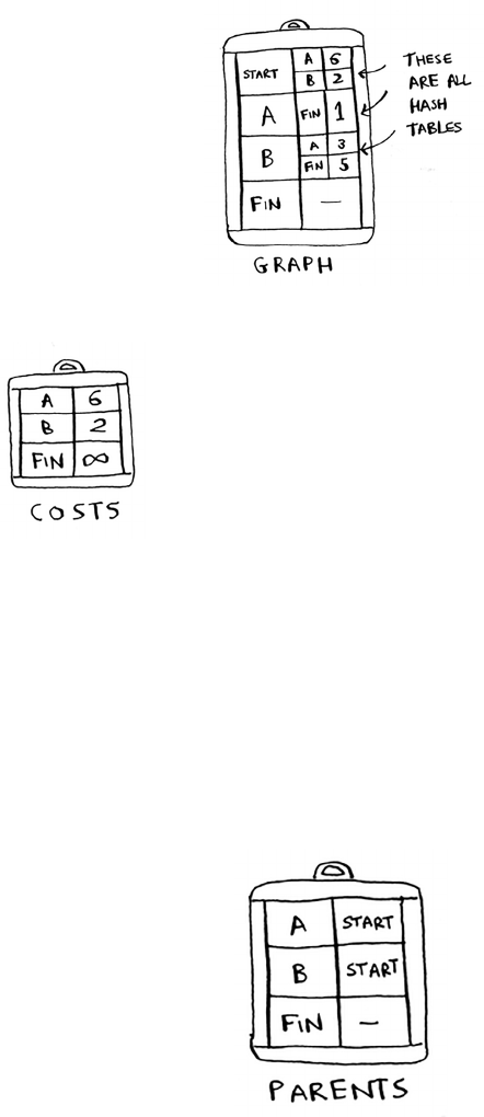
133Implementation

e full graph hash table looks like this.

Next you need a hash table to store the costs for each node.

e cost of a node is how long it takes to get to that

node from the start. You know it takes 2 minutes from

Start to node B. You know it takes 6 minutes to get to

node A (although you may nd a path that takes less

time). You don’t know how long it takes to get to the

nish. If you don’t know the cost yet, you put down

innity. Can you represent innity in Python? Turns

out, you can:

infinity = float(“inf”)

Here’s the code to make the costs table:

infinity = float(“inf”)

costs = {}

c o sts[“a”] = 6

c o sts[“b”] = 2

c o sts[“fi n”] = i n fi n it y

You also need another hash table for the parents:

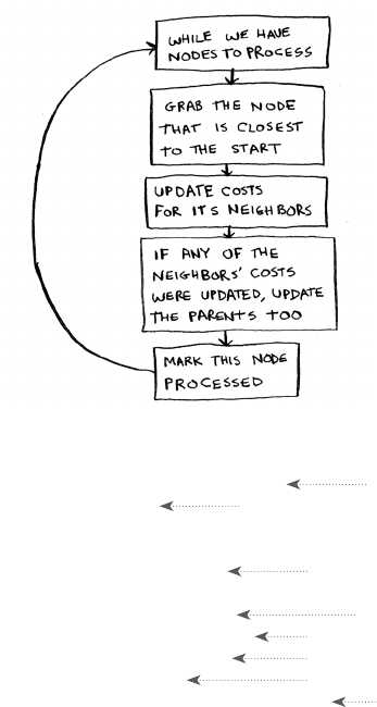
134 Chapter 7

I

Dijkstra’s algorithm

Here’s the code to make the hash table for the parents:

parents = {}

p a r e nts[“a”] = “sta r t”

p a r e nts[“b”] = “st a r t”

parents[“fin”] = None

Finally, you need an array to keep track of all the nodes you’ve already

processed, because you don’t need to process a node more than once:

processed = []

at’s all the setup. Now let’s look at the algorithm.

I’ll show you the code rst and then walk through it. Here’s the code:

node = find_lowest_cost_node(costs)

while node is not None:

cost = costs[node]

neighbors = graph[node]

for n in neighbors.keys():

new_cost = cost + neighbors[n]

if costs[n] > new_cost:

costs[n] = new_cost

parents[n] = node

processed.append(node)

node = find_lowest_cost_node(costs)

at’s Dijkstra’s algorithm in Python! I’ll show you the code for the

function later. First, let’s see this

find_lowest_cost_node

algorithm

code in action.

Find the lowest-cost node

that you haven’t processed yet.

If you’ve processed all the nodes, this while loop is done.

Go through all the neighbors of this node.

If it’s cheaper to get to this neighbor

by going through this node …

… update the cost for this node.

This node becomes the new parent for this neighbor.

Mark the node as processed.

Find the next node to process, and loop.

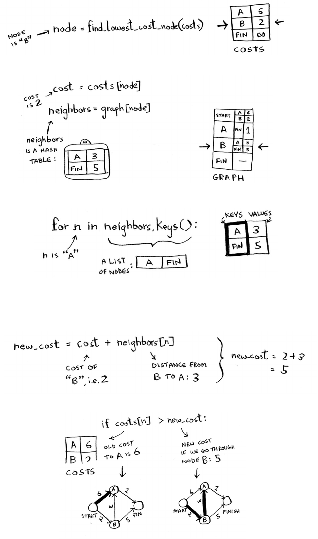
135Implementation

Find the node with the lowest cost.

Get the cost and neighbors of that node.

Loop through the neighbors.

Each node has a cost. e cost is how long it takes to get to that node

from the start. Here, you’re calculating how long it would take to get to

node A if you went Start > node B > node A, instead of Start > node A.

Let’s compare those costs.

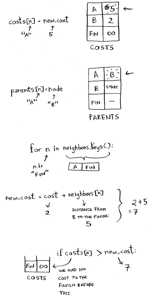
136 Chapter 7

I

Dijkstra’s algorithm

You found a shorter path to node A! Update the cost.

e new path goes through node B, so set B as the new parent.

Ok, you’re back at the top of the loop. e next neighbor

for

is the

Finish node.

How long does it take to get to the nish if you go through node B?

It takes 7 minutes. e previous cost was innity minutes, and

7 minutes is less than that.

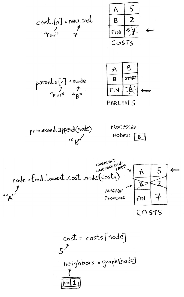
137Implementation

Set the new cost and the new parent for the Finish node.

Ok, you updated the costs for all the neighbors of node B. Mark it as

processed.

Find the next node to process.

Get the cost and neighbors for node A.

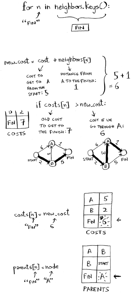
138 Chapter 7

I

Dijkstra’s algorithm

Node A only has one neighbor: the Finish node.

Currently it takes 7 minutes to get to the Finish node. How long would

it take to get there if you went through node A?

It’s faster to get to Finish from node A! Let’s update the cost

and parent.

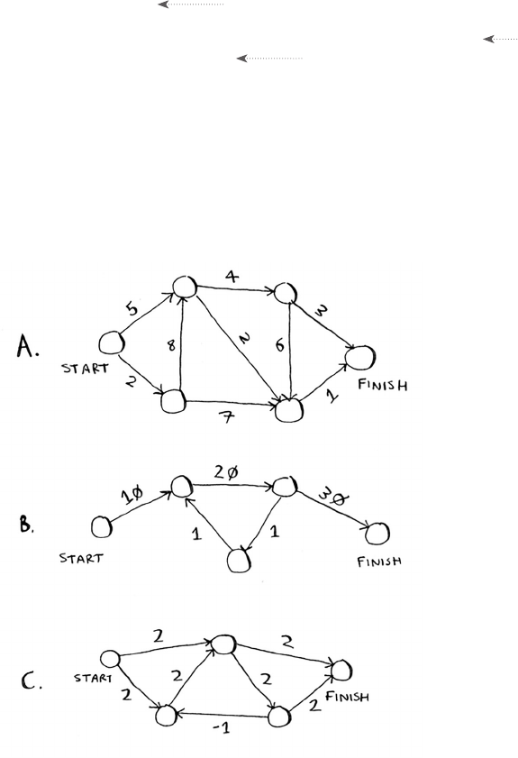
139Implementation

If it’s the lowest cost

so far and hasn’t been

processed yet …

def find_lowest_cost_node(costs):

lowest_cost = float(“inf”)

lowest_cost_node = None

for node in costs: Go through each node.

cost = costs[node]

if cost < lowest_cost and node not in processed:

lowest_cost = cost … set it as the new lowest-cost node.

lowest_cost_node = node

return lowest_cost_node

Once you’ve processed all the nodes, the algorithm is over. I hope

the walkthrough helped you understand the algorithm a little better.

Finding the lowest-cost node is pretty easy with the

find _lowest_

cost_node

function. Here it is in code:

EXERCISE

7.1 In each of these graphs, what is the weight of the shortest path from

start to nish?

140 Chapter 7

I

Dijkstra’s algorithm

Recap

• Breadth-rst search is used to calculate the shortest path for

an unweighted graph.

• Dijkstra’s algorithm is used to calculate the shortest path for

a weighted graph.

• Dijkstra’s algorithm works when all the weights are positive.

• If you have negative weights, use the Bellman-Ford algorithm.

141

greedy

algorithms

In this chapter

• You learn how to tackle the impossible:

problems that have no fast algorithmic solution

(NP-complete problems).

• You learn how to identify such problems when you

see them, so you don’t waste time trying to nd a

fast algorithm for them.

• You learn about approximation algorithms, which

you can use to nd an approximate solution to an

NP-complete problem quickly.

• You learn about the greedy strategy, a very simple

problem-solving strategy.

8

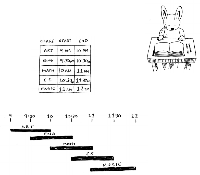
142 Chapter 8

I

Greedy algorithms

The classroom scheduling problem

Suppose you have a classroom and want to hold as many classes

here as possible. You get a list of classes.

You can’t hold all of these classes in there, because some of them

overlap.

You want to hold as many classes as possible in this classroom. How

do you pick what set of classes to hold, so that you get the biggest set of

classes possible?

Sounds like a hard problem, right? Actually, the algorithm is so easy, it

might surprise you. Here’s how it works:

1. Pick the class that ends the soonest. is is the rst class you’ll hold

in this classroom.

2. Now, you have to pick a class that starts aer the rst class.

Again, pick the class that ends the soonest. is is the second

class you’ll hold.

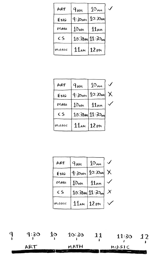
143The classroom scheduling problem

Keep doing this, and you’ll end up with the answer! Let’s try it out. Art

ends the soonest, at 10:00 a.m., so that’s one of the classes you pick.

Now you need the next class that starts aer 10:00 a.m. and ends

the soonest.

English is out because it conicts with Art, but Math works.

Finally, CS conicts with Math, but Music works.

So these are the three classes you’ll hold in this classroom.

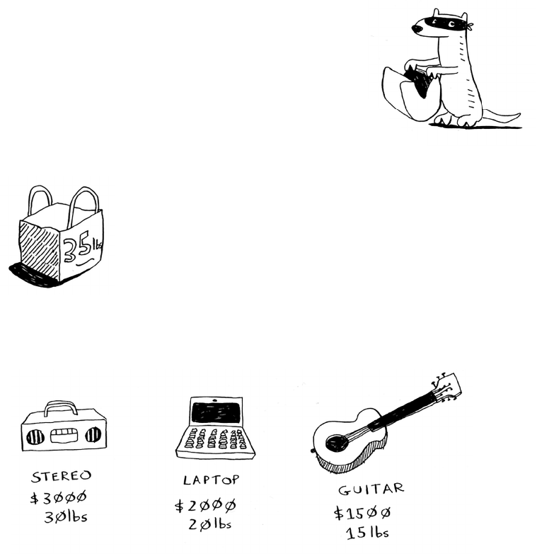
144 Chapter 8

I

Greedy algorithms

A lot of people tell me that this algorithm seems easy. It’s too obvious,

so it must be wrong. But that’s the beauty of greedy algorithms: they’re

easy! A greedy algorithm is simple: at each step, pick the optimal move.

In this case, each time you pick a class, you pick the class that ends the

soonest. In technical terms: at each step you pick the locally optimal

solution, and in the end you’re le with the globally optimal solution.

Believe it or not, this simple algorithm nds the optimal solution to this

scheduling problem!

Obviously, greedy algorithms don’t always work. But they’re simple to

write! Let’s look at another example.

The knapsack problem

Suppose you’re a greedy thief. You’re in a store with a

knapsack, and there are all these items you can steal.

But you can only take what you can t in your knapsack.

e knapsack can hold 35 pounds.

You’re trying to maximize the value of the items you put

in your knapsack. What algorithm do you use?

Again, the greedy strategy is pretty simple:

1. Pick the most expensive thing that will t in your

knapsack.

2. Pick the next most expensive thing that will t in

your knapsack. And so on.

Except this time, it doesn’t work! For example, suppose there are three

items you can steal.

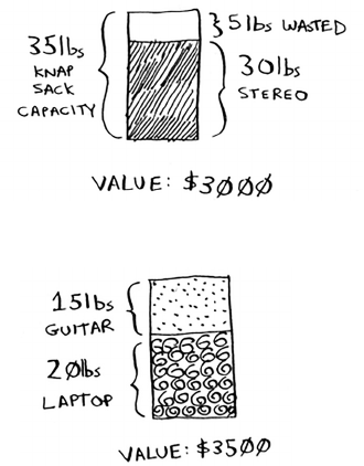
145The knapsack problem

Your knapsack can hold 35 pounds of items. e stereo system is

the most expensive, so you steal that. Now you don’t have space for

anything else.

You got $3,000 worth of goods. But wait! If you’d picked the laptop and

the guitar instead, you could have had $3,500 worth of loot!

Clearly, the greedy strategy doesn’t give you the optimal solution here.

But it gets you pretty close. In the next chapter, I’ll explain how to

calculate the correct solution. But if you’re a thief in a shopping center,

you don’t care about perfect. “Pretty good” is good enough.

Here’s the takeaway from this second example: sometimes, perfect is the

enemy of good. Sometimes all you need is an algorithm that solves the

problem pretty well. And that’s where greedy algorithms shine, because

they’re simple to write and usually get pretty close.

EXERCISES

8.1 You work for a furniture company, and you have to ship furniture

all over the country. You need to pack your truck with boxes. All

the boxes are of dierent sizes, and you’re trying to maximize the

space you use in each truck. How would you pick boxes to maximize

space? Come up with a greedy strategy. Will that give you the

optimal solution?

8.2 You’re going to Europe, and you have seven days to see everything

you can. You assign a point value to each item (how much you want

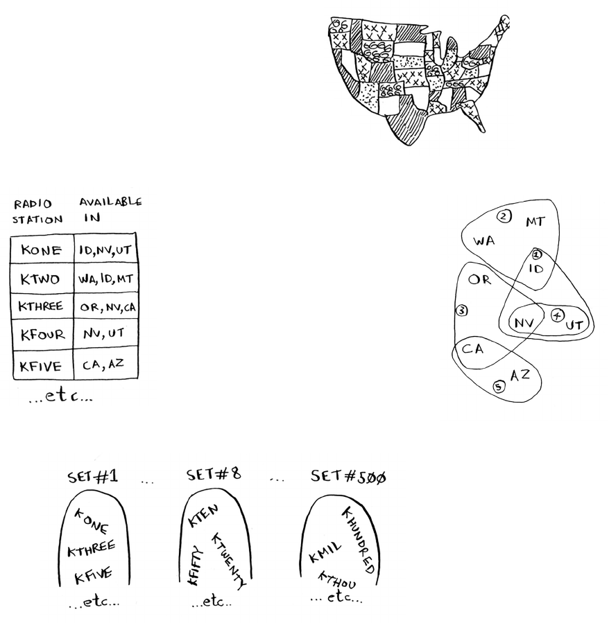
146 Chapter 8

I

Greedy algorithms

to see it) and estimate how long it takes. How can you maximize the

point total (seeing all the things you really want to see) during your

stay? Come up with a greedy strategy. Will that give you the optimal

solution?

Let’s look at one last example. is is an example where greedy

algorithms are absolutely necessary.

The set-covering problem

Suppose you’re starting a radio show. You want to

reach listeners in all 50 states. You have to decide what

stations to play on to reach all those listeners. It costs

money to be on each station, so you’re trying to minimize the

number of stations you play on. You have a list of stations.

Each station covers a region, and

there’s overlap.

How do you gure out the smallest set of

stations you can play on to cover all 50

states? Sounds easy, doesn’t it? Turns out

it’s extremely hard. Here’s how to do it:

1. List every possible subset of stations.

is is called the power set. ere are

2^n possible subsets.

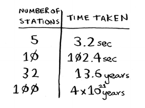
147The set-covering problem

2. From these, pick the set with the smallest number of stations that

covers all 50 states.

e problem is, it takes a long time to calculate every possible subset

of stations. It takes O(2^n) time, because there are 2^n stations. It’s

possible to do if you have a small set of 5 to 10 stations. But with all

the examples here, think about what will happen if you have a lot of

items. It takes much longer if you have more stations. Suppose you can

calculate 10 subsets per second.

ere’s no algorithm that solves it fast enough! What can you do?

Approximation algorithms

Greedy algorithms to the rescue! Here’s a greedy algorithm that comes

pretty close:

1. Pick the station that covers the most states that haven’t been covered

yet. It’s OK if the station covers some states that have been covered

already.

2. Repeat until all the states are covered.

is is called an approximation algorithm. When calculating the exact

solution will take too much time, an approximation algorithm will

work. Approximation algorithms are judged by

• How fast they are

• How close they are to the optimal solution

Greedy algorithms are a good choice because not only are they simple

to come up with, but that simplicity means they usually run fast, too.

In this case, the greedy algorithm runs in O(n^2) time, where n is the

number of radio stations.

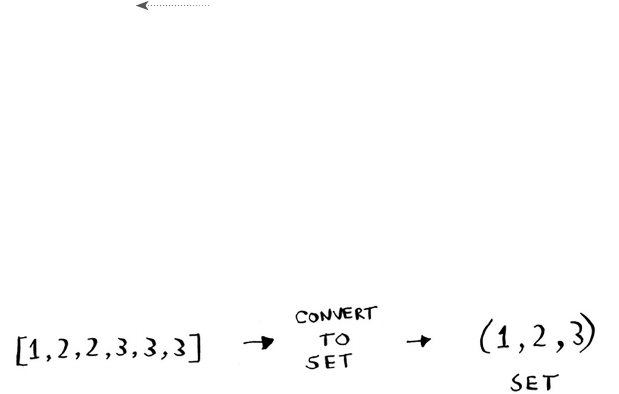
148 Chapter 8

I

Greedy algorithms

Let’s see how this problem looks in code.

Code for setup

For this example, I’m going to use a subset of the states and the stations

to keep things simple.

First, make a list of the states you want to cover:

states_needed = set([“mt”, “wa”, “or”, “id”, “nv”, “ut”,

“ c a ”, “ a z ”]) You pass an array in, and it gets converted to a set.

I used a set for this. A set is like a list, except that each item can show up

only once in a set. Sets can’t have duplicates. For example, suppose you

had this list:

>>> arr = [1, 2, 2, 3, 3, 3]

And you converted it to a set:

>>> set(arr)

set([1, 2, 3])

1, 2, and 3 all show up just once in a set.

You also need the list of stations that you’re choosing from. I chose to

use a hash for this:

stations = {}

st atio n s[“k o n e”] = s et([“id”, “n v”, “ut”])

st atio n s[“k t w o”] = s e t([“w a”, “id”, “m t”])

st atio n s[“k t h r e e”] = se t([“or”, “n v ”, “ca”])

st atio n s[“k fo u r”] = se t([“n v”, “ut”])

st atio n s[“k fi v e”] = s e t([“c a”, “az”])

e keys are station names, and the values are the states they cover.

So in this example, the kone station covers Idaho, Nevada, and Utah.

All the values are sets, too. Making everything a set will make your life

easier, as you’ll see soon.

Finally, you need something to hold the nal set of stations you’ll use:

final_stations = set()

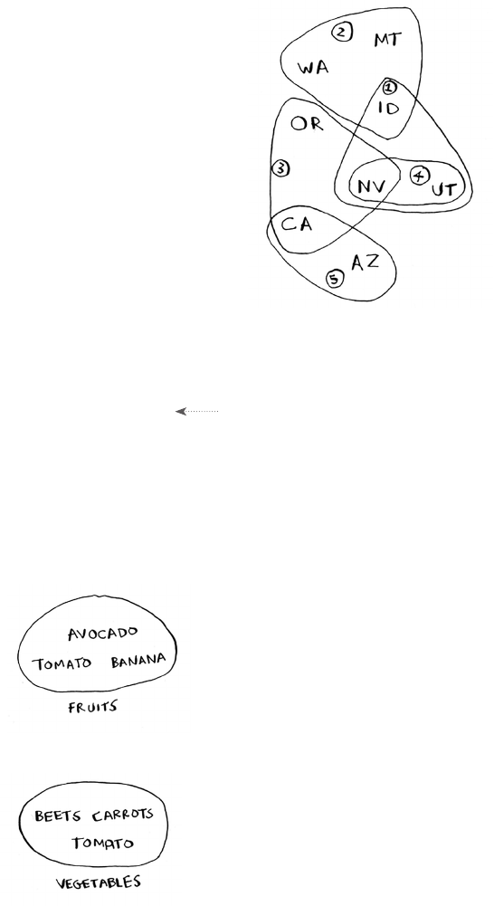
149The set-covering problem

Calculating the answer

Now you need to calculate what stations you’ll use. Take a look

at the image at right, and see if you can predict what stations you

should use.

ere can be more than one correct solution. You need to go

through every station and pick the one that covers the most

uncovered states. I’ll call this

best_station

:

best_station = None

states_covered = set()

for station, states_for_station in stations.items():

states_covered

is a set of all the states this station covers that

haven’t been covered yet. e

for

loop allows you to loop over

every station to see which one is the best station. Let’s look at the body

of the

for

loop:

covered = states_needed & states_for_station

if len(covered) > len(states_covered):

best_station = station

states_covered = covered

ere’s a funny-looking line here:

covered = states_needed & states_for_station

What’s going on?

Sets

Suppose you have a set of fruits.

You also have a set of vegetables.

When you have two sets, you can do some fun things with them.

New syntax! This is

called a set intersection.

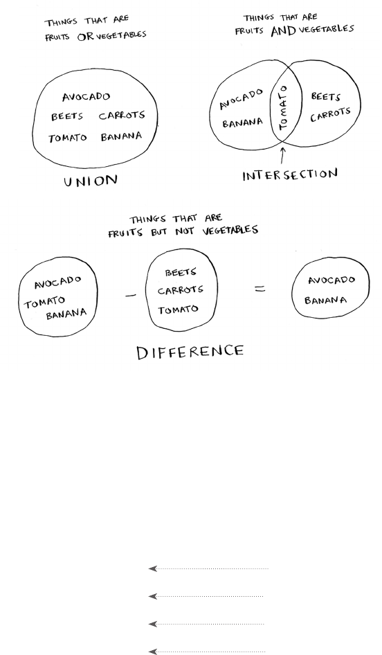
150 Chapter 8

I

Greedy algorithms

Here are some things you can do with sets.

• A set union means “combine both sets.”

• A set intersection means “nd the items that show up in both sets”

(in this case, just the tomato).

• A set dierence means “subtract the items in one set from the items

in the other set.”

For example:

>>> fruits = set([“avocado”, “tomato”, “banana”])

>>> vegetables = set([“beets”, “carrots”, “tomato”])

>>> fruits | vegetables This is a set union.

s e t([ “ a v o c a d o ”, “ b e e t s ”, “c a r r o t s ”, “ t o m a t o ”, “ b a n a n a ”])

>>> fruits & vegetables This is a set intersection.

se t([“to m ato”])

>>> fruits – vegetables This is a set difference.

se t([“a v o c ad o”, “b a n a n a”])

>>> vegetables – fruits What do you think this will do?

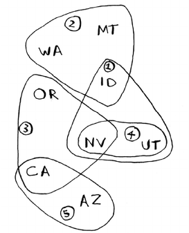
151The set-covering problem

To recap:

• Sets are like lists, except sets can’t have duplicates.

• You can do some interesting operations on sets, like union,

intersection, and dierence.

Back to the code

Let’s get back to the original example.

is is a set intersection:

covered = states_needed & states_for_station

covered

is a set of states that were in both

states_needed

and

states_for_station

. So

covered

is the set of uncovered states

that this station covers! Next you check whether this station

covers more states than the current

best_station

:

if len(covered) > len(states_covered):

best_station = station

states_covered = covered

If so, this station is the new

best_station

. Finally, aer the

for

loop is over, you add

best_station

to the nal list of stations:

final_stations.add(best_station)

You also need to update

states_needed

. Because this station covers

some states, those states aren’t needed anymore:

states_needed -= states_covered

And you loop until

states_needed

is empty. Here’s the full code for

the loop:

while states_needed:

best_station = None

states_covered = set()

for station, states in stations.items():

covered = states_needed & states

if len(covered) > len(states_covered):

best_station = station

states_covered = covered

states_needed -= states_covered

final_stations.add(best_station)

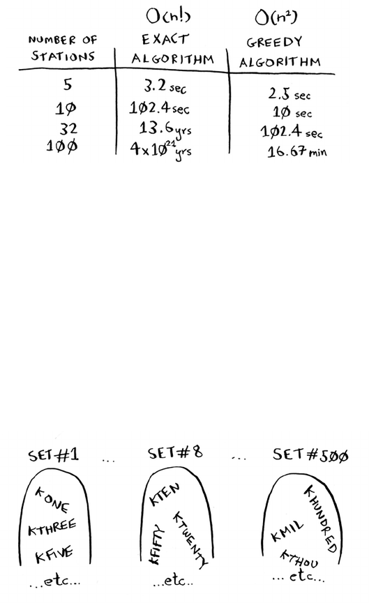
152 Chapter 8

I

Greedy algorithms

Finally, you can print

final_stations

, and you should see this:

>>> print final_stations

set([‘kt w o’, ‘k t h r e e’, ‘k o n e’, ‘k fi v e’])

Is that what you expected? Instead of stations 1, 2, 3, and 5, you could

have chosen stations 2, 3, 4, and 5. Let’s compare the run time of the

greedy algorithm to the exact algorithm.

EXERCISES

For each of these algorithms, say whether it’s a greedy algorithm or not.

8.3 Quicksort

8.4 Breadth-rst search

8.5 Dijkstra’s algorithm

NP-complete problems

To solve the set-covering problem, you had to calculate every

possible set.

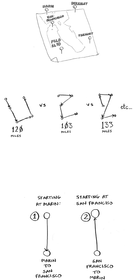
153NP-complete problems

Maybe you were reminded of the traveling salesperson problem from

chapter 1. In this problem, a salesperson has to visit ve dierent cities.

And he’s trying to gure out the shortest route that will take him to all

ve cities. To nd the shortest route, you rst have to calculate every

possible route.

How many routes do you have to calculate for ve cities?

Traveling salesperson, step by step

Let’s start small. Suppose you only have two cities. ere are two routes

to choose from.

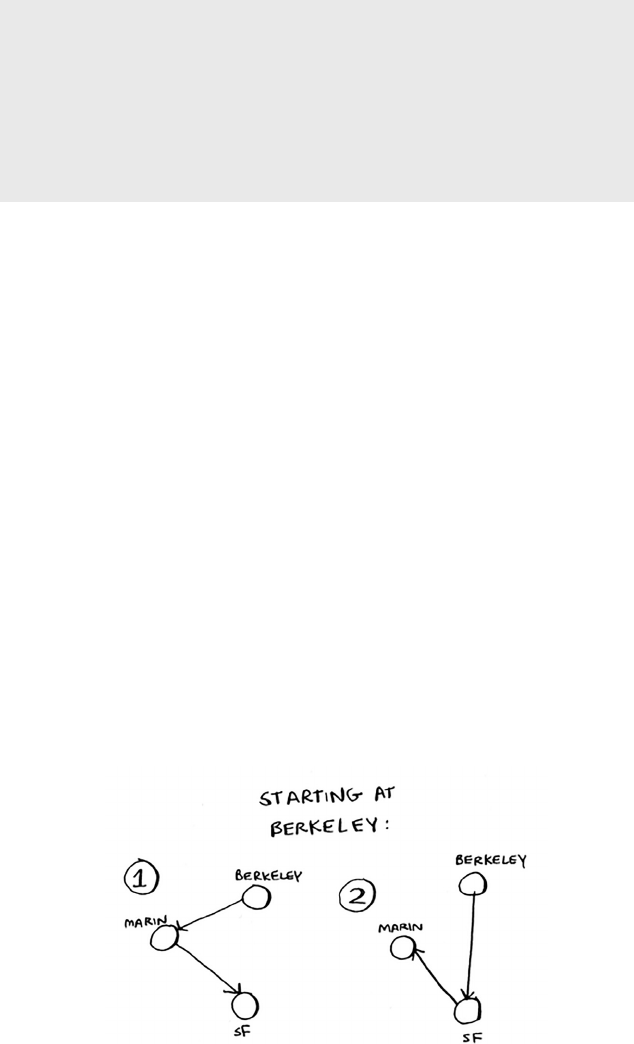
154 Chapter 8

I

Greedy algorithms

You may be wondering, “In the traveling salesperson problem, is there

a specic city you need to start from?” For example, let’s say I’m the

traveling salesperson. I live in San Francisco, and I need to go to four

other cities. San Francisco would be my start city.

But sometimes the start city isn’t set. Suppose you’re FedEx, trying

to deliver a package to the Bay Area. e package is being own in

from Chicago to one of 50 FedEx locations in the Bay Area. en

that package will go on a truck that will travel to dierent locations

delivering packages. Which location should it get own to? Here the

start location is unknown. It’s up to you to compute the optimal path

and start location for the traveling salesperson.

e running time for both versions is the same. But it’s an easier

example if there’s no dened start city, so I’ll go with that version.

Two cities = two possible routes.

3 cities

Now suppose you add one more city. How many possible routes

are there?

If you start at Berkeley, you have two more cities to visit.

Same route or dierent?

You may think this should be the same route. Aer all, isn’t SF > Marin

the same distance as Marin > SF? Not necessarily. Some cities (like San

Francisco) have a lot of one-way streets, so you can’t go back the way you

came. You might also have to go 1 or 2 miles out of the way to nd an on-

ramp to a highway. So these two routes aren’t necessarily the same.

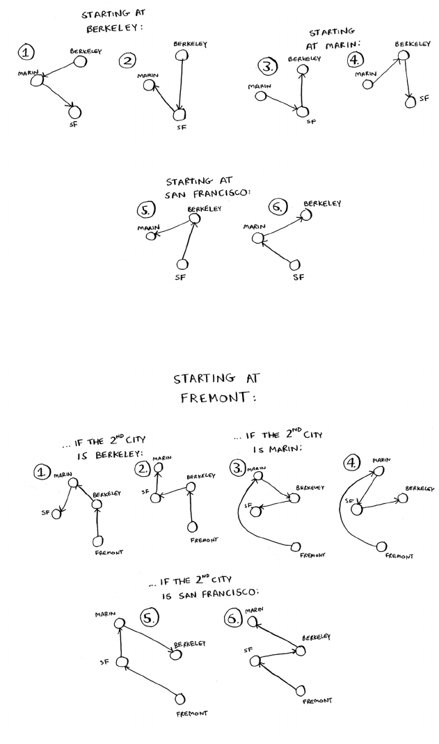
155NP-complete problems

ere are six total routes, two for each city you can start at.

So three cities = six possible routes.

4 cities

Let’s add another city, Fremont. Now suppose you start at Fremont.

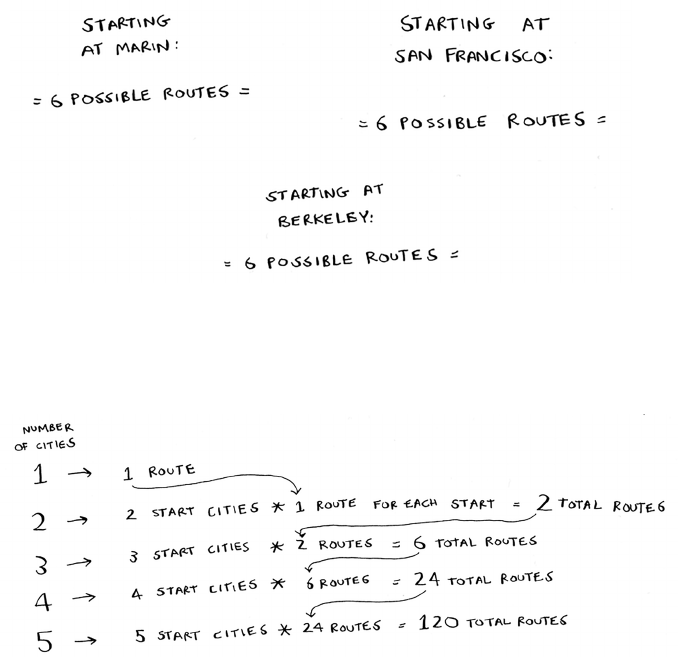
156 Chapter 8

I

Greedy algorithms

ere are six possible routes starting from Fremont. And hey! ey

look a lot like the six routes you calculated earlier, when you had only

three cities. Except now all the routes have an additional city, Fremont!

ere’s a pattern here. Suppose you have four cities, and you pick a start

city, Fremont. ere are three cities le. And you know that if there are

three cities, there are six dierent routes for getting between those cities.

If you start at Fremont, there are six possible routes. You could also start

at one of the other cities.

Four possible start cities, with six possible routes for each start city =

4 * 6 = 24 possible routes.

Do you see a pattern? Every time you add a new city, you’re increasing

the number of routes you have to calculate.

How many possible routes are there for six cities? If you guessed 720,

you’re right. 5,040 for 7 cities, 40,320 for 8 cities.

is is called the factorial function (remember reading about this in

chapter 3?). So 5! = 120. Suppose you have 10 cities. How many possible

routes are there? 10! = 3,628,800. You have to calculate over 3 million

possible routes for 10 cities. As you can see, the number of possible

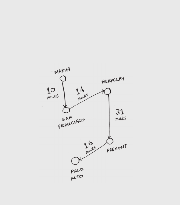
157NP-complete problems

routes becomes big very fast! is is why it’s impossible to compute the

“correct” solution for the traveling-salesperson problem if you have a

large number of cities.

e traveling-salesperson problem and the set-covering problem both

have something in common: you calculate every possible solution and

pick the smallest/shortest one. Both of these problems are NP-complete.

Here’s the short explanation of NP-completeness: some problems are

famously hard to solve. e traveling salesperson and the set-covering

problem are two examples. A lot of smart people think that it’s not

possible to write an algorithm that will solve these problems quickly.

Approximating

What’s a good approximation algorithm for the traveling salesperson?

Something simple that nds a short path. See if you can come up with an

answer before reading on.

Here’s how I would do it: arbitrarily pick a start city. en, each time the

salesperson has to pick the next city to visit, they pick the closest unvisited

city. Suppose they start in Marin.

Total distance: 71 miles. Maybe it’s not the shortest path, but it’s still

pretty short.

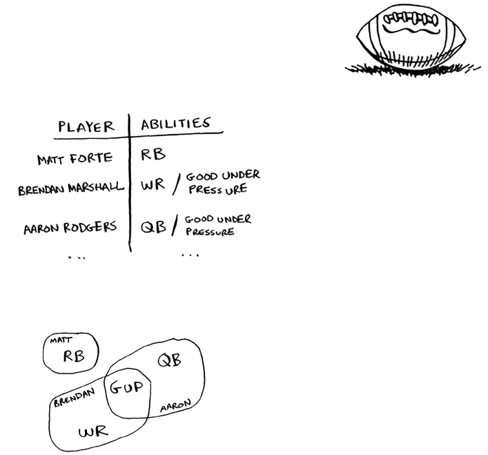
158 Chapter 8

I

Greedy algorithms

How do you tell if a problem is NP-complete?

Jonah is picking players for his fantasy football team. He has a list of

abilities he wants: good quarterback, good running back, good in rain,

good under pressure, and so on. He has a list of players, where each

player fullls some abilities.

Jonah needs a team that fullls all his abilities, and the team size

is limited. “Wait a second,” Jonah realizes. “is is a set-covering

problem!”

Jonah can use the same approximation algorithm to create his team:

1. Find the player who fullls the most abilities that haven’t been

fullled yet.

2. Repeat until the team fullls all abilities (or you run out of space

on the team).

NP-complete problems show up everywhere! It’s nice to know if the

problem you’re trying to solve is NP-complete. At that point, you can

stop trying to solve it perfectly, and solve it using an approximation

algorithm instead. But it’s hard to tell if a problem you’re working on is

NP-complete. Usually there’s a very small dierence between a problem

that’s easy to solve and an NP-complete problem. For example, in the

previous chapters, I talked a lot about shortest paths. You know how to

calculate the shortest way to get from point A to point B.

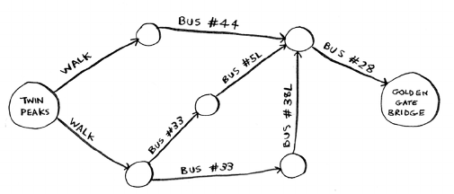
159NP-complete problems

But if you want to nd the shortest path that connects several points,

that’s the traveling-salesperson problem, which is NP-complete. e

short answer: there’s no easy way to tell if the problem you’re working

on is NP-complete. Here are some giveaways:

• Your algorithm runs quickly with a handful of items but really slows

down with more items.

• “All combinations of X” usually point to an NP-complete problem.

• Do you have to calculate “every possible version” of X because you

can’t break it down into smaller sub-problems? Might be

NP-complete.

• If your problem involves a sequence (such as a sequence of cities, like

traveling salesperson), and it’s hard to solve, it might be NP-complete.

• If your problem involves a set (like a set of radio stations) and it’s hard

to solve, it might be NP-complete.

• Can you restate your problem as the set-covering problem or the

traveling-salesperson problem? en your problem is denitely

NP-complete.

EXERCISES

8.6 A postman needs to deliver to 20 homes. He needs to nd the

shortest route that goes to all 20 homes. Is this an NP-complete

problem?

8.7 Finding the largest clique in a set of people (a clique is a set of people

who all know each other). Is this an NP-complete problem?

8.8 You’re making a map of the USA, and you need to color adjacent

states with dierent colors. You have to nd the minimum number

of colors you need so that no two adjacent states are the same color.

Is this an NP-complete problem?

160 Chapter 8

I

Greedy algorithms

Recap

• Greedy algorithms optimize locally, hoping to end up with a global

optimum.

• NP-complete problems have no known fast solution.

• If you have an NP-complete problem, your best bet is to use an

approximation algorithm.

• Greedy algorithms are easy to write and fast to run, so they make

good approximation algorithms.

161

In this chapter

• You learn dynamic programming, a

technique to solve a hard problem by

breaking it up into subproblems and

solving those subproblems rst.

• Using examples, you learn to how to come up

with a dynamic programming solution to a

new problem.

dynamic

programming 9

The knapsack problem

Let’s revisit the knapsack problem from chapter 8.

You’re a thief with a knapsack that can carry 4 lb

of goods.

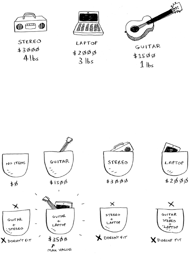
162 Chapter 9

I

Dynamic programming

You have three items that you can put into the knapsack.

What items should you steal so that you steal the maximum money’s

worth of goods?

The simple solution

e simplest algorithm is this: you try every possible set of goods and

nd the set that gives you the most value.

is works, but it’s really slow. For 3 items, you have to calculate 8

possible sets. For 4 items, you have to calculate 16 sets. With every

item you add, the number of sets you have to calculate doubles! is

algorithm takes O(2^n) time, which is very, very slow.

163The knapsack problem

at’s impractical for any reasonable number of goods. In chapter 8,

you saw how to calculate an approximate solution. at solution will be

close to the optimal solution, but it may not be the optimal solution.

So how do you calculate the optimal solution?

Dynamic programming

Answer: With dynamic programming! Let’s see how the dynamic-

programming algorithm works here. Dynamic programming starts by

solving subproblems and builds up to solving the big problem.

For the knapsack problem, you’ll start by solving the problem for

smaller knapsacks (or “sub-knapsacks”) and then work up to solving

the original problem.

Dynamic programming is a hard concept, so don’t worry if you don’t get it

right away. We’re going to look at a lot of examples.

I’ll start by showing you the algorithm in action rst. Aer you’ve seen

it in action once, you’ll have a lot of questions! I’ll do my best to address

every question.

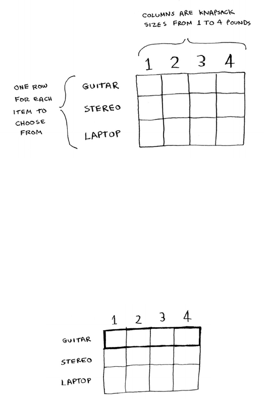
164 Chapter 9

I

Dynamic programming

Every dynamic-programming algorithm starts with a grid. Here’s a grid

for the knapsack problem.

e rows of the grid are the items, and the columns are knapsack

weights from 1 lb to 4 lb. You need all of those columns because they

will help you calculate the values of the sub-knapsacks.

e grid starts out empty. You’re going to ll in each cell of the grid.

Once the grid is lled in, you’ll have your answer to this problem!

Please follow along. Make your own grid, and we’ll ll it out together.

The guitar row

I’ll show you the exact formula for calculating this grid later. Let’s do a

walkthrough rst. Start with the rst row.

is is the guitar row, which means you’re trying to t the guitar into

the knapsack. At each cell, there’s a simple decision: do you steal the

guitar or not? Remember, you’re trying to nd the set of items to steal

that will give you the most value.

e rst cell has a knapsack of capacity 1 lb. e guitar is also 1 lb,

which means it ts into the knapsack! So the value of this cell is $1,500,

and it contains a guitar.

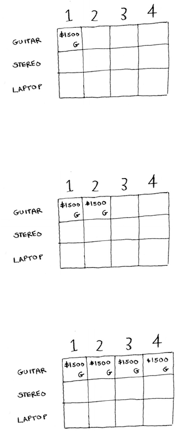
165The knapsack problem

Let’s start lling in the grid.

Like this, each cell in the grid will contain a list of all the items that t

into the knapsack at that point.

Let’s look at the next cell. Here you have a knapsack of capacity 2 lb.

Well, the guitar will denitely t in there!

e same for the rest of the cells in this row. Remember, this is the rst

row, so you have only the guitar to choose from. You’re pretending that

the other two items aren’t available to steal right now.

At this point, you’re probably confused. Why are you doing this for

knapsacks with a capacity of 1 lb, 2 lb, and so on, when the problem

talks about a 4 lb knapsack? Remember how I told you that dynamic

programming starts with a small problem and builds up to the big

problem? You’re solving subproblems here that will help you to solve

the big problem. Read on, and things will become clearer.

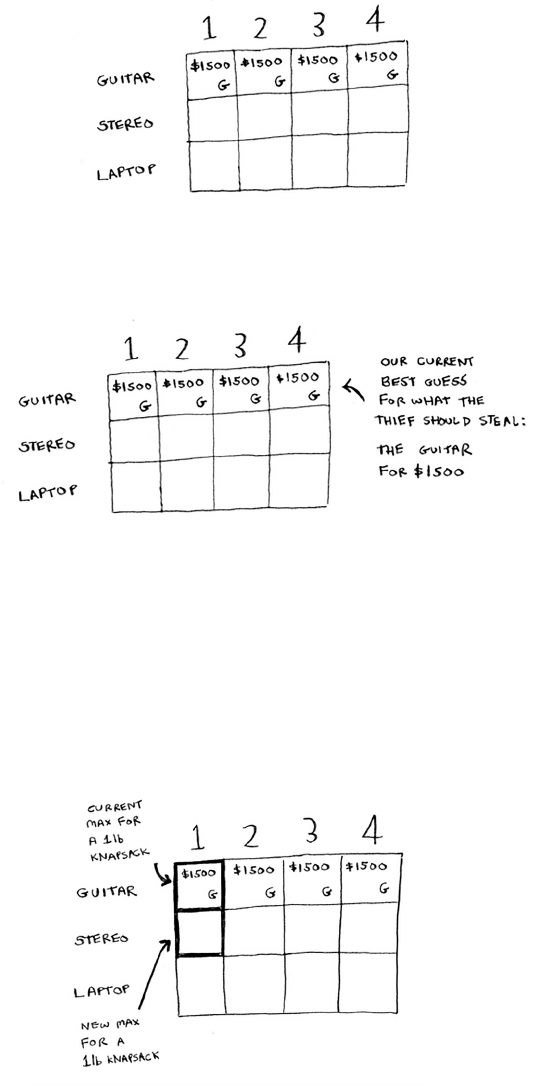
166 Chapter 9

I

Dynamic programming

At this point, your grid should look like this.

Remember, you’re trying to maximize the value of the knapsack.

is row represents the current best guess for this max. So right now,

according to this row, if you had a knapsack of capacity 4 lb, the max

value you could put in there would be $1,500.

You know that’s not the nal solution. As we go through the algorithm,

you’ll rene your estimate.

The stereo row

Let’s do the next row. is one is for the stereo. Now that you’re on the

second row, you can steal the stereo or the guitar. At every row, you can

steal the item at that row or the items in the rows above it. So you can’t

choose to steal the laptop right now, but you can steal the stereo and/or

the guitar. Let’s start with the rst cell, a knapsack of capacity 1 lb. e

current max value you can t into a knapsack of 1 lb is $1,500.

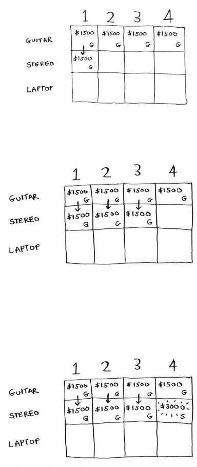
167The knapsack problem

Should you steal the stereo or not?

You have a knapsack of capacity 1 lb. Will the stereo t in there? Nope,

it’s too heavy! Because you can’t t the stereo, $1,500 remains the max

guess for a 1 lb knapsack.

Same thing for the next two cells. ese knapsacks have a capacity of

2 lb and 3 lb. e old max value for both was $1,500.

e stereo still doesn’t t, so your guesses remain unchanged.

What if you have a knapsack of capacity 4 lb? Aha: the stereo nally ts!

e old max value was $1,500, but if you put the stereo in there instead,

the value is $3,000! Let’s take the stereo.

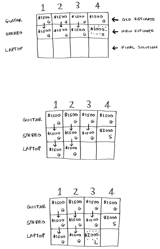
168 Chapter 9

I

Dynamic programming

You just updated your estimate! If you have a 4 lb knapsack, you can

t at least $3,000 worth of goods in it. You can see from the grid that

you’re incrementally updating your estimate.

The laptop row

Let’s do the same thing with the laptop! e laptop weighs 3 lb, so it

won’t t into a 1 lb or a 2 lb knapsack. e estimate for the rst two cells

stays at $1,500.

At 3 lb, the old estimate was $1,500. But you can choose the laptop

instead, and that’s worth $2,000. So the new max estimate is $2,000!

At 4 lb, things get really interesting. is is an important part. e

current estimate is $3,000. You can put the laptop in the knapsack, but

it’s only worth $2,000.

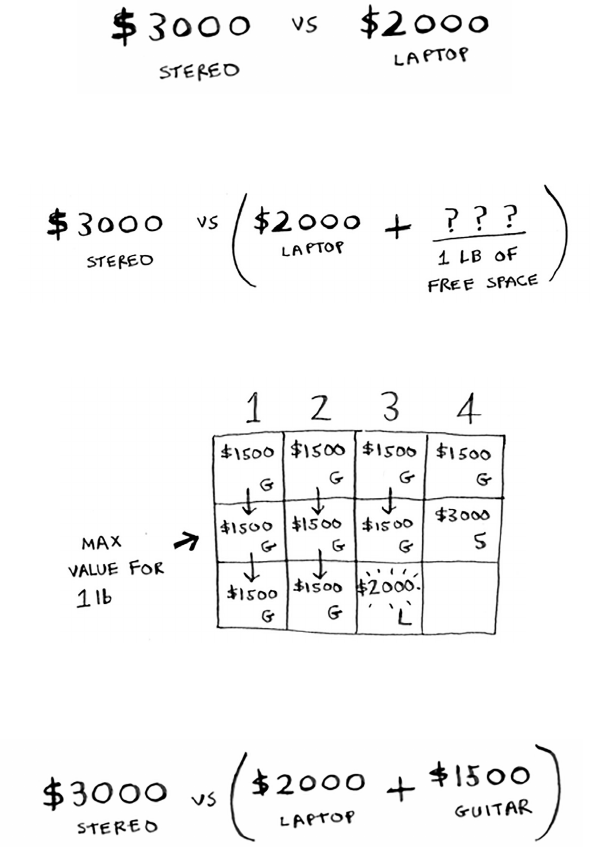
169The knapsack problem

Hmm, that’s not as good as the old estimate. But wait! e laptop

weighs only 3 lb, so you have 1 lb free! You could put something in

this 1 lb.

What’s the maximum value you can t into 1 lb of space? Well, you’ve

been calculating it all along.

According to the last best estimate, you can t the guitar into that 1 lb

space, and that’s worth $1,500. So the real comparison is as follows.

You might have been wondering why you were calculating max values

for smaller knapsacks. I hope now it makes sense! When you have

space le over, you can use the answers to those subproblems to gure

out what will t in that space. It’s better to take the laptop + the guitar

for $3,500.

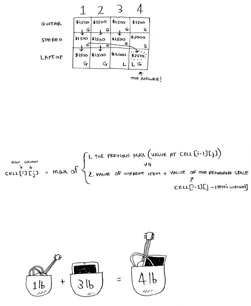
170 Chapter 9

I

Dynamic programming

e nal grid looks like this.

ere’s the answer: the maximum value that will t in the knapsack is

$3,500, made up of a guitar and a laptop!

Maybe you think that I used a dierent formula to calculate the value

of that last cell. at’s because I skipped some unnecessary complexity

when lling in the values of the earlier cells. Each cell’s value gets

calculated with the same formula. Here it is.

You can use this formula with every cell in this grid, and you should

end up with the same grid I did. Remember how I talked about solving

subproblems? You combined the solutions to two subproblems to solve

the bigger problem.

171Knapsack problem FAQ

Knapsack problem FAQ

Maybe this still feels like magic. is section answers some common

questions.

What happens if you add an item?

Suppose you realize there’s a fourth item you can steal that you didn’t

notice before! You can also steal an iPhone.

Do you have to recalculate everything to account for this new item?

Nope. Remember, dynamic programming keeps progressively

building on your estimate. So far, these are the max values.

at means for a 4 lb knapsack, you can steal $3,500 worth of goods.

You thought that was the nal max value. But let’s add a row for

the iPhone.

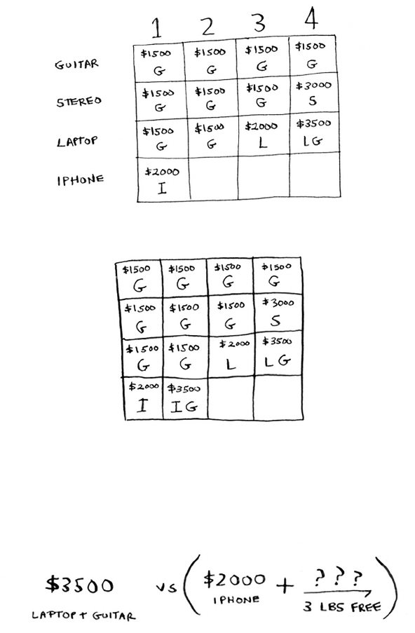
172 Chapter 9

I

Dynamic programming

Turns out you have a new max value! Try to ll in this new row before

reading on.

Let’s start with the rst cell. e iPhone ts into the 1 lb knapsack.

e old max was $1,500, but the iPhone is worth $2,000. Let’s take the

iPhone instead.

In the next cell, you can t the iPhone and the guitar.

For cell 3, you can’t do better than take the iPhone and the guitar again,

so leave it as is.

For the last cell, things get interesting. e current max is $3,500. You

can steal the iPhone instead, and you have 3 lb of space le over.

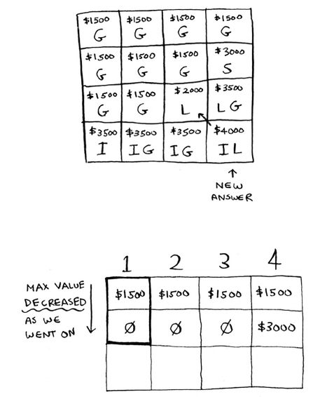
173Knapsack problem FAQ

ose 3 lb are worth $2,000! $2,000 from the iPhone + $2,000 from the

old subproblem: that’s $4,000. A new max!

Here’s the new nal grid.

Question: Would the value of a column ever go down? Is this possible?

ink of an answer before reading on.

Answer: No. At every iteration, you’re storing the current max estimate.

e estimate can never get worse than it was before!

EXERCISE

9.1 Suppose you can steal another item: an MP3 player. It weighs 1 lb

and is worth $1,000. Should you steal it?

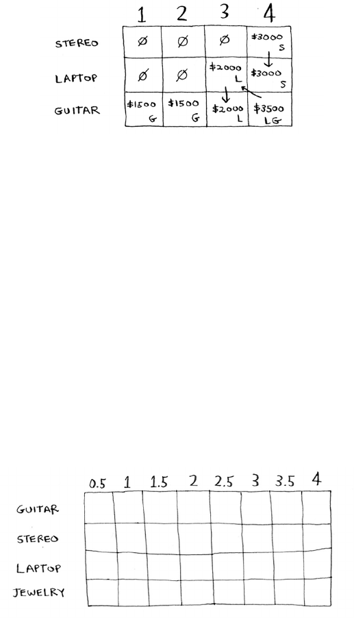
174 Chapter 9

I

Dynamic programming

What happens if you change the order of the rows?

Does the answer change? Suppose you ll the rows in this order: stereo,

laptop, guitar. What does the grid look like? Fill out the grid for yourself

before moving on.

Here’s what the grid looks like.

e answer doesn’t change. e order of the rows doesn’t matter.

Can you ll in the grid column-wise instead

of row-wise?

Try it for yourself! For this problem, it doesn’t make a dierence. It

could make a dierence for other problems.

What happens if you add a smaller item?

Suppose you can steal a necklace. It weighs 0.5 lb, and it’s worth $1,000.

So far, your grid assumes that all weights are integers. Now you decide

to steal the necklace. You have 3.5 lb le over. What’s the max value

you can t in 3.5 lb? You don’t know! You only calculated values for

1 lb, 2 lb, 3 lb, and 4 lb knapsacks. You need to know the value of a

3.5 lb knapsack.

Because of the necklace, you have to account for ner granularity, so the

grid has to change.

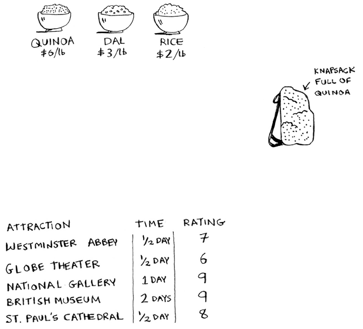
175Knapsack problem FAQ

Can you steal fractions of an item?

Suppose you’re a thief in a grocery store. You can steal bags of lentils

and rice. If a whole bag doesn’t t, you can open it and take as much as

you can carry. So now it’s not all or nothing—you can take a fraction of

an item. How do you handle this using dynamic programming?

Answer: You can’t. With the dynamic-programming solution, you

either take the item or not. ere’s no way for it to gure out that you

should take half an item.

But this case is also easily solved using a greedy algorithm! First, take as

much as you can of the most valuable item. When that runs out, take as

much as you can of the next most valuable item, and so on.

For example, suppose you have these items to choose from.

Quinoa is more expensive per pound than anything else. So, take all

the quinoa you can carry! If that lls your knapsack, that’s the best

you can do.

If the quinoa runs out and you still have space in your knapsack,

take the next most valuable item, and so on.

Optimizing your travel itinerary

Suppose you’re going to London for a nice vacation. You have two days

there and a lot of things you want to do. You can’t do everything, so you

make a list.

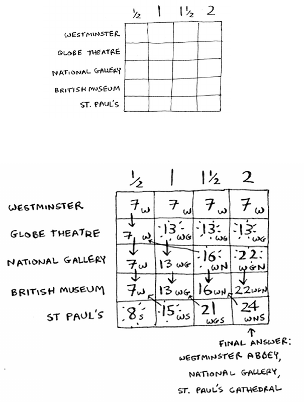
176 Chapter 9

I

Dynamic programming

For each thing you want to see, you write down how long it will take

and rate how much you want to see it. Can you gure out what you

should see, based on this list?

It’s the knapsack problem again! Instead of a knapsack, you have a

limited amount of time. And instead of stereos and laptops, you have a

list of places you want to go. Draw the dynamic-programming grid for

this list before moving on.

Here’s what the grid looks like.

Did you get it right? Fill in the grid. What places should you end up

seeing? Here’s the answer.

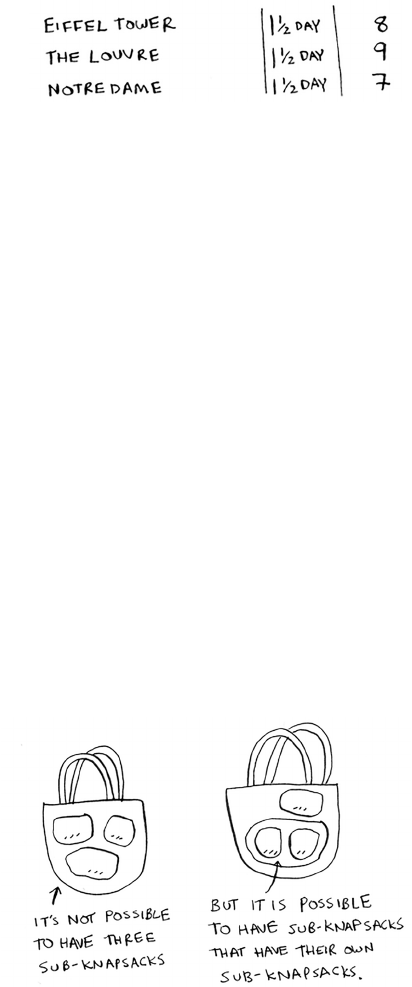
177Knapsack problem FAQ

Handling items that depend on each other

Suppose you want to go to Paris, so you add a couple of items on

the list.

ese places take a lot of time, because rst you have to travel from

London to Paris. at takes half a day. If you want to do all three items,

it will take four and a half days.

Wait, that’s not right. You don’t have to travel to Paris for each item.

Once you’re in Paris, each item should only take a day. So it should be

one day per item + half a day of travel = 3.5 days, not 4.5 days.

If you put the Eiel Tower in your knapsack, then the Louvre becomes

“cheaper”—it will only cost you a day instead of 1.5 days. How do you

model this in dynamic programming?

You can’t. Dynamic programming is powerful because it can solve

subproblems and use those answers to solve the big problem. Dynamic

programming only works when each subproblem is discrete—when it

doesn’t depend on other subproblems. at means there’s no way to

account for Paris using the dynamic-programming algorithm.

Is it possible that the solution will require

more than two sub-knapsacks?

It’s possible that the best solution involves stealing more than two items.

e way the algorithm is set up, you’re combining two knapsacks at

most—you’ll never have more than two sub-knapsacks. But it’s possible

for those sub-knapsacks to have their own sub-knapsacks.

178 Chapter 9

I

Dynamic programming

Is it possible that the best solution doesn’t

ll the knapsack completely?

Yes. Suppose you could also steal a diamond.

is is a big diamond: it weighs 3.5 pounds. It’s worth a million

dollars, way more than anything else. You should denitely steal it!

But there’s half a pound of space le, and nothing will t in

that space.

EXERCISE

9.2 Suppose you’re going camping. You have a knapsack that will hold

6 lb, and you can take the following items. Each has a value, and the

higher the value, the more important the item is:

• Water, 3 lb, 10

• Book, 1 lb, 3

• Food, 2 lb, 9

• Jacket, 2 lb, 5

• Camera, 1 lb, 6

What’s the optimal set of items to take on your camping trip?

Longest common substring

You’ve seen one dynamic programming problem so far. What are

the takeaways?

• Dynamic programming is useful when you’re trying to optimize

something given a constraint. In the knapsack problem, you had to

maximize the value of the goods you stole, constrained by the size of

the knapsack.

• You can use dynamic programming when the problem can be broken

into discrete subproblems, and they don’t depend on each other.

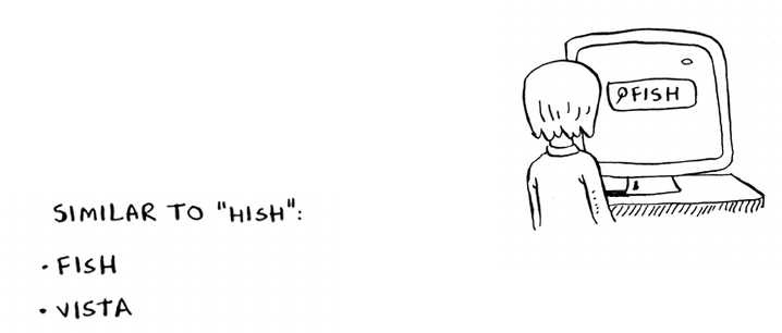
179Longest common substring

It can be hard to come up with a dynamic-programming solution. at’s

what we’ll focus on in this section. Some general tips follow:

• Every dynamic-programming solution involves a grid.

• e values in the cells are usually what you’re trying to optimize.

For the knapsack problem, the values were the value of the goods.

• Each cell is a subproblem, so think about how you can divide

your problem into subproblems. at will help you gure out what

the axes are.

Let’s look at another example. Suppose you run dictionary.com.

Someone types in a word, and you give them the denition.

But if someone misspells a word, you want to be able to guess

what word they meant. Alex is searching for sh, but he

accidentally put in hish. at’s not a word in your dictionary,

but you have a list of words that are similar.

(is is a toy example, so you’ll limit your list to two words. In reality,

this list would probably be thousands of words.)

Alex typed hish. Which word did Alex mean to type: sh or vista?

Making the grid

What does the grid for this problem look like? You need to answer these

questions:

• What are the values of the cells?

• How do you divide this problem into subproblems?

• What are the axes of the grid?

In dynamic programming, you’re trying to maximize something. In this

case, you’re trying to nd the longest substring that two words have in

common. What substring do hish and sh have in common? How about

hish and vista? at’s what you want to calculate.

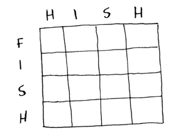
180 Chapter 9

I

Dynamic programming

Remember, the values for the cells are usually what you’re trying to

optimize. In this case, the values will probably be a number: the length

of the longest substring that the two strings have in common.

How do you divide this problem into subproblems? You could compare

substrings. Instead of comparing hish and sh, you could compare his

and s rst. Each cell will contain the length of the longest substring

that two substrings have in common. is also gives you a clue that the

axes will probably be the two words. So the grid probably looks like this.

If this seems like black magic to you, don’t worry. is is hard stu—

that’s why I’m teaching it so late in the book! Later, I’ll give you an

exercise so you can practice dynamic programming yourself.

Filling in the grid

Now you have a good idea of what the grid should look like. What’s the

formula for lling in each cell of the grid? You can cheat a little, because

you already know what the solution should be—hish and sh have a

substring of length 3 in common: ish.

But that still doesn’t tell you the formula to use. Computer scientists

sometimes joke about using the Feynman algorithm. e Feynman

algorithm is named aer the famous physicist Richard Feynman, and

it works like this:

1. Write down the problem.

2. ink real hard.

3. Write down the solution.

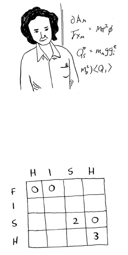
181Longest common substring

Computer scientists are a fun bunch!

e truth is, there’s no easy way to calculate the formula here. You

have to experiment and try to nd something that works. Sometimes

algorithms aren’t an exact recipe. ey’re a framework that you build

your idea on top of.

Try to come up with a solution to this problem yourself. I’ll give you a

hint—part of the grid looks like this.

What are the other values? Remember that each cell is the value of a

subproblem. Why does cell (3, 3) have a value of 2? Why does cell (3, 4)

have a value of 0?

Read on aer you’ve tried to come up with a formula yourself. Even if

you don’t get it right, my explanation will make a lot more sense.

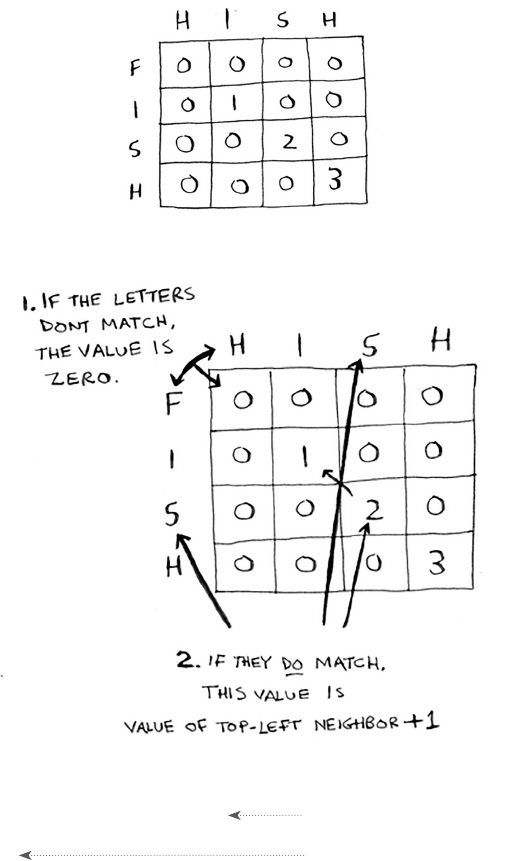
182 Chapter 9

I

Dynamic programming

The solution

Here’s the nal grid.

Here’s my formula for lling in each cell.

Here’s how the formula looks in pseudocode:

if word_a[i] == word_b[j]: The letters match.

c e l l[i][j] = c e l l[i-1][j-1] + 1

else: The letters don’t match.

cell[i][j] = 0

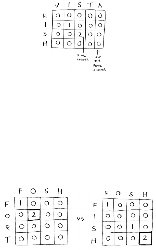
183Longest common substring

Here’s the grid for hish vs. vista.

One thing to note: for this problem, the nal solution may not be in

the last cell! For the knapsack problem, this last cell always had the

nal solution. But for the longest common substring, the solution is the

largest number in the grid—and it may not be the last cell.

Let’s go back to the original question: which string has more in

common with hish? hish and sh have a substring of three letters in

common. hish and vista have a substring of two letters in common.

Alex probably meant to type sh.

Longest common subsequence

Suppose Alex accidentally searched for fosh. Which word did he mean:

sh or fort?

Let’s compare them using the longest-common-substring formula.

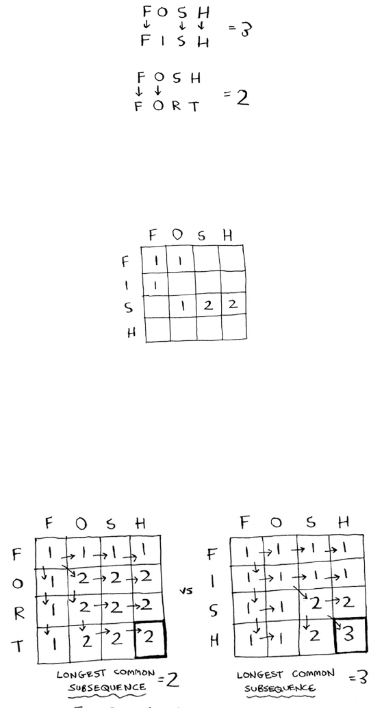
184 Chapter 9

I

Dynamic programming

ey’re both the same: two letters! But fosh is closer to sh.

You’re comparing the longest common substring, but you really need

to compare the longest common subsequence: the number of letters in

a sequence that the two words have in common. How do you calculate

the longest common subsequence?

Here’s the partial grid for sh and fosh.

Can you gure out the formula for this grid? e longest common

subsequence is very similar to the longest common substring, and

the formulas are pretty similar, too. Try to solve it yourself—I give the

answer next.

Longest common subsequence—solution

Here’s the nal grid.

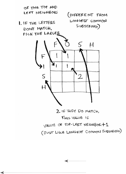
185Longest common substring

Here’s my formula for lling in each cell.

And here it is in pseudocode:

if word_a[i] == word_b[j]: The letters match.

c e l l[i][j] = c e l l[i-1][j-1] + 1

else: The letters don’t match.

c e l l[i][j] = m a x(c e l l[i-1][j], c e l l[i][j-1])

Whew—you did it! is is denitely one of the toughest chapters in the

book. So is dynamic programming ever really used? Yes:

• Biologists use the longest common subsequence to nd similarities

in DNA strands. ey can use this to tell how similar two animals or

two diseases are. e longest common subsequence is being used to

nd a cure for multiple sclerosis.

• Have you ever used di (like

git diff

)? Di tells you the dierences

between two les, and it uses dynamic programming to do so.

• We talked about string similarity. Levenshtein distance measures

how similar two strings are, and it uses dynamic programming.

Levenshtein distance is used for everything from spell-check to

guring out whether a user is uploading copyrighted data.

186 Chapter 9

I

Dynamic programming

• Have you ever used an app that does word wrap, like Microso Word?

How does it gure out where to wrap so that the line length stays

consistent? Dynamic programming!

EXERCISE

9.3 Draw and ll in the grid to calculate the longest common substring

between blue and clues.

Recap

• Dynamic programming is useful when you’re trying to optimize

something given a constraint.

• You can use dynamic programming when the problem can be

broken into discrete subproblems.

• Every dynamic-programming solution involves a grid.

• e values in the cells are usually what you’re trying to optimize.

• Each cell is a subproblem, so think about how you can divide your

problem into subproblems.

• ere’s no single formula for calculating a dynamic-programming

solution.

187

In this chapter

• You learn to build a classication system using

the k-nearest neighbors algorithm.

• You learn about feature extraction.

• You learn about regression: predicting a number,

like the value of a stock tomorrow, or how much

a user will enjoy a movie.

• You learn about the use cases and limitations

of k-nearest neighbors.

k-nearest

neighbors 10

Classifying oranges vs. grapefruit

Look at this fruit. Is it an orange or a grapefruit?

Well, I know that grapefruits are generally bigger

and redder.

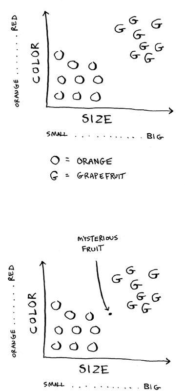
188 Chapter 10

I

k-nearest neighbors

My thought process is something like this: I have a graph in my mind.

Generally speaking, the bigger, redder fruit are grapefruits. is fruit

is big and red, so it’s probably a grapefruit. But what if you get a fruit

like this?

How would you classify this fruit? One way is to look at the neighbors of

this spot. Take a look at the three closest neighbors of this spot.

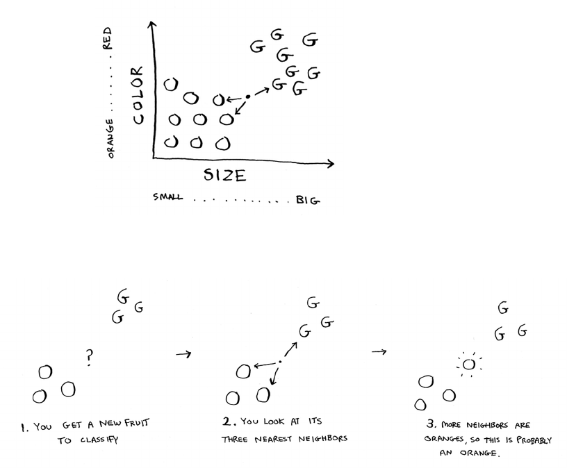
189Building a recommendations system

More neighbors are oranges than grapefruit. So this fruit is probably an

orange. Congratulations: You just used the k-nearest neighbors (KNN)

algorithm for classication! e whole algorithm is pretty simple.

e KNN algorithm is simple but useful! If you’re trying to classify

something, you might want to try KNN rst. Let’s look at a more

real-world example.

Building a recommendations system

Suppose you’re Netix, and you want to build a movie

recommendations system for your users. On a high level, this

is similar to the grapefruit problem!

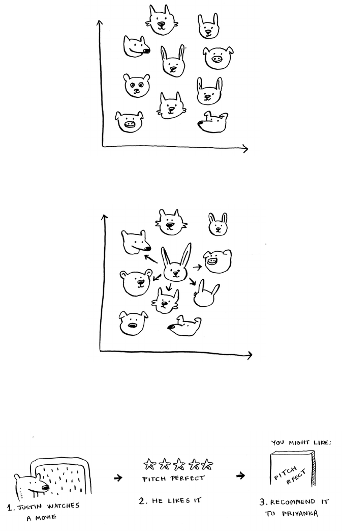
190 Chapter 10

I

k-nearest neighbors

You can plot every user on a graph.

ese users are plotted by similarity, so users with similar taste are

plotted closer together. Suppose you want to recommend movies for

Priyanka. Find the ve users closest to her.

Justin, JC, Joey, Lance, and Chris all have similar taste in movies. So

whatever movies they like, Priyanka will probably like too!

Once you have this graph, building a recommendations system is easy.

If Justin likes a movie, recommend it to Priyanka.

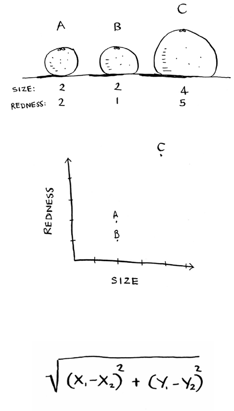
191Building a recommendations system

But there’s still a big piece missing. You graphed the users by similarity.

How do you gure out how similar two users are?

Feature extraction

In the grapefruit example, you compared fruit based on how

big they are and how red they are. Size and color are the features

you’re comparing. Now suppose you have three fruit. You can extract

the features.

en you can graph the three fruit.

From the graph, you can tell visually that fruits A and B are similar.

Let’s measure how close they are. To nd the distance between two

points, you use the Pythagorean formula.

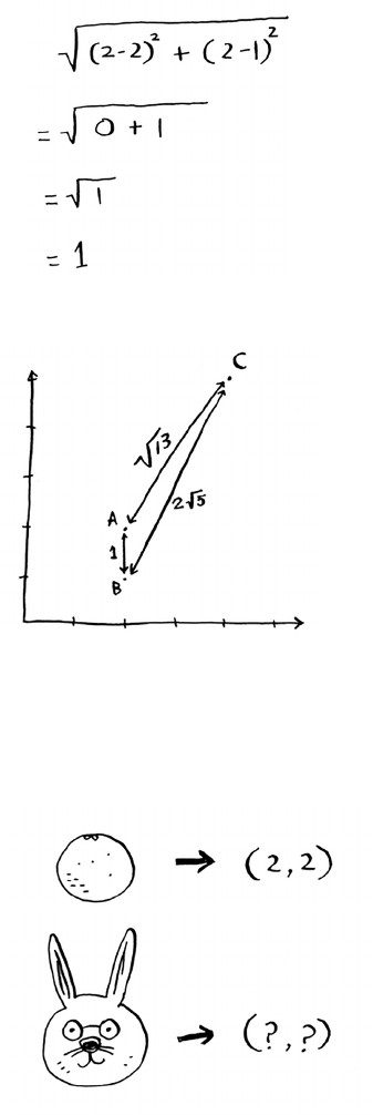
192 Chapter 10

I

k-nearest neighbors

Here’s the distance between A and B, for example.

e distance between A and B is 1. You can nd the rest of the

distances, too.

e distance formula conrms what you saw visually: fruits A and B

are similar.

Suppose you’re comparing Netix users, instead. You need some

way to graph the users. So, you need to convert each user to a set of

coordinates, just as you did for fruit.

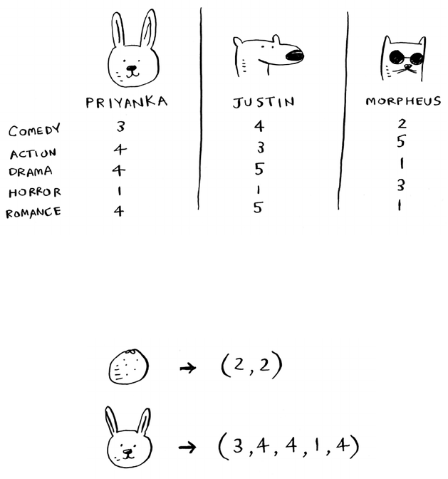
193Building a recommendations system

Once you can graph users, you can measure the distance between them.

Here’s how you can convert users into a set of numbers. When users

sign up for Netix, have them rate some categories of movies based on

how much they like those categories. For each user, you now have a set

of ratings!

Priyanka and Justin like Romance and hate Horror. Morpheus likes

Action but hates Romance (he hates when a good action movie gets

ruined by a cheesy romantic scene). Remember how in oranges versus

grapefruit, each fruit was represented by a set of two numbers? Here,

each user is represented by a set of ve numbers.

A mathematician would say, instead of calculating the distance in two

dimensions, you’re now calculating the distance in ve dimensions. But

the distance formula remains the same.

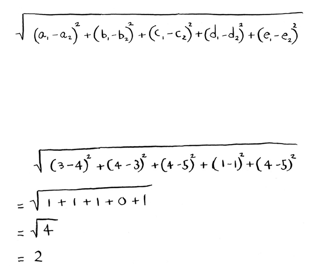
194 Chapter 10

I

K-nearest neighbors

It just involves a set of ve numbers instead of a set of two numbers.

e distance formula is exible: you could have a set of a million

numbers and still use the same old distance formula to nd the

distance. Maybe you’re wondering, “What does distance mean when

you have ve numbers?” e distance tells you how similar those sets of

numbers are.

Here’s the distance between Priyanka and Justin.

Priyanka and Justin are pretty similar. What’s the dierence between

Priyanka and Morpheus? Calculate the distance before moving on.

Did you get it right? Priyanka and Morpheus are 24 apart. e distance

tells you that Priyanka’s tastes are more like Justin’s than Morpheus’s.

Great! Now recommending movies to Priyanka is easy: if Justin likes a

movie, recommend it to Priyanka, and vice versa. You just built a movie

recommendations system!

If you’re a Netix user, Netix will keep telling you, “Please rate more

movies. e more movies you rate, the better your recommendations

will be.” Now you know why. e more movies you rate, the more

accurately Netix can see what other users you’re similar to.

195Building a recommendations system

EXERCISES

10.1 In the Netix example, you calculated the distance between two

dierent users using the distance formula. But not all users rate

movies the same way. Suppose you have two users, Yogi and Pinky,

who have the same taste in movies. But Yogi rates any movie he

likes as a 5, whereas Pinky is choosier and reserves the 5s for

only the best. ey’re well matched, but according to the distance

algorithm, they aren’t neighbors. How would you take their

dierent rating strategies into account?

10.2 Suppose Netix nominates a group of “inuencers.” For example,

Quentin Tarantino and Wes Anderson are inuencers on Netix,

so their ratings count for more than a normal user’s. How would

you change the recommendations system so it’s biased toward the

ratings of inuencers?

Regression

Suppose you want to do more than just recommend a movie: you want

to guess how Priyanka will rate this movie. Take the ve people closest

to her.

By the way, I keep talking about the closest ve people. ere’s nothing

special about the number 5: you could do the closest 2, or 10, or 10,000.

at’s why the algorithm is called k-nearest neighbors and not ve-

nearest neighbors!

Suppose you’re trying to guess a rating for Pitch Perfect. Well, how did

Justin, JC, Joey, Lance, and Chris rate it?

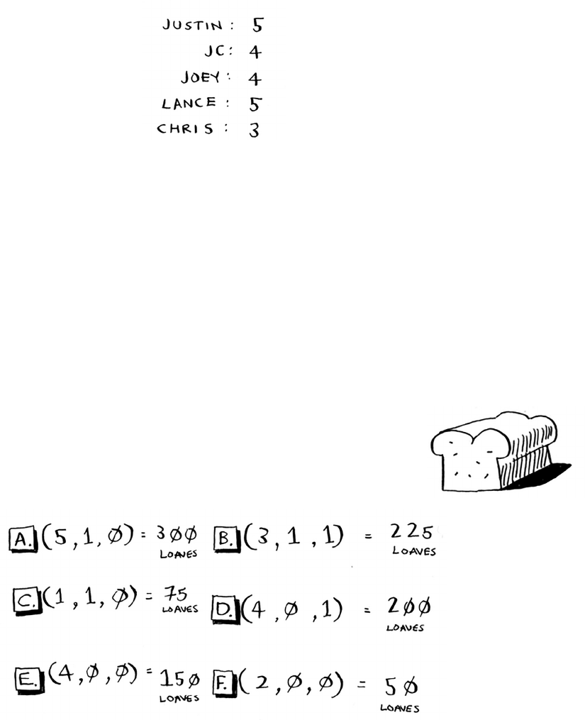
196 Chapter 10

I

k-nearest neighbors

You could take the average of their ratings and get 4.2 stars.

at’s called regression. ese are the two basic things you’ll do

with KNN—classication and regression:

• Classication = categorization into a group

• Regression = predicting a response (like a number)

Regression is very useful. Suppose you run a small bakery in Berkeley,

and you make fresh bread every day. You’re trying to predict how many

loaves to make for today. You have a set of features:

• Weather on a scale of 1 to 5 (1 = bad, 5 = great).

• Weekend or holiday? (1 if it’s a weekend or a holiday, 0 otherwise.)

• Is there a game on? (1 if yes, 0 if no.)

And you know how many loaves of bread you’ve sold in the

past for dierent sets of features.

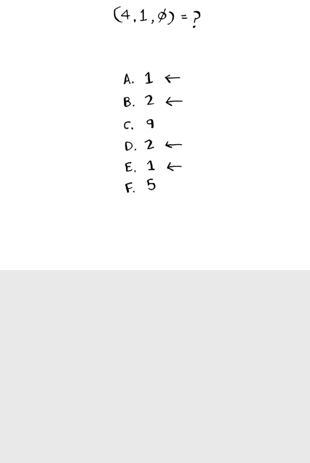
197Building a recommendations system

Today is a weekend day with good weather. Based on the data you just

saw, how many loaves will you sell? Let’s use KNN, where K = 4. First,

gure out the four nearest neighbors for this point.

Here are the distances. A, B, D, and E are the closest.

Take an average of the loaves sold on those days, and you get 218.75.

at’s how many loaves you should make for today!

Cosine similarity

So far, you’ve been using the distance formula to compare the distance

between two users. Is this the best formula to use? A common one used

in practice is cosine similarity. Suppose two users are similar, but one of

them is more conservative in their ratings. ey both loved Manmohan

Desai’s Amar Akbar Anthony. Paul rated it 5 stars, but Rowan rated it 4

stars. If you keep using the distance formula, these two users might not be

each other’s neighbors, even though they have similar taste.

Cosine similarity doesn’t measure the distance between two vectors.

Instead, it compares the angles of the two vectors. It’s better at dealing

with cases like this. Cosine similarity is out of the scope of this book, but

look it up if you use KNN!

198 Chapter 10

I

k-nearest neighbors

Picking good features

To gure out recommendations, you had users rate

categories of movies. What if you had them rate pictures

of cats instead? en you’d nd users who rated those

pictures similarly. is would probably be a worse recommendations

engine, because the “features” don’t have a lot to do with taste in

movies!

Or suppose you ask users to rate movies so you can give them

recommendations—but you only ask them to rate Toy Story, Toy Story

2, and Toy Story 3. is won’t tell you a lot about the users’ movie tastes!

When you’re working with KNN, it’s really important to pick the right

features to compare against. Picking the right features means

• Features that directly correlate to the movies you’re trying to

recommend

• Features that don’t have a bias (for example, if you ask the users to

only rate comedy movies, that doesn’t tell you whether they like

action movies)

Do you think ratings are a good way to recommend movies? Maybe I

rated e Wire more highly than House Hunters, but I actually spend

more time watching House Hunters. How would you improve this

Netix recommendations system?

Going back to the bakery: can you think of two good and two bad

features you could have picked for the bakery? Maybe you need to make

more loaves aer you advertise in the paper. Or maybe you need to

make more loaves on Mondays.

ere’s no one right answer when it comes to picking good features. You

have to think about all the dierent things you need to consider.

EXERCISE

10.3 Netix has millions of users. e earlier example looked at the ve

closest neighbors for building the recommendations system. Is this

too low? Too high?

199Introduction to machine learning

Introduction to machine learning

KNN is a really useful algorithm, and it’s your introduction to

the magical world of machine learning! Machine learning is all

about making your computer more intelligent. You already saw

one example of machine learning: building a recommendations

system. Let’s look at some other examples.

OCR

OCR stands for optical character recognition. It means you can take a

photo of a page of text, and your computer will automatically read the

text for you. Google uses OCR to digitize books. How does OCR work?

For example, consider this number.

How would you automatically gure out what number this is? You can

use KNN for this:

1. Go through a lot of images of numbers, and extract features of those

numbers.

2. When you get a new image, extract the features of that image, and

see what its nearest neighbors are!

It’s the same problem as oranges versus grapefruit. Generally speaking,

OCR algorithms measure lines, points, and curves.

en, when you get a new character, you can extract the same features

from it.

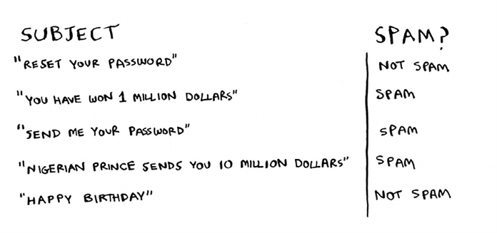
200 Chapter 10

I

k-nearest neighbors

Feature extraction is a lot more complicated in OCR than the

fruit example. But it’s important to understand that even complex

technologies build on simple ideas, like KNN. You could use the same

ideas for speech recognition or face recognition. When you upload a

photo to Facebook, sometimes it’s smart enough to tag people in the

photo automatically. at’s machine learning in action!

e rst step of OCR, where you go through images of numbers and

extract features, is called training. Most machine-learning algorithms

have a training step: before your computer can do the task, it must

be trained. e next example involves spam lters, and it has a

training step.

Building a spam lter

Spam lters use another simple algorithm called the Naive Bayes

classier. First, you train your Naive Bayes classier on some data.

Suppose you get an email with the subject “collect your million dollars

now!” Is it spam? You can break this sentence into words. en, for

each word, see what the probability is for that word to show up in a

spam email. For example, in this very simple model, the word million

only appears in spam emails. Naive Bayes gures out the probability

that something is likely to be spam. It has applications similar to KNN.

201Introduction to machine learning

For example, you could use Naive Bayes to categorize fruit: you have

a fruit that’s big and red. What’s the probability that it’s a grapefruit?

It’s another simple algorithm that’s fairly eective. We love those

algorithms!

Predicting the stock market

Here’s something that’s hard to do with machine learning: really

predicting whether the stock market will go up or down. How do

you pick good features in a stock market? Suppose you say that if the

stock went up yesterday, it will go up today. Is that a good feature? Or

suppose you say that the stock will always go down in May. Will that

work? ere’s no guaranteed way to use past numbers to predict future

performance. Predicting the future is hard, and it’s almost impossible

when there are so many variables involved.

Recap

I hope this gives you an idea of all the dierent things you can do with

KNN and with machine learning! Machine learning is an interesting

eld that you can go pretty deep into if you decide to:

• KNN is used for classication and regression and involves looking

at the k-nearest neighbors.

• Classication = categorization into a group.

• Regression = predicting a response (like a number).

202 Chapter 10

I

k-nearest neighbors

• Feature extraction means converting an item (like a fruit or a user)

into a list of numbers that can be compared.

• Picking good features is an important part of a successful KNN

algorithm.

203

In this chapter

• You get a brief overview of 10 algorithms

that weren’t covered in this book, and why

they’re useful.

• You get pointers on what to read next,

depending on what your interests are.

where to

go next 11

Trees

Let’s go back to the binary search example.

When a user logs in to Facebook, Facebook

has to look through a big array to see if the

username exists. We said the fastest way to

search through this array is to run binary

search. But there’s a problem: every time a new

user signs up, you insert their username into

the array. en you have to re-sort the array,

because binary search only works with sorted

arrays. Wouldn’t it be nice if you could insert

204 Chapter 11

I

Where to go next

the username into the right slot in the array right away, so you don’t

have to sort the array aerward? at’s the idea behind the binary search

tree data structure.

A binary search tree looks like this.

For every node, the nodes to its le are smaller in value, and the nodes

to the right are larger in value.

Suppose you’re searching for Maggie. You start at the root node.

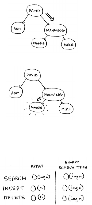
205Trees

Maggie comes aer David, so go toward the right.

Maggie comes before Manning, so go to the le.

You found Maggie! It’s almost like running a binary search! Searching

for an element in a binary search tree takes O(log n) time on average

and O(n) time in the worst case. Searching a sorted array takes O(log n)

time in the worst case, so you might think a sorted array is better. But a

binary search tree is a lot faster for insertions and deletions on average.

Binary search trees have some downsides too: for one thing, you

don’t get random access. You can’t say, “Give me the h element of

this tree.” ose performance times are also on average and rely on

the tree being balanced. Suppose you have an imbalanced tree like the

one shown next.

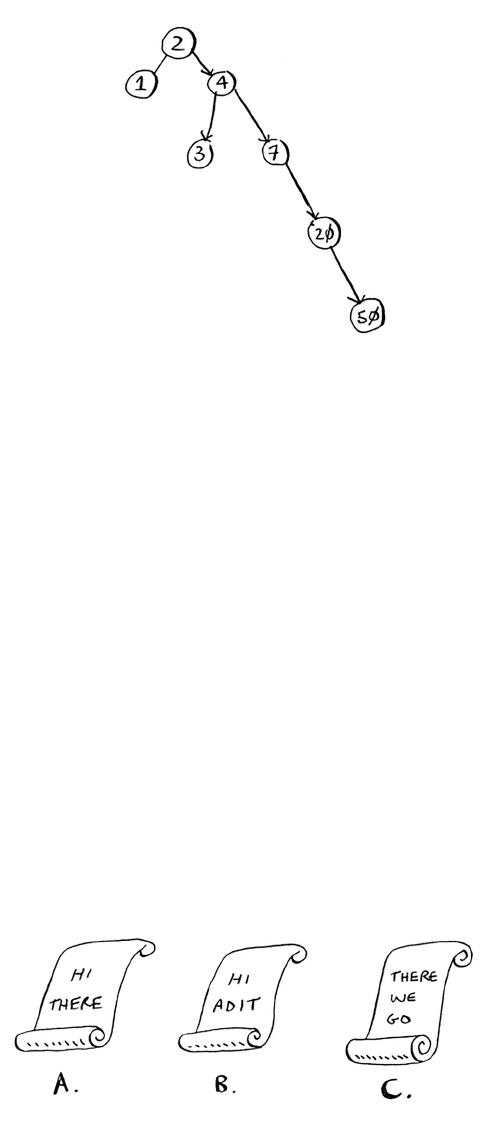
206 Chapter 11

I

Where to go next

See how it’s leaning to the right? is tree doesn’t have very good

performance, because it isn’t balanced. ere are special binary search

trees that balance themselves. One example is the red-black tree.

So when are binary search trees used? B-trees, a special type of binary

tree, are commonly used to store data in databases.

If you’re interested in databases or more-advanced data structures,

check these out:

• B-trees

• Red-black trees

• Heaps

• Splay trees

Inverted indexes

Here’s a very simplied version of how a search engine works. Suppose

you have three web pages with this simple content.

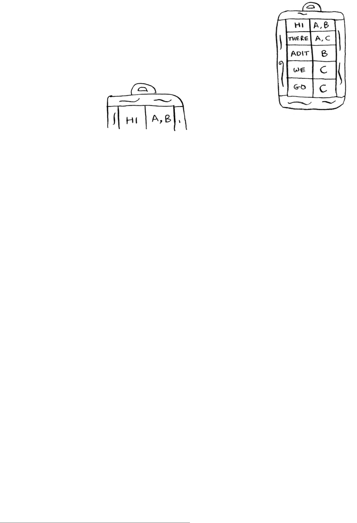
207The Fourier transform

Let’s build a hash table from this content.

e keys of the hash table are the words, and the values tell

you what pages each word appears on. Now suppose a user

searches for hi. Let’s see what pages hi shows up on.

Aha: It appears on pages A and B. Let’s show the user those pages as

the result. Or suppose the user searches for there. Well, you know that

it shows up on pages A and C. Pretty easy, huh? is is a useful data

structure: a hash that maps words to places where they appear. is

data structure is called an inverted index, and it’s commonly used to

build search engines. If you’re interested in search, this is a good place

to start.

The Fourier transform

e Fourier transform is one of those rare algorithms: brilliant,

elegant, and with a million use cases. e best analogy for the Fourier

transform comes from Better Explained (a great website that explains

math simply): given a smoothie, the Fourier transform will tell you the

ingredients in the smoothie.1 Or, to put it another way, given a song, the

transform can separate it into individual frequencies.

It turns out that this simple idea has a lot of use cases. For example, if

you can separate a song into frequencies, you can boost the ones you

care about. You could boost the bass and hide the treble. e Fourier

transform is great for processing signals. You can also use it to compress

music. First you break an audio le down into its ingredient notes. e

Fourier transform tells you exactly how much each note contributes

to the overall song. So you can just get rid of the notes that aren’t

important. at’s how the MP3 format works!

Music isn’t the only type of digital signal. e JPG format is another

compressed format, and it works the same way. People use the Fourier

transform to try to predict upcoming earthquakes and analyze DNA.

1 Kalid, “An Interactive Guide to the Fourier Transform,” Better Explained, http://mng.bx/874X.

208 Chapter 11

I

Where to go next

You can use it to build an app like Shazam, which guesses what song is

playing. e Fourier transform has a lot of uses. Chances are high that

you’ll run into it!

Parallel algorithms

e next three topics are about scalability and working with a lot of

data. Back in the day, computers kept getting faster and faster. If you

wanted to make your algorithm faster, you could wait a few months,

and the computers themselves would become faster. But we’re near the

end of that period. Instead, laptops and computers ship with multiple

cores. To make your algorithms faster, you need to change them to run

in parallel across all the cores at once!

Here’s a simple example. e best you can do with a sorting algorithm is

roughly O(n log n). It’s well known that you can’t sort an array in O(n)

time—unless you use a parallel algorithm! ere’s a parallel version of

quicksort that will sort an array in O(n) time.

Parallel algorithms are hard to design. And it’s also hard to make sure

they work correctly and to gure out what type of speed boost you’ll

see. One thing is for sure—the time gains aren’t linear. So if you have

two cores in your laptop instead of one, that almost never means your

algorithm will magically run twice as fast. ere are a couple of reasons

for this:

• Overhead of managing the parallelism—Suppose you have to sort

an array of 1,000 items. How do you divide this task among the two

cores? Do you give each core 500 items to sort and then merge the

two sorted arrays into one big sorted array? Merging the two arrays

takes time.

• Load balancing—Suppose you have 10 tasks to do, so you give each

core 5 tasks. But core A gets all the easy tasks, so it’s done in 10

seconds, whereas core B gets all the hard tasks, so it takes a minute.

at means core A was sitting idle for 50 seconds while core B was

doing all the work! How do you distribute the work evenly so both

cores are working equally hard?

If you’re interested in the theoretical side of performance and scalability,

parallel algorithms might be for you!

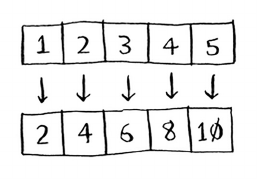
209MapReduce

MapReduce

ere’s a special type of parallel algorithm that is becoming increasingly

popular: the distributed algorithm. It’s ne to run a parallel algorithm

on your laptop if you need two to four cores, but what if you need

hundreds of cores? en you can write your algorithm to run across

multiple machines. e MapReduce algorithm is a popular distributed

algorithm. You can use it through the popular open source tool

Apache Hadoop.

Why are distributed algorithms useful?

Suppose you have a table with billions or trillions of rows, and you

want to run a complicated SQL query on it. You can’t run it on MySQL,

because it struggles aer a few billion rows. Use MapReduce through

Hadoop!

Or suppose you have to process a long list of jobs. Each job takes 10

seconds to process, and you need to process 1 million jobs like this. If

you do this on one machine, it will take you months! If you could run it

across 100 machines, you might be done in a few days.

Distributed algorithms are great when you have a lot of work to do

and want to speed up the time required to do it. MapReduce in

particular is built up from two simple ideas: the

map

function and the

reduce

function.

The map function

e

map

function is simple: it takes an array and applies the same

function to each item in the array. For example, here we’re doubling

every item in the array:

>>> arr1 = [1, 2, 3, 4, 5]

>>> arr2 = map(lambda x: 2 * x, arr1)

[2, 4, 6, 8, 10]

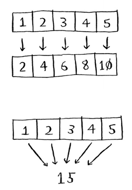
210 Chapter 11

I

Where to go next

arr2

now contains

[2, 4, 6, 8, 10]

—every element in

ar r1

was

doubled! Doubling an element is pretty fast. But suppose you apply a

function that takes more time to process. Look at this pseudocode:

>>> arr1 = # A list of URLs

>>> arr2 = map(download_page, arr1)

Here you have a list of URLs, and you want to download each page and

store the contents in

arr2

. is could take a couple of seconds for each

URL. If you had 1,000 URLs, this might take a couple of hours!

Wouldn’t it be great if you had 100 machines, and

map

could

automatically spread out the work across all of them? en you would

be downloading 100 pages at a time, and the work would go a lot faster!

is is the idea behind the “map” in MapReduce.

The reduce function

e

reduce

function confuses people sometimes. e idea is that you

“reduce” a whole list of items down to one item. With

map

, you go from

one array to another.

With

reduce

, you transform an array to a single item.

Here’s an example:

>>> arr1 = [1, 2, 3, 4, 5]

>>> reduce(lambda x,y: x+y, arr1)

15

211Bloom lters and HyperLogLog

In this case, you sum up all the elements in the array:

1 + 2 + 3 + 4

+ 5 = 15

! I won’t explain

reduce

in more detail here, because there are

plenty of tutorials online.

MapReduce uses these two simple concepts to run queries about data

across multiple machines. When you have a large dataset (billions

of rows), MapReduce can give you an answer in minutes where a

traditional database might take hours.

Bloom lters and HyperLogLog

Suppose you’re running Reddit. When someone posts a link, you want

to see if it’s been posted before. Stories that haven’t been posted before

are considered more valuable. So you need to gure out whether this

link has been posted before.

Or suppose you’re Google, and you’re crawling web pages. You only

want to crawl a web page if you haven’t crawled it already. So you need

to gure out whether this page has been crawled before.

Or suppose you’re running bit.ly, which is a URL shortener. You don’t

want to redirect users to malicious websites. You have a set of URLs that

are considered malicious. Now you need to gure out whether you’re

redirecting the user to a URL in that set.

All of these examples have the same problem. You have a very large set.

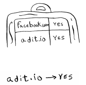
212 Chapter 11

I

Where to go next

Now you have a new item, and you want to see whether it belongs in

that set. You could do this quickly with a hash. For example, suppose

Google has a big hash in which the keys are all the pages it has crawled.

You want to see whether you’ve already crawled adit.io. Look it up in

the hash.

a d it.io

is a key in the hash, so you’ve already crawled it. e average

lookup time for hash tables is O(1).

a d it.io

is in the hash, so you’ve

already crawled it. You found that out in constant time. Pretty good!

Except that this hash needs to be huge. Google indexes trillions of web

pages. If this hash has all the URLs that Google has indexed, it will take

up a lot of space. Reddit and bit.ly have the same space problem. When

you have so much data, you need to get creative!

Bloom lters

Bloom lters oer a solution. Bloom lters are probabilistic data

structures. ey give you an answer that could be wrong but is probably

correct. Instead of a hash, you can ask your bloom lter if you’ve

crawled this URL before. A hash table would give you an accurate

answer. A bloom lter will give you an answer that’s probably correct:

• False positives are possible. Google might say, “You’ve already crawled

this site,” even though you haven’t.

• False negatives aren’t possible. If the bloom lter says, “You haven’t

crawled this site,” then you denitely haven’t crawled this site.

Bloom lters are great because they take up very little space. A hash

table would have to store every URL crawled by Google, but a bloom

lter doesn’t have to do that. ey’re great when you don’t need an exact

answer, as in all of these examples. It’s okay for bit.ly to say, “We think

this site might be malicious, so be extra careful.”

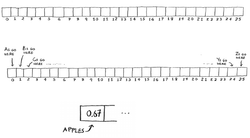
213The SHA algorithms

HyperLogLog

Along the same lines is another algorithm called HyperLogLog.

Suppose Google wants to count the number of unique searches

performed by its users. Or suppose Amazon wants to count the number

of unique items that users looked at today. Answering these questions

takes a lot of space! With Google, you’d have to keep a log of all the

unique searches. When a user searches for something, you have to see

whether it’s already in the log. If not, you have to add it to the log. Even

for a single day, this log would be massive!

HyperLogLog approximates the number of unique elements in a set.

Just like bloom lters, it won’t give you an exact answer, but it comes

very close and uses only a fraction of the memory a task like this would

otherwise take.

If you have a lot of data and are satised with approximate answers,

check out probabilistic algorithms!

The SHA algorithms

Do you remember hashing from chapter 5? Just to recap, suppose you

have a key, and you want to put the associated value in an array.

You use a hash function to tell you what slot to put the value in.

And you put the value in that slot.

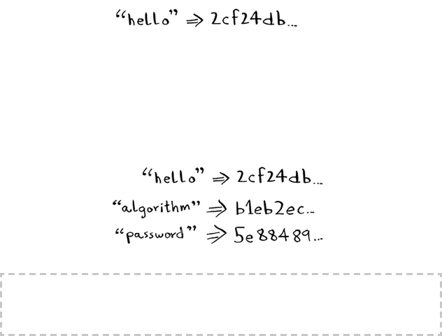
214 Chapter 11

I

Where to go next

is allows you to do constant-time lookups. When you want to know

the value for a key, you can use the hash function again, and it will tell

you in O(1) time what slot to check.

In this case, you want the hash function to give you a good distribution.

So a hash function takes a string and gives you back the slot number for

that string.

Comparing les

Another hash function is a secure hash algorithm (SHA) function.

Given a string, SHA gives you a hash for that string.

e terminology can be a little confusing here. SHA is a hash function.

It generates a hash, which is just a short string. e hash function for

hash tables went from string to array index, whereas SHA goes from

string to string.

SHA generates a dierent hash for every string.

Note

SHA hashes are long. They’ve been truncated here.

You can use SHA to tell whether two les are the same. is is useful

when you have very large les. Suppose you have a 4 GB le. You want

to check whether your friend has the same large le. You don’t have to

try to email them your large le. Instead, you can both calculate the

SHA hash and compare it.

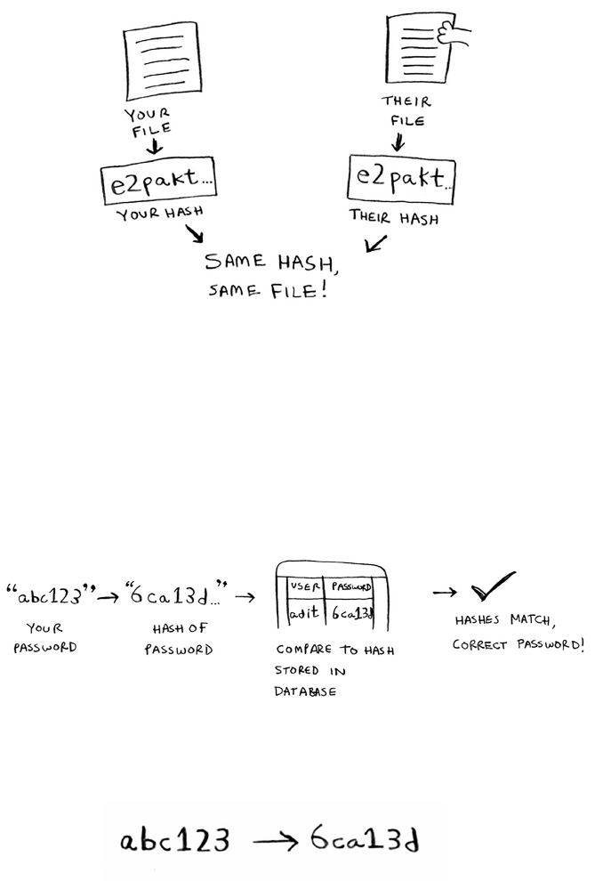
215The SHA algorithms

Checking passwords

SHA is also useful when you want to compare strings without revealing

what the original string was. For example, suppose Gmail gets hacked,

and the attacker steals all the passwords! Is your password out in the

open? No, it isn’t. Google doesn’t store the original password, only the

SHA hash of the password! When you type in your password, Google

hashes it and checks it against the hash in its database.

So it’s only comparing hashes—it doesn’t have to store your password!

SHA is used very commonly to hash passwords like this. It’s a one-way

hash. You can get the hash of a string.

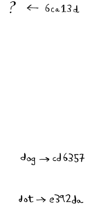
216 Chapter 11

I

Where to go next

But you can’t get the original string from the hash.

at means if an attacker gets the SHA hashes from Gmail, they can’t

convert those hashes back to the original passwords! You can convert a

password to a hash, but not vice versa.

SHA is actually a family of algorithms: SHA-0, SHA-1, SHA-2, and

SHA-3. As of this writing, SHA-0 and SHA-1 have some weaknesses.

If you’re using an SHA algorithm for password hashing, use SHA-2 or

SHA-3. e gold standard for password-hashing functions is currently

bcrypt (though nothing is foolproof).

Locality-sensitive hashing

SHA has another important feature: it’s locality insensitive. Suppose you

have a string, and you generate a hash for it.

If you change just one character of the string and regenerate the hash,

it’s totally dierent!

is is good because an attacker can’t compare hashes to see whether

they’re close to cracking a password.

Sometimes, you want the opposite: you want a locality-sensitive hash

function. at’s where Simhash comes in. If you make a small change

to a string, Simhash generates a hash that’s only a little dierent. is

allows you to compare hashes and see how similar two strings are,

which is pretty useful!

• Google uses Simhash to detect duplicates while crawling the web.

• A teacher could use Simhash to see whether a student was copying an

essay from the web.

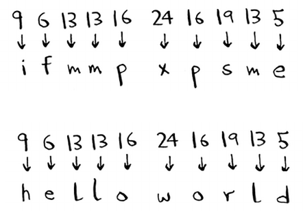
217Die-Hellman key exchange

• Scribd allows users to upload documents or books to share with

others. But Scribd doesn’t want users uploading copyrighted content!

e site could use Simhash to check whether an upload is similar to a

Harry Potter book and, if so, reject it automatically.

Simhash is useful when you want to check for similar items.

Die-Hellman key exchange

e Die-Hellman algorithm deserves a mention here, because it solves

an age-old problem in an elegant way. How do you encrypt a message

so it can only be read by the person you sent the message to?

e easiest way is to come up with a cipher, like a = 1, b = 2, and so on.

en if I send you the message “4,15,7”, you can translate it to “d,o,g”.

But for this to work, we both have to agree on the cipher. We can’t agree

over email, because someone might hack into your email, gure out

the cipher, and decode our messages. Heck, even if we meet in person,

someone might guess the cipher—it’s not complicated. So we should

change it every day. But then we have to meet in person to change it

every day!

Even if we did manage to change it every day, a simple cipher like this

is easy to crack with a brute-force attack. Suppose I see the message

“9,6,13,13,16 24,16,19,13,5”. I’ll guess that this uses a = 1, b = 2, and

so on.

at’s gibberish. Let’s try a = 2, b = 3, and so on.

218 Chapter 11

I

Where to go next

at worked! A simple cipher like this is easy to break. e Germans

used a much more complicated cipher in WWII, but it was still cracked.

Die-Hellman solves both problems:

• Both parties don’t need to know the cipher. So we don’t have to meet

and agree to what the cipher should be.

• e encrypted messages are extremely hard to decode.

Die-Hellman has two keys: a public key and a private key. e public

key is exactly that: public. You can post it on your website, email it

to friends, or do anything you want with it. You don’t have to hide it.

When someone wants to send you a message, they encrypt it using

the public key. An encrypted message can only be decrypted using the

private key. As long as you’re the only person with the private key, only

you will be able to decrypt this message!

e Die-Hellman algorithm is still used in practice, along with its

successor, RSA. If you’re interested in cryptography, Die-Hellman is a

good place to start: it’s elegant and not too hard to follow.

Linear programming

I saved the best for last. Linear programming is one of the coolest

things I know.

Linear programming is used to maximize something given some

constraints. For example, suppose your company makes two products,

shirts and totes. Shirts need 1 meter of fabric and 5 buttons. Totes need

2 meters of fabric and 2 buttons. You have 11 meters of fabric and 20

buttons. You make $2 per shirt and $3 per tote. How many shirts and

totes should you make to maximize your prot?

Here you’re trying to maximize prot, and you’re constrained by the

amount of materials you have.

Another example: you’re a politician, and you want to maximize the

number of votes you get. Your research has shown that it takes an

average of an hour of work (marketing, research, and so on) for each

vote from a San Franciscan or 1.5 hours/vote from a Chicagoan. You

need at least 500 San Franciscans and at least 300 Chicagoans. You have

219Epilogue

50 days. It also costs you $2/San Franciscan versus $1/Chicagoan. Your

total budget is $1,500. What’s the maximum number of total votes you

can get (San Francisco + Chicago)?

Here you’re trying to maximize votes, and you’re constrained by time

and money.

You might be thinking, “You’ve talked about a lot of optimization topics

in this book. How are they related to linear programming?” All the

graph algorithms can be done through linear programming instead.

Linear programming is a much more general framework, and graph

problems are a subset of that. I hope your mind is blown!

Linear programming uses the Simplex algorithm. It’s a complex

algorithm, which is why I didn’t include it in this book. If you’re

interested in optimization, look up linear programming!

Epilogue

I hope this quick tour of 10 algorithms showed you how much more is

le to discover. I think the best way to learn is to nd something you’re

interested in and dive in. is book gave you a solid foundation to do

just that.

221

answers

to exercises

CHAPTER 1

1.1 Suppose you have a sorted list of 128 names, and you’re searching

through it using binary search. What’s the maximum number of

steps it would take?

Answer: 7.

1.2 Suppose you double the size of the list. What’s the maximum

number of steps now?

Answer: 8.

1.3 You have a name, and you want to find the person’s phone

number in the phone book.

Answer: O(log n).

1.4 You have a phone number, and you want to find the person’s

name in the phone book. (Hint: You’ll have to search through

the whole book!)

Answer: O(n).

1.5 You want to read the numbers of every person in the phone book.

Answer: O(n).

1.6 You want to read the numbers of just the As.

Answer: O(n). You may think, “I’m only doing this for 1 out

of 26 characters, so the run time should be O(n/26).” A simple

rule to remember is, ignore numbers that are added, subtracted,

multiplied, or divided. None of these are correct Big O run times:

222 answers to exercises

O(n + 26), O(n - 26), O(n * 26), O(n / 26). They’re all the same as

O(n)! Why? If you’re curious, flip to “Big O notation revisited,” in

chapter 4, and read up on constants in Big O notation (a constant

is just a number; 26 was the constant in this question).

CHAPTER 2

2.1 Suppose you’re building an app to keep track of your finances.

Every day, you write down everything you spent money on. At

the end of the month, you review your expenses and sum up

how much you spent. So, you have lots of inserts and a few reads.

Should you use an array or a list?

Answer: In this case, you’re adding expenses to the list every day

and reading all the expenses once a month. Arrays have fast reads

and slow inserts. Linked lists have slow reads and fast inserts.

Because you’ll be inserting more often than reading, it makes sense

to use a linked list. Also, linked lists have slow reads only if you’re

accessing random elements in the list. Because you’re reading

every element in the list, linked lists will do well on reads too. So a

linked list is a good solution to this problem.

2.2 Suppose you’re building an app for restaurants to take customer

orders. Your app needs to store a list of orders. Servers keep adding

orders to this list, and chefs take orders off the list and make them.

It’s an order queue: servers add orders to the back of the queue,

and the chef takes the first order off the queue and cooks it.

223

Would you use an array or a linked list to implement this queue?

(Hint: linked lists are good for inserts/deletes, and arrays are good

for random access. Which one are you going to be doing here?)

Answer: A linked list. Lots of inserts are happening (servers

adding orders), which linked lists excel at. You don’t need search

or random access (what arrays excel at), because the chefs always

take the first order off the queue.

2.3 Let’s run a thought experiment. Suppose Facebook keeps a list of

usernames. When someone tries to log in to Facebook, a search is

done for their username. If their name is in the list of usernames,

they can log in. People log in to Facebook pretty often, so there are

a lot of searches through this list of usernames. Suppose Facebook

uses binary search to search the list. Binary search needs random

access—you need to be able to get to the middle of the list of

usernames instantly. Knowing this, would you implement the list

as an array or a linked list?

Answer: A sorted array. Arrays give you random access—you can

get an element from the middle of the array instantly. You can’t

do that with linked lists. To get to the middle element in a linked

list, you’d have to start at the first element and follow all the links

down to the middle element.

2.4 People sign up for Facebook pretty often, too. Suppose you

decided to use an array to store the list of users. What are the

downsides of an array for inserts? In particular, suppose you’re

using binary search to search for logins. What happens when you

add new users to an array?

Answer: Inserting into arrays is slow. Also, if you’re using binary

search to search for usernames, the array needs to be sorted.

Suppose someone named Adit B signs up for Facebook. Their

name will be inserted at the end of the array. So you need to sort

the array every time a name is inserted!

answers to exercises

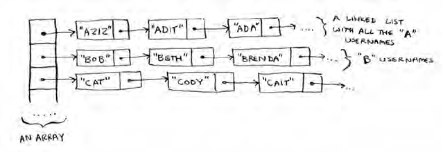
224

2.5 In reality, Facebook uses neither an array nor a linked list to store

user information. Let’s consider a hybrid data structure: an array

of linked lists. You have an array with 26 slots. Each slot points to a

linked list. For example, the first slot in the array points to a linked

list containing all the usernames starting with a. The second slot

points to a linked list containing all the usernames starting with b,

and so on.

Suppose Adit B signs up for Facebook, and you want to add them

to the list. You go to slot 1 in the array, go to the linked list for slot

1, and add Adit B at the end. Now, suppose you want to search for

Zakhir H. You go to slot 26, which points to a linked list of all the

Z names. Then you search through that list to find Zakhir H.

Compare this hybrid data structure to arrays and linked lists. Is it

slower or faster than each for searching and inserting? You don’t

have to give Big O run times, just whether the new data structure

would be faster or slower.

Answer: Searching—slower than arrays, faster than linked lists.

Inserting—faster than arrays, same amount of time as linked lists.

So it’s slower for searching than an array, but faster or the same

as linked lists for everything. We’ll talk about another hybrid

data structure called a hash table later in the book. This should

give you an idea of how you can build up more complex data

structures from simple ones.

So what does Facebook really use? It probably uses a dozen

different databases, with different data structures behind them:

hash tables, B-trees, and others. Arrays and linked lists are the

building blocks for these more complex data structures.

answers to exercises

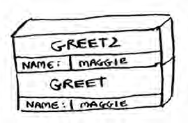
225

CHAPTER 3

3.1 Suppose I show you a call stack like this.

What information can you give me, just based on this call stack?

Answer: Here are some things you could tell me:

• e

greet

function is called rst, with

name = maggie.

• en the

greet

function calls the

greet2

function, with

name = maggie

.

• At this point, the

greet

function is in an incomplete,

suspended state.

• e current function call is the

greet2

function.

• Aer this function call completes, the

greet

function will

resume.

3.2 Suppose you accidentally write a recursive function that runs

forever. As you saw, your computer allocates memory on the

stack for each function call. What happens to the stack when

your recursive function runs forever?

Answer: The stack grows forever. Each program has a limited

amount of space on the call stack. When your program runs

out of space (which it eventually will), it will exit with a stack-

overflow error.

answers to exercises

226

CHAPTER 4

4.1 Write out the code for the earlier

sum

function.

Answer:

def sum(list):

if list == []:

return 0

return list[0] + sum(list[1:])

4.2 Write a recursive function to count the number of items in a list.

Answer:

def count(list):

if list == []:

return 0

return 1 + count(list[1:])

4.3 Find the maximum number in a list.

Answer:

def max(list):

if le n(list) = = 2:

return list[0] if list[0] > list[1] else list[1]

sub_max = max(list[1:])

return list[0] if list[0] > sub_max else sub_max

4.4 Remember binary search from chapter 1? It’s a divide-and-

conquer algorithm, too. Can you come up with the base case and

recursive case for binary search?

Answer: The base case for binary search is an array with one item.

If the item you’re looking for matches the item in the array, you

found it! Otherwise, it isn’t in the array.

In the recursive case for binary search, you split the array in half,

throw away one half, and call binary search on the other half.

How long would each of these operations take in Big O notation?

4.5 Printing the value of each element in an array.

Answer: O(n)

4.6 Doubling the value of each element in an array.

Answer: O(n)

4.7 Doubling the value of just the first element in an array.

Answer: O(1)

answers to exercises

227

4.8 Creating a multiplication table with all the elements in the array.

So if your array is [2, 3, 7, 8, 10], you first multiply every element

by 2, then multiply every element by 3, then by 7, and so on.

Answer: O(n2)

CHAPTER 5

Which of these hash functions are consistent?

5.1

f(x) = 1

Returns “1” for all input

Answer: Consistent

5.2

f(x) = rand()

Returns a random number every time

Answer: Not consistent

5.3

f(x) = next_empty_slot()

Returns the index of the next

empty slot in the hash table

Answer: Not consistent

5.4

f(x) = len(x)

Uses the length of the string as the index

Answer: Consistent

Suppose you have these four hash functions that work with strings:

A. Return “1” for all input.

B. Use the length of the string as the index.

C. Use the rst character of the string as the index. So, all strings

starting with a are hashed together, and so on.

D. Map every letter to a prime number: a = 2, b = 3, c = 5, d = 7,

e = 11, and so on. For a string, the hash function is the sum of

all the characters modulo the size of the hash. For example, if

your hash size is 10, and the string is “bag”, the index is 3 + 2 +

17 % 10 = 22 % 10 = 2.

For each of the following examples, which hash functions would

provide a good distribution? Assume a hash table size of 10 slots.

5.5 A phonebook where the keys are names and values are phone

numbers. The names are as follows: Esther, Ben, Bob, and Dan.

Answer: Hash functions C and D would give a good distribution.

answers to exercises

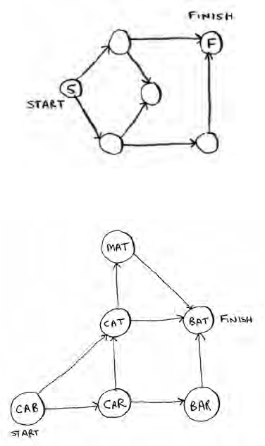
228

5.6 A mapping from battery size to power. The sizes are A, AA, AAA,

and AAAA.

Answer: Hash functions B and D would give a good distribution.

5.7 A mapping from book titles to authors. The titles are Maus, Fun

Home, and Watchmen.

Answer: Hash functions B, C, and D would give a good

distribution.

CHAPTER 6

Run the breadth-rst search algorithm on each of these graphs

to nd the solution.

6.1 Find the length of the shortest path from start to finish.

Answer: The shortest path has a length of 2.

6.2 Find the length of the shortest path from “cab” to “bat”.

Answer: The shortest path has a length of 2.

answers to exercises

229

6.3 Here’s a small graph of my morning routine.

For these three lists, mark whether each one is valid or invalid.

Answers: A—Invalid; B—Valid; C—Invalid.

6.4 Here’s a larger graph. Make a valid list for this graph.

Answer: 1—Wake up; 2—Exercise; 3—Shower; 4—Brush teeth;

5—Get dressed; 6—Pack lunch; 7—Eat breakfast.

answers to exercises

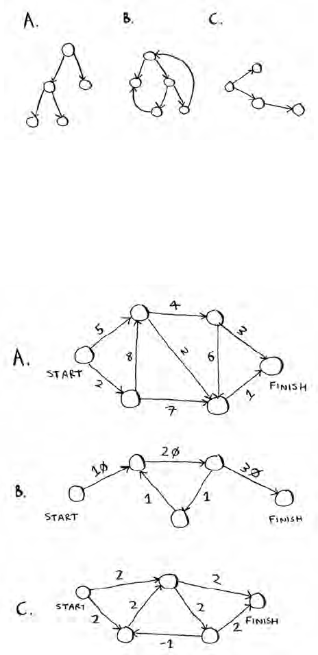
230

6.5 Which of the following graphs are also trees?

Answers: A—Tree; B—Not a tree; C—Tree. The last example is

just a sideways tree. Trees are a subset of graphs. So a tree is always

a graph, but a graph may or may not be a tree.

CHAPTER 7

7.1 In each of these graphs, what is the weight of the shortest path

from start to finish?

Answers: A: A—8; B—60; C—Trick question. No shortest path is

possible (negative-weight cycle).

answers to exercises

231

CHAPTER 8

8.1 You work for a furniture company, and you have to ship furniture

all over the country. You need to pack your truck with boxes. All

the boxes are of different sizes, and you’re trying to maximize

the space you use in each truck. How would you pick boxes to

maximize space? Come up with a greedy strategy. Will that give

you the optimal solution?

Answer: A greedy strategy would be to pick the largest box that

will fit in the remaining space, and repeat until you can’t pack any

more boxes. No, this won’t give you the optimal solution.

8.2 You’re going to Europe, and you have seven days to see everything

you can. You assign a point value to each item (how much you

want to see it) and estimate how long it takes. How can you

maximize the point total (seeing all the things you really want to

see) during your stay? Come up with a greedy strategy. Will that

give you the optimal solution?

Answer: Keep picking the activity with the highest point value that

you can still do in the time you have left. Stop when you can’t do

anything else. No, this won’t give you the optimal solution.

For each of these algorithms, say whether it’s a greedy algorithm or not.

8.3 Quicksort

Answer: No.

8.4 Breadth-first search

Answer: Yes.

8.5 Dijkstra’s algorithm

Answer: Yes.

8.6 A postman needs to deliver to 20 homes. He needs to find the

shortest route that goes to all 20 homes. Is this an NP-complete

problem?

Answer: Yes.

8.7 Finding the largest clique in a set of people (a clique is a set

of people who all know each other). Is this an NP-complete

problem?

Answer: Yes.

answers to exercises

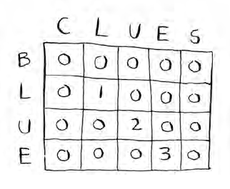
232

8.8 You’re making a map of the USA, and you need to color adjacent

states with different colors. You have to find the minimum

number of colors you need so that no two adjacent states are the

same color. Is this an NP-complete problem?

Answer: Yes.

CHAPTER 9

9.1 Suppose you can steal another item: an MP3 player. It weighs 1 lb

and is worth $1,000. Should you steal it?

Answer: Yes. Then you could steal the MP3 player, the iPhone, and

the guitar, worth a total of $4,500.

9.2 Suppose you’re going camping. You have a knapsack that holds

6 lb, and you can take the following items. They each have a value,

and the higher the value, the more important the item is:

• Water, 3 lb, 10

• Book, 1 lb, 3

• Food, 2 lb, 9

• Jacket, 2 lb, 5

• Camera, 1 lb, 6

What’s the optimal set of items to take on your camping trip?

Answer: You should take water, food, and a camera.

9.3 Draw and fill in the grid to calculate the longest common

substring between blue and clues.

Answer:

answers to exercises

233

CHAPTER 10

10.1 In the Netflix example, you calculated distance between two

different users using the distance formula. But not all users rate

movies the same way. Suppose you have two users, Yogi and Pinky,

who have the same taste in movies. But Yogi rates any movie he

likes as a 5, whereas Pinky is choosier and reserves the 5s for only

the best. They’re well matched, but according to the distance

algorithm, they aren’t neighbors. How would you take their

different rating strategies into account?

Answer: You could use something called normalization. You look

at the average rating for each person and use it to scale their

ratings. For example, you might notice that Pinky’s average rating

is 3, whereas Yogi’s average rating is 3.5. So you bump up Pinky’s

ratings a little, until her average rating is 3.5 as well. Then you can

compare their ratings on the same scale.

10.2 Suppose Netflix nominates a group of “influencers.” For example,

Quentin Tarantino and Wes Anderson are influencers on Netflix,

so their ratings count for more than a normal user’s. How would

you change the recommendations system so it’s biased toward the

ratings of influencers?

Answer: You could give more weight to the ratings of the

influencers when using KNN. Suppose you have three neighbors:

Joe, Dave, and Wes Anderson (an influencer). They rated

Caddyshack a 3, a 4, and a 5, respectively. Instead of just taking

the average of their ratings (3 + 4 + 5 / 3 = 4 stars), you could give

Wes Anderson’s rating more weight: 3 + 4 + 5 + 5 + 5 / 5 = 4.4

stars.

10.3 Netflix has millions of users. The earlier example looked at the

five closest neighbors for building the recommendations system.

Is this too low? Too high?

Answer: It’s too low. If you look at fewer neighbors, there’s a bigger

chance that the results will be skewed. A good rule of thumb is, if

you have N users, you should look at sqrt(N) neighbors.

answers to exercises

235

A

adit.io 212

algorithms

approximation algorithms

147–150

calculating answer 149

code for setup 147–148

sets 149–150

Bellman-Ford 130

Big O notation and 10–19

common run times 15–16

drawing squares example

13–14

exercises 17

growth of run times at dier-

ent rates 11–13

overview 10

traveling salesperson prob-

lem 17–19

worst-case run time 15

binary search 3–10

better way to search 5–7

exercises 6–9

overview 3–4

running time 10

breadth-rst search 107–113

exercise 111–113

running time 111

Dijkstra’s algorithm 115–139

exercise 139

implementation 131–139

negative-weight edges

128–130

overview 115–119

terminology related to

120–122

trading for piano example

122–128

distributed, usefulness of 209

Euclid’s 54

Feynman 180

greedy algorithms 141–159

classroom scheduling prob-

lem 142–144

exercises 145–146

knapsack problem 144–145

NP-complete problems

152–158

overview 141

set-covering problem

146–151

HyperLogLog algorithm 213

k-nearest neighbors algorithm

building recommendations

system 189–194

classifying oranges vs. grape-

fruit 187–189

exercises 195–199

machine learning 199–201

MapReduce algorithm 209–211

map function 209–210

reduce function 210–211

parallel 208

SHA algorithms 213–216

checking passwords 215–216

comparing les 214

overview 213

approximation algorithms

147–150

calculating answer 149

code for setup 147–148

sets 149–150

arrays

deletions and 30

exercises 30–31

insertions and 28–29

overview 28

terminology used with 27–28

uses of 26–27

B

base case 40–41, 41, 53

Bellman-Ford algorithm 130

best_station 151

Better Explained website 207

Big O notation 10–19

common run times 15–16

drawing squares example 13–14

exercises 17

growth of run times at dierent

rates 11–13

overview 10

quicksort and 66–71

average case vs. worst case

68–71

exercises 72

Index

236 index

merge sort vs. quicksort

67–68

overview 66

traveling salesperson problem

17–19

worst-case run time 15

binary search 3–10

better way to search 5–7

exercises 6–9

overview 3–4

running time 10

binary search trees 204–205

bloom lters 211–212

breadth-rst search 95–113

graphs and 99–104

exercises 104

nding shortest path

102–103

overview 107–110

queues 103–104

implementing 105–106

implementing algorithm

107–113

exercise 111–113

overview 107–110

running time 111

overview 95–98

built-in hash table 90

bye function 44

C

cache, using hash tables as 83–85

Caldwell, Leigh 40

call stack

overview 42–45

with recursion 45–50

cheapest node 117, 125

classication 189

classroom scheduling problem

142–144

common substring 184

constants 35

constant time 88–89

covered set 151

Ctrl-C shortcut 41

cycles, graph 121

D

DAGs (directed acyclic graphs)

122

D&C (divide and conquer) 52–60

def countdown(i) function 41

deletions 30

deque function 107

dict function 78

Die-Hellman key exchange 217

Dijkstra’s algorithm 115–139

exercise 139

implementation 131–139

negative-weight edges 128–130

overview 115–119

terminology related to 120–122

trading for piano example

122–128

directed graph 106

distance formula 194

distributed algorithms 209

DNS resolution 81

double-ended queue 107

duplicate entries, preventing

81–83

dynamic programming 161–185

exercises 173–178, 186

knapsack problem 161–171

changing order of rows 174

FAQ 171–173

lling in grid column-wise

174

guitar row 164–167

if solution doesn’t ll

knapsack completely 178

if solution requires more than

two sub-knapsacks 177

laptop row 168–170

optimizing travel itinerary

175–177

overview 161

simple solution 162–163

stealing fractions of an item

175

stereo row 166–168

longest common substring

178–185

lling in grid 180–182

longest common

subsequence 183–186

making grid 179–180

overview 179–180

solution 182–183

E

edges 99, 113

empty array 57, 58

encrypted messages 218

enqueue operation 104

Euclid’s algorithm 54

F

Facebook, user login and signups

example 31

fact function 45, 47

factorial function 45

factorial time 19

false negatives 212

false positives 212

Feynman algorithm 180

FIFO (First In, First Out) data

structure 104

nd_lowest_cost_node function

134, 139

rst-degree connection 103

for loop 149

for node 136

Fourier transform 207–208

G

git di 185

graphs

breadth-rst search and 99–104

exercises 104

nding shortest path

102–104

overview 99–101

queues 103–104

overview 96–98

graph[“start”] hash table 132

greedy algorithms 141–159

237index

classroom scheduling problem

142–144

exercises 145–146

knapsack problem 144–145

NP-complete problems 152–158

set-covering problem 146–151

approximation algorithms

147–150

back to code 151–152

exercise 152

overview 146

greet2 function 44

greet function 43–45

H

hash tables 73–88

collisions 86–88

hash functions 76–78

performance 88–91

exercises 93

good hash function 90–91

load factor 90–91

use cases 79–86

preventing duplicate entries

81–83

using hash tables as cache

83–85

using hash tables for lookups

79–81

Haskell 59

HyperLogLog algorithm 213

I

inductive proofs 65

innity, representing in Python

133

insertions 28–29

inverted indexes 206–207

IP address, mapping web address

to 81

J

JPG format 207

K

Khan Academy 7, 54

knapsack problem

changing order of rows 174

FAQ 171–173

lling in grid column-wise 174

guitar row 164–167

if solution doesn’t ll knapsack

completely 178

if solution requires more than

two sub-knapsacks 177

laptop row 168–170

optimizing travel itinerary

175–177

overview 144–145, 161

simple solution 162–163

stealing fractions of an item 175

stereo row 166–168

k-nearest neighbors algorithm

building recommendations

system 189–194

classifying oranges vs. grapefruit

187–189

exercises 195–198

machine learning 199–201

L

Levenshtein distance 185

LIFO (Last In, Last Out) data

structure 104

linear programming 218–219

linear time 10, 15, 89

linked lists 25–26

deletions and 30

exercises 28, 30–31

insertions and 28–29

overview 25–26

terminology used with 27–28

load balancing 208

locality-sensitive hashing 216

logarithmic time. Seelog time

logarithms 7

log time 7, 10, 15

lookups, using hash tables for

79–81

M

machine learning 199–201

MapReduce algorithm

map function 209–210

reduce function 210–211

memory 22–23

merge sort vs. quicksort 67–68

MP3 format 207

N

Naive Bayes classier 200

name variable 43

neighbors 99

n! (n factorial) operations 19

nodes 99, 105

n operations 12

NP-complete problems 152–158

O

OCR (optical character

recognition) 199–201

P

parallel algorithms 208

partitioning 61

person_is_seller function 108, 111

pivot element 60

pop (remove and read) action 42

Print function 43

print_items function 67

private key, Die-Hellman 218

probabilistic data structure 212

pseudocode 38, 40, 182

public key, Die-Hellman 218

push (insert) action 42

Pythagorean formula 191

Q

queues 30–31

quicksort, Big O notation and

66–71

238

average case vs. worst case

68–71

exercises 72

merge sort vs. quicksort 67–68

R

random access 30

recommendations system, building

189–194

recursion 37–49

base case and recursive case

40–41

call stack with 45–50

overview 37–39

regression 196

resizing 91

run time

common run times 15–16

growth of at dierent rates

11–13

overview 10

S

searches

binary search 3–10

as better way to search 5–7

exercises 6–9

overview 3–4

running time 10

breadth-rst search

graphs and 99–104

implementing 105–106

implementing algorithm

107–113

selection sort 32–33

sequential access 30

set-covering problem 146–151

approximation algorithms

calculating answer 149

code for setup 147–148

sets 149–150

exercise 152

overview 146

set dierence 150

set intersection 150

sets 148

set union 150

SHA algorithms 213–216

checking passwords 215–216

comparing les 214

overview 213

SHA (Secure Hash Algorithm)

function 92, 214

shortest path 98, 128

signals, processing 207

Simhash 216, 217

simple search 5, 11, 200

SQL query 209

stacks 42–49

call stack 43–45

call stack with recursion 45–50

exercise 45, 49–50

overview 42

states_covered set 149

states_for_station 151

states_needed 151

stock market, predicting 201

strings, mapping to numbers 76

sum function 57, 59

T

third-degree connection 103

topological sort 112

training 200

trees 203–206

U

undirected graph 122

unique searches 213

unweighted graph 120

W

weighted graph 120

index