Guide
User Manual: Pdf
Open the PDF directly: View PDF ![]() .
.
Page Count: 39
Time Series Database Interface (TSdbi)
Guide and Illustrations
Paul D. Gilbert
April 30, 2015
Contents
1 Introduction 1
2 Simple Examples of Time Series Data from the Internet 2
2.1 SDMX Data ............................. 3
2.2 histQuote and getSymbol ....................... 7
2.3 getSymbol withFRED........................ 9
2.4 TSjson with Statistics Canada . . . . . . . . . . . . . . . . . . . 14
2.5 xls ................................... 16
2.6 zip ................................... 19
3 SQL Time Series Databases 21
3.1 Writing to SQL Databases . . . . . . . . . . . . . . . . . . . . . . 22
4 More Examples 26
4.1 Examples Using SQL Databases . . . . . . . . . . . . . . . . . . 26
5 Comparing Time Series Databases 30
6 Vintages of Realtime Data 33
7 Just Want Data in a xls or csv File 34
1 Introduction
This vignette illustrates the various R(R Core Team, 2014) TSdbi packages
using time series data from several sources. The main purpose of TSdbi is to
provide a common API, so simplicity of changing the data source is a primary
feature. The vignette also illustrates some simple time series manipulation and
plotting using packages tframe and tfplot. While these do not need to be at-
tached for data retrieval, functions in these packages are used in several places
in this vignette so they should be attached to run examples in this vignette.
This is done with
> library("tframe")
> library("tfplot")
Package tframePlus is also used but will be attached when needed.
To generate this vignette requires most of the TS* packages, but users will
only need one, or a few of these packages. For example, a time series database
can be built with several SQL database backends, but typically only one would
be used. On the other hand, several packages pull data from various Internet
sources, so several of these might be used to accommodate the various specifics
of the sources.
If package TSdata is installed on your system, it should be possible to
view the pdf version of this guide with vignette(”Guide”, package=”TSdata”).
Otherwise, consider getting the pdf file directly from CRAN at http://cran.
at.r-project.org/web/packages/TSdata/index.html Many parts of the vi-
gnette can be run by loading the appropriate packages, but some examples use
data that has been loaded into a local database and it will not be possible to
reproduce those examples without the underlying database.
Section 2 of this vignette illustrates the mechanism for connecting to a data
source. The connection contains all the source specific information so, once the
connection is established, the syntax for retrieving data is similar for different
sources. The section illustrates packages that pull data from Internet sources.
This currently includes TSsdmx,TSjson, and TSmisc. (Package TSmisc is an
amalgamation of former packages TSgetSymbol TShistQuote,TSxls,TSzip, and
some new connections.) The section starts with a table indicating which pack-
ages and connections might be used for various data sources. These packages
only get data, they do not support writing data to the database. Finally, the
section also illustrates the flexibility to return different representations of time
series objects.
Section 3 illustrates the SQL packages TSPostgreSQL,TSMySQL,TSSQLite,
and TSodbc. These use a very standard SQL table structure and syntax, so it
should be possible to use other SQL backends. The package TSOracle is avail-
able on R-forge at http://tsdbi.r-forge.r-project.org/ but I currently do
not have a server in place to test it properly. (If anyone would be interested in
doing this, please contact me, pgilbert.ttv9z@ncf.ca.) These packages get data
and also support writing data to the database. See Appendix “B” (separate
1
vignette) and the vignette in package TSdbi for more explanation of the under-
lying database tables, and for bulk loading of data into a database. The section
illustrates the packages by writing artificial data to the database.
Section 4 provides additional examples of TSdbi functionality and of using
and graphing series. Subsection 4.1 illustrates fetching data from the web and
loading it into a local database.
Section 5 illustrates package TScompare for comparing time series databases,
and Section 6 illustrates the use of realtime vintages of data.
Section 7 illustrates some functions for exporting time series data from R
into .xls and .csv files. While regular Rusers may not be too interested in this,
it can be useful for colleagues that are not yet regular users. The section is
fairly self contained. (But will give non-users some exposure to R, so they may
decide they do not actually need to export the data.)
Appendix “A” provides connection details specific to the different database
sources, Appendix“B”provides more details about the structure of SQL databases,
and Appendix “C” provides some examples of SQL queries that may be useful
for database maintenance. Finally, Appendix “D” reproduces the README
file for package TSjson, to give details regarding installation of Python helper
utilities.
Many of the TS* packages are wrappers of other packages. The purpose is to
provide a common API for interfacing with time series databases, and an easy
mechanism to specify the type of time series object that should be returned,
for example, a ts object or a zoo (Zeileis and Grothendieck, 2005) object. One
consequence of providing a common interface is that special strengths of some of
the underlying packages cannot always be used. If you really need some of these
features then you will need to go directly to the underlying package. However,
if you limit your reliance on these special features then you will be able to move
from one data source to another much more easily.
Loading a TS* package will also attach or load the namespace of required
packages TSdbi,DBI (R Special Interest Group on Databases, 2009), methods
(R Core Team, 2013), tframePlus,zoo, and then any underlying package that
the specific TS* package uses.
2 Simple Examples of Time Series Data from
the Internet
This section uses packages to pull data from the Internet. The general syntax
of a connection is illustrated, and some simple calculations and graphs are done
to demonstrate how the data might be used. However, the purpose of the TS*
packages is to provide a common interface, not to do all time series calculations
and graphics. Once you have the data, you should be able to use whatever other
Rpackages you like for your calculations and graphs.
The generic aspect of the interface API is accomplished by putting the in-
formation specific to the underlying source into the “connection”. Once the
2

connection is established, other aspects of using data are the same, so one con-
nection can be easily interchanged with another, and so your programs do not
need to be changed when the data source is changed. (But, of course, some
changes will be needed if the series identifiers of the variables change on the
different databases.)
The following table indicates various data sources and the TS* connections
and packages that can be used to extract data from them, TSsdmx is a wrapper
for package RJSDMX (Mattiocco et al., 2014) maintained by Attilio Mattiocco
at the Banca d’Italia. It uses SDMX/REST to connect to several important
sources for economic data. This API is probably the main future direction, and
some of the other interfaces should be considered temporary, pending the institu-
tions getting SDMX/REST 2.1 in place. Package RJSDMX has an addProvider
function which can be used to add SDMX/REST 2.1 compliant servers.
The above URL is for the organization. The SDMX data web URL can be
determined with RJSDMX::sdmxHelp() using the build command action to give
the URL of an sdmx query.
The table is not comprehensive. In particular, Quandl, Bloomberg, Yahoo,
Oanda, and some others, provide access to data from a large number of sources,
especial market data.
2.1 SDMX Data
SDMX is emerging as a widely used standard for time series exchange. It is sup-
ported by several large organizations and has evolved over many years. Some
of the ad hoc mechanisms in other TS* packages will be replaced as more or-
ganizations implement this standard. It provides capabilites for transmitting
large dataset, mixed frequency, and metada. These are well beyond the scope
of what is used by the TSdbi API. The RJSDMX package provides an interface
to SDMX/REST 2.1 compliant databases. Similar to other TS* packages, the
wrapper TSsdmx uses only some of the capabilities of the underlying package.
Only reading of databases is supported.
By default RJSDMX prints more output than Rusers will typically expect.
This output can be supressed by settings in a configuration file, which has been
done for this vignette. See Appendix “A” for more details.
> library("TSsdmx")
> oecd <- TSconnect("sdmx", dbname="OECD")
> x <- TSget( QNA.CAN.PPPGDP.CARSA.Q , oecd)
> tfplot(x, title="Canada: Nominal GDP at PPP?",
subtitle="quarterly national accounts, SAAR",
ylab="guess the units")
>
3
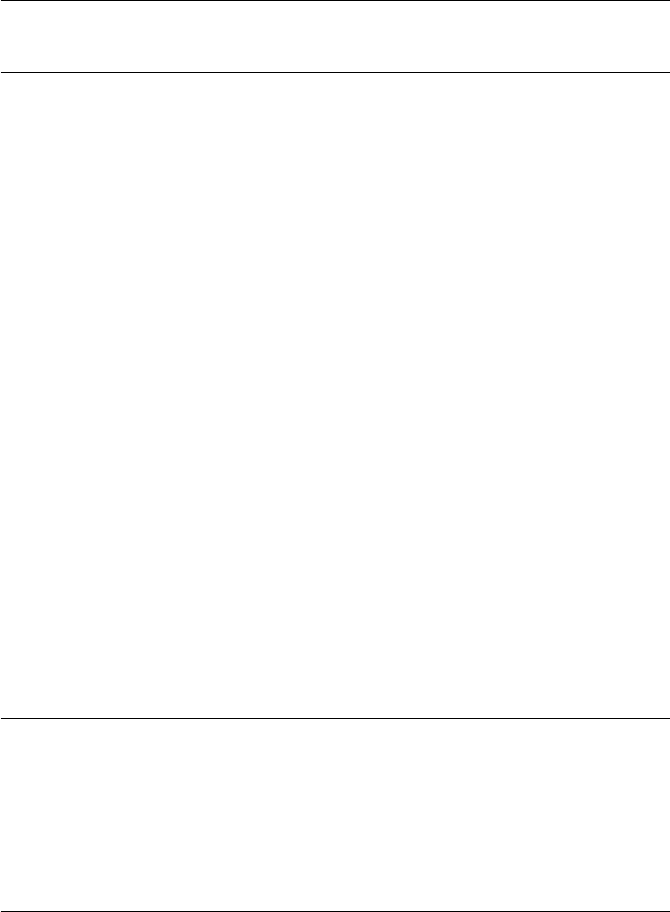
Table 1: Connections for various data sources.
Data source source URL Package Connection
ABS (Australia) www.abs.gov.au TSsdmx sdmx
ECB www.ecb.org TSsdmx sdmx
EuroStat epp.eurostat.ec.europa.eu TSsdmx sdmx
ILO www.ilo.org TSsdmx sdmx
IMF www.imf.org TSsdmx sdmx
INEGI (Mexico) www.inegi.org.mx TSsdmx sdmx
ISTAT5(Italy) www.istat.it TSsdmx sdmx
NBB (Belgium) www.nbb.be TSsdmx sdmx
OECD www.oecd.org TSsdmx sdmx
UIS www.uis.unesco.org TSsdmx sdmx
UN2comtrade.un.org TSsdmx sdmx
Unesco www.uis.unesco.org TSsdmx sdmx
World Bank1worldbank.org TSsdmx sdmx
BIS3www.bis.org TSsdmx sdmx
FRED research.stlouisfed.org TSmisc histQuote
FRED research.stlouisfed.org TSmisc getSymbol
RBA (Australia) www.rba.gov.au TSmisc xls
Statistics Canada www.statcan.gc.ca TSjson4,6json
Bank of Canada www.bank-banque-canada.ca TSmisc24Quandl
Yahoo quote.yahoo.com TSmisc getSymbol
Yahoo quote.yahoo.com TSmisc histQuote
Oanda www.oanda.com TSmisc histQuote
PiTrading pitrading.com TSmisc zip
Quandl www.quandl.com TSmisc24Quandl
Bloomberg www.bloomberg.com TSbbg4bbg
1beta
2planning
3requires an account
4not on CRAN, on R-forge tsdbi.r-forge.r-project.org/
5requires free registration at sdmx.istat.it/registr_ut_sep/
6using python mechanize, unstable website API
4
guess the units
1960 1966 1972 1978 1984 1990 1996 2002 2008 2014
0.95 1.05 1.15 1.25
quarterly national accounts, SAAR
Canada: Nominal GDP at PPP?
Determining what the above series is will be left as an exercise. SDMX
queries are roughly like database queries with the fields separated by dots. They
can use *,|, and +to return muliple series. TSget provides the ability to rename
series on retrieval when |, and +are used, but not when *is used.
> x <- TSget( QNA.CAN+USA+MEX.PPPGDP.CARSA.Q ,
names=c("Canada", "United States", "Mexico"), oecd)
> tfOnePlot(ytoypc(x), title="Nominal GDP Growth PPP?",
subtitle="quarterly national accounts, national currency, SAAR",
ylab="relative to USA", start=c(1975,1),
legend=seriesNames(x), legend.loc="topright")
relative to USA
1975 1979 1983 1987 1991 1995 1999 2003 2007 2011
0 50 100 150
Nominal GDP Growth PPP?
quarterly national accounts, national currency, SAAR
Canada
United States
Mexico
Several different connections can be defined, and data retreived from them.
> eurostat <- TSconnect("sdmx", dbname="EUROSTAT")
> ecb <- TSconnect("sdmx", dbname="ECB")
> abs <- TSconnect("sdmx", dbname="ABS")
> z <- TSget("ei_nama_q.Q.MIO-EUR.SWDA.CP.NA-P72.IT", eurostat)
TSget allows for specifying start and end dates.
5

> z <- TSget( EXR.Q.USD.EUR.SP00.A ,
start="2008-Q2", end="2014-Q3", ecb)
> z <- TSget( EXR.Q.USD.EUR.SP00.A ,
start=c(2008,2), end=c(2014,3), ecb)
The first request above uses SDMX syntax for start and end, which is passed
to the query, and only data in the range is returned from the server. The second
syntax uses an Rconvention which is difficult to translate into the query, because
it is necessary to first determine the frequency of the data. For this query all
the data is returned and the truncation is done in R. For sdmx connections,
character string start and end specifications are assumed to be SDMX and
are passed to the underlying RJSDMX call and on to the server, otherwise
truncation is done in Ron the returned data.
A connection can be specified to be used as the default, so it does not need
to be specified each time:
> options(TSconnection=abs)
> z <- TSget("BOP.1.100.10.Q", start=c(1990, 1), end=c(2012, 2))
Several different connections will be used in this vignette, and so a default
will not be used. To unset the default
> options(TSconnection=NULL)
By default most TSget methods return a class ts series when that is possible
(annual, quarterly, monthly, or semi-annual data) and zoo series otherwise. Thus
the class of the series returned above is ts, but zoo can be specified.
> class(z)
[1] "ts"
> z <- TSget("BOP.1.100.10.Q", start=c(1990, 1), end=c(2012, 2),
abs, TSrepresentation="zoo")
> class(z)
[1] "zoo"
A session default can also be set for this with
> options(TSrepresentation="zoo")
in which case all results will be return as zoo objects unless otherwise specified.
The session default is unset with
> options(TSrepresentation=NULL)
Beware that it does not make sense to set ts as the default, because it is already
the default for all series that can be represented as ts, and will not work correctly
for other series. Other representations are possible. See the TSget help for more
details.
6
2.2 histQuote and getSymbol
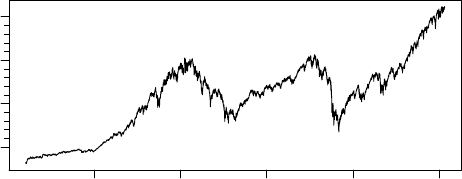
histQuote and getSymbol in package TSmisc provide mechanisms to retrieve his-
torical quote data from various sources. histQuote is a wrapper to get.hist.quote
in package tseries (Trapletti and Hornik, 2012). A connection to Yahoo Finance
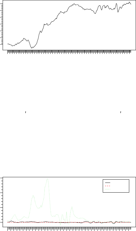
is established, and data retrieved and plotted by
> library("TSmisc")
> yahoo <- TSconnect("histQuote", dbname="yahoo")
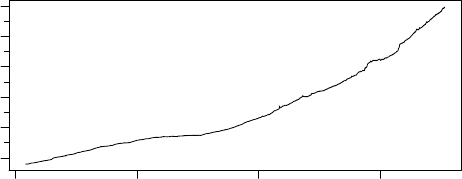
> x <- TSget("^gspc", quote = "Close", con=yahoo)
> library("tfplot")
> tfplot(x)
1995 2000 2005 2010 2015
^gspc
500 1000 1500 2000
Package getSymbol is a wrapper to getSymbols in package quantmod (Ryan,
2011). A connection to Yahoo using this, and retrieving the same data, can be
done by
> yahoo <- TSconnect("getSymbol", dbname="yahoo")
> x <- TSget("^gspc", quote = "Close", con=yahoo)
> tfplot(x)
2008 2010 2012 2014
^gspc
1000 1500 2000
7
Notice that the only difference is the name of the driver provided when
establishing the connection. After that, the code is the same (and the data
from the two connections should be the same, other than the difference in the
default start date). This is the coding approach one would typically follow, so
that changing the data source is easy. However, sometimes it is interesting to
compared the same data from differrent sources, so here is an example where the
connections are given different names, so the same data through two different
connection methods can be more easily compared:
> ya1 <- TSconnect("getSymbol", dbname="yahoo")
> ya2 <- TSconnect("histQuote", dbname="yahoo")
> ibmC1 <- TSget("ibm", ya1, quote = "Close", start="2011-01-03")
> ibmC2 <- TSget("ibm", ya2, quote = "Close", start="2011-01-03")
In this example the underlying packages both return zoo time series objects,
but the encoding of the date index vectors are of different classes (Date vs
POSIXct). This is usually not a problem because one would usually work with
one package or the other, but it does become a problem when comparing the two
objects returned by the different methods. The time representation of ibmC1
can be changed from POSIXct to Date by:
> tframe(ibmC1) <- as.Date(tframe(ibmC1))
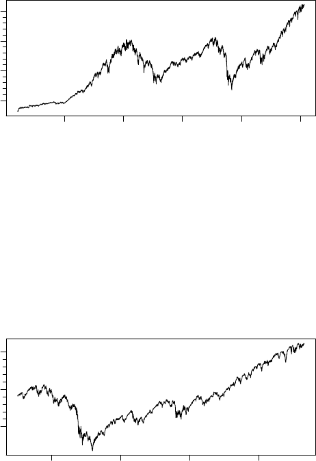
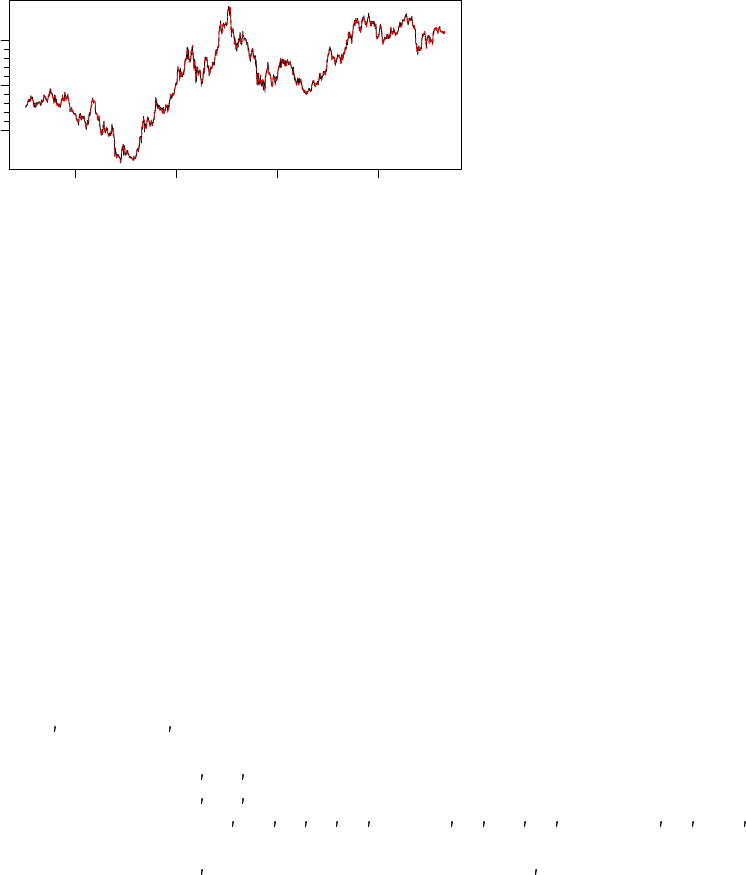
The two series can then be plotted:
> tfplot(ibmC2, ibmC1,
ylab="IBM Close",
title="IBM via getSymbol and histQuote",
lastObs=TRUE,
legend=c("via histQuote (black)", "via getSymbol (red)"),
source="Source: Yahoo")
2011 2012 2013 2014 2015
IBM Close
150 170 190 210
Source: Yahoo Last observation: 2015−04−29
via histQuote (black)
via getSymbol (red)
IBM via getSymbol and histQuote
Or the difference can be used to check equality:
> max(abs(ibmC2 - ibmC1))
8
[1] 0
(Note that this difference calculation does not catch a difference in length,
which occurs if new data has been release on one connection and not the other.
At some point Yahoo was releasing partial data early, and these connection are
correcting differently for this. So, at some times of day, the last available data
point is not the same on these two connections.)
A certain amount of meta data can be returned with the time series object
and can be extracted with these utilities:
> TSdescription(x)
[1] "^gspc Close from yahoo"
> TSdoc(x)
[1] "^gspc Close from yahoo retrieved 2015-04-30 17:37:11"
> TSlabel(x)
[1] "^gspc Close"
> TSsource(x)
[1] "yahoo"
2.3 getSymbol with FRED
getSymbol can also be used to get data from the Federal Reserve Bank of
St.Louis, as will be illustrated here. (Look at http://research.stlouisfed.
org/fred/ to find series identifiers.)
> library("TSmisc")
> fred <- TSconnect("getSymbol", dbname="FRED")
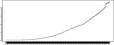
> tfplot(TSget("M2", fred))
1980 1990 2000 2010
M2
2000 6000 10000
Additional information can be specified in tfplot and tfOnePlot:
9
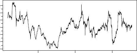
> tfOnePlot(percentChange(TSget("M2", fred), lag=52),
title = "Running commentary, blah, blah, blah",
subtitle="Broad Money (M2)",
ylab= "y/y percent change*",
source="Source: Federal Reserve Bank of St.Louis (M2)",
footnoteLeft = "seasonally adjusted data",
footnoteRight = "* approximated by 52 week growth",
lastObs = TRUE )
1990 2000 2010
y/y percent change*
0 2 4 6 8 10
Running commentary, blah, blah, blah
Broad Money (M2)
Source: Federal Reserve Bank of St.Louis (M2) Last observation: 2015−04−20
seasonally adjusted data * approximated by 52 week growth
It is also possible to return multiple series, but they should all be of the same
frequency. (The FRED series called M2 is a weekly series).
> x <- TSget(c("CPIAUCNS","M2SL"), fred)
> tfplot(x,
title = "Running commentary, blah, blah, blah",
subtitle=c("Consumer Price Index for All Urban Consumers: All Items",
"Broad Money"),
ylab= c("Index 1982-84=100", "Billions of dollars"),
source= c("Data Source: Federal Reserve Bank of St.Louis (CPIAUCNS)",
"Data Source: Federal Reserve Bank of St.Louis (M2SL)"),
footnoteLeft = c("not seasonally adjusted", "seasonally adjusted"),
footnoteRight = paste("Extracted:", date()),
lastObs = TRUE )
10
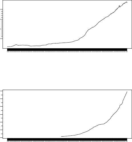
Index 1982−84=100
1913 1923 1933 1943 1953 1963 1973 1983 1993 2003 2013
50 100 150 200
Consumer Price Index for All Urban Consumers: All Items
Data Source: Federal Reserve Bank of St.Louis (CPIAUCNS) Last observation: Mar 2015
not seasonally adjusted Extracted: Thu Apr 30 17:37:12 2015
Running commentary, blah, blah, blah
Billions of dollars
1913 1923 1933 1943 1953 1963 1973 1983 1993 2003 2013
0 4000 8000 12000
Broad Money
Data Source: Federal Reserve Bank of St.Louis (M2SL) Last observation: Mar 2015
seasonally adjusted Extracted: Thu Apr 30 17:37:12 2015
> TSdates(c("CPIAUCNS","M2SL"), fred)
[,1]
[1,] "CPIAUCNS from 1913 1 to 2015 3 12"
[2,] "M2SL from 1959 1 to 2015 3 12"
It is possible to specify the type of object to return:
> x <- TSget(c("CPIAUCNS","M2SL"), fred, TSrepresentation="zoo")
> class(x)
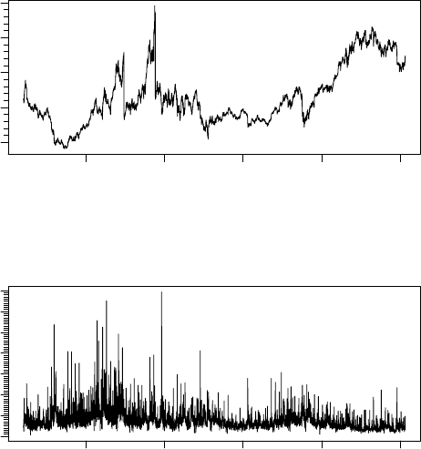
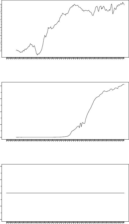
The following connects to yahoo and loads the ticker symbol for Ford. This
is a multivariate time series with open, close, etc.
> yahoo <- TSconnect("getSymbol", dbname="yahoo")
> x <- TSget("F", con=yahoo)
> plot(x)
11
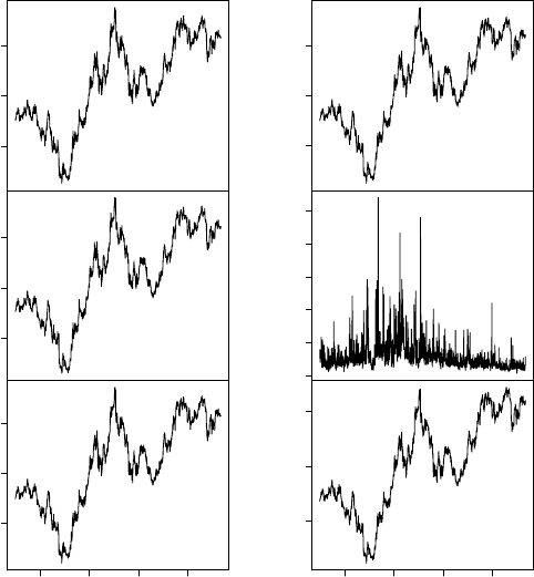
5 10 15
F.Open
5 10 15
F.High
2008 2010 2012 2014
Index
5 10 15
F.Low
5 10 15
F.Close
0e+00 2e+08 4e+08
F.Volume
2008 2010 2012 2014
Index
5 10 15
F.Adjusted
x
Most of the plots in this vignette are done with the utilities in the tfplot
package, but the usual plot function, used above, produces slightly different
results that may be preferable in some situations. Also, for some time series
objects, the plot method has been much improved from the default, so if you
are using these objects you may find that plot provides attractive features.
In the case of the ticker data above, tfplot displays graphs in verticle panels.
However, six panels do not nicely fit on a printed page. The first three are
displayed with:
> tfplot(x,series=1:3)
12
2008 2010 2012 2014
F.Open
5 10 15
2008 2010 2012 2014
F.High
5 10 15
2008 2010 2012 2014
F.Low
5 10 15
It is possible to specify the number of graphs on an ouput screen with
graphs.per.page, for example, tfplot(x, graphs.per.page=3). Set par(ask=TRUE)
if you want to stop and prompt for <Return>between pages in the graphics
output.
The quote argument to TSget can be used to specify that only a subset of
the market data should be returned:
13
> tfOnePlot(TSget("F", con=yahoo, quote=c("Open", "Close")),
title="Ford from Yahoo; Open (black); Close (red)",
ylab="Price")
2008 2010 2012 2014
Price
5 10 15
Ford from Yahoo; Open (black); Close (red)
2.4 TSjson with Statistics Canada
Package TSjson provides a mechanism to extract data from websites and pass
it to Rin JavaScript Object Notation (JSON) using package rjson (Couture-
Beil, 2013). Package RJSONIO (Lang, 2012) has previously been used to bring
the data into Rbut is not the current method. TSjson uses Python code to
mechanize clicking though web pages to get a downloadable file. This really
should be considered a temporary solution, until the data provider implements
a true API. The current version of TSjson provides a connection to Statistics
Canada’s http://www.statcan.gc.ca Cansim database. (You should look at
the Statistics Canada site to find series identifiers.)
The connection can be established in two different ways. The simplest re-
quires a system with Python installed, and Python modules sys, json, mechanize,
re, csv and urllib2. This requires Python 2 as not all modules are available for
Python 3. Additional details are provided in a README file distributed with
the TSjson package and also copied in an appendix here.
Checking that an adequate Python and modules are available on the system
can be done with
> require( findpython )
> cmdExists <- can_find_python_cmd(
minimum_version = 2.6 ,
maximum_version = 2.9 ,
required_modules = c( sys , re , urllib2 , csv , mechanize , json )
)
> if (!cmdExists) stop( adequate python was not found. )
An adequate python would normally have been needed to install package TSjson
but system changes after the installation could break it.
14
Installing Python may be difficult in environments where users cannot easily
install software, but a second method using a proxy server can be used. The
proxy server needs Python and the modules, as well as server software (e.g.
Web2Py), but the client machine requires nothing special other than Rand
TSjson. The proxy server can be anywhere on the Internet.
The following examples use the first method. More details on establish-
ing connections with the second method are provided in the appendix section
(separate vignette). First, establish a connection
Although the package TSjson usually works, it is not really stable because
the web interface is not a proper API and can change from time to time. For this
reason, TSjson is not on CRAN but available on R-forge at tsdbi.r-forge.
r-project.org/. The following examples are not being evaluated because fail-
ures prevent reliable automatic generation of the vignette.
> require("TSjson")
> cansim <- TSconnect("json", dbname="cansim")
Now data can be retrieved and a plot generated by
> x <- TSget("v498086", cansim)
> tfplot(x)
Meta data can also be retrieved:
> TSdescription("v498086", cansim)
> TSdoc("v498086", cansim)
> TSlabel("v498086", cansim)
> TSsource("v498086", cansim)
A transformation of the data can be done, more detail added to the graph,
and a start date specified:
> tfplot(ytoypc(x), start=c(1975,1),
ylab="Year-to-Year Growth Rate",
title="Canadian GDP",
source=paste("Statistics Canada ", seriesNames(x)),
lastObs=TRUE)
The default settings of tfplot parameters usually work fairly well for interac-
tive use but multi-series graphs may be squashed as above when pdf is output.
The next illustrates one way to achieve more specific control, which will often
be necessary for generating pdf documents. The series can be retreived and
plotted in one step:
> oldpar <- par(omi=c(0.1,0.1,0.1,0.1),mar=c(3.1,4.1,0.6,0.1))
> tfplot(ytoypc(TSget(c("v498086", "v498087"), cansim)))
> par(oldpar)
Sometimes it is useful to check availability:
15
> TSdates(c("v498086", "v498087"), cansim)
The meta data can also be retrieved with the series, which will generally be
faster than retreiving it separately, if it is needed:
> resMorg <- TSget("V122746", cansim, TSdescription=TRUE,
TSdoc=TRUE, TSlabel=TRUE)
> TSdescription(resMorg)
> TSdoc(resMorg)
> TSlabel(resMorg)
> TSseriesIDs(resMorg)
> TSsource(resMorg)
> seriesNames(resMorg) <- "Residential Mortgage Credit (SA)"
> tfplot(ytoypc(resMorg), annualizedGrowth(resMorg),
title=seriesNames(resMorg),
subtitle="year-to-year (black) and annualize monthly growth (red)",
ylab="Growth Rate",
source=paste("Bank of Canada, ", TSsource(x)),
lastObs=TRUE)
2.5 xls
The xls interface allows the use of spreadsheets as if they are a database. (This
is a poor substitute for a real database, but is sometimes convenient.) xls uses
read.xls in package gdata (Warnes et al., 2011) xls does not support writing
data to the spreadsheet (but to write time series data to a spreadsheet see
TSwriteXLS in tframePlus, discussed in section 7). The spreadsheet can be a
remote file, which is retrieved when the connection is established.
The following retrieves a file from the Reserve Bank of Australia and maps
the elements that are used: data, dates, identifiers, and series names.
> library("TSmisc")
> rba <- TSconnect("xls", dbname=
"http://www.rba.gov.au/statistics/tables/xls/d03hist.xls",
map=list(ids =list(i=11, j="B:Q"),
data =list(i=12:627, j="B:Q"),
dates=list(i=12:627, j="A"),
names=list(i=4:7, j="B:Q"),
description = NULL,
tsrepresentation = function(data,dates){
ts(data,start=c(1959,7), frequency=12)}))
This also illustrates how tsrepresentation can be specified as an arbitrary
function to set the returned time series object representation. Note also that
dates may display in the spreadsheet one way (e.g. 02-Jan-1989), show in the
spreadsheet formula box in another way (e.g. 1989-01-02), and import still dif-
ferently (e.g. 02/Jan/1989). And the format could change when the file is saved,
16
possibly depending on what features are available in the spreadsheet program.
The imported format needs to be used when tsrepresentation is specified. If in
doubt, look at the connection slot @dates (rba@dates above).
Beware that data is read into Rwhen the connection is established, so
changes in the spreadsheet will not be visible in Runtil a new connection is
established (in contrast to other TS* packages).
> x <- TSget("DMACN", rba)
> require("tfplot")
> tfplot(x)
DMACN
1959 1964 1969 1974 1979 1984 1989 1994 1999 2004 2009
0 10 20 30 40
> x <- TSget(c("DMAM1N", "DMAM3N"), rba)
> tfplot(x)
> TSdescription(x)
[1] " from http://www.rba.gov.au/statistics/tables/xls/d03hist.xls"
[2] " from http://www.rba.gov.au/statistics/tables/xls/d03hist.xls"
17
DMAM1N
1959 1964 1969 1974 1979 1984 1989 1994 1999 2004 2009
0 50 100 200
DMAM3N
1959 1964 1969 1974 1979 1984 1989 1994 1999 2004 2009
0 400 800 1200
tfplot treats each series in the first argument as a panel to be plotted. It is
possible to specify the number of graphs on each page of the output device with
the argument graphs.per.page. As previously illustrated, it is also possible to
specify that a subset of the series should be selected. (Also, as already illustrated
above, the function plot displays the series somewhat differently than tfplot, and
possibly differently depending on the objects time series representation.)
tfplot takes additional time series objects as arguments. Series in the first
argument are plotted in separate panels. Series in subsequent time series objects
will be plotted respectively on the same panels as the first, so the number of
series in each object must be the same.
> tfplot(TSget(c("DMAM1S", "DMAM3S", "DMABMS"), rba),
TSget(c("DMAM1N", "DMAM3N", "DMABMN"), rba),
ylab=c("DMAM1", "DMAM3", "DMABM"),
title="Australian Monetary Aggregates")
18
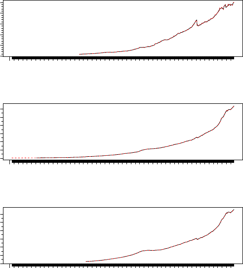
DMAM1
1959 1963 1967 1971 1975 1979 1983 1987 1991 1995 1999 2003 2007
0 50 100 200
Australian Monetary Aggregates
DMAM3
1959 1963 1967 1971 1975 1979 1983 1987 1991 1995 1999 2003 2007
0 400 800 1200
DMABM
1959 1963 1967 1971 1975 1979 1983 1987 1991 1995 1999 2003 2007
0 400 800 1200
2.6 zip
The zip interface allows the use of zipped files that can be read by read.table as
if each file is a database series (or group of series such as high, low, open, close,
for a stock). The dbname is a directory or url.zip does not support writing
data to the database.
The following retrieves zipped files from http://pitrading.com/free_market_
data.htm which provides some end of day data free of charge.
> library("TSmisc")
> pitr <- TSconnect("zip", dbname="http://pitrading.com/free_eod_data")
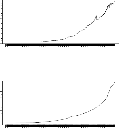
> z <- TSget("INDU", pitr)
> tfplot(z, series=c(1,4))
19
1920 1940 1960 1980 2000
INDU.Open
0 4000 8000 12000
1920 1940 1960 1980 2000
INDU.Close
0 4000 8000 12000
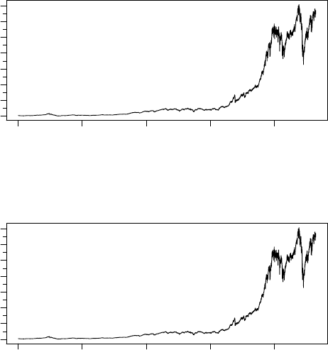
The following illustrates returning an xts (Ryan and Ulrich, 2011) time series
object.
> require("xts")
> z <- TSget(c("EURUSD", "GBPUSD"), pitr, quote=c("Open","Close"),
TSrepresentation=xts)
> tfplot(z,
title="EURUSD and GBPUSD open and closing values from pitrading",
start="1995-01-01",
par=list(omi=c(0.1,0.3,0.1,0.1),mar=c(2.1,3.1,1.0,0.1)))
20
1995 2000 2005 2010
EURUSD.Open
0.8 1.0 1.2 1.4 1.6
EURUSD and GBPUSD open and closing values from pitrading
1995 2000 2005 2010
EURUSD.Close
0.8 1.0 1.2 1.4 1.6
1995 2000 2005 2010
GBPUSD.Open
1.4 1.6 1.8 2.0
1995 2000 2005 2010
GBPUSD.Close
1.4 1.6 1.8 2.0
The default appearance of graphs can be changed (improved) by adjusting
graphics device margins omi and mar. (They are set by the vector in order:
bottom, left, top, right.) They can be set directly using par() or passed to
tfplot() as in this example. The default behaviour of tfplot() is a compromise
that usually works reasonally well for both screen and printed output. It is often
useful to adjust these when generating pdf files for publication.
3 SQL Time Series Databases
This section gives several simple examples of putting series on and reading them
from a database. (If a large number of series are to be loaded into a database,
one would typically do this with a batch process using the database program’s
utilities for loading data.) The examples in this section will use TSMySQL
but, other than the initial connection, access will be similar for other SQL TS*
packages. The syntax for connecting with other packages, and other options for
connecting with TSMySQL, are provided in Appendix “A”.
The packages TSPostgreSQL,TSMySQL,TSSQLite, and TSodbc use un-
derlying packages RPostgreSQL (Conway et al., 2012), RMySQL (James and
DebRoy, 2012), RSQLite (James, 2011), and RODBC (Ripley and from 1999 to
21
Oct 2002 Michael Lapsley, 2012). The TS* packages provide access to an SQL
database with an underlying table structure that is set up to store time series
data.
The next lines of code do some preliminary setup of the database. This uses
the underlying database connection (dbConnect) rather than TSconnect, be-
cause TSconnect will not recognize the database until it has been setup. Func-
ton removeTSdbTables() is used first to remove any existing tables, which would
cause createTSdbTables() to fail.
WARNING: running this will overwrite the “test” database on your server.
> setup <- RMySQL::dbConnect(RMySQL::MySQL(), dbname="test")
> TSsql::removeTSdbTables(setup, yesIknowWhatIamDoing=TRUE)
> TSsql::createTSdbTables(setup, index=FALSE)
> DBI::dbListTables(setup)
> DBI::dbDisconnect(setup)
3.1 Writing to SQL Databases
This subsection illustrates writing some simple artifical data to a database, and
reading it back. This part of the vignette is generated using TSMySQL, but
other backend SQL servers work in a similar way. See Appendix “A” for details
of establishing other SQL database connections.
The first thing to do is to establish a TSdbi connection to the database:
> library("TSMySQL")
> con <- TSconnect("MySQL", dbname="test")
TSconnect uses dbConnect from the DBI package, but checks that the database
has expected tables, and checks for additional features. (It cannot be used before
the tables are created, as was done above.)
The follow illustrates the use of the TSdbi interface, which is common to all
extension packages.
This puts a series called vec on the database and then reads is back
> z <- ts(rnorm(10), start=c(1990,1), frequency=1)
> seriesNames(z) <- "vec"
> if(TSexists("vec", con)) TSdelete("vec", con)
> TSput( z, con)
> z <- TSget("vec", con)
Note that the series name(s) and not the Rvariable name (in this case, vec
not z) are used on the database. If the retrieved series is printed it is seen to
be a “ts” time series with some extra attributes.
TSput fails if the series already exists on the con, so the above example
checks and deletes the series if it already exists. TSreplace does not fail if the
series does not yet exist, so examples below use it instead. TSput,TSdelete,
TSreplace, and TSexists all return logical values TRUE or FALSE.
22
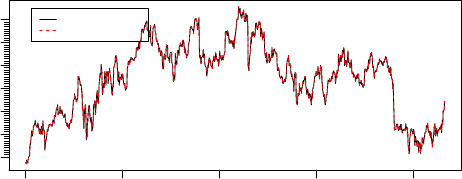
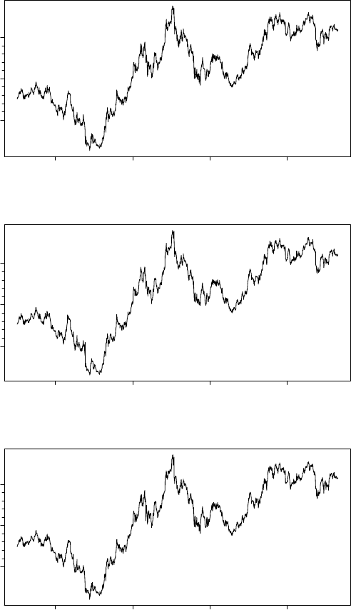
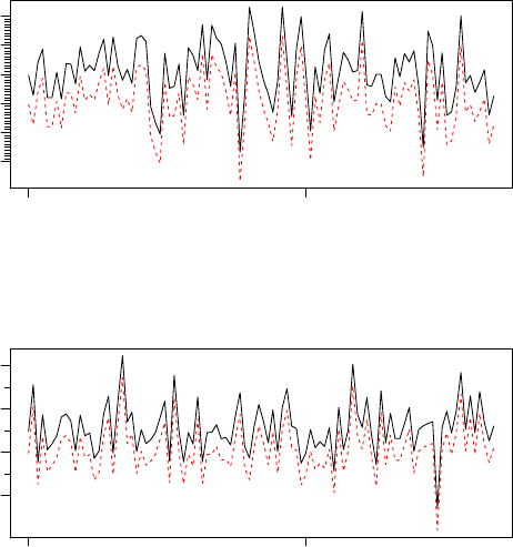
Several plots below show original data and the data retrieved after it is
written to the database. In the plot below, one is added to the original data so
that both lines are visible.
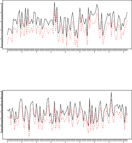
The Rvariable can contain multiple series of the same frequency. They are
stored separately on the database.
> z <- ts(matrix(rnorm(200),100,2), start=c(1995,1), frequency=12)
> seriesNames(z) <- c("mat2c1", "mat2c2")
> TSreplace(z, con)
[1] TRUE
> tfplot(z+1, TSget(c("mat2c1","mat2c2"), con),
lty=c("solid", "dashed"), col=c("black", "red"))
mat2c1
1995 1996 1997 1998 1999 2000 2001 2002 2003
−2 −1 0 1 2 3
mat2c2
1995 1996 1997 1998 1999 2000 2001 2002 2003
−2 0 1 2 3 4
The following extract information about the series from the database, al-
though not much information has been added for these examples.
> TSmeta("mat2c1", con)
serIDs: mat2c1
from dbname test using TSMySQLConnection
23
> TSmeta("vec", con)
serIDs: vec
from dbname test using TSMySQLConnection
> TSdates("vec", con)
[,1]
[1,] "vec from 1990 1 to 1999 1 A "
> TSdescription("vec", con)
[1] NA
> TSdoc("vec", con)
[1] NA
> TSlabel("vec", con)
[1] NA
Data documentation can be in three forms. A description specified by TS-
description, longer documentation specified by TSdoc, or a short label, typically
useful on a graph, specified by TSlabel. These can be added to the time se-
ries object, in which case they will be written to the database when TSput or
TSreplace is used to put the series on the database. Alternatively, they can
be specified as arguments to TSput or TSreplace. The description or documen-
tation will be retrieved as part of the series object with TSget only if this is
specified with the logical arguments TSdescription and TSdoc. They can also
be retrieved directly from the database with the functions TSdescription and
TSdoc.
> z <- ts(matrix(rnorm(10),10,1), start=c(1990,1), frequency=1)
> TSreplace(z, serIDs="Series1", con)
[1] TRUE
> zz <- TSget("Series1", con)
> TSreplace(z, serIDs="Series1", con,
TSdescription="short rnorm series",
TSdoc="Series created as an example in the vignette.")
[1] TRUE
> zz <- TSget("Series1", con, TSdescription=TRUE, TSdoc=TRUE)
> start(zz)
[1] 1990 1
24
> end(zz)
[1] 1999 1
> TSdescription(zz)
[1] "short rnorm series"
> TSdoc(zz)
[1] "Series created as an example in the vignette."
> TSdescription("Series1", con)
[1] "short rnorm series"
> TSdoc("Series1", con)
[1] "Series created as an example in the vignette."
The following examples use dates and times which are not handled by ts, so
the zoo time representation is used. It is necessary to specify the table where the
data should be stored in cases where it is difficult to determine the periodicity
of the data. See Appendix “B” for details of the specific tables.
> require("zoo")
> z <- zoo(matrix(rnorm(200),100,2), as.Date("1990-01-01") + 0:99)
> seriesNames(z) <- c("zooc1", "zooc2")
> TSreplace(z, con, Table="D")
[1] TRUE
> tfplot(z+1, TSget(c("zooc1","zooc2"), con),
lty=c("solid", "dashed"), col=c("black", "red"))
>
25
Jan Mar
zooc1
−2 −1 0 1 2 3
Jan Mar
zooc2
−2 0 2 4
> z <- zoo(matrix(rnorm(200),100,2), as.Date("1990-01-01") + 0:99 * 7)
> seriesNames(z) <- c("zooWc1", "zooWc2")
> TSreplace(z, con, Table="W")
[1] TRUE
> dbDisconnect(con)
> detach(package:TSMySQL)
4 More Examples
4.1 Examples Using SQL Databases
This section illustrates fetching data from the web and loading it into the
database. This would be a very slow way to load a database, but provides exam-
ples of different kinds of time series data. The fetching is done with histQuote.
Fetching data can fail due to lack of an Internet connection or delays, which will
cause the generation of this vignette to fail.
26
This part of the vignette is generated using TSPostgreSQL, but other back-
end SQL servers work in a similar way. See Appendix “A” for details of estab-
lishing other SQL database connections.
First set up the TS database structure on the database where data will be
saved (if it is not already in place)
> host <- Sys.getenv("POSTGRES_HOST")
> setup <- DBI::dbConnect(RPostgreSQL::PostgreSQL(), dbname="test", host=host)
> TSsql::createTSdbTables(setup)
tables:
[1] "meta" "a" "b" "d" "m" "u" "q" "s" "w" "i"
[11] "t"
> DBI::dbDisconnect(setup)
[1] TRUE
Then establish a TS connection to it:
> require("TSPostgreSQL")
> con <- TSconnect("PostgreSQL", dbname="test", host=host)
Now connect to the web server and fetch data:
> require("TSmisc")
> yahoo <- TSconnect("histQuote", dbname="yahoo")
> x <- TSget("^gspc", quote = "Close", con=yahoo)
Then write the data to the local server, specifying table B for business day
data (using TSreplace in case the series is already there from running this ex-
ample previously):
> TSreplace(x, serIDs="gspc", Table="B", con=con)
[1] TRUE
and check the saved version:
> TSrefperiod(TSget(serIDs="gspc", con=con))
[1] "Close"
> TSdescription("gspc", con=con)
[1] "^gspc Close from yahoo"
> TSdoc("gspc", con=con)
[1] "^gspc Close from yahoo retrieved 2015-04-30 17:37:57"
27
> tfplot(TSget(serIDs="gspc", con=con))
1995 2000 2005 2010 2015
gspc
500 1000 1500 2000
> x <- TSget("ibm", quote = c("Close", "Vol"), con=yahoo)
> TSreplace(x, serIDs=c("ibm.Cl", "ibm.Vol"), con=con, Table="B",
TSdescription.=c("IBM Close","IBM Volume"),
TSdoc.= paste(c(
"IBM Close retrieved on ",
"IBM Volume retrieved on "), Sys.Date()))
[1] TRUE
> z <- TSget(serIDs=c("ibm.Cl", "ibm.Vol"),
TSdescription=TRUE, TSdoc=TRUE, con=con)
> TSdescription(z)
[1] "IBM Close" "IBM Volume"
> TSdoc(z)
[1] "IBM Close retrieved on 2015-04-30"
[2] "IBM Volume retrieved on 2015-04-30"
> tfplot(z, xlab = TSdoc(z), title = TSdescription(z))
> tfplot(z, title="IBM", start="2007-01-01")
28
1995 2000 2005 2010 2015
IBM Close retrieved on 2015−04−30
ibm.Cl
50 100 150 200 250
IBM Close
IBM Volume
1995 2000 2005 2010 2015
IBM Volume retrieved on 2015−04−30
ibm.Vol
0e+00 3e+07 6e+07
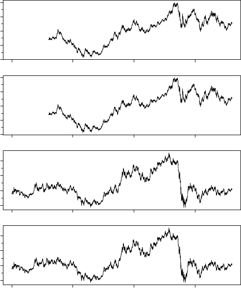
Oanda has maximum of 500 days, so the start date is specified here so as to
not exceed that.
> Oanda <- TSconnect("histQuote", dbname="oanda")
> x <- TSget("EUR/USD", start=Sys.Date() - 495, con=Oanda)
> TSreplace(x, serIDs="EUR/USD", Table="D", con=con)
[1] TRUE
Then check the saved version:
> z <- TSget(serIDs="EUR/USD",TSlabel=TRUE,
TSdescription=TRUE, con=con)
> tfplot(z, title = TSdescription(z), ylab=TSlabel(z),
start="2007-03-01")
29
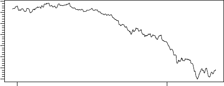
2014 2015
1.05 1.15 1.25 1.35
EUR/USD Close from oanda
> dbDisconnect(con)
> dbDisconnect(yahoo)
> dbDisconnect(Oanda)
> detach(package:TSPostgreSQL)
5 Comparing Time Series Databases
The purpose of package TScompare is to compare pairs of series on two database.
These series might have the same name, but for generality the main function,
TScompare, is set up to use name pairs. The pairs to compare are indicated by
a matrix of strings with two columns. (It would also be possible to compare
pairs on the same database, which might make sense if the names are different.)
The connections are established using other TSdbi packages such as TSMySQL,
TSPostgreSQL, etc. It will be necessary to establish two database connections,
so it will also be necessary to load the database specific packages. Examples
below use histQuote,TSMySQL and TSSQLite.
> library("TScompare")
> library("TSmisc")
> library("TSMySQL")
> library("TSSQLite")
First setup database tables that are used by TSdbi using a dbConnect con-
nection, after which a TSconnect connection can be used. This uses the package
TSsql which does not need to be attached for most purposes, but is needed for
the initial setup and for removing TSdbi database tables (which destroys the
structure TSconnect expects). When this is re-done it insure the databases are
empty:
> setup <- RMySQL::dbConnect(RMySQL::MySQL(), dbname="test")
> TSsql::removeTSdbTables(setup, yesIknowWhatIamDoing=TRUE)
> TSsql::createTSdbTables(setup, index=FALSE)
30
> DBI::dbListTables(setup)
> DBI::dbDisconnect(setup)
> setup <- RSQLite::dbConnect(RSQLite::SQLite(), dbname="test")
> TSsql::removeTSdbTables(setup, yesIknowWhatIamDoing=TRUE)
> TSsql::createTSdbTables(setup, index=FALSE)
> DBI::dbListTables(setup)
> DBI::dbDisconnect(setup)
Now TS connections to the databases are established.
> con1 <- TSconnect("MySQL", dbname="test")
> con2 <- TSconnect("SQLite", dbname="test")
Next a connection to yahoo is used to get some series and write them to
the local test database. TSreplace is used because TSput will fail if the series
already exisits.
> yahoo <- TSconnect("histQuote", dbname="yahoo")
> x <- TSget("^ftse", yahoo)
> TSreplace(x, serIDs="ftse", Table="B", con=con1)
[1] TRUE
> TSreplace(x, serIDs="ftse", Table="B", con=con2)
[1] TRUE
> x <- TSget("^gspc", yahoo)
> TSreplace(x, serIDs="gspc", Table="B", con=con1)
[1] TRUE
> TSreplace(x, serIDs="gspc", Table="B", con=con2)
[1] TRUE
> x <- TSget("ibm", con=yahoo, quote = c("Close", "Vol"))
> TSreplace(x, serIDs=c("ibmClose", "ibmVol"), Table="B", con=con1)
[1] TRUE
> TSreplace(x, serIDs=c("ibmC", "ibmV"), Table="B", con=con2)
[1] TRUE
Now to do a comparison:
> ids <- AllIds(con1)
> ids
31
[1] "ftse" "gspc" "ibmClose" "ibmVol"
If the second database has the same names then ids can be made into a
matrix with identical columns.
> ids <- cbind(ids, ids)
> eq <- TScompare(ids, con1, con2, na.rm=FALSE)
> summary(eq)
4 of 4 are available on con1.
2 of 4 are available on con2.
2 of 2 remaining have the same window.
2 of 2 remaining have the same window and values.
> eqrm <- TScompare(ids, con1, con2, na.rm=TRUE)
> summary(eqrm)
4 of 4 are available on con1.
2 of 4 are available on con2.
2 of 2 remaining have the same window.
2 of 2 remaining have the same window and values.
Since names are not identical the above indicates discrepancies, which are
resolves by indicating the corresponding name pairs:
> ids <- matrix(c("ftse","gspc","ibmClose", "ibmVol",
"ftse","gspc","ibmC", "ibmV"),4,2)
> ids
[,1] [,2]
[1,] "ftse" "ftse"
[2,] "gspc" "gspc"
[3,] "ibmClose" "ibmC"
[4,] "ibmVol" "ibmV"
> eq <- TScompare(ids, con1, con2, na.rm=FALSE)
> summary(eq)
4 of 4 are available on con1.
4 of 4 are available on con2.
4 of 4 remaining have the same window.
4 of 4 remaining have the same window and values.
> eqrm <- TScompare(ids, con1, con2, na.rm=TRUE)
> summary(eqrm)
4 of 4 are available on con1.
4 of 4 are available on con2.
4 of 4 remaining have the same window.
4 of 4 remaining have the same window and values.
32
While it may not be necessary to detach packages, the following prevents
warnings later about objects being masked:
> dbDisconnect(con1)
> dbDisconnect(con2)
> dbDisconnect(yahoo)
> detach(package:TSMySQL)
> detach(package:TSSQLite)
6 Vintages of Realtime Data
Examples in the section have been disabled pending availability of a different
dataset.
Data vintages, or “realtime data” are snapshots of data that was available
at different points in time. The most obvious feature of earlier snapshots is
that the series end earlier. However, the reason for retaining vintages is that
data is often revised, so, for some observations, earlier vintages have different
data. Typically most revisions happen for the most recent periods, but this is
often the data of most interest for forcasting and policy decisions. Thus, the
revision records are valuable for understanding the implications of differences
between early and revised releases of the data. A simple mechanism for accessing
vintages of data is available in several TS* packages. This is illustrated here
with an SQL database that has been set up with vintage support.
First establish a connection to th database and get a vector of the available
vintages:
> require("TSMySQL")
> require("tfplot")
> ets <- TSconnect("MySQL",dbname="etsv")
> v <- TSvintages(ets)
The following checks if a certain variable (Consumer Credit – V122707) is
available in the different vintages. (V numbers replaced B numbers circa 2003,
so the V numbers do not exist in older vintages. This could be supported by
implementing aliases, but that has not been done here.)
> ve <- TSexists("V122707", vintage=v, con=ets)
> ve[224:length(ve)] <- FALSE
The vintages can them be retrieved and plotted by
> CC <- TSget(serIDs="V122707", con=ets, vintage=v[ve])
> tfOnePlot(ytoypc(CC), start=c(2000,1),
ylab="Consumer Credit (V122707) y/y Growth",
title=paste("Vintages", v[ve][1], "to", v[ve][189]),
lastObs=TRUE, source="Source: Bank of Canada")
33

With package TSfame vintages are supported if the vintages are stored in
files with names like “etsmfacansim 20110513.db”. Then the vintages can be
accessed as follows:
> dbs <- paste("ets /path/to/etsmfacansim_", c(
"20110513.db", "20060526.db", "20110520.db"), sep="")
> names(dbs) <- c("2011-05-13", "2006-05-26", "2011-05-20")
> conetsV <-TSconnect("fame", dbname=dbs, "read", current="2011-05-13")
> z <- TSget("V122646", con=conetsV, vintage=c("2011-05-13", "2006-05-26"))
> dbDisconnect(conetsV)
(The above example should work, but beware that I am no longer testing it
because I no longer have Fame access.)
The package googleVis can be used to produce a plot that is very useful for
examining vintage more closely, and finding outliers and other data problems.
The names are used in the legend of this next plot, so the series names are
specified in the argument to ytoypc. (Otherwise they get reset to indicate the
year-to-year calculation, which makes the legend messy to read.)
> require("googleVis")
> tfVisPlot(ytoypc(CC, names=seriesNames(CC)), start=c(2006,1),
options=list(title="Vintages of Consumer Credit (V122707) y/y Growth"))
This will produce a graph in your web browser. It is not reproduced here.
(And beware that it may not be very fast.) Pointing your mouse at the legend
of this plot will highlight the corresponding vintage, and pointing at the graph
will give information about the source of a data point.
> dbDisconnect(ets)
> detach(package:TSMySQL)
7 Just Want Data in a xls or csv File
Occasionally one may need to get data into a program other than R. Or, perhaps
you have a friend that does not want to use Rbut would like easy access to data.
This section describes two utilities for putting time series data obtained with
TSdbi connections into .xls and .csv files. Since it is often straight forward to
downlaod an xls or csv file from a web site in the first place, the advantage of
this will usually be only in the case where you need to repeatedly get the data.
In that case, the process can be automated with these tools.
The starting point will be to get some data. Previous sections illustrate
several possibilities. For example purposes here use
> library("TSsdmx")
> # RJSDMX::sdmxHelp() # can be useful for finding series identifiers, etc
>
> oecd <- TSconnect("sdmx", dbname="OECD")
34

> x <- TSget( QNA.CAN|MEX|USA|.PPPGDP.CARSA.Q , oecd)
>
While this is optional, it might be useful to look at the data to see if it is
really what you expect:
> library("tframePlus")
> library("tfplot")
> tfplot(x, title="Nominal GDP at PPP? (relative to US)",
subtitle=paste(c("Canada","Mexico","US"),"quarterly national accounts, SAAR"),
ylab=rep("guess the units",3))
35
guess the units
1955 1959 1963 1967 1971 1975 1979 1983 1987 1991 1995 1999 2003 2007 2011
0.95 1.00 1.05 1.10 1.15 1.20 1.25
Canada quarterly national accounts, SAAR
Nominal GDP at PPP? (relative to US)
guess the units
1955 1959 1963 1967 1971 1975 1979 1983 1987 1991 1995 1999 2003 2007 2011
0 2 4 6 8
Mexico quarterly national accounts, SAAR
guess the units
1955 1959 1963 1967 1971 1975 1979 1983 1987 1991 1995 1999 2003 2007 2011
0.6 0.8 1.0 1.2 1.4
US quarterly national accounts, SAAR
If the data in one series starts at a different time then zwill be filled with
NA for missing points. It is possible to trim the NA data from the beginning
with
> start(x)
[1] 1955 1
36
> x <- trimNA(x, endNAs=FALSE)
> start(x)
[1] 1960 1
By default, trimNA will trim all series if any one of them is NA, so trimming
the end will not be what you want if you are interested in the most recent data.
Setting endNAs=FALSE) overrides the default.
It is also possible to trim the data to a specified subsample with
> x <- tfwindow(x, start=c(1995,1))
Now write the data to an .xls file using TSwriteXLS which uses WriteXLS
(Schwartz, 2012) but automatically adds time information:
> library("WriteXLS")
> tofile <- tempfile(fileext = ".xls")
> TSwriteXLS(x, FileName=tofile)
> unlink(tofile)
In this case a temporary file is written, then removed with unlink, so that
scratch files do not accumulate from building this vignette, but you would typ-
ically use a more meaningful name, and not remove the file. It is also possible
to write multiple sheets in the file. For more details on this see the help
> ?TSwriteXLS
The dates are written in some different formats in the .xls file, since this
is often convenient for calculations and graphing in a spreadsheet program.
Beware that .xls files have size limitations that you might encounter if you try
to put large amounts of data into the file. Consider using .csv files in that case.
To write the data to a .csv file
> tofile <- tempfile(fileext = ".csv")
> TSwriteCSV(x, FileName=tofile)
> unlink(tofile)
References
Conway, J., Eddelbuettel, D., Nishiyama, T., Prayaga, S. K., and Tiffin, N.
(2012). RPostgreSQL: R interface to the PostgreSQL database system. R
package version 0.3-2.
Couture-Beil, A. (2013). rjson: JSON for R. R package version 0.2.13.
James, D. A. (2011). RSQLite: SQLite interface for R. R package version
0.11.1.
James, D. A. and DebRoy, S. (2012). RMySQL: R interface to the MySQL
database. R package version 0.9-3.
37
Lang, D. T. (2012). RJSONIO: Serialize R objects to JSON, JavaScript Object
Notation. R package version 1.0-1.
Mattiocco, A., Nicoletti, D., Lopez, G., and d’Italia, B. (2014). RJSDMX: R
Interface to SDMX Web Services. R package version 1.3.
R Core Team (2013). R: A Language and Environment for Statistical Comput-
ing. R Foundation for Statistical Computing, Vienna, Austria.
R Core Team (2014). R: A Language and Environment for Statistical Comput-
ing. R Foundation for Statistical Computing, Vienna, Austria.
R Special Interest Group on Databases (2009). DBI: R Database Interface. R
package version 0.2-5.
Ripley, B. and from 1999 to Oct 2002 Michael Lapsley (2012). RODBC: ODBC
Database Access. R package version 1.3-6.
Ryan, J. A. (2011). quantmod: Quantitative Financial Modelling Framework. R
package version 0.3-17.
Ryan, J. A. and Ulrich, J. M. (2011). xts: eXtensible Time Series. R package
version 0.8-2.
Schwartz, M. (2012). WriteXLS: Cross-platform Perl based R function to create
Excel 2003 (XLS) files. R package version 2.1.1.
Trapletti, A. and Hornik, K. (2012). tseries: Time Series Analysis and Compu-
tational Finance. R package version 0.10-28.
Warnes, G. R., with contributions from Ben Bolker, Gorjanc, G., Grothendieck,
G., Korosec, A., Lumley, T., MacQueen, D., Magnusson, A., Rogers, J., and
others (2011). gdata: Various R programming tools for data manipulation. R
package version 2.8.2.
Zeileis, A. and Grothendieck, G. (2005). zoo: S3 infrastructure for regular and
irregular time series. Journal of Statistical Software, 14(6):1–27.
38
