Guide
ParaViewGuide-5.3.0
User Manual: Pdf
Open the PDF directly: View PDF ![]() .
.
Page Count: 251 [warning: Documents this large are best viewed by clicking the View PDF Link!]
- I User's Guide
- Introduction to ParaView
- Loading data
- Understanding data
- Displaying data
- Filtering data
- Understanding filters
- Creating filters in paraview
- Creating filters in pvpython
- Changing filter properties in paraview
- Changing filter properties in pvpython
- Filters for sub-setting data
- Filters for geometric manipulation
- Filters for sampling
- Filters for attribute manipulation
- White-box filters
- Best practices
- Selecting data
- Animation
- Saving results
- II Reference Manual
- Properties panel
- Customizing defaults
- Color maps and transfer functions
- Comparative visualization
- Programmable Filter
- Using NumPy for processing data
- Remote and parallel visualization
- Memory Inspector
- Multiblock Inspector
- Axes Grid
- Settings
- III Appendix

The ParaView Guide
Community Edition
Updated for ParaView version 5.0
Utkarsh Ayachit
With contributions from:
Berk Geveci, Cory Quammen, Dave DeMarle,
Ken Moreland, Andy Bauer, Ben Boeckel,
Dan Lipsa, Mathieu Westphal, Joachim Pouderoux,
Shawn Waldon, Aashish Choudhary, Sujin Philip,
George Zagaris, Burlen Loring,
Thomas Maxwell, John Patchett, James Ahrens,
Boonthanome Nouanesengsy, Bill Sherman,
Nikhil Shetty, Eric Whiting,
and the ParaView community
Editors:
Lisa Avila, Katie Osterdahl, Sandy McKenzie,
and Steve Jordan
November 10, 2016
http://paraview.org
http://kitware.com

Published by Kitware Inc. c
2016
All product names mentioned herein are the trademarks of their respective owners.
Part I and Part II of this document are available under a Creative Commons Attribution 4.0 International license available
at http://www.paraview.org/download/.
This project has been funded in whole or in part with Federal funds from the Department of Energy, including from
Sandia National Laboratories, Los Alamos National Laboratory (LANL), Advanced Simulation and Computing (ASC),
and the Army Research Laboratory (ARL).
Printed and produced in the United States of America.
ISBN number FILL IN ISBN NUMBERS HERE

CONTRIBUTORS
This book includes contributions from the ParaView community including the ParaView development team and the user
community. We would like to thank the following people for their significant contributions to this updated text:
Cory Quammen,Berk Geveci,Ben Boeckel,Dave DeMarle, and Shawn Waldon from Kitware for their contributions
throughout the text.
Ken Moreland, for large sections of text from his excellent The ParaView Tutorial[1] that formed the basis of Chap-
ter 15. Thomas Maxwell from National Aeronautics and Space Administration (NASA), John Patchett,Boonthanome
Nouanesengsy, and James Ahrens from Los Alamos National Labs (LANL), Bill Sherman from Indiana University,
Nikhil Shetty from the University of Wyoming, Aashish Choudhary from Kitware. Burlen Loring from Lawrence
Berkeley National Laboratory authored wiki posts that were made into Chapter 16.
Special thanks to the Kitware communications team including Katie Osterdahl,Sandy McKenzie,Lisa Avila, and Steve
Jordan. This guide would not have been possible without their patient and persistent efforts.
ABOUT THE COVER
The cover image is a visualization of magnetic reconnection from the VPIC project at Los Alamos National Laboratory.
The visualization is generated from a structured data containing 3.3 billion cells with two vector fields and one scalar
field, produced using 256 cores running ParaView on the interactive queue on the Kraken at the National Institute for
Computational Sciences (NICS).
The interior cover image is courtesy of Renato N. Elias, Associate Researcher at the CFD Group from NACAD/-
COPPE/UFRJ, Rio de Janeiro, Brazil.
The cover design was done by Steve Jordan.
Join the ParaView Commuity at www.paraview.org
CONTENTS
I User’s Guide 1
1 Introduction to ParaView 3
1.1 Introduction ......................................................... 3
1.1.1 In this guide ..................................................... 4
1.1.2 Getting help ..................................................... 4
1.1.3 Getting the software ................................................ 4
1.2 Basics of visualization in ParaView ............................................. 4
1.3 ParaView executables .................................................... 6
paraview ....................................................... 6
pvpython ....................................................... 6
pvbatch ....................................................... 6
pvserver ....................................................... 6
pvdataserver and pvrenderserver ........................................ 6
1.4 Getting started with paraview ................................................ 6
1.4.1 paraview graphical user interface ......................................... 6
1.4.2 Understanding the visualization process ...................................... 8
Creating a source ................................................... 8
Changing properties ................................................. 10
Applying filters .................................................... 10
1.5 Getting started with pvpython ................................................ 11
1.5.1 pvpython scripting interface ............................................ 12
1.5.2 Understanding the visualization process ...................................... 12
Creating a source ................................................... 12
Changing properties ................................................. 13
Applying filters .................................................... 14

CONTENTS
Alternative approach ................................................. 16
1.5.3 Updating the pipeline ................................................ 16
1.6 Scripting in paraview .................................................... 18
1.6.1 The Python shellPython shell .......................................... 18
1.6.2 Tracing actions for scripting ............................................ 18
2 Loading data 21
2.1 Opening data files in paraview ............................................... 21
2.1.1 Dealing with unknown extensions ......................................... 22
2.1.2 Handling temporal file series ............................................ 23
2.1.3 Dealing with time .................................................. 23
2.1.4 Reopening previously opened files ......................................... 23
2.1.5 Opening files using command line options ..................................... 24
2.1.6 Common properties for readers ........................................... 24
Selecting data arrays ................................................. 25
2.2 Opening data files in pvpython ............................................... 26
2.2.1 Handling temporal file series ............................................ 28
2.2.2 Dealing with time .................................................. 28
2.2.3 Common properties on readers ........................................... 28
Selecting data arrays ................................................. 28
2.3 Reloading files ........................................................ 30
3 Understanding data 31
3.1 VTK data model ....................................................... 31
3.1.1 Mesh ........................................................ 31
3.1.2 Attributes (fields, arrays) .............................................. 32
3.1.3 Uniform rectilinear grid (image data) ........................................ 32
3.1.4 Rectilinear grid ................................................... 33
3.1.5 Curvilinear grid (structured grid) .......................................... 34
3.1.6 AMR dataset .................................................... 35
3.1.7 Unstructured grid .................................................. 35
3.1.8 Polygonal grid (polydata) .............................................. 36
3.1.9 Table ........................................................ 37
3.1.10 Multiblock dataset ................................................. 37
3.1.11 Multipiece dataset .................................................. 38
3.2 Getting data information in paraview ............................................ 38
3.2.1 The Information panel .............................................. 38
3.2.2 The Statistics Inspector panel ........................................ 40
vi CONTENTS

CONTENTS
3.3 Getting data information in pvpython ............................................ 40
4 Displaying data 47
4.1 Multiple views ........................................................ 47
4.1.1 Multiple views in paraview ............................................ 47
4.1.2 Multiple views in pvpython ............................................ 49
4.2 View properties ........................................................ 50
4.2.1 View properties in paraview ............................................ 50
4.2.2 View properties in pvpython ............................................ 50
4.3 Display properties ...................................................... 51
4.3.1 Display properties in paraview .......................................... 51
4.3.2 Display properties in pvpython .......................................... 52
4.4 Render View ......................................................... 53
4.4.1 Understanding the rendering process ........................................ 53
4.4.2 Render View in paraview ............................................. 54
Creating a Render View ............................................... 54
Interactions ...................................................... 54
View properties .................................................... 55
Display properties .................................................. 57
4.4.3 Render View in pvpython ............................................. 62
Creating a Render View ............................................... 62
Interactions ...................................................... 62
View properties .................................................... 63
Display properties .................................................. 64
4.5 Line Chart View ....................................................... 64
4.5.1 Understanding plotting ............................................... 65
4.5.2 Line Chart View in paraview ........................................... 65
Creating a Line Chart View ............................................. 65
Interactions ...................................................... 65
View properties .................................................... 66
Display properties .................................................. 66
4.5.3 Line Chart View in pvpython ........................................... 68
4.6 Bar Chart View ........................................................ 69
4.7 Plot Matrix View ....................................................... 70
4.7.1 Interactions ..................................................... 70
4.7.2 View properties ................................................... 70
4.7.3 Display properties .................................................. 71
CONTENTS vii

CONTENTS
4.8 Parallel Coordinates View .................................................. 71
4.9 Spreadsheet View ...................................................... 71
4.10 Slice View .......................................................... 72
4.10.1 Interactions ..................................................... 72
4.10.2 Slice View in pvpython .............................................. 72
4.11 Python View ......................................................... 73
4.11.1 Selecting data arrays to plot ............................................ 74
4.11.2 Plotting data in Python ............................................... 76
Set up a matplotlib Figure .............................................. 77
4.12 Comparative Views ...................................................... 77
5 Filtering data 79
5.1 Understanding filters ..................................................... 79
5.2 Creating filters in paraview ................................................. 80
5.2.1 Multiple input connections ............................................. 81
5.2.2 Multiple input ports ................................................. 81
5.2.3 Changing input connections ............................................ 81
5.3 Creating filters in pvpython ................................................. 83
5.3.1 Multiple input connections ............................................. 83
5.3.2 Multiple input ports ................................................. 84
5.3.3 Changing input connections ............................................ 84
5.4 Changing filter properties in paraview ........................................... 84
5.5 Changing filter properties in pvpython ........................................... 84
5.6 Filters for sub-setting data .................................................. 85
5.6.1 Clip ......................................................... 86
Clip in paraview ................................................... 86
Clip in pvpython ................................................... 87
5.6.2 Slice ......................................................... 89
5.6.3 Extract Subset .................................................... 90
Extract Subset in paraview ............................................. 90
5.6.4 Threshold ...................................................... 90
Threshold in paraview ................................................ 90
Threshold in pvpython ................................................ 91
5.6.5 Iso Volume ..................................................... 92
5.6.6 Extract Selection .................................................. 92
5.7 Filters for geometric manipulation .............................................. 92
5.7.1 Transform ...................................................... 92
viii CONTENTS

CONTENTS
5.7.2 Transform in paraview ............................................... 92
5.7.3 Transform in pvpython ............................................... 93
5.7.4 Reflect ........................................................ 93
5.7.5 Warp By Vector ................................................... 94
5.7.6 Warp By Scalar ................................................... 94
5.8 Filters for sampling ...................................................... 94
5.8.1 Glyph ........................................................ 94
5.8.2 Glyph With Custom Source ............................................. 96
5.8.3 Stream Tracer .................................................... 96
5.8.4 Stream Tracer With Custom Source ........................................ 98
5.8.5 Resample With Dataset ............................................... 98
5.8.6 Resample To Image ................................................. 99
5.8.7 Probe ........................................................100
5.8.8 Plot over line ....................................................101
5.9 Filters for attribute manipulation ...............................................101
5.9.1 Calculator ......................................................101
5.9.2 Python calculator ..................................................102
Basic tutorial .....................................................103
Accessing data ....................................................104
Comparing multiple datasets .............................................104
Basic Operations ...................................................105
Functions .......................................................106
Trigonometric Functions ...............................................107
5.9.3 Gradient .......................................................108
5.9.4 Mesh Quality ....................................................108
5.10 White-box filters .......................................................108
5.11 Best practices .........................................................108
5.11.1 Avoiding data explosion ..............................................108
5.11.2 Culling data .....................................................110
6 Selecting data 113
6.1 Understanding selection ...................................................113
6.2 Creating selections using views ...............................................115
6.2.1 Selecting in Render View ..............................................115
6.2.2 Selecting in SpreadSheet View ...........................................116
6.2.3 Selecting in Line Chart View ............................................116
6.3 Creating selections using the Find Data dialog .......................................117
CONTENTS ix

CONTENTS
6.4 Displaying selections .....................................................120
6.5 Extracting selections .....................................................120
6.5.1 Extract selection ..................................................120
6.5.2 Plot selection over time ...............................................120
6.6 Freezing selections ......................................................121
7 Animation 123
7.1 Animation View. .......................................................123
7.2 Animation View header ...................................................124
7.3 Animating time-varying data .................................................125
7.4 Playing an animation .....................................................126
7.5 Animating the camera ....................................................126
7.5.1 Interpolate camera locations ............................................127
7.5.2 Orbit .........................................................127
7.5.3 Follow path .....................................................128
8 Saving results 129
8.1 Saving datasets ........................................................129
8.2 Saving rendered results ....................................................130
8.2.1 Saving screenshots .................................................130
8.2.2 Exporting scenes ..................................................132
8.3 Saving animation .......................................................132
8.4 Saving state ..........................................................133
II Reference Manual 135
9 Properties panel 137
9.1 Anatomy of the Properties panel .............................................137
9.1.1 Buttons .......................................................137
9.1.2 Search box .....................................................137
9.1.3 Properties ......................................................138
9.2 Customizing the layout ....................................................139
10 Customizing defaults 141
10.1 Customizing defaults for properties .............................................141
10.2 Example: specifying a custom background color ......................................141
10.3 Configuring default settings with JSON ...........................................142
10.4 Configuring site-wide default settings ............................................143
x CONTENTS

CONTENTS
11 Color maps and transfer functions 145
11.1 The basics ..........................................................145
11.1.1 Color mapping in paraview ............................................146
11.1.2 Color mapping in pvpython ............................................146
11.2 Editing the transfer functions in paraview .........................................147
11.2.1 Mapping data ....................................................148
11.2.2 Transfer function editor ...............................................149
11.2.3 Color mapping parameters .............................................150
11.3 Editing the transfer functions in pvpython .........................................150
11.4 Color legend .........................................................151
11.4.1 Color legend parameters ..............................................152
11.4.2 Color legend in pvpython .............................................153
11.5 Annotations ..........................................................154
11.5.1 Annotations in pvpython ..............................................155
11.6 Categorical colors ......................................................155
Categorical Color: User Interface ..........................................156
Categorical colors in pvpython ...........................................157
12 Comparative visualization 159
12.1 Setting up a comparative view ................................................159
12.2 Setting up a parameter study .................................................160
12.3 Adding annotations ......................................................162
13 Programmable Filter 163
13.1 Understanding the programmable modules .........................................164
13.2 Recipes for Programmable Source ..............................................165
13.2.1 Reading a CSV file .................................................165
13.2.2 Reading a CSV file series ..............................................166
13.2.3 Reading a CSV file with particles .........................................167
13.2.4 Reading binary 2D image ..............................................168
13.2.5 Helix source .....................................................168
13.3 Recipes for Programmable Filter ...............................................170
13.3.1 Adding a new point/cell data array based on an input array ............................171
13.3.2 Computing tetrahedra volume ...........................................171
13.3.3 Labeling common points between two datasets ..................................172
13.3.4 Coloring points ...................................................172
14 Using NumPy for processing data 175
CONTENTS xi

CONTENTS
14.1 Teaser .............................................................175
14.2 Understanding the dataset adapter module .......................................176
14.2.1 Dataset attributes ..................................................177
14.3 Working with arrays .....................................................178
14.3.1 The array API ....................................................179
14.3.2 Algorithms .....................................................180
14.4 Handling composite datasets .................................................181
15 Remote and parallel visualization 185
15.1 Understanding remote processing ..............................................185
15.2 Remote visualization in paraview ..............................................186
15.2.1 Starting a remote server ...............................................186
15.2.2 Configuring a server connection ..........................................186
15.2.3 Connect to the remote server ............................................188
15.2.4 Setting up a client/server visualization pipeline ..................................189
15.3 Remote visualization in pvpython ..............................................189
15.4 Reverse connections .....................................................189
15.5 Understanding parallel processing ..............................................190
15.5.1 Ghost levels .....................................................192
15.5.2 Data partitioning ..................................................192
15.5.3 D3 Filter .......................................................193
15.6 ParaView architecture ....................................................194
15.7 Parallel processing in paraview and pvpython .......................................196
15.8 Using pvbatch ........................................................197
15.9 Rendering ..........................................................198
15.9.1 Basic Rendering Settings ..............................................198
15.9.2 Basic Parallel Rendering ..............................................200
15.9.3 Image Level of Detail ................................................202
15.9.4 Parallel Render Parameters .............................................203
15.9.5 Parameters for Large Data .............................................204
16 Memory Inspector 207
16.1 User interface and layout ...................................................208
16.2 Advanced debugging features ................................................208
16.2.1 Remote commands .................................................208
16.2.2 Stack trace signal handler ..............................................209
16.3 Compilation and installation considerations .........................................210
xii CONTENTS

CONTENTS
17 Multiblock Inspector 213
18 Axes Grid 215
18.1 The basics ..........................................................215
18.2 Use cases ...........................................................215
18.3 Axes Grid in pvpython ...................................................217
19 Settings 221
19.1 General settings .......................................................221
19.2 Camera settings ........................................................223
19.3 Render View settings ....................................................224
19.4 Color Palette .......................................................224
III Appendix 227
Bibliography 229
Indexes 231
paraview UI Index .........................................................232
pvpython Index ...........................................................237
CONTENTS xiii
Part I
User’s Guide
CHAPTER
ONE
INTRODUCTION TO PARAVIEW
1.1 Introduction
ParaView is an open-source, multi-platform scientific data analysis and visualization tool that enables analysis and visual-
ization of extremely large datasets. ParaView is both a general purpose, end-user application with a distributed architecture
that can be seamlessly leveraged by your desktop or other remote parallel computing resources and an extensible frame-
work with a collection of tools and libraries for various applications including scripting (using Python), web visualization
(through ParaViewWeb), or in-situ analysis (with Catalyst).
ParaView leverages parallel data processing and rendering to enable interactive visualization for extremely large datasets.
It also includes support for large displays including tiled displays and immersive 3D displays with head tracking and wand
control capabilities.
ParaView also supports scripting and batch processing using Python. Using included Python modules, you can write scripts
that can perform almost all the functionality exposed by the interactive application and much more.
ParaView is open-source (BSD licensed, commercial software friendly). As with any successful open-source project,
ParaView is supported by an active user and developer community. Contributions to both the code and this user’s manual
that help make the tool and the documentation better are always welcome.
Did you know?
The ParaView project started in 2000 as a collaborative effort between Kitware Inc. and LANL. The initial funding
was provided by a three year contract with the US Department of Energy ASCI Views program. The first public
release, ParaView 0.6, was announced in October 2002.
Independent of ParaView, Kitware started developing a web-based visualization system in December 2001. This
project was funded by Phase I and II SBIRs from the US Arm Research Laboratory (ARL) and eventually became
the ParaView Enterprise Edition. PVEE significantly contributed to the development of ParaView’s client/server
architecture. PVEE was the precursor to ParaViewWeb, a modern web visualization solution based on ParaView.
Since the project began, Kitware has successfully collaborated with Sandia, LANL, the ARL, and various other
academic and government institutions to continue development. Today, the project is still going strong!
In September 2005, Kitware, Sandia National Labs and CSimSoft started the development of ParaView 3.0. This
was a major effort focused on rewriting the user interface to be more user friendly and on developing a quantitative
analysis framework. ParaView 3.0 was released in May 2007.

1.2. Basics of visualization in ParaView
1.1.1 In this guide
This user’s manual is designed as a guide for using the ParaView application. It is geared toward users who have a general
understanding of common data visualization techniques. For scripting, a working knowledge of the Python language is
assumed. If you are new to Python, there are several tutorials and guides for getting started that are available on the Internet.
Did you know?
In this guide, we will periodically use these Did you know? boxes to provide additional information related to the
topic at hand.
Common Errors
Common Errors blocks are used to highlight some of the common problems or complications you may run into
when dealing with the topic of discussion.
This guide can be split into two volumes. Chapter 1 to Chapter 8 can be considered the user’s guide, where various aspects
of data analysis and visualization with ParaView are covered. Chapter 9 to Chapter 19 are the user’s manual sections,
which provide details on various components in the UI and the scripting API.
1.1.2 Getting help
This guide tries to cover most of the commonly used functionality in ParaView. ParaView’s flexible, pipeline-based
architecture opens up numerous possibilities. If you find yourself looking for some feature not covered in this guide,
refer to the Wiki pages (http://paraview.org/Wiki/ParaView) and/or feel free to ask about it on the mailing list
(http://paraview.org/paraview/help/mailing.html).
1.1.3 Getting the software
ParaView is open source. The complete source code for all the functionality discussed in The ParaView Guide can be
downloaded from the ParaView website http://www.paraview.org. We also provide binaries for the major platforms:
Linux, Mac OS X, and Windows. You can get the source files and binaries for the official releases, as well as follow
ParaView’s active development, by downloading the nightly builds.
Providing details of how to build ParaView using the source files is beyond the scope of this guide. Refer to the ParaView
Wiki (http://paraview.org/Wiki/ParaView) for more information.
1.2 Basics of visualization in ParaView
Visualization is the process of converting raw data into images and renderings to gain a better cognitive understanding of
the data. ParaView uses VTK, the Visualization Toolkit, to provide the backbone for visualization and data processing.
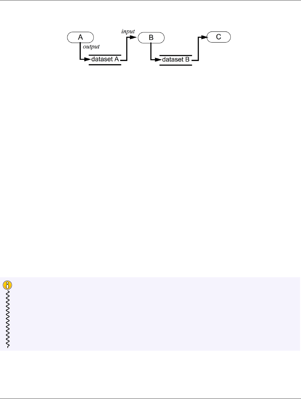
The VTK model is based on the data-flow paradigm. In this paradigm, data flows through the system being transformed
at each step by modules known as algorithms. Algorithms could be common operations such as clipping, slicing, or
generating contours from the data, or they could be computing derived quantities, etc. Algorithms have input ports through
which they take in data and output ports through which they produce output. You need producers that ingest data into the
4 Chapter 1. Introduction to ParaView
1.2. Basics of visualization in ParaView
Figure 1.1: Visualization model: Process objects A, B, and C input and/or output one or more data objects. Data objects
represent and provide access to data; process objects operate on the data. Objects A, B, and C are source, filter, and mapper
objects, respectively.[4]
system. These are simply algorithms that do not have an input port but have one or more output ports. They are called
sources. Readers that read data from files are examples of such sources. Additionally, there are algorithms that transform
the data into graphics primitives so that they can be rendered on a computer screen or saved to disk in another file. These
algorithms, which have one or more input ports but do not have output ports, are called sinks. Intermediate algorithms with
input ports and output ports are called filters. Together, sources, filters, and sinks provide a flexible infrastructure wherein
you can create complex processing pipelines by simply connecting algorithms to perform arbitrarily complex tasks.
For more information on VTK’s programming model, refer to.[4]
This way of looking at the visualization pipeline is at the core of ParaView’s work flow: You bring your data into the
system by creating a reader – the source. You then apply filters to either extract information (e.g., iso-contours) and render
the results in a view or to save the data to disk using writers – the sinks.
ParaView includes readers for a multitude of file formats typically used in the computational science world. To efficiently
represent data from various fields with varying characteristics, VTK provides a rich data model that ParaView uses. The
data model can be thought of simply as ways of representing data in memory. We will cover the different data types in
more detail in Section 3.1. Readers produce a data type suitable for representing the information the files contain. Based
on the data type, ParaView allows you to create and apply filters to transform the data. You can also show the data in a view
to produce images or renderings. Just as there are several types of filters, each perfoming different operations and types of
processing, there are several kinds of views for generating various types of renderings including 3D surface views, 2D bar
and line views, parallel coordinate views, etc.
Did you know?
The Visualization Toolkit (VTK) is an open-source, freely available software system for 3D computer graphics, mod-
eling, image processing, volume rendering, scientific visualization, and information visualization. VTK also includes
ancillary support for 3D interaction widgets, two and three-dimensional annotation, and parallel computing.
At its core, VTK is implemented as a C++ toolkit, requiring users to build applications by combining various objects
into an application. The system also supports automated wrapping of the C++ core into Python, Java, and Tcl so
that VTK applications may also be written using these interpreted programming languages. VTK is used world-wide
in commercial applications, research and development, and as the basis of many advanced visualization applications
such as ParaView, VisIt, VisTrails, Slicer, MayaVi, and OsiriX.
Chapter 1. Introduction to ParaView 5

1.3. ParaView executables
1.3 ParaView executables
ParaView comes with several executables that serve different purposes.
paraview
This is the main ParaView graphical user interface (GUI). In most cases, when we refer to ParaView, we are indeed talking
about this application. It is a Qt-based, cross-platform UI that provides access to the ParaView computing capabilities.
Major parts of this guide are dedicated to understanding and using this application.
pvpython
pvpython is the Python interpreter that runs ParaView’s Python scripts. You can think of this as the equivalent of the
paraview for scripting.
pvbatch
Similar to pvpython,pvbatch is also a Python interpreter that runs Python scripts for ParaView. The one difference is that,
while pvpython is meant to run interactive scripts, pvbatch is designed for batch processing. Additionally, when running
on computing resources with MPI capabilities, pvbatch can be run in parallel. We will cover this in more detail in Section .
pvserver
For remote visualization, this executable represents the server that does all of the data processing and, potentially, the
rendering. You can make paraview connect to pvserver running remotely on an HPC resource. This allows you to build
and control visualization and analysis on the HPC resource from your desktop as if you were simply processing it locally
on your desktop!
pvdataserver and pvrenderserver
These can be thought of as the pvserver split into two separate executables: one for the data processing part, pvdataserver,
and one for the rendering part, pvrenderserver. Splitting these into separate processes makes it possible to perform data
processing and rendering on separate sets of nodes with appropriate computing capabilities suitable for the two tasks. Just
as with pvserver,paraview can connect to a pvdataserver-pvrenderserver pair for remote visualization. Unless otherwise
noted, all discussion of remote visualization or client-server visualization in this guide is applicable to both pvserver and
pvdataserver-pvrenderserver configurations.
1.4 Getting started with paraview
1.4.1 paraview graphical user interface
paraview is the graphical front-end to the ParaView application. The UI is designed to allow you to easily create pipelines
for data processing with arbitrary complexity. The UI provides panels for you to inspect and modify the pipelines, to
change parameters that in turn affect the processing pipelines, to perform various data selection and inspection actions to
introspect the data, and to generate renderings. We will cover various aspects of the UI for the better part of this guide.
6 Chapter 1. Introduction to ParaView
1.4. Getting started with paraview
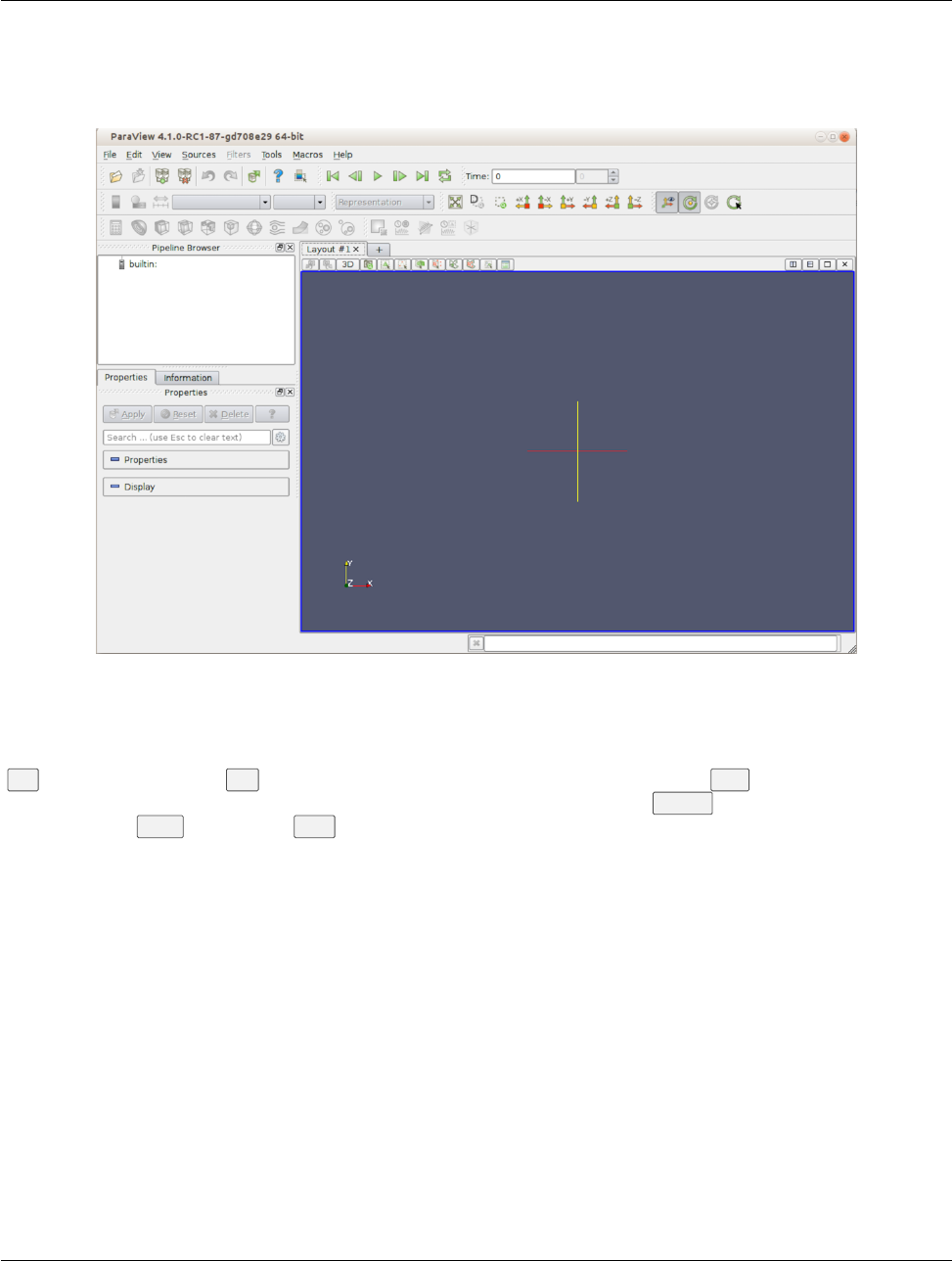
Let’s start by looking at the various components of the UI. If you run paraview for the first time, you will see something
similar to the Figure 1.2. The UI is comprised of menus, dockable panels, toolbars, and the viewport – the central portion
of the application window.
Figure 1.2: paraview application window.
Menus provide the standard set of options typical with a desktop application including options for opening/saving files
(File menu), for undo/redo ( Edit menu), for the toggle panel, and for toolbar visibilities ( View menu). Additionally, the
menus provide ways to create sources that generate test datasets of various types ( Sources menu), as well new filters for
processing data ( Filters menu). The Tools menu provides access to some of the advanced features in paraview such as
managing plugins and accessing the embedded Python shell.
Panels provide you with the ability to peek into the application’s state. For example, you can inspect the visualization
pipeline that has been set up (Pipeline Browser), as well as the memory that is being used (Memory Inspector) and the
parameters or properties for a processing module (Properties panel). Several of the panels also allow you to change the
values that are displayed, e.g., the Properties panel not only shows the processing module parameters, but it also allows
you to change them. Several of the panels are context sensitive. For example, the Properties panel changes to show the
parameters from the selected module as you change the active module in the Pipeline Browser.
Toolbars are designed to provide quick access to common functionality. Several of the actions in the toolbar are accessible
from other locations, including menus or panels. Similar to panels, some of the toolbar buttons are context sensitive and
will become enabled or disabled based on the selected module or view.
The viewport or the central portion of the paraview window is the area where ParaView renders results generated from the
data. The containers in which data can be rendered or shown are called views. You can create several different types of
views, all of which are laid out in this viewport area. By default, a 3D view is created, which is one of the most commonly
used views in ParaView.
Chapter 1. Introduction to ParaView 7
1.4. Getting started with paraview
1.4.2 Understanding the visualization process
To gain a better understanding of how to use the application interface, let’s consider a simple example: creating a data
source and applying a filter to it.
Creating a source
The visualization process in ParaView begins by bringing your data into the application. Chapter 2 explains how to read
data from various file formats. Besides reading files to bring in data into the application, ParaView also provides a collection
of data sources that can produce sample datasets. These are available under the Sources menu. To create a source, simply
click on any item in the Source menu.
Did you know?
As you move your cursor over the items in any menu, on most platforms (except Mac OS X), you’ll see a brief
description of the item in the status bar on the lower-left corner in the application window.
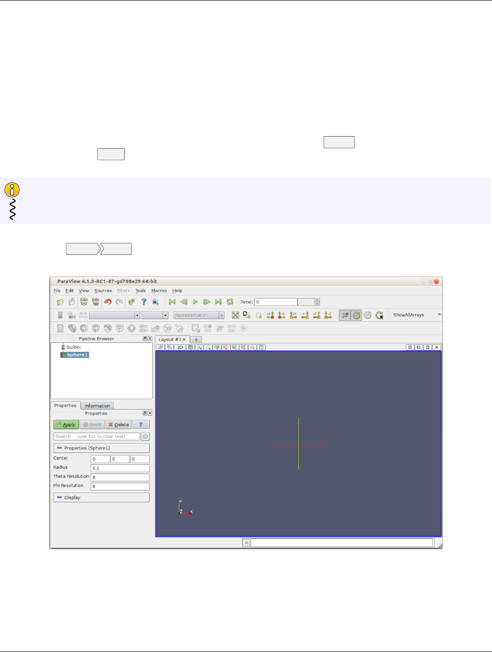
If you click on Sources Sphere , for example, you’ll create a producer algorithm that generates a spherical surface, as
shown in Figure 1.3.
Figure 1.3: Visualization in paraview: Step 1.
A few of things to note:
1. A pipeline module is added in the Pipeline Browser panel with a name derived from the menu item, as is high-
lighted.
8 Chapter 1. Introduction to ParaView
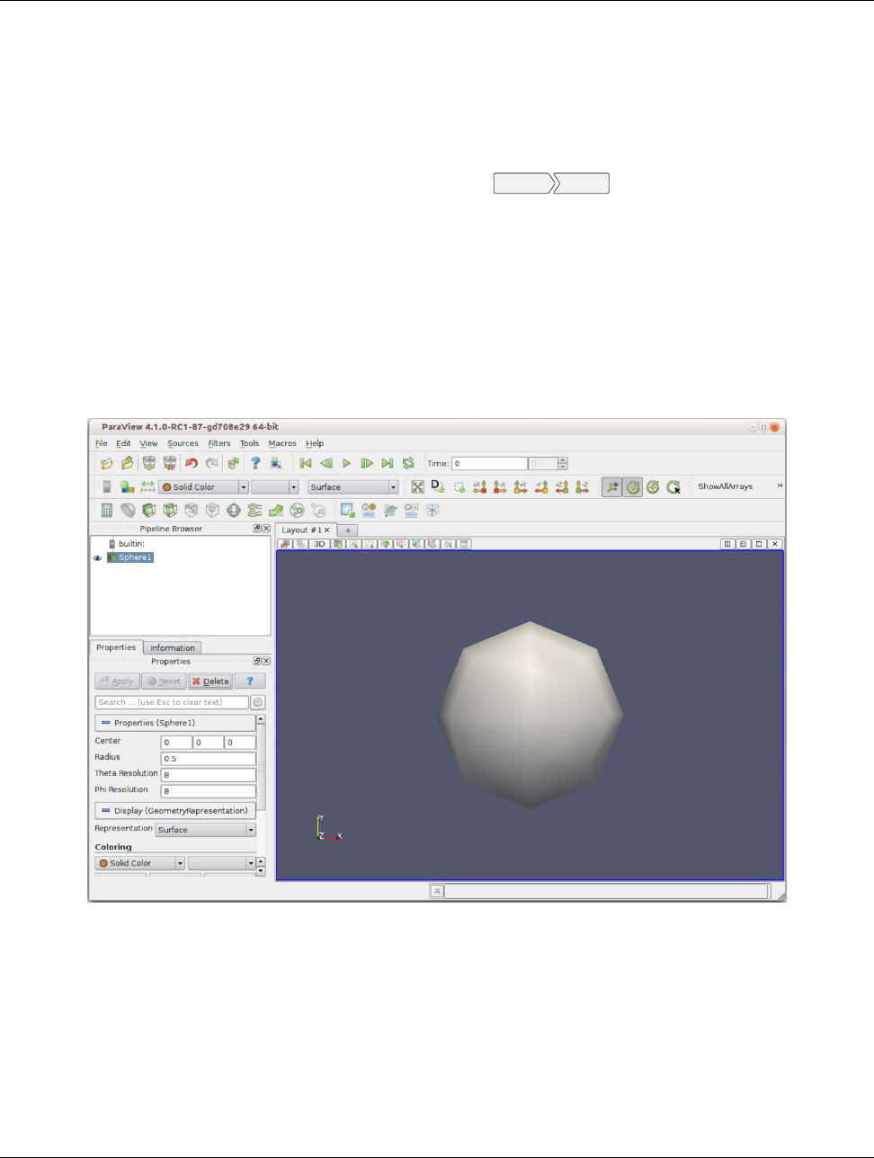
1.4. Getting started with paraview
2. The Properties panel fills up with text to indicate that it’s showing properties for the highlighted item (which, in
this case, is Sphere1), as well as to display some widgets for parameters such as Center,Radius, etc.
3. On the Properties panel, the Apply button becomes enabled and highlighted.
4. The 3D view remains unaffected, as nothing new is shown or rendered in this view as of yet.
Let’s take a closer look at what has happened. When we clicked on Sources Sphere , referring to Section 1.2, we created
an instance of a source that can produce a spherical surface mesh – that’s what is reflected in the Pipeline Browser. This
instance receives a name, which is used by the Sphere1 and the Pipeline Browser, as well as other components of the
UI, to refer to this instance of the source. Pipeline modules such as sources and filters have parameters on them that you
can change that affect that module’s behavior. We call them properties. The Properties panel shows these properties and
allows you to change them. Since the ingestion of data into the system can be a time-consuming process, paraview allows
you to change the properties before the module executes or performs the actual processing to ingest the data. Hence, the
Apply button is highlighted to indicate that you need to accept the properties before the application will proceed. Since no
data has entered the system yet, there’s nothing to show. Therefore, the 3D view remains unaffected.
Let’s assume we are okay with the default values for all of the properties on the Sphere1. Next, click on the Apply button.
Figure 1.4: Visualization in paraview: Step 2.
The following will ensue (Figure 1.4):
1. The Apply button goes back to its old disabled/un-highlighted state.
2. A spherical surface is rendered in the 3D view.
3. The Display section on the Properties panel now shows new parameters or properties.
Chapter 1. Introduction to ParaView 9
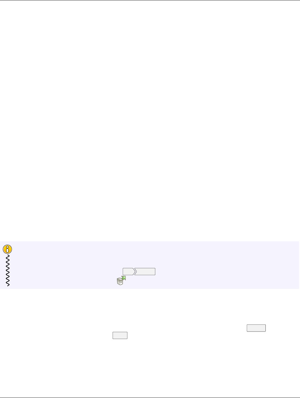
1.4. Getting started with paraview
4. Certain toolbars update, and you can see that toolbars with text, such as Solid Color and Surface, now become
enabled.
By clicking Apply, we told paraview to apply the properties shown on the Properties panel. When a new source (or
filter) is applied for the first time, paraview will automatically show the data that the pipeline module produces in the
current view, if possible. In this case, the sphere source produces a surface mesh, which is then shown or displayed in the
3D view.
The properties that allow you to control how the data is displayed in the view are now shown on the Properties panel
in the Display section. Things such as the surface color, rendering type or representation, shading parameters, etc., are
shown under this newly updated section. We will look at display properties in more detail in Chapter 4.
Some of the properties that are commonly used are also duplicated in the toolbar. These properties include the data array
with which the surface is colored and the representation type. These are the changes in the toolbar that allow you to quickly
change some display properties.
Changing properties
If you change any of the properties on the sphere source, such as the properties under the Properties section on the
Properties panel, including the Radius for the spherical mesh or its Center, the Apply button will be highlighted again.
Once you are finished with all of the property changes, you can hit Apply to apply the changes. Once the changes are
applied, paraview will re-execute the sphere source to produce a new mesh, as requested. It will then automatically update
the view, and you will see the new result rendered.
If you change any of the display properties for the sphere source, such as the properties under the Display section of the
Properties panel (including Representation or Opacity), the Apply button is not affected, the changes are immediately
applied, and the view is updated.
The rationale behind this is that, typically, the execution of the source (or filter) is more computationally intensive than the
rendering. Changing source (or filter) properties causes that algorithm to re-execute, while changing display properties, in
most cases, only triggers a fresh render with an updated graphics state.
Did you know?
For some workflows with smaller data sizes, it may be more convenient if the Apply button was automatically
applied even after changes are made to the pipeline module properties. You can change this from the application
settings dialog, which is accessible from the Edit Settings menu. The setting is called Auto Apply. You can also
change the Auto Apply state using the button from the toolbar.
Applying filters
As per the data-flow paradigm, one creates pipelines with filters to transform data. Similar to the Sources menu, which
allows us to create new data sources, there’s a Filters menu that provides access to the large set of filters that are available in
ParaView. If you peruse through the items in this menu, some of them will be enabled, and some of them will be disabled.
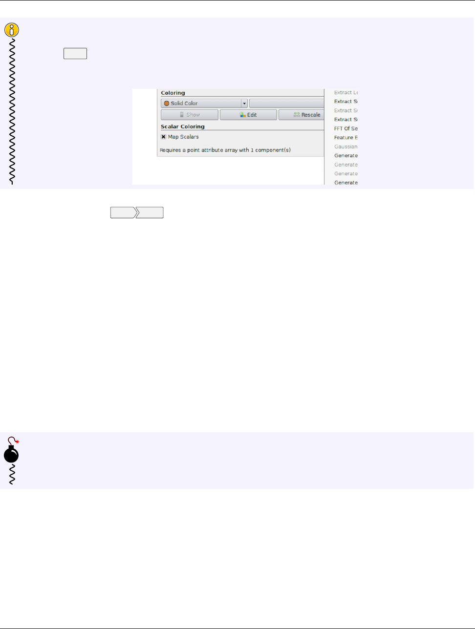
Filters that can work with the data type being produced by the sphere source are enabled, while others are disabled. You
can click on any of the enabled filters to create a new instance of that filter type.
10 Chapter 1. Introduction to ParaView
1.5. Getting started with pvpython
Did you know?
To figure out why a particular filter doesn’t work with the current source, simply move your mouse over the disabled
item in the Filters menu. On Linux and Windows (not OS X, however), the status bar will provide a brief explanation
of why that filter is not available.
For example, if you click on Filters Shrink , it will create a filter that shrinks each of the mesh cells by a fixed factor. Exactly
as before, when we created the sphere source, we see that the newly-created filter is given a new name, Shrink1, and is
highlighted in the Pipeline Browser. The Properties panel is also updated to show the properties for this new filter,
and the Apply button is highlighted to request that we accept the properties for the filter so that it can be executed and the
result can be rendered. If you click back and forth between the Sphere1 and Shrink1 in the Pipeline Browser, you’ll
see the Properties panel and toolbars update, reflecting the state of the selected pipeline module. This is an important
concept in ParaView. There’s a notion of active pipeline module, called the active source. Several panels, toolbars, and
menus will update based on the active source.
If you click Apply, as was the case before, the shrink filter will be executed and the resulting dataset will be generated and
shown in the 3D view. paraview will also automatically hide the result from the Sphere1 so that it is not shown in the view.
Otherwise, the two datasets will overlap. This is reflected by the change of state for the eyeball icons in the Pipeline
Browser next to each of the pipeline modules. You can show or hide results from any pipeline module by clicking on the
eyeballs.
This simple workflow forms the basis of all the data analysis and visualization in ParaView. The process involves creating
sources and filters, changing their parameters, and showing the generated result in one or more views. In the rest of this
guide, we will cover various types of filters and data processing that you can do. We will also cover different types of views
that can help you produce a wide array of 2D and 3D visualizations, as well as inspect your data and drill down into it.
Common Errors
Beginners often forget to hit the Apply button after creating sources or filters or after changing properties. This is
one of the most common pitfalls for users new to the ParaView workflow.
1.5 Getting started with pvpython
While this section refers to pvpython, everything that we discuss here is applicable to pvbatch as well. Until we start
looking into parallel processing, the only difference between the two executables is that pvpython provides an interactive
shell wherein you can type your commands, while pvbatch expects the Python script to be specified on the command line
argument.
Chapter 1. Introduction to ParaView 11
1.5. Getting started with pvpython
1.5.1 pvpython scripting interface
ParaView provides a scripting interface to write scripts for performing the tasks that you could do using the GUI. The
scripting interface can be accessed through Python, which is an interpreted programming language popular among the
scientific community for its simplicity and its capabilities. While a working knowledge of Python will be useful for writing
scripts with advanced capabilities, you should be able to follow most of the discussion in this book about ParaView scripting
even without much Python exposure.
ParaView provides a paraview package with several Python modules that expose various functionalities. The primary
scripting interface is provided by the simple module.
When you start pvpython, you should see a prompt in a terminal window as follows (with some platform specific differ-
ences).
1Python 2.7.5 (default , Sep 2 2013, 05:24:04)
2[GCC 4.2.1 Compatible Apple LLVM 5.0 (clang-500.0.68)] on darwin
3Type "help","copyright","credits"or "license"for more information
4>>>
You can now type commands at this prompt, and ParaView will execute them. To bring in the ParaView scripting API, you
first need to import the simple module from the paraview package as follows:
1>>> from paraview.simple import *
Common Errors
Remember to hit the Enter or Return key after every command to execute it. Any Python interpreter will not
execute the command until Enter is hit.
If the module is loaded correctly, pvpython will respond with a text output, which is the ParaView version number.
1>>> from paraview.simple import *
2paraview version 4.2.0
You can consider this as in the same state as when paraview was started (with some differences that we can ignore for
now). The application is ready to ingest data and start processing.
1.5.2 Understanding the visualization process
Let’s try to understand the workflow by looking at the same use-case as we did in Section 1.4.2.
Creating a source
In paraview, we created the data source by using the Sources menu. In the scripting environment, this maps to simply
typing the name of the source to create.
1>>> Sphere()
This will create the sphere source with a default set of properties. Just like with paraview, as soon as a new pipeline module
is created, it becomes the active source.
Now, to show the active source in a view, try:
12 Chapter 1. Introduction to ParaView
1.5. Getting started with pvpython
1>>> Show()
2>>> Render()
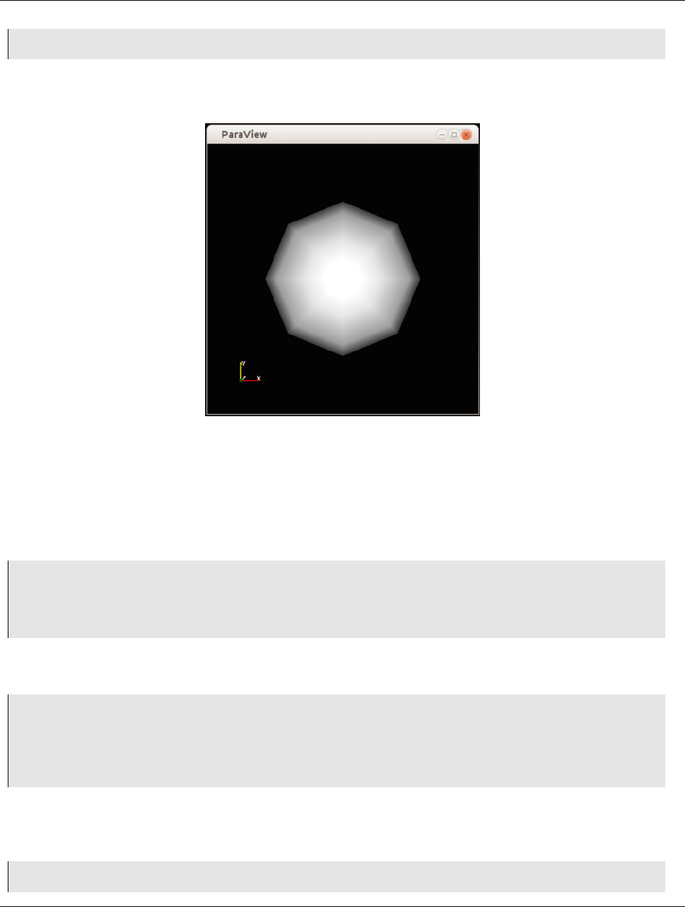
The Show call will prepare the display, while the Render call will cause the rendering to occur. In addition, a new window
will popup, showing the result (Figure 1.5). This is similar to the state after hitting Apply in the UI.
Figure 1.5: Window showing result from the Python code.
Changing properties
To change the properties on the sphere source, you can use the SetProperties function.
1# Set a single property on the active source.
2>>> SetProperties(Radius=1.0)
3
4# You can also set multiple properties.
5>>> SetProperties(Center=[1, 0, 0], StartTheta=100)
Similar to the Properties panel, SetProperties affects the active source. To query the current value of any property on
the active source, use GetProperty.
1>>> radius = GetProperty("Radius")
2>>> print radius
31.0
4>>> center = GetProperty("Center")
5>>> print center
6[1.0, 0.0, 0.0]
SetProperties and GetProperty functions serve the same function as the Properties section of the Properties panel
– they allow you to set and introspect the pipeline module properties for the active source. Likewise, for the Display
section of the panel, or the display properties, we have the SetDisplayProperties and GetDisplayProperty functions.
1>>> SetDisplayProperties(Opacity =0.5)
2
Chapter 1. Introduction to ParaView 13
1.5. Getting started with pvpython
3# FIXME: this function is not available yet, but here for completeness.
4>>> GetDisplayProperty("Opacity")
50.5
Common Errors
Note how the property names for the SetProperties and SetDisplayProperties functions are not en-
closed in double-quotes, while those for the GetProperty and GetDisplayProperty methods are.
In paraview, every time you hit Apply or change a display property, the UI automatically re-renders the view. In the
scripting environment, you have to do this manually by calling the Render function every time you want to re-render and
look at the updated result.
.
Applying filters
Similar to creating a source, to apply a filter, you can simply create the filter by name.
1# Create the ‘Shrink’ filter and connect it to the active source
2# which is the ‘Sphere’ instance.
3>>> Shrink()
4# As soon as the Shrink filter is created, it will now become the new active
5# source. All methods acting on active source now act on this filter instance
6# and not the Sphere instance created earlier.
7
8# Show the resulting data and render it.
9>>> Show()
10 >>> Render()
If you tried the above script, you’ll notice the result isn’t exactly what we expected. For some reason, the shrank cells are
not visible. This is because we missed one stage: In paraview, the UI was smart enough to automatically hide the input
dataset for the newly created filter after we hit apply. In the scripting interface, such operations are the user’s responsibility.
We should have hidden the sphere source from the view. We can use the Hide method, the counter part of Show, to hide
the active source. But, now we have a problem – when we created the shrink filter, we changed the active source to be the
shrink instance. Luckily, all the functions we discussed so far can take an optional first argument, which is the source or
filter instance on which to operate. If provided, that instance is used instead of the active source. The solution is as follows:
1# Get the input property for the active source, i.e. the input for the shrink.
2>>> shrinksInput = GetProperty("Input")
3
4# This is indeed the sphere instance we created earlier.
5>>> print shrinksInput
6<paraview.servermanager.Sphere object at 0x11d731e90 >
7
8# Hide the sphere instance explicitly.
9>>> Hide(shrinksInput)
10
11 # Re-render the result.
12 >>> Render()
14 Chapter 1. Introduction to ParaView

1.5. Getting started with pvpython
Alternatively, you could also get/set the active source using the GetActiveSource and
SetActiveSource functions.
1>>> shrinkInstance = GetActiveSource()
2>>> print shrinkInstance
3<paraview.servermanager.Shrink object at 0x11d731ed0 >
4
5# Get the input property for the active source, i.e. the input
6# for the shrink.
7>>> sphereInstance = GetProperty("Input")
8
9# This is indeed the sphere instance we created earlier.
10 >>> print sphereInstance
11 <paraview.servermanager.Sphere object at 0x11d731e90 >
12
13 # Change active source to sphere and hide it.
14 >>> SetActiveSource(sphereInstance)
15 >>> Hide()
16
17 # Now restore the active source back to the shrink instance.
18 >>> SetActiveSource(shrinkInstance)
19
20 # Re-render the result
21 >>> Render()
The result is shown in Figure 1.6.
Figure 1.6: Window showing result from the Python code after applying the shrink filter.
SetActiveSource has same effect as changing the pipeline module, highlighted in the Pipeline Browser, by clicking
on a different module.
Chapter 1. Introduction to ParaView 15

1.5. Getting started with pvpython
Alternative approach
Here’s another way of doing something similar to what we did in the previous section for those familiar with Python and/or
object-oriented programming. It’s totally okay to stick with the previous approach.
1>>> from paraview.simple import *
2>>> sphereInstance = Sphere()
3>>> sphereInstance.Radius = 1.0
4>>> sphereInstance.Center [1] = 1.0
5>>> print sphereInstance.Center
6[0.0, 1.0, 0.0]
7
8>>> sphereDisplay = Show(sphereInstance)
9>>> view = Render()
10 >>> sphereDisplay.Opacity = 0.5
11
12 # Render function can take in an optional view argument, otherwise it
13 # will simply use the active view.
14 >>> Render(view)
15
16 >>> shrinkInstance = Shrink(Input=sphereInstance ,
17 ShrinkFactor=1.0)
18 >>> print shrinkInstance.ShrinkFactor
19 1.0
20 >>> Hide(sphereInstance)
21 >>> shrinkDisplay = Show(shrinkInstance)
22 >>> Render()
1.5.3 Updating the pipeline
When changing properties on the Properties panel in paraview, we noticed that the algorithm doesn’t re-execute until
you hit Apply. In reality, Apply isn’t what’s actually triggering the execution or the updating of the processing pipeline.
What happens is that Apply updates the parameters on the pipeline module and causes the view to render. If the output
of the pipeline module is visible in the view, or if the output of any filter connected to it downstream is visible in the
view, ParaView will determine that the data rendered is obsolete and request the pipeline to re-execute. It implies that if
that pipeline module (or any of the filters downstream from it) is not visible in the view, ParaView will have no reason to
re-execute the pipeline, and the pipeline module will not be be updated. If, later on, you do make this module visible in
the view, ParaView will automatically update and execute the pipeline. This is often referred to as demand-driven pipeline
execution. It makes it possible to avoid unnecessary module executions.
In paraview, you can get by without ever noticing this since the application manages pipeline updates automatically. In
pvpython too, if your scripts are producing renderings in views, you’d never notice this as long as you remember to call
Render. However, you may want to write scripts to produce transformed datasets or to determine data characteristics. In
such cases, since you may never create a view, you’ll never be seeing the pipeline update, no matter how many times you
change the properties.
Accordingly, you must use the UpdatePipeline function. UpdatePipeline updates the pipeline connected to the active
source (or only until the active source, i.e., anything downstream from it, won’t be updated).
1>>> from paraview.simple import *
2>>> sphere = Sphere()
3
4# Print the bounds for the data produced by sphere.
5>>> print sphere.GetDataInformation().GetBounds()
16 Chapter 1. Introduction to ParaView

1.5. Getting started with pvpython
6(1e+299, -1e+299, 1e+299, -1e+299, 1e+299, -1e+299)
7# The bounds are invalid -- no data has been produced yet.
8
9# Update the pipeline explicitly on the active source.
10 >>> UpdatePipeline()
11
12 # Alternative way of doing the same but specifying the source
13 # to update explicitly.
14 >>> UpdatePipeline(proxy=sphere)
15
16 # Let’s check the bounds again.
17 >>> sphere.GetDataInformation().GetBounds()
18 (-0.48746395111083984, 0.48746395111083984, -0.48746395111083984, 0.48746395111083984,
-0.5, 0.5)
19
20 # If we call UpdatePipeline() again, this will have no effect since
21 # the pipeline hasn’t been modified, so there’s no need to re-execute.
22 >>> UpdatePipeline()
23 >>> sphere.GetDataInformation().GetBounds()
24 (-0.48746395111083984, 0.48746395111083984, -0.48746395111083984, 0.48746395111083984,
-0.5, 0.5)
25
26 # Now let’s change a property.
27 >>> sphere.Radius = 10
28
29 # The bounds won’t change since the pipeline hasn’t re-executed.
30 >>> sphere.GetDataInformation().GetBounds()
31 (-0.48746395111083984, 0.48746395111083984, -0.48746395111083984, 0.48746395111083984,
-0.5, 0.5)
32
33 # Let’s update and see:
34 >>> UpdatePipeline()
35 >>> sphere.GetDataInformation().GetBounds()
36 (-9.749279022216797, 9.749279022216797, -9.749279022216797, 9.749279022216797, -10.0,
10.0)
We will look at the sphere.GetDataInformation API in Section 3.3 in more detail.
For temporal datasets, UpdatePipeline takes in a time argument, which is the time for which the pipeline must be updated.
1# To update to time 10.0:
2>>> UpdatePipeline(10.0)
3
4# Alternative way of doing the same:
5>>> UpdatePipeline(time=10.0)
6
7# If not using the active source:
8>>> UpdatePipeline(10.0, source)
9>>> UpdatePipeline(time=10.0, proxy=source)
Chapter 1. Introduction to ParaView 17
1.6. Scripting in paraview
1.6 Scripting in paraview
1.6.1 The Python shell
The paraview application also provides access to an internal shell, in which you can enter Python commands and scripts
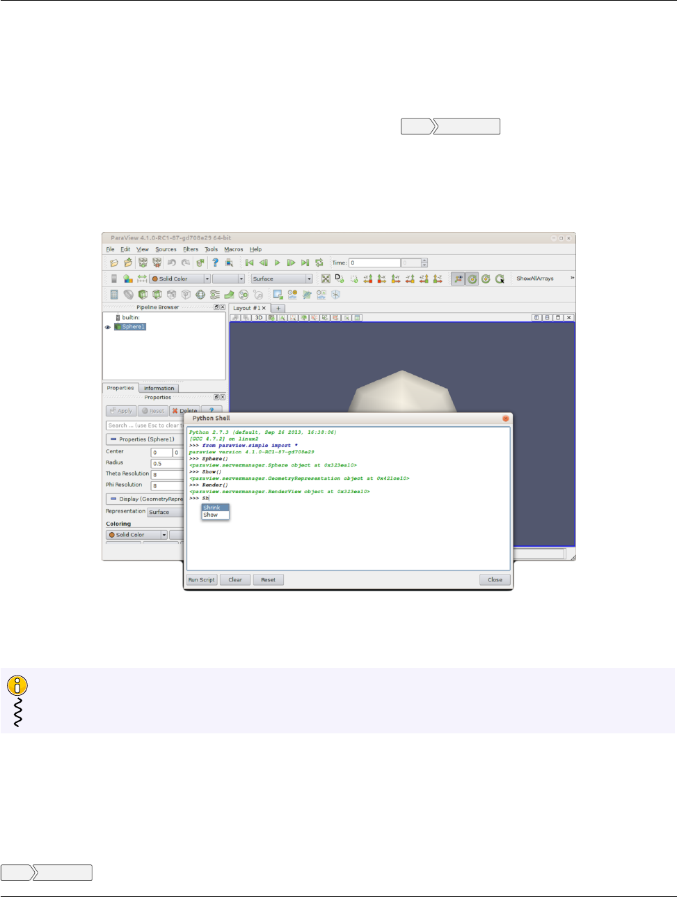
exactly as with pvpython. To access the Python shell in the GUI, use the Tools Python Shell menu option. A dialog will pop
up with a prompt exactly like pvpython. You can try inputting commands from the earlier section into this shell. As you
type each of the commands, you will see the user interface update after each command, e.g., when you create the sphere
source instance, it will be shown in the Pipeline Browser. If you change the active source, the Pipeline Browser and
other UI components will update to reflect the change. If you change any properties or display properties, the Properties
panel will update to reflect the change as well!
Figure 1.7: Python shell in paraview provides access to the scripting interface in the GUI.
Did you know?
The Python shell in paraview supports auto-completion for functions and instance methods. Try hitting the Tab key
after partially typing any command (as shown in Figure 1.7).
1.6.2 Tracing actions for scripting
This guide provides a fair overview of ParaView’s Python API. However, there will be cases when you just want to know
how to complete a particular action or sequence of actions that you can do with the GUI using a Python script instead. To
accomplish this, paraview supports tracing your actions in the UI as a Python script. Simply start tracing by clicking on
Tools Start Trace .paraview now enters a mode where all your actions (or at least those relevant for scripting) are monitored.
18 Chapter 1. Introduction to ParaView

1.6. Scripting in paraview
Any time you create a source or filter, open data files, change properties and hit Apply, interact with the 3D scene, or save
screenshots, etc., your actions will be monitored. Once you are done with the series of actions that you want to script,
click Tools Stop Trace .paraview will then pop up an editor window with the generated trace. This will be the Python script
equivalent for the actions you performed. You can now save this as a script to use for batch processing.
Chapter 1. Introduction to ParaView 19
CHAPTER
TWO
LOADING DATA
In a visualization pipeline, data sources bring data into the system for processing and visualization. Sources, such as the
Sphere source (accessible from the Sources menu in paraview), programmatically create datasets for processing. Another
type of data sources is readers. Readers can read data written out in disk files or other databases and bring it into ParaView
for processing. ParaView includes readers that can read several of the commonly used scientific data formats. It’s also
possible to write plugins that add support for new or proprietary file formats.
ParaView provides several sample datasets for you to get started. You can download an archive with several types of data
files from the download page at http://paraview.org.
2.1 Opening data files in paraview
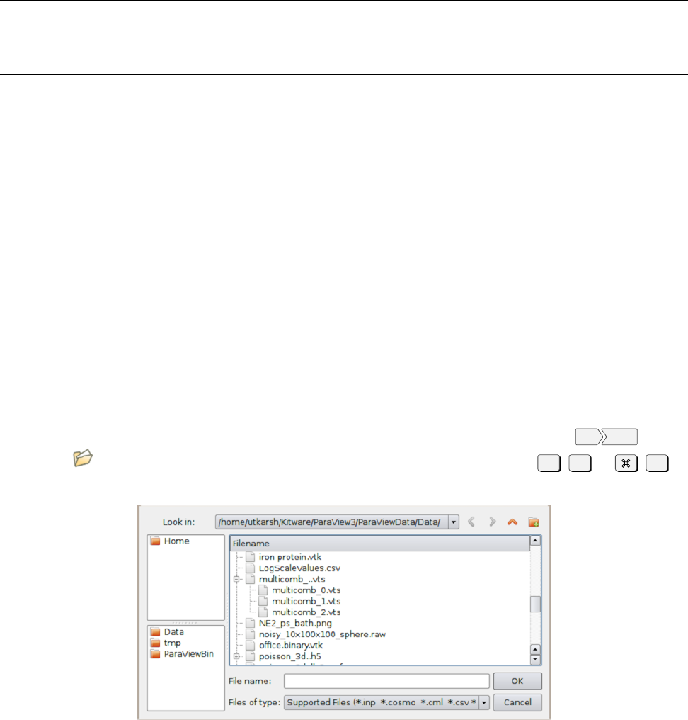
To open a data file in paraview, you use the Open File dialog. This dialog can be accessed from the File Open menu or
by using the button in the Main Controls toolbar. You can also use the keyboard shortcut Ctrl +O(or +O) to
open this dialog.
Figure 2.1: Open File dialog in paraview for opening data (and other) files.
The Open File dialog allows you to browse the file system on the data processing nodes. This will become clear when
we look at using ParaView for remote visualization. While several of the UI elements in this dialog are obvious such as
navigating up the current directory, creating a new directory, and navigating back and forth between directories, there are
a few things to note.
2.1. Opening data files in paraview
•The Favorites pane shows some platform-specific common locations such as your home directory and desktop.
•The Recent Directories pane shows a few most recently used directories.
You can browse to the directory containing your datasets and either select the file and hit Ok or simply double click on
the file to open it. You can also select multiple files using the Ctrl (or ) key. This will open each of the selected files
separately.
When a file is opened, paraview will create a reader instance of the type suitable for the selected file based on its extension.
The reader will simply be another pipeline module, similar to the source we created in Chapter 1. From this point forward,
the workflow will be the same as we discussed in Section 1.4.2: You adjust the reader properties, if needed, and hit Apply.
paraview will then read the data from the file and render it in the view.
If you selected multiple files using the Ctrl (or )key,paraview will create multiple reader modules. When you hit
Apply, all of the readers will be executed, and their data will be shown in the view.
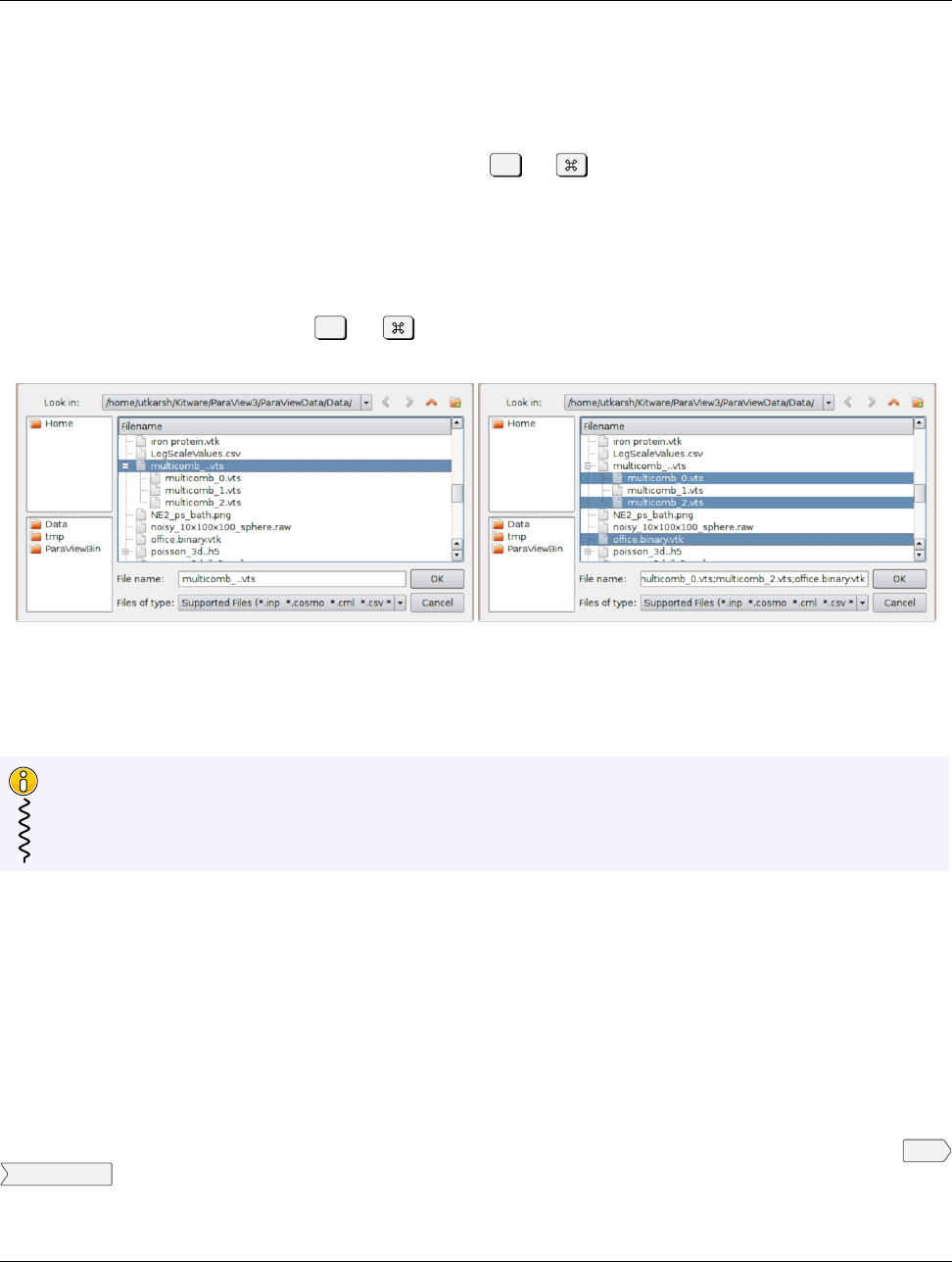
Figure 2.2: The Open File dialog can be used to select a temporal file series (left) or select multiple files to open separately
(right).
Did you know?
This ability to hit the Apply button once to accept changes on multiple readers applies to other pipeline modules,
including sources and filters. In general, you can change properties for multiple modules in a pipeline, and hit
Apply to accept all of the changes at once. It is possible to override this behavior from the Settings dialog.
2.1.1 Dealing with unknown extensions
On occasion, you will run into situations where a file is named unusually and, despite the fact that ParaView supports
reading the file format, paraview does not recognize the file, as its extension does not match the expected extension. In this
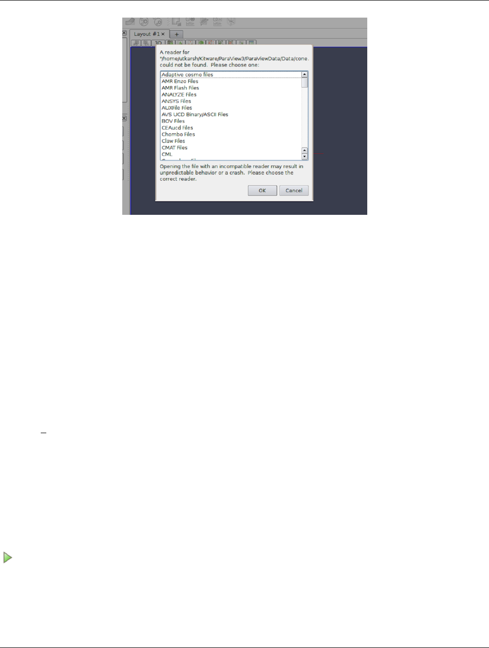
case, paraview will pop up the Open Data With... dialog, which lists several readers (Figure 2.3). You can then pick
the reader for the correct file format from this list and continue. If you picked an incorrect reader, however, you’ll get error
messages either when the reader module is instantiated or after you hit Apply. In either case, you can simply Delete the
reader module and try opening the file again, this time choosing a different reader.
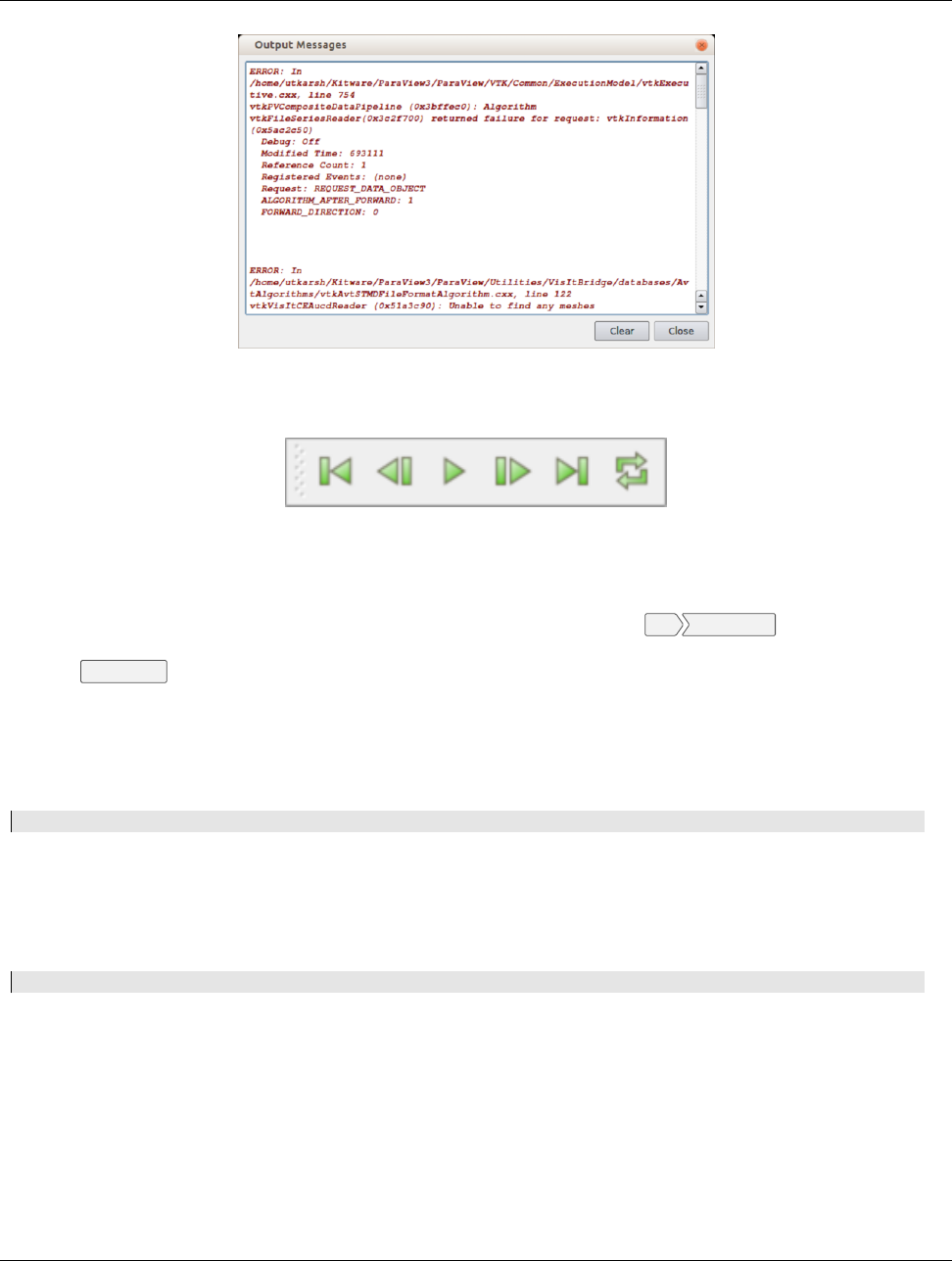
Error messages in paraview are shown in the Output Messages window (Figure 2.4). It is accessible from the Tools
Output Window menu. Whenever there’s a new error message, paraview will automatically pop open this window and raise
it to the top.
22 Chapter 2. Loading data
2.1. Opening data files in paraview
Figure 2.3: Open Data With... dialog shown to manually choose the reader to use for a file with an unknown extension.
2.1.2 Handling temporal file series
Most datasets produced by scientific simulation runs are temporal in nature. File formats differ in how this information is
saved in the file. While several file formats support saving multiple timesteps in the same file, others save them out as a
sequence of files, known as a file series.
The Open File dialog automatically detects file series and shows them as a grouped element, as shown in Figure 2.2.To
load the file series, simply select the group, and hit Ok. You can also open a single file in the series as a regular file. To do
so, open the file group and select the file you want to open.
paraview automatically detects several of the commonly-known file naming patterns used for indicating a file series. These
include:
•fooN.vtk
•foo N.vtk •fooN.vtk
•foo.N.vtk •Nfoo.vtk
•N.foo.vtk •foo.vtk.N
•foo.vtksN
where foo could be any filename, Nis a numeral sequence (with any number of leading zeros), and vtk could be any
extension.
2.1.3 Dealing with time
When you open a dataset with time, either as a file series or in a file format that natively supports time, paraview will
automatically setup an animation for you so that you can play through each of the time steps in the dataset by using the
button on the VCR Controls toolbar (Figure 2.5). You can change or modify this animation and further customize it,
as discussed in Chapter 7.
2.1.4 Reopening previously opened files
Chapter 2. Loading data 23
2.1. Opening data files in paraview
Figure 2.4: The Output Messages window is used to show errors, warnings, and other messages raised by the application.
Figure 2.5: VCR Controls toolbar for interacting with an animation.
paraview remembers most recently opened files (or file series). Simply use the File Recent Files menu. paraview also
remembers the reader type selected for files with unknown extensions or for occasions when multiple reader choices were
available. Recent Files
2.1.5 Opening files using command line options
paraview provides a command line option that can be used to open datasets on startup.
>paraview--data=.../ParaViewData/Data/can.ex2
This is equivalent to opening a can.ex2 data file from the Open File dialog. The same set of follow-up actions happen.
For example, paraview will try to locate a reader for the file, create that reader, and wait for you to hit Apply.
To open a file series, simply replace the numbers in the file name sequence by a ‘.’ For example, to open a file series named
my0.vtk,my1.vtk...myN.vtk, use my..vtk.
>paraview--data=.../ParaViewData/Data/my..vtk
2.1.6 Common properties for readers
ParaView uses different reader implementations for different file formats. Each of these have different properties available
to you to customize how the data is read and can vary greatly depending on the capabilities of the file format itself or the
particular reader implementation. Let’s look at some of the properties generally available on readers.
24 Chapter 2. Loading data
2.1. Opening data files in paraview
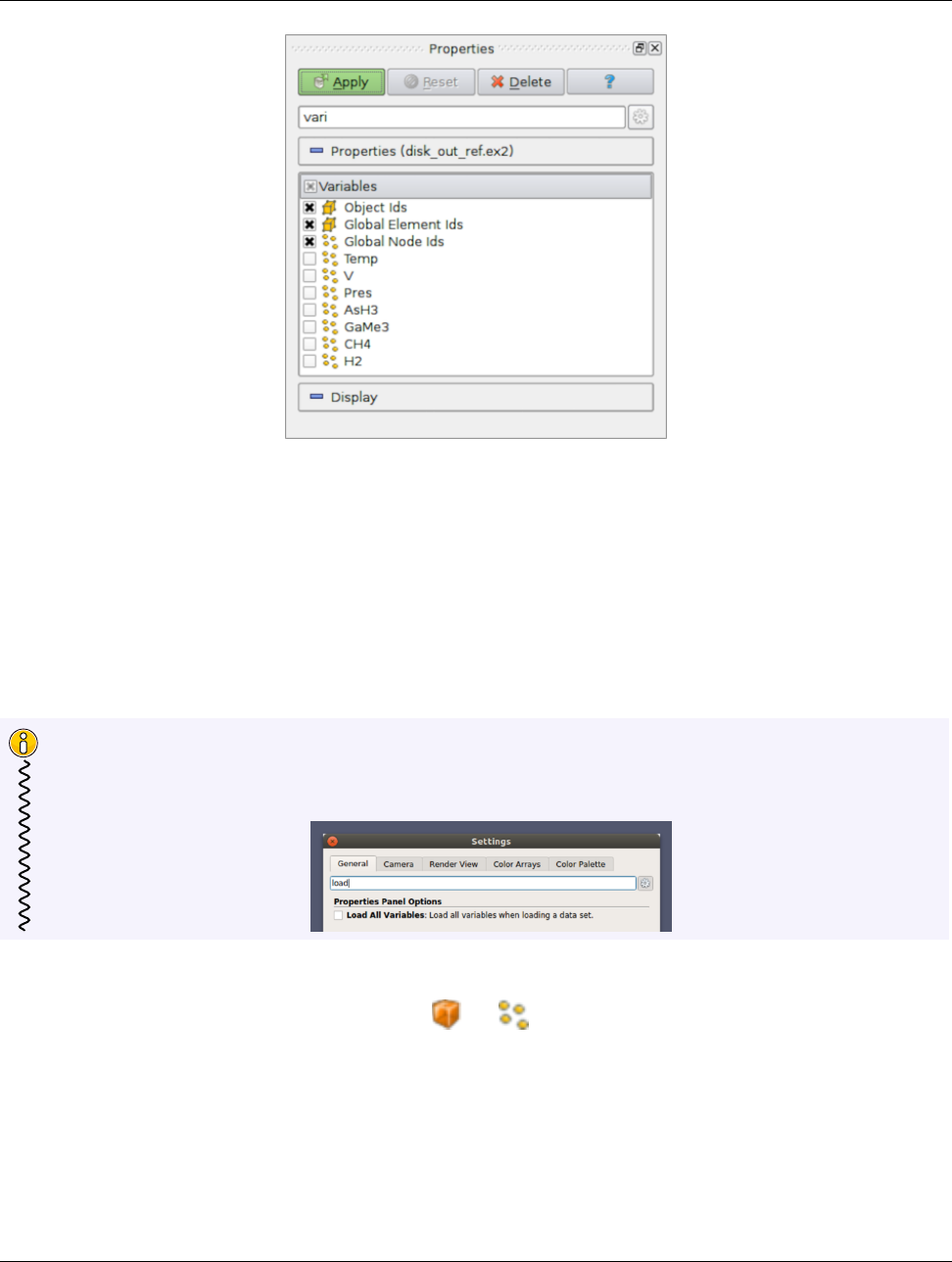
Figure 2.6: Array selection widget for selecting array to load from a data file.
Selecting data arrays
One of the most common properties on readers is one that allows you to select the data arrays (cell centered, point centered,
or otherwise, if applicable) to be loaded. Often times, loading only the data arrays you know you are going to use in the
visualization will save memory, as well as processing time, since the reader does not have to read in those data arrays, and
the filters in the pipeline do not have to process them.
Did you know?
You can change paraview’s default behavior to load all available data arrays by selecting the Load All
Variables checkbox under Settings/Properties Panel Options/Advanced.
The UI for selecting the arrays to load is simply a list with the names of the arrays and a checkbox indicating whether that
array is to be loaded or not (Figure 2.6). Icons, such as and are often used in this widget to give you an indication
of whether the array is cell-centered or point-centered, respectively.
If you unselected an array but realize, as you’re setting up your visualization pipeline, that you need that data array, you
can always go back to the Properties page for the reader by making the reader active in the Pipeline Browser and then
changing the array selection. ParaView will automatically re-execute any processing pipeline set up on the reader with this
new data array.
Chapter 2. Loading data 25
2.2. Opening data files in pvpython
Common Errors
Remember to hit Apply (or use Auto Apply) after changing the array selection for the change to take effect.
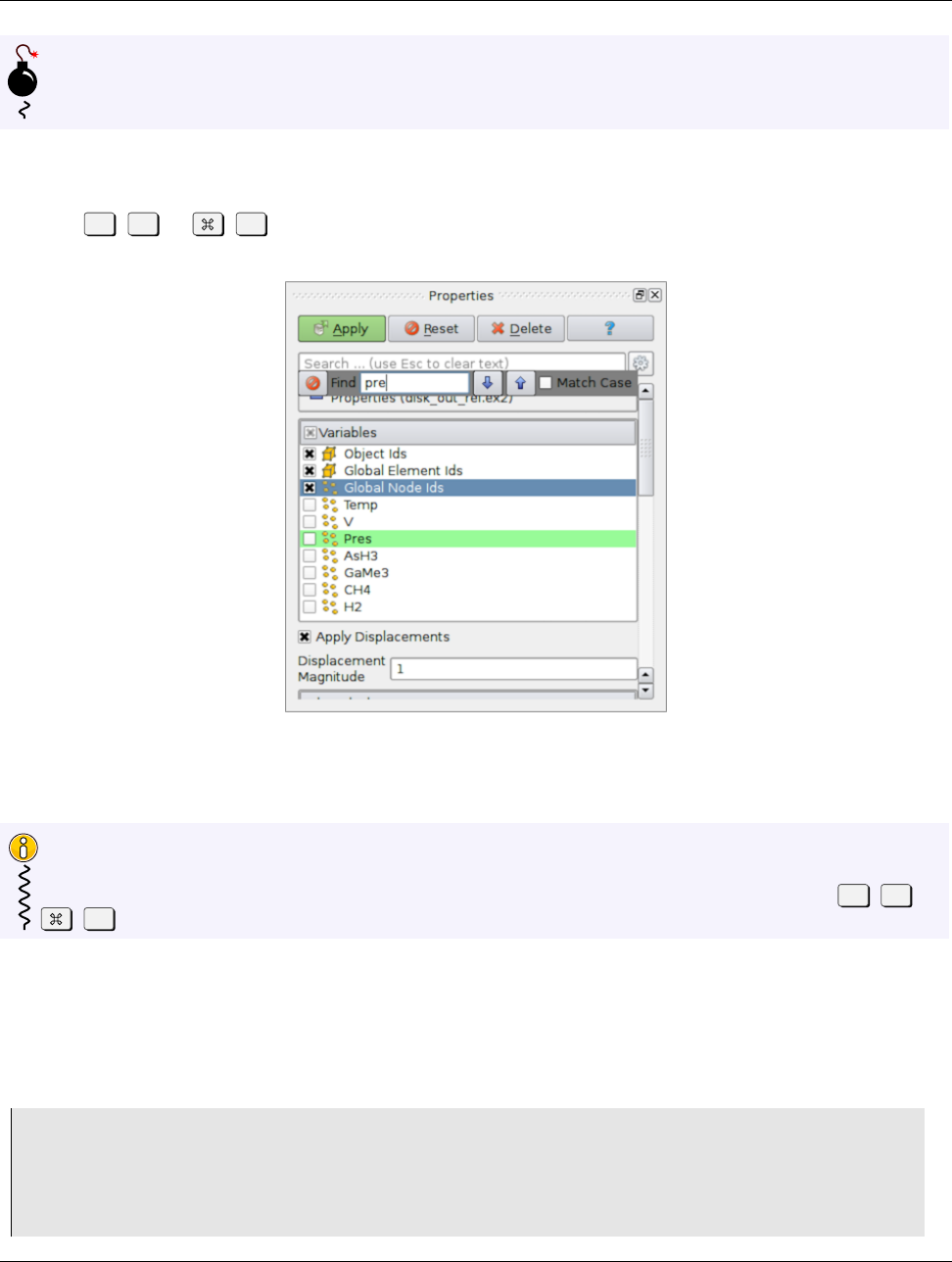
Sometimes this list can get quite large, and it can become cumbersome to find the array for which you are looking. To
help with such situations, paraview provides a mechanism to search lists. Click inside the widget to make it get the focus.
Then type Ctrl +F(or +F) to get a search widget. Now you can type in the text to search. Matching rows will be
highlighted (Figure 2.7).
Figure 2.7: To search through large lists in paraview, you can use ctrl+F. .
Did you know?
The ability to search for items in an array selection widget also applies to other list and tree widgets in the paraview
UI. Whenever you see a widget with a large number of entries in a list, table, or tree fashion, try using Ctrl +F(or
+F).
2.2 Opening data files in pvpython
To open data files using the scripting interface, ParaView provides the OpenDataFile function.
1>>> reader = OpenDataFile(".../ParaViewData/Data/can.ex2")
2>>> if reader:
3... print "Success"
4... else:
5... print "Failed"
6...
26 Chapter 2. Loading data
2.2. Opening data files in pvpython
OpenDataFile will try to determine an appropriate reader based on the file extension, just like paraview. If no reader is
determined, None is returned. If multiple readers can open the file, however, OpenDataFile simply picks the first reader.
If you explicitly want to create a specific reader, you can always create the reader by its name, similar to other sources and
filters.
1>>> reader = ExodusIIReader(FileName=".../ParaViewData/Data/can.ex2")
To find out information about the reader created and the properties available on it, you can use the help function.
1>>> reader = ExodusIIReader(FileName=".../ParaViewData/Data/can.ex2")
2>>> help(reader)
3Help on ExodusIIReader in module paraview.servermanager object:
4
5class ExodusIIReader(ExodusIIReaderProxy)
6|TheExodusreaderloads
7|ExodusIIfilesand produces an unstructured grid output.
8|Thedefaultfileextensionsare.g,.e,.ex2,.ex2v2,
9|.exo,.gen,.exoII,.exii,.0,.00,.000,and .0000. The
10 |fileformatis described fully at:
11 |http://endo.sandia.gov/SEACAS/Documentation/exodusII.pdf.
12 |...
13 |
14 | -----------------------------------------------------------------
15 |Datadescriptorsdefinedhere:
16 |
17 | AnimateVibrations
18 | If this flag is on and HasModeShapes is also on, then
19 |thisreaderwillreportacontinuoustimerange[0,1]and
20 |animatethedisplacementsin a periodic sinusoid. If this
21 | flag is off and HasModeShapes is on , this reader ignores
22 |time.Thisflaghasnoeffectif HasModeShapes is off.
23 |
24 | ApplyDisplacements
25 |Geometriclocationscanincludedisplacements.Whenthis
26 | option is on , the nodal positions are ’displaced’by the
27 |standardexodusdisplacementvector.Ifdisplacementsare
28 | turned ’off’,theusercanexplicitlyaddthembyapplying
29 |awarpfilter.
30 |...
Did you know?
The help function can be used to get information about properties available on any source or filter instance. It not
only lists the properties, but also provides information about how they affect the pipeline module. help can also be
used on functions. For example:
1>>> help(OpenDataFile)
2
3Help on function OpenDataFile in module paraview.simple:
4
5OpenDataFile(filename, **extraArgs)
6Creates a reader to read the given file, if possible.
7This uses extension matching to determine the best reader
8possible. If a reader cannot be identified, then this
9returns None.
Chapter 2. Loading data 27

2.2. Opening data files in pvpython
2.2.1 Handling temporal file series
Unlike paraview,pvpython does not automatically detect and load file series. You have to explicitly list the filenames in
the series and pass that to the OpenDataFile call.
1# Create a list with the names of all the files in the file series in
2# correct order.
3>>> files = [".../Data/multicomb_0.vts",
4".../Data/multicomb_1.vts",
5".../Data/multicomb_2.vts"]
6>>> reader = OpenDataFile(files)
2.2.2 Dealing with time
Similar to paraview, if you open a time series or a file with multiple timesteps, pvpython will automatically set up an
animation for you to play through the timesteps.
1>>> files = [".../Data/multicomb_0.vts",
2".../Data/multicomb_1.vts",
3".../Data/multicomb_2.vts"]
4>>> reader = OpenDataFile(files)
5>>> Show()
6>>> Render()
7
8# Get access to the animation scene.
9>>> scene = GetAnimationScene()
10 # Now you use the API on the scene when doing things such as playing
11 # the animation, stepping through it, etc.
12
13 # This will simply play through the animation once and stop. Watch
14 # the rendered view after you hit ‘Enter.’
15 >>> scene.Play()
2.2.3 Common properties on readers
Selecting data arrays
For those properties on readers that allow you to control what to read in from the file such as point data arrays, cell data
arrays, or data blocks, paraview uses a selection widget, as seen in Section 2.1.6. Likewise, pvpython provides an API that
allows you to determine the available options and then select/deselect them.
The name of the property that allows you to make such selections depends on the reader itself. When in doubt, use the
tracing capabilities in paraview (Section 1.6.2) to figure it out. You can also use help (Section 2.2).
ExodusIIReader has a PointVariables property that can be used to select the point data arrays to load. Let’s use this as
an example.
1# Open an ExodusII data file.
2>>> reader = OpenDataFile(".../Data/can.ex2")
3
4# Alternatively, you can explicitly create the reader instance as:
5>>> reader = ExodusIIReader(FileName = ".../Data/can.ex2")
6
28 Chapter 2. Loading data

2.2. Opening data files in pvpython
7# To query/print the current status for ‘PointVariables’ property,
8# we do what we would have done for any other property:
9>>> print GetProperty("PointVariables")
10 [’DISPL’,’VEL’,’ACCL’]
11
12 # An alternative way of doing the same is as follows:
13 >>> print reader.PointVariables
14 [’DISPL’,’VEL’,’ACCL’]
15
16 # To set the property, simply set it to list containing the names to
17 # enable, e.g., if we want to read only the ’DISPL’ array, we do
18 # the following:
19 >>> SetProperties(PointVariables=[’DISPL’])
20
21 # Or using the alternative way for doing the same:
22 >>> reader.PointVariables = [’DISPL’]
23
24 # Now, the new value for PointVariables is:
25 >>> print reader.PointVariables
26 [’DISPL’]
27
28 # To determine the array available, use:
29 >>> print reader.PointVariables.Available
30 [’DISPL’,’VEL’,’ACCL’]
31 # These are the arrays available in the file.
Changing PointVariables only changes the value on the property. The reader does not re-execute until a re-execution is
requested either by calling Render or by explicitly updating the pipeline using UpdatePipeline.
1>>> reader.PointVariables = [’DISPL’,’VEL’,’ACCL’]
2
3# Assuming that the reader is indeed the active source, let’s update
4# the pipeline:
5>>> UpdatePipeline()
6
7# Or you can use the following form if you’re unsure of the active
8# source or just do not want to worry about it.
9>>> UpdatePipeline(proxy=reader)
10
11 # Print the list of point arrays read in.
12 >>> print reader.PointData[:]
13 [Array: ACCL, Array: DISPL, Array: GlobalNodeId , Array: PedigreeNodeId , Array: VEL]
14
15 # Change the selection.
16 >>> reader.PointVariables = [’DISPL’]
17
18 # Print the list of point arrays read in, nothing changes!
19 >>> print reader.PointData[:]
20 [Array: ACCL, Array: DISPL, Array: GlobalNodeId , Array: PedigreeNodeId , Array: VEL]
21
22 # Update the pipeline.
23 >>> UpdatePipeline()
24
25 # Now the arrays read in has indeed changed as we expected.
26 >>> print reader.PointData[:]
27 [Array: DISPL, Array: GlobalNodeId, Array: PedigreeNodeId]
Chapter 2. Loading data 29
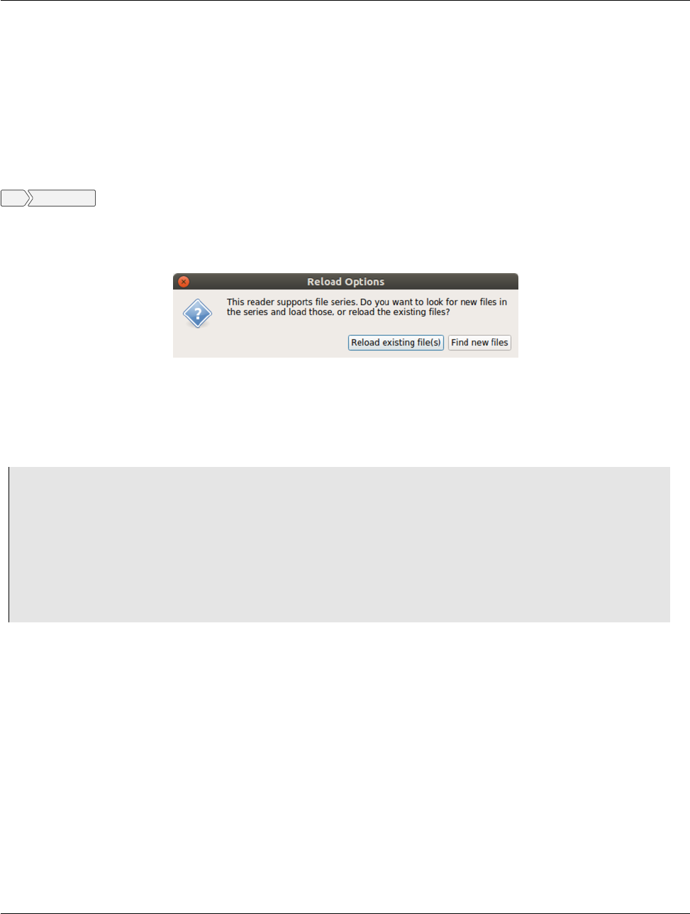
2.3. Reloading files
We will cover the reader.PointData API in more details in Section 3.3.
2.3 Reloading files
While ParaView is often used after the simulation has generated all the data, it is not uncommon to use ParaView to inspect
data files as they are being written out by the simulation. In such cases, the simulation may either be modifying existing
file(s) with new timesteps or creating new files for each timestep. In such cases, you may want to refresh ParaView to make
it aware of the changes. In paraview, this can be done using Reload Files. When the reader is active, you can use the
Edit Reload Files menu to request the reader to refresh. paraview will prompt you to choose whether to reload the existing
file(s) or look for new files in the file series, as shown in Figure 2.8. Click on Reload existing file(s), to force the
reader to re-read the files already opened. This is useful in cases where the simulation may have modified existing file(s).
Use Find new files to make the reader aware of any new files in the file series.
Figure 2.8: Reload Options dialog allowing you to choose how to refresh the reader.
Similar to paraview, in pvpython, you use ReloadFiles to reload existing files, and ExtendFilesSeries to look for new
files in a file series.
1
2# For file being modified in place per timestep
3>>> reader = OpenDataFile(file)
4...
5>>> ReloadFiles(reader)
6
7# For files being generated per timestep
8>>> reader = OpenDataFile(file)
9...
10 >>> ExtendFilesSeries(reader)
30 Chapter 2. Loading data
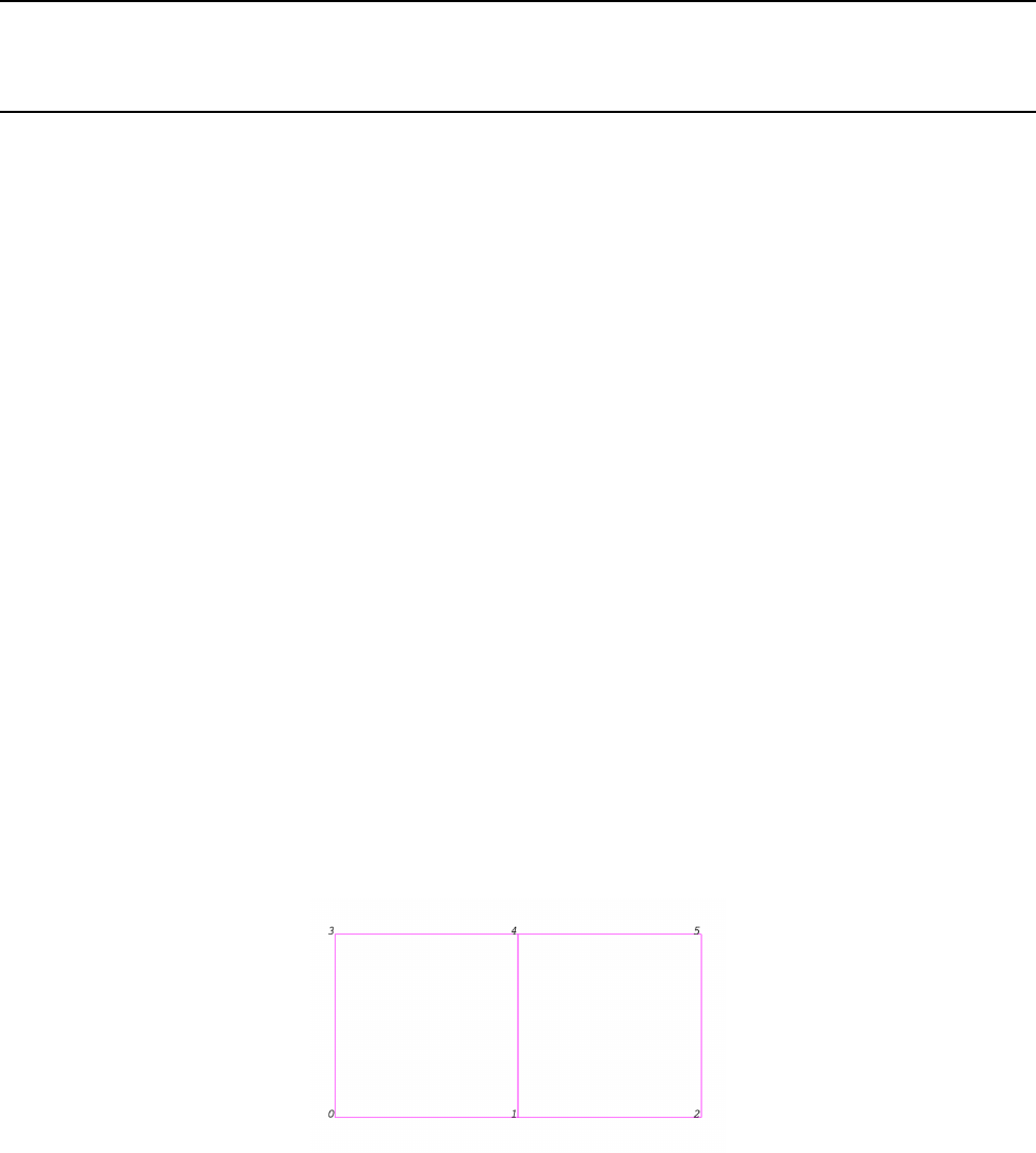
CHAPTER
THREE
UNDERSTANDING DATA
3.1 VTK data model
To use ParaView effectively, you need to understand the ParaView data model. ParaView uses VTK, the Visualization
Toolkit, to provide the visualization and data processing model. This chapter briefly introduces the VTK data model used
by ParaView. For more details, refer to one of the VTK books.
The most fundamental data structure in VTK is a data object. Data objects can either be scientific datasets, such as
rectilinear grids or finite elements meshes (see below), or more abstract data structures, such as graphs or trees. These
datasets are formed from smaller building blocks: mesh (topology and geometry) and attributes.
3.1.1 Mesh
Even though the actual data structure used to store the mesh in memory depends on the type of the dataset, some abstrac-
tions are common to all types. In general, a mesh consists of vertices (points) and cells (elements, zones). Cells are used to
discretize a region and can have various types such as tetrahedra, hexahedra, etc. Each cell contains a set of vertices. The
mapping from cells to vertices is called the connectivity. Note that even though it is possible to define data elements such as
faces and edges, VTK does not represent these explicitly. Rather, they are implied by a cell’s type and by its connectivity.
One exception to this rule is the arbitrary polyhedron, which explicitly stores its faces. Figure 3.5 is an example mesh that
consists of two cells. The first cell is defined by vertices (0,1,3,4), and the second cell is defined by vertices (1,2,4,5).
These cells are neighbors because they share the edge defined by the points (1,4).
Figure 3.1: Example of a mesh.
A mesh is fully defined by its topology and the spatial coordinates of its vertices. In VTK, the point coordinates may be
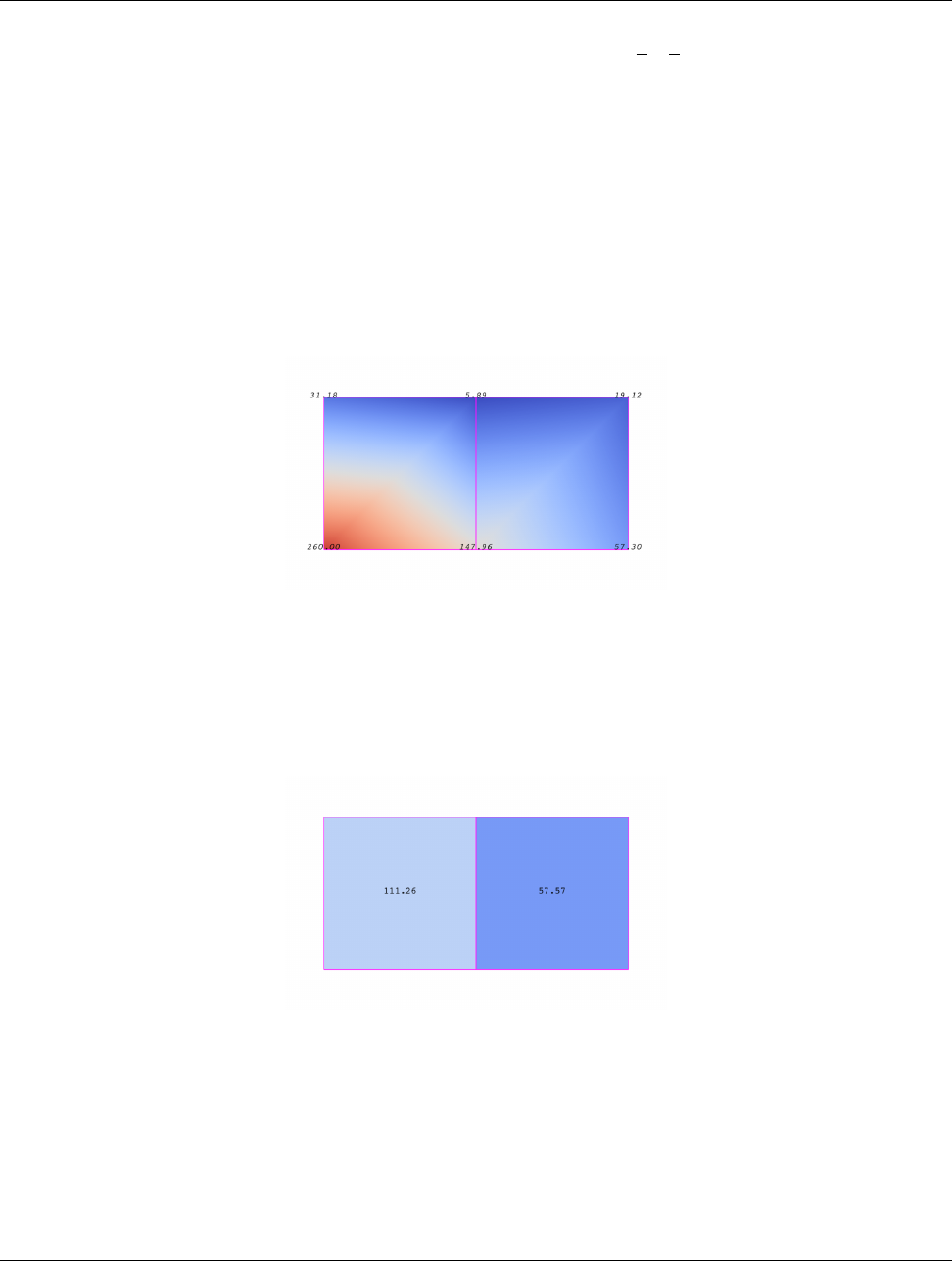
3.1. VTK data model
implicit, or they may be explicitly defined by a data array of dimensions (number of points ⇥3).
3.1.2 Attributes (fields, arrays)
An attribute (or a data array or field) defines the discrete values of a field over the mesh. Examples of attributes include
pressure, temperature, velocity, and stress tensor. Note that VTK does not specifically define different types of attributes.
All attributes are stored as data arrays, which can have an arbitrary number of components. ParaView makes some assump-
tions in regards to the number of components. For example, a 3-component array is assumed to be an array of vectors.
Attributes can be associated with points or cells. It is also possible to have attributes that are not associated with either.
Figure 3.2 demonstrates the use of a point-centered attribute. Note that the attribute is only defined on the vertices. Inter-
polation is used to obtain the values everywhere else. The interpolation functions used depend on the cell type. See the
VTK documentation for details.
Figure 3.2: Point-centered attribute in a data array or field.
Figure 3.3 demonstrates the use of a cell-centered attribute. Note that cell-centered attributes are assumed to be constant
over each cell. Due to this property, many filters in VTK cannot be directly applied to cell-centered attributes. It is normally
required to apply a Cell Data to Point Data filter. In ParaView, this filter is applied automatically, when necessary.
Figure 3.3: Cell-centered attribute.
3.1.3 Uniform rectilinear grid (image data)
A uniform rectilinear grid, or image data, defines its topology and point coordinates implicitly (Figure 3.4). To fully define
the mesh for an image data, VTK uses the following:
32 Chapter 3. Understanding data

3.1. VTK data model
Figure 3.4: Sample uniform rectilinear grid.
1. Extents - These define the minimum and maximum indices in each direction. For example, an image data of extents
(0,9),(0,19),(0,29)has 10 points in the x-direction, 20 points in the y-direction, and 30 points in the z-direction.
The total number of points is 10 ⇥20 ⇥30.
2. Origin - This is the position of a point defined with indices (0,0,0).
3. Spacing - This is the distance between each point. Spacing for each direction can defined independently.
The coordinate of each point is defined as follows: coordinate =origin +index ⇥spacing where coordinate, origin, index,
and spacing are vectors of length 3.
Note that the generic VTK interface for all datasets uses a flat index. The (i,j,k)index can be converted to this flat index
as follows: idx flat =k⇥(nptsx⇥nptsy)+ j⇥nptrx+i.
A uniform rectilinear grid consists of cells of the same type. This type is determined by the dimensionality of the dataset
(based on the extents) and can either be vertex (0D), line (1D), pixel (2D), or voxel (3D).
Due to its regular nature, image data requires less storage than other datasets. Furthermore, many algorithms in VTK have
been optimized to take advantage of this property and are more efficient for image data.
3.1.4 Rectilinear grid
A rectilinear grid, such as Figure 3.5, defines its topology implicitly and point coordinates semi-implicitly. To fully define
the mesh for a rectilinear grid, VTK uses the following:
1. Extents - These define the minimum and maximum indices in each direction. For example, a rectilinear grid of
extents (0,9),(0,19),(0,29)has 10 points in the x-direction, 20 points in the y-direction, and 30 points in the
z-direction. The total number of points is 10 ⇥20 ⇥30.
2. Three arrays defining coordinates in the x-, y- and z-directions - These arrays are of length nptsx,nptsy, and nptsz.
This is a significant savings in memory, as the total memory used by these arrays is nptsx+nptsy+nptszrather than
nptsx⇥nptsy⇥nptsz.
The coordinate of each point is defined as follows:
coordinate =(coordinate arrayx(i),coordinate arrayy(j),coordinate arrayz(k)).
Chapter 3. Understanding data 33
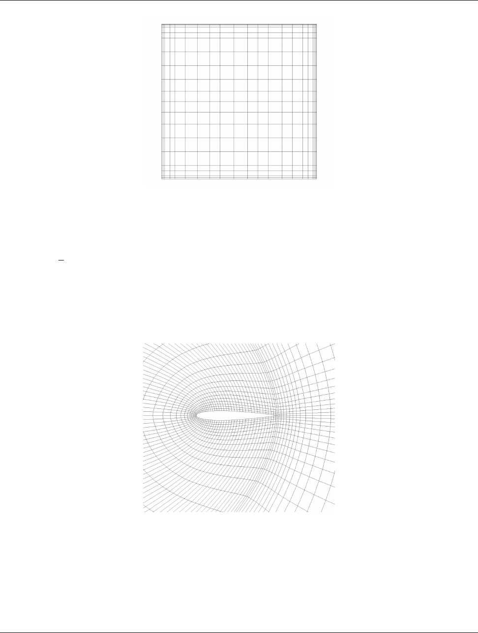
3.1. VTK data model
Figure 3.5: Rectilinear grid.
Note that the generic VTK interface for all datasets uses a flat index. The (i,j,k)index can be converted to this flat index
as follows: idx flat =k⇥(nptsx⇥nptsy)+ j⇥nptrx+i.
A rectilinear grid consists of cells of the same type. This type is determined by the dimensionality of the dataset (based on
the extents) and can either be vertex (0D), line (1D), pixel (2D), or voxel (3D).
3.1.5 Curvilinear grid (structured grid)
Figure 3.6: Curvilinear or structured grid.
A curvilinear grid, such as Figure 3.6, defines its topology implicitly and point coordinates explicitly. To fully define the
mesh for a curvilinear grid, VTK uses the following:
1. Extents - These define the minimum and maximum indices in each direction. For example, a curvilinear grid of
extents (0,9),(0,19),(0,29)has 10 ⇥20 ⇥30 points regularly defined over a curvilinear mesh.
2. An array of point coordinates - This array stores the position of each vertex explicitly.
34 Chapter 3. Understanding data
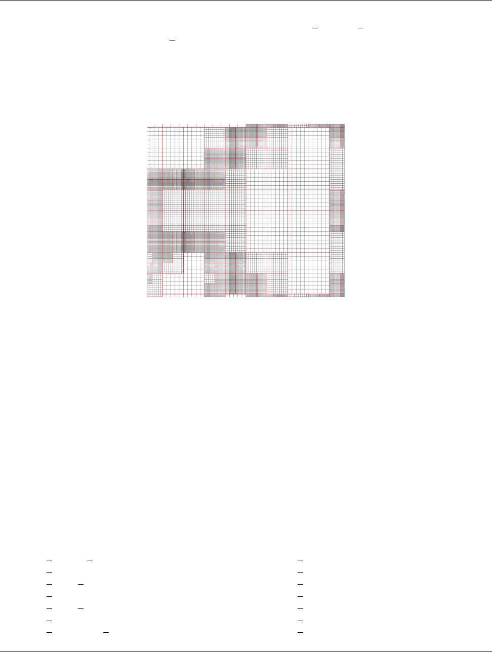
3.1. VTK data model
The coordinate of each point is defined as follows: coordinate =coordinate array(idx flat). The (i,j,k)index can be
converted to this flat index as follows: idx flat =k⇥(nptsx⇥nptsy)+ j⇥nptsx+i.
A curvilinear grid consists of cells of the same type. This type is determined by the dimensionality of the dataset (based
on the extents) and can either be vertex (0D), line (1D), quad (2D), or hexahedron (3D).
3.1.6 AMR dataset
Figure 3.7: AMR dataset.
VTK natively supports Berger-Oliger type Adaptive Mesh Refinement (AMR) datasets, as shown in Figure 3.7. An AMR
dataset is essentially a collection of uniform rectilinear grids grouped under increasing refinement ratios (decreasing spac-
ing). VTK’s AMR dataset does not force any constraint on whether and how these grids should overlap. However, it
provides support for masking (blanking) sub-regions of the rectilinear grids using an array of bytes. This allows VTK to
process overlapping grids with minimal artifacts. VTK can automatically generate the masking arrays for Berger-Oliger
compliant meshes.
3.1.7 Unstructured grid
An unstructured grid, such as Figure 3.8, is the most general primitive dataset type. It stores topology and point coordinates
explicitly. Even though VTK uses a memory-efficient data structure to store the topology, an unstructured grid uses
significantly more memory to represent its mesh. Therefore, use an unstructured grid only when you cannot represent your
dataset as one of the above datasets. VTK supports a large number of cell types, all of which can exist (heterogeneously)
within one unstructured grid. The full list of all cell types supported by VTK can be found in the file vtkCellType.h in the
VTK source code. Here is the list of cell types and their numeric values as of when this document was written:
•VTK EMPTY CELL = 0
•VTK VERTEX = 1
•VTK POLY VERTEX = 2
•VTK LINE = 3
•VTK POLY LINE = 4
•VTK TRIANGLE = 5
•VTK TRIANGLE STRIP = 6
•VTK POLYGON = 7
•VTK PIXEL = 8
•VTK QUAD = 9
•VTK TETRA = 10
•VTK VOXEL = 11
•VTK HEXAHEDRON = 12
•VTK WEDGE = 13
Chapter 3. Understanding data 35

3.1. VTK data model
Figure 3.8: Unstructured grid.
•VTK PYRAMID = 14
•VTK PENTAGONAL PRISM = 15
•VTK HEXAGONAL PRISM = 16
•VTK QUADRATIC EDGE = 21
•VTK QUADRATIC TRIANGLE = 22
•VTK QUADRATIC QUAD = 23
•VTK QUADRATIC TETRA = 24
•VTK QUADRATIC HEXAHEDRON = 25
•VTK QUADRATIC WEDGE = 26
•VTK QUADRATIC PYRAMID = 27
•VTK BIQUADRATIC QUAD = 28
•VTK TRIQUADRATIC HEXAHEDRON = 29
•VTK QUADRATIC LINEAR QUAD = 30
•VTK QUADRATIC LINEAR WEDGE = 31
•VTK BIQUADRATIC QUADRATIC WEDGE =
32
•VTK BIQUADRATIC QUADRATIC HEXAHEDRON
= 33
•VTK BIQUADRATIC TRIANGLE = 34
•VTK CUBIC LINE = 35
•VTK CONVEX POINT SET = 41
•VTK POLYHEDRON = 42
•VTK PARAMETRIC CURVE = 51
•VTK PARAMETRIC SURFACE = 52
•VTK PARAMETRIC TRI SURFACE = 53
•VTK PARAMETRIC QUAD SURFACE = 54
•VTK PARAMETRIC TETRA REGION = 55
•VTK PARAMETRIC HEX REGION = 56
•VTK HIGHER ORDER EDGE = 60
•VTK HIGHER ORDER TRIANGLE = 61
•VTK HIGHER ORDER QUAD = 62
•VTK HIGHER ORDER POLYGON = 63
•VTK HIGHER ORDER TETRAHEDRON = 64
•VTK HIGHER ORDER WEDGE = 65
•VTK HIGHER ORDER PYRAMID = 66
•VTK HIGHER ORDER HEXAHEDRON = 67
Many of these cell types are straightforward. For details, see the VTK documentation.
3.1.8 Polygonal grid (polydata)
A polydata, such as Figure 3.9, is a specialized version of an unstructured grid designed for efficient rendering. It consists
of 0D cells (vertices and polyvertices), 1D cells (lines and polylines), and 2D cells (polygons and triangle strips). Certain
filters that generate only these cell types will generate a polydata. Examples include the Contour and Slice filters. An
unstructured grid, as long as it has only 2D cells supported by polydata, can be converted to a polydata using the Extract
Surface Filter. A polydata can be converted to an unstructured grid using Clean to Grid.
36 Chapter 3. Understanding data
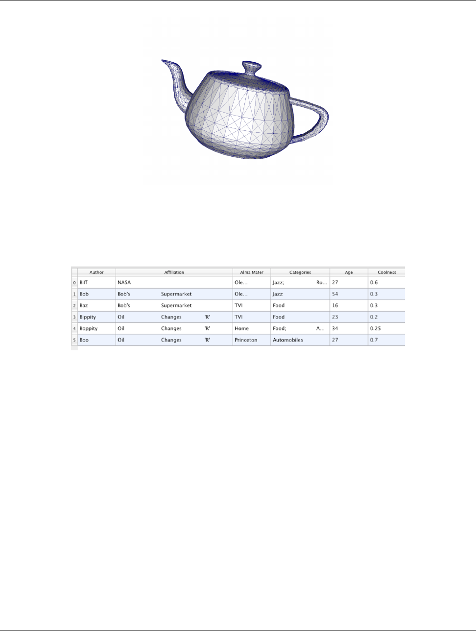
3.1. VTK data model
Figure 3.9: Polygonal grid.
3.1.9 Table
Figure 3.10: Table.
A table, such as Figure 3.10, is a tabular dataset that consists of rows and columns. All chart views have been designed to
work with tables. Therefore, all filters that can be shown within the chart views generate tables. Also, tables can be directly
loaded using various file formats such as the comma-separated values format. Tables can be converted to other datasets as
long as they are of the right format. Filters that convert tables include Table to Points and Table to Structured Grid.
3.1.10 Multiblock dataset
You can think of a multi-block dataset (Figure 3.11) as a tree of datasets where the leaf nodes are simple datasets. All of
the data types described above, except AMR, are simple datasets. Multi-block datasets are used to group together datasets
that are related. The relation between these datasets is not necessarily defined by ParaView. A multi-block dataset can
represent an assembly of parts or a collection of meshes of different types from a coupled simulation. Multi-block datasets
can be loaded or created within ParaView using the Group filter. Note that the leaf nodes of a multi-block dataset do not all
have to have the same attributes. If you apply a filter that requires an attribute, it will be applied only to blocks that have
that attribute.
Chapter 3. Understanding data 37
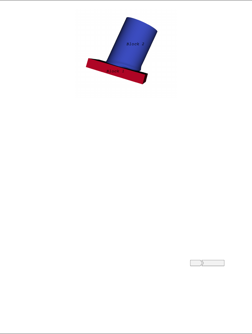
3.2. Getting data information in paraview
Figure 3.11: Multiblock dataset.
3.1.11 Multipiece dataset
Multi-piece datasets, such as Figure 3.12, are similar to multi-block datasets in that they group together simple datasets.
There is one key difference. Multi-piece datasets group together datasets that are part of a whole mesh - datasets of the
same type and with the same attributes. This data structure is used to collect datasets produced by a parallel simulation
without having to append the meshes together. Note that there is no way to create a multi-piece dataset within ParaView.
It can only be created by using certain readers. Furthermore, multi-piece datasets act, for the most part, as simple datasets.
For example, it is not possible to extract individual pieces or to obtain information about them.
3.2 Getting data information in paraview
In the visualization pipeline (Section 1.2), sources, readers, and filters are all producing data. In a VTK-based pipeline,
this data is one of the types discussed. Thus, when you create a source or open a data file in paraview and hit Apply, data is
being produced. The Information panel and the Statistics Inspector panel can be used to inspect the characteristics
of the data produced by any pipeline module.
3.2.1 The Information panel
The Information panel provides summary information about the data produced by the active source. By default, this
panel is tucked under a tab below the Properties panel. You can toggle its visibility using View Information .
The Information panel shows the data information for the active source. Thus, similar to the Properties panel, it
changes when the active source is changed (e.g., by changing the selection in the Pipeline Browser). One way to think
of this panel is as a panel showing a summary for the data currently produced by the active source. Remember that a
newly-created pipeline module does not produce any data until you hit Apply. Thus, valid information for a newly-created
source will be shown on this panel only after that Apply. Similarly, if you change properties on the source and hit Apply,
this panel will reflect any changes in data characteristics. Additionally, for temporal pipelines, this panel shows information
for the current timestep alone (except as noted). Thus, as you step through timesteps in a temporal dataset, the information
displayed will potentially change, and the panel will reflect those changes.
38 Chapter 3. Understanding data
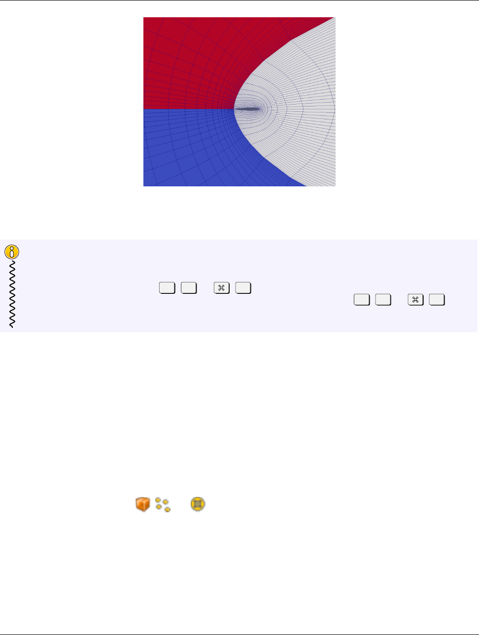
3.2. Getting data information in paraview
Figure 3.12: Multipiece dataset.
Did you know?
Any text on this panel is copy-able. For example, if want to copy the number of points value to use it as a property
value on the Properties panel, simply double-click on the number or click-and-drag to select the number and
use the common keyboard shortcut Ctrl +C(or +C) to copy that value to the clipboard. Now, you can paste
it in an input widget in paraview or any other application, such as an editor, by using Ctrl +V(or +V) or the
application-specific shortcut for pasting text from the clipboard. The same is true for numbers shown in lists, such
as the Data Ranges.
The panel itself is comprised of several groups of information. Groups may be hidden based on the type of pipeline module
or the type of data being produced.
The file Properties group is shown for readers with information about the file that is opened. For a temporal file series,
as you step through each time step, the file name is updated to point to the name of the file in the series that corresponds to
the current time step.
The Statistics group provides a summary of the dataset produced including its type, it number of cells and points (or
rows and columns in cases of Tabular datasets), and an estimate of the memory used by the dataset. This number only
includes the memory space needed to save the data arrays for the dataset. It does not include the memory space used by
the data structures themselves and, hence, must only be treated as an estimate.
The Data Arrays group lists all of the available point, cells, and field arrays, as well as their types and ranges for the
current time step. The Current data time field shows the time value for the current timestep as a reference. As with
other places in paraview, the icons , , and are used to indicate cell, point, and field data arrays. Since data arrays
can have multiple components, the range for each component of the data array is shown.
Bounds shows the spatial bounds of the datasets in 3D Cartesian space. This will be unavailable for non-geometric datasets
such as tables.
For reader modules, the Time group shows the available time steps and corresponding time values provided by the file.
For structured datasets such as uniform rectilinear grids or curvilinear grids, the Extents group is shown that displays the
structured extents and dimensions of the datasets.
All of the summary information discussed so far provides a synopsis of the entire dataset produced by the pipeline module,
Chapter 3. Understanding data 39
3.3. Getting data information in pvpython
including across all ranks (which will become clearer once we look at using ParaView for parallel data processing). In
cases of composite datasets, such as mutliblock datasets or AMR datasets, recall that these are datasets that are comprised
of other datasets. In such cases, these are summaries over all the blocks in the composite dataset. Every so often, you will
notice that the Data Arrays table lists an array with the suffix (partial) (Figure 3.14). Such arrays are referred to as
partial arrays. Partial arrays is a term used to refer to arrays that are present on some non-composite blocks or leaf nodes
in a composite dataset, but not all. The (partial) suffix to indicate partial arrays is also used by paraview in other places
in the UI.
While summaries over all of the datasets in the composite dataset are useful, you may also want to look at the data
information for individual blocks. To do so, you can use the Data Hierarchy group, which appears when summarizing
composite datasets. The Data Hierarchy widget shows the structure or hierarchy of the composite dataset (Figure 3.15).
The Information panel switches to showing the summaries for the selected sub-tree. By default, the root element will be
selected. You can now select any block in the hierarchy to view the summary limited to just that sub-tree.
Did you know?
Memory information shown on the Information panel and the Statistics Inspector should only be
used as an approximate reference and does not translate to how much memory the data produced by a particular
pipeline module takes. This is due to the following factors:
•The size does not include the amount of memory needed to build the data structures to store the data arrays.
While, in most cases, this is negligible compared to that of the data arrays, it can be nontrivial, especially
when dealing with deeply-nested composite datasets.
•Several filters such as Calculator and Shrink simply pass input data arrays through, so there’s no extra
space needed for those data arrays that are shared with the input. The memory size numbers shown, however,
do not take this into consideration.
If you need an overview of how much physical memory is being used by ParaView in its current state, you can use
the Memory Inspector (Section 16).
3.2.2 The Statistics Inspector panel
The Information panel shows data information for the active source. If you need a quick summary of the data produced
by all the pipeline modules, you can use the Statistics Inspector panel. It’s accessible from Views Statistics Inspector .
All of the information on this panel is also presented on the Information panel, except Geometry Size. This corresponds
to how much memory is needed for the transformed dataset used for rendering in the active view. For example, to render a
3D dataset as a surface in the 3D view, ParaView must extract the surface mesh as a polydata. Geometry Size represents
the memory needed for this polydata with the same memory-size-related caveats as with the Information panel.
3.3 Getting data information in pvpython
When scripting with ParaView, you will often find yourself needing information about the data. While paraview sets up
filter properties and color tables automatically using the information from the data, when scripting, you have to do that
explicitly.
In pvpython, for any pipeline module (sources, readers, or filters), you can use the following ways to get information about
the data produced.
1>>> from paraview.simple import *
2>>> reader = OpenDataFile(".../ParaViewData/Data/can.ex2")
3
40 Chapter 3. Understanding data

3.3. Getting data information in pvpython
4# We need to update the pipeline. Otherwise, all of the data
5# information we get will be from before the file is actually
6# read and, hence, will be empty.
7>>> UpdatePipeline()
8
9>>> dataInfo = reader.GetDataInformation()
10
11 # To get the number of cells or points in the dataset:
12 >>> dataInfo.GetNumberOfPoints()
13 10088
14 >>> dataInfo.GetNumberOfCells()
15 7152
16
17 # You can always nest the call, e.g.:
18 >>> reader.GetDataInformation().GetNumberOfPoints()
19 10088
20 >>> reader.GetDataInformation().GetNumberOfCells()
21 7152
22
23 # Use source.PointData or source.CellData to get information about
24 # point data arrays and cell data arrays, respectively.
25
26 # Let’s print the available point data arrays.
27 >>> reader.PointData[:]
28 [Array: ACCL, Array: DISPL, Array: GlobalNodeId , Array: PedigreeNodeId , Array: VEL]
29
30 # Similarly, for cell data arrays:
31 >>> reader.CellData[:]
32 [Array: EQPS, Array: GlobalElementId , Array: ObjectId, Array: PedigreeElementId]
PointData (and CellData) is a map or dictionary where the keys are the names of the arrays, and the values are objects
that provide more information about each of the arrays. In the rest of this section, anything we demonstrate on PointData
is also applicable to CellData.
1# Let’s get the number of available point arrays.
2>>> len(reader.PointData)
35
4
5# Print the names for all available point arrays.
6>>> reader.PointData.keys()
7[’ACCL’,’DISPL’,’GlobalNodeId’,’PedigreeNodeId’,’VEL’]
8
9>>> reader.PointData.values()
10 [Array: ACCL, Array: DISPL, Array: GlobalNodeId , Array: PedigreeNodeId , Array: VEL]
11
12 # To test if a particular array is present:
13 >>> reader.PointData.has_key("ACCL")
14 True
15
16 >>> reader.PointData.has_key("--non -existent -array --")
17 False
From PointData (or CellData), you can get access to an object that provides information for each of the arrays. This
object gives us methods to get data ranges, component counts, tuple counts, etc.
1
Chapter 3. Understanding data 41

3.3. Getting data information in pvpython
2# Let’s get information about ’ACCL’ array.
3>>> arrayInfo = reader.PointData["ACCL"]
4>>> arrayInfo.GetName()
5’ACCL’
6
7# To get the number of components in each tuple and the number
8# of tuples in the data array:
9>>> arrayInfo.GetNumberOfTuples()
10 10088
11 >>> arrayInfo.GetNumberOfComponents()
12 3
13
14 # Alternative way for doing the same:
15 >>> reader.PointData["ACCL"].GetNumberOfTuples()
16 10088
17 >>> reader.PointData["ACCL"].GetNumberOfComponents()
18 3
19
20 # To get the range for a particular component, e.g. component 0:
21 >>> reader.PointData["ACCL"].GetRange(0)
22 (-4.965284006175352e-07, 3.212448973499704e-07)
23
24 # To get the range for the magnitude in cases of multi-component arrays
25 # use -1 as the component number.
26 >>> reader.PointData["ACCL"].GetRange (-1)
27 (0.0, 1.3329898584157294e-05)
28
29 # To determine the data data type for this array:
30 >>> from paraview import vtk
31 >>> reader.PointData["ACCL"].GetDataType () == vtk. VTK_DOUBLE
32 True
33 # The paraview.vtk module provides access to these constants such as
34 # VTK_DOUBLE, VTK_FLOAT, VTK_INT, etc.
35
36 # Likewise, to test the dataset type, itself:
37 >>> reader.GetDataInformation().GetDataSetType() == \
38 vtk.VTK_MULTIBLOCK_DATA_SET
39 True
Here’s a sample script to iterate over all point data arrays and print their magnitude ranges:
1
2>>> def print_point_data_ranges(source):
3... """Prints array ranges for all point arrays """
4... for arrayInfo in source.PointData:
5... # get the array’s name
6... name = arrayInfo.GetName()
7... # get magnitude range
8... range = arrayInfo.GetRange(-1)
9... print " %s = [%.3f , %.3f ] " %(name,range[0],range[1])
10
11 # Let’s call this function on our reader.
12 >>> print_point_data_ranges(reader)
13 ACCL = [0.000, 0.000]
14 DISPL = [0.000, 0.000]
15 GlobalNodeId = [1.000, 10088.000]
42 Chapter 3. Understanding data

3.3. Getting data information in pvpython
16 PedigreeNodeId = [1.000, 10088.000]
17 VEL = [0.000 , 5000.000]
Chapter 3. Understanding data 43
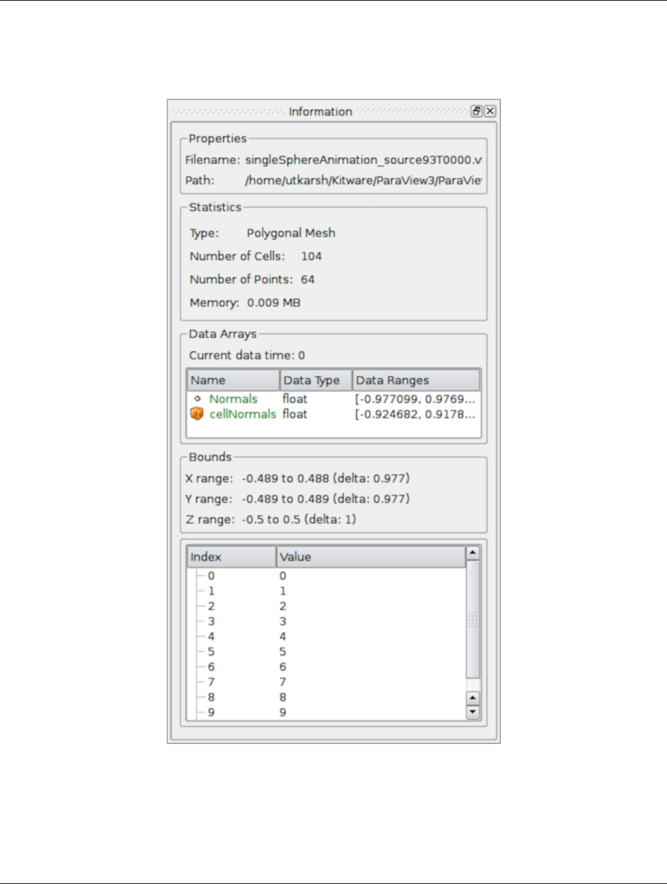
3.3. Getting data information in pvpython
Figure 3.13: The Information panel in paraview showing data summaries for the active source.
44 Chapter 3. Understanding data
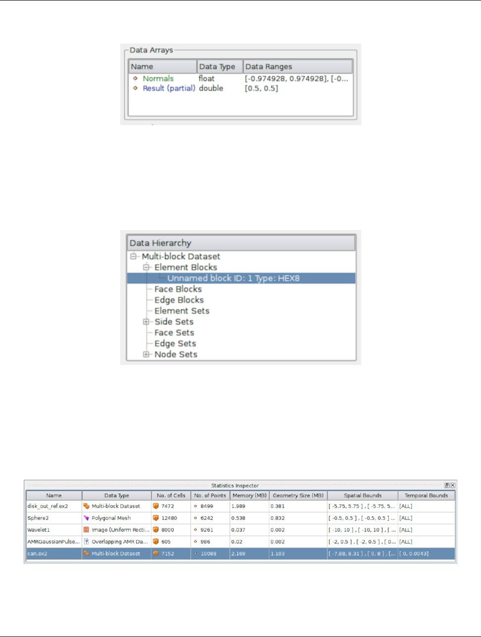
3.3. Getting data information in pvpython
Figure 3.14: The Data Arrays section on Information panel showing partial arrays. Partial arrays are arrays that present
on certain blocks in a composite dataset, but not all.
Figure 3.15: The Data Hierarchy section on the Information panel showing the composite data hierarchy. Selecting
a particular block or subtree in this widget will result in the reset of the Information panel showing summaries for that
block or subtree alone.
Figure 3.16: The Statistics Inspector panel in paraview showing summaries for all pipeline modules.
Chapter 3. Understanding data 45
CHAPTER
FOUR
DISPLAYING DATA
The goal of any visualization process is to produce visual representations of the data. The visual representations are shown
in modules called views. Views provide the canvas on which to display such visual representations, as well as to dictate
how these representations are generated from the raw data. The role of the visualization pipeline is often to transform the
data so that relevant information can be represented in these views.
Referring back to the visualization pipeline from Section 1.2, views are sinks that take in input data but do not produce
any data output. (I.e., one cannot connect other pipeline modules such as filters to process the results in a view.) However,
views often provide mechanisms to save the results as images or in other formats including PDF, VRML, and X3D.
Different types of views provide different ways of visualizing data. These can be broadly grouped as follows:
•Rendering Views are views that render geometries or volumes in a graphical context. The Render View is one such
view. Other Render View-based views, such as Slice View and Quad View, extend the basic render view to add
the ability to add mechanisms to easily inspect slices or generate orthogonal views.
•Chart Views cover a wide array of graphs and plots used for visualizing non-geometric data. These include views
such as line charts (Line Chart View), bar charts (Bar Chart View), bag charts (Bag Chart View), parallel co-
ordinates (Parallel Coordinates View), etc.
•Comparative Views are used to quickly generate side-by-side views for parameter study, i.e., to visualize the effects
of parameter changes. Comparative variants of Render View and several types of the Chart Views are available in
ParaView.
In this chapter, we take a close look at the various views available in ParaView and how to use these views for displaying
data.
4.1 Multiple views
With multiple types of views comes the need for creating and viewing multiple views at the same time. In this section, we
look at how you can create multiple views and lay them out.
Did you know?
Multiple views were first supported in ParaView 3.0. Before that, all data was shown in a single 3D render view,
including line plots!
4.1.1 Multiple views in paraview
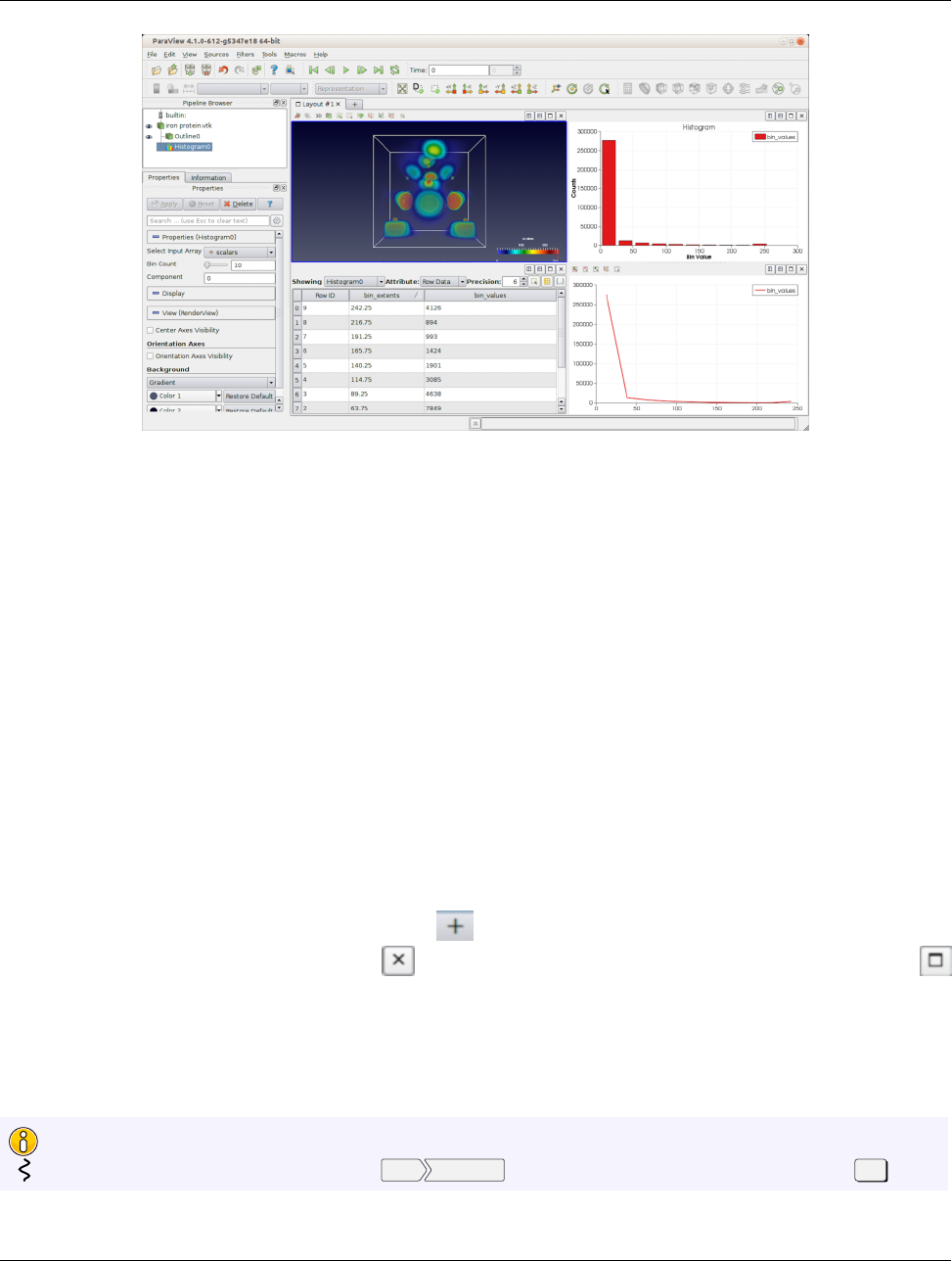
4.1. Multiple views
Figure 4.1: Using multiple views in paraview to generate different types of visualizations from a dataset.
paraview shows all views in the central part of the application window. When paraview starts up, the Render View is
created and shown in the application window by default.
New views can be created by splitting the view frame using the Split View controls at the top-right corner of the view
frame. Splitting a view splits the view into two equal parts, either vertically or horizontally, based on the button used for
the split. On splitting a view, an empty frame with buttons for all known types of views is shown. Simply click on one of
those buttons to create a new view of a chosen type.
You can move views by clicking and dragging the title bar for the view (or empty view frame) and dropping it on the title
bar on another view (or empty view frame). This will swap the positions of the two views.
Similar to the notion of active source, there is a notion of active view. Several panels, toolbars, and menus will update
based on the active view. The Display properties section on the Properties panel, for example, reflects the display
properties of the active source in the active view. Similarly, the eyeball icons in the Pipeline Browser show the visibility
status of the pipeline module in the active view. Active view is marked in the UI by a blue border around the view frame.
Only one view can be active at any time in the application.
Besides being able to create multiple views and laying them out in a pane, paraview also supports placing views in multiple
layouts under separate tabs. To create new tabs, use the button in the tab bar. You can close a tab, which will destroy
all views laid out in that tab, by clicking on the button. To pop out an entire tab as a separate window, use the
button on the tab bar.
The active view is always present in the active tab. Thus, if you change the active tab, the active view will also be changed
to be a view in the active tab layout. Conversely, if the active view is changed (by using the Python Shell, for example),
the active tab will automatically be updated to be the tab that contains the active view.
Did you know?
You can make the views fullscreen by using View Fullscreen . To return back to the normal mode, use the Esc key.
48 Chapter 4. Displaying data

4.1. Multiple views
4.1.2 Multiple views in pvpython
In pvpython, one can create new views using the CreateView function or its variants, e.g.,
CreateRenderView.
1>>> from paraview.simple import *
2>>> view = CreateRenderView()
3# Alternatively, use CreateView.
4>>> view = CreateView("RenderView")
When a new view is created, it is automatically made active. You can manually make a view active by using the
SetActiveView function. Several of the functions available in pvpython will use the active view when no view is passed
as an argument to the function.
1# Create a view
2>>> view1 = CreateRenderView()
3# Create a second view
4>>> view2 = CreateRenderView()
5
6# Check if view2 is the active view
7>>> view2 == GetActiveView()
8True
9
10 # Make view1 active
11 >>> SetActiveView(view1)
12 >>> view1 == GetActiveView()
13 True
When using Python Shell in paraview, if you create a new view, it will automatically be placed in the active tab by
splitting the active view. You can manually control the layout and placement of views from Python too, using the layout
API.
In Python, each tab that corresponds is referred to as a layout.
1# To get exisiting tabs/layouts
2>>> layouts = GetLayouts()
3>>> print layouts
4{(’ViewLayout1’,’264’): <paraview.servermanager.ViewLayout object at 0x2e5b7d0 >}
5
6# To get layout corresponding to a particular view
7>>> print GetLayout(view)
8<paraview.servermanager.ViewLayout object at 0x2e5b7d0>
9
10 # If view is not specified, active view is used
11 >>> print GetLayout()
12 <paraview.servermanager.ViewLayout object at 0x2e5b7d0>
13
14 # To create a new tab
15 >>> new_layout = servermanager.misc.ViewLayout(registrationGroup="layouts")
16
17 # To split the cell containing the view, either horizontally or vertically
18 >>> view = GetActiveView()
19 >>> layout = GetLayout(view)
20 >>> locationId = layout.SplitViewVertical(view=view,
21 fraction=0.5)
22 # fraction is optional, if not specified the frame is split evenly.
23
Chapter 4. Displaying data 49
4.2. View properties
24 # To assign a view to a particular cell.
25 >>> view2 = CreateRenderView()
26 >>> layout.AssignView(locationId , view2)
4.2 View properties
Just like parameters on pipeline modules, such as readers and filters, views provide parameters that can be used for cus-
tomizing the visualization such as changing the background color for rendering views and adding title texts for chart views.
These parameters are referred to as View Properties and are accessible from the Properties panel in paraview.
4.2.1 View properties in paraview
Similar to properties on pipeline modules like sources and readers, view properties are accessible from the Properties
panel. These are grouped under the View section. When the active view is changed, the Properties panel updates to
show the view properties for the active view. Unlike pipeline modules, however, when you change the view properties,
they affect the visualization immediately, without use of the Apply button.
Did you know?
It may seem odd that View and Display properties on the Properties panel don’t need to be Apply-ed to
take effect, while properties on pipeline modules like sources, readers and filter require you to hit the Apply button.
To understand the reasoning behind that, we need to understand why the Apply action is needed in the first place.
Generally, executing a data processing filter or reader is time consuming on large datasets. If the pipeline module
keeps on executing as you are changing the parameter, the user experience will quickly deteriorate, since the pipeline
will keep on executing with intermediate (and potentially invalid) property values. To avoid this, we have the Apply
action. This way, you can set up the pipeline properties to your liking and then trigger the potentially time consuming
execution.
Since the visualization process in general focuses on reducing data to generate visual representations, the rendering
(broadly speaking) is less time-intensive than the actual data processing. Thus, changing properties that affect
rendering are not as compute-intensive as transforming the data itself. (E.g., changing the color on a surface mesh
is not as expensive as generating the mesh in the first place.) Hence, the need to Apply such properties becomes
less relevant. At the same time, when changing display properties such as opacity, you may want to see the result as
you change the property to decide on the final value. Hence, it is desirable to see the updates immediately.
Of course, you can always enable Auto Apply to have the same immediate update behavior for all properties on
the Properties panel.
4.2.2 View properties in pvpython
In pvpython, once you have access to the view, you can directly change view properties on the view object. There are
several ways to get access to the view object.
1# 1. Save reference when a view is created
2>>> view = CreateView("RenderView")
3
4# 2. Get reference to the active view.
5>>> view = GetActiveView()
50 Chapter 4. Displaying data
4.3. Display properties
The properties available on the view will change based on the type of the view. You can use the help function to discover
available properties.
1>>> view = CreateRenderView()
2>>> help(view)
3
4Help on RenderView in module paraview.servermanager object:
5
6class RenderView(Proxy)
7|Viewproxyfor a3Dinteractiverender
8|view.
9|
10 | ----------------------------------------------------------------------
11 |Datadescriptorsdefinedhere:
12 |
13 | CenterAxesVisibility
14 |Togglethevisibilityoftheaxesshowingthecenterof
15 | rotation in the scene.
16 |
17 | CenterOfRotation
18 |Centerofrotationfor the interactor.
19 |
20 ...
Once you have a reference to the view, you can then get/set the properties.
1# Get the current value
2>>> print view.CenterAxesVisibility
31
4
5# Change the value
6>>> view.CenterAxesVisibility = 0
4.3 Display properties
Display properties refers to available parameters that control how data from a pipeline module is displayed in a view, e.g.,
choosing to view the output mesh as a wireframe, coloring the mesh using a data attribute, and selecting which attributes
to plot in chart view. A set of display properties is associated with a particular pipeline module and view. Thus, if the data
output from a source is shown in two views, there will be two sets of display properties used to control the appearance of
the data in each of the two views.
4.3.1 Display properties in paraview
Display properties are accessible from the Display section on the Properties panel. When the active source or active
view changes, this section updates to show the display properties for the active source in the active view, if available. If
the active source produces data that cannot be shown (or has never been shown) in the view, then the Display properties
section may be empty.
Similar to view properties, display property changes are immediately applied, without requiring the use of the Apply
button.
Chapter 4. Displaying data 51

4.3. Display properties
4.3.2 Display properties in pvpython
To access display properties in pvpython, you can use SetDisplayProperties and
GetDisplayProperty methods.
1
2# Using SetDisplayProperties/GetDisplayProperties to access the display
3# properties for the active source in the active view.
4
5>>> print GetDisplayProperties("Opacity")
61.0
7
8>>> SetDisplayProperties(Opacity =0.5)
Alternatively, you can get access to the display properties object using GetDisplayProperties and then changing prop-
erties directly on the object.
1# Get display properties object for the active source in the active view.
2>>> disp = GetDisplayProperties()
3
4# You can also save the object returned by Show.
5>>> disp = Show()
6
7# Now, you can directly access the properties
8>>> print disp.Opacity
90.5
10
11 >>> disp.Opacity = 0.75
As always, you can use the help method to discover available properties on a display object.
1>>> disp = Show()
2
3>>> help(disp)
4>>> help(a)
5Help on GeometryRepresentation in module paraview.servermanager object:
6
7class GeometryRepresentation(SourceProxy)
8|ParaView‘sdefaultrepresentationfor showing any type of
9|datasetin the render view.
10 |
11 |Methodresolutionorder:
12 | GeometryRepresentation
13 |SourceProxy
14 | Proxy
15 |__builtin__.object
16 |
17 | ----------------------------------------------------------------------
18 |Datadescriptorsdefinedhere:
19 |
20 |...
21 |
22 | CenterStickyAxes
23 |Keepthestickyaxescenteredin the view window.
24 |
25 | ColorArrayName
26 |Setthearraynametocolorby.Setittoemptystring
52 Chapter 4. Displaying data
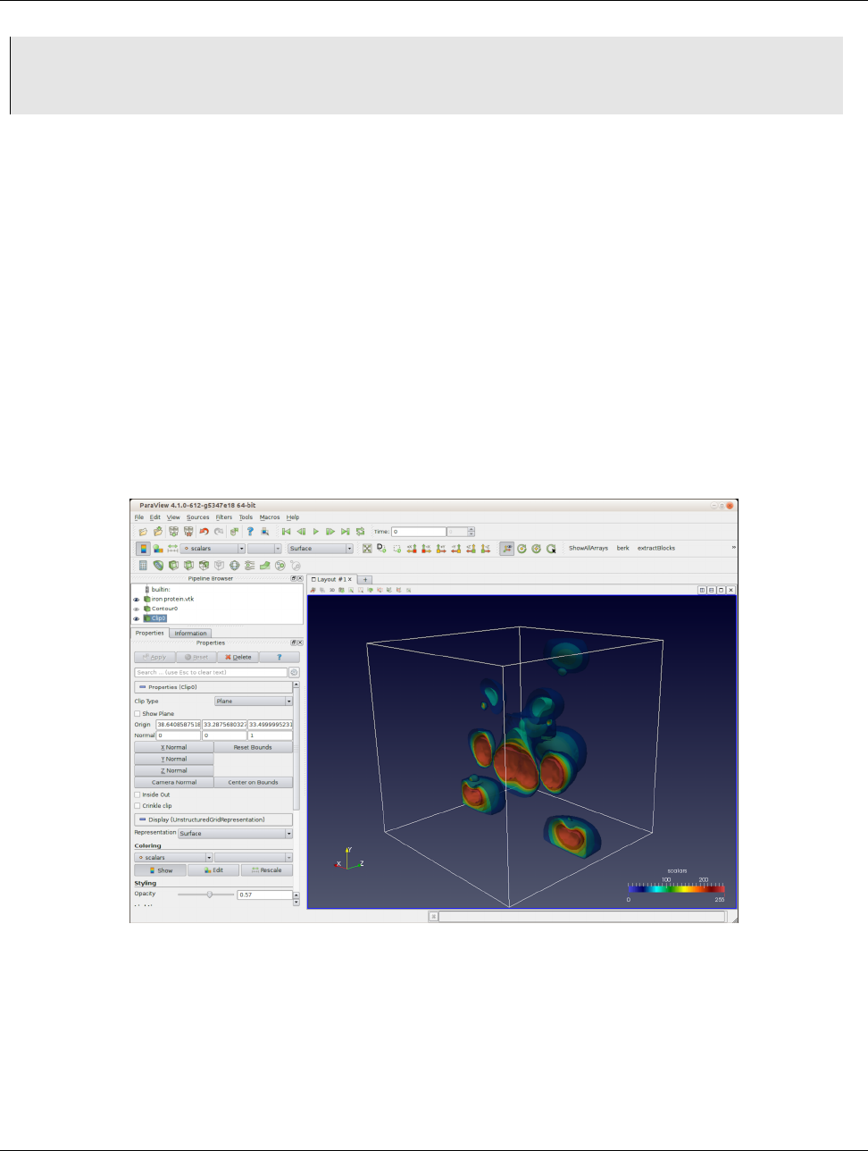
4.4. Render View
27 |tousesolidcolor.
28 |
29 | ColorAttributeType
30 |...
4.4 Render View
Render View is the most commonly used view in ParaView. It is used to render geometries and volumes in a 3D scene.
This is the view that you typically think of when referring to 3D visualization. The view relies on techniques to map data
to graphics primitives such as triangles, polygons, and voxels, and it renders them in a scene.
Most of the scientific datasets discussed in Section 3.1 are comprised of meshes. These meshes can be mapped to graphics
primitives using several of the established visualization techniques. (E.g., you can compute the outer surface of these
meshes and then render that surface as filled polygons, you can just render the edges, or you can render the data as
a nebulous blob to get a better understanding of the internal structure in the dataset.) Plugins, like Surface LIC, can
provide additional ways of rendering data using advanced techniques that provide more insight into the data.
If the dataset doesn’t represent a mesh, e.g., a table (Section 3.1.9), you cannot directly show that data in this view.
However, in such cases, it may be possible to construct a mesh by mapping columns in the table to positions to construct a
point cloud, for example.
Figure 4.2: paraview using Render View to generate 3D visualizations from a dataset.
4.4.1 Understanding the rendering process
Render View uses data processing techniques to map raw data to graphics primitives, which can then be rendered in a 3D
scene. These mapping techniques can be classified as follows:
Chapter 4. Displaying data 53
4.4. Render View
•Surface rendering methods provide general rendering by rendering a surface mesh for the dataset. For polygonal
datasets (Section 3.1.8), this is simply the raw data. In cases of other datasets including structured (Sections 3.1.3,
3.1.4, 3.1.5) and unstructured (Section 3.1.7) grids, this implies extracting a surface mesh for all external faces in
the dataset and then rendering that mesh. The surface mesh itself can then be rendered as a filled surface or as a
wireframe simply showing the edges, etc.
•Slice rendering is available for uniform rectilinear grid datasets (Section 3.1.3) where the visualization is generated
by simply rendering an orthogonal slice through the dataset. The slice position and alignment can be selected using
the display properties.
•Volume rendering generates rendering by tracing a ray through the dataset and accumulating intensities based on the
color and opacity transfer functions set.
Each of these techniques are referred to as representations. When available, you can change the representation type from
the display properties on the Properties panel or using the Representation Toolbar.
4.4.2 Render View in paraview
Creating a Render View
Unless you changed the default setting, a new Render View will be created when paraview starts up or connects to a new
server. To create a Render View in paraview, split or close a view, and select the Render View button. You can also
convert a view to a Render View (or any other type) by right-clicking on the view’s title bar and picking from the Convert
To sub-menu. It simply closes the chosen view and creates a selected view type in its place.
You can use the Pipeline Browser to control the visibility of datasets produced by pipeline modules in this view. The
eyeball icons reflect the visibility state. Clicking on the eyeball icon will toggle the visibility state. If no eyeball icon is
shown, it implies that the pipeline module doesn’t produce a data type that can be directly shown in the active view, e.g., if
the module produced a table, then when Render View is active, there will not be any eyeball icon next to that module.
Interactions
You can interact with the Render View to move the camera in the scene for exploring the visualization and setting up
optimal viewing angles. Each of the three mouse buttons, combined with keyboard modifier keys ( Ctrl or , and ),
move the camera differently. The interaction mode can be changed from the Camera tab in the Settings dialog, which is
accessible from Tools Settings (or ParaView Preferences on OS X). There are six interaction modes available in ParaView:
Pan for translating the camera in the view plane.
Zoom for zooming in or out of the center of the view.
Roll for rolling the camera.
Rotate for rotating the camera around the center of rotation.
Zoom To Mouse for zooming in or out of the projected point under the mouse position.
Multi Rotate for allowing azimuth and elevation rotations by dragging from the middle of the view and rolls by dragging
from the edges.
The default interactions options are as follows:
54 Chapter 4. Displaying data
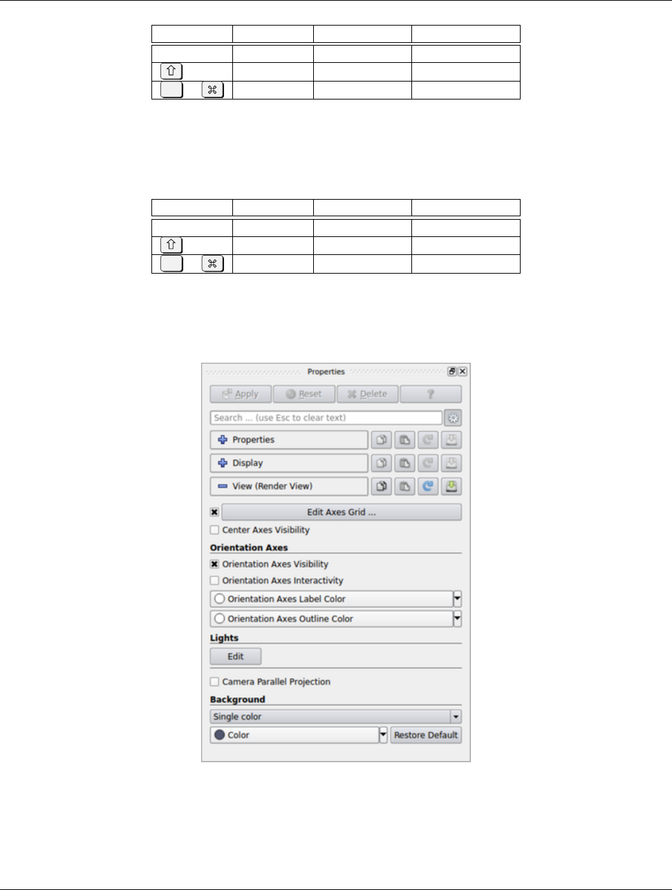
4.4. Render View
Modifier Left Button Middle Button Right Button
Rotate Pan Zoom
Roll Rotate Pan
Ctrl or Zoom Rotate Zoom To Mouse
Generally, you are interacting with a 3D scene, however, there are cases when you are working with a 2D dataset such as a
slice plane or a 2D image. In such cases, paraview provides a separate set of interaction options suitable for 2D interactions.
You can toggle between the default 3D interaction options and 2D interaction options by clicking the 2D or 3D button in
the view toolbar. The default interaction options for 2D interactions are as follows:
Modifier Left Button Middle Button Right Button
Pan Roll Zoom
Zoom Zoom Zoom To Mouse
Ctrl or Roll Pan Rotate
View properties
Several of the view properties in Render View control the annotations shown in the view (Figure 4.3).
Figure 4.3: The Properties panel showing view properties for Render View.
Axes Grid refers to an annotation axis rendered around all datasets in the view (Figure 4.4). You use the checkbox next
to the Edit Axis Grid button to show or hide this annotation. To control the annotation formatting, labels, etc., click on
the Edit Axes Grid... button. The Axes Grid is described in Chapter 18.
Chapter 4. Displaying data 55
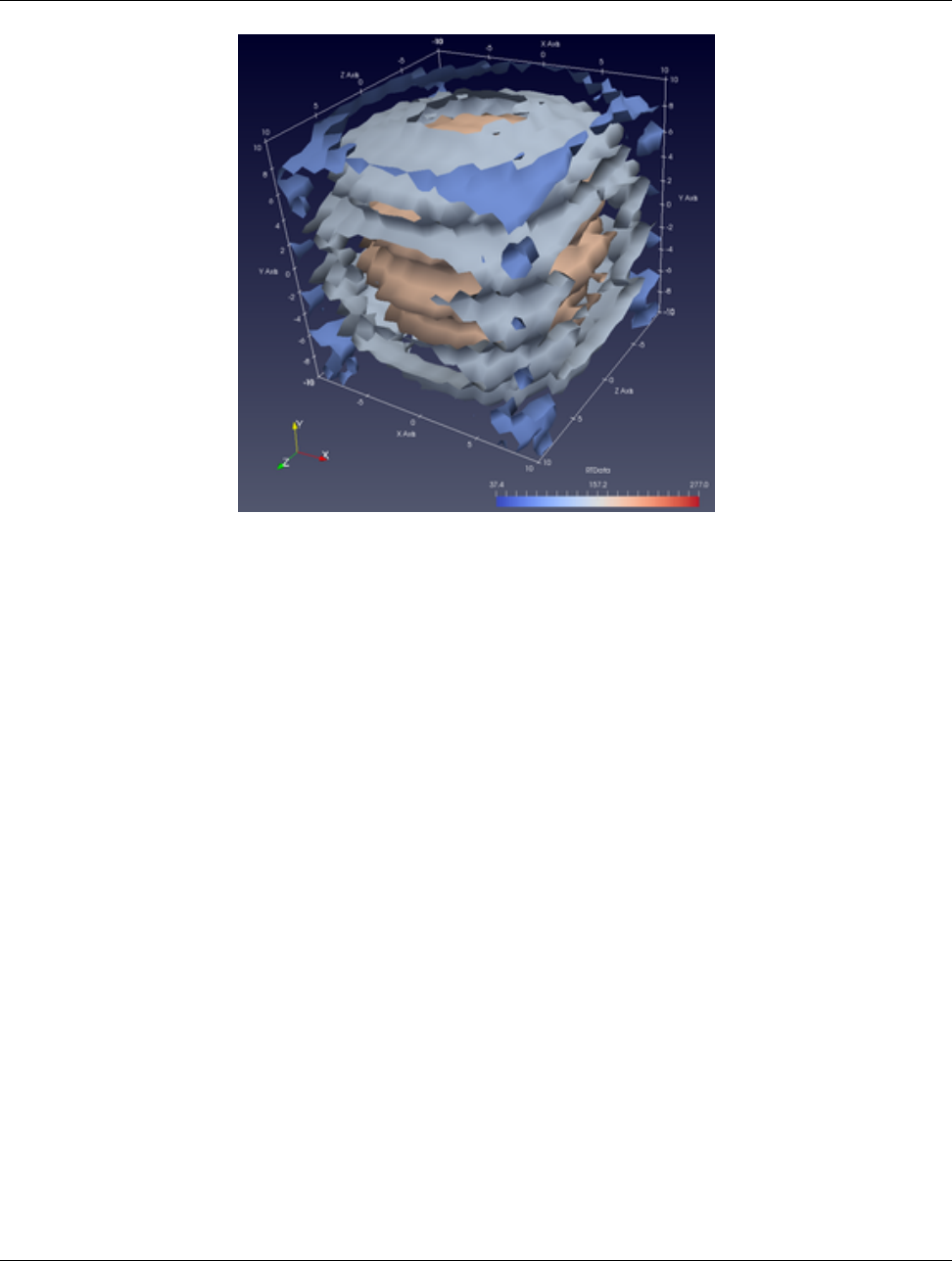
4.4. Render View
Figure 4.4: Axes Grid is used to annotate data bounds in Render View.
The Center axes refers to axes rendered in the scene positioned as the center of rotation, i.e., the location is space around
which the camera revolves during Rotate camera interaction. Center Axes Visibility controls the visibility of the
center axes.
The Orientation axes is the widget shown at the lower-left corner by default, which is used to get a sense for the orientation
of the scene. The properties grouped under the Orientation Axes group allow you to toggle the visibility and the
interactivity of this widget. When interactivity is enabled, you can click and drag this widget to the location of your
choosing in the scene.
You can also change the Background used for this view. You can either set it as a Single color or as a Gradient comprised
of two colors, or you can select an Image (or texture) to use as the background.
There are two advanced properties you may need to set: additional headlight and camera parallel projection. If your data
is 2D and is facing parallel to the viewing screen you may want to change the lighting for the scene. The default lights
in ParaView are designed similar with the lights in a photography studio. They make the shape of 3D objects more clear
however they result in dull colors when used with 2D objects. To use lighting more appropriate for 2D objects click on
the Edit button in the Lights section and then select Additional Headlight and deselect Light Kit. If you want to
render your data using parallel projection instead of the default perspective projection you can check Camera Parallel
Projection checkbox.
56 Chapter 4. Displaying data
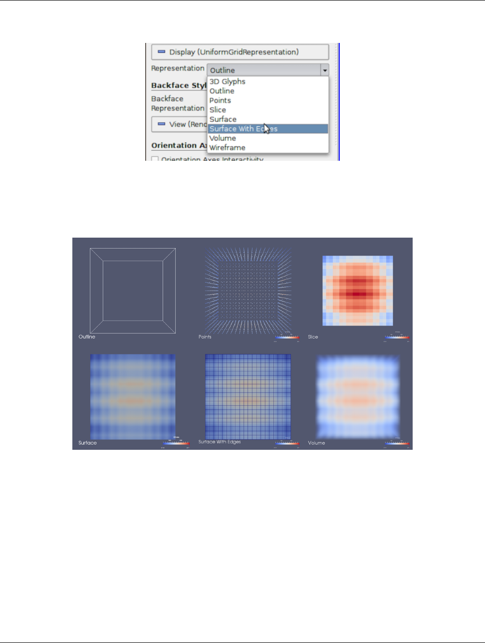
4.4. Render View
Display properties
One of the first (and probably the most often used) display properties is Representation.Representation allows
you to pick one of the mapping modes. The options available depend on the data type, as well as the plugins loaded.
While all display properties are accessible from the advanced view for the Properties panel, certain properties may be
shown/hidden from the default view based on the chosen representation type.
Figure 4.5: Different renderings generated by rendering data produced by the Wavelet source as outline, points, slice,
surface, surface with edges, and volume.
Outline representation can be used to render an outline for the dataset. This is arguably the fastest way of rendering the
dataset since only the bounding box is rendered. Scalar coloring options, i.e., selecting an array with which to color, has
no effect on this representation type. You can still, however, change the Solid Color to use as well as the Opacity.To
change the color, select Solid Color in the combo-box under Coloring, and then click Edit to pick the color to use. To
change the opacity, simply change the Opacity slider. 0 implies total transparency and, hence, invisiblity, while 1 implies
totally opacity.
Chapter 4. Displaying data 57
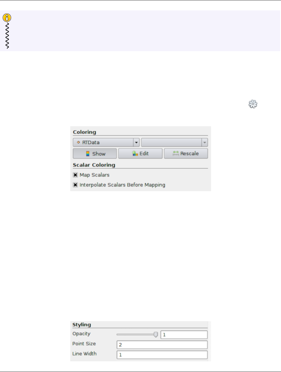
4.4. Render View
Did you know?
Rendering translucent data generally adds computational costs to the rendering process. Thus, when rendering
large datasets, you may want to leave changing opacities to anything less than 1 to the very end, after having set
up the visualization. In doing so, you avoid translucent geometries during exploration, but use them for generating
images or screenshots for presentations and publications.
Points,Surface,Surface With Edges, and Wireframe rely on extracting the surface mesh from the dataset and then
rendering that either as a collection of points, as solid surface, as solid surface with cell boundaries highlighted, or as a
wireframe of cell boundaries with empty cells. You can either set a single solid color to use, as with Outline, or select a
data array to use for scalar coloring (also known as pseudocoloring).
Next, we will cover each of the property groups available under Display properties. Several of these are marked as
advanced. Accordingly, you may need to either toggle the panel to show advanced properties using the button or
search for it by name using the search box.
Display properties under Coloring allow you to set how the dataset is colored. To select a single solid color to use to fill the
surface or with which to color wireframe or points, select Solid Color in the combo-box, and then click Edit. That will
pop up the standard color chooser dialog, allowing you to pick a color to use. If, instead, you want to pseudocolor using an
attribute array available on the dataset, select that array name from the combo-box. For multi-component arrays, you can
pick a particular component or Magnitude to use for scalar coloring. ParaView will automatically setup a color transfer
function to use to map the data array to colors. The default range for the transfer function is set up based on the application
Settings. To reset the transfer function range to the current data range, you can use the Rescale button. Remember that,
despite the fact that you can set the scalar array with which to color when rendering as Outline, the outline itself continues
to use the specified solid color. Scalar Coloring properties are only relevant when you have selected a data array with
which to pseudocolor. The Map Scalars checkbox affects whether a color transfer function should be used (Figure 4.6).
If unchecked, and the data array can directly be interpreted as colors, then those colors are used directly. If not, the color
transfer function will be used. A data array can be interpreted as colors if, and only if, it is an unsigned char array with two,
three, or four components. Interpolate Scalars Before Mapping controls how color interpolation happens across
rendered polygons. If on, scalars will be interpolated within polygons, and color mapping will occur on a per-pixel basis.
If off, color mapping occurs at polygon points, and colors are interpolated, which is generally less accurate. Refer to the
Kitware blog[3] for a detailed explanation of this option.
58 Chapter 4. Displaying data
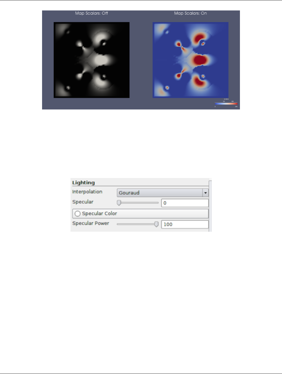
4.4. Render View
Figure 4.6: The Map Scalars property can be used to avoid using a transfer function and directly interpreting the array
values as colors, if possible.
Styling properties include Opacity (useful when rendering translucent geometries), Point Size (used to control size of
points rendered with using Points representation), and Line Width (used to control the thickness of lines when rendering
as Wireframe or that of the edges when rendering as Surface With Edges.
Lighting properties affect the shading for rendered surfaces. Interpolation allows you to pick between Flat and
Gouraud shading. Specular, together with Specular Color and Specular Power, affects the shininess of the surface.
Set this to a non-zero value to render shiny, metallic surfaces.
Chapter 4. Displaying data 59
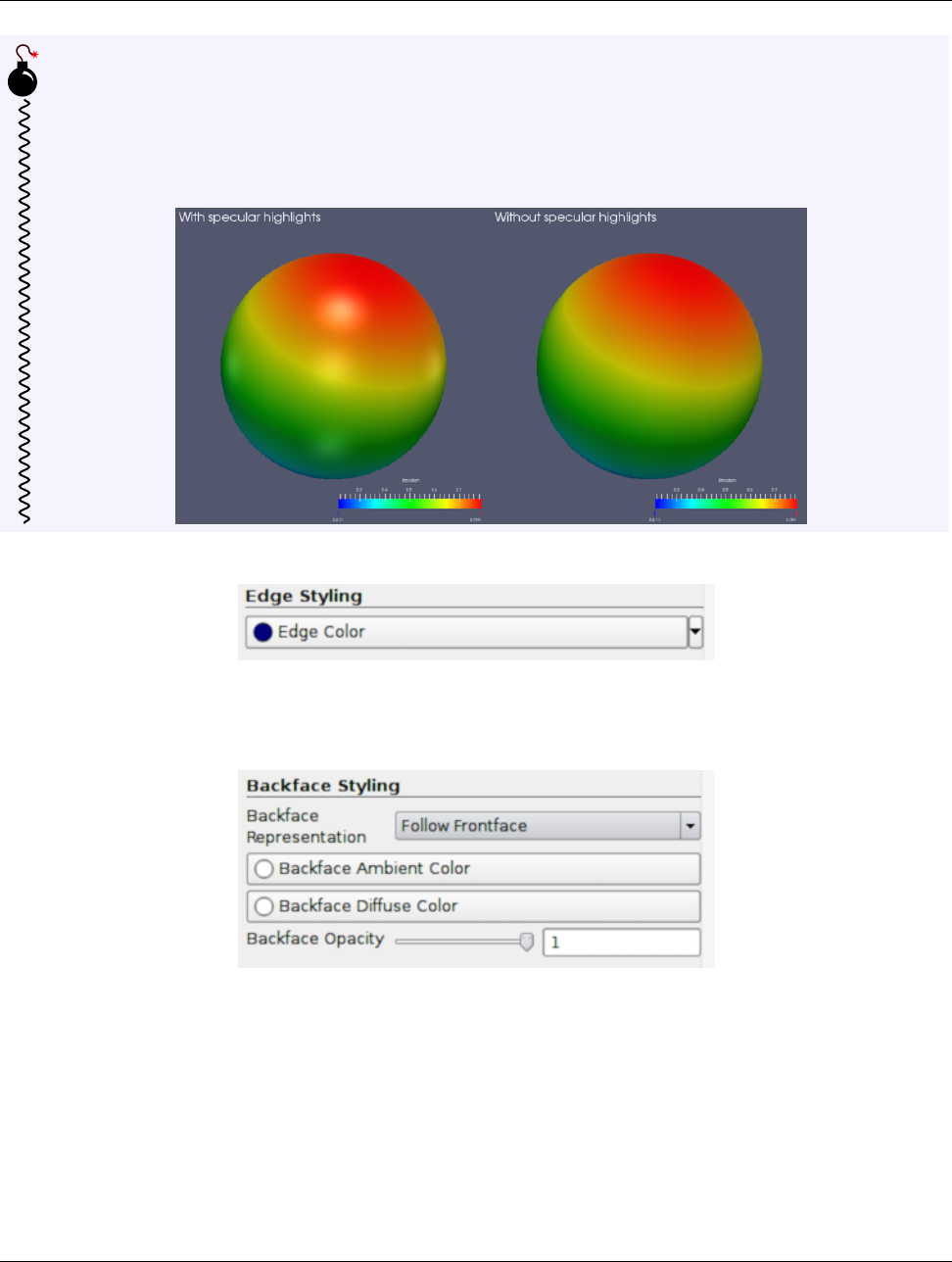
4.4. Render View
Common Errors
Specular highlights can lead to misinterpretation of scalar values when using scalar coloring, since the color
shown on the shiny part of the surface will not correspond to any color on the color transfer function. Hence, it is
generally advisable to use specular highlights on surfaces colored with a single solid color and not on those using
scalar coloring (or pseduocoloring).
Edge Styling allows you to set the Edge Color with which to color the edges when using Surface With Edges repre-
sentation.
Backface Styling provides advanced controls to fine-tune the rendering by controlling front and back faces. A front
face is any mesh face facing the camera, while a back face is the one facing away from the camera. By choosing to Cull
Frontface or Cull Backface, or by selecting a specific representation type to use for the backface, you can customize
your visualizations.
60 Chapter 4. Displaying data
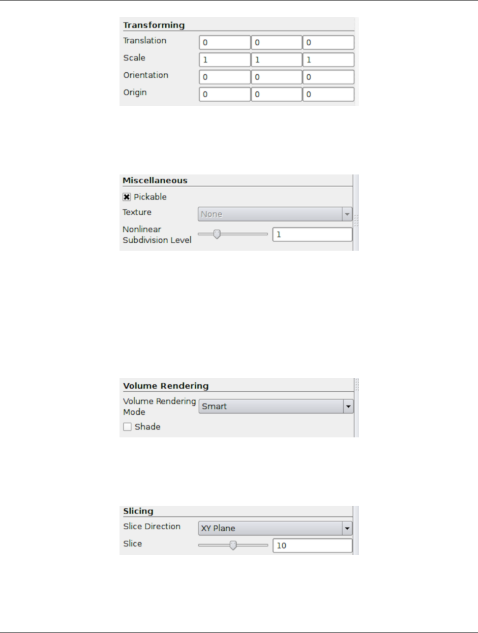
4.4. Render View
Transforming properties can be used to transform the rendered data in the scene without affecting the raw data itself.
Thus, if you apply filters on the data source, it will indeed be working with the untransformed data. To transform the data
itself, you should use the Transform filter.
Properties under the Miscellaneous group include Pickable. Uncheck this if you want the dataset to be ignored when
making selections. If the dataset has a texture coordinates array, you can apply a texture to the dataset surface using
the Texture combo-box. Choose Load to load a texture or apply a previously loaded texture listed in the combo-box.
If your dataset doesn’t have texture coordinates, you can create them by applying one of Texture Map to Cylinder,
Texture Map to Sphere, or Texture Map To Plane filters. The Nonlinear Subdivision Level is used when ren-
dering datasets with higher-order elements. Use this to set the subdivision level for triangulating higher order elements.
The higher the value, the smoother the edges. This comes at the cost of more triangles and, hence, potentially, increased
rendering time.
Volume Rendering options are available if the data can be volume rendered. You can pick a specific type of Volume
Rendering Mode, although the default (Smart) should work in most cases, since it attempts to pick a volume rendering
mode suitable for your data and graphics setup. To enable gradient-based shading, check Shade, if available.
Slicing properties are available when the Slice representation type is present. These allow you to pick the orthogonal
slice plane orientation and slice offset using Slice Direction and the Slice slider.
Chapter 4. Displaying data 61

4.4. Render View
4.4.3 Render View in pvpython
Creating a Render View
You use CreateRenderView or CreateView functions to create a new instance of a render view.
1>>> from paraview.simple import *
2>>> view = CreateRenderView()
3# Alternatively, use CreateView.
4>>> view = CreateView("RenderView")
You use Show and Hide to show or hide data produced by a pipeline module in the view.
1>>> source = Sphere()
2>>> view = CreateRenderView()
3
4# Show active source in active view.
5>>> Show()
6
7# Or specify source and view explicitly.
8>>> Show(source , view)
9
10 # Hide source in active view.
11 >>> Hide(source)
Interactions
Since pvpython is designed for scripting and batch processing, it currently does not support direct interaction with the view.
You can, however, programmatically change the camera as follows:
1# Get camera from the active view, if possible.
2>>> camera = GetActiveCamera()
3
4# or, get the camera from a specific render view.
5>>> camera = view.GetActiveCamera()
6
7# Now, you can use methods on camera to move it around the scene.
8
9# Divide the camera’s distance from the focal point by the given dolly value.
10 # Use a value greater than one to dolly-in toward the focal point, and use a
11 # value less than one to dolly-out away from the focal point.
12 >>> camera.Dolly(10)
13
14 # Set the roll angle of the camera about the direction of projection.
15 >>> camera.Roll(30)
16
17 # Rotate the camera about the view up vector centered at the focal point. Note
18 # that the view up vector is whatever was set via SetViewUp, and is not
19 # necessarily perpendicular to the direction of projection. The result is a
20 # horizontal rotation of the camera.
21 >>> camera.Aziumth(30)
22
23 # Rotate the focal point about the view up vector, using the camera’s position
24 # as the center of rotation. Note that the view up vector is whatever was set
25 # via SetViewUp, and is not necessarily perpendicular to the direction of
62 Chapter 4. Displaying data

4.4. Render View
26 # projection. The result is a horizontal rotation of the scene.
27 >>> camera.Yaw(10)
28
29 # Rotate the camera about the cross product of the negative of the direction
30 # of projection and the view up vector, using the focal point as the center
31 # of rotation. The result is a vertical rotation of the scene.
32 >>> camera.Elevation(10)
33
34 # Rotate the focal point about the cross product of the view up vector and the
35 # direction of projection, using the camera’s position as the center of
36 # rotation. The result is a vertical rotation of the camera.
37 >>> camera.Pitch(10)
Alternatively, you can explicitly set the camera position, focal point, view up, etc,. to explicitly place the camera in the
scene.
1>>> camera.SetFocalPoint(0, 0, 0)
2>>> camera.SetPosition(0, 0, -10)
3>>> camera.SetViewUp(0, 1, 0)
4>>> camera.SetViewAngle (30)
5>>> camera.SetParallelProjection(False)
6
7# If ParallelProjection is set to True, then you’ll need
8# to specify parallel scalar as well i.e. the height of the viewport in
9# world-coordinate distances. The default is 1. Note that the ‘scale’
10 # parameter works as an ‘inverse scale’ larger numbers produce smaller
11 # images. This method has no effect in perspective projection mode.
12 >>> camera.SetParallelScale(1)
View properties
In pvpython, view properties are directly accessible on the view object returned by
CreateRenderView or GetActiveView.
Once you get access to the view properties objects, you can then set properties on it similar to properties on pipeline
modules such as sources, filters, and readers.
1>>> view = GetActiveView()
2
3# Set center axis visibility
4>>> view.CenterAxesVisibility = 0
5
6# Or you can use this variant to set the property on the active view.
7>>> SetViewProperties(CenterAxesVisibility =0)
8
9# Another way of doing the same
10 >>> SetViewProperties(view, CenterAxesVisibility=0)
11
12 # Similarly, you can change orientation axes related properties
13 >>> view.OrientationAxesVisibility = 0
14 >>> view.OrientationAxesLabelColor = (1, 1, 1)
Chapter 4. Displaying data 63
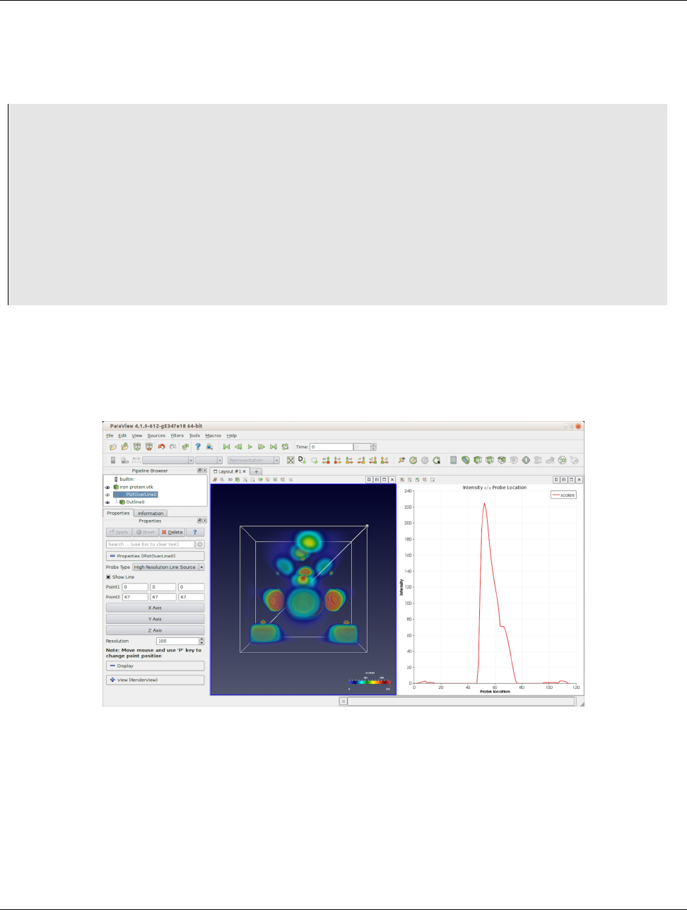
4.5. Line Chart View
Display properties
Similar to view properties, display properties are accessible from the display properties object or using the
SetDisplayProperties function.
1
2>>> displayProperties = GetDisplayProperties(source , view)
3# Both source and view are optional. If not specified, the active source
4# and active view will be used.
5
6# Now one can change properties on this object
7>>> displayProperties.Representation = "Outline"
8
9# Or use the SetDisplayProperties API.
10 >>> SetDisplayProperties (source , view , Representation =Outline)
11
12 # Here too, source and view are optional and when not specified,
13 # active source and active view will be used.
You can always use the help function to get information about available properties on a display properties object.
4.5 Line Chart View
Figure 4.7: paraview using Line Chart View to plot data values probed along a line through the dataset using Plot Over
Line filter.
Line Chart View can be used to plot data as a line plot representing changes in dependent variables against an indepen-
dent variable. Using display properties, you can also show scatter plots in this view. This view and other charting views
in ParaView follow a similar design, where you pick attribute arrays to plot using display properties, and they are plotted
in the view. How those values get plotted depends on the type of the view: Line Chart View draws a line connecting
sample points, Bar Chart View renders bars at each sample point, etc.
64 Chapter 4. Displaying data
4.5. Line Chart View
One of the most common ways of showing a line plot is to apply the Plot Over Line filter to any dataset. This will probe
the dataset along the probe line specified. You then plot the sampled values in the Line Chart View. Alternatively, if you
have a tabular dataset (i.e. vtkTable), then you can directly show the data in this view.
Did you know?
You can plot any arbitrary dataset, even those not producing vtkTable outputs, by using the Plot Data filter. Re-
member, however, that for extremely large datasets, while Render View may use parallel rendering strategies to
improve performance and reduce memory requirements, chart views rarely, if ever, support such parallel strategies.
4.5.1 Understanding plotting
Line Chart View plots data arrays. For any dataset being shown in the view, you first select which data array is to be
treated as the independent variable and plotted along the x-axis. Then, you select which arrays to plot along the Y-axis.
You can select multiple of these and setup properties for each of the series so they are rendered with different colors and
line styles. Since data arrays in VTK datasets are associated with cells or points, and the two are not directly comparable
to one another, you can only pick arrays associated with one type of attribute at any time.
4.5.2 Line Chart View in paraview
Creating a Line Chart View
Similar to creating Render View, you can split the viewport or convert an existing view to Line Chart View.Line
Chart View will also be automatically created if you apply a filter that needs this view, e.g., the Plot Over Line filter.
Did you know?
If you generate lengthy data for the Line Chart View, the default variables that are selected may be slow to
adjust. You can change paraview’s default behavior to initially load no variables at all by selecting the Load No
Chart Variables checkbox under Settings/General/Properties Panel Options.
Interactions
Interactions with the chart view result in changing the plotted axes ranges. You can left-click and drag to pan, i.e., change
the origin. To change the range on either of the axes, you can right-click and drag vertically and/or horizontally to change
the scale on the vertical axes and/or horizontal axes, respectively.
You can also explicitly specify the axes range using view properties.
Chapter 4. Displaying data 65
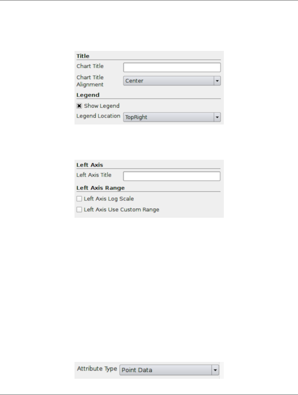
4.5. Line Chart View
View properties
The view properties for Line Chart View are grouped as properties that affect the view and those that affect each of the
potential four axes.
To set a title, use Chart Title. To toggle the visibility of the legend, use Show Legend. While you cannot interactively
place the legend in this view, you can use Legend Location to place it at one of the corners.
There are four axes possible in this view: left, bottom, top, and right. The top and right axes are shown only when some
series is set to use those. (We will cover this in the Display properties subsection.) For each of the axes, you can set a title
(e.g., Left Axis Title,Bottom Axis Title, etc.).
Next, you can customize the axes ranges. You can always simply interact with the mouse to set the axes ranges. To
precisely set the range, check the Axis Use Custom Range for the appropriate axis, e.g., Bottom Axis Use Custom
Range for fixing the bottom axis range, and then specify the data values to use for the min and the max.
The labels on the axes are, by default, automatically determined to avoid visual clutter. You can override the default
labelling strategy for any of the axes separately and, instead, specify the locations to label explicitly. This can be done
by checking Axis Use Custom Labels for a particular axis, e.g., Bottom Axis Use Custom Labels. When checked,
a list widget will be shown in which you can manually add values at which to place labels.
For generating log plots, simply check the corresponding Axis Use Log Scale, e.g., Left Axis Use Log Scale to use
log scale for Y-axis (Figure 4.8). Note that log scale should only be used for an axis with a non-zero positive range, since
the log of a number less than or equal to 0 is undefined.
Display properties
66 Chapter 4. Displaying data
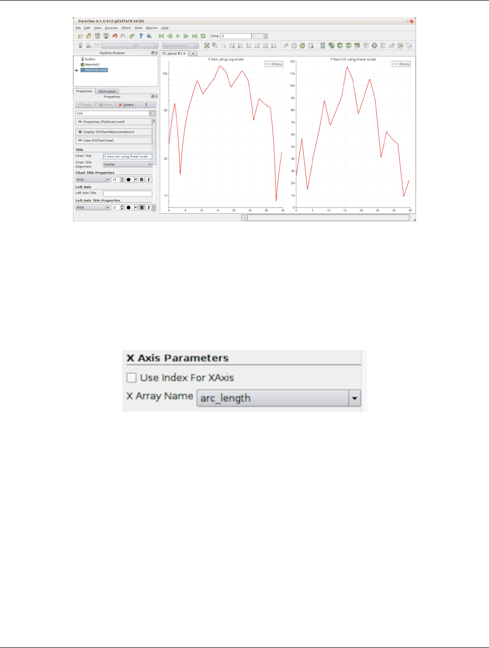
4.5. Line Chart View
Figure 4.8: Differences between line charts when using log scale for the Y-axis.
Display properties allow you to setup which series or data arrays are plotted in this view. You start by picking the
Attribute Type. Select the attribute type that has the arrays of interest. (E.g., if you are plotting arrays associated with
points, then you should pick Point Data.) Arrays with different associations cannot be plotted together. You may need
to apply filters such as Cell Data to Point Data or Point Data to Cell Data to convert arrays between different
associations for that.
Properties under X Axis Parameters allow you to select the independent variable plotted on the X axis by choosing the
X Array Name. If none of the arrays are appropriate, you can choose to use the element index in the array as the X axis by
checking Use Index for XAxis.
Chapter 4. Displaying data 67
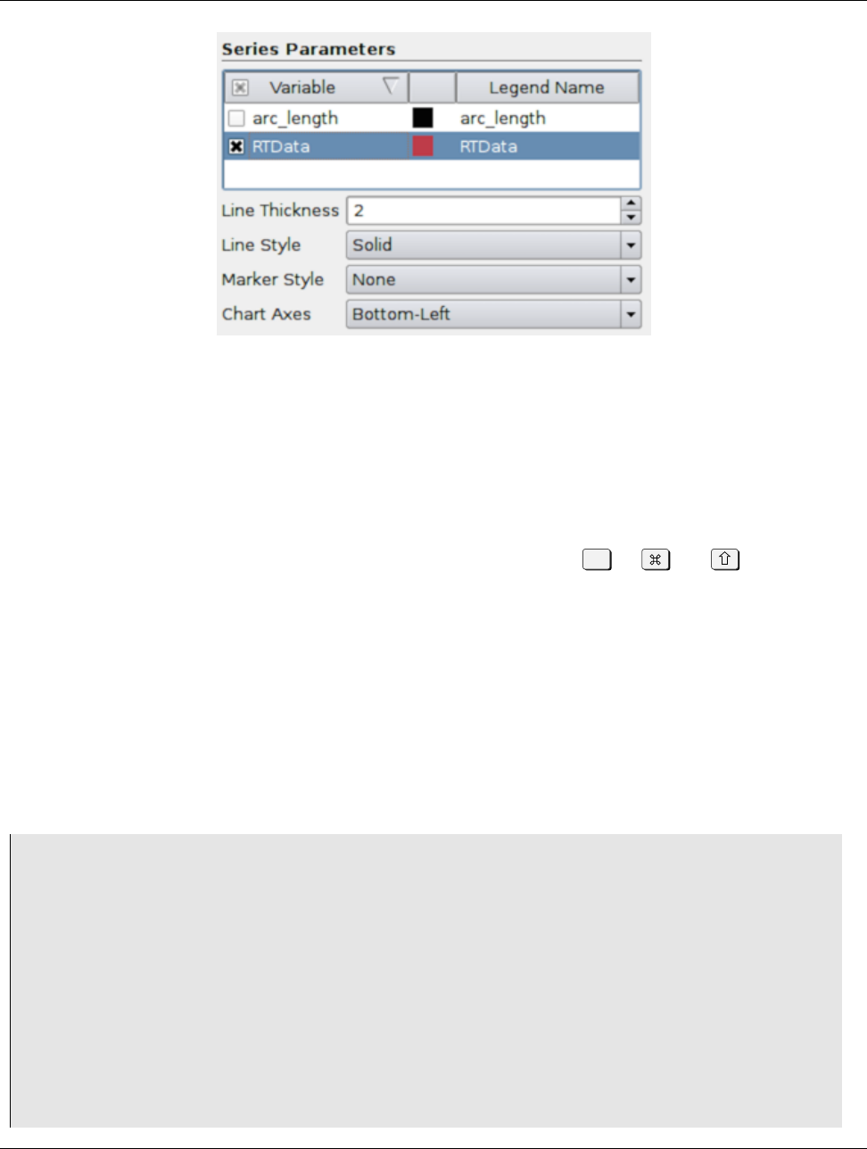
4.5. Line Chart View
Series Parameters control series or data arrays plotted on the Y-axis. All available data arrays are lists in the table
widget that allows you to check/uncheck a series to plot in the first column. The second column in the table shows the
associated color used to plot that series. You can double-click the color swatch to change the color to use. By default,
ParaView will try to pick a palette of discrete colors. The third column shows the label to use for that series in the legend.
By default, it is set to be the same as the array name. You can double-click to change the name to your choice, e.g., to add
units.
Other series parameters include Line Thickness,Line Style, and Marker Style. To change any of these, highlight a
row in the Series Parameters widget, and then change the associated parameter to affect the highlighted series. You can
change properties for multiple series and can select multiple of them by using the Ctrl (or ) and keys.
Using Chart Axes, you can change which axes on which a series is shown. The default is Bottom-Left, but you can
change it to be Bottom-Right,Top-Left, or Top-Right to accommodate series with widely different ranges in the same
plot.
4.5.3 Line Chart View in pvpython
The principles involved in accessing Line Chart View from pvpython are similar to those with Render View. You work
with the view properties and display properties objects to change views and display properties, respectively. The thing that
changes is the set of available properties.
The following script demonstrates the typical usage:
1>>> from paraview.simple import *
2
3# Create a data source to probe into.
4>>> Wavelet()
5<paraview.servermanager.Wavelet object at 0x1156fd810 >
6
7# We update the source so that when we create PlotOverLine filter
8# it has input data available to determine good defaults. Otherwise,
9# we will have to manually set the defaults up.
10 >>> UpdatePipeline()
11
12 # Now, create the PlotOverLine filter. It will be initialized using
13 # defaults based on the input data.
14 >>> PlotOverLine()
15 <paraview.servermanager.PlotOverLine object at 0x1156fd490 >
68 Chapter 4. Displaying data

4.6. Bar Chart View
16
17 # Show the result.
18 >>> Show()
19 <paraview.servermanager.XYChartRepresentation object at 0x1160a6a10 >
20
21 # This will automatically create a new Line Chart View if the
22 # the active view is no a Line Chart View since PlotOverLine
23 # filter indicates it as the preferred view. You can also explicitly
24 # create it by using CreateView() function.
25
26 # Display the result.
27 >>> Render()
28
29 # Access display properties object.
30 >>> dp = GetDisplayProperties()
31 >>> print dp.SeriesVisibility
32 [’arc_length’,’0 ’ ,’RTData’,’1’]
33
34 # This is list with key-value pairs where the first item is the name
35 # of the series, then its visibility and so on.
36 # To toggle visibility, change this list e.g.
37 >>> dp.SeriesVisibility = [’arc_length’,’ 1 ’ ,’RTData’,’ 1 ’]
38
39 # Same is true for other series parameters including series color,
40 # line thickness etc.
41
42 # For series color, the value consists of 3 values: red, green, and blue
43 # color components.
44 >>> print dp.SeriesColor
45 [’arc_length’,’0 ’ ,’ 0 ’,’ 0 ’,’RTData’,’0.89’,’0.1’,’0.11’]
46
47 # For series labels, value is the label to use.
48 >>> print dp.SeriesLabel
49 [’arc_length’,’arc_length’,’RTData’,’RTData’]
50
51 # e.g. to change RTData’s legend label, we can do something as follows:
52 >>> dp.SeriesLabel[3] = ’RTData -- new label’
53
54 # Access view properties object.
55 >>> view = GetActiveView()
56 # or
57 >>> view = GetViewProperties()
58
59 # To change titles
60 >>> view.ChartTitle = "My Title"
61 >>> view.BottomAxisTitle = " X Axis"
62 >>> view.LeftAxisTitle = " Y Axis"
4.6 Bar Chart View
Bar Chart View is very similar to Line Chart View when it comes to creating the view, view properties, and display
properties. One difference is that, instead of rendering lines for each series, this view renders bars. In addition, under the
display properties, the Series Parameters like Line Style and Line Thickness are not available, since they are not
Chapter 4. Displaying data 69
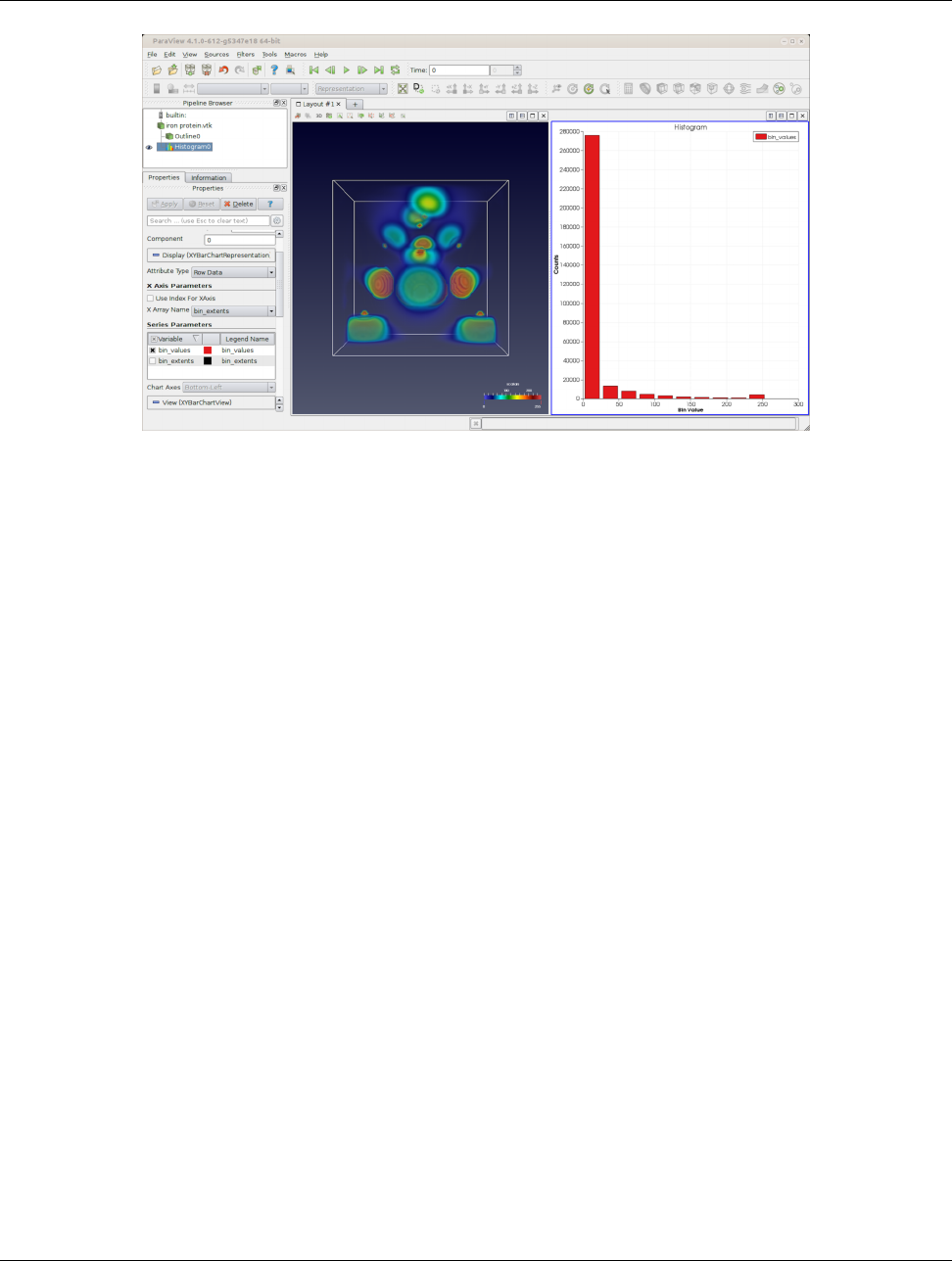
4.7. Plot Matrix View
Figure 4.9: paraview using Bar Chart View to plot the histogram for a dataset using the Histogram filter.
applicable to bars.
4.7 Plot Matrix View
Plot Matrix View is a chart view that renders a scatter plot matrix. It allows you to spot patterns in the small scatter
plots, change focus to those plots of interest, and perform basic selection. The principle is that, for all selected arrays or
series to be plotted, the view generates a scatter plot for each pair. You can activate a particular scatter plot, in which case
the active plot is re-drawn at a bigger scale to make it easier to inspect. Additionally, the view shows a histogram for each
plotted variable or series.
The view properties allow you to set colors to use for active plot, histograms, etc., while the display properties allow you
to pick which series are plotted.
4.7.1 Interactions
You can click on any of the plots (except the histograms) in the matrix to make it active. Once actived, the active plot will
show that plot. You can then interact with the active plot exactly like Line Chart View or Bar Chart View for panning
and zoom.
4.7.2 View properties
View properties on this view allow you to pick styling parameters for the rendering ranging from title (Chart Title) to
axis colors (Active Plot Axis Color,Active Plot Grid Color). You can also control the visibility of the histrogram
plots, the active plot, the axes labels, the grids, and so on.
70 Chapter 4. Displaying data
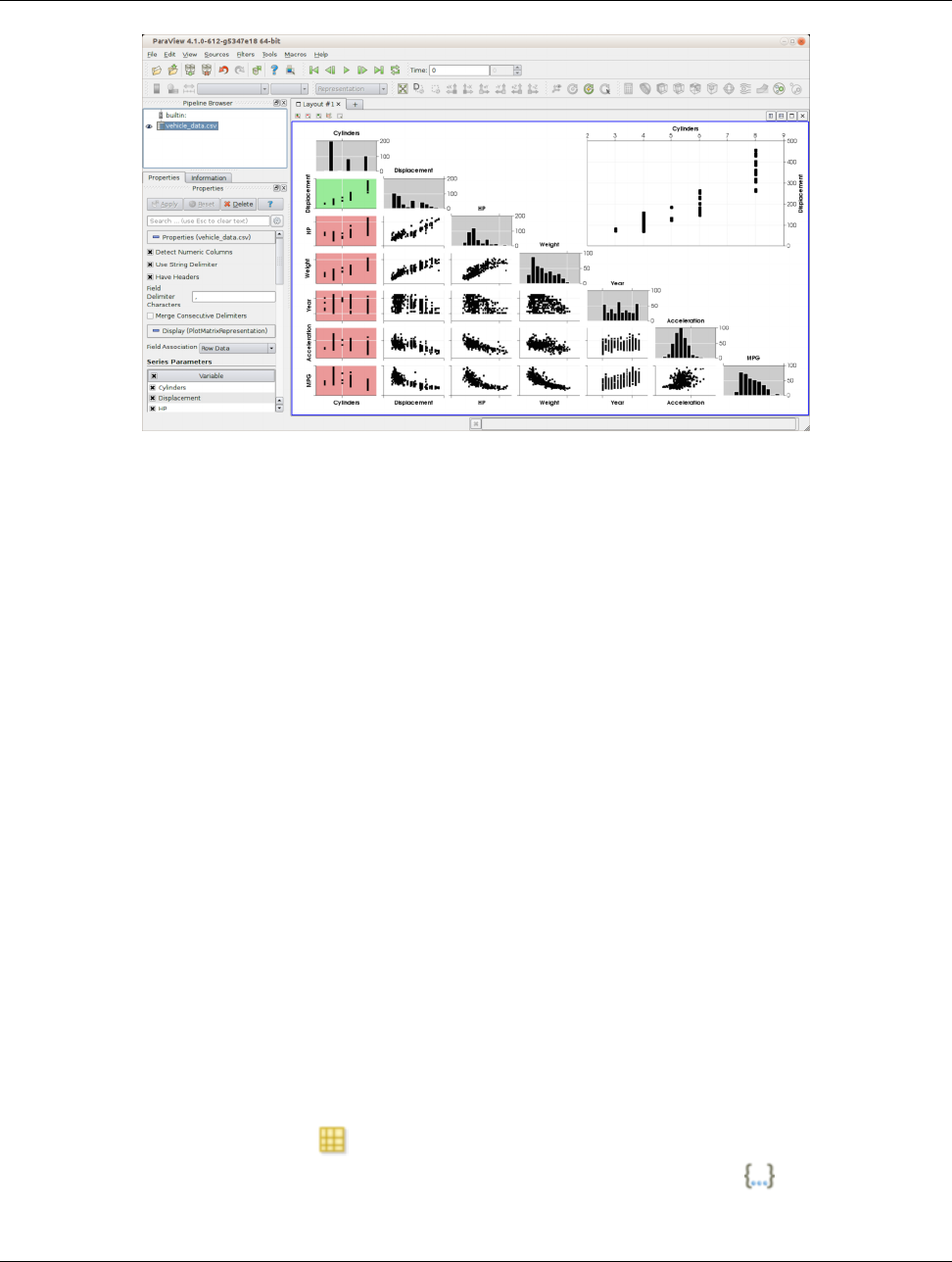
4.8. Parallel Coordinates View
Figure 4.10: paraview using Plot Matrix View to generate a scatter plot matrix to understand correlations between
variables.
4.7.3 Display properties
Similar to Line Chart View, you select the Attribute Type and then the arrays to plot. Since, in a scatter plot matrix,
the order in which the selected series are rendered can make it easier to understand correlations, you can change the order
by clicking and dragging the rows in the Series Parameters table.
4.8 Parallel Coordinates View
Like Plot Matrix View,Parallel Coordinates View is also used to visualize correlations between data arrays.
4.9 Spreadsheet View
SpreadSheet View is used to inspect raw data values in a tabular form. Unlike most other views, this view is primarily
intended to be used in the paraview user interface and, hence, is not available in pvpython.
To use this view, simply create this view and show the dataset produced by any pipeline module in it by using the Pipeline
Browser.SpreadSheet View can only show one dataset at a time. Therefore, showing a new dataset will automatically
hide the previously shown dataset.
The view’s toolbar provides quick access to several of this view’s capabilities. Use the Showing widget on the view toolbar
to view as well as to change the dataset being shown. The Attribute field allows you to pick which types of elements
to show, e.g., Cell Data,Point Data,Field Data, etc. Precision can be utilized to change the precision used when
displaying floating point numbers. The button enables you to select columns to show. Click on the button to get a
popup menu in which you check/uncheck the columns to show/hide. If showing Cell Data, the button, when checked,
enables you to see the point ids that form each of the cells.
Chapter 4. Displaying data 71
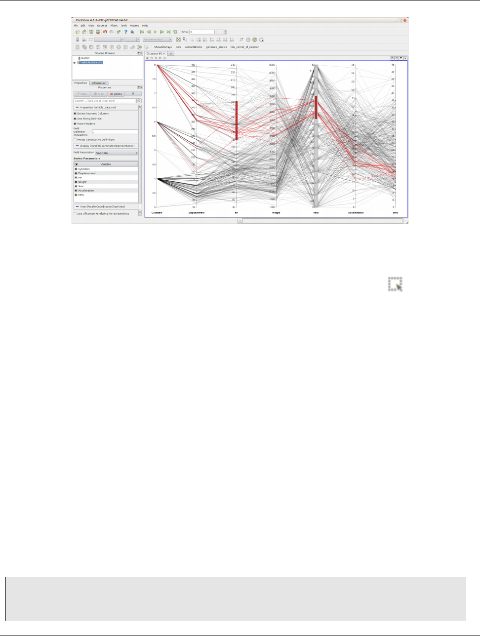
4.10. Slice View
Figure 4.11: paraview using Parallel Coordinates View to plot correlations between columns in a table.
section 6.1 discusses how selections can be made in views to select elements of interest. Use the button to make the
view show only selected elements. Now, as you make selections in other views, this SpreadSheet View will update to
only show the values of the selected elements (as long as the dataset selected in are indeed being shown in the view).
4.10 Slice View
Slice View is special type of Render View that can be used to view orthogonal slices from any dataset. Any dataset
shown in the view will be sliced in axis-aligned slices based on the locations specified on the view. The slice locations
along the three orthogonal axis planes can be specified by using the frame decoration around the view window.
4.10.1 Interactions
Since this view is a type of Render View, the camera interactions are same as that of Render View. Additionally, you can
interact with the frame decoration to manipulate slice locations along the three axis planes.
•Double-click the left mouse button in the region between the axis border and the view to add a new slice.
•You can click-and-drag a marker to move the slice location.
•To remove a slice, double-click with the left mouse button on the marker corresponding to that slice.
•To toggle visibility of the slice, you can right-click on the marker.
4.10.2 Slice View in pvpython
1# To create a slice view in use:
2>>> view = CreateView("MultiSlice")
3
4# Use properties on view to set/get the slice offsets.
72 Chapter 4. Displaying data
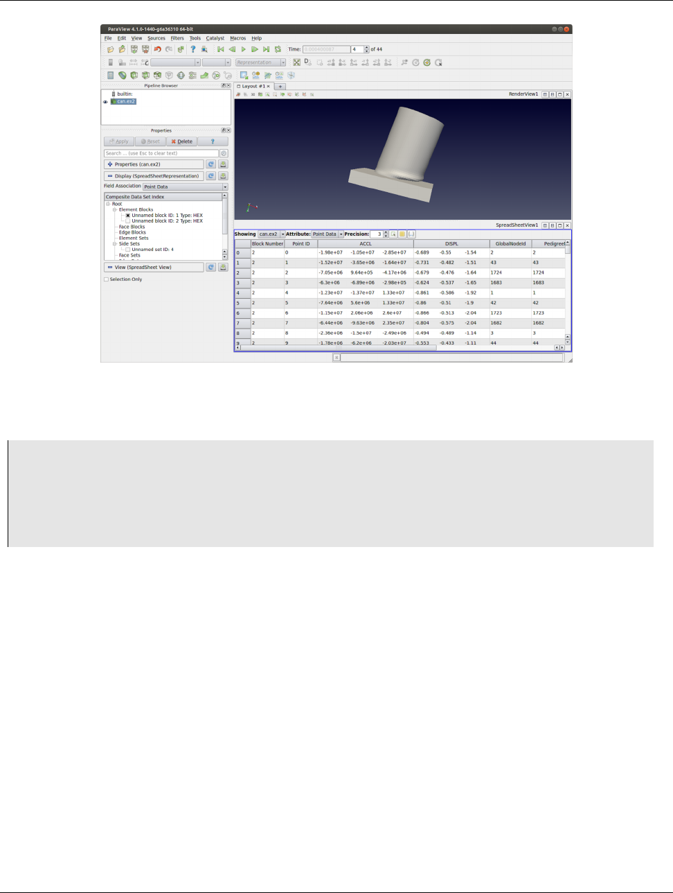
4.11. Python View
Figure 4.12: paraview using SpreadSheet View to plot raw data values for the can.ex2 dataset.
5>>> view.XSliceValues = [-10, 0, 10]
6>>> print view.XSliceValues
7[-10, 0, 10]
8
9# Similar to XSliceValues, you have YSliceValues and ZSliceValues.
10 >>> view.YSliceValues = [0]
11 >>> view.ZSliceValues = []
4.11 Python View
Some Python libraries, such as matplotlib, are widely used for making publication-quality plots of data. The Python View
provides a way to display plots made in a Python script right within paraview.
The Python View has a single property, a Python script that generates the image to be displayed in the viewport. All
the Python bindings for ParaView and VTK that are available in the Python scripting module are available from within
this script, making it possible to plot any array from just about any dataset that can be loaded into ParaView. The Python
script for the view is evaluated in a unique Python environment so that global variables defined in the script do not clobber
global variables in other Python scripts (either in other instances of the Python View or in the Python interpreter). This
environment is reset each time the script is evaluated, so data cannot be saved between evaluations.
The Python View requires that the Python script where the plotting occurs define two functions. In the first function, you
request which arrays you would like to transfer to the client for rendering. At present, all rendering in this view takes place
on the client, even in client-server mode. These arrays can be point data, cell data, field data, and table row data. This
function runs only on data-server processes. It provides access to the underlying data object on the server so that you can
query any aspect of the data using the Python-wrapped parts of VTK and ParaView.
The second function is where you put Python plotting or rendering commands. This function runs only on the ParaView
Chapter 4. Displaying data 73
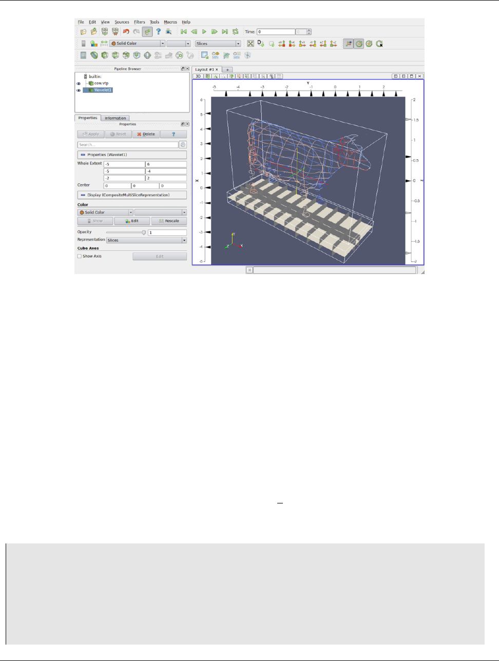
4.11. Python View
Figure 4.13: Slice View can be used to show orthogonal slices from datasets.
client. It has access to the complete data object gathered from the data server nodes, but only has access to the arrays
requested in the first function. This function will typically set up objects from a plotting library, convert data from VTK to
a form that can be passed to the plotting library, plot the data, and convert the plot to an image (a vtkImageData object)
that can be displayed in the viewport.
4.11.1 Selecting data arrays to plot
All the rendering in the Python View occurs in the client, so the client must get the data from the server. Because the
dataset residing on the ParaView server may be large, transferring all the data to the client may not be possible or practical.
For that reason, we have provided a mechanism to select which data arrays in a data object on the server to transfer to
the client. The overall structure of the data object, however, (including cell connectivity, point positions, and hierarchical
block structure) is always transferred to the client. By default, no data arrays are selected for transfer from the server.
The Python script for the view must define a function called setup data(view). The view argument is the VTK object
for the Python View. The current datasets loaded into ParaView may be accessed through the view object.
Here’s an example of this function that was used to generate the image in Figure 4.14:
1def setup_data(view):
2# Iterate over visible data objects
3for iin xrange(view.GetNumberOfVisibleDataObjects()):
4# You need to use GetVisibleDataObjectForSetup(i)
5# in setup_data to access the data object.
6dataObject = view.GetVisibleDataObjectForSetup(i)
7
8# The data object has the same data type and structure
9# as the data object that sits on the server. You can
74 Chapter 4. Displaying data
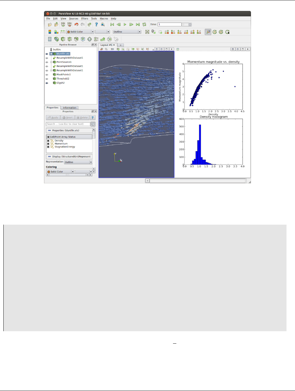
4.11. Python View
Figure 4.14: paraview using Python View with matplotlib to display a scatterplot of momentum magnitude versus density
(upper right) and a histogram of density (lower right) in the bluntfin.vts dataset.
10 # query the size of the data, for instance, or do anything
11 # else you can do through the Python wrapping.
12 print "Memory size: " ,dataObject.GetActualMemorySize(),"kilobytes"
13
14 # Clean up from previous calls here. We want to unset
15 # any of the arrays requested in previous calls to this function.
16 view.DisableAllAttributeArrays()
17
18 # By default, no arrays will be passed to the client.
19 # You need to explicitly request the arrays you want.
20 # Here, we’ll request the Density point data array
21 view. SetAttributeArrayStatus (i, vtkDataObject .POINT , "Density",1)
22 view. SetAttributeArrayStatus (i, vtkDataObject .POINT , "Momentum",1)
23
24 # Other attribute arrays can be set similarly
25 view. SetAttributeArrayStatus (i, vtkDataObject .FIELD , "fieldData",1)
The vtkPythonView class passed in as the view argument to setup data(view) defines several methods useful for
specifying which data arrays to copy:
•GetNumberOfVisibleDataObjects() - This returns the number of visible data objects in the view. If an object is
not visible, it should not show up in the rendering, so all the methods provided by the view deal only with visible
objects.
Chapter 4. Displaying data 75

4.11. Python View
•GetVisibleDataObjectForSetup(visibleObjectIndex) - This returns the
visibleObjectIndex’th visible data object in the view. (The data object will have an open eye next to it in the
pipeline browser.)
•GetNumberOfAttributeArrays(visibleObjectIndex, attributeType) - This returns the number of attribute
arrays for the visibleObjectIndex’th visible object and the given
attributeType (e.g., vtkDataObject.POINT,vtkDataObject.CELL, etc.).
•GetAttributeArrayName(visibleObjectIndex, attributeType, arrayIndex) - This returns the name of
the array of the given attribute type at the given array index for the
visibleObjectIndex’th object.
•SetAttributeArrayStatus(visibleObjectIndex, vtkDataObject.POINT, "Density", 1) -
This sets the array status of an attribute array. The first argument is the visible object index, the second object is the
attribute association of the array, the third argument is the name of the array, and the last argument specifies if the
array is to be copied (1) or not (0).
•GetAttributeArrayStatus(visibleObjectIndex, vtkDataObject.POINT, "Density") - This retrieves the
array status for the object with the given visible index with a given attribute association (second argument) and a
name (last argument).
•EnableAllAttributeArrays() - This sets all arrays to be copied.
•DisableAllAttributeArrays() - This sets all arrays to not be copied.
The methods GetNumberOfVisibleDataObjects(),GetVisibleDataObjectForSetup(...),
GetNumberOfAttributeArrays(...), and GetAttributeArrayName(...) are all convenient methods for obtaining
information about visible data objects in the view that could otherwise be accessed with existing view and representation
methods. The last four methods are valid only from within the setup data(view) function.
4.11.2 Plotting data in Python
After the setup data(view) function has been called, ParaView will transfer the data object and selected arrays to the
client. When that is done, it will call the render(view, width, height) function you have defined in your script.
The view argument to the render(view, width, height) function is the vtkPythonView object on the client. The
width and height arguments are the width and height of the viewport, respectively. The render(view, width,
height) function uses the data available through the view, along with the width and height, to generate a vtkImageData
object that will be displayed in the viewport. This vtkImageData object must be returned from the render(view,
width, height) function. If no vtkImageData is returned, the viewport will be black. If the size of the image does not
match the size of the viewport, the image will be stretched to fit the viewport.
Putting it all together, here is a simple example that generates a solid red image to display in the viewport.
1def render(view , width , height):
2from paraview.vtk import vtkImageData
3image = vtkImageData()
4image.SetDimensions (width , height , 1)
5from paraview.numeric import VTK_UNSIGNED_CHAR
6image.AllocateScalars(VTK_UNSIGNED_CHAR , 4)
7pixel_array = image.GetPointData().GetArray(0)
8pixel_array.FillComponent(0, 255.0)
9pixel_array.FillComponent(1, 0.0)
10 pixel_array.FillComponent(2, 0.0)
76 Chapter 4. Displaying data

4.12. Comparative Views
11 pixel_array.FillComponent(3, 0.0)
12
13 return image
This example does not produce an interesting visualization, but serves as a minimal example of how the render(view,
width, height) function should be implemented. Typically, we expect that the Python plotting library you use has some
utilities to expose the generated plot image pixel data. You need to copy that pixel data to the vtkImageData object
returned by the render(view, width, height) function. Exactly how you do this is up to you, but ParaView comes
with some utilities to make this task easier for matplotlib.
Set up a matplotlib Figure
The Python View comes with a Python module, called python view, that has some utility functions you can use. To
import it, use:
1from paraview import python_view
This module has a function, called matplotlib figure(view, width, height), that returns a
matplotlib.figure.Figure given width and height arguments. This figure can be used with matplotlib plotting
commands to plot data as in the following:
1def render(view , width , height):
2figure = python_view.matplotlib_figure(width, height)
3
4ax = figure.add_subplot (1,1,1)
5ax.minorticks_on ()
6ax.set_title(’Plot title’)
7ax.set_xlabel(’X label’)
8ax.set_ylabel(’Y label’)
9
10 # Process only the first visible object in the pipeline browser
11 dataObject = view.GetVisibleDataObjectForRendering (0)
12
13 x=dataObject.GetPointData().GetArray(’ X ’)
14
15 # Convert VTK data array to numpy array for plotting
16 from paraview.numpy_support import vtk_to_numpy
17 np_x = vtk_to_numpy(x)
18
19 ax.hist (np_x , bins =10)
20
21 return python_view.figure_to_image(figure)
This definition of the render(view, width, height) function creates a histogram of a point data array named Xfrom
the first visible object in the pipeline browser. Note the conversion function,
python view.figure to image(figure), in the last line. This converts the matplotlib Figure object created with
python view.matplotlib figure(width, height) into a vtkImageData object suitable for display in the viewport.
4.12 Comparative Views
Comparative Views, including Render View (Comparative),Line Chart View (Comparative), and Bar Chart
View (Comparative), are used for generating comparative visualization from parameter studies. We will cover these
views in Chapter 12.
Chapter 4. Displaying data 77
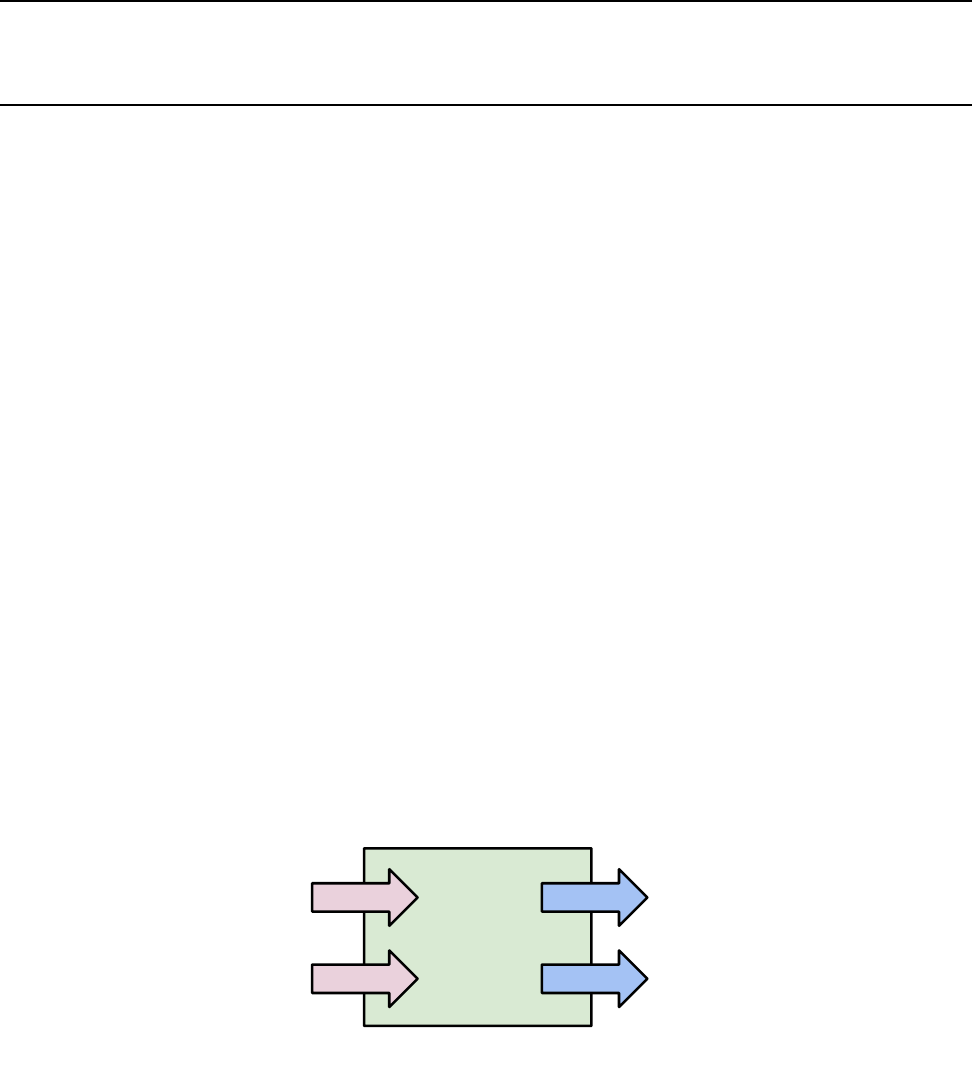
CHAPTER
FIVE
FILTERING DATA
Visualization can be characterized as a process of transforming raw data produced from experiments or simulations until
it takes a form in which it can be interpreted and analysed. The visualization pipeline introduced in Section 1.2 formalizes
this concept as a data flow paradigm where a pipeline is set up of sources, filters, and sinks (collectively called pipeline
modules or algorithms). Data flows through this pipeline, being transformed at each node until it is in a form where it can
be consumed by the sinks. In previous chapters, we saw how to ingest data into ParaView (Chapter 2) and how to display
it in views (Chapter 4). If the data ingested into ParaView already has all the relevant attribute data, and it is in the form
that can be directly represented in one the existing views, then that is all you would need. The true power of the
visualization process, however, comes from leveraging the various visualization techniques such as slicing, contouring,
clipping, etc., which are available as filters. In this chapter, we look at constructing pipelines to transform data using such
filters.
5.1 Understanding filters
In ParaView, filters are pipeline modules or algorithms that have inputs and outputs. They take in data on their inputs and
produce transformed data or results on their outputs. A filter can have multiple input and output ports. The number of
input and output ports on a filter is fixed. Each input port accepts input data for a specific purpose or role within the filter.
(E.g., the Resample With Dataset filter has two input ports. The one called Input is the input port through which the
dataset providing the attributes to interpolate is ingested. The other, called Source, is the input port through which the
dataset used as the mesh on which to re-sample is accepted.)
Filter
Port 0
Port 1
Port 0
Port 1
Figure 5.1: A filter is a pipeline module comprised of inputs and outputs. Data enters a filter through the inputs. The filter
transforms the data and produces the resulting data on its outputs. A filter can have one or more input and output ports.
Each input port can, optionally, accept multiple input connections.
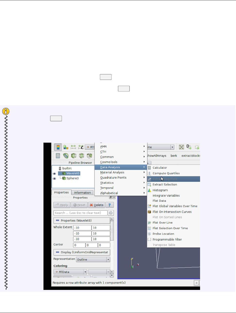
5.2. Creating filters in paraview
An input port itself can, optionally, accept multiple input connections, e.g., the Append Datasets filter, which appends
multiple datasets to create a single dataset only has one input port (named Input). However, that port can accept multiple
connections for each of the datasets to be appended . Filters define whether a particular input port can accept one or many
input connections.
Similar to readers, the properties on the filter allow you to control the filtering algorithm. The properties available depend
on the filter itself.
5.2 Creating filters in paraview
All available filters in paraview are listed under the Filters menu. These are organized in various categories. To create a
filter to transform the data produced by a source or a reader, you select the source in the Pipeline Browser to make it
active, and then click on the corresponding menu item in the Filters menu. If a menu item is disabled, it implies that the
active source does not produce data that can be transformed by this filter.
Did you know?
If a menu item in the Filters menu is disabled, it implies that the active source(s) is not producing data of the expected
type or the characteristics needed by the filter. On Windows and Linux machines, if you hover over the disabled menu
item, the status bar will show the reason why the filter is not available.
80 Chapter 5. Filtering data
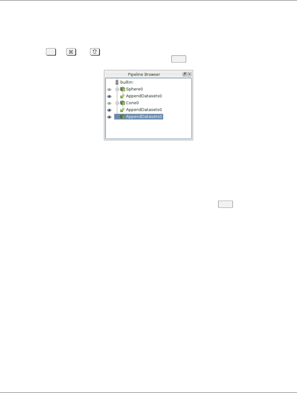
5.2. Creating filters in paraview
5.2.1 Multiple input connections
When you create a filter, the active source is connected to the first input port of the filter. Filters like Append Datasets
can take multiple input connections on that input port. In such a case, to pass multiple pipeline modules as connections on
a single input port of a filter, select all the relevant pipeline modules in the Pipeline Browser. You can select multiple
items by using the Ctrl (or ) and key modifiers. When multiple pipeline modules are selected, only the filters that
accept multiple connections on their input ports will be enabled in the Filters menu.
Figure 5.2: The Pipeline Browser showing a pipeline with multiple input connections. The Append Datasets filter has
two input connections on its only input port, Sphere0 and Cone0.
5.2.2 Multiple input ports
Most filters have just one input port. Hence, as soon as you click on the filter name in the Filters menu, it will create a new
filter instance and that will show up in the Pipeline Browser. Certain filters, such as Resample With Dataset, have
multiple inputs that must be set up before the filter can be created. In such a case, when you click on the filter name, the
Change Input Dialog will pop up, as seen in Figure 5.3. This dialog allows you to select the pipeline modules to be
connected to each of the input ports. The active source(s) is connected by default to the first input port. You are free to
change those as well.
5.2.3 Changing input connections
paraview allows you to change the inputs to a filter after the filter has been created. To change inputs to a filter, right-click
on the filter in the Pipeline Browser to get the context menu, and then select Change Input.... This will pop up the
same Change Input Dialog as when creating a filter with multiple input ports. You can use this dialog to set new inputs
for this filter.
Chapter 5. Filtering data 81
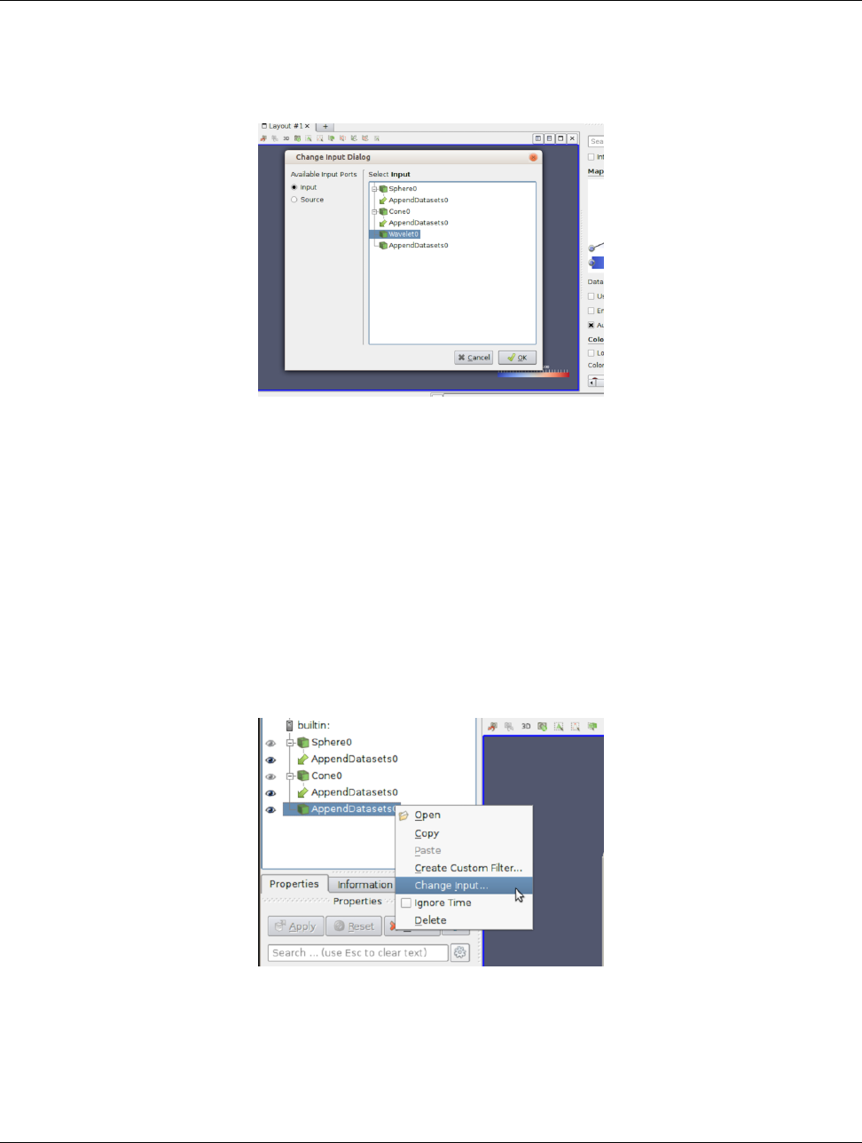
5.2. Creating filters in paraview
Figure 5.3: The Change Input Dialog is shown to allow you to pick inputs for each of the input ports for a filter with
multiple input ports. To use this dialog, first select the Input Port you want to edit on the left side, and select the pipeline
module(s) that are to be connected to this input port. Repeat the step for the other input port(s). If an input port can accept
multiple input connections, you can select multiple modules, just like in the Pipeline Browser.
Figure 5.4: The context menu in the Pipeline Browser showing the option to change inputs for a filter.
82 Chapter 5. Filtering data
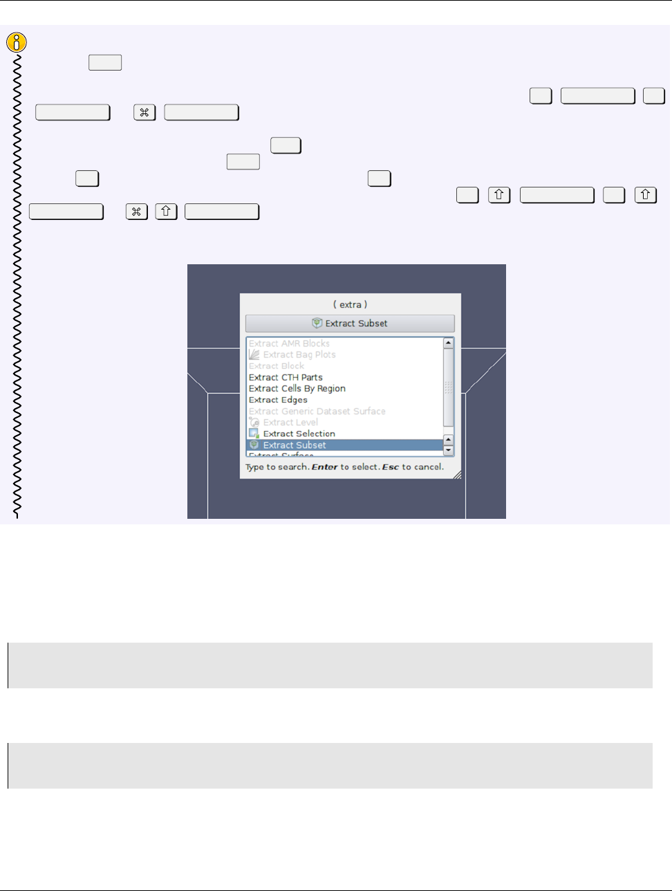
5.3. Creating filters in pvpython
Did you know?
While the Filters menu is a handy way to create new filters, with the long list of filters available in ParaView,
manually finding a particular filter in this menu can be very challenging. To make it easier, ParaView incorporates
a quick launch mechanism. When you want to create a new filter (or a source), simply hit Ctrl +Space ,Alt
+Space , or +Space . This will pop up the quick-launch dialog. Now, start typing the name of the
filter you want. As you type, the dialog will update to show the filters and sources that match the typed text. You can
use the arrow keys to navigate and use the Enter key to create the selected filter (or source). Note that filters may
be disabled, as was the case in the Filters menu but by default the selected item will be the first enabled filter. You
can use Esc to clear the text you have typed so far. Hit the Esc a second time, and the dialog will close without
creating any new filter. You can also display the quick-launch dialog using Ctrl + + Space ,Alt + +
Space , or + + Space . In this case, the selected filter will be automatically applied once created
i.e. equivalent to creating the filter and then hitting the Apply button.
5.3 Creating filters in pvpython
To create a filter in pvpython, you simply create the object by using its name as a constructor function.
1>>> from paraview.simple import *
2...
3>>> filter = Shrink()
Similar to paraview, the filter will use the active source(s) as the input. Additionally, you can explicitly specify the input
in the function arguments.
1>>> reader = OpenDataFile (...)
2...
3>>> shrink = Shift(Input=reader)
5.3.1 Multiple input connections
To setup multiple input connections, you can specify the connections as follows:
Chapter 5. Filtering data 83
5.4. Changing filter properties in paraview
1>>> sphere = Sphere()
2>>> cone = Cone()
3
4# Simply pass the sources as a list to the constructor function.
5>>> appendDatasets = AppendDatasets(Input=[sphere , cone])
6>>> print appendDatasets.Input
7[<paraview.servermanager.Sphere object at 0x6d75f90 >, <paraview.servermanager.Cone
object at 0x6d75c50 >]
5.3.2 Multiple input ports
Setting up connections to multiple input ports is similar to the multiple input connections, except that you need to ensure
that you name the input ports properly.
1>>> sphere = Sphere()
2>>> wavelet = Wavelet()
3
4>>> resampleWithDataSet = ResampleWithDataset(Input=sphere , Source=wavelet)
5.3.3 Changing input connections
Changing inputs in Python is as simple as setting any other property on the filter.
1# For filter with single input connection
2>>> shrink.Input = cone
3
4# for filters with multiple input connects
5>>> appendDatasets.Input = [reader , cone]
6
7# to add a new input.
8>>> appendDatasets.Input.append(sphere)
9
10 # to change multiple ports
11 >>> resampleWithDataSet.Input = wavelet2
12 >>> resampleWithDataSet.Source = cone
5.4 Changing filter properties in paraview
Filters provide properties that you can change to control the processing algorithm employed by the filter. Changing and
viewing properties on filters is the same as with any other pipeline module, including readers and sources. You can view
and change these properties, when available, using the Properties panel. Chapter 9 covers how to effectively use the
Properties panel. Since this panel only shows the properties present on the active source, you must ensure that the filter
you are interested in is active. To make the filter active, use the Pipeline Browser to click on the filter and select it.
5.5 Changing filter properties in pvpython
With pvpython, the available properties are accessible as properties on the filter object, and you can get or set their values
by name (similar to changing the input connections (Section 5.3.3)).
84 Chapter 5. Filtering data

5.6. Filters for sub-setting data
1
2# You can save the object reference when it’s created.
3>>> shrink = Shrink()
4
5# Or you can get access to the active source.
6>>> Shrink() # <-- this will make the Shrink the active source.
7>>> shrink = GetActiveSource()
8
9# To figure out available properties, you can always use help.
10 >>> help(shrink)
11 Help on Shrink in module paraview.servermanager object:
12
13 class Shrink(SourceProxy)
14 |TheShrinkfilter
15 |causestheindividualcellsofadatasettobreak apart
16 |from each other by moving each cell’ s points toward the
17 |centroid of the cell. ( The centroid of acell is the
18 |average position of its points.) This filter operates on
19 |any type of dataset and produces unstructured grid
20 |output.
21 |----------------------------------------------------------------------
22 |Data descriptors defined here:
23 |
24 |Input
25 |This property specifies the input to the Shrink
26 |filter.
27 |
28 |ShrinkFactor
29 |The value of this property determines how far the points
30 |will move. A value of 0positions the points at the centroid of the
31 |cell; a value of 1leaves them at their original
32 |positions.
33 ....
34
35 #To get the current value of aproperty:
36 >>> sf =shrink.ShrinkFactor
37 >>> print sf
38 0.5
39
40 #To set the value
41 >>> shrink.ShrinkFactor =0.75
In the rest of this chapter, we will discuss some of the commonly used filters in detail. They are grouped under categories
based on the type of operation that they perform.
5.6 Filters for sub-setting data
These filters are used for extracting subsets from an input dataset. How this subset is defined and how it is extracted
depends on the type of the filter.
Chapter 5. Filtering data 85
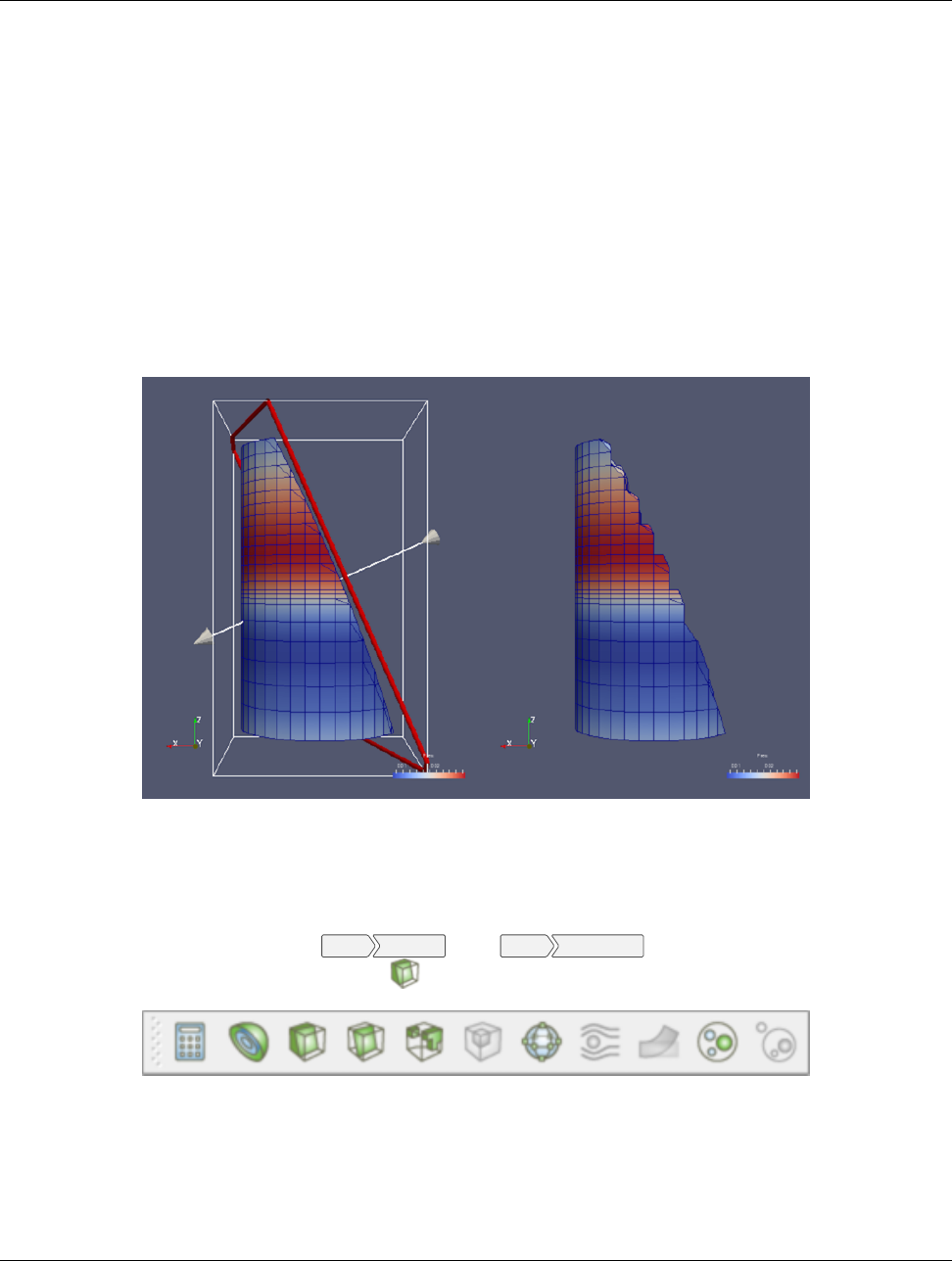
5.6. Filters for sub-setting data
5.6.1 Clip
Clip is used to clip any dataset using either an implicit function (such as a plane, sphere, or a box) or using values of a
scalar data array in the input dataset. A scalar array is a point or cell attribute array with a single component. Clipping
involves iterating over all cells in the input dataset and then removing those cells that are considered outside of the space
defined by the implicit function or that have an attribute values less than the selected value. For cells that straddle the
clipping surface, these are clipped to pass through the part of the cell that is truly inside the specified implicit function (or
greater than the scalar value).
This filter converts any dataset into an unstructured grid (Section 3.1.7) or a multi-block of unstructured grids
(Section 3.1.10) in the case of composite datasets.
Clip in paraview
Figure 5.5: Comparison between results produced by the Clip filter with Crinkle Clip unchecked (left) and checked
(right) when clipping with an implicit plane. The image on the left also shows the 3D widget used to interactivly place the
implicit plane for the clipping operation.
To create the Clip filter, you can use the Filters Common or the Filters Alphabetical menu. This filter is also accessible
from the Common filters toolbar. You can click the button to create this filter.
Figure 5.6: The Common filters toolbar in paraview for quick access to the commonly used filters.
On the Properties panel, you will see the available properties for this filter. One of the first things that you should select
is the Clip Type.Clip Type is used to specify the type of implicit function to use for the clipping operations. The
available options include Plane,Box,Sphere, and Scalar. Selecting any one of these options will update the panel to
86 Chapter 5. Filtering data
5.6. Filters for sub-setting data
show properties that are used to define the implicit function, e.g., the Origin and the Normal for the Plane or the Center
and the Radius for the Sphere. If you select Scalar, the panel will let you pick the data array and the value with which
to clip. Remember, cells with the data value greater than or equal to the selected value are considered in and are passed
through the filter.
Did you know?
When clipping with implicit functions, ParaView renders widgets in the active view that you can use to interactively
control the implicit function, called 3D widgets. As you interact with the 3D widget, the panel will update to
reflect the current values. The 3D widget is considered as an aid and not as a part of the actual visualization scene.
Thus, if you change the active source and the Properties panel navigates away from this filter, the 3D widget
will automatically be hidden.
The Inside Out option can be used to invert the behavior of this filter. Basically, it flips the notion of what is considered
inside and outside of the given clipping space.
Check Crinkle Clip if you don’t want this filter to truly clip cells on the boundary, but want to preserve the input cell
structure and to pass the entire cell on through the boundary (Figure 5.5). This option is not available when clipping by
Scalar.
Clip in pvpython
This following script demonstrates various aspects of using the Clip filter in pvpython.
1
2# Create the Clip filter.
3>>> clip = Clip(Input=...)
4
5# Specify a ’ClipType’ to use.
6>>> clip.ClipType = ’Plane’
7
8# You can also use the SetProperties API instead.
9>>> SetProperties(clip , ClipType=’Plane’)
10
11 >>> print clip.GetProperty(’ClipType’).GetAvailable()
12 [’Plane’,’Box’,’Sphere’,’Scalar’]
13
14 # To set the plane origin and normal
15 >>> clip.ClipType.Origin = [0, 0, 0]
16 >>> clip.ClipType.Normal = [1, 0, 0]
17
18 # If you want to change to Sphere and set center and
19 # radius, you can do the following.
20 >>> clip.ClipType = ’Sphere’
21 >>> clip.ClipType.Center = [0, 0, 0]
22 >>> clip.ClipType.Radius = 12
23
24 # Using SetProperties API, the same looks like
25 >>> SetProperties(clip , ClipType=’Sphere’)
26 >>> SetProperties(clip.ClipType , Center=[0, 0, 0],
27 Radius = 12)
28
29 # To set Crinkle clipping.
Chapter 5. Filtering data 87

5.6. Filters for sub-setting data
30 >>> clip.Crinkleclip = 1
31
32 # For clipping with scalar, you pick the scalar array
33 # and then the value as follows:
34 >>> clip.ClipType = ’Scalar’
35 >>> clip.Scalars = (’POINTS’,’Temp’)
36 >>> clip.Value = 100
37
38 # To get available values, use
39 >>> clip.GetProperty(’Scalars’).GetAvailable()
40
41 # As always, to get the list of available properties on
42 # the clip filter, use help()
43 >>> help(clip)
44 Help on Clip in module paraview.servermanager object:
45
46 class Clip(SourceProxy)
47 |TheClipfilter
48 |cutsawayaportionoftheinputdatasetusingan
49 |implicitplane.Thisfilteroperatesonalltypesofdata
50 |sets,and it returns unstructured grid data on
51 |output.
52 |
53 | ----------------------------------------------------------------------
54 |Datadescriptorsdefinedhere:
55 |
56 | ClipType
57 |Thispropertyspecifiestheparametersoftheclip
58 |function(animplicitplane)usedtoclipthedataset.
59 |
60 |Crinkleclip
61 |Thisparametercontrolswhethertoextractentirecells
62 |in the given region or clip those cells so all of the output one stay
63 |onlyinsidethatregion.
64 |
65 | Input
66 |ThispropertyspecifiesthedatasetonwhichtheClip
67 |filterwilloperate.
68 |
69 | InsideOut
70 |Ifthispropertyis set to 0, the clip filter will
71 |return that portion of the dataset that lies within the clip function.
72 |Ifsetto1,theportionsofthedatasetthatlieoutsidetheclip
73 |functionwillbereturnedinstead.
74 ...
75
76 # To get help on a specific implicit function type, make it the active
77 # ClipType and then use help()
78 >>> clip.ClipType = ’Plane’
79 >>> help(clip.ClipType)
80 Help on Plane in module paraview.servermanager object:
81
82 class Plane(Proxy)
83 ...
88 Chapter 5. Filtering data
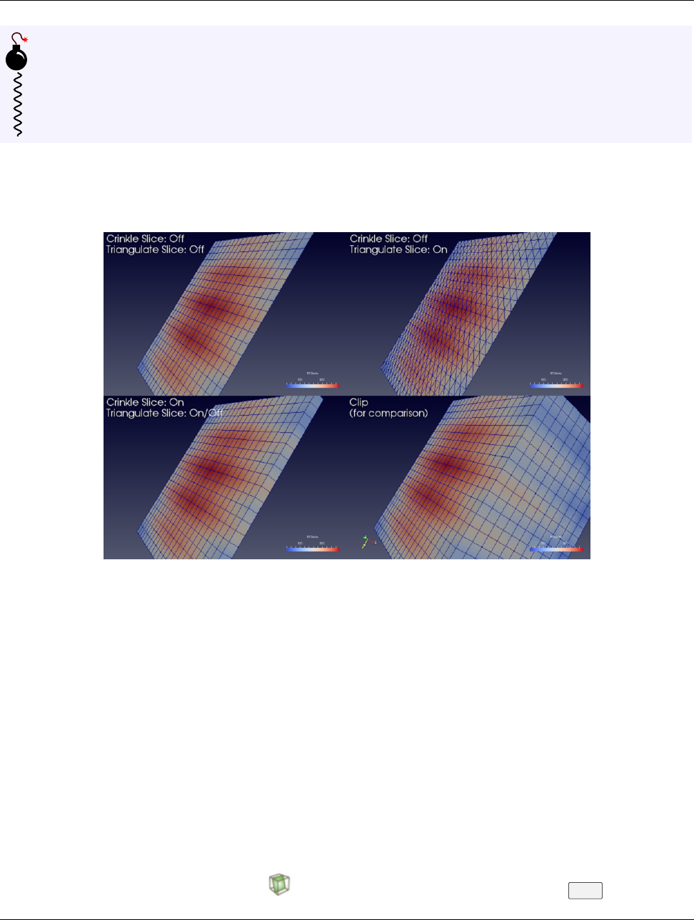
5.6. Filters for sub-setting data
Common Errors
It is very easy to forget that clipping a structured dataset such as image data can dramtically increase the memory
requirements, since this filter will convert the structured dataset into an unstructured grid due to the nature of the
clipping operation itself. For structured dataset, think about using Slice or Extract Subset filters instead,
whenever appropriate. Those are not entirely identical operations, but they are often sufficient.
5.6.2 Slice
Figure 5.7: Comparison between results produced by the Slice filter when slicing image data with an implicit plane with
different options. The lower-left image shows the output produced by the Clip filter when clipping with the same implicit
function, for contrast.
The Slice filter slices through the input dataset with an implicit function such as a plane, a sphere, or a box. Since this
filter returns data elements along the implicit function boundary, this is a dimensionality reducing filter (except when
crinkle slicing is enabled), i.e., if the input dataset has 3D elements like tetrahedrons or hexahedrons, the output will have
2D elements, line triangles, and quads, if any. While slicing through a dataset with 2D elements, the result will be lines.
The properties available on this filter, as well as the way of setting this filter up, is very similar to the Clip filter with a
few notable differences. What remains similar is the set up of the implicit function – you have similar choices: Plane,
Sphere, and Box, as well as the option to toggle Crinkle slice (i.e., to avoid cutting through cells, pass complete cells
from the input dataset that intersects the implicit function).
What is different includes the lack of slicing by Scalar (for that, you can use the Contour filter) and a new option,
Triangulate the slice. Figure 5.7 shows the difference in the generated meshes when various slice properties are
changed.
In paraview, this filter can be created using the button on the Common filters toolbar, besides the Filters menu.
Chapter 5. Filtering data 89
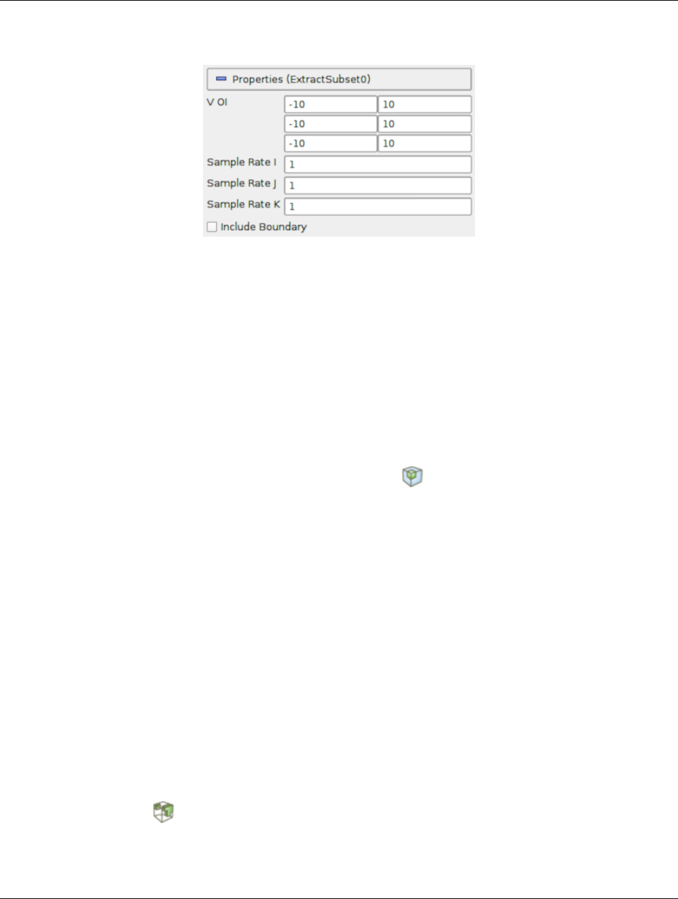
5.6. Filters for sub-setting data
5.6.3 Extract Subset
Figure 5.8: The Properties panel for the Extract Subset filter showing all available properties (including the advanced
properties).
For structured datasets such as image datasets (Section 3.1.3), rectilinear grids (Section 3.1.4), and curvilinear grids
(Section 3.1.5), Extract Subset filter can be used to extract a region of interest or a subgrid. The region to extract is
specified using structured coordinates, i.e., the i,j,kvalues. Whenever possible, this filter should be preferred over Clip
or Slice for structured datasets, since it preserves the input data type. Besides extracting a subset, this filter can also be
used to resample the dataset to a coarser resolution by specifying the sample rate along each of the structured dimensions.
Extract Subset in paraview
This is one of the common filters available on the Common filters toolbar . To specify the region of interest, you use the
VOI property. The values are specified as min and max values for each of the structured dimensions (i,j,k,) in each row.
Sample Rate I,Sample Rate J, and Sample Rate K specify the sub-sampling rate. Set it to a value greater than one
to sub-sample. Include Boundary is used to determine if the boundary slab should be included in the extracted result, if
the sub-sampling rate along that dimension is greater than 1, and the boundary slab would otherwise have been skipped.
5.6.4 Threshold
The Threshold filter extracts the portions of the input dataset whose scalars lie within the specified range. This filter
operates on either point-centered or cell-centered data. This filter operates on any type of dataset and produces an
unstructured grid output. To use this filter, you select the Scalars with which to threshold, and then specify the range
through which to pass. When thresholding with cell data, all cells that have scalars within the specified range will be
passed through the filter. When thresholding with point data, cells with all points with scalar values within the range are
passed through if All Scalars is checked; otherwise, cells with any point that passes the thresholding criteria are passed
through.
Threshold in paraview
This filter is represented as on the Common filters toolbar. After selecting the Scalars with which to threshold from
the combo-box, you select the Minimum and Maximum values to specify the range. If the range shown by the sliders is not
sufficient, you can manually type the values in the input boxes. The values are deliberately not clamped to the current data
90 Chapter 5. Filtering data
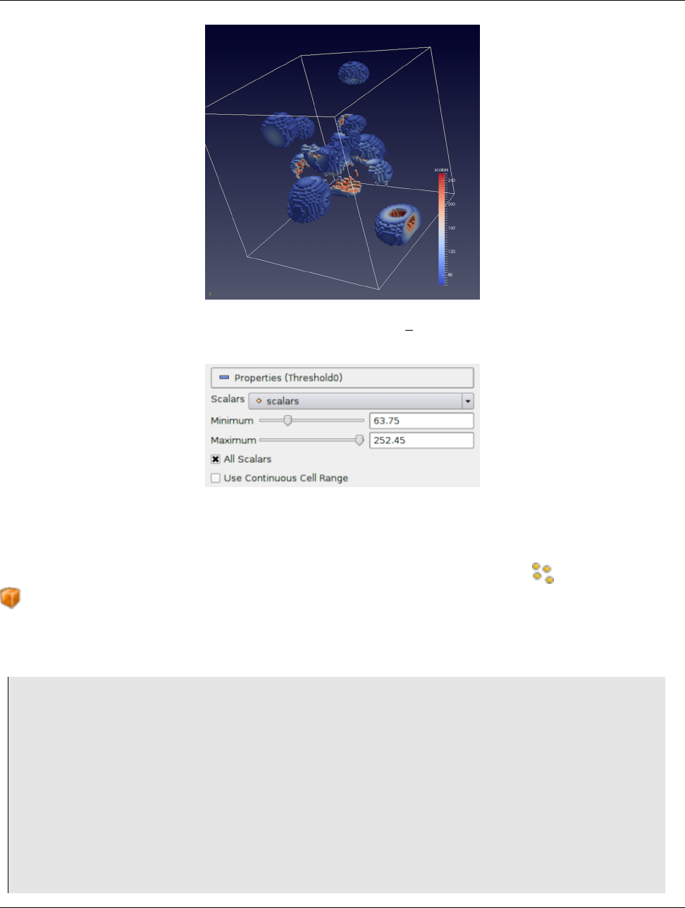
5.6. Filters for sub-setting data
Figure 5.9: Results from using the Threshold filter on the iron protein.vtk dataset from ParaView data.
Figure 5.10: The Properties panel for the Threshold filter.
range. The Scalars combo-box uses icons to help you differentiate between point data arrays and cell data arrays
.
Threshold in pvpython
1# To create the filter (if Input is not specified, the active source will be
2# used as the input.
3>>> threshold = Threshold(Input=...)
4
5# Here’s how to select a scalar array,
6>>> threshold.Scalars = ("POINTS","scalars")
7
8# The value is a tuple with first value as the association:
9# either "POINTS" or "CELLS" and the second value is the name of the selected
10 array.
11
12 >>> print threshold.Scalars
13 [’POINTS’,’scalars’]
14
Chapter 5. Filtering data 91

5.7. Filters for geometric manipulation
15 >>>> print threshold.Scalars.GetArrayName()
16 ’scalars’
17
18 >>> print threshold.Scalars.GetAssociation()
19 ’POINTS’
20
21 # The threshold range is specified as:
22 >>> threshold.ThresholdRange = [63.75, 252.45]
To determine the types of arrays available in the input dataset, and their ranges, refer to the discussion on data information
in Section 3.3.
5.6.5 Iso Volume
The Iso Volume filter is similar to Threshold in that you use this to create an output dataset from an input where the
cells that satisfy the specified range are scalar values. In fact, the filter is identical to Threshold when the cell data scalars
are selected. For point data scalars, however, this filter acts similar to the Clip filters when clipping with scalars, in that
cells are clipped along the iso-surface formed the scalar range.
5.6.6 Extract Selection
Extract Selection is a general-purpose filter to extract selected elements from a dataset. There are several ways of
making selections in ParaView. Once you have made the selection, this filter allows you to extract the selected elements
as a new dataset for further processing. We will cover this filter in more detail when looking at selections in ParaView in
Section 6.5.
5.7 Filters for geometric manipulation
These filters are used to transform the geometry of the dataset without affecting its topology or its connectivity.
5.7.1 Transform
The Transform can be used to arbitrarily translate, rotate, and scale a dataset. The transformation is applied by scaling
the dataset, rotating it, and then translating it based on the values specified.
As this is a geometric manipulation filter, this filter does not affect connectivity in the input dataset. While it tries to
preserve the input dataset type, whenever possible, there are cases when the transformed dataset can no longer be
represented in the same data type as the input. For example, with image data (Section 3.1.3) and rectilinear grids
(Section 3.1.4), due to the ability of rotating the dataset, the output dataset can be non-axis aligned and, hence, cannot be
represented as either data types. In such cases, the dataset is converted to an unstructured grid (Section 3.1.7). Since
unstructured grids are not as compact as data structured as the other two, this implies a considerable increase in the
memory footprint.
5.7.2 Transform in paraview
You can create a new Transform from the Filters Alphabetical menu. Once created, you can set the transform as the
translation, rotation, and scale to use utilizing the Properties panel. Similar to Clip, this filter also supports using a 3D
widget to interactively set the transformation.
92 Chapter 5. Filtering data
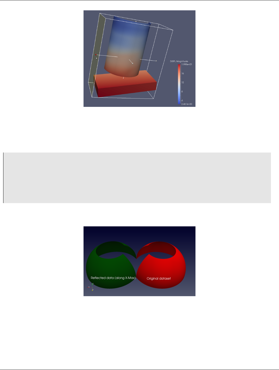
5.7. Filters for geometric manipulation
Figure 5.11: The Transform filter showing the 3D widget that can be used to interactively set the transform.
5.7.3 Transform in pvpython
1# To create the filter(if Input is not specified, the active source will be
2# used as the input).
3>>> transform = Transform(Input=...)
4
5# Set the transformation properties.
6>>> transform.Translate.Scale = [1, 2, 1]
7>>> transform.Transform.Translate = [100, 0, 0]
8>>> transform.Transform.Rotate = [0, 0, 0]
5.7.4 Reflect
Figure 5.12: The Reflect filter can be used to reflect a dataset along a specific axis plane.
Reflect can be used to reflect any dataset across an axis plane. You can pick the axis plane to be one of the planes
formed by the bounding box of the dataset. For that, set Plane as X Min,X Max,Y Min,Y Max,Z Min, or Z Max.To
reflect across an arbitrary axis plane, select X,Y, or Zfor the Plane property, and then set the Center to the plane offset
from the origin.
This filter reflects the input dataset and produces an unstructured grid (Section 3.1.7). Thus, the same caveats for Clip
Chapter 5. Filtering data 93
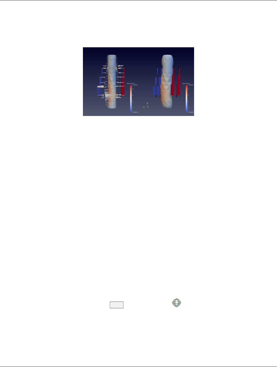
5.8. Filters for sampling
and Threshold filter apply here when dealing with structured datasets.
5.7.5 Warp By Vector
Figure 5.13: The Warp By Vector filter can be used to displace points in original data shown on the left, using the
displacement vectors (indicated by arrow glyphs 5.8.1) to produce the result shown on the right.
Warp By Vector can be used to displace point coordinates in an input mesh using vectors in the dataset itself. You select
the vectors to use utilizing the Vectors property on the Properties panel. Scale Factor can be used to scale the
displacement applied.
5.7.6 Warp By Scalar
Warp By Scalar is similar to Warp By Vector in the sense that it warps the input mesh. However, it does so using a
scalar array in the input dataset. The direction of displacement can either be explicitly specified using the Normal
property, or you can check Use Normal to use normals at the point locations.
5.8 Filters for sampling
These filters compute new datasets that represent some essential features from the datasets that they take as input.
5.8.1 Glyph
Glyph is used to place markers or glyphs at point locations in the input dataset. The glyphs can be oriented or scaled
based on vector and scalar attributes on those points.
To create this filter in paraview, you can use the Filters menu, as well as the button on the Common filters toolbar. You
first select the type for the glyph using one of the options in Glyph Type. The choices include Arrow,Sphere,Cylinder,
etc. Next, you select the point arrays to treat as the Scalars and the Vectors. This selection is then used when scaling or
orienting the glyphs. To orient the glyphs using the selected Vectors, check the Orient checkbox.
The Scale Mode controls how the glyphs are scaled. The options are as follows:
•off: This disables scaling on glyphs based on point arrays.
•scalar: This scales the glyphs using the point array selected using Scalars.
94 Chapter 5. Filtering data
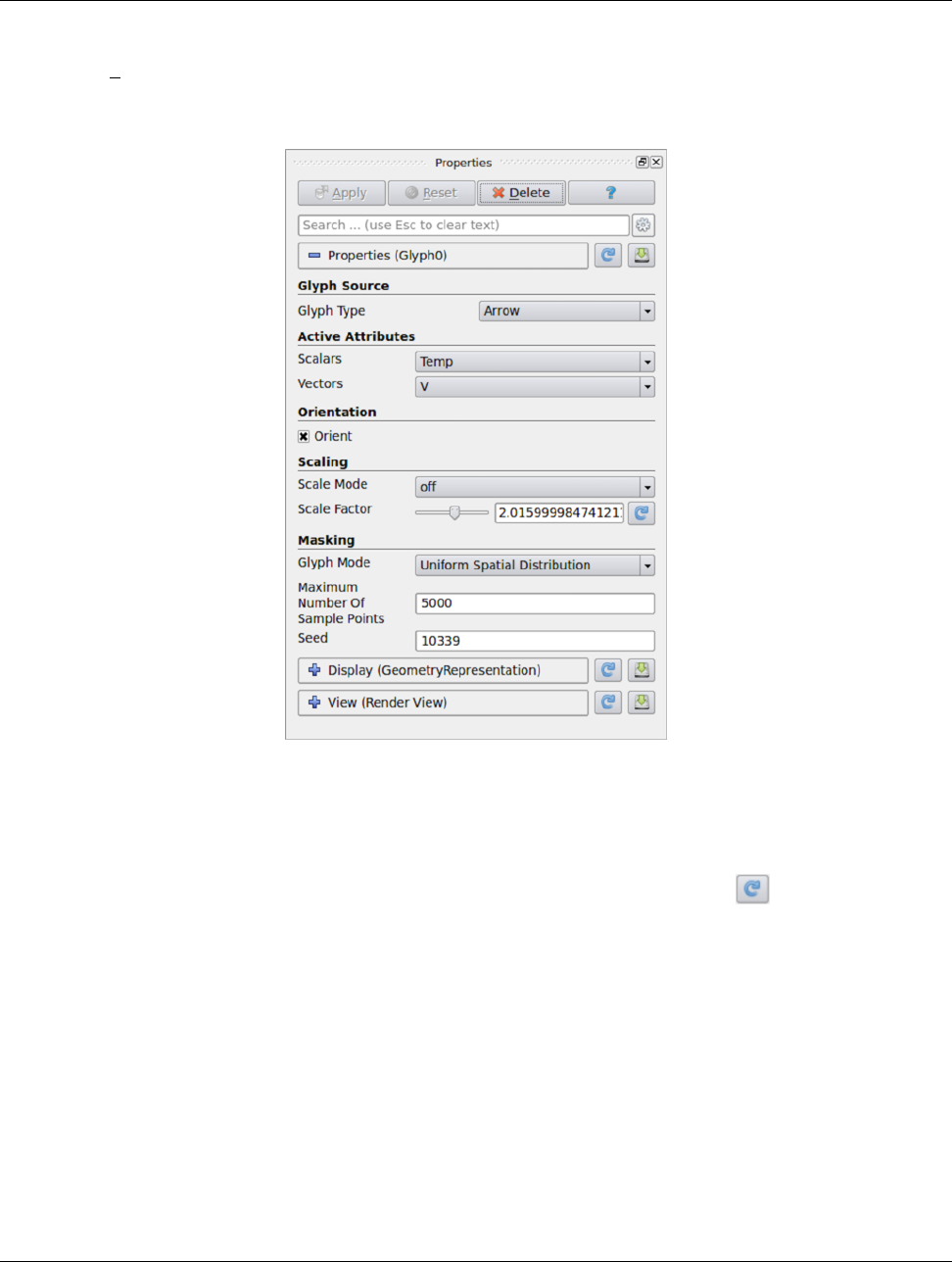
5.8. Filters for sampling
•vector: This scales the glyphs using the magnitude for the point array selected for Vectors.
•vector components: This is similar to vector; however, instead of scaling the glyph in all three directions using
the magnitude of the vectors, the scale factor for each direction is obtained from the point array by treating each
component individually.
Figure 5.14: The Properties panel for the Glyph filter.
The Scale Factor is used to apply a constant scaling to all the glyphs, independent of the Scale Mode. Choosing a
good scale factor depends on several things including the bounds on the input dataset, the Scale Mode selected, and the
range for the array that would affect the glyph scaling based on Scale Mode. You can use the button next to the
Scale Factor widget to have paraview pick a scale factor value based on the current dataset and selections.
The Masking properties allow you to control which points from the input dataset get glyphed. The Glyph Mode controls
how points are selected to be glyphs (Figure 5.15). The available options are as follows:
•All Points: This selects all points in the input dataset for glyphing. Use this mode with caution and only when
the input dataset has relatively few points. Since all points in the input dataset are glyphed, this can not only cause
visual clutter, but also clog up memory and take a long to time to generate and render the glyphs.
•Every Nth Points: This elects every nth point in the input dataset for glyphing, where ncan be specified using
Stride. Setting Stride to 1 will have the same effect as All Points.
•Uniform Spatial Distribution: This selects a random set of points. The algorithm works by first computing
up to Maximum Number of Sample Points in the space defined by the bounding box of the input dataset. Then,
points in the input dataset that are close to the point in this set of sample points are glyphed. The Seed is used to
seed the random number generator used to generate the sample points. This ensures that the random sample points
are reproducible and consistent.
Chapter 5. Filtering data 95
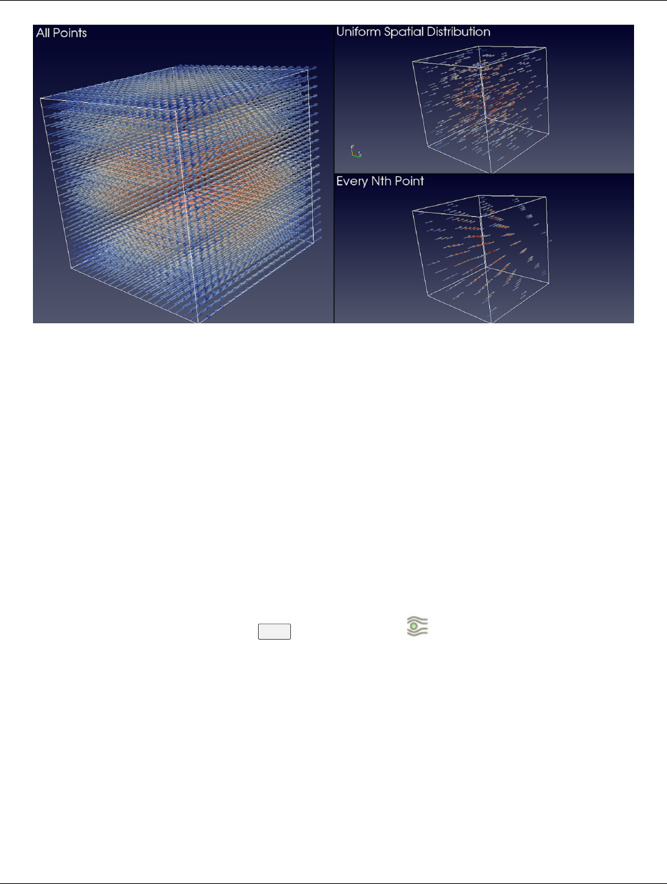
5.8. Filters for sampling
Figure 5.15: Comparison between various Glyph Modes when applied to the same dataset generated by the Wavelet
source.
5.8.2 Glyph With Custom Source
Glyph With Custom Source is the same as Glyph, except that instead of a limited set of Glyph Type, you can select
any data source producing a polygonal dataset (Section 3.1.8) available in the Pipeline Browser.
5.8.3 Stream Tracer
The Stream Tracer filter is used to generate streamlines for vector fields. In visualization, streamlines refer to curves
that are instanteneously tangential to the the vector field in the dataset. They provide an indication of the direction in
which the particles in the dataset would travel at that instant in time. The algorihm works by taking a set of points, known
as seed points, in the dataset and then inegrating the streamlines starting at these seed points.
In paraview, you can create this filter using the Filters menu, as well as the button on the Common filters toolbar. To use
this filter, you first select the attribute array to use as the Vectors for generaing the streamline. Integration
Parameters let you fine tune the streamline integration by specifying the direction to integrate, Integration
Direction, as well as the type of integration algorithm to use, Integrator Type. Advanced integration parameters are
available in the advanced view of the Properties panel that let you further tune the integration, including specifying the
step size and others. You use the Maximum Streamline Length to limit the maximum length for the streamline – the
longer the length, the longer the generated streamlines.
Seeds group lets you set how the seed points for generating the streamlines are produced. You have two options: Point
Source, which produces a point clound around the user-specified Point based on the parameters specified, and High
Resolution Line Source, which produces seed points along the user-specified line. You can use the 3D widgets shown
in the active Render View to interactively place the center for the point cloud or for defining the line.
96 Chapter 5. Filtering data
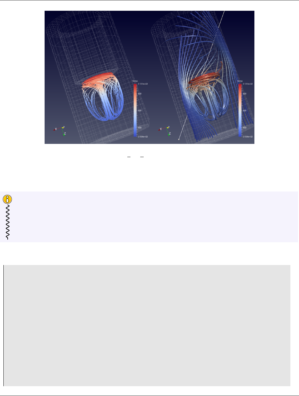
5.8. Filters for sampling
Figure 5.16: Streamlines generated from the disk out ref.ex2 dataset using the Point Source (left) and the High
Resolution Line Source (right). On the left, we also added the Tube filter to the output of the Stream Tracer filter to
generate 3D tubes rather than 1D polygonal lines, which can be hard to visualize due to lack of shading.
Did you know?
The Stream Tracer filter produces a polydata with 1D lines for each of the generated streamlines. Since 1D
lines cannot be shaded like surfaces in the Render View, you can get visualizations where it is hard to follow the
streamlines. To give the streamlines some 3D structure, you can apply the Tube filter to the output of the streamlines.
The properties on the Tube filter let you control the thickness of the tubes. You can also vary the thickness of the
tubes based on data array, e.g., the magnitude of the vector field at the sample points in the streamline!
A script using the Stream Tracer filter in paraview typically looks like this:
1# find source
2>>> disk_out_refex2 = FindSource(’disk_out_ref.ex2’)
3
4# create a new ’Stream Tracer’
5>>> streamTracer1 = StreamTracer(Input=disk_out_refex2 ,
6SeedType=’Point Source’)
7>>> streamTracer1.Vectors = [’POINTS’,’V’]
8
9# init the ’Point Source’ selected for ’SeedType’
10 >>> streamTracer1.SeedType.Center = [0.0, 0.0, 0.07999992370605469]
11 >>> streamTracer1.SeedType.Radius = 2.015999984741211
12
13 # show data in view
14 >>> Show()
15
16 # create a new ’Tube’
17 >>> tube1 = Tube(Input=streamTracer1)
18
Chapter 5. Filtering data 97
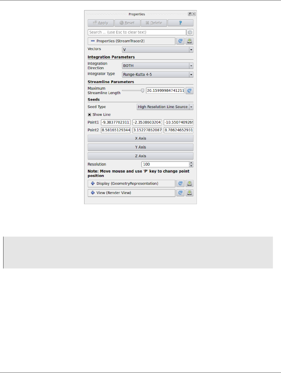
5.8. Filters for sampling
Figure 5.17: The Properties panel showing the default properties for the Stream Tracer filter.
19 # Properties modified on tube1
20 >>> tube1.Radius = 0.1611409378051758
21
22 # show the data from tubes in view
23 >>> Show()
5.8.4 Stream Tracer With Custom Source
Stream Tracer allows you to specify the seed points either as a point cloud or as a line source. However, if you want to
provide your own seed points from a another data producer, use the Stream Tracer With Custom Source. Similar to
Glyph With Custom Source, this filter allows you to pick a second input connection to use as the seed points.
5.8.5 Resample With Dataset
Resample With Dataset samples the point and cell attributes of one dataset on to the points of another dataset. The two
datasets are supplied to the filter using its two input ports: Input, which is the dataset that provides the attributes to
98 Chapter 5. Filtering data
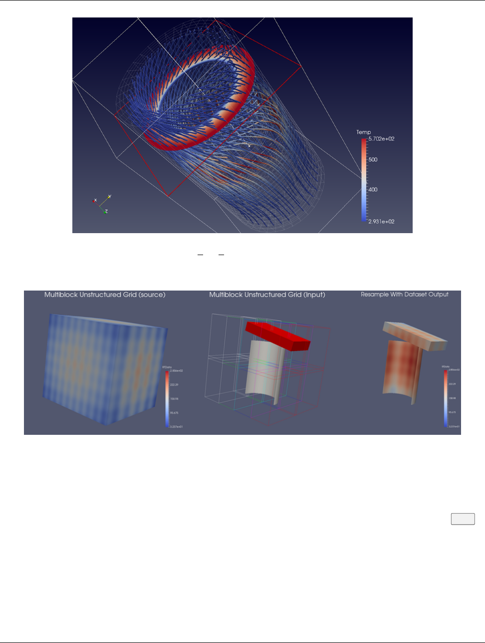
5.8. Filters for sampling
Figure 5.18: Streamlines generated from the disk out ref.ex2 dataset using the output of the Slice filter as the Source
for seed points.
Figure 5.19: An example of Resample With Dataset. On the left is a multiblock tetrahedra mesh (Input). The middle
shows a multiblock unstructured grid (Source). The outline of Input is also shown in this view. The result of applying
the filter is shown on the right
resample, and Source, which is the dataset that provides the points to sample at. This filter is available under the Filters
menu.
5.8.6 Resample To Image
Resample To Image is a specialization of Resample With Dataset. The filter takes one input and samples its point
and cell attributes onto a uniform grid of points. The bounds and extents of the uniform grid can be specified using the
properties panel. By default, the bounds are set to the bounds of the input dataset. The output of the filter is an Image
dataset.
Chapter 5. Filtering data 99
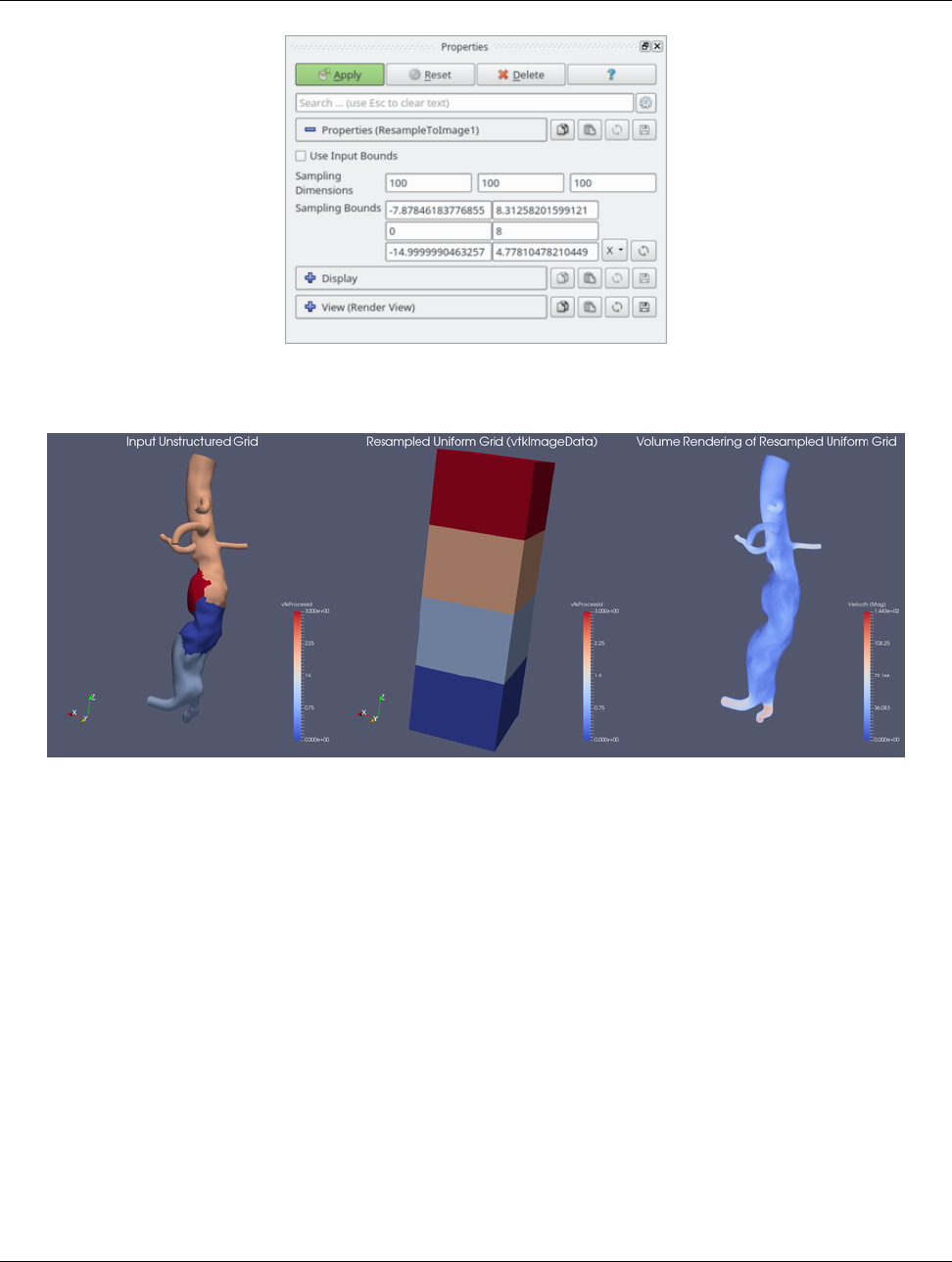
5.8. Filters for sampling
Figure 5.20: The Properties panel for Resample To Image filter
Figure 5.21: An example of Resample To Image. The left portion shows the input (unstructured grid), and the middle
displays the output Image data. On the right is a volume rendering of the resampled data.
Some operations can be performed more efficiently on uniform grid datasets. Volume rendering is one such operation.
The Resample to Image filter can be used to convert any dataset to Image data before performing such operations.
5.8.7 Probe
Probe samples the input dataset at a specific point location to obtain the cell data attributes for the cell containing the
point as well as the interpolated point data attributes. You can either use the SpreadSheet View or the Information
panel to inspect the probed values. The probe location can be specified using the interactive 3D widget shown in the
active Render View.
100 Chapter 5. Filtering data
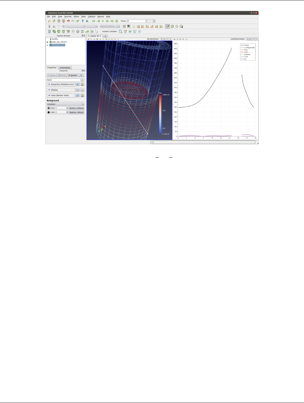
5.9. Filters for attribute manipulation
Figure 5.22: The Plot Over Line filter applied to the disk out ref.ex2 dataset to plot values at sampled locations
along the line. Gaps in the line correspond to the locations in the input dataset where the line falls outside the dataset.
5.8.8 Plot over line
Plot Over Line will sample the input dataset along the specified line and then plot the results in Line Chart View.
Internally, this filter uses the same mechanism as the Probe filter, probing along the points in the line to get the containing
cell attributes and interpolated point attributes.
Using the Resolution property on the Properties panel, you can control the number of sample points along the line.
5.9 Filters for attribute manipulation
The filters covered in this section are used to add new attribute arrays to the dataset, which are typically used to add
derived quantities to use in pipelines for further processing.
5.9.1 Calculator
The Calculator filter computes a new data array or new point coordinates as a function of existing input arrays. If
point-centered arrays are used in the computation of a new data array, the resulting array will also be point-centered.
Similarly, computations using cell-centered arrays will produce a new cell-centered array. If the function is computing
point coordinates (requested by checking the Coordinate Results property on the Properties panel) , the result of the
function must be a three-component vector. The Calculator interface operates similarly to a scientific calculator. In
creating the function to evaluate, the standard order of operations applies. Each of the calculator functions is described
below. Unless otherwise noted, enclose the operand in parentheses using the (and )buttons.
•Clear: Erase the current function.
•/: Divide one scalar by another. The operands for this function are not required to be enclosed in parentheses.
•*: Multiply two scalars, or multiply a vector by a scalar (scalar multiple). The operands for this function are not
Chapter 5. Filtering data 101

5.9. Filters for attribute manipulation
required to be enclosed in parentheses.
•-: Negate a scalar or vector (unary minus), or subtract one scalar or vector from another. The operands for this
function are not required to be enclosed in parentheses.
•+: Add two scalars or two vectors. The operands for this function are not required to be enclosed in parentheses.
•sin: Compute the sine of a scalar.
•cos: Compute the cosine of a scalar.
•tan: Compute the tangent of a scalar.
•asin: Compute the arcsine of a scalar.
•acos: Compute the arccosine of a scalar.
•atan: Compute the arctangent of a scalar.
•sinh: Compute the hyperbolic sine of a scalar.
•cosh: Compute the hyperbolic cosine of a scalar.
•tanh: Compute the hyperbolic tangent of a scalar.
•min: Compute minimum of two scalars.
•max: Compute maximum of two scalars.
•xˆy: Raise one scalar to the power of another scalar. The operands for this function are not required to be enclosed
in parentheses.
•sqrt: Compute the square root of a scalar.
•eˆx: Raise e to the power of a scalar.
•log10: Compute the logarithm of a scalar to the base 10.
•ln: Compute the logarithm of a scalar to the base e.
•ceil: Compute the ceiling of a scalar.
•floor: Compute the floor of a scalar.
•abs: Compute the absolute value of a scalar.
•v1.v2: Compute the dot product of two vectors. The operands for this function are not required to be enclosed in
parentheses. cross: Compute cross product of two vectors. mag: Compute the magnitude of a vector. norm:
Normalize a vector. The operands are described below. The digits 0 - 9 and the decimal point are used to enter
constant scalar values.
•iHat,jHat, and kHat are vector constants representing unit vectors in the X, Y, and Z directions, respectively.
The Scalars menu lists the names of the scalar arrays and the components of the vector arrays of either the point-centered
or cell-centered data. The Vectors menu lists the names of the point-centered or cell-centered vector arrays. The function
will be computed for each point (or cell) using the scalar or vector value of the array at that point (or cell). The filter
operates on any type of data set, but the input data set must have at least one scalar or vector array. The arrays can be
either point-centered or cell-centered. The Calculator filter’s output is of the same data set type as the input.
A common use-case is to convert three input scalars into a vector array. For that, the Function would look something
like: scalarx⇤iHat +scalary⇤jHat +scalarz⇤kHat.
The Properties panel provides access to several options for this filter. Checking Coordinate Results,Result
Normals, or Result TCoords will set the computed array as the point coordinates, normals, or texture coordinates,
respectively. Result Array Name is used to specify a name for the computed array. The default is Result.
Sometimes, the expression can yield invalid values. To replace all invalid values with a specific value, check the Replace
Invalid Results checkbox and then enter the value to use to replace invalid values using the Replacement Value.
5.9.2 Python calculator
The Python Calculator is similar to Calculator in that it processes one or more input arrays based on an expression
provided by the user to produce a new output array. However, it uses Python (and numpy) to do the computation.
Therefore, it provides more expressive expression capabilities.
Specify the Expression to use, the Array Association to indicate the array association (Point Data or Cell Data),
102 Chapter 5. Filtering data
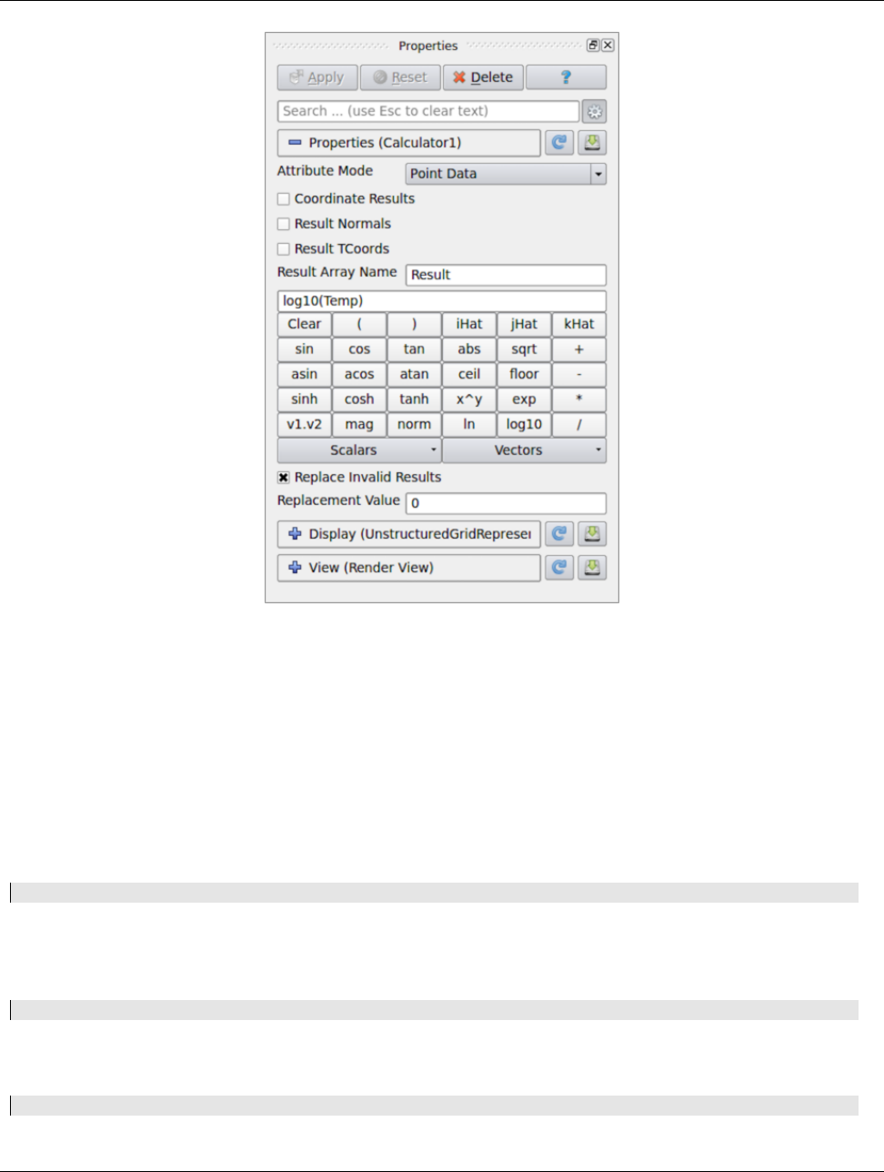
5.9. Filters for attribute manipulation
Figure 5.23: The Properties panel for the Calculator filter showing the advanced properties.
the name of output array (Array Name), and a toggle that controls whether the input arrays are copied to the output (Copy
Array).
Basic tutorial
Start by creating a Sphere source and applying the Python Calculator to it. As the first expression, use the following and
apply:
15
This should create an array name result in the output point data. Note that this is an array that has a value of 5 for each
point. When the expression results in a single value, the calculator will automatically make a constant array. Next, try the
following:
1Normals
Now, the result array should be the same as the input array Normals. As described in detail later, various functions are
available through the calculator. For example, the following is a valid expression:
1sin(Normals) + 5
Chapter 5. Filtering data 103
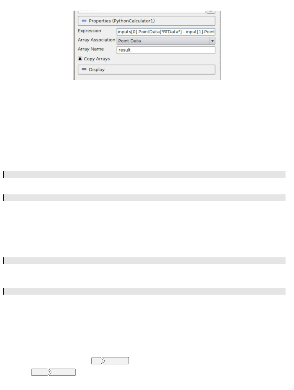
5.9. Filters for attribute manipulation
Figure 5.24: The Properties Panel for Python Calculator
It is very important to note that the Python Calculator has to produce one value per point or cell depending on the Array
Association parameter. Most of the functions described here apply individually to all point or cell values and produce an
array the same dimensions as the input. However, some of them (such as min() and max()) produce single values.
Accessing data
There are several ways of accessing input arrays within expressions. The simplest way is to access it by name:
1sin(Normals) + 5
This is equivalent to:
1sin(inputs[0]. PointData[’Normals’]) + 5
The example above requires some explanation. Here, inputs[0] refer to the first input (dataset) to the filter. Python
Calculator can accept multiple inputs. Each input can be accessed as inputs[0], inputs[1], ... You can access the point or
cell data of an input using the .PointData or .CellData qualifiers. You can then access individual arrays within the point or
cell data containers using the [] operator. Make sure to use quotes or double-quotes around the array name. Arrays that
have names with certain characters (such as space, +, -, *, /) can only be accessed using this method.
Certain functions apply directly on the input mesh. These filters expect an input dataset as argument. For example,
1area(inputs[0])
For data types that explicitly define the point coordinates, you can access the coordinates array using the .Points qualifier.
The following extracts the first component of the coordinates array:
1inputs[0].Points[:,0]
Note that for certain data types, mainly image data (uniform rectilinear grids) and rectilinear grids, point coordinates are
defined implicitly and cannot be accessed as an array.
Comparing multiple datasets
The Python Calculator can be used to compare multiple datasets, as shown by the following example.
•Go to the Menu Bar, and select File Disconnect to clear the Pipeline.
•Select Source Mandelbrot , and then click Apply, which will set up a default version of the Mandelbrot Set. The data
for this set are stored in a 251 ⇥251 scalar array.
104 Chapter 5. Filtering data

5.9. Filters for attribute manipulation
•Select Source Mandelbrot again, and then go to the Properties panel and set the Maximum Number of Iterations to
50. Click Apply, which will set up a different version of the Mandelbrot Set, represented by the same size array.
•Hold the Shift key down and select both of the Mandelbrot entries in the Pipeline Inspector, and then go to the
Menu Bar, and select Filter Python Calculator . The two Mandelbrot entries will now be shown as linked, as inputs, to
the Python Calculator.
•In the Properties panel for the Python Calculator filter, enter the following into the Expression box:
1inputs[1].PointData[’Iterations’]-inputs[0].PointData[’Iterations’]
This expression specifies the difference between the second and the first Mandelbrot arrays. The result is saved in a
new array called ’results’. The prefixes in the names for the array variables, inputs[1] and inputs[0], refer to the first
and second Mandelbrot entries, respectively, in the Pipeline. PointData specifies that the inputs contain point
values. The quoted label ’Iterations’ is the local name for these arrays. Click Apply to initiate the calculation.
Click the Display tab in the Properties panel for the Python Calculator, and go to the first tab to the right of the Color by
label. Select the item results in that tab, which will cause the display window to the right to show the results of the
expression we entered in the Python Calculator. The scalar values representing the difference between the two
Mandelbrot arrays are represented by colors that are set by the current color map (see Edit Color Map... for details).
There are a few things to note:
•Python Calculator will always copy the mesh from the first input to its output.
•All operations are applied point-by-point. In most cases, this requires that the input meshes (topology and
geometry) are the same. At the least, it requires that the inputs have the same number of points and cells.
•In parallel execution mode, the inputs have to be distributed exactly the same way across processes.
Basic Operations
The Python calculator supports all of the basic arithmetic operations using the +,,⇤and /operators. These are always
applied element-by-element to point and cell data including scalars, vectors, and tensors. These operations also work with
single values. For example, the following adds 5 to all components of all Normals.
1Normals + 5
The following adds 1 to the first component, 2 to the second component, and 3 to the third component:
1Normals + [1,2,3]
This is specially useful when mixing functions that return single values. For example, the following normalizes the
Normals array:
1(Normals - min(Normals))/(max(Normals) - min(Normals))
A common use case in a calculator is to work on one component of an array. This can be accomplished with the following:
1Normals[:, 0]
The expression above extracts the first component of the Normals vector. Here, ‘:’ is a placeholder for “all elements”.
One element can be extracted by replacing ‘:’ with an index. For example, the following creates a constant array from the
first component of the normal of the first point:
1Normals[0, 0]
Chapter 5. Filtering data 105
5.9. Filters for attribute manipulation
Alternatively, the following assigns the normal of the first point to all points:
1Normals[0, :]
It is also possible to merge multiple scalars into an array using the hstack() function:
1hstack([velocity_x , velocity_y , velocity_z]) # Note the square brackets ([]).
For temporal datasets, you also have access to the dataset timestep index or time value in the expression as t index or
time index, and t value or time value respectively. When dealing with multiple inputs, you can specify the same
variable names scoped on the appropriate input e.g. inputs[0].t index.
Did you know?
Under the cover, the Python Calculator uses NumPy. All arrays in the expression are compatible with NumPy arrays
and can be used where NumPy arrays can be used. For more information on what you can do with these arrays,
consult with the NumPy references.[2]
Functions
The following is a list of functions available in the Python Calculator. Note that this is a partial list, since most of the
NumPy and SciPy functions can be used in the Python Calculator. Many of these functions can take single values or
arrays as argument.
•abs (x) : Returns the absolute value(s) of x.
•add (x, y): Returns the sum of two values. x and y can be single values or arrays. This is the same as x+y.
•area (dataset) : Returns the surface area of each cell in a mesh.
•aspect (dataset) : Returns the aspect ratio of each cell in a mesh.
•aspect gamma (dataset) : Returns the aspect ratio gamma of each cell in a mesh.
•condition (dataset) : Returns the condition number of each cell in a mesh.
•cross (x, y) : Returns the cross product for two 3D vectors from two arrays of 3D vectors.
•curl (array): Returns the curl of an array of 3D vectors.
•divergence (array): Returns the divergence of an array of 3D vectors.
•divide (x, y): Element-by-element division. x and y can be single values or arrays. This is the same as x
y.
•det (array) : Returns the determinant of an array of 2D square matrices.
•determinant (array) : Returns the determinant of an array of 2D square matrices.
•diagonal (dataset) : Returns the diagonal length of each cell in a dataset.
•dot (a1, a2): Returns the dot product of two scalars/vectors of two array of scalars/vectors.
•eigenvalue (array) : Returns the eigenvalue of an array of 2D square matrices.
•eigenvector (array) : Returns the eigenvector of an array of 2D square matrices.
•exp (x): Returns ex.
•global max(array): Returns the maximum value of an array of scalars, vectors, or tensors among all process. This
is not yet supported for multi-block and AMR datasets.
•global mean (array) : Returns the mean value of an array of scalars, vectors, or tensors among all processes. This is
not yet supported for multi-block and AMR datasets.
•global min(array): Returns the minimum value of an array of scalars/vectors/tensors among all process. This is not
yet supported for multi-block and AMR datasets.
•gradient(array): Returns the gradient of an array of scalars or vectors.
•inv (array) : Returns the inverse an array of 2D square matrices.
•inverse (array) : Returns the inverse of an array of 2D square matrices.
•jacobian (dataset) : Returns the jacobian of an array of 2D square matrices.
106 Chapter 5. Filtering data

5.9. Filters for attribute manipulation
•laplacian (array) : Returns the jacobian of an array of scalars.
•ln (array) : Returns the natural logarithm of an array of scalars/vectors/tensors.
•log (array) : Returns the natural logarithm of an array of scalars/vectors/tensors.
•log10 (array) : Returns the base 10 logarithm of an array of scalars/vectors/tensors.
•make point mask from NaNs(dataset, array): This function will create a ghost array corresponding to an input
with NaN values. For each NaN value, the output array will have a corresponding value of
vtk.vtkDataSetAttributes.HIDDENPOINT. These values are also combined with any ghost values that the dataset
may have.
•make cell mask from NaNs(dataset, array): This function will create a ghost array corresponding to an input
with NaN values. For each NaN value, the output array will have a corresponding value of
vtk.vtkDataSetAttributes.HIDDENCELL. These values are also combined with any ghost values that the dataset
may have.
•max (array): Returns the maximum value of the array as a single value. Note that this function returns the
maximum within a block for AMR and multi-block datasets, not across blocks/grids. Also, this returns the
maximum within each process when running in parallel.
•max angle (dataset) : Returns the maximum angle of each cell in a dataset.
•mag (a) : Returns the magnigude of an array of scalars/vectors.
•mean (array) : Returns the mean value of an array of scalars/vectors/tensors.
•min (array) : Returns the minimum value of the array as a single value. Note that this function returns the minimum
within a block for AMR and multi-block datasets, not across blocks/grids. Also, this returns the minimum within
each process when running in parallel.
•min angle (dataset) : Returns the minimum angle of each cell in a dataset.
•mod (x, y): Same as remainder (x,y).
•multiply (x, y): Returns the product of x and y. x and y can be single values or arrays. Note that this is an
element-by-element operation when x and y are both arrays. This is the same as x⇥y.
•negative (x): Same as -x.
•norm (a) : Returns the normalized values of an array of scalars/vectors.
•power (x, a): Exponentiation of x with a. Here, both x and a can either be a single value or an array. If x and y are
both arrays, a one-by-one mapping is used between two arrays.
•reciprocal (x): Returns 1
x.
•remainder (x, y): Returns xy⇥f loor(x
y). x and y can be single values or arrays.
•rint (x): Rounds x to the nearest integer(s).
•shear (dataset) : Returns the shear of each cell in a dataset.
•skew (dataset) : Returns the skew of each cell in a dataset.
•square (x): Returns x⇤x.
•sqrt (x): Returns 2
px.
•strain (array) : Returns the strain of an array of 3D vectors.
•subtract (x, y): Returns the difference between two values. x and y can be single values or arrays. This is the same
as xy.
•surface normal (dataset) : Returns the surface normal of each cell in a dataset.
•trace (array) : Returns the trace of an array of 2D square matrices.
•volume (dataset) : Returns the volume normal of each cell in a dataset.
•vorticity(array): Returns the vorticity/curl of an array of 3D vectors.
•vertex normal (dataset) : Returns the vertex normal of each point in a dataset.
Trigonometric Functions
Below is a list of supported trigonometric functions:
Chapter 5. Filtering data 107

5.10. White-box filters
•sin (x)
•cos (x)
•tan (x)
•arcsin (x)
•arccos (x)
•arctan (x)
•hypot (x1, x2)
•sinh(x)
•cosh (x)
•tanh (x)
•arcsinh (x)
•arccosh (x)
•arctanh (x)
5.9.3 Gradient
There are two filters that can compute gradients:
•Gradient: This is designed for efficiently computing gradients of point data arrays on a uniform rectilinear grid
(Section 3.1.3).
•Gradient of Unstructured DataSet: This computes gradient quantities for a cell or point data array for any
type of dataset. This filter optionally computes the gradient, divergence, vorticity which is also known as the curl,
and Q-criterion. By default only the gradient computation is enabled. A 3-component array is required in order to
compute divergence, vorticity or Q-criterion.
5.9.4 Mesh Quality
The Mesh Quality filter creates a new cell array containing a geometric measure of each cell’s fitness. Different quality
measures can be chosen for different cell shapes.
Triangle Quality indicates which quality measure will be used to evaluate triangle quality. The Radius Ratio is the
size of a circle circumscribed by a triangle’s three vertices divided by the size of a circle tangent to a triangle’s three
edges. The Edge Ratio is the ratio of the longest edge length to the shortest edge length.
Quad Quality indicates which quality measure will be used to evaluate quad cells.
Tet Quality indicates which quality measure will be used to evaluate tetrahedral quality. The Radius Ratio is the size
of a sphere circumscribed by a tetrahedron’s four vertices divided by the size of a circle tangent to a tetrahedron’s four
faces. The Edge Ratio is the ratio of the longest edge length to the shortest edge length. The Collapse Ratio is the
minimum ratio of height of a vertex above the triangle opposite it, divided by the longest edge of the opposing triangle
across all vertex/triangle pairs.
HexQualityMeasure indicates which quality measure will be used to evaluate quality of hexahedral cells.
5.10 White-box filters
This includes the Programmable Filter and Programmable Source. For these filters/sources, you can add Python
code to do the data generation or processing. We’ll cover writing Python code for these in Chapter 13.
5.11 Best practices
5.11.1 Avoiding data explosion
The pipeline model that ParaView presents is very convenient for exploratory visualization. The loose coupling between
components provides a very flexible framework for building unique visualizations, and the pipeline structure allows you
to tweak parameters quickly and easily.
108 Chapter 5. Filtering data

5.11. Best practices
The downside of this coupling is that it can have a larger memory footprint. Each stage of this pipeline maintains its own
copy of the data. Whenever possible, ParaView performs shallow copies of the data so that different stages of the pipeline
point to the same block of data in memory. However, any filter that creates new data or changes the values or topology of
the data must allocate new memory for the result. If ParaView is filtering a very large mesh, inappropriate use of filters
can quickly deplete all available memory. Therefore, when visualizing large datasets, it is important to understand the
memory requirements of filters.
Please keep in mind that the following advice is intended only for when dealing with very large amounts of data and the
remaining available memory is low. When you are not in danger of running out of memory, the following advice is not
relevant.
When dealing with structured data, it is absolutely important to know what filters will change the data to unstructured.
Unstructured data has a much higher memory footprint, per cell, than structured data because the topology must be
explicitly written out. There are many filters in ParaView that will change the topology in some way, and these filters will
write out the data as an unstructured grid, because that is the only dataset that will handle any type of topology that is
generated. The following list of filters will write out a new unstructured topology in its output that is roughly equivalent to
the input. These filters should never be used with structured data and should be used with caution on unstructured data.
•Append Datasets
•Append Geometry
•Clean
•Clean to Grid
•Connectivity
•D3
•Delaunay 2D/3D
•Extract Edges
•Linear Extrusion
•Loop Subdivision
•Reflect
•Rotational Extrusion
•Shrink
•Smooth
•Subdivide
•Tessellate
•Tetrahedralize
•Triangle Strips
•Triangulate
Technically, the Ribbon and Tube filters should fall into this list. However, as they only work on 1D cells in poly data, the
input data is usually small and of little concern.
This similar set of filters also outputs unstructured grids, but also tends to reduce some of this data. Be aware though that
this data reduction is often smaller than the overhead of converting to unstructured data. Also note that the reduction is
often not well balanced. It is possible (often likely) that a single process may not lose any cells. Thus, these filters should
be used with caution on unstructured data and extreme caution on structured data.
•Clip
•Decimate
•Extract Cells by Region
•Extract Selection
•Quadric Clustering
•Threshold
Similar to the items in the preceding list, Extract Subset performs data reduction on a structured dataset, but also outputs a
structured dataset. So the warning about creating new data still applies, but you do not have to worry about converting to
an unstructured grid.
This next set of filters also outputs unstructured data, but it also performs a reduction on the dimension of the data (for
example 3D to 2D), which results in a much smaller output. Thus, these filters are usually safe to use with unstructured
data and require only mild caution with structured data.
•Cell Centers
•Contour
•Extract CTH Fragments
•Extract CTH Parts
•Extract Surface
•Feature Edges
•Mask Points
•Outline (curvilinear)
•Slice
•Stream Tracer
Chapter 5. Filtering data 109

5.11. Best practices
The filters below do not change the connectivity of the data at all. Instead, they only add field arrays to the data. All the
existing data is shallow copied. These filters are usually safe to use on all data.
•Block Scalars
•Calculator
•Cell Data to Point Data
•Curvature
•Elevation
•Generate Surface Normals
•Gradient
•Level Scalars
•Median
•Mesh Quality
•Octree Depth Limit
•Octree Depth Scalars
•Point Data to Cell Data
•Process Id Scalars
•Random Vectors
•Resample with dataset
•Surface Flow
•Surface Vectors
•Texture Map to...
•Transform
•Warp (scalar)
•Warp (vector)
This final set of filters either add no data to the output (all data of consequence is shallow copied) or the data they add is
generally independent of the size of the input. These are almost always safe to add under any circumstances (although
they may take a lot of time).
•Annotate Time
•Append Attributes
•Extract Block
•Extract Datasets
•Extract Level
•Glyph
•Group Datasets
•Histogram
•Integrate Variables
•Normal Glyphs
•Outline
•Outline Corners
•Plot Global Variables Over Time
•Plot Over Line
•Plot Selection Over Time
•Probe Location
•Temporal Shift Scale
•Temporal Snap-to-Time-Steps
•Temporal Statistics
There are a few special case filters that do not fit well into any of the previous classes. Some of the filters, currently
Temporal Interpolator and Particle Tracer, perform calculations based on how data changes over time. Thus, these filters
may need to load data for two or more instances of time, which can double or more the amount of data needed in memory.
The Temporal Cache filter will also hold data for multiple instances of time. Keep in mind that some of the temporal
filters such as the Temporal Statistics and the filters that plot over time may need to iteratively load all data from disk.
Thus, it may take an impractically long amount of time even if does not require any extra memory.
The Programmable Filter is also a special case that is impossible to classify. Since this filter does whatever it is
programmed to do, it can fall into any one of these categories.
5.11.2 Culling data
When dealing with large data, it is best to cull out data whenever possible and do so as early as possible. Most large data
starts as 3D geometry and the desired geometry is often a surface. As surfaces usually have a much smaller memory
footprint than the volumes that they are derived from, it is best to convert to a surface early on. Once you do that, you can
apply other filters in relative safety.
A very common visualization operation is to extract isosurfaces from a volume using the Contour filter. The Contour filter
usually outputs geometry much smaller than its input. Thus, the Contour filter should be applied early if it is to be used at
all. Be careful when setting up the parameters to the Contour filter because it still is possible for it to generate a lot of
110 Chapter 5. Filtering data

5.11. Best practices
data. which can happen if you specify many isosurface values. High frequencies such as noise around an isosurface value
can also cause a large, irregular surface to form.
Another way to peer inside of a volume is to perform a Slice on it. The Slice filter will intersect a volume with a plane and
allow you to see the data in the volume where the plane intersects. If you know the relative location of an interesting
feature in your large dataset, slicing is a good way to view it.
If you have little a-priori knowledge of your data and would like to explore the data without the long memory and
processing time for the full dataset, you can use the Extract Subset filter to subsample the data. The subsampled data can
be dramatically smaller than the original data and should still be well load balanced. Of course, be aware that you may
miss small features if the subsampling steps over them and that once you find a feature you should go back and visualize
it with the full data set.
There are also several features that can pull out a subset of a volume: Clip, Threshold, Extract Selection, and Extract
Subset can all extract cells based on some criterion. Be aware, however, that the extracted cells are almost never well
balanced; expect some processes to have no cells removed. All of these filters, with the exception of Extract Subset, will
convert structured data types to unstructured grids. Therefore, they should not be used unless the extracted cells are of at
least an order of magnitude less than the source data.
When possible, replace the use of a filter that extracts 3D data with one that will extract 2D surfaces. For example, if you
are interested in a plane through the data, use the Slice filter rather than the Clip filter. If you are interested in knowing the
location of a region of cells containing a particular range of values, consider using the Contour filter to generate surfaces
at the ends of the range rather than extract all of the cells with the Threshold filter. Be aware that substituting filters can
have an effect on downstream filters. For example, running the Histogram filter after Threshold will have an entirely
different effect then running it after the roughly equivalent Contour filter.
Chapter 5. Filtering data 111
CHAPTER
SIX
SELECTING DATA
A typical visualization process has two components: setting up the visualization scene and performing the analysis of the
results to gain insight. It is not uncommon for this process to be iterative. Often, what you are looking for drives from
what filters you should use to extract the relevant information from the input datasets and what views will best represent
that data. One of the ways of evaluating the results is inspecting the data or probing into it by identifying elements of
interest. ParaView data selection mechanisms are designed specifically for such use-cases. In this chapter, we take a
closer look at various ways of selecting data in ParaView and making use of these selections for data analysis.
6.1 Understanding selection
Broadly speaking, selection refers to selecting elements (either cells, points, rows (in case of tabular datasets), etc.) from
datasets. Since data is ingested into ParaView using readers or sources and transformed using filters, when you create a
selection, you are selecting elements from the dataset produced as the output of source, filter, or any such pipeline module.
There are many ways to create selections. Several views provide means to create specific selections. For example, in the
SpreadSheet View, which shows the data attributes as a spreadsheet, you can simply click on any row to select that row.
You can, of course, use the and Ctrl (or ) keys to select multiple rows, as in typical spreadsheet-based
applications.
While this seems like an exercise in futility, you are hardly achieving anything by highlighting rows in a spreadsheet.
What transforms this into a key tool is the fact that selections are linked among views (whenever possible). Linked
selection means that you select an element from a dataset in a specific view. All other views that are showing the same
dataset will also highlight the selected elements.
To make this easier, let’s try a quick demo:
Starting with a fresh paraview session, create a sample dataset using the Sources Wavelet menu, and then hit the Apply
button. If you are using paraview with a default setup, that should result in a dataset outline being shown in the default
Render View. Next, let’s split the view and create SpreadSheet View. The SpreadSheet View will automatically
show the data produced by the Wavelet source. Upon closer inspection of the header in the SpreadSheet View, we see
that the view is showing the Point Data or point attributes associated with the dataset. Now we have the same dataset,
the data produced by the Wavelet source, shown in two views. Now, highlight a few rows in the SpreadSheet View by
clicking on them. As soon as you start selecting rows, the Render View will start highlighting some points in space as
tiny magenta specks (Figure 6.1). That’s linked selection in action! What is happening is that, as you highlight rows in the
SpreadSheet View, you are creating a selection for selecting points (since the view is showing Point Data)
corresponding to the rows. Due to the linking of selections between views, any other view that is showing the dataset (in
this case, the Render View) will also highlight the selected points.
Of course, if you want to select cells instead of points, switch the SpreadSheet View to show cells by flipping the
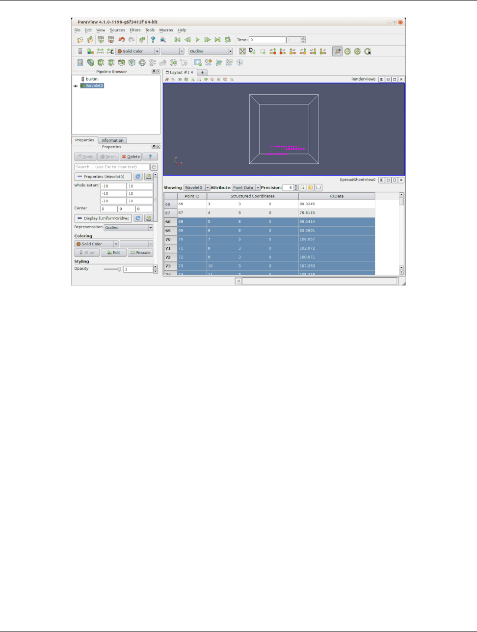
6.1. Understanding selection
Figure 6.1: Linked selection between views allows you to select elements in a view and view them in all other views
showing the selected data. In this demo, as we select rows in the SpreadSheet View, the corresponding points in the 3D
View get highlighted.
Attribute combo-box to Cell Data and then highlight rows. The Render View will show the selected cells as a
wireframe, rather than points.
Conversely, you could have created the selection in the Render View, and the SpreadSheet View will also highlight the
selected elements. We will see how to create such selection later in this chapter.
The first thing to note is that, when you create a new selection, the existing selection is cleared. Thus, there is at most one
active selection in the application at any given time. As we shall see, certain views provide ways of expanding on the
existing selection.
The second thing to note is that selections are transient, i.e., they cannot be undone/redone or saved in state files and
loaded back. Nor can you apply filters or other transformation to the selections themselves. There are cases, however,
where you may want to subset your dataset using the selection defined interactively and then apply filters and other
analysis to that extracted subset. For that, there are filters available, namely Extract Selection and Plot Selection
Over Time, that can capture the active selection in as the filter parameters and then produce a new dataset that is
comprised of the selected elements.
The third thing to note is that there are different types of selections, e.g., id-based selections, where the selected elements
are identified by their indices; frustum-based selections, where the selected elements are those that intersect a frustum
defined in 3D space; query-based selections, where the selected elements are those that match the specified query string;
and so on.
114 Chapter 6. Selecting data
6.2. Creating selections using views
Did you know?
While, technically, selection is possible using a Python-based API, that API is currently cumbersome and requires
understanding of some of ParaView internals. There are plans to simplify that API in future releases. As a result,
we do not cover Python API for selection in this chapter. Once this new API is available, it will be included in this
chapter.
6.2 Creating selections using views
Views provide a convenient mechanism for creating selections interactively. Views like Render View can create multiple
types of selection (id- or frustum-based selections for selecting points and cells), while others like the SpreadSheet
View and Line Chart View only support one type (id-based selections for points or cells).
6.2.1 Selecting in Render View
To create a selection in the Render View, you use the toolbar at the top of the view frame. There are two ways of
selecting cells, points or blocks in ParaView: interactive and non-interactive.
ParaView enters a non-interactive selection mode when the user clicks one of the non-interactive selection buttons:
. The type of selection you are creating will depend on the button you clicked. Once in
non-interactive selection mode, the cursor will switch to cross-hair and you can click and drag to create a selection region.
Once you release the mouse, ParaView will attempt to create a selection for any elements in the selection region and will
go back to default interaction mode.
To create a selection for cells visible in the view, use the button. For selecting visible points, use the button
instead. Visible cells (and points) are only those cells (or points) that are currently rendered on the screen. Thus, elements
that are occluded or are too small to be rendered on the screen will not be selected. If you want to select all data elements
that intersect the view frustum formed by the selection rectangle you drew on the screen, use the button (or for
points). In this case, all elements, visible or otherwise, that are within the 3D space defined by the selection frustum are
selected.
To create a selection for blocks visible in the view use the button. Note that there is no frustum selection for blocks.
While most selection modes allow you to define the selection region as a rectangle, (and for points) enables you
to define the selection region as a closed polygon. However, this is limited to surface elements (i.e., no frustum-based
selection).
ParaView enters an interactive selection mode when the user clicks on one of the interactive selection buttons: . In
interactive selection mode, the user acts on visible elements (cells or points). ParaView highlights elements of the dataset
as a user moves the cursor over them. An element can be selected by clicking on it. Clicking repeatedly on different
elements adds them to the selection. A user ends the interactive selection mode by clicking on the interactive selection
button pushed in or by pressing the Esc key. This mode is also ended when the user enters a non-interactive selection
mode. You can use button to interactively select cells of the dataset and use button to interactively select points.
When there are selected elements, button can be used to clear the selection.
Several of these buttons have hotkeys too, such as Sfor visible cell selection, Dfor visible points selection, Ffor
Chapter 6. Selecting data 115
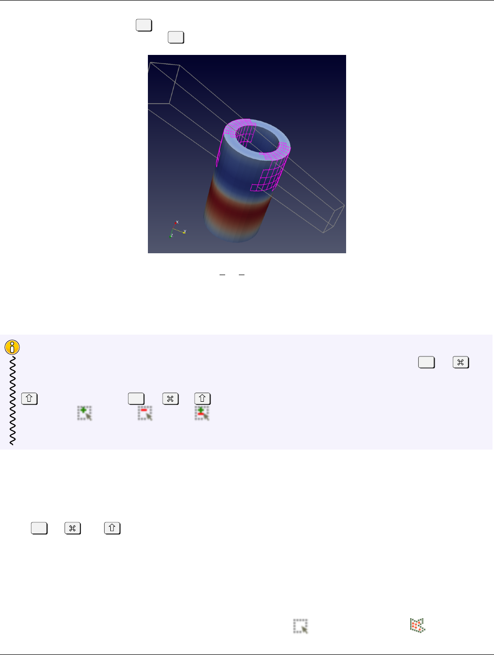
6.2. Creating selections using views
frustum-based cell selection, and Gfor frustum-based point selection. If you notice, these are keys are right next to
each other on the keyboard, starting with S, and are in the same order as the toolbar buttons themselves.
Figure 6.2: Result of a frustum cell selection on disk out ref.ex2 dataset showing the frustum used to identify selected
cells. All cells that fall in that frustum or that intersect it, irrespective of whether they were visible from the view angle
when the selection was made, are selected.
Did you know?
For id-based visible cell (or point) selection, you can expand the current selection by keeping the Ctrl (or )key
pressed when clicking and dragging in selection mode. paraview will then try to add to the current selection by
adding the newly selected elements to the existing one. You can also subtract from the current selection using the
, or even toggle using Ctrl (or )+ . Selection modifier buttons, in the toolbar, can be used for the same
effect. Add : , remove : , toggle : . These modifiers do not work, however, if the selection type (or the
selected data) is different from the current selection. If so, the current selection will be cleared (as is the norm) and
then the new selection will be created.
6.2.2 Selecting in SpreadSheet View
To create a selection in the SpreadSheet View, you simply click on the corresponding rows in the spreadsheet. You can
use the Ctrl (or ) and keys to add to the selection. Based on which data attribute the view is currently showing,
i.e., Point Data,Cell Data, or Row Data, the selection will select points, cells, or rows, respectively.
6.2.3 Selecting in Line Chart View
Line Chart View enables you to select the elements corresponding to the plotted data values. The selection interaction
is similar to Render View. By default, you are in the interaction mode. You enter selection mode to create a selection by
using the buttons in the view toolbar for creating a rectangular selection or a polygonal selection . Once in
116 Chapter 6. Selecting data
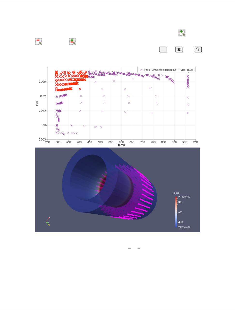
6.3. Creating selections using the Find Data dialog
selection mode, you can click and drag to define the selection region. The selection is created once you release the mouse
press.
When a new selection is created, by default, it will clear any existing selection in the view. The selection modifier buttons
in the view toolbar can be used to control whether a new selection adds to selected elements , removes points from the
selected elements , or toggles it . These modifier buttons are mutually exclusive and modal, i.e., they remain
pressed until you click to unpress them or until you press another modifier button. Ctrl (or ) and can also be used
to add to/subtract from the selection.
Figure 6.3: Selection in Line Chart View can be used to locate elements matching attribute criteria. In this visualization,
by generating a scatter plot plotting Pres against Temp in the disk out ref.ex2 dataset by selecting the top-left corner of
the Line Chart View, we can easily locate elements in the high Pres, low Temp regions in the dataset.
6.3 Creating selections using the Find Data dialog
Views provide mechanisms to create selections interactively. Selections in chart views and SpreadSheet View can be
used to select elements with certain data properties, rather than spatial locations (Figure 6.3). For a richer data-based
Chapter 6. Selecting data 117
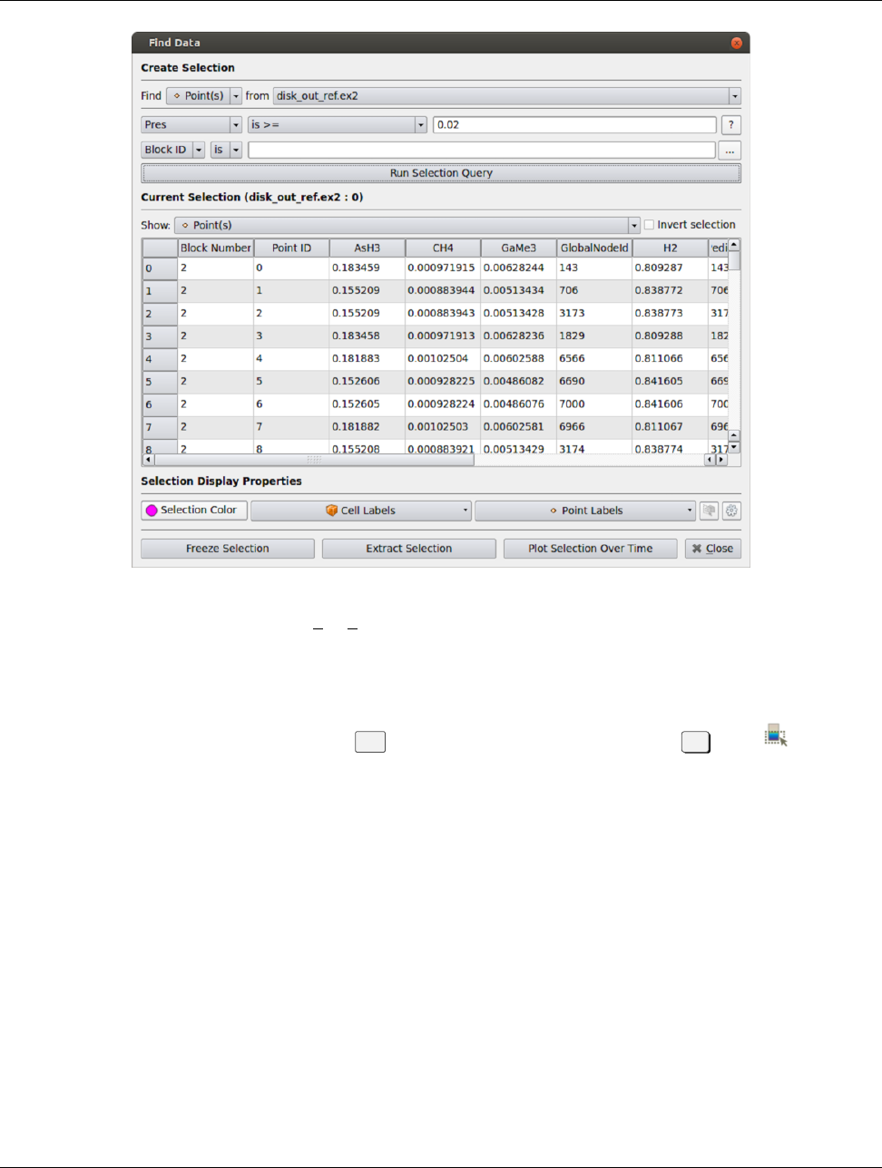
6.3. Creating selections using the Find Data dialog
Figure 6.4: The Find Data dialog in paraview can be used to find data elements matching specific conditions. In this
example, we are selecting all Points in disk out ref.ex2 dataset where Pres is >=0.02.
selection for selecting elements matching certain criteria, you can use the Find Data mechanism in paraview.
The Find Data dialog can be accessed from the Edit menu or by using the keyboard shortcut Vor the button on
the Main Controls toolbar.
The Find Data dialog can be split into three components, reflecting how you would use this dialog. The Create
Selection component includes UI elements to help you define the selection criteria or the query for defining the data
elements to find. The Current Selection component shows the results from the most recent selection results in a
spreadsheet. Finally, the Selection Display Properties component allows you to control how the selected elements
are shown in the active view.
You can create selections or define queries in the Find Data dialog using the widgets under the Create Selection
group. The UI is designed to be read left-to-right. Thus, you start by specifying which data attributes you are interested in
selecting: cells, points, or rows. Then select which pipeline module is producing the dataset of interest. Once that’s done,
the next step is to specify the selection criteria. The left-most combo-box is used to select the array of interest. The
available options reflect the data array currently available on the dataset. The next combo-box is used to select the
operator. Options include the following:
•is matches a single value
•is between matches a range of values specified by min and max
•is one of matches a list of comma separated values
•is >=matches all values greater than or equal to the specified value
118 Chapter 6. Selecting data
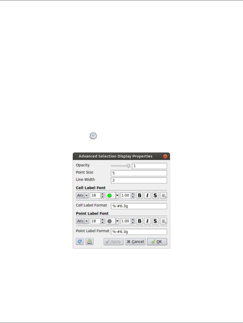
6.3. Creating selections using the Find Data dialog
•is <=matches all values lesser than or equal to the specified value
•is min matches the minimum value for the array for the current time step
•is max matches the maximum value for the array for the current time step
•is <= mean matches values lesser than or equal to the mean
•is >= mean matches values greater than or equal to the mean
•is equal to mean with tolerance matches values equal to the mean within the specified tolerance
Based on your selection of the operator, input widgets will be shown next to this combo-box, where you enter the
corresponding values. For example, for is between, you enter the min and max values for defining the range in the two
text entry widgets.
Once you are satisfied with the selection criteria, hit the Run Selection Query button to execute the query. On success,
the Current Selection spreadsheet will update to show the selected elements. You switch which element attributes
your are viewing in the spreadsheet using the Show combo-box. Additionally, you can invert the selection by checking
Invert selection.
Similar to selecting in views, once you create a selection, any view showing the selected data will also highlight the
selected elements, if possible. For example, the Render View will show a colored wireframe marking the selected
elements, SpreadSheet View will highlight the rows, etc. The Selection Display Properties group allows you to
change the selection that is shown in the active view. Currently, it is primarily designed for Render View. In the future,
however, it could support changing selection attributes for other views as well. The available options allow you select the
color to use to show the selected elements, as well as the data attributes to use to label the cells/points. For finer control on
the label formatting, color, font, etc., use the button. That will pop up the Advanced Selection Display
Properties dialog (Figure 6.5).
Figure 6.5: Advanced Selection Display Properties dialog for controlling selection labelling parameters.
Chapter 6. Selecting data 119
6.4. Displaying selections
Did you know?
Besides creating new selections, the Find Data dialog can also be used to inspect the current selection made
from outside the dialog. For example, if you select elements in the Render View using the options described in
Section 6.2.1, the Current Selection component in the Find Data dialog will indeed update to reflect the
newly selected elements. Furthermore, you can change its display properties and extract this selection using the
extraction buttons (which we will cover in Section 6.5).
6.4 Displaying selections
The Find Data dialog provides easy access to changing the Selection Display Properties for the selection in the
active view. The same functionality can also be accessed using the Selection Display Inspector panel, which is a
dockable panel that can be shown/hidden using the View Selection Display Inspector menu. Currently, selection display
properties apply to Render Views alone. In the future, this will be expanded to other view types, as appropriate.
The Current Selection section in the Find Data dialog shows the selected elements in a spreadsheet view. You can
also make a regular SpreadSheet View do the same by checking the button in the view toolbar to show only selected
elements.
6.5 Extracting selections
All the types of selections created through mechanisms discussed so far are transient and primarily used for highlighting
data. If you want to do further operations on the selected subset, such as extract the selected elements and then save the
result out as a new dataset or apply other filters only on the selected elements, then you need to use one of the extract
selection filters. The Extract Selection and Plot Selection Over Time filters fall in this category of filters.
6.5.1 Extract selection
The Extract Selection filter is used to extract the selected elements as a new dataset for further filtering. There are
multiple ways of creating this filter. You can use the conventional method for creating filters, i.e., using the Filters menu.
When the filter is created, if there is any active selection, the filter will automatically copy that selection for convenience.
Another way to extract the active selection is using the Extract Selection button in the Find Data dialog (Figure 6.4).
The Properties panel shows what defines the selection. You can update the selection by making a new active selection
using any of the mechanisms described earlier in this Chapter and then clicking on the Copy Active Selection button
on the Properties panel for the Extract Selection filter.
By default, the filter is set up to extract the selected elements alone. This filter also supports passing the entire input
dataset through by simply marking which elements are selected. For that, check the Preserve Topology check box on
the Properties panel.
6.5.2 Plot selection over time
Plot Selection Over Time is similar to Extract Selection in the sense that it too extracts the selected elements
from the input dataset. However, instead of simply extracting the result, the goal here is to plot attributes at the selected
elements over time.
120 Chapter 6. Selecting data
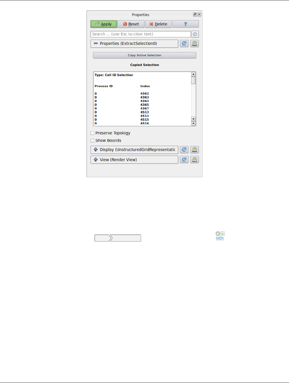
6.6. Freezing selections
Figure 6.6: Properties panel showing the properties for the Extract Selection filter.
Figure 6.7 shows an example use of this filter. In this case, we wanted to see how the strain (or EQPS) cell attribute
changes over time for two specific cells that we selected in the Render View using the view-based selection mechanism.
The selected cells are the highlighted elements in the left view. After having selected the cells, we create the Plot
Selection Over Time filter using the Filters Data Analysis menu. (You could also use the from the Data Analysis
toolbar.) Similar to the Extract Selection filter, when this filter is created, it copies the active selection. You can
change it afterwards using the Copy Active Selection button on the filter’s Properties panel. On hitting Apply,
paraview will show a visualization similar to the one shown here.
Instead of using the view for defining the selection, you could have used the Find Data dialog. In that case, instead of
being able to plot each element over time, you will be plotting summaries for the selected subset over time. This is
essential since the selected subset can have a varying number of elements over time. The summaries include quantities
like min, max, and median of available variables. You can make the filter always produce these statics alone (even when
the selection is created by selecting specific elements in a view) by checking the Only Report Selection Statistics
property on the Properties panel for the Plot Selection Over Time filter.
6.6 Freezing selections
When extracting selections, you can use views or the Find Data dialog to define the selection. Since the extraction filters
are indeed like any other filters in ParaView, they are re-executed any time the input dataset changes, properties on the
filter change, or the current time changes. Every time the filter re-executes, it performs the selection and extraction
operations. Thus, if you created the selection using Render View to create an id-based selection, the filter will identify
Chapter 6. Selecting data 121
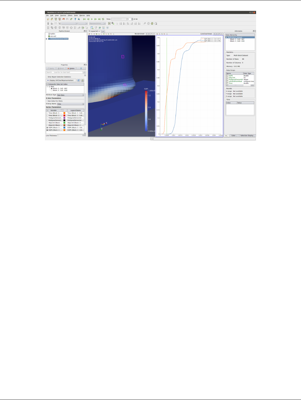
6.6. Freezing selections
Figure 6.7: Plot Selection Over Time in action in paraview. The filter provides a convenient way to plot changes in
attributes over time for the selected set of cells or for points in a temporal dataset.
which of the elements are of the requested ids and then pass those. For frustum-based selection, it will determine what
elements fall within the frustum and extract those. Similarly, with query-based selections created using the Find Data
dialog, the query is re-evaluated. This can result in the selection of different elements with changes in timestep. For
example, if you are selecting the cells where the strain is maximum, that cell(s) will potentially be different for each time
step. Suppose you want to plot the changes in a cell that has maximum strain at the last time step – how can we do that?
The answer is using the Freeze Selection button on the Find Data dialog. What that does is convert any type of
selection (frustum, query-based) to an id-based selection matching the currently selected element ids. Now you can use
this frozen, id-based selection for Extract Selection or Plot Selection Over Time.
122 Chapter 6. Selecting data
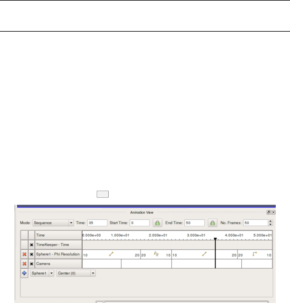
CHAPTER
SEVEN
ANIMATION
In ParaView, you can create animations by recording a series of keyframes. At each keyframe, you set values for the
properties of the readers, sources, and filters that make up the visualization pipeline, as well as the position and orientation
of the camera. Once you have chosen the parameters, you can play through the animation. When you play the animation,
you can cache the geometric output of the visualization pipeline in memory. When you replay the animation, playback
will be much faster because very little computation must be done to generate the images. Also, the results of the animation
can be saved to image files (one image per animation frame) or to a movie file. The geometry rendered at each frame can
also be saved in ParaView’s PVD file format, which can be loaded back into ParaView as a time varying data set.
7.1 Animation View.
Animation View is the user interface used to create animations by adding keyframes. It is modeled similar to popular
animation and keyframe editing applications with the ability to create tracks for animating multiple parameters. The
Animation View is accessible from the View menu.
Figure 7.1: Animation View.
As seen in Figure 7.1, this view is presented as a table. Above the table are the controls that administers how time
progresses in the animation. These were discussed previously. Within the table, the tracks of the animation appear as
rows, and animation time is presented as increasing from left-to-right. The first row in the table, simply labeled Time,
shows the total span of time that the animation can cover. The current displayed time is indicated both in the Time field at
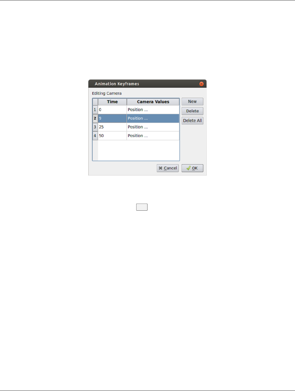
7.2. Animation View header
the top and with a thick, vertical, draggable line within the table.
Along the left side of the Animation View is an expandable list of the names of the animation tracks (i.e., a particular
object and property to animate). You choose a data source and then a particular property of the data source in the bottom
row. To create an animation track with keyframes for that property, click the +on the left-hand side; this will create a new
track. In the figure, tracks already exist for SphereSource1’s Phi Resolution property and for the camera’s position. To
delete a track, press the Xbutton. You can temporarily disable a track by unchecking the check box on the right of the
track. To enter values for the property, double-click within the white area to the right of the track name. This will bring up
the Animation Keyframes dialog. Double-clicking in the camera entry brings up a dialog like the one in Figure 7.2.
Figure 7.2: Editing the camera track.
From the Animation Keyframes dialog, you can press New to create new keyframes. You can also press Delete or
Delete All to delete some or all of the keyframes. Clicking New will add a new row to the table. In any row, you can
click within the Time column to choose a particular time for the keyframe, and you can click in the right-hand column to
enter values for the parameter. The exact user interface components that let you set values for the property at the keyframe
time vary. When available, you can change the interpolation between two keyframes by double-clicking on the central
interpolation column.
Within the tracks of the Animation View, the place in time where each keyframe occurs is shown as a vertical line. The
values chosen for the property at that time and the interpolation function used between that value and the next are shown
as text, when appropriate. In the previous figure, for example, the sphere resolution begins at 10 and then changes to 20,
varying by linear interpolation between them. The camera values are too lengthy to show as text so they are not displayed
in the track, but we can easily see that there are four keyframes spaced throughout the animation. The vertical lines in the
tracks themselves may be dragged, so you can easily adjust the time at which each keyframe occurs.
7.2 Animation View header
The Animation View has a header-bar that lets you control some properties of the animation itself, as you can see in
Figure 7.3.
Mode controls the animation playback mode. ParaView supports three modes for playing animation. In Sequence mode,
the animation is played as a sequence of images (or frames) generated one after the other and rendered in immediate
succession. The number of frames is controlled by the No. Frames spinbox at the end of the header. Note that the
frames are rendered as fast as possible. Thus, the viewing frame rate depends on the time needed to generate and render
each frame.
124 Chapter 7. Animation
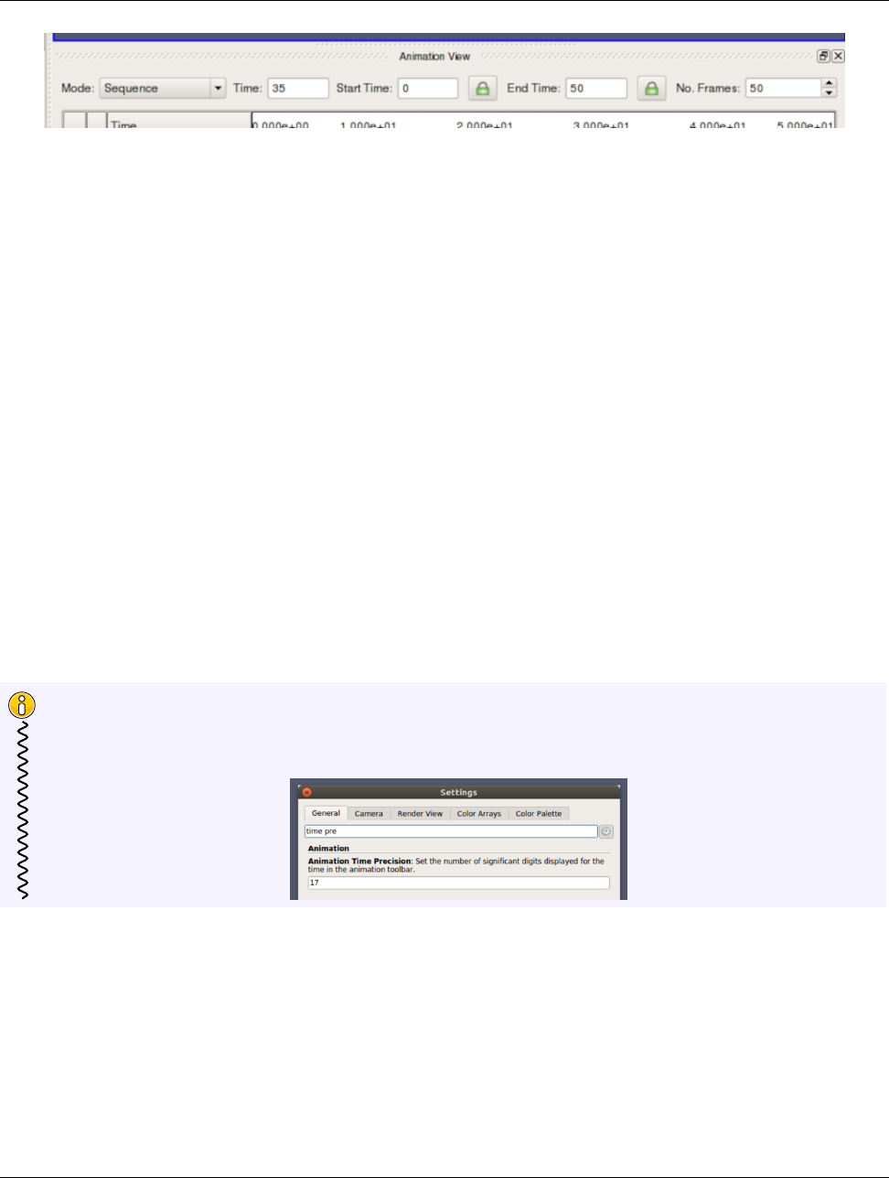
7.3. Animating time-varying data
Figure 7.3: Animation View Header.
In Real Time mode, the Duration spinbox (replacing the No. Frames spinbox) indicates the time in seconds over
which the entire animation should run. Each frame is rendered using the current wall clock time in seconds, relative to the
start time. The animation runs for nearly the number of seconds specified by the Duration (secs) spinbox. In turn, the
number of frames actually generated (or rendered) depends on the time to generate (or render) each frame.
In Snap To TimeSteps mode, the number of frames in the animation is determined by the number of time values in the
data set being animated. This is the animation mode used for ParaView’s default animations: playing through the time
values in a data set one after the other. Default animations are created by ParaView when a data set with time values is
loaded; no action is required by the user to create the animation. Note that using this mode when no time-varying data is
loaded will result in no animation at all.
In Sequence mode, the final item in the header is the No. Frames spinbox. This spinbox lets you pick the total number
of frames for the animation. Similarly, in Real Time mode, the final line lets you choose the duration of the animation. In
Snap To TimeSteps mode, the total number of frames is dictated by the data set and, therefore, the spinbox is disabled.
The Time entry-box shows the current animation time, which is the same as shown by a vertical marker in this view. You
can change the current animation time by either entering a value in this box, if available, or by dragging the vertical
marker. The Start Time and End Time entry-boxes display the start and end times for the animation. By default, when
you load time varying data sets, the start and end times are automatically adjusted to cover the entire time range present in
the data. The lock check-buttons to the right of the Start Time and End Time widgets will prevent this from happening,
so that you can ensure that your animation covers a particular time domain of your choosing.
Did you know?
You can change the precision (number of significant digits) displayed by the animation clock by changing the
Animation Time Precision value under Settings/Properties Panel Options/Advanced.
7.3 Animating time-varying data
When you load time-varying data, ParaView automatically creates a default animation that allows you to play through the
temporal domain of the data without manually creating an animation to do so. With the Animation View, you can
uncouple the data time from the animation time so that you can create keyframes that manipulate the data time during
animation as well.
If you double-click in the TimeKeeper Time track, the Animation Keyframes dialog, an example of which is shown in
Chapter 7. Animation 125
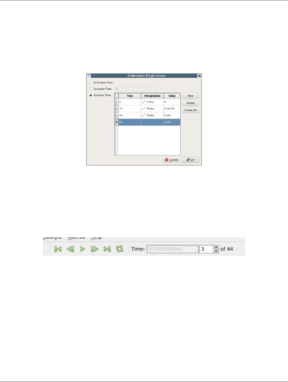
7.4. Playing an animation
Figure 7.4, appears. In this dialog, you can make data time progress in three fundamentally different ways. If the
Animation Time radio-button is selected, the data time will be tied to and scaled with the animation time so that, as the
animation progresses, you will see the data evolve naturally. If you want to ignore the time varying nature of the data, you
can select Constant Time instead. In this case, you choose a particular time value at which the data will be displayed for
the duration of the animation. Finally, you can select the Variable Time radio-button to have full control over data time
and to control it as you do any other animatible property in the visualization pipeline. In the example shown in Figure 7.4,
time is made to progress forward for the first 15 frames of the animation, backward for the next 30, and forward for the
final 15.
Figure 7.4: Controlling Data Time with keyframes.
7.4 Playing an animation
Once you have designed your animation, you can play through it with the VCR controls toolbar seen in Figure 2.5.
Figure 7.5: VCR Controls and Current Time Controls toolbars in paraview.
7.5 Animating the camera
Just like you can change parameters on sources and filters in an animation, you can also change the camera parameters.
As seen in Figure 7.6, you can add animation tracks to animate the camera for all the 3D render views in the setup
separately. To add a camera animation track for a view, with the view selected, click on the +button after choosing
Camera from the first drop-down menu. The second drop-down list allows you to choose how to animate the camera.
There are three possible options, each of which provides different mechanisms to specify the keyframes. It’s not possible
to change the mode after the animation track has been added, but you can simply delete the track and create a new one.
126 Chapter 7. Animation
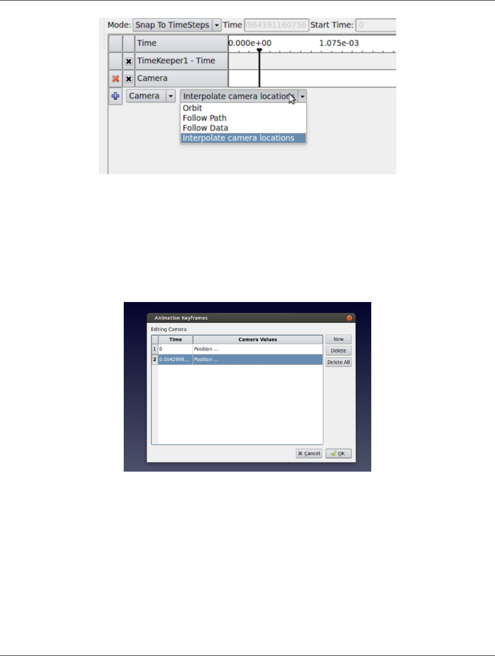
7.5. Animating the camera
Figure 7.6: Add camera track.
7.5.1 Interpolate camera locations
In this mode, you specify camera position, focal point, view angle, and up direction at each keyframe. The animation
player interpolates between these specified locations. As with other parameters, to edit the keyframes, double-click on the
track. It is also possible to capture the current location as a keyframe by using the Use Current button.
Figure 7.7: Setting animation parameters.
It can be quite challenging to add keyframes correctly and frequently to ensure that the animation results in a smooth
visualization using this mode.
7.5.2 Orbit
This mode makes it possible to quickly create a camera animation in which the camera revolves around objects of interest.
Before adding the Camera track, select the objects in the pipeline browser that you want to revolve around; then choose
Orbit from the Camera combo-box in the Animation View, and hit +. This will pop up a dialog where you can edit
the orbit parameters such as the center of revolution, the normal for the plane of revolution, and the origin (i.e., a point on
Chapter 7. Animation 127
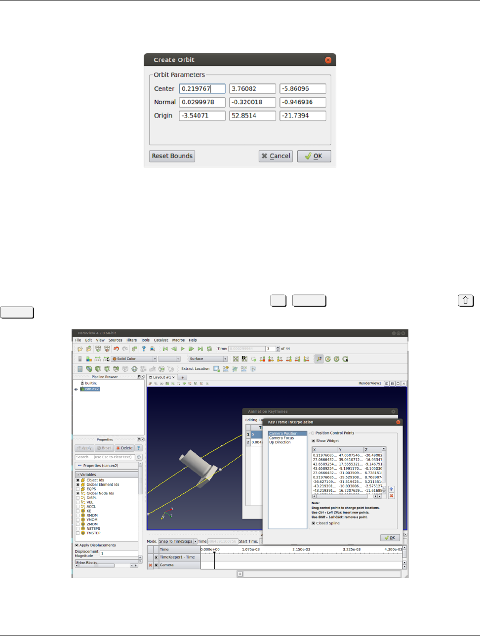
7.5. Animating the camera
the plane where the revolution begins). By default, the Center is the center of the bounds of the selected objects, the
Normal is the current up direction used by the camera, while the origin is the current camera position.
Figure 7.8: Creating a camera orbit.
7.5.3 Follow path
In this mode, you get the opportunity to specify the path taken by the camera position and the camera focal point. By
default, the path is set up to orbit around the selected objects. You can then edit the keyframe to change the paths.
Figure 7.9 shows the dialog for editing these paths for a keyframe. When Camera Position or Camera Focus is selected, a
widget is shown in the 3D view that can be used to set the path. Use Ctrl +Left Click to insert new control points, and +
Left Click to remove control points. You can also toggle when the path should be closed or not.
Figure 7.9: Creating a camera path.
128 Chapter 7. Animation

CHAPTER
EIGHT
SAVING RESULTS
In this chapter, we will introduce various ways of saving visualization results in ParaView. Results generated throughout
the visualization process not only include the images and the rendering results, but also include the datasets generated by
filters, the scene representations that will be imported into other rendering applications, and the movies generated from
animations.
8.1 Saving datasets
You can save the dataset produced by any pipeline module in ParaView, including sources, readers, and filters. To save the
dataset in paraview, begin by selecting the pipeline module in the Pipeline browser to make it the active source. For
modules with multiple output ports, select the output port producing the dataset of interest. To save the dataset, use the
File Save Data menu or the button in the Main Controls toolbar. You can also use the keyboard shortcut Ctrl +S
(or +S). The Save File dialog (Figure 8.1) will allow you to select the filename and the file format. The available
list of file formats depends on the type of the dataset you are trying to save.
Figure 8.1: Save File dialog in paraview.
On accepting a filename and file format to use, paraview may show the Configure Writer dialog (Figure 8.2). This
dialog allows you to further customize the writing process. The properties shown in this dialog depend on the selected file
format and range from enabling you to Write All Time Steps, to selecting the attributes to write in the output file.
In pvpython too, you can save the datasets as follows:
1
2# Saving the data using the default properties for
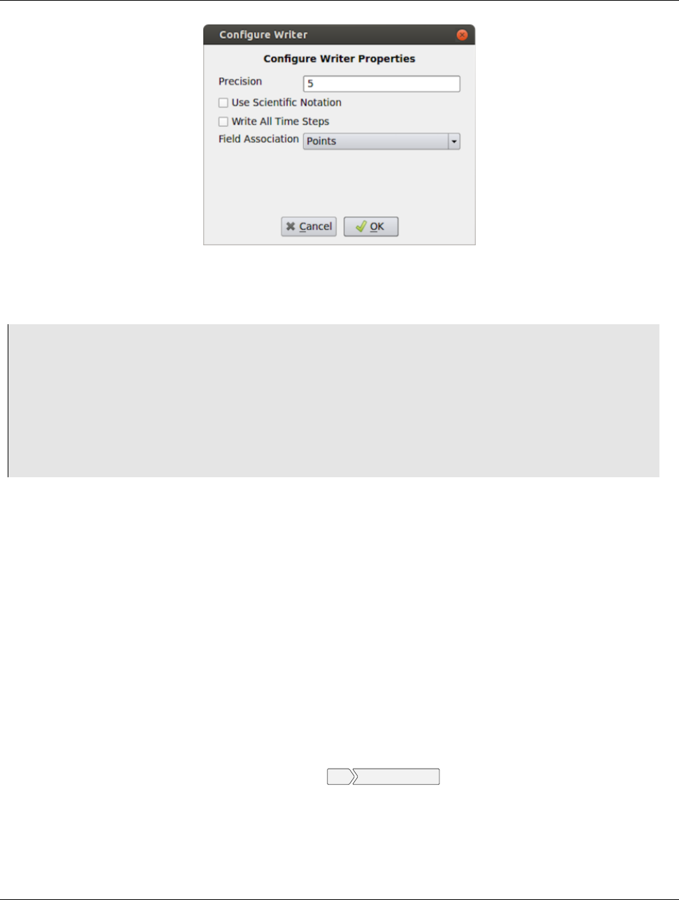
8.2. Saving rendered results
Figure 8.2: Configure Writer dialog in paraview shown when saving a dataset as a csv file.
3# the used writer, if any.
4>>> SaveData("sample.csv",source)
5
6# the second argument is optional, and refers to the pipeline module
7# to write the data from. If none is specified the active source is used.
8
9# To pass parameters to configure the writer
10 >>> SaveData("sample.csv",source,
11 Precision=2,
12 FieldAssociation=’Cells’)
pvpython will pick a writer based on the file extension and the dataset type selected for writing, similar to what it does in
paraview. Admittedly, it can be tricky to figure out what options are available for the writer. The best way is to use the
Python tracing capabilities in paraview and to use the generated sample script as a reference (Section 1.6.2). Make sure
you use a similar type of dataset and the same file format as you want to use in your Python script, when tracing, to avoid
runtime issues.
8.2 Saving rendered results
Views that render results (this includes almost all of the views, except SpreadSheet View) support saving images (or
screenshots) in one of the standard image formats (png, jpeg, tiff, bmp, ppm). Certain views also support exportings the
results in several formats such as pdf, x3d, and vrml.
8.2.1 Saving screenshots
To save the render image from a view in paraview, use the File Save Screenshot menu option. This will pop up the Save
Screenshot Options dialog (Figure 8.3). This dialog allows you to select various image parameters, such as image
resolution and image quality (which depends on the file format chosen). The dialog also provides an option to change the
color palette to use to save the image using Override Color Palette.
By default, paraview will save rendered results from the active view. Optionally, you can save an image comprising of all
the views layed out exactly as on the screen by unchecking the Save only selected view button.
130 Chapter 8. Saving results
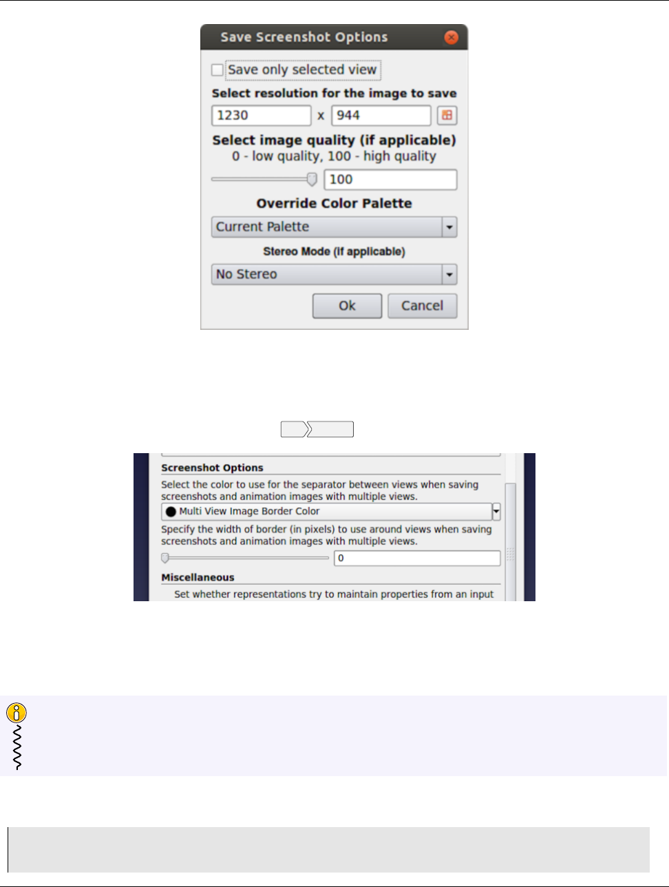
8.2. Saving rendered results
Figure 8.3: The Save Screenshot Options dialog, which is used to customize saving screenshots in paraview.
When saving mutliple views, you can customize the border to use between views, as well as the color to use for that
border, from the General tab in Settings dialog ( Edit Settings ), as shown in the Figure 8.4
Figure 8.4: Screenshot Options in the Settings dialog allow you to set the size in pixels and the color for the border
to use to separate views with saving multiple views in a screenshot.
Did you know?
You can save high-resolution images at a resolution higher than your monitor by specifying a higher resolution in
the Save Screenshot Options dialog. paraview will use tiling and magnification internally to produce an
image of the requested size.
Saving a screenshot is also possible in paraview.
1# Save a screenshot from a specific view.
2>>> myview = GetActiveView()
3>>> SaveScreenshot("sample.png",view=myview)
Chapter 8. Saving results 131
8.3. Saving animation
4
5# To specify magnification and quality, use the following form:
6>>> SaveScreenshot("sample2X.png",view=myview,magnification=2,quality=100)
7
8# You can skip the ’view’ parameter if you simply want to save the active view.
9>>> SaveScreenshot("sample.png")
10
11 # To save multiple views, you can use the following form:
12
13 # Get the layout in which a specific view is placed
14 # if ’myview’ is not provided, active view will be used.
15 >>> layout = GetLayout(myview)
16
17 >>> SaveScreenshot("multiview.png", layout=layout)
As always, you can use Python tracing in paraview to trace the exact form of the method to use to save a specific
screenshot image.
8.2.2 Exporting scenes
When available, you can export a visualization in a view in several of the supported formats using the File Export View
menu option in paraview. For a Render View (or similar), the available formats include EPS, PDF, PS, SVG, POV,
VRML, WebGL, X3D, and X3DB. On selecting a file as which to export, paraview may pop up an Export Options
dialog that allows you to set up parameters for the exporter, similar to saving datasets (Section 8.1).
In addition, from paraview, exporting takes the following form (again, just use Python trace to figure out the proper form
– that’s the easiest way).
1>>> myview = GetActiveView()
2>>> ExportView(’/ tmp/sample.svg’,view=myview,
3Plottitle=’ParaView GL2PS Export’,
4Compressoutputfile=1)
5# the arguments after ’view’ depend on the exporter selected.
8.3 Saving animation
In paraview, you use the File Save Animation menu option to save the animation results as a movie or as a series of images.
This will pop up the Animation Settings Dialog. Here, you can pick the Frame Rate in frames-per-second for the
generated movie (if applicable for the chosen file format) and the total Number Of Frames to render. The Animation
Duration (sec) field tells you how long the movie file would play given the specified settings. Animation always saves
out all the views currently visible in paraview. Thus, if you maximize a view, the animation will only include the
maximized view. When saving multiple views, the Screenshot Options in the Settings (Figure 8.4) are used to add
borders between views. Frame range can be used to specify the range of frame over which to animate, thus allowing you
to skip parts of the total animation in the saved file(s).
The available file formats include avi and ogg (when available) movie formats, as well as image formats such png, jpg,
and tif. If saving as images, ParaView will generate a series of image files sequentially numbered using the frame number
as a suffix to the specified filename.
In paraview, you can save an animation using WriteAnimation.
1>>> WriteAnimation(’animation.avi’,Magnification=1,FrameRate=15.0,Compression=True
)
132 Chapter 8. Saving results
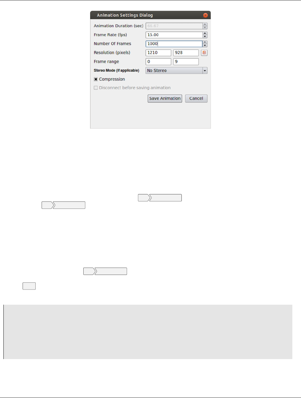
8.4. Saving state
Figure 8.5: The Animation Settings Dialog in paraview, which is used to customize saving of animation files.
8.4 Saving state
Besides saving the results produced by your visualization setup, you can save the state of the visualization pipeline itself,
including all the pipeline modules, views, their layout, and their properties. This is referred to as the application state or,
just, state. In paraview, you can save the state using the File Save State. . . menu option. Conversely, to load a saved state
file, you can use File Load State. . . .
There are two types of state files that you can save in paraview:ParaView state file (*.pvsm) and Python state file (*.py).
The PVSM files are XML-based text files that are human and machine readable, although not necessarily a novice user
human friendly. However, if you don’t plan to read and make sense of the state files, PVSM is the most robust and reliable
way to save the application state. For those who want to save the state and then modify it manually, using Python state
files may be better, as using Python trace simply traces the actions that you perform in the UI as a Python script. Python
state files, on the other hand, save the entire current state of the application as a Python script that you can use in paraview
or the Python Shell.
To load a PVSM file, you use the File Load State. . . menu. Note that loading a state file will affect the current
visualization state. To load the Python state file in paraview, you will need to use the Python Shell, which is accessible
from the Tools menu.
You can save/load the PVSM state file in pvpython as follows:
1>>> from paraview.simple import *
2
3# Save the PVSM state file. Currently, this doesn’t support
4# saving Python state files.
5>>> SaveState("sample.pvsm")
6
7# To load a PVSM state file.
8>>> LoadState("sample.pvsm")
Chapter 8. Saving results 133
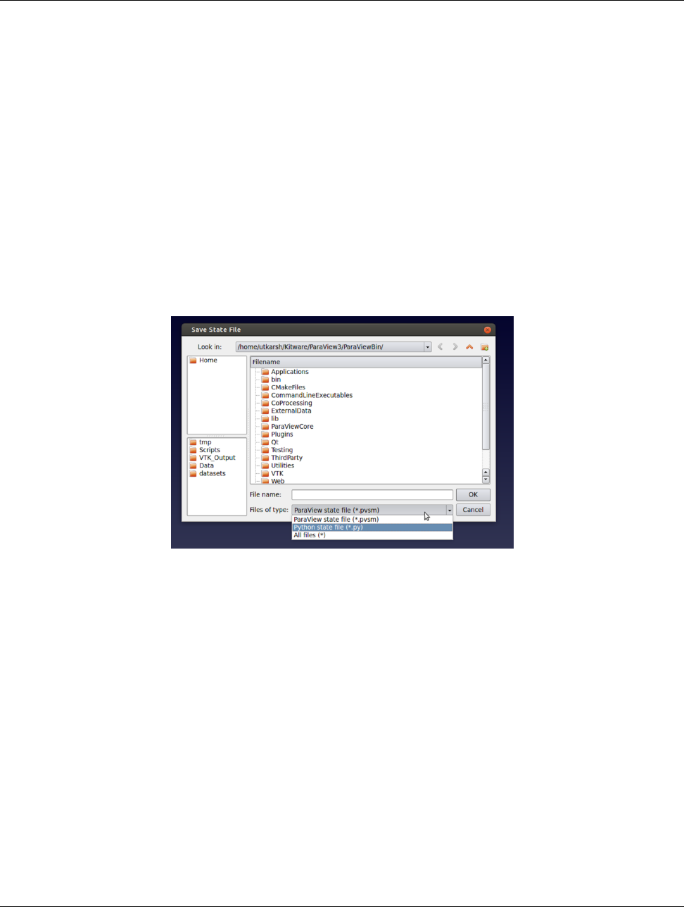
8.4. Saving state
Figure 8.6: The Save State File dialog in paraview.
134 Chapter 8. Saving results
Part II
Reference Manual
CHAPTER
NINE
PROPERTIES PANEL
The Properties panel is perhaps the most often used panel in paraview. This is the panel you would use to change
properties on modules in the visualization pipeline, including sources and filters, to control how they are displayed in
views using the Display properties, and to customize the view itself. In this chapter, we take a closer look at the
Properties panel to understand how it works.
9.1 Anatomy of the Properties panel
Before we start dissecting the Properties, remember that the Properties panel works on active objects, i.e., it shows
the properties for the active source and active view, as well as the display properties, if any, for active source in the active
view.
9.1.1 Buttons
Figure 9.1 shows the various parts of the Properties panel. At the top is the group of buttons that let you accept, reject
your changes to the panel or Delete the active source.
Did you know?
You can delete multiple sources by selecting them using the Ctrl (or ) key when selecting in the Pipeline
Browser and then clicking on the Delete button. Sometimes, the Delete button may be disabled. That happens
when the selected source(s) have other filters connected to them. You will need to delete those filters first.
9.1.2 Search box
The Search box allows you to search for a property by using the name or the label for the property. Simply start typing
text in the Search box, and the panel will update to show widgets for the properties matching the text.
The Properties panel has two modes that control the verbosity of the panel: default and advanced. In the default mode,
a smaller subset of the available properties is shown. These are generally the frequently used properties for the pipeline
modules. In advanced mode, you can see all the available properties. You can toggle between default and advanced modes
using the button next the Search box.
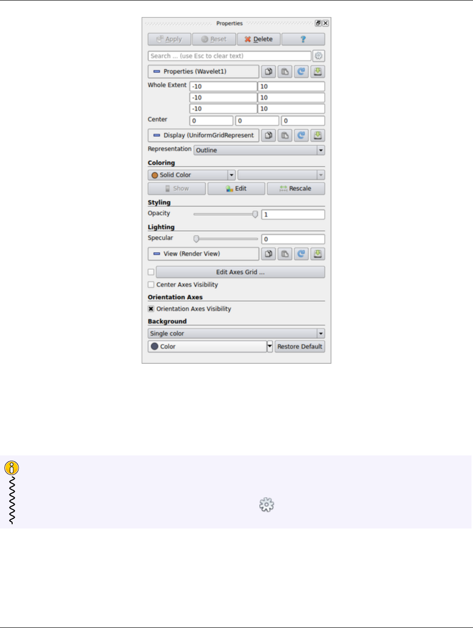
9.1. Anatomy of the Properties panel
Figure 9.1: Properties Panel in paraview
When you start searching for a property by typing text in the Search box, irrespective of the current mode of the panel
(i.e., default or advanced), all properties that match the search text will be shown.
Did you know?
The Search box is a recurring widget in paraview. Several other panels and dialog boxes, including the
Settings dialog and the Color Map Editor, show a similar widget. Its behavior is also exactly the same as
in the case of the Properties panel. Don’t forget that the button can be used to toggle between default and
advanced modes.
9.1.3 Properties
The Properties,Display, and View sections in the panel show widgets for properties on the active source, its display
properties in the active view, and the properties for the active view, respectively. You can collapse/expand each of these
138 Chapter 9. Properties panel
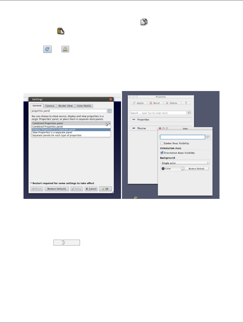
9.2. Customizing the layout
sections by clicking on the section name.
To the right of each section name is a set of four buttons. Clicking the copies the current set of property values to the
clipboard while clicking the will paste those property values into another compatible panel section. Note that the
paste icon is enabled only for panel sections where the copied properties can be pasted.
The next two buttons and enable customizing the default values used for those properties. Refer to Chapter 10 to
learn more about customizing default property values.
9.2 Customizing the layout
Figure 9.2: Options for customizing the Properties panel layout using the Settings (left). View properties in a separate
dock panel (right).
The Properties panel, by default, is set up to show the source, display, and view properties on the same panel. You may,
however, prefer to have each of these sections in a separate dockable panel. You can indeed doso using the Settings
dialog accessible from the Edit Settings menu.
On the General tab search of the properties panel using the Search box, you should see the setting that lets you pick
whether to combine all the sections in one (default), to separate out either the Display or View sections in a panel, or to
create separate panels for each of the sections. You will need to restart paraview for this change to take effect. Also, since
the Apply and Reset buttons only apply to the Properties section, they will only be shown in the dock panel that
houses it.
Chapter 9. Properties panel 139

CHAPTER
TEN
CUSTOMIZING DEFAULTS
The chapter describes how to specify custom default settings for the properties of sources, readers, filters, representations,
and views. This can be used to specify, for example, the default background color for new views, whether a gradient
background should be used, the resolution of a sphere source, which data arrays to load from a particular file format, and
the default setting for almost any other object property.
The same custom defaults are used across all the ParaView executables. This means that custom defaults specified in the
paraview executable are also used as defaults in pvpython and pvbatch, which makes it easier to set up a visualization
with paraview and use pvpython or pvbatch to generate an animation from time-series data, for example.
10.1 Customizing defaults for properties
The Properties panel in paraview has three sections, Properties,Display, and View. Each section has two buttons.
These buttons are circled in red in Figure 10.1. The button with the disk icon is used to save the current property values in
that section that have been applied with the Apply button. Property values that have been changed but not applied with the
Apply button will not be saved as custom default settings.
The button with the circular arrow (or reload icon) is used to restore any custom property settings for the object to
ParaView’s application defaults. Once you save the current property settings as defaults, those values will be treated as the
defaults from then on until you change them to another value or reset them. The saved defaults are written to a
configuration file so that they are available when you close and launch ParaView again.
You can undo your changes to the default property values by clicking on the reload button. This will reset the current view
property values to paraview’s application defaults. To fully restore paraview’s default values, you need to click the save
button again. If you don’t, the restored default values will be applied only to the current object, and new instances of that
object will have the custom default values that were saved the last time you clicked the save button.
10.2 Example: specifying a custom background color
Suppose you want to change the default background color in the Render View. To do this, scroll down to the View
section of the Properties panel and click on the combo box that shows the current background color. Select a new color,
and click OK. Next, scroll up to the View (Render View) section header and click on the disk button to the right of the
header. This will save the new background color as the default background color for new views. To see this, click on the +
sign next to the tab above the 3D view to create a new layout. Click on the Render View button. A new render view will
be created with the custom background color you just saved as default.
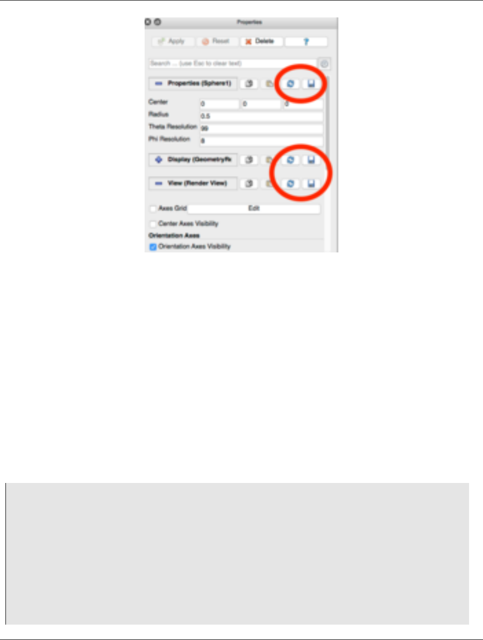
10.3. Configuring default settings with JSON
Figure 10.1: Buttons for saving and restoring default property values in the Properties panel.
10.3 Configuring default settings with JSON
Custom default settings are stored in a text file in the JavaScript Object Notation (JSON) format. We recommend to use
the user interface in paraview to set most default values, but it is possible to set them by editing the JSON settings file
directly. It is always a good idea to make a backup copy of a settings file prior to manual editing.
The ParaView executables read from and write to a file named ParaView-UserSettings.json, which is located in your
home directory on your computer. On Windows, this file is located at
%APPDATA%/ParaView/ParaView-UserSettings.json, where the APPDATA environment variable is usually something
like C:/Users/USERNAME/AppData/Roaming, where USERNAME is your login name. On Unix-like systems, it is located
under ˜/.config/ParaView/ParaView-UserSettings.json. This file will exist if you have made any default settings
changes through the user interface in the paraview executable. Once set, these default settings will be available in
subsequent versions of ParaView.
A simple example of a file that specifies custom default settings is shown below:
1{
2"sources":{
3"SphereSource":{
4"Radius":3.5,
5"ThetaResolution":32
6},
7"CylinderSource":{
8"Radius":2
9}
10 },
11 "views":{
12 "RenderView":{
13 "Background":[0.0,0.0,0.0]
142 Chapter 10. Customizing defaults
10.4. Configuring site-wide default settings
14 }
15 }
16 }
Note the hierarchical organization of the file. The first level of the hierarchy specifies the group to which the object whose
settings are being specified refers (“sources” in this example). The second level names the object whose settings are being
specified. Finally, the third level specifies the custom default settings themselves. Note that default values can be set to
literal numbers, strings, or arrays (denoted by comma-separated literals in square brackets).
The names of groups and objects come from the XML proxy definition files in ParaView’s source code in the directory
ParaView/ParaViewCore/ServerManager/SMApplication/Resources. The group name is defined by the name
attribute in a ProxyGroup element. The object name comes from the name attribute in the Proxy element (or elements of
vtkSMProxy subclasses). The property names come from the name attribute in the *Property XML elements for the
object.
Did you know?
The application-wide settings available in paraview through the Edit Settings menu are also saved to this user
settings file. Hence, if you have changed the application settings, you will see some entries under a group named
“settings”.
10.4 Configuring site-wide default settings
In addition to individual custom default settings, ParaView offers a way to specify site-wide custom default settings for a
ParaView installation. These site-wide custom defaults must be defined in a JSON file with the same structure as the user
settings file. In fact, one way to create a site settings file is to set the custom defaults desired in paraview, close the
program, and then copy the user settings file to the site settings file. The site settings file must be named
ParaView-SiteSettings.json.
The ParaView executables will search for the site settings file in several locations. If you installed ParaView in the
directory INSTALL, then the ParaView executables will search for the site settings file in these directories in the specified
order:
•INSTALL/share/paraview-X.Y
•INSTALL/lib
•INSTALL
•INSTALL/..
where Xis ParaView’s major version number and Yis the minor version number. ParaView executables will search these
directories in the given order, reading in the first ParaView-SiteSettings.json file it finds. The conventional location
for this kind of configuration file is in the share directory (the first directory searched), so we recommend placing the site
settings file there.
Custom defaults in the user settings file take precedence over custom defaults in the site settings. If the same default is
specified in both the ParaView-SiteSettings.json file and ParaView-UserSettings.json file in a user’s directory,
the default specified in the ParaView-UserSettings.json file will be used. This is true for both object property settings
and application-settings set through the Edit Settings menu.
Chapter 10. Customizing defaults 143

10.4. Configuring site-wide default settings
To aid in debugging problems with the site settings file location, you can define an evironment variable named
PV SETTINGS DEBUG to something other than an empty string. This will turn on verbose output showing where the
ParaView executables are looking for the site settings file.
144 Chapter 10. Customizing defaults

CHAPTER
ELEVEN
COLOR MAPS AND TRANSFER FUNCTIONS
One of the first things that any visualization tool user does when opening a new dataset and looking at the mesh is to color
the mesh with some scalar data. Color mapping is a common visualization technique that maps data to colo, and displays
the colors in the rendered image. Of course, to map the data array to colors, we use a transfer function. A transfer
function can also be used to map the data array to opacity for rendering translucent surfaces or for volume rendering. This
chapter desribes the basics of mapping data arrays to color and opacity.
11.1 The basics
Color mapping (which often also includes opacity mapping) goes by various names including scalar mapping and
pseudo-coloring. The basic principle entails mapping data arrays to colors when rendering surface meshes or volumes.
Since data arrays can have arbitrary values and types, you may want to create a mapping to define to which color a
particular data value maps. This mapping is defined using what are called color maps or transfer functions. Since such
mapping from data values to rendering primitives can be defined for not just colors, but opacity values as well, we will use
the more generic term transfer functions.
Of course, there are cases when your data arrays indeed specify the red-green-blue color values to use when rendering
(i.e., not using a transfer function at all). This can controlled using the Map Scalars display property. Refer to
Chapter 4.4.2 for details. This chapter relates to cases when Map Scalars is enabled, i.e., when the transfer function is
being used to map arrays to colors and/or opacity.
In ParaView, you can set up a transfer function for each data array for both color and opacity separately. ParaView
associates a transfer function with the data array identified by its name. The same transfer function is used when coloring
with the same array in different 3D views or results from different stages in the pipeline.
For arrays with more than one component, such as vectors or tensors, you can specify whether to use the magnitude or a
specific component for the color/opacity mapping. Similar to the transfer functions themselves, this selection of how to
map a multi-component array to colors is also associated with the array name. Thus, two pipeline modules being colored
with the arrays that have the same name will not only be using the same transfer functions for opacity and color, but also
the component/magnitude selection.
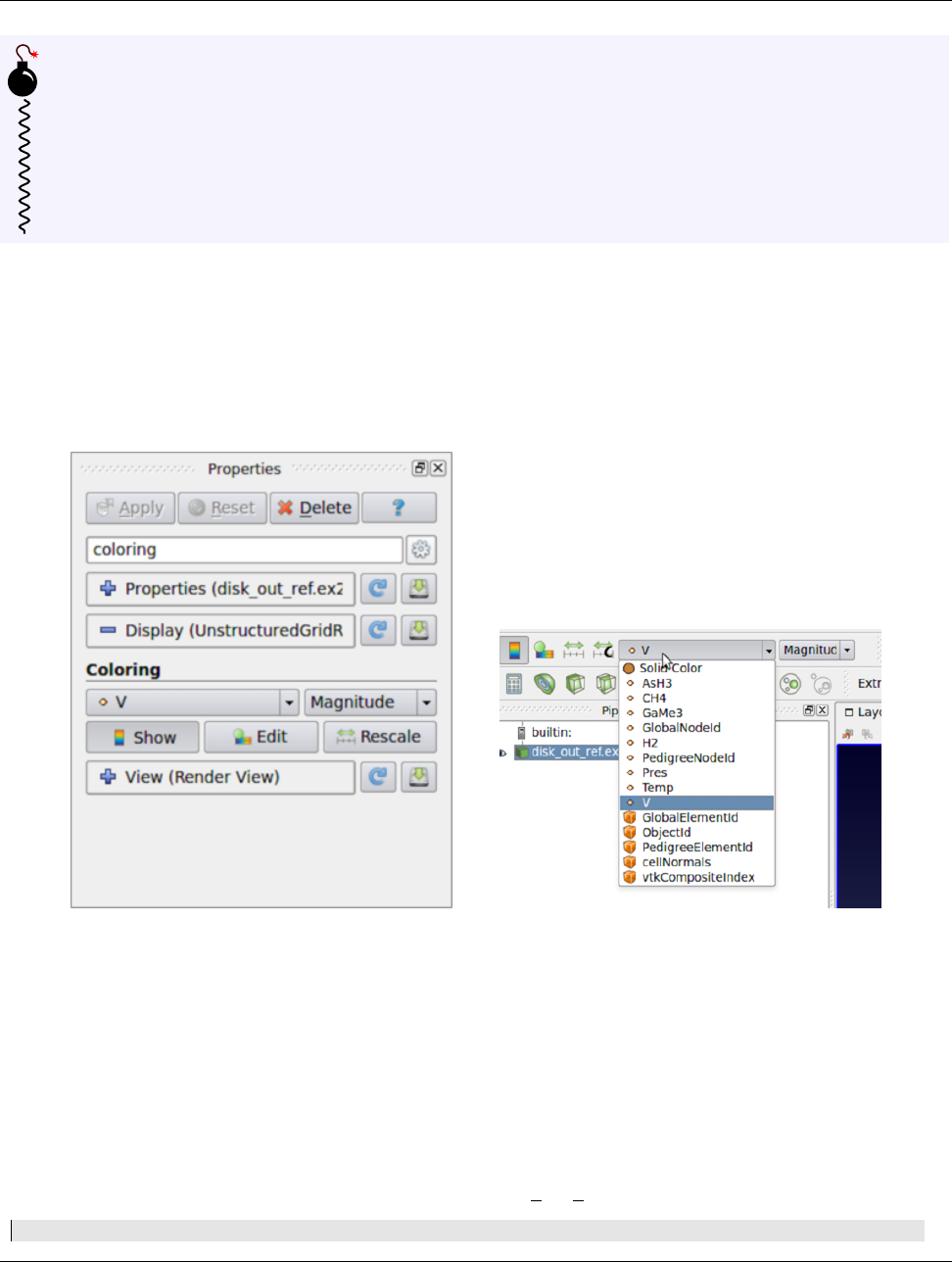
11.1. The basics
Common Errors
Beginners find it easy to forget that the transfer function is associated with an array name and, hence, are surprised
when changing the transfer function for a dataset being shown in one view affects other views as well. Using
different transfer functions for the same variable is discouraged by design in ParaView, since it can lead to the
misinterpretation of values. If you want to use different transfer functions, despite this caveat, you can use a filter
like the Calculator or Programmable Filter to rename the array and then use a different transfer function
for it.
There are separate transfer functions for color and opacity. The opacity transfer function is optional when doing surface
renderings (You can turn it on/off by using the Color Map Editor as explained later), but it gets used for volume
rendering.
11.1.1 Color mapping in paraview
Figure 11.1: The controls used for selecting the array to color within the Properties panel (left) and the Active
Variables Controls toolbar (right).
You can pick an array to use for color mapping, using either the Properties panel or the Active Variables Controls
toolbar. You first select the array with which to color and then select the component or magnitude for multi-component
arrays. ParaView will either use an existing transfer function or create a new one for the selected array.
11.1.2 Color mapping in pvpython
Here’s a sample script for coloring using a data array from the disk out ref.ex2 dataset.
1from paraview.simple import *
146 Chapter 11. Color maps and transfer functions
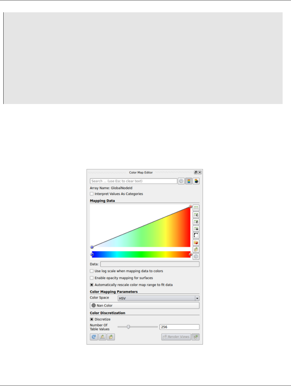
11.2. Editing the transfer functions in paraview
2
3# create a new ’ExodusIIReader’
4reader = ExodusIIReader(FileName=[’disk_out_ref.ex2’])
5reader.PointVariables = [’V’]
6reader.ElementBlocks = [’Unnamed block ID: 1 Type:HEX8’]
7
8# show data in view
9display = Show(reader)
10
11 # set scalar coloring
12 ColorBy(display , (’POINTS’,’ V ’))
13
14 # rescale color and/or opacity maps used to include current data range
15 display.RescaleTransferFunctionToDataRange(True)
The ColorBy function provided by the simple module ensures that the color and opacity transfer functions are setup
correctly for the selected array, which is using an existing one already associated with the array name or is creating a new
one. Passing None as the second argument to ColorBy will display scalar coloring.
11.2 Editing the transfer functions in paraview
Figure 11.2: Color Map Editor panel in paraview showing the major components of the panel.
In paraview, you use the Color Map Editor to customize the color and opacity transfer functions. You can toggle the
Chapter 11. Color maps and transfer functions 147
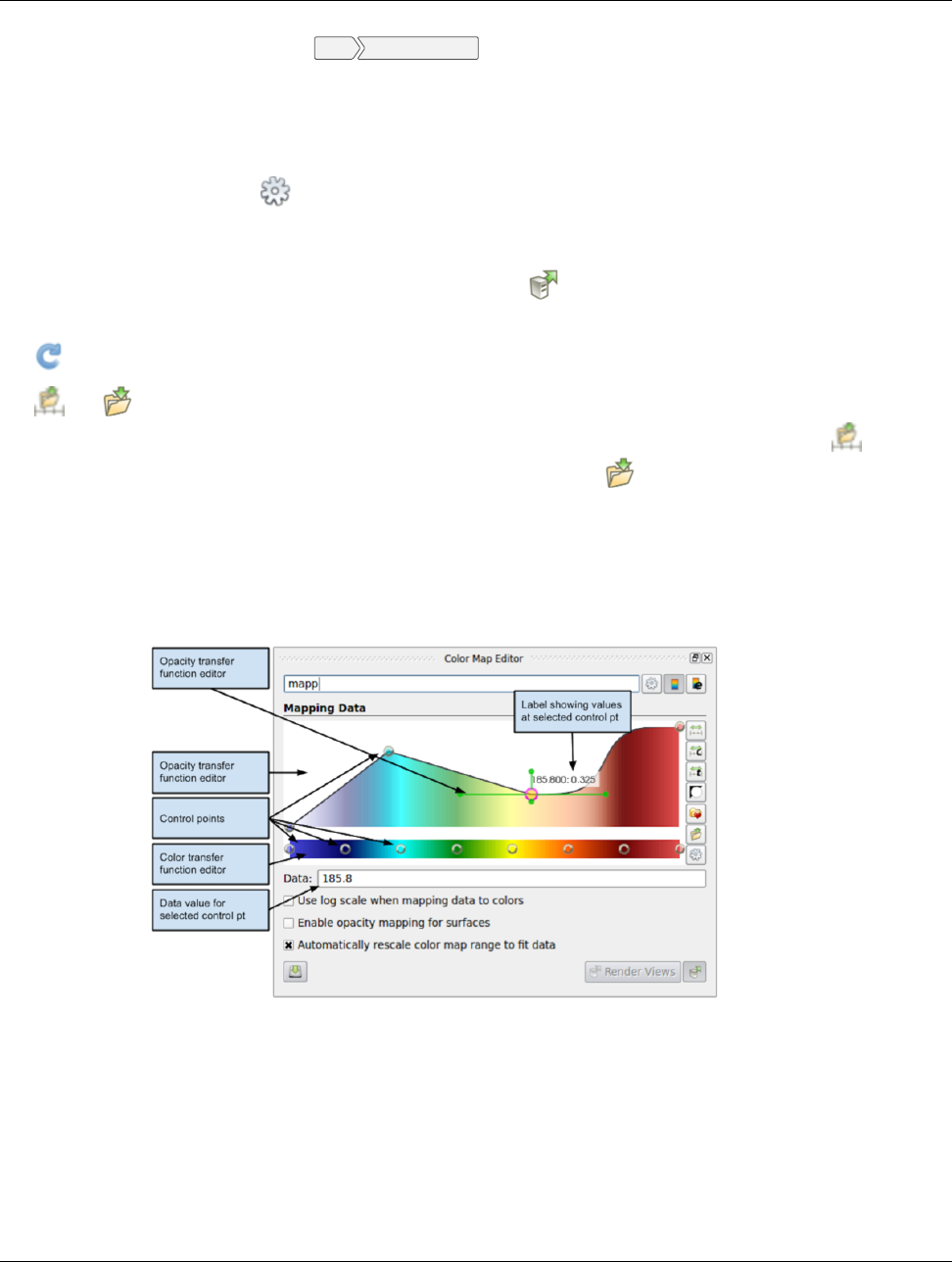
11.2. Editing the transfer functions in paraview
Color Map Editor visibility using the View Color Map Editor menu option.
As shown in Figure 11.2, the panel follows a layout similar to the Properties panel. The panel shows the properties for
the transfer function, if any, used for coloring the active data source (or filter) in the active view. If the active source if not
visible in the active view, or is not employing scalar coloring, then the panel will be empty.
Similar to the Properties panel, by default, the commonly used properties are shown. You can toggle the visibility of
advanced properties by using the button. Additionally, you can search for a particular property by typing its name in
the Search box.
Whenever the transfer function is changed, we need to re-render, which may be time consuming. By default, the panel
requests renders on every change. To avoid this, you can toggle the button. When unchecked, you will need to
manually update the panel using the Render Views button.
The button restores the application default settings for the current color map.
The and buttons save the current color and opacity transfer function, with all its properties, as the default transfer
function. ParaView will use it next time it needs to setup a transfer function to color a new data array. The button
saves the transfer function as default for an array of the same name while the button saves the transfer function as
default for all arrays. Note that this will not affect transfer functions already setup. Also this is saved across sessions, so
ParaView will remember this even after restart.
11.2.1 Mapping data
Figure 11.3: Transfer function editor and related properties
The Mapping Data group of properties controls how the data is mapped to colors or opacity. The transfer function editor
widgets are used to control the transfer function for color and opacity. The panel always shows both the transfer functions.
Whether the opacity transfer function gets used depends on several things:
•When doing surface mesh rendering, it will be used only if Enable opacity mapping for surfaces is checked
•When doing volume rendering, the opacity mapping will always be used.
148 Chapter 11. Color maps and transfer functions
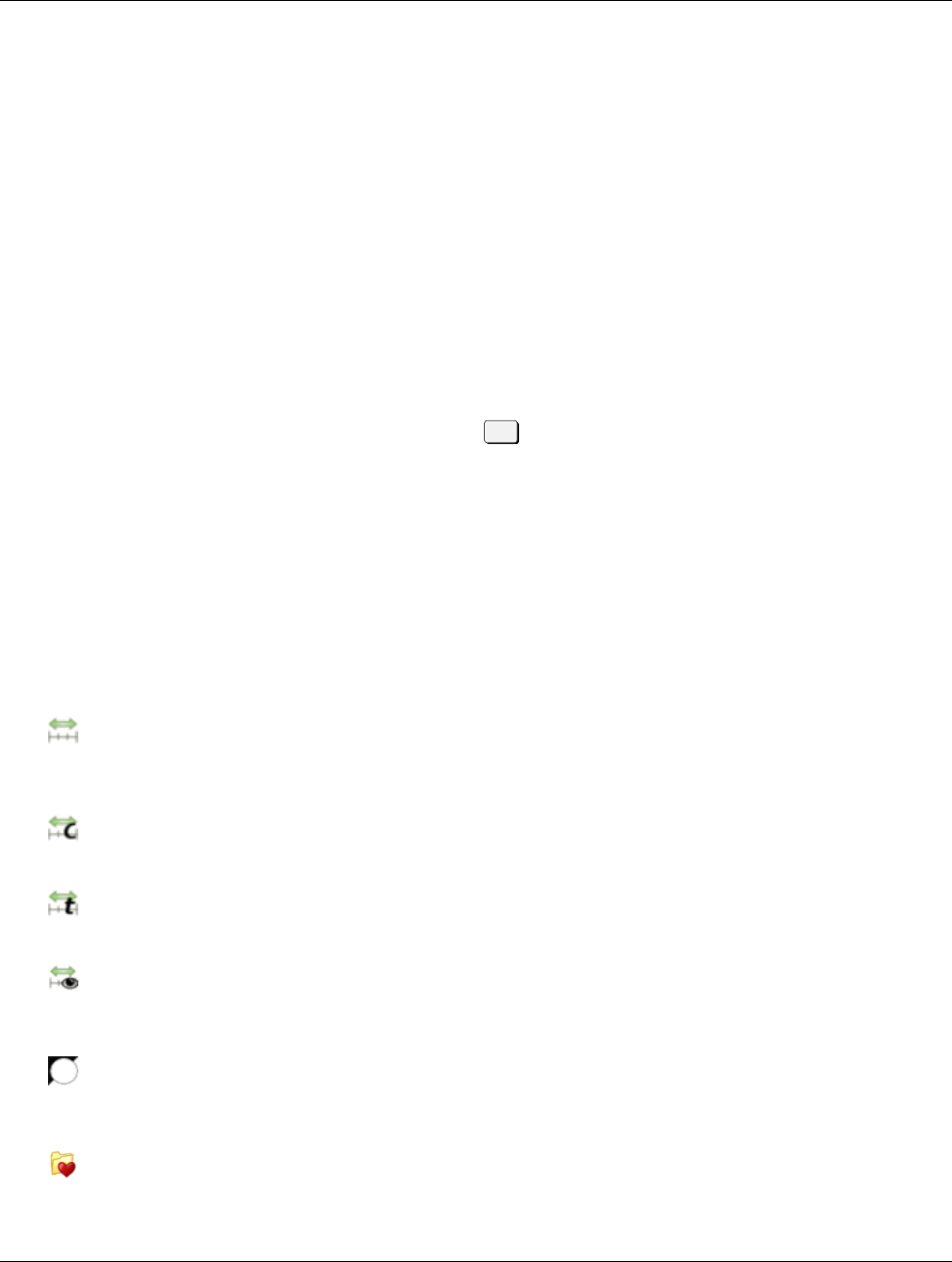
11.2. Editing the transfer functions in paraview
To map the data to color using a log scale, rather than a linear scale, check the Use log scale when mapping data to
colors. It is assumed that the data is in the non-zero, positive range. ParaView will report errors and try to automatically
fix the range if it’s ever invalid for log mapping.
Based on the user preference set in the Settings dialog, ParaView can automatically rescale the transfer function every
time when the user hits the Apply button on the Properties panel or when the time step changes. This behavior can be
disabled by unchecking the Automatically rescale transfer functions to fit data checkbox. When
unchecked, whatever scalar range you specify for the transfer function will remain unchanged.
11.2.2 Transfer function editor
Using the transfer function editors is pretty straight forward. Control points in the opacity editor widget and the color
editor widget are independent of each other. To select a control point, click on it. When selected, the control point is
highlighted with a red circle and data value associated with the control point is shown in the Data input box under the
widget. Clicking in an empty area will add a control point at that location. To move a control point, click on the control
point and drag it. You can fine tune the data value associated with the selected control point using the Data input box. To
delete a control point, select the control point and then hit the Del. key. Note that the mouse pointer should be within the
transfer function widget for Qt to send the event to the editor widget correctly. While the end control points cannot be
moved or deleted, you can rescale the entire transfer function to move the control points, as is explained later.
In the opacity transfer function widget, you can move the control points vertically to control the opacity value associated
with that control point. In the color transfer function widget, you can double click on the control point to pop up a color
chooser widget to set the color associated with that control point.
The opacity transfer function widget also offers some control over the interpolation between the control points. Double
click on a control point to show the interpolation control widget, which allows for changing the sharpness and midpoint
that affect the interpolation. Click and drag the control points to see the change in interpolation.
The several control buttons on the right side of the transfer function widgets support the following actions:
•: Rescales the color and opacity transfer functions using the data range from the data source selected in the
Pipeline browser, i.e., the active source. This rescales the entire transfer function. Thus, all control points including
the intermediate ones are proportionally adjusted to fit the new range.
•: Rescales the color and opacity transfer functions using a range provided by the user. A dialog will be popped
up for the user to enter the custom range.
•: Rescales the color and opacity transfer functions to the range of values for data over all timesteps. This
operation may be costly as data for all timesteps needs to be read.
•: Rescales the color and opacity transfer functions using the range of values for the elements (cells or points)
visible in the view. This operations assigns the entire range of colors to visible elements which may reveal patterns
not visible otherwise.
•: Inverts the color transfer function by moving the control points, e.g,. a red-to-green transfer function will be
inverted to a green-to-red one. This only affects the color transfer function and leaves the opacity transfer function
untouched.
•: Loads the color transfer function from a preset. Color present manager dialog pops up to allow the user to load
presets from file, if needed. Currently, this only supports the color transfer function. In the future, however, it will
be extended to support the opacity transfer function as well.
Chapter 11. Color maps and transfer functions 149
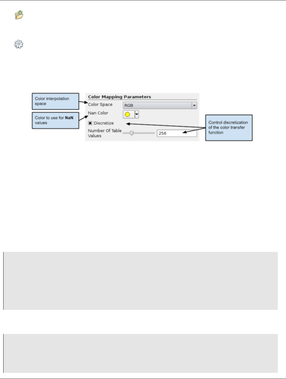
11.3. Editing the transfer functions in pvpython
•: Saves the current color transfer function to presets. Color present manager dialog pops up to allow the user to
export the transfer function to a file, if needed. Currently, this only supports the color transfer function. In the
future, however, it will be extended to support the opacity transfer function as well.
•: This toggles the detailed view for the transfer function control points. This is useful to manually enter values
for the control points rather than using the UI.
11.2.3 Color mapping parameters
Figure 11.4: Color Mapping Parameters (showing advanced properties as well)
The Color Mapping Parameters group of properties provides additional control over the color transfer function,
including control over the color interpolation space: RGB, HSV, Lab, or diverging. When color mapping floating point
arrays with NaNs, you can select the color to use for NaN values. You can also affect whether the color transfer function
uses smooth interpolation or a discretization of the same into a fixed number of bins.
11.3 Editing the transfer functions in pvpython
In pvpython, you control the transfer functions by getting access to the transfer function objects and then changing
properties on those. The following script shows how you can access transfer functions objects.
1from paraview.simple import *
2
3# You can access the color and opacity transfer functions
4# for a particular array as follows. These functions will
5# create new transfer functions if none exist.
6# The argument is the array name used to locate the transfer
7# functions.
8>>> colorMap = GetColorTransferFunction(’Temp’)
9>>> opacityMap = GetOpacityTransferFunction(’Temp’)
Once you have access to the color and opacity transfer functions, you can change properties on these similar to other
sources, views, etc. Using the Python tracing capabilities to discover this API is highly recommended.
1# Rescale transfer functions to a specific range
2>>> colorMap.RescaleTransferFunction(1.0, 19.9495)
3>>> opacityMap.RescaleTransferFunction(1.0, 19.9495)
4
5# Invert the color map.
6>>> colorMap.InvertTransferFunction()
150 Chapter 11. Color maps and transfer functions

11.4. Color legend
7
8# Map color map to log-scale preserving relative positions for
9# control points
10 >>> colorMap.MapControlPointsToLogSpace()
11 >>> colorMap.UseLogScale = 1
12
13 # Return back to linear space.
14 >>> colorMap.MapControlPointsToLinearSpace()
15 >>> colorMap.UseLogScale = 0
16
17 # Change using of opacity mapping for surfaces
18 >>> colorMap.EnableOpacityMapping = 1
19
20 # Explicitly specify color map control points
21 # The value is a flattened list of tuples
22 # (data-value, red, green, blue). The color components
23 # must be in the range [0.0, 1.0]
24 >>> colorMap.RGBPoints = [1.0, 0.705, 0.015, 0.149,
25 5.0, 0.865 , 0.865, 0.865,
26 10.0, 0.627 , 0.749 , 1.0,
27 19.9495, 0.231373 , 0.298039 , 0.752941]
28
29 # Similarly, for opacity map. The value here is
30 # a flattened list of (data-value, opacity, mid-point, sharpness)
31 >>> opacity.Points = [1.0, 0.0, 0.5, 0.0,
32 9.0, 0.404, 0.5, 0.0,
33 19.9495, 1.0, 0.5, 0.0]
34
35 # Note, in both these cases the controls points are assumed to be sorted
36 # based on the data values. Also, not setting the first and last
37 # control point to have same data value can have unexpected artifacts
38 # in the ’Color Map Editor’ panel.
Oftentimes, you want to rescale the color and opacity maps to fit the current data ranges. You can do this as follows:
1>>> source = GetActiveSource()
2
3# Update the pipeline, if hasn’t been updated already.
4>>> source.UpdatePipeline()
5
6# First, locate the display properties for the source of interest.
7>>> display = GetDisplayProperties()
8
9# Reset the color and opacity maps currently used by ’display’ to
10 # using the range for the array ’display’ is set to color with.
11 # This requires that the ’display’ has been set to use scalar coloring
12 # using an array that is available in the data generated. If not, you will
13 # get errors.
14 >>> display.RescaleTransferFunctionToDataRange()
11.4 Color legend
The color legend, also known as scalar bar or color bar, is designed to provide the user information about which color
corresponds to what data value in the rendered view. You can toggle the visibility of the color legend corresponding to the
Chapter 11. Color maps and transfer functions 151
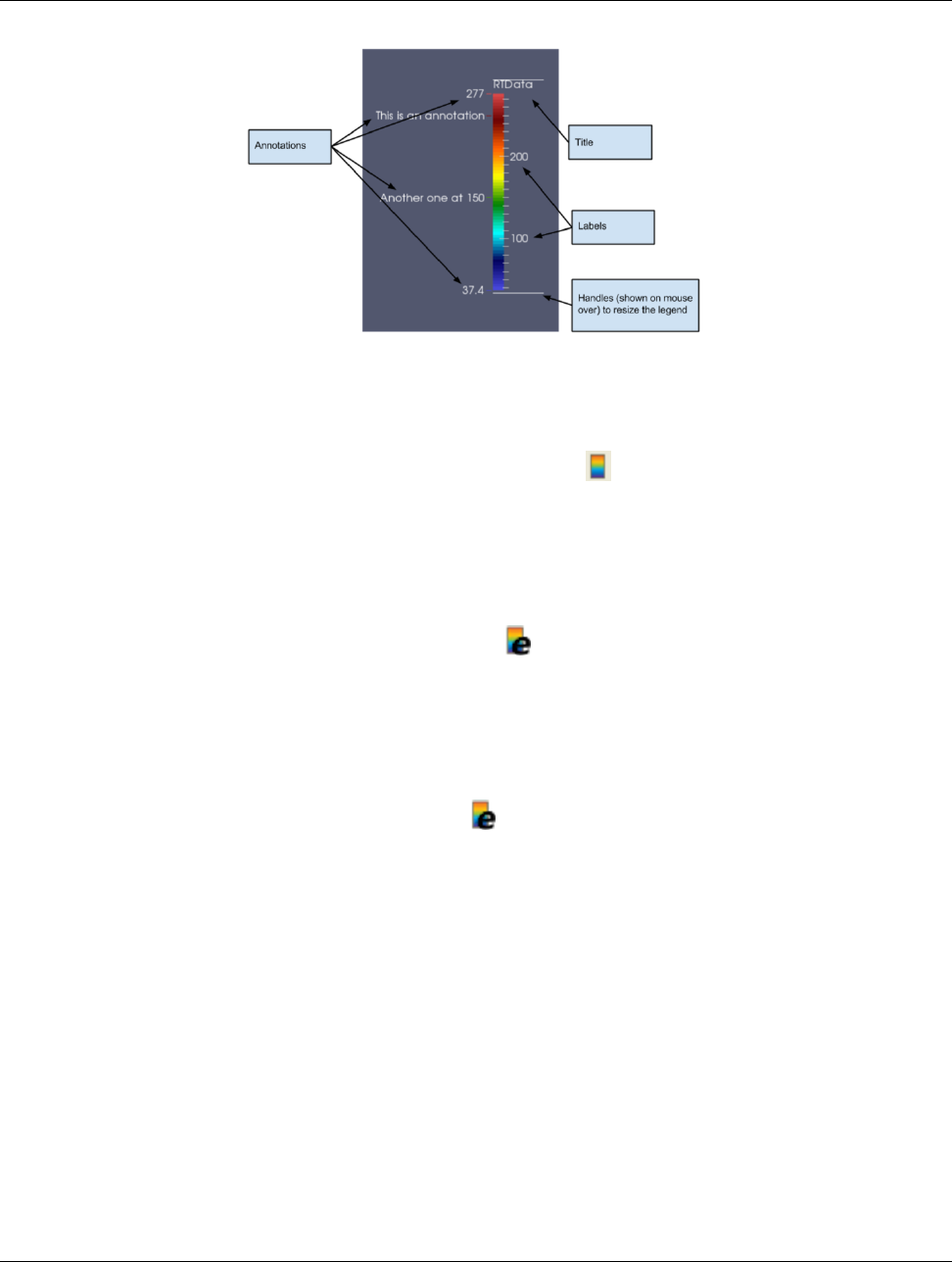
11.4. Color legend
Figure 11.5: Color legend in ParaView.
transfer function being shown/edit in the Color Map Editor by using the button near the top of the panel. This
button affects the visibility of the legend in the active view.
Figure 11.4 shows the various components of the color legend. By default, the title is typically the name of the array (and
component number or magnitude for non-scalar data arrays) being mapped. On one side are the automatically generated
labels, while on the other side are the annotations, including the start and end annotations, which correspond to the data
range being mapped.
You can control the characteristics of the color legend using the button. The color legend is interactive. You can click
and drag the legend to place it interactively at any position in the view. Additionally, you can change the length of the
legend by dragging the end-markers shown when you hover the mouse pointer over the legend.
11.4.1 Color legend parameters
You can edit the color legend parameters by clicking on the button on the Color Map Editor panel. This will pop up
a dialog that shows the available parameters. Any changes made only affect the particular color legend in the active view.
Besides the obvious changing of title text and font properties for the title, labels, and annotations, some of the other
parameters that the user can change are as follows: Draw Annotations controls whether the annotations (including the
start and end annotations) are to be drawn at all.
When checked, Draw NaN Annotations results in the color legend showing the NaN color setup in the Color Map
Editor panel in a separate box right beside the color legend. The annotation text shown for that box can be modified by
changing the NaN Annotation text.
If Automatic Label Format is checked, ParaView will try to pick an optimal representation for numerical values based
on the value and available screen space. By unchecking it, you can explicitly specify the printf-style format to use for
numeric values. Number of Labels is a suggestion for maximum number of labels to show on the legend. Note that this is
a suggestion and may not exactly match the number of labels shown. To explicitly label values of interest, use the
annotations discussed later in this post. Aspect Ratio is used to control the thickness of the legend: The greater the
number, the thinner the legend.
152 Chapter 11. Color maps and transfer functions
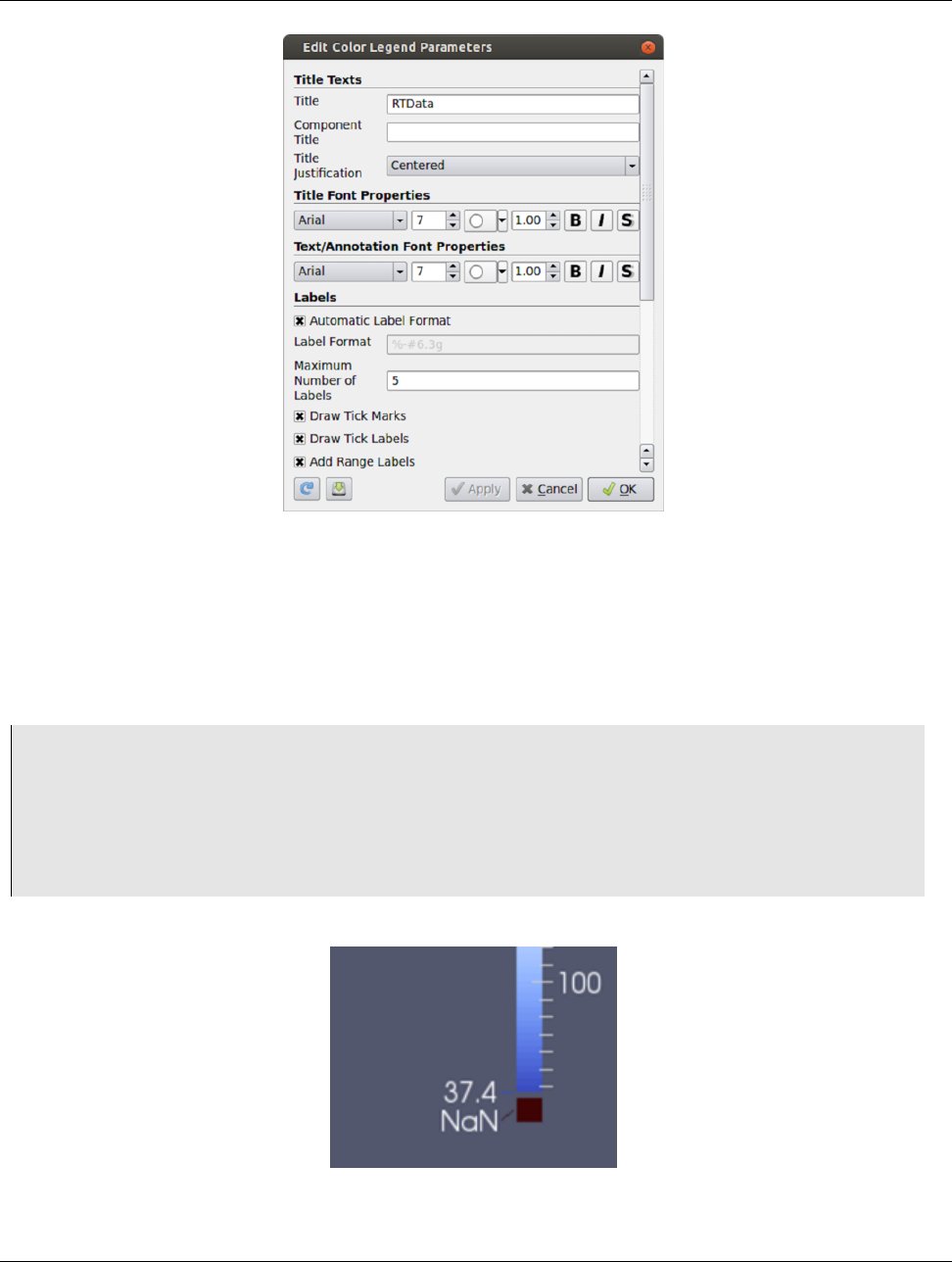
11.4. Color legend
Figure 11.6: Edit Color Legend Parameters dialog in paraview.
11.4.2 Color legend in pvpython
To show the color legend or scalar bar for the transfer function used for scalar mapping a source in a view, you can use
API on its display properties:
1>>> source = ...
2>>> display = GetDisplayProperties(source , view)
3
4# to show the color legend
5>>> display.SetScalarBarVisibility(view, True)
6
7# to hide the same
8>>> display.SetScalarBarVisibility(view, False)
Figure 11.7: Color legend showing NaN annotation
Chapter 11. Color maps and transfer functions 153
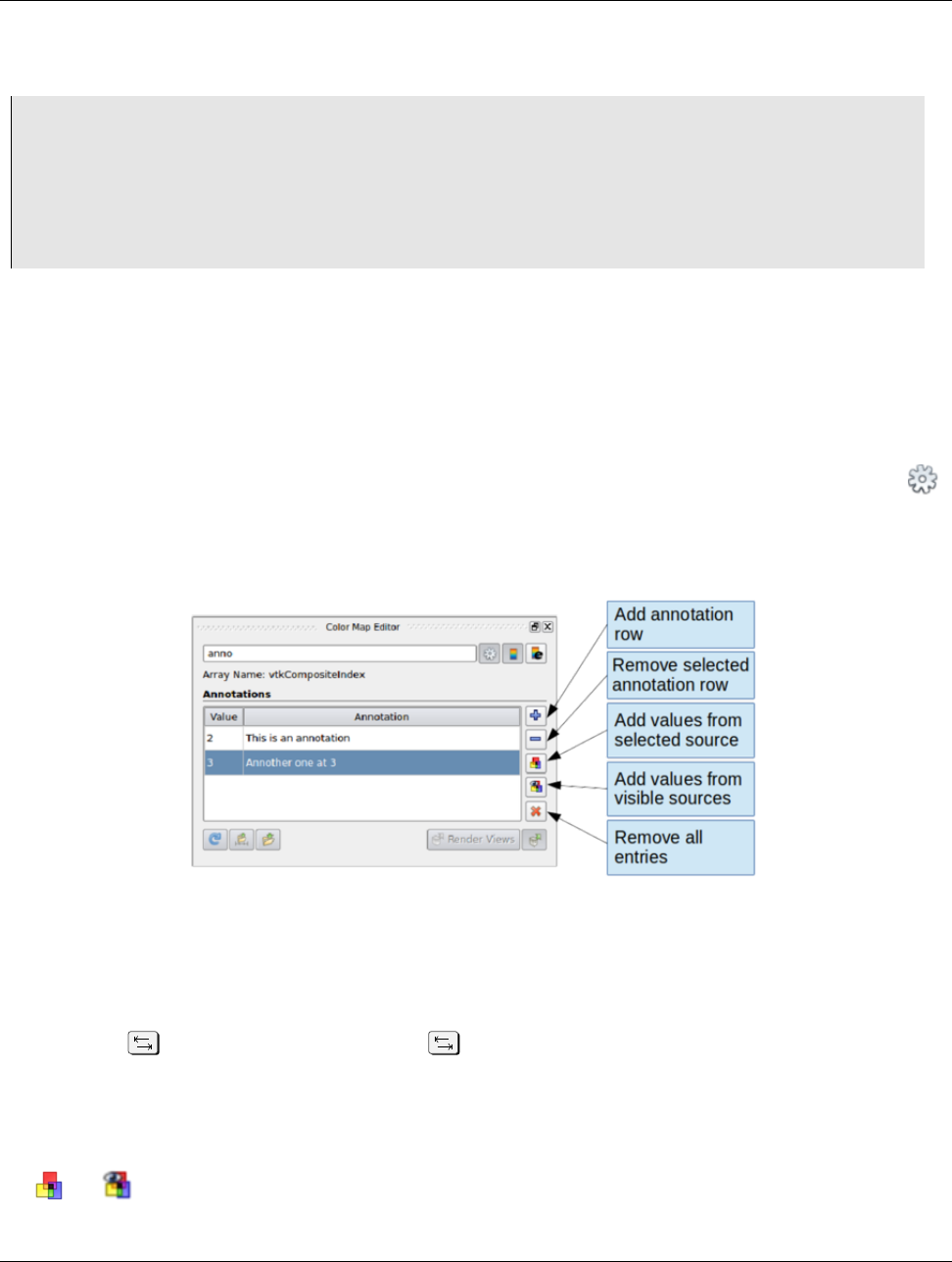
11.5. Annotations
To change the color legend properties as in Section 11.4.1, you need to first get access to the color legend object for the
color transfer function in a particular view. These are analogous to display properties for a source in a view.
1>>> colorMap = GetColorTransferFunction(’Temp’)
2
3# get the scalar bar in a view (akin to GetDisplayProperties)
4>>> scalarBar = GetScalarBar(colorMap , view)
5
6# Now, you can change properties on the scalar bar object.
7>>> scalarBar.TitleFontSize = 8
8>>> scalarBar.DrawNanAnnotation = 1
11.5 Annotations
Simply put, annotations allow users to put custom text at particular data values in the color legend. The min and max data
mapped value annotations are automatically added. To add any other custom annotations, you can use the Color Map
Editor.
Since annotations is an advanced parameter, you have to either toggle the visibility of advanced properties using the
icon near the top of the panel or simply search for annotations in the search box. That will show the Annotations
widget, which is basically a list widget where users can enter key-value pairs, rather than value-annotation pairs, as shown
in Figure 11.5.
Figure 11.8: Widget to add/edit annotations on the Color Map Editor panel
You can use the buttons of the right on the widget to add/remove entries. Enter the data value to annotate under the Value
column and then enter the text to use under the Annotation column.
You can use the key to edit the next entry. Hitting after editing the last entry in the table will automatically result
in adding a new row, thus, making it easier to add bunch of annotations without having to click any buttons.
There are two reasons in which annotation texts may not show up on the legend: First, the value added is outside the
mapped range of the color transfer function; second, Draw Annotations is unchecked in the Color Legend
Parameters dialog.
The and buttons can be used to fill the annotations widget with unique discrete values from a data array, if
possible. Based on the number of distinct values present in the data array, this may not yield any result (Instead, a warning
154 Chapter 11. Color maps and transfer functions
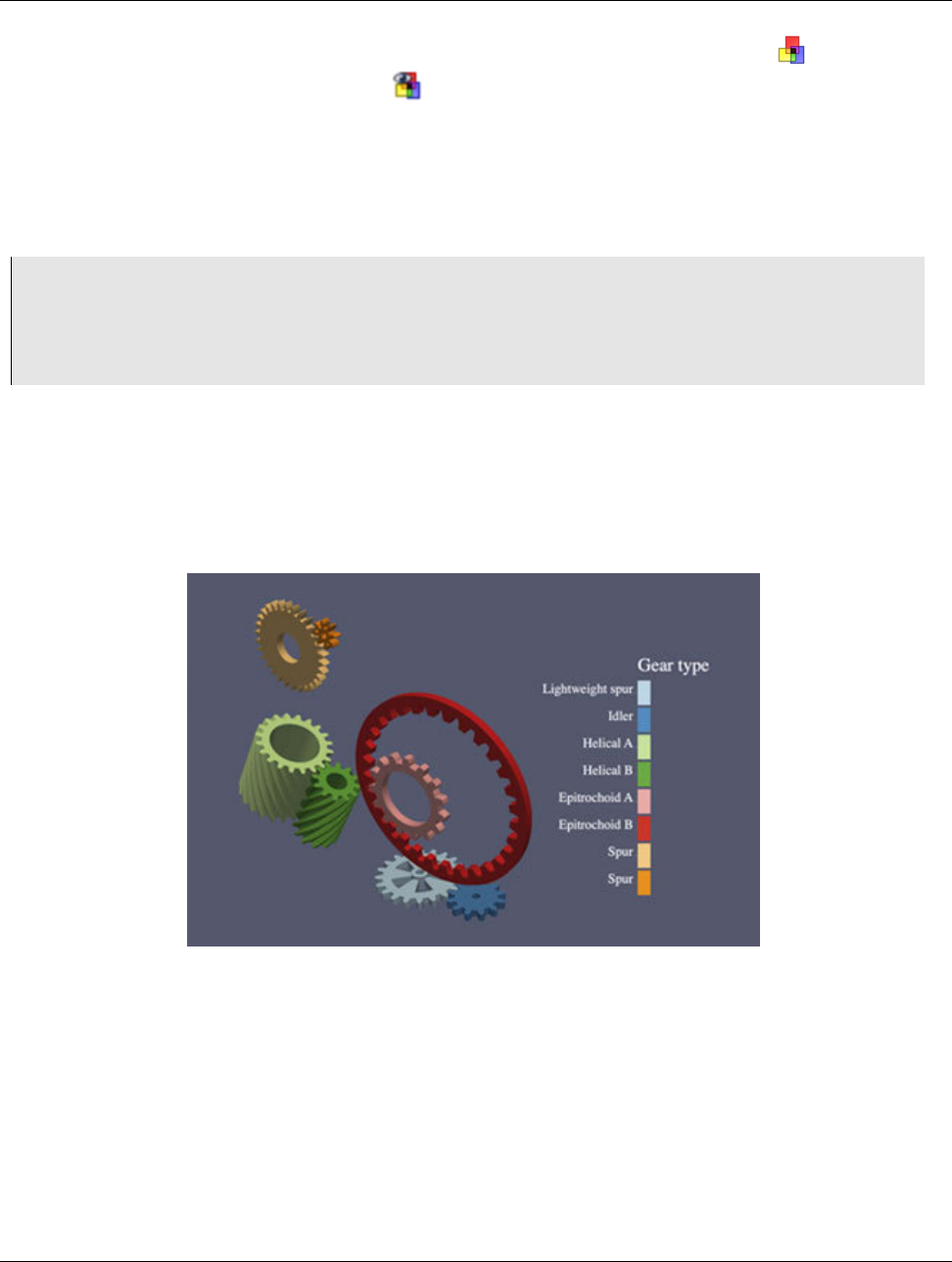
11.6. Categorical colors
message will be shown). The data array comes either from the selected source object if you use the button or it comes
from one of visible pipeline objects if you use the button.
11.5.1 Annotations in pvpython
Annotations is a property on the color map object. You simply get access to the color map of interest and then change the
Annotations property.
1>>> colorMap = GetColorTransferFunction(’Temp’)
2
3# Annotations are specified as a flattened list of tuples
4# (data-value, annotation-text)
5>>> colorMap.Annotations = [’ 1 ’,’Slow’,
6’10’,’Fast’]
11.6 Categorical colors
A picture is worth a thousand words, they say, so let’s just let the picture do the talking. Categorical color maps allow you
to render visualizations as shown in Figure 11.6.
Figure 11.9: Visualization using a categorical color map for discrete coloring
When one thinks of scalar coloring, one is typically talking of mapping numerical values to colors. However, in some
cases, the numerical values are not really numbers, but enumerations such as elements types and gear types (as in
Figure 11.6) or generally, speaking, categories. The traditional approach of using an interpolated color map specifying the
range of values with which to color doesn’t really work here. While users could always play tricks with the number of
discrete steps, multiple control points, and annotations, it is tedious and cumbersome.
Categorical color maps provide an elegant solution for such cases. Instead of a continuous color transfer function, the user
specifies a set of discrete values and colors to use for those values. For any element where the data value matches the
values in the lookup table exactly, ParaView renders the specified color; otherwise, the NaN color is used.
Chapter 11. Color maps and transfer functions 155
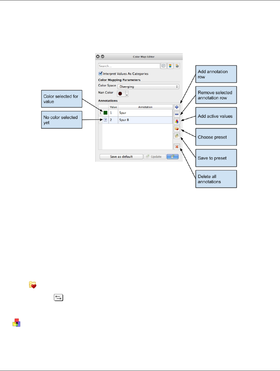
11.6. Categorical colors
The color legend or scalar bar also switches to a new mode where it renders swatches with annotations, rather than a
single bar. You can add custom annotations for each value in the lookup table.
Categorical Color: User Interface
Figure 11.10: Default Color Map Editor when Interpret Values As Categories is checked
To tell ParaView that the data array is to be treated as categories for coloring, check the Interpret Values As
Categories checkbox in the Color Map Editor panel. As soon as that’s checked, the panel switches to categorical
mode: The Mapping Data group is hidden, and the Annotations group becomes a non-advanced group, i.e., the
annotations widget is visible even if the panel is not showing advanced properties, as is shown in Figure 11.6.
The annotations widget will still show any annotations that may have been added earlier, or it may be empty if none were
added. You can add annotations for data values as was the case before using the buttons on the side of the widget. This
time, however, each annotation entry also has a column for color. If color has not been specified, a question mark icon
will show up; otherwise, a color swatch will be shown. You can double click the color swatch or the question mark icon to
specify the color to use for that entry. Alternatively, you can choose from a preset collection of categorical color maps by
clicking the button.
As before, you can use key to edit and add multiple values. Hence, you can first add all the values of interest in one
pass and then pick a preset color map to set colors for the values added. If the preset has fewer colors than the annotated
values, then the user may have to manually set the colors for those extra annotations.
Also plays the same role as described in the previous post: Fill the annotations widget with unique discrete values
from the data array, is possible. Based on the number of distinct values present in the data array, this may not yield any
result (instead, a warning message will be shown.)
156 Chapter 11. Color maps and transfer functions
11.6. Categorical colors
Common Errors
Categorical color maps are designed for data arrays with enumerations, which are typically integer arrays. How-
ever, they can be used for arrays with floating point numbers as well. With floating point numbers, the value specified
for annotation may not match the value in the dataset exactly, even when the user expects it to match. In that case,
the NaN color will be used. In the future, we may add a mechanism to specify a delta to use to when comparing data
values to annotated values.
Categorical colors in pvpython
1>>> categoricalColorMap = GetColorTransferFunction(’Modes’)
2>>> categoricalColorMap.InterpretValuesAsCategories = 1
3
4# specify the labels for the categories. This is similar to how
5# other annotations are specified.
6>>> categoricalColorMap.Annotations = [’ 0 ’ ,’Alpha’,’ 1 ’,’Beta’]
7
8# now, set the colors for each category. These are an ordered list
9# of flattened tuples (red, green, blue). The first color gets used for
10 # the first annotation, second for second, and so on
11 >>> categoricalColorMap.IndexedColors = [0.0, 0.0, 0.0,
12 0.89, 0.10, 0.10]
Chapter 11. Color maps and transfer functions 157

CHAPTER
TWELVE
COMPARATIVE VISUALIZATION
Comparative visualization in ParaView refers to the ability to create side-by-side visualizations for comparing with one
another. In its most basic form, you can indeed use ParaView’s ability to show multiple views side by side to set up
simultaneous visualizations. But, that can get cumbersome too quickly. Let’s take a look at a simple example: Let’s say
you want to do a parameter study where you want to compare isosurfaces generated by a set of isovalues in a dataset. To
set such a visualization up, you’ll need to first create as many Render Views as isovalues. Then, create just as many
Contour filters, setting each one up with a right isovalue for the contour to generate and display the result in one of the
views. As the number of isovalues increases, you can see how this can get tedious. It is highly error prone, as you need to
keep track of which view shows which isovalue. Now, imagine after having set up the entire visualization that you need to
change the Representation type for all the of the isosurfaces to Wireframe!
Comparative Views were designed to handle such use-cases. Instead of creating separate views, you create a single view
Render View (Comparative). The view itself comprises of a configurable m⇥nRender Views. Any data that you
show in this view gets shown in all the internal views simultaneously. Any display property changes, such as scalar
coloring and representation type are also maintained consistently between these internal views. The interactions in the
internal views are linked, so when you interact with one, all other views update as well. While this is all nice and well,
where the real power of Comparative Views becomes apparent is when you set up a parameter to vary across the views.
This parameter can be any of the properties on the pipeline modules such as filter properties and opacity, or it could be the
data time. Each of these internal views will now render the result obtained by setting the parameter as per your selection.
Going back to our original example, we will create a single Contour filter that we show in Render View
(Comparative) with as many internal views as the isovalue to compare. Next, we will set up a parameter study for
varying the Isosurfaces property on the Contour filter, and, viola! The view will generate the comparative visualization
for us!
In this chapter, we look at how to configure this view and how to set these parameters to compare. We limit our discussion
to Render View (Comparative). However, the same principles are applicable to other comparative views, including
Bar Chart View (Comparative) and Line Chart View (Comparative).
12.1 Setting up a comparative view
To create Render View (Comparative) in paraview, split or close the active view and select Render View
(Comparative) from the new view creation widget. paraview will immediately show four Render Views laid out in a
2⇥2 grid. While you cannot resize these internal views, notice that you can still split the view frame and create other
views if needed.
The Properties panel will show properties similar to those available on the Render View under the View properties
section. If you change any of these properties, they will affect all these internal views, e.g., setting the Background color
to Gradient will make all the views show a gradient background.
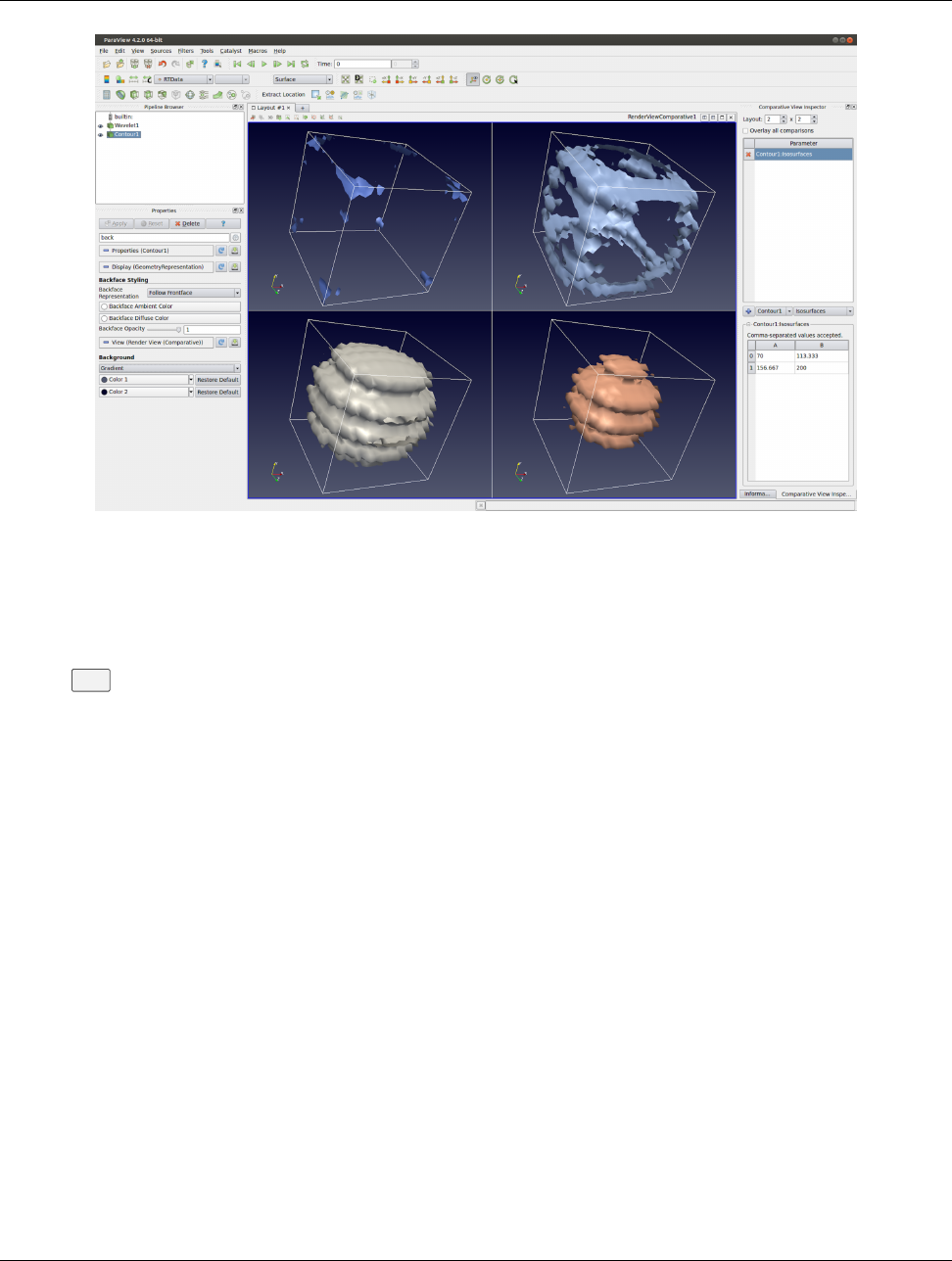
12.2. Setting up a parameter study
Figure 12.1: Render View (Comparative) in paraview showing a parameter study. In this case, we are comparing the
visualization generated using different isovalues for the Contour filter. The Comparative View Inspector dockpanel
(on the right) is used to configure the parameter study.
To configure the comparative view itself, you must to use the Comparative View Inspector (Figure 12.2) accessible
from the View menu. The Comparative View Inspector is a dockable panel that becomes enabled when the active
view is a comparative view.
To change how many internal views are used in the active comparative view and how they are laid out, use the Layout.
The first value is the number of views in the horizontal direction and the second is the count in the vertical direction.
Besides doing a parameter study in side-by-side views, you can also show all the results in a single view. For that, simply
check the Overlay all comparisons checkbox. When checked, instead of getting a grid of m⇥nviews, you will only
see one view with all visible data displayed m⇥ntimes.
To show data in this view is the same as any other view: Make this view active and use the Pipeline Browser to toggle
the eyeball icons to show data produced by the selected pipeline module(s). Showing any dataset in this view will result in
the data being shown in all the internal views simultaneously. As is true with View properties, with Display properties,
changing Coloring,Styling, or any other properties will reflect in all internal views.
Since the cameras among the internal views are automatically linked, if you interact with one of the views, all views will
also update simultaneously when you release the mouse button.
12.2 Setting up a parameter study
To understand how to setup a parameter study, let’s go back to our original example. Our visualization pipeline is simply
Wavelet!Contour (assuming default property values), and we are showing the result from the Contour filter in the
2⇥2Render View (Comparative) with Overlay all comparisons unchecked.
Now, we want to vary the Isosurfaces property value for the visualization in each of the internal views. That’s our
160 Chapter 12. Comparative visualization
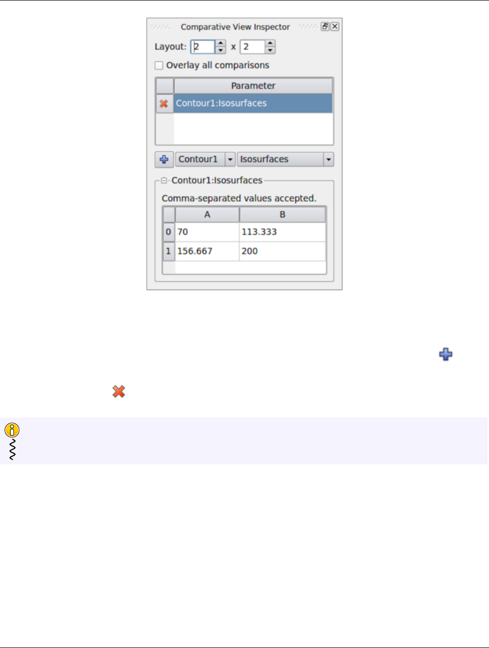
12.2. Setting up a parameter study
Figure 12.2: Comparative View Inspector in paraview used to configure the active comparative view.
parameter to study. Since that’s a property on the Contour filter, we select the Contour filter instance. Then, its property
Isosurfaces is in the parameter selection combo-boxes. To add the parameter to the study, you must hit the button.
The parameter Contour1:Isosurfaces will then show up in the Parameter list above the combo-boxes. You can delete
this parameter by using the button next to the parameter name.
Did you know?
Notice how this mechanism for setting up a parameter study is similar to how animations are set up. In fact, under
the cover, the two mechanisms are not that different, and they share a lot of implementation code.
Simultaneously, the table widget below the combo-boxes is populated with a default set of values for the Isosurfaces.
This is where you specify the parameter values for each of the views. The location of the views matches the location in
the table. Hence, 0 Ais the top-left view, 0 Bis the second view from the left in the topmost row, and so on. The
parameter value at a specific location in the table is the value used to generate the visualization in the corresponding view.
To change the parameter (in our case Isosurfaces) value, you can double click on the cell in the table and change it one
at a time. Also, to make it easier to fill the cells with a range of values, you can click and drag over multiple cells. When
you release the mouse, a dialog will prompt you to enter the data value range (Figure 12.4). In case you selected a
combination of rows and columns, the dialog will also let you select in which direction must the parameter be varied
using the range specified. You can choose to vary the parameter horizontally first, vertically first, or only along one of the
directions while keeping the other constant. This is useful when doing a study with multiple parameters.
As soon as you change the parameter values, the view will update to reflect the change.
Chapter 12. Comparative visualization 161
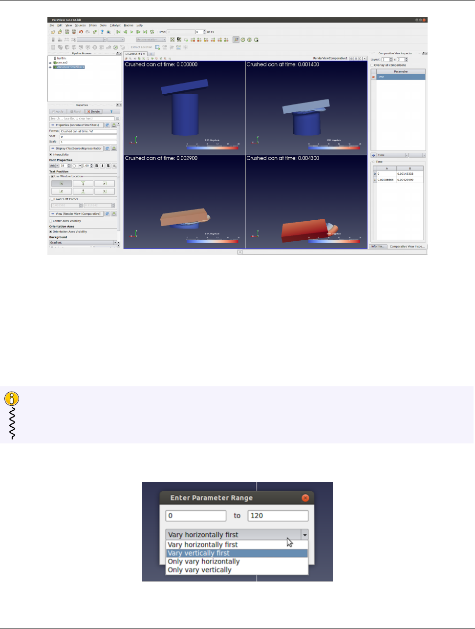
12.3. Adding annotations
Figure 12.3: Render View (Comparative) with Annotate Time filter showing the time for each of the views. In this
case, the parameter study is varying Time across the views.
12.3 Adding annotations
You add annotations like scalar bar (or color legends), text, and cube-axes exactly as you would with a regular Render
View. As with other properties, when added, these will show up in all of the internal views.
Did you know?
You can use the Annotate Time source or filter to show the data time or the view time in each of the internal
views. If Time is one of the parameters in your study, the text will reflect the time values for each of the individual
views, as expected (Figure 12.3)!
Figure 12.4: Dialog used to select a range of parameter values and control how to vary them in paraview.
162 Chapter 12. Comparative visualization
CHAPTER
THIRTEEN
PROGRAMMABLE FILTER
Any of the pipeline modules in ParaView are doing one of two things: They are either generating data or processing input
data. The generation of data can happen either using mathematical models (any of the sources created from the Sources
menu) or by reading files on disks or other media. ParaView includes several types of readers and filters, many (if not all)
of which are written using C++ by the ParaView and VTK developers and then compiled into the executables and runtime
libraries.
One of the primary focuses of ParaView since its early development is customizability. We wanted to enable developers
and users to plug in their own code to read custom file formats or to execute special algorithms for data processing. Thus,
an extensive plugin infrastructure was born, enabling developers to write C++ code that be compiled into plugins that can
be imported into the ParaView executables at runtime. While such plugins are immensely flexible, the process can be
tedious and overwhelming, since developers would need to familiarize themselves with the large C++ APIs provided by
VTK and ParaView. Hence, easier mechanisms were needed to enable ParaView end users to create such custom sources
and filters more easily. Thus, the programmable modules, which includes the Programmable Source and Programmable
Filter, were born.
With these programmable modules, you can write Python scripts that get executed by ParaView to generate and process
data, just like the other C++ modules. Since the programming environment is Python, it means that you have access to a
plethora of Python packages including NumPy and SciPy By using such packages, along with the data processing API
provided by the ParaView, you can quickly put together readers, and filters to extend and customize ParaView.
In this chapter, we will look at writing Programmable Sources and Programmable Filters using ParaView’s
Python-based data processing API through a collection of recipes and examples. A thorough discussion on the data
processing API itself is covered in Chapter 14.
Common Errors
In this guide so far, we have been looking at examples of Python scripts for pvpython. These scripts are used to script
the actions you would perform using the paraview UI. The scripts you would write for Programmable Source
and Programmable Filter are entirely different. The data processing API executes within the data processing
pipeline and, thus, has access to the data being processed. In client-server mode, this means that such scripts are
indeed executed on the server side, potentially in parallel, across several MPI ranks. Therefore, attempting to import
the paraview.simple Python module in the Programmable Source script, for example, is not supported
and will have unexpected consequences.
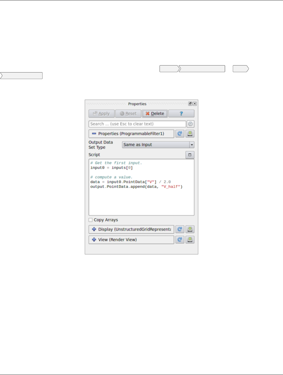
13.1. Understanding the programmable modules
13.1 Understanding the programmable modules
With programmable modules, you are writing custom code for filters and sources. You are expected to understand the
basics of a VTK (and ParaView) data processing pipeline, including the various stages of the pipeline execution as well as
the data model. Refer to Section 3.1 for an overview of the VTK data model. While a detailed discussion of the VTK
pipeline execution model is beyond the scope of this book, the fundamentals covered in this section, along with the
examples in the rest of this chapter, should give you enough to get started and write useful scripts.
To create the programmable source or filter in paraview, you use the Sources Programmable Source or Filters
Programmable Filter menus, respectively. Since the Programmable Filter is a filter, like other filters, it gets connected to
the currently active source(s), i.e., the currently active source(s) become the input to this new filter. Programmable
Source, on the other hand, does not have any inputs.
Figure 13.1: Properties panel for Programmable Filter in paraview.
One of the first things that you specify after creating any of these programmable modules is the Output Data Set Type.
This option lets you select the type of dataset this module will produce. The options provided include several of the data
types discussed in Section 3.1. Additionally, for the Programmable Filter, you can select Same as Input to indicate
that the filter preserves the input dataset type.
Next is the primary part: the Script. This is where you enter the Python script to generate or process from the inputs the
dataset that the module will produce. As with any Python script, you can import other Python packages and modules in
this script. Just be aware that when running in client-server mode, this script is going to be executed on the server side.
Accordingly, any modules or packages you import must be available on the server side to avoid errors.
This script gets executed in what’s called the RequestData pass of the pipeline execution. This is the pipeline pass in
which an algorithm is expected to produce the output dataset.
There are several other passes in a pipeline’s execution. The ones for which you can specify a Python script to execute
164 Chapter 13. Programmable Filter
13.2. Recipes for Programmable Source
with these programmable modules are:
•RequestInformation: In this pass, the algorithm is expected to provide the pipeline with any meta-data available
about the data that will be produced by it. This includes things like number of timesteps in the dataset and their time
values for temporal datasets or extents for structured datasets. This gets called before RequestData pass. In the
RequestData pass, the pipeline could potentially qualify the request based on the meta-data provided in this pass.
(E.g., if an algorithm announces that the temporal dataset has multiple timesteps, in RequestData, the pipeline
could request the algorithm in a specific timestep to produce.)
•RequestUpdateExtent: In this pass, a filter gets the opportunity to qualify requests for execution passed on to the
upstream pipeline. (E.g., if an upstream reader announced in its RequestInformation that it can produce several
timesteps, in RequestUpdateExtent, this filter can make a request to the upstream reader for a specific timestep.)
This pass gets called after RequestInformation, but before RequestData. It’s not very common to provide a script
for this pass.
You can specify the script for RequestInformation pass in RequestInformation Script and for RequestUpdateExtent
pass in RequestUpdateExtent Script. Since RequestUpdateExtent pass does not make much sense for an algorithm
that does not have any inputs, RequestUpdateExtent Script is not available on Programmable Source.
13.2 Recipes for Programmable Source
In this section, we look at several recipes for Programmable Source. A common use of Programmable Source is to
prototype readers. If your reader library already provides a Python API, then you can easily import the appropriate Python
package to read your dataset using Programmable Source.
Did you know?
Most of the examples in this chapter use a NumPy-centric API for accessing and creating data arrays. Additionally,
you can use VTK’s Python wrapped API for creating and accessing arrays. Given the omnipresence of NumPy, there
is rarely any need for using this API directly, however.
13.2.1 Reading a CSV file
For this example, we will read in a CSV file to produce a Table (Section 3.1.9) using Programmable Source. We will
use NumPy to do the parsing of the CSV files and pass the arrays read in directly to the pipeline.
Output DataSet Type must be set to vtkTable.
1# Code for ’Script’
2
3# We will use NumPy to read the csv file.
4# Refer to NumPy documentation for genfromtxt() for details on
5# customizing the CSV file parsing.
6
7import numpy as np
8# assuming data.csv is a CSV file with the 1st row being the names names for
9# the columns
10 data = np.genfromtxt("data.csv", dtype=None, names=True, delimiter=’,’, autostrip=True
)
Chapter 13. Programmable Filter 165

13.2. Recipes for Programmable Source
11 for name in data.dtype.names:
12 array = data[name]
13
14 # You can directly pass a NumPy array to the pipeline.
15 # Since ParaView expects all arrays to be named, you
16 # need to assign it a name in the ’append’ call.
17 output.RowData.append(array , name)
13.2.2 Reading a CSV file series
Building on the example from Section 13.2.1, let’s say we have a series of files that we want to read in as a temporal
series. Recall from Section 13.1 that meta-data about data to be produced, including timestep information, is announced
in RequestInformation pass. Hence, for this example, we will need to specify the RequestInformation Script as well.
As was true earlier, Output DataSet Type must be set to vtkTable. Now, to announce the timesteps, we use the
following as the RequestInformation Script.
1# Code for ’RequestInformation Script’.
2def setOutputTimesteps(algorithm , timesteps):
3"helper routine to set timestep information"
4executive = algorithm.GetExecutive()
5outInfo = executive.GetOutputInformation(0)
6
7outInfo.Remove(executive.TIME_STEPS())
8for timestep in timesteps:
9outInfo.Append(executive.TIME_STEPS(), timestep)
10
11 outInfo.Remove(executive.TIME_RANGE())
12 outInfo.Append(executive.TIME_RANGE(), timesteps [0])
13 outInfo.Append(executive.TIME_RANGE(), timesteps [-1])
14
15 # As an example, let’s say we have 4 files in the file series that we
16 # want to say are producing time 0, 10, 20, and 30.
17 setOutputTimesteps(self,(0,10,20,30))
The Script is similar to earlier, except that based on which timestep was requested, we will read a specific CSV file.
1# Code for ’Script’
2def GetUpdateTimestep(algorithm):
3"""Returns the requested time value ,or None if not present"""
4executive = algorithm.GetExecutive()
5outInfo = executive.GetOutputInformation(0)
6return outInfo.Get(executive.UPDATE_TIME_STEP()) \
7if outInfo.Has(executive.UPDATE_TIME_STEP()) else None
8
9# This is the requested time-step. This may not be exactly equal to the
10 # timesteps published in RequestInformation(). Your code must handle that
11 # correctly
12 req_time = GetUpdateTimestep(self)
13
14 # Now, use req_time to determine which CSV file to read and read it as before.
15 # Remember req_time need not match the time values put out in
16 # ’RequestInformation Script’. Your code need to pick an appropriate file to
17 # read, irrespective.
18
166 Chapter 13. Programmable Filter

13.2. Recipes for Programmable Source
19 ...
20 # TODO: Generate the data as you want.
21
22 # Now mark the timestep produced.
23 output.GetInformation().Set(output.DATA_TIME_STEP(), req_time)
13.2.3 Reading a CSV file with particles
This is similar to Section 13.2.1. Now, however, let’s say the CSV has three columns named “X”, “Y” and “Z” that we
want to treat as point coordinates and produce a vtkPolyData with points instead of a vtkTable. For that, we first ensure
that Output DataSet Type is set to vtkPolyData. Next, we use the following Script:
1# Code for ’Script’
2
3from vtk.numpy_interface import algorithms as algs
4from vtk.numpy_interface import dataset_adapter as dsa
5import numpy as np
6
7# assuming data.csv is a CSV file with the 1st row being the names names for
8# the columns
9data = np.genfromtxt(" / tmp/points.csv", dtype=None, names=True, delimiter=’,’,
autostrip=True)
10
11 # convert the 3 arrays into a single 3 component array for
12 # use as the coordinates for the points.
13 coordinates = algs.make_vector(data["X"], data["Y"], data["Z"])
14
15 # create a vtkPoints container to store all the
16 # point coordinates.
17 pts = vtk.vtkPoints()
18
19 # numpyTovtkDataArray is needed to called directly to convert the NumPy
20 # to a vtkDataArray which vtkPoints::SetData() expects.
21 pts.SetData(dsa.numpyTovtkDataArray(coordinates , "Points"))
22
23 # set the pts on the output.
24 output.SetPoints(pts)
25
26 # next, we define the cells i.e. the connectivity for this mesh.
27 # here, we are creating merely a point could, so we’ll add
28 # that as a single poly vextex cell.
29 numPts = pts.GetNumberOfPoints()
30 # ptIds is the list of point ids in this cell
31 # (which is all the points)
32 ptIds = vtk.vtkIdList()
33 ptIds.SetNumberOfIds(numPts)
34 for ain xrange(numPts):
35 ptIds.SetId(a, a)
36
37 # Allocate space for 1 cell.
38 output.Allocate(1)
39 output.InsertNextCell(vtk.VTK_POLY_VERTEX , ptIds)
40
41 # We can also pass all the array read from the CSV
Chapter 13. Programmable Filter 167
13.2. Recipes for Programmable Source
42 # as point data arrays.
43 for name in data.dtype.names:
44 array = data[name]
45 output.PointData.append(array , name)
The thing to note is that this time, we need to define the geometry and topology for the output dataset. Each data type has
different requirements on how these are specified. For example, for unstructured datasets like vtkUnstructuredGrid and
vtkPolyData, we need to explicitly specify the geometry and all the connectivity information. For vtkImageData, the
geometry is defined using origin, spacing, and extents, and connectivity is implicit.
13.2.4 Reading binary 2D image
This recipe shows how to read raw binary data representing a 3D volume. Since raw binary files don’t encode information
about the volume extents and data type, we will assume that the extents and data type are known and fixed.
For producing image volumes, you need to provide the information about the structured extents in RequestInformation.
Ensure that the Output Data Set Type is set to vtkImageData.
1# Code for ’RequestInformation Script’.
2executive = self.GetExecutive()
3outInfo = executive.GetOutputInformation(0)
4# we assume the dimensions are (48, 62, 42).
5outInfo.Set(executive.WHOLE_EXTENT (), 0, 47, 0, 61, 0, 41)
6outInfo.Set(vtk.vtkDataObject.SPACING(), 1, 1, 1)
The Script to read the data can be written as follows.
1# Code for ’Script’
2import numpy as np
3
4# read raw binary data.
5# ensure ’dtype’ is set properly.
6data = np.fromfile("HeadMRVolume.raw",dtype=np.uint8)
7
8dims = [48, 62, 42]
9assert data.shape[0] == dims[0]* dims[1]* dims[2],
10 "dimension mismatch"
11
12 output.SetExtent(0, dims[0]-1, 0, dims[1]-1, 0, dims[2]-1)
13 output.PointData.append(data, "scalars")
14 output.PointData.SetActiveScalars("scalars")
13.2.5 Helix source
Here is another polydata source example. This time, we generate the data programmatically.
1# Code for ’Script’
2
3#This script generates a helix curve.
4#This is intended as the script of a ’Programmable Source’
5import math
6import numpy as np
7from vtk.numpy_interface import algorithms as algs
8from vtk.numpy_interface import dataset_adapter as dsa
168 Chapter 13. Programmable Filter
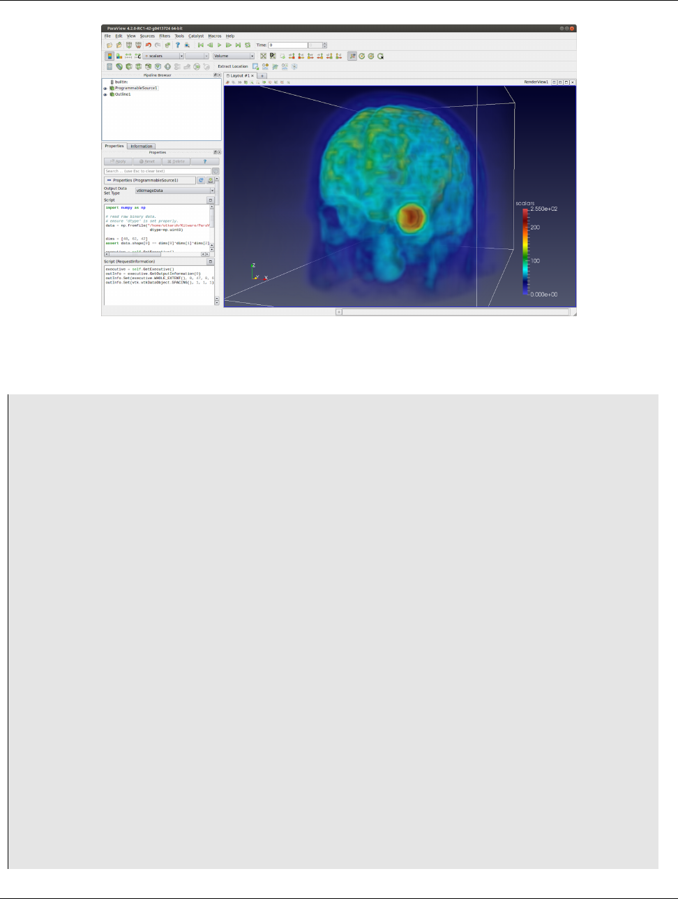
13.2. Recipes for Programmable Source
Figure 13.2: Programmable Source used to read HeadMRVolume.raw file available in the VTK data repository.
9
10 numPts = 80 # Points along Helix
11 length = 8.0 # Length of Helix
12 rounds = 3.0 # Number of times around
13
14 # Compute the point coorindates for the helix.
15 index = np.arange(0, numPts, dtype=np.int32)
16 scalars = index * rounds * 2 * math.pi / numPts
17 x=index*length/numPts;
18 y=np.sin(scalars)
19 z=np.cos(scalars)
20
21 # Create a (x,y,z) coorindates array and associate that with
22 # points to pass to the output dataset.
23 coordinates = algs.make_vector(x, y, z)
24 pts = vtk.vtkPoints()
25 pts.SetData(dsa.numpyTovtkDataArray(coordinates , ’Points’))
26 output.SetPoints(pts)
27
28 # Add scalars to the output point data.
29 output.PointData.append(index , ’Index’)
30 output.PointData.append(scalars , ’Scalars’)
31
32 # Next, we need to define the topology i.e.
33 # cell information. This helix will be a single
34 # polyline connecting all the points in order.
35 ptIds = vtk.vtkIdList()
36 ptIds.SetNumberOfIds(numPts)
37 for iin xrange(numPts):
38 #Add the points to the line. The first value indicates
39 #the order of the point on the line. The second value
Chapter 13. Programmable Filter 169
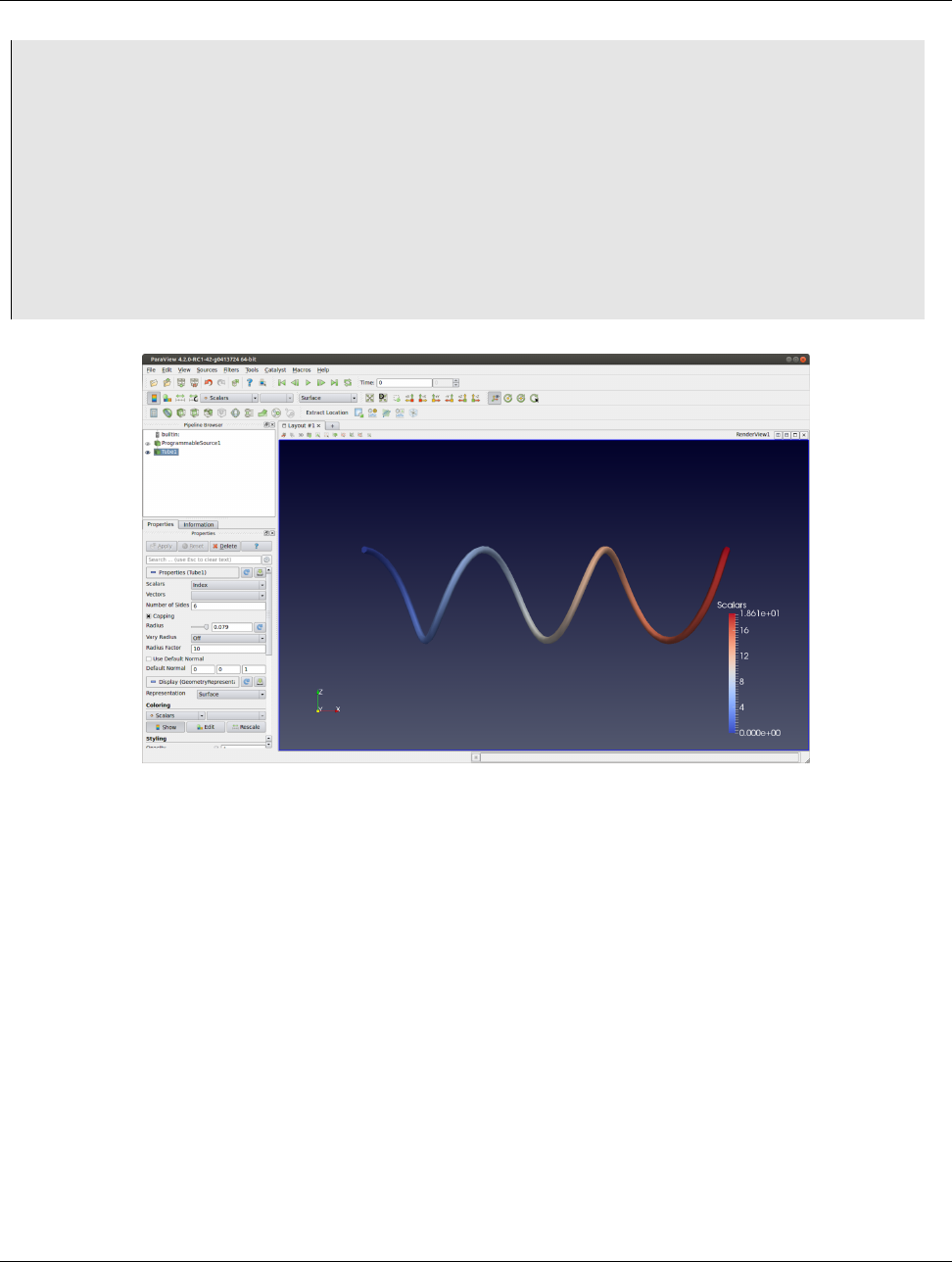
13.3. Recipes for Programmable Filter
40 #is a reference to a point in a vtkPoints object. Depends
41 #on the order that Points were added to vtkPoints object.
42 #Note that this will not be associated with actual points
43 #until it is added to a vtkPolyData object which holds a
44 #vtkPoints object.
45 ptIds.SetId(i, i)
46
47 # Allocate the number of ’cells’ that will be added. We are just
48 # adding one vtkPolyLine ’cell’ to the vtkPolyData object.
49 output.Allocate(1, 1)
50
51 # Add the poly line ’cell’ to the vtkPolyData object.
52 output.InsertNextCell(vtk.VTK_POLY_LINE , ptIds)
Figure 13.3: Programmable Source output generated using the script in Section 13.2.5. This visualization uses Tube
filter to make the output polyline more prominent.
13.3 Recipes for Programmable Filter
One of the differences between the Programmable Source and the Programmable Filter is that the latter expects at
least 1 input. Of course, the code in the Programmable Filter is free to disregard the input entirely and work exactly as
Programmable Source.Programmable Filter is designed to customize data transformations. (E.g., when you want to
compute derived quantities using expressions not directly possible with Python Calculator and Calculator or when
you want to use other Python packages or even VTK filters not exposed in ParaView for processing the inputs.)
In this section we look at various recipes for Programmable Filters.
170 Chapter 13. Programmable Filter

13.3. Recipes for Programmable Filter
13.3.1 Adding a new point/cell data array based on an input array
Python Calculator provides an easy mechanism of computing derived variables. You can also use the Programmable
Filter. Typically, for such cases, ensure that the Output DataSet Type is set to Same as Input.
1# Code for ’Script’
2
3# ’inputs’ is set to an array with data objects produced by inputs to
4# this filter.
5
6# Get the first input.
7input0 = inputs[0]
8
9# compute a value.
10 dataArray = input0.PointData["V"]/2.0
11
12 # To access cell data, you can use input0.CellData.
13
14 # ’output’ is a variable set to the output dataset.
15 output.PointData.append(dataArray , "V_half")
The thing to note about this code is that it will work as expected even when the input dataset is a composite dataset such as
a Multiblock dataset (Section 3.1.10). Refer to Chapter 14 for details on how this works. There are cases, however, when
you may want to explicitly iterate over blocks in an input multiblock dataset. For that, you can use the following snippet.
1input0 = inputs[0]
2if input0.IsA("vtkCompositeDataSet"):
3# iterate over all non-empty blocks in the input
4# composite dataset, including multiblock and AMR datasets.
5for block in input0:
6processBlock(block)
7else:
8processBlock(input0)
13.3.2 Computing tetrahedra volume
This recipe computes the volume for each tetrahedral cell in the input dataset. You can always simply use the Python
Calculator to compute cell volume using the expression volume(inputs[0]). This recipe is provided to illustrate the
API.
Ensure that the output type is set to Same as Input, and this filter assumes the input is an unstructured grid
(Section 3.1.7).
1# Code for ’Script’.
2
3import numpy as np
4
5# This filter computes the volume of the tetrahedra in an unstructured mesh.
6# Note, this is just an illustration and not the most efficient way for
7# computing cell volume. You should use ’Python Calculator’ instead.
8input0 = inputs[0]
9
10 numTets = input0.GetNumberOfCells()
11
12 volumeArray = np.empty(numTets , dtype=np.float64)
Chapter 13. Programmable Filter 171

13.3. Recipes for Programmable Filter
13 for iin xrange(numTets):
14 cell = input0.GetCell(i)
15 p1 = input0.GetPoint(cell.GetPointId (0))
16 p2 = input0.GetPoint(cell.GetPointId (1))
17 p3 = input0.GetPoint(cell.GetPointId (2))
18 p4 = input0.GetPoint(cell.GetPointId (3))
19 volumeArray[i] = vtk.vtkTetra.ComputeVolume(p1,p2,p3,p4)
20
21 output.CellData.append(volumeArray , "Volume")
13.3.3 Labeling common points between two datasets
In this example, the programmable filter to takes two input datasets: A and B. It outputs dataset B with a new scalar array
that labels the points in B that are also in A. You should select two datasets in the pipeline browser and then apply the
programmable filter.
1# Code for ’Script’
2
3# Get the two inputs
4A=inputs[0]
5B=inputs[1]
6# use len(inputs) to determine now many inputs are connected
7# to this filter.
8
9# We use numpy.in1d to test all which point coordinate components
10 # in B are present in A as well.
11 maskX = np.in1d(B.Points[:,0], A.Points [:,0])
12 maskY = np.in1d(B.Points[:,1], A.Points [:,1])
13 maskZ = np.in1d(B.Points[:,2], A.Points [:,2])
14
15 # Combining each component mask, we get the mask for point
16 # itself.
17 mask = maskX & maskY & maskZ
18
19 # Now convert it to uint8, since bool arrays
20 # cannot be passed back to the VTK pipeline.
21 mask = np. asarray (mask , dtype =np.uint8)
22
23 # Initialize the output and add the labels array
24
25 # This ShallowCopy is needed since by default the output is
26 # initialized to be a shallow copy of the first input (inputs[0]),
27 # but we want it to be a description of the second input.
28 output.ShallowCopy(B.VTKObject)
29 output.PointData.append(mask, "labels")
13.3.4 Coloring points
Let’s consider a case where you have three scalar colors (“R”, “G”, and “B”) available on the point data. Let’s say each of
these has values in the range [0,1], and we want to use these for coloring the points directly without using a color map.
Remember, to not use a color map, you uncheck Map Scalars in the Display properties section on the Properties
panel. However, the array being color with needs to be an unsigned-char array with values in the range [0,255]for each
172 Chapter 13. Programmable Filter

13.3. Recipes for Programmable Filter
component. So, we’ll need to convert the three scalar arrays into a single vector and then scale it too. This can be done as
follows:
1# Code for ’Script’
2
3from vtk.numpy_interface import algorithms as algs
4import numpy as np
5
6r=inputs[0].PointData["R"]
7g=inputs[0].PointData["G"]
8b=inputs[0].PointData["B"]
9
10 # combine components into a single array.
11 rgb = algs.make_vector(r, g, b)
12
13 # now scale and convert the type to uint8 ==> unsigned char
14 rgb = np.asarray(rgb * 255.0 , dtype=np.uint8)
15
16 # Add the array
17 output.PointData.append(rgb , "RGBColors")
As before, this will work just fine for composite datasets too, without having to iterate over the blocks in the composite
dataset explicitly.
Chapter 13. Programmable Filter 173
CHAPTER
FOURTEEN
USING NUMPY FOR PROCESSING DATA
In chapter 13, we looked at several recipes for writing Python script for data processing that relied heavily on using
NumPy for accessing arrays and performing operations on them. In this chapter, we take a closer look at the VTK-NumPy
integration layer that makes it possible to use VTK and NumPy together, despite significant differences in the data
representations between the two systems.
14.1 Teaser
Let’s start with a teaser by creating a simple pipeline with Sphere connected to an Elevation filter, followed by the
Programmable Filter. Let’s see how we would access the input data object in the Script for the Programmable
Filter.
1from vtk.numpy_interface import dataset_adapter as dsa
2from vtk.numpy_interface import algorithms as algs
3
4data = inputs[0]
5print data.PointData.keys()
6print data.PointData[’Elevation’]
This example prints out the following in the output window.
1[’Normals’,’Elevation’]
2[ 0.67235619 0.32764378 0.72819519 0.7388373 0.70217478 0.62546903
30.52391261 0.41762003 0.75839448 0.79325461 0.77003199 0.69332629
40.57832992 0.44781935 0.72819519 0.7388373 0.70217478 0.62546903
50.52391261 0.41762003 0.65528756 0.60746235 0.53835285 0.46164712
60.39253765 0.34471244 0.58238 0.47608739 0.37453097 0.29782525
70.2611627 0.27180481 0.55218065 0.42167011 0.30667371 0.22996798
80.20674542 0.24160551 0.58238 0.47608739 0.37453097 0.29782525
90.2611627 0.27180481 0.65528756 0.60746235 0.53835285 0.46164712
10 0.39253765 0.34471244]
The importance lies in the last three lines. In particular, note how we used a different API to access the PointData and
the Elevation array in the last two lines. Also note that, when we printed the Elevation array, the output didn’t look like
one from a vtkDataArray. In fact:
1elevation = data.PointData[’Elevation’]
2print type(elevation)
3
4import numpy
14.2. Understanding the dataset adapter module
5print isinstance(elevation , numpy.ndarray)
This will produce the following:
1<class ’vtk.numpy_interface.dataset_adapter.VTKArray’>
2True
So, a VTK array is a NumPy array? What kind of trickery is this, you say? What kind of magic makes the following
possible?
1data.PointData.append(elevation + 1, ’ e plus one’)
2print algs.max(elevation)
3print algs.max(data.PointData[’e plus one’])
4print data.VTKObject
The output here is:
10.5
21.5
3vtkPolyData (0x7fa20d011c60)
4...
5Point Data:
6...
7Number Of Arrays: 3
8Array 0 name = Normals
9Array 1 name = Elevation
10 Array 2 name = e plus one
It is all in the numpy interface module. It ties VTK datasets and data arrays to NumPy arrays and introduces a number of
algorithms that can work on these objects. There is quite a bit to this module, and we will introduce it piece by piece in
the rest of this chapter.
Let’s wrap up this section with one final teaser.
1print algs.gradient(data.PointData[’Elevation’])
Output:
1[[ 0.32640398 0.32640398 0.01982867]
2[ 0.32640402 0.32640402 0.01982871]
3...
4[0.41252578 0.20134845 0.2212007]
5[0.41105482 0.21514832 0.0782456]]
Please note that this example is not very easily replicated by using pure NumPy. The gradient function returns the
gradient of an unstructured grid – a concept that does not exist in NumPy. However, the ease-of-use of NumPy is there.
14.2 Understanding the dataset adapter module
In this section, let’s take a closer look at the dataset adapter module. This module was designed to simplify accessing
VTK datasets and arrays from Python and to provide a NumPy-style interface.
Let’s continue with the example from the previous section. Remember, this script is being put in the Programmable
Filter’s Script, connected to the Sphere, followed by the Elevation filter pipeline.
176 Chapter 14. Using NumPy for processing data
14.2. Understanding the dataset adapter module
1from vtk.numpy_interface import dataset_adapter as dsa
2...
3print data
4print isinstance(data, dsa.VTKObjectWrapper)
This will print:
1<vtk.numpy_interface.dataset_adapter.PolyData object at 0x1101fbb50 >
2True
We can access the underlying VTK object using the VTKObject member:
1>>> print type(data.VTKObject)
2<type ’vtkobject’>
What we get as the inputs in the Programmable Filter is actually a Python object that wraps the VTK data object itself.
The Programmable Filter does this by manually calling the WrapDataObject function from the
vtk.numpy interface.dataset adapter module on the VTK data object. Note that the WrapDataObject function
will return an appropriate wrapper class for all vtkDataSet subclasses, vtkTable, and all vtkCompositeData subclasses.
Other vtkDataObject subclasses are not currently supported.
VTKObjectWrapper forwards VTK methods to its VTKObject so the VTK API can be accessed directy as follows:
1>> print data.GetNumberOfCells()
296L
However, VTKObjectWrappers cannot be directly passed to VTK methods as an argument.
1>>> s = vtk.vtkShrinkPolyData()
2>>> s.SetInputData(data)
3TypeError: SetInputData argument 1: method requires a VTK object
4>>> s.SetInputData(data.VTKObject)
14.2.1 Dataset attributes
So far, we have a wrapper for VTK data objects that partially behaves like a VTK data object. This gets a little bit more
interesting when we start looking at how to access the fields (arrays) contained within this dataset.
For simplicity, we will embed the output generated by the script in the code itself and use the >>> prefix to differentiate
the code from the output.
1>>> data.PointData
2<vtk.numpy_interface.dataset_adapter.DataSetAttributes at 0x110f5b750 >
3
4>>> data.PointData.keys()
5[’Normals’,’Elevation’]
6
7>>> data.CellData.keys()
8[]
9
10 >>> data.PointData[’Elevation’]
11 VTKArray([ 0.5 , 0. , 0.45048442, 0.3117449 , 0.11126047,
12 0. , 0. , 0. , 0.45048442 , 0.3117449 ,
13 0.11126047, 0. , 0. , 0. , 0.45048442,
14 ...,
15 0.11126047, 0. , 0. , 0. , 0.45048442,
Chapter 14. Using NumPy for processing data 177

14.3. Working with arrays
16 0.3117449 , 0.11126047, 0. , 0. , 0. ], dtype=float32
)
17
18 >>> elevation = data.PointData[’Elevation’]
19
20 >>> elevation[:5]
21 VTKArray([0.5, 0., 0.45048442, 0.3117449, 0.11126047], dtype=float32)
22 Note that this works with composite datasets as well:
23
24 >>> mb = vtk.vtkMultiBlockDataSet()
25 >>> mb.SetNumberOfBlocks(2)
26 >>> mb.SetBlock(0, data.VTKObject)
27 >>> mb.SetBlock(1, data.VTKObject)
28 >>> mbw = dsa.WrapDataObject(mb)
29 >>> mbw.PointData
30 <vtk.numpy_interface.dataset_adapter.CompositeDataSetAttributes instance at 0
x11109f758 >
31
32 >>> mbw.PointData.keys()
33 [’Normals’,’Elevation’]
34
35 >>> mbw.PointData[’Elevation’]
36 <vtk.numpy_interface.dataset_adapter.VTKCompositeDataArray at 0x1110a32d0 >
It is possible to access PointData,CellData,FieldData,Points (subclasses of vtkPointSet only), and Polygons
(vtkPolyData only) this way. We will continue to add accessors to more types of arrays through this API.
14.3 Working with arrays
For this section, let’s change our test pipeline to consist of the Wavelet source connected to the Programmable Filter.
In the Script, we access the RTData point data array as follows:
1# Code for ’Script’
2image = output
3rtdata = image.PointData[’RTData’]
4
5# Let’s transform this data as well, using another VTK filter.
6
7tets = vtk.vtkDataSetTriangleFilter()
8tets.SetInputDataObject(image.VTKObject)
9tets.Update()
10
11 # Here, now we need to explicitly warp the output dataset to get a
12 # VTKObjectWrapper instance.
13 ugrid = dsa.WrapDataObject(tets.GetOutput())
14 rtdata2 = ugrid.PointData[’RTData’]
Here, we created two datasets: an image data (vtkImageData) and an unstructured grid (vtkUnstructuredGrid). They
essentially represent the same data but the unstructured grid is created by tetrahedralizing the image data. So, we expect
the unstructured grid to have the same points but more cells (tetrahedra).
178 Chapter 14. Using NumPy for processing data

14.3. Working with arrays
14.3.1 The array API
numpy interface array objects behave very similar to NumPy arrays. In fact, arrays from vtkDataSet subclasses are
instances of VTKArray, which is a subclass of numpy.ndarray. Arrays from vtkCompositeDataSet and subclasses are
not NumPy arrays, but they behave very similarly. We will outline the differences in a separate section. Let’s start with
the basics. All of the following work as expected.
As before, for simplicity, we will embed the output generated by the script in the code itself and use the >>> prefix to
differentiate the code from the output.
1>>> print rtdata[0]
260.763466
3
4>>> print rtdata[-1]
557.113735
6
7>>> print ‘rtdata[0:10:3]‘
8VTKArray([ 60.76346588, 95.53707886, 94.97672272, 108.49817657], dtype=float32)
9
10 >>> print ‘rtdata + 1‘
11 VTKArray([ 61.
12 76346588, 86.87795258, 73.80931091, ..., 68.51051331,
13 44.34006882, 58.1137352 ], dtype=float32)
14
15 >>> print rtdata < 70
16 VTKArray([ True ,False,False,..., True,True,True], dtype=bool)
17
18 # We will cover algorithms later. This is to generate a vector field.
19 >>> avector = algs.gradient(rtdata)
20
21 # To demonstrate that avector is really a vector
22 >>> print algs.shape(rtdata)
23 (9261,)
24
25 >>> print algs.shape(avector)
26 (9261, 3)
27
28 >>> print ‘avector[:, 0]‘
29 VTKArray([ 25.69367027, 6.59600449, 5.38400745, ..., -6.58120966,
30 -5.77147198, 13.19447994])
A few things to note in this example:
•Single component arrays always have the following shape: (ntuples,) and not (ntuples, 1)
•Multiple component arrays have the following shape: (ntuples, ncomponents)
•Tensor arrays have the following shape: (ntuples, 3, 3)
•The above holds even for images and other structured data. All arrays have one dimension (1 component arrays),
two dimensions (multi-component arrays), or three dimensions (tensor arrays).
One more cool thing: It is possible to use boolean arrays to index arrays. Thus, the following works very nicely:
1>>> print ‘rtdata[rtdata < 70]‘
2VTKArray([ 60.76346588, 66.75043488 , 69.19681549, 50.62128448,
364.8801651 , 57.72655106, 49.75050354 , 65.05570221,
457.38450241, 69.51113129 , 64.24596405, 67.54656982,
5...,
661.18143463, 66.61872864 , 55.39360428, 67.51051331,
Chapter 14. Using NumPy for processing data 179

14.3. Working with arrays
743.34006882, 57.1137352 ], dtype=float32)
8
9>>> print ‘avector[avector[:,0] > 10]‘
10 VTKArray([[ 25.69367027, 9.01253319, 7.51076698],
11 [13.1944809, 9.01253128, 7.51076508],
12 [25.98717642, -4.49800825, 7.80427408],
13 ...,
14 [12.9009738,-16.86548471, -7.80427504],
15 [25.69366837, -3.48665428, -7.51076889],
16 [13.19447994, -3.48665524, -7.51076794]])
14.3.2 Algorithms
You can do a lot simply using the array API. However, things get much more interesting when we start using the
numpy interface.algorithms module. We introduced it briefly in the previous examples. We will expand on it a bit
more here. For a full list of algorithms, use help(algs). Here are some self-explanatory examples:
1>> print ‘algs.sin(rtdata)‘
2VTKArray([-0.87873501, -0.86987603, -0.52497 , ..., -0.99943125,
3-0.59898132, 0.53547275], dtype=float32)
4
5>>> print ‘algs.min(rtdata)‘
6VTKArray(37.35310363769531)
7
8>>> print ‘algs.max(avector)‘
9VTKArray(34.781060218811035)
10
11 >>> print ‘algs.max(avector , axis=0)‘
12 VTKArray([ 34.78106022, 29.01940918, 18.34743023])
13
14 >>> print ‘algs.max(avector , axis=1)‘
15 VTKArray([ 25.69367027, 9.30603981, 9.88350773, ..., -4.35762835,
16 -3.78016186, 13.19447994])
If you haven’t used the axis argument before, it is pretty easy. When you don’t pass an axis value, the function is applied
to all values of an array without any consideration for dimensionality. When axis =0, the function will be applied to each
component of the array independently. When axis =1, the function will be applied to each tuple independently.
Experiment if this is not clear to you. Functions that work this way include sum, min, max, std, and var.
Another interesting and useful function is where the indices of an array are returned where a particular condition occurs.
1>>> print ‘algs.where(rtdata < 40)‘
2(array([ 420, 9240]),)
3# For vectors, this will also return the component index if an axis is not
4# defined.
5
6>>> print ‘algs.where(avector < -29.7)‘
7(VTKArray([4357, 4797, 4798, 4799, 5239]), VTKArray([1, 1, 1, 1, 1]))
So far, all of the functions that we discussed are directly provided by numpy. Many of the numpy ufuncs are included in
the algorithms module. They all work with single arrays and composite data arrays. Algorithms also provide some
functions that behave somewhat differently than their numpy counterparts. These include cross, dot, inverse, determinant,
eigenvalue, eigenvector, etc. All of these functions are applied to each tuple rather than to a whole array/matrix. For
example:
180 Chapter 14. Using NumPy for processing data

14.4. Handling composite datasets
1>>> amatrix = algs.gradient(avector)
2>>> print ‘algs.determinant(amatrix)‘
3VTKArray([ -1221.2732624 , -648.48272183, -3.55133937, ..., 28.2577152 ,
4-629.28507693, -1205.81370163])
Note that everything above only leveraged per-tuple information and did not rely on the mesh. One of VTK’s biggest
strengths is that its data model supports a large variety of meshes, while its algorithms work generically on all of these
mesh types. The algorithms module exposes some of this functionality. Other functions can be easily implemented by
leveraging existing VTK filters. We used gradient before to generate a vector and a matrix. Here it is again:
1>>> avector = algs.gradient(rtdata)
2>>> amatrix = algs.gradient(avector)
Functions like this require access to the dataset containing the array and the associated mesh. This is one of the reasons
why we use a subclass of ndarray in dataset adapter:
1>>> print ‘rtdata.DataSet‘
2<vtk.numpy_interface.dataset_adapter.DataSet at 0x11b61e9d0 >
Each array points to the dataset containing it. Functions such as gradient use the mesh and the array together. Numpy
provides a gradient function too, you say. What is so exciting about yours? Well, this:
1>>> print ‘algs.gradient(rtdata2)‘
2VTKArray([[ 25.46767712, 8.78654003, 7.28477383],
3[6.02292252, 8.99845123, 7.49668884],
4[5.23528767, 9.80230141, 8.3005352],
5...,
6[ -6.43249083, -4.27642155 , -8.30053616],
7[ -5.19838905, -3.47257614 , -7.49668884],
8[13.42047501, -3.26066017, -7.28477287]])
9>>> rtdata2.DataSet.GetClassName()
10 ’vtkUnstructuredGrid’
Gradient and algorithms that require access to a mesh work whether that mesh is a uniform grid, a curvilinear grid, or an
unstructured grid thanks to VTK’s data model. Take a look at various functions in the algorithms module to see all the
cool things that can be accomplished using it. In the remaining sections, we demonstrate how specific problems can be
solved using these modules.
14.4 Handling composite datasets
In this section, we take a closer look at composite datasets. For this example, our pipeline is Sphere source, and Cone
source is set as two inputs to the Programmable Filter.
We can create a multiblock dataset in the Programmable Filter’s Script as follows:
1# Let’s assume inputs[0] is the output from Sphere and
2# inputs[1] is the output from Cone.
3mb = vtk.vtkMultiBlockDataSet ()
4mb. SetBlock (0, inputs [0]. VTKObject )
5mb. SetBlock (1, inputs [1]. VTKObject )
Many of VTK’s algorithms work with composite datasets without any change. For example:
1e=vtk.vtkElevationFilter()
2e.SetInputData(mb)
Chapter 14. Using NumPy for processing data 181
14.4. Handling composite datasets
3e.Update()
4
5mbe = e.GetOutputDataObject(0)
6print mbe.GetClassName()
This will output vtkMultiBlockDataSet.
Now that we have a composite dataset with a scalar, we can use numpy interface. As before, for simplicity, we will
embed the output generated by the script in the code itself and use the >>> prefix to differentiate the code from the output.
1>>> from vtk.numpy_interface import dataset_adapter as dsa
2>>> mbw = dsa.WrapDataObject(mbe)
3>>> print ‘mbw.PointData.keys()‘
4[’Normals’,’Elevation’]
5>>> elev = mbw.PointData[’Elevation’]
6>>> print ‘elev‘
7<vtk.numpy_interface.dataset_adapter.VTKCompositeDataArray at 0x1189ee410 >
Note that the array type is different than we have previously seen (VTKArray). However, it still works the same way.
1>>> from vtk.numpy_interface import algorithms as algs
2>>> print algs.max(elev)
30.5
4>>> print algs.max(elev + 1)
51.5
You can individually access the arrays of each block as follows.
1>>> print ‘elev.Arrays[0]‘
2VTKArray([ 0.5 , 0. , 0.45048442, 0.3117449 , 0.11126047,
30. , 0. , 0. , 0.45048442 , 0.3117449 ,
40.11126047, 0. , 0. , 0. , 0.45048442,
50.3117449 , 0.11126047, 0. , 0. , 0. ,
60.45048442, 0.3117449 , 0.11126047 , 0. , 0. ,
70. , 0.45048442 , 0.3117449 , 0.11126047 , 0. ,
80. , 0. , 0.45048442 , 0.3117449 , 0.11126047 ,
90. , 0. , 0. , 0.45048442 , 0.3117449 ,
10 0.11126047, 0. , 0. , 0. , 0.45048442,
11 0.3117449 , 0.11126047, 0. , 0. , 0. ], dtype=float32
)
Note that indexing is slightly different.
1>>> print elev[0:3]
2[VTKArray([ 0.5, 0., 0.45048442], dtype=float32),
3VTKArray([ 0., 0., 0.43301269], dtype=float32)]
The return value is a composite array consisting of two VTKArrays. The [] operator simply returned the first four values
of each array. In general, all indexing operations apply to each VTKArray in the composite array collection. It is similar
for algorithms, where:
1>>> print algs.where(elev < 0.5)
2[(array ([ 1, 2, 3, 4, 5, 6, 7, 8, 9, 10, 11, 12, 13, 14, 15, 16, 17,
318, 19, 20, 21, 22, 23, 24, 25, 26, 27, 28, 29, 30, 31, 32, 33, 34,
435, 36, 37, 38, 39, 40, 41, 42, 43, 44, 45, 46, 47, 48, 49]) ,),
5(array([0, 1, 2, 3, 4, 5, 6]),)]
Now, let’s look at the other array called Normals.
182 Chapter 14. Using NumPy for processing data

14.4. Handling composite datasets
1>>> normals = mbw.PointData[’Normals’]
2>>> print ‘normals.Arrays[0]‘
3VTKArray([[ 0.00000000e+00, 0.00000000e+00, 1.00000000e+00],
4[0.00000000e+00, 0.00000000e+00, -1.00000000e+00],
5[4.33883727e-01, 0.00000000e+00, 9.00968850e-01],
6[7.81831503e-01, 0.00000000e+00, 6.23489797e-01],
7[9.74927902e-01, 0.00000000e+00, 2.22520933e-01],
8...
9[6.89378142e-01, -6.89378142e-01, 2.22520933e-01],
10 [6.89378142e-01, -6.89378142e-01, -2.22520933e-01],
11 [5.52838326e-01, -5.52838326e-01, -6.23489797e-01],
12 [3.06802124e-01, -3.06802124e-01, -9.00968850e-01]],dtype=float32)
13 >>> print ‘normals.Arrays[1]‘
14 <vtk.numpy_interface.dataset_adapter.VTKNoneArray at 0x1189e7790 >
Notice how the second array is a VTKNoneArray. This is because vtkConeSource does not produce normals. Where an
array does not exist, we use a VTKNoneArray as placeholder. This allows us to maintain a one-to-one mapping between
datasets of a composite dataset and the arrays in the VTKCompositeDataArray. It also allows us to keep algorithms
working in parallel without a lot of specialized code.
Where many of the algorithms apply independently to each array in a collection, some algorithms are global. Take min
and max, for example, as we demonstrated above. It is sometimes useful to get per-block answers. For this, you can use
per block algorithms.
1>>> print algs.max_per_block(elev)
2[VTKArray(0.5, dtype=float32), VTKArray(0.4330126941204071, dtype=float32)]
These work very nicely together with other operations. For example, here is how we can normalize the elevation values in
each block.
1>>> _min = algs.min_per_block(elev)
2>>> _max = algs.max_per_block(elev)
3>>> _norm = (elev - _min) / (_max - _min)
4>>> print algs.min(_norm)
50.0
6>>> print algs.max(_norm)
71.0
Once you grasp these features, you should be able to use composite arrays very similarly to single arrays.
A final note on composite datasets: The composite data wrapper provided by numpy interface.dataset adapter
offers a few convenience functions to traverse composite datasets. Here is a simple example:
1>>> for ds in mbw:
2>>> print type(ds)
3<class ’vtk.numpy_interface.dataset_adapter.PolyData’>
4<class ’vtk.numpy_interface.dataset_adapter.PolyData’>
Chapter 14. Using NumPy for processing data 183
CHAPTER
FIFTEEN
REMOTE AND PARALLEL VISUALIZATION
One of the goals of the ParaView application is enabling data analysis and visualization for large datasets. ParaView was
born out of the need for visualizating simulation results from simulations run on supercomputing resources that are often
too big for a single desktop machine to handle. To enable interactive visualization of such datasets, ParaView uses remote
and/or parallel data processing. The basic concept is that if a dataset cannot fit on a desktop machine due to memory or
other limitations, we can split the dataset among a cluster of machines, driven from your desktop. In this chapter, we will
look at the basics of remote and parallel data processing using ParaView. For information on setting up clusters, please
refer to the ParaView Wiki.[5]
Did you know?
Remote and parallel processing are often used together, but they refer to different concepts, and it is possible to
have one without the other.
In the case of ParaView, remote processing refers to the concept of having a client, typically paraview or pvpython,
connecting to a pvserver, which could be running on a different, remote machine. All the data processing and,
potentially, the rendering can happen on the pvserver. The client drives the visualization process by building the
visualization pipeline and viewing the generated results.
Parallel processing refers to a concept where instead of single core — which we call a rank — processing the
entire dataset, we split the dataset among multiple ranks. Typically, an instance of pvserver runs in parallel on
more than one rank. If a client is connected to a server that runs in parallel, we are using both remote and parallel
processing.
In the case of pvbatch, we have an application that operates in parallel but without a client connection. This is a
case of parallel processing without remote processing.
15.1 Understanding remote processing
Let’s consider a simple use-case. Let’s say you have two computers, one located at your office and another in your home.
The one at the office is a nicer, beefier machine with larger memory and computing capabilities than the one at home.
That being the case, you often run your simulations on the office machine, storing the resulting files on the disk attached
to your office machine. When you’re at work, to visualize those results, you simply launch paraview and open the data
file(s). Now, what if you need to do the visualization and data analysis from home? You have several options:
15.2. Remote visualization in paraview
•You can copy the data files over to your home machine and then use paraview to visualize them. This is tedious,
however, as you not only have to constantly keep copying/updating your files manually, but your machine has
poorer performance due to the decreased compute capabilities and memory available on it!
•You can use a desktop sharing system like Remote Desktop or VNC, but those can be flaky depending on your
network connection.
Alternatively, you can use ParaView’s remote processing capabilities. The concept is fairly simple. You have two separate
processes: pvserver (which runs on your work machine) and a paraview client (which runs on your home machine). They
communicate with each other over sockets (over an SHH tunnel, if needed). As far as using paraview in this mode, it’s no
different than how we have been using it so far – you create pipelines and then look at the data produced by those
pipelines in views and so on. The pipelines themselves, however, are created remotely on the pvserver process. Thus, the
pipelines have access to the disks on your work machine. The Open File dialog will in fact browse the file system on
your work machine, i.e., the machine on which pvserver is running. Any filters that you create in your visualization
pipeline execute on the pvserver.
While all the data processing happens on the pvserver, when it comes to rendering, paraview can be configured to either
do the rendering on the server process and deliver only images to the client (remote rendering) or to deliver the geometries
to be rendered to the client and let it do the rendering locally (local rendering). When remote rendering, you’ll be using
the graphics capabilities on your work machine (the machine running the pvserver). Every time a new rendering needs to
be obtained (for example, when pipeline parameters are changed or you interact with the camera, etc.), the pvserver
process will re-render a new image and deliver that to the client. When local rendering, the geometries to be rendered are
delivered to the client and the client renders those locally. Thus, not all interactions require server-side processing. Only
when the visualization pipeline is updated does the server need to deliver updated geometries to the client.
15.2 Remote visualization in paraview
15.2.1 Starting a remote server
To begin using ParaView for remote data processing and visualization, we must first start the server application pvserver
on the remote system. To do this, connect to your remote system using a shell and run:
> pvserver
You will see this startup message on the terminal:
Waiting for client...
Connection URL: cs://myhost:11111
Accepting connection(s): myhost:11111
This means that the server has started and is listening for a connection from a client.
15.2.2 Configuring a server connection
To connect to this server with the paraview client, select File Connect or click the icon in the toolbar to bring up the
Choose Server Configuration dialog.
186 Chapter 15. Remote and parallel visualization
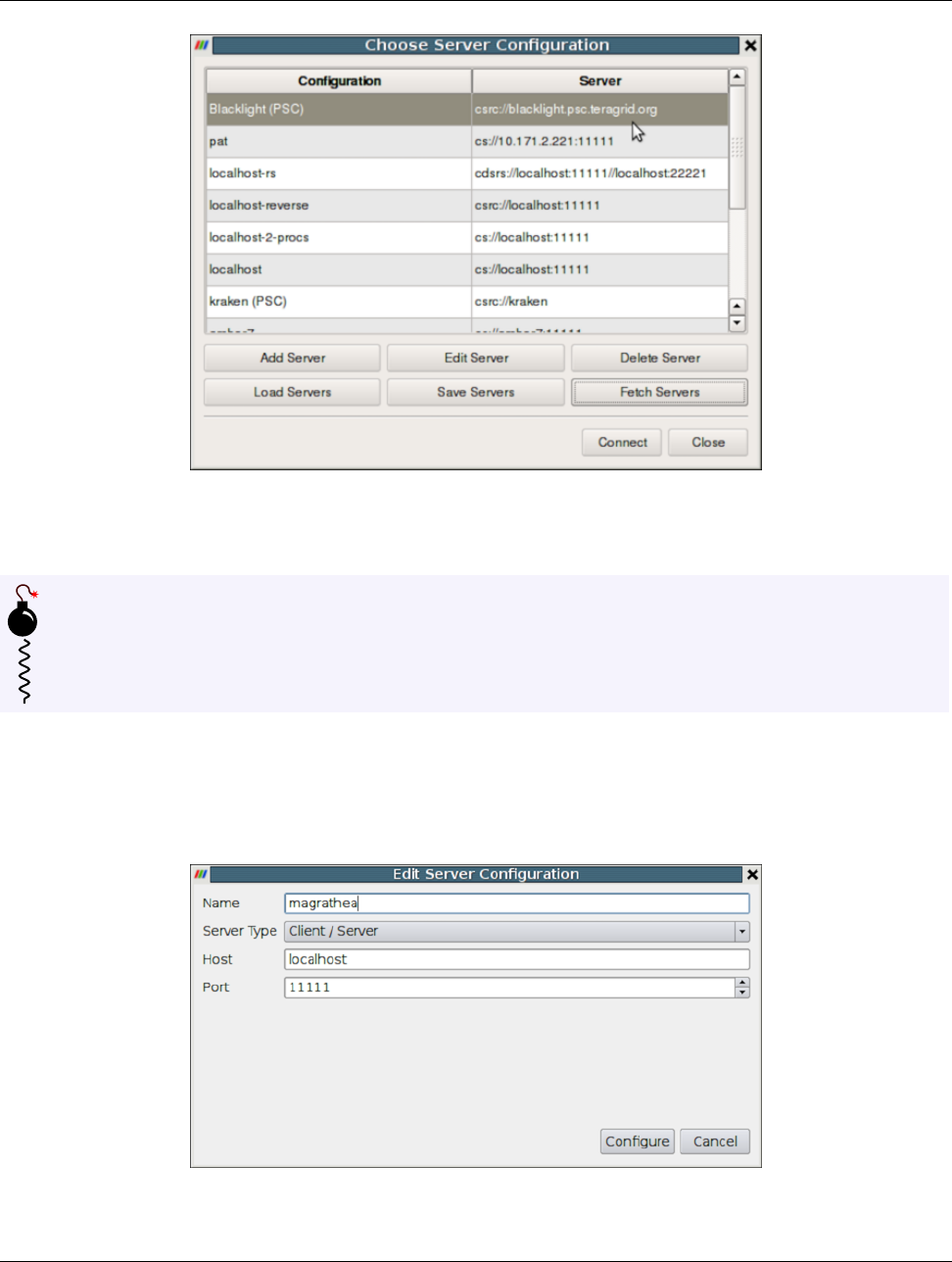
15.2. Remote visualization in paraview
Figure 15.1: The Choose Server Configuration dialog is used to connect to a server.
Common Errors
If your server is behind a firewall and you are attempting to connect to it from outside the firewall, the connection
may not be established successfully. You may also try reverse connections ( Section 15.4) as a workaround for
firewalls. Please consult your network manager if you have network connection problems.
Figure 15.1 shows the Choose Server Configuration dialog with a number of entries for remote servers. In the figure,
a number of servers have already been configured, but when you first open this dialog, this list will be empty. Before you
can connect to a remote server, you will need to add an entry to the list by clicking on the Add Server button. When you
do, you will see the Edit Server Configuration dialog as in Figure 15.2.
Figure 15.2: The Edit Server Configuration dialog is used to configure settings for connecting to remote servers.
Chapter 15. Remote and parallel visualization 187
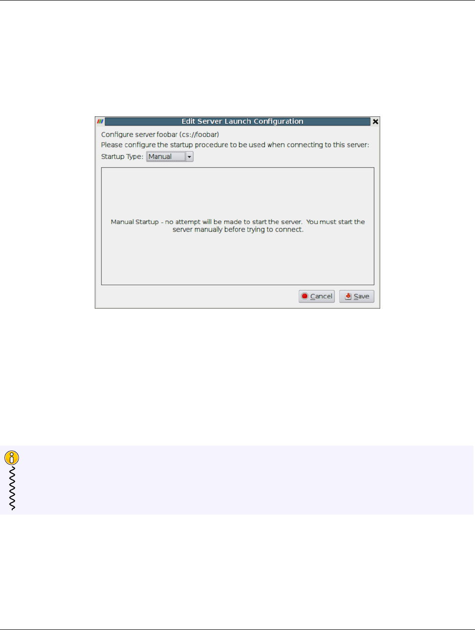
15.2. Remote visualization in paraview
You will need to set a name for the connection, the server type, the DNS name of the host on which you just started the
server, and the port. The default Server Type is set to Client / Server, which means that the server will be listening for an
incoming connection from the client. There are several other options for this setting that we will discuss later.
When you are done, click the Configure button. Another dialog, as shown in Figure 15.3, will appear where you specify
how to start the server. Since we started the server manually, we will leave the Startup Type on the default Manual
setting. You can optionally set the Startup Type to Command and specify an external shell command to launch a server
process.
Figure 15.3: Configure the server manually. It must be started outside of ParaView.
When you click the Save button, this particular server configuration will be saved for future use. You can go back and edit
the server configuration by selecting the entry in the list of servers and clicking the Edit Server button in the Choose
Server Configuration dialog. You can delete it by clicking the Delete button.
Server configurations can be imported and exported through the Choose Server Configuration dialog. Use the Load
Servers button to load a server configuration file and the Save Servers button to save a server configuration file. Files
can be exchanged with others to access the same remote servers.
Did you know?
Visualization centers can provide system-wide server configurations on web servers to allow non-experts to simply
select an already configured ParaView server. The format of the XML file for saving the server configurations is dis-
cussed online on the ParaView Wiki at http://paraview.org/Wiki/Server_Configuration. These
site-wide settings can be loaded with the Fetch Servers button.
15.2.3 Connect to the remote server
To connect to the server, select the server configuration you just set up from the configuration list and click Connect.We
are now ready to build the visualization pipelines.
188 Chapter 15. Remote and parallel visualization
15.3. Remote visualization in pvpython
Common Errors
ParaView does not perform any kind of authentication when clients attempt to connect to a server. For that reason,
we recommend that you do not run pvserver on a computing resource that is open to the outside world.
ParaView also does not encrypt data sent between the client and server. If your data is sensitive, please ensure that
proper network security measures have been taken. The typical approach is to use an SSH tunnel.
15.2.4 Setting up a client/server visualization pipeline
Using paraview when connected to a remote server is not any different than when it’s being used in the default
stand-alone mode. The only difference, as far as the user interface goes, is that the Pipeline Browser reflects the name
of the server to which you are connected. The address of the server connection next to the icon changes from
builtin: to cs://myhost:11111.
Since the data processing pipelines are executing on the server side, all file I/O also happens on the server side. Hence, the
Open File dialog, when opening a new data file, will browse the file system local to the pvserver executable and not the
paraview client.
15.3 Remote visualization in pvpython
The pvpython executable can be used by itself for visualization of local data, but it can also act as a client that connects to
a remote pvserver. Before creating a pipeline in pvpython, use the Connect function:
1# Connect to remote server "myhost" on the default port, 11111
2>>> Connect("myhost")# Connect to remote server "myhost" on a
3# specified port
4>>> Connect("myhost", 11111)
Now, when new sources are created, the data produced by the sources will reside on the server. In the case of pvpython,
all data remains on the server and images are generated on the server too. Images are sent to the client for display or for
saving to the local filesystem.
15.4 Reverse connections
It is frequently the case that remote computing resources are located behind a network firewall, making it difficult to
connect a client outside the firewall to a server behind it. ParaView provides a way to set up a reverse connection that
reverses the usual client server roles when establishing a connection.
To use a remote connection, two steps must be performed. First, in paraview, a new connection must be configured with
the connection type set to reverse. To do this, open the Choose Server Configuration dialog through the File
Connect menu item. Add a new connection, setting the Name to “myhost (reverse)”, and select Client / Server
(reverse connection) for Server Type. Click Configure. In the Edit Server Launch Configuration dialog
that comes up, set the Startup Type to Manual. Save the configuration. Next, select this configuration and click
Connect. A message window will appear showing that the client is awaiting a connection from the server.
Chapter 15. Remote and parallel visualization 189
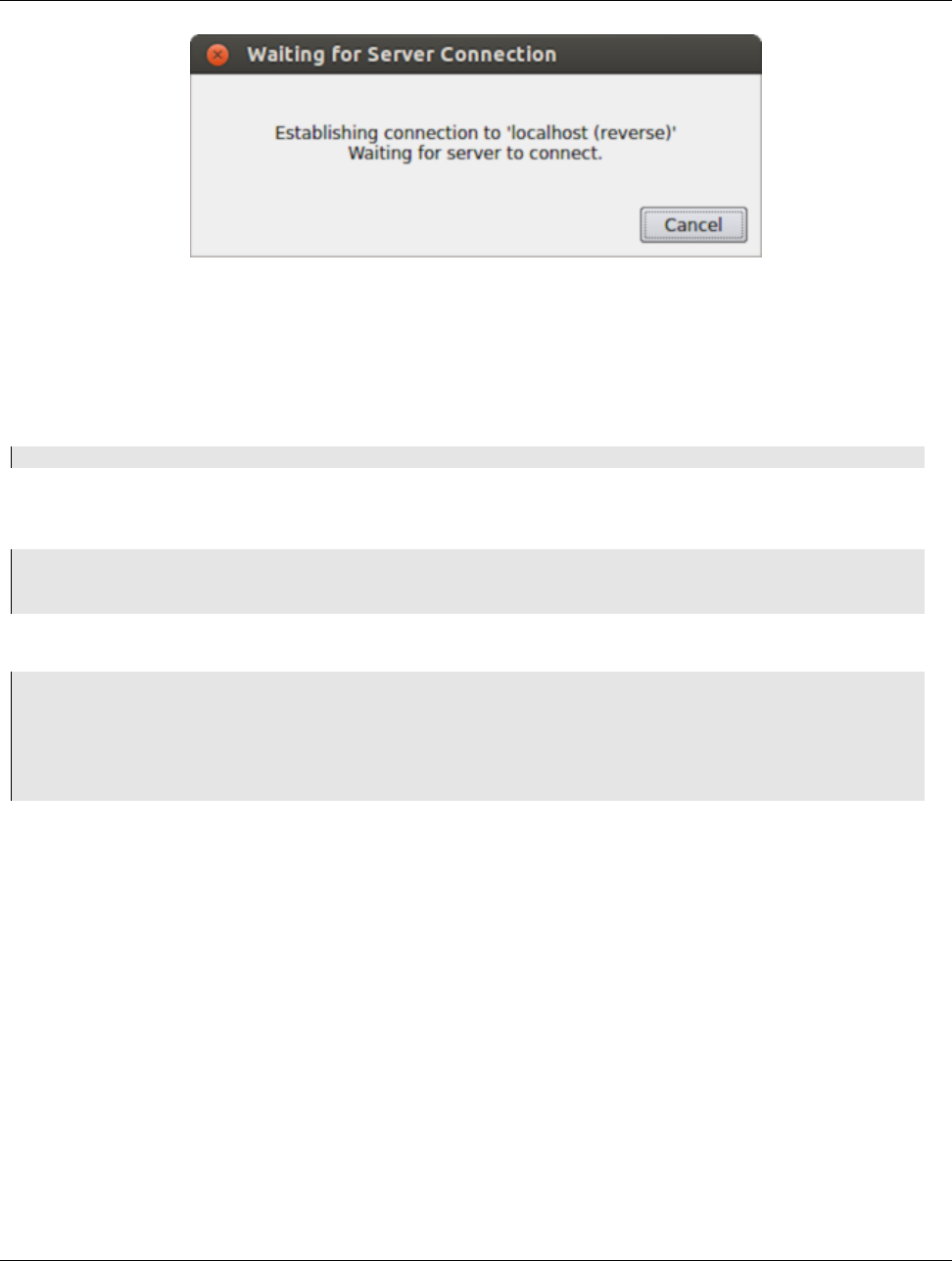
15.5. Understanding parallel processing
Figure 15.4: Message window showing that the client is awaiting a connection from a server.
Second, pvserver must be started with the --reverse-connection (-rc) flag. To tell pvserver the name of the client, set
the --client-host (-ch) command-line argument to the hostname of the machine on which the paraview client is
running. You can specify a port with the --server-port (-sp) command-line argument.
pvserver -rc --client -host= mylocalhost --server -port=11111
When the server starts, it prints a message indicating the success or failure of connecting to the client. When the
connection is successful, you will see the following text in the shell:
Connecting to client (reverse connection requested)...
Connection URL: csrc://mylocalhost:11111
Client connected.
To wait for reverse connections from a pvserver in pvpython, you use ReverseConnect instead of Connect.
1# To wait for connects from a ’pvserver’ on the default port
2# viz. 11111
3>>> ReverseConnect()
4
5# Optionally, you can specify the port number as the argument.
6>>> ReverseConnect(11111)
15.5 Understanding parallel processing
Parallel processing, put simply, implies processing the data in parallel, simultaneously using multiple workers. Typically,
these workers are different processes that could be running on a multicore machine or on several nodes of a cluster. Let’s
call these ranks. In most data processing and visualization algorithms, work is directly related to the amount of data that
needs to be processed, i.e., the number of cells or points in the dataset. Thus, a straight-forward way of distributing the
work among ranks is to split an input dataset into multiple chunks and then have each rank operate only an independent
set of chunks. Conveniently, for most algorithms, the result obtained by splitting the dataset and processing it separately is
same as the result that we’d get if we processed the dataset in a single chunk. There are, of course, exceptions. Let’s try to
understand this better with an example. For demonstration purposes, consider this very simplified mesh.
190 Chapter 15. Remote and parallel visualization
15.5. Understanding parallel processing
Now, let us say we want to perform visualizations on this mesh using three processes. We can divide the cells of the mesh
as shown below with the blue, yellow, and pink regions.
Once partitioned, some visualization algorithms will work by simply allowing each process to independently run the
algorithm on its local collection of cells. Take clipping as an example. Let’s say that we define a clipping plane and give
that same plane to each of the processes.
Each process can independently clip its cells with this plane. The end result is the same as if we had done the clipping
serially. If we were to bring the cells together (which we would never actually do for large data for obvious reasons), we
would see that the clipping operation took place correctly.
Chapter 15. Remote and parallel visualization 191
15.5. Understanding parallel processing
15.5.1 Ghost levels
Unfortunately, blindly running visualization algorithms on partitions of cells does not always result in the correct answer.
As a simple example, consider the external faces algorithm. The external faces algorithm finds all cell faces that belong to
only one cell, thereby, identifying the boundaries of the mesh.
Oops! We see that when all the processes ran the external faces algorithm independently, many internal faces where
incorrectly identified as being external. This happens where a cell in one partition has a neighbor in another partition. A
process has no access to cells in other partitions, so there is no way of knowing that these neighboring cells exist.
The solution employed by ParaView and other parallel visualization systems is to use ghost cells. Ghost cells are cells that
are held in one process but actually belong to another. To use ghost cells, we first have to identify all the neighboring cells
in each partition. We then copy these neighboring cells to the partition and mark them as ghost cells, as indicated with the
gray colored cells in the following example.
When we run the external faces algorithm with the ghost cells, we see that we are still incorrectly identifying some
internal faces as external. However, all of these misclassified faces are on ghost cells, and the faces inherit the ghost status
of the cell from which it came. ParaView then strips off the ghost faces, and we are left with the correct answer.
In this example, we have shown one layer of ghost cells: only those cells that are direct neighbors of the partition’s cells.
ParaView also has the ability to retrieve multiple layers of ghost cells, where each layer contains the neighbors of the
previous layer not already contained in a lower ghost layer or in the original data itself. This is useful when we have
cascading filters that each require their own layer of ghost cells. They each request an additional layer of ghost cells from
upstream, and then remove a layer from the data before sending it downstream.
15.5.2 Data partitioning
Since we are breaking up and distributing our data, it is prudent to address the ramifications of how we partition the data.
The data shown in the previous example has a spatially coherent partitioning. That is, all the cells of each partition are
192 Chapter 15. Remote and parallel visualization
15.5. Understanding parallel processing
located in a compact region of space. There are other ways to partition data. For example, you could have a random
partitioning.
Random partitioning has some nice features. It is easy to create and is friendly to load balancing. However, a serious
problem exists with respect to ghost cells.
In this example, we see that a single level of ghost cells nearly replicates the entire data set on all processes. We have thus
removed any advantage we had with parallel processing. Because ghost cells are used so frequently, random partitioning
is not used in ParaView.
15.5.3 D3 Filter
The previous section described the importance of load balancing and ghost levels for parallel visualization. This section
describes how to achieve that.
Load balancing and ghost cells are handled automatically by ParaView when you are reading structured data (image data,
rectilinear grid, and structured grid). The implicit topology makes it easy to break the data into spatially coherent chunks
and identify where neighboring cells are located.
It is an entirely different matter when you are reading in unstructured data (poly data and unstructured grid). There is no
implicit topology and no neighborhood information available. ParaView is at the mercy of how the data was written to
Chapter 15. Remote and parallel visualization 193
15.6. ParaView architecture
disk. Thus, when you read in unstructured data, there is no guarantee of how well-load balanced your data will be. It is
also unlikely that the data will have ghost cells available, which means that the output of some filters may be incorrect.
Fortunately, ParaView has a filter that will both balance your unstructured data and create ghost cells. This filter is called
D3, which is short for distributed data decomposition. Using D3 is easy; simply attach the filter (located in Filters
Alphabetical D3 ) to whatever data you wish to repartition.
The most common use case for D3 is to attach it directly to your unstructured grid reader. Regardless of how well-load
balanced the incoming data might be, it is important to be able to retrieve ghost cell so that subsequent filters will generate
the correct data. The example above shows a cutaway of the extract surface filter on an unstructured grid. On the left, we
see that there are many faces improperly extracted because we are missing ghost cells. On the right, the problem is fixed
by first using the D3 filter.
15.6 ParaView architecture
Before we see how to use ParaView for parallel data processing, let’s take a closer look at the ParaView architecture.
ParaView is designed as a three-tier client-server architecture. The three logical units of ParaView are as follows.
Data Server The unit responsible for data reading, filtering, and writing. All of the pipeline objects seen in the pipeline
browser are contained in the data server. The data server can be parallel.
Render Server The unit responsible for rendering. The render server can also be parallel, in which case built-in parallel
rendering is also enabled.
Client The unit responsible for establishing visualization. The client controls the object creation, execution, and
destruction in the servers, but does not contain any of the data (thus allowing the servers to scale without
bottlenecking on the client). If there is a GUI, that is also in the client. The client is always a serial application.
These logical units need not by physically separated. Logical units are often embedded in the same application, removing
the need for any communication between them. There are three modes in which you can run ParaView.
194 Chapter 15. Remote and parallel visualization
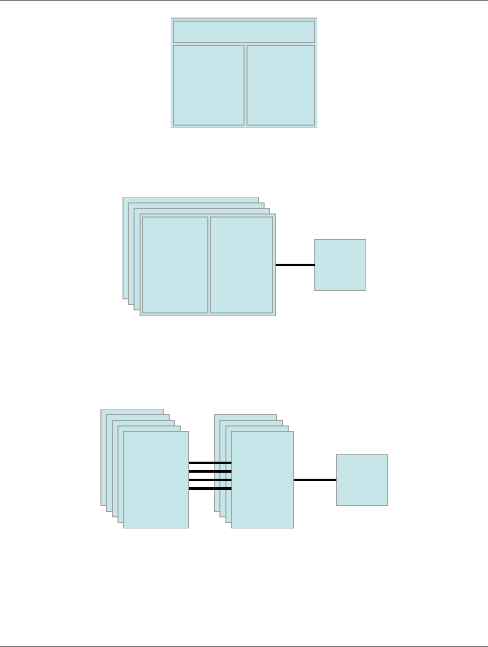
15.6. ParaView architecture
Client
Data
Server
Render
Server
The first mode, with which you are already familiar, is standalone mode. In standalone mode, the client, data server, and
render server are all combined into a single serial application. When you run the paraview application, you are
automatically connected to a builtin server so that you are ready to use the full features of ParaView.
Client
Data
Server
Render
Server
The second mode is client-server mode. In client-server mode, you execute the pvserver program on a parallel machine
and connect to it with the paraview client application (or pvpython). The pvserver program has both the data server and
render server embedded in it, so both data processing and rendering take place there. The client and server are connected
via a socket, which is assumed to be a relatively slow mode of communication, so data transfer over this socket is
minimized. We saw this mode of operation in Section 15.2.
Client
Data
Server
Render
Server
The third mode is client-render server-data server mode. In this mode, all three logical units are running in separate
programs. As before, the client is connected to the render server via a single socket connection. The render server and
data server are connected by many socket connections, one for each process in the render server. Data transfer over the
sockets is minimized.
Although the client-render server-data server mode is supported, we almost never recommend using it. The original
intention of this mode is to take advantage of heterogeneous environments where one might have a large, powerful
computational platform and a second smaller parallel machine with graphics hardware in it. However, in practice, we find
Chapter 15. Remote and parallel visualization 195
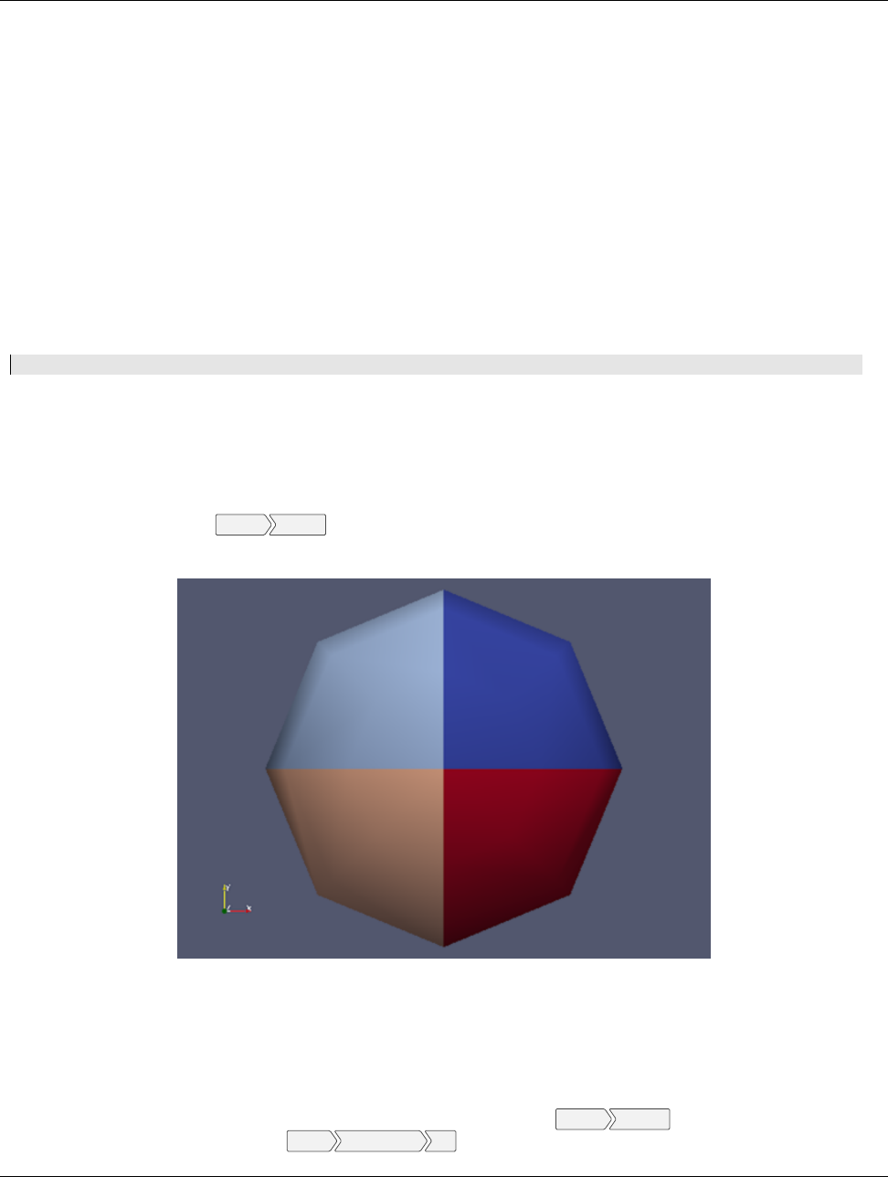
15.7. Parallel processing in paraview and pvpython
any benefit is almost always outstripped by the time it takes to move geometry from the data server to the render server. If
the computational platform is much bigger than the graphics cluster, then use software rendering on the large
computational platform. If the two platforms are about the same size, just perform all the computation on the graphics
cluster. The executables used for this mode are paraview (or pvpython) (acting as the client), pvdataserver for the
data-server, and pvrenderserver for the render-server.
15.7 Parallel processing in paraview and pvpython
To leverage parallel processing capabilities in paraview or pvpython, one has to use remote visualization, i.e., one has to
connect to a pvserver. The processing for connecting to this pvserver is not different from what we say in Sections 15.2
and 15.3. The only thing that changes is how the pvserver is launched.
You can start pvserver to run on more than one processing core using mpirun.
mpirun -np 4 pvserver
This will run pvserver on four processing cores. It will still listen for an incoming connection from a client on the default
port. The big difference when running pvserver this way is that when data is loaded from a source, it will be distributed
across the four cores if the data source is “parallel aware” and supports distributing the data across the different
processing cores.
To see how this data is distributed, run pvserver as the command above and connect to it with paraview. Next, create
another Sphere source using Source Sphere . Change the array to color by to vtkProcessId. You will see an image like
Figure 15.5.
Figure 15.5: Sphere source colored by vtkProcessId array that encodes the processing core on which the sphere data
resides. Here, the sphere data is split among the four processing cores invoked by the command mpirun -np 4 pvserver.
If a data reader or source is not “parallel aware”, you can still get the benefits of spreading the data among processing
cores by using the D3 filter. This filter partitions a dataset into convex regions and transfers each region to a different
processing core. To see an example of how D3 partitions a data set, create a Source Wavelet while paraview is still
connected to the pvserver. Next, select Filters Alphabetical D3 and click Apply. The output of D3 will not initially appear
196 Chapter 15. Remote and parallel visualization
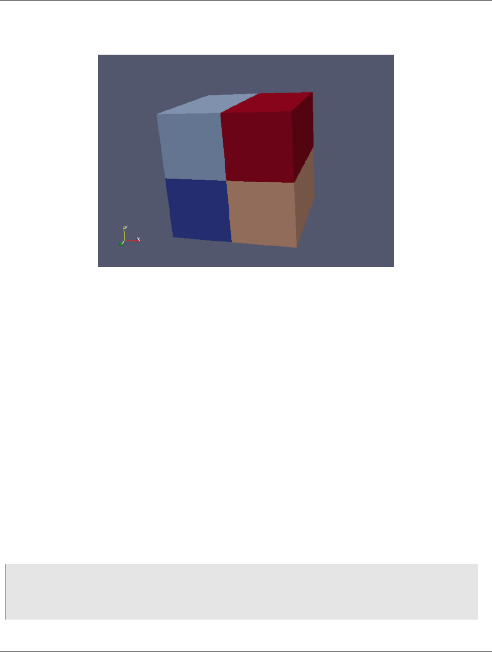
15.8. Using pvbatch
different from the original wavelet source. If you color by vtkProcessId, however, you will see the four partitions that
have been distributed to the server processing cores.
Figure 15.6: Wavelet source processed by the D3 filter and colored by vtkProcessId array. Note how four regions of the
image data are split evenly among the four processing cores when pvserver is run with mpirun -np 4 pvserver.
15.8 Using pvbatch
In Section 15.7, we said that to use parallel processing capabilities, one has to use remote visualization, i.e., one must use
ParaView in a client-server mode with the client (paraview or pvpython) connecting to a server (pvserver) that is being
run in parallel using mpirun. However, there is one exception: pvbatch.pvpython and pvbatch are quite similar in that
both are similar to the python executable that can be used to run Python scripts. The extra thing that these executables do
when compared with the standard python is that they initialize the environment so that any scripts that you run will be
able to locate the ParaView Python modules and libraries automatically. pvpython is exactly like the paraview executable
without the GUI. You can think of it as the GUI from paraview is replaced by a Python interpreter in pvpython.pvbatch,
on the other hand, can be thought of a pvserver where, instead of taking the control command from a remote client
(paraview or pvpython), in pvbatch, the commands are taken from a Python script that is executed in the pvbatch
executable itself. Since pvbatch is akin to the pvserver, unlike pvpython, it can be run in parallel using mpirun. In that
case, the root rank (or the first rank or the rank with index 0) is the one that acts as the client, interpreting the Python
script to execute the commands. Since pvbatch is designed to act is its own server, you cannot connect to a remote server
in the Python script, i.e., you cannot use simple.Connect. Furthermore, pvbatch is designed for batch operation, which
means that you can only specify the Python script as a command line argument. Unlike pvpython, you cannot run this
executable to get an interactive shell to enter Python commands.
# process the sample.py script in single process mode.
>pvbatchsample.py
# process the sample.py script in parallel.
>mpirun-np4sample.py
Chapter 15. Remote and parallel visualization 197
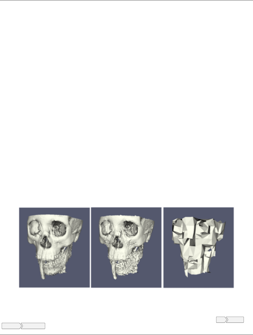
15.9. Rendering
In general, you should use pvpython if you will be using the interpreter interactively and pvbatch if you are running in
parallel.
15.9 Rendering
Rendering is the process of synthesizing the images that you see based on your data. The ability to effectively interact
with your data depends highly on the speed of the rendering. Thanks to advances in 3D hardware acceleration, fueled by
the computer gaming market, we have the ability to render 3D quickly even on moderately-priced computers. But, of
course, the speed of rendering is proportional to the amount of data being rendered. As data gets bigger, the rendering
process naturally gets slower.
To ensure that your visualization session remains interactive, ParaView supports two modes of rendering that are
automatically flipped as necessary. In the first mode, still render, the data is rendered at the highest level of detail. This
rendering mode ensures that all of the data is represented accurately. In the second mode, interactive render, speed takes
precedence over accuracy. This rendering mode endeavors to provide a quick rendering rate regardless of data size.
While you are interacting with a 3D view (for example, rotating, panning, or zooming with the mouse), ParaView uses an
interactive render. This is because, during the interaction, a high frame rate is necessary to make these features usable and
because each frame is immediately replaced with a new rendering while the interaction is occurring so that fine details are
less important during this mode. At any time when interaction of the 3D view is not taking place, ParaView uses a still
render so that the full detail of the data is available as you study it. As you drag your mouse in a 3D view to move the
data, you may see an approximate rendering. The full detail will be presented as soon as you release the mouse button.
The interactive render is a compromise between speed and accuracy. As such, many of the rendering parameters concern
when and how lower levels of detail are used.
15.9.1 Basic Rendering Settings
Some of the most important rendering options are the LOD parameters. During interactive rendering, the geometry may
be replaced with a lower level of detail (LOD), an approximate geometry with fewer polygons.
The resolution of the geometric approximation can be controlled. In the proceeding images, the left image is the full
resolution, the middle image is the default decimation for interactive rendering, and the right image is ParaView’s
maximum decimation setting.
The 3D rendering parameters are located in the settings dialog box, which is accessed in the menu from Edit Settings
(ParaView Preferences on the Mac). The rendering options in the dialog are in the Render View tab.
198 Chapter 15. Remote and parallel visualization
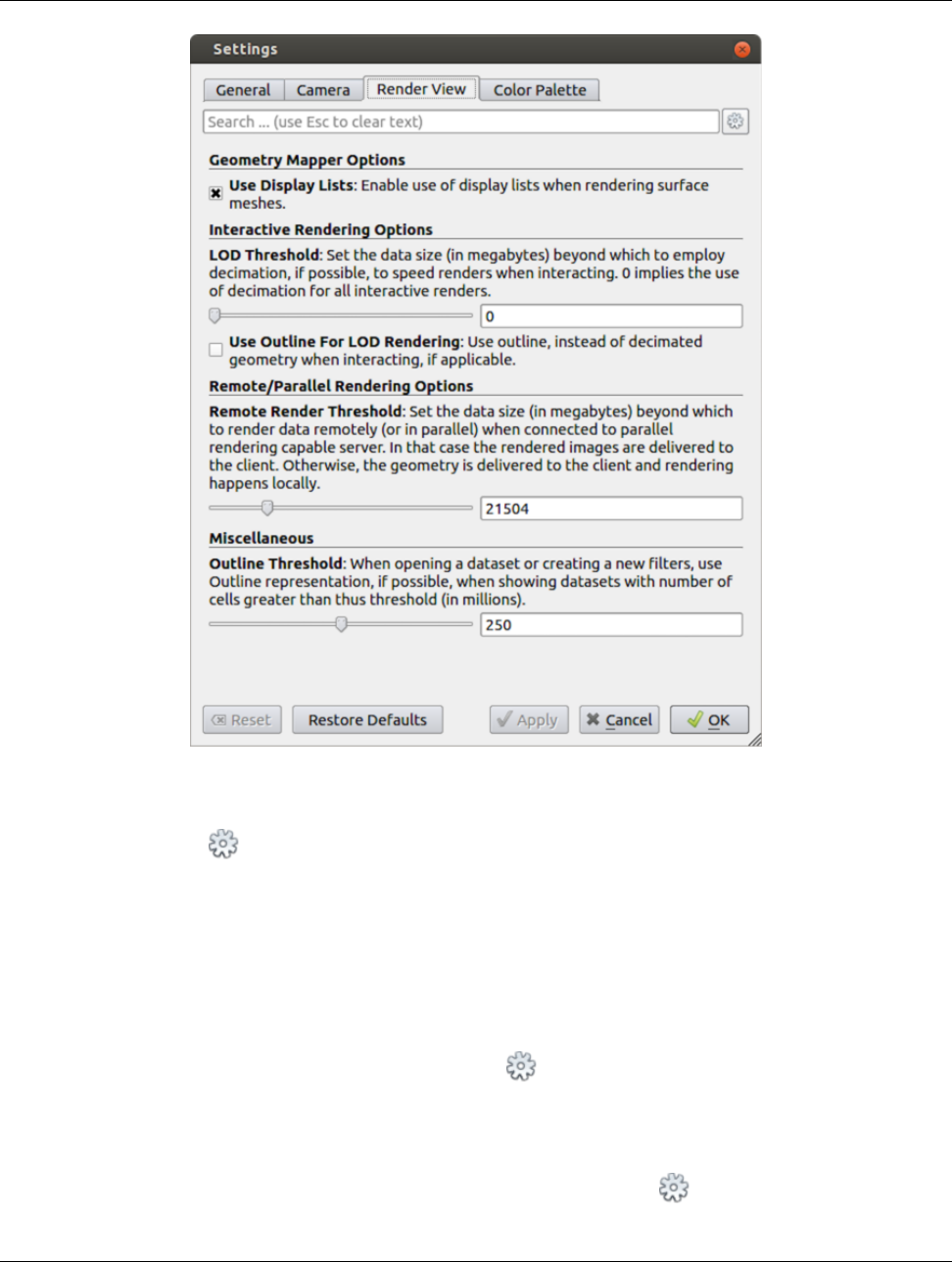
15.9. Rendering
The options pertaining to the geometric decimation for interactive rendering are located in a section labeled Interactive
Rendering Options. Some of these options are considered advanced, so to access them, you have to either toggle on the
advanced options with the button or search for the option using the edit box at the top of the dialog. The interactive
rendering options include the following.
•LOD Threshold: Set the data size at which to use a decimated geometry in interactive rendering. If the geometry
size is under this threshold, ParaView always renders the full geometry. Increase this value if you have a decent
graphics card that can handle larger data. Try decreasing this value if your interactive renders are too slow.
•LOD Resolution: Set the factor that controls how large the decimated geometry should be. This control is set to a
value between 0 and 1. 0 produces a very small number of triangles but, possibly, with a lot of distortion. 1
produces more detailed surfaces but with larger geometry.
•Non Interactive Render Delay: Add a delay between an interactive render and a still render. ParaView usually
performs a still render immediately after an interactive motion is finished (for example, releasing the mouse button
after a rotation). This option can add a delay that can give you time to start a second interaction before the still
render starts, which is helpful if the still render takes a long time to complete.
Chapter 15. Remote and parallel visualization 199

15.9. Rendering
•Use Outline For LOD Rendering: Use an outline in place of decimated geometry. The outline is an alternative
for when the geometry decimation takes too long or still produces too much geometry. However, it is more difficult
to interact with just an outline.
ParaView contains many more rendering settings. Here is a summary of some other settings that can effect the rendering
performance regardless of whether ParaView is run in client-server mode or not. These options are spread among several
categories, and several are considered advanced.
Geometry Mapper Options
•Use Display Lists: Enable or disable the use of display lists. Display lists are internal structures built by
graphics systems. They can potentially speed up rendering but can also take up memory.
Translucent Rendering Options
•Depth Peeling: Enable or disable depth peeling. Depth peeling is a technique ParaView uses to properly
render translucent surfaces. With it, the top surface is rendered and then “peeled away” so that the next lower
surface can be rendered and so on. If you find that making surfaces transparent really slows things down or
renders completely incorrectly, then your graphics hardware may not be implementing the depth peeling
extensions well; try shutting off depth peeling.
•Maximum Number Of Peels: Set the maximum number of peels to use with depth peeling. Using more peels
allows more depth complexity, but allowing less peels runs faster. You can try adjusting this parameter if
translucent geometry renders too slow or translucent images do not look correct.
Miscellaneous
•Outline Threshold: When creating very large datasets, default to the outline representation. Surface
representations usually require ParaView to extract geometry of the surface, which takes time and memory.
For data with sizes above this threshold, use the outline representation, which has very little overhead, by
default instead.
•Show Annotation: Show or hide annotation providing rendering performance information. This information
is handy when diagnosing performance problems.
Note that this is not a complete list of ParaView rendering settings. We have left out settings that do not significantly
effect rendering performance. We have also left out settings that are only valid for parallel client-server rendering, which
are discussed in Section 15.9.4.
15.9.2 Basic Parallel Rendering
When performing parallel visualization, we are careful to ensure that the data remains partitioned among all of the
processes up to and including the rendering processes. ParaView uses a parallel rendering library called IceT. IceT uses a
sort-last algorithm for parallel rendering. This parallel rendering algorithm has each process independently render its
partition of the geometry and then composites the partial images together to form the final image.
200 Chapter 15. Remote and parallel visualization
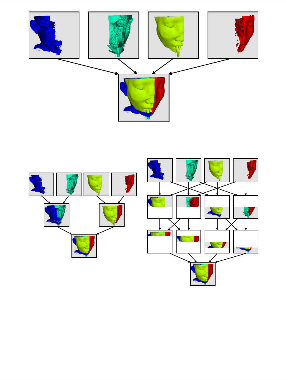
15.9. Rendering
The preceding diagram is an oversimplification. IceT contains multiple parallel image compositing algorithms such as
binary tree, binary swap, and radix-k that efficiently divide work among processes using multiple phases.
The wonderful thing about sort-last parallel rendering is that its efficiency is completely insensitive to the amount of data
being rendered. This makes it a very scalable algorithm and well suited to large data. However, the parallel rendering
overhead does increase linearly with the number of pixels in the image. Consequently, some of the rendering parameters
deal with the image size.
Chapter 15. Remote and parallel visualization 201
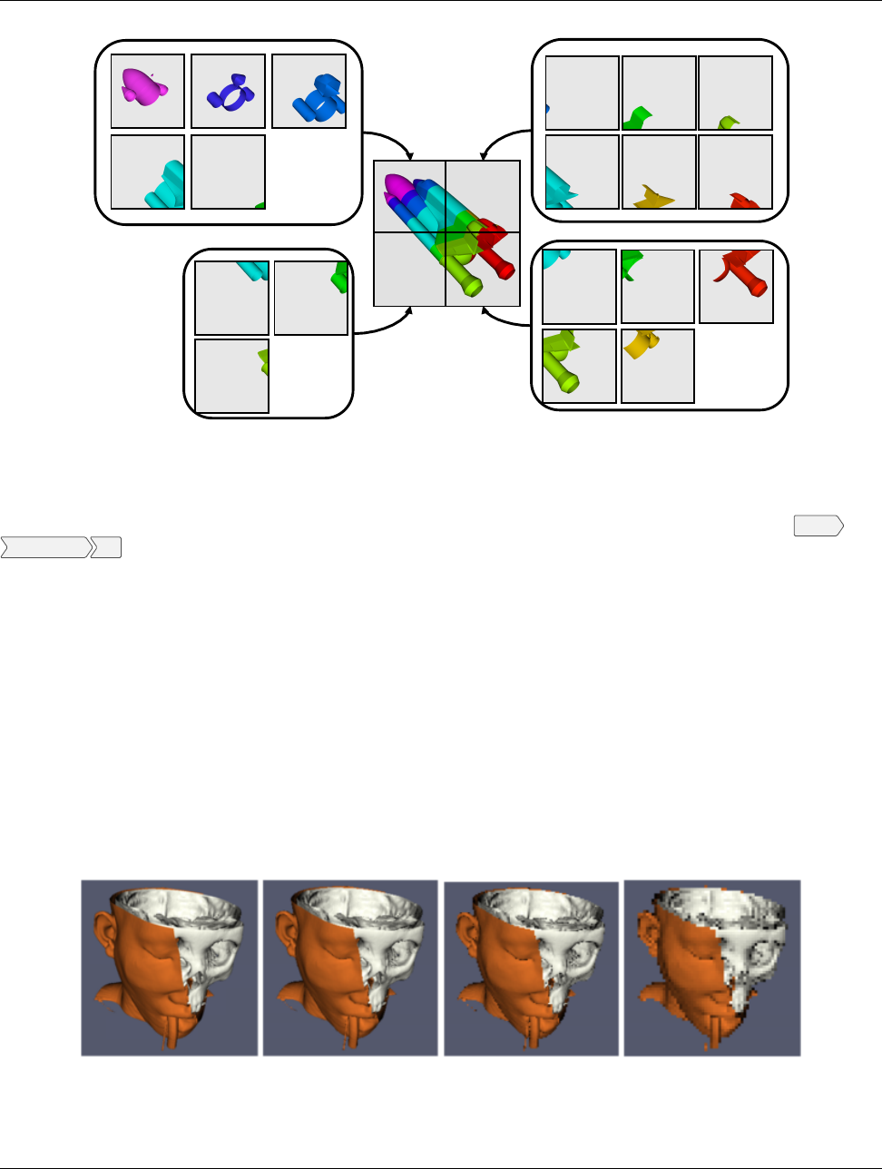
15.9. Rendering
IceT also has the ability to drive tiled displays, which are large, high-resolution displays comprising an array of monitors
or projectors. Using a sort-last algorithm on a tiled display is a bit counterintuitive because the number of pixels to
composite is so large. However, IceT is designed to take advantage of spatial locality in the data on each process to
drastically reduce the amount of compositing necessary. This spatial locality can be enforced by applying the Filters
Alphabetical D3 filter to your data.
Because there is an overhead associated with parallel rendering, ParaView has the ability to turn off parallel rendering at
any time. When parallel rendering is turned off, the geometry is shipped to the location where display occurs. Obviously,
this should only happen when the data being rendered is small.
15.9.3 Image Level of Detail
The overhead incurred by the parallel rendering algorithms is proportional to the size of the images being generated. Also,
images generated on a server must be transfered to the client, a cost that is also proportional to the image size. To help
increase the frame rate during interaction, ParaView introduces a new LOD parameter that controls the size of the images.
During interaction while parallel rendering, ParaView can optionally subsample the image. That is, ParaView will reduce
the resolution of the image in each dimension by a factor during interaction. Reduced images will be rendered,
composited, and transfered. On the client, the image is inflated to the size of the available space in the GUI.
The resolution of the reduced images is controlled by the factor with which the dimensions are divided. In the proceeding
images, the left image has the full resolution. The following images were rendered with the resolution reduced by a factor
of 2, 4, and 8, respectively.
202 Chapter 15. Remote and parallel visualization
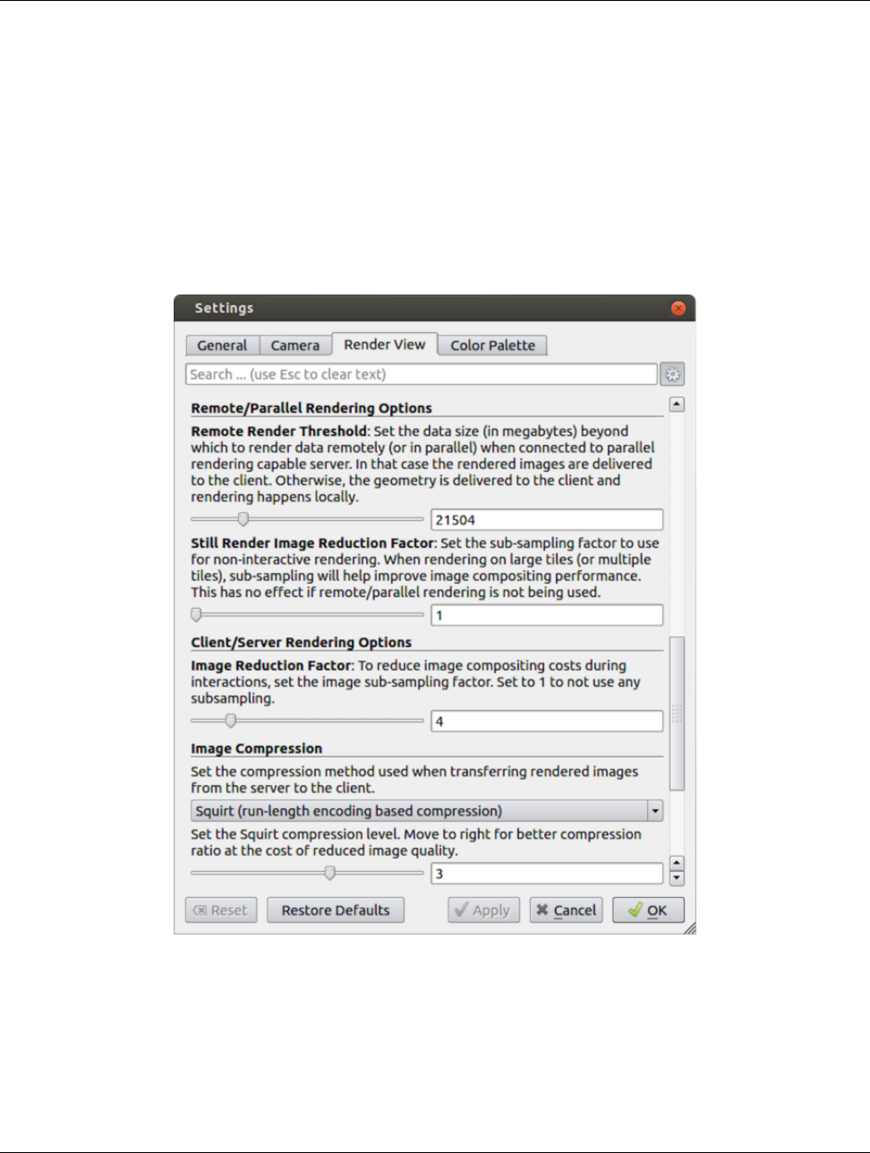
15.9. Rendering
ParaView also has the ability to compress images before transferring them from server to client. Compression, of course,
reduces the amount of data transferred and, therefore, makes the most of the available bandwidth. However, the time it
takes to compress and decompress the images adds to the latency.
ParaView contains two different image compression algorithms for client-server rendering. The first is a custom algorithm
called Squirt, which stands for Sequential Unified Image Run Transfer. Squirt is a run-length encoding compression that
reduces color depth to increase run lengths. The second algorithm uses the Zlib compression library, which implements a
variation of the Lempel-Ziv algorithm. Zlib typically provides better compression than Squirt, but it takes longer to
perform and, hence, adds to the latency.
15.9.4 Parallel Render Parameters
Like the other 3D rendering parameters, the parallel rendering parameters are located in the Settings dialog. The
parallel rendering options in the dialog are in the Render View tab (intermixed with several other rendering options such
as those described in Section 15.9.1). The parallel and client-server options are divided among several categories, and
several are considered advanced.
Remote/Parallel Rendering Options
•Remote Render Threshold: Set the data size at which to render remotely in parallel or to render locally. If
Chapter 15. Remote and parallel visualization 203
15.9. Rendering
the geometry is over this threshold (and ParaView is connected to a remote server), the data is rendered in
parallel remotely, and images are sent back to the client. If the geometry is under this threshold, the geometry
is sent back to the client, and images are rendered locally on the client.
•Still Render Image Reduction Factor: Set the sub-sampling factor for still (non-interactive) rendering.
Some large displays have more resolution than is really necessary, so this sub-sampling reduces the resolution
of all images displayed.
Client/Server Rendering Options
•Image Reduction Factor: Set the interactive subsampling factor. The overhead of parallel rendering is
proportional to the size of the images generated. Thus, you can speed up interactive rendering by specifying
an image subsampling rate. When this box is checked, interactive renders will create smaller images, which
are then magnified when displayed. This parameter is only used during interactive renders.
Image Compression
•Before images are shipped from server to client, they optionally can be compressed using one of two
compression algorithms: Squirt or Zlib. To make the compression more effective, either algorithm can reduce
the color resolution of the image before compression. The sliders determine the amount of color bits saved.
Full color resolution is always used during a still render.
•Suggested image compression presets are provided for several common network types. When attempting to
select the best image compression options, try starting with the presets that best match your connection.
15.9.5 Parameters for Large Data
The default rendering parameters are suitable for most users. However, when dealing with very large data, it can help to
tweak the rendering parameters. While the optimal parameters depend on your data and the hardware on which ParaView
is running, here are several pieces of advice that you should follow.
•Try turning off display lists. Turning this option off will prevent the graphics system from building special
rendering structures. If you have graphics hardware, these rendering structures are important for feeding the GPUs
fast enough. However, if you do not have GPUs, these rendering structures do not help much.
•If there is a long pause before the first interactive render of a particular data set, it might be the creation of the
decimated geometry. Try using an outline instead of decimated geometry for interaction. You could also try
lowering the factor of the decimation to 0 to create smaller geometry.
•Avoid shipping large geometry back to the client. The remote rendering will use the power of the entire server to
render and ship images to the client. If remote rendering is off, geometry is shipped back to the client. When you
have large data, it is always faster to ship images than to ship data. (Although, if your network has a high latency,
this could become problematic for interactive frame rates.)
•Adjust the interactive image sub-sampling for client-server rendering as needed. If image compositing is slow, if
the connection between client and server has low bandwidth, or if you are rendering very large images, then a
higher subsample rate can greatly improve your interactive rendering performance.
•Make sure Image Compression is on. It has a tremendous effect on desktop delivery performance, and the artifacts
it introduces, which are only there during interactive rendering, are minimal. Lower bandwidth connections can try
using Zlib instead of Squirt compression. Zlib will create smaller images at the cost of longer
compression/decompression times.
204 Chapter 15. Remote and parallel visualization

15.9. Rendering
•If the network connection has a high latency, adjust the parameters to avoid remote rendering during interaction. In
this case, you can try turning up the remote rendering threshold a bit, and this is a place where using the outline for
interactive rendering is effective.
•If the still (non-interactive) render is slow, try turning on the delay between interactive and still rendering to avoid
unnecessary renders.
Chapter 15. Remote and parallel visualization 205
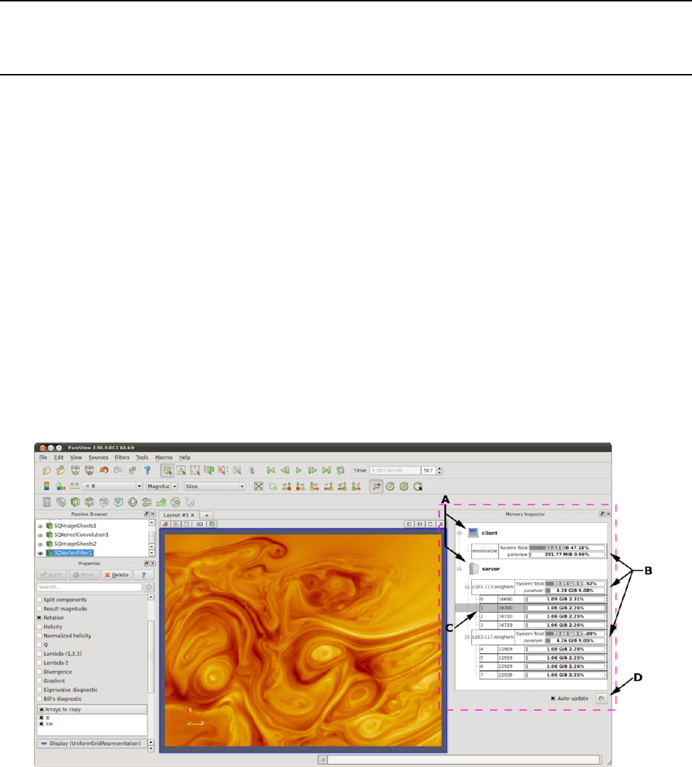
CHAPTER
SIXTEEN
MEMORY INSPECTOR
The ParaView Memory Inspector panel provides users with a convenient way to monitor ParaView’s memory usage
during interactive visualization. It also provides developers with a point-and-click interface for attaching a debugger to
local or remote client and server processes. As explained earlier, both the Information panel and the Statistics
Inspector are prone to over and under estimate the total memory used for the current pipeline. The Memory Inspector
addresses those issues through direct queries to the operating system. A number of diagnostic statistics are gathered and
reported, including the total memory used by all processes on a per-host basis, the total cumulative memory use by
ParaView on a per-host basis, and the individual per-rank use by each ParaView process. When memory consumption
reaches a critical level, either cumulatively on the host or in an individual rank, the corresponding GUI element will turn
red, alerting you that you are in danger of potentially being shut down. This gives you a chance to save state and restart
the job with more nodes to aviod losing your work. On the flip side, knowing when you’re not close to using the full
capacity of available memory can be useful to conserve computational resources by running smaller jobs. Of course, the
memory foot print is only one factor in determining the optimal run size.
Figure 16.1: The main UI elements of the Memory Inspector panel. A: Process Groups, B: Per-Host statistics, C: Per-
Rank statistics, and D: Update controls.

16.1. User interface and layout
16.1 User interface and layout
The Memory Inspector panel displays information about the current memory usage on the client and server hosts.
Figure 16.1 shows the main UI elements labeled A-D. A number of additional features are provided via specialized
context menus accessible from the Client and Server group, Host, and Rank’s UI elements. The main UI elements are:
AProcess Groups
*Client : There is always a client group that reports statistics about the ParaView client.
*Server : When running in client-server mode, a server group reports statistics about the hosts where pvserver
processes are running.
*Data Sever : When running in client-data-render server mode, a data server group reports statistics about the
hosts where pvdataserver processes are running.
* Render Sever : When running in client-data-render server mode, a render server group reports statistics about
the hosts where pvrenderserver processes are running.
BPer-Host Statistics : Per-host statics are reported for each host where a ParaView process is running. Hosts are
organized by host name, which is shown in the first column. Two statics are reported: 1) total memory used by all
processes on the host and 2) ParaView’s cumulative usage on this host. The absolute value is printed in a bar that
shows the percentage of the total available memory used. On systems where job-wide resource limits are enforced,
ParaView is made aware of the limits via the PV HOST MEMORY LIMIT environment variable, in which case,
ParaView’s cumulative percent used is computed using the smaller of the host total and the resource limit.
CUpdate Controls : By default, when the panel is visible, memory use statistics are updated automatically as pipeline
objects are created, modified, or destroyed and after the scene is rendered. Updates may be triggered manually by
using the refresh button. Automatic updates may be disabled by un-checking the Auto-update check box. Queries
to remote systems have proven to be very fast even for fairly large jobs. Hence, the auto-update feature is enabled
by default.
DHost Properties Dialog : The Host context menu provides the Host Properties dialog, which reports various
system details such as the OS version and the CPU version, as well as the memory installed and available to the host
context and process context. While the Memory Inspector panel reports memory use as a percent of the available
in the given context, the Host Properties dialog reports the total memory installed and available in each context.
Comparing the installed and available memory can be used to determine if you are impacted by resource limits.
16.2 Advanced debugging features
16.2.1 Remote commands
The Memory Inspector Panel provides a remote (or local) command feature, allowing you to execute a shell command
on a given host. This feature is exposed via a specialized Rank item context menu. Because we have information such as a
rank’s process id, individual processes may be targeted. For example, this allows you to quickly attach a debugger to a
server process running on a remote cluster. If the target rank is not on the same host as the client, then the command is
considered remote. Otherwise, it is considered local. Therefore, remote commands are executed via ssh, while local
commands are not. A list of command templates is maintained. In addition to a number of pre-defined command
templates, you may add templates or edit existing ones. The default templates allow you to:
1. Attach gdb to the selected process
2. Run top on the host of the selected process
208 Chapter 16. Memory Inspector
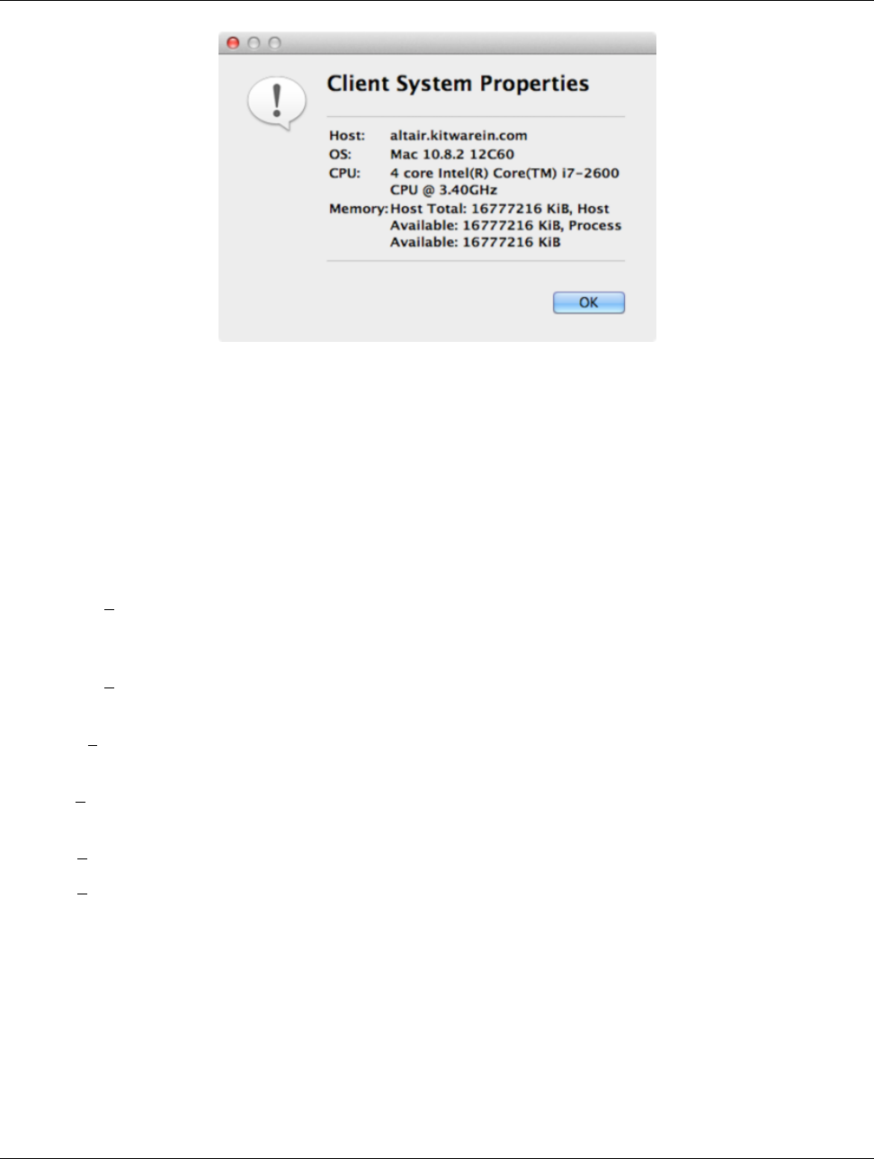
16.2. Advanced debugging features
Figure 16.2: Host properties dialog.
3. Send a signal to the selected process
Prior to execution, the selected template is parsed, and a list of special tokens are replaced with runtime-determined or
user-provide values. User-provided values can be set and modified in the dialog’s parameter group. The command, with
tokens replaced, is shown for verification in the dialog’s preview pane.
The following tokens are available and may be used in command templates as needed:
1. $TERM EXEC$ : The terminal program that will be used to execute commands. On Unix systems, xterm is
typically used. On Windows systems, cmd.exe is typically used. If the program is not in the default path, then the
full path must be specified.
2. $TERM OPTS$ : Command line arguments for the terminal program. On Unix, these may be used to set the
terminals window title, size, colors, and so on.
3. $SSH EXEC$ : The program to use to execute remote commands. On Unix, this is typically ssh. On Windows,
one option is plink.exe. If the program is not in the default path, then the full path must be specified.
4. $FE URL$ : Ssh URL to use when the remote processes are on compute nodes that are not visible to the outside
world. This token is used to construct command templates where two ssh hops are made to execute the command.
5. $PV HOST$ : The hostname where the selected process is running.
6. $PV PID$ : The process-id of the selected process.
Note: On Windows, the debugging tools found in Microsoft’s SDK need to be installed in addition to Visual Studio (e.g.,
windbg.exe). The ssh program plink.exe for Windows doesn’t parse ANSI escape codes that are used by Unix shell
programs. In general, the Windows-specific templates need some polishing.
16.2.2 Stack trace signal handler
The Process Group’s context menu provides a back trace signal handler option. When enabled, a signal handler is
installed that will catch signals such as SEGV, TERM, INT, and ABORT and that will print a stack trace before the
process exits. Once the signal handler is enabled, you may trigger a stack trace by explicitly sending a signal. The stack
Chapter 16. Memory Inspector 209
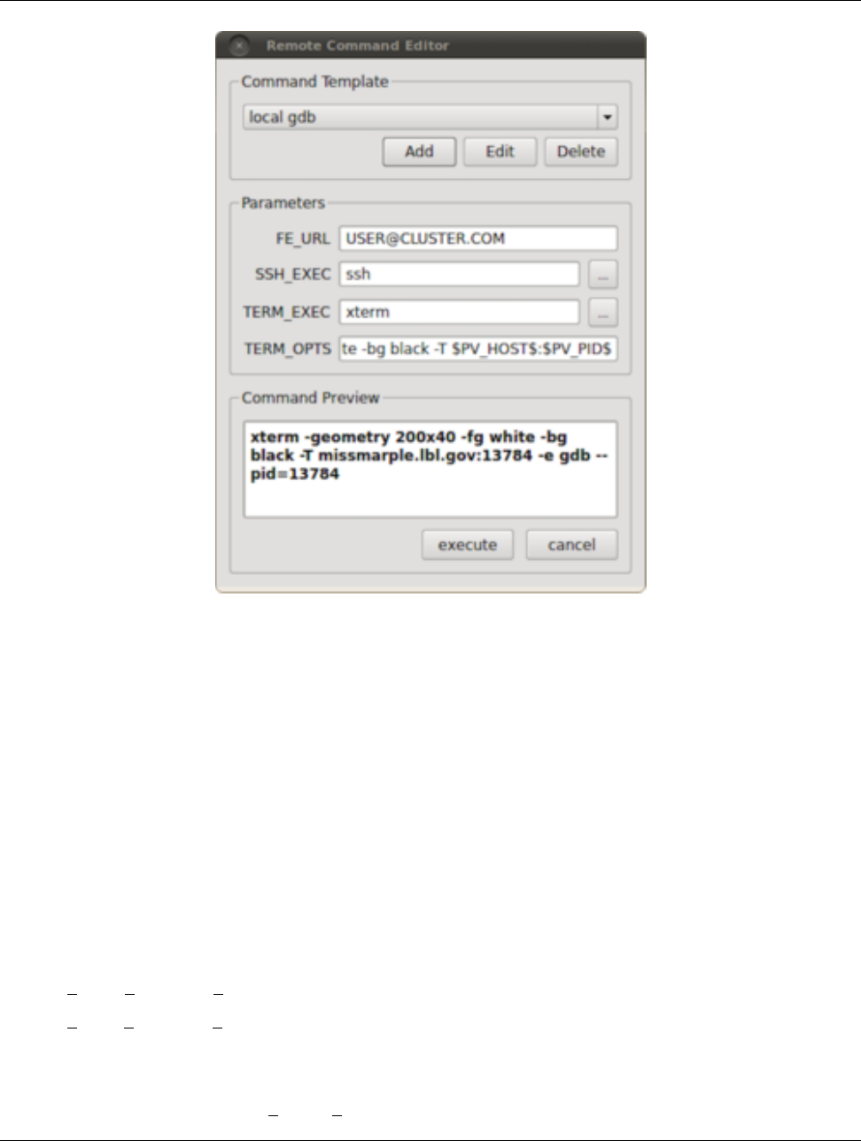
16.3. Compilation and installation considerations
Figure 16.3: The remote command dialog.
trace signal handler can be used to collect information about crashes or to trigger a stack trace during deadlocks when it’s
not possible to ssh into compute nodes. Sites that restrict users’ ssh access to compute nodes often provide a way to signal
running processes from the login node. Note that this feature is only available on systems that provide support for POSIX
signals, and we currently only have implemented stack trace for GNU-compatible compilers.
16.3 Compilation and installation considerations
If the system on which ParaView will run has special resource limits enforced, such as job-wide memory use limits, or
non-standard per-process memory limits, then the system administrators need to provide this information to the running
instances of ParaView via the following environment variables. For example, those could be set in the batch system
launch scripts.
1. PV HOST MEMORY LIMIT : For reporting host-wide resource limits.
2. PV PROC MEMORY LIMIT : For reporting per-process memory limits. that are not enforced via standard Unix
resource limits.
A few of the debugging features (such as printing a stack trace) require debug symbols. These features will work best
when ParaView is built with CMAKE BUILD TYPE=Debug or, for release builds,
210 Chapter 16. Memory Inspector

16.3. Compilation and installation considerations
CMAKE BUILD TYPE=RelWithDebugSymbols.
Chapter 16. Memory Inspector 211
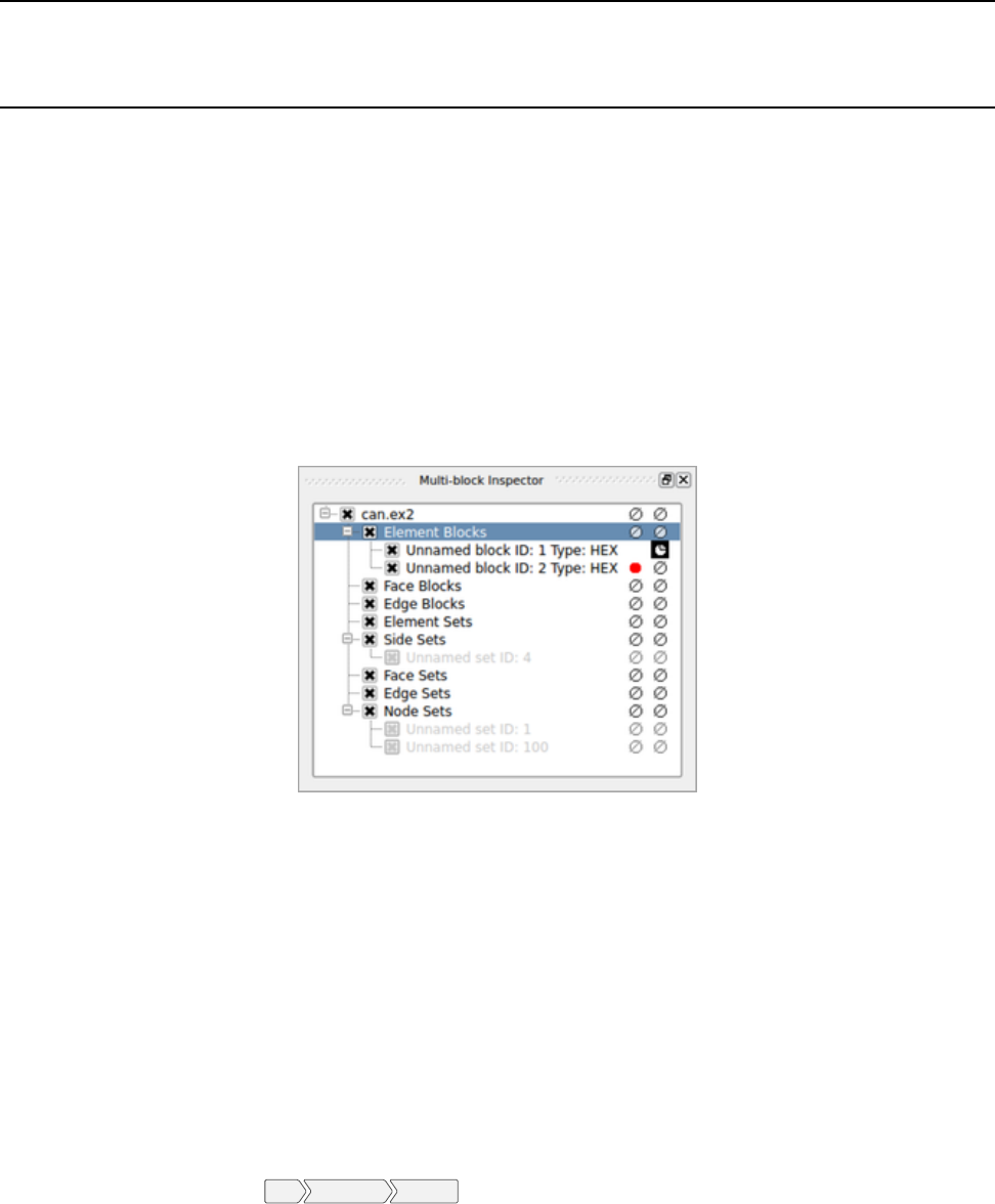
CHAPTER
SEVENTEEN
MULTIBLOCK INSPECTOR
The Multiblock Inspector is a panel used to show the block hierarchy of a multiblock dataset as well as to show and
modify block rendering properties. Block rendering properties include block visibility, color and opacity. These
properties are inherited, so changing a property for a non-leaf node affects all its children. Figure 17.1 shows a multiblock
dataset with two blocks colored white and red with opacity for the white block set to 0.3. The black square around opacity
shows that this property was overridden. We’ll described overridden properties in the next paragraphs.
Figure 17.1: The Multiblock Inspector
To show or hide a block you have to click on the checkbox next to the block name. The two column to the right side of the
Multiblock Inspector show block colors and opacities. A block color (and opacity) can be set for all blocks or can be
individually overridden for each block. Block colors can be set for all blocks either by choosing the color of the entire
dataset to be a Solid Color or by using the vtkBlockColors field array. Block colors set this way can be overridden for
individual blocks. Blocks usually have many colors and opacities if the dataset is colored by a point or cell array. In this
case Multiblock Inspector shows the color and opacity for blocks as nil.
The first way of setting block colors and opacities is to color the entire dataset using a Solid Color or to adjust the
Opacity in the Display properties panel. In this case, all blocks have the same color and opacity.
If you want to color blocks differently, you can color the dataset using a special field array of size one called
vtkBlockColors. This array is generated by ParaView for a multiblock dataset. For each block its value is equal to the
remainder of the block index divided by BlockColorsDistinctValues.BlockColorsDistinctValues is a user
configurable value accessible in Edit Settings... General . If you color by this array a categorical color map is
automatically selected.

Finally, block color and opacity can be set by double clicking on the color or opacity icon. This allows the user to override
block colors that are set as described previously. We provide visual feedback for overridden colors or opacities by
enclosing them in a black square.
A context menu associated with a block displayed in the Multiblock Inspector allows you to set the visibility, color
and opacity and to reset these properties to the values set for all blocks. The context menu, shown in Figure 17.2, is
activated using a right click on the block you want to modify.
Figure 17.2: The Multiblock Inspector context menu.
Rendering properties for blocks can also be modified directly in the Render View through a context menu. Simply right
click on a block in the scene and a menu will be displayed allowing you modify rendering properties for the selected
block. If several blocks are selected, the context menu commands will apply to all selected blocks.
Blocks in a multiblock dataset can be selected in the Multiblock Inspector by selecting the rows listing the blocks.
Note that you can use multiple selection to select several blocks by keeping the Ctrl key pressed and clicking on several
rows or by keeping the Shift key pressed and dragging the mouse over the rows you want to select.
Block selection is synchronized between the Render View and in the Multiblock Inspector: a selection in one view is
reflected in the other.
214 Chapter 17. Multiblock Inspector
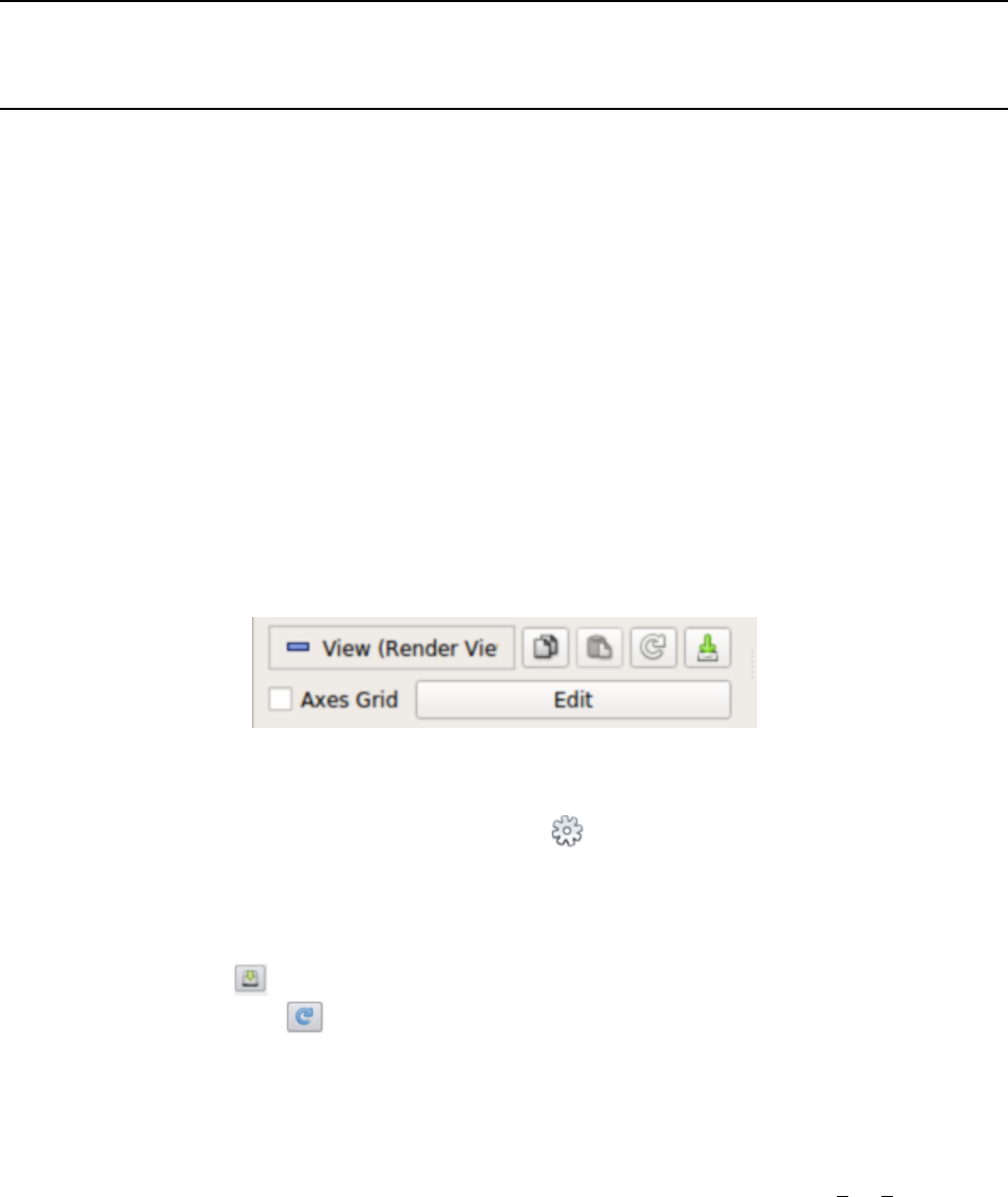
CHAPTER
EIGHTEEN
AXES GRID
Oftentimes, you want to render a reference grid in the backgroud for a visualization – think axes in a chart view, except
this time we are talking of the 3D Render View. Such a grid is useful to get an understanding for the data bounds and
placement in 3D space. In such cases, you use the Axes Grid.Axes Grid renders a 3D grid with labels around the
rendered scene. In this chapter, we will take a closer look at using and customizing the Axes Grid.
18.1 The basics
To turn on the Axes Grid for a Render View, you use the Properties panel. Under the View section, you check the
Axes Grid checkbox to turn the Axes Grid on for the active view.
Clicking on the Edit button will pop up the Axes Grid properties dialog (Figure 18.1) that allows you to customize the
Axes Grid. As with the Properties panel, this is a searchable dialog, hence you can use the Search box at the top of
the dialog to search of properties of interest. At the same time, the button can be used to toggle between default and
advanced modes for the panel.
Using this dialog, you can change common properties like the titles (X Title,Y Title, and Z Title), title and label
fonts using Title Font Properties and Label Font Properties for each of the axes directions, as well as the Grid
Color. Besides labelling the axes, you can render a grid by checking Show Grid. Once you have the Axes Grid setup to
your liking, you can use the to save your selections so that they are automatically loaded next time you launch
ParaView. You can always use the to revert back to ParaView defaults.
18.2 Use cases
To get a better look at the available customizations, let’s look at various visualizations possible and then see how you can
set those up using the properties on the Edit Axes Grid dialog. In these examples, we use the disk out ref.ex2
example dataset distributed with ParaView.
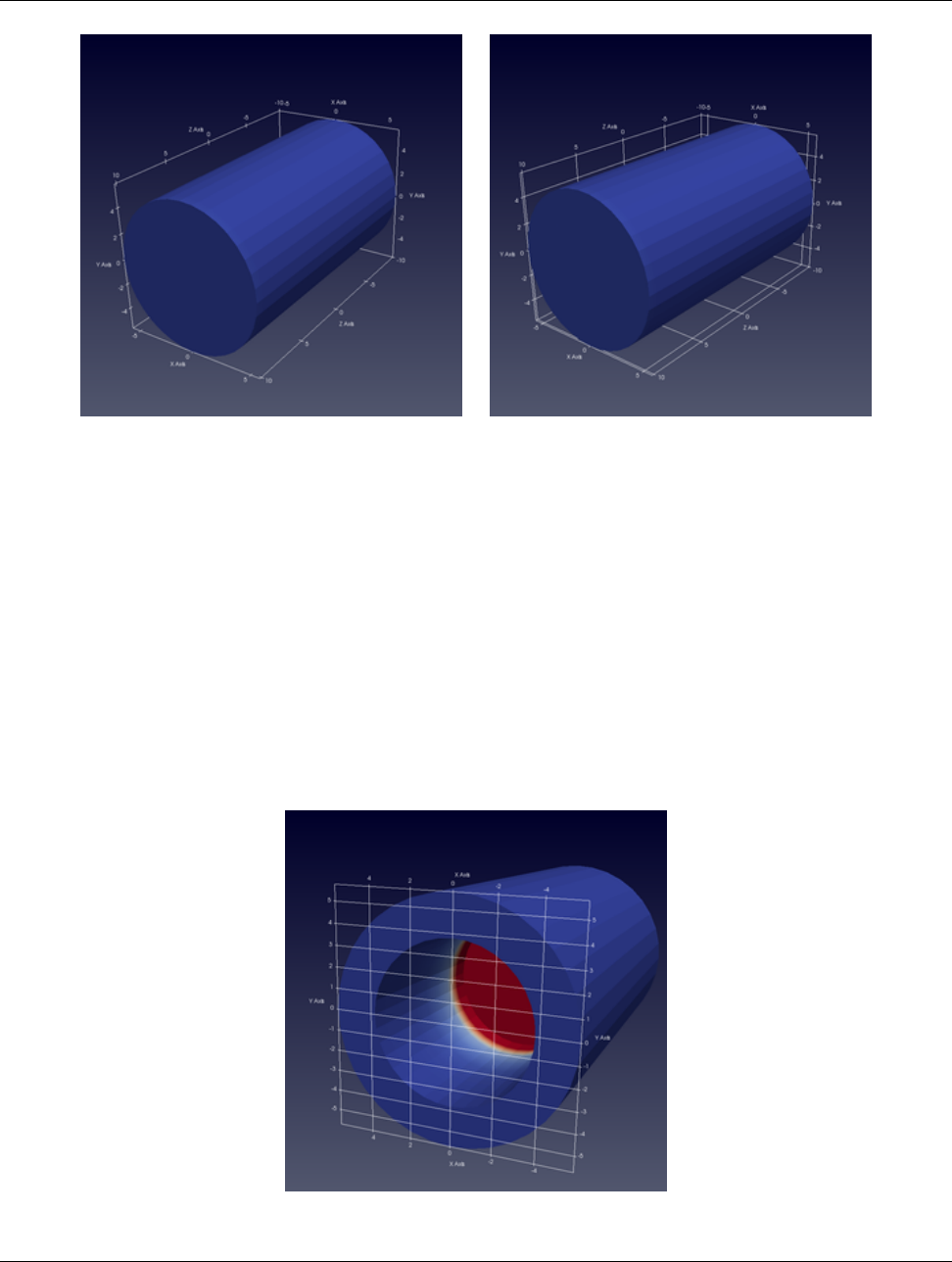
18.2. Use cases
In the images above, on the left is the default Axes Grid. Simply turning on the visibility of the Axes Grid will generate
such a visualization. The axes places always stay behind the rendered geometry even as you interact with the scene. As
you zoom in and out, the labels and ticks will be updated based on visual cues.
Now to show a grid along the axes planes, alined with the ticks and labels, turn on the Show Grid checkbox, resulting in a
visualization on the right.
By default, the gridded faces are always the fartest faces i.e. they stay behind the rendered geometry and keep on updating
as you rotate the scene. To fix which faces of the bounding-box are to be rendered, use the Faces To Render button (it’s
an advanced property, so you may have to search for it using the Seach box in the Edit Axes Grid dialog). Suppose, we
want to label just one face, the lower XY face. In that case, uncheck all the other faces except Min-XY in menu popped up
on clicking on the Faces to Render button. This will indeed just show the min-XY face, however as you rotate the
scene, the face will get hidden as soon as the face gets closer to the camera than the dataset. This is because, by default,
Cull Frontfaces is enabled. Uncheck Cull Frontfaces and ParaView will stop removing the face as it comes ahead
of the geometry, enabling a visualization as follows.
216 Chapter 18. Axes Grid
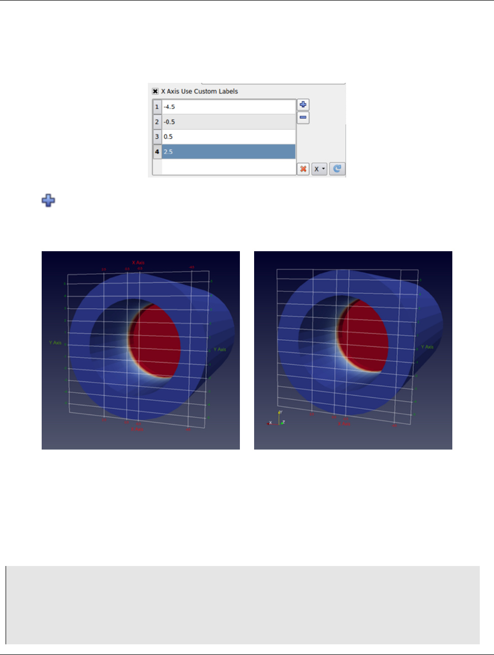
18.3. Axes Grid in pvpython
Besides controlling which faces to render, you can also control where the labels are placed. Let’s say we want ParaView
to decide how to place labels along the Y axis, however for the X axis, we want to explicitly label the values 2.5, 0.5,
0.5, and 4.5. To that, assuming we are the advanced mode for the Edit Axes Grid panel, check X Axis Use
Custom Labels. That will show a table widget that allows you to add values as shown below.
Using the button, add the custom values. While at it, let’s also change the X Axis Label Font Properties and X
Axis Title Font Properties to change the color to red and similar for the Y axis, let’s change the color to green.
Increase the title font sizes to 18, to make them stand out and you will get a visualization as follows (below, left).
Here we see that both sides of the axis plane are labelled. Suppose you only want to label one of the sides, in that case use
the Axes To Label property to uncheck all but Min-X and Min-Y. This will result in the visualization shown above, right.
18.3 Axes Grid in pvpython
In pvpython,Axes Grid is accessible as the AxesGrid property on the render view.
1>>> renderView = GetActiveView()
2
3# AxesGrid property provides access to the AxesGrid object.
4>>> axesGrid = renderView.AxesGrid
5
6# To toggle visibility of the axes grid,
7>>> axesGrid.Visibility = 1
Chapter 18. Axes Grid 217

18.3. Axes Grid in pvpython
All properties on the Axes Grid that you set using the Edit Axes Grid dialog are avialble on this axesGrid object and
can be changed as follows:
1>>> axesGrid.XTitle = ’X Title’
2>>> axesGrid.XTitleColor = [0.6, 0.6, 0.0]
3>>> axesGrid.XAxisLabels = [-0.5, 0.5, 2.5, 3.5]
Note you can indeed use the tracing capabilities described in Section 1.6.2 to determine what Python API to use to change
a specific property on the Edit Axes Grid dialog or use help.
1>>> help(axesGrid)
2Help on GridAxes3DActor in module paraview.servermanager object:
3
4class GridAxes3DActor(Proxy)
5|GridAxes3DActorcanbeusedtorenderagridin arenderview.
6|
7|Methodresolutionorder:
8|GridAxes3DActor
9| Proxy
10 |__builtin__.object
11 |
12 |Methodsdefinedhere:
13 |
14 |Initialize=aInitialize(self, connection=None,update=True)
15 |
16 | ----------------------------------------------------------------------
17 |Datadescriptorsdefinedhere:
18 |
19 |AxesToLabel
20 |Setthemasktoselecttheaxestolabel.Theaxeslabelledwillbeasubset
of the
21 |axesselecteddependingonwhichfacesarealsobeingrendered.
22 |
23 | CullBackface
24 |Settotruetohidefacesofthegridfacingawayfrom the camera i.e. hide
all
25 |backfaces.
26 |
27 |CullFrontface
28 |Settotruetohidefacesofthegridfacingtowardsfrom the camera i.e. hide
all
29 | front faces.
30 |
31 | DataPosition
32 |Ifdatais being translated , you can show the original data bounds for the
axes
33 |insteadofthetranslatedboundsbysettingtheDataPositiontomatchthe
34 |translationappliedtothedataset.
35 |
36 ...
218 Chapter 18. Axes Grid
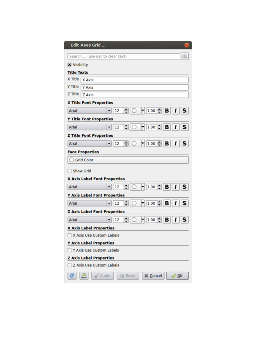
18.3. Axes Grid in pvpython
Figure 18.1: Edit Axes Grid dialog is used to customize the Axes Grid.
Chapter 18. Axes Grid 219
CHAPTER
NINETEEN
SETTINGS
As with any large application, paraview provides mechanisms to customize some of its application behavior. These are
referred to as application settings or, just, settings. Such settings can be changed using the Settings dialog, which is
accessed from the Edit Settings (ParaView Preferences on the Mac) menu. We have seen parts of this dialog earlier, e.g., in
Sections 9.2, 15.9.1, and 15.9.4. In this chapter, we will take a closer look at some of the other options available in this
dialog.
The Settings dialog is split into several tabs. The General tab consolidates most of the miscellaneous settings. The
Camera tab enables you to change the mouse interaction mappings for the Render View and similar views. The Render
View tab, which we saw earlier in Sections 15.9.1 and 15.9.4, provides options in regards to rendering in Render View
and similar views. The Color Palette tab is used to change the active color palette.
Using this dialog is not much different than the Properties panel. You have the Search box at the top, which allows you
to search properties matching the input text (Section 9.1.2). The button can be used to toggle between default and
advanced modes.
To apply the changes made to any of the settings, use the Apply or OK buttons. OK will apply the changes and close the
dialog, while Cancel will reject any changes made and close the dialog. Any changes made to the options in this dialog
are persistent across sessions. (I.e., the next time you launch paraview, you’ll still be using the same settings chosen
earlier.) To revert to the default, use the Restore Defaults button. You can also manually edit the setting file as in
Section 10.3. Furthermore, site maintainers can provide site-wide defaults for these, as is explained in Section 10.4.
Next, we will see some of the important options available. Those that are only available in the advanced mode are
indicated as such using the icon. You will either need to toggle on the advanced options with the button or search
for the option using the Search box.
19.1 General settings
General Options
•Show Splash Screen: Uncheck this to not show the splash screen at application startup. You will need to
restart paraview to see the effect.
•Crash Recovery: When this is checked, paraview will intermittently save a backup state file as you make
changes in the visualization pipeline. If paraview crashes for some reason, then when you relaunch paraview,
it will provide you with a choice to load the backup state saved before the crash occurred. This is not 100%
reliable, but some users may find it useful to avoid loosing their visualization state due to a crash.
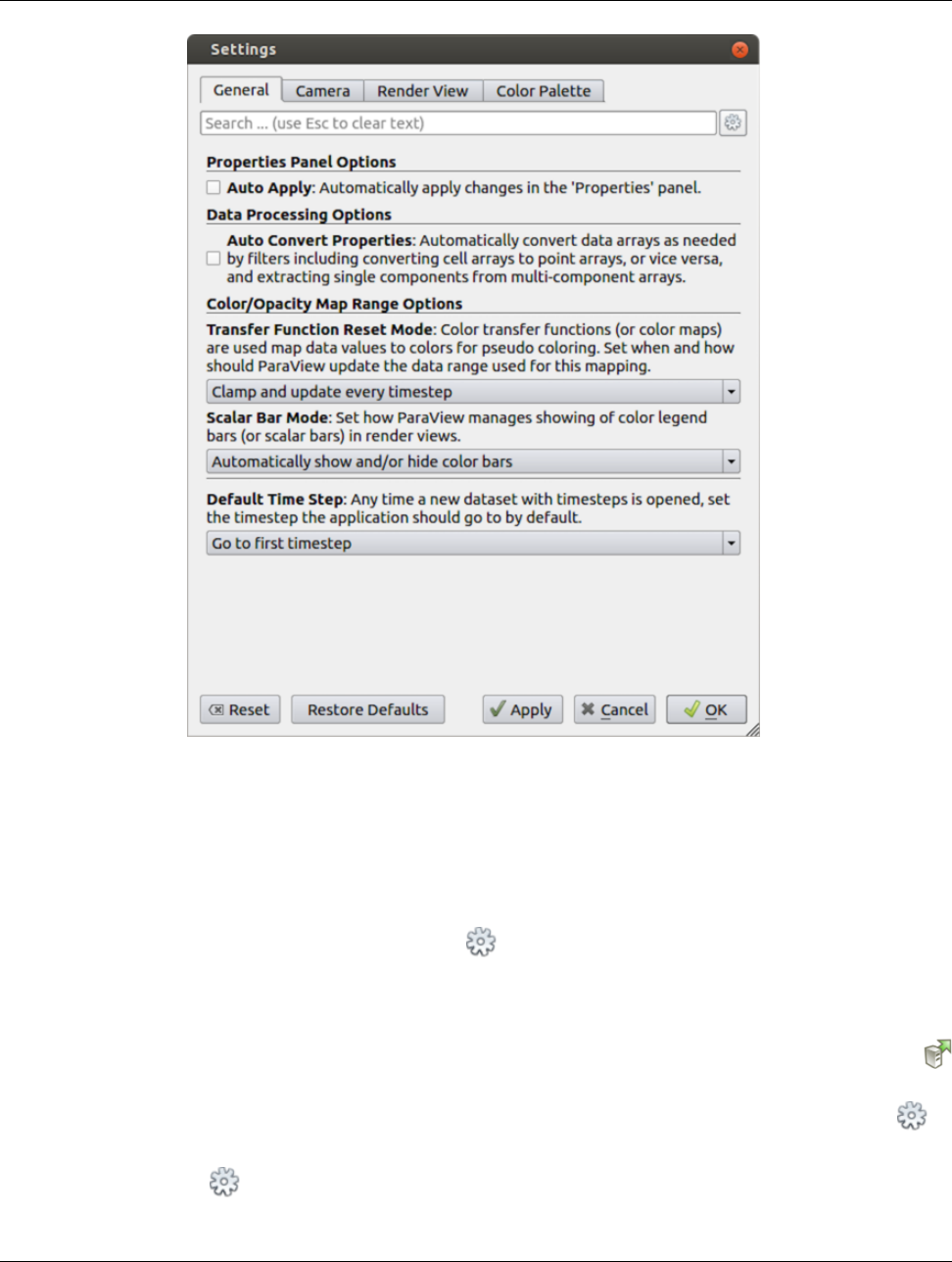
19.1. General settings
Figure 19.1: Settings dialog in paraview showing the General settings tab.
Default View
•Default View Type: When paraview starts up, it creates Render View by default. You can use this option
to change the type of the view that is created by default, instead of the Render View. You can even pick None
if you don’t want to create any view by default.
Properties Panel Options
•Auto Apply: When checked, the Properties panel will automatically apply any changes you make to the
properties without requiring you to click the Apply button. The same setting can also be toggled using the
button in the Main Controls toolbar.
•Auto Apply Active Only: This limits the auto-applying to the properties on the active source alone.
•Properties Panel Mode: This allows you to split the Properties panel into separate panels as described
in Section 9.2.
Data Processing Options
222 Chapter 19. Settings

19.2. Camera settings
•Auto Convert Properties: Several filters only work on one type of array, e.g., point data arrays or cell data
arrays. Before using such filters, you are expected to apply the Point Data To Cell Data or Cell Data
To Point Data filters. To avoid having to add these filters explicitly, you can check this checkbox. When
checked, ParaView will automatically convert data arrays as needed by filters, including converting cell array
to point arrays and vice-versa, as well as extracting a single component from a multi-component array.
Color/Opacity Map Range Options
•Transfer Function Reset Mode: This setting controls when ParaView will reset the ranges for color and
opacity maps (or transfer functions). This only affects those color/opacity maps that have the Automatically
rescale transfer functions to fit data setting enabled (Section 11.2.1). When Grow and update
on ’Apply’ is selected, ParaView will grow the color/opacity map range to include the current data range
every time you hit Apply on the Properties panel. Thus, when the data range changes, if the timestep is
changed, the color/opacity map range won’t be affected. To grow the range on change in timestep as well, use
the Grow and update every timestep option. Now the range will be updated on Apply as well as when
the timestep changes. Grow indicates that the color/opacity map range will only be increased, never shrunk, to
include the current data range. If you want the range to match the current data range exactly, then you should
use the Clamp and update every timestep option. Now the range will be clamped to the exact data range
each time you hit Apply on the Properties panel or when the timestep changes.
•Scalar Bar Mode: This settings controls how paraview manages showing the color legend (or scalar bar) in
Render View and similar views.
Default Time Step
Whenever a dataset with timesteps is opened, this setting controls how paraview will update the current time shown
by the application. You can choose between Leave current time unchanged, if possible,Go to first
timestep, and Go to last timestep.
Animation
•Cache Geometry For Animation: This enables caching of geometry when playing animations to attempt to
speed up animation playback in a loop. When caching is enabled, data ranges reported by the Information
panel and others can be incorrect, since the pipeline may not have updated.
•Animation Geometry Cache Limit: When animation caching is enabled, this setting controls how much
geometry (in kilobytes) can be cached by any rank. As soon as a rank’s cache size reaches this limit, ParaView
will no longer cache the remaining timesteps.
Screenshot Options
•When saving screenshots (or animations) with multiple views, these settings allow you to control the width of
the border between multiple views, as well as the color to use for the border. Multi View Image Border
Color sets the color for the border, while Multi View Image Border Width sets the width for the border in
pixels.
•Transparent Background: When set, all screenshots will be saved with the background color replaced with
a transparent background. Currently, this only works for Render View and similar views.
19.2 Camera settings
This tab allows you to control how you can interact in Render View and similar views. Basically, you are setting up a
mapping between each of the mouse buttons and keyboard modifiers, and the available interaction types including
Chapter 19. Settings 223
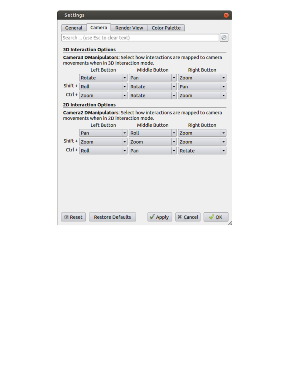
19.3. Render View settings
Figure 19.2: Settings dialog in paraview showing the Camera settings tab.
Rotate,Pan,Zoom, etc. The dialog allows you to set the interaction mapping separately for 3D and 2D interaction modes
(see Section 4.4.2).
19.3 Render View settings
Refer to Sections 15.9.1 and 15.9.4 for various options available on the Render View tab.
19.4 Color Palette
The Color Palette tab (Figure 19.4) allows you to change the colors in the active color palette. The tab lists the
available color categories viz. Surface,Foreground,Edges,Background,Text, and Selection. You can manually set
colors to use for each of these categories or load one of the predefined palettes using the Load Palette option. To
understand color palettes, let’s look at an example.
224 Chapter 19. Settings
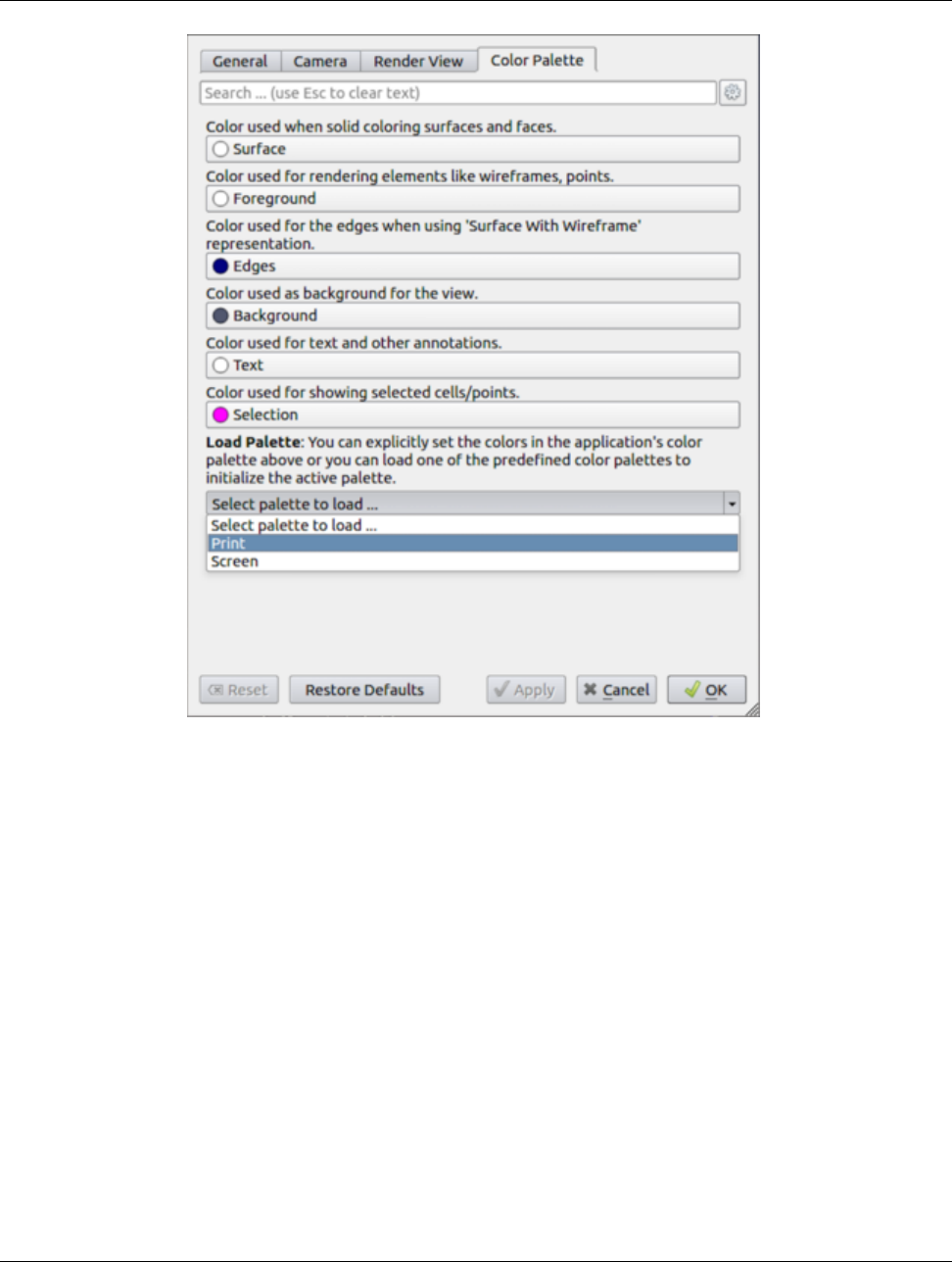
19.4. Color Palette
Figure 19.3: Settings dialog in paraview showing the Color Palette settings tab.
Let’s start paraview and split the active view to create two Render View instances side by side. You may want to start
paraview with the -dr command line argument to stop any of your current settings from interfering with this demo. Next,
show Sphere as Wireframe in the view on the left, and show Cone as Surface in the view on the right. Also, turn on
Cube Axis for Cone. You will see something like Figure 19.4 (left).
Now let’s say you want to generate a image for printing. Typically, for printing, you’d want the background color to be
white, while the wireframes and annotations to be colored black. To do that, one way is to go change each of the colors
for each each of the views, displays and cube-axes. You can imagine how tedious that will get especially with larger
pipelines. Alternatively, using the Settings dialog, change the active color palette to Print as shown in Figure 19.4 and
then hit OK or Apply. The visualization will immediately change to something like Figure 19.4 (right).
Essentially, ParaView allows you to link any color property to one of the color categories. When the color palette is
changed, any color property linked to a palette category will also be automatically updated to match the category color.
Figure 19.4 shows how to link a color property to a color palette category in the Properties panel. Use the tiny
drop-down menu marker to make the menu pop up that shows the color palette categories. Select any one of them to link
that property with the category. The link is automatically severed if you manually change the color by simply clicking on
the button.
Chapter 19. Settings 225
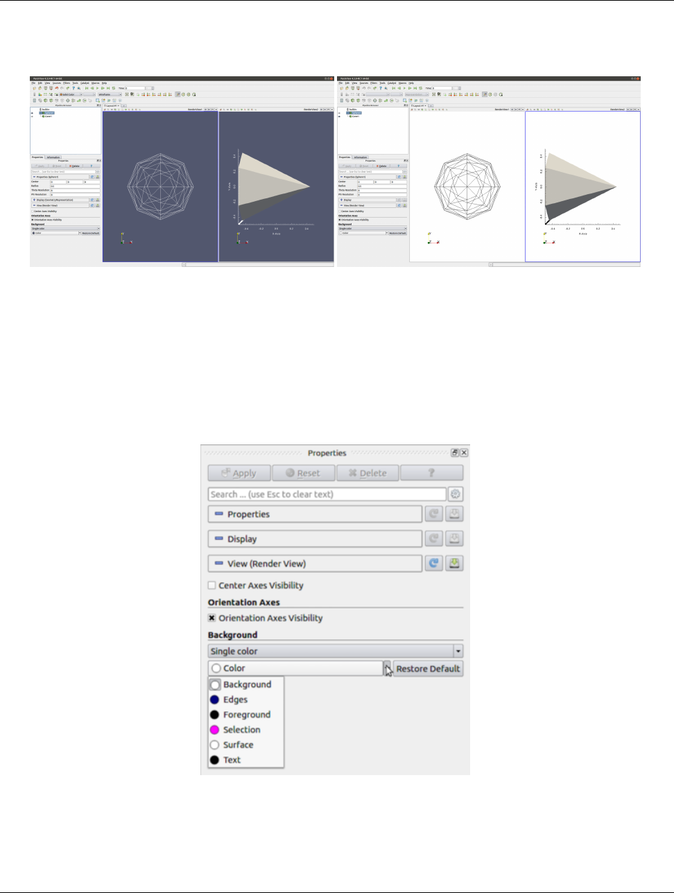
19.4. Color Palette
Figure 19.4: The effect of loading the Print color palette as the active palette. The left is the original visualization and the
right shows the result after loading the Print palette.
Figure 19.5: Popup menu allows you to link a color property to a color palette category in the Properties panel.
226 Chapter 19. Settings
Part III
Appendix
BIBLIOGRAPHY
[1] Ken Moreland. The ParaView Tutorial. http://www.paraview.org/Wiki/The_ParaView_Tutorial.
[2] Numpy developers. NumPy. http://www.numpy.org/.
[3] Pat Marion. What is InterpolateScalarsBeforeMapping in VTK? http://www.kitware.com/blog/home/post/414.
[4] W. J. Schroeder, K. M. Martin, and W. E. Lorensen. The design and implementation of an object-oriented toolkit for 3d graphics
and visualization. In Proceedings of the 7th Conference on Visualization ’96, VIS ’96, pages 93–ff., Los Alamitos, CA, USA,
1996. IEEE Computer Society Press.
[5] The ParaView Community. Setting up a ParaView server.
http://www.paraview.org/Wiki/Setting_up_a_ParaView_Server.

APPENDIX
INDEXES

paraview UI Index
paraview UI Index
(partial), 40
+, 124, 126, 127, 141
2D, 55
3D, 55
3D View, 114
3D widgets, 87
abs, 102
acos, 102
Active Plot Axis Color, 70
Active Plot Grid Color, 70
Active Variables Controls, 146
Add Server, 187
Additional Headlight, 56
Advanced Selection Display Properties, 119
All Points, 95
All Scalars, 90
Animation, 223
Animation Duration (sec), 132
Animation Geometry Cache Limit, 223
Animation Keyframes, 124, 125
Animation Settings Dialog, 132, 133
Animation Time, 126
Animation Time Precision, 125
Animation View, 123–125, 127
Annotate Time, 162
Annotation, 154
Annotations, 154, 156
Append Datasets, 80, 81
Apply, 9–11, 13, 14, 16, 19, 22, 24, 26, 38, 50, 51, 83, 113,
121, 139, 141, 149, 196, 221–223, 225
Array Association, 102
Array Name, 103
Arrow, 94
asin, 102
Aspect Ratio, 152
atan, 102
Attribute, 71, 114
Attribute Type, 67, 71
Auto Apply, 10, 26, 50, 222
Auto Apply Active Only, 222
Auto Convert Properties, 223
Automatic Label Format, 152
Automatically rescale transfer functions to fit data, 149, 223
Axes Grid, 55, 56, 215–219
Axes To Label, 217
Axis Use Custom Labels, 66
Axis Use Custom Range, 66
Axis Use Log Scale, 66
Backface Styling, 60
Background, 56, 159, 224
Bag Chart View, 47
Bar Chart View, 47, 64, 69, 70
Bar Chart View (Comparative), 77, 159
BlockColorsDistinctValues, 213
Bottom Axis Title, 66
Bottom Axis Use Custom Labels, 66
Bottom Axis Use Custom Range, 66
Bottom-Left, 68
Bottom-Right, 68
Bounds, 39
Box, 86, 89
builtin:, 189
Cache Geometry For Animation, 223
Calculator, 40, 101–103, 146, 170
Camera, 54, 127, 221, 224
Camera Parallel Projection, 56
Cancel, 221
ceil, 102
Cell Data, 71, 102, 114, 116
Cell Data To Point Data, 223
Cell Data to Point Data, 67
Center, 9, 10, 87, 93
Center Axes Visibility, 56
Change Input Dialog, 81, 82
Change Input..., 81
Chart Axes, 68
Chart Title, 66, 70
Chart Views, 47
Choose Server Configuration, 186–189
Clamp and update every timestep, 223
Clean to Grid, 36
Clear, 101
Client / Server (reverse connection), 189
Client/Server Rendering Options, 204
Clip, 86, 87, 89, 90, 92, 93
Clip Type, 86
Collapse Ratio, 108
Color Legend Parameters dialog, 154
Color Map Editor, 138, 146–148, 152, 154, 156
Color Mapping Parameters, 150
Color Palette, 221, 224, 225
Color/Opacity Map Range Options, 223
Coloring, 57, 58, 160
Command, 188
Common, 86, 89, 90, 94, 96
Comparative View, 159
Comparative View Inspector, 160, 161
Comparative Views, 77
Cone, 181, 225
Cone0, 81
Configure, 188, 189
232 Appendix . Indexes

paraview UI Index
Configure Writer, 129, 130
Connect, 188, 189
Constant Time, 126
Contour, 89, 159–161
Contour1:Isosurfaces, 161
Convert To, 54
Coordinate Results, 101, 102
Copy Active Selection, 120, 121
Copy Array, 103
cos, 102
cosh, 102
Crash Recovery, 221
Create Selection, 118
Crinkle Clip, 86, 87
Crinkle slice, 89
cross, 102
cs://myhost:11111, 189
Cube Axis, 225
Cull Backface, 60
Cull Frontface, 60
Cull Frontfaces, 216
Current data time, 39
Current Selection, 118–120
Current Time Controls, 126
Cylinder, 94
D3, 196
Data, 149
Data Analysis, 121
Data Arrays, 39, 40, 45
Data Hierarchy, 40, 45
Data Processing Options, 222
Data Ranges, 39
Default Time Step, 223
Default View, 222
Default View Type, 222
Delete, 22, 124, 137, 188
Delete All, 124
Depth Peeling, 200
Display, 9, 10, 13, 48, 50, 51, 58, 137–139, 141, 160, 172, 213
Draw Annotations, 152, 154
Draw NaN Annotations, 152
Duration, 125
Duration (secs), 125
eˆx, 102
Edge Color, 60
Edge Ratio, 108
Edge Styling, 60
Edges, 224
Edit, 56–58, 215
Edit Axes Grid, 215–219
Edit Axes Grid..., 55
Edit Axis Grid, 55
Edit Color Legend Parameters, 153
Edit Server, 188
Edit Server Configuration, 187
Edit Server Launch Configuration, 189
Elevation, 175, 176
Enable opacity mapping for surfaces, 148
End Time, 125
Enter, 12
Every Nth Points, 95
Export Options, 132
Expression, 102
Extents, 39
Extract Selection, 92, 114, 120–122
Extract Subset, 89, 90
Extract Surface Filter, 36
Faces To Render, 216
Faces to Render, 216
Favorites, 22
Fetch Servers, 188
Field Data, 71
Find Data, 118, 120–122
Find new files, 30
Flat, 59
floor, 102
Foreground, 224
Frame range, 132
Frame Rate, 132
Freeze Selection, 122
Function, 102
General, 131, 139, 221, 222
General Options, 221
Geometry Mapper Options, 200
Geometry Size, 40
Glyph, 94–96
Glyph Mode, 95, 96
Glyph Type, 94, 96
Glyph With Custom Source, 96, 98
Gouraud, 59
Gradient, 56, 108, 159
Gradient of Unstructured DataSet, 108
Grid Color, 215
Grow and update every timestep, 223
Grow and update on ’Apply’, 223
HexQualityMeasure, 108
High Resolution Line Source, 96, 97
Histogram, 70
Host Properties, 208
iHat, 102
Image, 56
Image Compression, 204
Image Reduction Factor, 204
Include Boundary, 90
Information, 38, 40, 44, 45, 100, 207, 223
Input, 79, 80, 98, 99
Appendix . Indexes 233

paraview UI Index
Input Port, 82
Inside Out, 87
Integration Direction, 96
Integration Parameters, 96
Integrator Type, 96
Interactive Rendering Options, 199
Interpolate Scalars Before Mapping, 58
Interpolation, 59
Interpret Values As Categories, 156
Invert selection, 119
is, 118
is <=, 119
is >=, 118
is ¡= mean, 119
is ¿= mean, 119
is between, 118, 119
is equal to mean with tolerance, 119
is max, 119
is min, 119
is one of, 118
Iso Volume, 92
Isosurfaces, 159–161
jHat, 102
kHat, 102
Label Font Properties, 215
Layout, 160
Left Axis Title, 66
Left Axis Use Log Scale, 66
Legend Location, 66
Light Kit, 56
Lighting, 59
Lights, 56
Line Chart View, 47, 64–66, 68–71, 101, 115–117
Line Chart View (Comparative), 77, 159
Line Style, 68, 69
Line Thickness, 68, 69
Line Width, 59
ln, 102
Load, 61
Load All Variables, 25
Load No Chart Variables, 65
Load Palette, 224
Load Servers, 188
LOD Resolution, 199
LOD Threshold, 199
log10, 102
mag, 102
Magnitude, 58
Main Controls, 21, 118, 129, 222
Manual, 188, 189
Map Scalars, 58, 59, 145, 172
Mapping Data, 148, 156
Marker Style, 68
Masking, 95
max, 102
Maximum, 90
Maximum Number Of Peels, 200
Maximum Number of Sample Points, 95
Maximum Streamline Length, 96
Memory Inspector, 7, 40, 207, 208
Memory Inspector Panel, 208
Mesh Quality, 108
min, 102
Min-X, 217
Min-XY, 216
Min-Y, 217
Minimum, 90
Miscellaneous, 61, 200
Mode, 124
mpirun -np 4 pvserver, 197
Multi View Image Border Color, 223
Multi View Image Border Width, 223
Multiblock Inspector, 213, 214
Name, 189
NaN Annotation, 152
New, 124
No. Frames, 124, 125
Non Interactive Render Delay, 199
Nonlinear Subdivision Level, 61
norm, 102
Normal, 87, 94
Number Of Frames, 132
off, 94
OK, 141, 221, 225
Ok, 22, 23
Only Report Selection Statistics, 121
Opacity, 10, 57, 59, 213
Open Data With..., 22, 23
Open File, 21–24, 186, 189
Orbit from the Camera, 127
Orient, 94
Orientation Axes, 56
Origin, 87
Outline, 57, 58
Outline Threshold, 200
Output Data Set Type, 164, 168
Output DataSet Type, 165–167, 171
Output Messages, 22, 24
Overlay all comparisons, 160
Override Color Palette, 130
Parallel Coordinates View, 47, 71, 72
Parameter, 161
paraview, 12
Phi Resolution, 124
Pickable, 61
234 Appendix . Indexes

paraview UI Index
Pipeline, 129
Pipeline Browser, 7–9, 11, 18, 25, 38, 48, 54, 71, 80–82, 84,
96, 137, 160, 189
Plane, 86, 87, 89, 93
Plot Data, 65
Plot Matrix View, 70, 71
Plot Over Line, 64, 65, 101
Plot Selection Over Time, 114, 120–122
Point, 96
Point Data, 67, 71, 102, 113, 116
Point Data To Cell Data, 223
Point Data to Cell Data, 67
Point Size, 59
Point Source, 96, 97
Points, 58, 59
Precision, 71
Preserve Topology, 120
Print, 225, 226
Probe, 100, 101
Programmable Filter, 108, 146, 163, 164, 170, 171, 175–178,
181
Programmable Source, 108, 163–165, 169, 170
Properties, 7, 9–11, 13, 16, 18, 25, 38, 39, 48, 50, 51, 54, 55,
57, 84, 86, 87, 90–92, 94–96, 98, 100–103, 120,
121, 137–139, 141, 142, 146, 148, 149, 159, 164,
172, 215, 221–223, 225, 226
Properties Panel Mode, 222
Properties Panel Options, 222
Python Calculator, 102, 170, 171
Python Shell, 48, 49, 133
Python shell, 18
Python View, 73–75
Quad Quality, 108
Quad View, 47
Radius, 9, 10, 87
Radius Ratio, 108
Recent Directories, 22
Reflect, 93
Reload existing file(s), 30
Reload Files, 30
Reload Options, 30
Remote Render Threshold, 203
Remote/Parallel Rendering Options, 203
Render View, 47, 48, 53–56, 65, 68, 72, 96, 97, 100, 113–116,
119–121, 132, 141, 159, 162, 198, 203, 214, 215,
221–225
Render View (Comparative), 77, 159, 160, 162
Render Views, 148
Replace Invalid Results, 102
Replacement Value, 102
Representation, 10, 57, 159
Representation Toolbar, 54
RequestData, 165
RequestInformation Script, 165, 166
RequestUpdateExtent Script, 165
Resample To Image, 99, 100
Resample to Image, 100
Resample With Dataset, 79, 81, 98, 99
Rescale, 58
Reset, 139
Resolution, 101
Restore Defaults, 221
Result Array Name, 102
Result Normals, 102
Result TCoords, 102
Return, 12
Rotate, 56
Row Data, 116
Run Selection Query, 119
Same as Input, 164, 171
Sample Rate I, 90
Sample Rate J, 90
Sample Rate K, 90
Save, 188
Save File, 129
Save only selected view, 130
Save Screenshot Options, 130, 131
Save Servers, 188
Save State File, 134
Scalar, 86, 87, 89
scalar, 94
Scalar Bar Mode, 223
Scalar Coloring, 58
Scalars, 90, 91, 94, 102
Scale Factor, 94, 95
Scale Mode, 94, 95
Screenshot Options, 131, 132, 223
Script, 164, 166–168, 175, 176, 178, 181
Seach, 216
Search, 137–139, 148, 215, 221
Seed, 95
Seeds, 96
Selection, 224
Selection Display Inspector, 120
Selection Display Properties, 118–120
Series Parameters, 68, 69, 71
Server Type, 188, 189
Settings, 22, 54, 58, 131, 132, 138, 139, 149, 203, 221, 222,
224, 225
Settings/General/Properties Panel Options, 65
Settings/Properties Panel Options/Advanced, 25, 125
Shade, 61
Show, 119
Show Annotation, 200
Show Grid, 215, 216
Show Legend, 66
Show Splash Screen, 221
Showing, 71
Shrink, 40
Appendix . Indexes 235

paraview UI Index
Shrink1, 11
sin, 102
Single, 56
sinh, 102
Slice, 61, 89, 90, 99
Slice Direction, 61
Slice View, 47, 72, 74
Slicing, 61
Smart, 61
Solid Color, 10, 57, 58, 213
Source, 79, 99
Sources, 21
Specular, 59, 60
Specular Color, 59
Specular Power, 59
Sphere, 21, 86, 87, 89, 94, 175, 176, 181, 196, 225
Sphere0, 81
Sphere1, 9, 11
Split View, 48
SpreadSheet View, 71–73, 100, 113–117, 119, 120, 130
sqrt, 102
Start Time, 125
Startup Type, 188, 189
Statistics, 39
Statistics Inspector, 38, 40, 45, 207
Still Render Image Reduction Factor, 204
Stream Tracer, 96–98
Stream Tracer With Custom Source, 98
Stride, 95
Styling, 59, 160
Surface, 10, 58, 224, 225
Surface LIC, 53
Surface With Edges, 58–60
Tab, 18
tan, 102
tanh, 102
Tet Quality, 108
Text, 224
Texture, 61
Texture Map to Cylinder, 61
Texture Map To Plane, 61
Texture Map to Sphere, 61
Threshold, 90–92, 94
Time, 39, 124, 125, 162
TimeKeeper Time, 125
Title Font Properties, 215
Top-Left, 68
Top-Right, 68
Transfer Function Reset Mode, 223
Transform, 61, 92, 93
Transforming, 61
Translucent Rendering Options, 200
Transparent Background, 223
Triangle Quality, 108
Triangulate the slice, 89
Tube, 97, 170
Uniform Spatial Distribution, 95
Use Current, 127
Use Display Lists, 200
Use Index for XAxis, 67
Use log scale when mapping data to colors, 149
Use Normal, 94
Use Outline For LOD Rendering, 200
v1.v2, 102
Value, 154
Variable Time, 126
VCR Controls, 23, 24, 126
vector, 95
vector components, 95
Vectors, 94–96, 102
View, 50, 138, 141, 159, 160, 215
View (Render View), 141
View Properties, 50
VOI, 90
Volume Rendering, 61
Volume Rendering Mode, 61
vtkBlockColors, 213
vtkImageData, 168
vtkPolyData, 167
vtkProcessId, 196, 197
vtkTable, 165, 166
Warp By Scalar, 94
Warp By Vector, 94
Wavelet, 57, 96, 113, 160, 178
Wireframe, 58, 59, 159, 225
Write All Time Steps, 129
X, 93, 124
X Array Name, 67
X Axis Label Font Properties, 217
X Axis Parameters, 67
X Axis Title Font Properties, 217
X Axis Use Custom Labels, 217
X Max, 93
X Min, 93
X Title, 215
xˆy, 102
Y, 93
Y Max, 93
Y Min, 93
Y Title, 215
Z, 93
Z Max, 93
Z Min, 93
Z Title, 215
236 Appendix . Indexes

pvpython Index
pvpython Index
Annotations, 155
attributeType, 76
AxesGrid, 217
axesGrid, 218
CellData, 41, 178
ColorBy, 147
Connect, 189, 190
CreateRenderView, 49, 62, 63
CreateView, 49, 62
dataset adapter, 176
DisableAllAttributeArrays(), 76
Elevation, 175
EnableAllAttributeArrays(), 76
ExodusIIReader, 28
ExtendFilesSeries, 30
FieldData, 178
Figure, 77
GetActiveSource, 15
GetActiveView, 63
GetAttributeArrayName(...), 76
GetAttributeArrayName(visibleObjectIndex, attributeType,
arrayIndex), 76
GetAttributeArrayStatus(visibleObjectIndex,
vtkDataObject.POINT, Density), 76
GetDisplayProperties, 52
GetDisplayProperty, 13, 14, 52
GetNumberOfAttributeArrays(...), 76
GetNumberOfAttributeArrays(visibleObjectIndex,
attributeType), 76
GetNumberOfVisibleDataObjects(), 75, 76
GetProperty, 13, 14
GetVisibleDataObjectForSetup(...), 76
GetVisibleDataObjectForSetup(visibleObjectIndex), 76
height, 76, 77
help, 27, 28, 51, 52, 64, 218
Hide, 14, 62
inputs[0].t index, 106
matplotlib.figure.Figure, 77
matplotlib figure(view, width, height), 77
None, 27
numpy.ndarray, 179
numpy interface, 179
numpy interface.algorithms, 180
numpy interface.dataset adapter, 183
OpenDataFile, 26–28
paraview.simple, 163
Pipeline Browser, 15
PointData, 41, 175, 178
Points, 178
PointVariables, 28, 29
Polygons, 178
Python View, 77
python view, 77
python view.figure to image(figure), 77
python view.matplotlib figure(width, height), 77
reader.PointData, 30
ReloadFiles, 30
Render, 13, 14, 16, 29
render(view, width, height), 76, 77
ReverseConnect, 190
SetActiveSource, 15
SetActiveView, 49
SetAttributeArrayStatus(visibleObjectIndex,
vtkDataObject.POINT, Density, 1), 76
SetDisplayProperties, 13, 14, 52, 64
SetProperties, 13, 14
setup data(view), 74–76
Show, 13, 14, 62
simple, 12, 147
simple.Connect, 197
sphere.GetDataInformation, 17
t index, 106
t value, 106
time index, 106
time value, 106
UpdatePipeline, 16, 17, 29
view, 74–76
visibleObjectIndex’th, 76
vtk.numpy interface.dataset adapter, 177
vtkDataObject.CELL, 76
vtkDataObject.POINT, 76
vtkImageData, 74, 76, 77
VTKObjectWrapper, 177
vtkPythonView, 75, 76
width, 76, 77
WrapDataObject, 177
WriteAnimation, 132
X, 77
Appendix . Indexes 237