Guide EC2020 Vle
User Manual: Pdf
Open the PDF directly: View PDF ![]() .
.
Page Count: 355 [warning: Documents this large are best viewed by clicking the View PDF Link!]

Elements of econometrics
C. Dougherty
EC2020
2016
Undergraduate study in
Economics, Management,
Finance and the Social Sciences
This subject guide is for a 200 course offered as part of the University of London
International Programmes in Economics, Management, Finance and the Social Sciences.
This is equivalent to Level 5 within the Framework for Higher Education Qualifications in
England, Wales and Northern Ireland (FHEQ).
For more information about the University of London International Programmes
undergraduate study in Economics, Management, Finance and the Social Sciences, see:
www.londoninternational.ac.uk
This guide was prepared for the University of London International Programmes by:
Dr. C. Dougherty, Senior Lecturer, Department of Economics, London School of Economics
and Political Science.
With typesetting and proof-reading provided by:
James S. Abdey, BA (Hons), MSc, PGCertHE, PhD, Department of Statistics, London School
of Economics and Political Science.
This is one of a series of subject guides published by the University. We regret that due
to pressure of work the author is unable to enter into any correspondence relating to, or
arising from, the guide. If you have any comments on this subject guide, favourable or
unfavourable, please use the form at the back of this guide.
University of London International Programmes
Publications Office
Stewart House
32 Russell Square
London WC1B 5DN
United Kingdom
www.londoninternational.ac.uk
Published by: University of London
© University of London 2011
Reprinted with minor revisions 2016
The University of London asserts copyright over all material in this subject guide except
where otherwise indicated. All rights reserved. No part of this work may be reproduced
in any form, or by any means, without permission in writing from the publisher. We make
every effort to respect copyright. If you think we have inadvertently used your copyright
material, please let us know.

Contents
Contents
Preface 1
0.1 Introduction.................................. 1
0.2 What is econometrics, and why study it? . . . . . . . . . . . . . . . . . . 1
0.3 Aims...................................... 1
0.4 Learningoutcomes .............................. 2
0.5 How to make use of the textbook . . . . . . . . . . . . . . . . . . . . . . 3
0.6 How to make use of this subject guide . . . . . . . . . . . . . . . . . . . 3
0.7 How to make use of the website . . . . . . . . . . . . . . . . . . . . . . . 4
0.7.1 Slideshows............................... 4
0.7.2 Datasets ............................... 4
0.8 Online study resources . . . . . . . . . . . . . . . . . . . . . . . . . . . . 5
0.8.1 TheVLE ............................... 5
0.8.2 Making use of the Online Library . . . . . . . . . . . . . . . . . . 6
0.9 Prerequisite for studying this subject . . . . . . . . . . . . . . . . . . . . 6
0.10 Application of linear algebra to econometrics . . . . . . . . . . . . . . . . 7
0.11Theexamination ............................... 7
0.12Overview.................................... 9
0.13Learningoutcomes .............................. 10
0.14Additionalexercises.............................. 10
0.15 Answers to the starred exercises in the textbook . . . . . . . . . . . . . . 11
0.16 Answers to the additional exercises . . . . . . . . . . . . . . . . . . . . . 22
1 Simple regression analysis 27
1.1 Overview.................................... 27
1.2 Learningoutcomes .............................. 27
1.3 Additionalexercises.............................. 28
1.4 Answers to the starred exercises in the textbook . . . . . . . . . . . . . . 30
1.5 Answers to the additional exercises . . . . . . . . . . . . . . . . . . . . . 35
2 Properties of the regression coefficients and hypothesis testing 41
2.1 Overview.................................... 41
i
Contents
2.2 Learningoutcomes .............................. 41
2.3 Furthermaterial................................ 42
2.4 Additionalexercises.............................. 43
2.5 Answers to the starred exercises in the textbook . . . . . . . . . . . . . . 48
2.6 Answers to the additional exercises . . . . . . . . . . . . . . . . . . . . . 53
3 Multiple regression analysis 59
3.1 Overview.................................... 59
3.2 Learningoutcomes .............................. 59
3.3 Additionalexercises.............................. 60
3.4 Answers to the starred exercises in the textbook . . . . . . . . . . . . . . 63
3.5 Answers to the additional exercises . . . . . . . . . . . . . . . . . . . . . 64
4 Transformations of variables 69
4.1 Overview.................................... 69
4.2 Learningoutcomes .............................. 69
4.3 Furthermaterial................................ 70
4.4 Additionalexercises.............................. 72
4.5 Answers to the starred exercises in the textbook . . . . . . . . . . . . . . 74
4.6 Answers to the additional exercises . . . . . . . . . . . . . . . . . . . . . 77
5 Dummy variables 85
5.1 Overview.................................... 85
5.2 Learningoutcomes .............................. 85
5.3 Additionalexercises.............................. 85
5.4 Answers to the starred exercises in the textbook . . . . . . . . . . . . . . 94
5.5 Answers to the additional exercises . . . . . . . . . . . . . . . . . . . . . 100
6 Specification of regression variables 115
6.1 Overview.................................... 115
6.2 Learningoutcomes .............................. 115
6.3 Additionalexercises.............................. 116
6.4 Answers to the starred exercises in the textbook . . . . . . . . . . . . . . 123
6.5 Answers to the additional exercises . . . . . . . . . . . . . . . . . . . . . 129
7 Heteroskedasticity 145
7.1 Overview.................................... 145
7.2 Learningoutcomes .............................. 145
ii
Contents
7.3 Additionalexercises.............................. 145
7.4 Answers to the starred exercises in the textbook . . . . . . . . . . . . . . 152
7.5 Answers to the additional exercises . . . . . . . . . . . . . . . . . . . . . 159
8 Stochastic regressors and measurement errors 169
8.1 Overview.................................... 169
8.2 Learningoutcomes .............................. 169
8.3 Additionalexercises.............................. 170
8.4 Answers to the starred exercises in the textbook . . . . . . . . . . . . . . 172
8.5 Answers to the additional exercises . . . . . . . . . . . . . . . . . . . . . 180
9 Simultaneous equations estimation 185
9.1 Overview.................................... 185
9.2 Learningoutcomes .............................. 185
9.3 Furthermaterial................................ 186
9.4 Additionalexercises.............................. 187
9.5 Answers to the starred exercises in the textbook . . . . . . . . . . . . . . 194
9.6 Answers to the additional exercises . . . . . . . . . . . . . . . . . . . . . 199
10 Binary choice and limited dependent variable models, and maximum
likelihood estimation 213
10.1Overview.................................... 213
10.2Learningoutcomes .............................. 213
10.3Furthermaterial................................ 214
10.4Additionalexercises.............................. 219
10.5 Answers to the starred exercises in the textbook . . . . . . . . . . . . . . 225
10.6 Answers to the additional exercises . . . . . . . . . . . . . . . . . . . . . 231
11 Models using time series data 239
11.1Overview.................................... 239
11.2Learningoutcomes .............................. 239
11.3Additionalexercises.............................. 240
11.4 Answers to the starred exercises in the textbook . . . . . . . . . . . . . . 245
11.5 Answers to the additional exercises . . . . . . . . . . . . . . . . . . . . . 250
12 Properties of regression models with time series data 261
12.1Overview.................................... 261
12.2Learningoutcomes .............................. 261
iii
Contents
12.3Additionalexercises.............................. 262
12.4 Answers to the starred exercises in the textbook . . . . . . . . . . . . . . 269
12.5 Answers to the additional exercises . . . . . . . . . . . . . . . . . . . . . 273
13 Introduction to nonstationary time series 285
13.1Overview.................................... 285
13.2Learningoutcomes .............................. 285
13.3Furthermaterial................................ 286
13.4Additionalexercises.............................. 287
13.5 Answers to the starred exercises in the textbook . . . . . . . . . . . . . . 291
13.6 Answers to the additional exercises . . . . . . . . . . . . . . . . . . . . . 295
14 Introduction to panel data 299
14.1Overview.................................... 299
14.2Learningoutcomes .............................. 299
14.3Additionalexercises.............................. 300
14.4 Answer to the starred exercise in the textbook . . . . . . . . . . . . . . . 304
14.5 Answers to the additional exercises . . . . . . . . . . . . . . . . . . . . . 306
15 Regression analysis with linear algebra primer 313
15.1Overview.................................... 313
15.2Notation.................................... 314
15.3Testexercises ................................. 314
15.4 The multiple regression model . . . . . . . . . . . . . . . . . . . . . . . . 314
15.5 The intercept in a regression model . . . . . . . . . . . . . . . . . . . . . 315
15.6 The OLS regression coefficients . . . . . . . . . . . . . . . . . . . . . . . 316
15.7 Unbiasedness of the OLS regression coefficients . . . . . . . . . . . . . . . 317
15.8 The variance-covariance matrix of the OLS regression coefficients . . . . 317
15.9 The Gauss–Markov theorem . . . . . . . . . . . . . . . . . . . . . . . . . 319
15.10 Consistency of the OLS regression coefficients . . . . . . . . . . . . . . 319
15.11 Frisch–Waugh–Lovell theorem . . . . . . . . . . . . . . . . . . . . . . . 320
15.12 Exact multicollinearity . . . . . . . . . . . . . . . . . . . . . . . . . . . 323
15.13 Estimation of a linear combination of regression coefficients . . . . . . . 324
15.14 Testing linear restrictions . . . . . . . . . . . . . . . . . . . . . . . . . . 325
15.15 Weighted least squares and heteroskedasticity . . . . . . . . . . . . . . 325
15.16 IV estimators and TSLS . . . . . . . . . . . . . . . . . . . . . . . . . . 327
15.17 Generalised least squares . . . . . . . . . . . . . . . . . . . . . . . . . . 329
iv
Contents
15.18 Appendix A: Derivation of the normal equations . . . . . . . . . . . . . 330
15.19 Appendix B: Demonstration that bu0bu/(n−k) is an unbiased estimator
of σ2
u...................................... 332
15.20 Appendix C: Answers to the exercises . . . . . . . . . . . . . . . . . . . 334
A Syllabus for the EC2020 Elements of econometrics examination 341
A.1 Review: Random variables and sampling theory . . . . . . . . . . . . . . 341
A.2 Chapter 1 Simple regression analysis . . . . . . . . . . . . . . . . . . . . 341
A.3 Chapter 2 Properties of the regression coefficients . . . . . . . . . . . . . 342
A.4 Chapter 3 Multiple regression analysis . . . . . . . . . . . . . . . . . . . 342
A.5 Chapter 4 Transformation of variables . . . . . . . . . . . . . . . . . . . 343
A.6 Chapter 5 Dummy variables . . . . . . . . . . . . . . . . . . . . . . . . . 343
A.7 Chapter 6 Specification of regression variables . . . . . . . . . . . . . . . 343
A.8 Chapter 7 Heteroskedasticity . . . . . . . . . . . . . . . . . . . . . . . . . 343
A.9 Chapter 8 Stochastic regressors and measurement errors . . . . . . . . . 344
A.10 Chapter 9 Simultaneous equations estimation . . . . . . . . . . . . . . . 344
A.11 Chapter 10 Binary choice models and maximum likelihood estimation . . 344
A.12 Chapter 11 Models using time series data . . . . . . . . . . . . . . . . . . 345
A.13 Chapter 12 Autocorrelation . . . . . . . . . . . . . . . . . . . . . . . . . 345
A.14 Chapter 13 Introduction to nonstationary processes . . . . . . . . . . . . 346
v
Contents
vi

Preface
0.1 Introduction
0.2 What is econometrics, and why study it?
Econometrics is the application of statistical methods to the quantification and critical
assessment of hypothetical economic relationships using data. It is with the aid of
econometrics that we discriminate between competing economic theories and put
numerical clothing onto the successful ones. Econometric analysis may be motivated by
a simple desire to improve our understanding of how the economy works, at either the
microeconomic or macroeconomic level, but more often it is undertaken with a specific
objective in mind. In the private sector, the financial benefits that accrue from a
sophisticated understanding of relevant markets and an ability to predict change may
be the driving factor. In the public sector, the impetus may come from an awareness
that evidence-based policy initiatives are likely to have the greatest impact.
It is now generally recognised that nearly all professional economists, not just those
actually working with data, should have a basic understanding of econometrics. There
are two major benefits. One is that it facilitates communication between
econometricians and the users of their work. The other is the development of the ability
to obtain a perspective on econometric work and to make a critical evaluation of it.
Econometric work is more robust in some contexts than in others. Experience with the
practice of econometrics and a knowledge of the potential problems that can arise are
essential for developing an instinct for judging how much confidence should be placed
on the findings of a particular study.
Such is the importance of econometrics that, in common with intermediate
macroeconomics and microeconomics, an introductory course forms part of the core of
any serious undergraduate degree in economics and is a prerequisite for admission to a
serious Master’s level course in economics or finance.
0.3 Aims
The aim of EC2020 Elements of econometrics is to give you an opportunity to
develop an understanding of econometrics to a standard that will equip you to
understand and evaluate most applied analysis of cross-sectional data and to be able to
undertake such analysis yourself. The restriction to cross-sectional data (data raised at
one moment in time, often through a survey of households, individuals, or enterprises)
should be emphasised because the analysis of time series data (observations on a set of
variables over a period of time) is much more complex. Chapters 11 to 13 of the
textbook, Introduction to econometrics, and this subject guide are devoted to the
1

Preface
analysis of time series data, but, beyond very simple applications, the objectives are
confined to giving you an understanding of the problems involved and making you
aware of the need for a Master’s level course if you intend to work with such data.
Specifically the aims of the course are to:
develop an understanding of the use of regression analysis and related techniques
for quantifying economic relationships and testing economic theories
equip you to read and evaluate empirical papers in professional journals
provide you with practical experience of using mainstream regression programmes
to fit economic models.
0.4 Learning outcomes
By the end of this course, and having completed the Essential reading and activities,
you should be able to:
describe and apply the classical regression model and its application to
cross-sectional data
describe and apply the:
•Gauss–Markov conditions and other assumptions required in the application of
the classical regression model
•reasons for expecting violations of these assumptions in certain circumstances
•tests for violations
•potential remedial measures, including, where appropriate, the use of
instrumental variables
recognise and apply the advantages of logit, probit and similar models over
regression analysis when fitting binary choice models
competently use regression, logit and probit analysis to quantify economic
relationships using standard regression programmes (Stata and EViews) in simple
applications
describe and explain the principles underlying the use of maximum likelihood
estimation
apply regression analysis to fit time-series models using stationary time series, with
awareness of some of the econometric problems specific to time-series applications
(for example, autocorrelation) and remedial measures
recognise the difficulties that arise in the application of regression analysis to
nonstationary time series, know how to test for unit roots, and know what is meant
by cointegration.
2

0.5. How to make use of the textbook
0.5 How to make use of the textbook
The only reading required for this course is my textbook:
C. Dougherty, Introduction to econometrics (Oxford: Oxford University Press,
2016) fifth edition [ISBN 9780199676828].
The syllabus is the same as that for EC220 Introduction to econometrics, the
corresponding internal course at the London School of Economics. The textbook has
been written to cover it with very little added and nothing subtracted.
When writing a textbook, there is a temptation to include a large amount of non-core
material that may potentially be of use or interest to students. There is much to be said
for this, since it allows the same textbook to be used to some extent for reference as
well as a vehicle for a taught course. However, my textbook is stripped down to nearly
the bare minimum for two reasons. First, the core material provides quite enough
content for an introductory year-long course and I think that students should initially
concentrate on gaining a good understanding of it. Second, if the textbook is focused
narrowly on the syllabus, students can read through it as a continuous narrative
without a need for directional guidance. Obviously, this is particularly important for
those who are studying the subject on their own, as is the case for most of those
enrolled on EC2020 Elements of econometrics.
An examination syllabus is provided as an appendix to this subject guide, but its
function is mostly to indicate the expected depth of understanding of each topic, rather
than the selection of the topics themselves.
0.6 How to make use of this subject guide
The function of this subject guide differs from that of other subject guides you may be
using. Unlike those for other courses, this subject guide acts as a supplementary
resource, with the textbook as the main resource. Each chapter forms an extension to a
corresponding chapter in the textbook with the same title. You must have a copy of the
textbook to be able to study this course. The textbook will give you the information you
need to carry out the activities and achieve the learning outcomes in the subject guide.
The main purpose of the subject guide is to provide you with opportunities to gain
experience with econometrics through practice with exercises. Each chapter of the
subject guide falls into two parts. The first part begins with an overview of the
corresponding chapter in the textbook. Then there is a checklist of learning outcomes
anticipated as a result of studying the chapter in the textbook, doing the exercises in
the subject guide, and making use of the corresponding resources on the website.
Finally, in some of the chapters, comes a section headed ‘Further material’. This
consists of new topics that may be included in the next edition of the textbook. The
second part of each chapter consists of additional exercises, followed by answers to the
starred exercises in the text and answers to the additional exercises.
You should organise your studies in the following way:
first read this introductory chapter
3

Preface
read the Overview section from the Review chapter of the subject guide
read the Review chapter of the textbook and do the starred exercises
refer to the subject guide for answers to the starred exercises in the text and for
additional exercises
check that you have covered all the items in the learning outcomes section in the
subject guide.
You should repeat this process for each of the numbered chapters. Note that the subject
guide chapters have the same titles as the chapters in the text. In those chapters where
there is a ‘Further material’ section in the subject guide, this should be read after
reading the chapter in the textbook.
0.7 How to make use of the website
You should make full use of the resources available at the Online Resource Centre
maintained by the publisher, Oxford University Press (OUP):
www.oup.com/uk/orc/bin/9780199567089. Here you will find PowerPoint slideshows
that provide a graphical treatment of the topics covered in the textbook, data sets for
practical work and statistical tables.
0.7.1 Slideshows
In principle you will be able to acquire mastery of the subject by studying the contents
of the textbook with the support of this subject guide and doing the exercises
conscientiously. However, I strongly recommend that you do study all the slideshows as
well. Some do not add much to the material in the textbook, and these you can skim
through quickly. Some, however, provide a much more graphical treatment than is
possible with print and they should improve your understanding. Some present and
discuss regression results and other hands-on material that could not be included in the
text for lack of space, and they likewise should be helpful.
0.7.2 Data sets
To use the data sets, you must have access to a proper statistics application with
facilities for regression analysis, such as Stata or EViews. The student versions of such
applications are adequate for doing all, or almost all, the exercises and of course are
much cheaper than the professional ones. Product and pricing information can be
obtained from the applications’ websites, the URL usually being the name of the
application sandwiched between ‘www.’ and ‘.com’.
If you do not have access to a commercial econometrics application, you should use
gretl. This is a sophisticated application almost as powerful as the commercial ones, and
it is free. See the gretl manual on the OUP website for further information.
Whatever you do, do not be tempted to try to get by with the regression engines built
into some spreadsheet applications, such as Microsoft Excel. They are not remotely
4

0.8. Online study resources
adequate for your needs.
There are three major data sets on the website. The most important one, for the
purposes of this subject guide, is the Consumer Expenditure Survey (CES) data set.
You will find on the website versions in the formats used by Stata, EViews and gretl. If
you are using some other application, you should download the text version
(comma-delimited ASCII) and import it. Answers to all of the exercises are provided in
the relevant chapters of this subject guide.
The exercises for the CES data set cover Chapters 1–10 of the text. For Chapters
11–13, you should use the Demand Functions data set, another major data set, to do
the additional exercises in the corresponding chapters of this subject guide. Again you
should download the data set in the appropriate format. For these exercises, also,
answers are provided.
The third major data set on the website is the Educational Attainment and Earnings
Function data set, which provides practical work for the first 10 chapters of the text
and Chapter 14. No answers are provided, but many parallel examples will be found in
the text.
0.8 Online study resources
In addition to the subject guide and the Essential reading, it is crucial that you take
advantage of the study resources that are available online for this course, including the
VLE and the Online Library.
You can access the VLE, the Online Library and your University of London email
account via the Student Portal at: http://my.londoninternational.ac.uk
You should have received your login details for the Student Portal with your official
offer, which was emailed to the address that you gave on your application form. You
have probably already logged into the Student Portal in order to register! As soon as
you registered, you will automatically have been granted access to the VLE, Online
Library and your fully functional University of London email account.
If you forget your login details at any point, please email uolia.support@london.ac.uk
quoting your student number.
0.8.1 The VLE
The VLE, which complements this subject guide, has been designed to enhance your
learning experience, providing additional support and a sense of community. It forms an
important part of your study experience with the University of London and you should
access it regularly.
The VLE provides a range of resources for EMFSS courses:
Electronic study materials: All of the printed materials which you receive from
the University of London are available to download, to give you flexibility in how
and where you study.
Discussion forums: An open space for you to discuss interests and seek support
5

Preface
from your peers, working collaboratively to solve problems and discuss subject
material. Some forums are moderated by an LSE academic.
Videos: Recorded academic introductions to many subjects; interviews and
debates with academics who have designed the courses and teach similar ones at
LSE.
Recorded lectures: For a few subjects, where appropriate, various teaching
sessions of the course have been recorded and made available online via the VLE.
Audio-visual tutorials and solutions: For some of the first year and larger later
courses such as Introduction to Economics, Statistics, Mathematics and Principles
of Banking and Accounting, audio-visual tutorials are available to help you work
through key concepts and to show the standard expected in examinations.
Self-testing activities: Allowing you to test your own understanding of subject
material.
Study skills: Expert advice on getting started with your studies, preparing for
examinations and developing your digital literacy skills.
Note: Students registered for Laws courses also receive access to the dedicated Laws
VLE.
Some of these resources are available for certain courses only, but we are expanding our
provision all the time and you should check the VLE regularly for updates.
0.8.2 Making use of the Online Library
The Online Library (http://onlinelibrary.london.ac.uk) contains a huge array of journal
articles and other resources to help you read widely and extensively.
To access the majority of resources via the Online Library you will either need to use
your University of London Student Portal login details, or you will be required to
register and use an Athens login.
The easiest way to locate relevant content and journal articles in the Online Library is
to use the Summon search engine.
If you are having trouble finding an article listed in a reading list, try removing any
punctuation from the title, such as single quotation marks, question marks and colons.
For further advice, please use the online help pages
(http://onlinelibrary.london.ac.uk/resources/summon) or contact the Online Library
team: onlinelibrary@shl.london.ac.uk
0.9 Prerequisite for studying this subject
The prerequisite for studying this subject is a solid background in mathematics and
elementary statistical theory. The mathematics requirement is a basic understanding of
multivariate differential calculus. With regard to statistics, you must have a clear
understanding of what is meant by the sampling distribution of an estimator, and of the
6
0.10. Application of linear algebra to econometrics
principles of statistical inference and hypothesis testing. This is absolutely essential. I
find that most problems that students have with introductory econometrics are not
econometric problems at all but problems with statistics, or rather, a lack of
understanding of statistics. There are no short cuts. If you do not have this background
knowledge, you should put your study of econometrics on hold and study statistics first.
Otherwise there will be core parts of the econometrics syllabus that you do not begin to
understand.
In addition, it would be helpful if you have some knowledge of economics. However,
although the examples and exercises relate to economics, most of them are so
straightforward that a previous study of economics is not a requirement.
0.10 Application of linear algebra to econometrics
At the end of this subject guide you will find a primer on the application of linear
algebra (matrix algebra) to econometrics. It is not part of the syllabus for the
examination, and studying it is unlikely to confer any advantage for the examination. It
is provided for the benefit of those students who intend to take a further course in
econometrics, especially at the Master’s level. The present course is ambitious, by
undergraduate standards, in terms of its coverage of concepts and, above all, its focus
on the development of an intuitive understanding. For its purposes, it has been quite
sufficient and appropriate to work with uncomplicated regression models, typically with
no more than two explanatory variables.
However, when you progress to the next level, it is necessary to generalise the theory to
cover multiple regression models with many explanatory variables, and linear algebra is
ideal for this purpose. The primer does not attempt to teach it. There are many
excellent texts and there is no point in duplicating them. The primer assumes that such
basic study has already been undertaken, probably taking about 20 to 50 hours,
depending on the individual. It is intended to show how the econometric theory in the
text can be handled with this more advanced mathematical approach, thus serving as
preparation for the higher-level course.
0.11 The examination
Important: the information and advice given here are based on the examination
structure used at the time this subject guide was written. Please note that subject
guides may be used for several years. Because of this we strongly advise you to always
check both the current Programme regulations for relevant information about the
examination, and the VLE where you should be advised of any forthcoming changes.
You should also carefully check the rubric/instructions on the paper you actually sit
and follow those instructions.
Candidates should answer eight out of 10 questions in three hours: all of the questions
in Section A (8 marks each) and three questions from Section B (20 marks each).
A calculator may be used when answering questions on this paper and it must comply
in all respects with the specification given with your Admission Notice.
7

Preface
Remember, it is important to check the VLE for:
up-to-date information on examination and assessment arrangements for this course
where available, past examination papers and Examiners’ commentaries for the
course which give advice on how each question might best be answered.
8

0.12. Overview
Review: Random variables and
sampling theory
0.12 Overview
The textbook and this subject guide assume that you have previously studied basic
statistical theory and have a sound understanding of the following topics:
descriptive statistics (mean, median, quartile, variance, etc.)
random variables and probability
expectations and expected value rules
population variance, covariance, and correlation
sampling theory and estimation
unbiasedness and efficiency
loss functions and mean square error
normal distribution
hypothesis testing, including:
•ttests
•Type I and Type II error
•the significance level and power of a ttest
•one-sided versus two-sided ttests
confidence intervals
convergence in probability, consistency, and plim rules
convergence in distribution and central limit theorems.
There are many excellent textbooks that offer a first course in statistics. The Review
chapter of my textbook is not a substitute. It has the much more limited objective of
providing an opportunity for revising some key statistical concepts and results that will
be used time and time again in the course. They are central to econometric analysis and
if you have not encountered them before, you should postpone your study of
econometrics and study statistics first.
9

Preface
0.13 Learning outcomes
After working through the corresponding chapter in the textbook, studying the
corresponding slideshows, and doing the starred exercises in the textbook and the
additional exercises in this subject guide, you should be able to explain what is meant
by all of the items listed in the Overview. You should also be able to explain why they
are important. The concepts of efficiency, consistency, and power are often
misunderstood by students taking an introductory econometrics course, so make sure
that you aware of their precise meanings.
0.14 Additional exercises
[Note: Each chapter has a set of additional exercises. The answers to them are
provided at the end of the chapter after the answers to the starred exercises in the text.]
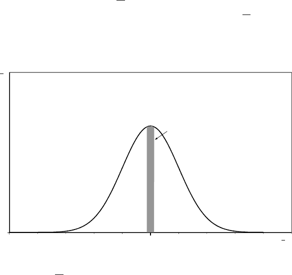
AR.1 A random variable Xhas a continuous uniform distribution from 0 to 2. Define its
probability density function.
X
( )
s.d. s.d.
acceptance regionrejection region rejection region
2.5%
2.5%
probability
density
0
2
X
AR.2 Find the expected value of Xin Exercise AR.1, using the expression given in Box
R.1 in the text.
AR.3 Derive E(X2) for Xdefined in Exercise AR.1, using the expression given in Box
R.1.
AR.4 Derive the population variance and the standard deviation of Xas defined in
Exercise AR.1, using the expression given in Box R.1.
AR.5 Using equation (R.9), find the variance of the random variable Xdefined in
Exercise AR.1 and show that the answer is the same as that obtained in Exercise
AR.4. (Note: You have already calculated E(X) in Exercise AR.2 and E(X2) in
Exercise AR.3.)
AR.6 In Table R.6, µ0and µ1were three standard deviations apart. Construct a similar
table for the case where they are two standard deviations apart.
10

0.15. Answers to the starred exercises in the textbook
AR.7 Suppose that a random variable Xhas a normal distribution with unknown mean µ
and variance σ2. To simplify the analysis, we shall assume that σ2is known. Given
a sample of observations, an estimator of µis the sample mean, X. An investigator
wishes to test H0:µ= 0 and believes that the true value cannot be negative. The
appropriate alternative hypothesis is therefore H1:µ > 0 and the investigator
decides to perform a one-sided test. However, the investigator is mistaken because
µcould in fact be negative. What are the consequences of erroneously performing a
one-sided test when a two-sided test would have been appropriate?
AR.8 Suppose that a random variable Xhas a normal distribution with mean µand
variance σ2. Given a sample of nindependent observations, it can be shown that:
bσ2=1
n−1XXi−X2
is an unbiased estimator of σ2. Is √bσ2either an unbiased or a consistent estimator
of σ?
0.15 Answers to the starred exercises in the textbook
R.2 A random variable Xis defined to be the larger of the two values when two dice
are thrown, or the value if the values are the same. Find the probability
distribution for X.
Answer:
The table shows the 36 possible outcomes. The probability distribution is derived
by counting the number of times each outcome occurs and dividing by 36. The
probabilities have been written as fractions, but they could equally well have been
written as decimals.
red123456
green
1 123456
2 223456
3 333456
4 444456
5 555556
6 666666
Value of X1 2 3 4 5 6
Frequency 1 3 5 7 9 11
Probability 1/36 3/36 5/36 7/36 9/36 11/36
11

Preface
R.4 Find the expected value of Xin Exercise R.2.
Answer:
The table is based on Table R.2 in the text. It is a good idea to guess the outcome
before doing the arithmetic. In this case, since the higher numbers have the largest
probabilities, the expected value should clearly lie between 4 and 5. If the
calculated value does not conform with the guess, it is possible that this is because
the guess was poor. However, it may be because there is an error in the arithmetic,
and this is one way of catching such errors.
X p Xp
1 1/36 1/36
2 3/36 6/36
3 5/36 15/36
4 7/36 28/36
5 9/36 45/36
6 11/36 66/36
Total 161/36 = 4.4722
R.7 Calculate E(X2) for Xdefined in Exercise R.2.
Answer:
The table is based on Table R.3 in the text. Given that the largest values of X2
have the highest probabilities, it is reasonable to suppose that the answer lies
somewhere in the range 15–30. The actual figure is 21.97.
X X2p X2p
1 1 1/36 1/36
2 4 3/36 12/36
3 9 5/36 45/36
4 16 7/36 112/36
5 25 9/36 225/36
6 36 11/36 396/36
Total 791/36 = 21.9722
R.10 Calculate the population variance and the standard deviation of Xas defined in
Exercise R.2, using the definition given by equation (R.8).
Answer:
The table is based on Table R.4 in the textbook. In this case it is not easy to make
a guess. The population variance is 1.97, and the standard deviation, its square
root, is 1.40. Note that four decimal places have been used in the working, even
though the estimate is reported to only two. This is to eliminate the possibility of
the estimate being affected by rounding error.
12

0.15. Answers to the starred exercises in the textbook
X p X −µX(X−µX)2(X−µX)2p
1 1/36 −3.4722 12.0563 0.3349
2 3/36 −2.4722 6.1119 0.5093
3 5/36 −1.4722 2.1674 0.3010
4 7/36 −0.4722 0.2230 0.0434
5 9/36 0.5278 0.2785 0.0696
6 11/36 1.5278 2.3341 0.7132
Total 1.9715
R.12 Using equation (R.9), find the variance of the random variable Xdefined in
Exercise R.2 and show that the answer is the same as that obtained in Exercise
R.10. (Note: You have already calculated µXin Exercise R.4 and E(X2) in
Exercise R.7.)
Answer:
E(X2) is 21.9722 (Exercise R.7). E(X) is 4.4722 (Exercise R.4), so µ2
Xis 20.0006.
Thus the variance is 21.9722 −20.0006 = 1.9716. The last-digit discrepancy
between this figure and that in Exercise R.10 is due to rounding error.
R.14 Suppose a variable Yis an exact linear function of X:
Y=λ+µX
where λand µare constants, and suppose that Zis a third variable. Show that
ρXZ =ρY Z
Answer:
We start by noting that Yi−Y=µXi−X. Then:
ρY Z =
EhYi−YZi−Zi
sEYi−Y2EZi−Z2
=
EhµXi−XZi−Zi
sEµ2Xi−X2Eµ2Zi−Z2
=
µE hXi−XZi−Zi
sµ2EXi−X2EZi−Z2
=ρXZ .
R.16 Show that, when you have nobservations, the condition that the generalised
estimator (λ1X1+··· +λnXn) should be an unbiased estimator of µXis
λ1+··· +λn= 1.
13

Preface
Answer:
E(Z) = E(λ1X1+··· +λnXn)
=E(λ1X1) + ··· +E(λnXn)
=λ1E(X1) + ··· +λnE(Xn)
=λ1µX+··· +λnµX
= (λ1+··· +λn)µX.
Thus E(Z) = µXrequires λ1+··· +λn= 1.
R.19 In general, the variance of the distribution of an estimator decreases when the
sample size is increased. Is it correct to describe the estimator as becoming more
efficient?
Answer:
No, it is incorrect. When the sample size increases, the variance of the estimator
decreases, and as a consequence it is more likely to give accurate results. Because it
is improving in this important sense, it is very tempting to describe the estimator
as becoming more efficient. But it is the wrong use of the term. Efficiency is a
comparative concept that is used when you are comparing two or more alternative
estimators, all of them being applied to the same data set with the same sample
size. The estimator with the smallest variance is said to be the most efficient. You
cannot use efficiency as suggested in the question because you are comparing the
variances of the same estimator with different sample sizes.
R.21 Suppose that you have observations on three variables X,Y, and Z, and suppose
that Yis an exact linear function of Z:
Y=λ+µZ
where λand µare constants. Show that bρXZ =bρXY . (This is the counterpart of
Exercise R.14.)
Answer:
We start by noting that Yi−Y=µZi−Z. Then:
bρXY =PXi−XYi−Y
rPXi−X2PYi−Y2
=PXi−XµZi−Z
rPXi−X2Pµ2Zi−Z2
=PXi−XZi−Z
rPXi−X2PZi−Z2
=bρXZ
14
0.15. Answers to the starred exercises in the textbook
R.26 Show that, in Figures R.18 and R.22, the probabilities of a Type II error are 0.15
in the case of a 5 per cent significance test and 0.34 in the case of a 1 per cent test.
Note that the distance between µ0and µ1is three standard deviations. Hence the
right-hand 5 per cent rejection region begins 1.96 standard deviations to the right
of µ0. This means that it is located 1.04 standard deviations to the left of µ1.
Similarly, for a 1 per cent test, the right-hand rejection region starts 2.58 standard
deviations to the right of µ0, which is 0.42 standard deviations to the left of µ1.
Answer:
For the 5 per cent test, the rejection region starts 3 −1.96 = 1.04 standard
deviations below µ1, given that the distance between µ1and µ0is 3 standard
deviations. See Figure R.18. According to the standard normal distribution table,
the cumulative probability of a random variable lying 1.04 standard deviations (or
less) above the mean is 0.8508. This implies that the probability of it lying 1.04
standard deviations below the mean is 0.1492. For the 1 per cent test, the rejection
region starts 3 −2.58 = 0.42 standard deviations below the mean. See Figure R.22.
The cumulative probability for 0.42 in the standard normal distribution table is
0.6628, so the probability of a Type II error is 0.3372.
R.27 Explain why the difference in the power of a 5 per cent test and a 1 per cent test
becomes small when the distance between µ0and µ1becomes large.
Answer:
The powers of both tests tend to one as the distance between µ0and µ1becomes
large. The difference in their powers must therefore tend to zero.
R.28 A random variable Xhas unknown population mean µ. A researcher has a sample
of observations with sample mean X. He wishes to test the null hypothesis
H0:µ=µ0. The figure shows the potential distribution of Xconditional on H0
being true. It may be assumed that the distribution is known to have variance
equal to one.
0
0
5% rejection region
X
f(X)
µ
0
The researcher decides to implement an unorthodox (and unwise) decision rule. He
decides to reject H0if Xlies in the central 5 per cent of the distribution (the tinted
area in the figure).
(a) Explain why his test is a 5 per cent significance test.
15
Preface
(b) Explain in intuitive terms why his test is unwise.
(c) Explain in technical terms why his test is unwise.
Answer:
The following discussion assumes that you are performing a 5 per cent significance
test, but it applies to any significance level.
If the null hypothesis is true, it does not matter how you define the 5 per cent
rejection region. By construction, the risk of making a Type I error will be 5 per
cent. Issues relating to Type II errors are irrelevant when the null hypothesis is true.
The reason that the central part of the conditional distribution is not used as a
rejection region is that it leads to problems when the null hypothesis is false. The
probability of not rejecting H0when it is false will be lower. To use the obvious
technical term, the power of the test will be lower.
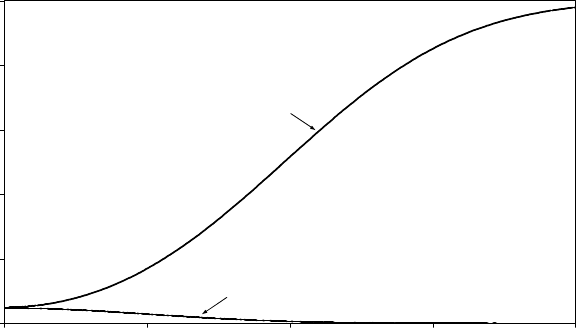
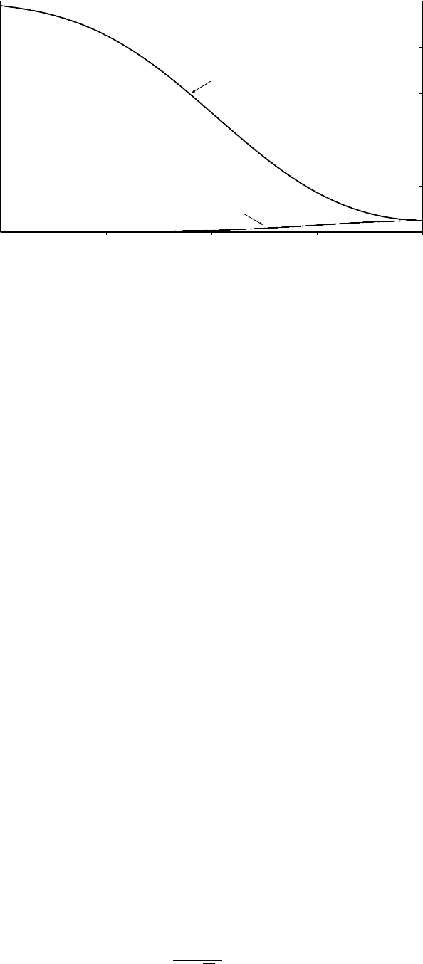
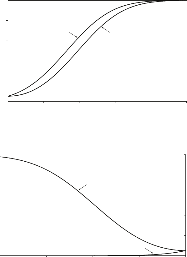
The figure shows the power functions for the test using the conventional upper and
lower 2.5 per cent tails and the test using the central region. The horizontal axis is
the difference between the true value and the hypothetical value µ0in terms of
standard deviations. The vertical axis is the power of the test. The first figure has
been drawn for the case where the true value is greater than the hypothetical value.
The second figure is for the case where the true value is lower than the hypothetical
value. It is the same, but reflected horizontally.
The greater the difference between the true value and the hypothetical mean, the
more likely is it that the sample mean will lie in the right tail of the distribution
conditional on H0being true, and so the more likely is it that the null hypothesis
will be rejected by the conventional test. The figure shows that the power of the
test approaches one asymptotically. However, if the central region of the
distribution is used as the rejection region, the probability of the sample mean
lying in it will diminish as the difference between the true and hypothetical values
increases, and the power of the test approaches zero asymptotically. This is an
extreme example of a very bad test procedure.
0.0
0.2
0.4
0.6
0.8
1.0
01234
conventional rejection region
(upper and lower 2.5% tails)
rejection region central 5%
Figure 1: Power functions of a conventional 5 per cent test and one using the central
region (true value > µ0).
16
0.15. Answers to the starred exercises in the textbook
0.0
0.2
0.4
0.6
0.8
1.0
-4 -3 -2 -1 0
conventional rejection region
(upper and lower 2.5% tails)
rejection region central 5%
Figure 2: Power functions of a conventional 5 per cent test and one using the central
region (true value < µ0).
R.29 A researcher is evaluating whether an increase in the minimum hourly wage has
had an effect on employment in the manufacturing industry in the following three
months. Taking a sample of 25 firms, what should she conclude if:
(a) the mean decrease in employment is 9 per cent, and the standard error of the
mean is 5 per cent
(b) the mean decrease is 12 per cent, and the standard error is 5 per cent
(c) the mean decrease is 20 per cent, and the standard error is 5 per cent
(d) there is a mean increase of 11 per cent, and the standard error is 5 per cent?
Answer:
There are 24 degrees of freedom, and hence the critical values of tat the 5 per cent,
1 per cent, and 0.1 per cent levels are 2.06, 2.80, and 3.75, respectively.
(a) The tstatistic is −1.80. Fail to reject H0at the 5 per cent level.
(b) t=−2.40. Reject H0at the 5 per cent level but not the 1 per cent level.
(c) t=−4.00. Reject H0at the 1 per cent level. Better, reject at the 0.1 per cent
level.
(d) t= 2.20. This would be a surprising outcome, but if one is performing a
two-sided test, then reject H0at the 5 per cent level but not the 1 per cent
level.
R3.33 Demonstrate that the 95 per cent confidence interval defined by equation (R.89)
has a 95 per cent probability of capturing µ0if H0is true.
Answer:
If H0is true, there is 95 per cent probability that:
X−µ0
s.e.(X)< tcrit.
17

Preface
Hence there is 95 per cent probability that |X−µ0|< tcrit ×s.e.(X). Hence there is
95 per cent probability that (a) X−µ0< tcrit ×s.e.(X) and (b)
µ0−X < tcrit ×s.e.(X).
(a) can be rewritten X−tcrit ×s.e.(X)< µ0, giving the lower limit of the confidence
interval.
(b) can be rewritten X−µ0>−tcrit ×s.e.(X) and hence X+tcrit ×s.e.(X)> µ0,
giving the upper limit of the confidence interval.
Hence there is 95 per cent probability that µ0will lie in the confidence interval.
R.34 In Exercise R.29, a researcher was evaluating whether an increase in the minimum
hourly wage has had an effect on employment in the manufacturing industry.
Explain whether she might have been justified in performing one-sided tests in
cases (a) – (d), and determine whether her conclusions would have been different.
Answer:
First, there should be a discussion of whether the effect of an increase in the
minimum wage could have a positive effect on employment. If it is decided that it
cannot, we can use a one-sided test and the critical values of tat the 5 per cent, 1
per cent, and 0.1 per cent levels become 1.71, 2.49, and 3.47, respectively.
1. The tstatistic is −1.80. We can now reject H0at the 5 per cent level.
2. t=−2.40. No change, but much closer to rejecting at the 1 per cent level.
3. t=−4.00. No change. Reject at the 1 per cent level (and 0.1 per cent level).
4. t= 2.20. Here there is a problem because the coefficient has the unexpected
sign. In principle we should stick to our guns and fail to reject H0. However,
we should consider two further possibilities. One is that the justification for a
one-sided test is incorrect (not very likely in this case). The other is that the
model is misspecified in some way and the misspecification is responsible for
the unexpected sign. For example, the coefficient might be distorted by
omitted variable bias, to be discussed in Chapter 6.
R.37 A random variable Xhas population mean µXand population variance σ2
X. A
sample of nobservations {X1, . . . , Xn}is generated. Using the plim rules,
demonstrate that, subject to a certain condition that should be stated:
plim 1
X=1
µX
.
Answer:
plim X=µXby the weak law of large numbers. Provided that µX6= 0, we are
entitled to use the plim quotient rule, so:
plim 1
X=plim 1
plim X=1
µX
.
18

0.15. Answers to the starred exercises in the textbook
R.39 A random variable Xhas unknown population mean µXand population variance
σ2
X. A sample of nobservations {X1, . . . , Xn}is generated. Show that:
Z=1
2X1+1
4X2+1
8X3+··· +1
2n−1+1
2n−1Xn
is an unbiased estimator of µX. Show that the variance of Zdoes not tend to zero
as ntends to infinity and that therefore Zis an inconsistent estimator, despite
being unbiased.
Answer:
The weights sum to unity, so the estimator is unbiased. However, its variance is:
σ2
Z=1
4+1
16 +··· +1
4n−1+1
4n−1σ2
X.
This tends to σ2
X/3 as nbecomes large, not zero, so the estimator is inconsistent.
Note: the sum of a geometric progression is given by:
1 + a+a2+··· +an=1−an+1
1−a.
Hence:
1
2+1
4+1
8+··· +1
2n−1+1
2n−1=1
21 + 1
2+··· +1
2n−2+1
2n−1
=1
2×1−1
2n−1
1−1
2
+1
2n−1
= 1 −1
2n−1+1
2n−1= 1
and:
1
4+1
16 +··· +1
4n−1+1
4n−1=1
41 + 1
4+··· +1
4n−2+1
4n−1
=1
4×1−1
4n−1
1−1
4
+1
4n−1
=1
3 1−1
4n−1!+1
4n−1→1
3
as nbecomes large.
R.41 A random variable Xhas a continuous uniform distribution over the interval from
0 to θ, where θis an unknown parameter.
19

Preface
0
0
θ
X
f (X)
The following three estimators are used to estimate θ, given a sample of n
observations on X:
(a) twice the sample mean
(b) the largest value of Xin the sample
(c) the sum of the largest and smallest values of Xin the sample.
Explain verbally whether or not each estimator is (1) unbiased, and (2) consistent.
Answer:
(a) It is evident that E(X) = E(X) = θ/2. Hence 2Xis an unbiased estimator of θ.
The variance of Xis σ2
X/n. The variance of 2Xis therefore 4σ2
X/n. This will
tend to zero as ntends to infinity. Thus the distribution of 2Xwill collapse to
a spike at θand the estimator is consistent.
(b) The estimator will be biased downwards since the highest value of Xin the
sample will always be less than θ. However, as nincreases, the distribution of
the estimator will be increasingly concentrated in a narrow range just below θ.
To put it formally, the probability of the highest value being more than
below θwill be 1−
θnand this will tend to zero, no matter how small is,
as ntends to infinity. The estimator is therefore consistent. It can in fact be
shown that the expected value of the estimator is n
n+1 θand this tends to θas n
becomes large.
(c) The estimator will be unbiased. Call the maximum value of Xin the sample
Xmax and the minimum value Xmin. Given the symmetry of the distribution of
X, the distributions of Xmax and Xmin will be identical, except that that of
Xmin will be to the right of 0 and that of Xmax will be to the left of θ. Hence,
for any n,E(Xmin)−0 = θ−E(Xmax) and the expected value of their sum is
equal to θ. The estimator will be consistent for the same reason as explained in
(b).
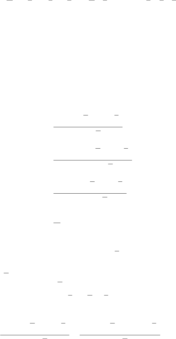
The first figure shows the distributions of the estimators (a) and (b) for 1,000,000
samples with only four observations in each sample, with θ= 1. The second figure
shows the distributions when the number of observations in each sample is equal to
20
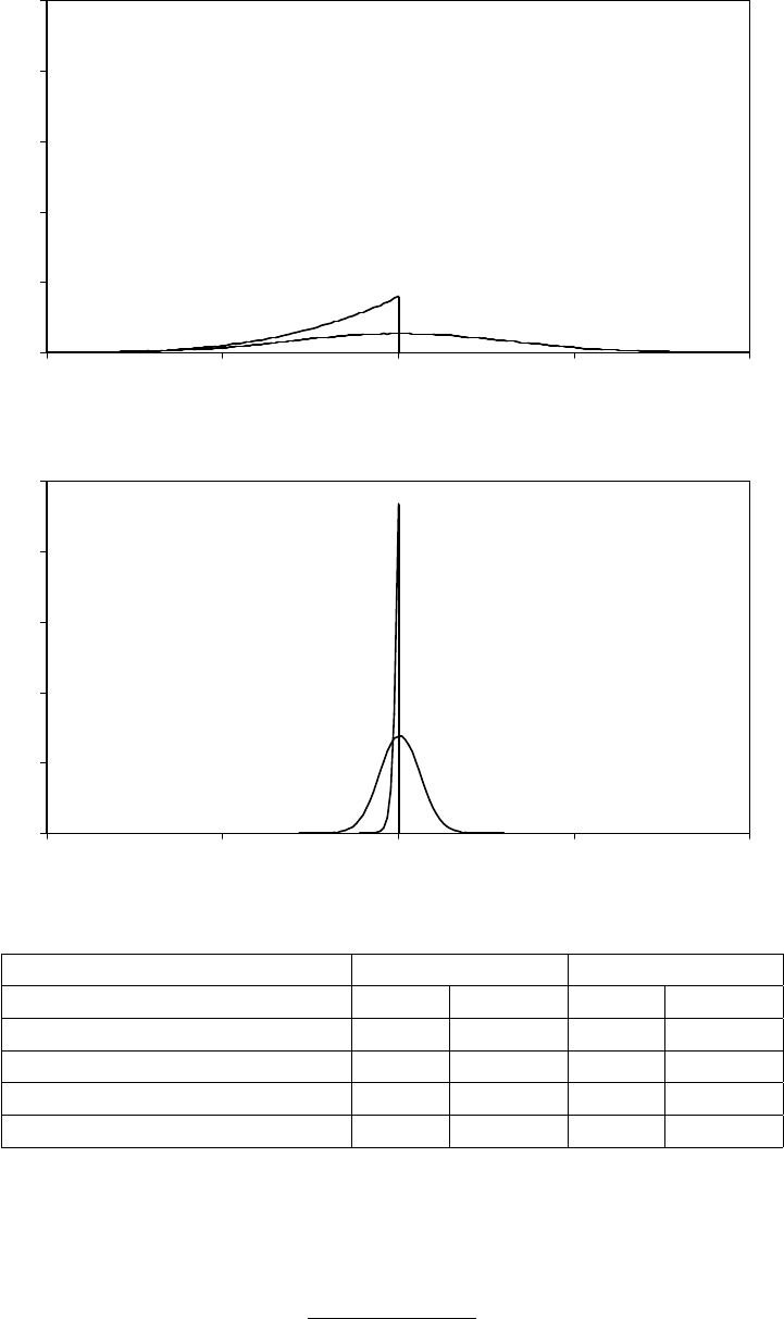
0.15. Answers to the starred exercises in the textbook
100. The table gives the means and variances of the distributions as computed from
the results of the simulations. If the mean square error is used to compare the
estimators, which should be preferred for sample size 4? For sample size 100?
0
5
10
15
20
25
0 0.5 1 1.5 2
0
5
10
15
20
25
0 0.5 1 1.5 2
(b)
(b)
(a)
(a)
Sample size = 4
Sample size = 100
Sample size 4 Sample size 100
(a) (b) (a) (b)
Mean 1.0000 0.8001 1.0000 0.9901
Variance 0.0833 0.0267 0.0033 0.0001
Estimated bias 0.0000 −0.1999 0.0000 −0.0099
Estimated mean square error 0.0833 0.0667 0.0033 0.0002
It can be shown (Larsen and Marx, An Introduction to Mathematical Statistics and
Its Applications, p.382, that estimator (b) is biased downwards by an amount
θ/(n+ 1) and that its variance is:
nθ2
(n+ 1)2(n+ 2)
21

Preface
while estimator (a) has variance θ2/3n. How large does nhave to be for (b) to be
preferred to (a) using the mean square error criterion?
The crushing superiority of (b) over (a) may come as a surprise, so accustomed are
we to finding that the sample mean in the best estimator of a parameter. The
underlying reason in this case is that we are estimating a boundary parameter,
which, as its name implies, defines the limit of a distribution. In such a case the
optimal properties of the sample mean are no longer guaranteed and it may be
eclipsed by a score statistic such as the largest observation in the sample. Note that
the standard deviation of the sample mean is inversely proportional to √n, while
that of (b) is inversely proportional to n(disregarding the differences between n,
n+ 1, and n+ 2). (b) therefore approaches its limiting (asymptotically unbiased)
value much faster than (a) and is said to be superconsistent. We will encounter
superconsistent estimators again when we come to cointegration in Chapter 13.
Note that if we multiply (b) by (n+ 1)/n, it is unbiased for finite samples as well
as superconsistent.
0.16 Answers to the additional exercises
AR.1 The total area under the function over the interval [0,2] must be equal to 1. Since
the length of the rectangle is 2, its height must be 0.5. Hence f(X) = 0.5 for
0≤X≤2, and f(X) = 0 for X < 0 and X > 2.
AR.2 Obviously, since the distribution is uniform, the expected value of Xis 1. However
we will derive this formally.
E(X) = Z2
0
Xf(X) dX=Z2
0
0.5XdX=X2
42
0
=22
4−02
4= 1.
AR.3 The expected value of X2is given by:
E(X2) = Z2
0
X2f(X) dX=Z2
0
0.5X2dX=X3
62
0
=23
6−03
6= 1.3333.
AR.4 The variance of Xis given by:
E[X−µX]2=Z2
0
[X−µX]2f(X) dX=Z2
0
0.5[X−1]2dX
=Z2
0
(0.5X2−X+ 0.5) dX
=X3
6−X2
2+X
22
0
=8
6−2+1−[0] = 0.3333.
The standard deviation is equal to the square root, 0.5774.
22

0.16. Answers to the additional exercises
AR.5 From Exercise AR.3, E(X2)=1.3333. From Exercise AR.2, the square of E(X) is
1. Hence the variance is 0.3333, as in Exercise AR.4.
AR.6 Table R.6 is reproduced for reference:
Table R.6 Trade-off between Type I and Type II errors, one-sided and two-sided tests
Probability of Type II error if µ=µ1
One-sided test Two-sided test
5 per cent significance test 0.09 0.15
2.5 per cent significance test 0.15 (not investigated)
1 per cent significance test 0.25 0.34
Note: The distance between µ1and µ0in this example was 3 standard deviations.
Two-sided tests
Under the (false) H0:µ=µ0, the right rejection region for a two-sided 5 per cent
significance test starts 1.96 standard deviations above µ0, which is 0.04 standard
deviations below µ1. A Type II error therefore occurs if Xis more than 0.04
standard deviations to the left of µ1. Under H1:µ=µ1, the probability is 0.48.
Under H0, the right rejection region for a two-sided 1 per cent significance test
starts 2.58 standard deviations above µ0, which is 0.58 standard deviations above
µ1. A Type II error therefore occurs if Xis less than 0.58 standard deviations to
the right of µ1. Under H1:µ=µ1, the probability is 0.72.
One-sided tests
Under H0:µ=µ0, the right rejection region for a one-sided 5 per cent significance
test starts 1.65 standard deviations above µ0, which is 0.35 standard deviations
below µ1. A Type II error therefore occurs if Xis more than 0.35 standard
deviations to the left of µ1. Under H1:µ=µ1, the probability is 0.36.
Under H0, the right rejection region for a one-sided 1 per cent significance test
starts 2.33 standard deviations above µ0, which is 0.33 standard deviations above
µ1. A Type II error therefore occurs if Xis less than 0.33 standard deviations to
the right of µ1. Under H1:µ=µ1, the probability is 0.63.
Hence the table is:
Trade-off between Type I and Type II errors, one-sided and two-sided tests
Probability of Type II error if µ=µ1
One-sided test Two-sided test
5 per cent significance test 0.36 0.48
1 per cent significance test 0.63 0.72
AR.7 We will assume for sake of argument that the investigator is performing a 5 per
cent significance test, but the conclusions apply to all significance levels.
If the true value is 0, the null hypothesis is true. The risk of a Type I error is, by
construction, 5 per cent for both one-sided and two-sided tests. Issues relating to
Type II error do not arise because the null hypothesis is true.
23
Preface
If the true value is positive, the investigator is lucky and makes the gain associated
with a one-sided test. Namely, the power of the test is uniformly higher than that
for a two-sided test for all positive values of µ. The power functions for one-sided
and two-sided tests are shown in the first figure below.
If the true value is negative, the power functions are as shown in the second figure.
That for the two-sided test is the same as that in the first figure, but reflected
horizontally. The larger (negatively) is the true value of µ, the greater will be the
probability of rejecting H0and the power approaches 1 asymptotically. However,
with a one-sided test, the power function will decrease from its already very low
value. The power is not automatically zero for true values that are negative because
even for these it is possible that a sample might have a mean that lies in the right
tail of the distribution under the null hypothesis. But the probability rapidly falls
to zero as the (negative) size of µgrows.
0.0
0.2
0.4
0.6
0.8
1.0
0 1 2 3 4 5
one-sided 5% test
two-sided 5% test
Figure 3: Power functions of one-sided and two-sided 5 per cent tests (true value >0).
0.0
0.2
0.4
0.6
0.8
1.0
-4 -3 -2 -1 0
one-sided 5% test
two-sided 5% test
!
Figure 4: Power functions of one-sided and two-sided 5 per cent tests (true value <0).
24

0.16. Answers to the additional exercises
AR.8 We will refute the unbiasedness proposition by considering the more general case
where Z2is an unbiased estimator of θ2. We know that:
E(Z−θ)2=E(Z2)−2θE(Z) + θ2= 2θ2−2θE(Z).
Hence:
E(Z) = θ−1
2θE(Z−θ)2.
Zis therefore a biased estimator of θexcept for the special case where Zis equal
to θfor all samples, that is, in the trivial case where there is no sampling error.
Nevertheless, since a function of a consistent estimator will, under quite general
conditions, be a consistent estimator of the function of the parameter, √bσ2will be
a consistent estimator of σ.
25
Preface
26

Chapter 1
Simple regression analysis
1.1 Overview
This chapter introduces the least squares criterion of goodness of fit and demonstrates,
first through examples and then in the general case, how it may be used to develop
expressions for the coefficients that quantify the relationship when a dependent variable
is assumed to be determined by one explanatory variable. The chapter continues by
showing how the coefficients should be interpreted when the variables are measured in
natural units, and it concludes by introducing R2, a second criterion of goodness of fit,
and showing how it is related to the least squares criterion and the correlation between
the fitted and actual values of the dependent variable.
1.2 Learning outcomes
After working through the corresponding chapter in the text, studying the
corresponding slideshows, and doing the starred exercises in the text and the additional
exercises in this subject guide, you should be able to explain what is meant by:
dependent variable
explanatory variable (independent variable, regressor)
parameter of a regression model
the nonstochastic component of a true relationship
the disturbance term
the least squares criterion of goodness of fit
ordinary least squares (OLS)
the regression line
fitted model
fitted values (of the dependent variable)
residuals
total sum of squares, explained sum of squares, residual sum of squares
R2.
27

1. Simple regression analysis
In addition, you should be able to explain the difference between:
the nonstochastic component of a true relationship and a fitted regression line, and
the values of the disturbance term and the residuals.
1.3 Additional exercises
A1.1 The output below gives the result of regressing FDHO, annual household
expenditure on food consumed at home, on EXP, total annual household
expenditure, both measured in dollars, using the Consumer Expenditure Survey
data set. Give an interpretation of the coefficients.
. reg FDHO EXP if FDHO>0
Source | SS df MS Number of obs = 6334
-------------+------------------------------ F( 1, 6332) = 3431.01
Model | 972602566 1 972602566 Prob > F = 0.0000
Residual | 1.7950e+09 6332 283474.003 R-squared = 0.3514
-------------+------------------------------ Adj R-squared = 0.3513
Total | 2.7676e+09 6333 437006.15 Root MSE = 532.42
------------------------------------------------------------------------------
FDHO | Coef. Std. Err. t P>|t| [95% Conf. Interval]
-------------+----------------------------------------------------------------
EXP | .0627099 .0010706 58.57 0.000 .0606112 .0648086
_cons | 369.4418 10.65718 34.67 0.000 348.5501 390.3334
------------------------------------------------------------------------------
A1.2 Download the CES data set from the website (see Appendix B of the text),
perform a regression parallel to that in Exercise A1.1 for your category of
expenditure, and provide an interpretation of the regression coefficients.
A1.3 The output shows the result of regressing the weight of the respondent, in pounds,
in 2011 on the weight in 2004, using EAWE Data Set 22. Provide an interpretation
of the coefficients. Summary statistics for the data are also provided.
. reg WEIGHT11 WEIGHT04
Source | SS df MS Number of obs = 500
-------------+------------------------------ F( 1, 498) = 1207.55
Model | 769248.875 1 769248.875 Prob > F = 0.0000
Residual | 317241.693 498 637.031513 R-squared = 0.7080
-------------+------------------------------ Adj R-squared = 0.7074
Total | 1086490.57 499 2177.33581 Root MSE = 25.239
------------------------------------------------------------------------------
WEIGHT11 | Coef. Std. Err. t P>|t| [95% Conf. Interval]
-------------+----------------------------------------------------------------
WEIGHT04 | .9739736 .0280281 34.75 0.000 .9189056 1.029042
_cons | 17.42232 4.888091 3.56 0.000 7.818493 27.02614
------------------------------------------------------------------------------
28
1.3. Additional exercises
. sum WEIGHT04 WEIGHT11
Variable | Obs Mean Std. Dev. Min Max
-------------+--------------------------------------------------------
WEIGHT04 | 500 169.686 40.31215 95 330
WEIGHT11 | 500 182.692 46.66193 95 370
A1.4 The output shows the result of regressing the hourly earnings of the respondent, in
dollars, in 2011 on height in 2004, measured in inches, using EAWE Data Set 22.
Provide an interpretation of the coefficients, comment on the plausibility of the
interpretation, and attempt to give an explanation.
. reg EARNINGS HEIGHT
Source | SS df MS Number of obs = 500
-------------+------------------------------ F( 1, 498) = 9.23
Model | 1393.77592 1 1393.77592 Prob > F = 0.0025
Residual | 75171.3726 498 150.946531 R-squared = 0.0182
-------------+------------------------------ Adj R-squared = 0.0162
Total | 76565.1485 499 153.437171 Root MSE = 12.286
------------------------------------------------------------------------------
EARNINGS | Coef. Std. Err. t P>|t| [95% Conf. Interval]
-------------+----------------------------------------------------------------
HEIGHT | .4087231 .1345068 3.04 0.003 .1444523 .6729938
_cons | -9.26923 9.125089 -1.02 0.310 -27.19765 8.659188
------------------------------------------------------------------------------
A1.5 A researcher has data for 50 countries on N, the average number of newspapers
purchased per adult in one year, and G, GDP per capita, measured in US $, and
fits the following regression (RSS = residual sum of squares):
b
N= 25.0+0.020G R2= 0.06,RSS = 4,000.0
The researcher realises that GDP has been underestimated by $100 in every
country and that Nshould have been regressed on G∗, where G∗=G+ 100.
Explain, with mathematical proofs, how the following components of the output
would have differed:
•the coefficient of GDP
•the intercept
•RSS
•R2.
A1.6 A researcher with the same model and data as in Exercise A1.5 believes that GDP
in each country has been underestimated by 50 per cent and that Nshould have
been regressed on G∗, where G∗= 2G. Explain, with mathematical proofs, how the
following components of the output would have differed:
•the coefficient of GDP
•the intercept
•RSS
•R2.
29

1. Simple regression analysis
A1.7 Some practitioners of econometrics advocate ‘standardising’ each variable in a
regression by subtracting its sample mean and dividing by its sample standard
deviation. Thus, if the original regression specification is:
Yi=β1+β2Xi+ui
the revised specification is:
Y∗
i=β∗
1+β∗
2X∗
i+vi
where:
Y∗
i=Yi−Y
bσY
and X∗
i=Xi−X
bσX
Yand Xare the sample means of Yand X,bσYand bσXare the estimators of the
standard deviations of Yand X, defined as the square roots of the estimated
variances:
bσ2
Y=1
n−1
n
X
i=1
(Yi−Y)2and bσ2
X=1
n−1
n
X
i=1
(Xi−X)2
and nis the number of observations in the sample. We will write the fitted models
for the two specifications as: b
Yi=b
β1+b
β2Xi
and: b
Y∗
i=b
β∗
1+b
β∗
2X∗
i.
Taking account of the definitions of Y∗and X∗, show that b
β∗
1= 0 and that
b
β∗
2=bσX
bσYb
β2. Provide an interpretation of b
β∗
2.
A1.8 For the model described in Exercise A1.7, suppose that Y∗is regressed on X∗
without an intercept: b
Y∗
i=b
β∗∗
2X∗
i.
Determine how b
β∗∗
2is related to b
β∗
2.
A1.9 A variable Yiis generated as:
Yi=β1+ui(1.1)
where β1is a fixed parameter and uiis a disturbance term that is independently
and identically distributed with expected value 0 and population variance σ2
u. The
least squares estimator of β1is Y, the sample mean of Y. Give a mathematical
demonstration that the value of R2in such a regression is zero.
1.4 Answers to the starred exercises in the textbook
1.9 The output shows the result of regressing the weight of the respondent in 2004,
measured in pounds, on his or her height, measured in inches, using EAWE Data
Set 21. Provide an interpretation of the coefficients.
30

1.4. Answers to the starred exercises in the textbook
. reg WEIGHT04 HEIGHT
Source | SS df MS Number of obs = 500
-------------+------------------------------ F( 1, 498) = 176.74
Model | 211309 1 211309 Prob > F = 0.0000
Residual | 595389.95 498 1195.56215 R-squared = 0.2619
-------------+------------------------------ Adj R-squared = 0.2605
Total | 806698.98 499 1616.63116 Root MSE = 34.577
------------------------------------------------------------------------------
WEIGHT04 | Coef. Std. Err. t P>|t| [95% Conf. Interval]
-------------+----------------------------------------------------------------
HEIGHT | 5.073711 .381639 13.29 0.000 4.32389 5.823532
_cons | -177.1703 25.93501 -6.83 0.000 -228.1258 -126.2147
------------------------------------------------------------------------------
Answer:
Literally the regression implies that, for every extra inch of height, an individual
tends to weigh an extra 5.1 pounds. The intercept, which literally suggests that an
individual with no height would weigh −177 pounds, has no meaning.
1.11 A researcher has international cross-sectional data on aggregate wages, W,
aggregate profits, P, and aggregate income, Y, for a sample of ncountries. By
definition:
Yi=Wi+Pi.
The regressions:
c
Wi=bα1+bα2Yi
b
Pi=b
β1+b
β2Yi
are fitted using OLS regression analysis. Show that the regression coefficients will
automatically satisfy the following equations:
bα2+b
β2= 1
bα1+b
β1= 0.
Explain intuitively why this should be so.
Answer:
bα2+b
β2=PYi−YWi−W
PYi−Y2+PYi−YPi−P
PYi−Y2
=PYi−YWi+Pi−W−P
PYi−Y2
=PYi−YYi−Y
PYi−Y2
= 1
31
1. Simple regression analysis
bα1+b
β1=W−bα2Y+P−b
β2Y=W+P−(bα2+b
β2)Y=Y−Y= 0.
The intuitive explanation is that the regressions break down income into predicted
wages and profits and one would expect the sum of the predicted components of
income to be equal to its actual level. The sum of the predicted components is
c
Wi+b
Pi= (bα1+bα2Yi)+(b
β1+b
β2Yi), and in general this will be equal to Yionly if
the two conditions are satisfied.
1.13 Suppose that the units of measurement of Xare changed so that the new measure,
X∗, is related to the original one by X∗
i=µ2Xi. Show that the new estimate of the
slope coefficient is b
β2/µ2, where b
β2is the slope coefficient in the original regression.
Answer:
b
β∗
2=PX∗
i−X∗Yi−Y
PX∗
i−X∗2
=Pµ2Xi−µ2XYi−Y
Pµ2Xi−µ2X2
=
µ2PXi−XYi−Y
µ2
2PXi−X2
=b
β2
µ2
.
1.14 Demonstrate that if Xis demeaned but Yis left in its original units, the intercept
in a regression of Yon demeaned Xwill be equal to Y.
Answer:
Let X∗
i=Xi−Xand b
β∗
1and b
β∗
2be the intercept and slope coefficient in a
regression of Yon X∗. Note that X∗= 0. Then:
b
β∗
1=Y−b
β∗
2X∗=Y.
The slope coefficient is not affected by demeaning:
b
β∗
2=PX∗
i−X∗Yi−Y
PX∗
i−X∗2=P[Xi−X]−0Yi−Y
P[Xi−X]−02=b
β2.
1.15 The regression output shows the result of regressing weight on height using the
same sample as in Exercise 1.9, but with weight and height measured in kilos and
centimetres: WMETRIC = 0.454 ∗WEIGHT04 and HMETRIC = 2.54 ∗HEIGHT .
Confirm that the estimates of the intercept and slope coefficient are as should be
expected from the changes in the units of measurement.
32

1.4. Answers to the starred exercises in the textbook
. gen WTMETRIC = 0.454*WEIGHT04
. gen HMETRIC = 2.54*HEIGHT
. reg WTMETRIC HMETRIC
Source | SS df MS Number of obs = 500
-------------+------------------------------ F( 1, 498) = 176.74
Model | 43554.1641 1 43554.1641 Prob > F = 0.0000
Residual | 122719.394 498 246.424486 R-squared = 0.2619
-------------+------------------------------ Adj R-squared = 0.2605
Total | 166273.558 499 333.213544 Root MSE = 15.698
------------------------------------------------------------------------------
WMETRIC | Coef. Std. Err. t P>|t| [95% Conf. Interval]
-------------+----------------------------------------------------------------
HMETRIC | .9068758 .0682142 13.29 0.000 .7728527 1.040899
_cons | -80.43529 11.77449 -6.83 0.000 -103.5691 -57.30148
------------------------------------------------------------------------------
Answer:
Abbreviate WEIGHT04 to W,HEIGHT to H,WMETRIC to W M, and
HMETRIC to HM.W M = 0.454Wand HM = 2.54H. The slope coefficient and
intercept for the regression in metric units, b
βM
2and b
βM
1, are then given by:
b
βM
2=PHMi−HMW Mi−W M
PHMi−HM2
=P2.54 Hi−H0.454 Wi−W
P2.542Hi−H2
= 0.179PHi−HWi−W
PHi−H2
= 0.179b
β2
= 0.179 ×5.074
= 0.908
b
βM
1=W M −b
βM
2HM
= 0.454W−0.454
2.54 b
β2(2.54H)
= 0.454(W−b
β2H)
= 0.454b
β1
= 0.454 × −177.2
=−80.4.
33

1. Simple regression analysis
The regression output confirms that the calculations are correct (subject to
rounding error in the last digit).
1.16 Consider the regression model:
Yi=β1+β2Xi+ui.
It implies:
Y=β1+β2X+u
and hence that:
Y∗
i=β2X∗
i+vi
where Y∗
i=Yi−Y,X∗
i=Xi−Xand vi=ui−u.
Demonstrate that a regression of Y∗on X∗using (1.49) will yield the same
estimate of the slope coefficient as a regression of Yon X. Note: (1.49) should be
used instead of (1.35) because there is no intercept in this model.
Evaluate the outcome if the slope coefficient were estimated using (1.35), despite
the fact that there is no intercept in the model.
Determine the estimate of the intercept if Y∗were regressed on X∗with an
intercept included in the regression specification.
Answer:
Let b
β∗
2be the slope coefficient in a regression of Y∗on X∗using (1.49). Then:
b
β∗
2=PX∗
iY∗
i
PX∗2
i
=PXi−XYi−Y
PXi−X2=b
β2.
Let b
β∗∗
2be the slope coefficient in a regression of Y∗on X∗using (1.35). Note that
Y∗and X∗are both zero. Then:
b
β∗∗
2=PX∗
i−X∗Y∗
i−Y∗
PX∗
i−X∗2=PX∗
iY∗
i
PX∗2
i
=b
β2.
Let b
β∗∗
1be the intercept in a regression of Y∗on X∗using (1.35). Then:
b
β∗∗
1=Y∗−b
β∗∗
2X∗= 0.
1.18 Demonstrate that the fitted values of the dependent variable are uncorrelated with
the residuals in a simple regression model. (This result generalises to the multiple
regression case.)
Answer:
The numerator of the sample correlation coefficient for b
Yand bucan be decomposed
as follows, using the fact that bu= 0:
1
nXb
Yi−b
Ybui−bu=1
nX[b
β1+b
β2Xi]−[b
β1+b
β2X]bui
=1
nb
β2XXi−Xbui
= 0
34

1.5. Answers to the additional exercises
by (1.65). Hence the correlation is zero.
1.23 Demonstrate that, in a regression with an intercept, a regression of Yon X∗must
have the same R2as a regression of Yon X, where X∗=µ2X.
Answer:
Let the fitted regression of Yon X∗be written b
Y∗
i=b
β∗
1+b
β∗
2X∗
i.b
β∗
2=b
β2/µ2
(Exercise 1.13).
b
β∗
1=Y−b
β∗
2X∗=Y−b
β2
µ2
µ2X=b
β1.
Hence:
b
Y∗
i=b
β1+b
β2
µ2
µ2Xi=b
Yi.
The fitted and actual values of Yare not affected by the transformation and so R2
is unaffected.
1.25 The output shows the result of regressing weight in 2011 on height, using EAWE
Data Set 21. In 2011 the respondents were aged 27–31. Explain why R2is lower
than in the regression reported in Exercise 1.9.
. reg WEIGHT11 HEIGHT
Source | SS df MS Number of obs = 500
-------------+------------------------------ F( 1, 498) = 139.97
Model | 236642.736 1 236642.736 Prob > F = 0.0000
Residual | 841926.912 498 1690.61629 R-squared = 0.2194
-------------+------------------------------ Adj R-squared = 0.2178
Total | 1078569.65 499 2161.46222 Root MSE = 41.117
------------------------------------------------------------------------------
WEIGHT11 | Coef. Std. Err. t P>|t| [95% Conf. Interval]
-------------+----------------------------------------------------------------
HEIGHT | 5.369246 .4538259 11.83 0.000 4.477597 6.260895
_cons | -184.7802 30.8406 -5.99 0.000 -245.3739 -124.1865
------------------------------------------------------------------------------
Answer:
The explained sum of squares is actually higher than that in Exercise 1.9. The
reason for the fall in R2is the huge increase in the total sum of squares, no doubt
caused by the cumulative effect of variations in eating habits.
1.5 Answers to the additional exercises
A1.1 Expenditure on food consumed at home increases by 6.3 cents for each dollar of
total household expenditure. Literally the intercept implies that $369 would be
spent on food consumed at home if total household expenditure were zero.
Obviously, such an interpretation does not make sense. If the explanatory variable
were income, and household income were zero, positive expenditure on food at
home would still be possible if the household received food stamps or other
transfers, but here the explanatory variable is total household expenditure.
35

1. Simple regression analysis
A1.2 For each category, the regression sample has been restricted to households with
non-zero expenditure. All the slope coefficients are highly significant. Housing has
the largest coefficient, as one should expect. Surprisingly, it is followed by
education. However, most households spent nothing at all on this category. For
those that did, it was important.
EXP
nb
β2R2
ADM 2,815 0.0235 0.228
CLOT 4,500 0.0316 0.176
DOM 1,661 0.0409 0.134
EDUC 561 0.1202 0.241
ELEC 5,828 0.0131 0.180
FDAW 5,102 0.0527 0.354
FDHO 6,334 0.0627 0.351
FOOT 1,827 0.0058 0.082
FURN 487 0.0522 0.102
GASO 5,710 0.0373 0.278
HEAL 4,802 0.0574 0.174
HOUS 6,223 0.1976 0.469
LIFE 1,253 0.0193 0.101
LOCT 692 0.0068 0.059
MAPP 399 0.0329 0.102
PERS 3,817 0.0069 0.213
READ 2,287 0.0048 0.104
SAPP 1,037 0.0045 0.034
TELE 5,788 0.0160 0.268
TEXT 992 0.0040 0.051
TOB 1,155 0.0165 0.088
TOYS 2,504 0.0145 0.076
TRIP 516 0.0466 0.186
A1.3 The summary data indicate that, on average, the respondents put on 13 pounds
over the period 2004–2011. Was this due to the relatively heavy becoming even
heavier, or to a general increase in weight? The regression output indicates that
weight in 2011 was approximately equal to weight in 2004 plus 17 pounds, so the
second explanation appears to be the correct one. Note that this is an instance
where the constant term can be given a meaningful interpretation and where it is as
of much interest as the slope coefficient. The R2indicates that 2004 weight accounts
for 71 per cent of the variance in 2011 weight, so other factors are important.
A1.4 The slope coefficient indicates that hourly earnings increase by 41 cents for every
extra inch of height. The negative intercept has no possible interpretation. The
interpretation of the slope coefficient is obviously highly implausible, so we know
that something must be wrong with the model. The explanation is that this is a
very poorly specified earnings function and that, in particular, we are failing to
control for the sex of the respondent. Later on, in Chapter 5, we will find that
36

1.5. Answers to the additional exercises
males earn more than females, controlling for observable characteristics. Males also
tend to be taller. Hence we find an apparent positive association between earnings
and height in a simple regression. Note that R2is very low.
A1.5 The coefficient of GDP: Let the revised measure of GDP be denoted G∗, where
G∗=G+ 100. Since G∗
i=Gi+ 100 for all i,G∗=G+ 100 and so G∗
i−G∗=Gi−G
for all i. Hence the new slope coefficient is:
b
β∗
2=PG∗
i−G∗Ni−N
PG∗
i−G∗2=PGi−GNi−N
PGi−G2=b
β2.
The coefficient is unchanged.
The intercept: The new intercept is:
b
β∗
1=N−b
β∗
2G∗=N−b
β2G+ 100=b
β1−100b
β2= 23.0.
RSS: The residual in observation iin the new regression, bu∗
i, is given by:
bu∗
i=Ni−b
β∗
1−b
β∗
2G∗
i=Ni−(b
β1−100b
β2)−b
β2(Gi+ 100) = bui
the residual in the original regression. Hence RSS is unchanged.
R2:
R2= 1 −RSS
PNi−N2
and is unchanged since RSS and PNi−N2are unchanged.
Note that this makes sense intuitively. R2is unit-free and so it is not possible for
the overall fit of a relationship to be affected by the units of measurement.
A1.6 The coefficient of GDP: Let the revised measure of GDP be denoted G∗, where
G∗= 2G. Since G∗
i= 2Gifor all i,G∗= 2Gand so G∗
i−G∗= 2 Gi−Gfor all i.
Hence the new slope coefficient is:
b
β∗
2=PG∗
i−G∗Ni−N
PG∗
i−G∗2
=P2Gi−GNi−N
P4Gi−G2
=
2PGi−GNi−N
4PGi−G2
=b
β2
2
= 0.010
37

1. Simple regression analysis
where b
β2= 0.020 is the slope coefficient in the original regression.
The intercept: The new intercept is:
b
β∗
1=N−b
β∗
2G∗=N−b
β2
22G=N−b
β2G=b
β1= 25.0
the original intercept.
RSS: The residual in observation iin the new regression, bu∗
i, is given by:
bu∗
i=Ni−b
β∗
1−b
β∗
2G∗
i=Ni−b
β1−b
β2
22Gi=bui
the residual in the original regression. Hence RSS is unchanged.
R2:
R2= 1 −RSS
PNi−N2
and is unchanged since RSS and PNi−N2are unchanged. As in Exercise A1.6,
this makes sense intuitively.
A1.7 By construction, Y∗=X∗= 0. So b
β∗
1=Y∗−b
β∗
2X∗= 0.
b
β∗
2=PX∗
i−X∗Y∗
i−Y∗
PX∗
i−X∗2
=PX∗
iY∗
i
PX∗2
i
=PXi−¯
X
bσXYi−¯
Y
bσY
PXi−¯
X
bσX2
=bσX
bσYPXi−XYi−Y
PXi−X2
=bσX
bσYb
β2.
b
β∗
2provides an estimate of the effect on Y, in terms of standard deviations of Y, of
a one-standard deviation change in X.
A1.8 We have:
b
β∗∗
2=PX∗
iY∗
i
PX∗2
i
=PX∗
i−X∗Y∗
i−Y∗
PX∗
i−X∗2=b
β∗
2.
38

1.5. Answers to the additional exercises
A1.9 We have:
R2=Pb
Yi−Y2
PYi−Y2
and b
Yi=Yfor all i.
39
1. Simple regression analysis
40

Chapter 2
Properties of the regression
coefficients and hypothesis testing
2.1 Overview
Chapter 1 introduced least squares regression analysis, a mathematical technique for
fitting a relationship given suitable data on the variables involved. It is a fundamental
chapter because much of the rest of the text is devoted to extending the least squares
approach to handle more complex models, for example models with multiple explanatory
variables, nonlinear models, and models with qualitative explanatory variables.
However, the mechanics of fitting regression equations are only part of the story. We are
equally concerned with assessing the performance of our regression techniques and with
developing an understanding of why they work better in some circumstances than in
others. Chapter 2 is the starting point for this objective and is thus equally
fundamental. In particular, it shows how two of the three main criteria for assessing the
performance of estimators, unbiasedness and efficiency, are applied in the context of a
regression model. The third criterion, consistency, will be considered in Chapter 8.
2.2 Learning outcomes
After working through the corresponding chapter in the text, studying the
corresponding slideshows, and doing the starred exercises in the text and the additional
exercises in this subject guide, you should be able to explain what is meant by:
cross-sectional, time series, and panel data
unbiasedness of OLS regression estimators
variance and standard errors of regression coefficients and how they are determined
Gauss–Markov theorem and efficiency of OLS regression estimators
two-sided ttests of hypotheses relating to regression coefficients and one-sided t
tests of hypotheses relating to regression coefficients
Ftests of goodness of fit of a regression equation
in the context of a regression model. The chapter is a long one and you should take
your time over it because it is essential that you develop a perfect understanding of
every detail.
41

2. Properties of the regression coefficients and hypothesis testing
2.3 Further material
Derivation of the expression for the variance of the na¨ıve estimator in
Section 2.3.
The variance of the na¨ıve estimator in Section 2.3 and Exercise 2.9 is not of any great
interest in itself, but its derivation provides an example of how one obtains expressions
for variances of estimators in general.
In Section 2.3 we considered the na¨ıve estimator of the slope coefficient derived by
joining the first and last observations in a sample and calculating the slope of that line:
b
β2=Yn−Y1
Xn−X1
.
It was demonstrated that the estimator could be decomposed as:
b
β2=β2+un−u1
Xn−X1
and hence that E(b
β2) = β2.
The population variance of a random variable Xis defined to be E([X−µX]2) where
µX=E(X). Hence the population variance of b
β2is given by:
σ2
b
β2=E[b
β2−β2]2=E β2+un−u1
Xn−X1−β22!=E un−u1
Xn−X12!.
On the assumption that Xis nonstochastic, this can be written as:
σ2
b
β2=1
Xn−X12
E[un−u1]2.
Expanding the quadratic, we have:
σ2
b
β2=1
Xn−X12
Eu2
n+u2
1−2unu1
=1
Xn−X12E(u2
n) + E(u2
1)−2E(unu1).
Each value of the disturbance term is drawn randomly from a distribution with mean 0
and population variance σ2
u, so E(u2
n) and E(u2
1) are both equal to σ2
u.unand u1are
drawn independently from the distribution, so E(unu1) = E(un)E(u1) = 0. Hence:
σ2
b
β2=2σ2
u
(Xn−X1)2=σ2
u
1
2(Xn−X1)2.
42

2.4. Additional exercises
Define A=1
2(X1+Xn), the average of X1and Xn, and D=Xn−A=A−X1. Then:
1
2(Xn−X1)2=1
2(Xn−A+A−X1)2
=1
2(Xn−A)2+ (A−X1)2+ 2(Xn−A)(A−X1)
=1
2D2+D2+ 2(D)(D)= 2D2
= (Xn−A)2+ (A−X1)2
= (Xn−A)2+ (X1−A)2
= (Xn−X+X−A)2+ (X1−X+X−A)2
= (Xn−X)2+ (X−A)2+ 2(Xn−X)(X−A)
+(X1−X)2+ (X−A)2+ 2(X1−X)(X−A)
= (X1−X)2+ (Xn−X)2+ 2(X−A)2+ 2(X1+Xn−2X)(X−A)
= (X1−X)2+ (Xn−X)2+ 2(X−A)2+ 2(2A−2X)(X−A)
= (X1−X)2+ (Xn−X)2−2(X−A)2
= (X1−X)2+ (Xn−X)2−2(A−X)2
= (X1−X)2+ (Xn−X)2−1
2(X1+Xn−2X)2.
Hence we obtain the expression in Exercise 2.9. There must be a shorter proof.
2.4 Additional exercises
A2.1 A variable Ydepends on a nonstochastic variable Xwith the relationship:
Y=β1+β2X+u
where uis a disturbance term that satisfies the regression model assumptions.
Given a sample of nobservations, a researcher decides to estimate β2using the
expression:
b
β2=PXiYi
PX2
i
.
(This is the OLS estimator of β2for the model Y=β2X+u.)
(a) Demonstrate that b
β2is in general a biased estimator of β2.
(b) Discuss whether it is possible to determine the sign of the bias.
(c) Demonstrate that b
β2is unbiased if β1= 0.
(d) Demonstrate that b
β2is unbiased if X= 0.
A2.2 A variable Yiis generated as:
Yi=β1+ui
43
2. Properties of the regression coefficients and hypothesis testing
where β1is a fixed parameter and uiis a disturbance term that is independently
and identically distributed with expected value 0 and population variance σ2
u. The
least squares estimator of β1is Y, the sample mean of Y. However, a researcher
believes that Yis a linear function of another variable Xand uses ordinary least
squares to fit the relationship:
b
Y=b
β1+b
β2X
calculating b
β1as Y−b
β2X, where Xis the sample mean of X.Xmay be assumed to
be a nonstochastic variable. Determine whether the researcher’s estimator b
β1is
biased or unbiased, and if biased, determine the direction of the bias.
A2.3 With the model described in Exercise A2.2, standard theory states that the
population variance of the researcher’s estimator of β1is:
σ2
u
1
n+X2
PXi−X2
.
In general, this is larger than the population variance of Y, which is σ2
u/n. Explain
the implications of the difference in the variances.
In the special case where X= 0, the variances are the same. Give an intuitive
explanation.
A2.4 A variable Ydepends on a nonstochastic variable Xwith the relationship:
Y=β1+β2X+u
where uis a disturbance term that satisfies the regression model assumptions.
Given a sample of nobservations, a researcher decides to estimate β2using the
expression:
b
β2=PXiYi
PX2
i
.
It can be shown that the population variance of this estimator is σ2
u/PX2
i.
We saw in Exercise A2.1 that b
β2is in general a biased estimator of β2. However, if
either β1= 0 or X= 0, the estimator is unbiased. What can be said in this case
about the efficiency of the estimator in these two cases, comparing it with the
estimator: PXi−XYi−Y
PXi−X2?
Returning to the general case where β16= 0 and X6= 0, suppose that there is very
little variation in Xin the sample. Is it possible that b
β2might be a better
estimator than the OLS estimator?
A2.5 Using the output for the regression in Exercise A1.1, reproduced below, perform
appropriate statistical tests.
44
2.4. Additional exercises
. reg FDHO EXP if FDHO>0
Source | SS df MS Number of obs = 6334
-------------+------------------------------ F( 1, 6332) = 3431.01
Model | 972602566 1 972602566 Prob > F = 0.0000
Residual | 1.7950e+09 6332 283474.003 R-squared = 0.3514
-------------+------------------------------ Adj R-squared = 0.3513
Total | 2.7676e+09 6333 437006.15 Root MSE = 532.42
------------------------------------------------------------------------------
FDHO | Coef. Std. Err. t P>|t| [95% Conf. Interval]
-------------+----------------------------------------------------------------
EXP | .0627099 .0010706 58.57 0.000 .0606112 .0648086
_cons | 369.4418 10.65718 34.67 0.000 348.5501 390.3334
------------------------------------------------------------------------------
A2.6 Using the output for your regression in Exercise A1.2, perform appropriate
statistical tests.
A2.7 Using the output for the regression of weight in 2004 on height in Exercise 1.9,
reproduced below, perform appropriate statistical tests.
. reg WEIGHT04 HEIGHT
Source | SS df MS Number of obs = 500
-------------+------------------------------ F( 1, 498) = 176.74
Model | 211309 1 211309 Prob > F = 0.0000
Residual | 595389.95 498 1195.56215 R-squared = 0.2619
-------------+------------------------------ Adj R-squared = 0.2605
Total | 806698.95 499 1616.63116 Root MSE = 34.577
------------------------------------------------------------------------------
WEIGHT04 | Coef. Std. Err. t P>|t| [95% Conf. Interval]
-------------+----------------------------------------------------------------
HEIGHT | 5.073711 .381639 13.29 0.000 4.32389 5.823532
_cons | -177.1703 25.93501 -6.83 0.000 -228.1258 -126.2147
------------------------------------------------------------------------------
A2.8 Using the output for the regression of earnings on height in Exercise A1.4,
reproduced below, perform appropriate statistical tests.
. reg EARNINGS HEIGHT
Source | SS df MS Number of obs = 500
-------------+------------------------------ F( 1, 498) = 9.23
Model | 1393.77592 1 1393.77592 Prob > F = 0.0025
Residual | 75171.3726 498 150.946531 R-squared = 0.0182
-------------+------------------------------ Adj R-squared = 0.0162
Total | 76565.1485 499 153.437171 Root MSE = 12.286
------------------------------------------------------------------------------
EARNINGS | Coef. Std. Err. t P>|t| [95% Conf. Interval]
-------------+----------------------------------------------------------------
HEIGHT | .4087231 .1345068 3.04 0.003 .1444523 .6729938
_cons | -9.26923 9.125089 -1.02 0.310 -27.19765 8.659188
------------------------------------------------------------------------------
45

2. Properties of the regression coefficients and hypothesis testing
A2.9 Explain whether it would be justifiable to use a one-sided test on the slope
coefficient in the regression of the rate of growth of employment on the rate of
growth of GDP in Exercise 2.20.
A2.10 Explain whether it would be justifiable to use a one-sided test on the slope
coefficient in the regression of weight on height in Exercise 1.9.
A2.11 With the information given in Exercise A1.5, how would the change in the
measurement of GDP affect:
•the standard error of the coefficient of GDP
•the Fstatistic for the equation?
A2.12 With the information given in Exercise A1.6, how would the change in the
measurement of GDP affect:
•the standard error of the coefficient of GDP
•the Fstatistic for the equation?
A2.13 [This is a continuation of Exercise 1.16 in the text.] A sample of data consists of n
observations on two variables, Yand X. The true model is:
Yi=β1+β2Xi+ui
where β1and β2are parameters and uis a disturbance term that satisfies the usual
regression model assumptions. In view of the true model:
Y=β1+β2X+u
where Y,X, and uare the sample means of Y,X, and u. Subtracting the second
equation from the first, one obtains:
Y∗
i=β2X∗
i+u∗
i
where Y∗
i=Yi−Y,X∗
i=Xi−Xand u∗
i=ui−u. Note that, by construction, the
sample means of Y∗,X∗, and u∗are all equal to zero.
One researcher fits: b
Y=b
β1+b
β2X. (1)
A second researcher fits:
b
Y∗=b
β∗
1+b
β∗
2X∗.(2)
[Note: The second researcher included an intercept in the specification.]
•Comparing regressions (1) and (2), demonstrate that b
Y∗
i=b
Yi−Y.
•Demonstrate that the residuals in (2) are identical to the residuals in (1).
•Demonstrate that the OLS estimator of the variance of the disturbance term
in (2) is equal to that in (1).
•Explain how the standard error of the slope coefficient in (2) is related to that
in (1).
46
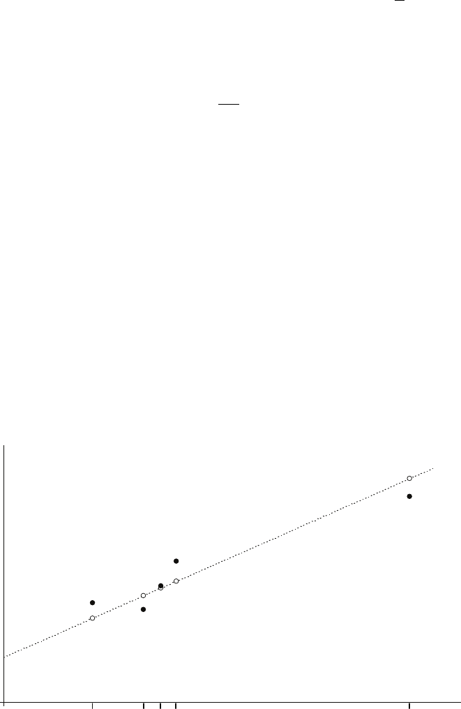
2.4. Additional exercises
•Explain how R2in (2) is related to R2in (1).
•Explain why, theoretically, the specification (2) of the second researcher is
incorrect and he should have fitted:
b
Y∗=b
β∗
2X∗(3)
not including a constant in his specification.
•If the second researcher had fitted (3) instead of (2), how would this have
affected his estimator of β2? Would dropping the unnecessary intercept lead to
a gain in efficiency?
A2.14 For the model described in Exercise A1.7, show that b
Y∗
i= (b
Yi−Y)/bσY, and thus
that bu∗
i=bui/bσY, where b
Y∗
iand bu∗
iare the fitted value of Y∗
iand the residual in the
transformed model.
Hence show that:
s.e.(b
β∗
2) = bσX
bσY×s.e.(b
β2).
Hence find the relationship between the tstatistic for b
β∗
2and the tstatistic for b
β2
and the relationship between R2for the original specification and R2for the revised
specification.
A2.15 A variable Yiis generated as:
Yi=β1+β2Xi+ui(1)
where β1and β2are fixed parameters and uiis a disturbance term that satisfies the
regression model assumptions. The values of Xare fixed and are as shown in the
figure. Four of them, X1to X4, are close together. The fifth, X5, is much larger.
The corresponding values that Ywould take, if there were no disturbance term, are
given by the circles on the line. The presence of the disturbance term in the model
causes the actual values of Yin a sample to be different. The solid black circles
depict a typical sample of observations.
0
0
X1
X2
X3
X4
X5
X
Y
1
47

2. Properties of the regression coefficients and hypothesis testing
Discuss the advantages and disadvantages of dropping the observation
corresponding to X5when regressing Yon X. If you keep the observation in the
sample, will this cause the regression estimates to be biased?
2.5 Answers to the starred exercises in the textbook
2.1 Derive the decomposition of b
β1shown in equation (2.29):
b
β1=β1+Xciui
where ci=1
n−aiXand aiis defined in equation (2.23).
Answer:
b
β1=Y−b
β2X=β1+β2X+u−Xβ2+Xaiui
=β1+1
nXui−XXaiui
=β1+Xciui.
2.5 An investigator correctly believes that the relationship between two variables X
and Yis given by:
Yi=β1+β2Xi+ui.
Given a sample of observations on Y,X, and a third variable Z(which is not a
determinant of Y), the investigator estimates β2as:
PZi−ZYi−Y
PZi−ZXi−X.
Demonstrate that this estimator is unbiased.
Answer:
Noting that Yi−Y=β2Xi−X+ui−u, we have:
b
β2=PZi−ZYi−Y
PZi−ZXi−X
=PZi−Zβ2Xi−X+PZi−Z(ui−u)
PZi−ZXi−X
=β2+PZi−Z(ui−u)
PZi−ZXi−X.
48

2.5. Answers to the starred exercises in the textbook
Hence:
E(b
β2) = β2+PZi−ZE(ui−u)
PZi−ZXi−X=β2.
2.8 Using the decomposition of b
β1obtained in Exercise 2.1, derive the expression for
σ2
b
β1given in equation (2.42).
Answer:
b
β1=β1+Pciui, where ci=1
n−aiX, and E(b
β1) = β1. Hence:
σ2
b
β1=EXciui2=σ2
uXc2
i=σ2
u n1
n2−2X
nXai+X2Xa2
i!.
From Box 2.2, Pai= 0 and:
Xa2
i=1
PXi−X2.
Hence:
σ2
b
β1=σ2
u
1
n+X2
PXi−X2
.
2.9 Given the decomposition in Exercise 2.2 of the OLS estimator of β2in the model
Yi=β2Xi+ui, demonstrate that the variance of the slope coefficient is given by:
σ2
b
β2=σ2
u
PX2
j
.
Answer:
b
β2=β2+
n
P
i=1
diui, where di=Xi/
n
P
j=1
X2
j, and E(b
β2) = β2. Hence:
σ2
b
β2=E
n
X
i=1
diui!2
=σ2
u
n
X
i=1
d2
i=σ2
u
n
X
i=1
X2
i
n
P
j=1
X2
j!2
=σ2
u
n
P
j=1
X2
j!2
n
X
i=1
X2
i
=σ2
u
n
P
j=1
X2
j
.
49

2. Properties of the regression coefficients and hypothesis testing
2.12 It can be shown that the variance of the estimator of the slope coefficient in
Exercise 2.5: PZi−ZYi−Y
PZi−ZXi−X
is given by:
σ2
b
β2=σ2
u
PXi−X2×1
r2
XZ
where rXZ is the correlation between Xand Z. What are the implications for the
efficiency of the estimator?
Answer:
If Zhappens to be an exact linear function of X, the population variance will be
the same as that of the OLS estimator. Otherwise 1/r2
XZ will be greater than 1, the
variance will be larger, and so the estimator will be less efficient.
2.15 Suppose that the true relationship between Yand Xis Yi=β1+β2Xi+uiand
that the fitted model is b
Yi=b
β1+b
β2Xi. In Exercise 1.13 it was shown that if
X∗
i=µ2Xi, and Yis regressed on X∗, the slope coefficient b
β∗
2=b
β2/µ2. How will
the standard error of b
β∗
2be related to the standard error of b
β2?
Answer:
In Exercise 1.23 it was demonstrated that the fitted values of Ywould be the same.
This means that the residuals are the same, and hence bσ2
u, the estimator of the
variance of the disturbance term, is the same. The standard error of b
β∗
2is then
given by:
s.e.(b
β∗
2) = v
u
u
tbσ2
u
PX∗
i−X∗2
=v
u
u
tbσ2
u
Pµ2Xi−µ2X2
=v
u
u
tbσ2
u
µ2
2PXi−X2
=1
µ2
s.e.(b
β2).
2.17 A researcher with a sample of 50 individuals with similar education, but differing
amounts of training, hypothesises that hourly earnings, EARNINGS, may be
related to hours of training, TRAINING, according to the relationship:
EARNINGS =β1+β2TRAINING +u.
50
2.5. Answers to the starred exercises in the textbook
He is prepared to test the null hypothesis H0:β2= 0 against the alternative
hypothesis H1:β26= 0 at the 5 per cent and 1 per cent levels. What should he
report:
(a) if b
β2= 0.30, s.e.(b
β2) = 0.12?
(b) if b
β2= 0.55, s.e.(b
β2) = 0.12?
(c) if b
β2= 0.10, s.e.(b
β2) = 0.12?
(d) if b
β2=−0.27, s.e.(b
β2) = 0.12?
Answer:
There are 48 degrees of freedom, and hence the critical values of tat the 5 per cent,
1 per cent, and 0.1 per cent levels are 2.01, 2.68, and 3.51, respectively.
(a) The tstatistic is 2.50. Reject H0at the 5 per cent level but not at the 1 per
cent level.
(b) t= 4.58. Reject at the 0.1 per cent level.
(c) t= 0.83. Fail to reject at the 5 per cent level.
(d) t=−2.25. Reject H0at the 5 per cent level but not at the 1 per cent level.
2.22 Explain whether it would have been possible to perform one-sided tests instead of
two-sided tests in Exercise 2.17. If you think that one-sided tests are justified,
perform them and state whether the use of a one-sided test makes any difference.
Answer:
First, there should be a discussion of whether the parameter β2in:
EARNINGS =β1+β2TRAINING +u
can be assumed not to be negative. The objective of training is to impart skills. It
would be illogical for an individual with greater skills to be paid less on that
account, and so we can argue that we can rule out β2<0. We can then perform a
one-sided test. With 48 degrees of freedom, the critical values of tat the 5 per cent,
1 per cent, and 0.1 per cent levels are 1.68, 2.40, and 3.26, respectively.
(a) The tstatistic is 2.50. We can now reject H0at the 1 per cent level (but not at
the 0.1 per cent level).
(b) t= 4.58. Not affected by the change. Reject at the 0.1 per cent level.
(c) t= 0.83. Not affected by the change. Fail to reject at the 5 per cent level.
(d) t=−2.25. Reject H0at the 5 per cent level but not at the 1 per cent level.
Here there is a problem because the coefficient has an unexpected sign and is
large enough to reject H0at the 5 per cent level with a two-sided test.
In principle we should ignore this and fail to reject H0. Admittedly, the
likelihood of such a large negative tstatistic occurring under H0is very small,
but it would be smaller still under the alternative hypothesis H1:β2>0.
However, we should consider two further possibilities. One is that the
justification for a one-sided test is incorrect. For example, some jobs pay
relatively low wages because they offer training that is valued by the employee.
51
2. Properties of the regression coefficients and hypothesis testing
Apprenticeships are the classic example. Alternatively, workers in some
low-paid occupations may, for technical reasons, receive a relatively large
amount of training. In either case, the correlation between training and
earnings might be negative instead of positive.
Another possible reason for a coefficient having an unexpected sign is that the
model is misspecified in some way. For example, the coefficient might be
distorted by omitted variable bias, to be discussed in Chapter 6.
2.27 Suppose that the true relationship between Yand Xis Yi=β1+β2Xi+uiand
that the fitted model is b
Yi=b
β1+b
β2Xi. In Exercise 1.13 it was shown that if
X∗
i=µ2Xi, and Yis regressed on X∗, the slope coefficient b
β∗
2=b
β2/µ2. How will
the tstatistic for b
β∗
2be related to the tstatistic for b
β2? (See also Exercise 2.15.)
Answer:
In Exercise 2.15 it was shown that s.e.(b
β∗
2) = s.e.(b
β2)/µ2. Hence the tstatistic is
unaffected by the transformation.
Alternatively, since we saw in Exercise 1.23 that R2must be the same, it follows
that the Fstatistic for the equation must be the same. For a simple regression the
Fstatistic is the square of the tstatistic on the slope coefficient, so the tstatistic
must be the same.
2.30 Calculate the 95 per cent confidence interval for β2in the price inflation/wage
inflation example:
bp=−1.21 + 0.82w.
(0.05) (0.10)
What can you conclude from this calculation?
Answer:
With nequal to 20, there are 18 degrees of freedom and the critical value of tat
the 5 per cent level is 2.10. The 95 per cent confidence interval is therefore:
0.82 −0.10 ×2.10 ≤β2≤0.82 + 0.10 ×2.10
that is:
0.61 ≤β2≤1.03.
We see that we cannot (quite) reject the null hypothesis H0:β2= 1.
2.36 Suppose that the true relationship between Yand Xis Yi=β1+β2Xi+uiand
that the fitted model is b
Yi=b
β1+b
β2Xi. Suppose that X∗
i=µ2Xi, and Yis
regressed on X∗. How will the Fstatistic for this regression be related to the F
statistic for the original regression? (See also Exercises 1.23, 2.15, and 2.27.)
Answer:
We saw in Exercise 1.23 that R2would be the same, and it follows that Fmust
also be the same.
52

2.6. Answers to the additional exercises
2.6 Answers to the additional exercises
Note: Each of the exercises below relates to a simple regression. Accordingly, the Ftest
is equivalent to a two-sided ttest on the slope coefficient and there is no point in
performing both tests. The Fstatistic is equal to the square of the tstatistic and, for
any significance level, the critical value of Fis equal to the critical value of t. Obviously
a one-sided ttest, when justified, is preferable to either in that it has greater power for
any given significance level.
A2.1 We have:
b
β2=PXiYi
PX2
i
=PXi(β1+β2Xi+ui)
PX2
i
=β1PXi
PX2
i
+β2+PXiui
PX2
i
.
Hence:
E(b
β2) = β1PXi
PX2
i
+β2+EPXiui
PX2
i=β1PXi
PX2
i
+β2+PXiE(ui)
PX2
i
assuming that Xis nonstochastic. Since E(ui) = 0, then:
E(b
β2) = β1PXi
PX2
i
+β2.
Thus b
β2will in general be a biased estimator. The sign of the bias depends on the
signs of β1and PXi. In general, we have no information about either of these.
However, if either β1= 0 or X= 0 (and so PXi= 0), the bias term disappears and
b
β2is unbiased after all.
A2.2 First we need to show that E(b
β2) = 0.
b
β2=PXi−XYi−Y
PXi−X2=PXi−X(β1+ui−β1−u)
PXi−X2=PXi−X(ui−u)
PXi−X2.
Hence, given that we are told that Xis nonstochastic:
E(b
β2) = E
PXi−X(ui−u)
PXi−X2
=1
PXi−X2EXXi−X(ui−u)
=1
PXi−X2XXi−XE(ui−u)
= 0
since E(u) = 0. Thus:
E(b
β1) = EY−b
β2X=β1−XE(b
β2) = β1
and the estimator is unbiased.
53

2. Properties of the regression coefficients and hypothesis testing
A2.3 In general, the researcher’s estimator will have a larger variance than Yand
therefore will be inefficient. However, if X= 0, the variances are the same. This is
because the estimators are then identical. Y−b
β2Xreduces to Y.
A2.4 The variance of the estimator is σ2
u/PX2
iwhereas that of the estimator:
P(Xi−X)(Yi−Y)
P(Xi−X)2
is:
σ2
u
P(Xi−X)2=σ2
u
PX2
i−nX2.
Thus, provided X6= 0, σ2
u/PX2
iis more efficient than:
P(Xi−X)(Yi−Y)
P(Xi−X)2
if β1= 0 because it is unbiased and has a smaller variance. It is the OLS estimator
in this case.
If X= 0, the estimators are equally efficient because the population variance
expressions are identical. The reason for this is that the estimators are now
identical:
P(Xi−X)(Yi−Y)
P(Xi−X)2=PXi(Yi−Y)
PX2
i
=PXiYi
PX2
i−YPXi
PX2
i
=PXiYi
PX2
i
since PXi=nX = 0.
Returning to the general case, if there is little variation in Xin the sample,
P(Xi−X)2may be small and hence the population variance of
P(Xi−X)(Yi−Y)/P(Xi−X)2may be large. Thus using a criterion such as mean
square error, b
β2may be preferable if the bias is small.
A2.5 The tstatistic for the coefficient of EXP is 58.57, very highly significant. There is
little point performing a ttest on the intercept, given that it has no plausible
meaning. The Fstatistic is 3431.0, very highly significant. Since this is a simple
regression model, the two tests are equivalent.
A2.6 The slope coefficient for every category is significantly different from zero at a very
high significance level. (The Ftest is equivalent to the ttest on the slope
coefficient.)
54

2.6. Answers to the additional exercises
EXP
nb
β2s.e.(b
β2)t R2F
ADM 2,815 0.0235 0.0008 28.86 0.228 832.8
CLOT 4,500 0.0316 0.0010 30.99 0.176 960.6
DOM 1,661 0.0409 0.0026 16.02 0.134 256.6
EDUC 561 0.1202 0.0090 13.30 0.241 177.0
ELEC 5,828 0.0131 0.0004 35.70 0.180 1274.8
FDAW 5,102 0.0527 0.0010 52.86 0.354 2794.7
FDHO 6,334 0.0627 0.0011 58.57 0.351 3431.0
FOOT 1,827 0.0058 0.0005 12.78 0.082 163.4
FURN 487 0.0522 0.0070 7.44 0.102 55.3
GASO 5,710 0.0373 0.0008 46.89 0.278 2198.5
HEAL 4,802 0.0574 0.0018 31.83 0.174 1013.4
HOUS 6,223 0.1976 0.0027 74.16 0.469 5499.9
LIFE 1,253 0.0193 0.0016 11.86 0.101 140.7
LOCT 692 0.0068 0.0010 6.59 0.059 43.5
MAPP 399 0.0329 0.0049 6.72 0.102 45.1
PERS 3,817 0.0069 0.0002 32.15 0.213 1033.4
READ 2,287 0.0048 0.0003 16.28 0.104 265.1
SAPP 1,037 0.0045 0.0007 6.03 0.034 36.4
TELE 5,788 0.0160 0.0003 46.04 0.268 2119.7
TEXT 992 0.0040 0.0006 7.32 0.051 53.5
TOB 1,155 0.0165 0.0016 10.56 0.088 111.6
TOYS 2,504 0.0145 0.0010 14.34 0.076 205.7
TRIP 516 0.0466 0.0043 10.84 0.186 117.5
A2.7 The tstatistic, 13.29, is very highly significant. (The Ftest is equivalent.)
A2.8 The tstatistic for height, 3.04, suggests that the effect of height on earnings is
highly significant, despite the very low R2. In principle the estimate of an extra 41
cents of hourly earnings for every extra inch of height could have been a purely
random result of the kind that one obtains with nonsense models. However, the
fact that it is apparently highly significant causes us to look for other explanations,
the most likely one being that suggested in the answer to Exercise A1.4. Of course,
we would not attempt to test the negative constant.
A2.9 One could justify a one-sided test on the slope coefficient in the regression of the
rate of growth of employment on the rate of growth of GDP on the grounds that an
increase in the rate of growth of GDP is unlikely to cause a decrease in the rate of
growth of employment.
A2.10 One could justify a one-sided test on the slope coefficient in the regression of
weight on height in Exercise 1.9 on the grounds that an increase in height is
unlikely to cause a decrease in weight.
55

2. Properties of the regression coefficients and hypothesis testing
A2.11 The standard error of the coefficient of GDP. This is given by:
pbσ∗2
u
rPG∗
i−G∗2
where bσ∗2
u, the estimator of the variance of the disturbance term, is Pbu∗2
i/(n−2).
Since RSS is unchanged, bσ∗2
u=bσ2
u.
We saw in Exercise A1.6 that G∗
i−G∗=Gi−Gfor all i. Hence the new standard
error is given by: pbσ2
u
rPGi−G2
and is unchanged.
F=ESS
RSS/(n−2)
where:
ESS = explained sum of squares = Xb
Y∗
i−b
Y∗2
.
Since bu∗
i=bui,b
Y∗
i=b
Yiand ESS is unchanged. We saw in Exercise A1.6 that RSS
is unchanged. Hence Fis unchanged.
A2.12 The standard error of the coefficient of GDP. This is given by:
pbσ∗2
u
rPG∗
i−G∗2
where bσ∗2
u, the estimator of the variance of the disturbance term, is Pbu∗2
i/(n−2).
We saw in Exercise 1.7 that bu∗
i=buiand so RSS is unchanged. Hence bσ∗2
u=bσ2
u.
Thus the new standard error is given by:
pbσ2
u
rP2Gi−2G2=1
2pbσ2
u
rPGi−G2= 0.005.
F=ESS/(RSS/(n−2)) where:
ESS = explained sum of squares = Xb
Y∗
i−b
Y∗2
.
Since bu∗
i=bui,b
Y∗
i=b
Yiand ESS is unchanged. Hence Fis unchanged.
A2.13 One way of demonstrating that b
Y∗
i=b
Yi−Y:
b
Y∗
i=b
β∗
1+b
β∗
2X∗
i=b
β2(Xi−X)
b
Yi−Y= (b
β1+b
β2Xi)−Y=Y−b
β2X+b
β2Xi−Y=b
β2Xi−X.
56

2.6. Answers to the additional exercises
Demonstration that the residuals are the same:
bu∗
i=Y∗
i−b
Y∗
i=Yi−Y−b
Yi−Y=bui.
Demonstration that the OLS estimator of the variance of the disturbance term in
(2) is equal to that in (1):
bσ∗2
u=Pbu∗2
i
n−2=Pbu2
i
n−2=bσ2
u.
The standard error of the slope coefficient in (2) is equal to that in (1).
bσ2
b
β∗
2
=bσ∗2
u
PX∗
i−X2=bσ2
u
PX∗2
i
=bσ2
u
PXi−X2=bσ2
b
β2.
Hence the standard errors are the same.
Demonstration that R2in (2) is equal to R2in (1):
R2∗=Pb
Y∗
i−b
Y∗2
PY∗
i−Y∗2.
b
Y∗
i=b
Yi−Yand b
Y=Y. Hence b
Y∗= 0. Y∗=Y−Y= 0. Hence:
R2∗=Pb
Y∗
i2
P(Y∗
i)2=Pb
Yi−Y2
PYi−Y2=R2.
The reason that specification (2) of the second researcher is incorrect is that the
model does not include an intercept.
If the second researcher had fitted (3) instead of (2), this would not in fact have
affected his estimator of β2. Using (3), the researcher should have estimated β2as:
b
β∗
2=PX∗
iY∗
i
PX∗2
i
.
However, Exercise 1.16 demonstrates that, effectively, he has done exactly this.
Hence the estimator will be the same. It follows that dropping the unnecessary
intercept would not have led to a gain in efficiency.
A2.14 We have:
b
Y∗
i=b
β∗
2X∗
i=bσX
bσYb
β2 Xi−X
bσX!=1
bσYb
β2(Xi−X)
and: b
Yi=b
β1+b
β2Xi= (Y−b
β2X) + b
β2Xi=Y+b
β2(Xi−X).
Hence:
b
Y∗
i=1
bσY
(b
Yi−Y).
57

2. Properties of the regression coefficients and hypothesis testing
Also:
bu∗
i=Y∗
i−b
Y∗
i=1
bσY
(Yi−Y)−1
bσY
(b
Yi−Y) = 1
bσY
(Yi−b
Yi) = 1
bσYbui
and:
s.e.(b
β∗
2) = s1
n−2Pbu∗2
i
P(X∗
i−X∗)2=v
u
u
u
u
t1
bσY21
n−2Pbu2
i
PXi−¯
X
bσX2=bσX
bσY×s.e.(b
β2).
Given the expressions for b
β∗
2and s.e.(b
β∗
2), the tstatistic for b
β∗
2is the same as that
for b
β2. Hence the Fstatistic will be the same and R2will be the same.
A2.15 The inclusion of the fifth observation does not cause the model to be misspecified
or the regression model assumptions to be violated, so retaining it in the sample
will not give rise to biased estimates. There would be no advantages in dropping it
and there would be one major disadvantage. PXi−X2would be greatly
reduced and hence the variances of the coefficients would be increased, adversely
affecting the precision of the estimates.
This said, in practice one would wish to check whether it is sensible to assume that
the model relating Yto Xfor the other observations really does apply to the
observation corresponding to X5as well. This question can be answered only by
being familiar with the context and having some intuitive understanding of the
relationship between Yand X.
58

Chapter 3
Multiple regression analysis
3.1 Overview
This chapter introduces regression models with more than one explanatory variable.
Specific topics are treated with reference to a model with just two explanatory
variables, but most of the concepts and results apply straightforwardly to more general
models. The chapter begins by showing how the least squares principle is employed to
derive the expressions for the regression coefficients and how the coefficients should be
interpreted. It continues with a discussion of the precision of the regression coefficients
and tests of hypotheses relating to them. Next comes multicollinearity, the problem of
discriminating between the effects of individual explanatory variables when they are
closely related. The chapter concludes with a discussion of Ftests of the joint
explanatory power of the explanatory variables or subsets of them, and shows how a t
test can be thought of as a marginal Ftest.
3.2 Learning outcomes
After working through the corresponding chapter in the text, studying the
corresponding slideshows, and doing the starred exercises in the text and the additional
exercises in this subject guide, you should be able to explain what is meant by:
the principles behind the derivation of multiple regression coefficients (but you are
not expected to learn the expressions for them or to be able to reproduce the
mathematical proofs)
how to interpret the regression coefficients
the Frisch–Waugh–Lovell graphical representation of the relationship between the
dependent variable and one explanatory variable, controlling for the influence of
the other explanatory variables
the properties of the multiple regression coefficients
what factors determine the population variance of the regression coefficients
what is meant by multicollinearity
what measures may be appropriate for alleviating multicollinearity
what is meant by a linear restriction
the Ftest of the joint explanatory power of the explanatory variables
59

3. Multiple regression analysis
the Ftest of the explanatory power of a group of explanatory variables
why ttests on the slope coefficients are equivalent to marginal Ftests.
You should know the expression for the population variance of a slope coefficient in a
multiple regression model with two explanatory variables.
3.3 Additional exercises
A3.1 The output shows the result of regressing FDHO, expenditure on food consumed at
home, on EXP, total household expenditure, and SIZE, number of persons in the
household, using the CES data set. Provide an interpretation of the regression
coefficients and perform appropriate tests.
. reg FDHO EXP SIZE if FDHO>0
Source | SS df MS Number of obs = 6334
-------------+------------------------------ F( 2, 6331) = 2257.59
Model | 1.1521e+09 2 576056293 Prob > F = 0.0000
Residual | 1.6154e+09 6331 255164.645 R-squared = 0.4163
-------------+------------------------------ Adj R-squared = 0.4161
Total | 2.7676e+09 6333 437006.15 Root MSE = 505.14
------------------------------------------------------------------------------
FDHO | Coef. Std. Err. t P>|t| [95% Conf. Interval]
-------------+----------------------------------------------------------------
EXP | .056366 .0010435 54.02 0.000 .0543204 .0584116
SIZE | 115.1636 4.341912 26.52 0.000 106.652 123.6752
_cons | 130.5997 13.53959 9.65 0.000 104.0575 157.1419
------------------------------------------------------------------------------
A3.2 Perform a regression parallel to that in Exercise A3.1 for your CES category of
expenditure, provide an interpretation of the regression coefficients and perform
appropriate tests. Delete observations where expenditure on your category is zero.
A3.3 The output shows the result of regressing FDHOPC, expenditure on food
consumed at home per capita, on EXPPC, total household expenditure per capita,
and SIZE, number of persons in the household, using the CES data set. Provide an
interpretation of the regression coefficients and perform appropriate tests.
. reg FDHOPC EXPPC SIZE if FDHO>0
Source | SS df MS Number of obs = 6334
-------------+------------------------------ F( 2, 6331) = 1572.95
Model | 202590496 2 101295248 Prob > F = 0.0000
Residual | 407705728 6331 64398.3143 R-squared = 0.3320
-------------+------------------------------ Adj R-squared = 0.3317
Total | 610296223 6333 96367.6336 Root MSE = 253.77
60
3.3. Additional exercises
------------------------------------------------------------------------------
FDHOPC | Coef. Std. Err. t P>|t| [95% Conf. Interval]
-------------+----------------------------------------------------------------
EXPPC | .0480294 .0010064 47.72 0.000 .0460564 .0500023
SIZE | -26.45917 2.253999 -11.74 0.000 -30.87777 -22.04057
_cons | 283.2498 8.412603 33.67 0.000 266.7582 299.7413
------------------------------------------------------------------------------
A3.4 Perform a regression parallel to that in Exercise A3.3 for your CES category of
expenditure. Provide an interpretation of the regression coefficients and perform
appropriate tests.
A3.5 The output shows the result of regressing FDHOPC, expenditure on food
consumed at home per capita, on EXPPC, total household expenditure per capita,
and SIZEAM,SIZEAF,SIZEJM,SIZEJF, and SIZEIN, numbers of adult males,
adult females, junior males, junior females, and infants, respectively, in the
household, using the CES data set. Provide an interpretation of the regression
coefficients and perform appropriate tests.
. reg FDHOPC EXPPC SIZEAM SIZEAF SIZEJM SIZEJF SIZEIN if FDHO>0
Source | SS df MS Number of obs = 6334
-------------+------------------------------ F( 6, 6327) = 524.59
Model | 202746894 6 33791149 Prob > F = 0.0000
Residual | 407549329 6327 64414.3084 R-squared = 0.3322
-------------+------------------------------ Adj R-squared = 0.3316
Total | 610296223 6333 96367.6336 Root MSE = 253.8
------------------------------------------------------------------------------
FDHOPC | Coef. Std. Err. t P>|t| [95% Conf. Interval]
-------------+----------------------------------------------------------------
EXPPC | .0479717 .0010087 47.56 0.000 .0459943 .0499491
SIZEAM | -25.77747 4.757056 -5.42 0.000 -35.10291 -16.45203
SIZEAF | -32.38649 5.065782 -6.39 0.000 -42.31714 -22.45584
SIZEJM | -20.24693 5.731645 -3.53 0.000 -31.4829 -9.010967
SIZEJF | -26.66374 6.122262 -4.36 0.000 -38.66544 -14.66203
SIZEIN | -28.6047 11.75666 -2.43 0.015 -51.65174 -5.557656
_cons | 287.5695 9.280372 30.99 0.000 269.3769 305.7622
------------------------------------------------------------------------------
A3.6 Perform a regression parallel to that in Exercise A3.5 for your CES category of
expenditure. Provide an interpretation of the regression coefficients and perform
appropriate tests.
A3.7 A researcher hypothesises that, for a typical enterprise, V, the logarithm of value
added per worker, is related to K, the logarithm of capital per worker, and S, the
logarithm of the average years of schooling of the workers, the relationship being:
V=β1+β2K+β3S+u
where uis a disturbance term that satisfies the usual regression model
assumptions. She fits the relationship (1) for a sample of 25 manufacturing
enterprises, and (2) for a sample of 100 services enterprises. The table provides
some data on the samples.
61

3. Multiple regression analysis
(1) (2)
Manufacturing Services
sample sample
Number of enterprises 25 100
Estimate of variance of u0.16 0.64
Mean square deviation of K4.00 16.00
Correlation between Kand S0.60 0.60
The mean square deviation of Kis defined as 1
nPKi−K2, where nis the
number of enterprises in the sample and Kis the average value of Kin the sample.
The researcher finds that the standard error of the coefficient of Kis 0.050 for the
manufacturing sample and 0.025 for the services sample. Explain the difference
quantitatively, given the data in the table.
A3.8 A researcher is fitting earnings functions using a sample of data relating to
individuals born in the same week in 1958. He decides to relate Y, gross hourly
earnings in 2001, to S, years of schooling, and PWE, potential work experience,
using the semilogarithmic specification:
log Y=β1+β2S+β3PWE +u
where uis a disturbance term assumed to satisfy the regression model assumptions.
PWE is defined as age – years of schooling – 5. Since the respondents were all aged
43 in 2001, this becomes:
PWE = 43 −S−5 = 38 −S.
The researcher finds that it is impossible to fit the model as specified. Stata output
for his regression is reproduced below:
. reg LGY S PWE
Source | SS df MS Number of obs = 5660
-------------+------------------------------ F( 1, 5658) = 1232.62
Model | 237.170265 1 237.170265 Prob > F = 0.0000
Residual | 1088.66373 5658 .192411405 R-squared = 0.1789
-------------+------------------------------ Adj R-squared = 0.1787
Total | 1325.834 5659 .234287682 Root MSE = .43865
------------------------------------------------------------------------------
LGY | Coef. Std. Err. t P>|t| [95% Conf. Interval]
-------------+----------------------------------------------------------------
S | .1038011 .0029566 35.11 0.000 .0980051 .1095971
PWE | (dropped)
_cons | .5000033 .0373785 13.38 0.000 .4267271 .5732795
------------------------------------------------------------------------------
Explain why the researcher was unable to fit his specification.
Explain how the coefficient of Smight be interpreted.
62

3.4. Answers to the starred exercises in the textbook
3.4 Answers to the starred exercises in the textbook
3.5 Explain why the intercept in the regression of EEARN on ES is equal to zero.
Answer:
The intercept is calculated as EEARN −b
β2ES. However, since the mean of the
residuals from an OLS regression is zero, both EEARN and ES are zero, and hence
the intercept is zero.
3.6 Show that, in the general case, the mean of the residuals from a fitted OLS
multiple regression is equal to zero, provided that an intercept is included in the
specification. Note: This is an extension of one of the useful results in Section 1.5.
Answer:
If the model is:
Y=β1+β2X2+··· +βkXk+u
b
β1=Y−b
β2X2− ··· − b
βkXk.
For observation iwe have:
bui=Yi−b
Yi=Yi−b
β1−b
β2X2i− ··· − b
βkXki.
Hence:
bu=Y−b
β1−b
β2X2− ··· − b
βkXk
=Y−hY−b
β2X2− ··· − b
βkXki−b
β2X2− ··· − b
βkXk= 0.
3.16 A researcher investigating the determinants of the demand for public transport in a
certain city has the following data for 100 residents for the previous calendar year:
expenditure on public transport, E, measured in dollars; number of days worked,
W; and number of days not worked, NW. By definition NW is equal to 365 −W.
He attempts to fit the following model:
E=β1+β2W+β3NW +u.
Explain why he is unable to fit this equation. (Give both intuitive and technical
explanations.) How might he resolve the problem?
Answer:
There is exact multicollinearity since there is an exact linear relationship between
W,NW and the constant term. As a consequence it is not possible to tell whether
variations in Eare attributable to variations in Wor variations in NW, or both.
Noting that NWi−NW =−(Wi−W), we have:
b
β2=PEi−EWi−WPNWi−N W2
−PEi−ENWi−N WPWi−WNWi−NW
PWi−W2PNWi−NW2
−PWi−WNWi−NW2
=PEi−EWi−WPWi−W2
−PEi−E−Wi+WPWi−W−Wi+W
PWi−W2PWi−W2
−PWi−W−Wi+W2
=0
0.
63

3. Multiple regression analysis
One way of dealing with the problem would be to drop NW from the regression.
The interpretation of b
β2now is that it is an estimate of the extra expenditure on
transport per day worked, compared with expenditure per day not worked.
3.21 The researcher in Exercise 3.16 decides to divide the number of days not worked
into the number of days not worked because of illness, I, and the number of days
not worked for other reasons, O. The mean value of Iin the sample is 2.1 and the
mean value of Ois 120.2. He fits the regression (standard errors in parentheses):
b
E=−9.6+2.10W+ 0.45O R2= 0.72
(8.3) (1.98) (1.77)
Perform ttests on the regression coefficients and an Ftest on the goodness of fit of
the equation. Explain why the ttests and Ftest have different outcomes.
Answer:
Although there is not an exact linear relationship between Wand O, they must
have a very high negative correlation because the mean value of Iis so small.
Hence one would expect the regression to be subject to multicollinearity, and this is
confirmed by the results. The tstatistics for the coefficients of Wand Oare only
1.06 and 0.25, respectively, but the Fstatistic:
F(2,97) = 0.72/2
(1 −0.72)/97 = 124.7
is greater than the critical value of Fat the 0.1 per cent level, 7.41.
3.5 Answers to the additional exercises
A3.1 The regression indicates that 5.6 cents out of the marginal expenditure dollar is
spent on food consumed at home, and that expenditure on this category increases
by $115 for each individual in the household, keeping total expenditure constant.
Both of these effects are very highly significant. Just over 40 per cent of the
variance in FDHO is explained by EXP and SIZE. The intercept has no plausible
interpretation.
A3.2 With the exception of LOCT, all of the categories have positive coefficients for
EXP, with high significance levels, but the SIZE effect varies:
•Positive, significant at the 1 per cent level: FDHO,TELE,CLOT,FOOT,
GASO.
•Positive, significant at the 5 per cent level: LOCT.
•Negative, significant at the 1 per cent level: TEXT,FEES,READ.
•Negative, significant at the 5 per cent level: SHEL,EDUC.
•Not significant: FDAW,DOM,FURN,MAPP,SAPP,TRIP,HEAL,ENT,
TOYS,TOB.
At first sight it may seem surprising that SIZE has a significant negative effect for
some categories. The reason for this is that an increase in SIZE means a reduction
64

3.5. Answers to the additional exercises
in expenditure per capita, if total household expenditure is kept constant, and thus
SIZE has a (negative) income effect in addition to any direct effect. Effectively
poorer, the larger household has to spend more on basics and less on luxuries. To
determine the true direct effect, we need to eliminate the income effect, and that is
the point of the re-specification of the model in the next exercise.
EXP SIZE
nb
β2s.e.(b
β2)b
β3s.e.(b
β3)R2F
ADM 2,815 0.0238 0.0008 −8.09 4.19 0.230 418.7
CLOT 4,500 0.0309 0.0010 16.39 4.50 0.178 488.2
DOM 1,661 0.0388 0.0026 52.34 14.06 0.141 136.2
EDUC 561 0.1252 0.0090 −179.23 48.92 0.258 97.2
ELEC 5,828 0.0121 0.0004 18.92 1.57 0.199 725.5
FDAW 5,102 0.0538 0.0010 −20.72 4.47 0.357 1,413.7
FDHO 6,334 0.0564 0.0010 115.16 4.34 0.416 2,257.6
FOOT 1,827 0.0056 0.0005 3.24 2.05 0.083 83.0
FURN 487 0.0541 0.0071 −61.87 35.92 0.108 29.3
GASO 5,710 0.0347 0.0008 50.29 3.40 0.305 1,250.9
HEAL 4,802 0.0580 0.0019 −9.96 8.60 0.175 507.4
HOUS 6,223 0.1997 0.0027 −38.78 11.41 0.470 2,760.4
LIFE 1,253 0.0198 0.0017 −9.01 8.99 0.102 70.9
LOCT 692 0.0062 0.0011 14.61 4.72 0.072 26.8
MAPP 399 0.0309 0.0050 44.48 23.94 0.110 24.4
PERS 3,817 0.0070 0.0002 −2.17 1.03 0.214 519.4
READ 2,287 0.0049 0.0003 −1.06 1.58 0.104 132.7
SAPP 1,037 0.0046 0.0008 −3.12 3.99 0.035 18.5
TELE 5,788 0.0150 0.0004 17.92 1.47 0.287 1,161.2
TEXT 992 0.0041 0.0006 −0.71 2.90 0.051 26.8
TOB 1,155 0.0161 0.0016 6.79 6.24 0.089 56.4
TOYS 2,504 0.0140 0.0010 12.19 4.88 0.078 106.2
TRIP 516 0.0450 0.0045 37.48 31.21 0.188 59.5
A3.3 Another surprise, perhaps. The purpose of this specification is to test whether
household size has an effect on expenditure per capita on food consumed at home,
controlling for the income effect of variations in household size mentioned in the
answer to Exercise A3.2. Expenditure per capita on food consumed at home
increases by 4.8 cents out of the marginal dollar of total household expenditure per
capita. Now SIZE has a very significant negative effect. Expenditure per capita on
FDHO decreases by $26 per year for each extra person in the household, suggesting
that larger households are more efficient than smaller ones with regard to
expenditure on this category, the effect being highly significant. R2is lower than in
Exercise A3.1, but a comparison is invalidated by the fact that the dependent
variable is different.
A3.4 Nearly all of the categories have negative SIZE effects, the majority highly
significant. One explanation of the negative effects could be economies of scale, but
65

3. Multiple regression analysis
this is not plausible in the case of some. Another might be family composition –
larger families having more children. In the case of DOM,SIZE has a positive
effect, significant at the 5 per cent level. Again, this might be attributable to larger
families having more children and needing greater expenditure on childcare.
EXP SIZE
nb
β2s.e.(b
β2)b
β3s.e.(b
β3)R2F
ADM 2,815 0.0244 0.0008 2.56 2.26 0.251 470.4
CLOT 4,500 0.0324 0.0012 −1.07 2.91 0.151 400.8
DOM 1,661 0.0311 0.0025 18.54 7.35 0.086 78.1
EDUC 561 0.1391 0.0108 −31.92 27.57 0.290 113.7
ELEC 5,828 0.0117 0.0004 −17.53 0.89 0.247 953.9
FDAW 5,102 0.0528 0.0011 −13.51 2.53 0.375 1,526.3
FDHO 6,334 0.0480 0.0010 −26.46 2.25 0.332 1,573.0
FOOT 1,827 0.0068 0.0005 −8.13 1.11 0.194 219.5
FURN 487 0.0935 0.0091 3.40 26.82 0.216 66.6
GASO 5,710 0.0308 0.0008 −12.43 1.80 0.255 976.5
HEAL 4,802 0.0597 0.0020 −34.16 4.99 0.197 588.5
HOUS 6,223 0.2127 0.0030 −48.86 6.67 0.501 3,123.3
LIFE 1,253 0.0205 0.0017 −10.33 4.65 0.131 94.4
LOCT 692 0.0062 0.0010 −9.06 2.54 0.098 37.4
MAPP 399 0.0384 0.0051 −15.52 12.32 0.171 41.0
PERS 3,817 0.0071 0.0003 −3.96 0.63 0.228 564.0
READ 2,287 0.0052 0.0003 −3.60 0.84 0.154 208.1
SAPP 1,037 0.0076 0.0010 −6.71 2.61 0.090 51.1
TELE 5,788 0.0139 0.0003 −9.77 0.75 0.307 1,282.6
TEXT 992 0.0041 0.0005 −8.96 1.45 0.138 79.2
TOB 1,155 0.0220 0.0019 −22.68 3.55 0.187 132.1
TOYS 2,504 0.0216 0.0012 −8.86 2.92 0.141 205.7
TRIP 516 0.0361 0.0043 −16.33 16.32 0.150 45.2
A3.5 The coefficients of the SIZE variables are fairly similar, suggesting that household
composition is not important for this category of expenditure.
A3.6 The regression results for this specification are summarised in the table below. In
the case of SHEL, the regression indicates that the SIZE effect is attributable to
SIZEAM. To investigate this further, the regression was repeated: (1) restricting
the sample to households with at least one adult male, and (2) restricting the
sample to households with either no adult male or just 1 adult male. The first
regression produces a negative effect for SIZEAM, but it is smaller than with the
whole sample and not significant. In the second regression the coefficient of
SIZEAM jumps dramatically, from −$424 to −$793, suggesting very strong
economies of scale for this particular comparison.
As might be expected, the SIZE composition variables on the whole do not appear
to have significant effects if the SIZE variable does not in Exercise A3.4. The
66

3.5. Answers to the additional exercises
results for TOB are puzzling, in that the apparent economies of scale do not
appear to be related to household composition.
Category ADM CLOT DOM EDUC ELEC FDAW FDHO FOOT
EXP 0.0245 0.0309 0.0422 0.1191 0.0120 0.0531 0.0561 0.0056
(0.0008) (0.0011) (0.0026) (0.0092) (0.0004) (0.0010) (0.0011) (0.0005)
SIZEAM −37.17 12.84 −141.47 120.11 23.40 29.36 129.69 2.65
(9.22) (10.33) (32.71) (107.51) (3.44) (9.88) (9.64) (4.71)
SIZEAF −40.47 12.26 −67.26 −58.21 35.73 −45.07 105.17 9.40
(9.52) (10.95) (34.79) (107.96) (3.60) (10.17) (9.96) (5.25)
SIZEJM 1.33 17.11 114.68 −413.28 12.53 −24.45 126.94 1.23
(9.86) (11.41) (31.91) (107.79) (4.06) (11.53) (11.35) (4.99)
SIZEJF 48.55 29.98 93.82 −287.35 8.93 −26.03 105.01 6.32
(10.54) (12.15) (33.66) (103.15) (4.31) (12.05) (12.07) (5.01)
SIZEIN −34.51 −2.08 441.46 −123.20 −4.05 −61.38 95.90 −16.33
(22.79) (22.20) (59.10) (289.63) (8.36) (23.77) (23.34) (11.07)
R20.243 0.179 0.184 0.278 0.204 0.361 0.417 0.086
F150.1 163.0 62.1 35.6 249.2 480.2 753.6 28.5
n2,815 4,500 1,661 561 5,828 5,102 6,334 1,827
Category FURN GASO HEAL HOUS LIFE LOCT MAPP PERS
EXP 0.0547 0.0341 0.0579 0.2022 0.0195 0.0061 0.0321 0.0071
(0.0072) (0.0008) (0.0019) (0.0027) (0.0017) (0.0011) (0.0051) (0.0002)
SIZEAM −119.30 90.70 3.01 −175.23 10.54 12.02 2.41 −13.99
(81.65) (7.47) (18.25) (25.24) (19.50) (9.90) (54.58) (2.23)
SIZEAF −55.42 52.23 89.64 −111.39 25.43 19.16 0.75 12.33
(93.37) (7.79) (19.10) (26.12) (20.83) (10.61) (63.11) (2.34)
SIZEJM −27.44 30.83 −62.83 52.32 −23.28 −6.41 131.15 −3.33
(87.24) (8.72) (22.56) (29.65) (21.17) (12.81) (61.75) (2.59)
SIZEJF −15.06 46.24 −57.94 34.65 −15.65 32.97 24.87 −2.10
(89.23) (9.27) (23.96) (31.58) (22.98) (15.85) (64.61) (2.71)
SIZEIN −146.90 −8.90 −109.08 119.91 −116.37 33.48 26.25 −11.30
(160.29) (18.02) (46.46) (61.40) (46.00) (25.82) (139.98) (5.32)
R20.110 0.310 0.181 0.475 0.109 0.077 0.116 0.228
F9.9 427.6 177.0 937.6 25.3 9.6 8.6 187.4
n487 5,710 4,802 6,223 1,253 692 399 3,817
Category READ SAPP TELE TEXT TOB TOYS TRIP
EXP 0.0049 0.0046 0.0148 0.0040 0.0151 0.0148 0.0448
(0.0003) (0.0008) (0.0004) (0.0006) (0.0016) (0.0010) (0.0045)
SIZEAM −6.37 −1.64 29.33 7.42 30.92 −39.66 64.35
(3.46) (8.26) (3.25) (5.98) (13.49) (11.19) (59.55)
SIZEAF 1.69 8.95 35.59 2.58 22.09 1.30 4.87
(3.80) (9.65) (3.38) (6.77) (13.68) (12.49) (71.23)
SIZEJM 0.63 −13.21 6.38 −15.90 17.42 42.46 81.61
(3.93) (9.73) (3.78) (7.51) (16.52) (11.30) (79.96)
SIZEJF 4.73 1.17 12.74 −4.92 −45.12 19.34 102.45
(4.26) (10.88) (4.06) (7.50) (16.82) (11.71) (91.86)
SIZEIN −18.98 −19.58 −26.42 19.17 2.92 50.91 −294.14
(8.56) (18.58) (7.82) (14.13) (32.83) (22.49) (157.82)
R20.108 0.038 0.296 0.059 0.100 0.090 0.197
F45.8 6.7 404.9 10.4 21.2 41.2 20.8
n2,287 1,037 5,788 992 368 2,504 516
67

3. Multiple regression analysis
A3.7 The standard error is given by:
s.e.(b
β2) = bσu×1
√n×1
pMSD(K)×1
q1−r2
K,S
.
Data Factors
manufacturing services manufacturing services
sample sample sample sample
Number of 25 100 0.20 0.10
enterprises
Estimate of 0.16 0.64 0.40 0.80
variance of u
Mean square 4 16 0.50 0.25
deviation of K
Correlation 0.6 0.6 1.25 1.25
between Kand S
Standard errors 0.050 0.025
The table shows the four factors for the two sectors. Other things being equal, the
larger number of enterprises and the greater MSD of Kwould separately cause the
standard error of b
β2for the services sample to be half that in the manufacturing
sample. However, the larger estimate of the variance of uwould, taken in isolation,
causes it to be double. The net effect, therefore, is that it is half.
A3.8 Exact multicollinearity. An extra year of schooling implies one fewer year of
potential work experience. Thus the coefficient of schooling estimates the
proportional increase in earnings associated with an additional year of schooling,
taking account of the loss of a year of potential work experience.
68

Chapter 4
Transformations of variables
4.1 Overview
This chapter shows how least squares regression analysis can be extended to fit
nonlinear models. Sometimes an apparently nonlinear model can be linearised by taking
logarithms. Y=β1Xβ2and Y=β1eβ2Xare examples. Because they can be fitted using
linear regression analysis, they have proved very popular in the literature, there usually
being little to be gained from using more sophisticated specifications. If you plot
earnings on schooling, using the EAWE data set, or expenditure on a given category of
expenditure on total household expenditure, using the CES data set, you will see that
there is so much randomness in the data that one nonlinear specification is likely to be
just as good as another, and indeed a linear specification may not be obviously inferior.
Often the real reason for preferring a nonlinear specification to a linear one is that it
makes more sense theoretically. The chapter shows how the least squares principle can
be applied when the model cannot be linearised.
4.2 Learning outcomes
After working through the corresponding chapter in the text, studying the
corresponding slideshows, and doing the starred exercises in the text and the additional
exercises in this subject guide, you should be able to:
explain the difference between nonlinearity in parameters and nonlinearity in
variables
explain why nonlinearity in parameters is potentially a problem while nonlinearity
in variables is not
define an elasticity
explain how to interpret an elasticity in simple terms
perform basic manipulations with logarithms
interpret the coefficients of semi-logarithmic and logarithmic regressions
explain why the coefficients of semi-logarithmic and logarithmic regressions should
not be interpreted using the method for regressions in natural units described in
Chapter 1
perform a RESET test of functional misspecification
69

4. Transformations of variables
explain the role of the disturbance term in a nonlinear model
explain how in principle a nonlinear model that cannot be linearised may be fitted
perform a transformation for comparing the fits of models with linear and
logarithmic dependent variables.
4.3 Further material
Box–Cox tests of functional specification
The theory behind the procedure for discriminating between a linear and a logarithmic
specification of the dependent variable is explained in the Appendix to Chapter 10 of
the text. However, the exposition there is fairly brief. An expanded version is offered
here. It should be skipped on first reading because it makes use of material on maximum
likelihood estimation. To keep the mathematics uncluttered, the theory will be
described in the context of the simple regression model, where we are choosing between:
Y=β1+β2X+u
and:
log Y=β1+β2X+u.
It generalises with no substantive changes to the multiple regression model.
The two models are actually special cases of the more general model:
Yλ=Yλ−1
λ=β1+β2X+u
with λ= 1 yielding the linear model (with an unimportant adjustment to the intercept)
and λ= 0 yielding the logarithmic specification at the limit as λtends to zero.
Assuming that uis iid (independently and identically distributed) N(0, σ2), the density
function for uiis:
f(ui) = 1
σ√2πe−u2
i/2σ2
and hence the density function for Yλi is:
f(Yλi) = 1
σ√2πe−(Yλi−β1−β2Xi)2/2σ2.
From this we obtain the density function for Yi:
f(Yi) = 1
σ√2πe−(Yλi−β1−β2Xi)2/2σ2
∂Yλi
∂Yi=1
σ√2πe−(Yλi−β1−β2Xi)2/2σ2Yλ−1
i.
The factor ∂Yλi
∂Yiis the Jacobian for relating the density function of Yλi to that of Yi.
Hence the likelihood function for the parameters is:
L(β1, β2, σ, λ) = 1
σ√2πnn
Y
i=1
e−(Yλi−β1−β2Xi)2/2σ2
n
Y
i=1
Yλ−1
i
70

4.3. Further material
and the log-likelihood is:
log L(β1, β2, σ, λ) = −n
2log 2πσ2−
n
X
i=1
1
2σ2(Yλi −β1−β2Xi)2+
n
X
i=1
log Yλ−1
i
=−n
2log 2π−nlog σ−1
2σ2
n
X
i=1
(Yλi −β1−β2Xi)2+ (λ−1)
n
X
i=1
log Yi.
From the first-order condition ∂log L/∂σ = 0, we have:
−n
σ+1
σ3
n
X
i=1
(Yλi −β1−β2Xi)2= 0
giving:
bσ2=1
n
n
X
i=1
(Yλi −β1−β2Xi)2.
Substituting into the log-likelihood function, we obtain the concentrated log-likelihood:
log L(β1, β2, λ) = −n
2log 2π−n
2log 1
n
n
X
i=1
(Yλi −β1−β2Xi)2−n
2+ (λ−1)
n
X
i=1
log Yi.
The expression can be simplified (Zarembka, 1968) by working with Y∗
irather than Yi,
where Y∗
iis Yidivided by YGM, the geometric mean of the Yiin the sample, for:
n
X
i=1
log Y∗
i=
n
X
i=1
log(Yi/YGM) =
n
X
i=1
(log Yi−log YGM)
=
n
X
i=1
log Yi−nlog YGM =
n
X
i=1
log Yi−nlog n
Y
i=1
Yi!1/n
=
n
X
i=1
log Yi−log n
Y
i=1
Yi!=
n
X
i=1
log Yi−
n
X
i=1
log Yi= 0.
With this simplification, the log-likelihood is:
log L(β1, β2, λ) = −n
2log 2π+ log 1
n+ 1−n
2log
n
X
i=1
(Y∗
λi −β1−β2Xi)2
and it will be maximised when β1,β2and λare chosen so as to minimise
n
P
i=1
(Y∗
λi −β1−β2Xi)2, the residual sum of squares from a least squares regression of the
scaled, transformed Yon X. One simple procedure is to perform a grid search, scaling
and transforming the data on Yfor a range of values of λand choosing the value that
leads to the smallest residual sum of squares (Spitzer, 1982).
A null hypothesis λ=λ0can be tested using a likelihood ratio test in the usual way.
Under the null hypothesis, the test statistic 2(log Lλ−log L0) will have a chi-squared
distribution with one degree of freedom, where log Lλis the unconstrained log-likelihood
and L0is the constrained one. Note that, in view of the preceding equation:
2(log Lλ−log L0) = n(log RSS0−log RSSλ)
71
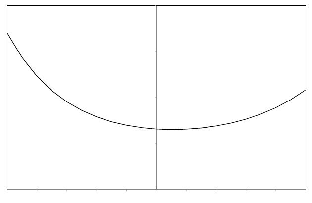
4. Transformations of variables
where RSS0and RSSλare the residual sums of squares from the constrained and
unconstrained regressions with Y∗.
The most obvious tests are λ= 0 for the logarithmic specification and λ= 1 for the
linear one. Note that it is not possible to test the two hypotheses directly against each
other. As with all tests, one can only test whether a hypothesis is incompatible with the
sample result. In this case we are testing whether the log-likelihood under the
restriction is significantly smaller than the unrestricted log-likelihood. Thus, while it is
possible that we may reject the linear but not the logarithmic, or vice versa, it is also
possible that we may reject both or fail to reject both.
Example
0
100
200
300
400
-1 -0.8 -0.6 -0.4 -0.2 0 0.2 0.4 0.6 0.8 1
The figure shows the residual sum of squares for values of λfrom −1 to 1 for the wage
equation example described in Section 4.2 in the text. The maximum likelihood estimate
is 0.10, with RSS = 130.3. For the linear and logarithmic specifications, RSS was 217.0
and 131.4, respectively, with likelihood ratio statistics 500(log 217.0−log 130.3) = 255.0
and 500(log 131.4−log 130.3) = 4.20.The logarithmic specification is clearly much to be
preferred, but even it is rejected at the 5 per cent level, with χ2(1) = 3.84.
4.4 Additional exercises
A4.1 Is expenditure on your category per capita related to total expenditure per capita?
An alternative model specification.
Define a new variable LGCATPC as the logarithm of expenditure per capita on
your category. Define a new variable LGEXPPC as the logarithm of total
household expenditure per capita. Regress LGCATPC on LGEXPPC. Provide an
interpretation of the coefficients, and perform appropriate statistical tests.
A4.2 Is expenditure on your category per capita related to household size as well as to
total expenditure per capita? An alternative model specification.
Regress LGCATPC on LGEXPPC and LGSIZE. Provide an interpretation of the
coefficients, and perform appropriate statistical tests.
72

4.4. Additional exercises
A4.3 A researcher is considering two regression specifications:
log Y=β1+β2log X+u(1)
and:
log Y
X=α1+α2log X+u(2)
where uis a disturbance term.
Writing y= log Y,x= log X, and z= log Y
X, and using the same sample of n
observations, the researcher fits the two specifications using OLS:
by=b
β1+b
β2x(3)
and:
bz=bα1+bα2x. (4)
•Using the expressions for the OLS regression coefficients, demonstrate that
b
β2=bα2+ 1.
•Similarly, using the expressions for the OLS regression coefficients,
demonstrate that b
β1=bα1.
•Hence demonstrate that the relationship between the fitted values of y, the
fitted values of z, and the actual values of x, is byi−xi=bzi.
•Hence show that the residuals for regression (3) are identical to those for (4).
•Hence show that the standard errors of b
β2and bα2are the same.
•Determine the relationship between the tstatistic for b
β2and the tstatistic for
bα2, and give an intuitive explanation for the relationship.
•Explain whether R2would be the same for the two regressions.
A4.4 A researcher has data on a measure of job performance, SKILL, and years of work
experience, EXP, for a sample of individuals in the same occupation. Believing
there to be diminishing returns to experience, the researcher proposes the model:
SKILL =β1+β2log(EXP) + β3log EXP2+u.
Comment on this specification.
A4.5 A researcher hypothesises that a variable Yis determined by a variable Xand
considers the following four alternative regression specifications, using
cross-sectional data:
Y=β1+β2X+u(1)
log Y=β1+β2X+u(2)
Y=β1+β2log X+u(3)
log Y=β1+β2log X+u. (4)
Explain why a direct comparison of R2, or of RSS, in models (1) and (2) is
illegitimate. What should be the strategy of the researcher for determining which of
the four specifications has the best fit?
73
4. Transformations of variables
A4.6 Is a logarithmic specification preferable to a linear specification for an expenditure
function?
Use your category of expenditure from the CES data set. Define CATPCST as
CATPC scaled by its geometric mean and LGCATST as the logarithm of
CATPCST. Regress CATPCST on EXPPC and SIZE and regress LGCATST on
LGEXPPC and LGSIZE. Compare the RSS for these equations.
A4.7
. reg LGEARN S EXP ASVABC SASVABC
Source | SS df MS Number of obs = 500
-------------+------------------------------ F( 4, 495) = 22.68
Model | 23.6368302 4 5.90920754 Prob > F = 0.0000
Residual | 128.96239 495 .26053008 R-squared = 0.1549
-------------+------------------------------ Adj R-squared = 0.1481
Total | 152.59922 499 .30581006 Root MSE = .51042
------------------------------------------------------------------------------
LGEARN | Coef. Std. Err. t P>|t| [95% Conf. Interval]
-------------+----------------------------------------------------------------
S | .0764243 .0116879 6.54 0.000 .0534603 .0993883
EXP | .0400506 .0096479 4.15 0.000 .0210948 .0590065
ASVABC | -.2096325 .1406659 -1.49 0.137 -.4860084 .0667434
SASVABC | .0188685 .0093393 2.02 0.044 .0005189 .0372181
_cons | 1.386753 .2109596 6.57 0.000 .9722664 1.80124
------------------------------------------------------------------------------
The output above shows the result of regressing the logarithm of hourly earnings
on years of schooling, years of work experience, ASVABC score, and SASVABC, an
interactive variable defined as the product of Sand ASVABC, using EAWE Data
Set 21. The mean values of S,EXP, and ASVABC in the sample were 14.9, 6.4,
and 0.27, respectively. Give an interpretation of the regression output.
A4.8 Perform a RESET test of functional misspecification. Using your EAWE data set,
regress WEIGHT11 on HEIGHT. Save the fitted values as YHAT and define
YHATSQ as its square. Add YHATSQ to the regression specification and test its
coefficient.
4.5 Answers to the starred exercises in the textbook
4.8 Suppose that the logarithm of Yis regressed on the logarithm of X, the fitted
regression being:
log b
Y=b
β1+b
β2log X.
Suppose X∗=µX, where µis a constant, and suppose that log Yis regressed on
log X∗. Determine how the regression coefficients are related to those of the original
regression. Determine also how the tstatistic for b
β2and R2for the equation are
related to those in the original regression.
74

4.5. Answers to the starred exercises in the textbook
Answer:
Nothing of substance is affected since the change amounts only to a fixed constant
shift in the measurement of the explanatory variable.
Let the fitted regression be:
log b
Y=b
β∗
1+b
β∗
2log X∗.
Note that:
log X∗
i−log X∗= log µXi−1
n
n
X
j=1
log X∗
j
= log µXi−1
n
n
X
j=1
log µXj
= log µ+ log Xi−1
n
n
X
j=1
(log µ+ log Xj)
= log Xi−1
n
n
X
j=1
log Xj
= log Xi−log X.
Hence b
β∗
2=b
β2. To compute the standard error of b
β∗
2, we will also need b
β∗
1.
b
β∗
1= log Y−b
β∗
2log X∗= log Y−b
β2
1
n
n
X
j=1
(log µ+ log Xj)
= log Y−b
β2log µ−b
β2log X
=b
β1−b
β2log µ.
Thus the residual bu∗
iis given by:
bu∗
i= log Yi−b
β∗
1−b
β∗
2log X∗
i= log Yi−(b
β1−b
β2log µ)−b
β2(log Xi+ log µ) = bui.
Hence the estimator of the variance of the disturbance term is unchanged and so
the standard error of b
β∗
2is the same as that for b
β2. As a consequence, the tstatistic
must be the same. R2must also be the same:
R2∗= 1 −Pbu∗2
i
Plog Yi−log Y= 1 −Pbu2
i
Plog Yi−log Y=R2.
4.11 RSS was the same in Tables 4.6 and 4.8. Demonstrate that this was not a
coincidence.
Answer:
This is a special case of the transformation in Exercise 4.7.
75
4. Transformations of variables
4.14
. gen LGHTSQ = ln(HEIGHTSQ)
. reg LGWT04 LGHEIGHT LGHTSQ
Source | SS df MS Number of obs = 500
-------------+------------------------------ F( 1, 498) = 211.28
Model | 7.90843858 1 7.90843858 Prob > F = 0.0000
Residual | 18.6403163 498 .037430354 R-squared = 0.2979
-------------+------------------------------ Adj R-squared = 0.2965
Total | 26.5487548 499 .053203918 Root MSE = .19347
------------------------------------------------------------------------------
LGWT04 | Coef. Std. Err. t P>|t| [95% Conf. Interval]
-------------+----------------------------------------------------------------
LGHEIGHT | (dropped)
LGHTSQ | 1.053218 .0724577 14.54 0.000 .9108572 1.195578
_cons | -3.78834 .610925 -6.20 0.000 -4.988648 -2.588031
------------------------------------------------------------------------------
The output shows the results of regressing, LGWT04, the logarithm of
WEIGHT04, on LGHEIGHT, the logarithm of HEIGHT, and LGHTSQ, the
logarithm of the square of HEIGHT, using EAWE Data Set 21. Explain the
regression results, comparing them with those in Exercise 4.2.
Answer:
LGHTSQ = 2 LGHEIGHT, so the specification is subject to exact
multicollinearity. In such a situation, Stata drops one of the variables responsible.
4.18
. nl (S = {beta1} + {beta2}/({beta3} + SIBLINGS)) if SIBLINGS>0
(obs = 473)
Iteration 0: residual SS = 3502.041
Iteration 1: residual SS = 3500.884
.....................................
Iteration 14: residual SS = 3482.794
Source | SS df MS
-------------+------------------------------ Number of obs = 473
Model | 132.339291 2 66.1696453 R-squared = 0.0366
Residual | 3482.7939 470 7.41019979 Adj R-squared = 0.0325
-------------+------------------------------ Root MSE = 2.722168
Total | 3615.13319 472 7.65918049 Res. dev. = 2286.658
------------------------------------------------------------------------------
S | Coef. Std. Err. t P>|t| [95% Conf. Interval]
-------------+----------------------------------------------------------------
/beta1 | 10.45811 5.371492 1.95 0.052 -.0970041 21.01322
/beta2 | 47.95198 125.3578 0.38 0.702 -198.3791 294.2831
/beta3 | 8.6994 15.10277 0.58 0.565 -20.97791 38.37671
------------------------------------------------------------------------------
Parameter beta1 taken as constant term in model & ANOVA table
76

4.6. Answers to the additional exercises
The output uses EAWE Data Set 21 to fit the nonlinear model:
S=β1+β2
β3+SIBLINGS +u
where Sis the years of schooling of the respondent and SIBLINGS is the number
of brothers and sisters. The specification is an extension of that for Exercise 4.1,
with the addition of the parameter β3. Provide an interpretation of the regression
results and compare it with that for Exercise 4.1.
Answer:
As in Exercise 4.1, the estimate of β1provides an estimate of the lower bound of
schooling, 10.46 years, when the number of siblings is large. The other parameters
do not have straightforward interpretations. The figure below represents the
relationship. Comparing this figure with that for Exercise 4.1, it can be seen that it
gives a very different picture of the adverse effect of additional siblings. The
specification in Exercise 4.1 suggests that the adverse effect is particularly large for
the first few siblings, and then attenuates. The revised specification indicates that
the adverse effect is more evenly spread and is more enduring. However, the
relationship has been fitted with imprecision since the estimates of β2and β3are
not significant.
12
13
14
15
16
17
0 1 2 3 4 5 6 7 8 9 10 11 12 13 14 15
Years of schooling
Siblings
Exercise 4.1
Exercise 4.18
4.6 Answers to the additional exercises
A4.1
. reg LGFDHOPC LGEXPPC
Source | SS df MS Number of obs = 6334
-------------+------------------------------ F( 1, 6332) = 4757.00
Model | 1502.58932 1 1502.58932 Prob > F = 0.0000
Residual | 2000.08269 6332 .315869029 R-squared = 0.4290
-------------+------------------------------ Adj R-squared = 0.4289
Total | 3502.67201 6333 .553082585 Root MSE = .56202
77

4. Transformations of variables
------------------------------------------------------------------------------
LGFDHOPC | Coef. Std. Err. t P>|t| [95% Conf. Interval]
-------------+----------------------------------------------------------------
LGEXPPC | .6092734 .0088338 68.97 0.000 .5919562 .6265905
_cons | .8988291 .0703516 12.78 0.000 .7609161 1.036742
------------------------------------------------------------------------------
The regression implies that the income elasticity of expenditure on food is 0.61
(supposing that total household expenditure can be taken as a proxy for permanent
income). In addition to testing the null hypothesis that the elasticity is equal to
zero, which is rejected at a very high significance level for all the categories, one
might test whether it is different from 1, as a means of classifying the categories of
expenditure as luxuries (elasticity >1) and necessities (elasticity <1).
The table gives the results for all the categories of expenditure.
Regression of LGCATPC on EXPPC
nb
β2s.e.(b
β2)t(β2= 0) t(β2= 1) R2RSS
ADM 2,815 1.098 0.030 37.20 3.33 0.330 1,383.9
CLOT 4,500 0.794 0.021 37.34 −9.69 0.237 1,394.0
DOM 1,661 0.812 0.049 16.54 −3.84 0.142 273.5
EDUC 561 1.382 0.090 15.43 4.27 0.299 238.1
ELEC 5,828 0.586 0.011 50.95 −36.05 0.308 2,596.3
FDAW 5,102 0.947 0.015 64.68 −3.59 0.451 4,183.6
FDHO 6,334 0.609 0.009 68.97 −44.23 0.429 4,757.0
FOOT 1,827 0.608 0.027 22.11 −14.26 0.211 488.7
FURN 487 0.912 0.085 10.66 −1.03 0.190 113.7
GASO 5,710 0.677 0.012 56.92 −27.18 0.362 3,240.1
HEAL 4,802 0.868 0.021 40.75 −6.22 0.257 1,660.6
HOUS 6,223 1.033 0.014 73.34 2.34 0.464 5,378.5
LIFE 1,253 0.607 0.047 13.00 −8.40 0.119 169.1
LOCT 692 0.510 0.055 9.29 −8.92 0.111 86.2
MAPP 399 0.817 0.033 9.87 −2.21 0.197 97.5
PERS 3,817 0.891 0.019 48.14 −5.88 0.378 2,317.3
READ 2,287 0.909 0.032 28.46 −2.84 0.262 809.9
SAPP 1,037 0.665 0.045 14.88 −7.49 0.176 221.3
TELE 5,788 0.710 0.012 58.30 −23.82 0.370 3,398.8
TEXT 992 0.629 0.046 13.72 −8.09 0.160 188.2
TOB 1,155 0.721 0.035 20.39 −7.87 0.265 415.8
TOYS 2,504 0.733 0.028 26.22 −9.57 0.216 687.5
TRIP 516 0.723 0.077 9.43 −3.60 0.147 88.9
78
4.6. Answers to the additional exercises
A4.2
. reg LGFDHOPC LGEXPPC LGSIZE
----------------------------------------------------------------------------
Source | SS df MS Number of obs = 6334
-----------+------------------------------ F( 2, 6331) = 2410.79
Model | 1514.30728 2 757.15364 Prob> F = 0.0000
Residual | 1988.36473 6331 .314068035 R-squared = 0.4323
-----------+------------------------------ Adj R-squared = 0.4321
Total | 3502.67201 6333 .553082585 Root MSE = .56042
----------------------------------------------------------------------------
LGFDHOPC | Coef. Std. Err. t P>|t| [95% Conf. Interval]
-----------+----------------------------------------------------------------
LGEXPPC | .5842097 .0097174 60.12 0.000 .5651604 .6032591
LGSIZE | -.0814427 .0133333 -6.11 0.000 -.1075806 -.0553049
_cons | 1.158326 .0820119 14.12 0.000 .9975545 1.319097
----------------------------------------------------------------------------
The income elasticity, 0.58, is now a little lower than before. The size elasticity is
significantly negative, suggesting economies of scale and indicating that the model
in the previous exercise was misspecified.
The specification is equivalent to that in Exercise 4.5 in the text. Writing the latter
again as:
LGCAT =β1+β2LGEXP +β3LGSIZE +u
we have:
LGCAT −LGSIZE =β1+β2(LGEXP −LGSIZE)+(β3+β2−1)LGSIZE +u
and so:
LGCATPC =β1+β2LGEXPPC + (β3+β2−1)LGSIZE +u.
Note that the estimates of the income elasticity are identical to those in Exercise
4.5 in the text. This follows from the fact that the theoretical coefficient, β2, has
not been affected by the manipulation. The specification differs from that in
Exercise A4.1 in that we have not dropped the LGSIZE term and so we are not
imposing the restriction β3+β2−1 = 0.
79

4. Transformations of variables
Dependent variable LGCATPC
LGEXPPC LGSIZE
nb
β2s.e.(b
β2)b
β3s.e.(b
β3)R2FRSS
ADM 2,815 1.080 0.033 −0.055 0.043 0.330 692.9 3,945.2
CLOT 4,500 0.842 0.024 0.146 0.032 0.240 710.1 5,766.1
DOM 1,661 0.941 0.054 0.415 0.075 0.157 154.6 4,062.5
EDUC 561 1.229 0.101 −0.437 0.139 0.311 125.9 1,380.1
ELEC 5,828 0.372 0.012 −0.362 0.017 0.359 1,627.8 2,636.3
FDAW 5,102 0.879 0.016 −0.213 0.022 0.461 2,176.6 3,369.1
FDHO 6,334 0.584 0.010 −0.081 0.013 0.432 2,410.8 1,988.4
FOOT 1,827 0.396 0.031 −0.560 0.042 0.281 356.1 1,373.5
FURN 487 0.807 0.103 −0.246 0.137 0.195 58.7 913.9
GASO 5,710 0.676 0.013 −0.004 0.018 0.362 1,691.8 2,879.3
HEAL 4,802 0.779 0.023 −0.306 0.031 0.272 894.6 6,062.5
HOUS 6,223 0.989 0.016 −0.140 0.021 0.467 2,729.5 4,825.6
LIFE 1,253 0.464 0.050 −0.461 0.065 0.154 113.4 1,559.2
LOCT 692 0.389 0.060 −0.396 0.086 0.138 54.9 1,075.1
MAPP 399 0.721 0.094 −0.264 0.123 0.206 51.5 576.8
PERS 3,817 0.824 0.020 −0.217 0.028 0.388 1,206.3 3,002.2
READ 2,287 0.764 0.034 −0.503 0.047 0.297 482.8 2,892.1
SAPP 1,037 0.467 0.048 −0.592 0.066 0.236 160.1 1,148.9
TELE 5,788 0.640 0.013 −0.222 0.018 0.386 1,816.3 3,055.1
TEXT 992 0.388 0.049 −0.713 0.067 0.246 161.0 1,032.9
TOB 1,155 0.563 0.037 −0.515 0.049 0.329 282.1 873.4
TOYS 2,504 0.638 0.031 −0.304 0.043 0.231 375.8 2,828.3
TRIP 516 0.681 0.083 −0.142 0.109 0.150 45.3 792.8
A4.3 A researcher is considering two regression specifications:
log Y=β1+β2log X+u(1)
and:
log Y
X=α1+α2log X+u(2)
where uis a disturbance term.
Determine whether (2) is a reparameterised or a restricted version of (1).
(2) may be rewritten:
log Y=α1+ (α2+ 1) log X+u
so it is a reparameterised version of (1) with β1=α1and β2=α2+ 1.
Writing y= log Y,x= log X, and z= log Y
X, and using the same sample of n
observations, the researcher fits the two specifications using OLS:
by=b
β1+b
β2x(3)
and:
bz=bα1+bα2x. (4)
80

4.6. Answers to the additional exercises
Using the expressions for the OLS regression coefficients, demonstrate that
b
β2=bα2+ 1.
bα2=P(xi−x)(zi−z)
P(xi−x)2=P(xi−x)([yi−xi]−[y−x])
P(xi−x)2
=P(xi−x)(yi−y)
P(xi−x)2−P(xi−x)2
P(xi−x)2=b
β2−1.
Similarly, using the expressions for the OLS regression coefficients, demonstrate
that b
β1=bα1.
bα1=z−bα2x= (y−x)−bα2x=y−(bα2+ 1)x=y−b
β2x=b
β1.
Hence demonstrate that the relationship between the fitted values of y,the fitted
values of z,and the actual values of x,is byi−xi=bzi.
bzi=bα1+bα2xi=b
β1+ (b
β2−1)xi=b
β1+b
β2xi−xi=byi−xi.
Hence show that the residuals for regression (3) are identical to those for (4).
Let buibe the residual in (3) and bvithe residual in (4). Then:
bvi=zi−bzi=yi−xi−(byi−xi) = yi−byi=bui.
Hence show that the standard errors of b
β2and bα2are the same.
The standard error of b
β2is:
s.e.(b
β2) = sPbu2
i/(n−2)
P(xi−x)2=sPbv2
i/(n−2)
P(xi−x)2= s.e.(bα2).
Determine the relationship between the tstatistic for b
β2and the tstatistic for bα2,
and give an intuitive explanation for the relationship.
tb
β2=b
β2
s.e.(b
β2)=bα2+ 1
s.e.(bα2).
The tstatistic for b
β2is for the test of H0:β2= 0. Given the relationship, it is also
for the test of H0:α2=−1. The tests are equivalent since both of them reduce the
model to log Ydepending only on an intercept and the disturbance term.
Explain whether R2would be the same for the two regressions.
R2will be different because it measures the proportion of the variance of the
dependent variable explained by the regression, and the dependent variables are
different.
A4.4 The proposed model:
SKILL =β1+β2log(EXP) + β3log(EXP2) + u
cannot be fitted since:
log(EXP2) = 2 log(EXP)
and the specification is therefore subject to exact multicollinearity.
81
4. Transformations of variables
A4.5 In (1) R2is the proportion of the variance of Yexplained by the regression. In (2)
it is the proportion of the variance of log Yexplained by the regression. Thus,
although related, they are not directly comparable. In (1) RSS has dimension the
squared units of Y. In (2) it has dimension the squared units of log Y. Typically it
will be much lower in (2) because the logarithm of Ytends to be much smaller
than Y.
The specifications with the same dependent variable may be compared directly in
terms of RSS (or R2) and hence two of the specifications may be eliminated
immediately. The remaining two specifications should be compared after scaling,
with Yreplaced by Y∗where Y∗is defined as Ydivided by the geometric mean of
Yin the sample. RSS for the scaled regressions will then be comparable.
A4.6 The RSS comparisons for all the categories of expenditure indicate that the
logarithmic specification is overwhelmingly superior to the linear one. The
differences are actually surprisingly large and suggest that some other factor may
also be at work. One possibility is that the data contain many outliers, and these
do more damage to the fit in linear than in logarithmic specifications. To see this,
plot CATPC and EXPPC and compare with a plot of LGCATPC and LGEXPPC.
(Strictly speaking, you should control for SIZE and LGSIZE using the
Frisch–Waugh–Lovell method described in Chapter 3.)
The following Stata output gives the results of fitting the model for FDHO,
assuming that both the dependent variable and the explanatory variables are
subject to the Box–Cox transformation with the same value of λ. Iteration
messages have been deleted. The maximum likelihood estimate of λis 0.10, so the
logarithmic specification is a better approximation than the linear specification.
The latter is very soundly rejected by the likelihood-ratio test.
. boxcox FDHOPC EXPPC SIZE if FDHO>0, model(lambda)
Number of obs = 6334
LR chi2(2) = 3592.55
Log likelihood = -41551.328 Prob > chi2 = 0.000
------------------------------------------------------------------------------
FDHOPC | Coef. Std. Err. z P>|z| [95% Conf. Interval]
-------------+----------------------------------------------------------------
/lambda | .1019402 .0117364 8.69 0.000 .0789372 .1249432
------------------------------------------------------------------------------
Estimates of scale-variant parameters
----------------------------
| Coef.
-------------+--------------
Notrans |
_cons | 2.292828
-------------+--------------
Trans |
EXPPC | .4608736
SIZE | -.1486856
-------------+--------------
/sigma | .9983288
----------------------------
82
4.6. Answers to the additional exercises
---------------------------------------------------------
Test Restricted LR statistic P-value
H0: log likelihood chi2 Prob > chi2
---------------------------------------------------------
lambda = -1 -50942.835 18783.01 0.000
lambda = 0 -41590.144 77.63 0.000
lambda = 1 -44053.749 5004.84 0.000
---------------------------------------------------------
A4.7 Let the theoretical model for the regression be written:
LGEARN =β1+β2S+β3EXP +β4ASVABC +β5SA +u.
The estimate of β4is negative, at first sight suggesting that cognitive ability has an
adverse effect on earnings, contrary to common sense and previous results with
wage equations of this kind. However, rewriting the model as:
LGEARN =β1+β2S+β3EXP + (β4+β5S)ASVABC +u
it can be seen that, as a consequence of the inclusion of the interactive term, β4
represents the effect of a marginal year of schooling for an individual with no
schooling. Since no individual in the sample had fewer than 8 years of schooling,
the perverse sign of the estimate illustrates only the danger of extrapolating
outside the data range. It makes better sense to evaluate the implicit coefficient for
an individual with the mean years of schooling, 14.9. This is
(−0.2096 + 0.0189 ×14.9) = 0.072, implying a much more plausible 7.2 per cent
increase in earnings for each standard deviation increase in cognitive ability. The
positive sign of the coefficient of SA suggests that schooling and cognitive ability
have mutually reinforcing effects on earnings.
One way of avoiding nonsense parameter estimates is to measure the variables in
question from their sample means. This has been done in the regression output
below, where S1 and ASVABC1 are schooling and ASVABC measured from their
sample means and SASVABC1 is their interaction. The coefficients of Sand
ASVABC now provide estimates of their effects when the other variable is equal to
its sample mean.
. reg LGEARN S1 EXP ASVABC1 SASVABC1
----------------------------------------------------------------------------
Source | SS df MS Number of obs = 500
-----------+------------------------------ F( 4, 495) = 22.68
Model | 23.6368304 4 5.90920759 Prob > F = 0.0000
Residual | 128.962389 495 .260530079 R-squared = 0.1549
-----------+------------------------------ Adj R-squared = 0.1481
Total | 152.59922 499 .30581006 Root MSE = .51042
----------------------------------------------------------------------------
LGEARN | Coef. Std. Err. t P>|t| [95% Conf. Interval]
-----------+----------------------------------------------------------------
S1 | .0815188 .0116521 7.00 0.000 .0586252 .1044125
EXP | .0400506 .0096479 4.15 0.000 .0210948 .0590065
ASVABC1 | .0715084 .0298278 2.40 0.017 .0129036 .1301132
SASVABC1 | .0188685 .0093393 2.02 0.044 .0005189 .0372181
_cons | 2.544783 .0675566 37.67 0.000 2.41205 2.677516
----------------------------------------------------------------------------
83
4. Transformations of variables
A4.8 In the first part of the output, WEIGHT11 is regressed on HEIGHT, using EAWE
Data Set 21. The predict command saves the fitted values from the most recent
regression, assigning them the variable name that follows the command, in this
case YHAT.YHATSQ is defined as the square of YHAT, and this is added to the
regression specification. Somewhat surprisingly, its coefficient is not significant. A
logarithmic regression of WEIGHT11 on HEIGHT yields an estimated elasticity of
2.05, significantly different from 1 at a high significance level. Multicollinearity is
responsible for the failure to detect nonlinearity hear. YHAT is very highly
correlated with HEIGHT.
. reg WEIGHT11 HEIGHT
----------------------------------------------------------------------------
Source | SS df MS Number of obs = 500
-----------+------------------------------ F( 1, 498) = 139.97
Model | 236642.736 1 236642.736 Prob > F = 0.0000
Residual | 841926.912 498 1690.61629 R-squared = 0.2194
-----------+------------------------------ Adj R-squared = 0.2178
Total | 1078569.65 499 2161.46222 Root MSE = 41.117
----------------------------------------------------------------------------
WEIGHT11 | Coef. Std. Err. t P>|t| [95% Conf. Interval]
-----------+----------------------------------------------------------------
HEIGHT | 5.369246 .4538259 11.83 0.000 4.477597 6.260895
_cons | -184.7802 30.8406 -5.99 0.000 -245.3739 -124.1865
----------------------------------------------------------------------------
. predict YHAT
. gen YHATSQ = YHAT*YHAT
. reg WEIGHT11 HEIGHT YHATSQ
----------------------------------------------------------------------------
Source | SS df MS Number of obs = 500
-----------+------------------------------ F( 2, 497) = 70.33
Model | 237931.888 2 118965.944 Prob > F = 0.0000
Residual | 840637.76 497 1691.42407 R-squared = 0.2206
-----------+------------------------------ Adj R-squared = 0.2175
Total | 1078569.65 499 2161.46222 Root MSE = 41.127
----------------------------------------------------------------------------
WEIGHT11 | Coef. Std. Err. t P>|t| [95% Conf. Interval]
-----------+----------------------------------------------------------------
HEIGHT | -.4995924 6.737741 -0.07 0.941 -13.73756 12.73837
YHATSQ | .0030233 .003463 0.87 0.383 -.0037807 .0098273
_cons | 114.5523 344.2538 0.33 0.739 -561.8199 790.9244
----------------------------------------------------------------------------
84

Chapter 5
Dummy variables
5.1 Overview
This chapter explains the definition and use of a dummy variable, a device for allowing
qualitative characteristics to be introduced into the regression specification. Although
the intercept dummy may appear artificial and strange at first sight, and the slope
dummy even more so, you will become comfortable with the use of dummy variables
very quickly. The key is to keep in mind the graphical representation of the regression
model.
5.2 Learning outcomes
After working through the corresponding chapter in the text, studying the
corresponding slideshows, and doing the starred exercises in the text and the additional
exercises in this subject guide, you should be able to explain:
how the intercept and slope dummy variables are defined
what impact they have on the regression specification
how the choice of reference (omitted) category affects the interpretation of ttests
on the coefficients of dummy variables
how a change of reference category would affect the regression results
how to perform a Chow test
when and why a Chow test is equivalent to a particular Ftest of the joint
explanatory power of a set of dummy variables.
5.3 Additional exercises
A5.1 In Exercise A1.4 the logarithm of earnings was regressed on height using EAWE
Data Set 21 and, somewhat surprisingly, it was found that height had a highly
significant positive effect. We have seen that the logarithm of earnings is more
satisfactory than earnings as the dependent variable in a wage equation. Fitting the
semilogarithmic specification, we obtain:
85
5. Dummy variables
. reg LGEARN HEIGHT
----------------------------------------------------------------------------
Source | SS df MS Number of obs = 500
-----------+------------------------------ F( 1, 498) = 6.27
Model | 1.84965685 1 1.84965685 Prob > F = 0.0126
Residual | 146.79826 498 .294775622 R-squared = 0.0124
-----------+------------------------------ Adj R-squared = 0.0105
Total | 148.647917 499 .297891616 Root MSE = .54293
----------------------------------------------------------------------------
LGEARN | Coef. Std. Err. t P>|t| [95% Conf. Interval]
-----------+----------------------------------------------------------------
HEIGHT | .0148894 .005944 2.50 0.013 .003211 .0265678
_cons | 1.746174 .4032472 4.33 0.000 .9538982 2.538449
----------------------------------------------------------------------------
The tstatistic for HEIGHT is again significant, if only at the 5 per cent level. In
Exercise A1.4 it was hypothesised that the effect might be attributable to males
tending to have greater earnings than females and also tending to be taller. The
output below shows the result of adding the dummy variable to the specification,
to control for sex. Comment on the results.
. reg LGEARN HEIGHT MALE
----------------------------------------------------------------------------
Source | SS df MS Number of obs = 500
-----------+------------------------------ F( 2, 497) = 4.20
Model | 2.47043329 2 1.23521664 Prob > F = 0.0155
Residual | 146.177483 497 .294119685 R-squared = 0.0166
-----------+------------------------------ Adj R-squared = 0.0127
Total | 148.647917 499 .297891616 Root MSE = .54233
----------------------------------------------------------------------------
LGEARN | Coef. Std. Err. t P>|t| [95% Conf. Interval]
-----------+----------------------------------------------------------------
HEIGHT | .0060845 .0084844 0.72 0.474 -.0105852 .0227541
MALE | .1007018 .0693157 1.45 0.147 -.0354862 .2368898
_cons | 2.292078 .5508559 4.16 0.000 1.209784 3.374371
----------------------------------------------------------------------------
A5.2 Does ethnicity have an effect on household expenditure?
The variable REFRACE in the CES data set is coded 1 if the reference individual
in the household, usually the head of the household, is white and it is coded greater
than 1 for other ethnicities. Define a dummy variable NONWHITE that is 0 if
REFRACE is 1 and 1 if REFRACE is greater than 1. Regress LGCATPC on
LGEXPPC,LGSIZE, and NONWHITE. Provide an interpretation of the
coefficients, and perform appropriate statistical tests.
A5.3 Does education have an effect on household expenditure?
The variable REFEDUC in the CES data set provides information on the
education of the reference individual in the household. Define dummy variables
EDUCDO (high-school drop out or less), EDUCSC (some college), and EDUCBA
(complete college or more) using the following rules:
86
5.3. Additional exercises
•EDUCDO = 1 if REFEDUC <12, 0 otherwise
•EDUCSC = 1 if REFEDUC = 13 or 14, 0 otherwise
•EDUCBA = 1 if REFEDUC >14, 0 otherwise.
Regress LGCATPC on LGEXPPC,LGSIZE,EDUCDO,EDUCSC, and EDUCBA.
Provide an interpretation of the coefficients, and perform appropriate statistical
tests. Note that the reference (omitted) category for the dummy variables is high
school graduate with no college (REFEDUC = 12).
A5.4 Using the CES data set, evaluate whether the education dummies as a group have
significant explanatory power for expenditure on your category of expenditure by
comparing the residual sums of squares in the regressions in Exercises A4.2 and
A5.3.
A5.5 Repeat Exercise A5.3 making EDUCDO the reference (omitted) category.
Introduce a new dummy variable EDUCHSD for high school diploma, since this is
no longer the omitted category:
•EDUCHSD = 1 if REFEDUC = 12, 0 otherwise.
Evaluate the impact on the interpretation of the coefficients and the statistical
tests.
A5.6 A researcher has data on hourly earnings in dollars, EARNINGS, years of schooling
(highest grade completed), S, and sector of employment, GOV, for 1,355 male
respondents in the National Longitudinal Survey of Youth 1979– for 2002. GOV is
defined as a dummy variable equal to 0 if the respondent was working in the
private sector and 1 if the respondent was working in the government sector. 91 per
cent of the private sector workers and 95 per cent of the government sector workers
had at least 12 years of schooling. The mean value of Swas 13.5 for the private
sector and 14.6 for the government sector. The researcher regresses LGEARN, the
natural logarithm of EARNINGS:
•(1) on GOV alone
•(2) on GOV and S
•(3) on GOV,S, and SGOV
where the variable SGOV is defined to be the product of Sand GOV, with the
results shown in the following table.
Standard errors are shown in parentheses and tstatistics in square brackets. RSS
= residual sum of squares.
87

5. Dummy variables
(1) (2) (3)
0.007 −0.121 0.726
GOV (0.043) (0.038) (0.193)
[0.16] [−3.22] [3.76]
0.116 0.130
S— (0.006) (0.006)
[21.07] [20.82]
−0.059
SGOV — — (0.013)
[−4.48]
2.941 1.372 1.195
constant (0.018) (0.076) (0.085)
[163.62] [18.04] [14.02]
R20.000 0.247 0.258
RSS 487.7 367.2 361.8
•Explain verbally why the estimates of the coefficient of GOV are different in
regressions (1) and (2).
•Explain the difference in the estimates of the coefficient of GOV in regressions
(2) and (3).
•The correlation between GOV and SGOV was 0.977. Explain the variations in
the standard error of the coefficient of GOV in the three regressions.
A5.7 A researcher has data on the average annual rate of growth of employment, e, and
the average annual rate of growth of GDP, x, both measured as percentages, for a
sample of 27 developing countries and 23 developed ones for the period 1985–1995.
He defines a dummy variable Dthat is equal to 1 for the developing countries and
0 for the others. Hypothesising that the impact of GDP growth on employment
growth is lower in the developed countries than in the developing ones, he defines a
slope dummy variable xD as the product of xand Dand fits the regression
(standard errors in parentheses):
whole sample be=−1.45 + 0.19x+ 0.78xD R2= 0.61
(0.36) (0.10) (0.10) RSS = 50.23
He also runs simple regressions of eon xfor the whole sample, for the developed
countries only, and for the developing countries only, with the following results:
whole sample be=−0.56 + 0.24x R2= 0.04
(0.53) (0.16) RSS = 121.61
developed be=−2.74 + 0.50x R2= 0.35
countries (0.58) (0.15) RSS = 18.63
developing be=−0.85 + 0.78x R2= 0.51
countries (0.42) (0.15) RSS = 25.23
•Explain mathematically and graphically the role of the dummy variable xD in
this model.
88
5.3. Additional exercises
•The researcher could have included Das well as xD as an explanatory variable
in the model. Explain mathematically and graphically how it would have
affected the model.
•Suppose that the researcher had included Das well as xD.
◦What would the coefficients of the regression have been?
◦What would the residual sum of squares have been?
◦What would the tstatistic for the coefficient of Dhave been?
•Perform two tests of the researcher’s hypothesis. Explain why you would not
test it with a ttest on the coefficient of xD in regression (1).
A5.8 Does going to college have an effect on household expenditure?
Using the CES data set, define a dummy variable COLLEGE that is 0 if
REFEDUC is less than 13 (no college education) and 1 if REFEDUC is greater
than 12 (partial or complete college education). Regress LGCATPC on LGEXPPC
and LGSIZE: (1) for those respondents with COLLEGE = 1, (2) for those
respondents with COLLEGE = 0, and (3) for the whole sample. Perform a Chow
test.
A5.9 How does education impact on household expenditure?
In Exercise A5.8 you defined an intercept dummy COLLEGE that allowed you to
investigate whether going to college caused a shift in your expenditure function.
Now define slope dummy variables that allow you to investigate whether going to
college affects the coefficients of LGEXPPC and LGSIZE. Define LEXPCOL as the
product of LGEXPPC and COLLEGE, and define LSIZECOL as the product of
LGSIZE and COLLEGE. Regress LGCATPC on LGEXPPC,LGSIZE,
COLLEGE,LEXPCOL, and LSIZECOL. Provide an interpretation of the
coefficients, and perform appropriate tests. Include a test of the joint explanatory
power of the dummy variables by comparing RSS in this regression with that in
Exercise A4.3. Verify that the outcome of this Ftest is identical to that for the
Chow test in Exercise A5.8.
A5.10 You are given the following data on 2,800 respondents in the National Longitudinal
Survey of Youth 1979– with jobs in 2011:
•hourly earnings in the respondent’s main job at the time of the 2011 interview
•educational attainment (highest grade completed)
•mother’s and father’s educational attainment
•ASVABC score
•sex
•ethnicity: black, Hispanic, or white, that is (not black nor Hispanic)
•whether the main job in 2011 was in the government sector or the private
sector.
As a policy analyst, you are asked to investigate whether there is evidence of
earnings discrimination, positive or negative, by sex or ethnicity in (1) the
89

5. Dummy variables
government sector, and (2) the private sector. Explain how you would do this,
giving a mathematical representation of your regression specification(s).
You are also asked to investigate whether the incidence of earnings discrimination,
if any, is significantly different in the two sectors. Explain how you would do this,
giving a mathematical representation of your regression specification(s). In
particular, discuss whether a Chow test would be useful for this purpose.
A5.11 A researcher has data from the National Longitudinal Survey of Youth 1997– for
the year 2000 on hourly earnings, Y, years of schooling, S, and years of work
experience, EXP, for a sample of 1,774 males and 1,468 females. She defines a
dummy variable MALE for being male, a slope dummy variable SMALE as the
product of Sand MALE, and another slope dummy variable EXPMALE as the
product of EXP and MALE. She performs the following regressions (1) log Yon S
and EXP for the entire sample, (2) log Yon Sand EXP for males only, (3) log Y
on Sand EXP for females only, (4) log Yon S,EXP, and MALE for the entire
sample, and (5) log Yon S,EXP,MALE,SMALE, and EXPMALE for the entire
sample. The results are shown in the table, with standard errors in parentheses.
RSS is the residual sum of squares and nis the number of observations.
(1) (2) (3) (4) (5)
S0.094 0.099 0.094 0.0967 0.094
(0.003) (0.004) (0.005) (0.003) (0.005)
EXP 0.046 0.042 0.039 0.040 0.039
(0.002) (0.003) (0.002) (0.002) (0.003)
MALE — — — 0.234 0.117
(0.016) (0.108)
SMALE — — — — 0.005
(0.007)
EXPMALE — — — — 0.003
(0.004)
constant 5.165 5.283 5.166 5.111 5.166
(0.054) (0.083) (0.068) (0.052) (0.074)
R20.319 0.277 0.363 0.359 0.359
RSS 714.6 411.0 261.6 672.8 672.5
n3,242 1,774 1,468 3,242 3,242
The correlations between MALE and SMALE, and MALE and EXPMALE, were
both 0.96. The correlation between SMALE and EXPMALE was 0.93.
•Give an interpretation of the coefficients of Sand SMALE in regression (5).
•Give an interpretation of the coefficients of MALE in regressions (4) and (5).
•The researcher hypothesises that the earnings function is different for males
and females. Perform a test of this hypothesis using regression (4), and also
using regressions (1) and (5).
•Explain the differences in the tests using regression (4) and using regressions
(1) and (5).
90
5.3. Additional exercises
•At a seminar someone suggests that a Chow test could shed light on the
researcher’s hypothesis. Is this correct?
•Explain which of (1), (4), and (5) would be your preferred specification.
A5.12 A researcher has data for the year 2000 from the National Longitudinal Survey of
Youth 1997– on the following characteristics of the respondents: hourly earnings,
EARNINGS, measured in dollars; years of schooling, S; years of work experience,
EXP; sex; and ethnicity (blacks, hispanics, and ‘whites’ (those not classified as
black or hispanic). She drops the hispanics from the sample, leaving 2,135 ‘whites’
and 273 blacks, and defines dummy variables MALE and BLACK.MALE is
defined to be 1 for males and 0 for females. BLACK is defined to be 1 for blacks
and 0 for ‘whites’. She defines LGEARN to be the natural logarithm of
EARNINGS. She fits the following ordinary least squares regressions, each with
LGEARN as the dependent variable:
•(1) Explanatory variables S,EXP, and MALE, whole sample
•(2) Explanatory variables S,EXP,MALE, and BLACK, whole sample
•(3) Explanatory variables S,EXP, and MALE, ‘whites’ only
•(4) Explanatory variables S,EXP, and MALE, blacks only.
She then defines interaction terms SB =S×BLACK,EB =EXP×BLACK, and
MB =MALE×BLACK, and runs a fifth regression, still with LGEARN as the
dependent variable:
•(5) Explanatory variables S,EXP,MALE,BLACK,SB,EB,MB, whole
sample.
The results are shown in the table. Unfortunately, some of those for Regression 4
are missing from the table. RSS = residual sum of squares. Standard errors are
given in parentheses.
91

5. Dummy variables
(1) (2) (3) (4) (5)
whole whole ‘whites’ blacks whole
sample sample only only sample
S0.124 0.121 0.122 V0.122
(0.004) (0.004) (0.004) (0.004)
EXP 0.033 0.032 0.033 W0.033
(0.002) (0.002) (0.003) (0.003)
MALE 0.278 0.277 0.306 X0.306
(0.020) (0.020) (0.021) (0.021)
BLACK —−0.144 — — 0.205
(0.032) (0.225)
SB — — — — −0.009
(0.016)
EB — — — — −0.006
(0.007)
MB — — — — −0.280
(0.065)
constant 0.390 0.459 0.411 Y0.411
(0.075) (0.076) (0.084) (0.082)
R20.335 0.341 0.332 0.321 0.347
RSS 610.0 605.1 555.7 Z600.0
n2,408 2,408 2,135 273 2,408
•Calculate the missing coefficients V,W,X, and Yin Regression 4 (just the
coefficients, not the standard errors) and Z, the missing RSS, giving an
explanation of your computations.
•Give an interpretation of the coefficient of BLACK in Regression 2.
•Perform an Ftest of the joint explanatory power of BLACK,SB,EB, and
MB in Regression 5.
•Explain whether it is possible to relate the Ftest in part (c) to a Chow test
based on Regressions 1, 3, and 4.
•Give an interpretation of the coefficients of BLACK and MB in Regression 5.
•Explain whether a simple ttest on the coefficient of BLACK in Regression 2 is
sufficient to show that the wage equations are different for blacks and ‘whites’.
A5.13 As part of a workshop project, four students are investigating the effects of
ethnicity and sex on earnings using data for the year 2002 in the National
Longitudinal Survey of Youth 1979–. They all start with the same basic
specification:
log Y=β1+β2S+β3EXP +u
where Yis hourly earnings, measured in dollars, Sis years of schooling completed,
and EXP is years of work experience. The sample contains 123 black males, 150
black females, 1,146 white males, and 1,127 white females. (All respondents were
either black or white. The Hispanic subsample was dropped.) The output from
fitting this basic specification is shown in column 1 of the table (standard errors in
92

5.3. Additional exercises
parentheses; RSS is residual sum of squares, nis the number of observations in the
regression).
Basic Student C Student D
(1) (2) (3) (4a) (4b) (5a) (5b)
All All All Males Females Whites Blacks
S0.126 0.121 0.121 0.133 0.112 0.126 0.112
(0.004) (0.004) (0.004) (0.006) (0.006) (0.005) (0.012)
EXP 0.040 0.032 0.032 0.032 0.035 0.041 0.028
(0.002) (0.002) (0.002) (0.004) (0.003) (0.003) (0.005)
MALE — 0.277 0.308 — — — —
(0.020) (0.021)
BLACK —−0.144 −0.011 — — —- —
(0.032) (0.043)
MALEBLACK — — −0.290 — — — —
(0.063)
constant 0.376 0.459 0.447 0.566 0.517 0.375 0.631
(0.078) (0.076) (0.076) (0.124) (0.097) (0.087) (0.172)
R20.285 0.341 0.346 0.287 0.275 0.271 0.320
RSS 659 608 603 452 289 609 44
n2,546 2,546 2,546 1,269 1,277 2,273 273
Student A divides the sample into the four ethnicity/sex categories. He chooses
white females as the reference category and fits a regression that includes three
dummy variables BM,WM, and BF.BM is 1 for black males, 0 otherwise; WM is
1 for white males, 0 otherwise, and BF is 1 for black females, 0 otherwise.
Student B simply fits the basic specification separately for the four ethnicity/sex
subsamples.
Student C defines dummy variables MALE, equal to 1 for males and 0 for females,
and BLACK, equal to 1 for blacks and 0 for whites. She also defines an interactive
dummy variable MALEBLACK as the product of MALE and BLACK. She fits a
regression adding MALE and BLACK to the basic specification, and a further
regression adding MALEBLACK as well. The output from these regressions is
shown in columns 2 and 3 in the table.
Student D divides the sample into males and females and performs the regression
for both sexes separately, using the basic specification. The output is shown in
columns 4a and 4b. She also divides the sample into whites and blacks, and again
runs separate regressions using the basic specification. The output is shown in
columns 5a and 5b.
Reconstruction of missing output.
Students A and B left their output on a bus on the way to the workshop. This is
why it does not appear in the table.
•State what the missing output of Student A would have been, as far as this is
can be done exactly, given the results of Students C and D. (Coefficients,
standard errors, R2,RSS.)
93
5. Dummy variables
•Explain why it is not possible to reconstruct any of the output of Student B.
Tests of hypotheses.
The approaches of the students allowed them to perform different tests, given the
output shown in the table and the corresponding output for Students A and B.
Explain the tests relating to the effects of sex and ethnicity that could be
performed by each student, giving a clear indication of the null hypothesis in each
case. (Remember, all of them started with the basic specification (1), before
continuing with their individual regressions.) In the case of Ftests, state the test
statistic in terms of its components.
•Student A (assuming he had found his output)
•Student B (assuming he had found his output)
•Student C
•Student D.
If you had been participating in the project and had had access to the data set,
what regressions and tests would you have performed?
5.4 Answers to the starred exercises in the textbook
5.2 The Stata output for Data Set 21 shows the result of regressing weight in 2004,
measured in pounds, on height, measured in inches, first with a linear specification,
then with a logarithmic one, in both cases including a dummy variable MALE,
defined as in Exercise 5.1. Give an interpretation of the coefficients and perform
appropriate statistical tests. See Box 5.1 for a guide to the interpretation of dummy
variable coefficients in logarithmic regressions.
. reg WEIGHT04 HEIGHT MALE
----------------------------------------------------------------------------
Source | SS df MS Number of obs = 500
-----------+------------------------------ F( 2, 497) = 90.45
Model | 215264.34 2 107632.17 Prob > F = 0.0000
Residual | 591434.61 497 1190.00927 R-squared = 0.2668
-----------+------------------------------ Adj R-squared = 0.2639
Total | 806698.95 499 1616.63116 Root MSE = 34.497
----------------------------------------------------------------------------
WEIGHT04 | Coef. Std. Err. t P>|t| [95% Conf. Interval]
-----------+----------------------------------------------------------------
HEIGHT | 4.424345 .5213809 8.49 0.000 3.399962 5.448727
MALE | 7.702828 4.225065 1.82 0.069 -.598363 16.00402
_cons | -136.9713 33.9953 -4.03 0.000 -203.7635 -70.17904
----------------------------------------------------------------------------
94
5.4. Answers to the starred exercises in the textbook
. reg LGWT04 LGHEIGHT MALE
----------------------------------------------------------------------------
Source | SS df MS Number of obs = 500
-----------+------------------------------ F( 2, 497) = 109.53
Model | 8.12184709 2 4.06092355 Prob > F = 0.0000
Residual | 18.4269077 497 .037076273 R-squared = 0.3059
-----------+------------------------------ Adj R-squared = 0.3031
Total | 26.5487548 499 .053203918 Root MSE = .19255
----------------------------------------------------------------------------
LGWT04 | Coef. Std. Err. t P>|t| [95% Conf. Interval]
-----------+----------------------------------------------------------------
LGHEIGHT | 1.7814 .1978798 9.00 0.000 1.392616 2.170185
MALE | .0566894 .0236289 2.40 0.017 .0102645 .1031142
_cons | -2.44656 .8261259 -2.96 0.003 -4.06969 -.8234307
----------------------------------------------------------------------------
Answer:
The first regression indicates that weight increase by 4.4 pounds for each inch of
stature and that males tend to weigh 7.7 pounds more than females, controlling for
height, but the coefficient of MALE is not significant. The second regression
indicates that the elasticity of weight with respect to height is 1.78, and that males
weigh 5.7 per cent more than females, the latter effect now being significantly
different from zero at the 5 per cent level.
The null hypothesis that the elasticity is zero is not worth testing, except perhaps
in a negative sense, for if the result were not highly significant there would have to
be something seriously wrong with the model specification. Two other hypotheses
might be of greater interest: the elasticity being equal to 1, weight growing
proportionally with height, and the elasticity being equal to 3, all dimensions
increasing proportionally with height. The tstatistics are 4.27 and −8.37,
respectively, so both hypotheses are rejected.
5.5 Suppose that the relationship:
Yi=β1+β2Xi+ui
is being fitted and that the value of Xis missing for some observations. One way of
handling the missing values problem is to drop those observations. Another is to
set X= 0 for the missing observations and include a dummy variable Ddefined to
be equal to 1 if Xis missing, 0 otherwise. Demonstrate that the two methods must
yield the same estimates of β1and β2. Write down an expression for RSS using the
second approach, decompose it into the RSS for observations with Xpresent and
RSS for observations with Xmissing, and determine how the resulting expression
is related to RSS when the missing value observations are dropped.
Answer:
Let the fitted model, with Dincluded, be:
b
Yi=b
β1+b
β2Xi+b
β3Di.
95

5. Dummy variables
If Xis missing for observations m+ 1 to n, then:
RSS =
n
X
i=1
(Yi−b
Yi)2=
n
X
i=1
(Yi−(b
β1+b
β2Xi+b
β3Di))2
=
m
X
i=1
(Yi−(b
β1+b
β2Xi+b
β3Di))2+
n
X
i=m+1
(Yi−(b
β1+b
β2Xi+b
β3Di))2
=
m
X
i=1
(Yi−(b
β1+b
β2Xi))2+
n
X
i=m+1
(Yi−(b
β1+b
β3))2.
The normal equation for b
β3will yield:
b
β3=b
β1−Ymissing
where Ymissing is the mean value of Yfor those observations for which Xis missing.
This relationship means that b
β1and b
β2may be chosen so as to minimise the first
term in RSS. This, of course, is RSS for the regression omitting the observations
for which Xis missing, and hence b
β1and b
β2will be the same as for that regression.
5.7
. reg LGEARN EDUCPROF EDUCPHD EDUCMAST EDUCBA EDUCAA EDUCGED EDUCDO EXP MALE
----------------------------------------------------------------------------
Source | SS df MS Number of obs = 500
-----------+------------------------------ F( 8, 491) = 17.75
Model | 34.2318979 8 4.27898724 Prob > F = 0.0000
Residual | 118.367322 491 .241073975 R-squared = 0.2243
-----------+------------------------------ Adj R-squared = 0.2117
Total | 152.59922 499 .30581006 Root MSE = .49099
----------------------------------------------------------------------------
LGEARN | Coef. Std. Err. t P>|t| [95% Conf. Interval]
-----------+----------------------------------------------------------------
EDUCPROF | 1.233278 .1920661 6.42 0.000 .8559049 1.610651
EDUCPHD | (dropped)
EDUCMAST | .7442879 .0875306 8.50 0.000 .5723071 .9162686
EDUCBA | .3144576 .0578615 5.43 0.000 .2007709 .4281443
EDUCAA | .2076079 .084855 2.45 0.015 .0408843 .3743316
EDUCGED | -.2000523 .0886594 -2.26 0.024 -.374251 -.0258537
EDUCDO | -.2216305 .132202 -1.68 0.094 -.4813819 .038121
EXP | .0261946 .0085959 3.05 0.002 .0093054 .0430839
MALE | .1756002 .0445659 3.94 0.000 .0880369 .2631636
_cons | 2.385391 .0804166 29.66 0.000 2.227388 2.543394
----------------------------------------------------------------------------
The Stata output shows the result of a semilogarithmic regression of earnings on
highest educational qualification obtained, work experience, and the sex of the
respondent, the educational qualifications being a professional degree, a PhD (no
respondents in this sample), a Master’s degree, a Bachelor’s degree, an Associate of
Arts degree, the GED certification, and no qualification (high school drop-out).
The high school diploma was the reference category. Provide an interpretation of
the coefficients and perform ttests.
96
5.4. Answers to the starred exercises in the textbook
Answer:
The regression results indicate that those with professional degrees earn 123 per
cent more than high school graduates, or 243 per cent more if calculated as
100(e1.233 −1), the coefficient being significant at the 0.1 per cent level. There was
no respondent with a PhD in this subsample. For the other qualifications the
corresponding figures are:
•Master’s: 74.4, 110.4, 0.1 per cent.
•Bachelor’s: 31.4, 36.9, 0.1 per cent.
•Associate’s: 20.8, 23.1, 5 per cent.
•GED: −20.0, −18.1, 5 per cent.
•Drop-out: −22.2, −19.9, 5 per cent, using a one-sided test, as seems reasonable.
Males earn 17.6 per cent (19.2 per cent) more than females, and every year of work
experience increases earnings by 2.6 per cent. The coefficient of those with a
professional degree should be treated cautiously since there were only seven such
individuals in the subsample (EAWE 21). For the other categories the numbers of
observations were: Master’s 42; Bachelor’s 168; Associate’s 44; High school diploma
187; GED 37; and drop-out 15.
5.8 Given a hierarchical classification such as that of educational qualifications in
Exercise 5.7, some researchers unthinkingly choose the bottom category as the
omitted category. In the case of Exercise 5.7, this would be EDUCDO, the high
school drop-outs. Explain why this procedure may be undesirable (and, in the case
of Exercise 5.7, definitely would not be recommended).
Answer:
The use of drop-outs as the reference category would make the tests of the
coefficients of the other categories of little interest. If one wishes to evaluate the
earnings premium for a bachelor’s or associate’s degree, it is much more sensible to
use high school diploma as the benchmark. There is also the consideration that the
drop-out category is tiny and unrepresentative.
5.16 Column (1) of the table shows the result of regressing WEIGHT04 on HEIGHT,
MALE, and ethnicity dummy variables, using EAWE Data Set 21. The omitted
ethnicity category was ETHWHITE. Column (2) shows in abstract the result of the
same regression, using ETHBLACK as the omitted ethnicity category instead of
ETHWHITE. As far as this is possible, determine the numbers represented by the
letters.
97

5. Dummy variables
(1) (2)
HEIGHT 4.45 A
(0.53) (B)
MALE 7.68 C
(4.26) (D)
ETHBLACK 4.08 —
(4.52)
ETHHISP 0.07 E
(4.90) (F)
ETHWHITE —G
(H)
constant −139.41 I
(34.64) (J)
R20.27 K
RSS 590,443 L
n500 500
Answer:
The parts of the output unrelated to the dummy variables will not be affected, so
A, B, C, D, K, and L are as in column (1). G = −4.08 and H = 4.52.
E=0.07 −4.08 = −4.01. I = −139.41 + 4.08 = −135.33. F and J cannot be
determined.
5.19 Is the effect of education on earnings different for members of a union? In the
output below, COLLBARG is a dummy variable defined to be 1 for workers whose
wages are determined by collective bargaining and 0 for the others. SBARG is a
slope dummy variable defined as the product of Sand COLLBARG. Provide an
interpretation of the regression coefficients, comparing them with those in Exercise
5.10, and perform appropriate statistical tests.
98
5.4. Answers to the starred exercises in the textbook
. gen SBARG=S*COLLBARG
. reg LGEARN S EXP MALE COLLBARG SBARG
----------------------------------------------------------------------------
Source | SS df MS Number of obs = 500
-----------+------------------------------ F( 5, 494) = 23.88
Model | 29.6989993 5 5.93979987 Prob > F = 0.0000
Residual | 122.90022 494 .248785871 R-squared = 0.1946
-----------+------------------------------ Adj R-squared = 0.1865
Total | 152.59922 499 .30581006 Root MSE = .49878
----------------------------------------------------------------------------
LGEARN | Coef. Std. Err. t P>|t| [95% Conf. Interval]
-----------+----------------------------------------------------------------
S | .093675 .010815 8.66 0.000 .072426 .1149241
EXP | .0423016 .0094148 4.49 0.000 .0238037 .0607995
MALE | .1713487 .0453584 3.78 0.000 .0822295 .2604679
COLLBARG | .2982818 .3573731 0.83 0.404 -.4038769 1.000441
SBARG | -.0026071 .0226557 -0.12 0.908 -.0471205 .0419064
_cons | 1.034781 .2049246 5.05 0.000 .6321502 1.437413
----------------------------------------------------------------------------
Answer:
In this specification, the coefficient of Sis an estimate of the effect of schooling on
the earnings of those whose earnings are not subject to collective bargaining
(henceforward, for short, unionised workers, though obviously the category includes
some who do not actually belong to unions), and the coefficient of SBARG is the
extra effect in the case of those whose earnings are. One might have anticipated a
negative coefficient, since seniority and skills are often thought to be more
important than schooling for the earnings of union workers, but in fact there is no
significant difference.
5.23 Column (1) of the table shows the result of regressing HOURS, hours worked per
week, on S,MALE, and MALES using EAWE Data Set 21. MALES is defined as
the product of MALE and S. Provide an interpretation of the coefficients.
Column (2) gives the output in abstract when FEMALE is used instead of MALE
and FEMALES instead of MALES.FEMALES is the product of FEMALE and S.
As far as this is possible, determine the numbers represented by the letters.
99

5. Dummy variables
(1) (2)
S0.79 A
(0.24) (B)
MALE 14.00 —
(4.99)
FEMALE —C
(D)
MALES −0.69 —
(0.33)
FEMALES —E
(F)
constant 25.56 G
(3.71) (H)
R20.05 I
RSS 49,384 J
n500 500
Answer:
The coefficient of MALE indicates that a male with no schooling works 14 hours
longer than a similar female. The coefficient of Sindicates that a female works an
extra 0.79 hours per year of schooling. For males, the corresponding figure would
be 0.10 hours, taking account of the interactive effect.
A=0.79 −0.69 = 0.10. C = −14.00. D = 4.99. E = 0.69.
G = 25.56 + 14.00 = 39.56. I and J are not affected. B, F and H cannot be
determined.
5.29 The first paragraph of Section 5.4 used the words ‘satisfactory’ and ‘better’. Such
intuitive terms have no precise meaning in econometrics. What ideas were they
trying to express?
Answer:
The Chow test is effectively an Ftest of the joint explanatory power of a full set of
dummy variables. If the joint explanatory power is significant, this implies that the
model is misspecified if they are omitted. In this sense, it is ‘better’ to include them.
5.5 Answers to the additional exercises
A5.1 As was to be expected, the coefficient of HEIGHT falls with the addition of MALE
to the specification and is no longer significant. However, the coefficient of MALE
is not significant, either. This is because MALE and HEIGHT are sufficiently
correlated (correlation coefficient 0.71) to give rise to a problem of multicollinearity.
100
5.5. Answers to the additional exercises
A5.2
. reg LGFDHOPC LGEXPPC LGSIZE NONWHITE
----------------------------------------------------------------------------
Source | SS df MS Number of obs = 6334
-----------+------------------------------ F( 3, 6330) = 1607.67
Model | 1514.69506 3 504.898354 Prob > F = 0.0000
Residual | 1987.97695 6330 .31405639 R-squared = 0.4324
-----------+------------------------------ Adj R-squared = 0.4322
Total | 3502.67201 6333 .553082585 Root MSE = .56041
----------------------------------------------------------------------------
LGFDHOPC | Coef. Std. Err. t P>|t| [95% Conf. Interval]
-----------+----------------------------------------------------------------
LGEXPPC | .5831052 .0097679 59.70 0.000 .5639568 .6022535
LGSIZE | -.0814498 .0133331 -6.11 0.000 -.1075871 -.0553124
NONWHITE | -.0195916 .0176311 -1.11 0.267 -.0541544 .0149713
_cons | 1.171052 .0828062 14.14 0.000 1.008723 1.33338
----------------------------------------------------------------------------
The regression indicates that, controlling for total household expenditure per
capita and size of household, non-whites spend 2.0 per cent less per year than
whites on food consumed at home. However, the effect is not significant. The
coefficients of LGEXPPC and LGSIZE are not affected by the introduction of the
dummy variable.
Summarising the effects for all the categories of expenditure, one finds:
•Positive, significant at the 1 per cent level: HOUS,LOCT,PERS.
•Positive, significant at the 5 per cent level: FOOT,TELE.
•Negative, significant at the 1 per cent level: HEAL,TOB.
•Not significant: the rest.
Under the hypothesis that non-whites tend to live in urban areas, some of these
effects may have more to do with residence than ethnicity – for example, the
positive effect on LOCT. The results for all the categories are shown in the table.
101

5. Dummy variables
Dependent variable LGCATPC
LGEXPPC LGSIZE NONWHITE
nb
β2s.e.(b
β2)b
β3s.e.(b
β3)b
β4s.e.(b
β4)R2F
ADM 2,815 1.078 0.033 −0.053 0.043 −0.084 0.061 0.331 462.7
CLOT 4,500 0.843 0.024 0.146 0.032 0.006 0.042 0.240 473.3
DOM 1,661 0.927 0.055 0.420 0.075 −0.152 0.096 0.159 104.0
EDUC 561 1.231 0.101 −0.436 0.139 0.107 0.166 0.312 84.0
ELEC 5,828 0.475 0.012 −0.363 0.017 0.042 0.022 0.359 1,086.9
FDAW 5,102 0.879 0.016 −0.213 0.022 −0.010 0.029 0.461 1,450.9
FDHO 6,334 0.583 0.010 −0.081 0.013 −0.020 0.018 0.432 1,607.7
FOOT 1,827 0.404 0.031 −0.555 0.042 0.119 0.050 0.283 239.9
FURN 487 0.826 0.104 −0.251 0.137 0.248 0.159 0.199 40.1
GASO 5,710 0.676 0.013 −0.004 0.018 0.008 0.024 0.362 1,079.7
HEAL 4,802 0.773 0.023 −0.306 0.031 −0.142 0.042 0.273 601.4
HOUS 6,223 1.001 0.016 −0.140 0.021 0.206 0.028 0.472 1,853.6
LIFE 1,253 0.470 0.050 −0.460 0.065 0.082 0.081 0.154 75.9
LOCT 692 0.418 0.061 −0.390 0.086 −0.390 0.100 0.150 40.3
MAPP 399 0.725 0.094 −0.266 0.124 0.073 0.157 0.207 34.3
PERS 3,817 0.834 0.020 −0.224 0.028 0.188 0.038 0.391 817.5
READ 2,287 0.760 0.034 −0.504 0.047 −0.127 0.068 0.298 323.4
SAPP 1,037 0.465 0.049 −0.591 0.066 −0.036 0.085 0.237 106.7
TELE 5,788 0.642 0.013 −0.222 0.018 0.053 0.024 0.386 1,213.3
TEXT 992 0.384 0.049 −0.712 0.067 −0.072 0.083 0.246 107.5
TOB 1,155 0.552 0.037 −0.531 0.049 −0.257 0.067 0.337 195.2
TOYS 2,504 0.639 0.031 −0.306 0.043 0.032 0.062 0.231 250.6
TRIP 516 0.691 0.084 −0.146 0.109 0.158 0.136 0.152 30.7
A5.3
. reg LGFDHOPC LGEXPPC LGSIZE EDUCBA EDUCSC EDUCDO;
----------------------------------------------------------------------------
Source | SS df MS Number of obs = 6334
-----------+------------------------------ F( 5, 6328) = 1012.42
Model | 1556.69485 5 311.33897 Prob > F = 0.0000
Residual | 1945.97716 6328 .307518514 R-squared = 0.4444
-----------+------------------------------ Adj R-squared = 0.4440
Total | 3502.67201 6333 .553082585 Root MSE = .55454
----------------------------------------------------------------------------
LGFDHOPC | Coef. Std. Err. t P>|t| [95% Conf. Interval]
-----------+----------------------------------------------------------------
LGEXPPC | .6268014 .0102972 60.87 0.000 .6066154 .6469874
LGSIZE | -.0660179 .0132808 -4.97 0.000 -.0920527 -.0399831
EDUCBA | -.1639669 .0193625 -8.47 0.000 -.201924 -.1260097
EDUCSC | -.0702103 .0189683 -3.70 0.000 -.1073947 -.0330259
EDUCDO | .1022739 .0245346 4.17 0.000 .0541778 .15037
_cons | .8718572 .0854964 10.20 0.000 .7042553 1.039459
----------------------------------------------------------------------------
The dummies have been defined with high school graduate as the reference
category. Their coefficients indicate a significant negative association between level
102

5.5. Answers to the additional exercises
of education and expenditure on food consumed at home, controlling for
expenditure per person and the size of the household. The finding does not shed
light on the reason for the negative association. Possibly those with greater
education tend to eat less. There is also a negative association between level of
education and expenditure on tobacco.
Dependent variable LGCATPC
Category ADM CLOT DOM EDUC ELEC FDAW FDHO FOOT
LGEXPPC 1.049 0.832 0.040 1.132 0.541 0.882 0.627 0.307
(0.034) (0.026) (0.058) (0.107) (0.013) (0.017) (0.010) (0.033)
LGSIZE −0.060 0.141 0.386 −0.448 −0.334 −0.214 −0.066 −0.560
(0.043) (0.033) (0.076) (0.139) (0.017) (0.022) (0.013) (0.043)
EDUCBA 0.239 0.072 0.187 0.601 −0.319 0.011 −0.164 0.005
(0.065) (0.047) (0.113) (0.214) (0.024) (0.031) (0.019) (0.058)
EDUCSC 0.193 0.055 −0.035 0.320 −0.114 −0.014 −0.070 0.012
(0.068) (0.048) (0.120) (0.218) (0.024) (0.032) (0.019) (0.057)
EDUCDO 0.000 0.035 0.075 0.133 0.055 0.065 0.102 0.009
(0.116) (0.062) (0.163) (0.320) (0.031) (0.044) (0.025) (0.077)
R20.334 0.240 0.160 0.323 0.384 0.461 0.444 0.281
F281.8 284.5 63.3 52.8 724.7 871.5 1,012.4 142.2
n2,815 4,500 1,661 461 5,828 5,102 6,334 1,827
Dependent variable LGCATPC
Category FURN GASO HEAL HOUS LIFE LOCT MAPP PERS
LGEXPPC 0.875 0.719 0.822 0.960 0.468 0.464 0.728 0.826
(0.107) (0.014) (0.024) (0.017) (0.053) (0.067) (0.100) (0.021)
LGSIZE −0.228 0.015 −0.279 −0.155 −0.453 −0.394 −0.268 −0.213
(0.137) (0.018) (0.031) (0.021) (0.066) (0.086) (0.124) (0.028)
EDUCBA −0.345 −0.215 −0.222 0.190 0.045 −0.325 −0.058 −0.043
(0.174) (0.026) (0.044) (0.031) (0.087) (0.143) (0.171) (0.039)
EDUCSC −0.363 −0.010 −0.152 0.127 −0.031 −0.404 −0.375 −0.002
(0.177) (0.025) (0.045) (0.030) (0.089) (0.146) (0.167) (0.041)
EDUCDO 0.071 −0.004 0.002 0.084 0.190 0.558 −0.150 −0.087
(0.297) (0.034) (0.061) (0.039) (0.134) (0.167) (0.214) (0.057)
R20.206 0.373 0.276 0.471 0.156 0.154 0.219 0.388
F24.9 679.8 366.1 1,105.8 46.0 25.0 22.1 483.4
n487 5,710 4,802 6,223 1,253 692 399 3,817
103

5. Dummy variables
Dependent variable LGCATPC
Category READ SAPP TELE TEXT TOB TOYS TRIP
LGEXPPC 0.748 0.486 0.676 0.376 0.667 0.644 0.652
(0.036) (0.052) (0.014) (0.052) (0.038) (0.033) (0.087)
LGSIZE −0.512 −0.586 −0.204 −0.718 −0.483 −0.300 −0.155
(0.047) (0.066) (0.018) (0.068) (0.048) (0.043) (0.110)
EDUCBA 0.112 −0.150 −0.205 0.015 −0.593 −0.030 0.092
(0.066) (0.093) (0.026) (0.093) (0.075) (0.059) (0.175)
EDUCSC 0.169 −0.180 −0.017 0.038 −0.258 0.031 −0.031
(0.069) (0.094) (0.026) (0.096) (0.061) (0.059) (0.189)
EDUCDO −0.036 −0.093 −0.056 −0.095 0.117 −0.021 −0.147
(0.113) (0.138) (0.033) (0.135) (0.077) (0.085) (0.299)
R20.300 0.239 0.394 0.246 0.375 0.232 0.153
F195.1 64.9 752.8 64.5 137.7 150.5 18.4
n2,287 1,037 5,788 992 1,155 2,504 516
A5.4 For FDHO,RSS was 1,988.4 without the education dummy variables and 1,946.0
with them. 3 degrees of freedom were consumed when adding them, and
6334 −6 = 6328 degrees of freedom remained after they had been added. The F
statistic is, therefore:
F(3,6328) = (1988.4−1946.0)/3
1946.0/6328 = 45.98.
The critical value of F(3,1000) at the 5 per cent level is 2.61. The critical value of
F(3,6328) must be lower. Hence we reject the null hypothesis that the dummy
variables have no explanatory power (that is, that all their coefficients are jointly
equal to zero).
Ftest of dummy variables as a group
nRSS without dummies RSS with dummies F
ADM 2,815 3,945.2 3,922.3 5.47
CLOT 4,500 5,766.1 5,763.0 0.81
DOM 1,661 4,062.5 4,047.0 2.12
EDUC 561 1,380.1 1,356.9 3.16
ELEC 5,828 2,636.3 2,533.2 79.01
FDAW 5,102 3,369.1 3,366.7 1.23
FDHO 6,334 1,988.4 1,946.0 45.98
FOOT 1,827 1,373.5 1,373.5 0.01
FURN 487 913.9 902.0 2.12
GASO 5,710 2,879.3 2,828.4 34.23
HEAL 4,802 6,062.5 6,023.7 10.30
HOUS 6,223 4,825.6 4,795.7 12.91
LIFE 1,253 1,559.2 1,555.2 1.08
LOCT 692 1,075.1 1,054.7 4.41
MAPP 399 576.8 567.4 2.18
PERS 3,817 3,002.2 2,999.2 1.25
READ 2,287 2,892.1 2,882.2 2.61
SAPP 1,037 1,148.9 1,144.5 1.31
TELE 5,788 3,055.1 3,012.4 27.31
104

5.5. Answers to the additional exercises
TEXT 992 1,032.9 1,031.8 0.36
TOB 1,155 873.4 813.5 28.18
TOYS 2,504 2,828.3 2,826.7 0.48
TRIP 516 792.8 790.6 0.48
A5.5
. reg LGFDHOPC LGEXPPC LGSIZE EDUCBA EDUCSC EDUCHSD;
----------------------------------------------------------------------------
Source | SS df MS Number of obs = 6334
-----------+------------------------------ F( 5, 6328) = 1012.42
Model | 1556.69485 5 311.33897 Prob > F = 0.0000
Residual | 1945.97716 6328 .307518514 R-squared = 0.4444
-----------+------------------------------ Adj R-squared = 0.4440
Total | 3502.67201 6333 .553082585 Root MSE = .55454
----------------------------------------------------------------------------
LGFDHOPC | Coef. Std. Err. t P>|t| [95% Conf. Interval]
-----------+----------------------------------------------------------------
LGEXPPC | .6268014 .0102972 60.87 0.000 .6066154 .6469874
LGSIZE | -.0660179 .0132808 -4.97 0.000 -.0920527 -.0399831
EDUCBA | -.2662408 .0246636 -10.79 0.000 -.3145898 -.2178917
EDUCSC | -.1724842 .0239688 -7.20 0.000 -.2194713 -.1254972
EDUCHSD | -.1022739 .0245346 -4.17 0.000 -.15037 -.0541778
_cons | .9741311 .0845451 11.52 0.000 .8083941 1.139868
----------------------------------------------------------------------------
The results for all the categories of expenditure have not been tabulated but are
easily summarised:
•The analysis of variance in the upper half of the output is unaffected.
•The results for variables other than the dummy variables are unaffected.
•The results for EDUCHSD are identical to those for EDUCDO in the first
regression, except for a change of sign in the coefficient, the tstatistic, and the
limits of the confidence interval.
•The constant is equal to the old constant plus the coefficient of EDUCDO in
the first regression.
•The coefficients of the other dummy variables are equal to their values in the
first regression minus the coefficient of EDUCDO in the first regression.
•One substantive change is in the standard errors of EDUCIC and EDUCCO,
caused by the fact that the comparisons are now between these categories and
EDUCDO, not EDUCHSD.
•The other is that the tstatistics are for the new comparisons, not the old ones.
105
5. Dummy variables
A5.6 Explain verbally why the estimates of the coefficient of GOV are different in
regressions (1) and (2).
The second specification indicates that earnings are positively related to schooling
and negatively related to working in the government sector. Shas a significant
coefficient in (2) and therefore ought to be in the model. If Sis omitted from the
specification the estimate of the coefficient of GOV will be biased upwards because
schooling is positively correlated with working in the government sector. (We are
told in the question that government workers on average have an extra year of
schooling.) The bias is sufficiently strong to make the negative coefficient disappear.
Explain the difference in the estimates of the coefficient of GOV in regressions (2)
and (3).
The coefficient of GOV in the third regression is effectively a linear function of S:
0.726 −0.059S. The coefficient of the GOV intercept dummy is therefore an
estimate of the extra earnings of a government worker with no schooling. The
premium disappears for S= 12 and becomes negative for higher values of S. The
second regression does not take account of the variation of the coefficient of GOV
with Sand hence yields an average effect of GOV. The average effect was negative
since only a small minority of government workers had fewer than 12 years of
schooling.
The correlation between GOV and SGOV was 0.977. Explain the variations in the
standard error of the coefficient of GOV in the three regressions.
The standard error in the first regression is meaningless given severe omitted
variable bias. For comparing the standard errors in (2) and (3), it should be noted
that the same problem in principle applies in (2), given that the coefficient of
SGOV in (3) is highly significant. However, part of the reason for the huge increase
must be the high correlation between GOV and SGOV.
A5.7 1. The dummy variable allows the slope coefficient to be different for developing
and developed countries. From equation (1) one may derive the following
relationships:
developed countries be=−1.45 + 0.19x
developing countries be=−1.45 + 0.19x+ 0.78x
=−1.45 + 0.97x.
106
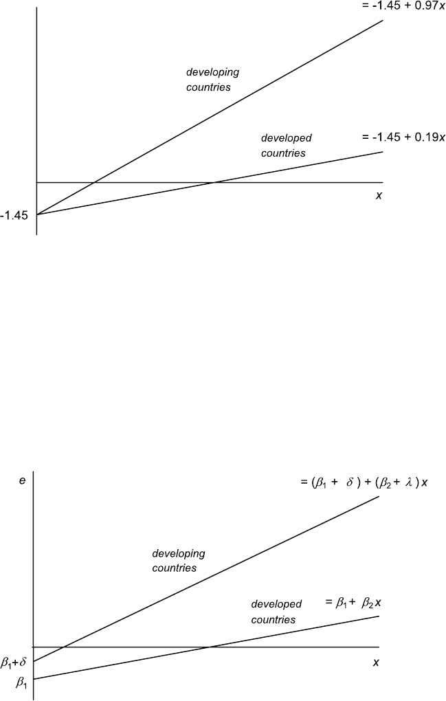
5.5. Answers to the additional exercises
e
ˆ
e
ˆ
e
2. The inclusion of Dwould allow the intercept to be different for the two types
of country. If the model was written as:
e=β1+β2x+δD +λDx +u
the implicit relationships for the two types of country would be:
developed countries e=β1+β2x+u
developing countries e=β1+β2x+δ+λx +u
= (β1+δ)+(β2+λ)x+u.
e
e
3. When the specification includes both an intercept dummy and a slope dummy,
the coefficients for the two categories will be the same as in the separate
regressions (2) and (3). Hence the intercept and coefficient of xwill be the
same as in the regression for the reference category, regression (3), and the
coefficients of the dummies will be such that they modify the intercept and
slope coefficient so that they are equal to their counterparts in regression (4):
be=−2.74 + 0.50x+ 1.89D+ 0.28xD.
Since the coefficients are the same, the overall fit for this regression will be the
same as that for regressions (2) and (3). Hence RSS = 18.63 + 25.23 = 43.86.
107

5. Dummy variables
The tstatistic for the coefficient of xwill be the square root of the Fstatistic
for the test of the marginal explanatory power of Dwhen it is included in the
equation. The Fstatistic is:
F(1,46) = (50.23 −43.86)/1
43.86/46 = 6.6808.
The tstatistic is therefore 2.58.
4. One method is to use a Chow test comparing RSS for the pooled regression,
regression (2), with the sum of RSS regressions (3) and (4):
F(2,46) = (121.61 −43.86)/2
43.86/46 = 40.8.
The critical value of F(2,40) at the 0.1 per cent significance level is 8.25. The
critical value of F(2,46) must be lower. Hence the null hypothesis that the
coefficients are the same for developed and developing countries is rejected.
We should also consider ttests on the coefficients of Dand xD. We saw in (3)
that the tstatistic for the coefficient of Dwas 2.58, so we would reject the null
hypothesis of no intercept shift at the 5 per cent level, and nearly at the 1 per
cent level. We do not have enough information to derive the tstatistic for xD.
We would not perform a ttest on the coefficient of xD in regression (1)
because that regression is clearly misspecified.
A5.8
Chow test
RSS RSS RSS
nAll COLLEGE = 0 COLLEGE = 1 F
ADM 2,815 3,945.2 789.5 3,129.9 6.15
CLOT 4,500 5,766.1 1,837.9 3,913.8 3.77
DOM 1,661 4,062.5 1,048.5 2,984.0 4.10
EDUC 561 1,380.1 278.0 1,087.0 2.05
ELEC 5,828 2,636.3 962.6 1,594.6 60.02
FDAW 5,102 3,369.1 1,114.8 2,251.7 1.32
FDHO 6,334 1,988.4 751.9 1,205.3 33.63
FOOT 1,827 1,373.5 513.1 858.5 0.82
FURN 487 913.9 238.7 662.1 2.32
GASO 5,710 2,879.3 1,043.2 1,811.7 16.27
HEAL 4,802 6,062.5 2,211.7 3,796.6 14.42
HOUS 6,223 4,825.6 2,234.6 2,566.5 10.55
LIFE 1,253 1,559.2 424.0 1,119.6 4.20
LOCT 692 1,075.1 283.3 769.3 4.88
MAPP 399 576.8 205.6 367.5 0.84
PERS 3,817 3,002.2 918.5 2,081.1 1.10
READ 2,287 2,892.1 752.6 2,129.1 2.75
SAPP 1,037 1,148.9 342.9 802.1 1.18
TELE 5,788 3,055.1 1,132.8 1,903.2 12.10
108

5.5. Answers to the additional exercises
TEXT 992 1,032.9 278.0 754.1 0.25
TOB 1,155 873.4 351.3 476.8 20.91
TOYS 2,504 2,828.3 862.5 1,964.2 0.46
TRIP 516 792.8 114.2 675.6 0.66
For FDHO,RSS for the logarithmic regression without college in Exercise A4.2 was
1,988.4. When the sample is split, RSS for COLLEGE = 0 is 751.9 and for
COLLEGE = 1 is 1,205.3. Three degrees of freedom are consumed because the
coefficients of LGEXPPC and LGSIZE and the constant have to be estimated
twice. The number of degrees of freedom remaining after splitting the sample is
6334 −6 = 6328. Hence the Fstatistic is:
F(3,6328) = (1988.4−(751.9 + 1205.3))/3
(751.9 + 1205.3)/6328 = 33.63.
The critical value of F(3,1000) at the 1 per cent level is 2.62 and so we reject the
null hypothesis of no difference in the expenditure functions at that significance
level. The results for all the categories are shown in the table.
A5.9 . gen LEXPCOL = LGEXPPC*COLLEGE
. gen LSIZECOL = LGSIZE*COLLEGE
. reg LGFDHOPC LGEXPPC LGSIZE COLLEGE LEXPCOL LSIZECOL
----------------------------------------------------------------------------
Source | SS df MS Number of obs = 6334
-----------+------------------------------ F( 5, 6328) = 999.36
Model | 1545.47231 5 309.094462 Prob > F = 0.0000
Residual | 1957.1997 6328 .309291987 R-squared = 0.4412
-----------+------------------------------ Adj R-squared = 0.4408
Total | 3502.67201 6333 .553082585 Root MSE = .55614
----------------------------------------------------------------------------
LGFDHOPC | Coef. Std. Err. t P>|t| [95% Conf. Interval]
-----------+----------------------------------------------------------------
LGEXPPC | .648295 .0171599 37.78 0.000 .6146559 .6819342
LGSIZE | -.0559735 .0216706 -2.58 0.010 -.0984552 -.0134917
COLLEGE | .3046012 .1760486 1.73 0.084 -.0405137 .6497161
LEXPCOL | -.0558931 .0211779 -2.64 0.008 -.097409 -.0143772
LSIZECOL | -.0198021 .0274525 -0.72 0.471 -.0736182 .034014
_cons | .7338499 .1403321 5.23 0.000 .4587514 1.008948
----------------------------------------------------------------------------
The example output is for FDHO. In Exercise A4.2, RSS was 1,988.4 for the same
regression without the dummy variables. To perform the Ftest of the explanatory
power of the intercept dummy variable and the two slope dummy variables as a
group, we evaluate whether RSS for this regression is significantly lower. RSS has
fallen from 1,988.4 to 1,957.2. 3 degrees of freedom are consumed by adding the
dummy variables, and 6334 −6 = 6328 degrees of freedom remain after adding the
dummy variables. The Fstatistic is therefore:
F(3,6328) = (1988.4−1957.2)/3
1957.2/6328 = 33.63.
This is highly significant. This Ftest is, of course, equivalent to the Chow test in
the previous exercise. One possible explanation was offered there. The present
109

5. Dummy variables
regression suggests another. The slope dummy variable LGEXPCOL has a
significant negative coefficient, implying that the elasticity falls as income rises.
This is plausible for a basic necessity such as food.
A5.10 (a) You should fit models such as:
LGEARN =β1+β2S+β3ASVABC +β4MALE +β5ETHBLACK +β6ETHHISP +u
separately for the private and government sectors. To investigate
discrimination, for each sector ttests should be performed on the coefficients
of MALE,ETHBLACK, and ETHHISP and an Ftest on the joint
explanatory power of ETHBLACK and ETHHISP.
(b) You should combine the earnings functions for the two sectors, while still
allowing their parameters to differ, by fitting a model such as:
LGEARN =β1+β2S+β3ASVABC +β4MALE +β5ETHBLACK +β6ETHHISP
+δ1GOV +δ2GOVS +δ3GOVASV +δ4GOVMALE +δ5GOVBLACK
+δ6GOVHISP +u
where GOV is equal to 1 if the respondent works in the government sector and
0 otherwise, and GOVS,GOVASV,GOVMALE,GOVBLACK, and GOVHISP
are slope dummy variables defined as the product of GOV and the respective
variables. To investigate whether the level of discrimination is different in the
two sectors, one should perform ttests on the coefficients of GOVMALE,
GOVBLACK, and GOVHISP and an Ftest on the joint explanatory power of
GOVBLACK and GOVHISP.
A Chow test would not be appropriate because if it detected a significant
difference in the earnings functions, this could be due to differences in the
coefficients of Sand ASVABC rather than the discrimination variables.
A5.11 Give an interpretation of the coefficients of S and SMALE in regression (5).
An extra year of schooling increases female earnings by 9.4 per cent. (Strictly,
100(e0.094 −1) = 9.9 per cent.) For males, an extra year of schooling leads to an
increase in earnings 0.5 per cent greater than for females, i.e. 9.9 per cent.
Give an interpretation of the coefficients of MALE in regressions (4) and (5).
(4): males earn 23.4 per cent more than females (controlling for other factors). (5):
males with no schooling or work experience earn 11.7 per cent more than similar
females.
The researcher hypothesises that the earnings function is different for males and
females. Perform a test of this hypothesis using regression (4), and also using
regressions (1) and (5).
Looking at regression (4), the coefficient of MALE is highly significant, indicating
that the earnings functions are indeed different. Looking at regression (5), and
comparing it with (1), the null hypothesis is that the coefficients of the male
dummy variables in (5) are all equal to zero.
F(3,3236) = (714.6−672.5)/3
672.5/3236 = 67.5.
110

5.5. Answers to the additional exercises
The critical value of F(3,1000) at the 1 per cent level is 3.80. The corresponding
critical value for F(3,3236) must be lower, so we reject the null hypothesis and
conclude that the earnings functions are different.
Explain the differences in the tests using regression (4) and using regressions (1)
and (5).
In regression (4) the coefficient of MALE is highly significant. In regression (5) it is
not. Likewise the coefficients of the slope dummies are not significant. This is
(partly) due to the effect of multicollinearity. The male dummy variables are very
highly correlated and as a consequence the standard error of the coefficient of
MALE is much larger than in regression (4). Nevertheless the Ftest reveals that
their joint explanatory power is highly significant.
At a seminar someone suggests that a Chow test could shed light on the researcher’s
hypothesis. Is this correct?
Yes. Using regressions (1)–(3):
F(3,3236) = (714.6−(411.0 + 261.6))/3
(411.0 + 261.6)/3236 = 67.4.
The null hypothesis that the coefficients are the same for males and females is
rejected at the 1 per cent level. The test is, of course, equivalent to the dummy
variable test comparing (1) and (5).
Explain which of (1), (4), and (5) would be your preferred specification.
(4) seems best, given that the coefficients of Sand EXP are fairly similar for males
and females and that introducing the slope dummies causes multicollinearity. The
Fstatistic of their joint explanatory power is only 0.72, not significant at any
significance level.
A5.12 Calculate the missing coefficients V,W,X, and Yin Regression 4 (just the
coefficients, not the standard errors) and Z, the missing RSS, giving an explanation
of your computations.
Since Regression 5 includes a complete set of black intercept and slope dummy
variables, the basic coefficients will be the same as for a regression using the
‘whites’ only subsample and the coefficients modified by the dummies will give the
counterparts for the blacks only subsample. Hence V= 0.122 −0.009 = 0.113;
W= 0.033 −0.006 = 0.027; X= 0.306 −0.280 = 0.026; and
Y= 0.411 + 0.205 = 0.616. The residual sum of squares for Regression 5 will be
equal to the sum of RSS for the ‘whites’ and blacks subsamples. Hence
Z= 600.0−555.7 = 44.3.
Give an interpretation of the coefficient of BLACK in Regression 2.
It suggests that blacks earn 14.4 per cent less than whites, controlling for other
characteristics.
Perform an F test of the joint explanatory power of BLACK, SB, EB, and MB in
Regression 5.
Write the model as:
LGEARN =β1+β2S+β3EXP +β4MALE +β5BLACK +β6SB +β7EB +β8MB +u.
111

5. Dummy variables
The null hypothesis for the test is if H0:β5=β6=β7=β8= 0, and the alternative
hypothesis is H1: at least one coefficient different from 0. The Fstatistic is:
F(4,2400) = (610.0−600.0)/4
600.0/2400 =2400
240 = 10.0.
This is significant at the 0.1 per cent level (critical value 4.65) and so the null
hypothesis is rejected.
Explain whether it is possible to relate the F test in part (c) to a Chow test based
on Regressions 1, 3, and 4.
The Chow test would be equivalent to the Ftest in this case.
Give an interpretation of the coefficients of BLACK and MB in Regression 5.
Re-write the model as:
LGEARN =β1+β2S+β3EXP+β4MALE+(β5+β6S+β7EXP+β8MALE )BLACK +u.
From this it follows that β5is the extra proportional earnings of a black, compared
with a white, when S=EXP =MALE = 0. Thus the coefficient of BLACK
indicates that a black female with no schooling or experience earns 20.5 per cent
more than a similar white female. The interpretation of the coefficient of any
interactive term requires care. Holding S=EXP =MALE = 0, the coefficients of
MALE and BLACK indicate that black males will earn 30.6 + 20.5 = 51.1 per cent
more than white females. The coefficient of MB modifies this estimate, reducing it
by 28.0 per cent to 23.1 per cent.
Explain whether a simple t test on the coefficient of BLACK in Regression 2 is
sufficient to show that the wage equations are different for blacks and whites.
Regression 2 is misspecified because it embodies the restriction that the effect of
being black is the same for males and females, and that is contradicted by
Regression 5. Hence any test is in principle invalid. However, the fact that the
coefficient has a very high tstatistic is suggestive that something associated with
being black is affecting the wage equation.
A5.13 Reconstruction of missing output
Students A and B left their output on a bus on the way to the workshop. This is
why it does not appear in the table.
State what the missing output of Student A would have been, as far as this can be
done exactly, given the results of Students C and D. (Coefficients, standard errors,
R2, RSS.)
The output would be as for column (3) (coefficients, standard errors, R2), with the
following changes:
•the row label MALE should be replaced with WM
•the row label BLACK should be replaced with BF
•the row label MALEBLACK should be replaced with BM and the coefficient
for that row should be the sum of the coefficients in column (3):
0.308 −0.011 −0.290 = 0.007, and the standard error would not be known.
112

5.5. Answers to the additional exercises
Explain why it is not possible to reconstruct any of the output of Student B.
One could not predict the coefficients of either Sor EXP in the four regressions
performed by Student B. They will, except by coincidence, be different from any of
the estimates of the other students because the coefficients for Sand EXP in the
other specifications are constrained in some way. As a consequence, one cannot
predict exactly any part of the rest of the output, either.
Tests of hypotheses
•Student A (assuming he had found his output)
Student A could perform tests of the differences in earnings between white
males and white females, black males and white females, and black females and
white females, through simple ttests on the coefficients of WM,BM, and BF.
He could also test the null hypothesis that there are no sex/ethnicity
differences with an Ftest, comparing RSS for his regression with that of the
basic regression:
F(3,2540) = (922 −603)/3
603/2540 .
This would be compared with the critical value of Fwith 3 and 2,540 degrees
of freedom at the significance level chosen and the null hypothesis of no
sex/ethnicity effects would be rejected if the Fstatistic exceeded the critical
value.
•Student B (assuming he had found his output)
In the case of Student B, with four separate subsample regressions, candidates
are expected say that no tests would be possible because no relevant standard
errors would be available. We have covered Chow tests only for two categories.
However, a four-category test could be performed, with:
F(9,2534) = (922 −X)/9
X/2534
where RSS = 922 for the basic regression and Xis the sum of RSS in the four
separate regressions.
•Student C
Student C could perform the same ttests and the same Ftest as Student A,
with one difference: the ttest of the difference between the earnings of black
males and white females would not be available. Instead, the tstatistic of
MALEBLACK would allow a test of whether there is any interactive effect of
being black and being male on earnings.
•Student D
Student D could perform a Chow test to see if the wage equations of males
and females differed:
F(3,2540) = (659 −(322 + 289))/3
(322 + 289)/2540 .
RSS = 322 for males and 289 for females. This would be compared with the
critical value of Fwith 3 and 2,540 degrees of freedom at the significance level
113

5. Dummy variables
chosen and the null hypothesis of no sex/ethnicity effects would be rejected if
the Fstatistic exceeded the critical value. She could also perform a
corresponding Chow test for blacks and whites:
F(3,2540) = (659 −(609 + 44))/3
(609 + 44)/2540 .
If you had been participating in the project and had had access to the data set, what
regressions and tests would you have performed?
The most obvious development would be to relax the sex/ethnicity restrictions on
the coefficients of Sand EXP by including appropriate interaction terms. This
could be done by interacting these variables with the dummy variables defined by
Student A or those defined by Student C.
114

Chapter 6
Specification of regression variables
6.1 Overview
This chapter treats a variety of topics relating to the specification of the variables in a
regression model. First there are the consequences for the regression coefficients, their
standard errors, and R2of failing to include a relevant variable, and of including an
irrelevant one. This leads to a discussion of the use of proxy variables to alleviate a
problem of omitted variable bias. Next come Fand ttests of the validity of a
restriction, the use of which was advocated in Chapter 3 as a means of improving
efficiency and perhaps mitigating a problem of multicollinearity. The chapter concludes
by outlining the potential benefit to be derived from examining observations with large
residuals after fitting a regression model.
6.2 Learning outcomes
After working through the corresponding chapter in the text, studying the
corresponding slideshows, and doing the starred exercises in the text and the additional
exercises in this subject guide, you should be able to:
derive the expression for the bias in an OLS estimator of a slope coefficient when
the true model has two explanatory variables but the regression model has only one
determine the likely direction of omitted variable bias, given data on the
correlation between the explanatory variables
explain the consequence of omitted variable bias for the standard errors of the
coefficients and for ttests and Ftests
explain the consequences of including an irrelevant variable for the regression
coefficients, their standard errors, and tand Ftests
explain how the regression results are affected by the substitution of a proxy
variable for a missing explanatory variable
perform an Ftest of a restriction, stating the null hypothesis for the test
perform a ttest of a restriction, stating the null hypothesis for the test.
115
6. Specification of regression variables
6.3 Additional exercises
A6.1 Does the omission of total household expenditure or household size give rise to
omitted variable bias in your CES regressions?
Regress LGCATPC (1) on both LGEXPPC and LGSIZE, (2) on LGEXPPC only,
and (3) on LGSIZE only. Assuming that (1) is the correct specification, analyse the
likely direction of the bias in the estimate of the coefficient of LGEXPPC in (2)
and that of LGSIZE in (3). Check whether the regression results are consistent
with your analysis.
A6.2 A school has introduced an extra course of reading lessons for children starting
school and a researcher is evaluating the impact of the course on the scores on a
literacy test taken at the age of seven. In the first year of its implementation, those
children whose surnames begin A–M are assigned to the extra course, while the rest
have the normal curriculum. The researcher hypothesises that:
Y=β1+β2D+β3A+u
where Yis the score on the literacy test, Dis a dummy variable that is equal to 1
for those assigned to the extra course and 0 for the others, Ais a measure of the
cognitive ability of the child when starting school, and uis an iid (independently
and identically distributed) disturbance term assumed to have a normal
distribution. Unfortunately, the researcher has no data on A. Using OLS (ordinary
least squares), she fits the regression:
b
Y=b
β1+b
β2D.
•Demonstrate that b
β2is an unbiased estimator of β2.
•A commentator says that the standard error of b
β2will be invalid because an
important variable, A, has been omitted from the specification. The researcher
replies that the standard error will remain valid if Acan be assumed to have a
normal distribution. Explain whether the commentator or the researcher is
correct.
•Another commentator says that whether the distribution of Ais normal or not
makes no difference to the validity of the standard error. Evaluate this
assertion.
A6.3 A researcher obtains data on household annual expenditure on books, B, and
annual household income, Y, for 100 households. He hypothesises that Bis related
to Yand the average cognitive ability of adults in the household, IQ, by the
relationship:
log B=β1+β2log Y+β3log IQ +u(A)
where uis a disturbance term that satisfies the regression model assumptions. He
also considers the possibility that log Bmay be determined by log Yalone:
log B=β1+β2log Y+u. (B)
116

6.3. Additional exercises
He does not have data on IQ and decides to use average years of schooling of the
adults in the household, S, as a proxy in specification (A). It may be assumed that
Yand Sare both nonstochastic. In the sample the correlation between log Yand
log Sis 0.86. He performs the following regressions: (1) log Bon both log Yand
log S, and (2) log Bon log Yonly, with the results shown in the table (standard
errors in parentheses):
(1) (2)
log Y1.10 2.10
(0.69) (0.35)
log S0.59 —
(0.35)
constant −6.89 −3.37
(2.28) (0.89)
R20.29 0.27
•Assuming that (A) is the correct specification, explain, with a mathematical
proof, whether you would expect the coefficient of log Yto be greater in
regression (2).
•Assuming that (A) is the correct specification, describe the various benefits
from using log Sas a proxy for log IQ, as in regression (1), if log Sis a good
proxy.
•Explain whether the low value of R2in regression (1) implies that log Sis not
a good proxy.
•Assuming that (A) is the correct specification, provide an explanation of why
the coefficients of log Yand log Sin regression (1) are not significantly
different from zero, using two-sided ttests.
•Discuss whether the researcher would be justified in using one-sided ttests in
regression (1).
•Assuming that (B) is the correct specification, explain whether you would
expect the coefficient of log Yto be lower in regression (1).
•Assuming that (B) is the correct specification, explain whether the standard
errors in regression (1) are valid estimates.
A6.4 A researcher has the following data for the year 2012: T, annual total sales of
cinema tickets per household, and P, the average price of a cinema ticket in the
city. She believes that the true relationship is:
log T=β1+β2log P+β3log Y+u
where Yis average household income, but she lacks data on Yand fits the
regression (standard errors in parentheses):
[
log T= 13.74 + 0.17 log P R2= 0.01
(0.52) (0.23)
117

6. Specification of regression variables
Explain analytically whether the slope coefficient is likely to be biased. You are
told that if the researcher had been able to obtain data on Y, her regression would
have been:
[
log T=−1.63 −0.48 log P+ 1.83 log Y R2= 0.44
(2.93) (0.21) (0.35)
You are also told that Yand Pare positively correlated.
The researcher is not able to obtain data on Ybut, from local records, she is able
to obtain data on H, the average value of a house in each city, and she decides to
use it as a proxy for Y. She fits the following regression (standard errors in
parentheses):
[
log T=−0.63 −0.37 log P+ 1.69 log H R2= 0.36
(3.22) (0.22) (0.38)
Describe the theoretical benefits from using Has a proxy for Y, discussing whether
they appear to have been obtained in this example.
A6.5 A researcher has data on years of schooling, S, weekly earnings in dollars, W, hours
worked per week, H, and hourly earnings, E(computed as W/H) for a sample of
1,755 white males in the United States in the year 2000. She calculates LW,LE,
and LH as the natural logarithms of W,E, and H, respectively, and fits the
following regressions, with the results shown in the table below (standard errors in
parentheses; RSS = residual sum of squares):
•Column 1: a regression of LE on S.
•Column 2: a regression of LW on Sand LH.
•Column 3: a regression of LE on Sand LH.
The correlation between Sand LH is 0.06.
(1) (2) (3) (4) (5)
Respondents All All All FT PT
Dependent variable LE LW LE LW LW
S0.099 0.098 0.098 0.101 0.030
(0.006) (0.006) (0.006) (0.006) (0.049)
LH — 1.190 0.190 0.980 0.885
(0.065) (0.065) (0.088) (0.325)
constant 6.111 5.403 5.403 6.177 7.002
(0.082) (0.254) (0.254) (0.345) (1.093)
RSS 741.5 737.9 737.9 626.1 100.1
Observations 1,755 1,755 1,755 1,669 86
•Explain why specification (1) is a restricted version of specification (2), stating
and interpreting the restriction.
•Supposing the restriction to be valid, explain whether you expect the
coefficient of Sand its standard error to differ, or be similar, in specifications
(1) and (2).
118

6.3. Additional exercises
•Supposing the restriction to be invalid, how would you expect the coefficient of
Sand its standard error to differ, or be similar, in specifications (1) and (2)?
•Perform an Ftest of the restriction.
•Perform a ttest of the restriction.
•Explain whether the Ftest and the ttest could lead to different conclusions.
•At a seminar, a commentator says that part-time workers tend to be paid
worse than full-time workers and that their earnings functions are different.
Defining full-time workers as those working at least 35 hours per week, the
researcher divides the sample and fits the earnings functions for full-time
workers (column 4) and part-time workers (column 5). Test whether the
commentator’s assertion is correct.
•What are the implications of the commentator’s assertion for the test of the
restriction?
A6.6 A researcher investigating whether government expenditure tends to crowd out
investment has data on government recurrent expenditure, G, investment, I, and
gross domestic product, Y, all measured in US$ billion, for 30 countries in 2012.
She fits two regressions (standard errors in parentheses; tstatistics in square
brackets; RSS = residual sum of squares).
(1) A regression of log Ion log Gand log Y:
d
log I=−2.44 −0.63 log G+ 1.60 log Y R2= 0.98 (1)
(0.26) (0.12) (0.12) RSS = 0.90
[9.42] [−5.23] [12.42]
(2) a regression of log(I/Y ) on log(G/Y ):
\
log I
Y= 2.65 −0.63 log G
YR2= 0.48 (2)
(0.23) (0.12) RSS = 0.99
[11.58] [−5.07]
The correlation between log Gand log Yin the sample is 0.98. The table gives
some further basic data on log G, log Y, and log(G/Y ).
Sample mean Mean square
deviation
log G3.75 2.00
log Y5.57 1.95
log (G/Y )−1.81 0.08
•Explain why the second specification is a restricted version of the first. State
the restriction.
•Perform a test of the restriction.
119

6. Specification of regression variables
•The researcher expected the standard error of the coefficient of log(G/Y ) in
(2) to be smaller than the standard error of the coefficient of log Gin (1).
Explain why she expected this.
•However, the standard error is the same, at least to two decimal places. Give
an explanation.
•Show how the restriction could be tested using a ttest in a reparameterised
version of the specification for (1).
A6.7 Is expenditure per capita on your CES category related to total household
expenditure per capita?
The model specified in Exercise A4.1 is a restricted version of that in Exercise 4.5
in the text. Perform an Ftest of the restriction. Also perform a ttest of the
restriction.
[Exercise 4.5: regress LGCAT on LGEXP and LGSIZE; Exercise A4.1: regress
LGCATPC on LGEXPPC.]
A6.8 A researcher is considering two regression specifications:
log Y=β1+β2log X+u(1)
and:
log Y
X=α1+α2log X+u(2)
where uis a disturbance term. Determine whether (2) is a reparameterised or a
restricted version of (1).
A6.9 Three researchers investigating the determinants of hourly earnings have the
following data for a sample of 104 male workers in the United States in 2006: E,
hourly earnings in dollars; S, years of schooling; NUM, score on a test of numeracy;
and VERB, score on a test of literacy. The NUM and VERB tests are marked out
of 100. The correlation between them is 0.81. Defining LGE to be the natural
logarithm of E, Researcher 1 fits the following regression (standard errors in
parentheses; RSS = residual sum of squares):
[
LGE = 2.02 + 0.063S+ 0.0044NUM + 0.0026VERB RSS = 2,000
(1.81) (0.007) (0.0011) (0.0010)
Researcher 2 defines a new variable SCORE as the average of NUM and VERB.
She fits the regression:
[
LGE = 1.72 + 0.050S+ 0.0068SCORE RSS = 2,045
(1.78) (0.005) (0.0010)
Researcher 3 fits the regression:
[
LGE = 2.02 + 0.063S+ 0.0088SCORE −0.0018VERB RSS = 2,000
(1.81) (0.007) (0.0022) (0.0012)
120

6.3. Additional exercises
•Show that the specification of Researcher 2 is a restricted version of the
specification of Researcher 1, stating the restriction.
•Perform an Ftest of the restriction.
•Show that the specification of Researcher 3 is a reparameterised version of the
specification of Researcher 1 and hence perform a ttest of the restriction in
the specification of Researcher 2.
•Explain whether the Ftest and the ttest could have led to different results.
•Perform a test of the hypothesis that the numeracy score has a greater effect
on earnings than the literacy score.
•Compare the regression results of the three researchers.
A6.10 It is assumed that manufacturing output is subject to the production function:
Q=AKαLβ(1)
where Qis output and Kand Lare capital and labour inputs. The cost of
production is:
C=ρK +wL (2)
where ρis the cost of capital and wis the wage rate. It can be shown that, if the
cost is minimised, the wage bill wL will be given by the relationship:
log wL =1
α+βlog Q+α
α+βlog ρ+β
α+βlog w+ constant.(3)
(Note: You are not expected to prove this.)
A researcher has annual data for 2002 for Q,K,L,ρ, and w(all monetary
measures being converted into US dollars) for the manufacturing sectors of 30
industrialised countries and regresses log wL on log Q, log ρ, and log w.
•Demonstrate that relationship (3) embodies a testable restriction and show
how the model may be reformulated to take advantage of it.
•Explain how the restriction could be tested using an Ftest.
•Explain how the restriction could be tested using a ttest.
•Explain the theoretical benefits of making use of a valid restriction. How could
the researcher assess whether there are any benefits in practice, in this case?
•At a seminar, someone suggests that it is reasonable to hypothesise that
manufacturing output is subject to constant returns to scale, so that
α+β= 1. Explain how the researcher could test this hypothesis (1) using an
Ftest, (2) using a ttest.
A6.11 A researcher hypothesises that the net annual growth of private sector purchases of
government bonds, B, is positively related to the nominal rate of interest on the
bonds, I, and negatively related to the rate of price inflation, P:
B=β1+β2I+β3P+u
121

6. Specification of regression variables
where uis a disturbance term. The researcher anticipates that β2>0 and β3<0.
She also considers the possibility that Bdepends on the real rate of interest on the
bonds, R, where R=I−P. Using a sample of observations for 40 countries, she
regresses B:
•(1) on Iand P
•(2) on R
•(3) on I
•(4) on Pand R
with the results shown in the corresponding columns of the table below (standard
errors in parentheses; RSS is the residual sum of squares). The correlation
coefficient for Iand Pwas 0.97.
(1) (2) (3) (4)
I2.17 — 0.69 —
(1.04) (0.25)
P−3.19 — — −1.02
(2.17) (1.19)
R— 1.37 — 2.17
(0.44) (1.04)
constant −5.14 −3.15 −1.53 −5.14
(2.62) (1.21) (0.92) (2.62)
R20.22 0.20 0.17 0.22
RSS 967.9 987.1 1,024.3 967.9
•Explain why the researcher was dissatisfied with the results of regression (1).
•Demonstrate that specification (2) may be considered to be a restricted
version of specification (1).
•Perform an Ftest of the restriction, stating carefully your null hypothesis and
conclusion.
•Perform a ttest of the restriction.
•Demonstrate that specification (3) may also be considered to be a restricted
version of specification (1).
•Perform both an Ftest and a ttest of the restriction in specification (3),
stating your conclusion in each case.
•At a seminar, someone suggests that specification (4) is also a restricted
version of specification (1). Is this correct? If so, state the restriction.
•State, with an explanation, which would be your preferred specification.
A6.12 A researcher has a sample of 43 observations on a dependent variable, Y, and two
potential explanatory variables, Xand Z. He defines two further variables Vand
Was the sum of Xand Zand the difference between them:
Vi=Xi+Zi
Wi=Xi−Zi.
122

6.4. Answers to the starred exercises in the textbook
He fits the following four regressions:
(1) A regression of Yon Xand Z.
(2) A regression of Yon Vand W.
(3) A regression of Yon V.
(4) A regression of Yon Zand V.
The table shows the regression results (standard errors in parentheses; RSS =
residual sum of squares; there was an intercept, not shown, in each regression).
Unfortunately, a goat ate part of the regression output and some of the numbers
are missing. These are indicated by letters.
(1) (2) (3) (4)
X0.60 — — —
(0.04)
Z0.80 — — H
(0.04) (I)
V—A0.72 J
(B) (0.02) (K)
W—C— —
(D)
R20.60 E G L
RSS 200 F220 M
Each regression included an intercept (not shown).
Reconstruct each missing number if this is possible, giving a brief explanation. If it
is not possible to reconstruct a number, give a brief explanation.
A6.13 In Exercise A6.7, a researcher proposes to test the restriction using variations in R2
instead of variations in RSS. For food consumed at home, the unrestricted
regression of LGFDHO on LGEXP and LGSIZE had R2= 0.4831. For the
regression of LGFDHOPC on LGEXPPC,R2= 0.4290. Hence the researcher’s
statistic is:
F=(0.4831 −0.4290)/1
(1 −0.4290)/6331 = 599.8.
Explain why this is different from the Fstatistic reported for food consumed at
home in the answer to Exercise A6.7.
6.4 Answers to the starred exercises in the textbook
6.4 The table gives the results of multiple and simple regressions of LGFDHO, the
logarithm of annual household expenditure on food eaten at home, on LGEXP, the
logarithm of total annual household expenditure, and LGSIZE, the logarithm of
the number of persons in the household, using a sample of 6,334 households in the
2013 Consumer Expenditure Survey. The correlation coefficient for LGEXP and
LGSIZE was 0.32. Explain the variations in the regression coefficients.
123

6. Specification of regression variables
(1) (2) (3)
LGEXP 0.58 0.67 —
(0.01) (0.01)
LGSIZE 0.33 — 0.58
(0.01) (0.02)
constant 1.16 0.70 6.04
(0.08) (0.08) (0.01)
R20.48 0.43 0.19
Answer:
If the model is written as:
LGFDHO =β1+β2LGEXP +β3LGSIZE +u
the expected value of b
β2in the second regression is given by:
E(b
β2) = β2+β3PLGEXPi−LGEXPLGSIZEi−LGSIZE
PLGEXPi−LGEXP2.
We know that the covariance is positive because the correlation is positive, and it is
reasonable to suppose that β3is also positive, especially given the highly significant
positive estimate in the first regression, and so b
β2is biased upwards. This accounts
for the large increase in its size in the second regression. In the third regression:
E(b
β3) = β3+β2PLGEXPi−LGEXPLGSIZEi−LGSIZE
PLGSIZEi−LGSIZE2.
β2is certainly positive, especially given the highly significant positive estimate in
the first regression, and so b
β3is also biased upwards. As a consequence, the
estimate in the third regression is greater than that in the first.
6.7 A researcher thinks that the level of activity in the shadow economy, Y, depends
either positively on the level of the tax burden, X, or negatively on the level of
government expenditure to discourage shadow economy activity, Z.Ymight also
depend on both Xand Z. International cross-sectional data on Y,X, and Z, all
measured in US$ million, are obtained for a sample of 30 industrialised countries
and a second sample of 30 developing countries. The researcher regresses (1) log Y
on both log Xand log Z, (2) log Yon log Xalone, and (3) log Yon log Zalone, for
each sample, with the following results (standard errors in parentheses):
Industrialised countries Developing countries
(1) (2) (3) (1) (2) (3)
log X0.699 0.201 — 0.806 0.727 —
(0.154) (0.112) (0.137) (0.090)
log Z−0.646 — −0.053 −0.091 — 0.427
(0.162) (0.124) (0.117) (0.116)
constant −1.137 −1.065 1.230 −1.122 −1.024 2.824
(0.863) (1.069) (0.896) (0.873) (0.858) (0.835)
R20.44 0.10 0.01 0.71 0.70 0.33
124

6.4. Answers to the starred exercises in the textbook
Xwas positively correlated with Zin both samples. Having carried out the
appropriate statistical tests, write a short report advising the researcher how to
interpret these results.
Answer:
One way to organise an answer to this exercise is, for each sample, to consider the
evidence for and against each of the three specifications in turn. The tstatistics for
the slope coefficients are given in the following table. * indicates significance at the
5 per cent level, ** at the 1 per cent level, and *** at the 0.1 per cent level, using
one-sided tests. (Justification for one-sided tests: one may rule out a negative
coefficient for Xand a positive one for Y.)
Industrialised countries Developing countries
(1) (2) (3) (1) (2) (3)
log X4.54*** 1.79* — 5.88**** 8.08*** —
log Z−3.99*** — −0.43 −0.78 — 3.68***
Industrialised countries:
The first specification is clearly the only satisfactory one for this sample, given the
tstatistics. Writing the model as:
log Y=β1+β2log X+β3log Z+u
in the second specification:
E(b
β2) = β2+β3Plog Xi−log Xlog Zi−Z
Plog Xi−log X2.
Anticipating that β3is negative, and knowing that Xand Zare positively
correlated, the bias term should be negative. The estimate of β2is indeed lower in
the second specification. In the third specification:
E(b
β3) = β3+β2Plog Xi−log Xlog Zi−Z
Plog Zi−log Z2
and the bias should be positive, assuming β2is positive. b
β3is indeed less negative
than in the first specification.
Note that the sum of the R2statistics for the second and third specifications is less
than R2in the first. This is because the bias terms undermine the apparent
explanatory power of Xand Zin the second and third specifications. In the third
specification, the bias term virtually neutralises the true effect and R2is very low
indeed.
Developing countries:
In principle the first specification is acceptable. The failure of the coefficient of Zto
be significant might be due to a combination of a weak effect of Zand a relatively
small sample.
125

6. Specification of regression variables
The second specification is also acceptable since the coefficient of Zand its t
statistic in the first specification are very low. Because the tstatistic of Zis low,
R2is virtually unaffected when it is omitted.
The third specification is untenable because it cannot account for the highly
significant coefficient of Xin the first. The omitted variable bias is now so large
that it overwhelms the negative effect of Zwith the result that the estimated
coefficient is positive.
6.11 A researcher has data on output per worker, Y, and capital per worker, K, both
measured in thousands of dollars, for 50 firms in the textiles industry in 2012. She
hypothesises that output per worker depends on capital per worker and perhaps
also the technological sophistication of the firm, TECH :
Y=β1+β2K+β3TECH +u
where uis a disturbance term. She is unable to measure TECH and decides to use
expenditure per worker on research and development in 2012, R&D, as a proxy for
it. She fits the following regressions (standard errors in parentheses):
b
Y= 1.02 + 0.32K R2= 0.749
(0.45) (0.04)
b
Y= 0.34 + 0.29K+ 0.05R&D R2= 0.750
(0.61) (0.22) (0.15)
The correlation coefficient for Kand R&Dis 0.92. Discuss these regression results:
1. assuming that Ydoes depend on both Kand TECH
2. assuming that Ydepends only on K.
Answer:
If Ydepends on both Kand TECH, the first specification is subject to omitted
variable bias, with the expected value of b
β2being given by:
E(b
β2) = β2+β3PKi−KTECH i−TECH
PKi−K2.
Since Kand R&Dhave a high positive correlation, it is reasonable to assume that
Kand TECH are positively correlated. It is also reasonable to assume that β3is
positive. Hence one would expect b
β2to be biased upwards. It is indeed greater than
in the second equation, but not by much. The second specification is clearly subject
to multicollinearity, with the consequence that, although the estimated coefficients
remain unbiased, they are erratic, this being reflected in large standard errors. The
large variance of the estimate of the coefficient of Kmeans that much of the
difference between it and the estimate in the first specification is likely to be purely
random, and this could account for the fact that the omitted variable bias appears
to be so small.
If Ydepends only on K, the inclusion of R&D in the second specification gives rise
to inefficiency. Since the standard errors in both equations remain valid, they can
126
6.4. Answers to the starred exercises in the textbook
be compared and it is evident that the loss of efficiency is severe. As expected in
this case, the coefficient of R&D is not significantly different from zero and the
increase in R2in the second specification is minimal.
6.14 The first regression shows the result of regressing LGFDHO, the logarithm of
annual household expenditure on food eaten at home, on LGEXP, the logarithm of
total annual household expenditure, and LGSIZE, the logarithm of the number of
persons in the household, using a sample of 6,334 households in the 2013 Consumer
Expenditure Survey. In the second regression, LGFDHOPC, the logarithm of food
expenditure per capita (FDHO/SIZE), is regressed on LGEXPPC, the logarithm
of total expenditure per capita (EXP/SIZE ). In the third regression LGFDHOPC
is regressed on LGEXPPC and LGSIZE.
. reg LGFDHO LGEXP LGSIZE
----------------------------------------------------------------------------
Source | SS df MS Number of obs = 6334
-----------+------------------------------ F( 2, 6331) = 2958.94
Model | 1858.61471 2 929.307357 Prob> F = 0.0000
Residual | 1988.36474 6331 .314068037 R-squared = 0.4831
-----------+------------------------------ Adj R-squared = 0.4830
Total | 3846.97946 6333 .60744978 Root MSE = .56042
----------------------------------------------------------------------------
LGFDHO | Coef. Std. Err. t P>|t| [95% Conf. Interval]
-----------+----------------------------------------------------------------
LGEXP | .5842097 .0097174 60.12 0.000 .5651604 .6032591
LGSIZE | .3343475 .0127587 26.21 0.000 .3093362 .3593589
_cons | 1.158326 .0820119 14.12 0.000 .9975545 1.319097
----------------------------------------------------------------------------
. gen LGFDHOPC = ln(FDHO/SIZE)
. gen LGEXPPC = ln(EXP/SIZE)
. reg LGFDHOPC LGEXPPC
----------------------------------------------------------------------------
Source | SS df MS Number of obs = 6334
-----------+------------------------------ F( 1, 6332) = 4757.00
Model | 1502.58928 1 1502.58928 Prob> F = 0.0000
Residual | 2000.0827 6332 .31586903 R-squared = 0.4290
-----------+------------------------------ Adj R-squared = 0.4289
Total | 3502.67197 6333 .553082579 Root MSE = .56202
----------------------------------------------------------------------------
LGFDHOPC | Coef. Std. Err. t P>|t| [95% Conf. Interval]
-----------+----------------------------------------------------------------
LGEXPPC | .6092734 .0088338 68.97 0.000 .5919562 .6265905
_cons | .8988292 .0703516 12.78 0.000 .7609162 1.036742
----------------------------------------------------------------------------
127

6. Specification of regression variables
. reg LGFDHOPC LGEXPPC LGSIZE
----------------------------------------------------------------------------
Source | SS df MS Number of obs = 6334
-----------+------------------------------ F( 2, 6331) = 2410.79
Model | 1514.30723 2 757.153617 Prob> F = 0.0000
Residual | 1988.36474 6331 .314068037 R-squared = 0.4323
-----------+------------------------------ Adj R-squared = 0.4321
Total | 3502.67197 6333 .553082579 Root MSE = .56042
----------------------------------------------------------------------------
LGFDHOPC | Coef. Std. Err. t P>|t| [95% Conf. Interval]
-----------+----------------------------------------------------------------
LGEXPPC | .5842097 .0097174 60.12 0.000 .5651604 .6032591
LGSIZE | -.0814427 .0133333 -6.11 0.000 -.1075805 -.0553049
_cons | 1.158326 .0820119 14.12 0.000 .9975545 1.319097
----------------------------------------------------------------------------
1. Explain why the second model is a restricted version of the first, stating the
restriction.
2. Perform an Ftest of the restriction.
3. Perform a ttest of the restriction.
4. Summarise your conclusions from the analysis of the regression results.
Answer:
Write the first specification as:
LGFDHO =β1+β2LGEXP +β3LGSIZE +u.
Then the restriction implicit in the second specification is β3= 1 −β2, for:
LGFDHO =β1+β2LGEXP + (1 −β2)LGSIZE +u
LGFDHO −LGSIZE =β1+β2(LGEXP −LGSIZE) + u
log FDHO
SIZE =β1+β2log EXP
SIZE +u
LGFDHOPC =β1+β2LGEXPPC +u
the last equation being the second specification. The Fstatistic for the null
hypothesis H0:β3= 1 −β2is:
F(1,6331) = (2000.1−1988.4)/1
1988.4/6331 = 37.3.
The critical value of F(1,1000) at the 0.1 per cent level is 10.9, and hence the
restriction is rejected at that significance level.
Alternatively, we could use the ttest approach. Under the null hypothesis that the
restriction is valid, θ= 1 −β2−β3= 0. Substituting for β3, the unrestricted
version may be rewritten:
LGFDHO =β1+β2LGEXP + (1 −β2−θ)LGSIZE +u.
128

6.5. Answers to the additional exercises
This may be rewritten:
log FDHO
SIZE =β1+β2log EXP
SIZE −θlog SIZE +u
that is:
LGFDHOPC =β1+β2LGEXPPC −θLGSIZE +u.
The tstatistic for the coefficient of LGSIZE is −6.11, so we reject the restriction at
a very high significance level. Note that the tstatistic is the square root of the F
statistic and the critical value of tat the 0.1 per cent level will be the square root
of the critical value of F.
6.5 Answers to the additional exercises
A6.1 The output below gives the results of a simple regression of LGFDHOPC on
LGSIZE. See Exercise A4.1 for the simple regression of LGFDHOPC on
LGEXPPC and Exercise A4.2 for the multiple regression of LGFDHOPC on
LGEXPPC and LGSIZE.
. reg LGFDHOPC LGSIZE
----------------------------------------------------------------------------
Source | SS df MS Number of obs = 6334
-----------+------------------------------ F( 1, 6332) = 768.56
Model | 379.128845 1 379.128845 Prob> F = 0.0000
Residual | 3123.54316 6332 .493294877 R-squared = 0.1082
-----------+------------------------------ Adj R-squared = 0.1081
Total | 3502.67201 6333 .553082585 Root MSE = .70235
----------------------------------------------------------------------------
LGFDHOPC | Coef. Std. Err. t P>|t| [95% Conf. Interval]
-----------+----------------------------------------------------------------
LGSIZE | -.4199282 .0151473 -27.72 0.000 -.449622 -.3902344
_cons | 6.040547 .0143586 420.69 0.000 6.012399 6.068695
----------------------------------------------------------------------------
If the true model is assumed to be:
LGFDHOPC =β1+β2LGEXPPC +β3LGSIZE +u
the expected value of b
β2in the simple regression of LGFDHOPC on LGEXPPC is
given by:
E(b
β2) = β2+β3PLGEXPPC i−LGEXPPCLGSIZE i−LGSIZE
PLGEXPPC i−LGEXPPC2.
We know that the numerator of the second factor in the bias term is negative
because the correlation is negative:
129

6. Specification of regression variables
. cor LGEXPPC LGSIZE
(obs=6334)
| LGEXPPC LGSIZE
-----------+------------------
LGEXPPC | 1.0000
LGSIZE | -0.4223 1.0000
It is reasonable to suppose that economies of scale will cause β3to be negative, and
the highly significant negative estimate in the multiple regression provides
empirical support, so b
β2is biased upwards. This accounts for the increase in its size
in the second regression. In the third regression:
E(b
β3) = β3+β2PLGEXPPC i−LGEXPPCLGSIZE i−LGSIZE
PLGSIZEi−LGSIZE2.
β2is certainly positive, especially given the highly significant positive estimate in
the first regression, and so b
β3is biased downwards. As a consequence, the estimate
in the third regression is lower than that in the first.
Similar results are obtained for the other categories of expenditure. The correlation
between LGEXPPC and LGSIZE varies because the missing observations are
different for different categories.
Omitted variable bias, dependent variable LGCATPC
Multiple regression Simple regressions
nLGEXPPC LGSIZE LGEXPPC LGSIZE
ADM 2,815 1.080 −0.055 1.098 −0.678
CLOT 4,500 0.842 0.146 0.794 −0.375
DOM 1,661 0.941 0.415 0.812 −0.150
EDUC 561 1.229 −0.437 1.382 −1.243
ELEC 5,828 0.472 −0.362 0.586 −0.645
FDAW 5,102 0.879 −0.213 0.947 −0.735
FDHO 6,334 0.584 −0.081 0.609 −0.420
FOOT 1,827 0.396 −0.560 0.608 −0.842
FURN 487 0.807 −0.246 0.912 −0.848
GASO 5,710 0.676 −0.004 0.677 −0.410
HEAL 4,802 0.779 −0.306 0.868 −0.723
HOUS 6,223 0.989 −0.140 1.033 −0.716
LIFE 1,253 0.464 −0.461 0.607 −0.701
LOCT 692 0.389 −0.396 0.510 −0.639
MAPP 399 0.721 −0.264 0.817 −0.717
PERS 3,817 0.824 −0.217 0.891 −0.703
READ 2,287 0.764 −0.503 0.909 −0.923
SAPP 1,037 0.467 −0.592 0.665 −0.879
TELE 5,788 0.640 −0.222 0.710 −0.603
TEXT 992 0.388 −0.713 0.629 −0.959
TOB 1,155 0.563 −0.515 0.721 −0.822
TOYS 2,504 0.638 −0.304 0.733 −0.691
TRIP 516 0.681 −0.142 0.723 −0.492
130

6.5. Answers to the additional exercises
A6.2 Demonstrate that b
β2is an unbiased estimator of β2.
b
β2=PDi−DYi−Y
PDi−D2
=PDi−D(β1+β2Di+β3Ai+ui)−(β1+β2D+β3A+u)
PDi−D2
=β2+β3PDi−DAi−A
PDi−D2+PDi−D(ui−u)
PDi−D2.
Hence: b
β2=β2+β3Xdi(Ai−A) + Xdi(ui−u)
where:
di=Di−D
P(Dj−D)2.
Hence:
E(b
β2) = β2+β3XE(di(Ai−A)) + XE(di(ui−u)).
Now, since the assignment to the course was random, Dis distributed
independently of both Aand u, and hence:
E(di(Ai−A)) = E(di)E(Ai−A) = 0
and:
E(di(ui−u)) = E(di)E(ui−u)=0.
Hence b
β2is an unbiased estimator of β2.
A commentator says that the standard error of b
β2will be invalid because an
important variable, A, has been omitted from the specification. The researcher
replies that the standard error will remain valid if Acan be assumed to have a
normal distribution. Explain whether the commentator or the researcher is correct.
The researcher is nearly correct. Given the random selection of the sample, Awill
be distributed independently of Dand so it can be treated as part of the
disturbance term and the standard error will remain valid. The requirement that A
have a normal distribution is too strong, since the expression for the standard error
does not depend on it. However, if the standard error is to be used for ttests, then
it is important that the enlarged standard error should have a normal distribution,
and this will be the case if an only if Ahas a normal distribution (assuming that u
has one). If both Aand uhave normal distributions, a linear combination will also
have one.
Another commentator says that whether the distribution of Ais normal or not
makes no difference to the validity of the standard error. Evaluate this assertion.
The commentator is correct for the reasons just explained.
131

6. Specification of regression variables
A6.3 Assuming that (A) is the correct specification, explain, with a mathematical proof,
whether you would expect the coefficient of log Y to be greater in regression (2).
To simplify the algebra, throughout this answer log B, log Y, log Sand log IQ will
be written as B,Y,Sand IQ, it being understood that these are logarithms.
b
β2=PBi−BYi−Y
PYi−Y2
=Pβ1+β2Yi+β3IQi+ui−β1−β2Y−β3IQ −uYi−Y
PYi−Y2
=Pβ2Yi−β2YYi−Y+Pβ3IQi−β3IQYi−Y+P(ui−u)Yi−Y
PYi−Y2
=β2+β3PIQi−IQYi−Y
PYi−Y2+P(ui−u)Yi−Y
PYi−Y2.
Hence:
E(b
β2) = β2+β3PIQi−IQYi−Y
PYi−Y2+1
PYi−Y2EX(ui−u)(Yi−Y)
=β2+β3PIQi−IQYi−Y
PYi−Y2+1
PYi−Y2XE(ui−u)(Yi−¯
Y)
=β2+β3PIQi−IQYi−Y
PYi−Y2+1
PYi−Y2X(Yi−Y)E(ui−u)
=β2+β3PIQi−IQYi−Y
PYi−Y2
assuming that Yand IQ are nonstochastic. Thus b
β2is biased, the direction of the
bias depending on the signs of β3and PIQi−IQYi−Y. We would expect
the former to be positive and we expect the latter to be positive since we are told
that the correlation between Sand Yis positive and Sis a proxy for IQ. So we
would expect an upward bias in regression (2).
Assuming that (A) is the correct specification, describe the various benefits from
using log S as a proxy for log IQ, as in regression (1), if log S is a good proxy.
The use of Sas a proxy for IQ will alleviate the problem of omitted variable bias.
In particular, comparing the results of regression (1) with those that would have
been obtained if Bhad been regressed on Yand IQ:
132

6.5. Answers to the additional exercises
•the coefficient of Ywill be approximately the same
•its standard error will be approximately the same
•the tstatistic for Swill be approximately equal to that of IQ
•R2will be approximately the same.
Explain whether the low value of R2in regression (1) implies that log S is not a
good proxy.
Not necessarily. It could be that Sis a poor proxy for IQ, but it could also be that
the original model had low explanatory power.
Assuming that (A) is the correct specification, provide an explanation of why the
coefficients of log Y and log S in regression (1) are not significantly different from
zero, using two-sided t tests.
The high correlation between Yand Shas given rise to multicollinearity, the
standard errors being so large that the coefficients are not significantly different
from zero.
Discuss whether the researcher would be justified in using one-sided t tests in
regression (1).
Yes. It is reasonable to suppose that expenditure on books should not be negatively
influenced by either income or cognitive ability. (Note that one should not say that
it is reasonable to suppose that expenditure on books is positively influenced by
them. This rules out the null hypothesis.)
Assuming that (B) is the correct specification, explain whether you would expect the
coefficient of log Y to be lower in regression (1).
No. It would be randomly higher or lower, if Sis an irrelevant variable.
Assuming that (B) is the correct specification, explain whether the standard errors
in regression (1) are valid estimates.
Yes. The inclusion of an irrelevant variable in general does not invalidate the
standard errors. It causes them to be larger than those in the correct specification.
A6.4 Explain analytically whether the slope coefficient is likely to be biased.
If the fitted model is: [
log T=b
β1+b
β2log P
then:
b
β2=Plog Pi−log Plog Ti−log T
Plog Pi−log P2
=Plog Pi−log Pβ1+β2log Pi+β3log Yi+ui−β1−β2log P−β3log Y−u
Plog Pi−log P2
=β2+β3Plog Pi−log Plog Yi−log Y
Plog Pi−log P2+Plog Pi−log P(ui−u)
Plog Pi−log P2.
133

6. Specification of regression variables
Hence:
E(b
β2) = β2+β3Plog Pi−log Plog Yi−log Y
Plog Pi−log P2
provided that any random component of log Pis distributed independently of u.
Since it is reasonable to assume β3>0, and since we are told that Yand Pare
positively correlated, the bias will be upwards. This accounts for the nonsensical
positive price elasticity in the fitted equation.
Describe the theoretical benefits from using H as a proxy for Y, discussing whether
they appear to have been obtained in this example.
Suppose that His a perfect proxy for Y:
log Y=λ+µlog H.
Then the relationship may be rewritten:
log T=β1+β3λ+β2log P+β3µlog H+u.
The coefficient of log Pought to be the same as in the true relationship. However in
this example it is not the same. However it is of the right order of magnitude and
much more plausible than the estimate in the first regression. The standard error of
the coefficient ought to be the same as in the true relationship, and this is the case.
The coefficient of log Hwill be an estimate of β3µ, and since µis unknown, β3is
not identified. However, if it can be assumed that the average household income in
a city is proportional to average house values, it could be asserted that µis equal
to 1, in which case the coefficient of log Hwill be a direct estimate of β3after all.
The coefficient of log His indeed quite close to that of log Y. The tstatistic for the
coefficient of log Hought to be the same as that for log Y, and this is approximately
true, being a little lower. R2ought to be the same, but it is somewhat lower,
suggesting that Happears to have been a good proxy, but not a perfect one.
A6.5 Explain why specification (1) is a restricted version of specification (2), stating and
interpreting the restriction.
First note that, since E=W/H,LE = log(W/H) = LW −LH.
Write specification (2) as:
LW =β1+β2S+β3LH +u.
If one imposes the restriction β3= 1, the model becomes specification (1):
LW −LH =β1+β2S+u.
The restriction implies that weekly earnings are proportional to hours worked,
controlling for schooling.
Supposing the restriction to be valid, explain whether you expect the coefficient of S
and its standard error to differ, or be similar, in specifications (1) and (2).
If the restriction is valid, the coefficient of Sshould be similar in the restricted
specification (1) and the unrestricted specification (2). Both estimates will be
134

6.5. Answers to the additional exercises
unbiased, but that in specification (1) will be more efficient. The gain in efficiency
in specification (1) should be reflected in a smaller standard error. However, the
gain will be small, given the low correlation.
Supposing the restriction to be invalid, how would you expect the coefficient of S
and its standard error to differ, or be similar, in specifications (1) and (2)?
The estimate of the coefficient of Swould be biased. The standard error in
specification (1) would be invalid and so a comparison with the standard error in
specification (2) would be illegitimate.
Perform an F test of the restriction.
The null and alternative hypotheses are H0:β3= 1 and H1:β36= 1.
F(1,1752) = (741.5−737.9)/1
737.9/1752 = 8.5.
The critical value of F(1,1000) at the 1 per cent level is 6.66. The critical value of
F(1,1752) must be lower. Thus we reject the restriction at the 1 per cent level.
(The critical value at the 0.1 per cent level is about 10.8.)
Perform a t test of the restriction.
The restriction is so simple that it can be tested with no reparameterisation: a
simple ttest on the coefficient of LH in specification (2), H0:β3= 1.
Alternatively, mechanically following the standard procedure, we rewrite the
restriction as β3−1 = 0. The reparameterisation will be:
θ=β3−1
and so:
β3=θ+ 1.
Substituting this into the unrestricted specification, the latter may be rewritten:
LW =β1+β2S+ (θ+ 1)LH +u.
Hence:
LW −LH =β1+β2S+θLH +u.
This is regression specification (3) and the restriction may be tested with a ttest
on the coefficient of LH, the null hypothesis being H0:θ=β3−1 = 0. The t
statistic is 2.92, which is significant at the 1 per cent level, implying that the
restriction should be rejected.
Explain whether the F test and the t test could lead to different conclusions.
The tests must lead to the same conclusion since the Fstatistic is the square of the
tstatistic and the critical value of Fis the square of the critical value of t.
At a seminar, a commentator says that part-time workers tend to be paid worse
than full-time workers and that their earnings functions are different. Defining
full-time workers as those working at least 35 hours per week, the researcher divides
the sample and fits the earnings functions for full-time workers (column 4) and
part-time workers (column 5). Test whether the commentators assertion is correct.
135

6. Specification of regression variables
The appropriate test is a Chow test. The test statistic under the null hypothesis of
no difference in the earnings functions is:
F(3,1749) = (737.9−626.1−100.1)/3
(626.1 + 100.1)/1749 = 9.39.
The critical value of F(3,1000) at the 0.1 per cent level is 5.46. Hence we reject the
null hypothesis and conclude that the commentator is correct.
What are the implications of the commentators assertion for the test of the
restriction?
The elasticity of LH is now not significantly different from 1 for either full-time or
part-time workers, so the restriction is no longer rejected.
A6.6 Explain why the second specification is a restricted version of the first. State the
restriction.
Write the second equation as:
log I
Y=β1+β2log G
Y+u.
It may be re-written as:
log I=β1+β2log G+ (1 −β2) log Y+u.
This is a special case of the specification of the first equation:
log I=β1+β2log G+β3log Y+u
with the restriction β3= 1 −β2.
Perform a test of the restriction.
The null hypothesis is H0:β2+β3= 1. The test statistic is:
F(1,27) = (0.99 −0.90)/1
0.90/27 = 2.7.
The critical value of F(1,27) is 4.21 at the 5 per cent level. Hence we do not reject
the null hypothesis that the restriction is valid.
The researcher expected the standard error of the coefficient of log (G/Y) in (2) to
be smaller than the standard error of the coefficient of log G in (1). Explain why
she expected this.
The imposition of the restriction, if valid, should lead to a gain in efficiency and
this should be reflected in lower standard errors.
However the standard error is the same, at least to two decimal places. Give an
explanation.
The standard errors of the coefficients of Gin (1) and G/Y in (2) are given by:
sbσ2
u
nMSD(G)×1
1−r2
G,Y
and sbσ2
u
nMSD(G/Y )
136

6.5. Answers to the additional exercises
respectively, where bσ2
uis an estimate of the variance of the disturbance term, nis
the number of observations, MSD is the mean square deviation in the sample, and
rG,Y is the sample correlation coefficient of Gand Y.nis the same for both
standard errors and bσ2
uwill be very similar. We are told that rG,Y = 0.98, so its
square is 0.96 and the second factor in the expression for the standard error of Gis
(1/0.04) = 25. Hence, other things being equal, the standard error of G/Y should
be much lower than that of G. However the table shows that the MSD of G/Y is
only 1/25 as great as that of G. This just about exactly negates the gain in
efficiency attributable to the elimination of the correlation between Gand Y.
Show how the restriction could be tested using a t test in a reparameterised version
of the specification for (1).
Define θ=β2+β3−1, so that the restriction may be written θ= 0. Then
β3=θ−β2+ 1. Use this to substitute for β3in the unrestricted model:
log I=β1+β2log G+β3log Y+u
=β1+β2log G+ (θ−β2+ 1) log Y+u.
Then:
log I−log Y=β1+β2(log G−log Y) + θlog Y+u
and:
log I
Y=β1+β2G
Y+θlog Y+u.
Hence the restriction may be tested by a ttest of the coefficient of log Yin a
regression using this specification.
A6.7 This is a generalisation of the example with FDHO in Exercise 6.14 in the text.
The reason for the discrepancy in the number of observations is not known.
Possibly it used an earlier version of the data set.
. reg LGFDHO LGEXP LGSIZE
----------------------------------------------------------------------------
Source | SS df MS Number of obs = 6334
-----------+------------------------------ F( 2, 6331) = 2958.94
Model | 1858.61471 2 929.307357 Prob> F = 0.0000
Residual | 1988.36474 6331 .314068037 R-squared = 0.4831
-----------+------------------------------ Adj R-squared = 0.4830
Total | 3846.97946 6333 .60744978 Root MSE = .56042
----------------------------------------------------------------------------
LGFDHO | Coef. Std. Err. t P>|t| [95% Conf. Interval]
-----------+----------------------------------------------------------------
LGEXP | .5842097 .0097174 60.12 0.000 .5651604 .6032591
LGSIZE | .3343475 .0127587 26.21 0.000 .3093362 .3593589
_cons | 1.158326 .0820119 14.12 0.000 .9975545 1.319097
----------------------------------------------------------------------------
137

6. Specification of regression variables
. reg LGFDHOPC LGEXPPC
----------------------------------------------------------------------------
Source | SS df MS Number of obs = 6334
-----------+------------------------------ F( 1, 6332) = 4757.00
Model | 1502.58932 1 1502.58932 Prob> F = 0.0000
Residual | 2000.08269 6332 .315869029 R-squared = 0.4290
-----------+------------------------------ Adj R-squared = 0.4289
Total | 3502.67201 6333 .553082585 Root MSE = .56202
----------------------------------------------------------------------------
LGFDHOPC | Coef. Std. Err. t P>|t| [95% Conf. Interval]
-----------+----------------------------------------------------------------
LGEXPPC | .6092734 .0088338 68.97 0.000 .5919562 .6265905
_cons | .8988291 .0703516 12.78 0.000 .7609161 1.036742
----------------------------------------------------------------------------
Write the first specification as:
LGFDHO =β1+β2LGEXP +β3LGSIZE +u.
Then the restriction implicit in the second specification is β3= 1 −β2, for then:
LGFDHO =β1+β2LGEXP + (1 −β2)LGSIZE +u
LGFDHO −LGSIZE =β1+β2(LGEXP −LGSIZE) + u
log FDHO
SIZE =β1+β2log EXP
SIZE +u
LGFDHOPC =β1+β2LGEXPPC +u
the last equation being the second specification. The Fstatistic for the null
hypothesis H0:β3= 1 −β2is:
F(1,6331) = (2000.1−1988.4)/1
1998.4/6331 = 37.25.
The critical value of F(1,1000) at the 0.1 per cent level is 10.9, and hence the
restriction is rejected at that significance level. This is not a surprising result, given
that the estimates of β2and β3in the unrestricted specification were 0.58 and 0.33,
respectively, their sum being well short of 1, as implied by the restriction.
Summarising the results of the test for all the categories, we have:
•Restriction rejected at the 1 per cent level: FDHO,FDAW,HOUS,TELE,
FURN,MAPP,SAPP,CLOT,HEAL,ENT,FEES,READ,TOB.
•Restriction rejected at the 5 per cent level: TRIP,LOCT.
•Restriction not rejected at the 5 per cent level: DOM,TEXT,FOOT,GASO,
TOYS,EDUC.
138

6.5. Answers to the additional exercises
nRSS restricted RSS unrestricted F t
ADM 2,815 3,947.5 3,945.2 1.6 −1.26
CLOT 4,500 5,792.0 5,766.1 20.2 4.50
DOM 1,661 4,138.0 4,062.5 30.8 5.55
EDUC 561 1,404.6 1,380.1 9.9 −3.15
ELEC 5,828 2,842.9 2,636.3 456.4 −21.36
FDAW 5,102 3,430.9 3,369.1 93.6 −9.68
FDHO 6,334 2,000.1 1,988.4 37.2 −6.11
FOOT 1,827 1,506.4 1,373.5 176.4 −13.28
FURN 487 920.0 913.9 3.2 −1.80
GASO 5,710 2,879.4 2,879.3 0.0 −0.20
HEAL 4,802 6,183.4 6,062.5 95.7 −9.79
HOUS 6,223 4,859.4 4,825.6 43.6 −6.60
LIFE 1,253 1,622.7 1,559.2 50.9 −7.13
LOCT 692 1,108.1 1,075.1 21.1 −4.60
MAPP 399 583.5 576.8 4.6 −2.14
PERS 3,817 3,049.1 3,002.2 59.6 −7.72
READ 2,287 3,038.1 2,892.1 115.3 −10.74
SAPP 1,037 1,239.6 1,148.9 81.6 −9.03
TELE 5,788 3,133.1 3,055.1 147.6 −12.15
TEXT 992 1,150.5 1,032.9 112.6 −10.61
TOB 1,155 956.3 873.4 109.4 −10.46
TOYS 2,504 2,885.4 2,828.3 50.5 −7.11
TRIP 516 795.4 792.8 1.7 −1.30
For the ttest, we first rewrite the restriction as β2+β3−1 = 0. The test statistic is
therefore θ=β2+β3−1. This allows us to write β3=θ−β2+ 1. Substituting for
β3, the unrestricted version becomes:
LGFDHO =β1+β2LGEXP + (θ−β2+ 1)LGSIZE +u.
Hence the unrestricted version may be rewritten:
LGFDHO −LGSIZE =β1+β2(LGEXP −LGSIZE) + θLGSIZE +u
that is:
LGFDHOPC =β1+β2LGEXPPC +θLGSIZE +u.
We use a ttest to see if the coefficient of LGSIZE is significantly different from 0.
If it is not, we can drop the LGSIZE term and we conclude that the restricted
specification is an adequate representation of the data. If it is, we have to stay with
the unrestricted specification.
From the output for the third regression, we see that tis −6.11 and hence the null
hypothesis H0:β2+β3−1 = 0 is rejected (critical value of tat the 0.1 per cent
level is 3.29). Note that the tstatistic is the square root of the Fstatistic and the
critical value of tat the 0.1 per cent level is the square root of the critical value of
F. The results for the other categories are likewise identical to those for the Ftest.
139

6. Specification of regression variables
. reg LGFDHOPC LGEXPPC LGSIZE
----------------------------------------------------------------------------
Source | SS df MS Number of obs = 6334
-----------+------------------------------ F( 2, 6331) = 2410.79
Model | 1514.30728 2 757.15364 Prob> F = 0.0000
Residual | 1988.36473 6331 .314068035 R-squared = 0.4323
-----------+------------------------------ Adj R-squared = 0.4321
Total | 3502.67201 6333 .553082585 Root MSE = .56042
----------------------------------------------------------------------------
LGFDHOPC | Coef. Std. Err. t P>|t| [95% Conf. Interval]
-----------+----------------------------------------------------------------
LGEXPPC | .5842097 .0097174 60.12 0.000 .5651604 .6032591
LGSIZE | -.0814427 .0133333 -6.11 0.000 -.1075806 -.0553049
_cons | 1.158326 .0820119 14.12 0.000 .9975545 1.319097
----------------------------------------------------------------------------
A6.8 (2) may be rewritten:
log Y=α1+ (α2+ 1) log X+u
so it is a reparameterised version of (1) with β1=α1and β2=α2+ 1.
A6.9 Show that the specification of Researcher 2 is a restricted version of the
specification of Researcher 1, stating the restriction.
Let the model be written:
LGE =β1+β2S+β3NUM +β4VERB +u.
The restriction is β4=β3since NUM and VERB are given equal weights in the
construction of SCORE. Using the restriction, the model can be rewritten
LGE =β1+β2S+β3(NUM +VERB) + u
=β1+β2S+ 2β3SCORE +u.
Perform an F test of the restriction.
The null and alternative hypotheses are H0:β4=β3and H1:β46=β3. The F
statistic is:
F(1,100) = (2045 −2000)/1
2000/100 = 2.25.
The critical value of F(1,100) is 3.94 at the 5 per cent level. Hence we do not reject
the restriction at the 5 per cent level.
Show that the specification of Researcher 3 is a reparameterised version of the
specification of Researcher 1 and hence perform a t test of the restriction in the
specification of Researcher 2.
The restriction may be rewritten β4−β3= 0. The test statistic is therefore
θ=β4−β3. Hence β4=θ+β3. Substituting for β4in the unrestricted model, one
has:
LGE =β1+β2S+β3NUM + (θ+β3)VERB +u
=β1+β2S+β3(NUM +VERB) + θVERB +u
=β1+β2S+ 2β3SCORE +θVERB +u.
140

6.5. Answers to the additional exercises
This is the specification of Researcher 3. To test the hypothesis that the restriction
is valid, we perform a ttest on the coefficient of VERB. The tstatistic is −1.5, so
we do not reject the restriction at the 5 per cent level.
Explain whether the F test in (b) and the t test in (c) could have led to different
results.
No, the Ftest and the ttest must give the same result because the Fstatistic
must be the square of the tstatistic and the critical value of Fmust be the square
of the critical value of tfor any given significance level. Note that this assumes a
two-sided ttest. If one is in a position to perform a one-sided test, the ttest would
be more powerful.
Perform a test of the hypothesis that the numeracy score has a greater effect on
earnings than the literacy score.
One should perform a one-sided ttest on the coefficient of VERB in regression 3
with the null hypothesis H0:θ= 0 and the alternative hypothesis H1:θ < 0. The
null hypothesis is not rejected and hence one concludes that there is no significant
difference.
Compare the regression results of the three researchers.
The regression results of Researchers 1 and 3 are equivalent, the only difference
being that the coefficient of VERB provides a direct estimate of β4in the
specification of Researcher 1 and (β4−β3) in the specification of Researcher 3.
Assuming the restriction is valid, there is a large gain in efficiency in the estimation
of β3in specification (2) because its standard error is effectively 0.0005, as opposed
to 0.0011 in specifications (1) and (3).
A6.10 Demonstrate that relationship (3) embodies a testable restriction and show how the
model may be reformulated to take advantage of it.
The coefficients of log ρand log wsum to 1. Hence the model should be
reformulated as:
log L=1
α+βlog Q+α
α+βlog ρ
w(4)
(plus a disturbance term).
Explain how the restriction could be tested using an F test.
Let RSSUand RSSRbe the residual sums of squares from the unrestricted and
restricted regressions. To test the null hypothesis that the coefficients of log ρand
log wsum to 1, one should calculate the Fstatistic:
F(1,27) = (RSSR−RSSU)/1
RSSU/27
and compare it with the critical values of F(1,27).
Explain how the restriction could be tested using a t test.
Alternatively, writing (3) as an unrestricted model:
log wL =γ1log Q+γ2log ρ+γ3log w+u(5)
141

6. Specification of regression variables
the restriction is γ2+γ3−1 = 0. Define θ=γ2+γ3−1. Then γ3=θ−γ2+ 1 and
the unrestricted model may be rewritten as:
log wL =γ1log Q+γ2log ρ+ (θ−γ2+ 1) log w+u.
Hence:
log wL −log w=γ1log Q+γ2(log ρ−log w) + θlog w+u.
Hence:
log L=γ1log Q+γ2log ρ
w+θlog w+u.
Thus one should regress log Lon log Q, log(ρ/w), and log wand perform a ttest on
the coefficient of log w.
Explain the theoretical benefits of making use of a valid restriction. How could the
researcher assess whether there are any benefits in practice, in this case?
The main theoretical benefit of making use of a valid restriction is that one obtains
more efficient estimates of the coefficients. The use of a restriction would eliminate
the problem of duplicate estimates of the same parameter. Reduced standard errors
should provide evidence of the gain in efficiency.
At a seminar, someone suggests that it is reasonable to hypothesise that
manufacturing output is subject to constant returns to scale, so that α+β= 1.
Explain how the researcher could test this hypothesis (1) using an F test, (2) using
a t test.
Under the assumption of constant returns to scale, the model becomes:
log L
Q=αlog ρ
w.(6)
One could test the hypothesis by computing the Fstatistic:
F(1,28) = (RSSR−RSSU)/1
RSSU/28
where RSSUand RSSRare for the specifications in (4) and (6) respectively.
Alternatively, one could perform a simple ttest of the hypothesis that the
coefficient of log Qin (4) is equal to 1.
A6.11 Explain why the researcher was dissatisfied with the results of regression (1).
The high correlation between Iand Phas given rise to a problem of
multicollinearity. The standard errors are relatively large and the tstatistics low.
Demonstrate that specification (2) may be considered to be a restricted version of
specification (1).
The restriction is β3=−β2. Imposing it, we have:
B=β1+β2I+β3P+u
=β1+β2I−β2P+u
=β1+β2R+u.
142

6.5. Answers to the additional exercises
Perform an F test of the restriction, stating carefully your null hypothesis and
conclusion.
The null hypothesis is H0:β3=−β2. The test statistic is:
F(1,37) = (987.1−967.9)/1
967.9/37 = 0.73.
The null hypothesis is not rejected at any significance level since F < 1.
Perform a t test of the restriction
The unrestricted specification may be rewritten:
B=β1+β2I+β3P+u
=β1+β2(P+R) + β3P+u
=β1+ (β2+β3)P+β2R+u.
Thus a ttest on the coefficient of Pin this specification is a test of the restriction.
The null hypothesis is not rejected, given that the tstatistic is 0.86. Of course, the
Fstatistic is the square of the tstatistic and the tests are equivalent.
Demonstrate that specification (3) may also be considered to be a restricted version
of specification (1)
The restriction is β3= 0.
Perform both an F test and a t test of the restriction in specification (3), stating
your conclusion in each case.
F(1,37) = (1024.3−967.9)/1
967.9/37 = 2.16.
The critical value of F(1,37) at 5 per cent is approximately 4.08, so the null
hypothesis that Pdoes not influence Bis not rejected. Of course, with t=−1.47,
the ttest, which is equivalent, leads to the same conclusion.
At a seminar, someone suggests that specification (4) is also a restricted version of
specification (1). Is this correct? If so, state the restriction.
No, it is not correct. As shown above, it is an alternative form of the unrestricted
specification.
State, with an explanation, which would be your preferred specification.
None of the specifications has been rejected. The second should be preferred
because it should be more efficient than the unrestricted specification. The much
lower standard error of the slope coefficient provides supportive evidence. The third
specification should be eliminated on the grounds that price inflation ought to be a
determinant.
A6.12 Write the original model:
Y=β1+β2X+β3Z+u. (1)
Then, with:
X= 0.5(V+W), Z = 0.5(V−W)
143

6. Specification of regression variables
the other specifications are:
Y=β1+ 0.5(β2+β3)V+ 0.5(β2−β3)W+u(2)
Y=β1+β2V+u(3)
with the implicit restriction β3=β2, and, using X=V−Z:
Y=β1+β2V+ (β3−β2)Z+u. (4)
(2) and (4) are reparameterisations of (1), so the measures of fit are unchanged: E
=L= 0.60, F=M= 200.
Given the relationships among the parameters, A= 0.70, C=−0.10, J= 0.60, H
= 0.20.
The standard errors Band Dcannot be reconstructed because the standard errors
of b
β2and b
β3cannot be used (on their own) to construct standard errors of linear
combinations (a loose explanation is acceptable because we have hardly touched on
covariances between estimators).
K= 0.04 since J= coefficient of Xin specification (1).
The Fstatistic for the restriction β3=β2implicit in specification (3) is:
F(1,40) = (220 −200)/1
200/40 = 4.0.
In terms of R2it would be:
F(1,40) = (0.60 −G)/1
0.40/40 .
Hence G= 0.56.
A two-sided ttest on the coefficient of Zin specification (4) provides an equivalent
test of the restriction. The tstatistic must therefore be √4.0=2.0 and so I= 0.10.
[Note: One may also compute Gusing the tstatistic for the coefficient of Vin
specification (3):
G
(1 −G)/41 =t2.
Yet another was of computing Gis as follows. Since R2in specification (1) is 0.60,
TSS must be 500, using:
R2= 1 −RSS
T SS .
TSS is the same in specification (3). Hence one obtains G= 0.56.]
A6.13 Fstatistics should always be computed using RSS, not R2. Often the R2version is
equivalent, but often it is not, and this is a case in point. The reason is very simple:
the dependent variables in the two specifications are different, and so the R2for the
specifications are not comparable. The RSS are comparable because:
LGFDHOPC −LGFDHOPC = (LGFDHO −LGSIZE)−(
\
LGFDHO −LGSIZE)
=LGFDHO −
\
LGFDHO.
144

Chapter 7
Heteroskedasticity
7.1 Overview
This chapter begins with a general discussion of homoskedasticity and
heteroskedasticity: the meanings of the terms, the reasons why the distribution of a
disturbance term may be subject to heteroskedasticity, and the consequences of the
problem for OLS estimators. It continues by presenting several tests for
heteroskedasticity and methods of alleviating the problem. It shows how apparent
heteroskedasticty may be caused by model misspecification. It concludes with a
description of the use of heteroskedasticity-consistent standard errors.
7.2 Learning outcomes
After working through the corresponding chapter in the text, studying the
corresponding slideshows, and doing the starred exercises in the text and the additional
exercises in this subject guide, you should be able to:
explain the concepts of homoskedasticity and heteroskedasticity
describe how the problem of heteroskedasticity may arise
explain the consequences of heteroskedasticity for OLS estimators, their standard
errors, and tand Ftests
perform the Goldfeld–Quandt test for heteroskedasticity
perform the White test for heteroskedasticity
explain how the problem of heteroskedasticity may be alleviated
explain why a mathematical misspecification of the regression model may give rise
to a problem of apparent heteroskedasticity
explain the use of heteroskedasticity-consistent standard errors.
7.3 Additional exercises
A7.1 Is the disturbance term in your CES expenditure function heteroskedastic?
Sort the data by EXPPC. Excluding observations for which EXPPC is zero,
regress CATPC on EXPPC and SIZE (a) for the first three-eighths of the non-zero
145
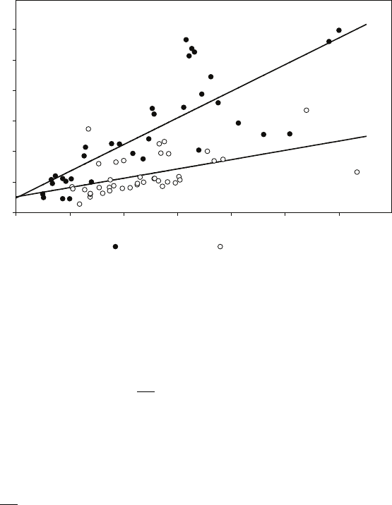
7. Heteroskedasticity
observations, and (b) for the last three-eighths. Perform a Goldfeld–Quandt test to
test for heteroskedasticity in the EXPPC dimension. Repeat using LGCATPC as
the dependent variable and regressing it on LGEXPPC and LGSIZE.
A7.2 Repeat Exercise A7.1, using a White test instead of a Goldfeld–Quandt test.
A7.3 The observations for the occupational schools (see Chapter 5 in the text) in the
figure suggest that a simple linear regression of cost on number of students,
restricted to the subsample of these schools, would be subject to heteroskedasticity.
Download the data set from the Online Resource Centre and use a
Goldfeld–Quandt test to investigate whether this is the case. If the relationship is
heteroskedastic, what could be done to alleviate the problem?
0
100000
200000
300000
400000
500000
600000
0 200 400 600 800 1000 1200
Occupational schools Regular schools
COST
N
ˆ
A7.4 A researcher hypothesises that larger economies should be more self-sufficient than
smaller ones and that M/G, the ratio of imports, M, to gross domestic product, G,
should be negatively related to G:
M
G=β1+β2G+u
with β2<0. Using data for a sample of 42 countries, with Mand Gboth measured
in US$ billion, he fits the regression (standard errors in parentheses):
c
M
G= 0.37 −0.000086G R2= 0.12 (1)
(0.03) (0.000036)
He plots a scatter diagram, reproduced as Figure 7.1, and notices that the ratio
M/G tends to have relatively high variance when Gis small. He also plots a scatter
diagram for Mand G, reproduced as Figure 7.2. Defining GSQ as the square of G,
he regresses Mon Gand GSQ:
c
M= 7.27 + 0.30G−0.000049GSQ R2= 0.86 (2)
(10.77) (0.03) (0.000009)
146
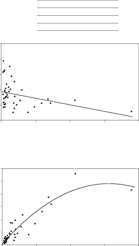
7.3. Additional exercises
Finally, he plots a scatter diagram for log Mand log G, reproduced as Figure 7.3,
and regresses log Mon log G:
\
log M=−0.14 + 0.80 log G R2= 0.78 (3)
(0.37) (0.07)
Having sorted the data by G, he tests for heteroskedasticity by regressing
specifications (1) – (3) first for the 16 countries with smallest G, and then for the
16 countries with the greatest G.RSS1and RSS2, the residual sums of squares for
these regressions, are summarised in the following table.
Specification RSS1RSS2
(1) 0.53 0.21
(2) 3178 71404
(3) 3.45 3.60
0.0
0.2
0.4
0.6
0.8
1.0
0 1000 2000 3000 4000
G
M/G
Figure 7.1: Scatter diagram of M/G against G.
0
100
200
300
400
500
600
0 1000 2000 3000 4000
G
M
Figure 7.2: Scatter diagram of Magainst G.
147
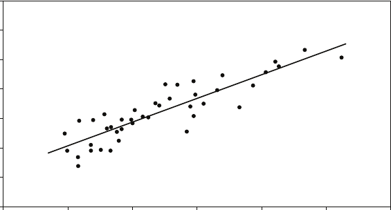
7. Heteroskedasticity
1
2
3
4
5
6
7
8
3456789
log G
log M
Figure 7.3: Scatter diagram of log Magainst log G.
•Discuss whether (1) appears to be an acceptable specification, given the data
in the table and Figure 7.1.
•Explain what the researcher hoped to achieve by running regression (2).
•Discuss whether (2) appears to be an acceptable specification, given the data
in the table and Figure 7.2.
•Explain what the researcher hoped to achieve by running regression (3).
•Discuss whether (3) appears to be an acceptable specification, given the data
in the table and Figure 7.3.
•What are your conclusions concerning the researcher’s hypothesis?
A7.5 A researcher has data on the number of children attending, N, and annual
recurrent expenditure, EXP, measured in US$, for 50 nursery schools in a US city
for 2006 and hypothesises that the cost function is of the quadratic form:
EXP =β1+β2N+β3NSQ +u
where NSQ is the square of N, anticipating that economies of scale will cause β3to
be negative. He fits the following equation:
[
EXP = 17999 + 1060N−1.29NSQ R2= 0.74 (1)
(12908) (133) (0.30)
Suspecting that the regression was subject to heteroskedasticity, the researcher
runs the regression twice more, first with the 19 schools with lowest enrolments,
then with the 19 schools with the highest enrolments. The residual sums of squares
in the two regressions are 8.0 million and 64.0 million, respectively.
The researcher defines a new variable, EXPN, expenditure per student, as EXPN
=EXP/N, and fits the equation:
\
EXPN = 1080 −1.25N+ 16114NREC R2= 0.65 (2)
(90) (0.25) (6000)
148

7.3. Additional exercises
where NREC = 1/N. He again runs regressions with the 19 smallest schools and
the 19 largest schools and the residual sums of squares are 900,000 and 600,000.
•Perform a Goldfeld–Quandt test for heteroskedasticity on both of the
regression specifications.
•Explain why the researcher ran the second regression.
•R2is lower in regression (2) than in regression (1). Does this mean that
regression (1) is preferable?
A7.6 This is a continuation of Exercise A6.5.
•When the researcher presents her results at a seminar, one of the participants
says that, since Iand Ghave been divided by Y, (2) is less likely to be subject
to heteroskedasticity than (1). Evaluate this suggestion.
A7.7 A researcher has data on annual household expenditure on food, F, and total
annual household expenditure, E, both measured in dollars, for 400 households in
the United States for 2010. The scatter plot for the data is shown as Figure 7.4.
The basic model of the researcher is:
F=β1+β2E+u(1)
where uis a disturbance term. The researcher suspects heteroskedasticity and
performs a Goldfeld–Quandt test and a White test. For the Goldfeld–Quandt test,
she sorts the data by size of Eand fits the model for the subsample with the 150
smallest values of Eand for the subsample with the 150 largest values. The
residual sums of squares (RSS) for these regressions are shown in column (1) of the
table. She also fits the regression for the entire sample, saves the residuals, and
then fits an auxiliary regression of the squared residuals on Eand its square. R2for
this regression is also shown in column (1) in the table. She performs parallel tests
of heteroskedasticity for two alternative models:
F
A=β1
1
A+β2
E
A+v(2)
log F=β1+β2log E+w. (3)
Ais household size in terms of equivalent adults, giving each adult a weight of 1
and each child a weight of 0.7. The scatter plot for F/A and E/A is shown as Figure
7.5, and that for log Fand log Eas Figure 7.6. The data for the heteroskedasticity
tests for models (2) and (3) are shown in columns (2) and (3) of the table.
Specification (1) (2) (3)
Goldfeld–Quandt test
RSS smallest 150 200 million 40 million 20.0
RSS largest 150 820 million 240 million 21.0
White test
R2from auxiliary regression 0.160 0.140 0.001
•Perform the Goldfeld–Quandt test for each model and state your conclusions.
149
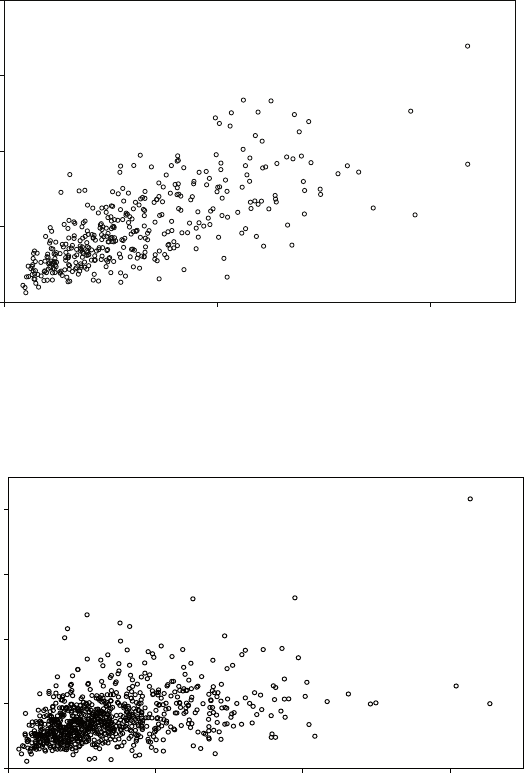
7. Heteroskedasticity
•Explain why the researcher thought that model (2) might be an improvement
on model (1).
•Explain why the researcher thought that model (3) might be an improvement
on model (1).
•When models (2) and (3) are tested for heteroskedasticity using the White
test, auxiliary regressions must be fitted. State the specification of this
auxiliary regression for model (2).
•Perform the White test for the three models.
•Explain whether the results of the tests seem reasonable, given the scatter
plots of the data.
0
5000
10000
15000
20000
0 50000 100000
Total household expenditure ($)
Household expenditure on food ($)
Figure 7.4: Scatter diagram of household expenditure on food against total household
expenditure.
0
2000
4000
6000
8000
0 20000 40000 60000
Total household expenditure per equivalent adult ($)
Household expenditure on food
per equivalent adult ($)
Figure 7.5: Scatter diagram of household expenditure on food per equivalent adult against
total household expenditure per equivalent adult.
150
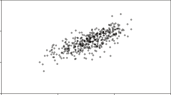
7.3. Additional exercises
5
7
9
11
7 9 11 13
log total household expenditure
log household expenditure on food
Figure 7.6: Scatter diagram of log household expenditure on food against log total
household expenditure.
A7.8 Explain what is correct, mistaken, confused or in need of further explanation in the
following statements relating to heteroskedasticity in a regression model:
•‘Heteroskedasticity occurs when the disturbance term in a regression model is
correlated with one of the explanatory variables.’
•‘In the presence of heteroskedasticity ordinary least squares (OLS) is an
inefficient estimation technique and this causes ttests and Ftests to be
invalid.’
•‘OLS remains unbiased but it is inconsistent.
•‘Heteroskedasticity can be detected with a Chow test.’
•‘Alternatively one can compare the residuals from a regression using half of the
observations with those from a regression using the other half and see if there
is a significant difference. The test statistic is the same as for the Chow test.’
•‘One way of eliminating the problem is to make use of a restriction involving
the variable correlated with the disturbance term.’
•‘If you can find another variable related to the one responsible for the
heteroskedasticity, you can use it as a proxy and this should eliminate the
problem.’
•‘Sometimes apparent heteroskedasticity can be caused by a mathematical
misspecification of the regression model. This can happen, for example, if the
dependent variable ought to be logarithmic, but a linear regression is run.’
151

7. Heteroskedasticity
7.4 Answers to the starred exercises in the textbook
7.5 The following regressions were fitted using the Shanghai school cost data
introduced in Section 6.1 (standard errors in parentheses):
\
COST = 24000 + 339N R2= 0.39
(27000) (50)
\
COST = 51000 −4000OCC + 152N+ 284NOCC R2= 0.68.
(31000) (41000) (60) (76)
where COST is the annual cost of running a school, Nis the number of students,
OCC is a dummy variable defined to be 0 for regular schools and 1 for
occupational schools, and NOCC is a slope dummy variable defined as the product
of Nand OCC. There are 74 schools in the sample. With the data sorted by N, the
regressions are fitted again for the 26 smallest and 26 largest schools, the residual
sums of squares being as shown in the table.
26 smallest 26 largest
First regression 7.8×10¹⁰ 54.4×10¹⁰
Second regression 6.7×10¹⁰ 13.8×10¹⁰
Perform a Goldfeld–Quandt test for heteroskedasticity for the two models and,
with reference to Figure 6.5, explain why the problem of heteroskedasticity is less
severe in the second model.
Answer:
For both regressions RSS will be denoted RSS1for the 26 smallest schools and
RSS2for the 26 largest schools. In the first regression,
RSS2/RSS1= (54.4×10¹⁰)/(7.8×1010) = 6.97. There are 24 degrees of freedom in
each subsample (26 observations, 2 parameters estimated). The critical value of
F(24,24) is approximately 3.7 at the 0.1 per cent level, and so we reject the null
hypothesis of homoskedasticity at that level. In the second regression,
RSS2/RSS1= (13.8×10¹⁰)/(6.7×1010)=2.06. There are 22 degrees of freedom in
each subsample (26 observations, 4 parameters estimated). The critical value of
F(22,22) is 2.05 at the 5 per cent level, and so we (just) do not reject the null
hypothesis of homoskedasticity at that significance level.
Why is the problem of heteroskedasticity less severe in the second regression? The
figure in Exercise A7.2 reveals that the cost function is much steeper for the
occupational schools than for the regular schools, reflecting their higher marginal
cost. As a consequence the two sets of observations diverge as the number of
students increases and the scatter is bound to appear heteroskedastic, irrespective
of whether the disturbance term is truly heteroskedastic or not. The first regression
takes no account of this and the Goldfeld–Quandt test therefore indicates
significant heteroskedasticity. In the second regression the problem of apparent
heteroskedasticity does not arise because the intercept and slope dummy variables
allow separate implicit regression lines for the two types of school.
152
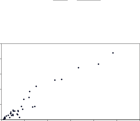
7.4. Answers to the starred exercises in the textbook
Looking closely at the diagram, the observations for the occupational schools
exhibit a classic pattern of true heteroskedasticity, and this would be confirmed by
a Goldfeld–Quandt test confined to the subsample of those schools (see Exercise
A7.2). However the observations for the regular schools appear to be homoskedastic
and this accounts for the fact that we did not (quite) reject the null hypothesis of
homoskedasticity for the combined sample.
7.6 The file educ.dta on the website contains contains international cross-sectional data
on aggregate expenditure on education, EDUC, gross domestic product, GDP, and
population, P OP , for a sample of 38 countries in 1997. EDUC and GDP are
measured in US$ million and POP is measured in thousands. Download the data
set, plot a scatter diagram of EDUC on GDP, and comment on whether the data
set appears to be subject to heteroskedasticity. Sort the data set by GDP and
perform a Goldfeld–Quandt test for heteroskedasticity, running regressions using
the subsamples of 14 countries with the smallest and greatest GDP.
Answer:
The figure plots expenditure on education, EDUC, and gross domestic product,
GDP, for the 38 countries in the sample, measured in $ billion rather than $ million.
The observations exhibit heteroskedasticity. Sorting them by GDP and regressing
EDUC on GDP for the subsamples of 14 countries with smallest and greatest
GDP, the residual sums of squares for the first and second subsamples, denoted
RSS1and RSS2, respectively, are 1,660,000 and 63,113,000, respectively. Hence:
F(12,12) = RSS2
RSS1
=63113000
1660000 = 38.02.
The critical value of F(12,12) at the 0.1 per cent level is 7.00, and so we reject the
null hypothesis of homoskedasticity.
0
5
10
15
20
25
0 100 200 300 400 500 600
GDP ($ billion)
Expenditure on education ($ billion)
Figure 7.7: Expenditure on education and GDP ($ billion).
7.9 Repeat Exercise 7.6, using the Goldfeld–Quandt test to investigate whether scaling
by population or by GDP, or whether running the regression in logarithmic form,
153
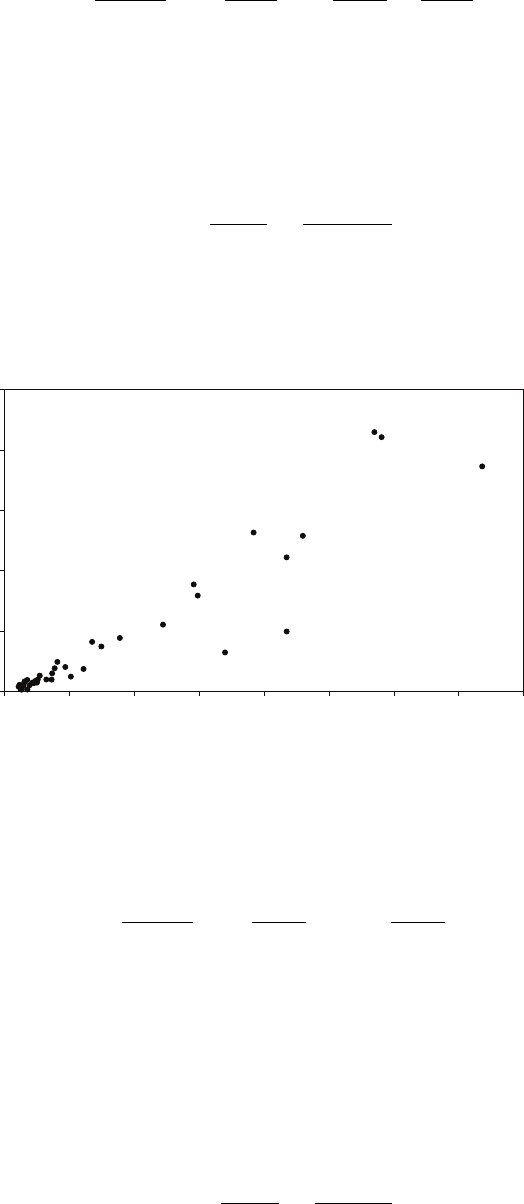
7. Heteroskedasticity
would eliminate the heteroskedasticity. Compare the results of regressions using the
entire sample and the alternative specifications.
Answer:
Dividing through by population, POP, the model becomes:
EDUC
POP =β1
1
POP +β2
GDP
POP +u
POP
with expenditure on education per capita, denoted EDUCPOP, hypothesised to be
a function of gross domestic product per capita, GDPPOP, and the reciprocal of
population, POPREC, with no intercept. Sorting the sample by GDPPOP and
running the regression for the subsamples of 14 countries with smallest and largest
GDPPOP,RSS1= 0.006788 and RSS2= 1.415516. Now:
F(12,12) = RSS2
RSS1
=1.415516
0.006788 = 208.5.
Thus the model is still subject to heteroskedasticity at the 0.1 per cent level. This
is evident in Figure 7.8.
0
500
1,000
1,500
2,000
2,500
0 5,000 10,000 15,000 20,000 25,000 30,000 35,000 40,000
GDP/POP
EDUC/POP
Figure 7.8: Expenditure on education per capita and GDP per capita ($ per capita).
Dividing through instead by GDP, the model becomes:
EDUC
GDP =β1
1
GDP +β2+u
GDP
with expenditure on education as a share of gross domestic product, denoted
EDUCGDP, hypothesised to be a simple function of the reciprocal of gross
domestic product, GDPREC, with no intercept. Sorting the sample by GDPREC
and running the regression for the subsamples of 14 countries with smallest and
largest GDPREC,RSS1= 0.00413 and RSS2= 0.00238. Since RSS2is less than
RSS1, we test for heteroskedasticity under the hypothesis that the standard
deviation of the disturbance term is inversely related to GDPREC :
F(12,12) = RSS1
RSS2
=0.00413
0.00238 = 1.74.
154
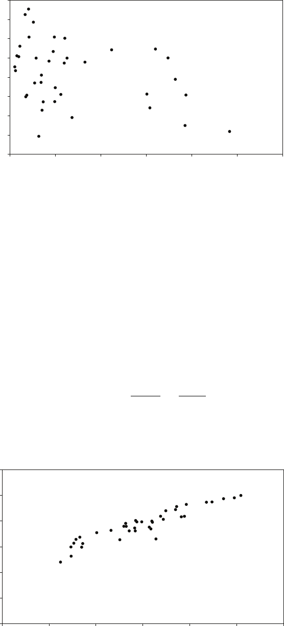
7.4. Answers to the starred exercises in the textbook
0
0.01
0.02
0.03
0.04
0.05
0.06
0.07
0.08
0 0.02 0.04 0.06 0.08 0.1 0.12
1/GDP
EDUC/GDP
Figure 7.9: Expenditure on education as a proportion of GDP and the reciprocal of GDP
(measured in $ billion).
The critical value of F(12,12) at the 5 per cent level is 2.69, so we do not reject the
null hypothesis of homoskedasticity. Could one tell this from Figure 7.9? It is a
little difficult to say.
Finally, we will consider a logarithmic specification. If the true relationship is
logarithmic, and homoskedastic, it would not be surprising that the linear model
appeared heteroskedastic. Sorting the sample by GDP,RSS1and RSS2are 2.733
and 3.438 for the subsamples of 14 countries with smallest and greatest GDP. The
Fstatistic is:
F(12,12) = RSS1
RSS2
=3.438
2.733 = 1.26.
Thus again we would not reject the null hypothesis of homoskedasticity.
0
2
4
6
8
10
12
8 9 10 11 12 13 14
log GDP
log EDUC
Figure 7.10: Expenditure on education and GDP, logarithmic.
155

7. Heteroskedasticity
The third and fourth models both appear to be free from heteroskedasticity. How
do we choose between them? We will examine the regression results, shown for the
two models with the full sample:
. reg EDUCGDP GDPREC
Source | SS df MS Number of obs = 38
---------+------------------------------ F( 1, 36) = 5.62
Model | .001348142 1 .001348142 Prob > F = 0.0233
Residual | .008643037 36 .000240084 R-squared = 0.1349
---------+------------------------------ Adj R-squared = 0.1109
Total | .009991179 37 .000270032 Root MSE = .01549
------------------------------------------------------------------------------
EDUCGDP | Coef. Std. Err. t P>|t| [95% Conf. Interval]
---------+--------------------------------------------------------------------
GDPREC | -234.0823 98.78309 -2.370 0.023 -434.4236 -33.74086
_cons | .0484593 .0036696 13.205 0.000 .0410169 .0559016
------------------------------------------------------------------------------
. reg LGEE LGGDP
Source | SS df MS Number of obs = 38
---------+------------------------------ F( 1, 36) = 246.20
Model | 51.9905508 1 51.9905508 Prob > F = 0.0000
Residual | 7.6023197 36 .211175547 R-squared = 0.8724
---------+------------------------------ Adj R-squared = 0.8689
Total | 59.5928705 37 1.61061812 Root MSE = .45954
------------------------------------------------------------------------------
LGEE | Coef. Std. Err. t P>|t| [95% Conf. Interval]
---------+--------------------------------------------------------------------
LGGDP | 1.160594 .0739673 15.691 0.000 1.010582 1.310607
_cons | -5.025204 .8152239 -6.164 0.000 -6.678554 -3.371853
------------------------------------------------------------------------------
In equation form, the first regression is:
\
EDUC
GDP = 0.048 −234.11
GDP R2= 0.13
(0.004) (98.8)
Multiplying through by GDP, it may be rewritten:
\
EDUC =−234.1+0.048GDP.
It implies that expenditure on education accounts for 4.8 per cent of gross domestic
product at the margin. The constant does not have any sensible interpretation. We
will compare this with the output from an OLS regression that makes no attempt
to eliminate heteroskedasticity:
156
7.4. Answers to the starred exercises in the textbook
. reg EDUC GDP
Source | SS df MS Number of obs = 38
---------+------------------------------ F( 1, 36) = 509.80
Model | 1.0571e+09 1 1.0571e+09 Prob > F = 0.0000
Residual | 74645819.2 36 2073494.98 R-squared = 0.9340
---------+------------------------------ Adj R-squared = 0.9322
Total | 1.1317e+09 37 30586911.0 Root MSE = 1440.0
------------------------------------------------------------------------------
EDUC | Coef. Std. Err. t P>|t| [95% Conf. Interval]
---------+--------------------------------------------------------------------
GDP | .0480656 .0021288 22.579 0.000 .0437482 .052383
_cons | -160.4669 311.699 -0.515 0.610 -792.6219 471.688
------------------------------------------------------------------------------
The slope coefficient, 0.048, is identical to three decimal places. This is not entirely
a surprise, since heteroskedasticity does not give rise to bias and so there should be
no systematic difference between the estimate from an OLS regression and that
from a specification that eliminates heteroskedasticity. Of course, it is a surprise
that the estimates are so close. Generally there would be some random difference,
and of course the OLS estimate would tend to be less accurate. In this case, the
main difference is in the estimated standard error. That for the OLS regression is
actually smaller than that for the regression of EDUCGDP on GDPREC, but it is
misleading. It is incorrectly calculated and we know that, since OLS is inefficient,
the true standard error for the OLS estimate is actually larger.
The logarithmic regression in equation form is:
\
log EDUC =−5.03 + 1.16 log GDP R2= 0.87
(0.82) (0.07)
implying that the elasticity of expenditure on education with regard to gross
domestic product is 1.16. In substance the interpretations of the models are similar,
since both imply that the proportion of GDP allocated to education increases
slowly with GDP, but the elasticity specification seems a little more informative
and probably serves as a better starting point for further exploration. For example,
it would be natural to add the logarithm of population to see if population had an
independent effect.
7.10 It was reported above that the heteroskedasticity-consistent estimate of the
standard error of the coefficient of GDP in equation (7.18) was 0.18. Explain why
the corresponding standard error in equation (7.20) ought to be lower and
comment on the fact that it is not.
Answer:
(7.20), unlike (7.18) appears to be free from heteroskedasticity and therefore should
provide more efficient estimates of the coefficients, reflected in lower standard
errors when computed correctly. However the sample may be too small for the
heteroskedasticity-consistent estimator to be a good guide.
7.11 A health economist plans to evaluate whether screening patients on arrival or
spending extra money on cleaning is more effective in reducing the incidence of
157

7. Heteroskedasticity
infections by the MRSA bacterium in hospitals. She hypothesises the following
model:
MRSAi=β1+β2Si+β3Ci+ui
where, in hospital i,MRSA is the number of infections per thousand patients, Sis
expenditure per patient on screening, and Cis expenditure per patient on cleaning.
uiis a disturbance term that satisfies the usual regression model assumptions. In
particular, uiis drawn from a distribution with mean zero and constant variance
σ2. The researcher would like to fit the relationship using a sample of hospitals.
Unfortunately, data for individual hospitals are not available. Instead she has to
use regional data to fit:
MRSAj=β1+β2Sj+β3Cj+uj
where MRSAj,Sj,Cj, and ujare the averages of MRSA,S,C, and ufor the
hospitals in region j. There were different numbers of hospitals in the regions, there
being njhospitals in region j.
Show that the variance of ujis equal to σ2/njand that an OLS regression using the
grouped regional data to fit the relationship will be subject to heteroskedasticity.
Assuming that the researcher knows the value of njfor each region, explain how
she could re-specify the regression model to make it homoskedastic. State the
revised specification and demonstrate mathematically that it is homoskedastic.
Give an intuitive explanation of why the revised specification should tend to
produce improved estimates of the parameters.
Answer:
var(uj) = var 1
n
nj
X
k=1
ujk!=1
nj2
var nj
X
k=1
ujk!=1
nj2nj
X
k=1
var(ujk)
since the covariance terms are all 0. Hence:
var(uj) = 1
nj2
njσ2=σ2
nj
.
To eliminate the heteroskedasticity, multiply observation jby √nj. The regression
becomes: √njMRSAj=β1√nj+β2√njSj+β3√njCj+√njuj.
The variance of the disturbance term is now:
var √njuj=√nj2var(uj) = nj
σ2
nj
=σ2
and is thus the same for all observations.
From the expression for var(uj), we see that, the larger the group, the more reliable
should be its observation (the closer its observation should tend to be to the
population relationship). The scaling gives greater weight to the more reliable
observations and the resulting estimators should be more efficient.
158

7.5. Answers to the additional exercises
7.5 Answers to the additional exercises
A7.1 The first step is to drop the zero-observations from the data set and sort it by
EXPPC. The Fstatistic is then computed as:
F(n2−k, n1−k) = RSS2/(n2−k)
RSS1/(n1−k)
where n1and n2are the number of available observations and kis the number of
parameters in the regression specification.
. drop if FDHO == 0
(0 observations deleted)
. gen EXPPC = EXP/SIZE
. sort EXPPC
. gen LGEXPPC = ln(EXPPC)
. gen LGSIZE = ln(SIZE)
. gen FDHOPC = FDHO/SIZE
. gen LGFDHOPC = ln(FDHOPC)
. reg FDHOPC EXPPC SIZE in 1/2375
----------------------------------------------------------------------------
Source | SS df MS Number of obs = 2375
-----------+------------------------------ F( 2, 2372) = 278.36
Model | 7382348.18 2 3691174.09 Prob> F = 0.0000
Residual | 31453534.1 2372 13260.3432 R-squared = 0.1901
-----------+------------------------------ Adj R-squared = 0.1894
Total | 38835882.2 2374 16358.8383 Root MSE = 115.15
----------------------------------------------------------------------------
FDHOPC | Coef. Std. Err. t P>|t| [95% Conf. Interval]
-----------+----------------------------------------------------------------
EXPPC | .1107869 .0051862 21.36 0.000 .1006169 .1209569
SIZE | -4.462209 1.438899 -3.10 0.002 -7.283838 -1.640579
_cons | 85.38055 9.590628 8.90 0.000 66.57366 104.1874
----------------------------------------------------------------------------
. reg FDHOPC EXPPC SIZE in 3960/6334
----------------------------------------------------------------------------
Source | SS df MS Number of obs = 2375
-----------+------------------------------ F( 2, 2372) = 170.94
Model | 40643447.8 2 20321723.9 Prob> F = 0.0000
Residual | 281980931 2372 118878.976 R-squared = 0.1260
-----------+------------------------------ Adj R-squared = 0.1252
Total | 322624379 2374 135899.064 Root MSE = 344.79
----------------------------------------------------------------------------
FDHOPC | Coef. Std. Err. t P>|t| [95% Conf. Interval]
-----------+----------------------------------------------------------------
EXPPC | .0286606 .0019716 14.54 0.000 .0247944 .0325268
SIZE | -54.33452 7.047302 -7.71 0.000 -68.15403 -40.51501
_cons | 508.6148 22.37631 22.73 0.000 464.7356 552.4939
----------------------------------------------------------------------------
159

7. Heteroskedasticity
. reg LGFDHOPC LGEXPPC LGSIZE in 1/2375
----------------------------------------------------------------------------
Source | SS df MS Number of obs = 2375
-----------+------------------------------ F( 2, 2372) = 369.49
Model | 207.241064 2 103.620532 Prob> F = 0.0000
Residual | 665.204785 2372 .280440466 R-squared = 0.2375
-----------+------------------------------ Adj R-squared = 0.2369
Total | 872.445849 2374 .367500357 Root MSE = .52957
----------------------------------------------------------------------------
LGFDHOPC | Coef. Std. Err. t P>|t| [95% Conf. Interval]
-----------+----------------------------------------------------------------
LGEXPPC | .6510802 .0265608 24.51 0.000 .5989953 .703165
LGSIZE | -.0567001 .0198997 -2.85 0.004 -.0957227 -.0176775
_cons | .6450249 .1965331 3.28 0.001 .2596305 1.030419
----------------------------------------------------------------------------
. reg LGFDHOPC LGEXPPC LGSIZE in 3960/6334
----------------------------------------------------------------------------
Source | SS df MS Number of obs = 2375
-----------+------------------------------ F( 2, 2372) = 138.91
Model | 94.0495475 2 47.0247737 Prob> F = 0.0000
Residual | 802.969196 2372 .338519897 R-squared = 0.1048
-----------+------------------------------ Adj R-squared = 0.1041
Total | 897.018744 2374 .377851198 Root MSE = .58182
----------------------------------------------------------------------------
LGFDHOPC | Coef. Std. Err. t P>|t| [95% Conf. Interval]
-----------+----------------------------------------------------------------
LGEXPPC | .4072631 .0297285 13.70 0.000 .3489666 .4655596
LGSIZE | -.1426229 .0247966 -5.75 0.000 -.1912482 -.0939976
_cons | 2.742439 .2635057 10.41 0.000 2.225714 3.259165
----------------------------------------------------------------------------
The Fstatistic for the linear specification is:
F(2372,2372) = 281980931/2372
31453534/2372 = 8.97.
This is significant at the 0.1 per cent level. The corresponding Fstatistic for the
logarithmic specification is 1.21. The critical value of F(200,200) at the 5 per cent
level is 1.26. The critical value for F(2372,2372) must be lower, so the null
hypothesis of homoskedasticity is probably rejected at that level. However, the
problem has evidently been largely eliminated.
The logarithmic specification in general appears to be much less heteroskedastic
than the linear one and for some categories the null hypothesis of homoskedasticity
would not be rejected. Note that for a few of these RSS2< RSS1for the
logarithmic specification.
160

7.5. Answers to the additional exercises
Goldfeld–Quandt tests
Linear Logarithmic
n1n2RSS1×10−6RSS2×10−6F RSS1RSS2F
ADM 1,056 1,056 1.95 62.93 32.30 1,324.96 1,593.31 1.20
CLOT 1,688 1,688 7.17 316.80 44.17 2,107.28 2,196.79 1.04
DOM 623 623 7.23 238.90 33.05 1,571.19 1,505.92 1.04*
EDUC 210 210 11.70 376.01 32.15 495.12 507.27 1.02
ELEC 2,186 2,186 7.55 33.34 4.41 1,034.70 923.18 1.12*
FDAW 1,913 1,913 9.00 278.13 30.89 1,136.09 1,361.12 1.20
FDHO 2,375 2,375 31.45 281.98 8.97 665.20 802.97 1.21
FOOT 685 685 0.55 5.74 10.37 513.08 514.24 1.00
FURN 183 183 7.17 258.26 36.00 322.50 368.42 1.14
GASO 2,141 2,141 11.06 159.54 14.43 921.26 1,245.55 1.35
HEAL 1,801 1,801 32.91 876.72 26.64 2,233.73 2,192.92 1.02*
HOUS 2,334 2,334 105.48 3,031.19 28.74 2,129.27 1,475.02 1.44*
LIFE 470 470 2.85 48.37 16.95 503.19 667.14 1.33
LOCT 260 260 0.58 5.32 9.13 366.16 409.90 1.12
MAPP 150 150 2.85 37.01 12.96 211.71 243.18 1.15
PERS 1,431 1,431 0.47 9.01 19.34 1,045.70 1,204.31 1.15
READ 858 858 0.36 4.95 13.69 1,076.35 1,085.38 1.01
SAPP 389 389 0.56 10.68 19.04 396.41 433.37 1.09
TELE 2,171 2,171 3.27 26.80 8.19 1,133.43 1,123.46 1.01*
TEXT 372 372 0.57 2.05 3.61 410.29 393.80 1.04*
TOB 433 433 1.56 27.81 17.84 312.71 338.28 1.08
TOYS 939 939 6.83 87.65 12.83 1,079.76 1,064.92 1.01*
TRIP 194 194 9.62 77.65 8.07 300.70 335.75 1.12
* indicates RSS2< RSS1
A7.2 The table shows the construction of the White test statistics for the linear and
logarithmic specifications for each category of expenditure. The regressors in the
auxiliary regression were expenditure per capita and its square, size and its square,
and the product of expenditure per capita and size. Hence there were five degrees
of freedom for the chi-squared test. The critical values are 11.1 and 15.1 at the 5
per cent and 1 per cent levels. Thus there is strong evidence of heteroskedasticity
for all of the categories in the linear specification. There is also evidence for some
categories in the logarithmic specification. It is possible that the White test, being
more general, is finding evidence of heteroskedasticity not detected by the
Goldfeld–Quandt test.
161

7. Heteroskedasticity
White tests
Linear Logarithmic
n R2nR2R2nR2
ADM 2,815 0.1710 481.4 0.0097 27.3
CLOT 4,500 0.0180 81.0 0.0074 33.3
DOM 1,661 0.0191 31.7 0.0062 10.3
EDUC 561 0.1432 80.3 0.0078 4.4
ELEC 5,828 0.0487 283.8 0.0090 52.5
FDAW 5,102 0.1072 546.9 0.0067 34.2
FDHO 6,334 0.1143 724.0 0.0129 81.7
FOOT 1,827 0.0191 34.9 0.0023 4.2
FURN 487 0.3287 160.1 0.0197 9.6
GASO 5,710 0.0575 328.3 0.0152 86.8
HEAL 4,802 0.0608 292.0 0.0021 10.1
HOUS 6,223 0.2002 1,245.8 0.0120 74.7
LIFE 1,253 0.0535 67.0 0.0132 16.5
LOCT 692 0.0388 26.8 0.0192 13.3
MAPP 399 0.0882 35.2 0.0168 6.7
PERS 3,817 0.0607 231.7 0.0086 32.8
READ 2,287 0.0158 36.1 0.0072 16.5
SAPP 1,037 0.0221 22.9 0.0032 3.3
TELE 5,788 0.0724 419.1 0.0021 12.2
TEXT 992 0.0183 18.2 0.0049 4.9
TOB 1,155 0.0235 27.1 0.0061 7.0
TOYS 2,504 0.0347 86.9 0.0026 6.5
TRIP 516 0.0571 29.5 0.0047 2.4
A7.3 Having sorted by N, the number of students, RSS1and RSS2are 2.02 ×10¹⁰ and
22.59 ×10¹⁰, respectively, for the subsamples of the 13 smallest and largest schools.
The Fstatistic is 11.18. The critical value of F(11,11) at the 0.1 per cent level
must be a little below 8.75, the critical value for F(10,10), and so the null
hypothesis of homoskedasticity is rejected at that significance level.
One possible way of alleviating the heteroskedasticity is by scaling through by the
number of students. The dependent variable now becomes the unit cost per student
year, and this is likely to be more uniform than total recurrent cost. Scaling
through by N, and regressing UNITCOST, defined as COST divided by N, on
NREC, the reciprocal of N, having first sorted by NREC,RSS1and RSS2are now
349,000 and 504,000. The Fstatistic is therefore 1.44, and this is not significant
even at the 5 per cent level since the critical value must be a little above 2.69, the
critical value for F(12,12). The regression output for this specification using the
full sample is shown.
. reg UNITCOST NREC
Source | SS df MS Number of obs = 34
---------+------------------------------ F( 1, 32) = 0.74
Model | 27010.3792 1 27010.3792 Prob > F = 0.3954
Residual | 1164624.44 32 36394.5138 R-squared = 0.0227
---------+------------------------------ Adj R-squared = -0.0079
Total | 1191634.82 33 36110.1461 Root MSE = 190.77
162

7.5. Answers to the additional exercises
------------------------------------------------------------------------------
UNITCOST | Coef. Std. Err. t P>|t| [95% Conf. Interval]
---------+--------------------------------------------------------------------
NREC | 10975.91 12740.7 0.861 0.395 -14976.04 36927.87
_cons | 524.813 53.88367 9.740 0.000 415.0556 634.5705
------------------------------------------------------------------------------
In equation form, the regression is:
\
COST
N= 524.8 + 10976 1
NR2= 0.03
(53.9) (12741)
Multiplying through by N, it may be rewritten:
\
COST = 10976 + 524.8N.
The estimate of the marginal cost is somewhat higher than the estimate of 436
obtained using OLS in Section 5.3 of the text.
A second possible way of alleviating the heteroskedasticity is to hypothesise that
the true relationship is logarithmic, in which case the use of an inappropriate linear
specification would give rise to apparent heteroskedasticity. Scaling through by N,
and regressing LGCOST, the (natural) logarithm of COST, on LGN, the logarithm
of N,RSS1and RSS2are 2.16 and 1.58. The Fstatistic is therefore 1.37, and
again this is not significant even at the 5 per cent level. The regression output for
this specification using the full sample is shown.
. reg LGCOST LGN
Source | SS df MS Number of obs = 34
---------+------------------------------ F( 1, 32) = 100.98
Model | 14.7086057 1 14.7086057 Prob > F = 0.0000
Residual | 4.66084501 32 .145651406 R-squared = 0.7594
---------+------------------------------ Adj R-squared = 0.7519
Total | 19.3694507 33 .58695305 Root MSE = .38164
------------------------------------------------------------------------------
LGCOST | Coef. Std. Err. t P>|t| [95% Conf. Interval]
---------+--------------------------------------------------------------------
LGN | .909126 .0904681 10.049 0.000 .7248485 1.093404
_cons | 6.808312 .5435035 12.527 0.000 5.701232 7.915393
------------------------------------------------------------------------------
The estimate of the elasticity of cost with respect to number of students, 0.91, is
less than 1 and thus suggests that the schools are subject to economies of scale.
However, we are not able to reject the null hypothesis that the elasticity is equal to
1 and thus that costs are proportional to numbers, the tstatistic for the null
hypothesis being too low:
t=0.909 −1.000
0.091 =−1.00.
163

7. Heteroskedasticity
A7.4 Discuss whether (1) appears to be an acceptable specification, given the data in the
table and Figure 7.1.
Using the Goldfeld–Quandt test to test specification (1) for heteroskedasticity
assuming that the standard deviation of u is inversely proportional to G, we have:
F(14,14) = 0.53
0.21 = 2.52.
The critical value of F(14,14) at the 5 per cent level is 2.48, so we just reject the
null hypothesis of homoskedasticity at that level. Figure 7.1 does strongly suggest
heteroskedasticity. Thus (1) does not appear to be an acceptable specification.
Explain what the researcher hoped to achieve by running regression (2).
If it is true that the standard deviation of uis inversely proportional to G, the
heteroskedasticity could be eliminated by multiplying through by G. This is the
motivation for the second specification. An intercept that in principle does not
exist has been added, thereby changing the model specification slightly.
Discuss whether (2) appears to be an acceptable specification, given the data in the
table and Figure 7.2.
F(13,13) = 71404
3178 = 22.47.
The critical value of F(13,13) at the 0.1 per cent level is about 6.4, so the null
hypothesis of homoskedasticity is rejected. Figure 7.2 confirms the
heteroskedasticity.
Explain what the researcher hoped to achieve by running regression (3).
Heteroskedasticity can appear to be present in a regression in natural units if the
true relationship is logarithmic. The disturbance term in a logarithmic regression is
effectively increasing or decreasing the value of the dependent variable by random
proportions. Its effect in absolute terms will therefore tend to be greater, the larger
the value of G. The researcher is checking to see if this is the reason for the
heteroskedasticity in the second specification.
Discuss whether (3) appears to be an acceptable specification, given the data in the
table and Figure 7.3.
Obviously there is no problem with the Goldfeld–Quandt test, since:
F(14,14) = 3.60
3.45 = 1.04.
Figure 7.3 looks free from heteroskadasticity.
What are your conclusions concerning the researcher’s hypothesis?
Evidence in support of the hypothesis is provided by (3) where, with:
t=0.80 −1
0.07 =−2.86
the elasticity is significantly lower than 1. Figures 7.1 and 7.2 also strongly suggest
that on balance larger economies have lower import ratios than smaller ones.
164

7.5. Answers to the additional exercises
A7.5 Perform a Goldfeld–Quandt test for heteroskedasticity on both of the regression
specifications.
The Fstatistics for the G–Q test for the two specifications are:
F(16,16) = 64/16
8/16 = 8.0 and F(16,16) = 900/16
600/16 = 1.5.
The critical value of F(16,16) is 2.33 at the 5 per cent level and 5.20 at the 0.1 per
cent level. Hence one would reject the null hypothesis of homoskedasticity at the
0.1 per cent level for regression 1 and one would not reject it even at the 5 per cent
level for regression 2.
Explain why the researcher ran the second regression.
He hypothesised that the standard deviation of the disturbance term in observation
iwas proportional to Ni:σi=λNifor some λ. If this is the case, dividing through
by Nimakes the specification homoskedastic, since:
var ui
Ni=1
N2var(ui) = 1
N2
i
(λNi)2=λ2
and is therefore the same for all i.
R2is lower in regression (2) than in regression (1). Does this mean that regression
(1) is preferable?
R2is not comparable because the dependent variable is different in the two
regressions. Regression (2) is to be preferred since it is free from heteroskedasticity
and therefore ought to tend to yield more precise estimates of the coefficients with
valid standard errors.
A7.6 When the researcher presents her results at a seminar, one of the participants says
that, since I and G have been divided by Y, (2) is less likely to be subject to
heteroskedasticity than (1). Evaluate this suggestion.
If the restriction is valid, imposing it will have no implications for the disturbance
term and so it could not lead to any mitigation of a potential problem of
heteroskedasticity. [If there were heteroskedasticity, and if the specification were
linear, scaling through by a variable proportional in observation ito the standard
deviation of uiin observation iwould lead to the elimination of heteroskedasticity.
The present specification is logarithmic and dividing Iand Gby Ydoes not affect
the disturbance term.]
A7.7 Perform the Goldfeld–Quandt test for each model and state your conclusions.
The ratios are 4.1, 6.0, and 1.05. In each case we should look for the critical value
of F(148,148). The critical values of F(150,150) at the 5 per cent, 1 per cent, and
0.1 per cent levels are 1.31, 1.46, and 1.66, respectively. Hence we reject the null
hypothesis of homoskedasticity at the 0.1 per cent level (1 per cent is OK) for
models (1) and (2). We do not reject it even at the 5 per cent level for model (3).
165

7. Heteroskedasticity
Explain why the researcher thought that model (2) might be an improvement on
model (1).
If the assumption that the standard deviation of the disturbance term is
proportional to household size, scaling through by Ashould eliminate the
heteroskedasticity, since:
E(v2) = Ehu
Ai2=1
A2E(u2) = λ2
if the standard deviation of u=λA.
Explain why the researcher thought that model (3) might be an improvement on
model (1).
It is possible that the (apparent) heteroskedasticity is attributable to mathematical
misspecification. If the true model is logarithmic, a homoskedastic disturbance
term would appear to have a heteroskedastic effect if the regression is performed in
the original units.
When models (2) and (3) are tested for heteroskedasticity using the White test,
auxiliary regressions must be fitted. State the specification of this auxiliary
regression for model (2).
The dependent variable is the squared residuals from the model regression. The
explanatory variables are the reciprocal of Aand its square, E/A and its square,
and the product of the reciprocal of Aand E/A. (No constant.)
Perform the White test for the three models.
nR2is 64.0, 56.0, and 0.4 for the three models. Under the null hypothesis of
homoskedasticity, this statistic has a chi-squared distribution with degrees of
freedom equal to the number of terms on the right side of the regression, minus
one. This is two for models (1) and (3). The critical value of chi-squared with two
degrees of freedom is 5.99, 9.21, and 13.82 at the 5, 1, and 0.1 per cent levels. Hence
H0 is rejected at the 0.1 per cent level for model (1), and not rejected even at the 5
per cent level for model (3). In the case of model (2), there are five terms on the
right side of the regression. The critical value of chisquared with four degrees of
freedom is 18.47 at the 0.1 per cent level. Hence H0is rejected at that level.
Explain whether the results of the tests seem reasonable, given the scatter plots of
the data.
Absolutely. In Figures 7.1 and 7.2, the variances of the dispersions of the dependent
variable clearly increase with the size of the explanatory variable. In Figure 7.3, the
dispersion is much more even.
A7.8 ‘Heteroskedasticity occurs when the disturbance term in a regression model is
correlated with one of the explanatory variables.’
This is false. Heteroskedasticity occurs when the variance of the disturbance term
is not the same for all observations.
166
7.5. Answers to the additional exercises
‘In the presence of heteroskedasticity ordinary least squares (OLS) is an inefficient
estimation technique and this causes t tests and F tests to be invalid.’
It is true that OLS is inefficient and that the tand Ftests are invalid, but ‘and
this causes’ is wrong.
‘OLS remains unbiased but it is inconsistent.’
It is true that OLS is unbiased, but false that it is inconsistent.
‘Heteroskedasticity can be detected with a Chow test.’
This is false.
‘Alternatively one can compare the residuals from a regression using half of the
observations with those from a regression using the other half and see if there is a
significant difference. The test statistic is the same as for the Chow test.’
The first sentence is basically correct with the following changes and clarifications:
one is assuming that the standard deviation of the disturbance term is proportional
to one of the explanatory variables; the sample should first be sorted according to
the size of the explanatory variable; rather than split the sample in half, it would
be better to compare the first three-eighths (or one third) of the observations with
the last three-eighths (or one third); ‘comparing the residuals’ is too vague: the F
statistic is F(n0−k, n0−k) = RSS2/RSS1assuming n0observations and k
parameters in each subsample regression, and placing the larger RSS over the
smaller.
The second sentence is false.
‘One way of eliminating the problem is to make use of a restriction involving the
variable correlated with the disturbance term.’
This is nonsense.
‘If you can find another variable related to the one responsible for the
heteroskedasticity, you can use it as a proxy and this should eliminate the problem.’
This is more nonsense.
‘Sometimes apparent heteroskedasticity can be caused by a mathematical
misspecification of the regression model. This can happen, for example, if the
dependent variable ought to be logarithmic, but a linear regression is run.’
True. A homoskedastic disturbance term in a logarithmic regression, which is
responsible for proportional changes in the dependent variable, may appear to be
heteroskedastic in a linear regression because the absolute changes in the
dependent variable will be proportional to its size.
167
7. Heteroskedasticity
168

Chapter 8
Stochastic regressors and
measurement errors
8.1 Overview
Until this point it has been assumed that the only random element in a regression
model is the disturbance term. This chapter extends the analysis to the case where the
variables themselves have random components. The initial analysis shows that in
general OLS estimators retain their desirable properties. A random component
attributable to measurement error, the subject of the rest of the chapter, is however
another matter. While measurement error in the dependent variable merely inflates the
variances of the regression coefficients, measurement error in the explanatory variables
causes OLS estimates of the coefficients to be biased and invalidates standard errors, t
tests, and Ftests. The analysis is illustrated with reference to the Friedman permanent
income hypothesis, the most celebrated application of measurement error analysis in the
economic literature. The chapter then introduces instrumental variables (IV) estimation
and gives an example of its use to fit the Friedman model. The chapter concludes with a
description of the Durbin–Wu–Hausman test for investigating whether measurement
errors are serious enough to warrant using IV instead of OLS.
8.2 Learning outcomes
After working through the corresponding chapter in the text, studying the
corresponding slideshows, and doing the starred exercises in the text and the additional
exercises in this subject guide, you should be able to:
explain the conditions under which OLS estimators remain unbiased when the
variables in the regression model possess random components
derive the large-sample expression for the bias in the slope coefficient in a simple
regression model with measurement error in the explanatory variable
demonstrate, within the context of the same model, that measurement error in the
dependent variable does not cause the regression coefficients to be biased but does
increase their standard errors
describe the Friedman permanent income hypothesis and explain why OLS
estimates of a conventional consumption function will be biased if it is correct
explain what is meant by an instrumental variables estimator and state the
conditions required for its use
169

8. Stochastic regressors and measurement errors
demonstrate that the IV estimator of the slope coefficient in a simple regression
model is consistent, provided that the conditions required for its use are satisfied
explain the factors responsible for the population variance of the IV estimator of
the slope coefficient in a simple regression model
perform the Durbin–Wu–Hausman test in the context of measurement error.
8.3 Additional exercises
A8.1 A researcher believes that a variable Yis determined by the simple regression
model:
Y=β1+β2X+u.
She thinks that Xis not distributed independently of ubut thinks that another
variable, Z, would be a suitable instrument. The instrumental estimator of the
intercept, b
βIV
1, is given by:
b
βIV
1=Y−b
βIV
2X
where b
βIV
2is the IV estimator of the slope coefficient. [Exercise 8.12 in the textbook
asks for a proof that b
βIV
1is a consistent estimator of β1.]
Explain, with a brief mathematical proof, why b
βOLS
1, the ordinary least squares
estimator of β1, would be inconsistent, if the researcher is correct in believing that
Xis not distributed independently of u.
The researcher has only 20 observations in her sample. Does the fact that b
βIV
1is
consistent guarantee that it has desirable small-sample properties? If not, explain
how the researcher might investigate the small-sample properties.
A8.2 Suppose that the researcher in Exercise A8.1 is wrong and Xis in fact distributed
independently of u. Explain the consequences of using b
βIV
1instead of b
βOLS
1to
estimate β1.
Note: The population variance of b
βIV
1is given by:
σ2
b
βIV
1
=1 + µ2
X
σ2
X×1
r2
XZ σ2
u
n
where µXis the population mean of X,σ2
Xis its population variance, rXZ is the
correlation between Xand Z, and σ2
uis the population variance of the disturbance
term, u. For comparison, the population variance of the OLS estimator is:
σ2
b
βOLS
1
=1 + µ2
X
σ2
Xσ2
u
n
when the model is correctly specified and the regression model assumptions are
satisfied.
170
8.3. Additional exercises
A8.3 A researcher investigating the incidence of teenage knife crime has the following
data for each of 35 cities for 2008:
•K= number of knife crimes per 1,000 population in 2008
•N= number of teenagers per 1,000 population living in social deprivation in
2008.
The researcher hypothesises that the relationship between Kand Nis given by:
K=β1+β2N+u(1)
where uis a disturbance term that satisfies the usual regression model
assumptions. However, knife crime tends to be under-reported, with the degree of
under-reporting worst in the most heavily afflicted boroughs, so that:
R=K+w(2)
where R= number of reported knife crimes per 1,000 population in 2008 and wis
a random variable with E(w)<0 and cov(w, K)<0. wmay be assumed to be
distributed independently of u. Note that cov(w, K)<0 implies cov(w, N)<0.
Derive analytically the sign of the bias in the estimator of β2if the researcher
regresses Ron Nusing ordinary least squares.
A8.4 Suppose that in the model:
Y=β1+β2X+u
where the disturbance term usatisfies the regression model assumptions, the
variable Xis subject to measurement error, being underestimated by a fixed
amount αin all observations.
•Discuss whether it is true that the ordinary least squares estimator of β2will
be biased downwards by an amount proportional to both αand β2.
•Discuss whether it is true that the fitted values of Yfrom the regression will
be reduced by an amount αβ2.
•Discuss whether it is true that R2will be reduced by an amount proportional
to α.
A8.5 A researcher believes that the rate of migration from Country B to Country A, Mt,
measured in thousands of persons per year, is a linear function of the relative
average wage, RWt, defined as the average wage in Country A divided by the
average wage in Country B, both measured in terms of the currency of Country A:
Mt=β1+β2RWt+ut.(1)
utis a disturbance term that satisfies the regression model assumptions. However,
Country B is a developing country with limited resources for statistical surveys and
the wage data for that country, derived from a small sample of social security
records, are widely considered to be unrepresentative, with a tendency to overstate
the true average wage because those working in the informal sector are excluded.
As a consequence the measured relative wage, MRWt, is given by
MRWt=RWt+wt(2)
171

8. Stochastic regressors and measurement errors
where wtis a random quantity with expected value less than 0. It may be assumed
to be distributed independently of utand RWt.
The researcher also has data on relative GDP per capita, RGDPt, defined as the
ratio of GDP per capita in countries A and B, respectively, both measured in terms
of the currency of Country A. He has annual observations on Mt,MRWt, and
RGDPtfor a 30-year period. The correlation between MRWt, and RGDPtin the
sample period is 0.8. Analyse mathematically the consequences for the estimates of
the intercept and the slope coefficient, the standard errors and the tstatistics, if
the migration equation (1) is fitted:
•using ordinary least squares with MRWtas the explanatory variable.
•using OLS, with RGDPtas a proxy for RWt.
•using instrumental variables, with RGDPtas an instrument for MRWt.
A8.6 Suppose that in Exercise A8.5 RGDPtis subject to the same kind of measurement
error as RWt, and that as a consequence there is an exact linear relationship
between RGDPtand MRWt. Demonstrate mathematically how this would affect
the IV estimator of β2in part (3) of Exercise A8.5 and give a verbal explanation of
your result.
8.4 Answers to the starred exercises in the textbook
8.5 A variable Qis determined by the model:
Q=β1+β2X+v
where Xis a variable and vis a disturbance term that satisfies the regression
model assumptions. The dependent variable is subject to measurement error and is
measured as Ywhere:
Y=Q+r
and ris the measurement error, distributed independently of v. Describe
analytically the consequences of using OLS to fit this model if:
1. The expected value of ris not equal to zero (but ris distributed independently
of Q).
2. ris not distributed independently of Q(but its expected value is zero).
Answer:
Substituting for Q, the model may be rewritten:
Y=β1+β2X+v+r
=β1+β2X+u
where u=v+r. Then:
b
β2=β2+Xi−X(ui−u)
PXi−X2=β2+PXi−X(vi−v) + PXi−X(ri−r)
PXi−X2
172

8.4. Answers to the starred exercises in the textbook
and:
E(b
β2) = E
β2+PXi−X(vi−v) + PXi−X(ri−r)
PXi−X2
=β2+1
PXi−X2EXXi−X(vi−v) + XXi−X(ri−r)
=β2+1
PXi−X2XXi−XE(vi−v) + XXi−XE(ri−r)
=β2
provided that Xis nonstochastic. (If Xis stochastic, the proof that the expected
value of the error term is zero is parallel to that in Section 8.2 of the text.) Thus b
β2
remains an unbiased estimator of β2.
However, the estimator of the intercept is affected if E(r) is not zero.
b
β1=Y−b
β2X=β1+β2X+u−b
β2X=β1+β2X+v+r−b
β2X.
Hence:
E(b
β1) = β1+β2X+E(v) + E(r)−E(b
β2X)
=β1+β2X+E(v) + E(r)−XE(b
β2)
=β1+E(r).
Thus the intercept is biased if E(r) is not equal to zero, for then E(r) is not equal
to 0.
If ris not distributed independently of Q, the situation is a little bit more
complicated. For it to be distributed independently of Q, it must be distributed
independently of both Xand v, since these are the determinants of Q. Thus if it is
not distributed independently of Q, one of these two conditions must be violated.
We will consider each in turn.
(a) rnot distributed independently of X. We now have:
plim b
β2=β2+
plim 1
nPXi−X(vi−v) + plim 1
nPXi−X(ri−r)
plim 1
nPXi−X2
=β2+σXr
σ2
X
.
Since σXr 6= 0, b
β2is an inconsistent estimator of β2. It follows that b
β1will also
be an inconsistent estimator of β1:
b
β1=β1+β2X+v+r−b
β2X.
173

8. Stochastic regressors and measurement errors
Hence:
plim b
β1=β1+β2X+ plim v+ plim r−Xplim b
β2
=β1+X(β2−plim b
β2)
and this is different from β1if plim b
β2is not equal to β2.
(b) ris not distributed independently of v. This condition is not required in the
proof of the unbiasedness of either b
β1or b
β2and so both remain unbiased.
8.6 A variable Yis determined by the model:
Y=β1+β2Z+v
where Zis a variable and vis a disturbance term that satisfies the regression model
conditions. The explanatory variable is subject to measurement error and is
measured as Xwhere:
X=Z+w
and wis the measurement error, distributed independently of v. Describe
analytically the consequences of using OLS to fit this model if:
(1) the expected value of wis not equal to zero (but wis distributed
independently of Z)
(2) wis not distributed independently of Z(but its expected value is zero).
Answer:
Substituting for Z, we have:
Y=β1+β2(X−w) + v=β1+β2X+u
where u=v−β2w.
b
β2=β2+PXi−X(ui−u)
PXi−X2.
It is not possible to obtain a closed-form expression for the expectation of the error
term since both its numerator and its denominator depend on w. Instead we take
plims, having first divided the numerator and the denominator of the error term by
nso that they have limits:
plim b
β2=β2+
plim 1
nPXi−X(ui−u)
plim 1
nPXi−X2
=β2+cov(X, u)
var(X)=β2+cov([Z+w],[v−β2w])
var(X)
=β2+cov(Z, v)−β2cov(Z, w) + cov(w, v)−β2cov(w, w)
var(X).
174

8.4. Answers to the starred exercises in the textbook
If E(w) is not equal to zero, b
β2is not affected. The first three terms in the
numerator are zero and:
plim b
β2=β2+−β2σ2
w
σ2
X
so b
β2remains inconsistent as in the standard case. If wis not distributed
independently of Z, then the second term in the numerator is not 0. b
β2remains
inconsistent, but the expression is now:
plim b
β2=β2+−β2(σZw +σ2
w)
σ2
X
.
The OLS estimator of the intercept is affected in both cases, but like the slope
coefficient, it was inconsistent anyway.
b
β1=Y−b
β2X=β1+β2X+u−b
β2X=β1+β2X+v−β2w−b
β2X.
Hence:
plim b
β1=β1+ (β2−plim b
β2)X+ plim v−β2plim w.
In the standard case this would reduce to:
plim b
β1=β1+ (β2−plim b
β2)X
=β1+β2
σ2
w
σ2
X
X.
If whas expected value µw, not equal to zero:
plim b
β1=β1+β2σ2
w
σ2
X
X−µw.
If wis not distributed independently of Z:
plim b
β1=β1+β2
σZw +σ2
w
σ2
X
X.
8.10 A researcher investigating the shadow economy using international crosssectional
data for 25 countries hypothesises that consumer expenditure on shadow goods and
services, Q, is related to total consumer expenditure, Z, by the relationship:
Q=β1+β2Z+v
where vis a disturbance term that satisfies the regression model assumptions. Qis
part of Zand any error in the estimation of Qaffects the estimate of Zby the
same amount. Hence:
Yi=Qi+wi
and:
Xi=Zi+wi
where Yiis the estimated value of Qi,Xiis the estimated value of Zi, and wiis the
measurement error affecting both variables in observation i. It is assumed that the
expected value of wis 0 and that vand ware distributed independently of Zand
of each other.
175
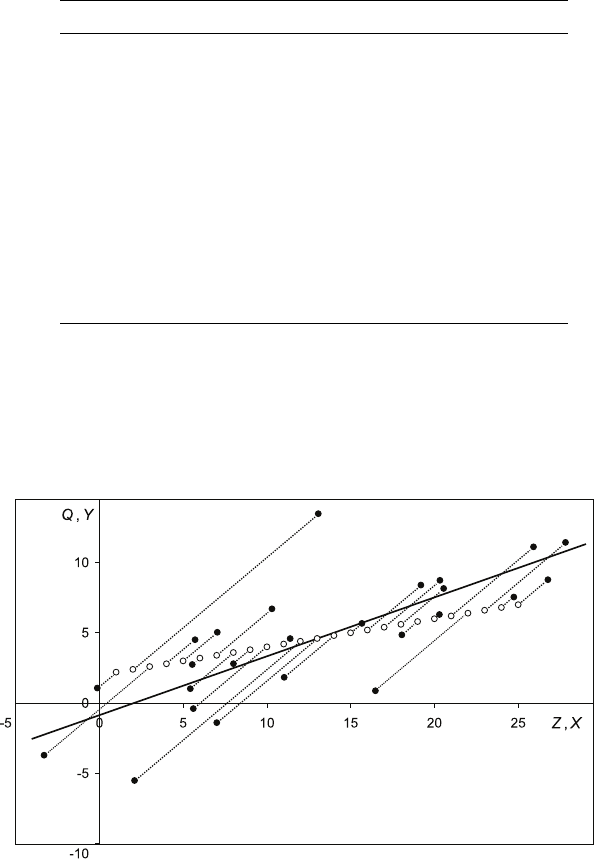
8. Stochastic regressors and measurement errors
1. Derive an expression for the large-sample bias in the estimate of β2when OLS
is used to regress Yon X, and determine its sign if this is possible. [Note: The
standard expression for measurement error bias is not valid in this case.]
2. In a Monte Carlo experiment based on the model above, the true relationship
between Qand Zis:
Q= 2.0+0.2Z.
A sample of 25 observations is generated using the integers 1, 2,..., 25 as data
for Z. The variance of Zis 52.0. A normally distributed random variable with
mean 0 and variance 25 is used to generate the values of the measurement
error in the dependent and explanatory variables. The results with 10 samples
are summarised in the table below. Comment on the results, stating whether
or not they support your theoretical analysis.
Sample b
β1s.e.(b
β1)b
β2s.e.(b
β2)R2
1−0.85 1.09 0.42 0.07 0.61
2−0.37 1.45 0.36 0.10 0.36
3−2.85 0.88 0.49 0.06 0.75
4−2.21 1.59 0.54 0.10 0.57
5−1.08 1.43 0.47 0.09 0.55
6−1.32 1.39 0.51 0.08 0.64
7−3.12 1.12 0.54 0.07 0.71
8−0.64 0.95 0.45 0.06 0.74
9 0.57 0.89 0.38 0.05 0.69
10 −0.54 1.26 0.40 0.08 0.50
3. The figure below plots the points (Q, Z), represented as circles, and (Y, X),
represented as solid markers, for the first sample, with each (Q, Z) point linked
to the corresponding (Y, X) point. Comment on this graph, given your answers
to parts 1 and 2.
Answer:
1. Substituting for Qand Zin the first equation:
(Y−w) = β1+β2(X−w) + v.
176

8.4. Answers to the starred exercises in the textbook
Hence:
Y=β1+β2X+v+ (1 −β2)w
=β1+β2X+u
where u=v+ (1 −β2)w. So:
b
β2=β2+PXi−X(ui−u)
PXi−X2.
It is not possible to obtain a closed-form expression for the expectation of the
error term since both its numerator and its denominator depend on w. Instead
we take plims, having first divided the numerator and the denominator of the
error term by nso that they have limits:
plim b
β2=β2+
plim 1
nPXi−X(ui−u)
plim 1
nPXi−X2
=β2+cov(X, u)
var(u)=β2+cov([Z+w],[v+ (1 −β2)w])
var(X)
=β2+cov(Z, v) + (1 −β2)cov(Z, w) + cov(w, v) + (1 −β2)cov(w, w)
var(X).
Since vand ware distributed independently of Zand of each other,
cov(Z, v) = cov(Z, w) = cov(w, v) = 0, and so:
plim b
β2=β2+ (1 −β2)σ2
w
σ2
X
.
β2clearly should be positive and less than 1, so the bias is positive.
2. σ2
X=σ2
Z+σ2
w, given that wis distributed independently of Z, and hence
σ2
X= 52 + 25 = 77. Thus:
plim b
β2= 0.2 + (1 −0.2) ×25
77 = 0.46.
The estimates of the slope coefficient do indeed appear to be distributed
around this number.
As a consequence of the slope coefficient being overestimated, the intercept is
underestimated, negative estimates being obtained in each case despite the
fact that the true value is positive. The standard errors are invalid, given the
severe problem of measurement error.
3. The diagram shows how the measurement error causes the observations to be
displaced along 45◦lines. Hence the slope of the regression line will be a
compromise between the true slope, β2and 1. More specifically, plim b
β2is a
177

8. Stochastic regressors and measurement errors
weighted average of β2and 1, the weights being proportional to the variances
of Zand w:
plim b
β2=β1+ (1 −β2)σ2
w
σ2
Z+σ2
w
=σ2
Z
σ2
Z+σ2
w
β2+σ2
w
σ2
Z+σ2
w
.
8.16 It is possible that the ASVABC test score is a poor measure of the kind of ability
relevant for earnings. Accordingly, perform an OLS regression of the logarithm of
hourly earnings on S,EXP,ASVABC,MALE,ETHBLACK, and ETHHISP using
your EAWE data set and an IV regression using SM,SF, and SIBLINGS as
instruments for ASVABC. Perform a Durbin–Wu–Hausman test to evaluate
whether ASVABC appears to be subject to measurement error.
Answer:
Contrary to expectations, the coefficient of ASVABC is lower in the IV regression.
It is 0.048 in the OLS regression and −0.094 in the IV regression. The chi-squared
statistic, 1.21, is low. One might therefore conclude that there is no serious
measurement error and the change in the coefficient is random. Another possibility
is that the instruments are too weak. ASVABC is not highly correlated with any of
the instruments and the standard error of the coefficient rises from 0.028 in the
OLS regression to 0.132 in the IV regression.
. ivreg LGEARN S EXP MALE ETHBLACK ETHHISP (ASVABC=SM SF SIBLINGS)
Instrumental variables (2SLS) regression
----------------------------------------------------------------------------
Source | SS df MS Number of obs = 500
-----------+------------------------------ F( 6, 493) = 22.29
Model | 27.631679 6 4.60527983 Prob> F = 0.0000
Residual | 121.501359 493 .246453061 R-squared = 0.1853
-----------+------------------------------ Adj R-squared = 0.1754
Total | 149.133038 499 .298863804 Root MSE = .49644
----------------------------------------------------------------------------
LGEARN | Coef. Std. Err. t P>|t| [95% Conf. Interval]
-----------+----------------------------------------------------------------
ASVABC | -.0938253 .1319694 -0.71 0.477 -.3531172 .1654666
S | .1203265 .0251596 4.78 0.000 .0708931 .1697599
EXP | .0444094 .0092246 4.81 0.000 .026285 .0625338
MALE | .1909863 .0456252 4.19 0.000 .1013424 .2806302
ETHBLACK | -.1678914 .1355897 -1.24 0.216 -.4342963 .0985136
ETHHISP | .075698 .0828383 0.91 0.361 -.0870617 .2384576
_cons | .6503199 .3570741 1.82 0.069 -.0512548 1.351895
----------------------------------------------------------------------------
Instrumented: ASVABC
Instruments: S EXP MALE ETHBLACK ETHHISP SM SF SIBLINGS
----------------------------------------------------------------------------
178
8.4. Answers to the starred exercises in the textbook
. estimates store IV1
. reg LGEARN S EXP ASVABC MALE ETHBLACK ETHHISP
----------------------------------------------------------------------------
Source | SS df MS Number of obs = 500
-----------+------------------------------ F( 6, 493) = 23.81
Model | 33.5095496 6 5.58492493 Prob> F = 0.0000
Residual | 115.623489 493 .234530403 R-squared = 0.2247
-----------+------------------------------ Adj R-squared = 0.2153
Total | 149.133038 499 .298863804 Root MSE = .48428
----------------------------------------------------------------------------
LGEARN | Coef. Std. Err. t P>|t| [95% Conf. Interval]
-----------+----------------------------------------------------------------
S | .0953713 .0106101 8.99 0.000 .0745246 .1162179
EXP | .043139 .0089279 4.83 0.000 .0255976 .0606805
ASVABC | .0477892 .0282877 1.69 0.092 -.00779 .1033685
MALE | .1954406 .0443323 4.41 0.000 .1083371 .2825441
ETHBLACK | -.0448382 .074738 -0.60 0.549 -.1916824 .102006
ETHHISP | .1226463 .0692577 1.77 0.077 -.0134303 .258723
_cons | .9766376 .1938648 5.04 0.000 .5957345 1.357541
----------------------------------------------------------------------------
. estimates store OLS1
. hausman IV1 OLS1, constant
---- Coefficients ----
| (b) (B) (b-B) sqrt(diag(V_b-V_B))
| IV1 OLS1 Difference S.E.
-------------+----------------------------------------------------------------
ASVABC | -.0938253 .0477892 -.1416145 .1289021
S | .1203265 .0953713 .0249552 .022813
EXP | .0444094 .043139 .0012704 .0023208
MALE | .1909863 .1954406 -.0044543 .0107847
ETHBLACK | -.1678914 -.0448382 -.1230532 .1131318
ETHHISP | .075698 .1226463 -.0469484 .0454484
_cons | .6503199 .9766376 -.3263177 .2998639
------------------------------------------------------------------------------
b = consistent under Ho and Ha; obtained from ivreg
B = inconsistent under Ha, efficient under Ho; obtained from regress
Test: Ho: difference in coefficients not systematic
chi2(7) = (b-B)’[(V_b-V_B)^(-1)](b-B)
= 1.21
Prob>chi2 = 0.9908
. cor ASVABC SM SF SIBLINGS
(obs=500)
| ASVABC SM SF SIBLINGS
-------------+------------------------------------
ASVABC | 1.0000
SM | 0.3426 1.0000
SF | 0.3613 0.5622 1.0000
SIBLINGS | -0.2360 -0.3038 -0.2516 1.0000
179

8. Stochastic regressors and measurement errors
8.17 What is the difference between an instrumental variable and a proxy variable (as
described in Section 6.4)? When would you use one and when would you use the
other?
Answer:
An instrumental variable estimator is used when one has data on an explanatory
variable in the regression model but OLS would give inconsistent estimates because
the explanatory variable is not distributed independently of the disturbance term.
The instrumental variable partially replaces the original explanatory variable in the
estimator and the estimator is consistent.
A proxy variable is used when one has no data on an explanatory variable in a
regression model. The proxy variable is used as a straight substitute for the original
variable. The interpretation of the regression coefficients will depend on the
relationship between the proxy and the original variable, and the properties of the
other estimators in the model and the tests and diagnostic statistics will depend on
the degree of correlation between the proxy and the original variable.
8.5 Answers to the additional exercises
A8.1
b
βOLS
1=Y−b
βOLS
2X
=β1+β2X+u−b
βOLS
2X.
Therefore:
plim b
βOLS
1=β1−(plim b
βOLS
2−β2) plim X
6=β1.
However:
b
βIV
1=Y−b
βIV
2X
=β1+β2X+u−b
βIV
2X
=β1−(b
βIV
2−β2)X+u.
Therefore:
plim b
βIV
1=β1−(plim b
βIV
2−β2) plim X
=β1.
Consistency does not guarantee desirable small-sample properties. The latter could
be investigated with a Monte Carlo experiment.
A8.2 Both estimators will be consistent (actually, unbiased) but the IV estimator will be
less efficient than the OLS estimator, as can be seen from a comparison of the
expressions for the population variances.
180

8.5. Answers to the additional exercises
A8.3 The regression model is:
R=β1+β2N+u+w.
Hence:
b
βOLS
2=β2+PNi−N(ui+wi−u−w)
PNi−N2.
It is not possible to obtain a closed-form expression for the expectation since N
and ware correlated. Hence, instead, we investigate the plim:
plim b
βOLS
2=β2+ plim
1
nPNi−N(ui+wi−u−w)
1
nPNi−N2
=β2+cov(N, u) + cov(N, w)
var(N)< β2
since cov(N, u) = 0 and cov(N, w)<0.
A8.4 Discuss whether it is true that the ordinary least squares estimator of β2will be
biased downwards by an amount proportional to both αand β2.
It is not true. Let the measured Xbe X0, where X0=X−α. Then:
b
βOLS
2=P(X0
i−X0)Yi−Y
P(X0
i−X0)2=PXi−α−[X−α]Yi−Y
PXi−α−[X−α]2=PXi−XYi−Y
PXi−X2.
Thus the measurement error has no effect on the estimate of the slope coefficient.
Discuss whether it is true that the fitted values of Y from the regression will be
reduced by an amount αβ2.
The estimator of the intercept will be Y−b
β2X0=Y−b
β2(X−α). Hence the fitted
value in observation iwill be:
Y−b
β2(X−α) + b
β2X0
i=Y−b
β2(X−α) + b
β2(Xi−α) = Y−b
β2X+b
β2Xi
which is what it would be in the absence of the measurement error.
Discuss whether it is true that R2will be reduced by an amount proportional to α.
Since R2is the variance of the fitted values of Ydivided by the variance of the
actual values, it will be unaffected.
A8.5 Using ordinary least squares with MRWtas the explanatory variable.
plim b
βOLS
2=β2−β2
σ2
w
σ2
Rw +σ2
w
=β2
σ2
Rw
σ2
Rw +σ2
w
(standard theory). Hence the bias is towards zero.
b
βOLS
1=M−b
βOLS
2MRW
=β1+β2RW +u−b
βOLS
2RW +w
=β1+ (β2−b
βOLS
2)RW +u−b
βOLS
2w
181

8. Stochastic regressors and measurement errors
and so:
plim b
βOLS
1=β1+β2
σ2
w
σ2
Rw +σ2
w
RW −β2
σ2
Rw
σ2
Rw +σ2
w
µw
where µwis the population mean of w. The first component of the bias will be
positive and the second negative, given that µwis negative. It is not possible
without further information to predict the direction of the bias. The standard
errors and tstatistics will be invalidated if there is substantial measurement error
in MRW.
Using OLS, with RGDPtas a proxy for RW.
Suppose RW =α1+α2RGDP. Then the migration equation may be rewritten:
Mt=β1+β2(α1+α2RGDPt) + ut
= (β1+α1β2) + α2β2RGDPt+ut.
In general it would not be possible to derive estimates of either β1or β2. Likewise
one has no information on the standard errors of either b
β1or b
β2. Nevertheless the t
statistic for the slope coefficient would be approximately equal to the tstatistic in
a regression of Mon RW, if the proxy is a good one. R2will be approximately the
same as it would have been in a regression of Mon RW, if the proxy is a good one.
One might hypothesise that RGDP might be approximately equal to RW, in which
case α1= 0 and α2= 1 and one can effectively fit the original model.
Using instrumental variables, with RGDPtas an instrument for MRWt.
The IV estimator of β2is consistent:
b
βIV
2=PMi−MRGDPi−RGDP
PMRWi−MRWRGDPi−RGDP
=β2+P(ui−β2wi−u+β2w)RGDPi−RGDP
PMRWi−MRWRGDPi−RGDP.
Hence plim b
βIV
2=β2if uand ware distributed independently of RGDP. Likewise
the IV estimator of b
β1is consistent:
b
βIV
1=M−b
βIV
2MRW=β1+β2RW +u−b
βIV
2RW −b
βIV
2w.
Hence:
plim b
βIV
1=β1+β2RW + plim u−plim b
βIV
2RW −plim b
βIV
2plim w
=β1
since plim b
βIV
2=β2and plim u= plim w= 0. The standard errors will be higher,
and hence tstatistics lower, than they would have been if it had been possible to
run the original regression using OLS.
182

8.5. Answers to the additional exercises
A8.6 Suppose RGDP =θ+φMRW . Then:
b
βIV
2=PMi−MRGDPi−RGDP
PMRWi−MRWRGDPi−RGDP
=PMi−MφMRWi−φMRW
PMRWi−MRWφMRWi−φMRW
=b
βOLS
2.
The instrument is no longer valid because it is correlated with the measurement
error.
183
8. Stochastic regressors and measurement errors
184

Chapter 9
Simultaneous equations estimation
9.1 Overview
Until this point the analysis has been confined to the fitting of a single regression
equation on its own. In practice, most economic relationships interact with others in a
system of simultaneous equations, and when this is the case the application of ordinary
least squares (OLS) to a single relationship in isolation yields biased estimates. Having
defined what is meant by an endogenous variable, an exogenous variable, a structural
equation, and a reduced form equation, the first objective of this chapter is to
demonstrate this. The second is to show how it may be possible to use instrumental
variables (IV) estimation, with exogenous variables acting as instruments for
endogenous ones, to obtain consistent estimates of the coefficients of a relationship. The
conditions for exact identification, underidentification, and overidentification are
discussed. In the case of overidentification, it is shown how two-stage least squares can
be used to obtain estimates that are more efficient than those obtained with simple IV
estimation. The chapter concludes with a discussion of the problem of unobserved
heterogeneity and the use of the Durbin–Wu–Hausman test in the context of
simultaneous equations estimation.
9.2 Learning outcomes
After working through the corresponding chapter in the text, studying the
corresponding slideshows, and doing the starred exercises in the text and the additional
exercises in this subject guide, you should be able to:
explain what is meant by:
•an endogenous variable
•an exogenous variable
•a structural equation
•a reduced form equation
explain why the application of OLS to a single equation in isolation is likely to
yield inconsistent estimates of the coefficients if the equation is part of a
simultaneous equations model
derive an expression for the large-sample bias in the slope coefficient when OLS is
used to fit a simple regression equation in a simultaneous equations model
185

9. Simultaneous equations estimation
explain how consistent estimates of the coefficients of an equation in a simultaneous
equations model might in principle be obtained using instrumental variables
explain what is meant by exact identification, underidentification, and
overidentification
explain the principles underlying the use of two-stage least squares, and the reason
why it is more efficient than simple IV estimation
explain what is meant by the problem of unobserved heterogeneity
perform the Durbin–Wu–Hausman test in the context of simultaneous equations
estimation.
9.3 Further material
Good governance and economic development
In development economics it has long been observed that there is a positive association
between economic performance, Y, and good governance, R, especially in developing
countries. However, quantification of the relationship is made problematic by the fact
that it is unlikely that causality is unidirectional. While good governance may
contribute to economic performance, better performing countries may also develop
better institutions. Hence in its simplest form one has a simultaneous equations mode:
Y=β1+β2R+u(1)
R=α1+α2Y+v(2)
where uand vare disturbance terms. Assuming that the latter are distributed
independently, an OLS regression of the first equation will lead to an upwards biased
estimate of β2, at least in large samples. The proof is left as an exercise (Exercise
A9.10). Thus to fit the first equation, one needs an instrument for R. Obviously a
better-specified model would have additional explanatory variables in both equations,
but there is a problem. In general any variable that influences Ris also likely to
influence Yand is therefore unavailable as an instrument.
In a study of 64 ex-colonial countries that is surely destined to become a classic, ‘The
colonial origins of comparative development: an empirical investigation’, American
Economic Review 91(5): 1369–1401, December 2001, Acemoglu, Johnson, and Robinson
(henceforward AJR) argue that settler mortality rates provide a suitable instrument.
Put simply, the thesis is that where mortality rates were low, European colonisers
founded neo-European settlements with European institutions and good governance.
Such settlements eventually prospered. Examples are the United States, Canada,
Australia, and New Zealand. Where mortality rates were high, on account of malaria,
yellow fever and other diseases for which Europeans had little or no immunity,
settlements were not viable. In such countries the main objective of the coloniser was
economic exploitation, especially of mineral wealth. Institutional development was not a
consideration. Post-independence regimes have often been as predatory as their
186

9.4. Additional exercises
predecessors, indigenous rulers taking the place of the former colonisers. Think of the
Belgian Congo, first exploited by King Leopold and more recently by Mobutu.
The study is valuable as an example of IV estimation in that it places minimal technical
demands on the reader. There is nothing that would not be easily comprehensible to
students in an introductory econometrics course that covers IV. Nevertheless, it gives
careful attention to the important technical issues. In particular, it discusses at length
the validity of the exclusion restriction. To use mortality as an instrument for Rin the
first equation, one must be sure that it is not a determinant of Yin its own right, either
directly or indirectly (other than through R).
The conclusion of the study is surprising. According to theory (see Exercise A9.10), the
OLS estimate of β2will be biased upwards by the endogeneity of R. The objective of the
study was to demonstrate that the estimate remains positive and significant even when
the upward bias has been removed by using IV. However, the IV estimate turns out to
be higher than the OLS estimate. In fact it is nearly twice as large. AJR suggest that
this is attributable to measurement error in the measurement of R. This would cause the
OLS estimate to be biased downwards, and the bias would be removed (asymptotically)
by the use of IV. AJR conclude that the downward bias in the OLS estimate caused by
measurement error is greater than the upward bias caused by endogeneity.
9.4 Additional exercises
A9.1 In a certain agricultural country, aggregate consumption, C, is simply equal to
2,000 plus a random quantity z that depends upon the weather:
C= 2000 + z.
zhas mean zero and standard deviation 100. Aggregate investment, I, is subject to
a four-year trade cycle, starting at 200, rising to 300 at the top of the cycle, and
falling to 200 in the next year and to 100 at the bottom of the cycle, rising to 200
again the year after that, and so on. Aggregate income, Y, is the sum of Cand I:
Y=C+I.
Data on Cand I, and hence Y, are given in the table. zwas generated by taking
normally distributed random numbers with mean zero and unit standard deviation
and multiplying them by 100.
t C I Y t C I Y
1 1,813 200 2,013 11 1,981 200 2,181
2 1,893 300 2,193 12 2,211 100 2,311
3 2,119 200 2,319 13 2,127 200 2,327
4 1,967 100 2,067 14 1,953 300 2,253
5 1,997 200 2,197 15 2,141 200 2,341
6 2,050 300 2,350 16 1,836 100 1,936
7 2,035 200 2,235 17 2,103 200 2,303
8 2,088 100 2,188 18 2,058 300 2,358
9 2,023 200 2,223 19 2,119 200 2,319
10 2,144 300 2,444 20 2,032 100 2,132
187

9. Simultaneous equations estimation
An orthodox economist regresses Con Y, using the data in the table, and obtains
(standard errors in parentheses):
b
C= 512 + 0.68Y R2= 0.67
(252) (0.11) F= 36.49
Explain why this result was obtained, despite the fact that Cdoes not depend on
Yat all. In particular, comment on the tand Fstatistics.
A9.2 A small macroeconomic model of a closed economy consists of a consumption
function, an investment function, and an income identity:
Ct=β1+β2Yt+ut
It=α1+α2rt+vt
Yt=Ct+It+Gt
where Ctis aggregate consumer expenditure in year t, It is aggregate investment,
Gtis aggregate current public expenditure, Ytis aggregate output, and rtis the
rate of interest. State which variables in the model are endogenous and exogenous,
and explain how you would fit the equations, if you could.
A9.3 The model is now expanded to include a demand for money equation and an
equilibrium condition for the money market:
Md
t=δ1+δ2Yt+δ3rt+wt
Md
t=Mt
where Md
tis the demand for money in year tand Mtis the supply of money,
assumed exogenous. State which variables are endogenous and exogenous in the
expanded model and explain how you would fit the equations, including those in
Exercise A9.2, if you could.
A9.4 Table 9.2 reports a simulation comparing OLS and IV parameter estimates and
standard errors for 10 samples. The reported R2(not shown in that table) for the
OLS and IV regressions are shown in the table below.
Sample OLS R2IV R2
1 0.59 0.16
2 0.69 0.52
3 0.78 0.73
4 0.61 0.37
5 0.40 0.06
6 0.72 0.57
7 0.60 0.33
8 0.58 0.44
9 0.69 0.43
10 0.39 0.13
188
9.4. Additional exercises
We know that, for large samples, the IV estimator is preferable to the OLS
estimator because it is consistent, while the OLS estimator is inconsistent.
However, do the smaller OLS standard errors in Table 9.2 and the larger OLS
values of R2in the present table indicate that OLS is actually preferable for small
samples (n= 20 in the simulation)?
A9.5 A researcher investigating the relationship between aggregate wages, W, aggregate
profits, P, and aggregate income, Y, postulates the following model:
W=β1+β2Y+u(1)
P=α1+α2Y+α3K+v(2)
Y=W+P(3)
where Kis aggregate stock of capital and uand vare disturbance terms that satisfy
the usual regression model assumptions and may be assumed to be distributed
independently of each other. The third equation is an identity, all forms of income
being classified either as wages or as profits. The researcher intends to fit the model
using data from a sample of industrialised countries, with the variables measured
on a per capita basis in a common currency. Kmay be assumed to be exogenous.
•Explain why ordinary least squares (OLS) would yield inconsistent estimates if
it were used to fit (1) and derive the large-sample bias in the slope coefficient.
•Explain what can be inferred about the finite-sample properties of OLS if used
to fit (1).
•Demonstrate mathematically how one might obtain a consistent estimate of β2
in (1).
•Explain why (2) is not identified (underidentified).
•Explain whether (3) is identified.
•At a seminar, one of the participants asserts that it is possible to obtain an
estimate of α2even though equation (2) is underidentified. Any change in
income that is not a change in wages must be a change in profits, by definition,
and so one can estimate α2as (1 −b
β2), where b
β2is the consistent estimate of
β2found in the third part of this question. The researcher does not think that
this is right but is confused and says that he will look into it after the seminar.
What should he have said?
A9.6 A researcher has data on e, the annual average rate of growth of employment, xthe
annual average rate of growth of output, and p, the annual average rate of growth
of productivity, for a sample of 25 countries, the average rates being calculated for
the period 1995–2005 and expressed as percentages. The researcher hypothesises
that the variables are related by the following model:
e=β1+β2x+u(1)
x=e+p. (2)
The second equation is an identity because pis defined as the difference between x
and e. The researcher believes that pis exogenous. The correlation coefficient for x
and pis 0.79.
189
9. Simultaneous equations estimation
•Explain why the OLS estimator of β2would be inconsistent, if the researcher’s
model is correctly specified. Derive analytically the large-sample bias, and
state whether it is possible to determine its sign.
•Explain how the researcher might use pto construct an IV estimator of β2,
that is consistent if pis exogenous. Demonstrate analytically that the
estimator is consistent.
•The OLS and IV regressions are summarised below (standard errors in
parentheses). Comment on them, making use of your answers to the first two
parts of this question.
OLS be=−0.52 + 0.48x(3)
(0.27) (0.08)
IV be= 0.37 + 0.17x(4)
(0.42) (0.14)
•A second researcher hypothesises that both xand pare exogenous and that
equation (2) should be written:
e=x−p. (5)
On the assumption that this is correct, explain why the slope coefficients in (3)
and (4) are both biased and determine the direction of the bias in each case.
•Explain what would be the result of fitting (5), regressing eon xand p.
A9.7 A researcher has data from the World Bank World Development Report 2000 on F,
average fertility (average number of children born to each woman during her life),
M, under-five mortality (number of children, per 100, dying before reaching the age
of 5), and S, average years of female schooling, for a sample of 54 countries. She
hypothesises that fertility is inversely related to schooling and positively related to
mortality, and that mortality is inversely related to schooling:
F=β1+β2S+β3M+u(1)
M=α1+α2S+v(2)
where uand vare disturbance terms that may be assumed to be distributed
independently of each other. Smay be assumed to be exogenous.
•Derive the reduced form equations for Fand M.
•Explain what would be the most appropriate method to fit equation (1).
•Explain what would be the most appropriate method to fit equation (2).
The researcher decides to fit (1) using ordinary least squares, and she decides also
to perform a simple regression of Fon S, again using ordinary least squares, with
the following results (standard errors in parentheses):
b
F= 4.08 −0.17S+ 0.015M R2= 0.83 (3)
(0.61) (0.04) (0.003)
b
F= 6.99 −0.36S R2= 0.71 (4)
(0.39) (0.03)
190
9.4. Additional exercises
•Explain why the coefficient of Sdiffers in the two equations.
•Explain whether one may validly perform ttests on the coefficients of (4).
At a seminar someone hypothesises that female schooling may be negatively
influenced by fertility, especially in the poorer developing countries in the sample,
and this would affect (4). To investigate this, the researcher adds the following
equation to the model:
S=δ1+δ2F+δ3G+w(5)
where Gis GNP per capita and wis a disturbance term. She regresses Fon S(1)
instrumenting for Swith G(column (b) in the output below), and (2) using
ordinary least squares, as in equation (4) (column (B) in the output below). The
correlation between Sand Gwas 0.70. She performs a Durbin–Wu–Hausman test
to compare the coefficients.
---- Coefficients ----
| (b) (B) (b-B) sqrt(diag(V_b-V_B))
| IV OLS Difference S.E.
-------------+----------------------------------------------------------------
S | -.2965323 -.3637397 .0672074 .0347484
_cons | 6.162605 6.992907 -.8303019 .4194891
------------------------------------------------------------------------------
b = consistent under Ho and Ha; obtained from ivreg
B = inconsistent under Ha, efficient under Ho; obtained from regress
Test: Ho: difference in coefficients not systematic
chi2( 1) = (b-B)’[(V_b-V_B)^(-1)](b-B)
= 3.31
Prob>chi2 = 0.1158
•Discuss whether Gis likely to be a valid instrument.
•What should the researcher’s conclusions be with regard to the test?
A9.8 Aggregate demand QDfor a certain commodity is determined by its price, P,
aggregate income, Y, and population, POP:
QD=β1+β2P+β3Y+β4POP +uD
and aggregate supply is given by:
QS=α1+α2P+uS
where uDand uSare independently distributed disturbance terms.
•Demonstrate that the estimator of α2will be inconsistent if ordinary least
squares (OLS) is used to fit the supply equation, showing that the
large-sample bias is likely to be negative.
•Demonstrate that a consistent estimator of α2will be obtained if the supply
equation is fitted using instrumental variables (IV), using Yas an instrument.
The model is used for a Monte Carlo experiment, with α2set equal to 0.2 and
suitable values chosen for the other parameters. The table shows the estimates of
191

9. Simultaneous equations estimation
α2obtained in 10 samples using OLS, using IV with Yas an instrument, using IV
with POP as an instrument, and using two-stage least squares (TSLS) with Yand
POP. s.e. is standard error. The correlation between Pand Yaveraged 0.50 across
the samples. The correlation between Pand POP averaged 0.63 across the
samples. Discuss the results obtained.
OLS IV with YIV with POP TSLS
coef. s.e. coef. s.e. coef. s.e. coef. s.e.
1 0.15 0.03 0.22 0.05 0.21 0.05 0.21 0.03
2 0.08 0.04 0.24 0.11 0.19 0.08 0.21 0.06
3 0.11 0.02 0.18 0.06 0.19 0.05 0.19 0.04
4 0.16 0.02 0.20 0.04 0.19 0.03 0.19 0.02
5 0.15 0.02 0.27 0.09 0.18 0.04 0.20 0.03
6 0.14 0.03 0.24 0.08 0.18 0.05 0.20 0.04
7 0.20 0.03 0.22 0.05 0.26 0.04 0.25 0.03
8 0.15 0.03 0.21 0.06 0.24 0.05 0.23 0.04
9 0.11 0.02 0.17 0.05 0.14 0.03 0.15 0.03
10 0.17 0.03 0.16 0.05 0.24 0.05 0.20 0.03
A9.9 A researcher has the following data for a sample of 1,000 manufacturing enterprises
on the following variables, each measured as an annual average for the period
2001–2005: G, average annual percentage rate of growth of sales; R, expenditure on
research and development; and A, expenditure on advertising. Rand Aare
measured as a proportion of sales revenue. He hypothesises the following model:
G=β1+β2R+β3A+uG(1)
R=α1+α2G+uR(2)
where uGand uRare disturbance terms distributed independently of each other.
A second researcher believes that expenditure on quality control, Q, measured as a
proportion of sales revenue, also influences the growth of sales, and hence that the
first equation should be written:
G=β1+β2R+β3A+β4Q+uG.(1∗)
Aand Qmay be assumed to be exogenous variables.
•Derive the reduced form equation for Gfor the first researcher.
•Explain why ordinary least squares (OLS) would be an inconsistent estimator
of the parameters of equation (2).
•The first researcher uses instrumental variables (IV) to estimate α2in (2).
Explain the procedure and demonstrate that the IV estimator of α2is
consistent.
•The second researcher uses two stage least squares (TSLS) to estimate α2in
(2). Explain the procedure and demonstrate that the TSLS estimator is
consistent.
192
9.4. Additional exercises
•Explain why the TSLS estimator used by the second researcher ought to
produce ‘better’ results than the IV estimator used by the first researcher, if
the growth equation is given by (1*). Be specific about what you mean by
‘better’.
•Suppose that the first researcher is correct and the growth equation is actually
given by (1), not (1*). Compare the properties of the two estimators in this
case.
•Suppose that the second researcher is correct and the model is given by (1*)
and (2), but A is not exogenous after all. Suppose that Ais influenced by G:
A=γ1+γ2G+uA(3)
where uAis a disturbance term distributed independently of uGand uR. How
would this affect the properties of the IV estimator of α2used by the first
researcher?
A9.10 A researcher has data for 100 workers in a large organisation on hourly earnings,
EARNINGS, skill level of the worker, SKILL, and a measure of the intelligence of
the worker, IQ. She hypothesises that LGEARN, the natural logarithm of
EARNINGS, depends on SKILL, and that SKILL depends on IQ.
LGEARN =β1+β2SKILL +u(1)
SKILL =α1+α2IQ +v(2)
where uand vare disturbance terms. The researcher is not sure whether uand v
are distributed independently of each other.
•State, with a brief explanation, whether each variable is endogenous or
exogenous, and derive the reduced form equations for the endogenous variables.
•Explain why the researcher could use ordinary least squares (OLS) to fit
equation (1) if uand vare distributed independently of each other.
•Show that the OLS estimator of β2is inconsistent if uand vare positively
correlated and determine the direction of the large-sample bias.
•Demonstrate mathematically how the researcher could use instrumental
variables (IV) estimation to obtain a consistent estimate of β2.
•Explain the advantages and disadvantages of using IV, rather than OLS, to
estimate β2, given that the researcher is not sure whether uand vare
distributed independently of each other.
•Describe in general terms a test that might help the researcher decide whether
to use OLS or IV. What are the limitations of the test?
•Explain whether it is possible for the researcher to fit equation (2) and obtain
consistent estimates.
193

9. Simultaneous equations estimation
A9.11 This exercise relates to the Further material section.
In general in an introductory econometrics course, issues and problems are treated
separately, one at a time. In practice in empirical work, it is common for multiple
problems to be encountered simultaneously. When this is the case, the
one-at-a-time analysis may no longer be valid. In the case of the AJR study, both
endogeneity and measurement error seem to be issues. This exercise looks at both
together, within the context of that model.
Let Sbe the correct good governance variable and let Rbe the measured variable,
with measurement error w. Thus the model may be written:
Y=β1+β2S+u
S=α1+α2Y+v
R=S+w.
It may be assumed that whas zero expectation and constant variance σ2
wacross
observations, and that it is distributed independently of Sand the disturbance
terms in the equations in the model. Investigate the likely direction of the bias in
the OLS estimator of β2in large samples.
9.5 Answers to the starred exercises in the textbook
9.1 A simple macroeconomic model consists of a consumption function and an income
identity:
C=β1+β2Y+u
Y=C+I
where Cis aggregate consumption, Iis aggregate investment, Yis aggregate
income, and uis a disturbance term. On the assumption that Iis exogenous, derive
the reduced form equations for Cand Y.
Answer:
Substituting for Yin the first equation:
C=β1+β2(C+I) + u.
Hence:
C=β1
1−β2
+β2I
1−β2
+u
1−β2
and:
Y=C+I=β1
1−β2
+I
1−β2
+u
1−β2
.
9.2 It is common to write an earnings function with the logarithm of the hourly wage
as the dependent variable and characteristics such as years of schooling, cognitive
ability, years of work experience, etc as the explanatory variables. Explain whether
194

9.5. Answers to the starred exercises in the textbook
such an equation should be regarded as a reduced form equation or a structural
equation.
Answer:
In the conventional model of the labour market, the wage rate and the quantity of
labour employed are both endogenous variables jointly determined by the
interaction of demand and supply. According to this model, the wage equation is a
reduced form equation.
9.3 In the simple macroeconomic model:
C=β1+β2Y+u
Y=C+I
described in Exercise 9.1, demonstrate that OLS would yield inconsistent results if
used to fit the consumption function, and investigate the direction of the bias in
the slope coefficient.
Answer:
The first step in the analysis of the OLS slope coefficient is to break it down into
the true value and error component in the usual way:
b
βOLS
2=PYi−YCi−C
PYi−Y2=β2+PYi−Y(ui−u)
PYi−Y2.
From the reduced form equation in Exercise 9.1 we see that Ydepends on uand
hence we will not be able to obtain a closed-form expression for the expectation of
the error term. Instead we take plims, having first divided the numerator and the
denominator of the error term by nso that they will possess limits as ngoes to
infinity.
plim b
βOLS
2=β2+
plim 1
nPYi−Y(ui−u)
plim 1
nPYi−Y2=β2+cov(Y, u)
var(Y) .
We next substitute for Ysince it is an endogenous variable. We have two choices:
we could substitute from the structural equation, or we could substitute from the
reduced form. If we substituted from the structural equation, in this case the
income identity, we would introduce another endogenous variable, C, and we would
find ourselves going round in circles. So we must choose the reduced form.
plim b
βOLS
2=β2+
cov h β1
1−β2+I
1−β2+u
1−β2i, u
var β1
1−β2+I
1−β2+u
1−β2
=β2+
1
1−β2(cov(I, u) + cov(u, u))
1
1−β22var(I+u)
=β2+ (1 −β2)cov(I, u) + var(u)
var(I) + var(u) + 2cov(I, u).
195

9. Simultaneous equations estimation
On the assumption that Iis exogenous, it is distributed independently of uand
cov(I, u) = 0. So:
plim b
βOLS
2=β2+ (1 −β2)σ2
u
σ2
I+σ2
u
since the sample variances tend to the population variances as the sample becomes
large. Since the variances are positive, the sign of the bias depends on the sign of
(1 −β2). It is reasonable to assume that the marginal propensity to consume is
positive and less than 1, in which case this term will be positive and the
large-sample bias in b
βOLS
2will be upwards.
The OLS estimate of the intercept is also inconsistent:
b
βOLS
1=C−b
βOLS
2Y=β1+β2Y+u−b
βOLS
2Y.
Hence:
plim b
βOLS
1=β1+ (β2−plim b
βOLS
2) plim Y
=β1−(1 −β2)σ2
u
σ2
I+σ2
u
plim Y.
This is evidently biased downwards, as one might expect, given that the slope
coefficient was biased upwards.
9.6 The table gives consumption per capita, C, gross fixed capital formation per capita,
I, and gross domestic product per capita, Y, all measured in US$, for 33 countries
in 1998. The output from an OLS regression of Con Y, and an IV regression using
Ias an instrument for Y, are shown. Comment on the differences in the results.
C I Y C I Y
Australia 15,024 4,749 19,461 South Korea 4,596 1,448 6,829
Austria 19,813 6,787 26,104 Luxembourg 26,400 9,767 42,650
Belgium 18,367 5,174 24,522 Malaysia 1,683 873 3,268
Canada 15,786 4,017 20,085 Mexico 3,359 1,056 4,328
China–PR 446 293 768 Netherlands 17,558 4,865 24,086
China–HK 17,067 7,262 24,452 New Zealand 11,236 2,658 13,992
Denmark 25,199 6,947 32,769 Norway 23,415 9,221 32,933
Finland 17,991 4,741 24,952 Pakistan 389 79 463
France 19,178 4,622 24,587 Philippines 760 176 868
Germany 20,058 5,716 26,219 Portugal 8,579 2,644 9,976
Greece 9,991 2,460 11,551 Spain 11,255 3,415 14,052
Iceland 25,294 6,706 30,622 Sweden 20,687 4487 26,866
India 291 84 385 Switzerland 27,648 7,815 36,864
Indonesia 351 216 613 Thailand 1,226 479 1,997
Ireland 13,045 4,791 20,132 UK 19,743 4,316 23,844
Italy 16,134 4,075 20,580 USA 26,387 6,540 32,377
Japan 21,478 7,923 30,124
196

9.5. Answers to the starred exercises in the textbook
. reg C Y
----------------------------------------------------------------------------
Source | SS df MS Number of obs = 33
-----------+------------------------------ F( 1, 31) = 1331.29
Model | 2.5686e+09 1 2.5686e+09 Prob> F = 0.0000
Residual | 59810749.2 31 1929379.01 R-squared = 0.9772
-----------+------------------------------ Adj R-squared = 0.9765
Total | 2.6284e+09 32 82136829.4 Root MSE = 1389
----------------------------------------------------------------------------
C | Coef. Std. Err. t P>|t| [95% Conf. Interval]
-----------+----------------------------------------------------------------
Y | .7303066 .0200156 36.49 0.000 .6894845 .7711287
_cons | 379.4871 443.6764 0.86 0.399 -525.397 1284.371
----------------------------------------------------------------------------
. ivregress 2sls C (Y=I)
------------------------------------------------------------------------------
Instrumental variables (2SLS) regression Number of obs = 33
Wald chi2(1) = 1269.09
Prob> chi2 = 0.0000
R-squared = 0.9770
Root MSE = 1353.9
----------------------------------------------------------------------------
C | Coef. Std. Err. z P>|z| [95% Conf. Interval]
-----------+----------------------------------------------------------------
Y | .7183909 .0201658 35.62 0.000 .6788667 .7579151
_cons | 600.946 442.7386 1.36 0.175 -266.8057 1468.698
----------------------------------------------------------------------------
Instrumented: Y
Instruments: I
----------------------------------------------------------------------------
Answer:
Assuming the simple macroeconomic model:
C=β1+β2Y+u
Y=C+I
where Cis consumption per capita, Iis investment per capita, and Yis income per
capita, and Iis assumed exogenous, the OLS estimator of the marginal propensity
to consume will be biased upwards. As was shown in Exercise 9.3:
plim b
βOLS
2=β2+ (1 −β2)σ2
u
σ2
I+σ2
u
.
Hence the IV estimate should be expected to be lower, but only by a small amount,
given the data. With b
β2estimated at 0.72, (1 −b
β2) is 0.28. σ2
uis estimated at 1.95
million and σ2
Iis 7.74 million. Hence, on the basis of these estimates, the bias
should be about 0.06. The actual difference in the OLS and IV estimates is smaller
still. However, the actual difference would depend on the purely random sampling
error as well as the bias, and it is possible that in this case the sampling error
happens to have offset the bias to some extent.
197

9. Simultaneous equations estimation
9.11 Consider the price inflation/wage inflation model given by equations (9.1) and (9.2):
p=β1+β2w+up
w=α1+α2p+α3U+uw.
We have seen that the first equation is exactly identified, Ubeing used as an
instrument for w. Suppose that TSLS is applied to this model, despite the fact that
it is exactly identified, rather than overidentified. How will the results differ?
Answer:
If we fit the reduced form, we obtain a fitted equation:
bw=h1+h2U.
The TSLS estimator is then given by
b
βTSLS
2=Pbwi−bw(pi−p)
Pbwi−bw(wi−w)
=Ph1+h2Ui−h1−h2U(pi−p)
Ph1+h2Ui−h1−h2U(wi−w)
=Ph2Ui−U(pi−p)
Ph2Ui−U(wi−w)
=b
βIV
2
where b
βIV
2is the IV estimator using U. Hence the estimator is exactly the same.
[Note: This is a special case of Exercise 8.18.]
9.15 Suppose the first equation in the model in Box 9.2 is fitted, with Qused as an
instrument for Y. Describe the likely properties of the estimator of α2.
Answer:
The first equation in Box 9.2 is:
X=α1+α2Y+u
The reduced form equation for Yis:
Y=1
1−α2β2
(β1+α1β2+β2u+v).
Qis not a valid instrument for Ybecause it is not a determinant of Y.
Mathematically, it can be shown that:
plim bαIV
2=α2+cov(Q, u)
cov(Q, Y ).
The numerator of the second term is zero, but so is its denominator and therefore
the expression is undefined.
198
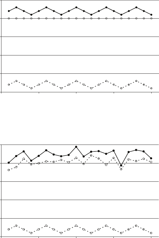
9.6. Answers to the additional exercises
9.6 Answers to the additional exercises
A9.1 The positive coefficient of Ytin the regression is attributable wholly to
simultaneous equations bias. The three figures show this graphically.
The first diagram shows what the time series for Ct,It, and Ytwould look like if
there were no random component of consumption. The series for Ctis constant at
2,000. That for Itis a wave form, and that for Ytis the same wave form shifted
upward by 2,000. The second diagram shows the effect of adding the random
component to consumption. Ytstill has a wave form, but there is a clear correlation
between it and Ct.
0
500
1,000
1,500
2,000
2,500
0 5 10 15 20
Y
C
I
Y
C
I
C
Y
0
500
1,000
1,500
2,000
2,500
0 5 10 15 20
Y
C
I
C
Y
199

9. Simultaneous equations estimation
1,800
1,900
2,000
2,100
2,200
1,900 2,000 2,100 2,200 2,300 2,400
C
Y
In the third diagram, Ctis plotted against Yt, with and without the random
component. The three large circles represent the data when there is no random
component. One circle represents the five data points [C= 2,000, Y= 2,100]; the
middle circle represents the ten data points [C= 2,000, Y= 2,200]; and the other
circle represents the five data points [C= 2,000, Y= 2,300]. A regression line
based on these three points would be horizontal (the dashed line). The solid circles
represent the 20 data points when the random component is affecting Ctand Yt,
and the solid line is the regression line for these points. Note that these 20 data
points fall into three groups: five which lie on a 45 degree line through the left large
circle, 10 which lie on the 45 degree line through the middle circle (actually, you
can only see nine), and five on the 45 degree line through the right circle.
If OLS is used to fit the equation:
b
βOLS
2=PYi−YCi−C
PYi−Y2=PYi−Y([2000 + zi]−[2000 +z])
PYi−Y2=PYi−Y(zi−z)
PYi−Y2.
Note that at this stage we have broken down the slope coefficient into its true value
plus an error term. The true value does not appear explicitly because it is zero, so
we only have the error term. We cannot take expectations because both the
numerator and the denominator are functions of z:
Y=C+I= 2000 + I+z.
zis a component of Cand hence of Y. As a second-best procedure, we investigate
the large-sample properties of the estimator by taking plims. We must first divide
the numerator and denominator by nso that they tend to finite limits:
plim b
βOLS
2=
plim 1
nPYi−Y(zi−z)
plim 1
nPYi−Y2=cov(Y, z)
var(Y).
Substituting for Yfrom its reduced form equation:
plim b
βOLS
2=cov([2000 + i+z], z)
var(2000 + I+z)=cov(I, z) + var(z)
var(I) + var(z) + 2cov(I, z)=σ2
z
σ2
I+σ2
z
.
200

9.6. Answers to the additional exercises
cov(I, z) = 0 because Iis distributed independently of z.σ2
zis equal to 10,000
(since we are told that σzis equal to 100). Over a four-year cycle, the mean value
of Iis 200 and hence its population variance is given by:
σ2
I=1
40 + 1002+ 0 + (−100)2= 5000.
Hence:
plim b
βOLS
2=10000
15000 = 0.67.
The actual coefficient in the 20-observation sample, 0.68, is very close to this
(probably atypically close for such a model).
The estimator of the intercept, whose true value is 2,000, is biased downwards
because b
βOLS
2is biased upwards. The standard errors of the coefficients are invalid
because the regression model assumption B.7 is violated, and hence ttests would
be invalid.
By virtue of the fact that Y=C+I,Cis being regressed against a variable which
is largely composed of itself. Hence the high R2is inevitable, despite the fact that
there is no behavioural relationship between Cand Y. Mathematically, R2is equal
to the square of the sample correlation between the actual and fitted values of C.
Since the fitted values of Care a linear function of the values of Y,R2is equal to
the square of the sample correlation between Cand Y. The population correlation
coefficient is given by
ρC,Y =cov(C, Y )
pvar(C)var(Y)=cov ([2000 + z],[2000 + I+z])
pvar ([2000 + z]) var ([2000 + I+z])
=var(z)
pvar(z)var[I+z]=σ2
z
pσ2
z(σ2
I+σ2
z).
Hence in large samples:
R2=100002
10000[10000 + 5000] = 0.67.
R2in the regression is exactly equal to this, the closeness probably being
something of a coincidence.
Since regression model assumption B.7 is violated, the Fstatistic cannot be used
to perform an Ftest of goodness of fit.
A9.2 Ct,It, and Ytare endogenous, the first two being the dependent variables of the
behavioural relationships and the third being defined by an identity. Gtand rtare
exogenous.
Either Itor rtcould be used as an instrument for Ytin the consumption function.
If it can be assumed that utand vtare distributed independently, It can also be
regarded as exogenous as far as the determination of Ctand Ytare concerned. It
would be preferable to rtsince it is more highly correlated with Yt. One’s first
thought, then, would be to use TSLS, with the first stage fitting the equation:
Yt=β1
1−β2
+It
1−β2
+Gt
1−β2
+ut
1−β2
.
201

9. Simultaneous equations estimation
Note, however, that the equation implies the restriction that the coefficients of It
and Gtare equal. Hence all one has to do is to define a variable:
Zt=It+Gt
and use Ztas an instrument for Ytin the consumption function.
The investment function would be fitted using OLS since rtis exogenous. The
income identity does not need to be fitted.
A9.3 Md
tis endogenous because it is determined by the second of the two new
relationships. The addition of the first of these relationships makes rtendogenous.
To see this, substituting for Ctand Itin the income identity, using the
consumption function and the investment function, one obtains:
Yt=(α1+β1) + α2rt+ut+vt
1−β2
.
This is usually known as the IS curve. Substituting for Md
tin the first of the two
new relationships, using the second, one has:
Mt=δ1+δ2Yt+δ3rt+wt.
This is usually known as the LM curve. The equilibrium values of both Ytand rt
are determined by the intersection of these two curves and hence rtis endogenous
as well as Yt.Gtremains exogenous, as before, and Mtis also exogenous.
The consumption and investment functions are overidentified and one would use
TSLS to fit them, the exogenous variables being government expenditure and the
supply of money. The demand for money equation is exactly identified, two of the
explanatory variables, rtand Yt, being endogenous, and the two exogenous
variables being available to act as instruments for them.
A9.4 The OLS standard errors are invalid so a comparison is illegitimate. They are not
of any great interest anyway because the OLS estimator is biased. Figure 9.3 in the
text shows that the variance of the OLS estimator is smaller than that of the IV
estimator, but, using a criterion such as the mean square error, there is no doubt
that the IV estimator should be preferred. The comment about R2is irrelevant.
OLS has a better fit but we have had to abandon the least squares principle
because it yields inconsistent estimates.
A9.5 Explain why ordinary least squares (OLS) would yield inconsistent estimates if it
were used to fit (1) and derive the large-sample bias in the slope coefficient.
At some point we will need the reduced form equation for Y. Substituting into the
third equation from the first two, and rearranging, it is:
Y=1
1−α2−β2
(α1+β1+α3K+u+v).
Since Ydepends on u, the assumption that the disturbance term be distributed
independently of the regressors is violated in (1).
b
βOLS
2=PYi−YWi−W
PYi−Y2=β2+PYi−Y(ui−u)
PYi−Y2
202
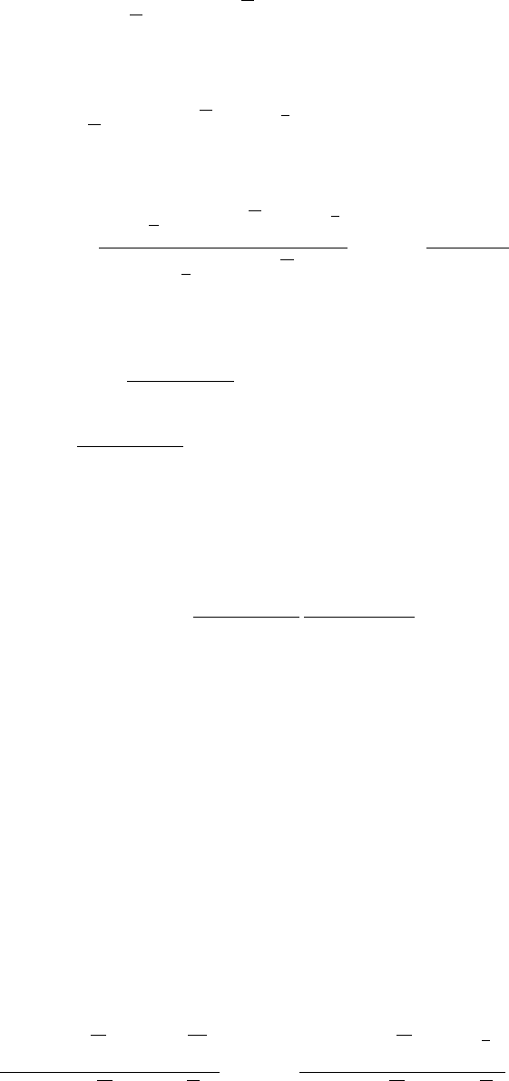
9.6. Answers to the additional exercises
after substituting for Wfrom (1) and simplifying. We are not able to obtain a
closed-form expression for the expectation of the error term because uinfluences
both its numerator and denominator, directly and by virtue of being a component
of Y, as seen in the reduced form. Dividing both the numerator and denominator
by n, and noting that:
plim 1
nXYi−Y2= var(Y)
as a consequence of a law of large numbers, and that it can also be shown that:
plim 1
nXYi−Y(ui−u) = cov(Y, u)
we can write
plim b
βOLS
2=β2+
plim 1
nPYi−Y(ui−u)
plim 1
nPYi−Y2=β2+cov(Y, u)
var(Y).
Now:
cov(Y, u) = cov 1
1−α2−β2
(α1+β1+α3K+u+v), u
=1
1−α2−β2
(α3cov(K, u) + var(u) + cov(v, u))
the covariance of uwith the constants being zero. Since Kis exogenous,
cov(K, u) = 0. We are told that uand vare distributed independently of each
other, and so cov(u, v) = 0. Hence:
plim b
βOLS
2=β2+1
1−α2−β2
σ2
u
plim var(Y).
From the reduced form equation for Yit is evident that (1 −α2−β2)>0, and so
the large-sample bias will be positive.
Explain what can be inferred about the finite-sample properties of OLS if used to fit
(1).
It is not possible for an estimator that is unbiased in a finite sample to develop a
bias if the sample size increases. Therefore, since the estimator is biased in large
samples, it must also be biased in finite ones. The plim may well be a guide to the
mean of the estimator in a finite sample, but this is not guaranteed and it is
unlikely to be exactly equal to the mean.
Demonstrate mathematically how one might obtain a consistent estimate of β2in
(1).
Use Kas an instrument for Y:
b
βIV
2=PKi−KWi−W
PKi−KYi−Y=β2+PKi−K(ui−u)
PKi−KYi−Y203

9. Simultaneous equations estimation
after substituting for Wfrom (1) and simplifying. We are not able to obtain a
closed-form expression for the expectation of the error term because uinfluences
both its numerator and denominator, directly and by virtue of being a component
of Y, as seen in the reduced form. Dividing both the numerator and denominator
by n, and noting that it can be shown that:
plim 1
nXKi−K(ui−u) = cov(K, u) = 0
since Kis exogenous, and that:
plim 1
nXKi−KYi−Y= cov(K, Y )
we can write:
plim b
βIV
2=β2+cov(K, u)
cov(K, Y )=β2.
cov(K, Y ) is non-zero since the reduced form equation for Yreveals that Kis a
determinant of Y. Hence the instrumental variable estimator is consistent.
Explain why (2) is not identified (underidentified).
(2) is underidentified because the endogenous variable Yis a regressor and there is
no valid instrument to use with it. The only potential instrument is the exogenous
variable Kand it is already a regressor in its own right.
Explain whether (3) is identified.
(3) is an identity so the issue of identification does not arise.
At a seminar, one of the participants asserts that it is possible to obtain an estimate
of α2even though equation (2) is underidentified. Any change in income that is not
a change in wages must be a change in profits, by definition, and so one can
estimate α2as (1 −b
β2), where b
β2is the consistent estimate of β2found in the third
part of this question. The researcher does not think that this is right but is confused
and says that he will look into it after the seminar. What should he have said?
The argument would be valid if Ywere exogenous, in which case one could
characterise β2and α2as being the effects of Yon Wand P, holding other
variables constant. But Yis endogenous, and so the coefficients represent only part
of an adjustment process. Ycannot change autonomously, only in response to
variations in K,u, or v.
The reduced form equations for Wand Pare:
W=β1+β2
1−α2−β2
(α1+β1+α3K+u+v) + u
=1
1−α2−β2
(β1+α1β2−α2β1+α3β2K+ (1 −α2)u+β2v)
P=α1+α2
1−α2−β2
(α1+β1+α3K+u+v) + α3K+v
=1
1−α2−β2
(α1−α1β2+α2β1+α3(1 −β2)K+α2u+ (1 −β2)v).
204

9.6. Answers to the additional exercises
Thus, for example, a change in Kwill lead to changes in Wand Pin the
proportions β2: (1 −β2), not β2:α2. The same is true of changes caused by a
variation in v. For a variation in u, the proportions would be (1 −α2) : α2.
A9.6 Explain why the OLS estimator of β2would be inconsistent, if the researcher’s
model is correctly specified. Derive analytically the largesample bias, and state
whether it is possible to determine its sign.
The reduced form equation for xis:
x=β1+p+u
1−β2
.
Thus:
b
βOLS
2=P(xi−x)(ei−e)
P(xi−x)2=P(xi−x)(β1+β2xi+ui−β1−β2x−u)
P(xi−x)2
=β2+P(xi−x)(ui−u)
P(xi−x)2.
It is not possible to obtain a closed-form expression for the expectation of the
estimator because the error term is a nonlinear function of u. Instead we
investigate whether the estimator is consistent, first dividing the numerator and the
denominator of the error term by nso that they tend to limits as the sample size
becomes large.
plim b
βOLS
2=β2+
plim 1
nP1
1−β2[β1+pi+ui−β1−p−u](ui−u)
plim 1
nP(xi−x)2
=β2+1
1−β2
plim 1
nP(pi−p)(ui−u) + plim 1
nP(ui−u)2
plim 1
nP(xi−x)2
=β2+1
1−β2
cov(p, u) + var(u)
var(x)=β2+1
1−β2
σ2
u
σ2
x
since cov(p, u) = 0, pbeing exogenous. It is reasonable to assume that employment
grows less rapidly than output, and hence β2, and so (1 −β2), are less than 1. The
bias is therefore likely to be positive.
Explain how the researcher might use p to construct an IV estimator of β2that is
consistent if p is exogenous. Demonstrate analytically that the estimator is
consistent.
pis available as an instrument, being exogenous, and therefore independent of u,
being correlated with x, and not being in the equation in its own right.
b
βIV
2=P(pi−p)(ei−e)
P(pi−p)(xi−x)=P(pi−p)(β1+β2xi+ui−β1−β2x−u)
P(pi−p)(xi−x)
=β2+P(pi−p)(ui−¯u)
P(pi−p)(xi−x).
205
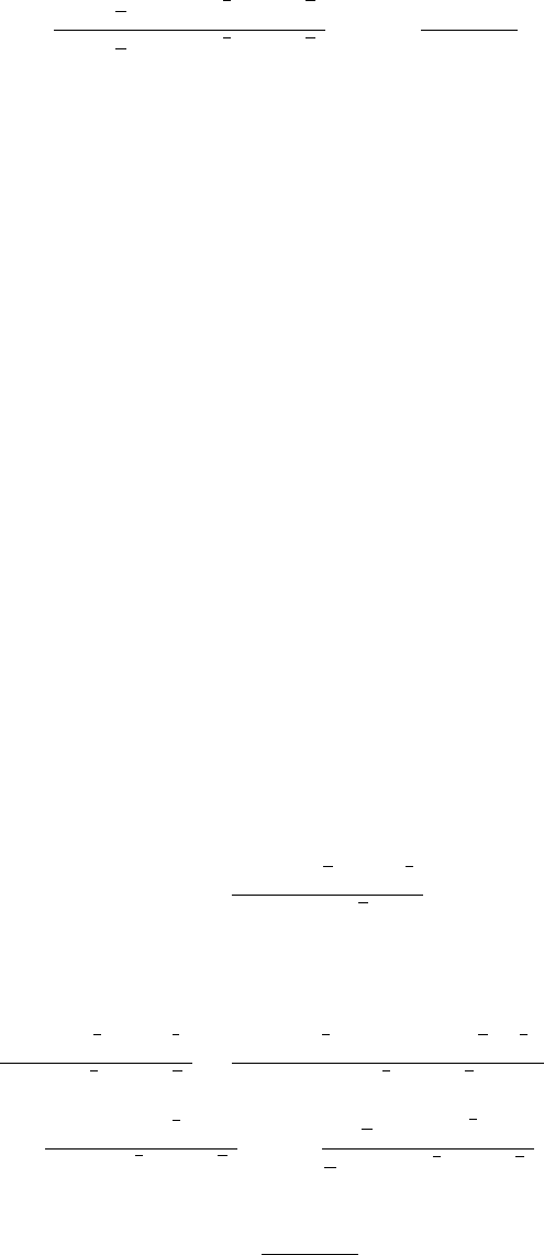
9. Simultaneous equations estimation
Hence, dividing the numerator and the denominator of the error term by nso that
they tend to limits as the sample size becomes large,
plim b
βIV
2=β2+plim 1
nP(pi−p)(ui−u)
plim 1
nP(pi−p)(xi−x)=β2+cov(p, u)
cov(p, x)=β2
since cov(p, u) = 0, pbeing exogenous, and cov(p, x)6= 0, xbeing determined
partly by p.
The OLS and IV regressions are summarised below (standard errors in
parentheses). Comment on them, making use of your answers to the first two parts
of this question.
OLS be=−0.52 + 0.48x(3)
(0.27) (0.08)
IV be= 0.37 + 0.17x(4)
(0.42) (0.14)
The IV estimate of the slope coefficient is lower than the OLS estimate, as
expected. The standard errors are not comparable because the OLS ones are
invalid.
A second researcher hypothesises that both x and p are exogenous and that equation
(2) should be written:
e=x−p. (5)
On the assumption that this is correct, explain why the slope coefficients in (3) and
(4) are both biased and determine the direction of the bias in each case.
If (5) is correct, (3) is a misspecification that omits pand includes a redundant
intercept. From the identity, the true values of the coefficients of xand pare 1 and
−1, respectively. For (3):
E(b
βOLS
2) = 1 −1×P(xi−x)(pi−p)
P(xi−x)2.
xand pare positively correlated, so the bias will be downwards.
For (4):
b
βIV
2=P(pi−p)(ei−e)
P(pi−p)(xi−x)=P(pi−p)([xi−pi]−[x−p])
P(pi−p)(xi−x)
= 1 −P(pi−p)2
P(pi−p)(xi−x)= 1 −
1
nP(pi−p)2
1
nP(pi−p)(xi−x).
Hence:
plim b
βIV
2= 1 −var(p)
cov(x, p)
and so again the bias is downwards.
Explain what would be the result of fitting (5), regressing e on x and p.
One would obtain a perfect fit with the coefficient of xequal to 1, the coefficient of
pequal to −1, and R2= 1.
206
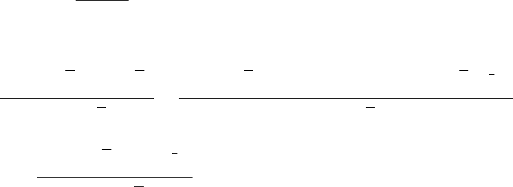
9.6. Answers to the additional exercises
A9.7 Derive the reduced form equations for F and M.
(2) is the reduced form equation for M. Substituting for Min (1), we have:
F= (β1+α1β3)+(β2+α2β3)S+u+β3v.
Explain what would be the most appropriate method to fit equation (1).
Since Mdoes not depend on u, OLS may be used to fit (1).
Explain what would be the most appropriate method to fit equation (2).
There are no endogenous explanatory variables in (2), so again OLS may be used.
Explain why the coefficient of S differs in the two equations.
In (3), the coefficient is an estimate of the direct effect of Son fertility, controlling
for M. In (4), the reduced form equation, it is an estimate of the total effect, taking
account of the indirect effect via M(female education reduces mortality, and a
reduction in mortality leads to a reduction in fertility).
Explain whether one may validly perform t tests on the coefficients of (4).
It is legitimate to use OLS to fit (4), so the ttests are valid.
Discuss whether G is likely to be a valid instrument.
Gshould be a valid instrument since it is highly correlated with S, it may
reasonably be considered to be exogenous and therefore uncorrelated with the
disturbance term in (4), and it does not appear in the equation in its own right
(though perhaps it should).
What should the researchers conclusions be with regard to the test?
With 1 degree of freedom as indicated by the output, the critical value of
chi-squared at the 5 per cent significance level is 3.84. Therefore we do not reject
the null hypothesis of no significant difference between the estimates of the
coefficients and conclude that there is no need to instrument for S. (4) should be
preferred because OLS is more efficient than IV, when both are consistent.
A9.8 Demonstrate that the estimate of α2will be inconsistent if ordinary least squares
(OLS) is used to fit the supply equation, showing that the large-sample bias is likely
to be negative.
The reduced form equation for Pis:
P=1
α2−β2
(β1−α1+β3Y+β4P OP +uD−uS).
The OLS estimator of α2is:
bαOLS
2=PPi−PQi−Q
PPi−P2=PPi−Pα1+α2Pi+uSi −α1−α2P−uS
PPi−P2
=α2+PPi−P(uSi −uS)
PPi−P2.
207

9. Simultaneous equations estimation
We cannot take expectations because uSis a determinant of both the numerator
and the denominator of the error term, in view of the reduced form equation for P.
Instead, we take probability limits, after first dividing the numerator and the
denominator of the error term by nto ensure that limits exist.
plim bαOLS
2=α2+
plim 1
nPPi−P(uSi −uS)
plim 1
nPPi−P2=α2+cov(P, uS)
var(P).
Substituting from the reduced form equation for P:
plim bαOLS
2=α2+
cov 1
α2−β2(β1−α1+β3Y+β4P OP +uD−uS), uS
var(P)
=α2−
1
α2−β2var(uS)
var(P)=α2−1
α2−β2
σ2
uS
σ2
P
assuming that Yand POP are exogenous and so cov(uS, Y ) = cov(uS, P OP ) = 0.
We are told that uSand uDare distributed independently, so cov(uS, uD) = 0.
Since it is reasonable to suppose that α2is positive and β2is negative, the
large-sample bias will be negative.
Demonstrate that a consistent estimate of α2will be obtained if the supply equation
is fitted using instrumental variables (IV), using Y as an instrument.
bαIV
2=PYi−YQi−Q
PYi−YPi−P=PYi−Yα1+α2Pi+uSi −α1−α2P−uS
PYi−YPi−P
=α2+PYi−Y(uSi −uS)
PYi−YPi−P.
We cannot take expectations because uSis a determinant of both the numerator
and the denominator of the error term, in view of the reduced form equation for P.
Instead, we take probability limits, after first dividing the numerator and the
denominator of the error term by nto ensure that limits exist.
plim bαIV
2=α2+
plim 1
nPYi−Y(uSi −uS)
plim 1
nPYi−YPi−P=α2+cov(Y, u)
cov(Y, P )=α2
since cov(Y, us) = 0 and cov(P, Y )6= 0, Ybeing a determinant of P.
The model is used for a Monte Carlo experiment ... Discuss the results obtained.
•The OLS estimates are clearly biased downwards.
•The IV and TSLS estimates appear to be distributed around the true value,
although one would need a much larger number of samples to be sure of this.
•The IV estimates with POP appear to be slightly closer to the true value than
those with Y, as should be expected given the higher correlation, and the TSLS
estimates appear to be slightly closer than either, again as should be expected.
208

9.6. Answers to the additional exercises
•The OLS standard errors should be ignored. The standard errors for the IV
regressions using POP tend to be smaller than those using Y, reflecting the
fact that POP is a better instrument. Those for the TSLS regressions are
smallest of all, reflecting its greater efficiency.
A9.9 Derive the reduced form equation for G for the first researcher.
G=1
1−α2β2
(β1+α1β2+β3A+uG+β2uR).
Explain why ordinary least squares (OLS) would be an inconsistent estimator of the
parameters of equation (2).
The reduced form equation for Gdemonstrates that Gis not distributed
independently of the disturbance term uR, a requirement for the consistency of
OLS when fitting (2).
The first researcher uses instrumental variables (IV) to estimate α2in (2). Explain
the procedure and demonstrate that the IV estimator of α2is consistent.
The first researcher would use Aas an instrument for G. It is exogenous, so
independent of uR; correlated with G; and not in the equation in its own right. The
estimator of the slope coefficient is:
bαIV
2=PAi−ARi−R
PAi−AGi−G=PAi−A[α1+α2Gi+uRi]−[α1+α2G=u]
PAi−AGi−G
=α2+PAi−A(uRi −uR)
PAi−AGi−G.
Hence:
plim bαIV
2=α2+ plim
1
nPAi−A(uRi −uR)
1
nPAi−AGi−G=α2+cov(A, uR)
cov(A, G)=α2
since cov(A, uR) = 0, Abeing exogenous, and cov(A, G)6= 0, Abeing a
determinant of G.
The second researcher uses two stage least squares (TSLS) to estimate α2in (2).
Explain the procedure and demonstrate that the TSLS estimator is consistent.
The reduced form equation for Gfor the second researcher is:
G=1
1−α2β2
(β1+α1β2+β3A+β4Q+uG+β2uR).
It is fitted using TSLS. The fitted values of Gare used as the instrument:
bαTSLS
2=Pb
Gi−b
GRi−R
Pb
Gi−b
GGi−G.
209

9. Simultaneous equations estimation
Following the same method as in the third part of the question:
plim bαTSLS
2=α2+cov( b
G, uR)
cov( b
G, G)=α2
cov( b
G, uR) because b
Gis a linear combination of the exogenous variables, and
cov( b
G, G)6= 0.
Explain why the TSLS estimator used by the second researcher ought to produce
‘better’ results than the IV estimator used by the first researcher, if the growth
equation is given by (1*). Be specific about what you mean by ‘better’.
The TSLS estimator of α2should have a smaller variance. The variance of an IV
estimator is inversely proportional to the square of the correlation of Gand the
instrument. b
Gis the linear combination of Aand Qthat has the highest correlation.
It will therefore, in general, have a lower variance than the IV estimator using A.
Suppose that the first researcher is correct and the growth equation is actually given
by (1), not (1*). Compare the properties of the two estimators in this case.
If the first researcher is correct, Ais the optimal instrument because it will be more
highly correlated with G(in the population) than the TSLS combination of Aand
Qand it will therefore be more efficient.
Suppose that the second researcher is correct and the model is given by (1*) and
(2), but A is not exogenous after all. Suppose that A is influenced by G:
A=γ1+γ2G+uA
where uAis a disturbance term distributed independently of uGand uR. How would
this affect the properties of the IV estimator of α2used by the first researcher?
cov(A, uR) would not be equal to 0 and so the estimator would be inconsistent.
A9.10 State, with a brief explanation, whether each variable is endogenous or exogenous,
and derive the reduced form equations for the endogenous variables.
In this model LGEARN and SKILL are endogenous. IQ is exogenous. The reduced
form equation for LGEARN is:
LGEARN =β1+α1β2+α2β2IQ +u+β2v.
The reduced form equation for SKILL is the structural equation.
Explain why the researcher could use ordinary least squares (OLS) to fit equation
(1) if u and v are distributed independently of each other.
SKILL is not determined either directly or indirectly by u. Thus in equation (1)
there is no violation of the requirement that the regressor be distributed
independently of the disturbance term.
210

9.6. Answers to the additional exercises
Show that the OLS estimator of β2is inconsistent if u and v are positively
correlated and determine the direction of the large-sample bias.
Writing Lfor LGEARN,Sfor SKILL:
b
βOLS
2=PSi−SLi−L
PSi−S2=PSi−S[β1+β2Si+ui]−[β1+β2S+u]
PSi−S2
=β2+PSi−S(ui−u)
PSi−S2.
We cannot obtain a closed-form expression for the expectation of the error term
since Sdepends on vand vis correlated with u. Hence instead we take plims,
dividing the numerator and the denominator by nto ensure that the limits exist:
plim b
βOLS
2=β2+
plim 1
nPSi−S(ui−u)
plim 1
nPSi−S2=β2+cov(S, u)
var(S).
Now:
cov(S, u) = cov([α1+α2IQ +v], u) = cov(v, u)
since α1is a constant and IQ is exogenous. Hence the numerator of the error term
is positive in large samples. The denominator, being a variance, is also positive. So
the large-sample bias is positive.
Demonstrate mathematically how the researcher could use instrumental variables
(IV) estimation to obtain a consistent estimate of β2.
The researcher could use IQ as an instrument for SKILL:
b
βIV
2=PIi−ILi−L
PIi−ISi−S=PIi−I[β1+β2Si+ui]−[β1+β2S+u]
PIi−ISi−S
=β2+PIi−I(ui−u)
PIi−ISi−S.
We cannot obtain a closed-form expression for the expectation of the error term
since Sdepends on vand vis correlated with u. Hence instead we take plims,
dividing the numerator and the denominator by nto ensure that the limits exist:
plim b
βIV
2=β2+
plim 1
nPIi−I(ui−u)
plim 1
nPIi−ISi−S=β2+cov(I, u)
cov(I, s).
The numerator of the error term is zero because Iis exogenous. The denominator
is not zero because Sis determined by I. Hence the IV estimator is consistent.
211

9. Simultaneous equations estimation
Explain the advantages and disadvantages of using IV, rather than OLS, to
estimate β2, given that the researcher is not sure whether u and v are distributed
independently of each other.
The advantage of IV is that, being consistent, there will be no bias in large samples
and hence one may hope that there is no serious bias in a finite sample. One
disadvantage is that there is a loss of efficiency if uand vare independent. Even if
they are not independent, the IV estimator may be inferior to the OLS estimator
using some criterion such as the mean square error that allows a trade-off between
the bias of an estimator and its variance.
Describe in general terms a test that might help the researcher decide whether to
use OLS or IV. What are the limitations of the test?
Durbin–Wu–Hausman test. Also known as Hausman test. The test statistic is a
chi-squared statistic based on the differences of all the coefficients in the regression.
The null hypothesis is that SKILL is distributed independently of uand the
differences in the coefficients are random. If the test statistic exceeds its critical
value, given the significance level of the test, we reject the null hypothesis and
conclude that we ought to use IV rather than OLS. The main limitation is lack of
power if the instrument is weak.
Explain whether it is possible for the researcher to fit equation (2) and obtain
consistent estimates.
There is no reason why the equation should not be fitted using OLS.
A9.11 Substituting for Yfrom the first equation into the second, and re-arranging, we
have the reduced form equation for S:
S=α1+α2β1+v+α2u
1−α2β2
.
Substituting from the third equation into the first, we have:
Y=β1+β2R+u−β2w.
If this equation is fitted using OLS, we have:
plim b
βOLS
2=β2+cov(R, [u−β2w])
var(R)=β2+cov([S+w],[u−β2w])
var(S+w)
=β2+α2γσ2
u−β2σ2
w
σ2
S+σ2
w
=β2+α2γσ2
u−β2σ2
w
γ2(σ2
v+α2
2σ2
u) + σ2
w
where:
γ=1
1−α2β2
.
The denominator of the bias term is positive. Hence the bias will be positive if (the
component attributable to simultaneity) is greater than (the component
attributable to measurement error), and negative if it is smaller.
212

Chapter 10
Binary choice and limited dependent
variable models, and maximum
likelihood estimation
10.1 Overview
The first part of this chapter describes the linear probability model, logit analysis, and
probit analysis, three techniques for fitting regression models where the dependent
variable is a qualitative characteristic. Next it discusses tobit analysis, a censored
regression model fitted using a combination of linear regression analysis and probit
analysis. This leads to sample selection models and heckman analysis. The second part
of the chapter introduces maximum likelihood estimation, the method used to fit all of
these models except the linear probability model.
10.2 Learning outcomes
After working through the corresponding chapter in the text, studying the
corresponding slideshows, and doing the starred exercises in the text and the additional
exercises in this subject guide, you should be able to:
describe the linear probability model and explain its defects
describe logit analysis, giving the mathematical specification
describe probit analysis, including the mathematical specification
calculate marginal effects in logit and probit analysis
explain why OLS yields biased estimates when applied to a sample with censored
observations, even when the censored observations are deleted
explain the problem of sample selection bias and describe how the heckman
procedure may provide a solution to it (in general terms, without mathematical
detail)
explain the principle underlying maximum likelihood estimation
apply maximum likelihood estimation from first principles in simple models.
213

10. Binary choice and limited dependent variable models, and maximum likelihood estimation
10.3 Further material
Limiting distributions and the properties of maximum likelihood estimators
Provided that weak regularity conditions involving the differentiability of the likelihood
function are satisfied, maximum likelihood (ML) estimators have the following
attractive properties in large samples:
(1) They are consistent.
(2) They are asymptotically normally distributed.
(3) They are asymptotically efficient.
The meaning of the first property is familiar. It implies that the probability density
function of the estimator collapses to a spike at the true value. This being the case,
what can the other assertions mean? If the distribution becomes degenerate as the
sample size becomes very large, how can it be described as having a normal
distribution? And how can it be described as being efficient, when its variance, and the
variance of any other consistent estimator, tend to zero?
To discuss the last two properties, we consider what is known as the limiting
distribution of an estimator. This is the distribution of the estimator when the
divergence between it and its population mean is multiplied by √n. If we do this, the
distribution of a typical estimator remains nondegenerate as nbecomes large, and this
enables us to say meaningful things about its shape and to make comparisons with the
distributions of other estimators (also multiplied by √n).
To put this mathematically, suppose that there is one parameter of interest, θ, and that
b
θis its ML estimator. Then (2) says that:
√nb
θ−θ∼N(0, σ2)
for some variance σ2. (3) says that, given any other consistent estimator ˜
θ,p˜
θ−θ
cannot have a smaller variance.
Test procedures for maximum likelihood estimation
This section on ML tests contains material that is a little advanced for an introductory
econometrics course. It is provided because likelihood ratio tests are encountered in the
sections on binary choice models and because a brief introduction may be of help to
those who proceed to a more advanced course.
There are three main approaches to testing hypotheses in maximum likelihood
estimation: likelihood ratio (LR) tests, Wald tests, and Lagrange multiplier (LM) tests.
Since the theory behind Lagrange multiplier tests is relatively complex, the present
discussion will be confined to the first two types. We will start by assuming that the
probability density function of a random variable Xis a known function of a single
unknown parameter θand that the likelihood function for θgiven a sample of n
observations on X,L(θ|X1, . . . , Xn), satisfies weak regularity conditions involving its
214

10.3. Further material
differentiability. In particular, we assume that θis determined by the first-order
condition dL/dθ= 0. (This rules out estimators such as that in Exercise A10.7) The
null hypothesis is H0:θ=θ0, the alternative hypothesis is H1:θ6=θ0, and the
maximum likelihood estimate of θis b
θ.
Likelihood ratio tests
A likelihood ratio test compares the value of the likelihood function at θ=b
θwith its
value at θ=θ0. In view of the definition of b
θ,L(b
θ)≥L(θ0) for all θ0. However, if the
null hypothesis is true, the ratio L(b
θ)/L(θ0) should not be significantly greater than 1.
As a consequence, the logarithm of the ratio:
log L(b
θ)
L(θ0)!= log L(b
θ)−log L(θ0)
should not be significantly different from zero. In that it involves a comparison of the
measures of goodness of fit for unrestricted and restricted versions of the model, the LR
test is similar to an Ftest.
Under the null hypothesis, it can be shown that in large samples the test statistic:
LR = 2 log L(b
θ)−log L(θ0)
has a chi-squared distribution with one degree of freedom. If there are multiple
parameters of interest, and multiple restrictions, the number of degrees of freedom is
equal to the number of restrictions.
Examples
We will return to the example in Section 10.6 in the textbook, where we have a
normally-distributed random variable Xwith unknown population mean µand known
standard deviation equal to 1. Given a sample of nobservations, the likelihood function
is:
L(bµ|X1, . . . , Xn) = 1
√2πe(X1−µ)2/2× ··· × 1
√2πe(Xn−µ)2/2.
The log-likelihood is:
log L(bµ|X1, . . . , Xn) = nlog 1
√2π−1
2X(Xi−bµ)2
and the unrestricted ML estimate is bµ=X. The LR statistic for the null hypothesis
H0:µ=µ0is therefore:
LR = 2 nlog 1
√2π−1
2X(Xi−X)2−nlog 1
√2π−1
2(Xi−µ0)2
=X(Xi−µ0)2−X(Xi−X)2=n(X−µ0)2.
If we relaxed the assumption σ= 1, the unrestricted likelihood function is:
L(bµ, bσ|X1, . . . , Xn) = 1
bσ√2πe−1
2X1−bµ
bσ2× ··· × 1
bσ√2πe−1
2(Xn−bµ
bσ)2
215

10. Binary choice and limited dependent variable models, and maximum likelihood estimation
and the log-likelihood is:
log L(bµ, bσ|X1, . . . , Xn) = nlog 1
√2π−nlog bσ−1
2bσ2X(Xi−bµ)2.
The first-order condition obtained by differentiating by σis:
∂log L
∂σ =−n
σ+1
σ3X(Xi−µ)2= 0
from which we obtain:
bσ2=1
nX(Xi−bµ)2.
Substituting back into the log-likelihood function, the latter now becomes a function of
µonly (and is known as the concentrated log-likelihood function or, sometimes, the
profile log-likelihood function):
log L(µ|X1, . . . , Xn) = nlog 1
√2π−nlog 1
nX(Xi−µ)21/2
−n
2.
As before, the ML estimator of µis ¯
X. Hence the LR statistic is:
LR = 2 nlog 1
√2π−nlog 1
nX(Xi−X)21/2
−n
2!
− nlog 1
√2π−nlog 1
nX(Xi−µ0)21/2
−n
2!!
=nlog X(Xi−µ0)2−log X(Xi−X)2.
It is worth noting that this is closely related to the Fstatistic obtained when one fits
the least squares model:
Xi=µ+ui.
The least squares estimator of µis Xand RSS =P(Xi−X)2.
If one imposes the restriction µ=µ0, we have RSSR=P(Xi−µ0)2and the Fstatistic:
F(1, n −1) = P(Xi−µ0)2−P(Xi−X)2
P(Xi−X)2/(n−1)
.
Returning to the LR statistic, we have:
LR =nlog P(Xi−µ0)2
P(Xi−X)2=nlog 1 + P(Xi−µ0)2−P(Xi−X)2
P(Xi−X)2!
∼
=nP(Xi−µ0)2−P(Xi−X)2
P(Xi−X)2=n
n−1F∼
=F.
Note that we have used the approximation log(1 + a) = awhich is valid when ais small
enough for higher powers to be neglected.
216

10.3. Further material
Wald tests
Wald tests are based on the same principle as ttests in that they evaluate whether the
discrepancy between the maximum likelihood estimate θand the hypothetical value θ0
is significant, taking account of the variance in the estimate. The test statistic for the
null hypothesis H0:b
θ−θ0= 0 is: b
θ−θ02
bσ2
b
θ
where bσ2
b
θis the estimate of the variance of θevaluated at the maximum likelihood
value. bσ2
b
θcan be estimated in various ways that are asymptotically equivalent if the
likelihood function has been specified correctly. A common estimator is that obtained as
minus the inverse of the second differential of the log-likelihood function evaluated at
the maximum likelihood estimate. Under the null hypothesis that the restriction is
valid, the test statistic has a chi-squared distribution with one degree of freedom. When
there are multiple restrictions, the test statistic becomes more complex and the number
of degrees of freedom is equal to the number of restrictions.
Examples
We will use the same examples as for the LR test, first, assuming that σ= 1 and then
assuming that it has to be estimated along with µ. In the first case the log-likelihood
function is:
log L(µ|X1, . . . , Xn) = nlog 1
√2π−1
2X(Xi−µ)2.
The first differential is P(Xi−µ) and the second is −n, so the estimate of the variance
is 1/n. The Wald test statistic is therefore n(X−µ0)2.
In the second example, where σwas unknown, the concentrated log-likelihood function
is:
log L(µ|X1, . . . , Xn) = nlog 1
√2π−nlog 1
nX(Xi−µ)21/2
−n
2
=nlog 1
√2π−n
2log 1
n−n
2log X(Xi−µ)2−n
2.
The first derivative with respect to µis:
d log L
dµ=nP(Xi−µ)
P(Xi−µ)2.
The second derivative is:
d2log L
dµ2=n(−n) (P(Xi−µ)2)−(P(Xi−µ)) (−2P(Xi−µ))
[P(Xi−µ)2]2.
Evaluated at the ML estimator bµ=X,P(Xi−µ) = 0 and hence:
d2log L
dµ2=−n2
P(Xi−µ)2
217

10. Binary choice and limited dependent variable models, and maximum likelihood estimation
giving an estimated variance bσ2/n, given:
bσ2=1
nX(Xi−X)2.
Hence the Wald test statistic is:
(X−µ0)2
bσ2/n .
Under the null hypothesis, this is distributed as a chi-squared statistic with one degree
of freedom.
When there is just one restriction, as in the present case, the Wald statistic is the square
of the corresponding asymptotic tstatistic (asymptotic because the variance has been
estimated asymptotically). The chi-squared test and the ttest are equivalent, given
that, when there is one degree of freedom, the critical value of the chi-squared statistic
for any significance level is the square of the critical value of the normal distribution.
LR test of restrictions in a regression model
Given the regression model:
Yi=β1+
k
X
j=2
βjXij +ui
with uassumed to be iid N(0, σ2), the log-likelihood function for the parameters is:
log L(β1, . . . , βk, σ |Yi, Xi, i = 1, . . . , n) = nlog 1
σ√2π−1
2σ2X Yi−β1−
k
X
j=2
βjXij!2
.
This is a straightforward generalisation of the expression for a simple regression derived
in Section 10.6 in the textbook. Hence
log L(β1, . . . , βk, σ |Yi, Xi, i = 1, . . . , n) = −nlog σ−n
2log 2π−1
2σ2Z
where:
Z=X Yi−β1−
k
X
j=2
βjXij!2
.
The estimates of the βparameters affect only Z. To maximise the log-likelihood, they
should be chosen so as to minimise Z, and of course this is exactly what one is doing
when one is fitting a least squares regression. Hence Z=RSS. It remains to determine
the ML estimate of σ. Taking the partial differential with respect to σ, we obtain one of
the first-order conditions for a maximum:
∂log L(β1, . . . , βk, σ)
∂σ =−n
σ+1
σ3RSS = 0.
From this we obtain:
bσ2=RSS
n.
218

10.4. Additional exercises
Hence the ML estimator is the sum of the squares of the residuals divided by n. This is
different from the least squares estimator, which is the sum of the squares of the
residuals divided by n−k, but the difference disappears as the sample size becomes
large. Substituting for bσ2in the log-likelihood function, we obtain the concentrated
likelihood function:
log L(β1, . . . , βk|Yi, Xi, i = 1, . . . , n) = −nlog RSS
n1/2
−n
2log 2π−1
2Z/nRSS
=−n
2log RSS
n−n
2log 2π−n
2
=−n
2(log RSS + 1 + log 2π−log n).
We will re-write this as:
log LU=−n
2(log RSSU+ 1 + log 2π−log n)
the subscript U emphasising that this is the unrestricted log-likelihood. If we now
impose a restriction on the parameters and maximise the loglikelihood function subject
to the restriction, it will be:
log LR=−n
2(log RSSR+ 1 + log 2π−log n)
where RSSR≥RSSUand hence log LR≤log LU. The LR statistic for a test of the
restriction is therefore:
2(log LU−LR) = n(log RSSR−log RSSU) = nlog RSSR
RSSU
.
It is distributed as a chi-squared statistic with one degree of freedom under the null
hypothesis that the restriction is valid. If there is more than one restriction, the test
statistic is the same but the number of degrees of freedom under the null hypothesis
that all the restrictions are valid is equal to the number of restrictions.
An example of its use is the common factor test in Section 12.3 in the text. As with all
maximum likelihood tests, it is valid only for large samples. Thus for testing linear
restrictions we should prefer the Ftest approach because it is valid for finite samples.
10.4 Additional exercises
A10.1 What factors affect the decision to make a purchase of your category of expenditure
in the CES data set?
Define a new variable CATBUY that is equal to 1 if the household makes any
purchase of your category and 0 if it makes no purchase at all. Regress CATBUY
on EXPPC,SIZE,REFAGE, and COLLEGE (as defined in Exercise A5.6) using:
(1) the linear probability model, (2) the logit model, and (3) the probit model.
Calculate the marginal effects at the mean of EXPPC,SIZE,REFAGE, and
COLLEGE for the logit and probit models and compare them with the coefficients
of the linear probability model.
219
10. Binary choice and limited dependent variable models, and maximum likelihood estimation
A10.2 Logit analysis was used to relate the event of a respondent working (WORKING,
defined to be 1 if the respondent was working, and 0 otherwise) to the respondent’s
educational attainment (S, defined as the highest grade completed) using 1994 data
from the National Longitudinal Survey of Youth 1979–. In this year the respondents
were aged 29–36 and a substantial number of females had given up work to raise a
family. The analysis was undertaken for females and males separately, with the
output shown below (first females, then males, with iteration messages deleted):
. logit WORKING S if MALE==0
Logit Estimates Number of obs = 2726
chi2(1) = 70.42
Prob > chi2 = 0.0000
Log Likelihood = -1586.5519 Pseudo R2 = 0.0217
------------------------------------------------------------------------------
WORKING | Coef. Std. Err. z P>|z| [95% Conf. Interval]
---------+--------------------------------------------------------------------
S | .1511872 .0186177 8.121 0.000 .1146971 .1876773
_cons | -1.049543 .2448064 -4.287 0.000 -1.529355 -.5697314
------------------------------------------------------------------------------
. logit WORKING S if MALE==1
Logit Estimates Number of obs = 2573
chi2(1) = 75.03
Prob > chi2 = 0.0000
Log Likelihood = -802.65424 Pseudo R2 = 0.0446
------------------------------------------------------------------------------
WORKING | Coef. Std. Err. z P>|z| [95% Conf. Interval]
---------+--------------------------------------------------------------------
S | .2499295 .0306482 8.155 0.000 .1898601 .3099989
_cons | -.9670268 .3775658 -2.561 0.010 -1.707042 -.2270113
------------------------------------------------------------------------------
95 per cent of the respondents had Sin the range 9–18 years and the mean value of
Swas 13.3 and 13.2 years for females and males, respectively.
From the logit analysis, the marginal effect of Son the probability of working at
the mean was estimated to be 0.030 and 0.020 for females and males, respectively.
Ordinary least squares regressions of WORKING on Syielded slope coefficients of
0.029 and 0.020 for females and males, respectively.
As can be seen from the second figure below, the marginal effect of educational
attainment was lower for males than for females over most of the range S≥9.
Discuss the plausibility of this finding.
As can also be seen from the second figure, the marginal effect of educational
attainment decreases with educational attainment for both males and females over
the range S≥9. Discuss the plausibility of this finding.
Compare the estimates of the marginal effect of educational attainment using logit
analysis with those obtained using ordinary least squares.
220
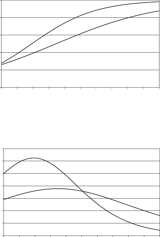
10.4. Additional exercises
0.0
0.2
0.4
0.6
0.8
1.0
0 2 4 6 8 10 12 14 16 18 20
S
probability
males
females
males
females
Figure 10.1: Probability of working, as a function of S.
0.00
0.01
0.02
0.03
0.04
0.05
0.06
0.07
0 2 4 6 8 10 12 14 16 18 20
S
marginal effect
males
females
Figure 10.2: Marginal effect of Son the probability of working.
A10.3 A researcher has data on weight, height, and schooling for 540 respondents in the
National Longitudinal Survey of Youth 1979– for the year 2002. Using the data on
weight and height, he computes the body mass index for each individual. If the
body mass index is 30 or greater, the individual is defined to be obese. He defines a
binary variable, OBESE, that is equal to 1 for the 164 obese individuals and 0 for
the other 376. He wishes to investigate whether obesity is related to schooling and
fits an ordinary least squares (OLS) regression of OBESE on S, years of schooling,
with the following result (tstatistics in parentheses):
\
OBESE = 0.595 −0.021S(1)
(5.30) (2.63)
This is described as the linear probability model (LPM). He also fits the logit
221
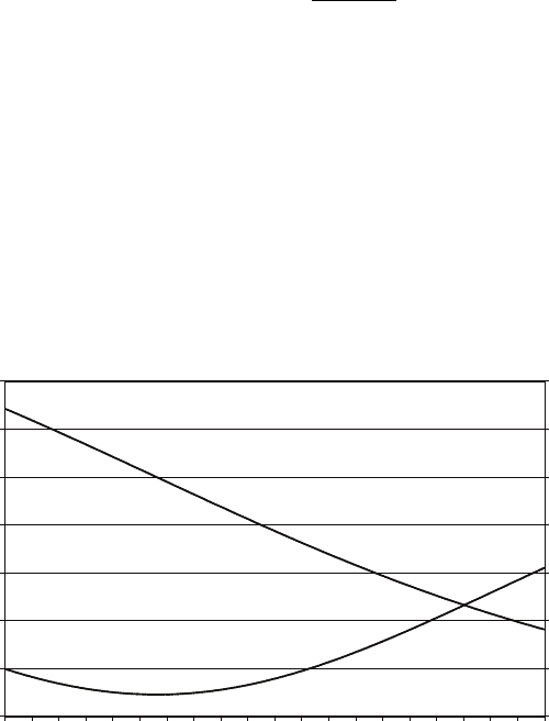
10. Binary choice and limited dependent variable models, and maximum likelihood estimation
model:
F(Z) = 1
1+e−Z
where F(Z) is the probability of being obese and Z=β1+β2S, with the following
result (again, tstatistics in parentheses):
b
Z= 0.588 −0.105S(2)
(1.07) (2.60)
The figure below shows the probability of being obese and the marginal effect of
schooling as a function of S, given the logit regression. Most (492 out of 540) of the
individuals in the sample had 12 to 18 years of schooling.
0
0.1
0.2
0.3
0.4
0.5
0.6
0.7
0 1 2 3 4 5 6 7 8 9 10 11 12 13 14 15 16 17 18 19 20
years of schooling
probability of being obese
-0.028
-0.024
-0.020
-0.016
-0.012
-0.008
-0.004
0.000
marginal effect
probability
marginal effect
Figure 10.3: Scatter diagram of probability of being obese against years of schooling.
•Discuss whether the relationships indicated by the probability and marginal
effect curves appear to be plausible.
•Add the probability function and the marginal effect function for the LPM to
the diagram. Explain why you drew them the way you did.
•The logit model is considered to have several advantages over the LPM.
Explain what these advantages are. Evaluate the importance of the advantages
of the logit model in this particular case.
•The LPM is fitted using OLS. Explain how, instead, it might be fitted using
maximum likelihood estimation:
◦Write down the probability of being obese for any obese individual, given
Sifor that individual, and write down the probability of not being obese
for any non-obese individual, again given Sifor that individual.
◦Write down the likelihood function for this sample of 164 obese
individuals and 376 non-obese individuals.
◦Explain how one would use this function to estimate the parameters.
[Note: You are not expected to attempt to derive the estimators of the
parameters.]
222

10.4. Additional exercises
◦Explain whether your maximum likelihood estimators will be the same or
different from those obtained using least squares.
A10.4 A researcher interested in the relationship between parenting, age and schooling
has data for the year 2000 for a sample of 1,167 married males and 870 married
females aged 35 to 42 in the National Longitudinal Survey of Youth 1979–. In
particular, she is interested in how the presence of young children in the household
is related to the age and education of the respondent. She defines CHILDL6 to be
1 if there is a child less than 6 years old in the household and 0 otherwise and
regresses it on AGE, age, and S, years of schooling, for males and females
separately using probit analysis. Defining the probability of having a child less than
6 in the household to be p=F(Z) where:
Z=β1+β2AGE +β3S
she obtains the results shown in the table below (asymptotic standard errors in
parentheses).
Males Females
AGE −0.137 −0.154
(0.018) (0.023)
S0.132 0.094
(0.015) (0.020)
constant 0.194 0.547
(0.358) (0.492)
Z−0.399 −0.874
f(Z) 0.368 0.272
For males and females separately, she calculates:
Z=b
β1+b
β2AGE +b
β3S
where AGE and Sare the mean values of AGE and Sand b
β1,b
β2, and b
β3are the
probit coefficients in the corresponding regression, and she further calculates:
f(Z) = 1
√2πe−¯
Z2/2
where f(Z) = dF/dZ. The values of Zand f(Z) are shown in the table.
•Explain how one may derive the marginal effects of the explanatory variables
on the probability of having a child less than 6 in the household, and calculate
for both males and females the marginal effects at the means of AGE and S.
•Explain whether the signs of the marginal effects are plausible. Explain
whether you would expect the marginal effect of schooling to be higher for
males or for females.
223

10. Binary choice and limited dependent variable models, and maximum likelihood estimation
•At a seminar someone asks the researcher whether the marginal effect of Sis
significantly different for males and females. The researcher does not know how
to test whether the difference is significant and asks you for advice. What
would you say?
A10.5 A health economist investigating the relationship between smoking, schooling, and
age, defines a dummy variable Dto be equal to 1 for smokers and 0 for
nonsmokers. She hypothesises that the effects of schooling and age are not
independent of each other and defines an interactive term schooling*age. She
includes this as an explanatory variable in the probit regression. Explain how this
would affect the estimation of the marginal effects of schooling and age.
A10.6 A researcher has data on the following variables for 5,061 respondents in the
National Longitudinal Survey of Youth 1979–:
•MARRIED, marital status in 1994, defined to be 1 if the respondent was
married with spouse present and 0 otherwise;
•MALE, defined to be 1 if the respondent was male and 0 if female;
•AGE in 1994 (the range being 29–37);
•S, years of schooling, defined as highest grade completed, and
•ASVABC, score on a test of cognitive ability, scaled so as to have mean 50 and
standard deviation 10.
She uses probit analysis to regress MARRIED on the other variables, with the
output shown:
. probit MARRIED MALE AGE S ASVABC
Probit estimates Number of obs = 5061
LR chi2(4) = 229.78
Prob > chi2 = 0.0000
Log likelihood = -3286.1289 Pseudo R2 = 0.0338
------------------------------------------------------------------------------
MARRIED | Coef. Std. Err. z P>|z| [95% Conf. Interval]
-------------+----------------------------------------------------------------
MALE | -.1215281 .036332 -3.34 0.001 -.1927375 -.0503188
AGE | .028571 .0081632 3.50 0.000 .0125715 .0445705
S | -.0017465 .00919 -0.19 0.849 -.0197587 .0162656
ASVABC | .0252911 .0022895 11.05 0.000 .0208038 .0297784
_cons | -1.816455 .2798724 -6.49 0.000 -2.364995 -1.267916
------------------------------------------------------------------------------
Variable Mean Marginal effect
MALE 0.4841 −0.0467
AGE 32.52 0.0110
S13.31 −0.0007
ASVABC 48.94 0.0097
The means of the explanatory variables, and their marginal effects evaluated at the
means, are shown in the table.
224
10.5. Answers to the starred exercises in the textbook
•Discuss the conclusions one may reach, given the probit output and the table,
commenting on their plausibility.
•The researcher considers including CHILD, a dummy variable defined to be 1
if the respondent had children, and 0 otherwise, as an explanatory variable.
When she does this, its z-statistic is 33.65 and its marginal effect 0.5685.
Discuss these findings.
10.7 Suppose that the time, t, required to complete a certain process has probability
density function:
f(t) = αe−α(t−β)with t > β > 0
and you have a sample of nobservations with times T1, . . . , Tn.
Determine the maximum likelihood estimate of α, assuming that βis known.
A10.8 In Exercise 10.14 in the text, an event could occur with probability p. Given that
the event occurred mtimes in a sample of nobservations, the exercise required
demonstrating that m/n was the ML estimator of p. Derive the LR statistic for the
null hypothesis p=p0. If m= 40 and n= 100, test the null hypothesis p= 0.5.
A10.9 For the variable in Exercise A10.8, derive the Wald statistic and test the null
hypothesis p= 0.5.
10.5 Answers to the starred exercises in the textbook
10.1 [This exercise does not have a star in the text, but an answer to it is needed for
comparison with the answer to Exercise 10.3.]
The output shows the result of an investigation of how the probability of a
respondent obtaining a bachelor’s degree from a four-year college is related to the
score on ASVABC, using EAWE Data Set 21. BACH is a dummy variable equal to
1 for those with bachelor’s degrees (years of schooling at least 16) and 0 otherwise.
ASVABC is a measure of cognitive ability, scaled so that in the population it has
mean 0 and standard deviation 1. Provide an interpretation of the coefficients.
Explain why OLS is not a satisfactory estimation method for this kind of model.
. reg BACH ASVABC
----------------------------------------------------------------------------
Source | SS df MS Number of obs = 500
-----------+------------------------------ F( 1, 498) = 123.14
Model | 24.7674233 1 24.7674233 Prob > F = 0.0000
Residual | 100.160577 498 .201125656 R-squared = 0.1983
-----------+------------------------------ Adj R-squared = 0.1966
Total | 124.928 499 .250356713 Root MSE = .44847
----------------------------------------------------------------------------
BACH | Coef. Std. Err. t P>|t| [95% Conf. Interval]
-----------+----------------------------------------------------------------
ASVABC | .2479312 .0223421 11.10 0.000 .2040348 .2918277
_cons | .4206845 .0209535 20.08 0.000 .3795163 .4618526
----------------------------------------------------------------------------
225
10. Binary choice and limited dependent variable models, and maximum likelihood estimation
Answer:
The slope coefficient indicates that the probability of earning a bachelor’s degree
rises by 25 per cent for every additional unit of the ASVABC score. ASVABC is
scaled so that one unit is one standard deviation and it has mean zero. While this
may be realistic for a range of values of ASVABC, it is not for very low ones. Very
few of those with scores in the low end of the spectrum earned bachelors degrees
and variations in the ASVABC score would be unlikely to have an effect on the
probability. The intercept literally indicates that an individual with average score
would have a 42 per cent probability of earning a bachelor’s degree.
However, the linear probability model predicts nonsense negative probabilities for
all those with scores less of −1.70 or less. It also suffers from the problem that the
standard errors and tand Ftests are invalid because the disturbance term does
not have a normal distribution. Its distribution is not even continuous, consisting of
only two possible values for each value of ASVABC.
10.3 The output shows the results of fitting a logit regression for BACH, as defined in
Exercise 10.1, with the iteration messages deleted. 48.8 per cent of the respondents
earned bachelor’s degrees.
. logit BACH ASVABC
----------------------------------------------------------------------------
Logistic regression Number of obs = 500
LR chi2(1) = 110.38
Prob > chi2 = 0.0000
Log likelihood = -291.23809 Pseudo R2 = 0.1593
----------------------------------------------------------------------------
BACH | Coef. Std. Err. z P>|z| [95% Conf. Interval]
-----------+----------------------------------------------------------------
ASVABC | 1.240198 .1377998 9.00 0.000 .9701151 1.51028
_cons | -.4077999 .1088093 -3.75 0.000 -.6210623 -.1945375
----------------------------------------------------------------------------
The diagram shows the probability of earning a bachelor’s degree as a function of
ASVABC. It also shows the marginal effect function.
•With reference to the diagram, discuss the variation of the marginal effect of
the ASVABC score implicit in the logit regression.
•Sketch the probability and marginal effect diagrams for the OLS regression in
Exercise 10.1 and compare them with those for the logit regression.
Answer:
ASVABC is scaled so that it has a mean of zero. From the curve for the cumulative
probability in the figure it can be seen that, for a respondent with mean score, the
probability of graduating from college is about 40 per cent. For those one standard
deviation above the mean, it is nearly 70 per cent. For those one standard
deviation below, a little lower than 20 percent. Looking at the curve for the
marginal probability, it can be seen that the marginal effect is greatest for those of
average cognitive ability, and still quite high a standard deviation either way. For
those two standard deviations above the mean, the marginal effect is low because
most are going to college anyway. For those two standard deviations below, the
effect is gain low, for the opposite reason.
226
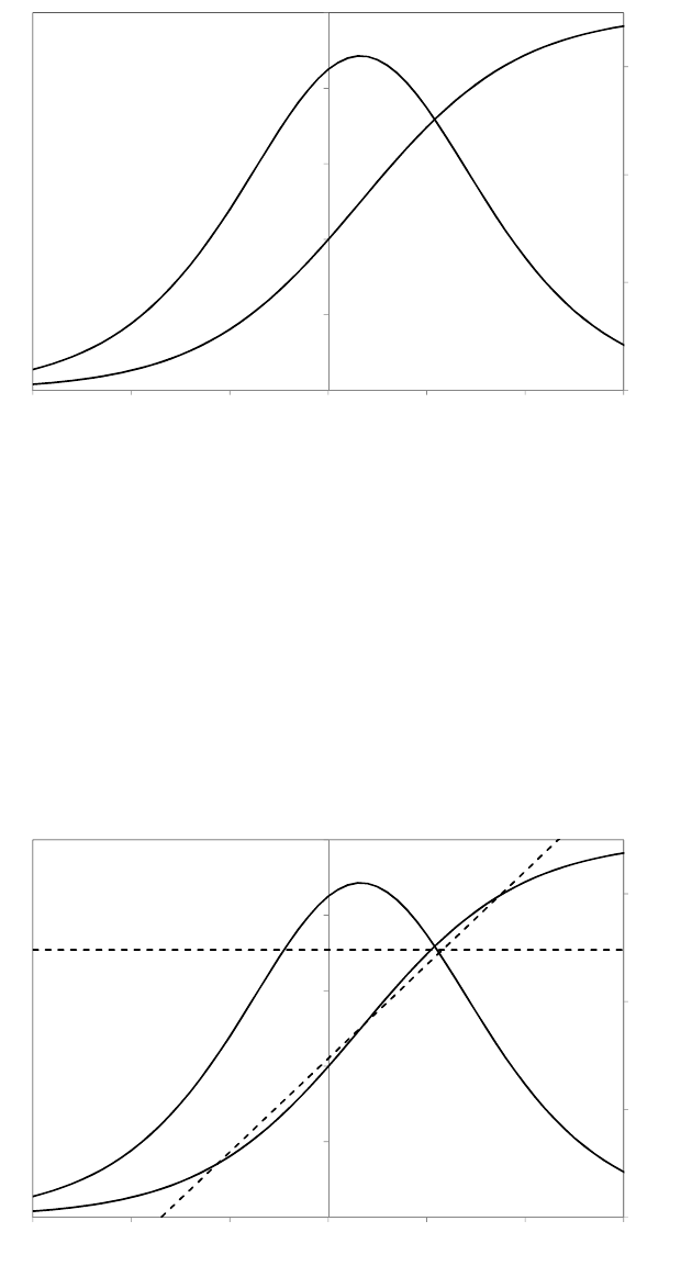
10.5. Answers to the starred exercises in the textbook
0.0
0.1
0.2
0.3
0.0
0.2
0.4
0.6
0.8
1.0
-3.0 -2.0 -1.0 0.0 1.0 2.0 3.0
Marginal effect
Cumulative effect
ASVABC
Figure 10.4: Scatter diagram of cumulative and marginal effects against ASVABC.
For the linear probability model in Exercise 10.1, the counterpart to the cumulative
probability curve in the figure is a straight line using the regression result. In this
example, the predictions of the linear probability model do not differ much from
those of the logit model over the central range of the data. Its deficiencies become
visible only at the extremes. The OLS counterpart to the marginal probability
curve is a horizontal straight line at 0.25, showing that the marginal effect is
somewhat underestimated in the central range and overestimated elsewhere.
0.0
0.1
0.2
0.3
0.0
0.2
0.4
0.6
0.8
1.0
-3.0 -2.0 -1.0 0.0 1.0 2.0 3.0
Marginal effect
Cumulative effect
ASVABC
Figure 10.5: Scatter diagram of cumulative and marginal effects against ASVABC.
10.7 The following probit regression, with iteration messages deleted, was fitted using
2,108 observations on females in the National Longitudinal Survey of Youth using
the LFP2011 data set described in Exercise 10.2. The respondents were aged 27 to
31 and many of them were raising young families.
227
10. Binary choice and limited dependent variable models, and maximum likelihood estimation
. probit WORKING S AGE CHILDL06 CHILDL16 MARRIED ETHBLACK ETHHISP if MALE==0
----------------------------------------------------------------------------
Probit regression Number of obs = 2108
LR chi2(7) = 170.55
Prob > chi2 = 0.0000
Log likelihood = -972.89229 Pseudo R2 = 0.0806
----------------------------------------------------------------------------
WORKING | Coef. Std. Err. z P>|z| [95% Conf. Interval]
-----------+----------------------------------------------------------------
S | .1046085 .0127118 8.23 0.000 .0796939 .1295232
AGE | -.0029273 .0237761 -0.12 0.902 -.0495277 .043673
CHILDL06 | -.4490263 .08128 -5.52 0.000 -.6083322 -.2897204
CHILDL16 | -.3055774 .1060307 -2.88 0.004 -.5133938 -.097761
MARRIED | -.1286145 .0724189 -1.78 0.076 -.2705529 .0133239
ETHBLACK | -.1070784 .0861386 -1.24 0.214 -.2759069 .0617502
ETHHISP | .0364241 .0987625 0.37 0.712 -.1571468 .229995
_cons | -.1885982 .7046397 -0.27 0.789 -1.569667 1.19247
----------------------------------------------------------------------------
WORKING is a binary variable equal to 1 if the respondent was working in 2011, 0
otherwise. CHILDL06 is a dummy variable equal to 1 if there was a child aged less
than 6 in the household, 0 otherwise. CHILDL16 is a dummy variable equal to 1 if
there was a child aged less than 16, but no child less than 6, in the household, 0
otherwise. MARRIED is equal to 1 if the respondent was married with spouse
present, 0 otherwise. The remaining variables are as described in Appendix B. The
mean values of the variables are given in the output from the sum command:
. sum WORKING S AGE CHILDL06 CHILDL16 MARRIED ETHBLACK ETHHISP if MALE==0
--------------------------------------------------------------------
Variable | Obs Mean Std. Dev. Min Max
-----------+--------------------------------------------------------
WORKING | 2108 .7988615 .4009465 0 1
S | 2108 14.32922 2.882736 6 20
AGE | 2108 28.99336 1.386405 27 31
CHILDL06 | 2108 .4407021 .4965891 0 1
CHILDL16 | 2108 .1465844 .3537751 0 1
MARRIED | 2108 .420778 .4938011 0 1
ETHBLACK | 2108 .1783681 .3829132 0 1
ETHHISP | 2108 .1233397 .3289047 0 1
--------------------------------------------------------------------
Calculate the marginal effects and discuss whether they are plausible.
Answer:
The marginal effects are calculated in the table below. As might be expected,
having a child aged less than 6 has a large adverse effect, very highly significant.
Schooling also has a very significant effect, more educated mothers making use of
their investment by tending to stay in the labour force. Age has a significant
negative effect, the reason for which is not obvious (the respondents were aged
29–36 in 1994). Being black also has an adverse effect, the reason for which is
likewise not obvious. (The WORKING variable is defined to be 1 if the individual
has recorded hourly earnings of at least $3. If the definition is tightened to
including also the requirement that the employment status is employed, the latter
effect is smaller, but still significant at the 5 per cent level.)
228

10.5. Answers to the starred exercises in the textbook
Variable Mean b
β2Mean×b
β2f(Z)b
β2×f(Z)
S14.3292 0.1046 1.4990 0.2627 0.0275
AGE 28.9934 −0.0029 −0.0849 0.2627 −0.0008
CHILD06 0.4407 −0.4490 −0.1979 0.2627 −0.1180
CHILDL16 0.1466 −0.3056 −0.0448 0.2627 −0.0803
MARRIED 0.4208 −0.1286 −0.0541 0.2627 −0.0338
ETHBLACK 0.1784 −0.1071 −0.0191 0.2627 −0.0281
ETHHISP 0.1233 0.1233 0.0045 0.2627 0.0096
constant 1.0000 −0.1886 −0.1886
Total 0.9141
10.12 Show that the tobit model may be regarded as a special case of a selection bias
model.
Answer:
The selection bias model may be written:
B∗
i=δ1+
m
X
j=2
δjQji +εi
Y∗
i=β1
k
X
j=2
βjXji +ui
Yi=Y∗
ifor B∗
i>0
Yiis not observed for B∗
i≤0
where the Qvariables determine selection. The tobit model is the special case
where the Qvariables are identical to the Xvariables and B∗is the same as Y∗.
10.14 An event is hypothesised to occur with probability p. In a sample of nobservations,
it occurred mtimes. Demonstrate that the maximum likelihood estimator of pis
m/n.
Answer:
In each observation where the event did occur, the probability was p. In each
observation where it did not occur, the probability was (1 −p). Since there were m
of the former and n−mof the latter, the joint probability was pm(1 −p)n−m.
Reinterpreting this as a function of p, given mand n, the log-likelihood function for
pis:
log L(p)−mlog p+ (n−m) log(1 −p).
Differentiating with respect to p, we obtain the first-order condition for a minimum:
d log L(p)
dp=m
p−n−m
1−p= 0.
This yields p=m/n. We should check that the second differential is negative and
that we have therefore found a maximum. The second differential is:
d2log L(p)
dp2=−m
p2−n−m
(1 −p)2.
229

10. Binary choice and limited dependent variable models, and maximum likelihood estimation
Evaluated at p=m/n:
d2log L(p)
dp2=−n2
m−n−m
1−m
n2=−n21
m+1
n−m.
This is negative, so we have indeed chosen the value of pthat maximises the
probability of the outcome.
10.18 Returning to the example of the random variable Xwith unknown mean µand
variance σ2, the log-likelihood for a sample of nobservations was given by equation
(10.36):
log L=−n
2log 2π−n
2log σ2+1
σ2−1
2(X1−µ)2− ··· − 1
2(Xn−µ)2.
The first-order condition forµproduced the ML estimator of µand the first order
condition for σthen yielded the ML estimator for σ. Often, the variance is treated
as the primary dispersion parameter, rather than the standard deviation. Show
that such a treatment yields the same results in the present case. Treat σ2as a
parameter, differentiate log Lwith respect to it, and solve.
Answer:
∂log L
∂σ2=−n
2σ2−1
σ4−1
2(X1−µ)2− ··· − 1
2(Xn−µ)2.
Hence:
bσ2=1
n(X1−µ)2+··· + (Xn−µ)2
as before. The ML estimator of µis Xas before.
10.19 In Exercise 10.7, log L0is −1058.17. Compute the pseudo-R2and confirm that it is
equal to that reported in the output.
Answer:
As defined in equation (10.48):
pseudo-R2= 1 −log L
log L0
= 1 −−972.8923
−1058.17 = 0.0806
as appears in the output.
10.20 In Exercise 10.7, compute the likelihood ratio statistic 2(log L−log L0), confirm
that it is equal to that reported in the output, and perform the likelihood ratio test.
Answer:
The likelihood ratio statistic is 2(−972.89 + 1058.17) = 170.56, which is that
reported in the output, apart from rounding error in the last digit. Under the null
hypothesis that the coefficients of the explanatory variables are all jointly equal to
0, this is distributed as a chi-squared statistic with degrees of freedom equal to the
number of explanatory variables, in this case 7. The critical value of chi-squared at
the 0.1 per cent significance level with 7 degrees of freedom is 24.32, and so we
reject the null hypothesis at that level.
230

10.6. Answers to the additional exercises
10.6 Answers to the additional exercises
A10.1 In the case of FDHO there were no non-purchasing households and so it was not
possible to undertake the analysis.
The results for the logit analysis and the probit analysis were very similar. The
linear probability model also yielded similar results for most of the commodities,
the coefficients being similar to the logit and probit marginal effects and the t
statistics being of the same order of magnitude as the zstatistics for the logit and
probit.
Most of the effects seem plausible with simple explanations. The total expenditure
of the household and the size of the household were both highly significant factors
in the decision to make a purchase for most categories of expenditure. The main
exception, TOB. was instead influenced (negatively: survival bias?) by the age of
the reference individual and, unsurprisingly, by his or her education.
Linear probability model, dependent variable CATBUY
EXPPC ×10−4SIZE ×10−2REFAGE ×10−2COLLEGE Cases with
probability
nb
β2tb
β3tb
β4tb
β5t < 0>1
ADM 2,815 0.38 20.41 4.00 9.54 −0.34 −9.92 0.22 17.74 0 44
CLOT 4,500 0.33 18.74 5.38 13.61 −0.35 −10.72 0.05 4.12 0 144
DOM 1,661 0.30 17.37 4.18 10.78 0.16 5.08 0.09 7.99 0 181
EDUC 561 0.13 11.83 3.13 12.38 −0.12 −5.80 0.05 6.01 612 0
ELEC 5,828 0.08 7.33 2.71 11.09 0.16 7.76 0.02 2.07 0 254
FDAW 5,102 0.23 14.57 2.23 6.41 −0.27 −9.56 0.11 10.85 0 223
FDHO* 6,334
FOOT 1,827 0.28 15.83 5.93 14.81 −0.22 −6.65 0.01 1.01 0 4
FURN 487 0.14 13.47 1.65 6.87 −0.07 −3.74 0.01 1.66 149 0
GASO 5,710 0.09 7.70 3.23 12.07 −0.00 −0.14 0.07 8.61 0 331
HEAL 4,802 0.21 12.82 3.18 8.77 0.82 27.46 0.11 9.82 0 406
HOUS 6,223 0.03 5.24 0.52 4.36 0.04 4.44 0.01 2.30 0 484
LIFE 1,253 0.35 15.82 3.91 11.02 0.19 8.36 0.04 3.49 0 1
LOCT 692 0.04 3.42 −0.23 −0.80 −0.15 −6.38 0.00 0.42 0 0
MAPP 399 0.10 10.34 1.59 7.23 −0.00 −0.01 −0.01 −1.54 0 0
PERS 3,817 0.30 15.56 4.55 10.53 0.29 8.19 0.12 9.28 0 66
READ 2,287 0.25 13.48 2.52 5.98 0.37 10.76 0.16 13.03 0 10
SAPP 1,037 0.20 13.80 2.86 8.61 −0.03 −1.12 0.03 3.30 0 0
TELE 5,788 0.07 6.29 3.52 14.09 0.31 15.12 0.01 1.65 0 455
TEXT 992 0.19 13.25 2.45 7.50 −0.03 −1.22 0.04 3.84 0 0
TOB 1,155 −0.01 −0.54 0.24 0.69 −0.17 −5.90 −0.10 −9.16 0 0
TOYS 2,504 0.24 12.14 6.26 14.36 −0.13 −3.58 0.06 4.70 0 4
TRIP 516 0.23 21.63 0.93 3.88 −0.03 −1.39 0.03 4.58 415 0
*FDHO had no observations with zero expenditure.
231

10. Binary choice and limited dependent variable models, and maximum likelihood estimation
Logit model, dependent variable CATBUY
EXPPC ×10−4SIZE ×10−2REFAGE ×10−2COLLEGE
nb
β2zb
β3zb
β4zb
β5z
ADM 2,815 2.06 18.34 20.02 10.04 −1.69 10.02 1.00 16.52
CLOT 4,500 2.51 17.22 32.00 13.44 −1.72 −9.92 0.18 2.98
DOM 1,661 1.50 15.28 22.50 10.55 0.91 4.99 0.54 8.01
EDUC 561 1.38 11.60 35.93 12.32 −2.22 −7.14 0.81 6.99
ELEC 5,828 1.63 7.28 44.17 10.57 2.03 7.48 0.19 1.89
FDAW 5,102 2.71 14.40 17.42 6.78 −1.79 −8.99 0.63 9.16
FDHO 6,334
FOOT 1,827 1.39 14.69 29.17 14.24 −1.25 −7.00 0.08 1.23
FURN 487 1.43 12.00 21.16 6.66 −1.28 −4.17 0.28 2.46
GASO 5,710 1.50 7.50 47.81 11.71 0.16 0.66 0.71 7.87
HEAL 4,802 2.29 13.58 21.11 9.12 5.22 24.36 0.59 8.61
HOUS 6,223 4.31 5.78 37.81 4.81 2.42 4.27 0.35 1.76
LIFE 1,253 1.38 13.94 24.61 10.71 1.28 6.33 0.27 3.71
LOCT 692 0.41 3.50 −1.75 −0.60 −1.57 −6.35 0.05 0.51
MAPP 399 1.21 9.65 23.27 5.89 −0.05 −0.16 −0.13 −1.11
PERS 3,817 1.78 15.07 21.91 10.92 1.30 8.11 0.48 8.46
READ 2,287 1.18 12.35 11.97 5.97 1.77 10.61 0.77 12.64
SAPP 1,037 1.24 12.47 19.99 8.37 −0.29 −1.37 0.29 3.71
TELE 5,788 1.24 6.20 51.87 12.34 3.82 13.66 0.18 1.78
TEXT 992 1.20 11.97 17.77 7.28 −0.31 −1.44 0.34 4.27
TOB 1,155 −0.07 −0.64 1.28 0.55 −1.17 −5.85 −0.62 −8.95
TOYS 2,504 1.04 11.53 27.08 13.84 −0.59 −3.69 0.27 4.70
TRIP 516 1.92 15.76 9.60 2.62 −0.42 −1.41 0.75 5.92
Probit model, dependent variable CATBUY
EXPPC ×10−4SIZE ×10−2REFAGE ×10−2COLLEGE
nb
β2zb
β3zb
β4zb
β5z
ADM 2,815 1.17 19.26 11.97 9.93 −1.01 −10.03 0.61 16.96
CLOT 4,500 1.34 18.00 18.37 13.62 −1.03 −10.00 0.12 3.31
DOM 1,661 0.89 15.77 13.35 10.52 0.53 5.00 0.31 7.95
EDUC 561 0.78 11.88 19.78 12.61 −1.15 −7.36 0.40 7.02
ELEC 5,828 0.71 7.18 19.93 10.53 0.96 7.17 0.10 2.03
FDAW 5,102 1.37 14.87 9.53 6.72 −1.03 −9.08 0.37 9.50
FDHO 6,334
FOOT 1,827 0.82 15.39 17.60 14.43 −0.74 −6.98 0.05 1.29
FURN 487 0.80 12.45 11.37 6.83 −0.63 −4.15 0.12 2.24
GASO 5,710 0.61 7.37 21.79 11.79 0.08 0.60 0.40 8.43
HEAL 4,802 1.18 13.94 11.97 9.11 3.05 25.25 0.34 8.56
HOUS 6,223 1.33 5.76 14.17 4.56 0.98 4.22 0.19 2.26
LIFE 1,253 0.81 14.78 14.40 10.74 0.76 6.56 0.15 3.69
LOCT 692 0.21 3.30 −0.80 −0.54 −0.79 −6.26 0.02 0.50
MAPP 399 0.67 9.94 12.10 7.00 −0.03 −0.17 −0.07 −1.32
PERS 3,817 0.97 15.47 12.93 10.79 0.80 8.15 0.31 8.81
READ 2,287 0.70 12.74 7.14 5.86 1.07 10.63 0.47 12.87
SAPP 1,037 0.73 12.95 11.49 8.42 −0.15 −1.28 0.15 3.63
TELE 5,788 0.55 6.11 24.85 12.54 1.91 13.66 0.10 2.01
TEXT 992 0.71 12.53 10.21 7.33 −0.18 −1.46 0.18 4.16
TOB 1,155 −0.05 −0.79 0.84 0.63 −0.67 −5.86 −0.35 −8.89
TOYS 2,504 0.62 11.91 16.57 14.04 −0.37 −3.72 0.17 4.77
TRIP 516 1.06 16.91 4.84 2.66 −0.21 −1.42 0.35 5.93
232

10.6. Answers to the additional exercises
Marginal effects, linear probability model, logit and probit
EXPPC4 ×10−4SIZE×10−2
LPM logit probit LPM logit probit
ADM 0.38 0.51 0.46 4.00 4.93 4.72
CLOT 0.33 0.48 0.44 5.38 6.14 6.04
DOM 0.30 0.28 0.28 4.18 4.21 4.25
EDUC 0.13 0.09 0.10 3.13 2.24 2.57
ELEC 0.08 0.10 0.09 2.71 2.73 2.66
FDAW 0.23 0.36 0.34 2.23 2.32 2.37
FDHO
FOOT 0.28 0.28 0.28 5.93 5.82 5.89
FURN 0.14 0.09 0.10 1.65 1.32 1.48
GASO 0.09 0.11 0.09 3.23 3.47 3.35
HEAL 0.21 0.35 0.33 3.18 3.23 3.34
HOUS 0.03 0.04 0.04 −0.23 −0.17 −0.15
LIFE 0.35 0.21 0.22 3.91 3.72 3.86
LOCT 0.04 0.04 0.04 −0.23 −0.17 −0.15
MAPP 0.10 0.07 0.08 1.59 1.27 1.39
PERS 0.30 0.42 0.37 4.55 5.18 4.96
READ 0.25 0.27 0.26 2.52 2.73 2.65
SAPP 0.20 0.16 0.17 2.86 2.60 2.74
TELE 0.07 0.08 0.07 3.52 3.14 3.29
TEXT 0.19 0.15 0.16 2.45 2.23 2.36
TOB −0.01 −0.01 −0.01 0.24 0.19 0.22
TOYS 0.24 0.25 0.24 6.26 6.45 6.36
TRIP 0.23 0.11 0.13 0.93 0.58 0.61
233

10. Binary choice and limited dependent variable models, and maximum likelihood estimation
Marginal effects, linear probability model, logit and probit
REFAGE ×10−2COLLEGE
LPM logit probit LPM logit probit
ADM −0.34 −0.42 −0.40 0.22 0.24 0.24
CLOT −0.35 −0.33 −0.34 0.05 0.04 0.04
DOM 0.16 0.17 0.17 0.09 0.10 0.10
EDUC −0.12 −0.14 −0.15 0.05 0.05 0.05
ELEC 0.16 0.13 0.13 0.02 0.01 0.01
FDAW −0.27 −0.24 −0.26 0.11 0.08 0.09
FDHO
FOOT −0.22 −0.25 −0.25 0.01 0.02 0.02
FURN −0.07 −0.08 −0.08 0.01 0.02 0.02
GASO −0.00 0.01 0.01 0.07 0.05 0.06
HEAL 0.82 0.80 0.85 0.11 0.09 0.09
HOUS 0.04 0.02 0.03 0.01 0.00 0.01
LIFE 0.19 0.19 0.20 0.04 0.04 0.04
LOCT −0.15 −0.15 −0.15 0.00 0.00 0.00
MAPP −0.00 0.00 0.00 −0.01 −0.01 −0.01
PERS 0.29 0.31 0.31 0.12 0.11 0.12
READ 0.37 0.40 0.40 0.16 0.18 0.17
SAPP −0.03 −0.04 −0.04 0.03 0.04 0.04
TELE 0.31 0.23 0.25 0.01 0.01 0.01
TEXT −0.03 −0.04 −0.04 0.04 0.04 0.04
TOB −0.17 −0.17 −0.17 −0.10 −0.09 −0.09
TOYS −0.13 −0.14 −0.14 0.06 0.06 0.06
TRIP −0.03 −0.03 −0.03 0.03 0.04 0.04
A10.2 The finding that the marginal effect of educational attainment was lower for males
than for females over most of the range S≥9 is plausible because the probability
of working is much closer to 1 for males than for females for S≥9, and hence the
possible sensitivity of the participation rate to Sis smaller.
The explanation of the finding that the marginal effect of educational attainment
decreases with educational attainment for both males and females over the range
S≥9 is similar. For both sexes, the greater is S, the greater is the participation
rate, and hence the smaller is the scope for it being increased by further education.
The OLS estimates of the marginal effect of educational attainment are given by
the slope coefficients and they are very similar to the logit estimates at the mean,
the reason being that most of the observations on Sare confined to the middle part
of the sigmoid curve where it is relatively linear.
A10.3 Discuss whether the relationships indicated by the probability and marginal effect
curves appear to be plausible.
The probability curve indicates an inverse relationship between schooling and the
probability of being obese. This seems entirely plausible. The more educated tend
to have healthier lifestyles, including eating habits. Over the relevant range, the
marginal effect falls a little in absolute terms (is less negative) as schooling
234
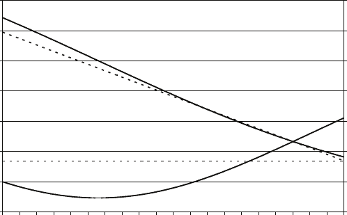
10.6. Answers to the additional exercises
increases. This is in keeping with the idea that further schooling may have less
effect on the highly educated than on the less educated (but the difference is not
large).
Add the probability function and the marginal effect function for the LPM to the
diagram. Explain why you drew them the way you did.
0
0.1
0.2
0.3
0.4
0.5
0.6
0.7
0 1 2 3 4 5 6 7 8 9 10 11 12 13 14 15 16 17 18 19 20
years of schooling
probability of being obese
-0.028
-0.024
-0.020
-0.016
-0.012
-0.008
-0.004
0.000
marginal effect
probability
marginal effect
!
!
!
Figure 10.6: Scatter diagram of probability of being obese and marginal effect against
years of schooling.
The estimated probability function for the LPM is just the regression equation and
the marginal effect is the coefficient of S. They are shown as the dashed lines in the
diagram.
The logit model is considered to have several advantages over the LPM. Explain
what these advantages are. Evaluate the importance of the advantages of the logit
model in this particular case.
The disadvantages of the LPM are (1) that it can give nonsense fitted values
(predicted probabilities greater than 1 or less than 0); (2) the disturbance term in
observation i must be equal to either −1−F(Zi) (if the dependent variable is equal
to 1) or −F(Zi) (if the dependent variable is equal to 0) and so it violates the usual
assumption that the disturbance term is normally distributed, although this may
not matter asymptotically; (3) the disturbance term will be heteroskedastic
because Ziis different for different observations; (4) the LPM implicitly assumes
that the marginal effect of each explanatory variable is constant over its entire
range, which is often intuitively unappealing.
In this case, nonsense predictions are clearly not an issue. The assumption of a
constant marginal effect does not seem to be a problem either, given the
approximate linearity of the logit F(Z).
The LPM is fitted using OLS. Explain how, instead, it might be fitted using
maximum likelihood estimation:
Write down the probability of being obese for any obese individual, given Sifor that
individual, and write down the probability of not being obese for any non-obese
235

10. Binary choice and limited dependent variable models, and maximum likelihood estimation
individual, again given Sifor that individual.
Obese: pO
i=β1+β2Si; not obese: pNO
i= 1 −β1−β2Si.
Write down the likelihood function for this sample of 164 obese individuals and 376
non-obese individuals.
L(β1, β2|data) = Y
OBESE
pO
iY
NOT OBESE
pNO
i=Y
OBESE
(β1+β2Si)Y
NOT OBESE
(1−β1−β2Si).
Explain how one would use this function to estimate the parameters. [Note: You
are not expected to attempt to derive the estimators of the parameters.]
You would use some algorithm to find the values of β1and β2that maximises the
function.
Explain whether your maximum likelihood estimators will be the same or different
from those obtained using least squares.
Least squares involves finding the extremum of a completely different expression
and will therefore lead to different estimators.
10.4 Explain how one may derive the marginal effects of the explanatory variables on the
probability of having a child less than 6 in the household, and calculate for both
males and females the marginal effects at the means of AGE and S.
Since pis a function of Z, and Zis a linear function of the Xvariables, the
marginal effect of Xjis:
∂p
∂Xj
=dp
dZ
∂Z
∂Xj
=dp
dZβj
where βjis the coefficient of Xjin the expression for Z. In the case of probit
analysis, p=F(Z) is the cumulative standardised normal distribution. Hence
dp/dZis just the standardised normal distribution.
For males, this is 0.368 when evaluated at the means. Hence the marginal effect of
AGE is 0.368 × −0.137 = −0.050 and that of Sis 0.368 ×0.132 = 0.049. For
females the corresponding figures are 0.272 × −0.154 = −0.042 and
0.272 ×0.094 = 0.026, respectively. So for every extra year of age, the probability is
reduced by 5.0 per cent for males and 4.2 per cent for females. For every extra year
of schooling, the probability increases by 4.9 per cent for males and 2.6 per cent for
females.
Explain whether the signs of the marginal effects are plausible. Explain whether you
would expect the marginal effect of schooling to be higher for males or for females.
Yes. Given that the cohort is aged 35–42, the respondents have passed the age at
which most adults start families, and the older they are, the less likely they are to
have small children in the household. At the same time, the more educated the
respondent, the more likely he or she is to have started having a family relatively
late, so the positive effect of schooling is also plausible. However, given the age of
the cohort, it is likely to be weaker for females than for males, given that most
females intending to have families will have started them by this time, irrespective
of their education.
236

10.6. Answers to the additional exercises
At a seminar someone asks the researcher whether the marginal effect of S is
significantly different for males and females. The researcher does not know how to
test whether the difference is significant and asks you for advice. What would you
say?
Fit a probit regression for the combined sample, adding a male intercept dummy
and male slope dummies for AGE and S. Test the coefficient of the slope dummy
for S.
10.5 The Zfunction will be of the form:
Z=β1+β2A+β3S+β4AS
so the marginal effects are:
∂p
∂A =dp
dZ
∂Z
∂A =f(Z)(β2+β4S)
and: ∂p
∂S =dp
dZ
∂Z
∂S =f(Z)(β3+β4A).
Both factors depend on the values of Aand/or S, but the marginal effects could be
evaluated for a representative individual using the mean values of Aand Sin the
sample.
A10.6 Discuss the conclusions one may reach, given the probit output and the table,
commenting on their plausibility.
Being male has a small but highly significant negative effect. This is plausible
because males tend to marry later than females and the cohort is still relatively
young.
Age has a highly significant positive effect, again plausible because older people are
more likely to have married than younger people.
Schooling has no apparent effect at all. It is not obvious whether this is plausible.
Cognitive ability has a highly significant positive effect. Again, it is not obvious
whether this is plausible.
The researcher considers including CHILD, a dummy variable defined to be 1 if the
respondent had children, and 0 otherwise, as an explanatory variable. When she
does this, its z-statistic is 33.65 and its marginal effect 0.5685. Discuss these
findings.
Obviously one would expect a high positive correlation between being married and
having children and this would account for the huge and highly significant
coefficient. However getting married and having children are often a joint decision,
and accordingly it is simplistic to suppose that one characteristic is a determinant
of the other. The finding should not be taken at face value.
A10.7 Determine the maximum likelihood estimate of α, assuming that βis known.
The log-likelihood function is:
log L(α|β, T1, . . . , Tn) = nlog α−αX(Ti−β).
237

10. Binary choice and limited dependent variable models, and maximum likelihood estimation
Setting the first derivative with respect to αequal to zero, we have:
n
bα−X(Ti−β)=0
and hence:
bα=1
T−β.
The second derivative is −n/bα2, which is negative, confirming we have maximised
the loglikelihood function.
A10.8 From the solution to Exercise 10.14, the log-likelihood function for pis:
log L(p) = mlog p+ (n−m) log(1 −p).
Thus the LR statistic is:
LR = 2 mlog m
n+ (n−m) log 1−m
n−(mlog p0+ (n−m) log(1 −p0))
= 2 mlog m/n
p0+ (n−m) log 1−m/n
1−p0.
If m= 40 and n= 100, the LR statistic for H0:p= 0.5 is:
LR = 2 40 log 0.4
0.5+ 60 log 0.6
0.5= 4.03.
We would reject the null hypothesis at the 5 per cent level (critical value of
chi-squared with one degree of freedom 3.84) but not at the 1 per cent level
(critical value 6.64).
A10.9 The first derivative of the log-likelihood function is:
d log L(p)
dp=m
p−n−m
1−p= 0
and the second differential is:
d log L(p)
dp2=−m
p2−n−m
(1 −p)2.
Evaluated at p=m/n:
d log L(p)
dp2=−n2
m−n−m
1−m
n2=−n21
m+1
n−m=−n3
m(n−m).
The variance of the ML estimate is given by:
−d log L(p)
dp2−1
=n3
m(n−m)−1
=m(n−m)
n3.
The Wald statistic is therefore:
m
n−p02
m(n−m)
n3
=m
n−p02
1
n
m
n
n−m
n
.
Given the data, this is equal to:
(0.4−0.5)2
1
100 ×0.4×0.6= 4.17.
Under the null hypothesis this has a chi-squared distribution with one degree of
freedom, and so the conclusion is the same as in Exercise A.8.
238

Chapter 11
Models using time series data
11.1 Overview
This chapter introduces the application of regression analysis to time series data,
beginning with static models and then proceeding to dynamic models with lagged
variables used as explanatory variables. It is shown that multicollinearity is likely to be
a problem in models with unrestricted lag structures and that this provides an incentive
to use a parsimonious lag structure, such as the Koyck distribution. Two models using
the Koyck distribution, the adaptive expectations model and the partial adjustment
model, are described, together with well-known applications to aggregate consumption
theory, Friedman’s permanent income hypothesis in the case of the former and Brown’s
habit persistence consumption function in the case of the latter. The chapter concludes
with a discussion of prediction and stability tests in time series models.
11.2 Learning outcomes
After working through the corresponding chapter in the text, studying the
corresponding slideshows, and doing the starred exercises in the text and the additional
exercises in this subject guide, you should be able to:
explain why multicollinearity is a common problem in time series models, especially
dynamic ones with lagged explanatory variables
describe the properties of a model with a lagged dependent variable (ADL(1,0)
model)
describe the assumptions underlying the adaptive expectations and partial
adjustment models
explain the properties of OLS estimators of the parameters of ADL(1,0) models
explain how predetermined variables may be used as instruments in the fitting of
models using time series data
explain in general terms the objectives of time series analysts and those
constructing VAR models.
239
11. Models using time series data
11.3 Additional exercises
A11.1 The output below shows the result of linear and logarithmic regressions of
expenditure on food on income, relative price, and population (measured in
thousands) using the Demand Functions data set, together with the correlations
among the variables. Provide an interpretation of the regression coefficients and
perform appropriate statistical tests.
============================================================
Dependent Variable: FOOD
Method: Least Squares
Sample: 1959 2003
Included observations: 45
============================================================
Variable Coefficient Std. Error t-Statistic Prob.
============================================================
C -19.49285 88.86914 -0.219343 0.8275
DPI 0.031713 0.010658 2.975401 0.0049
PRELFOOD 0.403356 0.365133 1.104681 0.2757
POP 0.001140 0.000563 2.024017 0.0495
============================================================
R-squared 0.988529 Mean dependent var 422.0374
Adjusted R-squared 0.987690 S.D. dependent var 91.58053
S.E. of regression 10.16104 Akaike info criteri7.559685
Sum squared resid 4233.113 Schwarz criterion 7.720278
Log likelihood -166.0929 F-statistic 1177.745
Durbin-Watson stat 0.404076 Prob(F-statistic) 0.000000
============================================================
============================================================
Dependent Variable: LGFOOD
Method: Least Squares
Sample: 1959 2003
Included observations: 45
============================================================
Variable Coefficient Std. Error t-Statistic Prob.
============================================================
C 5.293654 2.762757 1.916077 0.0623
LGDPI 0.589239 0.080158 7.351014 0.0000
LGPRFOOD -0.122598 0.084355 -1.453361 0.1537
LGPOP -0.289219 0.258762 -1.117706 0.2702
============================================================
R-squared 0.992245 Mean dependent var 6.021331
Adjusted R-squared 0.991678 S.D. dependent var 0.222787
S.E. of regression 0.020324 Akaike info criter-4.869317
Sum squared resid 0.016936 Schwarz criterion -4.708725
Log likelihood 113.5596 F-statistic 1748.637
Durbin-Watson stat 0.488502 Prob(F-statistic) 0.000000
============================================================
240
11.3. Additional exercises
Correlation Matrix
============================================================
LGFOOD LGDPI LGPRFOOD LGPOP
============================================================
LGFOOD 1.000000 0.995896 -0.613437 0.990566
LGDPI 0.995896 1.000000 -0.604658 0.995241
LGPRFOOD -0.613437 -0.604658 1.000000 -0.641226
LGPOP 0.990566 0.995241 -0.641226 1.000000
============================================================
A11.2 Perform regressions parallel to those in Exercise A11.1 using your category of
expenditure and provide an interpretation of the coefficients.
A11.3 The output shows the result of a logarithmic regression of expenditure on food per
capita, on income per capita, both measured in US$ million, and the relative price
index for food. Provide an interpretation of the coefficients, demonstrate that the
specification is a restricted version of the logarithmic regression in Exercise A11.1,
and perform an Ftest of the restriction.
============================================================
Dependent Variable: LGFOODPC
Method: Least Squares
Sample: 1959 2003
Included observations: 45
============================================================
Variable Coefficient Std. Error t-Statistic Prob.
============================================================
C -5.425877 0.353655 -15.34231 0.0000
LGDPIPC 0.280229 0.014641 19.14024 0.0000
LGPRFOOD 0.052952 0.082588 0.641160 0.5249
============================================================
R-squared 0.927348 Mean dependent var-6.321984
Adjusted R-squared 0.923889 S.D. dependent var 0.085249
S.E. of regression 0.023519 Akaike info criter-4.597688
Sum squared resid 0.023232 Schwarz criterion -4.477244
Log likelihood 106.4480 F-statistic 268.0504
Durbin-Watson stat 0.417197 Prob(F-statistic) 0.000000
============================================================
A11.4 Perform a regression parallel to that in Exercise A11.3 using your category of
expenditure. Provide an interpretation of the coefficients, and perform an Ftest of
the restriction.
A11.5 The output shows the result of a logarithmic regression of expenditure on food per
capita, on income per capita, the relative price index for food, and population.
Provide an interpretation of the coefficients, demonstrate that the specification is
equivalent to that for the logarithmic regression in Exercise A11.1, and use it to
perform a ttest of the restriction in Exercise A11.3.
============================================================
Dependent Variable: LGFOODPC
Method: Least Squares
Sample: 1959 2003
241
11. Models using time series data
Included observations: 45
============================================================
Variable Coefficient Std. Error t-Statistic Prob.
============================================================
C 5.293654 2.762757 1.916077 0.0623
LGDPIPC 0.589239 0.080158 7.351014 0.0000
LGPRFOOD -0.122598 0.084355 -1.453361 0.1537
LGPOP -0.699980 0.179299 -3.903973 0.0003
============================================================
R-squared 0.947037 Mean dependent var-6.321984
Adjusted R-squared 0.943161 S.D. dependent var 0.085249
S.E. of regression 0.020324 Akaike info criter-4.869317
Sum squared resid 0.016936 Schwarz criterion -4.708725
Log likelihood 113.5596 F-statistic 244.3727
Durbin-Watson stat 0.488502 Prob(F-statistic) 0.000000
============================================================
A11.6 Perform a regression parallel to that in Exercise A11.5 using your category of
expenditure, and perform a ttest of the restriction implicit in the specification in
Exercise A11.4.
A11.7 In Exercise 11.9 you fitted the model:
LGCAT =β1+β2LGDPI +β3LGDPI (−1) + β4LGPRCAT +β5LGPRCAT (−1) + u
where CAT stands for your category of expenditure.
•Show that (β2+β3) and (β4+β5) are theoretically the long-run (equilibrium)
income and price elasticities.
•Reparameterise the model and fit it to obtain direct estimates of these
long-run elasticities and their standard errors.
•Confirm that the estimates are equal to the sum of the individual shortrun
elasticities found in Exercise 11.9.
•Compare the standard errors with those found in Exercise 11.9 and state your
conclusions.
A11.8 In a certain bond market, the demand for bonds, Bt, in period tis negatively
related to the expected interest rate, ie
t+1, in period t+ 1:
Bt=β1+β2ie
t+1 +ut(1)
where utis a disturbance term not subject to autocorrelation. The expected
interest rate is determined by an adaptive expectations process:
ie
t+1 −ie
t=λ(it−ie
t) (2)
where itis the actual rate of interest in period t. A researcher uses the following
model to fit the relationship:
Bt=γ1+γ2it+γ3Bt−1+vt(3)
where vtis a disturbance term.
242
11.3. Additional exercises
•Show how this model may be derived from the demand function and the
adaptive expectations process.
•Explain why inconsistent estimates of the parameters will be obtained if
equation (3) is fitted using ordinary least squares (OLS). (A mathematical
proof is not required. Do not attempt to derive expressions for the bias.)
•Describe a method for fitting the model that would yield consistent estimates.
•Suppose that utwas subject to the first-order autoregressive process:
ut=ρut−1+εt
where εtis not subject to autocorrelation. How would this affect your answer
to the second part of this question?
•Suppose that the true relationship was actually:
Bt=β1+β2it+ut(1∗)
with utnot subject to autocorrelation, and the model is fitted by regressing Bt
on itand Bt−1, as in equation (3), using OLS. How would this affect the
regression results?
•How plausible do you think an adaptive expectations process is for modelling
expectations in a bond market?
A11.9 The output shows the result of a logarithmic regression of expenditure on food on
income, relative price, population, and lagged expenditure on food using the
Demand Functions data set. Provide an interpretation of the regression coefficients,
paying attention to both short-run and long-run dynamics, and perform
appropriate statistical tests.
============================================================
Dependent Variable: LGFOOD
Method: Least Squares
Sample(adjusted): 1960 2003
Included observations: 44 after adjusting endpoints
============================================================
Variable Coefficient Std. Error t-Statistic Prob.
============================================================
C 1.487645 2.072156 0.717921 0.4771
LGDPI 0.143829 0.090334 1.592194 0.1194
LGPRFOOD -0.095749 0.061118 -1.566613 0.1253
LGPOP -0.046515 0.189453 -0.245524 0.8073
LGFOOD(-1) 0.727290 0.113831 6.389195 0.0000
============================================================
R-squared 0.995886 Mean dependent var 6.030691
Adjusted R-squared 0.995464 S.D. dependent var 0.216227
S.E. of regression 0.014564 Akaike info criter-5.513937
Sum squared resid 0.008272 Schwarz criterion -5.311188
Log likelihood 126.3066 F-statistic 2359.938
Durbin-Watson stat 1.103102 Prob(F-statistic) 0.000000
============================================================
243
11. Models using time series data
A11.10 Perform a regression parallel to that in Exercise A11.9 using your category of
expenditure. Provide an interpretation of the coefficients, and perform appropriate
statistical tests.
A11.11 In his classic study Distributed Lags and Investment Analysis (1954), Koyck
investigated the relationship between investment in railcars and the volume of
freight carried on the US railroads using data for the period 1884–1939. Assuming
that the desired stock of railcars in year tdepended on the volume of freight in
year t−1 and year t−2 and a time trend, and assuming that investment in
railcars was subject to a partial adjustment process, he fitted the following
regression equation using OLS (standard errors and constant term not reported):
b
It= 0.077Ft−1+ 0.017Ft−2−0.0033t−0.110Kt−1R2= 0.85
where It=Kt−Kt−1is investment in railcars in year t(thousands), Ktis the stock
of railcars at the end of year t(thousands), and Ftis the volume of freight handled
in year t(ton-miles).
Provide an interpretation of the equation and describe the dynamic process implied
by it. (Note: It is best to substitute Kt−Kt−1for Itin the regression and treat it
as a dynamic relationship determining Kt.)
A11.12 Two researchers agree that a model consists of the following relationships:
Yt=α1+α2Xt+ut(1)
Xt=β1+β2Yt−1+vt(2)
Zt=γ1+γ2Yt+γ3Xt+γ4Qt+wt(3)
where ut,vt, and wt, are disturbance terms that are drawn from fixed distributions
with zero mean. It may be assumed that they are distributed independently of Qt
and of each other and that they are not subject to autocorrelation. All the
parameters may be assumed to be positive and it may be assumed that α2β2<1.
•One researcher asserts that consistent estimates will be obtained if (2) is fitted
using OLS and (1) is fitted using IV, with Yt−1as an instrument for Xt.
Determine whether this is true.
•The other researcher asserts that consistent estimates will be obtained if both
(1) and (2) are fitted using OLS, and that the estimate of β2will be more
efficient than that obtained using IV. Determine whether this is true.
244

11.4. Answers to the starred exercises in the textbook
11.4 Answers to the starred exercises in the textbook
11.6
Year Y K L Year Y K L
1899 100 100 100 1911 153 216 145
1900 101 107 105 1912 177 226 152
1901 112 114 110 1913 184 236 154
1902 122 122 118 1914 169 244 149
1903 124 131 123 1915 189 266 154
1904 122 138 116 1916 225 298 182
1905 143 149 125 1917 227 335 196
1906 152 163 133 1918 223 366 200
1907 151 176 138 1919 218 387 193
1908 126 185 121 1920 231 407 193
1909 155 198 140 1921 179 417 147
1910 159 208 144 1922 240 431 161
Source: Cobb and Douglas (1928)
The table gives the data used by Cobb and Douglas (1928) to fit the original
Cobb–Douglas production function:
Yt=β1Kβ2
tLβ3
tvt
Yt,Kt, and Lt, being index number series for real output, real capital input, and
real labour input, respectively, for the manufacturing sector of the United States for
the period 1899–1922 (1899 = 100). The model was linearised by taking logarithms
of both sides and the following regressions was run (standard errors in parentheses):
[
log Y=−0.18 + 0.23 log K+ 0.81 log L R2= 0.96
(0.43) (0.06) (0.15)
Provide an interpretation of the regression coefficients.
Answer:
The elasticities of output with respect to capital and labour are 0.23 and 0.81,
respectively, both coefficients being significantly different from zero at very high
significance levels. The fact that the sum of the elasticities is close to one suggests
that there may be constant returns to scale. Regressing output per worker on
capital per worker, one has:
\
log Y
L= 0.01 + 0.25 log K
LR2= 0.63
(0.02) (0.04)
The smaller standard error of the slope coefficient suggests a gain in efficiency.
Fitting a reparameterised version of the unrestricted model:
\
log Y
L=−0.18 + 0.23 log K
L+ 0.04 log L R2= 0.64
(0.43) (0.06) (0.09)
we find that the restriction is not rejected.
245

11. Models using time series data
11.7 The Cobb–Douglas model in Exercise 11.6 makes no allowance for the possibility
that output may be increasing as a consequence of technical progress,
independently of Kand L. Technical progress is difficult to quantify and a common
way of allowing for it in a model is to include an exponential time trend:
Yt=β1Kβ2
tLβ3
teρtvt
where ρis the rate of technical progress and tis a time trend defined to be 1 in the
first year, 2 in the second, etc. The correlations between log K, log Land tare
shown in the table. Comment on the regression results.
[
log Y= 2.81 −0.53 log K+ 0.91 log L+ 0.047t R2= 0.97
(1.38) (0.34) (0.14) (0.021)
Correlation
================================================
LGK LGL TIME
================================================
LGK 1.000000 0.909562 0.996834
LGL 0.909562 1.000000 0.896344
TIME 0.996834 0.896344 1.000000
================================================
Answer:
The elasticity of output with respect to labour is higher than before, now
implausibly high given that, under constant returns to scale, it should measure the
share of wages in output. The elasticity with respect to capital is negative and
nonsensical. The coefficient of time indicates an annual exponential growth rate of
4.7 per cent, holding Kand Lconstant. This is unrealistically high for the period
in question. The implausibility of the results, especially those relating to capital
and time (correlation 0.997), may be attributed to multicollinearity.
11.16 Demonstrate that the dynamic process (11.18) implies the long-run relationship
given by (11.15).
Answer:
Equations (11.15) and (11.18) are:
˜
Y=β1
1−β3
+β2
1−β3
˜
X(11.15)
Yt=β1(1 + β3+β2
3+···) + β2Xt+β2β3Xt−1+β2β2
3Xt−2+··· (11.18)
+ut+β3ut−1+β2
3ut−2+··· .
Putting X=˜
Xfor all Xin (11.18), and ignoring the disturbance terms, the
long-run relationship between Yand Xis given by:
˜
Y=β1(1 + β3+β2
3+···) + β2˜
X+β2β3˜
X+β2β2
3˜
X+···
=β1
1−β3
+ (1 + β3+β2
3+···)β2˜
X
=β1
1−β3
+β2
1−β3
˜
X.
246
11.4. Answers to the starred exercises in the textbook
11.17 The compound disturbance term in the adaptive expectations model (11.37) does
potentially give rise to a problem that will be discussed in Chapter 12 when we
come to the topic of autocorrelation. It can be sidestepped by representing the
model in the alternative form.
Yt=β1+β2λXt+β2λ(1 −λ)Xt−1+···+β2λ(1 −λ)sXt−s+β2(1 −λ)s+1Xe
t−s+ut.
Show how this form might be obtained, and discuss how it might be fitted.
Answer:
We start by reprising equations (11.31) – (11.34) in the text. We assume that the
dependent variable Ytis related to Xe
t+1, the value of Xanticipated in the next
time period:
Yt=γ1+γ2Xe
t+1 +ut.(11.31)
To make the model operational, we hypothesise that expectations are updated in
response to the discrepancy between what had been anticipated for the current
time period, Xe
t+1, and the actual outcome, Xt:
Xe
t+1 −Xe
t=λ(Xt−Xe
t) (11.32)
where λmay be interpreted as a speed of adjustment. We can rewrite this as
(11.33):
Xe
t+1 =λXt+ (1 −λ)Xe
t.(11.33)
Hence we obtain (11.34):
Yt=γ1+γ2λXt+γ2(1 −λ)Xe
t+ut.(11.34)
This includes the unobservable Xe
ton the right side. However, lagging (11.33), we
have:
Xe
t=λXt−1+ (1 −λ)Xe
t−1.
Hence:
Yt=γ1+γ2λXt+γ2λ(1 −λ)Xt−1+γ2(1 −λ)2Xe
t−1+ut.
This includes the unobservable Xe
t−1on the right side. However, continuing to lag
and substitute, we have:
Yt=γ1+γ2λXt+γ2λ(1 −λ)Xt−1+··· +γ2λ(1 −λ)sXt−s+γ2(1 −λ)s+1Xe
t−s+ut.
Provided that sis large enough for γ2(1 −λ)s+1 to be very small, this may be
fitted, omitting the unobservable final term, with negligible omitted variable bias.
We would fit it with a nonlinear regression technique that respected the constraints
implicit in the theoretical structure of the coefficients.
11.19 The output below shows the result of fitting the model:
LGFOOD =β1+β2λLGDPI +β2λ(1 −λ)LGDPI (−1) + β2λ(1 −λ)2LGDPI (−2)
+β2λ(1 −λ)3LGDPI (−3) + β3LGPRFOOD +u
using the data on expenditure on food in the Demand Functions data set.
LGFOOD and LGPRFOOD are the logarithms of expenditure on food and the
247
11. Models using time series data
relative price index series for food. C(1), C(2), C(3), and C(4) are estimates of β1,
β2,λand β3, respectively. Explain how the regression equation could be interpreted
as an adaptive expectations model and discuss the dynamics implicit in it, both
short-run and long-run. Should the specification have included further lagged
values of LGDPI ?
============================================================
Dependent Variable: LGFOOD
Method: Least Squares
Sample(adjusted): 1962 2003
Included observations: 42 after adjusting endpoints
Convergence achieved after 25 iterations
LGFOOD=C(1)+C(2)*C(3)*LGDPI + C(2)*C(3)*(1-C(3))*LGDPI(-1) + C(2)
*C(3)*(1-C(3))^2*LGDPI(-2) + C(2)*C(3)*(1-C(3))^3*LGDPI(-3) +
C(4)*LGPRFOOD
============================================================
Coefficient Std. Error t-Statistic Prob.
============================================================
C(1) 2.339513 0.468550 4.993091 0.0000
C(2) 0.496425 0.012264 40.47818 0.0000
C(3) 0.915046 0.442851 2.066264 0.0457
C(4) -0.089681 0.083250 -1.077247 0.2882
============================================================
R-squared 0.989621 Mean dependent var 6.049936
Adjusted R-squared 0.988802 S.D. dependent var 0.201706
S.E. of regression 0.021345 Akaike info criter-4.765636
Sum squared resid 0.017313 Schwarz criterion -4.600143
Log likelihood 104.0784 Durbin-Watson stat 0.449978
============================================================
Answer:
Suppose that the model is:
LGFOODt=γ1+γ2LGDPI e
t+1 +γ3LGPRFOODt+ut
where LGDPI e
t+1 is expected LGDPI at time t+ 1, and that expectations for
income are subject to the adaptive expectations process:
LGDPI e
t+1 −LGDPI e
t=λ(LGDPI t−LGDPI e
t).
The adaptive expectations process may be rewritten:
LGDPI e
t+1 =λLGDPI t+ (1 −λ)LGDPI e
t.
Lagging this equation one period and substituting, one has:
LGDPI e
t+1 =λLGDPI t+λ(1 −λ)LGDPI t−1+ (1 −λ)2LGDPI e
t−1.
Lagging a second time and substituting, one has:
LGDPI e
t+1 =λLGDPI t+λ(1−λ)LGDPI t−1+λ(1−λ)2LGDPI t−2+(1−λ)3LGDPI e
t−2.
Lagging a third time and substituting, one has:
LGDPI e
t+1 =λLGDPI t+λ(1 −λ)LGDPI t−1+λ(1 −λ)2LGDPI t−2
+λ(1 −λ)3LGDPI e
t−3+ (1 −λ)4LGDPI e
t−3.
248

11.4. Answers to the starred exercises in the textbook
Substituting this into the model, dropping the final unobservable term, one has the
regression specification as stated in the question.
The estimates imply that the short-run income elasticity is 0.50. The speed of
adjustment of expectations is 0.92. Hence the long-run income elasticity is
0.50/0.92 = 0.54. The price side of the model has been assumed to be static. The
estimate of the price elasticity is −0.09. The coefficient of the dropped
unobservable term is γ2(1 −λ)4. Given our estimates of γ2and λ, its estimate is
0.0003. Hence we are justified in neglecting it.
11.22 A researcher is fitting the following supply and demand model for a certain
commodity, using a sample of time series observations:
Qdt =β1+β2Pt+udt
Qst =α1+α2Pt+ust
where Qdt is the amount demanded at time t,Qst is the amount supplied, Ptis the
market clearing price, and udt and ust are disturbance terms that are not
necessarily independent of each other. It may be assumed that the market clears
and so Qdt =Qst.
•What can be said about the identification of (a) the demand equation, (b) the
supply equation?
•What difference would it make if supply at time twas determined instead by
price at time t−1? That is:
Qst =α1+α2Pt−1+ust.
•What difference would it make if it could be assumed that udt is distributed
independently of ust?
Answer:
The reduced form equation for Ptis:
Pt=1
α2−β2
(β1−α1+udt −ust).
Ptis not independent of the disturbance term in either equation and so OLS would
yield inconsistent estimates. There is no instrument available, so both equations are
underidentified.
Provided that udt is not subject to autocorrelation, Pt−1could be used as an
instrument in the demand equation. Provided that ust is not subject to
autocorrelation, OLS could be used to fit the second equation. It makes no
difference whether or not udt is distributed independently of ust.
The first equation could, alternatively, be fitted using OLS, with the variables
switched. From the second equation, Pt−1determines Qt, and then, given Qt, the
demand equation determines Pt:
Pt=1
β2
(Qt−β1−udt).
The reciprocal of the slope coefficient provides a consistent estimator of β2.
249
11. Models using time series data
11.24 Consider the following simple macroeconomic model:
Ct=β1+β2Yt+uCt
It=α1+α2(Yt−Yt−1) + uIt
Yt=Ct+It
where Ct,It, and Ytare aggregate consumption, investment, and income and uCt
and uItare disturbance terms. The first relationship is a conventional consumption
function. The second relates investment to the change of output from the previous
year. (This is known as an ‘accelerator’ model.) The third is an income identity.
What can be said about the identification of the relationships in the model?
Answer:
The restriction on the coefficients of Ytand Yt−1in the investment equation
complicates matters. A simple way of handling it is to define:
∆Yt=Yt−Yt−1
and to rewrite the investment equation as:
It=α1+α2∆Yt+uIt.
We now have four endogenous variables and four equations, and one exogenous
variable. The consumption and investment equations are exactly identified. We
would fit them using Yt−1as an instrument for Ytand ∆Yt, respectively. The other
two equations are identities and do not need to be fitted.
11.5 Answers to the additional exercises
A11.1 The linear regression indicates that expenditure on food increases by $0.032 billion
for every extra $ billion of disposable personal income (in other words, by 3.2 cents
out of the marginal dollar), that it increases by $0.403 billion for every point
increase in the price index, and that it increases by $0.001 billion for every
additional thousand population. The income coefficient is significant at the 1 per
cent level (ignoring problems to be discussed in Chapter 12). The positive price
coefficient makes no sense (remember that the dependent variable is measured in
real terms). The intercept has no plausible interpretation.
The logarithmic regression indicates that the income elasticity is 0.59 and highly
significant, and the price elasticity is −0.12, not significant. The negative elasticity
for population is not plausible. One would expect expenditure on food to increase
in line with population, controlling for other factors, and hence, as a first
approximation, the elasticity should be equal to 1. However, an increase in
population, keeping income constant, would lead to a reduction in income per
capita and hence to a negative income effect. Given that the income elasticity is
less than 1, one would still expect a positive elasticity overall for population. At
least the estimate is not significantly different from zero. In view of the high
correlation, 0.995, between LGDPI and LGPOP, the negative estimate may well be
a result of multicollinearity.
250

11.5. Answers to the additional exercises
A11.2
OLS logarithmic regressions
LGDPI LGP LGPOP R2
coef. s.e. coef. s.e. coef. s.e.
ADM −1.43 0.20 −0.28 0.10 6.88 0.61 0.975
BOOK −0.29 0.28 −1.18 0.21 4.94 0.82 0.977
BUSI 0.36 0.19 −0.11 0.27 2.79 0.51 0.993
CLOT 0.71 0.10 −0.70 0.05 0.15 0.36 0.998
DENT 1.23 0.14 −0.95 0.09 0.26 0.54 0.995
DOC 0.97 0.14 0.26 0.13 −0.27 0.52 0.993
FLOW 0.46 0.32 0.16 0.33 3.07 1.21 0.987
FOOD 0.59 0.08 −0.12 0.08 −0.29 0.26 0.992
FURN 0.36 0.28 −0.48 0.26 1.66 1.12 0.985
GAS 1.27 0.24 −0.24 0.06 −2.81 0.74 0.788
GASO 1.46 0.16 −0.10 0.04 −2.35 0.49 0.982
HOUS 0.91 0.08 −0.54 0.06 0.38 0.25 0.999
LEGL 1.17 0.16 −0.08 0.13 −1.50 0.54 0.976
MAGS 1.05 0.22 −0.73 0.44 −0.82 0.54 0.970
MASS −1.92 0.22 −0.57 0.14 6.14 0.65 0.785
OPHT 0.30 0.45 0.28 0.59 3.68 1.40 0.965
RELG 0.56 0.13 −0.99 0.23 2.72 0.41 0.996
TELE 0.91 0.13 −0.61 0.11 1.79 0.49 0.998
TOB 0.54 0.17 −0.42 0.04 −1.21 0.57 0.883
TOYS 0.59 0.10 −0.54 0.06 2.57 0.39 0.999
The price elasticities mostly lie in the range 0 to −1, as they should, and therefore
seem plausible. However the very high correlation between income and population,
0.995, has given rise to a problem of multicollinearity and as a consequence the
estimates of their elasticities are very erratic. Some of the income elasticities look
plausible, but that may be pure chance, for many are unrealistically high, or
negative when obviously they should be positive. The population elasticities are
even less convincing.
Correlations between prices, income and population
LGP,LGDPI LGP,LGPOP LGP,LGDPI LGP,LGPOP
ADM 0.61 0.61 GASO 0.05 0.03
BOOK 0.88 0.87 HOUS 0.49 0.55
BUSI 0.98 0.97 LEGL 0.99 0.99
CLOT −0.94 −0.96 MAGS 0.99 0.98
DENT 0.94 0.96 MASS 0.90 0.89
DOC 0.98 0.98 OPHT −0.68 −0.67
FLOW −0.93 −0.95 RELG 0.92 0.92
FOOD −0.60 −0.64 TELE −0.98 −0.99
FURN −0.95 −0.97 TOB 0.83 0.86
GAS 0.77 0.76 TOYS −0.97 −0.98
251

11. Models using time series data
A11.3 The regression indicates that the income elasticity is 0.40 and the price elasticity
0.21, the former very highly significant, the latter significant at the 1 per cent level
using a one-sided test. If the specification is:
log FOOD
POP =β1+β2log DPI
POP +β3log PRELFOOD +u
it may be rewritten:
log FOOD =β1+β2log DPI +β3log PRELFOOD + (1 −β2) log POP +u.
This is a restricted form of the specification in Exercise A11.2:
log FOOD =β1+β2log DPI +β3log PRELFOOD +β4log POP +u
with β4= 1 −β2. We can test the restriction by comparing RSS for the two
regressions:
F(1,41) = (0.023232 −0.016936)/1
0.016936/41 = 15.24.
The critical value of F(1,40) at the 0.1 per cent level is 12.61. The critical value for
F(1,41) must be slightly lower. Thus we reject the restriction. Since the restricted
version is misspecified, our interpretation of the coefficients of this regression and
the ttests are invalidated.
A11.4 Given that the critical values of F(1,41) at the 5 and 1 per cent levels are 4.08 and
7.31 respectively, the results of the Ftest may be summarised as follows:
•Restriction not rejected: CLOT,DENT,DOC,FURN,HOUS.
•Restriction rejected at the 5 per cent level: MAGS.
•Restriction rejected at the 1 per cent level: ADM,BOOK,BUSI,FLOW,
FOOD,GAS,GASO,LEGL,MASS,OPHT,RELG,TELE,TOB,TOYS.
However, for reasons that will become apparent in the next chapter, these findings
must be regarded as provisional.
252

11.5. Answers to the additional exercises
Tests of a restriction
RSSURSSRF t
ADM 0.125375 0.480709 116.20 10.78
BOOK 0.223664 0.461853 43.66 6.61
BUSI 0.084516 0.167580 40.30 6.35
CLOT 0.021326 0.021454 0.25 −0.50
DENT 0.033275 0.034481 1.49 1.22
DOC 0.068759 0.069726 0.58 −0.76
FLOW 0.220256 0.262910 7.94 2.82
FOOD 0.016936 0.023232 15.24 −3.90
FURN 0.157153 0.162677 1.44 1.20
GAS 0.185578 0.300890 25.48 −5.05
GASO 0.078334 0.139278 31.90 −5.65
HOUS 0.011270 0.012106 3.04 1.74
LEGL 0.082628 0.102698 9.96 −3.16
MAGS 0.096620 0.106906 4.36 −2.09
MASS 0.143775 0.330813 53.34 7.30
OPHT 0.663413 0.822672 9.84 3.14
RELG 0.053785 0.135532 62.32 7.89
TELE 0.054519 0.080728 19.71 4.44
TOB 0.062452 0.087652 16.54 −4.07
TOYS 0.031269 0.071656 52.96 7.28
A11.5 If the specification is:
log FOOD
POP =β1+β2log DPI
POP +β3log PRELFOOD +γ1POP +u
it may be rewritten:
log FOOD =β1+β2log DPI +β3log PRELFOOD + (1 −β2+γ1) log POP +u.
This is equivalent to the specification in Exercise A11.1:
log FOOD =β1+β2log DPI +β3log PRELFOOD +β4log POP +u
with β4= 1 −β2+γ1. Note that this is not a restriction. (1) – (3) are just different
ways of writing the unrestricted model.
Attest of H0:γ1= 0 is equivalent to a ttest of H0:β4= 1 −β2, that is, that the
restriction in Exercise A11.3 is valid. The tstatistic for LGPOP in the regression is
−3.90, and hence again we reject the restriction. Note that the test is equivalent to
the Ftest. −3.90 is the square root of 15.24, the Fstatistic, and it can be shown
that the critical value of tis the square root of the critical value of F.
A11.6 The tstatistics for all the categories of expenditure are supplied in the table in the
answer to Exercise A11.4. Of course they are equal to the square root of the F
statistic, and their critical values are the square roots of the critical values of F, so
the conclusions are identical and, like those of the Ftest, should be treated as
provisional.
253

11. Models using time series data
A11.7 Show that β2+β3and (β4+β5)are theoretically the long-run (equilibrium) income
and price elasticities.
In equilibrium, LGCAT =LGCAT,LGDPI =LGDPI (−1) = LGDPI and
LGPRCAT =LGPRCAT (−1) = LGPRCAT. Hence, ignoring the transient effect
of the disturbance term:
LGCAT =β1+β2LGDPI +β3LGDPI +β4LGPRCAT +β5LGPRCAT
=β1+ (β2+β3)LGDPI + (β4+β5)LGPRCAT.
Thus the long-run equilibrium income and price elasticities are θ=β2+β3and
φ=β4+β5, respectively.
Reparameterise the model and fit it to obtain direct estimates of these long-run
elasticities and their standard errors.
We will reparameterise the model to obtain direct estimates of θand φand their
standard errors. Write β3=θ−β2and φ=β4+β5and substitute for β3and β5in
the model. We obtain:
LGCAT =β1+β2LGDPI + (θ−β2)LGDPI (−1) + β4LGPRCAT + (φ−β4)LGPRCAT (−1) + u
=β1+β2(LGDPI −LGDPI (−1)) + θLGDPI (−1)
+β4(LGPRCAT −LGPRCAT (−1)) + φLGPRCAT (−1) + u
=β1+β2DLGDPI +θLGDPI (−1) + β4DLGPRCAT +φLGPRCAT (−1) + u
where DLGDPI =LGDPI −LGDPI (−1) and DLGPRCAT =LGPRCAT −
LGPRCAT (−1).
The output for HOUS is shown below. DLGPRCAT has been abbreviated as
DLGP.
============================================================
Dependent Variable: LGHOUS
Method: Least Squares
Sample(adjusted): 1960 2003
Included observations: 44 after adjusting endpoints
============================================================
Variable Coefficient Std. Error t-Statistic Prob.
============================================================
C 0.020785 0.144497 0.143844 0.8864
DLGDPI 0.329571 0.150397 2.191340 0.0345
LGDPI(-1) 1.013147 0.006815 148.6735 0.0000
DLGP -0.088813 0.165651 -0.536144 0.5949
LGPRHOUS(-1) -0.447176 0.035927 -12.44689 0.0000
============================================================
R-squared 0.999039 Mean dependent var 6.379059
Adjusted R-squared 0.998940 S.D. dependent var 0.421861
S.E. of regression 0.013735 Akaike info criter-5.631127
Sum squared resid 0.007357 Schwarz criterion -5.428379
Log likelihood 128.8848 F-statistic 10131.80
Durbin-Watson stat 0.536957 Prob(F-statistic) 0.000000
============================================================
Confirm that the estimates are equal to the sum of the individual shortrun
elasticities found in Exercise 11.9.
The estimates of the long-run income and price elasticities are 1.01 and −0.45,
respectively. The output below is for the model in its original form, where the
254
11.5. Answers to the additional exercises
coefficients are all short-run elasticities. It may be seen that, for both income and
price, the sum of the estimates of the shortrun elasticities is indeed equal to the
estimate of the long-run elasticity in the reparameterised specification.
============================================================
Dependent Variable: LGHOUS
Method: Least Squares
Sample(adjusted): 1960 2003
Included observations: 44 after adjusting endpoints
============================================================
Variable Coefficient Std. Error t-Statistic Prob.
============================================================
C 0.020785 0.144497 0.143844 0.8864
LGDPI 0.329571 0.150397 2.191340 0.0345
LGDPI(-1) 0.683575 0.147111 4.646648 0.0000
LGPRHOUS -0.088813 0.165651 -0.536144 0.5949
LGPRHOUS(-1) -0.358363 0.165782 -2.161660 0.0368
============================================================
R-squared 0.999039 Mean dependent var 6.379059
Adjusted R-squared 0.998940 S.D. dependent var 0.421861
S.E. of regression 0.013735 Akaike info criter-5.631127
Sum squared resid 0.007357 Schwarz criterion -5.428379
Log likelihood 128.8848 F-statistic 10131.80
Durbin-Watson stat 0.536957 Prob(F-statistic) 0.000000
============================================================
Compare the standard errors with those found in Exercise 11.9 and state your
conclusions.
The standard errors of the long-run elasticities in the reparameterised version are
much smaller than those of the short-run elasticities in the original specification,
and the tstatistics accordingly much greater. Our conclusion is that it is possible
to obtain relatively precise estimates of the long-run impact of income and price,
even though multicollinearity prevents us from deriving precise short-run estimates.
A11.8 Show how this model may be derived from the demand function and the adaptive
expectations process.
The adaptive expectations process may be rewritten:
ie
t+1 =λit+ (1 −λ)ie
t.
Substituting this into (1), one obtains:
Bt=β1+β2λit+β2(1 −λ)ie
t+ut.
We note that if we lag (1) by one time period:
Bt−1=β1+β2ie
t+ut−1.
Hence:
β2ie
t=Bt−1−β1−ut−1.
Substituting this into the second equation above, one has:
Bt=β1λ+β2λit+ (1 −λ)Bt−1+ut−(1 −λ)ut−1.
255
11. Models using time series data
This is equation (3) in the question, with γ1=β1λ,γ2=β2λ,γ3= 1 −λ, and
vt=ut−(1 −λ)ut−1.
Explain why inconsistent estimates of the parameters will be obtained if equation
(3) is fitted using ordinary least squares (OLS). (A mathematical proof is not
required. Do not attempt to derive expressions for the bias.)
In equation (3), the regressor Bt−1is partly determined by ut−1. The disturbance
term vtalso has a component ut−1. Hence the requirement that the regressors and
the disturbance term be distributed independently of each other is violated. The
violation will lead to inconsistent estimates because the regressor and the
disturbance term are contemporaneously correlated.
Describe a method for fitting the model that would yield consistent estimates.
If the first equation in this exercise is true for time period t+ 1, it is true for time
period t:
ie
t=λit−1+ (1 −λ)ie
t−1.
Substituting into the second equation in (a), we now have:
Bt=β1+β2λit+β2λ(1 −λ)it−1+ (1 −λ)2ie
t−1+ut.
Continuing to lag and substitute, we have:
Bt=β1+β2λit+β2λ(1 −λ)it−1+··· +β2λ(1 −λ)s−1it−s+1 + (1 −λ)sie
t−s+1 +ut.
For slarge enough, (1 −λ)swill be so small that we can drop the unobservable term
ie
t−s+1 with negligible omitted variable bias. The disturbance term is distributed
independently of the regressors and hence we obtain consistent estimates of the
parameters. The model should be fitted using a nonlinear estimation technique that
takes account of the restrictions implicit in the specification.
Suppose that utwere subject to the first-order autoregressive process:
ut=ρut−1+εt
where εtis not subject to autocorrelation. How would this affect your answer to the
second part of this question?
vtis now given by:
vt=ut−(1 −λ)ut−1=ρut−1+εt−(1 −λ)ut−1=εt−(1 −ρ−λ)ut−1.
Since ρand λmay reasonably be assumed to lie between 0 and 1, it is possible that
their sum is approximately equal to 1, in which case vtis approximately equal to
the innovation t. If this is the case, there would be no violation of the regression
assumption described in the second part of this question and one could use OLS to
fit (3) after all.
Suppose that the true relationship was actually:
Bt=β1+β2it+ut(1∗)
with utnot subject to autocorrelation, and the model is fitted by regressing Bton it
and Bt−1, as in equation (3), using OLS. How would this affect the regression
results?
256

11.5. Answers to the additional exercises
The estimators of the coefficients will be inefficient in that Bt−1is a redundant
variable. The inclusion of Bt−1will also give rise to finite sample bias that would
disappear in large samples.
How plausible do you think an adaptive expectations process is for modelling
expectations in a bond market?
The adaptive expectations model is implausible since the expectations process
would change as soon as those traders taking advantage of their knowledge of it
started earning profits.
A11.9 The regression indicates that the short-run income, price, and population
elasticities for expenditure on food are 0.14, −0.10, and −0.05, respectively, and
that the speed of adjustment is (1 −0.73) = 0.27. Dividing by 0.27, the long-run
elasticities are 0.52, −0.37, and −0.19, respectively. The income and price
elasticities seem plausible. The negative population elasticity makes no sense, but it
is small and insignificant. The estimates of the short-run income and price
elasticities are likewise not significant, but this is not surprising given that the
point estimates are so small.
A11.10 The table gives the result of the specification with a lagged dependent variable for
all the categories of expenditure.
OLS logarithmic regression
LGDPI LGP LGPOP LGCAT (−1) Long-run effects
coef. s.e. coef. s.e. coef. s.e. coef. s.e. DPI P
ADM −0.38 0.18 −0.10 0.06 2.03 0.74 0.68 0.09 −1.18 −0.33
BOOK −0.36 0.20 −0.21 0.22 2.07 0.74 0.75 0.12 −1.46 −1.05
BUSI 0.10 0.13 0.03 0.18 0.78 0.45 0.72 0.11 0.33 0.09
CLOT 0.44 0.10 −0.40 0.07 0.01 0.32 0.43 0.09 0.77 −0.70
DENT 0.71 0.18 −0.46 0.16 −0.13 0.51 0.47 0.13 1.34 −0.87
DOC 0.23 0.14 −0.11 0.10 0.21 0.35 0.78 0.10 1.04 −0.52
FLOW 0.20 0.24 −0.31 0.27 0.07 0.98 0.75 0.11 0.81 −1.25
FOOD 0.14 0.09 −0.10 0.06 −0.05 0.19 0.73 0.11 0.53 −0.35
FURN 0.07 0.22 −0.07 0.22 0.82 0.91 0.68 0.12 0.21 −0.23
GAS 0.10 0.17 −0.06 0.03 −0.13 0.45 0.76 0.08 0.42 −0.26
GASO 0.32 0.11 −0.10 0.02 −0.59 0.25 0.80 0.06 1.56 −0.47
HOUS 0.30 0.05 −0.09 0.04 −0.13 0.10 0.73 0.05 1.11 −0.32
LEGL 0.40 0.14 0.10 0.09 −0.90 0.36 0.68 0.09 1.23 0.30
MAGS 0.57 0.21 −0.48 0.37 −0.56 0.44 0.55 0.12 1.27 −1.08
MASS −0.28 0.29 −0.23 0.11 1.08 0.89 0.75 0.12 −1.14 −0.93
OPHT 0.30 0.24 −0.28 0.33 −0.45 0.85 0.88 0.09 2.48 −2.25
RELG 0.34 0.09 −0.71 0.17 1.25 0.38 0.51 0.09 0.68 −1.44
TELE 0.15 0.14 0.00 0.12 0.68 0.37 0.81 0.12 0.77 0.02
TOB 0.12 0.14 −0.12 0.05 −0.31 0.43 0.71 0.11 0.43 −0.43
TOYS 0.31 0.11 −0.27 0.08 1.44 0.47 0.47 0.12 0.58 −0.51
257

11. Models using time series data
A11.11 In his classic study Distributed Lags and Investment Analysis (1954), Koyck
investigated the relationship between investment in railcars and the volume of
freight carried on the US railroads using data for the period 1884–1939. Assuming
that the desired stock of railcars in year tdepended on the volume of freight in year
t−1and year t−2and a time trend, and assuming that investment in railcars was
subject to a partial adjustment process, he fitted the following regression equation
using OLS (standard errors and constant term not reported):
b
It= 0.077Ft−1+ 0.017Ft−2−0.0033t−0.110Kt−1R2= 0.85
where It=Kt−Kt−1is investment in railcars in year t(thousands), Ktis the
stock of railcars at the end of year t(thousands), and Ftis the volume of freight
handled in year t(ton-miles).
Provide an interpretation of the equation and describe the dynamic process implied
by it. (Note: It is best to substitute Kt−Kt−1for Itin the regression and treat it as
a dynamic relationship determining Kt).
Given the information in the question, the model may be written:
K∗
t=β1+β2Ft−1+β3Ft−2+β4t+ut
Kt−Kt−1=It=λ(K∗
t−Kt−1).
Hence:
It=λβ1+λβ2Ft−1+λβ3Ft−2+λβ4t−λKt−1+λut.
From the fitted equation:
b
λ= 0.110
b
β2=0.077
0.110 = 0.70
b
β3=0.017
0.110 = 0.15
b
β4=−0.0033
0.110 =−0.030.
Hence the short-run effect of an increase of 1 million ton-miles of freight is to
increase investment in railcars by 7,000 one year later and 1,500 two years later. It
does not make much sense to talk of a short-run effect of a time trend.
In the long-run equilibrium, neglecting the effects of the disturbance term, Ktand
K∗
tare both equal to the equilibrium value Kand Ft−1and Ft−2are both equal to
their equilibrium value F. Hence, using the first equation:
K=β1+ (β2+β3)F+β4t.
Thus an increase of one million ton-miles of freight will increase the stock of
railcars by 940 and the time trend will be responsible for a secular decline of 33
railcars per year.
258
11.5. Answers to the additional exercises
A11.12 One researcher asserts that consistent estimates will be obtained if (2) is fitted
using OLS and (1) is fitted using IV, with Yt−1as an instrument for Xt. Determine
whether this is true.
(2) may indeed be fitted using OLS. Strictly speaking, there may be an element of
bias in finite samples because of noncontemporaneous correlation between vtand
future values of Yt−1.
We could indeed use Yt−1as an instrument for Xtin (1) because Yt−1is a
determinant of Xtbut is not (contemporaneously) correlated with ut.
The other researcher asserts that consistent estimates will be obtained if both (1)
and (2) are fitted using OLS, and that the estimate of β2will be more efficient than
that obtained using IV. Determine whether this is true.
This assertion is also correct. Xtis not correlated with ut, and OLS estimators are
more efficient than IV estimators when both are consistent. Strictly speaking, there
may be an element of bias in finite samples because of noncontemporaneous
correlation between utand future values of Xt.
259
11. Models using time series data
260

Chapter 12
Properties of regression models with
time series data
12.1 Overview
This chapter begins with a statement of the regression model assumptions for
regressions using time series data, paying particular attention to the assumption that
the disturbance term in any time period be distributed independently of the regressors
in all time periods. There follows a general discussion of autocorrelation: the meaning of
the term, the reasons why the disturbance term may be subject to it, and the
consequences of it for OLS estimators. The chapter continues by presenting the
Durbin–Watson test for AR(1) autocorrelation and showing how the problem may be
eliminated. Next it is shown why OLS yields inconsistent estimates when the
disturbance term is subject to autocorrelation and the regression model includes a
lagged dependent variable as an explanatory variable. Then the chapter shows how the
restrictions implicit in the AR(1) specification may be tested using the common factor
test, and this leads to a more general discussion of how apparent autocorrelation may be
caused by model misspecification. This in turn leads to a general discussion of the issues
involved in model selection and, in particular, to the general-to-specific methodology.
12.2 Learning outcomes
After working through the corresponding chapter in the text, studying the
corresponding slideshows, and doing the starred exercises in the text and the additional
exercises in this subject guide, you should be able to:
explain the concept of autocorrelation and the difference between positive and
negative autocorrelation
describe how the problem of autocorrelation may arise
describe the consequences of autocorrelation for OLS estimators, their standard
errors, and tand Ftests, and how the consequences change if the model includes a
lagged dependent variable
perform the Breusch–Godfrey and Durbin–Watson dtests for autocorrelation
explain how the problem of AR(1) autocorrelation may be eliminated
describe the restrictions implicit in the AR(1) specification
261

12. Properties of regression models with time series data
perform the common factor test
explain how apparent autocorrelation may arise as a consequence of the omission of
an important variable or the mathematical misspecification of the regression model
demonstrate that the static, AR(1), and ADL(1,0) specifications are special cases
of the ADL(1,1) model
explain the principles of the general-to-specific approach to model selection and the
defects of the specific-to-general approach.
12.3 Additional exercises
A12.1 The output shows the result of a logarithmic regression of expenditure on food on
income, relative price, and population, using an AR(1) specification. Compare the
results with those in Exercise A11.1.
============================================================
Dependent Variable: LGFOOD
Method: Least Squares
Sample(adjusted): 1960 2003
Included observations: 44 after adjusting endpoints
Convergence achieved after 14 iterations
============================================================
Variable Coefficient Std. Error t-Statistic Prob.
============================================================
C 2.945983 3.943913 0.746969 0.4596
LGDPI 0.469216 0.118230 3.968687 0.0003
LGPRFOOD -0.361862 0.122069 -2.964413 0.0052
LGPOP 0.072193 0.379563 0.190200 0.8501
AR(1) 0.880631 0.092512 9.519085 0.0000
============================================================
R-squared 0.996695 Mean dependent var 6.030691
Adjusted R-squared 0.996356 S.D. dependent var 0.216227
S.E. of regression 0.013053 Akaike info criter-5.732970
Sum squared resid 0.006645 Schwarz criterion -5.530221
Log likelihood 131.1253 F-statistic 2940.208
Durbin--Watson stat 1.556480 Prob(F-statistic) 0.000000
============================================================
Inverted AR Roots .88
============================================================
A12.2 Perform Breusch–Godfrey and Durbin–Watson tests for autocorrelation for the
logarithmic regression in Exercise A11.2. If you reject the null hypothesis of no
autocorrelation, run the regression again using an AR(1) specification, and
compare the results with those in Exercise A11.2.
A12.3 Perform an OLS ADL(1,1) logarithmic regression of expenditure on your category
on current income, price, and population and lagged expenditure, income, price,
and population. Use the results to perform a common factor test of the validity of
the AR(1) specification in Exercise A12.2.
262

12.3. Additional exercises
A12.4 A researcher has annual data on LIFE, aggregate consumer expenditure on life
insurance, DPI, aggregate disposable personal income, and PRELLIFE, a price
index for the cost of life insurance relative to general inflation, for the United
States for the period 1959–1994. LIFE and DPI are measured in US$ billion.
PRELLIFE is an index number series with 1992 = 100. She defines LGLIFE,
LGDPI, and LGPRLIFE as the natural logarithms of LIFE,DPI, and PRELLIFE,
respectively. She fits the regressions shown in columns (1) – (4) of the table, each
with LGLIFE as the dependent variable. (Standard errors in parentheses; OLS =
ordinary least squares; AR(1) is a specification appropriate when the disturbance
term follows a first-order autoregressive process; B–Gis the Breusch–Godfrey test
statistic for AR(1) autocorrelation; d= Durbin–Watson dstatistic; bρis the
estimate of the autoregressive parameter in a first-order autoregressive process.)
(1) (2) (3) (4) (5)
OLS AR(1) OLS OLS OLS
LGDPI 1.37 1.41 0.42 0.28 —
(0.10) (0.25) (0.60) (0.17)
LGPRLIFE −0.67 −0.78 −0.59 −0.26 —
(0.35) (0.50) (0.51) (0.21)
LGLIFE(−1) — — 0.82 0.79 0.98
(0.10) (0.09) (0.02)
LGDPI (−1) — — −0.15 — —
(0.61)
LGPRLIFE(−1) — — 0.38 — —
(0.53)
constant −4.39 −4.20 −0.50 −0.51 0.12
(0.88) (1.69) (0.72) (0.70) (0.08)
R20.958 0.985 0.986 0.986 0.984
RSS 0.2417 0.0799 0.0719 0.0732 0.0843
B–G23.48 — 0.61 0.34 0.10
d0.36 1.85 2.02 1.92 2.05
bρ— 0.82 — — —
(0.11)
•Discuss whether specification (1) is an adequate representation of the data.
•Discuss whether specification (3) is an adequate representation of the data.
•Discuss whether specification (2) is an adequate representation of the data.
•Discuss whether specification (4) is an adequate representation of the data.
•If you were presenting these results at a seminar, what would you say were
your conclusions concerning the most appropriate of specifications (1) – (4)?
•At the seminar a commentator points out that in specification (4) neither
LGDPI nor LGPRLIFE have significant coefficients and so these variables
should be dropped. As it happens, the researcher has considered this
specification, and the results are shown as specification (5) in the table. What
would be your answer to the commentator?
263

12. Properties of regression models with time series data
A12.5 A researcher has annual data on the yearly rate of change of the consumer price
index, p, and the yearly rate of change of the nominal money supply, m, for a
certain country for the 51-year period 1958–2008. He fits the following regressions,
each with pas the dependent variable. The first four regressions are fitted using
OLS. The fifth is fitted using a specification appropriate when the disturbance term
is assumed to follow an AR(1) process. p(−1) indicates plagged one year. m(−1),
m(−2), and m(−3) indicate mlagged 1, 2, and 3 years, respectively.
(1) explanatory variable m.
(2) explanatory variables m,m(−1), m(−2), and m(−3).
(3) explanatory variables m,p(−1), and m(−1).
(4) explanatory variables mand p(−1).
(5) explanatory variable m.
The results are shown in the table. Standard errors are shown in parentheses. RSS
is the residual sum of squares. B−Gis the Breusch–Godfrey test statistic for
AR(1) autocorrelation. dis the Durbin–Watson dstatistic.
12345
OLS OLS OLS OLS AR(1)
m0.95 0.50 0.40 0.18 0.90
(0.05) (0.30) (0.12) (0.09) (0.08)
m(−1) — 0.30 −0.30 — —
(0.30) (0.10)
m(−2) — −0.15 — — —
(0.30)
m(−3) — 0.30 — — —
(0.30)
p(−1) — — 0.90 0.80 —
(0.20) (0.20)
constant 0.05 0.04 0.06 0.05 0.06
(0.04) (0.04) (0.04) (0.04) (0.03)
RSS 0.0200 0.0150 0.0100 0.0120 0.0105
B–G35.1 27.4 0.39 0.26 0.57
d0.10 0.21 2.00 2.00 1.90
•Looking at all five regressions together, evaluate the adequacy of:
◦specification 1.
◦specification 2.
◦specification 3.
◦specification 4.
•Explain why specification 5 is a restricted version of one of the other
specifications, stating the restriction, and explaining the objective of the
manipulations that lead to specification 5.
•Perform a test of the restriction embodied in specification 5.
•Explain which would be your preferred specification.
264

12.3. Additional exercises
A12.6 Derive the short-run (current year) and long-run (equilibrium) effect of mon pfor
each of the five specifications in Exercise A12.5, using the estimated coefficients.
A12.7 A researcher has annual data on aggregate consumer expenditure on taxis, TAXI,
and aggregate disposable personal income, DPI, both measured in $ billion at 2000
constant prices, and a relative price index for taxis, P, equal to 100 in 2000, for the
United States for the period 1981–2005.
Defining LGTAXI,LGDPI, and LGP as the natural logarithms of TAXI,DPI, and
P, respectively, he fits regressions (1) – (4) shown in the table. OLS = ordinary
least squares; AR(1) indicates that the equation was fitted using a specification
appropriate for first-order autoregressive autocorrelation; bρis an estimate of the
parameter in the AR(1) process; B–Gis the Breusch–Godfrey statistic for AR(1)
autocorrelation; dis the Durbin–Watson dstatistic; standard errors are given in
parentheses.
(1) (2) (3) (4)
OLS AR(1) OLS AR(1)
LGDPI 2.06 1.28 2.28 2.24
(0.10) (0.84) (0.05) (0.07)
LGP — — −0.99 −0.97
(0.09) (0.11)
constant −12.75 −7.45 −9.58 −9.45
(0.68) (5.89) (0.40) (0.54)
bρ— 0.88 — 0.26
(0.09) (0.22)
B–G17.84 — 1.47 —
d0.31 1.40 1.46 1.88
R20.95 0.98 0.99 0.99
Figure 12.1 shows the actual values of LGTAXI and the fitted values from
regression (1). Figure 12.2 shows the residuals from regression (1) and the values of
LGP.
•Evaluate regression (1).
•Evaluate regression (2). Explain mathematically what assumptions were being
made by the researcher when he used the AR(1) specification and why he
hoped the results would be better than those obtained with regression (1).
•Evaluate regression (3).
•Evaluate regression (4). In particular, discuss the possible reasons for the
differences in the standard errors in regressions (3) and (4).
•At a seminar one of the participants says that the researcher should consider
adding lagged values of LGTAXI,LGDPI, and LGP to the specification. What
would be your view?
265
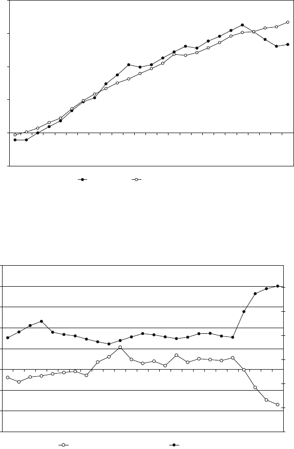
12. Properties of regression models with time series data
-0.5
0.0
0.5
1.0
1.5
2.0
1981 1984 1987 1990 1993 1996 1999 2002 2005
LGTAXI
actual values fitted values, regression (1)
Figure 12.1: Actual values of LGTAXI and the fitted values from regression (1).
-0.6
-0.4
-0.2
0.0
0.2
0.4
0.6
0.8
1.0
1981 1984 1987 1990 1993 1996 1999 2002 2005
3.8
4.0
4.2
4.4
4.6
4.8
5.0
residuals, regression (1) (left scale) LGP (right scale)
Figure 2
Figure 12.2: Residuals from regression (1) and the values of LGP.
A12.8 A researcher has annual data on I, investment as a percentage of gross domestic
product, and r, the real long-term rate of interest for a certain economy for the
period 1981–2010. He regresses Ion r, (1) using ordinary least squares (OLS), (2)
using an estimator appropriate for AR(1) residual autocorrelation, and (3) using
OLS but adding I(−1) and r(−1) (Iand rlagged one time period) as explanatory
variables. The results are shown in columns (1), (2), and (3) of the table below.
The residuals from regression (1) are shown in Figure 12.3.
He then obtains annual data on g, the rate of growth of gross domestic product of
the economy, for the same period, and repeats the regressions, adding g(and,
where appropriate, g(−1)) to the specifications as an explanatory variable. The
results are shown in columns (4), (5), and (6) of the table. rand gare measured as
per cent per year. The data for gare plotted in the figure.
266
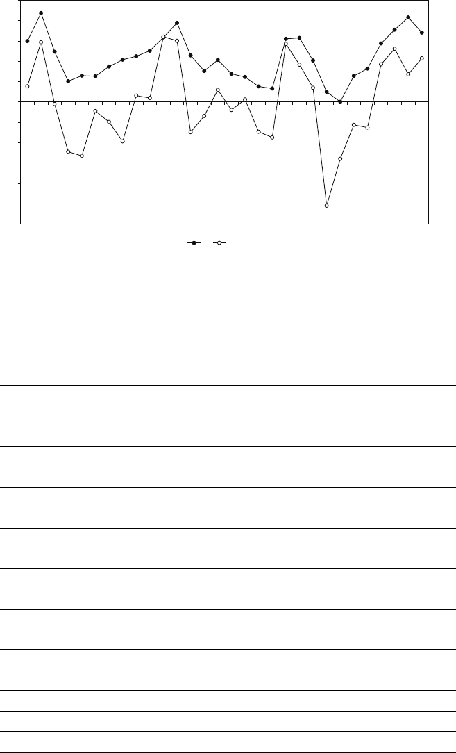
12.3. Additional exercises
-6
-5
-4
-3
-2
-1
0
1
2
3
4
5
1981 1988 1995 2002 2009
gresiduals
Figure 12.3: Residuals from regression (1).
OLS AR(1) OLS OLS AR(1) OLS
(1) (2) (3) (4) (5) (6)
r−0.87 −0.83 −0.87 −1.81 −1.88 −1.71
(0.98) (1.05) (1.08) (0.49) (0.50) (0.52)
I(−1) — — 0.37 — — −0.22
(0.16) (0.18)
r(−1) — — 0.64 — — −0.98
(1.08) (0.64)
g— — — 1.61 1.61 1.92
(0.17) (0.18) (0.20)
g(−1) — — — — — −0.02
(0.33)
bρ— 0.37 — — −0.16 —
(0.18) (0.20)
Constant 9.31 9.21 4.72 9.26 9.54 13.24
(3.64) (3.90) (4.48) (1.77) (1.64) (2.69)
B–G4.42 — 4.24 0.70 — 0.98
d0.99 1.36 1.33 2.30 2.05 2.09
RSS 120.5 103.9 103.5 27.4 26.8 23.5
Note: standard errors are given in parentheses. bρis the
estimate of the autocorrelation parameter in the AR(1)
specification. B–Gis the Breusch–Godfrey statistic for AR(1)
autocorrelation. dis the Durbin–Watson dstatistic.
•Explain why the researcher was not satisfied with regression (1).
•Evaluate regression (2). Explain why the coefficients of I(−1) and r(−1) are
not reported, despite the fact that they are part of the regression specification.
•Evaluate regression (3).
267
12. Properties of regression models with time series data
•Evaluate regression (4).
•Evaluate regression (5).
•Evaluate regression (6).
•Summarise your conclusions concerning the evaluation of the different
regressions. Explain whether an examination of the figure supports your
conclusions
A12.9 In Exercise A11.5 you performed a test of a restriction. The result of this test will
have been invalidated if you found that the specification was subject to
autocorrelation. How should the test be performed, assuming the correct
specification is ADL(1,1)?
A12.10 Given data on a univariate process:
Yt=β1+β2yt−1+ut
where |β2|<1 and utis iid, the usual OLS estimators will be consistent but
subject to finite-sample bias. How should the model be fitted if utis subject to an
AR(1) process?
A12.11 Explain what is correct, incorrect, confused or incomplete in the following
statements, giving a brief explanation if not correct.
•The disturbance term in a regression model is said to be autocorrelated if its
values in a sample of observations are not distributed independently of each
other.
•When the disturbance term is subject to autocorrelation, the ordinary least
squares estimators are inefficient and inconsistent, but they are not biased,
and the ttests are invalid.
•It is a common problem in time series models because it always occurs when
the dependent variable is correlated with its previous values.
•If this is the case, it could be eliminated by including the lagged value of the
dependent variable as an explanatory variable.
•However, if the model is correctly specified and the disturbance term satisfies
the regression model assumptions, adding the lagged value of the dependent
variable as an explanatory variable will have the opposite effect and cause the
disturbance term to be autocorrelated.
•A second way of dealing with the problem of autocorrelation is to use an
instrumental variable.
•If the autocorrelation is of the AR(1) type, randomising the order of the
observations will cause the Breusch–Godfrey statistic to be near zero, and the
Durbin–Watson statistic to be near 2, thereby eliminating the problem.
268

12.4. Answers to the starred exercises in the textbook
12.4 Answers to the starred exercises in the textbook
12.7 Prove that σ2
uis related to σ2
εas shown in (12.31), and show that weighting the
first observation by p1−ρ2eliminates the heteroskedasticity.
Answer:
(12.31) is:
σ2
u=1
1−ρ2σ2
ε
and it assumes the first order AR(1) process (12.26): ut=ρut−1+εt. From the
AR(1) process, neglecting transitory effects, σut=σut−1=σuand so:
σ2
u=ρ2σ2
u+σ2
ε=1
1−ρ2σ2
ε.
(Note that the covariance between ut−1and εtis zero.) If the first observation is
weighted by p1−ρ2, the variance of the disturbance term will be:
p1−ρ22σ2
u= (1 −ρ2)1
1−ρ2σ2
ε=σ2
ε
and it will therefore be the same as in the other observations in the sample.
12.10 The table gives the results of three logarithmic regressions using the Cobb–Douglas
data for Yt,Kt, and Lt, index number series for real output, real capital input, and
real labor input, respectively, for the manufacturing sector of the United States for
the period 1899–1922, reproduced in Exercise 11.6 (method of estimation as
indicated; standard errors in parentheses; d= Durbin–Watson dstatistic; B–G=
Breusch–Godfrey test statistic for first-order autocorrelation):
1: OLS 2: AR(1) 3: OLS
log K0.23 0.22 0.18
(0.06) (0.07) (0.56)
log L0.81 0.86 1.03
(0.15) (0.16) (0.15)
log Y(−1) — — 0.40
(0.21)
log K(−1) — — 0.17
(0.51)
log L(−1) — — −1.01
(0.25)
constant −0.18 −0.35 1.04
(0.43) (0.51) (0.41)
bρ— 0.19 —
(0.25)
R20.96 0.96 0.98
RSS 0.0710 0.0697 0.0259
d1.52 1.54 1.46
B–G0.36 — 1.54
269

12. Properties of regression models with time series data
The first regression is that performed by Cobb and Douglas. The second fits the
same specification, allowing for AR(1) autocorrelation. The third specification uses
OLS with lagged variables. Evaluate the three regression specifications.
Answer:
For the first specification, the Breusch–Godfrey LM test for autocorrelation yields
statistics of 0.36 (first order) and 1.39 (second order), both satisfactory. For the
Durbin–Watson test, dLand dUare 1.19 and 1.55 at the 5 per cent level and 0.96
and 1.30 at the 1 per cent level, with 24 observations and two explanatory
variables. Hence the specification appears more or less satisfactory. Fitting the
model with an AR(1) specification makes very little difference, the estimate of ρ
being low. However, when we fit the general ADL(1,1) model, neither of the first
two specifications appears to be an acceptable simplification. The Fstatistic for
dropping all the lagged variables is:
F(3,18) = (0.0710 −0.0259)/3
0.0259/18 = 10.45.
The critical value of F(3,18) at the 0.1 per cent level is 8.49. The common factor
test statistic is:
23 log 0.0697
0.0259 = 22.77
and the critical value of chi-squared with two degrees of freedom is 13.82 at the 0.1
per cent level. The Breusch–Godfrey statistic for first-order autocorrelation is 1.54.
We come to the conclusion that Cobb and Douglas, who actually fitted a restricted
version of the first specification, imposing constant returns to scale, were a little
fortunate to obtain the plausible results they did.
12.11 Derive the final equation in Box 12.2 from the first two equations in the box. What
assumptions need to be made when fitting the model?
Answer:
This exercise overlaps Exercise 11.17. The first two equations in the box are:
Yt=β1+β2Xe
t+1 +ut
Xe
t+1 −Xe
t=λ(Xt−Xe
t).
We can rewrite the second equation as:
Xe
t+1 =λXt+ (1 −λ)Xe
t.
Substituting this into the first equation, we have:
Yt=β1+β2λXt+β2(1 −λ)Xe
t+ut.
This includes the unobservable Xe
ton the right side. However, lagging the second
equation, we have:
Xe
t=λXt−1+ (1 −λ)Xe
t−1.
Hence:
Yt=β1+β2λXt+β2λ(1 −λ)Xt−1+β2(1 −λ)2Xe
t−1+ut.
270
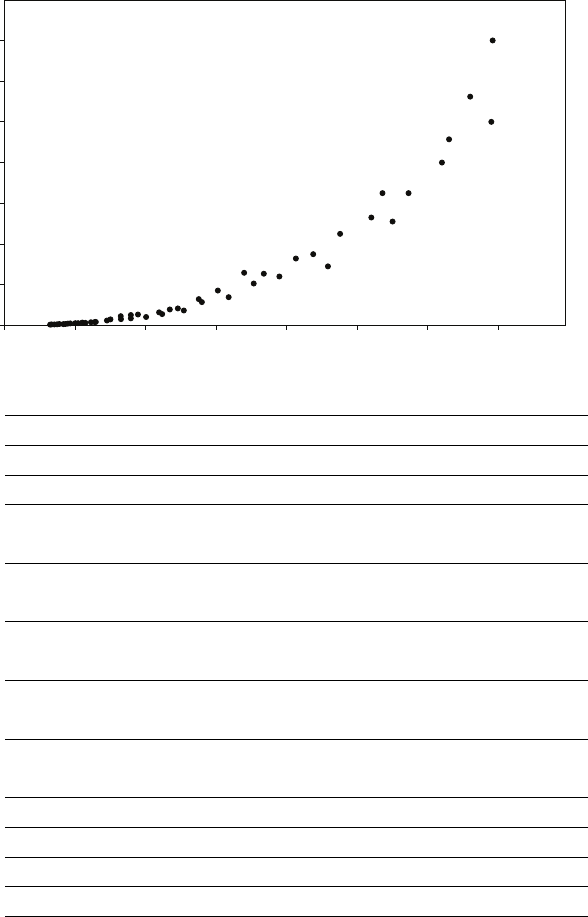
12.4. Answers to the starred exercises in the textbook
This includes the unobservable Xe
t−1on the right side. However, continuing to lag
and substitute, we have:
Yt=β1+β2λXt+β2λ(1 −λ)Xt−1+···+β2λ(1 −λ)sXt−s+β2(1 −λ)s+1Xe
t−s+ut.
Provided that sis large enough for β2(1 −λ)s+1 to be very small, this may be
fitted, omitting the unobservable final term, with negligible omitted variable bias.
We would fit it with a nonlinear regression technique that respected the constraints
implicit in the theoretical structure of the coefficients. The disturbance term is
unaffected by the manipulations. Hence it is sufficient to assume that it is
well-behaved in the original specification.
12.14 Using the 50 observations on two variables Yand Xshown in the diagram below,
an investigator runs the following five regressions (estimation method as indicated;
standard errors in parentheses; all variables as logarithms in the logarithmic
regressions; d= Durbin–Watson dstatistic; B–G= Breusch–Godfrey test statistic):
0
20
40
60
80
100
120
140
0 100 200 300 400 500 600 700
Y
X
1 2 3 4 5
Linear Logarithmic
OLS AR(1) OLS AR(1) OLS
X0.16 0.03 2.39 2.39 1.35
(0.01) (0.05) (0.03) (0.03) (0.70)
Y(−1) — — — — −0.11
(0.15)
X(−1) — — — — 1.30
(0.75)
bρ— 1.16 — −0.14 —
(0.06) (0.15)
constant −21.88 −2.52 −11.00 −10.99 −12.15
(3.17) (8.03) (0.15) (0.14) (1.67)
R20.858 0.974 0.993 0.993 0.993
RSS 7663 1366 1.011 0.993 0.946
d0.26 2.75 2.17 1.86 21.95
B–G39.54 — 0.85 — 1.03
271

12. Properties of regression models with time series data
Discuss each of the five regressions, explaining which is your preferred specification.
Answer:
The scatter diagram reveals that the relationship is nonlinear. If it is fitted with a
linear regression, the residuals must be positive for the largest and smallest values
of Xand negative for the middle ones. As a consequence it is no surprise to find a
high Breusch–Godfrey statistic, above 10.83, the critical value of χ2(1) at the 0.1%
level, and a low Durbin–Watson statistic, below 1.32, the critical value at the 1 per
cent level. Equally it is no surprise to find that an AR(1) specification does not
yield satisfactory results, the Durbin–Watson statistic now indicating negative
autocorrelation.
By contrast the logarithmic specification appears entirely satisfactory, with a
Breusch–Godfrey statistic of 0.85 and a Durbin–Watson statistic of 1.82 (dUis 1.59
at the 5 per cent level). Comparing it with the ADL(1,1) specification, the F
statistic for dropping the lagged variables is:
F(2,46) = (1.084 −1.020)/2
1.020/46 = 1.44.
The critical value of F(2,40) at the 5 per cent level is 3.23. Hence we conclude that
specification (3) is an acceptable simplification. Specifications (4) and (5) are
inefficient, and this accounts for their larger standard errors.
12.15 Using the data on food in the Demand Functions data set, the following regressions
were run, each with the logarithm of food as the dependent variable: (1) an OLS
regression on a time trend Tdefined to be 1 in 1959, 2 in 1960, etc., (2) an AR(1)
regression using the same specification, and (3) an OLS regression on Tand the
logarithm of food lagged one time period, with the results shown in the table
(standard errors in parentheses).
1: OLS 2: AR(1) 3: OLS
T0.0181 0.0166 0.0024
(0.0005) (0.0021) (0.0016)
LGFOOD(−1) — — 0.8551
(0.0886)
constant 5.7768 5.8163 0.8571
(0.0106) (0.0586) (0.5101)
bρ— 0.8551 —
(0.0886)
R20.9750 0.9931 0.9931
RSS 0.0327 0.0081 0.0081
d0.2752 1.3328 1.3328
h— — 2.32
Discuss why each regression specification appears to be unsatisfactory. Explain why
it was not possible to perform a common factor test.
272
12.5. Answers to the additional exercises
Answer:
The Durbin–Watson statistic in regression (1) is very low, suggesting AR(1)
autocorrelation. However, it remains below 1.40, dLfor a 5 per cent significance
test with one explanatory variable and 35 observations, in the AR(1) specification
in regression (2). The reason of course is that the model is very poorly specified,
with two obvious major variables, income and price, excluded.
With regard to the impossibility of performing a common factor test, suppose that
the original model is written:
LGFOODt=β1+β2T+ut.
Lagging the model and multiplying through by ρ, we have:
ρLGFOODt−1=β1ρ+β2ρ(T−1) + ρut−1.
Subtracting and rearranging, we obtain the AR(1) specification:
LGFOODt=β1(1 −ρ) + ρLGFOODt−1+β2T−β2ρ(T−1) + ut−ρut−1
=β1(1 −ρ) + β2ρ+ρLGFOODt−1+β2(1 −ρ)T+εt.
However, this specification does not include any restrictions. The coefficient of
LGFOODt−1provides an estimate of ρ. The coefficient of Tthen provides an
estimate of β2. Finally, given these estimates, the intercept provides an estimate of
β1. The AR(1) and ADL(1,1) specifications are equivalent in this model, the reason
being that the variable (T−1) is merged into Tand the intercept.
12.5 Answers to the additional exercises
A12.1 The Durbin–Watson statistic in the OLS regression is 0.49, causing us to reject the
null hypothesis of no autocorrelation at the 1 per cent level. The Breusch–Godfrey
statistic (not shown) is 25.12, also causing the null hypothesis of no autocorrelation
to be rejected at a high significance level. Apart from a more satisfactory
Durbin–Watson statistic, the results for the AR(1) specification are similar to those
of the OLS one. The income and price elasticities are a little larger. The estimate of
the population elasticity, negative in the OLS regression, is now effectively zero,
suggesting that the direct effect of population on expenditure on food is offset by a
negative income effect. The standard errors are larger than those for the OLS
regression, but the latter are invalidated by the autocorrelation and therefore
should not be taken at face value.
A12.2 All of the regressions exhibit strong evidence of positive autocorrelation. The
Breusch–Godfrey test statistic for AR(1) autocorrelation is above the critical value
of 10.82 (critical value of chi-squared with one degree of freedom at the 0.1%
significance level) and the Durbin–Watson dstatistic is below 1.20 (dL, 1 per cent
level, 45 observations, k= 4). The Durbin–Watson statistics for the AR(1)
specification are generally much more healthy than those for the OLS one, being
scattered around 2.
273

12. Properties of regression models with time series data
Breusch–Godfrey and Durbin–Watson statistics,
logarithmic OLS regression including population
B–G d B–G d
ADM 19.37 0.683 GASO 36.21 0.212
BOOK 25.85 0.484 HOUS 23.88 0.523
BUSI 24.31 0.507 LEGL 24.30 0.538
CLOT 18.47 0.706 MAGS 19.27 0.667
DENT 14.02 0.862 MASS 21.97 0.612
DOC 24.74 0.547 OPHT 31.64 0.328
FLOW 24.13 0.535 RELG 26.30 0.497
FOOD 24.95 0.489 TELE 30.08 0.371
FURN 22.92 0.563 TOB 27.84 0.421
GAS 23.41 0.569 TOYS 20.04 0.668
Since autocorrelation does not give rise to bias, one would not expect to see
systematic changes in the point estimates of the coefficients. However, since
multicollinearity is to some extent a problem for most categories, the coefficients do
exhibit greater volatility than is usual when comparing OLS and AR(1) results.
Fortunately, most of the major changes seem to be for the better. In particular,
some implausibly high income elasticities are lower. Likewise, the population
elasticities are a little less erratic, but most are still implausible, with large
standard errors that reflect the continuing underlying problem of multicollinearity.
AR(1) logarithmic regression
LGDPI LGP LGPOP bρ R2d
coef. s.e. coef. s.e. coef. s.e. coef. s.e.
ADM −0.34 0.34 0.00 0.20 3.73 0.95 0.76 0.08 0.992 2.03
BOOK 0.46 0.41 −1.06 0.29 2.73 1.25 0.82 0.10 0.990 1.51
BUSI 0.43 0.24 0.19 0.25 2.45 0.70 0.69 0.10 0.997 1.85
CLOT 1.07 0.16 −0.56 0.15 −0.49 0.71 0.84 0.08 0.999 2.19
DENT 1.14 0.18 −1.01 0.15 0.69 0.73 0.56 0.13 0.996 1.86
DOC 0.85 0.25 −0.30 0.26 1.26 0.77 0.83 0.10 0.997 1.61
FLOW 0.71 0.41 −1.04 0.44 0.74 1.33 0.78 0.09 0.994 1.97
FOOD 0.47 0.12 −0.36 0.12 0.07 0.38 0.88 0.09 0.997 1.56
FURN 1.73 0.36 −0.37 0.51 −1.62 1.55 0.92 0.06 0.994 2.00
GAS −0.02 0.34 0.01 0.08 0.29 0.97 0.83 0.06 0.933 2.12
GASO 0.75 0.15 −0.14 0.03 −0.64 0.48 0.93 0.04 0.998 1.65
HOUS 0.27 0.08 −0.27 0.09 −0.03 0.54 0.98 0.00 0.997 1.66
LEGL 0.89 0.20 −0.19 0.22 −0.54 0.80 0.77 0.10 0.989 1.90
MAGS 0.98 0.30 −1.24 0.39 −0.23 0.92 0.73 0.12 0.983 1.73
MASS 0.06 0.28 −0.72 0.11 1.31 0.97 0.94 0.04 0.944 1.95
OPHT 1.99 0.60 −0.92 0.97 −1.45 1.85 0.90 0.08 0.991 1.67
RELG 0.86 0.18 −1.15 0.26 2.00 0.56 0.66 0.10 0.999 2.08
TELE 0.70 0.20 −0.56 0.13 2.44 0.71 0.87 0.10 0.999 1.51
TOB 0.38 0.22 −0.35 0.07 −0.99 0.66 0.79 0.10 0.960 2.37
TOYS 0.89 0.18 −0.58 0.13 1.61 0.66 0.75 0.12 0.999 1.77
274

12.5. Answers to the additional exercises
A12.3 The table gives the residual sum of squares for the unrestricted ADL(1,1)
specification and that for the restricted AR(1) one, the fourth column giving the
chi-squared statistic for the common factor test.
Before performing the common factor test, one should check that the ADL(1,1)
specification is itself free from autocorrelation using the Breusch–Godfrey test. The
fifth column gives the B–Gstatistic for AR(1) autocorrelation. All but one of the
statistics are below the critical value at the 5 per cent level, 3.84. The exception is
that for LEGL. It should be remembered that the Breusch–Godfrey test is a
large-sample tests and in this application, with only 44 observations, the sample is
rather small.
Common factor test and tests of autocorrelation for ADL(1,1) model
RSSADL(1,2) RSSAR(1) Chi-squared B–G
ADM 0.029792 0.039935 12.89 0.55
BOOK 0.070478 0.086240 8.88 1.25
BUSI 0.032074 0.032703 0.85 0.57
CLOT 0.009097 0.010900 7.96 1.06
DENT 0.019281 0.021841 5.49 1.22
DOC 0.025598 0.028091 4.09 0.33
FLOW 0.084733 0.084987 0.13 0.01
FOOD 0.005562 0.006645 7.83 3.12
FURN 0.050880 0.058853 6.41 0.29
GAS 0.035682 0.045433 10.63 0.66
GASO 0.006898 0.009378 13.51 2.91
HOUS 0.001350 0.002249 22.46 0.77
LEGL 0.026650 0.034823 11.77 8.04
MAGS 0.043545 0.051808 7.64 0.03
MASS 0.029125 0.033254 5.83 0.15
OPHT 0.139016 0.154629 4.68 0.08
RELG 0.013910 0.014462 1.71 0.32
TELE 0.014822 0.017987 8.52 0.97
TOB 0.021403 0.021497 0.19 3.45
TOYS 0.015313 0.015958 1.82 2.60
For the common factor test, the critical values of chi-squared are 7.81 and 11.34 at
the 5 and 1 per cent levels, respectively, with 3 degrees of freedom. Summarising
the results, we find:
•AR(1) specification not rejected: BUSI,DENT ,DOC,F LOW ,F URN ,
MAGS,MASS,OP HT ,RELG,T OB,T OY S.
•AR(1) specification rejected at 5 per cent level: BOOK,CLOT ,F OOD,
GAS,T ELE.
•AR(1) specification rejected at 1 per cent level: ADM,GASO,HOUS,LEGL.
A12.4 Discuss whether specification (1) is an adequate representation of the data.
The Breusch–Godfrey statistic is well in excess of the critical value at the 0.1 per
cent significance level, 10.83. Likewise, the Durbin–Watson statistic is far below
275

12. Properties of regression models with time series data
1.15, dLat the 1 per cent level with two explanatory variables and 36 observations.
There is therefore strong evidence of either severe AR(1) autocorrelation or some
serious misspecification.
Discuss whether specification (3) is an adequate representation of the data.
The only item that we can check is whether it is free from autocorrelation. The
Breusch–Godfrey statistic is well under 3.84, the critical value at the 5 per cent
significance level, and so there is no longer evidence of autocorrelation or
misspecification.
Discuss whether specification (2) is an adequate representation of the data.
Let the original model be written:
LGLIFE =β1+β2LGDPI +β3LGDPRLIFE +u
ut=ρut−1+εt.
The AR(1) specification is then:
LGLIFE =β1(1 −ρ) + ρLGLIFE(−1) + β2LGDPI −β2ρLGDPI (−1)
+β3LGDPRLIFE −β3ρLGPRLIFE(−1) + εt.
This is a restricted version of the ADL(1,1) model because it incorporates
nonlinear restrictions on the coefficients of LGDPI (−1) and LGPRLIFE(−1). In
the ADL(1,1) specification, minus the product of the coefficients of LGLIFE(−1)
and LGDPI is −0.82 ×0.42 = −0.34. The coefficient of LGDPI (−1) is smaller
than this, but then its standard error is large. Minus the product of the coefficients
of LGLIFE(−1) and LGPRLIFE is −0.82 × −0.59 = 0.48. The coefficient of
LGPRLIFE(−1) is fairly close, bearing in mind that its standard error is also
large. The coefficient of LGLIFE (−1) is exactly equal to the estimate of ρin the
AR(1) specification.
The common factor test statistic is:
35 loge
0.799
0.719 = 3.69.
The null hypothesis is that the two restrictions are valid. Under the null
hypothesis, the test statistic has a chi-squared distribution with 2 degrees of
freedom. Its critical value at the 5 per cent level is 5.99. Hence we do not reject the
restrictions and the AR(1) specification therefore does appear to be acceptable.
Discuss whether specification (4) is an adequate representation of the data.
We note that LGLDPI (−1) and LGPRLIFE(−1) do not have significant t
statistics, but since they are being dropped simultaneously, we should perform an
Ftest of their joint explanatory power:
F(2,29) = (0.732 −0.719)/2
0.719/29 = 0.26.
Since this is less than 1, it is not significant at any significance level and so we do
not reject the null hypothesis that the coefficients of LGLDPI (−1) and
276

12.5. Answers to the additional exercises
LGPRLIFE(−1) are both 0. Hence it does appear that we can drop these
variables. We should also check for autocorrelation. The Breusch–Godfrey statistic
indicates that there is no problem.
If you were presenting these results at a seminar, what would you say were your
conclusions concerning the most appropriate of specifications (1) – (4)?
There is no need to mention (1). (3) is not a candidate because we have found
acceptable simplifications that are likely to yield more efficient parameter estimates
, and this is reflected in the larger standard errors compared with (2) and (4). We
cannot discriminate between (2) and (4).
At the seminar a commentator points out that in specification (4) neither LGDPI
nor LGPRLIFE have significant coefficients and so these variables should be
dropped. As it happens, the researcher has considered this specification, and the
results are shown as specification (5) in the table. What would be your answer to
the commentator?
Comparing (3) and (5):
F(4,29) = (0.843 −0.719)/4
0.719/29 = 1.25.
The critical value of F(4,29) at the 5 per cent level is 2.70, so it would appear that
the joint explanatory power of the 4 income and price variables is not significant.
However, it does not seem sensible to drop current income and current price from
the model. The reason that they have so little explanatory power is that the
short-run effects are small, life insurance being subject to long-term contracts and
thus a good example of a category of expenditure with a large amount of inertia.
The fact that income in the AR(1) specification has a highly significant coefficient
is concrete evidence that it should not be dropped.
A12.5 Looking at all five regressions together, evaluate the adequacy of:
•specification 1.
•specification 2.
•specification 3.
•specification 4.
•Specification 1 has a very high Breusch–Godfrey statistic and a very low
Durbin–Watson statistic. There is evidence of either severe autocorrelation or
model misspecification.
•Specification 2 also has a very high Breusch–Godfrey statistic and a very low
Durbin–Watson statistic. Further, there is evidence of multicollinearity: large
standard errors (although comparisons are very dubious given low DW), and
implausible coefficients.
•Specification 3 seems acceptable. In particular, there is no evidence of
autocorrelation since the Breusch–Godfrey statistic is low.
•Specification 4: dropping m(−1) may be expected to cause omitted variable
bias since the tstatistic for its coefficient was −3.0 in specification 3.
277

12. Properties of regression models with time series data
(Equivalently, the Fstatistic is:
F(1,46) = (0.0120 −0.0100)/1
0.0100/46 = 0.2×46 = 9.2
the square of the tstatistic and similarly significant.)
Explain why specification 5 is a restricted version of one of the other specifications,
stating the restriction, and explaining the objective of the manipulations that lead to
specification 5.
Write the original model and AR(1) process:
pt=β1+β2mt+ut
uy=ρut−1+εt.
Then fitting:
pt=β1(1 −ρ) + ρpt−1+β2mt−β2ρmt−1+εt
removes the autocorrelation. This is a restricted version of specification 3, with
restriction that the coefficient of mt−1is equal to minus the product of the
coefficients of mtand pt−1.
Perform a test of the restriction embodied in specification 5.
Comparing specifications 3 and 5, the common factor test statistic is:
nlogeRSSR
RSSU= 50 log 0.0105
0.0100= 50 log 1.05 ∼
=50 ×0.05 = 2.5.
Under the null hypothesis that the restriction implicit in the specification is valid,
the test statistic is distributed as chi-squared with one degree of freedom. The
critical value at the 5 per cent significance level is 3.84, so we do not reject the
restriction. Accordingly, specification 5 appears to be an adequate representation of
the data.
Explain which would be your preferred specification.
Specifications (3) and (5) both appear to be adequate representations of the data.
(5) should yield more efficient estimators of the parameters because, exploiting an
apparently-valid restriction, it is less susceptible to multicollinearity, and this
appears to be confirmed by the lower standard errors.
A12.6 The models are:
1. pt=β1+β2mt+ut
2. pt=β1+β2mt+β3mt−1+β4mt−2+β5mt−3+ut
3. pt=β1+β2mt+β3mt−1+β6pt−1+ut
4. pt=β1+β2mt+β6pt−1+ut
5. pt=β1(1 −β6) + β6pt−1+β2mt−β2β6mt−1+εt(writing ρ=β6).
278

12.5. Answers to the additional exercises
Hence we obtain the following estimates of ∂pt/∂mt:
1. 0.95
2. 0.50
3. 0.40
4. 0.18
5. 0.90.
Putting pand mequal to equilibrium values, and ignoring the disturbance term,
we have:
1. p=β1+β2m
2. p=β1+ (β2+β3+β4)m
3. p=1
1−β6(β1+ (β2+β3)m)
4. p=1
1−β6(β1+β2m)
5. p=β1+β2m.
Hence we obtain the following estimates of dp/dm:
1. 0.95
2. 0.95
3. 1.00
4. 0.90
5. 0.90.
A12.7 Evaluate regression (1).
Regression (1) has a very high Breusch–Godfrey statistic and a very low
Durbin–Watson statistic. The null hypothesis of no autocorrelation is rejected at
the 1 per cent level for both tests. Alternatively, the test statistics might indicate
some misspecification problem.
Evaluate regression (2). Explain mathematically what assumptions were being made
by the researcher when he used the AR(1) specification and why he hoped the results
would be better than those obtained with regression (1).
Regression (2) has been run on the assumption that the disturbance term follows
an AR(1) process:
ut=ρut−1+εt.
On the assumption that the regression model should be:
LGTAXI t=β1+β2LGDPI t+ut,
the autocorrelation can be eliminated in the following way: lag the regression
model by one time period and multiply through by ρ:
ρLGTAXI t−1=β1ρ+β2ρLGDPI t−1+ρut−1.
Subtract this from the regression model:
LGTAXI t−ρLGTAXI t−1=β1(1 −ρ) + β2LGDPI t−β2ρLGDPI t−1+ut−ρut−1.
279
12. Properties of regression models with time series data
Hence one obtains a specification free from autocorrelation:
LGTAXI t=β1(1 −ρ) + ρLGTAXI t−1+β2LGDPI t−β2ρLGDPI t−1+εt.
The Durbin–Watson statistic is still low, suggesting that fitting the AR(1)
specification was an inappropriate response to the problem.
Evaluate regression (3).
In regression (3) the Breusch–Godfrey statistic suggests that, for this specification,
there is not a problem of autocorrelation (the Durbin–Watson statistic is
indecisive). This suggests that the apparent autocorrelation in the regression (1) is
in fact attributable to the omission of the price variable.
This is corroborated by the diagrams, which show that large negative residuals
occurred when the price rose and positive ones when it fell. The effect is especially
obvious in the final years of the sample period.
Evaluate regression (4). In particular, discuss the possible reasons for the
differences in the standard errors in regressions (3) and (4).
In regression (4), the Durbin–Watson statistic does not indicate a problem of
autocorrelation. Overall, there is little to choose between regressions (3) and (4). It
is possible that there was some autocorrelation in regression (3) and that it has
been rectified by using AR(1) in regression (4). It is also possible that
autocorrelation was not actually a problem in regression (3). Regressions (3) and
(4) yield similar estimates of the income and price elasticities and in both cases the
elasticities are significantly different from zero at a high significance level. If
regression (4) is the correct specification, the lower standard errors in regression (3)
should be disregarded because they are invalid. If regression (3) is the correct
specification, AR(1) estimation will yield inefficient estimates; which could account
for the higher standard errors in regression (4).
At a seminar one of the participants says that the researcher should consider adding
lagged values of LGTAXI, LGDPI, and LGP to the specification. What would be
your view?
Specifications (2) and (4) already contain the lagged values, with restrictions on
the coefficients of LGDPI (−1) and LGP (−1).
A12.8 Explain why the researcher was not satisfied with regression (1).
The researcher was not satisfied with the results of regression (1) because the
Breusch–Godfrey statistic was 4.42, above the critical value at the 5 per cent level,
3.84, and because the Durbin–Watson dstatistic was only 0.99. The critical value
of dLwith one explanatory variable and 30 observations is 1.35. Thus there is
evidence that the specification may be subject to autocorrelation.
Evaluate regression (2). Explain why the coefficients of I(-1) and r(-1) are not
reported, despite the fact that they are part of the regression specification.
Specification (2) is equally unsatisfactory. The fact that the Durbin–Watson
statistic has remained low is an indication that the reason for the low din (1) was
not an AR(1) disturbance term. RSS is very high compared with those in
specifications (4) – (6). The coefficient of I(−1) is not reported as such because it
280

12.5. Answers to the additional exercises
is the estimate bρ. The coefficient of r(−1) is not reported because it is constrained
to be minus the product of bρ. and the coefficient of I.
Evaluate regression (3).
Specification (3) is the unrestricted ADL(1,1) model of which the previous AR(1)
model was a restricted version and it suffers from the same problems. There is still
evidence of positive autocorrelation, since the Breusch–Godfrey statistic, 4.24, is
high and RSS is still much higher than in the three remaining specifications.
Evaluate regression (4).
Specification (4) seems fine. The null hypothesis of no autocorrelation is not
rejected by either the Breusch–Godfrey statistic or the Durbin–Watson statistic.
The coefficients are significant and have the expected signs.
Evaluate regression (5).
The AR(1) specification (5) does not add anything because there was no evidence
of autocorrelation in (4). The estimate of ρis not significantly different from zero.
Evaluate regression (6).
Specification (6) does not add anything either. ttests on the coefficients of the
lagged variables indicate that they are individually not significantly different from
zero. Likewise the joint hypothesis that their coefficients are all equal to zero is not
rejected by an Ftest comparing RSS in (4) and (6):
F(3,23) = (27.4−23.5)/3
23.5/23 = 1.27.
The critical value of F(3,23) at the 5 per cent level is 3.03. [There is no point in
comparing (5) and (6) using a common factor test, but for the record the test
statistic is:
nloge
RSSR
RSSU
= 29 loge
26.8
23.5= 3.81.
The critical value of chi-squared with 2 degrees of freedom at the 5 per cent level is
5.99.]
Summarise your conclusions concerning the evaluation of the different regressions.
Explain whether an examination of the figure supports your conclusions.
The overall conclusion is that the static model (4) is an acceptable representation
of the data and the apparent autocorrelation in specifications (1) – (3) is
attributable to the omission of g. Figure 12.3 shows very clearly that the residuals
in specification (1) follow the same pattern as g, confirming that the apparent
autocorrelation in the residuals is in fact attributable to the omission of gfrom the
specification.
A12.9 In Exercise A11.5 you performed a test of a restriction. The result of this test will
have been invalidated if you found that the specification was subject to
autocorrelation. How should the test be performed, assuming the correct
specification is ADL(1,1)?
281

12. Properties of regression models with time series data
If the ADL(1,1) model is written:
log CAT =β1+β2log DPI +β3log P+β4log POP +β5log CAT −1
+β6logDPI −1+β7log P−1+β8log POP−1+u
the restricted version with expenditure per capita a function of income per capita
is:
log CAT
POP =β1+β2log DPI
POP +β3log P+β5log CAT −1
POP−1
+β6log DPI −1
POP−1
+β7log P−1+u.
Comparing the two equations, we see that the restrictions are β4= 1 −β2and
β8=−β5−β6. The usual Fstatistic should be constructed and compared with the
critical values of F(2,28).
A12.10 Let the AR(1) process be written:
ut=ρut−1+εt.
As the specification stands, OLS would yield inconsistent estimates because both
the explanatory variable and the disturbance term depend on ut−1. Applying the
standard procedure, multiplying the lagged relationship by ρand subtracting, one
has:
Yt−ρYt−1=β1(1 −ρ) + β2Yt−1−β2ρYt−1+ut−ρut−1.
Hence:
Yt=β1(1 −ρ)+(β2+ρ)Yt−1−β2ρYt−2+εt.
It follows that the model should be fitted as a second-order, rather than as a
first-order, process. There are no restrictions on the coefficients. OLS estimators
will be consistent, but subject to finite-sample bias.
A12.11 Explain what is correct. incorrect, confused or incomplete in the following
statements, giving a brief explaination if not correct.
•The disturbance term in a regression model is said to be autocorrelated if its
values in a sample of observations are not distributed independently of each
other.
Correct.
•When the disturbance term is subject to autocorrelation, the ordinary least
squares estimators are inefficient ...
Correct.
•...and inconsistent...
Incorrect, unless there is a lagged dependent variable.
•...but they are not biased...
Correct, unless there is a lagged dependent variable.
282
12.5. Answers to the additional exercises
•...and the t tests are invalid.
Correct.
•It is a common problem in time series models because it always occurs when
the dependent variable is correlated with its previous values.
Incorrect.
•If this is the case, it could be eliminated by including the lagged value of the
dependent variable as an explanatory variable.
In general, incorrect. However, a model requiring a lagged dependent variable
could appear to exhibit autocorrelation if the lagged dependent variable were
omitted, and including it could eliminate the apparent problem.
•However, if the model is correctly specified and the disturbance term satisfies
the regression model assumptions, adding the lagged value of the dependent
variable as an explanatory variable will have the opposite effect and cause the
disturbance term to be autocorrelated.
Nonsense.
•A second way of dealing with the problem of autocorrelation is to use an
instrumental variable.
More nonsense.
•If the autocorrelation is of the AR(1) type, randomising the order of the
observations will cause the Durbin–Watson statistic to be near 2...
Correct.
•...thereby eliminating the problem.
Incorrect. The problem will have been disguised, not rectified.
283
12. Properties of regression models with time series data
284

Chapter 13
Introduction to nonstationary time
series
13.1 Overview
This chapter begins by defining the concepts of stationarity and nonstationarity as
applied to univariate time series and, in the case of nonstationary series, the concepts of
difference-stationarity and trend-stationarity. It next describes the consequences of
nonstationarity for models fitted using nonstationary time-series data and gives an
account of the Granger–Newbold Monte Carlo experiment with random walks. Next the
two main methods of detecting nonstationarity in time series are described, the
graphical approach using correlograms and the more formal approach using Augmented
Dickey–Fuller unit root tests. This leads to the topic of cointegration. The chapter
concludes with a discussion of methods for fitting models using nonstationary time
series: detrending, differencing, and error-correction models.
13.2 Learning outcomes
After working through the corresponding chapter in the text, studying the
corresponding slideshows, and doing the starred exercises in the text and the additional
exercises in this subject guide, you should be able to:
explain what is meant by stationarity and nonstationarity.
explain what is meant by a random walk and a random walk with drift
derive the condition for the stationarity of an AR(1) process
explain what is meant by an integrated process and its order of integration
explain why Granger and Newbold obtained the results that they did
explain what is depicted by a correlogram
perform an Augmented Dickey–Fuller unit root test to test a time series for
nonstationarity
test whether a set of time series are cointegrated
construct an error-correction model and describe its advantages over detrending
and differencing.
285
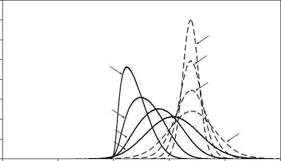
13. Introduction to nonstationary time series
13.3 Further material
Addition to Section 13.6 Cointegration
Section 13.6 contains the following paragraph on page 507:
In the case of a cointegrating relationship, least squares estimators can be shown to be
superconsistent (Stock, 1987). An important consequence is that OLS may be used to fit
a cointegrating relationship, even if it belongs to a system of simultaneous relationships,
for any simultaneous equations bias tends to zero asymptotically.
This cries out for an illustrative simulation, so here is one. Consider the model:
Yt=β1+β2Xt+β3Zt+εY t
Xt=α1+α2Yt+εXt
Zt=ρZt−1+εZt
where Ytand Xtare endogenous variables, Ztis exogenous, and εY t,εXt, and εZt are iid
N(0,1) disturbance terms. We expect OLS estimators to be inconsistent if used to fit
either of the first two equations. However, if ρ= 1, Zis nonstationary, and Xand Y
will also be nonstationary. So, if we fit the second equation, for example, the OLS
estimator of α2will be superconsistent. This is illustrated by a simulation where the
first two equations are:
Yt= 1.0+0.8Xt+ 0.5Zt+εY t
Xt= 2.0+0.4Yt+εXt.
The distributions in the right of the figure below (dashed lines) are for the case ρ= 0.5.
Zis stationary, and so are Yand X. You will have no difficulty in demonstrating that
plim bαOLS
2= 0.68. The distributions to the left of the figure (solid lines) are for ρ= 1,
and you can see that in this case the estimator is consistent. But is it superconsistent?
The variance seems to be decreasing relatively slowly, not fast, especially for small
sample sizes. The explanation is that the superconsistency becomes apparent only for
very large sample sizes, as shown in the second figure.
0
2
4
6
8
10
12
14
16
0 0.2 0.4 0.6 0.8 1
T = 200
T = 200
T = 50
T = 50
T = 100
T = 100
T = 25
T = 25
= 200
= 400
= 800
= 1,600
= 3,200
286
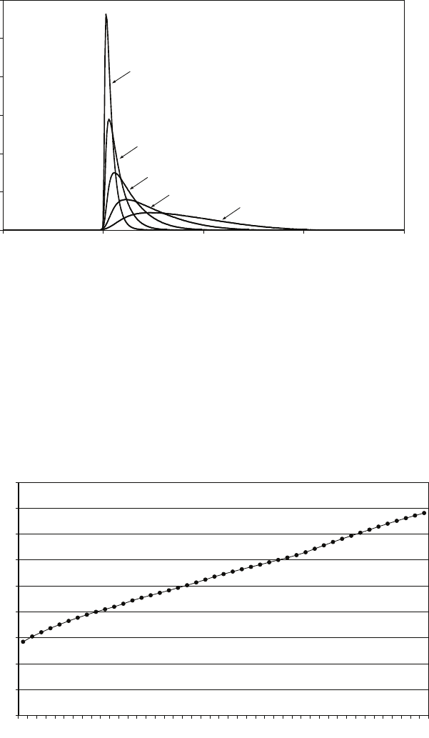
13.4. Additional exercises
0
20
40
60
80
100
120
0.3 0.4 0.5 0.6 0.7
T = 200
T = 400
T = 800
T = 1,600
T = 3,200
13.4 Additional exercises
A13.1 The Figure 13.1 plots the logarithm of the US population for the period 1959–2003.
It is obviously nonstationary. Discuss whether it is more likely to be
difference-stationary or trend-stationary.
11.8
11.9
12
12.1
12.2
12.3
12.4
12.5
12.6
12.7
1959 1963 1967 1971 1975 1979 1983 1987 1991 1995 1999 2003
Figure 13.1: Logarithm of the US population.
A13.2 Figure 13.2 plots the first difference of the logarithm of the US population for the
period 1959–2003. Explain why the vertical axis measures the proportional growth
rate. Comment on whether the series appears to be stationary or nonstationary.
A13.3 The regression output below shows the results of ADF unit root tests on the
logarithm of the US population, and its difference, for the period 1959–2003.
Comment on the results and state whether they confirm or contradict your
conclusions in Exercise A13.2.
287
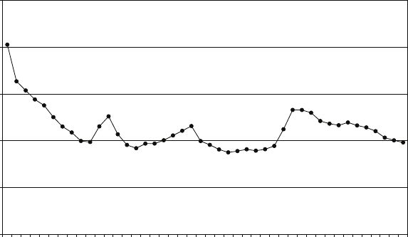
13. Introduction to nonstationary time series
0.000
0.005
0.010
0.015
0.020
0.025
1960 1964 1968 1972 1976 1980 1984 1988 1992 1996 2000
Figure 13.2: Logarithm of the US population, first difference.
Augmented Dickey--Fuller Unit Root Test on LGPOP
============================================================
Null Hypothesis: LGPOP has a unit root
Exogenous: Constant, Linear Trend
Lag Length: 1 (Fixed)
============================================================
t-Statistic Prob.*
============================================================
Augmented Dickey--Fuller test statistic -2.030967 0.5682
Test critical values1% level -4.186481
5% level -3.518090
10% level -3.189732
============================================================
*MacKinnon (1996) one-sided p-values.
Augmented Dickey--Fuller Test Equation
Dependent Variable: D(LGPOP)
Method: Least Squares
Sample(adjusted): 1961 2003
Included observations: 43 after adjusting endpoints
============================================================
Variable Coefficient Std. Error t-Statistic Prob.
============================================================
LGPOP(-1) -0.047182 0.023231 -2.030967 0.0491
D(LGPOP(-1)) 0.687772 0.058979 11.66139 0.0000
C 0.574028 0.281358 2.040209 0.0481
@TREND(1959) 0.000507 0.000246 2.060295 0.0461
============================================================
R-squared 0.839263 Mean dependent var 0.011080
Adjusted R-squared 0.826898 S.D. dependent var 0.001804
S.E. of regression 0.000750 Akaike info criter-11.46327
Sum squared resid 2.20E-05 Schwarz criterion -11.29944
Log likelihood 250.4603 F-statistic 67.87724
Durbin-Watson stat 1.164933 Prob(F-statistic) 0.000000
============================================================
288
13.4. Additional exercises
Augmented Dickey--Fuller Unit Root Test on DLGPOP
============================================================
Null Hypothesis: DLGPOP has a unit root
Exogenous: Constant, Linear Trend
Lag Length: 1 (Fixed)
============================================================
t-Statistic Prob.*
============================================================
Augmented Dickey--Fuller test statistic -2.513668 0.3203
Test critical values1% level -4.192337
5% level -3.520787
10% level -3.191277
============================================================
*MacKinnon (1996) one-sided p-values.
Augmented Dickey--Fuller Test Equation
Dependent Variable: D(DLGPOP)
Method: Least Squares
Sample(adjusted): 1962 2003
Included observations: 42 after adjusting endpoints
============================================================
Variable Coefficient Std. Error t-Statistic Prob.
============================================================
DLGPOP(-1) -0.161563 0.064274 -2.513668 0.0163
D(DLGPOP(-1)) 0.294717 0.117766 2.502573 0.0167
C 0.001714 0.000796 2.152327 0.0378
@TREND(1959) -1.32E-07 9.72E-06 -0.013543 0.9893
============================================================
R-squared 0.320511 Mean dependent var-0.000156
Adjusted R-squared 0.266867 S.D. dependent var 0.000827
S.E. of regression 0.000708 Akaike info criter-11.57806
Sum squared resid 1.90E-05 Schwarz criterion -11.41257
Log likelihood 247.1393 F-statistic 5.974780
Durbin-Watson stat 1.574084 Prob(F-statistic) 0.001932
============================================================
A13.4 A researcher believes that a time series is generated by the process:
Xt=ρXt−1+εt
where εtis a white noise series generated randomly from a normal distribution with
mean zero, constant variance, and no autocorrelation. Explain why the null
hypothesis for a test of nonstationarity is that the series is nonstationary, rather
than stationary.
A13.5 A researcher correctly believes that a time series is generated by the process:
Xt=ρXt−1+εt
where εtis a white noise series generated randomly from a normal distribution with
mean zero, constant variance, and no autocorrelation. Unknown to the researcher,
the true value of ρis 0.7. The researcher uses a unit root test to test the series for
nonstationarity. The output is shown. Discuss the result of the test.
289
13. Introduction to nonstationary time series
Augmented Dickey--Fuller Unit Root Test on X
============================================================
ADF Test Statistic -2.528841 1% Critical Value*-3.6289
5% Critical Value -2.9472
10% Critical Value -2.6118
============================================================
*MacKinnon critical values for rejection of hypothesis of a unit root.
Augmented Dickey--Fuller Test Equation
Dependent Variable: D(X)
Method: Least Squares
Sample(adjusted): 2 36
Included observations: 35 after adjusting endpoints
============================================================
Variable Coefficient Std. Error t-Statistic Prob.
============================================================
X(-1) -0.379661 0.150132 -2.528841 0.0164
C 0.222066 0.203435 1.091580 0.2829
============================================================
R-squared 0.162331 Mean dependent var-0.052372
Adjusted R-squared 0.136947 S.D. dependent var 1.095782
S.E. of regression 1.017988 Akaike info criteri2.928979
Sum squared resid 34.19792 Schwarz criterion 3.017856
Log likelihood -49.25714 F-statistic 6.395035
Durbin-Watson stat 1.965388 Prob(F-statistic) 0.016406
============================================================
A13.6 Test of cointegration. Perform a logarithmic regression of expenditure on your
commodity on income, relative price, and population. Save the residuals and test
them for stationarity. (Note: the critical values in the regression output do not
apply to tests of cointegration. For the correct critical values, see the text.)
A13.7 A variable Ytis generated by the autoregressive process:
Yt=β1+β2Yt−1+εt
where β2= 1 and εtsatisfies the regression model assumptions. A second variable
Ztis generated as the lagged value of Yt:
Zt=Yt−1.
Show that Yand Zare nonstationary processes. Show that nevertheless they are
cointegrated.
A13.8 Xtand Ztare independent I(1) (integrated of order 1) time series. Wtis a
stationary time series. Ytis generated as the sum of Xt,Zt, and Wt. Not knowing
this, a researcher regresses Yton Xtand Zt. Explain whether he would find a
cointegrating relationship.
290
13.5. Answers to the starred exercises in the textbook
A13.9 Two random walks RAtand RBt, and two stationary processes SAtand SBtare
generated by the following processes:
RAt=RAt−1+ε1t
RBt=RBt−1+ε2t
SAt=ρASAt−1+ε3t,0< ρA<1
SBt=ρBSBt−1+ε4t,0< ρB<1
where ε1t,ε2t,ε3t, and ε4t, are iid N(0,1) (independently and identically
distributed from a normal distribution with mean 0 and variance 1).
•Two series XAtand XBtare generated as:
XAt=RAt+SAt
XBt=RBt+SBt.
Explain whether it is possible for XAtand XBtto be stationary.
Explain whether it is possible for them to be cointegrated.
•Two series YAtand YBtare generated as:
YAt=RAt+SAt
YBt=RAt+SBt.
Explain whether it is possible for YAtand YBtto be cointegrated.
•Two series ZAtand ZBtare generated as:
ZAt=RAt+RBt+SAt
ZBt=RAt−RBt+SBt.
Explain whether it is possible for ZAtand ZBtto be stationary.
Explain whether it is possible for them to be cointegrated.
13.5 Answers to the starred exercises in the textbook
13.1 Demonstrate that the MA(1) process:
Xt=εt+α2εt−1
is stationary. Does the result generalise to higher-order MA processes?
Answer:
The expected value of Xtis zero and therefore independent of time:
E(Xt) = E(εt+α2εt−1) = E(εt) + α2E(εt−1) = 0 + 0 = 0.
291

13. Introduction to nonstationary time series
Since εtand εt−1are uncorrelated:
σ2
Xt=σ2
εt+α2
2σ2
εt−1
and this is independent of time. Finally, because:
Xt−1=εt−1+α2εt−2,
the population covariance of Xtand Xt−1is given by:
σXt,Xt−1=α2σ2
ε.
This is fixed and independent of time. The population covariance between Xtand
Xt−sis zero for all s > 1 since then Xtand Xt−1have no elements in common.
Thus the third condition for stationarity is also satisfied.
All MA processes are stationary, the general proof being a simple extension of that
for the MA(1) case.
13.2 A stationary AR(1) process:
Xt=β1+β2Xt−1+εt
with |β2|<1, has initial value X0, where X0is defined as:
X0=β1
1−β2
+s1
1−β2
2
ε0.
Demonstrate that X0is a random draw from the ensemble distribution for X.
Answer:
Lagging and substituting, it was shown, equation (13.12), that:
Xt=βt
2X0+β1
1−βt
2
1−β2
+βt−1
2ε1+··· +β2
2εt−2+β2εt−1+εt.
With the stochastic definition of X0, we now have:
Xt=βt
2 β1
1−β2
+s1
1−β2
2
ε0!+β1
1−βt
2
1−β2
+βt−1
2ε1+··· +β2
2εt−2+β2εt−1+εt
=β1
1−β2
+βt
2s1
1−β2
2
ε0+βt−1
2ε1+··· +β2
2εt−2+β2εt−1+εt.
Hence:
E(Xt) = β1
1−β2
and:
var(Xt) = var βt
2s1
1−β2
2
ε0+βt−1
2ε1+··· +β2
2εt−2+β2εt−1+εt!
=β2t
2
1−β2
2
σ2
ε+β2t−2
2+··· +β4
2+β2
2+ 1σ2
ε
=β2t
2
1−β2
2
σ2
ε+1−β2t
2
1−β2
2
σ2
ε=σ2
ε
1−β2
2
.
292

13.5. Answers to the starred exercises in the textbook
Given the generating process for X0, one has:
E(X0) = β1
1−β2
and var(X0) = σ2
ε
1−β2
2
.
Hence X0is a random draw from the ensemble distribution. Implicitly it has been
assumed that the distributions of εand X0are both normal. This should have been
stated explicitly.
13.4 Suppose that Ytis determined by the process:
Yt=Yt−1+εt+λεt−1
where εtis iid. Show that the process for Ytis nonstationary unless λtakes a
certain value.
Answer:
Lagging and substituting back to time 0:
Yt=Y0+
t
X
s=1
εt+λ
t−1
X
s=0
εt=Y0+ (1 + λ)
t−1
X
s=1
εt+εt+λε0.
The expectation of Yt, taken at time 0, is Y0and independent of time. The variance
of Ytis ((t−1)(1 + λ)2+1+λ2)σ2
ε. The process is nonstationary because the
variance is dependent on time, unless λ=−1, in which case the process is
stationary. It reduces to:
Yt=Y0+εt−ε0.
The covariance between Ytand Yt−sis zero for all sgreater than 0 if ε0is taken as
predetermined. It is equal to the variance of εif ε0is treated as random. Either
way, it is independent of time.
13.11 Suppose that a series is generated as:
Xt=β2Xt−1+εt
with β2equal to 1 −δ, where δis small. Demonstrate that, if δis small enough that
terms involving δ2may be neglected, the variance may be approximated as:
σ2
Xt= ((1 −[2t−2]δ) + ··· + (1 −2δ) + 1) σ2
ε
= (1 −(t−1)δ)t σ2
ε
and draw your conclusions concerning the properties of the time series.
Answer:
Xt=βt
2X0+βt−1
2ε1+··· +εt.
Hence:
σ2
Xt=β2t−2
2+··· +β2
2+ 1σ2
ε
=(1 −δ)2t−2+··· + (1 −δ)2+ 1σ2
ε
= ((1 −(2t−2)δ) + ··· + (1 −2δ) + 1) σ2
ε
293

13. Introduction to nonstationary time series
assuming that δis so small that terms involving δ2may be neglected. (Note that
the expansion of (1 + x)nis 1 + nx +n(n−1)
2! x2+···and if xis so small that
terms involving x2and higher powers of xmay be neglected, the expansion reduces
to (1 + nx).) Thus:
σ2
Xt= (t−2δ(t−1 + ··· + 1)) σ2
ε
= (t−δt(t−1)) σ2
ε
= (1 −(t−1)δ)t σ2
ε.
It follows that, for finite t, the variance is a function of tand hence that the series
exhibits nonstationary behavior for finite t, even though it is stationary.
13.15 Demonstrate that, for Case (e), Ytis determined by:
Yt=t β1+t(t+ 1)
2δ+Y0+
t
X
s=1
εs.
This implies that the process is a convex quadratic function of time, implausible
empirically.
Answer:
The simplest proof is a proof by induction. Suppose that the expression is valid for
time t. Then Yt+1 is given by:
Yt=β1+Yt+δ(t+ 1) + εt+1
=β1+ t β1+t(t+ 1)
2δ+Y0+
t
X
s=1
εs!+δ(t+ 1) + εt+1
= (t+ 1)β1+(t+ 1)(t+ 2)
2δ+Y0+
t+1
X
s=1
εs
and so it is valid for time t+ 1. But it is true for time 1. So it is valid for all t≥1.
13.17 Demonstrate that the OLS estimator of δin the model:
Yt=β1+δt +εt, t = 1, . . . , T
is hyperconsistent. Show also that it is unbiased in finite samples, despite the fact
that Ytis nonstationary.
Answer:
Let b
δbe the OLS estimator of δ. Following the analysis in Chapter 2, b
δmay be
decomposed as:
b
δ=δ+
T
X
t=1
atut
where:
at=t−0.5T
T
P
s=1
(s−0.5T)2
.
294

13.6. Answers to the additional exercises
Since atis deterministic:
E(b
δ) = δ+
T
X
t=1
atE(ut) = δ
and the estimator is unbiased. The variance of b
δ, conditional on T, is:
σ2
b
δ=σ2
ε
T
P
t=1
(t−0.5(T+ 1))2
.
Now:
T
X
t=1 t−1
2(T+ 1)2
=
T
X
t=1
t2−(T+ 1)
T
X
t=1
t+1
4T(T+ 1)2
=1
6T(T+ 1)(2T+ 1) −1
2T(T+ 1)2+1
4T(T+ 1)2
=T+ 1
12 (4T2+ 2T−6T2−6T+ 3T2+ 3T)
=T3−T
12 .
Thus the variance is (asymptotically) inversely proportional to T3and the
estimator is hyperconsistent.
13.6 Answers to the additional exercises
A13.1 The population series exhibits steady growth and is therefore obviously
nonstationary. The growth is partly due to an excess of births over deaths and
partly due to immigration. The question is whether variations in these factors are
likely to be offsetting in the sense that a relatively large birth/ death excess one
year is somehow automatically counterbalanced by a relatively small one in a
subsequent year, or that a relatively large rate of immigration one year stimulates a
reaction that leads to a relatively small one later. Such compensating mechanisms
do not seem to exist, so trendstationarity may be ruled out. Population is a very
good example of an integrated series with the effects of shocks being permanently
incorporated in its level.
A13.2 It is difficult to come to any firm conclusion regarding this series. At first sight it
looks like a random walk. On closer inspection, you will notice that after an initial
decline in the first few years, the series appears to be stationary, with a high degree
of correlation. The series is too short to allow one to discriminate between the two
possibilities.
A13.3 As expected, given that the series is evidently nonstationary, the coefficient of
LGPOP(−1), −0.05, is close to zero and not significant. When we difference the
295

13. Introduction to nonstationary time series
series, the coefficient of DLGPOP(−1) is −0.16 and not significant, even at the 5
per cent level. One possibility, which does not seem plausible, is that the
population series is I(2). It is more likely that it is I(1), the first difference being
stationary but highly autocorrelated.
A13.4 If the process is nonstationary, ρ= 1. If it is stationary, it could lie anywhere in the
range −1<ρ<1. We must have a specific value for the null hypothesis. Hence we
are forced to use nonstationarity as the null hypothesis, despite the inconvenience
of having to compute alternative critical values of t.
A13.5 The model has been rewritten:
Xt−Xt−1= (ρ−1)Xt−1+εt
so that the coefficient of Xt−1is zero under the null hypothesis of nonstationarity.
We see that the null hypothesis is not rejected at any significance level, despite the
fact that we know that the series is stationary. However, the estimate of the
coefficient of Xt−1,−0.38, is not particularly close to zero. It implies an estimate of
0.67 for ρ, close to the actual value. This is a common outcome. Unit root tests
generally have low power, making it generally difficult or impossible to discriminate
between nonstationary processes and highly autocorrelated stationary processes.
A13.6 Where the hypothetical cointegrating relationship has a constant but no trend, as
in the present case, the critical values of tare −3.34 and −3.90 at the 5 and 1 per
cent levels, respectively (Davidson and MacKinnon, 1993). Hence the test indicates
that we have a cointegrating relationship only for DENT and then only at the 5 per
cent level. However, one knows in advance that the residuals are likely to be highly
autocorrelated. Many of the coefficients are greater than 0.2 in absolute terms and
perfectly compatible with a hypothesis of highly autocorrelated stationarity.
Test of cointegration
b
β2s.e. tb
β2s.e. t
ADM −0.09 0.06 −1.69 GASO −0.08 0.05 −1.62
BOOK −0.17 0.08 −2.24 HOUS −0.31 0.12 −2.52
BUSI −0.23 0.09 −2.40 LEGL −0.26 0.10 −2.59
CLOT −0.41 0.13 −3.17 MAGS −0.39 0.13 −3.03
DENT −0.51 0.15 −3.51 MASS −0.07 0.05 −1.48
DOC −0.35 0.12 −2.99 OPHT −0.14 0.08 −1.86
FLOW −0.22 0.10 −2.14 RELG −0.17 0.07 −2.35
FOOD −0.29 0.11 −2.61 TELE −0.22 0.09 −2.35
FURN −0.32 0.10 −3.29 TOB −0.16 0.10 −1.66
GAS −0.24 0.09 −2.79 TOYS −0.17 0.09 −1.96
A13.7 The expected value of Ytis β1t+Y0, and thus it is not independent of t, one of the
conditions for stationarity. Similarly for Zt. However:
Yt−β1−β2Zt=εt
and is therefore I(0).
296
13.6. Answers to the additional exercises
A13.8
Yt−Xt−Zt=Wt.
Since Wtis stationary, the left side of the equation is a cointegrating relationship.
A13.9 Two series XAtand XBtare generated as:
XAt=RAt+SAt
XBt=RBt+SBt.
Explain whether it is possible for XAtand XBtto be stationary.
Explain whether it is possible for them to be cointegrated.
A combination of a nonstationary process and a stationary one is nonstationary.
Hence both XAand XBare nonstationary.
Since the nonstationary components of XAand XBare unrelated, there is no linear
combination that is stationary, and so the series are not cointegrated.
Two series Y Atand Y Btare generated as
YAt=RAt+SAt
YBt=RAt+SBt.
Explain whether it is possible for YAtand YBtto be cointegrated.
YAt−YBt=SAt−SBt.
This is a cointegrating relationship for YAtand YBtsince SAt−SBtis stationary.
Two series ZAtand ZBtare generated as
ZAt=RAt+RBt+SAt
ZBt=RAt−RBt+SBt.
Explain whether it is possible for ZAtand ZBtto be stationary.
No linear combination of RAtand RBtcan be stationary since they are
independent random walks, and so ZAtand ZBtare both nonstationary.
Explain whether it is possible for them to be cointegrated.
No linear combination of ZAtand ZBtcan eliminate both RAtand RBt, so there is
no cointegrating relationship.
297
13. Introduction to nonstationary time series
298

Chapter 14
Introduction to panel data
14.1 Overview
Increasingly, researchers are now using panel data where possible in preference to
cross-sectional data. One major reason is that dynamics may be explored with panel
data in a way that is seldom possible with crosssectional data. Another is that panel
data offer the possibility of a solution to the pervasive problem of omitted variable bias.
A further reason is that panel data sets often contain very large numbers of
observations and the quality of the data is high. This chapter describes fixed effects
regression and random effects regression, alternative techniques that exploit the
structure of panel data.
14.2 Learning outcomes
After working through the corresponding chapter in the text, studying the
corresponding slideshows, and doing the starred exercises in the text and the additional
exercises in this subject guide, you should be able to:
explain the differences between panel data, cross-sectional data, and time series
data
explain the benefits that can be obtained using panel data
explain the differences between OLS pooled regressions, fixed effects regressions,
and random effects regressions
explain the potential advantages of the fixed effects model over pooled OLS
explain the differences between the within-groups, first differences, and least
squares dummy variables variants of the fixed effects model
explain the assumptions required for the use of the random effects model
explain the advantages of the random effects model over the fixed effects model
when the assumptions are valid
explain how to use a Durbin–Wu–Hausman test to determine whether the random
effects model may be used instead of the fixed effects model.
299

14. Introduction to panel data
14.3 Additional exercises
A14.1 The NLSY2000 data set contains the following data for a sample of 2,427 males
and 2,392 females for the years 1980–2000: years of work experience, EXP, years of
schooling, S, and age, AGE. A researcher investigating the impact of schooling on
willingness to work regresses EXP on S, including potential work experience,
PWE, as a control. PWE was defined as:
PWE =AGE −S−5.
The following regressions were performed for males and females separately:
(1) an ordinary least squares (OLS) regression pooling the observations
(2) a within-groups fixed effects regression
(3) a random effects regression.
The results of these regressions are shown in the table below. Standard errors are
given in parentheses.
Males Females
OLS FE RE OLS FE RE
S0.78 0.65 0.72 0.89 0.71 0.85
(0.01) (0.01) (0.01) (0.01) (0.02) (0.01)
PWE 0.83 0.94 0.94 0.74 0.88 0.87
(0.003) (0.001) (0.001) (0.004) (0.002) (0.002)
constant −10.16 dropped −10.56 −11.11 dropped −12.39
(0.09) (0.14) (0.12) (0.19)
R20.79 — — 0.71 — —
n24,057 24,057 24,057 18,758 18,758 18,758
DHW χ2(2) 10.76 1.43
•Explain why the researcher included PWE as a control.
•Evaluate the results of the Durbin–Wu–Hausman tests.
•For males and females separately, explain the differences in the coefficients of
Sin the OLS and FE regressions.
•For males and females separately, explain the differences in the coefficients of
PWE in the OLS and FE regressions.
A14.2 Using the NLSY2000 data set, a researcher fits OLS and fixed effects regressions of
the logarithm of hourly wages on schooling, years of work experience, EXP,
ASVABC score, and dummies MALE,ETHBLACK, and ET HHISP for being
male, black, or hispanic. Schooling was split into years of high school, SH, and
years of college, SC. The results are shown in the table below, with standard errors
placed in parentheses.
300

14.3. Additional exercises
OLS FE RE
SH 0.026 0.005 0.016
(0.002) (0.007) (0.004)
SC 0.063 0.073 0.067
(0.001) (0.004) (0.002)
EXP 0.033 0.032 0.033
(0.004) (0.003) (0.003)
ASVABC 0.012 — 0.011
(0.003) (0.001)
MALE 0.193 0.197
(0.004) (0.009)
ETHBLACK −0.040 — −0.030
(0.007) (0.015)
ETHHISP 0.047 — 0.033
(0.008) (0.018)
constant 5.639 — 5.751
(0.028) (0.051)
R20.0367 — —
DWH χ2(3) — — 9.31
If an individual reported being in high school or college, the observation for that
individual for that year was deleted from the sample. As a consequence, the
observations for most individuals in the sample begin when the formal education of
that individual has been completed. However, a small minority of individuals,
having apparently completed their formal education and having taken employment,
subsequently resumed their formal education, either to complete high school with a
general educational development (GED) degree equivalent to the high school
diploma, or to complete one or more years of college.
•Discuss the differences in the estimates of the coefficient of SH.
•Discuss the differences in the estimates of the coefficient of SC.
A14.3 A researcher has data on G, the average annual rate of growth of GDP 2001–2005,
and S, the average years of schooling of the workforce in 2005, for 28 European
Union countries. She believes that Gdepends on Sand on E, the level of
entrepreneurship in the country, and a disturbance term u:
G=β1+β2S+β3E+u. (1)
umay be assumed to satisfy the usual regression model assumptions.
Unfortunately the researcher does not have data on E.
•Explain intuitively and mathematically the consequences of performing a
simple regression of Gon S. For this purpose Sand Emay be treated as
nonstochastic variables.
The researcher does some more research and obtains data on G∗, the average
annual rate of growth of GDP 1996–2000, and S∗, the average years of
schooling of the workforce in 2000, for the same countries. She thinks that she
301
14. Introduction to panel data
can deal with the unobservable variable problem by regressing ∆G, the change
in G, on ∆S, the change in S, where:
∆G=G−G∗
∆S=S−S∗
assuming that Ewould be much the same for each country in the two periods.
She fits the equation:
∆G=δ1+δ2∆S+w(2)
where wis a disturbance term that satisfies the usual regression model
assumptions.
•Compare the properties of the estimators of the coefficient of Sin (1) and of
the coefficient of ∆Sin (2).
•Explain why in principle you would expect the estimate of δ1in (2) not to be
significant. Suppose that nevertheless the researcher finds that the coefficient is
significant. Give two possible explanations.
Random effects regressions have potential advantages over fixed effect regressions.
•Could the researcher have used a random effects regression in the present case?
A14.4 A researcher has the following data for 3,763 respondents in the National
Longitudinal Survey of Youth 1979– : hourly earnings in dollars in 1994 and 2000,
years of schooling as recorded in 1994 and 2000, and years of work experience as
recorded in 1994 and 2000. The respondents were aged 14–21 in 1979, so they were
aged 29–36 in 1994 and 35–42 in 2000. 371 of the respondents had increased their
formal schooling between 1994 and 2000, 210 by one year, 101 by two years, 47 by
three years, and 13 by more than three years, mostly at college level in non-degree
courses. The researcher performs the following regressions:
(1) the logarithm of hourly earnings in 1994 on schooling and work experience in
1994
(2) the logarithm of hourly earnings in 2000 on schooling and work experience in
2000
(3) the change in the logarithm of hourly earnings from 1994 to 2000 on the
changes in schooling and work experience in that interval.
The results are shown in columns (1) – (3) in the table (tstatistics in parentheses),
and are presented at a seminar.
302

14.3. Additional exercises
(1) (2) (3) (4) (5)
Dependent log earnings log earnings Change in log earnings Change in
variable 1994 2000 log earnings 2000 log earnings
1994–2000 1994–2000
Schooling 0.114 0.116 — 0.108 —
(30.16) (28.99) (24.53)
Experience 0.052 0.038 — 0.037 —
(18.81) (14.59) (14.10) —
Cognitive — — — 0.004 —
ability score (4.79)
Male 0.214 0.229 — 0.230 —
(12.03) (11.77) (11.88)
Black −0.149 −0.199 — −0.167 —
(−5.23) (−6.44) (−5.29)
Hispanic 0.039 0.053 — 0.071 —
(1.11) (1.38) (1.84)
Change in — — 0.090 — −0.006
schooling (5.00) (−0.16)
Change in — — 0.024 — 0.003
experience (2.75) (0.15)
constant 4.899 5.023 0.102 4.966 0.389
(74.59) (65.02) (2.13) (63.69) (3.05)
R20.265 0.243 0.007 0.248 0.0002
n3,763 3,763 3,763 3,763 371
•The researcher is unable to explain why the coefficient of the change in
schooling in regression (3) is so much lower than the schooling coefficients in
(1) and (2). Someone says that it is because he has left out relevant variables
such as cognitive ability, region of residence, etc, and the coefficients in (1) and
(2) are therefore biased. Someone else says that cannot be the explanation
because these variables are also omitted from regression (3). Explain what
would be your view.
•He runs regressions (1) and (2) again, adding a measure of cognitive ability.
The results for the 2000 regression are shown in column (4). The results for
1994 were very similar. Discuss possible reasons for the fact that the estimate
of the schooling coefficient differs from those in (2) and (3).
•Someone says that the researcher should not have included a constant in
regression (3). Explain why she made this remark and assess whether it is
valid.
•Someone else at the seminar says that the reason for the relatively low
coefficient of schooling in regression (3) is that it mostly represented
non-degree schooling. Hence one would not expect to find the same
relationship between schooling and earnings as for the regular pre-employment
schooling of young people. Explain in general verbal terms what investigation
the researcher should undertake in response to this suggestion.
•Another person suggests that the small minority of individuals who went back
to school or college in their thirties might have characteristics different from
303
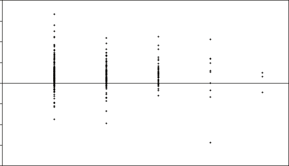
14. Introduction to panel data
those of the individuals who did not, and that this could account for a
different coefficient. Explain in general verbal terms what investigation the
researcher should undertake in response to this suggestion.
•Finally, another person says that it might be a good idea to look at the
relationship between earnings and schooling for the subsample who went back
to school or college, restricting the analysis to these 371 individuals. The
researcher responds by running the regression for that group alone. The result
is shown in column (5) in the table. The researcher also plots a scatter
diagram, reproduced below, showing the change in the logarithm of earnings
and the change in schooling. For those with one extra year of schooling, the
mean change in log earnings was 0.40. For those with two extra years, 0.37.
For those with three extra years, 0.47. What conclusions might be drawn from
the regression results?
-4
-3
-2
-1
0
1
2
3
4
0
change in schooling
change in log earnings
1
2
3
4
5
A14.5 In the discussion of the DWH test, it was stated that the test compares the
coefficients of those variables not dropped in the FE regression. Explain why the
constant is not included in the comparison.
14.4 Answer to the starred exercise in the textbook
14.9 The NLSY2000 data set contains the following data for a sample of 2,427 males
and 2,392 females for the years 1980–2000: weight in pounds, years of schooling,
age, marital status in the form of a dummy variable MARRIED defined to be 1 if
the respondent was married, 0 if single, and height in inches. Hypothesizing that
weight is influenced by schooling, age, marital status, and height, the following
regressions were performed for males and females separately:
(1) an ordinary least squares (OLS) regression pooling the observations
(2) a within-groups fixed effects regression
(3) a random effects regression.
304

14.4. Answer to the starred exercise in the textbook
The results of these regressions are shown in the table. Standard errors are given in
parentheses.
Males Females
OLS FE RE OLS FE RE
Year of −0.98 −0.02 −0.45 −1.95 −0.60 −1.25
schooling (0.09) (0.23) (0.16) (0.12) (0.27) (0.18)
Age 1.61 1.64 1.65 2.03 1.66 1.72
(0.04) (0.02) (0.02) (0.05) (0.03) (0.03)
Married 3.70 2.92 3.00 −8.27 3.08 1.98
(0.48) (0.33) (0.32) (0.59) (0.46) (0.44)
Height 5.07 dropped 4.95 3.48 dropped 3.38
(0.08) (0.18) (0.10) (0.21)
constant −209.52 dropped −209.81 −105.90 dropped −107.61
(5.39) (12.88) (6.62) (13.43)
R20.27 — — 0.17 — —
n17,299 17,299 17,299 13,160 13,160 13,160
DWH χ2(3) 7.22 92.94
Explain why height is excluded from the FE regression.
Evaluate, for males and females separately, whether the fixed effects or random
effects model should be preferred.
For males and females separately, compare the estimates of the coefficients in the
OLS and FE models and attempt to explain the differences.
Explain in principle how one might test whether individual-specific fixed effects
jointly have significant explanatory power, if the number of individuals is small.
Explain why the test is not practical in this case.
Answer:
Height is constant over observations. Hence, for each individual:
HEIGHT it −HEIGHT i= 0
for all t, where HEIGHT iis the mean height for individual ifor the observations
for that individual. Hence height has to be dropped from the regression model.
The critical value of chi-squared, with three degrees of freedom, is 7.82 at the 5
percent level and 16.27 at the 0.1 percent level. Hence there is a possibility that the
random effects model may be appropriate for males, but it is definitely not
appropriate for females.
Males
The OLS regression suggests that schooling has a small (one pound less per year of
schooling) but highly significant negative effect on weight. The fixed effects
regression eliminates the effect, indicating that an unobserved effect is responsible:
males with unobserved qualities that have a positive effect on educational
attainment, controlling for other measured variables, have lower weight as a
consequence of the same unobserved qualities. We cannot compare estimates of the
effect of height since it is dropped from the FE regression. The effect of age is the
same in the two regressions. There is a small but highly significant positive effect of
being married, the OLS estimate possibly being inflated by an unobserved effect.
305
14. Introduction to panel data
Females
The main, and very striking, difference is in the marriage coefficient. The OLS
regression suggests that marriage reduces weight by eight pounds, a remarkable
amount. The FE regression suggests the opposite, that marriage leads to an
increase in weight that is similar to that for males. The clear implication is that
women who weigh less are relatively successful in the marriage market, but once
they are married they put on weight.
For schooling the story is much the same as for males, except that the OLS
coefficient is much larger and the coefficient remains significant at the 5 percent
level in the FE regression. The effect of age appears to be exaggerated in the OLS
regression, for reasons that are not obvious.
One might test whether individual-specific fixed effects jointly have significant
explanatory power by performing a LSDV regression, eliminating the intercept in
the model and adding a dummy variable for each individual. One would compare
RSS for this regression with that for the regression without the dummy variables,
using a standard Ftest. In the present case it is not a practical proposition
because there are more than 17,000 males and 13,000 females.
14.5 Answers to the additional exercises
A14.1 Explain why the researcher included PWE as a control.
Clearly actual work experience is positively influenced by PWE. Omitting it would
cause the coefficient of Sto be biased downwards since PWE and Sare negatively
correlated.
Evaluate the results of the Durbin–Wu–Hausman tests
With two degrees of freedom, the critical value of chi-squared is 5.99 at the 5
percent level and 9.21 at the 1 percent level. Thus the random effects model is
rejected for males but seemingly not for females.
For males and females separately, explain the differences in the coefficients of S in
the OLS and FE regressions.
For both sexes the OLS estimate is greater than the FE estimate. One possible
reason is that some unobserved characteristics, for example drive, are positively
correlated with both acquiring schooling, and seeking and gaining employment.
For males and females separately, explain the differences in the coefficients of PWE
in the OLS and FE regressions.
Since Sand PWE are negatively correlated, these same unobserved characteristics
would cause the OLS estimate of the coefficient of PWE to be biased downwards.
A14.2 First, note that the DWH statistic is significant at the 5 per cent level (critical
value 7.82) but not at the 1 per cent level (critical value 11.35).
The coefficients of SH and SC in the OLS regression is an estimate of the impact
of variations in years of high school and years of college among all the individuals
in the sample. Most individuals in fact completed high school and so had SH = 12.
306

14.5. Answers to the additional exercises
However, a small minority did not and this variation made possible the estimation
of the SH coefficient. The majority of the remainder did not complete any years of
college and therefore had SC = 0, but a substantial minority did have a partial or
complete college education, some even pursuing postgraduate studies, and this
variation made possible the estimation of the SC coefficient.
Most individuals completed their formal education before entering employment. For
them, SHit =SHifor all tand hence SHit −SHi= 0 for all t. As a consequence,
the observations for such individuals provide no variation in the SH variable.
Likewise they provide no variation in the SC variable. If all observations pertained
to such individuals, schooling would be washed out in the FE regression along with
other unchanging characteristics such as sex, ethnicity, and ASVABC score. The
schooling coefficients in the FE regression therefore relate to those individuals who
returned to formal education after a break in which they found employment.
The fact that these individuals account for a relatively small proportion of the
observations in the data set has an adverse effect on the precision of the FE
estimates of the coefficients of SH and SC. This is reflected in standard errors that
are much larger than those obtained in the OLS pooled regression.
Discuss the differences in the estimates of the coefficient of SH.
Most of the variation in SH in the FE regressions come from individuals earning
the GED degree. This degree provides an opportunity for high school drop-outs to
make good their shortfall by taking courses and passing the examinations required
for this diploma. These courses may be civilian or military adult education classes,
but very often they are programmes offered to those in jail. In principle the GED
should be equivalent to the high school diploma, but there is some evidence that
standards are sometimes lower. The results in the table appear to corroborate this
view. The OLS regression indicates that a year of high school raises earnings by 2.6
per cent, with the coefficient being highly significant, whereas the FE coefficient
indicates that the effect is only 0.5 per cent and not significant.
Discuss the differences in the estimates of the coefficient of SC.
Some of the variation in SC in the FE regressions comes from individuals entering
employment for a year or two after finishing high school and then going to college,
resuming their formal education. However, most comes from individuals returning
to college for a year or two after having been employment for a number of years. A
typical example is a high school graduate who has settled down in an occupation
and who has then decided to upgrade his or her professional skills by taking a
two-year associate of arts degree. Similarly one encounters college graduates who
upgrade to masters level after having worked for some time. One would expect such
students to be especially well motivated – they are often undertaking studies that
are relevant to an established career, and they are often bearing high opportunity
costs from loss of earnings while studying – and accordingly one might expect the
payoff in terms of increased earnings to be relatively high. This seems to be borne
out in a comparison of the OLS and FE estimates of the coefficient of SC, though
the difference is not dramatic.
On the surface, this exercise appeared to be about how one might use FE to
eliminate the bias in OLS pooled regression caused by unobserved effects. Has the
analysis been successful in this respect? Absolutely not. In particular, the apparent
307

14. Introduction to panel data
conclusion that high school education has virtually no effect on earnings should not
be taken at face value. The reason is that the issue of biases attributable to
unobserved effects has been overtaken by the much more important issue of the
difference in the interpretation of the SH and SC coefficients discussed in the
exercise. This illustrates a basic point in econometrics: understanding the context
of the data is often just as important as being proficient at technical analysis.
A14.3 Explain intuitively and mathematically the consequences of performing a simple
regression of G on S. For this purpose S and E may be treated as nonstochastic
variables.
If one fits the regression: b
G=b
β1+b
β2S
then
b
β2=PSi−SGi−G
PSi−S2
=PSi−S(β1+β2Si+β3Ei+ui)−β1+β2S+β2E+u
PSi−S2
=β2+β3PSiSEi−E
PSi−S2+PSi−S(ui−u)
PSi−S2.
Taking expectations, and making use of the invitation to treat Sand Eas
nonstochastic:
E(b
β2) = β2+β3PSiSEi−E
PSi−S2+PSi−SE(ui−u)
PSi−S2
=β2+β3PSi−SEi−E
PSi−S2.
Hence the estimator is biased unless Sand Ehappen to be uncorrelated in the
sample. As a consequence, the standard errors will be invalid.
Compare the properties of the estimators of the coefficient of S in (1) and of the
coefficient of ∆Sin (2).
Given (1), the differenced model should have been:
∆G=δ2∆S+w
where w=u−u∗.
The estimator of the coefficient of ∆Sin (2) should be unbiased, while that of Sin
(1) will be subject to omitted variable bias. However:
308
14.5. Answers to the additional exercises
•it is possible that the bias in (1) may be small. This would be the case if E
were a relatively unimportant determinant of Gor if its correlation with S
were low.
•it is possible that the variance in ∆Sis smaller than that of S. This would be
the case if Swere changing slowly in each country, or if the rate of change of S
were similar in each country.
Thus there may be a trade-off between bias and variance and it is possible that the
estimator of β2using specification (1) could actually be superior according to some
criterion such as the mean square error. It should be noted that the inclusion of δ1
in (2) will make the estimation of δ2even less efficient.
Explain why in principle you would expect the estimate of δ1in (2) not to be
significant. Suppose that nevertheless the researcher finds that the coefficient is
significant. Give two possible explanations.
If specification (1) is correct, there should be no intercept in (2) and for this reason
the estimate of the intercept should not be significantly different from zero. If it is
significant, this could have occurred as a matter of Type I error. Alternatively, it
might indicate a shift in the relationship between the two time periods. Suppose
that (1) should have included a dummy variable set equal to 0 in the first time
period and 1 in the second. b
δ1would then be an estimate of its coefficient.
Could the researcher have used a random effects regression in the present case?
Random effects requires the sample to be drawn randomly from a population and
for unobserved effects to be uncorrelated with the regressors. The first condition is
not satisfied here, so random effects would be inappropriate.
A14.4 The researcher is unable to explain why the coefficient of the change in schooling in
regression (3) is so much lower than the schooling coefficients in (1) and (2).
Someone says that it is because he has left out relevant variables such as cognitive
ability, region of residence, etc, and the coefficients in (1) and (2) are therefore
biased. Someone else says that cannot be the explanation because these variables are
also omitted from regression (3). Explain what would be your view.
Suppose that the true model is:
LGEARN =β1+β2S+β3EXP +β4ASVABC +β5MALE
+β6ETHBLACK +β7ETHHISP +β8X8+u
where X8is some further fixed characteristic of the respondent. ASVABC and X8
are absent from regressions (1) and (2) and so those regressions will be subject to
omitted variable bias. In particular, since ASVABC is likely to be positively
correlated with S, and to have a positive coefficient, its omission will tend to bias
the coefficient of Supwards.
However, if the specification is valid for both 1994 and 2000 and unchanged, one can
eliminate the omitted variable bias by taking first differences as in regression (3):
∆LGEARN =β2∆S+β3∆EXP + ∆u.
By fitting this specification one should obtain unbiased estimates of the coefficients
of schooling and experience, and the former should therefore be smaller than in (1)
309
14. Introduction to panel data
and (2). Note that all the fixed characteristics have been washed out. The
suggestion that ASVABC should have been included in (3) is therefore incorrect.
Note that (3) should not have included an intercept. This is discussed later in the
question.
He runs regressions (1) and (2) again, adding a measure of cognitive ability. The
results for the 2000 regression are shown in column (4). The results for 1994 were
very similar. Discuss possible reasons for the fact that the estimate of the schooling
coefficient differs from those in (2) and (3).
The estimate of the coefficient of Sdiffers from that in (2) because the omitted
variable bias attributable to the omission of ASVABC in that specification has now
been corrected. However it is still biased if X8(representing other omitted
characteristics) is a determinant of earnings and is correlated with S. This partial
rectification of the omitted variable problem accounts for the fact that the
coefficient of Sin (4) lies between those in (2) and (3).
Someone says that the researcher should not have included a constant in regression
(3). Explain why she made this remark and assess whether it is valid.
Given the specification in (1) and (2), there should have been no intercept in the
first differences specification (3). One would therefore expect the estimate of the
intercept to be somewhere near zero in the sense of not being significantly different
from it. Nevertheless, it is significantly different at the 5 percent level. However,
suppose that the relationship shifted between 1994 and 2000, and that the shift
could be represented by a dummy variable Dequal to zero in 1994 and 1 in 2000,
with coefficient δ. Then (3) should have an intercept δ. Its estimate, 0.102, suggests
that earnings grew by 10 percent from 1994 to 2000, holding other factors constant.
This seems entirely reasonable, perhaps even a little low.
Alternatively, the apparently significant tstatistic might have arisen as a matter of
Type I error.
Someone else at the seminar says that the reason for the relatively low coefficient of
schooling in regression (3) is that it mostly represented non-degree schooling. Hence
one would not expect to find the same relationship between schooling and earnings
as for the regular preemployment schooling of young people. Explain in general
verbal terms what investigation the researcher should undertake in response to this
suggestion.
Divide Sinto two variables, schooling as of 1994 and extra schooling as of 2000,
with separate coefficients. Then use a standard Ftest (or ttest) of a restriction to
test whether the coefficients are significantly different.
Another person suggests that the small minority of individuals who went back to
school or college in their thirties might have characteristics different from those of
the individuals who did not, and that this could account for a different coefficient.
Explain in general verbal terms what investigation the researcher should undertake
in response to this suggestion.
The issue is sample selection bias and an appropriate procedure would be that
proposed by Heckman. One would use probit analysis with an appropriate set of
determinants to model the decision to return to school between 1994 and 2000, and
a regression model to explain variations in the logarithm of earnings of those
310
14.5. Answers to the additional exercises
respondents who do return to school, linking the two models by allowing their
disturbance terms to be correlated. One would test whether the estimate of this
correlation is significantly different from zero.
Finally, another person says that it might be a good idea to look at the relationship
between earnings and schooling for the subsample who went back to school or
college, restricting the analysis to these 371 individuals. The researcher responds by
running the regression for that group alone. The result is shown in column (5) in
the table. The researcher also plots a scatter diagram, reproduced below, showing the
change in the logarithm of earnings and the change in schooling. For those with one
extra year of schooling, the mean change in log earnings was 0.40. For those with
two extra years, 0.37. For those with three extra years, 0.47. What conclusions
might be drawn from the regression results?
The schooling coefficient is effectively zero! [These are real data, incidentally.] The
scatter diagram shows why. Irrespective of whether the respondent had one, two, or
three years of extra schooling, the gain is about the same, on average. (These are
the only categories with large numbers of observations, given the information at the
beginning of the question, confirmed by the scatter diagram.) So the results
indicate that the fact of going back to school, rather than the duration of the
schooling, is the relevant determinant of the change in earnings. The intercept
indicates that this subsample on average increased their earnings between 1994 and
2000 by 38.9 percent. (As a first approximation. The actual proportion would be
better estimated as e0.389 −1 = 0.476.) This figure is confirmed by the diagram, and
it would appear to be much greater than the effect of regular schooling. One
explanation could be sample selection bias, as already discussed. A more likely
possibility is that the respondents were presented with opportunities to increase
their earnings substantially if they undertook certain types of formal course, and
they took advantage of these opportunities.
A14.5 In a random effects regression, the interpretation of an intercept is not affected by
the estimation technique. In a fixed effects regression, the intercept is washed out.
Hence there is no basis for a comparison. In general, the model is fitted without an
intercept. The only case where an intercept should be included is in first-differences
fixed effects estimation of a model containing a deterministic trend. For example,
suppose one is fitting the model:
Yit =β1+β2Xit +δt +uit.
For individual iin the previous time period, one has:
Yi, t−1=β1+β2Xi, t−1+δ(t−1) + ui, t−1.
Subtracting, one obtains:
Yit −Yi, t−1=β2(Xit −Xi, t−1) + δ+uit −ui, t−1.
The model now does have an intercept, but its meaning is different from that in the
original specification. It now provides an estimate of δ, not β1.
311
14. Introduction to panel data
312

Chapter 15
Regression analysis with linear
algebra primer
15.1 Overview
This primer is intended to provide a mathematical bridge to a master’s level course that
uses linear algebra for students who have taken an undergraduate econometrics course
that does not. Why should we make the mathematical shift? The most immediate
reason is the huge double benefit of allowing us to generalise the core results to models
with many explanatory variables while simultaneously permitting a great simplification
of the mathematics. This alone justifies the investment in time – probably not more
than ten hours – required to acquire the necessary understanding of basic linear algebra.
In fact, one could very well put the question the other way. Why do introductory
econometrics courses not make this investment and use linear algebra from the start?
Why do they (almost) invariably use ordinary algebra, leaving students to make the
switch when they take a second course?
The answer to this is that the overriding objective of an introductory econometrics
course must be to encourage the development of a solid intuitive understanding of the
material and it is easier to do this with familiar, everyday algebra than with linear
algebra, which for many students initially seems alien and abstract. An introductory
course should ensure that at all times students understand the purpose and value of
what they are doing. This is far more important than proofs and for this purpose it is
usually sufficient to consider models with one, or at most two, explanatory variables.
Even in the relatively advanced material, where we are forced to consider asymptotics
because we cannot obtain finite-sample results, the lower-level mathematics holds its
own. This is especially obvious when we come to consider finite-sample properties of
estimators when only asymptotic results are available mathematically. We invariably
use a simple model for a simulation, not one that requires a knowledge of linear algebra.
These comments apply even when it comes to proofs. It is usually helpful to see a proof
in miniature where one can easily see exactly what is involved. It is then usually
sufficient to know that in principle it generalises, without there being any great urgency
to see a general proof. Of course, the linear algebra version of the proof will be general
and often simpler, but it will be less intuitively accessible and so it is useful to have
seen a miniature proof first. Proofs of the unbiasedness of the regression coefficients
under appropriate assumptions are obvious examples.
At all costs, one wishes to avoid the study of econometrics becoming an extended
exercise in abstract mathematics, most of which practitioners will never use again. They
will use regression applications and as long as they understand what is happening in
313
15. Regression analysis with linear algebra primer
principle, the actual mechanics are of little interest.
This primer is not intended as an exposition of linear algebra as such. It assumes that a
basic knowledge of linear algebra, for which there are many excellent introductory
textbooks, has already been acquired. For the most part, it is sufficient that you should
know the rules for multiplying two matrices together and for deriving the inverse of a
square matrix, and that you should understand the consequences of a square matrix
having a zero determinant.
15.2 Notation
Matrices and vectors will be written bold, upright, matrices upper case, for example A,
and vectors lower case, for example b. The transpose of a matrix will be denoted by a
prime, so that the transpose of Ais A0, and the inverse of a matrix will be denoted by a
superscript −1, so that the inverse of Ais A−1.
15.3 Test exercises
Answers to all of the exercises in this primer will be found at its end. If you are unable
to answer the following exercises, you need to spend more time learning basic matrix
algebra before reading this primer. The rules in Exercises 3–5 will be used frequently
without further explanation.
1. Demonstrate that the inverse of the inverse of a matrix is the original matrix.
2. Demonstrate that if a (square) matrix possesses an inverse, the inverse is unique.
3. Demonstrate that, if A=BC,A0=C0B0.
4. Demonstrate that, if A=BC,A−1=C−1B−1, provided that B−1and C−1exist.
5. Demonstrate that [A0]−1= [A−1]0.
15.4 The multiple regression model
The most obvious benefit from switching to linear algebra is convenience. It permits an
elegant simplification and generalisation of much of the mathematical analysis
associated with regression analysis. We will consider the general multiple regression
model:
Yi=β1Xi1+··· +βkXik +ui(1)
where the second subscript identifies the variable and the first the observation. In the
textbook, as far as the fourth edition, the subscripts were in the opposite order. The
reason for the change of notation here, which will be adopted in the next edition of the
textbook, is that it is more compatible with a linear algebra treatment.
314
15.5. The intercept in a regression model
Equation (1) is a row relating to observation iin a sample of nobservations. The entire
layout would be:
Y1
.
.
.
Yi
.
.
.
Yn
=
β1X11 +··· +βjX1j+··· +βkX1k
.
.
.
β1Xi1+··· +βjXij +··· +βkXik
.
.
.
β1Xn1+··· +βjXnj +··· +βkXnk
+
u1
.
.
.
ui
.
.
.
un
.
This, of course, may be written in linear algebra form as:
y=Xβ+u(2)
where:
y=
Y1
.
.
.
Yi
.
.
.
Yn
,X=
X11 ···X1j···X1k
.
.
.
Xi1···Xij ···Xik
.
.
.
Xn1···Xnj ···Xnk
,β=
β1
.
.
.
βi
.
.
.
βn
,and u=
u1
.
.
.
ui
.
.
.
un
with the first subscript of Xij relating to the row and the second to the column, as is
conventional with matrix notation. This was the reason for the change in the order of
the subscripts in equation (1).
Frequently, it is convenient to think of the matrix Xas consisting of a set of column
vectors:
X= [x1···xj···xk]
where:
xj=
X1j
.
.
.
Xij
.
.
.
Xnj
.
xjis the set of observations relating to explanatory variable j. It is written lower case,
bold, not italic because it is a vector.
15.5 The intercept in a regression model
As described above, there is no special intercept term in the model. If, as is usually the
case, one is needed, it is accommodated within the matrix framework by including an X
variable, typically placed as the first, with value equal to 1 in all observations:
x1=
1
.
.
.
1
.
.
.
1
.
315

15. Regression analysis with linear algebra primer
The coefficient of this unit vector is the intercept in the regression model. If it is
included, and located as the first column, the Xmatrix becomes:
X=
1X12 ··· X1j··· X1k
.
.
.
1Xi2··· Xij ··· Xik
.
.
.
1Xn2··· Xnj ··· Xnk
= [1 x2··· xj··· xk].
15.6 The OLS regression coefficients
Using the matrix and vector notation, we may write the fitted equation:
b
Yi=b
β1Xi1+··· +b
βkXik
as:
b
y=Xb
β
with obvious definitions of b
yand b
β. Then we may define the vector of residuals as:
b
u=y−b
y=y−Xb
β
and the residual sum of squares as:
RSS =b
u0b
u= (y−Xb
β)0(y−Xb
β)
=y0y−y0Xb
β−b
β0X0y+b
β0X0Xb
β
=y0y−2y0Xb
β+b
β0X0Xb
β
(y0Xb
β=b
β0X0ysince it is a scalar.) The next step is to obtain the normal equations:
∂RSS
∂b
βj
= 0
for j= 1, . . . , k and solve them (if we can) to obtain the least squares coefficients. Using
linear algebra, the normal equations can be written:
X0Xb
β−X0y=0.
The derivation is straightforward but tedious and has been consigned to Appendix A.
X0Xis a square matrix with krows and columns. If assumption A.2 is satisfied (that it
is not possible to write one Xvariable as a linear combination of the others), X0Xhas
an inverse and we obtain the OLS estimator of the coefficients:
b
β= [X0X]−1X0y.(3)
Exercises
6. If Y=β1+β2X+u, obtain the OLS estimators of β1and β2using (3).
7. If Y=β2+u, obtain the OLS estimator of β2using (3).
8. If Y=β1+u, obtain the OLS estimator of β1using (3).
316
15.7. Unbiasedness of the OLS regression coefficients
15.7 Unbiasedness of the OLS regression coefficients
Substituting for yfrom (2) into (3), we have:
b
β= [X0X]−1X0(Xβ+u)
= [X0X]−1X0Xβ+ [X0X]−1X0u
=β+ [X0X]−1X0u.
Hence each element of b
βis equal to the corresponding value of βplus a linear
combination of the values of the disturbance term in the sample. Next:
E(b
β|X) = β+E([X0X]−1X0u|X).
To proceed further, we need to be specific about the data generation process (DGP) for
Xand the assumptions concerning uand X. In Model A, we have no DGP for X: the
data are simply taken as given. When we describe the properties of the regression
estimators, we are either talking about the potential properties, before the sample has
been drawn, or about the distributions that we would expect in repeated samples using
those given data on X. If we make the assumption E(u|X) = 0, then:
E(b
β|X) = β+ [X0X]−1X0E(u|X) = β
and so b
βis an unbiased estimator of β. It should be stressed that unbiasedness in
Model A, along with all other properties of the regression estimators, are conditional on
the actual given data for X.
In Model B, we allow Xto be drawn from a fixed joint distribution of the explanatory
variables. The appropriate assumption for the disturbance term is that it is distributed
independently of Xand hence its conditional distribution is no different from its
absolute distribution: E(u|X) = E(u) for all X. We also assume E(u) = 0. The
independence of the distributions of Xand uallows us to write:
E(b
β|X) = β+E[X0X]−1X0u|X
=β+E[X0X]−1X0E(u)
=β.
15.8 The variance-covariance matrix of the OLS
regression coefficients
We define the variance-covariance matrix of the disturbance term to be the matrix
whose element in row iand column jis the population covariance of uiand uj. By
assumption A.4, the covariance of uiand ujis constant and equal to σ2
uif j=iand by
assumption A.5 it is equal to zero if j6=i. Thus the variance-covariance matrix is:
317
15. Regression analysis with linear algebra primer
σ2
u0 0 ··· 0 0 0
0σ2
u0··· 0 0 0
0 0 σ2
u··· 0 0 0
··· ··· ··· ··· ··· ··· ···
0 0 0 ··· σ2
u0 0
0 0 0 ··· 0σ2
u0
0 0 0 ··· 0 0 σ2
u
that is, a matrix whose diagonal elements are all equal to σ2
uand whose off-diagonal
elements are all zero. It may more conveniently be written Inσ2
uwhere Inis the identity
matrix of order n.
Similarly, we define the variance-covariance matrix of the regression coefficients to be
the matrix whose element in row iand column jis the population covariance of b
βiand
b
βj:
cov(b
βi,b
βj) = Eh(b
βi−E(b
βi))(b
βj−E(b
βj))i=Eh(b
βi−βi)(b
βj−βj)i.
The diagonal elements are of course the variances of the individual regression
coefficients. We denote this matrix var( b
β). If we are using the framework of Model A,
everything will be conditional on the actual given data for X, so we should refer to
var( b
β|X) rather than var( b
β). Then:
var( b
β|X) = E(( b
β−E(b
β))( b
β−E(b
β))0|X)
=E(( b
β−β)( b
β−β)0|X)
=E([X0X]−1X0u)([X0X]−1X0u)0|X
=E[X0X]−1X0uu0X[X0X]−1|X
= [X0X]−1X0E(uu0|X)X[X0X]−1
= [X0X]−1X0Inσ2
uX[X0X]−1
= [X0X]−1σ2
u.
If we are using Model B, we can obtain the unconditional variance of busing the
standard decomposition of a variance in a joint distribution:
var( b
β) = Ehvar( b
β|X)i+ var hE(b
β|X)i.
Now E(b
β|X) = βfor all X, so var[E(b
β|X)] = var(β) = 0since βis a constant vector,
so:
var( b
β) = E[X0X]−1σ2
u=σ2
uE[X0X]−1
the expectation being taken over the distribution of X.
To estimate var( b
β), we need to estimate σ2
u. An unbiased estimator is provided by
b
u0b
u/(n−k). For a proof, see Appendix B.
318
15.9. The Gauss–Markov theorem
15.9 The Gauss–Markov theorem
We will demonstrate that the OLS estimators are the minimum variance unbiased
estimators that are linear in y. For simplicity, we will do this within the framework of
Model A, with the analysis conditional on the given data for X. The analysis generalises
straightforwardly to Model B, where the explanatory variables are stochastic but drawn
from fixed distributions.
Consider the general estimator in this class:
b
β∗=Ay
where Ais a kby nmatrix. Let:
C=A−[X0X]−1X0.
Then:
b
β∗=[X0X]−1X0+Cy
=[X0X]−1X0+C(Xβ+u)
=β+CXβ+ [X0X]−1X0u+Cu.
Unbiasedness requires:
CX =0k
where 0is a kby kmatrix consisting entirely of zeros. Then, with E(b
β∗) = β, the
variance-covariance matrix of b
β∗is given by:
Eh(b
β∗−β)( b
β∗−β)0i=Eh[X0X]−1X0+Cuu0[X0X]−1X0+C0i
=[X0X]−1X0+CInσ2
u[X0X]−1X0+C0
=[X0X]−1X0+C[X0X]−1X0+C0σ2
u
=[X0X]−1+CC00σ2
u.
Now diagonal element iof CC0is the inner product of row iof Cand column iof C0.
These are the same, so it is given by:
k
X
s=1
c2
ik
which is positive unless cis = 0 for all s. Hence minimising the variances of the
estimators of all of the elements of βrequires C=0. This implies that OLS provides
the minimum variance unbiased estimator.
15.10 Consistency of the OLS regression coefficients
Since: b
β=β+ [X0X]−1X0u
319

15. Regression analysis with linear algebra primer
the probability limit of b
βis given by:
plim b
β=β+ plim [X0X]−1X0u
=β+ plim 1
nX0X−11
nX0u!.
Now, if we are working with cross-sectional data with the explanatory variables drawn
from fixed (joint) distributions, it can be shown that:
plim 1
nX0X−1
has a limiting matrix and that:
plim 1
nX0u= 0.
Hence we can decompose:
plim 1
nX0X−11
nX0u!= plim 1
nX0X−1
plim 1
nX0u= 0
and so plim b
β=β. Note that this is only an outline of the proof. For a proper proof
and a generalisation to less restrictive assumptions, see Greene pp.64–65.
15.11 Frisch–Waugh–Lovell theorem
We will precede the discussion of the Frisch–Waugh–Lovell (FWL) theorem by
introducing the residual-maker matrix. We have seen that, when we fit:
y=Xβ+u
using OLS, the residuals are given by:
b
u=y−b
y=y−Xb
β.
Substituting for b
β, we have:
b
u=y−X[X0X]−1X0y
=I−X[X0X]−1X0y
=My
where:
M=I−X[X0X]−1X0.
Mis known as the ‘residual-maker’ matrix because it converts the values of yinto the
residuals of ywhen regressed on X. Note that Mis symmetric, because M0=M, and
idempotent, meaning that MM =M.
Now suppose that we divide the kvariables comprising Xinto two subsets, the first s
and the last k−s. (For the present purposes, it makes no difference whether there is or
320
15.11. Frisch–Waugh–Lovell theorem
is not an intercept in the model, and if there is one, whether the vector of ones
responsible for it is in the first or second subset.) We will partition Xas:
X= [X1X2]
where X+1comprises the first scolumns and X2comprises the last k−s, and we will
partition βsimilarly, so that the theoretical model may be written:
y= [X1X2]β1
β2+u.
The FWL theorem states that the OLS estimates of the coefficients in β1are the same
as those that would be obtained by the following procedure: regress yon the variables
in X2and save the residuals as b
uy. Regress each of the variables in X1on X2and save
the matrix of residuals as b
uX1. If we regress b
uyon b
uX1, we will obtain the same
estimates of the coefficients of β1as we did in the straightforward multiple regression.
(Why we might want to do this is another matter. We will come to this later.) Applying
the preceding discussion relating to the residual-maker, we have:
b
uy=M2y
where:
M2=I−X2[X20X2]−1X20
and:
b
uX1=M2X1.
Let the vector of coefficients obtained when we regress b
uyon b
uX1be denoted b
β∗
1. Then:
b
β∗
1= [b
u0
X1b
uX1]−1b
u0
X1b
uy
= [X10M20M2X1]−1X10M20M2y
= [X10M2X1]−1X1M2y.
(Remember that M2is symmetric and idempotent.) Now we will derive an expression
for b
β1from the orthodox multiple regression of yon X. For this purpose, it is easiest to
start with the normal equations:
X0Xb
β−X0y=0.
We partition b
βas "b
β1
b
β2#.X0is X10
X20, and we have the following:
X0X=X10X1X10X2
X20X1X20X2
X0Xb
β=X10X1X10X2
X20X1X20X2"b
β1
b
β2#="X10X1b
β1+X10X2b
β2
X20X1b
β1+X20X2b
β2#
X0y=X10y
X20y.
321
15. Regression analysis with linear algebra primer
Hence, splitting the normal equations into their upper and lower components, we have:
X10X1b
β1+X10X2b
β2−X10y=0
and:
X20X1b
β1+X20X2b
β2−X20y=0.
From the second we obtain:
X20X2b
β2=X20y−X20X1b
β1
and so: b
β2= [X20X2]−1[X20y−X20X1b
β1].
Substituting for b
β2in the first normal equation:
X10X1b
β1+X10X2[X20X2]−1[X20y−X20X1b
β1]−X10y=0.
Hence:
X10X1b
β1−X10X2[X20X2]−1X20X1b
β1=X10y−X10X2[X20X2]−1X20y
and so:
X10I−X2[X20X2]−1X0
2X1b
β1=X10I−X2[X20X2]−1X20y.
Hence:
X10M2X1b
β1=X10M2y
and: b
β1= [X10M2X1]−1X10M2y=b
β∗
1.
Why should we be interested in this result? The original purpose remains instructive. In
early days, econometricians working with time series data, especially macroeconomic
data, were concerned to avoid the problem of spurious regressions. If two variables both
possessed a time trend, it was very likely that ‘significant’ results would be obtained
when one was regressed on the other, even if there were no genuine relationship between
them. To avoid this, it became the custom to detrend the variables before using them
by regressing each on a time trend and then working with the residuals from these
regressions. Frisch and Waugh (1933) pointed out that this was an unnecessarily
laborious procedure. The same results would be obtained using the original data, if a
time trend was added as an explanatory variable.
Generalising, and this was the contribution of Lovell, we can infer that, in a multiple
regression model, the estimator of the coefficient of any one variable is not influenced by
any of the other variables, irrespective of whether they are or are not correlated with
the variable in question. The result is so general and basic that it should be understood
by all students of econometrics. Of course, it fits neatly with the fact that the multiple
regression coefficients are unbiased, irrespective of any correlations among the variables.
A second reason for being interested in the result is that it allows one to depict
graphically the relationship between the observations on the dependent variable and
those on any single explanatory variable, controlling for the influence of all the other
explanatory variables. This is described in the textbook in Section 3.2.
322
15.12. Exact multicollinearity
Exercise
9. Using the FKL theorem, demonstrate that, if a multiple regression model contains
an intercept, the same slope coefficients could be obtained by subtracting the
means of all of the variables from the data for them and then regressing the model
omitting an intercept.
15.12 Exact multicollinearity
We will assume, as is to be expected, that k, the number of explanatory variables
(including the unit vector, if there is one), is less than n, the number of observations. If
the explanatory variables are independent, the Xmatrix will have rank kand likewise
X0Xwill have rank kand will possess an inverse. However, if one or more linear
relationships exist among the explanatory variables, the model will be subject to exact
multicollinearity. The rank of X, and hence of X0X, will then be less than kand X0X
will not possess an inverse.
Suppose we write Xas a set of column vectors xj, each corresponding to the
observations on one of the explanatory variables:
X= [x1··· xj··· xk]
where:
xj=
x1j
.
.
.
xij
.
.
.
xnj
.
Then:
X0=
x10
.
.
.
xj0
.
.
.
xk0
and the normal equations:
X0Xb
β−X0y=0
may be written:
x10Xb
β
.
.
.
xj0Xb
β
.
.
.
xk0Xb
β
−
x10y
.
.
.
xj0y
.
.
.
xk0y
=0.
323
15. Regression analysis with linear algebra primer
Now suppose that one of the explanatory variables, say the last, can be written as a
linear combination of the others:
xk=
k−1
X
i=1
λixi.
Then the last of the normal equations is that linear combination of the other k−1.
Hence it is redundant, and we are left with a set of k−1 equations for determining the
kunknown regression coefficients. The problem is not that there is no solution. It is the
opposite: there are too many possible solutions, in fact an infinite number. One
coefficient could be chosen arbitrarily, and then the normal equations would provide a
solution for the other k−1. Some regression applications deal with this situation by
dropping one of the variables from the regression specification, effectively assigning a
value of zero to its coefficient.
Exact multicollinearity is unusual because it mostly occurs as a consequence of a logical
error in the specification of the regression model. The classic example is the dummy
variable trap. This occurs when a set of dummy variables Dj,j= 1, . . . , s are defined
for a qualitative characteristic that has scategories. If all sdummy variables are
included in the specification, in observation iwe will have:
s
X
j=1
Dij = 1
since one of the dummy variables must be equal to 1 and the rest are all zero. But this
is the (unchanging) value of the unit vector. Hence the sum of the dummy variables is
equal to the unit vector. As a consequence, if the unit vector and all of the dummy
variables are simultaneously included in the specification, there will be exact
multicollinearity. The solution is to drop one of the dummy variables, making it the
reference category, or, alternatively, to drop the intercept (and hence unit vector),
effectively making the dummy variable coefficient for each category the intercept for
that category. As explained in the textbook, it is illogical to wish to include a complete
set of dummy variables as well as the intercept, for then no interpretation can be given
to the dummy variable coefficients.
15.13 Estimation of a linear combination of
regression coefficients
Suppose that one wishes to estimate a linear combination of the regression parameters:
k
X
j=1
λjβj.
In matrix notation, we may write this as λ0βwhere:
λ=
λ1
.
.
.
λj
.
.
.
λk
.
324

15.14. Testing linear restrictions
The corresponding linear combination of the regression coefficients, λ0b
β, provides an
unbiased estimator of λ0β. However, we will often be interested also in its standard
error, and this is not quite so straightforward. We obtain it via the variance:
var(λ0b
β) = Eh(λ0b
β−E(λ0b
β))2i=Eh(λ0b
β−λ0β)2i.
Since (λ0b
β−λ0β) is a scalar, it is equal to its own transpose, and so (λ0b
β−λ0β)2may
be written:
var(λ0b
β) = Ehλ0(b
β−β)( b
β−β)0λi
=λ0Eh(b
β−β)( b
β−β)0iλ
=λ0[X0X]−1λσ2
u.
The square root of this expression provides the standard error of λ0b
βafter we have
replaced σ2
uby its estimator b
u0b
u/(n−k) in the usual way.
15.14 Testing linear restrictions
An obvious application of the foregoing is its use in testing a linear restriction. Suppose
that one has a hypothetical restriction:
k
X
j=1
λjβj=λ0.
We can perform a ttest of the restriction using the tstatistic:
t=λ0b
β−λ0
s.e.(λ0b
β)
where the standard error is obtained via the variance-covariance matrix as just
described. Alternatively, we could reparameterise the regression specification so that
one of the coefficients is λ0β. In practice, this is often more convenient since it avoids
having to work with the variancecovariance matrix. If there are multiple restrictions
that should be tested simultaneously, the appropriate procedure is an Ftest comparing
RSS for the unrestricted and fully restricted models.
15.15 Weighted least squares and heteroskedasticity
Suppose that the regression model:
y=Xβ+u
satisfies the usual regression model assumptions and suppose that we premultiply the
elements of the model by the nby nmatrix Awhose diagonal elements are Aii,
325

15. Regression analysis with linear algebra primer
i= 1, . . . , n, and whose off-diagonal elements are all zero:
A=
A11 ··· 0··· 0
··· ··· ··· ··· ···
0··· Aii ··· 0
··· ··· ··· ··· ···
0··· 0··· Ann
.
The model becomes:
Ay =AXβ+Au.
If we fit it using least squares, the point estimates of the coefficients are given by:
b
βWLS = [X0A0AX]−1X0A0Ay
(WLS standing for weighted least squares). This is unbiased but heteroskedastic
because the disturbance term in observation iis Aiiuiand has variance A2
iiσ2
u.
Now suppose that the disturbance term in the original model was heteroskedastic, with
variance σ2
uiin observation i. If we define the matrix Aso that the diagonal elements
are determined by:
Aii =1
pσ2
ui
the corresponding variance in the weighted regression will be 1 for all observations and
the WLS model will be homoskedastic. The WLS estimator is then:
b
βWLS = [X0CX]−1X0Cy
where:
C=A0A=
1
σ2
u1··· 0··· 0
··· ··· ··· ··· ···
0··· 1
σ2
ui··· 0
··· ··· ··· ··· ···
0··· 0··· 1
σ2
un
.
The variance-covariance matrix of the WLS coefficients, conditional on the data for X,
is:
var( b
βWLS) = Eh(b
βWLS −E(b
βWLS))( b
βWLS −E(b
βWLS))0i
=Eh(b
βWLS −β))( b
βWLS −β))0i
=E([X0A0AX]−1X0A0Au)([X0A0AX]−1X0A0Au)0
=E[X0A0AX]−1X0A0Auu0A0AX[X0A0AX]−1
=[X0A0AX]−1X0A0AE(uu0)A0AX[X0A0AX]−1
= [X0A0AX]−1X0A0AX[X0A0AX]−1
= [X0CX]−1X0CX[X0CX]−1σ2
u
= [X0CX]−1σ2
u
326

15.16. IV estimators and TSLS
since Ahas been defined so that:
AE(uu0)A0=I.
Of course, in practice we seldom know σ2
ui, but if it is appropriate to hypothesise that
the standard deviation is proportional to some measurable variable Zi, then the WLS
regression will be homoskedastic if we define Ato have diagonal element iequal to the
reciprocal of Zi.
15.16 IV estimators and TSLS
Suppose that we wish to fit the model:
y=Xβ+u
where one or more of the explanatory variables is not distributed independently of the
disturbance term. For convenience, we will describe such variables as ‘endogenous’,
irrespective of the reason for the violation of the independence requirement. Given a
sufficient number of suitable instruments, we may consider using the IV estimator:
b
βIV = [W0X]−1W0y(4)
where Wis the matrix of instruments. In general Wwill be a mixture of (1) those
original explanatory variables that are distributed independently of the disturbance
term (these are then described as acting as instruments for themselves), and (2) new
variables that are correlated with the endogenous variables but distributed
independently of the disturbance term. If we substitute for y:
b
βIV = [W0X]−1W0(Xβ+u) = β+ [W0X]−1W0u.
We cannot obtain a closed-form expression for the expectation of the error term, so
instead we take plims:
plim b
βIV =β+ plim 1
nW0X−11
nW0u!.
Now if we are using cross-sectional data, it is usually reasonable to suppose that:
plim 1
nW0X−1!and plim 1
nW0u
both exist, in which case we can decompose the plim of the error term:
plim b
βIV =β+ plim 1
nW0X−1!plim 1
nW0u.
Further, if the matrix of instruments has been correctly chosen, it can be shown that:
plim 1
nW0u= 0
327

15. Regression analysis with linear algebra primer
and hence the IV estimator is consistent.
It is not possible to derive a closed-form expression for the variance of the IV estimator
in finite samples. The best we can do is to invoke a central limit theorem that gives the
limiting distribution asymptotically and work backwards from that, as an
approximation, for finite samples. A central limit theorem can be used to establish that:
√n(b
βIV −β)d
−→ N 0,(σ2
uplim 1
nW0X−1
plim 1
nW0Wplim 1
nX0W−1)!.
From this, we may infer, that as an approximation, for sufficiently large samples:
b
βIV ∼N β,(σ2
u
nplim 1
nW0X−1
plim 1
nW0Wplim 1
nX0W−1)!.(5)
We have implicitly assumed so far that Whas the same dimensions as Xand hence
that W0Xis a square kby kmatrix. However, the model may be overidentified, with
the number of columns of Wexceeding k. In that case, the appropriate procedure is
two-stage least squares. One regresses each of the variables in Xon Wand saves the
fitted values. The matrix of fitted values is then used as the instrument matrix in place
of W.
Exercises
10. Using (4) and (5), demonstrate that, for the simple regression model:
Yi=β1=β2Xi+ui
with Zacting as an instrument for X(and the unit vector acting as an instrument
for itself):
b
βIV
1=Y−b
βIV
2X
b
βIV
2=PZi−ZYi−Y
PZi−ZXi−X
and, as an approximation:
var(b
βIV
2) = σ2
u
PXi−X2×1
r2
XZ
where Zis the instrument for Xand rXZ is the correlation between Xand Z.
11. Demonstrate that any variable acting as an instrument for itself is unaffected by
the first stage of two-stage least squares.
12. Demonstrate that TSLS is equivalent to IV if the equation is exactly identified.
328
15.17. Generalised least squares
15.17 Generalised least squares
The final topic in this introductory primer is generalised least squares and its
application to autocorrelation (autocorrelated disturbance terms). One of the basic
regression model assumptions is that the disturbance terms in the observations in a
sample are distributed identically and independently of each other. If this is the case,
the variance-covariance matrix of the disturbance terms is the identity matrix of order
n, multiplied by σ2
u. We have encountered one type of violation, heteroskedasticity,
where the values of the disturbance term are independent but not identical. The
consequence was that the off-diagonal elements of the variance-covariance matrix
remained zero, but the diagonal elements differed. Mathematically, autocorrelation is
complementary. It occurs when the values of the disturbance term are not independent
and as a consequence some, or all, of the off-diagonal elements are non-zero. It is usual
in initial treatments to retain the assumption of identical distributions, so that the
diagonal elements of the variance-covariance matrix are the same. Of course, in
principle one could have both types of violation at the same time.
In abstract, it is conventional to denote the variance-covariance matrix of the
disturbance term Ωσ2
u, where Ω is the Greek upper case omega, writing the model:
y=Xβwith E(uu0) = Ωσ2
u.(6)
If the values of the disturbance term are iid, Ω=I. If they are not iid, OLS is in
general inefficient and the standard errors are estimated incorrectly. Then, it is desirable
to transform the model so that the transformed disturbance terms are iid. One possible
way of doing this is to multiply through by some suitably chosen matrix P, fitting:
Py =PXβ+Pu
choosing Pso that E(Puu0P0) = Iαwhere αis some scalar. The solution for
heteroskedasticity was a simple example of this type. We had:
Ω=
σ2
u1··· 0··· 0
··· ··· ··· ··· ···
0··· σ2
ui··· 0
··· ··· ··· ··· ···
0··· 0··· σ2
un
and the appropriate choice of Pwas:
P=
q1
σ2
u1··· 0··· 0
··· ··· ··· ··· ···
0··· q1
σ2
ui··· 0
··· ··· ··· ··· ···
0··· 0··· q1
σ2
un
.
In the case of heteroskedasticity, the choice of Pis obvious, provided, of course, that
one knows the values of the diagonal elements of Ω. The more general theory requires
an understanding of eigenvalues and eigenvectors that will be assumed. Ωis a
329

15. Regression analysis with linear algebra primer
symmetric matrix since cov(ui, uj) is the same as cov(uj, ui). Hence all its eigenvalues
are real. Let Λbe the diagonal matrix with the eigenvalues as the diagonal elements.
Then there exists a matrix of eigenvectors, C, such that:
C0ΩC =Λ.(7)
Chas the properties that CC0=Iand C0=C−1. Since Λ is a diagonal matrix, if its
eigenvalues are all positive (which means that it is what is known as a ‘positive definite’
matrix), it can be factored as Λ=Λ1/2Λ1/2where Λ1/2is a diagonal matrix whose
diagonal elements are the square roots of the eigenvalues. It follows that the inverse of
Λcan be factored as Λ−1=Λ−1/2Λ−1/2. Then, in view of (7):
Λ−1/2[C0ΩC]Λ−1/2=Λ−1/2ΛΛ−1/2=Λ−1/2Λ1/2Λ1/2Λ−1/2=I.(8)
This, if we define P=Λ−1/2C0,(8) becomes:
PΩP0=I.
As a consequence, if we premultiply (6) through by P, we have:
Py =PXβ+Pu
or:
y∗=X∗β+u∗
where y∗=Py,X∗=PX, and u∗=Pu, and E(u∗u∗0) = Iσ2
u. An OLS regression of y∗
on X∗will therefore satisfy the usual regression model assumptions and the estimator of
βwill have the usual properties. Of course, the approach usually requires the estimation
of Ω,Ωbeing positive definite, and there being no problems in extracting the
eigenvalues and determining the eigenvectors.
Exercise
13. Suppose that the disturbance term in a simple regression model (with an intercept)
is subject to AR(1) autocorrelation with |ρ|<1, and suppose that the sample
consists of just two observations. Determine the variance-covariance matrix of the
disturbance term, find its eigenvalues, and determine its eigenvectors. Hence
determine Pand state the transformed model. Verify that the disturbance term in
the transformed model is iid.
15.18 Appendix A: Derivation of the normal equations
We have seen that RSS is given by:
RSS =y0y−2y0Xb
β+b
β0X0Xb
β.(A.1)
The normal equations are:
∂RSS
∂b
βj
= 0 (A.2)
330

15.18. Appendix A: Derivation of the normal equations
for j= 1, . . . , k. We will show that they can be written:
X0Xb
β−X0y=0.
The proof is mathematically unchallenging but tedious because one has to keep careful
track of the dimensions of all of the elements in the equations. As far as I know, it is of
no intrinsic interest and once one has seen it there should never be any reason to look
at it again.
First note that the term y0yin (A.1) is not a function of any of the bjand disappears in
(A.2). Accordingly we will restrict our attention to the other two terms on the right side
of (A.1). Suppose that we write the Xmatrix as a set of column vectors:
X= [x1··· xj··· xk] (A.3)
where:
xj=
X1j
.
.
.
Xij
.
.
.
Xnj
.
Then:
y0Xb
β= [y0x1··· y0xj··· y0xk]
b
β1
.
.
.
b
βj
.
.
.
b
βk
= [y0x1b
β1+··· +y0xjb
βj+··· +y0xkb
βk].
Hence:
∂y0Xb
β
∂b
βj
=y0xj.
We now consider the b
β0X0Xb
βterm. Using (A.3):
b
β0X0Xb
β= [x1b
β1+··· +xjb
βj+··· +xkb
βk]0[x1b
β1+··· +xjb
βj+··· +xkb
βk]
=
k
X
p=1
k
X
q=1 b
βpb
βqx0
pxq.
The subset of terms including b
βjis:
k
X
q=1 b
βjb
βqx0
jxq+
k
X
p=1 b
βpb
βjx0
pxj.
Hence:
∂b
β0X0Xb
β
∂b
βj
=
k
X
q=1 b
βqx0
jxq+
k
X
p=1 b
βpx0
pxj= 2
k
X
p=1 b
βpx0
pxj.
331

15. Regression analysis with linear algebra primer
Putting these results together:
∂RSS
∂b
βj
=∂[y0y−2y0Xb
β+b
β0X0Xb
β]
∂b
βj
=−2y0xj+ 2
k
X
p=1 b
βpx0
pxj.
Hence the normal equation ∂RSS/∂ b
βj= 0 is:
k
X
p=1 b
βpx0
jxp=x0
jy.
(Note that x0
pxj=x0
jxpand y0xj=x0
jy) since they are scalars.) Hence:
x0
j"k
X
p=1 b
βpxp#=x0
jy.
Hence:
x0
jXb
β=x0
jy
since:
Xb
β= [x1··· xp··· xk]
b
β1
.
.
.
b
βp
.
.
.
b
βk
=
k
X
p=1
xpb
βp.
Hence, stacking the knormal equations:
x10Xb
β
.
.
.
xj0Xb
β
.
.
.
xk0Xb
β
=
x10y
.
.
.
xj0y
.
.
.
xk0y
.
Hence:
x0
1
.
.
.
x0
j
.
.
.
x0
k
Xb
β=
x0
1
.
.
.
x0
j
.
.
.
x0
k
y.
Hence:
X0Xb
β=X0y.
15.19 Appendix B: Demonstration that b
u0b
u/(n−k)is
an unbiased estimator of σ2
u
This classic proof is both elegant, in that it is much shorter than any proof not using
matrix algebra, and curious, in that it uses the trace of a matrix, a feature that I have
332
15.19. Appendix B: Demonstration that b
u0b
u/(n−k)is an unbiased estimator of σ2
u
never seen used for any other purpose. The trace of a matrix, defined for square
matrices only, is the sum of its diagonal elements. We will first need to demonstrate
that, for any two conformable matrices whose product is square:
tr(AB) = tr(BA).
Let Ahave nrows and mcolumns, and let Bhave mrows and ncolumns. Diagonal
element iof AB is: m
X
p=1
aipbpi.
Hence:
tr(AB) =
n
X
i=1 m
X
p=1
aipbpi!.
Similarly, diagonal element iof BA is:
n
X
p=1
bipapi.
Hence:
tr(BA) =
m
X
i=1 n
X
p=1
bipapi!.
What we call the symbols used to index the summations makes no difference.
Re-writing pas iand ias p, and noting that the order of the summation makes no
difference, we have tr(BA) = tr(AB).
We also need to note that:
tr(A+B) = tr(A) + tr(B)
where Aand Bare square matrices of the same dimension. This follows immediately
from the way that we sum conformable matrices.
By definition:
b
u=y−b
y=y−Xb
β.
Using: b
β= [X0X]−1X0y
we have:
b
u=y−X[X0X]−1X0y
=Xβ+u−X[X0X]−1X0(Xβ+u)
=Inu−X[X0X]−1X0u
=Mu
where Inis an identity matrix of dimension nand:
M=In−X[X0X]−1X0.
333
15. Regression analysis with linear algebra primer
Hence:
b
u0b
u=u0M0Mu.
Now Mis symmetric and idempotent: M0=Mand MM =M. Hence:
b
u0b
u=u0Mu
b
u0b
uis a scalar, and so the expectation of b
u0b
uand the expectation of the trace of b
u0b
uare
the same. So:
E(b
u0b
u) = E(tr(b
u0b
u)) = E(tr(u0Mu)) = E(tr(Muu0)) = tr(E(Muu0)).
The penultimate line uses tr(AB) = tr(BA). The last line uses the fact that the
expectation of the sum of the diagonal elements of a matrix is equal to the sum of their
individual expectations. Assuming that X, and hence M, is nonstochastic:
E(b
u0b
u) = tr(ME(uu0))
=tr(MInσ2
u)
=σ2
utr(M)
=σ2
utr(In−X[X0X]−1X0)
=σ2
u(tr(In)−tr(X[X0X]−1X0)).
The last step uses tr((A) + B) = tr(A) + tr(B). The trace of an identity matrix is equal
to its dimension. Hence:
E(b
u0b
u) = σ2
u(n−tr(X[X0X]−1X0)) = σ2
u(n−tr(X0X[X0X]−1)) = σ2
u(n−tr(Ik)) = σ2
u(n−k).
Hence b
u0b
u/(n−k) is an unbiased estimator of σ2
u.
15.20 Appendix C: Answers to the exercises
1. Given any square matrix C, another matrix Dis said to be its inverse if and only if
CD =DC =I. Thus, if Bis the inverse of A,AB =BA =I. Now focus on the
matrix B. Since BA =AB =I,Ais its inverse. Hence the inverse of an inverse is
the original matrix.
2. Suppose that two different matrices Band Cboth satisfied the conditions for being
the inverse of A. Then BA =Iand AC =I. Consider the matrix BAC. Using
BA =I,BAC =C. However, using AC =I,BAC =B. Hence B=Cand it is
not possible for Ato have two separate inverses.
3. Aij, and hence A0
ji, is the inner product of row iof Band column jof C. If one
writes D=C0B0,Dji is the inner product of row jof C0and column iof B0, that
is, column jof Cand row iof B. Hence Dji =Aij , so D=A0and C0B0= (BC)0.
4. Let Dbe the inverse of A. Then Dmust satisfy AD =DA =I. Now A=BC, so
Dmust satisfy BCD =DBC =I.C−1B−1satisfies both of these conditions, since
BCC−1B−1=BIB−1=Iand C−1B−1BC =C−1IC =I. Hence C−1B−1is the
inverse of BC (assuming that B−1and C−1exist).
334

15.20. Appendix C: Answers to the exercises
5. Let B=A−1. Then BA =AB =I. Hence, using the result from Exercise 3,
A0B0=B0A0=I0=I. Hence B0is the inverse of A0. In other words,
[A−1]0= [A0]−1.
6. The relationship Y=β1+β2X+umay be written in linear algebra form as
y=Xβ+uwhere X= [1 x] and 1is the unit vector and:
x=
X1
.
.
.
Xi
.
.
.
Xn
.
Then:
X0X=10
x0[1 x] = 101 10x
x01 x0x=nPXi
PXiPX2
i.
The determinant of X0Xis:
nXX2
i−XXi2=nXX2
i−n2X2.
Hence:
[X0X]−1=1
nPX2
i−n2X2PX2
i−nX
−nX n .
We also have:
X0y=10y
x0y=PYi
PXiYi.
So:
b
β= [X0X]X0y
=1
nPX2
i−n2X2PX2
i−nX
−nX n nY
PXiYi
=1
nPX2
i−n2X2nY PX2
i−nX PXiYi
−n2XY +nPXiYi
=1
PXi−X2"YPX2
i−XPXiYi
PXi−XYiY#.
Thus:
b
β2=PXi−XYi−Y
PXi−X2
and:
b
β1=YPX2
i−XPXiYi
PXi−X2.
335

15. Regression analysis with linear algebra primer
b
β1may be written in its more usual form as follows:
b1=
YPX2
i−nX2+YnX2−XPXiYi
PXi−X2
=
YPXi−X2−XPXiYi−nXY
PXi−X2
=Y−
XPXi−XYi−Y
PXi−X2
=Y−b
β2X.
7. If Y=β2X+u,y=Xβ+uwhere:
X=x=
X1
.
.
.
Xi
.
.
.
Xn
.
Then:
X0X=x0x=XX2
i.
The inverse of X0Xis 1/PX2
i. In this model, X0y=x0y=PXiYi. So:
b
β= [X0X]−1X0y=PXiYi
PX2
i
.
8. If Y=β1+u,y=Xβ+uwhere X=1, the unit vector. Then X0X=101=nand
its inverse is 1/n.
X0y=10y=XYi=nY.
So:
b
β= [X0X]−1X0y=1
nnY =Y.
9. We will start with Y. If we regress it on the intercept, we are regressing it on 1, the
unit vector, and, as we saw in Exercise 8, the coefficient is Y. Hence the residual in
observation iis Yi−Y. The same is true for each of the Xvariables when regressed
on the intercept. So when we come to regress the residuals of Yon the residuals of
the Xvariables, we are in fact using the demeaned data for Yand the demeaned
data for the Xvariables.
10. The general form of the IV estimator is b
βIV = [W0X]−1W0y. In the case of the
simple regression model, with Zacting as an instrument for Xand the unit vector
acting as an instrument for itself, W= [1 z] and X= [1 x]. Thus:
W0X=10
z0[1 x] = 101 10x
z01 z0x=nPXi
PZiPZiXi.
336

15.20. Appendix C: Answers to the exercises
The determinant of W0Xis:
nXZiXi−XZiXXi=nXZiXi−n2ZX.
Hence:
[W0X]−1=1
nPZiXi−n2ZX =PZiXi−nX
−nZ n .
We also have:
W0y=10y
z0y=PYi
PZiYi.
So:
b
βIV = [W0X]−1W0y
=1
nPZiXi−n2ZX PZ−iXi−nX
−nZ n nY
PZiYi
=1
nPZiXi−n2ZX nYPZiXi−nX PZiYi
−n2ZX +nPZiYi
=1
PZi−ZXi−X"YPZiXi−XPZiYi
PZi−ZYi−Y#.
Thus:
b
βIV
2=PZi−ZYi−Y
PZi−ZXi−X
and:
b
βIV
1=¯
YPZiXi−XPZiYi
PZi−ZXi−X.
b
βIV
1may be written in its more usual form as follows:
b
βIV
1=
YPZiXi−nZX+YnZX −XPZiYi
PZi−ZXi−X
=
YPZi−ZXi−X−XPZiYi−nZY
PZi−ZXi−X
=Y−
XPZi−ZYi−Y
PZi−ZXi−X
=Y−b
βIV
2X.
11. By definition, if one of the variables in Xis acting as an instrument for itself, it is
included in the Wmatrix. If it is regressed on W, a perfect fit is obtained by
337
15. Regression analysis with linear algebra primer
assigning its column in Wa coefficient of 1 and assigning zero values to all the
other coefficients. Hence its fitted values are the same as its original values and it is
not affected by the first stage of Two-Stage Least Squares.
12. If the variables in Xare regressed on Wand the matrix of fitted values of Xsaved:
b
X=W[W0W]−1W0X.
If b
Xis used as the matrix of instruments:
b
βTSLS = [ b
X0X]−1b
X0y
= [X0W[W0W]−1W0X]−1X0W[W0W]−1W0y
= [W0X]−1W0W[X0W]−1X0W[W0W]−1W0y
= [W0X]−1W0y
=b
βIV.
Note that, in going from the second line to the third, we have used
[ABC]−1=C−1B−1A−1, and we have exploited the fact that W0Xis square and
possesses an inverse.
13. The variance-covariance matrix of uis:
1ρ
ρ1
and hence the characteristic equation for the eigenvalues is:
(1 −λ)2−ρ2= 0.
The eigenvalues are therefore 1 −ρand 1 + ρ. Since we are told |ρ|<1, the matrix
is positive definite.
Let:
c=c1
c2.
If λ= 1 −ρ, the matrix A−λIis given by:
A−λI=ρ ρ
ρ ρ
and hence the equation:
[A−λI]c=0
yields:
ρc1+ρc2= 0.
Hence, also imposing the normalisation:
c0c=c2
1+c2
2= 1
338

15.20. Appendix C: Answers to the exercises
we have c1= 1/√2 and c2=−1/√2, or vice versa. If λ= 1 + ρ:
A−λI=−ρ ρ
ρ−ρ
and hence [A−λI]c=0yields:
−ρc1+ρc2= 0.
Hence, also imposing the normalisation:
c0c=c2
1+c2
2= 1
we have c1=c2= 1/√2. Thus:
C="1
√2
1
√2
−1
√2
1
√2#
and:
P=Λ−1/2C0="1
√1−ρ0
01
√1+ρ#" 1
√2−1
√2
1
√2
1
√2#=1
√2"1
√1−ρ−1
√1−ρ
1
√1+ρ
1
√1+ρ#.
It may then be verified that PΩP0=I:
1
√2"1
√1−ρ−1
√1−ρ
1
√1+ρ
1
√1+ρ#1ρ
ρ11
√2"1
√1−ρ
1
√1+ρ
−1
√1−ρ
1
√1+ρ#
=1
2"1
√1−ρ−1
√1−ρ
1
√1+ρ
1
√1+ρ#" 1−ρ
√1−ρ
1+ρ
√1+ρ
ρ−1
√1−ρ
1+ρ
√1+ρ#
=1
2"1
√1−ρ−1
√1−ρ
1
√1+ρ
1
√1+ρ#√1−ρ√1 + ρ
−√1−ρ√1 + ρ
=1
22 0
0 2 =1 0
0 1 .
The transformed model has:
y∗=1
√2"1
√1−ρ(y1−y2)
1
√1+ρ(y1+y2)#
and parallel transformations for the Xvariables and u. Given that:
u∗=1
√2"1
√1−ρ(u1−u2)
1
√1+ρ(u1+u2)#
339

15. Regression analysis with linear algebra primer
none of its elements is the white noise εin the AR(1) process, but nevertheless its
elements are iid.
var(u∗
1) = 1
2
1
1−ρ(var(u1) + var(u2)−2cov(u1, u2))
=1
2
1
1−ρσ2
u+σ2
u−2ρσ2
u=σ2
u
var(u∗
2) = 1
2
1
1 + ρ(var(u1) + var(u2) + 2cov(u1, u2))
=1
2
1
1 + ρσ2
u+σ2
u+ 2ρσ2
u=σ2
u
cov(u∗
1, u∗
2) = 1
2
1
p1−ρ2cov ((u1−u2),(u1+u2))
=1
2
1
p1−ρ2(var(u1) + cov(u1, u2)−cov(u2, u1)−var(u2))
= 0.
Hence E(u∗u∗0) = Iσ2
u. Of course, this was the objective of the Ptransformation.
340

Appendix A
Syllabus for the EC2020 Elements of
econometrics examination
This syllabus is intended to provide an explicit list of all the mathematical formulae and
proofs that you are expected to know for the EC2020 Elements of Econometrics
examination. You are warned that the examination is intended to be an opportunity for
you to display your understanding of the material, rather than of your ability to
reproduce standard items.
A.1 Review: Random variables and sampling theory
Probability distribution of a random variable. Expected value of a random variable.
Expected value of a function of a random variable. Population variance of a discrete
random variable and alternative expression for it. Expected value rules. Independence of
two random variables. Population covariance, covariance and variance rules, and
correlation. Sampling and estimators. Unbiasedness. Efficiency. Loss functions and mean
square error. Estimators of variance, covariance and correlation. The normal
distribution. Hypothesis testing. Type II error and the power of a test. ttests.
Confidence intervals. One-sided tests. Convergence in probability and plim rules.
Consistency. Convergence in distribution (asymptotic limiting distributions) and the
role of central limit theorems.
Formulae and proofs: This chapter is concerned with statistics, not econometrics, and is
not examinable. However, you are expected to know the results in this chapter and to
be able to use them.
A.2 Chapter 1 Simple regression analysis
Simple regression model. Derivation of linear regression coefficients. Interpretation of a
regression equation. Goodness of fit.
Formulae and proofs: You are expected to know, and be able to derive, the expressions
for the regression coefficients in a simple regression model, including variations where
either the intercept or the slope coefficient may be assumed to be zero. You are expected
to know the definition of R2and how it is related to the residual sum of squares. You
are expected to know the relationship between R2and the correlation between the
actual and fitted values of the dependent variable, but not to be able to prove it.
341
A. Syllabus for the EC2020 Elements of econometrics examination
A.3 Chapter 2 Properties of the regression
coefficients
Types of data and regression model. Assumptions for Model A. Regression coefficients
as random variables. Unbiasedness of the regression coefficients. Precision of the
regression coefficients. Gauss–Markov theorem. ttest of a hypothesis relating to a
regression coefficient. Type I error and Type II error. Confidence intervals. One-sided
tests. Ftest of goodness of fit.
Formulae and proofs: You are expected to know the regression model assumptions for
Model A. You are expected to know, though not be able to prove, that, in the case of a
simple regression model, an Ftest on the goodness of fit is equivalent to a two-sided t
test on the slope coefficient. You are expected to know how to make a theoretical
decomposition of an estimator and hence how to investigate whether or not it is biased.
In particular, you are expected to be able to show that the OLS estimator of the slope
coefficient in a simple regression model can be decomposed into the true value plus a
weighted linear combination of the values of the disturbance term in the sample. You
are expected to be able to derive the expression for the variance of the slope coefficient
in a simple regression model. You are expected to know how to estimate the variance of
the disturbance term, given the residuals, but you are not expected to be able to derive
the expression. You are expected to understand the Gauss–Markov theorem, but you
are not expected to be able to prove it.
A.4 Chapter 3 Multiple regression analysis
Multiple regression with two explanatory variables. Graphical representation of a
relationship in a multiple regression model. Properties of the multiple regression
coefficients. Population variance of the regression coefficients. Decomposition of their
standard errors. Multicollinearity. Ftests in a multiple regression model. Hedonic
pricing models. Prediction.
Formulae and proofs: You are expected to know how, in principle, the multiple
regression coefficients are derived, but you do not have to remember the expressions,
nor do you have to be able to derive them mathematically. You are expected to know,
but not to be able to derive, the expressions for the population variance of a slope
coefficient and its standard error in a model with two explanatory variables. You are
expected to be able to perform Ftests on the goodness of fit of the model as a whole
and for the improvement in fit when a group of explanatory variables is added to the
model. You are expected to be able to demonstrate the properties of predictions within
the context of the classical linear regression model. In particular, you are expected to be
able to demonstrate that the expected value of the prediction error is 0, if the model is
correctly specified and the regression model assumptions are satisfied. You are not
expected to know the population variance of the prediction error.
342
A.5. Chapter 4 Transformation of variables
A.5 Chapter 4 Transformation of variables
Linearity and nonlinearity. Elasticities and double-logarithmic models. Semilogarithmic
models. The disturbance term in nonlinear models. Box–Cox transformation. Models
with quadratic and interactive variables. Nonlinear regression.
Formulae and proofs: You are expected to know how to perform a Box–Cox
transformation for comparing the goodness of fit of alternative versions of a model with
Yand log Yas the dependent variable.
A.6 Chapter 5 Dummy variables
Dummy variables. Dummy classification with more than two categories. The effects of
changing the reference category. Multiple sets of dummy variables. Slope dummy
variables. Chow test. Relationship between Chow test and dummy group test.
Formulae and proofs: You are expected to be able to perform a Chow test and a test of
the explanatory power of a group of dummy variables, and to understand the
relationship between them.
A.7 Chapter 6 Specification of regression variables
Omitted variable bias. Consequences of the inclusion of an irrelevant variable. Proxy
variables. Ftest of a linear restriction. Reparameterisation of a regression model (see
the Further material handout). ttest of a restriction. Tests of multiple restrictions.
Tests of zero restrictions.
Formulae and proofs: You are expected to be able to derive the expression for omitted
variable bias when the true model has two explanatory variables and the fitted model
omits one of them. You are expected to know how to perform an Ftest on the validity
of a linear restriction, given appropriate data on the residual sum of squares. You are
expected to understand the logic behind the ttest of a linear restriction and to be able
to reparameterise a regression specification to perform such a test in a simple context.
You are expected to be able to perform Ftests of multiple linear restrictions.
A.8 Chapter 7 Heteroskedasticity
Meaning of heteroskedasticity. Consequences of heteroskedasticity. Goldfeld–Quandt
and White tests for heteroskedasticity. Elimination of heteroskedasticity using weighted
or logarithmic regressions. Use of heteroskedasticity-consistent standard errors.
Formulae and proofs: You are expected to know how to perform the Goldfeld–Quandt
and White tests for heteroskedasticity.
343

A. Syllabus for the EC2020 Elements of econometrics examination
A.9 Chapter 8 Stochastic regressors and
measurement errors
Stochastic regressors. Assumptions for models with stochastic regressors. Finite sample
and asymptotic properties of the regression coefficients in models with stochastic
regressors. Measurement error and its consequences. Friedman’s Permanent Income
Hypothesis. Instrumental variables (IV). Asymptotic properties of IV estimators,
including the asymptotic limiting distribution of √n(b
βIV
2−β2). b
βIV
2is the IV estimator
of β2in a simple regression model. Use of simulation to investigate the finite-sample
properties of estimators when only asymptotic properties can be determined
analytically. Application of the Durbin–Wu–Hausman test.
Formulae and proofs: You are expected to be able to demonstrate that, in a simple
regression model, the OLS estimator of the slope coefficient is inconsistent when there is
measurement error in the explanatory variable. You should know the expression for the
bias and be able to derive it. You should be able to explain the consequences of
measurement error in the dependent variable. You should know the expression for an
instrumental variable estimator of the slope coefficient in a simple regression model and
be able to demonstrate that it yields consistent estimates, provided that certain
assumptions are satisfied. You should also know the expression for the asymptotic
population variance of an instrumental variable estimator in a simple regression model
and to understand why it provides only an approximation for finite samples. You are
not expected to know the formula for the Durbin–Wu–Hausman test.
A.10 Chapter 9 Simultaneous equations estimation
Definitions of endogenous variables, exogenous variables, structural equations and
reduced form. Inconsistency of OLS. Use of instrumental variables. Exact identification,
underidentification, and overidentification. Two-stage least squares (TSLS). Order
condition for identification. Application of the Durbin–Wu–Hausman test.
Formulae and proofs: You are expected to be able to derive an expression for
simultaneous equations bias in a simple regression equation and to be able to
demonstrate the consistency of an IV estimator in a simple regression equation. You are
expected to be able to explain in general terms why TSLS is used in overidentified
models.
A.11 Chapter 10 Binary choice models and maximum
likelihood estimation
Linear probability model. Logit model. Probit model. Maximum likelihood estimation of
the population mean and variance of a random variable. Maximum likelihood
estimation of regression coefficients. Likelihood ratio tests.
Formulae and proofs: You are expected to know the expression for the probability of an
event occurring in the logit model, and to know the expressions for the marginal
344
A.12. Chapter 11 Models using time series data
functions in the logit and probit models. You would not be expected to calculate
marginal effects in an examination, but you should be able to explain how they are
calculated and to comment on calculations of them. You are expected to be able to
derive a maximum likelihood estimator in a simple example. In more complex examples,
you would only be expected to explain how the estimates are obtained, in principle. You
are expected to be able to perform, from first principles, likelihood ratio tests in a
simple context.
A.12 Chapter 11 Models using time series data
Static demand functions fitted using aggregate time series data. Lagged variables and
naive attempts to model dynamics. Autoregressive distributed lag (ADL) models with
applications in the form of the partial adjustment and adaptive expectations models.
Error correction models. Asymptotic properties of OLS estimators of ADL models,
including asymptotic limiting distributions. Use of simulation to investigate the finite
sample properties of parameter estimators for the ADL(1,0) model. Use of
predetermined variables as instruments in simultaneous equations models using time
series data. (Section 11.7 of the textbook, Alternative dynamic representations. . . , is
not in the syllabus.)
Formulae and proofs: You are expected to be able to analyse the short-run and long-run
dynamics inherent in ADL(1,0) models in general and the adaptive expectations and
partial adjustment models in particular. You are expected to be able to explain why the
OLS estimators of the parameters of ADL(1,0) models are subject to finite-sample bias
and, within the context of the model Yt=β1+β2Yt−1+utto be able to demonstrate
that they are consistent.
A.13 Chapter 12 Autocorrelation
Assumptions for regressions with time series data. Assumption of the independence of
the disturbance term and the regressors. Definition of autocorrelation. Consequences of
autocorrelation. Breusch–Godfrey, Lagrange multiplier and Durbin–Watson dtests for
autocorrelation. AR(1) nonlinear regression. Potential advantages and disadvantages of
such estimation, in comparison with OLS. Autocorrelation with a lagged dependent
variable. Common factor test and implications for model selection. Apparent
autocorrelation caused by variable or functional misspecification. General-to-specific
versus specific-to-general model specification.
Formulae and proofs: You are expected to know how to perform the tests for
autocorrelation mentioned above and to know how to perform a common factor test.
You are expected to be able to explain why the properties of estimators obtained by
fitting the AR(1) nonlinear regression specification are not necessarily superior to those
obtained using OLS.
345
A. Syllabus for the EC2020 Elements of econometrics examination
A.14 Chapter 13 Introduction to nonstationary
processes
Stationary and nonstationary processes. Granger–Newbold experiments with random
walks. Unit root tests. Akaike Information Criterion and Schwarz’s Bayes Information
Criterion. Cointegration. Error correction models.
Formulae and proofs: You are expected to be able to determine whether a simple
random process is stationary or nonstationary. You would not be expected to perform a
unit root test in an examination, but you are expected to understand the test and to be
able to comment on the results of such a test.
346

Comment form
We welcome any comments you may have on the materials which are sent to you as part of your
study pack. Such feedback from students helps us in our effort to improve the materials produced
for the International Programmes.
If you have any comments about this guide, either general or specific (including corrections,
non-availability of Essential readings, etc.), please take the time to complete and return this form.
Title of this subject guide:
Name
Address
Email
Student number
For which qualification are you studying?
Comments
Please continue on additional sheets if necessary.
Date:
Please send your completed form (or a photocopy of it) to:
Publishing Manager, Publications Office, University of London International Programmes,
Stewart House, 32 Russell Square, London WC1B 5DN, UK.
