HBase: The Definitive Guide, 2nd Edition HBase Guide Second Early Release
HBase%20-%20The%20Definitive%20Guide%20-%20Second%20Edition%20-%20Early%20Release
HBase%20-%20The%20Definitive%20Guide%20-%20Second%20Edition%20-%20Early%20Release
User Manual: Pdf
Open the PDF directly: View PDF ![]() .
.
Page Count: 984 [warning: Documents this large are best viewed by clicking the View PDF Link!]
- Chapter 1. Introduction Before we start looking into all the moving parts of HBase, let us pause to think about why there was a need to come up with yet another storage architecture. Relational database management systems (RDBMSes) have been around since the early 1970s, and have helped countless companies and organizations to implement their solution to given problems. And they are equally helpful today. There are many use cases for which the relational model makes perfect sense. Yet there also seem to be specific problems that do not fit this model very well.1 The Dawn of Big Data We live in an era in which we are all connected over the Internet and expect to find results instantaneously, whether the question concerns the best turkey recipe or what to buy mom for her birthday. We also expect the results to be useful and tailored to our needs. Because of this, companies have become focused on delivering more targeted information, such as recommendations or online ads, and their abilit
- Chapter 1. Introduction
- Chapter 2. Installation In this chapter, we will look at how HBase is installed and initially configured. The first part is a quickstart section that gets you going fast, but then shifts gears into proper planning and set up of a HBase cluster. Towards the end we will see how HBase can be used from the command line for basic operations, such as adding, retrieving, and deleting data. Note All of the following assumes you have the Java Runtime Environment (JRE) installed. Hadoop and also HBase require at least version 1.7 (also called Java 7)1, and the recommended choice is the one provided by Oracle (formerly by Sun), which can be found at http://www.java.com/download/. If you do not have Java already or are running into issues using it, please see “Java”. Quick-Start Guide Let us get started with the “tl;dr” section of this book: you want to know how to run HBase and you want to know it now! Nothing is easier than that because all you have to do is download the most recent binary relea
- Chapter 2. Installation
- Chapter 3. Client API: The Basics This chapter will discuss the client APIs provided by HBase. As noted earlier, HBase is written in Java and so is its native API. This does not mean, though, that you must use Java to access HBase. In fact, Chapter 6 will show how you can use other programming languages. General Notes Note As noted in [Link to Come], we are mostly looking at APIs that are flagged as public regarding their audience. See [Link to Come] for details on the annotations in use. The primary client entry point to HBase is the Table interface in the org.apache.hadoop.hbase.client package. It provides the user with all the functionality needed to store and retrieve data from a HBase table, as well as delete obsolete values and so on. It is retrieved by means of the Connection instance that is the umbilical cord to the HBase cluster. Before looking at the various methods these classes provide, let us address some general aspects of their usage. All operations that mutate data are
- Chapter 3. Client API: The Basics
- Chapter 4. Client API: Advanced Features Now that you understand the basic client API, we will discuss the advanced features that HBase offers to clients. Filters HBase filters are a powerful feature that can greatly enhance your effectiveness when working with data stored in tables. You will find predefined filters, already provided by HBase for your use, as well as a framework you can use to implement your own. You will now be introduced to both. Introduction to Filters The two prominent read functions for HBase are Table.get() and Table.scan(), both supporting either direct access to data or the use of a start and end key, respectively. You can limit the data retrieved by progressively adding more limiting selectors to the query. These include column families, column qualifiers, timestamps or ranges, as well as version numbers. While this gives you control over what is included, it is missing more fine-grained features, such as selection of keys, or values, based on regular expressi
- Chapter 4. Client API: Advanced Features
- Chapter 5. Client API: Administrative Features Apart from the client API used to deal with data manipulation features, HBase also exposes a data definition-like API. This is similar to the DDL and DML separation found in RDBMSes. First we will look at the classes used by this HBase DDL defining data schemas and subsequently the API that makes use of these classes, for example, creating new HBase tables. These APIs and other operator functions comprise the HBase administration API and are described below. Schema Definition Creating a table in HBase implicitly involves the definition of a table schema, as well as the schemas for all contained column families. They define the pertinent characteristics of how—and when—the data inside the table and columns is ultimately stored. On a higher level, every table is part of a namespace, and we will start with their defining data structures first. Namespaces Namespaces were introduced into HBase to solve the problem of organizing many tables.1 Be
- Chapter 5. Client API: Administrative Features
- Chapter 6. Available Clients HBase comes with a variety of clients that can be used from various programming languages. This chapter will give you an overview of what is available. Introduction Access to HBase is possible from virtually every popular programming language and environment. You either use the client API directly, or access it through some sort of proxy that translates your request into an API call. These proxies wrap the native Java API into other protocol APIs so that clients can be written in any language the external API provides. Typically, the external API is implemented in a dedicated Java-based server that can internally use the provided Table client API. This simplifies the implementation and maintenance of these gateway servers. On the other hand, there are tools that hide away HBase and its API as much as possible. You talk to a specific interface, or develop against a set of libraries that generalize the access layer, for example, providing a persistencl layer
- Chapter 6. Available Clients
- Chapter 7. Hadoop Integration Hadoop consists of two major components at heart: the file system (HDFS) and the processing framework (YARN). We have discussed in earlier chapters how HBase is using HDFS (if not configured otherwise) to keep the stored data safe, relying on the built-in replication of data blocks, transparent checksumming, as well as access control and security (the latter you will learn about in [Link to Come]). In this chapter we will look into how HBase is fitting nicely into the processing side of Hadoop as well. Framework The primary purpose of Hadoop is to store data in a reliable and scalable manner, and in addition provide means to process the stored data efficiently. That latter task is usually handed to YARN, which stands for Yet Another Resource Negotiator, replacing the monolithic MapReduce framework in Hadoop 2.2. MapReduce is still present in Hadoop, but was split into two parts: a resource management framework named YARN, and a MapReduce application runnin
- Chapter 7. Hadoop Integration
- Chapter 8. Advanced Usage This chapter goes deeper into the various design implications imposed by HBase’s storage architecture. It is important to have a good understanding of how to design tables, row keys, column names, and so on, to take full advantage of the architecture. Key Design HBase has two fundamental key structures: the row key and the column key. Both can be used to convey meaning, by either the data they store, or by exploiting their sorting order. In the following sections, we will use these keys to solve commonly found problems when designing storage solutions based on HBase. Concepts The first concept to explain in more detail is the logical layout of a table, compared to on-disk storage. HBase’s main unit of separation within a table is the column family--not the actual columns as expected from a column-oriented database in their traditional sense. Figure 8-1 shows the fact that, although you store cells in a table format logically, in reality these rows are stored a
- Chapter 8. Advanced Usage
- Chapter 9. Cluster Monitoring Once you have your HBase cluster up and running, it is essential to continuously ensure that it is operating as expected. This chapter explains how to monitor the status of the cluster with a variety of tools. Introduction Just as it is vital to monitor production systems, which typically expose a large number of metrics that provide details regarding their current status, it is vital that you monitor HBase. HBase actually inherits its monitoring APIs from Hadoop. But while Hadoop is a batch-oriented system, and therefore often is not immediately user-facing, HBase is user-facing, as it serves random access requests to, for example, drive a website. The response times of these requests should stay within specific limits to guarantee a positive user experience—also commonly referred to as a service-level agreement (SLA). With distributed systems the administrator is facing the difficult task of making sense of the overall status of the system, while looking
- Chapter 9. Cluster Monitoring
- Chapter 10. Performance Tuning Thus far, you have seen how to set up a cluster and make use of it. Using HBase in production often requires that you turn many knobs to make it hum as expected. This chapter covers various advanced techniques for tuning a cluster and testing it repeatedly to verify its performance. Heap Tuning In this section we are going to discuss two topics: sizing of the Java VM heap overall, and the subsequent splitting of said heap for various uses once the servers run. Java Heap Sizing Before Java 8, you were forced to set, at least, the maximum size of the JVM using the provided configuration files, or the built in default of up to 1 GB of memory was used—which is not useful in the context of HBase region servers, and considering the memory available on modern servers. More specifically, the JVM used to set (and still does for 32bit VMs) its minimum heap size to 1/64th of the available physical memory, and 1/4th of the latter, but only up to 1 GB, for the maximum
- Chapter 10. Performance Tuning
- Chapter 11. Cluster Administration There are many lifecycle stages for a HBase cluster, including the initial planing, installation, and, eventually, the deployment of workloads. Once a cluster is in operation, it may become necessary to change its size or add extra measures for failover scenarios, all while the cluster is in use. Data should be backed up and/or moved between distinct clusters. In this chapter, we will look how this can be done with minimal to no interruption. Operational Tasks This section introduces the various tasks necessary while operating a cluster, including adding and removing nodes. First is a discussion about HBase sizing, as this may affect subsequent cluster administration tasks. Cluster Sizing Sizing HBase is one of the longer standing exercises that repeatedly causes concerns. But that is not really necessary, as it just needs a little bit of background how HBase uses the allotted Java heap. The following will recap many of the concepts and information ex
- Chapter 11. Cluster Administration
- Blank Page
1. 1. Introduction
1. The Dawn of Big Data
2. The Problem with Relational Database Systems
3. Nonrelational Database Systems, Not-Only SQL or NoSQL?
1. Dimensions
2. Scalability
3. Database (De-)Normalization
4. Building Blocks
1. Backdrop
2. Namespaces, Tables, Rows, Columns, and Cells
3. Auto-Sharding
4. Storage API
5. Implementation
6. Summary
5. HBase: The Hadoop Database
1. History
2. Nomenclature
3. Summary
2. 2. Installation
1. Quick-Start Guide
2. Requirements
1. Hardware
2. Software
3. Filesystems for HBase
1. Local
2. HDFS
3. S3
4. Other Filesystems
4. Installation Choices
1. Apache Binary Release
2. Building from Source
5. Run Modes
1. Standalone Mode
2. Distributed Mode
6. Configuration
1. hbase-site.xml and hbase-default.xml
2. hbase-env.sh and hbase-env.cmd
3. regionserver
4. log4j.properties
5. Example Configuration
6. Client Configuration
7. Deployment
1. Script-Based
2. Apache Whirr
3. Puppet and Chef
8. Operating a Cluster
1. Running and Confirming Your Installation
2. Web-based UI Introduction
3. Shell Introduction
4. Stopping the Cluster
3. 3. Client API: The Basics
1. General Notes
2. Data Types and Hierarchy
1. Generic Attributes
2. Operations: Fingerprint and ID
3. Query versus Mutation
4. Durability, Consistency, and Isolation
5. The Cell
6. API Building Blocks
3. CRUD Operations
1. Put Method
2. Get Method
3. Delete Method
4. Append Method
5. Mutate Method
4. Batch Operations
5. Scans
1. Introduction
2. The ResultScanner Class
3. Scanner Caching
4. Scanner Batching
5. Slicing Rows
6. Load Column Families on Demand
7. Scanner Metrics
6. Miscellaneous Features
1. The Table Utility Methods
2. The Bytes Class
4. 4. Client API: Advanced Features
1. Filters
1. Introduction to Filters
2. Comparison Filters
3. Dedicated Filters
4. Decorating Filters
5. FilterList
6. Custom Filters
7. Filter Parser Utility
8. Filters Summary
2. Counters
1. Introduction to Counters
2. Single Counters
3. Multiple Counters
3. Coprocessors
1. Introduction to Coprocessors
2. The Coprocessor Class Trinity
3. Coprocessor Loading
4. Endpoints
5. Observers
6. The ObserverContext Class
7. The RegionObserver Class
8. The MasterObserver Class
9. The RegionServerObserver Class
10. The WALObserver Class
11. The BulkLoadObserver Class
12. The EndPointObserver Class
5. 5. Client API: Administrative Features
1. Schema Definition
1. Namespaces
2. Tables
3. Table Properties
4. Column Families
2. Cluster Administration
1. Basic Operations
2. Namespace Operations
3. Table Operations
4. Schema Operations
5. Cluster Operations
6. Cluster Status Information
3. ReplicationAdmin
6. 6. Available Clients
1. Introduction
1. Gateways
2. Frameworks
2. Gateway Clients
1. Native Java
2. REST
3. Thrift
4. Thrift2
5. SQL over NoSQL
3. Framework Clients
1. MapReduce
2. Hive
3. Pig
4. Cascading
5. Other Clients
4. Shell
1. Basics
2. Commands
3. Scripting
5. Web-based UI
1. Master UI Status Page
2. Master UI Related Pages
3. Region Server UI Status Page
4. Shared Pages
7. 7. Hadoop Integration
1. Framework
1. MapReduce Introduction
2. Processing Classes
3. Supporting Classes
4. MapReduce Locality
5. Table Splits
2. MapReduce over Tables
1. Preparation
2. Table as a Data Sink
3. Table as a Data Source
4. Table as both Data Source and Sink
5. Custom Processing
3. MapReduce over Snapshots
4. Bulk Loading Data
8. 8. Advanced Usage
1. Key Design
1. Concepts
2. Tall-Narrow Versus Flat-Wide Tables
3. Partial Key Scans
4. Pagination
5. Time Series Data
6. Time-Ordered Relations
7. Aging-out Regions
8. Application-driven Replicas
2. Advanced Schemas
3. Secondary Indexes
4. Search Integration
5. Transactions
1. Region-local Transactions
6. Versioning
1. Implicit Versioning
2. Custom Versioning
9. 9. Cluster Monitoring
1. Introduction
2. The Metrics Framework
1. Metrics Building Blocks
2. Configuration
3. Metrics UI
4. Master Metrics
5. Region Server Metrics
6. RPC Metrics
7. UserGroupInformation Metrics
8. JVM Metrics
3. Ganglia
1. Installation
2. Usage
4. JMX
1. JConsole
2. JMX Remote API
5. Nagios
6. OpenTSDB
10. 10. Performance Tuning
1. Heap Tuning
1. Java Heap Sizing
2. Tuning Heap Shares
2. Garbage Collection Tuning
1. Introduction
2. Concurrent Mark Sweep (CMS)
3. Garbage First (G1)
4. Garbage Collection Information
3. Memstore-Local Allocation Buffer
4. HDFS Read Tuning
1. Short-Circuit Reads
2. Hedged Reads
5. Block Cache Tuning
1. Introduction
2. Cache Types
3. Single vs. Multi-level Caching
4. Basic Cache Configuration
5. Advanced Cache Configuration
6. Cache Selection
6. Compression
1. Available Codecs
2. Verifying Installation
3. Enabling Compression
7. Key Encoding
1. Available Codecs
2. Enabling Key Encoding
8. Bloom Filters
9. Region Split Handling
1. Number of Regions
2. Managed Splitting
3. Region Hotspotting
4. Presplitting Regions
10. Merging Regions
1. Online: Merge with API and Shell
2. Offline: Merge Tool
11. Region Ergonomics
12. Compaction Tuning
1. Compaction Settings
2. Compaction Throttling
13. Region Flush Tuning
14. RPC Tuning
1. RPC Scheduling
2. Slow Query Logging
15. Load Balancing
16. Client API: Best Practices
17. Configuration
18. Load Tests
1. Performance Evaluation
2. Load Test Tool
3. YCSB
11. 11. Cluster Administration
1. Operational Tasks
1. Cluster Sizing
2. Resource Management
3. Bulk Moving Regions
4. Node Decommissioning
5. Draining Servers
6. Rolling Restarts
7. Adding Servers
8. Reloading Configuration
9. Canary & Health Checks
10. Region Server Memory Pinning
11. Cleaning an Installation
2. Data Tasks
1. Renaming a Table
2. Import and Export Tools
3. CopyTable Tool
4. Export Snapshots
5. Bulk Import
6. Replication
3. Additional Tasks
1. Coexisting Clusters
2. Required Ports
3. Changing Logging Levels
4. Region Replicas
4. Troubleshooting
1. HBase Fsck
2. Analyzing the Logs
3. Common Issues
4. Tracing Requests
12. A. Upgrade from Previous Releases
1. Upgrading to HBase 0.90.x
1. From 0.20.x or 0.89.x
2. Within 0.90.x
2. Upgrading to HBase 0.92.0
3. Upgrading to HBase 0.98.x
4. Migrate API to HBase 1.0.x
1. Migrate Coprocessors to post HBase 0.96
2. Migrate Custom Filters to post HBase 0.96
HBase: The Definitive Guide
Second Edition
Lars George

HBase: The Definitive Guide
by Lars George
Copyright © 2016 Lars George. All rights reserved.
Printed in the United States of America.
Published by O’Reilly Media, Inc. , 1005 Gravenstein Highway North, Sebastopol, CA 95472.
O’Reilly books may be purchased for educational, business, or sales promotional use. Online
editions are also available for most titles ( http://safaribooksonline.com ). For more information,
contact our corporate/institutional sales department: 800-998-9938 or corporate@oreilly.com .
Editors: Ann Spencer and Marie Beaugureau
Production Editor: FILL IN PRODUCTION EDITOR
Copyeditor: FILL IN COPYEDITOR
Proofreader: FILL IN PROOFREADER
Indexer: FILL IN INDEXER
Interior Designer: David Futato
Cover Designer: Karen Montgomery
Illustrator: Rebecca Demarest
December 2015: Second Edition

Revision History for the Second Edition
2015-04-10: First Early Release
2015-07-07: Second Early Release
2016-06-17: Third Early Release
2016-07-06: Fourth Early Release
2016-11-15: Fifth Early Release
2017-03-28: Sixth Early Release
See http://oreilly.com/catalog/errata.csp?isbn=9781491905852 for release details.
The O’Reilly logo is a registered trademark of O’Reilly Media, Inc. HBase: The Definitive
Guide, the cover image, and related trade dress are trademarks of O’Reilly Media, Inc.
While the publisher and the author(s) have used good faith efforts to ensure that the information
and instructions contained in this work are accurate, the publisher and the author(s) disclaim all
responsibility for errors or omissions, including without limitation responsibility for damages
resulting from the use of or reliance on this work. Use of the information and instructions
contained in this work is at your own risk. If any code samples or other technology this work
contains or describes is subject to open source licenses or the intellectual property rights of
others, it is your responsibility to ensure that your use thereof complies with such licenses and/or
rights.
978-1-491-90585-2
[FILL IN]

Chapter 1. Introduction
Before we start looking into all the moving parts of HBase, let us pause to think about why there
was a need to come up with yet another storage architecture. Relational database management
systems (RDBMSes) have been around since the early 1970s, and have helped countless
companies and organizations to implement their solution to given problems. And they are
equally helpful today. There are many use cases for which the relational model makes perfect
sense. Yet there also seem to be specific problems that do not fit this model very well.1
(1)

The Dawn of Big Data
We live in an era in which we are all connected over the Internet and expect to find results
instantaneously, whether the question concerns the best turkey recipe or what to buy mom for her
birthday. We also expect the results to be useful and tailored to our needs.
Because of this, companies have become focused on delivering more targeted information, such
as recommendations or online ads, and their ability to do so directly influences their success as a
business. Systems like Hadoop2 now enable them to gather and process petabytes of data, and
the need to collect even more data continues to increase with, for example, the development of
new machine learning algorithms. Where previously companies had the liberty to ignore certain
data sources because there was no cost-effective way to store or process the information, less and
less is this so. There is an increasing need to store and analyze every data point generated. The
results then feed directly back into the business often generating yet more more data to analyze.
In the past, the only option to retain all the collected data was to prune it to, for example, retain
the last N days. While this is a viable approach in the short term, it lacks the opportunities that
having all the data, which may have been collected for months and years, offers: you can build
better mathematical models when the model spans the entire time range rather than the most
recent changes only.
Dr. Ralph Kimball, for example, states3 that
Data assets are [a] major component of the balance sheet, replacing traditional physical
assets of the 20th century
and that there is a
Widespread recognition of the value of data even beyond traditional enterprise boundaries
Google and Amazon are prominent examples of companies that realized the value of data early
on and started developing solutions to fit their needs. For instance, in a series of technical
publications, Google described a scalable storage and processing system based on commodity
hardware. These ideas were then implemented outside of Google as part of the open source
Hadoop project: HDFS and MapReduce.
Hadoop excels at storing data of arbitrary, semi-, or even unstructured formats, since it lets you
decide how to interpret the data at analysis time, allowing you to change the way you classify the
data at any time: once you have updated the algorithms, you simply run the analysis again.
Hadoop also complements existing database systems of almost any kind. It offers a limitless pool
into which one can sink data and still pull out what is needed when the time is right. It is
optimized for large file storage and batch-oriented, streaming access. This makes analysis easy
and fast, but users also need access to the final data, not in batch mode but using random access
—this is akin to a full table scan versus using indexes in a database system.
We are used to querying databases when it comes to random access for structured data.
RDBMSes are the most prominent systems, but there are also quite a few specialized variations
and implementations, like object-oriented databases. Most RDBMSes strive to implement
(2)

Codd’s 12 rules,4 which forces them to comply with very rigid requirements. The architecture
used underneath is well researched and has not changed significantly in quite some time. The
recent advent of different approaches, like column-oriented or massively parallel processing
(MPP) databases, has shown that we can rethink the technology to fit specific workloads, but
most solutions still implement all or the majority of Codd’s 12 rules in an attempt to not break
with tradition.
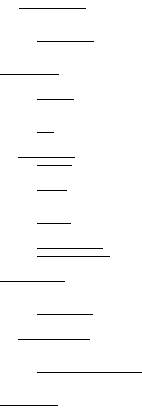
Column-Oriented Databases
Column-oriented databases save their data grouped by columns. Subsequent column values are
stored contiguously on disk. This differs from the usual row-oriented approach of traditional
databases, which store entire rows contiguously—see Figure 1-1 for a visualization of the
different physical layouts.
The reason to store values on a per-column basis instead is based on the assumption that, for
specific queries, not all of the values are needed. This is often the case in analytical databases in
particular, and therefore they are good candidates for this different storage schema.
Reduced I/O is one of the primary reasons for this new layout, but it offers additional advantages
playing into the same category: since the values of one column are often very similar in nature or
even vary only slightly between logical rows, they are often much better suited for compression
than the heterogeneous values of a row-oriented record structure; most compression algorithms
only look at a finite window of data.
Specialized algorithms—for example, delta and/or prefix compression—selected based on the
type of the column (i.e., on the data stored) can yield huge improvements in compression ratios.
Better ratios result in more efficient bandwidth usage.
Note, though, that HBase is not a column-oriented database in the typical RDBMS sense, but
utilizes an on-disk column storage format. This is also where the majority of similarities end,
because although HBase stores data on disk in a column-oriented format, it is distinctly different
from traditional columnar databases: whereas columnar databases excel at providing real-time
analytical access to data, HBase excels at providing key-based access to a specific cell of data, or
a sequential range of cells.
In fact, I would go as far as classifying HBase as column-family-oriented storage, since it does
group columns into families, and within each of those data is stored row-oriented. [Link to
Come] has much more on the storage layout.
(3)
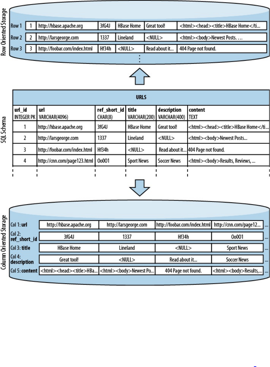
Figure 1-1. Column-oriented and row-oriented storage layouts
The speed at which data is generated today is accelerating. We can take for granted that with the
coming of the Internet of Things, where devices will outnumber people as data sources, along
with the rapid pace of globalization, that the rate of data generation will continue to explode.
Websites like Google, Amazon, eBay, and Facebook now reach the majority of people on this
planet. These companies are deploying planet-size web applications.
Facebook, for example, is adding more than 15 TB of data into its Hadoop cluster every day5 and
is subsequently processing it all. One source of this data is click-stream logging, saving every
step a user performs on its website, or on sites that use the social plug-ins offered by Facebook.
This is a canonical example of where batch processing to build machine learning models for
predictions and recommendations can reap substantial rewards.
Facebook also has a real-time component, which is its messaging system, including chat,
(4)

timeline posts, and email. This amounts to 135+ billion messages per month,6 and storing this
data over a certain number of months creates a huge tail that needs to be handled efficiently.
Even though larger parts of emails—for example, attachments—are stored in a secondary
system,7 the amount of data generated by all these messages is mind-boggling. If we were to take
140 bytes per message, as used by Twitter, it would total more than 17 TB every month. Even
before the transition to HBase, the existing system had to handle more than 25 TB a month.8
In addition, less web-oriented companies from across all major industries are collecting an ever-
increasing amount of data. For example:
Financial
Such as data generated by stock tickers
Bioinformatics
Such as the Global Biodiversity Information Facility (http://www.gbif.org/)
Smart grid
Such as the OpenPDC (http://openpdc.codeplex.com/) project
Sales
Such as the data generated by point-of-sale (POS) or stock/inventory systems
Genomics
Such as the Crossbow (http://bowtie-bio.sourceforge.net/crossbow/index.shtml) project
Cellular services, military, environmental
Which all collect a tremendous amount of data as well
Storing petabytes of data efficiently so that updates and retrieval are still performed well is no
easy feat. We will now look deeper into some of the challenges.
(5)

The Problem with Relational Database
Systems
RDBMSes have typically played (and, for the foreseeable future at least, will play) an integral
role when designing and implementing business applications. As soon as you have to retain
information about your users, products, sessions, orders, and so on, you are typically going to use
some storage backend providing a persistence layer for the frontend application server. This
works well for a limited number of records, but with the dramatic increase of data being retained,
some of the architectural implementation details of common database systems show signs of
weakness.
Let us use Hush, the HBase URL Shortener discussed in detail in [Link to Come], as an example.
Assume that you are building this system so that it initially handles a few thousand users, and
that your task is to do so with a reasonable budget—in other words, use free software. The
typical scenario here is to use the open source LAMP9 stack to quickly build out a prototype for
the business idea.
The relational database model normalizes the data into a user table, which is accompanied by url,
shorturl, and click tables that link to the former by means of a foreign key. The tables also have
indexes so that you can look up URLs by their short ID, or the users by their username. If you
need to find all the shortened URLs for a particular list of customers, you could run an SQL JOIN
over both tables to get a comprehensive list of URLs for each customer that contains not just the
shortened URL but also the customer details you need.
In addition, you are making use of built-in features of the database: for example, stored
procedures, which allow you to consistently update data from multiple clients while the database
system guarantees that there is always coherent data stored in the various tables.
Transactions make it possible to update multiple tables in an atomic fashion so that either all
modifications are visible or none are visible. The RDBMS gives you the so-called ACID10
properties, which means your data is strongly consistent (we will address this in greater detail in
“Consistency Models”). Referential integrity takes care of enforcing relationships between
various table schemas, and you get a domain-specific language, namely SQL, that lets you form
complex queries over everything. Finally, you do not have to deal with how data is actually
stored, but only with higher-level concepts such as table schemas, which define a fixed layout
your application code can reference.
This usually works very well and will serve its purpose for quite some time. If you are lucky, you
may be the next hot topic on the Internet, with more and more users joining your site every day.
As your user numbers grow, you start to experience an increasing amount of pressure on your
shared database server. Adding more application servers is relatively easy, as they share their
state only with the central database. Your CPU and I/O load goes up and you start to wonder how
long you can sustain this growth rate.
The first step to ease the pressure is to add secondary database servers that are used to read from
in parallel. You still have a single master, but that is now only taking writes, and those are much
fewer compared to the many reads your website users generate. But what if that starts to fail as
well, or slows down as your user count steadily increases?
(6)

A common next step is to add a cache—for example, Memcached.11 Now you can offload the
reads to a very fast, in-memory system—however, you are losing consistency guarantees, as you
will have to invalidate the cache on modifications of the original value in the database, and you
have to do this fast enough to keep the time where the cache and the database views are
inconsistent to a minimum.
While this may help when rising read rates, you have not addressed how you can take on more
writes. Once the master database server is hit too hard with writers, you may replace it with a
beefed-up server—scaling up vertically—with more cores, more memory, and faster disks… and
costs a lot more money than your first server. Also note that if you already opted for the
master/worker setup mentioned earlier, you need to make the workers as powerful as the master
or the imbalance may mean the workers fail to keep up with the master’s update rate. This is
going to double or triple your cost, if not more.
With more site popularity, you are asked to add more features to your application, which
translates into more queries to your database. The SQL JOINs you were happy to run in the past
are suddenly slowing down and are simply not performing well enough at scale. You will have to
denormalize your schemas. If things get even worse, you will also have to cease your use of
stored procedures, as they are also simply becoming too slow to complete. Essentially, you
reduce the database to just storing your data in a way that is optimized for your access patterns.
Your load continues to increase as more and more users join your site, so another logical step is
to pre-materialize the most costly queries from time to time so that you can serve the data to your
customers faster. Finally, you start dropping secondary indexes as their maintenance becomes
too much of a burden and slows down the database too much. You end up with queries that can
only use the primary key and nothing else.
Where do you go from here? What if your load is expected to increase by another order of
magnitude or more over the next few months? You could start sharding (see the sidebar titled
“Sharding”) your data across many databases, but this turns into an operational nightmare, is
very costly, and your solution strikes you as an awkward fit for the problem at hand. If only there
was an alternative?
Sharding
The term sharding describes the logical separation of records into horizontal partitions. The idea
is to spread data across multiple storage files—or servers—as opposed to having each stored
contiguously.
The separation of values into those partitions is performed on fixed boundaries: you have to set
fixed rules ahead of time to route values to their appropriate store. A poor choice in boundaries
will require that you have to reshard the data when one of the horizontal partitions exceeds its
capacity.
Resharding is a very costly operation, since the storage layout has to be rewritten. This entails
defining new boundaries and then horizontally splitting the rows across them. Massive copy
operations can take a huge toll on I/O performance as well as temporarily elevated storage
requirements. And you may still need to take on updates from the client applications during the
resharding process.
This can be mitigated by using virtual shards, which define a much larger key partitioning range,
(7)
with each server assigned an equal number of these shards. When you add more servers, you can
reassign shards to the new server. This still requires that the data be moved over to the added
server.
Sharding is often a simple afterthought or is completely left to the operator to figure out. Without
proper support from the database system, sharding (and resharding) can wreak havoc on
production serving systems.
Let us stop here, though, and, to be fair, mention that a lot of companies are using RDBMSes
successfully as part of their technology stack. For example, Facebook—and also Google—has a
very large MySQL setup, and for their purposes it works sufficiently. These database farms suit
the given business goals and may not be replaced anytime soon. The question here is if you were
to start working on implementing a new product and knew that it needed to scale very fast,
would you use an RDBMS and sharding, or is there another storage technology that you could
use that was built from the ground up to scale?
(8)

Nonrelational Database Systems, Not-Only
SQL or NoSQL?
As it happens, over the past four or five years, a whole world of technologies have grown up to
fill the scaling datastore niche. It seems that every week another framework or project is
announced in this space. This realm of technologies was informally dubbed NoSQL, a term
coined by Eric Evans in response to a question from Johan Oskarsson, who was trying to find a
name for an event in that very emerging, new data storage system space.12
The term quickly became popular as there was simply no other name for this new class of
products. It was (and is) discussed heavily, as it was also somewhat deemed the nemesis of
“SQL"ߞtoday we see a more sensible positioning with many major vendors offering a NoSQL
solution as part of their software stack.
Note
The actual idea of different data store architectures for specific problem sets is not new at all.
Systems like Berkeley DB, Coherence, GT.M, and object-oriented database systems have been
around for years, with some dating back to the early 1980s. These old technologies are part of
NoSQL by definition also.
This term is actually a good fit: it is true that most new storage systems do not provide SQL as a
means to query data, but rather a different, often simpler, API-like interface to the data.
On the other hand, tools are available that provide SQL dialects to NoSQL data stores, and they
can be used to form approximations of complex queries run on relational databases. So,
limitations querying the datastore are seen less of a differentiator between RDBMSes and their
non-relational kin.
The difference is actually on a lower level, especially when it comes to schemas or ACID-like
transactional features, but also regarding the actual storage architecture. A lot of these new kinds
of systems do one thing first: throw out factors that will get in the way of scaling the datastore (a
topic that is discussed in “Dimensions”). For example, they often have no support for
transactions or secondary indexes. More importantly, they often have no fixed schemas so that
the storage can evolve with the application using it.
Consistency Models
It seems fitting to talk about consistency a bit more since it is mentioned often throughout this
book. Consistency is about guaranteeing that a database always appears truthful to its clients.
Every operation on the database must carry its state from one consistent state to the next. How
this is achieved or implemented is not specified explicitly so that a system has multiple choices.
In the end, it has to get to the next consistent state, or return to the previous consistent state, to
fulfill its obligation.
Consistency can be classified, for example, in decreasing order of its properties, or guarantees,
offered to clients. Here is an informal list:
(9)

Strict
The changes to the data are atomic and appear to take effect instantaneously. This is the
highest form of consistency.
Sequential
Every client sees all changes in the same order they were applied.
Causal
All changes that are causally related are observed in the same order by all clients.
Eventual
When no updates occur for a period of time, eventually all updates will propagate through
the system and all replicas will be consistent.
Weak
No guarantee is made that all updates will propagate and changes may appear out of order
to various clients.
The class of systems that are eventually consistent can be even further divided into subtle
subsets. These subsets can even coexist in the one system. Werner Vogels, CTO of Amazon, lists
them in his post titled “Eventually Consistent”. The article also picks up on the topic of the CAP
theorem,13 which states that a distributed system can only achieve two out of the following three
properties: consistency, availability, and partition tolerance. The CAP theorem is a highly
discussed topic, and is certainly not the only way to classify distributed systems, but it does point
out that they are not easy to develop given certain requirements. Vogels, for example, mentions:
An important observation is that in larger distributed scale systems, network partitions are a
given and as such consistency and availability cannot be achieved at the same time. This
means that one has two choices on what to drop; relaxing consistency will allow the system
to remain highly available […] and prioritizing consistency means that under certain
conditions the system will not be available.
Relaxing consistency, while at the same time gaining availability, is a powerful proposition.
However, it can force handling inconsistencies into the application layer and may increase
complexity.
There are many overlapping features within the group of nonrelational databases, but some of
these features also overlap with traditional storage solutions. So the new systems are not really
revolutionary, but rather, from an engineering perspective, are more evolutionary.
Even projects like Memcached are lumped into the NoSQL category, as if anything that is not an
RDBMS is automatically NoSQL. This branding of all systems that lack SQL as NoSQL
obscures the exciting technical possibilities these systems have to offer. And there are many;
within the NoSQL category, there are numerous dimensions along which to classify particular
systems.
(10)

Dimensions
Let us take a look at a handful of these dimensions here. Note that this is not a comprehensive
list, or the only way to classify these systems.
Data model
There are many variations in how the data is stored, which include key/value stores
(compare to a HashMap), semistructured, column-oriented, and document-oriented stores.
How is your application accessing the data? Can the schema evolve over time?
Storage model
In-memory or persistent? This is fairly easy to decide since we are comparing with
RDBMSes, which usually persist their data to permanent storage, such as physical disks.
But you may explicitly need a purely in-memory solution, and there are choices for that
too. As far as persistent storage is concerned, does this affect your access pattern in any
way?
Consistency model
Strictly or eventually consistent? The question is, how does the storage system achieve its
goals: does it have to weaken the consistency guarantees? While this seems like a cursory
question, it can make all the difference in certain use cases. It may especially affect
latency, that is, how fast the system can respond to read and write requests. This is often
measured in harvest and yield.14
Atomic read-modify-write
While RDBMSes offer you a lot of these operations directly (because you are talking to a
central, single server), they can be more difficult to achieve in distributed systems. They
allow you to prevent race conditions in multithreaded or shared-nothing application server
design. Having these compare and swap (CAS) or check and set operations available can
reduce client-side complexity.
Locking, waits, and deadlocks
It is a known fact that complex transactional processing, like two-phase commits, can
increase the possibility of multiple clients waiting for a resource to become available. In a
worst-case scenario, this can lead to deadlocks, which are hard to resolve. What kind of
locking model does the system you are looking at support? Can it be free of waits, and
therefore deadlocks?
Physical model
Distributed or single machine? What does the architecture look like—is it built from
distributed machines or does it only run on single machines with the distribution handled
on the client-side, that is, in your own code? Maybe the distribution is only an afterthought
and could cause problems once you need to scale the system. And if it does offer
scalability, does it imply specific steps to do so? The easiest solution would be to add one
(11)

machine at a time, while sharded setups (especially those not supporting virtual shards)
sometimes require for each shard to be increased simultaneously because each partition
needs to be equally powerful.
Read/write performance
You have to understand what your application’s access patterns look like. Are you
designing something that is written to a few times, but is read much more often? Or are
you expecting an equal load between reads and writes? Or are you taking in a lot of writes
and just a few reads? Does it support range scans or is it better suited doing random reads?
Some of the available systems are advantageous for only one of these operations, while
others may do well (but maybe not optimally) in all of them.
Secondary indexes
Secondary indexes allow you to sort and access tables based on different fields and sorting
orders. The options here range from systems that have absolutely no secondary indexes
and no guaranteed sorting order (like a HashMap, i.e., you need to know the keys) to some
that weakly support them, all the way to those that offer them out of the box. Can your
application cope, or emulate, if this feature is missing?
Failure handling
It is a fact that machines crash, and you need to have a mitigation plan in place that
addresses machine failures (also refer to the discussion of the CAP theorem in
“Consistency Models”). How does each data store handle server failures? Is it able to
continue operating? This is related to the “Consistency model” dimension discussed
earlier, as losing a machine may cause holes in your data store, or even worse, make it
completely unavailable. And if you are replacing the server, how easy will it be to get back
to being 100% operational? Another scenario is decommissioning a server in a clustered
setup, which would most likely be handled the same way.
Compression
When you have to store terabytes of data, especially of the kind that consists of prose or
human-readable text, it is advantageous to be able to compress the data to gain substantial
savings in required raw storage. Some compression algorithms can achieve a 10:1
reduction in storage space needed. Is the compression method pluggable? What types are
available?
Load balancing
Given that you have a high read or write rate, you may want to invest in a storage system
that transparently balances itself while the load shifts over time. It may not be the full
answer to your problems, but it may help you to ease into a high-throughput application
design.
Note
We will look back at these dimensions later on to see where HBase fits and where its strengths
lie. For now, let us say that you need to carefully select the dimensions that are best suited to the
issues at hand. Be pragmatic about the solution, and be aware that there is no hard and fast rule,
(12)
in cases where an RDBMS is not working ideally, that a NoSQL system is the perfect match.
Evaluate your options, choose wisely, and mix and match if needed.
An interesting term to describe this issue is impedance match, which describes the need to find
the ideal solution for a given problem. Instead of using a “one-size-fits-all” approach, you should
know what else is available. Try to use the system that solves your problem best.
(13)

Scalability
While the performance of RDBMSes is well suited for transactional processing, it is less so for
very large-scale analytical processing. This refers to very large queries that scan wide ranges of
records or entire tables. Analytical databases may contain hundreds or thousands of terabytes,
causing queries to exceed what can be done on a single server in a reasonable amount of time.
Scaling that server vertically—that is, adding more cores or disks—is simply not good enough.
What is even worse is that with RDBMSes, waits and deadlocks are increasing nonlinearly with
the size of the transactions and concurrency—that is, the square of concurrency and the third or
even fifth power of the transaction size.15 Sharding is often an impractical solution, as it has to
be done within the application layer, and may involve complex and costly (re)partitioning
procedures.
Commercial RDBMSes are available that solve many of these issues, but they are often
specialized and only cover certain problem domains. Above all, they are usually expensive.
Looking at open source alternatives in the RDBMS space, you will likely have to give up many
or all relational features, such as secondary indexes, to gain some level of performance.
The question is: wouldn’t it be good to trade relational features permanently for performance?
You could denormalize (see the next section) the data model and avoid waits and deadlocks by
minimizing necessary locking. How about built-in horizontal scalability without the need to
repartition as your data grows? Finally, throw in fault tolerance and data availability, using the
same mechanisms that allow scalability, and what you get is a NoSQL solution—more
specifically, one that matches what HBase has to offer.
(14)
Database (De-)Normalization
At scale, it is often a requirement that we design schemas differently, and a good term to describe
this principle is Denormalization, Duplication, and Intelligent Keys (DDI).16 It is about
rethinking how data is stored in Bigtable-like storage systems, and how to make use of them in
an appropriate way.
Part of the principle is to denormalize schemas by, for example, duplicating data in more than
one table so that, at read time, no further join or aggregation is required. Likewise, pre-
materialization of required views is an optimization that supports fast reads; no further
processing is required before serving the data.
There is much more on this topic in Chapter 8, where you will find many ideas on how to design
solutions that make the best use of the features HBase provides. Let us look at an example to
understand the basic principles of converting a classic relational database model to one that fits
the columnar nature of HBase much better.
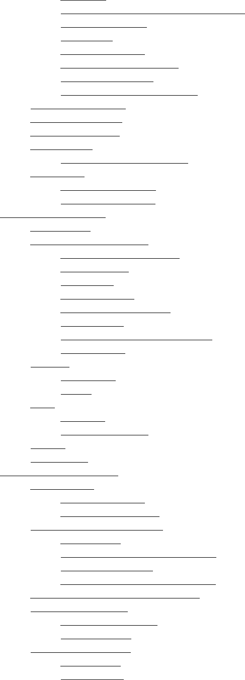
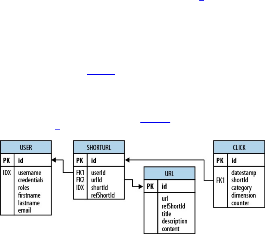
Consider the HBase URL Shortener, Hush, which allows us to map long URLs to short URLs.
The entity relationship diagram (ERD) can be seen in Figure 1-2. The full SQL schema can be
found in [Link to Come].17
Figure 1-2. The Hush schema expressed as an ERD
The shortened URL, stored in the shorturl table, can then be given to others that subsequently
click on it to open the linked full URL. Each click is tracked, recording the number of times it
was followed, and, for example, the country the click originated in. This is stored in the click
table, which aggregates the click data on a daily basis, similar to a counter.
Users, stored in the user table, can sign up with Hush to create their own list of shortened URLs,
which can be edited to add a description. This links the user and shorturl tables with a foreign
key relationship.
The system also downloads the linked page in the background, and extracts, for instance, the
TITLE tag from the HTML, if present. The entire page is saved for later processing with
asynchronous batch jobs, for analysis purposes. This is represented by the url table.
(15)

Every linked page is only stored once, but since many users may link to the same long URL, yet
want to maintain their own details, such as the usage statistics, a separate entry in the shorturl is
created. This links the url, shorturl, and click tables.
It also allows you to aggregate statistics about the original short ID, refShortId, so that you can
see the overall usage of any short URL to map to the same long URL. The shortId and refShortId
are the hashed IDs assigned uniquely to each shortened URL. For example, in
http://hush.li/a23eg
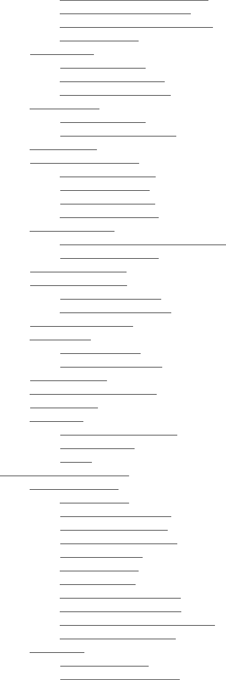
the ID is a23eg. Figure 1-3 shows how the same schema could be represented in HBase. Every
shortened URL is stored in a table, shorturl, which also contains the usage statistics, storing
various time ranges in separate column families, with distinct time-to-live settings. The columns
form the actual counters, and their name is a combination of the date, plus an optional
dimensional postfix—for example, the country code.
(16)
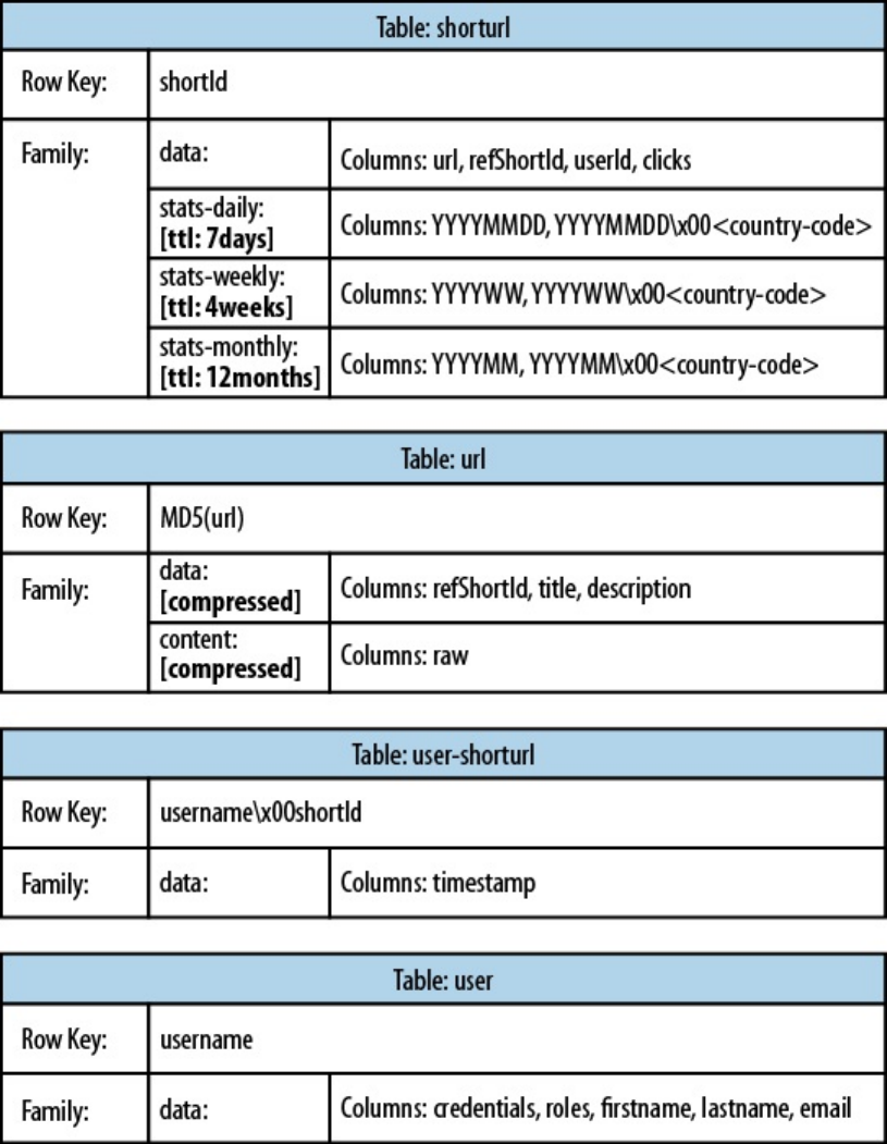
Figure 1-3. The Hush schema in HBase
The downloaded page, and the extracted details, are stored in the url table. This table uses
compression to minimize the storage requirements, because the pages are mostly HTML, which
is inherently verbose and contains a lot of text.
The user-shorturl table acts as a lookup so that you can quickly find all short IDs for a given
user. This is used on the user’s home page, once she has logged in. The user table stores the
actual user details.
We still have the same number of tables, but their meaning has changed: the clicks table has
(17)
been absorbed by the shorturl table, while the statistics columns use the date as their key,
formatted as YYYYMMDD — for instance, 20150302 — so that they can be accessed sequentially. The
additional user-shorturl table is replacing the foreign key relationship, making user-related
lookups faster.
There are various approaches to converting one-to-one, one-to-many, and many-to-many
relationships to fit the underlying architecture of HBase. You could implement even this simple
example in different ways. You need to understand the full potential of HBase storage design to
make an educated decision regarding which approach to take.
The support for sparse, wide tables and column-oriented design often eliminates the need to
normalize data and, in the process, the costly JOIN operations needed to aggregate the data at
query time. Use of intelligent keys gives you fine-grained control over how—and where—data is
stored. Partial key lookups are possible, and when combined with compound keys, they have the
same properties as leading, left-edge indexes. Designing the schemas properly enables you to
grow the data from 10 entries to 10 billion entries, while still retaining the same write and read
performance.
(18)
Building Blocks
This section provides you with an overview of the architecture behind HBase. After giving you
some background information on its lineage, the section will introduce the general concepts of
the data model and the available storage API, and presents a high-level overview on
implementation.
(19)

Backdrop
In 2003, Google published a paper titled “The Google File System”. This scalable distributed file
system, abbreviated as GFS, uses a cluster of commodity hardware to store huge amounts of
data. The filesystem handled data replication between nodes so that losing a storage server would
have no effect on data availability. It was also optimized for streaming reads so that data could
be read for processing later on.
Shortly afterward, another paper by Google was published, titled “MapReduce: Simplified Data
Processing on Large Clusters”. MapReduce was the missing piece to the GFS architecture, as it
made use of the vast number of CPUs each commodity server in the GFS cluster provided.
MapReduce plus GFS formed the backbone for processing massive amounts of data, including
the entire Google search index.
What was missing, though, was the ability to access data randomly and in close to real-time
(meaning good enough to drive a web service, for example). A drawback of the GFS design was
that it was good with a few very, very large files, but not as good with millions of tiny files,
because the data retained in memory for each file by the master node ultimately bounds the
number of files under management. The more files, the higher the pressure on the memory of the
master.
So, Google was trying to find a solution that could drive interactive applications, such as Mail or
Analytics, while making use of the same infrastructure and relying on GFS for replication and
data availability. The data stored should be composed of much smaller entities, and the system
would transparently take care of aggregating the small records into very large storage files and
offer some sort of indexing that allows the user to retrieve data with a minimal number of disk
seeks. Finally, it should be able to store the entire web crawl and work with MapReduce to build
the entire search index in a timely manner.
Being aware of the shortcomings of RDBMSes at scale (see [Link to Come] for a discussion of
one fundamental issue), the engineers approached this problem differently: forfeit relational
features and use a simple API that has basic create, read, update, and delete (or CRUD)
operations, plus a scan function to iterate over larger key ranges or entire tables. The culmination
of these efforts was published in 2006 in a paper titled “Bigtable: A Distributed Storage System
for Structured Data”, two excerpts from which follow:
Bigtable is a distributed storage system for managing structured data that is designed to
scale to a very large size: petabytes of data across thousands of commodity servers.
…a sparse, distributed, persistent multi-dimensional sorted map.
It is highly recommended that everyone interested in HBase read that paper. It describes a lot of
reasoning behind the design of Bigtable and, ultimately, HBase. We will, however, go through
the basic concepts, since they apply directly to the rest of this book.
HBase is implementing the Bigtable storage architecture very faithfully so that we can explain
everything using HBase. [Link to Come] provides an overview of where the two systems differ.
(20)

Namespaces, Tables, Rows, Columns, and Cells
First a quick summary: One or more columns form a row that is addressed uniquely by a row key.
A number of rows, in turn, form a table, and a user is allowed to create many tables. Each
column may have multiple versions, with each distinct, timestamped value contained in a
separate cell. On a higher level, tables are grouped into namespaces, which help, for example,
with grouping tables by users or application, or with access control.
This sounds like a reasonable description for a typical database, but with the extra dimension of
allowing multiple versions of each column. But obviously there is a bit more to it: All rows are
always sorted lexicographically by their row key. Example 1-1 shows how this will look when
adding a few rows with different keys.
Example 1-1. The sorting of rows done lexicographically by their key
hbase(main):001:0> scan 'table1'
ROW COLUMN+CELL
row-1 column=cf1:, timestamp=1297073325971 ...
row-10 column=cf1:, timestamp=1297073337383 ...
row-11 column=cf1:, timestamp=1297073340493 ...
row-2 column=cf1:, timestamp=1297073329851 ...
row-22 column=cf1:, timestamp=1297073344482 ...
row-3 column=cf1:, timestamp=1297073333504 ...
row-abc column=cf1:, timestamp=1297073349875 ...
7 row(s) in 0.1100 seconds
Note how the numbering is not in sequence as you may have expected it. You may have to pad
keys to get a proper sorting order. In lexicographical sorting, each key is compared on a binary
level, byte by byte, from left to right. Since row-1... is less than row-2..., no matter what
follows, it is sorted first.
Having the row keys always sorted can give you something like the primary key index you find
in the world of RDBMSes. It is also always unique, that is, you can have each row key only
once, or you are updating the same row. While the original Bigtable paper only considers a
single index, HBase adds support for secondary indexes (see “Secondary Indexes”). The row
keys can be any arbitrary array of bytes and are not necessarily human-readable.
Rows are composed of columns, and those, in turn, are grouped into column families. This helps
in building semantical or topical boundaries between the data, and also in applying certain
features to them, for example, compression, or denoting them to stay in-memory. All columns in
a column family are stored together in the same low-level storage files, called HFile.
The initial set of column families is defined when the table is created and should not be changed
too often, nor should there be too many of them within each table. There are a few known
tradeoffs in the current implementation that force the count to be limited to the low tens, though
in practice only a low number is usually needed (see Chapter 8 for details). The name of the
column family must be composed of printable characters, and not start with a period symbol
(".").
Columns are often referenced as family:qualifier pair with the qualifier being any arbitrary array
of bytes.18 As opposed to the limit on column families, there is no such thing for the number of
columns: you could have millions of columns in a particular column family. There is also no type
(21)
nor length boundary on the column values.
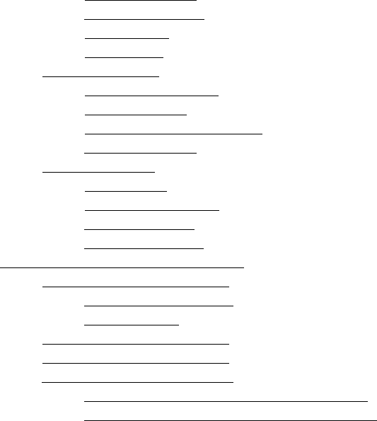
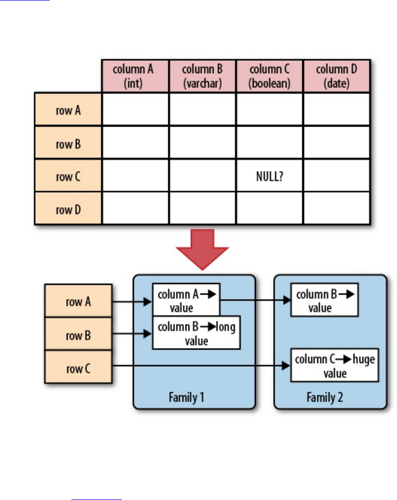
Figure 1-4 helps to visualize how different rows are in a normal database as opposed to the
column-oriented design of HBase. You should think about rows and columns as not being
arranged like the classic spreadsheet model, but rather use a tag metaphor, that is, information is
available under a specific tag.
Figure 1-4. Rows and columns in HBase
Note
The "NULL?" in Figure 1-4 indicates that, for a database with a fixed schema, you have to store
NULLs where there is no value, but for HBase’s storage architectures, you simply omit the whole
column; in other words, NULLs are free of any cost: they do not occupy any storage space.
All rows and columns are defined in the context of a table. Table adds a few more concepts and
properties that are applied to all included column families. We will discuss these shortly.
Every column value, or cell, either is timestamped implicitly by the system or explicitly by the
user. This can be used, for example, to save multiple versions of a value as it changes over time.
Different versions of a column are stored in decreasing timestamp order, allowing you to read the
newest value first.
(22)
The user can specify how many versions of a column (that is, how many cells per column)
should be kept. In addition, there is support for predicate deletions (see [Link to Come] for the
concepts behind them) allowing you to keep, for example, only values written in the past week.
The values (or cells) are also just uninterpreted arrays of bytes, that the client needs to know how
to handle.
If you recall from the quote earlier, the Bigtable model, as implemented by HBase, is a sparse,
distributed, persistent, multidimensional map, which is indexed by row key, column key, and a
timestamp. Putting this together, we can express the access to data like so:
(Table, RowKey, Family, Column, Timestamp) → Value
Note
This representation is not entirely correct as physically it is the column family that separates
columns and creates rows per family. We will pick this up in [Link to Come] later on.
In a more programming language style, this may be expressed as:
SortedMap<
RowKey, List<
SortedMap<
Column, List<
Value, Timestamp
>
>
>
>
Or all in one line:
SortedMap<RowKey, List<SortedMap<Column, List<Value, Timestamp>>>>
The first SortedMap is the table, containing a List of column families. The families contain
another SortedMap, which represents the columns, and their associated values. These values are in
the final List that holds the value and the timestamp it was set with, and is sorted in descending
order by timestamp.
An interesting feature of the model is that cells may exist in multiple versions, and different
columns may have been written at different times. The API, by default, provides you with a
coherent view of all columns wherein it automatically picks the most current value of each cell.
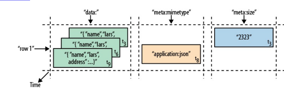
Figure 1-5 shows a piece of one specific row in an example table.
Figure 1-5. A time-oriented view into parts of a row
(23)
The diagram visualizes the time component using tn as the timestamp when the cell was written.
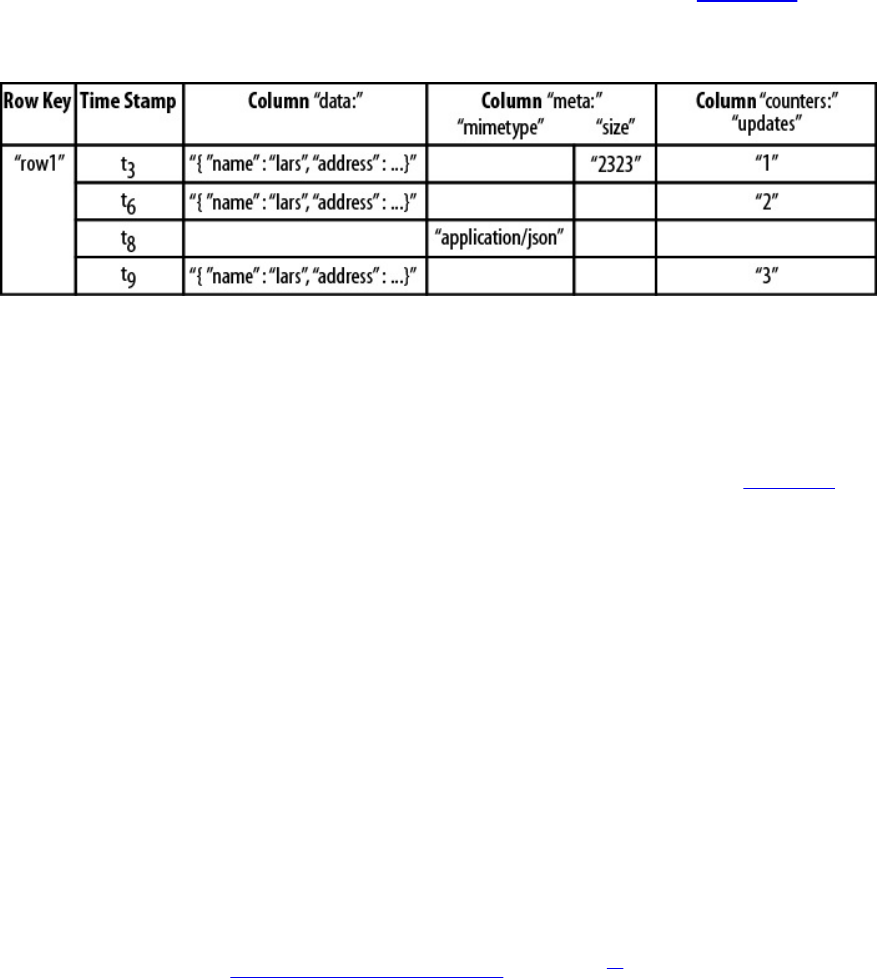
The ascending index shows that the values have been added at different times. Figure 1-6 is
another way to look at the data, this time in a more spreadsheet-like layout wherein the
timestamp was added to its own column.
Figure 1-6. The same parts of the row rendered as a spreadsheet
Although they have been added at different times and exist in multiple versions, you would still
see the row as the combination of all columns and their most current versions—in other words,
the highest tn from each column. There is a way to ask for values at (or before) a specific
timestamp, or more than one version at a time, which we will see a little bit later in Chapter 3.
The Webtable
The canonical use case for Bigtable and HBase was the webtable, that is, the web pages stored
while crawling the Internet.
The row key is the reversed URL of the page—for example, org.hbase.www. There is a column
family storing the actual HTML code, the contents family, as well as others like anchor, which is
used to store outgoing links, another one to store inbound links, and yet another for metadata like
the language of the page.
Using multiple versions for the contents family allows you to store a few older copies of the
HTML, and is helpful when you want to analyze how often a page changes, for example. The
timestamps used are the actual times when they were fetched from the crawled website.
Access to row data is atomic and includes any number of columns being read or written to. The
only additional guarantee is that you can span a mutation across colocated rows atomically using
region-local transactions (see “Region-local Transactions” for details19). There is no further
guarantee or transactional feature that spans multiple rows across regions, or across tables. The
atomic access is also a contributing factor to this architecture being strictly consistent, as each
concurrent reader and writer can make safe assumptions about the state of a row. Using
multiversioning and timestamping can help with application layer consistency issues as well.
Finally, cells, since HBase 0.98, can carry an arbitrary set of tags. They are used to flag any cell
with metadata that is used to make decisions about the cell during data operations. A prominent
use-case is security (see [Link to Come]) where tags are set for cells containing access details.
Once a user is authenticated and has a valid security token, the system can use the token to filter
specific cells for the given user. Tags can be used for other things as well, and [Link to Come]
will explain their application in greater detail.
(24)
Auto-Sharding
The basic unit of scalability and load balancing in HBase is called a region. Regions are
essentially contiguous ranges of rows stored together. They are dynamically split by the system
when they become too large. Alternatively, they may also be merged to reduce their number and
required storage files (see “Merging Regions”).
Note
The HBase regions are equivalent to range partitions as used in database sharding. They can be
spread across many physical servers, thus distributing the load, and therefore providing
scalability.
Initially there is only one region for a table, and as you start adding data to it, the system is
monitoring it to ensure that you do not exceed a configured maximum size. If you exceed the
limit, the region is split into two at the middle key--the row key in the middle of the region—
creating two roughly equal halves (more details in [Link to Come]).
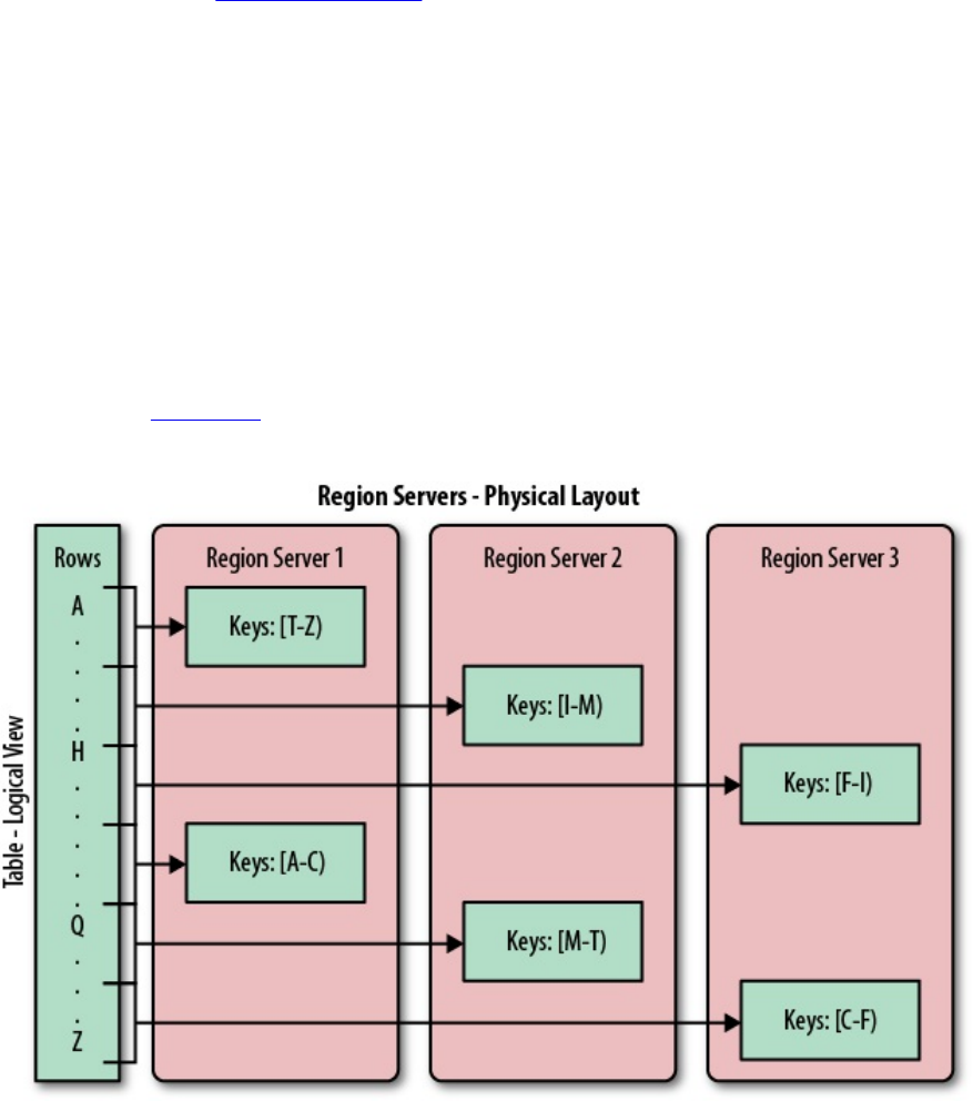
Each region is served by exactly one region server, and each of these servers can serve many
regions at any time. Figure 1-7 shows how the logical view of a table is actually a set of regions
hosted by many region servers.
Figure 1-7. Rows grouped in regions and served by different servers
Note
The Bigtable paper notes that the aim is to keep the region count between 10 and 1,000 per
(25)
server and each at roughly 100 MB to 200 MB in size. This refers to the hardware in use in 2006
(and earlier). For HBase and modern hardware, the number would be more like 10 to 1,000
regions per server, but each between 1 GB and 10 GB in size.
But, while the numbers have increased, the basic principle is the same: the number of regions per
server, and their respective sizes, depend on what can be handled sufficiently by a single server.
Splitting and serving regions can be thought of as autosharding, as offered by other systems. The
regions allow for fast recovery when a server fails, and fine-grained load balancing since they
can be moved between servers when the load of the server currently serving the region is under
pressure, or if that server becomes unavailable because of a failure or because it is being
decommissioned.
Splitting is also very fast—close to instantaneous—because the split regions simply read from
the original storage files until a compaction rewrites them into separate ones asynchronously.
This is explained in detail in [Link to Come].
(26)

Storage API
Bigtable does not support a full relational data model; instead, it provides clients with a
simple data model that supports dynamic control over data layout and format […]
The API offers operations to create and delete tables and column families. In addition, it has
functions to change the table and column family metadata, such as compression or block sizes.
Furthermore, there are the usual operations for clients to create or delete values as well as
retrieving them with a given row key.
A scan API allows you to efficiently iterate over ranges of rows and be able to limit which
columns are returned or the number of versions of each cell. You can match columns using filters
and select versions using time ranges, specifying start and end times.
On top of this basic functionality are more advanced features. The system has support for single-
row and region-local20 transactions, and with this support it implements atomic read-modify-
write sequences on data stored under a single row key, or multiple colocated ones.
Cell values can be interpreted as counters and updated atomically. These counters can be read
and modified in one operation so that, despite the distributed nature of the architecture, clients
can use this mechanism to implement global, strictly consistent, sequential counters.
There is also the option to run client-supplied code in the address space of the server. The server-
side framework to support this is called coprocessors.21 The code has access to the server local
data and can be used to implement lightweight batch jobs, or use expressions to analyze or
summarize data based on a variety of operators.
Finally, the system is integrated with the MapReduce framework by supplying wrappers that
convert tables into input source and output targets for MapReduce jobs.
Unlike in the RDBMS landscape, there is no domain-specific language, such as SQL, to query
data. Access is not done declaratively, but purely imperatively through the client-side API. For
HBase, this is mostly Java code, but there are many other choices to access the data from other
programming languages.
(27)

Implementation
Bigtable […] allows clients to reason about the locality properties of the data represented in
the underlying storage.
The data is stored in store files, called HFiles, which are persistent and ordered immutable maps
from keys to values. Internally, the files are sequences of blocks with a block index stored at the
end. The index is loaded and kept in memory when the HFile is opened. The default block size is
64 KB but can be configured differently if required. The store files internally provide an API to
access specific values as well as to scan ranges of values given a start and end key.
Note
Implementation is discussed in great detail in [Link to Come]. The text here is an introduction
only, while the full details are discussed in the referenced chapter(s).
Since every HFile has a block index, lookups can be performed with a single disk seek.22 First,
the block possibly containing the given key is determined by doing a binary search in the in-
memory block index, followed by a block read from disk to find the actual key.
The store files are typically saved in the Hadoop Distributed File System (HDFS), which
provides a scalable, persistent, replicated storage layer for HBase. It guarantees that data is never
lost by writing the changes across a configurable number of physical servers.
When data is updated it is first written to a commit log, called a write-ahead log (WAL) in
HBase, and then stored in the in-memory memstore. Once the data in memory has exceeded a
given maximum size, it is flushed as a HFile to disk. After the flush, the commit logs can be
discarded up to the last unflushed modification. While the system is flushing the memstore to
disk, it can continue to serve readers and writers without having to block. This is achieved by
rolling the memstore in memory where a new/empty one starts taking updates while the old/full
one is converted into a file. Note that the data in the memstores is already sorted by keys
matching exactly what HFiles represent on disk, so no sorting or other special processing has to
be performed.
Note
We can now start to make sense of what the locality properties are, mentioned in the Bigtable
quote at the beginning of this section. Since all files contain sorted key/value pairs, ordered by
the key, and are optimized for block operations such as reading these pairs sequentially, you
should specify keys to keep related data together. Referring back to the webtable example earlier,
you may have noted that the key used is the reversed FQDN (the domain name part of the URL),
such as org.hbase.www. The reason is to store all pages from hbase.org close to one another, and
reversing the URL puts the most important part of the URL first, that is, the top-level domain
(TLD). Pages under blog.hbase.org would then be sorted with those from www.hbase.org--or in the
actual key format, org.hbase.blog sorts next to org.hbase.www.
Because store files are immutable, you cannot simply delete values by removing the key/value
pair from them. Instead, a delete marker (also known as a tombstone marker) is written to
indicate the fact that the given key has been deleted. During the retrieval process, these delete
(28)

markers mask out the actual values and hide them from reading clients.
Reading data back involves a merge of what is stored in the memstores, that is, the data that has
not been written to disk, and the on-disk store files. Note that the WAL is never used during data
retrieval, but solely for recovery purposes when a server has crashed before writing the in-
memory data to disk.
Since flushing memstores to disk causes more and more HFiles to pile up, HBase has a
housekeeping mechanism that merges the files into larger ones using compaction. There are two
types of compaction: minor compactions and major compactions. The former reduce the number
of storage files by rewriting smaller files into fewer but larger ones, performing an n-way merge.
Since all the data is already sorted in each HFile, this merge is fast and bound only by disk I/O
performance.
The major compactions rewrite all files within a column family for a region into a single new
one. They also have another distinct feature compared to the minor compactions: based on the
fact that they scan all key/value pairs, they can drop deleted entries including their deletion
marker. Predicate deletes are handled here as well—for example, removing values that have
expired according to the configured time-to-live (TTL) or when there are too many versions.
Note
This architecture is taken from LSM-trees (see [Link to Come]). The only difference is that
LSM-trees store data in multipage blocks that are arranged in a B-tree-like structure on disk.
They are updated, or merged, in a rotating fashion, while in Bigtable the update is more coarse-
grained and the whole memstore is saved as a new store file and not merged right away. You
could call HBase’s architecture “Log-Structured Sort-and-Merge-Maps.” The background
compactions correspond to the merges in LSM-trees, but occur on a store file level instead of the
partial tree updates, giving the LSM-trees their name.
There are three major components to HBase: the client library, at least one master server, and
many region servers. The region servers can be added or removed while the system is up and
running to accommodate changing workloads. The master is responsible for assigning regions to
region servers and uses Apache ZooKeeper, a reliable, highly available, persistent and distributed
coordination service, to facilitate that task.
Apache ZooKeeper
ZooKeeper23 is a separate open source project, and is also part of the Apache Software
Foundation. ZooKeeper is the comparable system to Google’s use of Chubby for Bigtable. It
offers filesystem-like semantics with directories and files (called znodes) that distributed systems
can use to negotiate ownership, register services, or watch for updates.
Every region server creates its own ephemeral node in ZooKeeper, which the master, in turn,
uses to discover available servers. They are also used to track server failures or network
partitions.
Ephemeral nodes are bound to the session between ZooKeeper and the client which created it.
The session has a heartbeat keepalive mechanism that, once it fails to report, is declared lost by
ZooKeeper and the associated ephemeral nodes are deleted.
(29)
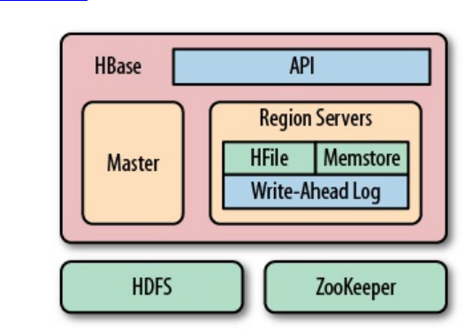
HBase also uses ZooKeeper to ensure that there is only one master running, to store the bootstrap
location for region discovery, as a registry for region servers, as well as for other purposes.
ZooKeeper is a critical component, and without it HBase is not operational. This is facilitated by
ZooKeeper’s distributed design using an ensemble of servers and the Zab protocol to keep its
state consistent.
Figure 1-8 shows the various components of an HBase system including HDFS and ZooKeeper.
Figure 1-8. HBase using its own components while leveraging existing systems
The master server is also responsible for handling load balancing of regions across region
servers, to unload busy servers and move regions to less occupied ones. The master is not part of
the actual data storage or retrieval path. It negotiates load balancing and maintains the state of the
cluster, but never provides any data services to either the region servers or the clients, and is
therefore lightly loaded in practice. In addition, it takes care of schema changes and other
metadata operations, such as creation of tables and column families.
Region servers are responsible for all read and write requests for all regions they serve, and also
split regions that have exceeded the configured region size thresholds. Clients communicate
directly with them to handle all data-related operations.
[Link to Come] has more details on how clients perform the region lookup.
(30)
Summary
Billions of rows * millions of columns * thousands of versions = terabytes or petabytes of
storage
The HBase Project
We have seen how the Bigtable storage architecture uses many servers to distribute ranges of
rows sorted by their key for load-balancing purposes, and can scale to petabytes of data on
thousands of machines. The storage format used is ideal for reading adjacent key/value pairs and
is optimized for block I/O operations that can saturate disk transfer channels.
Table scans run in linear time and row key lookups or mutations are performed in logarithmic
order—or, in extreme cases, even constant order (using Bloom filters). Designing the schema in
a way to completely avoid explicit locking, combined with row-level atomicity, gives you the
ability to scale your system without any notable effect on read or write performance.
The column-oriented architecture allows for huge, wide, sparse tables as storing NULLs is free.
Because each row is served by exactly one server, HBase is strongly consistent, and using its
multiversioning can help you to avoid edit conflicts caused by concurrent decoupled processes,
or retain a history of changes.
The actual Bigtable has been in production at Google since at least 2005, and it has been in use
for a variety of different use cases, from batch-oriented processing to real-time data-serving. The
stored data varies from very small (like URLs) to quite large (e.g., web pages and satellite
imagery) and yet successfully provides a flexible, high-performance solution for many well-
known Google products, such as Google Earth, Google Reader, Google Finance, and Google
Analytics.
(31)
HBase: The Hadoop Database
Having looked at the Bigtable architecture, we could simply state that HBase is a faithful, open
source implementation of Google’s Bigtable. But that would be a bit too simplistic, and there are
a few (mostly subtle) differences worth addressing.
(32)
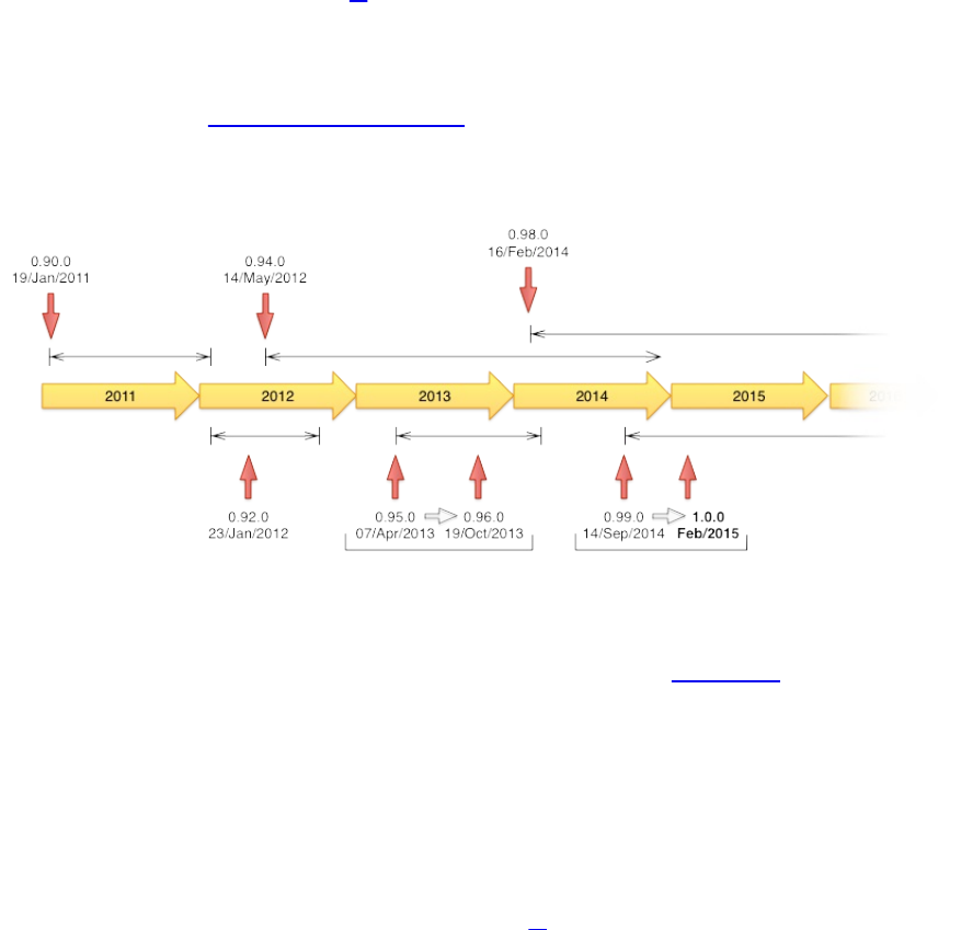
History
HBase was created in 2007 at Powerset24 and was initially part of the contributions directory in
Hadoop. Since then, it has become its own top-level project under the Apache Software
Foundation umbrella. It is available under the Apache Software License, version 2.0.
The project home page is http://hbase.apache.org/, where you can find links to the
documentation, wiki, and source repository, as well as download sites for the binary and source
releases.
Figure 1-9. The release timeline of HBase.
Here is a short overview of how HBase has evolved over time, which Figure 1-9 shows in a
timeline form:
November 2006
Google releases paper on Bigtable
February 2007
Initial HBase prototype created as Hadoop contrib25
October 2007
First “usable" HBase (Hadoop 0.15.0)
January 2008
Hadoop becomes an Apache top-level project, HBase becomes subproject
October 2008
HBase 0.18.1 released
January 2009
(33)

HBase 0.19.0 released
September 2009
HBase 0.20.0 released, the performance release
May 2010
HBase becomes an Apache top-level project
June 2010
HBase 0.89.20100621, first developer release
January 2011
HBase 0.90.0 released, the durability and stability release
January 2012
HBase 0.92.0 released, tagged as coprocessor and security release
May 2012
HBase 0.94.0 released, tagged as performance release
October 2013
HBase 0.96.0 released, tagged as the singularity
February 2014
HBase 0.98.0 released
February 2015
HBase 1.0.0 released
Figure 1-9 shows as well how many months or years a release has been—or still is—active. This
mainly depends on the release managers and their need for a specific major version to keep
going.
Note
Around May 2010, the developers decided to break with the version numbering that used to be in
lockstep with the Hadoop releases. The rationale was that HBase had a much faster release cycle
and was also approaching a version 1.0 level sooner than what was expected from Hadoop.26
To that effect, the jump was made quite obvious, going from 0.20.x to 0.89.x. In addition, a
decision was made to title 0.89.x the early access version for developers and bleeding-edge
integrators. Version 0.89 was eventually released as 0.90 for everyone as the next stable release.
(34)

Nomenclature
One of the biggest differences between HBase and Bigtable concerns naming, as you can see in
Table 1-1, which lists the various terms and what they correspond to in each system.
Table 1-1. Differences in naming
HBase Bigtable
Region Tablet
RegionServer Tablet server
Flush Minor compaction
Minor compaction Merging compaction
Major compaction Major compaction
Write-ahead log Commit log
HDFS GFS
Hadoop MapReduce MapReduce
MemStore memtable
HFile SSTable
ZooKeeper Chubby
More differences are described in [Link to Come].
(35)

Summary
Let us now circle back to “Dimensions”, and how these dimensions can be used to classify
HBase. HBase is a distributed, persistent, strictly consistent storage system with near-optimal
write—in terms of I/O channel saturation—and excellent read performance, and it makes
efficient use of disk space by supporting pluggable compression algorithms that can be selected
based on the nature of the data in specific column families.
HBase extends the Bigtable model, which only considers a single index, similar to a primary key
in the RDBMS world, offering the server-side hooks to implement flexible secondary index
solutions. In addition, it provides push-down predicates, that is, filters, reducing data transferred
over the network.
There is no declarative query language as part of the core implementation, and it has limited
support for transactions. Row atomicity and read-modify-write operations make up for this in
practice, as they cover many use cases and remove the wait or deadlock-related pauses
experienced with other systems.
HBase handles shifting load and failures gracefully and transparently to the clients. Scalability is
built in, and clusters can be grown or shrunk while the system is in production. Changing the
cluster does not involve any complicated rebalancing or resharding procedure, and is usually
completely automated.27
1 See, for example, “‘One Size Fits All’: An Idea Whose Time Has Come and Gone”) by
Michael Stonebraker and Uğur Çetintemel.
2 Information can be found on the project’s website. Please also see the excellent Hadoop: The
Definitive Guide (Fourth Edition) by Tom White (O’Reilly) for everything you want to know
about Hadoop.
3 The quotes are from a presentation titled “Rethinking EDW in the Era of Expansive
Information Management” by Dr. Ralph Kimball, of the Kimball Group, available online. It
discusses the changing needs of an evolving enterprise data warehouse market.
4 Edgar F. Codd defined 13 rules (numbered from 0 to 12), which define what is required from a
database management system (DBMS) to be considered relational. While HBase does fulfill the
more generic rules, it fails on others, most importantly, on rule 5: the comprehensive data
sublanguage rule, defining the support for at least one relational language. See Codd’s 12 rules
on Wikipedia.
5 See this note published by Facebook.
6 See this blog post, as well as this one, by the Facebook engineering team. Timeline messages
count for 15 billion and chat for 120 billion, totaling 135 billion messages a month. Then they
also add SMS and others to create an even larger number.
7 Facebook uses Haystack, which provides an optimized storage infrastructure for large binary
objects, such as photos.
(36)
8 See this presentation, given by Facebook employee and HBase committer, Nicolas Spiegelberg.
9 Short for Linux, Apache, MySQL, and PHP (or Perl and Python).
10 Short for Atomicity, Consistency, Isolation, and Durability. See “ACID” on Wikipedia.
11 Memcached is an in-memory, nonpersistent, nondistributed key/value store. See the
Memcached project home page.
12 See “NoSQL” on Wikipedia.
13 See Eric Brewer’s original paper on this topic and the follow-up post by Coda Hale, as well as
this PDF by Gilbert and Lynch.
14 See Brewer: “Lessons from giant-scale services.”, Internet Computing, IEEE (2001) vol. 5 (4)
pp. 46–55.
15 See “FT 101” by Jim Gray et al.
16 The term DDI was coined in the paper “Cloud Data Structure Diagramming Techniques and
Design Patterns” by D. Salmen et al. (2009).
17 Note, though, that this is provided purely for demonstration purposes, so the schema is
deliberately kept simple.
18 You will see in “Column Families” that the qualifier also may be left unset.
19 This was introduced in HBase 0.94.0. More on ACID guarantees and MVCC in [Link to
Come].
20 Region-local transactions, along with a row-key prefix aware split policy, were added in
HBase 0.94. See HBASE-5229.
21 Coprocessors were added to HBase in version 0.92.0.
22 This is a simplification as newer HFile versions use a multi-level index, loading partial index
blocks as needed. This adds to the latency, but once the index is cached the behavior is back to
what is described here.
23 For more information on Apache ZooKeeper, please refer to the official project website.
24 Powerset was a company based in San Francisco that was developing a natural language
search engine for the Internet. On July 1, 2008, Microsoft acquired Powerset, and subsequent
support for HBase development was abandoned.
25 For an interesting flash back in time, see HBASE-287 on the Apache JIRA, the issue tracking
system. You can see how Mike Cafarella did a code drop that was then quickly picked up by Jim
Kellerman, who was with Powerset back then.
26 Oh, the irony! Hadoop 1.0.0 was released on December 27th, 2011, which means three years
(37)


Chapter 2. Installation
In this chapter, we will look at how HBase is installed and initially configured. The first part is a
quickstart section that gets you going fast, but then shifts gears into proper planning and set up of
a HBase cluster. Towards the end we will see how HBase can be used from the command line for
basic operations, such as adding, retrieving, and deleting data.
Note
All of the following assumes you have the Java Runtime Environment (JRE) installed. Hadoop
and also HBase require at least version 1.7 (also called Java 7)1, and the recommended choice is
the one provided by Oracle (formerly by Sun), which can be found at
http://www.java.com/download/. If you do not have Java already or are running into issues using
it, please see “Java”.
(39)

Quick-Start Guide
Let us get started with the “tl;dr” section of this book: you want to know how to run HBase and
you want to know it now! Nothing is easier than that because all you have to do is download the
most recent binary release of HBase from the Apache HBase release page.
Note
HBase is shipped as a binary and source tarball.2 Look for bin or src in their names respectively.
For the quickstart you need the binary tarball, for example hbase-1.0.0-bin.tar.gz.
You can download and unpack the contents into a suitable directory, such as /usr/local or /opt,
like so:
$ cd /usr/local
$ wget http://archive.apache.org/dist/hbase/hbase-1.0.0/hbase-1.0.0-bin.tar.gz
$ tar -zxvf hbase-1.0.0-bin.tar.gz
Setting the Data Directory
At this point, you are ready to start HBase. But before you do so, it is advisable to set the data
directory to a proper location. You need to edit the configuration file conf/hbase-site.xml and set
the directory you want HBase—and ZooKeeper—to write to by assigning a value to the property
key named hbase.rootdir and hbase.zookeeper.property.dataDir:
<?xml version="1.0"?>
<?xml-stylesheet type="text/xsl" href="configuration.xsl"?>
<configuration>
<property>
<name>hbase.rootdir</name>
<value>file:///<PATH>/hbase</value>
</property>
<property>
<name>hbase.zookeeper.property.dataDir</name>
<value>file:///<PATH>/zookeeper</value>
</property>
</configuration>
Replace <PATH> in the preceding example configuration file with a path to a directory where you
want HBase to store its data. By default, hbase.rootdir is set to /tmp/hbase-${user.name}, which
could mean you lose all your data whenever your server or test machine reboots because a lot of
operating systems (OSes) clear out /tmp during a restart.
With that in place, we can start HBase and try our first interaction with it. We will use the
interactive shell to enter the status command at the prompt (complete the command by pressing
the Return key):
$ cd /usr/local/hbase-1.0.0
$ bin/start-hbase.sh
starting master, logging to \
/usr/local/hbase-1.0.0/bin/../logs/hbase-<username>-master-localhost.out
$ bin/hbase shell
HBase Shell; enter 'help<RETURN>' for list of supported commands.
Type "exit<RETURN>" to leave the HBase Shell
Version 1.0.0, r6c98bff7b719efdb16f71606f3b7d8229445eb81, Sat Feb 14 19:49:22 PST 2015
hbase(main):001:0> status
1 servers, 0 dead, 2.0000 average load
(40)

This confirms that HBase is up and running, so we will now issue a few commands to show that
we can put data into it and retrieve the same data subsequently.
Note
It may not be clear, but what we are doing right now is similar to sitting in a car with its brakes
engaged and in neutral while turning the ignition key. There is much more that you need to
configure and understand before you can use HBase in a production-like environment. But it lets
you get started with some basic HBase commands and become familiar with top-level concepts.
We are currently running in the so-called Standalone Mode. We will look into the available
modes later on (see “Run Modes”), but for now it’s important to know that in this mode
everything is run in a single Java process and all files are stored in /tmp by default—unless you
did heed the important advice given earlier to change it to something different. Many people
have lost their test data during a reboot, only to learn that they kept the default paths. Once it is
deleted by the OS, there is no going back!
Let us now create a simple table and add a few rows with some data:
hbase(main):002:0> create 'testtable', 'colfam1'
0 row(s) in 0.2930 seconds
=> Hbase::Table - testtable
hbase(main):003:0> list
TABLE
testtable
1 row(s) in 0.1920 seconds
=> ["testtable"]
hbase(main):004:0> put 'testtable', 'myrow-1', 'colfam1:q1', 'value-1'
0 row(s) in 0.1020 seconds
hbase(main):005:0> put 'testtable', 'myrow-2', 'colfam1:q2', 'value-2'
0 row(s) in 0.0410 seconds
hbase(main):006:0> put 'testtable', 'myrow-2', 'colfam1:q3', 'value-3'
0 row(s) in 0.0380 seconds
After we create the table with one column family, we verify that it actually exists by issuing a
list command. You can see how it outputs the testtable name as the only table currently known.
Subsequently, we are putting data into a number of rows. If you read the example carefully, you
can see that we are adding data to two different rows with the keys myrow-1 and myrow-2. As we
discussed in Chapter 1, we have one column family named colfam1, and can add an arbitrary
qualifier to form actual columns, here colfam1:q1, colfam1:q2, and colfam1:q3.
Next we want to check if the data we added can be retrieved. We are using a scan operation to do
so:
hbase(main):007:0> scan 'testtable'
ROW COLUMN+CELL
myrow-1 column=colfam1:q1, timestamp=1425041048735, value=value-1
myrow-2 column=colfam1:q2, timestamp=1425041060781, value=value-2
myrow-2 column=colfam1:q3, timestamp=1425041069442, value=value-3
2 row(s) in 0.2730 seconds
You can observe how HBase is printing the data in a cell-oriented way by outputting each
column separately. It prints out myrow-2 twice, as expected, and shows the actual value for each
column next to it.
If we want to get exactly one row back, we can also use the get command. It has many more
(41)
options, which we will look at later, but for now simply try the following:
hbase(main):008:0> get 'testtable', 'myrow-1'
COLUMN CELL
colfam1:q1 timestamp=1425041048735, value=value-1
1 row(s) in 0.2220 seconds
What is missing in our basic set of operations is delete of a value. Again, the aptly named delete
command offers many options, but for now we just delete one specific cell and check that it is
gone:
hbase(main):009:0> delete 'testtable', 'myrow-2', 'colfam1:q2'
0 row(s) in 0.0390 seconds
hbase(main):010:0> scan 'testtable'
ROW COLUMN+CELL
myrow-1 column=colfam1:q1, timestamp=1425041048735, value=value-1
myrow-2 column=colfam1:q3, timestamp=1425041069442, value=value-3
2 row(s) in 0.0620 seconds
Before we conclude this simple exercise, we have to clean up by first disabling and then
dropping the test table:
hbase(main):011:0> disable 'testtable'
0 row(s) in 1.4880 seconds
hbase(main):012:0> drop 'testtable'
0 row(s) in 0.5780 seconds
Finally, we close the shell by means of the exit command and return to our command-line
prompt:
hbase(main):013:0> exit
$ _
The last thing to do is stop HBase on our local system. We do this by running the stop-hbase.sh
script:
$ bin/stop-hbase.sh
stopping hbase.....
That is all there is to it. We have successfully created a table, added, retrieved, and deleted data,
and eventually dropped the table using the HBase Shell.
(42)


Hardware
It is difficult to specify a particular server type that is recommended for HBase. In fact, the
opposite is more appropriate, as HBase runs on many, very different hardware configurations.
The usual description is commodity hardware. But what does that mean?
For starters, we are not talking about desktop PCs, but server-grade machines. Given that HBase
is written in Java, you at least need support for a current Java Runtime, and since the majority of
the memory needed per region server is for internal structures—for example, the memstores and
the block cache—you will have to install a 64-bit operating system to be able to address enough
memory, that is, more than 4 GB.
In practice, a lot of HBase setups are colocated with Hadoop, to make use of data locality using
HDFS as well as MapReduce. This can significantly reduce the required network I/O and boost
processing speeds. Running Hadoop and HBase on the same server results in at least three Java
processes running (datanode, task tracker or node manager3, and region server) and may spike to
much higher numbers when executing MapReduce or other processing jobs. All of these
processes need a minimum amount of memory, disk, and CPU resources to run sufficiently.
Note
It is assumed that you have a reasonably good understanding of Hadoop, since it is used as the
backing store for HBase in all known production systems (as of this writing). If you are
completely new to HBase and Hadoop, it is recommended that you get familiar with Hadoop
first, even on a very basic level. For example, read the recommended Hadoop: The Definitive
Guide (Fourth Edition) by Tom White (O’Reilly), and set up a working HDFS and MapReduce
or YARN cluster.
Giving all the available memory to the Java processes is also not a good idea, as most operating
systems need some spare resources to work effectively—for example, disk I/O buffers
maintained by Linux kernels.
We can separate the requirements into two categories: servers and networking. We will look at
the server hardware first and then into the requirements for the networking setup subsequently.
Servers
In HBase and Hadoop there are two types of machines: masters (the HDFS NameNode, the
MapReduce JobTracker or YARN ResourceManager, and the HBase Master) and workers (the
HDFS DataNodes, the MapReduce TaskTrackers or YARN NodeManagers, and the HBase
RegionServers). When possible, it can be beneficial having the masters and workers have slightly
different hardware specifications. It is also quite common to use exactly the same hardware for
both (out of convenience). For example, the master role does not use much storage so it makes
sense to not add too many disks on the master machines. And since the masters are more
important than the slaves, you could beef them up with redundant hardware components. We will
address the differences between the two where necessary.
Since Java runs in user land, you can run it on top of every operating system that supports a Java
(44)

Runtime—though there are recommended ones, and those where it does not run without user
intervention (more on this in “Operating system”). It allows you to select from a wide variety of
vendors, or even build your own hardware. It comes down to more generic requirements like the
following:
CPU
It makes little sense to run three or more Java processes, plus the services provided by the
operating system itself, on single-core CPU machines. For production use, it is typical that
you use multicore processors.4 4 to 8 cores are state of the art and affordable, while
processors with 10 or more cores are also becoming more popular. Most server hardware
supports more than one CPU so that you can use two quad-core CPUs for a total of eight
cores. This allows for each basic Java process to run on its own core while the background
tasks like Java garbage collection can be executed in parallel. In addition, hyperthreading
makes a single core look like two (virtual) CPUs to the operating system.
As far as CPU is concerned, you should spec the master and worker machines roughly the
same.
Node type Recommendation
Master Dual 4 to 8+ core CPUs, 2.0-2.6 GHz
Worker Dual 4 to 10+ core CPUs, 2.0-2.6 GHz
HBase use-cases are mostly I/O bound, so having more cores will help keep the data drives
busy. On the other hand, higher clock rates are not required (but do not hurt either).
Memory
The question really is: is there too much memory? In theory, no, but in practice, it has been
empirically determined that when using Java you should not set the amount of memory
given to a single process too high. Memory (called heap in Java terms) can start to get
fragmented, and in a worst-case scenario, the entire heap would need rewriting—this is
similar to the well-known disk fragmentation, but it cannot run in the background. The
Java Runtime pauses all processing to clean up the mess, which can lead to quite a few
problems (more on this later). The larger you have set the heap, the longer this process will
take. Processes that do not need a lot of memory should only be given their required
amount to avoid this scenario, but with the region servers and their block cache there is, in
theory, no upper limit. You need to find a sweet spot depending on your access pattern.
Caution
At the time of this writing, setting the heap of the region servers to larger than 16 GB is
considered dangerous. Once a stop-the-world garbage collection is required, it simply
takes too long to rewrite the fragmented heap. Your server could be considered dead by the
master and be removed from the working set.
This may change sometime as this is ultimately bound to the Java Runtime Environment
(45)

used, and there is development going on to implement JREs that do not stop the running
Java processes when performing garbage collections.
Note
Another recent addition to Java is the G1 garbage collector (”garbage first“), which is
fully supported by Java 7 update 4 and later. It holds promises to run with much larger
heap sizes, as reported by an Intel engineering team in a blog post. The majority of users at
the time of writing are not using large heaps though, i.e. with more than 16 GB. Test
carefully!
Table 2-1 shows a very basic distribution of memory to specific processes. Please note that
this is an example only and highly depends on the size of your cluster and how much data
you put in, but also on your access pattern, such as interactive access only or a
combination of interactive and batch use (using MapReduce). [Link to Come] will help
showing various case-studies and how the memory allocation was tuned.
Table 2-1. Exemplary memory allocation per Java process for a cluster with 800 TB of raw
disk storage space
Process Heap Description
Active
NameNode 8 GB About 1 GB of heap for every 100 TB of raw data stored, or per
every million files/inodes
Standby
NameNode 8 GB Tracks the Active NameNode and therefore needs the same
amount
ResourceManager 2 GB Moderate requirements
HBase Master 4 GB Usually lightly loaded, moderate requirements only
DataNode 1 GB Moderate requirements
NodeManager 1 GB Moderate requirements
HBase
RegionServer
12
GB
Majority of available memory, while leaving enough room for
the operating system (for the buffer cache), and for the Task
Attempt processes
Task Attempts 1 GB
(ea.) Multiply by the maximum number you allow for each
(46)

ZooKeeper 1 GB Moderate requirements
An exemplary setup could be as such: for the master machine, running the Active and
Standby NameNode, ResourceManager, ZooKeeper, and HBase Master, 24 GB of
memory; and for the slaves, running the DataNodes, NodeManagers, and HBase
RegionServers, 24 GB or more.5
Node type Minimal Recommendation
Master 24 GB
Worker 24 GB (and up)
Tip
It is recommended that you optimize your RAM for the memory channel width of your
server. For example, when using dual-channel memory, each machine should be
configured with pairs of DIMMs. With triple-channel memory, each server should have
triplets of DIMMs. This could mean that a server has 18 GB (9 × 2 GB) of RAM instead of
16 GB (4 × 4 GB).
Also make sure that not just the server’s motherboard supports this feature, but also your
CPU: some CPUs only support dual-channel memory, and therefore, even if you put in
triple-channel DIMMs, they will only be used in dual-channel mode.
Disks
The data is stored on the worker machines, and therefore it is those servers that need plenty
of capacity. Depending on whether you are more read/write- or processing-oriented, you
need to balance the number of disks with the number of CPU cores available. Typically,
you should have at least one core per disk, so in an eight-core server, adding six disks is
good, but adding more might not be optimal.
RAID or JBOD?
A common question concerns how to attach the disks to the server. Here is where we can
draw a line between the master server and the slaves. For the slaves, you should not use
RAID,6 but rather what is called JBOD.7 RAID is slower than separate disks because of
the administrative overhead and pipelined writes, and depending on the RAID level
(usually RAID 0 to be able to use the entire raw capacity), entire datanodes can become
unavailable when a single disk fails.
For the master nodes, on the other hand, it does make sense to use a RAID disk setup to
protect the crucial filesystem data. A common configuration is RAID 1+0 (or RAID 10 for
short).
For both servers, though, make sure to use disks with RAID firmware. The difference
(47)

between these and consumer-grade disks is that the RAID firmware will fail fast if there is
a hardware error, and therefore will not freeze the DataNode in disk wait for a long time.
Some consideration should be given regarding the type of drives—for example, 2.5”
versus 3.5” drives or SATA versus SAS. In general, SATA drives are recommended over
SAS since they are more cost-effective, and since the nodes are all redundantly storing
replicas of the data across multiple servers, you can safely use the more affordable disks.
On the other hand, 3.5” disks are more reliable compared to 2.5” disks, but depending on
the server chassis you may need to go with the latter.
The disk capacity is usually 1 to 2 TB per disk, but you can also use larger drives if
necessary. Using from six to 12 high-density servers with 1 TB to 2 TB drives is good, as
you get a lot of storage capacity and the JBOD setup with enough cores can saturate the
disk bandwidth nicely.
Node type Minimal Recommendation
Master 4 × 1 TB SATA, RAID 1+0 (2 TB usable)
Worker 6 × 1 TB SATA, JBOD
IOPS
The size of the disks is also an important vector to determine the overall I/O operations
per second (IOPS) you can achieve with your server setup. For example, 4 × 1 TB drives
is good for a general recommendation, which means the node can sustain about 400 IOPS
and 400 MB/second transfer throughput for cold data accesses.8
What if you need more? You could use 8 × 500 GB drives, for 800 IOPS/second and near
GigE network line rate for the disk throughput per node. Depending on your requirements,
you need to make sure to combine the right number of disks to achieve your goals.
Chassis
The actual server chassis is not that crucial, as most servers in a specific price bracket
provide very similar features. It is often better to shy away from special hardware that
offers proprietary functionality and opt for generic servers so that they can be easily
combined over time as you extend the capacity of the cluster.
As far as networking is concerned, it is recommended that you use a two- or four-port
Gigabit Ethernet card—or two channel-bonded cards. If you already have support for 10
Gigabit Ethernet or InfiniBand, you should use it.
For the worker servers, a single power supply unit (PSU) is sufficient, but for the master
node you should use redundant PSUs, such as the optional dual PSUs available for many
servers.
In terms of density, it is advisable to select server hardware that fits into a low number of
rack units (abbreviated as “U”). Typically, 1U or 2U servers are used in 19” racks or
(48)

cabinets. A consideration while choosing the size is how many disks they can hold and
their power consumption. Usually a 1U server is limited to a lower number of disks or
forces you to use 2.5” disks to get the capacity you want.
Node type Minimal Recommendation
Master Gigabit Ethernet, dual PSU, 1U or 2U
Worker Gigabit Ethernet, single PSU, 1U or 2U
Networking
In a data center, servers are typically mounted into 19” racks or cabinets with 40U or more in
height. You could fit up to 40 machines (although with half-depth servers, some companies have
up to 80 machines in a single rack, 40 machines on either side) and link them together with a top-
of-rack (ToR) switch. Given the Gigabit speed per server, you need to ensure that the ToR switch
is fast enough to handle the throughput these servers can create. Often the backplane of a switch
cannot handle all ports at line rate or is oversubscribed—in other words, promising you
something in theory it cannot do in reality.
Switches often have 24 or 48 ports, and with the aforementioned channel-bonding or two-port
cards, you need to size the networking large enough to provide enough bandwidth. Installing 40
1U servers would need 80 network ports; so, in practice, you may need a staggered setup where
you use multiple rack switches and then aggregate to a much larger core aggregation switch
(CaS). This results in a two-tier architecture, where the distribution is handled by the ToR switch
and the aggregation by the CaS.
While we cannot address all the considerations for large-scale setups, we can still notice that this
is a common design pattern.9 Given that the operations team is part of the planning, and it is
known how much data is going to be stored and how many clients are expected to read and write
concurrently, this involves basic math to compute the number of servers needed—which also
drives the networking considerations.
When users have reported issues with HBase on the public mailing list or on other channels,
especially regarding slower-than-expected I/O performance bulk inserting huge amounts of data,
it became clear that networking was either the main or a contributing issue. This ranges from
misconfigured or faulty network interface cards (NICs) to completely oversubscribed switches in
the I/O path. Please make sure that you verify every component in the cluster to avoid sudden
operational problems—the kind that could have been avoided by sizing the hardware
appropriately.
Finally, albeit recent improvements of the built-in security in Hadoop and HBase, it is common
for the entire cluster to be located in its own network, possibly protected by a firewall to control
access to the few required, client-facing ports.
(49)
Software
After considering the hardware and purchasing the server machines, it’s time to consider
software. This can range from the operating system itself to filesystem choices and configuration
of various auxiliary services.
Note
Most of the requirements listed are independent of HBase and have to be applied on a very low,
operational level. You may have to advise with your administrator to get everything applied and
verified.
Operating system
Recommending an operating system (OS) is a tough call, especially in the open source realm. In
terms of the past seven or more years, there is a strong preference for using Linux with HBase. In
fact, Hadoop and HBase are inherently designed to work with Linux, or any other Unix-like
system. While you are free to run on any system as long as it supports Java, Hadoop and HBase
have been most thoroughly tested on Unix-like systems. The supplied start and stop scripts, more
specifically, expect a command-line shell as provided by Unix systems. There are also start and
stop scripts for Windows.
(50)

Running on Windows
HBase running on Windows was not well tested before 0.96, therefore running a production
install of HBase on top of Windows. There has been work done recently to add the necessary
scripts and other scaffolding to support Windows in HBase 0.96 and later.10
Within the Unix and Unix-like group you can also differentiate between those that are free (as in
they cost no money) and those you have to pay for. Again, both will work and your choice is
often limited by company-wide regulations. Here is a short list of operating systems that are
commonly found as a basis for HBase clusters:
CentOS
CentOS is a community-supported, free software operating system, based on Red Hat
Enterprise Linux (known as RHEL). It mirrors RHEL in terms of functionality, features,
and package release levels as it is using the source code packages Red Hat provides for its
own enterprise product to create CentOS-branded counterparts. Like RHEL, it provides the
packages in RPM format.
It is also focused on enterprise usage, and therefore does not adopt new features or newer
versions of existing packages too quickly. The goal is to provide an OS that can be rolled
out across a large-scale infrastructure while not having to deal with short-term gains of
small, incremental package updates.
Fedora
Fedora is also a community-supported, free and open source operating system, and is
sponsored by Red Hat. But compared to RHEL and CentOS, it is more a playground for
new technologies and strives to advance new ideas and features. Because of that, it has a
much shorter life cycle compared to enterprise-oriented products. An average maintenance
period for a Fedora release is around 13 months.
The fact that it is aimed at workstations and has been enhanced with many new features
has made Fedora a quite popular choice, only beaten by more desktop-oriented operating
systems.11 For production use, you may want to take into account the reduced life cycle
that counteracts the freshness of this distribution. You may also want to consider not using
the latest Fedora release, but trailing by one version to be able to rely on some feedback
from the community as far as stability and other issues are concerned.
Debian
Debian is another Linux-kernel-based OS that has software packages released as free and
open source software. It can be used for desktop and server systems and has a conservative
approach when it comes to package updates. Releases are only published after all included
packages have been sufficiently tested and deemed stable.
As opposed to other distributions, Debian is not backed by a commercial entity, but rather
is solely governed by its own project rules. It also uses its own packaging system that
supports DEB packages only. Debian is known to run on many hardware platforms as well
(51)
as having a very large repository of packages.
Ubuntu
Ubuntu is a Linux distribution based on Debian. It is distributed as free and open source
software, and backed by Canonical Ltd., which does not charge for the OS. Canonical sells
technical support for Ubuntu.
The life cycle is split into a longer- and a shorter-term release. The long-term support
(LTS) releases are supported for three years on the desktop and five years on the server.
The packages are also DEB format and are based on the unstable branch of Debian:
Ubuntu, in a sense, is for Debian what Fedora is for RHEL. Using Ubuntu as a server
operating system is made more difficult as the update cycle for critical components is very
frequent.
Solaris
Solaris is offered by Oracle, and is available for a limited number of hardware
architectures. It is a descendant of Unix System V Release 4, and therefore, the most
different OS in this list. Some of the source code is available as open source while the rest
is closed source. Solaris is a commercial product and needs to be purchased. The
commercial support for each release is maintained for 10 to 12 years.
Red Hat Enterprise Linux
Abbreviated as RHEL, Red Hat’s Linux distribution is aimed at commercial and
enterprise-level customers. The OS is available as a server and a desktop version. The
license comes with offerings for official support, training, and a certification program.
The package format for RHEL is called RPM (the Red Hat Package Manager), and it
consists of the software packaged in the .rpm file format, and the package manager itself.
Being commercially supported and maintained, RHEL has a very long life cycle of 7 to 10
years.
Note
You have a choice when it comes to the operating system you are going to use on your servers. A
sensible approach is to choose one you feel comfortable with and that fits into your existing
infrastructure.
As for a recommendation, many production systems running HBase are on top of CentOS, or
RHEL.
Filesystem
With the operating system selected, you will have a few choices of filesystems to use with your
disks. There is not a lot of publicly available empirical data in regard to comparing different
filesystems and their effect on HBase, though. The common systems in use are ext3, ext4, and
XFS, but you may be able to use others as well. For some there are HBase users reporting on
their findings, while for more exotic ones you would need to run enough tests before using it on
(52)

your production cluster.
Note
Note that the selection of filesystems is for the HDFS datanodes.
Here are some notes on the more commonly used filesystems:
ext3
One of the most ubiquitous filesystems on the Linux operating system is ext312. It has been
proven stable and reliable, meaning it is a safe bet as a filesystem choice. Being part of
Linux since 2001, it has been steadily improved over time and has been the default
filesystem for years.
There are a few optimizations you should keep in mind when using ext3. First, you should
set the noatime option when mounting the filesystem of the data drives to reduce the
administrative overhead required for the kernel to keep the access time for each file. It is
not needed or even used by HBase, and disabling it speeds up the disk’s read performance.
Note
Disabling the last access time gives you a performance boost and is a recommended
optimization. Mount options are typically specified in a configuration file called
/etc/fstab. Here is a Linux example line where the noatime option is specified:
/dev/sdd1 /data ext3 defaults,noatime 0 0
Note that this also implies the nodiratime option, so no need to specify it explicitly.
Another optimization is to make better use of the disk space provided by ext3. By default,
it reserves a specific number of bytes in blocks for situations where a disk fills up but
crucial system processes need this space to continue to function. This is really useful for
critical disks—for example, the one hosting the operating system—but it is less useful for
the storage drives, and in a large enough cluster it can have a significant impact on
available storage capacities.
Tip
You can reduce the number of reserved blocks and gain more usable disk space by using
the tune2fs command-line tool that comes with ext3 and Linux. By default, it is set to 5%
but can safely be reduced to 1% (or even 0%) for the data drives. This is done with the
following command:
tune2fs -m 1 <device-name>
Replace <device-name> with the disk you want to adjust—for example, /dev/sdd1. Do this
for all disks on which you want to store data. The -m 1 defines the percentage, so use -m 0,
for example, to set the reserved block count to zero.
A final word of caution: only do this for your data disk, NOT for the disk hosting the OS
nor for any drive on the master node!
(53)

Yahoo! -at one point- did publicly state that it is using ext3 as its filesystem of choice on
its large Hadoop cluster farm. This shows that, although it is by far not the most current or
modern filesystem, it does very well in large clusters. In fact, you are more likely to
saturate your I/O on other levels of the stack before reaching the limits of ext3.
The biggest drawback of ext3 is that the bootstrap process takes a long time relatively.
Formatting a disk with ext3 can take minutes to complete and may become a nuisance
when spinning up machines dynamically on a regular basis—although that is not a very
common practice.
ext4
The successor to ext3 is called ext4 (see http://en.wikipedia.org/wiki/Ext4 for details) and
initially was based on the same code but was subsequently moved into its own project. It
has been officially part of the Linux kernel since the end of 2008. To that extent, it has had
only a few years to prove its stability and reliability. Nevertheless, Google has announced
plans13 to upgrade its storage infrastructure from ext2 to ext4. This can be considered a
strong endorsement, but also shows the advantage of the extended filesystem (the ext in
ext3, ext4, etc.) lineage to be upgradable in place. Choosing an entirely different filesystem
like XFS would have made this impossible.
Performance-wise, ext4 does beat ext3 and allegedly comes close to the high-performance
XFS. It also has many advanced features that allow it to store files of up to 16 TB in size
and support volumes up to 1 exabyte (i.e., 1018 bytes).
A more critical feature is the so-called delayed allocation, and it is recommended that you
turn it off for Hadoop and HBase use. Delayed allocation keeps the data in memory and
reserves the required number of blocks until the data is finally flushed to disk. It helps in
keeping blocks for files together and can at times write the entire file into a contiguous set
of blocks. This reduces fragmentation and improves performance when reading the file
subsequently. On the other hand, it increases the possibility of data loss in case of a server
crash.
XFS
XFS14 became available on Linux at about the same time as ext3. It was originally
developed by Silicon Graphics in 1993. Most Linux distributions today have XFS support
included.
Its features are similar to those of ext4; for example, both have extents (grouping
contiguous blocks together, reducing the number of blocks required to maintain per file)
and the aforementioned delayed allocation.
A great advantage of XFS during bootstrapping a server is the fact that it formats the entire
drive in virtually no time. This can significantly reduce the time required to provision new
servers with many storage disks.
On the other hand, there are some drawbacks to using XFS. There is a known shortcoming
in the design that impacts metadata operations, such as deleting a large number of files.
The developers have picked up on the issue and applied various fixes to improve the
situation. You will have to check how you use HBase to determine if this might affect you.
(54)

For normal use, you should not have a problem with this limitation of XFS, as HBase
operates on fewer but larger files.
ZFS
Introduced in 2005, ZFS15 was developed by Sun Microsystems. The name is an
abbreviation for zettabyte filesystem, as it has the ability to store 256 zettabytes (which, in
turn, is 278, or 256 x 1021, bytes) of data.
ZFS is primarily supported on Solaris and has advanced features that may be useful in
combination with HBase. It has built-in compression support that could be used as a
replacement for the pluggable compression codecs in HBase.
It seems that choosing a filesystem is analogous to choosing an operating system: pick one that
you feel comfortable with and that fits into your existing infrastructure. Simply picking one over
the other based on plain numbers is difficult without proper testing and comparison. If you have
a choice, it seems to make sense to opt for a more modern system like ext4 or XFS, as sooner or
later they will replace ext3 and are already much more scalable and perform better than their
older sibling.
Caution
Installing different filesystems on a single server is not recommended. This can have adverse
effects on performance as the kernel may have to split buffer caches to support the different
filesystems. It has been reported that, for certain operating systems, this can have a devastating
performance impact. Make sure you test this issue carefully if you have to mix filesystems.
Java
It was mentioned in the note that Java is required by HBase. Not just any version of Java, but
version 7, a.k.a. 1.7, or later-unless you have an older version of HBase that still runs on Java 6,
or 1.6. The recommended choice is the one provided by Oracle (formerly by Sun), which can be
found at http://www.java.com/download/. Table 2-2 shows a matrix of what is needed for various
HBase versions.
Table 2-2. Supported Java Versions
HBase Version JDK 6 JDK 7 JDK 8
1.0 no yes yesa
0.98 yes yes yesab
0.96 yes yes n/a
0.94 yes yes n/a
(55)

a Running with JDK 8 will work but is not well tested.
b Building with JDK 8 would require removal of the deprecated remove() method of the PoolMap
class and is under consideration. See HBASE-7608 for more information about JDK 8 support.
Note
In HBase 0.98.5 and newer, you must set JAVA_HOME on each node of your cluster. The hbase-
env.sh script provides a mechanism to do this.
You also should make sure the java binary is executable and can be found on your path. Try
entering java -version on the command line and verify that it works and that it prints out the
version number indicating it is version 1.7 or later—for example, java version "1.7.0_45". You
usually want the latest update level, but sometimes you may find unexpected problems (version
1.6.0_18, for example, is known to cause random JVM crashes) and it may be worth trying an
older release to verify.
If you do not have Java on the command-line path or if HBase fails to start with a warning that it
was not able to find it (see Example 2-1), edit the conf/hbase-env.sh file by commenting out the
JAVA_HOME line and changing its value to where your Java is installed.
Example 2-1. Error message printed by HBase when no Java executable was found
+======================================================================+
| Error: JAVA_HOME is not set and Java could not be found |
+----------------------------------------------------------------------+
| Please download the latest Sun JDK from the Sun Java web site |
| > http://java.sun.com/javase/downloads/ < |
| |
| HBase requires Java 1.7 or later. |
| NOTE: This script will find Sun Java whether you install using the |
| binary or the RPM based installer. |
+======================================================================+
Hadoop
In the past HBase was bound very tightly to the Hadoop version it ran with. This has changed
due to the introduction of Protocol Buffer based Remote Procedure Calls (RPCs) as well as other
work to loosen the bindings. Table 2-3 summarizes the versions of Hadoop supported with each
version of HBase. Based on the version of HBase, you should select the most appropriate version
of Hadoop. You can use Apache Hadoop, or a vendor’s distribution of Hadoop—no distinction is
made here. See [Link to Come] for information about vendors of Hadoop.
Tip
Hadoop 2.x is faster and includes features, such as short-circuit reads, which will help improve
your HBase random read performance. Hadoop 2.x also includes important bug fixes that will
improve your overall HBase experience. HBase 0.98 drops support for Hadoop 1.0 and
deprecates use of Hadoop 1.1 or later (all 1.x based versions). Finally, HBase 1.0 does not
support Hadoop 1.x at all anymore.
When reading Table 2-3, please note that the ✓ symbol means the combination is supported,
(56)

while ✗ indicates it is not supported. A ? indicates that the combination is not tested.
Table 2-3. Hadoop version support matrix
HBase-0.92.x HBase-0.94.x HBase-0.96.x HBase-0.98.xaHBase-1.0.xb
Hadoop-0.20.205 ✓✗✗✗ ✗
Hadoop-0.22.x ✓✗✗✗ ✗
Hadoop-1.0.x ✗✗✗✗ ✗
Hadoop-1.1.x ? ✓✓?✗
Hadoop-0.23.x ✗✓?✗ ✗
Hadoop-2.0.x-alpha ✗?✗ ✗ ✗
Hadoop-2.1.0-beta ✗?✓ ✗ ✗
Hadoop-2.2.0 ✗?✓ ✓ ?
Hadoop-2.3.x ✗?✓ ✓ ?
Hadoop-2.4.x ✗?✓ ✓ ✓
Hadoop-2.5.x ✗?✓ ✓ ✓
a Support for Hadoop 1.x is deprecated.
b Hadoop 1.x is not supported.
Because HBase depends on Hadoop, it bundles an instance of the Hadoop JAR under its lib
directory. The bundled Hadoop is usually the latest available at the time of HBase’s release, and
for HBase 1.0.0 this means Hadoop 2.5.1. It is important that the version of Hadoop that is in use
on your cluster matches what is used by HBase. Replace the Hadoop JARs found in the HBase
lib directory with the one you are running on your cluster to avoid version mismatch issues.
Make sure you replace the JAR on all servers in your cluster that run HBase. Version mismatch
issues have various manifestations, but often the result is the same: HBase does not throw an
(57)

error, but simply blocks indefinitely.
Note
The bundled JAR that ships with HBase is considered only for use in standalone mode. Also note
that Hadoop, like HBase, is a modularized project, which means it has many JAR files that have
to go with each other. Look for all JARs starting with the prefix hadoop to find the ones needed.
Hadoop, like HBase, is using Protocol Buffer based RPCs, so mixing clients and servers from
within the same major version will usually just work. That said, mixed version deploys is
generally not well tested so advise you always replace the HBase included version with the
appropriate one from the used HDFS version-just to be safe. The Hadoop project site has more
information about the compatibility of Hadoop versions.
For earlier versions of HBase, please refer to the online reference guide.
ZooKeeper
ZooKeeper version 3.4.x is required as of HBase 1.0.0. HBase makes use of the multi
functionality that is only available since version 3.4.0. Additionally, the useMulti configuration
option defaults to true in HBase 1.0.0.16
SSH
Note that ssh must be installed and sshd must be running if you want to use the supplied scripts to
manage remote Hadoop and HBase daemons. A commonly used software package providing
these commands is OpenSSH, available from http://www.openssh.com/. Check with your operating
system manuals first, as many OSes have mechanisms to install an already compiled binary
release package as opposed to having to build it yourself. On a Ubuntu workstation, for example,
you can use:
$ sudo apt-get install openssh-client
On the servers, you would install the matching server package:
$ sudo apt-get install openssh-server
You must be able to ssh to all nodes, including your local node, using passwordless login. You
will need to have a public key pair—you can either use the one you already have (see the .ssh
directory located in your home directory) or you will have to generate one—and add your public
key on each server so that the scripts can access the remote servers without further intervention.
Tip
The supplied shell scripts make use of SSH to send commands to each server in the cluster. It is
strongly advised that you not use simple password authentication. Instead, you should use public
key authentication-only!
When you create your key pair, also add a passphrase to protect your private key. To avoid the
hassle of being asked for the passphrase for every single command sent to a remote server, it is
(58)

recommended that you use ssh-agent, a helper that comes with SSH. It lets you enter the
passphrase only once and then takes care of all subsequent requests to provide it.
Ideally, you would also use the agent forwarding that is built in to log in to other remote servers
from your cluster nodes.
Domain Name Service
HBase uses the local hostname to self-report its IP address. Both forward and reverse DNS
resolving should work. You can verify if the setup is correct for forward DNS lookups by
running the following command:
$ ping -c 1 $(hostname)
You need to make sure that it reports the public17 IP address of the server and not the loopback
address 127.0.0.1. A typical reason for this not to work concerns an incorrect /etc/hosts file,
containing a mapping of the machine name to the loopback address.
If your machine has multiple interfaces, HBase will use the interface that the primary hostname
resolves to. If this is insufficient, you can set hbase.regionserver.dns.interface (see
“Configuration” for information on how to do this) to indicate the primary interface. This only
works if your cluster configuration is consistent and every host has the same network interface
configuration.
Another alternative is to set hbase.regionserver.dns.nameserver to choose a different name server
than the system-wide default.
Synchronized time
The clocks on cluster nodes should be in basic alignment. Some skew is tolerable, but wild skew
can generate odd behaviors. Even differences of only one minute can cause unexplainable
behavior. Run NTP on your cluster, or an equivalent application, to synchronize the time on all
servers.
If you are having problems querying data, or you are seeing weird behavior running cluster
operations, check the system time!
File handles and process limits
HBase is a database, so it uses a lot of files at the same time. The default ulimit -n of 1024 on
most Unix or other Unix-like systems is insufficient. Any significant amount of loading will lead
to I/O errors stating the obvious: java.io.IOException: Too many open files. You may also notice
errors such as the following:
2010-04-06 03:04:37,542 INFO org.apache.hadoop.hdfs.DFSClient: Exception
in createBlockOutputStream java.io.EOFException
2010-04-06 03:04:37,542 INFO org.apache.hadoop.hdfs.DFSClient: Abandoning
block blk_-6935524980745310745_1391901
Tip
(59)

These errors are usually found in the log files. See “Analyzing the Logs” for details on their
location, and how to analyze their content.
You need to change the upper bound on the number of file descriptors. Set it to a number larger
than 10,000. To be clear, upping the file descriptors for the user who is running the HBase
process is an operating system configuration, not a HBase configuration. Also, a common
mistake is that administrators will increase the file descriptors for a particular user but HBase is
running with a different user account.
Note
You can estimate the number of required file handles roughly as follows: Per column family,
there is at least one storage file, and possibly up to five or six if a region is under load; on
average, though, there are three storage files per column family. To determine the number of
required file handles, you multiply the number of column families by the number of regions per
region server. For example, say you have a schema of 3 column families per region and you have
100 regions per region server. The JVM will open 3 × 3 × 100 storage files = 900 file
descriptors, not counting open JAR files, configuration files, CRC32 files, and so on. Run lsof -
p REGIONSERVER_PID to see the accurate number.
As the first line in its logs, HBase prints the ulimit it is seeing, as shown in Example 2-2. Ensure
that it’s correctly reporting the increased limit.18 See “Analyzing the Logs” for details on how to
find this information in the logs, as well as other details that can help you find—and solve—
problems with a HBase setup.
Example 2-2. Example log output when starting HBase
Fri Feb 27 13:30:38 CET 2015 Starting master on de1-app-mba-1
core file size (blocks, -c) 0
data seg size (kbytes, -d) unlimited
file size (blocks, -f) unlimited
max locked memory (kbytes, -l) unlimited
max memory size (kbytes, -m) unlimited
open files (-n) 2560
pipe size (512 bytes, -p) 1
stack size (kbytes, -s) 8192
cpu time (seconds, -t) unlimited
max user processes (-u) 709
virtual memory (kbytes, -v) unlimited
2015-02-27 13:30:39,352 INFO [main] util.VersionInfo: HBase 1.0.0
...
You may also need to edit /etc/sysctl.conf and adjust the fs.file-max value. See this post on
Server Fault for details.
Example: Setting File Handles on Ubuntu
If you are on Ubuntu, you will need to make the following changes.
In the file /etc/security/limits.conf add this line:
hadoop - nofile 32768
Replace hadoop with whatever user is running Hadoop and HBase. If you have separate users, you
will need two entries, one for each user.
(60)

In the file /etc/pam.d/common-session add the following as the last line in the file:
session required pam_limits.so
Otherwise, the changes in /etc/security/limits.conf won’t be applied.
Don’t forget to log out and back in again for the changes to take effect!
You should also consider increasing the number of processes allowed by adjusting the nproc
value in the same /etc/security/limits.conf file referenced earlier. With a low limit and a server
under duress, you could see OutOfMemoryError exceptions, which will eventually cause the entire
Java process to end. As with the file handles, you need to make sure this value is set for the
appropriate user account running the process.
Datanode handlers
A Hadoop HDFS datanode has an upper bound on the number of files that it will serve at any one
time. The upper bound property is called dfs.datanode.max.transfer.threads.19 Again, before
doing any loading, make sure you have configured Hadoop’s conf/hdfs-site.xml file, setting the
property value to at least the following:
<property>
<name>dfs.datanode.max.transfer.threads</name>
<value>10240</value>
</property>
Caution
Be sure to restart your HDFS after making the preceding configuration changes.
Not having this configuration in place makes for strange-looking failures. Eventually, you will
see a complaint in the datanode logs about the xcievers limit being exceeded, but on the run up to
this one manifestation is a complaint about missing blocks. For example:
10/12/08 20:10:31 INFO hdfs.DFSClient: Could not obtain block
blk_XXXXXXXXXXXXXXXXXXXXXX_YYYYYYYY from any node: java.io.IOException:
No live nodes contain current block. Will get new block locations from
namenode and retry...
Swappiness
You need to prevent your servers from running out of memory over time. We already discussed
one way to do this: setting the heap sizes small enough that they give the operating system
enough room for its own processes. Once you get close to the physically available memory, the
OS starts to use the configured swap space. This is typically located on disk in its own partition
and is used to page out processes and their allocated memory until it is needed again.
Swapping—while being a good thing on workstations—is something to be avoided at all costs on
servers. Once the server starts swapping, performance is reduced significantly, up to a point
where you may not even be able to log in to such a system because the remote access process
(e.g., SSHD) is coming to a grinding halt.
HBase needs guaranteed CPU cycles and must obey certain freshness guarantees—for example,
(61)

to renew the ZooKeeper sessions. It has been observed over and over again that swapping servers
start to miss renewing their leases and are considered lost subsequently by the ZooKeeper
ensemble. The regions on these servers are redeployed on other servers, which now take extra
pressure and may fall into the same trap.
Even worse are scenarios where the swapping server wakes up and now needs to realize it is
considered dead by the master node. It will report for duty as if nothing has happened and
receive a YouAreDeadException in the process, telling it that it has missed its chance to continue,
and therefore terminates itself. There are quite a few implicit issues with this scenario—for
example, pending updates, which we will address later. Suffice it to say that this is not good.
You can tune down the swappiness of the server by adding this line to the /etc/sysctl.conf
configuration file on Linux and Unix-like systems:
vm.swappiness=5
You can try values like 0 or 5 to reduce the system’s likelihood to use swap space.
Caution
Since Linux kernel version 2.6.32 the behavior of the swappiness value has changed. It is
advised to use 1 or greater for this setting, not 0, as the latter disables swapping and might lead to
random process termination when the server is under memory pressure.
Some more radical operators have turned off swapping completely (see swappoff on Linux), and
would rather have their systems “run into a wall” than deal with swapping issues. Choose
something you feel comfortable with, but make sure you keep an eye on swap.
Finally, you may have to reboot the server for the changes to take effect, as a simple
sysctl -p
might not suffice. This obviously is for Unix-like systems and you will have to adjust this for
your operating system.
(62)

Filesystems for HBase
The most common filesystem used with HBase is HDFS. But you are not locked into HDFS
because the FileSystem used by HBase has a pluggable architecture and can be used to replace
HDFS with any other supported system. In fact, you could go as far as implementing your own
filesystem—maybe even on top of another database. The possibilities are endless and waiting for
the brave at heart.
Note
In this section, we are not talking about the low-level filesystems used by the operating system
(see “Filesystem” for that), but the storage layer filesystems. These are abstractions that define
higher-level features and APIs, which are then used by Hadoop to store the data. The data is
eventually stored on a disk, at which point the OS filesystem is used.
HDFS is the most used and tested filesystem in production. Almost all production clusters use it
as the underlying storage layer. It is proven stable and reliable, so deviating from it may impose
its own risks and subsequent problems.
The primary reason HDFS is so popular is its built-in replication, fault tolerance, and scalability.
Choosing a different filesystem should provide the same guarantees, as HBase implicitly
assumes that data is stored in a reliable manner by the filesystem implementation. HBase has no
added means to replicate data or even maintain copies of its own storage files. This functionality
must be provided by the filesystem.
You can select a different filesystem implementation by using a URI20 pattern, where the scheme
(the part before the first “:”, i.e., the colon) part of the URI identifies the driver to be used.
Figure 2-1 shows how the Hadoop filesystem is different from the low-level OS filesystems for
the actual disks.
(63)
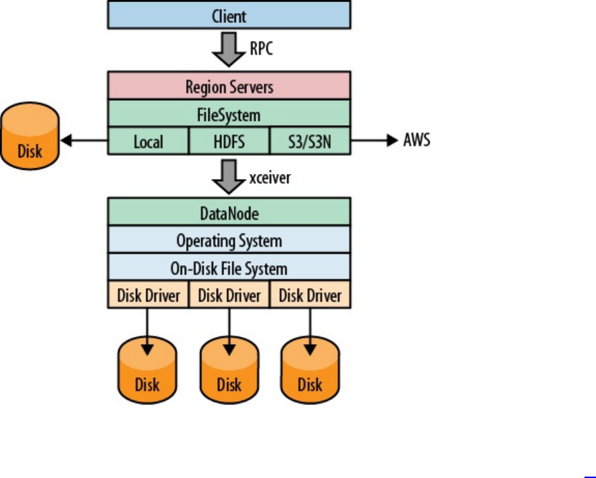
Figure 2-1. The filesystem negotiating transparently where data is stored
You can use a filesystem that is already supplied by Hadoop: it ships with a list of filesystems,21
which you may want to try out first. As a last resort—or if you’re an experienced developer—
you can also write your own filesystem implementation.
(64)

Local
The local filesystem actually bypasses Hadoop entirely, that is, you do not need to have a HDFS
or any other cluster at all. It is handled all in the FileSystem class used by HBase to connect to the
filesystem implementation. The supplied ChecksumFileSystem class is loaded by the client and uses
local disk paths to store all the data.
The beauty of this approach is that HBase is unaware that it is not talking to a distributed
filesystem on a remote or colocated cluster, but actually is using the local filesystem directly.
The standalone mode of HBase uses this feature to run HBase only (without HDFS). You can
select it by using the following scheme:
file:///<path>
Similar to the URIs used in a web browser, the file: scheme addresses local files.
Caution
Note that before HBase version 1.0.0 (and 0.98.3) there was a rare problem with data loss, during
very specific situations, using the local filesystem. While this setup is just for testing anyways,
because HDFS or another reliable filesystem is used in production, you should still be careful.22
(65)
HDFS
The Hadoop Distributed File System (HDFS) is the default filesystem when deploying a fully
distributed cluster. For HBase, HDFS is the filesystem of choice, as it has all the required
features. As we discussed earlier, HDFS is built to work with MapReduce, taking full advantage
of its parallel, streaming access support. The scalability, fail safety, and automatic replication
functionality is ideal for storing files reliably. HBase adds the random access layer missing from
HDFS and ideally complements Hadoop. Using MapReduce, you can do bulk imports, creating
the storage files at disk-transfer speeds.
The URI to access HDFS uses the following scheme:
hdfs://<namenode>:<port>/<path>
(66)

S3
Amazon’s Simple Storage Service (S3)23 is a storage system that is primarily used in
combination with dynamic servers running on Amazon’s complementary service named Elastic
Compute Cloud (EC2).24
S3 can be used directly and without EC2, but the bandwidth used to transfer data in and out of S3
is going to be cost-prohibitive in practice.
Transferring between EC2 and S3 is free, and therefore a viable option. One way to start an EC2-
based cluster is shown in “Apache Whirr”.
The S3 FileSystem implementation provided by Hadoop supports three different modes: the raw
(or native) mode, the block-based mode, and the newer AWS SDK based mode. The raw mode
uses the s3n: URI scheme and writes the data directly into S3, similar to the local filesystem.
You can see all the files in your bucket the same way as you would on your local disk.
The s3: scheme is the block-based mode and was used to overcome S3’s former maximum file
size limit of 5 GB. This has since been changed, and therefore the selection is now more difficult
—or easy: opt for s3n: if you are not going to exceed 5 GB per file.
The block mode emulates the HDFS filesystem on top of S3. It makes browsing the bucket
content more difficult as only the internal block files are visible, and the HBase storage files are
stored arbitrarily inside these blocks and strewn across them.
Both these filesystems share the fact that they use the external JetS3t open source Java toolkit to
do the actual heavy lifting. A more recent addition is the s3a: scheme that replaces the JetS3t
block mode with an AWS SDK based one.25 It is closer to the native S3 API and can optimize
certain operations, resulting in speed ups, as well as integrate better overall compared to the
existing implementation.
You can select the filesystem using these URIs:
s3://<bucket-name>
s3n://<bucket-name>
s3a://<bucket-name>
What about EBS and ephemeral disk using EC2?
While we are talking about Amazon Web Services, you might wonder what can be said about
EBS volumes vs. ephemeral disk drives (aka instance storage). The former has proper
persistency across server restarts, something that instance storage does not provide. On the other
hand, EBS is connected to the EC2 instance using a storage network, making it much more
susceptible to latency fluctuations. Some posts recommend to only allocate the maximum size of
a volume and combine four of them in a RAID-0 group.
Instance storage also exposes more latency issues compared to completely local disks, but is
slightly more predictable.26 There is still an impact and that has to be factored into the cluster
design. Not being persistent is one of the major deterrent using ephemeral disks, because losing a
server will cause data to rebalance—something that might be avoided by starting another EC2
(67)
instance and reconnecting to an existing EBS volume.
Amazon recently added the option to use SSD (solid-state drive) backed EBS volumes, for low-
latency use-cases. This should be interesting for HBase setups running in EC2, as it supposedly
smoothes out the latency spikes incurred by the built-in write caching of the EBS storage
network. Your mileage may vary!
(68)

Other Filesystems
There are other filesystems, and one to mention is QFS, the Quantcast File System.27 It is an
open source, distributed, high-performance filesystem written in C++, with similar features to
HDFS. Find more information about it at the Quantcast website.28
There are other file systems, for example the Azure filesystem, or the Swift filesystem. Both use
the native APIs of Microsoft Azure Blob Storage and OpenStack Swift respectively allowing
Hadoop to store data in these systems. We will not further look into these choices, so please
carefully evaluate what you need given a specific use-case. Note though that the majority of
clusters in production today are based on HDFS.
Wrapping up the Hadoop supported filesystems, Table 2-4 shows a list of all the important
choices. There are more supported by Hadoop, but they are used in different ways and are
therefore excluded here.
Table 2-4. A list of HDFS filesystem implementations
File System URI
Scheme Description
HDFS hdfs: The original Hadoop Distributed Filesystem
S3 Native s3n: Stores in S3 in a readable format for other S3 users
S3 Block s3: Data is stored in proprietary binary blocks in S3, using JetS3t
S3 Block (New) s3a: Improved proprietary binary block storage, using the AWS
API
Quantcast FS qfs: External project providing a HDFS replacement
Azure Blob
Storage wasb:aUses the Azure blob storage API to store binary blocks
OpenStack Swift swift: Provides storage access for OpenStack’s Swift blob storage
a There is also a wasbs: scheme for secure access to the blob storage.
(69)
Installation Choices
Once you have decided on the basic OS-related options, you must somehow get HBase onto your
servers. You have a couple of choices, which we will look into next. Also see [Link to Come] for
even more options.
(70)

Apache Binary Release
The canonical installation process of most Apache projects is to download a release, usually
provided as an archive containing all the required files. Some projects, including HBase since
version 0.95, have separate archives for a binary and source release—the former intended to
have everything needed to run the release and the latter containing all files needed to build the
project yourself. Over the years the HBase packing has changed a bit, being modularized along
the way. Due to the inherent external dependencies to Hadoop, it also had to support various
features and versions of Hadoop. Table 2-5 shows a matrix with the available packages for each
major HBase version. Single means a combined package for source and binary release
components, Security indicates a separate—but also source and binary combined—package for
kerberized setups, Source is just for source packages, same for Binary but here just for binary
packages for Hadoop 2.x and later. Finally, Hadoop 1 Binary and Hadoop 2 Binary are both
binary packages that are specific to the Hadoop version targeted.
Table 2-5. HBase packaging evolution
Version Single Security Source Binary Hadoop 1 Binary Hadoop 2 Binary
0.90.0 ✓ ✗ ✗ ✗ ✗ ✗
0.92.0 ✓ ✓ ✗ ✗ ✗ ✗
0.94.0 ✓ ✓ ✗ ✗ ✗ ✗
0.96.0 ✗ ✗ ✓ ✗ ✓ ✓
0.98.0 ✗ ✗ ✓ ✗ ✓ ✓
1.0.0 ✗ ✗ ✓ ✓ ✗ ✗
The table also shows that as of version 1.0.0 HBase will only support Hadoop 2 as mentioned
earlier. For more information on HBase releases, you may also want to check out the Release
Notes page. Another interesting page is titled Change Log, and it lists everything that was added,
fixed, or changed in any form or shape for each released version.
You can download the most recent release of HBase from the Apache HBase release page and
unpack the contents into a suitable directory, such as /usr/local or /opt, like so-shown here for
version 1.0.0:
$ cd /usr/local
$ wget http://archive.apache.org/dist/hbase/hbase-1.0.0/hbase-1.0.0-bin.tar.gz
$ tar -zxvf hbase-1.0.0-bin.tar.gz
Once you have extracted all the files, you can make yourself familiar with what is in the project’s
(71)

directory. The content may look like this:
$ cd hbase-1.0.0
$ ls -l
-rw-r--r-- 1 larsgeorge staff 130672 Feb 15 04:40 CHANGES.txt
-rw-r--r-- 1 larsgeorge staff 11358 Jan 25 10:47 LICENSE.txt
-rw-r--r-- 1 larsgeorge staff 897 Feb 15 04:18 NOTICE.txt
-rw-r--r-- 1 larsgeorge staff 1477 Feb 13 01:21 README.txt
drwxr-xr-x 31 larsgeorge staff 1054 Feb 15 04:21 bin
drwxr-xr-x 9 larsgeorge staff 306 Feb 27 13:37 conf
drwxr-xr-x 48 larsgeorge staff 1632 Feb 15 04:49 docs
drwxr-xr-x 7 larsgeorge staff 238 Feb 15 04:43 hbase-webapps
drwxr-xr-x 115 larsgeorge staff 3910 Feb 27 13:29 lib
drwxr-xr-x 8 larsgeorge staff 272 Mar 3 22:18 logs
The root of it only contains a few text files, stating the license terms (LICENSE.txt and NOTICE.txt)
and some general information on how to find your way around (README.txt). The CHANGES.txt file
is a static snapshot of the change log page mentioned earlier. It contains all the changes that went
into the current release you downloaded.
The remainder of the content in the root directory consists of other directories, which are
explained in the following list:
bin
The bin--or binaries--directory contains the scripts supplied by HBase to start and stop
HBase, run separate daemons,29 or start additional master nodes. See “Running and
Confirming Your Installation” for information on how to use them.
conf
The configuration directory contains the files that define how HBase is set up.
“Configuration” explains the contained files in great detail.
docs
This directory contains a copy of the HBase project website, including the documentation
for all the tools, the API, and the project itself. Open your web browser of choice and open
the docs/index.html file by either dragging it into the browser, double-clicking that file, or
using the File→Open (or similarly named) menu.
hbase-webapps
HBase has web-based user interfaces which are implemented as Java web applications,
using the files located in this directory. Most likely you will never have to touch this
directory when working with or deploying HBase into production.
lib
Java-based applications are usually an assembly of many auxiliary libraries, plus the JAR
file containing the actual program. All of these libraries are located in the lib directory.
For newer versions of HBase with a binary package structure and modularized
architecture, all HBase JAR files are also in this directory. Older versions have one or few
more JARs directly in the project root path.
logs
Since the HBase processes are started as daemons (i.e., they are running in the background
(72)

of the operating system performing their duty), they use log files to report their state,
progress, and optionally, errors that occur during their life cycle. “Analyzing the Logs”
explains how to make sense of their rather cryptic content.
Note
Initially, there may be no logs directory, as it is created when you start HBase for the first time.
The logging framework used by HBase is creating the directory and log files dynamically.
Since you have unpacked a binary release archive, you can now move on to “Run Modes” to
decide how you want to run HBase.
(73)

Building from Source
Note
This section is important only if you want to build HBase from its sources. This might be
necessary if you want to apply patches, which can add new functionality you may be requiring.
HBase uses Maven to build the binary packages. You therefore need a working Maven
installation, plus a full Java Development Kit (JDK)--not just a Java Runtime as used in “Quick-
Start Guide”.
You can download the most recent source release of HBase from the Apache HBase release page
and unpack the contents into a suitable directory, such as /home/<username> or /tmp, like so-shown
here for version 1.0.0 again:
$ cd /usr/username
$ wget http://archive.apache.org/dist/hbase/hbase-1.0.0/hbase-1.0.0-src.tar.gz
$ tar -zxvf hbase-1.0.0-src.tar.gz
Once you have extracted all the files, you can make yourself familiar with what is in the project’s
directory, which is now different from above, because you have a source package. The content
may look like this:
$ cd hbase-1.0.0
$ ls -l
-rw-r--r-- 1 larsgeorge admin 130672 Feb 15 04:40 CHANGES.txt
-rw-r--r-- 1 larsgeorge admin 11358 Jan 25 10:47 LICENSE.txt
-rw-r--r-- 1 larsgeorge admin 897 Feb 15 04:18 NOTICE.txt
-rw-r--r-- 1 larsgeorge admin 1477 Feb 13 01:21 README.txt
drwxr-xr-x 31 larsgeorge admin 1054 Feb 15 04:21 bin
drwxr-xr-x 9 larsgeorge admin 306 Feb 13 01:21 conf
drwxr-xr-x 25 larsgeorge admin 850 Feb 15 04:18 dev-support
drwxr-xr-x 4 larsgeorge admin 136 Feb 15 04:42 hbase-annotations
drwxr-xr-x 4 larsgeorge admin 136 Feb 15 04:43 hbase-assembly
drwxr-xr-x 4 larsgeorge admin 136 Feb 15 04:42 hbase-checkstyle
drwxr-xr-x 4 larsgeorge admin 136 Feb 15 04:42 hbase-client
drwxr-xr-x 4 larsgeorge admin 136 Feb 15 04:42 hbase-common
drwxr-xr-x 5 larsgeorge admin 170 Feb 15 04:43 hbase-examples
drwxr-xr-x 4 larsgeorge admin 136 Feb 15 04:42 hbase-hadoop-compat
drwxr-xr-x 4 larsgeorge admin 136 Feb 15 04:42 hbase-hadoop2-compat
drwxr-xr-x 4 larsgeorge admin 136 Feb 15 04:43 hbase-it
drwxr-xr-x 4 larsgeorge admin 136 Feb 15 04:42 hbase-prefix-tree
drwxr-xr-x 5 larsgeorge admin 170 Feb 15 04:42 hbase-protocol
drwxr-xr-x 4 larsgeorge admin 136 Feb 15 04:43 hbase-rest
drwxr-xr-x 4 larsgeorge admin 136 Feb 15 04:42 hbase-server
drwxr-xr-x 4 larsgeorge admin 136 Feb 15 04:43 hbase-shell
drwxr-xr-x 4 larsgeorge admin 136 Feb 15 04:43 hbase-testing-util
drwxr-xr-x 4 larsgeorge admin 136 Feb 15 04:43 hbase-thrift
-rw-r--r-- 1 larsgeorge admin 86635 Feb 15 04:21 pom.xml
drwxr-xr-x 3 larsgeorge admin 102 May 22 2014 src
Like before, the root of it only contains a few text files, stating the license terms (LICENSE.txt and
NOTICE.txt) and some general information on how to find your way around (README.txt). The
CHANGES.txt file is a static snapshot of the change log page mentioned earlier. It contains all the
changes that went into the current release you downloaded. The final, yet new file, is the Maven
POM file pom.xml, and it is needed for Maven to build the project.
The remainder of the content in the root directory consists of other directories, which are
explained in the following list:
(74)

bin
The bin--or binaries--directory contains the scripts supplied by HBase to start and stop
HBase, run separate daemons, or start additional master nodes. See “Running and
Confirming Your Installation” for information on how to use them.
conf
The configuration directory contains the files that define how HBase is set up.
“Configuration” explains the contained files in great detail.
hbase-webapps
HBase has web-based user interfaces which are implemented as Java web applications,
using the files located in this directory. Most likely you will never have to touch this
directory when working with or deploying HBase into production.
logs
Since the HBase processes are started as daemons (i.e., they are running in the background
of the operating system performing their duty), they use log files to report their state,
progress, and optionally, errors that occur during their life cycle. “Analyzing the Logs”
explains how to make sense of their rather cryptic content.
Note
Initially, there may be no logs directory, as it is created when you start HBase for the first time.
The logging framework used by HBase is creating the directory and log files dynamically.
hbase-XXXXXX
These are the source modules for HBase, containing all the required sources and other
resources. They are structured as Maven modules, which means allowing you to build
them separately if needed.
src
Contains all the source for the project site and documentation.
dev-support
Here are some scripts and related configuration files for specific development tasks.
The lib and docs directories as seen in the binary package above are absent as you may have
noted. Both are created dynamically-but in other locations-when you compile the code. There are
various build targets you can choose to build them separately, or together, as shown below. In
addition, there is also a target directory once you have built HBase for the first time. It holds the
compiled JAR, site, and documentation files respectively, though again dependent on the Maven
command you have executed.
Once you have the sources and confirmed that both Maven and JDK are set up properly, you can
build the JAR files using the following command:
$ mvn package
(75)

Note that the tests for HBase need more than one hour to complete. If you trust the code to be
operational, or you are not willing to wait, you can also skip the test phase, adding a command-
line switch like so:
$ mvn -DskipTests package
This process will take a few minutes to complete while creating the target directory in the HBase
project home directory. Once the build completes with a Build Successful message, you can find
the compiled JAR files in the target directory. If you rather want to additionally build the binary
package, you need to run this command:
$ mvn -DskipTests package assembly:single
With that archive you can go back to “Apache Binary Release” and follow the steps outlined
there to install your own, private release on your servers. Finally, here the Maven command to
build just the site details, which is the website and documentation mirror:
$ mvn site
More information about building and contribute to HBase can be found online.
(76)

Run Modes
HBase has two run modes: standalone and distributed. Out of the box, HBase runs in standalone
mode, as seen in “Quick-Start Guide”. To set up HBase in distributed mode, you will need to edit
files in the HBase conf directory.
Whatever your mode, you may need to edit conf/hbase-env.sh to tell HBase which java to use. In
this file, you set HBase environment variables such as the heap size and other options for the
JVM, the preferred location for log files, and so on. Set JAVA_HOME to point at the root of your java
installation. You can also set this variable in your shell environment, but you would need to do
this for every session you open, and across all machines you are using. Setting JAVA_HOME in the
conf/hbase-env.sh is simply the easiest and most reliable way to do that.
(77)

Standalone Mode
This is the default mode, as described and used in “Quick-Start Guide”. In standalone mode,
HBase does not use HDFS—it uses the local filesystem instead—and it runs all HBase daemons
and a local ZooKeeper in the same JVM process. ZooKeeper binds to a well-known port so that
clients may talk to HBase.
(78)

Distributed Mode
The distributed mode can be further subdivided into pseudo-distributed--all daemons run on a
single node—and fully distributed--where the daemons are spread across multiple, physical
servers in the cluster.30
Distributed modes require an instance of the Hadoop Distributed File System (HDFS). See the
Hadoop requirements and instructions for how to set up HDFS. Before proceeding, ensure that
you have an appropriate, working HDFS installation.
The following subsections describe the different distributed setups. Starting, verifying, and
exploring of your install, whether a pseudo-distributed or fully distributed configuration, is
described in “Running and Confirming Your Installation”. The same verification steps apply to
both deploy types.
Pseudo-distributed mode
A pseudo-distributed mode is simply a distributed mode that is run on a single host. Use this
configuration for testing and prototyping on HBase. Do not use this configuration for production
or for evaluating HBase performance.
Once you have confirmed your HDFS setup, edit conf/hbase-site.xml. This is the file into which
you add local customizations and overrides for the default HBase configuration values (see [Link
to Come] for the full list, and “HDFS-Related Configuration”). Point HBase at the running
Hadoop HDFS instance by setting the hbase.rootdir property. For example, adding the following
properties to your hbase-site.xml file says that HBase should use the /hbase directory in the
HDFS whose name node is at port 9000 on your local machine, and that it should run with one
replica only (recommended for pseudo-distributed mode):
<configuration>
...
<property>
<name>hbase.rootdir</name>
<value>hdfs://localhost:9000/hbase</value>
</property>
<property>
<name>dfs.replication</name>
<value>1</value>
</property>
...
</configuration>
Note
In the example configuration, the server binds to localhost. This means that a remote client
cannot connect. Amend accordingly, if you want to connect from a remote location.
The dfs.replication setting of 1 in the configuration assumes you are also running HDFS in that
mode. On a single machine it means you only have one DataNode process/thread running, and
therefore leaving the default of 3 for the replication would constantly yield warnings that blocks
are under-replicated. The same setting is also applied to HDFS in its hdfs-site.xml file. If you
have a fully distributed HDFS instead, you can remove the dfs.replication setting altogether.
(79)

If all you want to try for now is the pseudo-distributed mode, you can skip to “Running and
Confirming Your Installation” for details on how to start and verify your setup. See Chapter 11
for information on how to start extra master and region servers when running in pseudo-
distributed mode.
Fully distributed mode
For running a fully distributed operation on more than one host, you need to use the following
configurations. In hbase-site.xml, add the hbase.cluster.distributed property and set it to true,
and point the HBase hbase.rootdir at the appropriate HDFS name node and location in HDFS
where you would like HBase to write data. For example, if your name node is running at a server
with the hostname namenode.foo.com on port 9000 and you want to home your HBase in HDFS at
/hbase, use the following configuration:
<configuration>
...
<property>
<name>hbase.rootdir</name>
<value>hdfs://namenode.foo.com:9000/hbase</value>
</property>
<property>
<name>hbase.cluster.distributed</name>
<value>true</value>
</property>
...
</configuration>
In addition, a fully distributed mode requires that you modify the conf/regionservers file. It lists
all the hosts on which you want to run HRegionServer daemons. Specify one host per line (this
file in HBase is like the Hadoop slaves file). All servers listed in this file will be started and
stopped when the HBase cluster start or stop scripts are run. By default the file only contains the
localhost entry, referring back to itself for standalone and pseudo-distributed mode:
$ cat conf/regionservers
localhost
A distributed HBase setup also depends on a running ZooKeeper cluster. All participating nodes
and clients need to be able to access the running ZooKeeper ensemble. HBase, by default,
manages a ZooKeeper cluster (which can be as low as a single node) for you. It will start and
stop the ZooKeeper ensemble as part of the HBase start and stop process. You can also manage
the ZooKeeper ensemble independent of HBase and just point HBase at the cluster it should use.
To toggle HBase management of ZooKeeper, use the HBASE_MANAGES_ZK variable in conf/hbase-
env.sh. This variable, which defaults to true, tells HBase whether to start and stop the ZooKeeper
ensemble servers as part of the start and stop commands supplied by HBase.
When HBase manages the ZooKeeper ensemble, you can specify the ZooKeeper configuration
options directly in conf/hbase-site.xml.31 You can set a ZooKeeper configuration option as a
property in the HBase hbase-site.xml XML configuration file by prefixing the ZooKeeper option
name with hbase.zookeeper.property. For example, you can change the clientPort setting in
ZooKeeper by setting the hbase.zookeeper.property.clientPort property. For all default values
used by HBase, including ZooKeeper configuration, see [Link to Come]. Look for the
hbase.zookeeper.property prefix.32
zoo.cfg Versus hbase-site.xml
(80)
Please note that the following information is applicable to versions of HBase before 0.95, or
when you enable the old behavior by setting hbase.config.read.zookeeper.config to true.
There is some confusion concerning the usage of zoo.cfg and hbase-site.xml in combination with
ZooKeeper settings. For starters, if there is a zoo.cfg on the classpath (meaning it can be found
by the Java process), it takes precedence over all settings in hbase-site.xml--but only those
starting with the hbase.zookeeper.property prefix, plus a few others.
There are some ZooKeeper client settings that are not read from zoo.cfg but must be set in hbase-
site.xml. This includes, for example, the important client session timeout value set with
zookeeper.session.timeout. The following table describes the dependencies in more detail.
Property zoo.cfg + hbase-site.xml
hbase-site.xml
only
hbase.zookeeper.quorum Constructed from server.__n__ lines as specified in
zoo.cfg. Overrides any setting in hbase-site.xml.
Used as
specified.
hbase.zookeeper.property.* All values from zoo.cfg override any value
specified in hbase-site.xml.
Used as
specified.
zookeeper.* Only taken from hbase-site.xml. Only taken from
hbase-site.xml.
To avoid any confusion during deployment, it is highly recommended that you not use a zoo.cfg
file with HBase, and instead use only the hbase-site.xml file. Especially in a fully distributed
setup where you have your own ZooKeeper servers, it is not practical to copy the configuration
from the ZooKeeper nodes to the HBase servers.
You must at least set the ensemble servers with the hbase.zookeeper.quorum property. It otherwise
defaults to a single ensemble member at localhost, which is not suitable for a fully distributed
HBase (it binds to the local machine only and remote clients will not be able to connect).
There are three prefixes to specify ZooKeeper related properties:
zookeeper.
Specifies client settings for the ZooKeeper client used by the HBase client library.
hbase.zookeeper
Used for values pertaining to the HBase client communicating to the ZooKeeper servers.
hbase.zookeeper.properties.
These are only used when HBase is also managing the ZooKeeper ensemble, specifying
ZooKeeper server parameters.
How Many ZooKeepers Should I Run?
(81)
You can run a ZooKeeper ensemble that comprises one node only, but in production it is
recommended that you run a ZooKeeper ensemble of three, five, or seven machines; the more
members an ensemble has, the more tolerant the ensemble is of host failures. Also, run an odd
number of machines, since running an even count does not make for an extra server building
consensus—you need a majority vote, and if you have three or four servers, for example, both
would have a majority with three nodes. Using an odd number, larger than 3, allows you to have
two servers fail, as opposed to only one with even numbers.
Give each ZooKeeper server around 1 GB of RAM, and if possible, its own dedicated disk (a
dedicated disk is the best thing you can do to ensure the ZooKeeper ensemble performs well).
For very heavily loaded clusters, run ZooKeeper servers on separate machines from
RegionServers, DataNodes, TaskTrackers, or NodeManagers.
For example, in order to have HBase manage a ZooKeeper quorum on nodes
rs{1,2,3,4,5}.foo.com, bound to port 2222 (the default is 2181), you must ensure that
HBASE_MANAGES_ZK is commented out or set to true in conf/hbase-env.sh and then edit conf/hbase-
site.xml and set hbase.zookeeper.property.clientPort and hbase.zookeeper.quorum. You should
also set hbase.zookeeper.property.dataDir to something other than the default, as the default has
ZooKeeper persist data under /tmp, which is often cleared on system restart. In the following
example, we have ZooKeeper persist to /var/zookeeper:
Tip
Keep in mind that setting HBASE_MANAGES_ZK either way implies that you are using the supplied
HBase start scripts. This might not be the case for a packaged distribution of HBase (see [Link to
Come]). There are many ways to manage processes and therefore there is no guarantee that any
setting made in hbase-env.sh, and hbase-site.xml, are really taking affect. Please consult with
your distribution’s documentation ensuring you use the proper approach.
<configuration>
...
<property>
<name>hbase.zookeeper.property.clientPort</name>
<value>2222</value>
</property>
<property>
<name>hbase.zookeeper.quorum</name>
<value>rs1.foo.com,rs2.foo.com,rs3.foo.com,rs4.foo.com,rs5.foo.com</value>
</property>
<property>
<name>hbase.zookeeper.property.dataDir</name>
<value>/var/zookeeper</value>
</property>
...
</configuration>
To point HBase at an existing ZooKeeper cluster, one that is not managed by HBase, set
HBASE_MANAGES_ZK in conf/hbase-env.sh to false:
...
# Tell HBase whether it should manage it's own instance of Zookeeper or not.
export HBASE_MANAGES_ZK=false
Next, set the ensemble locations and client port, if nonstandard, in hbase-site.xml. When HBase
manages ZooKeeper, it will start/stop the ZooKeeper servers as a part of the regular start/stop
scripts. If you would like to run ZooKeeper yourself, independent of HBase start/stop, do the
following:
(82)

${HBASE_HOME}/bin/hbase-daemons.sh {start,stop} zookeeper
Note that you can use HBase in this manner to spin up a ZooKeeper cluster, unrelated to HBase.
Just make sure to set HBASE_MANAGES_ZK to false if you want it to stay up across HBase restarts so
that when HBase shuts down, it doesn’t take ZooKeeper down with it.
For more information about running a distinct ZooKeeper cluster, see the ZooKeeper Getting
Started Guide. Additionally, see the ZooKeeper wiki, or the ZooKeeper documentation for more
information on ZooKeeper sizing.
(83)

Configuration
Now that the basics are out of the way (we’ve looked at all the choices when it comes to
selecting the filesystem, discussed the run modes, and fine-tuned the operating system
parameters), we can look at how to configure HBase itself. Similar to Hadoop, all configuration
parameters are stored in files located in the conf directory. These are simple text files either in
XML format arranged as a set of properties, or in simple flat files listing one option per line.
Tip
For more details on how to modify your configuration files for specific workloads refer to
“Configuration”.
Here a list of current configuration files, as available in HBase 1.0.0, with the detailed
description of each following in due course:
hbase-env.cmd and hbase-env.sh
Set up the working environment for HBase, specifying variables such as JAVA_HOME. For
Windows and Linux respectively.
hbase-site.xml
The main HBase configuration file. This file specifies configuration options which
override HBase’s default configuration.
backup-masters
This file is actually not present on a fresh install. It is a text file that lists all the hosts
which should have backup masters started on.
regionservers
Lists all the nodes that are designated to run a region server instance.
hadoop-metrics2-hbase.properties
Specifies settings for the metrics framework integrated into each HBase process.
hbase-policy.xml
In secure mode, this file is read and defines the authorization rules for clients accessing the
servers.
log4j.properties
Configures how each process logs its information using the Log4J libraries.
Configuring a HBase setup entails editing the conf/hbase-env.{sh|cmd} file containing
environment variables, which is used mostly by the shell scripts (see “Operating a Cluster”) to
start or stop a cluster. You also need to add configuration properties to the XML file33
conf/hbase-site.xml to, for example, override HBase defaults, tell HBase what filesystem to use,
(84)

and tell HBase the location of the ZooKeeper ensemble.
When running in distributed mode, after you make an edit to a HBase configuration file, make
sure you copy the content of the conf directory to all nodes of the cluster. HBase will not do this
for you.
Tip
There are many ways to synchronize your configuration files across your cluster. The easiest is
to use a tool like rsync. There are many more elaborate ways, and you will see a selection in
“Deployment”.
We will now look more closely at each configuration file.
(85)

hbase-site.xml and hbase-default.xml
Just as in Hadoop where you add site-specific HDFS configurations to the hdfs-site.xml file, for
HBase, site-specific customizations go into the file conf/hbase-site.xml. For the list of
configurable properties, see [Link to Come], or view the raw hbase-default.xml source file in the
HBase source code at hbase-common/src/main/resources. The doc directory also has a static HTML
page that lists the configuration options.
Caution
Not all configuration options are listed in hbase-default.xml. Configurations that users would
rarely change do exist only in code; the only way to turn find such configuration options is to
read the source code itself.
The servers always read the hbase-default.xml file first and subsequently merge it with the hbase-
site.xml file content—if present. The properties set in hbase-site.xml always take precedence
over the default values loaded from hbase-default.xml.
Most changes here will require a cluster restart for HBase to notice the change. However, there is
a way to reload some specific settings while the processes are running. See “Reloading
Configuration” for details.
HDFS-Related Configuration
If you have made HDFS-related configuration changes on your Hadoop cluster—in other words,
properties you want the HDFS clients to use as opposed to the server-side configuration—HBase
will not see these properties unless you do one of the following:
Add a pointer to your $HADOOP_CONF_DIR to the HBASE_CLASSPATH environment variable in
hbase-env.sh.
Add a copy of core-site.xml, hdfs-site.xml, etc. (or hadoop-site.xml) or, better, symbolic
links, under ${HBASE_HOME}/conf.
Add them to hbase-site.xml directly.
An example of such a HDFS client property is dfs.replication. If, for example, you want to run
with a replication factor of 5, HBase will create files with the default of 3 unless you do one of
the above to make the configuration available to HBase.
When you add Hadoop configuration files to HBase, they will always take the lowest priority. In
other words, the properties contained in any of the HBase-related configuration files, that is, the
default and site files, take precedence over any Hadoop configuration file containing a property
with the same name. This allows you to override Hadoop properties in your HBase configuration
file.
(86)
hbase-env.sh and hbase-env.cmd
You set HBase environment variables in these files. Examples include options to pass to the
JVM when a HBase daemon starts, such as Java heap size and garbage collector configurations.
You also set options for HBase configuration, log directories, niceness, SSH options, where to
locate process pid files, and so on. Open the file at conf/hbase-env.{cmd,sh} and peruse its
content. Each option is fairly well documented. Add your own environment variables here if you
want them read when a HBase daemon is started.
(87)

regionserver
This file lists all the known region server names. It is a flat text file that has one hostname per
line. The list is used by the HBase maintenance script to be able to iterate over all the servers to
start the region server process. An example can be seen in “Example Configuration”.
Note
If you used previous versions of HBase, you may miss the masters file, available in the 0.20.x
line. It has been removed as it is no longer needed. The list of masters is now dynamically
maintained in ZooKeeper and each master registers itself when started.
(88)

log4j.properties
Edit this file to change the rate at which HBase files are rolled and to change the level at which
HBase logs messages. Changes here will require a cluster restart for HBase to notice the change,
though log levels can be changed for particular daemons via the HBase UI. See “Changing
Logging Levels” for information on this topic, and “Analyzing the Logs” for details on how to
use the log files to find and solve problems.
(89)
Example Configuration
Here is an example configuration for a distributed 10-node cluster. The nodes are named
master.foo.com, host1.foo.com, and so on, through node host9.foo.com. The HBase Master and the
HDFS name node are running on the node master.foo.com. Region servers run on nodes
host1.foo.com to host9.foo.com. A three-node ZooKeeper ensemble runs on zk1.foo.com,
zk2.foo.com, and zk3.foo.com on the default ports. ZooKeeper data is persisted to the directory
/var/zookeeper. The following subsections show what the main configuration files--hbase-
site.xml, regionservers, and hbase-env.sh--found in the HBase conf directory might look like.
hbase-site.xml
The hbase-site.xml file contains the essential configuration properties, defining the HBase cluster
setup.
<?xml version="1.0"?>
<?xml-stylesheet type="text/xsl" href="configuration.xsl"?>
<configuration>
<property>
<name>hbase.zookeeper.quorum</name>
<value>zk1.foo.com,zk2.foo.com,zk3.foo.com</value>
</property>
<property>
<name>hbase.zookeeper.property.dataDir</name>
<value>/var/zookeeper</value>
</property>
<property>
<name>hbase.rootdir</name>
<value>hdfs://master.foo.com:9000/hbase</value>
</property>
<property>
<name>hbase.cluster.distributed</name>
<value>true</value>
</property>
</configuration>
regionservers
In this file, you list the nodes that will run region servers. In our example, we run region servers
on all but the head node master.foo.com, which is carrying the HBase Master and the HDFS
NameNode.
host1.foo.com
host2.foo.com
host3.foo.com
host4.foo.com
host5.foo.com
host6.foo.com
host7.foo.com
host8.foo.com
host9.foo.com
hbase-env.sh
Here are the lines that were changed from the default in the supplied hbase-env.sh file. We are
setting the HBase heap to be 4 GB:
...
# export HBASE_HEAPSIZE=1000
(90)

export HBASE_HEAPSIZE=4096
...
Before HBase version 1.0 the default heap size was 1 GB. This has been changed34 in 1.0 and
later to the default value of the JVM. This usually amounts to one-fourth of the available
memory, for example on a Mac with Java version 1.7.0_45:
$ hostinfo | grep memory
Primary memory available: 48.00 gigabytes
$ java -XX:+PrintFlagsFinal -version | grep MaxHeapSize
uintx MaxHeapSize := 12884901888 {product}
You can see that the JVM reports a maximum heap of 12 GB, which is the mentioned one-fourth
of the full 48 GB.
Once you have edited the configuration files, you need to distribute them across all servers in the
cluster. One option to copy the content of the conf directory to all servers in the cluster is to use
the rsync command on Unix and Unix-like platforms. This approach and others are explained in
“Deployment”.
Tip
“Configuration” discusses the settings you are most likely to change first when you start scaling
your cluster.
(91)

Client Configuration
Since the HBase Master may move around between physical machines (see “Adding Servers” for
details), clients start by requesting the vital information from ZooKeeper—something visualized
in [Link to Come]. For that reason, clients require the ZooKeeper quorum information in a hbase-
site.xml file that is on their Java $CLASSPATH.
Note
You can also set the hbase.zookeeper.quorum configuration key in your code. Doing so would lead
to clients that need no external configuration files. This is explained in “Put Method”.
If you are configuring an IDE to run a HBase client, you could include the conf/ directory in
your class path. That would make the configuration files discoverable by the client code.
Minimally, a Java client needs the following JAR files specified in its $CLASSPATH, when
connecting to HBase, as retrieved with the HBase shell mapredcp command (and some shell string
mangling):
$ bin/hbase mapredcp | tr ":" "\n" | sed "s/\/usr\/local\/hbase-1.0.0\/lib\///"
zookeeper-3.4.6.jar
hbase-common-1.0.0.jar
hbase-protocol-1.0.0.jar
htrace-core-3.1.0-incubating.jar
protobuf-java-2.5.0.jar
hbase-client-1.0.0.jar
hbase-hadoop-compat-1.0.0.jar
netty-all-4.0.23.Final.jar
hbase-server-1.0.0.jar
guava-12.0.1.jar
Run the same bin/hbase mapredcp command without any string mangling to get a properly
configured class path output, which can be fed directly to an application setup. All of these JAR
files come with HBase and are usually postfixed with the a version number of the required
release. Ideally, you use the supplied JARs and do not acquire them somewhere else because
even minor release changes could cause problems when running the client against a remote
HBase cluster.
A basic example hbase-site.xml file for client applications might contain the following
properties:
<?xml version="1.0"?>
<?xml-stylesheet type="text/xsl" href="configuration.xsl"?>
<configuration>
<property>
<name>hbase.zookeeper.quorum</name>
<value>zk1.foo.com,zk2.foo.com,zk3.foo.com</value>
</property>
</configuration>
(92)

Deployment
After you have configured HBase, the next thing you need to do is to think about deploying it on
your cluster. There are many ways to do that, and since Hadoop and HBase are written in Java,
there are only a few necessary requirements to look out for. You can simply copy all the files
from server to server, since they usually share the same configuration. Here are some ideas on
how to do that. Please note that you would need to make sure that all the suggested selections
and adjustments discussed in “Requirements” have been applied—or are applied at the same time
when provisioning new servers.
Besides what is mentioned below, the much more common way these days to deploy Hadoop
and HBase is using a prepackaged distribution, which are listed in [Link to Come].
(93)

Script-Based
Using a script-based approach seems archaic compared to the more advanced approaches listed
shortly. But they serve their purpose and do a good job for small to even medium-size clusters. It
is not so much the size of the cluster but the number of people maintaining it. In a larger
operations group, you want to have repeatable deployment procedures, and not deal with
someone having to run scripts to update the cluster.
The scripts make use of the fact that the regionservers configuration file has a list of all servers in
the cluster. Example 2-3 shows a very simple script that could be used to copy a new release of
HBase from the master node to all slave nodes.
Example 2-3. Example Script to copy the HBase files across a cluster
#!/bin/bash
# Rsync's HBase files across all slaves. Must run on master. Assumes
# all files are located in /usr/local
if [ "$#" != "2" ]; then
echo "usage: $(basename $0) <dir-name> <ln-name>"
echo " example: $(basename $0) hbase-0.1 hbase"
exit 1
fi
SRC_PATH="/usr/local/$1/conf/regionservers"
for srv in $(cat $SRC_PATH); do
echo "Sending command to $srv...";
rsync -vaz --exclude='logs/*' /usr/local/$1 $srv:/usr/local/
ssh $srv "rm -fR /usr/local/$2 ; ln -s /usr/local/$1 /usr/local/$2"
done
echo "done."
Another simple script is shown in Example 2-4; it can be used to copy the configuration files of
HBase from the master node to all slave nodes. It assumes you are editing the configuration files
on the master in such a way that the master can be copied across to all region servers.
Example 2-4. Example Script to copy configurations across a cluster
#!/bin/bash
# Rsync's HBase config files across all region servers. Must run on master.
for srv in $(cat /usr/local/hbase/conf/regionservers); do
echo "Sending command to $srv...";
rsync -vaz --delete --exclude='logs/*' /usr/local/hadoop/ $srv:/usr/local/hadoop/
rsync -vaz --delete --exclude='logs/*' /usr/local/hbase/ $srv:/usr/local/hbase/
done
echo "done."
The second script uses rsync just like the first script, but adds the --delete option to make sure
the region servers do not have any older files remaining but have an exact copy of what is on the
originating server.
There are obviously many ways to do this, and the preceding examples are simply for your
perusal and to get you started. Ask your administrator to help you set up mechanisms to
synchronize the configuration files appropriately. Many beginners in HBase have run into a
problem that was ultimately caused by inconsistent configurations among the cluster nodes.
(94)


Apache Whirr
Recently, we have seen an increase in the number of users who want to run their cluster in
dynamic environments, such as the public cloud offerings by Amazon’s EC2, or Rackspace
Cloud Servers, as well as in private server farms, using open source tools like Eucalyptus or
OpenStack.
The advantage is to be able to quickly provision servers and run analytical workloads and, once
the result has been retrieved, to simply shut down the entire cluster, or reuse the servers for other
dynamic workloads. Since it is not trivial to program against each of the APIs providing dynamic
cluster infrastructures, it would be useful to abstract the provisioning part and, once the cluster is
operational, simply launch the MapReduce jobs the same way you would on a local, static
cluster. This is where Apache Whirr comes in.
Whirr has support for a variety of public and private cloud APIs and allows you to provision
clusters running a range of services. One of those is HBase, giving you the ability to quickly
deploy a fully operational HBase cluster on dynamic setups.
You can download the latest Whirr release from the project’s website and find preconfigured
configuration files in the recipes directory. Use it as a starting point to deploy your own dynamic
clusters.
The basic concept of Whirr is to use very simple machine images that already provide the
operating system (see “Operating system”) and SSH access. The rest is handled by Whirr using
services that represent, for example, Hadoop or HBase. Each service executes every required
step on each remote server to set up the user accounts, download and install the required software
packages, write out configuration files for them, and so on. This is all highly customizable and
you can add extra steps as needed.
(96)

Puppet and Chef
Similar to Whirr, there are other deployment frameworks for dedicated machines. Puppet by
Puppet Labs and Chef by Opscode are two such offerings.
Both work similar to Whirr in that they have a central provisioning server that stores all the
configurations, combined with client software, executed on each server, which communicates
with the central server to receive updates and apply them locally.
Also similar to Whirr, both have the notion of recipes, which essentially translate to scripts or
commands executed on each node. In fact, it is quite possible to replace the scripting employed
by Whirr with a Puppet- or Chef-based process. Some of the available recipe packages are an
adaption of early EC2 scripts, used to deploy HBase to dynamic, cloud-based server. For Chef,
you can find HBase-related examples at http://cookbooks.opscode.com/cookbooks/hbase. For
Puppet, please refer to http://hstack.org/hstack-automated-deployment-using-puppet/ and the
repository with the recipes at http://github.com/hstack/puppet as a starting point. There are other
such modules available on the Internet.
While Whirr solely handles the bootstrapping, Puppet and Chef have further support for
changing running clusters. Their master process monitors the configuration repository and, upon
updates, triggers the appropriate remote action. This can be used to reconfigure clusters on-the-
fly or push out new releases, do rolling restarts, and so on. It can be summarized as configuration
management, rather than just provisioning.
Note
You heard it before: select an approach you like and maybe even are familiar with already. In the
end, they achieve the same goal: installing everything you need on your cluster nodes. If you
need a full configuration management solution with live updates, a Puppet- or Chef-based
approach—maybe in combination with Whirr for the server provisioning—is the right choice.
(97)
Operating a Cluster
Now that you have set up the servers, configured the operating system and filesystem, and edited
the configuration files, you are ready to start your HBase cluster for the first time.
(98)

Running and Confirming Your Installation
Make sure HDFS is running first. Start and stop the Hadoop HDFS daemons by running
bin/start-dfs.sh over in the $HADOOP_HOME directory. You can ensure that it started properly by
testing the put and get of files into the Hadoop filesystem. HBase does not normally use the
YARN daemons. You only need to start them for actual MapReduce jobs, something we will
look into in detail in Chapter 7.
If you are managing your own ZooKeeper, start it and confirm that it is running, since otherwise
HBase will fail to start.
Just as you started the standalone mode in “Quick-Start Guide”, you start a fully distributed
HBase with the following command:
$ bin/start-hbase.sh
Run the preceding command from the $HBASE_HOME directory. You should now have a running
HBase instance. The HBase log files can be found in the logs subdirectory. If you find that
HBase is not working as expected, please refer to “Analyzing the Logs” for help finding the
problem.
Once HBase has started, see “Quick-Start Guide” for information on how to create tables, add
data, scan your insertions, and finally, disable and drop your tables.
(99)

Web-based UI Introduction
HBase also starts a web-based user interface (UI) listing vital attributes. By default, it is
deployed on the master host at port 16010 (HBase region servers use 16030 by default).35 If the
master is running on a host named master.foo.com on the default port, to see the master’s home
page you can point your browser at http://master.foo.com:16010. Figure 2-2 is an example of how
the resultant page should look. You can find a more detailed explanation in “Web-based UI”.
(100)

Figure 2-2. The HBase Master User Interface
(101)
From this page you can access a variety of status information about your HBase cluster. The
page is separated into multiple sections. The top part has the information about the available
region servers, as well as any optional backup masters. This is followed by the known tables,
system tables, and snapshots—these are tabs that you can select to see more detail.
The lower part shows the currently running tasks—if there are any-- and again using tabs, you
can switch to other details here, for example, the RPC handler status, active calls, and so on.
Finally the bottom of the page lists key attributes pertaining to the cluster setup.
After you have started the cluster, you should verify that all the region servers have registered
themselves with the master and appear in the appropriate table with the expected hostnames (that
a client can connect to). Also verify that you are indeed running the correct version of HBase and
Hadoop.
(102)

Shell Introduction
You already used the command-line shell that comes with HBase when you went through
“Quick-Start Guide”. You saw how to create a table, add and retrieve data, and eventually drop
the table.
The HBase Shell is (J)Ruby’s IRB with some HBase-related commands added. Anything you
can do in IRB, you should be able to do in the HBase Shell. You can start the shell with the
following command:
$ bin/hbase shell
HBase Shell; enter 'help<RETURN>' for list of supported commands.
Type "exit<RETURN>" to leave the HBase Shell
Version 1.0.0, r6c98bff7b719efdb16f71606f3b7d8229445eb81, Sat Feb 14 19:49:22 PST 2015
hbase(main):001:0>
Type help and then press Return to see a listing of shell commands and options. Browse at least
the paragraphs at the end of the help text for the gist of how variables and command arguments
are entered into the HBase Shell; in particular, note how table names, rows, and columns, must
be quoted. Find the full description of the shell in “Shell”.
Since the shell is JRuby-based, you can mix Ruby with HBase commands, which enables you to
do things like this:
hbase(main):001:0> create 'testtable', 'colfam1'
hbase(main):002:0> for i in 'a'..'z' do for j in 'a'..'z' do \
put 'testtable', "row-#{i}#{j}", "colfam1:#{j}", "#{j}" end end
The first command is creating a new table named testtable, with one column family called
colfam1, using default values (see “Column Families” for what that means). The second
command uses a Ruby loop to create rows with columns in the newly created tables. It creates
row keys starting with row-aa, row-ab, all the way to row-zz.
(103)
Stopping the Cluster
To stop HBase, enter the following command. Once you have started the script, you will see a
message stating that the cluster is being stopped, followed by “.” (period) characters printed in
regular intervals (just to indicate that the process is still running, not to give you any percentage
feedback, or some other hidden meaning):
$ bin/stop-hbase.sh
stopping hbase...............
Shutdown can take several minutes to complete. It can take longer if your cluster is composed of
many machines. If you are running a distributed operation, be sure to wait until HBase has shut
down completely before stopping the Hadoop daemons.
Chapter 11 has more on advanced administration tasks—for example, how to do a rolling restart,
add extra master nodes, and more. It also has information on how to analyze and fix problems
when the cluster does not start, or shut down.
1 See “Java” for information of supported Java versions for older releases of HBase.
2 Previous versions were shipped just as source archive and had no special postfix in their name.
The quickstart steps will still work though.
3 The naming of the processing daemon per node has changed between the former MapReduce
v1 and the newer YARN based framework.
4 See “Multi-core processor” on Wikipedia.
5 Setting up a production cluster is a complex thing, the examples here are given just as a starting
point. See the O’Reilly Hadoop Operations book by Eric Sammer for much more details.
6 See “RAID” on Wikipedia.
7 See “JBOD” on Wikipedia.
8 This assumes 100 IOPS per drive, and 100 MB/second per drive.
9 There is more on this in Eric Sammer’s Hadoop Operations book, and in online post, such as
Facebook’s Fabric.
10 See HBASE-6814.
11 DistroWatch has a list of popular Linux and Unix-like operating systems and maintains a
ranking by popularity.
12 See http://en.wikipedia.org/wiki/Ext3 on Wikipedia for details.
13 See this post on the Ars Technica website. Google hired the main developer of ext4, Theodore
Ts’o, who announced plans to keep working on ext4 as well as other Linux kernel features.
(104)
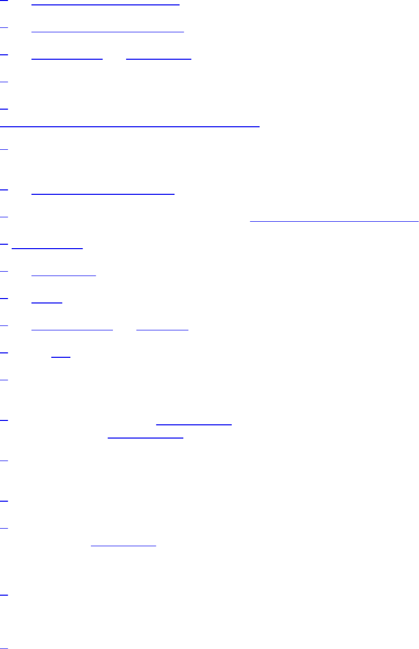
14 See http://en.wikipedia.org/wiki/Xfs on Wikipedia for details.
15 See http://en.wikipedia.org/wiki/ZFS on Wikipedia for details
16 See HBASE-12241 and HBASE-6775 for background.
17 Public here means external IP, i.e. the one used in the LAN to route traffic to this server.
18 A useful document on setting configuration values on your Hadoop cluster is Aaron Kimball’s
“Configuration Parameters: What can you just ignore?”.
19 In previous versions of Hadoop this parameter was called dfs.datanode.max.xcievers, with
xciever being misspelled.
20 See “Uniform Resource Identifier” on Wikipedia.
21 A full list was compiled by Tom White in his post “Get to Know Hadoop Filesystems”.
22 HBASE-11218 has the details.
23 See “Amazon S3” for more background information.
24 See “EC2” on Wikipedia.
25 See HADOOP-10400 and AWS SDK for details.
26 See this post for a more in-depth discussion on I/O performance on EC2.
27 QFS used to be called CloudStore, which in turn was formerly known as the Kosmos
filesystem, abbreviated as KFS and the namesake of the original URI scheme.
28 Also check out the JIRA issue HADOOP-8885 for the details on QFS. Info about the removal
of KFS is found under HADOOP-8886.
29 Processes that are started and then run in the background to perform their task are often
referred to as daemons.
30 The pseudo-distributed versus fully distributed nomenclature comes from Hadoop.
31 In versions before HBase 0.95 it was also possible to read an external zoo.cfg file. This has
been deprecated in HBASE-4072. The issue mentions hbase.config.read.zookeeper.config to
enable the old behavior for existing, older setups, which is still available in HBase 1.0.0 though
should not be used if possible.
32 For the full list of ZooKeeper configurations, see ZooKeeper’s zoo.cfg. HBase does not ship
with that file, so you will need to browse the conf directory in an appropriate ZooKeeper
download.
33 Be careful when editing XML files. Make sure you close all elements. Check your file using a
tool like xmllint, or something similar, to ensure well-formedness of your document after an edit
(105)


Chapter 3. Client API: The Basics
This chapter will discuss the client APIs provided by HBase. As noted earlier, HBase is written
in Java and so is its native API. This does not mean, though, that you must use Java to access
HBase. In fact, Chapter 6 will show how you can use other programming languages.
(107)

General Notes
Note
As noted in [Link to Come], we are mostly looking at APIs that are flagged as public regarding
their audience. See [Link to Come] for details on the annotations in use.
The primary client entry point to HBase is the Table interface in the
org.apache.hadoop.hbase.client package. It provides the user with all the functionality needed to
store and retrieve data from a HBase table, as well as delete obsolete values and so on. It is
retrieved by means of the Connection instance that is the umbilical cord to the HBase cluster.
Before looking at the various methods these classes provide, let us address some general aspects
of their usage.
All operations that mutate data are guaranteed to be atomic on a per-row basis. This applies to all
other concurrent readers and writers of that same row. In other words, it does not matter if
another client or thread is reading from or writing to the same row: they either read a consistent
last mutation, or may have to wait before being able to apply their edits change.1 More on this in
[Link to Come].
Suffice it to say for now that during normal operations and load, a reading client will not be
affected by another updating a particular row since their contention is nearly negligible. There is,
however, an issue with many clients trying to update the same row at the same time. Try to batch
updates together to reduce the number of separate operations on the same row as much as
possible.
It also does not matter how many columns are written for the particular row; all of them are
covered by this guarantee of atomicity.
Finally, creating an initial connection to HBase is not without cost. Each instantiation involves
scanning the hbase:meta table to check if the table actually exists and if it is enabled, as well as a
few other operations that make this call quite heavy. Therefore, it is recommended that you
create a Connection instances only once and reuse that instance for the rest of the lifetime of your
client application.
Once you have a connection instance you can retrieve references to the actual tables. Ideally you
do this per thread since the underlying implementation of Table is not guaranteed to the thread-
safe. Ensure that you close all of the resources you acquire though to trigger important house-
keeping activities. All of this will be explained in detail in the rest of this chapter.
Note
The examples you will see in partial source code can be found in full detail in the publicly
available GitHub repository at https://github.com/larsgeorge/hbase-book. For details on how to
compile them, see [Link to Come].
Initially you will see the import statements, but they will be subsequently omitted for the sake of
brevity. Also, specific parts of the code are not listed if they do not immediately help with the
topic explained. Refer to the full source if in doubt.
(108)

Data Types and Hierarchy
Before we delve into the actual operations and their API classes, let us first see how the classes
that we will use throughout the chapter are related. There is some very basic functionality
introduced in lower-level classes, which surface in the majority of the data-centric classes, such
as Put, Get, or Scan. Table 3-1 list all of the basic data-centric types that are introduced in this
chapter.
Table 3-1. List of basic data-centric types
Type Kind Description
Get Query Retrieve previously stored data from a single row.
Scan Query Iterate over all or specific rows and return their data.
Put Mutation Create or update one or more columns in a single row.
Delete Mutation Remove a specific cell, column, row, etc.
Increment Mutation Treat a column as a counter and increment its value.
Append Mutation Attach the given data to one or more columns in a single row.
Throughout the book we will collectively refer to these classes as operations. Figure 3-1 shows
you the hierarchy of the data-centric types and their relationship to the more generic superclasses
and interfaces. The remainder of this section will discuss what these base classes and interfaces
add to each derived data-centric type.
(109)
Figure 3-1. The class hierarchy of the basic client API data classes
(110)

Generic Attributes
One fundamental interface is Attributes, which introduces the following methods:
Attributes setAttribute(String name, byte[] value)
byte[] getAttribute(String name)
Map<String, byte[]> getAttributesMap()
They provide a general mechanism to add any kind of information in the form of attributes to all
of the data-centric classes. By default there are no attributes set (apart from possibly internal
ones) and a developer can make use of setAttribute() to add custom ones as needed. Since most
of the time the construction of a data type, such as Put, is immediately followed by an API call to
send it off to the servers, a valid question is: where can I make use of attributes?
One thing to note is that attributes are serialized and sent to the server, which means you can use
them to inspect their value, for example, in a coprocessor (see “Coprocessors”). Another use-
case is the Append class, which uses the attributes to return information back to the user after a
call to the servers (see “Append Method”).
(111)

Operations: Fingerprint and ID
Another fundamental type is the abstract class Operation, which adds the following methods to all
data types:
abstract Map<String, Object> getFingerprint()
abstract Map<String, Object> toMap(int maxCols)
Map<String, Object> toMap()
String toJSON(int maxCols) throws IOException
String toJSON() throws IOException
String toString(int maxCols)
String toString()
These were introduces when HBase 0.92 had the slow query logging added (see “Slow Query
Logging”), and help in generating useful information collection for logging and general
debugging purposes. All of the latter methods really rely on the specific implementation of
toMap(int maxCols), which is abstract in Operation. The Mutation class implements it for all
derived data classes as described in Table 3-2. The default number of columns included in the
output is 5 (hardcoded in HBase 1.0.0) when not specified explicitly.
In addition, the intermediate OperationWithAttributes class extends the above Operation class,
implements the Attributes interface, and adds the following methods:
OperationWithAttributes setId(String id)
String getId()
The ID is a client-provided value, which identifies the operation when logged or emitted
otherwise. For example, the client could set it to the method name that is invoking the API, so
that when the operation—say the Put instance—is logged it can be determined which client call
is the root cause. Add the hostname, process ID, and other useful information and it will be much
easier determining the originating client.
Table 3-2. The various methods to retrieve instance information
Method Description
getId() Returns what was set by the setId() method.
getFingerprint() Returns the list of column families included in the instance.
toMap(int
maxCols)
Compiles a list including fingerprint, column families with all columns and
their data, total column count, row key, and—if set—the ID and cell-level
TTL.
toMap() Same as above, but only for 5 columns.a
toJSON(int
maxCols)
Same as toMap(maxCols) but converted to JSON. Might fail due to encoding
issues.
(112)

toJSON()
Same as above, but only for 5 columns.a
toString(int
maxCols) Attempts to call toJSON(maxCols), but when it fails, falls back to toMap(maxCols).
toString() Same as above, but only for 5 columns.a
a Hardcoded in HBase 1.0.0. Might change in the future.
The repository accompanying the book has an example named FingerprintExample.java which
you can experiment with to see the fingerprint, ID, and toMap() in action.
(113)

Query versus Mutation
Before we discuss the basic data-centric types, there are a few more superclasses of importance.
First the Row interface, which adds:
byte[] getRow()
The method simply returns the given row key of the instance. This is implemented by the Get
class, as it handles exactly one row. It is also implemented by the Mutation superclass, which is
the basis for all the types that are needed when changing data. Additionally, Mutation implements
the CellScannable interface to provide the following method:
CellScanner cellScanner()
With it, a client can iterate over the returned cells, which we will learn about in “The Cell” very
soon. The Mutation class also has many other functions that are shared by all derived classes.
Here is a list of the most interesting ones:
Table 3-3. Methods provided by the Mutation superclass
Method Description
getACL()/setACL() The Access Control List (ACL) for this operation. See
[Link to Come] for details.
getCellVisibility()/setCellVisibility() The cell level visibility for all included cells. See [Link
to Come] for details.
getClusterIds()/setClusterIds() The cluster ID as needed for replication purposes. See
[Link to Come] for details.
getDurability()/setDurability() The durability settings for the mutation. See
“Durability, Consistency, and Isolation” for details.
getFamilyCellMap()/setFamilyCellMap() The list of all cells per column family available in this
instance.
getTimeStamp()
Retrieves the associated timestamp of the Put instance.
Can be optionally set using the constructor’s ts
parameter. If not set, may return Long.MAX_VALUE (also
defined as HConstants.LATEST_TIMESTAMP).
getTTL()/setTTL()
Sets the cell level TTL value, which is being applied to
all included Cell instances before being persisted.
(114)

heapSize()
Computes the heap space required for the current Put
instance. This includes all contained data and space
needed for internal structures.
isEmpty() Checks if the family map contains any Cell instances.
numFamilies() Convenience method to retrieve the size of the family
map, containing all Cell instances.
size() Returns the number of Cell instances that will be added
with this Put.
While there are many that you learn about at an opportune moment later in the book (see the
links provided above), there are also a few that we can explain now and will not have to repeat
them later, since they are shared by most data-centric types. First is the getFamilyCellMap() and
setFamilyCellMap() pair. Mutations hold a list of columns they act on, and columns are
represented as Cell instances (“The Cell” will introduce them properly). So these two methods let
you retrieve the current list of cells held by the mutation, or set—or replace—the entire list in
one go.
The getTimeStamp() method returns the instance-wide timestamp set during instantiation, or via a
call to setTimestamp()2 if present. Usually the constructor is the common way to optionally hand
in a timestamp. What that timestamp means is different for each derived class. For example, for
Delete it sets a global filter to delete cells that are of that version or before. For Put it is stored
and applied to all subsequent addColumn() calls when no explicit timestamp is specified.
Another pair are the getTTL() and setTTL() methods, allowing the definition of a cell-level time-
to-live (TTL). They are useful for all mutations that add new columns (or cells, in case of
updating an existing column), and in fact for Delete the call to setTTL() will throw an exception
that the operation is unsupported. The getTTL() is to recall what was set previously, and by
default the TTL is unset. Once assigned, you cannot unset the value, so to disable it again, you
have to set it to Long.MAX_VALUE.
The size(), isEmpty(), and numFamilies() all return information about what was added to the
mutation so far, either using the addColumn(), addFamily() (and class specific variants), or
setFamilyCellMap(). size just returns the size of the list of cells. So if you, for example, added
three specific columns, two to column family 1, and one to column family 2, you would be
returned 3. isEmpty() compares size() to 0 and will return true if they are equal, false otherwise.
numFamilies() keeps track of how many column families have been added by the addColumn() and
addFamily() calls. In our example we would return 2 as we have added this many families.
The other larger superclass on the retrieval side is Query, which provides a common substrate for
all data types concerned with reading data from the HBase tables. The following table shows the
methods introduced:
Table 3-4. Methods provided by the Query superclass
(115)

Table 3-4. Methods provided by the Query superclass
Method Description
getAuthorizations()/setAuthorizations() Visibility labels for the operation. See [Link to Come]
for details.
getACL()/setACL() The Access Control List (ACL) for this operation. See
[Link to Come] for details.
getFilter()/setFilter() The filters that apply to the retrieval operation. See
“Filters” for details.
getConsistency()/setConsistency() The consistency level that applies to the current query
instance.
getIsolationLevel()/setIsolationLevel() Specifies the read isolation level for the operation.
getReplicaId()/setReplicaId() Gives access to the replica ID that served the data.
We will address the latter ones in “CRUD Operations” and “Durability, Consistency, and
Isolation”, as well as in other parts of the book as we go along. For now please note their
existence and once we make use of them you can transfer their application to any other data type
as needed. In summary, and to set nomenclature going forward, we can say that all operations
are either part of writing data and represented by mutations, or they are part of reading data and
are referred to as queries.
Before we can move on, we first have to introduce another set of basic types required to
communicate with the HBase API to read or write data.
(116)

Durability, Consistency, and Isolation
While we are still talking about the basic data-related types of the HBase API, we have to go on
a little tangent now, covering classes (or enums) that are used in conjunction with the just
mentioned methods of Mutation and Query, in all derived data types, such as Get, Put, or Delete.
The first group revolves around durabilty, as seen, for example, above in the setDurability()
method of Mutation. Since it is part of the write path, the durability concerns how the servers
handle updates sent by clients. The list of options provided by the implementing Durability
enumeration are:
Table 3-5. Durability levels
Level Description
USE_DEFAULT For tables use the global default setting, which is SYNC_WAL. For a mutation use the
table’s default value.
SKIP_WAL Do not write the mutation to the WAL.a
ASYNC_WAL Write the mutation asynchronously to the WAL.
SYNC_WAL Write the mutation synchronously to the WAL.
FSYNC_WAL Write the Mutation to the WAL synchronously and force the entries to disk.b
a This replaces the setWriteToWAL(false) call from earlier versions of HBase.
b This is currently not supported and will behave identical to SYNC_WAL. See HADOOP-6313.
Note
WAL stands for write-ahead log, and is the central mechanism to keep data safe. The topic is
explained in detail in [Link to Come].
There are some subtleties here that need explaining. For USE_DEFAULT there are two locations
where the setting applies, at the table level and per mutation. We will see in “Tables” how tables
are defined in code using the HTableDescriptor class. For now, please note that this class also
offers a setDurability() and getDurability() pair of methods. It defines the table-wide durability
in case it is not overridden by a client operation. This is where the Mutation comes in with its
same pair of methods: here you can specify a durability level different from the table wide
setting.
(117)

But what does durability really mean? It lets you decide how important your data is to you. Note
that HBase is a complex distributed system, with many moving parts. Just because the client
library you are using accepts the operation does not imply that it has been applied, or persisted
even. This is where the durability parameter comes in. By default HBase is using the SYNC_WAL
setting, meaning data is written to the underlying filesystem before we return success to the
client. This does not imply it has reached disks, or another storage media, and in catastrophic
circumstances-say the entire rack or even data center loses power-you could lose data. This is the
default as it strikes a good balance between performance and durability. With the proper cluster
architecture and this durability default, it should be pretty much impossible to lose data.
If you do not trust your cluster design, or it out of your control, or you have seen Murphy’s Law
in action, you can opt for the highest durability guarantee, named FSYNC_WAL. It implies that the
file system has been advised to push the data to the storage media, before returning success to the
client caller. More on this later in [Link to Come].
Caution
As of this writing, the proper fsync support needed for FSYNC_WAL is not implemented by Hadoop!
Effectively this means that FSYNC_WAL does the same currently as SYNC_WAL.
The ASYNC_WAL defers the writing to an opportune moment, controlled by the HBase region server
and its WAL implementation. It has group write and sync features, but strives to persist the data
as quickly as possible. This is the second weakest durability guarantee. This leaves the SKIP_WAL
option, which simply means not to write to the write-ahead log at all—fire and forget style! If
you do not care about losing data during a server loss, then this is your option. Be careful, here
be dragons!
This leads us to the read side of the equation, which is controlled by two settings, first the
consistency level, as used by the setConsistency() and getConsistency() methods of the Query base
class.3 It is provided by the Consistency enumeration and has the following options:
Table 3-6. Consistency Levels
Level Description
STRONG Strong consistency as per the default of HBase. Data is always current.
TIMELINE Replicas may not be consistent with each other, but updates are guaranteed to be
applied in the same order at all replicas. Data might be stale.
The consistency levels are needed when region replicas are in use (see “Region Replicas” on
how to enable them). You have two choices here, either use the default STRONG consistency, which
is native to HBase and means all client operations for a specific set of rows are handled by one
specific server. Or you can opt for the TIMELINE level, which means you instruct the client library
to read from any server hosting the same set of rows.
HBase always writes and commits all changes strictly serially, which means that completed
transactions are always presented in the exact same order. You can slightly loosen this on the
read side by trying to read from multiple copies of the data. Some copies might lag behind the
authoritative copy, and therefore return some slightly outdated data. But the great advantage here
(118)

is that you can retrieve data faster as you now have multiple replicas to read from.
Using the API you can think of this example (ignore for now the classes you have not been
introduced to yet):
Get get = new Get(row);
get.setConsistency(Consistency.TIMELINE);
...
Result result = table.get(get);
...
if (result.isStale()) {
...
}
The isStale() method is used to check if we have retrieved data from a replica, not the
authoritative master. In this case it is left to the client to decide what to do with the result, in
other words HBase will not attempt to reconcile data for you. On the other hand, receiving stale
data, as indicated by isStale() does not imply that the result is outdated. The general contract
here is that HBase delivered something from a replica region, and it might be current—or it
might be behind (in other words stale). We will discuss the implications and details in later parts
of the book, so please stay tuned.
The final lever at your disposal on the read side, is the isolation level4, as used by the
setIsolationLevel() and getIsolationLevel() methods of the Query superclass.
Table 3-7. Isolation Levels
Level Description
READ_COMMITTED Read only data that has been committed by the authoritative server.
READ_UNCOMMITTED Allow reads of data that is in flight, i.e. not committed yet.
Usually the client reading data is expected to see only committed data (see [Link to Come] for
details), but there is an option to forgo this service and read anything a server has stored, be it in
flight or committed. Once again, be careful when applying the READ_UNCOMMITTED setting, as results
will vary greatly dependent on your write patterns.
We looked at the data types, their hierarchy, and the shared functionality. There are more types
we need to introduce you to before we can use the API, so let us move to the next now.
(119)
The Cell
From your code you may have to work with Cell instances directly. As you may recall from our
discussion earlier in this book, these instances contain the data as well as the coordinates of one
specific cell. The coordinates are the row key, name of the column family, column qualifier, and
timestamp. The interface provides access to the low-level details:
getRowArray(), getRowOffset(), getRowLength()
getFamilyArray(), getFamilyOffset(), getFamilyLength()
getQualifierArray(), getQualifierOffset(), getQualifierLength()
getValueArray(), getValueOffset(), getValueLength()
getTagsArray(), getTagsOffset(), getTagsLength()
getTimestamp()
getTypeByte()
getSequenceId()
There are a few additional methods that we have not explained yet. We will see those in [Link to
Come] and for the sake of brevity ignore their use for the time being. Since Cell is just an
interface, you cannot simple create one. The implementing class, named KeyValue as of and up to
HBase 1.0, is private and cannot be instantiated either. The CellUtil class, among many other
convenience functions, provides the necessary methods to create an instance for us:
static Cell createCell(final byte[] row, final byte[] family,
final byte[] qualifier, final long timestamp, final byte type,
final byte[] value)
static Cell createCell(final byte[] rowArray, final int rowOffset,
final int rowLength, final byte[] familyArray, final int familyOffset,
final int familyLength, final byte[] qualifierArray,
final int qualifierOffset, final int qualifierLength)
static Cell createCell(final byte[] row, final byte[] family,
final byte[] qualifier, final long timestamp, final byte type,
final byte[] value, final long memstoreTS)
static Cell createCell(final byte[] row, final byte[] family,
final byte[] qualifier, final long timestamp, final byte type,
final byte[] value, byte[] tags, final long memstoreTS)
static Cell createCell(final byte[] row, final byte[] family,
final byte[] qualifier, final long timestamp, Type type,
final byte[] value, byte[] tags)
static Cell createCell(final byte[] row)
static Cell createCell(final byte[] row, final byte[] value)
static Cell createCell(final byte[] row, final byte[] family,
final byte[] qualifier)
There are probably many you will never need, yet, there they are. They also show what can be
assigned to a Cell instance, and what can be retrieved subsequently. Note that memstoreTS above
as a parameter is synonymous with sequenceId, as exposed by the getter Cell.getSequenceId().
Usually though, you will not have to explicitly create the cells at all, they are created for you as
you add columns to, for example, Put or Delete instances. You can then retrieve them, again for
example, using the following methods of Query and Mutation respectively, as explained earlier:
CellScanner cellScanner()
NavigableMap<byte[], List<Cell>> getFamilyCellMap()
The data as well as the coordinates are stored as a Java byte[], that is, as a byte array. The design
behind this type of low-level storage is to allow for arbitrary data, but also to be able to
efficiently store only the required bytes, keeping the overhead of internal data structures to a
minimum. This is also the reason that there is an Offset and Length parameter for each byte array
parameter. They allow you to pass in existing byte arrays while doing very fast byte-level
operations. And for every member of the coordinates, there is a getter in the Cell interface that
(120)

can retrieve the byte arrays and their given offset and length.
The CellUtil class has many more useful methods, which will help the avid HBase client
developer handle Cells with ease. For example, you can clone every part of the cell, such as the
row or value. There are helpers to create CellScanners over a given list of cell instance, do
comparisons, or determine the type of mutation. Please consult the CellUtil class directly for
more information.
There is one more field per Cell instance that represents an additional dimension on its unique
coordinates: the type. Table 3-8 lists the possible values. We will discuss their meaning a little
later, but for now you should note the different possibilities.
Table 3-8. The possible type values for a given Cell instance
Type Description
Put The Cell instance represents a normal Put operation.
Delete This instance of Cell represents a Delete operation, also known as a
tombstone marker.
DeleteFamilyVersion This is the same as Delete, but more broadly deletes all columns of a
column family matching a specific timestamp.
DeleteColumn This is the same as Delete, but more broadly deletes an entire column.
DeleteFamily This is the same as Delete, but more broadly deletes an entire column
family, including all contained columns.
You can see the type of an existing Cell instance by, for example, using the getTypeByte() method
shown earlier, or using the CellUtil.isDeleteFamily(cell) and other similarly named methods.
We can combine the cellScanner() with the Cell.toString() to see the cell type in human
readable form as well. The following comes from the CellScannerExample.java provided in the
books online code repository:
Example 3-1. Shows how to use the cell scanner
Put put = new Put(Bytes.toBytes("testrow"));
put.addColumn(Bytes.toBytes("fam-1"), Bytes.toBytes("qual-1"),
Bytes.toBytes("val-1"));
put.addColumn(Bytes.toBytes("fam-1"), Bytes.toBytes("qual-2"),
Bytes.toBytes("val-2"));
put.addColumn(Bytes.toBytes("fam-2"), Bytes.toBytes("qual-3"),
Bytes.toBytes("val-3"));
CellScanner scanner = put.cellScanner();
while (scanner.advance()) {
Cell cell = scanner.current();
System.out.println("Cell: " + cell);
}
(121)

The output looks like this:
Cell: testrow/fam-1:qual-1/LATEST_TIMESTAMP/Put/vlen=5/seqid=0
Cell: testrow/fam-1:qual-2/LATEST_TIMESTAMP/Put/vlen=5/seqid=0
Cell: testrow/fam-2:qual-3/LATEST_TIMESTAMP/Put/vlen=5/seqid=0
It prints out the meta information of the current Cell instances, and has the following format:
<row-key>/<family>:<qualifier>/<version>/<type>/<value-length>/<sequence-id>
Versioning of Data
A special feature of HBase is the possibility to store multiple versions of each cell (the value of a
particular column). This is achieved by using timestamps for each of the versions and storing
them in descending order. Each timestamp is a long integer value measured in milliseconds. It
records the time that has passed since midnight, January 1, 1970 UTC—also known as Unix
time, or Unix epoch.5 Most operating systems provide a timer that can be read from
programming languages. In Java, for example, you could use the System.currentTimeMillis()
function.
When you put a value into HBase, you have the choice of either explicitly providing a timestamp
(see the ts parameter above), or omitting that value, which in turn is then filled in by the
RegionServer when the put operation is performed.
As noted in “Requirements”, you must make sure your servers have the proper time and are
synchronized with one another. Clients might be outside your control, and therefore have a
different time, possibly different by hours or sometimes even years.
As long as you do not specify the time in the client API calls, the server time will prevail. But
once you allow or have to deal with explicit timestamps, you need to make sure you are not in
for unpleasant surprises. Clients could insert values at unexpected timestamps and cause
seemingly unordered version histories.
While most applications never worry about versioning and rely on the built-in handling of the
timestamps by HBase, you should be aware of a few peculiarities when using them explicitly.
Here is a larger example of inserting multiple versions of a cell and how to retrieve them:
hbase(main):001:0> create 'test', { NAME => 'cf1', VERSIONS => 3 }
0 row(s) in 0.1540 seconds
=> Hbase::Table - test
hbase(main):002:0> put 'test', 'row1', 'cf1', 'val1'
0 row(s) in 0.0230 seconds
hbase(main):003:0> put 'test', 'row1', 'cf1', 'val2'
0 row(s) in 0.0170 seconds
hbase(main):004:0> scan 'test'
ROW COLUMN+CELL
row1 column=cf1:, timestamp=1426248821749, value=val2
1 row(s) in 0.0200 seconds
hbase(main):005:0> scan 'test', { VERSIONS => 3 }
ROW COLUMN+CELL
row1 column=cf1:, timestamp=1426248821749, value=val2
row1 column=cf1:, timestamp=1426248816949, value=val1
1 row(s) in 0.0230 seconds
(122)

The example creates a table named test with one column family named cf1, and instructs HBase
to keep three versions of each cell (the default is 1). Then two put commands are issued with the
same row and column key, but two different values: val1 and val2, respectively. Then a scan
operation is used to see the full content of the table. You may not be surprised to see only val2,
as you could assume you have simply replaced val1 with the second put call.
But that is not the case in HBase. Because we set the versions to 3, you can slightly modify the
scan operation to get all available values (i.e., versions) instead. The last call in the example lists
both versions you have saved. Note how the row key stays the same in the output; you get all
cells as separate lines in the shell’s output.
For both operations, scan and get, you only get the latest (also referred to as the newest) version,
because HBase saves versions in time descending order and is set to return only one version by
default. Adding the maximum versions parameter to the calls allows you to retrieve more than
one. Set it to the aforementioned Long.MAX_VALUE (or a very high number in the shell) and you get
all available versions.
The term maximum versions stems from the fact that you may have fewer versions in a particular
cell. The example sets VERSIONS (a shortcut for MAX_VERSIONS) to “3”, but since only two are stored,
that is all that is shown.
Another option to retrieve more versions is to use the time range parameter these calls expose.
They let you specify a start and end time and will retrieve all versions matching the time range.
More on this in “Get Method” and “Scans”.
There are many more subtle (and not so subtle) issues with versioning and we will discuss them
in [Link to Come], as well as revisit the advanced concepts and nonstandard behavior in
“Versioning”.
Finally, there is the CellComparator class, forming the basis of classes which compare given cell
instances using the Java Comparator pattern. One class is publicly available as an inner class of
CellComparator, namely the RowComparator. You can use this class to compare cells by just their
row component, in other words, the given row key. An example can be seen in
CellComparatorExample.java in the code repository.
(123)

API Building Blocks
With the above introduction of base classes and Interfaces out of the way, we can resume our
review of the client API. An understanding of the client API is (mostly) required for any of the
following examples that connect to an HBase instance, be it local, pseudo-distributed, or fully
deployed on a remote cluster. The basic flow for a client connecting to a cluster manipulating
data looks like this:
Configuration conf = HBaseConfiguration.create();
Connection connection = ConnectionFactory.createConnection(conf);
TableName tableName = TableName.valueOf("testtable");
Table table = connection.getTable(tableName);
...
Result result = table.get(get);
...
table.close();
connection.close();
There are a few classes introduced here in this code snippet:
Configuration
This is a Hadoop class, shared by HBase, to load and provide the configuration to the
client application. It loads the details from the configuration files explained in “hbase-
site.xml and hbase-default.xml”.
ConnectionFactory
Provides a factory method to retrieve a Connection instance, configured as per the given
configuration.
Connection
The actual connection. Create this instance only once per application and share it during its
runtime. Needs to be closed when not needed anymore to free resources.
TableName
Represents a table name with its namespace. The latter may be unset (An unspecified
namespace implies default namespace). The table name, before namespaces were
introduced into HBase, used to be just a String.
Table
The lightweight, not thread-safe representation of a data table within the client API. Create
one per thread, and close it if not needed anymore to free resources.
In practice you should take care of allocating the HBase client resources in a reliable manner.
You can see this from the code examples in the book repository. Especially
GetTryWithResourcesExample.java is a good one showing how to make use of a newer Java 7 (and
later) construct called try-with-resources (refer to the online tutorial for more info).
The remaining classes from the example will be explained as we go through the remainder of the
chapter, as part of the client API usage.
(124)

Accessing Configuration Files from Client Code
“Client Configuration” introduced the configuration files used by HBase client applications.
They need access to the hbase-site.xml file to learn where the cluster resides—or you need to
specify this location in your code.
Either way, you need to use an HBaseConfiguration class within your code to handle the
configuration properties. This is done using one of the following static methods, provided by that
class:
static Configuration create()
static Configuration create(Configuration that)
As you will see soon, the Example 3-2 is using create() to retrieve a Configuration instance. The
second method allows you to hand in an existing configuration to merge with the HBase-specific
one.
When you call any of the static create() methods, the code behind it will attempt to load two
configuration files, hbase-default.xml and hbase-site.xml, using the current Java classpath.
If you specify an existing configuration, using create(Configuration that), it will take the highest
precedence over the configuration files loaded from the classpath.
The HBaseConfiguration class actually extends the Hadoop Configuration class, but is still
compatible with it: you could hand in a Hadoop configuration instance and it would be merged
just fine.
After you have retrieved an HBaseConfiguration instance, you will have a merged configuration
composed of the default values and anything that was overridden in the hbase-site.xml
configuration file—and optionally the existing configuration you have handed in. You are then
free to modify this configuration in any way you like, before you use it with your Connection
instances. For example, you could override the ZooKeeper quorum address, to point to a
different cluster:
Configuration config = HBaseConfiguration.create();
config.set("hbase.zookeeper.quorum", "zk1.foo.com,zk2.foo.com");
In other words, you could simply omit any external, client-side configuration file by setting the
quorum property in code. That way, you create a client that needs no extra configuration.
Resource Sharing
Every instance of Table requires a connection to the remote servers. This is handled by the
Connection implementation instance, acquired using the ConnectionFactory as demonstrated in
“API Building Blocks”. But why not create a connection for every table that you need in your
application? Why is it a good idea to create the connection only once and then share it within
your application? There are good reasons for this to happen, because every connection does a lot
of internal resource handling, such as:
Share ZooKeeper Connections
As each client eventually needs a connection to the ZooKeeper ensemble to perform the
initial lookup of where user table regions are located, it makes sense to share this
(125)

connection once it is established, with all subsequent client instances.
Cache Common Resources
Every lookup performed through ZooKeeper, or the catalog tables, of where user table
regions are located requires network round-trips. The location is then cached on the client
side to reduce the amount of network traffic, and to speed up the lookup process. Since this
list is the same for every local client connecting to a remote cluster, it is equally useful to
share it among multiple clients running in the same process. This is accomplished by the
shared Connection instance.
In addition, when a lookup fails—for instance, when a region was split—the connection
has the built-in retry mechanism to refresh the stale cache information. This is then
immediately available to all other application threads sharing the same connection
reference, thus further reducing the number of network round-trips initiated by a client.
Note
There are no known performance implications for sharing a connection, even for heavily
multithreaded applications.
The drawback of sharing a connection is when to do the cleanup: when you do not explicitly
close a connection, it is kept open until the client process exits. This can result in many
connections that remain open to ZooKeeper, especially for heavily distributed applications, such
as MapReduce jobs talking to HBase. In a worst-case scenario, you can run out of available
connections, and receive an IOException instead.
You can avoid this problem by explicitly closing the shared connection, when you are done using
it. This is accomplished with the close() method provided by Connection.
Previous versions of HBase (before 1.0) used to handle connections differently, and in fact tried
to manage them for you. An attempt to make usage of shared resources easier was the HTablePool,
that wrapped a shared connection to hand out shared table instances. All of that was too
cumbersome and error-prone (there are quite a few JIRAs over the years documenting the
attempts to fix connection management), and in the end the decision was made to put the onus on
the client to manage them. That way the contract is clearer and if misuse occurs, it is fixable in
the application code.
HTablePool was a stop-gap solution to reuse the older HTable instances. This was superseded by
the Connection.getTable() call, returning a light-weight table implementation.6 Light-weight here
means that acquiring them is fast. In the past this was not the case, so caching instances was the
primary purpose of HTablePool. Suffice it to say, the API is much cleaner in HBase 1.0 and later,
so that following the easy steps described in this section should lead to production grade
applications with no late surprises.
One last note is the advanced option to hand in your own ExecutorService instance when creating
the initial, shared connection:
static Connection createConnection(Configuration conf, ExecutorService pool)
throws IOException
The thread pool is needed to parallelize work across region servers for example. You are allowed
(126)
to hand in your own pool, but be diligent setting the pool to appropriate levels. If you do not use
your own pool, but rely on the one created for you, there are still configuration properties you
can set to control its parameters:
Table 3-9. Connection thread pool configuration parameters
Key Default Description
hbase.hconnection.threads.max 256 Sets the maximum number of threads allowed.
hbase.hconnection.threads.core 256 Minimum number of threads to keep in the
pool.
hbase.hconnection.threads.keepalivetime 60s Sets the amount in seconds to keep excess idle
threads alive.
If you use your own, or the supplied one, is up to you. There are many knobs (often only
accessible by reading the code—hey, it is open-source after all!) that you could potentially turn
on, so as always, test carefully and evaluate thoroughly. The defaults should suffice in most
cases.
(127)
CRUD Operations
The initial set of basic operations are often referred to as CRUD, which stands for create, read,
update, and delete. HBase has a set of those and we will look into each of them subsequently.
They are provided by the Table interface, and the remainder of this chapter will refer directly to
the methods without specifically mentioning the containing interface again.
Most of the following operations are often seemingly self-explanatory, but the subtle details
warrant a close look. However, this means you will start to see a pattern of repeating
functionality so that we do not have to explain them again and again.
(128)

Put Method
Most methods come as a whole set of variants, and we will look at each in detail. The group of
put operations can be split into separate types: those that work on single rows, those that work on
lists of rows, and one that provides a server-side, atomic check-and-put. We will look at each
group separately, and along the way, you will also be introduced to accompanying client API
features.
Note
Region-local transactions are explained in “Region-local Transactions”. They still revolve
around the Put set of methods and classes, so the same applies.
Single Puts
The very first method you may want to know about is one that lets you store data in HBase. Here
is the call that lets you do that:
void put(Put put) throws IOException
It expects exactly one Put object that, in turn, is created with one of these constructors:
Put(byte[] row)
Put(byte[] row, long ts)
Put(byte[] rowArray, int rowOffset, int rowLength)
Put(ByteBuffer row, long ts)
Put(ByteBuffer row)
Put(byte[] rowArray, int rowOffset, int rowLength, long ts)
Put(Put putToCopy)
You need to supply a row to create a Put instance. A row in HBase is identified by a unique row
key and—as is the case with most values in HBase—this is a Java byte[] array. You are free to
choose any row key you like, but please also note that Chapter 8 provides a whole section on row
key design (see “Key Design”). For now, we assume this can be anything, and often it represents
a fact from the physical world—for example, a username or an order ID. These can be simple
numbers but also UUIDs7 and so on.
HBase is kind enough to provide us with the helper Bytes class that has many static methods to
convert Java types into byte[] arrays. Here a short list of what it offers:
static byte[] toBytes(ByteBuffer bb)
static byte[] toBytes(String s)
static byte[] toBytes(boolean b)
static byte[] toBytes(long val)
static byte[] toBytes(float f)
static byte[] toBytes(int val)
...
For example, here is how to convert a username from string to byte[]:
byte[] rowkey = Bytes.toBytes("johndoe");
Besides this direct approach, there are also constructor variants that take an existing byte array
and, respecting a given offset and length parameter, copy the needed row key bits from the given
(129)

array instead. For example:
byte[] data = new byte[100];
...
String username = "johndoe";
byte[] username_bytes = username.getBytes(Charset.forName("UTF8"));
...
System.arraycopy(username_bytes, 0, data, 45, username_bytes.length);
...
Put put = new Put(data, 45, username_bytes.length);
Similarly, you can also hand in an existing ByteBuffer, or even an existing Put instance. They all
take the details from the given object. The difference is that the latter case, in other words
handing in an existing Put, will copy everything else the class holds. What that might be can be
seen if you read on, but keep in mind that this is often used to clone the entire object. Once you
have created the Put instance you can add data to it. This is done using these methods:
Put addColumn(byte[] family, byte[] qualifier, byte[] value)
Put addColumn(byte[] family, byte[] qualifier, long ts, byte[] value)
Put addColumn(byte[] family, ByteBuffer qualifier, long ts, ByteBuffer value)
Put addImmutable(byte[] family, byte[] qualifier, byte[] value)
Put addImmutable(byte[] family, byte[] qualifier, long ts, byte[] value)
Put addImmutable(byte[] family, ByteBuffer qualifier, long ts,
ByteBuffer value)
Put add(Cell kv) throws IOException
Each call to addColumn()8 specifies exactly one column, or, in combination with an optional
timestamp, one single cell. Note that if you do not specify the timestamp with the addColumn()
call, the Put instance will use the optional timestamp parameter from the constructor (also called
ts), or, if also not set, it is the region server that assigns the timestamp based on its local clock. If
the timestamp is not set on the client side, the getTimeStamp() of the Put instance will return
Long.MAX_VALUE (also defined in HConstants as LATEST_TIMESTAMP).
Note that calling any of the addXYZ() methods will internally create a Cell instance. This is
evident by looking at the other functions listed in Table 3-10, for example getFamilyCellMap()
returning a list of all Cell instances for a given family. Similarly, the size() method simply
returns the number of cells contain in the Put instance.
There are copies of each addColumn(), named addImmutable(), which do the same as their
counterpart, apart from not copying the given byte arrays. It assumes you do not modify the
specified parameter arrays. They are more efficient memory and performance wise, but rely on
proper use by the client (you!).
The variant that takes an existing Cell9 instance is for advanced users that have learned how to
retrieve, or create, this low-level class. To check for the existence of specific cells, you can use
the following set of methods:
boolean has(byte[] family, byte[] qualifier)
boolean has(byte[] family, byte[] qualifier, long ts)
boolean has(byte[] family, byte[] qualifier, byte[] value)
boolean has(byte[] family, byte[] qualifier, long ts, byte[] value)
They increasingly ask for more specific details and return true if a match can be found. The first
method simply checks for the presence of a column. The others add the option to check for a
timestamp, a given value, or both.
There are more methods provided by the Put class, summarized in Table 3-10. Most of them are
(130)

inherited from the base types discussed in “Data Types and Hierarchy”, so no further explanation
is needed here. All of the security related ones are discussed in [Link to Come].
Note
Note that the getters listed in Table 3-10 for the Put class only retrieve what you have set
beforehand. They are rarely used, and make sense only when you, for example, prepare a Put
instance in a private method in your code, and inspect the values in another place or for unit
testing.
Table 3-10. Quick overview of additional methods provided by the Put class
Method Description
cellScanner() Provides a scanner over all cells available in this
instance.
getACL()/setACL() The ACLs for this operation (might be null).
getAttribute()/setAttribute() Set and get arbitrary attributes associated with this
instance of Put.
getAttributesMap() Returns the entire map of attributes, if any are set.
getCellVisibility()/setCellVisibility() The cell level visibility for all included cells.
getClusterIds()/setClusterIds() The cluster IDs as needed for replication purposes.
getDurability()/setDurability() The durability settings for the mutation.
getFamilyCellMap()/setFamilyCellMap() The list of all cells of this instance.
getFingerprint() Compiles details about the instance into a map for
debugging, or logging.
getId()/setId() An ID for the operation, useful for identifying the
origin of a request later.
getRow() Returns the row key as specified when creating the Put
instance.
(131)

getTimeStamp() Retrieves the associated timestamp of the Put instance.
getTTL()/setTTL() Sets the cell level TTL value, which is being applied to
all included Cell instances before being persisted.
heapSize()
Computes the heap space required for the current Put
instance. This includes all contained data and space
needed for internal structures.
isEmpty() Checks if the family map contains any Cell instances.
numFamilies() Convenience method to retrieve the size of the family
map, containing all Cell instances.
size() Returns the number of Cell instances that will be
applied with this Put.
toJSON()/toJSON(int) Converts the first 5 or N columns into a JSON format.
toMap()/toMap(int) Converts the first 5 or N columns into a map. This is
more detailed than what getFingerprint() returns.
toString()/toString(int) Converts the first 5 or N columns into a JSON, or map
(if JSON fails due to encoding problems).
Example 3-2 shows how all this is put together (no pun intended) into a basic application.
Note
The examples in this chapter use a very limited, but exact, set of data. When you look at the full
source code you will notice that it uses an internal class named HBaseHelper. It is used to create a
test table with a very specific number of rows and columns. This makes it much easier to
compare the before and after.
Feel free to run the code as-is against a standalone HBase instance on your local machine for
testing—or against a fully deployed cluster. [Link to Come] explains how to compile the
examples. Also, be adventurous and modify them to get a good feel for the functionality they
demonstrate.
The example code usually first removes all data from a previous execution by dropping the table
it has created. If you run the examples against a production cluster, please make sure that you
have no name collisions. Usually the table is called testtable to indicate its purpose.
(132)
Example 3-2. Example application inserting data into HBase
import org.apache.hadoop.conf.Configuration;
import org.apache.hadoop.hbase.HBaseConfiguration;
import org.apache.hadoop.hbase.TableName;
import org.apache.hadoop.hbase.client.Connection;
import org.apache.hadoop.hbase.client.ConnectionFactory;
import org.apache.hadoop.hbase.client.Put;
import org.apache.hadoop.hbase.client.Table;
import org.apache.hadoop.hbase.util.Bytes;
import java.io.IOException;
public class PutExample {
public static void main(String[] args) throws IOException {
Configuration conf = HBaseConfiguration.create();
Connection connection = ConnectionFactory.createConnection(conf);
Table table = connection.getTable(TableName.valueOf("testtable"));
Put put = new Put(Bytes.toBytes("row1"));
put.addColumn(Bytes.toBytes("colfam1"), Bytes.toBytes("qual1"),
Bytes.toBytes("val1"));
put.addColumn(Bytes.toBytes("colfam1"), Bytes.toBytes("qual2"),
Bytes.toBytes("val2"));
table.put(put);
table.close();
connection.close();
}
}
Create the required configuration.
Instantiate a new client.
Create put with specific row.
Add a column, whose name is “colfam1:qual1”, to the put.
Add another column, whose name is “colfam1:qual2”, to the put.
Store row with column into the HBase table.
Close table and connection instances to free resources.
This is a (nearly) full representation of the code used and every line is explained. The following
examples will omit more and more of the boilerplate code so that you can focus on the important
(133)

parts.
You can, once again, make use of the command-line shell (see “Quick-Start Guide”) to verify
that our insert has succeeded:
hbase(main):001:0> list
TABLE
testtable
1 row(s) in 0.0400 seconds
hbase(main):002:0> scan 'testtable'
ROW COLUMN+CELL
row1 column=colfam1:qual1, timestamp=1426248302203, value=val1
row1 column=colfam1:qual2, timestamp=1426248302203, value=val2
1 row(s) in 0.2740 seconds
As mentioned earlier, either the optional parameter while creating a Put instance called ts, short
for timestamp, or the ts parameter for the addColumn() etc. calls, allow you to store a value at a
particular version in the HBase table.
Client-side Write Buffer
Each put operation is effectively an RPC (“remote procedure call”) that is transferring data from
the client to the server and back. This is OK for a low number of operations, but not for
applications that need to store thousands of values per second into a table.
Note
The importance of reducing the number of separate RPC calls is tied to the round-trip time,
which is the time it takes for a client to send a request and the server to send a response over the
network. This does not include the time required for the data transfer. It simply is the overhead of
sending packages over the wire. On average, these take about 1ms on a LAN, which means you
can handle 1,000 round-trips per second only.
The other important factor is the message size: if you send large requests over the network, you
already need a much lower number of round-trips, as most of the time is spent transferring data.
But when doing, for example, counter increments, which are small in size, you will see better
performance when batching updates into fewer requests.
The HBase API comes with a built-in client-side write buffer that collects put and delete
operations so that they are sent in one RPC call to the server(s). The entry point to this
functionality is the BufferedMutator class.10 It is obtained from the Connection class using one of
these methods:
BufferedMutator getBufferedMutator(TableName tableName) throws IOException
BufferedMutator getBufferedMutator(BufferedMutatorParams params) throws IOException
The returned BufferedMutator instance is thread-safe (note that Table instances are not) and can be
used to ship batched put and delete operations, collectively referred to as mutations, or
operations, again (as per the class hierarchy superclass, see “Data Types and Hierarchy”). There
are a few things to remember when using this class:
1. You have to call close() at the very end of its lifecycle. This flushes out any pending
operations synchronously and frees resources.
(134)
2. It might be necessary to call flush() when you have submitted specific mutations that need
to go to the server immediately.
3. If you do not call flush() then you rely on the internal, asynchronous updating when
specific thresholds have been hit—or close() has been called.
4. Any local mutation that is still cached could be lost if the application fails at that very
moment.
Caution
The local buffer is not backed by a persistent storage, but rather relies solely on the applications
memory to hold the details. If you cannot deal with operations not making it to the servers, then
you would need to call flush() before signalling success to the user of your application—or
forfeit the use of the local buffer altogether and use a Table instance.
We will look into each of these requirements in more detail in this section, but first we need to
further explain how to customize a BufferedMutator instance.
There are two BufferedMutator getters in Connection. The first takes the table name to send the
operation batches to, while the second is a bit more elaborate. It needs an instance of the
BufferedMutatorParams class which has the necessary table name, but also other, more advanced
parameters:
BufferedMutatorParams(TableName tableName)
TableName getTableName()
long getWriteBufferSize()
BufferedMutatorParams writeBufferSize(long writeBufferSize)
int getMaxKeyValueSize()
BufferedMutatorParams maxKeyValueSize(int maxKeyValueSize)
ExecutorService getPool()
BufferedMutatorParams pool(ExecutorService pool)
BufferedMutator.ExceptionListener getListener()
BufferedMutatorParams listener(BufferedMutator.ExceptionListener listener)
The first in the list is the constructor of the parameter class which takes the table name. Then you
can further get or set the following parameters:
WriteBufferSize
If you recall the heapSize() method of Put, inherited from the common Mutation class, is
called internally to add the size of the mutations you add to a counter. If this counter
exceeds the value assigned to WriteBufferSize, then all cached mutations are sent to the
servers asynchronously.
If the client does not set this value, it defaults to what is configured on the table level. This,
in turn, defaults to what is set in the configuration under the property
hbase.client.write.buffer. It defaults to 2097152 bytes in hbase-default.xml (and in the code
if the latter XML is missing altogether), or, in other words, to 2 MB.
Caution
A bigger buffer takes more memory—on both the client and server-side since the server
deserializes the passed write buffer to process it. On the other hand, a larger buffer size
reduces the number of RPCs made. For an estimate of server-side memory-used, evaluate
(135)

the following formula: hbase.client.write.buffer * hbase.regionserver.handler.count *
number of region servers.
Referring to the round-trip time again, if you only store larger cells (say 1 KB and larger),
the local buffer is less useful, since the transfer is then dominated by the transfer time. In
this case, you are better advised to not increase the client buffer size.
The default of 2 MB represents a good balance between RPC package size and amount of
data kept in the client process.
MaxKeyValueSize
Before an operation is allowed by the client API to be sent to the server, the size of the
included cells is checked against the MaxKeyValueSize setting. If the cell exceeds the set
limit, it is denied and the client sent an IllegalArgumentException("KeyValue size too
large") exception. This is to ensure you use HBase within reasonable boundaries. More on
this in Chapter 8.
Like above, when unset on the instance, this value is taken from the table level
configuration, and that equals to the value of the hbase.client.keyvalue.maxsize
configuration property. It is set to 10485760 bytes (or 10 MB) in the hbase-default.xml file,
but not in code.
Pool
Since all asynchronous operations are performed by the client library in the background, it
is required to hand in a standard Java ExecutorService instance. If you do not set the pool,
then a default pool is created instead, controlled by hbase.htable.threads.max, set to
Integer.MAX_VALUE (meaning unlimited), and hbase.htable.threads.keepalivetime, set
to 60 seconds.
Listener
Lastly, you can use a listener hook to be notified when an error occurs during the
application of a mutation on the servers. For that you need to implement a
BufferedMutator.ExceptionListener which provides the onException() callback. The default
just throws an exception when it is received. If you want to enforce a more elaborate error
handling, then the listener is what you need to provide.
Example 3-3 shows the usage of the listener in action.
Example 3-3. Shows the use of the client side write buffer
private static final int POOL_SIZE = 10;
private static final int TASK_COUNT = 100;
private static final TableName TABLE = TableName.valueOf("testtable");
private static final byte[] FAMILY = Bytes.toBytes("colfam1");
public static void main(String[] args) throws Exception {
Configuration configuration = HBaseConfiguration.create();
BufferedMutator.ExceptionListener listener =
new BufferedMutator.ExceptionListener() {
@Override
public void onException(RetriesExhaustedWithDetailsException e,
BufferedMutator mutator) {
for (int i = 0; i < e.getNumExceptions(); i++) {
LOG.info("Failed to sent put: " + e.getRow(i));
(136)
}
}
};
BufferedMutatorParams params =
new BufferedMutatorParams(TABLE).listener(listener);
try (
Connection conn = ConnectionFactory.createConnection(configuration);
BufferedMutator mutator = conn.getBufferedMutator(params)
) {
ExecutorService workerPool = Executors.newFixedThreadPool(POOL_SIZE);
List<Future<Void>> futures = new ArrayList<>(TASK_COUNT);
for (int i = 0; i < TASK_COUNT; i++) {
futures.add(workerPool.submit(new Callable<Void>() {
@Override
public Void call() throws Exception {
Put p = new Put(Bytes.toBytes("row1"));
p.addColumn(FAMILY, Bytes.toBytes("qual1"), Bytes.toBytes("val1"));
mutator.mutate(p);
// [...]
// Do work... Maybe call mutator.flush() after many edits to ensure
// any of this worker's edits are sent before exiting the Callable
return null;
}
}));
}
for (Future<Void> f : futures) {
f.get(5, TimeUnit.MINUTES);
}
workerPool.shutdown();
} catch (IOException e) {
LOG.info("Exception while creating or freeing resources", e);
}
}
}
Create a custom listener instance.
Handle callback in case of an exception.
Generically retrieve the mutation that failed, using the common superclass.
Create a parameter instance, set the table name and custom listener reference.
Allocate the shared resources using the Java 7 try-with-resource pattern.
Create a worker pool to update the shared mutator in parallel.
Start all the workers up.
(137)

Each worker uses the shared mutator instance, sharing the same backing buffer, callback
listener, and RPC execuor pool.
Wait for workers and shut down the pool.
The try-with-resource construct ensures that first the mutator, and then the connection are
closed. This could trigger exceptions and call the custom listener.
Tip
Setting these values for every BufferedMutator instance you create may seem cumbersome and
can be avoided by adding a higher value to your local hbase-site.xml configuration file—for
example, adding:
<property>
<name>hbase.client.write.buffer</name>
<value>20971520</value>
</property>
This will increase the limit to 20 MB.
As mentioned above, the primary use case for the client write buffer is an application with many
small mutations, which are put and delete requests. The latter are especially small as they do not
carry any value: deletes are just the key information of the cell with the type set to one of the
possible delete markers (see “The Cell” again if needed).
Another good use case is MapReduce jobs against HBase (see Chapter 7), since they are all
about emitting mutations as fast as possible. Each of these mutations is most likely independent
of any other mutation, and therefore there is no good flush point. Here the default
BufferedMutator logic works quite well as it accumulates enough operations based on size and,
eventually, ships them asynchronously to the servers, while the job task continues to do its work.
The implicit flush or explicit call to the flush() method ships all the modifications to the remote
server(s). The buffered Put and Delete instances can span many different rows. The client is smart
enough to batch these updates accordingly and send them to the appropriate region server(s). Just
as with the single put() or delete() call, you do not have to worry about where data resides, as
this is handled transparently for you by the HBase client. Figure 3-2 shows how the operations
are sorted and grouped before they are shipped over the network, with one single RPC per region
server.
(138)
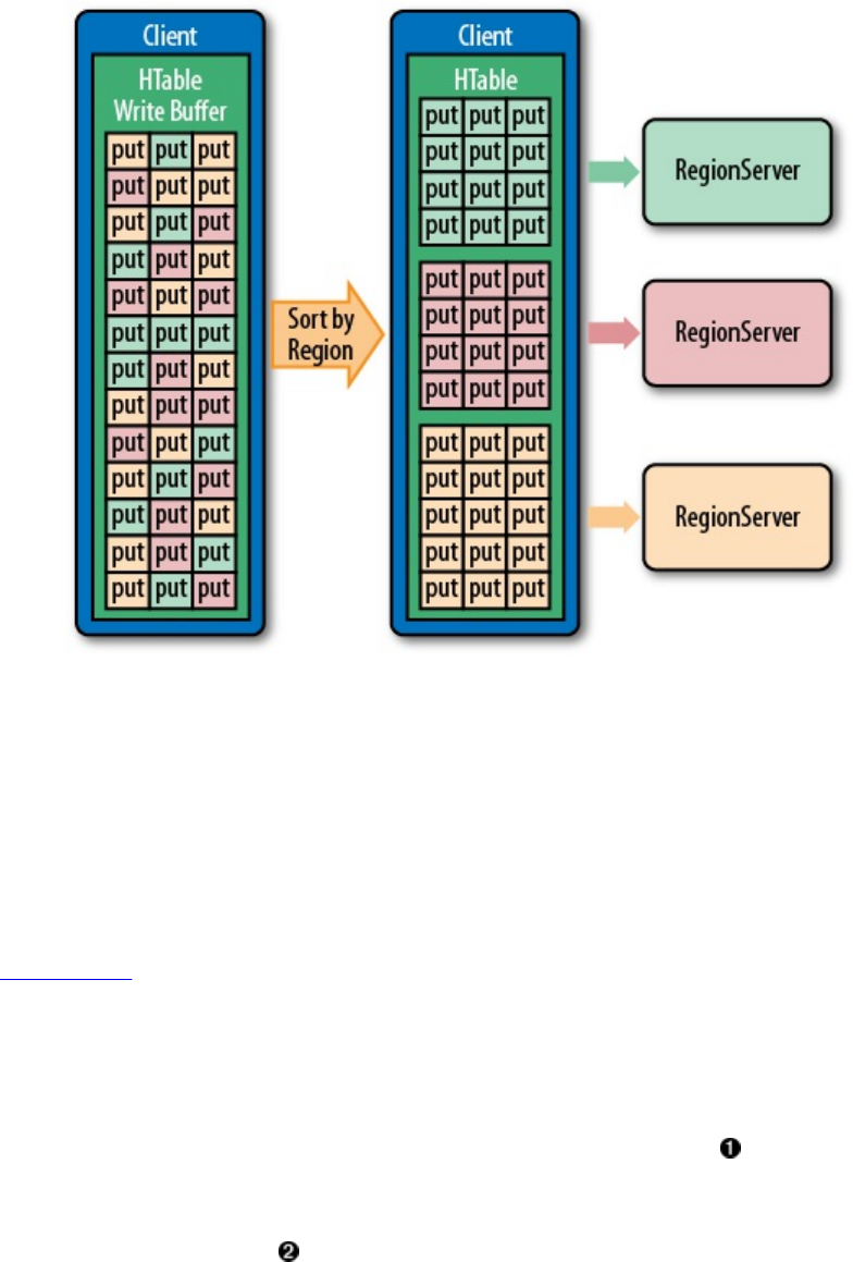
Figure 3-2. The client-side puts sorted and grouped by region server
One note in regards to the executor pool mentioned above. It says that it is controlled by
hbase.htable.threads.max and is by default set to Integer.MAX_VALUE, meaning unbounded. This
does not mean that each client sending buffered writes to the servers will create an endless
amount of worker threads. It really is creating only one thread per region server. This scales with
the number of servers you have, but once you grow into the thousands, you could consider
setting this configuration property to some maximum, bounding it explicitly where you need it.
Example 3-4 shows another example of how the write buffer is used from the client API.
Example 3-4. Example using the client-side write buffer
TableName name = TableName.valueOf("testtable");
Connection connection = ConnectionFactory.createConnection(conf);
Table table = connection.getTable(name);
BufferedMutator mutator = connection.getBufferedMutator(name);
Put put1 = new Put(Bytes.toBytes("row1"));
put1.addColumn(Bytes.toBytes("colfam1"), Bytes.toBytes("qual1"),
Bytes.toBytes("val1"));
mutator.mutate(put1);
Put put2 = new Put(Bytes.toBytes("row2"));
put2.addColumn(Bytes.toBytes("colfam1"), Bytes.toBytes("qual1"),
Bytes.toBytes("val2"));
mutator.mutate(put2);
Put put3 = new Put(Bytes.toBytes("row3"));
put3.addColumn(Bytes.toBytes("colfam1"), Bytes.toBytes("qual1"),
Bytes.toBytes("val3"));
mutator.mutate(put3);
Get get = new Get(Bytes.toBytes("row1"));
(139)
Result res1 = table.get(get);
System.out.println("Result: " + res1);
mutator.flush();
Result res2 = table.get(get);
System.out.println("Result: " + res2);
mutator.close();
table.close();
connection.close();
Get a mutator instance for the table.
Store some rows with columns into HBase.
Try to load previously stored row, this will print “Result: keyvalues=NONE”.
Force a flush, this causes an RPC to occur.
Now the row is persisted and can be loaded.
This example also shows a specific behavior of the buffer that you may not anticipate. Let’s see
what it prints out when executed:
Result: keyvalues=NONE
Result: keyvalues={row1/colfam1:qual1/1426438877968/Put/vlen=4/seqid=0}
While you have not seen the get() operation yet, you should still be able to correctly infer what it
does, that is, reading data back from the servers. But for the first get() in the example, asking for
a column value that has had a previous matching put call, the API returns a NONE value—what
does that mean? It is caused by two facts, with the first explained already above:
1. The client write buffer is an in-memory structure that is literally holding back any
unflushed records, in other words, nothing was sent to the servers yet.
2. The get() call is synchronous and goes directly to the servers, missing the client-side
cached mutations.
You have to be aware of this percularity when designing applications making use of the client
buffering.
List of Puts
The client API has the ability to insert single Put instances as shown earlier, but it also has the
advanced feature of batching operations together. This comes in the form of the following call:
void put(List<Put> puts) throws IOException
(140)

You will have to create a list of Put instances and hand it to this call. Example 3-5 updates the
previous example by creating a list to hold the mutations and eventually calling the list-based
put() method.
Example 3-5. Example inserting data into HBase using a list
List<Put> puts = new ArrayList<Put>();
Put put1 = new Put(Bytes.toBytes("row1"));
put1.addColumn(Bytes.toBytes("colfam1"), Bytes.toBytes("qual1"),
Bytes.toBytes("val1"));
puts.add(put1);
Put put2 = new Put(Bytes.toBytes("row2"));
put2.addColumn(Bytes.toBytes("colfam1"), Bytes.toBytes("qual1"),
Bytes.toBytes("val2"));
puts.add(put2);
Put put3 = new Put(Bytes.toBytes("row2"));
put3.addColumn(Bytes.toBytes("colfam1"), Bytes.toBytes("qual2"),
Bytes.toBytes("val3"));
puts.add(put3);
table.put(puts);
Create a list that holds the Put instances.
Add put to list.
Add another put to list.
Add third put to list.
Store multiple rows with columns into HBase.
A quick check with the HBase Shell reveals that the rows were stored as expected. Note that the
example actually modified three columns, but in two rows only. It added two columns into the
row with the key row2, using two separate qualifiers, qual1 and qual2, creating two uniquely
named columns in the same row.
hbase(main):001:0> scan 'testtable'
ROW COLUMN+CELL
row1 column=colfam1:qual1, timestamp=1426445826107, value=val1
row2 column=colfam1:qual1, timestamp=1426445826107, value=val2
row2 column=colfam1:qual2, timestamp=1426445826107, value=val3
2 row(s) in 0.3300 seconds
Since you are issuing a list of row mutations to possibly many different rows, there is a chance
that not all of them will succeed. This could be due to a few reasons—for example, when there is
an issue with one of the region servers and the client-side retry mechanism needs to give up
because the number of retries has exceeded the configured maximum. If there is a problem with
(141)
any of the put calls on the remote servers, the error is reported back to you subsequently in the
form of an IOException.
Example 3-6 uses a bogus column family name to insert a column. Since the client is not aware
of the structure of the remote table—it could have been altered since it was created—this check
is done on the server-side.
Example 3-6. Example inserting a faulty column family into HBase
Put put1 = new Put(Bytes.toBytes("row1"));
put1.addColumn(Bytes.toBytes("colfam1"), Bytes.toBytes("qual1"),
Bytes.toBytes("val1"));
puts.add(put1);
Put put2 = new Put(Bytes.toBytes("row2"));
put2.addColumn(Bytes.toBytes("BOGUS"), Bytes.toBytes("qual1"),
Bytes.toBytes("val2"));
puts.add(put2);
Put put3 = new Put(Bytes.toBytes("row2"));
put3.addColumn(Bytes.toBytes("colfam1"), Bytes.toBytes("qual2"),
Bytes.toBytes("val3"));
puts.add(put3);
table.put(puts);
Add put with non existent family to list.
Store multiple rows with columns into HBase.
The call to put() fails with the following (or similar) error message:
WARNING: #3, table=testtable, attempt=1/35 failed=1ops, last exception: null \
on server-1.internal.foobar.com,65191,1426248239595, tracking \
started Sun Mar 15 20:35:52 CET 2015; not retrying 1 - final failure
Exception in thread "main" \
org.apache.hadoop.hbase.client.RetriesExhaustedWithDetailsException: \
Failed 1 action: \
org.apache.hadoop.hbase.regionserver.NoSuchColumnFamilyException: \
Column family BOGUS does not exist in region \
testtable,,1426448152586.deecb9559bde733aa2a9fb1e6b42aa93. in table \
'testtable', {NAME => 'colfam1', DATA_BLOCK_ENCODING => 'NONE', \
BLOOMFILTER => 'ROW', REPLICATION_SCOPE => '0', COMPRESSION => 'NONE', \
VERSIONS => '1', TTL => 'FOREVER', MIN_VERSIONS => '0', \
KEEP_DELETED_CELLS => 'FALSE', BLOCKSIZE => '65536', \
IN_MEMORY => 'false', BLOCKCACHE => 'true'}
: 1 time,
The first three line state the request ID (#3), the table name (testtable), the attempt count
(1/35) with number of failed operations (1ops), and the last error (null), as well as the
server name, and when the asynchronous processing started.
This is followed by the exception name, which usually is
RetriesExhaustedWithDetailsException.
(142)
Lastly, the details of the failed operations are listed, here only one failed (Failed 1 action)
and it did so with a NoSuchColumnFamilyException. The last line (: 1 time) lists how often it
failed.
You may wonder what happened to the other, non-faulty puts in the list. Using the shell again
you should see that the two correct puts have been applied:
hbase(main):001:0> scan 'testtable'
ROW COLUMN+CELL
row1 column=colfam1:qual1, timestamp=1426448152808, value=val1
row2 column=colfam1:qual2, timestamp=1426448152808, value=val3
2 row(s) in 0.3360 seconds
The servers iterate over all operations and try to apply them. The failed ones are returned and the
client reports the remote error using the RetriesExhaustedWithDetailsException, giving you insight
into how many operations have failed, with what error, and how many times it has retried to
apply the erroneous modification. It is interesting to note that, for the bogus column family, the
retry is automatically set to 1 (see the NoSuchColumnFamilyException: 1 time), as this is an error
from which HBase cannot recover.
In addition, you can make use of the exception instance to gain access to more details about the
failed operation, and even the faulty mutation itself. Example 3-7 extends the original erroneous
example by introducing a special catch block to gain access to the error details.
Example 3-7. Special error handling with lists of puts
try {
table.put(puts);
} catch (RetriesExhaustedWithDetailsException e) {
int numErrors = e.getNumExceptions();
System.out.println("Number of exceptions: " + numErrors);
for (int n = 0; n < numErrors; n++) {
System.out.println("Cause[" + n + "]: " + e.getCause(n));
System.out.println("Hostname[" + n + "]: " + e.getHostnamePort(n));
System.out.println("Row[" + n + "]: " + e.getRow(n));
}
System.out.println("Cluster issues: " + e.mayHaveClusterIssues());
System.out.println("Description: " + e.getExhaustiveDescription());
}
Store multiple rows with columns into HBase.
Handle failed operations.
Gain access to the failed operation.
The output of the example looks like this (some lines are omitted for the sake of brevity):
Mar 16, 2015 9:54:41 AM org.apache....client.AsyncProcess logNoResubmit
WARNING: #3, table=testtable, attempt=1/35 failed=1ops, last exception: \
null on srv1.foobar.com,65191,1426248239595, \
tracking started Mon Mar 16 09:54:41 CET 2015; not retrying 1 - final failure
Number of exceptions: 1
(143)

Cause[0]: org.apache.hadoop.hbase.regionserver.NoSuchColumnFamilyException: \
org.apache.hadoop.hbase.regionserver.NoSuchColumnFamilyException: Column \
family BOGUS does not exist in region \
testtable,,1426496081011.8be8f8bc862075e8bea355aecc6a5b16. in table \
'testtable', {NAME => 'colfam1', DATA_BLOCK_ENCODING => 'NONE', \
BLOOMFILTER => 'ROW', REPLICATION_SCOPE => '0', COMPRESSION => 'NONE', \
VERSIONS => '1', TTL => 'FOREVER', MIN_VERSIONS => '0', \
KEEP_DELETED_CELLS => 'FALSE', BLOCKSIZE => '65536', IN_MEMORY => 'false', \
BLOCKCACHE => 'true'}
at org.apache.hadoop.hbase.regionserver.RSRpcServices.doBatchOp(...)
...
Hostname[0]: srv1.foobar.com,65191,1426248239595
Row[0]: {"totalColumns":1,"families":{"BOGUS":[{ \
"timestamp":9223372036854775807,"tag":[],"qualifier":"qual1", \
"vlen":4}]},"row":"row2"}
Cluster issues: false
Description: exception from srv1.foobar.com,65191,1426248239595 for row2
org.apache.hadoop.hbase.regionserver.NoSuchColumnFamilyException: \
org.apache.hadoop.hbase.regionserver.NoSuchColumnFamilyException: \
Column family BOGUS does not exist in region \
testtable,,1426496081011.8be8f8bc862075e8bea355aecc6a5b16. in table '\
testtable', {NAME => 'colfam1', ... }
at org.apache.hadoop.hbase.regionserver.RSRpcServices.doBatchOp(...)
...
at java.lang.Thread.run(...)
As you can see, you can ask for the number of errors incurred, the causes, the servers reporting
them, and the actual mutation(s). Here we only have one that we triggered with the bogus
column family used. Interesting is that the exception also gives you access to the overall cluster
status to determine if there are larger problems at play.
Table 3-11. Methods of the RetriesExhaustedWithDetailsException class
Method Description
getCauses() Returns a summary of all causes for all failed operations.
getExhaustiveDescription() More detailed list of all the failures that were detected.
getNumExceptions() Returns the number of failed operations.
getCause(int i) Returns the exact cause for a given failed operation.a
getHostnamePort(int i) Returns the exact host that reported the specific error.a
getRow(int i) Returns the specific mutation instance that failed.a
mayHaveClusterIssues() Allows to determine if there are wider problems with the cluster.b
(144)

a Where i greater or equal to 0 and less than getNumExceptions().
b This is determined by all operations failing as do not retry, indicating that all servers involved
are giving up.
We already mentioned the MaxKeyValueSize parameter for the BufferedMutator before, and how the
API ensures that you can only submit operations that comply to that limit (if set). The same
check is done when you submit a single put, or a list of puts. In fact, there is actually one more
test done, which is that the mutation submitted is not entirely empty. These checks are done on
the client side, though, and in the event of a violation the client throws an exception that leaves
the operations preceding the faulty one in the client buffer.
Caution
The list-based put() call uses the client-side write buffer—in the form of an internal instance of
BatchMutator--to insert all puts into the local buffer and then to call flush() implicitly. While
inserting each instance of Put, the client API performs the mentioned check. If it fails, for
example, at the third put out of five, the first two are added to the buffer while the last two are
not. It also then does not trigger the flush command at all. You need to keep inserting put
instances or call close() to trigger a flush of all cached instances.
Because of this behavior of plain Table instances and their put(List) method, it is recommended
to use the BufferedMutator directly as it has the most flexibility. If you read the HBase source
code, for example the TableOutputFormat, you will see the same approach, that is using the
BufferedMutator for all cases where a client-side write buffer is wanted.
You need to watch out for another peculiarity using the list-based put call: you cannot control the
order in which the puts are applied on the server-side, which implies that the order in which the
servers are called is also not under your control. Use this call with caution if you have to
guarantee a specific order—in the worst case, you need to create smaller batches and explicitly
flush the client-side write cache to enforce that they are sent to the remote servers. This also is
only possible when using the BufferedMutator class directly.
An example for updates that need to be controlled tightly are foreign key relations, where
changes to an entity are reflected in multiple rows, or even tables. If you need to ensure a
specific order in which these mutations are applied, you may have to batch them separately, to
ensure one batch is applied before another.
Finally, Example 3-8 shows the same example as in “Client-side Write Buffer” using the client-
side write buffer, but using a list of mutations, instead of separate calls to mutate(). This is akin
to what you just saw in this section for the list of puts. If you recall the advanced usage of a
Listener, you have all the tools to do the same list based submission of mutations, but using the
more flexible approach.
Example 3-8. Example using the client-side write buffer
List<Mutation> mutations = new ArrayList<Mutation>();
Put put1 = new Put(Bytes.toBytes("row1"));
put1.addColumn(Bytes.toBytes("colfam1"), Bytes.toBytes("qual1"),
Bytes.toBytes("val1"));
(145)
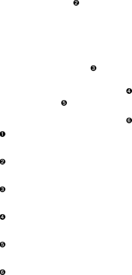
mutations.add(put1);
Put put2 = new Put(Bytes.toBytes("row2"));
put2.addColumn(Bytes.toBytes("colfam1"), Bytes.toBytes("qual1"),
Bytes.toBytes("val2"));
mutations.add(put2);
Put put3 = new Put(Bytes.toBytes("row3"));
put3.addColumn(Bytes.toBytes("colfam1"), Bytes.toBytes("qual1"),
Bytes.toBytes("val3"));
mutations.add(put3);
mutator.mutate(mutations);
Get get = new Get(Bytes.toBytes("row1"));
Result res1 = table.get(get);
System.out.println("Result: " + res1);
mutator.flush();
Result res2 = table.get(get);
System.out.println("Result: " + res2);
Create a list to hold all mutations.
Add Put instance to list of mutations.
Store some rows with columns into HBase.
Try to load previously stored row, this will print “Result: keyvalues=NONE”.
Force a flush, this causes an RPC to occur.
Now the row is persisted and can be loaded.
Atomic Check-and-Put
There is a special variation of the put calls that warrants its own section: check and put. The
method signatures are:
boolean checkAndPut(byte[] row, byte[] family, byte[] qualifier, byte[] value,
Put put) throws IOException
boolean checkAndPut(byte[] row, byte[] family, byte[] qualifier,
CompareFilter.CompareOp compareOp, byte[] value, Put put) throws IOException
These calls allow you to issue atomic, server-side mutations that are guarded by an
accompanying check. If the check passes successfully, the put operation is executed; otherwise,
it aborts the operation completely. It can be used to update data based on current, possibly
related, values.
(146)
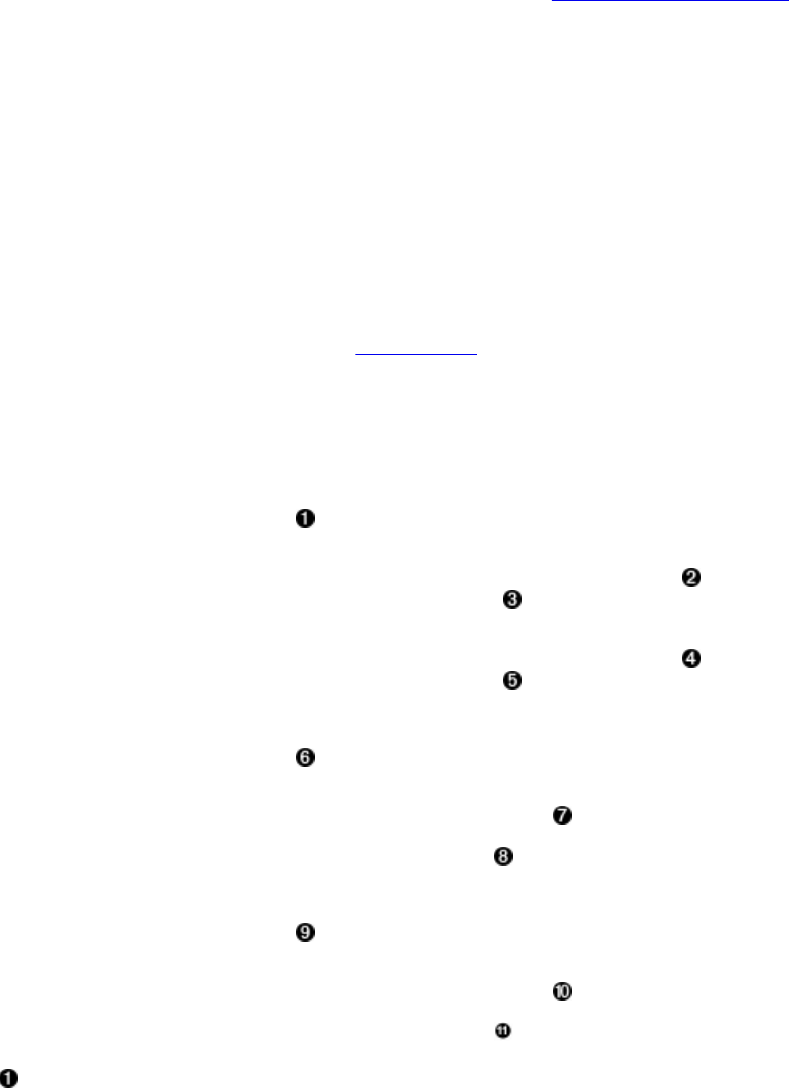
Such guarded operations are often used in systems that handle, for example, account balances,
state transitions, or data processing. The basic principle is that you read data at one point in time
and process it. Once you are ready to write back the result, you want to make sure that no other
client has changed the value in the meantime. You use the atomic check to see if the value read
has since been modified and only if has not, apply the new value.
The first call implies that the given value has to be equal to the stored one. The second call lets
you specify the actual comparison operator (explained in “Comparison Operators”), which
enables more elaborate testing, for example, if the given value is equal or less than the stored
one. This is useful to track some kind of modification ID, and you want to ensure you have
reached a specific point in the cells lifecycle, for example, when it is updated by many
concurrent clients.
Note
A special type of check can be performed using the checkAndPut() call: only update if another
value is not already present. This is achieved by setting the value parameter to null. In that case,
the operation would succeed when the specified column is nonexistent.
The call returns a boolean result value, indicating whether the Put has been applied or not,
returning true or false, respectively. Example 3-9 shows the interactions between the client and
the server, returning the expected results.
Example 3-9. Example application using the atomic compare-and-set operations
Put put1 = new Put(Bytes.toBytes("row1"));
put1.addColumn(Bytes.toBytes("colfam1"), Bytes.toBytes("qual1"),
Bytes.toBytes("val1"));
boolean res1 = table.checkAndPut(Bytes.toBytes("row1"),
Bytes.toBytes("colfam1"), Bytes.toBytes("qual1"), null, put1);
System.out.println("Put 1a applied: " + res1);
boolean res2 = table.checkAndPut(Bytes.toBytes("row1"),
Bytes.toBytes("colfam1"), Bytes.toBytes("qual1"), null, put1);
System.out.println("Put 1b applied: " + res2);
Put put2 = new Put(Bytes.toBytes("row1"));
put2.addColumn(Bytes.toBytes("colfam1"), Bytes.toBytes("qual2"),
Bytes.toBytes("val2"));
boolean res3 = table.checkAndPut(Bytes.toBytes("row1"),
Bytes.toBytes("colfam1"), Bytes.toBytes("qual1"),
Bytes.toBytes("val1"), put2);
System.out.println("Put 2 applied: " + res3);
Put put3 = new Put(Bytes.toBytes("row2"));
put3.addColumn(Bytes.toBytes("colfam1"), Bytes.toBytes("qual1"),
Bytes.toBytes("val3"));
boolean res4 = table.checkAndPut(Bytes.toBytes("row1"),
Bytes.toBytes("colfam1"), Bytes.toBytes("qual1"),
Bytes.toBytes("val1"), put3);
System.out.println("Put 3 applied: " + res4);
Create a new Put instance.
(147)

Check if column does not exist and perform optional put operation.
Print out the result, should be “Put 1a applied: true”.
Attempt to store same cell again.
Print out the result, should be “Put 1b applied: false” as the column now already exists.
Create another Put instance, but using a different column qualifier.
Store new data only if the previous data has been saved.
Print out the result, should be “Put 2 applied: true” as the checked column exists.
Create yet another Put instance, but using a different row.
Store new data while checking a different row.
We will not get here as an exception is thrown beforehand!
The output is:
Put 1a applied: true
Put 1b applied: false
Put 2 applied: true
Exception in thread "main" org.apache.hadoop.hbase.DoNotRetryIOException:
org.apache.hadoop.hbase.DoNotRetryIOException:
Action's getRow must match the passed row
...
The last call in the example threw a DoNotRetryIOException error because checkAndPut() enforces
that the checked row has to match the row of the Put instance. You are allowed to check one
column and update another, but you cannot stretch that check across row boundaries.
Caution
The compare-and-set operations provided by HBase rely on checking and modifying the same
row! As with most other operations only providing atomicity guarantees on single rows, this also
applies to this call. Trying to check and modify two different rows will return an exception.
(148)
Compare-and-set (CAS) operations are very powerful, especially in distributed systems, with
even more decoupled client processes. In providing these calls, HBase sets itself apart from other
architectures that give no means to reason about concurrent updates performed by multiple,
independent clients.
(149)

Get Method
The next step in a client API is to retrieve what was written. For this the Table provides you with
the get() call and accompanying classes. The operations are split into those that operate on a
single row and those that retrieve multiple rows in one call. Before we start though, please note
that we are using the Result class in the various examples provided. This class will be explained
in “The Result class” a little later, so bear with us for the time being. The code—and output
especially—should be self-explanatory.
Single Gets
First, the method that is used to retrieve specific values from a HBase table:
Result get(Get get) throws IOException
Similar to the Put class for the put() call, there is a matching Get class used by the
aforementioned get() function. A get() operation is bound to one specific row, but can retrieve
any number of columns and/or cells contained therein. Therefore, as another similarity, you will
have to provide a row key when creating an instance of Get, using one of these constructors:
Get(byte[] row)
Get(Get get)
The primary constructor of Get takes the row parameter specifying the row you want to access,
while the second constructor takes an existing instance of Get and copies the entire details from
it, effectively cloning the instance. And, similar to the put operations, you have methods to
specify rather broad criteria to find what you are looking for—or to specify everything down to
exact coordinates for a single cell:
Get addFamily(byte[] family)
Get addColumn(byte[] family, byte[] qualifier)
Get setTimeRange(long minStamp, long maxStamp) throws IOException
Get setTimeStamp(long timestamp)
Get setMaxVersions()
Get setMaxVersions(int maxVersions) throws IOException
The addFamily() call narrows the request down to the given column family. It can be called
multiple times to add more than one family. The same is true for the addColumn() call. Here you
can add an even narrower address space: the specific column. Then there are methods that let you
set the exact timestamp you are looking for—or a time range to match those cells that fall inside
it.
Lastly, there are methods that allow you to specify how many versions you want to retrieve,
given that you have not set an exact timestamp. By default, this is set to 1, meaning that the get()
call returns the most current match only. If you are in doubt, use getMaxVersions() to check what
it is set to. The setMaxVersions() without a parameter sets the number of versions to return to
Integer.MAX_VALUE--which is also the maximum number of versions you can configure in the
column family descriptor, and therefore tells the API to return every available version of all
matching cells (in other words, up to what is set at the column family level).
As mentioned earlier, HBase provides us with a helper class named Bytes that has many static
methods to convert Java types into byte[] arrays. It also can do the same in reverse: as you are
(150)
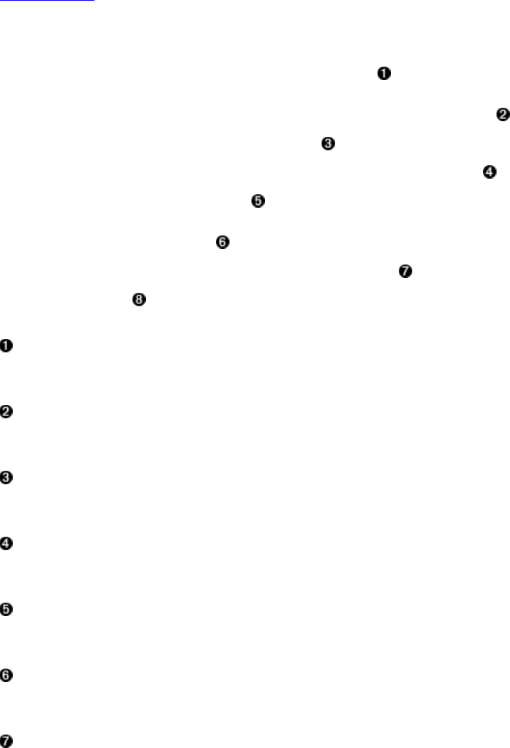
retrieving data from HBase—for example, one of the rows stored previously—you can make use
of these helper functions to convert the byte[] data back into Java types. Here is a short list of
what it offers, continued from the earlier discussion:
static String toString(byte[] b)
static boolean toBoolean(byte[] b)
static long toLong(byte[] bytes)
static float toFloat(byte[] bytes)
static int toInt(byte[] bytes)
...
Example 3-10 shows how this is all put together.
Example 3-10. Example application retrieving data from HBase
Configuration conf = HBaseConfiguration.create();
Connection connection = ConnectionFactory.createConnection(conf);
Table table = connection.getTable(TableName.valueOf("testtable"));
Get get = new Get(Bytes.toBytes("row1"));
get.addColumn(Bytes.toBytes("colfam1"), Bytes.toBytes("qual1"));
Result result = table.get(get);
byte[] val = result.getValue(Bytes.toBytes("colfam1"),
Bytes.toBytes("qual1"));
System.out.println("Value: " + Bytes.toString(val));
table.close();
connection.close();
Create the configuration.
Instantiate a new table reference.
Create get with specific row.
Add a column to the get.
Retrieve row with selected columns from HBase.
Get a specific value for the given column.
Print out the value while converting it back.
(151)

Close the table and connection instances to free resources.
If you are running this example after, say Example 3-2, you should get this as the output:
Value: val1
The output is not very spectacular, but it shows that the basic operation works. The example also
only adds the specific column to retrieve, relying on the default for maximum versions being
returned set to 1. The call to get() returns an instance of the Result class, which you will learn
about very soon in “The Result class”.
Using the Builder pattern
All of the data-related types and the majority of their add and set methods support the fluent
interface pattern, that is, all of these methods return the instance reference and allow chaining of
calls. Example 3-11 show this in action.
Example 3-11. Creates a get request using its fluent interface
Get get = new Get(Bytes.toBytes("row1"))
.setId("GetFluentExample")
.setMaxVersions()
.setTimeStamp(1)
.addColumn(Bytes.toBytes("colfam1"), Bytes.toBytes("qual1"))
.addFamily(Bytes.toBytes("colfam2"));
Result result = table.get(get);
System.out.println("Result: " + result);
Create a new get using the fluent interface.
Example 3-11 showing the fluent interface should emit the following on the console:
Before get call...
Cell: row1/colfam1:qual1/2/Put/vlen=4/seqid=0, Value: val1
Cell: row1/colfam1:qual1/1/Put/vlen=4/seqid=0, Value: val1
Cell: row1/colfam1:qual2/4/Put/vlen=4/seqid=0, Value: val2
Cell: row1/colfam1:qual2/3/Put/vlen=4/seqid=0, Value: val2
Cell: row1/colfam2:qual1/2/Put/vlen=4/seqid=0, Value: val1
Cell: row1/colfam2:qual1/1/Put/vlen=4/seqid=0, Value: val1
Cell: row1/colfam2:qual2/4/Put/vlen=4/seqid=0, Value: val2
Cell: row1/colfam2:qual2/3/Put/vlen=4/seqid=0, Value: val2
Result: keyvalues={row1/colfam1:qual1/1/Put/vlen=4/seqid=0,
row1/colfam2:qual1/1/Put/vlen=4/seqid=0}
An interesting part of this is the result that is printed last. While the example is adding the entire
column family colfam2, it only prints a single cell. This is caused by the setTimeStamp(1) call,
which affects all other selections. We essentially are telling the API to fetch “all cells from
column family #2 that have a timestamp equal or less than 1”.
The Get class provides additional methods, which are listed in Table 3-12 for your perusal. By
now you should recognize many of them as inherited methods from the Query and Row
superclasses.
Table 3-12. Quick overview of additional methods provided by the Get class
(152)
Table 3-12. Quick overview of additional methods provided by the Get class
Method Description
familySet()/getFamilyMap()
These methods give you access
to the column families and
specific columns, as added by
the addFamily() and/or
addColumn() calls. The family
map is a map where the key is
the family name and the value a
list of added column qualifiers
for this particular family. The
familySet() returns the Set of all
stored families, i.e., a set
containing only the family
names.
getACL()/setACL()
The Access Control List (ACL)
for this operation. See [Link to
Come] for details.
getAttribute()/setAttribute()
Set and get arbitrary attributes
associated with this instance of
Get.
getAttributesMap() Returns the entire map of
attributes, if any are set.
getAuthorizations()/setAuthorizations()
Visibility labels for the
operation. See [Link to Come]
for details.
getCacheBlocks()/setCacheBlocks()
Specify if the server-side cache
should retain blocks that were
loaded for this operation.
setCheckExistenceOnly()/isCheckExistenceOnly() Only check for existence of data,
but do not return any of it.
setClosestRowBefore()/isClosestRowBefore()
Return all the data for the row
that matches the given row key
exactly, or the one that
immediately precedes it.
(153)

getConsistency()/setConsistency()
The consistency level that
applies to the current query
instance.
getFilter()/setFilter()
The filters that apply to the
retrieval operation. See “Filters”
for details.
getFingerprint()
Compiles details about the
instance into a map for
debugging, or logging.
getId()/setId()
An ID for the operation, useful
for identifying the origin of a
request later.
getIsolationLevel()/setIsolationLevel() Specifies the read isolation level
for the operation.
getMaxResultsPerColumnFamily()/setMaxResultsPerColumnFamily() Limit the number of cells
returned per family.
getMaxVersions()/setMaxVersions()
Override the column family
setting specifying how many
versions of a column to retrieve.
getReplicaId()/setReplicaId() Gives access to the replica ID
that should serve the data.
getRow() Returns the row key as specified
when creating the Get instance.
getRowOffsetPerColumnFamily()/setRowOffsetPerColumnFamily() Number of cells to skip when
reading a row.
getTimeRange()/setTimeRange()
Retrieve or set the associated
timestamp or time range of the
Get instance.
Sets a specific timestamp for the
(154)

setTimeStamp() query. Retrieve with
getTimeRange().a
numFamilies()
Retrieves the size of the family
map, containing the families
added using the addFamily() or
addColumn() calls.
hasFamilies()
Another helper to check if a
family—or column—has been
added to the current instance of
the Get class.
toJSON()/toJSON(int) Converts the first 5 or N
columns into a JSON format.
toMap()/toMap(int)
Converts the first 5 or N
columns into a map. This is
more detailed than what
getFingerprint() returns.
toString()/toString(int)
Converts the first 5 or N
columns into a JSON, or map (if
JSON fails due to encoding
problems).
a The API converts a value assigned with setTimeStamp() into a TimeRange instance internally,
setting it to the given timestamp and timestamp + 1, respectively.
Note
The getters listed in Table 3-12 for the Get class only retrieve what you have set beforehand.
They are rarely used, and make sense only when you, for example, prepare a Get instance in a
private method in your code, and inspect the values in another place or for unit testing.
The list of methods is long indeed, and while you have seen the inherited ones before, there are
quite a few specific ones for Get that warrant a longer explanation. We start with setCacheBlocks()
and getCacheBlocks(), which control how the read operation is handled on the server-side. Each
HBase region server has a block cache that efficiently retains recently accessed data for
subsequent reads of contiguous information. In some events it is better to not engage the cache to
avoid too much churn when doing completely random gets. Instead of polluting the block cache
with blocks of unrelated data, it is better to skip caching these blocks and leave the cache
undisturbed for other clients that perform reading of related, co-located data.
(155)
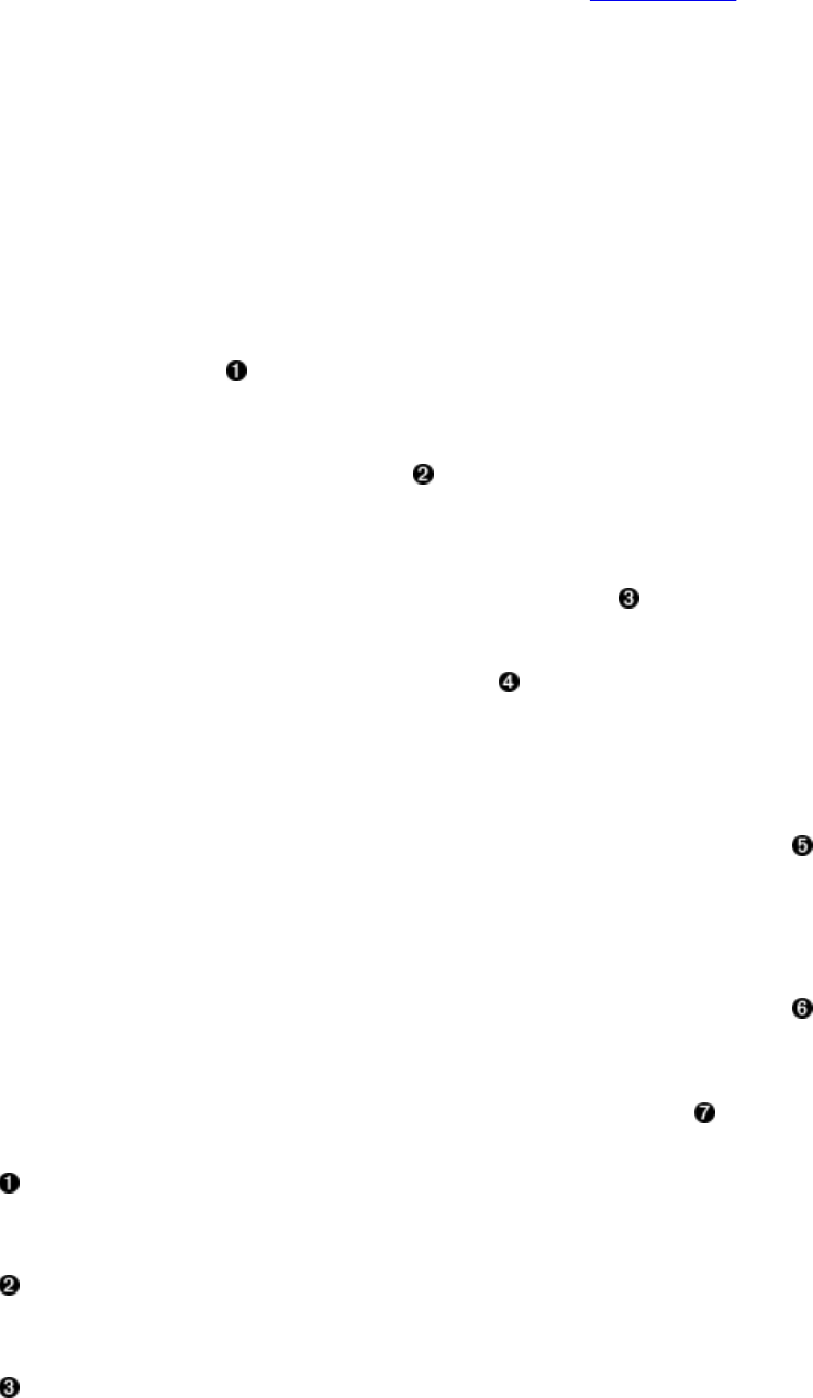
The setCheckExistenceOnly() and isCheckExistenceOnly() combination allows the client to check if
a specific set of columns, or column families exist. The Example 3-12 shows this in action.
Example 3-12. Checks for the existence of specific data
List<Put> puts = new ArrayList<Put>();
Put put1 = new Put(Bytes.toBytes("row1"));
put1.addColumn(Bytes.toBytes("colfam1"), Bytes.toBytes("qual1"),
Bytes.toBytes("val1"));
puts.add(put1);
Put put2 = new Put(Bytes.toBytes("row2"));
put2.addColumn(Bytes.toBytes("colfam1"), Bytes.toBytes("qual1"),
Bytes.toBytes("val2"));
puts.add(put2);
Put put3 = new Put(Bytes.toBytes("row2"));
put3.addColumn(Bytes.toBytes("colfam1"), Bytes.toBytes("qual2"),
Bytes.toBytes("val3"));
puts.add(put3);
table.put(puts);
Get get1 = new Get(Bytes.toBytes("row2"));
get1.addColumn(Bytes.toBytes("colfam1"), Bytes.toBytes("qual1"));
get1.setCheckExistenceOnly(true);
Result result1 = table.get(get1);
byte[] val = result1.getValue(Bytes.toBytes("colfam1"),
Bytes.toBytes("qual1"));
System.out.println("Get 1 Exists: " + result1.getExists());
System.out.println("Get 1 Size: " + result1.size());
System.out.println("Get 1 Value: " + Bytes.toString(val));
Get get2 = new Get(Bytes.toBytes("row2"));
get2.addFamily(Bytes.toBytes("colfam1"));
get2.setCheckExistenceOnly(true);
Result result2 = table.get(get2);
System.out.println("Get 2 Exists: " + result2.getExists());
System.out.println("Get 2 Size: " + result2.size());
Get get3 = new Get(Bytes.toBytes("row2"));
get3.addColumn(Bytes.toBytes("colfam1"), Bytes.toBytes("qual9999"));
get3.setCheckExistenceOnly(true);
Result result3 = table.get(get3);
System.out.println("Get 3 Exists: " + result3.getExists());
System.out.println("Get 3 Size: " + result3.size());
Get get4 = new Get(Bytes.toBytes("row2"));
get4.addColumn(Bytes.toBytes("colfam1"), Bytes.toBytes("qual9999"));
get4.addColumn(Bytes.toBytes("colfam1"), Bytes.toBytes("qual1"));
get4.setCheckExistenceOnly(true);
Result result4 = table.get(get4);
System.out.println("Get 4 Exists: " + result4.getExists());
System.out.println("Get 4 Size: " + result4.size());
Insert two rows into the table.
Check first with existing data.
Exists is “true”, while no cel was actually returned.
(156)

Check for an entire family to exist.
Check for a non-existent column.
Check for an existent, and non-existent column.
Exists is “true” because some data exists.
When executing this example, the output should read like the following:
Get 1 Exists: true
Get 1 Size: 0
Get 1 Value: null
Get 2 Exists: true
Get 2 Size: 0
Get 3 Exists: false
Get 3 Size: 0
Get 4 Exists: true
Get 4 Size: 0
The one peculiar result is the last, you will be returned true for any of the checks you added
returning true. In the example we tested a column that exists, and one that does not. Since one
does, the entire check returns positive. In other words, make sure you test very specifically for
what you are looking for. You may have to issue multiple get request (batched preferably) to test
the exact coordinates you want to verify.
Alternative checks for existence
The Table class has another way of checking for the existence of data in a table, provided by
these methods:
boolean exists(Get get) throws IOException
boolean[] existsAll(List<Get> gets) throws IOException;
You can set up a Get instance, just like you do when using the get() calls of Table. Instead of
having to retrieve the cells from the remote servers, just to verify that something exists, you can
employ these calls because they only return a boolean flag. In fact, these calls are just shorthand
for using Get.setCheckExistenceOnly(true) on the included Get instance(s).
Note
Using Table.exists(), Table.existsAll(), or Get.setCheckExistenceOnly() involves the same
lookup semantics on the region servers, including loading file blocks to check if a row or column
actually exists. You only avoid shipping the data over the network—but that is very useful if you
are checking very large columns, or do so very frequently. Consider using Bloom filters to speed
up this process (see “Bloom Filters”).
We move on to setClosestRowBefore() and isClosestRowBefore(). These allow you do fuzzy
matching around a particular row. Presume you have a complex row key design, employing
(157)
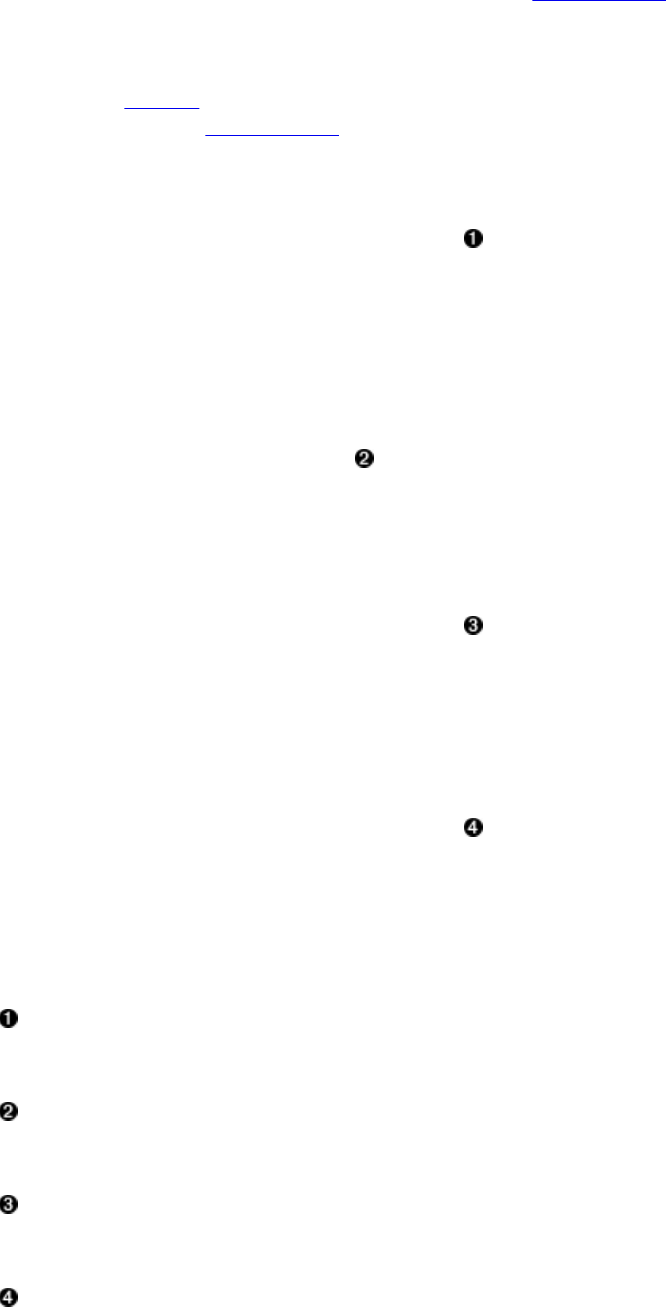
compound data comprised of many separate fields (see “Key Design”). You can only match data
from left to right in the row key, so again presume you have some leading fields, but not more
specific ones. You can ask for a specific row using get(), but what if the requested row key is too
specific and does not exist? Without jumping the gun, you could start using a scan operation,
explained in “Scans”. Instead, you can use the setClosestRowBefore() method, setting this
functionality to true. Example 3-13 shows the result:
Example 3-13. Retrieves a row close to the requested, if necessary
Get get1 = new Get(Bytes.toBytes("row3"));
get1.addColumn(Bytes.toBytes("colfam1"), Bytes.toBytes("qual1"));
Result result1 = table.get(get1);
System.out.println("Get 1 isEmpty: " + result1.isEmpty());
CellScanner scanner1 = result1.cellScanner();
while (scanner1.advance()) {
System.out.println("Get 1 Cell: " + scanner1.current());
}
Get get2 = new Get(Bytes.toBytes("row3"));
get2.addColumn(Bytes.toBytes("colfam1"), Bytes.toBytes("qual1"));
get2.setClosestRowBefore(true);
Result result2 = table.get(get2);
System.out.println("Get 2 isEmpty: " + result2.isEmpty());
CellScanner scanner2 = result2.cellScanner();
while (scanner2.advance()) {
System.out.println("Get 2 Cell: " + scanner2.current());
}
Get get3 = new Get(Bytes.toBytes("row2"));
get3.addColumn(Bytes.toBytes("colfam1"), Bytes.toBytes("qual1"));
get3.setClosestRowBefore(true);
Result result3 = table.get(get3);
System.out.println("Get 3 isEmpty: " + result3.isEmpty());
CellScanner scanner3 = result3.cellScanner();
while (scanner3.advance()) {
System.out.println("Get 3 Cell: " + scanner3.current());
}
Get get4 = new Get(Bytes.toBytes("row2"));
get4.addColumn(Bytes.toBytes("colfam1"), Bytes.toBytes("qual1"));
Result result4 = table.get(get4);
System.out.println("Get 4 isEmpty: " + result4.isEmpty());
CellScanner scanner4 = result4.cellScanner();
while (scanner4.advance()) {
System.out.println("Get 4 Cell: " + scanner4.current());
}
Attempt to read a row that does not exist.
Instruct the get() call to fall back to the previous row, if necessary.
Attempt to read a row that exists.
Read exactly a row that exists.
(158)
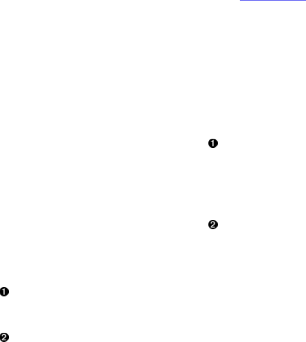
The output is interesting again:
Get 1 isEmpty: true
Get 2 isEmpty: false
Get 2 Cell: row2/colfam1:qual1/1426587567787/Put/vlen=4/seqid=0
Get 2 Cell: row2/colfam1:qual2/1426587567787/Put/vlen=4/seqid=0
Get 3 isEmpty: false
Get 3 Cell: row2/colfam1:qual1/1426587567787/Put/vlen=4/seqid=0
Get 3 Cell: row2/colfam1:qual2/1426587567787/Put/vlen=4/seqid=0
Get 4 isEmpty: false
Get 4 Cell: row2/colfam1:qual1/1426587567787/Put/vlen=4/seqid=0
The first call using the default Get instance fails to retrieve anything, as it asks for a row that does
not exist (row3, we assume the same two rows exist from the previous example). The second adds
a setClosestRowBefore(true) instruction to match the row exactly, or the closest one sorted before
the given row key. This, in our example, is row2, shown to work as expected. What is surprising
though is that the entire row is returned, not the specific column we asked for.
This is extended in get #3, which now reads the existing row2, but still leaves the fuzzy matching
on. We again get the entire row back, not just the columns we asked for. In get #4 we remove the
setClosestRowBefore(true) and get exactly what we expect, that is only the column we have
selected.
Finally, we will look at four methods in a row: getMaxResultsPerColumnFamily(),
setMaxResultsPerColumnFamily(), getRowOffsetPerColumnFamily(), and
setRowOffsetPerColumnFamily(), as they all work in tandem to allow the client to page through a
wide row. The former pair handles the maximum amount of cells returned by a get request. The
latter pair then sets an optional offset into the row. Example 3-14 shows this as simple as
possible.
Example 3-14. Retrieves parts of a row with offset and limit
Put put = new Put(Bytes.toBytes("row1"));
for (int n = 1; n <= 1000; n++) {
String num = String.format("%04d", n);
put.addColumn(Bytes.toBytes("colfam1"), Bytes.toBytes("qual" + num),
Bytes.toBytes("val" + num));
}
table.put(put);
Get get1 = new Get(Bytes.toBytes("row1"));
get1.setMaxResultsPerColumnFamily(10);
Result result1 = table.get(get1);
CellScanner scanner1 = result1.cellScanner();
while (scanner1.advance()) {
System.out.println("Get 1 Cell: " + scanner1.current());
}
Get get2 = new Get(Bytes.toBytes("row1"));
get2.setMaxResultsPerColumnFamily(10);
get2.setRowOffsetPerColumnFamily(100);
Result result2 = table.get(get2);
CellScanner scanner2 = result2.cellScanner();
while (scanner2.advance()) {
System.out.println("Get 2 Cell: " + scanner2.current());
}
Ask for ten cells to be returned at most.
(159)
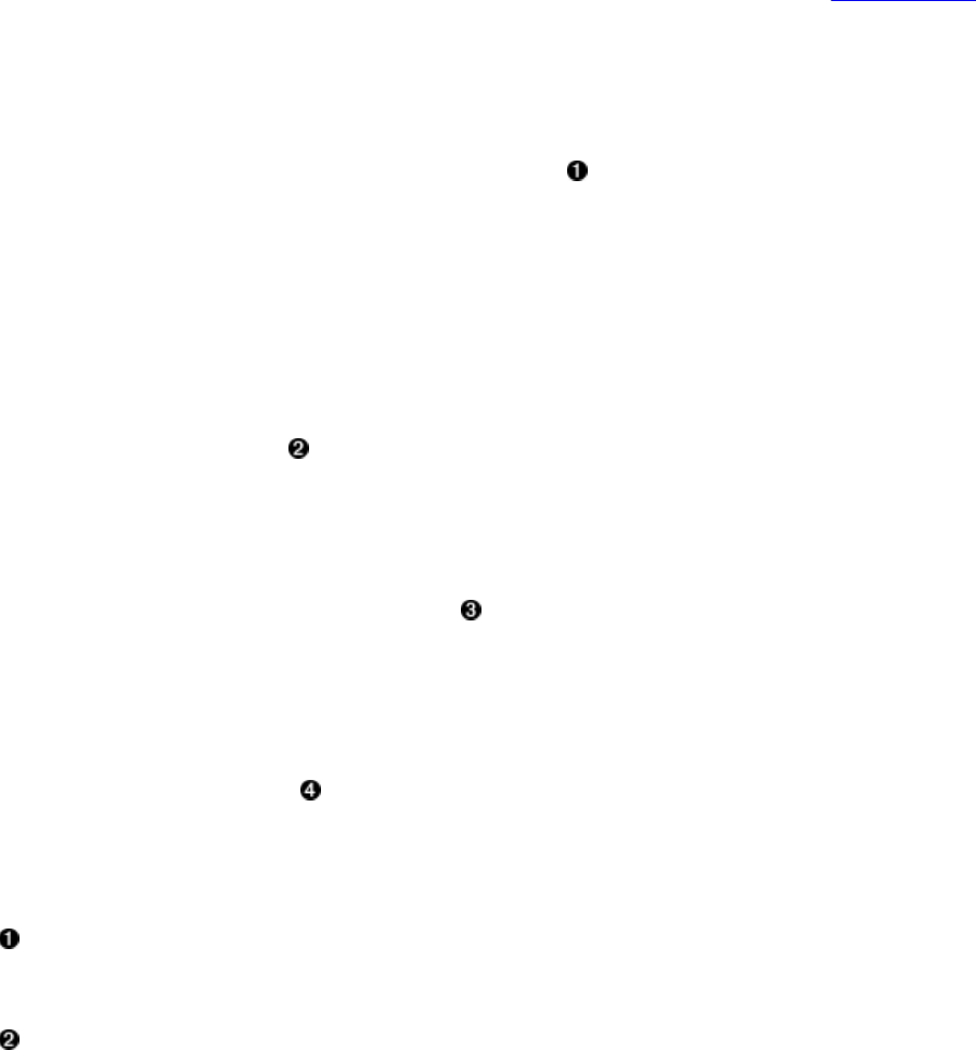
In addition, also skip the first 100 cells.
The output in abbreviated form:
Get 1 Cell: row1/colfam1:qual0001/1426592168066/Put/vlen=7/seqid=0
Get 1 Cell: row1/colfam1:qual0002/1426592168066/Put/vlen=7/seqid=0
...
Get 1 Cell: row1/colfam1:qual0009/1426592168066/Put/vlen=7/seqid=0
Get 1 Cell: row1/colfam1:qual0010/1426592168066/Put/vlen=7/seqid=0
Get 2 Cell: row1/colfam1:qual0101/1426592168066/Put/vlen=7/seqid=0
Get 2 Cell: row1/colfam1:qual0102/1426592168066/Put/vlen=7/seqid=0
...
Get 2 Cell: row1/colfam1:qual0109/1426592168066/Put/vlen=7/seqid=0
Get 2 Cell: row1/colfam1:qual0110/1426592168066/Put/vlen=7/seqid=0
This, on first sight, seems to make sense, we get ten columns (cells) returned from column 1 to
10. For get #2 we get the same but skip the first 100 columns, starting at 101 to 110. But that is
not exactly how these get options work, they really work on cells, not columns. Example 3-15
extends the previous example to write each column three times, creating three cells—or versions
—for each.
Example 3-15. Retrieves parts of a row with offset and limit #2
for (int version = 1; version <= 3; version++) {
Put put = new Put(Bytes.toBytes("row1"));
for (int n = 1; n <= 1000; n++) {
String num = String.format("%04d", n);
put.addColumn(Bytes.toBytes("colfam1"), Bytes.toBytes("qual" + num),
Bytes.toBytes("val" + num));
}
System.out.println("Writing version: " + version);
table.put(put);
Thread.currentThread().sleep(1000);
}
Get get0 = new Get(Bytes.toBytes("row1"));
get0.addColumn(Bytes.toBytes("colfam1"), Bytes.toBytes("qual0001"));
get0.setMaxVersions();
Result result0 = table.get(get0);
CellScanner scanner0 = result0.cellScanner();
while (scanner0.advance()) {
System.out.println("Get 0 Cell: " + scanner0.current());
}
Get get1 = new Get(Bytes.toBytes("row1"));
get1.setMaxResultsPerColumnFamily(10);
Result result1 = table.get(get1);
CellScanner scanner1 = result1.cellScanner();
while (scanner1.advance()) {
System.out.println("Get 1 Cell: " + scanner1.current());
}
Get get2 = new Get(Bytes.toBytes("row1"));
get2.setMaxResultsPerColumnFamily(10);
get2.setMaxVersions(3);
Result result2 = table.get(get2);
CellScanner scanner2 = result2.cellScanner();
while (scanner2.advance()) {
System.out.println("Get 2 Cell: " + scanner2.current());
}
Insert three versions of each column.
(160)

Get a column with all versions as a test.
Get ten cells, single version per column.
Do the same but now retrieve all versions of a column.
The output, in abbreviated form again:
Writing version: 1
Writing version: 2
Writing version: 3
Get 0 Cell: row1/colfam1:qual0001/1426592660030/Put/vlen=7/seqid=0
Get 0 Cell: row1/colfam1:qual0001/1426592658911/Put/vlen=7/seqid=0
Get 0 Cell: row1/colfam1:qual0001/1426592657785/Put/vlen=7/seqid=0
Get 1 Cell: row1/colfam1:qual0001/1426592660030/Put/vlen=7/seqid=0
Get 1 Cell: row1/colfam1:qual0002/1426592660030/Put/vlen=7/seqid=0
...
Get 1 Cell: row1/colfam1:qual0009/1426592660030/Put/vlen=7/seqid=0
Get 1 Cell: row1/colfam1:qual0010/1426592660030/Put/vlen=7/seqid=0
Get 2 Cell: row1/colfam1:qual0001/1426592660030/Put/vlen=7/seqid=0
Get 2 Cell: row1/colfam1:qual0001/1426592658911/Put/vlen=7/seqid=0
Get 2 Cell: row1/colfam1:qual0001/1426592657785/Put/vlen=7/seqid=0
Get 2 Cell: row1/colfam1:qual0002/1426592660030/Put/vlen=7/seqid=0
Get 2 Cell: row1/colfam1:qual0002/1426592658911/Put/vlen=7/seqid=0
Get 2 Cell: row1/colfam1:qual0002/1426592657785/Put/vlen=7/seqid=0
Get 2 Cell: row1/colfam1:qual0003/1426592660030/Put/vlen=7/seqid=0
Get 2 Cell: row1/colfam1:qual0003/1426592658911/Put/vlen=7/seqid=0
Get 2 Cell: row1/colfam1:qual0003/1426592657785/Put/vlen=7/seqid=0
Get 2 Cell: row1/colfam1:qual0004/1426592660030/Put/vlen=7/seqid=0
If we iterate over the same data, we get the same result (get #1 does that). But as soon as we
instruct the servers to return all versions, the results change. We added a Get.setMaxVersions(3)
(we could have used setMaxVersions() without a parameter as well) and therefore now iterate over
all cells, reflected in what get #2 shows. We still get ten cells back, but this time from column 1
to 4 only, with all versions of the columns in between.
Be wary when using these get parameters, you might not get what you expected initially. But
they behave as designed, and it is up to the client application and the accompanying table schema
to end up with the proper results.
The Result class
The above examples implicitly show you that when you retrieve data using the get() calls, you
receive an instance of the Result class that contains all the matching cells. It provides you with
the means to access everything that was returned from the server for the given row and matching
the specified query, such as column family, column qualifier, timestamp, and so on.
There are utility methods you can use to ask for specific results—just as Example 3-10 used
earlier—using more concrete dimensions. If you have, for example, asked the server to return all
columns of one specific column family, you can now ask for specific columns within that family.
In other words, you need to call get() with just enough concrete information to be able to process
the matching data on the client side. The first set of functions provided are:
byte[] getRow()
(161)

byte[] getValue(byte[] family, byte[] qualifier)
byte[] value()
ByteBuffer getValueAsByteBuffer(byte[] family, byte[] qualifier)
ByteBuffer getValueAsByteBuffer(byte[] family, int foffset, int flength,
byte[] qualifier, int qoffset, int qlength)
boolean loadValue(byte[] family, byte[] qualifier, ByteBuffer dst)
throws BufferOverflowException
boolean loadValue(byte[] family, int foffset, int flength, byte[] qualifier,
int qoffset, int qlength, ByteBuffer dst) throws BufferOverflowException
CellScanner cellScanner()
Cell[] rawCells()
List<Cell> listCells()
boolean isEmpty()
int size()
You saw getRow() before: it returns the row key, as specified, for example, when creating the
instance of the Get class used in the get() call providing the current instance of Result. size()
returns the number of Cell instances the server has returned. You may use this call—or isEmpty(),
which checks if size() returns a number greater than zero—to check in your own client code if
the retrieval call returned any matches.
The getValue() call allows you to get the data for a specific cell that was returned to you. As you
cannot specify what timestamp—in other words, version—you want, you get the newest one.
The value() call makes this even easier by returning the data for the newest cell in the first
column found. Since columns are also sorted lexicographically on the server, this would return
the value of the column with the column name (including family and qualifier) sorted first.
Note
Some of the methods to return data clone the underlying byte array so that no modification is
possible. Yet others do not and you have to take care not to modify the returned arrays—for your
own sake.
The following methods do clone (which means they create a copy of the byte array) the data
before returning it to the caller: getRow(), getValue(), value(), getMap(), getNoVersionMap(), and
getFamilyMap().11
There is another set of accessors for the value of available cells, namely getValueAsByteBuffer()
and loadValue(). They either create a new Java ByteBuffer, wrapping the byte array value, or copy
the data into a provided one respectively. You may wonder why you have to provide the column
family and qualifier name as a byte array plus specifying an offset and length into each of the
arrays. The assumption is that you may have a more complex array that holds all of the data
needed. In this case you can set the family and qualifier parameter to the very same array, just
pointing the respective offset and length to where in the larger array the family and qualifier are
stored.
Access to the raw, low-level Cell instances is provided by the rawCells() method, returning the
array of Cell instances backing the current Result instance. The listCells() call simply converts
the array returned by raw() into a List instance, giving you convenience by providing iterator
access, for example. The created list is backed by the original array of KeyValue instances. The
Result class also implements the already discussed CellScannable interface, so you can iterate
over the contained cells directly. The examples in the “Get Method” show this in action, for
instance, Example 3-13.
Note
(162)

The array of cells returned by, for example, rawCells() is already lexicographically sorted, taking
the full coordinates of the Cell instances into account. So it is sorted first by column family, then
within each family by qualifier, then by timestamp, and finally by type.
Another set of accessors is provided which are more column-oriented:
List<Cell> getColumnCells(byte[] family, byte[] qualifier)
Cell getColumnLatestCell(byte[] family, byte[] qualifier)
Cell getColumnLatestCell(byte[] family, int foffset, int flength,
byte[] qualifier, int qoffset, int qlength)
boolean containsColumn(byte[] family, byte[] qualifier)
boolean containsColumn(byte[] family, int foffset, int flength,
byte[] qualifier, int qoffset, int qlength)
boolean containsEmptyColumn(byte[] family, byte[] qualifier)
boolean containsEmptyColumn(byte[] family, int foffset, int flength,
byte[] qualifier, int qoffset, int qlength)
boolean containsNonEmptyColumn(byte[] family, byte[] qualifier)
boolean containsNonEmptyColumn(byte[] family, int foffset, int flength,
byte[] qualifier, int qoffset, int qlength)
By means of the getColumnCells() method you ask for multiple values of a specific column,
which solves the issue pointed out earlier, that is, how to get multiple versions of a given
column. The number returned obviously is bound to the maximum number of versions you have
specified when configuring the Get instance, before the call to get(), with the default being set to
1. In other words, the returned list contains zero (in case the column has no value for the given
row) or one entry, which is the newest version of the value. If you have specified a value greater
than the default of 1 version to be returned, it could be any number, up to the specified maximum
(see Example 3-15 for an example).
The getColumnLatestCell() methods return the newest cell of the specified column, but in contrast
to getValue(), they do not return the raw byte array of the value but the full Cell instance instead.
This may be useful when you need more than just the value data. The two variants only differ in
one being more convenient when you have two separate arrays only containing the family and
qualifier names. Otherwise you can use the second version that gives you access to the already
explained offset and length parameters.
The containsColumn() is a convenience method to check if there was any cell returned in the
specified column. Again, this comes in two variants for convenience. There are two more pairs
of functions for this check, containsEmptyColumn() and containsNonEmptyColumns(). They do not
only check that there is a cell for a specific column, but also if that cell has no value data (it is
empty) or has value data (it is not empty). All of these contains checks internally use the
getColumnLatestCell() call to get the newest version of a column cell, and then perform the check.
Note
These methods all support the fact that the qualifier can be left unspecified—setting it to null--
and therefore matching the special column with no name.
Using no qualifier means that there is no label to the column. When looking at the table from, for
example, the HBase Shell, you need to know what it contains. A rare case where you might want
to consider using the empty qualifier is in column families that only ever contain a single
column. Then the family name might indicate its purpose.
There is a third set of methods that provide access to the returned data from the get request.
These are map-oriented and look like this:
(163)

NavigableMap<byte[], NavigableMap<byte[],
NavigableMap<Long, byte[]>>> getMap()
NavigableMap<byte[], NavigableMap<byte[], byte[]>> getNoVersionMap()
NavigableMap<byte[], byte[]> getFamilyMap(byte[] family)
The most generic call, named getMap(), returns the entire result set in a Java Map class instance
that you can iterate over to access all values. This is different from accessing the raw cells, since
here you get only the data in a map, not any accessors or other internal information of the cells.
The map is organized as such: family → qualifier → values. The getNoVersionMap() does the
same while only including the latest cell for each column. Finally, the getFamilyMap() lets you
select the data for a specific column family only—but including all versions, if specified during
the get call.
Use whichever access method of Result matches your access pattern; the data has already been
moved across the network from the server to your client process, so it is not incurring any extra
server-side performance or resource incursion.
Finally, there are a few more methods provided, that do not fit into the above groups
Table 3-13. Additional methods provided by Result
Method Description
create() There is a set of these static methods to help create Result instances if
necessary.
copyFrom() Helper method to copy a reference of the list of cells from one instance
to another.
compareResults() Static method, does a deep compare of two instance, down to the byte
arrays.
getExists()/setExists() Optionally used to check for existence of cells only. See Example 3-12
for an example.
getTotalSizeOfCells() Static method, summarizes the estimated heap size of all contained
cells. Uses Cell.heapSize() for each contained cell.
isStale() Indicates if the result was served by a region replica, not the main one.
addResults()/getStats() This is used to return region statistics, if enabled (default is false).
toString() Dump the content of an instance for logging or debugging. See “Dump
the Contents”.
(164)

Dump the Contents
All Java objects have a toString() method, which, when overridden by a class, can be used to
convert the data of an instance into a text representation. This is not for serialization purposes,
but is most often used for debugging.
The Result class has such an implementation of toString(). Example 3-16 shows a brief snippet
on how it is used.
Example 3-16. Retrieve results from server and dump content
Get get = new Get(Bytes.toBytes("row1"));
Result result1 = table.get(get);
System.out.println(result1);
Result result2 = Result.EMPTY_RESULT;
System.out.println(result2);
result2.copyFrom(result1);
System.out.println(result2);
The output looks like this:
keyvalues={row1/colfam1:qual1/1426669424163/Put/vlen=4/seqid=0,
row1/colfam1:qual2/1426669424163/Put/vlen=4/seqid=0}
It simply prints all contained Cell instances, that is, calling Cell.toString() respectively. If the
Result instance is empty, the output will be:
keyvalues=NONE
This indicates that there were no Cell instances returned. The code examples in this book make
use of the toString() method to quickly print the results of previous read operations.
There is also a Result.EMPTY_RESULT field available, that returns a shared and final instance of
Result that is empty. This might be useful when you need to return an empty result from for
client code to, for example, a higher level caller.
Caution
As of this writing, the shared EMPTY_RESULT is not read-only, which means if you modify it, then
the shared instance is modified for any other user of this instance. For example:
Result result2 = Result.EMPTY_RESULT;
System.out.println(result2);
result2.copyFrom(result1);
System.out.println(result2);
Assuming we have the same result1 as shown in Example 3-16 earlier, you get this:
keyvalues=NONE
keyvalues={row1/colfam1:qual1/1426672899223/Put/vlen=4/seqid=0,
row1/colfam1:qual2/1426672899223/Put/vlen=4/seqid=0}
Be careful!
List of Gets
(165)
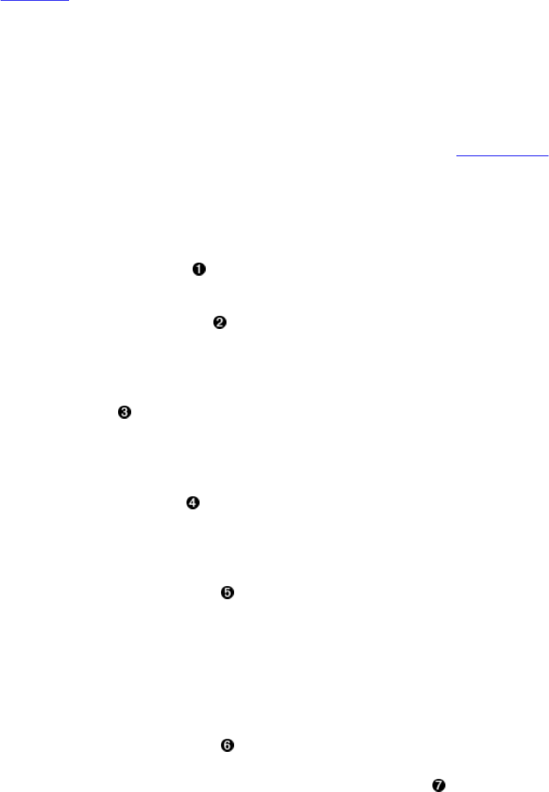
Another similarity to the put() calls is that you can ask for more than one row using a single
request. This allows you to quickly and efficiently retrieve related—but also completely random,
if required—data from the remote servers.
Note
As shown in Figure 3-2, the request may actually go to more than one server, but for all intents
and purposes, it looks like a single call from the client code.
The method provided by the API has the following signature:
Result[] get(List<Get> gets) throws IOException
Using this call is straightforward, with the same approach as seen earlier: you need to create a list
that holds all instances of the Get class you have prepared. This list is handed into the call and
you will be returned an array of equal size holding the matching Result instances. Example 3-17
brings this together, showing two different approaches to accessing the data.
Example 3-17. Example of retrieving data from HBase using lists of Get instances
byte[] cf1 = Bytes.toBytes("colfam1");
byte[] qf1 = Bytes.toBytes("qual1");
byte[] qf2 = Bytes.toBytes("qual2");
byte[] row1 = Bytes.toBytes("row1");
byte[] row2 = Bytes.toBytes("row2");
List<Get> gets = new ArrayList<Get>();
Get get1 = new Get(row1);
get1.addColumn(cf1, qf1);
gets.add(get1);
Get get2 = new Get(row2);
get2.addColumn(cf1, qf1);
gets.add(get2);
Get get3 = new Get(row2);
get3.addColumn(cf1, qf2);
gets.add(get3);
Result[] results = table.get(gets);
System.out.println("First iteration...");
for (Result result : results) {
String row = Bytes.toString(result.getRow());
System.out.print("Row: " + row + " ");
byte[] val = null;
if (result.containsColumn(cf1, qf1)) {
val = result.getValue(cf1, qf1);
System.out.println("Value: " + Bytes.toString(val));
}
if (result.containsColumn(cf1, qf2)) {
val = result.getValue(cf1, qf2);
System.out.println("Value: " + Bytes.toString(val));
}
}
System.out.println("Second iteration...");
for (Result result : results) {
for (Cell cell : result.listCells()) {
System.out.println(
"Row: " + Bytes.toString(
cell.getRowArray(), cell.getRowOffset(), cell.getRowLength()) +
" Value: " + Bytes.toString(CellUtil.cloneValue(cell)));
}
(166)

}
System.out.println("Third iteration...");
for (Result result : results) {
System.out.println(result);
}
Prepare commonly used byte arrays.
Create a list that holds the Get instances.
Add the Get instances to the list.
Retrieve rows with selected columns from HBase.
Iterate over results and check what values are available.
Iterate over results again, printing out all values.
Two different ways to access the cell data.
Assuming that you execute Example 3-5 just before you run Example 3-17, you should see
something like this on the command line:
First iteration...
Row: row1 Value: val1
Row: row2 Value: val2
Row: row2 Value: val3
Second iteration...
Row: row1 Value: val1
Row: row2 Value: val2
Row: row2 Value: val3
Third iteration...
keyvalues={row1/colfam1:qual1/1426678215864/Put/vlen=4/seqid=0}
keyvalues={row2/colfam1:qual1/1426678215864/Put/vlen=4/seqid=0}
keyvalues={row2/colfam1:qual2/1426678215864/Put/vlen=4/seqid=0}
All iterations return the same values, showing that you have a number of choices on how to
access them, once you have received the results. What you have not yet seen is how errors are
reported back to you. This differs from what you learned in “List of Puts”. The get() call either
returns the said array, matching the same size as the given list by the gets parameter, or throws
an exception. Example 3-18 showcases this behavior.
Example 3-18. Example trying to read an erroneous column family
List<Get> gets = new ArrayList<Get>();
Get get1 = new Get(row1);
(167)

get1.addColumn(cf1, qf1);
gets.add(get1);
Get get2 = new Get(row2);
get2.addColumn(cf1, qf1);
gets.add(get2);
Get get3 = new Get(row2);
get3.addColumn(cf1, qf2);
gets.add(get3);
Get get4 = new Get(row2);
get4.addColumn(Bytes.toBytes("BOGUS"), qf2);
gets.add(get4);
Result[] results = table.get(gets);
System.out.println("Result count: " + results.length);
Add the Get instances to the list.
Add the bogus column family get.
An exception is thrown and the process is aborted.
This line will never reached!
Executing this example will abort the entire get() operation, throwing the following (or similar)
error, and not returning a result at all:
org.apache.hadoop.hbase.client.RetriesExhaustedWithDetailsException:
Failed 1 action: NoSuchColumnFamilyException: 1 time,
servers with issues: 10.0.0.57:51640,
Exception in thread "main" \
org.apache.hadoop.hbase.client.RetriesExhaustedWithDetailsException: \
Failed 1 action: \
org.apache.hadoop.hbase.regionserver.NoSuchColumnFamilyException: \
Column family BOGUS does not exist in region \
testtable,,1426678215640.de657eebc8e3422376e918ed77fc33ba. \
in table 'testtable', {NAME => 'colfam1', ...}
at org.apache.hadoop.hbase.regionserver.HRegion.checkFamily(...)
at org.apache.hadoop.hbase.regionserver.HRegion.get(...)
...
One way to have more control over how the API handles partial faults is to use the batch()
operations discussed in “Batch Operations”.
(168)
Delete Method
You are now able to create, read, and update data in HBase tables. What is left is the ability to
delete from it. And surely you may have guessed by now that the Table provides you with a
method of exactly that name, along with a matching class aptly named Delete. Again you have a
few variants, one that takes a single delete, one that accepts a list of deletes, and another that
provides an atomic, server-side check-and-delete. The following discusses them in that order.
Single Deletes
The variant of the delete() call that takes a single Delete instance is:
void delete(Delete delete) throws IOException
Just as with the get() and put() calls you saw already, you will have to create a Delete instance
and then add details about the data you want to remove. The constructors are:
Delete(byte[] row)
Delete(byte[] row, long timestamp)
Delete(final byte[] rowArray, final int rowOffset, final int rowLength)
Delete(final byte[] rowArray, final int rowOffset, final int rowLength,
long ts)
Delete(final Delete d)
You need to provide the row you want to modify, and—optionally—a specific version/timestamp
to operate on. There are other variants to create a Delete instance, where the next two do the same
as the already described first pair, with the difference that they allow you to pass in a larger
array, with accompanying offset and length parameter. The final variant allows you to hand in an
existing delete instance and copy all parameters from it.
Otherwise, you would be wise to narrow down what you want to remove from the given row,
using one of the following methods:
Delete addFamily(final byte[] family)
Delete addFamily(final byte[] family, final long timestamp)
Delete addFamilyVersion(final byte[] family, final long timestamp)
Delete addColumns(final byte[] family, final byte[] qualifier)
Delete addColumns(final byte[] family, final byte[] qualifier,
final long timestamp)
Delete addColumn(final byte[] family, final byte[] qualifier)
Delete addColumn(byte[] family, byte[] qualifier, long timestamp)
void setTimestamp(long timestamp)
You do have a choice to narrow in on what to remove using four types of calls. First, you can use
the addFamily() methods to remove an entire column family, including all contained columns.
The next type is addColumns(), which operates on exactly one column. The third type is similar,
using addColumn(). It also operates on a specific, given column only, but deletes either the most
current or the specified version, that is, the one with the matching timestamp.
Finally, there is setTimestamp(), and it allows you to set a timestamp that is used for every
subsequent addXYZ() call. In fact, using a Delete constructor that takes an explicit timestamp
parameter is just shorthand to calling setTimestamp() just after creating the instance. Once an
instance wide timestamp is set, all further operations will make use of it. There is no need to use
(169)

the explicit timestamp parameter, though you can, as it has the same effect.
This changes quite a bit when attempting to delete the entire row, in other words when you do
not specify any family or column at all. The difference is between deleting the entire row or just
all contained columns, in all column families, that match or have an older timestamp compared
to the given one. Table 3-14 shows the functionality in a matrix to make the semantics more
readable.
Tip
The handling of the explicit versus implicit timestamps is the same for all addXYZ() methods, and
apply in the following order:
1. If you do not specify a timestamp for the addXYZ() calls, then the optional one from either
the constructor, or a previous call to setTimestamp() is used.
2. If that was not set, then HConstants.LATEST_TIMESTAMP is used, meaning all versions will be
affected by the delete.
LATEST_TIMESTAMP is simply the highest value the version field can assume, which is
Long.MAX_VALUE. Because the delete affects all versions equal or less than the given timestamp,
this means LATEST_TIMESTAMP covers all versions.
Table 3-14. Functionality matrix of the delete() calls
Method Deletes without timestamp Deletes with timestamp
none Entire row, that is, all
columns, all versions.
All versions of all columns in all column families,
whose timestamp is equal to or older than the given
timestamp.
addColumn()
Only the latest version of the
given column; older versions
are kept.
Only exactly the specified version of the given
column, with the matching timestamp. If
nonexistent, nothing is deleted.
addColumns() All versions of the given
column.
Versions equal to or older than the given timestamp
of the given column.
addFamily() All columns (including all
versions) of the given family.
Versions equal to or older than the given timestamp
of all columns of the given family.
For advanced user there is an additional method available:
Delete addDeleteMarker(Cell kv) throws IOException
This call checks that the provided Cell instance is of type delete (see Cell.getTypeByte() in “The
Cell”), and that the row key matches the one of the current delete instance. If that holds true, the
cell is added as-is to the family it came from. One place where this is used is in such tools as
(170)
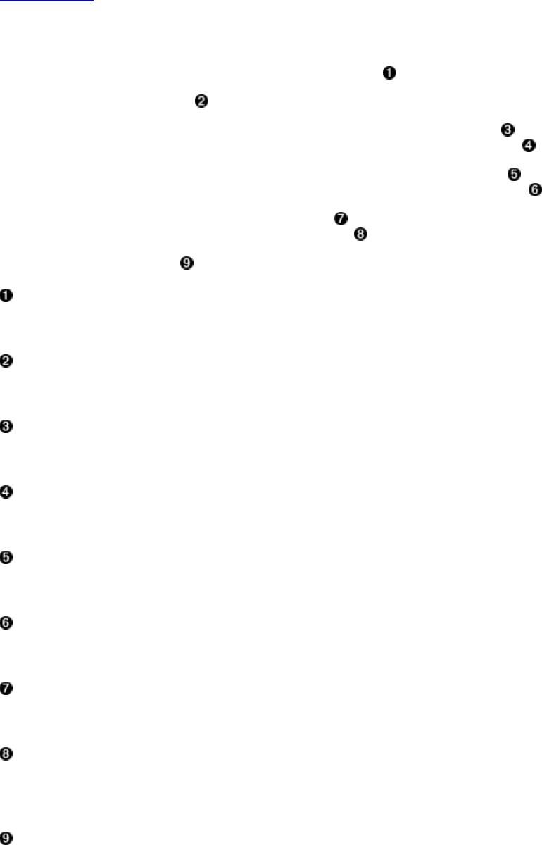
Import. These tools read and deserialize entire cells from an input stream (say a backup file or
write-ahead log) and want to add them verbatim, that is, no need to create another internal cell
instance and copy the data.
Example 3-19 shows how to use the single delete() call from client code.
Example 3-19. Example application deleting data from HBase
Delete delete = new Delete(Bytes.toBytes("row1"));
delete.setTimestamp(1);
delete.addColumn(Bytes.toBytes("colfam1"), Bytes.toBytes("qual1"));
delete.addColumn(Bytes.toBytes("colfam1"), Bytes.toBytes("qual3"), 3);
delete.addColumns(Bytes.toBytes("colfam1"), Bytes.toBytes("qual1"));
delete.addColumns(Bytes.toBytes("colfam1"), Bytes.toBytes("qual3"), 2);
delete.addFamily(Bytes.toBytes("colfam1"));
delete.addFamily(Bytes.toBytes("colfam1"), 3);
table.delete(delete);
Create delete with specific row.
Set timestamp for row deletes.
Delete the latest version only in one column.
Delete specific version in one column.
Delete all versions in one column.
Delete the given and all older versions in one column.
Delete entire family, all columns and versions.
Delete the given and all older versions in the entire column family, i.e., from all columns
therein.
Delete the data from the HBase table.
(171)

The example lists all the different calls you can use to parameterize the delete() operation. It
does not make too much sense to call them all one after another like this. Feel free to comment
out the various delete calls to see what is printed on the console.
Setting the timestamp for the deletes has the effect of only matching the exact cell, that is, the
matching column and value with the exact timestamp. On the other hand, not setting the
timestamp forces the server to retrieve the latest timestamp on the server side on your behalf.
This is slower than performing a delete with an explicit timestamp.
If you attempt to delete a cell with a timestamp that does not exist, nothing happens. For
example, given that you have two versions of a column, one at version 10 and one at version 20,
deleting from this column with version 15 will not affect either existing version.
Another note to be made about the example is that it showcases custom versioning. Instead of
relying on timestamps, implicit or explicit ones, it uses sequential numbers, starting with 1. This
is perfectly valid, although you are forced to always set the version yourself, since the servers do
not know about your schema and would use epoch-based timestamps instead. Another example
of using custom versioning can be found in “Search Integration”.
The Delete class provides additional calls, which are listed in Table 3-15 for your reference.
Once again, many are inherited from the superclasses, such as Mutation.
Table 3-15. Quick overview of additional methods provided by the Delete class
Method Description
cellScanner() Provides a scanner over all cells available in this
instance.
getACL()/setACL() The ACLs for this operation (might be null).
getAttribute()/setAttribute() Set and get arbitrary attributes associated with this
instance of Delete.
getAttributesMap() Returns the entire map of attributes, if any are set.
getCellVisibility()/setCellVisibility() The cell level visibility for all included cells.
getClusterIds()/setClusterIds() The cluster IDs as needed for replication purposes.
getDurability()/setDurability() The durability settings for the mutation.
getFamilyCellMap()/setFamilyCellMap() The list of all cells of this instance.
(172)
getFingerprint() Compiles details about the instance into a map for
debugging, or logging.
getId()/setId() An ID for the operation, useful for identifying the
origin of a request later.
getRow() Returns the row key as specified when creating the
Delete instance.
getTimeStamp() Retrieves the associated timestamp of the Delete
instance.
getTTL()/setTTL() Not supported by Delete, will throw an exception when
setTTL() is called.
heapSize()
Computes the heap space required for the current Delete
instance. This includes all contained data and space
needed for internal structures.
isEmpty() Checks if the family map contains any Cell instances.
numFamilies() Convenience method to retrieve the size of the family
map, containing all Cell instances.
size() Returns the number of Cell instances that will be
applied with this Delete.
toJSON()/toJSON(int) Converts the first 5 or N columns into a JSON format.
toMap()/toMap(int) Converts the first 5 or N columns into a map. This is
more detailed than what getFingerprint() returns.
toString()/toString(int) Converts the first 5 or N columns into a JSON, or map
(if JSON fails due to encoding problems).
List of Deletes
The list-based delete() call works very similarly to the list-based put(). You need to create a list
(173)
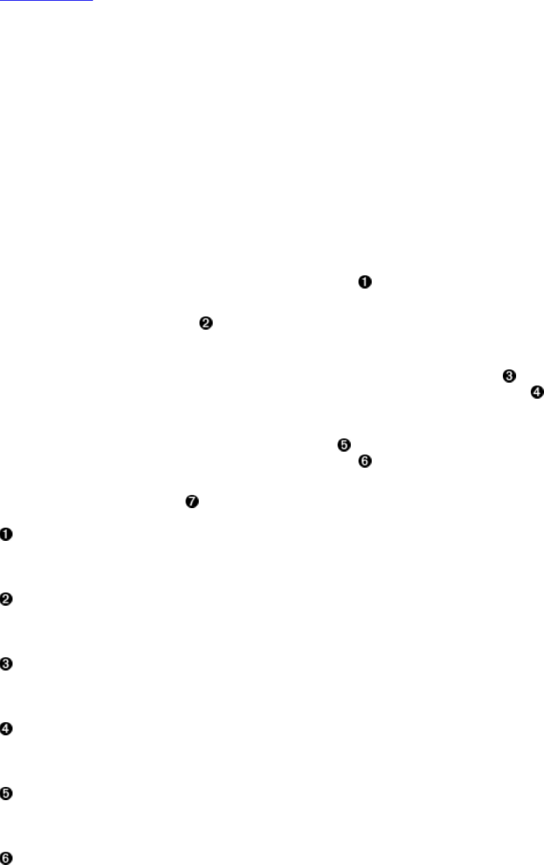
of Delete instances, configure them, and call the following method:
void delete(List<Delete> deletes) throws IOException
Example 3-20 shows where three different rows are affected during the operation, deleting
various details they contain. When you run this example, you will see a printout of the before and
after states of the delete. The output prints the raw KeyValue instances, using KeyValue.toString().
Note
Just as with the other list-based operation, you cannot make any assumption regarding the order
in which the deletes are applied on the remote servers. The API is free to reorder them to make
efficient use of the single RPC per affected region server. If you need to enforce specific orders
of how operations are applied, you would need to batch those calls into smaller groups and
ensure that they contain the operations in the desired order across the batches. In a worst-case
scenario, you would need to send separate delete calls altogether.
Example 3-20. Example application deleting lists of data from HBase
List<Delete> deletes = new ArrayList<Delete>();
Delete delete1 = new Delete(Bytes.toBytes("row1"));
delete1.setTimestamp(4);
deletes.add(delete1);
Delete delete2 = new Delete(Bytes.toBytes("row2"));
delete2.addColumn(Bytes.toBytes("colfam1"), Bytes.toBytes("qual1"));
delete2.addColumns(Bytes.toBytes("colfam2"), Bytes.toBytes("qual3"), 5);
deletes.add(delete2);
Delete delete3 = new Delete(Bytes.toBytes("row3"));
delete3.addFamily(Bytes.toBytes("colfam1"));
delete3.addFamily(Bytes.toBytes("colfam2"), 3);
deletes.add(delete3);
table.delete(deletes);
Create a list that holds the Delete instances.
Set timestamp for row deletes.
Delete the latest version only in one column.
Delete the given and all older versions in another column.
Delete entire family, all columns and versions.
(174)

Delete the given and all older versions in the entire column family, i.e., from all columns
therein.
Delete the data from multiple rows the HBase table.
The output you should see is:12
Before delete call...
Cell: row1/colfam1:qual1/2/Put/vlen=4/seqid=0, Value: val2
Cell: row1/colfam1:qual1/1/Put/vlen=4/seqid=0, Value: val1
Cell: row1/colfam1:qual2/4/Put/vlen=4/seqid=0, Value: val4
Cell: row1/colfam1:qual2/3/Put/vlen=4/seqid=0, Value: val3
Cell: row1/colfam1:qual3/6/Put/vlen=4/seqid=0, Value: val6
Cell: row1/colfam1:qual3/5/Put/vlen=4/seqid=0, Value: val5
Cell: row1/colfam2:qual1/2/Put/vlen=4/seqid=0, Value: val2
Cell: row1/colfam2:qual1/1/Put/vlen=4/seqid=0, Value: val1
Cell: row1/colfam2:qual2/4/Put/vlen=4/seqid=0, Value: val4
Cell: row1/colfam2:qual2/3/Put/vlen=4/seqid=0, Value: val3
Cell: row1/colfam2:qual3/6/Put/vlen=4/seqid=0, Value: val6
Cell: row1/colfam2:qual3/5/Put/vlen=4/seqid=0, Value: val5
Cell: row2/colfam1:qual1/2/Put/vlen=4/seqid=0, Value: val2
Cell: row2/colfam1:qual1/1/Put/vlen=4/seqid=0, Value: val1
Cell: row2/colfam1:qual2/4/Put/vlen=4/seqid=0, Value: val4
Cell: row2/colfam1:qual2/3/Put/vlen=4/seqid=0, Value: val3
Cell: row2/colfam1:qual3/6/Put/vlen=4/seqid=0, Value: val6
Cell: row2/colfam1:qual3/5/Put/vlen=4/seqid=0, Value: val5
Cell: row2/colfam2:qual1/2/Put/vlen=4/seqid=0, Value: val2
Cell: row2/colfam2:qual1/1/Put/vlen=4/seqid=0, Value: val1
Cell: row2/colfam2:qual2/4/Put/vlen=4/seqid=0, Value: val4
Cell: row2/colfam2:qual2/3/Put/vlen=4/seqid=0, Value: val3
Cell: row2/colfam2:qual3/6/Put/vlen=4/seqid=0, Value: val6
Cell: row2/colfam2:qual3/5/Put/vlen=4/seqid=0, Value: val5
Cell: row3/colfam1:qual1/2/Put/vlen=4/seqid=0, Value: val2
Cell: row3/colfam1:qual1/1/Put/vlen=4/seqid=0, Value: val1
Cell: row3/colfam1:qual2/4/Put/vlen=4/seqid=0, Value: val4
Cell: row3/colfam1:qual2/3/Put/vlen=4/seqid=0, Value: val3
Cell: row3/colfam1:qual3/6/Put/vlen=4/seqid=0, Value: val6
Cell: row3/colfam1:qual3/5/Put/vlen=4/seqid=0, Value: val5
Cell: row3/colfam2:qual1/2/Put/vlen=4/seqid=0, Value: val2
Cell: row3/colfam2:qual1/1/Put/vlen=4/seqid=0, Value: val1
Cell: row3/colfam2:qual2/4/Put/vlen=4/seqid=0, Value: val4
Cell: row3/colfam2:qual2/3/Put/vlen=4/seqid=0, Value: val3
Cell: row3/colfam2:qual3/6/Put/vlen=4/seqid=0, Value: val6
Cell: row3/colfam2:qual3/5/Put/vlen=4/seqid=0, Value: val5
After delete call...
Cell: row1/colfam1:qual3/6/Put/vlen=4/seqid=0, Value: val6
Cell: row1/colfam1:qual3/5/Put/vlen=4/seqid=0, Value: val5
Cell: row1/colfam2:qual3/6/Put/vlen=4/seqid=0, Value: val6
Cell: row1/colfam2:qual3/5/Put/vlen=4/seqid=0, Value: val5
Cell: row2/colfam1:qual1/1/Put/vlen=4/seqid=0, Value: val1
Cell: row2/colfam1:qual2/4/Put/vlen=4/seqid=0, Value: val4
Cell: row2/colfam1:qual2/3/Put/vlen=4/seqid=0, Value: val3
Cell: row2/colfam1:qual3/6/Put/vlen=4/seqid=0, Value: val6
Cell: row2/colfam1:qual3/5/Put/vlen=4/seqid=0, Value: val5
Cell: row2/colfam2:qual1/2/Put/vlen=4/seqid=0, Value: val2
Cell: row2/colfam2:qual1/1/Put/vlen=4/seqid=0, Value: val1
Cell: row2/colfam2:qual2/4/Put/vlen=4/seqid=0, Value: val4
Cell: row2/colfam2:qual2/3/Put/vlen=4/seqid=0, Value: val3
Cell: row2/colfam2:qual3/6/Put/vlen=4/seqid=0, Value: val6
Cell: row3/colfam2:qual2/4/Put/vlen=4/seqid=0, Value: val4
Cell: row3/colfam2:qual3/6/Put/vlen=4/seqid=0, Value: val6
(175)
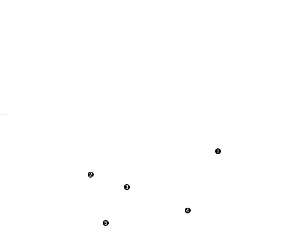
Cell: row3/colfam2:qual3/5/Put/vlen=4/seqid=0, Value: val5
The deleted original data is highlighted in the Before delete call… block. All three rows contain
the same data, composed of two column families, three columns in each family, and two versions
for each column.
The example code first deletes, from the entire row, everything up to version 4. This leaves the
columns with versions 5 and 6 as the remainder of the row content.
It then goes about and uses the two different column-related add calls on row2 to remove the
newest cell in the column named colfam1:qual1, and subsequently every cell with a version of 5
and older—in other words, those with a lower version number—from colfam1:qual3. Here you
have only one matching cell, which is removed as expected in due course.
Lastly, operating on row-3, the code removes the entire column family colfam1, and then
everything with a version of 3 or less from colfam2. During the execution of the example code,
you will see the printed Cell details, using something like this:
System.out.println("Cell: " + cell + ", Value: " +
Bytes.toString(cell.getValueArray(), cell.getValueOffset(),
cell.getValueLength()));
By now you are familiar with the usage of the Bytes class, which is used to print out the value of
the Cell instance, as returned by the getValueArray() method. This is necessary because the
Cell.toString() output (as explained in “The Cell”) does not print out the actual value, but rather
the key part only. The toString() does not print the value since it could be very large. Here, the
example code inserts the column values, and therefore knows that these are short and human-
readable; hence it is safe to print them out on the console as shown. You could use the same
mechanism in your own code for debugging purposes.
Please refer to the entire example code in the accompanying source code repository for this book.
You will see how the data is inserted and retrieved to generate the discussed output.
What is left to talk about is the error handling of the list-based delete() call. The handed-in
deletes parameter, that is, the list of Delete instances, is modified to only contain the failed delete
instances when the call returns. In other words, when everything has succeeded, the list will be
empty. The call also throws the exception—if there was one—reported from the remote servers.
You will have to guard the call using a try/catch, for example, and react accordingly. Example 3-
21 may serve as a starting point.
Example 3-21. Example deleting faulty data from HBase
Delete delete4 = new Delete(Bytes.toBytes("row2"));
delete4.addColumn(Bytes.toBytes("BOGUS"), Bytes.toBytes("qual1"));
deletes.add(delete4);
try {
table.delete(deletes);
} catch (Exception e) {
System.err.println("Error: " + e);
}
table.close();
System.out.println("Deletes length: " + deletes.size());
for (Delete delete : deletes) {
System.out.println(delete);
}
(176)

Add bogus column family to trigger an error.
Delete the data from multiple rows the HBase table.
Guard against remote exceptions.
Check the length of the list after the call.
Print out failed delete for debugging purposes.
Example 3-21 modifies Example 3-20 but adds an erroneous delete detail: it inserts a BOGUS
column family name. The output is the same as that for Example 3-20, but has some additional
details printed out in the middle part:
Before delete call...
Cell: row1/colfam1:qual1/2/Put/vlen=4/seqid=0, Value: val2
Cell: row1/colfam1:qual1/1/Put/vlen=4/seqid=0, Value: val1
...
Cell: row3/colfam2:qual3/6/Put/vlen=4/seqid=0, Value: val6
Cell: row3/colfam2:qual3/5/Put/vlen=4/seqid=0, Value: val5
Deletes length: 1
Error: org.apache.hadoop.hbase.client.RetriesExhaustedWithDetailsException: \
Failed 1 action: \
org.apache.hadoop.hbase.regionserver.NoSuchColumnFamilyException: \
Column family BOGUS does not exist ...
...
: 1 time,
{"ts":9223372036854775807,"totalColumns":1,"families":{"BOGUS":[{ \
"timestamp":9223372036854775807,"tag":[],"qualifier":"qual1","vlen":0}]}, \
"row":"row2"}
After delete call...
Cell: row1/colfam1:qual3/6/Put/vlen=4/seqid=0, Value: val6
Cell: row1/colfam1:qual3/5/Put/vlen=4/seqid=0, Value: val5
...
Cell: row3/colfam2:qual3/6/Put/vlen=4/seqid=0, Value: val6
Cell: row3/colfam2:qual3/5/Put/vlen=4/seqid=0, Value: val5
As expected, the list contains one remaining Delete instance: the one with the bogus column
family. Printing out the instance—Java uses the implicit toString() method when printing an
object—reveals the internal details of the failed delete. The important part is the family name
being the obvious reason for the failure. You can use this technique in your own code to check
why an operation has failed. Often the reasons are rather obvious indeed.
Finally, note the exception that was caught and printed out in the catch statement of the example.
It is the same RetriesExhaustedWithDetailsException you saw twice already. It reports the number
of failed actions plus how often it did retry to apply them, and on which server. An advanced
task that you will learn about in later chapters (for example Chapter 9) is how to verify and
monitor servers so that the given server address could be useful to find the root cause of the
failure. Table 3-11 had a list of available methods.
(177)
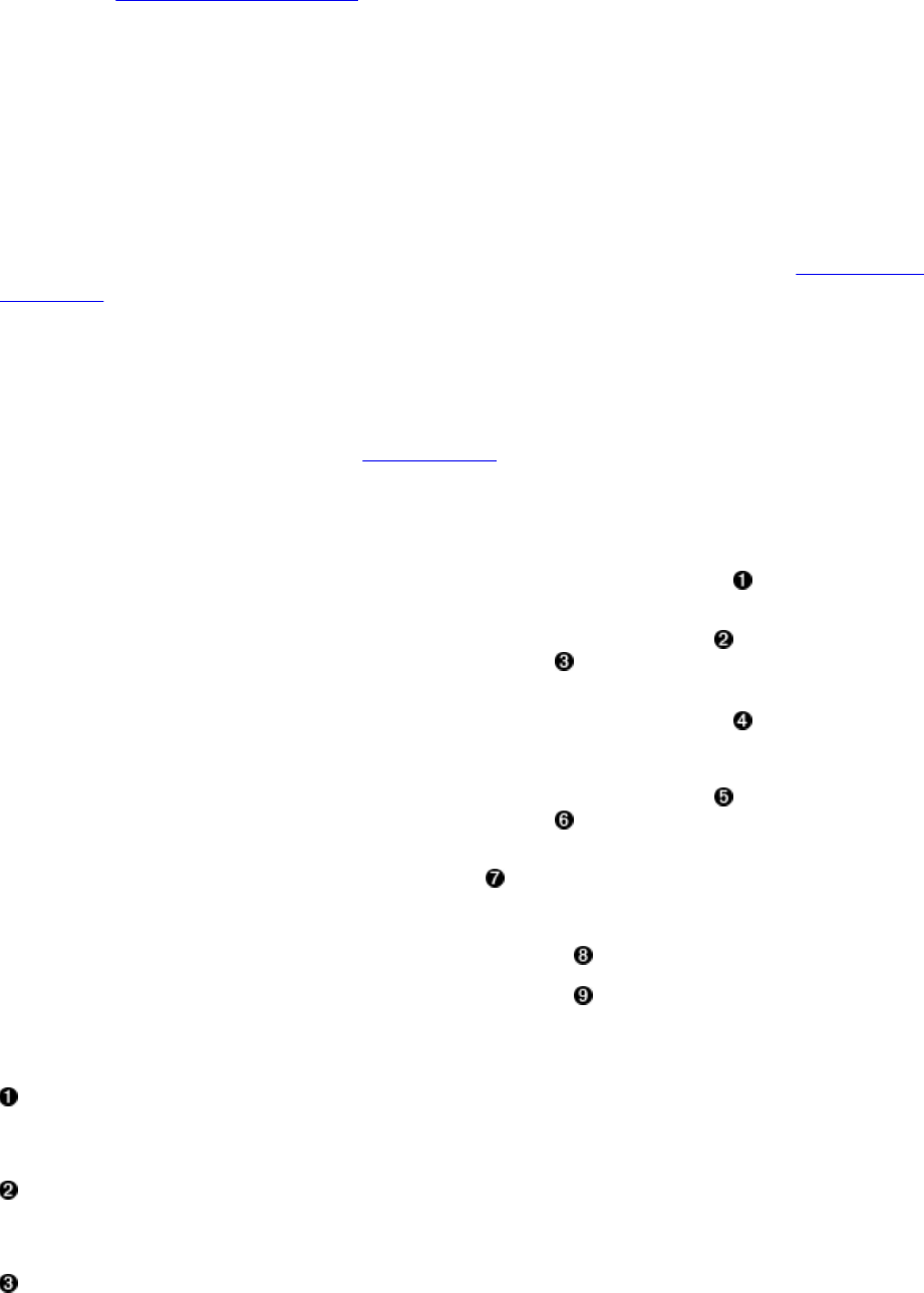
Atomic Check-and-Delete
You saw in “Atomic Check-and-Put” how to use an atomic, conditional operation to insert data
into a table. There are equivalent calls for deletes that give you access to server-side, read-
modify-write functionality:
boolean checkAndDelete(byte[] row, byte[] family, byte[] qualifier,
byte[] value, Delete delete) throws IOException
boolean checkAndDelete(byte[] row, byte[] family, byte[] qualifier,
CompareFilter.CompareOp compareOp, byte[] value, Delete delete)
throws IOException
You need to specify the row key, column family, qualifier, and value to check before the actual
delete operation is performed. The first call implies that the given value has to equal to the stored
one. The second call lets you specify the actual comparison operator (explained in “Comparison
Operators”), which enables more elaborate testing, for example, if the given value is equal or
less than the stored one. This is useful to track some kind of modification ID, and you want to
ensure you have reached a specific point in the cells lifecycle, for example, when it is updated by
many concurrent clients.
Should the test fail, nothing is deleted and the call returns a false. If the check is successful, the
delete is applied and true is returned. Example 3-22 shows this in context.
Example 3-22. Example application using the atomic compare-and-set operations
Delete delete1 = new Delete(Bytes.toBytes("row1"));
delete1.addColumns(Bytes.toBytes("colfam1"), Bytes.toBytes("qual3"));
boolean res1 = table.checkAndDelete(Bytes.toBytes("row1"),
Bytes.toBytes("colfam2"), Bytes.toBytes("qual3"), null, delete1);
System.out.println("Delete 1 successful: " + res1);
Delete delete2 = new Delete(Bytes.toBytes("row1"));
delete2.addColumns(Bytes.toBytes("colfam2"), Bytes.toBytes("qual3"));
table.delete(delete2);
boolean res2 = table.checkAndDelete(Bytes.toBytes("row1"),
Bytes.toBytes("colfam2"), Bytes.toBytes("qual3"), null, delete1);
System.out.println("Delete 2 successful: " + res2);
Delete delete3 = new Delete(Bytes.toBytes("row2"));
delete3.addFamily(Bytes.toBytes("colfam1"));
try{
boolean res4 = table.checkAndDelete(Bytes.toBytes("row1"),
Bytes.toBytes("colfam1"), Bytes.toBytes("qual1"),
Bytes.toBytes("val1"), delete3);
System.out.println("Delete 3 successful: " + res4);
} catch (Exception e) {
System.err.println("Error: " + e.getMessage());
}
Create a new Delete instance.
Check if column does not exist and perform optional delete operation.
(178)

Print out the result, should be “Delete successful: false”.
Delete checked column manually.
Attempt to delete same cell again.
Print out the result, should be “Delete successful: true” since the checked column now is
gone.
Create yet another Delete instance, but using a different row.
Try to delete while checking a different row.
We will not get here as an exception is thrown beforehand!
Here is the output you should see:
Before delete call...
Cell: row1/colfam1:qual1/1/Put/vlen=4/seqid=0, Value: val1
Cell: row1/colfam1:qual2/2/Put/vlen=4/seqid=0, Value: val2
Cell: row1/colfam1:qual3/3/Put/vlen=4/seqid=0, Value: val3
Cell: row1/colfam2:qual1/1/Put/vlen=4/seqid=0, Value: val1
Cell: row1/colfam2:qual2/2/Put/vlen=4/seqid=0, Value: val2
Cell: row1/colfam2:qual3/3/Put/vlen=4/seqid=0, Value: val3
Delete 1 successful: false
Delete 2 successful: true
Error: org.apache.hadoop.hbase.DoNotRetryIOException: \
Action's getRow must match the passed row
...
After delete call...
Cell: row1/colfam1:qual1/1/Put/vlen=4/seqid=0, Value: val1
Cell: row1/colfam1:qual2/2/Put/vlen=4/seqid=0, Value: val2
Cell: row1/colfam2:qual1/1/Put/vlen=4/seqid=0, Value: val1
Cell: row1/colfam2:qual2/2/Put/vlen=4/seqid=0, Value: val2
Using null as the value parameter triggers the nonexistence test, that is, the check is successful if
the column specified does not exist. Since the example code inserts the checked column before
the check is performed, the test will initially fail, returning false and aborting the delete
operation. The column is then deleted by hand and the check-and-modify call is run again. This
time the check succeeds and the delete is applied, returning true as the overall result.
Just as with the put-related CAS call, you can only perform the check-and-modify on the same
row. The example attempts to check on one row key while the supplied instance of Delete points
to another. An exception is thrown accordingly, once the check is performed. It is allowed,
though, to check across column families—for example, to have one set of columns control how
the filtering is done for another set of columns.
(179)
This example cannot justify the importance of the check-and-delete operation. In distributed
systems, it is inherently difficult to perform such operations reliably, and without incurring
performance penalties caused by external locking approaches, that is, where the atomicity is
guaranteed by the client taking out exclusive locks on the entire row. When the client goes away
during the locked phase the server has to rely on lease recovery mechanisms ensuring that these
rows are eventually unlocked again. They also cause additional RPCs to occur, which will be
slower than a single, server-side operation.
(180)

Append Method
Similar to the generic CRUD functions so far, there is another kind of mutation function, like
put(), but with a spin on it. Instead of creating or updating a column value, the append() method
does an atomic read-modify-write operation, adding data to a column. The API method provided
is:
Result append(final Append append) throws IOException
And similar once more to all other API data manipulation functions so far, this call has an
accompanying class named Append. You create an instance with one of these constructors:
Append(byte[] row)
Append(final byte[] rowArray, final int rowOffset, final int rowLength)
Append(Append a)
So you either provide the obvious row key, or an existing, larger array holding that byte[] array as
a subset, plus the necessary offset and length into it. The third choice, analog to all the other
data-related types, is to hand in an existing Append instance and copy all its parameters. Once the
instance is created, you move along and add details of the column you want to append to, using
one of these calls:
Append add(byte[] family, byte[] qualifier, byte[] value)
Append add(final Cell cell)
Like with Put, you must call one of those functions, or else a subsequent call to append() will
throw an exception. This does make sense as you cannot insert or append to the entire row. Note
that this is different from Delete, which of course can delete an entire row. The first provided
method takes the column family and qualifier (the column) name, plus the value to add to the
existing cell. The second copies all of these parameters from an existing cell instance.
Example 3-23 shows the use of append on an existing and empty column.
Example 3-23. Example application appending data to a column in HBase
Append append = new Append(Bytes.toBytes("row1"));
append.add(Bytes.toBytes("colfam1"), Bytes.toBytes("qual1"),
Bytes.toBytes("newvalue"));
append.add(Bytes.toBytes("colfam1"), Bytes.toBytes("qual2"),
Bytes.toBytes("anothervalue"));
table.append(append);
The output should be:
Before append call...
Cell: row1/colfam1:qual1/1/Put/vlen=8/seqid=0, Value: oldvalue
After append call...
Cell: row1/colfam1:qual1/1426778944272/Put/vlen=16/seqid=0,
Value: oldvaluenewvalue
Cell: row1/colfam1:qual1/1/Put/vlen=8/seqid=0, Value: oldvalue
Cell: row1/colfam1:qual2/1426778944272/Put/vlen=12/seqid=0,
Value: anothervalue
You will note in the output how we appended newvalue to the existing oldvalue for qual1. We also
added a brand new column with qual2, that just holds the new value anothervalue. The append
operation is binary, as is all the value related functionality in HBase. In other words, we
(181)

appended two strings but in reality we appended two byte[] arrays. If you use the append feature,
you may have to insert some delimiter to later parse the appended bytes into separate parts again.
One special option of append() is to not return any data from the servers. This is accomplished
with this pair of methods:
Append setReturnResults(boolean returnResults)
boolean isReturnResults()
Usually, the newly updated cells are returned to the caller. But if you want to send the append to
the server, and you do not care about the result(s) at this point, you can call
setReturnResults(false) to omit the shipping. It will then return null to you instead. The Append
class provides additional calls, which are listed in Table 3-16 for your reference. Once again,
many are inherited from the superclasses, such as Mutation.
Table 3-16. Quick overview of additional methods provided by the Append class
Method Description
cellScanner() Provides a scanner over all cells available in this
instance.
getACL()/setACL() The ACLs for this operation (might be null).
getAttribute()/setAttribute() Set and get arbitrary attributes associated with this
instance of Append.
getAttributesMap() Returns the entire map of attributes, if any are set.
getCellVisibility()/setCellVisibility() The cell level visibility for all included cells.
getClusterIds()/setClusterIds() The cluster IDs as needed for replication purposes.
getDurability()/setDurability() The durability settings for the mutation.
getFamilyCellMap()/setFamilyCellMap() The list of all cells of this instance.
getFingerprint() Compiles details about the instance into a map for
debugging, or logging.
getId()/setId() An ID for the operation, useful for identifying the
origin of a request later.
(182)
getRow()
Returns the row key as specified when creating the
Append instance.
getTimeStamp() Retrieves the associated timestamp of the Append
instance.
getTTL()/setTTL() Sets the cell level TTL value, which is being applied to
all included Cell instances before being persisted.
heapSize()
Computes the heap space required for the current Append
instance. This includes all contained data and space
needed for internal structures.
isEmpty() Checks if the family map contains any Cell instances.
numFamilies() Convenience method to retrieve the size of the family
map, containing all Cell instances.
size() Returns the number of Cell instances that will be
applied with this Append.
toJSON()/toJSON(int) Converts the first 5 or N columns into a JSON format.
toMap()/toMap(int) Converts the first 5 or N columns into a map. This is
more detailed than what getFingerprint() returns.
toString()/toString(int) Converts the first 5 or N columns into a JSON, or map
(if JSON fails due to encoding problems).
(183)

Mutate Method
Analog to all the other groups of operations, we can separate the mutate calls into separate ones.
One difference is though that we do not have a list based version, but single mutations and the
atomic compare-and-mutate. We will discuss them now in order.
Single Mutations
So far all operations had their specific method in Table and a specific data-related type provided.
But what if you want to update a row across these operations, and do so atomically. That is
where the mutateRow() call comes in. It has the following signature:
void mutateRow(final RowMutations rm) throws IOException
The RowMutations based parameter is a container that accepts either Put or Delete instance, and
then applies both in one call to the server-side data. The list of available constructors and
methods for the RowMutations class is:
RowMutations(byte[] row)
add(Delete)
add(Put)
getMutations()
getRow()
You create an instance with a specific row key, and then add any delete or put instance you have.
The row key you used to create the RowMutations instance must match the row key of any
mutation you add, or else you will receive an exception when trying to add them. Example 3-24
shows a working example.
Example 3-24. Modifies a row with multiple operations
Put put = new Put(Bytes.toBytes("row1"));
put.addColumn(Bytes.toBytes("colfam1"), Bytes.toBytes("qual1"),
4, Bytes.toBytes("val99"));
put.addColumn(Bytes.toBytes("colfam1"), Bytes.toBytes("qual4"),
4, Bytes.toBytes("val100"));
Delete delete = new Delete(Bytes.toBytes("row1"));
delete.addColumn(Bytes.toBytes("colfam1"), Bytes.toBytes("qual2"));
RowMutations mutations = new RowMutations(Bytes.toBytes("row1"));
mutations.add(put);
mutations.add(delete);
table.mutateRow(mutations);
The output should read like this:
Before delete call...
Cell: row1/colfam1:qual1/1/Put/vlen=4/seqid=0, Value: val1
Cell: row1/colfam1:qual2/2/Put/vlen=4/seqid=0, Value: val2
Cell: row1/colfam1:qual3/3/Put/vlen=4/seqid=0, Value: val3
After mutate call...
Cell: row1/colfam1:qual1/4/Put/vlen=5/seqid=0, Value: val99
Cell: row1/colfam1:qual1/1/Put/vlen=4/seqid=0, Value: val1
Cell: row1/colfam1:qual3/3/Put/vlen=4/seqid=0, Value: val3
Cell: row1/colfam1:qual4/4/Put/vlen=6/seqid=0, Value: val100
(184)

With one call we update row1, with column name qual1, setting it to a new value of val99. We
also added a whole new column, named qual4, with a value of val100. Finally, at the same time
we removed one column from the same row, namely column qual2.
Atomic Check-and-Mutate
You saw earlier, for example in “Atomic Check-and-Delete”, how to use an atomic, conditional
operation to modify data in a table. There are equivalent calls for mutations that give you access
to server-side, read-modify-write functionality:
public boolean checkAndMutate(final byte[] row, final byte[] family,
final byte[] qualifier, final CompareOp compareOp, final byte[] value,
final RowMutations rm) throws IOException
You need to specify the row key, column family, qualifier, and value to check before the actual
list of mutations is applied. The call lets you specify the actual comparison operator (explained in
“Comparison Operators”), which enables more elaborate testing, for example, if the given value
is equal or less than the stored one. This is useful to track some kind of modification ID, and you
want to ensure you have reached a specific point in the cells lifecycle, for example, when it is
updated by many concurrent clients.
Should the test fail, nothing is applied and the call returns a false. If the check is successful, the
mutations are applied and true is returned. Example 3-25 shows this in context.
Example 3-25. Example using the atomic check-and-mutate operations
Put put = new Put(Bytes.toBytes("row1"));
put.addColumn(Bytes.toBytes("colfam1"), Bytes.toBytes("qual1"),
4, Bytes.toBytes("val99"));
put.addColumn(Bytes.toBytes("colfam1"), Bytes.toBytes("qual4"),
4, Bytes.toBytes("val100"));
Delete delete = new Delete(Bytes.toBytes("row1"));
delete.addColumn(Bytes.toBytes("colfam1"), Bytes.toBytes("qual2"));
RowMutations mutations = new RowMutations(Bytes.toBytes("row1"));
mutations.add(put);
mutations.add(delete);
boolean res1 = table.checkAndMutate(Bytes.toBytes("row1"),
Bytes.toBytes("colfam2"), Bytes.toBytes("qual1"),
CompareFilter.CompareOp.LESS, Bytes.toBytes("val1"), mutations);
System.out.println("Mutate 1 successful: " + res1);
Put put2 = new Put(Bytes.toBytes("row1"));
put2.addColumn(Bytes.toBytes("colfam2"), Bytes.toBytes("qual1"),
4, Bytes.toBytes("val2"));
table.put(put2);
boolean res2 = table.checkAndMutate(Bytes.toBytes("row1"),
Bytes.toBytes("colfam2"), Bytes.toBytes("qual1"),
CompareFilter.CompareOp.LESS, Bytes.toBytes("val1"), mutations);
System.out.println("Mutate 2 successful: " + res2);
Check if the column contains a value that is less than “val1”. Here we receive “false” as
the value is equal, but not lesser.
(185)

Now “val1” is less than “val2” (binary comparison) and we expect “true” to be printed on
the console.
Update the checked column to have a value greater than what we check for.
Here is the output you should see:
Before check and mutate calls...
Cell: row1/colfam1:qual1/1/Put/vlen=4/seqid=0, Value: val1
Cell: row1/colfam1:qual2/2/Put/vlen=4/seqid=0, Value: val2
Cell: row1/colfam1:qual3/3/Put/vlen=4/seqid=0, Value: val3
Cell: row1/colfam2:qual1/1/Put/vlen=4/seqid=0, Value: val1
Cell: row1/colfam2:qual2/2/Put/vlen=4/seqid=0, Value: val2
Cell: row1/colfam2:qual3/3/Put/vlen=4/seqid=0, Value: val3
Mutate 1 successful: false
Mutate 2 successful: true
After check and mutate calls...
Cell: row1/colfam1:qual1/4/Put/vlen=5/seqid=0, Value: val99
Cell: row1/colfam1:qual1/1/Put/vlen=4/seqid=0, Value: val1
Cell: row1/colfam1:qual3/3/Put/vlen=4/seqid=0, Value: val3
Cell: row1/colfam1:qual4/4/Put/vlen=6/seqid=0, Value: val100
Cell: row1/colfam2:qual1/4/Put/vlen=4/seqid=0, Value: val2
Cell: row1/colfam2:qual1/1/Put/vlen=4/seqid=0, Value: val1
Cell: row1/colfam2:qual2/2/Put/vlen=4/seqid=0, Value: val2
Cell: row1/colfam2:qual3/3/Put/vlen=4/seqid=0, Value: val3
Just as before, using null as the value parameter triggers the nonexistence test, that is, the check
is successful if the column specified does not exist. Since the example code inserts the checked
column before the check is performed, the test will initially fail, returning false and aborting the
operation. The column is then updated by hand and the check-and-modify call is run again. This
time the check succeeds and the mutations are applied, returning true as the overall result.
Different to the earlier examples is that the Example 3-25 is using a LESS comparison for the
check: it specifies a column and asks the server to verify that the given value (val1) is less than
the currently stored value. They are exactly equal and therefore the test will fail. Once the value
is increased, the second test succeeds with the check and proceeds as expected.
As with the put- or delete-related CAS call, you can only perform the check-and-modify
operation on the same row. The earlier Example 3-22 did showcase this with a cross-row check.
We omit this here for the sake of brevity.
(186)
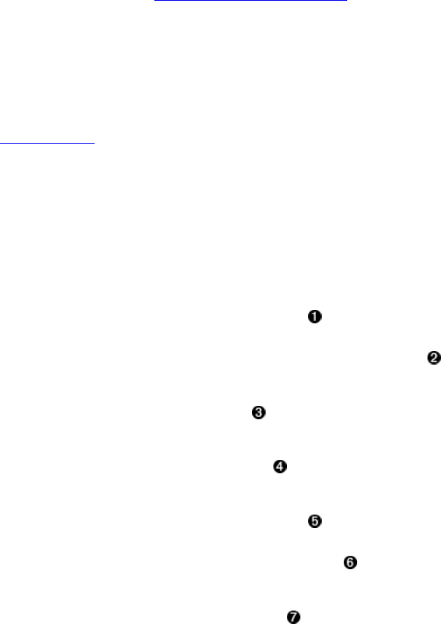
Batch Operations
You have seen how you can add, retrieve, and remove data from a table using single or list-based
operations, applied to a single row. In this section, we will look at API calls to batch different
operations across multiple rows.
Note
In fact, a lot of the internal functionality of the list-based calls, such as delete(List<Delete>
deletes) or get(List<Get> gets), are based on the batch() call introduced here. They are more or
less legacy calls and kept for convenience. If you start fresh, it is recommended that you use the
batch() calls for all your operations.
The following methods of the client API represent the available batch operations. You may note
the usage of Row, which is the ancestor, or parent class, for Get and all Mutation based types, such
as Put, as explained in “Data Types and Hierarchy”.
void batch(final List<? extends Row> actions, final Object[] results)
throws IOException, InterruptedException
void batchCallback(final List<? extends Row> actions, final Object[] results,
final Batch.Callback<R> callback) throws IOException, InterruptedException
Using the same parent class allows for polymorphic list items, representing any of the derived
operations. It is equally easy to use these calls, just like the list-based methods you saw earlier.
Example 3-26 shows how you can mix the operations and then send them off as one server call.
Caution
Be careful if you mix a Delete and Put operation for the same row in one batch call. There is no
guarantee that they are applied in order and might cause indeterminate results.
Example 3-26. Example application using batch operations
List<Row> batch = new ArrayList<Row>();
Put put = new Put(ROW2);
put.addColumn(COLFAM2, QUAL1, 4, Bytes.toBytes("val5"));
batch.add(put);
Get get1 = new Get(ROW1);
get1.addColumn(COLFAM1, QUAL1);
batch.add(get1);
Delete delete = new Delete(ROW1);
delete.addColumns(COLFAM1, QUAL2);
batch.add(delete);
Get get2 = new Get(ROW2);
get2.addFamily(Bytes.toBytes("BOGUS"));
batch.add(get2);
Object[] results = new Object[batch.size()];
try {
table.batch(batch, results);
} catch (Exception e) {
System.err.println("Error: " + e);
(187)
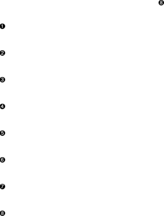
}
for (int i = 0; i < results.length; i++) {
System.out.println("Result[" + i + "]: type = " +
results[i].getClass().getSimpleName() + "; " + results[i]);
}
Create a list to hold all values.
Add a Put instance.
Add a Get instance for a different row.
Add a Delete instance.
Add a Get instance that will fail.
Create result array.
Print error that was caught.
Print all results and class types.
You should see the following output on the console:
Before batch call...
Cell: row1/colfam1:qual1/1/Put/vlen=4/seqid=0, Value: val1
Cell: row1/colfam1:qual2/2/Put/vlen=4/seqid=0, Value: val2
Cell: row1/colfam1:qual3/3/Put/vlen=4/seqid=0, Value: val3
Error: org.apache.hadoop.hbase.client.RetriesExhaustedWithDetailsException: \
Failed 1 action: \
org.apache.hadoop.hbase.regionserver.NoSuchColumnFamilyException: \
Column family BOGUS does not exist in ...
...
: 1 time,
Result[0]: type = Result; keyvalues=NONE
Result[1]: type = Result; keyvalues={row1/colfam1:qual1/1/Put/vlen=4/seqid=0}
Result[2]: type = Result; keyvalues=NONE
Result[3]: type = NoSuchColumnFamilyException; \
org.apache.hadoop.hbase.regionserver.NoSuchColumnFamilyException: \
org.apache.hadoop.hbase.regionserver.NoSuchColumnFamilyException: \
Column family BOGUS does not exist in ...
...
After batch call...
Cell: row1/colfam1:qual1/1/Put/vlen=4/seqid=0, Value: val1
Cell: row1/colfam1:qual3/3/Put/vlen=4/seqid=0, Value: val3
Cell: row2/colfam2:qual1/4/Put/vlen=4/seqid=0, Value: val5
(188)

As with the previous examples, there is some wiring behind the printed lines of code that inserts
a test row before executing the batch calls. The content is printed first, then you will see the
output from the example code, and finally the dump of the rows after everything else. The
deleted column was indeed removed, and the new column was added to the row as expected.
Finding the result of the Get operation requires you to investigate the middle part of the output,
that is, the lines printed by the example code. The lines starting with Result[n]--with n ranging
from zero to 3—is where you see the outcome of the corresponding operation in the batch
parameter. The first operation in the example is a Put, and the result is an empty Result instance,
containing no Cell instances. This is the general contract of the batch calls; they return a best
match result per input action, and the possible types are listed in Table 3-17.
Table 3-17. Possible result values returned by the batch() calls
Result Description
null The operation has failed to communicate with the remote server.
Empty
Result Returned for successful Put and Delete operations.
Result Returned for successful Get operations, but may also be empty when there was no
matching row or column.
Throwable
In case the servers return an exception for the operation it is returned to the client as-
is. You can use it to check what went wrong and maybe handle the problem
automatically in your code.
Looking through the returned result array in the console output you can see the empty Result
instances returned by the Put operation. They ouput keyvalues=NONE (Result[0]). The Get call also
succeeded and found a match, returning the Cell instances accordingly (Result[1]). The Delete
succeeded as well, and returned an empty Result instance (Result[2]). Finally, the operation with
the BOGUS column family has the exception for your perusal (Result[3]).
Note
When you use the batch() functionality, the included Put instances will not be buffered using the
client-side write buffer. The batch() calls are synchronous and send the operations directly to the
servers; no delay or other intermediate processing is used. This is obviously different compared
to the put() calls, so choose which one you want to use carefully.
All the operations are grouped by the destination region servers first and then sent to the servers,
just as explained and shown in Figure 3-2. Here we send many different operations though, not
just Put instances. The rest stays the same though, including the note there around the executor
pool used and its upper boundary on number of region servers (also see the
hbase.htable.threads.max configuration property). Suffice it to say that all operations are sent to
all affected servers in parallel, making this very efficient.
(189)
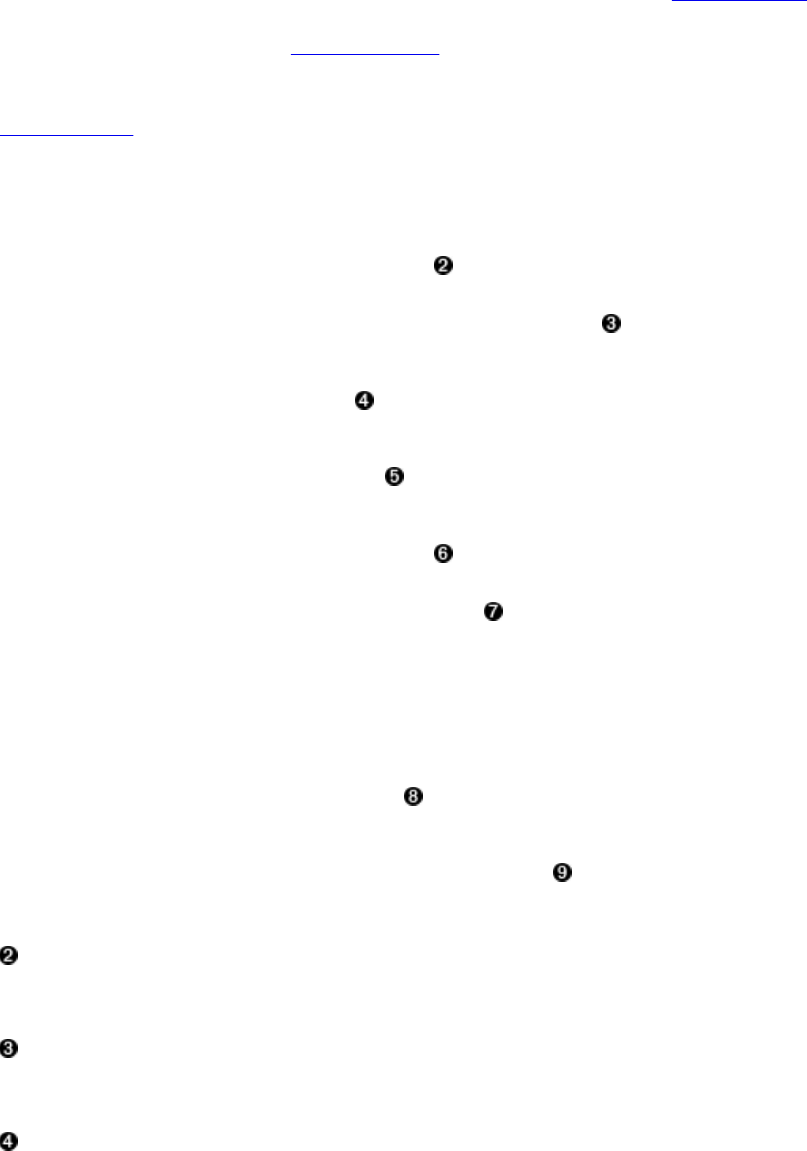
In addition, all batch operations are executed before the results are checked: even if you receive
an error for one of the actions, all the other ones have been applied. In a worst-case scenario, all
actions might return faults, though. On the other hand, the batch code is aware of transient errors,
such as the NotServingRegionException (indicating, for instance, that a region has been moved),
and is trying to apply the action(s) multiple times. The hbase.client.retries.number configuration
property (by default set to 35) can be adjusted to increase, or reduce, the number of retries.
There are two different batch calls that look very similar. The code in Example 3-26 makes use
of the first variant. The second one allows you to supply a callback instance (shared from the
coprocessor package, more in “Coprocessors”), which is invoked by the client library as it
receives the responses from the asynchronous and parallel calls to the server(s). You need to
implement the Batch.Callback interface, which provides the update() method called by the library.
Example 3-27 is a spin on the original example, just adding the callback instance—here
implemented as an anonymous inner class.
Example 3-27. Example application using batch operations with callbacks
List<Row> batch = new ArrayList<Row>();
Put put = new Put(ROW2);
put.addColumn(COLFAM2, QUAL1, 4, Bytes.toBytes("val5"));
batch.add(put);
Get get1 = new Get(ROW1);
get1.addColumn(COLFAM1, QUAL1);
batch.add(get1);
Delete delete = new Delete(ROW1);
delete.addColumns(COLFAM1, QUAL2);
batch.add(delete);
Get get2 = new Get(ROW2);
get2.addFamily(Bytes.toBytes("BOGUS"));
batch.add(get2);
Object[] results = new Object[batch.size()];
try {
table.batchCallback(batch, results, new Batch.Callback<Result>() {
@Override
public void update(byte[] region, byte[] row, Result result) {
System.out.println("Received callback for row[" +
Bytes.toString(row) + "] -> " + result);
}
});
} catch (Exception e) {
System.err.println("Error: " + e);
}
for (int i = 0; i < results.length; i++) {
System.out.println("Result[" + i + "]: type = " +
results[i].getClass().getSimpleName() + "; " + results[i]);
}
Create a list to hold all values.
Add a Put instance.
(190)

Add a Get instance for a different row.
Add a Delete instance.
Add a Get instance that will fail.
Create result array.
Print error that was caught.
Print all results and class types.
You should see the same output as in the example before, but with the additional information
emitted from the callback implementation, looking similar to this (further shortened for the sake
of brevity):
Before delete call...
Cell: row1/colfam1:qual1/1/Put/vlen=4/seqid=0, Value: val1
Cell: row1/colfam1:qual2/2/Put/vlen=4/seqid=0, Value: val2
Cell: row1/colfam1:qual3/3/Put/vlen=4/seqid=0, Value: val3
Received callback for row[row2] ->
keyvalues=NONE
Received callback for row[row1] ->
keyvalues={row1/colfam1:qual1/1/Put/vlen=4/seqid=0}
Received callback for row[row1] ->
keyvalues=NONE
Error: org.apache.hadoop.hbase.client.RetriesExhaustedWithDetailsException:
Failed 1 action:
...
: 1 time,
Result[0]: type = Result; keyvalues=NONE
Result[1]: type = Result; keyvalues={row1/colfam1:qual1/1/Put/vlen=4/seqid=0}
Result[2]: type = Result; keyvalues=NONE
Result[3]: type = NoSuchColumnFamilyException;
org.apache.hadoop.hbase.regionserver.NoSuchColumnFamilyException:
...
After batch call...
Cell: row1/colfam1:qual1/1/Put/vlen=4/seqid=0, Value: val1
Cell: row1/colfam1:qual3/3/Put/vlen=4/seqid=0, Value: val3
Cell: row2/colfam2:qual1/4/Put/vlen=4/seqid=0, Value: val5
The update() method in our example just prints out the information it has been given, here the
row key and the result of the operation. Obviously, in a more serious application the callback can
be used to immediately react to results coming back from servers, instead of waiting for all of
them to complete. Keep in mind that the overall runtime of the batch() call is dependent on the
slowest server to respond, maybe even to timeout after many retries. Using the callback can
improve client responsiveness as perceived by its users.
(191)

Introduction
Use of the scan operations is very similar to the get() methods. And again, similar to all the other
functions, there is also a supporting class, named Scan. But since scans are similar to iterators,
you do not have a scan() call, but rather a getScanner(), which returns the actual scanner instance
you need to iterate over. The available methods are:
ResultScanner getScanner(Scan scan) throws IOException
ResultScanner getScanner(byte[] family) throws IOException
ResultScanner getScanner(byte[] family, byte[] qualifier)
throws IOException
The latter two are for your convenience, implicitly creating an instance of Scan on your behalf,
and subsequently calling the getScanner(Scan scan) method.
The Scan class has the following constructors:
Scan()
Scan(byte[] startRow, Filter filter)
Scan(byte[] startRow)
Scan(byte[] startRow, byte[] stopRow)
Scan(Scan scan) throws IOException
Scan(Get get)
The difference between this and the Get class is immediately obvious: instead of specifying a
single row key, you now can optionally provide a startRow parameter—defining the row key
where the scan begins to read from the HBase table. The optional stopRow parameter can be used
to limit the scan to a specific row key where it should conclude the reading.
Note
The start row is always inclusive, while the end row is exclusive. This is often expressed as
[startRow, stopRow) in the interval notation.
A special feature that scans offer is that you do not need to have an exact match for either of
these rows. Instead, the scan will match the first row key that is equal to or larger than the given
start row. If no start row was specified, it will start at the beginning of the table. It will also end
its work when the current row key is equal to or greater than the optional stop row. If no stop
row was specified, the scan will run to the end of the table.
There is another optional parameter, named filter, referring to a Filter instance. Often, though,
the Scan instance is simply created using the empty constructor, as all of the optional parameters
also have matching getter and setter methods that can be used instead.
Like with the other data-related types, there is a convenience constructor to copy all parameter
from an existing Scan instance. There is also one that does the same from an existing Get instance.
You might be wondering why: the get and scan functionality is actually the same on the server
side. The only difference is that for a Get the scan has to include the stop row into the scan, since
both, the start and stop row are set to the same value. You will soon see that the Scan type has
more functionality over Get, but just because of its iterative nature. In addition, when using this
constructor based on a Get instance, the following method of Scan will return true as well:
boolean isGetScan()
(193)
Once you have created the Scan instance, you may want to add more limiting details to it—but
you are also allowed to use the empty scan, which would read the entire table, including all
column families and their columns. You can narrow down the read data using various methods:
Scan addFamily(byte [] family)
Scan addColumn(byte[] family, byte[] qualifier)
There is a lot of similar functionality compared to the Get class: you may limit the data returned
by the scan by setting the column families to specific ones using addFamily(), or, even more
constraining, to only include certain columns with the addColumn() call.
Note
If you only need subsets of the data, narrowing the scan’s scope is playing into the strengths of
HBase, since data is stored in column families and omitting entire families from the scan results
in those storage files not being read at all. This is the power of column family-oriented
architecture at its best.
Scan has other methods that are selective in nature, here are the first set that center around the cell
versions returned:
Scan setTimeStamp(long timestamp) throws IOException
Scan setTimeRange(long minStamp, long maxStamp) throws IOException
TimeRange getTimeRange()
Scan setMaxVersions()
Scan setMaxVersions(int maxVersions)
int getMaxVersions()
The setTimeStamp() method is shorthand for setting a time range with setTimeRange(time, time +
1), both resulting in a selection of cells that match the set range. Obviously the former is very
specific, selecting exactly one timestamp. getTimeRange() returns what was set by either method.
How many cells per column—in other words, how many versions—are returned by the scan are
controlled by setMaxVersions(), where one sets it to the given number, and the other to all
versions. The accompanying getter getMaxVersions() returns what was set.
The next set of methods relate to the rows that are included in the scan:
Scan setStartRow(byte[] startRow)
byte[] getStartRow()
Scan setStopRow(byte[] stopRow)
byte[] getStopRow()
Scan setRowPrefixFilter(byte[] rowPrefix)
Using setStartRow() and setStopRow() you can define the same parameters the constructors
exposed, all of them limiting the returned data even further, as explained earlier. The matching
getters return what is currently set (might be null since both are optional). The
setRowPrefixFilter() method is shorthand to set the start row to the value of the rowPrefix
parameter and the stop row to the next key that is greater than the current key: There is logic in
place to increment the binary key in such a way that it properly computes the next larger value.
For example, assume the row key is { 0x12, 0x23, 0xFF, 0xFF }, then incrementing it results in {
0x12, 0x24 }, since the last two bytes were already at their maximum value.
Next, there are methods around filters:
Filter getFilter()
Scan setFilter(Filter filter)
boolean hasFilter()
(194)

Filters are a special combination of time range and row based selectors. They go even further by
also adding column family and column name selection support. “Filters” explains them in full
detail, so for now please note that setFilter() assigns one or more filters to the scan. The
getFilter() call returns the current one—if set before--, and hasFilter() lets you check if there is
one set or not.
Then there are a few more specific methods provided by Scan, that handle particular use-cases.
You might consider them for advanced users only, but they really are straight forward, so let us
discuss them now, starting with:
Scan setReversed(boolean reversed)
boolean isReversed()
Scan setRaw(boolean raw)
boolean isRaw()
Scan setSmall(boolean small)
boolean isSmall()
The first pair enables the application to not iterate forward-only (as per the aforementioned
cursor reference) over rows, but do the same in reverse. Traditionally, HBase only provided the
forward scans, but recent versions14 of HBase introduced the reverse option. Since data is sorted
ascending (see [Link to Come] for details), doing a reverse scan involves some more involved
processing. In other words, reverse scans are slightly slower than forward scans, but alleviate the
previous necessity of building application-level lookup indexes for both directions. Now you can
do the same with a single one (we discuss this in “Secondary Indexes”).
One more subtlety to point out about reverse scans is that the reverse direction is per-row, but not
within a row. You still receive each row in a scan as if you were doing a forward scan, that is,
from the lowest lexicographically sorted column/cell ascending to the highest. Just each call to
next() on the scanner will return the previous row (or n rows) to you. More on iterating over
rows is discussed in “The ResultScanner Class”. Finally, when using reverse scans you also need
to flip around any start and stop row value, or you will not find anything at all (see Example 3-
28). In other words, if you want to scan, for example, row 20 to 10, you need to set the start row
to 20, and the stop row to 09 (assuming padding, and taking into consideration that the stop row
specified is excluded from the scan).
The second pair of methods, lead by setRaw(), switches the scanner into a special mode, returning
every cell it finds. This includes deleted cells that have not yet been removed physically, and also
the delete markers, as discussed in “Single Deletes”, and “The Cell”. This is useful, for example,
during backups, where you want to move everything from one cluster to another, including
deleted data. Making this more useful is the HColumnDescriptor.setKeepDeletedCells() method you
will learn about in “Column Families”.
The last pair of methods deal with small scans. These are scans that only ever need to read a very
small set of data, which can be returned in a single RPC. Calling setSmall(true) on a scan
instance instructs the client API to not do the usual open scanner, fetch data, and close scanner
combination of remote procedure calls, but do them in one single call. There are also some
server-side read optimizations in this mode, so the scan is as fast as possible.
Tip
What is the threshold for considering scans small? The rule of thumb is, that the data scanned
should ideally fit into one data block. By default the size of a block is 64 KB, but might be
different if customized cluster- or column family-wide. But this is not a hard limit. A small scan
(195)

might exceed a single block.
The isReversed(), isRaw(), and isSmall() return true if the respective setter has been invoked
beforehand.
The Scan class provides additional calls, which are listed in Table 3-18 for your perusal. As
before, you should recognize many of them as inherited methods from the Query superclass.
There are more methods described separately in the subsequent sections, since they warrant a
longer explanation.
Table 3-18. Quick overview of additional methods provided by the Scan class
Method Description
getACL()/setACL() The Access Control List (ACL) for this operation. See
[Link to Come] for details.
getAttribute()/setAttribute() Set and get arbitrary attributes associated with this
instance of Scan.
getAttributesMap() Returns the entire map of attributes, if any are set.
getAuthorizations()/setAuthorizations() Visibility labels for the operation. See [Link to Come]
for details.
getCacheBlocks()/setCacheBlocks() Specify if the server-side cache should retain blocks
that were loaded for this operation.
getConsistency()/setConsistency() The consistency level that applies to the current query
instance.
getFamilies() Returns an array of all stored families, i.e., containing
only the family names (as byte[] arrays).
getFamilyMap()/setFamilyMap()
These methods give you access to the column families
and specific columns, as added by the addFamily()
and/or addColumn() calls. The family map is a map
where the key is the family name and the value is a list
of added column qualifiers for this particular family.
getFilter()/setFilter() The filters that apply to the retrieval operation. See
“Filters” for details.
(196)

getFingerprint() Compiles details about the instance into a map for
debugging, or logging.
getId()/setId() An ID for the operation, useful for identifying the
origin of a request later.
getIsolationLevel()/setIsolationLevel() Specifies the read isolation level for the operation.
getReplicaId()/setReplicaId() Gives access to the replica ID that should serve the
data.
numFamilies()
Retrieves the size of the family map, containing the
families added using the addFamily() or addColumn()
calls.
hasFamilies() Another helper to check if a family—or column—has
been added to the current instance of the Scan class.
toJSON()/toJSON(int) Converts the first 5 or N columns into a JSON format.
toMap()/toMap(int) Converts the first 5 or N columns into a map. This is
more detailed than what getFingerprint() returns.
toString()/toString(int) Converts the first 5 or N columns into a JSON, or map
(if JSON fails due to encoding problems).
Refer to the end of “Single Gets” for an explanation of the above methods, for example
setCacheBlocks(). Others are explained in “Data Types and Hierarchy”.
Once you have configured the Scan instance, you can call the Table method, named getScanner(),
to retrieve the ResultScanner instance. We will discuss this class in more detail in the next section.
(197)

The ResultScanner Class
Scans usually do not ship all the matching rows in one RPC to the client, but instead do this on a
per-row basis. This obviously makes sense as rows could be very large and sending thousands,
and most likely more, of them in one call would use up too many resources, and take a long time.
The ResultScanner converts the scan into a get-like operation, wrapping the Result instance for
each row into an iterator functionality. It has a few methods of its own:
Result next() throws IOException
Result[] next(int nbRows) throws IOException
void close()
You have two types of next() calls at your disposal. The close() call is required to release all the
resources a scan may hold explicitly.
Scanner Leases
Make sure you release a scanner instance as quickly as possible. An open scanner holds quite a
few resources on the server side, which could accumulate and take up a large amount of heap
space. When you are done with the current scan call close(), and consider adding this into a
try/finally, or the previously explained try-with-resources construct to ensure it is called, even
if there are exceptions or errors during the iterations.
The example code does not follow this advice for the sake of brevity only.
Like row locks, scanners are protected against stray clients blocking resources for too long, using
the same lease-based mechanisms. You need to set the same configuration property to modify the
timeout threshold (in milliseconds):15
<property>
<name>hbase.client.scanner.timeout.period</name>
<value>120000</value>
</property>
You need to make sure that the property is set to a value that makes sense for locks as well as the
scanner leases.
The next() calls return a single instance of Result representing the next available row.
Alternatively, you can fetch a larger number of rows using the next(int nbRows) call, which
returns an array of up to nbRows items, each an instance of Result representing a unique row. The
resultant array may be shorter if there were not enough rows left—or could even be empty. This
obviously can happen just before you reach—or are at—the end of the table, or the stop row.
Otherwise, refer to “The Result class” for details on how to make use of the Result instances.
This works exactly like you saw in “Get Method”.
Note that next() might return null if you exhaust the table. But next(int nbRows) will always
return a valid array to you. It might be empty for the same reasons, you exhausted the table, but it
will be a valid array nevertheless. Example 3-28 brings together the explained functionality to
scan a table, while accessing the column data stored in a row.
(198)
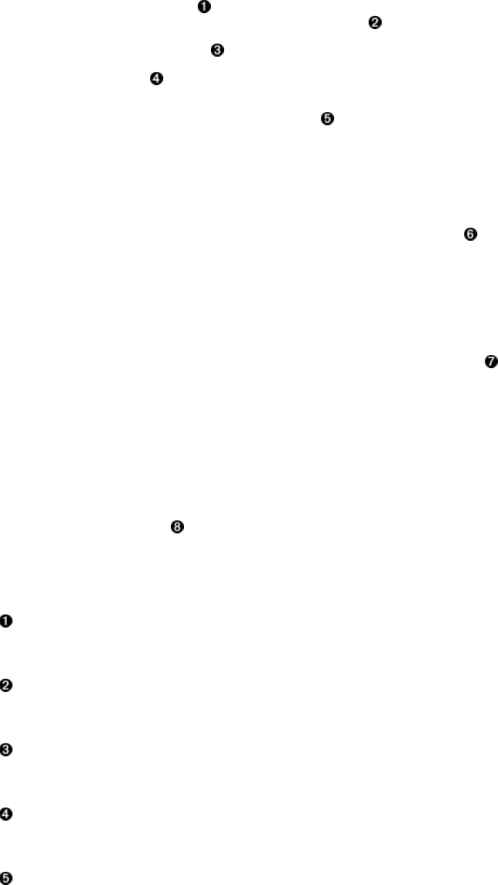
Example 3-28. Example using a scanner to access data in a table
Scan scan1 = new Scan();
ResultScanner scanner1 = table.getScanner(scan1);
for (Result res : scanner1) {
System.out.println(res);
}
scanner1.close();
Scan scan2 = new Scan();
scan2.addFamily(Bytes.toBytes("colfam1"));
ResultScanner scanner2 = table.getScanner(scan2);
for (Result res : scanner2) {
System.out.println(res);
}
scanner2.close();
Scan scan3 = new Scan();
scan3.addColumn(Bytes.toBytes("colfam1"), Bytes.toBytes("col-5")).
addColumn(Bytes.toBytes("colfam2"), Bytes.toBytes("col-33")).
setStartRow(Bytes.toBytes("row-10")).
setStopRow(Bytes.toBytes("row-20"));
ResultScanner scanner3 = table.getScanner(scan3);
for (Result res : scanner3) {
System.out.println(res);
}
scanner3.close();
Scan scan4 = new Scan();
scan4.addColumn(Bytes.toBytes("colfam1"), Bytes.toBytes("col-5")).
setStartRow(Bytes.toBytes("row-10")).
setStopRow(Bytes.toBytes("row-20"));
ResultScanner scanner4 = table.getScanner(scan4);
for (Result res : scanner4) {
System.out.println(res);
}
scanner4.close();
Scan scan5 = new Scan();
scan5.addColumn(Bytes.toBytes("colfam1"), Bytes.toBytes("col-5")).
setStartRow(Bytes.toBytes("row-20")).
setStopRow(Bytes.toBytes("row-10")).
setReversed(true);
ResultScanner scanner5 = table.getScanner(scan5);
for (Result res : scanner5) {
System.out.println(res);
}
scanner5.close();
Create empty Scan instance.
Get a scanner to iterate over the rows.
Print row content.
Close scanner to free remote resources.
Add one column family only, this will suppress the retrieval of “colfam2”.
(199)

Use fluent pattern to add specific details to the Scan.
Only select one column.
One column scan that runs in reverse.
The code inserts 100 rows with two column families, each containing 100 columns. The scans
performed vary from the full table scan, to one that only scans one column family, then to
another very restrictive scan, limiting the row range, and only asking for two very specific
columns. The final two limit the previous one to just a single column, and the last of those two
scans also reverses the scan order. The end of the abbreviated output should look like this:
...
Scanning table #4...
keyvalues={row-10/colfam1:col-5/1427010030763/Put/vlen=8/seqid=0}
keyvalues={row-100/colfam1:col-5/1427010039565/Put/vlen=9/seqid=0}
...
keyvalues={row-19/colfam1:col-5/1427010031928/Put/vlen=8/seqid=0}
keyvalues={row-2/colfam1:col-5/1427010029560/Put/vlen=7/seqid=0}
Scanning table #5...
keyvalues={row-20/colfam1:col-5/1427010032053/Put/vlen=8/seqid=0}
keyvalues={row-2/colfam1:col-5/1427010029560/Put/vlen=7/seqid=0}
...
keyvalues={row-11/colfam1:col-5/1427010030906/Put/vlen=8/seqid=0}
keyvalues={row-100/colfam1:col-5/1427010039565/Put/vlen=9/seqid=0}
Once again, note the actual rows that have been matched. The lexicographical sorting of the keys
makes for interesting results. You could simply pad the numbers with zeros, which would result
in a more human-readable sort order. This is completely under your control, so choose carefully
what you need. Also note how the stop row is exclusive in the scan results, meaning if you really
wanted all rows between 20 and 10 (for the reverse scan example), then specify row-20 as the start
and row-0 as the stop row. Try it yourself!
(200)

Scanner Caching
If not configured properly, then each call to next() would be a separate RPC for every row—
even when you use the next(int nbRows) method, because it is nothing else but a client-side loop
over next() calls. Obviously, this is not very good for performance when dealing with small cells
(see “Client-side Write Buffer” for a discussion). Thus it would make sense to fetch more than
one row per RPC if possible. This is called scanner caching and is enabled by default.
There is a cluster wide configuration property, named hbase.client.scanner.caching, which
controls the default caching for all scans. It is set to 10016 and will therefore instruct all scanners
to fetch 100 rows at a time, per RPC invocation. You can override this at the Scan instance level
with the following methods:
void setCaching(int caching)
int getCaching()
Specifying scan.setCaching(200) will increase the payload size to 200 rows per remote call. Both
types of next() take these settings into account. The getCaching() returns what is currently
assigned.
Note
You can also change the default value of 100 for the entire HBase setup. You do this by adding
the following configuration key to the hbase-site.xml configuration file:
<property>
<name>hbase.client.scanner.caching</name>
<value>200</value>
</property>
This would set the scanner caching to 200 for all instances of Scan. You can still override the
value at the scan level, but you would need to do so explicitly.
You may need to find a sweet spot between a low number of RPCs and the memory used on the
client and server. Setting the scanner caching higher will improve scanning performance most of
the time, but setting it too high can have adverse effects as well: each call to next() will take
longer as more data is fetched and needs to be transported to the client, and once you exceed the
maximum heap the client process has available it may terminate with an OutOfMemoryException.
Caution
When the time taken to transfer the rows to the client, or to process the data on the client,
exceeds the configured scanner lease threshold, you will end up receiving a lease expired error,
in the form of a ScannerTimeoutException being thrown.
Example 3-29 showcases the issue with the scanner leases.
Example 3-29. Example timeout while using a scanner
Scan scan = new Scan();
ResultScanner scanner = table.getScanner(scan);
(201)
int scannerTimeout = (int) conf.getLong(
HConstants.HBASE_CLIENT_SCANNER_TIMEOUT_PERIOD, -1);
try {
Thread.sleep(scannerTimeout + 5000);
} catch (InterruptedException e) {
// ignore
}
while (true){
try {
Result result = scanner.next();
if (result == null) break;
System.out.println(result);
} catch (Exception e) {
e.printStackTrace();
break;
}
}
scanner.close();
Get currently configured lease timeout.
Sleep a little longer than the lease allows.
Print row content.
The code gets the currently configured lease period value and sleeps a little longer to trigger the
lease recovery on the server side. The console output (abbreviated for the sake of readability)
should look similar to this:
Adding rows to table...
Current (local) lease period: 60000ms
Sleeping now for 65000ms...
Attempting to iterate over scanner...
org.apache.hadoop.hbase.client.ScannerTimeoutException: \
65017ms passed since the last invocation, timeout is currently set to 60000
at org.apache.hadoop.hbase.client.ClientScanner.next(ClientScanner.java)
at client.ScanTimeoutExample.main(ScanTimeoutExample.java:53)
...
Caused by: org.apache.hadoop.hbase.UnknownScannerException: \
org.apache.hadoop.hbase.UnknownScannerException: Name: 3915, already closed?
at org.apache.hadoop.hbase.regionserver.RSRpcServices.scan(...)
...
Caused by: org.apache.hadoop.hbase.ipc.RemoteWithExtrasException( \
org.apache.hadoop.hbase.UnknownScannerException): \
org.apache.hadoop.hbase.UnknownScannerException: Name: 3915, already closed?
at org.apache.hadoop.hbase.regionserver.RSRpcServices.scan(...)
...
Mar 22, 2015 9:55:22 AM org.apache.hadoop.hbase.client.ScannerCallable close
WARNING: Ignore, probably already closed
org.apache.hadoop.hbase.UnknownScannerException: \
org.apache.hadoop.hbase.UnknownScannerException: Name: 3915, already closed?
at org.apache.hadoop.hbase.regionserver.RSRpcServices.scan(...)
...
The example code prints its progress and, after sleeping for the specified time, attempts to iterate
over the rows the scanner should provide. This triggers the said timeout exception, while
reporting the configured values. You might be tempted to add the following into your code
Configuration conf = HBaseConfiguration.create()
conf.setLong(HConstants.HBASE_CLIENT_SCANNER_TIMEOUT_PERIOD, 120000)
(202)
assuming this increases the lease threshold (in this example, to two minutes). But that is not
going to work as the value is configured on the remote region servers, not your client application.
Your value is not being sent to the servers, and therefore will have no effect. If you want to
change the lease period setting you need to add the appropriate configuration key to the hbase-
site.xml file on the region servers—while not forgetting to restart (or reload) them for the
changes to take effect!
The stack trace in the console output also shows how the ScannerTimeoutException is a wrapper
around an UnknownScannerException. It means that the next() call is using a scanner ID that has
since expired and been removed in due course. In other words, the ID your client has memorized
is now unknown to the region servers—which is the namesake of the exception.
(203)
Scanner Batching
So far you have learned to use client-side scanner caching to make better use of bulk transfers
between your client application and the remote region’s servers. There is an issue, though, that
was mentioned in passing earlier: very large rows. Those—potentially—do not fit into the
memory of the client process, but rest assured that HBase and its client API have an answer for
that: batching. You can control batching using these calls:
void setBatch(int batch)
int getBatch()
As opposed to caching, which operates on a row level, batching works on the cell level instead. It
controls how many cells are retrieved for every call to any of the next() functions provided by
the ResultScanner instance. For example, setting the scan to use setBatch(5) would return five
cells per Result instance.
Note
When a row contains more cells than the value you used for the batch, you will get the entire row
piece by piece, with each next Result returned by the scanner.
The last Result may include fewer columns, when the total number of columns in that row is not
divisible by whatever batch it is set to. For example, if your row has 17 columns and you set the
batch to 5, you get four Result instances, containing 5, 5, 5, and the remaining two columns
respectively.
The combination of scanner caching and batch size can be used to control the number of RPCs
required to scan the row key range selected. Example 3-30 uses the two parameters to fine-tune
the size of each Result instance in relation to the number of requests needed.
Example 3-30. Example using caching and batch parameters for scans
private static void scan(int caching, int batch, boolean small)
throws IOException {
int count = 0;
Scan scan = new Scan()
.setCaching(caching)
.setBatch(batch)
.setSmall(small)
.setScanMetricsEnabled(true);
ResultScanner scanner = table.getScanner(scan);
for (Result result : scanner) {
count++;
}
scanner.close();
ScanMetrics metrics = scan.getScanMetrics();
System.out.println("Caching: " + caching + ", Batch: " + batch +
", Small: " + small + ", Results: " + count +
", RPCs: " + metrics.countOfRPCcalls);
}
public static void main(String[] args) throws IOException {
...
scan(1, 1, false);
scan(1, 0, false);
scan(1, 0, true);
scan(200, 1, false);
scan(200, 0, false);
(204)

scan(200, 0, true);
scan(2000, 100, false);
scan(2, 100, false);
scan(2, 10, false);
scan(5, 100, false);
scan(5, 20, false);
scan(10, 10, false);
...
}
Set caching and batch parameters.
Count the number of Results available.
Test various combinations.
The code prints out the values used for caching and batching, the number of results returned by
the servers, and how many RPCs were needed to get them. For example:
Caching: 1, Batch: 1, Small: false, Results: 200, RPCs: 203
Caching: 1, Batch: 0, Small: false, Results: 10, RPCs: 13
Caching: 1, Batch: 0, Small: true, Results: 10, RPCs: 0
Caching: 200, Batch: 1, Small: false, Results: 200, RPCs: 4
Caching: 200, Batch: 0, Small: false, Results: 10, RPCs: 3
Caching: 200, Batch: 0, Small: true, Results: 10, RPCs: 0
Caching: 2000, Batch: 100, Small: false, Results: 10, RPCs: 3
Caching: 2, Batch: 100, Small: false, Results: 10, RPCs: 8
Caching: 2, Batch: 10, Small: false, Results: 20, RPCs: 13
Caching: 5, Batch: 100, Small: false, Results: 10, RPCs: 5
Caching: 5, Batch: 20, Small: false, Results: 10, RPCs: 5
Caching: 10, Batch: 10, Small: false, Results: 20, RPCs: 5
You can tweak the two numbers to see how they affect the outcome. Table 3-19 lists a few
selected combinations. The numbers relate to Example 3-30, which creates a table with two
column families, adds 10 rows, with 10 columns per family in each row. This means there are a
total of 200 columns—or cells, as there is only one version for each column—with 20 columns
per row. The value in the RPCs column also includes the calls to open and close a scanner for
normal scans, increasing the count by two for every such scan. Small scans currently do not
report their counts and appear as zero.
Table 3-19. Example settings and their effects
Caching Batch Results RPCs Notes
1 1 200 203 Each column is returned as a separate Result instance. One more
RPC is needed to realize the scan is complete.
200 1 200 4 Each column is a separate Result, but they are all transferred in
one RPC (plus the extra check).
2 10 20 13 The batch is half the row width, so 200 divided by 10 is 20
Results needed. 10 RPCs (plus the check) to transfer them.
(205)
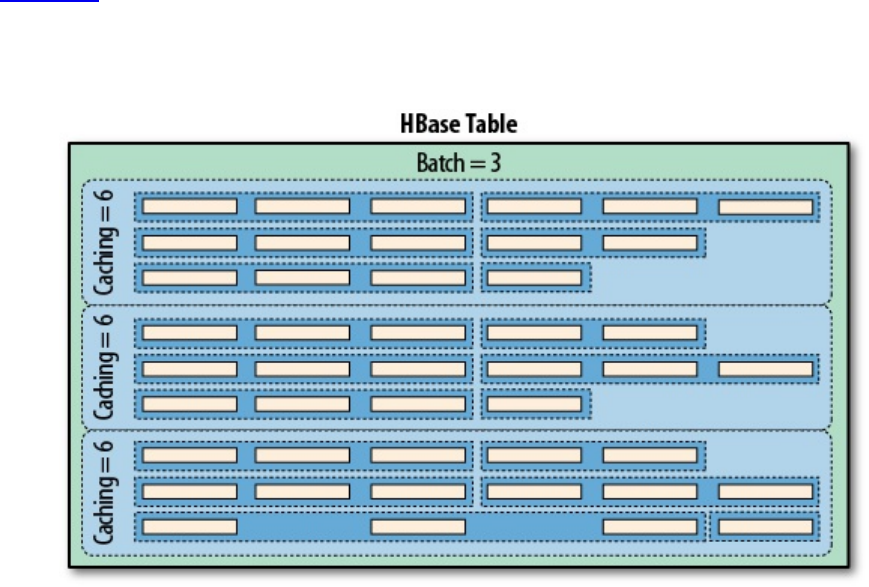
5 100 10 5
The batch is too large for each row, so all 20 columns are
batched. This requires 10 Result instances. Caching brings the
number of RPCs down to two (plus the check).
5 20 10 5 This is the same as above, but this time the batch matches the
columns available. The outcome is the same.
10 10 20 5 This divides the table into smaller Result instances, but larger
caching also means only two RPCs are needed.
To compute the number of RPCs required for a scan, you need to first multiply the number of
rows with the number of columns per row (at least some approximation). Then you divide that
number by the smaller value of either the batch size or the columns per row. Finally, divide that
number by the scanner caching value. In mathematical terms this could be expressed like so:
RPCs = (Rows * Cols per Row) / Min(Cols per Row, Batch Size) / Scanner Caching
Figure 3-3 shows how the caching and batching works in tandem. It has a table with nine rows,
each containing a number of columns. Using a scanner caching of six, and a batch set to three,
you can see that three RPCs are necessary to ship the data across the network (the dashed,
rounded-corner boxes).
Figure 3-3. The scanner caching and batching controlling the number of RPCs
The small batch value causes the servers to group three columns into one Result, while the
scanner caching of six causes one RPC to transfer six rows—or, more precisely, results--sent in
the batch. When the batch size is not specified but scanner caching is specified, the result of the
call will contain complete rows, because each row will be contained in one Result instance. Only
when you start to use the batch mode are you getting access to the intra-row scanning
(206)
functionality.
You may not have to worry about the consequences of using scanner caching and batch mode
initially, but once you try to squeeze the optimal performance out of your setup, you should keep
all of this in mind and find the sweet spot for both values.
Finally, batching cannot be combined with filters that return true from their hasFilterRow()
method. Such filters cannot deal with partial results, in other words, the row being chunked into
batches. It needs to see the entire row to make a filtering decision. It might be that the important
column needed for that decision is not yet present. Or, it could be that there have been batches of
results sent to the client already, just to realize later that the entire row should have been skipped.
Another combination disallowed is batching with small scans. The latter are an optimization
returning the entire result in one call, not in further, smaller chunks. If you try to set the scan
batching and small scan flag together, you will receive an IllegalArgumentException exception in
due course.
(207)

Slicing Rows
But wait, this is not all you can do with scans! There is more, and first we will discuss the related
slicing of table data using the following methods:
int getMaxResultsPerColumnFamily()
Scan setMaxResultsPerColumnFamily(int limit)
int getRowOffsetPerColumnFamily()
Scan setRowOffsetPerColumnFamily(int offset)
long getMaxResultSize()
Scan setMaxResultSize(long maxResultSize)
The first four work together by allowing the application to cut out a piece of each row selected,
using an offset to start from a specific column, and a max results per column family limit to stop
returning data once reached. The latter pair of functions allow to add (and retrieve) an upper size
limit of the data returned by the scan. It keeps a running tally of the cells selected by the scan and
stops returning them once the size limit is exceeded. Example 3-31 shows this in action:
Example 3-31. Example using offset and limit parameters for scans
private static void scan(int num, int caching, int batch, int offset,
int maxResults, int maxResultSize, boolean dump) throws IOException {
int count = 0;
Scan scan = new Scan()
.setCaching(caching)
.setBatch(batch)
.setRowOffsetPerColumnFamily(offset)
.setMaxResultsPerColumnFamily(maxResults)
.setMaxResultSize(maxResultSize)
.setScanMetricsEnabled(true);
ResultScanner scanner = table.getScanner(scan);
System.out.println("Scan #" + num + " running...");
for (Result result : scanner) {
count++;
if (dump) System.out.println("Result [" + count + "]:" + result);
}
scanner.close();
ScanMetrics metrics = scan.getScanMetrics();
System.out.println("Caching: " + caching + ", Batch: " + batch +
", Offset: " + offset + ", maxResults: " + maxResults +
", maxSize: " + maxResultSize + ", Results: " + count +
", RPCs: " + metrics.countOfRPCcalls);
}
public static void main(String[] args) throws IOException {
...
scan(1, 11, 0, 0, 2, -1, true);
scan(2, 11, 0, 4, 2, -1, true);
scan(3, 5, 0, 0, 2, -1, false);
scan(4, 11, 2, 0, 5, -1, true);
scan(5, 11, -1, -1, -1, 1, false);
scan(6, 11, -1, -1, -1, 10000, false);
...
}
The example’s hidden scaffolding creates a table with two column families, with ten rows and
ten columns in each family. The output, abbreviated, looks something like this:
Scan #1 running...
Result [1]:keyvalues={row-01/colfam1:col-01/1/Put/vlen=9/seqid=0,
row-01/colfam1:col-02/2/Put/vlen=9/seqid=0,
row-01/colfam2:col-01/1/Put/vlen=9/seqid=0,
row-01/colfam2:col-02/2/Put/vlen=9/seqid=0}
(208)
...
Result [10]:keyvalues={row-10/colfam1:col-01/1/Put/vlen=9/seqid=0,
row-10/colfam1:col-02/2/Put/vlen=9/seqid=0,
row-10/colfam2:col-01/1/Put/vlen=9/seqid=0,
row-10/colfam2:col-02/2/Put/vlen=9/seqid=0}
Caching: 11, Batch: 0, Offset: 0, maxResults: 2, maxSize: -1,
Results: 10, RPCs: 3
Scan #2 running...
Result [1]:keyvalues={row-01/colfam1:col-05/5/Put/vlen=9/seqid=0,
row-01/colfam1:col-06/6/Put/vlen=9/seqid=0,
row-01/colfam2:col-05/5/Put/vlen=9/seqid=0,
row-01/colfam2:col-06/6/Put/vlen=9/seqid=0}
...
Result [10]:keyvalues={row-10/colfam1:col-05/5/Put/vlen=9/seqid=0,
row-10/colfam1:col-06/6/Put/vlen=9/seqid=0,
row-10/colfam2:col-05/5/Put/vlen=9/seqid=0,
row-10/colfam2:col-06/6/Put/vlen=9/seqid=0}
Caching: 11, Batch: 0, Offset: 4, maxResults: 2, maxSize: -1,
Results: 10, RPCs: 3
Scan #3 running...
Caching: 5, Batch: 0, Offset: 0, maxResults: 2, maxSize: -1,
Results: 10, RPCs: 5
Scan #4 running...
Result [1]:keyvalues={row-01/colfam1:col-01/1/Put/vlen=9/seqid=0,
row-01/colfam1:col-02/2/Put/vlen=9/seqid=0}
Result [2]:keyvalues={row-01/colfam1:col-03/3/Put/vlen=9/seqid=0,
row-01/colfam1:col-04/4/Put/vlen=9/seqid=0}
...
Result [31]:keyvalues={row-10/colfam1:col-03/3/Put/vlen=9/seqid=0,
row-10/colfam1:col-04/4/Put/vlen=9/seqid=0}
Result [32]:keyvalues={row-10/colfam1:col-05/5/Put/vlen=9/seqid=0}
Caching: 11, Batch: 2, Offset: 0, maxResults: 5, maxSize: -1,
Results: 32, RPCs: 5
Scan #5 running...
Caching: 11, Batch: -1, Offset: -1, maxResults: -1, maxSize: 1,
Results: 10, RPCs: 13
Scan #6 running...
Caching: 11, Batch: -1, Offset: -1, maxResults: -1, maxSize: 10000,
Results: 10, RPCs: 5
The first scan starts at offset 0 and asks for a maximum of 2 cells, returning columns one and two.
The second scan does the same but sets the offset to 4, therefore retrieving the columns five to
six. Note how the offset really defines the number of cells to skip initially, and our value of 4
causes the first four columns to be skipped.
The next scan, #3, does not emit anything, since we are only interested in the metrics. It is the
same as scan #1, but using a caching value of 5. You will notice how the minimal amount of
RPCs is 3 (open, fetch, and close call for a non-small scanner). Here we see 5 RPCs that have
taken place, which makes sense, since now we cannot fetch our 10 results in one call, but need
two calls with five results each, plus an additional one to figure that there are no more rows left.
Scan #4 is combining the previous scans with a batching value of 2, so up to two cells are
returned per call to next(), but at the same time we limit the amount of cells returned per column
family to 5. Additionally combined with the caching value of 11 we see five RPCs made to the
server.
Finally, scan #5 and #6 are using setMaxResultSize() to limit the amount of data returned to the
caller. Just to recall, the scanner caching is set as number of rows, while the max result size is
specified in bytes. What do we learn from the metrics (the rows are omitted as both print the
entire table) as printed in the output?
(209)

We need to set the caching to 11 to fetch all ten rows in our example in one RPC. When
you set it to 10 an extra RPC is incurred, just to realize that there are no more rows.
The caching setting is bound by the max result size, so in scan #5 we force the servers to
return every row as a separate result, because setting the max result size to 1 byte means
we cannot ship more than one row in a call. The caching is rendered useless.
Even if we set the max result size to 1 byte, we still get at least one row per request.
Which means, for very large rows we might still experience memory pressure.17
The max result size should be set as an upper boundary that could be computed as max
result size = caching * average row size. The idea is to fit in enough rows into the max
result size but still ensure that caching is working.
This is a rather involved section, showing you how to tweak many scan parameters to optimize
the communication with the region servers. Like I mentioned a few times so far, your mileage
may vary, so please test this carefully and evaluate your options.
(210)
Load Column Families on Demand
Scans have another advanced feature, one that deserves a longer explanation: loading column
families on demand. This is controlled by the following methods:
Scan setLoadColumnFamiliesOnDemand(boolean value)
Boolean getLoadColumnFamiliesOnDemandValue()
boolean doLoadColumnFamiliesOnDemand()
This functionality is a read optimization, useful only for tables with more than one column
family, and especially then for those use-cases with a dependency between data in those families.
For example, assume you have one family with meta data, and another with a heavier payload.
You want to scan the meta data columns, and if a particular flag is present in one column, you
need to access the payload data in the other family. It would be costly to include both families
into the scan if you expect the cardinality of the flag to be low (in comparison to the table size).
This is because such a scan would load the payload for every row, just to then ignore it. Enabling
this feature with setLoadColumnFamiliesOnDemand(true) is only half the of the preparation work:
you also need a filter that implements the following method, returning a boolean flag:
boolean isFamilyEssential(byte[] name) throws IOException
The idea is that the filter is the decision maker if a column family is essential or not. When the
servers scan the data, they first set up internal scanners for each column family. If load column
families on demand is enabled and a filter set, it calls out to the filter and asks it to decide if an
included column family is to be scanned or not. The filter’s isFamilyEssential() is invoked with
the name of the family under consideration, before the column family is added, and must return
true to approve. If it returns false, then the column family is ignored for now and loaded on
demand later if needed.
On the other hand, you must add all column families to the scan, no matter if they are essential or
not. The framework will only consult the filter about the inclusion of a family, if they have been
added in the first place. If you do not explicitly specify any family, then you are OK. But as soon
as you start using the addColumn() or addFamily() methods of Scan, then you have to ensure you
add the non-essential columns or families too.
(211)

Scanner Metrics
The Example 3-30 uses another feature of the scan class, allowing the client to reason about the
effectiveness of the operation. This is accomplished with the following methods:
Scan setScanMetricsEnabled(final boolean enabled)
boolean isScanMetricsEnabled()
ScanMetrics getScanMetrics()
As shown in the example, you can enable the collection of scan metrics by invoking
setScanMetricsEnabled(true). Once the scan is complete you can retrieve the ScanMetrics using the
getScanMetrics() method. The isScanMetricsEnabled() is a check if the collection of metrics has
been enabled previously. The returned ScanMetrics instance has a set of fields you can read to
determine what cost the operation accrued:
Table 3-20. Metrics provided by the ScanMetrics class
Metric Field Description
countOfRPCcalls The total amount of RPC calls incurred by the scan.
countOfRemoteRPCcalls The amount of RPC calls to a remote host.
sumOfMillisSecBetweenNexts The sum of milliseconds between sequential next() calls.
countOfNSRE Number of NotServingRegionException caught.
countOfBytesInResults Number of bytes in Result instances returned by the servers.
countOfBytesInRemoteResults Same as above, but for bytes transferred from remote servers.
countOfRegions Number of regions that were involved in the scan.
countOfRPCRetries Number of RPC retries incurred during the scan.
countOfRemoteRPCRetries Same again, but RPC retries for non-local servers.
In the example we are printing the countOfRPCcalls field, since we want to figure out how many
calls have taken place. When running the example code locally the countOfRemoteRPCcalls would
be zero, as all RPC calls are made to the very same machine. Since scans are executed by region
servers, and iterate over all regions included in the selected row range, the metrics are internally
collected region by region and accumulated in the ScanMetrics instance of the Scan object. While
(212)
it is possible to call upon the metrics as the scan is taking place, only at the very end of the scan
will you see the final count.
(213)
Miscellaneous Features
Before looking into more involved features that clients can use, let us first wrap up a handful of
miscellaneous features and functionality provided by HBase and its client API.
(214)

The Table Utility Methods
The client API is represented by an instance of the Table class and gives you access to an existing
HBase table. Apart from the major features we already discussed, there are a few more notable
methods of this class that you should be aware of:
void close()
This method was mentioned before, but for the sake of completeness, and its importance, it
warrants repeating. Call close() once you have completed your work with a table. There is
some internal housekeeping work that needs to run, and invoking this method triggers this
process. Wrap the opening and closing of a table into a try/catch, or even better (on Java 7
or later), a try-with-resources block.
TableName getName()
This is a convenience method to retrieve the table name. It is provided as an instance of the
TableName class, providing access to the namespace and actual table name.
Configuration getConfiguration()
This allows you to access the configuration in use by the Table instance. Since this is
handed out by reference, you can make changes that are effective immediately.
HTableDescriptor getTableDescriptor()
Each table is defined using an instance of the HTableDescriptor class. You gain access to
the underlying definition using getTableDescriptor().
For more information about the management of tables using the administrative API, please
consult “Tables”.
(215)

The Bytes Class
You saw how this class was used to convert native Java types, such as String, or long, into the
raw, byte array format HBase supports natively. There are a few more notes that are worth
mentioning about the class and its functionality. Most methods come in three variations, for
example:
static long toLong(byte[] bytes)
static long toLong(byte[] bytes, int offset)
static long toLong(byte[] bytes, int offset, int length)
You hand in just a byte array, or an array and an offset, or an array, an offset, and a length value.
The usage depends on the originating byte array you have. If it was created by toBytes()
beforehand, you can safely use the first variant, and simply hand in the array and nothing else.
All the array contains is the converted value.
The API, and HBase internally, store data in larger arrays using, for example, the following call:
static int putLong(byte[] bytes, int offset, long val)
This call allows you to write the long value into a given byte array, at a specific offset. If you
want to access the data in that larger byte array you can make use of the latter two toLong() calls
instead. The length parameter is a bit of an odd one as it has to match the length of the native
type, in other words, if you try to convert a long from a byte[] array but specify 2 as the length,
the conversion will fail with an IllegalArgumentException error. In practice, you should really
only have to deal with the first two variants of the method.
The Bytes class has support to convert from and to the following native Java types: String,
boolean, short, int, long, double, float, ByteBuffer, and BigDecimal. Apart from that, there are some
noteworthy methods, which are listed in Table 3-21.
Table 3-21. Overview of additional methods provided by the Bytes class
Method Description
toStringBinary()
While working very similar to toString(), this variant has an extra
safeguard to convert non-printable data into human-readable hexadecimal
numbers. Whenever you are not sure what a byte array contains you should
use this method to print its content, for example, to the console, or into a
log file.
compareTo()/equals()
These methods allow you to compare two byte[], that is, byte arrays. The
former gives you a comparison result and the latter a boolean value,
indicating whether the given arrays are equal to each other.
add()/head()/tail()
You can use these to combine two byte arrays, resulting in a new,
concatenated array, or to get the first, or last, few bytes of the given byte
array.
(216)

binarySearch()
This performs a binary search in the given array of values. It operates on
byte arrays for the values and the key you are searching for.
incrementBytes()
This increments a long value in its byte array representation, as if you had
used toBytes(long) to create it. You can decrement using a negative amount
parameter.
There is some overlap of the Bytes class with the Java-provided ByteBuffer. The difference is that
the former does all operations without creating new class instances. In a way it is an
optimization, because the provided methods are called many times within HBase, while avoiding
possibly costly garbage collection issues.
For the full documentation, please consult the JavaDoc-based API documentation.18
1 The region servers use a multiversion concurrency control mechanism, implemented internally
by the MultiVersionConsistencyControl (MVCC) class, to guarantee that readers can read without
having to wait for writers. Equally, writers do need to wait for other writers to complete before
they can continue.
2 As of this writing, there is unfortunately a disparity in spelling in these methods.
3 Available since HBase 1.0 as part of HBASE-10070.
4 This was introduced in HBase 0.94 as HBASE-4938.
5 See “Unix time” on Wikipedia.
6 See HBASE-6580, which introduced the getTable() in 0.98 and 0.96 (also backported to
0.94.11).
7 Universally Unique Identifier; see http://en.wikipedia.org/wiki/Universally_unique_identifier
for details.
8 In HBase versions before 1.0 these methods were named add(). They have been deprecated in
favor of a coherent naming convention with Get and other API classes. “Migrate API to HBase
1.0.x” has more info.
9 This was changed in 1.0.0 from KeyValue. Cell is now the proper public API class, while
KeyValue is only used internally.
10 This class replaces the functionality that used to be available via
HTableInterface#setAutoFlush(false) in HBase before 1.0.0.
11 Be wary as this might change in future versions.
12 For easier readability, the related details were broken up into groups using blank lines.
(217)

13 Scans are similar to nonscrollable cursors. You need to declare, open, fetch, and eventually
close a database cursor. While scans do not need the declaration step, they are otherwise used in
the same way. See “Cursors” on Wikipedia.
14 This was added in HBase 0.98, with HBASE-4811.
15 This property was called hbase.regionserver.lease.period in earlier versions of HBase.
16 This was changed from 1 in releases before 0.96. See HBASE-7008 for details.
17 This has been addressed with implicit row chunking in HBase 1.1.0 and later. See HBASE-
11544 for details.
18 See the Bytes documentation online.
(218)
Chapter 4. Client API: Advanced Features
Now that you understand the basic client API, we will discuss the advanced features that HBase
offers to clients.
(219)
Filters
HBase filters are a powerful feature that can greatly enhance your effectiveness when working
with data stored in tables. You will find predefined filters, already provided by HBase for your
use, as well as a framework you can use to implement your own. You will now be introduced to
both.
(220)

Introduction to Filters
The two prominent read functions for HBase are Table.get() and Table.scan(), both supporting
either direct access to data or the use of a start and end key, respectively. You can limit the data
retrieved by progressively adding more limiting selectors to the query. These include column
families, column qualifiers, timestamps or ranges, as well as version numbers.
While this gives you control over what is included, it is missing more fine-grained features, such
as selection of keys, or values, based on regular expressions. Both classes support filters for
exactly these reasons: what cannot be solved with the provided API functionality selecting the
required row or column keys, or values, can be achieved with filters. The base interface is aptly
named Filter, and there is a list of concrete classes supplied by HBase that you can use without
doing any programming.
You can, on the other hand, extend the Filter classes to implement your own requirements. All
the filters are actually applied on the server side, also referred to as predicate pushdown. This
ensures the most efficient selection of the data that needs to be transported back to the client.
You could implement most of the filter functionality in your client code as well, but you would
have to transfer much more data—something you need to avoid at scale.
Figure 4-1 shows how the filters are configured on the client, then serialized over the network,
and then applied on the server.
Figure 4-1. The filters created on the client side, sent through the RPC, and executed on the server side
The Filter Hierarchy
The lowest level in the filter hierarchy is the Filter interface, and the abstract FilterBase class
that implements an empty shell, or skeleton, that is used by the actual filter classes to avoid
having the same boilerplate code in each of them. Most concrete filter classes are direct
(221)

descendants of FilterBase, but a few use another, intermediate ancestor class. They all work the
same way: you define a new instance of the filter you want to apply and hand it to the Get or Scan
instances, using:
setFilter(filter)
While you initialize the filter instance itself, you often have to supply parameters for whatever
the filter is designed for. There is a special subset of filters, based on CompareFilter, that ask you
for at least two specific parameters, since they are used by the base class to perform its task. You
will learn about the two parameter types next so that you can use them in context.
Filters have access to the entire row they are applied to. This means that they can decide the fate
of a row based on any available information. This includes the row key, column qualifiers, actual
value of a column, timestamps, and so on. When referring to values, or comparisons, as we will
discuss shortly, this can be applied to any of these details. Specific filter implementations are
available that consider only one of those criteria each.
While filters can apply their logic to a specific row, they have no state and cannot span across
multiple rows. There are also some scan related features—such as batching (see “Scanner
Batching”)--that counteract the ability of a filter to do its work. We will discuss these limitations
in due course below.
Comparison Operators
As CompareFilter-based filters add one more feature to the base FilterBase class, namely the
compare() operation, it has to have a user-supplied operator type that defines how the result of the
comparison is interpreted. The values are listed in Table 4-1.
Table 4-1. The possible comparison operators for CompareFilter-based filters
Operator Description
LESS Match values less than the provided one.
LESS_OR_EQUAL Match values less than or equal to the provided one.
EQUAL Do an exact match on the value and the provided one.
NOT_EQUAL Include everything that does not match the provided value.
GREATER_OR_EQUAL Match values that are equal to or greater than the provided one.
GREATER Only include values greater than the provided one.
NO_OP Exclude everything.
(222)

The comparison operators define what is included, or excluded, when the filter is applied. This
allows you to select the data that you want as either a range, subset, or exact and single match.
Comparators
The second type that you need to provide to CompareFilter-related classes is a comparator, which
is needed to compare various values and keys in different ways. They are derived from
ByteArrayComparable, which implements the Java Comparable interface. You do not have to go into
the details if you just want to use an implementation provided by HBase and listed in Table 4-2.
The constructors usually take the control value, that is, the one to compare each table value
against.
Table 4-2. The HBase-supplied comparators, used with CompareFilter-based filters
Comparator Description
LongComparator Assumes the given value array is a Java Long number and uses
Bytes.toLong() to convert it.
BinaryComparator Uses Bytes.compareTo() to compare the current with the provided value.
BinaryPrefixComparator Similar to the above, but only compares up to the provided value’s
length.
NullComparator Does not compare against an actual value, but checks whether a given
one is null, or not null.
BitComparator Performs a bitwise comparison, providing a BitwiseOp enumeration with
AND, OR, and XOR operators.
RegexStringComparator Given a regular expression at instantiation, this comparator does a
pattern match on the data.
SubstringComparator Treats the value and table data as String instances and performs a
contains() check.
Caution
The last four comparators listed in Table 4-2—the NullComparator, BitComparator,
RegexStringComparator, and SubstringComparator—only work with the EQUAL and NOT_EQUAL
operators, as the compareTo() of these comparators returns 0 for a match or 1 when there is no
match. Using them in a LESS or GREATER comparison will yield erroneous results.
(223)

Each of the comparators usually has a constructor that takes the comparison value. In other
words, you need to define a value you compare each cell against. Some of these constructors take
a byte[], a byte array, to do the binary comparison, for example, while others take a String
parameter—since the data point compared against is assumed to be some sort of readable text.
Example 4-1 shows some of these in action.
Caution
The string-based comparators, RegexStringComparator and SubstringComparator, are more
expensive in comparison to the purely byte-based versions, as they need to convert a given value
into a String first. The subsequent string or regular expression operation also adds to the overall
cost.
(224)

Comparison Filters
The first type of supplied filter implementations are the comparison filters. They take the
comparison operator and comparator instance as described above. The constructor of each of
them has the same signature, inherited from CompareFilter:
CompareFilter(final CompareOp compareOp, final ByteArrayComparable comparator)
You need to supply the comparison operator and comparison class for the filters to do their work.
Next you will see the actual filters implementing a specific comparison.
Please keep in mind that the general contract of the HBase filter API means you are filtering out
information—filtered data is omitted from the results returned to the client. The filter is not
specifying what you want to have, but rather what you do not want to have returned when
reading data.
In contrast, all filters based on CompareFilter are doing the opposite, in that they include the
matching values. In other words, be careful when choosing the comparison operator, as it makes
the difference in regard to what the server returns. For example, instead of using LESS to skip
some information, you may need to use GREATER_OR_EQUAL to include the desired data points.
RowFilter
This filter gives you the ability to filter data based on row keys.
Example 4-1 shows how the filter can use different comparator instances to get the desired
results. It also uses various operators to include the row keys, while omitting others. Feel free to
modify the code, changing the operators to see the possible results.
Example 4-1. Example using a filter to select specific rows
Scan scan = new Scan();
scan.addColumn(Bytes.toBytes("colfam1"), Bytes.toBytes("col-1"));
Filter filter1 = new RowFilter(CompareFilter.CompareOp.LESS_OR_EQUAL,
new BinaryComparator(Bytes.toBytes("row-22")));
scan.setFilter(filter1);
ResultScanner scanner1 = table.getScanner(scan);
for (Result res : scanner1) {
System.out.println(res);
}
scanner1.close();
Filter filter2 = new RowFilter(CompareFilter.CompareOp.EQUAL,
new RegexStringComparator(".*-.5"));
scan.setFilter(filter2);
ResultScanner scanner2 = table.getScanner(scan);
for (Result res : scanner2) {
System.out.println(res);
}
scanner2.close();
Filter filter3 = new RowFilter(CompareFilter.CompareOp.EQUAL,
new SubstringComparator("-5"));
scan.setFilter(filter3);
ResultScanner scanner3 = table.getScanner(scan);
for (Result res : scanner3) {
(225)

System.out.println(res);
}
scanner3.close();
Create filter, while specifying the comparison operator and comparator. Here an exact
match is needed.
Another filter, this time using a regular expression to match the row keys.
The third filter uses a substring match approach.
Here is the full printout of the example on the console:
Adding rows to table...
Scanning table #1...
keyvalues={row-1/colfam1:col-1/1427273897619/Put/vlen=7/seqid=0}
keyvalues={row-10/colfam1:col-1/1427273899185/Put/vlen=8/seqid=0}
keyvalues={row-100/colfam1:col-1/1427273908651/Put/vlen=9/seqid=0}
keyvalues={row-11/colfam1:col-1/1427273899343/Put/vlen=8/seqid=0}
keyvalues={row-12/colfam1:col-1/1427273899496/Put/vlen=8/seqid=0}
keyvalues={row-13/colfam1:col-1/1427273899643/Put/vlen=8/seqid=0}
keyvalues={row-14/colfam1:col-1/1427273899785/Put/vlen=8/seqid=0}
keyvalues={row-15/colfam1:col-1/1427273899925/Put/vlen=8/seqid=0}
keyvalues={row-16/colfam1:col-1/1427273900064/Put/vlen=8/seqid=0}
keyvalues={row-17/colfam1:col-1/1427273900202/Put/vlen=8/seqid=0}
keyvalues={row-18/colfam1:col-1/1427273900343/Put/vlen=8/seqid=0}
keyvalues={row-19/colfam1:col-1/1427273900484/Put/vlen=8/seqid=0}
keyvalues={row-2/colfam1:col-1/1427273897860/Put/vlen=7/seqid=0}
keyvalues={row-20/colfam1:col-1/1427273900623/Put/vlen=8/seqid=0}
keyvalues={row-21/colfam1:col-1/1427273900757/Put/vlen=8/seqid=0}
keyvalues={row-22/colfam1:col-1/1427273900881/Put/vlen=8/seqid=0}
Scanning table #2...
keyvalues={row-15/colfam1:col-1/1427273899925/Put/vlen=8/seqid=0}
keyvalues={row-25/colfam1:col-1/1427273901253/Put/vlen=8/seqid=0}
keyvalues={row-35/colfam1:col-1/1427273902480/Put/vlen=8/seqid=0}
keyvalues={row-45/colfam1:col-1/1427273903582/Put/vlen=8/seqid=0}
keyvalues={row-55/colfam1:col-1/1427273904633/Put/vlen=8/seqid=0}
keyvalues={row-65/colfam1:col-1/1427273905577/Put/vlen=8/seqid=0}
keyvalues={row-75/colfam1:col-1/1427273906453/Put/vlen=8/seqid=0}
keyvalues={row-85/colfam1:col-1/1427273907327/Put/vlen=8/seqid=0}
keyvalues={row-95/colfam1:col-1/1427273908211/Put/vlen=8/seqid=0}
Scanning table #3...
keyvalues={row-5/colfam1:col-1/1427273898394/Put/vlen=7/seqid=0}
keyvalues={row-50/colfam1:col-1/1427273904116/Put/vlen=8/seqid=0}
keyvalues={row-51/colfam1:col-1/1427273904219/Put/vlen=8/seqid=0}
keyvalues={row-52/colfam1:col-1/1427273904324/Put/vlen=8/seqid=0}
keyvalues={row-53/colfam1:col-1/1427273904428/Put/vlen=8/seqid=0}
keyvalues={row-54/colfam1:col-1/1427273904536/Put/vlen=8/seqid=0}
keyvalues={row-55/colfam1:col-1/1427273904633/Put/vlen=8/seqid=0}
keyvalues={row-56/colfam1:col-1/1427273904729/Put/vlen=8/seqid=0}
keyvalues={row-57/colfam1:col-1/1427273904823/Put/vlen=8/seqid=0}
keyvalues={row-58/colfam1:col-1/1427273904919/Put/vlen=8/seqid=0}
keyvalues={row-59/colfam1:col-1/1427273905015/Put/vlen=8/seqid=0}
You can see how the first filter did an exact match on the row key, including all of those rows
that have a key, equal to or less than the given one. Note once again the lexicographical sorting
and comparison, and how it filters the row keys.
The second filter does a regular expression match, while the third uses a substring match
approach. The results show that the filters work as advertised.
(226)
FamilyFilter
This filter works very similar to the RowFilter, but applies the comparison to the column families
available in a row—as opposed to the row key. Using the available combinations of operators
and comparators you can filter what is included in the retrieved data on a column family level.
Example 4-2 shows how to use this.
Example 4-2. Example using a filter to include only specific column families
Filter filter1 = new FamilyFilter(CompareFilter.CompareOp.LESS,
new BinaryComparator(Bytes.toBytes("colfam3")));
Scan scan = new Scan();
scan.setFilter(filter1);
ResultScanner scanner = table.getScanner(scan);
for (Result result : scanner) {
System.out.println(result);
}
scanner.close();
Get get1 = new Get(Bytes.toBytes("row-5"));
get1.setFilter(filter1);
Result result1 = table.get(get1);
System.out.println("Result of get(): " + result1);
Filter filter2 = new FamilyFilter(CompareFilter.CompareOp.EQUAL,
new BinaryComparator(Bytes.toBytes("colfam3")));
Get get2 = new Get(Bytes.toBytes("row-5"));
get2.addFamily(Bytes.toBytes("colfam1"));
get2.setFilter(filter2);
Result result2 = table.get(get2);
System.out.println("Result of get(): " + result2);
Create filter, while specifying the comparison operator and comparator.
Scan over table while applying the filter.
Get a row while applying the same filter.
Create a filter on one column family while trying to retrieve another.
Get the same row while applying the new filter, this will return “NONE”.
The output—reformatted and abbreviated for the sake of readability—shows the filter in action.
The input data has four column families, with two columns each, and 10 rows in total.
Adding rows to table...
Scanning table...
keyvalues={row-1/colfam1:col-1/1427274088598/Put/vlen=7/seqid=0,
row-1/colfam1:col-2/1427274088615/Put/vlen=7/seqid=0,
row-1/colfam2:col-1/1427274088598/Put/vlen=7/seqid=0,
row-1/colfam2:col-2/1427274088615/Put/vlen=7/seqid=0}
(227)

keyvalues={row-10/colfam1:col-1/1427274088673/Put/vlen=8/seqid=0,
row-10/colfam1:col-2/1427274088675/Put/vlen=8/seqid=0,
row-10/colfam2:col-1/1427274088673/Put/vlen=8/seqid=0,
row-10/colfam2:col-2/1427274088675/Put/vlen=8/seqid=0}
...
keyvalues={row-9/colfam1:col-1/1427274088669/Put/vlen=7/seqid=0,
row-9/colfam1:col-2/1427274088671/Put/vlen=7/seqid=0,
row-9/colfam2:col-1/1427274088669/Put/vlen=7/seqid=0,
row-9/colfam2:col-2/1427274088671/Put/vlen=7/seqid=0}
Result of get(): keyvalues={
row-5/colfam1:col-1/1427274088652/Put/vlen=7/seqid=0,
row-5/colfam1:col-2/1427274088654/Put/vlen=7/seqid=0,
row-5/colfam2:col-1/1427274088652/Put/vlen=7/seqid=0,
row-5/colfam2:col-2/1427274088654/Put/vlen=7/seqid=0}
Result of get(): keyvalues=NONE
The last get() shows that you can (inadvertently) create an empty set by applying a filter for
exactly one column family, while specifying a different column family selector using
addFamily().
QualifierFilter
Example 4-3 shows how the same logic is applied on the column qualifier level. This allows you
to filter specific columns from the table.
Example 4-3. Example using a filter to include only specific column qualifiers
Filter filter = new QualifierFilter(CompareFilter.CompareOp.LESS_OR_EQUAL,
new BinaryComparator(Bytes.toBytes("col-2")));
Scan scan = new Scan();
scan.setFilter(filter);
ResultScanner scanner = table.getScanner(scan);
for (Result result : scanner) {
System.out.println(result);
}
scanner.close();
Get get = new Get(Bytes.toBytes("row-5"));
get.setFilter(filter);
Result result = table.get(get);
System.out.println("Result of get(): " + result);
The output is the following (abbreviated again):
Adding rows to table...
Scanning table...
keyvalues={row-1/colfam1:col-1/1427274739258/Put/vlen=7/seqid=0,
row-1/colfam1:col-10/1427274739309/Put/vlen=8/seqid=0,
row-1/colfam1:col-2/1427274739272/Put/vlen=7/seqid=0,
row-1/colfam2:col-1/1427274739258/Put/vlen=7/seqid=0,
row-1/colfam2:col-10/1427274739309/Put/vlen=8/seqid=0,
row-1/colfam2:col-2/1427274739272/Put/vlen=7/seqid=0}
...
keyvalues={row-9/colfam1:col-1/1427274739441/Put/vlen=7/seqid=0,
row-9/colfam1:col-10/1427274739458/Put/vlen=8/seqid=0,
row-9/colfam1:col-2/1427274739443/Put/vlen=7/seqid=0,
row-9/colfam2:col-1/1427274739441/Put/vlen=7/seqid=0,
row-9/colfam2:col-10/1427274739458/Put/vlen=8/seqid=0,
row-9/colfam2:col-2/1427274739443/Put/vlen=7/seqid=0}
Result of get(): keyvalues={
row-5/colfam1:col-1/1427274739366/Put/vlen=7/seqid=0,
row-5/colfam1:col-10/1427274739384/Put/vlen=8/seqid=0,
row-5/colfam1:col-2/1427274739368/Put/vlen=7/seqid=0,
row-5/colfam2:col-1/1427274739366/Put/vlen=7/seqid=0,
(228)
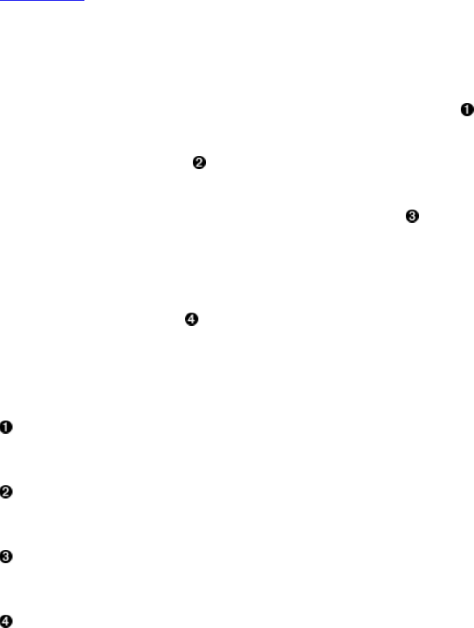
row-5/colfam2:col-10/1427274739384/Put/vlen=8/seqid=0,
row-5/colfam2:col-2/1427274739368/Put/vlen=7/seqid=0}
Since the filter asks for columns, or in other words column qualifiers, with a value of col-2 or
less, you can see how col-1 and col-10 are also included, since the comparison—once again—is
done lexicographically (means binary).
ValueFilter
This filter makes it possible to include only columns that have a specific value. Combined with
the RegexStringComparator, for example, this can filter using powerful expression syntax.
Example 4-4 showcases this feature. Note, though, that with certain comparators—as explained
earlier—you can only employ a subset of the operators. Here a substring match is performed and
this must be combined with an EQUAL, or NOT_EQUAL, operator.
Example 4-4. Example using the value based filter
Filter filter = new ValueFilter(CompareFilter.CompareOp.EQUAL,
new SubstringComparator(".4"));
Scan scan = new Scan();
scan.setFilter(filter);
ResultScanner scanner = table.getScanner(scan);
for (Result result : scanner) {
for (Cell cell : result.rawCells()) {
System.out.println("Cell: " + cell + ", Value: " +
Bytes.toString(cell.getValueArray(), cell.getValueOffset(),
cell.getValueLength()));
}
}
scanner.close();
Get get = new Get(Bytes.toBytes("row-5"));
get.setFilter(filter);
Result result = table.get(get);
for (Cell cell : result.rawCells()) {
System.out.println("Cell: " + cell + ", Value: " +
Bytes.toString(cell.getValueArray(), cell.getValueOffset(),
cell.getValueLength()));
}
Create filter, while specifying the comparison operator and comparator.
Set filter for the scan.
Print out value to check that filter works.
Assign same filter to Get instance.
The output, confirming the proper functionality:
Adding rows to table...
Results of scan:
(229)

Cell: row-1/colfam1:col-4/1427275408429/Put/vlen=7/seqid=0, Value: val-1.4
Cell: row-1/colfam2:col-4/1427275408429/Put/vlen=7/seqid=0, Value: val-1.4
...
Cell: row-9/colfam1:col-4/1427275408605/Put/vlen=7/seqid=0, Value: val-9.4
Cell: row-9/colfam2:col-4/1427275408605/Put/vlen=7/seqid=0, Value: val-9.4
Result of get:
Cell: row-5/colfam1:col-4/1427275408527/Put/vlen=7/seqid=0, Value: val-5.4
Cell: row-5/colfam2:col-4/1427275408527/Put/vlen=7/seqid=0, Value: val-5.4
The example’s wiring code (hidden, see the online repository again) set the value to row key +
“.” + column number. The rows and columns start at 1. The filter is instructed to retrieve all cells
that have a value containing .4--aiming at the fourth column. And indeed, we see that only
column col-4 is returned.
DependentColumnFilter
Here you have a more complex filter that does not simply filter out data based on directly
available information. Rather, it lets you specify a dependent column—or reference column—
that controls how other columns are filtered. It uses the timestamp of the reference column and
includes all other columns that have the same timestamp. Here are the constructors provided:
DependentColumnFilter(final byte[] family, final byte[] qualifier)
DependentColumnFilter(final byte[] family, final byte[] qualifier,
final boolean dropDependentColumn)
DependentColumnFilter(final byte[] family, final byte[] qualifier,
final boolean dropDependentColumn, final CompareOp valueCompareOp,
final ByteArrayComparable valueComparator)
Since this class is based on CompareFilter, it also offers you to further select columns, but for this
filter it does so based on their values. Think of it as a combination of a ValueFilter and a filter
selecting on a reference timestamp. You can optionally hand in your own operator and
comparator pair to enable this feature. The class provides constructors, though, that let you omit
the operator and comparator and disable the value filtering, including all columns by default, that
is, performing the timestamp filter based on the reference column only.
Example 4-5 shows the filter in use. You can see how the optional values can be handed in as
well. The dropDependentColumn parameter is giving you additional control over how the reference
column is handled: it is either included or dropped by the filter, setting this parameter to false or
true, respectively.
Example 4-5. Example using a filter to include only specific column families
private static void filter(boolean drop,
CompareFilter.CompareOp operator,
ByteArrayComparable comparator)
throws IOException {
Filter filter;
if (comparator != null) {
filter = new DependentColumnFilter(Bytes.toBytes("colfam1"),
Bytes.toBytes("col-5"), drop, operator, comparator);
} else {
filter = new DependentColumnFilter(Bytes.toBytes("colfam1"),
Bytes.toBytes("col-5"), drop);
}
Scan scan = new Scan();
scan.setFilter(filter);
// scan.setBatch(4); // cause an error
ResultScanner scanner = table.getScanner(scan);
for (Result result : scanner) {
(230)

for (Cell cell : result.rawCells()) {
System.out.println("Cell: " + cell + ", Value: " +
Bytes.toString(cell.getValueArray(), cell.getValueOffset(),
cell.getValueLength()));
}
}
scanner.close();
Get get = new Get(Bytes.toBytes("row-5"));
get.setFilter(filter);
Result result = table.get(get);
for (Cell cell : result.rawCells()) {
System.out.println("Cell: " + cell + ", Value: " +
Bytes.toString(cell.getValueArray(), cell.getValueOffset(),
cell.getValueLength()));
}
}
public static void main(String[] args) throws IOException {
filter(true, CompareFilter.CompareOp.NO_OP, null);
filter(false, CompareFilter.CompareOp.NO_OP, null);
filter(true, CompareFilter.CompareOp.EQUAL,
new BinaryPrefixComparator(Bytes.toBytes("val-5")));
filter(false, CompareFilter.CompareOp.EQUAL,
new BinaryPrefixComparator(Bytes.toBytes("val-5")));
filter(true, CompareFilter.CompareOp.EQUAL,
new RegexStringComparator(".*\\.5"));
filter(false, CompareFilter.CompareOp.EQUAL,
new RegexStringComparator(".*\\.5"));
}
Create the filter with various options.
Call filter method with various options.
Caution
This filter is not compatible with the batch feature of the scan operations, that is, setting
Scan.setBatch() to a number larger than zero. The filter needs to see the entire row to do its work,
and using batching will not carry the reference column timestamp over and would result in
erroneous results.
If you try to enable the batch mode nevertheless, you will get an error:
Exception in thread "main" \
org.apache.hadoop.hbase.filter.IncompatibleFilterException: \
Cannot set batch on a scan using a filter that returns true for \
filter.hasFilterRow
at org.apache.hadoop.hbase.client.Scan.setBatch(Scan.java:464)
...
The example also proceeds slightly differently compared to the earlier filters, as it sets the
version to the column number for a more reproducible result. The implicit timestamps that the
servers use as the version could result in fluctuating results as you cannot guarantee them using
the exact time, down to the millisecond.
The filter() method used is called with different parameter combinations, showing how using
the built-in value filter and the drop flag is affecting the returned data set. Here is the output of
the first two filter() calls:
(231)

Adding rows to table...
Results of scan:
Cell: row-1/colfam2:col-5/5/Put/vlen=7/seqid=0, Value: val-1.5
Cell: row-10/colfam2:col-5/5/Put/vlen=8/seqid=0, Value: val-10.5
...
Cell: row-8/colfam2:col-5/5/Put/vlen=7/seqid=0, Value: val-8.5
Cell: row-9/colfam2:col-5/5/Put/vlen=7/seqid=0, Value: val-9.5
Result of get:
Cell: row-5/colfam2:col-5/5/Put/vlen=7/seqid=0, Value: val-5.5
Results of scan:
Cell: row-1/colfam1:col-5/5/Put/vlen=7/seqid=0, Value: val-1.5
Cell: row-1/colfam2:col-5/5/Put/vlen=7/seqid=0, Value: val-1.5
Cell: row-9/colfam1:col-5/5/Put/vlen=7/seqid=0, Value: val-9.5
Cell: row-9/colfam2:col-5/5/Put/vlen=7/seqid=0, Value: val-9.5
Result of get:
Cell: row-5/colfam1:col-5/5/Put/vlen=7/seqid=0, Value: val-5.5
Cell: row-5/colfam2:col-5/5/Put/vlen=7/seqid=0, Value: val-5.5
The only difference between the two calls is setting dropDependentColumn to true and false
respectively. In the first scan and get output you see the checked column in colfam1 being
omitted, in other words dropped as expected, while in the second half of the output you see it
included.
What is this filter good for you might wonder? It is used where applications require client-side
timestamps (these could be epoch based, or based on some internal global counter) to track
dependent updates. Say you insert some kind of transactional data, where across the row all
fields that are updated, should form some dependent update. In this case the client could set all
columns that are updated in one mutation to the same timestamp, and when later wanting to show
the entity at a certain point in time, get (or scan) the row at that time. All modifications from
earlier (or later, or exact) changes are then masked out (or included). See “Transactions” for
libraries on top of HBase that make use of such as schema.
(232)

Dedicated Filters
The second type of supplied filters are based directly on FilterBase and implement more specific
use cases. Many of these filters are only really applicable when performing scan operations,
since they filter out entire rows. For get() calls, this is often too restrictive and would result in a
very harsh filter approach: include the whole row or nothing at all.
PrefixFilter
Given a row prefix, specified when you instantiate the filter instance, all rows with a row key
matching this prefix are returned to the client. The constructor is:
PrefixFilter(final byte[] prefix)
Example 4-6 has this applied to the usual test data set.
Example 4-6. Example using the prefix based filter
Filter filter = new PrefixFilter(Bytes.toBytes("row-1"));
Scan scan = new Scan();
scan.setFilter(filter);
ResultScanner scanner = table.getScanner(scan);
for (Result result : scanner) {
for (Cell cell : result.rawCells()) {
System.out.println("Cell: " + cell + ", Value: " +
Bytes.toString(cell.getValueArray(), cell.getValueOffset(),
cell.getValueLength()));
}
}
scanner.close();
Get get = new Get(Bytes.toBytes("row-5"));
get.setFilter(filter);
Result result = table.get(get);
for (Cell cell : result.rawCells()) {
System.out.println("Cell: " + cell + ", Value: " +
Bytes.toString(cell.getValueArray(), cell.getValueOffset(),
cell.getValueLength()));
}
The output:
Results of scan:
Cell: row-1/colfam1:col-1/1427280142327/Put/vlen=7/seqid=0, Value: val-1.1
Cell: row-1/colfam1:col-10/1427280142379/Put/vlen=8/seqid=0, Value: val-1.10
...
Cell: row-1/colfam2:col-8/1427280142375/Put/vlen=7/seqid=0, Value: val-1.8
Cell: row-1/colfam2:col-9/1427280142377/Put/vlen=7/seqid=0, Value: val-1.9
Cell: row-10/colfam1:col-1/1427280142530/Put/vlen=8/seqid=0, Value: val-10.1
Cell: row-10/colfam1:col-10/1427280142546/Put/vlen=9/seqid=0, Value: val-10.10
...
Cell: row-10/colfam2:col-8/1427280142542/Put/vlen=8/seqid=0, Value: val-10.8
Cell: row-10/colfam2:col-9/1427280142544/Put/vlen=8/seqid=0, Value: val-10.9
Result of get:
It is interesting to see how the get() call fails to return anything, because it is asking for a row
that does not match the filter prefix. This filter does not make much sense when doing get() calls
but is highly useful for scan operations. The scan also is actively ended when the filter
(233)

encounters a row key that is larger than the prefix. In this way, and combining this with a start
row, for example, the filter is improving the overall performance of the scan as it has knowledge
of when to skip the rest of the rows altogether.
PageFilter
You paginate through rows by employing this filter. When you create the instance, you specify a
pageSize parameter, which controls how many rows per page should be returned.
PageFilter(final long pageSize)
Note
There is a fundamental issue with filtering on physically separate servers. Filters run on different
region servers in parallel and cannot retain or communicate their current state across those
boundaries. Thus, each filter is required to scan at least up to pageCount rows before ending the
scan. This means a slight inefficiency is given for the PageFilter as more rows are reported to the
client than necessary. The final consolidation on the client obviously has visibility into all results
and can reduce what is accessible through the API accordingly.
The client code would need to remember the last row that was returned, and then, when another
iteration is about to start, set the start row of the scan accordingly, while retaining the same filter
properties.
Because pagination is setting a strict limit on the number of rows to be returned, it is possible for
the filter to early out the entire scan, once the limit is reached or exceeded. Filters have a facility
to indicate that fact and the region servers make use of this hint to stop any further processing.
Example 4-7 puts this together, showing how a client can reset the scan to a new start row on the
subsequent iterations.
Example 4-7. Example using a filter to paginate through rows
private static final byte[] POSTFIX = new byte[] { 0x00 };
Filter filter = new PageFilter(15);
int totalRows = 0;
byte[] lastRow = null;
while (true) {
Scan scan = new Scan();
scan.setFilter(filter);
if (lastRow != null) {
byte[] startRow = Bytes.add(lastRow, POSTFIX);
System.out.println("start row: " +
Bytes.toStringBinary(startRow));
scan.setStartRow(startRow);
}
ResultScanner scanner = table.getScanner(scan);
int localRows = 0;
Result result;
while ((result = scanner.next()) != null) {
System.out.println(localRows++ + ": " + result);
totalRows++;
lastRow = result.getRow();
}
scanner.close();
if (localRows == 0) break;
}
System.out.println("total rows: " + totalRows);
(234)

The abbreviated output:
Adding rows to table...
0: keyvalues={row-1/colfam1:col-1/1427280402935/Put/vlen=7/seqid=0, ...}
1: keyvalues={row-10/colfam1:col-1/1427280403125/Put/vlen=8/seqid=0, ...}
...
14: keyvalues={row-110/colfam1:col-1/1427280404601/Put/vlen=9/seqid=0, ...}
start row: row-110\x00
0: keyvalues={row-111/colfam1:col-1/1427280404615/Put/vlen=9/seqid=0, ...}
1: keyvalues={row-112/colfam1:col-1/1427280404628/Put/vlen=9/seqid=0, ...}
...
14: keyvalues={row-124/colfam1:col-1/1427280404786/Put/vlen=9/seqid=0, ...}
start row: row-124\x00
0: keyvalues={row-125/colfam1:col-1/1427280404799/Put/vlen=9/seqid=0, ...}
...
start row: row-999\x00
total rows: 1000
Because of the lexicographical sorting of the row keys by HBase and the comparison taking care
of finding the row keys in order, and the fact that the start key on a scan is always inclusive, you
need to add an extra zero byte to the previous key. This will ensure that the last seen row key is
skipped and the next, in sorting order, is found. The zero byte is the smallest increment, and
therefore is safe to use when resetting the scan boundaries. Even if there were a row that would
match the previous plus the extra zero byte, the scan would be correctly doing the next iteration
—because the start key is inclusive.
KeyOnlyFilter
Some applications need to access just the keys of each Cell, while omitting the actual data. The
KeyOnlyFilter provides this functionality by applying the filter’s ability to modify the processed
columns and cells, as they pass through. It does so by applying some logic that converts the
current cell, stripping out the data part. The constructors of the filter are:
KeyOnlyFilter()
KeyOnlyFilter(boolean lenAsVal)
There is an optional boolean parameter, named lenAsVal. It is handed to the internal conversion
call as-is, controlling what happens to the value part of each Cell instance processed. The default
value of false simply sets the value to zero length, while the opposite true sets the value to the
number representing the length of the original value. The latter may be useful to your application
when quickly iterating over columns, where the keys already convey meaning and the length can
be used to perform a secondary sort. “Client API: Best Practices” has an example.
Example 4-8 tests this filter with both constructors, creating random rows, columns, and values.
Example 4-8. Only returns the first found cell from each row
int rowCount = 0;
for (Result result : scanner) {
for (Cell cell : result.rawCells()) {
System.out.println("Cell: " + cell + ", Value: " + (
cell.getValueLength() > 0 ?
Bytes.toInt(cell.getValueArray(), cell.getValueOffset(),
cell.getValueLength()) : "n/a" ));
}
rowCount++;
}
System.out.println("Total num of rows: " + rowCount);
scanner.close();
}
(235)
public static void main(String[] args) throws IOException {
Configuration conf = HBaseConfiguration.create();
HBaseHelper helper = HBaseHelper.getHelper(conf);
helper.dropTable("testtable");
helper.createTable("testtable", "colfam1");
System.out.println("Adding rows to table...");
helper.fillTableRandom("testtable", /* row */ 1, 5, 0,
/* col */ 1, 30, 0, /* val */ 0, 10000, 0, true, "colfam1");
Connection connection = ConnectionFactory.createConnection(conf);
table = connection.getTable(TableName.valueOf("testtable"));
System.out.println("Scan #1");
Filter filter1 = new KeyOnlyFilter();
scan(filter1);
Filter filter2 = new KeyOnlyFilter(true);
scan(filter2);
The abbreviated output will be similar to the following:
Adding rows to table...
Results of scan:
Cell: row-0/colfam1:col-17/6/Put/vlen=0/seqid=0, Value: n/a
Cell: row-0/colfam1:col-27/3/Put/vlen=0/seqid=0, Value: n/a
...
Cell: row-4/colfam1:col-3/2/Put/vlen=0/seqid=0, Value: n/a
Cell: row-4/colfam1:col-5/16/Put/vlen=0/seqid=0, Value: n/a
Total num of rows: 5
Scan #2
Results of scan:
Cell: row-0/colfam1:col-17/6/Put/vlen=4/seqid=0, Value: 8
Cell: row-0/colfam1:col-27/3/Put/vlen=4/seqid=0, Value: 6
...
Cell: row-4/colfam1:col-3/2/Put/vlen=4/seqid=0, Value: 7
Cell: row-4/colfam1:col-5/16/Put/vlen=4/seqid=0, Value: 8
Total num of rows: 5
The highlighted parts show how first the value is simply dropped and the value length is set to
zero. The second, setting lenAsVal explicitly to true see a different result. The value length of 4 is
attributed to the length of the payload, an integer of four bytes. The value is the random length of
old value, here values between 5 and 9 (the fixed prefix val- plus a number between 0 and
10,000).
FirstKeyOnlyFilter
Caution
Even if the name implies KeyValue, or key only, this is both a misnomer. The filter returns the first
cell it finds in a row, and does so with all its details, including the value. It should be named
FirstCellFilter, for example.
If you need to access the first column—as sorted implicitly by HBase—in each row, this filter
will provide this feature. Typically this is used by row counter type applications that only need to
check if a row exists. Recall that in column-oriented databases a row really is composed of
columns, and if there are none, the row ceases to exist.
Another possible use case is relying on the column sorting in lexicographical order, and setting
the column qualifier to an epoch value. This would sort the column with the oldest timestamp
name as the first to be retrieved. Combined with this filter, it is possible to retrieve the oldest
column from every row using a single scan. More interestingly, though, is when you reverse the
timestamp set as the column qualifier, and therefore retrieve the newest entry in a row in a single
(236)

scan.
This class makes use of another optimization feature provided by the filter framework: it
indicates to the region server applying the filter that the current row is done and that it should
skip to the next one. This improves the overall performance of the scan, compared to a full table
scan. The gain is more prominent in schemas with very wide rows, in other words, where you
can skip many columns to reach the next row. If you only have one column per row, there will be
no gain at all, obviously.
Example 4-9 has a simple example, using random rows, columns, and values, so your output will
vary.
Example 4-9. Only returns the first found cell from each row
Filter filter = new FirstKeyOnlyFilter();
Scan scan = new Scan();
scan.setFilter(filter);
ResultScanner scanner = table.getScanner(scan);
int rowCount = 0;
for (Result result : scanner) {
for (Cell cell : result.rawCells()) {
System.out.println("Cell: " + cell + ", Value: " +
Bytes.toString(cell.getValueArray(), cell.getValueOffset(),
cell.getValueLength()));
}
rowCount++;
}
System.out.println("Total num of rows: " + rowCount);
scanner.close();
The abbreviated output, showing that only one cell is returned per row, confirming the filter’s
purpose:
Adding rows to table...
Results of scan:
Cell: row-0/colfam1:col-10/19/Put/vlen=6/seqid=0, Value: val-76
Cell: row-1/colfam1:col-0/0/Put/vlen=6/seqid=0, Value: val-19
...
Cell: row-8/colfam1:col-10/4/Put/vlen=6/seqid=0, Value: val-35
Cell: row-9/colfam1:col-1/5/Put/vlen=5/seqid=0, Value: val-0
Total num of rows: 30
FirstKeyValueMatchingQualifiersFilter
This filter is an extension to the FirstKeyOnlyFilter, but instead of returning the first found cell, it
instead returns all the columns of a row, up to a given column qualifier. If the row has no such
qualifier, all columns are returned. The filter is mainly used in the rowcounter shell command, to
count all rows in HBase using a distributed process.
The constructor of the filter class looks like this:
FirstKeyValueMatchingQualifiersFilter(Set<byte[]> qualifiers)
Example 4-10 sets up a filter with two columns to match. It also loads the test table with random
data, so your output will most certainly vary.
Example 4-10. Returns all columns, or up to the first found reference qualifier, for each row
(237)

Set<byte[]> quals = new HashSet<byte[]>();
quals.add(Bytes.toBytes("col-2"));
quals.add(Bytes.toBytes("col-4"));
quals.add(Bytes.toBytes("col-6"));
quals.add(Bytes.toBytes("col-8"));
Filter filter = new FirstKeyValueMatchingQualifiersFilter(quals);
Scan scan = new Scan();
scan.setFilter(filter);
ResultScanner scanner = table.getScanner(scan);
int rowCount = 0;
for (Result result : scanner) {
for (Cell cell : result.rawCells()) {
System.out.println("Cell: " + cell + ", Value: " +
Bytes.toString(cell.getValueArray(), cell.getValueOffset(),
cell.getValueLength()));
}
rowCount++;
}
System.out.println("Total num of rows: " + rowCount);
scanner.close();
Here is the output on the console in an abbreviated form for one execution:
Adding rows to table...
Results of scan:
Cell: row-0/colfam1:col-0/1/Put/vlen=6/seqid=0, Value: val-48
Cell: row-0/colfam1:col-1/4/Put/vlen=6/seqid=0, Value: val-78
Cell: row-0/colfam1:col-5/1/Put/vlen=6/seqid=0, Value: val-62
Cell: row-0/colfam1:col-6/6/Put/vlen=5/seqid=0, Value: val-6
Cell: row-10/colfam1:col-1/3/Put/vlen=6/seqid=0, Value: val-73
Cell: row-10/colfam1:col-6/5/Put/vlen=6/seqid=0, Value: val-11
...
Cell: row-6/colfam1:col-1/0/Put/vlen=6/seqid=0, Value: val-39
Cell: row-7/colfam1:col-9/6/Put/vlen=6/seqid=0, Value: val-57
Cell: row-8/colfam1:col-0/2/Put/vlen=6/seqid=0, Value: val-90
Cell: row-8/colfam1:col-1/4/Put/vlen=6/seqid=0, Value: val-92
Cell: row-8/colfam1:col-6/4/Put/vlen=6/seqid=0, Value: val-12
Cell: row-9/colfam1:col-1/5/Put/vlen=6/seqid=0, Value: val-35
Cell: row-9/colfam1:col-2/2/Put/vlen=6/seqid=0, Value: val-22
Total num of rows: 47
Depending on the random data generated we see more or less cells emitted per row. The filter is
instructed to stop emitting cells when encountering one of the columns col-2, col-4, col-6, or col-
8. For row-0 this is visible, as it had one more column, named col-7, which is omitted. row-7 has
only one cell, and no matching qualifier, hence it is included completely.
InclusiveStopFilter
The row boundaries of a scan are inclusive for the start row, yet exclusive for the stop row. You
can overcome the stop row semantics using this filter, which includes the specified stop row.
Example 4-11 uses the filter to start at row-3, and stop at row-5 inclusively.
Example 4-11. Example using a filter to include a stop row
Filter filter = new InclusiveStopFilter(Bytes.toBytes("row-5"));
Scan scan = new Scan();
scan.setStartRow(Bytes.toBytes("row-3"));
scan.setFilter(filter);
ResultScanner scanner = table.getScanner(scan);
for (Result result : scanner) {
System.out.println(result);
}
scanner.close();
(238)

The output on the console, when running the example code, confirms that the filter works as
advertised:
Adding rows to table...
Results of scan:
keyvalues={row-3/colfam1:col-1/1427282689001/Put/vlen=7/seqid=0}
keyvalues={row-30/colfam1:col-1/1427282689069/Put/vlen=8/seqid=0}
...
keyvalues={row-48/colfam1:col-1/1427282689100/Put/vlen=8/seqid=0}
keyvalues={row-49/colfam1:col-1/1427282689102/Put/vlen=8/seqid=0}
keyvalues={row-5/colfam1:col-1/1427282689004/Put/vlen=7/seqid=0}
FuzzyRowFilter
This filter acts on row keys, but in a fuzzy manner. It needs a list of row keys that should be
returned, plus an accompanying byte[] array that signifies the importance of each byte in the row
key. The constructor is as such:
FuzzyRowFilter(List<Pair<byte[], byte[]>> fuzzyKeysData)
The fuzzyKeysData specifies the mentioned significance of a row key byte, by taking one of two
values:
0
Indicates that the byte at the same position in the row key must match as-is.
1
Means that the corresponding row key byte does not matter and is always accepted.
Example: Partial Row Key Matching
A possible example is matching partial keys, but not from left to right, rather somewhere inside a
compound key. Assuming a row key format of <userId>_<actionId>_<year>_<month>, with fixed
length parts, where <userId> is 4, <actionId> is 2, <year> is 4, and <month> is 2 bytes long. The
application now requests all users that performed certain action (encoded as 99) in January of any
year. Then the pair for row key and fuzzy data would be the following:
row key
"????_99_????_01", where the "?" is an arbitrary character, since it is ignored.
fuzzy data
= "\x01\x01\x01\x01\x00\x00\x00\x00\x01\x01\x01\x01\x00\x00\x00"
In other words, the fuzzy data array instructs the filter to find all row keys matching "????
_99_????_01", where the "?" will accept any character.
An advantage of this filter is that it can likely compute the next matching row key when it comes
to an end of a matching one. It implements the getNextCellHint() method to help the servers in
fast-forwarding to the next range of rows that might match. This speeds up scanning, especially
when the skipped ranges are quite large. Example 4-12 uses the filter to grab specific rows from
a test data set.
(239)

Example 4-12. Example filtering by column prefix
List<Pair<byte[], byte[]>> keys = new ArrayList<Pair<byte[], byte[]>>();
keys.add(new Pair<byte[], byte[]>(
Bytes.toBytes("row-?5"), new byte[] { 0, 0, 0, 0, 1, 0 }));
Filter filter = new FuzzyRowFilter(keys);
Scan scan = new Scan()
.addColumn(Bytes.toBytes("colfam1"), Bytes.toBytes("col-5"))
.setFilter(filter);
ResultScanner scanner = table.getScanner(scan);
for (Result result : scanner) {
System.out.println(result);
}
scanner.close();
The example code also adds a filtering column to the scan, just to keep the output short:
Adding rows to table...
Results of scan:
keyvalues={row-05/colfam1:col-01/1/Put/vlen=9/seqid=0,
row-05/colfam1:col-02/2/Put/vlen=9/seqid=0,
...
row-05/colfam1:col-09/9/Put/vlen=9/seqid=0,
row-05/colfam1:col-10/10/Put/vlen=9/seqid=0}
keyvalues={row-15/colfam1:col-01/1/Put/vlen=9/seqid=0,
row-15/colfam1:col-02/2/Put/vlen=9/seqid=0,
...
row-15/colfam1:col-09/9/Put/vlen=9/seqid=0,
row-15/colfam1:col-10/10/Put/vlen=9/seqid=0}
The test code wiring adds 20 rows to the table, named row-01 to row-20. We want to retrieve all
the rows that match the pattern row-?5, in other words all rows that end in the number 5. The
output above confirms the correct result.
ColumnCountGetFilter
You can use this filter to only retrieve a specific maximum number of columns per row. You can
set the number using the constructor of the filter:
ColumnCountGetFilter(final int n)
Since this filter stops the entire scan once a row has been found that matches the maximum
number of columns configured, it is not useful for scan operations, and in fact, it was written to
test filters in get() calls.
ColumnPaginationFilter
Tip
This filter’s functionality is superseded by the slicing functionality explained in “Slicing Rows”,
and provided by the setMaxResultsPerColumnFamily() and setRowOffsetPerColumnFamily() methods
of Scan, and Get.
Similar to the PageFilter, this one can be used to page through columns in a row. Its constructor
has two parameters:
ColumnPaginationFilter(final int limit, final int offset)
(240)

It skips all columns up to the number given as offset, and then includes limit columns afterward.
Example 4-13 has this applied to a normal scan.
Example 4-13. Example paginating through columns in a row
Filter filter = new ColumnPaginationFilter(5, 15);
Scan scan = new Scan();
scan.setFilter(filter);
ResultScanner scanner = table.getScanner(scan);
for (Result result : scanner) {
System.out.println(result);
}
scanner.close();
Running this example should render the following output:
Adding rows to table...
Results of scan:
keyvalues={row-01/colfam1:col-16/16/Put/vlen=9/seqid=0,
row-01/colfam1:col-17/17/Put/vlen=9/seqid=0,
row-01/colfam1:col-18/18/Put/vlen=9/seqid=0,
row-01/colfam1:col-19/19/Put/vlen=9/seqid=0,
row-01/colfam1:col-20/20/Put/vlen=9/seqid=0}
keyvalues={row-02/colfam1:col-16/16/Put/vlen=9/seqid=0,
row-02/colfam1:col-17/17/Put/vlen=9/seqid=0,
row-02/colfam1:col-18/18/Put/vlen=9/seqid=0,
row-02/colfam1:col-19/19/Put/vlen=9/seqid=0,
row-02/colfam1:col-20/20/Put/vlen=9/seqid=0}
...
Note
This example slightly changes the way the rows and columns are numbered by adding a padding
to the numeric counters. For example, the first row is padded to be row-01. This also shows how
padding can be used to get a more human-readable style of sorting, for example—as known
from dictionaries or telephone books.
The result includes all 10 rows, starting each row at column 16 (offset = 15) and printing five
columns (limit = 5). As a side note, this filter does not suffer from the issues explained in
“PageFilter”, in other words, although it is distributed and not synchronized across filter
instances, there are no inefficiencies incurred by reading too many columns or rows. This is
because a row is contained in a single region, and no overlap to another region is required to
complete the filtering task.
ColumnPrefixFilter
Analog to the PrefixFilter, which worked by filtering on row key prefixes, this filter does the
same for columns. You specify a prefix when creating the filter:
ColumnPrefixFilter(final byte[] prefix)
All columns that have the given prefix are then included in the result. Example 4-14 selects all
columns starting with col-1. Here we drop the padding again, to get binary sorted column names.
Example 4-14. Example filtering by column prefix
Filter filter = new ColumnPrefixFilter(Bytes.toBytes("col-1"));
(241)
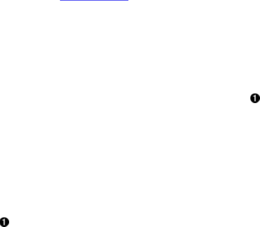
Scan scan = new Scan();
scan.setFilter(filter);
ResultScanner scanner = table.getScanner(scan);
for (Result result : scanner) {
System.out.println(result);
}
scanner.close();
The result of running this example should show the filter doing its job as advertised:
Adding rows to table...
Results of scan:
keyvalues={row-1/colfam1:col-1/1/Put/vlen=7/seqid=0,
row-1/colfam1:col-10/10/Put/vlen=8/seqid=0,
...
row-1/colfam1:col-19/19/Put/vlen=8/seqid=0}
...
MultipleColumnPrefixFilter
This filter is a straight extension to the ColumnPrefixFilter, allowing the application to ask for a
list of column qualifier prefixes, not just a single one. The constructor and use is also straight
forward:
MultipleColumnPrefixFilter(final byte[][] prefixes)
The code in Example 4-15 adds two column prefixes, and also a row prefix to limit the output.
Example 4-15. Example filtering by column prefix
Filter filter = new MultipleColumnPrefixFilter(new byte[][] {
Bytes.toBytes("col-1"), Bytes.toBytes("col-2")
});
Scan scan = new Scan()
.setRowPrefixFilter(Bytes.toBytes("row-1"))
.setFilter(filter);
ResultScanner scanner = table.getScanner(scan);
for (Result result : scanner) {
System.out.print(Bytes.toString(result.getRow()) + ": ");
for (Cell cell : result.rawCells()) {
System.out.print(Bytes.toString(cell.getQualifierArray(),
cell.getQualifierOffset(), cell.getQualifierLength()) + ", ");
}
System.out.println();
}
scanner.close();
Limit to rows starting with a specific prefix.
The following shows what is emitted on the console (abbreviated), note how the code also prints
out only the row key and column qualifiers, just to show another way of accessing the data:
Adding rows to table...
Results of scan:
row-1: col-1, col-10, col-11, col-12, col-13, col-14, col-15, col-16,
col-17, col-18, col-19, col-2, col-20, col-21, col-22, col-23, col-24,
col-25, col-26, col-27, col-28, col-29,
row-10: col-1, col-10, col-11, col-12, col-13, col-14, col-15, col-16,
col-17, col-18, col-19, col-2, col-20, col-21, col-22, col-23, col-24,
col-25, col-26, col-27, col-28, col-29,
row-18: col-1, col-10, col-11, col-12, col-13, col-14, col-15, col-16,
(242)

col-17, col-18, col-19, col-2, col-20, col-21, col-22, col-23, col-24,
col-25, col-26, col-27, col-28, col-29,
row-19: col-1, col-10, col-11, col-12, col-13, col-14, col-15, col-16,
col-17, col-18, col-19, col-2, col-20, col-21, col-22, col-23, col-24,
col-25, col-26, col-27, col-28, col-29,
ColumnRangeFilter
This filter acts like two QualifierFilter instances working together, with one checking the lower
boundary, and the other doing the same for the upper. Both would have to use the provided
BinaryPrefixComparator with a compare operator of LESS_OR_EQUAL, and GREATER_OR_EQUAL
respectively. Since all of this is error-prone and extra work, you can just use the
ColumnRangeFilter and be done. Here the constructor of the filter:
ColumnRangeFilter(final byte[] minColumn, boolean minColumnInclusive,
final byte[] maxColumn, boolean maxColumnInclusive)
You have to provide an optional minimum and maximum column qualifier, and accompanying
boolean flags if these are exclusive or inclusive. If you do not specify minimum column, then the
start of table is used. Same for the maximum column, if not provided the end of the table is
assumed. Example 4-16 shows an example using these parameters.
Example 4-16. Example filtering by columns within a given range
Filter filter = new ColumnRangeFilter(Bytes.toBytes("col-05"), true,
Bytes.toBytes("col-11"), false);
Scan scan = new Scan()
.setStartRow(Bytes.toBytes("row-03"))
.setStopRow(Bytes.toBytes("row-05"))
.setFilter(filter);
ResultScanner scanner = table.getScanner(scan);
for (Result result : scanner) {
System.out.println(result);
}
scanner.close();
The output is as follows:
Adding rows to table...
Results of scan:
keyvalues={row-03/colfam1:col-05/5/Put/vlen=9/seqid=0,
row-03/colfam1:col-06/6/Put/vlen=9/seqid=0,
row-03/colfam1:col-07/7/Put/vlen=9/seqid=0,
row-03/colfam1:col-08/8/Put/vlen=9/seqid=0,
row-03/colfam1:col-09/9/Put/vlen=9/seqid=0,
row-03/colfam1:col-10/10/Put/vlen=9/seqid=0}
keyvalues={row-04/colfam1:col-05/5/Put/vlen=9/seqid=0,
row-04/colfam1:col-06/6/Put/vlen=9/seqid=0,
row-04/colfam1:col-07/7/Put/vlen=9/seqid=0,
row-04/colfam1:col-08/8/Put/vlen=9/seqid=0,
row-04/colfam1:col-09/9/Put/vlen=9/seqid=0,
row-04/colfam1:col-10/10/Put/vlen=9/seqid=0}
In this example you can see the use of the fluent interface again to set up the scan instance. It
also limits the number of rows scanned (just because).
SingleColumnValueFilter
You can use this filter when you have exactly one column that decides if an entire row should be
returned or not. You need to first specify the column you want to track, and then some value to
(243)

check against. The constructors offered are:
SingleColumnValueFilter(final byte[] family, final byte[] qualifier,
final CompareOp compareOp, final byte[] value)
SingleColumnValueFilter(final byte[] family, final byte[] qualifier,
final CompareOp compareOp, final ByteArrayComparable comparator)
protected SingleColumnValueFilter(final byte[] family, final byte[] qualifier,
final CompareOp compareOp, ByteArrayComparable comparator,
final boolean filterIfMissing, final boolean latestVersionOnly)
The first one is a convenience function as it simply creates a BinaryComparator instance internally
on your behalf. The second takes the same parameters we used for the CompareFilter-based
classes. Although the SingleColumnValueFilter does not inherit from the CompareFilter directly, it
still uses the same parameter types. The third, and final constructor, adds two additional boolean
flags, which, alternatively, can be set with getter and setter methods after the filter has been
constructed:
boolean getFilterIfMissing()
void setFilterIfMissing(boolean filterIfMissing)
boolean getLatestVersionOnly()
void setLatestVersionOnly(boolean latestVersionOnly)
The former controls what happens to rows that do not have the column at all. By default, they are
included in the result, but you can use setFilterIfMissing(true) to reverse that behavior, that is,
all rows that do not have the reference column are dropped from the result.
Note
You must include the column you want to filter by, in other words, the reference column, into the
families you query for—using addColumn(), for example. If you fail to do so, the column is
considered missing and the result is either empty, or contains all rows, based on the
getFilterIfMissing() result.
By using setLatestVersionOnly(false)--the default is true--you can change the default behavior of
the filter, which is only to check the newest version of the reference column, to instead include
previous versions in the check as well. Example 4-17 combines these features to select a specific
set of rows only.
Example 4-17. Example using a filter to return only rows with a given value in a given column
SingleColumnValueFilter filter = new SingleColumnValueFilter(
Bytes.toBytes("colfam1"),
Bytes.toBytes("col-5"),
CompareFilter.CompareOp.NOT_EQUAL,
new SubstringComparator("val-5"));
filter.setFilterIfMissing(true);
Scan scan = new Scan();
scan.setFilter(filter);
ResultScanner scanner = table.getScanner(scan);
for (Result result : scanner) {
for (Cell cell : result.rawCells()) {
System.out.println("Cell: " + cell + ", Value: " +
Bytes.toString(cell.getValueArray(), cell.getValueOffset(),
cell.getValueLength()));
}
}
scanner.close();
Get get = new Get(Bytes.toBytes("row-6"));
get.setFilter(filter);
Result result = table.get(get);
(244)

System.out.println("Result of get: ");
for (Cell cell : result.rawCells()) {
System.out.println("Cell: " + cell + ", Value: " +
Bytes.toString(cell.getValueArray(), cell.getValueOffset(),
cell.getValueLength()));
}
The output shows how the scan is filtering out all columns from row-5, since their value starts
with val-5. We are asking the filter to do a substring match on val-5 and use the NOT_EQUAL
comparator to include all other matching rows:
Adding rows to table...
Results of scan:
Cell: row-1/colfam1:col-1/1427279447557/Put/vlen=7/seqid=0, Value: val-1.1
Cell: row-1/colfam1:col-10/1427279447613/Put/vlen=8/seqid=0, Value: val-1.10
...
Cell: row-4/colfam2:col-8/1427279447667/Put/vlen=7/seqid=0, Value: val-4.8
Cell: row-4/colfam2:col-9/1427279447669/Put/vlen=7/seqid=0, Value: val-4.9
Cell: row-6/colfam1:col-1/1427279447692/Put/vlen=7/seqid=0, Value: val-6.1
Cell: row-6/colfam1:col-10/1427279447709/Put/vlen=8/seqid=0, Value: val-6.10
...
Cell: row-9/colfam2:col-8/1427279447759/Put/vlen=7/seqid=0, Value: val-9.8
Cell: row-9/colfam2:col-9/1427279447761/Put/vlen=7/seqid=0, Value: val-9.9
Result of get:
Cell: row-6/colfam1:col-1/1427279447692/Put/vlen=7/seqid=0, Value: val-6.1
Cell: row-6/colfam1:col-10/1427279447709/Put/vlen=8/seqid=0, Value: val-6.10
...
Cell: row-6/colfam2:col-8/1427279447705/Put/vlen=7/seqid=0, Value: val-6.8
Cell: row-6/colfam2:col-9/1427279447707/Put/vlen=7/seqid=0, Value: val-6.9
SingleColumnValueExcludeFilter
The SingleColumnValueFilter we just discussed is extended in this class to provide slightly
different semantics: the reference column, as handed into the constructor, is omitted from the
result. In other words, you have the same features, constructors, and methods to control how this
filter works. The only difference is that you will never get the column you are checking against
as part of the Result instance(s) on the client side.
TimestampsFilter
When you need fine-grained control over what versions are included in the scan result, this filter
provides the means. You have to hand in a List of timestamps:
TimestampsFilter(List<Long> timestamps)
Note
As you have seen throughout the book so far, a version is a specific value of a column at a
unique point in time, denoted with a timestamp. When the filter is asking for a list of timestamps,
it will attempt to retrieve the column versions with the matching timestamps.
Example 4-18 sets up a filter with three timestamps and adds a time range to the second scan.
Example 4-18. Example filtering data by timestamps
List<Long> ts = new ArrayList<Long>();
ts.add(new Long(5));
ts.add(new Long(10));
ts.add(new Long(15));
(245)
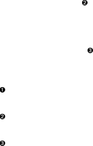
Filter filter = new TimestampsFilter(ts);
Scan scan1 = new Scan();
scan1.setFilter(filter);
ResultScanner scanner1 = table.getScanner(scan1);
for (Result result : scanner1) {
System.out.println(result);
}
scanner1.close();
Scan scan2 = new Scan();
scan2.setFilter(filter);
scan2.setTimeRange(8, 12);
ResultScanner scanner2 = table.getScanner(scan2);
for (Result result : scanner2) {
System.out.println(result);
}
scanner2.close();
Add timestamps to the list.
Add the filter to an otherwise default Scan instance.
Also add a time range to verify how it affects the filter
Here is the output on the console in an abbreviated form:
Adding rows to table...
Results of scan #1:
keyvalues={row-1/colfam1:col-10/10/Put/vlen=8/seqid=0,
row-1/colfam1:col-15/15/Put/vlen=8/seqid=0,
row-1/colfam1:col-5/5/Put/vlen=7/seqid=0}
keyvalues={row-100/colfam1:col-10/10/Put/vlen=10/seqid=0,
row-100/colfam1:col-15/15/Put/vlen=10/seqid=0,
row-100/colfam1:col-5/5/Put/vlen=9/seqid=0}
...
keyvalues={row-99/colfam1:col-10/10/Put/vlen=9/seqid=0,
row-99/colfam1:col-15/15/Put/vlen=9/seqid=0,
row-99/colfam1:col-5/5/Put/vlen=8/seqid=0}
Results of scan #2:
keyvalues={row-1/colfam1:col-10/10/Put/vlen=8/seqid=0}
keyvalues={row-10/colfam1:col-10/10/Put/vlen=9/seqid=0}
...
keyvalues={row-98/colfam1:col-10/10/Put/vlen=9/seqid=0}
keyvalues={row-99/colfam1:col-10/10/Put/vlen=9/seqid=0}
The first scan, only using the filter, is outputting the column values for all three specified
timestamps as expected. The second scan only returns the timestamp that fell into the time range
specified when the scan was set up. Both time-based restrictions, the filter and the scanner time
range, are doing their job and the result is a combination of both.
RandomRowFilter
Finally, there is a filter that shows what is also possible using the API: including random rows
into the result. The constructor is given a parameter named chance, which represents a value
between 0.0 and 1.0:
RandomRowFilter(float chance)
(246)

Internally, this class is using a Java Random.nextFloat() call to randomize the row inclusion, and
then compares the value with the chance given. Giving it a negative chance value will make the
filter exclude all rows, while a value larger than 1.0 will make it include all rows. Example 4-19
uses a chance of 50%, iterating three times over the scan:
Example 4-19. Example filtering rows randomly
Filter filter = new RandomRowFilter(0.5f);
for (int loop = 1; loop <= 3; loop++) {
Scan scan = new Scan();
scan.setFilter(filter);
ResultScanner scanner = table.getScanner(scan);
for (Result result : scanner) {
System.out.println(Bytes.toString(result.getRow()));
}
scanner.close();
}
The random results for one execution looked like:
Adding rows to table...
Results of scan for loop: 1
row-1
row-10
row-3
row-9
Results of scan for loop: 2
row-10
row-2
row-3
row-5
row-6
row-8
Results of scan for loop: 3
row-1
row-3
row-4
row-8
row-9
Your results will most certainly vary.
(247)
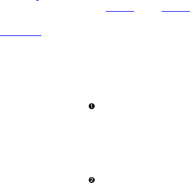
Decorating Filters
While the provided filters are already very powerful, sometimes it can be useful to modify, or
extend, the behavior of a filter to gain additional control over the returned data. Some of this
additional control is not dependent on the filter itself, but can be applied to any of them. This is
what the decorating filter group of classes is about.
Note
Decorating filters implement the same Filter interface, just like any other single-purpose filter.
In doing so, they can be used as a drop-in replacement for those filters, while combining their
behavior with the wrapped filter instance.
SkipFilter
This filter wraps a given filter and extends it to exclude an entire row, when the wrapped filter
hints for a Cell to be skipped. In other words, as soon as a filter indicates that a column in a row
is omitted, the entire row is omitted.
Note
The wrapped filter must implement the filterKeyValue() method, or the SkipFilter will not work
as expected.1 This is because the SkipFilter is only checking the results of that method to decide
how to handle the current row. See Table 4-9 on page Table 4-9 for an overview of compatible
filters.
Example 4-20 combines the SkipFilter with a ValueFilter to first select all columns that have no
zero-valued column, and subsequently drops all other partial rows that do not have a matching
value.
Example 4-20. Example of using a filter to skip entire rows based on another filter’s results
Filter filter1 = new ValueFilter(CompareFilter.CompareOp.NOT_EQUAL,
new BinaryComparator(Bytes.toBytes("val-0")));
Scan scan = new Scan();
scan.setFilter(filter1);
ResultScanner scanner1 = table.getScanner(scan);
for (Result result : scanner1) {
for (Cell cell : result.rawCells()) {
System.out.println("Cell: " + cell + ", Value: " +
Bytes.toString(cell.getValueArray(), cell.getValueOffset(),
cell.getValueLength()));
}
}
scanner1.close();
Filter filter2 = new SkipFilter(filter1);
scan.setFilter(filter2);
ResultScanner scanner2 = table.getScanner(scan);
for (Result result : scanner2) {
for (Cell cell : result.rawCells()) {
System.out.println("Cell: " + cell + ", Value: " +
(248)

Bytes.toString(cell.getValueArray(), cell.getValueOffset(),
cell.getValueLength()));
}
}
scanner2.close();
Only add the ValueFilter to the first scan.
Add the decorating skip filter for the second scan.
The example code should print roughly the following results when you execute it—note, though,
that the values are randomized, so you should get a slightly different result for every invocation:
Adding rows to table...
Results of scan #1:
Cell: row-01/colfam1:col-01/1/Put/vlen=5/seqid=0, Value: val-4
Cell: row-01/colfam1:col-02/2/Put/vlen=5/seqid=0, Value: val-4
Cell: row-01/colfam1:col-03/3/Put/vlen=5/seqid=0, Value: val-1
Cell: row-01/colfam1:col-04/4/Put/vlen=5/seqid=0, Value: val-3
Cell: row-01/colfam1:col-05/5/Put/vlen=5/seqid=0, Value: val-1
Cell: row-02/colfam1:col-01/1/Put/vlen=5/seqid=0, Value: val-1
Cell: row-02/colfam1:col-03/3/Put/vlen=5/seqid=0, Value: val-2
Cell: row-02/colfam1:col-04/4/Put/vlen=5/seqid=0, Value: val-4
Cell: row-02/colfam1:col-05/5/Put/vlen=5/seqid=0, Value: val-2
...
Cell: row-30/colfam1:col-01/1/Put/vlen=5/seqid=0, Value: val-2
Cell: row-30/colfam1:col-02/2/Put/vlen=5/seqid=0, Value: val-4
Cell: row-30/colfam1:col-03/3/Put/vlen=5/seqid=0, Value: val-4
Cell: row-30/colfam1:col-05/5/Put/vlen=5/seqid=0, Value: val-4
Total cell count for scan #1: 124
Results of scan #2:
Cell: row-01/colfam1:col-01/1/Put/vlen=5/seqid=0, Value: val-4
Cell: row-01/colfam1:col-02/2/Put/vlen=5/seqid=0, Value: val-4
Cell: row-01/colfam1:col-03/3/Put/vlen=5/seqid=0, Value: val-1
Cell: row-01/colfam1:col-04/4/Put/vlen=5/seqid=0, Value: val-3
Cell: row-01/colfam1:col-05/5/Put/vlen=5/seqid=0, Value: val-1
Cell: row-06/colfam1:col-01/1/Put/vlen=5/seqid=0, Value: val-4
Cell: row-06/colfam1:col-02/2/Put/vlen=5/seqid=0, Value: val-4
Cell: row-06/colfam1:col-03/3/Put/vlen=5/seqid=0, Value: val-4
Cell: row-06/colfam1:col-04/4/Put/vlen=5/seqid=0, Value: val-3
Cell: row-06/colfam1:col-05/5/Put/vlen=5/seqid=0, Value: val-2
...
Cell: row-28/colfam1:col-01/1/Put/vlen=5/seqid=0, Value: val-2
Cell: row-28/colfam1:col-02/2/Put/vlen=5/seqid=0, Value: val-1
Cell: row-28/colfam1:col-03/3/Put/vlen=5/seqid=0, Value: val-2
Cell: row-28/colfam1:col-04/4/Put/vlen=5/seqid=0, Value: val-4
Cell: row-28/colfam1:col-05/5/Put/vlen=5/seqid=0, Value: val-2
Total cell count for scan #2: 55
The first scan returns all columns that are not zero valued. Since the value is assigned at random,
there is a high probability that you will get at least one or more columns of each possible row.
Some rows will miss a column—these are the omitted zero-valued ones.
The second scan, on the other hand, wraps the first filter and forces all partial rows to be
dropped. You can see from the console output how only complete rows are emitted, that is, those
with all five columns the example code creates initially. The total Cell count for each scan
confirms the more restrictive behavior of the SkipFilter variant.
WhileMatchFilter
This second decorating filter type works somewhat similarly to the previous one, but aborts the
(249)

entire scan once a piece of information is filtered. This works by checking the wrapped filter and
seeing if it skips a row by its key, or a column of a row because of a Cell check.2
Example 4-21 is a slight variation of the previous example, using different filters to show how
the decorating class works.
Example 4-21. Example of using a filter to skip entire rows based on another filter’s results
Filter filter1 = new RowFilter(CompareFilter.CompareOp.NOT_EQUAL,
new BinaryComparator(Bytes.toBytes("row-05")));
Scan scan = new Scan();
scan.setFilter(filter1);
ResultScanner scanner1 = table.getScanner(scan);
for (Result result : scanner1) {
for (Cell cell : result.rawCells()) {
System.out.println("Cell: " + cell + ", Value: " +
Bytes.toString(cell.getValueArray(), cell.getValueOffset(),
cell.getValueLength()));
}
}
scanner1.close();
Filter filter2 = new WhileMatchFilter(filter1);
scan.setFilter(filter2);
ResultScanner scanner2 = table.getScanner(scan);
for (Result result : scanner2) {
for (Cell cell : result.rawCells()) {
System.out.println("Cell: " + cell + ", Value: " +
Bytes.toString(cell.getValueArray(), cell.getValueOffset(),
cell.getValueLength()));
}
}
scanner2.close();
Once you run the example code, you should get this output on the console:
Adding rows to table...
Results of scan #1:
Cell: row-01/colfam1:col-01/1/Put/vlen=9/seqid=0, Value: val-01.01
Cell: row-02/colfam1:col-01/1/Put/vlen=9/seqid=0, Value: val-02.01
Cell: row-03/colfam1:col-01/1/Put/vlen=9/seqid=0, Value: val-03.01
Cell: row-04/colfam1:col-01/1/Put/vlen=9/seqid=0, Value: val-04.01
Cell: row-06/colfam1:col-01/1/Put/vlen=9/seqid=0, Value: val-06.01
Cell: row-07/colfam1:col-01/1/Put/vlen=9/seqid=0, Value: val-07.01
Cell: row-08/colfam1:col-01/1/Put/vlen=9/seqid=0, Value: val-08.01
Cell: row-09/colfam1:col-01/1/Put/vlen=9/seqid=0, Value: val-09.01
Cell: row-10/colfam1:col-01/1/Put/vlen=9/seqid=0, Value: val-10.01
Total cell count for scan #1: 9
Results of scan #2:
Cell: row-01/colfam1:col-01/1/Put/vlen=9/seqid=0, Value: val-01.01
Cell: row-02/colfam1:col-01/1/Put/vlen=9/seqid=0, Value: val-02.01
Cell: row-03/colfam1:col-01/1/Put/vlen=9/seqid=0, Value: val-03.01
Cell: row-04/colfam1:col-01/1/Put/vlen=9/seqid=0, Value: val-04.01
Total cell count for scan #2: 4
The first scan used just the RowFilter to skip one out of 10 rows; the rest is returned to the client.
Adding the WhileMatchFilter for the second scan shows its behavior to stop the entire scan
operation, once the wrapped filter omits a row or column. In the example this is row-05,
triggering the end of the scan.
(250)

FilterList
So far you have seen how filters—on their own, or decorated—are doing the work of filtering out
various dimensions of a table, ranging from rows, to columns, and all the way to versions of
values within a column. In practice, though, you may want to have more than one filter being
applied to reduce the data returned to your client application. This is what the FilterList is for.
Note
The FilterList class implements the same Filter interface, just like any other single-purpose
filter. In doing so, it can be used as a drop-in replacement for those filters, while combining the
effects of each included instance.
You can create an instance of FilterList while providing various parameters at instantiation
time, using one of these constructors:
FilterList(final List<Filter> rowFilters)
FilterList(final Filter... rowFilters)
FilterList(final Operator operator)
FilterList(final Operator operator, final List<Filter> rowFilters)
FilterList(final Operator operator, final Filter... rowFilters)
The rowFilters parameter specifies the list of filters that are assessed together, using an operator
to combine their results. Table 4-3 lists the possible choices of operators. The default is
MUST_PASS_ALL, and can therefore be omitted from the constructor when you do not need a
different one. Otherwise, there are two variants that take a List or filters, and another that does
the same but uses the newer Java vararg construct (shorthand for manually creating an array).
Table 4-3. Possible values for the FilterList.Operator enumeration
Operator Description
MUST_PASS_ALL A value is only included in the result when all filters agree to do so, i.e., no filter
is omitting the value.
MUST_PASS_ONE As soon as a value was allowed to pass one of the filters, it is included in the
overall result.
Adding filters, after the FilterList instance has been created, can be done with:
void addFilter(Filter filter)
You can only specify one operator per FilterList, but you are free to add other FilterList
instances to an existing FilterList, thus creating a hierarchy of filters, combined with the
operators you need.
You can further control the execution order of the included filters by carefully choosing the List
implementation you require. For example, using ArrayList would guarantee that the filters are
applied in the order they were added to the list. This is shown in Example 4-22.
(251)
Example 4-22. Example of using a filter list to combine single purpose filters
List<Filter> filters = new ArrayList<Filter>();
Filter filter1 = new RowFilter(CompareFilter.CompareOp.GREATER_OR_EQUAL,
new BinaryComparator(Bytes.toBytes("row-03")));
filters.add(filter1);
Filter filter2 = new RowFilter(CompareFilter.CompareOp.LESS_OR_EQUAL,
new BinaryComparator(Bytes.toBytes("row-06")));
filters.add(filter2);
Filter filter3 = new QualifierFilter(CompareFilter.CompareOp.EQUAL,
new RegexStringComparator("col-0[03]"));
filters.add(filter3);
FilterList filterList1 = new FilterList(filters);
Scan scan = new Scan();
scan.setFilter(filterList1);
ResultScanner scanner1 = table.getScanner(scan);
for (Result result : scanner1) {
for (Cell cell : result.rawCells()) {
System.out.println("Cell: " + cell + ", Value: " +
Bytes.toString(cell.getValueArray(), cell.getValueOffset(),
cell.getValueLength()));
}
}
scanner1.close();
FilterList filterList2 = new FilterList(
FilterList.Operator.MUST_PASS_ONE, filters);
scan.setFilter(filterList2);
ResultScanner scanner2 = table.getScanner(scan);
for (Result result : scanner2) {
for (Cell cell : result.rawCells()) {
System.out.println("Cell: " + cell + ", Value: " +
Bytes.toString(cell.getValueArray(), cell.getValueOffset(),
cell.getValueLength()));
}
}
scanner2.close();
And the output again:
Adding rows to table...
Results of scan #1 - MUST_PASS_ALL:
Cell: row-03/colfam1:col-03/3/Put/vlen=9/seqid=0, Value: val-03.03
Cell: row-04/colfam1:col-03/3/Put/vlen=9/seqid=0, Value: val-04.03
Cell: row-05/colfam1:col-03/3/Put/vlen=9/seqid=0, Value: val-05.03
Cell: row-06/colfam1:col-03/3/Put/vlen=9/seqid=0, Value: val-06.03
Total cell count for scan #1: 4
Results of scan #2 - MUST_PASS_ONE:
Cell: row-01/colfam1:col-01/1/Put/vlen=9/seqid=0, Value: val-01.01
Cell: row-01/colfam1:col-02/2/Put/vlen=9/seqid=0, Value: val-01.02
...
Cell: row-10/colfam1:col-04/4/Put/vlen=9/seqid=0, Value: val-10.04
Cell: row-10/colfam1:col-05/5/Put/vlen=9/seqid=0, Value: val-10.05
Total cell count for scan #2: 50
The first scan filters out a lot of details, as at least one of the filters in the list excludes some
information. Only where they all let the information pass is it returned to the client.
In contrast, the second scan includes all rows and columns in the result. This is caused by setting
the FilterList operator to MUST_PASS_ONE, which includes all the information as soon as a single
filter lets it pass. And in this scenario, all values are passed by at least one of them, including
everything.
(252)

Custom Filters
Eventually, you may exhaust the list of supplied filter types and need to implement your own.
This can be done by either implementing the abstract Filter class, or extending the provided
FilterBase class. The latter provides default implementations for all methods that are members of
the interface. The Filter class has the following structure:
public abstract class Filter {
public enum ReturnCode {
INCLUDE, INCLUDE_AND_NEXT_COL, SKIP, NEXT_COL, NEXT_ROW,
SEEK_NEXT_USING_HINT
}
public void reset() throws IOException
public boolean filterRowKey(byte[] buffer, int offset, int length)
throws IOException
public boolean filterAllRemaining() throws IOException
public ReturnCode filterKeyValue(final Cell v) throws IOException
public Cell transformCell(final Cell v) throws IOException
public void filterRowCells(List<Cell> kvs) throws IOException
public boolean hasFilterRow()
public boolean filterRow() throws IOException
public Cell getNextCellHint(final Cell currentKV) throws IOException
public boolean isFamilyEssential(byte[] name) throws IOException
public void setReversed(boolean reversed)
public boolean isReversed()
public byte[] toByteArray() throws IOException
public static Filter parseFrom(final byte[] pbBytes)
throws DeserializationException
}
The interface provides a public enumeration type, named ReturnCode, that is used by the
filterKeyValue() method to indicate what the execution framework should do next. Instead of
blindly iterating over all values, the filter has the ability to skip a value, the remainder of a
column, or the rest of the entire row. This helps tremendously in terms of improving performance
while retrieving data.
Note
The servers may still need to scan the entire row to find matching data, but the optimizations
provided by the filterKeyValue() return code can reduce the work required to do so.
Table 4-4 lists the possible values and their meaning.
Table 4-4. Possible values for the Filter.ReturnCode enumeration
Return code Description
INCLUDE Include the given Cell instance in the result.
INCLUDE_AND_NEXT_COL Include current cell and move to next column, i.e. skip all further versions
of the current.
SKIP Skip the current cell and proceed to the next.
(253)
NEXT_COL Skip the remainder of the current column, proceeding to the next. This is
used by the TimestampsFilter, for example.
NEXT_ROW Similar to the previous, but skips the remainder of the current row, moving
to the next. The RowFilter makes use of this return code, for example.
SEEK_NEXT_USING_HINT
Some filters want to skip a variable number of cells and use this return
code to indicate that the framework should use the getNextCellHint()
method to determine where to skip to. The ColumnPrefixFilter, for
example, uses this feature.
Most of the provided methods are called at various stages in the process of retrieving a row for a
client—for example, during a scan operation. Putting them in call order, you can expect them to
be executed in the following sequence:
hasFilterRow()
This is checked first as part of the read path to do two things: first, to decide if the filter is
clashing with other read settings, such as scanner batching, and second, to call the
filterRow() and filterRowCells() methods subsequently. It also enforces to load the entire
row before calling these methods.
filterRowKey(byte[] buffer, int offset, int length)
The next check is against the row key, using this method of the Filter implementation.
You can use it to skip an entire row from being further processed. The RowFilter uses it to
suppress entire rows being returned to the client.
filterKeyValue(final Cell v)
When a row is not filtered (yet), the framework proceeds to invoke this method for every
Cell that is part of the current row being materialized for the read. The ReturnCode indicates
what should happen with the current cell.
transformCell()
Once the cell has passed the check and is available, the transform call allows the filter to
modify the cell, before it is added to the resulting row.
filterRowCells(List<Cell> kvs)
Once all row and cell checks have been performed, this method of the filter is called,
giving you access to the list of Cell instances that have not been excluded by the previous
filter methods. The DependentColumnFilter uses it to drop those columns that do not match
the reference column.
filterRow()
After everything else was checked and invoked, the final inspection is performed using
filterRow(). A filter that uses this functionality is the PageFilter, checking if the number of
rows to be returned for one iteration in the pagination process is reached, returning true
(254)

afterward. The default false would include the current row in the result.
reset()
This resets the filter for every new row the scan is iterating over. It is called by the server,
after a row is read, implicitly. This applies to get and scan operations, although obviously
it has no effect for the former, as `get()`s only read a single row.
filterAllRemaining()
This method can be used to stop the scan, by returning true. It is used by filters to provide
the early out optimization mentioned. If a filter returns false, the scan is continued, and the
aforementioned methods are called. Obviously, this also implies that for get() operations
this call is not useful.
filterRow() and Batch Mode
A filter using filterRow() to filter out an entire row, or filterRowCells() to modify the final list of
included cells, must also override the hasRowFilter() function to return true.
The framework is using this flag to ensure that a given filter is compatible with the selected scan
parameters. In particular, these filter methods collide with the scanner’s batch mode: when the
scanner is using batches to ship partial rows to the client, the previous methods are not called for
every batch, but only at the actual end of the current row.
Figure 4-2 shows the logical flow of the filter methods for a single row. There is a more fine-
grained process to apply the filters on a column level, which is not relevant in this context.
(255)
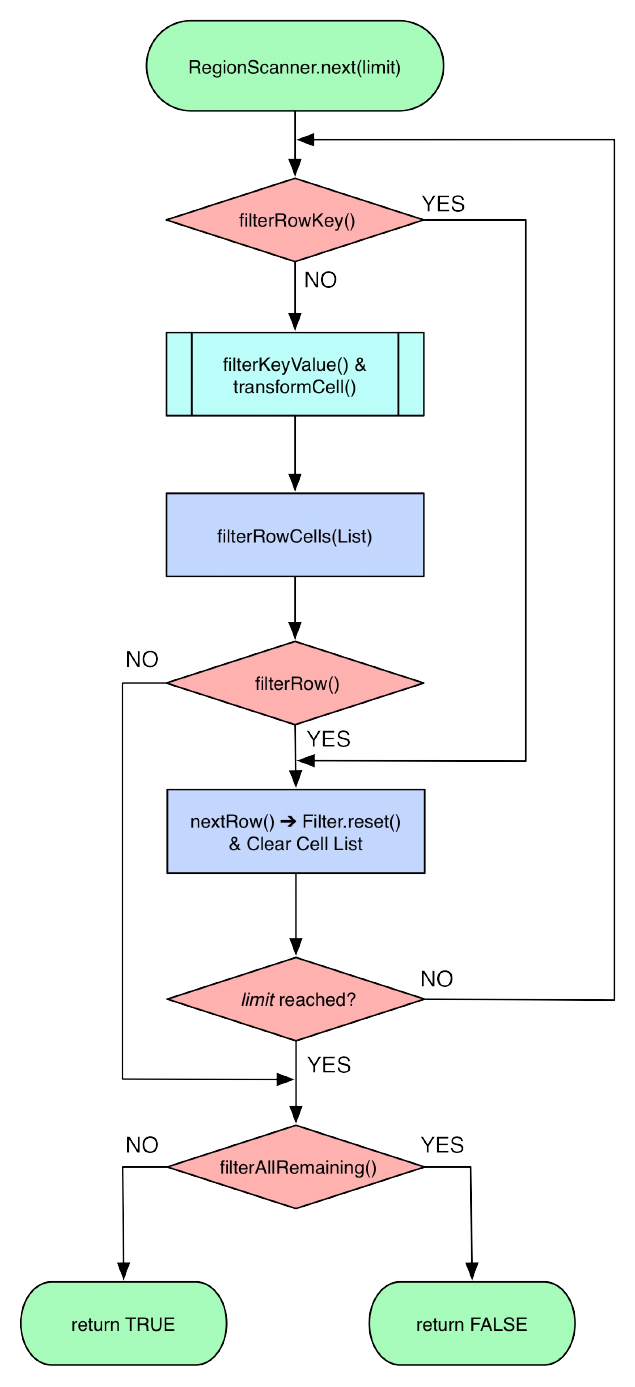
(256)

Figure 4-2. The logical flow through the filter methods for a single row
The Filter interface has a few more methods at its disposal. Table 4-5 lists them for your
perusal.
Table 4-5. Additional methods provided by the Filter class
Method Description
getNextCellHint()
This method is invoked when the filter’s filterKeyValue() method
returns ReturnCode.SEEK_NEXT_USING_HINT. Use it to skip large ranges
of rows—if possible.
isFamilyEssential()
Discussed in “Load Column Families on Demand”, used to avoid
unnecessary loading of cells from column families in low-cardinality
scans.
setReversed()/isReversed() Flags the direction the filter instance is observing. A reverse scan
must use reverse filters too.
toByteArray()/parseFrom() Used to de-/serialize the filter’s internal state to ship to the servers
for application.
The reverse flag, assigned with setReversed(true), helps the filter to come to the right decision.
Here is a snippet from the PrefixFilter.filterRowKey() method, showing how the result of the
binary prefix comparison is reversed based on this flag:
...
int cmp = Bytes.compareTo(buffer, offset, this.prefix.length,
this.prefix, 0, this.prefix.length);
if ((!isReversed() && cmp > 0) || (isReversed() && cmp < 0)) {
passedPrefix = true;
}
...
Example 4-23 implements a custom filter, using the methods provided by FilterBase, overriding
only those methods that need to be changed (or, more specifically, at least implement those that
are marked abstract). The filter first assumes all rows should be filtered, that is, removed from
the result. Only when there is a value in any column that matches the given reference does it
include the row, so that it is sent back to the client. See “Custom Filter Loading” for how to load
the custom filters into the Java server process.
Example 4-23. Implements a filter that lets certain rows pass
public class CustomFilter extends FilterBase {
private byte[] value = null;
private boolean filterRow = true;
public CustomFilter() {
super();
(257)
}
public CustomFilter(byte[] value) {
this.value = value;
}
@Override
public void reset() {
this.filterRow = true;
}
@Override
public ReturnCode filterKeyValue(Cell cell) {
if (CellUtil.matchingValue(cell, value)) {
filterRow = false;
}
return ReturnCode.INCLUDE;
}
@Override
public boolean filterRow() {
return filterRow;
}
@Override
public byte [] toByteArray() {
FilterProtos.CustomFilter.Builder builder =
FilterProtos.CustomFilter.newBuilder();
if (value != null) builder.setValue(ByteStringer.wrap(value));
return builder.build().toByteArray();
}
//@Override
public static Filter parseFrom(final byte[] pbBytes)
throws DeserializationException {
FilterProtos.CustomFilter proto;
try {
proto = FilterProtos.CustomFilter.parseFrom(pbBytes);
} catch (InvalidProtocolBufferException e) {
throw new DeserializationException(e);
}
return new CustomFilter(proto.getValue().toByteArray());
}
}
Set the value to compare against.
Reset filter flag for each new row being tested.
When there is a matching value, then let the row pass.
Always include, since the final decision is made later.
Here the actual decision is taking place, based on the flag status.
Writes the given value out so it can be sent to the servers.
(258)

Used by the servers to establish the filter instance with the correct values.
The most interesting part about the custom filter is the serialization using Protocol Buffers
(Protobuf, for short).3 The first thing to do is define a message in Protobuf, which is done in a
simple text file, here named CustomFilters.proto:
option java_package = "filters.generated";
option java_outer_classname = "FilterProtos";
option java_generic_services = true;
option java_generate_equals_and_hash = true;
option optimize_for = SPEED;
message CustomFilter {
required bytes value = 1;
}
The file defines the output class name, the package to use during code generation and so on. The
next step is to compile the definition file into code. This is done using the Protobuf protoc tool.
Tip
The Protocol Buffer library usually comes as a source package that needs to be compiled and
locally installed. There are also pre-built binary packages for many operating systems. On OS X,
for example, you can run the following, assuming Homebrew was installed:
$ brew install protobuf
You can verify the installation by running $ protoc --version and check it prints a version
number:
$ protoc --version
libprotoc 2.6.1
The online code repository of the book has a script bin/doprotoc.sh that runs the code generation.
It essentially runs the following command from the repository root directory:
$ protoc -Ich04/src/main/protobuf --java_out=ch04/src/main/java \
ch04/src/main/protobuf/CustomFilters.proto
This will place the generated class file in the source directory, as specified. After that you will be
able to use the generated types in your custom filter as shown in the example. Example 4-24 uses
the new custom filter to find rows with specific values in it, also using a FilterList.
Example 4-24. Example using a custom filter
List<Filter> filters = new ArrayList<Filter>();
Filter filter1 = new CustomFilter(Bytes.toBytes("val-05.05"));
filters.add(filter1);
Filter filter2 = new CustomFilter(Bytes.toBytes("val-02.07"));
filters.add(filter2);
Filter filter3 = new CustomFilter(Bytes.toBytes("val-09.01"));
filters.add(filter3);
FilterList filterList = new FilterList(
FilterList.Operator.MUST_PASS_ONE, filters);
(259)
Scan scan = new Scan();
scan.setFilter(filterList);
ResultScanner scanner = table.getScanner(scan);
for (Result result : scanner) {
for (Cell cell : result.rawCells()) {
System.out.println("Cell: " + cell + ", Value: " +
Bytes.toString(cell.getValueArray(), cell.getValueOffset(),
cell.getValueLength()));
}
}
scanner.close();
Just as with the earlier examples, here is what should appear as output on the console when
executing this example:
Adding rows to table...
Results of scan:
Cell: row-02/colfam1:col-01/1/Put/vlen=9/seqid=0, Value: val-02.01
Cell: row-02/colfam1:col-02/2/Put/vlen=9/seqid=0, Value: val-02.02
...
Cell: row-02/colfam1:col-06/6/Put/vlen=9/seqid=0, Value: val-02.06
Cell: row-02/colfam1:col-07/7/Put/vlen=9/seqid=0, Value: val-02.07
Cell: row-02/colfam1:col-08/8/Put/vlen=9/seqid=0, Value: val-02.08
...
Cell: row-05/colfam1:col-04/4/Put/vlen=9/seqid=0, Value: val-05.04
Cell: row-05/colfam1:col-05/5/Put/vlen=9/seqid=0, Value: val-05.05
Cell: row-05/colfam1:col-06/6/Put/vlen=9/seqid=0, Value: val-05.06
...
Cell: row-05/colfam1:col-10/10/Put/vlen=9/seqid=0, Value: val-05.10
Cell: row-09/colfam1:col-01/1/Put/vlen=9/seqid=0, Value: val-09.01
Cell: row-09/colfam1:col-02/2/Put/vlen=9/seqid=0, Value: val-09.02
...
Cell: row-09/colfam1:col-09/9/Put/vlen=9/seqid=0, Value: val-09.09
Cell: row-09/colfam1:col-10/10/Put/vlen=9/seqid=0, Value: val-09.10
As expected, the entire row that has a column with the value matching one of the references is
included in the result.
Custom Filter Loading
Once you have written your filter, you need to deploy it to your HBase setup. You need to
compile the class, pack it into a Java Archive (JAR) file, and make it available to the region
servers. You can use the build system of your choice to prepare the JAR file for deployment, and
a configuration management system to actually provision the file to all servers. Once you have
uploaded the JAR file, you have two choices how to load them:
Static Configuration
In this case, you need to add the JAR file to the hbase-env.sh configuration file, for
example:
# Extra Java CLASSPATH elements. Optional.
# export HBASE_CLASSPATH=
export HBASE_CLASSPATH="/hbase-book/ch04/target/hbase-book-ch04-2.0.jar"
This is using the JAR file created by the Maven build as supplied by the source code
repository accompanying this book. It uses an absolute, local path since testing is done on
a standalone setup, in other words, with the development environment and HBase running
on the same physical machine.
Note that you must restart the HBase daemons so that the changes in the configuration file
are taking effect. Once this is done you can proceed to test the new filter.
(260)

Dynamic Loading
You still build the JAR file the same way, but instead of hardcoding its path into the
configuration files, you can use the cluster wide, shared JAR file directory in HDFS that is
used to load JAR files from. See the following configuration property from the hbase-
default.xml file:
<property>
<name>hbase.dynamic.jars.dir</name>
<value>${hbase.rootdir}/lib</value>
</property>
The default points to ${hbase.rootdir}/lib, which usually resolves to /hbase/lib/ within
HDFS. The full path would be similar to this example path:
hdfs://master.foobar.com:9000/hbase/lib. If this directory exists and contains files ending
in .jar, then the servers will load those files and make the contained classes available. To
do so, the files are copied to a local directory named jars, located in a parent directory set
again in the HBase default properties:
<property>
<name>hbase.local.dir</name>
<value>${hbase.tmp.dir}/local/</value>
</property>
An example path for a cluster with a configured temporary directory pointing to /data/tmp/
you will see the JAR files being copied to /data/tmp/local/jars. You will see this directory
again later on when we talk about dynamic coprocessor loading in “Coprocessor Loading”.
The local JAR files are flagged to be deleted when the server process ends normally.
The dynamic loading directory is monitored for changes, and will refresh the JAR files
locally if they have been updated in the shared location.
Note that no matter how you load the classes and their containing JARs, HBase is currently not
able to unload a previously loaded class. This means that once loaded, you cannot replace a class
with the same name. The only way short of restarting the server processes is to add a version
number to the class and JAR name to load the new one by new name. This leaves the previous
classes loaded in memory and might cause memory issues after some time.
(261)

Filter Parser Utility
The client-side filter package comes with another helper class, named ParseFilter. It is used in
all the places where filters need to be described with text and then, eventually, converted to a
Java class. This happens in the gateway servers, such as for REST or Thrift. The HBase Shell
also makes use of the class allowing a shell user to specify a filter on the command line, and then
executing the filter as part of a subsequent scan, or get, operation. The following executes a scan
on one of the earlier test tables (so your results may vary), adding a row prefix and qualifier
filter, using the shell:
hbase(main):001:0> scan 'testtable', \
{ FILTER => "PrefixFilter('row-2') AND QualifierFilter(<=, 'binary:col-2')" }
ROW COLUMN+CELL
row-20 column=colfam1:col-0, timestamp=7, value=val-46
row-21 column=colfam1:col-0, timestamp=7, value=val-87
row-21 column=colfam1:col-2, timestamp=5, value=val-26
...
row-28 column=colfam1:col-2, timestamp=3, value=val-74
row-29 column=colfam1:col-1, timestamp=0, value=val-86
row-29 column=colfam1:col-2, timestamp=3, value=val-21
10 row(s) in 0.0170 seconds
What seems odd at first is the "binary:col-2" parameter. The second part after the colon is the
value handed into the filter. The first part is the way the filter parser class is allowing you to
specify a comparator for filters based on CompareFilter (see “Comparators”). Here is a list of
supported comparator prefixes:
Table 4-6. String representation of
Comparator types
String Type
binary BinaryComparator
binaryprefix BinaryPrefixComparator
regexstring RegexStringComparator
substring SubstringComparator
Since a comparison filter also requires a comparison operation, there is a way of expressing this
in string format. The example above uses "<=" to specify less than or equal. Since there is an
enumeration provided by the CompareFilter class, there is a matching pattern between the string
representation and the enumeration value, as shown in the next table (also see “Comparison
Operators”):
Table 4-7. String representation of
compare operation
String Type
< CompareOp.LESS
(262)

<= CompareOp.LESS_OR_EQUAL
> CompareOp.GREATER
>= CompareOp.GREATER_OR_EQUAL
= CompareOp.EQUAL
!= CompareOp.NOT_EQUAL
The filter parser supports a few more text based tokens that translate into filter classes. You can
combine filters with the AND and OR keywords, which are subsequently translated into FilterList
instances that are either set to MUST_PASS_ALL, or MUST_PASS_ONE respectively (“FilterList” describes
this in more detail). An example might be:
hbase(main):001:0> scan 'testtable', \
{ FILTER => "(PrefixFilter('row-2') AND ( \
QualifierFilter(>=, 'binary:col-2'))) AND (TimestampsFilter(1, 5))" }
ROW COLUMN+CELL
row-2 column=colfam1:col-9, timestamp=5, value=val-31
row-21 column=colfam1:col-2, timestamp=5, value=val-26
row-23 column=colfam1:col-5, timestamp=5, value=val-55
row-28 column=colfam1:col-5, timestamp=1, value=val-54
4 row(s) in 0.3190 seconds
Finally, there are the keywords SKIP and WHILE, representing the use of a SkipFilter (see
“SkipFilter”) and WhileMatchFilter (see “WhileMatchFilter”). Refer to the mentioned sections for
details on their features.
hbase(main):001:0> scan 'testtable', \
{ FILTER => "SKIP ValueFilter(>=, 'binary:val-5') " }
ROW COLUMN+CELL
row-11 column=colfam1:col-0, timestamp=8, value=val-82
row-48 column=colfam1:col-3, timestamp=6, value=val-55
row-48 column=colfam1:col-7, timestamp=3, value=val-80
row-48 column=colfam1:col-8, timestamp=2, value=val-65
row-7 column=colfam1:col-9, timestamp=6, value=val-57
3 row(s) in 0.0150 seconds
The precedence of the keywords the parser understands is the following, listed from highest to
lowest:
Table 4-8. Precedence of string keywords
Keyword Description
SKIP/WHILE Wrap filter into SkipFilter, or WhileMatchFilter instance.
AND Add both filters left and right of keyword to FilterList instance using MUST_PASS_ALL.
OR Add both filters left and right of keyword to FilterList instance using MUST_PASS_ONE.
(263)
From code you can invoke one of the following methods to parse a filter string into class
instances:
Filter parseFilterString(String filterString)
throws CharacterCodingException
Filter parseFilterString (byte[] filterStringAsByteArray)
throws CharacterCodingException
Filter parseSimpleFilterExpression(byte[] filterStringAsByteArray)
throws CharacterCodingException
The parseSimpleFilterExpression() parses one specific filter instance, and is used mainly from
within the parseFilterString() methods. The latter handles the combination of multiple filters
with AND and OR, plus the decorating filter wrapping with SKIP and WHILE. The two
parseFilterString() methods are the same, one is taking a string and the other a string converted
to a byte[] array.
The ParseFilter class—by default—only supports the filters that are shipped with HBase. The
unsupported filters on top of that are FirstKeyValueMatchingQualifiersFilter, FuzzyRowFilter, and
RandomRowFilter (as of this writing). In your own code you can register your own, and retrieve the
list of supported filters using the following methods of this class:
static Map<String, String> getAllFilters()
Set<String> getSupportedFilters()
static void registerFilter(String name, String filterClass)
(264)

Filters Summary
Table 4-9 summarizes some of the features and compatibilities related to the provided filter
implementations. The ✓ symbol means the feature is available, while ✗ indicates it is missing.
Table 4-9. Summary of filter features and compatibilities between them
Filter BatchaSkipbWhile-
MatchcListdEarly
OuteGetsfScansg
RowFilter ✓ ✓ ✓ ✓ ✓ ✗ ✓
FamilyFilter ✓ ✓ ✓ ✓ ✗ ✓ ✓
QualifierFilter ✓ ✓ ✓ ✓ ✗ ✓ ✓
ValueFilter ✓ ✓ ✓ ✓ ✗ ✓ ✓
DependentColumnFilter ✗ ✓ ✓ ✓ ✗ ✓ ✓
SingleColumnValueFilter ✓ ✓ ✓ ✓ ✗ ✗ ✓
SingleColumnValueExcludeFilter ✓ ✓ ✓ ✓ ✗ ✗ ✓
PrefixFilter ✓ ✗ ✓ ✓ ✓ ✗ ✓
PageFilter ✓ ✗ ✓ ✓ ✓ ✗ ✓
KeyOnlyFilter ✓ ✓ ✓ ✓ ✗ ✓ ✓
FirstKeyOnlyFilter ✓ ✓ ✓ ✓ ✗ ✓ ✓
FirstKeyValueMatchingQualifiersFilter ✓ ✓ ✓ ✓ ✗ ✓ ✓
InclusiveStopFilter ✓ ✗ ✓ ✓ ✓ ✗ ✓
(265)

FuzzyRowFilter ✓ ✓ ✓ ✓ ✓ ✗ ✓
ColumnCountGetFilter ✓ ✓ ✓ ✓ ✗ ✓ ✗
ColumnPaginationFilter ✓ ✓ ✓ ✓ ✗ ✓ ✓
ColumnPrefixFilter ✓ ✓ ✓ ✓ ✗ ✓ ✓
MultipleColumnPrefixFilter ✓ ✓ ✓ ✓ ✗ ✓ ✓
ColumnRange ✓ ✓ ✓ ✓ ✗ ✓ ✓
TimestampsFilter ✓ ✓ ✓ ✓ ✗ ✓ ✓
RandomRowFilter ✓ ✓ ✓ ✓ ✗ ✗ ✓
SkipFilter ✓✓/
✗h✓/✗h✓ ✗ ✗ ✓
WhileMatchFilter ✓✓/
✗h✓/✗h✓ ✓ ✗ ✓
FilterList ✓/✗h✓/
✗h✓/✗h✓✓/✗h✓ ✓
a Filter supports Scan.setBatch(), i.e., the scanner batch mode.
b Filter can be used with the decorating SkipFilter class.
c Filter can be used with the decorating WhileMatchFilter class.
d Filter can be used with the combining FilterList class.
e Filter has optimizations to stop a scan early, once there are no more matching rows ahead.
f Filter can be usefully applied to Get instances.
g Filter can be usefully applied to Scan instances.
(266)

Counters
In addition to the functionality we already discussed, HBase offers another advanced feature:
counters. Many applications that collect statistics—such as clicks or views in online advertising
—were used to collect the data in log files that would subsequently be analyzed. Using counters
offers the potential of switching to live accounting, foregoing the delayed batch processing step
completely.
(268)

Introduction to Counters
In addition to the check-and-modify operations you saw earlier, HBase also has a mechanism to
treat columns as counters. Otherwise, you would have to lock a row, read the value, increment it,
write it back, and eventually unlock the row for other writers to be able to access it subsequently.
This can cause a lot of contention, and in the event of a client process, crashing it could leave the
row locked until the lease recovery kicks in—which could be disastrous in a heavily loaded
system.
The client API provides specialized methods to do the read-modify-write operation atomically in
a single client-side call. Earlier versions of HBase only had calls that would involve an RPC for
every counter update, while newer versions started to add the same mechanisms used by the
CRUD operations—as explained in “CRUD Operations”--which can bundle multiple counter
updates in a single RPC.
Before we discuss each type separately, you need to have a few more details regarding how
counters work on the column level. Here is an example using the shell that creates a table,
increments a counter twice, and then queries the current value:
hbase(main):001:0> create 'counters', 'daily', 'weekly', 'monthly'
0 row(s) in 1.1930 seconds
hbase(main):002:0> incr 'counters', '20150101', 'daily:hits', 1
COUNTER VALUE = 1
0 row(s) in 0.0490 seconds
hbase(main):003:0> incr 'counters', '20150101', 'daily:hits', 1
COUNTER VALUE = 2
0 row(s) in 0.0170 seconds
hbase(main):04:0> get_counter 'counters', '20150101', 'daily:hits'
COUNTER VALUE = 2
Every call to incr increases the counter by the given value (here 1). The final check using
get_counter shows the current value as expected. The format of the shell’s incr command is as
follows:
incr '<table>', '<row>', '<column>', [<increment-value>]
Initializing Counters
You should not initialize counters, as they are automatically assumed to be zero when you first
use a new counter, that is, a column qualifier that does not yet exist. The first increment call to a
new counter will set it to 1--or the increment value, if you have specified one.
You can read and write to a counter directly, but you must use
Bytes.toLong()
to decode the value and
Bytes.toBytes(long)
for the encoding of the stored value. The latter, in particular, can be tricky, as you need to make
sure you are using a long number when using the toBytes() method. You might want to consider
(269)
typecasting the variable or number you are using to a long explicitly, like so:
byte[] b1 = Bytes.toBytes(1L)
byte[] b2 = Bytes.toBytes((long) var)
If you were to try to erroneously initialize a counter using the put method in the HBase Shell,
you might be tempted to do this:
hbase(main):001:0> put 'counters', '20150101', 'daily:clicks', '1'
0 row(s) in 0.0540 seconds
But when you are going to use the increment method, you would get this result instead:
hbase(main):013:0> incr 'counters', '20110101', 'daily:clicks', 1
ERROR: org.apache.hadoop.hbase.DoNotRetryIOException: Attempted to increment field that isn't
64 bits wide
at org.apache.hadoop.hbase.regionserver.HRegion.increment(HRegion.java:5856)
at org.apache.hadoop.hbase.regionserver.RSRpcServices.increment(RSRpcServices.java:490)
...
That is not the expected value of 2! This is caused by the put call storing the counter in the wrong
format: the value is the character 1, a single byte, not the byte array representation of a Java long
value—which is composed of eight bytes.
You can also access the counter with a get call, giving you this result:
hbase(main):005:0> get 'counters', '20150101'
COLUMN CELL
daily:hits timestamp=1427485256567, value=\x00\x00\x00\x00\x00\x00\x00\x02
1 row(s) in 0.0280 seconds
This is obviously not very readable, but it shows that a counter is simply a column, like any
other. You can also specify a larger increment value:
hbase(main):006:0> incr 'counters', '20150101', 'daily:hits', 20
COUNTER VALUE = 22
0 row(s) in 0.0180 seconds
hbase(main):007:0> get_counter 'counters', '20150101', 'daily:hits'
COUNTER VALUE = 22
hbase(main):008:0> get 'counters', '20150101'
COLUMN CELL
daily:hits timestamp=1427489182419, value=\x00\x00\x00\x00\x00\x00\x00\x16
1 row(s) in 0.0200 seconds
Accessing the counter directly gives you the byte[] array representation, with the shell printing
the separate bytes as hexadecimal values. Using the get_counter once again shows the current
value in a more human-readable format, and confirms that variable increments are possible and
work as expected.
Finally, you can use the increment value of the incr call to not only increase the counter, but also
retrieve the current value, and decrease it as well. In fact, you can omit it completely and the
default of 1 is assumed:
hbase(main):009:0> incr 'counters', '20150101', 'daily:hits'
COUNTER VALUE = 23
0 row(s) in 0.1700 seconds
hbase(main):010:0> incr 'counters', '20150101', 'daily:hits'
COUNTER VALUE = 24
0 row(s) in 0.0230 seconds
hbase(main):011:0> incr 'counters', '20150101', 'daily:hits', 0
(270)

COUNTER VALUE = 24
0 row(s) in 0.0170 seconds
hbase(main):012:0> incr 'counters', '20150101', 'daily:hits', -1
COUNTER VALUE = 23
0 row(s) in 0.0210 seconds
hbase(main):013:0> incr 'counters', '20150101', 'daily:hits', -1
COUNTER VALUE = 22
0 row(s) in 0.0200 seconds
Using the increment value—the last parameter of the incr command—you can achieve the
behavior shown in Table 4-10.
Table 4-10. The increment value and its effect on counter increments
Value Effect
greater than
zero Increase the counter by the given value.
zero Retrieve the current value of the counter. Same as using the get_counter shell
command.
less than zero Decrease the counter by the given value.
Obviously, using the shell’s incr command only allows you to increase a single counter. You can
do the same using the client API, described next.
(271)
Single Counters
The first type of increment call is for single counters only: you need to specify the exact column
you want to use. The methods, provided by Table, are as such:
long incrementColumnValue(byte[] row, byte[] family, byte[] qualifier,
long amount) throws IOException;
long incrementColumnValue(byte[] row, byte[] family, byte[] qualifier,
long amount, Durability durability) throws IOException;
Given the coordinates of a column, and the increment amount, these methods only differ by the
optional durability parameter—which works the same way as the Put.setDurability() method
(see “Durability, Consistency, and Isolation” for the general discussion of this feature). Omitting
durability uses the default value of Durability.SYNC_WAL, meaning the write-ahead log is active.
Apart from that, you can use them straight forward, as shown in Example 4-25.
Example 4-25. Example using the single counter increment methods
long cnt1 = table.incrementColumnValue(Bytes.toBytes("20110101"),
Bytes.toBytes("daily"), Bytes.toBytes("hits"), 1);
long cnt2 = table.incrementColumnValue(Bytes.toBytes("20110101"),
Bytes.toBytes("daily"), Bytes.toBytes("hits"), 1);
long current = table.incrementColumnValue(Bytes.toBytes("20110101"),
Bytes.toBytes("daily"), Bytes.toBytes("hits"), 0);
long cnt3 = table.incrementColumnValue(Bytes.toBytes("20110101"),
Bytes.toBytes("daily"), Bytes.toBytes("hits"), -1);
Increase counter by one.
Increase counter by one a second time.
Get current value of the counter without increasing it.
Decrease counter by one.
The output on the console is:
cnt1: 1, cnt2: 2, current: 2, cnt3: 1
Just as with the shell commands used earlier, the API calls have the same effect: they increment
the counter when using a positive increment value, retrieve the current value when using zero for
the increment, and decrease the counter by using a negative increment value.
(272)

Multiple Counters
Another way to increment counters is provided by the increment() call of Table. It works
similarly to the CRUD-type operations discussed earlier, using the following method to do the
increment:
Result increment(final Increment increment) throws IOException
You must create an instance of the Increment class and fill it with the appropriate details—for
example, the counter coordinates. The constructors provided by this class are:
Increment(byte[] row)
Increment(final byte[] row, final int offset, final int length)
Increment(Increment i)
You must provide a row key when instantiating an Increment, which sets the row containing all
the counters that the subsequent call to increment() should modify. There is also the variant
already known to you that takes a larger array with an offset and length parameter to extract the
row key from. Finally, there is also the one you have seen before, which takes an existing
instance and copies all state from it.
Once you have decided which row to update and created the Increment instance, you need to add
the actual counters—meaning columns—you want to increment, using these methods:
Increment addColumn(byte[] family, byte[] qualifier, long amount)
Increment add(Cell cell) throws IOException
The first variant takes the column coordinates, while the second is reusing an existing cell. This
is useful, if you have just retrieved a counter and now want to increment it. The add() call checks
that the given cell matches the row key of the Increment instance.
The difference here, as compared to the Put methods, is that there is no option to specify a
version—or timestamp—when dealing with increments: versions are handled implicitly.
Furthermore, there is no addFamily() equivalent, because counters are specific columns, and they
need to be specified as such. It therefore makes no sense to add a column family alone.
A special feature of the Increment class is the ability to take an optional time range:
Increment setTimeRange(long minStamp, long maxStamp) throws IOException
TimeRange getTimeRange()
Setting a time range for a set of counter increments seems odd in light of the fact that versions
are handled implicitly. The time range is actually passed on to the servers to restrict the internal
get operation from retrieving the current counter values. You can use it to expire counters, for
example, to partition them by time: when you set the time range to be restrictive enough, you can
mask out older counters from the internal get, making them look like they are nonexistent. An
increment would assume they are unset and start at 1 again. The getTimeRange() returns the
currently assigned time range (and might be null if not set at all).
Similar to the shell example shown earlier, Example 4-26 uses various increment values to
increment, retrieve, and decrement the given counters.
Example 4-26. Example incrementing multiple counters in one row
(273)

Increment increment1 = new Increment(Bytes.toBytes("20150101"));
increment1.addColumn(Bytes.toBytes("daily"), Bytes.toBytes("clicks"), 1);
increment1.addColumn(Bytes.toBytes("daily"), Bytes.toBytes("hits"), 1);
increment1.addColumn(Bytes.toBytes("weekly"), Bytes.toBytes("clicks"), 10);
increment1.addColumn(Bytes.toBytes("weekly"), Bytes.toBytes("hits"), 10);
Result result1 = table.increment(increment1);
for (Cell cell : result1.rawCells()) {
System.out.println("Cell: " + cell +
" Value: " + Bytes.toLong(cell.getValueArray(), cell.getValueOffset(),
cell.getValueLength()));
}
Increment increment2 = new Increment(Bytes.toBytes("20150101"));
increment2.addColumn(Bytes.toBytes("daily"), Bytes.toBytes("clicks"), 5);
increment2.addColumn(Bytes.toBytes("daily"), Bytes.toBytes("hits"), 1);
increment2.addColumn(Bytes.toBytes("weekly"), Bytes.toBytes("clicks"), 0);
increment2.addColumn(Bytes.toBytes("weekly"), Bytes.toBytes("hits"), -5);
Result result2 = table.increment(increment2);
for (Cell cell : result2.rawCells()) {
System.out.println("Cell: " + cell +
" Value: " + Bytes.toLong(cell.getValueArray(),
cell.getValueOffset(), cell.getValueLength()));
}
Increment the counters with various values.
Call the actual increment method with the above counter updates and receive the results.
Print the cell and returned counter value.
Use positive, negative, and zero increment values to achieve the wanted counter changes.
When you run the example, the following is output on the console:
Cell: 20150101/daily:clicks/1427651982538/Put/vlen=8/seqid=0 Value: 1
Cell: 20150101/daily:hits/1427651982538/Put/vlen=8/seqid=0 Value: 1
Cell: 20150101/weekly:clicks/1427651982538/Put/vlen=8/seqid=0 Value: 10
Cell: 20150101/weekly:hits/1427651982538/Put/vlen=8/seqid=0 Value: 10
Cell: 20150101/daily:clicks/1427651982543/Put/vlen=8/seqid=0 Value: 6
Cell: 20150101/daily:hits/1427651982543/Put/vlen=8/seqid=0 Value: 2
Cell: 20150101/weekly:clicks/1427651982543/Put/vlen=8/seqid=0 Value: 10
Cell: 20150101/weekly:hits/1427651982543/Put/vlen=8/seqid=0 Value: 5
When you compare the two sets of increment results, you will notice that this works as expected.
The Increment class provides additional methods, which are listed in Table 4-11 for your
reference. Once again, many are inherited from the superclasses, such as Mutation (see “Query
versus Mutation” again).
Table 4-11. Quick overview of additional methods provided by the Increment class
(274)
Method Description
cellScanner() Provides a scanner over all cells available in this
instance.
getACL()/setACL() The ACLs for this operation (might be null).
getAttribute()/setAttribute() Set and get arbitrary attributes associated with this
instance of Increment.
getAttributesMap() Returns the entire map of attributes, if any are set.
getCellVisibility()/setCellVisibility() The cell level visibility for all included cells.
getClusterIds()/setClusterIds() The cluster IDs as needed for replication purposes.
getDurability()/setDurability() The durability settings for the mutation.
getFamilyCellMap()/setFamilyCellMap() The list of all cells of this instance.
getFamilyMapOfLongs()
Returns a list of Long instance, instead of cells (which
getFamilyCellMap() does), for what was added to this
instance so far. The list is indexed by families, and then
by column qualifier.
getFingerprint() Compiles details about the instance into a map for
debugging, or logging.
getId()/setId() An ID for the operation, useful for identifying the
origin of a request later.
getRow() Returns the row key as specified when creating the
Increment instance.
getTimeStamp() Not useful with Increment. Defaults to
HConstants.LATEST_TIMESTAMP.
getTTL()/setTTL() Sets the cell level TTL value, which is being applied to
all included Cell instances before being persisted.
(275)

getTTL()/setTTL() all included Cell instances before being persisted.
hasFamilies()
Another helper to check if a family—or column—has
been added to the current instance of the Increment
class.
heapSize()
Computes the heap space required for the current
Increment instance. This includes all contained data and
space needed for internal structures.
isEmpty() Checks if the family map contains any Cell instances.
numFamilies() Convenience method to retrieve the size of the family
map, containing all Cell instances.
size() Returns the number of Cell instances that will be
applied with this Increment.
toJSON()/toJSON(int) Converts the first 5 or N columns into a JSON format.
toMap()/toMap(int) Converts the first 5 or N columns into a map. This is
more detailed than what getFingerprint() returns.
toString()/toString(int) Converts the first 5 or N columns into a JSON, or map
(if JSON fails due to encoding problems).
A non-Mutation method provided by Increment is:
Map<byte[], NavigableMap<byte[], Long>> getFamilyMapOfLongs()
The above Example 4-26 in the online repository shows how this can give you access to the list
of increment values of a configured Increment instance. It is omitted above for the sake of
brevity, but the online code has this available (around line number 40).
(276)
Coprocessors
Earlier we discussed how you can use filters to reduce the amount of data being sent over the
network from the servers to the client. With the coprocessor feature in HBase, you can even
move part of the computation to where the data lives.
Note
We slightly go on a tangent here as far as interface audience is concerned. If you refer back to
[Link to Come] you will see how we, up until now, solely covered Public APIs, that is, those that
are annotated as being public. For coprocessors we are now looking at an API annotated as
@InterfaceAudience.LimitedPrivate(HBaseInterfaceAudience.COPROC), since it is meant for HBase
system developers. A normal API user will make use of coprocessors, but most likely not
develop them. Coprocessors are very low-level, and are usually for very experienced developers
only.
(277)

Introduction to Coprocessors
Using the client API, combined with specific selector mechanisms, such as filters, or column
family scoping, it is possible to limit what data is transferred to the client. It would be good,
though, to take this further and, for example, perform certain operations directly on the server
side while only returning a small result set. Think of this as a small MapReduce framework that
distributes work across the entire cluster.
A coprocessor enables you to run arbitrary code directly on each region server. More precisely, it
executes the code on a per-region basis, giving you trigger- like functionality—similar to stored
procedures in the RDBMS world. From the client side, you do not have to take specific actions,
as the framework handles the distributed nature transparently.
There is a set of implicit events that you can use to hook into, performing auxiliary tasks. If this
is not enough, you can also extend the RPC protocol to introduce your own set of calls, which
are invoked from your client and executed on the server on your behalf.
Just as with the custom filters (see “Custom Filters”), you need to create special Java classes that
implement specific interfaces. Once they are compiled, you make these classes available to the
servers in the form of a JAR file. The region server process can instantiate these classes and
execute them in the correct environment. In contrast to the filters, though, coprocessors can be
loaded dynamically as well. This allows you to extend the functionality of a running HBase
cluster.
Use cases for coprocessors are, for instance, using hooks into row mutation operations to
maintain secondary indexes, or implementing some kind of referential integrity. Filters could be
enhanced to become stateful, and therefore make decisions across row boundaries. Aggregate
functions, such as sum(), or avg(), known from RDBMSes and SQL, could be moved to the
servers to scan the data locally and only returning the single number result across the network
(which is showcased by the supplied AggregateImplementation class).
Note
Another good use case for coprocessors is access control. The authentication, authorization, and
auditing features added in HBase version 0.92 are based on coprocessors. They are loaded at
system startup and use the provided trigger-like hooks to check if a user is authenticated, and
authorized to access specific values stored in tables.
The framework already provides classes, based on the coprocessor framework, which you can
use to extend from when implementing your own functionality. They fall into two main groups:
endpoint and observer. Here is a brief overview of their purpose:
Endpoint
Next to event handling there may be also a need to add custom operations to a cluster.
User code can be deployed to the servers hosting the data to, for example, perform server-
local computations.
Endpoints are dynamic extensions to the RPC protocol, adding callable remote procedures.
(278)

Think of them as stored procedures, as known from RDBMSes. They may be combined
with observer implementations to directly interact with the server-side state.
Observer
This type of coprocessor is comparable to triggers: callback functions (also referred to
here as hooks) are executed when certain events occur. This includes user-generated, but
also server-internal, automated events.
The interfaces provided by the coprocessor framework are:
MasterObserver
This can be used to react to administrative or DDL-type operations. These are
cluster-wide events.
RegionServerObserver
Hooks into commands sent to a region server, and covers region server-wide events.
RegionObserver
Used to handle data manipulation events. They are closely bound to the regions of a
table.
WALObserver
This provides hooks into the write-ahead log processing, which is region server-
wide.
BulkLoadObserver
Handles events around the bulk loading API. Triggered before and after the loading
takes place.
EndpointObserver
Whenever an endpoint is invoked by a client, this observer provides a callback
method.
Observers provide you with well-defined event callbacks, for every operation a cluster
server may handle.
All of these interfaces are based on the Coprocessor interface to gain common features, but then
implement their own specific functionality.
Finally, coprocessors can be chained, very similar to what the Java Servlet API does with request
filters. The following section discusses the various types available in the coprocessor framework.
Figure 4-3 shows an overview of all the classes we will be looking into.
(279)
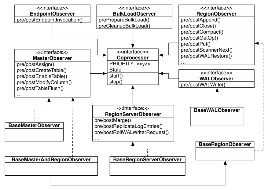
Figure 4-3. The class hierarchy of the coprocessor related classes
(280)

The Coprocessor Class Trinity
All user coprocessor classes must be based on the Coprocessor interface. It defines the basic
contract of a coprocessor and facilitates the management by the framework itself. The interface
provides two sets of types, which are used throughout the framework: the PRIORITY constants4,
and State enumeration. Table 4-12 explains the priority values.
Table 4-12. Priorities as defined by the Coprocessor.PRIORITY_<XYZ> constants
Name Value Description
PRIORITY_HIGHEST 0 Highest priority, serves as an upper boundary.
PRIORITY_SYSTEM 536870911 High priority, used for system coprocessors (Integer.MAX_VALUE / 4).
PRIORITY_USER 1073741823 For all user coprocessors, which are executed subsequently
(Integer.MAX_VALUE / 2).
PRIORITY_LOWEST 2147483647 Lowest possible priority, serves as a lower boundary
(Integer.MAX_VALUE).
The priority of a coprocessor defines in what order the coprocessors are executed: system-level
instances are called before the user-level coprocessors are executed.
Note
Within each priority level, there is also the notion of a sequence number, which keeps track of
the order in which the coprocessors were loaded. The number starts with zero, and is increased
by one thereafter.
The number itself is not very helpful, but you can rely on the framework to order the
coprocessors—in each priority group—ascending by sequence number. This defines their
execution order.
Coprocessors are managed by the framework in their own life cycle. To that effect, the
Coprocessor interface offers two calls:
void start(CoprocessorEnvironment env) throws IOException
void stop(CoprocessorEnvironment env) throws IOException
These two methods are called when the coprocessor class is started, and eventually when it is
decommissioned. The provided CoprocessorEnvironment instance is used to retain the state across
the lifespan of the coprocessor instance. A coprocessor instance is always contained in a
provided environment, which provides the following methods:
String getHBaseVersion()
(281)

Returns the HBase version identification string, for example "1.0.0".
int getVersion()
Returns the version of the Coprocessor interface.
Coprocessor getInstance()
Returns the loaded coprocessor instance.
int getPriority()
Provides the priority level of the coprocessor.
int getLoadSequence()
The sequence number of the coprocessor. This is set when the instance is loaded and
reflects the execution order.
Configuration getConfiguration()
Provides access to the current, server-wide configuration.
HTableInterface getTable(TableName tableName)
HTableInterface getTable(TableName tableName, ExecutorService service)
Returns a Table implementation for the given table name. This allows the coprocessor to
access the actual table data.5 The second variant does the same, but allows the
specification of a custom ExecutorService instance.
Coprocessors should only deal with what they have been given by their environment. There is a
good reason for that, mainly to guarantee that there is no back door for malicious code to harm
your data.
Note
Coprocessor implementations should be using the getTable() method to access tables. Note that
this class adds certain safety measures to the returned Table implementation. While there is
currently nothing that can stop you from retrieving your own Table instances inside your
coprocessor code, this is likely to be checked against in the future and possibly denied.
The start() and stop() methods of the Coprocessor interface are invoked implicitly by the
framework as the instance is going through its life cycle. Each step in the process has a well-
known state. Table 4-13 lists the life-cycle state values as provided by the coprocessor interface.
Table 4-13. The states as defined by the Coprocessor.State enumeration
Value Description
UNINSTALLED The coprocessor is in its initial state. It has no environment yet, nor is it initialized.
INSTALLED The instance is installed into its environment.
(282)

STARTING This state indicates that the coprocessor is about to be started, that is, its start()
method is about to be invoked.
ACTIVE Once the start() call returns, the state is set to active.
STOPPING The state set just before the stop() method is called.
STOPPED Once stop() returns control to the framework, the state of the coprocessor is set to
stopped.
The final piece of the puzzle is the CoprocessorHost class that maintains all the coprocessor
instances and their dedicated environments. There are specific subclasses, depending on where
the host is used, in other words, on the master, region server, and so on.
The trinity of Coprocessor, CoprocessorEnvironment, and CoprocessorHost forms the basis for the
classes that implement the advanced functionality of HBase, depending on where they are used.
They provide the life-cycle support for the coprocessors, manage their state, and offer the
environment for them to execute as expected. In addition, these classes provide an abstraction
layer that developers can use to easily build their own custom implementation.
Figure 4-4 shows how the calls from a client flow through the list of coprocessors. Note how the
order is the same on the incoming and outgoing sides: first are the system-level ones, and then
the user ones in the order in which they were loaded.
(283)
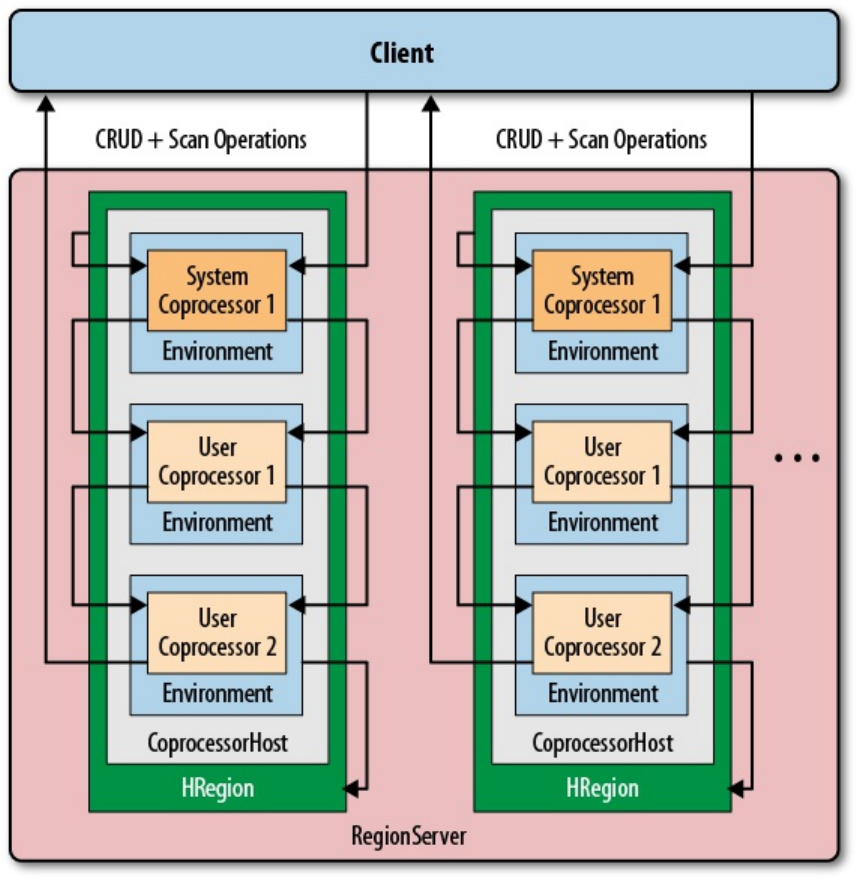
Figure 4-4. Coprocessors executed sequentially, in their environment, and per region
(284)
Coprocessor Loading
Coprocessors are loaded in a variety of ways. Before we discuss the actual coprocessor types and
how to implement your own, we will talk about how to deploy them so that you can try the
provided examples. You can either configure coprocessors to be loaded in a static way, or load
them dynamically while the cluster is running. The static method uses the configuration files and
table schemas, while the dynamic loading of coprocessors is only using the table schemas.
There is also a cluster-wide switch that allows you to disable all coprocessor loading, controlled
by the following two configuration properties:
hbase.coprocessor.enabled
The default is true and means coprocessor classes for system and user tables are loaded.
Setting this property to false stops the servers from loading any of them. You could use
this during testing, or during cluster emergencies.
hbase.coprocessor.user.enabled
Again, the default is true, that is, all user table coprocessors are loaded when the server
starts, or a region opens, etc. Setting this property to false suppresses the loading of user
table coprocessors only.
Caution
Disabling coprocessors, using the cluster-wide configuration properties, means that whatever
additional processing they add, your cluster will not have this functionality available. This
includes, for example, security checks, or maintenance of referential integrity. Be very careful!
Loading from Configuration
You can configure globally which coprocessors are loaded when HBase starts. This is done by
adding one, or more, of the following to the hbase-site.xml configuration file (but please, replace
the example class names with your own ones!):
<property>
<name>hbase.coprocessor.master.classes</name>
<value>coprocessor.MasterObserverExample</value>
</property>
<property>
<name>hbase.coprocessor.regionserver.classes</name>
<value>coprocessor.RegionServerObserverExample</value>
</property>
<property>
<name>hbase.coprocessor.region.classes</name>
<value>coprocessor.system.RegionObserverExample,
coprocessor.AnotherCoprocessor</value>
</property>
<property>
<name>hbase.coprocessor.user.region.classes</name>
<value>coprocessor.user.RegionObserverExample</value>
</property>
<property>
<name>hbase.coprocessor.wal.classes</name>
<value>coprocessor.WALObserverExample, bar.foo.MyWALObserver</value>
</property>
(285)

The order of the classes in each configuration property is important, as it defines the execution
order. All of these coprocessors are loaded with the system priority. You should configure all
globally active classes here so that they are executed first and have a chance to take authoritative
actions. Security coprocessors are loaded this way, for example.
Note
The configuration file is the first to be examined as HBase starts. Although you can define
additional system-level coprocessors in other places, the ones here are executed first. They are
also sometimes referred to as default coprocessors.
Only one of the five possible configuration keys is read by the matching CoprocessorHost
implementation. For example, the coprocessors defined in hbase.coprocessor.master.classes are
loaded by the MasterCoprocessorHost class.
Table 4-14 shows where each configuration property is used.
Table 4-14. Possible configuration properties and where they are used
Property Coprocessor Host Server Type
hbase.coprocessor.master.classes MasterCoprocessorHost Master Server
hbase.coprocessor.regionserver.classes RegionServerCoprocessorHost Region Server
hbase.coprocessor.region.classes RegionCoprocessorHost Region Server
hbase.coprocessor.user.region.classes RegionCoprocessorHost Region Server
hbase.coprocessor.wal.classes WALCoprocessorHost Region Server
There are two separate properties provided for classes loaded into regions, and the reason is this:
hbase.coprocessor.region.classes
All listed coprocessors are loaded at system priority for every table in HBase, including the
special catalog tables.
hbase.coprocessor.user.region.classes
The coprocessor classes listed here are also loaded at system priority, but only for user
tables, not the special catalog tables.
Apart from that, the coprocessors defined with either property are loaded when a region is
opened for a table. Note that you cannot specify for which user and/or system table, or region,
they are loaded, or in other words, they are loaded for every table and region. You need to keep
this in mind when designing your own coprocessors.
(286)
Be careful what you do as lifecycle events are triggered and your coprocessor code is setting up
resources. As instantiating your coprocessor is part of opening regions, any longer delay might
be noticeable. In other words, you should be very diligent to only do as light work as possible
during open and close events.
What is also important to consider is that when a coprocessor, loaded from the configuration,
fails to start, in other words it is throwing an exception, it will cause the entire server process to
be aborted. When this happens, the process will log the error and a list of loaded (or configured
rather) coprocessors, which might help identifying the culprit.
Loading from Table Descriptor
The other option to define which coprocessors to load is the table descriptor. As this is per table,
the coprocessors defined here are only loaded for regions of that table—and only by the region
servers hosting these regions. In other words, you can only use this approach for region-related
coprocessors, not for master, or WAL-related ones. On the other hand, since they are loaded in
the context of a table, they are more targeted compared to the configuration loaded ones, which
apply to all tables. You need to add their definition to the table descriptor using one of two
methods:
1. Using the generic HTableDescriptor.setValue() with a specific key, or
2. use the newer HTableDescriptor.addCoprocessor() method.
If you use the first method, you need to create a key that must start with COPROCESSOR, and the
value has to conform to the following format:
[<path-to-jar>]|<classname>|[<priority>][|key1=value1,key2=value2,...]
Here is an example that defines a few coprocessors, the first with system-level priority, the others
with user-level priorities:
'COPROCESSOR$1' => \
'hdfs://localhost:8020/users/leon/test.jar|coprocessor.Test|2147483647'
'COPROCESSOR$2' => \
'/Users/laura/test2.jar|coprocessor.AnotherTest|1073741822'
'COPROCESSOR$3' => \
'/home/kg/advacl.jar|coprocessor.AdvancedAcl|1073741823|keytab=/etc/keytab'
'COPROCESSOR$99' => '|com.foo.BarCoprocessor|'
The key is a combination of the prefix COPROCESSOR, a dollar sign as a divider, and an ordering
number, for example: COPROCESSOR$1. Using the $<number> postfix for the key enforces the order in
which the definitions, and therefore the coprocessors, are loaded. This is especially interesting
and important when loading multiple coprocessors with the same priority value. When you use
the addCoprocessor() method to add a coprocessor to a table descriptor, the method will look for
the highest assigned number and use the next free one after that. It starts out at 1, and increments
by one from there.
The value is composed of three to four parts, serving the following purpose:
path-to-jar
Optional — The path can either be a fully qualified HDFS location, or any other path
supported by the Hadoop FileSystem class. The second (and third) coprocessor definition,
(287)

for example, uses a local path instead. If left empty, the coprocessor class must be
accessible through the already configured class path.
If you specify a path in HDFS (or any other non-local file system URI), the coprocessor
class loader support will first copy the JAR file to a local location, similar to what was
explained in “Custom Filters”. The difference is that the file is located in a further
subdirectory named tmp, for example /data/tmp/hbase-hadoop/local/jars/tmp/. The name of
the JAR is also changed to a unique internal name, using the following pattern:
.<path-prefix>.<jar-filename>.<current-timestamp>.jar
The path prefix is usually a random UUID. Here is a complete example:
$ $ ls -A /data/tmp/hbase-hadoop/local/jars/tmp/
.c20a1e31-7715-4016-8fa7-b69f636cb07c.hbase-book-ch04.jar.1434434412813.jar
The local file is deleted upon normal server process termination.
classname
Required — This defines the actual implementation class. While the JAR may contain
many coprocessor classes, only one can be specified per table attribute. Use the standard
Java package name conventions to specify the class.
priority
Optional — The priority must be a number between the boundaries explained in Table 4-
12. If not specified, it defaults to Coprocessor.PRIORITY_USER, in other words 1073741823. You
can set any priority to indicate the proper execution order of the coprocessors. In the above
example you can see that coprocessor #2 has a one-lower priority compared to #3. This
would cause #3 to be called before #2 in the chain of events.
key=value
Optional — These are key/value parameters that are added to the configuration handed
into the coprocessor, and retrievable by calling CoprocessorEnvironment.getConfiguration()
from, for example, the start() method. For example:
private String keytab;
@Override
public void start(CoprocessorEnvironment env) throws IOException {
this.keytab = env.getConfiguration().get("keytab");
}
The above getConfiguration() call is returning the current server configuration file, merged with
any optional parameter specified in the coprocessor declaration. The former is the hbase-site.xml,
merged with the provided hbase-default.xml, and all changes made through any previous
dynamic configuration update. Since this is then merged with the per-coprocessor parameters (if
there are any), it is advisable to use a specific, unique prefix for the keys to not accidentally
override any of the HBase settings. For example, a key with a prefix made from the coprocessor
class, plus its assigned value, could look like this:
com.foobar.copro.ReferentialIntegrity.table.main=production:users.
Note
(288)
It is advised to avoid using extra whitespace characters in the coprocessor definition. The parsing
should take care of all leading or trailing spaces, but if in doubt try removing them to eliminate
any possible parsing quirks.
The last coprocessor definition in the example is the shortest possible, omitting all optional parts.
All that is needed is the class name, as shown, while retaining the dividing pipe symbols.
Example 4-27 shows how this can be done using the administrative API for HBase.
Example 4-27. Load a coprocessor using the table descriptor
public class LoadWithTableDescriptorExample {
public static void main(String[] args) throws IOException {
Configuration conf = HBaseConfiguration.create();
Connection connection = ConnectionFactory.createConnection(conf);
TableName tableName = TableName.valueOf("testtable");
HTableDescriptor htd = new HTableDescriptor(tableName);
htd.addFamily(new HColumnDescriptor("colfam1"));
htd.setValue("COPROCESSOR$1", "|" +
RegionObserverExample.class.getCanonicalName() +
"|" + Coprocessor.PRIORITY_USER);
Admin admin = connection.getAdmin();
admin.createTable(htd);
System.out.println(admin.getTableDescriptor(tableName));
admin.close();
connection.close();
}
}
Define a table descriptor.
Add the coprocessor definition to the descriptor, while omitting the path to the JAR file.
Acquire an administrative API to the cluster and add the table.
Verify if the definition has been applied as expected.
Using the second approach, using the addCoprocessor() method provided by the descriptor class,
simplifies all of this, as shown in Example 4-28. It will compute the next free coprocessor key
using the above rules, and assign the value in the proper format.
Example 4-28. Load a coprocessor using the table descriptor using provided method
HTableDescriptor htd = new HTableDescriptor(tableName)
.addFamily(new HColumnDescriptor("colfam1"))
.addCoprocessor(RegionObserverExample.class.getCanonicalName(),
null, Coprocessor.PRIORITY_USER, null);
Admin admin = connection.getAdmin();
admin.createTable(htd);
(289)

Use fluent interface to create and configure the instance.
Use the provided method to add the coprocessor.
The examples omit setting the JAR file name since we assume the same test setup as before, and
earlier we have added the JAR file to the hbase-env.sh file. With that, the coprocessor class is part
of the server class path and we can skip setting it again. Running the examples against the
assumed local, standalone HBase setup should emit the following:
'testtable', {TABLE_ATTRIBUTES => {METADATA => { \
'COPROCESSOR$1' => '|coprocessor.RegionObserverExample|1073741823'}}, \
{NAME => 'colfam1', DATA_BLOCK_ENCODING => 'NONE', BLOOMFILTER => 'ROW', \
REPLICATION_SCOPE => '0', VERSIONS => '1', COMPRESSION => 'NONE', \
MIN_VERSIONS => '0', TTL => 'FOREVER', KEEP_DELETED_CELLS => 'FALSE', \
BLOCKSIZE => '65536', IN_MEMORY => 'false', BLOCKCACHE => 'true'}
The coprocessor definition has been successfully applied to the table schema. Once the table is
enabled and the regions are opened, the framework will first load the configuration coprocessors
and then the ones defined in the table descriptor. The same considerations as mentioned before
apply here as well: be careful to not slow down the region deployment process by long running,
or resource intensive, operations in your lifecycle callbacks, and avoid any exceptions being
thrown or the server process might be ended.
The difference here is that for table coprocessors there is a configuration property named
hbase.coprocessor.abortonerror, which you can set to true or false, indicating what you want to
happen if an error occurs during the initialization of a coprocessor class. The default is true,
matching the behavior of the configuration-loaded coprocessors. Setting it to false will simply
log the error that was encountered, but move on with business as usual. Of course, the erroneous
coprocessor will neither be loaded nor be active.
Loading from HBase Shell
If you want to load coprocessors while HBase is running, there is an option to dynamically load
the necessary classes and containing JAR files. This is accomplished using the table descriptor
and the alter call, provided by the administrative API (see “Table Operations”) and exposed
through the HBase Shell. The process is to update the table schema and then reload the table
regions. The shell does this in one call, as shown in the following example:
hbase(main):001:0> alter 'testqauat:usertable', \
'coprocessor' => 'file:///opt/hbase-book/hbase-book-ch05-2.0.jar| \
coprocessor.SequentialIdGeneratorObserver|'
Updating all regions with the new schema...
1/11 regions updated.
6/11 regions updated.
11/11 regions updated.
Done.
0 row(s) in 5.0540 seconds
hbase(main):002:0> describe 'testqauat:usertable'
Table testqauat:usertable is ENABLED
testqauat:usertable, {TABLE_ATTRIBUTES => {coprocessor$1 => \
'file:///opt/hbase-book/hbase-book-ch05-2.0.jar|coprocessor \
.SequentialIdGeneratorObserver|'}
COLUMN FAMILIES DESCRIPTION
{NAME => 'cf1', DATA_BLOCK_ENCODING => 'NONE', BLOOMFILTER => 'ROW', \
REPLICATION_SCOPE => '0', COMPRESSION => 'NONE', VERSIONS => '1', \
(290)
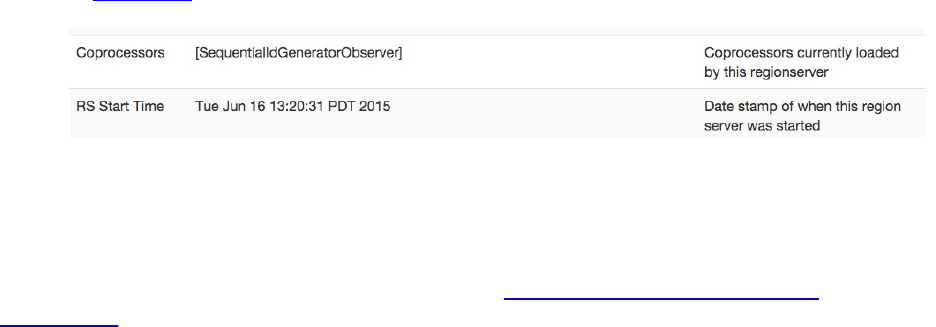
TTL => 'FOREVER', MIN_VERSIONS => '0', KEEP_DELETED_CELLS => 'FALSE', \
BLOCKSIZE => '65536', IN_MEMORY => 'false', BLOCKCACHE => 'true'}
1 row(s) in 0.0220 seconds
The second command uses describe to verify the coprocessor was set, and what the assigned key
for it is, here coprocessor$1. As for the path used for the JAR file, keep in mind that it is
considered the source for the JAR file, and that it is copied into the local temporary location
before being loaded into the Java process as explained above. You can use the region server UI
to verify that the class has been loaded successfully, by checking the Software Attributes section
at the end of the status page. In this table there is a line listing the loaded coprocessor classes, as
shown in Figure 4-5.
Figure 4-5. The Region Server status page lists the loaded coprocessors
Tip
While you will learn more about the HBase Shell in “Namespace and Data Definition
Commands”, a quick tip about using the alter command to add a table attribute: You can omit
the METHOD => 'table_att' parameter as shown above, because adding/setting a parameter is the
assumed default operation. Only for removing an attribute do you have to explicitly specify the
method, as shown next when removing the previously set coprocessor.
Once a coprocessor is loaded, you can also remove them in the same dynamic fashion, that is,
using the HBase Shell to update the schema and reload the affected table regions on all region
servers in one single command:
hbase(main):003:0> alter 'testqauat:usertable', METHOD => 'table_att_unset', \
NAME => 'coprocessor$1'
Updating all regions with the new schema...
2/11 regions updated.
8/11 regions updated.
11/11 regions updated.
Done.
0 row(s) in 4.2160 seconds
hbase(main):004:0> describe 'testqauat:usertable'
Table testqauat:usertable is ENABLED
testqauat:usertable
COLUMN FAMILIES DESCRIPTION
{NAME => 'cf1', DATA_BLOCK_ENCODING => 'NONE', BLOOMFILTER => 'ROW', \
REPLICATION_SCOPE => '0', COMPRESSION => 'NONE', VERSIONS => '1', \
TTL => 'FOREVER', MIN_VERSIONS => '0', KEEP_DELETED_CELLS => 'FALSE',
BLOCKSIZE => '65536', IN_MEMORY => 'false', BLOCKCACHE => 'true'}
1 row(s) in 0.0180 seconds
Removing a coprocessor requires you to know its key in the table schema. We have already
retrieved that one earlier with the describe command shown in the example. The unset (which
removes the table schema attribute) operation removes the key named coprocessor$1, which was
the said key we determined earlier. After all regions are reloaded, we can use the describe
command again to check if coprocessor reference has indeed be removed, which is the case here.
Loading coprocessors using the dynamic table schema approach bears the same burden as
mentioned before: you cannot unload classes or JAR files, therefore you may have to restart the
(291)
region server process for an update of the classes. You could work around for a limited amount
of time by versioning the class and JAR file names, but the loaded classes may cause memory
pressure eventually and force you to cycle the processes.
(292)
Endpoints
The first of two major features provided by the coprocessor framework that we are going to look
at are endpoints. They solve a problem with moving data for analytical queries, that would
benefit from pre-calculating intermediate results where the data resides, and then just shipping
the results back to the client. Sounds familiar? Yes, this is what MapReduce does in Hadoop, that
is, ship the code to the data, do the computation, and persist the results.
An inherent feature of MapReduce is that it has intrinsic knowledge of what datanode is holding
which block of information. When you execute a job, the NameNode will instruct the scheduler
to ship the code to all nodes that contain data that is part of job parameters. With HBase, we
could run a client-side scan that ships all the data to the client to do the computation. But at scale,
this will not be efficient, because the inertia of data exceeds the amount of processing performed.
In other words, all the time is spent in moving the data, the I/O.
What we need instead is the ability, just as with MapReduce, to ship the processing to the
servers, do the aggregation or any other computation on the server-side, and only return the much
smaller results back to the client. And that, in a nutshell, is what Endpoints are all about. You
instruct the servers to load code with every region of a given table, and when you need to scan
the table, partially or completely, it will call the server-side code, which then can scan the
necessary data where it resides: on the data servers.
Once the computation is completed, the results are shipped back to the client, one result per
region, and aggregated there for the final result. For example, if you were to have 1,000 regions
and 1 million columns, and you want to summarize the stored data, you would receive 1,000
decimal numbers on the client side—one for each region. This is fast to aggregate for the final
result. If you were to scan the entire table using a purely client API approach, in a worst-case
scenario you would transfer all 1 million numbers to build the sum.
The Service Interface
Endpoints are implemented as an extension to the RPC protocol between the client and server. In
the past (before HBase 0.96) this was done by literally extending the protocol classes. After the
move to the Protocol Buffer (Protobuf for short) based RPC, adding custom services on the
server side was greatly simplified. The payload is serialized as a Protobuf message and sent from
client to server (and back again) using the provided coprocessor services API.
In order to provide an endpoint to clients, a coprocessor generates a Protobuf implementation
that extends the Service class. This service can define any methods that the coprocessor wishes to
expose. Using the generated classes, you can communicate with the coprocessor instances via the
following calls, provided by Table:
CoprocessorRpcChannel coprocessorService(byte[] row)
<T extends Service, R> Map<byte[],R> coprocessorService(final Class<T> service,
byte[] startKey, byte[] endKey, final Batch.Call<T,R> callable)
throws ServiceException, Throwable
<T extends Service, R> void coprocessorService(final Class<T> service,
byte[] startKey, byte[] endKey, final Batch.Call<T,R> callable,
final Batch.Callback<R> callback) throws ServiceException, Throwable
<R extends Message> Map<byte[], R> batchCoprocessorService(
(293)

Descriptors.MethodDescriptor methodDescriptor, Message request,
byte[] startKey, byte[] endKey, R responsePrototype)
throws ServiceException, Throwable
<R extends Message> void batchCoprocessorService(
Descriptors.MethodDescriptor methodDescriptor,
Message request, byte[] startKey, byte[] endKey, R responsePrototype,
Batch.Callback<R> callback) throws ServiceException, Throwable
Since Service instances are associated with individual regions within a table, the client RPC calls
must ultimately identify which regions should be used in the service’s method invocations.
Though regions are seldom handled directly in client code and the region names may change
over time, the coprocessor RPC calls use row keys to identify which regions should be used for
the method invocations. Clients can call Service methods against one of the following:
Single Region
This is done by calling coprocessorService() with a single row key. This returns an instance
of the CoprocessorRpcChannel class, which directly extends Protobuf classes. It can be used
to invoke any endpoint call linked to the region containing the specified row. Note that the
row does not need to exist: the region selected is the one that does or would contain the
given key.
Ranges of Regions
You can call coprocessorService() with a start row key and an end row key. All regions in
the table from the one containing the start row key to the one containing the end row key
(inclusive) will be used as the endpoint targets. This is done in parallel up to the amount of
threads configured in the executor pool instance in use.
Batched Regions
If you call batchCoprocessorService() instead, you still parallelize the execution across all
regions, but calls to the same region server are sent together in a single invocation. This
will cut down the number of network roundtrips, and is especially useful when the
expected results of each endpoint invocation is very small.
Note
The row keys passed as parameters to the Table methods are not passed to the Service
implementations. They are only used to identify the regions for endpoints of the remote calls. As
mentioned, they do not have to actually exist, they merely identify the matching regions by start
and end key boundaries.
Some of the table methods to invoke endpoints are using the Batch class, which you have seen in
action in “Batch Operations” before. The abstract class defines two interfaces used for Service
invocations against multiple regions: clients implement Batch.Call to call methods of the actual
Service implementation instance. The interface’s call() method will be called once per selected
region, passing the Service implementation instance for the region as a parameter.
Clients can optionally implement Batch.Callback to be notified of the results from each region
invocation as they complete. The instance’s
void update(byte[] region, byte[] row, R result)
method will be called with the value returned by
(294)
R call(T instance)
from each region. You can see how the actual service type "T", and return type "R" are specified
as Java generics: they depend on the concrete implementation of an endpoint, that is, the
generated Java classes based on the Protobuf message declaring the service, methods, and their
types.
Implementing Endpoints
Implementing an endpoint involves the following two steps:
1. Define the Protobuf service and generate classes
This specifies the communication details for the endpoint: it defines the RPC service, its
methods, and messages used between the client and the servers. With the help of the
Protobuf compiler the service definition is compiled into custom Java classes.
2. Extend the generated, custom Service subclass
You need to provide the actual implementation of the endpoint by extending the generated,
abstract class derived from the Service superclass.
The following defines a Protobuf service, named RowCountService, with methods that a client can
invoke to retrieve the number of rows and Cells in each region where it is running. Following
Maven project layout rules, they go into ${PROJECT_HOME}/src/main/protobuf, here with the name
RowCountService.proto:
option java_package = "coprocessor.generated";
option java_outer_classname = "RowCounterProtos";
option java_generic_services = true;
option java_generate_equals_and_hash = true;
option optimize_for = SPEED;
message CountRequest {
}
message CountResponse {
required int64 count = 1 [default = 0];
}
service RowCountService {
rpc getRowCount(CountRequest)
returns (CountResponse);
rpc getCellCount(CountRequest)
returns (CountResponse);
}
The file defines the output class name, the package to use during code generation and so on. The
last thing in step #1 is to compile the definition file into code, which is accomplished by using
the Protobuf protoc tool.
Tip
The Protocol Buffer library usually comes as a source package that needs to be compiled and
locally installed. There are also pre-built binary packages for many operating systems. On OS X,
for example, you can run the following, assuming Homebrew was installed:
$ brew install protobuf
(295)

You can verify the installation by running $ protoc --version and check it prints a version
number:
$ protoc --version
libprotoc 2.6.1
The online code repository of the book has a script bin/doprotoc.sh that runs the code generation.
It essentially runs the following command from the repository root directory:
$ protoc -Ich04/src/main/protobuf --java_out=ch04/src/main/java \
ch04/src/main/protobuf/RowCountService.proto
This will place the generated class file in the source directory, as specified. After that you will be
able to use the generated types. Step #2 is to flesh out the generated code, since it creates an
abstract class for you. All the declared RPC methods need to be implemented with the user code.
This is done by extending the generated class, plus merging in the Coprocessor and
CoprocessorService interface functionality. The latter two define the lifecycle callbacks, plus
flagging the class as a service. Example 4-29 shows this for the above row-counter service, using
the coprocessor environment provided to access the region, and eventually the data with an
InternalScanner instance.
Example 4-29. Example endpoint implementation, adding a row and cell count method.
public class RowCountEndpoint extends RowCounterProtos.RowCountService
implements Coprocessor, CoprocessorService {
private RegionCoprocessorEnvironment env;
@Override
public void start(CoprocessorEnvironment env) throws IOException {
if (env instanceof RegionCoprocessorEnvironment) {
this.env = (RegionCoprocessorEnvironment) env;
} else {
throw new CoprocessorException("Must be loaded on a table region!");
}
}
@Override
public void stop(CoprocessorEnvironment env) throws IOException {
// nothing to do when coprocessor is shutting down
}
@Override
public Service getService() {
return this;
}
@Override
public void getRowCount(RpcController controller,
RowCounterProtos.CountRequest request,
RpcCallback<RowCounterProtos.CountResponse> done) {
RowCounterProtos.CountResponse response = null;
try {
long count = getCount(new FirstKeyOnlyFilter(), false);
response = RowCounterProtos.CountResponse.newBuilder()
.setCount(count).build();
} catch (IOException ioe) {
ResponseConverter.setControllerException(controller, ioe);
}
done.run(response);
}
@Override
public void getCellCount(RpcController controller,
RowCounterProtos.CountRequest request,
RpcCallback<RowCounterProtos.CountResponse> done) {
RowCounterProtos.CountResponse response = null;
(296)

try {
long count = getCount(null, true);
response = RowCounterProtos.CountResponse.newBuilder()
.setCount(count).build();
} catch (IOException ioe) {
ResponseConverter.setControllerException(controller, ioe);
}
done.run(response);
}
/**
* Helper method to count rows or cells.
* *
* @param filter The optional filter instance.
* @param countCells Hand in <code>true</code> for cell counting.
* @return The count as per the flags.
* @throws IOException When something fails with the scan.
*/
private long getCount(Filter filter, boolean countCells)
throws IOException {
long count = 0;
Scan scan = new Scan();
scan.setMaxVersions(1);
if (filter != null) {
scan.setFilter(filter);
}
try (
InternalScanner scanner = env.getRegion().getScanner(scan);
) {
List<Cell> results = new ArrayList<Cell>();
boolean hasMore = false;
byte[] lastRow = null;
do {
hasMore = scanner.next(results);
for (Cell cell : results) {
if (!countCells) {
if (lastRow == null || !CellUtil.matchingRow(cell, lastRow)) {
lastRow = CellUtil.cloneRow(cell);
count++;
}
} else count++;
}
results.clear();
} while (hasMore);
}
return count;
}
}
Note how the FirstKeyOnlyFilter is used to reduce the number of columns being scanned, in case
of performing a row count operation. For small rows, this will not yield much of an
improvement, but for tables with very wide rows, skipping all remaining columns (and more so
cells if you enabled multi-versioning) of a row can speed up the row count tremendously.
Note
You need to add (or amend from the previous examples) the following to the hbase-site.xml file
for the endpoint coprocessor to be loaded by the region server process:
<property>
<name>hbase.coprocessor.user.region.classes</name>
<value>coprocessor.RowCountEndpoint</value>
</property>
Just as before, restart HBase after making these adjustments.
Example 4-30 showcases how a client can use the provided calls of Table to execute the deployed
coprocessor endpoint functions. Since the calls are sent to each region separately, there is a need
(297)
to summarize the total number at the end.
Example 4-30. Example using the custom row-count endpoint
public class EndpointExample {
public static void main(String[] args) throws IOException {
Configuration conf = HBaseConfiguration.create();
TableName tableName = TableName.valueOf("testtable");
Connection connection = ConnectionFactory.createConnection(conf);
Table table = connection.getTable(tableName);
try {
final RowCounterProtos.CountRequest request =
RowCounterProtos.CountRequest.getDefaultInstance();
Map<byte[], Long> results = table.coprocessorService(
RowCounterProtos.RowCountService.class,
null, null,
new Batch.Call<RowCounterProtos.RowCountService, Long>() {
public Long call(RowCounterProtos.RowCountService counter)
throws IOException {
BlockingRpcCallback<RowCounterProtos.CountResponse> rpcCallback =
new BlockingRpcCallback<RowCounterProtos.CountResponse>();
counter.getRowCount(null, request, rpcCallback);
RowCounterProtos.CountResponse response = rpcCallback.get();
return response.hasCount() ? response.getCount() : 0;
}
}
);
long total = 0;
for (Map.Entry<byte[], Long> entry : results.entrySet()) {
total += entry.getValue().longValue();
System.out.println("Region: " + Bytes.toString(entry.getKey()) +
", Count: " + entry.getValue());
}
System.out.println("Total Count: " + total);
} catch (Throwable throwable) {
throwable.printStackTrace();
}
}
}
Define the protocol interface being invoked.
Set start and end row key to “null” to count all rows.
Create an anonymous class to be sent to all region servers.
The call() method is executing the endpoint functions.
Iterate over the returned map, containing the result for each region separately.
The code emits the region names, the count for each of them, and eventually the grand total:
Before endpoint call...
Cell: row1/colfam1:qual1/2/Put/vlen=4/seqid=0, Value: val2
(298)

Cell: row1/colfam2:qual1/2/Put/vlen=4/seqid=0, Value: val2
...
Cell: row5/colfam1:qual1/2/Put/vlen=4/seqid=0, Value: val2
Cell: row5/colfam2:qual1/2/Put/vlen=4/seqid=0, Value: val2
Region: testtable,,1427209872848.6eab8b854b5868ec...a66e83ea822c., Count: 2
Region: testtable,row3,1427209872848.3afd10e33044...8e071ce165ce., Count: 3
Total Count: 5
Example 4-31 slightly modifies the example to use the batch calls, that is, where all calls to a
region server are grouped and sent together, for all hosted regions of that server.
Example 4-31. Example using the custom row-count endpoint in batch mode
final CountRequest request = CountRequest.getDefaultInstance();
Map<byte[], CountResponse> results = table.batchCoprocessorService(
RowCountService.getDescriptor().findMethodByName("getRowCount"),
request, HConstants.EMPTY_START_ROW, HConstants.EMPTY_END_ROW,
CountResponse.getDefaultInstance());
long total = 0;
for (Map.Entry<byte[], CountResponse> entry : results.entrySet()) {
CountResponse response = entry.getValue();
total += response.hasCount() ? response.getCount() : 0;
System.out.println("Region: " + Bytes.toString(entry.getKey()) +
", Count: " + entry.getValue());
}
System.out.println("Total Count: " + total);
The output is the same (the region name will vary for every execution of the example, as it
contains the time a region was created), so we can refrain here from showing it again. Also, for
such a small example, and especially running on a local test rig, the difference of either call is
none. It will really show when you have many regions per server, and the returned data is very
small: only then the cost of the RPC roundtrips are noticeable.
Note
Example 4-31 does not use null for the start and end keys, but rather HConstants.EMPTY_START_ROW
and HConstants.EMPTY_END_ROW, as provided by the API classes. This is synonym to not specifying
the keys at all.6
If you want to perform additional processing on the results, you can further extend the Batch.Call
code. This can be seen in Example 4-32, which combines the row and cell count for each region.
Example 4-32. Example extending the batch call to execute multiple endpoint calls
final RowCounterProtos.CountRequest request =
RowCounterProtos.CountRequest.getDefaultInstance();
Map<byte[], Pair<Long, Long>> results = table.coprocessorService(
RowCounterProtos.RowCountService.class,
null, null,
new Batch.Call<RowCounterProtos.RowCountService, Pair<Long, Long>>() {
public Pair<Long, Long> call(RowCounterProtos.RowCountService counter)
throws IOException {
BlockingRpcCallback<RowCounterProtos.CountResponse> rowCallback =
new BlockingRpcCallback<RowCounterProtos.CountResponse>();
counter.getRowCount(null, request, rowCallback);
BlockingRpcCallback<RowCounterProtos.CountResponse> cellCallback =
new BlockingRpcCallback<RowCounterProtos.CountResponse>();
counter.getCellCount(null, request, cellCallback);
RowCounterProtos.CountResponse rowResponse = rowCallback.get();
Long rowCount = rowResponse.hasCount() ?
rowResponse.getCount() : 0;
(299)

RowCounterProtos.CountResponse cellResponse = cellCallback.get();
Long cellCount = cellResponse.hasCount() ?
cellResponse.getCount() : 0;
return new Pair<Long, Long>(rowCount, cellCount);
}
}
);
long totalRows = 0;
long totalKeyValues = 0;
for (Map.Entry<byte[], Pair<Long, Long>> entry : results.entrySet()) {
totalRows += entry.getValue().getFirst().longValue();
totalKeyValues += entry.getValue().getSecond().longValue();
System.out.println("Region: " + Bytes.toString(entry.getKey()) +
", Count: " + entry.getValue());
}
System.out.println("Total Row Count: " + totalRows);
System.out.println("Total Cell Count: " + totalKeyValues);
Running the code will yield the following output:
Region: testtable,,1428306403441.94e36bc7ab66c0e535dc3c21d9755ad6., Count: {2,4}
Region: testtable,row3,1428306403441.720b383e551e96cd290bd4b74b472e11., Count: {3,6}
Total Row Count: 5
Total KeyValue Count: 10
The examples so far all used the coprocessorService() calls to batch the requests across all
regions, matching the given start and end row keys. Example 4-33 uses the single-row
coprocessorService() call to get a local, client-side proxy of the endpoint. Since a row key is
specified, the client API will route the proxy calls to the region—and to the server currently
hosting it—that contains the given key (again, regardless of whether it actually exists or not:
regions are specified with a start and end key only, so the match is done by range only).
Example 4-33. Example using the proxy call of HTable to invoke an endpoint on a single region
HRegionInfo hri = admin.getTableRegions(tableName).get(0);
Scan scan = new Scan(hri.getStartKey(), hri.getEndKey())
.setMaxVersions();
ResultScanner scanner = table.getScanner(scan);
for (Result result : scanner) {
System.out.println("Result: " + result);
}
CoprocessorRpcChannel channel = table.coprocessorService(
Bytes.toBytes("row1"));
RowCountService.BlockingInterface service =
RowCountService.newBlockingStub(channel);
CountRequest request = CountRequest.newBuilder().build();
CountResponse response = service.getCellCount(null, request);
long cellsInRegion = response.hasCount() ? response.getCount() : -1;
System.out.println("Region Cell Count: " + cellsInRegion);
request = CountRequest.newBuilder().build();
response = service.getRowCount(null, request);
long rowsInRegion = response.hasCount() ? response.getCount() : -1;
System.out.println("Region Row Count: " + rowsInRegion);
The output will be:
Result: keyvalues={row1/colfam1:qual1/2/Put/vlen=4/seqid=0,
row1/colfam1:qual1/1/Put/vlen=4/seqid=0,
row1/colfam2:qual1/2/Put/vlen=4/seqid=0,
row1/colfam2:qual1/1/Put/vlen=4/seqid=0}
Result: keyvalues={row2/colfam1:qual1/2/Put/vlen=4/seqid=0,
row2/colfam1:qual1/1/Put/vlen=4/seqid=0,
row2/colfam2:qual1/2/Put/vlen=4/seqid=0,
row2/colfam2:qual1/1/Put/vlen=4/seqid=0}
(300)

Region Cell Count: 4
Region Row Count: 2
The local scan differs from the numbers returned by the endpoint, which is caused by the
coprocessor code setting setMaxVersions(1), while the local scan omits the limit and returns all
versions of any cell in that same region. It shows once more how careful you should be to set
these parameters to what is expected by the clients. If in doubt, you could make the maximum
version a parameter that is passed to the endpoint through the Request implementation.
With the proxy reference, you can invoke any remote function defined in your derived Service
implementation from within client code, and it returns the result for the region that served the
request. Figure 4-6 shows the difference between the two approaches offered by
coprocessorService(): single and multi region coverage.
(301)
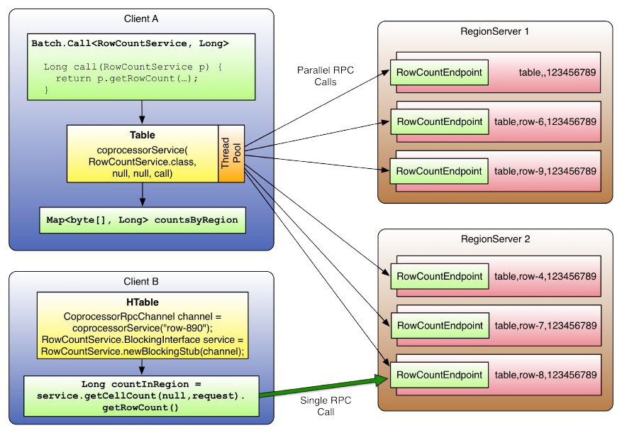
Figure 4-6. Coprocessor calls batched and executed in parallel, and addressing a single region only
(302)

Observers
While endpoints somewhat reflect the functionality of database stored procedures, the observers
are akin to triggers. The difference to endpoints is that observers are not only running in the
context of a region. They can run in many different parts of the system and react to events that
are triggered by clients, but also implicitly by servers themselves. For example, when one of the
servers is recovering a region after another server has failed. Or when the master is taking actions
on the cluster state, etc.
Another difference is that observers are using pre-defined hooks into the server processes, that is,
you cannot add your own custom ones. They also act on the server side only, with no connection
to the client. What you can do though is combine an endpoint with an observer for region-related
functionality, exposing observer state through a custom RPC API (see Example 4-34).
Since you can load many observers into the same set of contexts, that is, region, region server,
master server, WAL, bulk loading, and endpoints, it is crucial to set the order of their invocation
chain appropriately. We discussed that in “Coprocessor Loading”, looking into the priority and
ordering dependent on how they are declared. Once loaded, the observers are chained together
and executed in that order.
(303)
The ObserverContext Class
So far we have talked about the general architecture of coprocessors, their super class, how they
are loaded into the server process, and how to implement endpoints. Before we can move on into
the actual observers, we need to introduce one more basic class. For the callbacks provided by
the Observer classes, there is a special context handed in as the first parameter to all calls: an
instance of the ObserverContext class. It provides access to the current environment, but also adds
the interesting ability to indicate to the coprocessor framework what it should do after a callback
is completed.
Note
The observer context instance is the same for all coprocessors in the execution chain, but with
the environment swapped out for each coprocessor.
Here are the methods as provided by the context class:
E getEnvironment()
Returns the reference to the current coprocessor environment. It is paramterized to return
the matching environment for a specific coprocessor implementation. A RegionObserver for
example would be presented with an implementation instance of the
RegionCoprocessorEnvironment interface.
void prepare(E env)
Prepares the context with the specified environment. This is used internally only by the
static createAndPrepare() method.
void bypass()
When your code invokes this method, the framework is going to use your provided value,
as opposed to what usually is returned by the calling method.
void complete()
Indicates to the framework that any further processing can be skipped, skipping the
remaining coprocessors in the execution chain. It implies that this coprocessor’s response
is definitive.
boolean shouldBypass()
Used internally by the framework to check on the bypass flag.
boolean shouldComplete()
Used internally by the framework to check on the complete flag.
static <T extends CoprocessorEnvironment> ObserverContext<T> createAndPrepare(T env,
ObserverContext<T> context)
Static function to initialize a context. When the provided context is null, it will create a
new instance.
(304)
The important context functions are bypass() and complete(). These functions give your
coprocessor implementation the option to control the subsequent behavior of the framework. The
complete() call influences the execution chain of the coprocessors, while the bypass() call stops
any further default processing on the server within the current observer. For example, you could
avoid automated region splits like so:
@Override
public void preSplit(ObserverContext<RegionCoprocessorEnvironment> e) {
e.bypass();
e.complete();
}
There is a subtle difference between bypass and complete that needs to be clarified: they are
serving different purposes, with different effects dependent on their usage. The following table
lists the usual effects of either flag on the current and subsequent coprocessors, and when used in
the pre or post hooks.
Table 4-15. Overview of bypass and complete, and their effects on coprocessors
Bypass Complete Current - Pre Subsequent - Pre Current - Post Subsequent - Post
✗ ✗ no effect no effect no effect no effect
✓ ✗ skip further
processing no effect no effect no effect
✗ ✓ no effect skip no effect skip
✓ ✓ skip further
processing skip no effect skip
Note that there are exceptions to the rule, that is, some pre hooks cannot honor the bypass flag,
etc. Setting bypass for post hooks usually make no sense, since there is little to nothing left to
bypass. Consult the JavaDoc for each callback to learn if (and how) it honors the bypass flag.
(305)
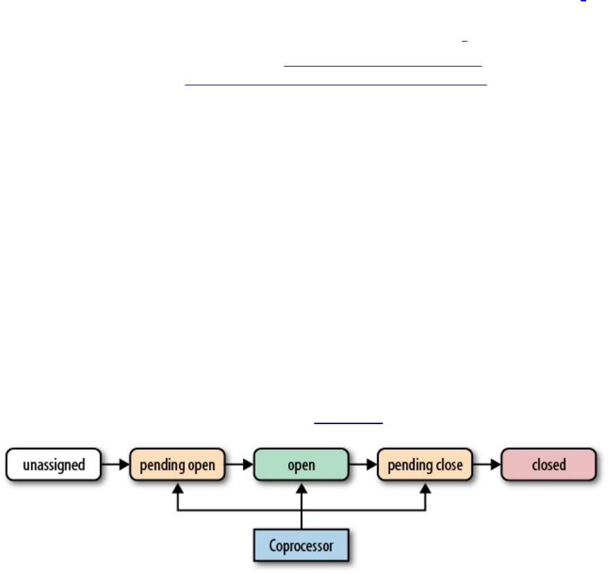
The RegionObserver Class
The first observer subclass of Coprocessor we will look into is the one used at the region level: the
RegionObserver class. For the sake of brevity, all parameters and exceptions are omitted when
referring to the observer calls. Please read the online documentation for the full specification.7
Note that all calls of this observer class have the same first parameter (denoted as part of the
“…” in the calls below), ObserverContext<RegionCoprocessorEnvironment> ctx8, providing access to
the context instance. The context is explained in “The ObserverContext Class”, while the special
environment class is explained in “The RegionCoprocessorEnvironment Class”.
The operations can be divided into two groups: region life-cycle changes and client API calls. We
will look into both in that order, but before we do, there is a generic callback for many operations
of both kinds:
enum Operation {
ANY, GET, PUT, DELETE, SCAN, APPEND, INCREMENT, SPLIT_REGION,
MERGE_REGION, BATCH_MUTATE, REPLAY_BATCH_MUTATE, COMPACT_REGION
}
postStartRegionOperation(..., Operation operation)
postCloseRegionOperation(..., Operation operation)
These methods in a RegionObserver are invoked when any of the possible Operations listed is
called. It gives the coprocessor the ability to take invasive, or more likely, evasive actions, such
as throwing an exception to stop the operation from taking place altogether.
Handling Region Life-Cycle Events
While [Link to Come] explains the region life-cycle, Figure 4-7 shows a simplified form.
Figure 4-7. The coprocessor reacting to life-cycle state changes of a region
The observers have the opportunity to hook into the pending open, open, and pending close state
changes. For each of them there is a set of hooks that are called implicitly by the framework.
State: pending open
A region is in this state when it is about to be opened. Observing coprocessors can either
piggyback or fail this process. To do so, the following callbacks in order of their
invocation are available:
postLogReplay(...)
(306)
preOpen(...)
preStoreFileReaderOpen(...)
postStoreFileReaderOpen(...)
preWALRestore(...) / postWALRestore(...)
postOpen(...)
These methods are called just before the region is opened, before and after the store files
are opened in due course, the WAL being replayed, and just after the region was opened.
Your coprocessor implementation can use them, for instance, to indicate to the framework
—in the preOpen() call—that it should abort the opening process. Or hook into the
postOpen() call to trigger a cache warm up, and so on.
The first event, postLogReplay(), is triggered dependent on what WAL recovery mode is
configured: distributed log splitting or log replay (see [Link to Come] and the
hbase.master.distributed.log.replay configuration property). The former runs before a
region is opened, and would therefore be triggering the callback first. The latter opens the
region, and then replays the edits, triggering the callback after the region open event.
In both recovery modes, but again dependent on which is active, the region server may
have to apply records from the write-ahead log (WAL). This, in turn, invokes the
pre/postWALRestore() methods of the observer. In case of using the distributed log splitting,
this will take place after the pending open, but just before the open state. Otherwise, this is
called after the open event, as edits are replayed. Hooking into these WAL calls gives you
fine-grained control over what mutation is applied during the log replay process. You get
access to the edit record, which you can use to inspect what is being applied.
State: open
A region is considered open when it is deployed to a region server and fully operational.
At this point, all the operations discussed throughout the book can take place; for example,
the region’s in-memory store could be flushed to disk, or the region could be split when it
has grown too large. The possible hooks are:
preFlushScannerOpen(...)
preFlush(...) / postFlush(...)
preCompactSelection(...) / postCompactSelection(...)
preCompactScannerOpen(...)
preCompact(...) / postCompact(...)
preSplit(...)
preSplitBeforePONR(...)
preSplitAfterPONR(...)
postSplit(...)
postCompleteSplit(...) / preRollBackSplit(...) / postRollBackSplit(...)
This should be quite intuitive by now: the pre calls are executed before, while the post
calls are executed after the respective operation. For example, using the preSplit() hook,
you could effectively disable the built-in region splitting process and perform these
operations manually. Some calls are only available as pre-hooks, some only as post-hooks.
The hooks for flush, compact, and split are directly linked to the matching region
housekeeping functions. There are also some more specialized hooks, that happen as part
of those three functions. For example, the preFlushScannerOpen() is called when the scanner
for the memstore (bear with me here, [Link to Come] will explain all the workings later) is
set up. This is just before the actual flush takes place.
Similarly, for compactions, first the server selects the files included, which is wrapped in
(307)
coprocessor callbacks (postfixed CompactSelection). After that the store scanners are
opened and, finally, the actual compaction happens.
For splits, there are callbacks reflecting current stage, with a particular point-of-no-return
(PONR) in between. This occurs, after the split process started, but before any definitive
actions have taken place. Splits are handled like a transaction internally, and when this
transaction is about to be committed, the preSplitBeforePONR() is invoked, and the
preSplitAfterPONR() right after. There is also a final completed or rollback call, informing
you of the outcome of the split transaction.
State: pending close
The last group of hooks for the observers is for regions that go into the pending close state.
This occurs when the region transitions from open to closed. Just before, and after, the
region is closed the following hooks are executed:
preClose(..., boolean abortRequested)
postClose(..., boolean abortRequested)
The abortRequested parameter indicates why a region was closed. Usually regions are
closed during normal operation, when, for example, the region is moved to a different
region server for load-balancing reasons. But there also is the possibility for a region
server to have gone rogue and be aborted to avoid any side effects. When this happens, all
hosted regions are also aborted, and you can see from the given parameter if that was the
case.
On top of that, this class also inherits the start() and stop() methods, allowing the allocation,
and release, of lifetime resources.
Handling Client API Events
As opposed to the life-cycle events, all client API calls are explicitly sent from a client
application to the region server. You have the opportunity to hook into these calls just before
they are applied, and just thereafter. Here is the list of the available calls:
Table 4-16. Callbacks for client API functions
API Call Pre-Hook Post-Hook
Table.put() prePut(...) void postPut(...)
Table.checkAndPut()
preCheckAndPut(...),
preCheckAndPutAfterRowLock(...),
prePut(...)
postPut(...), postCheckAndPut(...)
Table.get() preGetOp(...) void postGetOp(...)
Table.delete(), Table.batch() preDelete(...),
prePrepareTimeStampForDeleteVersion(...) void postDelete(...)
(308)

Table.checkAndDelete()
preCheckAndDelete(...),
preCheckAndDeleteAfterRowLock(...),
preDelete(...)
postDelete(...),
postCheckAndDelete(...)
Table.mutateRow() preBatchMutate(...),
prePut(...)/preGetOp(...)
postBatchMutate(...),
postPut(...)/postGetOp(...)
postBatchMutateIndispensably()
Table.append(),preAppend(...), preAppendAfterRowLock() postMutationBeforeWAL(...)
postAppend(...)
Table.batch()
preBatchMutate(...),
prePut(...)/preGetOp(...)/preDelete(...),
prePrepareTimeStampForDeleteVersion(...)/
postPut(...)/postGetOp(...)
postBatchMutate(...)
Table.checkAndMutate() preBatchMutate(...) postBatchMutate(...)
Table.getScanner() preScannerOpen(...),
preStoreScannerOpen(...)
postInstantiateDeleteTracker(...)
postScannerOpen(...)
ResultScanner.next() preScannerNext(...) postScannerFilterRow(...)
postScannerNext(...)
ResultScanner.close() preScannerClose(...) postScannerClose(...)
Table.increment(), Table.batch() preIncrement(...),
preIncrementAfterRowLock(...)
postMutationBeforeWAL(...)
postIncrement(...)
Table.incrementColumnValue() preIncrementColumnValue(...) postIncrementColumnValue(...)
`Table.getClosestRowBefore()`apreGetClosestRowBefore(...) postGetClosestRowBefore(...)
Table.exists() preExists(...) postExists(...)
completebulkload (tool) preBulkLoadHFile(...) postBulkLoadHFile(...)
a This API call has been removed in HBase 1.0. It will be removed in the coprocessor API soon as well.
The table lists the events in calling order, separated by comma. When you see a slash (“/”)
instead, then the callback depends on the contained operations. For example, when you batch a
(309)

put and delete in one batch() call, then you would receive the pre/postPut() and pre/postDelete()
callbacks, for each contained instance. There are many low-level methods, that allow you to
hook into very essential processes of HBase’s inner workings. Usually the method name should
explain the nature of the invocation, and with the parameters provided in the online API
documentation you can determine what your options are. If all fails, you are an expert at this
point anyways asking for such details, presuming you can refer to the source code, if need be.
Example 4-34 shows another (albeit somewhat advanced) way of figuring out the call order of
coprocessor methods. The example code combines a RegionObserver with a custom Endpoint, and
uses an internal list to track all invocations of any callback.
Example 4-34. Observer collecting invocation statistics.
@SuppressWarnings("deprecation") // because of API usage
public class ObserverStatisticsEndpoint
extends ObserverStatisticsProtos.ObserverStatisticsService
implements Coprocessor, CoprocessorService, RegionObserver {
private RegionCoprocessorEnvironment env;
private Map<String, Integer> stats = new LinkedHashMap<>();
// Lifecycle methods
@Override
public void start(CoprocessorEnvironment env) throws IOException {
if (env instanceof RegionCoprocessorEnvironment) {
this.env = (RegionCoprocessorEnvironment) env;
} else {
throw new CoprocessorException("Must be loaded on a table region!");
}
}
...
// Endpoint methods
@Override
public void getStatistics(RpcController controller,
ObserverStatisticsProtos.StatisticsRequest request,
RpcCallback<ObserverStatisticsProtos.StatisticsResponse> done) {
ObserverStatisticsProtos.StatisticsResponse response = null;
try {
ObserverStatisticsProtos.StatisticsResponse.Builder builder =
ObserverStatisticsProtos.StatisticsResponse.newBuilder();
ObserverStatisticsProtos.NameInt32Pair.Builder pair =
ObserverStatisticsProtos.NameInt32Pair.newBuilder();
for (Map.Entry<String, Integer> entry : stats.entrySet()) {
pair.setName(entry.getKey());
pair.setValue(entry.getValue().intValue());
builder.addAttribute(pair.build());
}
response = builder.build();
// optionally clear out stats
if (request.hasClear() && request.getClear()) {
synchronized (stats) {
stats.clear();
}
}
} catch (Exception e) {
ResponseConverter.setControllerException(controller,
new IOException(e));
}
done.run(response);
}
/**
* Internal helper to keep track of call counts.
*
* @param call The name of the call.
*/
private void addCallCount(String call) {
(310)

synchronized (stats) {
Integer count = stats.get(call);
if (count == null) count = new Integer(1);
else count = new Integer(count + 1);
stats.put(call, count);
}
}
// All Observer callbacks follow here
@Override
public void preOpen(
ObserverContext<RegionCoprocessorEnvironment> observerContext)
throws IOException {
addCallCount("preOpen");
}
@Override
public void postOpen(
ObserverContext<RegionCoprocessorEnvironment> observerContext) {
addCallCount("postOpen");
}
...
}
This is combined with the code in Example 4-35, which then executes every API call, followed
by calling on the custom endpoint getStatistics(), which returns (and optionally clears) the
collected invocation list.
Example 4-35. Use an endpoint to query observer statistics
private static Table table = null;
private static void printStatistics(boolean print, boolean clear)
throws Throwable {
final StatisticsRequest request = StatisticsRequest
.newBuilder().setClear(clear).build();
Map<byte[], Map<String, Integer>> results = table.coprocessorService(
ObserverStatisticsService.class,
null, null,
new Batch.Call<ObserverStatisticsProtos.ObserverStatisticsService,
Map<String, Integer>>() {
public Map<String, Integer> call(
ObserverStatisticsService statistics)
throws IOException {
BlockingRpcCallback<StatisticsResponse> rpcCallback =
new BlockingRpcCallback<StatisticsResponse>();
statistics.getStatistics(null, request, rpcCallback);
StatisticsResponse response = rpcCallback.get();
Map<String, Integer> stats = new LinkedHashMap<String, Integer>();
for (NameInt32Pair pair : response.getAttributeList()) {
stats.put(pair.getName(), pair.getValue());
}
return stats;
}
}
);
if (print) {
for (Map.Entry<byte[], Map<String, Integer>> entry : results.entrySet()) {
System.out.println("Region: " + Bytes.toString(entry.getKey()));
for (Map.Entry<String, Integer> call : entry.getValue().entrySet()) {
System.out.println(" " + call.getKey() + ": " + call.getValue());
}
}
System.out.println();
}
}
public static void main(String[] args) throws IOException {
Configuration conf = HBaseConfiguration.create();
Connection connection = ConnectionFactory.createConnection(conf);
HBaseHelper helper = HBaseHelper.getHelper(conf);
(311)
helper.dropTable("testtable");
helper.createTable("testtable", 3, "colfam1", "colfam2");
helper.put("testtable",
new String[]{"row1", "row2", "row3", "row4", "row5"},
new String[]{"colfam1", "colfam2"}, new String[]{"qual1", "qual1"},
new long[]{1, 2}, new String[]{"val1", "val2"});
System.out.println("Before endpoint call...");
helper.dump("testtable",
new String[]{"row1", "row2", "row3", "row4", "row5"},
null, null);
try {
TableName tableName = TableName.valueOf("testtable");
table = connection.getTable(tableName);
System.out.println("Apply single put...");
Put put = new Put(Bytes.toBytes("row10"));
put.addColumn(Bytes.toBytes("colfam1"), Bytes.toBytes("qual10"),
Bytes.toBytes("val10"));
table.put(put);
printStatistics(true, true);
System.out.println("Do single get...");
Get get = new Get(Bytes.toBytes("row10"));
get.addColumn(Bytes.toBytes("colfam1"), Bytes.toBytes("qual10"));
table.get(get);
printStatistics(true, true);
...
} catch (Throwable throwable) {
throwable.printStackTrace();
}
}
The output then reveals how each API call is triggering a multitude of callbacks, and different
points in time:
Apply single put...
Region: testtable,,1428081747767.4fe07b3f06d5a2ed0ceb686aa0920b0b.
postStartRegionOperation: 1
- postStartRegionOperation-BATCH_MUTATE: 1
prePut: 1
preBatchMutate: 1
postBatchMutate: 1
postPut: 1
postBatchMutateIndispensably: 1
postCloseRegionOperation: 1
- postCloseRegionOperation-BATCH_MUTATE: 1
Do single get...
Region: testtable,,1428081747767.4fe07b3f06d5a2ed0ceb686aa0920b0b.
preGetOp: 1
postStartRegionOperation: 2
- postStartRegionOperation-SCAN: 2
preStoreScannerOpen: 1
postInstantiateDeleteTracker: 1
postCloseRegionOperation: 2
- postCloseRegionOperation-SCAN: 2
postGetOp: 1
Send batch with put and get...
Region: testtable,,1428081747767.4fe07b3f06d5a2ed0ceb686aa0920b0b.
preGetOp: 1
postStartRegionOperation: 3
- postStartRegionOperation-SCAN: 2
preStoreScannerOpen: 1
postInstantiateDeleteTracker: 1
postCloseRegionOperation: 3
- postCloseRegionOperation-SCAN: 2
postGetOp: 1
- postStartRegionOperation-BATCH_MUTATE: 1
prePut: 1
preBatchMutate: 1
postBatchMutate: 1
postPut: 1
postBatchMutateIndispensably: 1
- postCloseRegionOperation-BATCH_MUTATE: 1
(312)
Scan single row...
-> after getScanner()...
Region: testtable,,1428081747767.4fe07b3f06d5a2ed0ceb686aa0920b0b.
preScannerOpen: 1
postStartRegionOperation: 1
- postStartRegionOperation-SCAN: 1
preStoreScannerOpen: 2
postInstantiateDeleteTracker: 2
postCloseRegionOperation: 1
- postCloseRegionOperation-SCAN: 1
postScannerOpen: 1
-> after next()...
Region: testtable,,1428081747767.4fe07b3f06d5a2ed0ceb686aa0920b0b.
preScannerNext: 1
postStartRegionOperation: 1
- postStartRegionOperation-SCAN: 1
postCloseRegionOperation: 1
- postCloseRegionOperation-ANY: 1
postScannerNext: 1
preScannerClose: 1
postScannerClose: 1
-> after close()...
Region: testtable,,1428081747767.4fe07b3f06d5a2ed0ceb686aa0920b0b.
Scan multiple rows...
-> after getScanner()...
Region: testtable,,1428081747767.4fe07b3f06d5a2ed0ceb686aa0920b0b.
preScannerOpen: 1
postStartRegionOperation: 1
- postStartRegionOperation-SCAN: 1
preStoreScannerOpen: 2
postInstantiateDeleteTracker: 2
postCloseRegionOperation: 1
- postCloseRegionOperation-SCAN: 1
postScannerOpen: 1
-> after next()...
Region: testtable,,1428081747767.4fe07b3f06d5a2ed0ceb686aa0920b0b.
preScannerNext: 1
postStartRegionOperation: 1
- postStartRegionOperation-SCAN: 1
postCloseRegionOperation: 1
- postCloseRegionOperation-ANY: 1
postScannerNext: 1
preScannerClose: 1
postScannerClose: 1
-> after close()...
Region: testtable,,1428081747767.4fe07b3f06d5a2ed0ceb686aa0920b0b.
Apply single put with mutateRow()...
Region: testtable,,1428081747767.4fe07b3f06d5a2ed0ceb686aa0920b0b.
postStartRegionOperation: 2
- postStartRegionOperation-ANY: 2
prePut: 1
postCloseRegionOperation: 2
- postCloseRegionOperation-ANY: 2
preBatchMutate: 1
postBatchMutate: 1
postPut: 1
postBatchMutateIndispensably: 1
Apply single column increment...
Region: testtable,,1428081747767.4fe07b3f06d5a2ed0ceb686aa0920b0b.
preIncrement: 1
postStartRegionOperation: 4
- postStartRegionOperation-INCREMENT: 1
- postStartRegionOperation-ANY: 1
postCloseRegionOperation: 4
- postCloseRegionOperation-ANY: 1
preIncrementAfterRowLock: 1
- postStartRegionOperation-SCAN: 2
preStoreScannerOpen: 1
postInstantiateDeleteTracker: 1
(313)
- postCloseRegionOperation-SCAN: 2
postScannerFilterRow: 1
postMutationBeforeWAL: 1
- postMutationBeforeWAL-INCREMENT: 1
- postCloseRegionOperation-INCREMENT: 1
postIncrement: 1
Apply multi column increment...
Region: testtable,,1428081747767.4fe07b3f06d5a2ed0ceb686aa0920b0b.
preIncrement: 1
postStartRegionOperation: 4
- postStartRegionOperation-INCREMENT: 1
- postStartRegionOperation-ANY: 1
postCloseRegionOperation: 4
- postCloseRegionOperation-ANY: 1
preIncrementAfterRowLock: 1
- postStartRegionOperation-SCAN: 2
preStoreScannerOpen: 1
postInstantiateDeleteTracker: 1
- postCloseRegionOperation-SCAN: 2
postScannerFilterRow: 1
postMutationBeforeWAL: 2
- postMutationBeforeWAL-INCREMENT: 2
- postCloseRegionOperation-INCREMENT: 1
postIncrement: 1
Apply single incrementColumnValue...
Region: testtable,,1428081747767.4fe07b3f06d5a2ed0ceb686aa0920b0b.
preIncrement: 1
postStartRegionOperation: 4
- postStartRegionOperation-INCREMENT: 1
- postStartRegionOperation-ANY: 1
postCloseRegionOperation: 4
- postCloseRegionOperation-ANY: 1
preIncrementAfterRowLock: 1
- postStartRegionOperation-SCAN: 2
preStoreScannerOpen: 1
postInstantiateDeleteTracker: 1
- postCloseRegionOperation-SCAN: 2
postMutationBeforeWAL: 1
- postMutationBeforeWAL-INCREMENT: 1
- postCloseRegionOperation-INCREMENT: 1
postIncrement: 1
Call single exists()...
Region: testtable,,1428081747767.4fe07b3f06d5a2ed0ceb686aa0920b0b.
preExists: 1
preGetOp: 1
postStartRegionOperation: 2
- postStartRegionOperation-SCAN: 2
preStoreScannerOpen: 1
postInstantiateDeleteTracker: 1
postCloseRegionOperation: 2
- postCloseRegionOperation-SCAN: 2
postGetOp: 1
postExists: 1
Apply single delete...
Region: testtable,,1428081747767.4fe07b3f06d5a2ed0ceb686aa0920b0b.
postStartRegionOperation: 4
- postStartRegionOperation-DELETE: 1
- postStartRegionOperation-BATCH_MUTATE: 1
preDelete: 1
prePrepareTimeStampForDeleteVersion: 1
- postStartRegionOperation-SCAN: 2
preStoreScannerOpen: 1
postInstantiateDeleteTracker: 1
postCloseRegionOperation: 4
- postCloseRegionOperation-SCAN: 2
preBatchMutate: 1
postBatchMutate: 1
postDelete: 1
postBatchMutateIndispensably: 1
- postCloseRegionOperation-BATCH_MUTATE: 1
- postCloseRegionOperation-DELETE: 1
Apply single append...
(314)
Region: testtable,,1428081747767.4fe07b3f06d5a2ed0ceb686aa0920b0b.
preAppend: 1
postStartRegionOperation: 4
- postStartRegionOperation-APPEND: 1
- postStartRegionOperation-ANY: 1
postCloseRegionOperation: 4
- postCloseRegionOperation-ANY: 1
preAppendAfterRowLock: 1
- postStartRegionOperation-SCAN: 2
preStoreScannerOpen: 1
postInstantiateDeleteTracker: 1
- postCloseRegionOperation-SCAN: 2
postScannerFilterRow: 1
postMutationBeforeWAL: 1
- postMutationBeforeWAL-APPEND: 1
- postCloseRegionOperation-APPEND: 1
postAppend: 1
Apply checkAndPut (failing)...
-> success: false
Region: testtable,,1428081747767.4fe07b3f06d5a2ed0ceb686aa0920b0b.
preCheckAndPut: 1
postStartRegionOperation: 4
- postStartRegionOperation-ANY: 2
postCloseRegionOperation: 4
- postCloseRegionOperation-ANY: 2
preCheckAndPutAfterRowLock: 1
- postStartRegionOperation-SCAN: 2
preStoreScannerOpen: 1
postInstantiateDeleteTracker: 1
- postCloseRegionOperation-SCAN: 2
postCheckAndPut: 1
Apply checkAndPut (succeeding)...
-> success: true
Region: testtable,,1428081747767.4fe07b3f06d5a2ed0ceb686aa0920b0b.
preCheckAndPut: 1
postStartRegionOperation: 5
- postStartRegionOperation-ANY: 2
postCloseRegionOperation: 5
- postCloseRegionOperation-ANY: 2
preCheckAndPutAfterRowLock: 1
- postStartRegionOperation-SCAN: 2
preStoreScannerOpen: 1
postInstantiateDeleteTracker: 1
- postCloseRegionOperation-SCAN: 2
postScannerFilterRow: 1
- postStartRegionOperation-BATCH_MUTATE: 1
prePut: 1
preBatchMutate: 1
postBatchMutate: 1
postPut: 1
postBatchMutateIndispensably: 1
- postCloseRegionOperation-BATCH_MUTATE: 1
postCheckAndPut: 1
Apply checkAndDelete (failing)...
-> success: false
Region: testtable,,1428081747767.4fe07b3f06d5a2ed0ceb686aa0920b0b.
preCheckAndDelete: 1
postStartRegionOperation: 4
- postStartRegionOperation-ANY: 2
postCloseRegionOperation: 4
- postCloseRegionOperation-ANY: 2
preCheckAndDeleteAfterRowLock: 1
- postStartRegionOperation-SCAN: 2
preStoreScannerOpen: 1
postInstantiateDeleteTracker: 1
- postCloseRegionOperation-SCAN: 2
postCheckAndDelete: 1
Apply checkAndDelete (succeeding)...
-> success: true
Region: testtable,,1428081747767.4fe07b3f06d5a2ed0ceb686aa0920b0b.
preCheckAndDelete: 1
postStartRegionOperation: 7
- postStartRegionOperation-ANY: 2
(315)

postCloseRegionOperation: 7
- postCloseRegionOperation-ANY: 2
preCheckAndDeleteAfterRowLock: 1
- postStartRegionOperation-SCAN: 4
preStoreScannerOpen: 2
postInstantiateDeleteTracker: 2
- postCloseRegionOperation-SCAN: 4
postScannerFilterRow: 1
- postStartRegionOperation-BATCH_MUTATE: 1
preDelete: 1
prePrepareTimeStampForDeleteVersion: 1
preBatchMutate: 1
postBatchMutate: 1
postDelete: 1
postBatchMutateIndispensably: 1
- postCloseRegionOperation-BATCH_MUTATE: 1
postCheckAndDelete: 1
Apply checkAndMutate (failing)...
-> success: false
Region: testtable,,1428081747767.4fe07b3f06d5a2ed0ceb686aa0920b0b.
postStartRegionOperation: 4
- postStartRegionOperation-ANY: 2
postCloseRegionOperation: 4
- postCloseRegionOperation-ANY: 2
- postStartRegionOperation-SCAN: 2
preStoreScannerOpen: 1
postInstantiateDeleteTracker: 1
- postCloseRegionOperation-SCAN: 2
Apply checkAndMutate (succeeding)...
-> success: true
Region: testtable,,1428081747767.4fe07b3f06d5a2ed0ceb686aa0920b0b.
postStartRegionOperation: 8
- postStartRegionOperation-ANY: 4
postCloseRegionOperation: 8
- postCloseRegionOperation-ANY: 4
- postStartRegionOperation-SCAN: 4
preStoreScannerOpen: 2
postInstantiateDeleteTracker: 2
- postCloseRegionOperation-SCAN: 4
prePut: 1
preDelete: 1
prePrepareTimeStampForDeleteVersion: 1
postScannerFilterRow: 1
preBatchMutate: 1
postBatchMutate: 1
postPut: 1
postDelete: 1
postBatchMutateIndispensably: 1
Refer to the code for details, but the console output above is complete and should give you
guidance to identify the various callbacks, and when they are invoked.
The RegionCoprocessorEnvironment Class
The environment instances provided to a coprocessor that is implementing the RegionObserver
interface are based on the RegionCoprocessorEnvironment class—which in turn is implementing the
CoprocessorEnvironment interface. The latter was discussed in “The Coprocessor Class Trinity”.
On top of the provided methods, the more specific, region-oriented subclass is adding the
methods described in Table 4-17.
Table 4-17. Specific methods provided by the RegionCoprocessorEnvironment class
Method Description
Returns a reference to the region the current observer is associated
(316)

getRegion() with.
getRegionInfo() Get information about the region associated with the current
coprocessor instance.
getRegionServerServices() Provides access to the shared RegionServerServices instance.
getSharedData() All the shared data between the instances of this coprocessor.
The getRegion() call can be used to get a reference to the hosting HRegion instance, and to invoke
calls this class provides. If you are in need of general information about the region, call
getRegionInfo() to retrieve a HRegionInfo instance. This class has useful functions that allow to get
the range of contained keys, the name of the region, and flags about its state. Some of the
methods are:
byte[] getStartKey()
byte[] getEndKey()
byte[] getRegionName()
boolean isSystemTable()
int getReplicaId()
...
Consult the online documentation to study the available list of calls. In addition, your code can
access the shared region server services instance, using the getRegionServerServices() method and
returning an instance of RegionServerServices. It provides many, very advanced methods, and
Table 4-18 list them for your perusal. We will not be discussing all the details of the provided
functionality, and instead refer you again to the Java API documentation.9
Table 4-18. Methods provided by the RegionServerServices class
abort() Allows aborting the entire server process, shutting down the
instance with the given reason.
addToOnlineRegions() Adds a given region to the list of online regions. This is used for
internal bookkeeping.
getCompactionRequester() Provides access to the shared CompactionRequestor instance. This
can be used to initiate compactions from within the coprocessor.
getConfiguration() Returns the current server configuration.
getConnection() Provides access to the shared connection instance.
getCoordinatedStateManager()
Access to the shared state manager, gives access to the
TableStateManager, which in turn can be used to check on the state
(317)
of a table.
getExecutorService() Used by the master to schedule system-wide events.
getFileSystem() Returns the Hadoop FileSystem instance, allowing access to the
underlying file system.
getFlushRequester() Provides access to the shared FlushRequester instance. This can be
used to initiate memstore flushes.
getFromOnlineRegions() Returns a HRegion instance for a given region, must be hosted by
same server.
getHeapMemoryManager() Provides access to a manager instance, gives access to heap
related information, such as occupancy.
getLeases() Returns the list of leases, as acquired for example by client side
scanners.
getMetaTableLocator() The method returns a class providing system table related
functionality.
getNonceManager() Gives access to the nonce manager, which is used to generate
unique IDs.
getOnlineRegions() Lists all online regions on the current server for a given table.
getRecoveringRegions() Lists all regions that are currently in the process of replaying
WAL entries.
getRegionServerAccounting()
Provides access to the shared RegionServerAccounting instance. It
allows you to check on what the server currently has allocated—
for example, the global memstore size.
getRegionsInTransitionInRS() List of regions that are currently in-transition.
getRpcServer()
Returns a reference to the low-level RPC implementation
(318)
instance.
getServerName() The server name, which is unique for every region server process.
getTableLockManager() Gives access to the lock manager. Can be used to acquire read
and write locks for the entire table.
getWAL() Provides access to the write-ahead log instance.
getZooKeeper() Returns a reference to the ZooKeeper watcher instance.
isAborted() Flag is true when abort() was called previously.
isStopped() Returns true when stop() (inherited from Stoppable) was called
beforehand.
isStopping() Returns true when the region server is stopping.
postOpenDeployTasks() Called by the region server after opening a region, does internal
housekeeping work.
registerService() Registers a new custom service. Called when server starts and
coprocessors are loaded.
removeFromOnlineRegions() Removes a given region from the internal list of online regions.
reportRegionStateTransition() Triggers a report chain when a state change is needed for a
region. Sent to the Master.
stop() Stops the server gracefully.
There is no need of having to implement your own RegionObserver class, based on the interface,
you can use the BaseRegionObserver class to only implement what is needed.
The BaseRegionObserver Class
This class can be used as the basis for all your observer-type coprocessors. It has placeholders for
(319)
all methods required by the RegionObserver interface. They are all left blank, so by default nothing
is done when extending this class. You must override all the callbacks that you are interested in
to add the required functionality.
Example 4-36 is an observer that handles specific row key requests.
Example 4-36. Example region observer checking for special get requests
public class RegionObserverExample extends BaseRegionObserver {
public static final byte[] FIXED_ROW = Bytes.toBytes("@@@GETTIME@@@");
@Override
public void preGetOp(ObserverContext<RegionCoprocessorEnvironment> e,
Get get, List<Cell> results) throws IOException {
if (Bytes.equals(get.getRow(), FIXED_ROW)) {
Put put = new Put(get.getRow());
put.addColumn(FIXED_ROW, FIXED_ROW,
Bytes.toBytes(System.currentTimeMillis()));
CellScanner scanner = put.cellScanner();
scanner.advance();
Cell cell = scanner.current();
results.add(cell);
}
}
}
Check if the request row key matches a well known one.
Create cell indirectly using a Put instance.
Get first cell from Put using the CellScanner instance.
Create a special KeyValue instance containing just the current time on the server.
Note
The following was added to the hbase-site.xml file to enable the coprocessor:
<property>
<name>hbase.coprocessor.user.region.classes</name>
<value>coprocessor.RegionObserverExample</value>
</property>
The class is available to the region server’s Java Runtime Environment because we have already
added the JAR of the compiled repository to the HBASE_CLASSPATH variable in hbase-env.sh—see
“Coprocessor Loading” for reference.
Do not forget to restart HBase, though, to make the changes to the static configuration files
active.
The row key @@@GETTIME@@@ is handled by the observer’s preGetOp() hook, inserting the current
(320)
time of the server. Using the HBase Shell—after deploying the code to servers—you can see this
in action:
hbase(main):001:0> get 'testtable', '@@@GETTIME@@@'
COLUMN CELL
@@@GETTIME@@@:@@@GETTIME@@@ timestamp=9223372036854775807, \
value=\x00\x00\x01L\x857\x9D\x0C
1 row(s) in 0.2810 seconds
hbase(main):002:0> Time.at(Bytes.toLong( \
"\x00\x00\x01L\x857\x9D\x0C".to_java_bytes) / 1000)
=> Sat Apr 04 18:15:56 +0200 2015
This requires an existing table, because trying to issue a get call to a nonexistent table will raise
an error, before the actual get operation is executed. Also, the example does not set the bypass
flag, in which case something like the following could happen:
hbase(main):003:0> create 'testtable2', 'colfam1'
0 row(s) in 0.6630 seconds
=> Hbase::Table - testtable2
hbase(main):004:0> put 'testtable2', '@@@GETTIME@@@', \
'colfam1:qual1', 'Hello there!'
0 row(s) in 0.0930 seconds
hbase(main):005:0> get 'testtable2', '@@@GETTIME@@@'
COLUMN CELL
@@@GETTIME@@@:@@@GETTIME@@@ timestamp=9223372036854775807, \
value=\x00\x00\x01L\x85M\xEC{
colfam1:qual1 timestamp=1428165601622, value=Hello there!
2 row(s) in 0.0220 seconds
A new table is created and a row with the special row key is inserted. Subsequently, the row is
retrieved. You can see how the artificial column is mixed with the actual one stored earlier. To
avoid this issue, Example 4-37 adds the necessary e.bypass() call.
Example 4-37. Example region observer checking for special get requests and bypassing further processing
if (Bytes.equals(get.getRow(), FIXED_ROW)) {
long time = System.currentTimeMillis();
Cell cell = CellUtil.createCell(get.getRow(), FIXED_ROW, FIXED_ROW,
time, KeyValue.Type.Put.getCode(), Bytes.toBytes(time));
results.add(cell);
e.bypass();
}
Create cell directly using the supplied utility.
Once the special cell is inserted all subsequent coprocessors are skipped.
Note
You need to adjust the hbase-site.xml file to point to the new example:
<property>
<name>hbase.coprocessor.user.region.classes</name>
<value>coprocessor.RegionObserverWithBypassExample</value>
</property>
(321)
Just as before, please restart HBase after making these adjustments.
As expected, and using the shell once more, the result is now different:
hbase(main):006:0> get 'testtable2', '@@@GETTIME@@@'
COLUMN CELL
@@@GETTIME@@@:@@@GETTIME@@@ timestamp=1428166075865, \
value=\x00\x00\x01L\x85T\xE5\xD9
1 row(s) in 0.2840 seconds
Only the artificial column is returned, and since the default get operation is bypassed, it is the
only column retrieved. Also note how the timestamp of this column is 9223372036854775807--
which is Long.MAX_VALUE-- for the first example, and 1428166075865 for the second. The former does
not set the timestamp explicitly when it creates the Cell instance, causing it to be set to
HConstants.LATEST_TIMESTAMP (by default), and that is, in turn, set to Long.MAX_VALUE. The second
example uses the CellUtil class to create a cell instance, which requires a timestamp to be
specified (for the particular method used, there are others that allow omitting it), and we set it to
the same server time as the value is set to.
Using e.complete() instead of the shown e.bypass() makes little difference here, since no other
coprocessor is in the chain. The online code repository has an example that you can use to
experiment with either flag, and both together.
(322)

The MasterObserver Class
The second observer subclass of Coprocessor discussed handles all possible callbacks the master
server may initiate. The operations and API calls are explained in Chapter 5, though they can be
classified as data-manipulation operations, similar to DDL used in relational database systems.
For that reason, the MasterObserver class provides the following hooks:
Table 4-19. Callbacks for master API functions
API Call Shell Call Pre-Hook Post-Hook
createTable() create preCreateTable(...),
preCreateTableHandler(...) postCreateTable(...)
deleteTable(),
deleteTables() drop preDeleteTable(...),
preDeleteTableHandler(...)
postDeleteTableHandler(...)
postDeleteTable(...)
modifyTable() alter preModifyTable(...),
preModifyTableHandler(...)
postModifyTableHandler(...)
postModifyTable(...)
modifyTable() alter preAddColumn(...),
preAddColumnHandler(...)
postAddColumnHandler(...)
postAddColumn(...)
modifyTable() alter preDeleteColumn(...),
preDeleteColumnHandler(...)
postDeleteColumnHandler(...)
postDeleteColumn(...)
modifyTable() alter preModifyColumn(...),
preModifyColumnHandler(...)
postModifyColumnHandler(...)
postModifyColumn(...)
enableTable(),
enableTables() enable preEnableTable(...),
preEnableTableHandler(...)
postEnableTableHandler(...)
postEnableTable(...)
disableTable(),
disableTables() disable preDisableTable(...),
preDisableTableHandler(...)
postDisableTableHandler(...)
postDisableTable(...)
flush() flush preTableFlush(...) postTableFlush(...)
truncateTable() truncate preTruncateTable(...),
preTruncateTableHandler(...)
postTruncateTableHandler(...)
postTruncateTable(...)
move() move preMove(...) postMove(...)
(323)

assign() assign preAssign(...) postAssign(...)
unassign() unassign preUnassign(...) postUnassign(...)
offline() n/a preRegionOffline(...) postRegionOffline(...)
balancer() balancer preBalance(...) postBalance(...)
setBalancerRunning() balance_switch preBalanceSwitch(...) postBalanceSwitch(...)
listTableNames() list preGetTableNames(...) postGetTableNames(...)
getTableDescriptors(),
listTables() list preGetTableDescriptors(...) postGetTableDescriptors(...)
createNamespace() create_namespace preCreateNamespace(...) postCreateNamespace(...)
deleteNamespace() drop_namespace preDeleteNamespace(...) postDeleteNamespace(...)
getNamespaceDescriptor() describe_namespace preGetNamespaceDescriptor(...) postGetNamespaceDescriptor(...)
listNamespaceDescriptors() list_namespace preListNamespaceDescriptors(...) postListNamespaceDescriptors(...)
modifyNamespace() alter_namespace preModifyNamespace(...) postModifyNamespace(...)
cloneSnapshot() clone_snapshot preCloneSnapshot(...) postCloneSnapshot(...)
deleteSnapshot(),
deleteSnapshots()
delete_snapshot,
delete_all_snapshot preDeleteSnapshot(...) postDeleteSnapshot(...)
restoreSnapshot() restore_snapshot preRestoreSnapshot(...) postRestoreSnapshot(...)
snapshot() snapshot preSnapshot(...) postSnapshot(...)
shutdown() n/a void preShutdown(...) n/aa
stopMaster() n/a preStopMaster(...) n/ab
(324)

n/a n/a preMasterInitialization(...) postStartMaster(...)
a There is no post hook, because after the shutdown, there is no longer a cluster to invoke the callback.
b There is no post hook, because after the master has stopped, there is no longer a process to invoke the callback.
Most of these methods are self-explanatory, since their name matches the admin API function.
They are grouped roughly into table and region, namespace, snapshot, and server related calls.
You will note that some API calls trigger more than one callback. There are special
pre/postXYZHandler hooks, that indicate the asynchronous nature of the call. The Handler instance
is needed to hand off the work to an executor thread pool. And as before, some pre hooks cannot
honor the bypass flag, so please, as before, read the online API reference carefully!
The MasterCoprocessorEnvironment Class
Similar to how the RegionCoprocessorEnvironment is enclosing a single RegionObserver coprocessor,
the MasterCoprocessorEnvironment is wrapping MasterObserver instances. It also implements the
CoprocessorEnvironment interface, thus giving you, for instance, access to the getTable() call to
access data from within your own implementation.
On top of the provided methods, the more specific, master-oriented subclass adds the one method
described in Table 4-20.
Table 4-20. Specific method provided by the MasterCoprocessorEnvironment
class
Method Description
getMasterServices() Provides access to the shared MasterServices instance.
Your code can access the shared master services instance, which exposes many functions of the
Master admin API, as described in Chapter 5. For the sake of not duplicating the description of
each, I have grouped them here by purpose, but refrain from explaining them. First are the table
related calls:
createTable(HTableDescriptor, byte[][])
deleteTable(TableName)
modifyTable(TableName, HTableDescriptor)
enableTable(TableName)
disableTable(TableName)
getTableDescriptors()
truncateTable(TableName, boolean)
addColumn(TableName, HColumnDescriptor)
deleteColumn(TableName, byte[])
modifyColumn(TableName, HColumnDescriptor)
This is continued by namespace related methods:
createNamespace(NamespaceDescriptor)
deleteNamespace(String)
modifyNamespace(NamespaceDescriptor)
getNamespaceDescriptor(String)
(325)

listNamespaceDescriptors()
listTableDescriptorsByNamespace(String)
listTableNamesByNamespace(String)
Finally, Table 4-21 lists the more specific calls with a short description.
Table 4-21. Methods provided by the MasterServices class
Method Description
abort() Allows aborting the entire server process, shutting down the
instance with the given reason.
checkTableModifiable() Convenient to check if a table exists and is offline so that it
can be altered.
dispatchMergingRegions() Flags two regions to be merged, which is performed on the
region servers.
getAssignmentManager()
Gives you access to the assignment manager instance. It is
responsible for all region assignment operations, such as
assign, unassign, balance, and so on.
getConfiguration() Returns the current server configuration.
getConnection() Provides access to the shared connection instance.
getCoordinatedStateManager()
Access to the shared state manager, gives access to the
TableStateManager, which in turn can be used to check on the
state of a table.
getExecutorService() Used by the master to schedule system-wide events.
getMasterCoprocessorHost() Returns the enclosing host instance.
getMasterFileSystem()
Provides you with an abstraction layer for all filesystem-
related operations the master is involved in—for example,
creating directories for table files and log files.
getMetaTableLocator() The method returns a class providing system table related
functionality.
(326)

getServerManager() Returns the server manager instance. With it you have access
to the list of servers, live or considered dead, and more.
getServerName() The server name, which is unique for every region server
process.
getTableLockManager() Gives access to the lock manager. Can be used to acquire read
and write locks for the entire table.
getZooKeeper() Returns a reference to the ZooKeeper watcher instance.
isAborted() Flag is true when abort() was called previously.
isInitialized() After the server process is operational, this call will return
true.
isServerShutdownHandlerEnabled() When an optional shutdown handler was set, this check
returns true.
isStopped() Returns true when stop() (inherited from Stoppable) was
called beforehand.
registerService() Registers a new custom service. Called when server starts and
coprocessors are loaded.
stop() Stops the server gracefully.
Even though I am listing all the master services methods, I will not be discussing all the details
on the provided functionality, and instead refer you to the Java API documentation once more.10
The BaseMasterObserver Class
Either you can base your efforts to implement a MasterObserver on the interface directly, or you
can extend the BaseMasterObserver class instead. It implements the interface while leaving all
callback functions empty. If you were to use this class unchanged, it would not yield any kind of
reaction.
Adding functionality is achieved by overriding the appropriate event methods. You have the
choice of hooking your code into the pre and/or post calls. Example 4-38 uses the post hook after
a table was created to perform additional tasks.
(327)
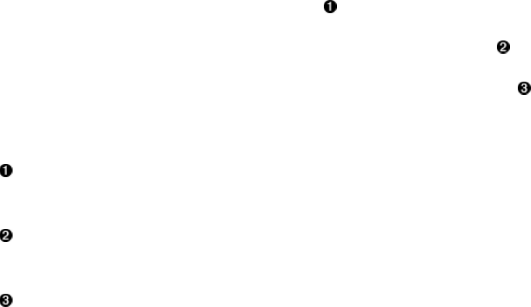
Example 4-38. Example master observer that creates a separate directory on the file system when a table is
created.
public class MasterObserverExample extends BaseMasterObserver {
@Override
public void postCreateTable(
ObserverContext<MasterCoprocessorEnvironment> ctx,
HTableDescriptor desc, HRegionInfo[] regions)
throws IOException {
TableName tableName = desc.getTableName();
MasterServices services = ctx.getEnvironment().getMasterServices();
MasterFileSystem masterFileSystem = services.getMasterFileSystem();
FileSystem fileSystem = masterFileSystem.getFileSystem();
Path blobPath = new Path(tableName.getQualifierAsString() + "-blobs");
fileSystem.mkdirs(blobPath);
}
}
Get the new table’s name from the table descriptor.
Get the available services and retrieve a reference to the actual file system.
Create a new directory that will store binary data from the client application.
Note
You need to add the following to the hbase-site.xml file for the coprocessor to be loaded by the
master process:
<property>
<name>hbase.coprocessor.master.classes</name>
<value>coprocessor.MasterObserverExample</value>
</property>
Just as before, restart HBase after making these adjustments.
Once you have activated the coprocessor, it is listening to the said events and will trigger your
code automatically. The example is using the supplied services to create a directory on the
filesystem. A fictitious application, for instance, could use it to store very large binary objects
(known as blobs) outside of HBase.
To trigger the event, you can use the shell like so:
hbase(main):001:0> create 'testtable3', 'colfam1'
0 row(s) in 0.6740 seconds
This creates the table and afterward calls the coprocessor’s postCreateTable() method. The
Hadoop command-line tool can be used to verify the results:
$ bin/hadoop dfs -ls
Found 1 items
drwxr-xr-x - larsgeorge supergroup 0 ... testtable3-blobs
(328)

There are many things you can implement with the MasterObserver coprocessor. Since you have
access to most of the shared master resources through the MasterServices instance, you should be
careful what you do, as it can potentially wreak havoc.
Finally, because the environment is wrapped in an ObserverContext, you have the same extra flow
controls, exposed by the bypass() and complete() methods. You can use them to explicitly disable
certain operations or skip subsequent coprocessor execution, respectively.
The BaseMasterAndRegionObserver Class
There is another, related base class provided by HBase, the BaseMasterAndRegionObserver. It is a
combination of two things: the BaseRegionObserver, as described in “The BaseRegionObserver
Class”, and the MasterObserver interface:
public abstract class BaseMasterAndRegionObserver
extends BaseRegionObserver implements MasterObserver {
...
}
In effect, this is like combining the previous BaseMasterObserver and BaseRegionObserver classes
into one. This class is only useful to run on the HBase Master since it provides both, a region
server and master implementation. This is used to host the system tables directly on the master.11
Otherwise the functionality of both have been described above, therefore we can move on to the
next coprocessor subclass.
(329)

The RegionServerObserver Class
You have seen how to run code next to regions, and within the master processes. The same is
possible within the region servers using the RegionServerObserver class. It exposes well-defined
hooks that pertain to the server functionality, that is, spanning many regions and tables. For that
reason, the following hooks are provided:
postCreateReplicationEndPoint(...)
Invoked after the server has created a replication endpoint (not to be confused with
coprocessor endpoints).
preMerge(...), postMerge(...)
Called when two regions are merged.
preMergeCommit(...), postMergeCommit(...)
Same as above, but with narrower scope. Called after preMerge() and before postMerge().
preRollBackMerge(...), postRollBackMerge(...)
These are invoked when a region merge fails, and the merge transaction has to be rolled
back.
preReplicateLogEntries(...), postReplicateLogEntries(...)
Tied into the WAL entry replay process, allows special treatment of each log entry.
preRollWALWriterRequest(...), postRollWALWriterRequest(...)
Wrap the rolling of WAL files, which will happen based on size, time, or manual request.
preStopRegionServer(...)
This pre-only hook is called when the from Stoppable inherited method stop() is called.
The environment allows access to that method on a region server.
The RegionServerCoprocessorEnvironment Class
Similar to how the MasterCoprocessorEnvironment is enclosing a single MasterObserver coprocessor,
the RegionServerCoprocessorEnvironment is wrapping RegionServerObserver instances. It also
implements the CoprocessorEnvironment interface, thus giving you, for instance, access to the
getTable() call to access data from within your own implementation.
On top of the provided methods, the specific, region server-oriented subclass adds the one
method described in Table 4-20.
Table 4-22. Specific method provided by the RegionServerCoprocessorEnvironment class
Method Description
(330)

getRegionServerServices() Provides access to the shared RegionServerServices instance.
We have discussed this class in “The RegionCoprocessorEnvironment Class” before, and refer
you to Table 4-18, which lists the available methods.
The BaseRegionServerObserver Class
Just with the other base observer classes you have seen, the BaseRegionServerObserver is an empty
implementation of the RegionServerObserver interface, saving you time and effort to otherwise
implement the many callback methods. Here you can focus on what you really need, and
overwrite the necessary methods only. The available callbacks are very advanced, and we refrain
from constructing a simple example at this point. Please refer to the source code if you need to
implement at this low level.
(331)

The WALObserver Class
The next observer class we are going to address is related to the write-ahead log, or WAL for
short. It offers a manageable list of callbacks, namely the following two:
preWALWrite(...), postWALWrite(...)
Wrap the writing of log entries to the WAL, allowing access to the full edit record.
Since you receive the entire record in these methods, you can influence what is written to the log.
For example, an advanced use-case might be to add extra cells to the edit, so that during a
potential log replay the cells could help fine tune the reconstruction process. You could add
information that trigger external message queueing, so that other systems could react
appropriately to the replay. Or you could use this information to create auxiliary data upon
seeing the special cells later on.
The WALCoprocessorEnvironment Class
Once again, there is a specialized environment that is provided as part of the callbacks. Here it is
an instance of the WALCoprocessorEnvironment class. It also extends the CoprocessorEnvironment
interface, thus giving you, for instance, access to the getTable() call to access data from within
your own implementation.
On top of the provided methods, the specific, WAL-oriented subclass adds the one method
described in Table 4-23.
Table 4-23. Specific method provided by the
WALCoprocessorEnvironment class
Method Description
getWAL() Provides access to the shared WAL instance.
With the reference to the WAL you can roll the current writer, in other words, close the current
log file and create a new one. You could also call the sync() method to force the edit records into
the persistence layer. Here are the methods available from the WAL interface:
void registerWALActionsListener(final WALActionsListener listener)
boolean unregisterWALActionsListener(final WALActionsListener listener)
byte[][] rollWriter() throws FailedLogCloseException, IOException
byte[][] rollWriter(boolean force) throws FailedLogCloseException, IOException
void shutdown() throws IOException
void close() throws IOException
long append(HTableDescriptor htd, HRegionInfo info, WALKey key, WALEdit edits,
AtomicLong sequenceId, boolean inMemstore, List<Cell> memstoreKVs)
throws IOException
void sync() throws IOException
void sync(long txid) throws IOException
boolean startCacheFlush(final byte[] encodedRegionName)
void completeCacheFlush(final byte[] encodedRegionName)
void abortCacheFlush(byte[] encodedRegionName)
WALCoprocessorHost getCoprocessorHost()
long getEarliestMemstoreSeqNum(byte[] encodedRegionName)
(332)
Once again, this is very low-level functionality, and at that point you most likely have read large
parts of the code already. We will defer the explanation of each method to the online Java
documentation.
The BaseWALObserver Class
The BaseWALObserver class implements the WALObserver interface. This is mainly done to help along
with a pending (as of this writing, for HBase 1.0) deprecation process of other variants of the
same callback methods. You can use this class to implement your own, or implement the
interface directly.
(333)

The BulkLoadObserver Class
This observer class is used during bulk loading operations, as triggered by the HBase supplied
completebulkload tool, contained in the server JAR file. Using the Hadoop JAR support, you can
see the list of tools like so:
$ bin/hadoop jar /usr/local/hbase-1.0.0-bin/lib/hbase-server-1.0.0.jar
An example program must be given as the first argument.
Valid program names are:
CellCounter: Count cells in HBase table
completebulkload: Complete a bulk data load.
copytable: Export a table from local cluster to peer cluster
export: Write table data to HDFS.
import: Import data written by Export.
importtsv: Import data in TSV format.
rowcounter: Count rows in HBase table
verifyrep: Compare the data from tables in two different clusters.
WARNING: It doesn't work for incrementColumnValues'd cells since the
timestamp is changed after being appended to the log.
Once the completebulkload tool is run, it will attempt to move all staged bulk load files into place
(more on this in Chapter 11, so for now please bear with me). During that operation the available
callbacks are triggered:
prePrepareBulkLoad(...)
Invoked before the bulk load operation takes place.
preCleanupBulkLoad(...)
Called when the bulk load is complete and clean up tasks are performed.
Both callbacks cannot skip the default processing using the bypass flag. They are merely invoked
but their actions take no effect on the further bulk loading process. The observer does not have
its own environment, instead it uses the RegionCoprocessorEnvironment explained in “The
RegionCoprocessorEnvironment Class”.
(334)

The EndPointObserver Class
The final observer is equally manageable, since it does not employ its own environment, but also
shares the RegionCoprocessorEnvironment (see “The RegionCoprocessorEnvironment Class”). This
makes sense, because endpoints run in the context of a region. The available callback methods
are:
preEndpointInvocation(...), postEndpointInvocation(...)
Whenever an endpoint method is called upon from a client, these callbacks wrap the server
side execution.
The client can replace (for the pre hook) or modify (for the post hook, using the provided
Message.Builder instance) the given Message instance to modify the outcome of the endpoint
method. If an exception is thrown during the pre hook, then the server-side call is aborted
completely.
1 The various filter methods are discussed in “Custom Filters”.
2 See Table 4-9 for an overview of compatible filters.
3 For users of older, pre-Protocol Buffer based HBase, please see “Migrate Custom Filters to post
HBase 0.96” for a migration guide.
4 This was changed in the final 0.92 release (after the book went into print) from enums to
constants in HBASE-4048.
5 The use of HTableInterface is an API remnant from before HBase 1.0. For HBase 2.0 and later
this is changed to the proper `Table in HBASE-12586.
6 As of this writing, there is an error thrown when using null keys. See HBASE-13417 for
details.
7 See the RegionServer documentation.
8 Sometimes inconsistently named "c" instead.
9 The Java HBase classes are documented online.
10 The Java HBase classes are documented online.
11 As of this writing, there are discussions to remove—or at least disable—this functionality in
future releases. See HBASE-11165 for details.
(335)
Chapter 5. Client API: Administrative
Features
Apart from the client API used to deal with data manipulation features, HBase also exposes a
data definition-like API. This is similar to the DDL and DML separation found in RDBMSes.
First we will look at the classes used by this HBase DDL defining data schemas and
subsequently the API that makes use of these classes, for example, creating new HBase tables.
These APIs and other operator functions comprise the HBase administration API and are
described below.
(336)
Schema Definition
Creating a table in HBase implicitly involves the definition of a table schema, as well as the
schemas for all contained column families. They define the pertinent characteristics of how—and
when—the data inside the table and columns is ultimately stored. On a higher level, every table
is part of a namespace, and we will start with their defining data structures first.
(337)

Namespaces
Namespaces were introduced into HBase to solve the problem of organizing many tables.1
Before this feature, you had a flat list of all tables, including the system catalog tables. This—at
scale—was causing difficulties when you had hundreds and hundreds of tables. With namespaces
you can organize your tables into groups, where related tables can be handled together. On top of
this, namespaces allow the further abstraction of generic concepts, such as security. You can
define access control on the namespace level to quickly apply the rules to all contained tables.
HBase creates two namespaces when it starts: default and hbase. The latter is for the system
catalog tables, and you should not create your own tables in this space. Using the shell, you can
list the namespaces and their content like so:
hbase(main):001:0> list_namespace
NAMESPACE
default
hbase
2 row(s) in 0.0090 seconds
hbase(main):002:0> list_namespace_tables 'hbase'
TABLE
foobar
meta
namespace
3 row(s) in 0.0120 seconds
The other namespace, called default, is the one namespace that all unspecified tables go into.
You do not have to specify a namespace when you generate a table. It will then automatically be
added to the default namespace on your behalf. Again, using the shell, here is what happens:
hbase(main):001:0> list_namespace_tables 'default'
TABLE
0 row(s) in 0.0170 seconds
hbase(main):002:0> create 'testtable', 'colfam1'
0 row(s) in 0.1650 seconds
=> Hbase::Table - testtable
hbase(main):003:0> list_namespace_tables 'default'
TABLE
testtable
1 row(s) in 0.0130 seconds
The new table (testtable) was created and added to the default namespace, since you did not
specify one.
Tip
If you have run the previous examples, it may be that you already have a table with the name
testtable. You will then receive an error like this one from the shell:
ERROR: Table already exists: testtable!
You can either use another name to test with, or use the disable 'testtable' and drop 'testtable'
commands to remove the table before moving on.
Since namespaces group tables, and their name is part of a table definition, you are free to create
(338)

tables with the same name in different namespaces:
hbase(main):001:0> create_namespace 'booktest'
0 row(s) in 0.0970 seconds
hbase(main):002:0> create 'booktest:testtable', 'colfam1'
0 row(s) in 0.1560 seconds
=> Hbase::Table - booktest:testtable
hbase(main):003:0> create_namespace 'devtest'
0 row(s) in 0.0140 seconds
hbase(main):004:0> create 'devtest:testtable', 'colfam1'
0 row(s) in 0.1490 seconds
=> Hbase::Table - devtest:testtable
This example creates two namespaces, booktest and devtest, and adds the table testtable to both.
Running the list commands is left for you to try, but you will see how the tables are now part of
their respective namespaces as expected. Dealing with namespaces in code revolves around the
NamespaceDescriptor class. These are constructed using the Builder pattern:
static Builder create(String name)
static Builder create(NamespaceDescriptor ns)
You either hand in a name for the new instance as a string, or pass an existing
NamespaceDescriptor instance, and the new instance will copy its details. The returned Builder
instance can then be used to add further configuration details to the new namespace, and
eventually build the instance. Example 5-1 shows this in action:
Example 5-1. Example how to create a NamespaceDescriptor in code
NamespaceDescriptor.Builder builder =
NamespaceDescriptor.create("testspace");
builder.addConfiguration("key1", "value1");
NamespaceDescriptor desc = builder.build();
System.out.println("Namespace: " + desc);
The result on the console:
Namespace: {NAME => 'testspace', key1 => 'value1'}
The class has a few more methods:
String getName()
String getConfigurationValue(String key)
Map<String, String> getConfiguration()
void setConfiguration(String key, String value)
void removeConfiguration(final String key)
String toString()
These methods are self-explanatory, they return the assigned namespace name, allow access to
the configuration values, the entire list of key/values, and retrieve the entire state as a string. This
class is used by the HBase admin API, explained in due course (see Example 5-7).
(339)

Tables
Everything stored in HBase is ultimately grouped into one or more tables. The primary reason to
have tables is to be able to control certain features that all columns in this table share. The typical
things you will want to define for a table are column families. The constructor of the table
descriptor in Java looks like the following:
HTableDescriptor(final TableName name)
HTableDescriptor(HTableDescriptor desc)
You either create a table with a name or an existing descriptor. You have to specify the name of
the table using the TableName class (as mentioned in “API Building Blocks”). This allows you to
specify the name of the table, and an optional namespace with one parameter. When you use the
latter constructor, that is, handing in an existing table descriptor, it will copy all settings and state
from that instance across to the new one.
Caution
A table cannot be renamed. The common approach to rename a table is to create a new table with
the desired name and copy the data over, using the API, or a MapReduce job (for example, using
the supplied copytable tool, as per “CopyTable Tool”). Another option is to use the snapshot
functionality as explained in “Renaming a Table”.
There are certain restrictions on the characters you can use to create a table name. The name is
used as part of the path to the actual storage files, and therefore has to comply with filename
rules. You can later browse the low-level storage system—for example, HDFS—to see the tables
as separate directories—in case you ever need to. The TableName class enforces these rules, as
shown in Example 5-2.
Example 5-2. Example how to create a TableName in code
private static void print(String tablename) {
print(null, tablename);
}
private static void print(String namespace, String tablename) {
System.out.print("Given Namespace: " + namespace +
", Tablename: " + tablename + " -> ");
try {
System.out.println(namespace != null ?
TableName.valueOf(namespace, tablename) :
TableName.valueOf(tablename));
} catch (Exception e) {
System.out.println(e.getClass().getSimpleName() +
": " + e.getMessage());
}
}
public static void main(String[] args) throws IOException, InterruptedException {
print("testtable");
print("testspace:testtable");
print("testspace", "testtable");
print("testspace", "te_st-ta.ble");
print("", "TestTable-100");
print("tEsTsPaCe", "te_st-table");
print("");
(340)

// VALID_NAMESPACE_REGEX = "(?:[a-zA-Z_0-9]+)";
// VALID_TABLE_QUALIFIER_REGEX = "(?:[a-zA-Z_0-9][a-zA-Z_0-9-.]*)";
print(".testtable");
print("te_st-space", "te_st-table");
print("tEsTsPaCe", "te_st-table@dev");
}
The result on the console:
Given Namespace: null, Tablename: testtable -> testtable
Given Namespace: null, Tablename: testspace:testtable -> testspace:testtable
Given Namespace: testspace, Tablename: testtable -> testspace:testtable
Given Namespace: testspace, Tablename: te_st-ta.ble -> testspace:te_st-ta.ble
Given Namespace: , Tablename: TestTable-100 -> TestTable-100
Given Namespace: tEsTsPaCe, Tablename: te_st-table -> tEsTsPaCe:te_st-table
Given Namespace: null, Tablename: -> IllegalArgumentException:
Table qualifier must not be empty
Given Namespace: null, Tablename: .testtable ->
IllegalArgumentException: Illegal first character \<46> at 0.
User-space table qualifiers can only start with 'alphanumeric characters':
i.e. [a-zA-Z_0-9]: .testtable
Given Namespace: te_st-space, Tablename: te_st-table ->
IllegalArgumentException: Illegal character \<45> at 5. Namespaces can
only contain 'alphanumeric characters': i.e. [a-zA-Z_0-9]: te_st-space
Given Namespace: tEsTsPaCe, Tablename: te_st-table@dev ->
IllegalArgumentException: Illegal character code:64, <@> at 11. User-space
table qualifiers can only contain 'alphanumeric characters':
i.e. [a-zA-Z_0-9-.]: te_st-table@dev
The class has many static helper methods, for example isLegalTableQualifierName(), allowing you
to check generated or user provided names before passing them on to HBase. It also has getters
to access the names handed into the valueOf() method as used in the example. Note that the table
name is returned using the getQualifier() method. The namespace has a matching getNamespace()
method.
The column-oriented storage format of HBase allows you to store many details into the same
table, which, under relational database modeling, would be divided into many separate tables.
The usual database normalization2 rules do not apply in HBase, and therefore the number of
tables is usually lower, in comparison. More on this is discussed in “Database (De-
)Normalization”.
Although conceptually a table is a collection of rows with columns, in HBase, tables are
physically stored in partitions called regions. This is how HBase divvies up big tables so they
can be distributed across a cluster. Figure 5-1 shows the difference between the logical and
physical layout of the stored data. Every region is served by exactly one region server, which in
turn serves the stored values directly to clients.3
(341)
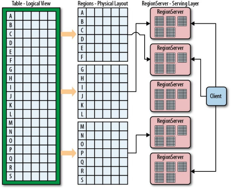
Figure 5-1. Logical and physical layout of rows within regions
Serialization
Before we move on to the table and its properties, there is something to be said about the
following specific methods of many client API classes:
byte[] toByteArray()
static HTableDescriptor parseFrom(final byte[] bytes)
TableSchema convert()
static HTableDescriptor convert(final TableSchema ts)
Every communication between remote disjoint systems—for example, the client talking to the
servers, but also the servers talking with one another—is done using the RPC framework. It
employs the Google Protocol Buffer (or Protobuf for short) library to serialize and deserialize
objects (I am treating class instance and object as synonyms), before they are passed between
remote systems.
The above methods are invoked by the framework to write the object’s data into the output
stream and, subsequently, to read it back on the receiving system. For the write, the framework
calls toByteArray() on the sending side, serializing the object’s fields out as a byte array. The
RPC framework takes care of sending metadata ahead of the bytes noting the class name the
bytes represent and other details. Alternatively, when writing, the convert() method in the case of
the HTableDescriptor class can be used to get an instance of the intermediate Protobuf class,
(342)

TableSchema in this case, which dependent on context can be a useful stepping stone serializing.
The convert() method is generally for use by HBase internally only.
On the receiving server, the RPC framework reads the metadata, and will create an object
instance using the static parseFrom() of the matching class. This will read back the field data and
leave you with a fully working and initialized copy of the sending object. The same is achieved
using the matching convert() call, which will take a Protobuf object instead of a byte array.
All of this is based on protocol description files, which you can find in the HBase source code.
They are like the ones we used in Chapter 4 for custom filters and coprocessor endpoints—but
much more elaborate. These protocol text files are compiled using the Protobuf protoc tool and
the generated classes are then checked into the HBase source tree. The advantage of using
Protobuf over, for example, Java Serialization, is that with care, protobufs can be evolved in a
compatible manner; if protobuf does not know how to interpret a field, it just passes it through.
You can even upgrade a cluster while it is operational, because an older (or newer) client can,
again with care to make sure new facility is additive only, communicate with a newer (or older)
server. Unknown Protobuf fields will just be ignored.
Since the receiver needs to create an instance of the original sending class, the receiving side
must have access to a matching, compiled class. Usually that is the case, as both the servers and
clients are using the same HBase Java archive file, or JAR. But if you develop your own
extensions to HBase—for example, the mentioned filters and coprocessors—you must ensure
that your custom class follows these rules:
Your custom extensions must be available on both sides of the RPC communication
channel, that is, the sending and receiving processes.
It implements the required Protobuf methods toByteArray() and parseFrom().
“Custom Filters” has an example and further notes if you intend extending HBase.
The RegionLocator Class
We could have mentioned this class in “API Building Blocks” but given the nature of the
RegionLocator class, we postponed explaination until now, so that you have the necessary context.
As you recall from “Auto-Sharding” and other references earlier, a table is divided into one to
many regions, which are consecutive, sorted sets of rows. They form the basis for HBase’s
scalability, and the implicit sharding (referred to as splitting) performed by the servers on your
behalf is one of the fundamental scaling mechanisms offered by HBase.
You could go the route of letting HBase deal with all region operations. Then there would be no
need to know more about how regions work under a table. In practice though, this is not always
possible. There may be times when you need to dig deeper and investigate the structure of a
table, for example, what regions a table has, what their boundaries are, and which specific region
is serving a given row key. So you can do that, there are a few methods provided by the
RegionLocator class:
public HRegionLocation getRegionLocation(final byte[] row)
throws IOException
public HRegionLocation getRegionLocation(final byte[] row,
boolean reload) throws IOException
public List<HRegionLocation> getAllRegionLocations()
throws IOException
(343)

public byte[][] getStartKeys() throws IOException
public byte[][] getEndKeys() throws IOException
public Pair<byte[][], byte[][]> getStartEndKeys() throws IOException
TableName getName()
A RegionLocator has a table scope. Its usage is similar to Table, that is, you retrieve an instance
from the shared connection by specifying what table it should go against, and once you are done
with your RegionLocator, you should free its resources by invoking close():
Configuration conf = HBaseConfiguration.create();
Connection connection = ConnectionFactory.createConnection(conf);
TableName tn = TableName.valueOf(tableName);
RegionLocator locator = connection.getRegionLocator(tn);
Pair<byte[][], byte[][]> pair = locator.getStartEndKeys();
...
locator.close();
The various methods provided are used to retrieve either HRegionLocation instances, or the binary
start and/or end keys, of the table regions. Regions are specified with the start key inclusive, but
the end key exclusive. This is done so we can connect regions contiguously, that it, without any
gaps in the key space. The HRegionLocation gives you access to region details, such as the server
currently hosting it, or the associated HRegionInfo object (explained in “The
RegionCoprocessorEnvironment Class”):
HRegionInfo getRegionInfo()
String getHostname()
int getPort()
String getHostnamePort()
ServerName getServerName()
long getSeqNum()
String toString()
Example 5-8 uses many of these methods in the context of creating a table in code.
Server and Region Names
There are two essential pieces of information that warrant a proper introduction: the server name
and region name. They appear in many places, such as the HBase Shell, the web-based UI, and
both APIs, the administrative and client. Sometimes they are just emitted in human readable
form, which includes encoding unprintable characters as codepoints. Other times, they are
returned by functions such as getServerName(), or getRegionNameAsString() (provided by
HRegionInfo), or are required as an input parameter to administrative API calls.
Example 5-3 creates a table and then locates the region that contains the row Foo. Once the region
is retrieved, the server name and region name are printed.
Example 5-3. Shows the use of server and region names
TableName tableName = TableName.valueOf("testtable");
HColumnDescriptor coldef1 = new HColumnDescriptor("colfam1");
HTableDescriptor desc = new HTableDescriptor(tableName)
.addFamily(coldef1)
.setValue("Description", "Chapter 5 - ServerAndRegionNameExample");
byte[][] regions = new byte[][] { Bytes.toBytes("ABC"),
Bytes.toBytes("DEF"), Bytes.toBytes("GHI"), Bytes.toBytes("KLM"),
Bytes.toBytes("OPQ"), Bytes.toBytes("TUV")
};
admin.createTable(desc, regions);
(344)
RegionLocator locator = connection.getRegionLocator(tableName);
HRegionLocation location = locator.getRegionLocation(Bytes.toBytes("Foo"));
HRegionInfo info = location.getRegionInfo();
System.out.println("Region Name: " + info.getRegionNameAsString());
System.out.println("Server Name: " + location.getServerName());
The output for one execution of the code looked like:
Region Name: testtable,DEF,1428681822728.acdd15c7050ec597b484b30b7c744a93.
Server Name: srv1.foobar.com,63360,1428669931467
The region name is a combination of table and region details (the start key, and region creation
time), plus a MD5 hash of the leading prefix of the name, surrounded by dots (“.”):
<table name>,<region start key>,<region creation time>.<md5hash(prefix)>.
In the example, "acdd15c7050ec597b484b30b7c744a93" is the MD5 hash of
"testtable,DEF,1428681822728". The getEncodedName() method of HRegionInfo returns just the hash,
not the leading, readable prefix. The hash itself is used when the system is creating the lower
level file structure within the storage layer. For example, the above region hash is visible when
listing the content of the storage directory for HBase (this is explained in detail in [Link to
Come], for now just notice the hash in the path):
$ bin/hdfs dfs -ls -R /hbase
drwxr-xr-x - larsgeorge supergroup 0 2015-04-10 18:03 \
/hbase/data/default/testtable/acdd15c7050ec597b484b30b7c744a93/colfam1
The region creation timestamp is issued when a region is created, for example when a table is
created, or an existing region split.
As for the server name, it is also a combination of various parts, including the host name of the
machine:
<host name>,<RPC port>,<server start time>
The server start time is used to handle multiple processes on the same physical machine, created
over time. When a region server is stopped and started again, the timestamp makes it possible for
the HBase Master to identify the new process on the same physical machine. It will then move
the old name, that is, the one with the lower timestamp, into the list of dead servers. On the flip
side, when you see a server process reported as dead, make sure to compare the listed timestamp
with the current one of the process on that same server using the same port. If the timestamp of
the current process is newer then all should be working as expected.
There is a class called ServerName that wraps the details into a convenient structure. Some API
calls expect to receive an instance of this class, which can be created from scratch, though the
practical approach is to use the API to retrieve an existing instance, for example, using the
getServerName() method mentioned before.
Keep the two names in mind as you read through the rest of this chapter, since they appear quite
a few times and it will make much more sense now that you know about their structure and
purpose.
(345)

Table Properties
The table descriptor offers getters and setters4 to set options for a table. In practice, a lot are not
used often, but it is important to know them all, as they can be used to fine-tune the table’s
performance. We will group the methods by the set of properties they influence.
Name
The constructor already had the parameter to specify the table name. The Java API has
additional methods to access the name.
TableName getTableName()
String getNameAsString()
This method returns the table name, as set during the construction of this instance. Refer to
“Column Families” for more details, and Figure 5-2 for an example of how the table name
is used to form a filesystem path.
Column Families
This is the most important part of defining a table. You need to specify the column families
you want to use with the table you are creating.
HTableDescriptor addFamily(final HColumnDescriptor family)
HTableDescriptor modifyFamily(final HColumnDescriptor family)
HColumnDescriptor removeFamily(final byte[] column)
HColumnDescriptor getFamily(final byte[] column)
boolean hasFamily(final byte[] familyName)
Set<byte[]> getFamiliesKeys()
HColumnDescriptor[] getColumnFamilies()
Collection<HColumnDescriptor> getFamilies()
You have the option of adding a family, modifying it, checking if it exists based on its
name, getting a list of all known families (in various forms), and getting or removing a
specific one. More on how to define the required HColumnDescriptor is explained in
“Column Families”.
Maximum File Size
This parameter specifies the maximum size a file in a region can grow to. The size is
specified in bytes and is read and set using the following methods:
long getMaxFileSize()
HTableDescriptor setMaxFileSize(long maxFileSize)
The maximum size is used to figure when to split regions. If any file reaches this limit, the
region is split. As discussed in “Building Blocks”, the unit of scalability and load
balancing in HBase is the region. You need to determine what a good number for this size
is. By default, it is set to 10 GB (the actual value is 10737418240 since it is specified in
bytes, and set in the default configuration as hbase.hregion.max.filesize), which is good for
many use cases. We will look into use-cases in [Link to Come] and show how this can
make a difference.
Please note that this is more or less a desired maximum size and that, given certain
(346)
conditions, this size can be exceeded and actually be rendered ineffective in rare
circumstances. As an example, you could set the maximum file size to 1 GB and insert a 2
GB cell in one row. Since a row cannot be split across regions, you end up with a region of
at least 2 GB in size, and the system cannot do anything about it.
Memstore Flush Size
We discussed the storage model earlier and identified how HBase uses an in-memory store
to buffer values before writing them to disk as a new storage file in an operation called
flush. This parameter of the table controls when this happens and is specified in bytes. It is
controlled by the following calls:
long getMemStoreFlushSize()
HTableDescriptor setMemStoreFlushSize(long memstoreFlushSize)
As you do with the aforementioned maximum file size, you need to check your
requirements before setting this value to something other than the default 128 MB (set as
hbase.hregion.memstore.flush.size to 134217728 bytes). A larger size means you are
generating larger store files, which is good. On the other hand, you might run into the
problem of longer blocking periods, if the region server cannot keep up with flushing the
added data. Also, it increases the time needed to replay the write-ahead log (the WAL) if
the server crashes and all in-memory updates are lost.
Compactions
Per table you can define if the underlying storage files should be compacted as part of the
automatic housekeeping. Setting (and reading) the flag is accomplished using these calls:
boolean isCompactionEnabled()
HTableDescriptor setCompactionEnabled(final boolean isEnable)
Split Policy
Along with specifying the maximum file size, you can further influence the splitting of
regions by specifying a split policy class for a table. Use the following to override the
system wide policy configured with hbase.regionserver.region.split.policy:
HTableDescriptor setRegionSplitPolicyClassName(String clazz)
String getRegionSplitPolicyClassName()
Region Normalization
If enabled, you can have the master process split and merge regions of a table
automatically, based on a pluggable RegionMormalizer class. See [Link to Come] for details.
The normalization has to be enabled cluster wide and on the table descriptor level. The
default is false, which means that usually a table is not balanced, even if the cluster is set
to do so.
boolean isNormalizationEnabled()
HTableDescriptor setNormalizationEnabled(final boolean isEnable)
Region Replicas
Specify a value for the number of region replicas you want to have for the current table.
The default is 1, which means just the main region. Setting it to 2, for example, adds a
single additional replica for every region of this table. This is controlled for the table
(347)

descriptor via:
int getRegionReplication()
HTableDescriptor setRegionReplication(int regionReplication)
Durability
Controls at the table level on how data is persisted in term of durability guarantees. We
discussed this option in “Durability, Consistency, and Isolation”, and you can set and
retrieve the parameter with these methods:
HTableDescriptor setDurability(Durability durability)
Durability getDurability()
Previous versions of HBase (before 0.94.7) used a boolean deferred log flush flag to
switch between an immediate sync of the WAL when data was written, or to a delayed
one. This has been replaced with the finer grained Durability class, that allows to indicate
what a client wishes to happen during write operations. The old setDeferredLogFlush(true)
is replaced by the Durability.ASYNC_WAL option.
Read-only
By default, all tables are writable, but it may make sense to specify the read-only option
for specific tables. If the flag is set to true, you can only read from the table and not
modify it at all. The flag is set and read by these methods:
boolean isReadOnly()
HTableDescriptor setReadOnly(final boolean readOnly)
Coprocessors
The listed calls allow you to configure any number of coprocessor classes for a table.
There are methods to add, check, list, and remove coprocessors from the current table
descriptor instance:
HTableDescriptor addCoprocessor(String className) throws IOException
HTableDescriptor addCoprocessor(String className, Path jarFilePath,
int priority, final Map<String, String> kvs) throws IOException
boolean hasCoprocessor(String className)
List<String> getCoprocessors()
void removeCoprocessor(String className)
Descriptor Parameters
In addition to those already mentioned, there are methods that let you set arbitrary
key/value pairs:
byte[] getValue(byte[] key)
String getValue(String key)
Map<ImmutableBytesWritable,ImmutableBytesWritable> getValues()
HTableDescriptor setValue(byte[] key, byte[] value)
HTableDescriptor setValue(final ImmutableBytesWritable key,
final ImmutableBytesWritable value)
HTableDescriptor setValue(String key, String value)
void remove(final String key)
void remove(ImmutableBytesWritable key)
void remove(final byte[] key)
They are stored with the table definition and can be retrieved later if necessary. You can
use them to access all configured values, as all of the above methods are effectively using
(348)
this list to set their parameters under the covers. Another use-case might be to store
application related metadata in this list, since it is persisted on the server and can be read
by any client subsequently. The schema manager in Hush uses this to store a table
description, which is handy in the HBase web-based UI to learn about the purpose of an
existing table.
Configuration
Allows you to override any HBase configuration property on a per table basis. This is
merged at runtime with the default values, and the cluster wide configuration file. Note
though that only properties related to the region or table will be useful to set. Other,
unrelated keys will not be used even if you override them.
String getConfigurationValue(String key)
Map<String, String> getConfiguration()
HTableDescriptor setConfiguration(String key, String value)
void removeConfiguration(final String key)
Miscellaneous Calls
There are some calls that do not fit into the above categories, so they are listed here for
completeness. They allow you to check the nature of the region or table they are related to,
and if it is a system region (or table). They further allow you to convert the entire, or
partial state of the instance into a string for further use, for example, to print the result into
a log file.
boolean isRootRegion()
boolean isMetaRegion()
boolean isMetaTable()
String toString()
String toStringCustomizedValues()
String toStringTableAttributes()
(349)

Column Families
We just saw how the HTableDescriptor exposes methods to add column families to a table.
Related to this is a class called HColumnDescriptor that wraps each column family’s settings into a
dedicated Java class. When using the HBase API in other programming languages, you may find
the same concept or some other means of specifying the column family properties.
Note
The class in Java is somewhat of a misnomer. A more appropriate name would be
HColumnFamilyDescriptor, which would indicate its purpose to define column family parameters as
opposed to actual columns.
Column families define shared features that apply to all columns that are created within them.
The client can create an arbitrary number of columns by simply using new column qualifiers on
the fly. Columns are addressed as a combination of the column family name and the column
qualifier (or sometimes also called the column key), divided by a colon:
`family:qualifier`
The column family name must not be empty but composed of only printable characters, cannot
start with a dot ("."), or contain a colon (":").5 The qualifier, on the other hand, can be composed
of any arbitrary binary characters. Recall the Bytes class mentioned earlier, which you can use to
convert your chosen names to byte arrays. The reason why the family name must be printable is
that the name is used as part of the directory name by the lower-level storage layer. Figure 5-2
visualizes how the families are mapped to storage files. The family name is added to the path and
must comply with filename standards. The advantage is that you can easily access families on the
filesystem level as you have the name in a human-readable format.
You should also be aware of the empty column qualifier. You can simply omit the qualifier and
specify just the column family name. HBase then creates a column with the special empty
qualifier. You can write and read that column like any other, but obviously there is only one of
these, and you will have to name the other columns to distinguish them. For simple applications,
using no qualifier is an option, but it also carries no meaning when looking at the data—for
example, using the HBase Shell. You should get used to naming your columns and do this from
the start. You cannot rename them later.
(350)
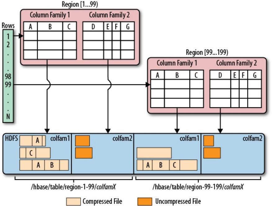
Figure 5-2. Column families mapping to separate storage files
Using the shell once again, we can try to create a column with no name, and see what happens if
we create a table with a column family name that does not comply to the checks:
hbase(main):001:0> create 'testtable', 'colfam1'
0 row(s) in 0.1400 seconds
=> Hbase::Table - testtable
hbase(main):002:0> put 'testtable', 'row1', 'colfam1:', 'val1'
0 row(s) in 0.1130 seconds
hbase(main):003:0> scan 'testtable'
ROW COLUMN+CELL
row1 column=colfam1:, timestamp=1428488894611, value=val1
1 row(s) in 0.0590 seconds
hbase(main):004:0> create 'testtable', 'col/fam1'
ERROR: Illegal character <47>. Family names cannot contain control characters or colons:
col/fam1
Here is some help for this command:
...
You can use the static helper method to verify the name:
static byte[] isLegalFamilyName(final byte[] b)
Use it in your program to verify user-provided input conforming to the specifications that are
required for the name. It does not return a boolean flag, but throws an IllegalArgumentException
when the name is malformed. Otherwise, it returns the given parameter value unchanged. The
(351)
constructors taking in a familyName parameter, shown below, uses this method internally to verify
the given name; in this case, you do not need to call the method beforehand.
Caution
A column family cannot be renamed. The common approach to rename a family is to create a
new family with the desired name and copy the data over, using the API.
When you create a column family, you can specify a variety of parameters that control all of its
features. The Java class has many constructors that allow you to specify most parameters while
creating an instance. Here are the choices:
HColumnDescriptor(final String familyName)
HColumnDescriptor(final byte[] familyName)
HColumnDescriptor(HColumnDescriptor desc)
The first two simply take the family name as a String or byte[] array. There is another one that
takes an existing HColumnDescriptor, which copies all state and settings over from the given
instance. Instead of using the constructor, you can also use the getters and setters to specify the
various details. We will now discuss each of them, grouped by their purpose.
Name
Each column family has a name, and you can use the following methods to retrieve it from
an existing HColumnDescriptor instance:
byte[] getName();
String getNameAsString();
You cannot set the name. You have to use the constructors to hand it in. Keep in mind the
requirement that the name be made of printable characters.
Note
The name of a column family must not start with a “.” (period) and may not contain “:”
(colon), “/” (slash), or ISO control characters, in other words, its code may not be in the
range \u0000 through \u001F or in the range \u007F through \u009F.
Maximum Versions
Per family, you can specify how many versions of each value you want to keep. Recall the
predicate deletion mentioned earlier where the housekeeping of HBase removes values
that exceed the set maximum. Getting and setting the value is done using the following
API calls:
int getMaxVersions()
HColumnDescriptor setMaxVersions(int maxVersions)
The default value is 1, set by the hbase.column.max.version configuration property. The
default is good for many use-cases, forcing the application developer to override the single
version setting to something higher if need be. For example, for a column storing
passwords, you could set this value to 10 to keep a history of previously used passwords.
Minimum Versions
(352)

Specifies how many versions should always be kept for a column. This works in tandem
with the time-to-live, avoiding the removal of the last value stored in a column. The default
is set to 0, which disables this feature.
int getMinVersions()
HColumnDescriptor setMinVersions(int minVersions)
Keep Deleted Cells
Controls whether the background housekeeping processes should remove deleted cells, or
not.
KeepDeletedCells getKeepDeletedCells()
HColumnDescriptor setKeepDeletedCells(boolean keepDeletedCells)
HColumnDescriptor setKeepDeletedCells(KeepDeletedCells keepDeletedCells)
The used KeepDeletedCells type is an enumeration, having the following options:
Table 5-1. The KeepDeletedCells enumeration
Value Description
FALSE Deleted cells are not retained.
TRUE
Deleted cells are retained until they are removed by other means such as time-to-
live (TTL) or a cell has exceeded the max number of allowed versions. If no TTL
is specified or no new versions of delete cells are written, they are retained forever.
TTL
Deleted cells are retained until the delete marker expires due to TTL. This is useful
when TTL is combined with the number of minimum versions, and you want to
keep a minimum number of versions around, but at the same time remove deleted
cells after the TTL.
The default is FALSE, meaning no deleted cells are kept during the housekeeping operation.
Compression
HBase has pluggable compression algorithm support (you can find more on this topic in
“Compression”) that allows you to choose the best compression—or none—for the data
stored in a particular column family. The possible algorithms are listed in Table 5-2.
Table 5-2. Supported compression algorithms
Value Description
NONE Disables compression (default).
GZ Uses the Java-supplied or native GZip compression (which needs to be installed
separately).
(353)

LZO Enables LZO compression; must be installed separately.
LZ4 Enables LZ4 compression; must be installed separately.
SNAPPY Enables Snappy compression; binaries must be installed separately.
The default value is NONE--in other words, no compression is enabled when you create a
column family. When you use the Java API and a column descriptor, you can use these
methods to change the value:
Compression.Algorithm getCompression()
Compression.Algorithm getCompressionType()
HColumnDescriptor setCompressionType(Compression.Algorithm type)
Compression.Algorithm getCompactionCompression()
Compression.Algorithm getCompactionCompressionType()
HColumnDescriptor setCompactionCompressionType(Compression.Algorithm type)
Note how the value is not a String, but rather a Compression.Algorithm enumeration that
exposes the same values as listed in Table 5-2. Another observation is that there are two
sets of methods, one for the general compression setting and another for the compaction
compression setting. Also, each group has a getCompression() and getCompressionType() (or
getCompactionCompression() and getCompactionCompressionType(), respectively) returning the
same type of value. They are indeed redundant, and you can use either to retrieve the
current compression algorithm type.6 As for compression versus compaction compression,
the latter defaults to what the former is set to, unless set differently.
We will look into this topic in much greater detail in “Compression”.
Encoding
Sets the encoding used for data blocks. The API methods involved are:
DataBlockEncoding getDataBlockEncoding()
HColumnDescriptor setDataBlockEncoding(DataBlockEncoding type)
These two methods control the encoding used, and employ the DataBlockEncoding
enumeration, containing the following options:
Table 5-3. Options of the DataBlockEncoding enumeration
Option Description
NONE No prefix encoding takes place (default).
PREFIX Represents the prefix compression algorithm, which removes repeating
common prefixes from subsequent cell keys.
DIFF The diff algorithm, which further compresses the key of subsequent cells by
storing only differences to previous keys.
(354)

FAST_DIFF
An optimized version of the diff encoding, which also omits repetitive cell
value data.
PREFIX_TREE Trades increased write time latencies for faster read performance. Uses a tree
structure to compress the cell key.
In addition to setting the encoding for each cell key (and value data in case of fast diff),
cells also may carry an arbitrary list of tags, used for different purposes, such as security
and cell-level TTLs. The following methods of the column descriptor allow you to fine-
tune if the encoding should also be applied to the tags:
HColumnDescriptor setCompressTags(boolean compressTags)
boolean isCompressTags()
The default is true, so all optional cell tags are encoded as part of the entire cell encoding.
Block Size
All stored files in HBase are divided into smaller blocks that are loaded during a get() or
scan() operation, analogous to pages in RDBMSes. The size of these blocks is set to 64 KB
by default and can be adjusted with these methods:
synchronized int getBlocksize()
HColumnDescriptor setBlocksize(int s)
The value is specified in bytes and can be used to control how much data HBase is
required to read from the storage files during retrieval as well as what is cached in memory
for subsequent access. How this can be used to optimize your setup can be found in
“Configuration”.
Note
There is an important distinction between the column family block size, or HFile block
size, and the block size specified on the HDFS level. Hadoop, and HDFS specifically, is
using a block size of—by default—128 MB to split up large files for distributed, parallel
processing using the YARN framework. For HBase the HFile block size is—again by
default—64 KB, or one 2048th of the HDFS block size. The storage files used by HBase
are using this much more fine-grained size to efficiently load and cache data in block
operations. It is independent from the HDFS block size and only used internally. See [Link
to Come] for more details, especially [Link to Come], which shows the two different block
types.
Block Cache
As HBase reads entire blocks of data for efficient I/O usage, it retains these blocks in an
in-memory cache so that subsequent reads do not need any disk operation. The default of
true enables the block cache for every read operation. Here is the API that allows you read
and set this flag:
boolean isBlockCacheEnabled()
HColumnDescriptor setBlockCacheEnabled(boolean blockCacheEnabled)
(355)

There are other options you can use to influence how the block cache is used, for example,
during a scan() operation by calling setCacheBlocks(false). This is useful during full table
scans so that you do not cause a major churn on the cache. See “Configuration” for more
information about this feature.
Besides the cache itself, you can configure the behavior of the system when data is being
written, and store files being closed or opened. The following set of methods define (and
query) this:
boolean isCacheDataOnWrite()
HColumnDescriptor setCacheDataOnWrite(boolean value)
boolean isCacheDataInL1()
HColumnDescriptor setCacheDataInL1(boolean value)
boolean isCacheIndexesOnWrite()
HColumnDescriptor setCacheIndexesOnWrite(boolean value)
boolean isCacheBloomsOnWrite()
HColumnDescriptor setCacheBloomsOnWrite(boolean value)
boolean isEvictBlocksOnClose()
HColumnDescriptor setEvictBlocksOnClose(boolean value)
boolean isPrefetchBlocksOnOpen()
HColumnDescriptor setPrefetchBlocksOnOpen(boolean value)
Please consult [Link to Come] and Chapter 10 for details on how the block cache works,
what L1 and L2 is, and what you can do to speed up your HBase setup. Note, for now, that
all of these latter settings default to false, meaning none of them are active, unless you
explicitly enable them for a column family.
Time-to-Live
HBase supports predicate deletions on the number of versions kept for each value, but also
on specific times. The time-to-live (or TTL) sets a threshold based on the timestamp of a
value and the internal housekeeping checks automatically if a value exceeds its TTL. If
that is the case, it is dropped during major compactions. The API provides the following
getters and setters to read and write the TTL:
+
int getTimeToLive()
HColumnDescriptor setTimeToLive(int timeToLive)
+ The value is specified in seconds and is, by default, set to HConstants.FOREVER, which in turn is
set to Integer.MAX_VALUE, or 2,147,483,647 seconds. The default value is treated as the special
case of keeping the values forever, that is, any positive value less than the default enables this
feature.
In-Memory
We mentioned the block cache and how HBase is using it to keep entire blocks of data in
memory for efficient sequential access to data. The in-memory flag defaults to false but
can be read and modified with these methods:
boolean isInMemory()
HColumnDescriptor setInMemory(boolean inMemory)
(356)

Setting it to true is not a guarantee that all blocks of a family are loaded into memory nor
that they stay there. Think of it as a promise, or elevated priority, to keep them in memory
as soon as they are loaded during a normal retrieval operation, and until the pressure on the
cache is too high, at which time they will be replaced by hotter blocks.
In general, this setting is good for small column families with few values, such as the
passwords of a user table, so that logins can be processed fast.
Bloom Filter
An advanced feature available in HBase is Bloom filters,7 allowing you to improve lookup
times given you have a specific access pattern (see “Bloom Filters” for details). They add
overhead in terms of storage and memory, but improve lookup performance and read
latencies. Table 5-4 shows the possible options.
Table 5-4. Supported Bloom Filter Types
Type Description
NONE Disables the filter.
ROW Use the row key for the filter (default).
ROWCOL Use the row key and column key (family+qualifier) for the filter.
As of HBase 0.96 the default is set to ROW for all column families of all user tables (they are
not enabled for the system catalog tables). Because there are usually many more columns
than rows (unless you only have a single column in each row), the last option, ROWCOL,
requires the largest amount of space. It is more fine-grained, though, since it knows about
each row/column combination, as opposed to just rows keys.
The Bloom filter can be changed and retrieved with these calls, taking or returning a
BloomType enumeration, reflecting the above options.
BloomType getBloomFilterType()
HColumnDescriptor setBloomFilterType(final BloomType bt)
Replication Scope
Another more advanced feature that comes with HBase is replication. It enables you to set
up configurations such that the edits applied at one cluster are also replicated to another.
By default, replication is disabled and the replication scope is set to 0, meaning do not
replicate edits. You can change the scope with these functions:
int getScope()
HColumnDescriptor setScope(int scope)
The only other supported value (as of this writing) is 1, which enables replication to a
remote cluster. There may be more scope values in the future. See Table 5-5 for a list of
supported values.
Table 5-5. Supported Replication Scopes
(357)

Table 5-5. Supported Replication Scopes
Scope Constant Description
0 REPLICATION_SCOPE_LOCAL Local scope, i.e., no replication for this family (default).
1 REPLICATION_SCOPE_GLOBAL Global scope, i.e., replicate family to a remote cluster.
The full details can be found in “Replication”. Note how the scope is also provided as a
public constant in the API class HConstants. When you need to set the replication scope in
code it is advisable to use the constants, as they make your intent more plain.
Encryption
Sets encryption related details. See [Link to Come] for details. The following API calls are
at your disposal to set and read the encryption type and key:
String getEncryptionType()
HColumnDescriptor setEncryptionType(String algorithm)
byte[] getEncryptionKey()
HColumnDescriptor setEncryptionKey(byte[] keyBytes)
Descriptor Parameters
In addition to those already mentioned, there are methods that let you set arbitrary
key/value pairs, just as you can set arbitrary tuples on HTableDescriptor:
byte[] getValue(byte[] key)
String getValue(String key)
Map<ImmutableBytesWritable, ImmutableBytesWritable> getValues()
HColumnDescriptor setValue(byte[] key, byte[] value)
HColumnDescriptor setValue(String key, String value)
void remove(final byte[] key)
They are stored with the column definition and can be retrieved later when needed. You
can use them to access all configured values, as all of the above methods are effectively
using this list to set their parameters under the hood. Another use-case might be to store
application related metadata in this list, since it is persisted on the server and can be read
by any client subsequently.
Configuration
Allows you to override any HBase configuration property on a per column family basis.
This is merged at runtime with the default values, the cluster wide configuration file, and
the table level settings. Note though that only properties related to the region or table will
be useful to set. Other, unrelated keys will not read even if you override them.
String getConfigurationValue(String key)
Map<String, String> getConfiguration()
HColumnDescriptor setConfiguration(String key, String value)
void removeConfiguration(final String key)
Miscellaneous Calls
There are some calls that do not fit into the above categories, so they are listed here for
completeness. They allow you to retrieve the unit for a configuration parameter, and get
(358)

hold of the list of all default values. They further allow you to convert the entire, or partial
state of the instance into a string for further use, for example, to print the result into a log
file.
static Unit getUnit(String key)
static Map<String, String> getDefaultValues()
String toString()
String toStringCustomizedValues()
The only supported unit as of this writing is for TTL. The set Unit is used during
formatting HColumnDescriptor when printed on the console or in the UI.
Example 5-4 uses the API to create a descriptor, set a custom and supplied value, and then print
out the settings in various ways.
Example 5-4. Example how to create a HColumnDescriptor in code
HColumnDescriptor desc = new HColumnDescriptor("colfam1")
.setValue("test-key", "test-value")
.setBloomFilterType(BloomType.ROWCOL);
System.out.println("Column Descriptor: " + desc);
System.out.print("Values: ");
for (Map.Entry<ImmutableBytesWritable, ImmutableBytesWritable>
entry : desc.getValues().entrySet()) {
System.out.print(Bytes.toString(entry.getKey().get()) +
" -> " + Bytes.toString(entry.getValue().get()) + ", ");
}
System.out.println();
System.out.println("Defaults: " +
HColumnDescriptor.getDefaultValues());
System.out.println("Custom: " +
desc.toStringCustomizedValues());
System.out.println("Units:");
System.out.println(HColumnDescriptor.TTL + " -> " +
desc.getUnit(HColumnDescriptor.TTL));
System.out.println(HColumnDescriptor.BLOCKSIZE + " -> " +
desc.getUnit(HColumnDescriptor.BLOCKSIZE));
The output of Example 5-4 shows a few interesting details:
Column Descriptor: {NAME => 'colfam1', DATA_BLOCK_ENCODING => 'NONE',
BLOOMFILTER => 'ROWCOL', REPLICATION_SCOPE => '0',
COMPRESSION => 'NONE', VERSIONS => '1', TTL => 'FOREVER',
MIN_VERSIONS => '0', KEEP_DELETED_CELLS => 'FALSE',
BLOCKSIZE => '65536', IN_MEMORY => 'false', BLOCKCACHE => 'true',
METADATA => {'test-key' => 'test-value'}}
Values: DATA_BLOCK_ENCODING -> NONE, BLOOMFILTER -> ROWCOL,
REPLICATION_SCOPE -> 0, COMPRESSION -> NONE, VERSIONS -> 1,
TTL -> 2147483647, MIN_VERSIONS -> 0, KEEP_DELETED_CELLS -> FALSE,
BLOCKSIZE -> 65536, IN_MEMORY -> false, test-key -> test-value,
BLOCKCACHE -> true
Defaults: {CACHE_BLOOMS_ON_WRITE=false, CACHE_DATA_IN_L1=false,
PREFETCH_BLOCKS_ON_OPEN=false, BLOCKCACHE=true,
CACHE_INDEX_ON_WRITE=false, TTL=2147483647, DATA_BLOCK_ENCODING=NONE,
BLOCKSIZE=65536, BLOOMFILTER=ROW, EVICT_BLOCKS_ON_CLOSE=false,
MIN_VERSIONS=0, CACHE_DATA_ON_WRITE=false, KEEP_DELETED_CELLS=FALSE,
COMPRESSION=none, REPLICATION_SCOPE=0, VERSIONS=1, IN_MEMORY=false}
Custom: {NAME => 'colfam1', BLOOMFILTER => 'ROWCOL',
METADATA => {'test-key' => 'test-value'}}
(359)
Units:
TTL -> TIME_INTERVAL
BLOCKSIZE -> NONE
The custom test-key property, with value test-value, is listed as METADATA, while the one setting
that was changed from the default, the Bloom filter set to ROWCOL, is listed separately. The
toStringCustomizedValues() only lists the changed or custom data, while the others print all. The
static getDefaultValues() lists the default values unchanged, since it is created once when this
class is loaded and never modified thereafter.
Before we move on, and as explained earlier in the context of the table descriptor, the
serialization functions required to send the configured instances over RPC are also present for
the column descriptor:
byte[] toByteArray()
static HColumnDescriptor parseFrom(final byte[] bytes) throws DeserializationException
static HColumnDescriptor convert(final ColumnFamilySchema cfs)
ColumnFamilySchema convert()
(360)
Cluster Administration
Just as with the client API, you also have an API for administrative tasks to do DDL-type
operations. These make use of the classes and properties described in the previous sections.
There is an API to create tables with specific column families, check for table existence, alter
table and column family definitions, drop tables, and much more. The provided functions can be
grouped into related operations; they’re discussed separately on the following pages.
(361)

Basic Operations
Before you can use the administrative API, you will have to obtain an instance of the Admin
interface implementation. You cannot create an instance directly. You need to use the same
approach as with tables (see “API Building Blocks”) to retrieve an instance from the Connection
class:
Configuration conf = HBaseConfiguration.create();
Connection connection = ConnectionFactory.createConnection(conf);
Admin admin = connection.getAdmin();
...
TableName[] tables = admin.listTableNames();
...
admin.close();
connection.close();
Note
For the sake of brevity, this section omits the fact that pretty much all methods may throw an
IOException (or an exception that inherits from it). The reason is usually a result of a
communication error between your client application and the remote servers, or an error that
occurred on the server-side and which was marshalled (as in wrapped) into a client-side I/O
error. In your own code, be sure to wrap operations in try/catch/finally or try-with-resources
blocks so you get a chance to handle any exception thrown and then close any Admin instance
outstanding.
Handing in an existing configuration instance gives enough details to the API to find the cluster
using the ZooKeeper quorum, just like the client API does. Use the administrative API instance
for the operation required and discard it afterward. In other words, you should not hold on to the
instance for too long. Call close() when you are done to free any resources still held on either
side of the communication.
The class implements the Abortable interface, adding the following call to it:
void abort(String why, Throwable e)
boolean isAborted()
This method is called by the framework implicitly—for example, when there is a fatal
connectivity issue and the API should be stopped. You should not call it directly, but rely on the
system taking care of invoking it, in the rare case of where a complete shutdown—and possible
restart—of the API instance is needed.
The Admin class also exports these basic calls:
Connection getConnection()
void close()
The getConnection() returns the connection instance, and close() frees all resources kept by the
current Admin instance, as shown above. This includes the connection to the remote servers.
(362)

Namespace Operations
You can use the API to create namespaces that subsequently hold the tables assigned to them.
And as expected, you can in addition modify or delete existing namespaces, and retrieve a
descriptor (see “Namespaces”). The list of API calls for these tasks are:
void createNamespace(final NamespaceDescriptor descriptor)
void modifyNamespace(final NamespaceDescriptor descriptor)
void deleteNamespace(final String name)
NamespaceDescriptor getNamespaceDescriptor(final String name)
NamespaceDescriptor[] listNamespaceDescriptors()
Example 5-5 shows these calls in action. The code creates a new namespace, then lists the
namespaces available. It then modifies the new namespace by adding a custom property. After
printing the descriptor it deletes the namespace, and eventually confirms the removal by listing
the available spaces again.
Example 5-5. Example using the administrative API to create etc. a namespace
Configuration conf = HBaseConfiguration.create();
Connection connection = ConnectionFactory.createConnection(conf);
Admin admin = connection.getAdmin();
NamespaceDescriptor namespace =
NamespaceDescriptor.create("testspace").build();
admin.createNamespace(namespace);
NamespaceDescriptor namespace2 =
admin.getNamespaceDescriptor("testspace");
System.out.println("Simple Namespace: " + namespace2);
NamespaceDescriptor[] list = admin.listNamespaceDescriptors();
for (NamespaceDescriptor nd : list) {
System.out.println("List Namespace: " + nd);
}
NamespaceDescriptor namespace3 =
NamespaceDescriptor.create("testspace")
.addConfiguration("Description", "Test Namespace")
.build();
admin.modifyNamespace(namespace3);
NamespaceDescriptor namespace4 =
admin.getNamespaceDescriptor("testspace");
System.out.println("Custom Namespace: " + namespace4);
admin.deleteNamespace("testspace");
NamespaceDescriptor[] list2 = admin.listNamespaceDescriptors();
for (NamespaceDescriptor nd : list2) {
System.out.println("List Namespace: " + nd);
}
The console output confirms what we expected to see:
Simple Namespace: {NAME => 'testspace'}
List Namespace: {NAME => 'default'}
List Namespace: {NAME => 'hbase'}
List Namespace: {NAME => 'testspace'}
Custom Namespace: {NAME => 'testspace', Description => 'Test Namespace'}
List Namespace: {NAME => 'default'}
List Namespace: {NAME => 'hbase'}
(363)
Table Operations
After the first set of basic and namespace operations, there is a group of calls related to HBase
tables. These calls help when working with the tables themselves, not the actual table schemas
(or the data in tables). The commands addressing schema are in “Schema Operations”.
Before you can do anything with HBase, you need to create tables. Here is the set of functions
you could use:
void createTable(HTableDescriptor desc)
void createTable(HTableDescriptor desc, byte[] startKey,
byte[] endKey, int numRegions)
void createTable(final HTableDescriptor desc, byte[][] splitKeys)
void createTableAsync(final HTableDescriptor desc, final byte[][] splitKeys)
All of these calls must be given an instance of HTableDescriptor, as described in detail in
“Tables”. It holds the details of the table to be created, including the column families.
Example 5-6 uses the simple variant of createTable() that just takes a table name.
Example 5-6. Example using the administrative API to create a table
Configuration conf = HBaseConfiguration.create();
Connection connection = ConnectionFactory.createConnection(conf);
Admin admin = connection.getAdmin();
TableName tableName = TableName.valueOf("testtable");
HTableDescriptor desc = new HTableDescriptor(tableName);
HColumnDescriptor coldef = new HColumnDescriptor(
Bytes.toBytes("colfam1"));
desc.addFamily(coldef);
admin.createTable(desc);
boolean avail = admin.isTableAvailable(tableName);
System.out.println("Table available: " + avail);
Create a administrative API instance.
Create the table descriptor instance.
Create a column family descriptor and add it to the table descriptor.
Call the createTable() method to do the actual work.
Check if the table is available.
(364)
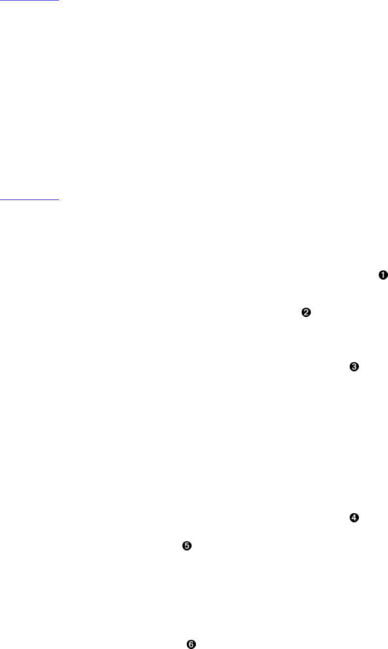
Example 5-7 shows the same, but adds a namespace into the mix.
Example 5-7. Example using the administrative API to create a table with a custom namespace
NamespaceDescriptor namespace =
NamespaceDescriptor.create("testspace").build();
admin.createNamespace(namespace);
TableName tableName = TableName.valueOf("testspace", "testtable");
HTableDescriptor desc = new HTableDescriptor(tableName);
HColumnDescriptor coldef = new HColumnDescriptor(
Bytes.toBytes("colfam1"));
desc.addFamily(coldef);
admin.createTable(desc);
The other createTable() versions have an additional—yet more advanced—feature set: they
allow you to create tables that are already populated with specific regions. The code in
Example 5-8 uses both possible ways to specify your own set of region boundaries.
Example 5-8. Example using the administrative API to create a table with predefined regions
private static Configuration conf = null;
private static Connection connection = null;
private static void printTableRegions(String tableName) throws IOException {
System.out.println("Printing regions of table: " + tableName);
TableName tn = TableName.valueOf(tableName);
RegionLocator locator = connection.getRegionLocator(tn);
Pair<byte[][], byte[][]> pair = locator.getStartEndKeys();
for (int n = 0; n < pair.getFirst().length; n++) {
byte[] sk = pair.getFirst()[n];
byte[] ek = pair.getSecond()[n];
System.out.println("[" + (n + 1) + "]" +
" start key: " +
(sk.length == 8 ? Bytes.toLong(sk) : Bytes.toStringBinary(sk)) +
", end key: " +
(ek.length == 8 ? Bytes.toLong(ek) : Bytes.toStringBinary(ek)));
}
locator.close();
}
public static void main(String[] args) throws IOException, InterruptedException {
conf = HBaseConfiguration.create();
connection = ConnectionFactory.createConnection(conf);
Admin admin = connection.getAdmin();
HTableDescriptor desc = new HTableDescriptor(
TableName.valueOf("testtable1"));
HColumnDescriptor coldef = new HColumnDescriptor(
Bytes.toBytes("colfam1"));
desc.addFamily(coldef);
admin.createTable(desc, Bytes.toBytes(1L), Bytes.toBytes(100L), 10);
printTableRegions("testtable1");
byte[][] regions = new byte[][] {
Bytes.toBytes("A"),
Bytes.toBytes("D"),
Bytes.toBytes("G"),
Bytes.toBytes("K"),
Bytes.toBytes("O"),
Bytes.toBytes("T")
};
HTableDescriptor desc2 = new HTableDescriptor(
TableName.valueOf("testtable2"));
desc2.addFamily(coldef);
admin.createTable(desc2, regions);
printTableRegions("testtable2");
(365)

}
Helper method to print the regions of a table.
Retrieve the start and end keys from the newly created table.
Print the key, but guarding against the empty start (and end) key.
Call the createTable() method while also specifying the region boundaries.
Manually create region split keys.
Call the createTable() method again, with a new table name and the list of region split
keys.
Running the example should yield the following output on the console:
Printing regions of table: testtable1
[1] start key: , end key: 1
[2] start key: 1, end key: 13
[3] start key: 13, end key: 25
[4] start key: 25, end key: 37
[5] start key: 37, end key: 49
[6] start key: 49, end key: 61
[7] start key: 61, end key: 73
[8] start key: 73, end key: 85
[9] start key: 85, end key: 100
[10] start key: 100, end key:
Printing regions of table: testtable2
[1] start key: , end key: A
[2] start key: A, end key: D
[3] start key: D, end key: G
[4] start key: G, end key: K
[5] start key: K, end key: O
[6] start key: O, end key: T
[7] start key: T, end key:
The example uses a method of the RegionLocator implementation that you saw earlier (see “The
RegionLocator Class”), getStartEndKeys(), to retrieve the region boundaries. The first start and
the last end keys are empty. The empty key is reserved for this purpose. In between the start and
end keys are either the computed, or the provided split keys. Note how the end key of a region is
also the start key of the subsequent one—just that it is exclusive for the former, and inclusive for
the latter, respectively.
The createTable(HTableDescriptor desc, byte[] startKey, byte[] endKey, int numRegions) call
takes a start and end key. You must provide a start value that is less than the end value, and a
numRegions that is at least 3: otherwise, the call will return with an exception. This is to ensure that
you end up with at least a minimum set of regions.
(366)

The start and end key values are interpreted as numbers, subtracted and divided by the given
number of regions to compute the region boundaries. In the example, you can see how we end up
with the correct number of regions, while the computed keys are filling in the range.
The createTable(HTableDescriptor desc, byte[][] splitKeys) method used in the second part of
the example, on the other hand, is expecting an already set array of split keys: they form the start
and end keys of the regions created. The output of the example demonstrates this as expected.
But take note how the first start key, and the last end key are the default empty one (set to null),
which means you end up with seven regions, albeit having provided only six split keys.
Note
The createTable() calls are, in fact, related. The createTable(HTableDescriptor desc, byte[]
startKey, byte[] endKey, int numRegions) method is calculating the region keys implicitly for
you, using the Bytes.split() method to use your given parameters to compute the boundaries. It
then proceeds to call the createTable(HTableDescriptor desc, byte[][] splitKeys), doing the
actual table creation.
Finally, there is the createTableAsync(HTableDescriptor desc, byte[][] splitKeys) method that
takes the table descriptor, and region keys, to asynchronously perform the same task as the
createTable() call.
Note
Most of the table-related administrative API functions are asynchronous in nature, which is
useful, as you can send off a command and not have to deal with waiting for a result. For a client
application, though, it is often necessary to know if a command has succeeded before moving on
with other operations. For that, the calls are provided in asynchronous—using the Async postfix—
and synchronous versions.
In fact, the synchronous commands are simply a wrapper around the asynchronous ones, adding
a loop at the end of the call to repeatedly check for the command to have done its task. The
createTable() method, for example, wraps the createTableAsync() method, while adding a loop
that waits for the table to be created on the remote servers before yielding control back to the
caller.
Once you have created a table, you can use the following helper functions to retrieve the list of
tables, retrieve the descriptor for an existing table, or check if a table exists:
HTableDescriptor[] listTables()
HTableDescriptor[] listTables(Pattern pattern)
HTableDescriptor[] listTables(String regex)
HTableDescriptor[] listTables(Pattern pattern, boolean includeSysTables)
HTableDescriptor[] listTables(String regex, boolean includeSysTables)
HTableDescriptor[] listTableDescriptorsByNamespace(final String name)
HTableDescriptor getTableDescriptor(final TableName tableName)
HTableDescriptor[] getTableDescriptorsByTableName(List<TableName> tableNames)
HTableDescriptor[] getTableDescriptors(List<String> names)
boolean tableExists(final TableName tableName)
Example 5-6 uses the tableExists() method to check if the previous command to create the table
has succeeded. The listTables() returns a list of HTableDescriptor instances for every table that
HBase knows about, while the getTableDescriptor() method returns it for a specific one.
Example 5-9 uses both to show what is returned by the administrative API.
(367)

Example 5-9. Example listing the existing tables and their descriptors
Connection connection = ConnectionFactory.createConnection(conf);
Admin admin = connection.getAdmin();
HTableDescriptor[] htds = admin.listTables();
for (HTableDescriptor htd : htds) {
System.out.println(htd);
}
HTableDescriptor htd1 = admin.getTableDescriptor(
TableName.valueOf("testtable1"));
System.out.println(htd1);
HTableDescriptor htd2 = admin.getTableDescriptor(
TableName.valueOf("testtable10"));
System.out.println(htd2);
The console output is quite long, since every table descriptor is printed, including every possible
property. Here is an abbreviated version:
Printing all tables...
'testtable1', {NAME => 'colfam1', DATA_BLOCK_ENCODING => 'NONE', BLOOMFILTER
=> 'ROW', REPLICATION_SCOPE => '0', VERSIONS => '1', COMPRESSION => 'NONE',
MIN_VERSIONS => '0', TTL => 'FOREVER', KEEP_DELETED_CELLS => 'FALSE',
BLOCKSIZE => '65536', IN_MEMORY => 'false', BLOCKCACHE => 'true'},
{NAME => 'colfam2', DATA_BLOCK_ENCODING => 'NONE', BLOOMFILTER => 'ROW',
REPLICATION_SCOPE => '0', VERSIONS => '1', COMPRESSION => 'NONE',
MIN_VERSIONS => '0', TTL => 'FOREVER', KEEP_DELETED_CELLS => 'FALSE',
BLOCKSIZE => '65536', IN_MEMORY => 'false', BLOCKCACHE => 'true'},
{NAME => 'colfam3', DATA_BLOCK_ENCODING => 'NONE', BLOOMFILTER => 'ROW',
REPLICATION_SCOPE => '0', VERSIONS => '1', COMPRESSION => 'NONE',
MIN_VERSIONS => '0', TTL => 'FOREVER', KEEP_DELETED_CELLS => 'FALSE',
BLOCKSIZE => '65536', IN_MEMORY => 'false', BLOCKCACHE => 'true'}
...
Exception in thread "main"
org.apache.hadoop.hbase.TableNotFoundException: testtable10
at org.apache.hadoop.hbase.client.HBaseAdmin.getTableDescriptor(...)
at admin.ListTablesExample.main(ListTablesExample.java:49)
...
The interesting part is the exception you should see being printed as well. The example uses a
nonexistent table name to showcase the fact that you must be using existing table names—or
wrap the call into a try/catch guard, handling the exception more gracefully. You could also use
the tableExists() call, avoiding such exceptions being thrown by first checking if a table exists.
But keep in mind, HBase is a distributed system, so just because you checked a table exists does
not mean it was already removed before you had a chance to apply the next operation on it. In
other words, using try/catch is advisable in any event.
There are additional listTables() calls, which take a varying amount of parameters. You can
specify a regular expression filter either as a string, or an already compiled Pattern instance.
Furthermore, you can instruct the call to include system tables by setting includeSysTables to
true, since by default they are excluded. Example 5-10 shows these calls in use.
Example 5-10. Example listing the existing tables with patterns
HTableDescriptor[] htds = admin.listTables(".*");
htds = admin.listTables(".*", true);
htds = admin.listTables("hbase:.*", true);
htds = admin.listTables("def.*:.*", true);
htds = admin.listTables("test.*");
Pattern pattern = Pattern.compile(".*2");
htds = admin.listTables(pattern);
htds = admin.listTableDescriptorsByNamespace("testspace1");
(368)

The output is as such:
List: .*
testspace1:testtable1
testspace2:testtable2
testtable3
List: .*, including system tables
hbase:meta
hbase:namespace
testspace1:testtable1
testspace2:testtable2
testtable3
List: hbase:.*, including system tables
hbase:meta
hbase:namespace
List: def.*:.*, including system tables
testtable3
List: test.*
testspace1:testtable1
testspace2:testtable2
testtable3
List: .*2, using Pattern
testspace2:testtable2
List by Namespace: testspace1
testspace1:testtable1
The next set of list methods revolve around the names, not the entire table descriptor we
retrieved so far. The same can be done on the table names alone, using the following calls:
TableName[] listTableNames()
TableName[] listTableNames(Pattern pattern)
TableName[] listTableNames(String regex)
TableName[] listTableNames(final Pattern pattern,
final boolean includeSysTables)
TableName[] listTableNames(final String regex,
final boolean includeSysTables)
TableName[] listTableNamesByNamespace(final String name)
Example 5-11 changes the previous example to use tables names, but otherwise applies the same
patterns.
Example 5-11. Example listing the existing tables with patterns
TableName[] names = admin.listTableNames(".*");
names = admin.listTableNames(".*", true);
names = admin.listTableNames("hbase:.*", true);
names = admin.listTableNames("def.*:.*", true);
names = admin.listTableNames("test.*");
Pattern pattern = Pattern.compile(".*2");
names = admin.listTableNames(pattern);
names = admin.listTableNamesByNamespace("testspace1");
The output is exactly the same and omitted here for the sake of brevity. There is one more table
information-related method available:
List<HRegionInfo> getTableRegions(final byte[] tableName)
List<HRegionInfo> getTableRegions(final TableName tableName)
This is similar to using the aforementioned RegionLocator (see “The RegionLocator Class”), but
instead of returning the more elaborate HRegionLocation details for each region of the table, this
call returns the slightly less detailed HRegionInfo records. The difference is that the latter is just
(369)
about the regions, while the former also includes their current region server assignments.
After creating a table, you might later want to delete it. The Admin calls to do so are:
void deleteTable(final TableName tableName)
HTableDescriptor[] deleteTables(String regex)
HTableDescriptor[] deleteTables(Pattern pattern)
Hand in a table name and the rest is taken care of for you: the table is removed from the servers,
and all data deleted. The pattern based versions of the call work the same way as shown for
listTables() above. Just be very careful not to delete the wrong table because of a wrong regular
expression pattern! The returned array for the pattern based calls is a list of all tables where the
operation failed. In other words, if the operation succeeds, the returned list will be empty (but not
null).
There is another related call, which does not delete the table itself, but removes all data from it:
public void truncateTable(final TableName tableName,
final boolean preserveSplits)
Since a table might have grown and been split across many regions, the preserveSplits flag
indicates what you want to have happen with the list of these regions. The truncate call is similar
to running a disable and drop call, followed by a create operation, to recreate the table. At this
point the preserveSplits flag decides if the servers recreate the table with a single region, as with
any other new table (which has no presplit region list), or with all of its former regions.
But before you can delete a table, you need to ensure that it is first disabled, using the following
methods:
void disableTable(final TableName tableName)
HTableDescriptor[] disableTables(String regex)
HTableDescriptor[] disableTables(Pattern pattern)
void disableTableAsync(final TableName tableName)
Disabling the table first tells every region server to flush any uncommitted changes to disk, close
all the regions, and update the system tables to reflect that no region of this table is deployed to
any servers. The choices are again between doing this asynchronously, or synchronously, and
supplying the table name in various formats for convenience. The returned list of descriptors for
the pattern based calls lists all failed tables, that is, those which were part of the pattern but failed
to disable. If all of them succeed to disable, the returned list will be empty (but not null).
Note
Disabling a table can potentially take a very long time, up to several minutes. This depends on
how much data is residual in the server’s memory and not yet persisted to disk. Undeploying a
region requires all the data to be written to disk first, and if you have a large heap value set for
the servers this may result in megabytes, if not gigabytes, of data being saved. In a heavily
loaded system this could contend with other processes writing to disk, and therefore require time
to complete.
Once a table has been disabled, but not deleted, you can enable it again:
void enableTable(final TableName tableName)
HTableDescriptor[] enableTables(String regex)
HTableDescriptor[] enableTables(Pattern pattern)
void enableTableAsync(final TableName tableName)
(370)

This call—again available in the usual flavors—reverses the disable operation by deploying the
regions of the given table to the active region servers. Just as with the other pattern based
methods, the returned array of descriptors is either empty, or contains the tables where the
operation failed.
Finally, there is a set of calls to check on the status of a table:
boolean isTableEnabled(TableName tableName)
boolean isTableDisabled(TableName tableName)
boolean isTableAvailable(TableName tableName)
boolean isTableAvailable(TableName tableName, byte[][] splitKeys)
Example 5-12 uses various combinations of the preceding calls to create, delete, disable, and
check the state of a table.
Example 5-12. Example using the various calls to disable, enable, and check that status of a table
Connection connection = ConnectionFactory.createConnection(conf);
Admin admin = connection.getAdmin();
TableName tableName = TableName.valueOf("testtable");
HTableDescriptor desc = new HTableDescriptor(tableName);
HColumnDescriptor coldef = new HColumnDescriptor(
Bytes.toBytes("colfam1"));
desc.addFamily(coldef);
admin.createTable(desc);
try {
admin.deleteTable(tableName);
} catch (IOException e) {
System.err.println("Error deleting table: " + e.getMessage());
}
admin.disableTable(tableName);
boolean isDisabled = admin.isTableDisabled(tableName);
System.out.println("Table is disabled: " + isDisabled);
boolean avail1 = admin.isTableAvailable(tableName);
System.out.println("Table available: " + avail1);
admin.deleteTable(tableName);
boolean avail2 = admin.isTableAvailable(tableName);
System.out.println("Table available: " + avail2);
admin.createTable(desc);
boolean isEnabled = admin.isTableEnabled(tableName);
System.out.println("Table is enabled: " + isEnabled);
The output on the console should look like this (the exception printout was abbreviated, for the
sake of brevity):
Creating table...
Deleting enabled table...
Error deleting table:
org.apache.hadoop.hbase.TableNotDisabledException: testtable
at org.apache.hadoop.hbase.master.HMaster.checkTableModifiable(...)
...
Disabling table...
Table is disabled: true
Table available: true
Deleting disabled table...
Table available: false
Creating table again...
Table is enabled: true
The error thrown when trying to delete an enabled table shows that you must disable it first to
(371)
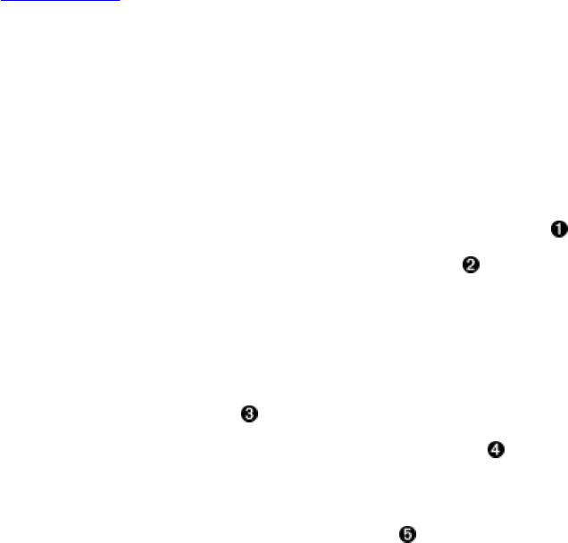
delete it.
Also note how the isTableAvailable() returns true, even when the table is disabled. In other
words, this method checks if the table is physically present, no matter what its state is. Use the
other two functions, isTableEnabled() and isTableDisabled(), to check for the state of the table.
After creating your tables with the specified schema, you must either delete the newly created
table and recreate it to change its details, or use the following method to alter its structure:
void modifyTable(final TableName tableName, final HTableDescriptor htd)
Pair<Integer, Integer> getAlterStatus(final TableName tableName)
Pair<Integer, Integer> getAlterStatus(final byte[] tableName)
The modifyTable() call is only asynchronous, and there is no synchronous variant. If you want to
make sure that changes have been propagated to all the servers and applied accordingly, you
should use the getAlterStatus() calls and loop in your client code until the schema has been
applied to all servers and regions. The call returns a pair of numbers, where their meaning is
summarized in the following table:
Table 5-6. Meaning of numbers returned by getAlterStatus() call
Pair Member Description
first Specifies the number of regions that still need to be updated.
second Total number of regions affected by the change.
As with the aforementioned deleteTable() commands, you must first disable the table to be able
to modify it. Example 5-13 creates a table, and subsequently modifies it. It also uses the
getAlterStatus() call to wait for all regions to be updated.
Example 5-13. Example modifying the structure of an existing table
Admin admin = connection.getAdmin();
TableName tableName = TableName.valueOf("testtable");
HColumnDescriptor coldef1 = new HColumnDescriptor("colfam1");
HTableDescriptor desc = new HTableDescriptor(tableName)
.addFamily(coldef1)
.setValue("Description", "Chapter 5 - ModifyTableExample: Original Table");
admin.createTable(desc, Bytes.toBytes(1L), Bytes.toBytes(10000L), 50);
HTableDescriptor htd1 = admin.getTableDescriptor(tableName);
HColumnDescriptor coldef2 = new HColumnDescriptor("colfam2");
htd1
.addFamily(coldef2)
.setMaxFileSize(1024 * 1024 * 1024L)
.setValue("Description",
"Chapter 5 - ModifyTableExample: Modified Table");
admin.disableTable(tableName);
admin.modifyTable(tableName, htd1);
Pair<Integer, Integer> status = new Pair<Integer, Integer>() {{
setFirst(50);
setSecond(50);
}};
for (int i = 0; status.getFirst() != 0 && i < 500; i++) {
status = admin.getAlterStatus(desc.getTableName());
(372)
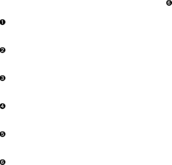
if (status.getSecond() != 0) {
int pending = status.getSecond() - status.getFirst();
System.out.println(pending + " of " + status.getSecond()
+ " regions updated.");
Thread.sleep(1 * 1000l);
} else {
System.out.println("All regions updated.");
break;
}
}
if (status.getFirst() != 0) {
throw new IOException("Failed to update regions after 500 seconds.");
}
admin.enableTable(tableName);
HTableDescriptor htd2 = admin.getTableDescriptor(tableName);
System.out.println("Equals: " + htd1.equals(htd2));
System.out.println("New schema: " + htd2);
Create the table with the original structure and 50 regions.
Get schema, update by adding a new family and changing the maximum file size property.
Disable and modify the table.
Create a status number pair to start the loop.
Loop over status until all regions are updated, or 500 seconds have been exceeded.
Check if the table schema matches the new one created locally.
The output shows that both the schema modified in the client code and the final schema retrieved
from the server after the modification are consistent:
50 of 50 regions updated.
Equals: true
New schema: 'testtable', {TABLE_ATTRIBUTES => {MAX_FILESIZE => '1073741824',
METADATA => {'Description' => 'Chapter 5 - ModifyTableExample:
Modified Table'}}, {NAME => 'colfam1', DATA_BLOCK_ENCODING => 'NONE',
BLOOMFILTER => 'ROW', REPLICATION_SCOPE => '0', VERSIONS => '1',
COMPRESSION => 'NONE', MIN_VERSIONS => '0', TTL => 'FOREVER',
KEEP_DELETED_CELLS => 'FALSE', BLOCKSIZE => '65536', IN_MEMORY =>
'false', BLOCKCACHE => 'true'}, {NAME => 'colfam2', DATA_BLOCK_ENCODING
=> 'NONE', BLOOMFILTER => 'ROW', REPLICATION_SCOPE => '0', COMPRESSION
=> 'NONE', VERSIONS => '1', TTL => 'FOREVER', MIN_VERSIONS => '0',
KEEP_DELETED_CELLS => 'FALSE', BLOCKSIZE => '65536', IN_MEMORY => 'false',
BLOCKCACHE => 'true'}
Calling the equals() method on the HTableDescriptor class compares the current with the specified
instance and returns true if they match in all properties, also including the contained column
families and their respective settings. It does not though compare custom settings, such as the
used Description key, modified from the original to the new value during the operation.
(373)

Schema Operations
Besides using the modifyTable() call, there are dedicated methods provided by the Admin class to
modify specific aspects of the current table schema. As usual, you need to make sure the table to
be modified is disabled first. The whole set of column-related methods is as follows:
void addColumn(final TableName tableName, final HColumnDescriptor column)
void deleteColumn(final TableName tableName, final byte[] columnName)
void modifyColumn(final TableName tableName,
final HColumnDescriptor descriptor)
You can add, delete, and modify column families. Adding or modifying a column family requires
that you first prepare a HColumnDescriptor instance, as described in detail in “Column Families”.
Alternatively, you could use the getTableDescriptor() call to retrieve the current table schema,
and subsequently invoke getColumnFamilies() on the returned HTableDescriptor instance to retrieve
the existing column family descriptors. Otherwise, you supply the table name, and optionally the
column name for the delete calls. All of these calls are asynchronous, so as mentioned before,
caveat emptor.
Use Case: Hush
An interesting use case for the administrative API is to create and alter tables and their schemas
based on an external configuration file. Hush makes use of this idea and defines the table and
column descriptors in an XML file, which is read and the contained schema compared with the
current table definitions. If there are any differences they are applied accordingly. The following
example has the core of the code that does this task:
Example 5-14. Creating or modifying table schemas using the HBase administrative API
private void createOrChangeTable(final HTableDescriptor schema)
throws IOException {
HTableDescriptor desc = null;
if (tableExists(schema.getTableName(), false)) {
desc = getTable(schema.getTableName(), false);
LOG.info("Checking table " + desc.getNameAsString() + "...");
final List<HColumnDescriptor> modCols =
new ArrayList<HColumnDescriptor>();
for (final HColumnDescriptor cd : desc.getFamilies()) {
final HColumnDescriptor cd2 = schema.getFamily(cd.getName());
if (cd2 != null && !cd.equals(cd2)) {
modCols.add(cd2);
}
}
final List<HColumnDescriptor> delCols =
new ArrayList<HColumnDescriptor>(desc.getFamilies());
delCols.removeAll(schema.getFamilies());
final List<HColumnDescriptor> addCols =
new ArrayList<HColumnDescriptor>(schema.getFamilies());
addCols.removeAll(desc.getFamilies());
if (modCols.size() > 0 || addCols.size() > 0 || delCols.size() > 0 ||
!hasSameProperties(desc, schema)) {
LOG.info("Disabling table...");
admin.disableTable(schema.getTableName());
if (modCols.size() > 0 || addCols.size() > 0 || delCols.size() > 0) {
for (final HColumnDescriptor col : modCols) {
LOG.info("Found different column -> " + col);
admin.modifyColumn(schema.getTableName(), col);
(374)
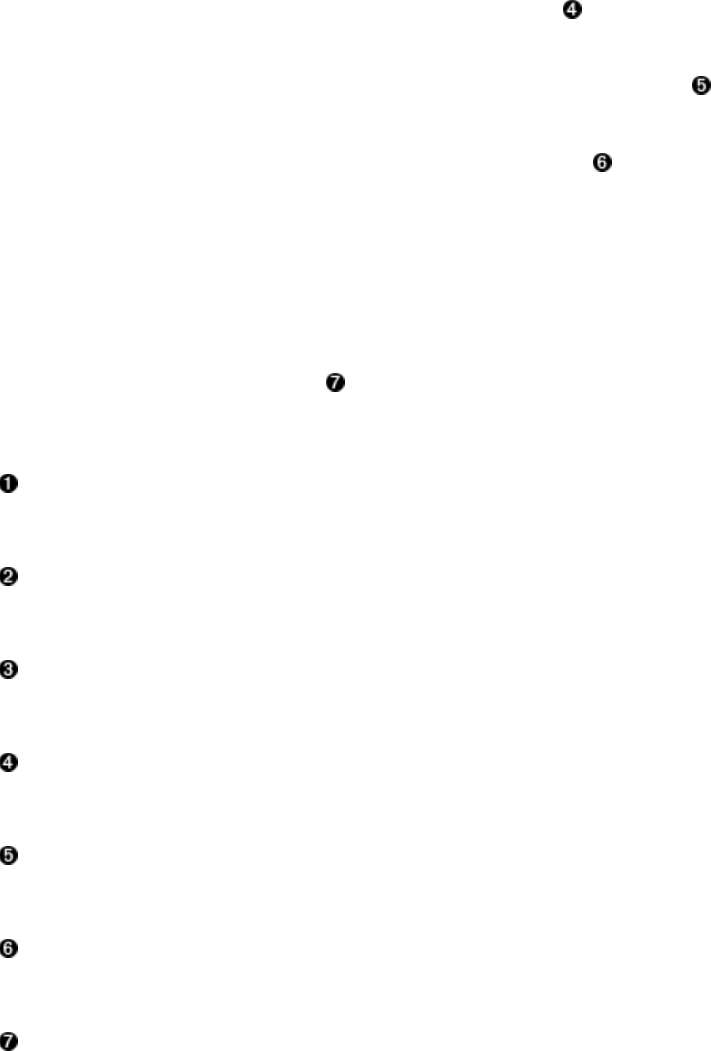
}
for (final HColumnDescriptor col : addCols) {
LOG.info("Found new column -> " + col);
admin.addColumn(schema.getTableName(), col);
}
for (final HColumnDescriptor col : delCols) {
LOG.info("Found removed column -> " + col);
admin.deleteColumn(schema.getTableName(), col.getName());
}
} else if (!hasSameProperties(desc, schema)) {
LOG.info("Found different table properties...");
admin.modifyTable(schema.getTableName(), schema);
}
LOG.info("Enabling table...");
admin.enableTable(schema.getTableName());
LOG.info("Table enabled");
getTable(schema.getTableName(), false);
LOG.info("Table changed");
} else {
LOG.info("No changes detected!");
}
} else {
LOG.info("Creating table " + schema.getNameAsString() + "...");
admin.createTable(schema);
LOG.info("Table created");
}
}
Compute the differences between the XML based schema and what is currently in HBase.
See if there are any differences in the column and table definitions.
Alter the columns that have changed. The table was properly disabled first.
Add newly defined columns.
Delete removed columns.
Alter the table itself, if there are any differences found.
In case the table did not exist yet create it now.
(375)

Cluster Operations
After the operations for the namespace, table, and column family schemas within a table, there
are a list of methods provided by the Admin implementation for operations on the regions and
tables themselves. They are more for use by HBase operators, as opposed to the schema
functions just described, which are more likely to be used by the application developer. The
cluster operations split into region, table, and server operations, and we will discuss them in that
order.
Region Operations
First are the region-related calls, that is, those concerned with the state of a region. [Link to
Come] has the details on regions and their life cycle. Also, recall the details about the server and
region name in “Server and Region Names”, as many of the calls below will need one or the
other.
Caution
Many of the following operations are for advanced users, so please handle with care.
List<HRegionInfo> getOnlineRegions(final ServerName sn)
Often you need to get a list of regions before operating on them, and one way to do that is
this method, which returns all regions hosted by a given server.
void closeRegion(final String regionname, final String serverName)
void closeRegion(final byte[] regionname, final String serverName)
boolean closeRegionWithEncodedRegionName(final String encodedRegionName, final String
serverName)
void closeRegion(final ServerName sn, final HRegionInfo hri)
Use these calls to close regions that have previously been deployed to region servers. Any
enabled table has all regions enabled, so you could actively close and undeploy one of
those regions.
You need to supply the exact regionname as stored in the system tables. Further, you may
optionally supply the serverName parameter, that overrides the server assignment as found
in the system tables as well. Some of the calls want the full name in text form, others the
hash only, while yet another is asking for objects encapsulating the details.
The last listed close call, the one that takes a ServerName, goes directly to the named region
rerver and asks it to close the region without notifying the master, that is, the region is
directly closed by the region server, unseen by the master node. It is a vestige from old
days used repairing damaged cluster state. You should have no need of this method.
void flush(final TableName tableName)
void flushRegion(final byte[] regionName)
As updates to a region (and the table in general) accumulate the MemStore instances of the
region servers fill with unflushed modifications. A client application can use these
synchronous methods to flush memory resident records to disk, before they are implicitly
(376)

written whenever they exceed the memstore flush size threshold (see “Table Properties”).
There is a method for flushing all regions of a given table, named flush(), and another to
flush a specific region, called flushRegion().
void compact(final TableName tableName)
void compact(final TableName tableName, final byte[] columnFamily)
void compactRegion(final byte[] regionName)
void compactRegion(final byte[] regionName, final byte[] columnFamily)
void compactRegionServer(final ServerName sn, boolean major)
As storage files accumulate the system compacts them in the background to keep the
number of files low. With these calls you can explicitly trigger the same operation for an
entire server, a table, or one specific region. When you specify a column family name, then
the operation is applied to that family only. Setting the major parameter to true promotes
the region server-wide compaction to a major one.
The call itself is asynchronous, as compactions can potentially take a long time to
complete. Invoking these methods queues the table(s), region(s), or column family for
compaction, which is executed in the background by the server hosting the named region,
or by all servers hosting any region of the given table (see “Auto-Sharding” for details on
compactions).
CompactionState getCompactionState(final TableName tableName)
CompactionState getCompactionStateForRegion(final byte[] regionName)
These are a continuation from the above, available to query the status of a running
compaction process. You either ask the status for an entire table, or a specific region.
void majorCompact(TableName tableName)
void majorCompact(TableName tableName, final byte[] columnFamily)
void majorCompactRegion(final byte[] regionName)
void majorCompactRegion(final byte[] regionName, final byte[] columnFamily)
These are the same as the compact() calls, but they queue the column family, region, or
table, for a major compaction instead. In case a table name is given, the administrative API
iterates over all regions of the table and invokes the compaction call implicitly for each of
them.
void split(final TableName tableName)
void split(final TableName tableName, final byte[] splitPoint)
void splitRegion(final byte[] regionName)
void splitRegion(final byte[] regionName, final byte[] splitPoint)
Using these calls allows you to split a specific region, or table. In case of the table-scoped
call, the system iterates over all regions of that table and implicitly invokes the split
command on each of them.
A noted exception to this rule is when the splitPoint parameter is given. In that case, the
split() command will try to split the given region at the provided row key. In the case of
using the table-scope call, all regions are checked and the one containing the splitPoint is
split at the given key.
The splitPoint must be a valid row key, and—in case you use the region specific method
—be part of the region to be split. It also must be greater than the region’s start key, since
splitting a region at its start key would make no sense. If you fail to give the correct row
key, the split request is ignored without reporting back to the client. The region server
(377)

currently hosting the region will log this locally with the following message:
2015-04-12 20:39:58,077 ERROR [PriorityRpcServer.handler=4,queue=0,port=62255]
regionserver.HRegion: Ignoring invalid split
org.apache.hadoop.hbase.regionserver.WrongRegionException: Requested row out
of range for calculated split on HRegion testtable,,1428863984023.
2d729d711208b37629baf70b5f17169c., startKey='', getEndKey()='ABC', row='ZZZ'
at org.apache.hadoop.hbase.regionserver.HRegion.checkRow(HRegion.java)
void mergeRegions(final byte[] encodedNameOfRegionA, final byte[] encodedNameOfRegionB, final
boolean forcible)
This method allows you to merge previously split regions. The operation usually requires
adjacent regions to be specified, but setting the forcible flag to true overrides this safety
latch.
void assign(final byte[] regionName)
void unassign(final byte[] regionName, final boolean force)
void offline(final byte[] regionName)
When a client requires a region to be deployed or undeployed from the region servers, it
can invoke these calls. The first would assign a region, based on the overall assignment
plan, while the second would unassign the given region, triggering a subsequent automatic
assignment. The third call allows you to offline a region, that is, leave it unassigned after
the call.
The force parameter set to true for unassign() means that a region already marked to be
unassigned—for example, from a previous call to unassign()--is forced to be unassigned
again. If force were set to false, this would have no effect.
void move(final byte[] encodedRegionName, final byte[] destServerName)
Using the move() call enables a client to actively control which server is hosting what
regions. You can move a region from its current region server to a new one. The
destServerName parameter can be set to null to pick a new server at random; otherwise, it
must be a valid server name, running a region server process. If the server name is wrong,
or currently not responding, the region is deployed to a different server instead. In a worst-
case scenario, the move could fail and leave the region unassigned.
The destServerName must comply with the rules explained in “Server and Region Names”,
that is, it must have a hostname, port, and timestamp component formatted properly with
comma delimiters.
boolean setBalancerRunning(final boolean on, final boolean synchronous)
boolean balancer()
boolean balancer(boolean force)
boolean isBalancerEnabled()
The first method allows you to switch the region balancer on or off. The synchronous flag
allows running the operation in said mode when set to true, or in asynchronous mode
when false is supplied.
When the balancer is enabled, a call to balancer() will start the process of moving regions
from those servers with excess regions, to those with fewer regions. “Load Balancing”
explains how this works in detail. The force flag allows to start another balancing process,
while some regions are still in the process of being moved from another, earlier balancer
run (which is otherwise prohibited).
(378)
The isBalancerEnabled() method allows an application to ask the master if the balancer is
currently enabled or not. true means it is, while false means that is not.
Example 5-15 assembles many of the above calls to showcase the administrative API and its
ability to modify the data layout within the cluster.
Example 5-15. Shows the use of the cluster operations
Connection connection = ConnectionFactory.createConnection(conf);
Admin admin = connection.getAdmin();
TableName tableName = TableName.valueOf("testtable");
HColumnDescriptor coldef1 = new HColumnDescriptor("colfam1");
HTableDescriptor desc = new HTableDescriptor(tableName)
.addFamily(coldef1)
.setValue("Description", "Chapter 5 - ClusterOperationExample");
byte[][] regions = new byte[][] { Bytes.toBytes("ABC"),
Bytes.toBytes("DEF"), Bytes.toBytes("GHI"), Bytes.toBytes("KLM"),
Bytes.toBytes("OPQ"), Bytes.toBytes("TUV")
};
admin.createTable(desc, regions);
BufferedMutator mutator = connection.getBufferedMutator(tableName);
for (int a = 'A'; a <= 'Z'; a++)
for (int b = 'A'; b <= 'Z'; b++)
for (int c = 'A'; c <= 'Z'; c++) {
String row = Character.toString((char) a) +
Character.toString((char) b) + Character.toString((char) c);
Put put = new Put(Bytes.toBytes(row));
put.addColumn(Bytes.toBytes("colfam1"), Bytes.toBytes("col1"),
Bytes.toBytes("val1"));
System.out.println("Adding row: " + row);
mutator.mutate(put);
}
mutator.close();
List<HRegionInfo> list = admin.getTableRegions(tableName);
int numRegions = list.size();
HRegionInfo info = list.get(numRegions - 1);
System.out.println("Number of regions: " + numRegions);
System.out.println("Regions: ");
printRegionInfo(list);
System.out.println("Splitting region: " + info.getRegionNameAsString());
admin.splitRegion(info.getRegionName());
do {
list = admin.getTableRegions(tableName);
Thread.sleep(1 * 1000L);
System.out.print(".");
} while (list.size() <= numRegions);
numRegions = list.size();
System.out.println();
System.out.println("Number of regions: " + numRegions);
System.out.println("Regions: ");
printRegionInfo(list);
System.out.println("Retrieving region with row ZZZ...");
RegionLocator locator = connection.getRegionLocator(tableName);
HRegionLocation location =
locator.getRegionLocation(Bytes.toBytes("ZZZ"));
System.out.println("Found cached region: " +
location.getRegionInfo().getRegionNameAsString());
location = locator.getRegionLocation(Bytes.toBytes("ZZZ"), true);
System.out.println("Found refreshed region: " +
location.getRegionInfo().getRegionNameAsString());
List<HRegionInfo> online =
admin.getOnlineRegions(location.getServerName());
online = filterTableRegions(online, tableName);
int numOnline = online.size();
System.out.println("Number of online regions: " + numOnline);
(379)
System.out.println("Online Regions: ");
printRegionInfo(online);
HRegionInfo offline = online.get(online.size() - 1);
System.out.println("Offlining region: " + offline.getRegionNameAsString());
admin.offline(offline.getRegionName());
int revs = 0;
do {
online = admin.getOnlineRegions(location.getServerName());
online = filterTableRegions(online, tableName);
Thread.sleep(1 * 1000L);
System.out.print(".");
revs++;
} while (online.size() <= numOnline && revs < 10);
numOnline = online.size();
System.out.println();
System.out.println("Number of online regions: " + numOnline);
System.out.println("Online Regions: ");
printRegionInfo(online);
HRegionInfo split = online.get(0);
System.out.println("Splitting region with wrong key: " +
split.getRegionNameAsString());
admin.splitRegion(split.getRegionName(),
Bytes.toBytes("ZZZ")); // triggers log message
System.out.println("Assigning region: " + offline.getRegionNameAsString());
admin.assign(offline.getRegionName());
revs = 0;
do {
online = admin.getOnlineRegions(location.getServerName());
online = filterTableRegions(online, tableName);
Thread.sleep(1 * 1000L);
System.out.print(".");
revs++;
} while (online.size() == numOnline && revs < 10);
numOnline = online.size();
System.out.println();
System.out.println("Number of online regions: " + numOnline);
System.out.println("Online Regions: ");
printRegionInfo(online);
System.out.println("Merging regions...");
HRegionInfo m1 = online.get(0);
HRegionInfo m2 = online.get(1);
System.out.println("Regions: " + m1 + " with " + m2);
admin.mergeRegions(m1.getEncodedNameAsBytes(),
m2.getEncodedNameAsBytes(), false);
revs = 0;
do {
list = admin.getTableRegions(tableName);
Thread.sleep(1 * 1000L);
System.out.print(".");
revs++;
} while (list.size() >= numRegions && revs < 10);
numRegions = list.size();
System.out.println();
System.out.println("Number of regions: " + numRegions);
System.out.println("Regions: ");
printRegionInfo(list);
Create a table with seven regions, and one column family.
Insert many rows starting from “AAA” to “ZZZ”. These will be spread across the regions.
List details about the regions.
(380)

Split the last region this table has, starting at row key “TUV”. Adds a new region starting
with key “WEI”.
Loop and check until the operation has taken effect.
Retrieve region infos cached and refreshed to show the difference.
Offline a region and print the list of all regions.
Attempt to split a region with a split key that does not fall into boundaries. Triggers log
message.
Reassign the offlined region.
Merge the first two regions. Print out result of operation.
Table Operations: Snapshots
The second set of cluster operations revolve around the actual tables. These are low-level tasks
that can be invoked from the administrative API and are applied to the entire given table. The
primary purpose is to archive the current state of a table, referred to as snapshots. Here are the
admin API methods to create a snapshot for a table:
void snapshot(final String snapshotName, final TableName tableName)
void snapshot(final byte[] snapshotName, final TableName tableName)
void snapshot(final String snapshotName, final TableName tableName,
Type type)
void snapshot(SnapshotDescription snapshot)
SnapshotResponse takeSnapshotAsync(SnapshotDescription snapshot)
boolean isSnapshotFinished(final SnapshotDescription snapshot)
You need to supply a unique name for each snapshot, following the same rules as enforced for
table names. This is because snapshots are stored in the underlying file system in the same way
as tables are, though in a particular snapshots location (see [Link to Come] for details). For
example, you could make use of the TableName.isLegalTableQualifierName() method to verify if a
given snapshot name matches the naming requirements. In addition, you have to name the table
you want to perform the snapshots on.
Besides these basic snapshot calls that take a name and table, there are a few other more involved
calls. The third call in the list above allows you hand in an extra parameter, type. It specifies the
type of snapshot you want to create, with the these choices available:
Table 5-7. Choices available for snapshot types
(381)
Type Table
State Description
FLUSH Enabled This is the default and is used to force a flush operation on online tables
before the snapshot is taken.
SKIPFLUSH Enabled If you do not want to cause a flush to occur, you can use this option to
immediately snapshot all persisted files of a table.
DISABLED Disabled This option is not for normal use, but might be returned if a snapshot was
created on a disabled table.
The same enumeration is used for the objects returned by the listSnapshot() call, noted below,
which explains why the DISABLED value is a possible snapshot type: it is what is returned if you
snapshot a disabled table.
Once you have created one or more snapshot, you are able to retrieve a list of the available
snapshots using the following methods:
List<SnapshotDescription> listSnapshots()
List<SnapshotDescription> listSnapshots(String regex)
List<SnapshotDescription> listSnapshots(Pattern pattern)
The first call lists all snapshots stored, while the other two filter the list based on a regular
expression pattern. The output looks similar to this, but of course depends on your cluster and
what has been snapshotted so far:
[name: "snapshot1"
table: "testtable"
creation_time: 1428924867254
type: FLUSH
version: 2
, name: "snapshot2"
table: "testtable"
creation_time: 1428924870596
type: DISABLED
version: 2]
Highlighted are the discussed types of each snapshot. The listSnapshots() calls return a list of
SnapshotDescription instances, which give access to the snapshot details. There are the obvious
getName() and getTable() methods to return the snapshot and table name. In addition, you can use
getType() to get access to the highlighted snapshot type, and getCreationTime() to retrieve the
timestamp when the snapshot was created. Lastly, there is getVersion() returning the internal
format version of the snapshot. This number is used to read older snapshots with newer versions
of HBase, so expect this number to increase over time with each new major version of HBase.
The description class has a few more getters for snapshot details, such as the amount of storage it
consumes, and convenience methods to retrieve the described information in other formats.
When it is time to restore a previously taken snapshot, you need to call one of these methods:
void restoreSnapshot(final byte[] snapshotName)
void restoreSnapshot(final String snapshotName)
void restoreSnapshot(final byte[] snapshotName,
final boolean takeFailSafeSnapshot)
(382)

void restoreSnapshot(final String snapshotName,
boolean takeFailSafeSnapshot)
Analogous, you specify a snapshot name, and the table is recreated with the data contained in the
snapshot. Before you can run a restore operation on a table though, you need to disable it first.
The restore operation is essentially a drop operation, followed by a recreation of the table with
the archived data. You need to provide the table name either as a string, or as a byte array. Of
course, the snapshot has to exist, or else you will receive an error.
The optional takeFailSafeSnapshot flag, set to true, will instruct the servers to first perform a
snapshot of the specified table, before restoring the snapshot. Should the restore operation fail,
the failsafe snapshot is restored instead. On the other hand, if the restore operation completes
successfully, then the failsafe snapshot is removed at the end of the operation. The name of the
failsafe snapshot is specified using the hbase.snapshot.restore.failsafe.name configuration
property, and defaults to hbase-failsafe-{snapshot.name}-{restore.timestamp}. The possible
variables you can use in the name are:
Variable Description
{snapshot.name} The name of the snapshot.
{table.name} The name of the table the snapshot represents.
{restore.timestamp} The timestamp when the snapshot is taken.
The default value for the failsafe name ensures that the snapshot is uniquely named, by adding
the name of the snapshot that triggered its creation, plus a timestamp. There should be no need to
modify this to something else, but if you want to you can using the above pattern and
configuration property.
You can also clone a snapshot, which means you are recreating the table under a new name:
void cloneSnapshot(final byte[] snapshotName, final TableName tableName)
void cloneSnapshot(final String snapshotName, final TableName tableName)
Again, you specify the snapshot name in one or another form, but also supply a new table name.
The snapshot is restored in the newly named table, like a restore would do for the original table.
Finally, removing a snapshot is accomplished using these calls:
void deleteSnapshot(final byte[] snapshotName)
void deleteSnapshot(final String snapshotName)
void deleteSnapshots(final String regex)
void deleteSnapshots(final Pattern pattern)
As with with the delete calls for tables, you can either specify an exact snapshot by name, or you
can apply a regular expression to remove more than one in a single call. Just as before, be very
careful what you hand in, there is no coming back from this operation (as in, there is no undo)!
Example 5-16 runs these commands across a single original table, that contains a single row
only, named "row1":
(383)
Example 5-16. Example showing the use of the admin snapshot API
admin.snapshot("snapshot1", tableName);
List<HBaseProtos.SnapshotDescription> snaps = admin.listSnapshots();
System.out.println("Snapshots after snapshot 1: " + snaps);
Delete delete = new Delete(Bytes.toBytes("row1"));
delete.addColumn(Bytes.toBytes("colfam1"), Bytes.toBytes("qual1"));
table.delete(delete);
admin.snapshot("snapshot2", tableName,
HBaseProtos.SnapshotDescription.Type.SKIPFLUSH);
admin.snapshot("snapshot3", tableName,
HBaseProtos.SnapshotDescription.Type.FLUSH);
snaps = admin.listSnapshots();
System.out.println("Snapshots after snapshot 2 & 3: " + snaps);
Put put = new Put(Bytes.toBytes("row2"))
.addColumn(Bytes.toBytes("colfam1"), Bytes.toBytes("qual10"),
Bytes.toBytes("val10"));
table.put(put);
HBaseProtos.SnapshotDescription snapshotDescription =
HBaseProtos.SnapshotDescription.newBuilder()
.setName("snapshot4")
.setTable(tableName.getNameAsString())
.build();
admin.takeSnapshotAsync(snapshotDescription);
snaps = admin.listSnapshots();
System.out.println("Snapshots before waiting: " + snaps);
System.out.println("Waiting...");
while (!admin.isSnapshotFinished(snapshotDescription)) {
Thread.sleep(1 * 1000);
System.out.print(".");
}
System.out.println();
System.out.println("Snapshot completed.");
snaps = admin.listSnapshots();
System.out.println("Snapshots after waiting: " + snaps);
System.out.println("Table before restoring snapshot 1");
helper.dump("testtable", new String[]{"row1", "row2"}, null, null);
admin.disableTable(tableName);
admin.restoreSnapshot("snapshot1");
admin.enableTable(tableName);
System.out.println("Table after restoring snapshot 1");
helper.dump("testtable", new String[]{"row1", "row2"}, null, null);
admin.deleteSnapshot("snapshot1");
snaps = admin.listSnapshots();
System.out.println("Snapshots after deletion: " + snaps);
admin.cloneSnapshot("snapshot2", TableName.valueOf("testtable2"));
System.out.println("New table after cloning snapshot 2");
helper.dump("testtable2", new String[]{"row1", "row2"}, null, null);
admin.cloneSnapshot("snapshot3", TableName.valueOf("testtable3"));
System.out.println("New table after cloning snapshot 3");
helper.dump("testtable3", new String[]{"row1", "row2"}, null, null);
Create a snapshot of the initial table, then list all available snapshots next.
(384)

Remove one column and do two more snapshots, one without first flushing, then another
with a preceding flush.
Add a new row to the table and take yet another snapshot.
Wait for the asynchronous snapshot to complete. List the snapshots before and after the
waiting.
Restore the first snapshot, recreating the initial table. This needs to be done on a disabled
table.
Remove the first snapshot, and list the available ones again.
Clone the second and third snapshot into a new table, dump the content to show the
difference between the “skipflush” and “flush” types.
The output (albeit a bit lengthy) reveals interesting things, please keep an eye out for snapshot
number #2 and #3:
Before snapshot calls...
Cell: row1/colfam1:qual1/2/Put/vlen=4/seqid=0, Value: val1
Cell: row1/colfam1:qual1/1/Put/vlen=4/seqid=0, Value: val1
...
Cell: row1/colfam2:qual3/6/Put/vlen=4/seqid=0, Value: val3
Cell: row1/colfam2:qual3/5/Put/vlen=4/seqid=0, Value: val3
Snapshots after snapshot 1: [name: "snapshot1"
table: "testtable"
creation_time: 1428918198629
type: FLUSH
version: 2
]
Snapshots after snapshot 2 & 3: [name: "snapshot1"
table: "testtable"
creation_time: 1428918198629
type: FLUSH
version: 2
, name: "snapshot2"
table: "testtable"
creation_time: 1428918200818
type: SKIPFLUSH
version: 2
, name: "snapshot3"
table: "testtable"
creation_time: 1428918200931
type: FLUSH
version: 2
]
Snapshots before waiting: [name: "snapshot1"
table: "testtable"
creation_time: 1428918198629
type: FLUSH
version: 2
, name: "snapshot2"
table: "testtable"
(385)
creation_time: 1428918200818
type: SKIPFLUSH
version: 2
, name: "snapshot3"
table: "testtable"
creation_time: 1428918200931
type: FLUSH
version: 2
]
Waiting...
.
Snapshot completed.
Snapshots after waiting: [name: "snapshot1"
table: "testtable"
creation_time: 1428918198629
type: FLUSH
version: 2
, name: "snapshot2"
table: "testtable"
creation_time: 1428918200818
type: SKIPFLUSH
version: 2
, name: "snapshot3"
table: "testtable"
creation_time: 1428918200931
type: FLUSH
version: 2
, name: "snapshot4"
table: "testtable"
creation_time: 1428918201570
version: 2
]
Table before restoring snapshot 1
Cell: row1/colfam1:qual1/1/Put/vlen=4/seqid=0, Value: val1
Cell: row1/colfam1:qual2/4/Put/vlen=4/seqid=0, Value: val2
...
Cell: row1/colfam2:qual3/5/Put/vlen=4/seqid=0, Value: val3
Cell: row2/colfam1:qual10/1428918201565/Put/vlen=5/seqid=0, Value: val10
Table after restoring snapshot 1
Cell: row1/colfam1:qual1/2/Put/vlen=4/seqid=0, Value: val1
Cell: row1/colfam1:qual1/1/Put/vlen=4/seqid=0, Value: val1
...
Cell: row1/colfam2:qual3/6/Put/vlen=4/seqid=0, Value: val3
Cell: row1/colfam2:qual3/5/Put/vlen=4/seqid=0, Value: val3
Snapshots after deletion: [name: "snapshot2"
table: "testtable"
creation_time: 1428918200818
type: SKIPFLUSH
version: 2
, name: "snapshot3"
table: "testtable"
creation_time: 1428918200931
type: FLUSH
version: 2
, name: "snapshot4"
table: "testtable"
creation_time: 1428918201570
version: 2
]
New table after cloning snapshot 2
Cell: row1/colfam1:qual1/2/Put/vlen=4/seqid=0, Value: val1
Cell: row1/colfam1:qual1/1/Put/vlen=4/seqid=0, Value: val1
Cell: row1/colfam1:qual2/4/Put/vlen=4/seqid=0, Value: val2
...
Cell: row1/colfam2:qual3/6/Put/vlen=4/seqid=0, Value: val3
Cell: row1/colfam2:qual3/5/Put/vlen=4/seqid=0, Value: val3
New table after cloning snapshot 3
Cell: row1/colfam1:qual1/1/Put/vlen=4/seqid=0, Value: val1
Cell: row1/colfam1:qual2/4/Put/vlen=4/seqid=0, Value: val2
Cell: row1/colfam1:qual2/3/Put/vlen=4/seqid=0, Value: val2
...
(386)

Cell: row1/colfam2:qual3/6/Put/vlen=4/seqid=0, Value: val3
Cell: row1/colfam2:qual3/5/Put/vlen=4/seqid=0, Value: val3
Since we performed snapshot #2 while skipping flushes, we do not see the preceding delete being
applied: the delete has been applied to the WAL and memstore, but not the store files yet.
Snapshot #3 does the same snapshot, but forces the flush to occur beforehand. The output in
testtable2 and testtable3 confirm that the former still contains the deleted data, and the latter
does not.
Some parting notes on snapshots:
You can only have one snapshot or restore in progress per table. In other words, if you
have two separate tables, you can snapshot them at the same time, but you cannot run two
concurrent snapshots on the same table—or run a snapshot while a restore is in progress.
The second operation would fail with an error message (for example: "Rejected taking
<snapshotname> because we are already running another snapshot...").
You can increase the snapshot concurrency from the default of 1 by setting a higher value
with the hbase.snapshot.master.threads configuration property. The default means only one
snapshot operation runs at any given time in the entire cluster. Subsequent operations
would be queued and executed sequentially.
Turning off snapshot support for the entire cluster is handled by hbase.snapshot.enabled. It
is set to true, that is, snapshot support is enabled on a cluster installed with default values.
Server Operations
The third group of methods provided by the Admin interface address the entire cluster. They are
either generic calls, or very low-level operations, so please again, be very careful when using the
methods listed below.
ClusterStatus getClusterStatus()
The getClusterStatus() call allows you to retrieve an instance of the ClusterStatus class,
containing detailed information about the cluster. See “Cluster Status Information” for
what you are provided with.
Configuration getConfiguration()
void updateConfiguration(ServerName server)
void updateConfiguration()
These calls allow the application to access the current configuration, and to reload that
configuration from disk. The latter is done for either all servers, when no parameter is
specified, or one given server only. You need to provide a server name, formatted as
discussed earlier in this chapter. Not all configuration properties are supported as
reloadable during the runtime of a server. See [Link to Come] for a list of those that can be
reloaded.
Using the getConfiguration() method gives access to the client configuration instance.
Since HBase is a distributed system it is very likely that the client-side settings are not the
same as the server-side ones. And using any of the set() methods on the returned
Configuration instance is just modifying the client-side settings. If you want to update the
servers, you need to deploy an updated hbase-site.xml to the servers and invoke the
(387)

updateConfiguration() call noted above.
int getMasterInfoPort()
Returns the current web-UI port of the HBase Master. This value is set with the
hbase.master.info.port property, but might be dynamically reassigned when the server
starts.
int getOperationTimeout()
Returns the value set with the hbase.client.operation.timeout property. It defines how long
the client should wait for the servers to respond, and defaults to Integer.MAX_VALUE, that is,
indefinitely.
void rollWALWriter(ServerName serverName)
Instructs the named server to close the current WAL file and create a new one.
boolean enableCatalogJanitor(boolean enable)
int runCatalogScan()
boolean isCatalogJanitorEnabled()
The HBase Master process runs a background housekeeping task, the catalog janitor,
which is responsible for cleaning up region operation remnants. For example, when a
region splits or is merged, the janitor will clean up the left-over region details, including
meta data and physical files. By default, the task runs on every standard cluster. You can
use these calls to stop the task running, invoke a run manually with runCatalogScan(), and
check the status of the task.
String[] getMasterCoprocessors()
CoprocessorRpcChannel coprocessorService()
CoprocessorRpcChannel coprocessorService(ServerName sn)
Provides access to the list of coprocessors loaded into the master process, and the RPC
channel (which is derived from a Protobuf superclass) for the active master, when no
parameter is provided, or for the given region server when one is supplied. See
“Coprocessors”, and especially “The Service Interface”, on how to make use of the RPC
endpoint.
void execProcedure(String signature, String instance, Map<String, String> props)
byte[] execProcedureWithRet(String signature, String instance, Map<String, String> props)
boolean isProcedureFinished(String signature, String instance, Map<String, String> props)
HBase has a server-side procedure framework, which is used by, for example, the master
to distribute an operation across many or all region servers. If a flush is triggered, the
procedure representing the flush operation is started on the cluster. There are calls to do
this as a one-off call, or with a built-in retry mechanism. The latter call allows to retrieve
the status of a procedure that was started beforehand.
void shutdown()
void stopMaster()
void stopRegionServer(final String hostnamePort)
These calls either shut down the entire cluster, stop the master server, or stop a particular
region server only. Once invoked, the affected servers will be stopped, that is, there is no
delay nor a way to revert the process.
Chapters [Link to Come] and Chapter 10 have more information on these advanced—yet very
(388)
powerful—features. Use with utmost care!
(389)

Cluster Status Information
When you query the cluster status using the Admin.getClusterStatus() call, you will be given a
ClusterStatus instance, containing all the information the master server has about the current
state of the cluster. Table 5-8 lists the methods of the ClusterStatus class.
Table 5-8. Overview of the information provided by the ClusterStatus class
Method Description
getAverageLoad() The total average number of regions per region server. This is
computed as number of regions/number of servers.
getBackupMasters() Returns the list of all known backup HBase Master servers.
getBackupMastersSize() The size of the list of all known backup masters.
getBalancerOn() Provides access to the internal Boolean instance, reflecting the balancer
tasks status. Might be null.
getClusterId()
Returns the unique identifier for the cluster. This is a UUID generated
when HBase starts with an empty storage directory. It is stored in
hbase.id under the HBase root directory.
getDeadServerNames()
A list of all server names currently considered dead. The names in the
collection are ServerName instances, which contain the hostname, RPC
port, and start code.
getDeadServers() The number of servers listed as dead. This does not contain the live
servers.
getHBaseVersion() Returns the HBase version identification string.
getLoad(ServerName sn) Retrieves the status information available for the given server name.
getMaster() The server name of the current master.
getMasterCoprocessors() A list of all loaded master coprocessors.
(390)

getRegionsCount() The total number of regions in the cluster.
getRegionsInTransition()
Gives you access to a map of all regions currently in transition, e.g.,
being moved, assigned, or unassigned. The key of the map is the
encoded region name (as returned by HRegionInfo.getEncodedName(), for
example), while the value is an instance of RegionState.a
getRequestsCount() The current number of requests across all region servers in the cluster.
getServers() The list of live servers. The names in the collection are ServerName
instances, which contain the hostname, RPC port, and start code.
getServersSize() The number of region servers currently live as known to the master
server. The number does not include the number of dead servers.
getVersion() Returns the format version of the ClusterStatus instance. This is used
during the serialization process of sending an instance over RPC.
isBalancerOn() Returns true if the balancer task is enabled on the master.
toString() Converts the entire cluster status details into a string.
a See [Link to Come] for the details.
Accessing the overall cluster status gives you a high-level view of what is going on with your
servers—as a whole. Using the getServers() array, and the returned ServerName instances, lets you
drill further into each actual live server, and see what it is doing currently. See “Server and
Region Names” again for details on the ServerName class.
Each server, in turn, exposes details about its load, by offering a ServerLoad instance, returned by
the getLoad() method of the ClusterStatus instance. Using the aforementioned ServerName, as
returned by the getServers() call, you can iterate over all live servers and retrieve their current
details. The ServerLoad class gives you access to not just the load of the server itself, but also for
each hosted region. Table 5-9 lists the provided methods.
Table 5-9. Overview of the information provided by the ServerLoad class
Method Description
getCurrentCompactedKVs() The number of cells that have been compacted, while
compactions are running.
(391)

getInfoServerPort() The web-UI port of the region server.
getLoad() Currently returns the same value as getNumberOfRegions().
getMaxHeapMB() The configured maximum Java Runtime heap size in megabytes.
getMemStoreSizeInMB() The total size of the in-memory stores, across all regions hosted
by this server.
getNumberOfRegions() The number of regions on the current server.
getNumberOfRequests() Returns the accumulated number of requests, and counts all API
requests, such as gets, puts, increments, deletes, and so on.a
getReadRequestsCount() The sum of all read requests for all regions of this server.a
getRegionServerCoprocessors() The list of loaded coprocessors, provided as a string array,
listing the class names.
getRegionsLoad()
Returns a map containing the load details for each hosted region
of the current server. The key is the region name and the value
an instance of the RegionsLoad class, discussed next.
getReplicationLoadSink() If replication is enabled, this call returns an object with
replication statistics.
getReplicationLoadSourceList() If replication is enabled, this call returns a list of objects with
replication statistics.
getRequestsPerSecond() Provides the computed requests per second value, accumulated
for the entire server.
getRootIndexSizeKB() The summed up size of all root indexes, for every storage file,
the server holds in memory.
getRsCoprocessors()
The list of coprocessors in the order they were loaded. Should be
equal to getRegionServerCoprocessors().
(392)

getStorefileIndexSizeInMB() The total size in megabytes of the indexes—the block and meta
index, to be precise—across all store files in use by this server.
getStorefiles() The number of store files in use by the server. This is across all
regions it hosts.
getStorefileSizeInMB() The total size in megabytes of the used store files.
getStores() The total number of stores held by this server. This is similar to
the number of all column families across all regions.
getStoreUncompressedSizeMB() The raw size of the data across all stores in megabytes.
getTotalCompactingKVs() The total number of cells currently compacted across all stores.
getTotalNumberOfRequests() Returns the total number of all requests received by this server.a
getTotalStaticBloomSizeKB() Specifies the combined size occupied by all Bloom filters in
kilobytes.
getTotalStaticIndexSizeKB() Specifies the combined size occupied by all indexes in kilobytes.
getUsedHeapMB() The currently used Java Runtime heap size in megabytes, if
available.
getWriteRequestsCount() The sum of all read requests for all regions of this server.a
hasMaxHeapMB() Check if the value with same name is available during the
accompanying getXYZ() call.
hasNumberOfRequests()
Check if the value with same name is available during the
accompanying getXYZ() call.
hasTotalNumberOfRequests() Check if the value with same name is available during the
accompanying getXYZ() call.
(393)

hasUsedHeapMB() Check if the value with same name is available during the
accompanying getXYZ() call.
obtainServerLoadPB() Returns the low-level Protobuf version of the current server load
instance.
toString() Converts the state of the instance with all above metrics into a
string for logging etc.
a Accumulated within the last hbase.regionserver.metrics.period, defaulting to 5 seconds. The
counter is reset at the end of this time frame.
Finally, there is a dedicated class for the region load, aptly named RegionLoad. See Table 5-10 for
the list of provided information.
Table 5-10. Overview of the information provided by the RegionLoad class
Method Description
getCompleteSequenceId() Returns the last completed sequence ID for the region, used in
conjunction with the MVCC.
getCurrentCompactedKVs() The currently compacted cells for this region, while a compaction
is running.
getDataLocality() A ratio from 0 to 1 (0% to 100%) expressing the locality of store
files to the region server process.
getMemStoreSizeMB() The heap size in megabytes as used by the MemStore of the current
region.
getName() The region name in its raw, byte[] byte array form.
getNameAsString() Converts the raw region name into a String for convenience.
getReadRequestsCount() The number of read requests for this region, since it was deployed
to the region server. This counter is not reset.
getRequestsCount() The number of requests for the current region.
(394)

getRootIndexSizeKB() The sum of all root index details help in memory for this region, in
kilobytes.
getStorefileIndexSizeMB() The size of the indexes for all store files, in megabytes, for this
region.
getStorefiles() The number of store files, across all stores of this region.
getStorefileSizeMB() The size in megabytes of the store files for this region.
getStores() The number of stores in this region.
getStoreUncompressedSizeMB() The size of all stores in megabyte, before compression.
getTotalCompactingKVs() The count of all cells being compacted within this region.
getTotalStaticBloomSizeKB() The size of all Bloom filter data in kilobytes.
getTotalStaticIndexSizeKB() The size of all index data in kilobytes.
getWriteRequestsCount() The number of write requests for this region, since it was deployed
to the region server. This counter is not reset.
toString() Converts the state of the instance with all above metrics into a
string for logging etc.
Example 5-17 shows all of the getters in action.
Example 5-17. Example reporting the status of a cluster
ClusterStatus status = admin.getClusterStatus();
System.out.println("Cluster Status:\n--------------");
System.out.println("HBase Version: " + status.getHBaseVersion());
System.out.println("Version: " + status.getVersion());
System.out.println("Cluster ID: " + status.getClusterId());
System.out.println("Master: " + status.getMaster());
System.out.println("No. Backup Masters: " +
status.getBackupMastersSize());
System.out.println("Backup Masters: " + status.getBackupMasters());
System.out.println("No. Live Servers: " + status.getServersSize());
(395)

System.out.println("Servers: " + status.getServers());
System.out.println("No. Dead Servers: " + status.getDeadServers());
System.out.println("Dead Servers: " + status.getDeadServerNames());
System.out.println("No. Regions: " + status.getRegionsCount());
System.out.println("Regions in Transition: " +
status.getRegionsInTransition());
System.out.println("No. Requests: " + status.getRequestsCount());
System.out.println("Avg Load: " + status.getAverageLoad());
System.out.println("Balancer On: " + status.getBalancerOn());
System.out.println("Is Balancer On: " + status.isBalancerOn());
System.out.println("Master Coprocessors: " +
Arrays.asList(status.getMasterCoprocessors()));
System.out.println("\nServer Info:\n--------------");
for (ServerName server : status.getServers()) {
System.out.println("Hostname: " + server.getHostname());
System.out.println("Host and Port: " + server.getHostAndPort());
System.out.println("Server Name: " + server.getServerName());
System.out.println("RPC Port: " + server.getPort());
System.out.println("Start Code: " + server.getStartcode());
ServerLoad load = status.getLoad(server);
System.out.println("\nServer Load:\n--------------");
System.out.println("Info Port: " + load.getInfoServerPort());
System.out.println("Load: " + load.getLoad());
System.out.println("Max Heap (MB): " + load.getMaxHeapMB());
System.out.println("Used Heap (MB): " + load.getUsedHeapMB());
System.out.println("Memstore Size (MB): " +
load.getMemstoreSizeInMB());
System.out.println("No. Regions: " + load.getNumberOfRegions());
System.out.println("No. Requests: " + load.getNumberOfRequests());
System.out.println("Total No. Requests: " +
load.getTotalNumberOfRequests());
System.out.println("No. Requests per Sec: " +
load.getRequestsPerSecond());
System.out.println("No. Read Requests: " +
load.getReadRequestsCount());
System.out.println("No. Write Requests: " +
load.getWriteRequestsCount());
System.out.println("No. Stores: " + load.getStores());
System.out.println("Store Size Uncompressed (MB): " +
load.getStoreUncompressedSizeMB());
System.out.println("No. Storefiles: " + load.getStorefiles());
System.out.println("Storefile Size (MB): " +
load.getStorefileSizeInMB());
System.out.println("Storefile Index Size (MB): " +
load.getStorefileIndexSizeInMB());
System.out.println("Root Index Size: " + load.getRootIndexSizeKB());
System.out.println("Total Bloom Size: " +
load.getTotalStaticBloomSizeKB());
System.out.println("Total Index Size: " +
load.getTotalStaticIndexSizeKB());
System.out.println("Current Compacted Cells: " +
load.getCurrentCompactedKVs());
System.out.println("Total Compacting Cells: " +
load.getTotalCompactingKVs());
System.out.println("Coprocessors1: " +
Arrays.asList(load.getRegionServerCoprocessors()));
System.out.println("Coprocessors2: " +
Arrays.asList(load.getRsCoprocessors()));
System.out.println("Replication Load Sink: " +
load.getReplicationLoadSink());
System.out.println("Replication Load Source: " +
load.getReplicationLoadSourceList());
System.out.println("\nRegion Load:\n--------------");
for (Map.Entry<byte[], RegionLoad> entry :
load.getRegionsLoad().entrySet()) {
System.out.println("Region: " + Bytes.toStringBinary(entry.getKey()));
RegionLoad regionLoad = entry.getValue();
System.out.println("Name: " + Bytes.toStringBinary(
regionLoad.getName()));
System.out.println("Name (as String): " +
(396)

regionLoad.getNameAsString());
System.out.println("No. Requests: " + regionLoad.getRequestsCount());
System.out.println("No. Read Requests: " +
regionLoad.getReadRequestsCount());
System.out.println("No. Write Requests: " +
regionLoad.getWriteRequestsCount());
System.out.println("No. Stores: " + regionLoad.getStores());
System.out.println("No. Storefiles: " + regionLoad.getStorefiles());
System.out.println("Data Locality: " + regionLoad.getDataLocality());
System.out.println("Storefile Size (MB): " +
regionLoad.getStorefileSizeMB());
System.out.println("Storefile Index Size (MB): " +
regionLoad.getStorefileIndexSizeMB());
System.out.println("Memstore Size (MB): " +
regionLoad.getMemStoreSizeMB());
System.out.println("Root Index Size: " +
regionLoad.getRootIndexSizeKB());
System.out.println("Total Bloom Size: " +
regionLoad.getTotalStaticBloomSizeKB());
System.out.println("Total Index Size: " +
regionLoad.getTotalStaticIndexSizeKB());
System.out.println("Current Compacted Cells: " +
regionLoad.getCurrentCompactedKVs());
System.out.println("Total Compacting Cells: " +
regionLoad.getTotalCompactingKVs());
System.out.println();
}
}
Get the cluster status.
Iterate over the included server instances.
Retrieve the load details for the current server.
Iterate over the region details of the current server.
Get the load details for the current region.
On a standalone setup, and running the Performance Evalutation tool (see “Performance
Evaluation”) in parallel, you should see something like this:
Cluster Status:
--------------
HBase Version: 1.0.0
Version: 2
Cluster ID: 25ba54eb-09da-4698-88b5-5acdfecf0005
Master: srv1.foobar.com,63911,1428996031794
No. Backup Masters: 0
Backup Masters: []
No. Live Servers: 1
Servers: [srv1.foobar.com,63915,1428996033410]
No. Dead Servers: 2
Dead Servers: [srv1.foobar.com,62938,1428669753889, \
srv1.foobar.com,60813,1428991052036]
No. Regions: 7
Regions in Transition: {}
No. Requests: 56047
Avg Load: 7.0
(397)

Balancer On: true
Is Balancer On: true
Master Coprocessors: [MasterObserverExample]
Server Info:
--------------
Hostname: srv1.foobar.com
Host and Port: srv1.foobar.com:63915
Server Name: srv1.foobar.com,63915,1428996033410
RPC Port: 63915
Start Code: 1428996033410
Server Load:
--------------
Info Port: 63919
Load: 7
Max Heap (MB): 12179
Used Heap (MB): 1819
Memstore Size (MB): 651
No. Regions: 7
No. Requests: 56047
Total No. Requests: 14334506
No. Requests per Sec: 56047.0
No. Read Requests: 2325
No. Write Requests: 1239824
No. Stores: 7
Store Size Uncompressed (MB): 491
No. Storefiles: 7
Storefile Size (MB): 492
Storefile Index Size (MB): 0
Root Index Size: 645
Total Bloom Size: 644
Total Index Size: 389
Current Compacted Cells: 51
Total Compacting Cells: 51
Coprocessors1: []
Coprocessors2: []
Replication Load Sink: \
org.apache.hadoop.hbase.replication.ReplicationLoadSink@582a4aa3
Replication Load Source: []
Region Load:
--------------
Region: TestTable,,1429009449882.3696e9469bb5a83bd9d7d67f7db65843.
Name: TestTable,,1429009449882.3696e9469bb5a83bd9d7d67f7db65843.
Name (as String): TestTable,,1429009449882.3696e9469bb5a83bd9d7d67f7db65843.
No. Requests: 248324
No. Read Requests: 0
No. Write Requests: 248324
No. Stores: 1
No. Storefiles: 1
Data Locality: 1.0
Storefile Size (MB): 89
Storefile Index Size (MB): 0
Memstore Size (MB): 151
Root Index Size: 116
Total Bloom Size: 128
Total Index Size: 70
Current Compacted Cells: 0
Total Compacting Cells: 0
Region: TestTable,00000000000000000000209715,1429009449882 \
.4be129aa6c8e3e00010f0a5824294eda.
Name: TestTable,00000000000000000000209715,1429009449882 \
.4be129aa6c8e3e00010f0a5824294eda.
Name (as String): TestTable,00000000000000000000209715,1429009449882 \
.4be129aa6c8e3e00010f0a5824294eda.
No. Requests: 248048
No. Read Requests: 0
No. Write Requests: 248048
No. Stores: 1
No. Storefiles: 1
Data Locality: 1.0
Storefile Size (MB): 101
Storefile Index Size (MB): 0
Memstore Size (MB): 125
(398)
Root Index Size: 132
Total Bloom Size: 128
Total Index Size: 80
Current Compacted Cells: 0
Total Compacting Cells: 0
Region: TestTable,00000000000000000000419430,1429009449882 \
.08acdaa21909f0085d64c1928afbf144.
Name: TestTable,00000000000000000000419430,1429009449882 \
.08acdaa21909f0085d64c1928afbf144.
Name (as String): TestTable,00000000000000000000419430,1429009449882 \
.08acdaa21909f0085d64c1928afbf144.
No. Requests: 247868
No. Read Requests: 0
No. Write Requests: 247868
No. Stores: 1
No. Storefiles: 1
Data Locality: 1.0
Storefile Size (MB): 101
Storefile Index Size (MB): 0
Memstore Size (MB): 125
Root Index Size: 133
Total Bloom Size: 128
Total Index Size: 80
Current Compacted Cells: 0
Total Compacting Cells: 0
Region: TestTable,00000000000000000000629145,1429009449882 \
.aaa91cddbfe2ed65bb35620f034f0c66.
Name: TestTable,00000000000000000000629145,1429009449882 \
.aaa91cddbfe2ed65bb35620f034f0c66.
Name (as String): TestTable,00000000000000000000629145,1429009449882 \
.aaa91cddbfe2ed65bb35620f034f0c66.
No. Requests: 247971
No. Read Requests: 0
No. Write Requests: 247971
No. Stores: 1
No. Storefiles: 1
Data Locality: 1.0
Storefile Size (MB): 88
Storefile Index Size (MB): 0
Memstore Size (MB): 151
Root Index Size: 116
Total Bloom Size: 128
Total Index Size: 70
Current Compacted Cells: 0
Total Compacting Cells: 0
Region: TestTable,00000000000000000000838860,1429009449882 \
.5a4243a8d734836f4818f115370fc089.
Name: TestTable,00000000000000000000838860,1429009449882 \
.5a4243a8d734836f4818f115370fc089.
Name (as String): TestTable,00000000000000000000838860,1429009449882 \
.5a4243a8d734836f4818f115370fc089.
No. Requests: 247453
No. Read Requests: 0
No. Write Requests: 247453
No. Stores: 1
No. Storefiles: 1
Data Locality: 1.0
Storefile Size (MB): 113
Storefile Index Size (MB): 0
Memstore Size (MB): 99
Root Index Size: 148
Total Bloom Size: 132
Total Index Size: 89
Current Compacted Cells: 0
Total Compacting Cells: 0
Region: hbase:meta,,1
Name: hbase:meta,,1
Name (as String): hbase:meta,,1
No. Requests: 2481
No. Read Requests: 2321
No. Write Requests: 160
No. Stores: 1
(399)

No. Storefiles: 1
Data Locality: 1.0
Storefile Size (MB): 0
Storefile Index Size (MB): 0
Memstore Size (MB): 0
Root Index Size: 0
Total Bloom Size: 0
Total Index Size: 0
Current Compacted Cells: 51
Total Compacting Cells: 51
Region: hbase:namespace,,1428669937904.0cfcd0834931f1aa683c765206e8fc0a.
Name: hbase:namespace,,1428669937904.0cfcd0834931f1aa683c765206e8fc0a.
Name (as String): hbase:namespace,,1428669937904 \
.0cfcd0834931f1aa683c765206e8fc0a.
No. Requests: 4
No. Read Requests: 4
No. Write Requests: 0
No. Stores: 1
No. Storefiles: 1
Data Locality: 1.0
Storefile Size (MB): 0
Storefile Index Size (MB): 0
Memstore Size (MB): 0
Root Index Size: 0
Total Bloom Size: 0
Total Index Size: 0
Current Compacted Cells: 0
Total Compacting Cells: 0
The region server process was restarted and therefore all previous instance are now listed
in the dead server list.
The example HBase Master coprocessor from earlier is still loaded.
In this region all pending cells are compacted (51 out of 51). Other regions have no
currently running compactions.
Data locality is 100% since only one server is active, since this test was run on a local
HBase setup.
The data locality for newer regions might return "0.0" because none of the cells have been
flushed to disk yet. In general, when no information is available the call will return zero. But
eventually you should see the locality value reflect the respective ratio. The servers count all
blocks that belong to all store file managed, and divide the ones local to the server by the total
number of blocks. For example, if a region has three column families, it has an equal amount of
stores, namely three. And if each holds two files with 2 blocks each, that is, four blocks per store,
and a total of 12 blocks, then if 6 of these blocks were stored on the same physical node as the
region server process, then the ration would 0.5, or 50%. This assumes that the region server is
colocated with the HDFS datanode, or else the locality would always be zero.
(400)

ReplicationAdmin
HBase provides a separate administrative API for all replication purposes. Just to clarify, we are
referring here to cluster-to-cluster replication, not the aforementioned region replicas. The
internals of cluster replication is explained in “Replication”, which means that we here are
mainly looking at the API side of it. If you want to fully understand the inner workings, or one of
the methods is unclear, then please refer to the referenced section.
The class exposes one constructor, which can be used to create a connection to the cluster
configured within the supplied configuration instance:
ReplicationAdmin(Configuration conf) throws IOException
Once you have created the instance, you can use the following methods to set up the replication
between the current and remote clusters:
void addPeer(String id, String clusterKey) throws ReplicationException
void addPeer(String id, String clusterKey, String tableCFs)
void addPeer(String id, ReplicationPeerConfig peerConfig, Map<TableName,
? extends Collection<String>> tableCfs) throws ReplicationException
void removePeer(String id) throws ReplicationException
void enablePeer(String id) throws ReplicationException
void disablePeer(String id) throws ReplicationException
boolean getPeerState(String id) throws ReplicationException
A peer is a remote cluster as far as the current cluster is concerned. It is referenced by a unique
ID, which is an arbitrary number, and the cluster key. The latter comprises the following details
from the peer’s configuration:
<hbase.zookeeper.quorum>:<hbase.zookeeper.property.clientPort>:<zookeeper.znode.parent>
An example might be: zk1.foo.com,zk2.foo.com,zk3.foo.com:2181:/hbase. There are three
hostnames for the remote ZooKeeper ensemble, the client port they are listening on, and the root
path HBase is storing its data in. This implies that the current cluster is able to communicate with
the listed remote servers, and the port is not blocked by, for example, a firewall.
Peers can be added or removed, so that replication between clusters are dynamically
configurable. Once the relationship is established, the actual replication can be enabled, or
disabled, without having to remove the peer details to do so. The enablePeer() method starts the
replication process, while the disablePeer() is stopping it for the named peer. The getPeerState()
lets you check the current state, that is, is replication to the named peer active or not.
Tip
Note that both clusters need additional configuration changes for replication of data to take place.
In addition, any column family from a specific table that should possibly be replicated to a peer
cluster needs to have the replication scope set appropriately. See Table 5-5 when using the
administrative API, and “Replication” for the required cluster wide configuration changes.
Once the relationship between a cluster and its peer are set, they can be queried in various ways,
for example, to determine the number of peers, and the list of peers with their details:
int getPeersCount()
(401)

Map<String, String> listPeers()
Map<String, ReplicationPeerConfig> listPeerConfigs()
ReplicationPeerConfig getPeerConfig(String id)
throws ReplicationException
List<HashMap<String, String>> listReplicated() throws IOException
We discussed how you have to enable the cluster wide replication support, then indicate for
every table which column family should be replicated. What is missing is the per peer setting
that defines which of the replicated families is sent to which peer. In practice, it would be
unreasonable to ship all replication enabled column families to all peer clusters. The following
methods allow the definition of per peer, per column family relationships:
String getPeerTableCFs(String id) throws ReplicationException
void setPeerTableCFs(String id, String tableCFs)
throws ReplicationException
void setPeerTableCFs(String id,
Map<TableName, ? extends Collection<String>> tableCfs)
void appendPeerTableCFs(String id, String tableCfs)
throws ReplicationException
void appendPeerTableCFs(String id,
Map<TableName, ? extends Collection<String>> tableCfs)
void removePeerTableCFs(String id, String tableCf)
throws ReplicationException
void removePeerTableCFs(String id,
Map<TableName, ? extends Collection<String>> tableCfs)
static Map<TableName, List<String>> parseTableCFsFromConfig(
String tableCFsConfig)
You can set and retrieve the list of replicated column families for a given peer ID, and you can
add to that list without replacing it. The latter is done by the appendPeerTablesCFs() calls. Note
how the earlier addPeer() also allows you to set the desired column families as you establish the
relationship (We brushed over it on first mention; it should make more sense now).
The static parseTableCFsFromConfig() utility method is used internally to parse string
representations of the tables and their column families into appropriate Java objects, suitable for
further processing. The setPeerTableCFs(String id, String tableCFs) for example is used by the
shell commands (see “Replication Commands”) to hand in the table and column family details as
text, and the utility method parses them subsequently. The allowed syntax is:
<tablename>[:<column family>,<column family> ...] \
[;<tablename>[:<column family>,<column family> ...] ...]
Each table name is followed—optionally—by a colon, which in turn is followed by a comma
separated list of column family names that should be part of the replication for the given peer.
Use a semicolon to separate more than one such declaration within the same string. Space
between any of the parts should be handled fine, but common advise is to not use any. As noted,
the column families are optional, if they are not specified then all column families that are
enabled to replicate (that is, with a replication scope of 1) are selected to ship data to the given
peer.
Finally, when done with the replication related administrative API, you should—as with any
other API class—close the instance to free any resources it may have accumulated:
void close() throws IOException
1 Namespaces were added in 0.96. See HBASE-8408.
2 See “Database normalization” on Wikipedia.
(402)

3 We are brushing over region replicas here for the sake of a more generic view at this point.
4 Getters and setters in Java are methods of a class that expose internal fields in a controlled
manner. They are usually named like the field, prefixed with get and set, respectively—for
example, getName() and setName().
5 There are also some reserved names, that is, those used by the system to generate necessary
paths.
6 After all, this is open source and a redundancy like this is often caused by legacy code being
carried forward. Please feel free to help clean this up and to contribute back to the HBase project.
7 See “Bloom filter” on Wikipedia.
(403)
Chapter 6. Available Clients
HBase comes with a variety of clients that can be used from various programming languages.
This chapter will give you an overview of what is available.
(404)
Introduction
Access to HBase is possible from virtually every popular programming language and
environment. You either use the client API directly, or access it through some sort of proxy that
translates your request into an API call. These proxies wrap the native Java API into other
protocol APIs so that clients can be written in any language the external API provides. Typically,
the external API is implemented in a dedicated Java-based server that can internally use the
provided Table client API. This simplifies the implementation and maintenance of these gateway
servers.
On the other hand, there are tools that hide away HBase and its API as much as possible. You
talk to a specific interface, or develop against a set of libraries that generalize the access layer,
for example, providing a persistencl layer with data access objects (DAOs). Some of these
abstractions are even active components themselves, acting like an application server or
middleware framework to implement data applications that can talk to any storage backend. We
will discuss these various approaches in order.
(405)

Gateways
Going back to the gateway approach, the protocol between them and their clients is driven by the
available choices and requirements of the remote client. An obvious choice is Representational
State Transfer (REST),1 which is based on existing web-based technologies. The actual transport
is typically HTTP—which is the standard protocol for web applications. This makes REST ideal
for communicating between heterogeneous systems: the protocol layer takes care of transporting
the data in an interoperable format.
REST defines the semantics so that the protocol can be used in a generic way to address remote
resources. By not changing the protocol, REST is compatible with existing technologies, such as
web servers, and proxies. Resources are uniquely specified as part of the request URI—which is
the opposite of, for example, SOAP-based2 services, which define a new protocol that conforms
to a standard.
However, both REST and SOAP suffer from the verbosity level of the protocol. Human-readable
text, be it plain or XML-based, is used to communicate between client and server. Transparent
compression of the data sent over the network can mitigate this problem to a certain extent.
As a result, companies with very large server farms, extensive bandwidth usage, and many
disjoint services felt the need to reduce the overhead and implemented their own RPC layers.
One of them was Google, which implemented the already mentioned Protocol Buffers. Since the
implementation was initially not published, Facebook developed its own version, named Thrift.
They have similar feature sets, yet vary in the number of languages they support, and have
(arguably) slightly better or worse levels of encoding efficiencies. The key difference with
Protocol Buffers, when compared to Thrift, is that it has no RPC stack of its own; rather, it
generates the RPC definitions, which have to be used with other RPC libraries subsequently.
HBase ships with auxiliary servers for REST and Thrift.3 They are implemented as standalone
gateway servers, which can run on shared or dedicated machines. Since Thrift has its own RPC
implementation, the gateway servers simply provide a wrapper around them. For REST, HBase
has its own implementation, offering access to the stored data.
Note
The supplied REST Server also supports Protocol Buffers. Instead of implementing a separate
RPC server, it leverages the Accept header of HTTP to send and receive the data encoded in
Protocol Buffers. See “REST” for details.
Figure 6-1 shows how dedicated gateway servers are used to provide endpoints for various
remote clients.
(406)
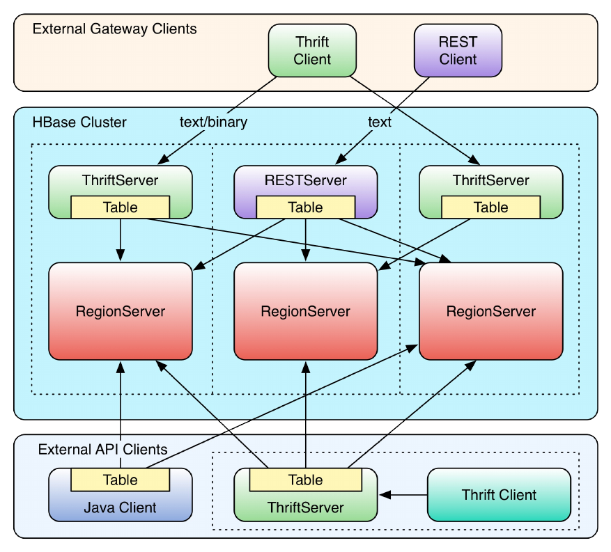
Figure 6-1. Clients connected through gateway servers
Internally, these servers use the common Table or BufferedMutator-based client API to access the
tables. You can see how they are started on top of the region server processes, sharing the same
physical machine. There is no one true recommendation for how to place the gateway servers.
You may want to colocate them, or have them on dedicated machines.
Another approach is to run them directly on the client nodes. For example, when you have web
servers constructing the resultant HTML pages using PHP, it is advantageous to run the gateway
process on the same server. That way, the communication between the client and gateway is
local, while the RPC between the gateway and HBase is using the native protocol.
Note
Check carefully how you access HBase from your client, to place the gateway servers on the
appropriate physical machine. This is influenced by the load on each machine, as well as the
amount of data being transferred: make sure you are not starving either process for resources,
such as CPU cycles, or network bandwidth.
The advantage of using a server as opposed to creating a new connection for every request goes
(407)

back to when we discussed “Resource Sharing”--you need to reuse connections to gain
maximum performance. Short-lived processes would spend more time setting up the connection
and preparing the metadata than in the actual operation itself. The caching of region information
in the server, in particular, makes the reuse important; otherwise, every client would have to
perform a full row-to-region lookup for every bit of data they want to access.
Selecting one server type over the others is a nontrivial task, as it depends on your use case. The
initial argument over REST in comparison to the more efficient Thrift, or similar serialization
formats, shows that for high-throughput scenarios it is advantageous to use a purely binary
format. However, if you have few requests, but they are large in size, REST is interesting. A
rough separation could look like this:
REST Use Case
Since REST supports existing web-based infrastructure, it will fit nicely into setups with
reverse proxies and other caching technologies. Plan to run many REST servers in parallel,
to distribute the load across them. For example, run a server on every application server
you have, building a single-app-to-server relationship.
Thrift Use Case
Use the compact binary protocol when you need the best performance in terms of
throughput. You can run fewer servers—for example, one per region server—with a many-
apps-to-server cardinality.
(408)

Frameworks
There is a long trend in software development to modularize and decouple specific units of work.
You might call this separation of responsibilities or other, similar names, yet the goal is the
same: it is better to build a commonly used piece of software only once, not having to reinvent
the wheel again and again. Many programming languages have the concept of modules, in Java
these are JAR files, providing shared code to many consumers. One set of those libraries is for
persistency, or data access in general. A popular choice is Hibernate, providing a common
interface for all object persistency.
There are also dedicated languages just for data manipulation, or such that make this task as
seamless as possible, so as not to distract from the business logic. We will look into domain-
specific languages (DSLs) below, which cover these aspects. Another, newer trend is to also
abstract away the application development, first manifested in platform-as-a-service (PaaS).
Here we are provided with everything that is needed to write applications as quick as possible.
There are application servers, accompanying libraries, databases, and so on.
With PaaS you still need to write the code and deploy it on the provided infrastructure. The
logical next step is to provide data access APIs that an application can use with no further setup
required. The Google App Engine services is one of those, where you can talk to a datastore API,
that is provided as a library. It limits the freedom of an application, but assuming the storage API
is powerful enough, and imposing no restrictions on the application developer’s creativity, it
makes deployment and management of applications much easier.
Hadoop is a very powerful and flexible system. In fact, any component in Hadoop could be
replaced, and you still have Hadoop, which is more of an ideology than a collection of specific
technologies. With this flexibility and likely change comes the opposing wish of developers to
stay clear of any hard dependency. For that reason, it is apparent how a new kind of active
framework is emerging. Similar to the Google App Engine service, they provide a server
component which accepts applications being deployed into, and with abstracted interfaces to
underlying services, such as storage.
Interesting is that these kinds of frameworks, we will call them data application servers, or data-
as-a-service (DaaS), embrace the nature of Hadoop, which is data first. Just like a smart phone,
you install applications that implement business use cases and run where the shared data resides.
There is no need to costly move large amounts of data around to produce a result. With HBase as
the storage engine, you can expect these frameworks to make best use of many built-in features,
for example server-side coprocessors to push down selection predicates and analytical
functionality. One example here is Cask.
Common to libraries and frameworks is the notion of an abstraction layer, be it a generic data
API or DSL. This is also apparent with yet another set of frameworks atop HBase, and other
storage layers in general, implementing SQL capabilities. We will discuss them in a separate
section below (see “SQL over NoSQL”), so suffice it to say that they provide a varying level of
SQL conformity, allowing access to data under the very popular idiom. Examples here are
Impala, Hive, and Phoenix.
Finally, what is hard to determine is where some of these libraries and frameworks really fit, as
they can be employed on various backends, some suitable for batch operations only, some for
(409)
interactive use, and yet others for both. The following will group them by that property, though
that means we may have to look at the same tool more than once. On the other hand, HBase is
built for interactive access, but can equally be used within long running batch processes, for
example, scanning analytical data for aggregation or model building. The grouping therefore
might be arbitrary, though helps with covering both sides of the coin.
(410)
Gateway Clients
The first group of clients consists of the gateway kind, those that send client API calls on
demand, such as get, put, or delete, to servers. Based on your choice of protocol, you can use the
supplied gateway servers to gain access from your applications. Alternatively, you can employ
the provided, storage specific API to implement generic, possibly hosted, data-centric solutions.
(411)

Native Java
The native Java API was discussed in Chapter 3 and Chapter 4. There is no need to start any
gateway server, as your client—using Table or BufferedMutator--is directly communicating with
the HBase servers, via the native RPC calls. Refer to the aforementioned chapters to implement a
native Java client.
(412)

REST
HBase ships with a powerful REST server, which supports the complete client and
administrative API. It also provides support for different message formats, offering many choices
for a client application to communicate with the server.
Operation
For REST-based clients to be able to connect to HBase, you need to start the appropriate gateway
server. This is done using the supplied scripts. The following commands show you how to get
the command-line help, and then start the REST server in a non-daemonized mode:
$ bin/hbase rest
usage: bin/hbase rest start [--infoport <arg>] [-p <arg>] [-ro]
--infoport <arg> Port for web UI
-p,--port <arg> Port to bind to [default: 8080]
-ro,--readonly Respond only to GET HTTP method requests [default:
false]
To run the REST server as a daemon, execute bin/hbase-daemon.sh start|stop
rest [--infoport <port>] [-p <port>] [-ro]
$ bin/hbase rest start
^C
You need to press Ctrl-C to quit the process. The help stated that you need to run the server using
a different script to start it as a background process:
$ bin/hbase-daemon.sh start rest
starting rest, logging to /var/lib/hbase/logs/hbase-larsgeorge-rest-<servername>.out
Once the server is started you can use curl4 on the command line to verify that it is operational:
$ curl http://<servername>:8080/
testtable
$ curl http://<servername>:8080/version
rest 0.0.3 [JVM: Oracle Corporation 1.7.0_51-24.51-b03] [OS: Mac OS X \
10.10.2 x86_64] [Server: jetty/6.1.26] [Jersey: 1.9]
Retrieving the root URL, that is "/" (slash), returns the list of available tables, here testtable.
Using "/version" retrieves the REST server version, along with details about the machine it is
running on.
Alternatively, you can open the web-based UI provided by the REST server. You can specify the
port using the above mentioned --infoport command line parameter, or by overriding the
hbase.rest.info.port configuration property. The default is set to 8085, and the content of the
page is shown in Figure 6-2.
(413)
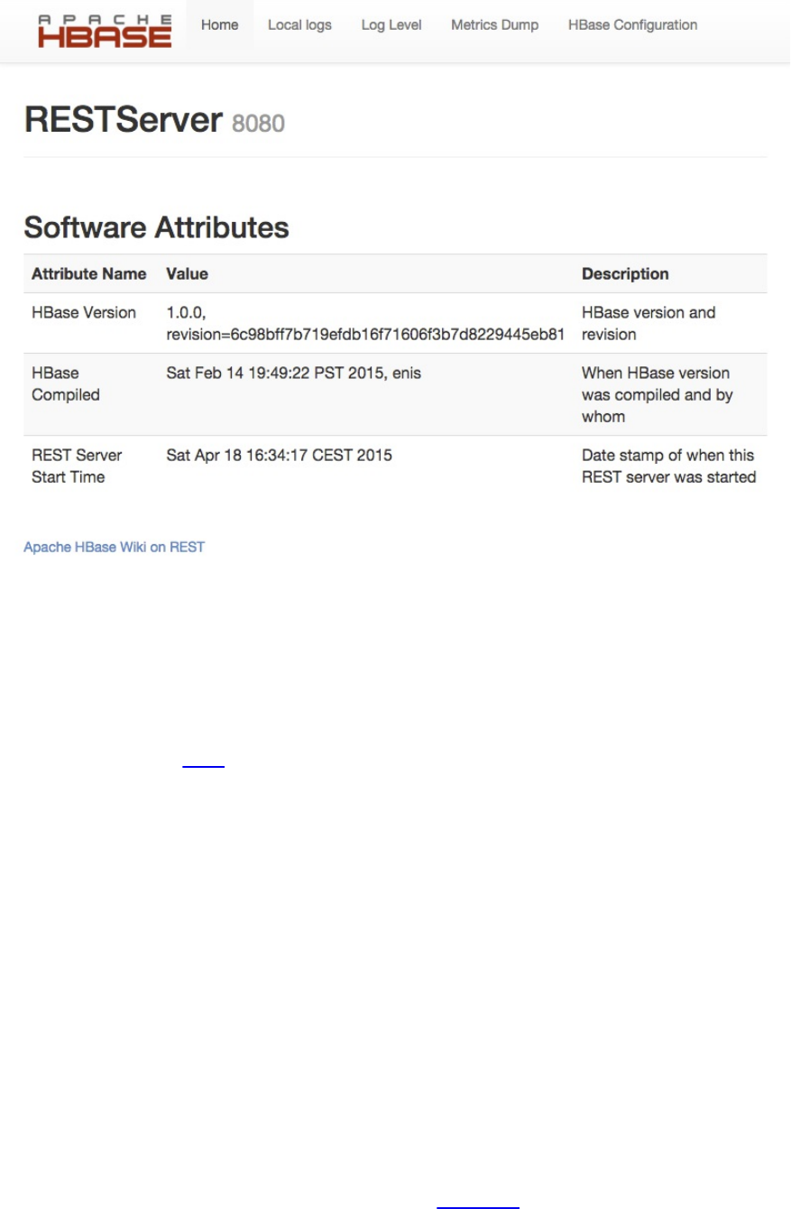
Figure 6-2. The web-based UI for the REST server
The UI has functionality that is common to many web-based UIs provided by HBase. The middle
part provides information about the server and its status. For the REST server there is not much
more than the HBase version, compile information, and server start time. At the bottom of the
page is a link to the HBase Wiki page explaining the REST API. At the top of the page are links
offering extra functionality:
Home
Links to the Home page of the server.
Local logs
Opens a page that lists the local log directory, providing web-based access to the otherwise
inaccessible log files.
Log Level
This page allows to query and set the log levels for any class or package loaded in the
server process.
Metrics Dump
All servers in HBase track activity as metrics (see Chapter 9), which can be accessed as
JSON using this link.
(414)

HBase Configuration
Prints the current configuration as used by the server process.
See “Shared Pages” for a deeper discussion on these shared server UI links.
Stopping the REST server, when running as a daemon, involves the same script, just replacing
start with stop:
$ bin/hbase-daemon.sh stop rest
stopping rest..
The REST server gives you all the operations required to work with HBase tables.
Note
The current documentation for the REST server is available online. Please refer to it for all the
provided operations. Also, be sure to carefully read the XML schemas documentation on that
page. It explains the schemas you need to use when requesting information, as well as those
returned by the server.
You can start as many REST servers as you like, and, for example, use a load balancer to route
the traffic between them. Since they are stateless—any state required is carried as part of the
request—you can use a round-robin (or similar) approach to distribute the load.
The --readonly, or -ro parameter switches the server into read-only mode, which means it only
responds to HTTP GET operations. Finally, use the -p, or --port, parameter to specify a different
port for the server to listen on. The default is 8080. There are additional configuration properties
that the REST server is considering as it is started. Table 6-1 lists them with default values.
Table 6-1. Configuration options for the REST server
Property Default Description
hbase.rest.dns.nameserver default Defines the DNS server used for the name lookup.a
hbase.rest.dns.interface default Defines the network interface that the name is
associated with.a
hbase.rest.port 8080
Sets the HTTP port the server will bind to. Also settable
per instance with the -p and --port command-line
parameter.
hbase.rest.host 0.0.0.0 Defines the address the server is listening on. Defaults
to the wildcard address.
hbase.rest.info.port 8085 Specifies the port the web-based UI will bind to. Also
settable per instance using the --infoport parameter.
(415)

hbase.rest.info.bindAddress 0.0.0.0 Sets the IP address the web-based UI is bound to.
Defaults to the wildcard address.
hbase.rest.readonly false Forces the server into normal or read-only mode. Also
settable by the --readonly, or -ro options.
hbase.rest.threads.max 100 Provides the upper boundary of the thread pool used by
the HTTP server for request handlers.
hbase.rest.threads.min 2 Same as above, but sets the lower boundary on number
of handler threads.
hbase.rest.connection.cleanup-
interval
10000
(10
secs)
Defines how often the internal housekeeping task
checks for expired connections to the HBase cluster.
hbase.rest.connection.max-
idletime
600000
(10
mins)
Amount of time after which an unused connection is
considered expired.
hbase.rest.support.proxyuser false Flags if the server should support proxy users or not.
This is used to enable secure impersonation.
a These two properties are used in tandem to look up the server’s hostname using the given
network interface and name server. The default value mean it uses whatever is configured on
the OS level.
The connection pool configured with the above settings is required since the server needs to keep
a separate connection for each authenticated user, when security is enabled. This also applies to
the proxy user settings, and both are explained in more detail in [Link to Come].
Supported Formats
Using the HTTP Content-Type and Accept headers, you can switch between different formats
being sent or returned to the caller. As an example, you can create a table and row in HBase
using the shell like so:
hbase(main):001:0> create 'testtable', 'colfam1'
0 row(s) in 0.6690 seconds
=> Hbase::Table - testtable
hbase(main):002:0> put 'testtable', "\x01\x02\x03", 'colfam1:col1', 'value1'
0 row(s) in 0.0230 seconds
(416)

hbase(main):003:0> scan 'testtable'
ROW COLUMN+CELL
\x01\x02\x03 column=colfam1:col1, timestamp=1429367023394, value=value1
1 row(s) in 0.0210 seconds
This inserts a row with the binary row key 0x01 0x02 0x03 (in hexadecimal numbers), with one
column, in one column family, that contains the value value1.
Plain (text/plain)
For some operations it is permissible to have the data returned as plain text. One example
is the aforementioned /version operation:
$ curl -H "Accept: text/plain" http://<servername>:8080/version
rest 0.0.3 [JVM: Oracle Corporation 1.7.0_45-24.45-b08] [OS: Mac OS X \
10.10.2 x86_64] [Server: jetty/6.1.26] [Jersey: 1.9]
On the other hand, using plain text with more complex return values is not going to work
as expected:
$ curl -H "Accept: text/plain" \
http://<servername>:8080/testtable/%01%02%03/colfam1:col1
<html>
<head>
<meta http-equiv="Content-Type" content="text/html; charset=ISO-8859-1"/>
<title>Error 406 Not Acceptable</title>
</head>
<body><h2>HTTP ERROR 406</h2>
<p>Problem accessing /testtable/%01%02%03/colfam1:col1. Reason:
<pre> Not Acceptable</pre></p>
<hr /><i><small>Powered by Jetty://</small></i><br/>
<br/>
...
<br/>
</body>
</html>
This is caused by the fact that the server cannot make any assumptions regarding how to
format a complex result value in plain text. You need to use a format that allows you to
express nested information natively.
Note
The row key used in the example is a binary one, consisting of three bytes. You can use
REST to access those bytes by encoding the key using URL encoding,5 which in this case
results in %01%02%03. The entire URL to retrieve a cell is then:
http://<servername>:8080/testtable/%01%02%03/colfam1:col1
See the online documentation referred to earlier for the entire syntax.
XML (text/xml)
When storing or retrieving data, XML is considered the default format. For example, when
retrieving the example row with no particular Accept header, you receive:
$ curl http://<servername>:8080/testtable/%01%02%03/colfam1:col1
<?xml version="1.0" encoding="UTF-8" standalone="yes"?>
<CellSet>
<Row key="AQID">
(417)

<Cell column="Y29sZmFtMTpjb2wx" \
timestamp="1429367023394">dmFsdWUx</Cell>
</Row>
</CellSet>
The returned format defaults to XML. The column name and the actual value are encoded
in Base64, as explained in the online schema documentation. Here is the respective part of
the schema:
<element name="Row" type="tns:Row"></element>
<complexType name="Row">
<sequence>
<element name="key" type="base64Binary"></element>
<element name="cell" type="tns:Cell" maxOccurs="unbounded" \
minOccurs="1"></element>
</sequence>
</complexType>
<element name="Cell" type="tns:Cell"></element>
<complexType name="Cell">
<sequence>
<element name="value" maxOccurs="1" minOccurs="1">
<simpleType><restriction base="base64Binary">
</simpleType>
</element>
</sequence>
<attribute name="column" type="base64Binary" />
<attribute name="timestamp" type="int" />
</complexType>
All occurrences of base64Binary are where the REST server returns the encoded data. This
is done to safely transport the binary data that can be contained in the keys, or the value.
This is also true for data that is sent to the REST server. Make sure to read the schema
documentation to encode the data appropriately, including the payload, in other words, the
actual data, but also the column name, row key, and so on.
A quick test on the console using the base64 command reveals the proper content:
$ echo AQID | base64 -D | hexdump
0000000 01 02 03
$ echo Y29sZmFtMTpjb2wx | base64 -D
colfam1:col1
$ echo dmFsdWUx | base64 -D
value1
This is obviously useful only to verify the details on the command line. From within your
code you can use any available Base64 implementation to decode the returned values.
JSON (application/json)
Similar to XML, requesting (or setting) the data in JSON simply requires setting the Accept
header:
$ curl -H "Accept: application/json" \
http://<servername>:8080/testtable/%01%02%03/colfam1:col1
{
"Row": [{
"key": "AQID",
"Cell": [{
"column": "Y29sZmFtMTpjb2wx",
"timestamp": 1429367023394,
"$": "dmFsdWUx"
(418)

}]
}]
}
Note
The preceding JSON result was reformatted to be easier to read. Usually the result on the
console is returned as a single line, for example:
{"Row":[{"key":"AQID","Cell":[{"column":"Y29sZmFtMTpjb2wx", \
"timestamp":1429367023394,"$":"dmFsdWUx"}]}]}
The encoding of the values is the same as for XML, that is, Base64 is used to encode any
value that potentially contains binary data. An important distinction to XML is that JSON
does not have nameless data fields. In XML the cell data is returned between Cell tags, but
JSON must specify key/value pairs, so there is no immediate counterpart available. For that
reason, JSON has a special field called "$" (the dollar sign). The value of the dollar field is
the cell data. In the preceding example, you can see it being used:
"$":"dmFsdWUx"
You need to query the dollar field to get the Base64-encoded data.
Protocol Buffer (application/x-protobuf)
An interesting application of REST is to be able to switch encodings. Since Protocol
Buffers have no native RPC stack, the HBase REST server offers support for its encoding.
The schemas are documented online for your perusal.
Getting the results returned in Protocol Buffer encoding requires the matching Accept
header:
$ curl -H "Accept: application/x-protobuf" \
http://<servername>:8080/testtable/%01%02%03/colfam1:col1 | hexdump -C
...
00000000 0a 24 0a 03 01 02 03 12 1d 12 0c 63 6f 6c 66 61 |.$.........colfa|
00000010 6d 31 3a 63 6f 6c 31 18 a2 ce a7 e7 cc 29 22 06 |m1:col1......)".|
00000020 76 61 6c 75 65 31 |value1|
The use of hexdump allows you to print out the encoded message in its binary format. You
need a Protocol Buffer decoder to actually access the data in a structured way. The ASCII
printout on the righthand side of the output shows the column name and cell value for the
example row.
Raw binary (application/octet-stream)
Finally, you can dump the data in its raw form, while omitting structural data. In the
following console command, only the data is returned, as stored in the cell.
$ curl -H "Accept: application/octet-stream" \
http://<servername>:8080/testtable/%01%02%03/colfam1:col1 | hexdump -C
00000000 76 61 6c 75 65 31 |value1|
Note
Depending on the format request, the REST server puts structural data into a custom header. For
example, for the raw get request in the preceding paragraph, the headers look like this (adding -D
(419)
to the curl command):
HTTP/1.1 200 OK
Content-Length: 6
X-Timestamp: 1429367023394
Content-Type: application/octet-stream
The timestamp of the cell has been moved to the header as X-Timestamp. Since the row and
column keys are part of the request URI, they are omitted from the response to prevent
unnecessary data from being transferred.
REST Java Client
The REST server also comes with a comprehensive Java client API. It is located in the
org.apache.hadoop.hbase.rest.client package. The central classes are RemoteHTable and
RemoteAdmin. Example 6-1 shows the use of the RemoteHTable class.
Example 6-1. Example of using the REST client classes
Cluster cluster = new Cluster();
cluster.add("localhost", 8080);
Client client = new Client(cluster);
RemoteHTable table = new RemoteHTable(client, "testtable");
Get get = new Get(Bytes.toBytes("row-30"));
get.addColumn(Bytes.toBytes("colfam1"), Bytes.toBytes("col-3"));
Result result1 = table.get(get);
System.out.println("Get result1: " + result1);
Scan scan = new Scan();
scan.setStartRow(Bytes.toBytes("row-10"));
scan.setStopRow(Bytes.toBytes("row-15"));
scan.addColumn(Bytes.toBytes("colfam1"), Bytes.toBytes("col-5"));
ResultScanner scanner = table.getScanner(scan);
for (Result result2 : scanner) {
System.out.println("Scan row[" + Bytes.toString(result2.getRow()) +
"]: " + result2);
}
Set up a cluster list adding all known REST server hosts.
Create the client handling the HTTP communication.
Create a remote table instance, wrapping the REST access into a familiar interface.
Perform a get operation as if it were a direct HBase connection.
(420)
Scan the table, again, the same approach as if using the native Java API.
Running the example requires that the REST server has been started and is listening on the
specified port. If you are running the server on a different machine and/or port, you need to first
adjust the value added to the Cluster instance.
Here is what is printed on the console when running the example:
Adding rows to table...
Get result1:
keyvalues={row-30/colfam1:col-3/1429376615162/Put/vlen=8/seqid=0}
Scan row[row-10]:
keyvalues={row-10/colfam1:col-5/1429376614839/Put/vlen=8/seqid=0}
Scan row[row-100]:
keyvalues={row-100/colfam1:col-5/1429376616162/Put/vlen=9/seqid=0}
Scan row[row-11]:
keyvalues={row-11/colfam1:col-5/1429376614856/Put/vlen=8/seqid=0}
Scan row[row-12]:
keyvalues={row-12/colfam1:col-5/1429376614873/Put/vlen=8/seqid=0}
Scan row[row-13]:
keyvalues={row-13/colfam1:col-5/1429376614891/Put/vlen=8/seqid=0}
Scan row[row-14]:
keyvalues={row-14/colfam1:col-5/1429376614907/Put/vlen=8/seqid=0}
Due to the lexicographical sorting of row keys, you will receive the preceding rows. The selected
columns have been included as expected.
The RemoteHTable is a convenient way to talk to a number of REST servers, while being able to
use the normal Java client API classes, such as Get or Scan.
Note
The current implementation of the Java REST client is using the Protocol Buffer encoding
internally to communicate with the remote REST server. It is the most compact protocol the
server supports, and therefore provides the best bandwidth efficiency.
(421)

Thrift
Apache Thrift is written in C++, but provides schema compilers for many programming
languages, including Java, C++, Perl, PHP, Python, Ruby, and more. Once you have compiled a
schema, you can exchange messages transparently between systems implemented in one or more
of those languages.
Installation
Before you can use Thrift, you need to install it, which is preferably done using a binary
distribution package for your operating system. If that is not an option, you need to compile it
from its sources.
Note
HBase ships with pre-built Thrift code for Java and all the included demos, which means that
there should be no need to install Thrift. You still will need the Thrift source package, because it
contains necessary code that the generated classes rely on. You will see in the example below
(see “Example: PHP”) how for some languages that is required, while for others it may not.
Download the source tarball from the website, and unpack it into a common location:
$ wget http://www.apache.org/dist/thrift/0.9.2/thrift-0.9.2.tar.gz
$ tar -xzvf thrift-0.9.2.tar.gz -C /opt
$ rm thrift-0.9.2.tar.gz
Install the dependencies, which are Automake, LibTool, Flex, Bison, and the Boost libraries:
$ sudo apt-get install build-essential automake libtool flex bison libboost
Now you can build and install the Thrift binaries like so:
$ cd /opt/thrift-0.9.2
$ ./configure
$ make
$ sudo make install
Alternative, on OS X you could, for example, use the Homebrew package manager for installing
the same like so:
$ brew install thrift
==> Installing dependencies for thrift: boost, openssl
...
==> Summary
/usr/local/Cellar/thrift/0.9.2: 90 files, 5.4M
When installed, you can verify that everything succeeded by calling the main thrift executable:
$ thrift -version
Thrift version 0.9.2
Once you have Thrift installed, you need to compile a schema into the programming language of
your choice. HBase comes with a schema file for its client and administrative API. You need to
use the Thrift binary to create the wrappers for your development environment.
(422)

Note
The supplied schema file exposes the majority of the API functionality, but is lacking in a few
areas. It was created when HBase had a different API and that is noticeable when using it. Newer
features might be not supported yet, for example the newer durability settings. See “Thrift2” for
a replacement service, implementing the current HBase API verbatim.
Before you can access HBase using Thrift, though, you also have to start the supplied
ThriftServer.
Thrift Operations
Starting the Thrift server is accomplished by using the supplied scripts. You can get the
command-line help by adding the -h switch, or omitting all options:
$ bin/hbase thrift
usage: Thrift [-b <arg>] [-c] [-f] [-h] [-hsha | -nonblocking |
-threadedselector | -threadpool] [--infoport <arg>] [-k <arg>] [-m
<arg>] [-p <arg>] [-q <arg>] [-w <arg>]
-b,--bind <arg> Address to bind the Thrift server to. [default:
0.0.0.0]
-c,--compact Use the compact protocol
-f,--framed Use framed transport
-h,--help Print help information
-hsha Use the THsHaServer This implies the framed
transport.
--infoport <arg> Port for web UI
-k,--keepAliveSec <arg> The amount of time in secods to keep a thread
alive when idle in TBoundedThreadPoolServer
-m,--minWorkers <arg> The minimum number of worker threads for
TBoundedThreadPoolServer
-nonblocking Use the TNonblockingServer This implies the
framed transport.
-p,--port <arg> Port to bind to [default: 9090]
-q,--queue <arg> The maximum number of queued requests in
TBoundedThreadPoolServer
-threadedselector Use the TThreadedSelectorServer This implies
the framed transport.
-threadpool Use the TBoundedThreadPoolServerThis is the
default.
-w,--workers <arg> The maximum number of worker threads for
TBoundedThreadPoolServer
To start the Thrift server run 'bin/hbase-daemon.sh start thrift'
To shutdown the thrift server run 'bin/hbase-daemon.sh stop thrift' or
send a kill signal to the thrift server pid
There are many options to choose from. The type of server, protocol, and transport used is
usually enforced by the client, since not all language implementations have support for them.
From the command-line help you can see that, for example, using the nonblocking server implies
the framed transport.
Using the defaults, you can start the Thrift server in non-daemonized mode:
$ bin/hbase thrift start
^C
You need to press Ctrl-C to quit the process. The help stated that you need to run the server using
a different script to start it as a background process:
$ bin/hbase-daemon.sh start thrift
starting thrift, logging to /var/lib/hbase/logs/ \
hbase-larsgeorge-thrift-<servername>.out
(423)
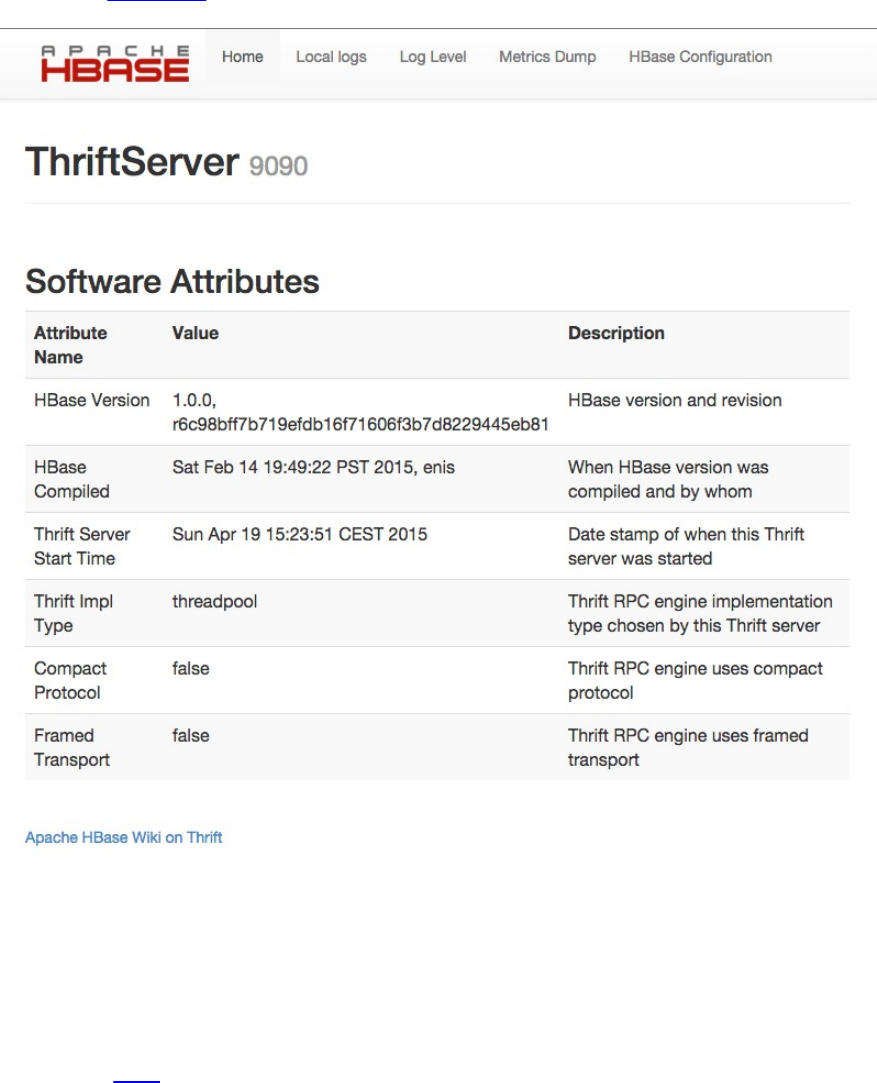
Stopping the Thrift server, running as a daemon, involves the same script, just replacing start
with stop:
$ bin/hbase-daemon.sh stop thrift
stopping thrift..
Once started either way, you can open the web-based UI provided by the Thrift server. You can
specify the port using the above listed --infoport command line parameter, or by overriding the
hbase.thrift.info.port configuration property. The default is set to 9095, and the content of the
page is shown in Figure 6-3.
Figure 6-3. The web-based UI for the Thrift server
The UI has functionality that is common to many web-based UIs provided by HBase. The middle
part provides information about the server and its status. For the Thrift server there is not much
more than the HBase version, compile information, server start time, and Thrift specific details,
such as the server type, protocol and transport options configured. At the bottom of the page is a
link to the HBase Wiki page explaining the Thrift API. At the top of the page are links offering
extra functionality:
(424)

Home
Links to the Home page of the server.
Local logs
Opens a page that lists the local log directory, providing web-based access to the otherwise
inaccessible log files.
Log Level
This page allows to query and set the log levels for any class or package loaded in the
server process.
Metrics Dump
All servers in HBase track activity as metrics (see Chapter 9), which can be accessed as
JSON using this link.
HBase Configuration
Prints the current configuration as used by the server process.
See “Shared Pages” for a deeper discussion on these shared server UI links.
Note
The current documentation for the Thrift server is available online (also see the package info).
You should refer to it for all the provided operations. It is also advisable to read the provided
$HBASE_HOME/hbase-thrift/src/main/resources/org/apache/hadoop/hbase/thrift/Hbase.thrift
schema definition file for the authoritative documentation of the available functionality.
The Thrift server provides you with all the operations required to work with HBase tables. You
can start as many Thrift servers as you like, and, for example, use a load balancer to route the
traffic between them. Since they are stateless, you can use a round-robin (or similar) approach to
distribute the load. Use the -p, or --port, parameter to specify a different port for the server to
listen on. The default is 9090.
There are additional configuration properties that the Thrift server is considering as it is started.
Table 6-2 lists them with default values.
Table 6-2. Configuration options for the Thrift server
Property Default Description
hbase.thrift.dns.nameserver default Defines the DNS server
used for the name lookup.a
hbase.thrift.dns.interface default
Defines the network
interface that the name is
associated with.a
(425)
hbase.regionserver.thrift.port 9090
Sets the port the server will
bind to. Also settable per
instance with the -p or --
port command-line
parameter.
hbase.regionserver.thrift.ipaddress 0.0.0.0
Defines the address the
server is listening on.
Defaults to the wildcard
address. Set with -b, --bind
per instance on the
command-line.
hbase.thrift.info.port 9095
Specifies the port the web-
based UI will bind to. Also
settable per instance using
the --infoport parameter.
hbase.thrift.info.bindAddress 0.0.0.0
Sets the IP address the web-
based UI is bound to.
Defaults to the wildcard
address.
hbase.regionserver.thrift.server.type threadpool
Sets the Thrift server type
in non-HTTP mode. See
below for details.
hbase.regionserver.thrift.compact false
Enables the compact
protocol mode if set to true.
Default means binary mode
instead. Also settable per
instance with -c, or --
compact.
hbase.regionserver.thrift.framed false
Sets the transport mode to
framed. Otherwise the
standard transport is used.
Framed cannot be used in
secure mode. When using
the hsha or nonblocking
server type, framed
transport is always used
irrespective of this
configuration property.
(426)
Also settable per instance
with -f, or --framed.
hbase.regionserver.thrift.framed.max_frame_size_in_mb 2097152 (2
MB)
The maximum frame size
when framed transport
mode is enabled.
hbase.thrift.minWorkerThreads 16
Sets the minimum amount
of worker threads to keep,
should be increased for
production use (for
example, to 200). Settable
on the command-line with -
m, or --minWorkers.
hbase.thrift.maxWorkerThreads 1000
Sets the upper limit of
worker threads. Settable on
the command-line with -w,
or --workers.
hbase.thrift.maxQueuedRequests 1000
Maximum number of
request to queue when
workers are all busy. Can
be set with -q, and --queue
per instance.
hbase.thrift.threadKeepAliveTimeSec 60 (secs)
Amount of time an
extraneous idle worker is
kept before it is discarded.
Also settable with -k, or --
keepAliveSec.
hbase.regionserver.thrift.http false
Flag that determines if the
server should run in HTTP
or native mode.
hbase.thrift.http_threads.max 100
Provides the upper
boundary of the thread pool
used by the HTTP server
for request handlers.
(427)
hbase.thrift.http_threads.min 2 Same as above, but sets the
lower boundary on number
of handler threads.
hbase.thrift.ssl.enabled false
When HTTP mode is
enabled, this flag sets the
SSL mode.
hbase.thrift.ssl.keystore.store "" When SSL is enabled, sets
the key store file.
hbase.thrift.ssl.keystore.password null
When SSL is enabled, sets
the password to unlock the
key store file.
hbase.thrift.ssl.keystore.keypassword null
When SSL is enabled, sets
the password to retrieve the
keys from the key store.
hbase.thrift.security.qop ""
Can be one of auth, auth-
int, or auth-conf to set the
SASL quality-of-protection
(QoP). See [Link to Come]
for details.
hbase.thrift.support.proxyuser false
Flags if the server should
support proxy users or not.
This is used to enable
secure impersonation.
hbase.thrift.kerberos.principal <hostname>
Can be used to set the
Kerberos principal to use in
secure mode.
hbase.thrift.keytab.file ""
Specifies the Kerberos
keytab file for secure
operation.
hbase.regionserver.thrift.coalesceIncrement false
Enables the coalesce mode
for increments, which is a
delayed, batch increment
(428)

operation.
hbase.thrift.filters ""
Loads filter classes into the
server process for
subsequent use.
hbase.thrift.connection.cleanup-interval 10000 (10
secs)
Defines how often the
internal housekeeping task
checks for expired
connections to the HBase
cluster.
hbase.thrift.connection.max-idletime 600000 (10
mins)
Amount of time after which
an unused connection is
considered expired.
a These two properties are used in tandem to look up the server’s hostname using the given
network interface and name server. The default value mean it uses whatever is configured on
the OS level.
There a few choices for the server type in Thrift native mode (that is, non-HTTP), which are:
nonblocking
Uses the TNonblockingServer class, which is based on Java NIO’s non-blocking I/O, where
the selector thread also processes the actual request. Settable per server instance with the -
nonblocking parameter.
hsha
Uses the THsHaServer class, implementing a Half-Sync/Half-Async (HsHa) server. The
difference to the non-blocking server is that it has a single thread accepting connections,
but a thread pool for the processing workers. Settable per server instance with the -hsha
parameter.
threadedselector
Extends on the HsHa server by maintaining two thread pools, one for network I/O
(selection), and another for processing (workers). Uses the TThreadedSelectorServer class.
Settable per server instance with the -threadedselector parameter.
threadpool
Has a single thread to accept connections, which are then scheduled to be worked on in an
ExecutorService. Each connection is dedicated to one client, therefore potentially many
threads are needed in highly concurrent setups. Uses the TBoundedThreadPoolServer class,
which is a customized implementation of the Thrift TThreadPoolServer class. Also settable
(429)

per server instance with the -threadpool parameter.
The default of type threadpool is a good choice for production use, as it combines many proven
techniques.6
Example: PHP
HBase not only ships with the required Thrift schema file, but also with an example client for
many programming languages. Here we will enable the PHP implementation to demonstrate the
required steps.
Before we start though, a few notes:
You need to enable PHP support for your web server! Follow your server documentation
to do so. On OS X, for example, you need to edit /etc/apache2/httpd.conf and uncomment
the following line, and (re)start the server with $ sudo apachectl restart:
LoadModule php5_module libexec/apache2/libphp5.so
HBase ships with a precompiled PHP Thrift module, so you are free to skip the part below
(that is, step #1) where we generate the module anew. Either way should get you to the
same result. The code shipped with HBase is in the `hbase-examples
The included DemoClient.php is not up-to-date, for example, it tests with an empty row key,
which is not allowed, and using a non-UTF8 row key, which is allowed. Both checks fail,
and you need to fix the PHP file taking care of the changes.
Apache Thrift has changed the layout of the PHP scaffolding files it ships with. In earlier
releases it only had a $THRIFT_SRC_HOME/lib/php/src directory, while newer versions have a
../src and ../lib folder.
Step 1
Optionally: The first step is to copy the supplied schema file and compile the necessary PHP
source files for it:
$ cp -r $HBASE_HOME/hbase-thrift/src/main/resources/org/apache/ \
hadoop/hbase/thrift ~/thrift_src
$ cd thrift_src/
$ thrift -gen php Hbase.thrift
The call to thrift should complete with no error or other output on the command line. Inside the
thrift_src directory you will now find a directory named gen-php containing the two generated
PHP files required to access HBase:
$ ls -l gen-php/Hbase/
total 920
-rw-r--r-- 1 larsgeorge staff 416357 Apr 20 07:46 Hbase.php
-rw-r--r-- 1 larsgeorge staff 52366 Apr 20 07:46 Types.php
If you decide to skip this step, you can copy the supplied, pre-generated PHP files from the
hbase-examples module in the HBase source tree:
$ ls -lR $HBASE_HOME/hbase-examples/src/main/php
total 24
-rw-r--r-- 1 larsgeorge admin 8438 Jan 25 10:47 DemoClient.php
(430)
drwxr-xr-x 3 larsgeorge admin 102 May 22 2014 gen-php
/usr/local/hbase-1.0.0-src/hbase-examples/src/main/php/gen-php:
total 0
drwxr-xr-x 4 larsgeorge admin 136 Jan 25 10:47 Hbase
/usr/local/hbase-1.0.0-src/hbase-examples/src/main/php/gen-php/Hbase:
total 800
-rw-r--r-- 1 larsgeorge admin 366528 Jan 25 10:47 Hbase.php
-rw-r--r-- 1 larsgeorge admin 38477 Jan 25 10:47 Types.php
Step 2
The generated files require the Thrift-supplied PHP harness to be available as well. They need to
be copied into your web server’s document root directory, along with the generated files:
$ cd /opt/thrift-0.9.2
$ sudo mkdir $DOCUMENT_ROOT/thrift/
$ sudo cp src/*.php $DOCUMENT_ROOT/thrift/
$ sudo cp -r lib/Thrift/* $DOCUMENT_ROOT/thrift/
$ sudo mkdir $DOCUMENT_ROOT/thrift/packages
$ sudo cp -r ~/thrift_src/gen-php/Hbase $DOCUMENT_ROOT/thrift/packages/
The generated PHP files are copied into a packages subdirectory, as per the Thrift documentation,
which needs to be created if it does not exist yet.
Note
The $DOCUMENT_ROOT in the preceding commands could be /var/www, for example, on a Linux
system using Apache, or /Library/WebServer/Documents/ on an Apple Mac OS X machine. Check
your web server configuration for the appropriate location.
HBase ships with a DemoClient.php file that uses the generated files to communicate with the
servers. This file is copied into the same document root directory of the web server:
$ sudo cp $HBASE_HOME/hbase-examples/src/main/php/DemoClient.php $DOCUMENT_ROOT/
You need to edit the DemoClient.php file and adjust the following fields at the beginning of the
file:
# Change this to match your thrift root
$GLOBALS['THRIFT_ROOT'] = 'thrift';
...
# According to the thrift documentation, compiled PHP thrift libraries should
# reside under the THRIFT_ROOT/packages directory. If these compiled libraries
# are not present in this directory, move them there from gen-php/.
require_once( $GLOBALS['THRIFT_ROOT'].'/packages/Hbase/Hbase.php' );
...
$socket = new TSocket( 'localhost', 9090 );
...
Usually, editing the first line is enough to set the THRIFT_ROOT path. Since the DemoClient.php file is
also located in the document root directory, it is sufficient to set the variable to thrift, that is, the
directory copied from the Thrift sources earlier.
The last line in the preceding excerpt has a hardcoded server name and port. If you set up the
example in a distributed environment, you need to adjust this line to match your environment as
well. After everything has been put into place and adjusted appropriately, you can open a
browser and point it to the demo page. For example:
http://<webserver-address>/DemoClient.php
(431)

This should load the page and output the following details (abbreviated here for the sake of
brevity):7
scanning tables...
found: testtable
creating table: demo_table
column families in demo_table:
column: entry:, maxVer: 10
column: unused:, maxVer: 3
Starting scanner...
...
The same Demo Client client is also available in C++, Java, Perl, Python, and Ruby. Follow the
same steps to start the Thrift server, compile the schema definition into the necessary language,
and start the client. Depending on the language, you will need to put the generated code into the
appropriate location first.
Example: Java
HBase already ships with the generated Java classes to communicate with the Thrift server,
though you can always regenerate them again from the schema file. The book’s online code
repository provides a script to generate them directly within the example directory for this
chapter. It is located in the bin directory of the repository root path, and is named dothrift.sh. It
requires you to hand in the HBase Thrift definition file, since that can be anywhere:
$ bin/dothrift.sh
Missing thrift file parameter!
Usage: bin/dothrift.sh <thrift-file>
$ bin/dothrift.sh $HBASE_HOME/hbase-thrift/src/main/resources/org/ \
apache/hadoop/hbase/thrift/Hbase.thrift
compiling thrift: /usr/local/hbase-1.0.0-src/hbase-thrift/src/main/ \
resources/org/apache/hadoop/hbase/thrift/Hbase.thrift
done.
After running the script, the generated classes can be found in the
ch06/src/main/java/org/apache/hadoop/hbase/thrift/ directory. Example 6-2 uses these classes to
communicate with the Thrift server. Make sure the gateway server is up and running and
listening on port 9090.
Example 6-2. Example using the Thrift generated client API
private static final byte[] TABLE = Bytes.toBytes("testtable");
private static final byte[] ROW = Bytes.toBytes("testRow");
private static final byte[] FAMILY1 = Bytes.toBytes("testFamily1");
private static final byte[] FAMILY2 = Bytes.toBytes("testFamily2");
private static final byte[] QUALIFIER = Bytes.toBytes
("testQualifier");
private static final byte[] COLUMN = Bytes.toBytes(
"testFamily1:testColumn");
private static final byte[] COLUMN2 = Bytes.toBytes(
"testFamily2:testColumn2");
private static final byte[] VALUE = Bytes.toBytes("testValue");
public static void main(String[] args) throws Exception {
TTransport transport = new TSocket("0.0.0.0", 9090, 20000);
TProtocol protocol = new TBinaryProtocol(transport, true, true);
Hbase.Client client = new Hbase.Client(protocol);
transport.open();
ArrayList<ColumnDescriptor> columns = new
ArrayList<ColumnDescriptor>();
(432)
ColumnDescriptor cd = new ColumnDescriptor();
cd.name = ByteBuffer.wrap(FAMILY1);
columns.add(cd);
cd = new ColumnDescriptor();
cd.name = ByteBuffer.wrap(FAMILY2);
columns.add(cd);
client.createTable(ByteBuffer.wrap(TABLE), columns);
ArrayList<Mutation> mutations = new ArrayList<Mutation>();
mutations.add(new Mutation(false, ByteBuffer.wrap(COLUMN),
ByteBuffer.wrap(VALUE), true));
mutations.add(new Mutation(false, ByteBuffer.wrap(COLUMN2),
ByteBuffer.wrap(VALUE), true));
client.mutateRow(ByteBuffer.wrap(TABLE), ByteBuffer.wrap(ROW),
mutations, null);
TScan scan = new TScan();
int scannerId = client.scannerOpenWithScan(ByteBuffer.wrap(TABLE),
scan, null);
for (TRowResult result : client.scannerGet(scannerId)) {
System.out.println("No. columns: " + result.getColumnsSize());
for (Map.Entry<ByteBuffer, TCell> column :
result.getColumns().entrySet()) {
System.out.println("Column name: " + Bytes.toString(
column.getKey().array()));
System.out.println("Column value: " + Bytes.toString(
column.getValue().getValue()));
}
}
client.scannerClose(scannerId);
ArrayList<ByteBuffer> columnNames = new ArrayList<ByteBuffer>();
columnNames.add(ByteBuffer.wrap(FAMILY1));
scannerId = client.scannerOpen(ByteBuffer.wrap(TABLE),
ByteBuffer.wrap(Bytes.toBytes("")), columnNames, null);
for (TRowResult result : client.scannerGet(scannerId)) {
System.out.println("No. columns: " + result.getColumnsSize());
for (Map.Entry<ByteBuffer, TCell> column :
result.getColumns().entrySet()) {
System.out.println("Column name: " + Bytes.toString(
column.getKey().array()));
System.out.println("Column value: " + Bytes.toString(
column.getValue().getValue()));
}
}
client.scannerClose(scannerId);
System.out.println("Done.");
transport.close();
}
Create a connection using the Thrift boilerplate classes.
Create two column descriptor instances.
Create the test table.
Insert a test row.
(433)

Scan with an instance of TScan. This is the most convenient approach. Print the results in a
loop.
Scan again, but with another Thrift method. In addition, set the columns to a specific
family only. Also print out the results in a loop.
Close the connection after everything is done.
The console output is:
No. columns: 2
Column name: testFamily1:testColumn
Column value: testValue
Column name: testFamily2:testColumn2
Column value: testValue
No. columns: 1
Column name: testFamily1:testColumn
Column value: testValue
Done.
Please consult the supplied classes, examples, and online documentation for more details.
(434)

Thrift2
Since the client API of HBase was changed significantly in version 0.90, it is apparent in many
places how the Thrift API is out of sync. An effort was started to change this by implementing a
new version of the Thrift gateway server, named Thrift2. It mirrors the current client API calls
and therefore feels more natural to the HBase developers familiar with the native, Java based
API. On the other hand, unfortunately, it is still work in progress and is lacking various features.
Overall the Thrift2 server is used the same way as the original Thrift server is, which means we
can skip the majority of the explanation. Read about the operations of the server in “Thrift
Operations”. You can see all command line options running the thrift2 option like so:
$ bin/hbase thrift2
usage: Thrift [-b <arg>] [-c] [-f] [-h] [-hsha | -nonblocking |
-threadpool] [--infoport <arg>] [-p <arg>]
-b,--bind <arg> Address to bind the Thrift server to. [default:
0.0.0.0]
-c,--compact Use the compact protocol
-f,--framed Use framed transport
-h,--help Print help information
-hsha Use the THsHaServer. This implies the framed
transport.
--infoport <arg> Port for web UI
-nonblocking Use the TNonblockingServer. This implies the framed
transport.
-p,--port <arg> Port to bind to [default: 9090]
-threadpool Use the TThreadPoolServer. This is the default.
To start the Thrift server run 'bin/hbase-daemon.sh start thrift2'
To shutdown the thrift server run 'bin/hbase-daemon.sh stop thrift2' or
send a kill signal to the thrift server pid
Using the defaults, you can start the Thrift server in non-daemonized mode:
$ bin/hbase thrift2 start
^C
You need to press Ctrl-C to quit the process. The help stated that you need to run the server using
a different script to start it as a background process:
$ bin/hbase-daemon.sh start thrift2
starting thrift2, logging to /var/lib/hbase/logs/ \
hbase-larsgeorge-thrift2-<servername>.out
Stopping the Thrift server, running as a daemon, involves the same script, just replacing start
with stop:
$ bin/hbase-daemon.sh stop thrift2
stopping thrift2.
Once started either way, you can open the web-based UI provided by the Thrift server, the same
way as explained for the original Thrift server earlier. Obviously, the main difference between
Thrift2 and its predecessor is the changes in API calls. Consult the Thrift service definition file,
that is, $HBASE_HOME/hbase-
thrift/src/main/resources/org/apache/hadoop/hbase/thrift/Hbase.thrift, for the details on the
provided services and data structures.
(435)

SQL over NoSQL
An interesting spin on NoSQL is the recent rise of SQL frameworks that make HBase look like
any other RDBMS: you have transactions, indexes, referential integrity, and other well-known
features—all atop an inherently non-SQL system. These frameworks have varying levels of
integration, adding several service around HBase itself to re-add all (or some) of the database
relevant features. Some notable projects are:
Phoenix
The most native integration into HBase is provided by the Apache Phoenix project. It is
available as open-source and under the Apache ASF license. The framework uses many
advanced features to optimize generic SQL queries executed against HBase tables,
including coprocessors for secondary indexes, and filtering.
Trafodion
Developed as open-source software by HP, Trafodion is a system that combines existing
database technology with HBase as the storage layer.
Impala
Another open-source, and Apache licensed, project is Impala. Primary built to perform
interactive queries against data stored in HDFS, it has the ability to directly access HBase
tables too. Impala shared
Hive with Tez/Spark
We will discuss Hive in detail in “Hive”, because originally it used the Hadoop batch
framework to execute the data processing. With the option to replace MapReduce with
other engines, such as the more recent Tez or Spark, you can also run HiveQL based
queries interactively over HBase tables.
(436)
Framework Clients
After the more direct gateway clients, we are now going to talk about the second class of clients,
referred to collectively as frameworks. They are offering a higher level of abstraction, usually in
the form of a domain specific language (DSL). This includes, for example, SQL, the lingua
franca of relational database system with external clients, and also MapReduce, the original
processing framework (and SDK) to write and execute longer running batch jobs.
(437)

MapReduce
The Hadoop MapReduce framework is built to process petabytes of data, in a reliable,
deterministic, yet easy-to-program way. There are a variety of ways to include HBase as a source
and target for MapReduce jobs.
Native Java
The Java-based MapReduce API for HBase is discussed in Chapter 7.
/** * * Licensed to the Apache Software Foundation (ASF) under one * or more contributor
license agreements. See the NOTICE file * distributed with this work for additional information
* regarding copyright ownership. The ASF licenses this file * to you under the Apache License,
Version 2.0 (the * “License”); you may not use this file except in compliance * with the License.
You may obtain a copy of the License at * . . http://www.apache.org/licenses/LICENSE-2.0 * *
Unless required by applicable law or agreed to in writing, software * distributed under the
License is distributed on an “AS IS” BASIS, * WITHOUT WARRANTIES OR CONDITIONS
OF ANY KIND, either express or implied. * See the License for the specific language governing
permissions and * limitations under the License. */
(438)

Hive
The Apache Hive project offers a data warehouse infrastructure atop Hadoop. It was initially
developed at Facebook, but is now part of the open source Hadoop ecosystem. Hive can be used
to run structured queries against HBase tables, which we will discuss now.
Introduction
Hive offers an SQL-like query language, called HiveQL, which allows you to query the
semistructured data stored in Hadoop. The query is eventually turned into a processing job,
traditionally MapReduce, which is executed either locally or on a distributed cluster. The data is
parsed at job execution time and Hive employs a storage handler8 abstraction layer that allows
for data not to just reside in HDFS, but other data sources as well. A storage handler
transparently makes arbitrarily stored information available to the HiveQL-based user queries.
Since version 0.6.0, Hive also comes with a handler for HBase.9 You can define Hive tables that
are backed by HBase tables or snapshots, mapping columns between them and the query schema
as required. The row key can be exposed as one or more extra column when needed, supporting
composite keys. Since storage handlers work transparently for the higher-level layers in Hive,
you can also use any user-defined function (UDF) shipped with Hive—or your own custom
functions.
HBase Version Support
As of this writing, the latest release of Hive, version 1.2.1, includes support for HBase 0.98.x.
There is a problem using this version with HBase 1.x, because a class signature has changed,
causing the HBase handler JAR shipped with Hive to throw a runtime exception when
confronted with the HBase 1.x libraries:
15/07/03 04:38:09 [main]: ERROR exec.DDLTask: java.lang.NoSuchMethodError: \
org.apache.hadoop.hbase.HTableDescriptor.addFamily( \
Lorg/apache/hadoop/hbase/HColumnDescriptor;)V
at org.apache.hadoop.hive.hbase.HBaseStorageHandler.preCreateTable(...)
at org.apache.hadoop.hive.metastore.HiveMetaStoreClient.createTable(...)
at org.apache.hadoop.hive.metastore.HiveMetaStoreClient.createTable(...)
The only way currently to resolve this problem is to build Hive from source, and update the
HBase dependencies to 1.x in the process. The steps are:
1. Clone the source repository of Hive
2. Build Hive with final packaging option for Hadoop 2 and the required HBase version
3. Install this custom version of Hive
In more concrete steps, here are the shell commands to build Hive for HBase 1.1.1 (see the -
Dhbase.hadoop2.version command line parameter for Maven):
$ git clone https://github.com/apache/hive.git
$ cd hive/
$ mvn clean install -Phadoop-2,dist -DskipTests \
(439)
-Dhbase.hadoop2.version=1.1.1
...
[INFO] ---------------------------------------------------------------------
[INFO] Building Hive HBase Handler 2.0.0-SNAPSHOT
[INFO] ---------------------------------------------------------------------
...
[INFO] --- maven-install-plugin:2.4:install (default-install) @ \
hive-hbase-handler ---
[INFO] Installing /home/larsgeorge/hive/hbase-handler/target/ \
hive-hbase-handler-2.0.0-SNAPSHOT.jar to /home/larsgeorge/.m2/ \
repository/org/apache/hive/hive-hbase-handler/2.0.0-SNAPSHOT/ \
hive-hbase-handler-2.0.0-SNAPSHOT.jar
...
[INFO] ---------------------------------------------------------------------
[INFO] Reactor Summary:
[INFO]
[INFO] Hive ............................................ SUCCESS [ 8.843 s]
...
[INFO] Hive HBase Handler .............................. SUCCESS [ 8.179 s]
...
[INFO] Hive Packaging .................................. SUCCESS [01:02 min]
[INFO] ---------------------------------------------------------------------
[INFO] BUILD SUCCESS
[INFO] ---------------------------------------------------------------------
[INFO] Total time: 08:11 min
[INFO] Finished at: 2015-07-03T06:16:43-07:00
[INFO] Final Memory: 210M/643M
[INFO] ---------------------------------------------------------------------
$ sudo tar -zxvf packaging/target/apache-hive-2.0.0-SNAPSHOT-bin.tar.gz \
-C /opt/
The build process will take a while, since Maven needs to download all required libraries, and
that depends on your Internet connection speed. Once the build is complete, you can start using
the HBase handler with the new version of HBase.
After you have installed Hive itself, you have to edit its configuration files so that it has access to
the HBase JAR file, and the accompanying configuration. Modify $HIVE_CONF_DIR/hive-env.sh to
contain these lines, while using the appropriate paths for your installation:
# Set HADOOP_HOME to point to a specific hadoop install directory
HADOOP_HOME=/opt/hadoop
HBASE_HOME=/opt/hbase
# Hive Configuration Directory can be controlled by:
# export HIVE_CONF_DIR=
export HIVE_CONF_DIR=/etc/opt/hive/conf
export HIVE_LOG_DIR=/var/opt/hive/log
# Folder containing extra libraries required for hive compilation/execution
# can be controlled by:
export HIVE_AUX_JARS_PATH=/usr/share/java/mysql-connector-java.jar: \
$HBASE_HOME/lib/hbase-client-1.1.1.jar
Note
You may have to copy the supplied $HIVE_CONF_DIR/hive-env.sh.template file, and save it in the
same directory, but without the .template extension. Once you have copied the file, you can edit
it as described.
Also note that the used {HADOOP|HBASE}_HOME directories for Hadoop and HBase need to be set to
match your environment. The shown /opt/ parent directory is used throughout the book for
exemplary purposes.
Part of the Hive setup is to configure the metastore database (here on the node named master-2),
which is then pointed to with the hive-site.xml, for example:
(440)

<?xml version="1.0" encoding="UTF-8" standalone="no"?>
<?xml-stylesheet type="text/xsl" href="configuration.xsl"?>
<configuration>
<property>
<name>javax.jdo.option.ConnectionURL</name>
<value>jdbc:mysql://master-2.internal.larsgeorge.com/metastore_db</value>
</property>
<property>
<name>javax.jdo.option.ConnectionDriverName</name>
<value>com.mysql.jdbc.Driver</value>
</property>
<property>
<name>javax.jdo.option.ConnectionUserName</name>
<value>dbuser</value>
</property>
<property>
<name>javax.jdo.option.ConnectionPassword</name>
<value>dbuser</value>
</property>
<property>
<name>datanucleus.autoCreateSchema</name>
<value>false</value>
</property>
<property>
<name>hive.mapred.reduce.tasks.speculative.execution</name>
<value>false</value>
</property>
</configuration>
There is more work needed to get Hive working, including the creation of the warehouse and
temporary work directory within HDFS, and so on. We refrain to go into all the details here, but
refer you to the aforementioned Hive wiki for all the details. Note that there is no need for any
extra processes to run for Hive to execute queries over HBase (or HDFS). The Hive Metastore
Server and Hive Server daemons are only needed for access to Hive by external clients.
Mapping Managed Tables
Once Hive is installed and operational, you can begin using the HBase handler. First start the
Hive command-line interface, create a native Hive table, and insert data from the supplied
example files:
Tip
Should you run into issue with the commands shown, you can start the Hive CLI overriding the
logging level to print details on the console using $ hive --hiveconf
hive.root.logger=INFO,console (or even DEBUG instead of INFO, printing many more details).10
$ hive
...
hive> CREATE TABLE pokes (foo INT, bar STRING);
OK
Time taken: 1.835 seconds
hive> LOAD DATA LOCAL INPATH '/opt/hive/examples/files/kv1.txt' \
OVERWRITE INTO TABLE pokes;
Loading data to table default.pokes
Table default.pokes stats: [numFiles=1, numRows=0, totalSize=5812, rawDataSize=0]
OK
Time taken: 2.695 seconds
Note
(441)

We will be switching between the HBase Shell and Hive CLI throughout this section, so please
take extra care to read the examples. Look at the prompt of the command to determine where it is
executed. Best practice is to open multiple connections to the machine you are using, and keep
the various shells open for quick selection.11
This is using the pokes example table, as described in the Hive Getting Started guide, with two
columns named foo and bar. The data loaded is provided as part of the Hive installation,
containing a key and value field, separated by the Ctrl-A ASCII control code (hexadecimal x01),
which is the default for Hive:
$ head /opt/hive/examples/files/kv1.txt | cat -v
238^Aval_238
86^Aval_86
311^Aval_311
27^Aval_27
165^Aval_165
409^Aval_409
255^Aval_255
278^Aval_278
98^Aval_98
484^Aval_484
Next you create a HBase-backed table like so:
hive> CREATE TABLE hbase_table_1(key int, value string) \
STORED BY 'org.apache.hadoop.hive.hbase.HBaseStorageHandler' \
WITH SERDEPROPERTIES ("hbase.columns.mapping" = ":key,cf1:val") \
TBLPROPERTIES ("hbase.table.name" = "hbase_table_1");
OK
Time taken: 2.369 seconds
This DDL statement creates and maps a HBase table, defined using the TBLPROPERTIES and
SERDEPROPERTIES parameters, using the provided HBase handler, to a Hive table named
hbase_table_1. The hbase.columns.mapping property has a special feature, which is mapping the
column with the name ":key" to the HBase row key. You can place this special column to
perform row key mapping anywhere in your definition. Here it is placed as the first column, thus
mapping the values in the key column of the Hive table to be the row key in the HBase table.
Much more on mapping is discussed in “Advanced Column Mapping Features”.
The hbase.table.name in the table properties is optional and only needed when you want to use
different names for the tables in Hive and HBase. Here it is set to the same value, and therefore
could be omitted. It is particularly useful when the target HBase table is part of a non-default
namespace. For example, you could map the Hive hbase_table_1 to a HBase table named
"warehouse:table1", which would place the table in the named warehouse namespace (you would
need to create that first of course, for example, using the HBase Shell’s create_namespace
command).
Loading the table from the previously filled pokes Hive table is done next. According to the
mapping, this will save the pokes.foo values in the row key, and the pokes.bar data in the column
cf1:val:
hive> INSERT OVERWRITE TABLE hbase_table_1 SELECT * FROM pokes;
Query ID = larsgeorge_20150704102808_6172915c-2053-473b-9554-c9ea972e0634
Total jobs = 1
Launching Job 1 out of 1
Number of reduce tasks is set to 0 since there's no reduce operator
Starting Job = job_1433933860552_0036, Tracking URL = \
http://master-1.internal.larsgeorge.com:8088/ \
proxy/application_1433933860552_0036/
Kill Command = /opt/hadoop/bin/hadoop job -kill job_1433933860552_0036
Hadoop job information for Stage-0: number of mappers: 1; \
(442)

number of reducers: 0
2015-07-04 10:28:23,743 Stage-0 map = 0%, reduce = 0%
2015-07-04 10:28:34,377 Stage-0 map = 100%, reduce = 0%, \
Cumulative CPU 3.43 sec
MapReduce Total cumulative CPU time: 3 seconds 430 msec
Ended Job = job_1433933860552_0036
MapReduce Jobs Launched:
Stage-Stage-0: Map: 1 Cumulative CPU: 3.43 sec \
HDFS Read: 15942 HDFS Write: 0 SUCCESS
Total MapReduce CPU Time Spent: 3 seconds 430 msec
OK
Time taken: 27.153 seconds
This starts the first MapReduce job in this example. You can see how the Hive command line
prints out the parameters it is using. The job copies the data from the HDFS-based Hive table
into the HBase-backed one. The execution time of around 30 seconds for this, and any
subsequent job shown, is attributed to the inherent work YARN and MapReduce have to
perform, which includes distributing the job JAR files, spinning up the Java processes on the
processing worker nodes, and persist any intermediate results.
In case you are wondering, we are going through a native Hive table here because the LOAD DATA
command does not support external tables as the target for its operation. If you would try, you
should receive the following error message:
hive> LOAD DATA LOCAL INPATH '/opt/hive/examples/files/kv1.txt' \
OVERWRITE INTO TABLE hbase_table_1;
FAILED: SemanticException [Error 10101]: A non-native table cannot be \
used as target for LOAD
Note
In certain setups, especially in the local, pseudo-distributed mode, the Hive job may fail with an
obscure error message. Before trying to figure out the details, try running the job in Hive local
MapReduce mode. In the Hive CLI enter:12
hive> SET mapreduce.framework.name=local;
The advantage is that you completely avoid the overhead of and any inherent issue with the
processing framework—which means you have one less part to worry about when debugging a
failed Hive job.
Loading the data using a table to table copy as shown in the example is good for limited amounts
of data, as it uses the standard HBase client APIs, here with put() calls, to insert the data. This is
not the most efficient way to load data at scale, and you may want to look into bulk loading of
data instead (see below). Another, rather dangerous option is to use the following parameter in
the Hive CLI:
hive> SET hive.hbase.wal.enabled=false;
Be advised that this is effectively disabling the use of the write-ahead log, your one place to keep
data safe during server failures. In other words, disabling the WAL is only advisable in very
specific situations, for example, when you do not worry about some data missing from the table
loading operation. On the other hand it removes one part of the write process, and will certainly
speed up loading data.
The following counts the rows in the pokes and hbase_table_1 tables (the CLI output of the job
details are omitted for the second and all subsequent queries):
(443)
hive> SELECT COUNT(*) FROM pokes;
Query ID = larsgeorge_20150705121407_ddc2ddfa-8cd6-4819-9460-5a88fdcf2639
Total jobs = 1
Launching Job 1 out of 1
Number of reduce tasks determined at compile time: 1
In order to change the average load for a reducer (in bytes):
set hive.exec.reducers.bytes.per.reducer=<number>
In order to limit the maximum number of reducers:
set hive.exec.reducers.max=<number>
In order to set a constant number of reducers:
set mapreduce.job.reduces=<number>
Starting Job = job_1433933860552_0045, Tracking URL = \
http://master-1.internal.larsgeorge.com:8088/proxy/ \
application_1433933860552_0045/
Kill Command = /opt/hadoop/bin/hadoop job -kill job_1433933860552_0045
Hadoop job information for Stage-1: number of mappers: 1; \
number of reducers: 1
2015-07-05 12:14:21,938 Stage-1 map = 0%, reduce = 0%
2015-07-05 12:14:30,443 Stage-1 map = 100%, reduce = 0%, \
Cumulative CPU 2.08 sec
2015-07-05 12:14:40,017 Stage-1 map = 100%, reduce = 100%, \
Cumulative CPU 4.23 sec
MapReduce Total cumulative CPU time: 4 seconds 230 msec
Ended Job = job_1433933860552_0045
MapReduce Jobs Launched:
Stage-Stage-1: Map: 1 Reduce: 1 Cumulative CPU: 4.23 sec \
HDFS Read: 12376 HDFS Write: 4 SUCCESS
Total MapReduce CPU Time Spent: 4 seconds 230 msec
OK
500
Time taken: 33.268 seconds, Fetched: 1 row(s)
hive> SELECT COUNT(*) FROM hbase_table_1;
...
OK
309
Time taken: 46.218 seconds, Fetched: 1 row(s)
What is interesting to note is the difference in the actual count for each table. They differ by
more than 100 rows, where the HBase-backed table is the shorter one. What could be the reason
for this? In HBase, you cannot have duplicate row keys, so every row that was copied over, and
which had the same value in the originating pokes.foo column, is saved as the same row. This is
the same as performing a SELECT DISTINCT on the source table:
hive> SELECT COUNT(DISTINCT foo) FROM pokes;
...
OK
309
Time taken: 30.512 seconds, Fetched: 1 row(s)
This is now the same outcome and proves that the previous results are correct. Finally, drop both
tables, which also removes the underlying HBase table:
Note
Do not drop the tables at this point while reading yet. We will make use of them in due course,
and the DROP TABLE command is mentioned here for the sake of completeness. If you want to drop
the table for testing, you certainly can. Simply run the CREATE TABLE and LOAD DATA commands
shown in this section of the book again.
hive> DROP TABLE pokes;
OK
Time taken: 0.85 seconds
hive> DROP TABLE hbase_table_1;
OK
Time taken: 3.132 seconds
(444)
hive> EXIT;
Mapping Existing Tables
You can also map an existing HBase table into Hive, or even map the table into multiple Hive
tables. This is useful when you have very distinct column families, and querying them is done
separately. This will improve the performance of the query significantly, since it uses a Scan
internally, selecting only the mapped column families. If you have a sparsely filled family, this
will only scan the much smaller files on disk, as opposed to running a job that has to scan
everything just to filter out the sparse data.
Another reason to map unmanaged, existing HBase tables into Hive is the ability to fine-tune the
table properties. For example, let’s create a Hive table that is backed by a managed HBase table,
using a non-direct table name mapping, and subsequently use the HBase shell with its describe
command to print the table properties:
hbase(main):001:0> create_namespace 'warehouse'
0 row(s) in 0.1190 seconds
hive> CREATE TABLE dwitems(key int, value string) \
STORED BY 'org.apache.hadoop.hive.hbase.HBaseStorageHandler' \
WITH SERDEPROPERTIES ("hbase.columns.mapping" = ":key,cf1:val") \
TBLPROPERTIES ("hbase.table.name" = "warehouse:items");
OK
Time taken: 1.961 seconds
hbase(main):002:0> describe 'warehouse:items'
Table warehouse:items is ENABLED
warehouse:items
COLUMN FAMILIES DESCRIPTION
{NAME => 'cf1', DATA_BLOCK_ENCODING => 'NONE', BLOOMFILTER => 'ROW', \
REPLICATION_SCOPE => '0', VERSIONS => '1', COMPRESSION => 'NONE', \
MIN_VERSIONS => '0', TTL => 'FOREVER', KEEP_DELETED_CELLS => 'FALSE', \
BLOCKSIZE => '65536', IN_MEMORY => 'false', BLOCKCACHE => 'true'}
1 row(s) in 0.2520 seconds
The managed table uses the properties provided by the cluster-wide configuration, without the
ability to override any of them from the Hive CLI. This is very limiting in practice, so you would
usually create the table in the HBase shell first, and then map it into Hive as an existing table.
This requires the Hive EXTERNAL keyword, which is also used in other places to access data stored
in unmanaged Hive tables, that is, those that are not under Hive’s control. The following
example first creates a namespace and table on the HBase side, and then a mapping within Hive:
hbase(main):003:0> create_namespace 'salesdw'
0 row(s) in 0.0700 seconds
hbase(main):004:0> create 'salesdw:itemdescs', { NAME => 'meta', VERSIONS => 5, \
COMPRESSION => 'Snappy', BLOCKSIZE => 8192 }, { NAME => 'data', \
COMPRESSION => 'GZ', BLOCKSIZE => 262144, BLOCKCACHE => 'false' }
0 row(s) in 1.3590 seconds
=> Hbase::Table - salesdw:itemdescs
hbase(main):005:0> describe 'salesdw:itemdescs'
Table salesdw:itemdescs is ENABLED
salesdw:itemdescs
COLUMN FAMILIES DESCRIPTION
{NAME => 'data', DATA_BLOCK_ENCODING => 'NONE', BLOOMFILTER => 'ROW', \
REPLICATION_SCOPE => '0', VERSIONS => '1', COMPRESSION => 'GZ', \
MIN_VERSIONS => '0', TTL => 'FOREVER', KEEP_DELETED_CELLS => 'FALSE', \
BLOCKSIZE => '262144', IN_MEMORY => 'false', BLOCKCACHE => 'false'}
{NAME => 'meta', DATA_BLOCK_ENCODING => 'NONE', BLOOMFILTER => 'ROW', \
REPLICATION_SCOPE => '0', VERSIONS => '5', COMPRESSION => 'SNAPPY', \
MIN_VERSIONS => '0', TTL => 'FOREVER', KEEP_DELETED_CELLS => 'FALSE', \
BLOCKSIZE => '8192', IN_MEMORY => 'false', BLOCKCACHE => 'true'}
2 row(s) in 0.0440 seconds
(445)

hive> CREATE EXTERNAL TABLE salesdwitemdescs(id string, \
title string, createdate string)
STORED BY 'org.apache.hadoop.hive.hbase.HBaseStorageHandler'
WITH SERDEPROPERTIES ("hbase.columns.mapping" = ":key,meta:title,meta:date")
TBLPROPERTIES("hbase.table.name" = "salesdw:itemdescs");
OK
Time taken: 0.33 seconds
The example HBase table overwrites a few properties, for example, the compression type and
block sizes to use, based on the assumption that the meta family is going to contain very small
columns, while the data family is holding a larger chunk of information. Before we are going to
look into further aspects of the Hive integration with HBase, let us use the HBase Shell to insert
some random data (see “Scripting” for details on how to use the Ruby based shell to its full
potential):
hbase(main):006:0> require 'date';
import java.lang.Long
import org.apache.hadoop.hbase.util.Bytes
def randomKey
rowKey = Long.new(rand * 100000).to_s
cdate = (Time.local(2011, 1,1) + rand * (Time.now.to_f - \
Time.local(2011, 1, 1).to_f)).to_i.to_s
recId = (rand * 10).to_i.to_s
rowKey + "|" + cdate + "|" + recId
end
1000.times do
put 'salesdw:itemdescs', randomKey, 'meta:title', \
('a'..'z').to_a.shuffle[0,16].join
end
0 row(s) in 0.0150 seconds
0 row(s) in 0.0070 seconds
...
0 row(s) in 0.0070 seconds
=> 1000
hbase(main):007:0> scan 'salesdw:itemdescs'
...
73240|1340109585|0 column=meta:title, timestamp=1436194770461,
value=owadqizytesfxjpk
7331|1320411151|5 column=meta:title, timestamp=1436194770291,
value=ygskbquxrhfpjdzl
73361|1333773850|1 column=meta:title, timestamp=1436194771546,
value=xvwpahoderlmkzyc
733|1322342049|7 column=meta:title, timestamp=1436194768921,
value=lxbewcargdkzhqnf
73504|1374527239|8 column=meta:title, timestamp=1436194773800,
value=knweopyzcfjmbxag
73562|1294318375|0 column=meta:title, timestamp=1436194770200,
value=cdhorqwgpatjvykx
73695|1415147780|1 column=meta:title, timestamp=1436194772545,
value=hjevgfwtscoiqxbm
73862|1358685650|7 column=meta:title, timestamp=1436194773488,
value=fephuajtyxsbcikn
73943|1324759091|0 column=meta:title, timestamp=1436194773597,
value=gvdentsxayhfrpoj
7400|1369244556|8 column=meta:title, timestamp=1436194774953,
value=hacgrvwbnfsieopy
74024|1363079462|3 column=meta:title, timestamp=1436194775155,
value=qsfjpabywuovmnrt...
Please note that for the row key this creates a compound key, that also varies in length. We will
discuss how this can be mapped into Hive next. The value for the meta:title column is
randomized, for the sake of simplicity. We can now query the table on the Hive side like so:
hive> SELECT * FROM salesdwitemdescs LIMIT 5;
OK
(446)

10106|1415138651|1 wbnajpegdfiouzrk NULL
10169|1429568580|9 nwlujxsyvperhqac NULL
1023|1397904134|5 srcbzdyavlemoptq NULL
10512|1419127826|0 xnyctsefodmzgaju NULL
10625|1435864853|2 ysqovchlzwptibru NULL
Time taken: 0.239 seconds, Fetched: 5 row(s)
Finally, external tables are not deleted when the table is dropped from inside Hive. It simply
removes the metadata information about the table.
Advanced Column Mapping Features
You already saw how Hive was mapping HBase tables into an SQL schema. We brushed over
the details a bit, and will use this section to show you the more advanced features available.
Binary Values
Let us take a quick step back and look at the initial, managed HBase table we created in Hive,
here with the slight variation to map the HBase table into the (previously created) warehouse
namespace (also, the command output is omitted if unimportant):
hive> CREATE TABLE hbase_table_1(key int, value string) \
STORED BY 'org.apache.hadoop.hive.hbase.HBaseStorageHandler' \
WITH SERDEPROPERTIES ("hbase.columns.mapping" = ":key,cf1:val") \
TBLPROPERTIES ("hbase.table.name" = "warehouse:hbase_table_1");
hive> INSERT OVERWRITE TABLE hbase_table_1 SELECT * FROM pokes;
This defines two columns in Hive, key as an integer, and value as a string. It also loads the data as
before from the native Hive table pokes into the HBase backed one. We can confirm the content
on the HBase side using the scan shell command:
hbase(main):008:0> scan 'warehouse:hbase_table_1', LIMIT => 4
ROW COLUMN+CELL
0 column=cf1:val, timestamp=1436274001312, value=val_0
10 column=cf1:val, timestamp=1436274001312, value=val_10
100 column=cf1:val, timestamp=1436274001312, value=val_100
103 column=cf1:val, timestamp=1436274001312, value=val_103
4 row(s) in 0.0580 seconds
This initially looks OK, but is rather different from what you might have expected when recalling
the earlier shell examples (more in “Shell”): if the key field is declared as an integer, and
converting those to the binary values HBase expects, the output of, for example, 10 for the
second row key is not what an integer converted into bytes would look like. Rather, you should
see four or eight bytes (depending on what INT is implemented as, for Hive this means four
bytes), printed separately. The number is rather stored as a string, as if you would have used
Bytes.toBytes("12") (note the quote characters), since that is what the HBase storage handler
supplied by Hive before version 0.9.0 does by default. In other words, no matter what data type
you map into the Hive schema, the actual value in HBase is always stored as a string.
As of Hive 0.9.0, this default behaviour has been extended, to not just support strings in HBase,
but also using the native serialization methods offered by the Bytes class, as discussed in “The
Bytes Class”. This creates a more organic mapping between data types, and in the case of our
Hive INT field we should see something on the HBase side that is parseable in Java code using
Bytes.toInt() without further conversion. The single difference to use the binary types over the
string based version is adding the following postfix to the column mapping:
<column-family-name>:[<column-name>][#(binary|string)]
(447)

You only need to specify the type with a prefix, thus the use of "#b" is the same as using
"#binary", or any lesser version (say "#bin"). If you do not specify the type explicitly, then the
default is taken from the hbase.table.default.storage.type table property, set to either string or
binary. Here is an example, which creates a new table, similar to the one before, while setting
both the key and value to be backed by a binary value in HBase:
hive> CREATE TABLE hbase_table_2(key int, value string) \
STORED BY 'org.apache.hadoop.hive.hbase.HBaseStorageHandler' \
WITH SERDEPROPERTIES ("hbase.columns.mapping" = ":key#b,cf1:val#b") \
TBLPROPERTIES ("hbase.table.name" = "warehouse:hbase_table_2");
hive> INSERT OVERWRITE TABLE hbase_table_2 SELECT * FROM pokes;
hbase(main):009:0> scan 'warehouse:hbase_table_2', LIMIT => 4
ROW COLUMN+CELL
\x00\x00\x00\x00 column=cf1:val, timestamp=1436274502764, value=val_0
\x00\x00\x00\x02 column=cf1:val, timestamp=1436274502764, value=val_2
\x00\x00\x00\x04 column=cf1:val, timestamp=1436274502764, value=val_4
\x00\x00\x00\x05 column=cf1:val, timestamp=1436274502764, value=val_5
4 row(s) in 0.0630 seconds
You could change the previous example to set the default storage type to binary at the table level,
so that we can drop the explicit postfix per column. For the sake of completeness, we do override
the type for the value column to use string instead:
hive> CREATE TABLE hbase_table_2b(key int, value string) \
STORED BY 'org.apache.hadoop.hive.hbase.HBaseStorageHandler' \
WITH SERDEPROPERTIES ("hbase.columns.mapping" = ":key,cf1:val#string", \
"hbase.table.default.storage.type" = "binary") \
TBLPROPERTIES ("hbase.table.name" = "warehouse:hbase_table_2");
The output above is what we had expected from the beginning, that is, the INT field value is now
serialized using the HBase native byte[] array format. This also affects the sorting obviously, as
shown in these two example. Rows are sorted using a lexicographical sorting, comparing byte by
byte in an array from left to right. The string "0" is less than any string that starts with a "1"--
resulting in a sorting that is a bit more human-readable, until you hit, for example, "11", which is
sorted after "103" etc. Using the binary types, you get the same sorting as seen in Chapter 3.
As for the value field, there is obviously no change, because it is declared a string type, and that
maps natively into a string already on the HBase side. In other words, switching a string field to
use a binary storage type is superfluous.
Composite Keys
There is only one key in HBase and that is the row key, mapped into the Hive schema using the
special :key entry. While you can place the key to appear anywhere in the Hive schema, you can
only ever name one of the schema columns to represent the HBase row key. This is usually done
as a primitive data type on the Hive side, like the INT or STRING types we have seen already.
As of Hive 0.13.0 (see HIVE-2599) there is an additional option to map the HBase row key as a
STRUCT, that is, a complex structure with multiple fields, into the Hive schema. This allows for
composite (also named compound) keys to map their parts into columns in Hive. The support is
providing a simple implementation, but more complex, custom implementations can be
developed as needed.
The simple implementation uses the Hive DDL to define the delimiter of the key parts, allowing
the Hive storage handler to do all the work implicitly. Here is an example of using our previous
salesdw:itemdescs table, which has a compound row key, with each part separated by a pipe (“|”)
symbol:
(448)
hive> CREATE EXTERNAL TABLE salesdwitemdescs2(
key struct<id:int,cdate:bigint,recid:tinyint>, title string)
ROW FORMAT DELIMITED COLLECTION ITEMS TERMINATED BY '|'
STORED BY 'org.apache.hadoop.hive.hbase.HBaseStorageHandler'
WITH SERDEPROPERTIES ("hbase.columns.mapping" = ":key,meta:title")
TBLPROPERTIES ("hbase.table.name" = "salesdw:itemdescs");
OK
Time taken: 0.218 seconds
hive> SELECT * FROM salesdwitemdescs2 LIMIT 4;
OK
{"id":10106,"cdate":1415138651,"recid":1} wbnajpegdfiouzrk
{"id":10169,"cdate":1429568580,"recid":9} nwlujxsyvperhqac
{"id":1023,"cdate":1397904134,"recid":5} srcbzdyavlemoptq
{"id":10512,"cdate":1419127826,"recid":0} xnyctsefodmzgaju
Time taken: 0.34 seconds, Fetched: 4 row(s)
hive> SELECT key.id, key.cdate FROM salesdwitemdescs2
WHERE key.recid = 5 LIMIT 3;
OK
1023 1397904134
10869 1410829458
10981 1376377347
Time taken: 0.383 seconds, Fetched: 3 row(s)
The subsequent two Hive queries show how the parsed row key can be accessed, with the first
query showing the key parts as a nested structure in the output. The second query selects a few
fields from the key and filters those rows that have a specific value in one of the other key parts,
here key.recid. Also note how we mapped this new Hive table schema into the same HBase table
we used earlier. You can map an external HBase table as often as you like, and with any
selection. In other words, you can omit columns and entire families during the mapping, as
needed. Of course, what is not mapped is not accessible by any query using the schema in
question.
The DDL allows you to specify either a custom composite key parser class, or a factory class that
has a few more options at its disposal, including the ability to return custom implementations for
other internal functionality. The following shows a custom key class, and the factory interface,
both with the Hive properties used from the DDL commands to set the classes for the desired
table:
public class MyCompositeKey extends HBaseCompositeKey {
MyCompositeKey(LazySimpleStructObjectInspector oi,
Properties tbl, Configuration conf) {
...
}
@Override Object getField(int n) {
...
}
}
CREATE TABLE <tablename>(...)
TBLPROPERTIES(...,
"hbase.composite.key.class"="my.package.MyCompositeKey");
public interface HBaseKeyFactory extends HiveStoragePredicateHandler {
void init(HBaseSerDeParameters hbaseParam, Properties properties)
ObjectInspector createKeyObjectInspector(TypeInfo type)
LazyObjectBase createKey(ObjectInspector inspector)
byte[] serializeKey(Object object, StructField field)
}
CREATE TABLE <tablename>(...)
TBLPROPERTIES(...,
"hbase.composite.key.factory"="my.package.MyCompositeKeyFactory");
(449)

Required constructor with specific signature. Creates a new instance of the class, handing
in the current field value.
Returns the requested part of the key.
Set the class as part of the table creation command.
The interface a custom factory class has to implement to supply the required functionality.
Specify a custom factory class as part of the table definition statement.
The following table properties are supported to specify custom composite key parsing classes,
and types:
Table 6-3. Table properties for custom composite keys
Property Description
hbase.composite.key.class Specifies a custom class that can parse the HBase row key.
hbase.composite.key.types
A comma separated list of Hive data types for each key component.
This is optional, and only used when the key parser class does not
provide the types itself.
hbase.composite.key.factory Wraps the key parser class and provides additional functionality.
Using the supplied simple composite key parser requires no class declaration whatsoever, you
simply declare the STRUCT in the key mapping as shown above, and Hive will load the default
classes automatically. In other words, only when you plan on supplying your own row key parser
classes will you need to make use of the listed table properties.
Timestamps
HBase has an additional dimension, that is, the timestamp associated with every inserted column
value, the latter referred to as cell. Each cell represents a specific value in time for a given
row/column combination. This is very useful if you want to track changes over time, for
example, for passwords, or web pages downloaded by a crawler. Exposing a third dimension is
difficult in a relational, two-dimensional schema, since now a single column could have many
values. As of Hive 1.1.0 (see HIVE-2828) the support for timestamps of the latest cell is
available by means of the special :timestamp mapping keyword. Work is in progress to extend
this support to all versions of a cell, but no ETA is—as of this writing—indicated (see HIVE-
8267).
(450)
Otherwise you can use the :timestamp mapping to place the timestamp of the cell somewhere in
your Hive schema. The following creates a HBase table first, inserts values into the same row,
and scans over the table to verify the content. It then maps the table into Hive and confirms the
expected results, that is, the latest cell will be printed, along with the associated timestamp:
hbase(main):010:0> create 'warehouse:orders', { NAME => 'data', VERSIONS => 5 }
0 row(s) in 1.2400 seconds
=> Hbase::Table - warehouse:orders
hbase(main):011:0> put 'warehouse:orders', 'O-12345', 'data:version', '1'
0 row(s) in 0.0320 seconds
hbase(main):012:0> put 'warehouse:orders', 'O-12345', 'data:version', '2'
0 row(s) in 0.0100 seconds
hbase(main):013:0> put 'warehouse:orders', 'O-12345', 'data:version', '3'
0 row(s) in 0.0070 seconds
hbase(main):014:0> put 'warehouse:orders', 'O-12345', 'data:version', '4'
0 row(s) in 0.0080 seconds
hbase(main):015:0> scan 'warehouse:orders', VERSIONS => 10
ROW COLUMN+CELL
O-12345 column=data:version, timestamp=1436302291818, value=4
O-12345 column=data:version, timestamp=1436302288813, value=3
O-12345 column=data:version, timestamp=1436302285636, value=2
O-12345 column=data:version, timestamp=1436302273712, value=1
1 row(s) in 0.0170 seconds
hbase(main):016:0> Time.at(1436302291818 / 1000)
=> Tue Jul 07 13:51:31 -0700 2015
hive> CREATE EXTERNAL TABLE edworders(id string, version int, time timestamp) \
STORED BY 'org.apache.hadoop.hive.hbase.HBaseStorageHandler' \
WITH SERDEPROPERTIES ( \
"hbase.columns.mapping" = ":key,data:version,:timestamp") \
TBLPROPERTIES("hbase.table.name" = "warehouse:orders");
hive>
OK
Time taken: 0.288 seconds
hive> SELECT * FROM edworders;
OK
O-12345 4 2015-07-07 13:51:31.818
Time taken: 2.232 seconds, Fetched: 1 row(s)
The JRuby Time.at() command uses epochs that are second based. The timestamps HBase is
using are milliseconds though, and therefore have to be divided by 1000 to make use of that
JRuby command—here only used to print the cell date in a human readable form. You can see
how the timestamp and value printed by the Hive SELECT statement match the latest cell inserted
above.
Since the timestamp is mapped like any other column into Hive, you can also use it as part of
selections using the WHERE clause, for example. Here we filter the records using a timestamp with
its native epoch representation:
hive> SELECT * FROM edworders WHERE time > 1436302291818;
OK
Time taken: 0.727 seconds
hive> SELECT * FROM edworders WHERE time > 1436302290;
OK
O-12345 4 2015-07-07 13:51:31.818
Time taken: 0.256 seconds, Fetched: 1 row(s)
hive> SELECT * FROM edworders WHERE time > 14363022911;
OK
Time taken: 0.31 seconds
Interesting to note is that the filtering only works on seconds granularity, not milliseconds, or
(451)

else the third select should have returned the row as well.
Hive 0.9.0 added an additional feature, allowing you to set the timestamp of any written cell to a
fixed value.13 By default, HBase is using the server time for every write operation, associating
the cells with the that time while they are processed. This is not always wanted, for example, if
you want to bulk load data into the table while ensuring that all inserted cells have the same
timestamp set, which might differ from the server time altogether. Using the hbase.put.timestamp
table property allows you to set a numeric timestamp that is then used for the insert operation. Its
default is set to -1, reverting the behavior back to the HBase default, that is, setting the server
time instead.
Maps
You have the option to map any HBase column directly to a Hive column, or you can map an
entire column family to a Hive MAP type. This is useful when you do not know the column
qualifiers ahead of time, and instead map the entire family while iterating over the columns from
within the Hive query. The next example creates a new HBase table, and fills it with a single row
containing 1000 columns. This table is then mapped into Hive, using the MAP data type for the
entire items column family:
hbase(main):017:0> create 'warehouse:orderitems', { NAME => 'items' }
hbase(main):018:0> 1000.times do
hbase(main):019:0> put 'warehouse:orderitems', "O-12345", \
'items:' + (rand * 1000).to_i.to_s, ('a'..'z').to_a.shuffle[0,16].join
hbase(main):020:0> end
...
0 row(s) in 0.0050 seconds
0 row(s) in 0.0090 seconds
=> 1000
hbase(main):021:0> scan 'warehouse:orderitems'
ROW COLUMN+CELL
O-12345 column=items:1, timestamp=1436346825297, value=jheydzlounbgkmax
O-12345 column=items:102, timestamp=1436346826963, value=cmsetnzhrpbuavqd
...
O-12345 column=items:991, timestamp=1436346825675, value=cyvekgjlabmxhrtu
O-12345 column=items:993, timestamp=1436346821511, value=rsgdeaqvmjolzxbc
O-12345 column=items:994, timestamp=1436346825509, value=ivrgnwjasobhtezd
O-12345 column=items:995, timestamp=1436346824639, value=txvmlyzdknqirecb
1 row(s) in 0.2870 seconds
hive> CREATE EXTERNAL TABLE edworderitems(items map<string,string>, id string) \
STORED BY 'org.apache.hadoop.hive.hbase.HBaseStorageHandler' \
WITH SERDEPROPERTIES ("hbase.columns.mapping" = "items:,:key") \
TBLPROPERTIES("hbase.table.name" = "warehouse:orderitems");
OK
Time taken: 0.573 seconds
hive> CREATE EXTERNAL TABLE edworderitems2(items map<int,string>, id string) \
STORED BY 'org.apache.hadoop.hive.hbase.HBaseStorageHandler' \
WITH SERDEPROPERTIES ("hbase.columns.mapping" = "items:,:key") \
TBLPROPERTIES("hbase.table.name" = "warehouse:orderitems");
OK
Time taken: 0.194 seconds
The two Hive tables mapping the same HBase table are only different in the data type they use
for the MAP field. Here we first use STRING, and the INT since the column qualifiers (the name of the
column) are all numeric. Now we can query the data and see how the MAP field is used as part of
the query. Note also that this examples is placing the row key at the end of the mapped columns,
just for good measure:
hive> SELECT * FROM edworderitems;
OK
{"1":"jheydzlounbgkmax","102":"cmsetnzhrpbuavqd","103":"efbznykiqmhwvdxo", \
(452)

...
"994":"ivrgnwjasobhtezd","995":"txvmlyzdknqirecb"} O-12345
Time taken: 0.189 seconds, Fetched: 1 row(s)
hive> SELECT * FROM edworderitems2;
OK
{1:"jheydzlounbgkmax",102:"cmsetnzhrpbuavqd",103:"efbznykiqmhwvdxo",
...
994:"ivrgnwjasobhtezd",995:"txvmlyzdknqirecb"} O-12345
Time taken: 0.207 seconds, Fetched: 1 row(s)
hive> SELECT items[10] FROM edworderitems;
OK
NULL
Time taken: 0.177 seconds, Fetched: 1 row(s)
hive> SELECT items[10] FROM edworderitems2;
OK
NULL
Time taken: 0.206 seconds, Fetched: 1 row(s)
hive> SELECT items["10"] FROM edworderitems2;
FAILED: SemanticException Line 0:-1 MAP key type does not match index \
expression type '"10"'
hive> SELECT items["10"] FROM edworderitems;
OK
NULL
Time taken: 0.241 seconds, Fetched: 1 row(s)
hive> SELECT items[200] FROM edworderitems;
OK
mpfrbgdakoqshluz
Time taken: 0.219 seconds, Fetched: 1 row(s)
hive> SELECT items[200] FROM edworderitems2;
OK
mpfrbgdakoqshluz
Time taken: 0.394 seconds, Fetched: 1 row(s)
hive> SELECT items["200"] FROM edworderitems;
OK
mpfrbgdakoqshluz
Time taken: 0.204 seconds, Fetched: 1 row(s)
The HBase table was filled randomly, so some of the columns between 0 and 100 will not exist.
This is shown when accessing column 10, returning NULL instead. Since we have two tables, one
with type STRING, the other with type INT, as the map index, we can try to specify the column key
as a string or number. It is apparent that a number is converted into a string, but not the other
way around, that is, when we try "10" on edworderitems2 which is declared as using the INT map
key type. If you would try to map a family to a primitive data type, you will receive an error such
as:
hive> CREATE EXTERNAL TABLE edworderitems3(items string, id string) \
STORED BY 'org.apache.hadoop.hive.hbase.HBaseStorageHandler' \
WITH SERDEPROPERTIES("hbase.columns.mapping" = "items:,:key") \
TBLPROPERTIES("hbase.table.name" = "warehouse:orderitems");
FAILED: Execution Error, return code 1 from \
org.apache.hadoop.hive.ql.exec.DDLTask. java.lang.RuntimeException: \
MetaException(message:org.apache.hadoop.hive.serde2.SerDeException \
org.apache.hadoop.hive.hbase.HBaseSerDe: hbase column family 'items' \
should be mapped to Map<? extends LazyPrimitive<?,?>,?>, that is the \
Key for the map should be of primitive type, but is mapped to string)
Finally, while it is useful to map unknown columns into a Hive schema, while being able to
query them using a map key, this might not be what you want in case your rows have hundreds,
thousand, or even millions of columns. Instead, you can use a regular expression to match only
certain columns. This was added in Hive 0.12.0 (see HIVE-3725) though with the limitation of
only being able to use a suffix expression, that is, using "<prefix>.*", as shown in the example
(453)

below. The feature is by default enabled, but can be disabled for a table by using the
hbase.columns.mapping.regex.matching SerDe property, by setting it to "false" when the table is
created. The following example creates another Hive table pointing to the same external HBase
table, while adding "items:5.*" to the mapping specification. This should include only those
columns that start with the number "5". We verify this by querying the table subsequently:
hive> CREATE EXTERNAL TABLE edworderitems3(items map<int,string>, id string) \
STORED BY 'org.apache.hadoop.hive.hbase.HBaseStorageHandler' \
WITH SERDEPROPERTIES ("hbase.columns.mapping" = "items:5.*,:key")
TBLPROPERTIES("hbase.table.name" = "warehouse:orderitems");
OK
Time taken: 0.219 seconds
hive> SELECT * FROM edworderitems3;
OK
{5:"bzutqlorfeagsidx",50:"xbosazrudiekqjcg",500:"jwhkmfvbztlxqdog",..., \
594:"dtelxvmcpiaubyhs",596:"ojwzknmlxdagtpvq",597:"fngdvliqyjahxbtz"} O-12345
Time taken: 0.219 seconds, Fetched: 1 row(s)
hive> SELECT items[50] FROM edworderitems3 WHERE items[594] LIKE 'dtel%';
OK
xbosazrudiekqjcg
Time taken: 0.232 seconds, Fetched: 1 row(s)
The last query shows another more complex query using the map items in the projection and
selection.
Custom Serialization
Sometimes columns in HBase might itself contain complex data structures, and as of Hive 0.14.0
(and 1.1.0) there is support to map them into Hive schemas. You need to declare the fields in the
Hive schema as either avro or struct types, along with the contained fields and their respective
data types. You also need to specify either the custom schema (for Avro) or class (for generic
structures) that can handle the conversion of the HBase binary data into typed records per
column on the Hive side. The details are in HIVE-6147, HIVE-6148, and related JIRAs, so we
are deferring to those places from here.
Mapping Existing Table Snapshots
On top of mapping existing HBase tables into Hive, you can do the same with HBase snapshots.
You initially do the same things, that is, define a table schema over a HBase table. This sets the
table name using the hbase.table.name property as shown above. When you execute a query it is
reading from the named table as expected. For reading from a snapshot instead, you have to set
its name just before you issue the same query as before, using the hive.hbase.snapshot.name
property interactively in the Hive shell. For example, first we snapshot the previously created
warehouse:itemdescs table, and then add another 1000 rows into it, bringing it to a total of 2000
rows:
hbase(main):005:0> snapshot 'salesdw:itemdescs', 'itemdescs-snap1'
0 row(s) in 0.7180 seconds
hbase(main):006:0> 1000.times do
put 'salesdw:itemdescs', randomKey, 'meta:title', \
('a'..'z').to_a.shuffle[0,16].join
end
...
0 row(s) in 0.0060 seconds
=> 1000
hbase(main):007:0> count 'salesdw:itemdescs'
Current count: 1000, row: 55291|1419780087|4
(454)

Current count: 2000, row: 999|1358386653|5
2000 row(s) in 0.6280 seconds
=> 2000
We can now assume that the snapshot itemdescs-snap1 has 1000 rows, while the live table has
2000. We switch to the Hive CLI and confirm the table count next:
hive> SELECT COUNT(*) FROM salesdwitemdescs;
...
OK
2000
Time taken: 41.224 seconds, Fetched: 1 row(s)
Before we can use the snapshot, we have to switch to the HBase super user (the one owning the
HBase files in HDFS, here hadoop) to be able to read the snapshot at all. This is explained in
detail in “MapReduce over Snapshots”, but suffice it to say that you have to exit the Hive CLI
and set a Hadoop variable to indicate the user like so:
$ export HADOOP_USER_NAME=hadoop
$ hive
Reading from a HBase snapshot requires the creation of a temporary table structure somewhere
in HDFS, which defaults to /tmp. You can override this from within Hive’s shell using the
hive.hbase.snapshot.restoredir property, if you want to use a different path. Now we are ready to
query the snapshot, instead of the table:
hive> SET hive.hbase.snapshot.name=itemdescs-snap1;
hive> SELECT COUNT(*) FROM salesdwitemdescs;
...
OK
1000
Time taken: 34.672 seconds, Fetched: 1 row(s)
As expected, we are returned a row count of 1000, matching the table as it was when the
snapshot was taken. A few more final notes on this feature:
You cannot unset the snapshot name easily, unless exiting the Hive CLI and starting it
again. Operating on the table instead of the snapshot will require this extra step.
Once the snapshot name is set, it applies to all operations that are targeting HBase-backed
tables. This very likely will cause problems when a snapshot name is set that does not
originate from the table of the current query.
The temporary data in the specified snapshot restore folder (which is /tmp in HDFS by
default) is not removed. You will need to clean up any obsolete directories yourself.
Bulk Load Data
In “Bulk Loading Data” you will learn about how HBase is able to import staged storage files,
prepared with output format classes that know how to generate HFiles as if you would have used
the client API and relied on the implicit flush and compaction of files. Here is another front-end
to the same functionality, using Hive as a higher level abstraction, avoiding the need to deal with
MapReduce directly. We refer you to the official HBase Bulk Load wiki page on the Apache
Hive site for all the details.
The feature was added in Hive 0.14.0 (see HIVE-6473) and has—as of this writing—still a few
(455)
restrictions, as listed on the linked wiki page, for example, it can only load data into new tables,
and only one column family is supported. Using the MapReduce based support gives you greater
freedom and full support, yet is also quite involved. It might be that the Hive bulk load is
covering what you need already and is your tool of choice for querying data. In that case, you
should consider Hive for the sake of simplicity.
(456)

Pig
The Apache Pig project provides a platform to analyze large amounts of data. It has its own high-
level query language, called Pig Latin, which uses an imperative programming style to formulate
the steps involved in transforming the input data to the final output. This is the opposite of
Hive’s declarative approach to emulate SQL. The nature of Pig Latin, in comparison to HiveQL,
appeals to everyone with a procedural programming background, but also lends itself to
significant parallelization. When it is combined with the power of Hadoop and its processing
engines, such as MapReduce or Spark, you can process massive amounts of data in reasonable
time frames.
Version 0.7.0 of Pig introduced the LoadFunc/StoreFunc classes and functionality, which allows
you to load and store data from sources other than the usual HDFS. One of those sources is
HBase, implemented in the HBaseStorage class. Pig’s support for HBase includes reading and
writing to existing tables. You can map table columns as Pig tuples, which optionally include the
row key as the first field for read operations. For writes, the first field is always used as the row
key.
The storage also supports basic filtering, working on the row level, and providing the comparison
operators explained in “Comparison Operators”.
Pig Installation
You should try to install the prebuilt binary packages for the operating system distribution of
your choice—ideally as part of a Hadoop distribution that aligns the Pig, Hadoop, and HBase
version so that all works out of the box. If this is not possible, you can download the source from
the project website, or the source repository, and build it locally. For example, on a Linux-based
system you could perform the following steps:14
Download and Preparation
Install the necessary packages, clone the source repository, and set up the environment (the
output of the commands is omitted for the sake of brevity):
$ sudo yum install ant ant-scripts ant-nodeps
$ sudo yum install subversion
$ svn co http://svn.apache.org/repos/asf/pig/trunk pig-trunk
$ cd pig-trunk/
$ export JAVA_HOME=/etc/alternatives/java_sdk
This assumes that Java, for example through the OpenJDK package, is installed and available.
Setting the $JAVA_HOME to the location of the JDK installation, as opposed to the runtime-only
JRE, is required to compile the Java sources. The build.xml shipped with Pig also requires some
additional Apache Ant packages, which are included in the nodeps package.
Build Pig
Now that the code is local, the environment prepared, you can build Pig. Before you do you have
to configure the build process to use the proper major Hadoop version, which is Hadoop 1 or 2.
The latter should be what you need, and since we use Hadoop 2.6.0, we specify hadoopversion=23,
which is a synonym for Hadoop 2:
(457)
$ ant clean jar -Dhadoopversion=23 -Dhbase95.version=1.1.0
The other option specified is the HBase version, overwriting the default 0.98 level. Apache Pig
uses Ant and Ivy2 to build the code artifacts, such as the JAR file specified in the command
shown. The defaults are in an Ivy2 properties file, but we can overwrite them as done above,
setting the HBase version to 1.1.0. The output (shortened) should look like this:
Buildfile: build.xml
...
compile:
[echo] *** Building Main Sources ***
[echo] *** To compile with all warnings enabled, supply \
-Dall.warnings=1 on command line ***
[echo] *** Else, you will only be warned about deprecations ***
[javac] Compiling 998 source files to \
/home/larsgeorge/pig-trunk/build/classes
...
jar:
[echo] svnString 1691320
[jar] Building jar: \
/home/larsgeorge/pig-trunk/build/pig-0.16.0-SNAPSHOT.jar
[echo] svnString 1691320
[jar] Building jar: \
/home/larsgeorge/pig-trunk/build/pig-0.16.0-SNAPSHOT- \
withouthadoop.jar
...
BUILD SUCCESSFUL
Total time: 1 minute 30 seconds
We must set the proper HBase version, or the created binary is very likely not to work. For
example, using the default Apache Pig 0.15.0 JAR file against the HBase 1.1.0 based test cluster
yields the following:
2015-07-16 02:55:44,001 [main] ERROR org.apache.pig.tools.grunt.Grunt - \
Failed to parse: Pig script failed to parse: <line 3, column 0> pig \
script failed to validate: java.lang.RuntimeException: could not \
instantiate 'org.apache.pig.backend.hadoop.hbase.HBaseStorage' with \
arguments '[colfam1:query]'
at org.apache.pig.parser.QueryParserDriver.parse(...)
at org.apache.pig.PigServer$Graph.validateQuery(...)
at org.apache.pig.PigServer$Graph.registerQuery(...)
at org.apache.pig.PigServer.registerQuery(...)
...
Caused by: java.lang.NoSuchMethodError: \
org.apache.hadoop.hbase.client.Scan.setCacheBlocks(Z)V
at org.apache.pig.backend.hadoop.hbase.HBaseStorage.initScan(...)
at org.apache.pig.backend.hadoop.hbase.HBaseStorage.<init>(...)
at org.apache.pig.backend.hadoop.hbase.HBaseStorage.<init>(...)
... 28 more
The error indicates the changes that have occurred since 0.98 was released, here the change to
setCacheBlocks(), now returning an instance of the scan instance, which was not the case before
1.0.0.
Copy JAR File
After you have build the new JAR, you can replace the original one with the proper suffix, which
is "h2" in our case, inside the Pig installation directory. If you have not done so already,
download and unpack a binary distribution of Pig, here 0.15.0, into a location of your choice,
which is /opt/pig for us for continuity:
$ wget http://www.apache.org/dist/pig/pig-0.15.0/pig-0.15.0.tar.gz
$ sudo tar -xzvf pig-0.15.0.tar.gz -C /opt
$ sudo ln -s /opt/pig-0.15.0 /opt/pig
$ sudo mv /opt/pig/pig-0.15.0-core-h2.jar \
/opt/pig/pig-0.15.0-core-h2.jar.orig
(458)
$ sudo cp pig-0.16.0-SNAPSHOT-core-h2.jar /opt/pig/pig-0.15.0-core-h2.jar
$ sudo chown -R hadoop:hadoop /opt/pig*
$ ls -la /opt/pig
total 16984
drwxr-xr-x 2 hadoop hadoop 4096 Jul 14 05:39 bin
...
-rw-rw-r-- 1 hadoop hadoop 4021860 Jun 1 11:45 pig-0.15.0-core-h1.jar
-rw-r--r-- 1 hadoop hadoop 4323242 Jul 18 02:40 pig-0.15.0-core-h2.jar
-rw-rw-r-- 1 hadoop hadoop 4321305 Jun 1 11:45 pig-0.15.0-core-h2.jar.orig
...
Configure Shell Access
Add the pig script to the shell’s search path, and set the $PIG_HOME environment variable like so:
$ export PIG_HOME=/opt/pig-0.15.0
$ export PATH=$PIG_HOME/bin:$PATH
You can also set the $PIG_CONF_DIR variable to point to a different configuration directory. After
that, you can try to see if the installation is working:
$ pig -version
Apache Pig version 0.16.0-SNAPSHOT (r1691320)
compiled Jul 16 2015, 02:22:48
The reported version is not 0.15.0, as per the chosen Apache Pig binary archive, but rather the
version of our custom compiled version of Pig for HBase 1.1.0, here 0.16.0-SNAPSHOT. This is to
be expected and has otherwise no bearing on the rest of this section.
You can use the supplied tutorial code and data to experiment with Pig and HBase. You do have
to create the table in the HBase Shell first to work with it from within Pig:
hbase(main):001:0> create 'excite', 'colfam1'
Starting the Pig Shell, aptly called Grunt, requires the pig command-line script. For local testing
add the -x local switch:
$ pig -x local
grunt>
Local mode implies that Pig is not using a separate MapReduce installation, but uses the
LocalJobRunner that comes as part of Hadoop. It runs the resultant MapReduce jobs within the
same process. This is useful for testing and prototyping, but should not be used for larger data
sets.
You have the option to write the script beforehand in an editor of your choice, and subsequently
specify it when you invoke the pig script. Or you can use Grunt, the Pig Shell, to enter the Pig
Latin statements interactively. Ultimately, the statements are translated into one or more
MapReduce jobs, but not all statements trigger the execution. Instead, you first define the steps
line by line, and a call to DUMP or STORE will eventually set the job in motion.
Pig assumes to find the details about the used Hadoop and HBase versions by checking the
respective environment variables. For Hadoop this is $HADOOP_HOME and $HADOOP_CONF_DIR. For
HBase it reads the similar $HBASE_HOME and $HBASE_CONF_DIR. The Hadoop home directories is
checked to determine the major version of Hadoop, which is Hadoop 1 or 2. We are using
Hadoop 2.6.0 throughout the book, so Pig will use its Hadoop 2 libraries as expected. Pig’s
scripts are also adding all the required libraries and configuration directories on its class path. In
other words, as long as you have those for environment variables set, you should have no
(459)
problem starting any Pig script as a whole, or type them into the Grunt shell interactively.
Note
Most of the Pig Latin keywords, such as operators, are case-insensitive, though commonly they
are written in uppercase. Names and fields you define are case-sensitive, and so are the Pig Latin
functions.
The Pig tutorial comes with a small data set that was published by Excite, and contains an
anonymous user ID, a timestamp, and the search terms used on its site. We will use this dataset
to insert data into HBase using Pig. The first step is to load the data into HBase using a slight
transformation to generate a compound key. This is needed to enforce uniqueness for each entry.
The dataset needs to be placed into HDFS to make is available to Pig when running in non-local
mode, that is, using YARN to execute the script on a dedicated cluster, as shown here:
$ unset HADOOP_USER_NAME
$ hdfs dfs -put /opt/pig/tutorial/data/excite-small.log
$ hdfs dfs -ls
Found 7 items
...
-rw-r--r-- 3 larsgeorge hadoop 208348 2015-07-18 02:46 excite-small.log
...
grunt> raw = LOAD 'excite-small.log' \
USING PigStorage('\t') AS (user, time, query);
grunt> T = FOREACH raw GENERATE CONCAT(CONCAT(user, ''), time), query;
grunt> STORE T INTO 'excite' USING \
org.apache.pig.backend.hadoop.hbase.HBaseStorage('colfam1:query');
...
2015-07-18 02:48:09,718 [JobControl] INFO org.apache.hadoop.yarn.client \
.RMProxy - Connecting to ResourceManager at \
master-1.internal.larsgeorge.com/10.0.10.1:8032
...
2015-07-18 02:48:11,139 [JobControl] INFO org.apache.hadoop.yarn.client \
.api.impl.YarnClientImpl - Submitted application \
application_1436216884304_0019
2015-07-18 02:48:11,177 [JobControl] INFO org.apache.hadoop.mapreduce.Job \
- The url to track the job: http://master-1.internal.larsgeorge.com:8088/ \
proxy/application_1436216884304_0019/
...
2015-07-18 02:48:37,633 [main] INFO org.apache.pig.backend.hadoop. \
executionengine.mapReduceLayer.MapReduceLauncher - 100% complete
2015-07-18 02:48:37,644 [main] INFO org.apache.pig.tools.pigstats. \
mapreduce.SimplePigStats - Script Statistics:
HadoopVersion PigVersion UserId StartedAt FinishedAt Features
2.6.0 0.16.0-SNAPSHOT larsgeorge 2015-07-18 02:48:07 \
2015-07-18 02:48:37 UNKNOWN
Success!
Job Stats (time in seconds):
JobId Maps Reduces MaxMapTime MinMapTime AvgMapTime \
MedianMapTime MaxReduceTime MinReduceTime AvgReduceTime \
MedianReducetime Alias Feature Outputs
job_1436216884304_0019 1 0 9 9 9 9 \
0 0 0 0 T,raw MAP_ONLY excite,
Input(s):
Successfully read 4501 records (208752 bytes) from: \
"hdfs://master-1.internal.larsgeorge.com:9000/user/larsgeorge/ \
excite-small.log"
Output(s):
Successfully stored 4501 records in: "excite"
Counters:
Total records written : 4501
Total bytes written : 0
(460)
Spillable Memory Manager spill count : 0
Total bags proactively spilled: 0
Total records proactively spilled: 0
Job DAG:
job_1436216884304_0019
Note
You can use the DEFINE statement to abbreviate the long Java package reference for the
HBaseStorage class. For example:
grunt> DEFINE LoadHBaseUser org.apache.pig.backend.hadoop.hbase. \
HBaseStorage('data:roles', '-loadKey');
grunt> U = LOAD 'user' USING LoadHBaseUser;
grunt> DUMP U;
...
This is useful if you are going to reuse the specific load or store function.
The STORE statement started a MapReduce job that read the data from the given log file and
copied it into the HBase table. The statement in between is changing the relation to generate a
compound row key—which is the first field specified in the STORE statement afterward—as a
combination of the user and time fields, separated by a zero byte.
Accessing the data involves another LOAD statement, this time using the HBaseStorage class as well,
though here we add a second string parameter defining how to load the data:
grunt> R = LOAD 'excite' USING \
org.apache.pig.backend.hadoop.hbase.HBaseStorage('colfam1:query', '-loadKey') \
AS (key: chararray, query: chararray);
The parameters in the brackets define the column to field mapping, as well as the extra option to
load the row key as the first field in relation R. The AS part explicitly defines that the row key and
the colfam1:query column are converted to chararray, which is Pig’s string type. By default, they
are returned as bytearray, matching the way they are stored in the HBase table. Converting the
data type allows you, for example, to subsequently split the row key.
Optional Parameters for the HBaseStorage Class
The special HBase storage class has many more options that can be specified in the Pig script, as
part of the USING declaration.
Table 6-4. Parameters available for the Pig HBase storage class
Parameter Description
loadKey When given, makes the HBase table row key available as the first column in
the relation.
gt Includes rows with a key greater than the specified value.
gte Same as above, but includes the given key as well.
(461)

lt Includes rows with a key that are less than the specified value
lte Same as above, but includes the given key as well.
regex Rows that have a matching row key are included in the relation.
cacheBlocks Must be set to true or false. Sets whether blocks should be cached for the scan
or not.
caching Number of rows scanners should cache during call to next().
limit Per-region limit of cells to scan.
delim Special column delimiter, default is space or comma. Also see ignoreWhitespace
for handling of spaces.
ignoreWhitespace Must be set to true or false. Ignore spaces when parsing column names.
caster
Caster to use for converting values. A class name, such as
HBaseBinaryConverter, or Utf8StorageConverter. For storage, casters must
implement LoadStoreCaster.
noWAL Controls if the WAL should be used or not. See “Durability, Consistency, and
Isolation” for the caveats.
minTimestamp Cells must have timestamp greater or equal to this value.
maxTimestamp Cells must have timestamp less then this value.
timestamp Cells must have timestamp equal to this value.
includeTimestamp Allows to set a timestamp for the cells.
includeTombstone Allows to specify if a cell is a normal Put or a Delete instead.
Many of the parameters are self-explanatory, while others are a bit more subtle to understand.
(462)

The cacheBlock and caching parameters use the Scan methods with the same name (see “Scanner
Caching”). The gt to regex parameters use the Scan methods like setStartRow() and setStopRow()
(see “Scans”), combined with various Filter classes (explained in “Filters”, see “RowFilter”
more specifically).
The boolean ignoreWhitespace option changes how spaces are handled when parsing column
names. Set it to true it will make the space characters a delimiter, while setting it to false will
include the spaces in the column names, only using the specified delimiter (defaults to comma)
as separator between names.
The boolean includeTimestamp and includeTombstone flags switch the format of the key value to be
a tuple, that not only specifies the actual row key, but also the timestamp for the Put and/or if the
operation is a Delete instead. For example, (<rowkey>, <timestamp>) is used when includeTimestamp
is set to true. If includeTombstone is set to true only, then the value for the row key columns
should have the form of (<rowkey>, {true|false}), and, finally, if both options are set to true the
value must look like this: (<rowkey>, <timestamp>, {true|false}).
You can test the statements entered so far by dumping the content of R, which is the result of the
previous statement.
grunt> DUMP R;
...
Success!
...
(002BB5A52580A8ED970916150445,margaret laurence the stone angel)
(002BB5A52580A8ED970916150505,margaret laurence the stone angel)
...
Pig supports the usual functions to limit or count the rows in a relation. For reference we also can
count the backing HBase table using the HBase shell:
grunt> L = LIMIT R 3;
...
grunt> DUMP L;
(002BB5A52580A8ED970916150445,margaret laurence the stone angel)
(002BB5A52580A8ED970916150505,margaret laurence the stone angel)
(002BB5A52580A8ED970916150524,margaret laurence the stone angel)
grunt> C = FOREACH (GROUP R ALL) GENERATE COUNT(R);
...
grunt> DUMP C;
...
(4482)
hbase(main):001:0> count 'excite'
Current count: 1000, row: 2C7FF7CA12A10696\x00970916132856
Current count: 2000, row: 66B377662547D14A\x00970916071307
Current count: 3000, row: A5033398CB2B7728\x00970916161651
Current count: 4000, row: DF3E47213C887544\x00970916121753
4482 row(s) in 1.7480 seconds
=> 4482
Using the optional parameters for the HBase storage class, we can also filter specific rows. Here
we specify we want all rows with a key starting at "FA" and end before we encounter "FB",
effectively including all rows that have a key prefix of "FA". Multiple parameters are specified by
separating them with space characters, or in other words, the HBase storage class is using the
usual command line options parser syntax to read the provided parameters:
grunt> R = LOAD 'excite' USING org.apache.pig.backend.hadoop.hbase. \
HBaseStorage('colfam1:query', '-loadKey -gt=FA -lt=FB') \
AS (key: chararray, query: chararray);
..
(463)

grunt> DUMP R;
(FA0ECA96038AD21E970916132626,diana pictures)
(FA0ECA96038AD21E970916132736,diana pictures)
(FA0ECA96038AD21E970916132901,diana pictures)
(FA0ECA96038AD21E970916133009,diana pictures)
(FA0ECA96038AD21E970916133412,diana pictures)
(FA0ECA96038AD21E970916133440,diana pictures)
(FA27C381A64FFDA5970916225342,automobiles)
(FA27C381A64FFDA5970916225407,automobiles duryea)
(FA27C381A64FFDA5970916231019,automobiles)
(FA27C381A64FFDA5970916231059,automobiles)
(FA75BB73B37F9E91970916032940,surgical ins.)
(FA75BB73B37F9E91970916033044,surgical ins.)
(FA75BB73B37F9E91970916033131,)
(FA75BB73B37F9E91970916033156,)
The row key, placed as the first field in the tuple, is the concatenated representation created
during the initial copying of the data from the file into HBase. It can now be split back into two
fields so that the original layout of the text file is re-created:
grunt> S = foreach R generate FLATTEN(STRSPLIT(key, '\u0000', 2)) AS \
(user: chararray, time: long), query;
grunt> DESCRIBE S;
S: {user: chararray,time: long, query: chararray}
Using DUMP once more, this time using relation S, shows the final result:
grunt> DUMP S;
(002BB5A52580A8ED,970916150445,margaret laurence the stone angel)
(002BB5A52580A8ED,970916150505,margaret laurence the stone angel)
...
With this in place, you can proceed to the remainder of the Pig tutorial, while replacing the LOAD
and STORE statements with the preceding code. Concluding this example, type in QUIT to finally
exit the Grunt shell:
grunt> QUIT;
$
Pig’s support for HBase has a few shortcomings in the current version, though:
No version support
There is currently no way to specify any version details when handling HBase cells. Pig
always returns the most recent version.
Fixed column mapping
The row key must be the first field and cannot be placed anywhere else. This can be
overcome, though, with a subsequent FOREACH...GENERATE statement, reordering the relation
layout.
Check with the Apache Pig project website to see if these features have since been added.
(464)

Cascading
Cascading is an alternative API to MapReduce. Under the covers, it uses MapReduce during
execution, but during development, users don’t have to think in MapReduce to create solutions
for execution on Hadoop.
The model used is similar to a real-world pipe assembly, where data sources are taps, and outputs
are sinks. These are piped together to form the processing flow, where data passes through the
pipe and is transformed in the process. Pipes can be connected to larger pipe assemblies to form
more complex processing pipelines from existing pipes.
Data then streams through the pipeline and can be split, merged, grouped, or joined. The data is
represented as tuples, forming a tuple stream through the assembly. This very visually oriented
model makes building MapReduce jobs more like construction work, while abstracting the
complexity of the actual work involved.
Cascading (as of version 1.0.1) has support for reading and writing data to and from a HBase
cluster. Detailed information and access to the source code can be found on the Cascading
Modules page (http://www.cascading.org/modules.html).
Example 6-3 shows how to sink data into a HBase cluster. See the GitHub repository, linked
from the modules page, for more up-to-date API information.
Example 6-3. Using Cascading to insert data into HBase
// read data from the default filesystem
// emits two fields: "offset" and "line"
Tap source = new Hfs(new TextLine(), inputFileLhs);
// store data in a HBase cluster, accepts fields "num", "lower", and "upper"
// will automatically scope incoming fields to their proper familyname,
// "left" or "right"
Fields keyFields = new Fields("num");
String[] familyNames = {"left", "right"};
Fields[] valueFields = new Fields[] {new Fields("lower"),
new Fields("upper") };
Tap hBaseTap = new HBaseTap("multitable", new HBaseScheme(keyFields,
familyNames, valueFields), SinkMode.REPLACE);
// a simple pipe assembly to parse the input into fields
// a real app would likely chain multiple Pipes together for more complex
// processing
Pipe parsePipe = new Each("insert", new Fields("line"),
new RegexSplitter(new Fields("num", "lower", "upper"), " "));
// "plan" a cluster executable Flow
// this connects the source Tap and hBaseTap (the sink Tap) to the parsePipe
Flow parseFlow = new FlowConnector(properties).connect(source, hBaseTap,
parsePipe);
// start the flow, and block until complete
parseFlow.complete();
// open an iterator on the HBase table we stuffed data into
TupleEntryIterator iterator = parseFlow.openSink();
while(iterator.hasNext()) {
// print out each tuple from HBase
System.out.println( "iterator.next() = " + iterator.next() );
}
(465)
iterator.close();
Cascading compared to Hive and Pig offers a Java API, as opposed to the domain-specific
languages (DSLs) provided by the others. There are add-on projects that provide DSLs on top of
Cascading.
(466)

Other Clients
There are other client libraries that allow you to access a HBase cluster. They can roughly be
divided into those that run directly on the Java Virtual Machine, and those that use the gateway
servers to communicate with a HBase cluster. Here are some examples:
Clojure
The HBase-Runner project (https://github.com/mudphone/hbase-runner/) offers support
for HBase from the functional programming language Clojure. You can write MapReduce
jobs in Clojure while accessing HBase tables.
JRuby
The HBase Shell is an example of using a JVM-based language to access the Java-based
API. It comes with the full source code, so you can use it to add the same features to your
own JRuby code.
HBql
HBql adds an SQL-like syntax on top of HBase, while adding the extensions needed where
HBase has unique features. See the project’s website for details.
HBase-DSL
This project gives you dedicated classes that help when formulating queries against a
HBase cluster. Using a builder-like style, you can quickly assemble all the options and
parameters necessary. See its wiki online for more information.
JPA/JDO
You can use, for example, DataNucleus to put a JPA/JDO access layer on top of HBase.
PyHBase
The PyHBase project offers a HBase client through the Avro gateway server.
AsyncHBase
AsyncHBase offers a completely asynchronous, nonblocking, and thread-safe client to
access HBase clusters. It uses the native RPC protocol to talk directly to the various
servers. See the project’s website for details.
Note
Note that some of these projects have not seen any activity for quite some time. They usually
were created to fill a need of the authors, and since then have been made public. You can use
them as a starting point for your own projects.
(467)
Shell
The HBase Shell is the command-line interface to your HBase cluster(s). You can use it to
connect to local or remote servers and interact with them. The shell provides both client and
administrative operations, mirroring the APIs discussed in the earlier chapters of this book.
(468)

Basics
The first step to experience the shell is to start it:
$ $HBASE_HOME/bin/hbase shell
HBase Shell; enter 'help<RETURN>' for list of supported commands.
Type "exit<RETURN>" to leave the HBase Shell
Version 1.0.0, r6c98bff7b719efdb16f71606f3b7d8229445eb81, \
Sat Feb 14 19:49:22 PST 2015
hbase(main):001:0>
The shell is based on JRuby, the Java Virtual Machine-based implementation of Ruby. More
specifically, it uses the Interactive Ruby Shell (IRB), which is used to enter Ruby commands and
get an immediate response. HBase ships with Ruby scripts that extend the IRB with specific
commands, related to the Java-based APIs. It inherits the built-in support for command history
and completion, as well as all Ruby commands.
Tip
There is no need to install Ruby on your machines, as HBase ships with the required JAR files to
execute the JRuby shell. You use the supplied script to start the shell on top of Java, which is
already a necessary requirement.
Once started, you can type in help, and then press Return, to get the help text (shown
abbreviated):
hbase(main):001:0> help
HBase Shell, version 1.0.0, r6c98bff7b719efdb16f71606f3b7d8229445eb81, \
Sat Feb 14 19:49:22 PST 2015
Type 'help "COMMAND"', (e.g. 'help "get"' -- the quotes are necessary) \
for help on a specific command.
Commands are grouped. Type 'help "COMMAND_GROUP"', (e.g. 'help "general"') \
for help on a command group.
COMMAND GROUPS:
Group name: general
Commands: status, table_help, version, whoami
Group name: ddl
Commands: alter, alter_async, alter_status, create, describe, disable, \
disable_all, drop, drop_all, enable, enable_all, exists, get_table, \
is_disabled, is_enabled, list, show_filters
...
SHELL USAGE:
Quote all names in HBase Shell such as table and column names. Commas
delimit command parameters. Type <RETURN> after entering a command to
run it.
Dictionaries of configuration used in the creation and alteration of tables
are Ruby Hashes. They look like this:
...
As stated, you can request help for a specific command by adding the command when invoking
help, or print out the help of all commands for a specific group when using the group name with
the help command. The optional command or group name has to be enclosed in quotes.
You can leave the shell by entering exit, or quit:
hbase(main):002:0> exit
$
(469)
The shell also has specific command-line options, which you can see when adding the -h, or --
help, switch to the command:
$ $HBASE_HOME/bin/hbase shell -h
Usage: shell [OPTIONS] [SCRIPTFILE [ARGUMENTS]]
--format=OPTION Formatter for outputting results.
Valid options are: console, html.
(Default: console)
-d | --debug Set DEBUG log levels.
-h | --help This help.
Debugging
Adding the -d, or --debug switch, to the shell’s start command enables the debug mode, which
switches the logging levels to DEBUG, and lets the shell print out any backtrace information—
which is similar to stacktraces in Java.
Once you are inside the shell, you can use the debug command to toggle the debug mode:
hbase(main):001:0> debug
Debug mode is ON
hbase(main):002:0> debug
Debug mode is OFF
You can check the status with the debug? command:
hbase(main):003:0> debug?
Debug mode is OFF
Without the debug mode, the shell is set to print only ERROR-level messages, and no backtrace
details at all, on the console.
There is an option to switch the formatting being used by the shell. As of this writing, only
console is available, though, albeit the CLI help (using -h for example) stating that html is
supported as well. Trying to set anything but console will yield an error message.
The shell start script automatically uses the configuration directory located in the same
$HBASE_HOME directory. You can override the location to use other settings, but most importantly to
connect to different clusters. Set up a separate directory that contains an hbase-site.xml file, with
an hbase.zookeeper.quorum property pointing to another cluster, and start the shell like so:
$ HBASE_CONF_DIR="/<your-other-config-dir>/" bin/hbase shell
Note that you have to specify an entire directory, not just the hbase-site.xml file.
(470)
Commands
The commands are grouped into five different categories, representing their semantic
relationships. When entering commands, you have to follow a few guidelines:
Quote Names
Commands that require a table or column name expect the name to be quoted in either
single or double quotes. Common advice is to use single quotes.
Quote Values
The shell supports the output and input of binary values using a hexadecimal—or octal—
representation. You must use double quotes or the shell will interpret them as literals.
hbase> get 't1', "key\x00\x6c\x65\x6f\x6e"
hbase> get 't1', "key\000\154\141\165\162\141"
hbase> put 't1', "test\xef\xff", 'f1:', "\x01\x33\x70"
Note the mixture of quotes: you need to make sure you use the correct ones, or the result
might not be what you had expected. Text in single quotes is treated as a literal, whereas
double-quoted text is interpolated, that is, it transforms the octal or hexadecimal values
into bytes.
Comma Delimiters for Parameters
Separate command parameters using commas. For example:
hbase(main):001:0> get 'testtable', 'row-1', 'colfam1:qual1'
Ruby Hashes for Properties
For some commands, you need to hand in a map with key/value properties. This is done
using Ruby hashes:
{'key1' => 'value1', 'key2' => 'value2', ...}
The keys/values are wrapped in curly braces, and in turn are separated by "=>" (the hash
rocket, or fat comma). Usually keys are predefined constants such as NAME, VERSIONS, or
COMPRESSION, and do not need to be quoted. For example:
hbase(main):001:0> create 'testtable', { NAME => 'colfam1', VERSIONS => 1, \
TTL => 2592000, BLOCKCACHE => true }
Restricting Output
The get command has an optional parameter that you can use to restrict the printed values by
length. This is useful if you have many columns with values of varying length. To get a quick
overview of the actual columns, you could suppress any longer value being printed in full—
which on the console can get unwieldy very quickly otherwise.
In the following example, a very long value is inserted and subsequently retrieved with a
restricted length, using the MAXLENGTH parameter:
(471)
hbase(main):001:0> put
'testtable','rowlong','colfam1:qual1','abcdefghijklmnopqrstuvwxyzabcdefghi \
jklmnopqrstuvwxyzabcdefghijklmnopqrstuvwxyzabcdefghijklmnopqrstuvwxyzabcde \
...
xyzabcdefghijklmnopqrstuvwxyzabcdefghijklmnopqrstuvwxyz'
hbase(main):018:0> get 'testtable', 'rowlong', MAXLENGTH => 60
COLUMN CELL
colfam1:qual1 timestamp=1306424577316, value=abcdefghijklmnopqrstuvwxyzabc
The MAXLENGTH is counted from the start of the row, that is, it includes the column name. Set it to
the width (or slightly less) of your console to fit each column into one line.
For any command, you can get detailed help by typing in help ’<command>’. Here is an
example:
hbase(main):001:0> help 'status'
Show cluster status. Can be 'summary', 'simple', 'detailed', or 'replication'. The
default is 'summary'. Examples:
hbase> status
hbase> status 'simple'
hbase> status 'summary'
hbase> status 'detailed'
hbase> status 'replication'
hbase> status 'replication', 'source'
hbase> status 'replication', 'sink'
The majority of commands have a direct match with a method provided by either the client or
administrative API. Next is a brief overview of each command and the matching API
functionality. They are grouped by their purpose, and aligned with how the shell groups the
command:
Table 6-5. Command Groups in HBase Shell
Group Description
general Comprises general commands that do not fit into any other category, for example
status.
configuration Some configuration properties can be changed at runtime, and reloaded with these
commands.
ddl Contains all commands for data-definition tasks, such as creating a table.
namespace Similar to the former, but for namespace related operations.
dml Has all the data-manipulation commands, which are used to insert or delete data,
for example.
snapshots Tables can be saved using snapshots, which are created, deleted, restored, etc.
using commands from this group.
(472)

tools There are tools supplied with the shell that can help run expert-level, cluster wide
operations.
replication All replication related commands are within this group, for example, adding a
peer cluster.
security The contained commands handle security related tasks.
visibility
labels
These commands handle cell label related functionality, such as adding or listing
labels.
You can use any of the group names to get detailed help using the same help ’<groupname>’
syntax, as shown above for the help of a specific command. For example, typing in help ddl will
print out the full help text for the data-definition commands.
General Commands
The general commands are listed in Table 6-6. They allow you, for example, to retrieve details
about the status of the cluster itself, and the version of HBase it is running.
Table 6-6. General Shell Commands
Command Description
status Returns various levels of information contained in the ClusterStatus class. See the
help to get the simple, summary, and detailed status information.
version Returns the current version, repository revision, and compilation date of your HBase
cluster. See ClusterStatus.getHBaseVersion() in Table 5-8.
table_help Prints a help text explaining the usage of table references in the Ruby shell.
whoami Shows the current OS user and group membership known to HBase about the shell
user.
Running status without any qualifier is the same as executing status 'summary', both printing the
number of active and dead servers, as well as the average load. The latter is the average number
of regions each region server holds. The status 'simple' prints out details about the active and
dead servers, which is their unique name, and for the active ones also their high-level statistics,
similar to what is shown in the region server web-UI, containing the number of requests, heap
details, disk- and memstore information, and so on. Finally, the detailed version of the status is,
in addition to the above, printing details about every region currently hosted by the respective
servers. See the ClusterStatus class in “Cluster Status Information” for further details.
(473)

We will look into the features shown with table_help in “Scripting”. The whoami command is
particularly useful when the cluster is running in secure mode (see [Link to Come]). In non-
secure mode the output is very similar to running the id and whoami commands in a terminal
window, that is, they print out the ID of the current user and associated groups:
hbase(main):001:0> whoami
larsgeorge (auth:SIMPLE)
groups: staff, ..., admin, ...
Another set of general commands are related to updating the server configurations at runtime.
Table 6-7 lists the available shell commands.
Table 6-7. Configuration Commands
Commands Description
update_config Update the configuration for a particular server. The name must be given as a
valid server name.
update_all_config Updates all region servers.
You can use the status command to retrieve a list of servers, and with those names invoke the
update command. Note though, that you need to slightly tweak the formatting of the emitted
names: the components of a server name (as explained in “Server and Region Names”) are
divided by commas, not colon or space. The following example shows this used together:
hbase(main):001:0> status 'simple'
1 live servers
127.0.0.1:62801 1431177060772
...
Aggregate load: 0, regions: 4
hbase(main):002:0> update_config '127.0.0.1,62801,1431177060772'
0 row(s) in 0.1290 seconds
hbase(main):003:0> update_all_config
0 row(s) in 0.0560 seconds
Namespace and Data Definition Commands
The namespace group of commands provides the shell functionality explained in “Namespaces”,
which is handling the creation, modification, and removal of namespaces. Table 6-8 lists the
available commands.
Table 6-8. Namespace Shell Commands
create_namespace Creates a namespace with the provided name.
drop_namespace Removes the namespace, which must be empty, that is, it must not
contain any tables.
alter_namespace Changes the namespace details by altering its configuration properties.
(474)

describe_namespace Prints the details of an existing namespace.
list_namespace Lists all known namespaces.
list_namespace_tables Lists all tables contained in the given namespace.
The data definition commands are listed in Table 6-9. Most of them stem from the administrative
API, as described in Chapter 5.
Table 6-9. Data Definition Shell Commands
Command Description
alter Modifies an existing table schema using modifyTable(). See “Schema Operations”
for details.
alter_async Same as above, but returns immediately without waiting for the changes to take
effect.
alter_status Can be used to query how many regions have the changes applied to them. Use this
after making asynchronous alterations.
create Creates a new table. See the createTable() call in “Table Operations” for details.
describe Prints the HTableDescriptor. See “Tables” for details. A shortcut for this command
is desc.
disable Disables a table. See “Table Operations” and the disableTable() method.
disable_all Uses a regular expression to disable all matching tables in a single command.
drop Drops a table. See the deleteTable() method in “Table Operations”.
drop_all Drops all matching tables. The parameter is a regular expression.
enable Enables a table. See the enableTable() call in “Table Operations” for details.
enable_all Using a regular expression to enable all matching tables.
(475)

exists Checks if a table exists. It uses the tableExists() call; see “Table Operations”.
is_disabled Checks if a table is disabled. See the isTableDisabled() method in “Table
Operations”.
is_enabled Checks if a table is enabled. See the isTableEnabled() method in “Table
Operations”.
list Returns a list of all user tables. Uses the listTables() method, described in “Table
Operations”.
show_filters Lists all known filter classes. See “Filter Parser Utility” for details on how to
register custom filters.
get_table Returns a table reference that can used in scripting. See “Scripting” for more
information.
The commands ending in _all accept a regular expression that applies the command to all
matching tables. For example, assuming you have one table in the system named test and using
the catch-all regular expression of ".*" you will see the following interaction:
hbase(main):001:0> drop_all '.*'
test
Drop the above 1 tables (y/n)?
y
1 tables successfully dropped
hbase(main):002:0> drop_all '.*'
No tables matched the regex .*
Note how the command is confirming the operation before executing it—better safe than sorry.
Data Manipulation Commands
The data manipulation commands are listed in Table 6-10. Most of them are provided by the
client API, as described in Chapters Chapter 3 and Chapter 4.
Table 6-10. Data Manipulation Shell Commands
Command Description
put Stores a cell. See the Put class, as described in “Put Method”.
get Retrieves a cell. See the Get class in “Get Method”.
(476)

delete Deletes a cell. See “Delete Method” and the Delete class.
deleteall Similar to delete but does not require a column. Deletes an entire family or
row. See “Delete Method” and the Delete class.
append Allows to append data to cells. See “Append Method” for details.
incr Increments a counter. Uses the Increment class; see “Counters” for details.
get_counter Retrieves a counter value. Same as the get command but converts the raw
counter value into a readable number. See the Get class in “Get Method”.
scan Scans a range of rows. Relies on the Scan class. See “Scans” for details.
count Counts the rows in a table. Uses a Scan internally, as described in “Scans”.
truncate
Truncates a table, which is the same as executing the disable and drop
commands, followed by a create, using the same schema. See “Table
Operations” and the truncateTable() method for details.
truncate_preserve Same as the previous command, but retains the regions with their start and
end keys.
Many of the commands have extensive optional parameters, please make sure you consult their
help within the shell. Some of the commands support visibility labels, which will be covered in
[Link to Come].
Formatting Binary Data
When printing cell values during a get operation, the shell implicitly converts the binary data
using the Bytes.toStringBinary() method. You can change this behavior on a per column basis by
specifying a different formatting method. The method has to accept a byte[] array and return a
printable representation of the value. It is defined as part of the column name, which is handed in
as an optional parameter to the get call:
<column family>[:<column qualifier>[:format method]]
For a get call, you can omit any column details, but if you do add them, they can be as detailed as
just the column family, or the family and the column qualifier. The third optional part is the
format method, referring to either a method from the Bytes class, or a custom class and method.
Since this implies the presence of both the family and qualifier, it means you can only specify a
format method for a specific column—and not for an entire column family, or even the full row.
(477)

Table 6-11 lists the two options with examples.
Table 6-11. Possible Format Methods
Method Examples Description
Bytes Method toInt, toLong Refers to a known method from the Bytes class.
Custom
Method c(CustomFormatClass).format Specifies a custom class and method converting
byte[] to text.
The Bytes Method is simply shorthand for specifying the Bytes class explicitly, for example,
colfam:qual:c(org.apache.hadoop.hbase.util.Bytes).toInt is the same as colfam:qual:toInt. The
following example uses a variety of commands to showcase the discussed:
hbase(main):001:0> create 'testtable', 'colfam1'
0 row(s) in 0.2020 seconds
=> Hbase::Table - testtable
hbase(main):002:0> incr 'testtable', 'row-1', 'colfam1:cnt1'
0 row(s) in 0.0580 seconds
hbase(main):003:0> get_counter 'testtable', 'row-1', 'colfam1:cnt1', 1
COUNTER VALUE = 1
hbase(main):004:0> get 'testtable', 'row-1', 'colfam1:cnt1'
COLUMN CELL
colfam1:cnt1 timestamp=..., value=\x00\x00\x00\x00\x00\x00\x00\x01
1 row(s) in 0.0150 seconds
hbase(main):005:0> get 'testtable', 'row-1', { COLUMN => 'colfam1:cnt1' }
COLUMN CELL
colfam1:cnt1 timestamp=..., value=\x00\x00\x00\x00\x00\x00\x00\x01
1 row(s) in 0.0160 seconds
hbase(main):006:0> get 'testtable', 'row-1', \
{ COLUMN => ['colfam1:cnt1:toLong'] }
COLUMN CELL
colfam1:cnt1 timestamp=..., value=1
1 row(s) in 0.0050 seconds
hbase(main):007:0> get 'testtable', 'row-1', 'colfam1:cnt1:toLong'
COLUMN CELL
colfam1:cnt1 timestamp=..., value=1
1 row(s) in 0.0060 seconds
The example shell commands create a table, and increments a counter, which results in a Long
value of 1 stored inside the incremented column. When we retrieve the column we usually see
the eight bytes comprising the value. Since counters are supported by the shell we can use the
get_counter command to retrieve a readable version of the cell value. The other option is to use a
format method to convert the binary value. By adding the :toLong parameter, we instruct the shell
to print the value as a human readable number instead. The example commands also show how {
COLUMN => 'colfam1:cnt1' } is the same as its shorthand 'colfam1:cnt1'. The former is useful when
adding other options to the column specification.
Snapshot Commands
These commands reflect the administrative API functionality explained in “Table Operations:
(478)

Snapshots”. They allow to take a snapshot of a table, restore or clone it subsequently, list all
available snapshots, and more. The commands are listed in Table 6-12.
Table 6-12. Snapshot Shell Commands
Command Description
snapshot Creates a snapshot. Use the SKIP_FLUSH => true option to not flush the table
before the snapshot.
clone_snapshot Clones an existing snapshot into a new table.
restore_snapshot Restores a snapshot under the same table name as it was created.
delete_snapshot Deletes a specific snapshot. The given name must match the name of a
previously created snapshot.
delete_all_snapshot Deletes all snapshots using a regular expression to match any number of
names.
list_snapshots Lists all snapshots that have been created so far.
Creating a snapshot lets you specify the mode like the API does, that is, if you want to first force
a flush of the table’s in-memory data (the default behavior), or if you want to only snapshot the
files that are already on disk. The following example shows this using a test table:
hbase(main):001:0> create 'testtable', 'colfam1'
0 row(s) in 0.4950 seconds
=> Hbase::Table - testtable
hbase(main):002:0> for i in 'a'..'z' do \
for j in 'a'..'z' do put 'testtable', "row-#{i}#{j}", "colfam1:#{j}", \
"#{j}" end end
0 row(s) in 0.0830 seconds
0 row(s) in 0.0070 seconds
...
hbase(main):003:0> count 'testtable'
676 row(s) in 0.1620 seconds
=> 676
hbase(main):004:0> snapshot 'testtable', 'snapshot1', \
{ SKIP_FLUSH => true }
0 row(s) in 0.4300 seconds
hbase(main):005:0> snapshot 'testtable', 'snapshot2'
0 row(s) in 0.3180 seconds
hbase(main):006:0> list_snapshots
SNAPSHOT TABLE + CREATION TIME
snapshot1 testtable (Sun May 10 20:05:11 +0200 2015)
(479)

snapshot2 testtable (Sun May 10 20:05:18 +0200 2015)
2 row(s) in 0.0560 seconds
=> ["snapshot1", "snapshot2"]
hbase(main):007:0> disable 'testtable'
0 row(s) in 1.2010 seconds
hbase(main):008:0> restore_snapshot 'snapshot1'
0 row(s) in 0.3430 seconds
hbase(main):009:0> enable 'testtable'
0 row(s) in 0.1920 seconds
hbase(main):010:0> count 'testtable'
0 row(s) in 0.0130 seconds
=> 0
hbase(main):011:0> disable 'testtable'
0 row(s) in 1.1920 seconds
hbase(main):012:0> restore_snapshot 'snapshot2'
0 row(s) in 0.4710 seconds
hbase(main):013:0> enable 'testtable'
0 row(s) in 0.3850 seconds
hbase(main):014:0> count 'testtable'
676 row(s) in 0.1670 seconds
=> 676
Note how we took two snapshots, first one with the SKIP_FLUSH option set, causing the table to not
be flushed before the snapshot is created. Since the table is new and not flushed at all yet, the
snapshot will have no data in it. The second snapshot is taken with the default flushing enabled,
and subsequently we test both snapshots by recreating the table in place with the
restore_snapshot command. Using the count command we test both and see how the first is
indeed empty, and the second contains the correct amount of rows.
Tool Commands
The tools commands are listed in Table 6-13. These commands are provided by the
administrative API; see “Cluster Operations” for details. Many of these commands are very low-
level, that is, they may apply disruptive actions. Please make sure to carefully read the shell help
for each command to understand their impact.
Table 6-13. Tools Shell Commands
Command Description
assign Assigns a region to a server. See “Cluster Operations” and the assign()
method.
balance_switch Toggles the balancer switch. See “Cluster Operations” and the
setBalancerRunning() method.
balancer Starts the balancer. See “Cluster Operations” and the balancer() method.
(480)

balancer_enabled Returns the balancer’s state, with true indicating it is enabled.
catalogjanitor_run
Runs the system catalog janitor process, which operates in the
background and cleans out obsolete files etc. See “Server Operations”
for details.
catalogjanitor_switch Toggles the system catalog janitor process, either enabling or disabling
it. See “Server Operations” for details.
catalogjanitor_enabled Returns the status of the catalog janitor background process. See “Server
Operations” for details.
close_region Closes a region. Uses the closeRegion() method, as described in “Cluster
Operations”.
compact Starts the asynchronous compaction of a region or table. Uses compact(),
as described in “Cluster Operations”.
compact_rs Compact all regions of a given region server. The optional boolean flag
decided between major and minor compactions.
flush Starts the asynchronous flush of a region or table. Uses flush(), as
described in “Cluster Operations”.
major_compact Starts the asynchronous major compaction of a region or table. Uses
majorCompact(), as described in “Cluster Operations”.
merge_region Merges two regions, specified as hashed names. The optional boolean
flag allows merging of non-subsequent regions.
move Moves a region to a different server. See the move() call, and “Cluster
Operations” for details.
normalize
Trigger region normalizer for all suitable tables. Returns true if
normalizer ran successfully, false otherwise. Has no effect if region
normalizer is disabled (see normalizer_switch command).
normalizer_switch
Toggles the region normalizer state, returning the previous state. When
normalizer is enabled, it handles all tables with NORMALIZATION_ENABLED set
(481)

to true.
normalizer_enabled Query the state of region normalizer.
split Splits a region or table. See the split() call, and “Cluster Operations”
for details.
splitormerge_enabled Checks if either splits or merges are currently suppressed.
splitormerge_switch Allows to suppress splits and merges temporarily.
trace Starts or stops a trace, using the HTrace framework. See “Tracing
Requests” for details.
unassign Unassigns a region. See the unassign() call, and “Cluster Operations” for
details.
wal_roll Rolls the WAL, which means close the current and open a new one.a
zk_dump
Dumps the ZooKeeper details pertaining to HBase. This is a special
function offered by an internal class. The web-based UI of the HBase
Master exposes the same information.
a Renamed from hlog_roll in earlier versions.
Replication Commands
The replication commands are listed in Table 6-14, and are explained in detail in
“ReplicationAdmin” and “Replication”.
Table 6-14. Replication Shell Commands
Command Description
add_peer Adds a replication peer.
remove_peer Removes a replication peer.
(482)

enable_peer Enables a replication peer.
disable_peer Disables a replication peer.
list_peers List all previously added peers.
list_replicated_tables Lists all tables and column families that have replication enabled on
the current cluster.
set_peer_tableCFs Sets specific column families that should be replicated to the given
peer.
append_peer_tableCFs Adds the given tables and (optionally) column families to the
specified peer’s list of replicated tables and column families.
remove_peer_tableCFs Removes the given list of tables and (optionally) column families
from the list of replicated tables and families for the given peer.
show_peer_tableCFs Lists the currently replicated column families for the given peer.
enable_table_replication Configures all column families of the given table to be part of
replication.
disable_table_replication Removes the replication flag from all column families of the given
table.
get_peer_config Returns the configuration details for a specific peer.
list_peer_configs Lists all of the known peer configurations.
Note
Some commands have been removed over time, namely start_replication and stop_replication
(as of HBase 0.98.0 and 0.95.2, see HBASE-8861), and others added, like the column families
per table options (as of HBase 1.0.0 and 0.98.1, see HBASE-8751).
The majority of the commands expect a peer ID, to apply the respective functionality to a
specific peer configuration. You can add a peer, remove it subsequently, enable or disable the
replication for an existing peer, and list all known peers or replicated tables. In addition, you can
(483)
set the desired column families per table per peer that should be replicated. This only applies to
column families with the replication scope set to 1, and allows to limit which are shipped to a
specific peer. The remaining commands add column families to an exiting per table per peer list,
remove some or all from it, and list the current configuration.
The list_replicated_tables accepts an optional regular expression that allows to filter the
matching tables. It uses the listReplicated() method of the ReplicationAdmin class to retrieve the
list first. It either prints all contained tables, or the ones matching the given expression.
Security Commands
This group of commands can be split into two, first the access control list, and then the visibility
label related ones. With the former group you can grant, revoke, and list the user permissions.
Note though that these commands are only applicable if the AccessController coprocessor was
enabled. See [Link to Come] for all the details on these commands, how they work, and the
required cluster configuration.
Table 6-15. Security Shell Commands
Command Description
grant Grant the named access rights to the given user.
revoke Revoke the previously granted rights of a given user.
user_permission Lists the current permissions of a user. The optional regular expression filters
the list.
The second group of security related commands address the cell-level visibility labels, explained
in [Link to Come]. Note again that you need some extra configuration to make these work, here
the addition of the VisibilityController coprocessor to the server processes.
Table 6-16. Visibility Label Shell Commands
Command Description
add_labels Adds a list of visibility labels to the system.
list_labels Lists all previously defined labels. An optional regular expression can be used to
filter the list.
set_auths Assigns the given list of labels to the provided user ID.
get_auths Returns the list of assigned labels for the given user.
(484)
clear_auths Removes all or only the specified list of labels from the named user.
set_visibility Adds a visibility expression to one or more cell.
(485)
Scripting
Inside the shell, you can execute the provided commands interactively, getting immediate
feedback. Sometimes, though, you just want to send one command, and possibly script this call
from the scheduled maintenance system (e.g., cron or at). Or you want to send a command in
response to a check run in Nagios, or another monitoring tool. You can do this by piping the
command into the shell:
$ echo "status" | bin/hbase shell
HBase Shell; enter 'help<RETURN>' for list of supported commands.
Type "exit<RETURN>" to leave the HBase Shell
Version 1.0.0, r6c98bff7b719efdb16f71606f3b7d8229445eb81, \
Sat Feb 14 19:49:22 PST 2015
status
1 servers, 2 dead, 3.0000 average load
Once the command is complete, the shell is closed and control is given back to the caller.
Finally, you can hand in an entire script to be executed by the shell at startup:
$ cat ~/hbase-shell-status.rb
status
$ bin/hbase shell ~/hbase-shell-status.rb
1 servers, 2 dead, 3.0000 average load
HBase Shell; enter 'help<RETURN>' for list of supported commands.
Type "exit<RETURN>" to leave the HBase Shell
Version 1.0.0, r6c98bff7b719efdb16f71606f3b7d8229445eb81, Sat Feb 14 19:49:22 PST 2015
hbase(main):001:0> exit
Once the script has completed, you can continue to work in the shell or exit it as usual. There is
also an option to execute a script using the raw JRuby interpreter, which involves running it
directly as a Java application. The hbase script sets up the class path to be able to use any Java
class necessary. The following example simply retrieves the list of tables from the remote
cluster:
$ cat ~/hbase-shell-status-2.rb
include Java
import org.apache.hadoop.hbase.HBaseConfiguration
import org.apache.hadoop.hbase.client.HBaseAdmin
import org.apache.hadoop.hbase.client.ConnectionFactory
conf = HBaseConfiguration.create
connection = ConnectionFactory.createConnection(conf)
admin = connection.getAdmin
tables = admin.listTables
tables.each { |table| puts table.getNameAsString() }
$ bin/hbase org.jruby.Main ~/hbase-shell-status-2.rb
testtable
Since the shell is based on JRuby’s IRB, you can use its built-in features, such as command
completion and history. Enabling or configuring them is a matter of creating an .irbrc in your
home directory, which is read when the shell starts:
$ cat ~/.irbrc
require 'irb/ext/save-history'
IRB.conf[:SAVE_HISTORY] = 100
IRB.conf[:HISTORY_FILE] = "#{ENV['HOME']}/.irb-save-history"
Kernel.at_exit do
(486)
IRB.conf[:AT_EXIT].each do |i|
i.call
end
end
This enables the command history to save across shell starts. The command completion is
already enabled by the HBase scripts. An additional advantage of the interactive interpreter is
that you can use the HBase classes and functions to perform, for example, something that would
otherwise require you to write a Java application. Here is an example of binary output received
from a Bytes.toBytes() call that is converted into an integer value:
hbase(main):001:0>
org.apache.hadoop.hbase.util.Bytes.toInt( \
"\x00\x01\x06[".to_java_bytes)
=> 67163
Note how the shell encoded the first three unprintable characters as hexadecimal values, while
the fourth, the "[", was printed as a character. Another example is to convert a date into a Linux
epoch number, and back into a human-readable date:
hbase(main):002:0> java.text.SimpleDateFormat.new("yyyy/MM/dd HH:mm:ss"). \
parse("2015/05/12 20:56:29").getTime
=> 1431456989000
hbase(main):002:0> java.util.Date.new(1431456989000).toString
=> "Tue May 12 20:56:29 CEST 2015"
You can also add many cells in a loop—for example, to populate a table with test data (which we
used earlier but did not explain):
hbase(main):003:0> for i in 'a'..'z' do for j in 'a'..'z' do \
put 'testtable', "row-#{i}#{j}", "colfam1:#{j}", "#{j}" end end
A more elaborate loop to populate counters could look like this:
hbase(main):004:0> require 'date';
import java.lang.Long
import org.apache.hadoop.hbase.util.Bytes
(Date.new(2011, 01, 01)..Date.today).each { |x| put "testtable", "daily", \
"colfam1:" + x.strftime("%Y%m%d"), Bytes.toBytes(Long.new(rand * \
4000).longValue).to_a.pack("CCCCCCCC") }
The shell’s JRuby code wraps many of the Java classes, such as Table or Admin, into its own
versions, making access to their functionality more amenable. A result is that you can use these
classes to your advantage when performing more complex scripting tasks. If you execute the
table_help command you can access the built-in help text on how to make use of the shell’s
wrapping classes, and in particular the table reference. You may have wondered up to now why
the shell sometimes responds with the ominous hash rocket, or fat comma, when executing
certain commands like create:
hbase(main):005:0> create 'testtable', 'colfam1'
0 row(s) in 0.1740 seconds
=> Hbase::Table - testtable
The create command really returns a reference to you, pointing to an instance of Hbase:Table,
which in turn references the newly created testtable. We can make use of this reference by
storing it in a variable and using the shell’s double tab feature to retrieve all the possible
functions it exposes:
Caution
(487)
You will have to remove the test table between these steps, or keep adding new tables by adding
a number postfix, to prevent the (obvious) error message that the table already exists. For the
former, use disable 'testtable' and drop 'testtable' to remove the table between these steps, or
to clean up from earlier test.
hbase(main):006:0> tbl = create 'testtable', 'colfam1'
0 row(s) in 0.1520 seconds
=> Hbase::Table - testtable
hbase(main):006:0> tbl. TAB TAB
...
tbl.append tbl.close tbl.delete
tbl.deleteall tbl.describe tbl.disable
...
tbl.help tbl.incr tbl.name
tbl.put tbl.snapshot tbl.table
...
The above is shortened and condensed for the sake of readability. You can see though how the
table Ruby class (here printed under its variable name tbl) is exposing all of the shell commands
with the same name. For example, the put command really is a shortcut to the table.put method.
The table.help prints out the same as table_help, and the table.table is the reference to the Java
Table instance. We will use the latter to access the native API when no other choice is left.
Another way to retrieve the same Ruby table reference is using the get_table command, which is
useful if the table already exists:
hbase(main):006:0> tbl = get_table 'testtable'
0 row(s) in 0.0120 seconds
=> Hbase::Table - testtable
Once you have the reference you can invoke any command using the matching method, without
having to enter the table name again:
hbase(main):007:0> tbl.put 'row-1', 'colfam1:qual1', 'val1'
0 row(s) in 0.0050 seconds
This inserts the given value into the named row and column of the test table. The same way you
can access the data:
hbase(main):008:0> tbl.get 'row-1'
COLUMN CELL
colfam1:qual1 timestamp=1431506646925, value=val1
1 row(s) in 0.0390 seconds
You can also invoke tbl.scan etc. to read the data. All the commands that are table related, that
is, they start with a table name as the first parameter, should be available using the table
reference syntax. Type in tbl.help ’<command>’ to see the shell’s built-in help for the
command, which usually includes examples for the reference syntax as well.
General administrative actions are also available directly on a table, for example, enable, disable,
flush, and drop by typing tbl.enable, tbl.flush, and so on. Note that after dropping a table, your
reference to it becomes useless and further usage is undefined (and not recommended).
And lastly, another example around the custom serialization and formatting. Assume you have
saved Java objects into a table, and want to recreate the instance on-the-fly, printing out the
textual representation of the stored object. As you have seen above, you can provide a custom
format method when retrieving columns with the get command. In addition, HBase already ships
(488)

with the Apache Commons Lang artifacts to use the included SerializationUtils class. It has a
static serialize() and deserialize() method, which can handle any Java object that implements
the Serializable interface. The following example goes deep into the bowls of the shell, since we
have to create our own Put instance. This is needed, because the provided put shell command
assumes the value is a string. For our example to work, we need access to the raw Put class
methods instead:
hbase(main):004:0> import org.apache.commons.lang.SerializationUtils
=> Java::OrgApacheCommonsLang::SerializationUtils
hbase(main):002:0> create 'testtable', 'colfam1'
0 row(s) in 0.1480 seconds
hbase(main):003:0> p = org.apache.hadoop.hbase.client. \
Put.new("row-1000".to_java_bytes)
=> #<Java::OrgApacheHadoopHbaseClient::Put:0x6d6bc0eb>
hbase(main):004:0> p.addColumn("colfam1".to_java_bytes, "qual1".to_java_bytes, \
SerializationUtils.serialize(java.util.ArrayList.new([1,2,3])))
=> #<Java::OrgApacheHadoopHbaseClient::Put:0x6d6bc0eb>
hbase(main):005:0> t.table.put(p)
hbase(main):006:0> scan 'testtable'
ROW COLUMN+CELL
row-1000 column=colfam1:qual1, timestamp=1431353253936, \
value=\xAC\xED\x00\x05sr\x00\x13java.util.ArrayListx\x81\xD2\x1D\x99...
\x03sr\x00\x0Ejava.lang.Long;\x8B\xE4\x90\xCC\x8F#\xDF\x02\x00\x01J...
\x10java.lang.Number\x86\xAC\x95\x1D\x0B\x94\xE0\x8B\x02\x00\x00xp...
1 row(s) in 0.0340 seconds
hbase(main):007:0> get 'testtable', 'row-1000', \
'colfam1:qual1:c(SerializationUtils).deserialize'
COLUMN CELL
colfam1:qual1 timestamp=1431353253936, value=[1, 2, 3]
1 row(s) in 0.0360 seconds
hbase(main):008:0> p.addColumn("colfam1".to_java_bytes, \
"qual1".to_java_bytes, SerializationUtils.serialize( \
java.util.ArrayList.new(["one", "two", "three"])))
=> #<Java::OrgApacheHadoopHbaseClient::Put:0x6d6bc0eb>
hbase(main):009:0> t.table.put(p)
hbase(main):010:0> scan 'testtable'
ROW COLUMN+CELL
row-1000 column=colfam1:qual1, timestamp=1431353620544, \
value=\xAC\xED\x00\x05sr\x00\x13java.util.ArrayListx\x81\xD2\x1D\x99 \
\xC7a\x9D\x03\x00\x01I\x00\x04sizexp\x00\x00\x00\x03w\x04\x00\x00\x00 \
\x03t\x00\x03onet\x00\x03twot\x00\x05threex
1 row(s) in 0.4470 seconds
hbase(main):011:0> get 'testtable', 'row-1000', \
'colfam1:qual1:c(SerializationUtils).deserialize'
COLUMN CELL
colfam1:qual1 timestamp=1431353620544, value=[one, two, three]
1 row(s) in 0.0190 seconds
First we import the already known (that is, they are already on the class path of the HBase Shell)
Apache Commons Lang class, and then create a test table, followed by a custom Put instance.
We set the put instance twice, once with a serialized array list of numbers, and then with an array
list of strings. After each we call the put() method of the wrapped Table instance, and scan the
content to verify the serialized content.
After each serialization we call the get command, with the custom format method pointing to the
deserialize() method. It parses the raw bytes back into a Java object, which is then printed
subsequently. Since the shell applies a toString() call, we see the original content of the array list
printed out that way, for example, [one, two, three]. This confirms that we can recreate the
serialized Java objects (and even set it as shown) directly within the shell.
(489)
This example could be ported, for example, to Avro, so that you can print the content of a
serialized column value directly within the shell. What is needed is already on the class path,
including the Avro artifacts. Obviously, this is getting very much into Ruby and Java itself. But
even with a little bit of programming skills in another language, you might be able to use the
features of the IRB-based shell to your advantage. Start easy and progress from there.
(490)

Web-based UI
The HBase processes expose a web-based user interface (UI), which you can use to gain insight
into the cluster’s state, as well as the tables it hosts. The majority of the functionality is read-
only, but a few selected operations can be triggered through the UI. On the other hand, it is
possible to get very detailed information, short of having to resort to the full-fidelity metrics (see
Chapter 9). It is therefore very helpful to be able to navigate through the various UI components,
being able to quickly derive the current status, including memory usage, number of regions,
cache efficiency, coprocessor resources, and much more.
(491)

Master UI Status Page
HBase also starts a web-based information service of vital attributes. By default, it is deployed
on the master host at port 16010, while region servers use 16030.15 If the master is running on a
host named master.foo.com on the default port, to see the master’s home page, you can point your
browser at http://master.foo.com:16010.
Note
The ports used by the embedded information servers can be set in the hbase-site.xml
configuration file. The properties to change are:
hbase.master.info.port
hbase.regionserver.info.port
Note that many of the information shown on the various status pages are fed by the underlying
server metrics, as, for example, exposed by the cluster information API calls explained in
“Cluster Status Information”.
Main Page
The first page you will see when opening the master’s web UI is shown in Figure 6-4. It consists
of multiple sections that give you insight into the cluster status itself, the tables it serves, what
the region servers are, and so on.
(492)
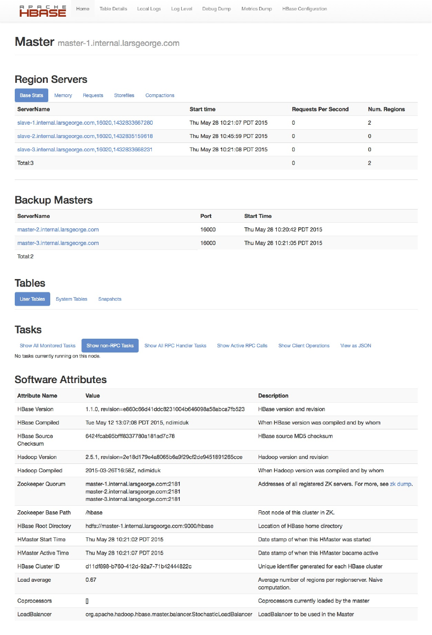
Figure 6-4. The HBase Master user interface
(493)
First we will look into the various parts of the page at a high level, followed by a more detailed
description in the subsequent sections. The details of the main Master UI page can be broken up
into the following groups:
Shared Header
At the very top there is a header with hyperlinks that is shared by many pages of the
HBase UIs. They contain references to specific subpages, such as Table Details, plus
generic pages that dump logs, let you set the logging levels, and dump debug, metric, and
configuration details.
Warnings
Optional — In case there are some issues with the current setup, there are optional warning
messages displayed at the very top of the page.
Region Servers
Lists the actual region servers the master knows about. The table lists the address, which
you can click on to see more details. The tabbed table is containing additional useful
information about each server, grouped by topics, such as memory, or requests.
Dead Region Servers
Optional — This section only appears when there are servers that have previously been
part of the cluster, but are now considered dead.
Backup Masters
This section lists all configured and started backup master servers. It is obviously empty if
you have none of them.
Tables
Lists all the user and system tables HBase knows about. In addition it also lists all known
snapshots of tables.
Regions in Transition
Optional — Any region that is currently in change of its state is listed here. If there is no
region that is currently transitioned by the system, then this entire section is omitted.
Tasks
The next group of details on the master’s main page is the list of currently running tasks.
Every internal operation performed by the master, such as region or log splitting, is listed
here while it is running, and for another minute after its completion.
Software Attributes
You will find cluster-wide details in a table at the bottom of the page. It has information on
the version of HBase and Hadoop that you are using, where the root directory is located,
the overall load average, and so on.
(494)
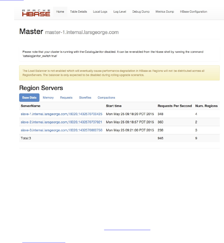
As mentioned above, we will discuss each of them now in that same order in the next sections.
Warning Messages
As of this writing, there are three checks the Master UI page performs and reports on, in case a
violation is detected: the JVM version, as well as the catalog janitor and balancer status.
Figure 6-5 shows the latter two of them.
Figure 6-5. The optional Master UI warnings section
There are certain Java versions that are known to cause issues when used to run HBase. Again, as
of this writing, the only known bad version is 1.6.0_18, which was unstable. This might be
extended in the future, if more troublesome Java versions are detected. If the test is finding such
a blacklisted JVM version a message is displayed at the very top of the page, just below the
header, stating: “Your current JVM version <version> is known to be unstable with HBase.
Please see the HBase wiki for details.”
The other two tests performed are more about the state of background operations, the so-called
chores. First the catalog janitor, explained in “Server Operations”, which is required to keep a
HBase cluster clean. If you disable the janitor process with the API call, or the shell command
shown in “Tool Commands”, you will see the message in the Master UI page as shown in the
screen shot. It reminds you to enable it again some time soon.
The check for the balancer status is very similar, as it checks if someone has deactivated the
background operation previously, and reminds you to re-enable it in the future — or else your
cluster might get skewed as region servers join or leave the collective.
(495)
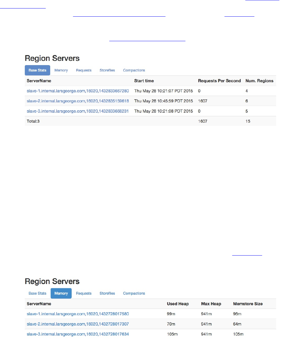
Region Servers
The region server section of the Master UI page is divided into multiple subsections, represented
as tabs. Each shows a set of information pertaining to a specific topic. The first tab is named
Base Stats and comprises generic region server details, such as the server name (see “Server and
Region Names” again for details), that also acts as a hyperlink to the dedicated region server
status page, explained in “Region Server UI Status Page”. The screen shot in Figure 6-6 lists
three region servers, named slave-1 to slave-3. The table also states, for each active region
server, the start time, number of requests per second observed in the last few seconds (more on
the timing of metrics can be found in “The Metrics Framework”), and number of regions hosted.
Figure 6-6. The region server section on the master page - Base Stats
Note
Please observe closely in the screen shot how there is one server, namely slave-2, that seems to
receive all the current requests only. This is—if sustained for a long time—potentially a problem
called hotspotting. We will use this later to show you how to identify which table is causing this
imbalance.
The second tab contains memory related details. You can see the currently used heap of the Java
process, and the configured maximum heap it may claim. The memstore size states the
accumulated memory occupied by all in-memory stores on each server. It can act as an indicator
of how many writes you are performing, influenced by how many regions are currently opened.
As you will see in [Link to Come], each table is at least one region, and each region comprises
one or more column families, with each requiring a dedicated in-memory store. Figure 6-7 shows
an example for our current cluster with three region servers.
Figure 6-7. The region server section on the master page - Memory
Note
(496)
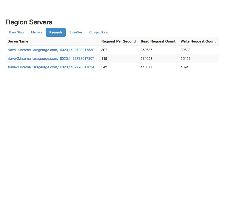
It is interesting to note that the used heap is close or even equal to the memstore size, which is
really only one component of the Java heap used. This can be attributed to the size metrics being
collected at different points in time and should therefore only be used as an approximation.
The third tab, titled Requests, contains more specific information about the current number of
requests per second, and also the observed total read request and write request counts,
accumulated across the life time of the region server process. Figure 6-8 shows another example
of the same three node cluster, but with an even usage.
Figure 6-8. The region server section on the master page - Requests
The Storefiles tab, which is the number four, shows information about the underlying store files
of each server. The number of stores states the total number of column families served by that
server—since each column family internally is represented as a store instance. The actual
number of files is the next column in the table. Once the in-memory stores have filled up (or the
dedicated heap for them is filled up) they are flushed out, that is, written to disk in the store they
belong to, creating a new store file.
Since each store file is containing the actual cells of a table, they require the most amount of disk
space as far as HBase’s storage architecture is concerned. The uncompressed size states their size
before any file compression is applied, but including any per-column family encodings, such as
prefix encoding. The storefile size column then contains the actual file size on disk, that is, after
any optional file compression has been applied.
Each file also stores various indexes to find the cells contained, and these indexes require storage
capacity too. The last two columns show the size of the block and Bloom filter indices, as
currently held in memory for all open store files. Dependent on how you compress the data, the
size of your cells and file blocks, this number will vary. You can use it as an indicator to estimate
the memory needs for your server processes after running your workloads for a while. Figure 6-9
shows an example.
(497)
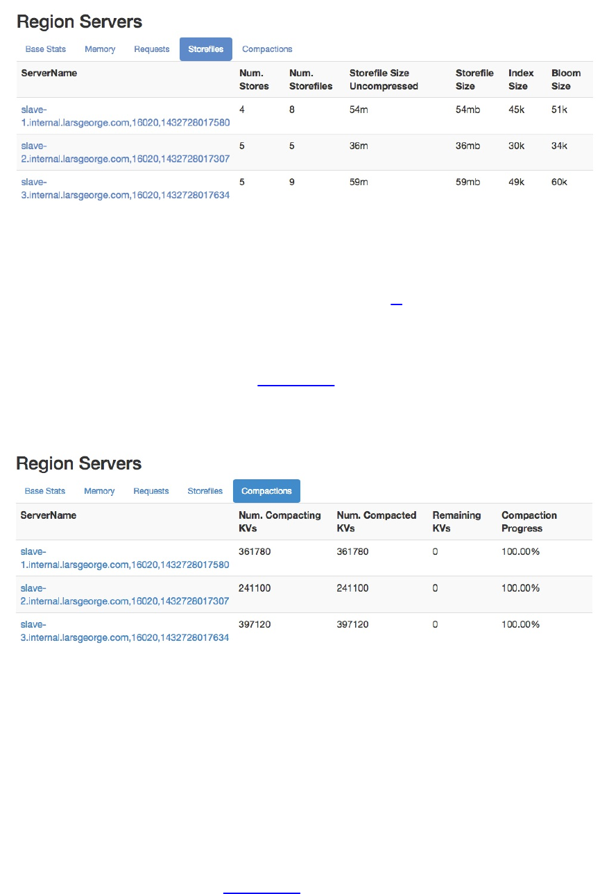
Figure 6-9. The region server section on the master page - Storefiles
The fifth and final tab shows details about compactions, which are one of the background
housekeeping tasks a region server is performing on your behalf.16 The table lists the number of
current cells that have been scheduled for compactions. The number of compacted cells trails the
former count, as each of them is processed by the server process. The remaining cells is what is
left of the scheduled cells, counting towards zero. Lastly, the compaction progress shows the
scheduled versus remaining as a percentage. Figure 6-10 shows that all compactions have been
completed, that is, nothing is remaining and therefore we reached 100% of the overall
compaction progress.
Figure 6-10. The region server section on the master page - Compactions
As a cluster is being written to, or compactions are triggered by API or shell calls, the
information in this table will vary. The percentage will drop back down as soon as new cells are
scheduled, and go back to 100% as the background task is catching up with the compaction
queue.
Dead Region Servers
This is an optional section, which only appears if there is a server that was active once, but is
now considered inoperational, or dead. Figure 6-11 shows an example, which has all three of our
exemplary worker servers with a now non-operational process. This might happen if servers are
restarted, or crash. In both cases the new process will have a new, unique server name,
containing the new start time.
(498)
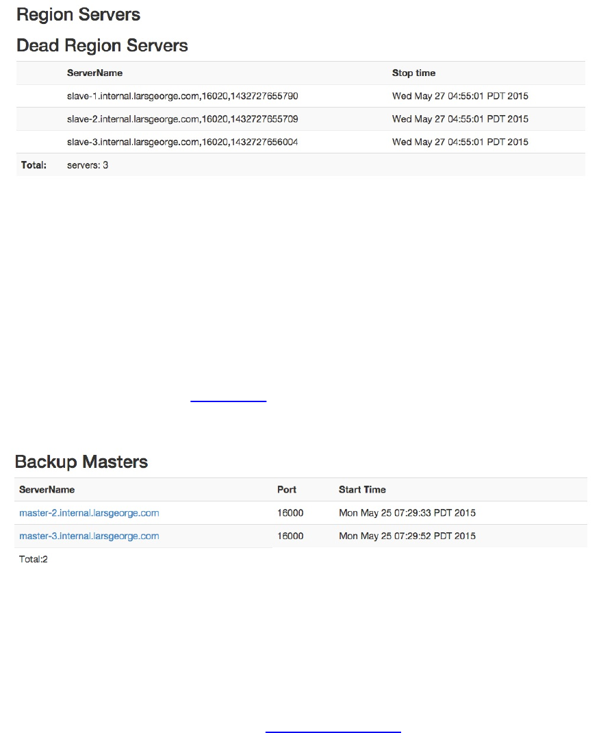
Figure 6-11. The optional dead region server section on the master page
If you have no such defunct process in your cluster, the entire section will be omitted.
Backup Masters
The Master UI page further lists all the known backup masters. These are HBase Master
processes started on the other servers. While it would be possible to start more than one Master
on the same physical machine, it is common to spread them across multiple servers, in case the
entire server becomes unavailable. Figure 6-12 shows an example where two more backup
masters have been started, on master-2 and master-3.
Figure 6-12. The backup master section on the Master page
The table has three columns, where the first has the hostname of the server running the backup
master process. The other two columns state the port and start time of that process. Note that the
port really is the RPC port, not the one for the information server. The server name acts as a
hyperlink to that said information server though, which means you can click on any of them to
open the Backup Master UI page, as shown in “Backup Master UI”.
Tables
The next major section on the Master UI page are the known tables and snapshots, comprising
user and system created ones. For that the Tables section is split into three tabs: User Tables,
System Tables, and Snapshots.
User Tables
Here you will see the list of all tables known to your HBase cluster. These are the ones you
—or your users—have created using the API, or the HBase Shell. The list has many
(499)
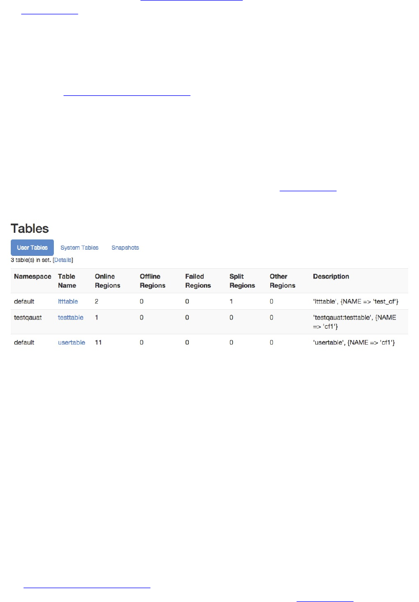
columns that state, for every user table, the namespace it belongs to, the name, region
count details, and a description. The latter gives you a printout of the table descriptor, just
listing the changed properties; see “Schema Definition” for an explanation of how to read
them. See Figure 6-13 for an example screen shot.
If you want more information about a user table, there are two options. First, next to the
number of user tables found, there is a link titled Details. It takes you to another page that
lists the same tables, but with their full table descriptors, including all column family
descriptions as well. Second, the table names are links to another page with details on the
selected table. See “Table Information Page” for an explanation of the contained
information.
The region counts holds more information about how the regions are distributed across the
tables, or, in other words, how many regions a table is divided into. The online regions
lists all currently active regions. The offline regions column should be always zero, as
otherwise a region is not available to serve its data. Failed regions is usually zero too, as it
lists the regions that could not be opened for some reason. See Figure 6-18 for an example
showing a table with a failed region.
Figure 6-13. The user tables
The split region count is the number of regions for which currently a log splitting process
is underway. They will eventually be opened and move the count from this column into the
online region one. Lastly, there is an other regions counter, which lists the number of
regions in any other state from the previous columns. [Link to Come] lists all possible
states, including the named and other ones accounted for here.
System Tables
This section list the all the catalog—or system—tables, usually hbase:meta and
hbase:namespace. There are additional, yet optional, tables, such as hbase:acl, hbase:labels,
and hbase:quota, which are created when the accompanying feature is enabled or used for
the first time. You can click on the name of the table to see more details on the table
regions—for example, on what server they are currently hosted. As before with the user
tables, see “Table Information Page” for more information. The final column in the
information table is a fixed description for the given system table. Figure 6-14 is an
example for a basic system table list.
(500)
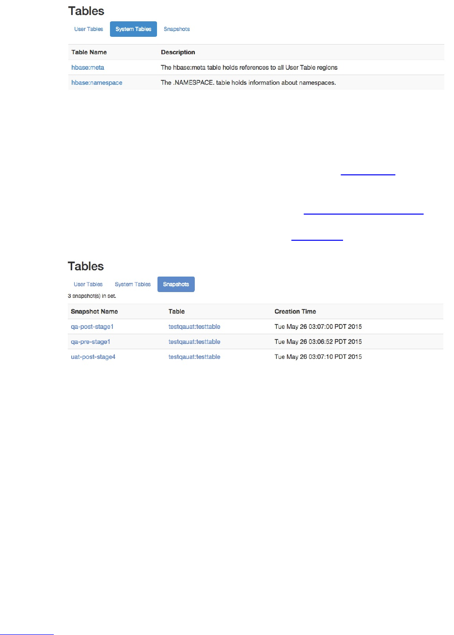
Figure 6-14. The system tables
Snapshots
The third and final tab available is listing all the known snapshots. Figure 6-15 shows an
example, with three different snapshots that were taken previously. It lists the snapshot
name, the table it was taken from, and the creation time. The table name is a link to the
table details page, as already seen earlier, and explained in “Table Information Page”. The
snapshot name links to yet another page, which lists details about the snapshot, and also
offers some related operations directly from the UI. See “Snapshot” for details.
Figure 6-15. The list of known snapshots
Optional Table Fragmentation Information
There is a way to enable an additional detail about user and system tables, called fragmentation.
It is enabled by adding the following configuration property to the cluster configuration file, that
is, hbase_site.xml:
<property>
<name>hbase.master.ui.fragmentation.enabled</name>
<value>true</value>
</property>
Once you have done so, the server will poll the storage file system to check how many store files
per store are currently present. If each store only has one file, for example, after a major
compaction of all tables, then the fragmentation amounts to zero. If you have more than a single
store file in a store, it is considered fragmented. In other words, not the amount of files matters,
but that there is more than one. For example, if you have 10 stores and 5 have more than one file
in them, then the fragmentation is 50%.
Figure 6-16 shows an example for a table with 11 regions, where 9 have more than one file, that
is, 9 divided by 11, and results in 0.8181 rounded up to 82%.
(501)
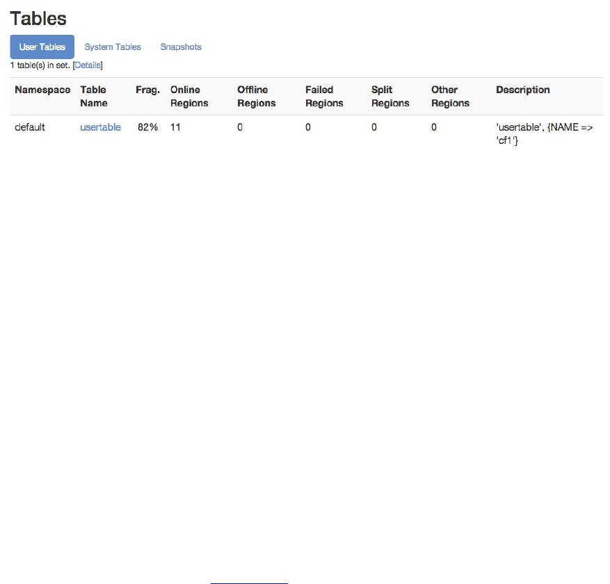
Figure 6-16. The optional table fragmentation information
Once enabled, the fragmentation is added to the user and system table information, and also to
the list of software attributes at the bottom of the page. The per-table information lists the
fragmentation for each table separately, while the one in the table at the end of the page is
summarizing the total fragmentation of the cluster, that is, across all known tables.
A word of caution about this feature: it polls the file system details on page load, which in a
cluster under duress might increase the latency of the UI page load. Because of this it is disabled
by default, and needs to be enabled explicitly.
Regions in Transition
As regions are managed by the master and region servers to, for example, balance the load across
servers, they go through short phases of transition. This applies to, for example, opening, closing,
and splitting a region. Before the operation is performed, the region is added to the list of regions
in transition, and once the operation is complete, it is removed. [Link to Come] describes the
possible states a region can be in.
When there is no region operation in progress, this section is omitted completely. Otherwise it
should look similar to the example in Figure 6-17, listing the regions with their encoded name,
the current state, and the time elapsed since the transition process started. As of this writing,
there is a hard limit of 100 entries being shown, since this list could be very large for larger
clusters. If that happens, then a message like “<N> more regions in transition not shown”,
where <N> is the number of omitted entries.
(502)
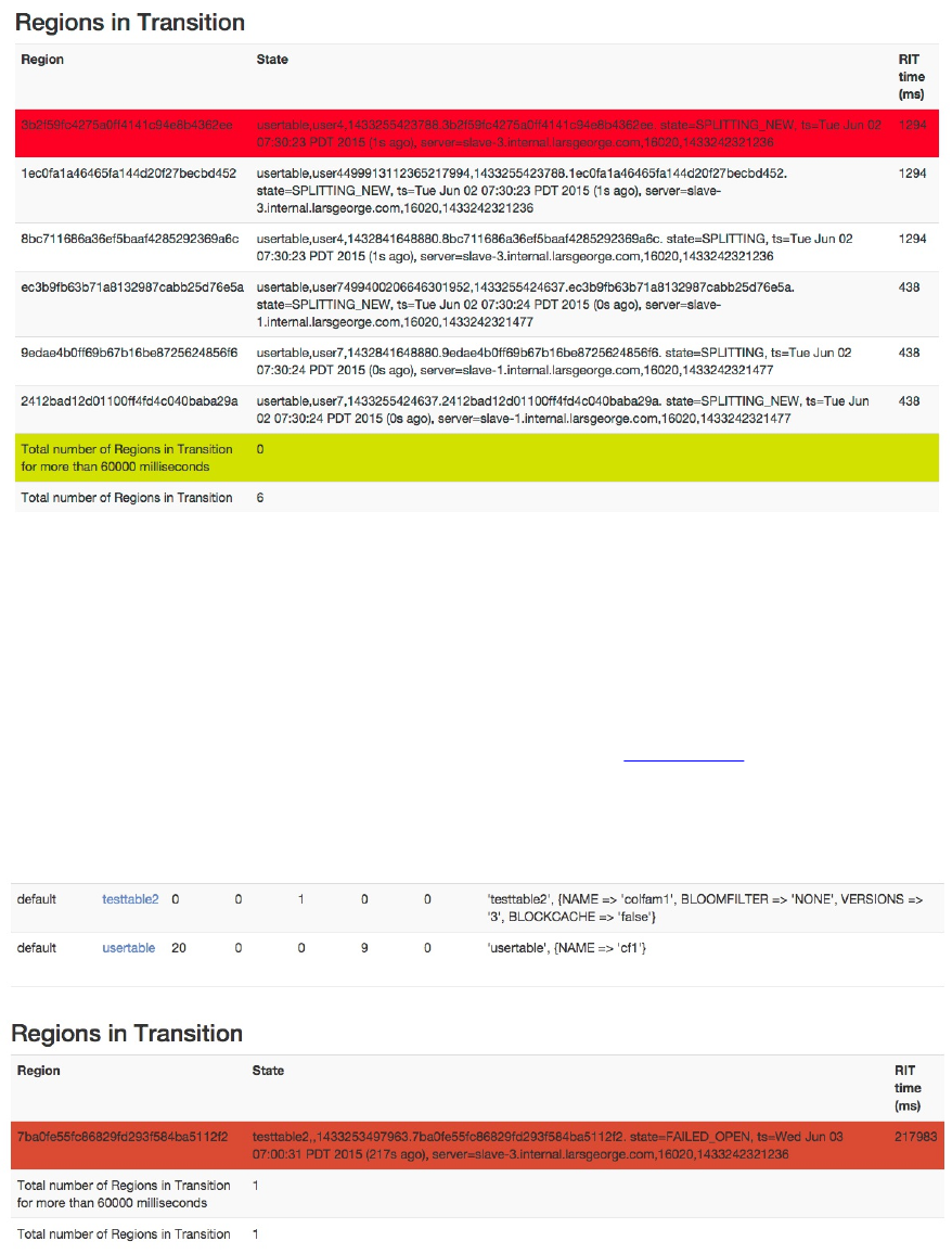
Figure 6-17. The regions in transitions table
Usually the regions in transition should be appearing only briefly, as region state transitioning is
a short operation. In case you have an issue that persists, you may see a region stuck in transition
for a very long time, or even forever. If that is the case there is a threshold (set by the
hbase.metrics.rit.stuck.warning.threshold configuration property and defaulting to one minute)
that counts those regions in excess regarding their time in the list. Figure 6-18 shows an example,
which was created by deliberately replacing a valid store file with one that was corrupt. The
server keeps trying to open the region for this table, but will fail until an operator either deletes
or repairs the file in question.
Figure 6-18. A failed region is stuck in the transition state
You will have noticed how the stuck region is counted in both summary lines, the last two lines
of the table. The screen shot also shows an example of a region counted into the failed regions in
the preceding user table list. In any event, the row containing the oldest region in the list (that is,
the one with the largest RIT time) is rendered with a red background color, while the first
summary row at the bottom of the table is rendered with a green-yellow background.
(503)
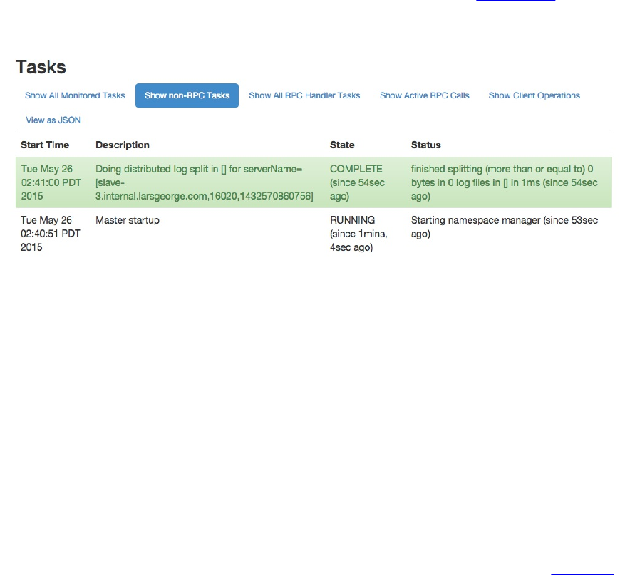
Tasks
HBase manages quite a few automated operations and background tasks to keep the cluster
healthy and operational. Many of these tasks involve a complex set of steps to be run through,
often across multiple, distributed sets of servers. These tasks include, for example, any region
operation, such as opening and closing them, or splitting the WAL files during a region recovery.
The tasks save their state so that they also can be recovered should the current server carrying out
one or more of the steps fail. The HBase UIs show the currently running tasks and their state in
the tasks section of their status pages.
Tip
The information about tasks applies to the UI status pages for the HBase Master and Region
Servers equally. In fact, they share the same HTML template to generate the content. The listed
tasks though are dependent on the type of server. For example, a get operation is only sent to the
region servers, not the master.
A row with a green background indicates a completed task, while all other tasks are rendered
with a white background. This includes entries that are currently running, or have been aborted.
The latter can happen when an operation failed due to an inconsistent state. Figure 6-19 shows a
completed and a running task.
Figure 6-19. The list of currently running, general tasks on the master
When you start a cluster you will see quite a few tasks show up and disappear, which is
expected, assuming they all turn green and age out. Once a tasks is not running anymore, it will
still be listed for 60 seconds, before it is removed from the UI.
The table itself starts out on the second tab, named non-RPC tasks. It filters specific tasks from
the full list, which is accessible on the first tab, titled all monitored tasks. The next two tabs filter
all RPC related tasks, that is, all of them, or only the active ones respectively. The last tab is
named view as JSON and returns the content of the second tab (the non-RPC tasks) as a JSON
structure. It really is not a tab per-se since it replaces the entire page with just the JSON output.
Use the browsers back button to return to the UI page.
The difference between RPC and non-RPC tasks is their origin. The former originate from a
remote call, while the latter are something triggered directly within the server process. Figure 6-
(504)
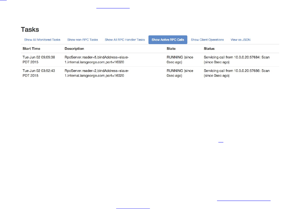
20 shows two RPC tasks, which also list their origin, that is, the remote client that invoked the
task. The previous screen shot in Figure 6-19 differs from this one, as the displayed tasks are
non-RPC ones, like the start of the namespace manager, and therefore have no caller info.
Figure 6-20. The list of currently running RPC tasks on the master
Software Attributes
This section of the Master UI status page lists cluster wide settings, such as the installed HBase
and Hadoop versions, the root ZooKeeper path and HBase storage directory17, and the cluster ID.
The table lists the attribute name, the current value, and a short description. Since this page is
generated on the current master, it lists what it assumes to be the authoritative values. If you have
some misconfiguration on other servers, you may be misled by what you see here. Make sure
you cross-check the attributes and settings on all servers.
The table also lists the ZooKeeper quorum used, which has a link in its description allowing you
to see the information for your current HBase cluster stored in ZooKeeper. “ZooKeeper page”
discusses its content. The screen shot in Figure 6-21 shows the current attributes of the test
cluster used throughout this part of the book.
(505)
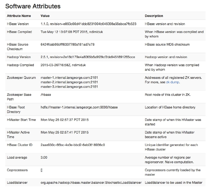
Figure 6-21. The list of attributes on the Master UI page
(506)

Master UI Related Pages
The following pages are related to the Master UI page, as they are directly linked from it. This
includes the detailed table, table information, and snapshot information pages.
Backup Master UI
If you have more than one HBase Master process started on your cluster (for more on how to do
that see “Fully Distributed Cluster”), then the active Master UI will list them. Each of the server
names is a link to the respective backup master, providing its dedicated status page, as shown in
Figure 6-22. The content of each backup master is pretty much the same, since they do nothing
else but wait for a chance to take over the lead. This happens of course only if the currently
active master server disappears.
At the top the page links to the currently active master, which makes it easy to navigate back to
the root of the cluster. This is followed by the list of tasks, as explained in “Tasks”, though here
we will only ever see one entry, which is the long running tasks to wait for the master to
complete its startup—which is only happening in the above scenario.
(507)
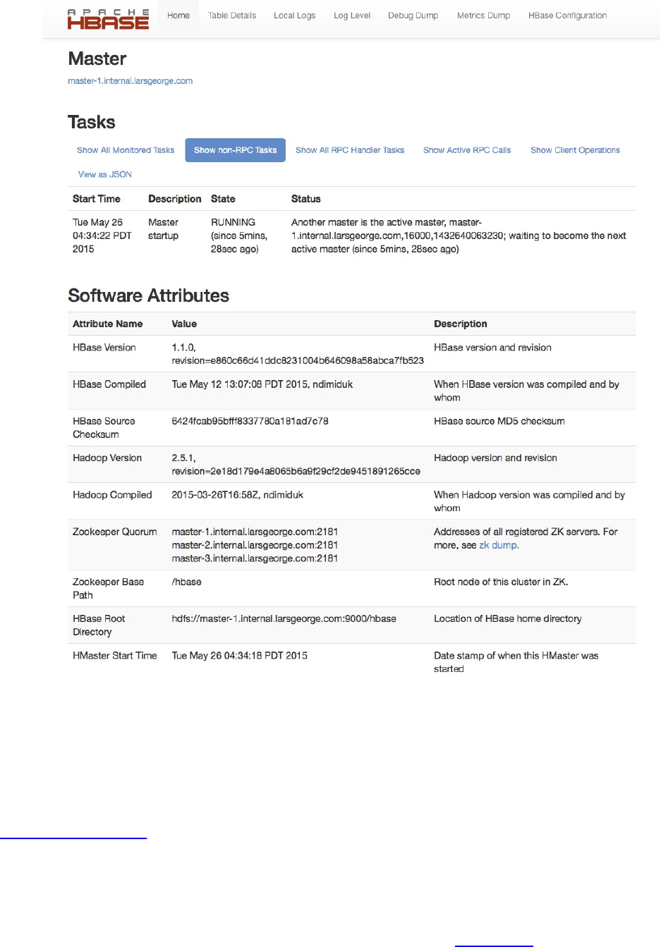
Figure 6-22. The backup master page
The page also lists an abbreviated list of software attributes. It is missing any current values,
such as the loaded coprocessors, or the region load. These values are only accessible when the
master process is started fully and active. Otherwise you have seen the list of attributes before, in
“Software Attributes”.
Table Information Page
When you click on the name of a user or system table in the master’s web-based user interface,
you have access to the information pertaining to the selected table. Figure 6-23 shows an
example of a user table.
(508)
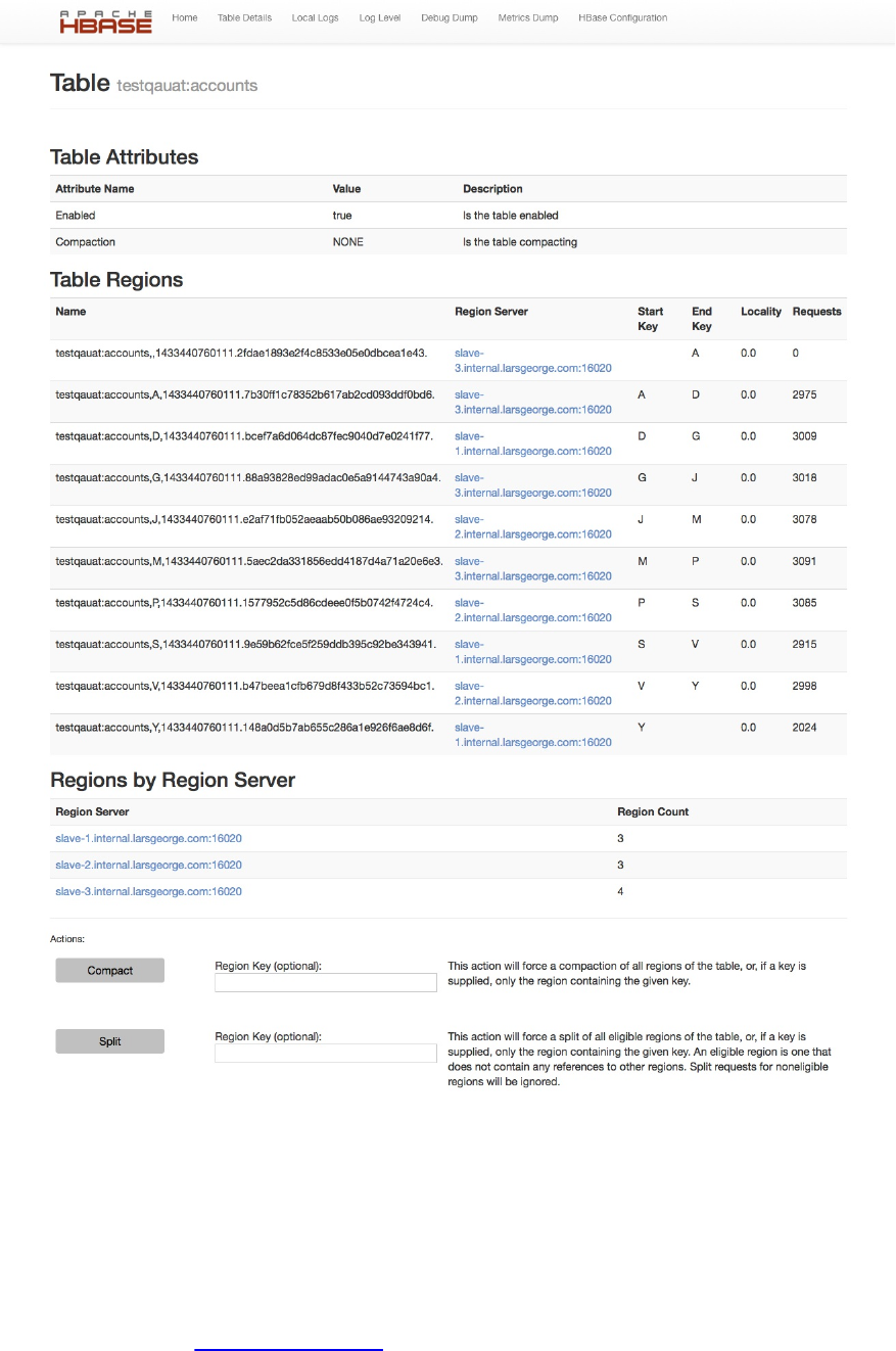
Figure 6-23. The Table Information page with information about the selected table
The following groups of information are available on the Table Information page:
Table Attributes
Here you can find details about the table itself. First, it lists the table status, that is, if it is
enabled or not. See “Table Operations”, and the disableTable() call especially. The
boolean value states whether the table is enabled, so when you see a true in the Value
column, this is the case. On the other hand, a value of false would mean the table is
(509)

currently disabled.
Second, the table shows if there are any compactions currently running for this table. It
either states NONE, MINOR, MAJOR, MAJOR_AND_MINOR, or Unknown. The latter is
rare but might show when, for example, a table with a single region splits and no
compaction state is known to the Master for that brief moment. You may wonder how a
table can have a minor and major compaction running at the same time, but recall how
compactions are triggered per region, which means it is possible for a table with many
regions to have more than one being compacted (minor and/or major) at the same time.
Lastly, if you have the optional fragmentation information enabled, as explained in
“Optional Table Fragmentation Information”, you have a third line that lists the current
fragmentation level of the table.
Table Regions
This list can be rather large and shows all regions of a table. The name column has the
region name itself, and the region server column has a link to the server hosting the region.
Clicking on the link takes you to the page explained in “Region Server UI Status Page”.
+ The start key and end key columns show the region’s start and end keys as expected. The
locality column indicates, in terms of a percentage, if the storage files are local to the server
which needs it, or if they are accessed through the network instead. See “Cluster Status
Information” and the getDataLocality() call for details
+ Finally, the requests column shows the total number of requests, including all read (get, scan,
etc.) and write (put, delete, etc.) operations, since the region was deployed to the hosting server.
Regions by Region Server
The last group on the Table Information page lists which region server is hosting how
many regions of the selected table. This number is usually distributed evenly across all
available servers. If not, you can use the HBase Shell or administrative API to initiate the
balancer, or use the move command to manually balance the table regions (see “Cluster
Operations”).
By default, the Table Information page also offers some actions that can be used to trigger
administrative operations on a specific region, or the entire table. These actions can be hidden by
setting the hbase.master.ui.readonly configuration property to true. See “Cluster Operations”
again for details about the actions, and “Region Split Handling” for information on when you
want to use them. The available operations are:
Compact
This triggers the compact functionality, which is asynchronously running in the
background. Specify the optional name of a region to run the operation more selectively.
The name of the region can be taken from the table above, that is, the entries in the name
column of the Table Regions table.
Note
Make sure to copy the entire region name as-is. This includes the trailing "." (the dot)!
(510)
If you do not specify a region name, the operation is performed on all regions of the table
instead.
Split
Similar to the compact action, the split action triggers the split command, operating on a
table or region scope. Not all regions may be splittable—for example, those that contain
no, or very few, cells, or one that has already been split, but which has not been compacted
to complete the process.
Once you trigger one of the operations, you will receive a confirmation page; for example, for a
split invocation, you will see:
As directed, use the Back button of your web browser, or simply wait a few seconds, to go back
to the previous page, showing the table information.
ZooKeeper page
This page shows the same information as invoking the zk_dump command of the HBase Shell. It
shows you the root directory HBase is using inside the configured filesystem. You also can see
the currently assigned master, the known backup masters, which region server is hosting the
hbase:meta catalog table, the list of region servers that have registered with the master, replication
details, as well as ZooKeeper internal details. Figure 6-24 shows an exemplary output available
on the ZooKeeper page (abbreviated for the sake of space).
(511)
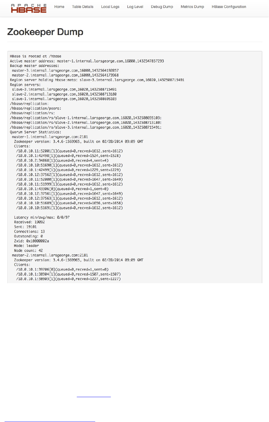
Figure 6-24. The ZooKeeper page, listing HBase and ZooKeeper details
While you will rarely use this page, which is linked to from the Master UI page, it is useful in
case your cluster is unstable, or you need to reassure yourself of its current configuration and
state. The information is very low-level in parts, but as you grow more accustomed to HBase and
how it is operated, the values reported might give you clues as to what is happening inside the
cluster.
Snapshot
Every snapshot name, listed on the Master UI status page, is a link to a dedicated page with
information about the snapshot. Figure 6-25 is an example screen shot, listing the table it was
taken from (which is a link back to the table information page), the creation time, the type of
snapshot, the format version, and state. You can refresh your knowledge about the meaning of
each in “Table Operations: Snapshots”.
(512)
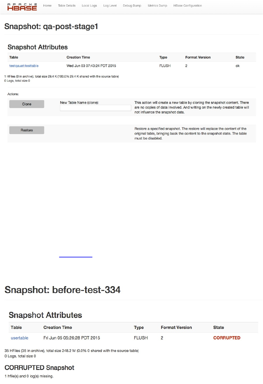
Figure 6-25. The snapshot details page
The page also shows some information about the files involved in the snapshot, for example:
36 HFiles (20 in archive), total size 250.9 M (45.3% 113.7 M shared with the source table)
0 Logs, total size 0
Here we have 36 storage files in the snapshot, and 20 of those are already replaced by newer
files, which means they have been archived to keep the snapshot consistent. Should you have had
any severe issues with the cluster and experienced data loss, it might happen that you see
something similar to what Figure 6-26 shows. The snapshot is corrupt because a file is missing
(which I have manually removed to just to show you this screen shot—do not try this unless you
know what you are doing), as listed in the CORRUPTED Snapshot section of the page.
Figure 6-26. A corrupt snapshot example
(513)
There are also actions you can perform—assuming you have not disabled them using the
hbase.master.ui.readonly configuration property as explained—based on the currently displayed
snapshot. You can either clone the snapshot into a new table, or restore it by replacing the
originating table. Both actions will show a confirmation message (or an error in case something
is wrong, for example, when specifying a non-existent namespace for a new table), similar to
this:
More elaborate functionality is only available through the API, which is mostly exposed through
the HBase Shell (as mentioned, see “Table Operations: Snapshots”).
(514)

Region Server UI Status Page
The region servers have their own web-based UI, which you usually access through the master
UI, by clicking on the server name links provided. You can access the page directly by entering
http://<region-server-address>:16030
into your browser (while making sure to use the configured port, here using the default of 16030).
Main page
The main page of the region servers has details about the server, the tasks it performs, the regions
it is hosting, and so on. Figure 6-27 shows an example of this page.
(515)
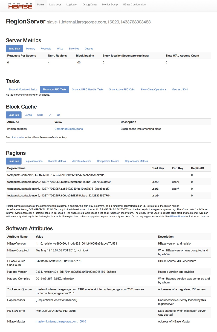
(516)

Figure 6-27. The Region Server main page
The page can be broken up into the following groups of distinct information, which we will—if
they have not been explained before—discuss in detail in the subsequent sections:
Server Metrics
First, there are statistics about the current state of the server, its memory usage, number of
requests observed, and more.
Tasks
The table lists all currently running tasks, as explained in “Tasks”. The only difference is
that region servers will work on different tasks compared to the master. The former are
concerned about data and region operations, while the latter will manage the region servers
and WALs, among many other things.
Block Cache
When data is read from the storage files, it is loaded in blocks. These are usually cached
for subsequent use, speeding up the read operations. The block cache has many
configuration options, and dependent on those this part of the region server page will vary
in its content.
Regions
Here you can see all the regions hosted by the currently selected region server. The table
has many tabs that contain basic information, as well as request, store file, compaction,
and coprocessor metrics.
Software Attributes
This group of information contains, for example, the version of HBase you are running,
when it was compiled, the ZooKeeper quorum used, server start time, and a link back to
the active HBase Master server. The content is self-explanatory, has a description column,
and is similar to what was explained in “Software Attributes”.
Server Metrics
The first part on the status page of a region server relates to summary statistics about the server
itself. This includes the number of region it holds, the memory used, client requests observed,
number of store files, WALs, and length of queues. Figure 6-28 combines them all into one
screen shot since they are all very short.
Note
Many of the values are backed by the server metrics framework (see “The Metrics Framework”)
and do refresh on a slower cadence. Even if you reload the page you will see changes only every
now and so often. The metrics update period is set by the hbase.regionserver.metrics.period
configuration property and defaults to 5 seconds. Metrics collection is a complex process, which
means that even with an update every 5 seconds, there are some values which update at a slower
(517)

rate. In other words, use the values displayed with caution, as they might trail the actual current
values.
The first tab, named base stats, lists the most high level details, so that you can have a quick
glimpse at the overall state of the process. It lists the requests per second, the number of region
hosted, the block locality percentage, the same for the replicas—if there are any--, and the
number of slow WAL append operations. The latter is triggered if writing to the write-ahead log
is delayed for some reason (most likely I/O pressure).18
(518)
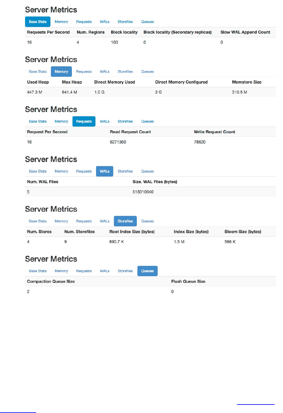
Figure 6-28. All tabs in the Server Metrics section
The second tab, titled memory, shows details of the currently used memory, both on-heap and
off-heap. If shows the current and maximum configured Java heap, and the same for the off-heap
memory, called direct memory. All of these are configured in the cluster-wide hbase-env.sh
configuration file for the Java process environment. The tab also lists the current combined
memory occupied by the all the in-memory stores hosted by this server. The region statistics
further down the page shows them separately.
The third tab is called requests and shows the combined, server-wide number of requests per
second served, and the total read and write request counts since the server started. The request
per seconds are over the configured time to collect metrics, which is explained in “The Metrics
Framework”.
(519)
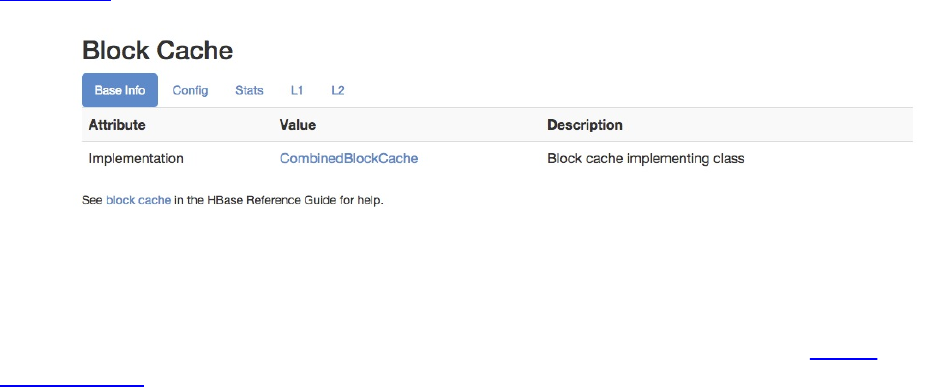
The tab named WALs lists write-ahead log metrics, here the number of WALs this server is
keeping around for recovery purposes. It also lists the combined size of these files, as occupied
on the underlying storage system.
Next is the store files tab, which lists information about the actual storage files. First the number
of stores is stated, currently served by this region server. Since a store can have zero to many
storage files, the next columns list the number of store files, plus their combined sizes regarding
the various indices contained in them. There are the root index, and the total index sizes, both
addressing the block index structure. The root index points to blocks in the overall block index,
and therefore is much smaller. Only the root index is kept in memory, while the block index
blocks are loaded and cached on demand. There is also the Bloom filter, which—if enabled for
the column family—is occupying space in the persisted store files. The value state in the table is
the combined size as needed for all the store files together. Note that it is cached on demand too,
so not all of that space is needed in memory.
The last and sixth tab titled queues lists the current size of the compaction and flush queues.
These are vital resources for a region server, and a high as well as steadily increasing queue size
indicates that the server is under pressure and has difficulties to keep up with the background
housekeeping tasks.
Block Cache
The first tab, named base info, lists the selected cache implementation class, as shown in
Figure 6-29.
Figure 6-29. The base info of the Block Cache section
The block cache was configured as a combined cache, which uses the purely in-memory LRU
cache as L1 (first level) cache, and the bucket cache as L2 (second level) cache (see “Block
Cache Tuning”). The LRU cache is set to use 20% of the maximum Java heap, not the default
40%. The block cache is configured as an off-heap cache, set to 1 GB, using the following
configuration settings:
<property>
<name>hbase.bucketcache.combinedcache.enabled</name>
<value>true</value>
</property>
<property>
<name>hfile.block.cache.size</name>
<value>0.2</value>
</property>
<property>
<name>hbase.bucketcache.ioengine</name>
<value>offheap</value>
</property>
<property>
<name>hbase.bucketcache.size</name>
(520)
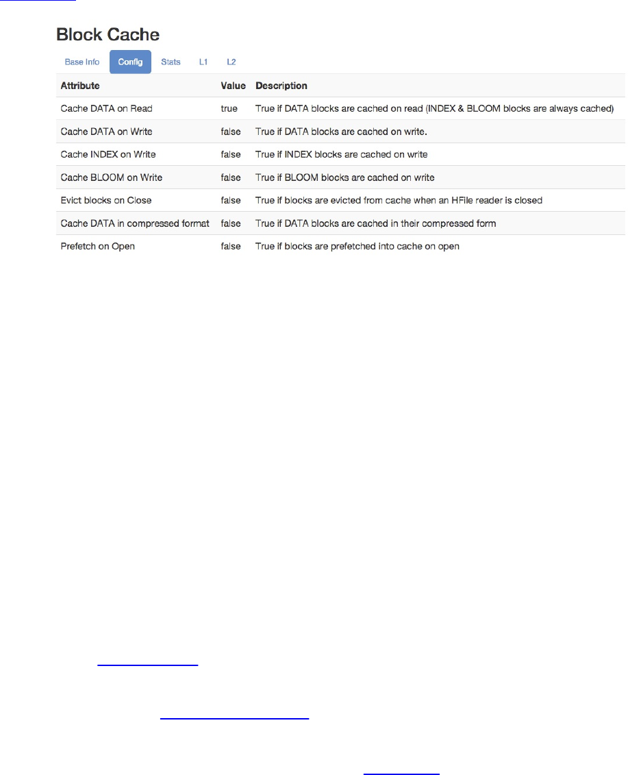
<value>1024</value>
</property>
The next tab shows the cluster wide configuration values, regarding the cache properties.
Figure 6-30 is an example screen shot.
Figure 6-30. The configuration tab of the Block Cache section
These values are set with the following configuration properties (see [Link to Come] for the
default values, their type, and description):
hfile.block.cache.size
hbase.rs.cacheblocksonwrite
hfile.block.index.cacheonwrite
hfile.block.bloom.cacheonwrite
hbase.rs.evictblocksonclose
hbase.block.data.cachecompressed
hbase.rs.prefetchblocksonopen
The first key, hfile.block.cache.size, sets the percentage used by the LRU cache, and if it is set
to 0% or less, the cache is completely disabled. In practice it is very unlikely that you would ever
go that far, since without any caching the entire I/O is purely based on the backing storage. Even
with SATA SSDs or PCIe flash memory cards, the incumbent x86-64 based architecture can
operate on DRAM a magnitude faster in comparison.
Note
With HBase 1.0 and later, there is now an option to specify ranges for the block cache size.
Please refer to “Heap Tuning” for details.
The majority of these options are turned off, which means you need to deliberately turn them on
within your cluster. See “Block Cache Tuning” for an in-depth discussion of cache
configurations. The next tab is titled statistics, and shows the overall cache state. Since there are
quite a few options available to configure the block cache, that is, with L1 only, or L1 and L2
together, the statistics combine the values if necessary. Figure 6-31 shows an example.
(521)
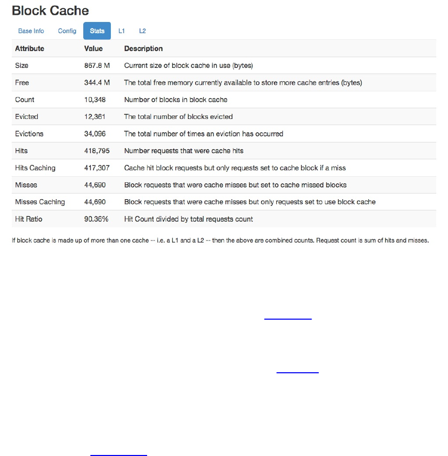
Figure 6-31. The statistics tab of the Block Cache section
As with many of the values the status pages show, you can access them in various ways. Here,
for example, you can also use the metrics API, explained in Chapter 9. The advantage of the
web-based UI pages is that they can nicely group the related attributes, format their value
human-readable, and add a short description for your perusal.
The screen shot was taken during a load test using YCSB (see “YCSB”). After the test table was
filled with random data, a subsequent read load-test was executed (workload B or C). You might
see with some of the statistics the expected effect, for example, the L1 being 100% effective,
because with a combined cache configuration, the L1 only caches index data, which fits easily
into the in-memory space for our test setup. This is also the reason that we decreased the
dedicated heap space allocated for the on-heap LRU cache—it is not needed and the space can be
used for other purposes. Figure 6-32 shows this on the next tab, titled L1.
(522)
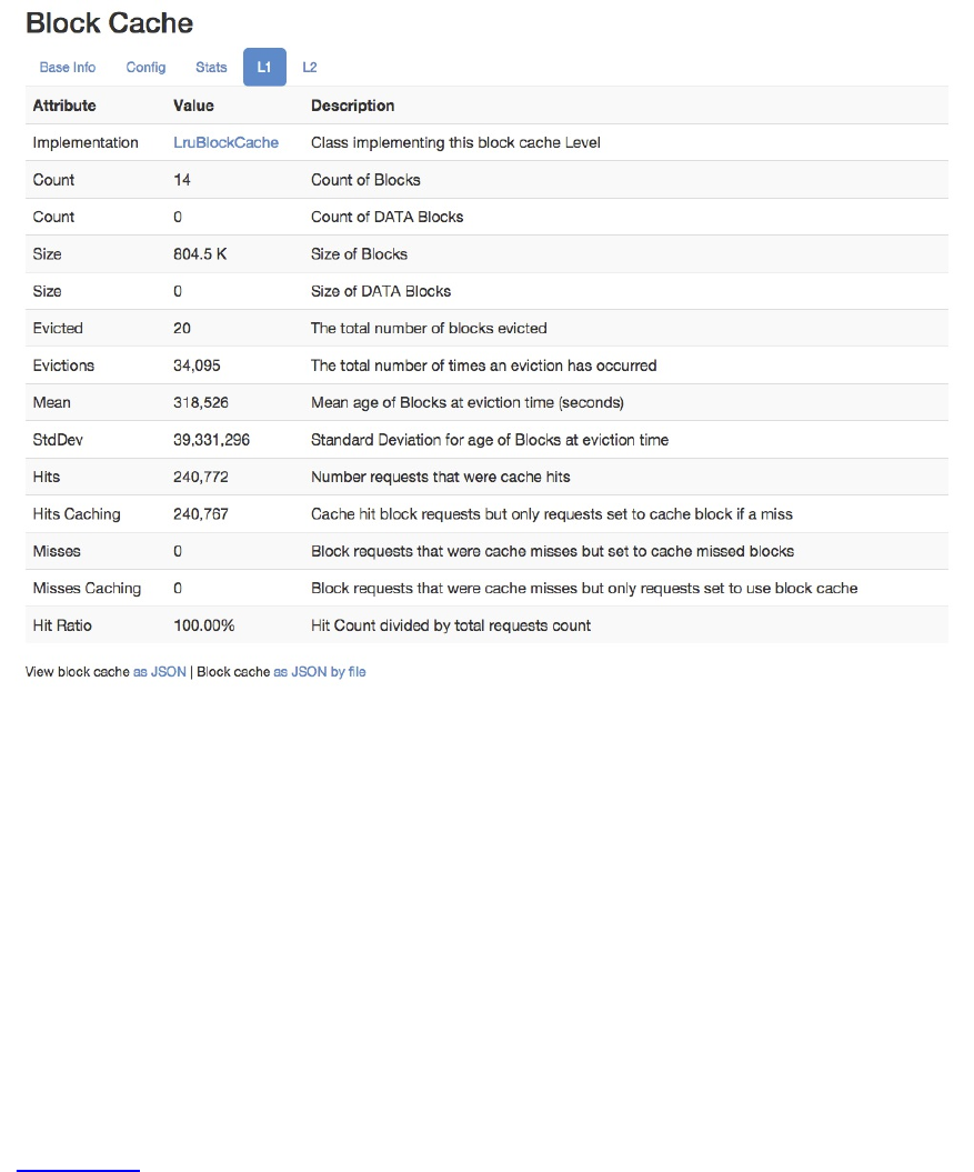
Figure 6-32. The L1 tab of the Block Cache section
The tab lists again many attributes, their values, and a short description. From these values you
can determine the amount of blocks cached, divided into all blocks and data blocks respectively.
Since we are not caching data blocks in L1 with an active L2, the count states the index blocks
only. Same goes for the size of these blocks. There are further statistics, such as the number of
evicted blocks, and the number of times an eviction check has run. The mean age and standard
deviation lets you determine how long blocks stay in the cache before they are removed. This is
related to the churn on the cache, because the LRU cache evicts the oldest blocks first, and if
these are relatively young, you will have a high churn on the cache. The remaining numbers state
the hits (the total number, and only those that are part of requests that had caching enabled),
misses, and the ration between them.
The L2 cache is more interesting in this example, as it does the heavy lifting of caching all data
blocks. Figure 6-33 shows the matching screen shot in tab number five, labeled appropriately L2.
It contains a list similar to that of the L1 cache, showing attributes, their current values, and a
short description. The link in the first line of the table is pointing to the online API
documentation for the configured class, here a BucketCache instance. You can further see the
number of blocks cached, their total size, the same eviction details as before, and again the same
for hits, misses, and the ratio. Some extra info here are the hits per second and time per hit
values. They show how stressed the cache is and how quickly it can deliver contained blocks.
(523)
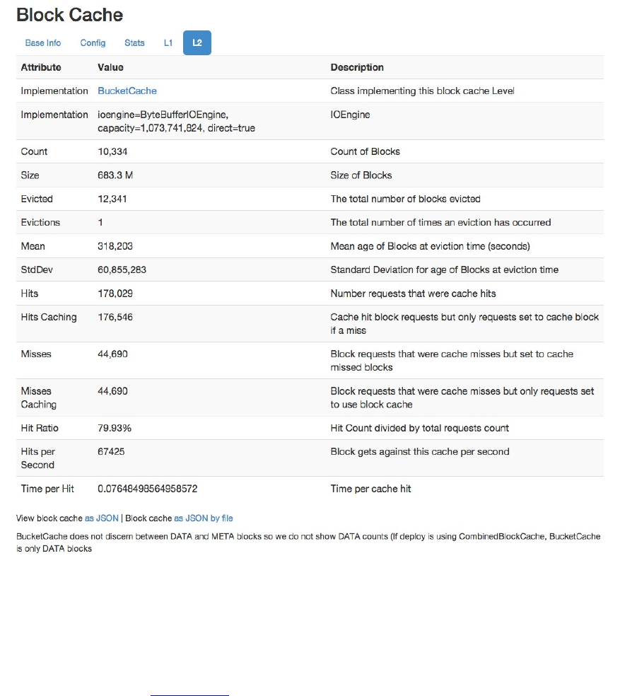
Figure 6-33. The L2 tab of the Block Cache section
When you switch the Block Cache section to the last tab, the L2 tab, you will be presented with
an additional section right below the Block Cache one, named bucketcache buckets, listing all the
buckets the cache maintains, and for each the configured allocation size, and the size of the free
and used blocks within. See Figure 6-34 for an example.
Note
The extra information section for the bucket cache only exists in few versions of HBase, between
1.0.0 and before 1.2.0. It was removed in the latter version as it could potentially produce
megabytes of output for large off-heap, or file based caches.
(524)
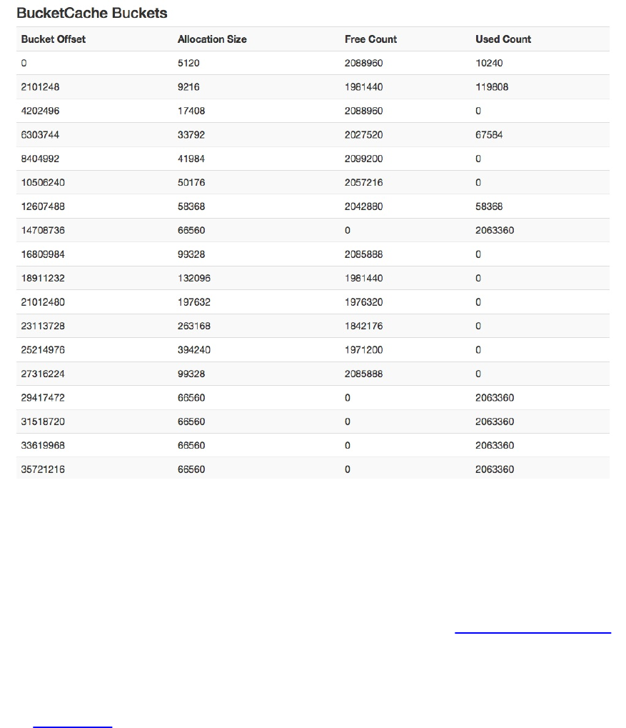
Figure 6-34. The extra bucket cache section
Since in this example the cache is configured to use 1 GB of off-heap memory, you see buckets
spreading from offset 0, all the way close to the maximum of 1073741824 bytes. The space is
divided equally based on the largest configured bucket size, and within each the space is divided
into blocks mentioned by the allocation size, which varies to be flexible when it comes to
assigning data to them. You can read more about this in aforementioned “Block Cache Tuning”.
Lastly, the Block Cache section has an additional as JSON link on some of the tabs, that lets you
access the summary statistics as a JSON structure. The content varies depending on the
configured cache implementation, including summary statistics as well as expanded details (if
available). Figure 6-35 shows an example JSON output. There is also another link, named as
JSON by file, which lists the summary statistics for all cached blocks, grouped by store files.
(525)
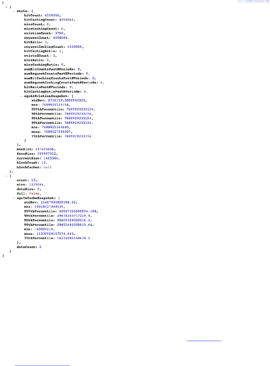
Figure 6-35. Output of cache metrics as JSON
Regions
The next major information section on the region server’s web-based UI status page is labeled
Regions, listing specific metrics for every region currently hosted by the server showing you its
status page. It has six tabs, with a lot of fine-grained data points, explained in order next. First is
the tab titled base info, showing you a brief overview of each region. Figure 6-36 has an
exemplary screen shot. You can see the region name, the start and end keys, as well as the
replica ID. The latter is a number different from zero if the region is a read replica. We will look
into this in “Region Replicas”.
(526)
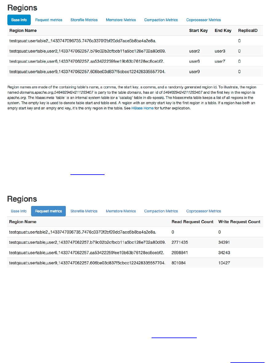
Figure 6-36. The regions details, basic information tab
The next tab, tab two titled request metrics, retains the region name column—all further tabs do
that, so they will not be mentioned again---but then prints the total read request, and write
request counts. These are accumulated in-memory on the region server, that is, restarting the
server will reset the counters. Figure 6-37 shows a screen shot where three regions of one table
are busy, while the remaining region from another has not been used at all.
Figure 6-37. The regions details, request metrics tab
Then there is the storefile metrics tab, number three, which lists the summary statistics about the
store files contained in each region. Recall that each store is equivalent to a column family, and
each can have zero (before anything was flushed) to many data files in them. The page also lists
the combined size of these files, both uncompressed and compressed, though the latter is optional
and here we see not much difference because of that (see “Compression” to learn more about
compression of data). The next two columns state the block index and Bloom filter size required
by all the store files in the given region. Lastly, you can see the data locality ratio, which is
expressed as a percentage from 0.0 to 1.0, meaning 0% to 100%. The screen shot in Figure 6-38
shows the four regions with their respective store file metrics.
(527)
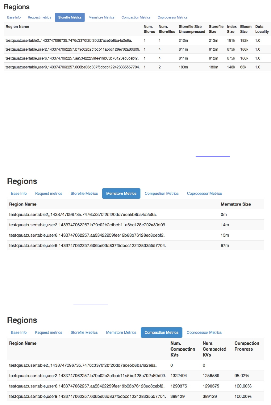
Figure 6-38. The regions details, storefile metrics tab
The fourth tab, named memstore metrics, lists the accumulated, combined amount of memory
occupied by the in-memory stores, that is, the Java heap backed structures keeping the mutations
(the put and delete records) before they are written to disk. The default flush size is 128 MB,
which means the sizes shown in this tab—assuming for a second that you have only one
memstore—should grow from 0m (zero megabyte) to somewhere around 128m and then after being
flushed in the background drop back down to zero. If you have more than one memstore then
you should expect the upper boundary to be a multiple of the flush size. Figure 6-39 shows an
example.
Figure 6-39. The regions details, memstore metrics tab
On tab five, the compaction metrics shows the summary statistics about the cells currently
scheduled for compaction, the number of cells that has been already compacted, and a progress
percentage. The screen shot in Figure 6-40 shows an example.
Figure 6-40. The regions details, compaction metrics tab
(528)
Finally, the sixth tab, named coprocessor metrics, displays the time spent in each coprocessor
that was invoked for any hosted region. As an example, the online code repository for this book
includes a coprocessor that does add a generated ID into each record that is written. Example 6-4
shows the code, which, when you read it carefully, also shows how the callback for prePut() is
artificially delaying the call. We just use this here to emulate a heavier processing task embedded
in a coprocessor.
Example 6-4. Adds a coprocessor local ID into the operation
private static String KEY_ID = "X-ID-GEN";
private byte[] family;
private byte[] qualifier;
private String regionName;
private Random rnd = new Random();
private int delay;
@Override
public void start(CoprocessorEnvironment e) throws IOException {
if (e instanceof RegionCoprocessorEnvironment) {
RegionCoprocessorEnvironment env = (RegionCoprocessorEnvironment) e;
Configuration conf = env.getConfiguration();
this.regionName = env.getRegionInfo().getEncodedName();
String family = conf.get("com.larsgeorge.copro.seqidgen.family", "cf1");
this.family = Bytes.toBytes(family);
String qualifier = conf.get("com.larsgeorge.copro.seqidgen.qualifier",
"GENID");
this.qualifier = Bytes.toBytes(qualifier);
int startId = conf.getInt("com.larsgeorge.copro.seqidgen.startId", 1);
this.delay = conf.getInt("com.larsgeorge.copro.seqidgen.delay", 100);
env.getSharedData().putIfAbsent(KEY_ID, new AtomicInteger(startId));
} else {
LOG.warn("Received wrong context.");
}
}
@Override
public void stop(CoprocessorEnvironment e) throws IOException {
if (e instanceof RegionCoprocessorEnvironment) {
RegionCoprocessorEnvironment env = (RegionCoprocessorEnvironment) e;
AtomicInteger id = (AtomicInteger) env.getSharedData().get(KEY_ID);
LOG.info("Final ID issued: " + regionName + "-" + id.get());
} else {
LOG.warn("Received wrong context.");
}
}
@Override
public void prePut(ObserverContext<RegionCoprocessorEnvironment> e, Put put,
WALEdit edit, Durability durability) throws IOException {
RegionCoprocessorEnvironment env = e.getEnvironment();
AtomicInteger id = (AtomicInteger) env.getSharedData().get(KEY_ID);
put.addColumn(family, qualifier, Bytes.toBytes(regionName + "-" +
id.incrementAndGet()));
try {
Thread.sleep(rnd.nextInt(delay));
} catch (InterruptedException e1) {
e1.printStackTrace();
}
}
Get environment and configuration instances.
(529)
Retrieve the settings passed into the configuration.
Set up generator if this has not been done yet on this region server.
Log the final number generated by this coprocessor.
Set the shared ID for this instance of put.
Sleep for 0 to “delay” milliseconds.
After compiling the project (see [Link to Come]), the generated JAR file is placed into the
/opt/hbase-book directory on the test cluster used throughout this section. We can then add the
coprocessor to one of the test tables, here one that is used with YCSB (see “YCSB”), so that
during a load test we can measure the impact of the callback. The class is added using the HBase
shell, and after running the load test, a scan is performed to print the generated IDs—here a
concatenation of the encoded region name and a shared, continuously increasing ID:
hbase(main):001:0> alter 'testqauat:usertable', \
METHOD => 'table_att', 'coprocessor' => \
'file:///opt/hbase-book/hbase-book-ch05-2.0.jar| \
coprocessor.SequentialIdGeneratorObserver|'
Updating all regions with the new schema...
1/11 regions updated.
11/11 regions updated.
Done.
0 row(s) in 3.5360 seconds
hbase(main):002:0> scan 'testqauat:usertable', \
{ COLUMNS => [ 'cf1:GENID' ], LIMIT => 2 }
ROW COLUMN+CELL
user1000257404909208451 column=cf1:GENID, timestamp=1433763441150, \
value=dcd5395044732242dfed39b09aa05c36-15853
user1000863415447421507 column=cf1:GENID, timestamp=1433763396342, \
value=dcd5395044732242dfed39b09aa05c36-14045
2 row(s) in 4.5070 seconds
While running the load test using YCSB (workload A) the example screen shot shown in
Figure 6-41 was taken. Since the coprocessor delays the processing between 1 and 100
milliseconds, you will find the values in the execution time statistics column reflect that closely.
For every region every active coprocessor is listed, and for each you will see the various timing
details, showing minimum, average, and maximum time observed. There is also a list of the 90th,
95th, and 99th percentile.
(530)
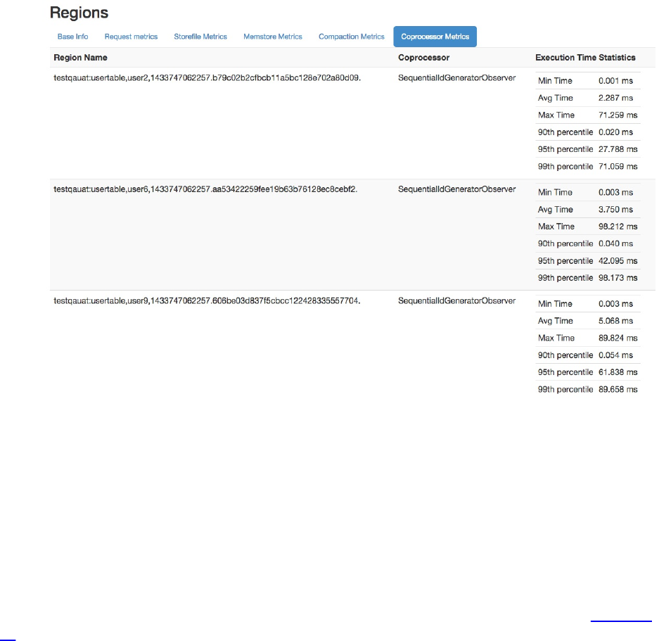
Figure 6-41. The regions details, coprocessor metrics tab
Software Attributes
This section of the Region Server UI status page lists cluster-wide settings, such as the installed
HBase and Hadoop versions, the ZooKeeper quorum, the loaded coprocessor classes, and more.
The table lists the attribute name, the current value, and a short description. Since this page is
generated on the current region server, it lists what it assumes to be the authoritative values. If
you have some misconfiguration on other servers, you may be misled by what you see here.
Make sure you cross-check the attributes and settings on all servers. The screen shot in Figure 6-
42 shows the current attributes of the test cluster used throughout this part of the book.
(531)
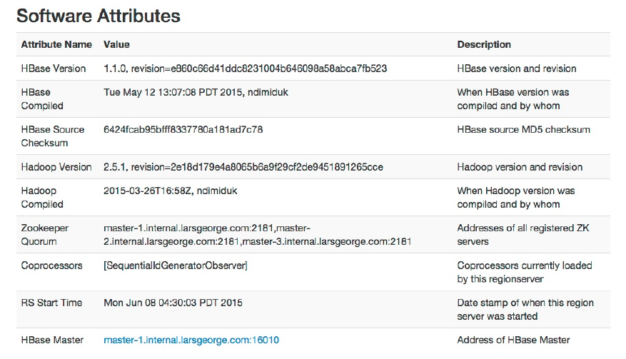
Figure 6-42. The list of attributes on the Region Server UI
(532)
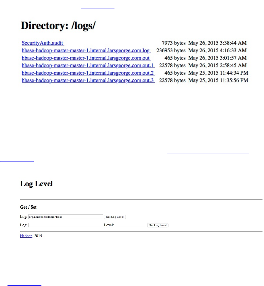
Shared Pages
On the top of the master, region server, and table pages there are also a few generic links that
lead to subsequent pages, displaying or controlling additional details of your setup:
Local Logs
This link provides a quick way to access the log files without requiring access to the server
itself. It firsts list the contents of the log directory where you can select the log file you
want to see. Click on a log to reveal its content. “Analyzing the Logs” helps you to make
sense of what you may see. Figure 6-43 shows an example page.
Figure 6-43. The Local Logs page
Log Level
This link leads you to a small form that allows you to retrieve and set the logging levels
used by the HBase processes. More on this is provided in “Changing Logging Levels”.
Figure 6-44 shows the form, already filled in with org.apache.hadoop.hbase as the log
hierarchy point to check the level for.
Figure 6-44. The Log Level page
When you click on the Get Log Level button, you should see a result similar to that shown
in Figure 6-45.
(533)
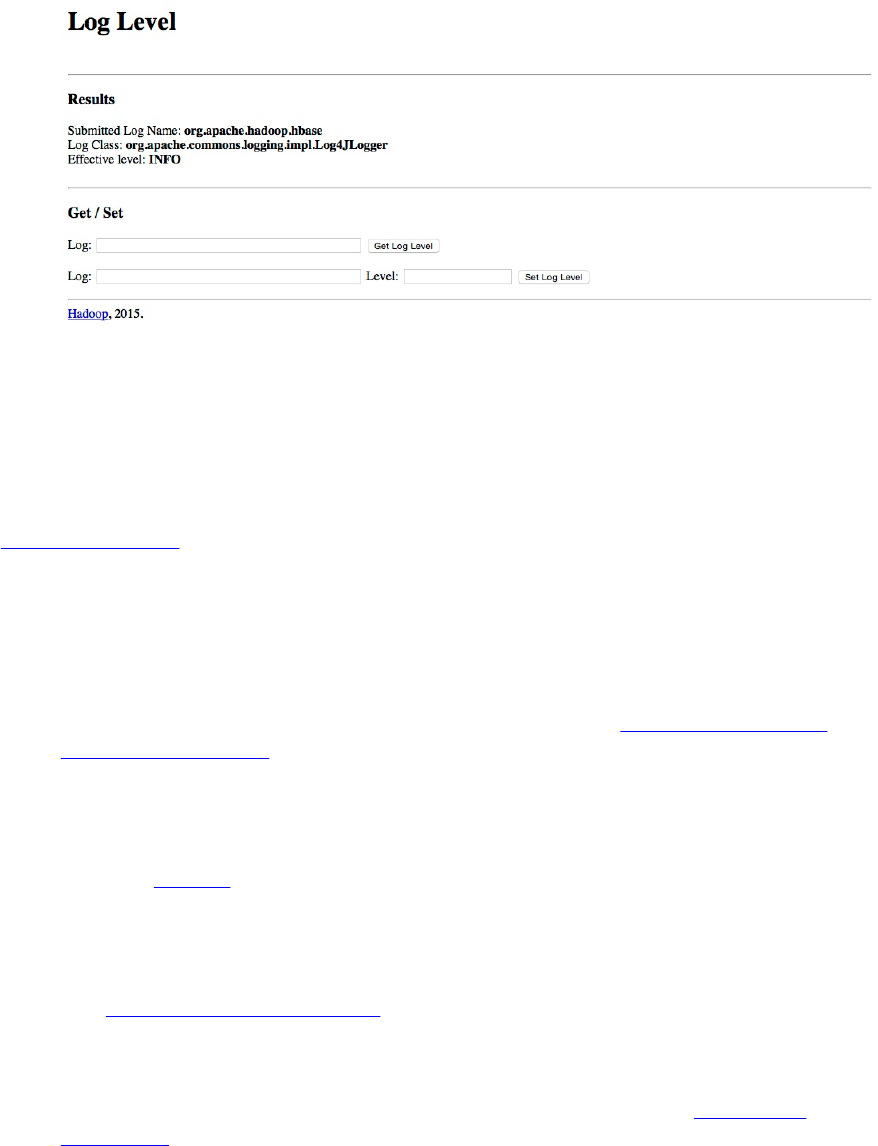
Figure 6-45. The Log Level Result page
Debug Dump
For debugging purposes, you can use this link to dump many details of the current Java
process, including the stack traces of the running threads. You can find more details in
“Troubleshooting”. The following details are included, with the difference between HBase
Master and Region Server mentioned (the Master has a few more sections listed in the
debug page):
Version Info
Lists some of the information shown at the bottom of the status pages, that is, the
HBase and Hadoop version, and who compiled them. See “Software Attributes” or
“Software Attributes”.
Tasks
Prints all of the monitored tasks running on the server. Same as explained in, for
example, “Tasks”.
Servers
Master Only—Outputs the name and server load of each known online region server
(see “Cluster Status Information” for details on the server load records).
Regions in Transition
Master Only—Lists the regions in transition, if there are any. See “Regions in
Transition” for details.
Executors
Shows all the currently configured executor threads, working on various tasks.
Stacks
Dumps the stack traces of all Java threads.
(534)

Configuration
Prints the configuration as loaded by the current server.
Recent Region Server Aborts
Master Only—Lists the reasons of the last region server aborts, that is, the reasons
why a worker server was abandoned or stopped.
Logs
The log messages of the server’s log are printed in this section. Lists the last 100
KBs, but can be changed per request by adding the tailkb parameter with the desired
number of kilobytes to the URL.
Region Server Queues
Shows detailed information about the compaction and flush queues. This includes
the different types of compaction entries (small, or large), as well as splits, and
region merges. Can be disabled setting the
hbase.regionserver.servlet.show.queuedump configuration property to false.
Figure 6-46 shows an abbreviated example output for a region server. The full pages are
usually very long, as the majority of the emitted information is very verbose.
(535)
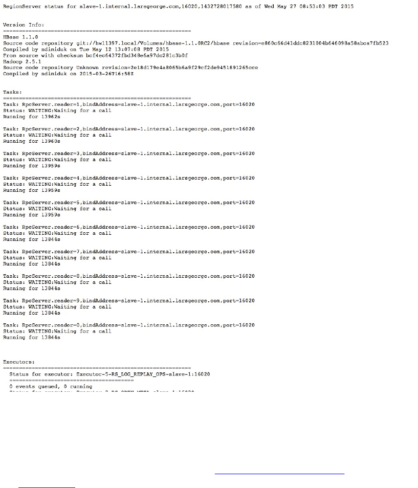
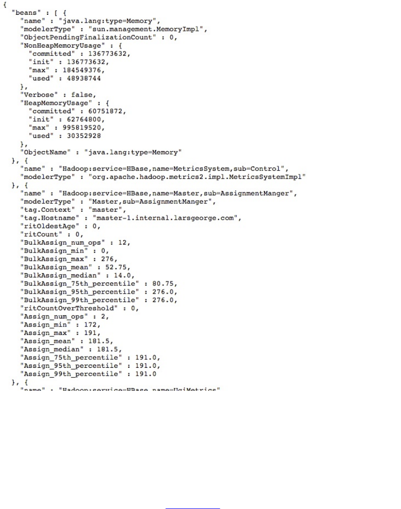
Figure 6-47. The Metrics Dump page
HBase Configuration
Last but not least, this shared link lets you output the current server configuration as
loaded by the process. This is not necessarily what is on disk in the configuration
directory, but what has been loaded at process start time, and possibly modified by
dynamically reloading the configuration. Figure 6-48 is an example XML output this link
produces. Depending on your browser (here Chrome) the rendering will vary.
(537)
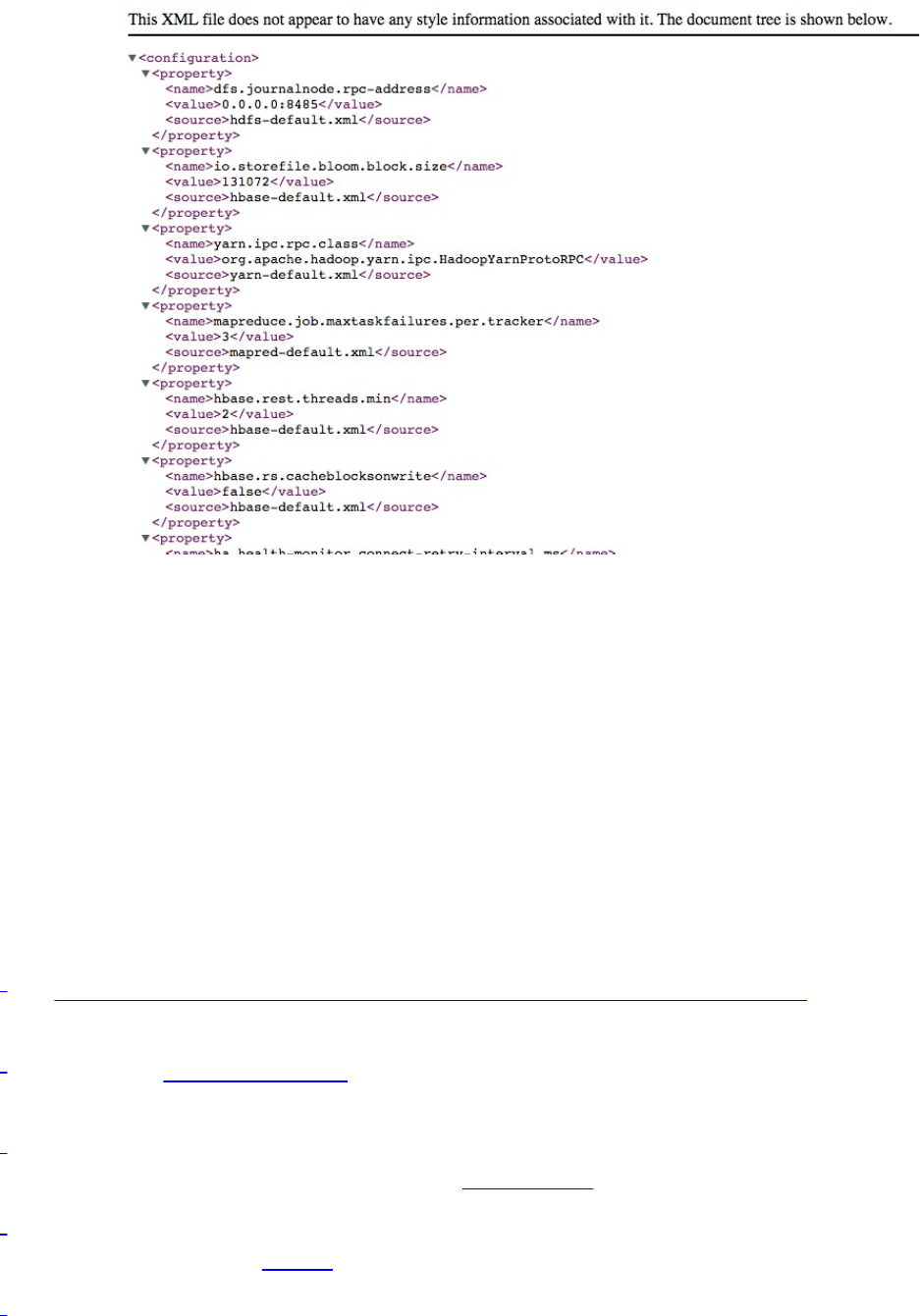
Figure 6-48. The HBase Configuration page
The web-based UI provided by the HBase servers is a good way to quickly gain insight into the
cluster, the hosted tables, the status of regions and tables, and so on. The majority of the
information can also be accessed using the HBase Shell, but that requires console access to the
cluster.
You can use the UI to trigger selected administrative operations; therefore, it might not be
advisable to give everyone access to it: similar to the shell, the UI should be used by the
operators and administrators of the cluster.
If you want your users to create, delete, and display their own tables, you will need an additional
layer on top of HBase, possibly using Thrift or REST as the gateway server, to offer this
functionality to end users.
1 See “Architectural Styles and the Design of Network-based Software Architectures”) by Roy T.
Fielding, 2000.
2 See the official SOAP specification online. SOAP—or Simple Object Access Protocol--also
uses HTTP as the underlying transport protocol, but exposes a different API for every service.
3 HBase used to also include a gateway server for Avro, but due to lack of interest and support it
was abandoned subsequently in HBase 0.96 (see HBASE-6553).
4 curl is a command-line tool for transferring data with URL syntax, supporting a large variety of
protocols. See the project’s website for details.
5 The basic idea is to encode any unsafe or unprintable character code as “%” + ASCII Code.
Because it uses the percent sign as the prefix, it is also called percent encoding. See the
(538)

Wikipedia page on percent encoding for details.
6 See this blog post for a comparison.
7 As of this writing, the supplied DemoClient.php is slightly outdated, running into a script error
during evaluation. This results in not all of the included tests being executed. This is tracked in
HBASE-13522.
8 See the Hive wiki for more details on storage handlers.
9 The Hive wiki has a full explanation of the HBase integration into Hive.
10 If you get an error starting the Hive CLI indicating an issue with JLine, please see HIVE-8609.
Hadoop 2.7.0 and later should work fine.
11 A good help here is using a terminal multiplexer like screen or tmux.
12 Before YARN, using the original MapReduce framework, this variable was named
mapred.job.tracker and was set in the Hive CLI with SET mapred.job.tracker=local;.
13 See HIVE-2781 for the details.
14 The full details can be found on the Pig Getting Started page.
15 This has changed from 60010 and 60030 in HBase 1.0 (see HBASE-10123 for details).
Version 1.0.0 of HBase had an odd state where the master would use the region server ports for
RPC, and the UI would redirect to a random port. HBASE-13453 fixes this in 1.0.1 and later.
16 As a side note, you will find that the columns are titled with KV in them, an abbreviation of
KeyValue and synonym for cell. The latter is the official term as of HBase version 1.0 going
forward.
17 Recall that this should not be started with /tmp, or you may lose your data during a machine
restart. Refer to “Quick-Start Guide” for details.
18 As of this writing, covering version 1.1.0 of HBase, the “Slow WAL Append” value is
hardcoded to be zero.
(539)
Chapter 7. Hadoop Integration
Hadoop consists of two major components at heart: the file system (HDFS) and the processing
framework (YARN). We have discussed in earlier chapters how HBase is using HDFS (if not
configured otherwise) to keep the stored data safe, relying on the built-in replication of data
blocks, transparent checksumming, as well as access control and security (the latter you will
learn about in [Link to Come]). In this chapter we will look into how HBase is fitting nicely into
the processing side of Hadoop as well.
(540)
Framework
The primary purpose of Hadoop is to store data in a reliable and scalable manner, and in addition
provide means to process the stored data efficiently. That latter task is usually handed to YARN,
which stands for Yet Another Resource Negotiator, replacing the monolithic MapReduce
framework in Hadoop 2.2. MapReduce is still present in Hadoop, but was split into two parts: a
resource management framework named YARN, and a MapReduce application running on top of
YARN.
The difference is that in the past (before Hadoop 2.2), MapReduce was the only native
processing framework in Hadoop. Now with YARN you can execute any processing
methodology, as long as it can be implemented as a YARN application. MapReduce’s processing
architecture has been ported to YARN as MapReduce v2, and effectively runs the same code as it
always did. What became apparent though over time is that there is a need for more complex
processing, one that allows to solve other classes of computational problems. One very common
one are iterative algorithms used in machine learning, with the prominent example of Page
Rank, made popular by Google’s search engine. The idea is to compute a graph problem that
iterates over approximations of solutions until a sufficiently stable one has been found.
MapReduce, with its two step, disk based processing model, is too rigid for these types of
problems, and new processing engines have been developed to fit that gap. Apache Giraph, for
example, can compute graph workloads, based on the Bulk Synchronous Parallel (BSP) model of
distributed computation introduced by Leslie Valiant. Another is Apache Spark, which is using a
Directed Acyclic Graphs (DAG) based engine, allowing the user to express many different
algorithms, including MapReduce and iterative computations.
No matter how you use HBase with one of these processing engines, the common approach is to
use the Hadoop provided mechanisms to gain access to data stored in HBase tables. There are
shared classes revolving around InputFormat and OutputFormat, which can (and should) be used in
a generic way, independent of how you process the data. In other words, you can use MapReduce
v1 (the one before Hadoop 2.2 and YARN), MapReduce v2, or Spark, while all of them use the
same lower level classes to access data stored in HDFS, or HBase. We will use the traditional
MapReduce framework to explain these classes, though their application in other frameworks is
usually the same. Before going into the application of HBase with MapReduce, we will first have
a look at the building blocks.
(541)
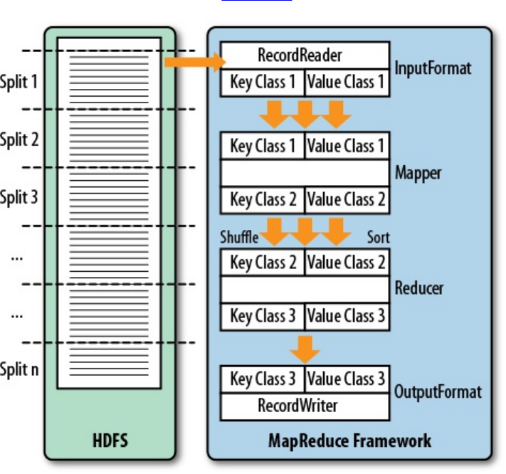
MapReduce Introduction
MapReduce as a process was designed to solve the problem of processing in excess of terabytes
of data in a scalable way. There should be a way to build such a system that increases in
performance linearly with the number of physical machines added. That is what MapReduce
strives to do. It follows a divide-and-conquer approach by splitting the data located on a
distributed filesystem, or other data sources, so that the servers (or rather CPUs, or, more
modern, “cores”) available can access these chunks of data and process them as fast as they can.
The problem with this approach is that you will have to consolidate the data at the end. Again,
MapReduce has this built right into it. Figure 7-1 gives a high-level overview of the process.
Figure 7-1. The MapReduce process
This (rather simplified) figure of the MapReduce process shows you how the data is processed.
The first thing that happens is the split, which is responsible for dividing the input data into
reasonably sized chunks that are then processed by one server at a time. This splitting has to be
done in a somewhat smart way to make best use of available servers and the infrastructure in
general. In this example, the data may be a very large log file that is divided into pieces of equal
size. This is good, for example, for Apache HTTP Server log files. Input data may also be binary,
though, in which case you may have to write your own getSplits() method—but more on that
shortly.
The basic principle of MapReduce (and a lot of other processing engines or frameworks) is to
extract key/value pairs from the input data. Depending on the processing engine, they might be
(542)

called tuples, feature vectors, or records. MapReduce refers to them as records (see ???), though
the idea is the same: we have data points that need to be processed. In MapReduce there is extra
emphasis on the key part of each record, since it is used to route and group the values as part of
the processing algorithm. Each key and value also has a defined type, which reflect its nature and
makes processing less ambiguous. As part of the setup of each MapReduce workflow, the job
designer has to assign the types to each key/value as it is passed through the processing stages.
...
Map-Reduce Framework
Map input records=289
Map output records=2157
Map output bytes=22735
Map output materialized bytes=10992
Input split bytes=137
Combine input records=2157
Combine output records=755
Reduce input groups=755
Reduce shuffle bytes=10992
Reduce input records=755
Reduce output records=755
...
(543)

Processing Classes
Figure 7-1 also shows you the classes that are involved in the Hadoop implementation of
MapReduce. Let us look at them and also at the specific implementations that HBase provides in
addition.
MapReduce versus Mapred, versus MapReduce v1 and v2
Hadoop version 0.20.0 introduced a new MapReduce API. Its classes are located in the package
named mapreduce, while the existing classes for the previous API are located in mapred. The older
API was deprecated and should have been dropped in version 0.21.0—but that did not happen. In
fact, the old API was undeprecated since the adoption of the new one was hindered by its initial
incompleteness.
HBase also has these two packages, which started to differ more and more over time, with the
new API being the actively supported one. This chapter will only refer to the new API, that is,
when you need to use the mapred package instead, you will have to replace the respective classes.
Some are named slightly different, but fulfil the same purpose (for example, TableMap versus
TableMapper). Yet others are not available in the older API, and would need to be ported by
manually. Most of the classes are self-contained or have little dependencies, which means you
can copy them into your own source code tree and compile them with your job archive file.
On the other hand, there is the difference between MapReduce v1 and v2, mentioned earlier. The
differences in v1 and v2 are not the API, but their implementations, with v1 being a single,
monolithic framework, and v2 being an application executed by YARN. This change had no
impact on the provided APIs by MapReduce, and both, v1 and v2, offer the mapreduce and mapred
packages. Since YARN is the official processing framework as of Hadoop 2.2 (released in 2013),
and since both expose the same API, this chapter will use YARN to execute the MapReduce
examples.
InputFormat
The first hierarchy of classes to deal with is based on the InputFormat class, shown in Figure 7-2.
They are responsible for two things: first, split the input data into chunks, and second, return a
RecordReader instance that defines the types of the key and value objects, and also provides a
nextKeyValue() method that is used to iterate over each input record.1
(544)
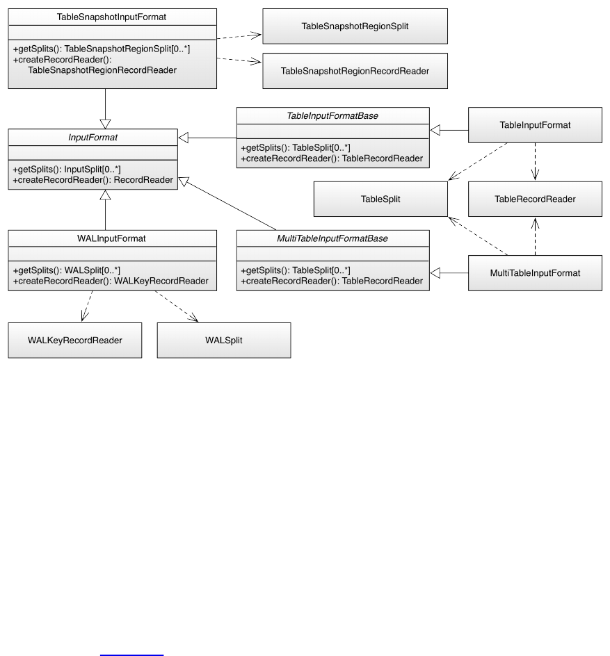
Figure 7-2. The InputFormat hierarchy
As far as HBase is concerned, there are the following special implementations:
TableInputFormat
This class is based on TableInputFormatBase, which implements the majority of the
functionality but remains abstract. TableInputFormat is used by many supplied examples,
tools, and real MapReduce classes, as it provides the most generic functionality to iterate
over data stored in a HBase table.
You either have to provide a Scan instance that you can prepare in any way you want:
specify start and stop keys, add filters, specify the number of versions, and so on, or you
have to hand in these parameters separately and the framework will set up the Scan instance
internally. See Table 7-1 for a list of all the basic properties.
Table 7-1. The basic TableInputFormat configuration properties
Property Description
hbase.mapreduce.inputtable Specifies the name of the table to read.
hbase.mapreduce.splittable
Specifies an optional table to use for split
boundaries. This is useful when you are
preparing data for bulkload.
hbase.mapreduce.scan
A fully configured, base-64 encoded scanner.
All other scan properties are ignored if this is
specified. See
TableMapReduceUtil.convertScanToString(Scan)
(545)

for more details.
hbase.mapreduce.scan.row.start The optional start row key of the scan (see
Scan.setStartRow()
hbase.mapreduce.scan.row.stop The optional stop row key for the scan (see
Scan.setStopRow()
hbase.mapreduce.scan.column.family When given, specifies the column family to
scan (see Scan.addFamily()
hbase.mapreduce.scan.columns
Optional space character-delimited list of
columns to include in scan (see
Scan.addColumn()).
hbase.mapreduce.scan.timestamp
Allows to set a specific timestamp for the
scan to return only those exact versions (see
Scan.setTimeStamp()
hbase.mapreduce.scan.timerange.start/hbase.mapreduce.scan.timerange.end
The starting and ending timestamp used to
filter columns with a specific range of
versions (see Scan.setTimeRange()
must be set to take effect.
hbase.mapreduce.scan.maxversions The maximum number of version to return
(see Scan.setMaxVersions()
hbase.mapreduce.scan.cacheblocks
Set to false to disable server-side caching of
blocks for this scan (see
Scan.setCacheBlocks()
hbase.mapreduce.scan.cachedrows The number of rows for caching that will be
passed to scanners (see
hbase.mapreduce.scan.batchsize Set the maximum number of values to return
for each call to next() (see
Some of these properties are assignable through dedicated setter methods, for example, the
setScan() or configureSplitTable() calls. You will see examples of that in “Supporting
Classes” and “MapReduce over Tables”.
(546)

The TableInputFormat splits the table into proper blocks for you and hands them over to the
subsequent classes in the MapReduce process. See “Table Splits” for details on how the
table is split. The provided, concrete implementations of the inherited getSplits() and
createRecordReader() methods return the special TableSplit and TableRecordReader classes,
respectively. They wrap each region of a table into a split record, and return the rows and
columns as configured by the scan parameters.
MultiTableInputFormat
Since a TableInputFormat is only handling a single table with a single scan instance, there is
another class extending the same idea to more than one table and scan, aptly named
MultiTableInputFormat. It is only accepting a single configuration property, named
hbase.mapreduce.scans, which holds the configured scan instance. Since the Configuration
class used allows to specify the same property more than once, you can add more than one
into the current job instance, for example:
List<Scan> scans = new ArrayList<Scan>();
Scan scan = new Scan();
scan.setAttribute(Scan.SCAN_ATTRIBUTES_TABLE_NAME,
Bytes.toBytes("prodretail:users"));
scans.add(scan);
scan = new Scan();
scan.setAttribute(Scan.SCAN_ATTRIBUTES_TABLE_NAME,
Bytes.toBytes("prodchannel:users"));
scan.setTimeRange(...);
scans.add(scan);
...
TableMapReduceUtil.initTableMapperJob(scans, ReportMapper.class,
ImmutableBytesWritable.class, ImmutableBytesWritable.class, job);
This uses an up until now unmentioned public constant, exposed by the Scan class:
static public final String SCAN_ATTRIBUTES_TABLE_NAME = \
"scan.attributes.table.name";
It is needed for the MultiTableInputFormat to determine the scanned tables. The previous
TableInputFormat works the other way around by explicitly setting the scanned table,
because there is only one. Here we assign the tables to the one or more scans handed into
the MultiTableInputFormat configuration, and then let it iterate over those implicitly.
TableSnapshotInputFormat
This input format class allows you to read a previously taken table snapshot. What has
been omitted from the class diagram is the relationship to another class in the mapreduce
package, the TableSnapshotInputFormatImpl. It is shared between the two API
implementations, and provides generic, API independent functionality. For example, it
wraps a special InputSplit class, which is then further wrapped into a
TableSnapshotRegionSplit class by the TableSnapshotInputFormat class. It also has the
getSplits() method that understands the layout of a snapshot within the HBase root
directory, and is able to wrap each contained region into a split instance. Since this is the
same no matter which MapReduce API is used, the functionality is implemented in the
shared class.
The dedicated snapshot input format also has a setter named setInput() that allows you to
assign the snapshot details. You can access this method directly, or use the utility methods
provided by TableMapReduceUtil, explained in “Supporting Classes”. The setInput() also
(547)
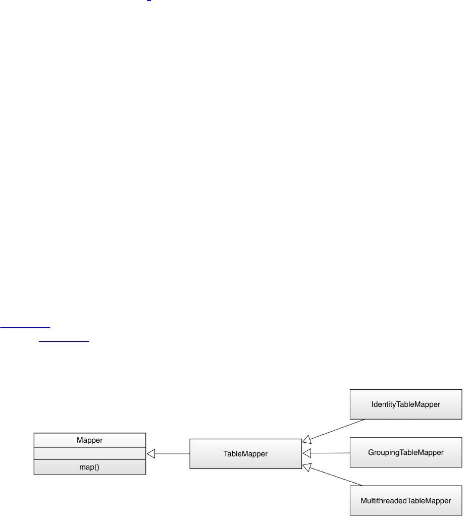
asks for the name of a temporary directory, which is used internally to restore the snapshot,
before it is read from. The user running the MapReduce job requires write permissions on
this directory, or the job will fail. This implies that the directory must be, for example,
outside the HBase root directory.
WALInputFormat
If you ever need to read the binary write-ahead logs that HBase generates, you can employ
this class to access them.2 It is primarily used by the WALPlayer class and tool to replay
write-ahead logs using MapReduce. Since WALs are rolled by default when they approach
the configured HDFS block size, it is not necessary to calculate splits. Instead, each WAL
is mapped to one split. The only exposed configuration properties for the WAL input
format are:
public static final String START_TIME_KEY = "wal.start.time";
public static final String END_TIME_KEY = "wal.end.time";
They allow the user to specify which entries should be read from the logs. Any record
before the start, and after the end time will be ignored. Of course, these properties are
optional, and if not given the entire logs are read and each record handed to the processing
function.
With all of these classes, you can always decide to create your own, or extend the given ones and
add your custom business logic as needed. The supplied classes also provide methods (some
have their Java scope set as protected) that you can override to slightly change the behavior
without the need of implementing the same functionality again. The classes ending Base are also
a good starting point for your own implementations, since they offer many features, and thus
form the basis for the provided concrete classes, and could do the same for your own.
Mapper
The Mapper class(es) is for the next stage of the MapReduce process and one of its namesakes
(Figure 7-3). In this step, each record read using the RecordReader is processed using the map()
method. Figure 7-1 also shows that the Mapper reads a specific type of key/value pair, but emits
possibly another type. This is handy for converting the raw data into something more useful for
further processing.
Figure 7-3. The Mapper hierarchy
HBase provides the TableMapper class that enforces key class 1 to be an ImmutableBytesWritable,
(548)
and value class 1 to be a Result type—since that is what the TableRecordReader and
TableSnapshotRecordReader are returning. There are multiple implementations of derived mapper
classes available:
IdentityTableMapper
One subclass of the TableMapper is the IdentityTableMapper, which is also a good example of
how to add your own functionality to the supplied classes. The TableMapper class itself does
not implement anything but only adds the signatures of the actual key/value pair classes.
The IdentityTableMapper is simply passing on the keys/values to the next stage of
processing.
GroupingTableMapper
This is a special subclass that needs a list of columns before it can be used. The mapper
code checks each row it is given by the framework in form of a Result instance, and if the
given columns exists, it creates a new key as a concatenation of all values assigned to each
named column. If any of the columns is missing in the row the entire row is skipped.
You can set the key columns using the static initJob() method of this class, or assign it to
the following configuration property, provided as a public constant in the mapper class:
public static final String GROUP_COLUMNS =
"hbase.mapred.groupingtablemap.columns";
The class expects the columns to be specified as a space character-delimited string, for
example "colfam1:col1 colfam1:col2". If these columns are found in the row, the row key is
replaced by a space character-delimited new key, for example:
Input:
"row1" -> cf1:col1 = "val1", cf1:col2 = "val2", cf1:col3 = "val3"
Output:
"val1 val2" -> cf1:col1 = "val1", cf1:col2 = "val2", cf1:col3 = "val3"
The purpose of this change of the map output key value is the subsequent reduce phase,
which receives key/values grouped based on the key. The shuffle and sort steps of the
MapReduce framework ensure that the records are sent to the appropriate Reducer instance,
which is usually another server somewhere in the cluster. By being able to group the rows
using some column values you can send related rows to a single reducer and therefore
perform some processing function across all of them.
MultiThreadedTableMapper
One of the basic principles of the MapReduce framework is that the map and reduce
functions are executed by a single thread, which simplifies the implementation because
there is no need to take care of thread-safety. Often—for performance reasons—class
instances are reused to process data as fast as can be read from disk, and not being slowed
down by object instantiation. This is especially true for very small data points.
On the other hand, sometimes the processing in the map function is requiring an excessive
amount of time, for example when data is acquired from an external resource, over the
network. An example is a web crawling map function, which loads the URL from one
HBase table, retrieves the page over the Internet, and writes the fetch content into another
HBase table. In this case you mostly wait for the external operation.
(549)

Since each map takes up a slot of the processing framework, it is considered scarce, and is
limited to what the scheduler is offering to your job. In other words, you can only crawl
the web as fast as you receive processing capacities, but then wait for an external resource
most of the time. The MultiThreadedTableMapper is available for exactly that reason,
enabling you to turbo-charge your map function by executing it in a parallel fashion using
a thread pool. The pool is controlled by the following configuration property, or the
respective getter and setter:
public static final String NUMBER_OF_THREADS = \
"hbase.mapreduce.multithreadedmapper.threads";
public static int getNumberOfThreads(JobContext job)
public static void setNumberOfThreads(Job job, int threads)
Caution
Since you effectively bypass the number of threads assigned to you by the scheduler and
instead multiply that number at your will, you must take not to exhaust any vital resources
in the process. For example, if you were to use the multithreaded mapper implementation
to just read from, and/or write to HBase, you can easily overload the disk I/O. Even with
YARN using Linux control groups (cgroups), or other such measures to guard system
resources, you have to be very careful.
The number of threads to use is dependent on your external wait time, for example, if you
fetch web pages as per the example above, you may want to gradually increase the thread
pool to reach CPU or network I/O saturation. The default size of the thread pool is 10,
which is conservative start point. Before you can use the threaded class you need to assign
the actual map function to run. This is done using the following configuration property, or
again using the provided getter and setter methods:
public static final String MAPPER_CLASS = \
"hbase.mapreduce.multithreadedmapper.mapclass";
public static <K2, V2> Class<Mapper<ImmutableBytesWritable, Result, K2, V2>> \
getMapperClass(JobContext job)
public static <K2, V2> void setMapperClass(Job job, \
Class<? extends Mapper<ImmutableBytesWritable, Result, K2, V2>> cls)
The only difference to a normal map method is that you have to implement it in a thread-
safe manner, just as any other Runnable based Java thread executable. This implies that you
cannot reuse simple instance variables, unless they refer to an object that itself is thread-
safe as well.
Reducer
The Reducer stage and class hierarchy (Figure 7-4) is very similar to the Mapper stage. This time
we get the output of a Mapper class and process it after the data has been shuffled and sorted.
In the implicit shuffle between the Mapper and Reducer stages, the intermediate data is copied from
different Map servers to the Reduce servers and the sort combines the shuffled (copied) data so
that the Reducer sees the intermediate data as a nicely sorted set where each unique key is now
associated with all of the possible values it was found with.
(550)
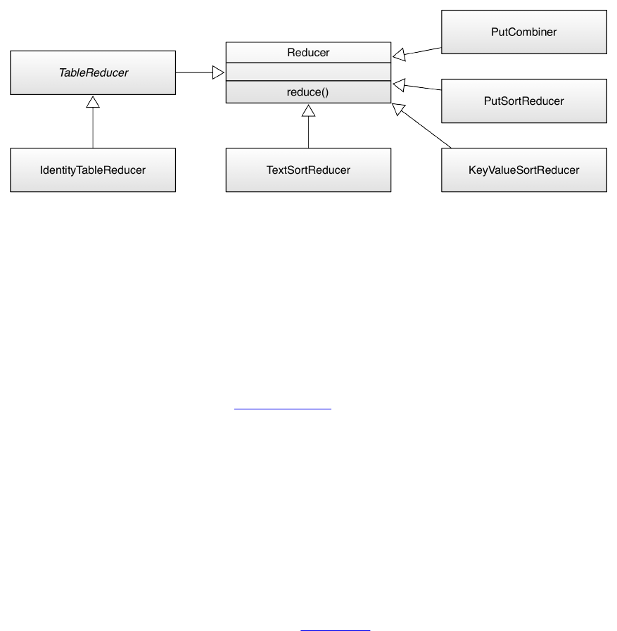
Figure 7-4. The Reducer hierarchy
There are again a set of derived classes available, though for direct table operations there is only
one: the TableReducer class. It has a subclass called IdentityTableReducer, and all it does is make
the former abstract class a concrete, usable one. In other words, the basic functionality of a
Reducer based class is to pass on the data unchanged. If you want anything else, you need to
implement your own.
Then there are a few more classes directly subclassing Reducer. These are all needed for bulk
loading data into HBase, as discussed in “Bulk Import”. Dependent on the type of data being
loaded, one of TextSortReducer, PutSortReducer, or KeyValueSortReducer is used to emit the bulk
loader data in a sorted manner. The PutCombiner is an optimization used in the ImportTsv tool to
combine many smaller puts into one larger one. This is close to the recommended Combiner usage
within Hadoop, reducing transfer of data between Mapper and Reducer instances during the shuffle
phase. There could potentially be hundreds or thousands of Put objects that would need to be
serialized and sent to the reducer process on a remote server. Combining these into one does not
reduce the size of the data, but reduces class overhead.
OutputFormat
The final stage is the OutputFormat class hierarchy (Figure 7-5), and the job of these classes is to
persist the data in various locations. There are specific implementations that allow output to files,
or to HBase tables, and we are going to discuss each of them subsequently.
(551)
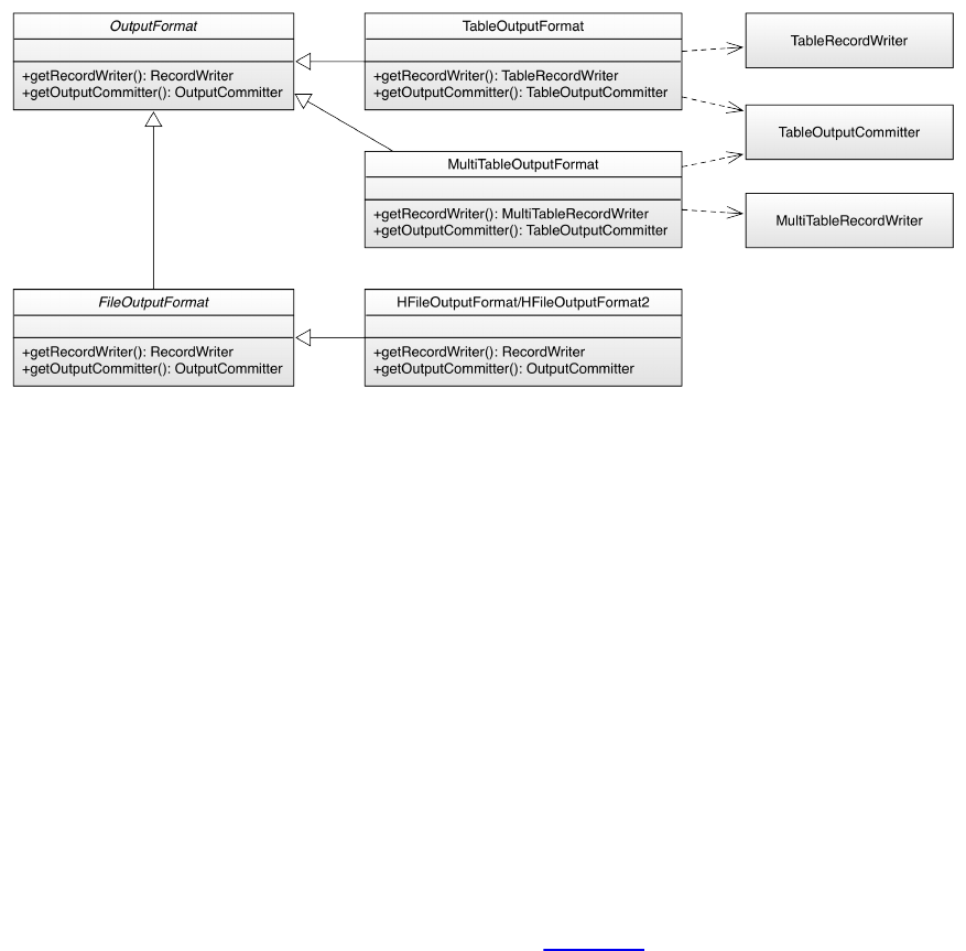
Figure 7-5. The OutputFormat hierarchy
TableOutputFormat
This class is the default output format for many MapReduce jobs that need to write data
back into HBase tables. It uses a TableRecordWriter to write the data into the specific HBase
output table. The latter uses a BufferedMutator instance to buffer writes before sending
them in batches to the servers. The provided write() method expects to receive either a Put
or a Delete instance, and uses the BufferedMutator.mutate() method to persist them. If you
hand in something else, for example a Get or Increment instance an error is thrown instead.
The close() method of the record writer class closes the mutator, enforcing the flush of any
pending write operations to the servers.
It is important to note the cardinality as well. Although many Mappers are handing records
to many Reducers, only one OutputFormat instance takes the output records from its assigned
Reducer subsequently. It is the final class that handles the key/value pairs and writes them
to their final destination, this being a file or a table. You need to configure the output
format using the configuration properties shown in Table 7-2.
Table 7-2. The TableOutputFormat configuration properties
Property Description
hbase.mapred.outputtable The table to write into (required).
hbase.mapred.output.quorum
Optional parameter to specify a peer cluster. Used to
specifying a remote cluster when copying between hbase
clusters (the source cluster is picked up from hbase-
site.xml).
hbase.mapred.output.quorum.port Optional parameter to specify the peer cluster’s
ZooKeeper client port.
hbase.mapred.output.rs.class Optional specification of the RegionServer class name of
the peer cluster.
(552)

hbase.mapred.output.rs.impl Optional specification of the RegionServer
implementation name of the peer cluster.
These properties are exposed as public constants, allowing you to refer to them as needed,
or you can use, for example, the initTableReducerJob() method of the TableMapReduceUtil
helper class to set the table name implicitly. The name of the output table must be
specified when the job is set up. Otherwise, the TableOutputFormat does not add much more
complexity.
The four optional properties allow you to set up a job that reads from one cluster—
configured by the current configuration instance—and write to another. The above
initTableReducerJob() call (one of the overloaded version) has facilities for assigning these
properties as well.
MultiTableOutputFormat
An extension to the direct TableOutputFormat is the ability to write to more than one single
output table. For that matter, the dedicated MultiTableRecordWriter uses a neat “trick” to
coax in the table name for every record emitted by the map or reduce task: it defines the
types of the writer as RecordWriter<ImmutableBytesWritable, Mutation>, using the key as the
table name. Usually the key is not needed for the HBase mutations to be written to a table,
as the name of the latter is set in the configuration of the job. In fact, the TableOutputFormat
with its TableRecordWriter completely ignores the key, while simply persisting the handed
in put or delete object into the globally configured buffered mutator.
In other words, the change in usage is that a map or reduce task needs to take care of what
to emit by specifying the destination table name, and the mutation (the put or delete). For
example, usually you would emit a mutation in a map or reduce method using the
TableOutFormat like so:
context.write(new ImmutableBytesWritable(rowkey), put);
Instead, you switch the key out to name the table instead:
context.write(new ImmutableBytesWritable(tableName), put);
Internally the class uses a BufferedMutator instance for every named table. In addition, the
following constants are exposed by the class:
public static final String WAL_PROPERTY = \
"hbase.mapreduce.multitableoutputformat.wal";
public static final boolean WAL_ON = true;
public static final boolean WAL_OFF = false;
They allow you to influence the durability settings for the write operation, as explained in
“Durability, Consistency, and Isolation”.
A few more general notes on the output formats and their supporting classes:
1. The TableOutputCommitter class, used by both the above output formats, is required for the
Hadoop framework to do its job. For HBase integration, this class is not needed. In fact, it
is a dummy and does not do anything. Other implementations of OutputFormat do require a
(553)

specific output committer, but for HBase an empty implementation is all that is needed.
2. The BufferedMutator instances used have no explicit setter or getter regarding their
configuration. Instead, you have to set the configuration properties influencing the
buffered mutators before you set up the MapReduce job. The settings will be passed into
the wrapping output formats through the job context. Table 7-3 lists the properties with
their default values. Especially the write buffer should be tuned based on the use-case,
where its size should account for a decent amount of mutations to save on the batched
network roundtrips.
Table 7-3. Important configuration settings influencing the BufferedMutator behavior
Property Default Description
hbase.client.write.buffer
2097152 (2
MB) Configures the local write buffer in bytes.
hbase.client.keyvalue.maxsize 10485760 (10
MB) Limits the maximum cell size a client can write.
hbase.client.retries.number 35 Number of retries before failing the operation.
hbase.client.pause 100 (ms) Initial pause between retries. Increases
incrementally for retries.
hbase.rpc.timeout 60000 (1 min) The connection timeout for the remote server call.
Finally, there is a third class of output format, which is not directly based on OutputFormat, but
FileOutputFormat instead. The reason to rather extend FileOutputFormat is based on the built in
features of that class and the need to write HBase storage files, called HFile, directly into the
configured file storage layer, usually HDFS.
HFileOutputFormat/HFileOutputFormat2
This output format is used to stage HFiles before they are loaded into the tables, as
explained in “Bulk Import”. The difference between these two classes is that the former is
for the now deprecated KeyValue class, for legacy reasons, and the latter is for the newer
Cell classes. The class exposes a static, overloaded method named
configureIncrementalLoad() which simplifies setting up a MapReduce job using this output
format.
Part of setting up the HFile specific RecordWriter is to set the appropriate table properties,
including maximum file size, compression format, Bloom filter type, the HFile block size,
and block encoding format. Many are optional, and will default to what the provided
hbase-site.xml file on the Java class path specifies. The emitted Cell will define which
column families are generated, thus there is no need of specifying them explicitly. For the
(554)
bulk load to work, there are quite a few steps involved, for example, sorting and routing
the written Cells at a cluster-wide scale, using the TotalOrderPartitioner provided by
Hadoop. This ensure that the cells for a specific row all end up being written in the
expected sort-order by one reducer.
(555)

Supporting Classes
The MapReduce support comes with the TableMapReduceUtil class that helps in setting up
MapReduce jobs over HBase. It has static methods that configure a job so that you can run it
with HBase as the source and/or the target. It also has other helper methods to configure various
aspects of working with the MapReduce framework. They can be grouped as such:
Class Path Setup
There are two variants of the addDependencyJars() method, with one finding all the
containing JAR files given a list of classes. It adds the found JAR files to the provided
configuration instance using the tmpjars property. This is honored by the MapReduce
system which includes these JARs into the job setup using the Hadoop distributed cache.
In other words, you will not have to do anything else to run the job.
The method is powerful enough to work in development environment, checking each
named class file, and if it is not contained in a JAR file already (that is, it was loaded from
a JAR before the check ran) it creates a JAR file on the fly and adds it to the configuration.
The temporary file is created using the File.createTempFile() method, and used "hadoop-"
as its name prefix. The location is set by the test.build.dir configuration property, and
defaults to target/test-dir.
The second variant of the addDependencyJars() call just asks for a Job instance, and adds all
HBase and user JARs necessary for the job execution, using the previous method. It looks
at every class named in the job configuration, for example, the mapper and reducer classes,
and adds them to the job configuration. Implicitly it calls a third class path related method
named addHBaseDependencyJars(), which does the same for all HBase JARs a client may
possibly need. The end result is that all required JAR files, from HBase or your own, are
specified in the supplied configuration instance.
Lastly, the buildDependencyClasspath() method uses the tmpjars property, retrieving all of
the configured JARs, and returning a string suitable for an operating system specific search
path definition. For example, on Linux this may return something of the following pattern:
<path-to-jar>/<jarname1>.jar:<path-to-jar>/<jarname2>.jar:.... It is using the path and
directory divider symbols configured for the platform it executes on.
Security Configuration
These calls allow you to set security credentials, but only do something useful when
security is enabled (see [Link to Come]). There is initCredentials() which passes on the
details about the configured Hadoop delegation tokens and configures the users
credentials. This is done by authenticating and retrieving the valid tokens to the job
configuration. Before though the method also configures the appropriate ZooKeeper
properties within the configuration, since it is needed to determine the unique cluster ID.
Eventually the method sends a request to the authentication coprocessor of that cluster to
retrieve the tokens, and assign them to the job configuration. This is done for the source
and target cluster, if configured with the hbase.mapred.output.quorum property (as explained
in “OutputFormat”).
(556)

The initCredentialsForCluster() always assumes an external cluster, and asks for
ZooKeeper quorum details explicitly. After that it does the same thing, that is, it
authenticates the user by sending a request to the coprocessor, and adding the returned
token information to the job configuration.
Configure Table as Input
The initTableMapperJob() call comes in many variations. They are essential in setting up
MapReduce jobs where the HBase table acts as in input to a Map instance. Here an example
signature of one variant:
public static void initTableMapperJob(String table, Scan scan,
Class<? extends TableMapper> mapper, Class<?> outputKeyClass,
Class<?> outputValueClass, Job job, boolean addDependencyJars,
boolean initCredentials, Class<? extends InputFormat> inputFormatClass)
throws IOException
The calls add more or less details to the job configuration, so that you can choose which is
the most suitable to your task at hand. In general, the calls do the following:
1. Configure the job with the given InputFormat class
2. If given, overwrite the output key and value class types
3. Assign the given mapper class to the job
4. Optionally, set the PutCombiner as combiner class, when the output value type is Put
5. Merge the currently visible Hadoop and HBase configuration into the job
configuration
6. Set the given table name in the configuration
7. Serialize the configured Scan instance and assign it to the configuration
8. Overwrite the default Hadoop Writable based serialization with a custom HBase one,
based on Protobufs:
conf.setStrings("io.serializations", conf.get("io.serializations"),
MutationSerialization.class.getName(),
ResultSerialization.class.getName(),
KeyValueSerialization.class.getName());
9. Optionally, call addDependencyJars() to add all JARs to the class path
10. Optionally, set up the security credentials using initCredentials()
The mentioned Serialization classes are also part of the mapreduce package, and
handle the conversion of mutations, query result, and cells in a platform independent
manner, using Google’s Protocol Buffers, and are discussed in-depth in
“Serialization”. They are not used explicitly anywhere else, so their implicit use by
the initTableMapperJob() is somewhat hidden. Especially if you do not use the utility
methods provided, you would need to set these classes manually, as shown in the
code excerpt above.
Configure Table as Output
(557)
The counterpart of the previous set of methods is this one, and it configures a
TableOutputFormat to use a HBase table as the target for data emitted from the MapReduce
job.
Note
Keep in mind that the MapReduce OutputFormat is used in combination with a single
Reducer instance. In case of a map-only job though the output format is called directly by
the map function.
The provided initTableReducerJob() call again comes in multiple versions, offering fewer
to more parameters. Here is the fully specified variant for your perusal:
public static void initTableReducerJob(String table,
Class<? extends TableReducer> reducer, Job job,
Class partitioner, String quorumAddress, String serverClass,
String serverImpl, boolean addDependencyJars) throws IOException
The following tasks are performed when invoking these methods:
1. Merge the currently visible Hadoop and HBase configuration into the job
configuration
2. Assign the given output format class to the job
3. If given, set the reducer class for the job
4. Set the output table name in the configuration
5. Overwrite the default Hadoop Writable based serialization with a custom HBase one,
based on Protobufs
6. Optionally, set the target cluster ZooKeeper quorum information
7. Optionally, assign the region server interface and implementation class name
8. Set the output key type to ImmutableBytesWritable and output value type to Writable
9. Assign the given partitioner to the job
1. In case of the supplied HRegionPartitioner, also limit the number of reduce
tasks to run to be not greater than the number of regions in the output table
10. Optionally, call addDependencyJars() to add all JARs to the class path
11. Set up the security credentials using initCredentials()
This is very similar to the above initTableMapperJob(), but with a few difference to
match the different purpose of writing into a table, instead of reading from it. Again,
if you decide not to use this helper method, please study carefully what it does and
make sure you do everything required for your use-case as well.
Configure Snapshot as Input
(558)
The supplied initTableSnapshotMapperJob() sets the name and temporary directory required
using the setInput() method of the TableSnapshotInputFormat class, and then proceeds to
invoke initTableMapperJob() while mostly passing on the parameters given by the caller. It
also assigns the TableSnapshotInputFormat as the input format class for the job. One special
function it performs is to overrides any block cache configuration that could cause the
MapReduce task to exhaust its (usually scarce) resources.
Miscellaneous Tasks
The utility class TableMapReduceUtil has a few more generic methods, which are called from
the other helpers, or can be called by your own code as necessary. The
limitNumReduceTasks() ensures the number of requested reduce tasks for the MapReduce job
does not exceed the number of available regions. setNumReduceTasks(), on the other hand,
sets the number of reduce tasks to be the matching number of regions for the given table.
This allows you to set up a job where you have a single reduce task responsible for exactly
one region of the output table.
The already mentioned resetCacheConfig() overrides the cache configuration for the sake of
memory limitations. And setScannerCaching() sets the hbase.client.scanner.caching
property of the job configuration to the given value. With that you can influence for the
particular job how many rows are fetched from the servers in one RPC. It obviously
overwrites any existing value, including the default value.
There are a few more classes that are used implicitly but are required for proper results.
HRegionPartitioner
As mentioned when we discussed the initTableReducerJob() method of the
TableMapReduceUtil utility class, this Hadoop Partitioner implementation serves the
purpose of routing the mutations to the TableOutputFormat handling a specific region of the
output table. It uses a RegionLocator instance configured with the specified output table to
decide where each Put or Delete has to be sent. Obviously, this implies to carefully presplit
a new table to achieve proper load distribution across all region servers. If you load into an
existing table, it still is frugal to ensure the table has enough regions to make, for example,
the staging of the bulk loading efficient.
CellCreator
This class is used internally as part of the bulk loading process with HFileOutputFormat, and
more specifically the TextSortReducer that receives the cells in text format and uses a parser
to separate out the details. Once the parsing is complete for a cell, the CellCreator is used
to convert the information into a Cell instance, which is then handed to the output format.
Internally there is also made use of the supplied VisibilityExpressionResolver and
DefaultVisibilityExpressionResolver classes, to convert security information into cell tags.
JarFinder
The mentioned addDependencyJars() uses this helper class to find, and optionally wrap
development classes into JAR files, for adding them to the job configuration.
SimpleTotalOrderPartitioner
You can use this class to distribute mutations in your own MapReduce jobs, based on a
configurable key range. The range is specified with the static setStartKey() and setEndKey()
(559)

methods of this class, where the end key must be exclusive, that is, at least one byte greater
than the biggest key you will use. It uses the BigDecimal class to convert the specified keys
into numbers, splitting them into equally sized partitions using the Bytes.split() utility
method.
The package provides a few more classes, with one group serving the bulk import feature
discussed in “Bulk Import”. The ImportTsv, TsvImporterMapper, TsvImporterTextMapper, and
LoadIncrementalHFiles classes are all used as part of that process. The remaining classes are used
in other HBase tools, explained in “Data Tasks”.
(560)
MapReduce Locality
One of the more ambiguous things in Hadoop is block replication: it happens automatically and
you should not have to worry about it. HBase relies on it to provide durability as it stores its files
into the distributed filesystem. Although block replication works completely transparently, users
sometimes ask how it affects performance.
This question usually arises when the user starts writing MapReduce jobs against either HBase or
Hadoop directly. Especially when larger amounts of data are being stored in HBase, how does
the system take care of placing the data close to where it is needed? This concept is referred to as
data locality, and in the case of HBase using the Hadoop File System (HDFS), users may have
doubts as to whether it is working.
First let us see how Hadoop handles this: the MapReduce documentation states that tasks run
close to the data they process. This is achieved by breaking up large files in HDFS into smaller
chunks, or blocks, with a default setting of 128 MB. Each block is assigned to a map task to
process the contained data. This means larger block sizes equal fewer map tasks to run as the
number of mappers is driven by the number of blocks that need processing.
Hadoop knows where blocks are located, and runs the map tasks directly on the node that hosts
the block. Since block replication ensures that we have (by default) three copies on three
different physical servers, the framework has the choice of executing the code on any of those
three, which it uses to balance workloads. This is how it guarantees data locality during the
MapReduce process.
Back to HBase. Once you understand that Hadoop can process data locally, you may start to
question how this may work with HBase. As discussed in [Link to Come], HBase transparently
stores files in HDFS. It does so for the actual data files (HFile) as well as the logs (WAL). And if
you look into the code, it uses the Hadoop API call FileSystem.create(Path path) to create these
files.
Note
If you do not co-share your cluster with Hadoop and HBase, but instead employ a separate
Hadoop as well as a standalone HBase cluster, there is no data locality—there can’t be. This is
the same as running a separate MapReduce cluster that would not be able to execute tasks
directly on the datanode. It is imperative for data locality to have the Hadoop and HBase
processes running on the same cluster.
How does Hadoop figure out where data is located as HBase accesses it? The most important
factor is that HBase servers are not restarted frequently and that they perform housekeeping on a
regular basis. These so-called compactions rewrite files as new data is added over time. All files
in HDFS, once written, are immutable (for all sorts of reasons). Because of that, data is written
into new files, and as their number grows, HBase compacts them into another set of new,
consolidated files.
And here is the kicker: HDFS is smart enough to put the data where it is needed! It has a block
placement policy in place that enforces all blocks to be written first on a colocated server. The
receiving datanode compares the server name of the writer with its own, and if they match, the
(561)

block is written to the local filesystem. Then a replica is placed on a server within a remote rack,
and another on a different server in the remote rack—all assuming you have rack-awareness
configured within HDFS. If not, the additional copies get placed on the least loaded datanode in
the cluster.
If you have configured a higher replication factor, more replicas are stored on distinct machines.
The important factor here, though, is that you now have a local copy of the block available. For
HBase, this means that if the region server stays up for long enough (which is what you want),
after a major compaction on all tables—which can be invoked manually or is triggered by a
configuration setting—it has the files stored locally on the same host. The datanode that shares
the same physical host has a copy of all data the region server requires. If you are running a scan
or get or any other use case, you can be sure to get the best performance.
An issue to be aware of is region movements during load balancing, or server failures. In that
case, the data is no longer local, but over time it will be once again. The master also takes this
into consideration when a cluster is restarted: it assigns all regions to the original region servers.
If one of them is missing, it has to fall back to the random region assignment approach.
Caution
The HDFS balancer is another factor that potentially could wreak havoc on block locality when
run without the knowledge that HBase needs specific blocks to be kept on a specific server. See
HDFS-6133 for the feature required to skip HBase blocks during balancer executions. It is
available in Hadoop 2.7 and later.
(562)

Table Splits
When running a MapReduce job in which you read from a table, you are typically using the
TableInputFormat. It fits into the framework by overriding the required public methods
getSplits() and createRecordReader(). Before a job is executed, the framework calls getSplits()
to determine how the data is to be separated into chunks, because it sets the number of map tasks
the job requires.
For HBase, the TableInputFormat uses the information about the table it represents—based on the
Scan instance you provided—to divide the table at region boundaries. Since it has no direct
knowledge of the effect of the optional filter, it uses the start and stop keys to narrow down the
number of regions. The number of splits, therefore, is equal to all regions between the start and
stop keys. If you do not set the start and/or stop key, all are included.3
When the job starts, the framework is calling createRecordReader() as many times as it has splits.
It iterates over the splits and creates a new TableRecordReader by calling createRecordReader() with
the current split. In other words, each TableRecordReader handles exactly one region, reading and
mapping every row between the region’s start and end keys.
The split also contains the server name hosting the region. This is what drives locality for
MapReduce jobs over HBase: the framework checks the server name, and if a YARN worker
node process is running on the same machine, it will preferably run it on that server. Because the
region server is also colocated with the datanode on that same node, the scan of the region will
be able to retrieve all data from the local disk.
Note
When running MapReduce over HBase, it is strongly advised that you turn off speculative
execution mode. It will only create more load on the same region and server, and also works
against locality: the speculative task is executed on a different machine, and therefore will not
have the region server local, which is hosting the region. This results in all data being sent over
the network, adding to the overall I/O load.
There are two more advanced features available while the table splitting is performed: balancing
for skewed tables, and shuffling the splits:
Auto-balance Splits
The split function iterates over the regions in their natural order, using their boundaries to
set up the start and end of each split. What it does not check by default is if all the region
actually contain the same amount of data. This is where the auto-balance feature comes in,
controlled by the following configuration properties, exposed by the TableInputFormatBase
class:
public static final String MAPREDUCE_INPUT_AUTOBALANCE = \
"hbase.mapreduce.input.autobalance";
public static final String INPUT_AUTOBALANCE_MAXSKEWRATIO = \
"hbase.mapreduce.input.autobalance.maxskewratio";
public static final String TABLE_ROW_TEXTKEY = "hbase.table.row.textkey";
Setting hbase.mapreduce.input.autobalance to true enables the feature, triggering an
(563)

additional check that is performed after the usual split function has run. It consults the
hbase.mapreduce.input.autobalance.maxskewratio property, defaulting to 3, to compare the
size of each region against a skew ratio. First it computes the average region size and
multiplies that by the specified skew ratio to determine the maximum skew threshold. It
then iterates over all regions checking if it exceeds the maximum skew threshold, and, if it
does, separates it into two splits. In other words, now two processing tasks will process
one half of the larger region each, instead of a single one doing all the work alone.
If the region size is less than the threshold, but greater than the average size, it is added as-
is. Should the region size be smaller than the average, it attempts to combine this region
plus all subsequent one until it reaches (but not exceed) the maximum skew threshold
value. Here there will be one process function reading more than one region. Obviously,
this is counterproductive in regards to locality, as the combined split is retaining the
locality information of the first small region. The remaining regions fold into the same
split, and will most likely be read across the network—unless coincidentally the
subsequent region is colocated on the same region server. You will need to weigh up the
advantages of splits being of similar size for a skewed table against the cost of read some
data over the network.
The hbase.table.row.textkey property is needed for those large regions that are split in two,
and helps the method to compute the key that is in the middle of the start and end key of
the region—assuming the data within is distributed uniformly. The default is true, which
retains a human readable split key. If set to false, the split is done on a binary level, which
could result in non-printable characters. Table 7-4 shows some examples.
Table 7-4. Example keys for auto-balanced splits
Start Key End Key Text Split Point
aaabcdefg aaafff Yes aaad
111000 1125790 Yes 111b
1110 1120 Yes 111_
{ 13, -19, 126, 127 } { 13, -19, 127, 0 } No { 13, -19, 127, -64 }
Set the text key flag appropriately for your use-case when you enable the auto-balance
functionality.
Shuffle Splits
The TableInputFormat class exposes another advanced property, allowing you to shuffle the
splits and therefore the map order:
public static final String SHUFFLE_MAPS = \
"hbase.mapreduce.inputtable.shufflemaps";
If set to true, this features runs after all the other split steps have been performed. It takes
(564)

the final list of splits and shuffles their order. This is useful in the context of copying data
from a table with many regions to a table with much fewer regions. Since all splits are
initially ordered by their regions, which are subsequent, it may cause the processing tasks
to stress out the target region server hosting the larger (in terms of key space) target region.
For example, assume you copy some data from a table with 100 regions to a table with 10
regions. Both have the same key space with the difference that in the target table a single
region covers the same key range as do 10 regions in the originating table. Also assume we
had 10 parallel processing tasks available, so now the regions 1 to 10 would be read in
parallel and written to the single region covering the same key range. This would cause
hotspotting, and is discussed in detail in “Region Hotspotting”.
The supplied CopyTable tool has a --shuffle option that allows you to enable this feature.
(565)
MapReduce over Tables
The following sections will introduce you to using HBase in combination with MapReduce.
Before you can use HBase as a source or sink, or both, for data processing jobs, you have to first
decide how you want to prepare the support by Hadoop.
(566)

Preparation
There are two vital steps required to execute MapReduce jobs:
1. Provide all necessary JAR files for the processing task to run.
2. Set all configuration parameters needed for the JARs to work as expected.
Since running a MapReduce job needs classes from libraries not shipped with Hadoop or the
MapReduce framework, as well as their configuration properties, you will need to make both
available before the job is executed. You have two choices: static preparation of all task nodes,
or dynamically supplying everything needed with the job at submission time. We will discuss
both in that order, but before we do, there is the need of figuring out what has to be made
available to a processing job, no matter how it is provided.
Provision Libraries
Adding HBase support requires a fair amount of JAR files, comprising HBase, ZooKeeper, and
other supporting libraries. The best way to figure out which classes are needed is employing the
HBase command line script like so:
$ hbase mapredcp | sed 's/:/\n/g'
...
/opt/hbase-1.1.0/lib/hbase-protocol-1.1.0.jar
/opt/hbase-1.1.0/lib/htrace-core-3.1.0-incubating.jar
/opt/hbase-1.1.0/lib/hbase-common-1.1.0.jar
/opt/hbase-1.1.0/lib/zookeeper-3.4.6.jar
/opt/hbase-1.1.0/lib/hbase-client-1.1.0.jar
/opt/hbase-1.1.0/lib/hbase-hadoop-compat-1.1.0.jar
/opt/hbase-1.1.0/lib/netty-all-4.0.23.Final.jar
/opt/hbase-1.1.0/lib/guava-12.0.1.jar
/opt/hbase-1.1.0/lib/protobuf-java-2.5.0.jar
/opt/hbase-1.1.0/lib/hbase-server-1.1.0.jar
The hbase shell script has two of these helper commands, classpath and mapredcp. The difference
is that the classpath command is printing all classes needed by HBase to operate, assuming you
are on a machine that is able to run any of the HBase processes. Included in this list are:
The HBase configuration directory, as set in $HBASE_CONF_DIR
For the web applications (UIs), the directory containing hbase-webapps (usually $HBASE_HOME)
Optionally, if HBase is in a development environment, all Maven dependencies
All JAR files supplied by HBase, located in the $HBASE_HOME/lib directory
If available, all known Hadoop class path details, as returned by hadoop classpath
Any optional JAR file configured with $HBASE_CLASSPATH in the hbase-env.sh configuration
file
In addition, if there is a $HBASE_CLASSPATH_PREFIX variable defined, its content is inserted at the
very end, but before any other $CLASSPATH content. This allows you to inject some dependencies
that would otherwise clash with the already included JAR files. Also, for the Hadoop class path
(567)

info to be set, you need to configure the $HADOOP_HOME variable, or otherwise ensure the hadoop
script is accessible to the hbase script.
As you can imagine, the resulting list is very long and most likely too verbose. Instead, using the
$hbase mapredcp command, you can retrieve a minimal list of JARs needed for a client
application, including MapReduce jobs. What you might also note from the above is that the
classpath command includes the configuration directory, while the mapredcp does not. We will
discuss the difference next.
Setting Configuration Properties
For many libraries there is an option to provide custom configuration files that modify, or fine
tune, their behavior. This is also true for HBase clients, which need to at least define the
ZooKeeper quorum of the cluster to contact. There are a few ways of doing that, for example, set
the property as a command line argument or in code, as shown in “Fully distributed mode” or
“API Building Blocks”. The most practical way is to have a local HBase configuration directory
that contains a hbase-site.xml file with the ZooKeeper quorum set in it. You can also use this file
to set other properties, such as number of retries for failed operations, or the connection timeout.
Note that the servers already have such a directory, and you could simply copy one over to the
client to make it available there.
Once you have a configuration directory, you usually assign its location to the $HBASE_CONF_DIR
environment variable. The task is now to make its content available to the job submission
application, that is, the job driver code. One of the first lines in that code is this:
Configuration conf = HBaseConfiguration.create();
The instantiation of the HBase configuration object triggers the load of the HBase default values,
and then the load of any custom hbase-site.xml with settings that override the defaults. For that to
work, you must have the configuration directory on the class path of the job driver application.
As you have just seen, the hbase classpath command does this for you, based on where
$HBASE_CONF_DIR is pointing to. For the hbase mapredcp command you will need to manually
specify the path as well, or it will not be known when the code executes. Falling back to the
default values will assume that the cluster is located at localhost, which is only good for local
test setups.
Specifying the configuration properties is a matter of setting the $HADOOP_CLASSPATH to include the
directory containing the hbase-site.xml file. Once the job driver code runs, it uses the above code
to load the information, which is subsequently handed into the job context:
Job job = Job.getInstance(conf, "<job-name>");
This line merges the HBase configuration settings into the configuration stored inside the
instantiated job. From here the MapReduce framework will take care of serializing the properties
and shipping them with the job to the processing nodes. Once the tasks execute there, the
configuration is further merged with the one available on the servers itself. This implies that you
could also have HBase settings available in the server-side configuration files, and thus be able
to omit them during the job submission. This is all part of the mentioned deployment models,
static or dynamic, which are explained now.
Static Provisioning
(568)
For a library that is used often, it can be useful to permanently install its JAR file(s) locally on
the YARN worker machines, that is, those machines that run the MapReduce tasks. This is
achieved by doing the following:
1. Copy the JAR files into a common location on all nodes.
2. Add the JAR files with full location into the hadoop-env.sh configuration file, into the
$HADOOP_CLASSPATH variable:
# Extra Java CLASSPATH elements. Optional.
# export HADOOP_CLASSPATH="<extra_entries>:$HADOOP_CLASSPATH"
1. Restart all NodeManagers for the changes to be effective.
Obviously this technique is quite static, and every update (for example, to add new libraries, or
update an existing one) requires a restart of the processing daemons. If you decide to use this
approach, edit the hadoop-env.sh to contain, for example, the following:
export HADOOP_CLASSPATH="opt/hbase-1.1.0/lib/hbase-protocol-1.1.0.jar: \
/opt/hbase-1.1.0/lib/htrace-core-3.1.0-incubating.jar:/opt/hbase-1.1.0/ \
lib/hbase-common-1.1.0.jar:/opt/hbase-1.1.0/lib/zookeeper-3.4.6.jar: \
/opt/hbase-1.1.0/lib/hbase-client-1.1.0.jar:/opt/hbase-1.1.0/lib/ \
hbase-hadoop-compat-1.1.0.jar:/opt/hbase-1.1.0/lib/netty-all-4.0.23. \
Final.jar:/opt/hbase-1.1.0/lib/guava-12.0.1.jar:/opt/hbase-1.1.0/lib/ \
protobuf-java-2.5.0.jar:/opt/hbase-1.1.0/lib/hbase-server-1.1.0.jar: \
$HADOOP_CLASSPATH"
Obviously the paths shown here are dependent on where HBase was installed. If you have
configured the $HBASE_HOME environment variable you could also use export
HADOOP_CLASSPATH="$HBASE_HOME/lib/hbase-protocol-1.1.0.jar:... and so on, replacing the absolute
path with the variable instead.
Note
Note that this fixes the versions of these globally provided libraries to whatever is specified on
the servers and in their configuration files.
The content of the $HADOOP_CLASSPATH is taken from the $hbase mapredcp output. You could even
add this to the Hadoop configuration file as an embedded command:
export HADOOP_CLASSPATH=$(hbase mapredcp):$HBASE_CONF_DIR:$HADOOP_CLASSPATH
This executes the HBase script (which of course needs to be available when the Hadoop script is
evaluated) every time the server processes are started. It also adds the HBase configuration
directory to the class path, which was not done in the previous example. You will need to decide
based on your use-case, if you want to configure only one or both statically. In practice, adding
the HBase JARs and configuration path to the server class path seems reasonable, as they often
go together.
The issue of locking into specific versions of required libraries can be circumvented with the
dynamic provisioning approach, explained next.
Dynamic Provisioning
In case you need to provide different libraries to each job you want to run, or you want to update
(569)

the library versions along with your job classes, then using the dynamic provisioning approach is
more useful. There is more than one way of deploying libraries dynamically alongside
processing jobs: fat jars, using libjars, or adding dependencies within the Java code, each
discussed in order next.
Note that you still need to hand in the configuration files for a job to succeed. This is
accomplished by adding the HBase configuration directory to the Hadoop class path during job
submission, as explained in “Preparation”. The easiest way is to interactively set the class path
environment variable Hadoop supports, and launch a job like so:
$ export HADOOP_CLASSPATH=$(hbase mapredcp):$HBASE_CONF_DIR
$ hadoop jar ch07/target/hbase-book-ch07-2.0.jar ImportFromFile -t testtable \
-i test-data.txt -c data:json
The other option to add the HBase configuration to the Hadoop environment was described
above in the static provisioning section, that is, you could edit the hadoop-env.sh file as
mentioned. This can be done on both the local client, or the remote processing servers. The
difference is that applying the edit locally will use the job submission code to ship the
configuration per job, while the server-side modification will apply to all jobs. You can still
override settings using the job submission process though.
Fat JARs
Hadoop’s JAR file support has a special feature: it reads all libraries from an optional /lib
directory contained in the job archive. You can use this feature to generate so-called fat JAR
files, as they ship not just with the actual job code, but also with all libraries needed. This results
in considerably larger job JAR files, but on the other hand, represents a complete, self-contained
processing job.
Using Maven
The example code for this book uses Maven to build the JAR files (see [Link to Come]). Maven
allows you to create the JAR files not just with the example code, but also to build the enhanced
fat JAR file that can be deployed to the MapReduce framework as-is. This avoids editing the
server-side configuration files.
Maven has support for so-called profiles, which can be used to customize the build process. The
pom.xml for this chapter makes use of this feature to add a fatjar profile that creates the required
/lib directory inside the final job JAR, and copies all required libraries into it. For this to work
properly, some of the dependencies need to be defined with a scope of provided so that they are
not included in the copy operation. This is done by adding the appropriate tag to all libraries that
are already available on the server, for instance, the Hadoop JARs:
<dependency>
<groupId>org.apache.hadoop</groupId>
<artifactId>hadoop-mapreduce-client-core</artifactId>
<version>2.6.0</version>
<scope>provided</scope>
...
</dependency>
This is done in the parent POM file, located in the root directory of the book repository, as well
as inside the POM for the chapter, depending on where a dependency is added. One example is
the Apache Commons CLI library, which is also part of Hadoop.
(570)
The fatjar profile uses the Maven Assembly plug-in with an accompanying
src/main/assembly/job.xml file that specifies what should, and what should not, be included in the
generated target JAR (for example, it skips the provided libraries). With the profile in place, you
can compile a lean JAR—one that only contains the job classes—like so:
$ mvn package
This will build a JAR that can be used to execute any of the included MapReduce, using the
hadoop jar command:
$ hadoop jar ch07/target/hbase-book-ch07-2.0.jar
An example program must be given as the first argument.
Valid program names are:
AnalyzeData: Analyze imported JSON
ImportFromFile: Import from file
ImportFromFileWithDeps: Import from file (with dependencies)
ParseJson: Parse JSON into columns
ParseJson2: Parse JSON into columns (map only)
ParseJsonMulti: Parse JSON into multiple tables
The command will list all possible job names. It makes use of the Hadoop ProgramDriver class,
which is prepared with all known job classes and their names. The Maven build takes care of
adding the custom Driver class—which is the one wrapping the ProgramDriver instance—as the
main class of the JAR file; hence, it is automatically executed by the hadoop jar command.
Building a fat JAR only requires the addition of the profile name:
$ mvn package -Dfatjar
The generated JAR file has an added postfix to distinguish it, but that is just a matter of taste
(you can simply override the lean JAR if you prefer, although I refrain from explaining it here):
$ hadoop jar ch07/target/hbase-book-ch07-2.0-job.jar
It behaves exactly like the lean JAR, and you can launch the same jobs with the same parameters.
The difference is that it includes the required libraries, avoiding the configuration change on the
servers:
$ unzip -l ch07/target/hbase-book-ch07-2.0-job.jar
Archive: ch07/target/hbase-book-ch07-2.0-job.jar
Length Date Time Name
--------- ---------- ----- ----
0 06-28-2015 07:25 META-INF/
165 06-28-2015 07:25 META-INF/MANIFEST.MF
0 06-28-2015 07:25 mapreduce/
4876 06-28-2015 07:25 mapreduce/ImportJsonFromFile.class
1699 06-28-2015 07:25 mapreduce/InvalidReducerOverride \
$InvalidOverrideReduce.class
1042 06-28-2015 07:25 mapreduce/ImportFromFile$Counters.class
...
0 06-28-2015 07:25 lib/
7912 06-27-2015 10:57 lib/hbase-book-common-2.0.jar
2556 06-27-2015 10:41 lib/hadoop-client-2.6.0.jar
3360985 06-27-2015 10:42 lib/hadoop-common-2.6.0.jar
2172168 06-27-2015 10:43 lib/guava-15.0.jar
792964 06-27-2015 10:41 lib/zookeeper-3.4.6.jar
67167 06-27-2015 10:41 lib/hadoop-auth-2.6.0.jar
32119 06-27-2015 10:42 lib/slf4j-api-1.7.10.jar
17035 06-27-2015 10:41 lib/hadoop-annotations-2.6.0.jar
1095441 06-27-2015 10:41 lib/hbase-client-1.0.0.jar
507776 06-27-2015 10:41 lib/hbase-common-1.0.0.jar
...
24409 06-27-2015 10:59 lib/log4j-over-slf4j-1.7.10.jar
44333 06-28-2015 07:25 lib/hbase-book-ch07-2.0.jar
16886830 05-14-2015 00:44 lib/jdk.tools-1.7.jar
(571)

--------- -------
39321170 59 files
Maven is not the only way to generate different job JARs; you can also use Apache Ant, for
example. What matters is not how you build the JARs, but that they contain the necessary
information (either just the code, or the code and its required libraries).
Once you build a fat job JAR, you can set the configuration and submit the job like so:
$ export HADOOP_CLASSPATH=$(hbase mapredcp):$HBASE_CONF_DIR
$ hadoop jar ch07/target/hbase-book-ch07-2.0-job.jar ImportFromFile -t testtable \
-i test-data.txt -c data:json
Since all necessary JARs are shipped inside the job JAR, the processing nodes can run the tasks
successfully without any further work.
Using “libjars”
Another way to dynamically provide the necessary libraries is the libjars feature of Hadoop’s
MapReduce framework. When you create a MapReduce job using the supplied
GenericOptionsParser harness, you get support for the libjars parameter for free. Here is the
documentation of the parser class:
public class GenericOptionsParser extends java.lang.Object
GenericOptionsParser is a utility to parse command line arguments generic to the Hadoop
framework. GenericOptionsParser recognizes several standard command line arguments, enabling
applications to easily specify a namenode, a ResourceManager, additional configuration
resources etc.
Generic Options
The supported generic options are:
-conf <configuration file> specify a configuration file
-D <property=value> use value for given property
-fs <local|namenode:port> specify a namenode
-jt <local|resourcemanager:port> specify a ResourceManager
-files <comma separated list of files> specify comma separated
files to be copied to the map reduce cluster
-libjars <comma separated list of jars> specify comma separated
jar files to include in the classpath.
-archives <comma separated list of archives> specify comma
separated archives to be unarchived on the compute machines.
The general command line syntax is:
bin/hadoop command [genericOptions] [commandOptions]
...
The reason to carefully read the documentation is that it not only states the libjars parameter, but
also how and where to specify it on the command line. Failing to add the libjars parameter
properly will result in the MapReduce job to fail. See “Debugging Job Submission Problems” for
a detailed discussion on fixing submission errors.
The following command line example shows a job submission that first sets up the required
Hadoop class path, including all necessary JARs and configuration files. It then proceeds to add
the same list of JAR files to the -libjars parameter, replacing all colon characters (“:”) the
mapredcp command emits with the necessary commas (“,”). This will ensure all of the needed
JARs are shipped with the job to the worker nodes:
$ export HADOOP_CLASSPATH=$(hbase mapredcp):$HBASE_CONF_DIR
$ hadoop jar ch07/target/hbase-book-ch07-2.0.jar ImportFromFile \
-libjars $(hbase mapredcp | tr ':' ',') -t testtable \
(572)

-i test-data.txt -c data:json
...
15/06/28 13:12:28 INFO client.RMProxy: Connecting to ResourceManager \
at master-1.internal.larsgeorge.com/10.0.10.1:8032
15/06/28 13:12:31 INFO input.FileInputFormat: Total input paths to process : 1
15/06/28 13:12:32 INFO mapreduce.JobSubmitter: number of splits:1
15/06/28 13:12:32 INFO mapreduce.JobSubmitter: Submitting tokens for job: \
job_1433933860552_0018
15/06/28 13:12:32 INFO impl.YarnClientImpl: Submitted application \
application_1433933860552_0018
...
15/06/28 13:12:33 INFO mapreduce.Job: Running job: job_1433933860552_0018
15/06/28 13:12:42 INFO mapreduce.Job: Job job_1433933860552_0018 running \
in uber mode : false
15/06/28 13:12:42 INFO mapreduce.Job: map 0% reduce 0%
15/06/28 13:12:51 INFO mapreduce.Job: map 100% reduce 0%
15/06/28 13:12:52 INFO mapreduce.Job: Job job_1433933860552_0018 \
completed successfully
15/06/28 13:12:52 INFO mapreduce.Job: Counters: 31
...
mapreduce.ImportFromFile$Counters
LINES=993
...
Adding Dependencies inside the Code
Finally, as discussed in “Supporting Classes”, the HBase helper class TableMapReduceUtil comes
with a set of methods that you can use from your own code to dynamically provision additional
JAR and configuration files with your job:
static void addDependencyJars(Job job) throws IOException
static void addDependencyJars(Configuration conf, Class... classes)
throws IOException
The former uses the latter function to add all the necessary libraries for HBase, ZooKeeper, job
classes, and so on to the job configuration. You can see in the source code of the ImportTsv class
how this is used:
public static Job createSubmittableJob(Configuration conf, String[] args)
throws IOException, ClassNotFoundException {
Job job = null;
...
job = Job.getInstance(conf, jobName);
...
TableMapReduceUtil.addDependencyJars(job);
TableMapReduceUtil.addDependencyJars(job.getConfiguration(),
com.google.common.base.Function.class /* Guava used by TsvParser */);
...
return job;
}
The first call to addDependencyJars() adds the job and its necessary classes, including the input
and output format, the various key and value types, and so on. The second call adds the Google
Guava JAR, which is needed on top of the others already added. Note how this method does not
require you to specify the actual JAR file. It uses the Java ClassLoader API and the supplied
JarFinder utility class to determine the name of the JAR containing the class in question. This
might resolve to the same JAR, but that is irrelevant in this context.
It is important that you have access to these classes in your Java CLASSPATH; otherwise, these calls
will fail with a ClassNotFoundException error, as discussed in “Debugging Job Submission
Problems”. You are still required to at least add the HADOOP_CLASSPATH as shown above to the
command line for an unprepared Hadoop setup, or else you will not be able to run the job. In
other words, the addDependencyJars() is a programmatic way of omitting the -libjars parameter
on the job submission command line. Both do the same thing though.
(573)
Note
Which approach you take is your choice. The fat JAR has the advantage of containing everything
that is needed for the job to run on a generic Hadoop setup. The other approaches require at least
a prepared class path.
As far as this book is concerned, for the sake of simplicity, we will be using the fat JAR to build
and launch MapReduce jobs.
Debugging Job Submission Problems
There are three types of issues to check first when submitting a MapReduce job and seeing them
fail: the local class path, the remote class path, and inclusion of JARs and/or configuration into
the job task attempts. Before you can even submit a job, it has to load JAR files locally to set up
the Hadoop and HBase environments. When you do not add one or both of them to the Java class
path, you see the following:
$ unset HADOOP_CLASSPATH
$ hadoop jar ch07/target/hbase-book-ch07-2.0.jar \
ImportFromFile -t testtable -i test-data.txt -c data:json
Exception in thread "main" java.lang.NoClassDefFoundError: \
org/apache/hadoop/hbase/HBaseConfiguration
at mapreduce.ImportFromFile.main(ImportFromFile.java:157)
...
at org.apache.hadoop.util.ProgramDriver.run(ProgramDriver.java:144)
at org.apache.hadoop.util.ProgramDriver.driver(ProgramDriver.java:152)
at mapreduce.Driver.main(Driver.java:28)
...
at org.apache.hadoop.util.RunJar.run(RunJar.java:221)
at org.apache.hadoop.util.RunJar.main(RunJar.java:136)
Caused by: java.lang.ClassNotFoundException: \
org.apache.hadoop.hbase.HBaseConfiguration
...
... 15 more
The submission fails to even set up the local application responsible for lodging the job. The
reason is clear, the HBase configuration class is missing locally. Hadoop does not know about
HBase (without any extra measures, like the static deployment option mentioned above) and
therefore fails to start the Java application. This is fixed by adding the libraries to the local
$HADOOP_CLASSPATH environment variable, either within the currently running interactive shell, or
by modifying the hadoop-env.sh in use, as explained above.
The following sets the class path as a shell variable interactively, and then submits the job again:
$ export HADOOP_CLASSPATH=$(hbase mapredcp)
$ hadoop jar ch07/target/hbase-book-ch07-2.0.jar \
ImportFromFile -t testtable -i test-data.txt -c data:json
15/06/28 05:12:34 INFO client.RMProxy: Connecting to ResourceManager at \
master-1.internal.larsgeorge.com/10.0.10.1:8032
15/06/28 05:12:35 INFO input.FileInputFormat: Total input paths to process : 1
15/06/28 05:12:35 INFO mapreduce.JobSubmitter: number of splits:1
15/06/28 05:12:35 INFO mapreduce.JobSubmitter: Submitting tokens for job: \
job_1433933860552_0010
15/06/28 05:12:36 INFO impl.YarnClientImpl: Submitted application \
application_1433933860552_0010
15/06/28 05:12:36 INFO mapreduce.Job: The url to track the job: \
http://master-1.internal.larsgeorge.com:8088/proxy/ \
application_1433933860552_0010/
15/06/28 05:12:36 INFO mapreduce.Job: Running job: job_1433933860552_0010
15/06/28 05:12:49 INFO mapreduce.Job: Job job_1433933860552_0010 running \
in uber mode : false
15/06/28 05:12:49 INFO mapreduce.Job: map 0% reduce 0%
15/06/28 05:12:49 INFO mapreduce.Job: Job job_1433933860552_0010 failed \
(574)
with state FAILED due to: Application application_1433933860552_0010 \
failed 2 times due to AM Container for appattempt_1433933860552_0010_000002 \
exited with exitCode: 1
For more detailed output, check application tracking \
page:http://master-1.internal.larsgeorge.com:8088/proxy/ \
application_1433933860552_0010/Then, click on links to logs of each attempt.
Diagnostics: Exception from container-launch.
Container id: container_1433933860552_0010_02_000001
Exit code: 1
Stack trace: ExitCodeException exitCode=1:
at org.apache.hadoop.util.Shell.runCommand(Shell.java:538)
at org.apache.hadoop.util.Shell.run(Shell.java:455)
at org.apache.hadoop.util.Shell$ShellCommandExecutor.execute(...)
at org.apache.hadoop.yarn.server.nodemanager.DefaultContainer...
at org.apache.hadoop.yarn.server.nodemanager.containermanager...
at org.apache.hadoop.yarn.server.nodemanager.containermanager...
at java.util.concurrent.FutureTask.run(FutureTask.java:262)
at java.util.concurrent.ThreadPoolExecutor.runWorker(ThreadPo...
at java.util.concurrent.ThreadPoolExecutor$Worker.run(ThreadP...
at java.lang.Thread.run(Thread.java:745)
Container exited with a non-zero exit code 1
Failing this attempt. Failing the application.
15/06/28 05:12:49 INFO mapreduce.Job: Counters: 0
The issue is here that the submission clearly failed, stating that the "container exited" and so on.
But what happened? How can you figure out what the true error is, since the root cause is
apparently not reported? This is where YARN and its scripts help, they have a facility to access
the underlying, low-level logs on the command line:
Note
The YARN UI is complex, making it difficult to find the proper logs that hold the true cause of
the failure. This is caused by YARN delegating work to an ApplicationMaster, which then runs
the actual MapReduce job. In addition logs are available in YARN, the application master, the
MapReduce job, its task attempts, and the MapReduce history server (if configured). Using the
shell scripts in the examples makes it slightly easier to see the errors, but your mileage may vary.
Both should get you to the same information nevertheless.
$ yarn logs -applicationId application_1433933860552_0010
15/06/28 05:19:22 INFO client.RMProxy: Connecting to ResourceManager at \
master-1.internal.larsgeorge.com/10.0.10.1:8032
Container: container_1433933860552_0010_02_000001 on \
slave-1.internal.larsgeorge.com_53706
==========================================================================...
LogType:stderr
Log Upload Time:28-Jun-2015 05:12:50
LogLength:240
Log Contents:
...
LogType:stdout
Log Upload Time:28-Jun-2015 05:12:50
LogLength:0
Log Contents:
LogType:syslog
Log Upload Time:28-Jun-2015 05:12:50
LogLength:3112
Log Contents:
2015-06-28 05:13:06,563 INFO [main] org.apache.hadoop.mapreduce.v2.app. \
MRAppMaster: Created MRAppMaster for application \
appattempt_1433933860552_0010_000002
...
2015-06-28 05:13:08,645 INFO [main] org.apache.hadoop.service. \
AbstractService: Service org.apache.hadoop.mapreduce.v2.app.MRAppMaster \
failed in state INITED; cause: org.apache.hadoop.yarn.exceptions. \
(575)

YarnRuntimeException: java.lang.RuntimeException: \
java.lang.ClassNotFoundException: Class org.apache.hadoop.hbase.mapreduce \
.TableOutputFormat not found
org.apache.hadoop.yarn.exceptions.YarnRuntimeException: java.lang. \
RuntimeException: java.lang.ClassNotFoundException: Class \
org.apache.hadoop.hbase.mapreduce.TableOutputFormat not found
at org.apache.hadoop.mapreduce.v2.app.MRAppMaster$1.call(...)
...
Caused by: java.lang.RuntimeException: java.lang.ClassNotFoundException: \
Class org.apache.hadoop.hbase.mapreduce.TableOutputFormat not found
...
The yarn logs command with the ID of the application prints the logs captured from the task
JVM, showing the root cause being the HBase class TableOutputFormat missing. This is expected
as we submitted a job that needs these classes, but have not supplied them in any form. The
submission worked, since locally the class path is functional, but on the remote servers it is not.
We fix this using the -libjars parameter interactively:
$ hadoop jar ch07/target/hbase-book-ch07-2.0.jar \
ImportFromFile -libjars $(hbase mapredcp | tr ':' ',') -t testtable \
-i testdata.txt -c data:json
15/06/28 10:14:11 INFO client.RMProxy: Connecting to ResourceManager at \
master-1.internal.larsgeorge.com/10.0.10.1:8032
15/06/28 10:14:13 INFO input.FileInputFormat: Total input paths to process : 1
15/06/28 10:14:13 INFO mapreduce.JobSubmitter: number of splits:1
15/06/28 10:14:14 INFO mapreduce.JobSubmitter: Submitting tokens for job: \
job_1433933860552_0015
15/06/28 10:14:14 INFO impl.YarnClientImpl: Submitted application \
application_1433933860552_0015
15/06/28 10:14:14 INFO mapreduce.Job: The url to track the job: \
http://master-1.internal.larsgeorge.com:8088/proxy/ \
application_1433933860552_0015/
15/06/28 10:14:14 INFO mapreduce.Job: Running job: job_1433933860552_0015
15/06/28 10:14:25 INFO mapreduce.Job: Job job_1433933860552_0015 running \
in uber mode : false
15/06/28 10:14:25 INFO mapreduce.Job: map 0% reduce 0%
15/06/28 10:14:52 INFO mapreduce.Job: map 100% reduce 0%
15/06/28 10:25:23 INFO mapreduce.Job: Task Id : \
attempt_1433933860552_0015_m_000000_0, Status : FAILED
AttemptID:attempt_1433933860552_0015_m_000000_0 Timed out after 600 secs
...
15/06/28 10:56:54 INFO mapreduce.Job: Job job_1433933860552_0015 failed \
with state FAILED due to: Task failed task_1433933860552_0015_m_000000
Job failed as tasks failed. failedMaps:1 failedReduces:0
15/06/28 10:56:54 INFO mapreduce.Job: Counters: 9
Job Counters
Failed map tasks=4
Launched map tasks=4
Other local map tasks=3
Data-local map tasks=1
Total time spent by all maps in occupied slots (ms)=20339752
Total time spent by all reduces in occupied slots (ms)=0
Total time spent by all map tasks (ms)=2542469
Total vcore-seconds taken by all map tasks=2542469
Total megabyte-seconds taken by all map tasks=2603488256
This now makes both class paths complete, locally and on the remote servers. As discussed
above, the -libjars parameter pulls the specified JAR files into the job configuration, which then
triggers the use of the distributed cache to copy the JARs with the job submission to every
worker node. There are actually two ways of fixing this problem: using -libjars on the command
line, or use addDependencyJars() within the code. Example 7-1 is amending the example we have
(without explaining it, which we will do in “Table as a Data Sink” though soon) used so far,
adding a call to addDependencyJars(). In doing so, we make the job set up the JARs on the remote
site the same way as the interactive -libjars does. Suffice it to say, the job submits fine and
passes the class path issue.
(576)

Example 7-1. MapReduce job that reads from a file and writes into a table.
Job job = Job.getInstance(conf, "Import from file " + input +
" into table " + table);
job.setJarByClass(ImportFromFile2.class);
job.setMapperClass(ImportMapper.class);
job.setOutputFormatClass(TableOutputFormat.class);
job.getConfiguration().set(TableOutputFormat.OUTPUT_TABLE, table);
job.setOutputKeyClass(ImmutableBytesWritable.class);
job.setOutputValueClass(Writable.class);
job.setNumReduceTasks(0);
FileInputFormat.addInputPath(job, new Path(input));
TableMapReduceUtil.addDependencyJars(job);
Add dependencies to the configuration.
You can try for yourself using the following command, replacing the driver parameter for the job
with ImportFromFileWithDeps:
$ hadoop jar ch07/target/hbase-book-ch07-2.0.jar \
ImportFromFileWithDeps -t testtable -i test-data.txt -c data:json
But when you check the result of the earlier job shown above, it still fails! This is attributed to
the last piece of the puzzle, the HBase configuration. It is missing in the examples so far, and
now since everything else is resolved we are stuck with connection issues, as apparent by the
logs again:
$ yarn logs -applicationId application_1433933860552_0015
...
LogType:syslog
Log Upload Time:28-Jun-2015 10:57:00
LogLength:1019903
Log Contents:
...
2015-06-28 10:25:32,882 INFO [main] org.apache.zookeeper.ZooKeeper: \
Initiating client connection, connectString=localhost:2181 \
sessionTimeout=90000 watcher=hconnection-0x5033d21
e0x0, quorum=localhost:2181, baseZNode=/hbase
2015-06-28 10:25:32,921 INFO [main-SendThread(localhost:2181)] \
org.apache.zookeeper.ClientCnxn: Opening socket connection to server \
localhost/127.0.0.1:2181. Will not attempt to
authenticate using SASL (unknown error)
2015-06-28 10:25:32,924 WARN [main-SendThread(localhost:2181)] \
org.apache.zookeeper.ClientCnxn: Session 0x0 for server null, unexpected \
error, closing socket connection and attempting reconnect
java.net.ConnectException: Connection refused
at sun.nio.ch.SocketChannelImpl.checkConnect(Native Method)
at sun.nio.ch.SocketChannelImpl.finishConnect(...)
at org.apache.zookeeper.ClientCnxnSocketNIO.doTransport(...)
at org.apache.zookeeper.ClientCnxn$SendThread.run(...)
...
2015-06-28 10:25:49,878 WARN [main] org.apache.hadoop.hbase.zookeeper. \
RecoverableZooKeeper: Possibly transient ZooKeeper, quorum=localhost:2181, \
exception=org.apache.zookeeper.KeeperException$ConnectionLossException: \
KeeperErrorCode = ConnectionLoss for /hbase/hbaseid
2015-06-28 10:25:49,878 ERROR [main] org.apache.hadoop.hbase.zookeeper. \
RecoverableZooKeeper: ZooKeeper exists failed after 4 attempts
2015-06-28 10:25:49,878 WARN [main] org.apache.hadoop.hbase.zookeeper. \
ZKUtil: hconnection-0x5033d21e0x0, quorum=localhost:2181, \
baseZNode=/hbase Unable to set watcher on znode (
/hbase/hbaseid)
org.apache.zookeeper.KeeperException$ConnectionLossException: \
KeeperErrorCode = ConnectionLoss for /hbase/hbaseid
at org.apache.zookeeper.KeeperException.create(...)
at org.apache.zookeeper.KeeperException.create(...)
at org.apache.zookeeper.ZooKeeper.exists(...)
at org.apache.hadoop.hbase.zookeeper.RecoverableZooKeeper.exists(...)
at org.apache.hadoop.hbase.zookeeper.ZKUtil.checkExists(...)
(577)
at org.apache.hadoop.hbase.zookeeper.ZKClusterId.readClusterIdZNode(..
at org.apache.hadoop.hbase.client.ZooKeeperRegistry.getClusterId(...)
...
at
org.apache.hadoop.security.UserGroupInformation.doAs(UserGroupInformation.java:1628)
at org.apache.hadoop.mapred.YarnChild.main(YarnChild.java:158)
2015-06-28 10:25:49,879 ERROR [main] org.apache.hadoop.hbase.zookeeper. \
ZooKeeperWatcher: hconnection-0x5033d21e0x0, quorum=localhost:2181, \
baseZNode=/hbase Received unexpected KeeperException, re-throwing exception
org.apache.zookeeper.KeeperException$ConnectionLossException: \
KeeperErrorCode = ConnectionLoss for /hbase/hbaseid
at org.apache.zookeeper.KeeperException.create(...)
at org.apache.zookeeper.KeeperException.create(...)
at org.apache.zookeeper.ZooKeeper.exists(...)
...
You can see the I/O errors logged, and above shows just a tiny excerpt. In the logs there will be
hundreds of them, since the connection attempts are retried a few times before giving up
eventually. The fix needed is to add the HBase configuration directory to the local class path, so
that it can be found by the job submission application. For example:
$ export HADOOP_CLASSPATH=$(hbase mapredcp):$HBASE_CONF_DIR
This assumes the HBase configuration directory is specified in the $HBASE_CONF_DIR environment
variable. Equally, you could specify an absolute path. The launcher application loads the
configuration as part of the HBaseConfiguration.create() call, which is usually one of the first
steps in setting up the job. Once loaded, the properties are merged into the job configuration,
which in turn is serialized and shipped with the job submission.
(578)
Table as a Data Sink
Subsequently, we will go through various MapReduce jobs that use HBase to read from, or write
to, as part of the process. The first use case explained is using HBase as a data sink. This is
facilitated by the TableOutputFormat class and demonstrated in Example 7-2.
Note
The example data used is based on the public RSS feed offered by Delicious. Arvind Narayanan
used the feed to collect a sample data set, which he published on his blog.
There is no inherent need to acquire the data set, or capture the RSS feed
(http://feeds.delicious.com/v2/rss/recent); if you prefer, you can use any other source, including
JSON records. On the other hand, the Delicious data set provides records that can be used nicely
with Hush: every entry has a link, user name, date, categories, and so on.
The test-data.txt included in the book’s repository is a small subset of the public data set. For
testing, this subset is sufficient, but you can obviously execute the jobs with the full data set just
as well.
The code, shown here in nearly complete form, includes some sort of standard template, and the
subsequent examples will not show these boilerplate parts. This includes, for example, the
command line parameter parsing.
Example 7-2. MapReduce job that reads from a file and writes into a table.
public class ImportFromFile {
public static final String NAME = "ImportFromFile";
public enum Counters { LINES }
static class ImportMapper
extends Mapper<LongWritable, Text, ImmutableBytesWritable, Mutation> {
private byte[] family = null;
private byte[] qualifier = null;
@Override
protected void setup(Context context)
throws IOException, InterruptedException {
String column = context.getConfiguration().get("conf.column");
byte[][] colkey = KeyValue.parseColumn(Bytes.toBytes(column));
family = colkey[0];
if (colkey.length > 1) {
qualifier = colkey[1];
}
}
@Override
public void map(LongWritable offset, Text line, Context context)
throws IOException {
try {
String lineString = line.toString();
byte[] rowkey = DigestUtils.md5(lineString);
Put put = new Put(rowkey);
put.addColumn(family, qualifier, Bytes.toBytes(lineString));
context.write(new ImmutableBytesWritable(rowkey), put);
context.getCounter(Counters.LINES).increment(1);
} catch (Exception e) {
e.printStackTrace();
(579)
}
}
}
private static CommandLine parseArgs(String[] args) throws ParseException {
Options options = new Options();
Option o = new Option("t", "table", true,
"table to import into (must exist)");
o.setArgName("table-name");
o.setRequired(true);
options.addOption(o);
o = new Option("c", "column", true,
"column to store row data into (must exist)");
o.setArgName("family:qualifier");
o.setRequired(true);
options.addOption(o);
o = new Option("i", "input", true,
"the directory or file to read from");
o.setArgName("path-in-HDFS");
o.setRequired(true);
options.addOption(o);
options.addOption("d", "debug", false, "switch on DEBUG log level");
CommandLineParser parser = new PosixParser();
CommandLine cmd = null;
try {
cmd = parser.parse(options, args);
} catch (Exception e) {
System.err.println("ERROR: " + e.getMessage() + "\n");
HelpFormatter formatter = new HelpFormatter();
formatter.printHelp(NAME + " ", options, true);
System.exit(-1);
}
return cmd;
}
public static void main(String[] args) throws Exception {
Configuration conf = HBaseConfiguration.create();
String[] otherArgs =
new GenericOptionsParser(conf, args).getRemainingArgs();
CommandLine cmd = parseArgs(otherArgs);
String table = cmd.getOptionValue("t");
String input = cmd.getOptionValue("i");
String column = cmd.getOptionValue("c");
conf.set("conf.column", column);
Job job = Job.getInstance(conf, "Import from file " + input +
" into table " + table);
job.setJarByClass(ImportFromFile.class);
job.setMapperClass(ImportMapper.class);
job.setOutputFormatClass(TableOutputFormat.class);
job.getConfiguration().set(TableOutputFormat.OUTPUT_TABLE, table);
job.setOutputKeyClass(ImmutableBytesWritable.class);
job.setOutputValueClass(Writable.class);
job.setNumReduceTasks(0);
FileInputFormat.addInputPath(job, new Path(input));
System.exit(job.waitForCompletion(true) ? 0 : 1);
}
}
Define a job name for later use.
Define the mapper class, extending the provided Hadoop class.
The map() function transforms the key/value provided by the InputFormat to what is
needed by the OutputFormat.
(580)

The row key is the MD5 hash of the line to generate a random key.
Store the original data in a column in the given table.
Parse the command line parameters using the Apache Commons CLI classes. These are
already part of HBase and therefore are handy to process the job specific parameters.
Give the command line arguments to the generic parser first to handle “-Dxyz” properties.
Define the job with the required classes.
This is a map only job, therefore tell the framework to bypass the reduce step.
The code sets up the MapReduce job in its main() class by first parsing the command line, which
determines the target table name and column, as well as the name of the input file. This could be
hardcoded here as well, but it is good practice to write your code in a configurable way. The next
step is setting up the job instance, assigning the variable details from the command line, as well
as all fixed parameters, such as class names. One of those is the mapper class, set to ImportMapper.
This class is located in the same source code file, implementing what should be done during the
map phase of the job.
The main() code also assigns the output format class, which is the aforementioned
TableOutputFormat class. It is provided by HBase and allows the job to easily write data into a
table. The key and value types needed by this class are implicitly fixed to ImmutableBytesWritable
for the key, and Mutation for the value. Before you can execute the job, you first have to create a
target table, for example, using the HBase Shell:
hbase(main):001:0> create 'testtable', 'data'
0 row(s) in 0.5330 seconds
Once the table is ready you can launch the job:
$ hdfs dfs -put ch07/test-data.txt .
$ export HADOOP_CLASSPATH=$(hbase mapredcp):$HBASE_CONF_DIR
$ hadoop jar ch07/target/hbase-book-ch07-2.0-job.jar ImportFromFile \
-t testtable -i test-data.txt -c data:json
15/06/29 01:15:43 INFO client.RMProxy: Connecting to ResourceManager at \
master-1.internal.larsgeorge.com/10.0.10.1:8032
15/06/29 01:15:45 INFO input.FileInputFormat: Total input paths to process : 1
15/06/29 01:15:45 INFO mapreduce.JobSubmitter: number of splits:1
15/06/29 01:15:45 INFO mapreduce.JobSubmitter: Submitting tokens for job: \
job_1433933860552_0019
15/06/29 01:15:46 INFO impl.YarnClientImpl: Submitted application \
application_1433933860552_0019
15/06/29 01:15:46 INFO mapreduce.Job: The url to track the job: \
http://master-1.internal.larsgeorge.com:8088/proxy/ \
application_1433933860552_0019/
15/06/29 01:15:46 INFO mapreduce.Job: Running job: job_1433933860552_0019
(581)

15/06/29 01:15:55 INFO mapreduce.Job: Job job_1433933860552_0019 running \
in uber mode : false
15/06/29 01:15:55 INFO mapreduce.Job: map 0% reduce 0%
15/06/29 01:16:04 INFO mapreduce.Job: map 100% reduce 0%
15/06/29 01:16:05 INFO mapreduce.Job: Job job_1433933860552_0019 \
completed successfully
15/06/29 01:16:05 INFO mapreduce.Job: Counters: 31
File System Counters
FILE: Number of bytes read=0
FILE: Number of bytes written=130677
FILE: Number of read operations=0
FILE: Number of large read operations=0
FILE: Number of write operations=0
HDFS: Number of bytes read=1015549
HDFS: Number of bytes written=0
HDFS: Number of read operations=2
HDFS: Number of large read operations=0
HDFS: Number of write operations=0
Job Counters
Launched map tasks=1
Data-local map tasks=1
Total time spent by all maps in occupied slots (ms)=61392
Total time spent by all reduces in occupied slots (ms)=0
Total time spent by all map tasks (ms)=7674
Total vcore-seconds taken by all map tasks=7674
Total megabyte-seconds taken by all map tasks=7858176
Map-Reduce Framework
Map input records=993
Map output records=993
Input split bytes=139
Spilled Records=0
Failed Shuffles=0
Merged Map outputs=0
GC time elapsed (ms)=48
CPU time spent (ms)=1950
Physical memory (bytes) snapshot=182571008
Virtual memory (bytes) snapshot=1618432000
Total committed heap usage (bytes)=173015040
mapreduce.ImportFromFile$Counters
LINES=993
File Input Format Counters
Bytes Read=1015410
File Output Format Counters
Bytes Written=0
The first command, hdfs dfs -put, stores the sample data in the user’s home directory in HDFS.
The second command sets up the class path, and the third launches the job itself, which
completes in a short amount of time. The data is read using the default TextInputFormat, as
provided by Hadoop and its MapReduce framework. This input format can read text files that
have newline characters at the end of each line. For every line read, it calls the map() function of
the defined mapper class. This triggers our ImportMapper.map() function.
As shown in Example 7-2, the ImportMapper defines two methods, overriding the ones with the
same name from the parent Mapper class.
Override Woes
It is highly recommended to add @Override annotations to your methods, so that wrong signatures
can be detected at compile time. Otherwise, the implicit map() or reduce() methods might be
called and do an identity function. For example, consider this reduce() method:
public void reduce(Writable key, Iterator<Writable> values,
Reducer.Context context) throws IOException, InterruptedException {
...
}
While this looks correct, it does not, in fact, override the reduce() method of the Reducer class,
(582)
but instead defines a new version of the method. The MapReduce framework will silently ignore
this method and execute the default implementation as provided by the Reducer class.
The reason is that the actual signature of the method is this:
protected void reduce(KEYIN key, Iterable<VALUEIN> values, \
Reducer.Context context) throws IOException, InterruptedException
This is a common mistake; the Iterable was erroneously replaced by an Iterator class. This is all
it takes to make for a new signature. Adding the @Override annotation to an overridden method in
your code will make the compiler (and hopefully your background compilation check of your
IDE) throw an error—before you run into what you might perceive as strange behavior during
the job execution. Adding the annotation to the previous example:
@Override
public void reduce(Writable key, Iterator<Writable> values,
Reducer.Context context) throws IOException, InterruptedException {
...
}
The IDE you are using should already display an error, but at a minimum the compiler will
report the mistake:
...
[INFO] ---------------------------------------------------------------------
[INFO] BUILD FAILURE
[INFO] ---------------------------------------------------------------------
...
[ERROR] Failed to execute goal org.apache.maven.plugins:maven-compiler- \
plugin:3.2:compile (default-compile) on project hbase-book-ch07: \
Compilation failure
[ERROR] ch07/src/main/java/mapreduce/InvalidReducerOverride.java:[14,5] \
method does not override or implement a method from a supertype
...
The setup() method of ImportMapper overrides the method called once when the class is
instantiated by the framework. Here it is used to parse the given column into a column family
and qualifier. The map() of that same class is doing the actual work. As noted, it is called for
every row in the input text file, each containing a JSON record. The code creates a HBase row
key by using an MD5 hash of the line content. It then stores the line content as-is in the provided
column, titled data:json.
The example makes use of the implicit write buffer set up by the TableOutputFormat class. The
call to context.write() issues an internal mutator.mutate() with the given instance of Put. The
TableOutputFormat takes care of calling close() when the job is complete—saving the remaining
data from the write buffer to the HBase target table.
Note
The map() method writes Put instances to store the input data. You can also write Delete instances
to delete data from the target table. This is also the reason why the output value type of the job is
set to Mutation, instead of the explicit Put class.
The TableOutputFormat can (currently) only handle Put and Delete instances. Passing anything else
will raise an IOException with the message set to "Pass a Delete or a Put".
Finally, note how the job is just using the map phase, and no reduce is needed. This is fairly
typical with MapReduce jobs in combination with HBase: since data is already stored in sorted
(583)
tables, or the raw data already has unique keys, you can avoid the more costly sort, shuffle, and
reduce phases in the process.
(584)
Table as a Data Source
After importing the raw data into the table, we can use the contained data to parse the JSON
records and extract information from it. This is accomplished using the TableInputFormat class,
the counterpart to TableOutputFormat. It sets up a table as an input to the MapReduce process.
Example 7-3 makes use of the provided InputFormat subclass.
Example 7-3. MapReduce job that reads the imported data and analyzes it.
static class AnalyzeMapper extends TableMapper<Text, IntWritable> {
private JSONParser parser = new JSONParser();
private IntWritable ONE = new IntWritable(1);
@Override
public void map(ImmutableBytesWritable row, Result columns, Context context)
throws IOException {
context.getCounter(Counters.ROWS).increment(1);
String value = null;
try {
for (Cell cell : columns.listCells()) {
context.getCounter(Counters.COLS).increment(1);
value = Bytes.toStringBinary(cell.getValueArray(),
cell.getValueOffset(), cell.getValueLength());
JSONObject json = (JSONObject) parser.parse(value);
String author = (String) json.get("author");
context.write(new Text(author), ONE);
context.getCounter(Counters.VALID).increment(1);
}
} catch (Exception e) {
e.printStackTrace();
System.err.println("Row: " + Bytes.toStringBinary(row.get()) +
", JSON: " + value);
context.getCounter(Counters.ERROR).increment(1);
}
}
}
static class AnalyzeReducer
extends Reducer<Text, IntWritable, Text, IntWritable> {
@Override
protected void reduce(Text key, Iterable<IntWritable> values,
Context context) throws IOException, InterruptedException {
int count = 0;
for (IntWritable one : values) count++;
context.write(key, new IntWritable(count));
}
}
public static void main(String[] args) throws Exception {
...
Scan scan = new Scan();
if (column != null) {
byte[][] colkey = KeyValue.parseColumn(Bytes.toBytes(column));
if (colkey.length > 1) {
scan.addColumn(colkey[0], colkey[1]);
} else {
scan.addFamily(colkey[0]);
}
}
Job job = Job.getInstance(conf, "Analyze data in " + table);
job.setJarByClass(AnalyzeData.class);
TableMapReduceUtil.initTableMapperJob(table, scan, AnalyzeMapper.class,
Text.class, IntWritable.class, job);
job.setReducerClass(AnalyzeReducer.class);
(585)
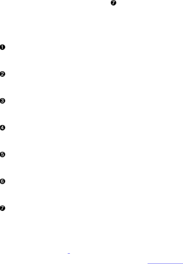
job.setOutputKeyClass(Text.class);
job.setOutputValueClass(IntWritable.class);
job.setNumReduceTasks(1);
FileOutputFormat.setOutputPath(job, new Path(output));
System.exit(job.waitForCompletion(true) ? 0 : 1);
}
Extend the supplied TableMapper class, setting your own output key and value types.
Parse the JSON data, extract the author and count the occurrence.
Extend a Hadoop Reducer class, assigning the proper types.
Count the occurrences and emit sum.
Create and configure a Scan instance.
Set up the table mapper phase using the supplied utility.
Configure the reduce phase using the normal Hadoop syntax.
This job runs as a full MapReduce process, where the map phase is reading the JSON data from
the input table, and the reduce phase is aggregating the counts for every user. This is very similar
to the WordCount example4 that ships with Hadoop: the mapper emits counts of ONE, while the
reducer counts those up to the sum per key (which in Example 7-3 is the Author). Executing the
job on the command line is done like so (leaving out the configuration of the $HADOOP_CLASSPATH
variable, for the sake of space, and assuming you have done so for the previous example):
$ hadoop jar ch07/target/hbase-book-ch07-2.0-job.jar AnalyzeData \
-t testtable -c data:json -o analyze1
...
15/06/29 02:02:35 INFO client.RMProxy: Connecting to ResourceManager at \
master-1.internal.larsgeorge.com/10.0.10.1:8032
...
15/06/29 02:02:40 INFO mapreduce.JobSubmitter: number of splits:1
...
15/06/29 02:02:41 INFO mapreduce.Job: Running job: job_1433933860552_0021
...
15/06/29 02:02:50 INFO mapreduce.Job: map 0% reduce 0%
15/06/29 02:03:02 INFO mapreduce.Job: map 100% reduce 0%
15/06/29 02:03:10 INFO mapreduce.Job: map 100% reduce 100%
15/06/29 02:03:11 INFO mapreduce.Job: Job job_1433933860552_0021 \
completed successfully
15/06/29 02:03:11 INFO mapreduce.Job: Counters: 53
...
mapreduce.AnalyzeData$Counters
COLS=993
ERROR=6
ROWS=993
(586)
VALID=987
...
The end result is a list of counts per author, and can be accessed from the command line using,
for example, the hdfs dfs -text command:
$ hdfs dfs -text analyze1/part-r-00000
10sr 1
13tohl 1
14bcps 1
21721725 1
2centime 1
33rpm 1
3sunset 1
52050361 1
6630nokia 1
...
The example also shows how to use the TableMapReduceUtil class, with its static methods, to
quickly configure a job with all the required classes. Since the job also needs a reduce phase, the
main() code adds the Reducer classes as required, once again making implicit use of the default
value when no other is specified (in this case, the TextOutputFormat class).
Obviously, this is a simple example, and in practice you will have to perform more involved
analytical processing. But even so, the template shown in the example stays the same: you read
from a table, extract the required information, and eventually output the results to a specific
target.
(587)

Table as both Data Source and Sink
As already shown, the source or target of a MapReduce job can be a HBase table, but it is also
possible for a job to use HBase as both input and output. In other words, a third kind of
MapReduce template uses a table for the input and output types. This involves setting the
TableInputFormat and TableOutputFormat classes into the respective fields of the job configuration.
This also implies the various key and value types, as shown before. Example 7-4 shows this in
context.
Example 7-4. MapReduce job that parses the raw data into separate columns.
static class ParseMapper
extends TableMapper<ImmutableBytesWritable, Mutation> {
private JSONParser parser = new JSONParser();
private byte[] columnFamily = null;
@Override
protected void setup(Context context)
throws IOException, InterruptedException {
columnFamily = Bytes.toBytes(
context.getConfiguration().get("conf.columnfamily"));
}
@Override
public void map(ImmutableBytesWritable row, Result columns, Context context)
throws IOException {
context.getCounter(Counters.ROWS).increment(1);
String value = null;
try {
Put put = new Put(row.get());
for (Cell cell : columns.listCells()) {
context.getCounter(Counters.COLS).increment(1);
value = Bytes.toStringBinary(cell.getValueArray(),
cell.getValueOffset(), cell.getValueLength());
JSONObject json = (JSONObject) parser.parse(value);
for (Object key : json.keySet()) {
Object val = json.get(key);
put.addColumn(columnFamily, Bytes.toBytes(key.toString()),
Bytes.toBytes(val.toString()));
}
}
context.write(row, put);
context.getCounter(Counters.VALID).increment(1);
} catch (Exception e) {
e.printStackTrace();
System.err.println("Error: " + e.getMessage() + ", Row: " +
Bytes.toStringBinary(row.get()) + ", JSON: " + value);
context.getCounter(Counters.ERROR).increment(1);
}
}
}
public static void main(String[] args) throws Exception {
...
Scan scan = new Scan();
if (column != null) {
byte[][] colkey = KeyValue.parseColumn(Bytes.toBytes(column));
if (colkey.length > 1) {
scan.addColumn(colkey[0], colkey[1]);
conf.set("conf.columnfamily", Bytes.toStringBinary(colkey[0]));
conf.set("conf.columnqualifier", Bytes.toStringBinary(colkey[1]));
} else {
scan.addFamily(colkey[0]);
conf.set("conf.columnfamily", Bytes.toStringBinary(colkey[0]));
}
(588)
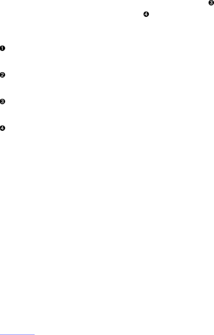
}
Job job = Job.getInstance(conf, "Parse data in " + input +
", write to " + output);
job.setJarByClass(ParseJson.class);
TableMapReduceUtil.initTableMapperJob(input, scan, ParseMapper.class,
ImmutableBytesWritable.class, Put.class, job);
TableMapReduceUtil.initTableReducerJob(output,
IdentityTableReducer.class, job);
System.exit(job.waitForCompletion(true) ? 0 : 1);
}
Store the top-level JSON keys as columns, with their value set as the column value.
Store the column family in the configuration for later use in the mapper.
Setup map phase details using the utility method.
Configure an identity reducer to store the parsed data.
The example uses the utility methods to configure the map and reduce phases, specifying the
ParseMapper, which extracts the details from the raw JSON, and an IdentityTableReducer to store
the data in the target table. Note that both—that is, the input and output table—can be the same.
Launching the job from the command line can be done like this:
$ hadoop jar ch07/target/hbase-book-ch07-2.0-job.jar ParseJson \
-i testtable -c data:json -o testtable
...
15/06/29 05:21:21 INFO impl.YarnClientImpl: Submitted application /
application_1433933860552_0022
...
15/06/29 05:21:21 INFO mapreduce.Job: Running job: job_1433933860552_0022
...
15/06/29 05:21:31 INFO mapreduce.Job: map 0% reduce 0%
15/06/29 05:21:42 INFO mapreduce.Job: map 100% reduce 0%
15/06/29 05:21:53 INFO mapreduce.Job: map 100% reduce 100%
15/06/29 05:21:54 INFO mapreduce.Job: Job job_1433933860552_0022 \
completed successfully
15/06/29 05:21:54 INFO mapreduce.Job: Counters: 53
...
mapreduce.ParseJson$Counters
COLS=993
ERROR=6
ROWS=993
VALID=987
...
The percentages show that both the map and reduce phases have been completed, and that the job
overall completed subsequently. Using the IdentityTableReducer to store the extracted data is not
necessary, and in fact the same code with one additional line turns the job into a map-only one.
Example 7-5 shows the added line.
Example 7-5. MapReduce job that parses the raw data into separate columns (map phase only).
...
(589)
Job job = Job.getInstance(conf, "Parse data in " + input +
", write to " + output + "(map only)");
job.setJarByClass(ParseJson2.class);
TableMapReduceUtil.initTableMapperJob(input, scan, ParseMapper.class,
ImmutableBytesWritable.class, Put.class, job);
TableMapReduceUtil.initTableReducerJob(output,
IdentityTableReducer.class, job);
job.setNumReduceTasks(0);
...
Running the job from the command line shows that the reduce phase has been skipped:
$ hadoop jar ch07/target/hbase-book-ch07-1.0-job.jar ParseJson2 \
-i testtable -c data:json -o testtable
...
15/06/29 05:29:17 INFO mapreduce.Job: map 0% reduce 0%
15/06/29 05:29:29 INFO mapreduce.Job: map 100% reduce 0%
15/06/29 05:29:30 INFO mapreduce.Job: Job job_1433933860552_0023 \
completed successfully
...
The reduce stays at 0%, even when the job has completed. You can also use the Hadoop
MapReduce UI to confirm that no reduce task have been executed for this job. The advantage of
bypassing the reduce phase is that the job will complete much faster, since no additional
processing of the data by the framework is required. Both variations of the ParseJson job
performed the same work. The result can be seen using the HBase Shell (omitting the repetitive
row key output for the sake of space):
hbase(main):001:0> scan 'testtable'
...
\xFB!Nn\x8F\x89}\xD8\x91+\xB9o9\xB3E\xD0
column=data:author, timestamp=1435580953962, value=bookrdr3
column=data:comments, timestamp=1435580953962,
value=http://delicious.com/url/409839abddbce807e4db07bf7d9cd7ad
column=data:guidislink, timestamp=1435580953962, value=false
column=data:id, timestamp=1435580953962,
value=http://delicious.com/url/409839abddbce807e4db07bf7d9cd7ad#bookrdr3
...
column=data:link, timestamp=1435580953962,
value=http://sweetsassafras.org/2008/01/27/how-to-alter-a-wool-sweater
...
column=data:updated, timestamp=1435580953962,
value=Mon, 07 Sep 2009 18:22:21 +0000
...
...
993 row(s) in 1.7070 seconds
The import makes use of the arbitrary column names supported by HBase: the JSON keys are
converted into qualifiers, and form new columns on the fly.
(590)
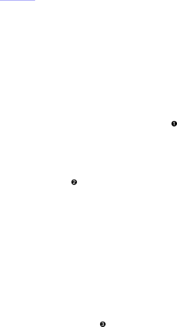
Custom Processing
You do not have to use any classes supplied by HBase to read and/or write to a table. In fact,
these classes are quite lightweight and only act as helpers to make dealing with tables easier.
Example 7-6 converts the previous example code to split the parsed JSON data into two target
tables. The link key and its value is stored in a separate table, named linktable, while all other
fields are stored in the table named infotable.
Example 7-6. MapReduce job that parses the raw data into separate tables.
static class ParseMapper
extends TableMapper<ImmutableBytesWritable, Writable> {
private Connection connection = null;
private BufferedMutator infoTable = null;
private BufferedMutator linkTable = null;
private JSONParser parser = new JSONParser();
private byte[] columnFamily = null;
@Override
protected void setup(Context context)
throws IOException, InterruptedException {
connection = ConnectionFactory.createConnection(
context.getConfiguration());
infoTable = connection.getBufferedMutator(TableName.valueOf(
context.getConfiguration().get("conf.infotable")));
linkTable = connection.getBufferedMutator(TableName.valueOf(
context.getConfiguration().get("conf.linktable")));
columnFamily = Bytes.toBytes(
context.getConfiguration().get("conf.columnfamily"));
}
@Override
protected void cleanup(Context context)
throws IOException, InterruptedException {
infoTable.flush();
linkTable.flush();
}
@Override
public void map(ImmutableBytesWritable row, Result columns, Context context)
throws IOException {
context.getCounter(Counters.ROWS).increment(1);
String value = null;
try {
Put infoPut = new Put(row.get());
Put linkPut = new Put(row.get());
for (Cell cell : columns.listCells()) {
context.getCounter(Counters.COLS).increment(1);
value = Bytes.toStringBinary(cell.getValueArray(),
cell.getValueOffset(), cell.getValueLength());
JSONObject json = (JSONObject) parser.parse(value);
for (Object key : json.keySet()) {
Object val = json.get(key);
if ("link".equals(key)) {
linkPut.addColumn(columnFamily, Bytes.toBytes(key.toString()),
Bytes.toBytes(val.toString()));
} else {
infoPut.addColumn(columnFamily, Bytes.toBytes(key.toString()),
Bytes.toBytes(val.toString()));
}
}
}
infoTable.mutate(infoPut);
linkTable.mutate(linkPut);
context.getCounter(Counters.VALID).increment(1);
} catch (Exception e) {
(591)
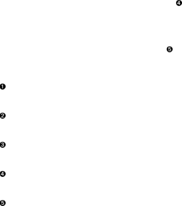
e.printStackTrace();
System.err.println("Error: " + e.getMessage() + ", Row: " +
Bytes.toStringBinary(row.get()) + ", JSON: " + value);
context.getCounter(Counters.ERROR).increment(1);
}
}
}
public static void main(String[] args) throws Exception {
...
conf.set("conf.infotable", cmd.getOptionValue("o"));
conf.set("conf.linktable", cmd.getOptionValue("l"));
...
Job job = Job.getInstance(conf, "Parse data in " + input +
", into two tables");
job.setJarByClass(ParseJsonMulti.class);
TableMapReduceUtil.initTableMapperJob(input, scan, ParseMapper.class,
ImmutableBytesWritable.class, Put.class, job);
job.setOutputFormatClass(NullOutputFormat.class);
job.setNumReduceTasks(0);
System.exit(job.waitForCompletion(true) ? 0 : 1);
}
Create and configure both target tables in the setup() method.
Flush all pending commits when the task is complete.
Save parsed values into two separate tables.
Store table names in configuration for later use in the mapper.
Set the output format to be ignored by the framework.
You need to create two more tables, using, for example, the HBase Shell:
hbase(main):001:0> create 'infotable', 'data'
hbase(main):002:0> create 'linktable', 'data'
These two new tables will be used as the target tables for the current example. Executing the job
is done on the command line, and emits the following output:
$ hadoop jar target/hbase-book-ch07-1.0-job.jar ParseJsonMulti \
-i testtable -c data:json -o infotable -l linktable
11/08/08 21:13:57 INFO mapred.JobClient: Running job: job_201108081021_0033
11/08/08 21:13:58 INFO mapred.JobClient: map 0% reduce 0%
11/08/08 21:14:06 INFO mapred.JobClient: map 100% reduce 0%
11/08/08 21:14:08 INFO mapred.JobClient: Job complete: job_201108081021_0033
...
So far, this is the same as the previous ParseJson examples. The difference is the resulting tables,
and their content. You can use the HBase Shell and the scan command to list the content of each
table after the job has completed. You should see that the link table contains only the links, while
the info table contains the remaining fields of the original JSON.
(592)
Writing your own MapReduce code allows you to perform whatever is needed during the job
execution. You can, for example, read lookup values from a different table while storing a
combined result in yet another table. There is no limit as to where you read from, or where you
write to. The supplied classes are helpers, nothing more or less, and serve well for a large
number of use cases. If you find yourself limited by their functionality, simply extend them, or
implement generic MapReduce code and use the API to access HBase tables in any shape or
form.
(593)

MapReduce over Snapshots
Up to this point we have operated directly on active, live HBase tables, either as a source, target,
or both. An additional mode of operation using the supplied input formats is to iterate over a
table snapshot instead. It allows you to freeze a table at a specific point in time, and then iterate
over its persisted content. This is useful for archival purposes, or for analytical workloads that
need to process subset of the data, or while the table is not allowed to change while the
processing is underway. You could copy a table, or disable all write operations to it somehow,
but by far the easiest way is to use the snapshot API HBase provides (see “Table Operations:
Snapshots” again for a refresher).
The utility class TableMapReduceUtil provides an easy to use helper method for setting up the
MapReduce job, named initTableSnapshotMapperJob(). “Supporting Classes” discussed this
method in more detail, but suffice it to say that all you have to do is provide an existing snapshot
name, and a writable location to stage the snapshot as temporary table. The full signature of the
method is:
public static void initTableSnapshotMapperJob(String snapshotName,
Scan scan, Class<? extends TableMapper> mapper,
Class<?> outputKeyClass, Class<?> outputValueClass, Job job,
boolean addDependencyJars, Path tmpRestoreDir) throws IOException
In addition, as with the other examples shown in this section, you can set a specific mapper class
to process the data, configure a Scan instance to limit and/or filter the data, set the output types,
and optionally add the necessary JAR file names to the job configuration. In fact, this is very
similar to a usual table as a data source approach, as shown in “Table as a Data Source”. This is
because all the snapshot based input format does is create a temporary table from the snapshot,
and then iterate over it as if it is like any other normal table.
Well, at least in a nutshell. There is a lot going on behind the scenes, that is, the snapshot
information is read, the layout for the temporary table created within the specified directory, the
snapshot storage files are linked into the temporary location, and then the processing can begin.
For the staging you need to have write access to both the temporary directory and the HBase root
directory. This implies that you need to run the MapReduce job using the snapshot backed input
format as the hbase user. In other words, this is an administrative operation, and requires elevated
privileges.
Splits are done at region boundaries, with the system trying to send the tasks to the servers with
the most storage files local. Keep in mind that reading the low level store files might involve
reading their underlying store blocks from HDFS across different machines. The
TableSnapshotInputFormat first determines the locality of the store file regarding the region they
are in. Assuming there was one region server writing the data for a while, you should find at least
one server—the one with the region server and datanode colocated—that has close, or exactly,
100% locality. It also checks the remaining block replicas, using a cutoff multiplier to include
them into the list of preferred processing nodes. It is controlled by
hbase.tablesnapshotinputformat.locality.cutoff.multiplier, with a default value of 0.8 (80%),
with all regions passing that threshold to be included into the split locality host list.
Favored Block Placement in HDFS
(594)

As of HDFS version 2.7.0 there is a feature allowing clients to specify preferred nodes for block
replica placement. This was added in HDFS-2576, and enables a DFS client to specify a list of
host names that are considered for replica placement. The matching HBase work to support that
is implemented in HBASE-4755, and its related subtasks, such as HBASE-7942.
There is a second part to this feature, the balancers, both for HDFS and HBase, need to honor the
special block placement and ensure they do not wreak havoc by moving blocks or regions to the
wrong servers. The JIRA issue for the HDFS side is HDFS-6133. For HBase the work to
enhance the load balancer was done in HBASE-7932, which places the regions on the configured
preferred nodes.
By default this feature is disabled, but can be switched on with the
hbase.master.loadbalancer.class configuration property, setting it to
org.apache.hadoop.hbase.master.balancer.FavoredNodeLoadBalancer. The assignment of regions
then follows the Hadoop rack-awareness, optionally placing servers into racks, and choosing
random servers across those racks to create full region copies. Given that all blocks of all files
for a region are now located on more than one server, the cluster can reassign regions to those
preferred nodes while retaining the locality benefits. The same advantage can be reaped by the
TableSnapshotInputFormat, which can add the info to the splits returned by its getSplits() method.
Example 7-7 shows an example that uses the earlier table with the imported test data in JSON
format. Here we first snapshot the table, and then iterate over it using a MapReduce job. The set
up and execution of the job is a bit different from before.
Example 7-7. MapReduce job that reads the data from a snapshot and analyzes it.
Configuration conf = HBaseConfiguration.create();
String[] otherArgs =
new GenericOptionsParser(conf, args).getRemainingArgs();
CommandLine cmd = parseArgs(otherArgs);
if (cmd.hasOption("d")) conf.set("conf.debug", "true");
String table = cmd.getOptionValue("t");
long time = System.currentTimeMillis();
String tmpName = "snapshot-" + table + "-" + time;
String snapshot = cmd.getOptionValue("s", tmpName);
Path restoreDir = new Path(cmd.getOptionValue("b", "/tmp/" + tmpName));
String column = cmd.getOptionValue("c");
String output = cmd.getOptionValue("o");
boolean cleanup = Boolean.valueOf(cmd.getOptionValue("x"));
...
Connection connection = ConnectionFactory.createConnection(conf);
Admin admin = connection.getAdmin();
LOG.info("Performing snapshot of table " + table + " as " + snapshot);
admin.snapshot(snapshot, TableName.valueOf(table));
LOG.info("Setting up job");
Job job = Job.getInstance(conf, "Analyze data in snapshot " + table);
job.setJarByClass(AnalyzeSnapshotData.class);
TableMapReduceUtil.initTableSnapshotMapperJob(snapshot, scan,
AnalyzeMapper.class, Text.class, IntWritable.class, job, true,
restoreDir);
TableMapReduceUtil.addDependencyJars(job.getConfiguration(),
JSONParser.class);
job.setReducerClass(AnalyzeReducer.class);
job.setOutputKeyClass(Text.class);
job.setOutputValueClass(IntWritable.class);
job.setNumReduceTasks(1);
FileOutputFormat.setOutputPath(job, new Path(output));
System.exit(job.waitForCompletion(true) ? 0 : 1);
if (cleanup) {
(595)
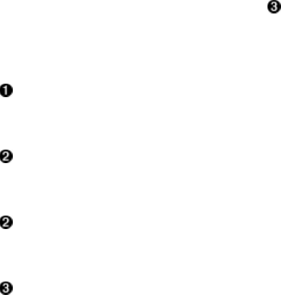
LOG.info("Cleaning up snapshot and restore directory");
admin.deleteSnapshot(snapshot);
restoreDir.getFileSystem(conf).delete(restoreDir, true);
}
admin.close();
connection.close();
Compute a name for the snapshot and restore directory, if not specified otherwise.
Create a snapshot of the table.
Set up the snapshot mapper phase using the supplied utility.
Optionally clean up after the job is complete.
For this job to complete successfully, you need to do a few things differently:
1. Stage the class path with all HBase and project libraries, to fulfill the dependency
requirements.
2. Switch the user to the owner of the HBase files, here hadoop.
As explained above, since there is a need for the TableSnapshotInputFormat to write into the HBase
root and temporary table directories, you need to switch the user executing the job. We do this by
setting the $HADOOP_USER_NAME environment variable to hadoop. Do not forget to unset it at the end
or your subsequent cluster interaction might be affected!
We also need to stage the class path variable with more details, as this job is needing additional,
non-HBase (or Hadoop) libraries. Using hbase classpath gives us all the HBase ones, more than
the previous hbase mapredcp call we used. This is caused by the TableSnapshotInputFormat to
interact deeper with HBase and Hadoop, thus requiring more libraries than the minimal set. In
addition we add all the JAR files that are part of the code repository build, using the mvn
dependency:build-classpath call triggering a Maven plugin that emits all libraries needed. This
includes the JSON libraries this example needs. An alternative approach would have been to use
the fat jar as done above, which includes the dependent JARs within the job jar. In that case we
would still have to use the hbase classpath output, but not the additional Maven command.
$ export HADOOP_CLASSPATH=$(hbase classpath):$(mvn -f ch07/pom.xml \
dependency:build-classpath | grep -v INFO)
$ export HADOOP_USER_NAME=hadoop
$ hadoop jar ch07/target/hbase-book-ch07-2.0.jar \
AnalyzeSnapshotData -t testtable -c data:json -o analyze2 -x
...
15/06/30 03:39:23 INFO mapreduce.AnalyzeSnapshotData: Performing snapshot \
of table testtable as snapshot-testtable-1435660759657
15/06/30 03:39:24 INFO mapreduce.AnalyzeSnapshotData: Setting up job
15/06/30 03:39:25 INFO snapshot.RestoreSnapshotHelper: \
region to add: 0be6bdf04700fa055129e69fff7790d2
15/06/30 03:39:25 INFO snapshot.RestoreSnapshotHelper: clone region= \
0be6bdf04700fa055129e69fff7790d2 as 0be6bdf04700fa055129e69fff7790d2
15/06/30 03:39:25 INFO regionserver.HRegion: creating HRegion testtable \
HTD == 'testtable', {NAME => 'data', DATA_BLOCK_ENCODING => 'NONE', \
BLOOMFILTER => 'ROW', REPLICATION_SCOPE => '0', VERSIONS => '1', \
(596)

COMPRESSION => 'NONE', MIN_VERSIONS => '0', TTL => 'FOREVER', \
KEEP_DELETED_CELLS => 'FALSE', BLOCKSIZE => '65536', IN_MEMORY => 'false', \
BLOCKCACHE => 'true'} RootDir = \
/tmp/snapshot-testtable-1435660759657/a2dd6a0c-0f1e-473f-8118-50028a88d945 \
Table name == testtable
15/06/30 03:39:25 INFO snapshot.RestoreSnapshotHelper: Adding HFileLink \
8b66d40caffd424099c21b7abbeda62c to table=testtable
15/06/30 03:39:25 INFO regionserver.HRegion: Closed \
testtable,,1435431398921.0be6bdf04700fa055129e69fff7790d2.
15/06/30 03:39:26 INFO client.RMProxy: Connecting to ResourceManager at \
master-1.internal.larsgeorge.com/10.0.10.1:8032
15/06/30 03:39:29 INFO mapreduce.JobSubmitter: number of splits:1
15/06/30 03:39:30 INFO mapreduce.JobSubmitter: Submitting tokens for job: \
job_1433933860552_0026
15/06/30 03:39:30 INFO impl.YarnClientImpl: Submitted application \
application_1433933860552_0026
...
15/06/30 03:39:30 INFO mapreduce.Job: Running job: job_1433933860552_0026
...
15/06/30 03:39:40 INFO mapreduce.Job: map 0% reduce 0%
15/06/30 03:39:50 INFO mapreduce.Job: map 100% reduce 0%
15/06/30 03:39:59 INFO mapreduce.Job: map 100% reduce 100%
15/06/30 03:40:00 INFO mapreduce.Job: Job job_1433933860552_0026 \
completed successfully
15/06/30 03:40:00 INFO mapreduce.Job: Counters: 53
...
mapreduce.AnalyzeSnapshotData$Counters
COLS=993
ERROR=6
ROWS=993
VALID=987
...
$ hdfs dfs -text analyze2/part-r-00000 | head -n 5
10sr 1
13tohl 1
14bcps 1
21721725 1
2centime 1
$ unset HADOOP_USER_NAME
Using the snapshot based input format requires write access to the HBase root directory because
it keeps reference of who is using what snapshot files. While no data is copied to stage the
temporary table, and only links are created, you still have to allow write access to both locations.
If you miss to switch the user to the administrative one, you will encounter errors like the one
show here:
...
15/06/30 02:30:35 INFO regionserver.HRegion: Closed \
testtable,,1435431398921.0be6bdf04700fa055129e69fff7790d2.
Exception in thread "main" java.io.IOException: \
java.util.concurrent.ExecutionException: \
org.apache.hadoop.security.AccessControlException: Permission denied: \
user=larsgeorge, access=WRITE, \
inode="/hbase/archive/data/default":hadoop:supergroup:drwxr-xr-x
at org.apache.hadoop.hdfs.server.namenode.FSPermissionChecker \
.checkFsPermission(FSPermissionChecker.java:271)
at org.apache.hadoop.hdfs.server.namenode.FSPermissionChecker....
...
Figure 7-6 shows the YARN main page with the applications list. You can see how the earlier
jobs were run as user larsgeorge, and then the latter ones as hadoop using the approach shown
above.
(597)
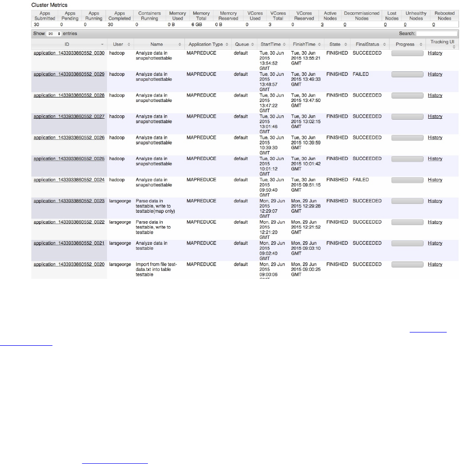
Figure 7-6. The class hierarchy of the basic client API data classes
An option to avoid write access to the HBase root is using the ExportSnapshot tool (see “Export
Snapshots”). Obviously, this tool has to copy the data from the active or archive location into the
target directory. At scale this is a costly operation and should be carefully evaluated. Also, since
you copy into an arbitrary HDFS location, you are ultimately responsible for managing that data.
This includes keeping the files while jobs are executing, and removing them when they are not
required anymore.
Finally, another reason for using snapshots as a data source instead of tables for MapReduce
processing is that it avoids RPCs and other inherent overhead of the server processes. This alone
can speed up the overall runtime of the job by a substantial margin. The JIRA adding this input
format class (see HBASE-8369) reports a factor of 5 to 6 times faster scanning performance for
single scanners.
(598)

Bulk Loading Data
Instead of going through the API using put() calls to insert data—or delete() to remove it
subsequently--, especially when you need to bootstrap a cluster with large amounts of existing
data, you can also stage and bulk load that data without going through the HBase servers. This is
a bit of a conundrum with HBase, as it is made for small data points, and optimized for writes,
with its sequential, Log-Structured Merge Tree based architecture (more about this in [Link to
Come]). Yet, the cost for maintaining said small data points is not negligible. Filling the in-
memory stores during write operation and flushing them subsequently, the compaction of data
asynchronously in an effort to keep the number of files in check, while handling explicit or
predicate deletes, is adding a non-trivial amount of noise to the system. Not to even speak of
memory management pressure during intense writing, due to Java heap fragmentation. What if
you could avoid all of that, because you have the data already in some amenable format and all
you need doing is transform it into HBase data? That is exactly what bulk loading is: an ETL job
that stages and loads the data into HBase in its native format.
What is misleading here it to speak of loading data into HBase. What really happens is that after
the staging of the data in native HBase store files, the so called HFiles, you atomically move
them into the HBase storage location, making them and the contained data immediately
available. Before you can do that though you have to do the staging part, and that is an
interesting one as well. Usually this is done by a MapReduce job which extracts the records from
the original data, then converts them into Put or Delete instances, which are then stored in HFiles.
This implies sorting the data into rows and columns, exactly the way HBase would have done if
you had used the client API.
And to complicate things, you often want to stage the store files in the same layout as the target
table is currently. You need to read the target table’s region details, to separate the staged files in
the same granularity. Then once you complete the bulk load, you have to ensure that this layout
is still the same, which means if a region has split since the initial region check, you may have to
split the staged files too to follow the new table layout. All of this is done by the supplied
ImportTsv and LoadIncrementalHFiles tools, as explained from an operations side in “Bulk Import”.
Here we are going to look more into the MapReduce integration, as it might help you stage other
sources, or create HFiles with a different processing framework, while using the same principles,
and output format classes.
(599)
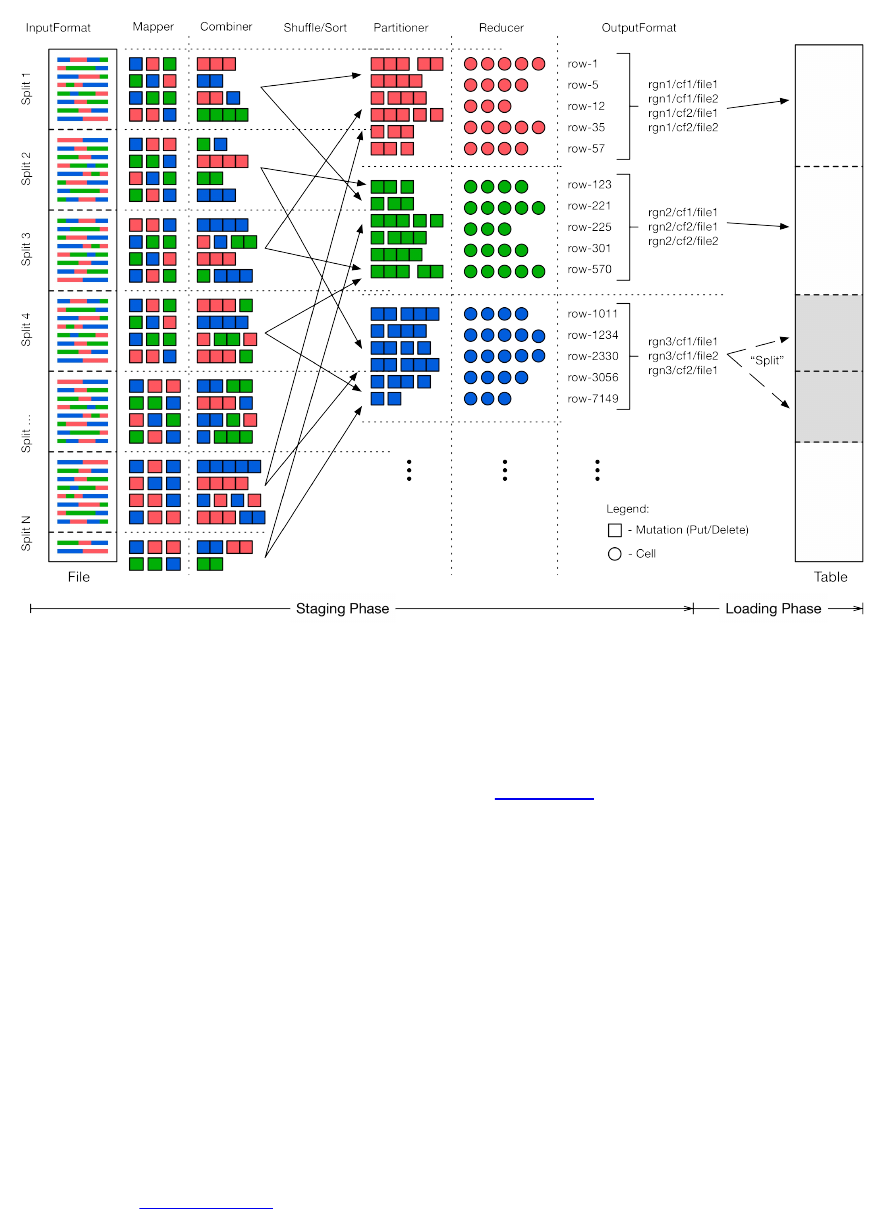
Figure 7-7. The bulk loading process
The ImportTsv tool can be used as a template for the first phase of bulk loading: the staging of
data. Once this step has completed you use the LoadIncrementalHFiles tool to do any final region
split adjustments, and then move the data files into place. Figure 7-7 shows a high level view of
how the bulk load process works. We will focus here on the first phase, which employs many
techniques to create the staged data files:
The ImportTsv Helper Tool
The ImportTsv tool only supports inserting data into the table. In other words, many used (and
provided) classes are solely supporting Put instances. There is no inherent reason not to extend
the idea to Deletes, but that has not been implemented yet. Adding support for other mutations
would not change the overall process.
The ImportTsv implementation has another special feature, it can delay the creation of Put
instances to coincide with the reduce function—referred to as text-mode hereafter. In other
words, instead of emitting Put objects from the mapper, then combining, and shipping them to
the reducer, you can keep the data in text form and do the work at the end of the process. This
was implemented in HBASE-8768 and available since HBase 0.98.0. You need to enable that
feature by overriding the mapper class using the command line parameter:
-Dimporttsv.mapper.class=org.apache.hadoop.hbase.mapreduce.TsvImporterTextMapper
The tool will then switch out the appropriate classes as needed during the job submission phase.
Read the Input Data
(600)
The first step is to read the original data, which is parsed into Put or Delete (referred to
collectively as mutation hereafter, for the sake of simplicity) instances at the available
granularity. This could be one mutation for every column, or one for the entire row—all
dependent on what your input data looks like. You might even get data for one row spread
across the input files, which creates mutation instances at random times during the
processing, spread across random worker nodes in the cluster. All of these need to be
grouped subsequently.
The mapper is expected to emit the mutations as values, while the row key of each
mutation is used as the key for each record. This will trigger the built-in shuffle and sorting
functionality of the MapReduce framework, grouping all mutations by row key. We will
see below how this is a boon and a bane (of sorts), since the default hash function used to
route the records would randomly distribute them to matching reducer tasks. It would
mean that the rows would not be contiguous across all partitions, but only within each.
For ImportTsv see the TsvImporterMapper (or TsvImporterTextMapper for text-mode) as an
example mapper implementation.
Combine Mutations
As an optimization, we can combine the mutations for the same row emitted by the same
mapper task. We might not have the entire row on this server, but if we have more than
one mutation for a specific row, we can combine them into a single one, saving object
overhead before the shuffle and sort take place.
Note that for ImportTsv this is provided by the PutCombiner class, and only supports Put
instances, as the name implies. The supplied class uses an implicit upper size boundary to
not run into memory pressure when combining puts. It is set to 1 GB and can be modified
by setting the putcombiner.row.threshold property in the configuration. For text-mode there
is no combiner used.
Route Mutations
This is where we get the grouping of rows within region boundaries working. The default
hash partitioner class is replaced with the TotalOrderPartitioner class, provided by
Hadoop. It requires a list of partitions, based on user provided boundaries. For bulk
loading we use the target table’s region boundaries and hand that list over to the special
partitioner class. Any mutation that is emitted is then send to the reducer handling the key
subrange. This also implies that we have to run as many reducers as we have regions in the
target table.
Sort Rows
There is not much that needs to be done for the rows to be sorted within a region (or
partition, both are used synonymously here), as the MapReduce framework is taking care
of that. This is one of the fundamental tasks of the framework, sending the records to the
proper partition (based on the used partitioner implementation), and the sorting them by
their key component. This is why the key type ImmutableBytesWritable is derived from the
Hadoop WritableComparable class, allowing for a natural sorting of records by keys.
Sort Columns
(601)

While records are grouped and sorted by key, it leaves the associated values to be ordered,
that is, the mutations and the contained columns forming a logical row in the resulting
HBase table. The PutSortReducer (or TextSortReducer for text-mode) class handles this task,
being provided with all mutations for a given row key, it sorts the contained columns just
like HBase would have done during an organic write operation using the client API.
The putsortreducer.row.threshold (or reducer.row.threshold for text-mode) property, set to
1 GB, defines an upper boundary to avoid memory issues in extreme cases, with very
memory intense rows (those that contain many columns, or very large cells). The output of
the reducer are the actual columns (the cells) as the value, and not a Put or Delete, while
the key stays unchanged and set as the row key. Figure 7-7 shows the difference by
switching from boxes to circles in the reducer step.
Write Files
The already discussed HFileOutputFormat2 class is responsible for writing the actual storage
files, that is, the HFiles. Its provided, static helper method configureIncrementalLoad() can
be used to configure all the output format related aspects of the ETL job. This includes
setting the above reducer and partitioner classes (along with its custom partition
information), as well as the HFile related properties, such as compression type, Bloom
filter settings, block sizes and encodings. Otherwise, the output format is honoring many
of the usual storage related configuration properties, such as hbase.hregion.max.filesize
(set to 10 GB by default) to specify the maximum file size.
These are, from a generic viewpoint, all of the steps involved in staging the bulk load data. The
new HFiles are created in a temporary location, which needs to be set per staging job, and
obviously requires read and write access for the user running the job. For ImportTsv you can
specify the location on the command line, using the importtsv.bulk.output parameter. The
mentioned LoadIncrementalHFiles utility performs the second stage of the bulk loading, by
moving the new files into the existing table directory, while ensuring any short term region
boundary changes are resolved in the process.
One caveat needs to be mentioned: loading potentially very large files into a region can trigger
splits right after the process completes. You saw above that the staging process is creating files
up to the maximum configured size. If you already have storage files in the region, you will
trigger region splits if the combined new size of loaded files plus existing ones exceeds the
configured store maximum (which is what the hbase.hregion.max.filesize really configures). This
is OK of course, because that is part of what makes HBase special, that is, it does the
housekeeping work for you asynchronously. On the other hand, that again adds background I/O
load to your cluster. It is advisable to calculate the sizes carefully, and maybe split regions at a
slower pace (say at off-peak times) before you do the loading.
Loading data into an existing table is a common exercise, and if that table has a decent number of
regions you will be able to efficiently load data into them. This is attributed by the number of
reducers matching the number of regions, allowing for parallelizing the work into as many
concurrent tasks as your MapReduce cluster can afford. But what about a bootstrap process, that
is, when you want to bulk load new data in a not-yet-existent table? You can certainly use the
create shell command to quickly create a table, but that will only have one region, and resulting
into a single reducer task doing all the data staging. Here is where presplitting a table comes in,
discussed in detail in “Presplitting Regions”. Suffice it to say that you create a certain number of
regions at the time you create the table. These regions will be empty, but then fill with data as it
is being written to.
(602)

If presplitting a new table is the answer to avoid hotspotting on a single region for staging the
bulk load, then how many splits do you need? And at what boundaries do you split them? This
requires detailed knowledge of the key space, which you may not have when faced with an
arbitrary set of input data. The common approach is to sample or parse the data at least once,
tracking the size of each record and building equally sized partitions. This is only possible if you
know where data will eventually be located in the resulting table, and thus you may have to run
the same staging logic twice, once to determine the number of regions and their boundaries based
on size, and then again to do the actual file staging. An alternative approach is to sample the
import data first, trying to extrapolate the region sizes and count from what you have access to.
This is a common analytical task and not specific to Hadoop or HBase. You need to calculate the
possible error rate to decide which sample rate works best for you. Either way, once you have
computed the split points based on the used row keys, you hand this list into first the shell’s
create command to presplit the new table, and second the TotalOrderPartitioner, which will do
the rest.
1 Note the switch of language here: sometimes Hadoop refers to the processed data as records,
sometimes as KeyValues. These are used interchangeably.
2 As of this writing, there is also a deprecated class named HLogInputFormat that only differs from
WALInputFormat in that it handles the equally deprecated HLogKey class, as opposed to the newer
WALKey.
3 This is not entirely true, the shared TableInputFormatBase class has a protected method named
includeRegionInSplit() which by default returns true. A custom subclass could override the
method and not include all regions belonging to the configured scan.
4 See the Hadoop wiki page for details.
(603)
Chapter 8. Advanced Usage
This chapter goes deeper into the various design implications imposed by HBase’s storage
architecture. It is important to have a good understanding of how to design tables, row keys,
column names, and so on, to take full advantage of the architecture.
(604)
Key Design
HBase has two fundamental key structures: the row key and the column key. Both can be used to
convey meaning, by either the data they store, or by exploiting their sorting order. In the
following sections, we will use these keys to solve commonly found problems when designing
storage solutions based on HBase.
(605)

Concepts
The first concept to explain in more detail is the logical layout of a table, compared to on-disk
storage. HBase’s main unit of separation within a table is the column family--not the actual
columns as expected from a column-oriented database in their traditional sense. Figure 8-1
shows the fact that, although you store cells in a table format logically, in reality these rows are
stored as linear sets of the actual cells, which in turn contain all the vital information inside them.
The top-left part of the figure shows the logical layout of your data: you have rows and columns.
The columns are the typical HBase combination of a column family name and a column
qualifier, forming the column key. The rows also have a row key so that you can address all
columns in one logical row.
(606)
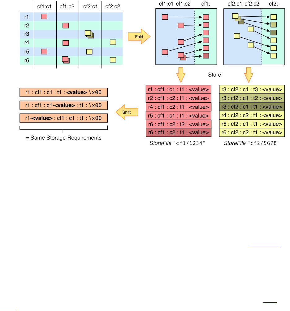
Figure 8-1. Rows stored as linear sets of actual cells, which contain all the vital information
The top-right hand side shows how the logical layout is folded into the actual physical storage
layout. The cells of each row are stored one after the other, in separate storage files per column
family. In other words, on disk you will have all cells of one family in (one or more) StoreFiles,
and all cells of another in a different file, located in a different directory.
Since HBase is not storing any unset cells (also referred to as NULL values by RDBMSes) from the
table, the on-disk files only contain the data that has been explicitly set. It therefore has to also
store the row key and column key with every cell so that it can retain this vital piece of
information. They form part of the coordinates of a cell in the table, as explained in “The Cell”
In addition, multiple versions of the same cell are stored as separate, consecutive cells, using the
required timestamp of when the cell was stored. The cells are sorted in descending order by that
timestamp so that a reader of the data will see the newest value first—which is the canonical
access pattern for the data using the client API.
The entire cell, with the added structural information, is called Cell in HBase terms (see “The
Cell”). It contains not just the column and actual value, but also the row key and timestamp,
stored for every cell for which you have set a value. The Cells are sorted by row key first, and
then by column key in case you have more than one cell per row in one column family. The said
descending sorting per version of a cell takes place last.
The lower-right part of the figure shows the resultant layout of the logical table inside the
physical storage files. The HBase API has various means of querying the stored data, with
decreasing granularity from left to right: you can select rows by row keys and effectively reduce
the amount of data that needs to be scanned when looking for a specific row, or a range of rows.
Specifying the column family as part of the query can eliminate the need to search the separate
storage files. If you only need the data of one family, it is highly recommended that you specify
the family for your read operation.
Note
(607)
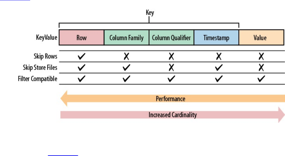
As far as reading data is concerned, get and scan operations are the same, see [Link to Come] for
details. The only difference is that a get operation is allowed to set the scan stoprow to be
inclusive. Otherwise they use exactly the same code path.
Although the timestamp--or version--of a cell is farther to the right, it is another important
selection criterion. The store files retain the timestamp range for all stored cells, so if you are
asking for a cell that was changed in the past two hours, but a particular store file only has data
that is four or more hours old it can be skipped completely. See also [Link to Come] for details.
The next level of query granularity is the column qualifier. You can employ exact column
lookups when reading data, or define filters that can include or exclude the columns you need to
access. But as you will have to look at each Cell to check if it should be included, there is only a
minor performance gain: data is ignored on the server-side and omitted as needed, reducing the
RPC traffic between client and region server.
The value remains the last, and broadest, selection criterion, equaling the column qualifier’s
effectiveness: you need to look at each cell to determine if it matches the read parameters. You
can only use a filter to specify a matching rule, making it the least efficient query option.
Figure 8-2 summarizes the effects of using the Cell fields.
Figure 8-2. Retrieval performance decreasing from left to right
The crucial part Figure 8-1 shows is the shift in the lower-lefthand side. Since the effectiveness
of selection criteria greatly diminishes from left to right for a Cell, you can move all, or partial,
details of the value into a more significant place—without changing how much data is stored.
(608)

Tall-Narrow Versus Flat-Wide Tables
At this time, you may be asking yourself where and how you should store your data. The two
fundamental choices are tall-narrow and flat-wide (though there is now hard boundary in
between). The former is a table with few columns but many rows, while the latter has fewer rows
but many columns. Given the explained query granularity of the Cell information, it seems to be
advisable to store parts of the cell’s data—especially the parts needed to query it—in the row
key, as it has the highest cardinality. This would lead to a tall-narrow table design, though
forfeiting the per-row atomicity of mutations.
In addition, HBase can only split at row boundaries, which also enforces the recommendation to
go with tall-narrow tables. Imagine you have all emails of a user in a single row. This will work
for the majority of users, but there will be outliers that will have magnitudes of emails more in
their inbox—so many, in fact, that a single row could outgrow the maximum file/region size and
work against the region split facility.
Example 8-1.
What is not obvious right away is that the blocks inside HFiles are also bound by the row size. In
other words, if you manage to create a row that occupies 1 GB of data, you will have a HFile with
a block of 1 GB in it. This makes accessing columns difficult, as the entire block has to be loaded
into the region servers memory for subsequent in-memory scanning. If you need most of that row
most of the time, that might OK. But if you only need a marginal number of columns, then you
are wasting precious memory and inadvertently slowing down the read operation.
The better approach would be to store each email of a user in a separate row, where the row key
is a combination of the user ID and the message ID. Looking at Figure 8-1 you can see that, on
disk, this makes no difference: if the message ID is in the column qualifier, or in the row key,
each cell still contains a single email message. Here is the flat-wide layout on disk, including
some examples:
<userId> : <colfam> : <messageId> : <timestamp> : <email-message>
12345 : data : 5fc38314-e290-ae5da5fc375d : 1464348181 : "Hi Lars, ..."
12345 : data : 725aae5f-d72e-f90f3f070419 : 1464354367 : "Welcome, and ..."
12345 : data : cc6775b3-f249-c6dd2b1a7467 : 1464379433 : "To Whom It ..."
12345 : data : dcbee495-6d5e-6ed48124632c : 1464383821 : "Hi, how are ..."
The same information stored as a tall-narrow table has virtually the same footprint when stored
on disk:
<userId>-<messageId> : <colfam> : <qualifier> : <timestamp> : <email-message>
12345-5fc38314-e290-ae5da5fc375d : data : : 1464348181 : "Hi Lars, ..."
12345-725aae5f-d72e-f90f3f070419 : data : : 1464354367 : "Welcome, and ..."
12345-cc6775b3-f249-c6dd2b1a7467 : data : : 1464379433 : "To Whom It ..."
12345-dcbee495-6d5e-6ed48124632c : data : : 1464383821 : "Hi, how are ..."
This layout makes use of the empty qualifier (see “Column Families”). The message ID is simply
moved to the left, making it more significant when querying the data, but also transforming each
email into a separate logical row. This results in a table that is easily splittable, with the
additional benefit of having a more fine-grained query granularity.
(609)

Partial Key Scans
The scan functionality of HBase, and the Table-based client API, offers the second crucial part
for transforming a table into a tall-narrow one, without losing query granularity: partial key
scans.
In the preceding example, you have a separate row for each message, across all users. Before you
had one row per user, so a particular inbox was a single row and could be accessed as a whole.
Each column was an email message of a user’s inbox. The exact row key would be used to match
the user ID when loading the data.
With the tall-narrow layout an arbitrary message ID is now postfixed to the user ID in each row
key. If you do not have an exact combination of these two IDs you cannot retrieve a particular
message. The way to get around this complication is to use partial key scans: you can specify a
start and stop key that is set to the exact user ID only, with the stop key set to userId + 1 (that is,
being binary one increment larger than the current start key).
The start key of a scan is inclusive, while the stop key is exclusive. Setting the start key to the
user ID triggers the internal lexicographic comparison mechanism of the scan to find the exact
row key, or the one sorting just after it. Since the table does not have an exact match for the user
ID, it positions the scan at the next row, which is:
<userId>-<lowest-messageId>
In other words, it is the row key with the lowest (in terms of sorting) user ID and message ID
combination. The scan will then iterate over all the messages of a user and you can parse the row
key to extract the message ID.
The partial key scan mechanism is quite powerful, as you can use it as a lefthand index, with
each added field adding to its cardinality. Consider the following row key structure:
<userId>-<date>-<messageId>-<attachmentId>
Note
Make sure that you pad the value of each field in the composite row key so that the
lexicographical (binary, and ascending) sorting works as expected. You will need a fixed-length
field structure to guarantee that the rows are sorted by each field, going from left to right.1
You can, with increasing precision, construct a start and stop key for the scan that selects the
required rows. Usually you only create the start key and set the stop key to the same value as the
start key, while increasing the least significant byte of its first field by one. For the preceding
inbox example, the start key could be 12345, and the stop key 12346.
Example 8-2.
Take extra care computing the stop key. Simply adding a 1 to the last byte might not result in the
correct key. For example, if your key is 0x01 0x00 0xff then you need to drop the last byte, and
increment the previous one (and so one in case multiple 0xff are at the tail end of the key array),
(610)

resulting in 0x01 0x01.
Also, as explained in “Introduction”, make sure for reverse scans to compute the keys
accordingly.
Table 8-1 shows some of the possible start keys and what they translate into.
Table 8-1. Possible start keys and their meaning
Command Description
<userId> Scan over all messages for a given user ID.
<userId>-<date> Scan over all messages on a given date for the given user
ID.
<userId>-<date>-<messageId> Scan over all parts of a message for a given user ID and
date.
<userId>-<date>-<messageId>-
<attachmentId>
Scan over all attachments of a message for a given user ID
and date.
These composite row keys are similar to what RDBMSes offer, yet you can control the sort order
for each field separately. For example, you could do a bitwise inversion of the date expressed as
a long value (the Linux epoch). This would then sort the rows in descending order by date.
Another approach is to compute the following:
Long.MAX_VALUE - <date-as-long>
This will reverse the dates and guarantee that the sorting order of the date field is descending.
In the preceding example, you have the date as the second field in the composite index for the
row key. This is only one way to express such a combination. If you were to never query by date,
you would want to drop the date from the key—and possibly use another, more suitable,
dimension instead.
It has been mentioned a few times already, but the issue of atomicity per row warrants a few
more remarks. While it seems to be a binary decision to spread an entity (that is, for example, the
user inbox in the examples) over more than a single row, while losing the ability to update it in
an ACID conforming way, there are other options too. One of which are region-local
transactions, explained in “Region-local Transactions”. In addition, it is often quite reasonable to
eschew the wide table and atomicity, as it depends on the access patterns of the application using
the table. If you are not concerned with updating the entire inbox with all the user messages in an
atomic fashion, the aforementioned design is appropriate. But if you need to have such
guarantees, you may have to go back to a flat-wide table design.
(611)

Pagination
Using the partial key scan approach, it is possible to iterate over subsets of rows. The principle is
the same: you have to specify an appropriate start and stop key to limit the overall number of
rows scanned. Then you take an offset and limit parameter, applying them to the rows on the
client side.
Note
You can also use the “PageFilter”, or “ColumnPaginationFilter” to achieve pagination. The
approach shown here is mainly to explain the concept of what a dedicated row key design can
achieve.
For pure pagination, the ColumnPaginationFilter is also the recommended approach, as it avoids
sending unnecessary data over the network to the client.
The steps are the following:
1. Open a scanner at the start row.
2. Skip offset rows.
3. Read the next limit rows and return to the caller.
4. Close the scanner.
Applying this to the inbox example, it is possible to paginate through all of the emails of a user.
Assuming an average user has a few hundred emails in his inbox, it is quite common for a web-
based email client to show only the first, for example, 50 emails. The remainder of the emails are
then accessed by clicking the Next button to load the next page.
The client would set the start row to the user ID, and the stop row to the user ID + 1. The
remainder of the process would follow the approach we just discussed, so for the first page,
where the offset is zero, you can read the first 50 emails. When the user clicks the Next button,
you would set the offset to 50, therefore skipping those first 50 rows, returning row 51 to 100,
and so on.
This approach works well for a low number of pages. If you were to page through thousands of
pages, a different approach would be required. You could add a sequential ID into the row key to
directly position the start key at the right offset. Or you could use the date field of the key—if
you are using one—to remember the date of the last displayed item and add the date to the start
key, but probably dropping the hour part of it. If you were using epochs, you could compute the
value for midnight of the last seen date. That way you can rescan that entire day and make a
more concise decision regarding what to return.
There are many ways to design the row key to allow for efficient selection of subranges and
enable pagination through records, such as the emails in the user inbox example. Using the
composite row key with the user ID and date gives you a natural order, displaying the newest
messages first, sorting them in descending order by date. But what if you also want to offer
sorting by different fields so that the user can switch at will? One way to do this is discussed in
(612)

Time Series Data
When dealing with stream processing of events, the most common use case is time series data.
Such data could be coming from a sensor in a power grid, a stock exchange, or a monitoring
system for computer systems. Its salient feature is that some part of its keys represents the event
time. This imposes a problem with the way HBase is arranging its rows: they are all stored sorted
in a distinct range, namely regions with specific start and stop keys.
The sequential, monotonously increasing nature of time series data causes all incoming data to be
written to the same region. And since this region is hosted by a single server, all the updates will
only tax this one machine. This can cause regions to really run hot with the number of accesses,
and in the process slow down the perceived overall performance of the cluster, because inserting
data is now bound to the performance of a single machine.
It is easy to overcome this problem by ensuring that data is spread over all region servers instead.
This can be done, for example, by prefixing the row key with a nonsequential prefix. Common
choices include:
Salting
You can use a salting (or bucketing, as a synonym) prefix to the key that guarantees a
spread of all rows across all region servers. For example:
byte prefix = (byte) (Long.hashCode(timestamp) %
<number of region servers>);
byte[] rowkey = Bytes.add(Bytes.toBytes(prefix),
Bytes.toBytes(timestamp));
This formula will generate enough prefix numbers to ensure that rows are sent to all region
servers. Of course, the formula assumes a specific number of servers, and if you are
planning to grow your cluster you should set this number to a multiple instead. Replacing
the the timestamps with something more readable (for the sake of the example), the
generated row keys might look like this:
0myrowkey-1, 1myrowkey-2, 2myrowkey-3, 0myrowkey-4, 1myrowkey-5, \
2myrowkey-6, ...
When these keys are lexicographically sorted and sent to the various regions the order
would be:
0myrowkey-1
0myrowkey-4
1myrowkey-2
1myrowkey-5
...
In other words, the updates for row keys 0myrowkey-1 and 0myrowkey-4 would be sent to one
region (assuming they do not overlap two regions, in which case there would be an even
broader spread), and 1myrowkey-2 and 1myrowkey-5 are sent to another, and both are likely to
be hosted by different region servers.
The drawback of this approach is that access to a range of rows must be fanned out in your
own code and read with <number of region servers> get or scan calls. On the upside, you
(614)

could use multiple threads to read this data from distinct servers, therefore parallelizing
read access. This is akin to a small map-only MapReduce job, and should result in
increased I/O performance.2
Use Case: Mozilla Socorro
The Mozilla organization has built a crash reporter—named Socorro3--for Firefox and
Thunderbird, which stores all the pertinent details pertaining to when a client asks its user
to report a program anomaly. These reports are subsequently read and analyzed by the
Mozilla development team to make their software more reliable on the vast number of
machines and configurations on which it is used.
The code is open source, available online, and contains the Python-based client code that
communicates with the HBase cluster using Happybase (code can be found in its
accompanying GitHub repository). Here is an example (as of the time of this writing) of
how the client is merging the previously salted, sequential keys when doing a scan
operation:
def _merge_scan_with_prefix(self, client, table, prefix, columns):
# TODO: Need assertion that columns is array containing at least
# one string
"""A generator based iterator that yields totally ordered rows starting
with a given prefix. The implementation opens up 16 scanners (one for
each leading hex character of the salt) simultaneously and then yields
the next row in order from the pool on each iteration."""
iterators = []
next_items_queue = []
for salt in '0123456789abcdef':
salted_prefix = "%s%s" % (salt, prefix)
scanner = client.scannerOpenWithPrefix(table,
salted_prefix,
columns)
iterators.append(self._salted_scanner_iterable(client,
salted_prefix,
scanner))
# The i below is so we can advance whichever scanner delivers us the
# polled item.
for i, it in enumerate(iterators):
try:
next = it.next
next_items_queue.append([next(), i, next])
except StopIteration:
pass
heapq.heapify(next_items_queue)
while True:
try:
while True:
row_tuple, iter_index, next = s = next_items_queue[0]
# tuple[1] is the actual nice row.
yield row_tuple[1]
s[0] = next()
heapq.heapreplace(next_items_queue, s)
except StopIteration:
heapq.heappop(next_items_queue)
except IndexError:
return
The Python code opens the required number of scanners, adding the salt prefix, which here
is composed of a fixed set of single-letter prefixes—16 different ones all together. Note
that an additional heapq object is used that manages the actual merging of the scanner
results against the global sorting order.
Field swap/promotion
(615)

Using the same approach as described in “Partial Key Scans”, you can move the timestamp
field within the row key, or prefix it with another field. The former approach uses the
composite row key concept to move the sequential, monotonously increasing timestamp to
a secondary position in the row key: if you already have a row key with more than one
field, you can swap them. If you have only the timestamp as the current row key, you need
to promote another field from the column keys, or even the value, into the row key.
There is a drawback to moving the time to the righthand side in the composite key: you
can only access data, especially time ranges, for a given swapped or promoted field.
Use Case: OpenTSDB
The OpenTSDB project provides a time series database used to store metrics about servers
and services, gathered by external collection agents. All of the data is stored in HBase, and
using the supplied user interface (UI) enables users to query various metrics, combining
and/or downsampling them—all in real time.
The schema promotes the metric ID into the row key, forming the following structure:
<metric-id><base-timestamp>...
Since a production system will have a considerable number of metrics, but their IDs will
be spread across a range and all updates occurring across them, you end up with an access
pattern akin to the salted prefix: the reads and writes are spread across the metric IDs.
This approach is ideal for a system that queries primarily by the leading field of the
composite key. In the case of OpenTSDB this makes sense, since the UI asks the users to
select from one or more metrics, and then displays the data points of those metrics ordered
by time.
OpenTSDB uses a few other interesting key design tricks, so it might be interesting for
you to look into it a bit deeper. In particular, the page that discusses the project’s schema is
a recommended read, as it adds advanced key design concepts for an efficient storage
format that also allows for high-performance querying of the stored data.
Randomization
A totally different approach is to randomize the row key using, for example:
byte[] rowkey = MD5(timestamp)
Using a hash function like MD5 will give you a random distribution of the key across all
available region servers. For time series data, this approach is obviously less than ideal,
since there is no way to scan entire ranges of consecutive timestamps.
On the other hand, since you can re-create the row key by hashing the timestamp
requested, it still is very suitable for random lookups of single rows. When your data is not
scanned in ranges but accessed randomly, you can use this strategy.
Summarizing the various approaches, you can see that it is not trivial to find the right balance
between optimizing for read and write performance. It depends on your access pattern, which
ultimately drives the decision on how to structure your row keys. Figure 8-3 shows the various
solutions and how they affect sequential read and write performance.
(616)
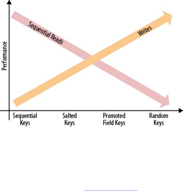
Figure 8-3. Finding the right balance between sequential read and write performance
Using the salted or promoted field keys can strike a good balance of distribution for write
performance, and sequential subsets of keys for read performance. If you are only doing random
reads, it makes most sense to use random keys: this will avoid creating region hot-spots. All of
these strategies can be adjusted as needed, and even mixed if necessary. It is vital to understand
the implications of each key design approach and choose the best matching one. A variation of
the above is explained in more detail in “Aging-out Regions”.
(617)

Time-Ordered Relations
In our preceding discussion, the time series data dealt with inserting new events as separate rows.
However, you can also store related, time-ordered data using the columns of a table. Since all of
the columns are sorted per column family, you can treat this sorting as a replacement for a
secondary index, as available in RDBMSes. Multiple secondary indexes can be emulated by
using multiple column families—although that is not the recommended way of designing a
schema. But for a small number of indexes, this might be what you need.
Consider the earlier example of the user inbox, which stores all of the emails of a user in a single
row. Since you want to display the emails in the order they were received, but, for example, also
sorted by subject, you can make use of column-based sorting to achieve the different views of the
user inbox.
Note
Given the advice to keep the number of column families in a table low—especially when mixing
large families with small ones (in terms of stored data)--you could store the inbox inside one
table, and the secondary indexes in another table. The drawback is that you cannot make use of
the provided per-table row-level atomicity. Also see “Secondary Indexes” for strategies to
overcome this limitation.
The first decision to make concerns what the primary sorting order is, in other words, how the
majority of users have set the view of their inbox. Assuming they have set the view in
descending order by date, you can use the same approach mentioned earlier, which reverses the
timestamp of the email, effectively sorting all of them in descending order by time:
Long.MAX_VALUE - <date-as-long>
The email itself is stored in the main column family, while the sort indexes are in separate
column families. You can extract the subject from the email address and add it to the column key
to build the secondary sorting order. If you need descending sorting as well, you would need
another family.
To circumvent the proliferation of column families, you can alternatively store all secondary
indexes in a single column family that is separate from the main column family. Once again, you
would make use of implicit sorting by prefixing the values with an index ID-, for example idx-
subject-desc, idx-to-asc, and so on. Next, you would have to attach the actual sort value. The
actual value of the cell is the key of the main index, which also stores the message. This also
implies that you need to either load the message details from the main table, display only the
information stored in the secondary index, or store the display details redundantly in the index,
avoiding the random lookup on the main information source. Recall that denormalization is quite
common in HBase to reduce the required read operations in favor of vastly improved user-facing
responsiveness.
Putting the aforementioned schema into action might result in something like this:
12345 : data : 5fc38314-e290-ae5da5fc375d : 1464348181 : "Hi Lars, ..."
12345 : data : 725aae5f-d72e-f90f3f070419 : 1464354367 : "Welcome, and ..."
12345 : data : cc6775b3-f249-c6dd2b1a7467 : 1464379433 : "To Whom It ..."
12345 : data : dcbee495-6d5e-6ed48124632c : 1464383821 : "Hi, how are ..."
(618)

12345 : data : 5fc38314-e290-ae5da5fc375d : 1464348181 : "Hi Lars, ..."
12345 : data : 725aae5f-d72e-f90f3f070419 : 1464354367 : "Welcome, and ..."
12345 : data : cc6775b3-f249-c6dd2b1a7467 : 1464379433 : "To Whom It ..."
12345 : data : dcbee495-6d5e-6ed48124632c : 1464383821 : "Hi, how are ..."
...
12345 : index : idx-from-asc-mary@foobar.com : 1464354367 : 725aae5f-d72e...
12345 : index : idx-from-asc-paul@foobar.com : 1464383821 : dcbee495-6d5e...
12345 : index : idx-from-asc-pete@foobar.com : 1464348181 : 5fc38314-e290...
12345 : index : idx-from-asc-sales@ignore.me : 1464379433 : cc6775b3-f249...
...
12345 : index : idx-subject-desc-\xa8\x90\x8d\x93\x9b\xde : \
1464383821 : dcbee495-6d5e-6ed48124632c
12345 : index : idx-subject-desc-\xb7\x9a\x93\x93\x90\xd3 : \
1464354367 : 725aae5f-d72e-f90f3f070419
...
In the preceding code, one index (idx-from-asc) is sorting the emails in ascending order by from
address, and another (idx-subject-desc) in descending order by subject. The subject itself is not
readable anymore as it was bit-inversed to achieve the descending sorting order. For example:
% String s = "Hello,";
% for (int i = 0; i < s.length(); i++) {
print(Integer.toString(s.charAt(i) ^ 0xFF, 16));
}
b7 9a 93 93 90 d3
All of the index values are stored in the column family index, using the prefixes mentioned
earlier. A client application can read the entire column family and cache the content to let the
user quickly switch the sorting order. Or, if the number of values is large, the client can read the
first 10 columns starting with idx-subject-desc to show the first 10 email messages sorted in
ascending order by the email subject lines. Using a scan with intra-row batching (see “Scanner
Batching”) enables you to efficiently paginate through the subindexes. Another option is the
ColumnPaginationFilter, combined with the ColumnPrefixFilter to iterate over an index page by
page.
(619)

Aging-out Regions
In practice it is sometimes necessary to use the possibilities of the HBase schema design to
achieve certain requirements. This is not unlike what happens with RDBMSes, which were
meant to keep implementation and data modelling separate, though we all know that with proper
index creation, it is very likely that at specific scale JOIN operations will slow down. A missing
index on a JOIN column results in a full table scan and therefore in the slowest I/O possible. On
the other hand, too many indexes will cause a management overhead that will eventually slow
down the entire database, trying desperately to keep up with maintaining those indexes.
For HBase, you may face a similar conundrum, as in, you will have to use the right mix of data
modelling to reach the project requirements. One of those challenges is the addressable storage
space for a HBase cluster. This is discussed in “Cluster Sizing”, though here we are looking into
one remedy, using the appropriate schema design. Before we do, let us first recap the issue in a
few words:
Every open region requires a few megabytes of memory for indexes and other structures.
When writing to a region, it requires (ideally) as much memory for memstores as the
configured flush size.
Reading from a region usually employs the block cache to hold recently used data blocks.
With those few assumption, we can derive that the heap configured for the region server
processes is divided across memstores, block cache, and other structures. The ratio of required
memory is skewed heavily though towards the writes, as HBase is trying to only flush out
memstores when they reach the set flush size, so that you do not run into the so-called
compaction storms (also see Chapter 10 for information on that topic), which could be
detrimental to your cluster performance. While reads may churn the block cache more, there is
no data that needs to be accrued in memory.
In other words, if you employ a normal write pattern, you will see most or even all of the regions
on a region server taking on mutations, and therefore requiring heap space. Doing the math as
shown in “Cluster Sizing”, you will see that a 10 GB heap with the usual 40% set for memstores,
you can only fit 32 write-active regions on a server. Given the default 10 GB region size, this
makes for a maximum of 320 GB of data addressed—which is less than what a current harddrive
offers. For modern servers you usually see 6-12 drives at 2-4TB each, providing between 12 and
48TB of storage.
The question is then, how can you address all of that storage with HBase? There is a technique
called aging-out regions, which is shown in Figure 8-4.
(620)
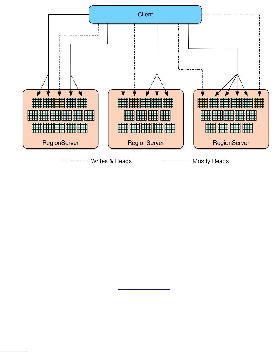
Figure 8-4. Clients reading from all regions, but writing only to few
The idea is to devise a key schema, that sees only a few regions on a server taking on writes.
Ideally, only as many regions are written to, as heap is reserved. All the other regions on that
server are read-mostly regions, that is, they are (again ideally) only used to read data from. This
approach combines the above techniques to bucket data, which has a time dependent component
in the key. The salting/bucketing will group the writes into as many regions as necessary (the
heap drives this), and the time component will cause for the key space to move along at the head
(or tail, depending on how you look at it) of the bucket and therefore have ranges in already
filled up regions that are not written to anymore.
While you may only have a few dozen write-active regions on a server, you can have many
hundreds of read-mostly ones. By the way, the term read-mostly is used to distinguish from the
read-only flag of the table descriptor (see “Table Properties”). As long as you ensure that your
application is sticking to the above plan, you will be able to address much more storage space per
server. Say you have another 1000 read-mostly regions at 10 GB each, you can address 10TB of
storage for retrieval purposes.
Finally, there is no library (as of this writing) that is helping you to support (let alone enforce)
such a schema design. You will need to implement this into your application yourself, and
monitor the memory usage of each region using the metrics subsystem, as explained in
Chapter 9.
(621)

Application-driven Replicas
Another, more advanced technique revolves around the need to keep data available at all times.
HBase trades its strict consistency guarantees by having only one cluster node serving a
particular region. All reads and writes go to that node, giving it the ability to atomically update
rows (or multiple rows within the same region). If that node becomes unavailable, the cluster will
reopen the regions the node hosted on other nodes. Detecting the node failure, and subsequent
region relocation takes a couple of seconds usually. During that time the rows of those regions
are not accessible to clients. While the API has built-in retry and timeout mechanisms, this may
still cause a glitch in latency that you are not willing to sustain.
One way of letting HBase take care of this, is explained in [Link to Come], where regions are
opened for read-only access on other nodes of the cluster, allowing clients to access those rows
during a node failure (or normal operations too, if they choose to do so). Since read-replicas are
quite new to HBase, and for the sake of showing more key design techniques that have been used
in practice, there is another approach to this topic: application-driven replicas.
Given that rows are sorted and distributed across the regions, what could you do to have more
than one server being able to serve a particularly important piece of data? You can use your
application to write it multiple times, and into separate buckets. The core of the idea is to have
regions distributed across the region servers, and then prefix the same key so that it is written to
more than one server. Your client application can then read from multiple locations, possibly
using an executor pool locally, parallelizing the operation. The first response is used to fulfill the
request, while all others are cancelled or simply ignored.
Obviously, this technique raises a few questions. First, how can you ensure that all application-
driven replicas are up-to-date? Second, how can you ensure that all copies (as a synonym for
replica here) have been updated or written at all? You buy into the same issues known from
BASE (basically available, soft state) focused systems, or eventual consistency to call it out. In
other words, you need your application to deal with distributed reads and writes, and the fact that
you may read stale data. There is no difference from what you may have read about these
approaches, for example the well-known Dynamo paper. While you are essentially reinventing
the wheel, you nonetheless achieve much higher levels of availability in the presence of node
failures, and possibly improve the perceived overall latency of operations, since you essentially
load-balance requests across nodes, where the fastest wins.
Lastly, ensuring the placement of replicas on different physical nodes is not trivial. While HBase
allows you to plug in your own LoadBalancer class that could handle the task of spreading regions
containing replicated data, this would require custom code to be developed. Since there is no
known library (as of this writing) supporting this kind of technique, I will leave this exercise to
you, the reader. It shows, though, that much can be added on top of the simple storage model and
client API provided by HBase. We will discuss more of that going forward.
(622)

Advanced Schemas
So far we have discussed how to use the provided table schemas to map data into the column-
oriented layout HBase supports. You will have to decide how to structure your row and column
keys to access data in a way that is optimized for your application.
Each column value is then an actual data point, stored as an arbitrary array of bytes. While this
type of schema, combined with the ability to create columns with arbitrary keys when needed,
enables you to evolve with new client application releases, there are use cases that require more
formal support of a more feature-rich, evolveable serialization API, where each value is a
compact representation of a more complex, nestable record structure.
Possible solutions include the already discussed serialization packages—see “Introduction” for
details—listed here as examples:
Avro
An exemplary project using Avro to store complex records in each column is HAvroBase.4
This project facilitates Avro’s interface definition language (IDL) to define the actual
schema, which is then used to store records in their serialized form within arbitrary table
columns. Hive also supports to store complex, nested in HBase columns, which can then
be exposed as structs to HiveQL, for example5:
CREATE EXTERNAL TABLE test_hbase_avro
ROW FORMAT SERDE 'org.apache.hadoop.hive.hbase.HBaseSerDe'
STORED BY 'org.apache.hadoop.hive.hbase.HBaseStorageHandler'
WITH SERDEPROPERTIES (
"hbase.columns.mapping" = ":key,test_col_fam:test_col",
"test_col_fam.test_col.serialization.type" = "avro",
"test_col_fam.test_col.avro.schema.url" = \
"hdfs://testcluster/tmp/schema.avsc")
TBLPROPERTIES (
"hbase.table.name" = "hbase_avro_table",
"hbase.mapred.output.outputtable" = "hbase_avro_table",
"hbase.struct.autogenerate"="true");
Protocol Buffers
Similar to Avro, you can use the Protocol Buffer’s IDL to define an external schema,
which is then used to serialize complex data structures into HBase columns. As of this
writing, there are no known tools that support Protocol Buffers in combination with
HBase, which means this onus is put on the application developer.
The idea behind this approach is that you get a definition language that allows you to define an
initial schema, which you can then update by adding or removing fields. The serialization API
takes care of reading older schemas with newer ones. Missing fields are ignored or filled in with
defaults. An additional benefit of using complex schemas is discussed in [Link to Come].
(623)
Secondary Indexes
Although HBase has no native support for secondary indexes, there are use cases that need them.
The requirements are usually that you can look up a cell with not just the primary coordinates—
the row key, column family name, and qualifier—but also an alternative coordinate. In addition,
you can scan a range of rows from the main table, but ordered by the secondary index.
Similar to an index in RDBMSes, secondary indexes store a mapping between the new
coordinates and the existing ones. Here is a list of possible solutions:
Client-managed
Moving the responsibility completely into the application layer, this approach typically
combines a data table and one (or more) lookup/mapping tables. Whenever the code writes
into the data table it also updates the lookup tables. Reading data requires either a direct
lookup in the main table, or, if the key is from a secondary index, a lookup of the main row
key, and then retrieval of the data in a second operation.
There are advantages and disadvantages to this approach. First, since the entire logic is
handled in the client code, you have all the freedom to map the keys exactly the way they
are needed. The list of shortcomings is longer, though: since you have no cross-row
atomicity, for example, in the form of transactions, you cannot guarantee consistency of
the main and dependent tables. This can be partially overcome using regular pruning jobs,
for instance, using MapReduce to scan the tables and remove obsolete—or add missing—
entries.
The missing transactional support could result in data being stored in the data table, but
with no mapping in the secondary index tables, because the operation failed after the main
table was updated, but before the index tables were written. This can be alleviated by
writing to the secondary index tables first, and to the data table at the end of the operation.
Should anything fail in the process, you are left with orphaned mappings, but those are
subsequently removed by the asynchronous, regular pruning jobs.
Having all the freedom to design the mapping between the primary and secondary indexes
comes with the drawback of having to implement all the necessary wiring to store and look
up the data. External keys need to be identified to access the correct table, for example:
myrowkey-1
@myrowkey-2
The first key denotes a direct data table lookup, while the second, using the prefix, is a
mapping that has to be performed through a secondary index table. The name of the table
could be also encoded as a number and added to the prefix. The flip side is that this is
hardcoded in your application and needs to evolve with overall schema changes, and new
requirements.
The following solutions are more or less for historical and research purposes. They have not seen
any changes in years, though did provide the advertised services when they were current. The
principles stay the same, and any of them could be updated to work again. They are marked as
(Stale) to clearly indicate their current state.
(624)

Indexed-Transactional HBase (Stale)
A different solution is offered by the open source Indexed-Transactional HBase (ITHBase)
project. The project started as a contrib module for HBase. It was subsequently moved to
an external repository allowing it to address different versions of HBase, and to develop at
its own pace. This solution extends HBase by adding special implementations of the client
and server-side classes.
The core extension is the addition of transactions, which are used to guarantee that all
secondary index updates are consistent. On top of this it adds index support, by providing
a client-side IndexedTableDescriptor, defining how a data table is backed by a secondary
index table.
Most client and server classes are replaced by ones that handle indexing support. For
example, Table is replaced with IndexedTable on the client side. It has a new method called
getIndexedScanner(), which enables the iteration over rows in the data table using the
ordering of a secondary index.
Just as with the client-managed index described earlier, this index stores the mappings
between the primary and secondary keys in separate tables. In contrast, though, these are
automatically created, and maintained, based on the descriptor. Combined with the
transactional updates of these indexes, this solution provides a complete implementation of
secondary indexes for HBase.
The drawback is that it may not support the latest version of HBase available, as it is not
tied to its release cycle. It also adds a considerable amount of synchronization overhead
that results in decreased performance, so you need to benchmark carefully.
Indexed HBase (Stale)
Another solution that allows you to add secondary indexes to HBase is Indexed HBase
(IHBase). Similar to ITHBase, IHBase started as a contrib project within HBase. It was
moved to an external repository for the same reasons. The original documentation of the
JIRA issue can be found under HBASE-2037. This solution forfeits the use of separate
tables for each index but maintains them purely in memory. The indexes are generated
when a region is opened for the first time, or when a memstore is flushed to disk—
involving an entire region’s scan to build the index. Depending on your configured region
size, this can take a considerable amount of time and I/O resources.
Only the on-disk information is indexed; the in-memory data is searched as-is: it uses the
memstore data directly to search for index-related details. The advantage of this solution is
that the index is never out of sync, and no explicit transactional control is necessary.
In comparison to table-based indexing, using this approach is very fast, as it has all the
required details in memory and can perform a fast binary search to find matching rows.
However, it requires a lot of extra heap to maintain the index. Depending on your
requirements and the amount of data you want to index, you might run into a situation
where IHBase cannot keep all the indexes you need.
The in-memory indexes are typed and allow for more fine-grained sorting, as well as more
memory-efficient storage. There is support for BYTE, CHAR, SHORT, INT, LONG, FLOAT, DOUBLE,
BIG_DECIMAL, BYTE_ARRAY, and CHAR_ARRAY. There is no explicit control over the sorting order;
(625)

thus data is always stored in ascending order. You will need to do the bitwise inversion of
the value described earlier to sort in descending order.
The definition of an index revolves around the IdxIndexDescriptor class that defines the
specific column of the data table that holds the index, and the type of the values it contains,
taken from the list in the preceding paragraph. Accessing an index is handled by the client-
side IdxScan class, which extends the normal Scan class by adding support to define
Expressions. A scan without an explicit expression defaults to normal scan behavior.
Expressions provide basic boolean logic with an And and Or construct. For example:
Expression expression = Expression
.or(
Expression.comparison(columnFamily1, qualifer1, operator1, value1)
)
.or(
Expression.and()
.and(Expression.comparison(columnFamily2, qualifer2, operator2, value2))
.and(Expression.comparison(columnFamily3, qualifer3, operator3, value3))
);
The preceding example uses builder-style helper methods to generate a complex
expression that combines three separate indexes. The lowest level of an expression is the
Comparison, which allows you to specify the actual index, and a filter-like syntax to select
values that match a comparison value and operator. Table 8-2 list the possible operator
choices.
Table 8-2. Possible values for the
Comparison.Operator enumeration
Operator Description
EQ The equals operator
GT The greater than operator
GTE The greater than or equals operator
LT The less than operator
LTE The less than or equals operator
NEQ The not equals operator
You have to specify a columnFamily, and a qualifier of an existing index, or else an
IllegalStateException will be thrown.
The Comparison class has an optional includeMissing parameter, which works similarly to
filterIfMissing, described in “SingleColumnValueFilter”. You can use it to fine-tune what
is included in the scan depending on how the expression is evaluated. The sorting order is
(626)

defined by the first evaluated index in the expression, while the other indexes are used to
intersect (for the and) or unite (for the or) the possible keys with the first index. In other
words, using complex expressions is predictable only when using the same index, but with
various comparisons.
The benefit of IHBase over ITHBase, for example, is that it achieves the same guarantees
—namely maintaining a consistent index based on an existing column in a data table—but
without the need to employ extra tables. It shares the same drawbacks, for the following
reasons:
It is quite intrusive, as its installation requires additional JAR files plus a
configuration that replaces vital client- and server-side classes.
It needs extra resources, although it trades memory for extra I/O requirements.
It does random lookups on the data table, based on the sorting order defined by the
secondary index.
It may not be available for the latest version of HBase.6
Coprocessor (Stale)
There is a discussion to implement an indexing solution based on coprocessors (see
HBASE-2038). Using the server-side hooks provided by the coprocessor framework, it is
possible to implement indexing similar to ITHBase, as well as IHBase while not having to
replace any client- and server-side classes. The coprocessor would load the indexing layer
for every region, which would subsequently handle the maintenance of the indexes.
The code can make use of the scanner hooks to transparently iterate over a normal data
table, or an index-backed view on the same. The definition of the index would need to go
into an external schema that is read by the coprocessor-based classes, or it could make use
of the generic attributes a column family can store.
Note
Unfortunately, the work on this implementation has stalled, and the related JIRAs have
been deferred or left unresolved. Watch the online issue tracking system for updates on the
work if you are interested—or kindly contribute to it.
(627)

Search Integration
Using indexes gives you the ability to iterate over a data table in more than the implicit row key
order. You are still confined to the available keys and need to use either filters or straight
iterations to find the values you are looking for. A very common use case is to combine the
arbitrary nature of keys with a search-based lookup, often backed by full search engine
integration.
Common choices are the Apache Lucene- based solutions, such as Lucene itself, or Solr and
Elasticsearch (ER), both high-performance enterprise search servers.7 Similar to the indexing
solutions, there are a few possible approaches (again marked with (Stale) for projects that have
seen little or no updates at all recently):
Client-managed
These range from implementations using HBase as the data store, and using MapReduce
jobs to build the search index, to those that use HBase as the backing store for Lucene.
Another approach is to route every update of the data table to the adjacent search index.
Implementing support for search indexes in combination with HBase is primarily driven
by how the data is accessed, and whether HBase is used as the data store or as the index
store.
A prominent implementation of a client-managed solution is the Facebook inbox search.
The schema is built roughly like this: * Every row is a single inbox, that is, every user has
a single row in the search table. * The columns are the terms indexed from the messages. *
The cell versions are used as the message IDs. * The values contain additional
information, such as the position of the term in the document.
+ With this schema it is easy to search a user’s inbox for messages containing specific
words. Boolean operators, such as and or or, can be implemented in the client code,
merging the lists of documents found. You can also efficiently implement type-ahead
queries: the user can start typing a word and the search finds all messages that contain
words that match the user’s input as a prefix.
+ Using a custom search index inside of a HBase table makes sense for localized
documents and simple query syntax support. The inbox search examples demonstrates this
nicely, since it only indexes documents per user and restricts the search query to simple
operators.
Lucene
A step up from rolling your own search in HBase is to combine it with a fully featured,
Lucene based search engine. This adds an additional system to your cluster that needs to
be taken care of, while complicating the data synchronization between HBase and the
search engine. You can bulk load data into both systems, speeding up the initial load task,
but still leaves the burden of keeping both in sync. One way to facilitate this is using the
Lily HBase Indexer library, which hooks into the replication feature of HBase to replicate
data added or changed in HBase tables into an accompanying, Solr-based search engine.
(628)

In general, this approach uses HBase only to store the data. If a search is performed
through Lucene, usually only the matching row keys are returned. A random lookup into
the data table is required to display the document. Depending on the number of lookups,
this can take a considerable amount of time. A better solution would be something that
combines the search directly with the stored data, thus avoiding the additional random
lookup.
HBasene (Stale)
The approach chosen by HBasene is to build an entire search index directly inside HBase,
while supporting the well-established Lucene API. The employed schema stores each
document field, or term, in a separate row, with the documents containing the term stored
as columns inside that row.
The schema also reuses the same table to store various other details required to implement
full Lucene support. It implements an IndexWriter that stores the documents directly into
the HBase table, as they are inserted using the normal Lucene API. Searching is then done
using the Lucene search API. Here is an example taken from the test class that comes with
HBasene:
private static final String[] AIRPORTS = { "NYC", "JFK", "EWR", "SEA",
"SFO", "OAK", "SJC" };
private final Map<String, List<Integer>> airportMap =
new TreeMap<String, List<Integer>>();
protected HTablePool tablePool;
protected void doInitDocs() throws CorruptIndexException, IOException {
Configuration conf = HBaseConfiguration.create();
HBaseIndexStore.createLuceneIndexTable("idxtbl", conf, true);
tablePool = new HTablePool(conf, 10);
HBaseIndexStore hbaseIndex = new HBaseIndexStore(tablePool, conf,
"idxtbl");
HBaseIndexWriter indexWriter = new HBaseIndexWriter(hbaseIndex, "id")
for (int i = 100; i >= 0; --i) {
Document doc = getDocument(i);
indexWriter.addDocument(doc, new StandardAnalyzer(Version.LUCENE_30));
}
}
private Document getDocument(int i) {
Document doc = new Document();
doc.add(new Field("id", "doc" + i, Field.Store.YES, Field.Index.NO));
int randomIndex = (int) (Math.random() * 7.0f);
doc.add(new Field("airport", AIRPORTS[randomIndex], Field.Store.NO,
Field.Index.ANALYZED_NO_NORMS));
doc.add(new Field("searchterm", Math.random() > 0.5f ?
"always" : "never",
Field.Store.NO, Field.Index.ANALYZED_NO_NORMS));
return doc;
}
public TopDocs search() throws IOException {
HBaseIndexReader indexReader = new HBaseIndexReader(tablePool, "idxtbl",
"id");
HBaseIndexSearcher indexSearcher = new HBaseIndexSearcher(indexReader);
TermQuery termQuery = new TermQuery(new Term("searchterm", "always"));
Sort sort = new Sort(new SortField("airport", SortField.STRING));
TopDocs docs = this.indexSearcher.search(termQuery
.createWeight(indexSearcher), null, 25, sort, false);
return docs;
}
public static void main(String[] args) throws IOException {
doInitDocs();
TopDocs docs = search();
(629)

// use the returned documents...
}
The example creates a small test index and subsequently searches it. You may note that
there is a lot of Lucene API usage, with small amendments to support the HBase-backed
index writer.
Note
The project—as of this writing—is more a proof of concept than a production-ready
implementation. It also has not been updated in years, which means it should only be
considered for research.
Coprocessors (Stale)
Yet another approach to complement a data table with Lucene-based search functionality
is based on coprocessors (see HBASE-3529). It uses the provided hooks to maintain the
index, which is stored directly on HDFS. Every region has its own index and search is
distributed across them to gather the full result.
This is another example of what is possible with coprocessors. Similar to the use of
coprocessors to build secondary indexes, you have the choice of where to store the actual
index: either in another table, or externally. The framework offers the enabling technology;
the implementing code has the choice of how to use it.
Note
The JIRA has been deferred unresolved, due to lack of development support or general
interest. Please check with the online issue tracking system to stay current regarding any
changes in circumstances.
(630)

Transactions
It seems somewhat counterintuitive to talk about transactions in regard to HBase. However, the
secondary index example showed that for some use cases it is beneficial to abandon the
simplified data model HBase offers, and in fact introduce concepts that are usually seen in
traditional database systems.
One of those concepts is transactions, offering ACID compliance across more than one row, and
more than one table. This is necessary in lieu of a matching schema pattern in HBase (but see
“Region-local Transactions” for a limited, built-in option). For example, updating the main data
table and the secondary index table requires transactions to be reliably consistent.
Often, transactions are not needed, as normalized data schemas can be folded into a single table
and row design that does not need the overhead of distributed transaction support. Or you can
employ the compare-and-set operations provided by the client API (see, for example, “Atomic
Check-and-Put”) in case you have localized mutations, and the chance to incur collisions by
multiple writers is marginal. Alas, if you cannot do without the extra control, here are a few
possible solutions to add transactional support to HBase:
Custom Versioning
A common approach to emulate transactions is to use a central oracle, which tracks and
hands out transaction IDs. These are timestamps, or epochs, that are then used during
updates to tag all related records (that is, cells). During reads, only data with matching
timestamps are loaded, and all transaction IDs that are not yet committed are filtered out
completely. Examples for libraries that support this kind of transaction handling are OMID
and Tephra.
Transactional HBase (Stale)
The Indexed Transactional HBase project comes with a set of extended classes that replace
the default client- and server-side classes, while adding support for transactions across row
and table boundaries. The region servers, and more precisely, each region, keeps a list of
transactions, which are initiated with a beginTransaction() call, and are finalized with the
matching commit() call. Every read and write operation then takes a transaction ID to guard
the call against other transactions.
ZooKeeper
HBase requires a ZooKeeper ensemble to be present, acting as the seed, or bootstrap
mechanism, for cluster setup. There are templates, or recipes, available that show how
ZooKeeper can also be used as a transaction control backend. For example, the Cages
project offers an abstraction to implement locks across multiple resources, and is
scheduled to add a specialized transactions class—using ZooKeeper as the distributed
coordination system.
ZooKeeper also comes with a lock recipe that can be used to implement a two-phase
commit protocol. It uses a specific znode representing the transaction, and a child znode
for every participating client. The clients can use their znodes to flag whether their part of
(631)


Region-local Transactions
Before HBase version 0.94 the only transactional guarantee offered to clients was that a single
row could be mutated atomically, no matter how many columns and families were included in
the operation. With 0.94 this guarantee was expanded to include all rows within the same region,
using a special coprocessor (MultiRowMutationEndpoint) that can lock multiple rows for the
duration of the update (see HBASE-5229 for details).
You have the choice of adding the supplied coprocessor to all tables using the following
configuration:
<property>
<name>hbase.coprocessor.user.region.classes</name>
<value>org.apache.hadoop.hbase.coprocessor.MultiRowMutationEndpoint</value>
</property>
The alternative is to load it for a specific table only, using the techniques shown in “Coprocessor
Loading”.
But how can you ensure that the rows that need to be updated atomically are really located in the
same region? For that, you need to use another advanced feature of HBase, which is configuring
a custom region split policy, as explained in [Link to Come]. Using, for example, the
KeyPrefixRegionSplitPolicy you can define a fixed prefix of the row key that causes all matching
keys to be kept together. For example, assume the following row keys:
user12345-001
user12345-002
user12345-003
user23456-010
user23456-020
user34567-555
user34567-556
Setting the prefix length to 9 would ensure that the rows with the same prefix up to the dash
symbol are always located in the same region. Make sure to selected the prefix carefully, or you
may end up with skew in your region size, due to very large entity groups, that is, colocated rows
with the same prefix.
If you manage to invoke the call to the coprocessor with row keys that do not belong to the same
region, then an error is returned and the operation cancelled completely. Example 8-3 shows an
example combining the custom split policy and atomic updates of data across multiple rows.
Example 8-3. Use the coprocessor based multi-row mutation call
HTableDescriptor htd = new HTableDescriptor(tableName)
.addFamily(new HColumnDescriptor("colfam1"))
.addCoprocessor(MultiRowMutationEndpoint.class.getCanonicalName(),
null, Coprocessor.PRIORITY_SYSTEM, null)
.setValue(HTableDescriptor.SPLIT_POLICY,
KeyPrefixRegionSplitPolicy.class.getName())
.setValue(KeyPrefixRegionSplitPolicy.PREFIX_LENGTH_KEY,
String.valueOf(2));
Admin admin = connection.getAdmin();
admin.createTable(htd);
Table table = connection.getTable(tableName);
(633)
for (int i = 0; i < 10; i++) {
Put put = new Put(Bytes.toBytes("00-row" + i));
put.addColumn(Bytes.toBytes("colfam1"), Bytes.toBytes("qual1"),
Bytes.toBytes("val1"));
table.put(put);
}
for (int i = 0; i < 10000; i++) {
Put put = new Put(Bytes.toBytes("99-row" + i));
put.addColumn(Bytes.toBytes("colfam1"), Bytes.toBytes("qual1"),
Bytes.toBytes("val1"));
table.put(put);
}
admin.flush(tableName);
Thread.sleep(3 * 1000L);
List<HRegionInfo> regions = admin.getTableRegions(tableName);
int numRegions = regions.size();
admin.split(tableName);
do {
regions = admin.getTableRegions(tableName);
Thread.sleep(1 * 1000L);
System.out.print(".");
} while (regions.size() <= numRegions);
numRegions = regions.size();
System.out.println("Number of regions: " + numRegions);
System.out.println("Regions: ");
for (HRegionInfo info : regions) {
System.out.print(" Start Key: " + Bytes.toString(info.getStartKey()));
System.out.println(", End Key: " + Bytes.toString(info.getEndKey()));
}
MutateRowsRequest.Builder builder = MutateRowsRequest.newBuilder();
Put put = new Put(Bytes.toBytes("00-row1"));
put.addColumn(Bytes.toBytes("colfam1"), Bytes.toBytes("qual1"),
Bytes.toBytes("val99999"));
builder.addMutationRequest(ProtobufUtil.toMutation(
ClientProtos.MutationProto.MutationType.PUT, put));
put = new Put(Bytes.toBytes("00-row5"));
put.addColumn(Bytes.toBytes("colfam1"), Bytes.toBytes("qual1"),
Bytes.toBytes("val99999"));
builder.addMutationRequest(ProtobufUtil.toMutation(
ClientProtos.MutationProto.MutationType.PUT, put));
CoprocessorRpcChannel channel = table.coprocessorService(
Bytes.toBytes("00"));
MultiRowMutationService.BlockingInterface service =
MultiRowMutationService.newBlockingStub(channel);
MutateRowsRequest request = builder.build();
service.mutateRows(null, request);
Set the coprocessor explicitly for the table.
Set the supplied split policy.
Set the length of the prefix keeping entities together to two.
Fill first entity prefixed with two zeros, adding 10 rows.
(634)

Fill second entity prefixed with two nines, adding 10k rows.
Force a flush of the created data.
Subsequently split the table to test the split policy.
The region was split exactly between the two entities, despite the difference in size.
Add puts that address separate rows within the same entity (prefixed with two zeros).
Get the endpoint to the region that holds the proper entity (same prefix).
Call the mutate method that updates the entity across multiple rows atomically.
The (abbreviated) output of the code when executed is:
Creating table...
Filling table with test data...
Flushing table...
Number of regions: 1
Splitting table...
Number of regions: 2
Regions:
Start Key: , End Key: 99
Start Key: 99, End Key:
Calling mutation service...
Scanning first entity...
Result: keyvalues={00-row0/colfam1:qual1/...}, Value: val1
Result: keyvalues={00-row1/colfam1:qual1/...}, Value: val99999
Result: keyvalues={00-row2/colfam1:qual1/...}, Value: val1
Result: keyvalues={00-row3/colfam1:qual1/...}, Value: val1
Result: keyvalues={00-row4/colfam1:qual1/...}, Value: val1
Result: keyvalues={00-row5/colfam1:qual1/...}, Value: val99999
Result: keyvalues={00-row6/colfam1:qual1/...}, Value: val1
Result: keyvalues={00-row7/colfam1:qual1/...}, Value: val1
Result: keyvalues={00-row8/colfam1:qual1/...}, Value: val1
Result: keyvalues={00-row9/colfam1:qual1/...}, Value: val1
'testtable', {TABLE_ATTRIBUTES => {coprocessor$1 => \
'|org.apache.hadoop.hbase.coprocessor.MultiRowMutationEndpoint|536870911|', \
METADATA => {'KeyPrefixRegionSplitPolicy.prefix_length' => '2', \
'SPLIT_POLICY' => \
'org.apache.hadoop.hbase.regionserver.KeyPrefixRegionSplitPolicy'}}, ...}
Adding the forced split shows how the single initial region is split into two regions at the entity
boundaries, that is, the shared prefix.
(635)
Versioning
Now that we have seen how data is stored and retrieved in HBase, it is time to revisit the subject
of versioning. There are a few advanced techniques when using timestamps that—given that you
understand their behavior—may be an option for specific use cases. They also expose a few
intricacies you should be aware of.
(636)

Implicit Versioning
I pointed out before that you should ensure that the clock on your servers is synchronized.
Otherwise, when you store data in multiple rows across different servers, using the implicit
timestamps, you may end up with completely different time settings.
For example, say you use the HBase URL Shortener and store three new shortened URLs for an
existing user. All of the keys are considered fully distributed, so all three of the new rows end up
on a different region server. Further, assuming that these servers are all one hour apart, if you
were to scan from the client side to get the list of new shortened URLs within the past hour, you
would miss a few, as they have been saved with a timestamp that is more than an hour different
from what the client considers current.
Note
The examples here are contrived ones, and in fact nearly impossible to replicate, as HBase has a
check built into the master process (inside the ServerManager class), that compares the time of a
RegionServer joining the cluster with the time on the HBase master itself. This is set by two
configuration values: hbase.master.maxclockskew (defaults to 30 seconds) is the upper boundary,
after which a ClockOutOfSyncException is thrown and the region server rejected. The other is
hbase.master.warningclockskew (set to 10 seconds), which is the threshold to start to emit warnings
in the master’s log file.
This can be avoided by setting an agreed, or shared, timestamp when storing these values. The
put operation allows you to set a client-side timestamp that is used instead, therefore overriding
the server time. Obviously, the better approach is to rely on the servers doing this work for you,
but you might be required to use this approach in some circumstances.9
Another issue with servers not being aligned by time is exposed by region splits. Assume you
have saved a value on a server that is one hour ahead of all other servers in the cluster, using the
implicit timestamp of the server. Ten minutes later the region is split and the half with your
update is moved to another server. Five minutes later you are inserting a new value for the same
column, again using the automatic server time. The new value is now considered older than the
initial one, because the first version has a timestamp one hour ahead of the current server’s time.
If you do a standard get call to retrieve the newest version of the value, you will get the one that
was stored first.
Once you have all the servers synchronized, there are a few more interesting side effects you
should know about. First, it is possible—for a specific time—to make versions of a column
reappear. This happens when you store more versions than are configured at the column family
level. The default is to only keep the last version of a cell, or value, but assume you have set it
something higher, like 3 (that is, the default before HBase version 0.96).
If you insert a new value 10 times into the same column, and request a complete list of all
versions retained, using the setMaxVersions() call of the Get class, you will always only receive up
to what is configured in the table schema, that is, the last three versions in our example.
But what would happen when you explicitly delete the last two versions? Example 8-4
demonstrates this.
(637)
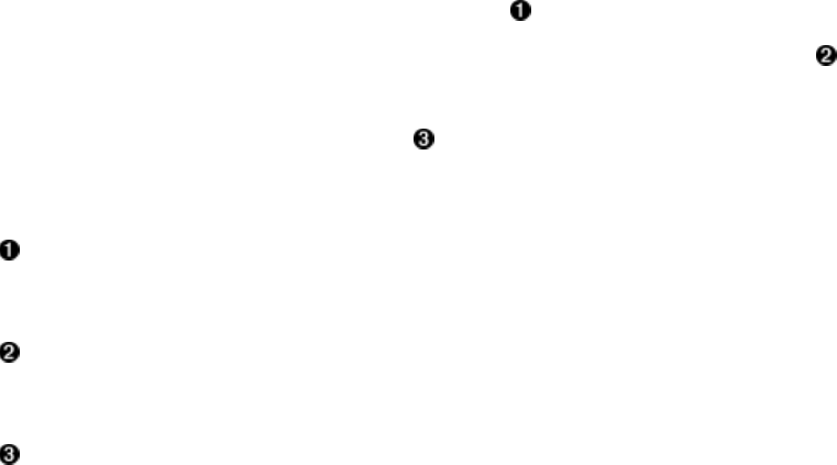
Example 8-4. Example application deleting with explicit timestamps
for (int count = 1; count <= 6; count++) {
Put put = new Put(ROW1);
put.addColumn(COLFAM1, QUAL1, count, Bytes.toBytes("val-" + count));
table.put(put);
}
Delete delete = new Delete(ROW1);
delete.addColumn(COLFAM1, QUAL1, 5);
delete.addColumn(COLFAM1, QUAL1, 6);
table.delete(delete);
Store the same column six times.
The version is set to a specific value, using the loop variable.
Delete the newest two versions.
When you run the example, you should see the following output:
After put calls...
Cell: row1/colfam1:qual1/6/Put/vlen=5/seqid=0, Value: val-6
Cell: row1/colfam1:qual1/5/Put/vlen=5/seqid=0, Value: val-5
Cell: row1/colfam1:qual1/4/Put/vlen=5/seqid=0, Value: val-4
After delete call...
Cell: row1/colfam1:qual1/4/Put/vlen=5/seqid=0, Value: val-4
Cell: row1/colfam1:qual1/3/Put/vlen=5/seqid=0, Value: val-3
Cell: row1/colfam1:qual1/2/Put/vlen=5/seqid=0, Value: val-2
An interesting observation is that you have resurrected versions 2 and 3! This is caused by the
fact that the servers delay the housekeeping to occur at well-defined times. The older versions of
the column are still kept, so deleting newer versions makes the older versions come back.
This is only possible until a major compaction has been performed, after which the older
versions are removed forever, using the predicate delete based on the configured maximum
versions to retain.
Tip
The example code has some commented-out code you can enable to enforce a flush and major
compaction. If you rerun the example, you will see this result instead:
After put calls...
Cell: row1/colfam1:qual1/6/Put/vlen=5/seqid=0, Value: val-6
Cell: row1/colfam1:qual1/5/Put/vlen=5/seqid=0, Value: val-5
Cell: row1/colfam1:qual1/4/Put/vlen=5/seqid=0, Value: val-4
After delete call...
Cell: row1/colfam1:qual1/4/Put/vlen=5/seqid=0, Value: val-4
Since the older versions have been removed during the compaction, they do not reappear
anymore.
Finally, when dealing with timestamps, there is another issue to watch out for: delete markers.
This refers to the fact that, in HBase, a delete is actually adding a tombstone marker into the
(638)
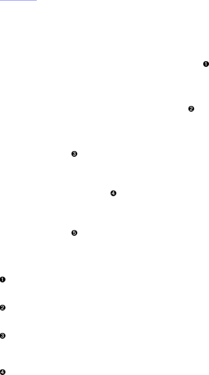
store that has a specific timestamp. Based on that, it masks out versions that are either a direct
match, or, in the case of a column delete marker, anything that is older than the given timestamp.
Example 8-5 shows this using the shell.
Example 8-5. Deletes can mask puts with explicit timestamps in the past
hbase(main):001:0> create 'testtable', 'colfam1'
0 row(s) in 1.1100 seconds
hbase(main):002:0> Time.now.to_i
=> 1464722416
hbase(main):003:0> put 'testtable', 'row1', 'colfam1:qual1', 'val1'
0 row(s) in 0.0290 seconds
hbase(main):004:0> scan 'testtable'
ROW COLUMN+CELL
row1 column=colfam1:qual1, timestamp=1464722432971, value=val1
1 row(s) in 0.0450 seconds
hbase(main):005:0> delete 'testtable', 'row1', 'colfam1:qual1'
0 row(s) in 0.0280 seconds
hbase(main):006:0> scan 'testtable'
ROW COLUMN+CELL
0 row(s) in 0.0260 seconds
hbase(main):007:0> put 'testtable', 'row1', 'colfam1:qual1', 'val1', \
Time.now.to_i - 50000
0 row(s) in 0.0260 seconds
hbase(main):008:0> scan 'testtable'
ROW COLUMN+CELL
0 row(s) in 0.0260 seconds
hbase(main):009:0> flush 'testtable'
0 row(s) in 0.2720 seconds
hbase(main):010:0> major_compact 'testtable'
0 row(s) in 0.0420 seconds
hbase(main):011:0> put 'testtable', 'row1', 'colfam1:qual1', 'val1', \
Time.now.to_i - 50000
0 row(s) in 0.0280 seconds
hbase(main):012:0> scan 'testtable'
ROW COLUMN+CELL
row1 column=colfam1:qual1, timestamp=1464672605, value=val1
1 row(s) in 0.0290 seconds
Store a value into the column of the newly created table, run a scan to verify.
Delete all values from the column, this sets the delete marker with a timestamp of now.
Store the value again into the column, but use a time in the past, the subsequent scan fails
to return the masked value.
Flush and major compact the table to remove the delete marker.
(639)


Custom Versioning
Since you can specify your own timestamp values—and therefore create your own versioning
scheme—while overriding the server-side timestamp generation based on the synchronized
server time, you are free to not use epoch-based versions at all.
For example, you could use the timestamp with a global number generator10 that supplies you
with ever increasing, sequential numbers starting at 1. Every time you insert a new value you
retrieve a new number and use that when calling the put function.
You must do this for every put operation, or the server will insert an epoch-based timestamp
instead. There is no flag in the table or column descriptors that indicates your use of custom
timestamp values to provide your own versioning. If you fail to set the value, it is silently
replaced with the server timestamp.
Caution
Be aware that negative timestamp values are untested and, while they have been discussed a few
times in HBase developer circles, they have never been confirmed to work properly.
Make sure to avoid collisions, which occur when the same value is used for two separate updates
to the same cell. Usually the last saved value is visible afterward.
With these warnings out of the way, here are a few use cases that show how a custom versioning
scheme can be beneficial in the overall concept of table schema design:
Record IDs
A prominent example using this technique was discussed in “Search Integration”, that is,
the Facebook inbox search. It uses the timestamp value to hold the message ID. Since
these IDs are increasing over time, and the implicit sort order of versions in HBase is
descending, you can retrieve, for example, the last 10 versions of a matching search term
column to get the latest 10 messages, sorted by time, that contain said term.
Number generator
This follows on with the initially given example, making use of a distributed number
generator. It may seem that a number generator would do the same thing as epoch-based
timestamps do: sort all values ascending by a monotonously increasing value. The
difference is more subtle, because the resolution of the Java timer used is down to the
millisecond, which means it is quite unlikely to store two values at the exact same time—
but that can happen. If you were to require a solution in which you need an absolutely
unique versioning scheme, using the number generator can solve this issue.
Transaction IDs
As discussed in “Transactions”, timestamps are often used to indicate which records
belong to the same “transaction”. A central server hands out epochs as transaction IDs,
which are then used to tag every related record, even across tables with the given
(641)

timestamp. Upon reading data, only those dependent cells that have the exact same
timestamp as the main record are considered. This is often used in client-driven secondary
indexes (see “Secondary Indexes”).
Using the time component of HBase is an interesting way to exploit this extra dimension offered
by the architecture. You have less freedom, because it only accepts long values, as opposed to
arbitrary binary keys supported by row and column keys. Nevertheless, it could help with your
specific use case.
1 You could, for example, use Orderly to generate the composite row keys.
2 For actual implementations please see the Sematext blog post and linked repository. Also
FINRA has posted about this more recently.
3 See the Mozilla wiki page on Socorro for details. The project’s wiki page has been idle for a
while, though its code repository is still quite active.
4 See the HAvroBase GitHub project page.
5 See the Hive wiki for more details
6 As of this writing, IHBase only supports HBase version 0.20.5.
7 Solr and ElasticSearch are based on Lucene, but they extend it to provide fully featured search
servers. See the project’s website for details.
8 More details can be found on the ZooKeeper project page.
9 One example, although very uncommon, is based on virtualized servers. See
http://support.ntp.org/bin/view/Support/KnownOsIssues#Section_9.2.2, which lists an issue with
NTP, the commonly used Network Time Protocol, on virtual machines.
10 As an example for a number generator based on ZooKeeper, see the zk_idgen project.
(642)
Chapter 9. Cluster Monitoring
Once you have your HBase cluster up and running, it is essential to continuously ensure that it is
operating as expected. This chapter explains how to monitor the status of the cluster with a
variety of tools.
(643)

Introduction
Just as it is vital to monitor production systems, which typically expose a large number of
metrics that provide details regarding their current status, it is vital that you monitor HBase.
HBase actually inherits its monitoring APIs from Hadoop. But while Hadoop is a batch-oriented
system, and therefore often is not immediately user-facing, HBase is user-facing, as it serves
random access requests to, for example, drive a website. The response times of these requests
should stay within specific limits to guarantee a positive user experience—also commonly
referred to as a service-level agreement (SLA).
With distributed systems the administrator is facing the difficult task of making sense of the
overall status of the system, while looking at each server separately. And even with a single
server system it is difficult to know what is going on when all you have to go by is a handful of
raw log files. When disaster strikes it would be good to see where—and when—it all started. But
digging through mega-, giga-, or even terabytes of text-based files to find the needle in the
haystack, so to speak, is something only few people have mastered. And even if you have mad
log-reading skills, it will take time to draw and test hypotheses to eventually arrive at the cause
of the disruption.
This is obviously not something new, and viable solutions have been around for years. These
solutions fall into the groups of graphing and monitoring--with some tools covering only one of
these groups, while others cover both. Graphing captures the exposed metrics of a system and
displays them in visual charts, typically with a range of time filters—for example, daily,
monthly, and yearly time frames. This is good, as it can quickly show you what your system has
been doing lately—like they say, a picture speaks a thousand words.
The graphs are good for historical, quantitative data, but with a rather large time granularity it is
also difficult to see what a system is doing right now. This is where qualitative data is needed,
which is handled by the monitoring kind of support systems. They keep an ear out on your behalf
to verify that each data point, or metric, exposed is within a specified range. Often, the support
tools already supply a significant set of checks, so you only have to tweak them for your own
purposes. Checks that are missing can be added in the form of plug-ins, or simple script-based
extensions. You can also fine-tune how often the checks are run, which can range from seconds
to days.
Whenever a check indicates a problem, or outright failure, evasive actions could be taken
automatically: servers could be decommissioned, restarted, or otherwise repaired. When a
problem persists there are rules to escalate the issue to, for example, the administrators to handle
it manually. This could be done by sending out emails to various recipients, or SMS messages to
telephones.
While there are many possible support systems you can choose from, the Java-based nature of
HBase, and its affinity to Hadoop, narrow down your choices to a more limited set of systems,
which also have been proven to work reliably in combination. For graphing, the system
supported natively by HBase is Ganglia. For monitoring, you need a system that can handle the
JMX1-based metrics API as exposed by the HBase processes. A common example in this
category is Nagios.
(644)
Note
You should set up the complete support system framework that you want to use in production,
even when prototyping a solution, or working on a proof-of-concept study based on HBase. That
way you have a head start in making sense of the numbers and configuring the system checks
accordingly. Using a cluster without monitoring and metrics is the same as driving a car while
blindfolded.
It is great to run load tests against your HBase cluster, but you need to correlate the cluster’s
performance with what the system is doing under the hood. Graphing the performance lets you
line up events across machines and subsystems, which is an invaluable when it comes to
understanding test results.
(645)

The Metrics Framework
Every HBase process, including the master and region servers, exposes a specific set of metrics.
These are subsequently made available to the various monitoring APIs and tools, including JMX
and Ganglia (or any other system that provides an integration). For each kind of server there are
multiple groups of metrics, usually pertaining to a subsystem within each server. For example,
one group of metrics is provided by the Java Virtual Machine (JVM) itself, giving insight into
many interesting details of the current process, such as garbage collection statistics and memory
usage.
Metrics 1 and 2
HBase has shared its metric classes with Hadoop from the start, and with version 0.962 it
migrated from the previous Hadoop metrics to the newer metrics2 package. With it, some of the
lessons learned from the earlier version have been applied, and certain shortcomings amended. In
particular, the classes have been redesigned to allow for a more flexible setup. Figure 9-1 shows
a high-level view on the classes used in either version of the Hadoop metrics.
(646)
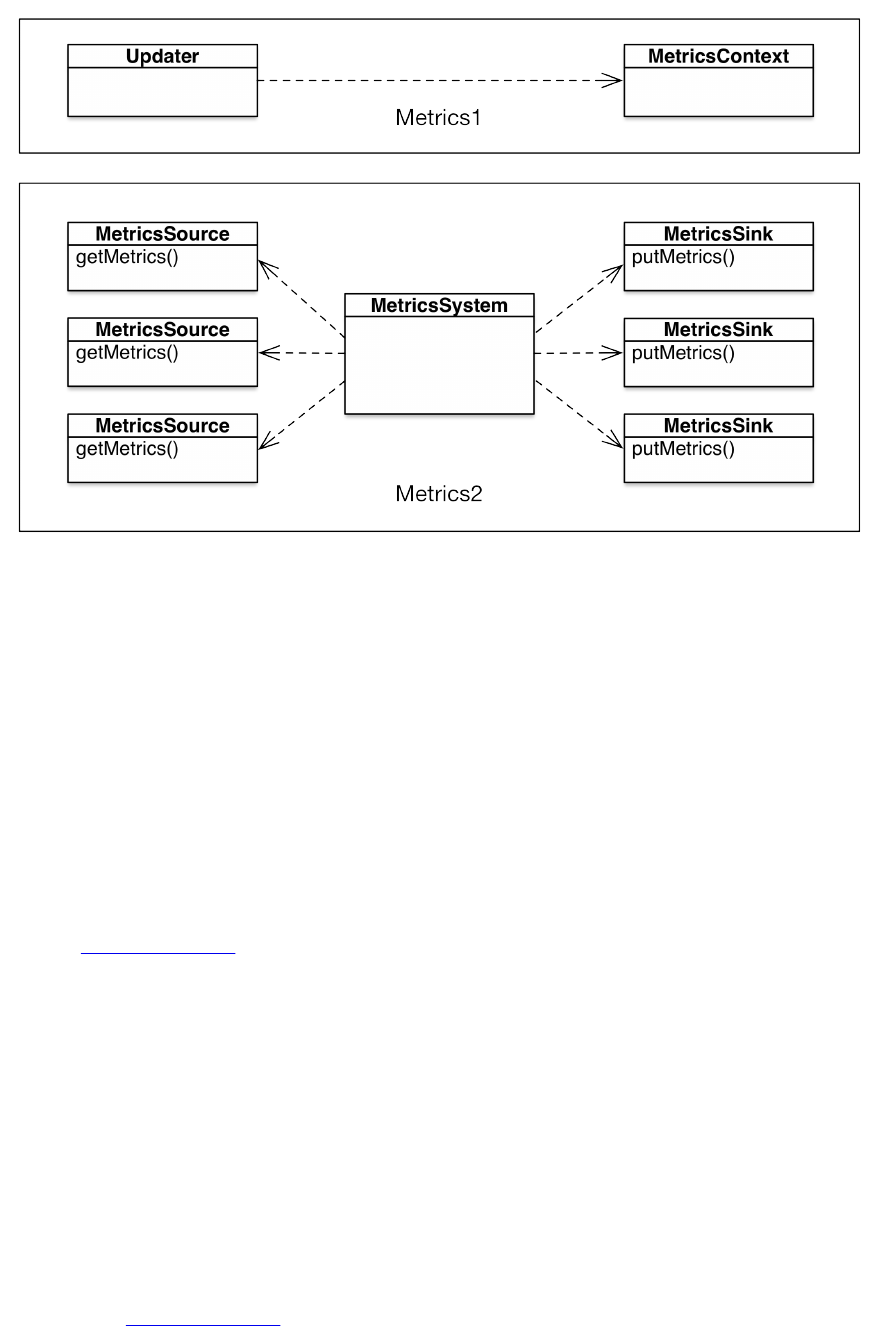
Figure 9-1. Difference in class architecture between metrics 1 and 2
Metrics1 centered around the MetricsContext class, which had specific subclasses for each output
format, for example the FileContext and GangliaContext. Each main server process class, like the
HRegionServer would then call upon the context to export the metrics it has collected. This design
would not allow to have more than one output connected to each group of metrics, and also
would always export everything it has collected.
Metrics2 on the other hand centers the MetricsSystem class and combines it with MetricsSource
and MetricsSink satellites, in a one-to-many relationship for each of the latter. In other words,
server processes can contain more than one source, while at the same time any number of sinks
are listening to the output of the sources. In addition, a filtering has been implemented, which
allows for the system administrator to only emit what is needed, and therefore saving precious
resources (see “Configuration”).
As far as the configuration is concerned, in Metrics1 you would see something like this:
context1.class=org.hadoop.metrics.file.FileContext
context2.class=org.hadoop.metrics.file.FileContext
...
contextn.class=org.hadoop.metrics.file.FileContext
The numbered context prefixes were determined by all of the subsystems Hadoop, or HBase,
had, for example hbase or jvm. For Metrics2, the new system, you would find:
prefix1.sink.file.class=org.hadoop.metrics2.sink.FileSink
Like the context above, the prefix here is that of a known (and provided) metrics system, and for
HBase this simply maps to hbase. All further selection and filtering, if required, is configured at a
different level (see “Configuration”).
You can simulate the previous behavior of sending metrics to a particular context to a specific
(647)

output backend by using the context option as part of the sink definition. First the Metrics1
version in its old format:
context0.class=org.hadoop.metrics.file.FileContext
context0.fileName=context0.out
context1.class=org.hadoop.metrics.file.FileContext
context1.fileName=context1.out
...
contextn.class=org.hadoop.metrics.file.FileContext
contextn.fileName=contextn.out
For Metrics2, you define this per sink and context combination:
prefix.sink.*.class=org.apache.hadoop.metrics2.sink.FileSink
prefix.sink.file0.context=context0
prefix.sink.file0.filename=context0.out
prefix.sink.file1.context=context1
prefix.sink.file1.filename=context1.out
...
prefix.sink.filen.context=contextn
prefix.sink.filen.filename=contextn.out
Another peculiarity in Metrics1 is that you had to configure the NullContextWithUpdateThread to
enable the collection of metrics and have them exposed through JMX:
# Configuration of the "hbase" context for null
#hbase.class=org.apache.hadoop.metrics.spi.NullContext
hbase.class=org.apache.hadoop.metrics.spi.NullContextWithUpdateThread
# Configuration of the "hbase" context for file
# hbase.class=org.apache.hadoop.hbase.metrics.file.TimeStampingFileContext
# hbase.period=10
# hbase.fileName=/tmp/metrics_hbase.log
In other words, you had to define any context class, besides the NullContext that acted as an off
switch, to enable the metrics subsystem. This is now obsolete in Metrics2, where the server
processes always export their metrics through JMX, no matter what sink is defined in the
configuration. An additional quirk from Metrics1 is shown here:
# HBase-specific configuration to reset long-running stats (e.g. compactions)
# If this variable is left out, then the default is no expiration.
hbase.extendedperiod = 3600
This was a side-effect of the old metrics system trying to accumulate statistics at the same time
as collecting counters. It had metrics classes, for example PersistentMetricsTimeVaryingRate,
which were used to collect data over a longer period of time, to be able to see the effect of
operations that run at a much slower pace, like the mentioned compaction process. In Metrics2
this has been abandoned and the task to collect such statistics has been pushed towards the
(optional) graphing system configured as a sink.
More details on the new metrics subsystem and its implementation in HBase was posted on the
HBase blog. And for upcoming versions, there is also a more radical suggestion to remove
Hadoop metrics altogether from HBase and use a more standard, open-source library instead.
(648)

Metrics Building Blocks
The majority of the classes for reporting operational, quantitative metrics used by HBase are
supplied by the Hadoop common module and packages. Figure 9-2 shows a simplified version of a
class diagramm3, just to set the stage. The important observation is that there is a direct
relationship between sources, metrics system, and the output sinks.
(649)
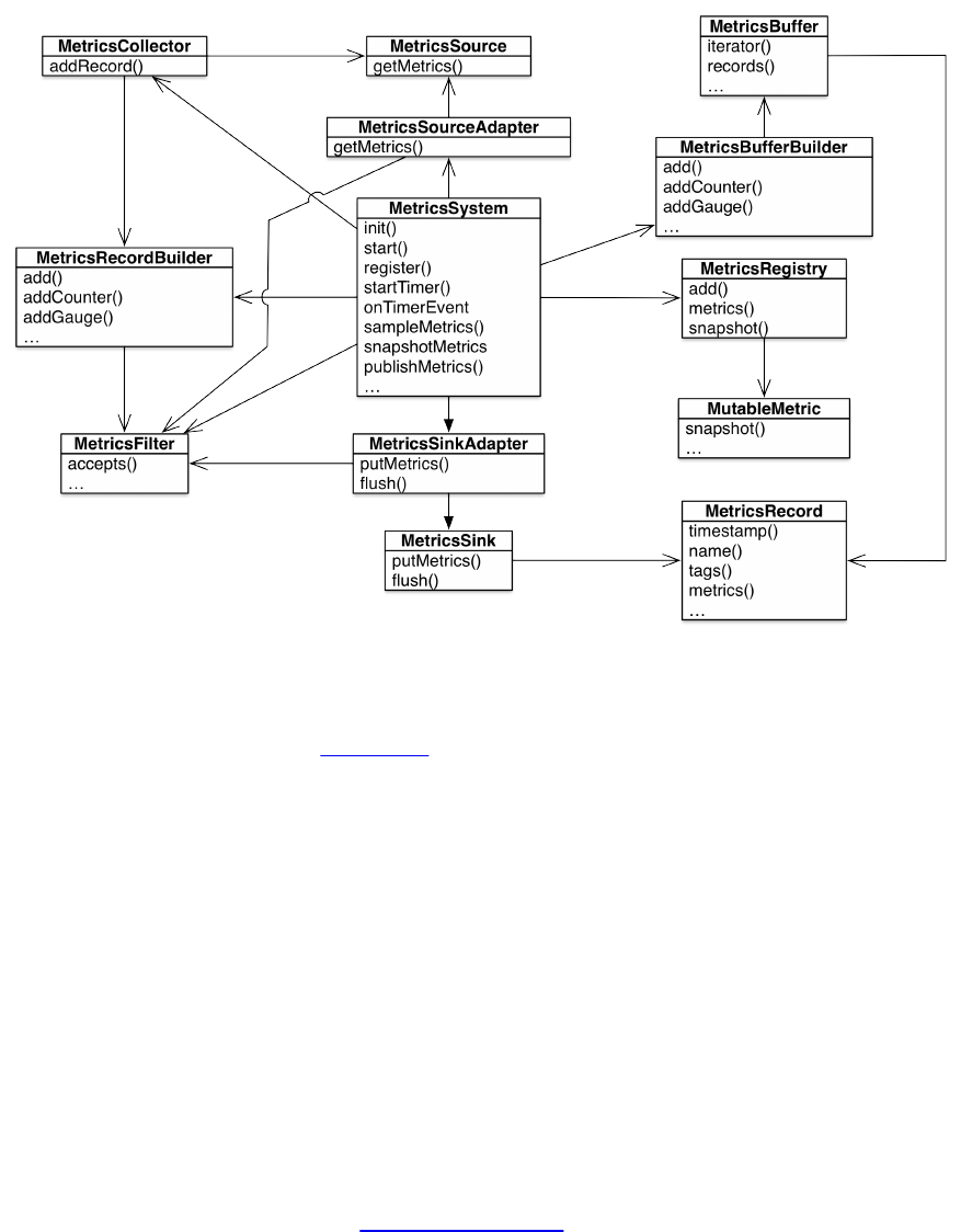
Figure 9-2. Overview of the Hadoop metrics classes
As shown in even further simplified Figure 9-1, there is a one-to-many relationship between the
sources and sinks, with the metrics system. This allows for many generating subsystems in a Java
processes to emit their respective metrics, for example in the HBase Master you will find
separate metrics grouped for RPC, region balancer, and so on. All of the registered sources
though are exported through JMX, no matter if you add an additional sink, or not.
The advantage of the new metric system is that it can get the metrics from each source ones, and
then emit it as many times as needed to each configured sink, not incurring any additional costs.
You should keep an eye on the number of metrics though as some sinks may not be capable of
handling the many datapoints provided. In addition, the sink layer has the ability to throttle the
output, which helps if the sinks fall behind the sources. In that event, the sink layer will hold on
to the last few metrics sets for the sinks to consume at their convenience.
Note
On top of the discussed HBase metrics, you will find many more that are added as MXBeans in
the JMX output. These are the so-called Platform MXBeans (for example, RuntimeMXBean), which
are automatically added by the JMX subsystem as a result of the first call to
ManagementFactory.getPlatformMBeanServer() by the Hadoop MBeans utility class. This happens as
soon as the Hadoop and HBase subsystems call the static register() method, exported by MBeans.
The main classes that are part of the metrics package are:
MetricsSystem
This class is the centerpoint and act as a fan-in and -out point for all metrics. It starts a
timer that polls all of the sources, and then sends the collected metrics towards the
(650)

configured sinks (with JMX being built-in).
MetricsSource
All of the classes that implement this interface can serve as a source for the metrics
system, which invokes the concrete getMetrics() method. The metrics system iterates over
all registered sources, and collects their emitted metrics, before sending the results toward
the sinks.
MetricsRecord
Every registered source generates a MetricsRecord instance, that holds the current metrics
pertaining to the source. It is an aggregation (or composition) comprising all known
metrics types of the source and their value(s) at the time of the invocation. This process is
referred to as taking a snapshot.
MetricsSink
After the metrics records have been instantiated, they are sent to the sinks. There is a
queue (SinkQueue) in between that decouples the collection from the persistence process. In
other words, records are collected at specific intervals, and queued for subsequent handling
by the configured sinks. There is a thread that runs at an (optionally) different pace, and is
invoking the sinks with the accumulated list of records. The two notable classes
implementing the sink interface are FileSink, GangliaSink31, and GraphiteSink.
MetricsCollector
During the iteration over the metrics sources, the framework is invoking the collector class
to instantiate a MetricsRecordBuilder, which in turn is responsible to eventually returns a
concrete metrics record. The collector accrues all of these records, and holds on to them
until they are consumed in the next step.
MetricsBuffer
The metrics system strives to buffer the collected metrics as much as possible, to avoid any
costly reiteration. The collector emits all of the collected records, and the system then
stores all of them in a single metrics buffer instance for further use later on.
MetricsFilter
While the metrics are collected, records combined, and finally emitted through sinks, there
is an optional filter layer in place, which can avoid any of these steps. This allows for a
configuration based filtering (see “Configuration”) early on, reducing the rather costly
metrics generation and collection to only what is needed later on.
MutableMetric
Each subsystem uses a concrete subclass of this abstract class to track each data point, that
is, the metric. The available classes are explained below.
MetricsRegistry
All of the registered MutableMetric instances are tracked (and created) by the metric
registry. The metric system holds a reference to a global instance, that can be used to
snapshot the current metrics state, and persist it in a metrics record.
(651)

AbstractMetric
Once all mutable metrics are persisted, they are converted into the simpler AbstractMetric-
based family of classes, including MetricGaugeDouble, MetricGaugeLong, MetricGaugeFloat,
MetricGaugeInt, MetricCounterLong, MetricCounterInt. You can see, there are only two
essential types of metrics, those that are only incremented (the counter), and those that can
fluctuate up and down (the gauge). Note that a single MutableMetric subclass can emit any
number of simple metrics during the snapshot process.
MetricsTag
We will not look deeper into the tag feature provided by the metrics package, but it should
be noted that for every metrics record the system will attach related tags too, which can be
used during the configuration-based filtering of the metrics. For example:
"beans" : [ {
"name" : "Hadoop:service=HBase,name=Master,sub=Balancer",
"modelerType" : "Master,sub=Balancer",
"tag.Context" : "master",
"tag.Hostname" : "master-1.internal.larsgeorge.com",
"miscInvocationCount" : 6,
"BalancerCluster_num_ops" : 0,
"BalancerCluster_min" : 0,
...
You can see the tag and its fields in the example, as added by the specific HBase
subsystem (see “Metrics UI” for a way of accessing this information).
More information on the class structure can be found online in the JIRA design document and
the Metrics2 package information.
Note
An additional complication around the metrics system is that it needed to support mixed versions
of Hadoop and HBase. For that reason, HBase is shipping with two modules, called hbase-
hadoop-compat and hbase-hadoop2-compat, both providing (among other subsystem) the actual
classes implementing the various metrics interfaces. The concrete classes often end in Impl, with
the interface name as the prefix.
Multiple metrics are grouped into a MetricsRecord, which commonly describes one specific
subsystem of a HBase server process, for example the master, its balancer and assignment
manager, the region server, and so on. Each group also has a unique name, which appears
differently dependent on where it is emitted. For Ganglia, for example, the context and the actual
metric name is combined with the record name to form the fully qualified metric:
<context-name>.<record-name>.<metric-name>
On the other hand, when the record is exported through JMX, its name is prefixed with "HBase",
and then identified by server process and subsystem name, for example:
"name" : "Hadoop:service=HBase,name=RegionServer,sub=Replication",
The actual metrics are then usually found in a hierarchical manner, located underneath the
subsystem. [Link to Come] shows an example using JConsole (see “JConsole”) with one metric
highlighted. Interesting to note is that the metric subsystem is offering a description for each
metric, so that you can make some (at least initial) sense out of what you are presented with.
(652)
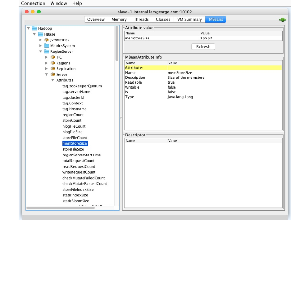
Figure 9-3. The metric record as seen in JConsole
The metric system has a built-in timer that triggers the pull (getMetrics()) and push
(putMetrics()) of the metrics on specific intervals, which can differ between the sources and the
sinks . The configuration file enabling them has a period property that is used to specify the
interval period in seconds for either separately. Specific context implementations might have
additional properties that control their behavior (see “Configuration” for details).
Figure 9-4 shows a sequence diagram with all the involved classes, and how they are
orchestrating the collection and emission of metrics group in records. The diagram is just to
illustrate the interactions between various classes in the metrics2 package within Hadoop. It also
shows how the collection is independent from the emission, as there is a decoupled, autonomous
thread handling the sink queue events.
(653)
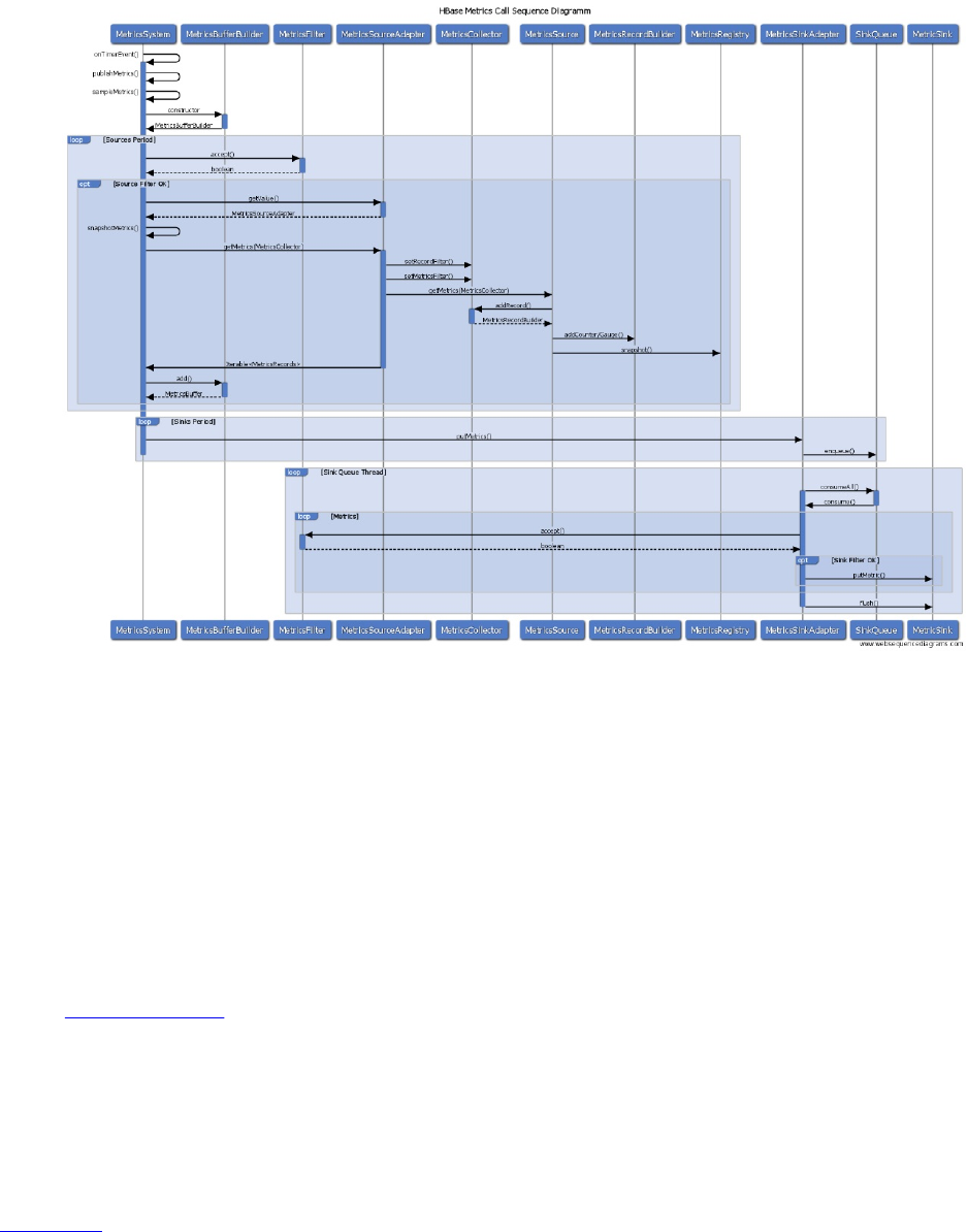
Figure 9-4. Sequence diagram of the classes involved in preparing the metrics
The collection period is printed in the server logs, when the processes are started, for example:
...
2016-06-07 04:11:42,957 INFO [main] impl.MetricsConfig: \
loaded properties from hadoop-metrics2-hbase.properties
2016-06-07 04:11:43,070 INFO [main] impl.MetricsSystemImpl: \
Scheduled snapshot period at 10 second(s).
2016-06-07 04:11:43,070 INFO [main] impl.MetricsSystemImpl: \
HBase metrics system started
...
The following discusses the sinks and sources in more detail, as well as the available metrics
types. “Configuration” ties this together by explaining how metrics can be wired from sources to
sinks, how their respective polling periods are set, and how filters can be used to keep the
number of generated data points in check.
Metrics Sources
There are many metrics sources that come with the Java VM and each specific server process.
Figure 9-5 shows each major server process and the groups of metrics they offer. You will note
that there are common groups, such as the IPC (that is, the remote procedure call layer of HBase)
and JVM. The latter alone provides many further groups giving insight into what the process is
doing in regards to memory usage, operating system (OS) resources, Java garbage collection
status, and much more.
(654)
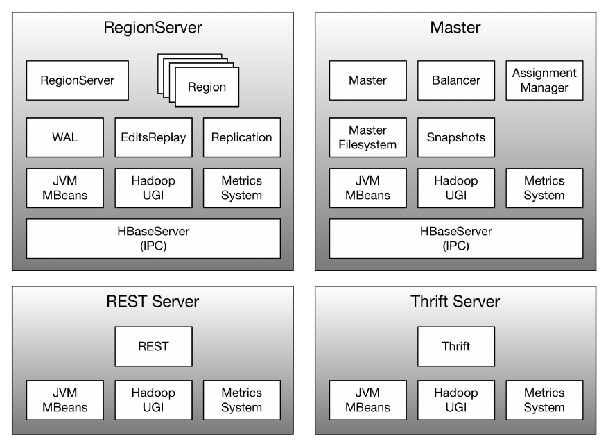
Figure 9-5. The metrics sources in their respective process context
Note
Each metric group is internally represented as a MetricsRecord instance, and provided by a
specific metrics source. In this chapter all three are used interchangeably, that is, group, record,
and source are treated as the same.
The shared metrics groups are listed here, with the technical name of the metrics as exported by
the system in parenthesis (if different from the group name):
IPC
These are provided by the server processes that use the native HBase remote procedure
call (RPC) subsystem, named IPC. It has counters that track method invocations, the time
spent within these methods, and so on.
MetricsSystem (Control/Stats)
Since all processes share the same metrics code, they all expose the built-in metrics the
system generates itself.
Hadoop UGI (UgiMetrics)
HBase uses the Hadoop UserGroupInformation class to handle the task of mapping the
current user to OS-level IDs. This class provides information about login attempts, and if
they were successful or not.
(655)

JVM MBeans (JvmMetrics)
There is an exhaustive list of platform MXBean that is automatically provided by the JMX
API, which all HBase processes offer. But only the JvmMetrics group is exposed to both
JMX and the rest of the sinks. In fact, the values in JvmMetrics are internally collected from
the same MXBeans, as shown in the following example:
{
name: "Hadoop:service=HBase,name=JvmMetrics",
modelerType: "JvmMetrics",
...
MemNonHeapUsedM: 43.937973,
MemNonHeapCommittedM: 131.3125,
MemNonHeapMaxM: 176,
MemHeapUsedM: 20.575905,
MemHeapCommittedM: 57.9375,
MemHeapMaxM: 941.375,
MemMaxM: 941.375,
...
},
{
name: "java.lang:type=Memory",
modelerType: "sun.management.MemoryImpl",
ObjectPendingFinalizationCount: 0,
HeapMemoryUsage: {
committed: 60751872,
init: 62762176,
max: 987103232,
used: 26865352
},
NonHeapMemoryUsage: {
committed: 137691136,
init: 136773632,
max: 184549376,
used: 46537216
},
...
}, ...
The highlighted lines are the same value, though in JvmMetrics it is converted to megabytes
(that is, divided by 1024 twice). The postfix M (short for MB) in MemNonHeapCommittedM
indicates that succinctly. The reason JvmMetrics is exporting the same values as the
MXBeans (though only a selected subset) is that using sinks, like the one for Ganglia,
would otherwise have no access to those values.
On top of the shared metrics, each server also provides metrics for each major sub-component.
Looking at the naming again, here is how the Master process exposes the Server sub-component
group metrics through JMX:
name: "Hadoop:service=HBase,name=Master,sub=Server", ...
The same is found in Ganglia (as this is sink dependent) as "master.Server". More generically
though, here is how the naming scheme is structured:
name: "Hadoop:service=HBase,name=<Process>,sub=<Metric Group>", ...
The prefix is always "HBase", followed by the process name (note that the name is modeled after
the HBase process names) and then the actual metric group it provides. For each process, there
are:
Master (Server)
The master process itself emits some statistics about its start time, and number of dead and
(656)
active region servers. Another peculiarity of the metrics system can be seen when looking
at the JMX output as JSON using the Master UI:
{
name: "Hadoop:service=HBase,name=Master,sub=Server",
modelerType: "Master,sub=Server",
tag.liveRegionServers: "slave-1.internal.larsgeorge.com,16020, \
1465909293646;slave-2.internal.larsgeorge.com,16020,1465909293694; \
slave-3.internal.larsgeorge.com,16020,1465909293581",
tag.deadRegionServers: "",
tag.zookeeperQuorum: "master-1.internal.larsgeorge.com:2181, \
master-2.internal.larsgeorge.com:2181, \
master-3.internal.larsgeorge.com:2181",
tag.serverName: "master-1.internal.larsgeorge.com,16000,1465909293281",
tag.clusterId: "49ffd33c-e051-4c00-b0da-df7737e1d3ec",
tag.isActiveMaster: "true",
tag.Context: "master",
tag.Hostname: "master-1.internal.larsgeorge.com",
masterActiveTime: 1465909297645,
masterStartTime: 1465909293281,
averageLoad: 13.666666666666666,
numRegionServers: 3,
numDeadRegionServers: 0,
clusterRequests: 4021
},
The JMX record uses the MetricsTag support of each group to set information that does not
lend itself for graphing. For example, the list of current region servers, or the cluster ID are
stored as tags. They can be accessed through JMX, but are usually skipped for graphing
and exporting to sinks, as those expect numeric values that change over time. Many
metrics groups use tags for the same reason, omitting them from the graphs, but exposing
interesting values nevertheless.
On top of the main server metrics group, the following groups are provided by the master
process as well:
AssignmentManager
Provides region-in-transition and region assignment information.
Balancer
Tracks the number of times the balancer has been invoked and the time it took to
complete its task.
Filesystem
All filesystem operations of the master are recored here, which are mainly the WAL
split actions as summary statistics (since log splitting is done on the region servers in
a distributed manner).
Snapshot
Any snapshot related operation, that is, taking a snapshot and then cloning or
restoring it, are reported here.
RegionServer (Server)
Just as the master, all region servers export this metric group to give insight into what the
server is doing. It records most API calls, such as mutations, gets, scans, flushes and
(657)
compactions, plus summaries counts for number of regions, store files, and so on. The
other groups it provides are:
EditsReplay (replay)
Records the various log replay statistics when distributed log splitting is enabled.
WAL
Here you will see information about the performance of the WAL, such as the
synchronization count and time (with a histogram), the append times and sizes, and
so on.
Regions
For every hosted region on this server you are provided with statistics around
memstore size, store file count, compaction details, and read and write accesses.
Replication
This group tracks the number of applied operations and batches, together with their
age.
REST Server (REST)
The metrics provided by the HBase REST server revolve around the number of successful
and failed operations, such as gets, puts, scans, and deletes.
Thrift Server (ThriftOne/ThriftTwo)
The Thrift servers supplied by HBase registers themselves under one of two names,
depending on the version of the server that is started. Only one of ThriftOne (for the thrift
package) or ThriftTwo (for thrift2 in HBase) is active when the respective server has been
started. While it is running, the server exposes various metrics about its state, including the
number of calls it has handled so far, call queue information, and batch call details.
Note
As of this writing, both ThriftOne and ThriftTwo are exposed through JMX, as they are
created at the same time by a factory class. Only one is then used, but both will show up in
various places, for example the JMX as JSON UI link.
The Thrift server internally is using a helper class named IncrementCoalescer, which
batches increment operations. That class also exposes itself through JMX—but without
any sub-component name. In other words, when inspecting the JMX metrics for the Thrift
server, you should encounter the following:
...
name: "hadoop:service=thrift,name=Thrift",
modelerType: "org.apache.hadoop.hbase.thrift.IncrementCoalescer",
...
All of the metrics within that group relate to said class, for example, counting the
increment operations.
(658)

Figure 9-6 shows all of the sources again in a class hierarchy. The BaseSource interface (and
related BaseSourceImpl for each metrics package) is providing the required methods to set or
change each registered metric (see “Metrics Classes” for the types). Of note is that all of these
classes are provided by HBase, in accordance to the design of the Hadoop metrics framework.
Internally they are then used to collect all the metrics they represent.
(659)
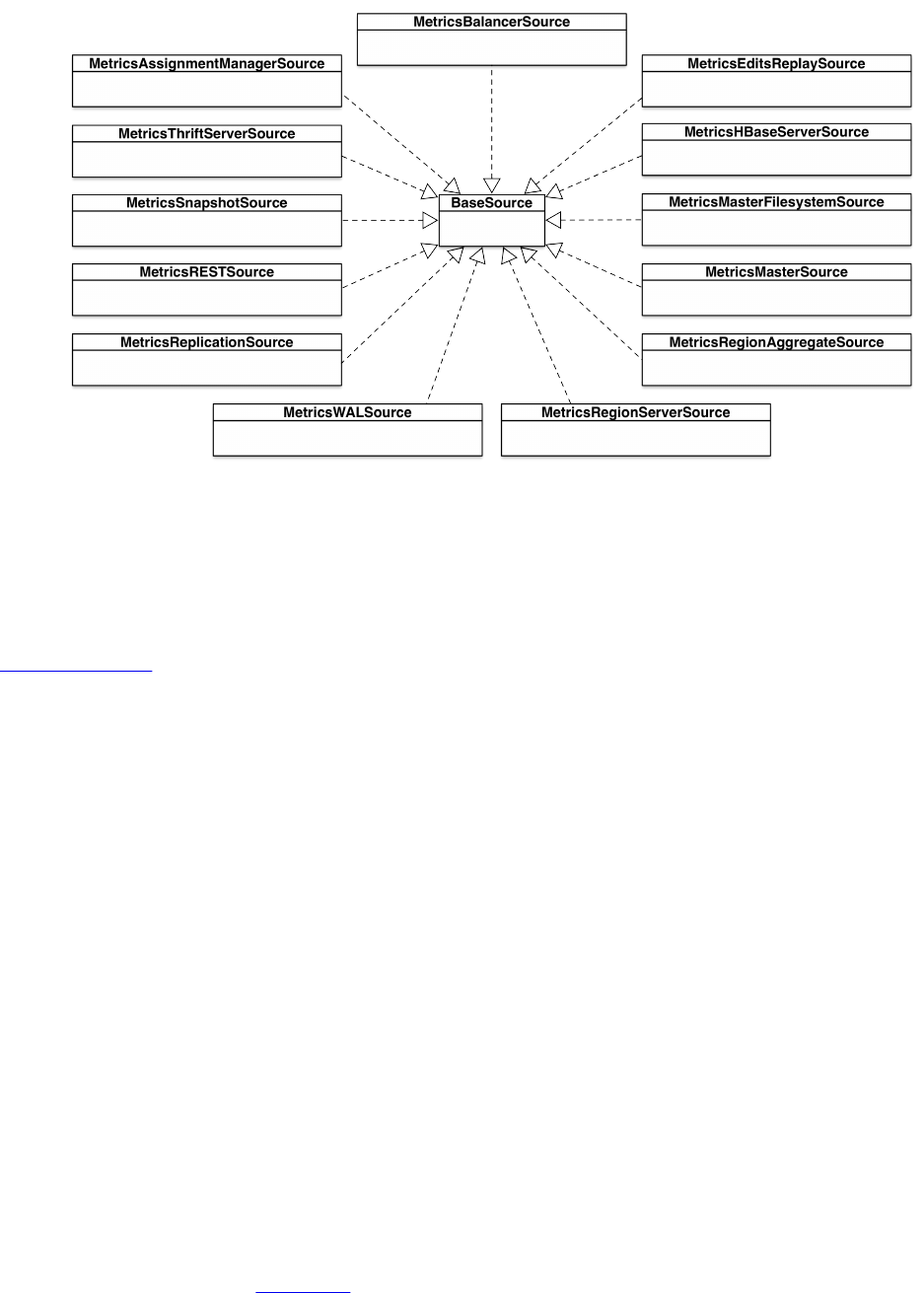
Figure 9-6. The metrics sinks hierarchy
Metrics Sinks
Once the metrics system has collected the metrics records at their configured period (see
“Configuration”), they are handed over to the sinks. Their purpose is to emit the contained data
points to the specific consumer that corresponds to the sink implementation. The sink classes are
all provided by the Hadoop metrics package, and no HBase specific one is needed. The supplied
sinks are:
File
This sink is responsible to write the metrics records to a disk file. It prints each record on a
separate line, starting with the timestamp (epoch) of the record. It then appends all tags (if
present), followed by the actual metrics. For example (lines are wrapped and abbreviated):
...
1466346380302 regionserver.RegionServer: Context=regionserver, Hostname= \
slave-1.internal.larsgeorge.com, queueSize=0, numCallsInGeneralQueue=0, \
numCallsInReplicationQueue=0, numCallsInPriorityQueue=0, ...
1466346380306 regionserver.WAL: Context=regionserver, Hostname= \
slave-1.internal.larsgeorge.com, rollRequest=0, SyncTime_num_ops=1, \
SyncTime_min=613, SyncTime_max=613, SyncTime_mean=613.0, \
SyncTime_median=613.0, ...
...
Note how there is little difference between tags and metrics, which makes it a little more
difficult to read, or parse.
Ganglia
If you want to connect Ganglia to your HBase cluster, you can use this provided sink
implementation; see “Ganglia” for details.
Graphite
(660)
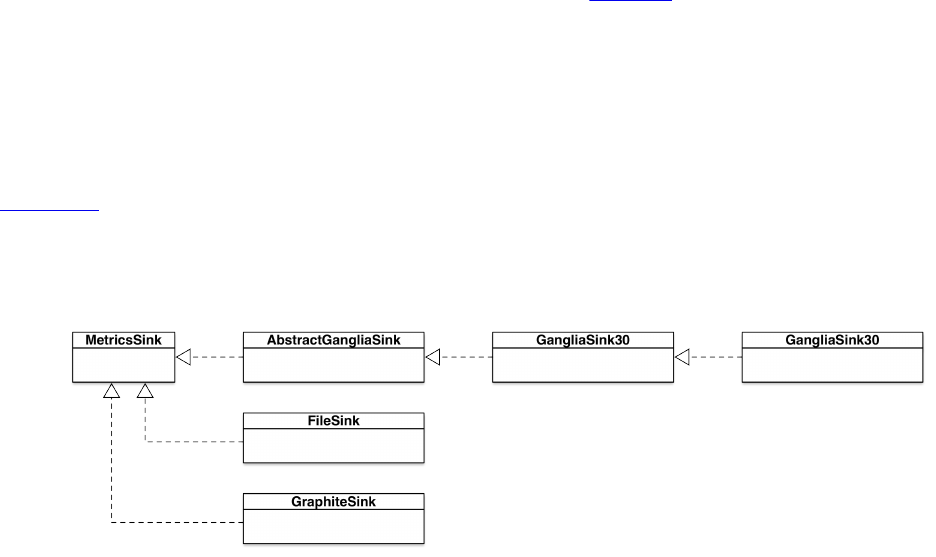
This sink lets you emit the collected metrics records to Graphite, an open-source
monitoring tool that stores and renders time-series data (that is, metrics).
By default, no sink is defined in the HBase configuration, and it is up to you to enable one or
more. As mentioned, the only active interface is JMX, exposing all of the source records through
that API standard. While JMX is not represented as an additional sink, you can still influence the
data exposed through JMX using filters.
Figure 9-7 shows the actual class hierarchy around the metrics sinks. You will note that there are
two separate Ganglia sink implementations, dependent on the version of Ganglia you are using.
As of this writing, the GangliaSink31 is also supporting all versions of Ganglia, up to 3.7.x (and it
is likely to stay the same for later versions).
Figure 9-7. The metrics sink hierarchy
The Hadoop metrics framework is flexible enough to wire any source to any number of sinks,
and filter records and metrics during the collection and emission process. The final piece around
the metrics classes are the metrics themselves, explained next.
Metrics Classes
While the sources are tasked to generate the metrics data, there are many helper classes to wrap
them into common types that are understood by the rest of the framework. During the
accumulation of the data, a special tree of classes based on MutableMetric is used to increment or
set the current state. These classes are ranging from simple to quite powerful, where each
invocation may update many internal fields in one operation. Once the MetricsRecord is created,
which is a snapshot of the current data that is collected, the metrics classes will emit much
simpler types that are not mutable anymore. In other words, the MutableMetrics classes act as a
fan out, converting a single data point into many more metrics points. The classes and their
functionality are explained next:
Long Counter (IC)
The counter class tracks a monotonically increasing number, that is increment by 1 for
each invocation. The long based implementation does this for numbers of that primitive
type. During the snapshot of the metrics record, this class simply passes on the current
value as a metrics counter primitive.
Integer Counter (LC)
Same as the above, but tracks an int type number.
(661)
Long Gauge (LG)
A gauge is similar to a counter, but also allows for the value to be decremented (by 1). The
long based implementation tracks a number of that same primitive type. During the
conversion to a record, this metric is stored as a gauge as well.
Integer Gauge (IG)
Same as the above, but handles numbers with the primitive type of int.
Note
Some of the data points are internally collected using Java native types, for example, as double.
These are then handed to the simplified metrics types or the sinks as Double Gauge (DG). While
there are no direct matches in the metrics classes, this is used in some instances, and those are
then flagged with the appropriate type, for example, DG for Double Gauge, and FG for Float
Gauge. They behave like the dedicated classes discussed above.
Statistics (S)
Allows to build common statistics based on an given data point. The values of that point
are accumulated during the collection interval (depends on the source configuration), and
then emitted during the record snapshot process as the number of values and the average
value observed. The implementing class allows this to be extended to standard deviation,
and the minimum and maximum value for the interval and across the process runtime.
Once the statistics have been snapshotted they are reset and start from zero again.
Rate (R)
Same as the above, but configured to track throughput measurements. It sets the count
description to Ops, and Time for the value. An example of its use can be found in the
MetricsSystems own metrics record:
name: "Hadoop:service=HBase,name=MetricsSystem,sub=Stats",
...
Sink_gangliaNumOps: 13,
Sink_gangliaAvgTime: 178,
Sink_gangliaDropped: 0,
Sink_gangliaQsize: 0,
SnapshotNumOps: 50026,
SnapshotAvgTime: 0.25,
...
All three rates above emit the number of operations and average time they needed. For
example, the Snapshot rate metric shows that 50026 operations have taken place, with an
average execution time of 0.25 milliseconds.
Rates (RG)
This is a proxy metric that allows to handle multiple named rate metrics (R) using a single
object. Internally it creates a rate metric for every named data point, and during collection
emits each separately as expected.
Quantiles vs. Histograms
(662)

For certain data points it is not enough to see the current count or average alone, but get an idea
of what the distribution of values is. Assume an RPC endpoint, say the get() method of the
region servers, which is invoked by clients. With just a rate metric, you might see 10,000
invocation during a 10 second period, with an average runtime of 125 milliseconds. While this
may sound reasonable to you, you cannot determine what the majority of calls experience—to
answer the question of SLAs4 and quality-of-service in general. For that, quantiles are used in
statistics and monitoring of services.
Quantiles work as such: take all of the observed values within a period of time, and sort them
ascending. Then divide the values into a specific number of ranges. Depending on the number of
ranges, you get, for example, quartiles, which use four ranges, and percentiles when you use 100
ranges. The former is more coarse grained compared to the latter, but may suffice. For metrics
however, you will most likely find percentiles in use, as they translate directly into percentages.
For example, the 50th percentile is the median of the values, and the 100th percentile is the
maximum value ever recorded. Each quantile will return a single value, computed with a specific
mathematical function. For percentiles, the Nearest Rank method is used to determine values that
are part of the original data set.
It is very common in throughput calculations to divide the collected values into percentiles, and
then look at the 75th, 90th, 95th, and 99th percentile. For example, the 95th percentile will give
you the value where 95% of all other values are less or the same. This takes away 5% of values
that are greater and might otherwise skew the vast average of values. Going back to the earlier
example, assume the 95th percentile is 50 milliseconds, meaning that 95% of the requests were
completed in 50ms or faster. That is much more telling compared to the simple average. A
cluster administrator could now dial into the remain 5% of the requests and see why they take
longer.
A histogram is similar to a quantile, though it simply counts the values in each range. As far as
HBase and its metrics classes is concerned, the MutableHistogram is really a percentile-based
metric, with additional statistics collected at the same time. The percentiles are calculated as
close as possible, which means they might fall between two observed values and are therefore
interpolated accordingly.
The biggest issue with quantiles is that you need to have all the values to calculate them exactly.
Consider our example once more, and now amplify the request rate by many multiples of
magnitude. You may start to wonder how much data needs to be kept before the quantiles are
computed. This is not trivial nor cheap, considering there are many metrics that are track as
quantiles. This is solved by sampling the data, that is, not all values are kept, but a significant
enough subset. Here is where in Hadoop the simpler histogram metrics are different from the
quantile ones. Histograms use a fixed sample size, which is fine for a lot of use-cases. Just for
high-throughput metrics they start to show their weakness, as the sampling error is compounded
to a degree that the results are not useful anymore. The quantiles implementation uses a
configurable error rate per quantile that trades memory usage for accuracy. More has been
discussed in a JIRA discussion, along with results of a comparison between the two.
Quantiles (Q)
Watches a stream of long values, maintaining online estimates of specific quantiles with
provably low error bounds. This is particularly useful for accurate, high-percentile (e.g.
95th, 99th) latency metrics. The following table lists the recorded percentiles with their
configured error rates:
(663)
Quantile Error Rate
50th 5%
75th 2.5%
90th 1%
95th 0.5%
99th 0.1%
When this complex metric is snapshotted and converted to metrics primitives, it emits the
current count and the values for each percentile. Internally there is a separate thread pool
in use to sample the values within the configured interval. Upon setting up a quantile, the
user can define what the internal interval should be in which the values are collected
accumulatively and the quantiles computed in an ongoing fashion. When that configured
quantile interval expires the values and quantiles are reset and start anew.
Note
As of this writing there are two implementations for the quantile metrics, one provided by
Hadoop (MutableQuantiles), and another that ships with HBase (MetricMutableQuantile). The
latter is a remnant of when the Hadoop metrics framework was not yet complete across all
versions and releases, and the lacking support forced HBase to adopt the class under a
different name.
Histogram (H)
Here all values are sampled into a constant space data structure. Every time a new data
point is added, the sample is updated accordingly. Once the metrics record is created (that
is, a snapshot is taken) the histogram implementation emits the number of values that have
been added so far, the minimum, maximum, mean, and median values, plus the 75th, 90th,
95th, and 99th percentile.
Size Histogram (SH)
An extension to the basic histogram, this type also records the counts per value band of
sizes in magnitudes. For example:
RequestSize_num_ops: 224,
RequestSize_min: 12,
RequestSize_max: 24999,
RequestSize_mean: 535.5714285714286,
RequestSize_median: 136.5,
RequestSize_75th_percentile: 137.75,
RequestSize_90th_percentile: 434,
RequestSize_95th_percentile: 434,
RequestSize_99th_percentile: 434,
(664)

RequestSize_SizeRangeCount_10-100: 130,
RequestSize_SizeRangeCount_100-1000: 84,
RequestSize_SizeRangeCount_1000-10000: 8,
RequestSize_SizeRangeCount_10000-100000: 2
The first lines are the ones emitted by any histogram metric, while the emphasized lines
are the addition of the size histogram. It tracks bands from 10 to 100,000,000 (100M)
counts.
Time Histogram (TH)
Another extension to the basic histogram metric, though here tracking bands of time. It
starts at 1ms and then roughly uses multiples of three, as in 1ms, 3ms, 10ms, 30ms, and so
on. An example here is from the IPC metric record, showing the time it took to process
incoming remote procedure calls:
ProcessCallTime_num_ops: 224,
ProcessCallTime_min: 0,
ProcessCallTime_max: 1260,
ProcessCallTime_mean: 24.026785714285715,
ProcessCallTime_median: 0.5,
ProcessCallTime_75th_percentile: 1.75,
ProcessCallTime_90th_percentile: 102,
ProcessCallTime_95th_percentile: 102,
ProcessCallTime_99th_percentile: 102,
ProcessCallTime_TimeRangeCount_0-1: 164,
ProcessCallTime_TimeRangeCount_1-3: 16,
ProcessCallTime_TimeRangeCount_3-10: 17,
ProcessCallTime_TimeRangeCount_10-30: 13,
ProcessCallTime_TimeRangeCount_30-100: 5,
ProcessCallTime_TimeRangeCount_100-300: 4,
ProcessCallTime_TimeRangeCount_300-1000: 4,
ProcessCallTime_TimeRangeCount_1000-3000: 1
Figure 9-8 shows the hierarchy of the metrics classes. The shading indicates the classes that are
supplied by HBase. All of the non-shaded classes are provided by the Hadoop Metrics2 package.
Each of the classes incorporate an instance of MetricsInfo, which provides the name and a short
description of the metric, and is assigned by the metrics source classes during the creation and
registration of the metric type.
(665)
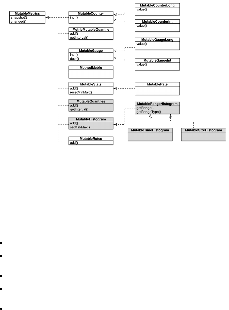
Figure 9-8. The mutable metrics class hierarchy
When we subsequently discuss the different metrics provided by HBase you will find the type
abbreviation next to it for reference, in case you are writing your own support tool.
Units of Measure for Metrics
All of the metrics listed have specific units used for measuring. Unfortunately, (as of this
writing) there is often no clear indication of what these are, though some names include a hint,
for example, MemHeapUsedM means the unit is megabytes. If that is not the case, you have can use
the following list of assumptions (short of reading the source code to find out yourself):
Metrics that refer to a point in time are usually expressed as a timestamp.
Metrics that refer to an age (such as ageOfLastAppliedOp) are usually expressed in
milliseconds.
Metrics that refer to memory sizes are in bytes.
Sizes of queues (such as splitQueueLength) are expressed as the number of items in the
queue.
Metrics that refer to things like the number of a given type of operations (such as
clusterRequests) are expressed as an integer.
(666)

Configuration
The main entry point to configuring the metrics subsystem in HBase is the hadoop-metrics2-
hbase.properties file, located in the configuration directory used by the java processes. If that file
is not found, the system will also try hadoop-metrics2.properties, that is, without the configured
prefix as a fallback. Example 9-1 shows the supplied properties file with two significant changes:
it adds and configures the Ganglia sink (more on that in “Ganglia”), and enables one file sink
(the one logging all metrics).
Example 9-1.
$ cat /etc/opt/hbase/conf/hadoop-metrics2-hbase.properties
# syntax: [prefix].[source|sink].[instance].[options]
# See javadoc of package-info.java for org.apache.hadoop.metrics2 for details
*.sink.file*.class=org.apache.hadoop.metrics2.sink.FileSink
# default sampling period
*.period=10
hbase.sink.ganglia.class=org.apache.hadoop.metrics2.sink.ganglia.GangliaSink31
hbase.sink.ganglia.servers=239.2.11.71:8649
#hbase.sink.ganglia.servers=master-3.internal.larsgeorge.com:8649
hbase.sink.ganglia.period=10
# Below are some examples of sinks that could be used
# to monitor different hbase daemons.
hbase.sink.file-all.class=org.apache.hadoop.metrics2.sink.FileSink
hbase.sink.file-all.filename=/var/opt/hbase/logs/all.metrics
# hbase.sink.file0.class=org.apache.hadoop.metrics2.sink.FileSink
# hbase.sink.file0.context=hmaster
# hbase.sink.file0.filename=master.metrics
# hbase.sink.file1.class=org.apache.hadoop.metrics2.sink.FileSink
# hbase.sink.file1.context=thrift-one
# hbase.sink.file1.filename=thrift-one.metrics
# hbase.sink.file2.class=org.apache.hadoop.metrics2.sink.FileSink
# hbase.sink.file2.context=thrift-two
# hbase.sink.file2.filename=thrift-one.metrics
# hbase.sink.file3.class=org.apache.hadoop.metrics2.sink.FileSink
# hbase.sink.file3.context=rest
# hbase.sink.file3.filename=rest.metrics
All of the sinks must be prefixed with the name under which they are registered. For HBase this
is always "hbase". The initial section that lists configuration settings starting with a star (that is,
"*."), and optionally also uses a star to match multiple instances, is for default values only. In
other words, in the example, the line
*.sink.file*.class=org.apache.hadoop.metrics2.sink.FileSink
says that all instances of sinks that start with "file" are set to use the FileSink class. That in itself
does not enable any sinks. You need to do that by commenting out the lines later on that define
the example sinks. You are, of course, free to name the sinks in any way you want, though the
same principles apply: all matching default values are assigned to the instance if there is no
specific setting that overrides it. As good example is the second default line:
# default sampling period
*.period=10
(667)
It sets the collection period for alls sinks to 10 seconds. You can override it for a specific sink,
but if you do not do that, then the 10 seconds will apply. The period for the sources is defined as
the greatest common denominator of all configured sinks. For example, assume you have two
sinks defined and set their respective collection periods to 10 and 50 seconds, then the sources
would be polled at a 10 second internal. Or, for 15 and 20 seconds the source period would be 5
seconds. Here the configuration (overriding the 10 seconds period set earlier) and log output for
the second example:
hbase-sink-file-all.period=30
...
hbase.sink.file0.period=15
2016-06-27 10:08:25,381 INFO [main] impl.MetricsSystemImpl: Scheduled snapshot period at 5
second(s).
Note
This affects the MBeans too, as they are simply all metrics sources exposed through JMX, with
their update frequency defined by the source poll period.
As for the syntax of each configuration key, explained as
[prefix].[source|sink].[instance].[options]
in the header of the properties file, the following applies:
Component Values Scope Description
<prefix> "hbase" All Fixed value for HBase metrics.
<type> "source" or
"sink" All One of those two values to address the respective part of
metrics processing.
<instance> custom All This is freely definable by the cluster administrator.
<options> "period" Sinks Sets the collection frequency for the given sink instance
(default is 10 seconds).
"source.filter" Both Defines the optional filter for sources that should be
processed (defaults to all).
"record.filter" Both Defines the optional filter for records that should be
processed (defaults to all).
"metric.filter" Both Defines the optional filter for metrics that should be
processed (defaults to all).
(668)

"queue.capacity"
Sinks
Defines the queue for the sink instance buffering collected
metrics records (defaults to 1).
"retry.delay" Sinks Sets the initial delay used when a sink errors out (defaults
to 10 seconds).
"retry.backoff" Sinks For every retry, multiply the current delay by this back-off
factor (default is 2).
"retry.count" Sinks If a sink fails, try as often as defined by the count property
(default is 1).
In addition, there are few more esoteric options that can be used to influence the metrics system
behavior. One is the "start_mbeans" parameter, which allows you to switch off the generation of
all JMX MBeans when the server starts:
*.source.start_mbeans=false
hbase.source.source.start_mbeans=false
Both of these lines accomplish the same: while the first is using the syntax for default values, the
latter explicitly addresses the proper configuration parameter. Even if you have switch off all
MBeans, you can use a tool like JConsole or VisualVM (with plugin) to trigger the creation of
the MBeans at runtime, as shown in Figure 9-9.
(669)
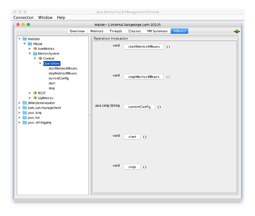
Figure 9-9. Operations of the metrics system control MBean
The image, listing the MBeans of the HBase REST server as an example, also shows that there
are no further attributes or MBeans currently created. If you click on the startMetricsMBeans()
button, you should see those appear right away.
Caution
According to the documentation, you should be able to switch off particular MBeans using the
hbase.source.<source-name>.source.start_mbeans configuration key pattern. As of this writing, any
attempt by the author to make that work has failed. Your mileage may vary.
As a final note, using the stop() and start() operations of the metrics system control MBean
allows you to reload the entire configuration, and set up the metrics from scratch without having
to restart the server process. An operator can use this to adjust the properties file and reload in
due course at runtime.
Metrics Filtering
One of the advanced features of the metrics system is the metrics filtering configuration by
source, context, record/tags, and specific metric name. The least expensive way to filter out
(670)

metrics would be at the source level, that is, for example, filtering out a source named "REST" (for
the HBase REST server). The most expensive way would be per metric filtering. Cost here is the
effort to compile the metrics, which at the source level would skip any further processing or
invocation completely. When you filter later on, say on the record or metric name level, you just
omit them after they have already been assembled internally.
In addition to the filter configuration keys shown above, there are additional postfixes that you
need to further define what a filter should do. These are:
Postfix Purpose
"context" Include only the metrics information of the given context.
"include" Allows to define a pattern with metrics details that should be included.
"exclude" Same, but allows to specify excluded metrics details.
"include.tags" Same as include, but operates on optionally available metrics tags.
"exclude.tags" Same as exclude, but operates on optionally available metrics tags.
For example, using the context filter is already provisioned in the original HBase metrics
properties file:
...
# hbase.sink.file0.class=org.apache.hadoop.metrics2.sink.FileSink
# hbase.sink.file0.context=hmaster
# hbase.sink.file0.filename=master.metrics
...
Note how the name of the context is given in lower-case. The context filter shown is operating
on a specific, named sink instance ("file0"). It instructs this sink to only accept metrics that are
assigned a specific context, here "hmaster". See “Metrics UI” for a good way to determine what
context values are available.
This next example filters on a source level instead, using a wildcard syntax that is required to fit
into the above pattern. The name of the source to filter is the given value (that is, after the equal
sign), and therefore cannot be used as the instance name:
...
hbase.*.source.filter.exclude=REST
...
When only include patterns are specified, the filter operates in the whitelisting mode, where only
matched items (that is, sources, records, metrics and so on) are included. Likewise, when only
exclude patterns are specified (as shown in the example), only matched items are excluded.
Items that are not matched in either patterns are included as well when both patterns are present.
(671)
Note that the include patterns have precedence over the exclude patterns.
Similarly, you can specify the "record.filter" and "metric.filter" options, which operate at
record and metric level, respectively. Filters can be combined to optimize the filtering efficiency,
and filtering out at the source level is applying it to all sinks, while filtering on the sink level is
specific for that sink only (like in the "context" example).
Note
Some of the filtering does apply differently to the JMX MBeans and the sinks. Any of the source
filtering only applies to the sinks, removing all metrics of the filtered sources from all the sink
output, that is, for all activated sinks. You can use the "source.start_mbeans" option to switch
entire MBeans off. The record and metric level filtering applies to both JMX and sinks equally.
There are two filter classes available (both in the org.apache.hadoop.metrics2.filter package,
supplied by Hadoop), which have slightly different matching pattern support:
GlobFilter
Similar to the Linux shell, allows for a simplified pattern definition, using the * symbol as
a wildcard, and the ? for single letter placeholder. For example, a pattern of foo* would
match foo, foobar, food, and so on. The filter internally is using the GlobPattern class, which
you should consult for the few, more advanced patterns it supports.
RegexFilter
This filter offers the full functionality of the Java Pattern class based regular expression
syntax.
If you do not explicitly define a filter class, they default to the GlobFilter, as implied in the
example above. You can explicitly set the class like so:
*.source.filter.class=org.apache.hadoop.metrics2.filter.GlobFilter
hbase.*.source.filter.include=...
hbase.*.source.filter.exclude=...
Debugging the Metrics System
What could you do when the metrics configuration is not giving you the expected results. For
example, say you have configured a sink instance, but for some reason it is not emitting any
metrics. The MetricsSystem class automatically adds a statistics MBean, which may help figuring
out what is going on:
...
}, {
"name" : "Hadoop:service=HBase,name=MetricsSystem,sub=Stats",
"modelerType" : "MetricsSystem,sub=Stats",
"tag.Context" : "metricssystem",
"tag.Hostname" : "de1-app-mpr-1.internal.larsgeorge.com",
"NumActiveSources" : 12,
"NumAllSources" : 12,
"NumActiveSinks" : 0,
"NumAllSinks" : 0,
"SnapshotNumOps" : 0,
"SnapshotAvgTime" : 0.0,
"PublishNumOps" : 0,
"PublishAvgTime" : 0.0,
"DroppedPubAll" : 0
(672)

}, {
...
Note how there are counters that show the number of configured source and sinks. In the
example there are 12 sources, but no single active sink that is configured. The server logs can be
used to emit DEBUG level information about what the metrics system is doing, which is
accomplished by added the following to the log4j.properties file in the configuration directory:
log4j.logger.org.apache.hadoop.metrics2=DEBUG
When enabled, the logs will show each configured sink and its status. Here you see the output for
a successful start of the Ganglia sink instance:
...
2016-06-13 04:55:33,287 DEBUG [HBase-Metrics2-1] ganglia.GangliaSink31: \
Initializing the GangliaSink for Ganglia metrics.
2016-06-13 04:55:33,295 INFO [HBase-Metrics2-1] impl.MetricsSinkAdapter: \
Sink ganglia started
...
2016-06-13 05:06:58,444 INFO [main] impl.MetricsConfig: \
loaded properties from hadoop-metrics2-hbase.properties
2016-06-13 05:06:58,480 INFO [main] impl.MetricsSinkAdapter: \
Sink ganglia started
2016-06-13 05:06:58,512 INFO [main] impl.MetricsSystemImpl: \
Scheduled snapshot period at 10 second(s).
2016-06-13 05:06:58,512 INFO [main] impl.MetricsSystemImpl: \
HBase metrics system started
...
In addition, the logs show you the name of the file used to load the settings from, as well as a
debug output of its contents (omitted here). An alternative is to use the JMX MBeans of the
metrics system again, as shown in Figure 9-10. The control MBean exposes a currentConfig()
method, returning the loaded configuration interactively and at runtime.
(673)
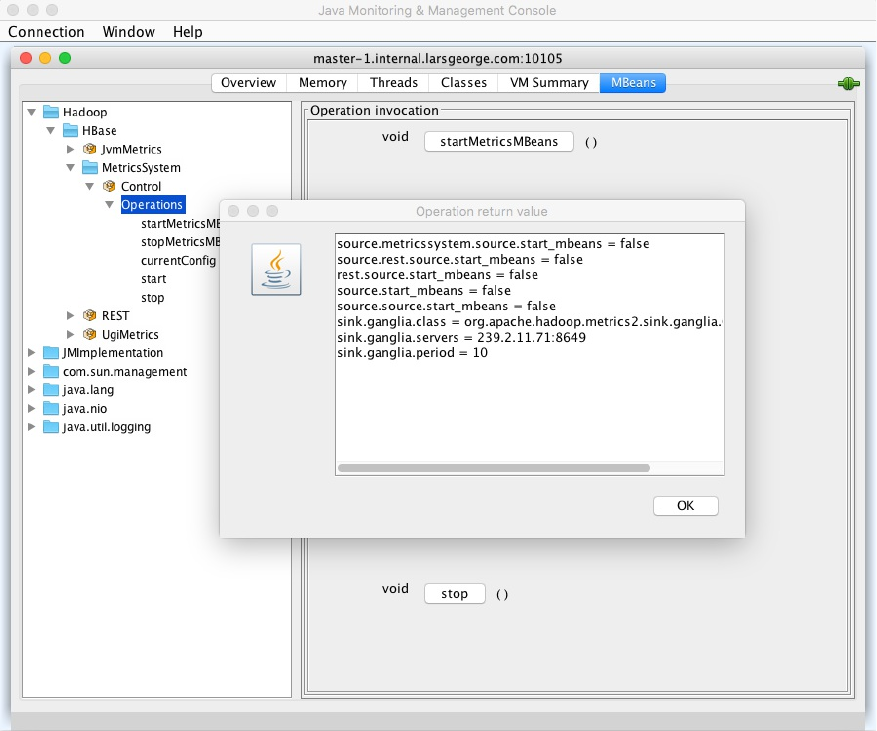
Figure 9-10. The currently active metrics configuration retrieved through JMX
Check for anything that looks suspicious, and either restart the server to ensure any modification
is actually loaded, or use the control MBean of the metrics system to reload everything at
runtime.
(674)
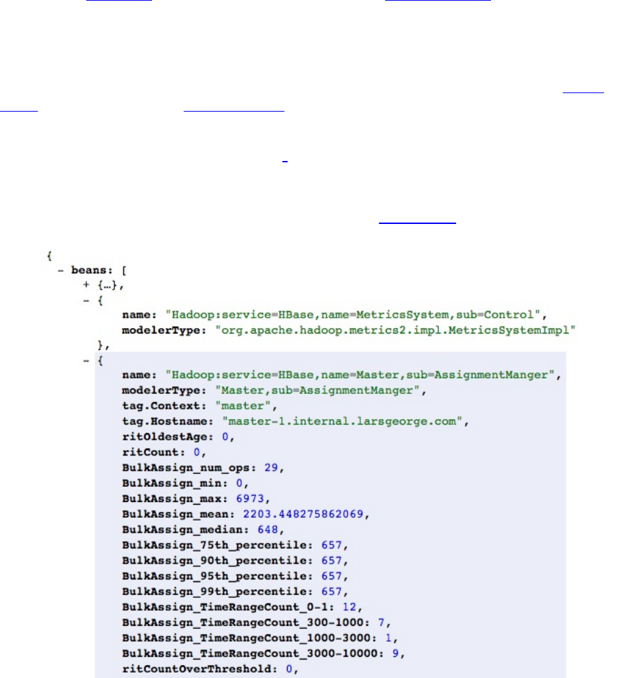
Metrics UI
Before configuring more complex metrics aggregation frameworks based on, for example,
Ganglia (see “Ganglia”), or emitting them to log files (see “Configuration”), it may be useful to
quickly check the current metrics without any complications. Or, if you are just starting out with
HBase and want to see what metrics are available and, optionally, apply some more advanced
filtering later on, you will find insight using the supplied metrics UI, included into every server
daemon. Once you open the UI of a process, for example, that of the HBase Master or
RegionServer, you will find a link on the top of page that is titled Metrics Dump. See “Main
Page” for a screenshot, and “Shared Pages” for a very short description of the page we are now
inspecting in detail.
The metrics page is inherited from Hadoop5 and emits all of the registered and active MBeans
with their current values in JSON format. Since the output can be overwhelming, and may
require a lot of scrolling around, it is highly recommended to install a browser plugin that allows
to collapse and expand parts of the structure, as shown in Figure 9-11
Figure 9-11. The metrics in JSON format, with browser support to collapse details
The metrics page has built-in support for a few parameters, which may help in reading or
accessing its output. First is description, which adds any available (though optional) description
for records, tags, metrics, and so to the JSON structure. In fact, if you look at the example, you
will see that the JSON itself is slightly altered to now include a nested objects for each affected
item, containing the description text, as well as the value itself:
(675)

...
"beans" : [ {
"name" : "java.lang:type=Memory",
"description" : "Information on the management interface of the MBean",
"modelerType" : "sun.management.MemoryImpl",
"Verbose" : false,
...
}, {
"name" : "Hadoop:service=HBase,name=Master,sub=Server",
"description" : "Metrics about HBase master server",
"modelerType" : "Master,sub=Server",
...
"tag.clusterId" : {
"description" : "Cluster Id",
"value" : "49ffd33c-e051-4c00-b0da-df7737e1d3ec"
},
...
"masterActiveTime" : {
"description" : "Master Active Time",
"value" : 1465909297645
},
"masterStartTime" : {
"description" : "Master Start Time",
"value" : 1465909293281
},
...
Adding the description parameter is achieved by postfixing the normal metrics page URL with a
parameter, like so:
http://<hbase-master-hostname>:16010/jmx?description=true
Another parameter the page supports is qry, which allows to filter out any not matching records.
For example, to only retrieve all Hadoop (and HBase) related records, you could use:
http://<hbase-server-hostname>:16010/jmx?qry=Hadoop:*
The name of the records can be taken from the full list, which the page returns by default. The
name is usually the first object member in the JSON. This works for all Hadoop records (starting
with "Hadoop:"), as per the example, but not (as of this writing) for other ones. Finally, there is a
parameter called get that lets you retrieve a particular metric of a given record. You need to hand
in the name of a metrics record and an attribute name, divided by two colon characters (“::”). For
example:
http://<hbase-master-hostname>:16010/jmx? \
get=Hadoop:service=HBase,name=Master,sub=Server::averageLoad
This should return the following for you, assuming you are sending the request to the active
master node:
{
"beans" : [ {
"name" : "Hadoop:service=HBase,name=Master,sub=Server",
"modelerType" : "Master,sub=Server",
"averageLoad" : 13.666666666666666
} ]
}
Obviously, every server type has their own specific metrics records, and in them the respective
metrics. You need to send the request to the proper server and port, asking for a metrics record
and name to get something useful returned. Otherwise an error message is added to the resulting
JSON. More can be found in the online documentation for the JMX service.
(676)

Master Metrics
The master process exposes all metrics relating to its role in a cluster. Since the master is
relatively lightweight and only involved in a few cluster-wide operations, it does expose only a
limited set of information (in comparison to the region server process, for example).
Nevertheless, there is a lot of insight to be gleaned from the provided metrics. They are usually
recorded within the effective polling period (see “Configuration”) and then reset thereafter. The
gauge metric type, for example, is used to track the varying numbers and accrue them
accordingly for the sinks.
Here is the list of metrics records, that is, the subsets (or grouped) metrics pertaining to a
particular feature of the server process, annotated with the metrics type for each available
attribute6 (refer to “Metrics Classes”):
AssignmentManager
Provides details about the assignment of regions to servers. There are these metrics
available:
Metric Type Description
ritOldestAge LG Reports the time of the oldest region in transition (in
milliseconds).
ritCount LG Counts the total number of regions in transition.
ritCountOverThreshold LG
The number of regions in transition that are over the
configured threshold (see
"hbase.metrics.rit.stuck.warning.threshold").
Assign TH A time-based histogram for all single region assignment
operations.
BulkAssign TH Same as above, but for all bulk assignments, which means
more than one region per operation.
Balancer
This group of metrics provides information about the central balancer instance, running
inside the currently active master. It provides the following metrics:
Metric Type Description
BalancerCluster TH Provides a time-based histogram of the balancer operations.
(677)
miscInvocationCount IC
Counts the number of times the balancer has been called upon
based on operator (e.g. move()) or cluster actions (during
region in transition or server changes).
Since this is one of the first records we are discussing, here an abbreviated list of the other
information provided. Of interest is the "name" attribute, which can be used for filtering or
searching. The part after the "sub=" part is the actual record name referred to in this
section. You can also see the associated metrics tags for the record, which in this case lists
the context and hostname:
name: "Hadoop:service=HBase,name=Master,sub=Balancer",
modelerType: "Master,sub=Balancer",
tag.Context: "master",
tag.Hostname: "master-1.internal.larsgeorge.com",
FileSystem
The master orchestrates the global WAL (aka HLog) handling, through the distributed log
splitting process. This record provides inside into that process. The available metrics are:
Metric Type Description
HLogSplitSize SH
Provides a histogram of the data processed during WAL
splitting for user tables. It reports the number of operations
recorded, along with the statistics about their sizes.
MetaHLogSplitSize SC Same as the previous, but for the meta system table.
HLogSplitTime TH
Provides a histogram of the time spent in WAL splitting for
user tables. It reports the number of operations recorded, along
with the statistics about their runtime.
MetaHLogSplitTime IC Same as the previous, but for the meta system table.
Server
High level information about the master server process itself. The available metrics are:
Metric Type Description
averageLoad DG Reports the average number of regions per server.
clusterRequests LC Counts the total number of requests across all active region
servers.
(678)

masterActiveTime LG Records the time the master has been active for (in
milliseconds).
masterStartTime LG The fixed start time of the server (as Linux epoch).
numRegionServers IG The number of currently active region servers.
numDeadRegionServers IG The number of region servers that once were active, but
now considered dead.
In addition to the metrics, the record also offers information that do not lend themselves to
metrics units. These are usually strings that list the number of active and dead region
servers, the configured ZooKeeper quorum, and so on. For example, on the test cluster
used they look like this:
tag.liveRegionServers: "slave-2.internal.larsgeorge.com, \
16020,1465909293694; \
slave-3.internal.larsgeorge.com,16020,1465909293581; \
slave-1.internal.larsgeorge.com,16020,1466346370329",
tag.deadRegionServers: "",
tag.zookeeperQuorum: "master-1.internal.larsgeorge.com:2181, \
master-2.internal.larsgeorge.com:2181, \
master-3.internal.larsgeorge.com:2181",
tag.serverName: "master-1.internal.larsgeorge.com,16000,1465909293281",
tag.clusterId: "49ffd33c-e051-4c00-b0da-df7737e1d3ec",
tag.isActiveMaster: "true",
tag.Context: "master",
tag.Hostname: "master-1.internal.larsgeorge.com",
Snapshots
Tracks all snapshot related operations. The metrics comprised by this record are:
Metric Type Description
SnapshotTime TH Provides a time-based histogram recording the time statistics
for table snapshots.
SnapshotCloneTime TH Same but for the snapshot clone operations.
SnapshotRestoreTime TH Same but for the snapshot restore operations.
There are more metrics records emitted on the master UI Metrics Dump page, some of which are
discussed in “RPC Metrics” and “JVM Metrics”.
Important Master Metrics
The master process is vital to keep a HBase cluster alive and well, though in itself it only reports
(679)
auxiliary information through its metrics records. The ones you should monitor (as opposed to
graph) are:
master.Server.numRegionServers
Make sure the number of active regions servers matches your expectations.
master.Server.numDeadRegionServers
Should you see a steep rise in dead region servers, you may have a problem where the
server processes repeatedly shut themselves down, and are then restarted by, for example,
a process agent.
master.Server.ritCount
It is normal for a HBase cluster to split and/or move regions over time. Such regions in
transition should stay at a low number, as they commonly incur some I/O cost (for
rewriting files, or reading data over the network).
master.Server.ritCountOverThreshold
In rare situations it may happen that a region stays in transition for too long, resulting in
collateral issues, such as tables that cannot be dropped, altered, or disabled. This counter
metric should stay at zero if the cluster is healthy.
master.Server.ritOldestAge
This time metric can be used to start warning operators, since transitions should eventually
complete. If the age of the oldest region in transition exceeds your threshold, you could
raise an alarm.
(680)
Region Server Metrics
The region servers are part of the actual data read and write path, and therefore collect a
substantial number of metrics. These include details about different parts of the overall
architecture inside the server—for example, the block cache and in-memory stores. Like before,
we will look at them in groups, as provided by the metrics records:
Regions
This group is (mostly) a dynamic one, adding a set of metrics for every open region hosted
by the given region server. As regions are opened they are added to this group, and
removed when they are closed. The naming of the dynamic metrics is following this
pattern:
Namespace_<namespace_name>_table_<table_name>_region_<region_id> \
_metric_<metric_name>
For each region, these are the exposed metrics, with their respective types:
Metric Type Description
storeCount LG The number of stores for the region, which equals the
number of column families.
storeFileCount LG The count of of all store files, across all stores for the
given region.
storeFileSize LG Same as the above, but summarizing the sizes of all
store files.
memStoreSize LG The sum of all memstore sizes, across all stores.
compactionsCompletedCount LC The number of completed compactions for the
region.
numBytesCompactedCount LC
The aggregated number of bytes that have been
compacted, which is the sum of the sizes of all
compacted store files.
numFilesCompactedCount LC Same as above, but reporting the number of store
files instead.
(681)
readRequestCount LC The number of read requests for the given region.
writeRequestCount LC Records the number of write requests for the region.
replicaid IC This static number states the replica ID of this region.
There is only one metric available in this group that spans all regions, which is:
Metric Type Description
numRegions IG The accumulated number of of regions for the current server.
Replication
This groups reports information about the replication state, if enabled at all (see [Link to
Come]). The metrics are a combination of static, as well as dynamic data points. Each
region server can act as a sender and receiver of replicated mutations (that is, the WAL
edits). As far as naming conventions are concerned, the region server receives edits from a
remote cluster into its sink, and sends edits to each registers peer cluster with a dedicated
source instance. In addition, there is a global set of metrics for the sources that accumulate
the data across all registered sources (which have the source ID in their metric name). The
sink and global source metrics are static, while the per source metrics are dynamic and
change at runtime as you add or remove peers.
The following attributes are available:
Metric Type Description
sink.appliedOps LC The total number of WAL entries that have
been applied to this server.
sink.appliedBatches LC Number of batches that comprised the WAL
entries.
sink.ageOfLastAppliedOp LG The remote write timestamp of the last locally
applied WAL edit.
source[.
<source_id>].sizeOfLogQueue LG Reports the size of the WAL queue per peer
(that is, source) cluster.
source[.
<source_id>].ageOfLastShippedOp LG Tracks the age of the last edit that was shipped
to a peer.
(682)
source[.
<source_id>].shippedBatches
LC The number of edit batches sent.
source[.<source_id>].shippedKBs LC The size of the shipped edits in kilobytes.
source[.<source_id>].shippedOps LC Count of shipping operations performed.
source[.
<source_id>].logReadInBytes LC The number of bytes read from the tracked
WALs.
source[.
<source_id>].logEditsRead LC The count of WAL edits that have been read.
source[.
<source_id>].logEditsFiltered LC Count of edits that have been filtered, for
example, those from system tables.
Server
This group of metrics is reporting all operational information available for the given region
server. There are many data points available, so we will discuss them in logical groups as
they often relate to each other.
Server Summary Information
A set of metrics provided summarize the current state of the region server, listing the
number of files and their accumulated sizes. This is particularly useful to estimate
the heap needed for the server process. Keep in mind that for multi-level indexes
(for Bloom filter, data, and metadata blocks) only the root indexes are loaded into
memory, while the various leaf index blocks are loaded on demand and cached in
the block cache. So the memory printed here as storeFileIndexSize plus the memory
occupied by the block cache (blockCacheSize), and memstores (memStoreSize) give
you an coarse approximation about the Java heap that is currently needed for reading
and writing data.
Metric Type Description
regionServerStartTime LG Holds the server start time as a Linux
epoch (will not change at runtime).
regionCount LG The currently served number of regions
of this server.
storeCount LG
The total store count across all regions
(which equals the count of column
(683)
families).
storeFileCount LG The number of HFiles that are held open
by the server.
storeFileSize LG Summarizes the size of all open store
files, across all regions.
storeFileIndexSize LG
The total size of all the store file data
and metadata indexes. This is what
needs to be loaded into memory when
the store files are opened.
staticIndexSize LG
Since HBase is supporting multi-level
indexes, this number is the combined
size of all data and metadata indexes,
including what is usually only partially
loaded.
staticBloomSize LG Same as above, but for the Bloom filter
indexes.
percentFilesLocal DG
The percentage (expressed as a double
value) of the open store files that are
local to this server.
percentFilesLocalSecondaryRegions DG
Same, but for regions that are served as
replicas, that is, they are open for
reading only.
hlogFileCount LG
The count of managed WALs. They are
held until all mutations they contain are
flushed to store files.
hlogFileSize LG The sum of all WAL sizes under
management.
API Usage Information
Here, all of the external client calls are tracked and reported appropriately. This
includes read and write operations, their type, how those were configured, and the
number of those exceeding a configured threshold (set to 1 second).
(684)
Metric Type Description
totalRequestCount LC The total number of requests handled by this
region server.
readRequestCount LC How many read requests have been served.
writeRequestCount LC Same, but for write requests.
checkMutateFailedCount LC Number of check-and-mutate calls that have
failed due to condition changes.
checkMutatePassedCount LC Counts the number of check-and-mutate
operations that have succeeded.
mutationsWithoutWALCount LC
Since WAL usage is selectable, this count states
how many writes have opted not to use the
WAL.
mutationsWithoutWALSize LC The accrued size of all writes that have not used
the WAL.
updatesBlockedTime LC
Total number in milliseconds that clients were
blocked due to forceful flushing of memstores
under pressure.
blockedRequestCount LC Counts how often clients were blocked due to
pressure.
Get TH Reports a time-based histogram for all read
operations using the get() API.
Mutate TH Same, but for all mutations, such as single or
batch puts.
Append TH Same, but for all append calls.
Delete TH Same, but for all delete calls.
(685)
ScanNext TH Same, but for all calls to next() on scanners.
Replay TH Same, but for log replay operations during a
distributed log replay.
Increment TH Same, but for all increment operations.
slowDeleteCount LC Tracks the number of delete operations that
were slower than the threshold (1 second).
slowIncrementCount LC Same, but for increment calls.
slowGetCount LC Same, but for get calls.
slowAppendCount LC Same, but for append calls.
slowPutCount LC Same, but for put operations.
Write Information
This metrics group tracks all the write path related data points, such as the current
accumulated space needed in memory for the memstores, as well as the subsequent
flush operations.
Metric Type Description
memStoreSize LG The current total heap size occupied by unflushed
mutations.
flushQueueLength IG
The flush queue length, which should be zero to a low
number, if the server can keep up writing out memstores
to persistent storage.
flushedCellsCount LC Number of cells that have been written to store files, since
the server was started.
flushedCellsSize LC Same, but for the total size of the written cells in bytes.
A time-based histogram showing details about the
(686)
FlushTime TH asynchronous flush process.
Compaction Information
After enough flushing of memstores, the compactions will rewrite the store files into
fewer, larger ones. This set of metrics shows the data points pertaining to that
process.
Metric Type Description
compactionQueueLength IG
The current size of the compaction queue,
which should be zero to a low number for
clusters that can keep up with the background
write workload.
compactedCellsCount LC Number of cells that have been compacted since
the server started (for minor compactions only).
majorCompactedCellsCount LC Same, but for cells that were handled by a major
compactions.
compactedCellsSize LC Accrued size of all cells that were processed by
all minor compactions.
majorCompactedCellsSize LC Same, but for major compactions.
Note
For all queues mentioned, that is, the compaction, split, and flush queue, you need to keep
in mind that these metrics are updated after the asynchronous process has completed. In
other words, the reported values slightly trail the actual value, as it is missing what is
currently in progress. Also keep in mind that major compactions will also cause a sharp
rise as they queue up all storage files. You need to account for this when looking at the
graphs.
Split Information
Once a store within a region reaches the configured maximum store size, the region
is split into two new once. This again happens asynchronously and is handled by a
thread pool with a queue (like flushes and compactions).
Metric Type Description
splitQueueLength IG
The number of regions lined up for splitting. This should
be zero to a low number, assuming the cluster can keep up
(687)
with the write workload.
splitSuccessCount LC Number of splits that completed successfully since the
server started.
splitRequestCount LC Number of splits that were requested since the server
started.
SplitTime TH A time-based histogram, giving insight into the split
performance.
Block Cache Information
The data and index blocks loaded at runtime are cached in the bock cache. There are
a number of metrics that help understanding how well the block cache performs.
Metric Type Description
blockCacheFreeSize LG The remaining free space in memory from
the configured maximum.
blockCacheCount LG The current number of blocks cached.
blockCacheSize LG The number of bytes occupied by the
cached blocks in memory.
blockCacheHitCount LC
The total number of block cache hits, that
is, requests for blocks that were already
cached.
blockCacheHitCountPrimary LC Same, but for the subset where the blocks
were for primary region replicas.
blockCacheMissCount LC The count of calls to the cache that failed
to return a requested block.
blockCacheMissCountPrimary LC Same, but for those blocks from primary
region replicas only.
blockCacheEvictionCount LC The total number of times a block was
removed from cache due to pressure.
(688)

blockCacheEvictionCountPrimary LC Same, but for blocks pertaining to primary
region replicas only.
blockCacheCountHitPercent DG The total percentage (as a double value) of
hits for block requests.
blockCacheExpressHitPercent DG
The number of hits for block requests that
also should stay cached (see, for example,
the setCacheBlocks() method in “Single
Gets”).
blockCacheFailedInsertionCount LC Counts how many times adding a block to
the cache has failed.
Note
Regarding the express hit percentage, all read operations will try to use the cache,
regardless of whether retaining the block in the cache has been requested. Use of
setCacheBlocks() only influences the retainment policy of the request.
WAL
Records the metrics for the write-ahead log (WAL) subsystem (see [Link to Come]). The
available attributes are:
Metric Type Description
appendCount LC Counts the number of append operation to the write-ahead
log.
slowAppendCount LC The number of append operations that exceeded the
configured threshold (set to 1 second).
rollRequest LC Increases for every requested roll of an active WAL.
lowReplicaRollRequest LC Counts how many times a log roll was requested due to too
few datanodes in the write pipeline.
SyncTime TH Information about the time it took to synchronize the WAL
with the underlying file system.
(689)

AppendSize SH
The accrued size of all the data that has been written to the
WAL.
AppendTime TH Tracks the time it took for the append operations to
complete.
Important Region Server Metrics
The region server process provides a lot of insight with its many metrics. Some of these metrics
are not that interesting, or are derivates of others, as in, they are collateral data points that go up
or down due to more essential metrics doing the same (or opposite). Here are the main attributes
you should keep an eye on during cluster operations:
regionserver.Server.{regionCount|storeFileCount|hlogFileCount}
When monitoring the region servers for their health, you should watch out for the total
count of regions, store files, and number of WALs that are still under management (that is,
not yet discarded after flushing all pending mutations they comprise). Too many WALs
can cause clients to be blocked, and too many store files (dependent on your access
patterns) may slow down reads. Too many regions that take on writes may cause
memstores to fill up their allocated heap space too fast, forcing early flushes and with it,
most likely, too many compactions to keep the file count in check (see “Cluster Sizing”).
hbase.regionserver.{flushQueueLength|compactionQueueLength|splitQueueLength}
These three queues are a great indicator for how busy a HBase cluster is. If you see their
levels rising over time, and not fall back to zero or some low levels, you are running into
danger of oversubscribing your ingest workload. Also, these queues, as they rise, give their
indication quite some time before the backlog will force clients being blocked eventually
with forceful flushing of old memstores to free WALs. Use a monitoring tool such as
Nagios to trigger alarms if the queue counts are increasing constantly.
regionserver.Server.{updatesBlockedTime|blockedRequestCount}
Those two metrics show the effects of the above write overload problem, counting how
often user threads where blocked, and how long the server blocked them for
accumulatively. Both counters should be zero, or even if they went up at one time, stay at a
constant level (which means no further blocking occurred).
regionserver.Server.percentFilesLocal
This percentage will indicate how efficient reads are, with local reads being much better
than reading over the (often already contended) network
regionserver.Server.<op>_<measure>
Operation latencies, where <op> is one of the above described Append, Delete, Mutate,
and so on. The <measure> is one of min, max, and so, along with the important
percentiles. Use these histograms to see how the client operations behave on the server.
(690)

Are there any with huge difference between the maximum and the 95th/99th percentile?
This could point to strugglers that may need investigation (for example, a row or entity
group might be heavily skewed and warrants a schema redesign).
regionserver.Server.slow<op>Count
If any of the client operations (here represent as <op>) is slow (which means it takes
longer than a second) the respective metric is increased. A heavily loaded cluster may see
these increase, but just as with the blocking of clients, you should not see them increasing
all the time. It indicates some form of overload, usually pointing to the shared storage,
such as HDFS.
regionserver.Server.mutationsWithoutWALCount
If clients opt to skip the WAL to, for example, gain some extra write performance, they do
so at the risk of losing data, if the memstores cannot be flushed to storage later on. Discuss
this carefully with your application developers to communicate the risk.
regionserver.Server.{blockCacheHitCount|blockCacheMissCount|blockCacheEvictionCount}
Use the various hit, miss, and eviction counters to monitor for the efficiency of the block
cache. You should aim for a high hit and a low miss rate, plus a low eviction count.
Dependent on your use-case, you may need to resize the block cache (see “Block Cache
Tuning”), or increase or decrease the store file block size.
If you suspect write performance to be an issue, and want to see more, you can check out the
regionserver.WAL record with the SyncTime and AppendTime histograms (TH), since writing to
the WAL is vital for HBase to keep up with the client ingest rate.
(691)
RPC Metrics
Both the master and region servers also provide metrics from the RPC subsystem (also referred
to as IPC at times). These are data points that are particularly related to the communication
between remote clients and the server process.
Note
The RPC metrics for the master and region servers are shared—in other words, you will see the
same metrics exposed on either server type. The difference is that the servers update the metrics
for the operations the process invokes. On the master, for example, you will not see updates to
the metrics for certain exceptions, since those are related to the region server only.
The following metrics are provided by the IPC metrics record, listed as master.Master and
regionserver.RegionServer respectively when provided to the sinks for each server type:
Metric Type Description
queueSize LG The total size in bytes of all requests in the queue.
numCallsInGeneralQueue IG The number of requests that are currently in the
queue.
numCallsInReplicationQueue IG Count of calls in the separate replication queue.
numCallsInPriorityQueue IG Count of calls in the separate priority queue.
numOpenConnections IG Number of connections from clients and other
servers.
numActiveHandler IG Number of active RPC handlers processing
requests.
TotalCallTime TH A histogram tracking the time requests took to be
processed.
QueueCallTime TH Same, but for the time requests spent in the queue
before processing.
ProcessCallTime TH Same, but the actual time the request took to be
(692)
handled.
RequestSize SH A histogram for the request sizes.
ResponseSize SH Same, but for the size of the responses.
sentBytes LC The total number of bytes sent by the server to
clients.
receivedBytes LC Same, but for the total number of received bytes.
authenticationFailures LC Tracks the number of authentication failures.
authorizationFailures LC Same, but for authorization failures instead.
authenticationFallbacks LC Counts how many times authentication had to fall
back to a different type.
authenticationSuccesses LC Each successful authentication is counted and
report under this attribute.
authorizationSuccesses LC Same, but for authorization successes instead.
exceptions LC Number of all exceptions this server has seen
regarding client calls.
exceptions.NotServingRegionException LC
Tracks a specific error, here when clients ask for
regions not served by this server, and no new
location is known.
exceptions.RegionTooBusyException LC Counts how many times the client saw an error due
to region overload (too many memstores).
exceptions.OutOfOrderScannerNextException LC Number of times an error was thrown due to client
scanners out of sync with the server.
Shows how often the scanner had to report an error
(693)
exceptions.multiResponseTooLarge LC due to resource limitations (see
"hbase.server.scanner.max.result.size").
exceptions.UnknownScannerException LC
Count of scanners trying to call next() but where
the server-side scanner is not available anymore
(usually due to a timeout).
exceptions.FailedSanityCheckException LC
Count of requests from clients with erroneous
parameters, for example a put with a timestamp
outside of a non-default slop threshold (see
"hbase.hregion.keyvalue.timestamp.slop.millisecs"
exceptions.RegionMovedException LC
Count of how many times a client ask for a region
that has been moved and is informed about that
fact.
Important RPC Metrics
While rather generic, the RPC metrics are a good source of information about the cluster status.
With the histograms provided you should be able to spot outliers, as far as request handling is
concerned. The exception counters should help you determine if you see an unusual amount of
issues, possibly caused by new workloads, or changes in behavior by the client applications. For
more specific notes:
QueueCallTime
Monitoring the queue time is a good idea, as it indicates the load on the server. You could
use thresholds to trigger warnings if this number goes over a certain limit. These are early
indicators of future problems, as too many calls in the queue are pointing to delays in
client call handling, driving up response latencies in the process.
(694)
UserGroupInformation Metrics
The shared “ugi.UgiMetrics” record exposes details about the underlying authentication process
of the server. As clients and other servers call RPC endpoints, they have to provide some form of
credentials (see [Link to Come] for more details). The UserGroupInformation class (abbreviated as
UGI), provided by Hadoop, exposes a few metrics that allow the operator to monitor and graph
login and group membership operations:
Metric Type Description
LoginSuccess RMeasures the successful login operations, counting the number of
operations with their average time.
LoginFailure R Same, but for failed login operations.
GetGroups R Same, but for calls to resolve the group membership of the given user.
(695)

JVM Metrics
When it comes to optimizing your HBase setup, tuning the JVM settings requires expert skills.
You will learn how to do this in “Garbage Collection Tuning”. This section discusses what you
can retrieve from each server process using the metrics framework. Every HBase process collects
and exposes JVM-related details that are helpful to correlate, for example, server performance
with underlying JVM internals. This information, in turn, is used when tuning your HBase
cluster setup.
The shared metrics record provided is prefixed with jvm.JvmMetrics when sent to any configured
sink. There are more Java Platform MXBeans, as discussed in Figure 9-2, that you can refer to
using the JMX API. These MXBeans have a great wealth of information to all aspects of
memory usage and the configured garbage collection implementation. “Metrics UI” explains
how to browse those metrics from the server UIs.
The provided data points can be grouped into related categories:
Memory Usage Metrics
You can retrieve the used memory and the committed memory7 in megabytes for both
heap and nonheap usage. The former is the space that is maintained by the JVM on your
behalf and garbage-collected at regular intervals. The latter is memory required for JVM
internal purposes, and off-heap caches.
Metric Type Description
MemNonHeapUsedM FG Megabytes of memory currently used for non-heap
purposes.
MemNonHeapCommittedM FG Same, but for committed non-heap memory.
MemNonHeapMaxM FG Configured maximum memory in megabyte that may
be used for non-heap purposes.
MemHeapUsedM FG Megabytes of memory currently used for on-heap
purposes.
MemHeapCommittedM FG Same, but for committed on-heap memory.
MemHeapMaxM FG Configured maximum memory in megabyte that may
be used for on-heap purposes.
MemMaxM FG Total configured memory in megabytes.
(696)

Garbage Collection Metrics
The JVM is maintaining the heap on your behalf by running garbage collections. The
GcCount metric is the number of garbage collections, and the GcTimeMillis is the
accumulated time spent in garbage collection since the last poll. What is omitted here are
the metrics provided by the chosen garbage collection implementation. For example, the
Parallel New collector provides a GcCountParNew metric, and the Concurrent Mark
Sweep (CMS) collector provides GcCountConcurrentMarkSweep (plus the time spent
counters that accompany them).
Metric Type Description
GcCount LC Number of garbage collections since the process was started.
GcTimeMillis LC Time spent in garbage collection since the process was started.
Stop the World!
Certain steps in the garbage collection process cause so-called stop-the-world pauses, which are
inherently difficult to handle when a system is bound by tight SLAs.
Usually these pauses are only a few milliseconds in length, but sometimes they can increase to
multiple seconds. Problems arise when these pauses approach the multiple minute range, because
this can cause a region server to miss its ZooKeeper lease renewal—forcing the master to take
evasive actions. The HBase development team has affectionately dubbed this scenario a Juliet
Pause—the master (Romeo) presumes the region server (Juliet) is dead when it is really just
sleeping, and thus takes some drastic action (recovery). When the server wakes up, it sees that a
great mistake has been made and takes its own life. Makes for a good play, but a pretty awful
failure scenario!8
Use the garbage collection metrics to track what the server is currently doing and how long the
collections take. As soon as you see a sharp increase, be prepared to investigate. Any pause that
is greater than the zookeeper.session.timeout configuration value should be considered a fault.
Thread metrics
This group of metrics reports a variety of numbers related to Java threads. You can see the
count for each possible thread state, including new, runnable, blocked, and so on.9
Metric Type Description
ThreadsNew IG Number of newly created threads.
ThreadsRunnable IG Number of threads that are currently running.
(697)
ThreadsBlocked IG Counts the threads that are blocked by some condition
(monitor lock etc.).
ThreadsWaiting IG Threads that are waiting for execution are counted here.
ThreadsTimedWaiting IG Same, but for threads that only wait for a given amount of
time.
ThreadsTerminated IG Counts the number of threads that have exited.
System Event Metrics
Finally, the events group contains metrics that are collected from the logging subsystem,
but are subsumed under the JVM metrics category (for lack of a better place). System
event metrics provide counts for various log-level events. For example, the LogError
metric provides the number of log events that occurred on the error level, since the last
time the metric was polled. In fact, all log event counters show you the counts accumulated
during the last poll period.
Metric Type Description
LogFatal LC The number of log entries made with the FATAL log level.
LogError LC The number of log entries made with the ERROR log level.
LogWarn LC The number of log entries made with the WARN log level.
LogInfo LC The number of log entries made with the INFO log level.
HBase ships without the necessary wiring to feed log events into the global EventCounter
class that ships with Hadoop. In other words, you see 0 for all of them out-of-the-box. You
can enable the LogXYZ metrics by adding/modifying the following (highlighted) lines in
the log4j.properties file in the configuration directory:
...
hbase.root.logger=INFO,console
...
# Define the root logger to the system property "hbase.root.logger".
log4j.rootLogger=${hbase.root.logger}, EventCounter
log4j.appender.EventCounter=org.apache.hadoop.log.metrics.EventCounter
...
Note that this is using the normal Appender hooks, which means if you leave the default
INFO level for the root logger, you will see no such messages in the logs, and therefore all
related metrics counters will stay at 0 as well.
(698)
Using these metrics, you are able to feed support systems that either graph the values over time,
or trigger warnings based on definable thresholds. It is really important to understand the values
and their usual ranges so that you can make use of them in production.
(699)

Ganglia
HBase inherits its native support for Ganglia10 directly from Hadoop, providing a sink that can
push the metrics directly to it.
Note
Hadoop (and in extension HBase) supports Ganglia 3.0.x, as well as 3.1.0 and greater. This
matters, as the network protocol was changed between those two releases. There is an
implementation for Ganglia30 and Ganglia31 available, where the the latter is supporting all
newer versions as well. As of this writing, Ganglia 3.7.x worked fine with the Ganglia31 code
provided.
Ganglia consists of three components:
Ganglia Monitoring Daemon (gmond)
The monitoring daemon needs to run on every machine that is monitored. It collects the
local data and prepares the statistics to be polled by other systems. It actively monitors the
host for changes, which it will announce using uni- or multicast network messages. If
configured in multicast mode, each monitoring daemon has the complete cluster state—of
all servers with the same multicast address—present.
Ganglia Meta Daemon (gmetad)
The meta daemon is installed on a central node and acts as the federation node to the entire
cluster. The meta daemon polls from one or more monitoring daemons to receive the
current cluster status, and saves it in a round-robin, time-series database, using RRDtool.11
The data is made available in XML format to other clients—for example, the web front
end.
Ganglia also supports a hierarchy of reporting daemons, where at each node of the
hierarchy tree a meta daemon is aggregating the results of its assigned monitoring
daemons. The meta daemons on a higher level then aggregate the statistics for multiple
clusters polling the status from their assigned, lower-level meta daemons.
Ganglia PHP Web Front End
The web front end, supplied by Ganglia, retrieves the combined statistics from the meta
daemon and presents it as HTML. It uses RRDtool to render the stored time-series data in
graphs.
(700)
Installation
Ganglia setup requires two steps: first you need to set up and configure Ganglia itself, and then
have HBase send the metrics to it.
Ganglia-related Steps
You should try to install prebuilt binary packages for the operating system distribution of your
choice. If this is not possible, you can download the source from the project website and build it
locally (though I will omit the details for the sake of brevity).
Ganglia Monitoring Daemon
Perform the following on all nodes you want to monitor. First install the binary package (here
shown for CentOS):
$ sudo yum install ganglia-gmond
The next step is to set up the configuration. Change the following in the /etc/ganglia/gmond.conf
file:
cluster {
name = "HBase Cluster 1"
owner = "Foo Company"
url = "http://foo.com/"
}
The cluster section defines details about your cluster, setting a name, and so on. By default,
Ganglia is configured to use multicast UDP messages with the IP address 239.2.11.71 to
communicate—which is a good for clusters less than ~120 nodes.
Multicast Versus Unicast
While the default communication method between monitoring daemons (gmond) is UDP
multicast messages, you may encounter environments where multicast is either not possible or a
limiting factor. The former is true, for example, when using Amazon’s cloud-based server
offerings, called EC2.
Another known issue is that multicast only works reliably in clusters of up to ~120 nodes. If
either is true for you, you can switch from multicast to unicast messages instead. In the
/etc/gmond.conf file, change these options:
udp_send_channel {
# mcast_join = 239.2.11.71
host = host0.foo.com
port = 8649
# ttl = 1
}
udp_recv_channel {
# mcast_join = 239.2.11.71
port = 8649
# bind = 239.2.11.71
}
(701)
This example assumes you dedicate the gmond on the master node to receive the updates from all
other gmond processes running on the rest of the machines. The host0.foo.com would need to be
replaced by the hostname or IP address of the master node. In larger clusters, you can have
multiple dedicated gmond processes on separate physical machines. That way you can avoid
having only a single gmond handling the updates.
You also need to adjust the /etc/gmetad.conf file to point to the dedicated node. See the note in
this chapter that discusses the use of unicast mode for details.
Start the monitoring daemon with the following commands, which also configure it to be started
when the server restarts:
$ sudo service gmond start
$ sudo chkconfig gmond on
Note
Test the daemon by connecting to it locally:
$ sudo yum install nc
$ nc localhost 8649
This should print out the raw XML based cluster status. Stopping the daemon is accomplished by
using the kill command.
Ganglia Meta Daemon
Perform the following on all nodes you want to use as meta daemon servers, aggregating the
downstream monitoring statistics. Usually this is only one machine for clusters less than 100
nodes. Note that the server has to create the graphs, and therefore needs some decent processing
capabilities.
Install the binary package (CentOS shown again):
$ sudo yum install ganglia-gmetad
The next step is to set up the configuration. Change the following in /etc/ganglia/gmetad.conf:
data_source "HBase Cluster" host0.foo.com
gridname "HBase Cluster"
The data_source line must contain the hostname or IP address of one or more gmonds.
Note
When you are using unicast mode you need to point your data_source to the server that acts as the
dedicated gmond server. If you have more than one, you can list them all, which adds failover
safety.
Start the daemon with the following commands, which also configure it to be started when the
server restarts:
$ sudo service gmetad start
$ sudo chkconfig gmetad on
(702)

Stopping the daemon requires the use of the kill command.
Ganglia Web Front End
The last part of the setup concerns the web-based frontend. A common scenario is to install it on
the same machine that runs the gmetad process. At a minimum, it needs to have access to the
round-robin, time-series database created by gmetad.
Install the binary package (CentOS shown again), which will pull in the required dependent
packages, such as php and Apache’s httpd:
$ sudo yum install ganglia-web
By default, httpd does not allow access to any random directory for security reasons, which
means a special configuration file needs to be created to allow access to the PHP pages that
Ganglia provides. Add the following to /etc/httpd/conf.d/ganglia.conf (create the file if it does
not exist):
#
# Ganglia monitoring system php web frontend
#
Alias /ganglia /usr/share/ganglia
<Location /ganglia>
Order deny,allow
Deny from all
Allow from 127.0.0.1
Allow from ::1
# Allow from HBase Cluster host network
Allow from 10.
# Allow from .example.com
</Location>
Note that you need to adjust the highlight line to include the network you are using to access the
front end. In this example, every client within the 10.x.x.x network is allowed access.
Restart Apache to reload the new configuration:
$ sudo service httpd restart
You should now be able to browse the web front end using http://ganglia.foo.com/ganglia--
assuming you have pointed the ganglia subdomain name to the host running gmetad first. You will
only see the basic graphs of the servers, since you still need to set up HBase to push its metrics to
Ganglia, which is discussed next.
HBase-related Steps
The central part of HBase and Ganglia integration is provided by the GangliaSinkNN class (with NN
being 30 or 31), which sends the metrics collected in each server process to the Ganglia
monitoring daemons. In addition, there is the hadoop-metrics2-hbase.properties configuration file,
located in the conf/ directory, which needs to be amended to enable the sink. Edit the file like so,
enabling the latest Ganglia protocol (which is the common choice for the last couple of years):
...
# default sampling period
*.period=10
hbase.sink.ganglia.class=org.apache.hadoop.metrics2.sink.ganglia.GangliaSink31
(703)
hbase.sink.ganglia.servers=239.2.11.71:8649
...
When you are using Unicast messages, the 239.2.11.71 default multicast address needs to be
changed to the dedicated gmond hostname or IP address. For example:
...
hbase.sink.ganglia.class=org.apache.hadoop.metrics2.sink.ganglia.GangliaSink31
#hbase.sink.ganglia.servers=239.2.11.71:8649
hbase.sink.ganglia.servers=host0.foo.com:8649
...
Replace host0.foo.com with the proper hostname. Once you have edited the configuration file you
need to restart the HBase cluster processes. No further changes are required. Ganglia will
automatically pick up all the metrics.
(704)

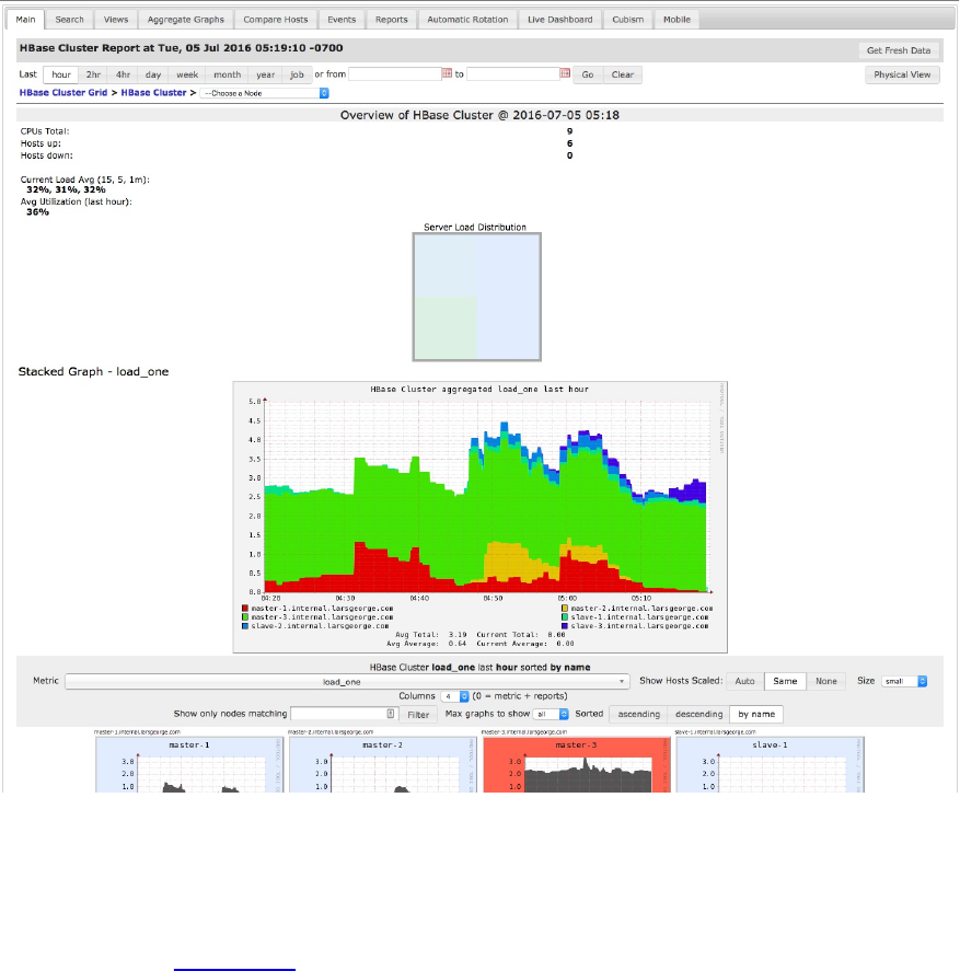
Figure 9-12. The Ganglia web-based front end that gives access to all graphs
Among many things, you can change the metric, time span, and sorting on that page; it will
reload automatically. On an underpowered machine, you might have to wait a little bit for all the
graphs to be rendered. Figure 9-13 shows the drop-down selection for the available metrics.
(706)
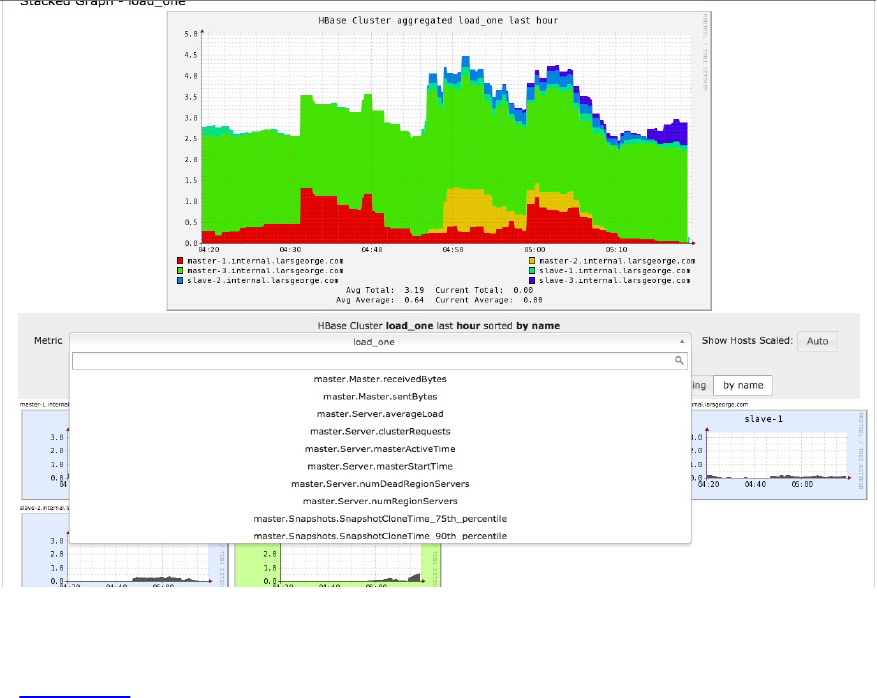
Figure 9-13. The drop-down box that provides access to the list of metrics
Finally, Figure 9-14 shows an example of how the metrics can be correlated to find root causes
of problems. The graphs show how, at around midnight, the garbage collection time sharply rose
for a heavily loaded server. This caused the compaction queue to increase significantly as well.
Note
It seems obvious that write-heavy loads cause a lot of I/O churn, but keep in mind that you can
see the same behavior (though not as often) for more read-heavy access patterns. For example,
major compactions that run in the background could have accrued many storage files that all
have to be rewritten. This can have an adverse effect on read latencies without an explicit write
load from the clients.
Ganglia and its graphs are a great tool to go back in time and find what caused a problem.
However, they are only helpful when dealing with quantitative data—for example, for
performing postmortem analysis of a cluster problem. In the next section, you will see how to
complement the graphing with a qualitative support system.
(707)
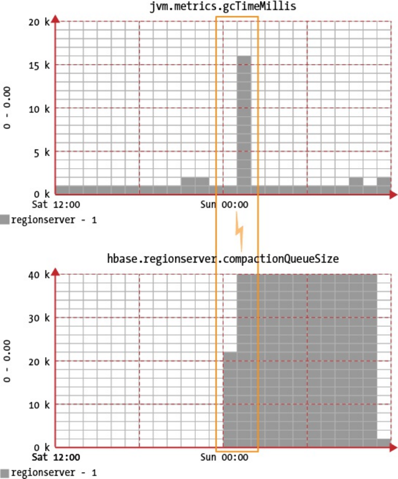
Figure 9-14. Graphs that can help align problems with related events
(708)

JMX
The Java Management Extensions (JMX) technology is the standard for Java applications to
export their status. JMX uses the so-called managed beans, in short MBeans, to provide access to
attributes and operations. Throughout this chapter, you have already heard a lot about JMX and
the provided MBeans, though as a small recap, here an overview for your perusal:
“Metrics Building Blocks” introduced the Java Platform MXBeans that are automatically
started when the server internal metrics system is started.
“Configuration” explains how to enable or disable MBeans selectively, and how to filter
details to reduce the amount of provided data points (if required). That section also has
examples of the operations provided by the MBeans to reload the configuration at runtime.
“Metrics UI” discusses the built-in metrics dump page, which can be used to browse all of
the metrics records (provided as MXBeans and MBeans through JMX) from the various
web-based server user interfaces.
“Master Metrics”, “Region Server Metrics”, and subsequent sections list all of the
attributes available through JMX by means of the MBeans.
What is left though is accessing JMX programmatically, that is, through its provided API. That
requires a change from the default configuration provided by HBase, which ships with
commented out examples on how to enable the access. Mostly what needs to be done is
uncomment those lines, and (only if necessary) edit them to your needs. Edit the hbase-env.sh file
in the configuration directory, like so:
# Uncomment and adjust to enable JMX exporting
# See jmxremote.password and jmxremote.access in $JRE_HOME/lib/management \
to configure remote password access.
...
export HBASE_JMX_BASE="-Dcom.sun.management.jmxremote.ssl=false \
-Dcom.sun.management.jmxremote.authenticate=false"
export HBASE_MASTER_OPTS="$HBASE_MASTER_OPTS $HBASE_JMX_BASE \
-Dcom.sun.management.jmxremote.port=10101"
export HBASE_REGIONSERVER_OPTS="$HBASE_REGIONSERVER_OPTS $HBASE_JMX_BASE \
-Dcom.sun.management.jmxremote.port=10102"
export HBASE_THRIFT_OPTS="$HBASE_THRIFT_OPTS $HBASE_JMX_BASE \
-Dcom.sun.management.jmxremote.port=10103"
export HBASE_ZOOKEEPER_OPTS="$HBASE_ZOOKEEPER_OPTS $HBASE_JMX_BASE \
-Dcom.sun.management.jmxremote.port=10104"
export HBASE_REST_OPTS="$HBASE_REST_OPTS $HBASE_JMX_BASE \
-Dcom.sun.management.jmxremote.port=10105"
Tip
This procedure is mirrored from core Hadoop, which means enabling JMX access to its
components is the same.
This enables JMX with remote access support, but with none of the optionally available security
features. If your cluster nodes are behind a firewall with no access to the above ports from the
outside, you should be fine. But for a cluster that is exposed over the network, it is (at least
eventually) necessary to add authentication, and even SSL for secured network connections. For
the sake of complexity we are going to omit the necessary setup steps here, but the official Java
(709)

JMX Documentation page has information on how to add those security features. You also need
to restart HBase (and Hadoop if you modified it too) for these changes to become active.
Dependent on how you configured the metrics systems (see “Configuration”) you should have
access to the selected MBeans, which are updated at the given interval. The default is to have
access to all MBeans, and have them refreshed every 10 seconds. Finding what beans are
available either requires an external tool to walk the exposed JMX hierarchy of a process (see
“JMX Remote API”), or using the provided Metrics Dump page. On that page, the bean name is
listed in each group as the first attribute, called "name". For example:
name: "Hadoop:service=HBase,name=RegionServer,sub=Server",
modelerType: "RegionServer,sub=Server",
tag.zookeeperQuorum: "zk1.foo.com:2181,zk2.foo.com:2181,zk3.foo.com:2181",
tag.serverName: "worker1.foo.com,16020,1467711907068",
tag.clusterId: "49ffd33c-e051-4c00-b0da-df7737e1d3ec",
tag.Context: "regionserver",
tag.Hostname: "worker1.foo.com",
The metrics system exposes these MBeans to the sinks using the context plus the sub name,
divided by a period character—in this example the prefix used for the sinks would be
"regionserver.Server". In fact, the MBeans are the metrics records explained in this chapter,
exposed under a slightly different naming scheme.
You have a few options to access the JMX attributes and operations, two of which are described
next.
(710)
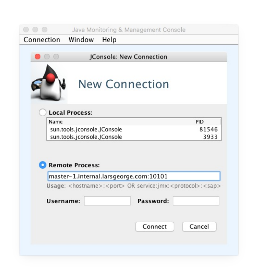
JConsole
Java ships with a helper application called JConsole, which can be used to connect to local and
remote Java processes. Given that you have the JAVA_HOME directory in your search path, you can
start it like so:
$ jconsole
Once the application opens, it shows you a dialog that lets you choose whether to connect to a
local or a remote process. Figure 9-15 shows the dialog.
Figure 9-15. Connecting to local or remote processes when JConsole starts
Since you have configured all HBase processes to listen to specific ports, it is advisable to use
those and treat them as remote processes—one advantage is that you can reconnect to a server,
even when the process ID has changed. With the local connection method this is not possible, as
(711)
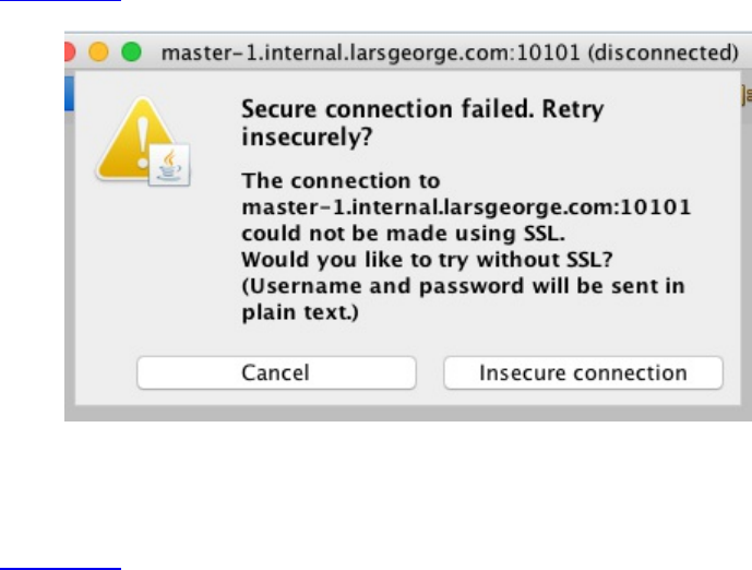
it is ultimately bound to said ID.
The canonical way of connecting to a remote HBase process is accomplished by using JMX
Service URLs, which follow this format:
service:jmx:rmi:///jndi/rmi://<server-address>:<port>/jmxrmi
This uses the Java Naming and Directory Interface (JNDI) registry to look up the required
details. Adjust the <port> to the process you want to connect to. In some cases, you may have
multiple Java processes running on the same physical machine—for example, the Hadoop name
node and the HBase Master—so that each of them requires a unique port assignment. See the
hbase-env.sh file contents shown earlier, which sets a port for every process. The master, for
example, listens on port 10101, the region server on port 10102, and so on. Since you usually only
run one region server per physical machine, it is valid to use the same port for all of them, as in
this case, the <server-address>--which is the hostname or IP address—changes to form a unique
address:port pair.
As you can see from the screenshot, you can simplify the URLs to just the hostname and port,
JConsole will implicitly add the necessary JNDI details.
Secure Connections
JMX can be configured with multiple levels of authentication and authorization controls,
including username and password checks, and encrypted communication over the network using
SSL. Since this would require the creation of certificates and reconfiguration of the HBase
processes, we omit this for the sake of simplicity. In a production environment you should
consider these options, so that no unauthorized access is possible. If you enter a URL that is not
secure, JConsole will ask you explicitly to switch to an unsecured connection, as shown in
Figure 9-16.
Figure 9-16. Confirmation dialog to switch to an unsecure connection
Once you connect to the process, you will see a tabbed window with various details in it.
Figure 9-17 shows the initial screen after you have connected to a process. The periodically
updated graphs are especially useful for seeing what a server is currently up to.
(712)
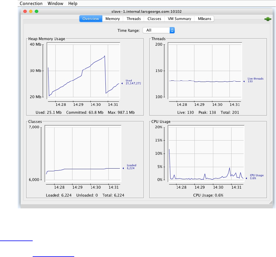
Figure 9-17. The JConsole application, which provides insight into a running Java process
Figure 9-18 is a screen shot of the MBeans tab that allows you to access the attributes and
operations exposed by the registered managed beans. Here you see the memStoreSize metric. See
the official documentation for all the possible options, and an explanation of each tab with its
content.
(713)
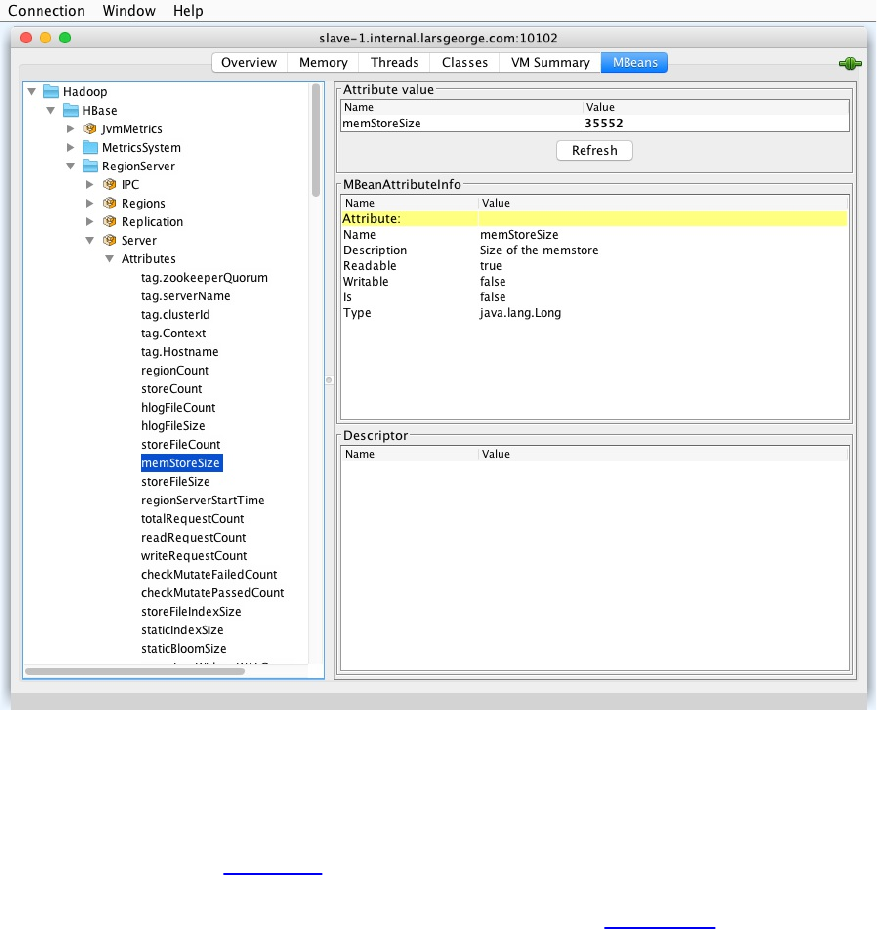
Figure 9-18. The MBeans tab, from which you can access any HBase process metric.
Alternative: VisualVM
An alternative to JConsole is VisualVM, supported by Oracle and developed by the Java.net
community as an open-source project. It aims at much more compared to JConsole, and in fact,
the support for JMX MBeans needs to be added as a separate plugin. Figure 9-19 shows
VisualVM and its optional MBeans information. As far as features go, both tools provide similar
support for MBeans, though VisualVM has many more options available. Consult the official
documentation for more details.
(714)
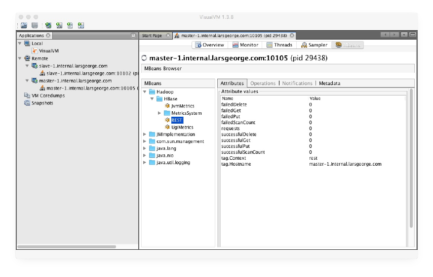
Figure 9-19. The VisualVM main window
(715)

JMX Remote API
Another way to get the same information is using the JMX Remote API programmatically, by
means of remote method invocation (RMI).12 Many tools are available that implement a client to
access the remote managed Java processes. Even the Hadoop project is providing a simple tool
for that, named JMXGet.13
As an example, we are going to use the JMXToolkit. You will need the git command-line tools,
and Apache Maven. Clone the repository and build the tool:
$ git clone git://github.com/larsgeorge/jmxtoolkit.git
Initialized empty Git repository in jmxtoolkit/.git/
...
$ cd jmxtoolkit
$ mvn package
[INFO] Scanning for projects...
[INFO]
[INFO] --------------------------------------------------------------------
[INFO] Building JMX Toolkit 2.0
[INFO] --------------------------------------------------------------------
...
[INFO] --------------------------------------------------------------------
[INFO] BUILD SUCCESS
[INFO] --------------------------------------------------------------------
[INFO] Total time: 11.500 s
[INFO] Finished at: 2016-07-06T11:10:02+02:00
[INFO] Final Memory: 28M/344M
[INFO] --------------------------------------------------------------------
After the building process is complete (and successful), you can see the provided options by
invoking the -h switch like so:
$ java -jar target/jmxtoolkit-2.0-toolkit.jar
Usage: JMXToolkit [-a <action>] [-c <user>] [-p <password>] [-u url]
[-f <config>] [-o <object>] [-e regexp] [-i <extends>] [-q <attr-oper>]
[-w <check>] [-m <message>] [-x] [-l] [-v] [-h]
-a <action> Action to perform, can be one of the following (default: query)
create Scan a JMX object for available attributes
query Query a set of attributes from the given objects
check Checks a given value to be in a valid range (see -w below)
encode Helps creating the encoded messages (see -m and -w below)
walk Walk the entire remote object list
...
-h Prints this help
You can use the JMXToolkit to walk, or print, the entire collection of available MBeans (referred
to as objects), with their attributes and operations. You do have to know the exact names of the
MBean and the attribute or operation you want to address. Since this is not an easy task, because
you do not have this list yet, it makes sense to set up a basic configuration file that will help in
subsequently retrieving the full list. For that we can use the supplied conf/hbase-1.2.x.properties
file with the following (abbreviated) content:
$ cat conf/hbase-1.2.x.properties
; HBase Master
[hbaseMasterServer]
@object=Hadoop:name=Master,service=HBase,sub=Server
@url=service:jmx:rmi:///jndi/rmi://${HOSTNAME1|localhost}:10101/jmxrmi
@user=${USER|controlRole}
@password=${PASSWORD|password}
(716)
[hbaseMasterRPC]
@object=Hadoop:name=Master,service=HBase,sub=IPC
@url=service:jmx:rmi:///jndi/rmi://${HOSTNAME1|localhost}:10101/jmxrmi
@user=${USER|controlRole}
@password=${PASSWORD|password}
...
This configuration can be fed into the tool to retrieve all the attributes and operations of the listed
MBeans. The result is saved in myjmx.properties, like so:
$ java -jar target/jmxtoolkit-2.0-toolkit.jar \
-f conf/hbase-1.2.x.properties -a create -x > myjmx.properties
$ cat myjmx.properties
[hbaseMasterServer]
@object=Hadoop:name=Master,service=HBase,sub=Server
@url=service:jmx:rmi:///jndi/rmi://${HOSTNAME1|localhost}:10101/jmxrmi
@user=${USER|controlRole}
@password=${PASSWORD|password}
tag.liveRegionServers=STRING
tag.deadRegionServers=STRING
tag.zookeeperQuorum=STRING
tag.serverName=STRING
tag.clusterId=STRING
tag.isActiveMaster=STRING
tag.Context=STRING
tag.Hostname=STRING
masterActiveTime=LONG
masterStartTime=LONG
averageLoad=DOUBLE
numRegionServers=INTEGER
numDeadRegionServers=INTEGER
clusterRequests=LONG
...
Note
These commands assume (for the sake of simplicity) that you are running them against a pseudo-
distributed, local HBase instance. When you need to run them against a remote set of servers,
simply set the variables included in the template properties file. For example, adding the
following parameters (using "-D") to the earlier command will specify the hostnames (or IP
addresses) for the master and a worker nodes:
$ java -DHOSTNAME1=m1.foo.com -DHOSTNAME2=w1.foo.com \
-jar target/...
When you look into the newly created myjmx.properties file you will see all the metrics you have
seen already. The operations are prefixed with a "*" (that is, the star character), as can be seen for
the MetricsSystem and its Control MBean:
[hbaseRegionServerMetricsControl]
@object=Hadoop:name=MetricsSystem,service=HBase,sub=Control
...
*start=VOID
*stop=VOID
...
You can now start requesting metric values on the command line using the toolkit and the
populated properties file. The first query is for an attribute value, while the second is triggering
an operation:
$ java -jar target/jmxtoolkit-2.0-toolkit.jar -f myjmx.properties \
-o hbaseRegionServerServer -q compactionQueueLength
compactionQueueLength:0
(717)
$ java -jar target/jmxtoolkit-2.0-toolkit.jar -f myjmx.properties \
-o hbaseRegionServerMetricsControl -q *currentConfig
currentConfig: \
sink.ganglia.class = org.apache.hadoop.metrics2.sink.ganglia.GangliaSink31
sink.ganglia.servers = 239.2.11.71:8649
sink.ganglia.period = 10
Once you have created the properties files, you can retrieve a single value, all values of an entire
MBean, trigger operations, and so on. The toolkit is great for quickly scanning a managed
process and documenting all the available information, thereby taking the guesswork out of
querying JMX MBeans. We will discuss Nagios next, which can also use the JMXToolkit to poll
metrics values.
(718)
Nagios
Nagios is a very commonly used support tool for gaining qualitative data regarding cluster status.
It polls current metrics on a regular basis and compares them with given thresholds. Once the
thresholds are exceeded it will start evasive actions, ranging from sending out emails, or SMS
messages to telephones, all the way to triggering scripts, or even physically rebooting the server
when necessary.
Typical checks in Nagios are either the supplied ones, those added as plug-ins, or custom scripts
that have to return a specific exit code and print the outcome to the standard output. Integrating
Nagios with HBase is typically done using JMX. There are many choices for doing so, including
the already discussed JMXToolkit.
The advantage of JMXToolkit is that once you have built your properties file with all the
attributes and operations in it, you can add Nagios thresholds to it. (You can also use a different
monitoring tool if you’d like, so long as it uses the same exit code and/or standard output
message approach as Nagios.) These are subsequently executed, and changing the check to, for
example, different values is just a matter of editing the properties file. For example:
attributeXYZ=INTEGER|0:OK%3A%20%7B0%7D|2:WARN%3A%20%7B0%7D:80:<| \
1:FAILED%3A%20%7B0%7D:95:<
*operationABC=FLOAT|0|2::0.1:>=|1::0.5:>
You can then wire the Nagios checks to the supplied JMXToolkit script. If you have checks
defined in the properties file, you only specify the object and attribute or operation to query. If
not, you can specify the check within Nagios like so:
$ bin/jmxtknagios-hbase.sh host0.foo.com hbaseRegionServerServer \
compactionQueueLength "0:OK%3A%20%7B0%7D|2:WARN%3A%20%7B0%7D:10:>=| \
1:FAIL%3A%20%7B0%7D:100:>"
OK: 0
Note that JMXToolkit also comes with an action to encode text into the appropriate format.
Obviously, using JMXToolkit is only one of many choices. The crucial point, though, is that
monitoring and graphing are essential to not only maintain a cluster, but also be able to track
down issues much more easily. It is highly recommended that you implement both monitoring
and graphing early in your project. It is also vital that you test your system with a load that
reflects your real workload, because then you can become familiar with the graphs, and how to
read them. Set thresholds and find sensible upper and lower limits—it may save you a lot of grief
when going into production later on.
(719)

OpenTSDB
As mentioned in “Use Case: OpenTSDB”, there is a metrics storage backend based on HBase
itself, called OpenTSDB. It uses a clever table schema design to distribute the metrics across all
regions and servers, so that you can efficiently write data points in vast amounts, and equally
efficiently read them back to create dashboards with graphs.
The data is collected on each generating system, and then periodically sent to a so-called Time
Series Daemon (TSD), which stores them in HBase. You can run many TSDs to scale to the
workload needed, and there are many tools and plugins available that can collect standard or
custom system metrics and send them to a TSD instance.
One obvious question is, can you monitor something while using the same system to store the
data points? Or put differently, could you run OpenTSDB on the same HBase instance that you
are monitoring? This is seemingly a chicken-or-the-egg, or observer problem, with no clear
answer. It seems frugal to advise that you should take extra care in planning such a setup. You
could use OpenTSDB to collect the vast majority of metrics for your organization, and
something more dedicated, out-of-bounds, like Ganglia, for HBase itself.
Figure 9-20 shows the main page of the OpenTSDB UI.
(720)
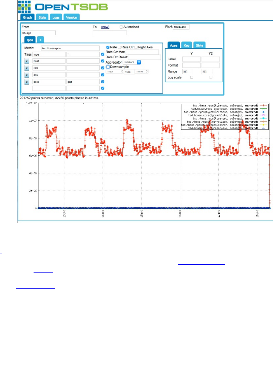
Figure 9-20. Main page of the OpenTSDB UI
1 JMX is an acronym for Java Management Extensions, a Java-based technology that helps in
building solutions to monitor and manage applications. See the project’s website for more
details, and “JMX”.--
2 See HBASE-4050 for details.
3 Disclaimer: I do not claim that the diagram is complete or 100% accurate. It shows the main
classes and their high-level interactions. Most of these are actually interfaces, but for the sake of
brevity I omitted that from the diagram.
4 A service level agreement (SLA) defines what exactly a service is supposed to deliver. For
example: “Serve 99% of all request in under 200ms.”
5 The metrics UI is barely used in core Hadoop itself. You can still access it by addressing the
JMX endpoint explicitly. For the NameNode, as an example, use http://<namenode-
hostname>:50070/jmx.
6 The words metrics and attributes are used interchangibly throughout this chapter.
(721)

7 See the official documentation on MemoryUsage for details on what used versus committed
memory means.
8 See this blog post.
9 The Java ThreadState class explains the states in more detail.
10 Ganglia is a distributed, scalable monitoring system suitable for large cluster systems. See its
project website for more details on its history and goals.
11 See the RRDtool project website for details.
12 See the official RMI documentation for details.
13 See HADOOP-4756 for details.
(722)
Chapter 10. Performance Tuning
Thus far, you have seen how to set up a cluster and make use of it. Using HBase in production
often requires that you turn many knobs to make it hum as expected. This chapter covers various
advanced techniques for tuning a cluster and testing it repeatedly to verify its performance.
(723)
Heap Tuning
In this section we are going to discuss two topics: sizing of the Java VM heap overall, and the
subsequent splitting of said heap for various uses once the servers run.
(724)

Java Heap Sizing
Before Java 8, you were forced to set, at least, the maximum size of the JVM using the provided
configuration files, or the built in default of up to 1 GB of memory was used—which is not
useful in the context of HBase region servers, and considering the memory available on modern
servers. More specifically, the JVM used to set (and still does for 32bit VMs) its minimum heap
size to 1/64th of the available physical memory, and 1/4th of the latter, but only up to 1 GB, for
the maximum heap size. You can override both using the following JVM parameters:
-Xms10g -Xmx10g
Another option provided by HBase is its hbase-env.sh configuration file, and setting the included
HBASE_HEAPSIZE variable to what you need. The file currently has the following, commented out
line as a starting point:
...
# The maximum amount of heap to use. Default is left to JVM default.
# export HBASE_HEAPSIZE=1G
...
One point of recent discussion is setting Xms to the same value as Xmx, or not, and setting those
values at all. The JVM has changed for Java 8, regarding the heap default sizes for 64-bit server
class platforms. The JVM considers all machines with 2 or more cores, and 2 or more GB of
memory as server class implicitly. You could also add the -server parameter to the JVM
command line to instruct the JVM about the mode it should run in. For 64-bit versions of the
JDK this is the only mode it supports, so the parameter is superfluous there.1
The 1/64 and 1/4 lower and upper shares are still the same for 64-bit Java 8, but it considers all
memory up to 128 GB for this computation.2 So, for example, the default upper heap size is set
to 32 GB for machines with 128 GB or more memory. For a 64 GB server, 16 GB would be set
as the maximum heap size, and so on. This makes a lot more sense, hence the commented out
HBASE_HEAPSIZE variable is useful as a starting point, leaving the JVM defaults to take its place.
But as soon as you deploy HBase in a production environment, you should be explicit about
what lower and upper boundary you want to use. You will see in “Garbage First (G1)” that for
some garbage collection implementations it is advantageous to lock the minimum and maximum
heap sizes to a single, fixed value. Not setting the lower boundary makes the VM start faster, but
then needs to grow the heap with each garbage collection to reach the steady state. This will have
an impact on latencies initially, something we commonly try to avoid with HBase as we are
serving interactive clients most likely. Setting the lower boundary to the same value as the upper
makes the JVM slower when it starts, but then no further implicit memory sizing has to take
place. And with HBase region servers, we can wait a little longer before assigning work to it,
mitigating the start up process cost.
For the HBase Master process you will only need a small amount of memory (in comparison), as
it does not allocate and discard objects at the rate of the RegionServers. Typically 2 GB to 4 GB
is sufficient for the master operations. For the region servers, you need to assign enough memory
to fit the structures used for writes and reads, though the latter depends on the optional use of off-
heap storage. The following sections explain this in much more detail (see “Tuning Heap Shares”
and “Block Cache Tuning”), though a typical starting size is 10 GB, assuming your servers have
at least 64 GB of physical memory. The larger sizes are up to 32 GB of heap, after which you are
(725)

forced to use the full 64-bit support of the JVM (happens automatically) that may affect the
perceived performance of your servers. You are also forced to use a garbage collection
implementation that can support larger heaps (see “Garbage Collection Tuning”).
Once you settle on a size, add the following to the beginning of the hbase-env.sh file:
...
# Set environment variables here.
export HBASE_MASTER_OPTS="-Xms2g -Xmx2g"
export HBASE_REGIONSERVER_OPTS="-Xms10g -Xmx10g"
...
This will force the boundaries to match, and sets the master and region servers separately.
Caution
As of this writing, the HBASE_HEAPSIZE value is only assigned to the -Xmx parameter, but not -Xms.
This would leave the lower boundary at its default, which, say, for 64 GB of memory on a server
class system would result in 1 GB (that is 1/64th). That number on a real cluster will have to
grow multiple times to reach its steady state, causing unnecessary memory re-allocations in the
process. It is therefore advised to set both size parameters explicitly as shown.
(726)

Tuning Heap Shares
The workers of HBase, the RegionServers, need to handle two major tasks: accept requests that
either read existing data, or write new data into the table. In addition, there is more internal
housekeeping information to be kept, for example for each open region there are structures in
memory that are necessary for normal operations. Since HBase and its processes are written in
Java, you can use the common settings defining the size of the JVM, once it is started.
Unfortunately, and as explained in “Garbage Collection Tuning”, you cannot simply allocate the
entire available physical memory to the JVM. Rather, you have to tune the memory used
carefully, and part of that is configuring the available space set aside for reads and writes.
Before HBase 1.0, there were two major settings to be adjusted, that is, the size of the memstores
(for writes) and block cache (for reads). The remaining memory was then used for all the other
miscellaneous Java structures mentioned. For the memstores, you were allowed to specify the
following settings (refer to [Link to Come] for the current settings):
Table 10-1. Old memstore related configuration properties
Property Default Description
hbase.regionserver.global.memstore.upperLimit 0.4
(40%)
Maximum amount of Java heap space all
memstores combined are allowed to use.
hbase.regionserver.global.memstore.lowerLimit 0.35
(35%)
Lower water mark of maximum heap
that triggers forced flushes.
The upper limit is important for this section, specifying the upper boundary of memory allowed
to be used for writes. For reads, there was only one property that could be set (refer to “Basic
Cache Configuration” for all the current details):
Table 10-2. Block cache related configuration properties
Property Default Description
hfile.block.cache.size 0.4 (40%)aThe share of the total heap assigned to the block cache.
a HBase versions before 0.96 used to default to 25%, and before 0.94/0.92 the default was 20%.
The upper limit of the memstore, combined with the block cache size, was not allowed to exceed
80% of the total heap, leaving enough room for the region server process to do its work (and to
avoid the dreaded Java out-of-memory exception). With HBase 1.0 and later, you now have an
extended set of options, allowing the definition of ranges that set upper and lower boundaries on
both the memstore and block cache sizes. The following table lists the new settings:
Table 10-3. Heap size range related configuration properties
Property Default Description
(727)

hbase.regionserver.global.memstore.size.min.range unset The lower boundary for the size of
all memstores.
hbase.regionserver.global.memstore.size.max.range unset The upper boundary for the size of
all memstores.
hbase.regionserver.global.memstore.size 0.4
(40%)
The default share of the total heap
set aside for memstores.
hfile.block.cache.size.min.range unset The lower boundary for the block
cache size.
hfile.block.cache.size.max.range unset The upper boundary for the block
cache size.
hfile.block.cache.size 0.4
(40%)
The default share of the total heap
assigned to the block cache.
hbase.regionserver.heapmemory.tuner.period 60000
(60s)
Defines how often the heap tuner
runs.
You must set both ranges, that is, for the memstore and block cache, or else the tuner is not
enabled. Furthermore, you should set each range so that it does not exceed the default value
given. For example, for the memstore the default (or starting value) is set using
hbase.regionserver.global.memstore.size, and the maximum with
hbase.regionserver.global.memstore.size.max.range. The former should be less or equal to the
latter. Otherwise you will see a warning in the server log file stating that the value was too large,
and that they are automatically corrected to be the same. This applies to the minimum the same
way, that is, you should set the default to a value equal or greater than the minimum, or else a
warning is emitted and the value corrected.
In addition, you must not exceed the total of 80% for both areas combined. If you do so, the tuner
will report an error and stop the server from working! This is for the same reason as before, that
is, leaving enough memory for the region server process to properly function. Apart from that,
you have to ensure that you are using a block cache implementation that actually supports
resizing, which you can read about in “Cache Types”. Figure 10-1 shows the default—and
previously the only available option—fixed heap distribution, along with the flexible setup using
the heap memory tuner.
(728)
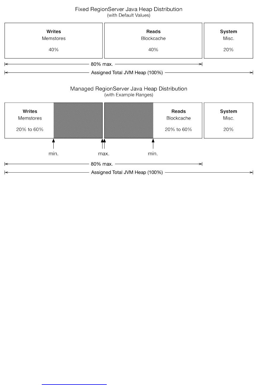
Figure 10-1. The fixed and managed heap distribution
Here are the configuration properties that match the diagram, setting the lower and upper
boundaries to 20% and 60% for both areas, that is, the memstore and block cache:
<property>
<name>hbase.regionserver.global.memstore.size.min.range</name>
<value>0.2</value>
</property>
<property>
<name>hbase.regionserver.global.memstore.size.max.range</name>
<value>0.6</value>
</property>
<property>
<name>hfile.block.cache.size.min.range</name>
<value>0.2</value>
</property>
<property>
<name>hfile.block.cache.size.max.range</name>
<value>0.6</value>
</property>
The starting values for both areas are left at their default of 40%, as shown in the diagram. With
these settings, the tuner is able to resize each area until one of them might reach the minimum of
20%, while the other then has 60% of heap assigned to it.
Note
The memory tuner computes the block cache size as a total, adding L1 and (optional) L2 on-heap
caches together. See “Block Cache Tuning” for details on L1 and L2 setups. Any modification of
the cache size during a tuning invocation only applies to the L1 cache, not the L2 (even if on-
heap).
(729)

The settings are read by the heap manager (HeapMemoryManager), which works in tandem with a
particular heap tuner (HeapMemoryTuner) implementation. HBase ships with a default
implementation (DefaultHeapMemoryTuner)3, that performs a check once every configured tuning
period, to see whether there is a need to move the boundaries between the memstores and the
block cache in a particular direction. The tuner can only increase one of the areas, while
decreasing the other by the same amount. The only other outcome of the tuner is to stay put, that
is, not modifying anything. All of this is based on the number of forced flushes for the
memstores due to memory pressure, and block cache evictions for that same reason.
The tuner carefully watches the memstores and block cache, employing complex heuristics that
help keep the changes reasonable, in an attempt to avoid any possible negative impact. It offers
advanced settings that can be modified to change its behavior:
Table 10-4. Default heap tuner related configuration properties
Property Default Description
hbase.regionserver.heapmemory.autotuner.step.max 0.04
(4%)
The maximum step
the tuner can take to
move the
boundaries.
hbase.regionserver.heapmemory.autotuner.step.min 0.00125
(0.125%)
The minimum step
the tuner can take to
move the
boundaries.
hbase.regionserver.heapmemory.autotuner.sufficient.memory.level 0.5
(50%)
If any of the areas
has that much free
space, it is
considered to have
sufficient memory.
hbase.regionserver.heapmemory.autotuner.lookup.periods 60
Defines how many
previous periods are
remembered to
influence the
decision for the next
tuning invocation.
hbase.regionserver.heapmemory.autotuner.ignored.periods 60
Sets how many
initial invocations
should be ignored to
wait for the server to
settle into normal
operation.
(730)
Finally, the hbase.regionserver.heapmemory.tuner.class property can be used to plug in a custom
class, in case the supplied one is not sufficient. At the time of this writing, the tuner only affects
the on-heap memory settings, but it is planned to extend this to off-heap caches too in HBase 2.0
and later. The same applies to operational metrics from the tuner class.
(731)
Garbage Collection Tuning
The Java JDK and its included reference implementation of the Java Virtual Machine, provided
by Oracle (acquired from Sun Microsystems in 2010), undoubtedly paved the way for many
enterprise software systems and stacks. It greatly simplifies the intrinsic details of writing large-
scale applications that have to handle mission-critical tasks. One area that is notoriously difficult
in development is memory management, which is where the JVM steps up and provides a fully
automated service to all the applications it executes. In an ideal world we could stop here, but
alas, sometimes we have to interact with the machinery and help it along to meet our needs. This
section discusses the optimization of the so-called garbage collection process, which is an
essential part of the automated memory management of Java.
(732)

Introduction
HBase ships with many reasonable default settings out of the box, allowing you to get started
quickly and focus on the data and business problems faster. Eventually though, one of the lower-
level settings you will need to adjust is the garbage collection parameters for the region server
processes. Note that the master is not a problem here as it does not handle any heavy loads, and
data does not pass through it. These parameters only need to be added to the region servers.
You might wonder why you have to tune the garbage collection parameters to run HBase
efficiently. The problem is that the Java Runtime Environment—just like HBase itself-- comes
with basic assumptions regarding what your programs are doing, how they create objects, how
they allocate the heap to handle data, and so on. These assumptions work well in a lot of cases.
In addition, the JRE has heuristic algorithms that adjust these assumptions as your process is
running. Even with those in place, the JRE is limited to the implementation of such heuristics
and can handle some use cases better than others.
The bottom line is that in practice the JRE does not handle HBase region servers very well, using
its default settings alone. This is caused by the workloads HBase is typically handling, involving
a mix of write and read operations. Often HBase is used as a random access store, allowing the
applications to write wherever they need in user tables, and doing the same for reads. While
sometimes the workload is tilted to one or the other operation, both impose challenges to the
underlying resources, including the JVM:
Write Operations
For write-heavy use cases, the memstores are creating and discarding objects at various
times, and in varying sizes. As the data is collected in the in-memory buffers, it needs to
remain there until it has outgrown the configured minimum flush size, set with
hbase.hregion.memstore.flush.size globally or at the table level. Once the data is greater
than that number, it is flushed to disk, creating a new store file. Since the data that is
written to disk mostly resides in different locations in the Java heap—assuming it was
written by the client at different times—it leaves holes in the heap (also refer to
“Memstore-Local Allocation Buffer” for an optimization feature).
Read Operations
A similar situation arises for reads, as they usually utilize the block cache (see “Block
Cache Tuning”) to achieve very high I/O rates. For that, the cache keeps the loaded HFile
blocks in memory (or some other intermediate storage technology) until they are forced to
be evicted. This leaves gaps that have to be filled subsequently. The advantage of the
cache is that the blocks are much larger usually, compared to the cells in the memstores,
causing less fragmentation in the process.
In addition, depending on how long the data was in memory, it resided in different areas in the
generational architecture of the Java heap: data that was inserted rapidly and is flushed equally
fast is often still in the so-called young generation (also called new generation) of the heap. The
memory can be reclaimed quickly and no harm is done. However, if the data stays in memory for
a longer period of time—for example, within a column family that is less rapidly inserted into—
it is promoted to the old generation (or tenured space). The difference between the young and
(733)

old generations is primarily size: the young generation is commonly between 128 MB and 512
MB, while the old generation holds the remaining available heap, which is usually many
gigabytes of memory.
Both young and old generation need to be maintained by the JRE, to reuse the holes created by
data that has been written to disk, or by blocks that were evicted from cache (and obviously any
other object that was created and discarded subsequently). If the application ever requests a
portion of heap that does not fit into one of those holes, the JRE needs to compact the fragmented
heap. This includes implicit requests, such as the promotion of longer-living objects from the
young to the old generation. If this fails, you will see a promotion failure in your garbage
collection logs (see “Garbage Collection Information”).
The way Java handles these (and other) areas of memory, collectively referred to as heap, has
changed over time. Memory management is handled by the so called garbage collection (GC)
algorithms, which can be chosen and configured when the Java process (that is, the JVM) is
started. The current Java 8 ships with these three main implementations:
Collector JVM Parameter Description
Parallel Compacting -XX:+UseParallelOldGC Throughput friendly collector
Concurrent Mark Sweep
(CMS)
-
XX:+UseConcMarkSweepGC
Low latency collector for heap < 32
GB
Garbage First (G1) -XX:+UseG1GC Low latency collector
In practice, and in the context of the HBase region server process, only CMS and G1 GC are
used. The older of the two, CMS, considerably improved the performance of HBase, and
especially the latencies of I/O requests. But it has limitations (or you may want to call them
tradeoffs), with the maximum amount of memory it can handle being its major downside. When
CMS was invented, it fit well with server hardware of its time, but with modern servers allowing
for usage in excess of 1TB of memory, heaps of up to 32 GB in size seem dated. The
fundamental issue is that eventually the collector will have to stop all user processing and clean
up the heap when it is too fragmented to allocate any additional object. This pause can last
several seconds with larger heaps, and inadvertently causes spikes in the latencies of requests.
JVM Pause Monitor
When the HBase region servers start, each creates and runs a lightweight thread that wakes up at
a regular interval, set to 500 milliseconds, comparing the elapsed time to their sleep time. Once
the thread detects that in reality it has slept much longer than the 500ms it expected, it logs a
message to the server log, for example:
2016-08-05 07:11:32,390 INFO [JvmPauseMonitor] util.JvmPauseMonitor: \
Detected pause in JVM or host machine (eg GC): \
pause of approximately 7448ms
GC pool 'ParNew' had collection(s): count=1 time=49ms
GC pool 'ConcurrentMarkSweep' had collection(s): count=1 time=7700ms
...
(734)

2016-08-11 23:01:56,686 WARN [JvmPauseMonitor] util.JvmPauseMonitor: \
Detected pause in JVM or host machine (eg GC): \
pause of approximately 3594293ms
No GCs detected
The first is caused by a lengthy garbage collection run, with CMS requiring more than 7 seconds
to complete. The second is not related to a machine pause (for example a suspended VM).
Depending on how much time has passed, the message is logged at an INFO or WARN level,
configured using the following properties:
Property Default Description
jvm.pause.info-
threshold.ms 1000 (1s) Log an INFO level message after this threshold.
jvm.pause.warn-
threshold.ms
10000
(10s)
Switch to a WARN level message after this time has
passed.
It is recommended in practice to monitor the logs for unusual events, and this is one of those you
should look out for. If you are using an automated log analysis system, you should pass on these
events if they approach or exceed specific timeouts, for example, the ZooKeeper setting that
would cause the region server to lose its lease and be considered dead.
G1 GC strives to minimize this, as it was developed with very large heaps in mind. Figure 10-2
shows how the two commonly used implementations, CMS and G1 GC, divide the assigned
memory, as we will subsequently refer to these areas by name and for specific JVM
configuration parameters.
(735)
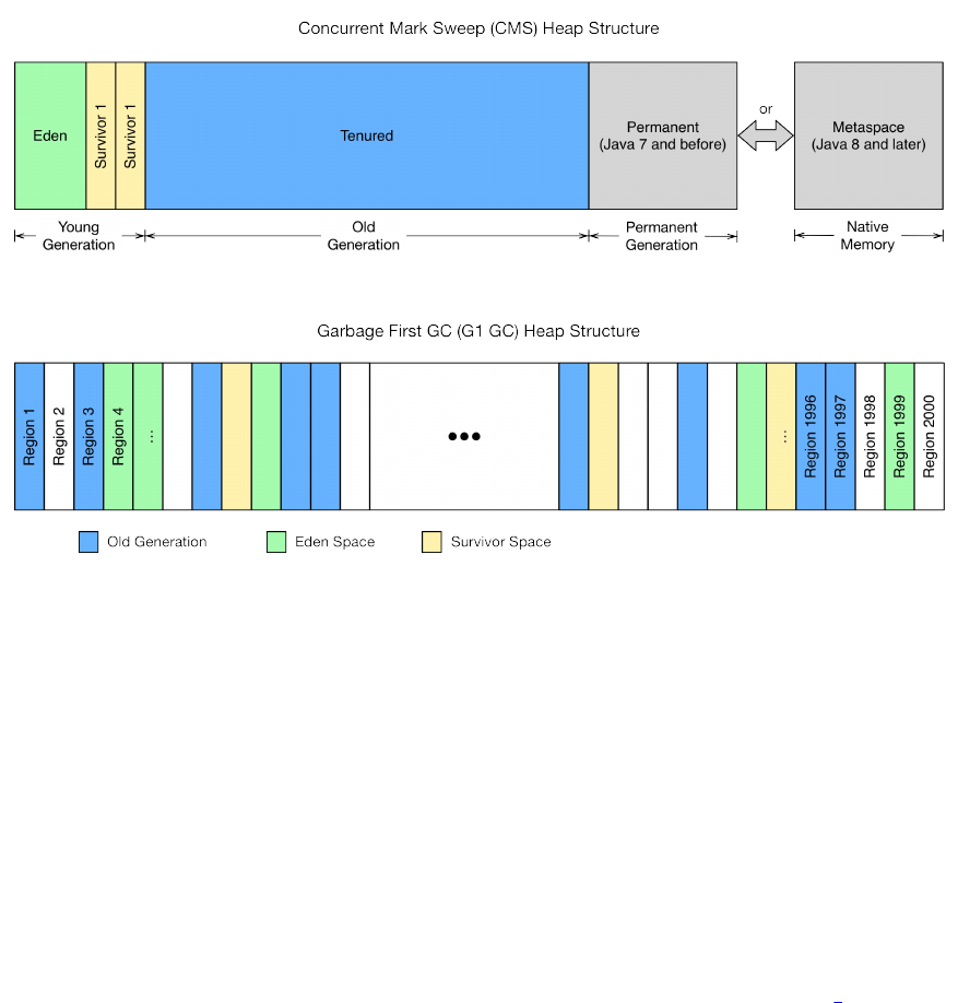
Figure 10-2. Commonly used garbage collections (Oracle JDK and OpenJDK)
Instead of relying on fixed size areas (configured when the process is started), it divides the
space into equal size regions, with the recommended count of about 2000 of those. With it, G1
GC can assign regions the role of acting as young, survivor, or old space. The tradeoff G1 GC
chooses is to run many more garbage collections on these regions in an attempt to keep any user
impacting pause to a minimum. That extra work has an noticeable impact on latencies, but over
time the shorter pauses offer a much more reliable latency quality.
Since both collectors provide their own, distinct set of parameters, they are discuss separately
below. For the sake of brevity, we will not dissect each algorithm in detail, but pointers to online
resources will be given where applicable.
As a final introductory note, G1 GC is meant to replace all other algorithms over time4, and is
supported as of Java 7u4. But, as it is often with software, there are ongoing improvements made
and Java updates might affect the performance of the garbage collector, and with it the perceived
quality of HBase. Check carefully and regularly to choose the right version at the right time.
You can set the garbage collection-related options by adding them in the hbase-env.sh
configuration file to the HBASE_OPTS or the HBASE_REGIONSERVER_OPTS variable. The latter only affects
the region server process (as opposed to the master, for example, which has its own variable),
and is the recommended way to set these options. Note that there are many parameters already
listed in that file, and you can simply comment out the ones you want to enable and optionally
edit them to your needs.
All of the discussed parameters apply to the Oracle JDK, and OpenJDK, for Java 7 and 8. Other
Java implementations may use other parameters.
(736)
Concurrent Mark Sweep (CMS)
CMS is the tried-and-true garbage collection implementation that has been used for many years
and is best understood. It is enabled setting the following JVM options:
-XX:+UseParNewGC -XX:+UseConcMarkSweepGC
Tip
Enabling CMS with -XX:+UseConcMarkSweepGC already implies setting -XX:+UseParNewGC too. The
latter is shown here just for the sake of discussion.
The first option is setting the garbage collection strategy for the young generation to use the
Parallel New Collector: it stops the entire Java process to clean up the young generation heap.
Since its size is small in comparison, this process does not take a long time, usually less than a
few hundred milliseconds. This is acceptable for the smaller young generation, but not for the old
generation: in a worst-case scenario this can result in processes being stopped for seconds, if not
minutes. Once you reach the configured ZooKeeper session timeout, this server is considered lost
by the master and it is abandoned. Once it comes back from the garbage collection-induced stop,
it is notified that it is abandoned and shuts itself down.
This is mitigated by using the Concurrent Mark-Sweep Collector (CMS), enabled with the latter
option. It works differently in that it tries to do as much work concurrently as possible, without
stopping the Java process. This takes extra effort and an increased CPU load, but avoids the
required stops to rewrite a fragmented old generation heap—until you hit the promotion error,
which forces the garbage collector to stop everything and clean up the mess. This is also the
default setting in the supplied hbase-env.sh file for all processes, which means no further actions
have to be taken.
What likely has to be changed is the size of the young generation, as its default is too small for
the region servers taking on write operations and collecting them in the memstores for a
considerable amount of time. The churn on the young generation and handling unnecessary
promotions can be mitigated by increasing the assigned space to a fixed, larger size, like so:
-XX:MaxNewSize=128m -XX:NewSize=128m
Or you can use the newer and shorter specification which combines the preceding code into one
convenient option:
-Xmn128m
Using 128 MB is a good starting point, and further observation of the JVM metrics should be
conducted to confirm satisfactory use of the new generation of the heap. Note that the default
value might be too low for heavy region server loads and should be increased. If you do not do
this, you might notice a steep increase in CPU load on your servers, as they spend most of their
time promoting objects from the new generation space.
The other smallish area configured by the CMS implementation, previous to Java 8, is the
permanent space, holding information about, for example, loaded classes. For larger heaps and
many loaded objects, there is the danger of triggering an out-of-memory-exception when the
(737)

permanent space is full. The following two options set the minimum and maximum size of this
crucial area to 128 MB:
-XX:PermSize=128m -XX:MaxPermSize=128m
Once again this is the default in HBase, and does not need to be added. With Java 8 the
permanent space was completely replaced with the newer Metaspace, that resides outside the
managed heap and is, by default, unbounded. Using Java 8 you will actually see a warning that
the obsolete parameters are ignored:
Java HotSpot(TM) 64-Bit Server VM warning: ignoring option \
PermSize=128m; support was removed in 8.0
Java HotSpot(TM) 64-Bit Server VM warning: ignoring option \
MaxPermSize=128m; support was removed in 8.0
It is safe to comment out these parameters for Java 8.
The CMS collector has an additional switch, which controls when it starts doing its concurrent
mark and sweep check. This value can be set with this option:
-XX:CMSInitiatingOccupancyFraction=85
The value is a percentage that specifies when the background process starts, and it needs to be set
to a level that avoids another issue: the concurrent mode failure. This occurs when the
background process to mark and sweep the heap for collection is still running when the heap runs
out of usable space (recall the holes analogy). In this case, the JRE must stop the Java process
and free the space by forcefully removing discarded objects, or tenuring those that are old
enough.
Setting the initiating occupancy fraction to 85% means that it will start the concurrent collection
process early enough before the heap runs out of space, but also not too early for it to run too
often. Of course, your mileage may vary, which means you should test carefully if the option
helps your workload, and at what value. A common formula is to set the fraction to slightly
larger than what the memstores and block cache occupy together, which is usually 80%
(assuming the default 40% memstore and 40% cache areas), leading us to the above 85%.
Here is an example set of options that could be used as a starting point for your
experimentations:
export HBASE_REGIONSERVER_OPTS="-Xms10g -Xmx10g -Xmn128m \
-XX:+UseConcMarkSweepGC -XX:CMSInitiatingOccupancyFraction=85 \
-XX:+UseCMSInitiatingOccupancyOnly"
Note
Note that -XX:+CMSIncrementalMode (also called i-cms) is not recommended on actual server
hardware, and in fact is deprecated in Java 8 (with no replacement).5
One final note for CMS: some users have experimented with increasing the parallelism of the
collector, using the following options:
-XX:ParallelGCThreads=<number>
-XX:ConcGCThreads=<number>
The first is the number of threads used during parallel phases of the GC process, that is, when a
stop-the-world pause is in process. The latter option sets the number of threads during concurrent
(738)
phases, which is while the JVM is still executing user code. Obviously, the number of parallel
threads can be slightly larger than the concurrent ones, as no user threads are running during the
parallel phases.
How many threads you should use is once again highly dependent on your workloads and use-
cases, as well as other services overlaying on the cluster. Creating too many threads would
require more synchronization work, while not enough may serialize some of the GC tasks
unnecessarily.
Tip
The same threading options apply to G1 GC, with the same caveats.
(739)

Garbage First (G1)
Enabling G1 GC is accomplished by setting the following JVM option:
-XX:+UseG1GC
Besides that, you need to set a target for the maximum garbage collection pauses you want to
encounter. Note that this is a soft goal, and while the JVM is trying to accommodate you, longer
pauses might be necessary in keeping up with your workload. The parameter is:
-XX:MaxGCPauseMillis=200
Shown is the default value of 200 milliseconds, which can be adjusted as needed. The last
additional parameter you may want to tune is the threshold when the collector should start a
concurrent GC cycle, specified as the percentage of the entire heap occupancy (and not just one
of the generations, as done for CMS). The default is 45% and set like so:
-XX:InitiatingHeapOccupancyPercent=45
What has been omitted from “Introduction” is the so-called humongous allocation feature used
by G1: if you attempt to allocate a space that is larger than 50% of the configured heap region
size (which can be uniformly set between 1 MB and 32 MB at the start of the JVM) then the G1
collector will spread the allocation across multiple regions, combining them to a humongous one.
Especially in HBase, where clients can potentially send multiple megabyte of data with a batch
request, it is likely to cause such large allocations—which are more costly to handle by the
collector as well.
Ideally, such allocations should be avoided, but they are a factor or workload and heap region
sizes. While you cannot restrict the former completely, it is vital to monitor the latter, and adjust
the region sizes if needed (though within the given boundaries). First advice is to set -Xms and -
Xmx to the same value, allowing the collector to properly calculate the region sizes. If you do not
set the upper boundary, the region sizes need to be guessed, as they are driven by the maximum
size of the JVM at runtime.
While we will discuss GC logging in detail in “Garbage Collection Information”, here is a JVM
parameter you should know about in the context of G1 GC and determining the region sizes:
-XX:+PrintAdaptiveSizePolicy
This will log all humongous allocations as they occur, including their sizes, which in turn can be
used to calculate a good regions size—as in, one that is about twice the size of the majority of
large allocations. Keep in mind that region sizes must be a power of 2, and that there should be,
if possible, around 2000 of them. The minimum region size is 1 MB, and the maximum 32 MB.
Doing the math by multiplying the maximum regions size by their recommended count, you end
up with about 62 GB of maximum addressable heap size. After that, you would need to increase
the number of regions accordingly. On the other hand, it might also force you for smaller heaps
to decrease the region count below the target of 2000 to reach a large enough size per region.
Once again, test carefully and monitor often!
After determining a suitable region size to match your workload, use the following parameter to
override the automatic calculation:
(740)

-XX:G1HeapRegionSize=8M
In summary, here a starting set of JVM parameters for G1 GC:
export HBASE_REGIONSERVER_OPTS="-Xmx20g -Xms20g -XX:+UseG1GC \
-XX:MaxGCPauseMillis=100 -XX:InitiatingHeapOccupancyPercent=45"
When it comes to tuning the G1 collector further, a team at Intel analyzed G1 GC with a 100 GB
Java heap for the region servers and published a blog post with their findings. It contains quite a
few advanced G1 options you could try in your environment. Furthermore, the Intel blog post
inspired a few engineers at HubSpot to spend a considerable amount of time analyzing and
understanding the G1 GC algorithm, publishing their findings in another blog post. They went
even further and published a G1 GC tuning guide for HBase too.
The HubSpot team amended or extended the suggested options to include the following:
-XX:MaxGCPauseMillis=50
-XX:+UnlockExperimentalVMOptions
-XX:-OmitStackTraceInFastThrow
-XX:+ParallelRefProcEnabled
-XX:+PerfDisableSharedMem
-XX:-ResizePLAB
-XX:ParallelGCThreads=8 + (<no. of logical processors> - 8) * (5/8)
This reduces the target GC pause to 50ms, and en-/disables quite a few specific JVM options. As
before, use these as a starting point for your advanced experimentations, ideally following along
the mentioned HBase sizing guide that reasons about each option in great detail. Particularly the
number of parallel GC threads (using -XX:ParallelGCThreads) requires careful testing, as a generic
formula for their count is heavily dependent on the workload you are running.
Also interesting is the approach to calculating the initiating heap occupancy threshold (akin to
CMS, but here for the entire stack, not just the old generation), which defines when the collector
should start processing based on the amount of heap in use. Here, HubSpot’s team recommends
analyzing the real usage of a cluster, and sizing the heap based on the numbers observed. The
heap should be large enough that only up to 70% of it is used for memstores, cache, the
miscellaneous space for indexes etc., and the young generation (here Eden space to be specific,
see Figure 10-2) combined:
heap >= (memstoreGB + cacheGB + otherGB + edenGB) / 0.7
Once you have a minimum size, make sure you assign it to both the lower and upper boundary,
as shown above. With that you can determine an initial IHOP (the initial heap occupancy
percentage) as:
IHOP = (memstorePercent + cachePercent + otherPercent + 20)
-XX:InitiatingHeapOccupancyPercent=IHOP
This implies not leaving the percentages for the major heap areas at their defaults of 40% for
both. Instead, you should reduce it while increasing the total heap size to leave enough wiggle
room for growth and temporary spikes in traffic.
Finally, the Intel team specifies the young generation sizing as the following, reducing its
percentage from the default 5% to a lower number depending on the size of the total heap:
Heap Size JVM Parameter Description
(741)
32 GB -XX:G1NewSizePercent=3 Use 3% for large heaps, from 32-64 GB.
64 GB -XX:G1NewSizePercent=2 Use 2% for larger heaps, from 64-100 GB.
100 GB+ -XX:G1NewSizePercent=1 Use 1% for very large heaps of 100 GB and above.
This was necessary in their testing to not spend too much time in processing the Eden space,
which amounted to more than what was configured for the overall target for GC pauses. This
also why the HubSpot team fixed the -XX:MaxGCPauseMillis parameter to 50ms, which in practice
means that the collector never really reaches the pause target, but pins the Eden space to its lower
end.
(742)

Garbage Collection Information
As was hinted earlier, there are quite a few advanced options that allow you to switch on the
JVMs logging of garbage collection details, where for CMS the following are commonly used:
-verbose:gc
-XX:+PrintGCDetails
-XX:+PrintGCDateStamps
-Xloggc:<filename>
Note that for -verbose:gc is doing the same as using -XX:+PrintGC, with the latter being deprecated
in Java 9 in favor of -Xlog:gc--which is also planned to subsume -Xloggc.6 Until then, the latter is
used to direct all GC related messages to a file that the process has access to, for example:
-Xloggc:$HBASE_HOME/logs/gc-$(hostname)-hbase.log
You can alternatively use -XX:+PrintGCDateStamps or -XX:+PrintGCTimeStamps, where the latter only
prints seconds since the Java VM started. The former prints real dates and is more human
readable for that matter. Once the log is enabled, you can monitor it for occurrences of concurrent
mode failure or promotion failed messages (for CMS), which oftentimes precede long pauses. For
the above options, the common output within the logs would look like this:
...
2016-08-18T22:51:26.289-0700: [GC [1 CMS-initial-mark: 21526K(40896K)] \
23569K(59328K), 0.0048530 secs] [Times: user=0.00 sys=0.00, real=0.00 secs]
2016-08-18T22:51:26.370-0700: [CMS-concurrent-mark: 0.076/0.076 secs] \
[Times: user=0.08 sys=0.04, real=0.08 secs]
2016-08-18T22:51:26.371-0700: [CMS-concurrent-preclean: 0.001/0.001 secs] \
[Times: user=0.00 sys=0.00, real=0.00 secs]
...
Note that before Java 7, the log file was not rolled like the other files are; you had to take care of
this manually (e.g., by using a cron-based daily log roll task). With Java 7 and later you have
additional options provided by the JVM that allow the automated rolling of logs:
-XX:+UseGCLogFileRotation
-XX:NumberOfGCLogFiles=<count>
-XX:GCLogFileSize=<size>
Here an example:
-XX:+UseGCLogFileRotation
-XX:NumberOfGCLogFiles=5
-XX:GCLogFileSize=20M
-Xloggc:$HBASE_HOME/logs/gc-$(hostname)-hbase.log
This enables the feature and sets the log roll size to 20 MB, with up to five (5) logs to be retained
for posterity.
Tip
You can use the -XX:+PrintFlagsFinal option to print out the defaults used:
% java -XX:+PrintFlagsFinal -version | grep -i "gc.*log"
uintx GCLogFileSize = 8192 {product}
uintx NumberOfGCLogFiles = 0 {product}
bool UseGCLogFileRotation = false {product}
java version "1.8.0_45"
(743)
The HubSpot team also used the following JVM options for their G1 GC debugging:
-XX:+PrintAdaptiveSizePolicy
-XX:+PrintGCApplicationStoppedTime
-XX:+PrintTenuringDistribution
Closing the topic of garbage collection tuning, please read the official tuning pages available
from Oracle, and for HBase specifically the HubSpot and Intel blogs. And keep in mind that the
source code for OpenJDK is available, so if all else fails, you can read that too and get your
information from the horse’s mouth.
(744)
Memstore-Local Allocation Buffer
Version 0.90 of HBase introduced an advanced mechanism to mitigate the issue of heap
fragmentation due to too much churn on the memstore instances of a region server: the
memstore-local allocation buffers, or MSLAB for short.
The preceding sections explained how tenured Cell instances, once they are flushed to disk,
cause holes in the old generation heap. Once there is no longer enough space for a new allocation
caused by the fragmentation, the JRE falls back to the stop-the-world garbage collector, which
rewrites the entire heap space and compacts it to the remaining active objects. Even with G1 GC
you may run into this scenario, and hence any measure to avoid this should be taken.
The key to reducing these compacting collections is to reduce fragmentation, and the MSLABs
were built to help with that. The idea behind them is that only objects of exactly the same size
should be allocated from the heap. Once these objects tenure and eventually get collected, they
leave holes in the heap of a specific size. Subsequent allocations of new objects of the exact
same size will always reuse these holes: there is no promotion_ (or related To-space exhaustion)
error, and therefore no stop-the-world compacting collection is required.
The MSLABs are buffers of fixed sizes containing Cell instances of varying sizes. Whenever a
buffer cannot completely fit a newly added cell, it is considered full and a new buffer is created,
once again of the given fixed size.
The feature is enabled by default in version 0.92 and later, and disabled in version 0.90 of
HBase. You can use the hbase.hregion.memstore.mslab.enabled configuration property to override
it either way. The size of each allocated, fixed-sized buffer is controlled by the
hbase.hregion.memstore.mslab.chunksize property. The default is 2 MB and is a sensible starting
point. Based on your data, you may have to adjust this value: if you store larger cells, for
example, 100 KB in size, you could increase the MSLAB size to fit more than just a few cells.
There is also an upper boundary of what is stored in the buffers. It is set by the
hbase.hregion.memstore.mslab.max.allocation property and defaults to 256 KB. Any cell that is
larger will be directly allocated in the Java heap. If you are storing a lot of Cell instances that are
larger than this upper limit, you may run into fragmentation-related pauses earlier. On the other
hand, just like the block cache, allocating larger chunks mitigates the issue of very small
allocations considerably.
The MSLABs do not come without a cost: they are more wasteful in regard to heap usage, as you
will most likely not fill every buffer to the last byte. The remaining unused capacity of the buffer
is wasted. Once again, it’s about striking a balance: you need to decide if you should use
MSLABs and benefit from better garbage collection but incur the extra space that is required, or
not use MSLABs and benefit from better memory efficiency but deal with the problem caused by
garbage collection pauses.
In addition, as garbage collector implementations become more elaborate over time, it may be
advantageous to completely disable MSLABs, as they are more efficient in maintaining heap and
defragmenting portions of it concurrently.
Tip
(745)
Especially with G1 GC users have reported that you can turn MSLABs off, without incurring any
measurable penalty.
Finally, because the buffers require an additional byte array copy operation, they are also slightly
slower, compared to directly using the Cell instances. Measure the impact on your workload and
see if it has no adverse effect to turn MSLABs off. In practice though, this feature is helping to
reduce lengthy garbage collection pauses significantly, and you should only disable it if you have
viable reasons.
Re-use of Chunks
The MSLAB subsystem has a pool that can hold on to chunks during the lifetime of the region
server process. The chunks are handed out empty when the memstores need them (assuming the
MSLAB feature is not turned off), and released when the memstore is flushed to storage. The
pool resets the returned chunks to empty and is going to hand them out preferably when being
asked for a chunk again.
By default the pool is disabled, and needs to be enabled explicitly. You can accomplish that and
tune the chunk pool with the following configuration parameters:
Property Default Description
hbase.hregion.memstore.chunkpool.maxsize 0.0
(0%)
Sets the maximum percentage of the
memstore space the pool is allowed to
use. A value of zero or less turns the pool
off.
hbase.hregion.memstore.chunkpool.initialsize 0.0
(0%)
Specifies the percentage of memstore
space to be allocated when the pool is set
up.
For example, the following enables the chunk pool, and sets it to 50% of the memstore space. If
your heap is 10 GB, and the memstore default of 40% set, you would assign 50% of the effective
4 GB to the pool, which is 2 GB. Of those, 20% of the chunks are initialized at start:
<property>
<name>hbase.hregion.memstore.chunkpool.maxsize</name>
<value>0.5</value>
</property>
<property>
<name>hbase.hregion.memstore.chunkpool.initialsize</name>
<value>0.2</value>
</property>
The region server logs contain a message from the pool that lets you confirm the pool is enabled,
and what portion of the memstore space it is assigned:
2016-08-22 17:43:46,753 INFO [StoreOpener-1588230740-1] \
regionserver.MemStoreChunkPool: Allocating MemStoreChunkPool \
with chunk size 2 MB, max count 406, initial count 81
The message also prints the real initial chunk count that is allocated by the pool when it starts up.
Finally, you can enable debug-level logging to gain more insight into the pool’s efficiency:
(746)
2016-08-22 18:00:03,338 DEBUG [StoreOpener-1588230740-1-MemStoreChunkPool \
Statistics] regionserver.MemStoreChunkPool: Stats: current pool \
size=80,created chunk count=0,reused chunk count=2,reuseRatio=100.00%
The pool logs those messages every five minutes, indicating the current size, and how many new
chunks were created, versus the count of chunks that were reused.
(747)
HDFS Read Tuning
There are a few options you have at your disposal that allow you to tune the HBase read
operations concerning HDFS as the storage backend. First, there is the option to bypass RPC
calls when HBase and HDFS are colocated, called short circuit reads, and second, you can turn
on an option that lets HDFS speculatively read from more than one datanode, called hedged
reads. Both are explained in this section.
(748)

Short-Circuit Reads
Commonly, HBase region servers are colocated with the HDFS datanodes to achieve the best
locality guarantees (that is, 100% local reads). But before Hadoop 1.0.0, all of the region server
to datanode communication went through the same RPC stack as remote clients did. Even with
the most optimized RPC configuration, there are still many layers of work and data handling
involved to move the data from storage into the cells needed by the HBase clients. This was
mitigated in Hadoop 1.0.0 by adding the so-called short-circuit read option, which can
completely bypass the RPC stack and have local clients read directly from the low-level file
system.
Hadoop 2.x further improved the implementation7 and a discussion about the difference can be
found in this blog post. Suffice it to say, the datanode and HDFS clients (where HBase is one of
them) can now use a feature called file descriptor passing, which allows the datanode to retain
control over the low-level files and their ownership, while opening the necessary storage blocks
and just returning the read-only file descriptors. This is done through a UNIX domain socket,
which is similar to network sockets, but all communication and data exchange solely occurs in
the OS kernel. In comparison they are much faster and more efficient, allowing processes on the
same server to interoperate.
Note
You will need the native libhadoop.so library installed beforehand (which was already referred to
in “Available Codecs”, also linking to the documentation on how to install the library), as UNIX
domain sockets in Java need some extra help using JNI.
You can refer to the official HDFS documentation for details on how to enable short-circuit reads
(also for older versions before Hadoop 2.x). The following is an example configuration enabling
short-circuit reads, which should be added to both the hbase-site.xml and the matching hdfs-
site.xml file (plus, the respective processes should be restarted to load the new settings):
<property>
<name>dfs.client.read.shortcircuit</name>
<value>true</value>
<description>
This configuration parameter turns on short-circuit local reads.
</description>
</property>
<property>
<name>dfs.domain.socket.path</name>
<value>/var/lib/hadoop-hdfs/dn_socket</value>
<description>
Optional. This is a path to a UNIX domain socket that will be used for
communication between the DataNode and local HDFS clients.
If the string "_PORT" is present in this path, it will be replaced by the
TCP port of the DataNode.
</description>
</property>
Every level of the UNIX domain socket path must be owned either by the OS root user, or the
service user running the datanode process. If that is not the case, the HDFS client library will
report an error and refuse to use the path. The optional _PORT placeholder in the path is useful if
there is more than one datanode on the same server and each needs to create its own, unique
path. If you use the placeholder on the HDFS side, you would need to hardcode the port in the
(749)

hbase-site.xml to match the datanode you want to use. In other words, the _PORT variable should
never be used inside the hbase-site.xml file.
Finally, the default size for the short-circuit read buffers, set by
dfs.client.read.shortcircuit.buffer.size, might be too high when your HBase cluster is very
busy.8 In HBase, if you have not set this value explicitly, it is reduced from the default of 1 MB
to 128 KB by means of the hbase.dfs.client.read.shortcircuit.buffer.size property.
Note
The HDFS client in HBase will allocate a direct byte buffer of this size for each block it has
open, which, given HBase keeps its HDFS files open all the time, can add up quickly.
(750)

Hedged Reads
Hedged reads are a feature of HDFS, introduced in Hadoop 2.4.0.9. Normally, a single thread is
spawned for each read request. However, if hedged reads are enabled, the client waits some
configurable amount of time, and if the read does not return, the client spawns a second read
request, against a different block replica of the same data. Whichever read returns first is used,
and the other read request is discarded. Hedged reads can be helpful for times where a rare slow
read is caused by a transient error such as a failing disk or flaky network connection.
Because a HBase region server is a HDFS client, you can enable hedged reads in HBase, by
adding the following properties to the RegionServer’s hbase-site.xml and tuning the values to
suit your environment:
Table 10-5. Configuration for Hedged Reads
Property Default Description
dfs.client.hedged.read.threadpool.size 0
The number of threads dedicated to servicing
hedged reads. If this is set to 0 (the default),
hedged reads are disabled.
dfs.client.hedged.read.threshold.millis 500 (0.5
secs)
The number of milliseconds to wait before
spawning a second read thread.
Here is an example configuration that sets the threshold to 10ms and the number of threads to 20:
<property>
<name>dfs.client.hedged.read.threadpool.size</name>
<value>20</value>
</property>
<property>
<name>dfs.client.hedged.read.threshold.millis</name>
<value>10</value>
</property>
Use the following metrics to tune the settings for hedged reads on your cluster. See “The Metrics
Framework” for more information:
Table 10-6. Metrics for Hedged Reads
Metric Description
hedgedReadOps
The number of times hedged read threads have been triggered. This could
indicate that read requests are often slow, or that hedged reads are triggered
too quickly.
hedgeReadOpsWin
The number of times the hedged read thread was faster than the original
thread. This could indicate that a given region server is having trouble
servicing requests.
(751)
Keep in mind that hedging reads in HDFS is somewhat similar to the speculative execution of
tasks in MapReduce: it requires additional resources that need to be accounted for. For example,
depending on your workload and settings, it may trigger many additional reads, which are then
mostly to remote block replicas. The additional I/O both in terms of storage and network may
have a considerable impact on your cluster performance. On the other hand, tuning the hedged
reads properly for low-latency applications may give you a performance boost and can even out
latency spikes, which, for example, are caused by a local disk having problems. Test carefully
and evaluate using your production workload.
(752)
Block Cache Tuning
In this section we will be discussing more about how data and supporting details are read and
cached as part of the common read path in the form of larger units called blocks. These blocks
are held in a cache to reduce disk I/O, and tuning that cache will help optimize the read
performance of HBase and the perceived latencies for related operations using the client API.
(753)
Introduction
Originally, HBase shipped with a single implementation of a cache, which was (and still is)
responsible for holding blocks that have been loaded from the underlying storage system, which
is usually HDFS. While up to HBase version 0.92 there were only two types of blocks that were
loaded and cached (optionally, since the client can influence this using, for example,
setCacheBlocks() for get and scan operations) on demand, namely the data and meta blocks, this
changed as of that release. With 0.92, a newer file format was introduced (see [Link to Come])
that allowed for a more space-efficient storage of auxiliary information within the store files.
In the past, the table cells were grouped and stored in the data blocks, indexed by a single block
index, and (optionally) further specified by a Bloom filter for each row key, or row plus column
key combination. The Bloom filter itself was stored as a single binary structure inside a meta
block. With compression and large region sizes, these files accumulated an eventually unhealthy
amount of index and filter data. This caused certain operations to take a substantial amount of
time for large store files, such as opening them and reading the index data, and subsequently
reading the Bloom filter from the meta block.
With the introduction of version 2 of the HBase store files, this changed so that many of these
structures could be split across many smaller chunks (that is, sub-blocks, although technically
and concerning the cache, a sub-block is simply a block like any other) that could be loaded on
demand, resulting in the so-called multi-level index support. There is now a root index for both
the block index and Bloom filter that helps find the necessary sub-blocks, and only the root index
needs to remain in memory after it is loaded when a HFile is opened. The sub-blocks are loaded
when they are needed, and then cached in the block cache along with the original data blocks.
The sub-blocks, or chunks, are written as the HFile is created during a memstore flush operation.
While table cells are grouped into data blocks and persisted, the block index and Bloom filter
sub-blocks are built up, and once they reach a configured size and/or state, they are persisted in
between the data blocks. The Bloom filter, in particular, is using special support by the low-level
HFile classes to inject these chunked details and append a root index of its own when the store
file is finalized with the file info and trailer block.
As far as the block cache is concerned, these partial index structures are cached just like the data
blocks are, once they are read into memory on demand. How they are cached is dependent upon
the block type and the configuration of the cache.
Note
The (optional) meta block index data stored with each HFile is not split into sub-blocks. There is
usually no or little metadata added, and thus multi-level support is not warranted.
Here are (some of) the categories of blocks handled by the store file, along with their default
sizes, whether they are stored as a multi-level index (only applies to index or filter blocks), and a
short description:
Table 10-7. Quick overview of the block categories stored in each store file
Name Category Def.
Size
Multi-
level Description
(754)
Data Data 64 KB n/a
Holds the actual table cells and make up the majority of
blocks in a store file (block size can be set per column
family).
Meta Data Custom n/a Metadata blocks are written as needed by the internal classes.
Block
Index Index 128 KB Yes Stores a leaf or intermediate part of the multi-level block
index.
Meta
Index Index Custom No Metadata blocks are written as needed by the internal classes.
Bloom
Filter Index 128 KB Yes Stores a leaf or intermediate part of the filter (if enabled).
Internally, there are more concrete block types, but for this chapter we can limit the scope to the
more coarsely-grained categories.
Finally, the common cache implementations available use a priority flag to evict blocks when
resources are getting scarce. We will look into the available priorities now and refer to them in
due course. There are three distinct priorities that allow for scan-resistance and in-memory
column families:
Single-Access Priority
The first time a block is loaded from HDFS it is given single-access priority, which means
that it will be part of the first group to be considered during evictions. Blocks loaded by
scan operations are more likely to be evicted than blocks that are used more frequently.
Multi-Access Priority
If a block in the single-access priority group is accessed again, that block is assigned
multi-access priority, which assigns it to the second group considered during evictions, and
is therefore less likely to be evicted.
In-memory Access Priority
If the block belongs to a column family which is configured with the in-memory
configuration option, its priority is changed to in-memory access priority, regardless of its
access pattern. This group is the last group considered during evictions, but is not
guaranteed not to be evicted. Catalog tables are configured with in-memory access
priority.
Configuring a column family for in-memory access is accomplished, for example, using
the following syntax in the HBase Shell:
hbase(main):001:0> alter 'testtable', 'cf1', \
CONFIGURATION => { IN_MEMORY => 'true' }
(755)

When using the client API to configure a column family for in-memory access, invoke the
HColumnDescriptor.setInMemory(true) method (see “Column Families”).
Note that these priorities are dividing the available cache space into so called buckets (which is
unfortunately overloaded by the bucket cache) that are used during eviction to logically group
the blocks. There is no copying (or similar operation) to change the priority of a block, for
example, when being promoted from single to multi-access priority. Only the field is adjusted
inside the blocks metadata, and subsequent evictions will consider the block accordingly.
(756)

Cache Types
The implementation of the block cache was, for the last 5+ years, based on a least-recently-used
(LRU) cache, which held all blocks in the main Java heap, until an eviction took place that
removed the oldest blocks eventually. With modern server hardware, there should be a lot of
heap available to serve as cache for data and index blocks. But with equally growing storage
pools, there is a need to use more memory still, as the number of regions and their sizes grow. A
common approach is the use of the so-called off-heap memory, which is using an advanced
feature of the Java API allocating memory outside of the Java process itself. With the many
choices of block types, and possible cache implementations, it made sense to build a more
elaborate class hierarchy, shown in Figure 10-3, addressing the needs of different workloads.
(757)
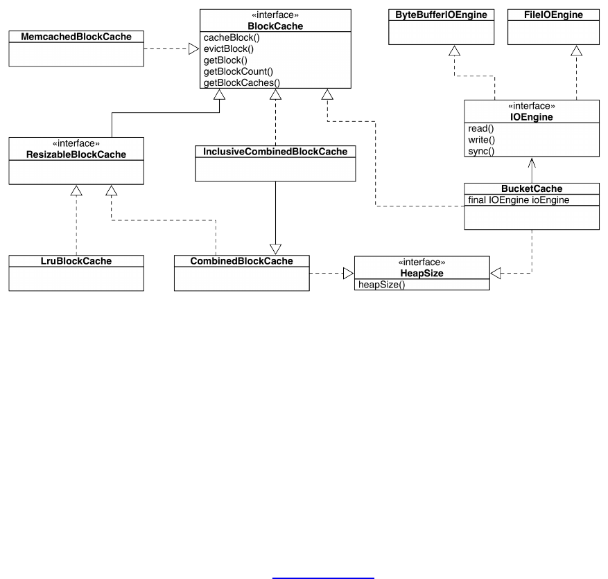
Figure 10-3. The hierarchy of the block cache classes
With this set of Java interfaces and classes, you have a wider choice of cache implementations.
Before we look into the more involved combinations, here is a separate overview of each:
BlockCache
This is the main interface that defines the methods to cache, retrieve, and evict blocks.
ResizeableBlockCache
Another intermediate interface which declares the implementing classes to support
reconfiguration at runtime. More specifically, it allows for the server process to react to
workloads and tune the memory assignment between block cache (for reads) and
memstores (for writes) dynamically (see “Heap Tuning”).
LruBlockCache
The least-recently-used cache implementations is the longest standing member of the
cache family. It holds on to all cached blocks until the memory it has been assigned is
exceeded. At that point the oldest block(s) are removed to make room. The cache also has
the mentioned eviction priority handling built in.
Here are the configuration properties that let you fine-tune the behavior:
Property Default Description
hbase.lru.blockcache.min.factor 0.95
(95%)
Percentage of total cache size which
serves as the target for an eviction
process. When an eviction process has
reduced the cache to this percentage, the
eviction process will cease. For example,
if set to 0.80 (80%), then an eviction will
keep on removing entries until the cache
size is down to 80% of the total size.
(758)

hbase.lru.blockcache.acceptable.factor 0.99
(99%)
Acceptable size of the cache. No
evictions will be started while the cache
size is less than this percentage of the
total size.
hbase.lru.blockcache.single.percentage 0.25
(25%)
The percent of the total configured cache
size set aside for blocks that were used
only once (so far).
hbase.lru.blockcache.multi.percentage 0.50
(50%)
The share of the cache memory for all
blocks that were used more than once.
hbase.lru.blockcache.memory.percentage
0.25
(25%)
Defines the portion of the memory of the
cache used for blocks tagged as in-
memory.
hbase.lru.rs.inmemoryforcemode false
When set to true, will try to retain in-
memory tagged blocks at all costs
(unless it remains the sole source of
memory to free). Otherwise the cache
will evict blocks from all priority
buckets to bring each back into its
boundaries. Evictions are ordered by the
level of oversubscription per bucket,
from highest to lowest.
hbase.lru.max.block.size
16777216
bytes
(16
MB)
Any block larger than this value will not
be cached at all.
Notes:
The percentages for the three priority buckets most not be negative, and in sum not
exceed 100%.
The hbase.lru.rs.inmemoryforcemode flag sets a global behavior, which means it
applies to any table created within HBase.
Setting the hbase.lru.blockcache.memory.percentage to 1.0 has the same effect as the
previous flag, that is, it forces the in-memory mode to be used.
Rows span a single block. If you create a row with more than max.block.size bytes
(759)

of data, it will never be cached, which would make subsequent reads as fast or slow
as the first.
BucketCache
This cache mirrors the LRU cache in that it has three priority based cache buckets, for
single-, multi-access, and in-memory blocks. One difference is that it makes the actual
location of the cache pluggable, with implementations provided for on-heap, off-heap, and
file based storage. “Block Cache” shows the server-based UI provided to inspect the cache
usage. The following lists the configuration properties of the bucket cache:
Property Default Description
hbase.bucketcache.ioengine <none>
Defines where to store the contents of
the bucket cache. Allowed values are
heap, offheap, or file. For the latter,
the location is defined right after the
type, that is, file:<path_to_file>.
hbase.bucketcache.size 0.0
A float that either represents a
percentage of total heap memory size
to give to the cache (if less than 1.0)--
or, it is the total capacity in megabytes
(if greater than 1.0).
hbase.bucketcache.persistent.path <none>
If set, enables the (optional)
persistence of the cache’s backing
structure and its metadata. Implies that
the selected IO engine is supporting
persistency (only file applies), or an
error is thrown at runtime.
hbase.bucketcache.writer.threads 3
The number of parallelism when
writing out the memory entries to the
IO engine.
hbase.bucketcache.writer.queuelength 64 For each writer thread, a queue of this
size is used to line up entries.
hbase.bucketcache.bucket.sizes <see
below>
A comma-separated list of sizes (in
bytes) for bucket allocations. Can be
multiple sizes, listed in order from
smallest to largest. If not set, it will
use a default layout explained below.
(760)

hbase.offheapcache.minblocksize HFile
Blocksize
The expected minimum block size to
compute the memory requirements.
hbase.bucketcache.combinedcache.enabled true
Whether or not the bucket cache is
used together with the LRU on-heap
block cache. See “Single vs. Multi-
level Caching” for details.
Notes:
Both the IO engine type (hbase.bucketcache.ioengine) and size of the cache
(hbase.bucketcache.size) must be set, or a runtime error will be thrown.
The minimum block size (hbase.offheapcache.minblocksize) is for estimations only,
as blocks in practice can vary significantly in size.
The three priority bucket sizes (single 25%, multi 50%, in-memory 25%), and their
maximum (95%) and minimum (85%) eviction sizes are hardcoded for this class.
Internally the cache entries are distributed over a shared map that contains cache
entry buckets of varying sizes.
Cache entries, when added, are hashed by their internal key and then evenly
distributed over the writer threads and their respective queues.
For the bucket allocation sizes (hbase.bucketcache.bucket.sizes), these range from slightly
more than 4 KB, 8 KB, 16 KB, and so on, to 256 KB, 384 KB, and 512 KB. The sizes
depend on the data access patterns, and are multiples of 1024 (1 KB, plus a few bytes extra
for edge cases, with the default adding 1 KB to be safe) to fit the possible HFile blocks.
More information can be found in “Advanced Cache Configuration”.
MemcachedBlockCache
This implementation is considered to be one of the external caches. It allows use of a
separate Memcached based in-memory object cache to act as the backing store for the
block cache. Obviously, this setup will need for all of the data to be sent over the network,
making its use dependent on the throughput and latency of a critical infrastructure
component. On the other hand, it would retain the cache across server restarts or region
migration. It can be configured with these properties:
Property Default Description
hbase.cache.memcached.servers localhost:11211
A comma separate list of servers, given
as pairs of hostname plus port (divided
by a colon symbol).
hbase.cache.memcached.optimeout 500 ms The default operation timeout in
milliseconds.
(761)

hbase.cache.memcached.timeout <optimeout> +
500 ms
Set the maximum amount of time (in
milliseconds) a client is willing to wait
for space to become available in an
output queue.
hbase.cache.memcached.spy.optimze false Determines if the operation
optimization should be enabled.
CombinedBlockCache
This implementation is a facade, that combines two of the above cache types, namely the
LRU cache for smaller on-heap usage (L1), and another block cache implementation,
which is usually the BucketCache, for larger storage usage (L2). All blocks that are evicted
from the L1, are moved to the L2 implicitly. See “Single vs. Multi-level Caching” for how
they are working together.
InclusiveCombinedBlockCache
Same as the CombinedBlockCache, but stores all blocks of any type in both internal caches.
(762)

Single vs. Multi-level Caching
So far we looked at each of the block cache implementations separately, but in practice only two
different scenarios are used: a single or multi-level block cache. The former is usually the LRU
cache implementation, for legacy reasons. The latter makes use of the two CombinedBlockCache
implementations, wiring together a more complex cache setup. As mentioned in “Block Cache”,
with the combined cache, there are two levels called L1 and L2, and dependent on how you
configure them, they have different purposes.
Here are the possible combinations the cache can be set up as:
L1 only
As mentioned, this setup entails a single-level cache, and that is the LruBlockCache class,
configured with the heap size and other LRU settings as explained.
Combined L1+L2
Here the L1 is used to store lightweight information only, which is all block types, apart
from data blocks. The latter, by default, go directly to the L2 cache. This can be
overridden on a per-column family basis (refer to “Column Families” and the
setCacheDataInL1() method for details). The L1 is still the LRU implementation, while the
L2 is the newer BucketCache class. They are wrapped into one using the CombinedBlockCache
facade class, which provides the described combined L1+L2 functionality.
Setting hbase.bucketcache.combinedcache.enabled to true enables this multi-level cache
mode. In fact, this setup is the default, with the LRU implementation set as the L1 cache.
Because of the empty default values for the L2, no further cache level is instantiated.
Inclusive Combined L1+L2
Provided by the InclusiveCombinedBlockCache class, this is essentially the same as the
previous item above, with the difference that all block types, including data blocks, are
inserted into both the L1 and L2 when cached. This is exclusively used for external caches,
which (at the time of this writing) only applies to the Memcached block cache
implementation.
Setting hbase.blockcache.use.external to true enables this setup (see “Basic Cache
Configuration” for more).
Common L1+L2
The last of the possible setups uses the multi-level caches as is commonly found in other
systems. Here, any block type is cached by the L1 first, and only on eviction there it is
moved to the L2 cache. It stays in L2 until eventually evicted there too. Note though, that
moving blocks between L1 (on-heap) and L2 (off-heap) is causing extra CPU cycles,
which may be significant for already heavily loaded clusters. In addition, the now much
more frequent need for Java garbage collection, freeing the on-heap memory after L1
eviction, might affect the cluster latency too.
(763)

Setting hbase.bucketcache.combinedcache.enabled to false, and
hbase.blockcache.use.external to false enables this multi-level cache mode.
Note that the L2 cache has to be explicitly enabled: You need to set hbase.bucketcache.size to a
percentage or absolute size, and hbase.bucketcache.ioengine to one of the supported IO engine
values, or else no L2 is used at all (see “Basic Cache Configuration”). If you have the L2
enabled, the eviction of a block from L1 always moves it into L2. It will stay in L2 until it is
eventually evicted there too, removing it completely from the caching subsystem. This applies to
any type block, that is, data, index, or filter.
During the eviction from L1 to L2, moving a block with in-memory priority will retain the
priority. For all other priorities, the moved block will start at single-access priority in the L2
cache. Only if it is accessed again will it be promoted to multi-access priority, just like in the L1
before. Figure 10-4 shows a diagram, which has an on-heap L1 and an off-heap L2, configured
as combined L1+L2. You can see from the legend that each block has many metadata fields,
including the type of block, the table type it belongs to, its current priority, and whether it should
be cached in L1 first or not (applies to data blocks only). You can also see the buckets in each
cache, where the L1 has only three based on priority, while the L2 has many more (only a subset
is shown) based on allocation sizes. Refer to “Advanced Cache Configuration” for fine-tuning
the bucket sizes.
(764)
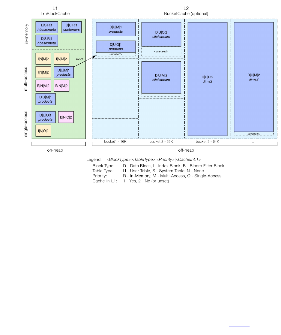
Figure 10-4. The combined L1 and L2 setup with an off-heap bucket cache
Interesting in the diagram is how some blocks of tables make it into the L1 cache, since they are
either configured as in-memory priority or have the cache-in-L1 set for the respective column
families. There is also an evicted block that starts out with single-access priority in the L2.
Moving a block from L1 to L2 can fail when, for example, the system is under pressure. In that
case, the block would need to be reloaded next time it is asked for. During reads, a cache lookup
always tries L1 first, then (if configured) the L2. It also does not matter if you have set the read
operation to not cache any block that needs to be loaded. Another read might have already asked
for the same block, but allowing it to be cached. Thus is makes sense to always try the cache
lookup for any kind of read, which is what happens here implicitly.
Finally, blocks larger than the configure maximum block size per cache type will not be cached
at all. This might not be obvious, but if you create a row that’s very wide and contains a lot of
data, you could end up having to read the block from storage at every access.10 “Cache
Selection” has more information about the best practices for selecting the various cache setups
and implementations.
(765)

Basic Cache Configuration
Configuring the block cache, there is one main knob to turn, explained in the table:
Property Default Description
hfile.block.cache.size 0.4 (40%)aThe share of the total heap assigned to the block cache.
a HBase versions before 0.96 used to default to 25%, and before 0.94/0.92 the default was 20%.
This value is the percentage of the total Java heap, given to the process, set aside for the block
cache to use. Setting it to 0 disables the cache altogether, but that is not recommended, as the
system requires a cache to at least hold index blocks warm. “Heap Tuning” explains the more
elaborate heap memory tuner option, using an upper and lower boundary for the actual memory
used.
By default, the block cache is always enabled and set to use the LRU cache for the L1, and
nothing is set as L2. The heap size set aside for the L1 LRU Cache is set to 40%. You now have
a few choices to add an L2, and reconfigure the L1 to fit that new setup. We will discuss some of
the more common configurations next, but please note these are for reference only. You can
further tweak the settings to match your use-case. The topic of choosing one option over the
other is discussed in “Cache Selection”.
Off-Heap Setup
The most common setup for the block cache is adding a bucket cache as L2, with the memory
located off-heap. This uses the Java NIO ByteBuffer class to allocate memory as direct, which is
in main memory, outside of the managed JVM memory (that is, the Java heap). The advantage is
that this memory is completely under control of the application, and does not impact garbage
collection performance (see “Garbage Collection Tuning”).
The following example sets the off-heap cache to 4 GB, and reduces the on-heap LRU cache to
20% of the total heap. The latter is useful since the L1 is usually used for block index and Bloom
filter blocks only, which are much smaller compared to the actual data blocks. If you plan on
using the in-memory or cache-in-L1 options of a column family, you may want to consider
keeping a slightly larger L1.
First, you have to edit the hbase-env.sh file in the used configuration directory, adding the
following line:
...
# Uncomment below if you intend to use off heap cache. For example, to
# allocate 8G of offheap, set the value to "8G".
# export HBASE_OFFHEAPSIZE=1G
HBASE_OFFHEAPSIZE=5G
...
Note how the value used is actually larger than the required 4 GB in our example. This is
required, as other parts of the JVM are also storing data in off-heap memory.11 Furthermore,
(766)

some Hadoop classes, such as the DFSClient may use off-heap cache too (see “Short-Circuit
Reads” for some details). How much larger is unfortunately not an exact science, though in
practice adding 1-2 GB extra has worked well. For example, just for the DFSClient it is the
number of open HFiles multiplied by hbase.dfs.client.read.shortcircuit.buffer.size, where the
latter is set to 128 KB in HBase. The hbase-default.xml file has more information.
Note
The HBASE_OFFHEAPSIZE environment variable passes the value to the JVM -XX:MaxDirectMemorySize
option, which is needed for the process to set the appropriate maximum boundaries (and avoid
overzealous applications allocating too much memory). This JVM option might change, which
makes using the HBase provided variable the future proof and recommended option.
Second, the following properties have to be added to the hbase-site.xml file:
<property>
<name>hbase.bucketcache.ioengine</name>
<value>offheap</value>
</property>
<property>
<name>hfile.block.cache.size</name>
<value>0.2</value>
</property>
<property>
<name>hbase.bucketcache.size</name>
<value>4196</value>
</property>
After you perform a restart of the server processes, you should have the L2 bucket cache
available. Use the web-based UI to confirm that the cache is set up properly, as shown in “Block
Cache”.
File-based Setup
One of the reasons the BucketCache class was added to HBase is that it supports the storage of
cached data in external files. This is particularly (you could say solely) useful when that file is
located on very fast storage, for example SSDs or PCIe flash storage cards. The latter provide
very high throughput, though are not as fast as on-board memory. This allows—at some cost—
extension of the cache to a much larger, but persistent, storage media. And with flash storage, the
cost of seeks (see [Link to Come]) is mitigated, allowing fast random access to file-based
caching structures. Enabling the file backed cache requires setting the I/O engine value
(hbase.bucketcache.ioengine) to file, followed by a colon and the fully specified file name:
file:<path-to-cache-file>
Example 10-1.
The path must exist and the process must be allowed to write into it, or else the start of the region
server process is aborted. For example:
016-08-15 02:19:54,423 FATAL [regionserver/s1.foo.int/10.0.10.10:16020] \
regionserver.HRegionServer: ABORTING region server \
s1.foo.int,16020,1471252790047: Unhandled: Region server startup failed
java.io.IOException: Region server startup failed
...
Caused by: java.lang.RuntimeException: java.io.FileNotFoundException: \
/data/hbase/cache/cache.dat (Permission denied)
...
(767)
Caused by: java.io.FileNotFoundException: /data/hbase/cache/cache.dat \
(Permission denied)
...
The file will be created in the specified location if it does not exist yet. Here is an example
configuration enabling the file backed cache, located on an SSD drive:
<property>
<name>hbase.bucketcache.ioengine</name>
<value>file:/mnt/ssd1/hbase/cache/cache.dat</value>
</property>
<property>
<name>hfile.block.cache.size</name>
<value>0.2</value>
</property>
<property>
<name>hbase.bucketcache.size</name>
<value>4196</value>
</property>
Note that you do not have to change the hbase-env.sh to set the HBASE_OFFHEAPSIZE environment
variable. That is only needed for off-heap cache (as the name implies). Otherwise, the file-based
cache variant behaves very similarly to the off-heap mode: it manages a larger space on its own,
without any impact on the Java heap and its garbage collection functionality.
On-Heap Setup
For rare situations, it is also possible to configure the bucket cache to reside on-heap, sharing the
space with the L1 cache. The following configuration example shows this setup:
<property>
<name>hbase.bucketcache.ioengine</name>
<value>onheap</value>
</property>
<property>
<name>hfile.block.cache.size</name>
<value>0.2</value>
</property>
<property>
<name>hbase.bucketcache.size</name>
<value>0.4</value>
</property>
While it is possible to have both L1 and L2 on-heap, in practice this option is not used often (if at
all).
(768)
Advanced Cache Configuration
There is a set of general configuration parameters controlling the cache behavior, and how the
server processes should handle various data structures. The prefixes of these properties indicate
where they apply: some of the settings are used at a region server level, while others are used at
the store file or block cache level. They can be grouped at a more general level into being block
or cache related, which we will discuss in that order next.
Block-related Properties
Here are the properties pertaining to how blocks are handled on the file and region server level:
Property Default HBase Shell Description
hbase.rs.cacheblocksonwrite false CACHE_DATA_ON_WRITE
If set to true forces all
blocks that are written to
be added to the cache
automatically.
hfile.block.index.cacheonwrite false CACHE_INDEX_ON_WRITE
If enabled, caches all types
of index blocks during
writes transparently.
hfile.block.bloom.cacheonwrite false CACHE_BLOOMS_ON_WRITE Same, but for all Bloom
filter block types.
hbase.block.data.cachecompressed false n/a
Defines how blocks are
cached, compressed (and
possibly encrypted) or not.
Only applies to data
blocks, not to the index
block types.
hbase.rs.evictblocksonclose false EVICT_BLOCKS_ON_CLOSE
Specifies what the system
should do with blocks of
store files that are being
closed.
hbase.rs.prefetchblocksonopen false PREFETCH_BLOCKS_ON_OPEN
Controls whether the server
should asynchronously
load all of the blocks (data,
meta, and index) when a
store file is opened.
(769)

hbase.hfile.drop.behind.compaction true n/a
Defines the handling of
low-level file data after
compactions.
The first seven properties in the table define how blocks are handled regarding the cache. You
can influence whether blocks are allowed to be cached in compressed form
(hbase.block.data.cachecompressed), as loaded from the store file. In addition, you can influence,
on a global level, how blocks are added or removed from the cache, based on store file
operations. For example, you can define that blocks are automatically added to the cache as
memstores are persisted to storage during a flush operation. You can further fine-tune the same
for the Bloom filter and block index chunks, that is, the blocks for leaf and intermediate index
levels, and the Bloom filter sub-blocks. Another advanced tuning option is the prefetching of
store file blocks (hbase.rs.prefetchblocksonopen).
Tuning Block Prefetching
Enabling the block prefetch option by setting hbase.rs.prefetchblocksonopen to true globally, or at
the column family level using the HColumnDescriptor method aptly named
setPrefetchBlocksOnOpen(), will instruct the server to read all blocks when a store file is opened.
Internally, it simply reads every block from the start of the file, up to the load-on-open section
(see [Link to Come]), since the latter is read no matter what you configure. Each block is read
and cached (in the single-access area, as expected), while not counting any of these block reads
as cache misses.
A client using the API might try to achieve the same by scanning the table the store file belongs
to from the beginning to the end. But that is not as efficient, as it transfers the data across the
network to the client to some degree (using the FirstKeyOnlyFilter filter, described in
“FirstKeyOnlyFilter”, will help to mitigate the amount of data transferred). In addition, it
occupies scarce resources unnecessarily, such as client and transfer threads, sockets, and so on.
And, as mentioned, the metrics would report probably all of these blocks as cache misses,
tainting the metrics subset in the process. Finally, some of the blocks, such as the meta blocks
and intermediate index blocks are included in the prefetch, which a normal scan would miss.
The server-side prefetch executor pool can be tweaked using the following properties:
Property Default Description
hbase.hfile.prefetch.delay 1000 ms The delay before the prefetch is started.
hbase.hfile.prefetch.delay.variation 0.2
(20%) Adds a jitter to the start of the prefetch operation.
hbase.hfile.thread.prefetch 4 The number of threads to create for running the
asynchronous prefetch operations.
The delay.variation creates an offset for each thread, avoiding stampede-like situations (where
(770)

all threads in the pool start at the same time and cause contention). For example, using the
default values, the delay for each prefetch operation is varied from 900 to 1000 milliseconds.
Most of these properties have very conservative defaults, and in fact disable all of the advanced
features. The only one enabled is to drop data from the operating system cache if the file has
been part of a compaction and is now obsolete (hbase.hfile.drop.behind.compaction), which is a
sensible default. This applies to data read from the existing store files, which is written to the
new one(s).
Note
This does not concern the store file blocks and the block cache in HBase, but the underlying
storage system. Compactions often read and write data from files that exceed the physical
memory of the machine, causing the I/O layer to thrash the OS caches.12
But before you have to decide to turn any of these features on for the entire cluster, you can do so
more selectively on the column family level instead. “Column Families” lists the following
methods of the HColumnDescriptor class:
boolean isCacheDataOnWrite()
HColumnDescriptor setCacheDataOnWrite(boolean value)
boolean isCacheIndexesOnWrite()
HColumnDescriptor setCacheIndexesOnWrite(boolean value)
boolean isCacheBloomsOnWrite()
HColumnDescriptor setCacheBloomsOnWrite(boolean value)
boolean isEvictBlocksOnClose()
HColumnDescriptor setEvictBlocksOnClose(boolean value)
boolean isPrefetchBlocksOnOpen()
HColumnDescriptor setPrefetchBlocksOnOpen(boolean value)
boolean isCacheDataInL1()
HColumnDescriptor setCacheDataInL1(boolean value)
These can be used when creating tables using the admin API (see “Table Operations”). The other
option is to use the HBase Shell, and add the property on the command line, for example:
hbase(main):001:0> create 'test', { NAME => 'cf1', \
CONFIGURATION => { CACHE_DATA_ON_WRITE => 'true' } }
The table (Table 10-7) lists the cache related properties that are available in the HBase Shell
column.
Example 10-2.
Unfortunately, most of the listed properties do not have direct support by the HBase Shell and
need to be handed in using a literal, like so (using the alter command for a change):
hbase(main):001:0> alter 't1', 'f1', \
{ CONFIGURATION => { 'hbase.hfile.drop.behind.compaction' => 'true' } }
And some of the values allow you to use both the long configuration property and its short form.
The following two lines achieve the same:
hbase(main):002:0> alter 't1', 'f1', \
{ CONFIGURATION => { 'hbase.hfile.drop.behind.compaction' => 'true' } }
(771)

hbase(main):003:0> alter 't1', 'f1', \
{ CONFIGURATION => { 'CACHE_INDEX_ON_WRITE' => 'true' } }
Note the quotes around the short name for the option in the second command. This is needed to
avoid a parse error by the shell, and you can use this technique with any of the long and short
options just to be safe.
Each of the cache related properties triggers specific functionality for the block of the column
family they belong to (or for all blocks, if you set these properties in the cluster-wide hbase-
site.xml file). We will discuss each separately now to introduce you to the finer details, as some
of the side-effects may not be obvious initially:
Note
As far as caching is concerned, an important concept is the working set size (WSS), which is:
“the amount of memory needed to compute the answer to a problem”. For a website, this would
be the data that is needed to answer the queries over a short amount of time.
Cache Data on Write
The first option forces all data blocks to be cached as they are written out by the region
server. This happens during a memstore flush operation or when a compaction is
performed. Internally, the writer implementation calls the configured cache instance to add
the newly written block, and the rules explained in “Single vs. Multi-level Caching” apply
the same way as they do for any other block that is read from storage. It is useful to cache
data as it gets persisted when you expect the working set to fit into memory, that is, the
block cache. Otherwise you may create a lot of churn as blocks are evicted once you run
out of memory.
Cache Indexes on Write
This is the same as the previous, but applies to the block index sub-blocks. This allows you
to pre-warm the L1 with index information as data is persisted. Just as with the above, you
need to make sure you only enable this for families that have index data not in excess of
the configured L1 space.
Cache Blooms on Write
Same for the Bloom filter sub-blocks. The same caveats apply.
Evict Blocks on Close
Instead of relying on the LRU functionality, which evicts the oldest cached blocks when
memory fills up, you can set this flag to force all blocks of a family to be evicted as soon
as the underlying store files are closed. One side-effect is that this also applies when
disabling a table, or when altering it. These operations close and re-open the table regions
in a rolling manner, which would lead to all of the previously cached blocks of that table to
be dropped from the L1 and (optionally) L2.
Prefetch Blocks on Open
This is somewhat the opposite of the previous option. Here all blocks of the underlying
store files are loaded when a table region is opened (refer to “Tuning Block Prefetching”
(772)

for details). Like the previous caveats, you will need to ensure the table data fits into the
cache, or else it will cause unnecessary churn through evictions.
Cache Data in L1
As shown in Figure 10-4, you can force a smaller table to reside in L1, instead of the L2.
And as with the above, the same caveats apply: if you enable this feature for a table that
exceeds the assigned L1 memory, you will cause a lot of block evictions that will affect the
overall perceived performance of HBase.
Cache Data Compressed
With this option enabled, all data blocks read from disk are left in their on-disk format. In
other words, if you have, for example, any compression configured (see “Compression”)
for a column family, all of its blocks would be cached compressed. Usually that is not the
case and blocks are decompressed (and decrypted) while being read from the store files,
and subsequently cached as such. Any access to a compressed block in the cache would
require a decompression to happen on-the-fly, adding CPU overhead. On the other hand,
you can fit more into the cache, as compression algorithms often yield a space saving ratio
of 3:1 and more (depending on the nature of the data).13
Use Block Cache
Finally, there is another option that is applicable in this context: the use-block-cache flag
of the column family descriptor. It defaults to true and can be set using the
setBlockCacheEnabled() method of the HColumnDescriptor class, or using the BLOCKCACHE
property within the HBase Shell. Setting this flag to false causes all read blocks for the
operation not to be cached. Previously cached blocks are used though, just any
extraneously loaded ones are dropped immediately. The advantage is that existing blocks
(even with the same initial single-access priority) in the cache are not affected, keeping
latencies for other data consistent.
Another scenario where this is useful is when the working set (that is, the data needed most
often) does not fit into the L1/L2, but into the OS buffer cache. The latter might be much
larger, given current server specifications, and therefore is able to hold on to the files. The
OS buffer cache is also known to be slightly slower in comparison, but it still is faster than
most storage media.
Caution
When planning for the capacity needed to hold data in the cache, keep in mind that rows can
span more than one block. For example, when you have updated a row between flushes, they are
stored as separate HFiles, and therefore increase the number of blocks that need to be loaded to
reconstruct the row as the client sees it. For scans that use the use-block-cache option this might
be mitigated, as longer scans will likely read surrounding row data from the same blocks.
Cache-related Properties
The last two configuration parameters available relate directly to the cache setup, and both are
shown in the following table:
(773)

Property Default Description
hbase.blockcache.use.external false
A flag that forces the use of a cache that is considered
external, like the MemcachedBlockCache. Set the next
property to plug in a custom class (see “Single vs.
Multi-level Caching”).
hbase.blockcache.external.class memcached
The name of the external cache implementation class
to use. The previous property must be set to true for
this to be supported (see “Single vs. Multi-level
Caching”).
Using these in tandem allows you to point the L2 to a shared, external (to the region server
process) cache instance, which might even be an entire cluster on its own. There is no empirical
data on how this setup helps, or is used in practice, thus we must defer the discussion to a later
time.
Lastly, one more topic concerns the cache setup, which is the bucket sizes for the BucketCache
class. It was mentioned how the default is a list of sizes, ranging from 4+1 KB, to 512+1 KB,
where the +1 KB is for avoiding edge cases as blocks also carry metadata that needs to fit into
the bucket.
The bucket cache reads the sizes, and multiplies the largest value, here 513 KB, by four,
assuming that a bucket should at least fit four blocks. This results in about 2 MB (that is, 2 MB +
4 KB to be exact) for each bucket, and if you give the entire cache 1 GB of space, you end up
dividing that space into 511 (because of the extra kilobytes) buckets. Figure 10-4 shows this in
an abbreviated form for the sake of brevity. Each of the buckets is assigned an allocation size,
which is the value from the sizes list. In other words, the first 2 MB bucket is assigned 5 KB as
its allocation size. The next is assigned 9 KB, and so on, until you reach the largest value, 513
KB. Every subsequent bucket is then assigned that last, largest value until the end is reached.
You will therefore have around 498 buckets that are set to a 513 KB allocation size.
The default block size for HFiles is 64 KB, and can be set per column family, or cluster wide.
Assuming a combined L1+L2 setup, and default values for both caches and the read operation,
when a 64 KB data block is read from disk (or cached during writes, if enabled) it is given to the
L2 for caching. The bucket cache now iterates over the buckets and tries to find one that fits the
block size. It arrives eventually at the one configured with 65 KB, and selects it as a match. The
64 KB block is written at the end of the 2 MB bucket, and subsequent 64 KB blocks will be
added in the free allocation space just before the last cached one.
Once the bucket fills up, it is considered full, and the following cache invocation will fail to find
a free 64 KB spot. Here the cache now falls back to get the next completely empty bucket, which
for the default values is 97 KB. Instead of adding the 64 KB as-is, and in the process waste the
33 KB of the allocation space, it reconfigures the empty bucket to fit 65 KB blocks instead. Over
time, you will observe (using the region server UI or the metrics, see “The Metrics Framework”)
that many of the initial 513 KB allocation size buckets have been reconfigured to fit the need. At
the same time, you may also observe on specific region servers that one (or more) 9 KB bucket
has been filled. This is attributed to the system catalog tables, which default to 8 KB HFile block
sizes. Or (obviously), those are from your own tables if you have chosen to configure them with
(774)

that block size.
The question now is, should you reconfigure the default values at all? The given allocation sizes
reflect a nice size progression, and seem to do a good enough job already. You could use the $
hbase hfile command (see [Link to Come]) to print out the block information for a persisted file.
Best would be to collect them across all of the tables (at least the important ones used must often
for reads) and determine a good bucket size distribution. Unfortunately, there is little information
available that would indicate a viable way to compute different allocation sizes, and best-practice
is to leave them as-is.
The reason the bucket cache is using fixed sized buckets and allocation spaces is an optimization
to use chunks in the backing I/O engine that make garbage collection easier. Obviously, just as
with the MSLAB (see “Memstore-Local Allocation Buffer”), there is a cost to rounding up the
block sizes to buckets. This is a tradeoff and needs to be fine-tuned if the impact is deemed too
expensive (Figure 10-4 shows this as unused space).
In case you want to change the allocation sizes, here is an example of how to do that. These lines
need to be added to the hbase-site.xml file to set the sizes to 5 KB, 9 KB, and so on respectively:
<property>
<name>hbase.bucketcache.bucket.sizes</name>
<value>5120,9216,17408,33792,66560,132096</value>
</property>
Each value has the extra 1 KB added just as the default values have, so that blocks configured on
the column family level to, for example, 8 KB, will have some extra room for Java overhead and
block metadata. In addition, the check for the set block size while writing the store files is done
after a cell was written, which means that in practice, a block is always larger than the
configured size. When tuning the allocation sizes for the bucket cache, you need to take this into
consideration. As mentioned, using the HFile command line tool to print out the block index
information is a good start to see how much larger your blocks actually are.
Ultimately, you need to avoid the case where your blocks are larger than the closest allocation
size, even including its extra overhead space. For example, assuming the 64 KB default HFile
block size and the example allocation sizes above, you could be a few bytes shy of closing the
current block, at 63 KB, and then you encounter a cell that is 10 KB in size. That would create a
block of 73 KB, and when the bucket cache is trying to find a matching bucket, it would have to
resort to the 128 KB bucket, leaving 55 KB unused space in that bucket slot.
(775)

Cache Selection
The HBase team has published the results of extensive block cache testing, which revealed the
following guidelines:
If the working set fits completely in the heap, the default configuration, which uses the on-
heap LruBlockCache, is the best choice, as the L2 cache will not provide much benefit. If the
eviction rate is low, garbage collection can be 50% less than that of the BucketCache, and
throughput can be at least 20% higher.
Otherwise, if your cache is experiencing a consistently high eviction rate, use the
BucketCache, which only causes 30-50% of the garbage collection of LruBlockCache when
the eviction rate is high.
The BucketCache using file mode on solid-state disks has a better garbage collection profile,
but lower throughput than the BucketCache using off-heap memory.
In general terms, on-heap is the fastest cache technology, followed by off-heap cache, OS buffer
cache, and, last but not least, the file based bucket cache. All of the cache approaches outside of
the heap will be some percentage slower (due to serialization), yet they are not affecting the Java
garbage collection process—which is already usually under duress on a busy cluster. Instead, for
non-heap caches, the bucket cache is handling the allocation and eviction of blocks itself. The
advantage is that fewer garbage collections mean better latencies for the read operations longer
term. Caching the index and Bloom filter blocks preferably in L1 is also attributed to
serialization, as these blocks default to 128 KB in size, and would take even longer to be
accessed outside of the heap, while being even more critical to read latencies.
In practice, most servers today offer plenty of memory to be used as cache, which makes the
combined L1+L2 the most commonly used block cache configuration. For tables with a small
enough working set, enabling the cache-in-L1 option can be used to improve the read latencies.
The L1 should be reasonably sized, especially when the workload is causing frequent evictions
from L1. If you have fast solid-state storage, you can use the file based bucket cache setup as
opposed to the off-heap mode, allowing you to cache much more data than in memory alone.14
(776)
Compression
HBase comes with support for a number of compression algorithms that can be enabled at the
column family level. It is recommended that you enable compression unless you have a reason
not to do so—for example, when using already compressed content, such as JPEG images. For
every other use case, compression usually will yield overall better performance, because the
overhead of the CPU performing the compression and decompression is less than what is
required to read more data from disk.
(777)

Available Codecs
You can choose from a fixed list of supported compression algorithms, as listed in Table 10-8,
that can be used with HBase column families to optionally compress the contained data. The
algorithms have different qualities when it comes to compression ratio, as well as CPU and
installation requirements. Many are based on the Lempel-Ziv LZ77 family of compression
algorithms, implemented either in C/C++ (referred to hereafter as native) or in pure Java, with
some available in both languages. Since Java is a managed language that trades programming
simplicity for closeness to the actual hardware, the native implementations are usually quite a bit
faster. Using those from Java is accomplished with JNI15, which adds some overhead, but still
results in much better performance compared to the Java versions of the algorithms. The latter
are really for convenience since JNI needs compilation and provisioning of conduit libraries,
which may not be provided (and you may be lacking the required build toolchain), or are not
available at all on the platform you are using.
Table 10-8. Available Compression Codecs
Compression Short Native Java Focus Provided Description
None none n/a n/a n/a n/a For the sake of completeness, means no
compression.
LZ4 lz4 Yes No Speed Yes LZ77 family implementation, with very fast
decompression performance.
LZO lzo Yes No Speed No Lempel-Ziv-Oberhumer algorithm,
optimized for decompression performance.
Snappy snappy Yes No Speed Opt. Google-donated Snappy (aka Zippy)
implementation.
bzip2 bzip2 Yes No Size Opt. Burrows-Wheeler implementation.
gzip gz Yes Yes Size Yes
Another LZ77 family implementation,
either using a native library, or a Java
implementation.
Note
Currently there is no support for pluggable compression algorithms in Hadoop and HBase. Also,
using one of the choices that require native library support will have problems when the external
dependencies are not available anymore.
(778)

Before looking into each available compression algorithm, refer to Table 10-9 to see the
compression algorithm comparison Google published in 2005.16 While the numbers are old, they
still can be used to compare the qualities of the algorithms.
Table 10-9. Comparison of Compression
Algorithms
Algorithm % Remaining Encoding Decoding
gzip 13.4% 21 MB/s 118 MB/s
LZO 20.5% 135 MB/s 410 MB/s
Zippy/Snappy 22.2% 172 MB/s 409 MB/s
Note that some of the algorithms have a better compression ratio while others are faster during
encoding, and a lot faster during decoding. Depending on your use case, you can choose one that
suits you best.
Before Snappy was made available in 2011, the recommended algorithm was LZO, even if it did
not have the best compression ratio. gzip is very CPU-intensive and its slight advantage in
storage savings is usually not worth the slower performance and CPU usage it exposes. Snappy
has similar qualities as LZO, it comes with a compatible license, and tests have shown that it
slightly outperforms LZO when used with Hadoop and HBase. The newer additions of LZ4 and
bzip2 are completing the list of choices, with LZ4 considered an alternative to LZO and Snappy,
while bzip2 is similar to gzip, providing higher compression ratios trading CPU usage. As of this
writing, the most popular compression implementation is Snappy, striking a sensible balance out-
of-the-box.
Support for all the native compression implementations except LZO is supplied with Hadoop, by
means of libhadoop.so.17 The Hadoop JARs, such as hadoop-common.jar will make an attempt to
load the native library, which in turn loads the available native compression libraries and exposes
them via JNI to the Java code. If loading libhadoop.so (or any dependent library) fails, some of
the algorithms fall back to the pure Java implementations (see the “Java” column in Table 10-8),
while others are simply not available at all. The following log messages are emitted when
loading a native compression library succeeds:
...
2016-09-01 20:09:26,870 INFO [main] hfile.CacheConfig: Created \
cacheConfig: CacheConfig:disabled
2016-09-01 20:09:27,073 INFO [main] zlib.ZlibFactory: Successfully loaded & \
initialized native-zlib library
2016-09-01 20:09:27,104 INFO [main] compress.CodecPool: \
Got brand-new compressor [.gz]
...
The next example shows a failed attempt to load a native library, and the code falling back to the
built-in Java version:
...
2016-09-01 18:25:07,029 WARN [main] util.NativeCodeLoader: Unable to load \
native-hadoop library for your platform... using builtin-java classes \
where applicable
(779)

2016-09-01 18:25:07,628 INFO [main] hfile.CacheConfig: Created \
cacheConfig: CacheConfig:disabled
2016-09-01 18:25:07,825 INFO [main] compress.CodecPool: \
Got brand-new compressor [.gz]
...
Keep in mind, that the provided libhadoop.so might have been compiled without support for
Snappy (also applies to bzip2), noticeable when you find the following in your log files:
...
2016-09-02 11:58:41,137 INFO [main] hfile.CacheConfig: Created cacheConfig: \
CacheConfig:disabled
Exception in thread "main" java.lang.RuntimeException: native snappy library \
not available: this version of libhadoop was built without snappy support.
at org.apache.hadoop.io.compress.SnappyCodec.checkNativeCodeLoaded(...)
at org.apache.hadoop.io.compress.SnappyCodec.getCompressorType(...)
at org.apache.hadoop.io.compress.CodecPool.getCompressor(...)
...
If that happens you will have to recompile the library yourself, or source a version that has
support for the needed compression type already enabled.
One additional step is necessary for HBase to be able to use the native implementations, which is
linking the Hadoop native library into the HBase directory tree, in a location that is implicitly
supported by the supplied scripts:
$ cd $HBASE_HOME
$ mkdir -p lib/native
$ ln -s $HADOOP_HOME/lib/native lib/native/Linux-amd64-64
Note
This is only necessary when using vanilla Hadoop. If you use a distribution, this task is (usually)
already taken care of. This includes making the Hadoop JARs available as part of the HBase
classpath (see “Configuration”) or else you will not be able to use any of the supplied
compression implementations.
The commands create a symbolic link for the Hadoop native library location within the newly
created lib/native directory, under the name Linux-amd64-64. This name is special and needs to
follow a Java naming convention. The shown example is for commonly used 64-bit Linux
servers. The necessary values are stored in the Java runtime properties, which are also logged
when the HBase server process starts:
...
2015-02-11 21:11:29,766 INFO [main] server.ZooKeeperServer: \
Server environment:os.name=Linux
2015-02-11 21:11:29,766 INFO [main] server.ZooKeeperServer: \
Server environment:os.arch=amd64
...
These two, followed by the number of bits supported by the platform—here 64—comprises the
special link name under which the Hadoop libraries are then subsequently found. When setting
up support for any of the native compression types, you must install the native binary libraries
(that is, libhadoop.so and all dependent compression libraries) on all region servers. Only then
are they usable by the JNI conduit libraries.
We will discuss more about how to check if the native libraries are available, and how to enable
compression for a column family below, after the compression algorithms (see “Verifying
Installation”).
(780)

Caution
One final word of caution, the Hadoop native library is trying to load very specific compression
libraries, and there are known issues with interdependent versioning that could make them fail,
regardless of their having been installed as advised.
LZ4
This LZ77 family algorithm has the JNI support already included in Hadoop (0.23.x, or
later), and can be used in HBase with minimal extra effort. The codec aims at fast
compression, but even faster decompression speed. This comes as a tradeoff to
compression efficiency, or ratio, which is slightly worse compared to LZO.18 But its
decompression performance makes it a great candidate for low-latency use-cases—which
is common for applications using HBase as a backing store.
The Hadoop native library includes a full copy of the LZ4 source code, meaning no
additional native library package needs to be installed.
LZO
Lempel-Ziv-Oberhumer (LZO) is a lossless data compression algorithm that is focused on
decompression speed, and written in ANSI C. Similar to Snappy and LZ4, it requires a JNI
library for HBase to be able to use it. Note that libhadoop.so does not include support for
LZO, and a separate JNI library needs to be provided.
Unfortunately, HBase cannot ship with LZO because of licensing issues: HBase uses the
Apache License, while LZO is using the incompatible GNU General Public License
(GPL). This means that the LZO installation needs to be performed separately, after HBase
has been installed. For the sake of brevity, and considering that Snappy is the primary
choice in practice (as of this writing) we will not further discuss LZO or its installation.19
Note though that some Hadoop distributions are offering pre-packaged LZO bundles,
making its addition to a managed cluster trivial.
Snappy
With Snappy, released by Google under the BSD License, you have access to the same
compression used by Bigtable (where it is called Zippy). The code is written in C++ and is
optimized to provide high speeds and reasonable compression, as opposed to being
compatible with other compression libraries.
It requires that you first install the native executable binaries (that is, libsnappy.so), by
either using a packet manager, such as apt, rpm, or yum, and installing the snappy-devel
package (the name may vary depending on your operating system), or building and
installing it from source code, so that the JNI library can find them subsequently.
gzip
The gzip compression algorithm will generally compress better than, for example, Snappy
or LZO, but is slower to do so in comparison. While this seems like a disadvantage, it
comes with additional savings in storage space. For storage heavy use-cases you could
devise a table schema that saves older, less frequently accessed data in a gzip compressed
family, while fewer, more current data is stored in a family with Snappy enabled instead.
(781)
The performance issue can be mitigated to some degree by using the native gzip libraries
that are available on your operating system. While common for most Linux systems, you
need to ensure that libz.so is installed, which is usually provided by the zlib package. An
additional disadvantage is that gzip needs a considerable amount of CPU resources. This
can put an unwanted load on your servers and needs to be carefully monitored.
bzip2
An alternative to the LZ77 family of compression types, bzip2 is based on the Burrows-
Wheeler algorithm instead. It is akin to gzip in its qualities, that is, it aims for efficient
compression ratios over I/O performance. The same caveats apply as well. You will have
to add the libbz2.so library, as provided by, for example, the bzip2-devel package using
your package manager.
(782)
Verifying Installation
Once you have installed a supported compression algorithm, it is highly recommended that you
check if the installation was successful. There are a few mechanisms in HBase to do that, but
before looking into those, here is an example of how to use the Hadoop supplied checknative
command:
$ $HADOOP_HOME/bin/hadoop checknative
16/08/28 08:56:35 WARN bzip2.Bzip2Factory: Failed to load/initialize \
native-bzip2 library system-native, will use pure-Java version
16/08/28 08:56:35 INFO zlib.ZlibFactory: Successfully loaded & initialized \
native-zlib library
Native library checking:
hadoop: true /opt/hadoop/lib/native/libhadoop.so.1.0.0
zlib: true /lib64/libz.so.1
snappy: false
lz4: true revision:99
bzip2: false
openssl: false Cannot load libcrypto.so (libcrypto.so: cannot open shared \
object file: No such file or directory)!
Some of the libraries have been installed (for example, libz.so for gzip), or are provided by
Hadoop (LZ4), while others have not been installed, have failed to load properly, or their support
was not included in the libhadoop.so file (here bzip2 and Snappy are both reported as false
because of that). Using checknative is your first line of tests to run when you want to ensure that
the HBase servers can use any of the supported compression types, before you move on to the
HBase provided tests, discussed next. You should execute this command on all HBase servers
and ensure you are seeing the support for the compression type(s) you want to use returning true
(followed by the library with full path, or the included, fixed version number).
Compression Test Tool
HBase includes a tool to test if compression is set up properly. To run it, type
$HBASE_HOME/bin/hbase org.apache.hadoop.hbase.util.CompressionTest. This will return information
on how to run the tool:
$ ./bin/hbase org.apache.hadoop.hbase.util.CompressionTest
Usage: CompressionTest <path> lzo|gz|none|snappy|lz4|bzip2
For example:
hbase class org.apache.hadoop.hbase.util.CompressionTest \
file:///tmp/testfile gz
You need to specify a file that the tool will create and test in combination with the selected
compression algorithm. For example, using a test file in HDFS (assuming the used HDFS
configuration points to hdfs://... as its custom default) and checking if gzip is installed, you can
run:
$ $HBASE_HOME/bin/hbase org.apache.hadoop.hbase.util.CompressionTest \
/user/larsgeorge/test.gz gz
2016-09-02 17:15:33,655 INFO [main] hfile.CacheConfig: Created cacheConfig: \
CacheConfig:disabled
2016-09-02 17:15:37,256 INFO [main] zlib.ZlibFactory: Successfully loaded & \
initialized native-zlib library
2016-09-02 17:15:37,405 INFO [main] compress.CodecPool: \
Got brand-new compressor [.gz]
2016-09-02 17:15:37,448 INFO [main] compress.CodecPool: \
Got brand-new compressor [.gz]
2016-09-02 17:15:40,978 INFO [main] hfile.CacheConfig: Created cacheConfig: \
(783)

CacheConfig:disabled
2016-09-02 17:15:41,351 INFO [main] compress.CodecPool: \
Got brand-new decompressor [.gz]
SUCCESS
The tool reports SUCCESS, and therefore confirms that you can use this compression type for a
column family definition. Trying the same tool (but, for the sake of variety, pointing to a local
file instead) with a compression type that is not properly installed will raise an exception:
$ $HBASE_HOME/bin/hbase org.apache.hadoop.hbase.util.CompressionTest \
file:///tmp/test.lzo lzo
...
Exception in thread "main" java.lang.RuntimeException: \
java.lang.ClassNotFoundException: com.hadoop.compression.lzo.LzoCodec
at org.apache.hadoop.hbase.io.compress.Compression$Algorithm$1.buildCodec
at org.apache.hadoop.hbase.io.compress.Compression$Algorithm$1.getCodec
...
If this happens, you need to go back and check the installation again. You also may have to
restart the servers after you installed the JNI and/or native compression libraries.
Startup Check
Even if the compression test tool reports success and confirms the proper installation of a
compression library, you can still run into problems later on: since JNI requires that you first
install the native libraries, it can happen that while you provision a new machine you miss this
step. Subsequently, the server fails to open regions that contain column families using the native
libraries (see “Basic Setup Checklist”).
This can be mitigated by specifying the (by default unset) hbase.regionserver.codecs property to
list all of the required compression types (use the short code as shown in Table 10-8). Should
one of them fail to find its native counterpart, it will prevent the entire region server from starting
up. This way you get a fast failing setup where you notice the missing libraries, instead of
running into issues later.
For example, this will check that the Snappy, LZ4, and bzip2 compression libraries are properly
installed when the region server starts:
<property>
<name>hbase.regionserver.codecs</name>
<value>snappy,lz4,bzip2</value>
</property>
If, for any reason, the JNI libraries fail to load the matching native ones, the server will abort at
startup with an IOException stating "Compression codec <codec-name> not supported, aborting RS
construction". Repair the setup and try to start the region server daemon again. You can conduct
this test for every compression algorithm supported by HBase. Do not forget to copy the changed
configuration file to all region servers and to restart them afterward.
(784)

Enabling Compression
Enabling compression requires installation of the JNI and native compression libraries (unless
you only want to use the Java code-based gzip compression), as described earlier, and specifying
the chosen algorithm in the column family schema.
One way to accomplish this is during table creation. The possible values are listed in “Column
Families”.
hbase(main):001:0> create 'testtable', { NAME => 'colfam1', COMPRESSION => 'GZ' }
0 row(s) in 1.3390 seconds
hbase(main):002:0> describe 'testtable'
Table testtable is ENABLED
testtable
COLUMN FAMILIES DESCRIPTION
{NAME => 'colfam1', BLOOMFILTER => 'ROW', VERSIONS => '1', \
IN_MEMORY => 'false', KEEP_DELETED_CELLS => 'FALSE', \
DATA_BLOCK_ENCODING => 'NONE', TTL => 'FOREVER', COMPRESSION => 'GZ', \
MIN_VERSIONS => '0', BLOCKCACHE => 'true', BLOCKSIZE => '65536', \
REPLICATION_SCOPE => '0'}
1 row(s) in 0.1860 seconds
The describe shell command is used to read back the schema of the newly created table. You can
see the compression is set to gzip (using the shorter GZ value as required). Another option to
enable—or change, or disable—the compression algorithm is to use the alter command for
existing tables:
hbase(main):003:0> create 'testtable2', 'colfam1'
0 row(s) in 1.1920 seconds
hbase(main):004:0> alter 'testtable2', { NAME => 'colfam1', COMPRESSION => 'GZ' }
Updating all regions with the new schema...
1/1 regions updated.
Done.
0 row(s) in 1.9350 seconds
Changing the compression format to NONE will disable the compression for the given column
family.
Delayed Action
Note that although you enable, disable, or change the compression algorithm, nothing happens
right away. All the store files are still compressed with the previously used algorithm—or not
compressed at all. All newly flushed store files after the change will use the new compression
format.
If you want to force that all existing files are rewritten with the newly selected format, issue
major_compact '<tablename>' in the shell to start a major compaction process in the background. It
will rewrite all files, and therefore use the new settings. Keep in mind that this might be very
resource-intensive, and therefore should only be forcefully done when you are sure that you have
the required resources available. Also note that the major compaction will run for a while,
depending on the number and size of the store files. Be patient!
(785)

Key Encoding
As discussed in “Concepts”, HBase really is, explained in simple terms, a kind of map, or rather,
associative array20, that in turn can be described as a structure that can map keys to values: every
cell is addressed by clients using a specific set of coordinates, including the row key, the column
family name, the column name, the cell timestamp, and some extra internal information,
amounting to multiple tens of bytes. Consider the following example, which hashes the leading
part of the key into an MD5 prefix as a technique to randomize yet bucket categorized timeseries
data. This is a common approach to load-balance data and the access to it, as well as retaining the
sequential scanning ability for a specific dataset. First, the row key structure is shown and an
example of the key hash (here shown being created using the Linux shell command for the sake
of brevity):
<md5>|<source-ID>|<metric-ID>|<timestamp> -> <measurement>
$ md5 -s "1244325|33422"
MD5 ("1244325|33422") = 9bbf883da6ec62f4ab0087ea539d5c72
$ date +%s
1473790610
Note
Note how the example is adding the hash as a prefix, not replacing the hashed information. This
is for good reason, as hash functions in general have collisions eventually, that is, they produce
the same hash for different input parameters. Like a hash map in computing, the hash should be
considered a bucket and further distinguishing details should be part of the key. This ensures that
even with the same leading hash, we still have the actual entity to retrieve the stored data.
The former also creates a Linux epoch from the current time to be used in the example data we
are going to insert next. A table is created with a single column family, which subsequently is
filled with three data points, using the incr command that implicitly encodes the given number as
a serialized long:
hbase(main):001:0> create_namespace 'ops'
0 row(s) in 1.2620 seconds
hbase(main):002:0> create 'ops:metrics', 'data'
0 row(s) in 1.2340 seconds
=> Hbase::Table - metrics
hbase(main):003:0> incr 'ops:metrics', \
'9bbf883da6ec62f4ab0087ea539d5c72|1244325|33422|1473790610', \
'data:value', 3243
COUNTER VALUE = 3243
0 row(s) in 0.0210 seconds
hbase(main):004:0> incr 'ops:metrics', \
'9bbf883da6ec62f4ab0087ea539d5c72|1244325|33422|1473791932', \
'data:value', 227
COUNTER VALUE = 227
0 row(s) in 0.0160 seconds
hbase(main):005:0> incr 'ops:metrics', \
'9bbf883da6ec62f4ab0087ea539d5c72|1244325|33422|1473793432', \
'data:value', 513
COUNTER VALUE = 513
0 row(s) in 0.0170 seconds
(786)
hbase(main):006:0> flush 'ops:metrics'
0 row(s) in 0.2700 seconds
The last command above flushes the table to storage, allowing us to dump the on-disk
representation of the contained cells:
Note
The following abbreviates the internal hashes used as region and file name, as they will vary in
practice because of their dependency on the time the region or file was created. Use the $ hdfs
dfs -ls -R /hbase/data command for example to find your current values.
$ hbase hfile -m -p -f \
/hbase/data/ops/metrics/cc11...1611/data/48ae...0aa0
...
K: 9bbf883da6ec62f4ab0087ea539d5c72|1244325|33422|1473790610/data:value/ \
1473791347590/Put/vlen=8/seqid=5 V: \x00\x00\x00\x00\x00\x00\x0C\xAB
K: 9bbf883da6ec62f4ab0087ea539d5c72|1244325|33422|1473791932/data:value/ \
1473791365737/Put/vlen=8/seqid=7 V: \x00\x00\x00\x00\x00\x00\x00\xE3
K: 9bbf883da6ec62f4ab0087ea539d5c72|1244325|33422|1473793432/data:value/ \
1473791393560/Put/vlen=8/seqid=9 V: \x00\x00\x00\x00\x00\x00\x02\x01
...
compression=none,
...
avgKeyLen=78,
avgValueLen=8,
entries=3,
length=5384
...
Scanned kv count -> 3
The cells are kept in a sorted fashion, stored sequentially next to each other enabling efficient
range scans over related data. For larger values, the overhead of the key may be negligible, but in
this example the keys are 78 bytes long, for a value that is addressed of 8 bytes (the encoded
long). One thing is immediately obvious: the full keys are very similar, and repeat a lot of
information unchanged. The only difference is the row key timestamp, and the related cell
timestamp, both increasing slightly. One way to reduce the repetition is to enable compression,
which can be achieved by altering the table in the shell:
hbase(main):007:0> alter 'ops:metrics', \
{ NAME => 'data', COMPRESSION => 'Snappy' }
Updating all regions with the new schema...
0/1 regions updated.
1/1 regions updated.
Done.
0 row(s) in 3.3710 seconds
hbase(main):008:0> major_compact 'ops:metrics'
0 row(s) in 0.1530 seconds
Initiating a major compaction is required to rewrite all data and apply the new compression
settings. After a short while (you can use the HBase UIs to see when the compaction is complete)
a new file has been written, and applying the same shell command to extract its metadata and
data, you should see a decrease in the file size (the cell data is omitted as it is unchanged):
$ hbase hfile -m -p -f \
/hbase/data/ops/metrics/cc11...1611/data/467d...215d
...
compression=snappy,
...
avgKeyLen=78,
avgValueLen=8,
entries=3,
length=5138
(787)

...
The difference is not that great due to the small file size and little data to compress. But
considering there are only three cells, the Snappy compression was able to remove a lot of the
repetitive information to achieve the noted decrease. With more data the compression will try its
best to generically remove duplicate data and achieve a decent reduction in effective storage
requirements. On the other hand, a more targeted compression algorithm with intrinsic
knowledge about cells should be able to achieve a similar reduction, as it has access to the cell
key components and can apply varying strategies to achieve maximum results. This is what the
HBase key encodings are all about, and a handful of them are included. The next section will
discuss them in more details.
Keep in mind that key encodings are only effective when they are applicable to the table schema:
you need to have keys that are physically close to each other (which implies they are addressing
a small value), have a medium to large size (making the removal of duplicate information
worthwhile), and do not change significantly from one cell to the next (maximizing the savings).
This is akin to compression, which is useless (or even has an adverse effect) when applied to
already dense or compressed data, such as JPEG images. You need to apply some sense while
choosing the best options for a column family or table level feature—or apply trial-and-error
based methods to determine reasonable settings.
Key encoding, when enabled and like compression, is applied during flushing of memstores to
storage, or during compactions (as shown in the example above), with the same caveats applied:
since encoding or compression of data is done transparently as blocks are written out, the
resulting block size will be much smaller than the limit that is configured on the column family
level (or the global default, set to 64 KB). The drawback is that more blocks are stored on disk in
each HFile, causing the block index to grow with it. This is mitigated by the multi-level support
(also see “Introduction”) that loads only a smaller root index, and index pages as needed, into
memory.
On the other hand, reading encoded data from disk loads much more actual data than it would
otherwise. And it stays encoded in memory, which is different from compression, where the
default is to decompress the block on the way into memory (but can be adjusted as described in
“Advanced Cache Configuration”). Having blocks stay key encoded in the cache allows for more
data being retained overall, which means less actual I/O. As with all tradeoffs, here you incur
some costs during flushes to encode the data, and later on during the decoding in memory. This
means that more CPU resources are needed, but those usually are much cheaper than reading
more data from storage.
Finally, you should consider combining key encoding with compression, as there are benefits
regarding the final storage requirements. This HBase blog post and related Blogspot post
compare the findings of some of the HBase community members, benchmarking compression
and key encoding in many combinations. The encoding and compression options have only
changed marginally since these posts were published, while servers have improved at the same
time yielding implicit performance gains. Your mileage may vary and you are advised to
carefully evaluate all the possible combinations together with your own data and key schemas.
(788)
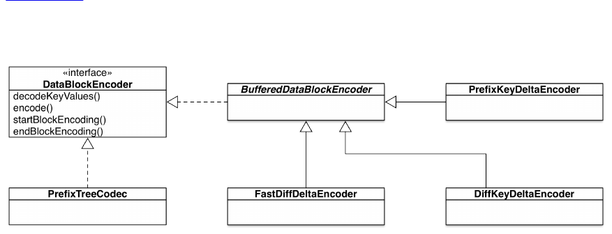
Available Codecs
HBase ships with a set of key encoder implementations, that vary mostly in the number of cell
components they handle, or how they encode the information. This spans from simple prefix
encoding, to more complex, search tree based algorithms, which optimize specific aspects of the
codec. Figure 10-5 shows an overview of the codec classes and their relationships, which are
sometimes named using Encoder as a suffix. This is a slight misnomer, as these classes contain
both encoding and decoding functionality, and should be considered full codecs.
Figure 10-5. The block encoder hierarchy
Refer to [Link to Come] for an overview of how a HBase cell, its lowest (that is, most basic) unit
of data, is structured. The overview explains the key components, such as row, column family,
column qualifier, and so on. For encoding, that layout is crucial, as it allows coverage of multiple
key components in one swoop. For example, consider the above section example with three rows
stored in the ops:metrics table. Since these cells are stored next to each other, and probably in the
same file, you can safely omit the column family name for all but the first cell in the same
containing HFile block. And since the family name is stored right after the row key, you can also
skip any additional checking of the family name when the row key is the same. This intrinsic
knowledge allows very efficient operations on the data, skipping any unnecessary comparison.
As an initial summary, here are all the available codecs with their short name, and information
regarding how far reaching their functionality is. They are described in the rest of this section in
detail:
Codec Short Key Value Description
none NONE No No For completeness. Disables encoding for the
given column family.
PrefixKeyDeltaEncoder PREFIX Yes No
Encodes repetitive prefix information for the row
key, and (if possible) the family, column
qualifier, and timestamp. The values are left as-is.
DiffKeyDeltaEncoder DIFF Yes No Covers the same cell details as PREFIX, but uses a
different encoding algorithm.
(789)
FastDiffDeltaEncoder FAST_DIFF Yes Yes Same as DIFF, but also omits repetitive cell values.
PrefixTreeCodec PREFIX_TREE Yes No Encodes the key using a tree structure. The values
are left as-is.
Caution
You need to use the short names for the key encodings as stated, or you will be returned an error
message instead. For example:
hbase(main):001:0> alter 'ops:metrics', { NAME => 'data', \
COMPRESSION => 'none', DATA_BLOCK_ENCODING => 'Prefix' }
...
ERROR: No enum constant \
org.apache.hadoop.hbase.io.encoding.DataBlockEncoding.Prefix
...
Each codec is also supplied with a context and state, which are used to track information across
every cell in its containing block. In other words, as a HFile block is created, the context
establishes the baseline for the encoder and defines the current encoding state, which can be used
to get access to the previous cell, or to other more advanced structures, such as tree data. At the
end of each block, the encoder also persists the state information, which includes either just
metadata, or the actual final tree data structures after they are compiled from all the cells that
have been encoded as part of the block. Similar, the decoder is supplied with just a context to
gain access to the persisted information that is needed to seek or decode cells as needed.
As for the native Java data types, all of the encoders further encode these into variable-length, or
7-bit, integers, resulting in one to five bytes being used. The most significant bit (MSB),
commonly used as the sign bit, is reserved to indicate if another byte is following. With that, you
can express, for example, the number 127 (0x7F) in a single byte as 0x7F, but 128 (0x80) would be
two bytes 0x81 0x00. When you remove the MSB for both bytes and then add them you get 000001
+ 0000000, which results in 10000000, or 0x80 again. Given you have short keys or values, say for a
serialized long counter you have 8 bytes, setting the integer-based length field to 8, you will save
three bytes most of the time when encoding takes place. In a worst case scenario though you will
need a total of five bytes to encode four source bytes due to the MSB being used differently.
The following uses a simplified example, for the sake of brevity. Imagine this table, showing two
different rows with multiple columns in each:
Key Len Value Len Row Key Col Fam Col Qual Timestamp Type Value
36 4 User1234 Orders OrderId-1 1473791347412 4 4321
36 4 User1234 Orders OrderId-2 1473791347412 4 5344
36 5 User1234 Orders OrderId-8 1473791363938 4 68582
(790)

37 5 User23456 Orders OrderId-1 1473791389274 4 93837
37 6 User23456 Orders OrderId-2 1473791452847 4 103833
… … … … … … … …
As a side note: The mutation type byte of a cell is indicating if the cell represents a put (here, "4")
or any of the possible delete operations. The latter are sorted at the beginning of a key range,
which is essential for the servers to see first what is removed from a row, before reading and
retaining any other cell while assembling the query result(s). Their actual value is an
implementation detail and should not be of concern for now.
The key length is the sum of all of the internal fields of the cell, including preceding length fields
for the column family and column qualifier. For the sake of example, we will not consider those
here, but just add the lengths of row key, column family, column qualifier, and timestamp. This
is very close to the real length, and makes the example easier to read.
BufferedDataBlockEncoder
This abstract base class is shared by many of the concrete implementations. It adds support
for, among other internal functionality, the optional encoding of cell tags. You can set this
as a property per column family, using, for example, the COMPRESS_TAGS option inside the
HBase Shell. The default is true, meaning tags are encoded implicitly. While the example
here is omitting tags, you can extend their encoding in the same manner as the other cell
fields are explained hereafter.
The particular encoding algorithm used for tags is based on a dictionary approach,
removing all duplicate entries by replacing it with a dictionary index ID (as a short value,
that is, using two bytes) pointing to the previous entry that matches. This is done inline
while the data block is written, which means that if you use the same tags for many cells
within one block, the majority of the tag data is replaced with two byte IDs, saving the
difference to their actual length.
PrefixKeyDeltaEncoder
The prefix based codec is the most basic one, which works by comparing the binary key
components in the order they are stored, while removing any shared common prefix. This
prefix can span the entire key length, all the way to the type byte indicating if the cell
represents a put or delete mutation. For the example table, we first encounter a difference
in the column qualifier of the first row, and then different cell timestamps, and so on,
resulting in the following cells being stored on disk:
Key
Len
Value
Len
Prefix
Len Row Key Col
Fam
Col
Qual Timestamp Type Value
36a4 0 User1234 Orders OrderId-
11473791347412 4 4321
(791)

14 4 22 --b2 1473791347412 4 5344
14 5 22 - - 8 1473791363938 4 68582
33 5 4 User Orders OrderId-
11473791389274 4 93837
14 6 23 - - 2 1473791452847 4 103833
… … … … … … … … …
a Italic numbers are variable-length encoded. For this example they would be one byte
only after encoding.
b A dash indicates that the value for this field has been completely omitted during the
encoding process.
The first cell is stored in its entire length, with just the internal key and value length
integers fields being serialized with variable-length encoding. After that, each subsequent
cell is stored encoded, provided that they share a common prefix at all. If the row key
component is identical to the previous cell, the encoder also omits the entire column
family, as it is redundant information at that point. This is the case when you have more
than one column per row, as the only difference for those is in the column qualifier and
(optionally) the cell timestamp. The last step is to check the column qualifier and cell
timestamp, removing any remaining shared details as well.
Note how there is an extra field value per cell (labeled Prefix Len in the table) that records
the length of the shared prefix, which is needed during the decoding phase later on to re-
add the proper prefix to the unique remainder that was stored in a subsequent cell. If you
have a different schema, for example one that uses cell versioning, you would save nearly
the full length of the entire key, storing just the different tail of the cell timestamp.
While probably a little too hard to read and for advanced reference only, here is the content
of the low-level store file of our earlier example, using a real-world schema. Instead of
using the HFile tool, we have to employ the Linux hexdump tool. It prints the actual binary
content of the store file, as opposed to the HBase supplied hfile tool, which is decoding
the data for you, thus not showing what the cells look like in their encoded form. Note the
highlighted full row key appearing only once, but not again for any of the other two cells.
The column family and column qualifier data:value (the colon is an API notation feature
that does not appear once the cell is serialized) are repeated for every cell, since the row
keys differ in our example using three separate rows:
$ $ hdfs dfs -text /hbase/data/ops/metrics/cc11...1611/ \
data/84a2...a950 | hexdump -c
0000000 D A T A B L K E \0 \0 \0 252 \0 \0 \0 246
0000010 377 377 377 377 377 377 377 377 002 \0 \0 @ \0 \0 \0 \0
(792)
0000020 307 \0 002 \0 \0 001 035 N \b \0 \0 9 9 b b f
0000030 8 8 3 d a 6 e c 6 2 f 4 a b 0 0
0000040 8 7 e a 5 3 9 d 5 c 7 2 | 1 2 4
0000050 4 3 2 5 | 3 3 4 2 2 | 1 4 7 3 7
0000060 9 0 6 1 0 004 d a t a v a l u e \0
0000070 \0 001 W ' 374 230 004 \0 \0 \0 \0 \0 \0 ~ 257
0000080 005 027 \b 7 1 9 3 2 004 d a t a v a l
0000090 u e \0 \0 001 W ' 374 s G 004 \0 \0 \0 \0 \0
00000a0 \0 \b 337 \a 027 \b 7 3 4 3 2 004 d a t a
00000b0 v a l u e \0 \0 001 W ' 374 316 235 004 \0 \0
00000c0 \0 \0 \0 \0 002 001 \t 215 202 N z B L M F B
00000d0 L K 2 \0 \0 \0 \f \0 \0 \0 \b 377 377 377 377 377
...
The entire data block is shown (note the magic bytes DATABLKE denoting this to be an
encoded data block), ending in the second last line (where the Bloom filter BLMFKLK2 magic
block marker starts). In summary, the prefix encoder removes any binary common prefix
between cells, and works most efficiently when you have more than a single column per
row. On the other hand, if you had large, completely random row keys, and large values
too, the encoding would add three extra bytes: two for the variable-length key and value
fields, requiring each five instead of four bytes, and, since there is no common key data, an
extra byte for the zero prefix length field.
DiffKeyDeltaEncoder
The Diff encoder fixes an important drawback of the prefix encoder: being able to omit
repetitive key information not just from left to right, using binary comparisons, but apply
the same for each key component separately. To do so, it needs to keep track of how the
current one differs from the previous one, and for that it adds a flags byte at the very
beginning of each encoded cell. The following flags are bits in that byte, recording the
vital comparison information:
Flag Bit Description
Same Key
Length 1 Set when the key length field is omitted.
Same Value
Length 2 Set when the value length field is omitted.
Same Mutation
Type 3 Set when the type field is omitted.
Timestamp
Different 4 Set when the internal timestamp of the cell is different.
Timestamp
Length
5-
7
Multiple bit record of the number of bytes used to encode the
timestamp difference.
Timestamp Sign 8 Tracks wether the given cell timestamp was positive or negative.
(793)
Most flags are single bits that are set when needed, while the timestamp length is using
multiple bits to record how many bytes the timestamp difference is encoded as. This saves
yet another length field being added. The following example (simplified again for the sake
of brevity) shows our example again, and what the encoded cells would be stored like:
Flag Key
Len
Value
Len
Prefix
Len Row Key Col
Fam
Col
Qual Timestamp Type Value
036 4 0 User1234 Orders OrderId-
11473791347412 4 4321
15
(00001111) - - 22 - - 2 0 - 5344
29
(00011101) -5 22 - - 8 16526 - 68582
28
(00011100) 37 5 4 User Orders OrderId-
125336 - 93837
29
(00011101) -6 23 - - 2 63573 - 103833
… … … … … … … … … …
As before, the first row is saved in its complete fidelity, but with the added flags and prefix
length fields. All length fields are encoded with variable-length as well. The difference to
the Prefix encoding is that each field is treated separately, and omitted whenever possible.
The single flags byte helps the decoder to determine per encoded cell what has been
persisted and what has been skipped, replacing the latter with the same field value from the
previous cell. One example is the mutation type field, omitted most of the time.
The cell timestamp is stored as a delta, as opposed to a binary prefix, allowing the decoder
to apply an addition function as opposed to a byte array manipulation. The length here is
mostly two bytes, setting bit five (as the decoder subtracts 1 from the length to save bits) as
well to denoted that fact, along with bit four to record the delta time as present.
The handling of column families is akin to the Prefix encoder, that is, the family name is
omitted as long as the row key is the same, since for a single HFile it is then guaranteed to
mean the previous and current cell belong to the same family. The column qualifier
handling is also the same, treating the value as a binary array and any shared prefix is
removed during the encoding.
(794)
The Diff encoder is more efficient compared to Prefix, as it performs more fine grained
operations on each cell component. Similar caveats and recommendations apply, that is,
the more repetition you have the better. If you store multiple columns in a row, you get the
same row key for each, can omit the family, and only store the difference for column
qualifier and cell timestamp. Lengths are variable-length encoded, and omitted, along with
other duplicate details, if possible. This will yield more efficient space usage both on disk,
the block cache, and in memory.
FastDiffDeltaEncoder
The Fast Diff encoder extends on the principles of the Diff encoder, but handles a few
things differently. First, the time is encoded using a binary prefix approach, as opposed to
a delta time. The length is encoded in the flags byte, but at a different position. This saves
the encoder from needing to handle negative timestamps, and reverts to what we have
already seen for the Prefix encoder. Second, this encoder also compares the value array,
and if identical to the previous cell, will omit the value for the current cell. This is once
again denoted as a new bit in the flags byte, for the decoder to handle appropriately.
Here are the flags for the Fast Diff encoder:
Flag Bit Description
Timestamp
Length
1-
3
Multiple bit record of the number of bytes used to encode the
timestamp difference.
Same Key
Length 4 Set when the key length field is omitted.
Same Value
Length 5 Set when the value length field is omitted.
Same Mutation
Type 6 Set when the type field is omitted.
Same Value 7 Set when the value is the same and is omitted.
Applying the changes in the encoding algorithm, we would end up with (roughly) the
following on storage, after the encoding of the example cells. Note that the cell timestamp
is actually encoded as an eight byte long value, so the prefix would be a binary array, and
the same applies to the remainder. The example uses the readable epoch digits for the sake
of argument:
Flag Key
Len
Value
Len
Prefix
Len Row Key Col
Fam
Col
Qual Timestamp Type Value
(795)

036 4 0 User1234 Orders OrderId-
1
1473791347412 4 4321
31
(00011111) - - 22 - - 2 2 - 5344
46
(00101110) -5 22 - - 8 63938 - 68582
38
(00100110) 37 5 4 User Orders OrderId-
189274 - 93837
45
(00101101) -6 23 - - 2 452847 - 103833
… … … … … … … … … …
Given you are expecting repetitive values, this encoder is even more efficient, and similar
pros and cons compared to the Diff encoder apply. The advantage of Fast Diff is its
enhanced performance, and the ability to also help with larger values—given they are
repeated between adjacent cells. In practice, this encoder is often the first choice when the
use-cases fit the pattern.
PrefixTreeCodec
The Prefix Tree encoder works completely differently from the earlier ones, applying a
tree data structure algorithm explained on the NIST Trie page. The name is written tree or
trie, as it is a tree structure used for fast retrieval of data. It trades encoding with decoding
performance, building lookup tables allowing the decoder to efficiently seek inside the
encoded data block they belong to.
There is a general issue with HBase HFile block sizing, as small blocks (< 16 KB) are
good for fast random access, but require more I/O calls to disk. Larger blocks (> 128 KB)
are much better I/O wise, but then the linear seeks inside are much less efficient. The
Prefix Tree encoding adds the necessary block structures to transform the linear seek into a
tree backed lookup.21
Showing the encoded data is inherently difficult, as binary tree structures are built and
persisted. We will refrain from attempting a visualization to spare you from the
unintelligible results.
Use the hbase hfile command line tool to print out the actual amount of data that is written to
storage. Compare unencoded data with encoded data, using a representative sample of what you
will be expecting on production, to gauge which of the encoder options is the most suitable for
your use-case. Prefix and Diff are likely to be bested in terms of effectiveness by Fast Diff, as the
(796)
latter is combining the best of the former, and also allows removal of duplicate values for an
even more dense encoding. In other words, start comparing Fast Diff with Prefix Tree, and add
Snappy or LZ4 compression to possibly gain some additional space savings.
Monitor carefully how adding encoding and compression is affecting your perceived latencies
and throughput, ensuring that using one or the other, or both, does not impose a penalty that
would inadvertently affect your use-case. Otherwise using both is likely to yield much more data
being held in cache and reduce overall storage I/O. You need to find the right balance, which can
only be done by carefully evaluating the options, and applying them in a test environment with
proper data.
(797)
Enabling Key Encoding
You can enable the key encoding on a per column family basis, using the DATA_BLOCK_ENCODING
property. For our initial real-world example, here is how you would disable the compression we
tried first, and at the same time enable Prefix encoding:
hbase(main):001:0> alter 'ops:metrics', { NAME => 'data', \
COMPRESSION => 'none', DATA_BLOCK_ENCODING => 'PREFIX' }
Updating all regions with the new schema...
0/1 regions updated.
1/1 regions updated.
Done.
0 row(s) in 6.4180 seconds
hbase(main):002:0> major_compact 'ops:metrics'
0 row(s) in 0.6220 seconds
We once again issue a major_compact shell command to force the changes being applied. We can
also verify with describe if the settings have been persisted to the table’s metadata:
hbase(main):003:0>
hbase(main):017:0> describe 'ops:metrics'
Table ops:metrics is ENABLED
ops:metrics
COLUMN FAMILIES DESCRIPTION
{NAME => 'data', DATA_BLOCK_ENCODING => 'PREFIX', BLOOMFILTER => 'ROW', \
REPLICATION_SCOPE => '0', VERSIONS => '1', COMPRESSION => 'NONE', \
MIN_VERSIONS => '0', TTL => 'FOREVER', KEEP_DELETED_CELLS => 'FALSE', \
BLOCKSIZE => '65536', IN_MEMORY => 'false', BLOCKCACHE => 'true'}
1 row(s) in 0.0320 seconds
(798)
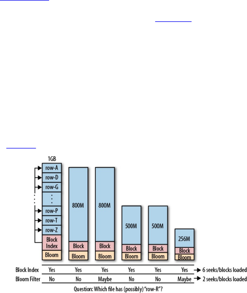
Bloom Filters
“Column Families” introduced the syntax to declare Bloom filters at the column family level,
and discussed specific use cases in which it makes sense to use them. As of HBase 0.96 the
default is to use the row based Bloom filter whenever you create a new column family. Given the
improvements of storing the filter as a multi-level index (see “Introduction”), this makes sense
and will improve many common use-cases.
The reason to use Bloom filters at all is that the default mechanisms to decide if a store file
contains a specific row key are limited to the available block index, which is, in turn, fairly
coarse-grained: the index stores the start row key of each contained block only. Given the default
block size of 64 KB, and a store file of, for example, 1 GB, you end up with 16,384 blocks, and
the same amount of indexed row keys. If we further assume your cell size is an average of 200
bytes, you will have more than 5 million of them stored in that single file. With that, and a
random row key you are looking for, it is very likely that this key will fall in between two block
start keys. The only way for HBase to figure out if the key actually exists is by loading the block
and scanning it to find the key.
This problem is compounded by the fact that, for a typical application, you will expect a certain
update rate, which results in flushing in-memory data to disk, and subsequent compactions
aggregating them into larger store files. Since minor compactions only combine the last few store
files, and only up to a configured maximum size, you will end up with a number of store files, all
acting as possible candidates to have some cells of the requested row key. Consider the example
in Figure 10-6.
Figure 10-6. Using Bloom filters to help reduce the number of I/O operations
The files are all from one column family and have a similar spread in row keys, although only a
(799)
few really hold an update to a specific row. The block index has a spread across the entire row
key range, and therefore always reports positive to contain a random row. The region server
would need to load every block to check if the block actually contains a cell of the row or not.
On the other hand, enabling the Bloom filter does give you the immediate advantage of knowing
if a file contains a particular row key or not. The nature of the filter is that it can give you a
definitive answer if the file does not contain the row—but might report a false positive, claiming
the file contains the data, where in reality it does not. The number of false positives can be tuned
and is usually set to 1%, meaning that in 1% of all reports by the filter that a file contains a
requested row, it is wrong—and a block is loaded and checked erroneously.
Note
This does not translate into an immediate performance gain on individual get operations, since
HBase does the reads in parallel, and is ultimately bound by disk read latency. Reducing the
number of unnecessary block loads improves the overall throughput of the cluster.
You can see from the example, however, that the number of block loads is greatly reduced,
which can make a big difference in a heavily loaded system. For this to be efficient, you must
also match a specific update pattern: if you modify all of the rows on a regular basis, the majority
of the store files will have a piece of the row you are looking for, and therefore would not be a
good use case for Bloom filters. But if you update data in batches so that each row is written into
only a few store files at a time, the filter is a great feature to reduce the overall number of I/O
operations.
Another place where you will find this to be advantageous is in the block cache. The hit rate of
the cache should improve as loading fewer blocks results in less churn. Since the server is now
loading blocks that contain the requested data most of the time, related data has a greater chance
to remain in the block cache and subsequent read operations can make use of it.
Besides the update pattern, another driving factor to decide if a Bloom filter makes sense for
your use case is the overhead it adds. For simplicity we can assume that every entry in the filter
requires about one byte of storage (which is 8 bit, see [Link to Come] for a more general
computation of Bloom filter sizes). Going back to the earlier example store file that was 1 GB in
size, assuming you store only counters (i.e., long values encoded as eight bytes), and adding the
overhead of the cell information—which is its coordinates, or, the row key, column family name,
column qualifier, timestamp, and type—then every cell is about 20 bytes (further assuming you
use very short keys) in size. Then the Bloom filter would be 1/20th of your file, or about 51 MB.
Now assume your cells are, on average, 1 KB in size; in this case, the filter needs only 1 MB.
Taking into account further optimizations, you often end up with a row-level Bloom filter of a
few hundred kilobytes for a store file of one or more gigabytes. In that case, using the filter
makes sense.
Bloom Filter Size
Computing the number of bits needed for an entry in a Bloom filter follows a fixed formula.
With that, the size of a Bloom filter really depends on how many keys you insert into it, and the
error rate you are willing to incur. Typically the latter is set to %1, which means that for every
100 keys you are filtering, you get one false positive. For region servers in HBase this means it
will load a block unnecessarily from storage.
(800)

With %1 error rate, you need about 10 bits for every inserted key, which you can multiply by the
number of cells you are expecting. This results in the size of the Bloom filter for a given amount
of data. The following Calca example (which you can copy and paste into Calca, and
subsequently modify to compute other sizes and combinations) computes the number of bits
needed for a specific error rate, by setting the number of inserted elements to one. After that it
computes the exact (theoretical) numbers for the earlier example, that is, 1 GB of cells data, and
1% of false positives:
# Compute Bloom Size
According to Wikipedia article
(https://en.wikipedia.org/wiki/Bloom_filter):
n = number of inserted elements.
p = false positive probability (i.e. error rate).
@precision = 2
number of bits = -((n * ln(p)) / (ln(2)^2)) in bits
number of bits(n = 1, p = 0.01) => 9.59 bits
number of bits(n = 1, p = 0.02) => 8.14 bits
number of bits(n = 1, p = 0.05) => 6.24 bits
fiftyK = number of bits(n = 50,000, p = 0.01)
=> 479,252.92 bits
oneM = number of bits(n = 1,000,000, p = 0.01)
=> 9,585,058.38 bits
Example:
data size = 1 GiB # size of the data blocks in one store file
cell size = 20 byte # payload and HBase internal cell details
error rate = 1%
cell count = data size / (cell size in GiB) => 53,687,091.2
bits needed = number of bits(n = cell count, p = error rate)
=> 514,593,903.26 bits
filter size = bits needed in MiB => 61.34 MiB
cell size = 1 KiB
cell count = data size / (cell size in GiB) => 1,048,576
bits needed = number of bits(n = cell count, p = error rate)
=> 10,050,662.17 bits
filter size = bits needed in MiB => 1.2 MiB
The final question is whether to use a row or a row+column Bloom filter. The answer depends
on your usage pattern: If you are doing only row scans, having the more specific row+column
filter will not help at all. The default row-level Bloom filter enables you to narrow down the
number of files that need to be checked, even when you do row+column read operations, but not
the other way around.
The row+column Bloom filter is useful when you cannot batch updates for a specific row, and
end up with store files which all contain parts of the row. The more specific row+column filter
can then identify which of the files contain the data you are requesting. Obviously, if you always
load the entire row, this filter is once again hardly useful, as the region server will need to load
the matching block(s) out of each file anyway.
Since the row+column filter will require more storage, you need to do the math to determine
whether it is worth the extra resources. It is also interesting to know that there is a maximum
number of elements a Bloom filter can hold. If you have too many cells in your store file, you
might exceed that number and would need to fall back to the row-level filter.
(801)
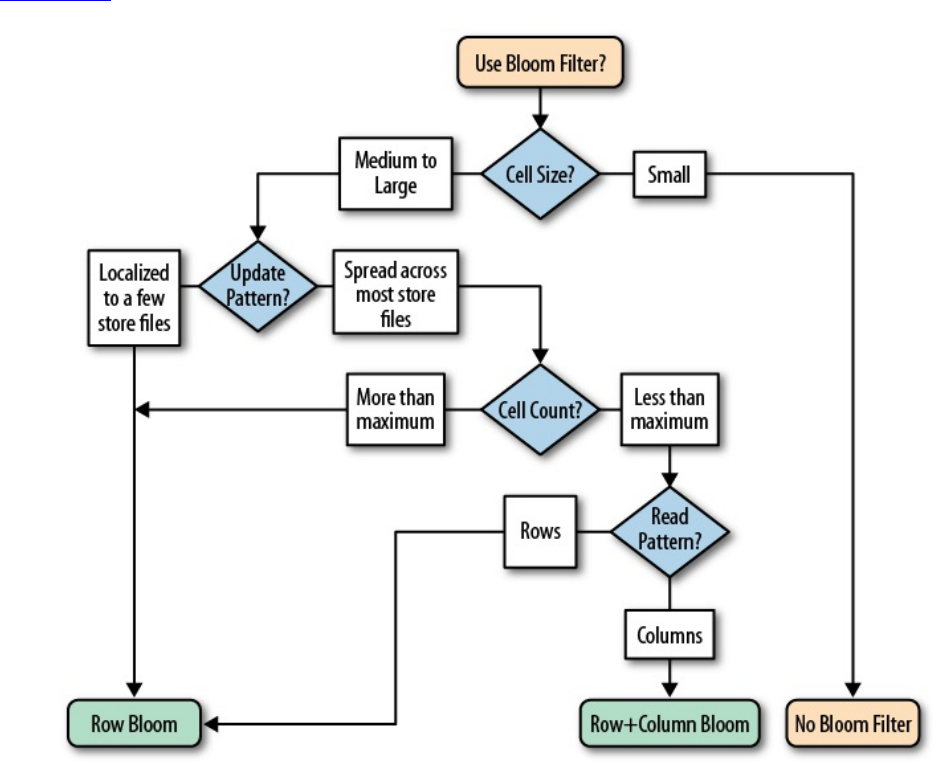
Figure 10-7 summarizes the selection criteria for the different Bloom filter levels.
Figure 10-7. Selection criteria for deciding what Bloom filter to use
Depending on your use case, it may be useful to disable the default row Bloom filter, to save
storage that is used up unnecessarily. Or switch to the more specific row+column Bloom filter, to
increase the overall performance of your system. As a general advice, you should leave the row-
level Bloom filter enabled, unless you have a good reason not to, as it strikes a good balance
between the additional space requirements and the gain in performance coming from its store file
selection filtering. Only resort to the more costly row+column Bloom filter when you would
otherwise gain no advantage from using the row-level one.
(802)
Region Split Handling
The built-in mechanisms of HBase to handle splits and compactions have sensible defaults and
perform their duty as expected. Sometimes, though, it is useful to change their behavior to gain
additional performance.
(803)

Number of Regions
As discussed throughout this chapter, you have a handful of configuration properties that you can
tune to optimize your HBase setup. Ultimately, HBase is hinged around memory and persistent
storage, with the servers constantly trying to use the most suitable area in an effort to provide the
fastest access to data. Both read and write operations are sharing the precious resources, and
striking a balance is important to not constrain one or the other eventually. The number of
regions has two separate levels of impact on capacity planning: the number of regions being
written to affects the memstore capacity, while the number of read-mostly regions is impacting
the remaining memory capacity of the server process.
While using the off-heap block cache (see “Block Cache Tuning”) is freeing memory for write
operations, you are still bound by the total heap assigned to each region server. The majority of
this space is divided across all regions, and when you reach its upper boundary, the servers start
to get under pressure. They are built to sustain peaks, but equally need time to catch up with the
overall workload. Ideally, you have a close eye on the number of regions per server and tables, as
too few could mean not enough parallelism, while too many could result in compaction storms.
“Cluster Sizing” goes it into more detail on how to do cluster sizing, but for the time being it
should be noted that you will need to do two things while setting up, and operating, a production
HBase cluster:
Presplit Tables
Presplit all tables, matching the expected key distribution ranges to achieve balanced
distribution of data across all servers. In addition, this should avoid region hotspotting
(when combined with proper key design, see “Time Series Data” for a specific use-case)
when it comes to reads and writes, which is a somewhat orthogonal problem (though
highly related).
Manage Region Count
After the presplit, you need to monitor the regions to determine if you have the right
amount of them. If you have too many, you need to increase the region size and merge
regions back together again. You should not have too few though, assuming you have done
proper presplit planning.
The following sections discuss the above in more detail. Also note that as of HBase 1.2, there is
also a region normalizer feature that, when enabled, is performing automated region splits and
merges to keep the region count of a cluster within some boundaries. You can read more about
that in [Link to Come]. Finally, [Link to Come] discusses the intricacies of splits in detail,
including an overview of the available split policies shipped with HBase.
(804)
Managed Splitting
Usually HBase handles the splitting of regions automatically: once the regions reach the
configured maximum size, they are split into two halves, which then can start taking on more
data and grow from there. This is the default behavior and is sufficient for the majority of use
cases. With the default policy and single region tables, you even get the advantage of splits
happening much sooner, bringing up the region count faster. This will increase parallelization
without having to presplit the table (though, as mention, you should always consider that latter
option).
There is one known problematic scenario, though, that can cause what is called split/compaction
storms: when you grow your regions roughly at the same rate, eventually they all need to be split
at about the same time, causing a large spike in disk I/O because of the required compactions to
rewrite the split regions. As explained in [Link to Come], these splits are queued and processed
by a thread pool, which is normally set to 1, meaning all splits are handled sequentially.
Rather than relying on HBase to handle the splitting, you can turn it off and manually invoke the
split command at your convenience. Disabling splits is accomplished by, for example, these two
methods:
Use Disable Region Split Policy
Configuring the DisabledRegionSplitPolicy class will effectively disable all compactions,
and you would need to trigger manual compactions as needed. Note that you must presplit
the table in question, and carefully monitor the manual or scripted splitting, or else you
will run into problems soon.
Set Large Region Size
Another option is setting the hbase.hregion.max.filesize to a very high number. Akin to the
former, setting this property to Long.MAX_VALUE is not recommended in case the manual
splits may fail to run. It is better to set this value to a reasonable upper boundary, such as
100 GB.
Note that both options can be set either for the entire cluster in the hbase-site.xml configuration
file, or at the column family level, when defining your table schema.
The advantage of running the command to split your regions manually is that you can time-
control them. Running them staggered across all regions spreads the I/O load as much as
possible, avoiding any split/compaction storm. You will need to implement a client that uses the
administrative API to call the split() method. Alternatively, you can use the shell to invoke the
commands interactively, or script their call using cron, for instance. Also see the RegionSplitter,
discussed shortly, for another way to split existing regions: it has a rolling split feature you can
use to carefully split the existing regions while waiting long enough for the involved
compactions to complete (see the -r and -o command-line options).
An additional advantage to managing the splits manually is that you have better control over
which regions are available at any time. This is good in the rare case that you have to do very
low-level debugging, to, for example, see why a certain region had problems. With automated
splits it might happen that by the time you want to check into a specific region, it has already
(805)
been replaced with two daughter regions. These regions have new names, and tracing the
evolution of the original region over longer periods of time makes it much more difficult to find
the information you require.
(806)

Region Hotspotting
Using the metrics discussed in “Region Server Metrics”,22 you can determine if you are dealing
with a write pattern that is causing a specific region to run hot. If this is the case, refer to the
approaches discussed in Chapter 8, especially those discussed in “Key Design”: you may need to
salt the keys, or use random keys to distribute the load across all servers evenly.
The only way to alleviate the situation is to manually split a hot region into one or more new
regions, at exact boundaries. This will divide the region’s load over multiple region servers. As
you split a region you can specify a split key, that is, the row key where you can split the given
region into two. You can specify any row key within that region so that you are also able to
generate halves that are completely different in size.
This might help only when you are not dealing with completely sequential key ranges, because
those are always going to hit one region for a considerable amount of time. “Key Encoding”
discusses a technique to group the timeseries into buckets, which will be the only remaining
option, short of randomizing the key and forfeiting time-based scanning.
Table Hotspotting
Sometimes an existing table with many regions is not distributed well—in other words, most of
its regions are located on the same region server. This means that, although you insert data with
random keys, you still load one region server much more often than the others. You can use the
move() function, as explained in “Cluster Operations”, from the HBase Shell, or use the Admin
class to explicitly move the server’s table regions to other servers. Alternatively, you can use the
unassign() method or shell command to simply remove a region of the affected table from the
current server. The master will immediately deploy it on another available server.
(807)
Presplitting Regions
Managing the splits is useful to tightly control when load is going to increase on your cluster.
You still face the problem that when initially loading a table, you need to split the regions rather
often, since you usually start out with a single region per table. Growing this single region to a
very large size is not recommended; therefore, it is better to start with a larger number of regions
right from the start. This is done by presplitting the regions of an existing table, or by creating a
table with the required number of regions.
The createTable() method of the administrative API, as well as the shell’s create command, both
take a list of split keys, which can be used to presplit a table when it is created. HBase also ships
with a utility called RegionSplitter, which you can use to create a presplit table, or split an
existing one at a later time. Starting it without a parameter will show usage information:
$ ./bin/hbase org.apache.hadoop.hbase.util.RegionSplitter
usage: RegionSplitter <TABLE> <SPLITALGORITHM>
SPLITALGORITHM is a java class name of a class
implementing SplitAlgorithm, or one of the special
strings HexStringSplit or UniformSplit, which are
built-in split algorithms. HexStringSplit treats
keys as hexadecimal ASCII, and UniformSplit treats
keys as arbitrary bytes.
-c <region count> Create a new table with a pre-split number of
regions
-D <property=value> Override HBase Configuration Settings
-f <family:family:...> Column Families to create with new table.
Required with -c
--firstrow <arg> First Row in Table for Split Algorithm
-h Print this usage help
--lastrow <arg> Last Row in Table for Split Algorithm
-o <count> Max outstanding splits that have unfinished
major compactions
-r Perform a rolling split of an existing region
--risky Skip verification steps to complete
quickly.STRONGLY DISCOURAGED for production
systems.
You need to specify either one of the supplied split algorithms, as stated in the command-line
help, or you can define your own algorithm by implementing the SplitAlgorithm interface
provided, and handing it into the utility using the fully specified class name (while making sure
your class is part of the Java class path). An example of using the supplied split algorithm class
and creating a presplit table is:
$ ./bin/hbase org.apache.hadoop.hbase.util.RegionSplitter \
-c 10 -f colfam1 testtable HexStringSplit
In the web UI of the master, you can click on the link with the newly created table name to see
the generated regions:
testtable,,1474660170667.a3d933c9770c7917e0204b931ad018de.
testtable,19999999,1474660170667.74da1d3c325190ed4534efe8488d7245.
testtable,33333332,1474660170667.c9288317826dd4d9b522442e6a1a0464.
testtable,4ccccccb,1474660170667.de631aa9082b1c27a7c82981cf05943c.
testtable,66666664,1474660170667.eecea2c0e8541d21670e85e8c412ea50.
testtable,7ffffffd,1474660170667.e3c46b25a00cace71ee4a0b83498c94e.
testtable,99999996,1474660170667.682e9bf2b2980fd87aeb9e6663d59c95.
testtable,b333332f,1474660170667.80537e3490878e8e4dfbdcbd1daf3b31.
testtable,ccccccc8,1474660170667.4a754d06c2d666cb10279e8465a4a3bb.
testtable,e6666661,1474660170667.3dd8e448e2b950743dad1ba8067a35ac.
Note
(808)

The HexStringSplit implementation splits the regions in equal distance sections, starting with
"00000000", and ending with "ffffffff". This is useful for application schemas that facilitate an
MD5 as the leading part of the row key. See “Key Encoding” for an example.
Or you can use the shell’s create command (here creating 15 regions):
hbase(main):001:0> create 'testtable', 'colfam1', \
{ NUMREGIONS => 15, SPLITALGO => 'HexStringSplit' }
0 row(s) in 1.1670 seconds
hbase(main):002:0> t = get_table 'testtable'
0 row(s) in 0.0760 seconds
=> Hbase::Table - testtable
hbase(main):003:0> t.get_splits
Total number of splits = 15
=> ["11111111", "22222222", "33333333", "44444444", "55555555", "66666666", \
"77777777", "88888888", "99999999", "aaaaaaaa", "bbbbbbbb", "cccccccc", \
"dddddddd", "eeeeeeee"]
This uses the same split algorithm as provided by the RegionSplitter class. You can also specify
your own split points, like so:
hbase(main):001:0> create 'testtable', 'colfam1', \
{ SPLITS => ['row-100', 'row-200', 'row-300', 'row-400'] }
0 row(s) in 1.1670 seconds
This generates the following regions:
testtable,,1474660840038.09c1de02beeb6a5db2684265a9b48108.
testtable,row-100,1474660840038.67e4722114a96159e7ac230daeded76e.
testtable,row-200,1474660840038.cdd0a630d9dc320e8cee928170f40124.
testtable,row-300,1474660840038.85ccf8a70da6d218d33d94bbb4001e12.
testtable,row-400,1474660840038.c03a4f8330cc68f556aebe97d19b8c86.
There is also an option SPLITS_FILE, which allows storage of the split points row by row in an
external file, which is then handed into the command. This is especially useful for tables with
many split points.
As for the number of presplit regions to use, you can start low with 10 presplit regions per server
and watch as data grows over time. It is better to err on the side of too few regions and use a
rolling split later, as having too many regions is usually not ideal in regard to overall cluster
performance.
Alternatively, you can determine how many presplit regions to use based on the largest store file
in your region: with a growing data size, this will get larger over time, and you want the largest
region to be just big enough so that is not selected for major compaction—or you might face the
mentioned compaction storms.
If you presplit your regions too thinly, you can increase the major compaction interval by
increasing the value for the hbase.hregion.majorcompaction configuration property. If your data
size grows too large, use the RegionSplitter utility to perform a network I/O safe rolling split of
all regions.
Use of manual splits and presplit regions is an advanced concept that requires a lot of planning
and careful monitoring. On the other hand, it can help you to avoid the compaction storms that
can happen for uniform data growth, or to shed load of hot regions by splitting them manually.
(809)

Merging Regions
While it is much more common for regions to split automatically over time as you are adding
data to the corresponding table, sometimes you may need to merge regions—for example, after
you have removed a large amount of data and you want to reduce the number of regions hosted
by each server. This can be achieved in a few ways, explained in detail next. Also see “Region
Ergonomics” for an automated way of managing the number of regions within a cluster.
(810)

Online: Merge with API and Shell
[Link to Come] explains the intricacies of the region merging functionality supplied by HBase.
As with many server features, there are multiple ways to invoke the operation, which here is
provided by a shell command, and a matching administrative API method. Example 5-15 shows
the API call, splitting and subsequently merging regions. As for the corresponding shell
command, here is an example that shows the functionality in action:
hbase(main):001:0> create 'testmerge', 'colfam1', \
{ NUMREGIONS => 2, SPLITALGO => 'HexStringSplit' }
0 row(s) in 1.3010 seconds
=> Hbase::Table - testmerge
hbase(main):002:0> get_table('testmerge').get_splits
0 row(s) in 0.0100 seconds
Total number of splits = 2
=> ["80000000"]
hbase(main):003:0> merge_region 'cb93020383d7939722dc093804ac1535', \
'a72f5aa5a84af7d0b44b20768c34b9f3'
0 row(s) in 0.0320 seconds
hbase(main):004:0> get_table('testmerge').get_splits
0 row(s) in 0.0000 seconds
Total number of splits = 1
=> []
The example first creates a table with two regions, that is, a presplit table, confirmed by querying
the number of start keys with get_splits. Then the regions are merged, using the merge_region
shell command, taking the encoding region names as parameters. The ones shown are specific to
the test environment, and yours will most certainly vary. The hashes were determined using the
web-based UI (see “Table Information Page”), where the hashes are displayed as the postfix to
the readable region names.
Once again, the example confirms that the merge command has taken effect by querying the
number of “splits” (which in fact is returning the start keys of the current table regions, while
omitting the always empty first one). The method returns 1, which is what we expected.
Obviously, you can also use the table detail UI page again to see the new single, merged region
where before you had two presplit ones.
(811)
Offline: Merge Tool
HBase ships with a tool that allows you to merge two adjacent regions as long as the cluster is
not online. You can use the command-line tool to get the usage details:
$ bin/hbase org.apache.hadoop.hbase.util.Merge
For hadoop 0.21+, Usage: bin/hbase org.apache.hadoop.hbase.util.Merge \
[-Dfs.defaultFS=hdfs://nn:port] <table-name> \
<region-1> <region-2>
Here is an example of a table that has more than one region, all of which are subsequently
merged:
$ bin/hbase shell
hbase(main):001:0> create 'testtable', 'colfam1', \
{ SPLITS => ['row-10','row-20','row-30','row-40','row-50'] }
0 row(s) in 0.2640 seconds
hbase(main):002:0> for i in '0'..'9' do for j in '0'..'9' do \
put 'testtable', "row-#{i}#{j}", "colfam1:#{j}", "#{j}" end end
0 row(s) in 0.1280 seconds
0 row(s) in 0.0050 seconds
...
hbase(main):003:0> flush 'testtable'
0 row(s) in 0.2000 seconds
hbase(main):004:0> scan 'hbase:meta', { COLUMNS => ['info:regioninfo']}
ROW COLUMN+CELL
...
testtable,,1475066895959.cc3c952371f4eca2b11e6a8362250b21. \
column=info:regioninfo, ... STARTKEY => \
'', ENDKEY => 'row-10'}
testtable,row-10,1475066895959.77cda2eedabf46bc6cdd490c2190 \
76e3. column=info:regioninfo, ... STARTKEY => \
'row-10', ENDKEY => 'row-20'}
testtable,row-20,1475066895959.7dd53e36213ad9c03b2736319365 \
e7d9. column=info:regioninfo, ... STARTKEY => \
'row-20', ENDKEY => 'row-30'}
testtable,row-30,1475066895959.3bc7f185e33dc1ddc4a1616c22eb \
21dc. column=info:regioninfo, ... STARTKEY => \
'row-30', ENDKEY => 'row-40'}
testtable,row-40,1475066895959.2d9f7f2b20411f4fce69a1c68741 \
f576. column=info:regioninfo, ... STARTKEY => \
'row-40', ENDKEY => 'row-50'}
testtable,row-50,1475066895959.8ff119f506b62a3c9bb0f68bbe5c \
f5ca. column=info:regioninfo, ... STARTKEY => \
'row-50', ENDKEY => ''}
7 row(s) in 0.0720 seconds
hbase(main):005:0> exit
$ bin/stop-hbase.sh
$ bin/hbase org.apache.hadoop.hbase.util.Merge testtable \
testtable,row-20,1475066895959.7dd53e36213ad9c03b2736319365e7d9. \
testtable,row-30,1475066895959.3bc7f185e33dc1ddc4a1616c22eb21dc.
...
2016-09-28 14:52:57,320 INFO [main] util.Merge: \
Verifying that file system is available...
2016-09-28 14:52:57,329 INFO [main] util.Merge: \
Verifying that HBase is not running...
...
2016-09-28 14:53:05,807 INFO [main] regionserver.HRegion: starting \
merge of regions: \
testtable,row-20,1475066895959.7dd53e36213ad9c03b2736319365e7d9. and \
testtable,row-30,1475066895959.3bc7f185e33dc1ddc4a1616c22eb21dc. \
(812)
into new region \
testtable,row-20,1475067185806.52ce0b01e535bdb9c44afef751630bc5. \
with start key <row-20> and end key <row-40>
...
2016-09-28 14:53:06,041 INFO [main] regionserver.HRegion: merge completed. \
New region is \
testtable,row-20,1475067185806.52ce0b01e535bdb9c44afef751630bc5.
Caution
The default shell login is very verbose, and will include some messages that look worrying, such
as warnings and errors from the ZooKeeper client library. These can be safely ignored, while
keeping an eye on the "merge completed" message instead.
The example creates a table with five split points, resulting in six regions (plus an internal one,
not shown here). It then inserts some rows and flushes the data to ensure that there are store files
for the subsequent merge. The scan is used to get the names of the regions, but you can also use
the web UI of the master. For example, click on the table name in the User Tables section to get
the same list of regions.
Note
Note how the shell wraps the values in each column. The region name is split over two lines,
which you need to copy and paste separately. The web UI is easier to use in that respect, as it has
the names in one column and in a single line.
The content of the column values is abbreviated to the start and end keys. You can see how the
create command using the split keys has created the regions. The example goes on to exit the
shell, and stop the HBase cluster. Note that HDFS still needs to run for the merge to work, as it
needs to read the store files of each region and merge them into a new, combined one.
Finally, we can confirm the merge has taken place by using the meta table scan again (here
abbreviated even further, as the start key of also part of the row key), or the get_splits shell
command, introduced in the previous section:
$ bin/start-hbase.sh
$ bin/hbase shell
hbase(main):001:0> scan 'hbase:meta', { COLUMNS => ['info:regioninfo']}
ROW COLUMN+CELL
hbase:namespace,,1475065977849.486bfd49a141c95be66d7ffce3ad ...
testtable,,1475066895959.cc3c952371f4eca2b11e6a8362250b21. ...
testtable,row-10,1475066895959.77cda2eedabf46bc6cdd490c2190 ...
testtable,row-20,1475067185806.52ce0b01e535bdb9c44afef75163 ... \
... STARTKEY => 'row-20', ENDKEY => 'row-40'}
testtable,row-40,1475066895959.2d9f7f2b20411f4fce69a1c68741 ...
testtable,row-50,1475066895959.8ff119f506b62a3c9bb0f68bbe5c ...
6 row(s) in 0.3120 seconds
hbase(main):001:0> get_table('testtable').get_splits
0 row(s) in 0.0140 seconds
Total number of splits = 5
=> ["row-10", "row-20", "row-40", "row-50"]
Both show that "row-30" is now gone, as it was merged with "row-20". This is also visible from
the start and end key of that region, spanning from "row-20" to "row-40", subsuming the region
that started with "row-30".
(813)

Region Ergonomics
Table region normalization was introduced in HBase 1.2.0, allowing the master process to
normalize regions in size for any given table in check periodically, on your behalf. While it is
automating the merge process, it is also advising on splits, helping to keep the regions in size at
an appropriate level. Before we look into the particulars, here is the list of options you can use to
tune the normalization functionality:
Table 10-10. Normalization related configuration properties
Property Default TableaDescription
hbase.normalizer.period 300000 (5 mins) No Period at which the region
normalizer runs in the master.
hbase.master.normalizer.class SimpleRegionNormalizer No
Class used to execute the region
normalization when the period
occurs.
a No - Can only be set cluster-wide; Yes - Set cluster-wide, but can be overwritten on the table
level
The functionality to monitor your tables, and initiate a region merge and/or split if necessary, is
provided by the RegionNormalizer implementations. As of this writing, there is only one available,
named SimpleRegionNormalizer. Its functionality is hardcoded and not changeable right now,
performing the following tasks:
1. Retrieve all regions for the given table
2. Compute the average region store size (sum of all stores within that region) across all
regions
3. Seek every single region one by one. Check if a region R0 is larger than two times the
average region store size, and if so
advise for this region to split, and
evaluate the next region R1.
4. Otherwise, check if the size of sum of the two regions R0 + R1 is less than the average, and
if so
advise for these two regions to be merged, and
evaluate the next region R2 and continue the steps for every single region until the
last region within the table.
(814)

Once the normalizer class collects all of the regions to be split or merged within the given table,
the master process triggers the actual work per the plan one by one. Region sizes are coarse and
approximate on the order of megabytes. Additionally, “empty” regions (less than 1MB, with the
previous note) are not merged away. You may have noticed that by default normalization is
turned off, which means an administrator needs to enable it explicitly via the API or the HBase
Shell. It is one of those newer features added to HBase, and will change how regions are sized. It
makes sense to require an explicit opt-in for it, instead of potentially rearranging an existing
cluster automatically. In addition, you need to also enable this feature per table descriptor. As
introduced in “Table Properties”, the setNormalizationEnabled() method can be used to switch the
flag for a given table using the administrative API like so:
TableName tableName = TableName.valueOf("testtable");
HTableDescriptor htd = admin.getTableDescriptor(tableName);
htd.setNormalizationEnabled(true);
admin.modifyTable(testTable, htd);
In addition, the shell also has the matching wrappers for the administrative API methods,
allowing the operator of a cluster to influence the global normalizer functionality (see “Tool
Commands” for an overview). You can use the normalize shell command to initiate a cluster-
wide normalizer run, affecting all tables which have been instrumented as shown above (that is,
the table property NORMALIZATION_ENABLED has been set to true), and assuming the normalizer is
enabled. The latter is toggled using the normalizer_switch command, and its state is queried with
normalizer_enabled, for example, using the following syntax:
hbase(main):001:0> disable 'testtable'
hbase(main):002:0> alter 'testtable', 'NORMALIZATION_ENABLED' => true
hbase(main):003:0> normalizer_switch true
hbase(main):004:0> normalizer_enabled
true
hbase(main):005:0> enable 'testtable'
(815)
Compaction Tuning
As explained on a more technical level in [Link to Come], HBase has a background janitorial
task that strives to keep the number of storage files at a reasonable level, in a process called
compaction. While files are rewritten, these compactions contribute to the overall read
performance of the cluster, as related data is colocated and written into the same data blocks. In
addition, specific types of compactions can also apply the explicit and predicate deletes
accumulated beforehand, possibly reducing the storage footprint of a HBase instance in its wake.
(816)

Compaction Settings
Compactions can be tuned to fit use-cases better, as their defaults are rather aggressively aiming
at keeping the number of files low. There are situations where this is not needed, for example
when you are doing random gets of entities that never change once they have been stored. In that
case you should rely on the row Bloom filter to efficiently load only the one block that holds the
data, making the number of store files irrelevant. In such a scenario, you could tune the
hbase.hstore.compaction.ratio property down from the default 1.2 to, for example, 1.0, or even
less. This would make the inclusion of larger HFiles rather infrequent, and calm down the
compaction eagerness. For reference, we are going to discuss the scenarios presented in
Figure 10-8.
Keep in mind that the examples are simplified to help explain the compaction settings. Notably,
the number and size of the store files have been selected in an effort to construct a real-life
situation—though in practice you will certainly see varying numbers. It is important to
understand the affects of the various settings, and apply them as needed.
(817)
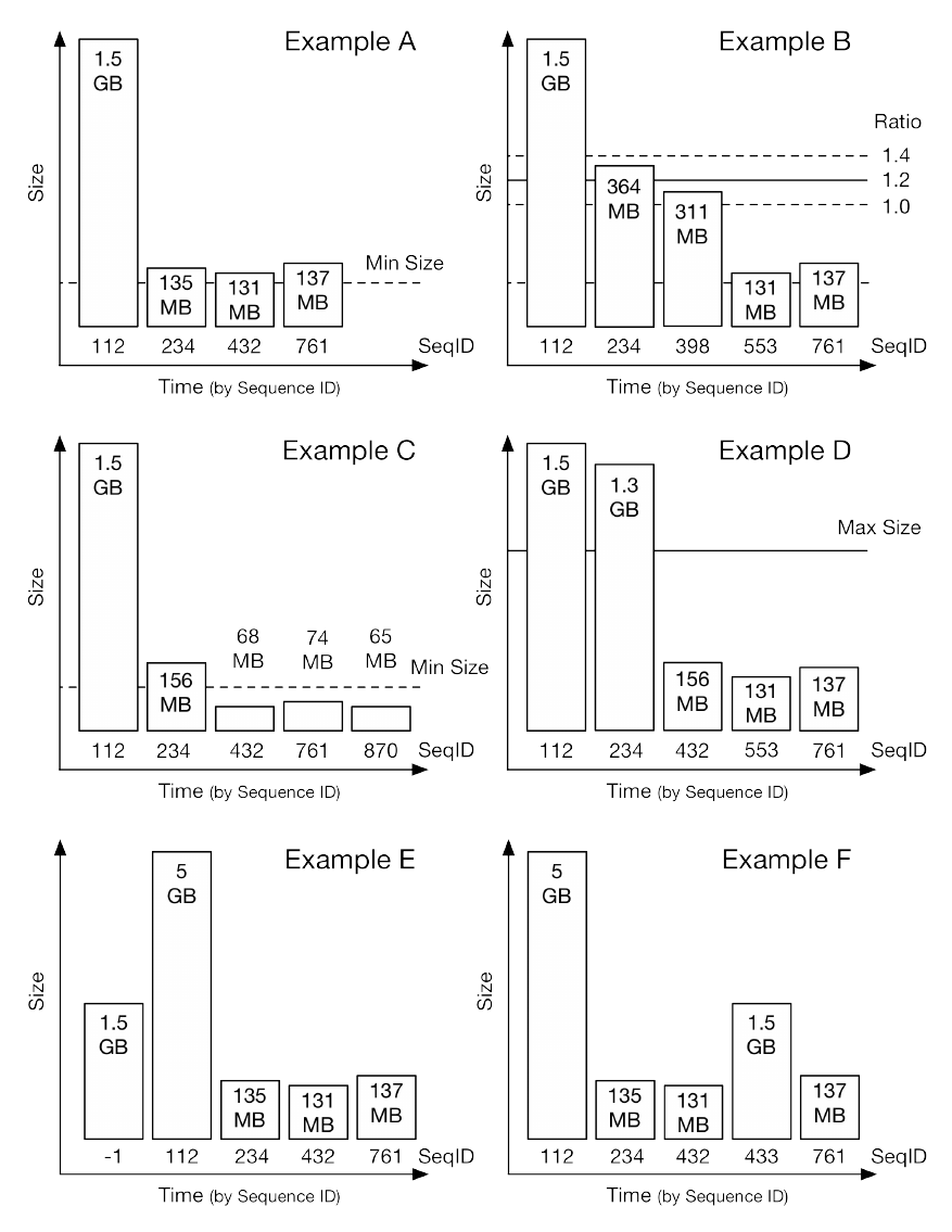
Figure 10-8. Example storage file layouts
Recapping the labels, the min size is the configured minimum size of files to be included in the
compaction selection, without further checking. The ratio is the percentage defining how many
larger files are included in the selection process: the larger the ratio, the more aggressively larger
files are included, and the lower the ratio, the fewer files are included. The SeqID is the sequence
ID of the last mutation (which, in general, is the result of either a put or a delete operation)
included in the file, which is a monotonically increasing number per region server that is used to
(818)
order modifications from clients. The sequence ID allows determination of how old the contents
of a store file are, as all other mutations in that file are older than the stated ID. Finally, the Size
is given per HFile, along with its unit (that is, gigabyte or megabyte).
Example A
This file layout is the most common one, as the flush size is set by default to 128 MB, and
it is checked after a mutation was added to its corresponding memstore. In other words, if
the cluster has enough memory and is not under pressure I/O wise, all flushed out data
should end up in files slightly larger than the configured flush size. With that, all of the
newly written files are larger than the default hbase.hstore.compaction.min.size setting,
which is the same as the flush size.
In the example, the three newest files (sorted to the right, by their ascending sequence
number) are automatically included in the compaction selection, and would trigger a minor
compaction. The minor compaction is attributed to the compaction ratio, explained in
Example B.
Example B
After a few compactions, you may encounter a file layout more akin to what this example
shows: there are newer, smaller files, and a few older, larger files that are the result of
previous compactions. Here is now where the compaction ratio comes into play, helping
the selection process to decide which files to include in the next compaction. The math is
such that all files are tested by size (and age) to see if they are within a certain size
threshold, while the selection will eventually stop considering files for compaction
inclusion, if it encounters large enough storage files.
In the example the newest flush files are 137 MB and 131 MB in size, which combined
makes 268 MB. With the default ratio of 1.2 the selection will also include the next file of
311 MB, as 1.2 * 268 MB = 321.6 MB, and that is more than 311 MB. The selection is
now at 268 MB + 311 MB, that is, 579 MB. Again, the next file at 364 MB is also under
the ratio of 1.2 * 579 MB = 694.8 MB, bringing the compaction to selection size to 934
MB. But here it ends as 1.2 * 934 MB = 1120.8 MB, and that is less than the remaining 1.5
GB file, which is therefore excluded and the compaction turns into a minor one.
Had you set the ratio to 1.0 (or 0.8, which would cause the same behavior), you would
have no compaction at all! This is because the initial two files at 268 MB are less than the
311 MB file next to them, resulting in only two files being selected, and that is less than
the default hbase.hstore.compaction.min threshold of 3 files.
The effect of the ratio becomes much more obvious with larger region sizes and when you
approach a higher fill level. Only then will the ratio based check start excluding larger,
older files. For example, setting the ratio to something low like 0.25 will eventually result
in about four store files remaining (different by a quarter in size).
Off-peak Ratio
Since setting the compaction ratio is tuning how aggressively the compaction is selecting files,
you may want to set different ratios according to how busy the cluster is: during peak hours you
may want to reduce the ratio, while at off-peak you may want to ramp it up to use the free I/O
(819)

resources for catching up with accrued storage files. The hbase.hstore.compaction.ratio.offpeak
property defaults to 5.0, which would cause files five times the size of the already selected file to
be included—which would often mean all of them, resulting in an auto-promoted major
compaction.
Off-peak is disabled by default, as both hbase.offpeak.start.hour and hbase.offpeak.end.hour are
set to -1. Enabling the off-peak requires you to set both to form a proper time range, specified in
full hours, with the start being inclusive, and end being exclusive. For example, the following
sets the off-peak time to start at 10PM, and end at 4AM in the morning:
<property>
<name>hbase.offpeak.start.hour</name>
<value>22</value>
</property>
<property>
<name>hbase.offpeak.end.hour</name>
<value>04</value>
</property>
Using the higher off-peak ratio is especially useful when you have tuned the on-peak ratio down,
to retain more store files in a trade-off to have fewer large compactions running asynchronously
with your business workloads. If you have a bell-curve like distribution of load, you could use
the slow time to catch up with the number of files.
Example C
This diagram shows you what happens when you have many premature flushes happening,
caused by oversubscribing the available memstore memory. The newer store files are all
under the configured (we assume defaults here) flush size, falling under the minimum
compaction size. This forces the compaction selection to unconditionally include them into
the next compaction, and with the default ratio the fourth file is included as well.
While this seems reasonable in this scenario, you have to note that this compaction will
have to rewrite about 160 MB, just to merge in about 5 MB of new data. With a cluster
that is heavily write loaded, you would constantly flush small files, and subsequently the
compactions will merge them into much larger files eventually, causing a so-called
compaction storm. This is why calculating the required heap size or the number of regions
(see “Number of Regions”) is vital for a good sustained HBase performance.
Example D
As described earlier, if your use-case is such that you can allow for more store files to stay
around (since the Bloom filter is effective for you), setting
hbase.hstore.compaction.max.size to a specific upper limit will result in files that pass this
limit to not be compacted anymore. With that you can stop minor compactions from
constantly merging all store files, which commonly happens with the default settings.
The caveat, besides degrading read performance for use-cases where the Bloom filters do
not work well, is that deletes are only applied during the scheduled major compactions, or
when the region eventually splits and is rewritten. This may have an impact if you remove
data frequently, delaying the reclamation of the storage space.
Note that there is also hbase.hstore.compaction.max.size.offpeak, allowing you to tune the
maximum size of files to be considered for compactions differently during off-peak hours
(if configured at all). Its default is the same as hbase.hstore.compaction.max.size, so even if
(820)
you enable off-peak for a different compaction ratio setting, the maximum file size limit
stays the same, unless you opt to change it explicitly.
Example E
When you bulk data into HBase, there is a special situation when it comes to ordering store
files for compactions: newly loaded files are created out-of-bands, meaning they have no
sequence ID that was created as part of the region server internal MVCC (see [Link to
Come]). This number is crucial in multiple ways, as it first orders mutations as far as client
applications are concerned (that is, defining the current state of a value in a particular
column). Second, the ID also orders the bulk load files such that a compaction might not
see them, assuming it has seen all possible files and auto-promotes the compaction to a
major one.
For the bulk load tool this was fixed by assigning a sequence ID to the bulk load files (set
with hbase.mapreduce.bulkload.assign.sequenceNumbers and default to true). Since files
cannot be mutated in storage, this is accomplished by renaming the file and adding the
sequence ID to its name, combined with a known prefix (that is, SeqId_) so that later
processes can parse it properly. With that, on opening the file the single sequence ID is
assigned to all edits in the respective file, making its content appear atomically.
In other words, as long as you use the default settings, the situation depicted in this
example should not occur, unless you have explicitly disabled the assignment of a
sequence ID during bulk loading. There are use-cases where this makes sense, as assigning
a sequence ID is forcing the servers to flush the memstores in an attempt to get the next ID
that falls between the last in-memory edits and any subsequent one. If you are loading, for
example, historical data only, which never overrides current one, you could skip this step.
But then you are back at the scenario depicted here, and compactions might be
problematic.
As of HBase 0.98 the default exploring compaction policy is handling bulk files fine, and
you are free to skip the assignment of sequence IDs to bulk files. The newer policy orders
the files by size and ID and can figure out the best constellation, avoiding erroneously
scheduled major compactions.
Example F
Finally an example showing what could happen if you (hopefully unintentionally) created
a very large cell that causes a flushed store file to grow much larger than the configured
upper threshold. Another possible reason for a layout shown in this example is many
flushes happening at about the same time, queueing them up for processing when the flush
worker pool has spare capacity. If HDFS is under pressure already at that point in time,
you may see slow flushes happening, while those queued memstores are still taking on
writes from clients. This can increase their size considerably (as explained in [Link to
Come]), leaving you with a skewed file size distribution.
Just as with the previous example, the exploring compaction policy is able to handle such
file skew, concentrating the compaction on the smaller files to make the compaction
worthwhile.
Obviously, these examples are simplified and represent a few selected (though common)
scenarios only. They do help though in understanding how you could potentially tune the
(821)
compactions cluster-, table-, or column family-wide to achieve the best balance of background
I/O (which compactions and flushes are responsible for) and client generated traffic. You need to
ensure all tests are done with the expected production data, or all optimizations might be ill-
advised once the load changes. And speaking of change, with every new workload onboarded to
an existing, shared cluster you should ascertain that the current settings are still valid, or if they
have to be adjusted accordingly.
(822)

Compaction Throttling
HBase provides two distinct mechanism to control how compactions are handled: a thread pool-
based throttling, and a throughput controller that keeps the storage I/O under control. Each of
these are discussed separately next.
Thread Pool Throttling
The technical details about compaction throttling are explained in [Link to Come]. Since both the
large and small compaction pool start at one worker thread by default their number can be used
to fine tune a larger cluster, setting the throttle threshold and thread count as needed. For
example, you could increase the small compaction thread pool to process those faster, and leave
the large compaction pool at a lower number for limited throughput. On the other hand, you can
also reduce the size threshold and allow mostly system tables to be compacted timely with a
single handler thread, while increasing the larger thread pool size for all user table processing.
Obviously, using two pools with a single threshold classifying what goes where, and then using
threads as a measure of throttling is rather coarse grained in comparison. In addition, each
compaction is trying to complete as fast as it can, causing possible spikes in I/O load. The
throughput controller, discussed next, mitigates this problem.
Throughput Controller
Besides being able to control the parallelism of compactions using the thread pool-based
throttling, you have further control over each compaction by means of the throughput controller.
In fact, this is not a single controller, but an entire hierarchy of controllers, as shown in
Figure 10-9.
(823)
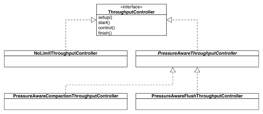
Figure 10-9. The throughput controller hierarchy
Before we dive deeper, here is the list of options pertaining to the compaction throughput
controllers:
Table 10-11. Pressure-aware compaction controller related options
Property Default Description
hbase.regionserver.throughput.controller NoLimitCompactionThroughputController
Sets the controller class
used by the region
server process.
hbase.hstore.compaction.throughput.lower.bound 10L * 1024 * 1024 (10 MB/s)
The lower throughput
boundary for a running
compaction.
hbase.hstore.compaction.throughput.higher.bound 20L * 1024 * 1024 (20 MB/s) The same, but for the
upper boundary.
hbase.hstore.compaction.throughput.offpeak Long.MAX_VALUE
The single throughput to
be used during off-peak
hours (if configured
using
hbase.offpeak.start.hour
and
hbase.offpeak.end.hour
Default means it is
unlimited.
hbase.hstore.compaction.throughput.tune.period 60 * 1000 (1 min)
Time how often the
system checks the
server-wide compaction
(824)

pressure.
You can override the controller using hbase.regionserver.throughput.controller, which is set by
default to the NoLimitCompactionThroughputController class. Note as well how the same class
hierarchy is used by flushes (see “Region Flush Tuning”). The default class implements a
straight no-op, which means it does not throttle anything at all. In practice, this is the same
behavior provided by HBase in all its previous versions. Only when you switch to the
PressureAwareCompactionThroughputController class, do you start having control over the
compaction I/O. For example, enabling the controller alone will cause for I/O to be limited based
on the default setting, which is 10-20 MB/s (as shown in the table) for on-peak hours:
<property>
<name>hbase.regionserver.throughput.controller</name>
<value>org.apache.hadoop.hbase.regionserver.throttle. \
PressureAwareCompactionThroughputController</value>
</property>
Note
The pressure-aware controller starts initially at the lower boundary, and would increase as
needed from there. In other words, it starts at 10 MB/s and then, every minute, adjusts the speed
as necessary between the two boundary limits.
Whether the single off-peak limit should be used depends on your setup, as the off-peak hours
also influence other parts discussed in this chapter, like, for example, major compactions. Its
default is unlimited (as it is set to the highest possible throughput value), and should be adjusted
accordingly if you want to limit compactions while having off-peak hours configured.
The controller is regularly updated (default is every minute, set with
hbase.hstore.compaction.throughput.tune.period) by the region server about the current pressure
it is experiencing. This is done using the following steps
1. Iterate over all open regions this server is hosting.
2. Iterate over all the stores contained in these regions.
3. Find the one store with the highest pressure and report its pressure back.
The pressure itself is measured by how many HFiles a store has, above the minimum compaction
size (hbase.hstore.compaction.min, defaulting to 3) and before it reaches the maximum number of
files allowed, causing the memstore flushes to be delayed (set by
hbase.hstore.blockingStoreFiles, defaulting to 10, while the delay is 90000, or 90 seconds, set by
hbase.hstore.blockingWaitTime). Assuming you have three store files, the pressure would be 0.0,
with six files the pressure would be 0.43 (rounded), and with 10 files you would get 1.0, or
100%. Once the memstores block for 90 seconds, they are flushed again, possibly raising the
number of files further, which results in a pressure of over 1.0, or larger than 100%.
The pressure-aware controller uses that percentage to adjust the throughput between the lower
and upper boundary, or 10 to 20 MB/s with the default values. Any pressure over 100% is will
cause for the upper boundary to be ignored completely, which means unlimited throughput.
During the compaction execution, the control() method is invoked for every cell that is written
to the new, compacted store file, making the compaction thread sleep long enough to match the
(825)
computed throughput, based on the current pressure. In effect, throughput is controlled by
starving the current compaction thread in an attempt to achieve the proper throughput.
As mentioned, the controller is set on the region server level, and takes the highest compaction
pressure to adjust all running compactions (which is controlled by the thread pool-based
compaction throttling described above). This is a simplification, based on the assumption that a
single server experiencing compaction pressure will have the same issue sooner or later for all
compactions, as they share the same storage backend. This holds true mostly for HDFS on bare
metal with JBOD configuration, but may not be the case for other storage backends, providing
independent (and more so different) writer throughput. Choose carefully and, as usual, test
thoroughly.
(826)

Region Flush Tuning
Akin to the compaction throughput control, there is also support to control the flush write
throughput. See [Link to Come] for the technical explanation of flushes. As shown in Figure 10-
9, the compaction and flush code share the same class hierarchy and default controller, one that
is not imposing any controls at all. There is a special derived class that can be used to switch on
throughput control, though before we dive deeper, here is the list of options pertaining to the
flush throughput controllers:
Table 10-12. Pressure-aware flush controller related options
Property Default Description
hbase.regionserver.flush.throughput.controller NoLimitCompactionThroughputController
Sets the
controller
class used
by the
region
server
process.
hbase.hstore.flush.throughput.lower.bound 100L * 1024 * 1024 (100 MB/s)
The lower
throughput
boundary
for a
running
flushes.
hbase.hstore.flush.throughput.upper.bound 200L * 1024 * 1024 (200 MB/s)
The same,
but for the
upper
boundary.
hbase.hstore.flush.throughput.tune.period 20 * 1000 (20 seconds)
Time how
often the
system
checks the
server-wide
flush
pressure.
hbase.hstore.flush.throughput.control.check.interval 10L * 1024 * 1024 (10 MB)
Size after
which a
check
should be
(827)
performed
again.
Note
System tables are always excluded from the controller checks, which means they can always
flush at unlimited I/O speeds.
You can override the controller using hbase.regionserver.flush.throughput.controller, which is
set by default to the NoLimitCompactionThroughputController class. When you switch to the
PressureAwareFlushThroughputController class, you start having control over the flush I/O. For
example, enabling the controller alone will cause for I/O to be limited based on the default
setting, which is 100-200 MB/s (as shown in the table, and a magnitude higher than the
compaction boundaries):
<property>
<name>hbase.regionserver.throughput.controller</name>
<value>org.apache.hadoop.hbase.regionserver.throttle. \
PressureAwareFlushThroughputController</value>
</property>
Note
The pressure-aware controller starts initially at the lower boundary, and would increase as
needed from there. In other words, it starts at 100 MB/s and then, every 20 seconds and interval
exceeded, adjusts the speed as necessary between the two boundary limits.
The controller is regularly updated (default is every 20 seconds, set with
hbase.hstore.flush.throughput.tune.period) by the region server about the current pressure it is
experiencing. For flushes, this is the amount of memory that is currently in use by all of the
memstores of the current server, compared to the configured lower pressure limit (see
hbase.regionserver.global.memstore.size.lower.limit, defaulting to 95% of the total configured
memstore size, controlled by hbase.regionserver.global.memstore.size). For example, if you have
10 GB of heap assigned to the region server process, and leave everything else to its default
values, you would have 4 GB (that is, 40% of the heap) set aside for all memstores. 95% of that
is 3.8 GB, and would cause the server to start flushing once the memstores pass this threshold.
Reaching this threshold would also result in a pressure of 1.0 (that is, 3.8 GB used memory
divided by the 3.8 GB threshold value). If the memstores continue to grow, say due to flushes
suffering from slow storage I/O, you would exceed 1.0, or 100%. Conversely, if all memstores
are empty, it would be 0.0 GB divided by 3.8 GB, which results in 0.0 (0%) or no pressure at all.
The pressure-aware controller uses that percentage to adjust the throughput between the lower
and upper boundary, or 100 to 200 MB/s with the default values. Unlike compactions, there is no
off-peak setting, meaning the upper and lower bound are enforced at any time of day. Any
pressure over 100% will cause for the upper boundary to be ignored completely, which means
unlimited throughput.
For the adjustment to take place, another test needs to complete successfully: the interval check,
set using hbase.hstore.flush.throughput.control.check.interval and defaulting to 10 MB. In other
words, after every 20 seconds and when more than 10 MB of data have been flushed to storage,
the server will adjust the current throughput level. Otherwise the current level will be left
unaltered, and all flushes of this server will have to abide by it.
(828)
During the compaction execution, the control() method is invoked for every cell that is written
to the new , flushed store file, making the flush thread sleep long enough to match the computed
throughput, based on the current pressure. In effect, throughput is controlled by starving the
current flush thread in an attempt to achieve the proper throughput.
As mentioned, the controller is set on the region server level, and takes the current flush pressure
to adjust all running flushes to the same I/O limit. This is a simplification, based on the
assumption that a single server experiencing flush pressure will have the same issue sooner or
later for all flushes, as they share the same storage backend. This holds true mostly for HDFS on
bare metal with JBOD configuration, but may not be the case for other storage backends,
providing independent (and more so different) writer throughput. Choose carefully and, as usual,
test thoroughly.
(829)

RPC Tuning
All of the internal and external client requests in a HBase cluster are handled by the remote-
procedure-call (RPC) subsystem (as explained in [Link to Come]). There are many different
aspects of the RPC stack that can be tuned to match specific use-case and workloads. We will
discuss the various major parts in the following sections. For the more operational side refer to
“RPC Throttling”.
(830)
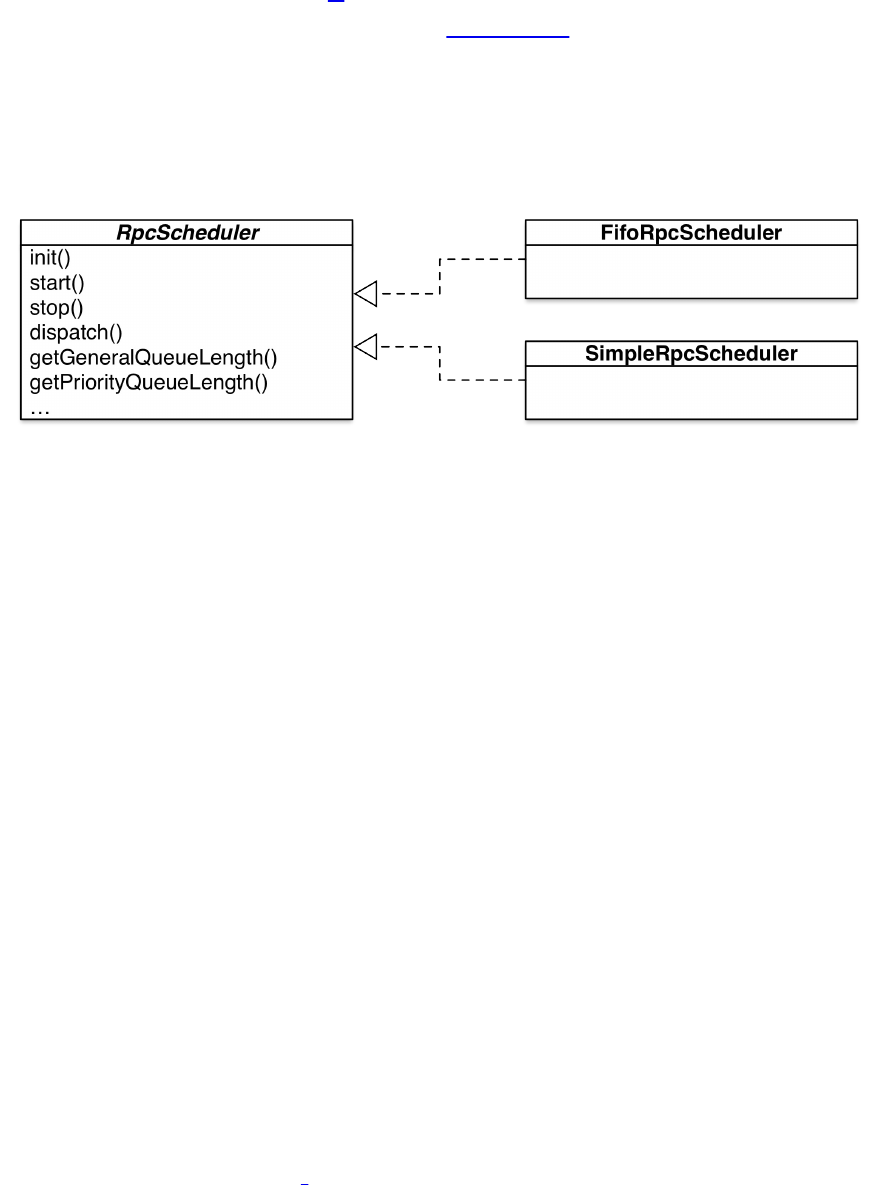
RPC Scheduling
As of HBase 1.0, the RPC subsystem of the region servers allows operators to tune the call
scheduling features in a variety of ways.23 This functionality is pluggable and encapsulated in the
RpcScheduler based hierarchy of classes, as shown in Figure 10-10. While there are two
subclasses, only the SimpleRpcFactory is fully featured and (as of this writing) used as the default
scheduler class. It can be replaced by means of an accompanying factory class, which here is
SimpleRpcSchedulerFactory. HBase system developers could supply their own scheduler and
factory class, and enable its use by setting the hbase.region.server.rpc.scheduler.factory.class
configuration property.
Figure 10-10. The RPC scheduler class hierarchy
Internally, the scheduler class is employing various RpcExecutor implementations to set up
specific call queue types, depending on how you configure the scheduler. Before we discuss the
possible setups, here is the list of configuration options pertaining to the scheduler setup:
Property Default Description
hbase.regionserver.handler.count 30
Defines how
many
handlers are
created to
process
regular
incoming
requests. Also
used by the
HBase
Master.
hbase.regionserver.metahandler.counta20
Defines the
extra handlers
created for
high priority
requests,
concerning
(831)
system table
and other
administrative
operations.
hbase.regionserver.replication.handler.count 3
Defines the
number of
extra handlers
for cluster
replication
requests.
hbase.ipc.server.max.callqueue.length hbase.regionserver.handler.count * 10
Upper
boundary on
the total
length of each
call queue,
defining how
many
outstanding
calls can be
queued.
Minimum is
250 items.
hbase.ipc.server.priority.max.callqueue.length hbase.ipc.server.max.callqueue.length
Same, but for
high priority
requests,
concerning
system or
administrative
operations.
hbase.ipc.server.callqueue.handler.factor 0.1
Determines
the number of
queues
available to
the handlers.
hbase.ipc.server.callqueue.read.ratio 0
Allows
splitting of
the queues
into dedicated
ones for reads
and writes.
(832)
Default is to
share the
same queue
with write
calls.
hbase.ipc.server.callqueue.scan.ratio 0
If a read
queue ratio
(above) was
given, further
split the read
queues into
read and scan
specific ones.
hbase.ipc.server.callqueue.type fifo
One of codel
deadline, or
fifo.
Influences
how calls are
prioritized in
each queue.
hbase.ipc.server.queue.max.call.delay 5000 (5 secs.)
For deadline
queue mode,
this is the
upper
boundary on
the wait time
for a scan
operation.
hbase.ipc.server.callqueue.codel.target.delay 100 (ms)
The target
delay for call
handling,
measured in
milliseconds.
hbase.ipc.server.callqueue.codel.interval 100 (ms)
Time in
milliseconds
that
determines
how often the
algorithm
adjusts itself.
(833)

hbase.ipc.server.callqueue.codel.lifo.threshold 0.8 (80%)
Fill
percentage
that triggers a
switch from
fifo to lifo.
a This property is a bit of a misnomer, as not only meta table requests (as the name might imply) are
concerned, but any higher priority request.
The Cost of RPCs
Before we are going to discuss the various RPC settings in detail, you need to consider all the
implications: tuning the most vital interface of your servers to communicate between themselves
and with remote client applications should have a positive effect—but may also incidentally
make things worse. For example, some of the internal classes are completely swapped out
dependent on your configuration choices, and some of those alternatives have different levels of
features supported. Or, configuring a more fair resource management using separate request
pools imposes extra work (that is, there are more code paths that need to be followed), while a
more simple implementation (like the first-in-first-out queue) is faster and results in a higher
overall request throughput.
Selecting a tuning option is foremost a question of its costs and benefits, which need to match
your use-case. You can use the tools explained in “Load Tests” to become familiar with the
effects of the RPC settings. But just as with varying use-cases over time, or mixed workloads, the
load testing is limited in reflecting the real effects of the tuning, forcing you to use the real data
and access patterns as anticipated (or, better, observed) in production. Using the metrics will give
you some insight into the operational aspects of the tuning, but will not point you into a viable
direction. Learning about RPC tuning and the configuration options is a tedious yet required task
that every HBase administrator will have to become acquainted with.
Start out with the default, and switch to separate handlers dedicated to writes, reads, and/or scans
only if your use-case warrants it. For example, if you have a roughly even mix of read and write
operations, and you need to guarantee low latencies to both of them. Otherwise a backlog of
writes could impede reads and overly delay their handling.
Queue Factor
The first step in tuning the advanced queue features is to increase their number, setting the call
queue factor, controlled by hbase.ipc.server.callqueue.handler.factor (defaulting to 0.1, or
10%). Figure 10-11 shows the different setups we are going to discuss, with Setup 1 depicting
what a queue factor of 0% results in, which is a single queue, serving the configured number of
handler threads, set globally with hbase.regionserver.handler.count, and defaulting to 30.
On the other hand, setting the queue factor to 100%, or 1.0, will cause the RPC scheduler to set
up as many queues as there are handlers, shown in Setup 3. Any value in between sets the
number of queues to the percentage of the total handler count. For example, 0.5 (50%) would
create half as many queues as there are handlers, so that every queue is serving two handler
(834)
threads. Setup 2 is reflecting the latter configuration.
Having more than one queue allows the executer to distribute the requests more evenly across the
handlers, resulting in a better overall handling of mixed requests. Conversely though, if all
handlers for one queue are busy with calls, any further queued call will have to wait. Even free
handlers connected to other queues will not be able to process those calls, as each is dedicated to
its queue only.
(835)
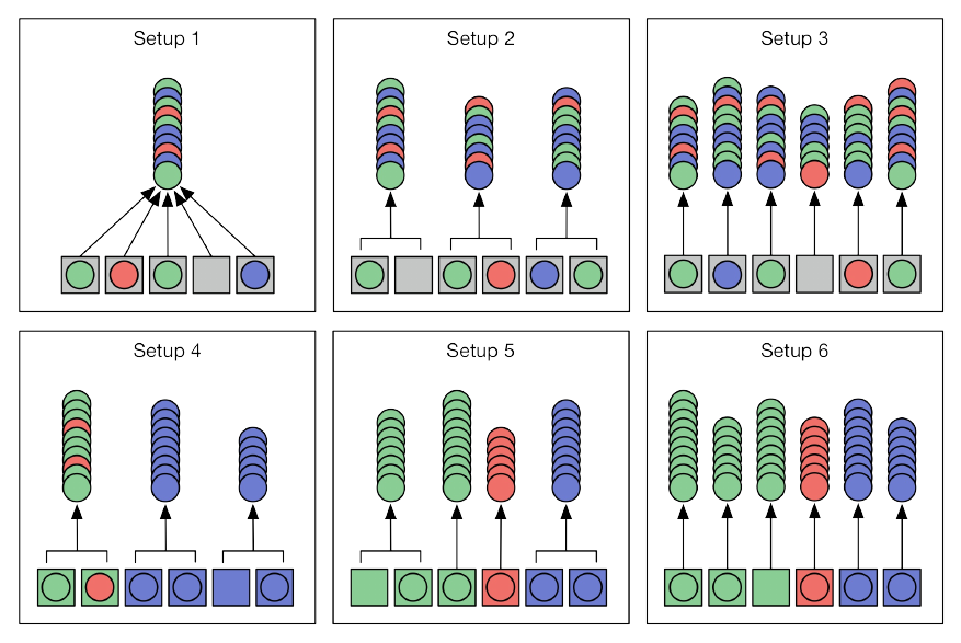
Figure 10-11. Example setups of the call handlers and queues
No matter how many queues you define, each is configured to maintain
hbase.ipc.server.max.callqueue.length elements, with a minimum of 250. The default is to
maintain 10-times the number of configured handlers, which is 30 * 10, or 300. The same limit
also applies to the queues created for the replication handlers. Only for the high priority handlers
(see hbase.regionserver.metahandler.count) is the limit set independently, using
hbase.ipc.server.priority.max.callqueue.length. Its default though is once again the same, that is
300 items maximum per queue. If any of the queues exceeds that number and is asked to add
another item, it will deny the request. This results in a call queue too big exception being thrown
and returned to the client.
Queue Type
You may wonder, while looking at Setup 1 to 3 in the diagram, if calls of any particular type
(which is reads, writes, and scans) are placed in the call queue(s) in some specific order. This is
configured with hbase.ipc.server.callqueue.type, setting the required queue type to one of the
following:
Fifo
This is the first-in-first-out queue type, which keeps all requests in the order in which they
have arrived. This is the default queue type used when the servers start.
Deadline
This queue type extends Fifo by treating scans specifically, demoting longer running ones
over other request types, or newer scans. As soon as a scanner is opened by a client, it is
monitored by the server, and the more RPCs have been tracked for a scanner (due to calls
(836)

to its next() method) the more it is pushed back in the queue’s ordering (that is, it is given
a lower priority). There is an upper boundary set with
hbase.ipc.server.queue.max.call.delay, defaulting to 5 seconds, which ensures that even
demoted scanner calls are eventually given to a handler thread, so that they can complete.
Otherwise all ordering is in first-in-first-out manner.
CoDel
Another queue type is based on the controlled delay scheduling algorithm used in network
routing. It attempts to avoid bufferbloat, which is a situation where a queue fills up and
cannot catch up with requests due to ongoing backlog of work. CoDel works with two
major thresholds: the number of elements in the queue (that is, its fill), and the delay each
element is experiencing while waiting inside the queue.
You can configure the queue fill threshold with
hbase.ipc.server.callqueue.codel.lifo.threshold (set to 80%), which will trigger a switch
from first-in-first-out to last-in-first-out call queue handling. In other words, once the
queue fills up to 80%, it will favor the most recent requests over others that are already in
the queue.
The delay threshold is configured using hbase.ipc.server.callqueue.codel.target.delay,
defaulting to 100ms, and causes all dequeued elements that have been in the queue for
longer than twice the target delay time to be dropped instead, given the queue detects it is
under pressure. The latter is updated every hbase.ipc.server.callqueue.codel.interval, set
to 100ms, and monitors the dequeued calls. Should any of those exceed the configured
target delay, it triggers the overload signal and causes the dropping to occur as mentioned.
Summarizing, Fifo is the simplest one, with the other two being much more specific—but also
harder to understand and properly utilize.24 The Deadline queue type is similar to Fifo, only
differing in how (long-running) scans are handled. Finally, CoDel is an adaptive queue handling
algorithm, which is known to work well in other routing scenarios, giving the operator an
advanced choice to tune the RPC call handling.
Call Type Ratios
So far we were able to tune the number of queues, and with it the distribution of calls over the
number of handlers. We also learned how to change the handling of calls within each queue. The
final tuning option is to group calls by their type, which can be a read, write, and scan as
mentioned. The scheduler has a set of options that allow the splitting of the handlers and queues
into two or three groups, handling reads and writes, or reads, writes, and scans respectively.
The main option to separate the requests by type is hbase.ipc.server.callqueue.read.ratio,
defaulting to 0.0 (0%). Increasing this number allows the operator to split reads and writes into
two groups. One group handles not just the reads, but also scans (which are reads essentially),
while the other handles all write operations. By definition, write requests send mutations to the
server, including puts and deletes (see “Data Types and Hierarchy” for the full list). Scan
requests are those a client scanner calls, while everything else is considered a read request.
Using Figure 10-11 again, Setup 4 shows the result setting the queue factor to 50%, and the read
ratio to 30% (or 0.3), dividing the six handlers into 30% read handlers, leaving the remaining
70% for writes. Reads and scans are mixed together, and handled according to the queue
configuration. Setup 5 shows the opposite read ratio of 70%, but with an additional 20% assigned
(837)

to hbase.ipc.server.callqueue.scan.ratio. This percentage only pertains to the read share, and
further carves out handlers only assigned to scanner related calls. In the example, you see how
three out of four handlers are given to reads, one is dedicated to scans, while the remaining two
are given to writes.
Note
Even if you set the read ratio to 100%, there will always be at least one handler given to
writes.
Be aware with the percentages in general, if you choose very low values, for example for
scans, the rounding that takes place during the handler and queue calculation may end up
at zero, or no scan handlers at all. Enabling DEBUG level logging for the IPC classes will
show the computed numbers and queue to handler mappings.
Write queues have a preference over read queues, for example, with 15 queues and 50%
split, you get eight write and seven read queues.
Finally, Setup 6 shows the same as the previous one, but with a queue factor of 100%, so that
each handler is assigned to one specific queue. You have the choice to combine the queue factor
and ratio as you see fit for your cluster. Keep in mind though that you will have to share the RPC
configuration across the entire cluster, no matter how many different workloads you are exposing
it to. The following tables show some of the possible combinations, and their effect on the
number of queues, and how many handlers are assigned to each of them (the column labeled
“H/Q”).
First, only the queue factor is modified:
Table 10-13. RPC queue factor tuning examples
Handler Factor Read Write Scans Queues H/Q
30 0% 0% 0% 0% 1 30
30 10% 0% 0% 0% 3 10a
30 30% 0% 0% 0% 9 3-4
30 50% 0% 0% 0% 15 2
30 70% 0% 0% 0% 21 1-2
30 100% 0% 0% 0% 30 1
a This is the system default.
(838)

Next, both the queue factor and the read ratio are adjusted at the same time, where the write ratio
is the remaining percentage:
Table 10-14. RPC queue factor and ratio tuning examples
Handler Factor Read Write Scans Queues H/Q
30 0% 30% 70% 0% 1 30a
30 30% 30% 70% 0% R:3 W:6 3-4
30 30% 50% 50% 0% R:4 W:5 3-4
30 30% 70% 30% 0% R:6 W:3 3-4
30 30% 100% 0% 0% R:8 W:1 3-4b
30 50% 30% 70% 0% R:4 W:11 2c
30 50% 50% 50% 0% R:7 W:8 2
30 50% 70% 30% 0% R:10 W:5 2
30 50% 100% 0% 0% R:14 W:1 2
30 70% 30% 70% 0% R:6 W:15 1-2
30 70% 50% 50% 0% R:10 W:11 1-2
30 70% 70% 30% 0% R:15 W:6 1-2
30 70% 100% 0% 0% R:20 W:1 1-2
30 100% 30% 70% 0% R:4 W:11 1
30 100% 50% 50% 0% R:7 W:8 1
(839)

30 100% 70% 30% 0% R:10 W:5 1
30 100% 100% 0% 0% R:14 W:1 1
a A zero queue factor means no splitting of queues is possible.
b There is always at least one writer queue and handler available.
c Write queues have preferences and get rounded up.
Finally, a shorter set of examples that also set the scan ratio, reserving additional resources out of
the read queue pool for long-running reads, that is, scans:
Table 10-15. RPC queue factor and ratio with scans
tuning examples
Handler Factor Read Write Scans Queues H/Q
30 70% 30% 70% 20% R:5 S:1 W:15 1-2
30 70% 50% 50% 20% R:8 S:2 W:11 1-2
30 70% 70% 30% 20% R:12 S:3 W:6 1-2
30 70% 100% 0% 20% R:16 S:4 W:1 1-2
(840)

Slow Query Logging
The HBase region servers emit specific log messages, referred to as slow query logging, which
can be used to identify operational problems with client requests. Every server takes note of
when a client request arrives at the server, when it is taken from the queue, and how long the
server spent on processing it. This information is on one hand surfaced through the server
metrics, as documented in “RPC Metrics”, aggregating the mentioned time periods. In addition,
and as discussed in “Region Server Metrics” under API Usage Information, there are counters for
slow operations, such as slowPutCount. These are increased whenever an operation took more
than a second to complete (which is, at the time of this writing, hardcoded).
On the other hand, the slow query log messages are emitted to the normal server logs, containing
a JSON message that can be parsed using a script. For example, the following show three such
messages printed at various times, and for different operations:
2016-09-23 21:53:32,460 WARN org.apache.hadoop.hbase.ipc.RpcServer: \
(responseTooSlow): {"call":"Scan(org.apache.hadoop.hbase.protobuf. \
generated.ClientProtos$ScanRequest)","starttimems":1474685601484, \
"responsesize":416,"method":"Scan","processingtimems":10976,"client": \
"172.18.100.101:32916","queuetimems":0,"class":"HRegionServer"}
2016-09-07 21:22:14,624 WARN org.apache.hadoop.hbase.ipc.RpcServer: \
(responseTooSlow): {"call":"BulkLoadHFile(org.apache.hadoop.hbase. \
protobuf.generated.ClientProtos$BulkLoadHFileRequest)","starttimems": \
1473301316403,"responsesize":2,"method":"BulkLoadHFile", \
"processingtimems":18221,"client":"172.18.100.17:38838", \
"queuetimems":0,"class":"HRegionServer"}
2016-03-01 13:19:13,259 WARN org.apache.hadoop.hbase.ipc.RpcServer: \
(responseTooSlow): {"call":"Multi(org.apache.hadoop.hbase.protobuf. \
generated.ClientProtos$MultiRequest)","starttimems":1456859885592, \
"responsesize":20,"method":"Multi","processingtimems":67667,"client": \
"172.18.100.11:46742","queuetimems":0,"class":"HRegionServer"}
Each are prefixed with "(responseTooSlow)" when the processing time (which excludes any
additional queueing time) is in excess of the configured threshold. Alternatively "
(responseTooLarge)" might be printed when the response size exceeds another configured
threshold. Should the response be too large and too slow, only the size warning is printed (as
large responses do imply slowness).25
There are two configuration properties that can be used to adjust the thresholds for when queries
are logged:
Property Default Description
hbase.ipc.warn.response.time 10000 (10 secs) Maximum number of milliseconds that a query
can be run without being logged.
hbase.ipc.warn.response.size 100 * 1024 *
1024 (100 MB)
Maximum byte size of response that a query can
return without being logged.
Note that setting any of the two to -1 will disable the respective log message completely.
(841)
The advantage of the slow query log over the metrics is that here you get related information.
Metrics only aggregate time spent in RPC, or how many slow calls you had, but not the nature of
the call itself. You can see from the examples that the JSON structure is containing the name of
the function invoked (for example, "Scan" or "Multi", where the latter is for batched up calls, such
as Put and Delete in one RPC invocation). You also get the call specific start time (as a Linux
epoch), as well as the actual queue and processing time in milliseconds. The client address and
response size complete the information, and allow checking with the application developers as to
the effects of the slow calls.
(842)

Load Balancing
Over time as regions split or merge (automatically or manually) and their number changes, the
cluster needs to take care of distributing the regions equally. For that, the HBase Master has a
built-in feature, called the balancer. By default, the balancer runs every five minutes, and it is
configured by the hbase.balancer.period property. There can only be one balancer operation
active, which means that after the balancer period lapses and there are still regions that are
moved, the master will not start another balancer operation but wait for the next lapse to check
again. Moving regions is not free (as it negatively impacts the data locality), making this cautious
approach a sensible one.
Once the balancer is started, it will attempt to equal out the number of assigned regions per
region server so that they are within specific boundaries, set by the configuration and enforced
by the active balancer implementation. The operation first determines a new assignment plan,
which describes which regions should be moved where. Then it starts the process of moving the
regions by (eventually) calling the unassign() method of the administrative API iteratively (see
“Region Operations”), while supplying a new destination server for each region based on the
plan.
Before we look into the details, here the list of important region balancing configuration
parameters, which we will refer to throughout this section:
Property Default
hbase.balancer.period 300000 (5 mins)
hbase.balancer.max.balancing -1
(843)
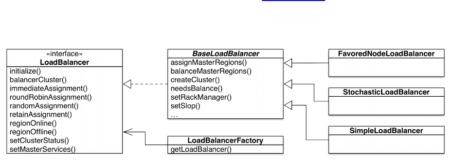
hbase.master.loadbalancer.class org.apache.hadoop.hbase.master.balancer.StochasticLoadBalancer
hbase.master.loadbalance.bytable false
hbase.regions.slop 0.001 (or 0.2)
Since HBase 0.96 the balancer implementation used by default is called StochasticLoadBalancer,
but it can be replaced by any other of the provided classes. Figure 10-12 shows the list of
available balancer implementation classes available to you, which are discussed in more detail
below.
Figure 10-12. The hierarchy of the LoadBalancer classes
The balancer, independent from the selected implementation, has an upper limit on how long it is
allowed to run, which is configured using the hbase.balancer.max.balancing property and defaults
to the same time set as the balancing period. The master iterates over the computed assignment
plan and executes the included region plans (which really is the move of an individual region
from one server to another) one after the other, while tracking the time each application of a plan
(that is, region move) required. Given there are many region plans, and considering each of the
region moves will take some time to complete, the operation will stop after the maximum
(844)

balancing threshold is exceeded.
You can control the balancer by means of the balancer switch: either use the shell’s
balance_switch command to toggle the balancer status between enabled and disabled, or use the
setBalancerRunning() API method to do the same. When you disable the balancer, it no longer
runs (as expected) at the configured intervals, leaving all region balancing work to the operator.
Refer to “Region Operations” and “Tool Commands” for the mentioned API calls and shell
commands.
Given the balancer is enabled, a balance operation can be explicitly started using the shell’s
balancer command, or using the balancer() API method. The time-controlled invocation
mentioned previously calls this method implicitly. It will determine if there is any work to be
done and return true if that is the case, while instructing the asynchronous balance operation to
do its work. A return value of false means that it was not able to run the balancer, because either
it was switched off, there was no work to be done (all is balanced), or something else was
prohibiting the operation. One example for this is the region in transition list (see “Main Page”):
if there is a region currently in transition, the balancer will be skipped. Instead of relying on the
balancer to do its work properly, you can use the move command and API method to assign
regions to other servers. This is useful when you want to control where the regions of a particular
table are assigned. See “Region Hotspotting” for an example.
As of HBase 0.94 there is also the hbase.master.loadbalance.bytable option, which configures the
load balancer to optionally take the distribution of regions in their tables context across servers
into consideration. Set to true, the balancer should try to ensure that all regions of a table are
(within reason) located on all available region servers. Before (and when setting this flag to
false) it was possible for all or most regions of a table to be hosted by the same server—even
with the overall number of regions per server in equilibrium—causing that single server to take
on all the requests. The default is false as the default balancer implementation is implicitly
taking care of this criteria as part of its cost functions.
The most basic balancing factor is the so-called region slop, set with hbase.regions.slop and
defaulting to 1% (or 20% for all balancers but the default stochastic-based one). It determines if
there is any work to be done by the balancing operation. This is done by computing the average
number of regions across all servers, and then applying the percentage of the slop. In Figure 10-
13, you can see in example 1 that the average number of regions per server is about 58. Adding
and substracting 20%, as done by the SimpleLoadBalancer, would result into an upper boundary of
70, and a lower one of 46 regions per server. Since all six region servers are within that range the
balancer would consider it balanced.
(845)
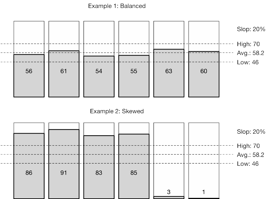
Figure 10-13. Example of region counts per server
In example 2 you are shown a situation where two new region servers were recently added, with
nearly no regions assigned to it yet. The upper, lower, and average values are all the same, as for
this example we assume that the cluster was filling up and thus the older servers carry the
majority of the regions still. Here all region servers are outside of the slop boundaries, and would
be considered as part of the next balancer operation. The balance operation handles the
computation of the new assignment plan and then rearranges the regions iteratively.
Note
Before the 0.94 release and the availability of the slop setting, the balancer would always try to
even out the region count, down to the exact count per server. With a cluster splitting regions
regularly, or adding new regions due to the creation of new tables, the result would be a constant
movement of regions with every balancer invocation. The slop acts as a bulk or batch threshold
in practice, reducing the movement of regions to controllable intervals.
Apart from these more generic features available to all balancer implementations, they differ
widely in how they decide what constitutes an assignment plan, or, in other words, what is
considered a misbalance that should be rectified. The following discusses the available balancer
classes in more detail:
SimpleLoadBalancer
This class was once called the DefaultLoadBalancer, but since balancers have been made
pluggable in 0.92 and other balancer implementations have been added in 0.96 and later, it
(846)

was renamed to its current name. The balancer mostly acts on the described region slop,
trying to move in some sensible manner. For that, it does not simply move a random list of
regions, but checks their age too, trying to alternate between older and newer regions so
that, for example, not all regions of a new table are affected by the move.
One of the more prominent features of this balancer is its implementation of the per region
balancing, set with hbase.master.loadbalance.bytable (which you would need to set to true
explicitly). It takes care of moving regions so that all of those belonging to the same table
are evenly spread across the available servers. Apart from that, it does not provide any
additional measure to balance out regions.
StochasticLoadBalancer
If you need a much more sophisticated balancer implementation, then the default
StochasticLoadBalancer class is right for you. It takes many more measures to balance out
regions, providing support for cost functions that are applied and weighed by a multiplier
to decide if a region needs to be moved or not. Since it uses statistics, the balancer
computes the cost based on many factors, such as
how many regions would need to be moved,
how much region count skew it would cause,
how evenly regions per table are distributed,
how it would affect the locality of store files,
how read and write requests are impacted,
how region replicas are affected, and
how memstore and store file sizes are impacted,
running an approximation function, iterating over thousands of combinations in an attempt
to find the one with the lowest cost. How often it iterates depends on the total number of
regions, which is multiplied by a coefficient (referred to as steps per region). There is also
a maximum number of steps that limits the iterations once you have too many regions. The
following lists the settings specifically available for the StochasticLoadBalancer:
Property Default Description
hbase.master.balancer.stochastic.stepsPerRegion 800
The coefficient by
which the number of
regions is multiplied
to try to get the
number of times the
balancer will mutate
all region to server
assignment plans.
Controls the
(847)

hbase.master.balancer.stochastic.maxSteps 1000000
maximum number of
times that the
balancer will try to
compute all possible
assignment plans.
Acts as an upper limit
on the number
computed by the
previous
configuration key and
the total number of
regions.
hbase.master.balancer.stochastic.maxRunningTime
30000
(30
secs)
Additional upper limit
on time spent
computing all
possible assignment
plans.
hbase.master.balancer.stochastic.numRegionLoadsToRemember 15
Specifies how many
server load records
(see “Cluster Status
Information”) should
be cached for more
accurate cost
computations.
Note that for the balancer to apply all factors as described, the
hbase.master.loadbalance.bytable property should be left to its default value of false. It
already includes a cost function that considers the effects of moving regions to servers that
host other regions of that same table. Though since this is just part of the overall
calculation, it does not have the same impact.
FavoredNodeLoadBalancer
This balancer differs from the above, as it does not consider the number of regions within
some boundaries, or a more elaborate list of cost functions, but instead uses a HDFS
feature that allows a client to specify preferred nodes to be used for the block replicas.
With that, it constructs a list of primary, secondary, and tertiary region servers that a
region should be written to. When a region opens, an attempt is made to open it in that
same order, that is, primary first, and if that fails it moves to the secondary and so on. This
reduces the problem of only the primary (local) replica of the store files for a region being
located on the same server. Typically, if a region is moved, the locality drops dramatically
while most data is read across the network from many different datanodes holding the
block replicas. Having pinned the replicas to two other nodes makes this failover scenario
more amenable—assuming these servers are available and not overly loaded already.
(848)
Once a region has been moved to another of the favored nodes after the primary failed, you
will need to run a tool to assign an additional, new node to that same region, bringing the
number back up to three nodes in total. The following shows the invocation of the supplied
tool and its default output:
$ hbase org.apache.hadoop.hbase.master.RegionPlacementMaintainer
usage: RegionPlacement < -w | -u | -n | -v | -t | -h | -overwrite -r
regionName -f favoredNodes -diff> [-l false] [-m
false] [-d] [-tables t1,t2,...tn] [-zk zk1,zk2,zk3]
[-fs hdfs://a.b.c.d:9000] [-hbase_root /HBASE]
-d,--verification-details print the details of verification report
-diff calculate difference between assignment plans
-f <arg> The new favored nodes
-fs <arg> to set HDFS
-h,--help print usage
-hbase_root <arg> to set hbase_root directory
-l,--locality <arg> enforce the maxium locality
-ld,--locality-dispersion print locality and dispersion information for
current plan
-m,--min-move <arg> enforce minium assignment move
-munkres use munkres to place secondaries and
tertiaries
-n,--dry-run do not write assignments to META
-overwrite overwrite the favored nodes for a single
region,for example: -update -r regionName -f
server1:port,server2:port,server3:port
-p,--print print the current assignment plan in META
-r <arg> The region name that needs to be updated
-tables <arg> The list of table names splitted by ',' ;For
example: -tables: t1,t2,...,tn
-u,--update update the assignments to hbase:meta and
RegionServers together
-v,--verify verify current assignments against META
-w,--write write the assignments to hbase:meta only
-zk <arg> to set the zookeeper quorum
Note
As of this writing, little experience has been reported regarding the favored node balancer.
You should proceed with caution and test carefully.
(849)

Client API: Best Practices
When reading or writing data from a client using the API, there are a handful of optimizations
you should consider to gain the best performance. Here is a list of the best practice options:
Maintain Number of Regions
As described in “Number of Regions”, you need to control how many write-active regions
you have on each region server, so as not to oversubscribe the memory set aside for the
memstores. Having too many active regions could lead to compaction storms, as tiny
memstores are constantly forced to flush, leading to excessive compactions that try to keep
up with the number of files created. Always presplit your tables (see “Presplitting
Regions”).
Use Buffered Mutations
When performing a lot of put and/or delete operations, you should use a BufferedMutator
instead of a Table reference. Otherwise, the mutations will be sent one at a time to the
region server(s). Refer to “Client-side Write Buffer” for details on how to configure the
client side buffer, and how to use, for example, the flush() call to submit the mutations to
the server(s).
Use Scanner Caching
Up to version 1.1, if HBase is used as an input source for a MapReduce job, for example,
make sure the input Scan instance to the MapReduce job has setCaching() set to something
greater than the default of 100 (or even 1 before version 0.96). Using the default value
means that the map task will make many callbacks to the region server(s) for every set of
records processed. Setting this value to 500, for example, will transfer 500 rows at a time
to the client to be processed.
From version 1.1 onwards, the internal handling of scans has been improved in such a way
that the default caching value is set to unlimited. Instead, you can increase the maximum
result size threshold, which determines how the client code groups cells for each RPC
invocation. See “Scanner Caching” for details. Look for the setMaxResultSize() of the Scan
class, and the hbase.client.scanner.max.result.size configuration setting. The latter
defaults to 2 MB, which you could increase to improve scan throughput performance.
There is a cost to using a larger caching or result size value, since it requires more memory
for both client and region servers: bigger is not always better. Experiment with larger
values to find the optimal value for your use-cases.
Limit Scan Scope
Whenever a Scan is used to process large numbers of rows (for example, when used as a
MapReduce source), be aware of which attributes are selected. If Scan.addFamily() is
called, all of the columns in the specified column family will be returned to the client. If
only a small number of the available columns are to be processed, only those should be
specified in the input scan because column overselection incurs a nontrivial performance
(850)

penalty over large data sets.
Close ResultScanners
This isn’t so much about improving performance, but rather avoiding performance
problems. If you forget to close ResultScanner instances, as returned by Table.getScanner(),
you can cause problems on the region servers, as it holds on to resources which are
otherwise better released. Always have ResultScanner processing enclosed in try/catch
blocks, for example:
Scan scan = new Scan();
// configure scan instance
ResultScanner scanner = table.getScanner(scan);
try {
for (Result result : scanner) {
// process result...
} finally {
scanner.close(); // always close the scanner!
}
table.close();
See the longer Example 3-28 for another, working example.
Read Row Keys With Filters
When performing a table scan where only the row keys are needed (no families, qualifiers,
values, or timestamps), add a FilterList with a MUST_PASS_ALL operator to the scanner using
setFilter(). The filter list should include both a FirstKeyOnlyFilter and a KeyOnlyFilter
instance, as explained in “Dedicated Filters”. Using this filter combination will cause the
region server to only load the row key of the first KeyValue (that is, from the first column)
found and return it to the client, resulting in minimized network traffic.
Do Not Turn Off WAL for Writes
A frequently discussed option for increasing throughput on writes is to call
setDurability(Durability.SKIP_WAL) on mutation instances. Turning the write-ahead log off
means that the region server will not append the mutation to the log, but rather only insert
it into the memstore. However, the consequence is that if there is a region server failure
there will be data loss. If you turn off the WAL, do so with extreme caution. You may find
that it actually makes little difference if your load is well distributed across the cluster.
Refer to “Durability, Consistency, and Isolation” for more details.
In general, it is best to use the WAL for writes, and, where loading throughput is a
concern, to use the bulk loading techniques instead, as explained in “Bulk Import”.
Block Cache Usage
Scan instances can be set to use the block cache in the region server via the
setCacheBlocks() method. For scans used with MapReduce jobs, or analytical queries that
process the entire table, this should be set to false. For frequently accessed rows, it is
advisable to use the block cache. Refer to “Advanced Cache Configuration” for more
details on how to tune the cache usage.
(851)

Configuration
Many configuration properties are available for you to use to fine-tune your cluster setup.
“Configuration” listed the ones you need to change or set to get your cluster up and running.
There are advanced options you can consider adjusting based on your use case. Here is a list of
the more commonly changed ones, and how to adjust them.
Note
The majority of the settings are properties in the hbase-site.xml configuration file. Edit the file,
copy it to all servers in the cluster, and restart the servers to effect the changes.
Decrease ZooKeeper Timeout
The default timeout between a region server and the ZooKeeper quorum is 1.5 minutes (set
as 90000, specified in milliseconds), and is configured with the zookeeper.session.timeout
property. This means that if a server crashes, it will be 1.5 minutes before the master
notices this fact and starts recovery. You can tune the timeout down to a minute, or even
less, so the master notices failures sooner.
Before changing this value, make sure you have your JVM garbage collection
configuration under control (refer to “Garbage Collection Tuning”), because otherwise, a
long garbage collection that lasts beyond the ZooKeeper session timeout will take out your
region server. You might be fine with this: you probably want recovery to start if a region
server has been in a garbage collection-induced pause for a long period of time.
The reason for the default value being rather high is that it avoids problems during very
large imports: such imports put a lot of stress on the servers, thereby increasing the
likelihood that they will run into the garbage collection pause problem. Also see “Stability
Issues” for information on how to detect such pauses.
Increase Handlers
The hbase.regionserver.handler.count configuration property defines the number of threads
that are kept open to answer incoming requests to user tables. The default of 30 is good,
but conservative, in order to prevent users from overloading their region servers when
using large write buffers with a high number of concurrent clients. The rule of thumb is to
keep this number low when the payload per request approaches megabytes (that is, big
puts, scans using a large cache) and high when the payload is small (that is, gets, small
puts, increments, deletes). It is safe to set that number to the maximum number of
incoming clients if their payloads are small, the typical example being a cluster that serves
a website, since puts are typically not buffered, and most of the operations are gets.
The reason why it is dangerous to keep this setting high is that the aggregate size of all the
puts that are currently happening in a region server may impose too much pressure on the
server’s memory, or even trigger an OutOfMemoryError exception. A region server running
on low memory will trigger its JVM’s garbage collector to run more frequently up to a
point where pauses become noticeable (the reason being that all the memory used to keep
all the requests’ payloads cannot be collected, no matter how hard the garbage collector
(852)

tries). After some time, the overall cluster throughput is affected since every request that
hits that region server will take longer, which exacerbates the problem. Refer to “RPC
Tuning” for details.
Increase Heap Settings
HBase ships with a reasonable, conservative configuration that will work on nearly all
machine types that people might want to test with. If you have larger machines—for
example, where you can assign 8 GB or more to HBase—you should adjust the
HBASE_HEAPSIZE setting in your hbase-env.sh file.
Consider using HBASE_REGIONSERVER_OPTS instead of changing the global HBASE_HEAPSIZE: this
way the master will run with the default heap size, while you can increase the region server
heap as needed independently. This option is set in hbase-env.sh, as opposed to the hbase-
site.xml file used for most of the other options. More can be found under “Heap Tuning”.
Enable Data Compression
You should enable compression for the storage files—in particular, Snappy or LZO. It’s
near-frictionless and, in most cases, boosts performance. See “Compression” for
information on all the compression algorithms.
Increase Region Size
Consider going to larger regions to cut down on the total number of regions on your
cluster. Generally, fewer regions to manage makes for a smoother-running cluster. You
can always manually split the big regions later should one prove hot and you want to
spread the request load over the cluster. “Region Split Handling” has the details.
By default, regions are 10 GB in size, which is a very reasonable starting point. You could
run with 20 GB, or even larger regions. Keep in mind that this needs to be carefully
assessed, since a large region also can mean longer pauses under high pressure, due to
compactions. Adjust hbase.hregion.max.filesize in your hbase-site.xml configuration file.
On the other hand, increasing the region sizes might have an impact on compactions too,
requiring you to switch to one of the more size oriented compaction methods, such as
stripe-based. See “Compaction Tuning” for inspiration.
Adjust Block Cache Size
The amount of heap used for the block cache is specified as a percentage, expressed as a
float value, and defaults to 40% (set as 0.4). The property to change this percentage is
hfile.block.cache.size. Carefully monitor your block cache usage (see “Region Server
Metrics”) to see if you are encountering many block evictions. In this case, you could
increase the cache to fit more blocks.
Another reason to increase the block cache size is if you have mainly reading workloads.
Then the block cache is what is needed most, and increasing it will help to cache more
data. Alternatively, also enable the off-heap, or on-storage cache options, as explained in
“Block Cache Tuning”.
Caution
(853)

The total value of the block cache percentage and the upper limit of the memstore should not be
100%. You need to leave room for other purposes, or you will cause the server to run out of
memory. The default total percentage is 80%, which is a reasonable value. Only go above that
percentage when you are absolutely sure it will help you—and that it will have no adverse effect
later on.
Adjust Memstore Limits
Memstore heap usage is set with the hbase.regionserver.global.memstore.size property, and
it defaults to 40% (set to 0.4). In addition, the
hbase.regionserver.global.memstore.size.lower.limit property (set to 95%, or 0.95) is used
to control the amount of flushing that will take place once the server is required to free
heap space. Consult “Tuning Heap Shares” for more information.
When you are dealing with mainly read-oriented workloads, you can consider reducing
both limits to make more room for the block cache. On the other hand, when you are
handling many writes, you should check the log files (or use the region server metrics as
explained in “Region Server Metrics”) if the flushes are mostly done at a very small size—
for example, 5 MB—and increase the memstore limits to reduce the excessive amount of
I/O this causes.
Increase Blocking Store Files
This value, set with the hbase.hstore.blockingStoreFiles property, defines when the region
servers block further updates from clients to give compactions time to reduce the number
of files. When you have a workload that sometimes spikes in regard to inserts, you should
increase this value slightly—the default is 10 files—to account for these spikes.
Use monitoring to graph the number of store files maintained by the region servers. If this
number is consistently high, you might not want to increase this value, as you are only
delaying the inevitable problems of overloading your servers.
Increase Block Multiplier
The property hbase.hregion.memstore.block.multiplier, set by default to 4, is a safety latch
that blocks any further updates from clients when the memstores exceed the multiplier *
flush size limit. When you have enough memory at your disposal, you can increase this
value to handle spikes more gracefully: instead of blocking updates to wait for the flush to
complete, you can temporarily accept more data.
Decrease Maximum Logfiles
Setting the hbase.regionserver.maxlogs property allows you to control how often flushes
occur based on the number of WAL files on disk. The default is 32, which can be high in a
write-heavy use case. Lower it to force the servers to flush data more often to disk so that
these logs can be subsequently discarded.
Prefetch Blocks on Open
Given you have a working set size that fits into memory (that is, the assigned block cache
memory, which could be on SSD too), and have a workload where you need the region
servers to respond to read requests as fast as possible, you can experiment with the block
(854)

prefetch option, explained in “Advanced Cache Configuration”. This can be turned on at
the column family level to instruct the servers to read all data from storage into cache
when the respective regions are opened.
Cache Blocks on Write
This option (described in the same section linked above) goes hand-in-hand with
prefetching, instructing the servers to cache all blocks as they are written out during a flush
or compaction. It keeps recent data hot, so that subsequent reads are not incurring a cache
miss and would have to wait for the block to be loaded from storage first. For use-cases
where latency is an issue, the cache-on-write option is worth a consideration.
Enable Short-Circuit Reads
For best read performance using HDFS it is highly recommended to enable the short-
circuit read option for the datanodes and the HDFS clients. This will bypass the normal
RPC stack for reading data, and instead use the underlying data blocks directly from within
HBase. See “Short-Circuit Reads” for details.
Enable Hedged Reads
Another HDFS option to consider is enabling hedged reads, as described in “Hedged
Reads”. With it, the HDFS client is able to spawn multiple reads of the same data from
different datanodes, and use the fastest result to return. It is akin to the speculative
execution mode that MapReduce offers. You will cause more I/O load, and also more
remote reads (from non-local blocks), which means a careful evaluation is recommended.
But for low-latency applications this feature can provide a noticeable performance boost.
(855)
Load Tests
After installing your cluster, it is advisable to run performance tests to verify its functionality.
These tests give you a baseline which you can refer to after making changes to the configuration
of the cluster, or the schemas of your tables. Doing a burn-in of your cluster will show you how
much you can gain from it, but this does not replace a test with the load as expected from your
use case(s).
(856)
Performance Evaluation
HBase ships with its own tool to execute a performance evaluation. It is aptly named
Performance Evaluation (PE) and its usage details can be gained from invoking it with no
command-line parameters (shown abbreviated):
$ bin/hbase pe
Usage: java org.apache.hadoop.hbase.PerformanceEvaluation \
<OPTIONS> [-D<property=value>]* <command> <nclients>
Options:
nomapred Run multiple clients using threads (rather than use mapreduce)
rows Rows each client runs. Default: 1048576
...
Command:
append Append on each row; clients overlap on keyspace so some \
concurrent operations
...
randomWrite Run random write test
scan Run scan test (read every row)
...
sequentialRead Run sequential read test
sequentialWrite Run sequential write test
Args:
nclients Integer. Required. Total number of clients (and \
HRegionServers) running. 1 <= value <= 500
Examples:
To run a single client doing the default 1M sequentialWrites:
$ bin/hbase org.apache.hadoop.hbase.PerformanceEvaluation sequentialWrite 1
To run 10 clients doing increments over ten rows:
$ bin/hbase org.apache.hadoop.hbase.PerformanceEvaluation --rows=10 \
--nomapred increment 10
By default, the PE is executed as a MapReduce job—unless you specify the --nomapred option.
You can see the default values from the usage information in the preceding command-line
output, which are reasonable starting points, and a command to run a test is given as well. Note
that it is not necessary to specify the entire class name, because the hbase shell command has
support for it built in by means of the pe sub-command. For example, starting PE could be as
simple as:
$ bin/hbase pe --nomapred sequentialWrite 1
2016-11-12 16:55:11,198 INFO [main] hbase.PerformanceEvaluation: \
SequentialWriteTest test run options={"addColumns":true,"autoFlush":false, \
"blockEncoding":"NONE","bloomType":"ROW","caching":30, \
"cmdName":"sequentialWrite","columns":1,"compression":"NONE", \
"filterAll":false,"flushCommits":true,"inMemoryCF":false,"multiGet":0, \
"noOfTags":1,"nomapred":false,"numClientThreads":1,"oneCon":false, \
"perClientRunRows":1048576,"period":104857,"presplitRegions":0, \
"randomSleep":0,"replicas":1,"reportLatency":false,"sampleRate":1.0, \
"size":1.0,"splitPolicy":null,"startRow":0,"tableName":"TestTable", \
"totalRows":1048576,"traceRate":0.0,"useTags":false,"valueRandom":false, \
"valueSize":1000,"valueZipf":false,"writeToWAL":true}
...
2016-11-12 17:05:00,582 INFO [TestClient-0] hbase.PerformanceEvaluation: \
0/104857/1048576, latency mean=26.02, min=2.00, max=208386.00, \
stdDev=1261.69, 95th=27.00, 99th=60.00
2016-11-12 17:05:02,772 INFO [TestClient-0] hbase.PerformanceEvaluation: \
0/209714/1048576, latency mean=23.26, min=2.00, max=217306.00, \
stdDev=1239.68, 95th=8.00, 99th=49.00
...
2016-11-12 17:05:25,126 INFO [TestClient-0] hbase.PerformanceEvaluation: \
Latency (us) : mean=25.68, min=2.00, max=611880.00, stdDev=1741.69, \
50th=3.00, 75th=3.00, 95th=3.00, 99th=9.00, 99.9th=77.00, \
99.99th=38957.40, 99.999th=307570.54
2016-11-12 17:05:25,127 INFO [TestClient-0] hbase.PerformanceEvaluation: \
(857)
Num measures (latency) : 1048576
2016-11-12 17:05:25,139 INFO [TestClient-0] hbase.PerformanceEvaluation: \
Mean = 25.68
Min = 2.00
Max = 611880.00
StdDev = 1741.69
50th = 3.00
75th = 3.00
95th = 3.00
99th = 9.00
99.9th = 77.00
99.99th = 38957.40
99.999th = 307570.54
...
2016-11-12 17:05:25,290 INFO [TestClient-0] hbase.PerformanceEvaluation: \
Finished class org.apache.hadoop.hbase. \
PerformanceEvaluation$SequentialWriteTest in 27528ms at offset 0 for \
1048576 rows (37.45 MB/s)
2016-11-12 17:05:25,290 INFO [TestClient-0] hbase.PerformanceEvaluation: \
Finished TestClient-0 in 27528ms over 1048576 rows
2016-11-12 17:05:25,290 INFO [main] hbase.PerformanceEvaluation: \
[SequentialWriteTest] Summary of timings (ms): [27528]
2016-11-12 17:05:25,291 INFO [main] hbase.PerformanceEvaluation: \
[SequentialWriteTest] Min: 27528ms Max: 27528ms Avg: 27528ms
The command starts a single client and performs a sequential write test. The output of the
command shows the progress, until the final results are printed. You need to increase the number
of clients (i.e., threads or MapReduce tasks) to a reasonable number, while making sure you are
not overloading the client machine.
There is no need to specify a table name, nor a column family, as the PE code is generating its
own schema: a table named TestTable with a family called info (though the table name can be
overridden using using the supplied --table option).
Note
The read tests require that you have previously executed the write tests. This will generate the
table and insert the data to read subsequently.
Using the random or sequential read and write tests allows you to emulate these specific
workloads. You cannot mix them, though, which means you must execute each test separately.
Also experiment with Bloom filters, compression, and other advanced table or column family
settings. This will help you come to terms with these features, and you can use, for example, the
web-based UIs of HBase to verify the amount of data that was actually written (that is, the store
file sizes, Bloom filter sizes, and so on).
(858)
Load Test Tool
Another tool supplied with HBase is the load test tool (LTT), which is can be accessed in a
similar fashion using the ltt subcommand. For example, supplying a -h causes printing out of all
of the available options (shown abbreviated):
$ bin/hbase ltt -h
usage: bin/hbase org.apache.hadoop.hbase.util.LoadTestTool <options>
Options:
-batchupdate Whether to use batch as opposed to separate \
updates for every column in a row
-bloom <arg> Bloom filter type, one of [NONE, ROW, ROWCOL]
-compression <arg> Compression type, one of \
[LZO, GZ, NONE, SNAPPY, LZ4]
-data_block_encoding <arg> Encoding algorithm (e.g. prefix compression) \
to use for data blocks in the test column
family, one of [NONE, PREFIX, DIFF, \
FAST_DIFF, PREFIX_TREE].
...
-read <arg> <verify_percent>[:<#threads=20>]
...
-update <arg> <update_percent>[:<#threads=20>] \
[:<#whether to ignore nonce collisions=0>]
...
-write <arg> <avg_cols_per_key>:<avg_data_size> \
[:<#threads=20>]
...
You may see from the parameter description, the LTT has more influence on what a read, write,
or update test is doing. More specifically, it supports the validation of written data, and can
execute multiple workloads in one run. For example, you could read, write, and update all at the
same time. For example, here is the LTT writing 100 rows, with an average of 3 columns per
row, and an average of 1 KB per column, all using a single thread. At the same time it is reading
10% with another single thread back in:
$ bin/hbase ltt -num_keys 100 -tn ltttest1 -write 3:1024:1 -read 10:1
Key range: [0..99]
Multi-puts: false
Columns per key: 1..6
Data size per column: 512..1536
Multi-gets (value of 1 means no multigets): 1
Percent of keys to verify: 10
Reader threads: 1
...
2016-11-12 17:43:21,565 INFO [main] util.LoadTestTool: \
Enabling table ltttest1
...
Starting to write data...
Starting to read data...
Failed to write keys: 0
The differences compared to PE is that LTT cannot be started in MapReduce mode, that is, it
always runs multithreaded on your current machine. In addition, there is no final output besides
that it did or did not fail, compared to PE, which prints out the evaluation results. This makes
senses, as PE is built to test the performance of a cluster, while LTT is built to stress test the
same. You can choose one or the other, dependent on your requirements.
(859)

YCSB
The Yahoo! Cloud Serving Benchmark (YCSB) is a suite of tools that can be used to run
comparable workloads against different storage systems. While primarily built to compare these
various systems, it is also a reasonable tool for performing a HBase cluster burn-in--or
performance test.
Installation
YCSB is available in an online repository, providing both a pre-packaged release archive and the
source code to compile a binary version yourself. The main page explains the two options in its
“Getting Started” section. Using the pre-packaged release archives provided, you have to
download the latest version, unpack and start using it, like so:
$ curl -O --location https://github.com/brianfrankcooper/YCSB/releases/ \
download/0.11.0/ycsb-0.11.0.tar.gz
$ tar xfvz ycsb-0.11.0.tar.gz
$ cd ycsb-0.11.0
On the other hand, when using the source code version, the first thing to do, using an OS shell, is
to clone the repository:
$ cd /tmp
$ git clone http://github.com/brianfrankcooper/YCSB.git
Initialized empty Git repository in /tmp/YCSB/.git/
...
Resolving deltas: 100% (475/475), done.
This will create a local YCSB directory in your current path. The next step is to change into the
newly created directory, and compile the executable code using Maven (and as usual with
Maven, you will initially have to wait some time for it to download all the necessary libraries):
$ cd YCSB/
$ mvn clean package
[INFO] Scanning for projects...
[INFO] ---------------------------------------------------------------------
[INFO] Reactor Build Order:
[INFO]
[INFO] YCSB Root
[INFO] Core YCSB
[INFO] Per Datastore Binding descriptor
[INFO] YCSB Datastore Binding Parent
...
[INFO] HBase 0.98.x DB Binding
[INFO] HBase 0.94.x DB Binding
[INFO] HBase 1.0 DB Binding
...
[INFO] ---------------------------------------------------------------------
[INFO] BUILD SUCCESS
[INFO] ---------------------------------------------------------------------
[INFO] Total time: 15:23 min
[INFO] Finished at: 2016-11-12T18:35:54+01:00
[INFO] Final Memory: 148M/668M
[INFO] ---------------------------------------------------------------------
This is all that is required and you can start running load tests (see below). Please also refer to
the $YCSB_HOME/hbase098/README.md for a quickstart guide on how to setup HBase for load testing
and common configuration details.26
(860)
Before you can use YCSB you need to create the required test table, with the default named
usertable. The name of the table can be different, though it requires an additional parameter
when you invoke YCSB to hand in the custom name. As for the column family, you are free to
create it with a name of your choice, as no default is set. For example, here we are creating a
presplit table as per the instructions given by the YCSB supplied hbase098/README.md file:
$ ./bin/hbase shell
hbase(main):001:0> n_splits = 200 # 10 * number of regionservers
hbase(main):002:0> create 'usertable', 'family', { SPLITS => \
(1..n_splits).map {|i| "user#{1000+i*(9999-1000)/n_splits}"} }
0 row(s) in 0.3420 seconds
Starting YCSB with the -h option gives you its usage information:
$ bin/ycsb -h
usage: bin/ycsb command database [options]
Commands:
load Execute the load phase
run Execute the transaction phase
shell Interactive mode
Databases:
accumulo https://github.com/brianfrankcooper/YCSB/tree/master/accumulo
...
hbase094 https://github.com/brianfrankcooper/YCSB/tree/master/hbase094
hbase098 https://github.com/brianfrankcooper/YCSB/tree/master/hbase098
hbase10 https://github.com/brianfrankcooper/YCSB/tree/master/hbase10
...
Options:
-P file Specify workload file
-cp path Additional Java classpath entries
-jvm-args args Additional arguments to the JVM
-p key=value Override workload property
-s Print status to stderr
-target n Target ops/sec (default: unthrottled)
-threads n Number of client threads (default: 1)
Workload Files:
There are various predefined workloads under workloads/ directory.
See https://github.com/brianfrankcooper/YCSB/wiki/Core-Properties
for the list of workload properties.
positional arguments:
{load,run,shell} Command to run.
{...hbase094,hbase098,hbase10...}
Database to test.
optional arguments:
-h, --help show this help message and exit
-cp CLASSPATH Additional classpath entries, e.g. '-cp
/tmp/hbase-1.0.1.1/conf'. Will be prepended to the
YCSB classpath.
-jvm-args JVM_ARGS Additional arguments to pass to 'java', e.g. '-Xmx4g'
The first step to test a running HBase cluster is to load it with a number of rows, which are
subsequently used for reads or updates (writes can overwrite existing, or add new rows,
depending on the parameters used when invoking ycsb):
$ bin/ycsb load hbase10 -P workloads/workloada \
-cp $HBASE_CONF_DIR -p table=usertable -p columnfamily=family \
-p recordcount=100000 -s > ycsb-load.log
This will run for a while and create the rows. The layout of the row is controlled by the given
workload file, here workloada, containing these settings:
$ cat workloads/workloada
(861)
# Copyright (c) 2010 Yahoo! Inc. All rights reserved.
...
# Yahoo! Cloud System Benchmark
# Workload A: Update heavy workload
# Application example: Session store recording recent actions
#
# Read/update ratio: 50/50
# Default data size: 1 KB records (10 fields, 100 bytes each, plus key)
# Request distribution: zipfian
recordcount=1000
operationcount=1000
workload=com.yahoo.ycsb.workloads.CoreWorkload
readallfields=true
readproportion=0.5
updateproportion=0.5
scanproportion=0
insertproportion=0
requestdistribution=zipfian
Refer to the online documentation of the YCSB project for details on how to modify, or set up
your own workloads. The description specifies the data size and number of columns that are
created during the load phase. The output of the tool is redirected into a log file, which will
contain lines like these:
[OVERALL], RunTime(ms), 45678.0
[OVERALL], Throughput(ops/sec), 2189.2377074302726
[TOTAL_GCS_PS_Scavenge], Count, 55.0
[TOTAL_GC_TIME_PS_Scavenge], Time(ms), 154.0
[TOTAL_GC_TIME_%_PS_Scavenge], Time(%), 0.337142606944262
[TOTAL_GCS_PS_MarkSweep], Count, 0.0
[TOTAL_GC_TIME_PS_MarkSweep], Time(ms), 0.0
[TOTAL_GC_TIME_%_PS_MarkSweep], Time(%), 0.0
[TOTAL_GCs], Count, 55.0
[TOTAL_GC_TIME], Time(ms), 154.0
[TOTAL_GC_TIME_%], Time(%), 0.337142606944262
[CLEANUP], Operations, 2.0
[CLEANUP], AverageLatency(us), 81261.0
[CLEANUP], MinLatency(us), 26.0
[CLEANUP], MaxLatency(us), 162559.0
[CLEANUP], 95thPercentileLatency(us), 162559.0
[CLEANUP], 99thPercentileLatency(us), 162559.0
[INSERT], Operations, 100000.0
[INSERT], AverageLatency(us), 388.25235
[INSERT], MinLatency(us), 172.0
[INSERT], MaxLatency(us), 347135.0
[INSERT], 95thPercentileLatency(us), 912.0
[INSERT], 99thPercentileLatency(us), 1563.0
[INSERT], Return=OK, 100000
This is useful to keep, as it states the observed write performance for the initial set of rows. The
default record count of 1000 was increased to reflect a more realistic number. You can override
any of the workload configuration options on the command line using the -p parameter, as shown
in the example above. If you are running the same workloads more often, create your own and
refer to it on the command line using the -P parameter.
The second step for a YCSB performance test is to execute the workload on the prepared table.
For example:
$ bin/ycsb run hbase10 -P workloads/workloada \
-cp $HBASE_CONF_DIR -p table=usertable -p columnfamily=family \
-p operationcount=100000 -s -threads 10 > ycsb-test.log
As with the loading step shown earlier, you need to override a few values to make this test
useful: increase (or use your own modified workload file) the number of operations to test, and
(862)

set the number of concurrent threads that should perform them to something reasonable. If you
use too many threads you may overload the test machine (the one you run YCSB on). In this
case, it is more useful to run the same test at the same time from different physical machines.
The output is also redirected into a log file so that you can evaluate the test run afterward. The
output will contain lines like these:
[OVERALL], RunTime(ms), 4857.0
[OVERALL], Throughput(ops/sec), 2058.8840848260243
[TOTAL_GCS_PS_Scavenge], Count, 4.0
[TOTAL_GC_TIME_PS_Scavenge], Time(ms), 53.0
[TOTAL_GC_TIME_%_PS_Scavenge], Time(%), 1.0912085649577927
[TOTAL_GCS_PS_MarkSweep], Count, 0.0
[TOTAL_GC_TIME_PS_MarkSweep], Time(ms), 0.0
[TOTAL_GC_TIME_%_PS_MarkSweep], Time(%), 0.0
[TOTAL_GCs], Count, 4.0
[TOTAL_GC_TIME], Time(ms), 53.0
[TOTAL_GC_TIME_%], Time(%), 1.0912085649577927
[READ], Operations, 4996.0
[READ], AverageLatency(us), 3845.049039231385
[READ], MinLatency(us), 526.0
[READ], MaxLatency(us), 151807.0
[READ], 95thPercentileLatency(us), 8407.0
[READ], 99thPercentileLatency(us), 21855.0
[READ], Return=OK, 4996
[CLEANUP], Operations, 20.0
[CLEANUP], AverageLatency(us), 5692.55
[CLEANUP], MinLatency(us), 4.0
[CLEANUP], MaxLatency(us), 113279.0
[CLEANUP], 95thPercentileLatency(us), 403.0
[CLEANUP], 99thPercentileLatency(us), 113279.0
[UPDATE], Operations, 5004.0
[UPDATE], AverageLatency(us), 3750.31274980016
[UPDATE], MinLatency(us), 688.0
[UPDATE], MaxLatency(us), 263423.0
[UPDATE], 95thPercentileLatency(us), 7327.0
[UPDATE], 99thPercentileLatency(us), 17919.0
[UPDATE], Return=OK, 5004
Each line is prefixed with the operation it provides information for. The [READ] lines, for
example, provide a histogram for the read operations. There are other groups that document the
Java garbage collection statistics—so that you can correlate the effects of Java on the test run--,
and those that provide a summary, including the total throughput.
Note though, that YCSB can hardly emulate the workload you will see in your use case, but it
can still be useful to test a varying set of loads on your cluster. Use the supplied workloads, or
create your own, to emulate cases that are bound to read, write, or both kinds of operations. Also
consider running YCSB while you are running batch jobs, such as a MapReduce process that
scans subsets, or entire tables. This will allow you to measure the impact of either on the other.
1 See the Oracle Documentation for details.
2 See the Default Heap Size section.
3 Refer to the API documentation for more details.
4 See the Oracle TechNote, and JEPS 248, making G1 GC the default in Java 9, for more info.
5 See the Java Technote for details.
6 See the JEP 158 information online.
(863)
7 See HDFS-347 for details.
8 See HBASE-8143 for details.
9 See HDFS-5776 for details
10 The OS buffer cache might still have the data cached, dependent on how recently it was
accessed.
11 That is also why the memory footprint of a running JVM is often greater than its configured
maximum size.
12 See HBASE-14098 for details.
13 See JIRA HBASE-11331 for performance evaluations of the feature.
14 See the Intel Solution Brief for one test that was performed by a hardware vendor.
15 Java uses the Java Native Interface (JNI) to integrate native libraries and applications.
16 The video of the presentation is available online.
17 The Hadoop project has a page describing the required steps to build and/or install the native
libraries, which includes the low-level compression support.
18 See the official LZ4 page, which has benchmark results listed.
19 Twitter has a GitHub project that explains the process.
20 See the Wikipedia page for details on the general principles.
21 See the HBASE-4676 JIRA issue for an extensive discussion about block seek performance.
22 As an alternative, you can also look at the number of requests values reported on the master UI
page; see “Main Page”.
23 See HBASE-11355 for more details and benchmarking information.
24 As of this writing, effort is going into improving the metrics collected for the RPC stack, and
call queues in particular.
25 HBase versions before 0.96 also had a "(operationTooSlow)" and "(operationTooLarge)" prefix,
dependent on the type of RPC received. As of 0.96 the internal calls have changed so that only
the documented ones are found in logs.
26 Referring to the 0.98 readme file is no mistake. The 1.0 readme aims at the unified API for
HBase and Bigtable, while primarily documenting the latter.
(864)
Chapter 11. Cluster Administration
There are many lifecycle stages for a HBase cluster, including the initial planing, installation,
and, eventually, the deployment of workloads. Once a cluster is in operation, it may become
necessary to change its size or add extra measures for failover scenarios, all while the cluster is
in use. Data should be backed up and/or moved between distinct clusters. In this chapter, we will
look how this can be done with minimal to no interruption.
(865)
Operational Tasks
This section introduces the various tasks necessary while operating a cluster, including adding
and removing nodes. First is a discussion about HBase sizing, as this may affect subsequent
cluster administration tasks.
(866)

Cluster Sizing
Sizing HBase is one of the longer standing exercises that repeatedly causes concerns. But that is
not really necessary, as it just needs a little bit of background how HBase uses the allotted Java
heap. The following will recap many of the concepts and information explained throughout this
book. I will point to the detailed locations where applicable.
The default split of heap usage is 40% for writes (the memstores), %40 for reads (the block
cache, which used to be 20% in earlier version), and the rest is for HBase itself to operate
properly (refer to “Heap Tuning” for details). What is hidden here is the part where we need to
store information about all open regions and their files. This includes block index and Bloom
filter data from the actual storage files, the HFiles.
Since HFile v2 (see [Link to Come]) HBase has multi-level lookup structures, so only smaller
root records need to be loaded at first (more is explained in “Block Cache Tuning”). There are
two types of structures: The block index, which is required to coarsely tell apart the cells
serialized in the file, marking the start of every (roughly) 64 KB data block. In other words, we
can only distinguish every n^th^ cell by its key (which includes the row key, the column family
name, the column name, a timestamp, and a flag). When opening a region, the root index block is
read into memory, and then, on demand, the system reads further index sub-blocks to find those
keys.
If the use-case warrants it, you can further improve the cell lookup by enabling the second
lookup structure: the Bloom filters, allowing to check for the existence of almost all row keys, or
row keys with column names, only loading data blocks that actually contain necessary data. The
block index alone would be too inefficient for those use-cases (since data of other rows is
colocated in a store file). The Bloom filter structure is also stored multi-leveled, just like the
block index, starting with the root filter block first and loading others on demand. Both sub-
blocks, block index and Bloom filter, are then kept in the block cache at a high priority.
When reading from HBase tables, the more index or filter data you need for an open region, the
more heap is used, as part of the 40% assigned to the block cache. When you write to a table you
start to fill up the in-memory store (memstore) space, that is, the default 40% set aside for it. You
should avoid oversubscribing that space as it will lead to premature flushes and compaction
storms eventually. Regions you only read from are not occupying any space within the
memstores, but usually cause data blocks to be held in cache, so that subsequent reads are served
directly out of memory. The more physical data you have on a region server, or rather the
underlying DataNode, the more you will see the block cache being only effective for a small
percent of lookups.
Figure 11-1 shows the memory distribution within a region server, along with an example for
sizing.
(867)
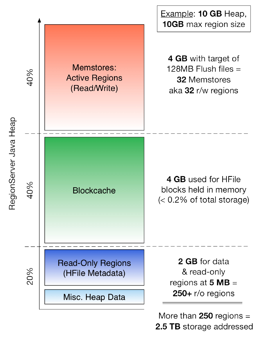
Figure 11-1. Java heap shared across different major components within a region server
The example starts with a fixed heap size of 10 GB, and 10 GB as the upper boundary of a
region, assuming they are nearly full (steady state). Given the 40% of the default memstore
share, we can use 4 GB of heap for writes, allowing us up to have 32 regions that are written to
while flushing at 128 MB. For the block cache we also have 40% and that means 4 GB available
in heap. You can see from the bottom left result line, that this is just 0.2% or less of the overall
(868)

storage—that means many actual disk reads are needed for random access use-cases.
Now look at the remaining 20% of the heap that HBase needs. Here the root index and filter
structures are stored for regions that are read from. Doing some (non-scientific) testing showed
that between 2 and 5 MB was needed for each store file. That means with 2 GB remaining heap,
we can maybe store index/filter data for (at least) 250 read-from regions. Assuming these are
also part of the 32 you write to, then you can address about 2.5TB of data on disk.
You can now twist and turn this math to your needs. For example, you could lower the block
cache share to have more room for read-from data. You should also try to design a table schema
that takes advantage of this behavior, for example have newer data being written to only as many
regions as the memstore share can hold safely, and then have the other regions only contain
historical data that you only read from (see “Aging-out Regions”).
Finally, as mentioned above, the index and filter data is cached in an LRU structure, which evicts
data that is old and used least. So you could open twice as many regions, addressing say 5TB of
raw storage but would incur more LRU cache misses and reload index and filter sub-blocks,
adding to the latency of reads. If you can live with that, then by all means give it a try. It is a
misconception to assume that HBase can only address relatively low amounts of data, compared
to a DataNode. You can address most of it, with some caveats. Be smart, do the math and decide
what works best for you.
(869)

Resource Management
Operating a HBase cluster comprises many tasks, one of which is controlling all of the vital (and
often scarce) resources, such as available and used storage, or how many requests are handled by
each server. The following discusses the available features in detail.
RPC Throttling
Since HBase 1.1 there is a feature allowing an operator to control specific aspects of the server-
side RPC layer. See “RPC Tuning” for a more technical overview of this feature. More
specifically, the requests can be throttle based on the following limits:
Request Quotas
Sets the allowed number, or size, of requests (read, write, or both) in a given timeframe.
Namespace Quotas
Controls the number of tables allowed in a namespace.
These limits can be enforced for a specified user, table, or namespace. Quotas are disabled by
default, but can be enabled by setting the hbase.quota.enabled property to true in the hbase-
site.xml file for all cluster nodes.
The general quota syntax, as shown in the examples later on, is as follows:
The THROTTLE_TYPE can be expressed as READ, WRITE, or the default type (that is both, read &
write)
Timeframes can be expressed in the following units: sec, min, hour, day
Request sizes can be expressed in the following units: B (bytes), K (kilobytes), M
(megabytes), G (gigabytes), T (terabytes), P (petabytes)
Numbers of requests are expressed as an integer followed by the string req
Limits relating to time are expressed as req/<time> or size/<time>, for example 10req/day or
100P/hour
The numbers of tables or regions are expressed as integers
Request Quotas
You can set quota rules ahead of time, or you can change the throttle at runtime. The change will
propagate after the quota refresh period has expired. This expiration period defaults to five
minutes. To change it, modify the hbase.quota.refresh.period property in hbase-site.xml
(expressed in milliseconds and set to 300000). The following shows you some example on how to
set quotas using using the HBase shell:
# Limit user u1 to 10 requests per second
hbase> set_quota TYPE => THROTTLE, USER => 'u1', LIMIT => '10req/sec'
(870)
# Limit user u1 to 10 read requests per second
hbase> set_quota TYPE => THROTTLE, THROTTLE_TYPE => READ, USER => 'u1', \
LIMIT => '10req/sec'
# Limit user u1 to 10 M per day everywhere
hbase> set_quota TYPE => THROTTLE, USER => 'u1', LIMIT => '10M/day'
# Limit user u1 to 10 M write size per sec
hbase> set_quota TYPE => THROTTLE, THROTTLE_TYPE => WRITE, USER => 'u1', \
LIMIT => '10M/sec'
# Limit user u1 to 5k per minute on table t2
hbase> set_quota TYPE => THROTTLE, USER => 'u1', TABLE => 't2', \
LIMIT => '5K/min'
# Limit user u1 to 10 read requests per sec on table t2
hbase> set_quota TYPE => THROTTLE, THROTTLE_TYPE => READ, USER => 'u1', \
TABLE => 't2', LIMIT => '10req/sec'
# Remove an existing limit from user u1 on namespace ns2
hbase> set_quota TYPE => THROTTLE, USER => 'u1', NAMESPACE => 'ns2', \
LIMIT => NONE
# Limit all users to 10 requests per hour on namespace ns1
hbase> set_quota TYPE => THROTTLE, NAMESPACE => 'ns1', LIMIT => '10req/hour'
# Limit all users to 10 T per hour on table t1
hbase> set_quota TYPE => THROTTLE, TABLE => 't1', LIMIT => '10T/hour'
# Remove all existing limits from user u1
hbase> set_quota TYPE => THROTTLE, USER => 'u1', LIMIT => NONE
Using the list_quotas shell command allows you to retrieve the current settings:
# List all quotas for user u1 in namespace ns2
hbase> list_quotas USER => 'u1, NAMESPACE => 'ns2'
# List all quotas for namespace ns2
hbase> list_quotas NAMESPACE => 'ns2'
# List all quotas for table t1
hbase> list_quotas TABLE => 't1'
# list all quotas
hbase> list_quotas
You can also place a global limit and exclude a user or a table from the limit by applying the
GLOBAL_BYPASS property:
# A per-namespace request limit
hbase> set_quota NAMESPACE => 'ns1', LIMIT => '100req/min'
# User u1 is not affected by the limit
hbase> set_quota USER => 'u1', GLOBAL_BYPASS => true
Namespace Quotas
You can specify the maximum number of tables or regions allowed in a given namespace, either
when you create the namespace or by altering an existing namespace, by setting the
hbase.namespace.quota.maxtables property for the namespace, for example, limiting tables per
namespace like so:
# Create a namespace with a max of 5 tables
hbase> create_namespace 'ns1', { 'hbase.namespace.quota.maxtables' => '5' }
# Alter an existing namespace to have a max of 8 tables
hbase> alter_namespace 'ns2', { METHOD => 'set', \
'hbase.namespace.quota.maxtables' => '8' }
# Show quota information for a namespace
(871)
hbase> describe_namespace 'ns2'
# Alter an existing namespace to remove a quota
hbase> alter_namespace 'ns2', { METHOD => 'unset', \
NAME => 'hbase.namespace.quota.maxtables' }
Doing the same for regions requires setting the hbase.namespace.quota.maxregions property
instead, as shown here:
# Create a namespace with a max of 10 regions
hbase> create_namespace 'ns1', { 'hbase.namespace.quota.maxregions' => '10' }
# Show quota information for a namespace
hbase> describe_namespace 'ns1'
# Alter an existing namespace to have a max of 20 tables
hbase> alter_namespace 'ns2', { METHOD => 'set', \
'hbase.namespace.quota.maxregions' => '20' }
# Alter an existing namespace to remove a quota
hbase> alter_namespace 'ns2', { METHOD => 'unset', \
NAME => 'hbase.namespace.quota.maxregions' }
Request Queues
If no throttling policy is configured, when the region server receives multiple requests, they are
placed into a queue waiting for a free execution slot. The simplest queue is a FIFO queue, where
each request waits for all previous requests in the queue to finish before running. One of the
known drawbacks of FIFO handling is that fast or interactive queries can get stuck behind large
requests.
If you are able to guess how long a request will take, you can reorder requests by pushing the
long requests to the end of the queue and allowing short requests to preempt them. Eventually,
you must still execute the large requests and prioritize the new requests behind them. The short
requests will be newer, so the result is not terrible, but still suboptimal compared to a mechanism
which allows large requests to be split into multiple smaller ones.
HBase 1.0 introduces such a system for deprioritizing long-running scanners. There are three
types of queues, fifo, deadline, and codel. To configure the type of queue used, configure the
hbase.ipc.server.callqueue.type property in hbase-site.xml. Since there is no way to estimate
how long each request may take, de-prioritization can only affect scans, and is based on the
number of next() calls a scan request has made. An assumption is made that when you are doing
a full table scan, your job is not likely to be interactive, so if there are concurrent requests, you
can delay long-running scans up to a limit tunable by setting the
hbase.ipc.server.queue.max.call.delay property. The slope of the delay is calculated by a simple
square root of numNextCall * weight, where the weight is configurable by setting the
hbase.ipc.server.scan.vtime.weight property.
Multiple-Typed Queues
You can also prioritize or deprioritize different kinds of requests by configuring a specified
number of dedicated handlers and queues. You can segregate the scan requests in a single queue
with a single handler, and all the other available queues can service short Get requests.
You can adjust the IPC queues and handlers based on the type of workload, using static tuning
options. This approach is an interim first step that will eventually allow you to change the
(872)
settings at runtime, and to dynamically adjust values based on the load.
Multiple Queues
To avoid contention and separate different kinds of requests, configure the
hbase.ipc.server.callqueue.handler.factor property, which allows you to increase the
number of queues and control how many handlers can share the same queue. It allows
admins to increase the number of queues and decide how many handlers share the same
queue.
Using more queues reduces contention when adding a task to a queue or selecting it from a
queue. You can even configure one queue per handler. The trade-off is that if some queues
contain long-running tasks, a handler may need to wait to execute from that queue rather
than stealing from another queue which has waiting tasks.
Read and Write Queues
With multiple queues, you can now divide read and write requests, giving more priority
(more queues) to one or the other type. Use the hbase.ipc.server.callqueue.read.ratio
property to choose to serve more reads or more writes.
Get and Scan Queues
Similar to the read/write split, you can split gets and scans by tuning the
hbase.ipc.server.callqueue.scan.ratio property to give more priority to gets or to scans. A
scan ratio of 0.1 will give more queue/handlers to the incoming gets, which means that
more gets can be processed at the same time and that fewer scans can be executed at the
same time. A value of 0.9 will give more queue/handlers to scans, so the number of scans
executed will increase and the number of gets will decrease.
(873)

Bulk Moving Regions
Disabling the Load Balancer
This and a few of the following sections concern themselves with region move operations, for
example, as an explicit task, or as part of another procedure, such as decommissioning a server.
If the region load balancer (see, for example, “Load Balancing”) runs while regions are moved
not on its behalf, there could be contention between the load balancer and the affected region(s).
Avoid any problems by disabling the balancer first, for example, using the shell to disable it like
so (refer to “Tool Commands” for more balancer related operations):
hbase(main):001:0> balance_switch false
true
0 row(s) in 0.3590 seconds
This turns the balancer off. To reenable it, enter the following:
hbase(main):002:0> balance_switch true
false
0 row(s) in 0.3590 seconds
Note that the balancer state is persisted across cluster restarts (which is primarily concerning the
active master).
Running a cluster sometimes requires an administrator to move regions from one region server to
another in a controlled manner. HBase ships with a JRuby script for that task, which can be run
through the supplied JRuby interpreter, like so:
$ bin/hbase org.jruby.Main bin/region_mover.rb
Usage: region_mover.rb [options] load|unload \
[<hostname>|<hostname:port>]
Load or unload regions by moving one at a time
-f, --filename=FILE File to save regions list into unloading, \
or read from loading; default /tmp/<hostname:port>
-h, --help Display usage information
-d, --debug Display extra debug logging
-x, --excludefile=FILE File with hosts-per-line to exclude as \
unload targets; default excludes only target host; useful for \
rack decommisioning.
-m, --maxthreads=XX Define the maximum number of threads to \
use to unload and reload the regions
The script offers the following to modes:
Unload
Upon first use it is assumed that you are unloading regions from a particular server,
moving them to the remaining servers equally. By default the script simply ignores the
server specified as the one to be unloaded. In addition, the optional -x parameter allows the
user to hand in a list of other servers to also ignore.
Running this command generates a file either in the default location in the system’s
temporary directory1, or in what is specified by the -f option. This file stores (as serialized
HRegionInfo instances) the information about the regions that were unloaded during the
operation for later use.
(874)

Load
Once a server is back online, an operator may wish to move the previously unloaded
region back onto it. The reason to do so is locality as all data should still be local to the
servers data node (and local storage in extension). Using the -f parameter with the load
option allows the script to get the list of regions back, and move those over subsequently.
Both modes support the specification of the number of threads to use during the execution, using
the -m parameter. It defaults to 1, meaning only one region is moved at a time. The following
example shows the region_mover.rb script used to unload regions from one specific region server:
$ bin/hbase org.jruby.Main bin/region_mover.rb unload \
worker-3.internal.larsgeorge.com
Valid region move targets:
worker-1.internal.larsgeorge.com,16020,1482996572051
worker-2.internal.larsgeorge.com,16020,1482996570909
2016-12-29 01:26:16,233 INFO [main] region_mover: Moving 95 region(s) from \
worker-3.internal.larsgeorge.com,16020,1482996572481 on 2 servers using \
1 threads.
2016-12-29 01:26:16,263 INFO [RubyThread-6: bin/thread-pool.rb:28] \
region_mover: Moving region e07b714ffea6eed2b76aeaae48bbfe12 (1 of 95) to \
server=worker-1.internal.larsgeorge.com,16020,1482996572051 for \
worker-3.internal.larsgeorge.com,16020,1482996572481
2016-12-29 01:26:16,295 INFO [main] region_mover: Waiting for the pool to \
complete
2016-12-29 01:26:17,750 INFO [RubyThread-6: bin/thread-pool.rb:28] \
region_mover: Moved region \
ltttest1,22222222,1479061251893.e07b714ffea6eed2b76aeaae48bbfe12. \
cost: 1.154
2016-12-29 01:26:17,751 INFO [RubyThread-6: bin/thread-pool.rb:28] \
region_mover: Moving region a83cada0bc587986f64476153cfca81c (2 of 95) to \
server=worker-2.internal.larsgeorge.com,16020,1482996570909 for \
worker-3.internal.larsgeorge.com,16020,1482996572481
2016-12-29 01:26:18,727 INFO [RubyThread-6: bin/thread-pool.rb:28] \
region_mover: Moved region \
ltttest1,88888888,1479061251893.a83cada0bc587986f64476153cfca81c. cost: 0.948
...
2016-12-29 01:27:36,446 INFO [main] region_mover: Pool completed
2016-12-29 01:27:36,474 INFO [main] region_mover: Wrote list of moved \
regions to /tmp/larsgeorgeworker-3.internal.larsgeorge.com:16020
After each region is moved (which applies to both the load and unload operation), which uses the
move() call of the administrative API (see “Region Operations”), a test is performed ensuring the
region is back online on the new server before moving to the next one. This test scans the table
by setting the Scans start row to the region start key, and calls next() on the ResultScanner
instance. The cost printed for each move is the time in seconds that was needed to move the
region. In case of a region being stuck on a server, the script will throw an exception to that
effect and exit.
(875)

Node Decommissioning
While not the best option, as you will read below, you can stop an individual region server by
running the following script in the HBase directory on the particular server:
$ bin/hbase-daemon.sh stop regionserver
Explained in simple terms, the region server will first close all regions and then shut itself down.
On shutdown, its ephemeral node in ZooKeeper will expire, which will be noticed by the master
as it has placed watches on all active region servers. This will be treated as a crashed server
event, which means the master will reassign the regions the server was carrying to other servers.
The following describes the events that happen during and after the execution of the command in
more detail:
The hbase-daemon.sh script sends a SIGTERM (15) Linux signal to the region server process
using the kill command.
At start time the region server did register a Java JVM shutdown hook, which is triggered
by the signal and calls the stop() method of the HRegionServer class.
The stop() call sets a global flag that the process is about to end, and wakes up the main
event loop in the run() method of the same class.
Leaving the main loop causes for all resources to be freed, including the many thread pools
in use and so on, as well as asking the server to close all the open regions it hosts.
Regions are closed in a multithreaded fashion, for example set for user regions with
hbase.regionserver.executor.closeregion.threads (defaulting to 3, meaning that three
regions are closed concurrently), going through the usual region close path (as if calling,
for example, the closeRegion() admin API call—see “Region Operations”).
Part of closing a region is to check if the region has enough data to warrant a pre-flush (see
[Link to Come] for details), followed by a final flush under a write lock to persist all
pending changes.
The shutdown process waits for all regions to be closed before proceeding with the
remaining ramp-down of other resources (for example, the WAL and RPC subsystems).
At the very end, the process removes the ephemeral ZooKeeper znode it holds and exits
normally.
The removal of the znode for the region server is sent to the active master in form of a
watch callback by the ZooKeeper client library, starting an immediate reassignment of
those closed regions to the remaining active region servers.
As closing regions includes the possibly time-consuming flush operations, resulting in
considerable time spent until all regions are closed and the process being terminated, it is wise to
disable the load balancer during the operation.
(876)

Note
For the region moving to not interfere with the load balancer and vice-versa, you should disable
the balancer as explained earlier. While the balancer is disabled, no reassignment will take place.
You will need to re-enable it to trigger the described reaction of the master.
One of the disadvantages using this method, especially when considering the maintenance of a
production cluster, is that regions are first shed as fast as possible by the process that is about to
be terminated, while the subsequent reassignment is invoked only at the very end, or possibly by
a timed event in the master (that is, the balancer task). This could cause the data located in those
regions to not be available for a considerable amount of time, as closing and re-opening are
hinged around decoupled events. It would be much more practical if regions are first moved
away from the decommissioned node, before it is terminated, and, in addition, being able to
control at what pace this is done. For that, HBase is shipping with another shell script, called
graceful_stop.sh, which invoked with no parameters is printing its command line options:
$ bin/graceful_stop.sh
Usage: graceful_stop.sh [--config <conf-dir>] [-d] [-e] [--restart \
[--reload]] [--thrift] [--rest] <hostname>
thrift If we should stop/start thrift before/after the hbase stop/start
rest If we should stop/start rest before/after the hbase stop/start
restart If we should restart after graceful stop
reload Move offloaded regions back on to the restarted server
d|debug Print helpful debug information
maxthreads xx Limit the number of threads used by the region mover. \
Default value is 1.
hostname Hostname of server we are to stop
e|failfast Set -e so exit immediately if any command exits with \
non-zero status
If you look behind the scenes, that is, into the source code of the graceful_stop.sh script, you will
notice that it is a combination of many techniques and other scripts to accomplish its goals. More
specifically, it disables the balancer at the beginning, and enables it again at the end as described
earlier. In between it calls upon the region_mover.rb script, as outlined in “Bulk Moving
Regions”, moving regions away from the server that is about to be stopped.
You also have an option to have the gateway processes for Thrift or REST APIs on the same
server stopped during the process, by adding the --thrift and/or --rest flags to the command
line. When you want to decommission a loaded region server, running the following command is
the most basic option:
$ bin/graceful_stop.sh <hostname>
Note that <hostname> is the host carrying the region server you want to decommission—which
does not have to be the same host you are running the command on. The <hostname> passed to
graceful_stop.sh must match the hostname that HBase is using to identify region servers. Check
the list of region servers in the master UI for how HBase is referring to each server. It is usually
the short host name, but it can also be an FQDN, such as hostname.foobar.com. Whatever HBase is
using, this is what you should pass the graceful_stop.sh decommission script.
Note
If you pass IP addresses, the script is not (at the time of this writing) smart enough to make a
hostname (or FQDN) out of it and will fail when it checks if the server is currently running,
causing the graceful unloading of regions to not run successfully. Also, when using an existing
short hostname that does not match the long server name, the unload of regions will fail, but the
(877)
stop call will still be issued, resulting in the above cold stop of the server process.
The graceful_stop.sh script will move the regions off the decommissioned region server, by
default, one at a time to minimize region churn. It will verify that the region is deployed in the
new location before it moves the next region, and so on, until the decommissioned server is
carrying no more regions. Using the --maxthreads parameter allows you to increase the
parallelism of the unload operation (with the option being passed on the region_mover.rb script
internally).
At this point, the graceful_stop.sh script tells the region server to stop. The master will notice the
region server gone but all regions will have already been redeployed, and because the region
server went down cleanly, there will be no WALs to split.
Caution
You need to run the graceful stop script as an administrative user, since the call to bin/hbase-
daemon.sh stop regionserver requires reading the OS process ID from the PID file, which was
created when the process was started. Lacking the appropriate rights will result in an error, such
as:
2017-01-27T02:37:43 Stopping regionserver on worker-3
worker-3: no regionserver to stop because no pid file \
/var/opt/hbase/run/hbase-larsgeorge-regionserver.pid
(878)
Draining Servers
Using the graceful decommission is useful to bring down one server at a time with minimal
impact on clients accessing the data stored within the affected regions. But in case you want to
decommission more than one server at a time, you may want to also run that process in parallel
itself, across more than one server at a time. Using the graceful_stop.sh script alone is a little
problematic, as it calls upon the region_mover.rb script internally, which in turn only excludes the
single decommissioned node it is tasked with from the list of potential targets for the region
move operation. The graceful stop also enables the balancer when it is done with its node,
possibly causing issues for other nodes that are still in the middle of their decommissioning
process.
What is needed is a central mechanism that allows for more than one server being
decommissioned at a time, while excluding them from any balancing work. In other words, it is
not enough to switch of the balancer yourself, as it would eventually interfere again. Instead,
HBase has a draining mode for nodes, which flags them for global exclusion from any upcoming
region balancing work. This is orchestrated—as with many other things in HBase and Hadoop—
using ZooKeeper as the service registry, placing a host specific entry under the /hbase/draining
znode. HBase ships with a script that enables an operator to automate that process, and running it
without any parameters will print its help as expected:
$ bin/hbase org.jruby.Main bin/draining_servers.rb
Usage: ./hbase org.jruby.Main draining_servers.rb [options] add|remove|list \
<hostname>|<host:port>|<servername> ...
Add remove or list servers in draining mode. Can accept either hostname to \
drain all region serversin that host, a host:port pair or a \
host,port,startCode triplet. More than one server can be given \
separated by space
-h, --help Display usage information
-d, --debug Display extra debug logging
For example, adding a region server with its full name, for example worker-
3.internal.larsgeorge.com, to the list of draining server is done like so:
$ bin/hbase org.jruby.Main bin/draining_servers.rb \
add worker-3.internal.larsgeorge.com
Listing all currently draining servers and removing the previously added one is done like this:
$ bin/hbase org.jruby.Main bin/draining_servers.rb list
...
worker-3.internal.larsgeorge.com,16020,1482996572481
$ bin/hbase org.jruby.Main bin/draining_servers.rb \
remove worker-3.internal.larsgeorge.com
While a server is in draining mode, it is ignored by the master, no matter the state of the load
balancer, as far as region assignments are concerned. You could, for example, create a new,
presplit table, that would span the draining server, but since it is marked as such it will not
receive any of the new regions either. Only after removing the server from the list and starting
(or waiting for) the balancer will cause for regions to be moved to that particular server again.
(879)

Rolling Restarts
There are multiple ways to perform a rolling restart of the cluster, which we will discuss in this
section. Before we do, a word of caution.
Caution
The scripts discussed in this section are no replacement for your own automated process
management, be it Ansible etc. or a commercial Hadoop management tool, that includes proper
procedure transactionality and monitoring. They may be used in lieu of anything else, but may
leave the cluster in an undefined state should something happen during their execution.
This is not referring to something disastrous, such as data or server loss, but an interrupted
rolling restart that has not completed. You may find some servers have been restarted, while
others are still pending. Or regions have been moved away from a server before its restart, but
with a failed restart you are left reloading the right regions manually yourself—and continue the
process of restarting the remaining servers. While this sounds scary, you should be advised that
running a (especially production) HBase cluster without proper management scaffolding is
asking for trouble.
Use Rolling Restart Script
HBase ships with a script, called rolling-restart.sh, that allows you to perform rolling restarts
on the entire cluster, or alternatively, the master(s) only, or the region servers only.
Note
The rolling restart script requires password-less SSH login to be configured as it is using the
supplied HBase daemon scripts to start and stop the processes on other machines (which,
obviously, need to be accessible too). That implicitly assumes that you have deployed HBase
using the Apache provided tarballs (see “Quick-Start Guide”), as only then the scripts will have
proper environment available.
Executing the script with -h will reveal the full list of parameters:
$ bin/rolling-restart.sh -h
Usage: rolling-restart.sh [--config <hbase-confdir>] [--rs-only] \
[--master-only] [--graceful] [--maxthreads xx]
The parameters influence how the rolling restart script is performing is duties:
Rolling Restart on Region Servers Only
Performing a rolling restart on the region servers only requires the use of the --rs-only
option. This might be necessary if you need to reboot the individual region servers or if
you make a configuration change that only affects region servers and not the other HBase
processes.
Rolling Restart on Master(s) Only
(880)

Performing a rolling restart on the active and backup masters is facilitated through the --
master-only option. You might use this if you know that your configuration change only
affects the master(s) and not the region servers, or if you need to restart the server where
the active master is running.
Graceful Restart
If you specify the --graceful option, region servers are restarted using the graceful_stop.sh
script, which moves regions off a region server before restarting it. This is safer, but can
delay the restart.
Limiting the Number of Threads
You can limit the rolling restart to using only a specific number of threads, use the --
maxthreads option.
Not setting any option will initiate a full rolling restart of the entire cluster, starting with all the
masters, and then proceeding to the region servers. Interesting to note is that the rolling restart
script is also equipped to restart a non-distributed HBase setup, that is, a full instance of all
services running on a single node (for testing and development purposes). In this case the script
is restarting the single process alone and is done with its work.
Use Graceful Stop Script
You can also use the graceful_stop.sh script explicitly to restart a region server after its shutdown
and move its old regions back into place, retaining data locality. A primitive rolling restart might
be effected by running something like the following:
$ for i in `cat conf/regionservers|sort`; do bin/graceful_stop.sh \
--restart --reload --debug $i; done &> /tmp/log.txt &
Tail the output of /tmp/log.txt to follow the script’s progress. The example pertains to region
servers only, and to be safe it is advised to disable the load balancer before using this code. You
also have to make sure to run this command using the proper OS user account, as per the
explanation earlier (that is, graceful_stop.sh needs access to the PID file).
A full manual rolling restart during a cluster update may follow these steps:
1. Extract the new release, verify its configuration, and synchronize it to all nodes of your
cluster using rsync, scp, or another secure synchronization mechanism.
2. Run hbck to ensure the cluster is consistent:
$ bin/hbase hbck
...
0 inconsistencies detected.
Status: OK
Perform repairs if required, as explained in “HBase Fsck”.
3. Restart the master(s). You may need to modify these commands if your new HBase
directory is different from the old one, such as for an upgrade:
$ bin/hbase-daemon.sh stop master; bin/hbase-daemon.sh start master
(881)
4. Disable the region load balancer:
$ echo "balance_switch false" | bin/hbase shell
5. Run the graceful_stop.sh script for the region servers. For example:
$ for i in `cat conf/regionservers|sort`; do bin/graceful_stop.sh \
--restart --reload --debug $i; done &> /tmp/log.txt &
If you are running Thrift or REST servers on the region server, pass the --thrift or --rest
option, as per the script’s usage instructions, shown earlier (when running it without any
command line options).
6. Restart the master again, clearing out the dead servers list and reenable the balancer.
$ bin/hbase-daemon.sh stop master; bin/hbase-daemon.sh start master
$ echo "balance_switch true" | bin/hbase shell
7. Run hbck once more ensuring the cluster is consistent:
$ bin/hbase hbck
...
0 inconsistencies detected.
Status: OK
It may be important to drain HBase regions slowly when restarting multiple region servers.
Otherwise, multiple regions go offline simultaneously and must be reassigned to other nodes,
which may also go offline soon. This can negatively affect performance. You can inject delays
into the script above, for instance, by adding a Shell command such as sleep. To wait for five
minutes between each region server restart, modify the above script to the following:
$ for i in `cat conf/regionservers|sort`; do bin/graceful_stop.sh \
--restart --reload --debug $i & sleep 5m; done &> /tmp/log.txt &
(882)

Adding Servers
One of the major features HBase offers is built-in scalability. As the load on your cluster
increases, you need to be able to add new servers to compensate for the new requirements.
Adding new servers is a straightforward process and can be done for clusters running in any of
the distribution modes, which are explained in “Distributed Mode”.
Pseudo-distributed Mode
It seems paradoxical to scale a HBase cluster in an all-local mode, even when all daemons are
run in separate processes. However, pseudo-distributed mode is the closest you can get to a real
cluster setup, and during development or prototyping it is advantageous to be able to replicate a
fully distributed setup on a single machine.
Since the processes have to share all the local resources, adding more processes obviously will
not make your test cluster perform any better. In fact, pseudo-distributed mode is really suitable
only for a very small amount of data. However, it allows you to test most of the architectural
features HBase has to offer.
For example, you can experiment with master failover scenarios, or regions being moved from
one server to another. Obviously, this does not replace testing at scale on the real cluster
hardware, with the load expected during production. However, it does help you to come to terms
with the administrative functionality offered by the HBase Shell and scripts, for example. Or,
you can use the administrative API as discussed in Chapter 5. Use it to develop tools that
maintain schemas, or to handle shifting server loads. There are many applications for this in a
production environment, and being able to develop and test a tool locally first is tremendously
helpful.
Note
You need to have set up a pseudo-distributed installation before you can add any servers in
pseudo-distributed mode, and it must be running to use the following commands. They add to the
existing processes, but do not take care of spinning up the local cluster itself.
Adding a Local Backup Master
Starting a local backup master process is accomplished by using the local-master-backup.sh script
in the bin directory, like so:
$ bin/local-master-backup.sh start 1
The number at the end of the command signifies an offset that is added to the default ports of
16000 for RPC and 16010 for the web-based UI. In this example, a new master process would be
started that reads the same configuration files as usual, but would listen on ports 16001 and 16011,
respectively.
In other words, the parameter is required and does not represent a number of servers to start, but
where their ports are bound to. Starting more than one is also possible:
(883)
$bin/local-master-backup.sh start 1 3 5
This starts three backup masters on ports 16001, 16003, and 16005 for RPC, plus 16011, 16013, and
16015 for the web UIs.
Caution
Make sure you do not specify an offset that could collide with a port that is already in use by
another process. For example, it is a bad idea to use 30 for the offset, since this would result in a
master RPC port on 16030--which is usually already assigned to the first region server as its UI
port.
The start script also adds the offset to the name of the log file the process is using, thus
differentiating it from the log files used by the other local processes. For an offset of 1, it would
set the log file name to be:
logs/hbase-${USER}-1-master-${HOSTNAME}.log
Note the added 1 in the name. Using an offset of, for instance, 10 would add that number into the
log file name.
Stopping the backup master(s) involves the same command, but replacing the start command
with the aptly named stop, like so:
$ bin/local-master-backup.sh stop 1
You need to specify the offsets of those backup masters you want to stop, and you have the
option to stop only one, or any other number, up to all of the ones you started: whatever offset
you specify is used to stop the master matching that number.
Adding a Local Region Server
In a similar vein, you are allowed to start additional local region servers. The script provided is
called local-regionservers.sh, and it takes the same parameters as the related local-master-
backup.sh script: you specify the command, that is, if you want to start or stop the server
process(es), and a list of offsets.
The difference is that these offsets are added to 16200 for RPC, and 16300 for the web UIs. For
example:
$ bin/local-regionservers.sh start 1
This command will start an additional region server using port 16201 for RPC, and 16301 for the
web UI. The log file name has the offset added to it, and would result in:
logs/hbase-${USER}-1-regionserver-${HOSTNAME}.log
The same concerns apply: you need to ensure that you are specifying an offset that results in a
port that is not already in use by another process, or you will receive a java.net.BindException:
Address already in use exception—as expected.
Starting more than one region server is accomplished by adding more offsets:
$ bin/local-regionservers.sh start 1 2 3
(884)

Note
You do not have to start with an offset of 1. Since these are added to the base port numbers, you
are free to specify any offset you prefer.
Stopping any additional region server involves replacing the start command with the stop
command:
$ bin/local-regionservers.sh stop 1
This would stop the region server using offset 1, or ports 16201 and 16301. If you specify the
offsets of all previously started region servers, they will all be stopped.
Fully Distributed Cluster
Operating a HBase cluster typically involves adding physical (or virtualized) servers over time.
This is more common for the region servers, as they are doing all the heavy lifting. For the
master, you have the option to start backup instances.
Adding a Backup Master
To prevent a HBase cluster master server from being the single point of failure, you can add
backup masters. These are typically located on separate physical machines so that in a worst-case
scenario, where the machine currently hosting the active master is failing, the system can fall
back to a backup master.
The master process uses ZooKeeper to negotiate which is the currently active master: there is a
dedicated ZooKeeper znode that all master processes race to create, and the first one to create it
wins. This happens at startup and the winning process moves on to become the current master.
All other machines simply loop around the znode check and wait for it to disappear—triggering
the race again.
The /hbase/master znode is ephemeral, and is the same kind the region servers use to report their
presence. When the master process that created the znode fails, ZooKeeper will notice the end of
the session with that server and remove the znode accordingly, triggering the election process.
Starting a server on multiple machines requires that it is configured just like the rest of the HBase
cluster (see “Configuration” for details). The master servers usually share the same configuration
with the other servers in the cluster. Once you have confirmed that this is set up appropriately,
you can run the following command on a server that is supposed to host the backup master:
$ bin/hbase-daemon.sh start master
Assuming you already had a master running, this command will bring up the new master to the
point where it waits for the znode to be removed. The backup master will listen on the UI port
and display a limited status page, linking to the currently active master (see “Backup Master
UI”).
If you want to start many masters in an automated fashion and dedicate a specific server to host
the current one, while all the others are considered backup masters, you can add the --backup
switch like so:
$ bin/hbase-daemon.sh start master --backup
(885)

This forces the newly started master to wait for the dedicated one—which is the one that was
started using the normal start-hbase.sh script, or by the previous command but without the --
backup parameter—to create the /hbase/master znode in ZooKeeper. Once this has happened, they
move on to the master election loop. Since now there is already a master present, they go into
idle mode as explained.
Finding the Active Master
If you started more than one master, and you experienced failovers, it may be difficult to tell
which master is currently active. You can try the backup master UI(s) to see which one has taken
over, but that is somewhat tedious. The currently active master is written to ZooKeeper, though
accessing the znode would require some shell programming. HBase ships with a short JRuby
script that makes this easier and can be used from your own scripts to retrieve the active master’s
hostname:
$ /bin/hbase org.jruby.Main bin/get-active-master.rb
master-1.internal.larsgeorge.com
An administrator could run the above (as part of a larger script) on a regular basis and update a
generic DNS entry for the HBase master UI to point to the returned hostname. This would make
accessing the UI much easier for the average user (though you are still bound by how fast DNS
changes are propagated).
There is also the option of creating a backup-masters file in the conf directory. This is akin to the
regionservers file, listing one hostname per line that is supposed to start a backup master. For the
example in “Example Configuration”, we could assume that we have three backup masters
running on the ZooKeeper servers. In that case, the conf/backup-masters, would contain these
entries:
zk1.foo.com
zk2.foo.com
zk3.foo.com
Adding backup masters to the ZooKeeper machines is reasonable in a small cluster, as the master
is more a coordinator in the overall design, and therefore does not need a lot of resources. In a
larger cluster the design is often such that there are 3-5 management nodes (that is, server
instances), which will hold the active and backup HBase masters, as well as ZooKeeper
processes.
Note
You should start as many backup masters as you feel satisfies your requirements to handle
machine failures. There is no harm in starting too many, but having too few might leave you with
a weak spot in the setup. This is mitigated by the use of monitoring solutions that report the first
master to fail. You can take action by repairing the server and adding it back to the cluster.
Overall, having two or three backup masters seems a reasonable number.
Note that the servers listed in backup-masters are what the backup master processes are started on,
while using the --backup switch. This happens as the start-hbase.sh script starts the primary
master, the region servers, and eventually the backup masters. Alternatively, you can invoke the
master-backup.sh script to initiate the start of the backup masters. Finally, using the rolling restart
script with the --master-only parameter (see “Rolling Restarts”) is another option to restart the
active and backup masters as configured (which is useful after the active master has switched to
(886)

a backup master).
Adding a Region Server
Adding a new region server is one of the more common procedures you will perform on a cluster
(along with adding a colocated HDFS data node). The first thing you should do is to edit the
regionservers file in the conf directory, enabling the launcher scripts to automate the server start
and stop procedure.2 Simply add a new line to the file specifying the hostname to add. Once you
have updated the file, you need to copy it across all machines in the cluster. You also need to
ensure that the newly added machine has HBase installed, and that the configuration is current.
Then you have a few choices to start the new region server process. One option is to run the
start-hbase.sh script on the master machine. It will skip all machines that have a process already
running. Since the new machine fails this check, it will appropriately start the region server
daemon. Another option is to use the launcher script directly on the new server. This is done like
so:
$ bin/hbase-daemon.sh start regionserver
Note
This must be run on the server on which you want to start the new region server process. For this
script invocation there is no need to update the regionservers configuration file—but it is
recommended to do that nevertheless, as later calls to start-hbase.sh would otherwise omit the
new server.
The region server process will start and register itself by creating a znode with its hostname in
ZooKeeper. It subsequently joins the collective and is assigned regions as soon as the balancer
process is lapsing. Alternatively, you may want to consider disabling the balancer when you are
adding a new node and then move regions to it at your own pace. Keep in mind that all moved
regions will have a locality of 0%, which may have an adverse impact on your cluster’s
performance. Moving the regions manually, and performing a major compaction to rewrite all
data locally, will be much less impactful—but of course take much more time.
(887)

Reloading Configuration
Some of the classes and subsystems provide support for configuration changes while the process
is running. For example, the region load balancer, RPC subsystem, compaction and split thread,
as well as the general region and master server processes use this feature to reload settings
without the need to restart the service and cause unnecessary disruption. The HBase Shell
provides a number of commands that can be used to reload the settings of specific sets of servers
(see “General Commands”), which in turn call the matching methods of the administrative API
(see “Server Operations”). Reloading the configuration on all servers (see note below) is
accomplished like this:
hbase(main):001:0> update_all_config
0 row(s) in 0.9620 seconds
Before HBase 1.4 and 2.0, the above command is only reloading the region servers, but not the
master(s). Reloading the configuration of a master node, and that of a specific region server,
needs another command that takes a specific server name. Recall that HBase server names are
not just the hostname, but also include the RPC port and start time of the process. For example, if
you want to reload the active master, you can use the zk_dump command to get a list of server
names and then feed that into the update_config command:3
hbase(main):001:0> zk_dump
HBase is rooted at /hbase
Active master address: master-1.internal.larsgeorge.com,16000,1485608557645
Backup master addresses:
master-2.internal.larsgeorge.com,16000,1485608558391
Region server holding hbase:meta: \
worker-1.internal.larsgeorge.com,16020,1485608638164
Region servers:
worker-1.internal.larsgeorge.com,16020,1485608638164
worker-3.internal.larsgeorge.com,16020,1485608659649
worker-2.internal.larsgeorge.com,16020,1485608650004
/hbase/replication:
...
hbase(main):002:0> update_config \
"master-1.internal.larsgeorge.com,16000,1485608557645"
0 row(s) in 0.3260 seconds
Both shell commands return immediately and without any feedback, apart from the time their
execution required. This lack of feedback includes the use of wrong server names. If you ask, for
example, to update a server foobar,123,456 that does not exist, you still see the same empty
feedback. One way to see if the command did actually arrive at the server is to check its log file.
Here, for instance, is the output of the master that we updated above (omitting unrelated details):
...
2017-01-28 07:33:23,789 INFO ... regionserver.HRegionServer: \
Reloading the configuration from disk.
2017-01-28 07:33:23,789 INFO ... conf.ConfigurationManager: \
Starting to notify all observers that config changed.
2017-01-28 07:33:24,084 INFO ... balancer.StochasticLoadBalancer: \
loading config
...
Once the server has reloaded the configuration (which assumes you have updated them on all the
targeted servers) it propagates the change to all internal listeners, which will reconfigure
themselves accordingly. The following table lists the classes that currently implement the listener
interface and describes what the update call triggers:
Table 11-1. List of classes handling online changes
(888)
Table 11-1. List of classes handling online changes
Class Name Description
CompactSplitThread Reconfigures the large and small compaction, split, and merge thread pools,
as well as the throughput controller.
HRegion Not implemented as of this writing.
HRegionServer Reloads the flush throughput controller, updating its properties.
HStore Reconfigures all stores, including all per column family settings, including
compaction and off-peak details.
LoadBalancer Updates the settings of the stochastic load balancer.
RpcServer Delegates the call to the currently configured RPC scheduler.
RSRpcServices Delegates the call to the RPC server instance (see above).
SimpleRpcScheduler Updates the executor queue sizes and the CoDel settings.
(889)
Canary & Health Checks
HBase ships with multiple facilities that help ensuring the cluster is healthy. You can use these
tools to instrument a test system outside of HBase to monitor its state, or have HBase perform its
own testing and react accordingly in case something is wrong.
Canary Tool
Since version 0.94 (and extended in 0.96) there is a tool that is shipped with HBase allowing you
to verify the current state of a cluster, by accessing regions in the cluster ensuring they are
available. The tool is integrated into the hbase shell script, and returns its list of parameters when
invoked with the -help parameter:
$ hbase canary -help
Usage: bin/hbase org.apache.hadoop.hbase.tool.Canary [opts] \
[table1 [table2]...] | [regionserver1 [regionserver2]..]
where [opts] are:
-help Show this help and exit.
-regionserver replace the table argument to regionserver,
which means to enable regionserver mode
-allRegions Tries all regions on a regionserver,
only works in regionserver mode.
-daemon Continuous check at defined intervals.
-interval <N> Interval between checks (sec)
-e Use table/regionserver as regular expression
which means the table/regionserver is regular expression pattern
-f <B> stop whole program if first error occurs, default is true
-t <N> timeout for a check, default is 600000 (milisecs)
-writeSniffing enable the write sniffing in canary
-treatFailureAsError treats read / write failure as error
-writeTable The table used for write sniffing. Default is hbase:canary
-D<configProperty>=<value> assigning or override the configuration params
The tool has two different test modes:
Region Test
Tests each region in the cluster of all specified tables (or all if none were given), accessing
a row per column family, reporting how long the request took—or outputting the error it
encountered. Starting the canary tool without any parameters starts the region test, for
example:
$ hbase canary
2017-02-04 03:35:13,425 INFO [main] tool.Canary: Number of exection threads 16
2017-02-04 03:35:24,229 INFO [pool-1-thread-6] tool.Canary: read from region \
TestTable,00000000000000000000524285,1468571711156. \
31e7e5b3c6e1f07e131ab86e3331a9be. column family info in 70ms
2017-02-04 03:35:24,232 INFO [pool-1-thread-1] tool.Canary: read from region \
TestTable,00000000000000000000209714,1468571711156. \
2b682bedc41955ab394fef40ebdc85f6. column family info in 81ms
...
Region Server Test
For each region server specified (or all if none were given) it pings one row of a region
from a random table that is currently located on that server, reporting how long the request
took—or outputting the error it encountered. You can add the -allRegions switch to extend
the test to all regions instead. For instance, the basic invocation looks like this:
(890)

$ hbase canary -regionserver
2017-02-04 03:19:06,877 INFO [main] tool.Canary: Number of exection threads 16
2017-02-04 03:19:14,357 INFO [pool-1-thread-1] tool.Canary: Read from \
table:ops:metrics on region server:worker-3.internal.larsgeorge.com in 37ms
2017-02-04 03:19:14,370 INFO [pool-1-thread-3] tool.Canary: Read from \
table:loadtest on region server:worker-2.internal.larsgeorge.com in 45ms
2017-02-04 03:19:14,439 INFO [pool-1-thread-2] tool.Canary: Read from \
table:testtable3 on region server:worker-1.internal.larsgeorge.com in 117ms
Once the check has completed, it exits with one of the following codes that can be used by
monitoring tools (see “Nagios” as an example) to react accordingly:
Table 11-2. Exit codes of the Canary tool
Code Description
0The test was successful, no errors occurred.
1Used when the usage information was requested with -help.
2Returned when setting up the check failed internally, for example, by specifying a non-
existent table.
3Indicates a timeout during the check has occurred.
4An error has occurred collecting the results.
5The check has observed a read and/or write failure and -treatFailureAsError has been
specified.
By default the test is performed only once, but running the canary tool with the -daemon
command-line switch, optionally setting a different -interval (default is 6 seconds, which may be
too low for larger clusters), will loop the tool to run continuously. For every interval period the
configured test is performed and the results printed on the console. You should consider adding
the -f false parameter and value to avoid for temporary errors aborting the loop prematurely.
An additional option is to also test writes (added in HBase 1.2.0), adding the -writeSniffing
switch in region test mode. This will create a small test table, with the default name of
hbase:canary (or set differently using the -writeTable parameter), that is presplit to the number of
region servers (verified before each test run, and adjusted if necessary). The write test then
performs a put operation for every region in that table, covering all servers in the process.
Besides using the provided command-line parameters and switches you can further define the
Canary tools settings by means of the following configuration options, which you can hand in
using -D (as shown in the overview printed by the -help option):
Table 11-3. Configuration properties for the Canary tool
Property Default Description
(891)
hbase.canary.threads.num 16
Sets the number of threads used to
perform the test, influencing the
parallelism.
hbase.canary.write.data.ttl 86400 (1
day)
Defines the TTL set for the test table
and its stored values. Keeps it from
bloating.
hbase.canary.write.perserver.regions.lowerLimit 1.0 Lower percentage threshold before the
test table is recreated.
hbase.canary.write.perserver.regions.upperLimit 1.5 Upper percentage threshold for the
same as the above.
hbase.canary.write.value.size 10 (10
bytes)
Size of the data to write per region
during a test run.
hbase.canary.write.table.check.period
600000
(10
mins)
How often the write test should be
performed.
hbase.canary.sink.class Sink
Allows to override the output sink
class, which can be used to redirect
the emitted information to a different
system.
The upper and lower limit properties pertain to the check how many region servers the current
test table covers. The default minimum is 100%, ensuring the write test is performed on all
servers. The upper limit is 150% by default, forcing the tool the recreate the table when the
overlap is too great (which can happen if you have removed region servers for example).
The tool has additional option, for example, influencing how errors are handled, or which servers
are scanned (including a regular expression matching option for hostnames, using the -e
parameter). Those should be self-explanatory and can be used to fine-tune your use of the tool in
practice.
Health Script
The second built-in option to check the cluster health is by means of a script that is executed on a
regular basis, called health script. If configured, it is executed by master and each region server
and on regular intervals. By default, this feature is disabled since
hbase.node.health.script.location is unset initially. Here all of the possible properties regarding
the health check feature:
Table 11-4. Configuration properties for the health script
(892)

Table 11-4. Configuration properties for the health script
Property Default Description
hbase.node.health.script.location `` If set, starts the asynchronous health check chore,
executing the given script.
hbase.node.health.script.timeout 60000 (1
min) Timeout for the script to consider it failed.
hbase.node.health.script.frequency 10000
(10 sec)
How often the script (if set) should be run to
perform a test.
hbase.node.health.failure.threshold 3 Defines after how many consecutive failures the
server should be stopped.
Enabling the health check requires a specific shell script that emits an OK or ERROR message when
it terminates, as that is read back by the calling Java code and investigated subsequently. For
example, the source code of HBase ships with an example script that you can use as a starting
point (here shown abbreviated):
$ cat hbase-examples/src/main/sh/healthcheck/healthcheck.sh
...
err=0;
function check_disks {
...
}
function check_link {
...
}
...
for check in disks link ; do
msg=`check_${check}` ;
if [ $? -eq 0 ] ; then
ok_msg="$ok_msg$msg,"
else
err_msg="$err_msg$msg,"
fi
done
if [ ! -z "$err_msg" ] ; then
echo -n "ERROR $err_msg "
fi
if [ ! -z "$ok_msg" ] ; then
echo -n "OK: $ok_msg"
fi
echo
exit 0
First thing to do is copy that script into, for example, the $HBASE_HOME/bin directory (not shown
here), and testing it locally:
$ bin/healthcheck.sh
/opt/hbase/bin/healthcheck.sh: line 45: /usr/bin/snmpwalk: No such file or directory
ERROR check link, OK: disks ok,
$ sudo yum install net-snmp-utils
(893)
$ bin/healthcheck.sh
Timeout: No Response from localhost
ERROR check link, OK: disks ok,
For this test, adding the required snmpwalk package was not enough to make the script working
(YMMV!). Adjust it until you only see an OK as part of its output, then set the script up for
regular execution by the servers by adding it to the hbase-site.xml configuration file (copying it
to all servers as usual, and restarting all HBase processes):
<property>
<name>hbase.node.health.script.location</name>
<value>/opt/hbase/bin/healthcheck.sh</value>
</property>
If the script emits ERROR, fails otherwise, or even times out, the check is considered failed and
logged. If the health check fails consecutively, exceeding the configured threshold (set to 3), it
will abort the affected master or region server process with an INFO log message, stating the fact:
...
2017-02-04 06:14:47,049 INFO [regionserver/worker-1.internal.larsgeorge.com/ \
10.0.10.10:16020] hbase.HealthCheckChore: Health Check Chore runs every 10sec
2017-02-04 06:14:47,050 INFO [regionserver/worker-1.internal.larsgeorge.com/ \
10.0.10.10:16020] hbase.HealthChecker: HealthChecker initialized with \
script at /opt/hbase/bin/healthcheck.sh, timeout=60000
...
2017-02-04 06:14:58,244 INFO [worker-1.internal.larsgeorge.com,16020, \
1486217683349_ChoreService_1] hbase.HealthCheckChore: Health status at \
412838hrs, 14mins, 58sec : ERROR check link, OK: disks ok,
...
2017-02-04 06:15:07,854 INFO [worker-1.internal.larsgeorge.com,16020, \
1486217683349_ChoreService_1] hbase.HealthCheckChore: Health status at \
412838hrs, 15mins, 7sec : ERROR check link, OK: disks ok,
...
2017-02-04 06:15:17,844 INFO [worker-1.internal.larsgeorge.com,16020, \
1486217683349_ChoreService_1] hbase.HealthCheckChore: Health status at \
412838hrs, 15mins, 17sec : ERROR check link, OK: disks ok,
...
2017-02-04 06:15:17,844 INFO [worker-1.internal.larsgeorge.com,16020, \
1486217683349_ChoreService_1] regionserver.HRegionServer: \
STOPPED: The node reported unhealthy 3 number of times consecutively.
...
(894)

Region Server Memory Pinning
In practice, handling process memory is a real concern (see “Heap Tuning” for reference). Not
only is sizing an intricate task, but ensuring the memory is not tainted by the kernel is equally
complex. During long running operations, especially that of a region server, many things can
happen that could negatively impact the server performance. One of those events is the eviction
of process memory when the system is under pressure. It is OK to reclaim memory from
processes, but doing so for the region server is counter intuitive, as it slows down access to data.
There is a feature in the Linux kernel, exposed by a function called mlockall(), which allows an
operator to cause all of the memory pages of a process to stay memory-resident until unlocked
later on, or until the process exits. Some software systems (especially those already written in C
or C++) call this function from their main code, achieving what they need: retain the memory as
much as possible. HBase chooses a different approach, using a Java agent library whose sole
purpose is to invoke the mlockall() feature.
For that reason, HBase ships with a native module, containing a small C-code source file that
compiles into a Java agent library, and which calls upon the mlockall() function when loaded.
Compiling the native code is done using Maven with a special native profile option:
$ mvn package -DskipTests -Pnative
This compiles the native code and, once you package the tarball, places it into
$HBASE_HOME/lib/native/libmlockall_agent.so. Enabling the loading of the agent at start time of
the region server process requires for you to uncomment these two lines in hbase-env.sh:
HBASE_REGIONSERVER_MLOCK=true
HBASE_REGIONSERVER_UID="hbase"
The first adds the necessary -agentpath option to the Java command, while the second is setting
the user that HBase is running as, and which must be used to call mlockall() with. Adjust the user
name to match what you are using to run your Java processes as, or else the memory locking will
fail. After these changes, all of the region server memory should stay resident as expected.
(895)
Cleaning an Installation
Sometimes an operator may be required to clean up an installation, or reset it to a clean (and
empty) state. The hbase script comes with a tool that allows for some of these tasks:
$ bin/hbase clean
Usage: hbase clean (--cleanZk|--cleanHdfs|--cleanAll)
Options:
--cleanZk cleans hbase related data from zookeeper.
--cleanHdfs cleans hbase related data from hdfs.
--cleanAll cleans hbase related data from both zookeeper and hdfs.
The options are self explaining, and do what they say they do. Afterwards HBase’s root in
ZooKeeper and/or HDFS are removed, allowing for a fresh start. Since it completely deletes the
information from either location, you need to stop all HBase processes (but not ZooKeeper)
before doing the cleanup.
Caution
Obviously you can do a lot of harm using this command-line tool. Be very careful and evaluate
your options first, as there is no coming back from either clean operation. For HDFS you could
also stop the cluster, rename the HBase root directory to some different than the configured
value, and then start the cluster again to achieve the same.
(896)
Data Tasks
When dealing with a HBase cluster, you also will deal with a lot of data, spread over one or more
tables. Sometimes you may be required to move the data as a whole—or in parts—to either
archive data for backup purposes or to bootstrap another cluster. The following describes the
possible ways in which you can accomplish this task.
(897)
Renaming a Table
While it was difficult in earlier versions of HBase to rename a table, as of version 0.94.x, you
can use the snapshot facility to rename a table without having to first export and then reimport
the data (see the next section). Here is how you would do it using the shell:
hbase(main):001:0> disable 'oldtable'
hbase(main):002:0> snapshot 'oldtable', 'oldtablesnap'
hbase(main):003:0> clone_snapshot 'oldtablesnap', 'newtable'
hbase(main):004:0> delete_snapshot 'oldtablesnap'
hbase(main):005:0> drop 'oldtable'
Alternatively, you can use the administrative API to accomplish the same, as shown in
Example 11-1.
Example 11-1. An example how to rename a table using the API.
private static void renameTable(Admin admin, TableName oldName, TableName newName)
throws IOException {
String snapshotName = "SnapRename-" + System.currentTimeMillis();
admin.disableTable(oldName);
admin.snapshot(snapshotName, oldName);
if (admin.tableExists(newName)) {
admin.disableTable(newName);
admin.deleteTable(newName);
}
try {
admin.cloneSnapshot(snapshotName, newName);
admin.deleteTable(oldName);
} finally {
admin.deleteSnapshot(snapshotName);
}
}
public static void main(String[] args)
throws IOException, InterruptedException {
Configuration conf = HBaseConfiguration.create();
Connection connection = ConnectionFactory.createConnection(conf);
Admin admin = connection.getAdmin();
TableName name = TableName.valueOf("testtable");
Table table = connection.getTable(name);
printFirstValue(table);
TableName rename = TableName.valueOf("newtesttable");
renameTable(admin, name, rename);
Table newTable = connection.getTable(rename);
printFirstValue(newTable);
table.close();
newTable.close();
admin.close();
connection.close();
}
Create a unique (timestamped) snapshot name avoiding collisions.
(898)

Disable table to avoid any concurrent writes. This is optional and could be done on
demand.
Take the snapshot of the table.
Check if the new table name already exists and, if so, remove it first.
Restore the snapshot, and remove the old table.
Drop the snapshot to clean up behind the rename operation.
Check the content of the original table. The helper method (see full source code) prints the
first value of the first row.
Rename the table calling the above method.
Perform another check on the new table to see if we get the same first value of the first row
back.
The output confirms that the table was renamed and is containing the same data (although the
check used in the example is too simplistic for any practical use):
Adding rows to table...
Table: testtable
Value: val-1.1
Table: newtesttable
Value: val-1.1
(899)

Import and Export Tools
HBase ships with a handful of useful tools, two of which are the Import and Export MapReduce
jobs. They can be used to write subsets, or an entire table, to files in HDFS, and subsequently
load them again. They are contained in the HBase JAR file and you need the hadoop jar
command to get a list of the tools:
$ hadoop jar $HBASE_HOME/lib/hbase-server-1.3.0.jar
An example program must be given as the first argument.
Valid program names are:
CellCounter: Count cells in HBase table.
WALPlayer: Replay WAL files.
completebulkload: Complete a bulk data load.
copytable: Export a table from local cluster to peer cluster.
export: Write table data to HDFS.
exportsnapshot: Export the specific snapshot to a given FileSystem.
import: Import data written by Export.
importtsv: Import data in TSV format.
rowcounter: Count rows in HBase table.
verifyrep: Compare the data from tables in two different clusters. \
WARNING: It doesn't work for incrementColumnValues'd cells since the \
timestamp is changed after being appended to the log.
Adding the export program name then displays the options for its usage:
$ hadoop jar $HBASE_HOME/lib/hbase-server-1.3.0.jar export
ERROR: Wrong number of arguments: 0
Usage: Export [-D <property=value>]* <tablename> <outputdir> \
[<versions> [<starttime> [<endtime>]] \
[^[regex pattern] or [Prefix] to filter]]
Note: -D properties will be applied to the conf used.
For example:
-D mapreduce.output.fileoutputformat.compress=true
-D mapreduce.output.fileoutputformat.compress.codec= \
org.apache.hadoop.io.compress.GzipCodec
-D mapreduce.output.fileoutputformat.compress.type=BLOCK
Additionally, the following SCAN properties can be specified
to control/limit what is exported..
-D hbase.mapreduce.scan.column.family=<familyName>
-D hbase.mapreduce.include.deleted.rows=true
-D hbase.mapreduce.scan.row.start=<ROWSTART>
-D hbase.mapreduce.scan.row.stop=<ROWSTOP>
For performance consider the following properties:
-Dhbase.client.scanner.caching=100
-Dmapreduce.map.speculative=false
-Dmapreduce.reduce.speculative=false
For tables with very wide rows consider setting the batch size as below:
-Dhbase.export.scanner.batch=10
You can see how you can supply various options. The only two required parameters are
tablename and outputdir. The others are optional and can be added as required. Table 11-5 lists
the possible options.
Table 11-5. Parameters for the Export tool
Name Description
tablename The name of the table to export.
outputdir The location in HDFS to store the exported data.
(900)

versions
The number of versions per column to store. Default is 1.
starttime The start time, further limiting the versions saved. See “Introduction” for details
on the setTimeRange() method that is used.
endtime The matching end time for the time range of the scan used.
regexp/prefix When starting with ^ it is treated as a regular expression pattern, matching row
keys; otherwise, it is treated as a row key prefix.
Note
The regexp parameter makes use of the RowFilter and RegexStringComparator, as explained in
“RowFilter”, and the prefix version uses the PrefixFilter, discussed in “PrefixFilter”.
You do need to specify the parameters from left to right, and you cannot omit any in between. In
other words, if you want to specify a row key filter, you must specify the versions, as well as the
start and end times. If you do not need them, set them to their minimum and maximum values—
for example, 0 for the start and 9223372036854775807 (since the time is given as a long value) for
the end timestamp. This will ensure that the time range is not taken into consideration.
Setting Up The Class Path
Before you can execute the HBase JAR file, you need to add the auxiliary JARs if HBase to the
Hadoop class path, or else you are going to encounter a class not found exception. The easiest
way to accomplish this is using the mapredcp command of the hbase script, which emits all of the
necessary JAR files. Capturing its output and setting the Hadoop class path variable will make
the subsequent commands work as expected:
$ export HADOOP_CLASSPATH=$(hbase mapredcp):$HBASE_CONF_DIR
This also adds the current HBase configuration path to the class path, which ensures that the
MapReduce job is able to find the ZooKeeper quorum configured in the hbase-site.xml file. If
you do not have HBASE_CONF_DIR set, then please replace it with the actual path. Another option is
setting the quorum on the command line like so:
$ hadoop jar $HBASE_HOME/lib/hbase-server-1.3.0.jar export \
-Dhbase.zookeeper.quorum=zk1.foo.com,zk2.foo.com,zk3.foo.com ...
Running the command will start the MapReduce job and print out the progress:
$ hadoop jar $HBASE_HOME/lib/hbase-server-1.3.0.jar export \
testtable /user/larsgeorge/backup-testtable
17/01/28 11:42:32 INFO mapreduce.Export: versions=1, starttime=0, \
endtime=9223372036854775807, keepDeletedCells=false
...
17/01/28 11:42:47 INFO mapreduce.Job: Running job: job_1485510677408_0004
17/01/28 11:43:01 INFO mapreduce.Job: map 0% reduce 0%
17/01/28 11:43:27 INFO mapreduce.Job: map 10% reduce 0%
17/01/28 11:43:45 INFO mapreduce.Job: map 20% reduce 0%
(901)
17/01/28 11:43:48 INFO mapreduce.Job: map 30% reduce 0%
17/01/28 11:43:58 INFO mapreduce.Job: map 40% reduce 0%
17/01/28 11:44:31 INFO mapreduce.Job: map 50% reduce 0%
17/01/28 11:44:34 INFO mapreduce.Job: map 70% reduce 0%
17/01/28 11:44:54 INFO mapreduce.Job: map 80% reduce 0%
17/01/28 11:45:07 INFO mapreduce.Job: map 90% reduce 0%
17/01/28 11:45:14 INFO mapreduce.Job: map 100% reduce 0%
17/01/28 11:45:17 INFO mapreduce.Job: Job job_1485510677408_0004 \
completed successfully
17/01/28 11:45:17 INFO mapreduce.Job: Counters: 32
File System Counters
FILE: Number of bytes read=0
FILE: Number of bytes written=1496000
FILE: Number of read operations=0
FILE: Number of large read operations=0
FILE: Number of write operations=0
HDFS: Number of bytes read=1838
HDFS: Number of bytes written=733979108
HDFS: Number of read operations=40
HDFS: Number of large read operations=0
HDFS: Number of write operations=20
Job Counters
Killed map tasks=2
Launched map tasks=12
Data-local map tasks=2
Rack-local map tasks=10
Total time spent by all maps in occupied slots (ms)=2818224
Total time spent by all reduces in occupied slots (ms)=0
Total time spent by all map tasks (ms)=352278
Total vcore-seconds taken by all map tasks=352278
Total megabyte-seconds taken by all map tasks=360732672
Map-Reduce Framework
Map input records=663633
Map output records=663633
Input split bytes=1838
Spilled Records=0
Failed Shuffles=0
Merged Map outputs=0
GC time elapsed (ms)=2836
CPU time spent (ms)=120550
Physical memory (bytes) snapshot=3219656704
Virtual memory (bytes) snapshot=16762765312
Total committed heap usage (bytes)=2323120128
File Input Format Counters
Bytes Read=0
File Output Format Counters
Bytes Written=733979108
Once the job is complete, you can check the filesystem for the exported data. Use the hadoop dfs
command (the lines have been shortened to fit horizontally):
$ hadoop dfs -lsr /user/larsgeorge/backup-testtable
Found 11 items
-rw-r--r-- 3 ... 0 2017-01-28 11:45 _SUCCESS
-rw-r--r-- 3 ... 73685142 2017-01-28 11:43 part-m-00000
-rw-r--r-- 3 ... 73554634 2017-01-28 11:43 part-m-00001
-rw-r--r-- 3 ... 73471674 2017-01-28 11:43 part-m-00002
-rw-r--r-- 3 ... 73197386 2017-01-28 11:43 part-m-00003
-rw-r--r-- 3 ... 73304678 2017-01-28 11:44 part-m-00004
-rw-r--r-- 3 ... 73603298 2017-01-28 11:44 part-m-00005
-rw-r--r-- 3 ... 73242742 2017-01-28 11:44 part-m-00006
-rw-r--r-- 3 ... 73435186 2017-01-28 11:45 part-m-00007
-rw-r--r-- 3 ... 73024850 2017-01-28 11:44 part-m-00008
-rw-r--r-- 3 ... 73459518 2017-01-28 11:45 part-m-00009
Each part-m-nnnnn file contains a piece of the exported data, and together they form the full
backup of the table. You can now, for example, use the hadoop distcp command to move the
directory from one cluster to another, and perform the import there. Also, using the optional
parameters, you can implement an incremental backup process: set the start time to the value of
the last backup. The job will still scan the entire table (though skipping store files that are older
than the configured start time), and only export what has been modified since. It is usually OK to
(902)
only export the last version of a column value, but if you want a complete table backup, set the
number of versions to 2147483647, which means all of them.
Importing the data is the reverse operation. First we can get the usage details by invoking the
command without any parameters, and then we can start the job with the tablename and inputdir
(the directory containing the exported files):
$ hadoop jar $HBASE_HOME/lib/hbase-server-1.3.0.jar import
ERROR: Wrong number of arguments: 0
Usage: Import [options] <tablename> <inputdir>
By default Import will load data directly into HBase. To instead generate
HFiles of data to prepare for a bulk data load, pass the option:
-Dimport.bulk.output=/path/for/output
If there is a large result that includes too much KeyValue whitch can occur \
OOME caused by the memery sort in reducer, pass the option:
-Dimport.bulk.hasLargeResult=true
To apply a generic org.apache.hadoop.hbase.filter.Filter to the input, use
-Dimport.filter.class=<name of filter class>
-Dimport.filter.args=<comma separated list of args for filter
NOTE: The filter will be applied BEFORE doing key renames via the \
HBASE_IMPORTER_RENAME_CFS property. Futher, filters will only use the \
Filter#filterRowKey(byte[] buffer, int offset, int length) method to \
identify whether the current row needs to be ignored completely for \
processing and Filter#filterKeyValue(KeyValue) method to determine if \
the KeyValue should be added; Filter.ReturnCode#INCLUDE and \
#INCLUDE_AND_NEXT_COL will be considered as including the KeyValue.
To import data exported from HBase 0.94, use
-Dhbase.import.version=0.94
For performance consider the following options:
-Dmapreduce.map.speculative=false
-Dmapreduce.reduce.speculative=false
-Dimport.wal.durability=<Used while writing data to hbase. Allowed \
values are the supported durability values like \
SKIP_WAL/ASYNC_WAL/SYNC_WAL/...>
$ hadoop jar $HBASE_HOME/lib/hbase-server-1.3.0.jar import \
testtable /user/larsgeorge/backup-testtable
...
17/01/28 12:03:01 INFO input.FileInputFormat: Total input paths to process : 10
...
17/01/28 12:03:19 INFO mapreduce.Job: map 0% reduce 0%
17/01/28 12:03:38 INFO mapreduce.Job: map 1% reduce 0%
17/01/28 12:03:44 INFO mapreduce.Job: map 3% reduce 0%
17/01/28 12:03:47 INFO mapreduce.Job: map 4% reduce 0%
...
17/01/28 12:05:54 INFO mapreduce.Job: map 91% reduce 0%
17/01/28 12:05:58 INFO mapreduce.Job: map 93% reduce 0%
17/01/28 12:06:01 INFO mapreduce.Job: map 95% reduce 0%
17/01/28 12:06:04 INFO mapreduce.Job: map 100% reduce 0%
17/01/28 12:06:08 INFO mapreduce.Job: Job job_1485510677408_0006 \
completed successfully
17/01/28 12:06:08 INFO mapreduce.Job: Counters: 31
File System Counters
FILE: Number of bytes read=0
FILE: Number of bytes written=1491470
FILE: Number of read operations=0
FILE: Number of large read operations=0
FILE: Number of write operations=0
HDFS: Number of bytes read=733980548
HDFS: Number of bytes written=0
HDFS: Number of read operations=30
HDFS: Number of large read operations=0
HDFS: Number of write operations=0
...
Map-Reduce Framework
Map input records=663633
Map output records=663633
...
File Input Format Counters
Bytes Read=733979108
File Output Format Counters
Bytes Written=0
(903)
Note
You can also use the Import job to store the data in a different table. As long as it has the same
schema, you are free to specify a different table name on the command line. You will have to
create the target table manually before running the import job.
The data from the exported files was read by the MapReduce job and stored in the specified
table. Finally, this Export/Import combination is per-table only. If you have more than one table,
you need to run them separately.
Using DistCp
You need to use a tool supplied by HBase to operate on a table. It seems tempting to use the
hadoop distcp command to copy the entire /hbase directory in HDFS. This is not a recommended
procedure—in fact, it copies files without regard for their state: you may copy store files that are
halfway through a memstore flush operation, leaving you with a mix of new and old files. With
an active cluster you will very likely end up with a corrupt copy.
You also ignore the in-memory data that has not been flushed yet. The low-level copy operation
only sees the persisted data. One way to overcome this is to disallow write operations to a table,
flush its memstores explicitly, and then copy the HDFS files.
Even with this approach, you would need to carefully monitor how far the flush operation has
proceeded, which is questionable, to say the least. Be warned!
(904)
CopyTable Tool
Another supplied tool is CopyTable, which is primarily designed to bootstrap cluster replication.
You can use is it to make a copy of an existing table from the master cluster to the peer cluster.
Here are its command-line options:
$ hadoop jar $HBASE_HOME/lib/hbase-server-1.3.0.jar copytable
Usage: CopyTable [general options] [--starttime=X] [--endtime=Y] \
[--new.name=NEW] [--peer.adr=ADR] <tablename>
Options:
rs.class hbase.regionserver.class of the peer cluster
specify if different from current cluster
rs.impl hbase.regionserver.impl of the peer cluster
startrow the start row
stoprow the stop row
starttime beginning of the time range (unixtime in millis)
without endtime means from starttime to forever
endtime end of the time range. Ignored if no starttime specified.
versions number of cell versions to copy
new.name new table's name
peer.adr Address of the peer cluster given in the format
hbase.zookeeer.quorum:hbase.zookeeper.client.port:zookeeper.znode.parent
families comma-separated list of families to copy
To copy from cf1 to cf2, give sourceCfName:destCfName.
To keep the same name, just give "cfName"
all.cells also copy delete markers and deleted cells
bulkload Write input into HFiles and bulk load to the destination table
Args:
tablename Name of the table to copy
Examples:
To copy 'TestTable' to a cluster that uses replication for a 1 hour window:
$ bin/hbase org.apache.hadoop.hbase.mapreduce.CopyTable \
--starttime=1265875194289 --endtime=1265878794289 \
--peer.adr=server1,server2,server3:2181:/hbase \
--families=myOldCf:myNewCf,cf2,cf3 TestTable
For performance consider the following general option:
It is recommended that you set the following to >=100. A higher value \
uses more memory but decreases the round trip time to the server and may \
increase performance.
-Dhbase.client.scanner.caching=100
The following should always be set to false, to prevent writing data \
twice, which may produce inaccurate results.
-Dmapreduce.map.speculative=false
CopyTable comes with an example command at the end of the usage output, which you can use
to set up your own copy process. The parameters are all documented in the output too, and you
may notice that you also have the start and end time options, which you can use the same way as
explained earlier for the Export/Import tool.
In addition, you can use the families parameter to limit the number of column families that are
included in the copy. The copy only considers the latest version of a column value. Here is an
example of copying a table within the same cluster:
$ hadoop jar $HBASE_HOME/lib/hbase-server-1.3.0.jar copytable \
--new.name=testtable2 testtable
...
17/01/28 12:20:18 INFO mapreduce.Job: Running job: job_1485510677408_0008
17/01/28 12:20:32 INFO mapreduce.Job: map 0% reduce 0%
17/01/28 12:21:13 INFO mapreduce.Job: map 10% reduce 0%
17/01/28 12:21:33 INFO mapreduce.Job: map 20% reduce 0%
17/01/28 12:21:34 INFO mapreduce.Job: map 30% reduce 0%
17/01/28 12:22:02 INFO mapreduce.Job: map 40% reduce 0%
17/01/28 12:22:54 INFO mapreduce.Job: map 50% reduce 0%
(905)

17/01/28 12:22:57 INFO mapreduce.Job: map 60% reduce 0%
17/01/28 12:23:52 INFO mapreduce.Job: map 70% reduce 0%
17/01/28 12:24:38 INFO mapreduce.Job: map 80% reduce 0%
17/01/28 12:25:08 INFO mapreduce.Job: map 90% reduce 0%
17/01/28 12:25:16 INFO mapreduce.Job: map 100% reduce 0%
17/01/28 12:25:17 INFO mapreduce.Job: Job job_1485510677408_0008 \
completed successfully
...
The copy process requires for the target table to exist: use the shell to get the definition of the
source table and create the target table using the same. You can omit the families you do not
include in the copy command. The example also uses the optional new.name parameter, which
allows you to specify a table name that is different from the original. The copy of the table is
stored on the same cluster, since the peer.adr parameter was not used.
Note
For both the CopyTable and Export/Import tools you can only rely on row-level atomicity. In
other words, if you export or copy a table while it is being modified by other clients, you may not
be able to tell exactly what has been copied to the new location.
Especially when dealing with more than one table, such as the secondary indexes, you need to
ensure from the client side that you have copied a consistent view of all tables. One way to
handle this is to use the start and end time parameters. This will allow you to run a second update
job that only addresses the recently updated data.
Finally, using the --bulkload parameter (available since HBase 1.0.0) allows you to switch to the
same functionality as explained in “Bulk Import”--that is, staging the files first and then loading
them atomically into the target HBase instance. This bypasses all of the usual put() API calls,
avoiding memory churn.
(906)

Export Snapshots
As shown in “Snapshot Commands” and “Table Operations: Snapshots”, you can use the
snapshot commands and API to freeze a moment in time regarding the data within a particular
HBase table. There are calls to create, restore, and delete (drop) snapshots, but what is missing is
the ability to export a snapshot to another HBase cluster. The HBase server JAR file offers a tool
for that, called ExportSnapshot:
$ hadoop jar $HBASE_HOME/lib/hbase-server-1.3.0.jar exportsnapshot
Snapshot name not provided.
Usage: bin/hbase org.apache.hadoop.hbase.snapshot.ExportSnapshot [options]
where [options] are:
-h|-help Show this help and exit.
-snapshot NAME Snapshot to restore.
-copy-to NAME Remote destination hdfs://
-copy-from NAME Input folder hdfs:// (default hbase.rootdir)
-no-checksum-verify Do not verify checksum, use name+length only.
-no-target-verify Do not verify the integrity of the \
exported snapshot.
-overwrite Rewrite the snapshot manifest if already exists
-chuser USERNAME Change the owner of the files to the specified one.
-chgroup GROUP Change the group of the files to the specified one.
-chmod MODE Change the permission of the files to the \
specified one.
-mappers Number of mappers to use during the copy \
(mapreduce.job.maps).
-bandwidth Limit bandwidth to this value in MB/second.
Examples:
hbase snapshot export \
-snapshot MySnapshot -copy-to hdfs://srv2:8082/hbase \
-chuser MyUser -chgroup MyGroup -chmod 700 -mappers 16
hbase snapshot export \
-snapshot MySnapshot -copy-from hdfs://srv2:8082/hbase \
-copy-to hdfs://srv1:50070/hbase
The premise is that you have previously taken a snapshot of a table, and now want to copy that
from one HBase cluster to another. Note that you cannot export a snapshot into just another
HDFS without HBase: the tool assumes a target HBase directory structure to land the data into. It
follows these steps:
1. Copy the snapshot descriptor into the .tmp directory under the configured snapshot
directory in HDFS, defaulting to /hbase/.hbase-snapshot. This will tell the target HBase (if
running, which is not required) that a snapshot is about to be copied.
2. Copy all store files pertaining to the snapshot from the source cluster to the target cluster
using a MapReduce job. Using the -mappers parameter allows you to increase (or decrease)
the parallelism used when reading the snapshot data on the originating cluster. The source
files may be located either in the data directory or archive directory (both also underneath
the configured HBase root directory in HDFS, or as specified by the -copy-from parameter),
dependent on if they are still active or have been retained on behalf of the snapshot.
The store files are always stored under the archive directory on the target cluster, since the
snapshot and its files is foreign to it, and therefore it acts as a fully archived snapshot
instead. The existence of the temporary snapshot descriptor is causing the file cleaner
process to retain those new files during the cleaners next check.
You can limit the bandwidth used to copy the snapshot files by setting the -bandwidth
(907)

parameter, which is given as an integer value representing megabytes per second. For
example add -bandwidth 200 to the command will set the maximum bandwidth to 200MB/s.
3. Once all files are copied, they are verified against the descriptor, ensuring all files have
been copied to the target cluster. You can omit this step by adding the -no-target-verify
option.
4. The snapshot descriptor is moved (atomically) from its temporary location into the final
snapshot directory (one level up).
Now the snapshot is known and can be restored on the target cluster like any other snapshot (see
“Snapshot Commands” for example). Consult the examples given by the tool’s output shown
above to get you started.
Export to Cloud Storage
Besides supporting another Hadoop cluster, and HDFS in particular, you can also specify other
target file systems:
Amazon S3
You can use an S3 bucket as a source and/or target for the export operation. Using the
s3a:// protocol variant you can specify, for example, -copy-to
s3a://<bucket>/<namespace>/hbase, or -copy-from s3a://<bucket>/<namespace>/hbase. Also
note that the SnapshotInfo tool (see [Link to Come]) still works when using the -remote-dir
option with the above path.
Prerequisites
You must be using HBase 1.0 or higher and Hadoop 2.6.1 or higher, which is the
first configuration that uses the Amazon AWS SDK.
You must use the s3a:// protocol to connect to Amazon S3. The older s3n:// and
s3:// protocols have various limitations and do not use the Amazon AWS SDK.
The s3a:// URI must be configured and available on the server where you run the
commands to export and restore the snapshot.
Microsoft Azure Blob Storage
The same procedure applies to Azure, but using the wasb://, or wasbs://, protocols. In other
words, add, for example, the -copy-to parameter with a wasb://... URI to export a
snapshot to the Azure Blob Storage service.
Prerequisites
You must be using HBase 1.2 or higher with Hadoop 2.7.1 or higher. No version of
HBase supports Hadoop 2.7.0.
Your hosts must be configured to be aware of the Azure blob storage filesystem. See
http://hadoop.apache.org/docs/r2.7.1/hadoop-azure/index.html.
(908)
As a final note, you cannot export a snapshot to the local file system, that is, file://, since the
copy runs as a MapReduce job and each task will write partial data to its local disk. During the
subsequent check of the integrity the ExportSnapshot tool is looking at the local filesystem of the
server the command was started on, which very likely will have no or only partial data available.
If you want to copy the snapshot for archival purposes, for instance, you can use the same HDFS
but with a non-HBase related directory:
$ hadoop jar $HBASE_HOME/lib/hbase-server-1.3.0.jar exportsnapshot \
-snapshot snapshot01 -copy-to /tmp/export-snapshot01
$ hdfs dfs -ls -R /tmp/export-snapshot01
drwxr-xr-x - ... 0 2017-01-29 11:12 .hbase-snapshot
drwxr-xr-x - ... 0 2017-01-29 11:12 .hbase-snapshot/.tmp
drwxr-xr-x - ... 0 2017-01-29 11:12 .hbase-snapshot/snapshot01
-rw-r--r-- 3 ... 33 2017-01-29 11:12 .hbase-snapshot/snapshot01/.snapshotinfo
-rw-r--r-- 3 ... 1014 2017-01-29 11:12 .hbase-snapshot/snapshot01/data.manifest
drwxr-xr-x - ... 0 2017-01-29 11:12 archive
drwxr-xr-x - ... 0 2017-01-29 11:12 archive/data
...
(909)

Bulk Import
HBase includes several methods of loading data into tables. The most straightforward method is
to either use the TableOutputFormat class from a MapReduce job (see Chapter 7), or use the
normal client APIs; however, these are not always the most efficient methods.
Another way to efficiently load large amounts of data is via a bulk import (also referred to as
bulk load). The bulk load feature uses, for example, a MapReduce job to output table data in
HBase’s internal data format, and then directly loads the data files into a running cluster. This
feature uses less CPU and network resources than simply using the HBase API.
Note
A problem with loading data into HBase using the normal put() API calls is that often this must
be done in short bursts, but with those bursts being potentially very large. This will put additional
stress on your cluster, and might overload it subsequently. Bulk imports are a way to alleviate
this problem by not causing unnecessary churn on region servers.
Bulk Load Procedure
The HBase bulk load process consists of two main steps:
Preparation of Data
The first step of a bulk load is to generate HBase data files from, for example, a
MapReduce or Spark job using HFileOutputFormat. This output format writes out data in
HBase’s internal storage format so that it can be later loaded very efficiently into the
cluster.
In order to function efficiently, HFileOutputFormat must be configured such that each output
HFile fits within a single region: jobs whose output will be bulk-loaded into HBase use
Hadoop’s TotalOrderPartitioner class to partition the map output into disjoint ranges of the
key space, corresponding to the key ranges of the regions in the table.
HFileOutputFormat includes a convenience function, configureIncrementalLoad(), which
automatically sets up a TotalOrderPartitioner based on the current region boundaries of a
table.4
Loading of Data
After the data has been prepared using HFileOutputFormat, it is loaded into the cluster using
the completebulkload tool. This tool iterates through the prepared data files, and for each
one it determines the region the file belongs to. It then contacts the appropriate region
server which adopts the HFile, moving it into its storage directory and making the data
available to clients.
If the region boundaries have changed during the course of bulk load preparation, or
between the preparation and completion steps, the completebulkload tool will automatically
(910)
split the data files into pieces corresponding to the new boundaries. This process is not
efficient (as it runs as a single thread), so you should take care to minimize the delay
between preparing a bulk load and importing it into the cluster, especially if other clients
are simultaneously loading data through other means.
This mechanism makes use of the merge read already in place on the servers to scan memstores
and on-disk file stores for Cell entries of a row. Adding the newly generated files from the bulk
import adds an additional file to handle—similar to new store files generated by a memstore
flush. What is even more important is that all of these files are sorted by the timestamps the
matching Cell instances have (see [Link to Come]). In other words, you can bulk-import newer
and older versions of a column value, while the region servers sort them appropriately. The end
result is that you immediately have a consistent and coherent view of the stored rows.
Using the importtsv Tool
HBase ships with a command-line tool called importtsv which, when given files containing data
in tab-separated value (TSV) format, can prepare this data for bulk import into HBase. This tool
uses the HBase put() API by default to insert data into HBase one row at a time. Alternatively,
you can use the importtsv.bulk.output option so that importtsv will instead generate files using
HFileOutputFormat. These can subsequently be bulk-loaded into HBase.
Note
The divider of the data can be overridden with the importtsv.separator parameter.
Running the tool with no arguments prints brief usage information:
$ hadoop jar $HBASE_HOME/lib/hbase-server-1.3.0.jar importtsv
ERROR: Wrong number of arguments: 0
Usage: importtsv -Dimporttsv.columns=a,b,c <tablename> <inputdir>
Imports the given input directory of TSV data into the specified table.
The column names of the TSV data must be specified using the
-Dimporttsv.columns option. This option takes the form of comma-separated
column names, where each column name is either a simple column family, or
a columnfamily:qualifier. The special column name HBASE_ROW_KEY is used
to designate that this column should be used as the row key for each
imported record. You must specify exactly one column to be the row key,
and you must specify a column name for every column that exists in the
input data. Another special columnHBASE_TS_KEY designates that this
column should be used as timestamp for each record. Unlike HBASE_ROW_KEY,
HBASE_TS_KEY is optional. You must specify at most one column as
timestamp key for each imported record. Record with invalid timestamps
(blank, non-numeric) will be treated as bad record. Note: if you use this
option, then 'importtsv.timestamp' option will be ignored.
Other special columns that can be specified are HBASE_CELL_TTL and
HBASE_CELL_VISIBILITY. HBASE_CELL_TTL designates that this column will be
used as a Cell's Time To Live (TTL) attribute. HBASE_CELL_VISIBILITY
designates that this column contains the visibility label expression.
HBASE_ATTRIBUTES_KEY can be used to specify Operation Attributes per record.
Should be specified as key=>value where -1 is used as the seperator.
Note that more than one OperationAttributes can be specified.
By default importtsv will load data directly into HBase. To instead generate
HFiles of data to prepare for a bulk data load, pass the option:
-Dimporttsv.bulk.output=/path/for/output
Note: if you do not use this option, then the target table must already \
exist in HBase
(911)

Other options that may be specified with -D include:
-Dimporttsv.dry.run=true - Dry run mode. Data is not actually populated \
into table. If table does not exist, it is created but deleted in the end.
-Dimporttsv.skip.bad.lines=false - fail if encountering an invalid line
-Dimporttsv.log.bad.lines=true - logs invalid lines to stderr
-Dimporttsv.skip.empty.columns=false - If true then skip empty columns \
in bulk import
'-Dimporttsv.separator=|' - eg separate on pipes instead of tabs
-Dimporttsv.timestamp=currentTimeAsLong - use the specified timestamp \
for the import
-Dimporttsv.mapper.class=my.Mapper - A user-defined Mapper to use instead \
of org.apache.hadoop.hbase.mapreduce.TsvImporterMapper
-Dmapreduce.job.name=jobName - use the specified mapreduce job name for \
the import
-Dcreate.table=no - can be used to avoid creation of table by this tool
Note: if you set this to 'no', then the target table must already exist \
in HBase
-Dno.strict=true - ignore column family check in hbase table. \
Default is false
For performance consider the following options:
-Dmapreduce.map.speculative=false
-Dmapreduce.reduce.speculative=false
The following example uses test data generated online5 and contains 100 lines of random
personal information. The first column is considered to be the HBase row key (a UUID), while
the last column is a timestamp that we are going to use as the cell time:
$ head bulkdata
GUID|Name|Address|City|ZIP|CC|version
F9A7475D-A86A-DE79-3243-E6B328C9674E|Keefe Nunez|P.O. Box 219, 6129 Non St.| \
Königs Wusterhausen|76051|6762435520019530519|1485690139
7CF38893-4E6E-DAAA-2A9F-2A66C69584FB|Branden Eaton|Ap #718-378 Sit Av.| \
Zerkegem|41038|50187345351146|1485690373
9A1B8349-69DD-F97A-7552-3019DF761F78|Norman Hoffman|P.O. Box 917, 4980 Nisi. \
Street|Vitrolles|39054|6759 497057 08610|1485690607
6CF045FA-099E-CB41-1D61-85C7B1C796B9|Ray Bernard|3584 Egestas Avenue| \
Coquitlam|67791|63045422732504304|1485690841
...
First we upload the file into HDFS and create a table that will later on hold the data:
$ hdfs dfs -put bulkdata
hbase(main):001:0> create 'customers', 'cf1', { NUMREGIONS => 15, \
SPLITALGO => 'HexStringSplit' }
0 row(s) in 4.7950 seconds
=> Hbase::Table - customers
We can now instrument the ImportTSV tool accordingly and execute the job:
$ hadoop jar $HBASE_HOME/lib/hbase-server-1.3.0.jar importtsv \
-Dimporttsv.columns=HBASE_ROW_KEY,cf1:name,cf1:address,cf1:city,cf1:zip, \
cf1:cc,HBASE_TS_KEY '-Dimporttsv.separator=|' -Dcreate.table=no \
-Dimporttsv.skip.bad.lines=true -Dimporttsv.bulk.output=/tmp/customers \
customers bulkdata
...
17/01/29 04:00:38 INFO mapreduce.HFileOutputFormat2: bulkload locality \
sensitive enabled
17/01/29 04:00:38 INFO mapreduce.HFileOutputFormat2: Looking up current \
regions for table customers
17/01/29 04:00:38 INFO mapreduce.HFileOutputFormat2: Configuring 15 reduce \
partitions to match current region count
17/01/29 04:00:38 INFO mapreduce.HFileOutputFormat2: Writing partition \
information to /user/larsgeorge/hbase-staging/ \
partitions_28a8df5e-c7ed-4850-b86d-164711e4d407
17/01/29 04:00:40 INFO mapreduce.HFileOutputFormat2: Incremental table \
customers output configured.
...
17/01/29 04:00:47 INFO mapreduce.Job: Running job: job_1485510677408_0010
17/01/29 04:01:02 INFO mapreduce.Job: map 0% reduce 0%
(912)
17/01/29 04:01:19 INFO mapreduce.Job: map 100% reduce 0%
17/01/29 04:01:33 INFO mapreduce.Job: map 100% reduce 7%
17/01/29 04:01:41 INFO mapreduce.Job: map 100% reduce 13%
17/01/29 04:01:44 INFO mapreduce.Job: map 100% reduce 20%
17/01/29 04:01:51 INFO mapreduce.Job: map 100% reduce 27%
...
17/01/29 04:02:47 INFO mapreduce.Job: map 100% reduce 80%
17/01/29 04:02:54 INFO mapreduce.Job: map 100% reduce 87%
17/01/29 04:02:55 INFO mapreduce.Job: map 100% reduce 93%
17/01/29 04:02:59 INFO mapreduce.Job: map 100% reduce 100%
17/01/29 04:03:00 INFO mapreduce.Job: Job job_1485510677408_0010 \
completed successfully
17/01/29 04:03:00 INFO mapreduce.Job: Counters: 50
File System Counters
FILE: Number of bytes read=25133
FILE: Number of bytes written=2493670
...
Map-Reduce Framework
Map input records=101
Map output records=100
Map output bytes=24743
...
ImportTsv
Bad Lines=1
...
File Input Format Counters
Bytes Read=11881
File Output Format Counters
Bytes Written=91367
Note how we have mapped the original columns into special ones like HBASE_ROW_KEY and
HBASE_TS_KEY. The latter sets the cell timestamp to the value in that particular column. We also
enabled skipping bad lines, as the original had a leading row with the names of each column
(called a header). The Bad Lines=1 confirms that line was skipped as it does not contain a valid
timestamp, causing the line to be considered bad. Looking at the job logs confirms it:
$ mapred job -logs job_1485510677408_0010 \
attempt_1485510677408_0010_m_000000_0 | grep -A1 "Bad line"
...
Bad line at offset: 0:
Invalid timestamp version
It is no mistake that '-Dimporttsv.separator=|' is shown and used with the extra single quotes.
That is required as otherwise the shell will interpret the pipe character as a special one and split
the command in two. Lastly, we can check the staging directory, which now contains the
prepared store files (output abbreviated to fit horizontally):
hbase(main):001:0> hdfs dfs -ls -R /tmp/customers
-rw-r--r-- 3 ... 0 2017-01-29 04:02 _SUCCESS
drwxr-xr-x - ... 0 2017-01-29 04:02 cf1
-rw-r--r-- 3 ... 8333 2017-01-29 04:01 cf1/00f45665453b4d70907b21c7a7f18c87
-rw-r--r-- 3 ... 7938 2017-01-29 04:02 cf1/0bc53724e1ca4a4d9cbdeb14a430877b
-rw-r--r-- 3 ... 8341 2017-01-29 04:02 cf1/1a6afba8858243f488b5a52a9fec2b75
-rw-r--r-- 3 ... 8295 2017-01-29 04:01 cf1/35549062168b4b9f8dfa484be4d6212f
-rw-r--r-- 3 ... 9909 2017-01-29 04:01 cf1/4aa041e6833c41c091beb6f5777c9bba
-rw-r--r-- 3 ... 6747 2017-01-29 04:02 cf1/8ef2dac1cf1d43128d1c5ab6fe0c824c
-rw-r--r-- 3 ... 6377 2017-01-29 04:02 cf1/a1fc074cf2be4f3cab9698fc37452900
-rw-r--r-- 3 ... 6766 2017-01-29 04:01 cf1/b887f93d1c6a4fc6a7e3f5fb3d6eaf69
-rw-r--r-- 3 ... 20331 2017-01-29 04:02 cf1/be916acd16a948ada5f09b7fe499688a
-rw-r--r-- 3 ... 8330 2017-01-29 04:02 cf1/ec18cd8a3ec84b6fa043080eb176500e
The remaining steps are covered in the next section. Before you move on, keep an eye on the
number of files that were created, which we will explain soon.
Using the completebulkload Tool
(913)
After a data import has been prepared, either by using the importtsv tool with the
importtsv.bulk.output option, or by some other staging job using the HFileOutputFormat, the
completebulkload tool is used to import the data into the running cluster.
The completebulkload tool simply takes the output path where importtsv or your MapReduce job
put its results, and the table name to import into:
$ hadoop jar $HBASE_HOME/lib/hbase-server-1.3.0-SNAPSHOT.jar completebulkload
usage: completebulkload /path/to/hfileoutputformat-output tablename
-Dcreate.table=no - can be used to avoid creation of table by this tool
Note: if you set this to 'no', then the target table must already exist \
in HBase
For our previously generated staging files, we can run the command like so:
$ hadoop jar $HBASE_HOME/lib/hbase-server-1.3.0.jar completebulkload \
-Dcreate.table=no /tmp/customers customers
17/01/29 05:15:19 WARN mapreduce.LoadIncrementalHFiles: Skipping \
non-directory \
hdfs://master-1.internal.larsgeorge.com:9000/tmp/customers/_SUCCESS
17/01/29 05:15:21 INFO mapreduce.LoadIncrementalHFiles: Trying to load \
hfile=hdfs://master-1.internal.larsgeorge.com:9000/tmp/customers/cf1/ \
00f45665453b4d70907b21c7a7f18c87 first=01776216-D59F-16AF-2B10-BACAE9312849 \
last=0FBD75A4-B304-4B1E-40AE-187B0A1235FF
17/01/29 05:15:21 INFO mapreduce.LoadIncrementalHFiles: Trying to load \
hfile=hdfs://master-1.internal.larsgeorge.com:9000/tmp/customers/cf1/ \
0bc53724e1ca4a4d9cbdeb14a430877b first=7A2D107D-FD40-E8BF-F326-A759768D8CD2 \
last=8689FE6E-5146-A231-B084-BC23B68FC1E1
...
17/01/29 05:15:21 INFO mapreduce.LoadIncrementalHFiles: Trying to load \
hfile=hdfs://master-1.internal.larsgeorge.com:9000/tmp/customers/cf1/ \
b887f93d1c6a4fc6a7e3f5fb3d6eaf69 first=121803B5-1B6B-C7CD-A11D-8D047A8F608C \
last=1EF3AC19-574A-1CB9-0E51-A17BD862E729
17/01/29 05:15:21 INFO mapreduce.LoadIncrementalHFiles: Trying to load \
hfile=hdfs://master-1.internal.larsgeorge.com:9000/tmp/customers/cf1/ \
be916acd16a948ada5f09b7fe499688a first=9A1B8349-69DD-F97A-7552-3019DF761F78 \
last=FEEA37A4-B247-CD39-1437-072BE9642146
17/01/29 05:15:21 INFO mapreduce.LoadIncrementalHFiles: Trying to load \
hfile=hdfs://master-1.internal.larsgeorge.com:9000/tmp/customers/cf1/ \
ec18cd8a3ec84b6fa043080eb176500e first=562E6713-96DB-9D3E-95A7-0BFB42141CE5 \
last=6542571C-B787-4029-37FF-A3A2B29C99D7
Note
If the target table does not already exist in HBase, this tool will create it for you, unless you
specify the -Dcreate.table=no option (as shown in the example).
The completebulkload tool completes quickly, after which point the new data will be visible in the
cluster. Scanning the table (abbreviated for the sake of brevity) shows the new rows and their
columns. The timestamps were assigned to the cells (which is also obvious as no timestamp
column is present in the resulting HBase table):
hbase(main):003:0> scan 'customers'
ROW COLUMN+CELL
01776216-D59F-16AF-2B10-BACAE9312849 column=cf1:address, \
timestamp=1485709561, value=786-8817 Nibh St.
01776216-D59F-16AF-2B10-BACAE9312849 column=cf1:cc, \
timestamp=1485709561, value=67623456256477
01776216-D59F-16AF-2B10-BACAE9312849 column=cf1:city, \
timestamp=1485709561, value=San Ram\xC3\xB3n
01776216-D59F-16AF-2B10-BACAE9312849 column=cf1:name, \
timestamp=1485709561, value=Gage Kennedy
01776216-D59F-16AF-2B10-BACAE9312849 column=cf1:zip, \
timestamp=1485709561, value=93519
02EAD95F-33A7-9AAF-ACD7-3903BA02719C column=cf1:address, \
timestamp=1485712369, value=P.O. Box 718, 7167 Tincidunt Ave
02EAD95F-33A7-9AAF-ACD7-3903BA02719C column=cf1:cc, \
(914)
timestamp=1485712369, value=56446407243094
02EAD95F-33A7-9AAF-ACD7-3903BA02719C column=cf1:city, \
timestamp=1485712369, value=Villers-aux-Tours
02EAD95F-33A7-9AAF-ACD7-3903BA02719C column=cf1:name, \
timestamp=1485712369, value=Reed Harris
02EAD95F-33A7-9AAF-ACD7-3903BA02719C column=cf1:zip, \
timestamp=1485712369, value=30663
...
FEEA37A4-B247-CD39-1437-072BE9642146 column=cf1:address, \
timestamp=1485697393, value=3062 Auctor Avenue
FEEA37A4-B247-CD39-1437-072BE9642146 column=cf1:cc, \
timestamp=1485697393, value=6304529973851
FEEA37A4-B247-CD39-1437-072BE9642146 column=cf1:city, \
timestamp=1485697393, value=Mesoraca
FEEA37A4-B247-CD39-1437-072BE9642146 column=cf1:name, \
timestamp=1485697393, value=Boris Levy
FEEA37A4-B247-CD39-1437-072BE9642146 column=cf1:zip, \
timestamp=1485697393, value=28762
100 row(s) in 4.2380 seconds
There is one small riddle left: Why were there only 10 store files created, while the table had 15
regions in total? The answer lies in the HexStringSplit class used above to presplit the table. It
assumes MD5 keys with all lowercase letters. Our data though contained UUIDs with all
uppercase letters instead. That causes for all of the regions that start with a lowercase prefix to
not being used at all (they are empty afterwards) and all UUIDs starting with uppercase letters.
This becomes obvious when looking at one of the logged messages above:
17/01/29 05:15:21 INFO mapreduce.LoadIncrementalHFiles: Trying to load \
hfile=hdfs://master-1.internal.larsgeorge.com:9000/tmp/customers/cf1/ \
be916acd16a948ada5f09b7fe499688a first=9A1B8349-69DD-F97A-7552-3019DF761F78 \
last=FEEA37A4-B247-CD39-1437-072BE9642146
See how the region is stretching from 9A to FE, since in the ASCII code table you will find first
numbers, then uppercase letters, followed by the lowercase ones. When presplitting the table into
15 regions their end keys are 11111111, 22222222, …, 99999999, aaaaaaaa, bbbbbbbb, …, and eeeeeeee
(the last region has the empty end key as usual). Doing the lexicographical sorting the UUIDs
with a prefix between 9 and F all fall into the region with start key of 99999999 and the end key of
aaaaaaaa. The takeaway is to pay close attention to how row keys and region boundaries are
constructed. A simple fix would be to lowercase the UUIDs before the preparation step.
Advanced Usage
Although the importtsv tool is useful in many cases, advanced users may want to generate data
using code, or import data from other formats. To get started doing so, peruse the ImportTsv.java
class, and check the JavaDoc for HFileOutputFormat.
The import step of the bulk load can also be done from within your code: see the
LoadIncrementalHFiles class for more information.
(915)

Replication
The architecture of the HBase replication feature was discussed in [Link to Come]. Here we will
look at what is required to enable replication of a table between two clusters. Since HBase 0.96
the underlying replication feature is enabled by default, while in earlier versions you had to
enable it by editing the hbase-site.xml configuration file in the conf directory to include the
following parameter:
<property>
<name>hbase.replication</name>
<value>true</value>
</property>
Setting the hbase.replication property to true enables the cluster-wide replication support. This
puts certain low-level features into place that are required (like tracking WALs). Otherwise, you
will (at least initially) not see any changes to your cluster setup and functionality. Do not forget
to copy the changed configuration file to all machines in your cluster, and to restart the servers.
It is time to add a peer cluster, which implicitly starts the replication for the listed tables (and,
optionally, column families):
hbase(main):007:0> add_peer '1', 'zk2:2181:/hbase', 'testtable1'
The command adds the ZooKeeper quorum details for the peer cluster so that modifications can
be shipped to it subsequently. It also adds testtable1 to the list of tables that should be replicated
to peer 1. You can specify more than one table, and also specific column families of a table if
you only want to replicate a subset (the help of the add_peer command states examples on how to
do that—or look at the append_peer_tableCFs examples below).
Note
For development and prototyping, you can use the approach of running two local clusters,
described in “Coexisting Clusters”, and configure the peer address to point to the second local
cluster:
hbase(main):006:0> add_peer '1', 'localhost:2182:/hbase', ...
Now you can either alter an existing table or create a new one with the replication scope set to 1
(also see “Column Families” for its value range) for all column families you want to enable
replication for:
hbase(main):001:0> create 'testtable1', 'colfam1'
hbase(main):002:0> alter 'testtable1', NAME => 'colfam1', \
REPLICATION_SCOPE => '1'
hbase(main):003:0> create 'testtable2', { NAME => 'colfam1', \
REPLICATION_SCOPE => 1 }
Another option is to use the convenience commands provided by the shell (see “Replication
Commands”), which configure all column families of a table for replication using
enable_table_replication, or disable the same with disable_table_replication. Of course, you
could also invoke the matching administrative API calls through your code (see
“ReplicationAdmin”).
(916)
Caution
Before you can call enable_table_replication you need to add a peer cluster, as the command
checks that the given table exists on the peer cluster, and optionally creates if it does not exist. If
there is no peer cluster defined beforehand, you will receive the following error message:
ERROR: Found no peer cluster for replication.
hbase(main):004:0> create 'testtable3', 'cf1', 'cf2', 'cf3'
hbase(main):005:0> enable_table_replication 'testtable3'
0 row(s) in 0.9730 seconds
The replication swith of table 'testtable3' successfully enabled
hbase(main):006:0> describe 'testtable3'
Table testtable3 is ENABLED
testtable3
COLUMN FAMILIES DESCRIPTION
{NAME => 'cf1', ..., REPLICATION_SCOPE => '1', VERSIONS => '1', ...}
{NAME => 'cf2', ..., REPLICATION_SCOPE => '1', VERSIONS => '1', ...}
{NAME => 'cf3', ..., REPLICATION_SCOPE => '1', VERSIONS => '1', ...}
3 row(s) in 0.0590 seconds
Setting the scope further prepares the master cluster for its role as the replication source. Since
replication is now enabled, you can add data into the master cluster, and within a few moments
see the data appear in the peer cluster table with the same name. For example:
hbase(main):007:0> put 'testtable1', 'row-1', 'cf1:col-1', 'val-1'
0 row(s) in 0.1300 seconds
On the second cluster, you can verify if the replicated has arrived, using the shell:
hbase(main):001:0> list
TABLE
testtable1
1 row(s) in 0.0330 seconds
hbase(main):002:0> scan 'testtable1'
ROW COLUMN+CELL
row-1 column=cf1:col-1, timestamp=1486113364075, value=val-1
1 row(s) in 0.0690 seconds
No further changes need to be applied to the peer cluster. The replication feature uses the client
API (through a dedicated method called replay()) on the peer cluster to apply the changes
locally.
What happened implicitly in the above is that the call to add_peer triggered a connection check
between the current cluster and the named peer. If that connection is working, the command will
create all the named tables on the peer cluster, but only if they are not existent. It uses the same
schema as on the originating cluster, mirroring the table(s) on the peer as necessary. Checking
the current setup is done with the following commands:
hbase(main):008:0> list_peers
PEER_ID CLUSTER_KEY STATE TABLE_CFS
1 zk2:2182:/hbase ENABLED testtable1
1 row(s) in 0.0100 seconds
hbase(main):009:0> list_peer_configs
PeerId 1
Cluster Key zk2:2181:/hbase
0 row(s) in 0.0160 seconds
hbase(main):010:0> get_peer_config '1'
Cluster Key zk2:2181:/hbase
0 row(s) in 0.0220 seconds
(917)

The first command shows that testtable1 is configured as a table that is replicated to peer 1.
Adding additional tables (and, optionally, the reduced list of column families to be included for
the given table, otherwise all are added) is done with another command:
hbase(main):011:0> append_peer_tableCFs '1', 'testtable2'
0 row(s) in 0.0220 seconds
hbase(main):012:0> show_peer_tableCFs '1'
testtable1;testtable2
hbase(main):013:0> append_peer_tableCFs '1', 'testtable3:cf1,cf3'
0 row(s) in 0.0080 seconds
hbase(main):014:0> show_peer_tableCFs '1'
testtable1;testtable2;testtable3:cf1,cf3
You must add the names of the table and optional column families to each peer, or else nothing is
replicated. If you run the above command, you also must manually create any additional table
you are adding. In other words, only the add_peer command is adding the listed table(s) to the
peer cluster, while append_peer_tableCFs does not. Instead of manually creating the same table on
the peer, you can use the following script that ships with HBase:
$ bin/hbase org.jruby.Main bin/replication/copy_tables_desc.rb
Usage: copy_tables_desc.rb \
master_zookeeper.quorum.peers:clientport:znode_parent \
slave_zookeeper.quorum.peers:clientport:znode_parent \
[table1,table2,table3,...]
$ bin/hbase org.jruby.Main bin/replication/copy_tables_desc.rb \
zk1:2181:/hbase zk2:2181:/hbase testtable3
...
Schema for table "testtable3" was succesfully copied to remote cluster.
Once you add the table to the peer, the replication is active and any modification (that is put and
delete operations) is sent to the peer as expected. Conversely, you can remove column families
for specific tables, or entire tables from the peer replication configuration:
hbase(main):015:0> remove_peer_tableCFs '1', 'testtable3:cf1'
0 row(s) in 0.0390 seconds
hbase(main):016:0> show_peer_tableCFs '1'
testtable1;testtable2;testtable3:cf3
hbase(main):017:0> remove_peer_tableCFs '1', 'testtable2'
0 row(s) in 0.0050 seconds
hbase(main):018:0> show_peer_tableCFs '1'
testtable1;testtable3:cf3
You are not limited in how you replicate between clusters, and in fact you can also create loops
between them, as shown in Figure 11-2. There are three clusters shown, which have their
neighboring cluster added as a peer, while the last one points back to the first. Adding a value to
the first causes the modification to be shipped to the next, adding the originating cluster ID (a
UUID, as shown in “Software Attributes”) to the shipped edit record. The first peer applies the
change, and triggers a shipping of the modification to the next peer, adding its own cluster UUID
in the process. At the end, the third cluster has applied the change locally and shipped the edit to
the original cluster. But since the edit is showing that the modification came from the very same
cluster, it is not applied on the originating cluster but dropped instead.
(918)
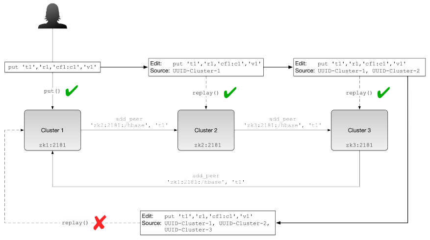
Figure 11-2. Replication in a loop
No matter how you build a network of replicating HBase clusters, the edits are only traversing as
far as their reach, which may be the cluster the record came from. In the example you could
apply the put to the third cluster instead, which would make it travel to cluster #1, then #2,
stopping again just before #3.
Checking the current replication status is achieved with the shell’s status command (here using
multiple local test instances):
hbase(main):001:0> status 'replication'
version 1.3.0
1 live servers
worker-1.internal.larsgeorge.com:
SOURCE: PeerID=1, AgeOfLastShippedOp=0, SizeOfLogQueue=0, \
TimeStampsOfLastShippedOp=Sat Feb 11 12:57:11 CET 2017, \
Replication Lag=0
SINK : AgeOfLastAppliedOp=0, \
TimeStampsOfLastAppliedOp=Sat Feb 11 12:37:46 CET 2017
For the sake of an example, we stop the peer instance now (not shown) and then insert more data.
After that we wait a some time and call the status command again to verify that a lag is now
experienced, as expected (since the peer is stopped and does not receive any mutations
currently):
hbase(main):002:0> put 'testtable', 'row-2', 'cf1:col-1', 'val-2'
0 row(s) in 0.0070 seconds
hbase(main):003:0> status 'replication'
version 1.3.0
1 live servers
worker-1.internal.larsgeorge.com:
SOURCE: PeerID=1, AgeOfLastShippedOp=20532, SizeOfLogQueue=0, \
TimeStampsOfLastShippedOp=Sat Feb 11 12:58:24 CET 2017,
Replication Lag=20532
SINK : AgeOfLastAppliedOp=0, \
TimeStampsOfLastAppliedOp=Sat Feb 11 12:37:46 CET 2017
(919)
Removing the peer entry will stop the replication for that cluster altogether:
hbase(main):019:0> remove_peer '1'
When remove_peer is invoked, all pending edits are discarded too, clearing up any lag shown in
the status command output.
Finally, verifying the replicated data on two clusters is easy to do in the shell when looking only
at a few rows, but doing a systematic comparison requires more computing power. This is why
the Verify Replication tool is provided; it is available as verifyrep using the hadoop jar command
once more:
$ hadoop jar $HBASE_HOME/lib/hbase-1.3.0.jar verifyrep
Usage: verifyrep [--starttime=X] [--stoptime=Y] [--families=A] \
<peerid> <tablename>
Options:
starttime beginning of the time range
without endtime means from starttime to forever
endtime end of the time range
versions number of cell versions to verify
families comma-separated list of families to copy
Args:
peerid Id of the peer used for verification, must match the one \
given for replication
tablename Name of the table to verify
Examples:
To verify the data replicated from TestTable for a 1 hour window with peer #5
$ bin/hbase org.apache.hadoop.hbase.mapreduce.replication.VerifyReplication \
--starttime=1265875194289 --endtime=1265878794289 5 TestTable
This has to be run on the master cluster and needs to be provided with a peer ID (the one
provided when establishing a replication stream) and a table name. Other options let you specify
a time range and specific families. Once the job completes it emits a number of counters that
state what the (if at all) the difference between the two tables amounts to:
Counter Description
GOODROWS Counts all rows that are the same in both tables.
BADROWS Counts all rows that are not the same or missing in either table.
ONLY_IN_SOURCE_TABLE_ROWS Number of rows that are only in the source table.
ONLY_IN_PEER_TABLE_ROWS Number of rows that are only in the replicated table.
CONTENT_DIFFERENT_ROWS Counts all rows that have the same key, but their values or number of
columns differ.
Using the --stoptime parameter allows you to skip the latest entries in case the table is currently
being written to, and replicated mutation may not have been shipped yet. Use a time that is a few
(920)
seconds or minutes before the current time to avoid issues with the tail end of the table. All
differences found during the verification run are printed to the task output logs, which can be
inspected later on through the YARN UI or the $ mapred job -logs <job-ID> <attempt-ID>
command.
(921)
Additional Tasks
On top of the operational and data tasks, there are additional tasks you may need to perform
when setting up or running a test or production HBase cluster. We will discuss these tasks in the
following subsections.
(922)

Coexisting Clusters
For testing purposes, it is useful to be able to run HBase in two or more separate instances, but
on the same physical machine. This can be helpful, for example, when you want to prototype
replication on your development machine.
Caution
Running multiple separate instances of HBase on a distributed cluster is not recommended, and
is not tested well in practice. While you can run multiple master or region server processes on the
same machine (within the same or a different cluster instance), orchestrating this for more
complex setups is not trivial and error-prone. Please be considerate!
Presuming you have set up a local installation of HBase, as described in Chapter 2, and
configured it to run in standalone mode (which means you unpacked the tarball of a binary
HBase release), you can first make a copy of the configuration directory like so:
$ cd $HBASE_HOME
$ cp -pR conf conf.2
The next step is to edit the hbase-env.sh file in the new conf.2 directory and modify the following
lines:
# Where log files are stored. $HBASE_HOME/logs by default.
export HBASE_LOG_DIR=${HBASE_HOME}/logs.2
# A string representing this instance of hbase. $USER by default.
export HBASE_IDENT_STRING=${USER}.2
This is required to have no overlap in local filenames. Lastly, you need to adjust the hbase-
site.xml file to at least contain the following settings:
<configuration>
<property>
<name>hbase.tmp.dir</name>
<value>/tmp/hbase-2-${user.name}</value>
</property>
<property>
<name>hbase.zookeeper.property.clientPort</name>
<value>2182</value>
</property>
<property>
<name>hbase.master.port</name>
<value>16100</value>
</property>
<property>
<name>hbase.master.info.port</name>
<value>16110</value>
</property>
<property>
<name>hbase.regionserver.port</name>
<value>16120</value>
</property>
<property>
<name>hbase.regionserver.info.port</name>
<value>16130</value>
</property>
</configuration>
You need to assign all ports differently so that you have a clear distinction between the two
(923)
cluster instances. This includes not just HBase itself, but also the embedded ZooKeeper that
usually listens on port 2181. The above increases the port number by one, but you are free to
chose any other free number. If you are planning to start a third instance, keep increasing the port
and directory numbers.
Operating the additional local cluster requires specification of the new configuration directory:
$ HBASE_CONF_DIR=conf.2 bin/start-hbase.sh
$ HBASE_CONF_DIR=conf.2 bin/hbase shell
$ HBASE_CONF_DIR=conf.2 bin/stop-hbase.sh
The first command starts the secondary local cluster, the middle one starts a shell connecting to
it, and the last command stops the cluster. Again, for cluster number three and higher, make an
additional copy of the configuration directory (for instance, conf.3), modify the settings
accordingly, and then use the same commands but the new number in the configuration name.
(924)

Required Ports
The HBase processes, when started, bind to two separate ports: one for the RPCs, and another for
the web-based UI. This applies to both the master and each region server. Since you are running
each process type on one machine only, you need to consider two ports per server type—unless
you run in a non-distributed setup. Table 11-6 lists the default ports.
Table 11-6. Default ports used by the HBase daemons
Node
Type Port Description
Master 16000 The RPC port the master listens on for client requests (set by
hbase.master.port).
Master 16010 The web-based UI port the master process listens on (set by
hbase.master.info.port).
Region
Server 16020 The RPC port the region server listens on for client requests (set by
hbase.regionserver.port).
Region
Server 16030 The web-based UI port the region server listens on (set by
hbase.regionserver.info.port).
REST 8080 The port the REST gateway server is listening to client requests (set by
hbase.rest.port).a
REST 8085 The port of the web-based UI of the REST gateway server (set by
hbase.rest.info.port).b
Thrift 9090 The RPC port of the Thrift gateway server (set by
hbase.regionserver.thrift.port).a
Thrift 9095 The web-based UI port the Thrift gateway server listens on (set by
hbase.thrift.info.port).b
ZooKeeper 2181 Optional: The RPC port used by the ZooKeeper clients to communicate with
the server (set by hbase.zookeeper.property.clientPort).c
(925)

ZooKeeper 2888 Optional: The ZooKeeper server peer port (set by hbase.zookeeper.peerport).c
ZooKeeper 3888 Optional: The ZooKeeper server leader port (set by
hbase.zookeeper.leaderport).c
a Can be set on the command-line using the -p or --port option, followed by the port number.
b Can be set on the command-line using the --infoport option, followed by the port number.
c Only used when ZooKeeper is managed by HBase.
Note
Setting the info port to -1 disables the built-in web-based information server of a specific node
type. This works for all of the listed types but ZooKeeper, as it has no information server.
In addition, if you want to configure a firewall, for example, you also have to ensure that the
ports for the Hadoop subsystems, that is, MapReduce and HDFS, are configured so that the
HBase daemons have access to them.6
Here are a few more configuration properties that might come in handy when configuring more
complex setups:
Table 11-7. Advanced network related properties
Property Default Description
hbase.master.hostname empty Global override of the hostname used for the
master. Must be unique for each master.
hbase.master.info.bindAddress 0.0.0.0
hbase.master.infoserver.redirect true
Whether or not the Master listens to the Master
web UI port (hbase.master.info.port) and redirects
requests to the web UI server shared by the Master
and RegionServer.
hbase.regionserver.hostname empty Global override for the hostname of the region
server. Must be unique for each region server.
hbase.regionserver.dns.interface default The name of the network interface (NIC) from
which a region server should report its IP address.
(926)
hbase.regionserver.dns.nameserver default
The host name or IP address of the name server
(DNS) which a region server should use to
determine the host name used by the master for
communication and display purposes.
hbase.regionserver.info.bindAddress 0.0.0.0
hbase.regionserver.info.port.auto false
Wether the built-in server should, in case the port
is already taken, start to increment the port to find
a free one.
The default value of the DNS interface related property causes the server to determine the local
server name first, and then using the DNS subsystem to resolve it into a hostname. In effect, that
causes the process to assume the IP address that is bound to the hostname as configured by the
OS name resolution. You can deviate from the defaults by, for example, specifying a different
name server to be used, which may return a different IP address for the local hostname.
In addition, you can override the interface the master and/or region server UIs are using. The
default causes the server to listen to all interfaces (set by 0.0.0.0), but often you are forced to
change the interface to an internal one, that is, one that can only be accessed within a
management network, and differs from where the data-related RPC ports are bound to.
(927)

Changing Logging Levels
By default, HBase ships with a configuration which sets the log level of its processes to INFO,
writing all common and more important messages (like warnings and fatal error messages) to the
low-level log files. It allows you to search through these files in case something goes wrong, as
discussed in “Analyzing the Logs”.
For a production environment, you can switch to a less verbose level, such as WARN, or even FATAL.
This is accomplished by editing the log4j.properties file in the conf directory. Here is an
example with the modified level for the HBase classes:
...
# Custom Logging levels
log4j.logger.org.apache.zookeeper=WARN
#log4j.logger.org.apache.hadoop.fs.FSNamesystem=DEBUG
log4j.logger.org.apache.hadoop.hbase=INFO
# Make these two classes INFO-level. Make them DEBUG to see more zk debug.
log4j.logger.org.apache.hadoop.hbase.zookeeper.ZKUtil=INFO
log4j.logger.org.apache.hadoop.hbase.zookeeper.ZooKeeperWatcher=INFO
#log4j.logger.org.apache.hadoop.dfs=DEBUG
# Set this class to log INFO only otherwise its OTT
...
This file needs to be copied to all servers, which need to be restarted subsequently for the
changes to take effect.
Another option to either temporarily change the level, or when you have made changes to the
properties file and want to delay the restart, use the web-based UIs and their log-level page. This
is discussed and shown in “Shared Pages”. Since the UI log-level change is only affecting the
server it is loaded from, you will need to adjust the level separately for every server in your
cluster.
(928)

Region Replicas
As introduced in “Durability, Consistency, and Isolation”, there is an option to increase the
availability of data for reads by setting a region replication factor of greater than one. The default
is 1, meaning there is only one copy of each region. How region replicas have to be configured
depends on if you are dealing only with read-only tables, or have tables that also take on writes.
For the former, it is sufficient to set the desired replica count (see example below), close and
reopen the table. It will instruct all replicas to also open the store files and serve requests.
Before you can make use of the region replica feature for tables that also receive writes, you
have to configure the cluster in one of two ways:
Monitor Store Files Only
In this mode (added in HBase 1.0.0) you have the replica monitor just the files within the
filesystem, and upon changes (for example, after a flush or compaction) have it open the
available files. Obviously, this will cause a delay until modifications are accessible by a
replica. Enabling the feature requires to set the following property to a non-zero value
(shown here is one minute):
<property>
<name>hbase.regionserver.storefile.refresh.period</name>
<value>60000</value>
</property>
Asynchronous WAL Replication
For all modifications to be replicated as they occur, the replica replication feature has to be
enabled (available as of HBase 1.1.0). With it, the primary server receiving mutations is
sending those to the peer replica(s) with minimal delay. The feature is enabled setting the
following property to true:
<property>
<name>hbase.region.replica.replication.enabled</name>
<value>true</value>
</property>
Using replication has an affect on the memory usage, since a read-only memstore is
required to retain all mutations from the primary on the secondary replica(s). That memory
will likely reduce what is available for other primary regions on the same server (see
“Cluster Sizing”). If you are concerned about the available memstore space, you may have
to opt for first option instead, that is, only monitoring the store files.
Memory Requirements for Reads
Both options, and in fact the entire region replica feature, share the side-effect of requiring more
memory for caching storage blocks. As soon as the primary is not responding within a
configured time, the secondary replica(s) is (are) asked to return the value instead—requiring a
block load into their own memory space. This can be somewhat mitigated setting the timeouts,
like the client-side hbase.client.primaryCallTimeout.get, to a slightly larger value. The drawback
is higher latencies in case of a failover.
(929)

The more additional replicas you specify, the more servers are loading the same block into
memory. When the primary replica is not responding within the default 10 milliseconds, all
replicas are asked in parallel to return the data instead. In other words, while it sounds like a
good idea to have plenty of replicas to have more redundancy, it will dilute your block cache
memory share on each region server, leaving less for other store file blocks.
One (or both) of these settings has to be added to the hbase-site.xml configuration file, which
then needs to be distributed to all servers again, and all HBase processes restarted. After that, you
can use the HBase Shell or API (see “Table Properties”) to enable multiple region replicas on
existing table, or immediately when you are creating a new one. For instance, assuming you have
enabled the replica replication option:
hbase(main):001:0> create 'replicatable', 'cf1', { NUMREGIONS => 10, \
SPLITALGO => 'HexStringSplit', REGION_REPLICATION => 2 }
0 row(s) in 4.3590 seconds
=> Hbase::Table - replicatable
hbase(main):002:0> list_peer_configs
PeerId region_replica_replication
Cluster Key master-1.internal.larsgeorge.com, \
master-2.internal.larsgeorge.com, \
master-3.internal.larsgeorge.com:2181:/hbase
Replication Endpoint org.apache.hadoop.hbase.replication. \
regionserver.RegionReplicaReplicationEndpoint
0 row(s) in 2.0550 seconds
hbase(main):003:0> put 'replicatable', 'row-1', 'cf1:col-1', 'val-1'
0 row(s) in 1.2270 seconds
hbase(main):004:0> get 'replicatable', 'row-1', \
{ CONSISTENCY => 'TIMELINE', REGION_REPLICA_ID => 0 }
COLUMN CELL
cf1:col-1 timestamp=1486289700708, value=val-1
1 row(s) in 0.0550 seconds
hbase(main):005:0> get 'replicatable', 'row-1', \
{ CONSISTENCY => 'TIMELINE', REGION_REPLICA_ID => 1 }
COLUMN CELL
cf1:col-1 timestamp=1486289700708, value=val-1
1 row(s) in 0.1000 seconds (possible stale results)
hbase(main):006:0> get 'replicatable', 'row-1', \
{ CONSISTENCY => 'TIMELINE', REGION_REPLICA_ID => 2 }
COLUMN CELL
ERROR: HRegionInfo was null in replicatable, \
2270 row=keyvalues={replicatable,e6666661,1486289678486...
...
After creating a presplit table with two region replicas configured, the system has automatically
added a replication endpoint (refer to [Link to Come] and “Replication”) that is responsible to
ship the edits from the primary to the replica(s). This functionality is tested by adding a value to
the table and verifying if it has been received by each configured replica. Asking for the value
with a specific replica ID will return a value from replica #0 (the primary) and #1 (the first
secondary), where the latter is tagged with a note that the result may be stale. Trying replica #2
fails, as there is no such replica configured (see the create command in the example). You can
omit the explicit replica ID as well, giving you the result of the primary, or, in case of the
primary failing, a secondary replica.
Refer to the official documentation in the HBase Guide for many more details, including a
discussion about the tradeoff of using region replicas.
(930)
Caution
The choice of load balancer can have an impact on how replica regions are distributed across the
cluster. As of this writing, only the (default) StochasticLoadBalancer class is considering replicas
so that they are not colocated on the same server (or even same rack).
(931)
Troubleshooting
This section deals with the things you can do to heal a cluster that does not work as expected.
(932)

HBase Fsck
HBase deals with three distinct locations storing vital system details:
Storage
Typically HBase runs atop a distributed file system, such as Hadoop’s HDFS. It relies on
the file system to keep information and data safe and available at all times. As such,
everything needed for a cluster to start after having been shut down (or being brand new)
is located in the HBase root directory, specified with the hbase.rootdir configuration
property. It contains all of the WALs and data files holding the actual user data, and
metadata for every table and region known to the system. There are files in many
directories that hold serialized structural information about the object they describe, for
example, the region and table info records.
System Tables
Just like user tables, HBase is using dedicated system tables to record details about tables
that are created by users over time. Every table is really a set of regions that are tracked by
the system tables, such as hbase:meta, to retain information such as the start and end keys,
the schema of each family, and what server is currently holding the region open for client
requests.
RegionServers
The last piece are the region servers themselves, serving regions and their contained data
to applications and interactive users. All of the regions of a table have to be assigned to
one of the available region servers, or there may be gaps in the stored data, manifesting
itself as missing (as in inaccessible) rows of the table.
Figure 11-3 summarizes how these three locations are connected in a higher level abstraction,
since system tables are also served by region servers. The diagram visualized how metadata
stored in HDFS is also present in the system table, and in the region server providing access to
the regions. All three locations must be in agreement and, although varying in the degree of
details, must align completely. If that is not the case, there is an inconsistency that may cause
problems in operations.
(933)
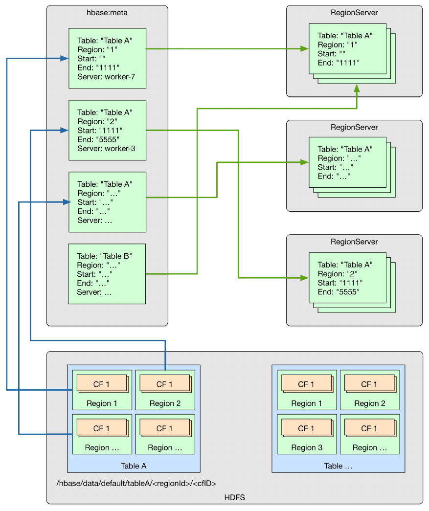
Figure 11-3. Relationship between HDFS, system tables, and region server data structures
As an operator though, you may want to identify problems before they cause any service impact.
For that, HBase ships with the hbck tool, that allows to scan all three locations and cross-
reference them in an attempt to find any mismatch, reporting them as inconsistencies. It provides
various command-line switches that influence its behavior. You can get a full list of its usage
information by running it with -h:
$ ./bin/hbase hbck -help
Usage: fsck [opts] {only tables}
where [opts] are:
-help Display help options (this)
-details Display full report of all regions.
(934)
-timelag <timeInSeconds> Process only regions that have not experienced \
any metadata updates in the last <timeInSeconds> seconds.
-sleepBeforeRerun <timeInSeconds> Sleep this many seconds before checking \
if the fix worked if run with -fix
-summary Print only summary of the tables and status.
-metaonly Only check the state of the hbase:meta table.
-sidelineDir <hdfs://> HDFS path to backup existing meta.
-boundaries Verify that regions boundaries are the same between META and \
store files.
-exclusive Abort if another hbck is exclusive or fixing.
-disableBalancer Disable the load balancer.
Metadata Repair options: (expert features, use with caution!)
-fix Try to fix region assignments. This is for backwards \
compatiblity
-fixAssignments Try to fix region assignments. Replaces the old -fix
-fixMeta Try to fix meta problems. This assumes HDFS region \
info is good.
-noHdfsChecking Don't load/check region info from HDFS. Assumes \
hbase:meta region info is good. Won't check/fix any \
HDFS issue, e.g. hole, orphan, or overlap
-fixHdfsHoles Try to fix region holes in hdfs.
-fixHdfsOrphans Try to fix region dirs with no .regioninfo file in hdfs
-fixTableOrphans Try to fix table dirs with no .tableinfo file in hdfs \
(online mode only)
-fixHdfsOverlaps Try to fix region overlaps in hdfs.
-fixVersionFile Try to fix missing hbase.version file in hdfs.
-maxMerge <n> When fixing region overlaps, allow at most <n> \
regions to merge. (n=5 by default)
-sidelineBigOverlaps When fixing region overlaps, allow to sideline big \
overlaps
-maxOverlapsToSideline <n> When fixing region overlaps, allow at most \
<n> regions to sideline per group. (n=2 by default)
-fixSplitParents Try to force offline split parents to be online.
-ignorePreCheckPermission ignore filesystem permission pre-check
-fixReferenceFiles Try to offline lingering reference store files
-fixEmptyMetaCells Try to fix hbase:meta entries not referencing any \
region (empty REGIONINFO_QUALIFIER rows)
Datafile Repair options: (expert features, use with caution!)
-checkCorruptHFiles Check all Hfiles by opening them to make sure \
they are valid
-sidelineCorruptHFiles Quarantine corrupted HFiles. \
implies -checkCorruptHFiles
Metadata Repair shortcuts
-repair Shortcut for -fixAssignments -fixMeta -fixHdfsHoles \
-fixHdfsOrphans -fixHdfsOverlaps -fixVersionFile \
-sidelineBigOverlaps -fixReferenceFiles -fixTableLocks \
-fixOrphanedTableZnodes
-repairHoles Shortcut for -fixAssignments -fixMeta -fixHdfsHoles
Table lock options
-fixTableLocks Deletes table locks held for a long time \
(hbase.table.lock.expire.ms, 10min by default)
Table Znode options
-fixOrphanedTableZnodes Set table state in ZNode to disabled if table \
does not exists
Replication options
-fixReplication Deletes replication queues for removed peers
The -details switch prints out the most information when running hbck, while -summary prints out
the least. No option at all invokes the normal output detail, for example:
$ bin/hbase hbck
HBaseFsck command line options:
Version: 1.3.0-SNAPSHOT
Number of live region servers: 3
Number of dead region servers: 0
Master: master-1.internal.larsgeorge.com,16000,1487405529857
Number of backup masters: 2
(935)
Average load: 44.333333333333336
Number of requests: 0
Number of regions: 133
Number of regions in transition: 0
Number of empty REGIONINFO_QUALIFIER rows in hbase:meta: 0
Number of Tables: 20
...
2017-02-18 00:14:57,827 WARN [hbasefsck-pool1-t30] util.HBaseFsck: No HDFS \
region dir found: { meta => replicatable,33333332,1486289678486_0001.\
3e0fdd7448dba08eda4857477408ecae., hdfs => null, deployed => worker-1. \
internal.larsgeorge.com,16020,1487405565238;replicatable,33333332, \
1486289678486_0001.3e0fdd7448dba08eda4857477408ecae., replicaId => 1 } \
meta={ENCODED => 3e0fdd7448dba08eda4857477408ecae, NAME => \
'replicatable,33333332,1486289678486_0001. \
3e0fdd7448dba08eda4857477408ecae.', STARTKEY => '33333332', ENDKEY => \
'4ccccccb', REPLICA_ID => 1}
...
2017-02-18 00:14:59,530 INFO [main] util.HBaseFsck: Checking and fixing \
region consistency
2017-02-18 00:14:59,861 INFO [main] util.HBaseFsck: Handling overlap merges \
in parallel. set hbasefsck.overlap.merge.parallel to false to run serially.
2017-02-18 00:14:59,878 INFO [main] util.HBaseFsck: Computing mapping of all \
store files
...
2017-02-18 00:15:00,762 INFO [main] util.HBaseFsck: Validating mapping using \
HDFS state
Summary:
Table ltttest1 is okay.
Number of regions: 15
Deployed on: worker-1.internal.larsgeorge.com,16020,1487405565238 \
worker-2.internal.larsgeorge.com,16020,1487405565197 \
worker-3.internal.larsgeorge.com,16020,1487405568118
Table testtable2 is okay.
Number of regions: 15
Deployed on: worker-1.internal.larsgeorge.com,16020,1487405565238 \
worker-2.internal.larsgeorge.com,16020,1487405565197 \
worker-3.internal.larsgeorge.com,16020,1487405568118
Table testtable is okay.
Number of regions: 1
Deployed on: worker-3.internal.larsgeorge.com,16020,1487405568118
...
Table replicatable is okay.
Number of regions: 10
Deployed on: worker-1.internal.larsgeorge.com,16020,1487405565238 \
worker-2.internal.larsgeorge.com,16020,1487405565197 \
worker-3.internal.larsgeorge.com,16020,1487405568118
...
Table WAREHOUSE.TEST is okay.
Number of regions: 1
Deployed on: worker-2.internal.larsgeorge.com,16020,1487405565197
0 inconsistencies detected.
Status: OK
Note
If you look at the WARN log message above, you can see how the check is coming across a read
replica region, which has no own files, but points back to the location where the primary region
is stored. In the end, the table is reported as consistent as expected.
The extra parameters, such as -timelag and -sleepBeforeRerun, are explained in the usage details
in the preceding code. They allow you to check subsets of data, as well as delay the eventual re-
check run, to report any remaining issues. You can also optionally specify one or more tables
when invoking the hbck command, limiting the check to only those tables:
(936)

$ bin/hbase hbck Table1
...
Allow checking/fixes for table: Table1
HBaseFsck command line options: Table1
...
Version: 1.3.0-SNAPSHOT
Once started, the hbck tool will scan the hbase:meta table to gather all the pertinent information it
holds. It also scans the HDFS root directory HBase is configured to use. It then proceeds to
compare the collected details to report on inconsistencies and integrity issues.
Consistency check
This check applies to a region on its own. It is checked whether the region is listed in
hbase:meta and exists in HDFS, as well as if it is assigned to exactly one region server.
Integrity check
This concerns a table as a whole. It compares the regions with the table details to find
missing regions, or those that have holes or overlaps in their row key ranges.
Note
Be aware that sometimes hbck reports inconsistencies which are temporal, or transitional only.
For example, when regions are unavailable for short periods of time during the internal
housekeeping process, hbck will report those as inconsistencies too. Add the details switch to get
more information on what is going on and rerun the tool a few times to confirm a permanent
problem.
The next sections will discuss the repair options in greater detail. Whatever you do though,
please make sure you have a backup strategy in place. A botched repair may cause data loss,
stressing the importance of first making a copy of the HBase root directory (space permitting,
possibly using a backup cluster) before performing the repairs.
Localized Region Repairs
When repairing a corrupted HBase, it is best to repair the lowest risk inconsistencies first. These
are generally region consistency repairs, that is, localized single region repairs that only modify
in-memory data, ephemeral zookeeper data, or patch holes in the system tables. Region
consistency requires that the HBase instance has the state of the region’s data in HDFS (the
mentioned .regioninfo files), the region’s row in the hbase:meta table., and region’s
deployment/assignments on region servers and the master in accordance. Options for repairing
region consistency include:
Fix Region Assignment
Using the -fixAssignments7 repairs unassigned, incorrectly assigned, or regions that have
been assigned to more than one region server.
Fix System Tables
The -fixMeta option removes meta table rows when corresponding regions are not present
in HDFS, and adds new meta table rows if the regions are present in HDFS, but not in the
(937)
system table.
You can run the following command to fix deployment and assignment problems:
$ bin/hbase hbck -fixAssignments
Combining deployment and assignment problems fixing, as well as repairing incorrect meta
rows, you can run this command:
$ bin/hbase hbck -fixAssignments -fixMeta
There are a few classes of table integrity problems that are low risk repairs. The first two are
degenerate regions (where the start key is the same as the end key), and backwards regions
(where the start key is greater then the end key). These are automatically handled by sidelining
the data to a temporary directory (set by the -sidelineDir option). The third low-risk class is
region holes in the data located on HDFS. This can be repaired by using an additional command-
line switch:
Fix Holes
Applying the -fixHdfsHoles option instructs the tool to create new, empty regions within
the file system in place where there are gaps. If holes are detected you can use -
fixHdfsHoles, combined with -fixMeta and -fixAssignments, to make the new region(s)
consistent.
$ bin/hbase hbck -fixAssignments -fixMeta -fixHdfsHoles
Since this is a common combination of switches, there is also for convenience a single
switch called -repairHoles, combining the three above into one:
$ bin/hbase hbck -repairHoles
If inconsistencies still remain after these steps, you most likely have table integrity problems
related to orphaned or overlapping regions.
Region Overlap Repairs
Table integrity problems can require repairs that deal with overlaps. This is a riskier operation
because it requires modifications to the file system, requires some decision making, and may
require some manual steps. For these repairs it is best to analyze the output of a hbck -details
execution so that you isolate repair attempts only upon problems the checks identify. Because
this is riskier, there are safeguards that should be used to limit the scope of the repairs.
Warning
As mentioned earlier, you should always consider backing up your HBase root directory in
HDFS first, before you perform the repairs. The tool is based on the experience the HBase
developers have collected over time, but are not foolproof. Use at your own risk in an active
production environment!
The options for repairing table integrity violations include:
Fix Orphaned Regions
(938)
Use the -fixHdfsOrphans option for adopting a region directory that is missing a region
metadata file (the .regioninfo file).
Fix Region Overlaps
With -fixHdfsOverlaps you have the ability for fixing overlapping regions, that is, those
where the start and end keys of two regions overlap in their range. Usually start and end
keys are contiguous, which forbids any gaps or overlaps in the key range.
When repairing overlapping regions, a region’s data can be modified on the file system in two
ways:
1. Merging regions into a new, larger region, or
2. sidelining regions by moving data to sideline directory where data could be restored later.
Merging a large number of regions is technically correct but could result in an extremely large
region that requires series of costly compactions and splitting operations. In these cases, it is
probably better to sideline the regions that overlap with the majority of the other regions (likely
the largest ranges) so that merges can happen on a more reasonable scale. Since these sidelined
regions are already laid out in HBase’s native directory and HFile format, they can be restored by
using HBase’s bulk load mechanism.
The default safeguard thresholds regarding the merging of regions are conservative. These
options let you override the default thresholds and enable the large region sidelining feature:
Table 11-8. Region merging threshold options
Property Default Description
-maxMerge <n> 5 Maximum number of overlapping regions to merge.
-sidelineBigOverlaps not set If more than maxMerge regions are overlapping, attempt to sideline
the regions overlapping with the most other regions.
-
maxOverlapsToSideline
<n>
2When sidelining large overlapping regions, sideline at most <n>
regions.
Since most of the times you would just want to get the tables repaired, you can use this option to
turn on all repair options:
Fix Everything
The -repair switch combines all the region consistency, hole, and overlap table repair
integrity options.
Note that there is a safeguard to limit repairs to only specific tables. For example the following
command would only attempt to check and repair table Table1 and Table2.
$ bin/hbase hbck -repair Table1 Table2
(939)
On top of the discussed so far, there are a few more special cases that hbck can handle as well,
which are:
Fix Meta Assignment
Sometimes the meta table’s region is inconsistently assigned or deployed. In this case there
is a special -metaonly option that you can try to fix meta assignments.
$ bin/hbase hbck -metaonly -fixAssignments
Fix Missing Version File
HBase’s data on the file system requires a version file in order to start. If this file is
missing, you can use the -fixVersionFile option to create a new HBase version file. This
assumes that the version of hbck you are running is the appropriate version for the HBase
cluster.
Fix Corrupt System Tables
The most drastic corruption scenario is the case where the system tables (that is, as of this
writing, hbase:meta) are corrupted and HBase will not start. In this case you can use the
OfflineMetaRepair tool to create new system regions and tables. This tool assumes that
HBase is offline. It then iterates through the existing HBase root directory, loads as much
information as possible from the region metadata files (that is, .regioninfo) from the file
system. If the region metadata has proper table integrity, it sidelines the original system
table directories, and builds new ones with pointers to the region directories and their data.
Starting it with -h (for the lack of a help switch) prints the supported parameters:
$ bin/hbase org.apache.hadoop.hbase.util.hbck.OfflineMetaRepair
Unknown command line option : -h
Usage: OfflineMetaRepair [opts]
where [opts] are:
-details Display full report of all regions.
-base <hdfs://> Base Hbase Data directory.
-sidelineDir <hdfs://> HDFS path to backup existing meta and root.
-fix Auto fix as many problems as possible.
-fixHoles Auto fix as region holes.
Note
This tool is not as fully featured as hbck but can be used to bootstrap repairs that hbck can
complete. If the tool succeeds you should be able to start HBase and run online repairs if
necessary.
Fix Offline Split Parent
Once a region is split, the offline parent will be cleaned up automatically. Sometimes,
daughter regions are split again before their parents are cleaned up. HBase can clean up
parents in the right order. However, there could be some lingering offline split parents
sometimes. They are in META, in HDFS, and not deployed. But HBase can’t clean them
up. In this case, you can use the -fixSplitParents option to reset them in META to be
online and not split. Therefore, hbck can merge them with other regions if fixing
overlapping regions option is used.
This option should not normally be used, and it is not in -fixAll.
(940)
Fix Table Locks
Using the -fixTableLocks option allows you to remove table locks that are held for too
long. Usually locks for tables are an internal feature, used for compare-and-swap type
operations server-side. They are held as set by hbase.table.lock.expire.ms, defaulting to 10
minutes. Should you need to release a lock earlier, you can use the -fixTableLocks option.
Fix Orphaned Table State
In very rare circumstances it may happen that a table has been dropped, but its state in
ZooKeeper is still present. This causes the system to stumble as the state is inconsistent
between ZooKeeper—which is (for most parts) transient, see [Link to Come] for details—
and the remaining three state stores, that is, HDFS, the system tables, and the region
servers. Using the -fixOrphanedTableZnodes switch instructs the check tool to set the missing
table’s state to disabled in ZooKeeper, helping the system to ignore it and proceed
normally.
Fix Replication Information
Also ZooKeeper related is the -fixReplication switch that allows an operator to remove the
replication queues for previously removed peer systems.
The hbck tool has a few extra options, for example disabling the load balancer while a check or
repair is running, that were not explained here. Consult the tool’s -help output for details.
(941)

Analyzing the Logs
In rare cases it is necessary to directly access the log files created by the various HBase
processes. They contain a mix of messages, some of which are printed for informational
purposes and others representing internal warnings or error messages. While some of these
messages are temporary, and do not mean that there is a permanent issue with the cluster, others
state a system failure and are printed just before the process is forcefully ended.
Tip
It is recommended to use a log aggregation framework, such as the open-source Elastic Stack, or
Apache Solr. These collect logs and make them searchable, with filtering by, for example, host
or service, and more advanced faceting techniques to further drill into the possible deluge of log
messages a distributed system, such as Hadoop and HBase, can create. It makes finding problems
much easier, and will speed up your operations tasks.
Table 11-9 lists the various default HBase, ZooKeeper, and Hadoop log files. <user> is replaced
with the user ID the process is started by, and <hostname> is the name of the machine the process
is running on.
Table 11-9. The various server types and the log files they create
Server Type Log File
HBase Master $HBASE_HOME/logs/hbase-<user>-master-<hostname>.log
HBase RegionServer $HBASE_HOME/logs/hbase-<user>-regionserver-<hostname>.log
HBase REST $HBASE_HOME/logs/hbase-<user>-rest-<hostname>.log
HBase Thrift $HBASE_HOME/logs/hbase-<user>-thrift-<hostname>.log
ZooKeeper Console log output only
HDFS NameNode $HADOOP_HOME/logs/hadoop-<user>-namenode-<hostname>.log
HDFS DataNode $HADOOP_HOME/logs/hadoop-<user>-datanode-<hostname>.log
YARN ResourceManager $HADOOP_HOME/logs/yarn-<user>-resourcemanager-<hostname>.log
YARN NodeManager $HADOOP_HOME/logs/yarn-<user>-nodemanager-<hostname>.log
(942)
Obviously, this can be modified by editing the configuration files for either of these systems. The
first thing a HBase process emits upon startup is a collection of low-level information that is of
interest to an operator. The first block prints the configured process limits, as per the available
operating system settings. For example:
Fri Jan 27 01:51:40 PST 2017 Starting master on \
master-1.internal.larsgeorge.com
core file size (blocks, -c) 0
data seg size (kbytes, -d) unlimited
scheduling priority (-e) 0
file size (blocks, -f) unlimited
pending signals (-i) 30494
max locked memory (kbytes, -l) unlimited
max memory size (kbytes, -m) unlimited
open files (-n) 65535
pipe size (512 bytes, -p) 8
POSIX message queues (bytes, -q) 819200
real-time priority (-r) 0
stack size (kbytes, -s) 10240
cpu time (seconds, -t) unlimited
max user processes (-u) 1024
virtual memory (kbytes, -v) unlimited
file locks (-x) unlimited
As part of the cluster setup, each node needs to be prepared to increase the number of file
handles a user can hold open, and processes a user can start. The recommended minimum is 32k,
which can be set like so (although a more flexible way of applying should be preferred, using, for
example, a configuration management tool like Ansible):
$ echo hdfs - nofile 32768 >> /etc/security/limits.conf
$ echo mapred - nofile 32768 >> /etc/security/limits.conf
$ echo hbase - nofile 32768 >> /etc/security/limits.conf
$ echo hdfs - nproc 32768 >> /etc/security/limits.conf
$ echo mapred - nproc 32768 >> /etc/security/limits.conf
$ echo hbase - nproc 32768 >> /etc/security/limits.conf
In the example above, the values differ, which could force an operator to adjust them
accordingly. Checking those values first clears the basic assumptions made about the process
environment. The next step is to read the next lines in the head of the log (shortened for the sake
of space):
2017-01-27 01:51:45,355 INFO [main] util.VersionInfo: HBase 1.3.0-SNAPSHOT
...
2017-01-27 01:51:45,356 INFO [main] util.VersionInfo: Compiled by \
laurageorge on Mon Aug 15 10:22:44 CEST 2016
...
2017-01-27 01:51:46,716 INFO [main] util.ServerCommandLine: \
env:JAVA_HOME=/etc/alternatives/jre
2017-01-27 01:51:46,716 INFO [main] util.ServerCommandLine: \
env:HBASE_HOME=/opt/hbase
...
2017-01-27 01:51:46,717 INFO [main] util.ServerCommandLine: \
env:HOSTNAME=master-1.internal.larsgeorge.com
...
2017-01-27 01:51:46,717 INFO [main] util.ServerCommandLine: \
env:HBASE_MASTER_OPTS= -XX:PermSize=128m -XX:MaxPermSize=128m \
-Dcom.sun.management.jmxremote.ssl=false -Dcom.sun.management.jmxremote. \
authenticate=false -Dcom.sun.management.jmxremote.port=10101
2017-01-27 01:51:46,722 INFO [main] util.ServerCommandLine: \
env:HBASE_MANAGES_ZK=false
2017-01-27 01:51:46,722 INFO [main] util.ServerCommandLine: \
env:JAVA_LIBRARY_PATH=/usr/local/lib:/usr/local/lib:/opt/hadoop-2.7.1/lib/native
...
2017-01-27 01:51:46,722 INFO [main] util.ServerCommandLine: \
env:HBASE_OFFHEAPSIZE=2G
...
(943)

2017-01-27 01:51:46,723 INFO [main] util.ServerCommandLine: \
env:HBASE_REGIONSERVER_OPTS= -XX:PermSize=128m -XX:MaxPermSize=128m \
-Dcom.sun.management.jmxremote.ssl=false -Dcom.sun.management.jmxremote. \
authenticate=false -Dcom.sun.management.jmxremote.port=10102
...
2017-01-27 01:51:46,724 INFO [main] util.ServerCommandLine: \
env:USERNAME=hadoop
2017-01-27 01:51:46,725 INFO [main] util.ServerCommandLine: \
env:HADOOP_CONF_DIR=/etc/opt/hadoop/conf
...
There is a lot of information in those printed environment variables and their values that could
give you an initial clue as to why a process is not working as expected.
When you start analyzing the log files, it is useful to begin with the master log file first, as it acts
as the coordinator service of the entire cluster. It contains informational messages, such as the
balancer printing out its background processing:
2017-02-18 06:02:26,885 INFO [ProcedureExecutor-3] \
balancer.BaseLoadBalancer: Reassigned 15 regions. \
15 retained the pre-restart assignment.
Or when a region is split on a region server, the master is using its internal state machine to
handle the various phases of the split:
2017-02-18 06:20:19,179 INFO [AM.ZK.Worker-pool2-t67] master.RegionStates: \
Transition null to {f3b6d4485881122f6c0184e678ad5ce7 state=SPLITTING_NEW, \
ts=1487427619179, server=worker-1.internal.larsgeorge.com,16020, \
1487405565238}
2017-02-18 06:20:22,758 INFO [AM.ZK.Worker-pool2-t63] master.RegionStates: \
Transition {f3b6d4485881122f6c0184e678ad5ce7 state=SPLITTING_NEW, \
ts=1487427622758, server=worker-1.internal.larsgeorge.com,16020, \
1487405565238} to {f3b6d4485881122f6c0184e678ad5ce7 state=OPEN, \
ts=1487427622758, server=worker-1.internal.larsgeorge.com,16020, \
1487405565238}
2017-02-18 06:20:22,773 INFO [AM.ZK.Worker-pool2-t63] \
master.AssignmentManager: Handled SPLIT event; parent=ltttest2,dddddddd, \
1487426512912.48705c792af50b399d70f8b288c1998c., daughter \
a=ltttest2,dddddddd,1487427619138.f3b6d4485881122f6c0184e678ad5ce7., \
daughter b=ltttest2,e68d60edfb709b5834cb5e9286b4ce4b-30907,1487427619138. \
0c6309c1611ae81e9ae9388952546f17., on \
worker-1.internal.larsgeorge.com,16020,1487405565238
Many of these messages at the INFO level show you how your cluster evolved over time. You can
use them to go back in time and see what happened earlier on. Typically the servers are simply
printing these messages on a regular basis, so when you look at specific time ranges you will see
the common patterns.
If something fails, though, these patterns will change: the log messages are interrupted by others
at the WARN (short for warning), or even ERROR and (very rarely) FATAL level. You should find those
patterns and reset just before the common pattern was disturbed.
Note
An interesting metric you can use as a gauge for where to start is discussed in “JVM Metrics”,
under System Event Metrics: the error log event metric. It gives you a graph showing you where
the server(s) started logging an increasing number of error messages in the log files. Find the
time before this graph started rising and use it as the entry point into your logs.
Once you have found where the processes began logging ERROR level messages, you should be
(944)

able to identify the root cause. A lot of subsequent messages are often collateral damage: they are
a side effect of the original problem. Not all of the logged messages that indicate a pattern
change are using an elevated log level. Here is an example of a region server where writing to its
underlying storage took longer than usual:
2017-02-18 06:17:31,711 INFO [sync.0] wal.FSHLog: Slow sync cost: 326 ms, \
current pipeline: [10.0.10.10:50010, 10.0.10.11:50010, 10.0.10.12:50010]
2017-02-18 06:17:31,711 INFO [sync.4] wal.FSHLog: Slow sync cost: 327 ms, \
current pipeline: [10.0.10.10:50010, 10.0.10.11:50010, 10.0.10.12:50010]
The message is logged on the info level because the system should eventually recover from it.
But it could indicate the beginning of larger problems—for example, when the servers start to get
overloaded. Make sure you reset your log analysis to where the normal patterns are disrupted.
Once you have investigated the master logs, move on to the region server logs. Use the
monitoring metrics to see if any of them shows an increase in log messages, and scrutinize that
server first. If you find an error message, use the online resources to search8 for the message in
the public HBase mailing lists. There is a good chance that this has been reported or discussed
before, especially with recurring issues, such as the mentioned server overload scenarios: even
errors follow a pattern at times.
You can search in the log files for occurrences of "ERROR", "FATAL" and "ABORTING" to find clues
about the reasons the server in question stopped working. For example, the following
(abbreviated) log messages at the tail end of the log file of a crashed server show that it failed to
access the cache file for the block cache, due to a permission error:
2016-08-15 02:19:54,422 ERROR [regionserver/worker-1.internal.larsgeorge.com/ \
10.0.10.10:16020] regionserver.HRegionServer: Failed init
java.lang.RuntimeException: java.io.FileNotFoundException: \
/data/hbase/cache/cache.dat (Permission denied)
at org.apache.hadoop.hbase.io.hfile.CacheConfig.getBucketCache
at org.apache.hadoop.hbase.io.hfile.CacheConfig.getL2
at org.apache.hadoop.hbase.io.hfile.CacheConfig.instantiateBlockCache
at org.apache.hadoop.hbase.io.hfile.CacheConfig.<init>
at org.apache.hadoop.hbase.regionserver.HRegionServer. \
handleReportForDutyResponse
at org.apache.hadoop.hbase.regionserver.HRegionServer.run
at java.lang.Thread.run
Caused by: java.io.FileNotFoundException: /data/hbase/cache/cache.dat \
(Permission denied)
at java.io.RandomAccessFile.open(Native Method)
...
2016-08-15 02:19:54,423 FATAL [regionserver/worker-1.internal.larsgeorge.com/ \
10.0.10.10:16020] regionserver.HRegionServer: ABORTING region server \
worker-1.internal.larsgeorge.com,16020,1471252790047: Unhandled: \
Region server startup failed
java.io.IOException: Region server startup failed
at org.apache.hadoop.hbase.regionserver.HRegionServer.convertThrowableToIOE
at org.apache.hadoop.hbase.regionserver.HRegionServer.handleReportForDutyResponse
at org.apache.hadoop.hbase.regionserver.HRegionServer.run
at java.lang.Thread.run
...
2016-08-15 02:19:54,424 FATAL [regionserver/worker-1.internal.larsgeorge.com/ \
10.0.10.10:16020] regionserver.HRegionServer: RegionServer abort: \
loaded coprocessors are: []
2016-08-15 02:19:54,462 INFO [regionserver/worker-1.internal.larsgeorge.com/ \
10.0.10.10:16020] regionserver.HRegionServer: \
Dump of metrics as JSON on abort: {
"beans" : [ {
"name" : "java.lang:type=Memory",
"modelerType" : "sun.management.MemoryImpl",
"ObjectPendingFinalizationCount" : 0,
"HeapMemoryUsage" : {
"committed" : 60751872,
"init" : 62762176,
"max" : 987103232,
(945)
"used" : 16738768
},
...
...
2016-08-15 02:19:55,019 ERROR [main] regionserver.HRegionServerCommandLine: \
Region server exiting
java.lang.RuntimeException: HRegionServer Aborted
at org.apache.hadoop.hbase.regionserver.HRegionServerCommandLine.start
at org.apache.hadoop.hbase.regionserver.HRegionServerCommandLine.run
at org.apache.hadoop.util.ToolRunner.run
at org.apache.hadoop.hbase.util.ServerCommandLine.doMain
at org.apache.hadoop.hbase.regionserver.HRegionServer.main
2016-08-15 02:19:55,022 INFO [Thread-8] regionserver.ShutdownHook: \
Shutdown hook starting; hbase.shutdown.hook=true; fsShutdownHook= \
org.apache.hadoop.fs.FileSystem$Cache$ClientFinalizer@88775b
2016-08-15 02:19:55,023 INFO [Thread-8] regionserver.ShutdownHook: \
Starting fs shutdown hook thread.
2016-08-15 02:19:55,027 INFO [Thread-8] regionserver.ShutdownHook: \
Shutdown hook finished.
In summary, these are the common steps to analyze log files:
Read Head and Tail
Check the head of the log to confirm the process is configured as expected. Then check the
tail end of the log to see what the last error message was.
Watch for Patterns
In between you need to watch for recurring patters, and then identify where these were
disrupted. Problems often rear their head some time before the services is noticeably
affected. You need to grab the logs of a few hours, if not days, before a problem was
noticed to identify the root cause.
Ask for Help
Do not be shy to ask for help on mailing list or other troubleshooting sites. Others may
have seen what you are facing and may be able to help you in identifying the problem
faster.
(946)

Common Issues
The following gives you a list to run through when you encounter problems with your cluster
setup.
Basic Setup Checklist
This section provides a checklist of things you should confirm for your cluster, before going into
a deeper analysis in case of problems or performance issues.
File Handles
The ulimit -n for the DataNode processes and the HBase processes should be set high (see
“Analyzing the Logs”). To verify the current ulimit setting you can also run the following:
$ cat /proc/<PID of JVM>/limits
You should see that the limit on the number of files is set reasonably high—it is safest to
just bump this up to 32k, or even more. “File handles and process limits” has the details on
how to configure this value.
DataNode Connections
The DataNodes should be configured with a large number of transfer threads (set through
dfs.datanode.max.transfer.threads in the hdfs-site.xml file in Hadoop, and previously
referred to as transceivers)--at least 4,096 (the default in Hadoop as of this writing), but
potentially more. There’s no particular harm in setting it up to as high as 16,000. See
“Datanode handlers” for more information.
Compression
Compression should almost always be on, unless you are storing precompressed data.
“Compression” discusses the details. Make sure that you have verified the installation so
that all region servers can load the required compression libraries. If not, you will see
errors like this:
hbase(main):001:0> create 'testtable', { NAME => 'colfam1', COMPRESSION => 'LZO' }
ERROR: org.apache.hadoop.hbase.DoNotRetryIOException: \
java.lang.RuntimeException: java.lang.ClassNotFoundException: \
com.hadoop.compression.lzo.LzoCodec \
Set hbase.table.sanity.checks to false \
at conf or table descriptor if you want to bypass sanity checks
at org.apache.hadoop.hbase.master.HMaster.warnOrThrowExceptionForFailure
at org.apache.hadoop.hbase.master.HMaster.sanityCheckTableDescriptor
at org.apache.hadoop.hbase.master.HMaster.createTable
...
Garbage Collection/Memory Tuning
We discussed the common Java garbage collector settings in “Garbage Collection
Tuning”. If enough memory is available, you should increase the region server heap up to
at least 4 GB, preferably more like 8 GB. The recommended garbage collection settings
(947)

ought to work for any heap size.
Also, if you are colocating the region server and MapReduce task tracker, be mindful of resource
contention on the shared system. Edit the mapred-site.xml or yarn-site.xml files to reduce the
number of slots or memory for nodes running with ZooKeeper, so you can allocate a good share
of memory to the region server. Do the math on memory allocation, accounting for memory
allocated to the node manager and region server, as well as memory allocated for each child task
to make sure you are leaving enough memory for the region server but you’re not
oversubscribing the system. Refer to the discussion in “Requirements”. You might want to
consider separating MapReduce and HBase functionality if you are otherwise strapped for
resources.
Lastly, HBase also needs some CPU resources: even if you have enough memory, check your
CPU utilization to determine if slots or vcores need to be reduced, using a simple Unix command
such as top, or the monitoring described in Chapter 9.
Stability Issues
In rare cases, a region server may shut itself down, or its process may be terminated
unexpectedly. You can check the log files as described in “Analyzing the Logs”, that is,
investigate the last error messages and see if and why the process was forced to abort. The latter
is often an issue when the server is losing its ZooKeeper session. If that is the case, you can look
into the following:
ZooKeeper Problems
It is vital to ensure that ZooKeeper can perform its tasks as the coordination service for HBase. It
is also important for the HBase processes to be able to communicate with ZooKeeper on a
regular basis. Here is a checklist you can use to ensure that you do not run into commonly known
problems with ZooKeeper:
Check Swapping
Check that the region server and ZooKeeper machines do not swap: if machines start
swapping, certain resources start to time out and the region servers will lose their
ZooKeeper session, causing them to abort themselves. You can use Ganglia, for example,
to graph the machines’ swap usage, or execute
$ vmstat 20
on the server(s) while running load against the cluster (e.g., a MapReduce job): make sure
the "si" and "so" columns stay at 0. These columns show the amount of data swapped in or
out. Also execute
$ free -m
to make sure that no swap space is used (the swap column should state 0). Also consider
tuning the kernel’s swappiness value (/proc/sys/vm/swappiness) down to 0 (or 1 on newer
kernels). This should help if the total memory allocation adds up to less than the box’s
available memory, yet swap is happening anyway.
(948)

Check Network Issues
If the network is flaky, region servers will lose their connections to ZooKeeper and abort.
For example, use the ip command to verify that no network packages were lost or
erroneous:
$ ip -s link
1: lo: <LOOPBACK,UP,LOWER_UP> mtu 65536 qdisc noqueue state UNKNOWN
link/loopback 00:00:00:00:00:00 brd 00:00:00:00:00:00
RX: bytes packets errors dropped overrun mcast
26659971 136649 0 0 0 0
TX: bytes packets errors dropped carrier collsns
26659971 136649 0 0 0 0
Check ZooKeeper Machine Deployment
ZooKeeper should not be co-deployed with task trackers, node manager, or datanodes. It is
permissible to deploy ZooKeeper with the name node, standby or secondary name node,
job tracker, or resource manager on small clusters (e.g., fewer than 40 nodes).
It is preferable to deploy just one ZooKeeper peer shared with the master than to deploy
three that are colocated with other, more resource intensive processes: the other processes
will stress the machine and ZooKeeper may start timing out. If all else fails, at least ensure
that ZooKeeper has a dedicated disk it can use and is not subject to iowait time, caused by
its transaction log disk being busy serving other processes.
Check Garbage Collection Pauses
Check the region server’s log files for a message containing "Detected pause in JVM" (see
the JVM Pause Monitor in “Introduction”). If you see this, it is probably due to either
garbage collection pauses or heavy swapping. If they are garbage collection pauses, refer
to the tuning options mentioned in “Basic Setup Checklist”.
Monitor Slow Disks
HBase does not degrade well when reading or writing a block on a data node with a slow
disk (coined the John Wayne syndrome). This problem can affect the entire cluster if the
block holds data from system table regions, causing compactions to slow and back up.
Again, use monitoring to carefully keep these vital metrics under control.
(949)

Tracing Requests
There are many ways to investigate possible performance issues, though often they involve
reading log files from distributed systems, which even may differ slightly in their system clocks.
This makes correlation a needle in the haystack problem, and issues are even harder to identify
properly among the overall level of noise. One way of isolating performance related data is to
employ a tracing utility, which instruments the calls throughout the system, capturing how often
they were invoked and how long their processing took. One such utility is Apache HTrace.9
The idea behind it is the ability to enable tracing of common code paths, allowing the developer
or operator to analyze where time has been spent during the included calls. For that a trace scope
is defined, which controls how the information is gathered, by, for example, setting specific
sample levels in case you have limit the amount of data collected. Method calls within a scope
produce spans, which are a hierarchical structure that maintain the order in which calls where
made. You can liken this to a stack trace in Java, but with added details, showing how much time
was spent in each method along the way.
Spans are collected while the trace is active and in the end their results are passed to a span
receiver, which is responsible to persist and/or present the contained information. For that, the
SpanReceiver interface defines a single method an implementation has to provide:
void receiveSpan(Span span)
HTrace ships with a few concrete classes (located in the org.apache.htrace.impl package) that
provide this interface and can be used to route the span details to various backends. Here are the
classes:10
Table 11-10. Available span receivers provided by HTrace
Class Description
FlumeSpanReceiver Emits the span records to a Flume agent as separate messages, with the
span info as JSON inside the message body.
HBaseSpanReceiver Stores the span information in a HBase table.
LocalFileSpanReceiver Writes the received span details in JSON format into a local file.
POJOSpanReceiver For testing only, stores the span instances in an in-memory list.
StandardOutSpanReceiver Prints the spans as JSON to the console, using the standard-out file
descriptor.
ZipkinSpanReceiver Sends the spans to a Zipkin server, provided by another open-source
project.
(950)
You are not limited to one receiver, but can provide a list of classes, so that the results of the
traces are send to multiple backends at the same time. This is accomplished setting the
hbase.trace.spanreceiver.classes configuration property to the fully specified receiver
implementation class name (divide them by comma for multiple receivers). For example,
enabling the local file receiver is done like so:
<property>
<name>hbase.trace.spanreceiver.classes</name>
<value>org.apache.htrace.impl.LocalFileSpanReceiver</value>
</property>
<property>
<name>hbase.htrace.local-file-span-receiver.path</name>
<value>/var/log/hbase/htrace.out</value>
</property>
Once configured, you can use the HBase shell to verify the functionality (assuming you have a
table handy to insert data into):
hbase(main):001:0> trace 'start'
0 row(s) in 0.2440 seconds
=> true
hbase(main):001:0> put 'testtable', 'row-1', 'cf1:col-1', 'val-1'
0 row(s) in 0.5420 seconds
hbase(main):001:0> trace 'stop'
0 row(s) in 0.0260 seconds
=> false
When you dump the content of the htrace.out file you may see something similar to this (which
is also HBase version dependent):
$ cat htrace.out
{"i":"5dcea54478186f93","s":"8dbe82290dd7014c","b":1486825596799, \
"e":1486825596801,"d":"RecoverableZookeeper.getData","r":"Main", \
"p":["5b793fac28088cb5"]}
{"i":"5dcea54478186f93","s":"3a9ff0146f4853af","b":1486825596808, \
"e":1486825596812,"d":"RecoverableZookeeper.getChildren","r":"Main", \
"p":["5b793fac28088cb5"]}
{"i":"5dcea54478186f93","s":"e6a9acddc54d680b","b":1486825596958, \
"e":1486825596974,"d":"RpcClientImpl.tracedWriteRequest","r":"Main",\
"p":["7d164333276c558b"]}
{"i":"5dcea54478186f93","s":"7d164333276c558b","b":1486825596816, \
"e":1486825597167,"d":"hconnection-0x27e95e3-metaLookup-shared--pool2-t1", \
"r":"Main","p":["5b793fac28088cb5"]}
{"i":"5dcea54478186f93","s":"0346ade985d0078e","b":1486825597232, \
"e":1486825597237,"d":"RpcClientImpl.tracedWriteRequest","r":"Main", \
"p":["0a60de73c58b4672"]}
{"i":"5dcea54478186f93","s":"0a60de73c58b4672","b":1486825597190, \
"e":1486825597255,"d":"AsyncProcess.sendMultiAction","r":"Main", \
"p":["5b793fac28088cb5"]}
{"i":"5dcea54478186f93","s":"5b793fac28088cb5","b":1486825562364, \
"e":1486825605587,"d":"HBaseShell","r":"Main","p":[]}
The i is the trace ID, the s the current span ID, the b and e are the begin and end time as epochs
in milliseconds, d provides a description, r is the process ID, and p is the parent span ID (as spans
can be nested). For a trained eye, this information is useful, as it shows a hierarchy of calls that
took place, how long they lasted, and what process issued them. For the HBase Shell, the process
ID will always be Main though.
What is also obvious here is that you only see local, client library calls that were traced. Where
are the server-side once then? They are on the server side, as HTrace is not shipping all the
(951)

collected information with each remote call, but only the span metadata, such as the trace and
span IDs. In order to see all the calls that pertain to this trace you need to collect the data in a
central system, one that ideally also is giving you easier access to the data in form of a UI, as
opposed to log files again. This is where Zipkin comes in, providing a server component that
collects and displays span details in a much more amenable format.
Following the Zipkin quickstart guide it is easy to start the server (you need Java 8 as of this
writing):
$ wget -O zipkin.jar 'https://search.maven.org/remote_content? \
g=io.zipkin.java&a=zipkin-server&v=LATEST&c=exec'
$ java -jar zipkin.jar
. ____ _ __ _ _
/\\ / ___'_ __ _ _(_)_ __ __ _ \ \ \ \
( ( )\___ | '_ | '_| | '_ \/ _` | \ \ \ \
\\/ ___)| |_)| | | | | || (_| | ) ) ) )
' |____| .__|_| |_|_| |_\__, | / / / /
=========|_|==============|___/=/_/_/_/
:: Spring Boot :: (v1.4.3.RELEASE)
2017-02-11 17:10:04.804 INFO 29466 --- [ main] \
zipkin.server.ZipkinServer : Starting ZipkinServer on \
master-3.internal.larsgeorge.com with PID 29466 \
(/opt/hbase-1.3.0/zipkin.jar started by larsgeorge in /opt/hbase-1.3.0)
...
2017-02-11 17:10:12.462 INFO 29466 --- [ main] \
c.f.nifty.core.NettyServerTransport : started transport thrift:9410
...
2017-02-11 17:10:12.959 INFO 29466 --- [ main] \
s.b.c.e.t.TomcatEmbeddedServletContainer : Tomcat started on port(s): \
9411 (http)
...
Navigating to port 9411 on the machine you started Zipkin on should now open a page with an
empty search page. Before you can see anything else, you need to tell all clients and servers
where to send trace information to. HTrace ships with a ZipkinSpanReceiver class that can be used
point all span producers to the central Zipkin instance. Unfortunately though, HBase does not
ship with the actual JAR file. You can either download the (matching) JAR file from the Maven
Central repository11 or build it locally, then copying the JAR file to all machines, including
clients and servers.
Building HTrace
Building HTrace locally requires the installation of a few dependencies, such as Go and LevelDB
etc. This can be avoided by only compiling what is needed for Zipkin, which is the htrace-zipkin
module. Without going into all of the details, here is the set of commands needed to compile the
matching version of HTrace (a newer version will not work as class signatures have changed
between HTrace 3.x and 4.x):
$ git clone https://github.com/apache/incubator-htrace.git
$ cd incubator-htrace
$ git co 3.1.0
$ vi pom.xml
<hbase.version>1.3.0</hbase.version>
<hadoop.version>2.7.0</hadoop.version>
$ cd htrace-zipkin
$ mvn install -DskipTests
$ cp target/htrace-zipkin-3.1.0-incubating.jar $HBASE_HOME/lib
First the repository is cloned, then the specific version checked out in the cloned directory. The
pom.xml is modified to match the HBase version in use, along with the Hadoop version for good
measure. We then switch into the htrace-zipkin module and build it, resulting into a JAR file in
(952)

the target directory. For the example, the JAR file is copied to the HBase library directory. Keep
in mind that the JAR has to be present on the class path for all processes that want to collect trace
information. In other words, you need to add it to all client applications, HBase, and Hadoop
server processes. For client applications, you can alternatively use the following dependency if
you use Maven as your build tool (but adjust the version number if necessary):
<dependency>
<groupId>org.apache.htrace</groupId>
<artifactId>htrace-zipkin</artifactId>
<version>3.1.0-incubating</version>
</dependency>
The ZipkinSpanReceiver looks in hbase-site.xml for a hbase.htrace.zipkin.collector-hostname and
hbase.htrace.zipkin.collector-port property with a value describing the Zipkin collector server
to which span information are sent. For example:
<property>
<name>hbase.trace.spanreceiver.classes</name>
<value>org.apache.htrace.impl.ZipkinSpanReceiver</value>
</property>
<property>
<name>hbase.htrace.zipkin.collector-hostname</name>
<value>localhost</value>
</property>
<property>
<name>hbase.htrace.zipkin.collector-port</name>
<value>9410</value>
</property>
Note
The shown localhost and port 9410 are the default values, and could be omitted. For a fully
distributed setup you have to make sure you specify the proper server and port (if you have
changed it). Obviously, that server and port needs to be accessible by all machines participating
in the collection of span information.
Now that we have Zipkin running and all HBase client and servers provisioned with the JAR file
and updated configuration settings, we restart all processes and use the same shell based example
from above to start the trace, put a new row, and stop the trace subsequently. Go back to the
Zipkin UI, reload the search page, adjust the start and end times in the search boxes (ensuring the
time you have done the shell example is included), select main from the first dropdown box and
press Find Traces. The result should have your trace listed, as shown in Figure 11-4.
(953)
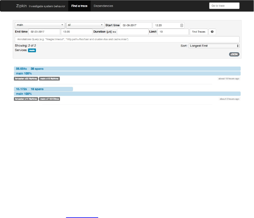
Figure 11-4. An example Zipkin search result
Clicking on the trace, which states the total time and number of spans it includes, will open the
trace detail page, as shown in Figure 11-5. Assuming you have configured the HBase server
processes properly, you should see how the spans migrated from the shell (the main service name)
to the servers (here listed as hmaster service, as for the sake of simplicity the test was performed
against a stand-alone HBase instance, which runs everything in a single HMaster process). From
here you can click on each span, which are the rows within the table on the details page. A popup
windows will show you details about the span for your peruse.
(954)
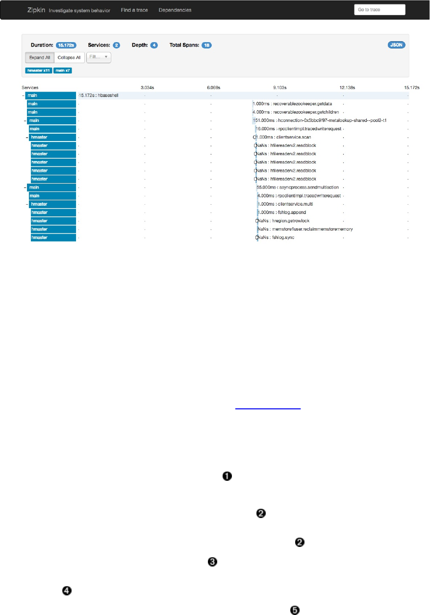
Figure 11-5. An example Zipkin trace with many spans
Compared to the earlier text representation, reading the Zipkin UI is much more intuitive. The
timeline is on the top of the table, showing where time was spent. For the shell example, most
time was used up by the shell code. Adding trace support to your own code is accomplished by
first loading the span receiver class with the available configuration, and then wrapping
interesting calls into a trace scope instance, as shown in Example 11-2.
Example 11-2. Shows the use of the HBase HTrace integration
private static SpanReceiverHost spanReceiverHost;
conf.set("hbase.trace.spanreceiver.classes",
"org.apache.htrace.impl.ZipkinSpanReceiver");
conf.set("hbase.htrace.zipkin.collector-hostname", "localhost");
conf.set("hbase.htrace.zipkin.collector-port", "9410");
spanReceiverHost = SpanReceiverHost.getInstance(conf);
Table table = connection.getTable(TableName.valueOf("testtable"));
TraceScope ts1 = Trace.startSpan("Get Trace", Sampler.ALWAYS);
try {
Get get = new Get(Bytes.toBytes("row-1"));
Result res = table.get(get);
} finally {
ts1.close();
}
System.out.println("Is trace detached? " + ts1.isDetached());
Span span = ts1.getSpan();
System.out.println("Span Time: " + span.getAccumulatedMillis());
System.out.println("Span: " + span);
//conf.set("hbase.htrace.sampler", "ProbabilitySampler");
//conf.set("hbase.htrace.sampler.fraction", "0.5");
(955)
conf.set("hbase.htrace.sampler", "CountSampler");
conf.set("hbase.htrace.sampler.frequency", "5");
HBaseHTraceConfiguration traceConf = new HBaseHTraceConfiguration(conf);
SamplerBuilder builder = new SamplerBuilder(traceConf);
Sampler sampler = builder.build();
System.out.println("Sampler: " + sampler.getClass().getName());
TraceScope ts2 = Trace.startSpan("Scan Trace", sampler);
try {
Scan scan = new Scan();
scan.setCaching(1);
ResultScanner scanner = table.getScanner(scan);
while (scanner.next() != null) ;
scanner.close();
} finally {
ts2.close();
}
Set up configuration to use the Zipkin span receiver class.
Initialize the span receiver host from the configuration settings.
Start a span, giving it a name and sample rate.
Perform common operations that should be traced.
Close the span to group performance details together.
Talk to the trace and span instances from within the code.
Start another span with a different sampler.
The scan performs a separate RPC call for each row it retrieves, creating a span for every
row.
The output is as follows:
Adding rows to table...
...
INFO: Created testtable
Feb 12, 2017 11:22:52 AM org.apache.hadoop.hbase.trace.SpanReceiverHost \
loadSpanReceivers
INFO: SpanReceiver org.apache.htrace.impl.ZipkinSpanReceiver was loaded \
successfully.
...
Is trace detached? true
Span Time: 15
Span: {"i":"4b650058e25f5d20","s":"cbdbb303a068f945","b":1486894975934, \
"e":1486894975949,"d":"Get Trace","r":"AppMain","p":[]}
(956)

Sampler: org.apache.htrace.impl.CountSampler
The code example performs three separate traces (only two are shown for the sake of brevity),
which wrap the creation of the HBase connection, a get operation, and a scan of a table, where
the latter is forced to do an RPC for each call the scanner’s next() method. The scanner tracing
also shows how to setup a different sampler instance, which either emits after every N calls
(using the HTrace CountSampler), or for only a specific percentage of all calls (by means of the
ProbabilitySampler class). Figure 11-6 shows the trace results with the default sampler
(AlwaysSampler) implementation. You can see each call to next and also how HBase is loading
blocks in between calls.
(957)
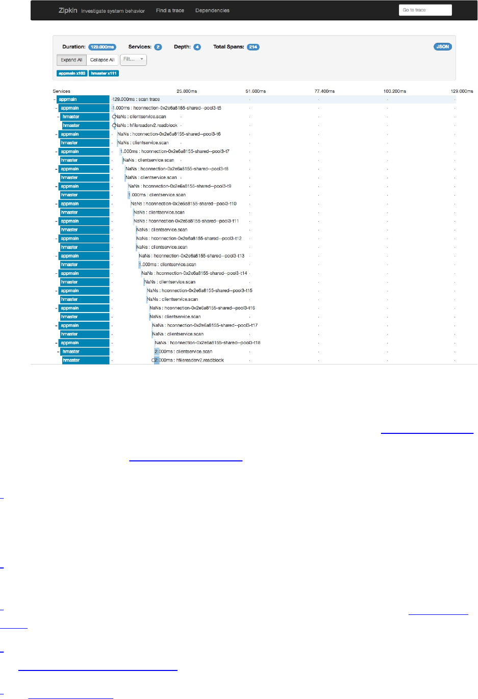
Figure 11-6. The trace result of the scan
Zipkin has many more features, for example concerning the delivery of events. Besides the
shown use Scribe protocol, it also supports HTTP and Apache Kafka (see the Zipkin architecture
page for details). Hadoop also has HTrace included and can be extended to send spans to Zipkin
or other receivers (see the Tracing documentation page for Hadoop). Note that the versions of
HTrace between HBase and Hadoop have to match for spans to be included into each other.
1 As of this writing, there is a slight error in the description given by the script and the actual
filename generated. It is missing the current username, resulting in a file named, for example:
/tmp/larsgeorgeworker-3.internal.larsgeorge.com\:16020 (note the username attached directly to
the host name).
2 Note that some distributions for HBase do not require this, since they do not make use of the
supplied start-hbase.sh script.
3 Another option is to use the ZooKeeper dump page of the master UI, as shown in “ZooKeeper
page”.
4 For a thorough discussion about the need to prepare data, and how to do that with Spark, please
see Tim Robertson’s OpenCore post.
5 See generatedata.com for example.
(958)

6 Hadoop uses a similar layout for the port assignments, but since it has more process types it
also has additional ports. See, for example, this documentation for more information.
7 This is equivalent to the HBase 0.90 -fix option.
8 A dedicated service you can use is Search Hadoop.
9 Also see Google Dapper, which is the inspiration for HTrace.
10 These classes are part of HTrace version 3.1.0, which is bundled with HBase 1.3.x.
11 For example, for HTrace 3.1.0.
(959)

Appendix A. Upgrade from Previous
Releases
Upgrading HBase involves careful planning, especially when the cluster is currently in
production. With the addition of rolling restarts (see “Rolling Restarts”), it has become much
easier to update HBase with no downtime.
Note
Depending on the version of HBase you are using or upgrading to, you may need to upgrade the
underlying Hadoop version first so that it matches the required version for the new version of
HBase you are installing. Follow the upgrade guide found on the Hadoop website.
(960)
Upgrading to HBase 0.90.x
Depending on the versions you are upgrading from, a different set of steps might be necessary to
update your existing cluster to a newer version. The following subsections address the more
common update scenarios.
(961)

From 0.20.x or 0.89.x
This version of 0.90.x HBase can be started on data written by HBase 0.20.x or HBase 0.89.x,
and there is no need for a migration step. HBase 0.89.x and 0.90.x do write out the names of
region directories differently—they name them with an MD5 hash of the region name rather than
a Jenkins hash, which means that once you have started, there is no going back to HBase 0.20.x.
Be sure to remove the hbase-default.xml file from your conf directory when you upgrade. A
0.20.x version of this file will have suboptimal configurations for HBase 0.90.x. The hbase-
default.xml file is now bundled into the HBase JAR and read from there. If you would like to
review the content of this file, you can find it in the src directory at
$HBASE_HOME/src/main/resources/hbase-default.xml or see [Link to Come].
Finally, if upgrading from 0.20.x, check your .META. schema in the shell. In the past, it was
recommended that users run with a 16 KB MEMSTORE_FLUSHSIZE. Execute
hbase(main):001:0> scan '-ROOT-'
in the shell. This will output the current .META. schema. Check if the MEMSTORE_FLUSHSIZE size is set
to 16 KB (16384). If that is the case, you will need to change this. The new default value is 64
MB (67108864). Run the script $HBASE_HOME/bin/set_meta_memstore_size.rb. This will make the
necessary changes to your .META. schema. Failure to run this change will cause your cluster to
run more slowly.1
(962)

Upgrading to HBase 0.92.0
No rolling restart is possible, as the wire protocol has changed between versions. You need to
prepare the installation in parallel, then shut down the cluster and start the new version of HBase.
No migration is needed otherwise.
(964)
Upgrading to HBase 0.98.x
(965)
Migrate API to HBase 1.0.x
TBD.
Table A-1. List of deprecated API methods and classes with their replacement
Name Type Replacement Type
HTable Class Table Interface
HConnection Interface Connection Interface
HConnectionManager Class ConnectionFactory Class
HTableFactory Class ConnectionFactory.createConnection() Method
HTableInterface Interface Table Interface
HTablePool Class Connection.getTable() Method
<tablename> String TableName Class
HTable.getWriteToWAL() Method Table.getDurabilty() Method
HTable.setWriteToWAL() Method Table.setDurabilty() Method
HTable.getFamilyMap() Method Table.getFamilyCellMap() Method
HTable.setFamilyMap() Method Table.setFamilyCellMap() Method
Delete.deleteColumn() Method Delete.addColumn() Method
Delete.deleteColumns() Method Delete.addColumns() Method
Delete.deleteFamily() Method Delete.addFamily() Method
(966)
Delete.deleteFamilyVersion() Method Delete.addFamilyVersion() Method
Table.batch(List<? extends Row>) Method Table.batch(List<? extends Row>,
Object[]) Method
Table.batchCallback(List<? extends
Row>, Callback<R>) Method Table.batchCallback(List<? extends Row>,
Object[], Callback<R>) Method
Batch.forMethod() Method dropped, no replacement n/a
(967)

Migrate Coprocessors to post HBase 0.96
Here are the steps needed to convert a Writable based coprocessor implementation into a new
Protocol Buffer based one. This is needed since as of HBase 0.96 (nicknamed the Singularity)
the entire RPC communication has been replaced by a proper, versioned serialization protocol.
With that the old format is not acceptable anymore, and a few changes had to take place. The
following uses the RowCount example from the first revision of the book, and how it was
converted to the new API.
Step 1
The first thing to do is to drop the custom protocol class in favor of a Protocol Buffer definition.
You can delete the entire class file that implements the protocol interface, which looks like this:
public interface RowCountProtocol extends CoprocessorProtocol {
long getRowCount() throws IOException;
long getRowCount(Filter filter) throws IOException;
long getKeyValueCount() throws IOException;
}
You need to create the replacement Protocol Buffer definition file, and following Maven project
layout rules, they go into ${PROJECT_HOME}/src/main/protobuf, here with the name
RowCountService.proto.
option java_package = "coprocessor.generated";
option java_outer_classname = "RowCounterProtos";
option java_generic_services = true;
option java_generate_equals_and_hash = true;
option optimize_for = SPEED;
message CountRequest {
}
message CountResponse {
required int64 count = 1 [default = 0];
}
service RowCountService {
rpc getRowCount(CountRequest)
returns (CountResponse);
rpc getCellCount(CountRequest)
returns (CountResponse);
}
The file defines the output class name, the package to use during code generation and so on. The
last thing in step #1 is to compile the definition file into code. This is done using the Protocol
Buffer protoc tool, as described in more detail in “Custom Filters”. Executing the command-line
compiler will place the generated class file in the source directory, as specified.
Step 2
The next step is to convert Endpoint to new API, which involves removing the old custom RPC
interface, and adding the new Protocol Buffer based one (see the RowCountEndpoint class in the
code repository). The old way to integrate the custom calls looked like this:
public class RowCountEndpoint extends BaseEndpointCoprocessor
implements RowCountProtocol {
(968)
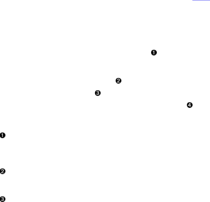
The new replaces the custom interface with the generated one from step #1 above:
public class RowCountEndpoint extends RowCounterProtos.RowCountService
implements Coprocessor, CoprocessorService {
We also implement two more coprocessor related interface directly: there is no
BaseEndpointProcessor anymore. The Coprocessor and CoprocessorService interfaces add vital
lifecycle methods to our class. We need the start() call to retrieve the coprocessor environment
like so:
@Override
public void start(CoprocessorEnvironment env) throws IOException {
if (env instanceof RegionCoprocessorEnvironment) {
this.env = (RegionCoprocessorEnvironment) env;
} else {
throw new CoprocessorException("Must be loaded on a table region!");
}
}
In the past the boilerplate BaseEndpointProcessor gave us a getEnvironment() method to retrieve the
same. We now need to do this on our own. On top of that we need to change the RPC call
handlers, where the old once simply implemented the custom RPC interface methods:
@Override
public long getRowCount() throws IOException {
return getRowCount(new FirstKeyOnlyFilter());
}
In the new API style we have to add a bit more wiring, especially around the marshalling of the
result—or error—and how it is returned to the framework (see the online documentation). Due to
the use of the Protocol Buffer library, we need to accept a request object and return a response
like so:
Example A-1.
@Override
public void getCellCount(RpcController controller,
RowCounterProtos.CountRequest request,
RpcCallback<RowCounterProtos.CountResponse> done) {
RowCounterProtos.CountResponse response = null;
try {
long count = getCount(null, true);
response = RowCounterProtos.CountResponse.newBuilder()
.setCount(count).build();
} catch (IOException ioe) {
ResponseConverter.setControllerException(controller, ioe);
}
done.run(response);
}
Custom RPC call with specific handler classes, such as the controller, and request/response
pair.
Call the internal helper to scan and summarize per region aggregates as usual.
Hand in resulting count into the response wrapper.
(969)
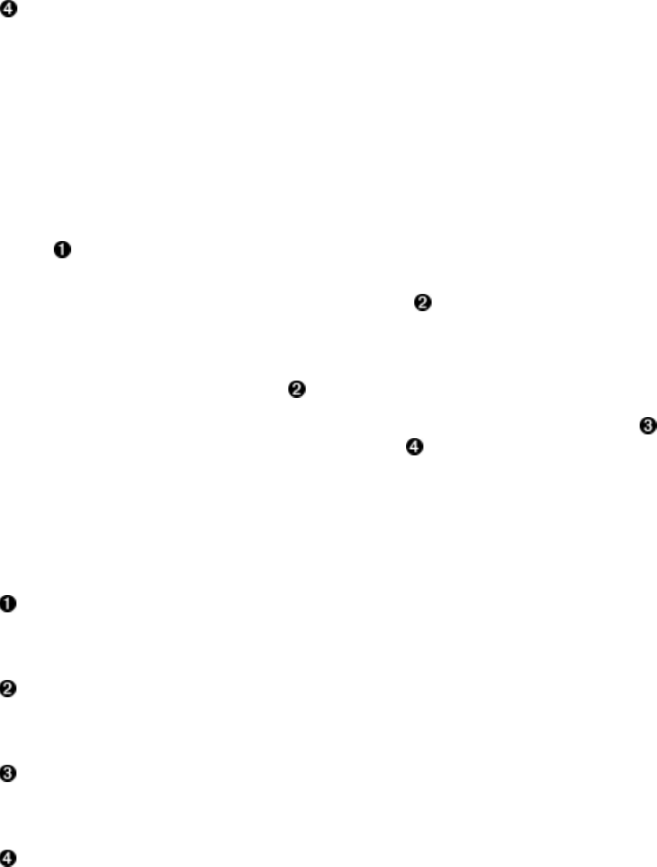
Handle exceptions by wrapping the error and returning it via the controller.
Apart from that there are more changes, unrelated to coprocessors, that are required to make the
old code work. For example, we need to change from KeyValue to Cell types, and adjust how we
do comparisons. The new code looks very similar, but has a few slight changes:
Example A-2.
try (
InternalScanner scanner = env.getRegion().getScanner(scan);
) {
List<Cell> results = new ArrayList<Cell>();
boolean hasMore = false;
byte[] lastRow = null;
do {
hasMore = scanner.next(results);
for (Cell cell : results) {
if (!countCells) {
if (lastRow == null || !CellUtil.matchingRow(cell, lastRow)) {
lastRow = CellUtil.cloneRow(cell);
count++;
}
} else count++;
}
results.clear();
} while (hasMore);
}
Use of the new try-with-resource pattern to simplify resources handling.
The new Cell interface is used to retrieve the data and iterate over it.
Comparing changed to use the CellUtil.matchingRow() method, for convenience.
The byte array has to be memorized, use again the CellUtil helper to clone the row key.
Apart from that, no further code changes on the server-side code were necessary.
Step 3
From here you need to do the same as before, that is deploy the coprocessor as a JAR file on the
servers, add the class name to the hbase-site.xml file, add the JAR name to the class path in the
hbase-env.sh file, and restart the servers.
Step 4
Last step is invoking the server-side code. This is now client API code that has to be adjusted.
This is located in the EndpointExample class, and looks like this for the old style API:
Map<byte[], Long> results = table.coprocessorExec(
(970)
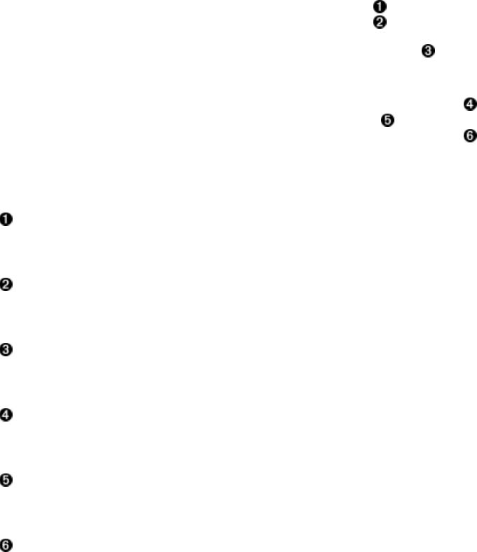
RowCountProtocol.class, null, null,
new Batch.Call<RowCountProtocol, Long>() {
@Override
public Long call(RowCountProtocol counter) throws IOException {
return counter.getRowCount();
}
});
For the new one there are a few changes, analog to what we have seen on the server-side code.
There is more wiring for the Protocol Buffer based RPC handling:
Example A-3.
final RowCounterProtos.CountRequest request =
RowCounterProtos.CountRequest.getDefaultInstance();
Map<byte[], Long> results = table.coprocessorService(
RowCounterProtos.RowCountService.class, null, null,
new Batch.Call<RowCounterProtos.RowCountService, Long>() {
public Long call(RowCounterProtos.RowCountService counter)
throws IOException {
BlockingRpcCallback<RowCounterProtos.CountResponse> rpcCallback =
new BlockingRpcCallback<RowCounterProtos.CountResponse>();
counter.getRowCount(null, request, rpcCallback);
RowCounterProtos.CountResponse response = rpcCallback.get();
return response.hasCount() ? response.getCount() : 0;
}
}
);
Create a request instance using the generated RPC class.
Call the new coprocessorService() method (the older coprocessorExec() has been removed).
Use the generated classes to paramterize the call.
Set up an RPC callback for the specific call and types.
Invoke the remote call.
Retrieve the response and, subsequently, the payload value (our row count).
These are all the changes that were needed to run the existing example using the new API.
(971)

Migrate Custom Filters to post HBase 0.96
Here are the steps needed to convert a Writable based filter implementation into a new Protocol
Buffer based one. This is needed since as of HBase 0.96 (nicknamed the Singularity) the entire
RPC communication has been replaced by a proper, versioned serialization protocol. With that
the old format is not acceptable anymore, and a few changes had to take place. The following
uses the CustomFilter example from the first revision of the book, and how it was converted to
the new API.
Step 1
First you need to create a Protocol Buffer definition, which covers all the internal fields of the
filter, setting its state. Following Maven project layout rules, they go into
${PROJECT_HOME}/src/main/protobuf, here with the name CustomFilters.proto. The content is the
following:
option java_package = "filters.generated";
option java_outer_classname = "FilterProtos";
option java_generic_services = true;
option java_generate_equals_and_hash = true;
option optimize_for = SPEED;
message CustomFilter {
required bytes value = 1;
}
The file defines the output class name, the package to use during code generation and so on. The
last thing in step #1 is to compile the definition file into code. This is done using the Protocol
Buffer protoc tool, as described in more detail in “Custom Filters”. Executing the command-line
compiler will place the generated class file in the source directory, as specified.
Step 2
Next step is the conversion of the existing, Writable based, serialization methods, over to the new
Protocal Buffer ones. For that we need to change to methods, here the old version:
@Override
public void write(DataOutput dataOutput) throws IOException {
Bytes.writeByteArray(dataOutput, this.value);
}
@Override
public void readFields(DataInput dataInput) throws IOException {
this.value = Bytes.readByteArray(dataInput);
Both of those methods can be dropped, and are replaced by the following two:
@Override
public byte [] toByteArray() {
FilterProtos.CustomFilter.Builder builder =
FilterProtos.CustomFilter.newBuilder();
if (value != null) builder.setValue(ByteStringer.wrap(value));
return builder.build().toByteArray();
}
public static Filter parseFrom(final byte[] pbBytes)
throws DeserializationException {
FilterProtos.CustomFilter proto;
try {
proto = FilterProtos.CustomFilter.parseFrom(pbBytes);
(972)

} catch (InvalidProtocolBufferException e) {
throw new DeserializationException(e);
}
return new CustomFilter(proto.getValue().toByteArray());
}
The look more complicated, but that is attributed to the Protocol Buffer handling, which is not as
hidden as the Writable version. The toByteArray() serialized the filter fields inside a Protocol
Buffer message. For that it creates a Builder instance that was generated in step #1. The builder is
then executed and the resulting byte array returned.
On the deserialization side the parseFrom() receives the byte array, which is then parse by the
generated code into a message instance. The contained data is handed into the filter constructor,
which is returned to the caller in due course.
Step 3
From here you need to do the same as before, that is deploy the coprocessor as a JAR file on the
servers, add the class name to the hbase-site.xml file, add the JAR name to the class path in the
hbase-env.sh file, and restart the servers. See “Custom Filters” for details on the deployment
options.
Step 4
Last step is invoking the filter as part of a read operation. This stays the same as well as before,
since we only adjusted the internal serialization process, which is otherwise not exposed to the
client. The usage and rest of the filter implementation stays the same (see Example 4-24 for an
example).
1 See “HBASE-3499 Users upgrading to 0.90.0 need to have their .META. table updated with
the right MEMSTORE_SIZE” (http://issues.apache.org/jira/browse/HBASE-3499) for details.
(973)
