HP Analysis User Guide Load Runner
User Manual: Pdf
Open the PDF directly: View PDF ![]() .
.
Page Count: 387 [warning: Documents this large are best viewed by clicking the View PDF Link!]
- LoadRunner Analysis
- Welcome to the Analysis User Guide
- Analysis
- Introducing Analysis
- Workflow
- Analysis Basics
- Session Explorer Window
- Analysis Window Layouts
- Printing Graphs or Reports
- Configuring Analysis
- Summary Data Versus Complete Data
- Importing Data Directly from the Analysis Machine
- How to Configure Settings for Analyzing Load Test Results
- General Tab (Options Dialog Box)
- Result Collection Tab (Options Dialog Box)
- Data Aggregation Configuration Dialog Box (Result Collection Tab)
- Database Tab (Options Dialog Box)
- Advanced Options Dialog Box (Database Tab)
- Web Page Diagnostics Tab (Options Dialog Box)
- Session Information Dialog Box (Options Dialog Box)
- Viewing Load Test Scenario Information
- Defining Service Level Agreements
- Service Level Agreements Overview
- Tracking Period
- How to Define Service Level Agreements
- How to Define Service Level Agreements - Use-Case Scenario
- Service Level Agreement Pane
- Advanced Options Dialog Box (Service Level Agreement Pane)
- Goal Details Dialog Box (Service Level Agreement Pane)
- Service Level Agreement Wizard
- Working with Application Lifecycle Management
- Setup
- Configuring Graph Display
- How to Customize the Analysis Display
- Display Options Dialog Box
- Editing Main Chart Dialog Box (Display Options Dialog Box)
- Chart Tab (Editing MainChart Dialog Box)
- Series Tab (Editing MainChart Dialog Box)
- Legend Window
- Measurement Description Dialog Box
- Measurement Options Dialog Box
- Legend Columns Options Dialog Box
- Apply/Edit Template Dialog Box
- Color Palettes
- Color Palette Dialog Box
- Working with Analysis Graph Data
- Filtering and Sorting Graph Data
- Cross Result and Merged Graphs
- Configuring Graph Display
- Analysis Graphs
- Open a New Graph Dialog Box
- Vuser Graphs
- Error Graphs
- Transaction Graphs
- Average Transaction Response Time Graph
- Total Transactions per Second Graph
- Transaction Breakdown Tree
- Transactions per Second Graph
- Transaction Performance Summary Graph
- Transaction Response Time (Distribution) Graph
- Transaction Response Time (Percentile) Graph
- Transaction Response Time (Under Load) Graph
- Transaction Response Time by Location Graph
- Transaction Summary Graph
- Web Resources Graphs
- Web Page Diagnostics Graphs
- Web Page Diagnostics Tree View Overview
- Web Page Diagnostics Graphs Overview
- How to View the Breakdown of a Transaction
- Web Page Diagnostics Content Icons
- Web Page Diagnostics Graph
- Page Component Breakdown Graph
- Page Component Breakdown (Over Time) Graph
- Page Download Time Breakdown Graph
- Page Download Time Breakdown (Over Time) Graph
- Page Download Time Breakdown Graph Breakdown Options
- Time to First Buffer Breakdown Graph
- Time to First Buffer Breakdown (Over Time) Graph
- Client Side Breakdown (Over Time) Graph
- Client Side Java Script Breakdown (Over Time) Graph
- Downloaded Component Size Graph
- User-Defined Data Point Graphs
- System Resource Graphs
- Network Virtualization Graphs
- Network Monitor Graphs
- Web Server Resource Graphs
- Web Application Server Resource Graphs
- Database Server Resource Graphs
- Streaming Media Graphs
- J2EE & .NET Diagnostics Graphs
- J2EE & .NET Diagnostics Graphs Overview
- How to Enable Diagnostics for J2EE & .NET
- Viewing J2EE to SAP R3 Remote Calls
- J2EE & .NET Diagnostics Data
- Example Transaction Breakdown
- Using the J2EE & .NET Breakdown Options
- Viewing Chain of Calls and Call Stack Statistics
- Understanding the Chain of Calls Window
- Graph Filter Properties
- J2EE/.NET - Average Method Response Time in Transactions Graph
- J2EE/.NET - Average Number of Exceptions in Transactions Graph
- J2EE/.NET - Average Number of Exceptions on Server Graph
- J2EE/.NET - Average Number of Timeouts in Transactions Graph
- J2EE/.NET - Average Number of Timeouts on Server Graph
- J2EE/.NET - Average Server Method Response Time Graph
- J2EE/.NET - Method Calls per Second in Transactions Graph
- J2EE/.NET - Probes Metrics Graph
- J2EE/.NET - Server Methods Calls per Second Graph
- J2EE/.NET - Server Requests per Second Graph
- J2EE/.NET - Server Request Response Time Graph
- J2EE/.NET - Server Request Time Spent in Element Graph
- J2EE/.NET - Transactions per Second Graph
- J2EE/.NET - Transaction Response Time Server Side Graph
- J2EE/.NET - Transaction Time Spent in Element Graph
- Application Component Graphs
- COM+ Average Response Time Graph
- COM+ Breakdown Graph
- COM+ Call Count Distribution Graph
- COM+ Call Count Graph
- COM+ Call Count Per Second Graph
- COM+ Total Operation Time Distribution Graph
- COM+ Total Operation Time Graph
- Microsoft COM+ Graph
- .NET Average Response Time Graph
- .NET Breakdown Graph
- .NET Call Count Distribution Graph
- .NET Call Count Graph
- .NET Call Count per Second Graph
- .NET Resources Graph
- .NET Total Operation Time Distribution Graph
- .NET Total Operation Time Graph
- Application Deployment Solutions Graphs
- Middleware Performance Graphs
- Infrastructure Resources Graphs
- HP Service Virtualization Graphs
- Flex Graphs
- WebSocket Statistics Graphs
- Diagnostics Graphs
- Siebel Diagnostics Graphs
- Siebel Diagnostics Graphs Overview
- Call Stack Statistics Window
- Chain of Calls Window
- Siebel Area Average Response Time Graph
- Siebel Area Call Count Graph
- Siebel Area Total Response Time Graph
- Siebel Breakdown Levels
- Siebel Diagnostics Graphs Summary Report
- Siebel Request Average Response Time Graph
- Siebel Transaction Average Response Time Graph
- Siebel DB Diagnostics Graphs
- Siebel DB Diagnostics Graphs Overview
- How to Synchronize Siebel Clock Settings
- Measurement Description Dialog Box
- Siebel Database Breakdown Levels
- Siebel Database Diagnostics Options Dialog Box
- Siebel DB Side Transactions Graph
- Siebel DB Side Transactions by SQL Stage Graph
- Siebel SQL Average Execution Time Graph
- Oracle - Web Diagnostics Graphs
- SAP Diagnostics Graphs
- SAP Diagnostics Graphs Overview
- How to Configure SAP Alerts
- SAP Diagnostics - Guided Flow Tab
- SAP Diagnostics Application Flow
- Dialog Steps per Second Graph
- OS Monitor Graph
- SAP Alerts Configuration Dialog box
- SAP Alerts Window
- SAP Application Processing Time Breakdown Graph
- SAP Primary Graphs
- SAP Average Dialog Step Response Time Breakdown Graph
- SAP Average Transaction Response Time Graph
- SAP Breakdown Task Pane
- SAP Server Time Breakdown (Dialog Steps) Graphs
- SAP Server Time Breakdown Graph
- SAP Database Time Breakdown Graph
- SAP Diagnostics Summary Report
- SAP Interface Time Breakdown Graph
- SAP System Time Breakdown Graph
- SAP Secondary Graphs
- Work Processes Graph
- Siebel Diagnostics Graphs
- TruClient - Native Mobile Graphs
- Analysis Reports
- Importing Data
- Troubleshooting and Limitations for Analysis
- Analysis API Reference

LoadRunner Analysis
Software Version: 12.50
User Guide
Document Release Date: August 2015
Software Release Date: August 2015
User Guide
LoadRunner Analysis
HP LoadRunner (12.50) Page 2
Legal Notices
Warranty
The only warranties for HP products and services are set forth in the express warranty statements accompanying such
products and services. Nothing herein should be construed as constituting an additional warranty. HP shall not be liable
for technical or editorial errors or omissions contained herein.
The information contained herein is subject to change without notice.
Restricted Rights Legend
Confidential computer software. Valid license from HP required for possession, use or copying. Consistent with FAR
12.211 and 12.212, Commercial Computer Software, Computer Software Documentation, and Technical Data for
Commercial Items are licensed to the U.S. Government under vendor's standard commercial license.
Copyright Notice
© Copyright 1993-2015 Hewlett-Packard Development Company, L.P.
Trademark Notices
Adobe® is a trademark of Adobe Systems Incorporated.
Microsoft® and Windows® are U.S. registered trademarks of Microsoft Corporation.
Oracle and Java are registered trademarks of Oracle and/or its affiliates.
UNIX® is a registered trademark of The Open Group.
Documentation Updates
The title page of this document contains the following identifying information:
lSoftware Version number, which indicates the software version.
lDocument Release Date, which changes each time the document is updated.
lSoftware Release Date, which indicates the release date of this version of the software.
To check for recent updates or to verify that you are using the most recent edition of a document, go to:
https://softwaresupport.hp.com.
This site requires that you register for an HP Passport and sign in. To register for an HP Passport ID, go to
https://softwaresupport.hp.com and click Register.
Support
Visit the HP Software Support Online web site at: https://softwaresupport.hp.com
This web site provides contact information and details about the products, services, and support that HP Software
offers.
HP Software online support provides customer self-solve capabilities. It provides a fast and efficient way to access
interactive technical support tools needed to manage your business. As a valued support customer, you can benefit by
using the support web site to:
User Guide
HP LoadRunner (12.50) Page 3
lSearch for knowledge documents of interest
lSubmit and track support cases and enhancement requests
lDownload software patches
lManage support contracts
lLook up HP support contacts
lReview information about available services
lEnter into discussions with other software customers
lResearch and register for software training
Most of the support areas require that you register as an HP Passport user and sign in. Many also require a support
contract. To register for an HP Passport ID, go to: https://softwaresupport.hp.com and click Register.
To find more information about access levels, go to: https://softwaresupport.hp.com/web/softwaresupport/access-
levels.
HP Software Solutions &Integrations and Best Practices
Visit HP Software Solutions Now at https://h20230.www2.hp.com/sc/solutions/index.jsp to explore how the products
in the HP Software catalog work together, exchange information, and solve business needs.
Visit the Cross Portfolio Best Practices Library at https://hpln.hp.com/group/best-practices-hpsw to access a wide
variety of best practice documents and materials.
User Guide
HP LoadRunner (12.50) Page 4

Contents
LoadRunner Analysis 1
Welcome to the Analysis User Guide 14
What's New in LoadRunner 12.50 14
Highlights 14
Analysis 20
Introducing Analysis 20
Results Overview 20
Analysis Toolbars 21
Analysis API 23
Workflow 23
Analysis Basics 24
Session Explorer Window 25
Analysis Window Layouts 26
Printing Graphs or Reports 27
Configuring Analysis 28
Summary Data Versus Complete Data 28
Importing Data Directly from the Analysis Machine 28
How to Configure Settings for Analyzing Load Test Results 30
General Tab (Options Dialog Box) 30
Result Collection Tab (Options Dialog Box) 33
Data Aggregation Configuration Dialog Box (Result Collection Tab) 36
Database Tab (Options Dialog Box) 37
Advanced Options Dialog Box (Database Tab) 41
Web Page Diagnostics Tab (Options Dialog Box) 42
Session Information Dialog Box (Options Dialog Box) 43
Viewing Load Test Scenario Information 45
Viewing Load Test Scenario Information 45
How to Configure Controller Output Messages Settings 46
Controller Output Messages Window 47
Summary Tab 47
Filtered Tab 49
Scenario Runtime Settings Dialog Box 51
Defining Service Level Agreements 51
Service Level Agreements Overview 51
Tracking Period 52
User Guide
HP LoadRunner (12.50) Page 5

How to Define Service Level Agreements 52
How to Define Service Level Agreements - Use-Case Scenario 54
Service Level Agreement Pane 56
Advanced Options Dialog Box (Service Level Agreement Pane) 57
Goal Details Dialog Box (Service Level Agreement Pane) 58
Service Level Agreement Wizard 58
Select a Measurement Page 59
Select Transactions Page 60
Set Load Criteria Page 60
Set Percentile Threshold Values Page 62
Set Threshold Values Page (Goal Per Time Interval) 62
Set Threshold Values Page (Goal Per Whole Run) 63
Working with Application Lifecycle Management 64
Managing Results Using ALM - Overview 64
How to Connect to ALM from Analysis 64
How to Work with Results in ALM - Without Performance Center 65
How to Work with Results in ALM - With Performance Center 66
How to Upload a Report to ALM 68
HP ALM Connection Dialog Box 69
Upload Report to Test Lab Dialog Box 71
Setup 72
Configuring Graph Display 72
How to Customize the Analysis Display 72
Display Options Dialog Box 73
Editing Main Chart Dialog Box (Display Options Dialog Box) 75
Chart Tab (Editing MainChart Dialog Box) 76
Series Tab (Editing MainChart Dialog Box) 77
Legend Window 78
Measurement Description Dialog Box 81
Measurement Options Dialog Box 82
Legend Columns Options Dialog Box 83
Apply/Edit Template Dialog Box 84
Color Palettes 86
Color Palette Dialog Box 86
Working with Analysis Graph Data 89
Determining a Point's Coordinates 89
Drilling Down in a Graph 90
Changing the Granularity of the Data 91
Viewing Measurement Trends 92
Auto Correlating Measurements 93
Viewing Raw Data 94
How to Manage Graph Data 94
User Guide
HP LoadRunner (12.50) Page 6

Drill Down Options Dialog Box 96
Auto Correlate Dialog Box 97
Graph/Raw Data View Table 100
Graph Properties Pane 101
Filtering and Sorting Graph Data 103
Filtering Graph Data Overview 103
Sorting Graph Data Overview 103
Filter Conditions 104
Custom Filter Dialog Box 113
Filter Dialog Boxes 114
Filter Builder Dialog Box 116
Hierarchical Path Dialog Box 117
Scenario Elapsed Time Dialog Box 117
Set Dimension Information Dialog Box 118
Vuser ID Dialog Box 119
Cross Result and Merged Graphs 120
Cross Result and Merged Graphs Overview 120
Cross Result Graphs Overview 120
Merging Types Overview 121
How to Generate Cross Results Graphs 123
How to Generate Merged Graphs 124
Merge Graphs Dialog Box 124
Analysis Graphs 125
Open a New Graph Dialog Box 125
Vuser Graphs 127
Rendezvous Graph (Vuser Graphs) 127
Running Vusers Graph 128
Vuser Summary Graph 129
Error Graphs 130
Errors per Second (by Description) Graph 130
Errors per Second Graph 131
Error Statistics (by Description) Graph 132
Error Statistics Graph 133
Total Errors per Second Graph 134
Transaction Graphs 135
Average Transaction Response Time Graph 135
Total Transactions per Second Graph 137
Transaction Breakdown Tree 138
Transactions per Second Graph 139
Transaction Performance Summary Graph 140
Transaction Response Time (Distribution) Graph 141
Transaction Response Time (Percentile) Graph 141
User Guide
HP LoadRunner (12.50) Page 7

Transaction Response Time (Under Load) Graph 143
Transaction Response Time by Location Graph 143
Transaction Summary Graph 144
Web Resources Graphs 145
Web Resources Graphs Overview 145
Hits per Second Graph 146
Throughput Graph 146
HTTP Status Code Summary Graph 147
HTTP Status Codes 148
HTTP Responses per Second Graph 150
Pages Downloaded per Second Graph 151
Retries per Second Graph 153
Retries Summary Graph 154
Connections Graph 154
Connections per Second Graph 155
SSLs per Second Graph 156
Web Page Diagnostics Graphs 157
Web Page Diagnostics Tree View Overview 157
Web Page Diagnostics Graphs Overview 158
How to View the Breakdown of a Transaction 159
Web Page Diagnostics Content Icons 160
Web Page Diagnostics Graph 161
Page Component Breakdown Graph 163
Page Component Breakdown (Over Time) Graph 164
Page Download Time Breakdown Graph 165
Page Download Time Breakdown (Over Time) Graph 167
Page Download Time Breakdown Graph Breakdown Options 169
Time to First Buffer Breakdown Graph 170
Time to First Buffer Breakdown (Over Time) Graph 172
Client Side Breakdown (Over Time) Graph 174
Client Side Java Script Breakdown (Over Time) Graph 175
Downloaded Component Size Graph 176
User-Defined Data Point Graphs 177
User-Defined Data Point Graphs Overview 178
Data Points (Average) Graph 178
Data Points (Sum) Graph 179
System Resource Graphs 180
Server Resources Performance Counters 180
Linux Resources Default Measurements 181
Windows Resources Default Measurements 182
Server Resources Graph 184
Host Resources Graph 184
User Guide
HP LoadRunner (12.50) Page 8

SNMP Resources Graph 185
Linux Resources Graph 186
Windows Resources Graph 187
Network Virtualization Graphs 188
Packet Loss Graph 188
Average Latency Graph 190
Average Bandwidth Utilization Graph 191
Average Throughput Graph 193
Total Throughput Graph 194
Network Monitor Graphs 195
Network Monitor Graphs Overview 196
Network Delay Time Graph 196
Network Segment Delay Graph 197
Network Sub-Path Time Graph 198
Web Server Resource Graphs 199
Web Server Resource Graphs Overview 199
Apache Server Measurements 199
IIS Server Measurements 200
Apache Server Graph 200
Microsoft Information Internet Server (IIS) Graph 201
Web Application Server Resource Graphs 202
Web Application Server Resource Graphs Overview 202
Web Application Server Resource Graphs Measurements 203
Microsoft Active Server Pages (ASP) Graph 211
Oracle9iAS HTTP Server Graph 211
WebLogic (SNMP) Graph 211
WebSphere Application Server Graph 212
Database Server Resource Graphs 212
DB2 Database Manager Counters 212
DB2 Database Counters 214
DB2 Application Counters 219
Oracle Server Monitoring Measurements 224
SQL Server Default Counters 225
Sybase Server Monitoring Measurements 226
DB2 Graph 230
Oracle Graph 230
SQL Server Graph 231
Sybase Graph 232
Streaming Media Graphs 232
Streaming Media Graphs Overview 232
Media Player Client Monitoring Measurements 233
RealPlayer Client Monitoring Measurements 234
User Guide
HP LoadRunner (12.50) Page 9

RealPlayer Server Monitoring Measurements 235
Windows Media Server Default Measurements 236
Media Player Client Graph 237
Real Client Graph 237
Real Server Graph 238
Windows Media Server Graph 239
J2EE & .NET Diagnostics Graphs 239
J2EE & .NET Diagnostics Graphs Overview 240
How to Enable Diagnostics for J2EE & .NET 240
Viewing J2EE to SAP R3 Remote Calls 240
J2EE & .NET Diagnostics Data 242
Example Transaction Breakdown 242
Using the J2EE & .NET Breakdown Options 247
Viewing Chain of Calls and Call Stack Statistics 249
The Chain of Calls Windows 250
Understanding the Chain of Calls Window 251
Graph Filter Properties 253
J2EE/.NET - Average Method Response Time in Transactions Graph 254
J2EE/.NET - Average Number of Exceptions in Transactions Graph 254
J2EE/.NET - Average Number of Exceptions on Server Graph 255
J2EE/.NET - Average Number of Timeouts in Transactions Graph 256
J2EE/.NET - Average Number of Timeouts on Server Graph 257
J2EE/.NET - Average Server Method Response Time Graph 258
J2EE/.NET - Method Calls per Second in Transactions Graph 258
J2EE/.NET - Probes Metrics Graph 259
J2EE/.NET - Server Methods Calls per Second Graph 261
J2EE/.NET - Server Requests per Second Graph 261
J2EE/.NET - Server Request Response Time Graph 262
J2EE/.NET - Server Request Time Spent in Element Graph 263
J2EE/.NET - Transactions per Second Graph 265
J2EE/.NET - Transaction Response Time Server Side Graph 266
J2EE/.NET - Transaction Time Spent in Element Graph 267
Application Component Graphs 268
COM+ Average Response Time Graph 269
COM+ Breakdown Graph 270
COM+ Call Count Distribution Graph 272
COM+ Call Count Graph 273
COM+ Call Count Per Second Graph 274
COM+ Total Operation Time Distribution Graph 275
COM+ Total Operation Time Graph 276
Microsoft COM+ Graph 277
.NET Average Response Time Graph 280
User Guide
HP LoadRunner (12.50) Page 10

.NET Breakdown Graph 281
.NET Call Count Distribution Graph 282
.NET Call Count Graph 283
.NET Call Count per Second Graph 284
.NET Resources Graph 285
.NET Total Operation Time Distribution Graph 288
.NET Total Operation Time Graph 289
Application Deployment Solutions Graphs 290
Citrix Measurements 291
Citrix Server Graph 295
Middleware Performance Graphs 296
IBM WebSphere MQ Counters 296
Tuxedo Resources Graph Measurements 298
IBM WebSphere MQ Graph 300
Tuxedo Resources Graph 301
Infrastructure Resources Graphs 302
Network Client Measurements 302
Network Client Graph 303
HP Service Virtualization Graphs 303
Service Virtualization Graphs Overview 304
HP Service Virtualization Operations Graph 304
HP Service Virtualization Services Graph 305
Flex Graphs 305
Flex RTMP Throughput Graph 306
Flex RTMP Other Statistics Graph 306
Flex RTMP Connections Graph 307
TruClient CPU Utilization Percentage Graph 308
Flex Average Buffering Time Graph 309
WebSocket Statistics Graphs 310
Diagnostics Graphs 310
Siebel Diagnostics Graphs 311
Siebel Diagnostics Graphs Overview 311
Call Stack Statistics Window 312
Chain of Calls Window 313
Siebel Area Average Response Time Graph 315
Siebel Area Call Count Graph 316
Siebel Area Total Response Time Graph 317
Siebel Breakdown Levels 318
Siebel Diagnostics Graphs Summary Report 321
Siebel Request Average Response Time Graph 322
Siebel Transaction Average Response Time Graph 323
Siebel DB Diagnostics Graphs 323
User Guide
HP LoadRunner (12.50) Page 11

Siebel DB Diagnostics Graphs Overview 324
How to Synchronize Siebel Clock Settings 325
Measurement Description Dialog Box 325
Siebel Database Breakdown Levels 326
Siebel Database Diagnostics Options Dialog Box 328
Siebel DB Side Transactions Graph 330
Siebel DB Side Transactions by SQL Stage Graph 330
Siebel SQL Average Execution Time Graph 331
Oracle - Web Diagnostics Graphs 331
Oracle - Web Diagnostics Graphs Overview 331
Measurement Description Dialog Box 332
Oracle Breakdown Levels 333
Oracle - WebDB Side Transactions Graph 336
Oracle - WebDB Side Transactions by SQL Stage Graph 336
Oracle - Web SQL Average Execution Time Graph 337
SAP Diagnostics Graphs 337
SAP Diagnostics Graphs Overview 337
How to Configure SAP Alerts 337
SAP Diagnostics - Guided Flow Tab 338
SAP Diagnostics Application Flow 340
Dialog Steps per Second Graph 341
OS Monitor Graph 341
SAP Alerts Configuration Dialog box 342
SAP Alerts Window 343
SAP Application Processing Time Breakdown Graph 344
SAP Primary Graphs 344
SAP Average Dialog Step Response Time Breakdown Graph 344
SAP Average Transaction Response Time Graph 345
SAP Breakdown Task Pane 346
SAP Server Time Breakdown (Dialog Steps) Graphs 348
SAP Server Time Breakdown Graph 349
SAP Database Time Breakdown Graph 350
SAP Diagnostics Summary Report 350
SAP Interface Time Breakdown Graph 352
SAP System Time Breakdown Graph 352
SAP Secondary Graphs 353
Work Processes Graph 353
TruClient - Native Mobile Graphs 354
TruClient CPU Utilization Percentage Graph 354
TruClient Free Memory In Device Graph 355
TruClient Memory Consumed by Application Graph 355
Analysis Reports 356
User Guide
HP LoadRunner (12.50) Page 12

Understanding Analysis Reports 356
Analysis Reports Overview 356
Analyze Transaction Settings Dialog Box 357
Analyze Transactions Dialog Box 358
New Report Dialog Box 360
Analysis Report Templates 362
Report Templates Overview 362
Report Templates Dialog Box 362
Report Templates - General Tab 364
Report Templates - Format Tab 365
Report Templates - Content Tab 367
Analysis Report Types 369
Summary Report Overview 369
Summary Report 369
HTML Reports 373
SLA Reports 374
Transaction Analysis Report 375
Importing Data 376
Import Data Tool Overview 376
How to Use the Import Data Tool 377
How to Define Custom File Formats 378
Supported File Types 378
Advanced Settings Dialog Box (Import Data Dialog Box) 380
Define External Format Dialog Box 381
Import Data Dialog Box 383
Troubleshooting and Limitations for Analysis 384
General 385
Graphs 385
ALM Integration 386
Microsoft SQL Server 386
Analysis APIReference 387
User Guide
HP LoadRunner (12.50) Page 13
Welcome to the Analysis User Guide
Welcome to the HP LoadRunner Analysis User Guide. This guide describes how to use the LoadRunner
Analysis graphs and reports in order to analyze system performance.
You use Analysis after running a load test scenario in the HP LoadRunner Controller or HP Performance
Center.
HP LoadRunner, a tool for performance testing, stresses your entire application to isolate and identify
potential client, network, and server bottlenecks.
HP Performance Center implements the capabilities of LoadRunner on an enterprise level.
You can access various additional documentation for LoadRunner from Start > All Programs > HP
Software > HP LoadRunner > Documentation. In icon-based such as Windows 8, search for the User
Guide.
What's New in LoadRunner 12.50
Highlights
lJavaScript as a new scripting language for the Web - HTTP/HTML protocol, empowering scripting
capabilities.
lImprovements in LoadRunner integration with HP Network Virtualization:
lNetwork Virtualization Analytics report provides advanced network performance breakdown,
including optimization suggestions.
lNetwork Virtualization emulation provides support for additional protocols.
lTruClient record and replay is now supported in Chromium, enabling cross-browser capabilities such
as the ability to record in one browser and replay in another.
lLoadRunner Help Center is accessible both locally and online. To access the online help, click
http://lrhelp.saas.hp.com/en/12.50/help/.
For details about these highlights, see the sections below and their associated links.
New supported technologies and platforms
lGoogle Compute Engine available as a cloud provider in the Controller.
lSupport of GWT DFEon Linux.
lSupport for the latest versions of Internet Explorer, Google Chrome, and Firefox browsers.
lSupport for latest versions of Eclipse and Selenium.
User Guide
Welcome to the Analysis User Guide
HP LoadRunner (12.50) Page 14
lUpdated Linux load generator matrix with extended support for 64-bit systems. For details, see the
section Supported Linux distributions in the Readme file.
Improved HP Network Virtualization integration
lSimplified process for creating a test with Network Virtualization Integration:
lPredefined virtual locations.
lSimpler access to the Network Virtualization settings from the LoadRunner user interface.
lAbility to define virtual locations for all protocols. For details, see the Product Availability Matrix.
lNew Analysis graph comparing transaction response times by location.
lUnified licensing management (LoadRunner and Network Virtualization).
lThe default installation of LoadRunner includes a Network Virtualization Community license with two
free Vusers capable of running in virtual locations.
HP NV Analytics
lEnhanced replay summary in VuGen, with Network Virtualization statistics for Web-based and
TruClient - Web protocols.
lA fully functional version of NV Analytics with a 30-day license.
lNetwork Virtualization Analytics Standalone and Predictor integrations, providing feedback that
enables you to improve your Web application performance. Analytics Standalone and Predictor are
separate installations, available in the DVD/Additional Components/HP NV folder.
For details, see Network Virtualization (NV) Analytics Report.
Protocol enhancements
lWeb - HTTP/HTML:
lAbility to create script code in JavaScript as an alternative to C. For details, see General > Script
Recording Options.
lUsability enhancements in GWT DFE mechanism.
lAbility to generate WebSocket code directly from pcap files. For details, see Analyzing Traffic.
lAbility to create Vuser Script from HTTP Archive (HAR) files. For details, see Analyzing Traffic.
lSupport for 64-bit recording in Google Chrome.
lAbility to set default SSL level in Runtime settings. For details, see Preferences View - Internet
Protocol.
lInitial Authentication for NTLM and Kerberos authentications. For details, see web_set_sockets_
option in the LoadRunner Function Reference.
lCorrelation settings enhancements, with improvements to the TestPad dialog box and ability to
exclude content types through the user interface. For details, see Correlations >
ConfigurationRecording Options.
User Guide
Welcome to the Analysis User Guide
HP LoadRunner (12.50) Page 15
lAutomatic password hiding within script code. For details, see HTTP Properties > Advanced
Recording Options.
lRecording alerts, issuing warnings to indicate that SSL is not being recorded.
lTruClient:
lNew protocol, TruClient - Web, allows cross-record and replay between Internet Explorer, Firefox,
and Chromium browsers. A script recorded with one browser, can be replayed in another browser.
For details, see Record a TruClient Script.
oAbility to convert TruClient - Firefox or TruClient - IE scripts to TruClient - Web.
oNew toolbox step, If Browser, allows you to add browser-specific steps.
lA global watch panel allows you to view variable values using breakpoints. For details, see Debug a
TruClient Script.
lSupport for download filters in TruClient - Web scripts. For details, see the hints in the Network >
Download Filters view of the Runtime settings (F4).
lTruClient Event Handlers support for the following dialog boxes: alert, confirm, prompt, and
authentication.
lAbility to mark Generic Browser steps as optional. For details, see Enhance a script with Toolbox
functions.
lImproved reporting, by designating the time spent on object identification for optional steps that
were not replayed, as wasted time. For details, see Resolve Object Identification Issues.
lEnhancements to the user interface:
oAbility to group multiple steps into an action.
oAbility to rename a function library.
oAbility to close dialog boxes using the Esc key.
oAbility to open context sensitive help using the F1 key from all dialog boxes.
oAbility to apply a dark theme to the TruClient sidebar.
lA TruClient standalone setup file allows you to install TruClient independent of VuGen. Access the
setup file in the Standalone Applications folder under the installation media's root folder.
lCitrix:
lSupport for XenApp with App-V.
lAbility to override recorded synchronization area by specifying exact values for top-left point,
width, and height of the synchronization area in the Snapshot Pane.
lAbility to synchronize when launching the Citrix agent. For details, see ctrx_wait_for_event in the
LoadRunner Function Reference.
lImproved Citrix Recording Tips with additional tips and guidelines.
l.NET:
lSupport for Async and Await modifiers for Asynchronous Calls.
lThe filter manager is now a dockable pane, accessible from the View menu. For details, see .NET
User Guide
Welcome to the Analysis User Guide
HP LoadRunner (12.50) Page 16
Recording Filter Pane.
lYou can manage a method's inclusion or exclusion from the VuGen editor's context menu. For
details, see Guidelines for Setting .NET Filters.
lWeb Services: Ability to create Vuser script from Fiddler .saz files. For details, see How to Create a
Script by Analyzing Traffic.
lFlex:
lSupport for RTMP over SSL (RTMPS).. For details, see RTMP/RTMPT Streaming.
lAbility to insert a text check from the Floating Recording Toolbar.
lRDP: Session management improvements, with ability to resume unclosed sessions and terminate
sessions at the end of a replay. For details, see the field descriptions in the RDP > Advanced view in
the Runtime settings.
lPOP3, SMTP, IMAP: When recording a login step in which an IP address was specified, the script saves
the IP address instead of the host name. For details, see Mailing Service Protocols Overview.
lRTE: New explicit disconnect API command. For details, see the TE_disconnect in the LoadRunner
Function Reference.
lSAP - Web, Siebel - Web: Support for remote and local proxy recording. For details, see Recording
via a Proxy - Overview.
lJava over HTTP: Support for DFE extensions (with the exception of GWT).
lWindows Sockets: Support for SSL. For details, see lrs_start_ssl in the LoadRunner Function
Reference.
VuGen replay summary improvements
lImproved replay statistics details and ability to view results for script actions.
lExport replay statistics to PDF.
lLink to Network Virtualization Analytics reports for Web-based and TruClient protocols.
For details, see Replay Summary Pane.
VuGen general usability improvements
lJavaScript language support for Web - HTTP/HTML protocol. For details, see General > Script
Recording Options.
lProxy recording enhancements: Support of traffic filtering, client-side certificates, and error
detection. For details, see Recording via a Proxy - Overview.
lAbility to enable/disable Async rules when recording a script. For details, see Asynchronous Options
Dialog Box.
lCorrelation support for JSON content type. For details, see web_reg_save_param_json in the
LoadRunner Function Reference.
lAbility to edit and save all file types in VuGen code Editor Pane.
User Guide
Welcome to the Analysis User Guide
HP LoadRunner (12.50) Page 17
lEnhanced keyboard support for the Runtime Settings views. For details, see Runtime Settings
Overview.
Analysis improvements
lSupport for HTML reports in Google Chrome and Firefox browsers. For details, see "HTML Reports" on
page373.
lNew "TruClient - Native Mobile Graphs" on page354 graphs were added showing CPU, memory, and
free memory on device.
lPerformance and Graphs UI improvements.
lNew "Transaction Response Time by Location Graph" on page143.
Security enhancements
lUpdated to OpenSSL version 1.0.2d incorporating all of the latest security fixes.
lFIPS Windows compatibility.
Load generator improvements
lDocker installation for Linux load generators. For details, see the LoadRunner Installation Guide.
Increased documentation accessibility
lLoadRunner Help Center is available on the Web. You can switch between the online and local Help
Centers using the button at the top right of the Help Center page.
Integrations with latest HP product versions
lHP Mobile Center:
lTruClient - Native Mobile protocol integration with version 1.50 of HP Mobile Center. For details
see the Mobile Center Help.
lNew TruClient - Native Mobile Monitors and "TruClient - Native Mobile Graphs" on page354
showing CPU, memory, and free memory on mobile device.
lHP Service Virtualization:
lIntegration with HP Service Virtualization 3.70.
lAuto deploy functionality allowing services to be deployed automatically when test run begins. For
details, see How to Use Service Virtualization when Designing Scenarios.
lImproved HP Service Virtualization Setup Dialog Box for configuring services before the test run.
lImproved HP Service Virtualization Runtime Dialog Box allowing interaction with services during
runtime.
lJenkins plugin: HP Application and Automation Tools integration with Jenkins version 1.602.
User Guide
Welcome to the Analysis User Guide
HP LoadRunner (12.50) Page 18
lIntegration with recent versions of the following HP products:
lHP Diagnostics
lHP SiteScope
lHP Unified Functional Testing (UFT)
lHP Application Lifecycle Management (ALM)
lHPPerformance Center
lHPBusiness Process Monitor (BPM)
For more details about the supported integrations for LoadRunner, see the HP Software Integrations
Support Matrices.
For details about the supported versions, see the Product Availability Matrix.
User Guide
Welcome to the Analysis User Guide
HP LoadRunner (12.50) Page 19
Analysis
HP Analysis is a component of LoadRunner, enabling you to create graphs and reports for analyzing
system performance after a test run.
To learn more, see "Introducing Analysis" below.
Introducing Analysis
Welcome to LoadRunner Analysis, HP's tool for gathering and presenting load test data. When you
execute a load test scenario, Vusers generate result data as they perform their transactions. The
Analysis tool provides graphs and reports enabling you to view and understand the data, and analyze
system performance after a test run.
What do you want to do?
lSet up Analysis
lCreate graphs
lGenerate reports
lDefine a Service Level Agreement
See also:
lResults overview
lAnalysis API
Results Overview
To view a summary of the results after test execution, use one or more of the following tools:
lVuser log files. These files contain a full trace of the load test scenario run for each Vuser. These
files are located in the scenario results folder. (When you run a Vuser script in standalone mode,
these files are stored in the Vuser script folder.)
lController Output window. The output window displays information about the load test scenario run.
If your scenario run fails, look for debug information in this window.
lAnalysis Graphs. Standard and protocol-specific graphs help you determine system performance
and provide information about transactions and Vusers.
lYou can compare multiple graphs by combining results from several load test scenarios or
merging several graphs into one.
User Guide
Analysis
HP LoadRunner (12.50) Page 20
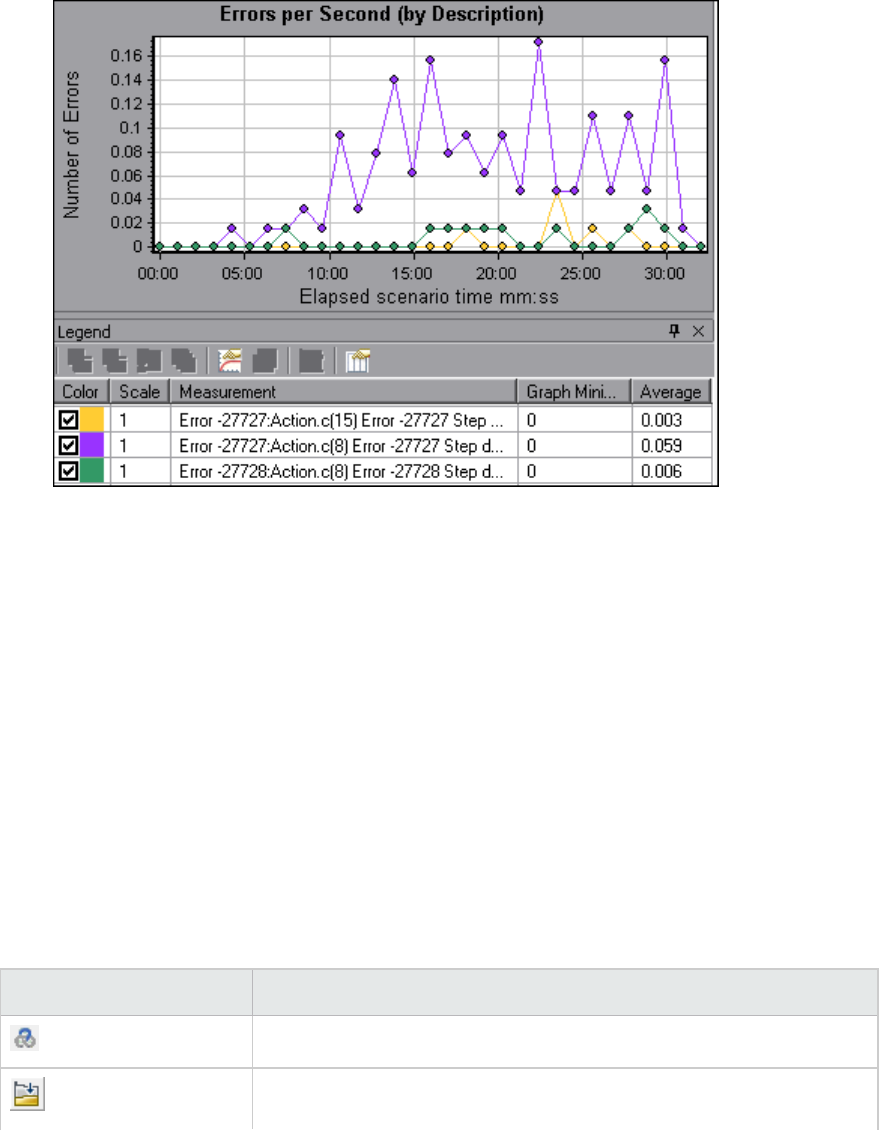
lEach graph has a legend which describes the metrics in the graph. You can also filter your data
and sort it by a specific field.
lAnalysis Graph Data and Raw Data Views. These views display the actual data used to generate the
graph in a spreadsheet format. You can copy this data into external spreadsheet applications for
further processing.
lAnalysis Reports. This utility enables you to generate a summary of each graph. The report
summarizes and displays the test's significant data in graphical and tabular format. You can
generate reports based on customizable report templates.
Analysis Toolbars
This section describes the buttons that you access from the main Analysis toolbars.
Common Toolbar
This toolbar is always accessible from the toolbar at top of the page and includes the following buttons:
User interface elements are described below:
UI Element Description
Create a new session.
Open an existing session.
User Guide
Analysis
HP LoadRunner (12.50) Page 21
UI Element Description
Generate a Cross Result graph.
Save a session.
Print item.
Create an HTML report.
View runtime settings.
Set global filter options.
Configure SLA rules
Analyze a transaction.
Undo the most recent action.
Reapply the last action that was undone.
Apply filter on summary page
Export Summary to Excel
Graph Toolbar
This toolbar is accessible from the top of the page when you have a graph open and includes the
following buttons
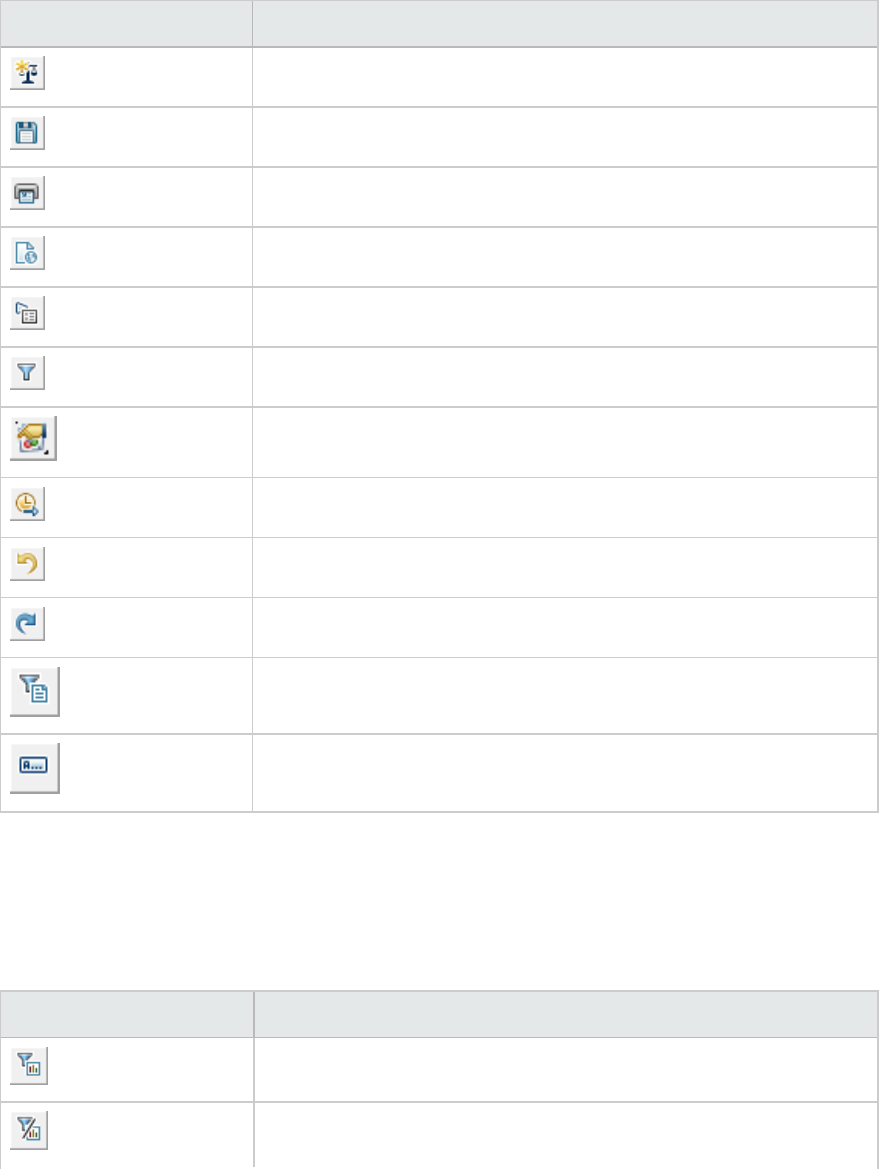
User interface elements are described below:
UI Element Description
Set filter settings.
Clear filter settings.
User Guide
Analysis
HP LoadRunner (12.50) Page 22
UI Element Description
Set granularity settings.
Merge graphs.
Configure auto correlation settings.
View raw data.
Add comments to a graph.
Add arrows to a graph.
Set display options.
Analysis API
The LoadRunner Analysis API enables you to write programs to perform some of the functions of the
Analysis user interface, and to extract data for use in external applications. Among other capabilities,
the API allows you to create an analysis session from test results, analyze raw results of an Analysis
session, and extract key session measurements for external use. You can also use the API to launch an
application from the LoadRunner Controller at the completion of a test.
To view this help from a LoadRunner machine, go to Start > All Programs > HP Software > HP
LoadRunner > Documentation > Analysis API Reference. In icon-based desktops, such as Windows 8,
search for API and select Analysis API Reference from the results.
Note: The Analysis API is only supported for 32-bit environments. If you use Visual Studio to
develop your script, make sure to define the platform as x86 in the project options.
Workflow
Click on one of the images below to learn more about the Analysis workflow.
User Guide
Analysis
HP LoadRunner (12.50) Page 23

What do you want to do?
lConfigure Analysis
lDefine a Service Level Agreement
lCreate graphs
lGenerate reports
See also:
lAnalysis Basics
lTroubleshooting Analysis
Analysis Basics
Creating Analysis Sessions
When you run a load test scenario, LoadRunner stores the runtime data in a result file with an .lrr
extension. LoadRunner Analysis is the utility that processes this data and generates graphs and
reports.
When you work with the LoadRunner Analysis, you work within an Analysis session. This session contains
one or more sets of scenario results (.lrr file). Analysis stores the display information and layout
settings for the active graphs in a file with an .lra extension.
Starting Analysis
You can open Analysis as an independent application or directly from the Controller. To open Analysis as
an independent application, choose one of the following:
lStart>All Programs > HP Software > HP LoadRunner > Analysis
lThe Analysis shortcut on the desktop
To open Analysis directly from the Controller, click the Analysis button on the toolbar or select
Results >Analyze Result. This option is only available after running a load test scenario. Analysis takes
the latest result file from the current scenario, and opens a new session using these results. You can
also instruct the Controller to automatically open Analysis after it completes scenario execution by
selecting Results>Auto Load Analysis.
Collating Execution Results
When you run a load test scenario, by default all Vuser information is stored locally on each Vuser host.
After scenario execution, the results from all of the hosts are automatically collated or consolidated in
the results folder.
User Guide
Analysis
HP LoadRunner (12.50) Page 24
You disable automatic collation by choosing Results >AutoCollate Results from the Controller window,
and clearing the check mark adjacent to the option. To manually collate results, choose Results >
Collate Results. If your results have not been collated, Analysis will automatically collate the results
before generating the analysis data.
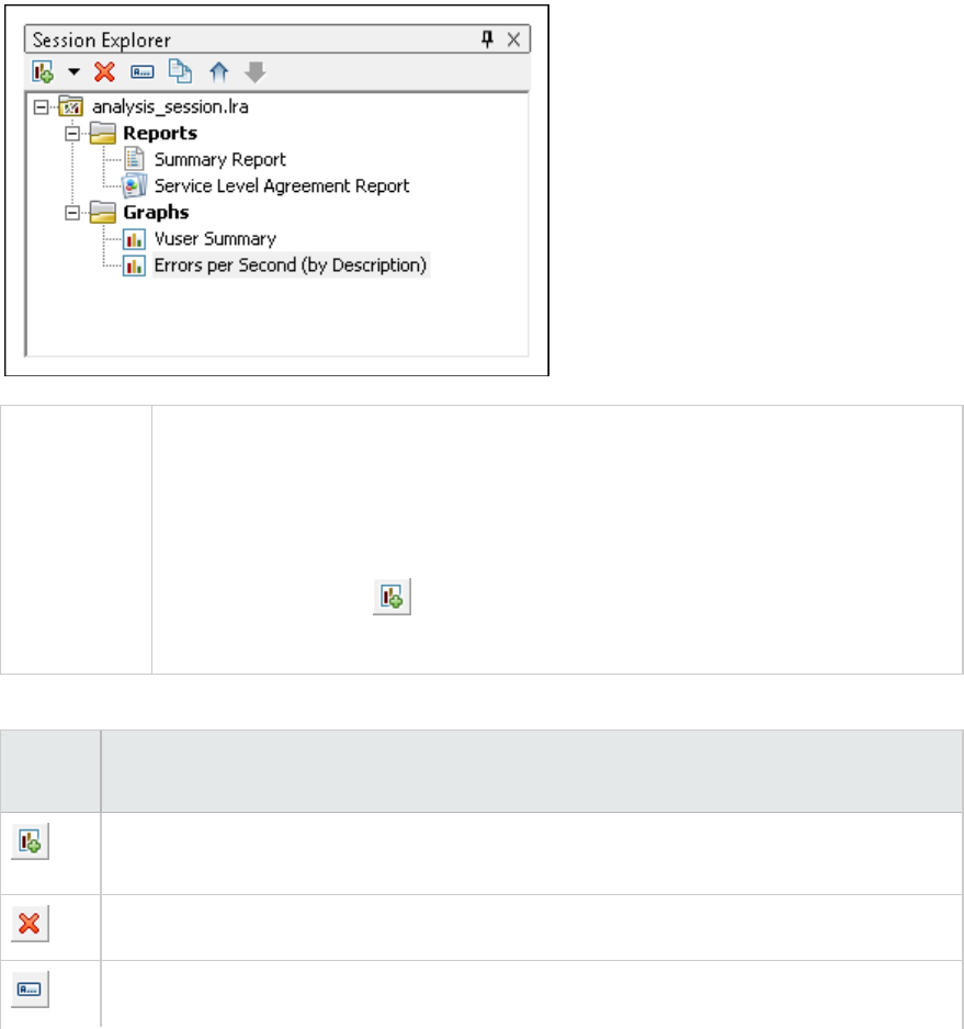
Session Explorer Window
This window displays a tree view of the items (graphs and reports) that are open in the current session.
When you click an item in the Session Explorer, it is activated in the main Analysis window.
To access Use one of the following:
lSession Explorer
lSession Explorer > Reports > Summary Report
lSession Explorer > Reports >Service Level Agreement Report
lSession Explorer > > Analyze Transaction
lSession Explorer > Graphs
User interface elements are described below:
UI
Element
Description
Add a new graph or report to the current Analysis session. Opens the Open a New Graph
dialog box. For details, see "Open a New Graph Dialog Box" on page125
Delete the selected graph or report.
Rename the selected graph or report.
User Guide
Analysis
HP LoadRunner (12.50) Page 25
UI
Element
Description
Create a copy of the selected graph.
Analysis Window Layouts
This section describes ways to customize the layout of the windows of the Analysis session.
Open Windows
You can open a window or restore a window that was closed by selecting the name of the relevant
window from the Windows menu.
Lock/Unlock the Layout of the Screen
Select Windows > Layout Locked to lock or unlock the layout of the screen.
Restore the Window Placement to the Default Layout
Select Windows > Restore Default Layout to restore the placement of the Analysis windows to their
default layout.
Note: This option is available only when no Analysis session is open.
Restore the Window Placement to the Classic Layout
Select Windows > Restore Classic Layout to restore the placement of the Analysis windows to their
classic layout. The classic layout resembles the layout of earlier versions of Analysis.
Note: This option is available only when no Analysis session is open.
Reposition and Dock Windows
You can reposition any window by dragging it to the desired position on the screen. You can dock a
window by dragging the window and using the arrows of the guide diamond to dock the window in the
desired position.
Note:
lOnly document windows (graphs or reports) can be docked in the center portion of the
screen.
User Guide
Analysis
HP LoadRunner (12.50) Page 26
lWindows > Layout Locked must not be selected when repositioning or docking windows.
Using Auto Hide
You can use the Auto Hide feature to minimize open windows that are not in use. The window is
minimized along the edges of the screen.
Click the Auto Hide button on the title bar of the window to enable or disable Auto Hide.
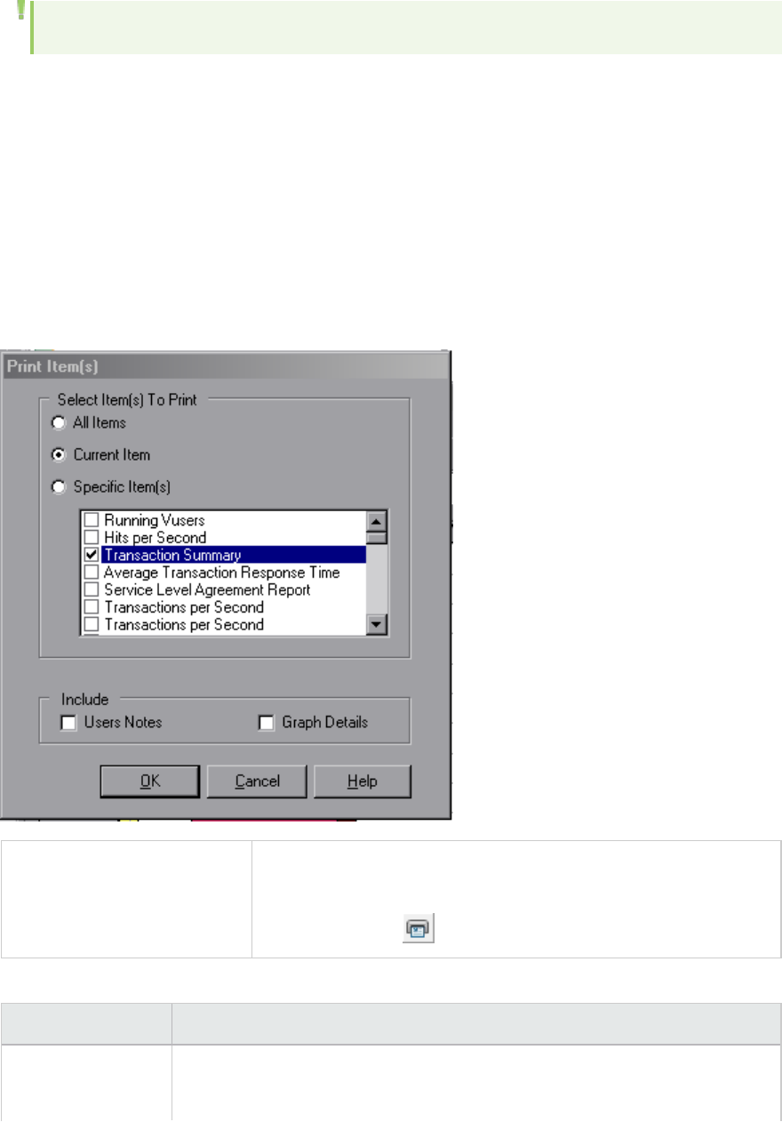
Printing Graphs or Reports
This dialog box enables you to print graphs or reports
To access Do one of the following:
lFile > Print
lMain toolbar >
User interface elements are described below:
UI Element Description
Select Items to
Print
lAll Items. Prints all graphs and reports in the current session.
lCurrent Item. Prints the graph or report currently selected in the Session
User Guide
Analysis
HP LoadRunner (12.50) Page 27

UI Element Description
Explorer.
lSpecific Item(s). Select the graphs or reports to print.
Include lUser Notes. Prints the notes in the User Notes window.
lGraph Details. Prints details such as graph filters and granularity settings.
Configuring Analysis
Summary Data Versus Complete Data
In large load test scenarios, with results exceeding 100 MB, it can take a long time for Analysis to
process the data. When you configure how Analysis generates result data from load test scenarios, you
can choose to generate complete data or summary data.
Complete data refers to the result data after it has been processed for use within Analysis.
Summary data refers to the raw, unprocessed data. The summary graphs contain general information
such as transaction names and times. Some fields are not available for filtering when you work with
summary graphs.
Note that some graphs will not be available when viewing only the summary data.
Importing Data Directly from the Analysis Machine
If you are using an SQL server / MSDE machine to store Analysis result data, you can configure Analysis
to import data directly from the Analysis machine.
Importing Data from the SQL Server
If you do not select the option to import data directly from the Analysis machine, Analysis creates CSV
files in a local temp folder. The CSV files are copied to a shared folder on the SQL Server machine. The
SQL server engine then imports the CSV files into the database. The following diagram illustrates the
data flow:
User Guide
Analysis
HP LoadRunner (12.50) Page 28
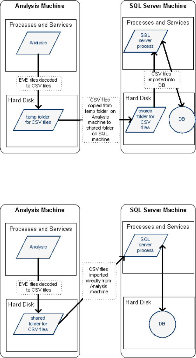
Importing Data from the Analysis Machine
If you selected the option to import data directly from the Analysis machine, Analysis creates the CSV
files in a shared folder on the Analysis machine and the SQL server imports these CSV files from the
Analysis machine directly into the database. The following diagram illustrates the data flow:
User Guide
Analysis
HP LoadRunner (12.50) Page 29
How to Configure Settings for Analyzing Load Test Results
The following steps describe how to configure certain Analysis settings that significantly impact the way
in which Analysis analyzes load test results.
Configure how Analysis processes result data
You define how Analysis processes result data from load test scenarios in the Tools > Options > Result
Collection tab. For example, you can configure how Analysis aggregates result data, to what extent the
data is processed, and whether output messages are copied from the Controller. For details on the user
interface, see "Result Collection Tab (Options Dialog Box)" on page33.
Configure template settings
For details on the user interface, see "Apply/Edit Template Dialog Box" on page84.
Configure analysis of transactions
You configure how transactions are analyzed and displayed in the summary report in the Summary
Report area of the Tools > Options > General tab. For details, see the description of "General Tab
(Options Dialog Box)" below.
General Tab (Options Dialog Box)
This tab enables you to configure general Analysis options, such as date formats, temporary storage
location, and transaction report settings.
User Guide
Analysis
HP LoadRunner (12.50) Page 30
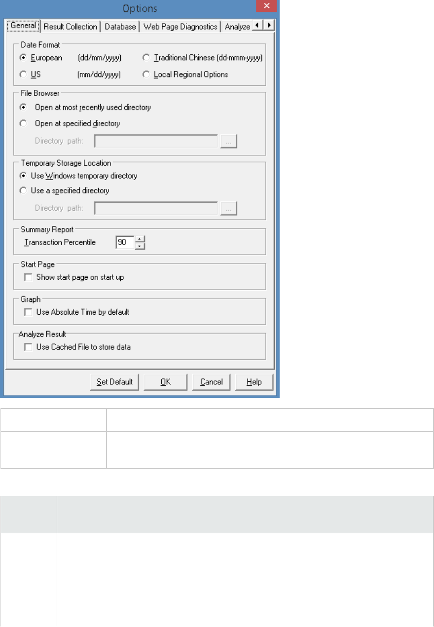
To access Tools > Options > General tab.
See Also "How to Configure Settings for Analyzing Load Test Results" on the previous
page
User interface elements are described below:
UI
Element
Description
Date
Format
Select a date format for storage and display. (For example, the date displayed in the
Summary report)
lEuropean. Displays the European date format.
lUS. Displays the U.S. date format.
lTraditional Chinese. Displays the Traditional Chinese date format.
User Guide
Analysis
HP LoadRunner (12.50) Page 31
UI
Element
Description
lLocal Regional Options. Displays the date format as defined in the current user's
regional settings.
Note: When you change the date format, it only affects newly created Analysis sessions.
The date format of existing sessions is not affected.
File
Browser
Select the directory location at which you want the file browser to open.
lOpen at most recently used directory. Opens the file browser at the previously used
directory location.
lOpen at specified directory. Opens the file browser at a specified directory.
In the Directory path box, enter the directory location where you want the file
browser to open.
Temporary
Storage
Location
Select the directory location in which you want to save temporary files.
lUse Windows temporary directory. Saves temporary files in your Windows temp
directory.
lUse a specified directory. Saves temporary files in a specified directory.
In the Directory path box, enter the directory location in which you want to save
temporary files.
Summary
Report
Set the following transaction settings in the Summary Report:
lTransaction Percentile. The Summary Report contains a percentile column showing
the response time of 90% of transactions (90% of transactions that fall within this
amount of time). To change the value of the default 90 percentile, enter a new figure
in the Transaction Percentile box.
The Transaction Percentile value is only applied to newly created templates . To create
a new template, select Tools >Templates. For details, see "Apply/Edit Template Dialog
Box" on page84.
Start Page Select Show start page on start up to display the Welcome to Analysis tab every time
you open the Analysis application.
Graph Select the way in which graphs shows the Elapsed Scenario Time on the x-axis.
Use Absolute time by default. Shows an elapsed time based on the absolute time of
the machine's system clock. If not checked, the graphs show the elapsed time relative
to the start of the scenario. The default is unchecked.
Analyze
Result
Use cached file to store data.Uses a cached file to store the analysis data.
This option should only be used when analyzing a large result file. Enabling this option
may increase the time required to analyze and open the results.
User Guide
Analysis
HP LoadRunner (12.50) Page 32
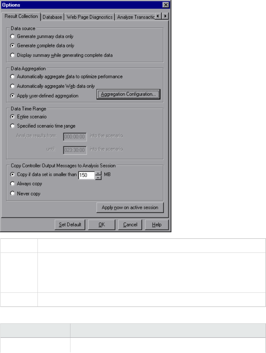
Result Collection Tab (Options Dialog Box)
This tab enables you to configure how Analysis processes result data from load test scenarios.
To access Tools > Options > Result Collection tab.
Important
information
The options in this tab are pre-defined with default settings. It is recommended to use
these default settings unless there is a specific need to change them. Changing some
of the settings, such as default aggregation, can significantly impact the amount of
data stored in the Analysis database.
See Also "How to Configure Settings for Analyzing Load Test Results" on page30
User interface elements are described below:
UI Element Description
Data Source In this area, you configure how Analysis generates result data from load
User Guide
Analysis
HP LoadRunner (12.50) Page 33
UI Element Description
test scenarios.
Complete data refers to the result data after it has been processed for
use within Analysis. Summary data refers to the raw, unprocessed data.
The summary graphs contain general information such as transaction
names and times. For more details on summary data versus complete
data, see "Summary Data Versus Complete Data" on page28.
Select one of the following options:
lGenerate summary data only. If this option is selected, Analysis will
not process the data for advanced use with filtering and grouping.
lGenerate complete data only. If this option is selected, the graphs can
then be sorted, filtered, and manipulated.
lDisplay summary data while generating complete data. Enables you
to view summary data while you wait for the complete data to be
processed.
Note: If you selected one of the options to generate complete
data, you can define how Analysis aggregates the complete data
in the Data Aggregation area.
Data Aggregation If you chose to generate complete data in the Data Source area, you use
this area to configure how Analysis aggregates the data.
Data aggregation is necessary in order to reduce the size of the database
and decrease processing time in large scenarios.
Select one of the following options:
lAutomatically aggregate data to optimize performance. Aggregates
data using built-in data aggregation formulas.
lAutomatically aggregate Web data only. Aggregates Web data only
using built-in data aggregation formulas.
lApply user-defined aggregation. Aggregates data using settings you
define.
Click the Aggregation Configuration button to open the Data
Aggregation Configuration Dialog Box and define your custom
aggregation settings. For details on the user interface, see "Data
Aggregation Configuration Dialog Box (Result Collection Tab)" on
page36.
Data Time Range In this area you specify whether to display data for the complete duration
of the scenario, or for a specified time range only. Select one of the
User Guide
Analysis
HP LoadRunner (12.50) Page 34
UI Element Description
following options:
lEntire scenario. Displays data for the complete duration of the load
test scenario
lSpecified scenario time range. Specify the time range using the
following boxes:
lAnalyze results from. Enter the amount of scenario time you want
to elapse (in hh:mm:ss format) before Analysis begins displaying
data.
luntil. Enter the point in the scenario (in hh:mm:ss format) at which
you want Analysis to stop displaying data.
Note:
lIt is not recommended to use the Specified scenario time
range option when analyzing the Oracle - Web and Siebel DB
Diagnostics graphs, since the data may be incomplete.
lThe Specified scenario time range settings are not applied to
the Connections and Running Vusers graphs.
Copy Controller Output
Messages to Analysis
Session
Controller output messages are displayed in Analysis in the Controller
Output Messages window. Select one of the following options for copying
output messages generated by the Controller to the Analysis session.
lCopy if data set is smaller than X MB. Copies the Controller output
data to the Analysis session if the data set is smaller than the amount
you specify.
lAlways Copy. Always copies the Controller output data to the Analysis
session.
lNever Copy. Never copies the Controller output data to the Analysis
session.
Click this button to apply the settings in the Result Collection tab to the
current session. The Controller output data is copied when the Analysis
session is saved.
User Guide
Analysis
HP LoadRunner (12.50) Page 35
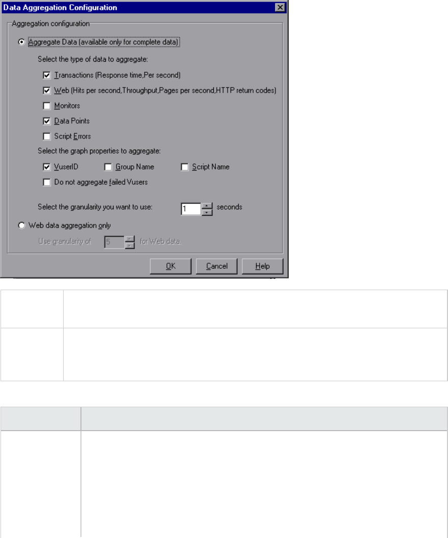
Data Aggregation Configuration Dialog Box (Result Collection
Tab)
If you choose to generate the complete data from the load lest scenario results, Analysis aggregates
the data using either built-in data aggregation formulas, or aggregation settings that you define. This
dialog box enables you to define custom aggregation settings.
To access Select Tools > Options > Result Collection. Select the Apply user-defined
aggregation option and click the Aggregation Configuration button.
Important
information
In this dialog box, you can select granularity settings. To reduce the size of the
database, increase the granularity. To focus on more detailed results, decrease the
granularity.
User interface elements are described below:
UI Element Description
Aggregate Data Select this option to define your custom aggregation settings using the following
criteria:
lSelect the type of data to aggregate. Use the check boxes to select the types
of graphs for which you want to aggregate data.
lSelect graph properties to aggregate. Use the check boxes to select the graph
properties you want to aggregate.
User Guide
Analysis
HP LoadRunner (12.50) Page 36
UI Element Description
To exclude data from failed Vusers, select Do not aggregate failed Vusers.
Note: You will not be able to drill down on the graph properties you select
in this list.
lSelect the granularity you want to use. Specify a custom granularity for the
data. The minimum granularity is 1 second.
Web data
aggregation
only
Select this option to aggregate Web data only. In the Use Granularity of X for
Web data box, specify a custom granularity for Web data.
The minimum granularity is 1 second. By default, Analysis summarizes Web
measurements every 5 seconds.
Database Tab (Options Dialog Box)
This tab enables you to specify the database in which to store Analysis session result data and to
configure the way in which CSV files will be imported into the database.
User Guide
Analysis
HP LoadRunner (12.50) Page 37
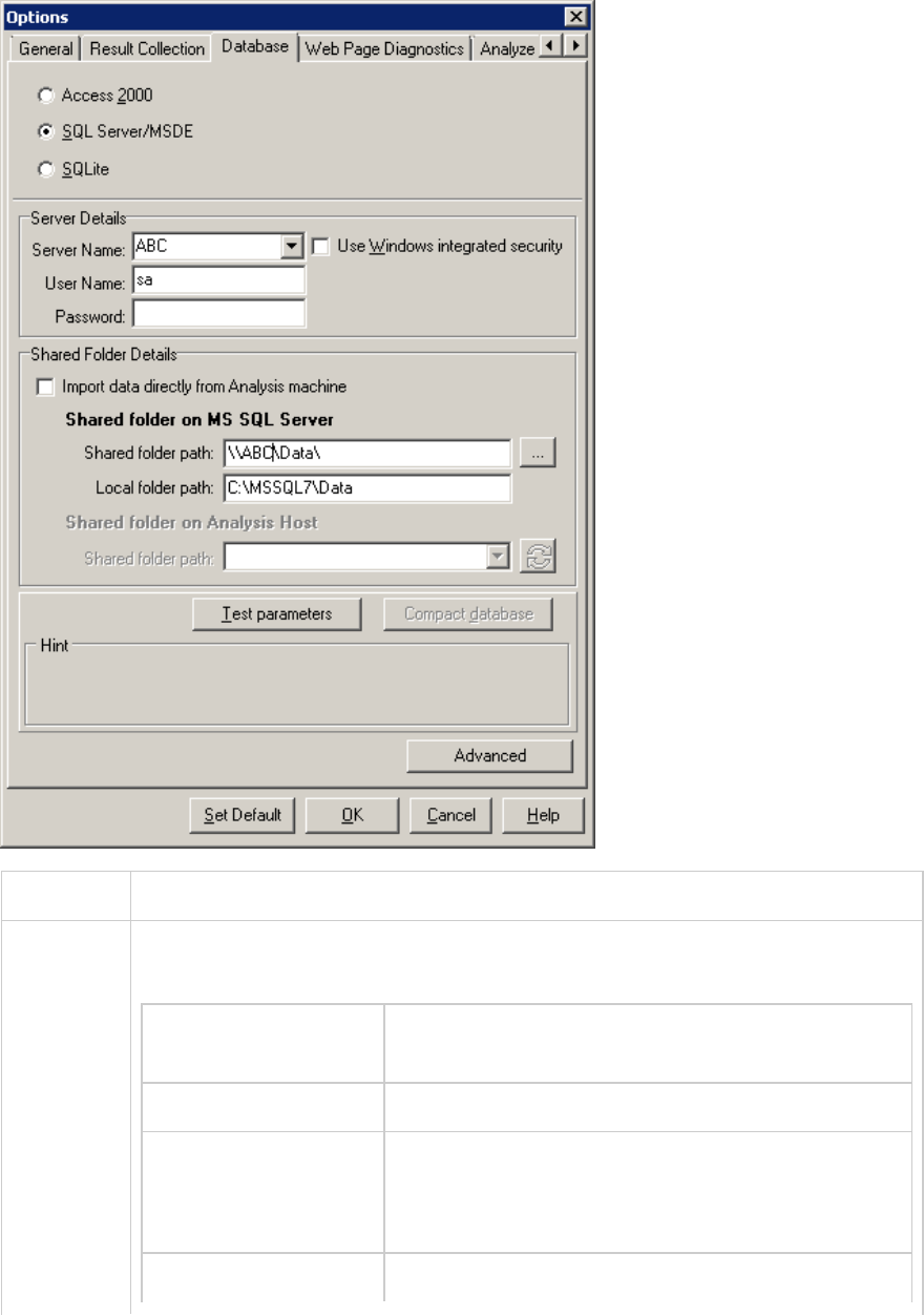
To access Analysis > Tools > Options > Database tab.
Important
information
Analysis data can be saved in one of three formats. Select the format based on the
size of the analysis session file, as shown in the table below:
Size of the Analysis
session file
Recommended format
lLess than 2 GB Access 2000
l2 GB to 10 GB SQLServer/MSDE
Select SQLServer/MSDE if you need to work in
multithread mode.
lMore than 10 GB SQLite
User Guide
Analysis
HP LoadRunner (12.50) Page 38
Note that the SQLite format allows you to store up to 32
terabytes of data.
Note: Both the Access 2000 database format and the SQLite format are
embedded databases. The session directory contains both the database and
the analysis data.
See also "Importing Data Directly from the Analysis Machine" on page28
User interface elements are described below:
UI Element Description
Access 2000 Instructs LoadRunner to save Analysis result data in an Access 2000 database
format. This setting is the default.
SQL Server/MSDE Instructs LoadRunner to save Analysis result data on an SQL server / MSDE
machine. If you select this option, you have to complete the Server Details
and Shared Folder Details, described below.
SQLite Instructs LoadRunner to save Analysis result data in an SQLite database
format.
If you choose this format, you will not be able to work in multithread mode.
Server Details area SQL server / MSDE machine details. See description below.
Shared Folder
Details area
SQL server / MSDE machine shared folder details. See description below.
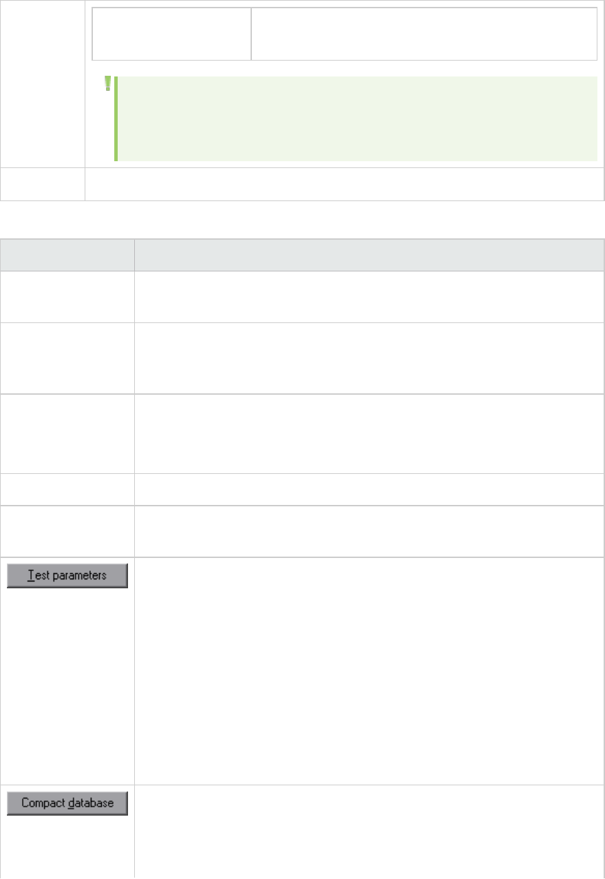
Depending on which database you are using, this button performs the
following action:
lFor Access. Checks the connection parameters to the Access database and
verifies that the delimiter on your machine's regional settings matches the
Microsoft JET delimiter on the database machine.
lFor SQL server / MSDE. Checks the connection parameters, the existence
of a shared server directory, whether there are write permissions on the
shared server directory, and whether the shared and physical server
directories are synchronized.
lFor SQLite. This button is disabled.
When you configure and set up your Analysis session, the database containing
the results may become fragmented. As a result, it will use excessive disk
space. For Access databases, the Compact database button enables you to
repair and compress your results and optimize your database. This button is
User Guide
Analysis
HP LoadRunner (12.50) Page 39
UI Element Description
disabled if you choose SQLite.
Note: Long load test scenarios (duration of two hours or more) will
require more time for compacting.
Opens the Advanced Options dialog box, allowing you to increase performance
when processing LoadRunner results or importing data from other
sources.This button is disabled if you choose SQLite. For user interface details
see "Advanced Options Dialog Box (Database Tab)" on the next page.
Server Details Area
If you choose to store Analysis result data on an SQL server / MSDE machine, you need to complete the
server details. User interface elements are described below:
UI Element Description
Server Name The name of the machine on which the SQL server / MSDE is running.
Use Windows
integrated
security
Enables you to use your Windows login, instead of specifying a user name and
password. By default, the user name "sa" and no password are used for the SQL
server.
User Name The user name for the master database.
Password The password for the master database.
Shared Folder Details Area
If you store Analysis result data on an SQL server / MSDE machine, you need to provide the shared folder
details. User interface elements are described below:
UI Element Description
Import Data
Directly
from
Analysis
machine
Select this option to import data directly from the Analysis machine. For details on this
option, see "Importing Data Directly from the Analysis Machine" on page28.
Shared
Folder on
MS SQL
lShared folder path. Enter a shared folder on the SQL server / MSDE machine. For
example, if your SQL server's name is fly, enter \\fly\<Analysis database
folder>\.
User Guide
Analysis
HP LoadRunner (12.50) Page 40
UI Element Description
Server This folder has different functions, depending on how you import the Analysis data:
lIf you did not select the option to import data directly from the Analysis
machine, this folder stores permanent and temporary database files. Analysis
results stored on an SQL server / MSDE machine can only be viewed on the
machine's local LAN.
lIf you selected the option to import data directly from the Analysis machine,
this folder is used to store an empty database template copied from the Analysis
machine.
lLocal folder path. Enter the real drive and folder path on the SQL server / MSDE
machine that correspond to the above shared folder path. For example, if the
Analysis database is mapped to an SQL server named fly, and fly is mapped to
drive D, enter D:\<Analysis database folder>.
If the SQL server / MSDE and Analysis are on the same machine, the logical storage
location and physical storage location are identical.
Shared
Folder on
Analysis
Host
If you selected the option to import data directly from the Analysis machine, the
Shared folder path box is enabled. Analysis detects all shared folders on your Analysis
machine and displays them in a drop-down list. Select a shared folder from the list.
Note:
lEnsure that the user running the SQL server (by default, SYSTEM) has
access rights to this shared folder.
lIf you add a new shared folder on your machine, you can click the refresh
button to display the updated list of shared folders.
lAnalysis creates the CSV files in this folder and the SQL server imports
these CSV files from the Analysis machine directly into the database. This
folder stores permanent and temporary database files.
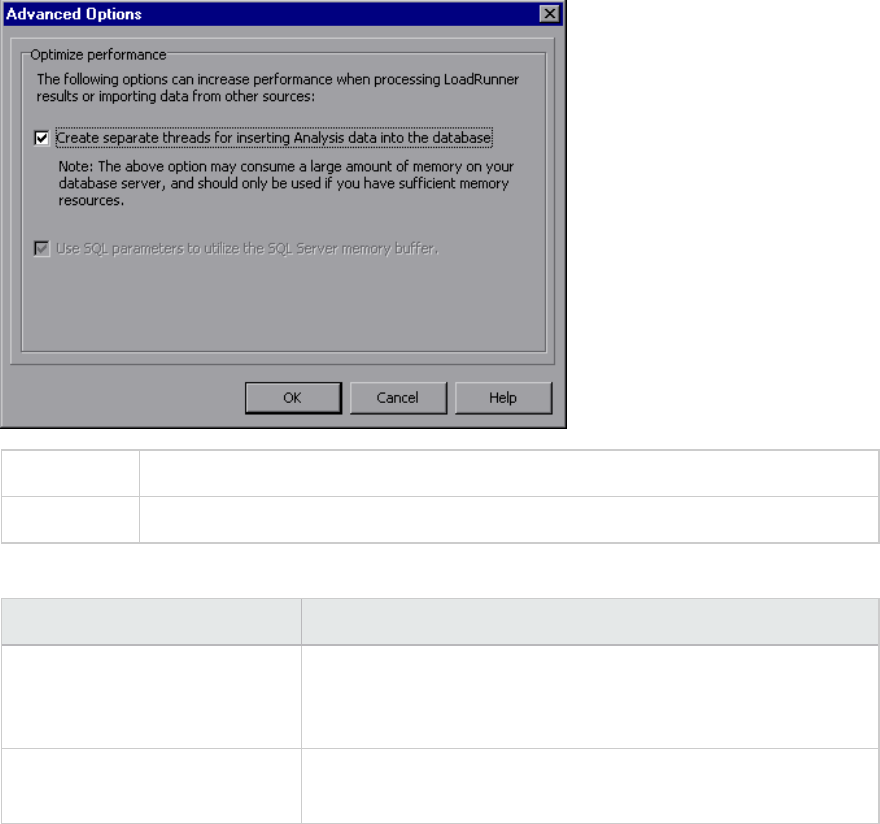
Advanced Options Dialog Box (Database Tab)
This dialog box enables you to increase performance when processing LoadRunner results or importing
data from other sources.
User Guide
Analysis
HP LoadRunner (12.50) Page 41
To access Analysis > Tools > Options > Database tab > Advanced button
See also "Database Tab (Options Dialog Box)" on page37
User interface elements are described below:
UI Element Description
Create separate threads for
inserting Analysis data into the
database.
This option may consume a large amount of memory on your
database server, and should only be used if you have sufficient
memory resources.
Use SQL parameters to utilize
the SQL Server memory buffer.
This option is only enabled when you store Analysis result data on
an SQL server or MSDE machine.
Web Page Diagnostics Tab (Options Dialog Box)
This tab enables you to set Web page breakdown options. You can choose how to aggregate the display
of URLs that include dynamic information, such as a session ID. You can display these URLs individually,
or you can unify them and display them as one line with merged data points.
User Guide
Analysis
HP LoadRunner (12.50) Page 42
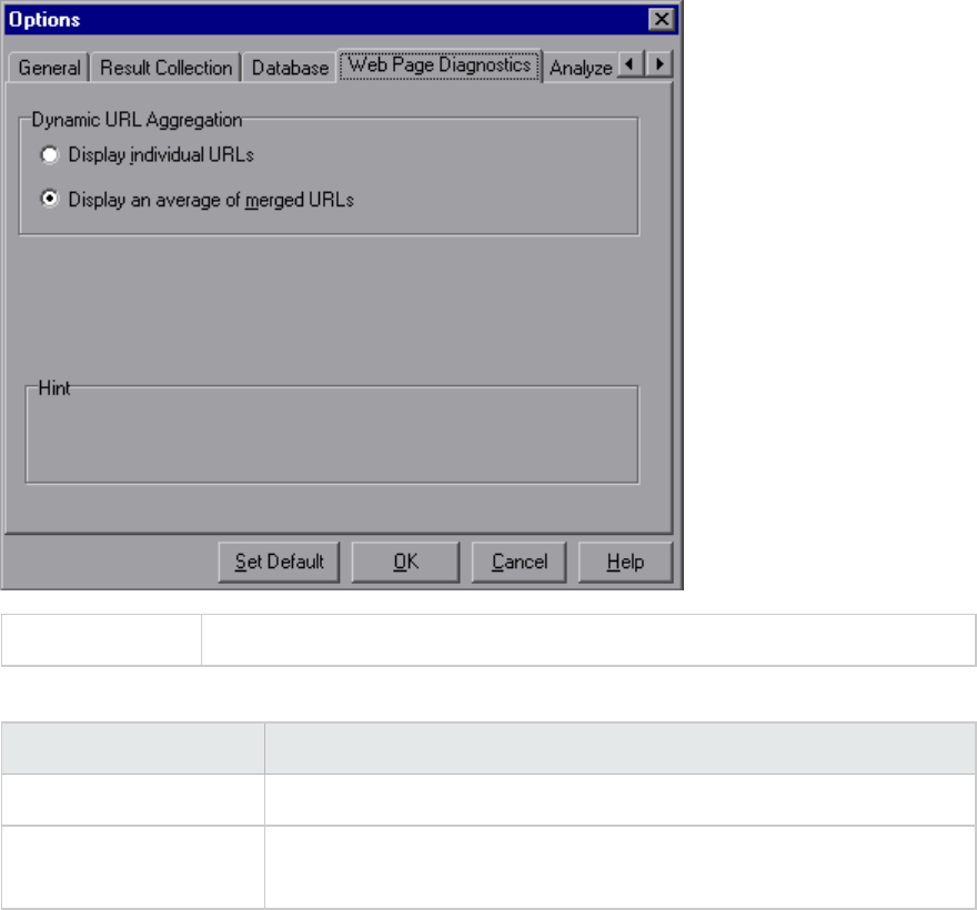
To access Tools > Options > Web Page Diagnostics tab
User interface elements are described below:
UI Element Description
Display individual URLs Displays each URL individually
Display an average of
merged URLs
Merges URLs from the same script step into one URL, and displays it with
merged (average) data points.
Session Information Dialog Box (Options Dialog Box)
This dialog box enables you to view a summary of the configuration properties of the current Analysis
session.
User Guide
Analysis
HP LoadRunner (12.50) Page 43
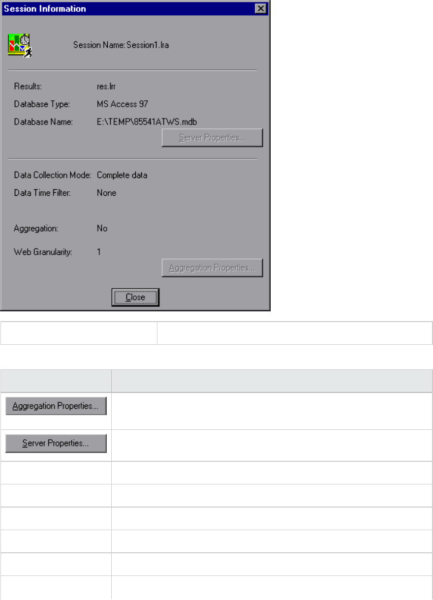
To access File > Session Information
User interface elements are described below:
UI Element Description
Displays the type of data aggregated, the criteria according to which it is
aggregated, and the time granularity of the aggregated data.
Displays the properties of the SQL server and MSDE databases.
Aggregation Indicates whether the session data has been aggregated.
Data Collection Mode Indicates whether the session displays complete data or summary data.
Data Time Filter Indicates whether a time filter has been applied to the session.
Database Name Displays the name and directory path of the database.
Database Type Displays the type of database used to store the load test scenario data.
Results Displays the name of the LoadRunner result file.
User Guide
Analysis
HP LoadRunner (12.50) Page 44
UI Element Description
Session Name Displays the name of the current session.
Web Granularity Displays the Web granularity used in the session.
Viewing Load Test Scenario Information
Viewing Load Test Scenario Information
In Analysis, you can view information about the load test scenario which you are analyzing. You can view
the scenario runtime settings and output messages that were generated by the Controller during the
scenario.
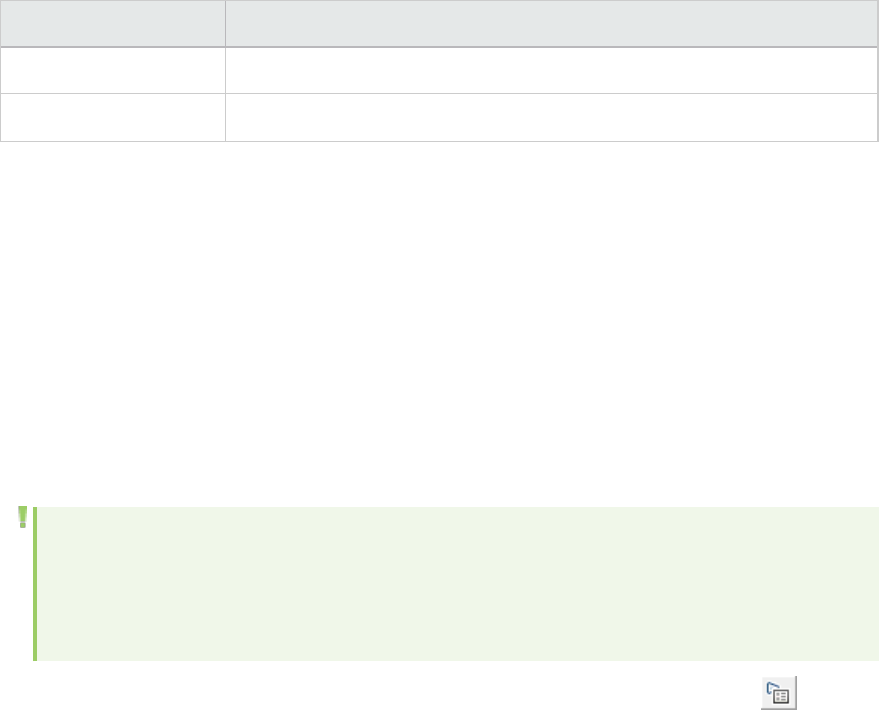
You can view information about the Vuser groups and scripts that were run in each scenario, as well as
the runtime settings for each script in a scenario, in the Scenario runtime settings dialog box.
Note: The runtime settings allow you to customize the way a Vuser script is executed. You
configure the runtime settings from the Controller or Virtual User Generator (VuGen) before
running a scenario. For information on configuring the runtime settings, refer to the online help
in those products.
Select File > View Scenario Runtime Settings, or click the View runtime settings button on the
toolbar.
The Scenario runtime settings dialog box opens, displaying the Vuser groups, scripts, and scheduling
information for each scenario. For each script in a scenario, you can view the runtime settings that were
configured in the Controller or VuGen before scenario execution.
User Guide
Analysis
HP LoadRunner (12.50) Page 45
How to Configure Controller Output Messages Settings
This task describes how to configure settings for output messages.
1. Choose Tools > Options and select the Result Collection tab.
2. In the Copy Controller Output Messages to Analysis Session area, choose one of the following
options:
lCopy if data set is smaller than X MB. Copies the Controller output data to the Analysis session
if the data set is smaller than the amount you specify.
lAlways Copy. Always copies the Controller output data to the Analysis session.
lNever Copy. Never copies the Controller output data to the Analysis session.
3. Apply your settings.
User Guide
Analysis
HP LoadRunner (12.50) Page 46
lTo apply these settings to the current session, click Apply now to active session.
lTo apply these settings after the current session is saved, click OK.
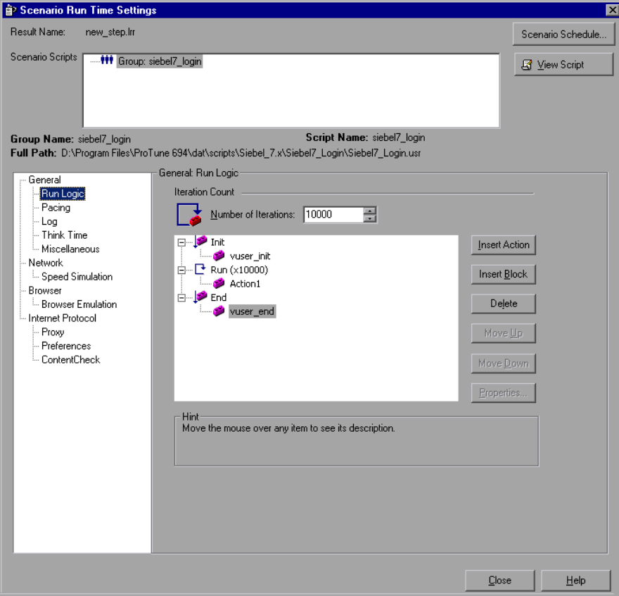
Controller Output Messages Window
This window displays error, notification, warning, debug, and batch messages that are sent to the
Controller by the Vusers and load generators during a scenario run.
To access Windows > Controller Output Messages
Important
information
lThe Summary tab is displayed by default when you open this window.
lAnalysis searches for the output data in the current Analysis session. If the data is
not found, it searches in the scenario results folder. If Analysis cannot locate the
results folder, no messages are displayed.
User interface elements are described below:
UI Element Description
Summary Tab See "Summary Tab" below
Filtered Tab See "Filtered Tab" on page49
Summary Tab
This tab displays summary information about the messages sent during a scenario run.
To access Controller Output Messages window > Summary tab
Important Information You can drill down further on any information displayed in blue.
Parent topic "Controller Output Messages Window" above
See also "Filtered Tab" on page49
User interface elements are described below:
User Guide
Analysis
HP LoadRunner (12.50) Page 47
UI Element Description
Displays the full text of the selected output message in the Detailed Message Text
area at the bottom of the Output window.
Remove all messages. Clears all log information from the Output window.
Export the view. Saves the output to a specified file.
lFreeze. Stops updating the Output window with messages.
lResume. Resumes updating the Output window with messages. The newly
updated log information is displayed in a red frame.
Detailed
Message Text
Displays the full text of the selected output message when you click the Details
button.
Generators Displays the number of load generators that generated messages with the specified
message code.
Help Displays an icon if there is a link to troubleshooting for the message.
Message
Code
Displays the code assigned to all similar messages. The number in parentheses
indicates the number of different codes displayed in the Output window.
Sample
Message Text
Displays an example of the text of a message with the specified code.
Scripts Displays the number of scripts whose execution generated messages with the
specified code.
Total
Messages
Displays the total number of sent messages with the specified code.
Type The type of message being displayed. The following icons indicate the various
message types. For more information about each type, see Type of Message below:
lBatch
lDebug
lErrors
lNotifications
lWarnings
User Guide
Analysis
HP LoadRunner (12.50) Page 48
UI Element Description
lAlerts
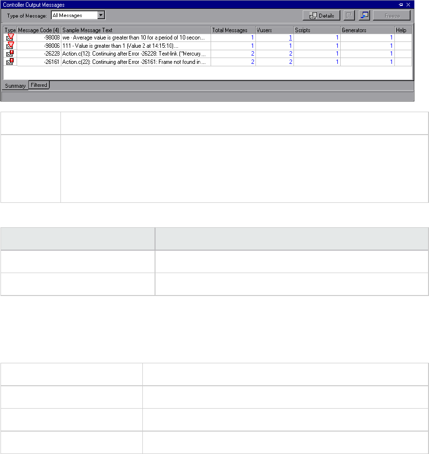
Type of
Message
Filters the output messages to display only certain message types. Select one of the
following filters:
lAll messages. Displays all message types.
lBatch. Sent instead of message boxes appearing in the Controller, if you are using
automation.
lDebug. Sent only if the debugging feature is enabled in the Controller. (Expert
mode: Tools > Options > Debug Information). For more information, see "Options
> Debug Information Tab" on page242.
lErrors. Usually indicate that the script failed.
lNotifications. Provides runtime information, such as message sent using lr_
output_message.
lWarnings. Indicates that the Vuser encountered a problem, but the scenario
continued to run.
lAlerts. Indicates a warning.
Vusers Displays the number of Vusers that generated messages with the specified code.
Filtered Tab
This tab displays a drilled down view by message, Vuser, script, or load generator. For example, if you
drill down on the Vuser column, the Filtered tab displays all the messages with the code you selected,
grouped by the Vusers that sent the messages.
To access Controller Output Messages window > Summary tab. Click the blue link on the
column that you wish to view more information about.
Important
information
The tab appears when you click on a blue link in the Summary tab.
See also "Summary Tab" on page47
User interface elements are described below (unlabeled elements are shown in angle brackets):
UI Element Description
Previous/Next View. Enables you to move between the various drill down levels.
Displays the full text of the selected output message in the Detailed Message Text
area at the bottom of the Output window.
User Guide
Analysis
HP LoadRunner (12.50) Page 49
UI Element Description
Export the view. Saves the output to a specified file.
Refreshes the Filtered tab with new log information that arrived in the Output
window updated in the Summary tab.
<Message
icon>
Displays an icon indicating the type of message by which the current Output view is
filtered.
Active Filter Displays the category or categories by which the current Output view is filtered.
Viewed By Displays the name of the column on which you selected to drill down. The following
icons indicate the various message types:
lBatch
lDebug
lErrors
lNotifications
lWarnings
lAlerts
Detailed
Message
Text
Displays the full text of the selected output message when the Details button is
selected.
Message Displays all instances of the sample message text.
Script The script on which the message was generated. If you click the blue link, VuGen
opens displaying the script.
Action The action in the script where the message was generated. If you click the blue link,
VuGen opens the script to the relevant action.
Line # The line in the script where the message was generated. If you click the blue link,
VuGen opens the script and highlights the relevant line.
# Lines The total number of lines in the script where the Vuser failed.
Time The time the message was generated.
Iteration The iteration during which the message was generated.
User Guide
Analysis
HP LoadRunner (12.50) Page 50
UI Element Description
Vuser The Vuser that generated the message.
Generator The load generator on which the message was generated. If you click the blue link,
the Load Generator dialog box opens.
# Messages The number of messages generated by a specific Vuser.
Scenario Runtime Settings Dialog Box
This dialog box enables you to view information about executed load test scenarios, as well as the
runtime settings for each script in a scenario.
To access Toolbar >
See also "Viewing Load Test Scenario Information" on page45
User interface elements are described below
UI Element Description
Result
Name
The name of the result file.
Scenario
Scripts
Displays the result set for each executed scenario, as well as the Vuser groups and
scripts that were run in the scenario.
Group Name Displays the name of the group to which the selected script belongs.
Full Path Displays the script's full directory path.
Script Name Displays the name of the selected script.
Scenario
Schedule
Displays goal-oriented or manual scenario scheduling information for the selected
scenario.
View Script Opens the Virtual User Generator, so that you can edit the script.
Defining Service Level Agreements
Service Level Agreements Overview
Service level agreements (SLAs) are specific goals that you define for your load test scenario. After a
scenario run, HP LoadRunner Analysis compares these goals against performance related data that was
gathered and stored during the course of the run, and determines whether the SLA passed or failed.
User Guide
Analysis
HP LoadRunner (12.50) Page 51
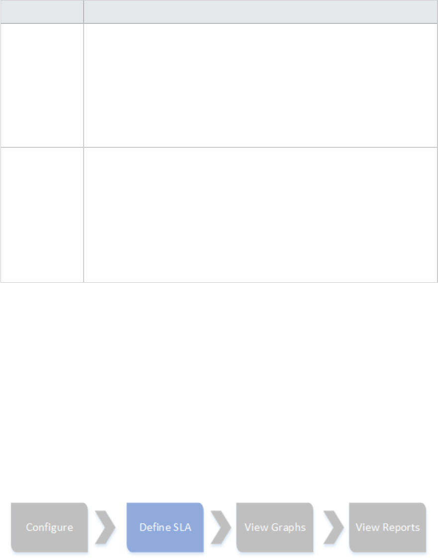
Depending on the measurements that you are evaluating for your goal, LoadRunner determines the SLA
status in one of the following ways:
SLA Type Description
SLA status
determined at
time intervals
over a timeline
Analysis displays SLA statuses at set time intervals over a timeline within the run.
At each time interval in the timeline—for example, every 10 seconds—Analysis
checks to see if the measurement's performance deviated from the threshold
defined in the SLA.
Measurements that can be evaluated in this way:
lTransaction Response Time (Average) per time interval
lErrors per Second per time interval
SLA status
determined over
the whole run
Analysis displays a single SLA status for the whole scenario run.
Measurements that can be evaluated in this way:
lTransaction Response Time (Percentile) per run
lTotal Hits per run
lAverage Hits (hits/second) per run
lTotal Throughput (bytes) per run
lAverage Throughput (bytes/second) per run
You can define and edit SLAs in the Controller or in Analysis.
Tracking Period
When you define service level agreements (SLAs)an SLA for measurements that are evaluated over a
timeline, Analysis determines SLA statuses at specified time intervals within that timeline. The
frequency of the time intervals is called the tracking period.
An internally-calculated tracking period is defined by default. You can change the tracking period by
entering a value in the Advanced Options dialog box which Analysis plugs into a built-in algorithm to
calculate the tracking period. For details, see "Advanced Options Dialog Box (Service Level Agreement
Pane)" on page57.
How to Define Service Level Agreements
This task describes how to define service level agreements (SLAs).
User Guide
Analysis
HP LoadRunner (12.50) Page 52

You can define service level agreements (SLAs) which measure scenario goals over time intervals, or
over a whole scenario run. For details, see "Service Level Agreements Overview" on page51.
Tip: For a use-case scenario related to this task, see "How to Define Service Level Agreements -
Use-Case Scenario" on the next page.
1. Prerequisites
If you are defining an SLA for Average Transaction Response Time, your scenario must include a
script that contains at least one transaction.
2. Run through the SLA wizard
In the Service Level Agreement pane, click New to open the Service Level Agreement wizard. For
user interface details, see "Service Level Agreement Wizard" on page58.
a. Select a measurement for the SLA.
b. If you are defining an SLA for Average Transaction Response Time or Transaction Response
Time (Percentile), select the transactions to include in your goal.
c. (Optional) When evaluating SLA statuses over a timeline, select load criteria to take into
account and define appropriate load value ranges for the load criteria. For an example, see
"How to Define Service Level Agreements - Use-Case Scenario" on the next page.
d. Set thresholds for the measurements.
oIf the Average Transaction Response Time or Errors per Second exceed the defined
thresholds, Analysis will produce a Failed SLA status.
oIf Transaction Response Time(Percentile),Total Hits per run,Average Hits (hits/second)
per run,Total Throughput (bytes) per run, or Average Throughput (bytes/second) per run
are lower than the defined threshold, Analysis will produce a Failed SLA status.
3. Define a tracking period - optional
For measurements whose SLA statuses are determined over time intervals, you need to define the
frequency of the time intervals, that is, the tracking period. For details, see "Tracking Period" on
the previous page.
For user interface details, see "Advanced Options Dialog Box (Service Level Agreement Pane)" on
page57.
4. Results
When analyzing your scenario run, HP LoadRunner Analysis compares the data collected from the
scenario run against the SLA settings, and determines SLA statuses which are included in the
default Summary Report.
User Guide
Analysis
HP LoadRunner (12.50) Page 53
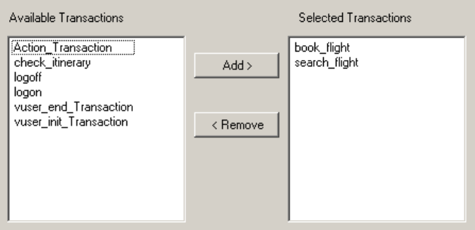
How to Define Service Level Agreements - Use-Case Scenario
This use-case scenario describes how to define a service level agreement (SLA) for Average Transaction
Response Time.
1. Background
The administrator of HP Web Tours would like to know when the average transaction response
time for booking a flight and searching for a flight exceeds a certain value. Assume that your
scenario includes a script that includes the following transactions: book_flight and search_flight.
2. Start the SLA wizard
In the Service Level Agreement pane, click New to open the Service Level Agreement wizard.
3. Select the measurement for the SLA
On the Select a Measurement page, under Select a Measurement for Your Goal, in the
Transaction Response Time box, select Average.
4. Select the transactions to evaluate in your goal
On the Select a Transaction page, select the transactions to be evaluated: book_flight and search_
flight.
5. Select a load criterion and define appropriate ranges of load- optional
On the Select Load Criteria page, select the load criterion to take into account when evaluating the
average transaction response time.
In this case, to see the effect that various quantities of Vusers running on the system has on the
average transaction response time of each transaction, in the Load Criteria box, select Running
Vusers.
Then set the value ranges for the running Vusers:
User Guide
Analysis
HP LoadRunner (12.50) Page 54
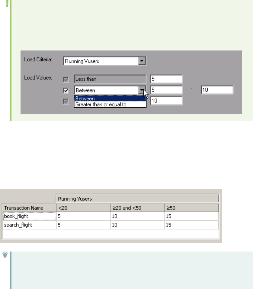
Consider less than 20 Vusers to be a light load, 20 – 50 Vusers an average load, and 50 Vusers or
more a heavy load. Enter these values in the Load Values boxes.
Note:
lYou can set up to three in-between ranges.
lValid load value ranges are consecutive—there are no gaps in the range—and span all
values from zero to infinity.
6. Set thresholds
On the Set Threshold Values page, you define the acceptable average transaction response times
for the transactions, taking into account the defined load criteria.
In this case, define the same threshold values for both transactions as follows: for a light load, a
reasonable average response time can be up to 5 seconds, for an average load, up to 10 seconds,
and for a heavy load, up to 15 seconds.
Tip: To define the same thresholds for all the transactions, you can type the values in the
table nearer the bottom of the Set Threshold Values page, and click Apply to all
transactions.
7. Define a tracking period - optional
When SLA statuses for a measurement are determined at time intervals over a timeline, the
frequency of the time intervals is determined by the tracking period.
This step is optional because an internally-calculated tracking period of at least 5 seconds is
defined by default. You can change the tracking period in the Advanced Options dialog box:
User Guide
Analysis
HP LoadRunner (12.50) Page 55
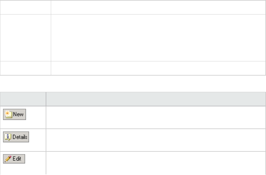
a. In the Service Level Agreement pane, click the Advanced button.
b. Select Tracking period of at least X seconds, and select a tracking period. The time intervals
are calculated by Analysis according to a built-in algorithm and as a function of the value you
enter here.
Example:
If you select a tracking period of 10, and the aggregation granularity for the scenario (defined
in Analysis) is 6, then the tracking period is set to the nearest multiple of 6 that is greater than
or equal to 10, that is, Tracking Period = 12.
For details, see "Tracking Period" on page52.
For user interface details, see "Advanced Options Dialog Box (Service Level Agreement Pane)"
on the next page.
8. Results
When analyzing your scenario run, Analysis applies your SLA settings to the default Summary
Report and the report is updated to include all the relevant SLA information.
For example, it displays the worst performing transactions in terms of defined SLAs, how specific
transactions performed over set time intervals, and overall SLA statuses.
Service Level Agreement Pane
This pane lists all the service level agreements (SLAs) defined for the scenario.
To access Tools menu > Configure SLA Rules >Service Level Agreement pane
Relevant Tasks lHow to Design a Goal-Oriented Scenario
lHow to Design a Manual Scenario
l"How to Define Service Level Agreements" on page52
l"How to Define Service Level Agreements - Use-Case Scenario" on page54
See also "Service Level Agreements Overview" on page51
User interface elements are described below:
UI Element Description
Starts the Service Level Agreement wizard where you can define new goals for the
load test scenario.
Opens the Goal Details dialog box which displays a summary of the details of the
selected SLA.
Opens the Service Level Agreement wizard where you can modify the goals defined
in the SLA.
User Guide
Analysis
HP LoadRunner (12.50) Page 56
UI Element Description
Deletes the selected SLA.
Opens the Advanced Options dialog box where you can adjust the tracking period
for measurements that are evaluated per time interval over a timeline.
For more information, see "Tracking Period" on page52.
For user interface details, see "Advanced Options Dialog Box (Service Level
Agreement Pane)" below.
Service Level
Agreement list
Lists the SLAs defined for the scenario.
Advanced Options Dialog Box (Service Level Agreement Pane)
This dialog box enables you to define a tracking period for load test scenario.
To access Tools menu > Configure SLA Rules >Service Level Agreement pane >
Important
information
The tracking period is calculated by Analysis according to a built-in algorithm and as
a function of the value entered here.
Relevant tasks l"How to Define Service Level Agreements" on page52
l"How to Define Service Level Agreements - Use-Case Scenario" on page54
See also "Service Level Agreements Overview" on page51
User interface elements are described below:
UI Element Description
Internally
calculated
tracking
period
Analysis sets the tracking period to the minimum value possible, taking into account
the aggregation granularity defined for the scenario. This value is at least 5 seconds.
It uses the following formula:
Tracking Period = Max (5 seconds, aggregation granularity)
Tracking
period of at
least X
seconds
Determines the minimum amount of time for the tracking period. This value can
never be less than 5 seconds.
Analysis sets the tracking period to the nearest multiple of the scenario's
aggregation granularity that is greater than or equal to the value (X) that you
selected.
For this option, Analysis uses the following formula:
Tracking Period =
User Guide
Analysis
HP LoadRunner (12.50) Page 57
UI Element Description
Max(5 seconds, m(Aggregation Granularity))
where mis a multiple of the scenario's aggregation granularity such that m
(Aggregation Granularity) is greater than or equal to X.
Example: If you select a tracking period of X=10, and the aggregation granularity for
the scenario is 6, then the tracking period is set to the nearest multiple of 6 that is
greater than or equal to 10, that is, Tracking Period = 12.
Goal Details Dialog Box (Service Level Agreement Pane)
This dialog box displays the thresholds that were set for the selected SLA.
To access Tools menu > Configure SLA Rules >Service Level Agreement pane >
Important
information
If you defined load criteria as part of your SLA, the threshold values are displayed
per the defined load value ranges.
See also "Service Level Agreements Overview" on page51
Service Level Agreement Wizard
This wizard enables you to define goals or service level agreements (SLAs) for your load test scenario.
To access Tools menu > Configure SLA Rules >Service Level Agreement pane >
Important
information
There are two modes for the Service Level Agreement wizard. The pages
included in the wizard depend on the measurement that is selected. See the
wizard maps below.
Relevant tasks l"How to Define Service Level Agreements" on page52
l"How to Define Service Level Agreements - Use-Case Scenario" on page54
Wizard map - Goal
measured per time
interval
The Service Level Agreement Wizard contains:
Welcome >"Select a Measurement Page" on the next page > ("Select
Transactions Page" on page60) > "Set Load Criteria Page" on page60 >"Set
Threshold Values Page (Goal Per Time Interval)" on page62
Wizard map - Goal
measured over
whole scenario run
The Service Level Agreement Wizard contains:
Welcome >"Select a Measurement Page" on the next page > ("Select
Transactions Page" on page60) > "Set Threshold Values Page (Goal Per Whole
User Guide
Analysis
HP LoadRunner (12.50) Page 58
Run)" on page63
See also "Service Level Agreements Overview" on page51
Select a Measurement Page
This wizard page enables you to select a measurement for your goal.
Important
information
lGeneral information about this wizard is available here: "Service Level
Agreement Wizard" on the previous page.
lThere are two modes for the Service Level Agreement wizard. The wizard
pages that follow depend on the measurement that you select on this
page. See the wizard maps below.
Wizard map - Goal
measured per time
interval
The "Service Level Agreement Wizard" on the previous page contains:
Welcome >Select a Measurement Page > ("Select Transactions Page" on the
next page) > "Set Load Criteria Page" on the next page >"Set Threshold
Values Page (Goal Per Time Interval)" on page62
Wizard map - Goal
measured over
whole scenario run
The "Service Level Agreement Wizard" on the previous page contains:
Welcome >Select a Measurement Page > ("Select Transactions Page" on the
next page) > "Set Threshold Values Page (Goal Per Whole Run)" on page63
See also "Service Level Agreements Overview" on page51
User interface elements are described below:
UI Element Description
SLA status determined over
the whole run
Evaluates a single SLA status for the whole scenario run. Select one of
the following measurements:
lTransaction Response Time (Percentile)
lTotal Hits per run
lAverage Hits (hits/second) per run
lTotal Throughput (bytes) per run
lAverage Throughput (bytes/second) per run
SLA status determined per
time intervals over a
timeline
Evaluates SLA statuses at set time intervals within the run. Select one
of the following measurements:
lAverage Transaction Response Time
lErrors per Second
The time intervals at which the SLA statuses are evaluated are known
as the tracking period. For details, see "Tracking Period" on page52.
User Guide
Analysis
HP LoadRunner (12.50) Page 59
Select Transactions Page
This wizard page enables you to select transactions to evaluate as part of your goal.
Important
information
lGeneral information about this wizard is available here: "Service Level
Agreement Wizard" on page58.
lThis page is displayed when creating an SLA for Transaction Response Time
by Average or by Percentile.
lIn order to define an SLA for Transaction Response Time by Average or by
Percentile, at least one of the Vuser scripts participating in the scenario
must include a transaction.
lYou can select multiple transactions using the CTRL key.
Wizard map - Goal
measured per
time interval
The "Service Level Agreement Wizard" on page58 contains:
Welcome >"Select a Measurement Page" on the previous page > (Select
Transactions Page) > "Set Load Criteria Page" below >"Set Threshold Values
Page (Goal Per Time Interval)" on page62
See also "Service Level Agreements Overview" on page51
User interface elements are described below:
UI Element Description
Available
Transactions
Lists the transactions in the Vuser scripts participating in the scenario.
To move a script to the Selected Transaction list, select it and click Add.
Selected
Transactions
Lists the transactions in the Vuser scripts participating in the scenario that have
been selected for the SLA.
To remove a script from this list, select it and click Remove.
Set Load Criteria Page
This wizard page enables you to select load criteria to take into account when testing your goal.
Important
information
lGeneral information about this wizard is available here: "Service Level
Agreement Wizard" on page58.
lThis page is displayed only when defining an SLA that determines SLA statuses
per time interval over a timeline.
lIn the next wizard step (Set Threshold Values page), you will set different
thresholds per each of the load ranges that you select here.
User Guide
Analysis
HP LoadRunner (12.50) Page 60

Wizard map -
Goal measured
per time interval
The "Service Level Agreement Wizard" on page58 contains:
Welcome >"Select a Measurement Page" on page59 > ("Select Transactions
Page" on the previous page) > Set Load Criteria Page >"Set Threshold Values
Page (Goal Per Time Interval)" on the next page
See also "Service Level Agreements Overview" on page51
User interface elements are described below:
UI Element Description
Load Criteria The relevant load criteria that you want to use
Example: If you want to see the impact of running Vusers on the measurement,
select Running Vusers.
To define an SLA without load criteria, select None.
Load Values Valid load value ranges are consecutive—there are no gaps in the range—and span
all values from zero to infinity.
lLess than. Enter the upper value for the lower range of values for the load
criteria.
The lower range is between 0 and the value you entered. It does not include the
upper value.
Example: If you enter 5, the lower range of values for the load criteria is between 0
and 5, but does not include 5.
lBetween. The in-between range of values for the load criteria. Enter lower and
upper values for this range. The lower range is included in this range; it does not
include the upper value.
Example: If you enter 5 and 10, the in-between range of values for the load criteria
is from 5 and up to, but not including, 10.
Note: You can set up to three in-between ranges.
lGreater than. Enter the lower value for the upper range of values for the load
criteria.
The upper range includes values from the value you entered and on.
Example: If you enter 10, the upper range of values for the load criteria is from 10
and on.
Selected
Measurement
The measurement selected for the goal.
User Guide
Analysis
HP LoadRunner (12.50) Page 61
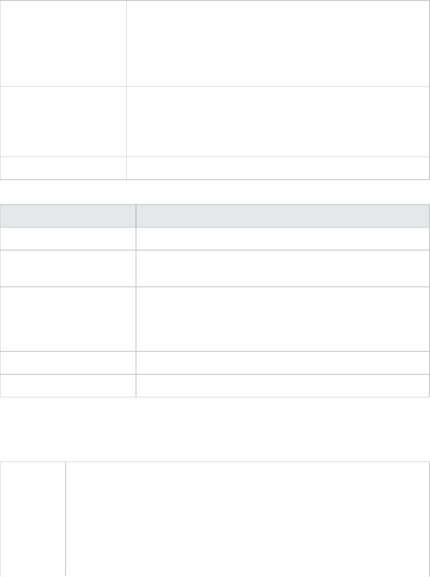
Set Percentile Threshold Values Page
This wizard page enables you to select load criteria to take into account when testing your goal.
Important information lGeneral information about this wizard is available here: "Service
Level Agreement Wizard" on page58.
lThe Percentile SLA enables you to measure whether the percentage
of transaction samples meets the defined threshold criteria.
lYou can enter a threshold value to 3 decimal places.
Wizard map - Goal
measured over whole
scenario run
The "Service Level Agreement Wizard" on page58 contains:
Welcome >"Select a Measurement Page" on page59 > ("Select
Transactions Page" on page60) > Set Percentile Threshold Values
Page
See also "Service Level Agreements Overview" on page51
User interface elements are described below:
UI Element Description
Selected Measurement The measurement selected for the goal.
Percentile Percentage of transactions to measure against the configured
threshold.
Provide threshold value for
all transactions
To apply one set of threshold values to all transactions selected for
the goal, enter the threshold value and click Apply to all. These
values are applied to all the transactions in the Thresholds table at
the bottom of the page.
Transaction name The transaction from the scenario run.
Threshold The threshold value for the selected transaction.
Set Threshold Values Page (Goal Per Time Interval)
This wizard page enables you to set thresholds for the measurements you are evaluating in your goal.
Important
information
lGeneral information about this wizard is available here: "Service Level Agreement
Wizard" on page58.
lIf you defined load criteria in the "Set Load Criteria Page" on page60, you must set
thresholds per each of the defined load ranges. If you did not define load criteria,
you set one threshold value. For Average Transaction response time, you set
threshold values for each transaction.
lYou can enter a threshold value to 3 decimal places.
User Guide
Analysis
HP LoadRunner (12.50) Page 62
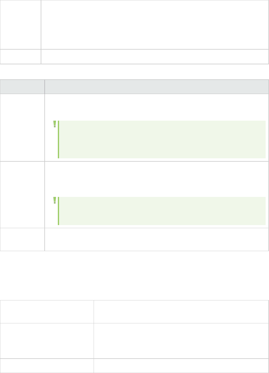
Wizard map
- Goal
measured
per time
interval
The "Service Level Agreement Wizard" on page58 contains:
Welcome >"Select a Measurement Page" on page59 > ("Select Transactions Page"
on page60) > "Set Load Criteria Page" on page60 >Set Threshold Values Page (Goal
Per Time Interval)
See also "Service Level Agreements Overview" on page51
User interface elements are described below (unlabeled elements are shown in angle brackets):
UI Element Description
<Thresholds
table>
The thresholds for your goal. If you defined load criteria, enter thresholds for each
range of values.
Note: If the maximum threshold value is exceeded during a particular time
interval during the run, Analysis displays an SLA status of Failed for that
time interval.
Apply to all
(Average
Transaction
Response
Time goal
only)
To apply one set of threshold values to all transactions selected for the goal, enter
the threshold values in this table and click Apply to all transactions. These values
are applied to all the transactions in the Thresholds table at the top of the page.
Note: Threshold values for selected transactions do not have to be the
same. You can assign different values for each transaction.
Selected
Measurement
The measurement selected for the goal.
Set Threshold Values Page (Goal Per Whole Run)
This wizard page enables you to set minimum thresholds for the measurements you are evaluating in
your goal.
Important information General information about this wizard is available here: "Service
Level Agreement Wizard" on page58.
Wizard map - Goal measured
over whole scenario run
The "Service Level Agreement Wizard" on page58 contains:
Welcome >"Select a Measurement Page" on page59 >Set
Threshold Values Page (Goal Per Whole Run)
See also "Service Level Agreements Overview" on page51
User interface elements are described below:
User Guide
Analysis
HP LoadRunner (12.50) Page 63
UI Element Description
Selected
measurement
The measurement selected for the goal.
Threshold The minimum threshold value for the selected measurement.
Note: If the value of the measurement is lower than this threshold during
the run, Analysis displays an SLA status of Failed for the entire run.
Working with Application Lifecycle Management
Managing Results Using ALM - Overview
Analysis works together with HP Application Lifecycle Management (ALM). ALM provides an efficient
method for storing and retrieving scenario and analysis results. You can store results in an ALM project
and organize them into unique groups.
In order for the Analysis to access an ALM project, you must connect it to the Web server on which ALM
is installed. You can connect to either a local or remote Web server.
When working against an ALM server with Performance Center, the ALM integration has several
additional capabilities, such as the ability to save the Analysis session to a new location, and upload a
report from the file system to ALM. For details, see "How to Work with Results in ALM - With
Performance Center" on page66.
For more information on working with ALM, see the Application Lifecycle Management User Guide.
How to Connect to ALM from Analysis
To store and retrieve Analysis results from ALM, you need to connect to an ALM project. You can connect
or disconnect from an ALM project at any time during the testing process.
You can connect to one version of HP ALM from Analysis and a different version from your browser. For
more information, see the Important Information section in "HP ALM Connection Dialog Box" on
page69.
Connect to ALM
1. Select Tools >HP ALM Connection. The HP ALM Connection dialog box opens.
2. Enter the required information in the HP ALM Connection dialog box, as described in "HP ALM
Connection Dialog Box" on page69.
3. To disconnect from ALM, click Disconnect.
User Guide
Analysis
HP LoadRunner (12.50) Page 64
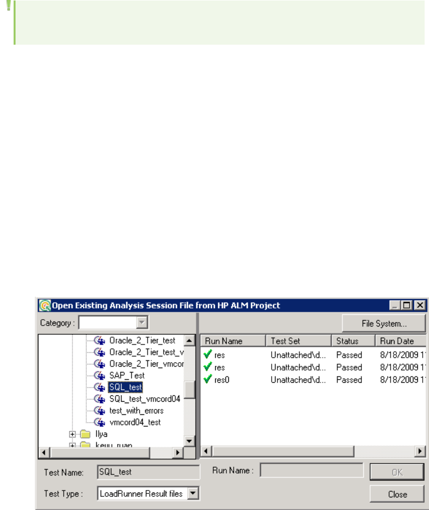
Note: There is no explicit option in the Analysis user interface for enabling CAC mode (as in
VuGen). Analysis automatically enables CAC mode if the ALM server machine supports it. .
How to Work with Results in ALM - Without Performance Center
The following steps describe the workflow for working with results saved in an ALM project, whose
server does not have a Performance Center installation.
When working against an ALM server with HP Performance Center, there are several differences. For
more information, see "How to Work with Results in ALM - With Performance Center" on the next page.
1. Connect to ALM
Open a connection to the ALM server and project that contains the LoadRunner result or Analysis
session files. For task details, see "How to Connect to ALM from Analysis" on the previous page.
2. Open an existing Analysis session file - optional
a. Select File > Open.
b. In the left pane select a script.
c. In the right pane, select the results for which the Analysis session file was created.
d. Click OK.
3. Create a new Analysis session file from the raw data - optional
This procedure describes how to create a new Analysis session file on the ALM server, from the raw
results file. If an Analysis session file already exists for the raw data, you can choose to overwrite
the existing file.
User Guide
Analysis
HP LoadRunner (12.50) Page 65
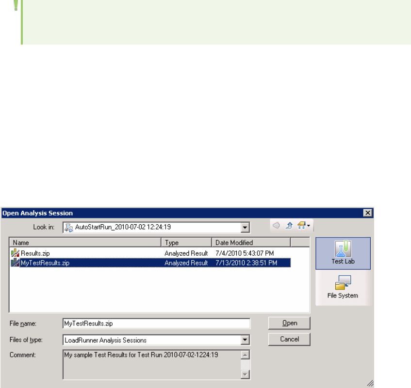
a. Select File > New.
b. In the left pane select a script.
c. In the right pane, select the results you want to analyze.
d. Click OK.
4. Save the LoadRunner results file
When you are finished analyzing your results and creating reports or graphs, save the changes.
Select File > Save. The Analysis session file is in the ALM project.
Note: When working with ALM without Performance Center, Save As is not supported—you
cannot save the Analysis session file to another location.
How to Work with Results in ALM - With Performance Center
ALM servers with Performance Center, allow you to perform the following operations:
Open an existing Analysis Session file
1. Select Tools > HP ALM Connection and make sure your connection to ALM is open.
2. Select File > Open.
3. Drill down to the Run level within the Test Plan module, and select an individual run.
4. Select a zip file containing the Analysis session file.
5. Click Open.
Open raw data and create a new Analysis session
1. Select Tools > HP ALM Connection and make sure your connection to ALM is open.
User Guide
Analysis
HP LoadRunner (12.50) Page 66
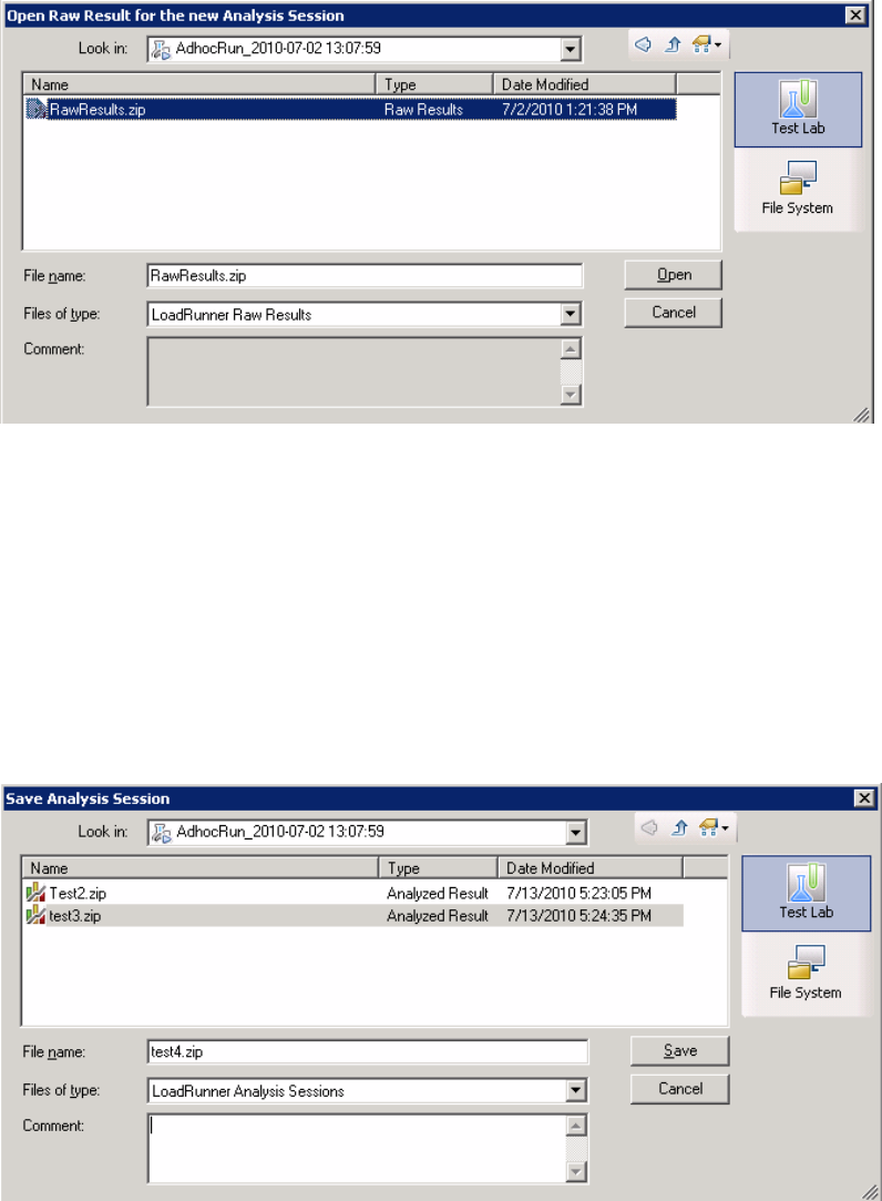
2. To create a new Analysis session file from the raw data, select File > New.
3. Drill down to the Run level within the Test Plan module, and select an individual run.
4. Select a zip file containing the run's raw data.
5. Click Open.
Save the changes to the Analysis session file
1. Complete your changes to the Analysis results.
2. Select Tools > HP ALM Connection and make sure your connection to ALM is open.
3. Select File > Save.
4. To save an Analysis session that was opened from the file system, click the Test Lab module
button.
5. Drill down to the Run level within the Test Plan module, and specify a name for the zip file.
6. Provide a comment about the Analysis session (optional).
User Guide
Analysis
HP LoadRunner (12.50) Page 67
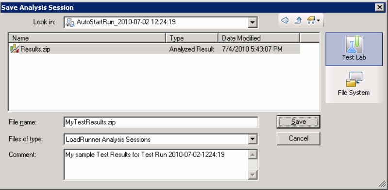
7. Click Save.
Save the Analysis session file to a new ALM location
1. Select Tools > HP ALM Connection and make sure your connection to ALM is open.
2. Open an Analysis session file from the file system, or from ALM as described above.
3. Select File > Save as.
4. Drill down to the Run level within the Test Plan module, and select an individual run.
5. Specify a name for the Analysis session zip file. The name Results is reserved.
6. Provide a comment about the Analysis session (optional).
7. Click Save.
Integration Methods - TestPlan or TestLab
Analysis uses different integration methods for ALM projects with Performance Center extensions,
depending on how it was invoked:
lThrough the Web-interface or from the Controller—TestPlan integration is used.
lThrough a manual launch, connected to a project through the HP ALM Connection dialog box—
TestLab integration is used.
How to Upload a Report to ALM
The following steps describe how to upload a report from the file system to an ALM's Test Lab module.
This capability is only available for ALM installation with Performance Center.
When working against an ALM server with HP Performance Center, there are several differences. For
more information, see "How to Work with Results in ALM - With Performance Center" on page66.
User Guide
Analysis
HP LoadRunner (12.50) Page 68
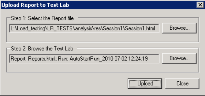
1. Connect to ALM
Open a connection to the ALM server and project that contains the LoadRunner result or Analysis
session files. For task details, see "How to Connect to ALM from Analysis" on page64.
2. Open the Upload dialog box
Select Tools > Upload Report to Test Lab.
3. Select a report
Click Browse in the Step 1 section.The Select the Report file dialog box opens. Select an HTML or
XML file from the file system. Click Open.
4. Select a location on ALM
Click Browse in the Step 2 section.The Select Location for the Report dialog box opens. Navigate
to a Run level in the Test Lab module. Specify a name for the report and include any relevant
comments. Click OK.
5. Begin the upload
Click Upload. The upload begins.
HP ALM Connection Dialog Box
This dialog box enables you to connect to an ALM project.
User Guide
Analysis
HP LoadRunner (12.50) Page 69
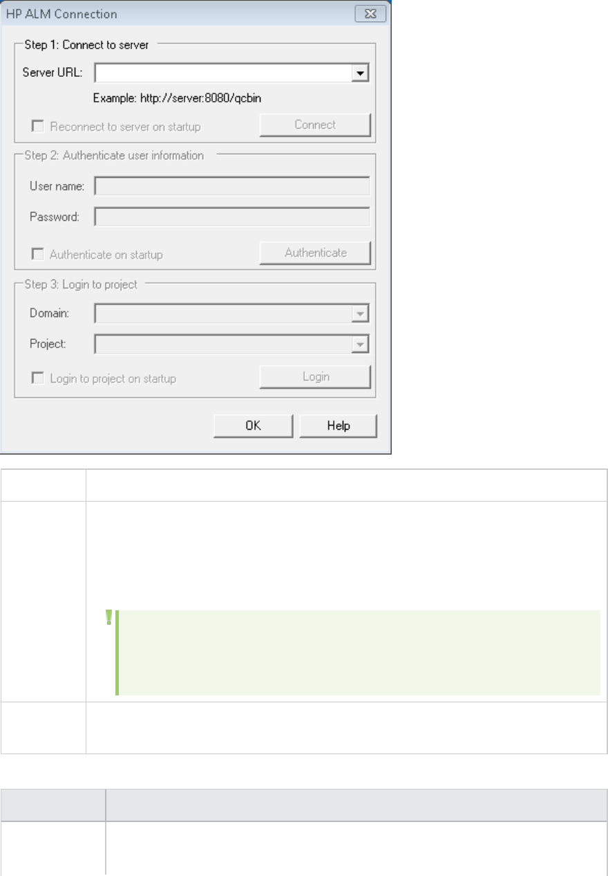
To access Tools > HP ALM Connection
Important
information
You can connect to one version of HP ALM from LoadRunner and a different version of
HP ALM from your browser.
You can only connect to different versions of HP ALM if one of the versions is HP ALM
11.00 or higher.
Note: Before you connect to ALM through the LoadRunner interface, it is
recommended that you first connect to the HPALMserver through your
browser.This automatically downloads the ALMclient files to your computer.
Relevant
tasks
"How to Connect to ALM from Analysis" on page64
User interface elements are described below:
UI Element Description
Step 1:
Connect to
lServer URL. The URL of the server on which ALM is installed. The URL must be in
the following form http://<server_name:port>/qcbin.
User Guide
Analysis
HP LoadRunner (12.50) Page 70
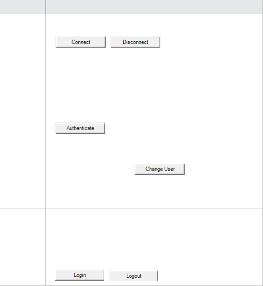
UI Element Description
Server lReconnect to server on startup. Automatically reconnect to the server every
time you start LoadRunner.
l/ . Connects to the server specified in
the Server URL box. Only one button is visible at a time, depending on your
connection status.
Step 2:
Authenticate
User
Information
lUser Name. Your ALM project user name.
lPassword. Your ALM project password.
lAuthenticate on startup. Authenticates your user information automatically,
the next time you open the application. This option is available only if you
selected Reconnect to server on startup above.
l. Authenticates your user information against the ALM
server.
After your user information has been authenticated, the fields in the
Authenticate user information area are displayed in read-only format. The
Authenticate button changes to .
You can log in to the same ALM server using a different user name by clicking
Change User, entering a new user name and password, and then clicking
Authenticate again.
Step 3: Login
to Project
lDomain. The domain that contains the ALM project. Only those domains
containing projects to which you have permission to connect to are displayed.
lProject. Enter the ALM project name or select a project from the list. Only those
projects that you have permission to connect to are displayed.
lLogin to project on startup. This option is only enabled when the Authenticate
on startup check box is selected.
l/ . Logs into and out of the ALM project.
Upload Report to Test Lab Dialog Box
This dialog box enables you to upload an Analysis report to an ALM project's Test Lab module.
User Guide
Analysis
HP LoadRunner (12.50) Page 71
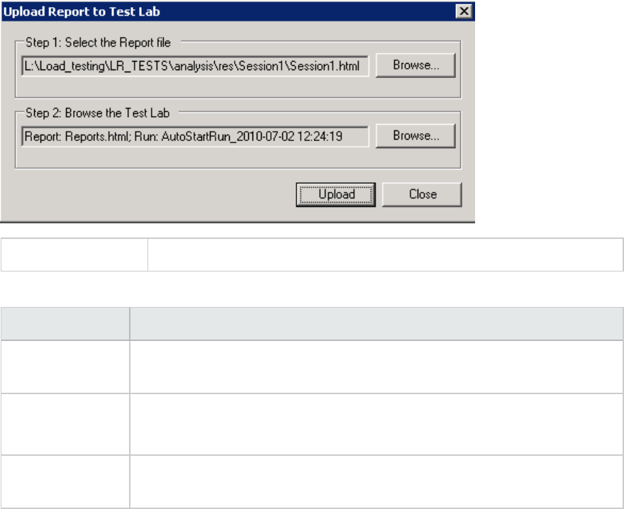
To access Reports > Upload Report to Test Lab
User interface elements are described below:
UI Element Description
Step 1: Select the
report file
Allows you to select an Analysis report from the file system. You can select an
HTML report, or Rich report in XML format.
Step 2: Browse
the test lab
Allows you to select an location within the Test Lab module, for the report.
Note: You must drill down to the level of a Run within the Test Lab module.
Upload Begins the uploading of the report. If the uploading succeeds, the Analysis
issues a message.
Setup
Configuring Graph Display
Analysis allows you to customize the display of the graphs and measurements in your session so that
you can view the data displayed in the most effective way possible.
How to Customize the Analysis Display
The following steps describes how to customize the display of analysis. You can customize the display of
the graphs and measurements in your session so that you can view the data displayed in the most
effective way possible.
User Guide
Analysis
HP LoadRunner (12.50) Page 72
Enlarging a section of the graph
To zoom in or enlarge a section of the graph, move and hold down the left mouse button over the
section of the graph you want to enlarge.
Using comments in a graph
To add a comment to a graph, click and then click the mouse over the section of the graph where
you would like to add a comment. Type your comment in the Add Comment dialog box.
To edit, format or delete a comment from the graph, click the comment and apply your change in the
Edit Comments dialog box. In the left pane, verify the relevant comment is selected before you edit,
format or delete.
Using arrows in a graph
To add an arrow to a graph, click and then click the mouse button within the graph to position the
base of the arrow.
To delete an arrow from a graph, select the arrow and press Delete.
Using the User Notes Window
In the User Notes window (Windows > User Notes), you can enter text about the graph or report that is
currently open. The text in the User Notes window is saved with the session.
To view the text that you entered for a specific graph or report, select the relevant graph or report and
open the User Notes window (Windows > User Notes).
Display Options Dialog Box
This dialog box enables you to select the graph type and configure the display of the graph.
Note: This option is not available for all graph types.
User Guide
Analysis
HP LoadRunner (12.50) Page 73
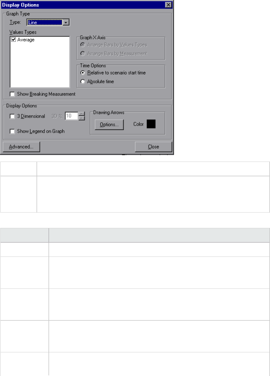
To access View > Display Options
See also l"Editing Main Chart Dialog Box (Display Options Dialog Box)" on the next page
l"Chart Tab (Editing MainChart Dialog Box)" on page76
l"Series Tab (Editing MainChart Dialog Box)" on page77
User interface elements are described below:
UI Elements Description
Type Select the type of graph to display from the drop-down list.
Values Types Select the type of display information from the list of available values. For
example, a bar graph displaying Average Transaction Response Time can be
configured to display minimum, maximum, average, STD, count, and sum averages.
Graph X Axis
(Bar graphs
only)
Select the bar arrangement along the x-axis. You can arrange the bars by value
types or measurement.
Time Options Select the way in which the graph shows the Elapsed Scenario Time on the x-axis.
You can choose an elapsed time relative to the beginning of the scenario or an
elapsed time from the absolute time of the machine's system clock.
Show Breaking
Measurement
Select this check box to display the name and properties of the breaking
measurement at the top of the graph (disabled by default).
User Guide
Analysis
HP LoadRunner (12.50) Page 74
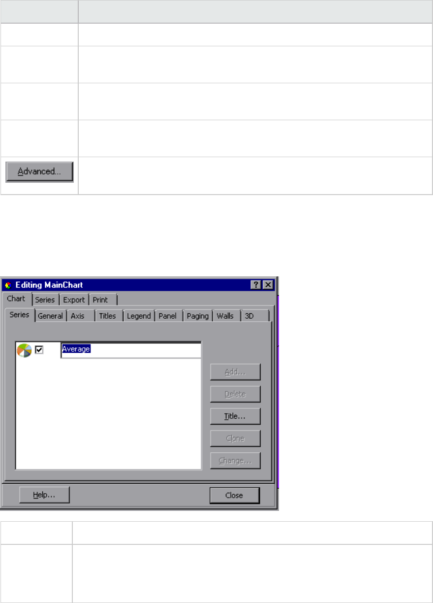
UI Elements Description
3 Dimensional Select this check box to enable a 3-dimensional display of the graph.
3D % Specify a percentage for the 3-dimensional aspect of lines in the graph. This
percentage indicates the thickness if the bar, grid, or pie chart.
Show Legend
on Graph
Select this check box to display a legend at the bottom of the graph.
Drawing
Arrows
Allows you to configure the style, color, and width of arrows you draw to highlight
graph information.
Opens the Editing MainChart dialog box. For more information, see "Editing Main
Chart Dialog Box (Display Options Dialog Box)" below.
Editing Main Chart Dialog Box (Display Options Dialog Box)
This dialog box enables you to configure the look and feel of your graph as well as its title and the
format of the data.
To access View > Display Options > Advanced button
See also l"Display Options Dialog Box" on page73
l"Chart Tab (Editing MainChart Dialog Box)" on the next page
l"Series Tab (Editing MainChart Dialog Box)" on page77
User interface elements are described below:
User Guide
Analysis
HP LoadRunner (12.50) Page 75
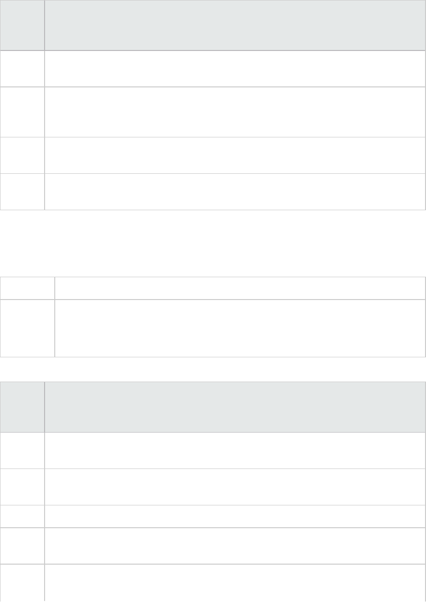
UI
Element
Description
Chart
tab
Enables you to configure the look and feel of your entire graph. You set Chart preferences
using the following tabs: For details, see "Chart Tab (Editing MainChart Dialog Box)" below.
Series
tab
Enables you to control the appearance of the individual points plotted in the graph. You set
Series preferences using the following tabs. For details, see "Series Tab (Editing MainChart
Dialog Box)" on the next page.
Export
tab
Enables you to store the current graph to an image file in the format of your choice—BMP,
JPG, or EMF. You can also export the graph's data to HTML, Excel, or XML
Print
tab
Enables you to print only the graph itself without the legend and other data such as the
User Notes.
Chart Tab (Editing MainChart Dialog Box)
This tab enables you to configure the look and feel of your entire graph.
To access View > Display Options > Advanced button > Chart tab
See also l"Display Options Dialog Box" on page73
l"Editing Main Chart Dialog Box (Display Options Dialog Box)" on the previous page
l"Series Tab (Editing MainChart Dialog Box)" on the next page
User interface elements are described below:
UI
Element
Description
Series
tab
Select the graph style (for example, bar or line), the hide/show settings, line and fill color,
and the title of the series.
General
tab
Select options for print preview, export, margins, scrolling, and magnification.
Axis tab Select which axes to show, as well as their scales, titles, ticks, and position.
Titles
tab
Set the title of the graph, its font, background color, border, and alignment.
Legend
tab
Set all legend related settings, such as position, fonts, and divider lines.
User Guide
Analysis
HP LoadRunner (12.50) Page 76
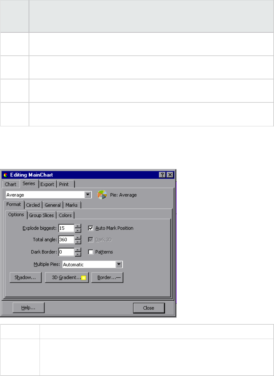
UI
Element
Description
Panel
tab
Show the background panel layout of the graph. You can modify its color, set a gradient
option, or specify a background image.
Paging
tab
Set all page related settings, such as amount of data per page, scale, and page numbering.
These settings are relevant when the graph data exceeds a single page.
Walls
tab
Set colors for the walls of 3-dimensional graphs.
3D Select the 3-dimensional settings, offset, magnification, and rotation angle for the active
graph.
Series Tab (Editing MainChart Dialog Box)
This page enables you to control the appearance of the individual points plotted in the graph.
To access View > Display Options > Advanced button > Series tab
See also l"Display Options Dialog Box" on page73
l"Editing Main Chart Dialog Box (Display Options Dialog Box)" on page75
l"Chart Tab (Editing MainChart Dialog Box)" on the previous page
User interface elements are described below:
User Guide
Analysis
HP LoadRunner (12.50) Page 77
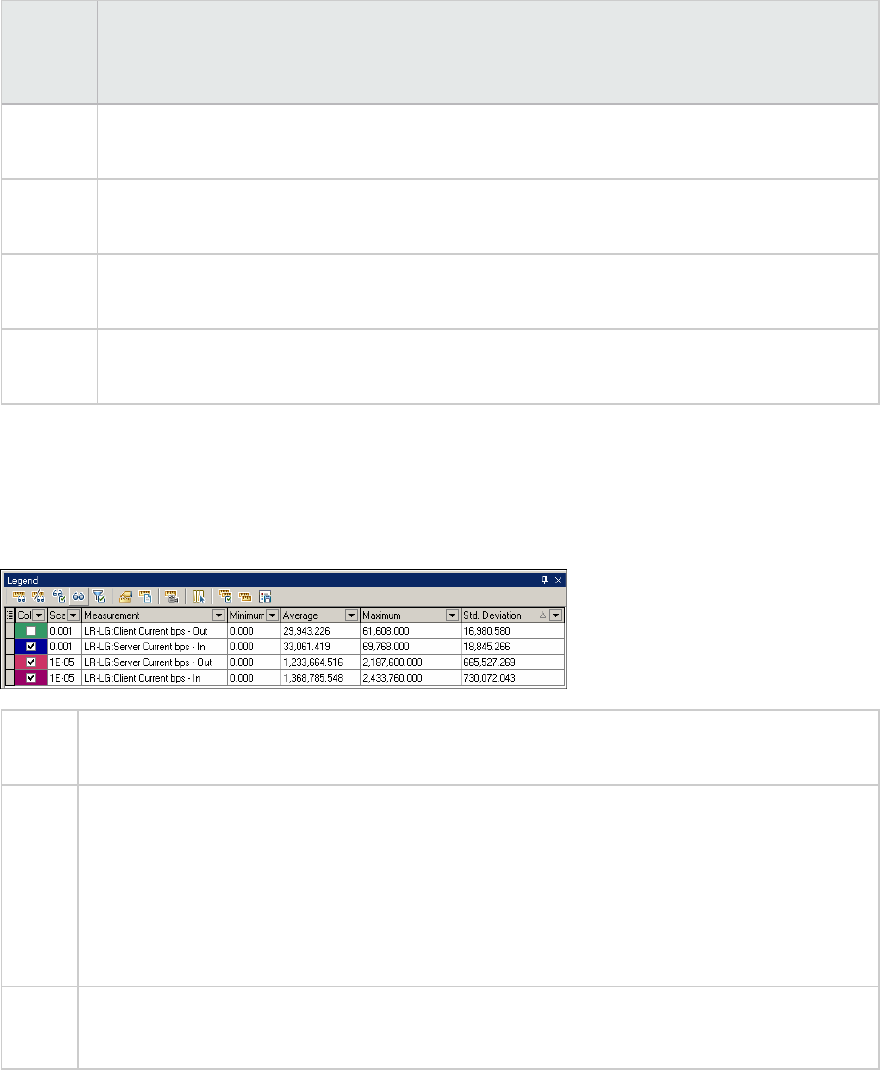
UI
Element
Description
Format
tab
Set the border color, line color, pattern, and invert property for the lines or bars in your
graph.
Point
tab
Set the size, color, and shape of the points that appear within your line graph.
General
tab
Select the type of cursor, the format of the axis values, and show/hide settings for the
horizontal and vertical axes.
Marks
tab
Configure the format for each point in the graph.
Legend Window
This window enables you to configure the color, scale, minimum, maximum, average, median, and
standard deviation of each measurement appearing in the graph.
To
access
Analysis Window > Legend window
Tip Filtering: To show only certain values, click the down arrow in the selected column and click
Custom. The Custom Filter dialog box opens. For details, see "Custom Filter Dialog Box" on
page113.
Sorting: To sort the measurements by a specific metrics, select a column header once to
display the measurements in ascending order. Click it again to display them in descending
order.
See
also
l"Measurement Description Dialog Box" on page81
l"Measurement Options Dialog Box" on page82
User Guide
Analysis
HP LoadRunner (12.50) Page 78
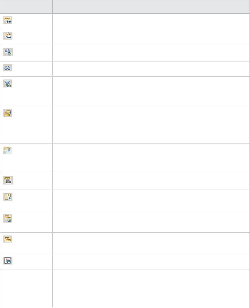
Legend Toolbar
User interface elements are described below:
UI Element Description
Show. Displays the selected measurements in the graph.
Hide. Hides the selected measurements in the graph.
Show only Selected. Displays the highlighted measurement only.
Show All. Displays all the available measurements in the graph.
Filter. Filters the graph by the measurements selected in the Legend window.
You can select multiple measurements. To clear the filter, select View > Clear
Filter/Group By.
Configure. Opens the Measurement Options dialog box that enables you to
configure measurement options (for example, set color and measurement
scale). For more information, see "Measurement Options Dialog Box" on
page82.
Show Description. Opens the Measurement Description dialog box that displays
the name, monitor type, and description of the selected measurement. For
more information, see "Measurement Description Dialog Box" on page81.
Animate. Displays the selected measurement as a flashing line.
Configure Columns. Opens the Legend Columns Options dialog box that enables
you to select the columns to display in the Legend window.
Copy Selection. Copies the selected rows to the clipboard. You can paste the
data in a text file or a spreadsheet.
Copy All. Copies all of the legend data to the clipboard, regardless of what is
selected. You can paste the data in a text file or a spreadsheet.
Export. Saves the legend data to a CSV file.
<Custom filter> After adding a custom filter (by expanding the down arrow in the column
headers), the window shows them at the bottom of the legend. Click the x
button to remove the filter, or clear the check box to disable it temporarily. For
details, see "Custom Filter Dialog Box" on page113.
User Guide
Analysis
HP LoadRunner (12.50) Page 79
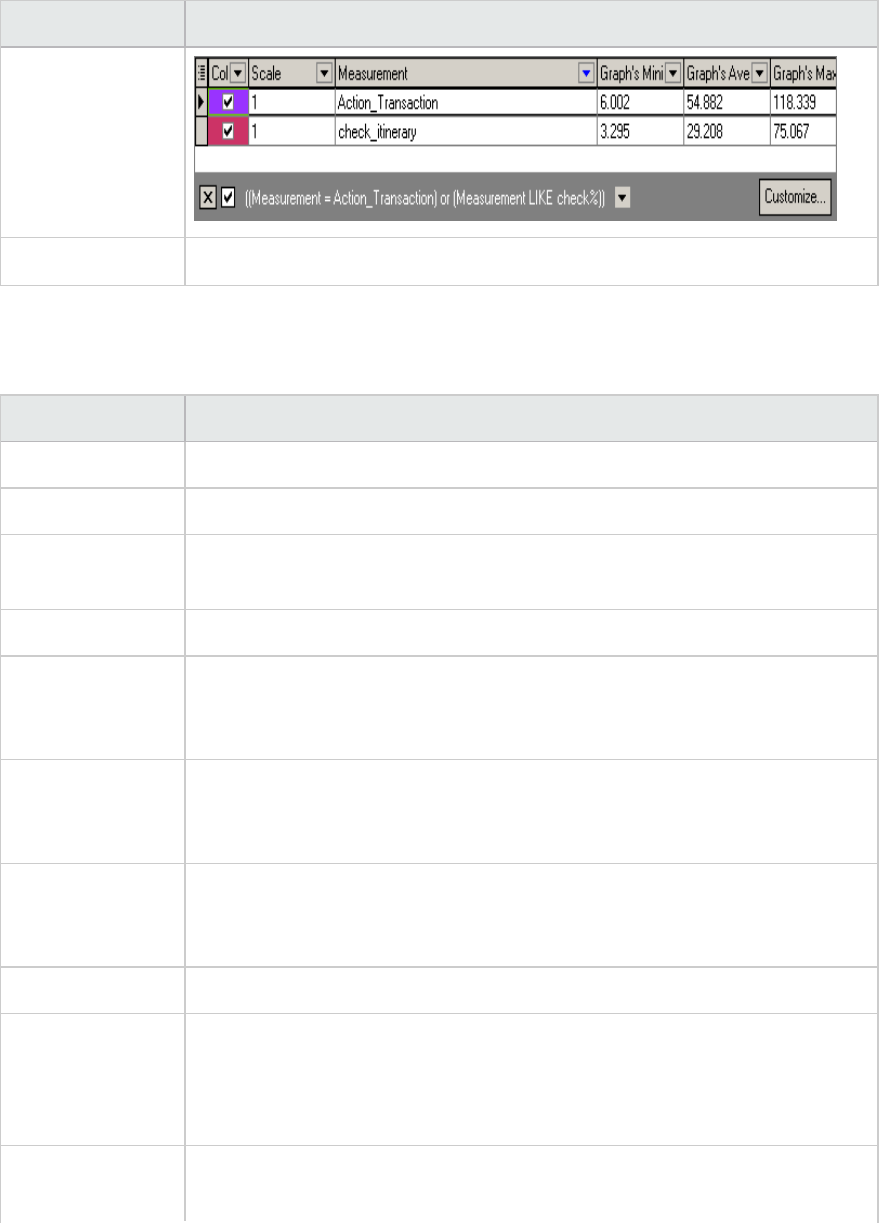
UI Element Description
Customize Opens the Filter Builder and allows you to save your filter settings to a file.
Legend grid shortcut menu
User interface elements are described below:
UI Element Description
Show Displays the selected measurements in the graph.
Hide Hides the selected measurements in the graph.
Show only
Selected
Displays the highlighted measurement only.
Show All Displays all the available measurements in the graph.
Filter Filters the graph by the measurements selected in the Legend window. You can
select multiple measurements. To clear the filter, select View > Clear
Filter/Group By.
Configure Opens the Measurement Options dialog box that enables you to configure
measurement options (for example, set color and measurement scale). For
more information, see "Measurement Options Dialog Box" on page82.
Show Description Opens the Measurement Description dialog box that displays the name, monitor
type, and description of the selected measurement. For more information, see
"Measurement Description Dialog Box" on the next page.
Animate Displays the selected measurement as a flashing line.
Auto Correlate Opens the Auto Correlate dialog box that enables you to correlate the selected
measurement with other monitor measurements in the load test scenario. For
more information on auto correlation, see "Auto Correlating Measurements" on
page93.
Configure Columns Opens the Legend Columns Options dialog box that enables you to select the
columns to display in the Legend window.
User Guide
Analysis
HP LoadRunner (12.50) Page 80
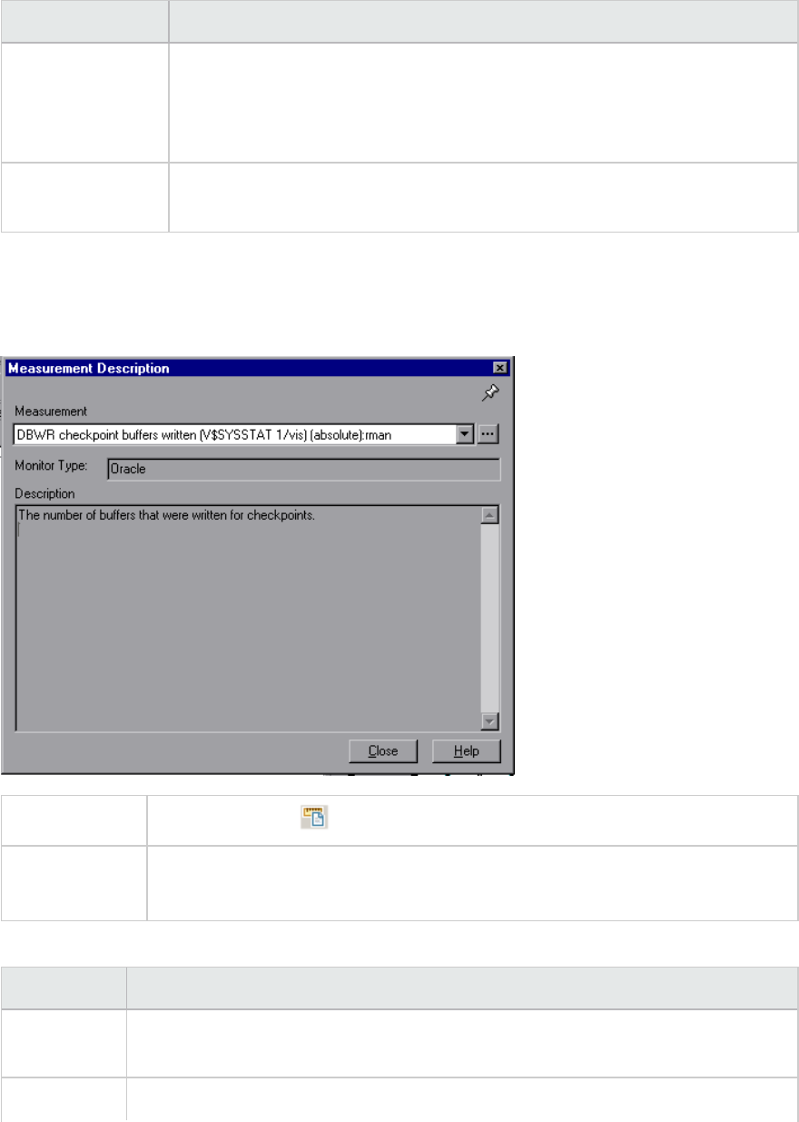
UI Element Description
Web Page
Diagnostics for
<selected
measurement>
Displays a Web Page Diagnostics graph for the selected transaction
measurement (only available for the Average Transaction Response Time and
Transaction Performance Summary graphs).
Break down Displays a graph with a breakdown of the selected page (only available for the
Web Page Diagnostics graphs).
Measurement Description Dialog Box
This dialog box shows you additional information about the selected measurement.
To access Legend Toolbar >
See also l"Legend Window" on page78
l"Measurement Options Dialog Box" on the next page
User interface elements are described below:
UI Element Description
Measurement Displays the name of the selected measurement. Click the drop-down arrow to select
a different measurement.
Monitor Type Displays the type of monitor used to obtain the selected measurement.
User Guide
Analysis
HP LoadRunner (12.50) Page 81
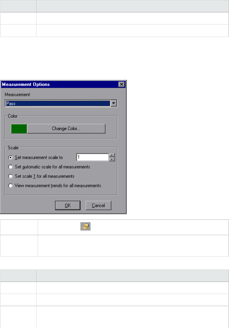
UI Element Description
Description Displays a description of the selected monitored measurement.
SQL If an SQL logical name is in use, displays the full SQL statement.
Measurement Options Dialog Box
This dialog box enables you to set the color and the scale for any measurement of the graph you
selected.
To access Legend Toolbar >
See also l"Legend Window" on page78
l"Measurement Description Dialog Box" on the previous page
User interface elements are described below:
UI Element Description
Measurement Select a measurement to configure.
Change Color Select a new color for the selected measurement.
Scale Select the desired scale option:
lSet measurement scale to x. Select the scale with which you want to view the
User Guide
Analysis
HP LoadRunner (12.50) Page 82
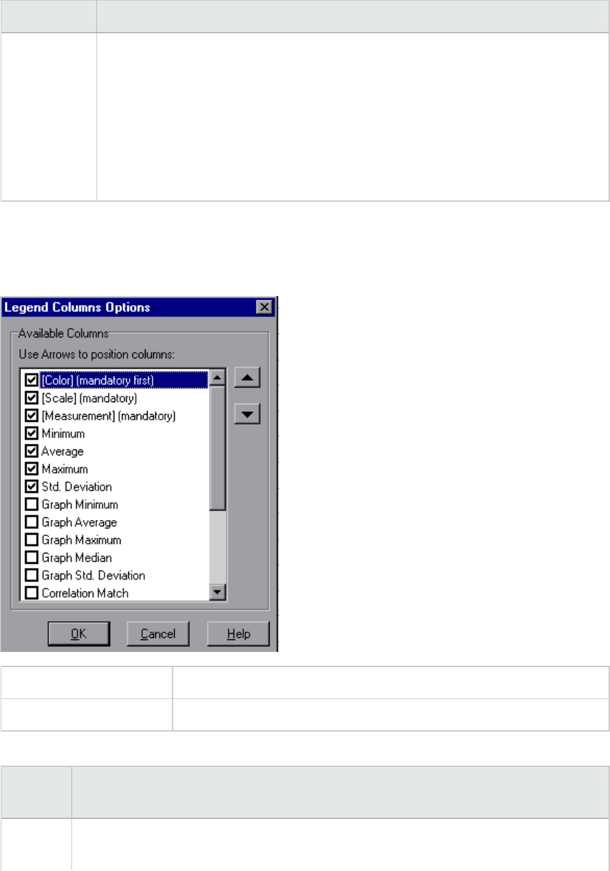
UI Element Description
lSet automatic scale for all measurements. Uses an automatic scale optimized to
display each measurement in the graph.
lSet scale 1 for all measurements. Sets the scale to one for all measurements in
the graph.
lView measurement trends for all measurements. Standardizes the y-axis values in
the graph, according to the following formula: New Y value = (Previous Y Value -
Average of previous values) / STD of previous values.
Legend Columns Options Dialog Box
This dialog box enables you to select the columns to be displayed.
To access View > Legend Columns
See also "Legend Window" on page78
User interface elements are described below:
UI
Element
Description
Available
Columns
Select or deselect the check boxes to the left of the column names to show or hide the
columns respectively.
User Guide
Analysis
HP LoadRunner (12.50) Page 83
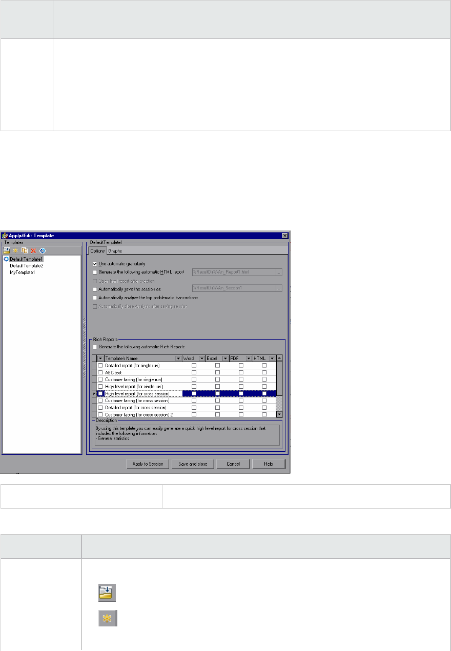
UI
Element
Description
Notes:
lThe Color, Scale, and Measurement columns are mandatory and cannot be deselected.
lTo rearrange the order in which the columns appear (from left to right), you use the
vertical arrows to the right of the Available Columns list to place the columns in the
desired order.
Apply/Edit Template Dialog Box
This dialog box enables you to configure template settings and select report template options. Using
this dialog box, you can create new templates, open existing ones, and set the default template for your
sessions.
To access Tools > Templates
User interface elements are described below (unlabeled elements are shown in angle brackets):
UI Element Description
Templates Select one of the following buttons:
lBrowse for a template.
lAdd a new template. Enter the title of the new template in the Add new
template dialog box.
User Guide
Analysis
HP LoadRunner (12.50) Page 84
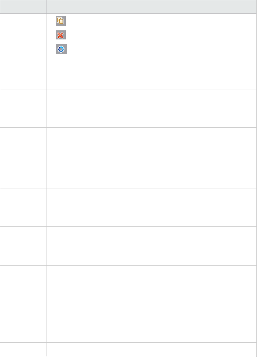
UI Element Description
lDuplicate the selected template.
lDelete the selected template.
lSet the selected template as the default.
Use automatic
granularity
Applies the default Analysis granularity (onesecond) to the template. For
information about setting Analysis granularity, see "Changing the Granularity of
the Data" on page91.
Generate the
following
automatic
HTML report
Generates an HTML report using the template. Specify or select a report name. For
information about generating HTML reports, see "HTML Reports" on page373.
Open html
report after
creation
If you selected the option of generating an automatic HTML report, select this
option to automatically open the HTML report after it is created.
Automatically
save the
session as
Automatically saves the session using the template you specify. Specify or select a
file name.
Automatically
analyze the top
problematic
transactions
Automatically generates Transaction Analysis reports for the transactions with the
worst SLA violations. Reports are generated for a maximum of five transactions.
For more information about Transaction Analysis reports, see "Analyze
Transactions Dialog Box" on page358.
Automatically
close Analysis
after saving
session
Automatically closes Analysis after a session is automatically saved (using the
previous option). This prevents the running of multiple instances of Analysis.
Generate the
following
automatic Rich
Reports
The selected reports are added to the template.
<check box on
left of
Template's
Name>
Select to add report template to selected template. The reports are added to the
session.
Word Generates a report using the selected report template to MS Word.
User Guide
Analysis
HP LoadRunner (12.50) Page 85
UI Element Description
Note: Take into account that the content load may affect the table format
within the MS Word document.
Excel Generates a report using the selected report template to Excel.
PDF Generates a report using the selected report template to PDF.
HTML Generates a report using the selected report template to HTML.
Graphs tab Displays the list of graphs that are included in the template. When the template is
applied to a session, the graphs are displayed under Graphs in Session Explorer. If
there is no data in the session, the graphs are not created.
Apply to
Session
Applies your changes to the current analysis session without closing the dialog box.
Color Palettes
Color Palettes allow you to define the colors that will be used in Analysis graphs and to allocate those
colors to specific series. There is a general, default palette and you can also define a Color Palette for a
specific session. You can add new colors to a palette and delete existing colors from a palette, but a
palette must contain at least thirty two colors.
When a new session is created, or when you open an existing session that does not have a Graph Colors
file, Analysis uses the general color palette. When you open an existing session that has a Graph Colors
file, Analysis uses the file from the session folder.
The colors are allocated to the graph in the order they appear in the palette. Colors allocated to a
series, are used to represent graph elements for the series in the order the colors were allocated. To
change the colors in the graph, update the palette, close and re-open the graph.
For more information, see "Color Palette Dialog Box" below.
Color Palette Dialog Box
This dialog box enables you to configure the colors that will be used in graphs. You use the General Color
Palette to define a default set of colors for all graphs and the Session Color Palette to define the set of
colors for a specific session.
User Guide
Analysis
HP LoadRunner (12.50) Page 86
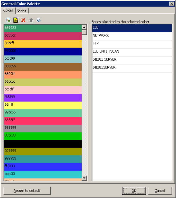
User Guide
Analysis
HP LoadRunner (12.50) Page 87
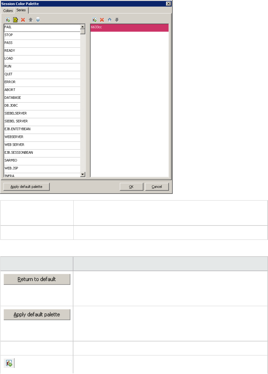
To access lTools > General Color Palette
lTools > Session Color Palette
See also "Color Palettes" on page86
User interface elements are described below:
UI Elements> Description
Restores the palette to the currently saved General Palette.
This button appears on the General Color Palette, not on the Session
Color Palette.
Applies the default palette as the session palette.
This button appears on the Session Color Palette, not on the General
Color Palette.
Colors tab Allows you to configure the colors on the palette.
Add a new color to the palette.
User Guide
Analysis
HP LoadRunner (12.50) Page 88
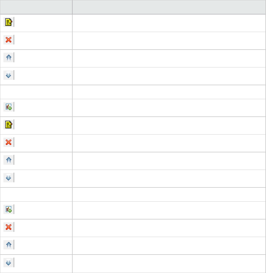
UI Elements> Description
Replace an existing color with a new color.
Delete a color from the palette.
Move the color upwards.
Move the color downwards.
Series tab - left pane Allows you to configure the series on the palette.
Add a new series to the palette.
Edit a series.
Delete a series from the palette.
Move the series upwards.
Move the series downwards.
Series tab - right pane Allows you to define colors for the selected series.
Add a color to the series.
Delete a color from the series.
Move the color upwards.
Move the color downwards.
Working with Analysis Graph Data
Analysis contains several utilities that enable you to manage graph data to most effectively view the
displayed data.
Determining a Point's Coordinates
You can determine the coordinates and values at any point in a graph. Place the cursor over the point
you want to evaluate and Analysis displays the axis values and other grouping information.
User Guide
Analysis
HP LoadRunner (12.50) Page 89
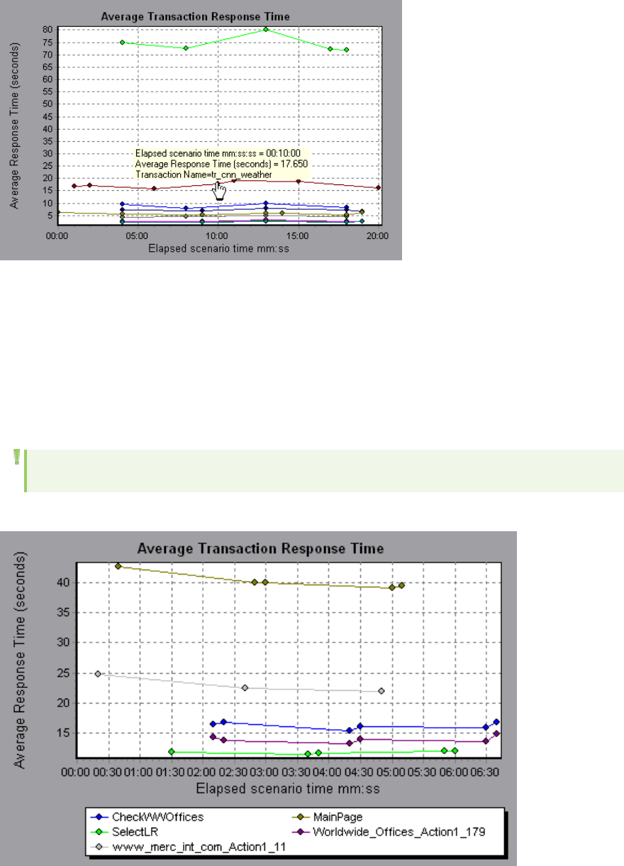
Drilling Down in a Graph
Drill down enables you to focus on a specific measurement within your graph and display it according to
a desired grouping. The available groupings depend on the graph. For example, the Average Transaction
Response Time graph shows one line per transaction. To determine the response time for each Vuser,
you drill down on one transaction and sort it according to Vuser ID. The graph displays a separate line
for each Vuser's transaction response time.
Note: The drill down feature is not available for the Web Page Diagnostics graph.
The following graph shows a line for each of five transactions.
User Guide
Analysis
HP LoadRunner (12.50) Page 90
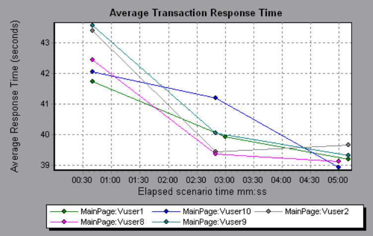
When you drill down on the MainPage transaction, grouped by Vuser ID, the graph displays the response
time only for the MainPage transaction, one line per Vuser.
You can see from the graph that the response time was longer for some Vusers than for others.
To determine the response time for each host, you drill down on one transaction and sort it according to
host. The graph displays a separate line for the transaction response time on each host. For more
information on drilling down in a graph, see "How to Manage Graph Data" on page94.
Changing the Granularity of the Data
You can make the graphs easier to read and analyze by changing the granularity (scale) of the x-axis.
The maximum granularity is half of the graph's time range. To ensure readability and clarity, Analysis
automatically adjusts the minimum granularity of graphs with ranges of 500 seconds or more.
In the following example, the Hits per Second graph is displayed using different granularities. The y-axis
represents the number of hits per second within the granularity interval. For a granularity of 1, the y-
axis shows the number of hits per second for each one second period of the load test scenario.
For a granularity of 5, the y-axis shows the number of hits per second for every five-second period of
the scenario.
User Guide
Analysis
HP LoadRunner (12.50) Page 91
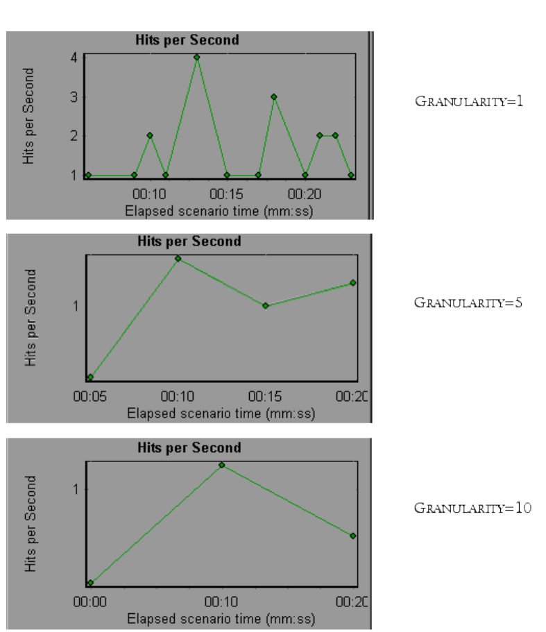
In the above graphs, the same load test scenario results are displayed in a granularity of 1, 5, and 10.
The lower the granularity, the more detailed the results. For example, using a low granularity as in the
upper graph, you see the intervals in which no hits occurred. It is useful to use a higher granularity to
study the overall Vuser behavior throughout the scenario.
By viewing the same graph with a higher granularity, you can see that overall, there was an average of
approximately 1 hit per second.
Viewing Measurement Trends
You can view the pattern of a line graph more effectively by standardizing the graph's y-axis values.
Standardizing a graph causes the graph's y-axis values to converge around zero. This cancels the
User Guide
Analysis
HP LoadRunner (12.50) Page 92
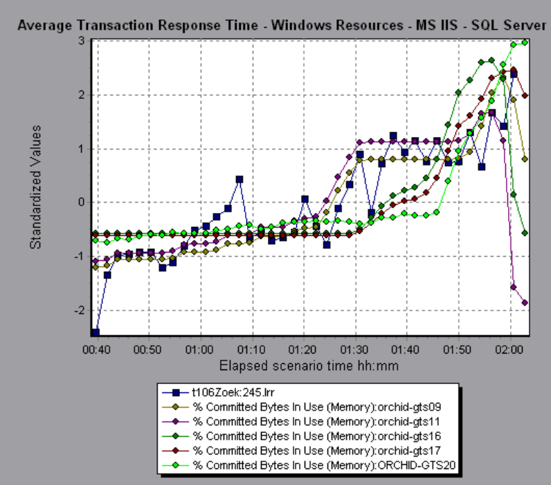
measurements' actual values and allows you to focus on the behavior pattern of the graph during the
course of the load test scenario.
Analysis standardizes the y-axis values in a graph according to the following formula:
New Y value = (Previous Y Value - Average of previous values) / STD of previous
values
Auto Correlating Measurements
You can detect similar trends among measurements by correlating a measurement in one graph with
measurements in other graphs. Correlation cancels the measurements' actual values and allows you to
focus on the behavior pattern of the measurements during a specified time range of the load test
scenario.
In the following example, the t106Zoek:245.lrr measurement in the Average Transaction Response
Time graph is correlated with the measurements in the Windows Resources, Microsoft IIS, and SQL
Server graphs. The five measurements most closely correlated with t106Zoek:245.lrr are displayed in
the graph below.
User Guide
Analysis
HP LoadRunner (12.50) Page 93

Note: This feature can be applied to all line graphs except the Web Page Diagnostics graph.
Viewing Raw Data
You can view the actual raw data collected during test execution for the active graph. The Raw Data
view is not available for all graphs.
Viewing the raw data can be especially useful in the following cases:
lTo determine specific details about a peak—for example, which Vuser was running the transaction
that caused the peak value(s).
lTo perform a complete export of unprocessed data for your own spreadsheet application.
For user interface details, click "Graph/Raw Data View Table" on page100.
How to Manage Graph Data
The following list includes the utilities you can use in Analysis to enable you to manage graph data to
most effectively view the displayed data.
Determine a point's coordinates
To determine the coordinates and values at any point in a graph, place the cursor over the point you
want to evaluate. Analysis displays the axis values and other grouping information.
Drill down in a graph
Drill down enables you to focus on a specific measurement within your graph and display it according to
the desired grouping.
1. Right-click on a line, bar, or segment within the graph, and select Drill Down. The Drill Down
Options dialog box opens, listing all of the measurements in the graph.
2. Select a measurement for drill down.
3. From the Group By box, select a group by which to sort.
4. Click OK. Analysis drills down and displays the new graph.
To undo the last drill down settings, choose Undo Set Filter/Group By from the right-click menu.
lTo perform additional drill-downs, repeat steps 1 to 4.
lTo clear all filter and drill down settings, choose Clear Filter/Group By from the right-click
menu.
Filter the data
This task describes how to filter the data and create custom filters.
User Guide
Analysis
HP LoadRunner (12.50) Page 94
1. In the Legend window, click the column header of the measurement you want to use as a base for
the filter.
2. To show a single entry, expand the drop-down list and select that entry.
3. To create a custom filter, select Custom in the drop-down list. The Custom Filter dialog box opens.
4. Select an evaluation expression and provide a value. To use wildcards, use an underscore, _, to
represent a single character and %for multiple characters. For details, see "Custom Filter Dialog
Box" on page113.
5. To provide additional criteria, select a logical operator, ANDor OR and set up the second
expression.
Change the granularity of the data
This task describes how to change the granularity of a graph.
1. Click inside a graph.
2. Select View >Set Granularity, or click theSet Granularity button . The Granularity dialog box
opens.
3. Enter the granularity of the x-axis and select a time measurement. The maximum granularity is
half of the graph's time range.
4. To ensure readability and clarity, LoadRunner automatically adjusts the minimum granularity of
graphs with ranges of 500 seconds or more.
5. Click OK.
View measurement trends
This task describes how to activate the View Measurements Trends option from a line graph.
1. Select View > View Measurement Trends, or right-click the graph and choose View Measurement
Trends. Alternatively, you can select View > Configure Measurements and check the View
measurement trends for all measurements box.
Note: The standardization feature can be applied to all line graphs except the Web Page
Diagnostics graph.
2. View the standardized values for the line graph you selected. The values in the Minimum, Average,
Maximum, and Std. Deviation legend columns are real values.
To undo the standardization of a graph, repeat step 1.
Note: If you standardize two line graphs, the two y-axes merge into one y-axis.
User Guide
Analysis
HP LoadRunner (12.50) Page 95

Auto correlate measurements
You can detect similar trends among measurements by correlating a measurement in one graph with
measurements in other graphs. Correlation cancels the measurements' actual values and allows you to
focus on the behavior pattern of the measurements during a specified time range of the load test
scenario.
1. From a graph or legend, right-click the measurement you want to correlate and choose Auto
Correlate. The Auto Correlate dialog box opens with the selected measurement displayed in the
graph.
2. Select a suggested time range method and time range.
3. If you applied a time filter to your graph, you can correlate values for the complete scenario time
range by clicking the Display button in the upper right-hand corner of the dialog box.
4. To specify the graphs you want to correlate with a selected measurement and the type of graph
output to be displayed, perform the following:
lSelect the Correlation Options tab.
lSelect the graphs to correlate, the data interval, and output options, as described in "Drill Down
Options Dialog Box" below.
lOn the Time Range tab, click OK. Analysis generates the correlated graph you specified. Note the
two new columns—Correlation Match and Correlation—that appear in the Legend window
below the graph.
To specify another measurement to correlate, select the measurement from the Measurement to
Correlate box at the top of the Auto Correlate dialog box.
The minimum time range should be more than 5% of the total time range of the measurement.
Trends which are smaller than 5% of the whole measurement will be contained in other larger
segments.
Sometimes, very strong changes in a measurement can hide smaller changes. In cases like these,
only the strong change is suggested, and the Next button will be disabled.
Note: This feature can be applied to all line graphs except the Web Page Diagnostics graph.
Drill Down Options Dialog Box
This dialog box lists all the measurements in the graph.
User Guide
Analysis
HP LoadRunner (12.50) Page 96
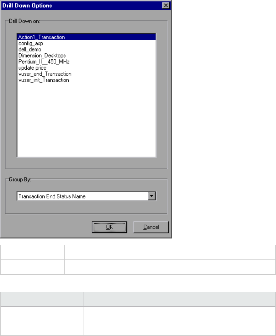
To access <Right-click> graph line/bar/segment > Drill Down
See also "Drilling Down in a Graph" on page90
User interface elements are described below:
UI Element Description
Drill Down on Filter graph by selected transaction.
Group By The selected transaction is sorted by selected criteria.
Auto Correlate Dialog Box
This dialog box enables you to configure settings used to correlate measurements from the selected
graph with measurements in other graphs.
User Guide
Analysis
HP LoadRunner (12.50) Page 97
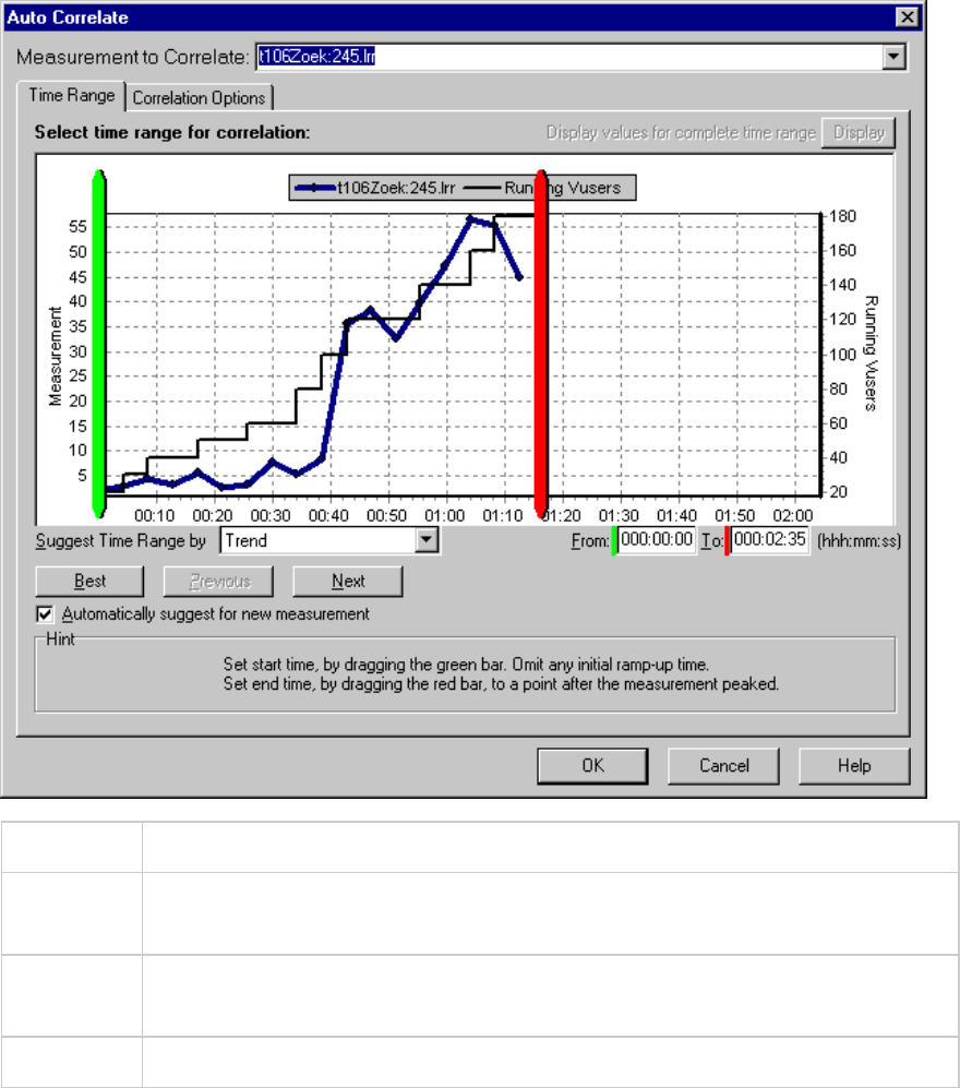
To access Click on a graph and select > Auto Correlate from the right-click menu
Important
information
You can also use the green and red vertical drag bars to specify the start and end
values for the scenario time range.
Note The granularity of the correlated measurements graph may differ from that of the
original graph, depending on the scenario time range defined.
See also "Auto Correlating Measurements" on page93
Time Range Tab
The Time Range tab of the Auto Correlate dialog box enables you to specify a load test scenario time
range for the correlated measurement graph.
User interface elements are described below:
User Guide
Analysis
HP LoadRunner (12.50) Page 98
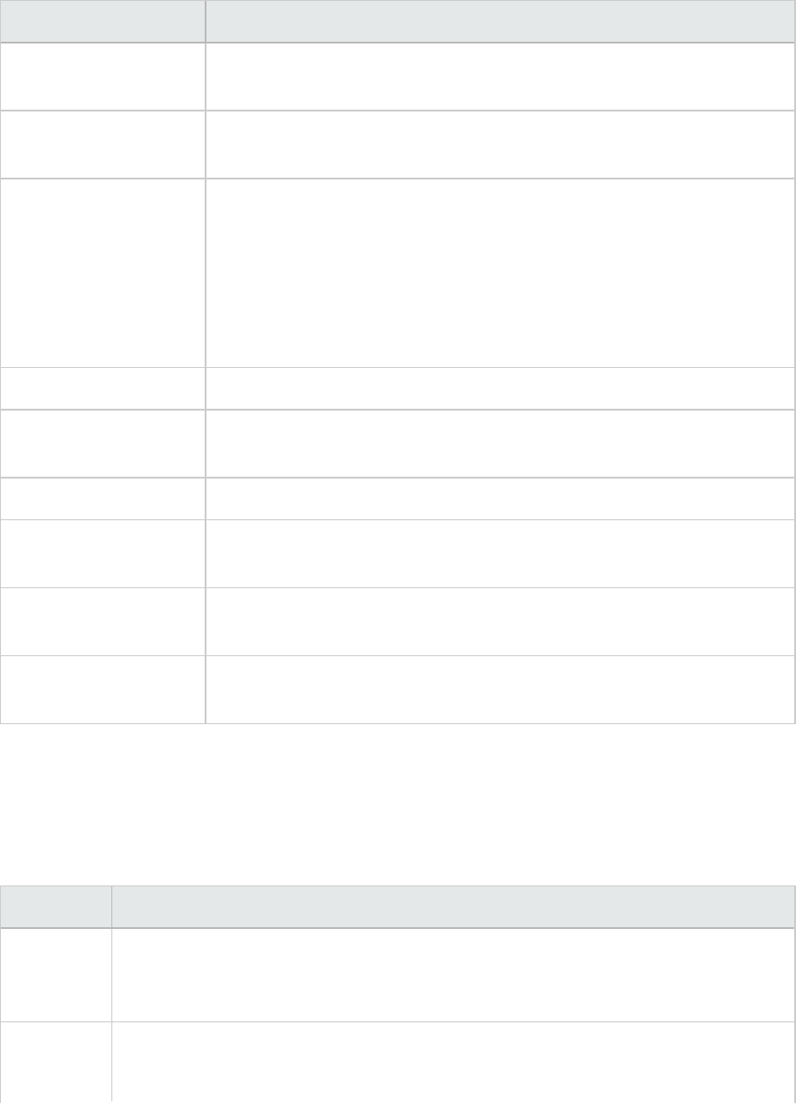
UI Element Description
Measurement to
Correlate
Select the measurement you want to correlate.
Display values for
complete time range
Click Display to correlate values for the complete scenario time range.
This option is available only if you applied a time filter to your graph.
Suggest Time Range By Analysis automatically demarcates the most significant time period for
the measurement in the scenario.
lTrend. Demarcated an extended time segment which contains the most
significant changes.
lFeature. Demarcates a smaller dimension segment which forms the
trend.
Best Choose the time segment most dissimilar to its adjacent segments.
Next Suggest the next time segment for auto correlation. Each suggestion is
successively less dissimilar.
Previous Return to the previous suggestion of a time segment.
Automatically suggest
for new measurement
Generates new suggestions each time that the Measurement to Correlate
item changes.
From Specify a start value (in hh:mm:ss format) for the desired scenario time
range.
To Specify an end value (in hh:mm:ss format) for the desired scenario time
range.
Correlation Options tab
You use the Correlation Options tab to set the graphs to correlate, the data interval, and the output
options.
User interface elements are described below:
UI Element Description
Select
Graphs for
Correlation
Select the graphs whose measurements you want to correlate with your selected
measurement.
Data
Interval
Calculate the interval between correlation measurement polls.
lAutomatic. Uses an automatic value, determined by the time range.
User Guide
Analysis
HP LoadRunner (12.50) Page 99
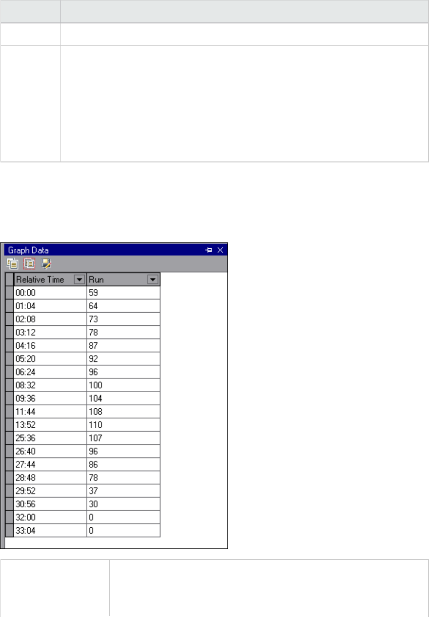
UI Element Description
lCorrelate data based on X second intervals. Enter a fixed value.
Output Choose the level of output displayed.
lShow the X most closely correlated measurements. Displays only the specified
number of measurements most closely related to the selected measurement. The
default value is 5.
lShow measurements with an influence factor of at least X%. Displays only those
measurements that converge to the specified percent with the selected
measurement. The default value is 50%.
Graph/Raw Data View Table
You can view graph data in spreadsheet view or raw data view. The data is instantly displayed on
request.
To access Click the appropriate tab on the right border of the Analysis window or do
one of the following:
lWindows > Graph Data
User Guide
Analysis
HP LoadRunner (12.50) Page 100
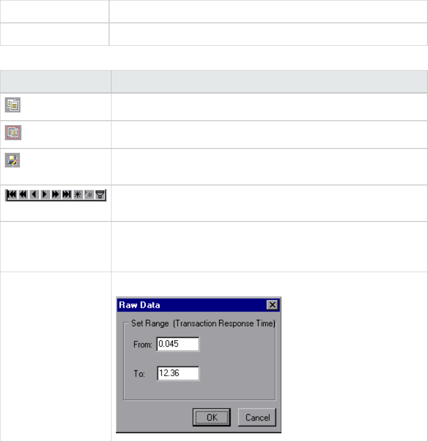
lWindows > Raw Data
Note Raw Data is not available for all graphs.
User interface elements are described below:
UI Element Description
Copies the data that you have selected.
Copies the spreadsheet to the clipboard. You can paste to a spreadsheet.
Saves the spreadsheet data to an Excel or CSV file. In Excel, you can
generate your own customized graphs.
Use the buttons on the toolbar to navigate through the table, and mark
any records for future reference.
Relative Time The first column in the Graph Data window. displays the elapsed scenario
time (the x-axis values). The following columns displays the relative y-axis
values for each measurement represented on the graph.
Raw Data dialog box In Set Range, set a time range.
Graph Properties Pane
This pane displays the details of the graph or report selected in the Session Explorer. Fields that appear
in black are editable. When you select an editable field, an edit button is displayed next to the selected
field value.
User Guide
Analysis
HP LoadRunner (12.50) Page 101
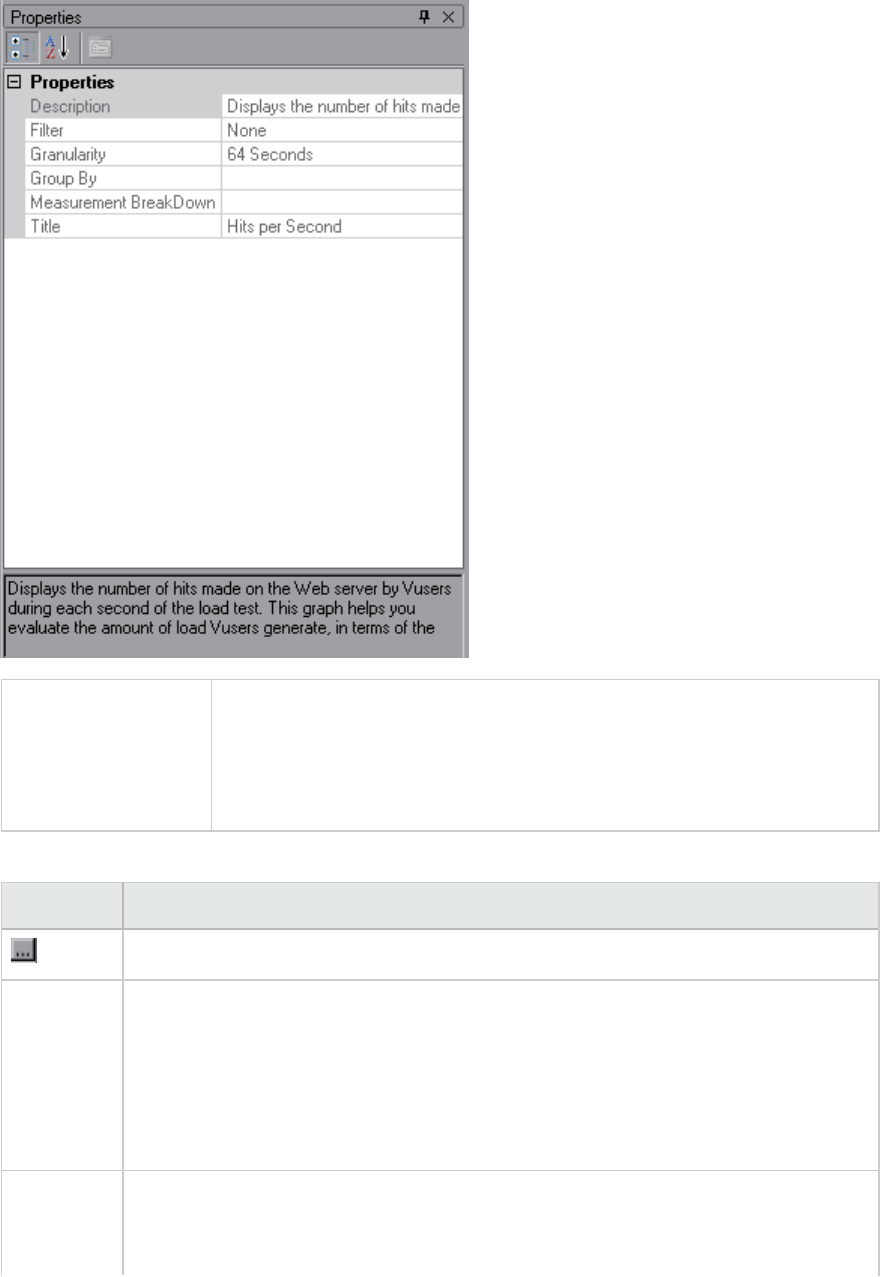
To access One of the following:
lWindows > Properties
lSelect a graph in the Session Explorer, and select Properties from the
right-click menu.
User interface elements are described below:
UI Element Description
Enables you to edit the value for the selected field.
Graph
fields
lFilter. Shows configured filter.
lGranularity. Shows configured granularity.
lGroup By. Shows the filter for selected group.
lMeasurement Breakdown. Shows the measurements of the graph.
lTitle. Shows the name of the graph in the graph display window.
Summary
Report
fields
lDescription. A short summary of what is included in the summary report.
lFilter. Shows configured filter for the summary report.
User Guide
Analysis
HP LoadRunner (12.50) Page 102
UI Element Description
lPercentile. The Summary Report contains a percentile column showing the
response time of 90% of transactions (90% of transactions that fall within this
amount of time). To change the value of the default 90 percentile, enter a new
figure in the Transaction Percentile box.
lTitle. The name of the summary report.
Transaction
Analysis
Report
fields
When clicking the edit button for some of the fields, the Analyze Transaction Settings
dialog box opens, enabling you to edit some of the Analyze Transaction settings.
Filtering and Sorting Graph Data
Filtering Graph Data Overview
You can filter graph data to show fewer transactions for a specific segment of the load test scenario.
More specifically, you can display four transactions beginning from five minutes into the scenario and
ending three minutes before the end of the scenario.
You can filter for a single graph, in all graphs in a load test scenario, or in the summary graph.
The available filter conditions differ for each type of graph. The filter conditions also depend on your
scenario. For example, if you only had one group or one load generator machine in your scenario, the
Group Name and Load Generator Name filter conditions do not apply.
Note: You can also filter merged graphs. The filter conditions for each graph are displayed on
separate tabs.
Sorting Graph Data Overview
You can sort graph data to show the data in more relevant ways. For example, Transaction graphs can
be grouped by the Transaction End Status, and Vuser graphs can be grouped by Scenario Elapsed Time,
Vuser End Status, Vuser Status, and Vuser ID.
You can sort by one or several groups—for example by Vuser ID and then Vuser status. The results are
displayed in the order in which the groups are listed. You can change the grouping order by rearranging
the list.
User Guide
Analysis
HP LoadRunner (12.50) Page 103
Filter Conditions
Common Filter Condition Options
The following filter conditions are common to many graphs:
Filter
Condition
Filters the graph according to...
Host Name The name of the Host machine. Select one or more hosts from the drop-down list.
Transaction
End Status
The end status of a transaction: pass, fail, stop.
Scenario
Elapsed
Time
The time that elapsed from the beginning to the end of the load test scenario. For
more information about setting the time range, see "Scenario Elapsed Time Dialog
Box" on page117.
Vuser ID The Vuser ID. For more information, see "Vuser ID Dialog Box" on page119.
Script
Name
The name of the script.
Group
Name
The name of the group to filter by.
Think Time The Think Time option in the graph filter for complete mode is turned off by default.
The transaction time displayed shows pure time.
Vuser Graphs
You can apply the following filter conditions to Vuser graphs:
Filter Condition Filters the graph according to...
Vuser Status The Vuser status: load, pause, quit, ready, run
Vuser End Status The status of the Vuser at the end of the transaction: error, failed,
passed, stopped.
Number of Released
Vusers
The number of Vusers that were released.
Rendezvous Name The name of the rendezvous point.
Error Graphs
You can apply the following filter conditions to Error graphs:
User Guide
Analysis
HP LoadRunner (12.50) Page 104
Filter Condition Filters the graph according to...
Error Type The type of error (per error number).
Parent Transaction The parent transaction.
Line Number in Script The line number in the script.
Transaction Graphs
You can apply the following filter conditions to Transaction graphs:
Filter Condition Filters the graph according to...
Transaction
Name
The name of the transaction.
Transaction
Response Time
The response time of the transaction.
Transaction
Hierarchical Path
The hierarchical path of the transaction. For more information on setting this
condition, see "Hierarchical Path Dialog Box" on page117.
Web Resource Graphs
You can apply the following filter conditions to Web Resources graphs:
Filter Condition Filters the graph according to...
Web Resource Name The name of the Web resource.
Web Resource Value The value of the Web resource.
Web Server Resource Name The name of the Web Server resource.
Web Server Resource Value The value of the Web Server resource.
Web Page Diagnostics Graphs
You can apply the following filter conditions to Web Page Diagnostics graphs:
Filter Condition Filters the graph according to...
Component
Name
The name of the component.
Component
Response Time
The response time of the component.
User Guide
Analysis
HP LoadRunner (12.50) Page 105

Filter Condition Filters the graph according to...
Component DNS
Resolution Time
The amount of time the component needs to resolve the DNS name to an IP
address, using the closest DNS server.
Component
Connection Time
The time taken for the component to establish an initial connection with the Web
server hosting the specified URL.
Component First
Buffer Time
The time that passes from the component's initial HTTP request (usually GET)
until the first buffer is successfully received back from the Web server.
Component
Receive Time
The time that passes until the component's last byte arrives from the server and
the downloading is complete.
Component SSL
Handshaking
Time
The time take for the component to establish an SSL connection. (Applicable to
HTTPS communication only.)
Component FTP
Authentication
Time
The time taken for the component to authenticate the client. (Applicable to FTP
protocol communication only).
Component Error
Time
The average amount of time that passes from the moment a component's HTTP
request is sent until the moment an error message (HTTP errors only) is
returned.
Component Size
(KB)
The size of the component (in kilobytes).
Component Type The type of component: Application; Image; Page; Text
Component
Hierarchical Path
The hierarchical path of the component. For more information on setting this
condition, see "Hierarchical Path Dialog Box" on page117.
Component
Network Time
The amount of time from the component's first HTTP request, until receipt of
ACK.
Component
Server Time
The amount of time from when the component receives of ACK, until the first
buffer is successfully received back from the Web server.
Component
Client Time
The average amount of time that passes while a component request is delayed
on the client machine due to browser think time or other client-related delays.
User Defined Data Point Graphs
You can apply the following filter conditions to User-Defined Data Point graphs:
User Guide
Analysis
HP LoadRunner (12.50) Page 106
Filter Condition Filters the graph according to...
Datapoint Name The name of the data point.
Datapoint Value The value of the data point.
System Resources Graphs
You can apply the following filter conditions to System Resource graphs:
Filter Condition Filters the graph according to...
System Resource
Name
The name of the system resource.
System Resource
Value
The value of the system resource. See "Set Dimension Information Dialog Box"
on page118.
Network Monitor Graphs
You can apply the following filter conditions to Network Monitor graphs:
Filter Condition Filters the graph according to...
Network Path Name The name of the network path.
Network Path Delay The delay of the network path.
Network Path Father The father of the network path.
Network SubPath Name The name of the network subpath.
Network SubPath Delay The delay of the network subpath.
Network Full Path The full network path.
Network Segment Name The name of the network segment.
Network Segment Delay The delay of the network segment.
Network Segment Full Path The full network segment path.
Firewall Graphs
You can apply the following filter conditions to Firewall graphs:
Filter Condition Filters the graph according to...
Firewall Resource The name of the Firewall resource.
User Guide
Analysis
HP LoadRunner (12.50) Page 107
Filter Condition Filters the graph according to...
Name
Firewall Resource
Value
The value of the firewall resource. See "Set Dimension Information Dialog
Box" on page118.
Web Server Resource Graphs
You can apply the following filter conditions to Web Server Resource graphs:
Filter Condition Filters the graph according to...
Measurement
Name
The name of the measurement.
Measurement
Value
The measurement value. See "Set Dimension Information Dialog Box" on
page118.
Web Application Server Resource Graphs
You can apply the following filter conditions to Web Application Server Resource graphs:
Filter Condition Filters the graph according to...
Resource Name The name of the resource.
Resource Value The value of the resource. See "Set Dimension Information Dialog Box" on
page118.
Database Server Resource Graphs
You can apply the following filter conditions to Database Server Resource graphs:
Filter Condition Filters the graph according to...
Database Resource
Name
The name of the database resource.
Database Resource
Value
The value of the database resource. See "Set Dimension Information Dialog
Box" on page118.
Streaming Media Graphs
You can apply the following filter conditions to Streaming Media graphs:
User Guide
Analysis
HP LoadRunner (12.50) Page 108
Filter Condition Filters the graph according to...
Streaming Media
Name
The name of the streaming media.
Streaming Media
Value
The value of the streaming media. See "Set Dimension Information Dialog Box"
on page118.
ERP/CRM Server Resource Graphs
You can apply the following filter conditions to ERP/CRM Server Resource graphs:
Filter Condition Filters the graph according to...
ERP/CRM Server
Resource Name
The name of the ERP/CRM server resource.
ERP/CRM Server
Resource Value
The value of the ERP/CRM Server resource. See "Set Dimension
Information Dialog Box" on page118.
ERP Server Resource
Name
The name of the ERP server resource.
ERP Server Resource
Value
The value of the ERP server resource. See "Set Dimension Information
Dialog Box" on page118.
Siebel Diagnostics Graphs
You can apply the following filter conditions to Siebel Diagnostics graphs:
Filter Condition Filters the graph according to...
Siebel Transaction Name The name of the Siebel transaction.
Siebel Request Name The name of the Siebel request.
Siebel Layer Name The name of the Siebel layer.
Siebel Area Name The name of the Siebel area.
Siebel Sub-Area Name The name of the Siebel sub-area.
Siebel Server Name The name of the Siebel server.
Siebel Script Name The name of the Siebel script.
Response Time The response time of the Siebel transaction.
Siebel Chain of Calls The chain of calls for the Siebel transaction.
User Guide
Analysis
HP LoadRunner (12.50) Page 109
Siebel DB Diagnostics Graphs
You can apply the following filter conditions to Siebel DB Diagnostics graphs:
Filter Condition Filters the graph according to...
Transaction Name - SIEBEL The name of the Siebel DB transaction.
SQL Chain of Calls The SQL chain of calls for the Siebel DB transaction.
SQL Alias Name The SQL alias name for the Siebel DB transaction.
SQL Response Time The SQL response time of the Siebel DB transaction.
Oracle - Web Diagnostics Graphs
You can apply the following filter conditions to Oracle - Web Diagnostics graphs:
Filter Condition Filters the graph according to...
Transaction Name - ORACLE The name of the Oracle transaction.
SQL Chain of Calls The SQL chain of calls for the Oracle transaction.
SQL Alias Name - Oracle The SQL alias name for the Oracle transaction.
SQL Response Time The SQL response time of the Oracle transaction.
Oracle SQL Parse Time The SQL parse time of the Oracle transaction.
Oracle SQL Execute Time The SQL execute time of the Oracle transaction.
Oracle SQL Fetch Time The SQL fetch time of the Oracle transaction.
Oracle SQL Other Time Other SQL time for the Oracle transaction.
Java Performance Graphs
You can apply the following filter conditions to Java Performance graphs:
Filter Condition Filters the graph according to...
Java Performance Resource Name The name of the Java performance resource.
Java Performance Resource Value The value of the Java performance resource.
J2EE & .NET Diagnostics Graphs
You can apply the following filter conditions to J2EE & .NET Diagnostics graphs:
User Guide
Analysis
HP LoadRunner (12.50) Page 110
Filter Condition Filters the graph according to...
Transaction
Name
The name of the Java transaction.
Method Chain of
Calls
The chain of calls for the Java method.
Layer Name The name of the layer.
Class Name The name of the class.
Method Name The name of the method.
SQL Logical
Name
The SQL logical name for the Java transaction.
Response Time The response time of the Java transaction.
Host Name -
J2EE/.NET
The name of the host for the J2EE & .NET transaction.
Application Host
Name - (VM)
The name of the application host for the VM.
Transaction
Request
The request for the transaction.
Transaction
Hierarchical Path
The hierarchical path of the transaction. For more information on setting this
condition, see "Hierarchical Path Dialog Box" on page117.
Application Component Graphs
You can apply the following filter conditions to Application Component graphs:
Filter Condition Filters the graph according to...
Component Resource
Name
The resource name of the component.
Component Resource
Value
The value of the component resource. See "Set Dimension Information
Dialog Box" on page118.
COM+ Interface The interface of the COM+ component.
COM+ Response Time The response time of the COM+ component.
COM+ Call Count The call count of the COM+ component.
User Guide
Analysis
HP LoadRunner (12.50) Page 111
Filter Condition Filters the graph according to...
COM+ Method The method of the COM+ component.
.NET Resource Name The resource name of the .NET component.
.NET Value The .NET resource value. See "Set Dimension Information Dialog Box" on
page118.
.NET Class The class of the .NET component.
.NET Response Time The response time of the .NET component.
.NET Call Count The call count of the .NET component.
.NET Method The method of the .NET component.
Application Deployment Graphs
You can apply the following filter conditions to Application Deployment graphs:
Filter Condition Filters the graph according to...
Citrix Resource
Name
The name of the Citrix resource.
Citrix Resource
Value
The value of the Citrix resource. See "Set Dimension Information Dialog Box" on
page118.
Middleware Performance Graphs
You can apply the following filter conditions to Middleware Performance graphs:
Filter Condition Filters the graph according to...
Message Queue
Resource Name
The name of the message queue resource.
Message Queue
Resource Value
The value of the Message Queue resource. See "Set Dimension Information
Dialog Box" on page118.
Infrastructure Resource Graphs
You can apply the following filter conditions to Infrastructure Resource graphs:
Filter Condition Filters the graph according to...
Network Client The name of the network client.
User Guide
Analysis
HP LoadRunner (12.50) Page 112
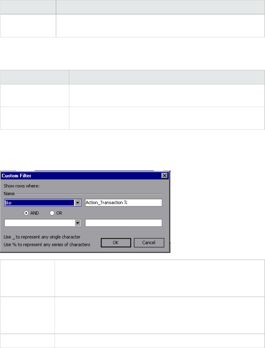
Filter Condition Filters the graph according to...
Network Client
Value
The value of the network client. See "Set Dimension Information Dialog Box" on
page118.
External Monitor Graphs
You can apply the following filter conditions to External Monitor graphs:
Filter Condition Filters the graph according to...
External Monitor
Resource Name
The name of the external monitor resource.
External Monitor
Resource Value
The value of the external monitor resource. See "Set Dimension
Information Dialog Box" on page118.
Custom Filter Dialog Box
This dialog box enables you to customize your filter criteria.
To access Do the following:
1. In a Legend window, click a column header.
2. Expand the down arrow and choose (Custom).
Tip You can use wildcards:
lUse _to represent a single character.
lUse %to represent a series of characters.
See also "Legend Window" on page78
User interface elements are described below:
User Guide
Analysis
HP LoadRunner (12.50) Page 113
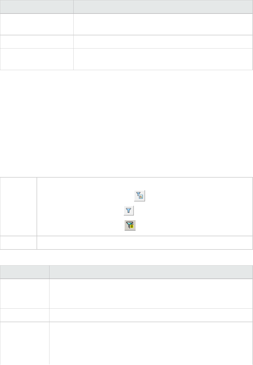
UI Element Description
<First Evaluator
Expression>
A drop-down list of evaluation expressions such as equals,is greater
than,like, and so forth, followed by a value.
Operator The logical operator by which to add a second expression: AND or OR.
<Second Evaluator
Expression>
A drop-down list of evaluation expressions such as equals,is greater
than,like, and so forth, followed by a value.
For example, the above image shows how to filter the data for transactions that begin with the phrase
"Action_Transaction", using Like and Action_Transaction%.
After you save a customization for one of the metrics, the Analysis displays it in the lower section of the
Legend window.
Filter Dialog Boxes
The filter dialog boxes (Graph Settings, Global Filter, and Analysis Summary Filter) enable you to filter
the data that is displayed in the graph or report.
When adding a graph, the filter and sort button is displayed which enables you to filter and sort data
before the graph is displayed.
To access Use one of the following:
lView > Set Filter/Group By or click
lFile > SetGlobal Filter or click
lView > Summary Filter or click
Note Some of the following fields are not displayed in all of the filter boxes.
User interface elements are described below:
UI Element Description
Filter Condition Select criteria and values for each filter condition that you want to employ. The
applicable filter conditions are displayed for each graph. For details on each
graphs filter conditions, see the chapter on the relevant graph.
Criteria Select "=" (equals) or "<>" (does not equal).
Values The filter conditions are grouped into three value types (discrete, continuous,
and time-based).
A discrete value is a distinct integer (whole number) or string value such as
Transaction Name or Vuser ID. Select the check box(es) of the value(s) that you
User Guide
Analysis
HP LoadRunner (12.50) Page 114
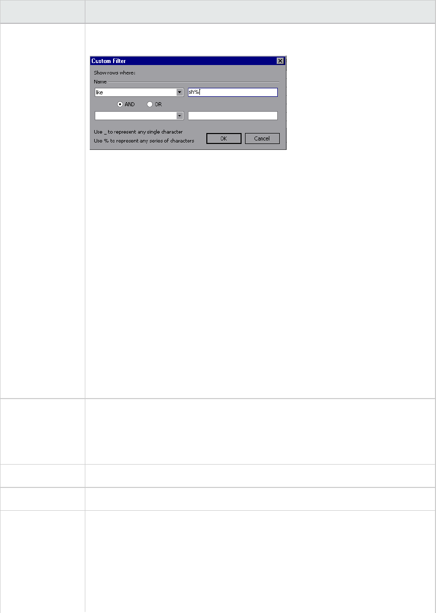
UI Element Description
want to include in your filter. You can also customize your filter by entering wild
cards to depict any single character or any series of characters.
lA continuous value is a variable dimension that can take any value within the
minimum and maximum range limits, such as Transaction Response Time. You
set the dimension information for each measurement in the "Set Dimension
Information Dialog Box" on page118.
lA time-based value is a value that is based on time relative to the start of the
load test scenario. Scenario Elapsed Time is the only condition that uses time-
based values. You specify time-based values in the "Scenario Elapsed Time
Dialog Box" on page117.
For some filter conditions, one of the following dialog boxes opens to enable you
to specify additional filtering details:
l"Set Dimension Information Dialog Box" on page118
l"Vuser ID Dialog Box" on page119
l"Scenario Elapsed Time Dialog Box" on page117
l"Hierarchical Path Dialog Box" on page117: Enables you to display the
hierarchical path of a transaction or component, or a method chain of calls.
Transaction
Percentile
The Summary Report contains a percentile column showing the response time of
90% of transactions (90% of transactions that fall within this amount of time). To
change the value of the default 90 percentile, enter a new figure in the
Transaction Percentile box.
Set Default Displays the default criteria and values for each filter condition.
Clear All Deletes all of the information you entered in the dialog box.
Group By
settings
Use these settings to sort the graph display by grouping the data. You can group
the data by:
lAvailable groups. Select the group by which you want to the sort the results,
and click the right arrow.
lSelected groups. Displays a list of all the selected groups by which the results
will be sorted. To remove a value, select it and click the left arrow.
User Guide
Analysis
HP LoadRunner (12.50) Page 115
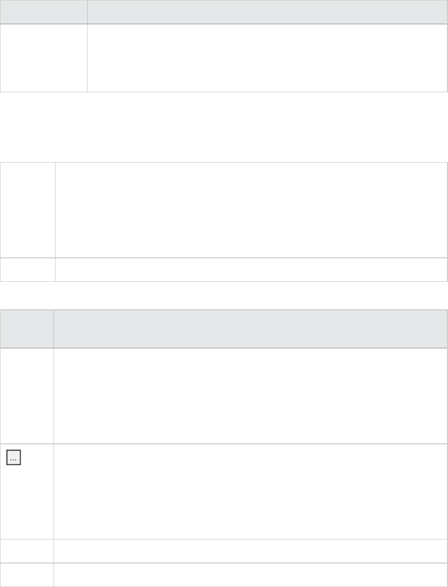
UI Element Description
Reset all graphs
to their defaults
prior to applying
the Global Filter
All graphs filter settings are reverted to their default.
Filter Builder Dialog Box
The Filter Builder dialog box enable you to design, add, and edit filters for your graph.
To access Use one of the following:
1. In the Legend pane, expand the down arrow in a column header.
2. Select Custom to open the Custom Filter dialog box. Provide filter details and click
OK.
3. Click Customize in the filter entry in the lower part of the Legend pane.
See also "Custom Filter Dialog Box" on page113
User interface elements are described below:
UI
Element
Description
Filter
button
Opens a menu with the following options:
lAdd Condition. Add another condition for the current filter.
lAdd Group. Adds a second condition, joined by a logical operator AND or OR, to the last
condition in the list.
lClear All. Removes all of the conditions in the window.
Opens a menu with the following options:
lAdd Condition. Add another condition for the current filter.
lAdd Group. Adds a second condition, joined by a logical operator AND or OR, to the
selected condition in the list.
lRemove Row. Removes the selected condition.
Open Opens an .flt file saved from a previous session.
Save as Saves all of the conditions to an .flt file.
User Guide
Analysis
HP LoadRunner (12.50) Page 116
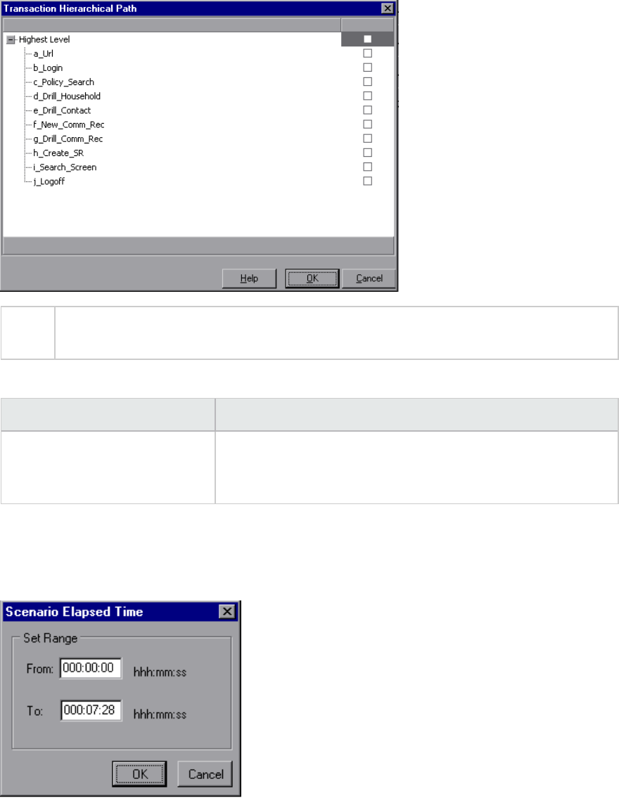
Hierarchical Path Dialog Box
This dialog box enables you to display the hierarchical path of a transaction or component, or a method
chain of calls.
To
access
View menu > Set Filter/Group by >Filter condition pane > Transaction, Component
Hierarchical Path or a method chain of calls
User interface elements are described below:
UI Element Description
Transaction, Component
Hierarchical Path or a method
chain of calls
Select the box for the path where you want to start to see
results. Only the selected path and its immediate sub-nodes will
be displayed.
Scenario Elapsed Time Dialog Box
This dialog box enables you to specify the start and end time range for the graph's x-axis.
User Guide
Analysis
HP LoadRunner (12.50) Page 117
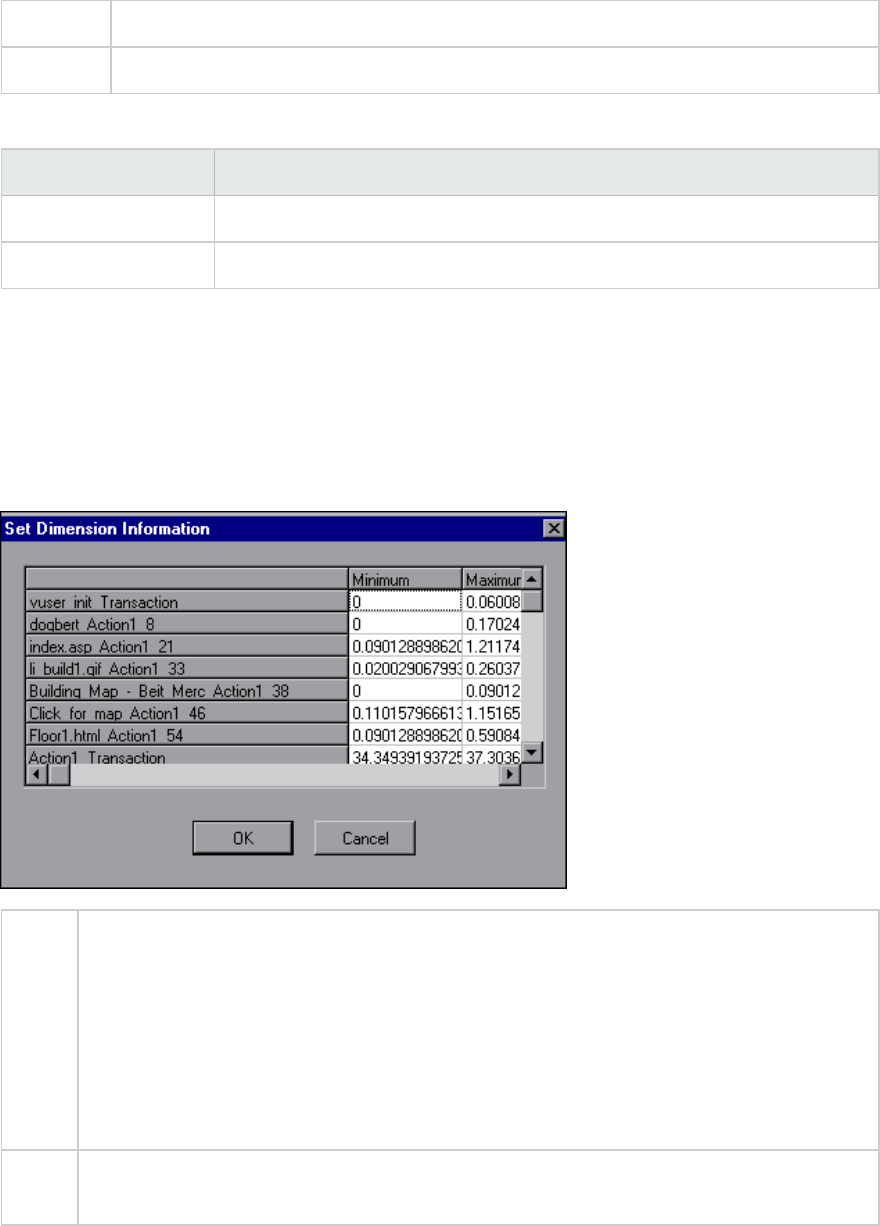
To access View menu > Set Filter/Group by >Filter condition pane > Scenario Elapsed Time
Note The time is relative to the start of the scenario.
User interface elements are described below:
UI Element Description
From Specify a start value for the desired range.
To Specify an end value for the desired range.
Set Dimension Information Dialog Box
This dialog box enables you to set the dimension information for each measurement (transaction,
number of released Vusers, resource) in the result set. You specify the minimum and maximum values
for each measurement you want in the analysis. By default, the full range of values for each
measurement is displayed.
To
access
You can open this dialog box from the following locations:
lTransaction graphs > View menu > Set Filter/Group by >Filter condition pane >
Transaction Response Time
lVusers graph > Rendezvous graph > View menu > Set Filter/Group by >Filter condition
pane > Number of Released Vusers
lAll graphs that measure resources (Web Server,Database Server, and so on) > View
menu > Set Filter/Group by >Filter condition pane > Resource Value
Note If you are specifying the start and end time for a transaction (in minutes:seconds format),
the time is relative to the beginning of the load test scenario.
User interface elements are described below:
User Guide
Analysis
HP LoadRunner (12.50) Page 118
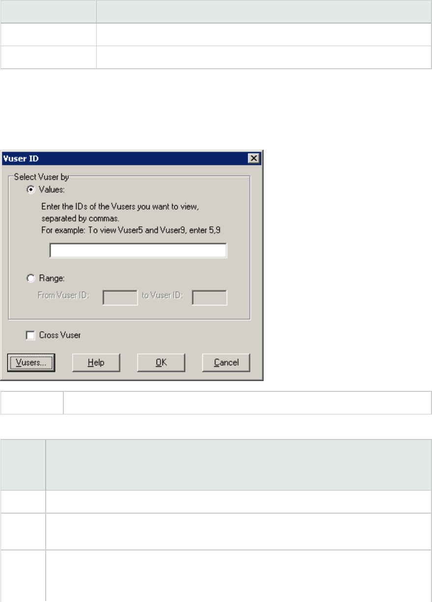
UI Element Description
Minimum Specify a minimum value for the measurement.
Maximum Specify a maximum value for the measurement.
Vuser ID Dialog Box
This dialog box opens to enable the entering of additional filter information for the Vuser ID filter
condition.
To access View menu > Set Filter/Group by > Filter condition pane > Vuser ID
User interface elements are described below:
UI
Element
Description
Value Enter the Vuser IDs of the Vusers you want the graph(s) to display, separated by commas.
Range Specify the beginning and end of the desired range of Vusers you want the graph(s) to
display.
Cross
Vuser
Cross Vuser transactions are transactions that start with one Vuser and end with a
different Vuser, such as sending an email. Selecting this check box places the value
"CrossVuser" in the Vuser ID filter. By default, the check box is not selected.
User Guide
Analysis
HP LoadRunner (12.50) Page 119
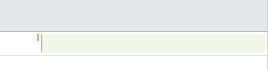
UI
Element
Description
Note: Only transaction graphs have Cross Vuser data.
Vusers Displays the existing Vuser IDs from which you can choose.
Cross Result and Merged Graphs
Comparing results is essential for determining bottlenecks and problems. You use Cross Result graphs
to compare the results of multiple load test scenario runs. You create Merged graphs to compare
results from different graphs within the same scenario run.
Cross Result and Merged Graphs Overview
Comparing results is essential for determining bottlenecks and problems. You use Cross Result graphs
to compare the results of multiple load test scenario runs. You create Merged graphs to compare
results from different graphs within the same scenario run.
Cross Result Graphs Overview
Cross Result graphs are useful for:
lBenchmarking hardware
lTesting software versions
lDetermining system capacity
If you want to benchmark two hardware configurations, you run the same load test scenario with both
configurations and compare the transaction response times using a single Cross Result graph.
Suppose that your vendor claims that a new software version is optimized to run quicker than a
previous version. You can verify this claim by running the same scenario on both versions of the
software, and comparing the scenario results.
You can also use Cross Result graphs to determine your system's capacity. You run scenarios using
different numbers of Vusers running the same script. By analyzing Cross Result graphs, you can
determine the number of users that cause unacceptable response times.
In the following example, two scenario runs are compared by crossing their results, res12, and res15.
The same script was executed twice—first with 100 Vusers and then with 50 Vusers.
In the first run, the average transaction time was approximately 59 seconds. In the second run, the
average time was 4.7 seconds. It is apparent that the system works much slower with a greater load.
User Guide
Analysis
HP LoadRunner (12.50) Page 120
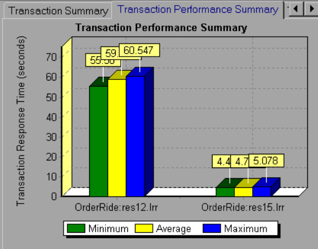
The Cross Result graphs have an additional filter and group by category: Result Name. The above graph
is filtered to the OrderRide transaction for results res12, and res15, grouped by Result Name.
Merging Types Overview
Analysis provides three types of merging:
Overlay
Superimpose the contents of two graphs that share a common x- axis. The left y-axis on the merged
graph shows the current graph's values. The right y-axis shows the values of the graph that was
merged. There is no limit to the number of graphs that you can overlay. When you overlay two graphs,
the y-axis for each graph is displayed separately to the right and left of the graph. When you overlay
more than two graphs, Analysis displays a single y-axis, scaling the different measurements accordingly.
In the following example, the Throughput and Hits per Second graph are overlaid with one another.
User Guide
Analysis
HP LoadRunner (12.50) Page 121
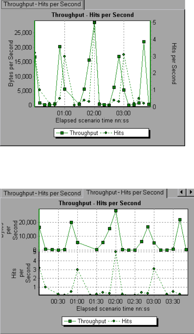
Tile
View contents of two graphs that share a common x-axis in a tiled layout, one above the other. In the
following example the Throughput and Hits per Second graph are tiled one above the other.
Correlate
Plot the y-axis of two graphs against each other. The active graph's y-axis becomes the x-axis of the
merged graph. The y-axis of the graph that was merged, becomes the merged graph's y-axis.
User Guide
Analysis
HP LoadRunner (12.50) Page 122
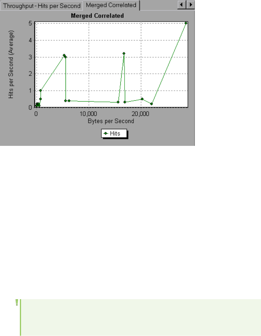
In the following example, the Throughput and Hits per Second graph are correlated with one another.
The x-axis displays the bytes per second (the Throughput measurement) and the y-axis shows the
average hits per second.
How to Generate Cross Results Graphs
This task describes how to create a Cross Result graph for two or more result sets. The Cross Result
dialog box enables you to compare the results of multiple load test scenario runs.
1. Choose File >Cross With Result. The Cross Results dialog box opens.
2. Click Add to add an additional result set to the Result List. The Select Result Files for Cross Results
dialog box opens.
3. Locate a results folder and select its result file (.lrr). Click OK. The scenario is added to the Result
List.
4. Repeat steps 2 and 3 until all the results you want to compare are in the Result List.
5. When you generate a Cross Result graph, by default it is saved as a new Analysis session. To save it
in an existing session, clear the Create New Analysis Session for Cross Result box.
6. Click OK. Analysis processes the result data and asks for a confirmation to open the default
graphs.
Note: When generating a Cross Results Session, verify that the transaction names do not
contain a <_> or <@> symbol. This will cause errors to occur when attempting to open the
Cross Results graphs.
User Guide
Analysis
HP LoadRunner (12.50) Page 123
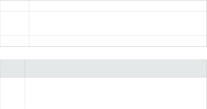
After you generate a Cross Result graph, you can filter it to display specific scenarios and
transactions. You can also manipulate the graph by changing the granularity, zoom, and scale.
You can view a summary report for the Cross Result graph.
How to Generate Merged Graphs
This task describes how to merge the results of two graphs from the same load test scenario into a
single graph. The merging allows you to compare several different measurements at once. For example,
you can make a merged graph to display the network delay and number of running Vusers, as a function
of the elapsed time.
You can merge all graphs with a common x-axis.
1. Select a graph in the Session Explorer or select its tab to make it active.
2. Choose View > Merge Graphs or click Merge Graphs. The Merge Graphs dialog box opens and
displays the name of the active graph.
3. Select a graph with which you want to merge your active graph. Only the graphs with a common x-
axis to the active graph are available.
4. Select the merge type and a title for the merged graph. By default, Analysis combines the titles of
the two graphs being merged. For more information, see "Merge Graphs Dialog Box" below.
5. Click OK.
6. Filter the graph just as you would filter any ordinary graph.
Merge Graphs Dialog Box
This dialog box enables you to merge two graphs into a single graph.
To access View > Merge Graphs
Important
information
In order to merge graphs, the graphs' x-axes must be the same measurement. For
example, you can merge Web Throughput and Hits per Second graphs, because their x-
axes are Scenario Elapsed Time.
See also "Merging Types Overview" on page121
User interface elements are described below:
UI
Element
Description
Select
Graph to
merge
with
The drop-down list shows all of the open graphs that share a common x-axis
measurement with the current graph. Select one of the graphs in the list.
User Guide
Analysis
HP LoadRunner (12.50) Page 124
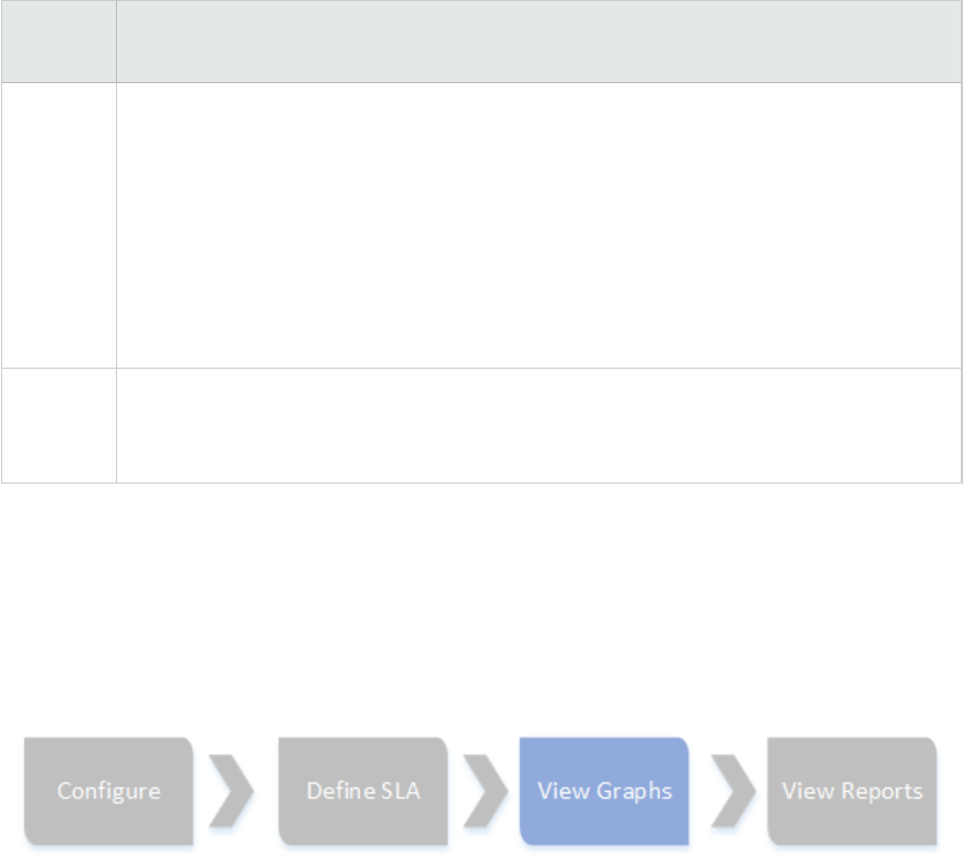
UI
Element
Description
Select
type of
merge
lOverlay. View contents of two graphs that share a common x-axis. The left y-axis on
the merged graph shows the current graph's values. The right y-axis shows the values
of the graph that was merged with the current graph.
lTile. View contents of two graphs that share a common x-axis in a tiled layout, one
above the other.
lCorrelate. Plot the y-axes of two graphs against each other. The active graph's y-axis
becomes the x-axis of the merged graph. The y-axis of the graph that was merged,
becomes the merged graph's y-axis.
Title of
Merged
Graph
Enter a title for the merged graph. This title will appear in the Session Explorer (Windows
> Session Explorer).
Analysis Graphs
Open a New Graph Dialog Box
User Guide
Analysis
HP LoadRunner (12.50) Page 125
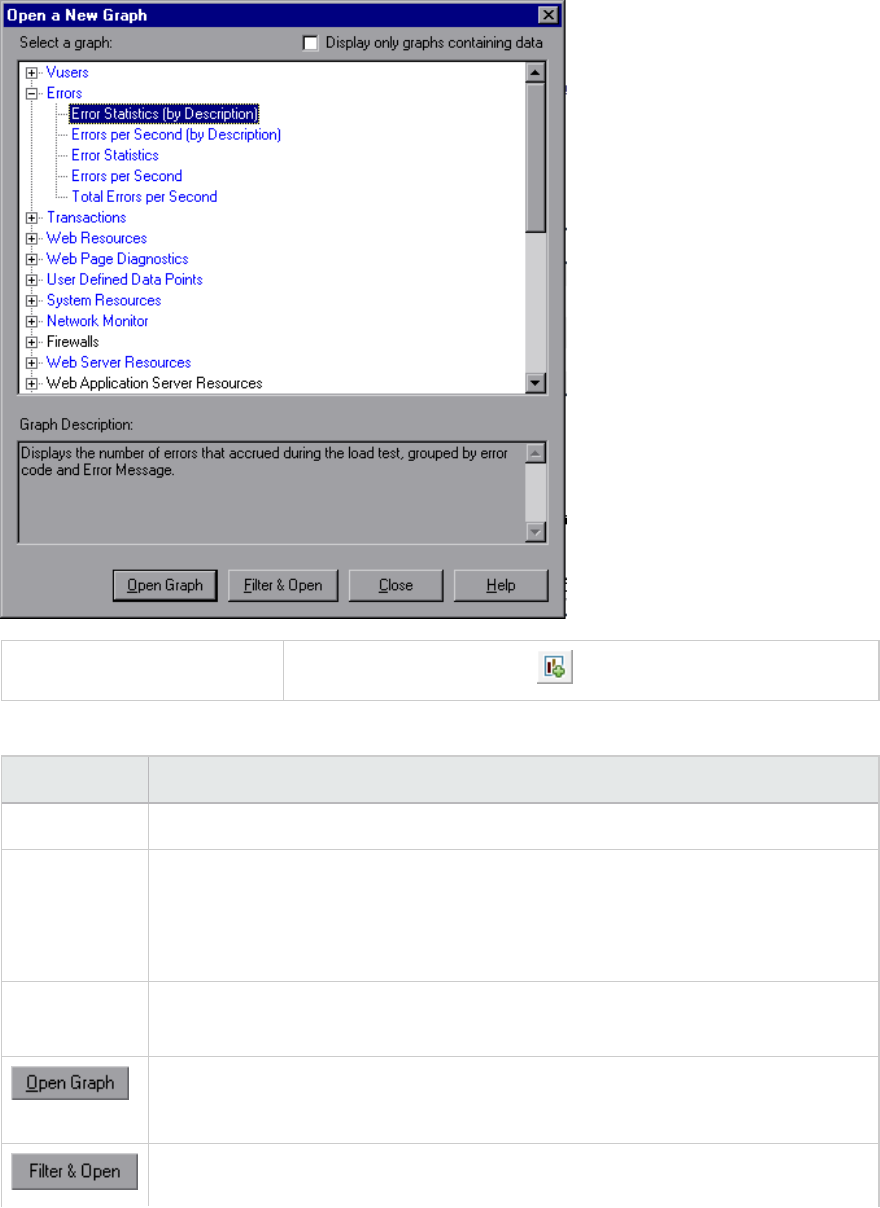
The Open a New Graph dialog box enables you to select the graph type to activate in the main Analysis
window.
To access Session Explorer > Graphs >
User interface elements are described below:
UI Element Description
Select a graph Displays list of graph types.
Display only
graphs
containing
data
If checked, only graphs that contain data are listed (in blue) in the Select a graph
area.
Graph
Description
Displays detailed information about the selected graph.
Analysis generates the selected graph and adds it to the
Session Explorer.
Opens the graphs Graph Settings dialog box. For details, see "Filter Dialog Boxes" on
User Guide
Analysis
HP LoadRunner (12.50) Page 126
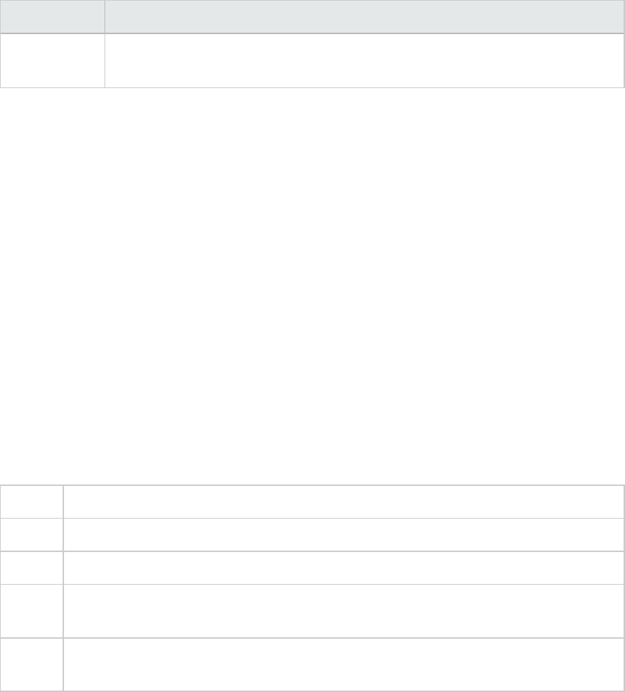
UI Element Description
page114. This option enables you to apply filter conditions on the selected graph
before the graph is displayed.
Vuser Graphs
During load test scenario execution, Vusers generate data as they perform transactions. The Vuser
graphs let you determine the overall behavior of Vusers during the scenario. They display the Vuser
states, the number of Vusers that completed the script, and rendezvous statistics. Use these graphs in
conjunction with Transaction graphs to determine the effect of the number of Vusers on transaction
response time. For more information about Transaction graphs, see "Transaction Graphs" on page135.
Rendezvous Graph (Vuser Graphs)
During a scenario run, you can instruct multiple Vusers to perform tasks simultaneously by using
rendezvous points. A rendezvous point creates intense user load on the server and enables LoadRunner
to measure server performance under load. For more information about using rendezvous points, see
the HP Virtual User Generator User Guide.
This graph indicates when Vusers were released from rendezvous points, and how many Vusers were
released at each point.
Purpose Helps you understand transaction performance times.
X-axis Elapsed time since the start of the run.
Y-axis Number of Vusers that were released from the rendezvous.
Tips Compare this to the Average Transaction Response Time graph. When you so this, you
can see how the load peak created by a rendezvous influences transaction times.
See
also
"Vuser Graphs" above
Example
User Guide
Analysis
HP LoadRunner (12.50) Page 127
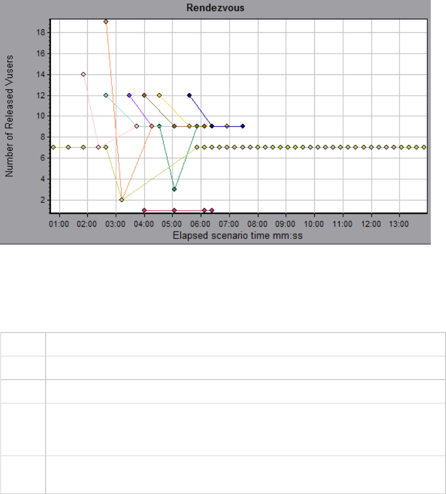
Running Vusers Graph
This graph displays the number of Vusers that executed Vuser scripts and their status during each
second of the test.
Purpose Helps you determine the Vuser load on your server at any given moment.
X-axis Elapsed time since the start of the run.
Y-axis Number of Vusers in the scenario.
Note By default, this graph only shows the Vusers with a Run status. To view another Vuser
status, set the filter conditions to the desired status. For more information, see "Filtering
and Sorting Graph Data" on page103.
See
also
"Vuser Graphs" on the previous page
Example
User Guide
Analysis
HP LoadRunner (12.50) Page 128
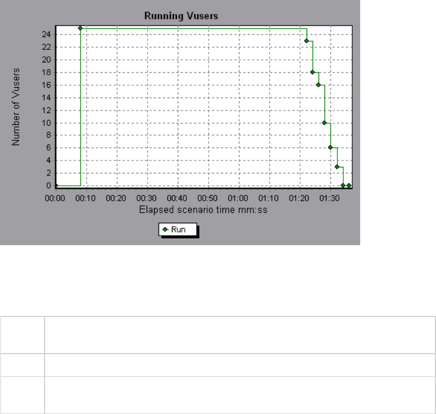
Vuser Summary Graph
This graph displays a summary of Vuser performance.
Purpose Lets you view the number of Vusers that successfully completed the load test scenario run
relative to those that did not.
Note This graph may only be viewed as a pie.
See
also
"Vuser Graphs" on page127
Example
User Guide
Analysis
HP LoadRunner (12.50) Page 129
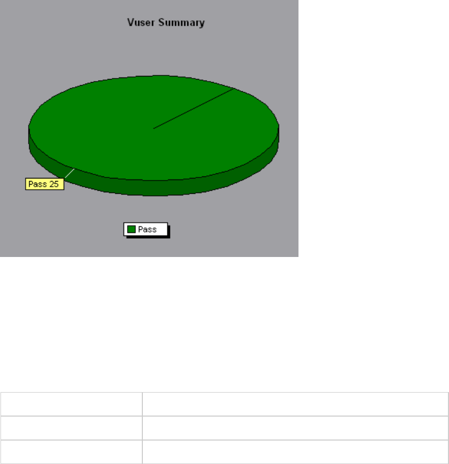
Error Graphs
Errors per Second (by Description) Graph
This graph displays the average number of errors that occurred during each second of the load test
scenario run, grouped by error description. The error description is displayed in the legend.
X-axis Elapsed time since the start of the run.
Y-axis Number of errors.
See also "Error Graphs" above
Example
User Guide
Analysis
HP LoadRunner (12.50) Page 130
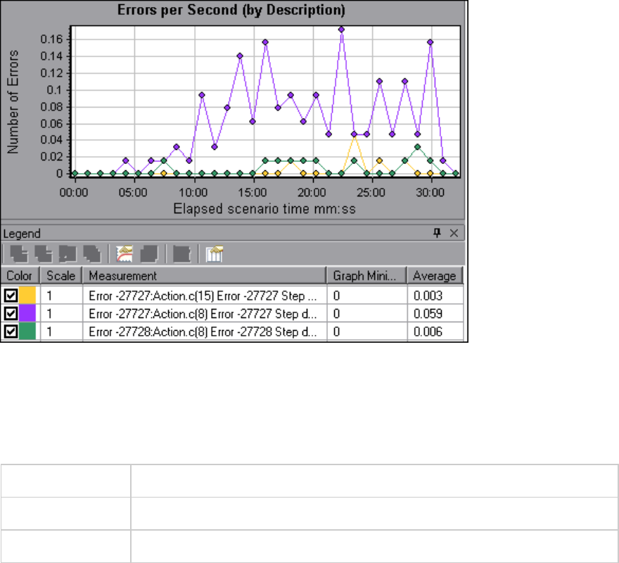
Errors per Second Graph
This graph displays the average number of errors that occurred during each second of the load test
scenario run, grouped by error code.
X-axis Elapsed time since the start of the run.
Y-axis Number of errors.
See also "Error Graphs" on the previous page
Example
User Guide
Analysis
HP LoadRunner (12.50) Page 131
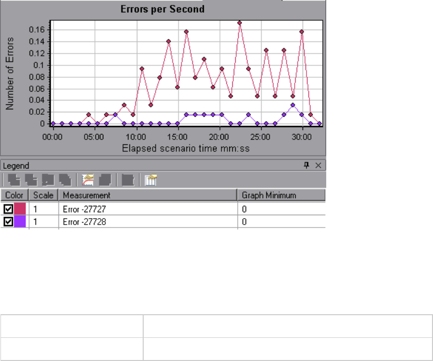
Error Statistics (by Description) Graph
This graph displays the number of errors that accrued during load test scenario execution, grouped by
error description. The error description is displayed in the legend.
Note This graph may only be viewed as a pie.
See also "Error Graphs" on page130
Example
User Guide
Analysis
HP LoadRunner (12.50) Page 132
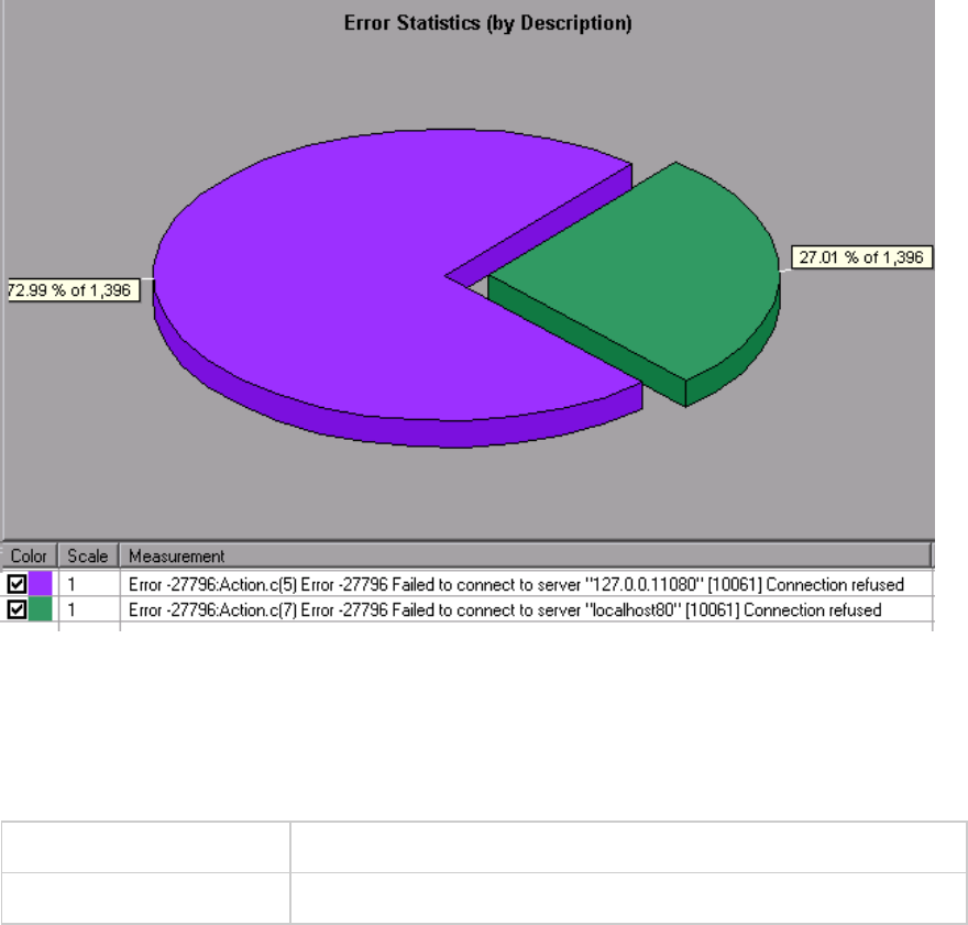
Error Statistics Graph
This graph displays the number of errors that accrued during load test scenario execution, grouped by
error code.
Note This graph may only be viewed as a pie.
See also "Error Graphs" on page130
Example
In the following example, out of a total of 178 errors that occurred during the scenario run, the second
error code displayed in the legend occurred twelve times, comprising 6.74% of the errors.
User Guide
Analysis
HP LoadRunner (12.50) Page 133
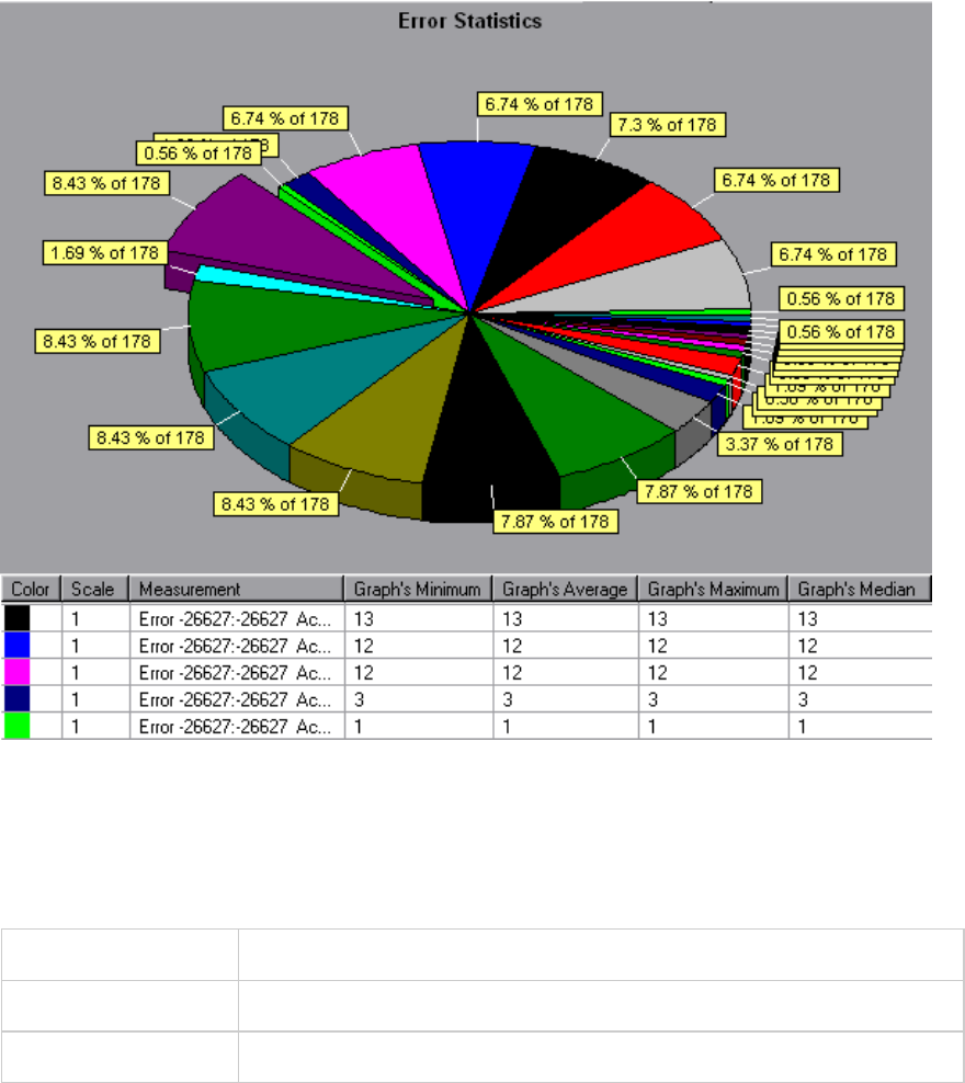
Total Errors per Second Graph
This graph displays the average number of errors that occurred during each second of the load test
scenario run. (complete: add sentence about being sum of all errors)
X-axis Elapsed time since the start of the run.
Y-axis Number of errors.
See also "Error Graphs" on page130
Example
User Guide
Analysis
HP LoadRunner (12.50) Page 134
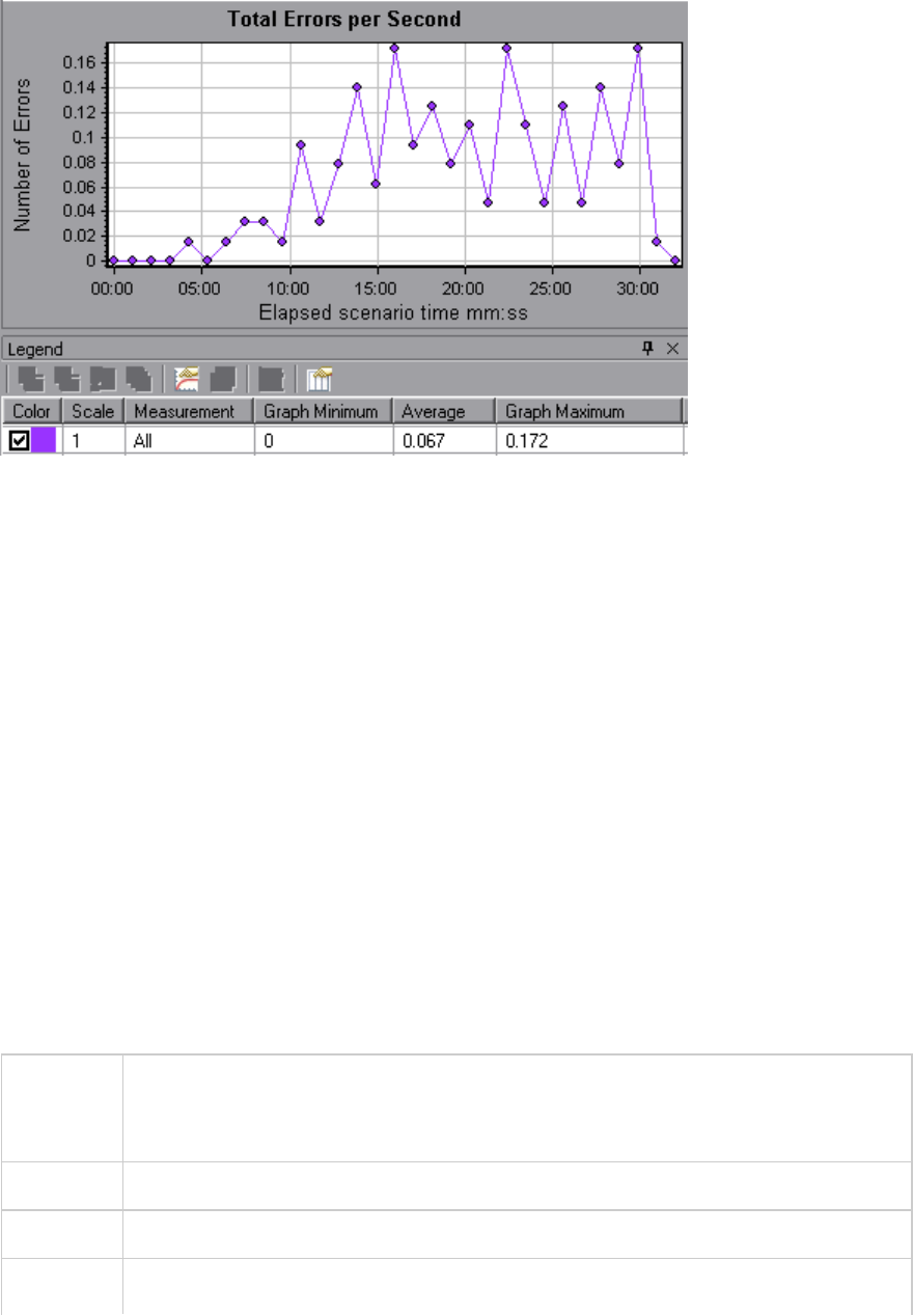
Transaction Graphs
During load test scenario execution, Vusers generate data as they perform transactions. Analysis
enables you to generate graphs that show the transaction performance and status throughout script
execution.
In addition, when working with HP Network Virtualization, you can view the transaction response times
per virtual location.
You can use additional Analysis tools such as merging and crossing results to understand your
transaction performance graphs. You can also sort the graph information by transactions and the
locations in which they were performed.
For more information, see the transaction graphs below.
Average Transaction Response Time Graph
This graph displays the average time taken to perform transactions during each second of the load test
scenario run.
Purpose If you have defined acceptable minimum and maximum transaction performance times,
you can use this graph to determine whether the performance of the server is within
the acceptable range.
X-axis Elapsed time since the start of the run.
Y-axis Average response time (in seconds) of each transaction
Breakdown Transaction Breakdown
User Guide
Analysis
HP LoadRunner (12.50) Page 135

options You can view a breakdown of a transaction by right-clicking the transaction in the
graph and selecting Show Transaction Breakdown Tree. In the Transaction
Breakdown Tree, right-click the transaction you want to break down, and select Break
Down <transaction name>. The Average Transaction Response Time graph displays
data for the sub-transactions. For more details, see "Transaction Breakdown Tree" on
page138.
Web Page Breakdown
To view a breakdown of the Web page(s) included in a transaction or sub-transaction,
right-click it and select Web Page Diagnostics for <transaction name>. For more
information on the Web Page Diagnostics graphs, see "Web Page Diagnostics Graphs"
on page157.
Tips Granularity
This graph is displayed differently for each granularity. The lower the granularity, the
more detailed the results. However, it may be useful to view the results with a higher
granularity to study the overall Vuser behavior throughout the scenario. For example,
using a low granularity, you may see intervals when no transactions were performed.
However, by viewing the same graph with a higher granularity, you will see the graph
for the overall transaction response time. For more information on setting the
granularity, see "How to Manage Graph Data" on page94.
Compare with Running Vusers
You can compare the Average Transaction Response Time graph to the Running
Vusers graph to see how the number of running Vusers affects the transaction
performance time. For example, if the Average Transaction Response Time graph
shows that performance time gradually improved, you can compare it to the Running
Vusers graph to see whether the performance time improved due to a decrease in
the Vuser load.
Note By default, only transactions that passed are displayed.
See also "Transaction Graphs" on the previous page
User Guide
Analysis
HP LoadRunner (12.50) Page 136
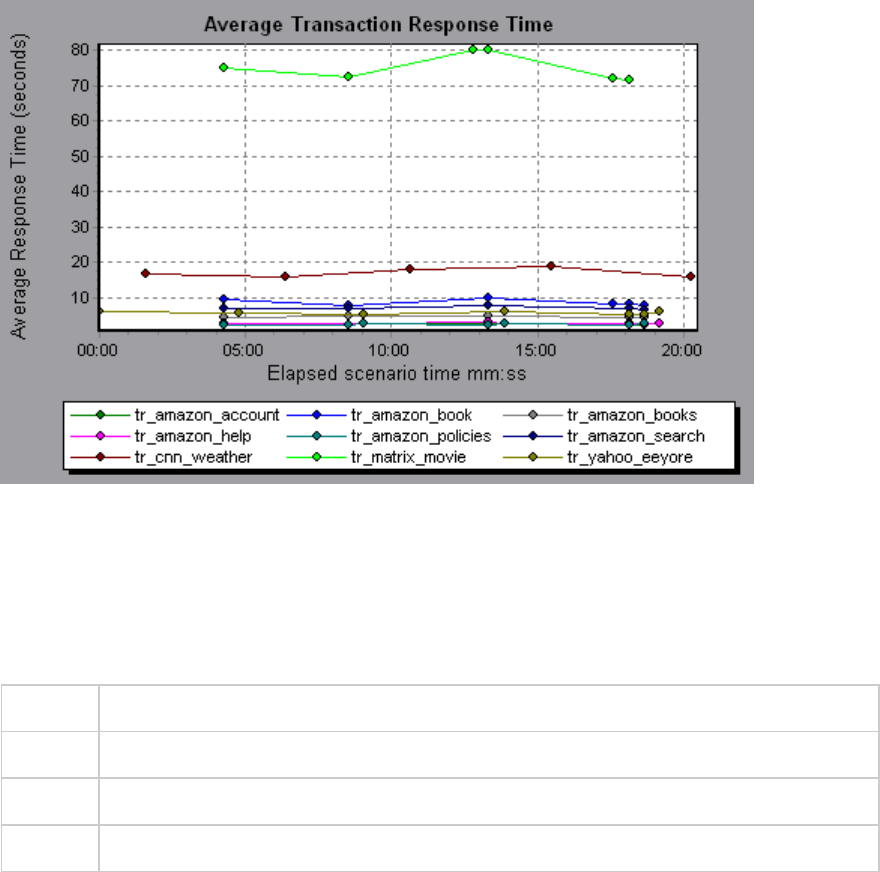
Example
Total Transactions per Second Graph
This graph displays the total number of transactions that passed, the total number of transactions that
failed, and the total number of transactions that were stopped, during each second of a load test
scenario run.
Purpose Helps you determine the actual transaction load on your system at any given moment.
X-axis Elapsed time since the start of the run.
Y-axis Total number of transactions performed during the scenario run.
See also "Transaction Graphs" on page135
User Guide
Analysis
HP LoadRunner (12.50) Page 137
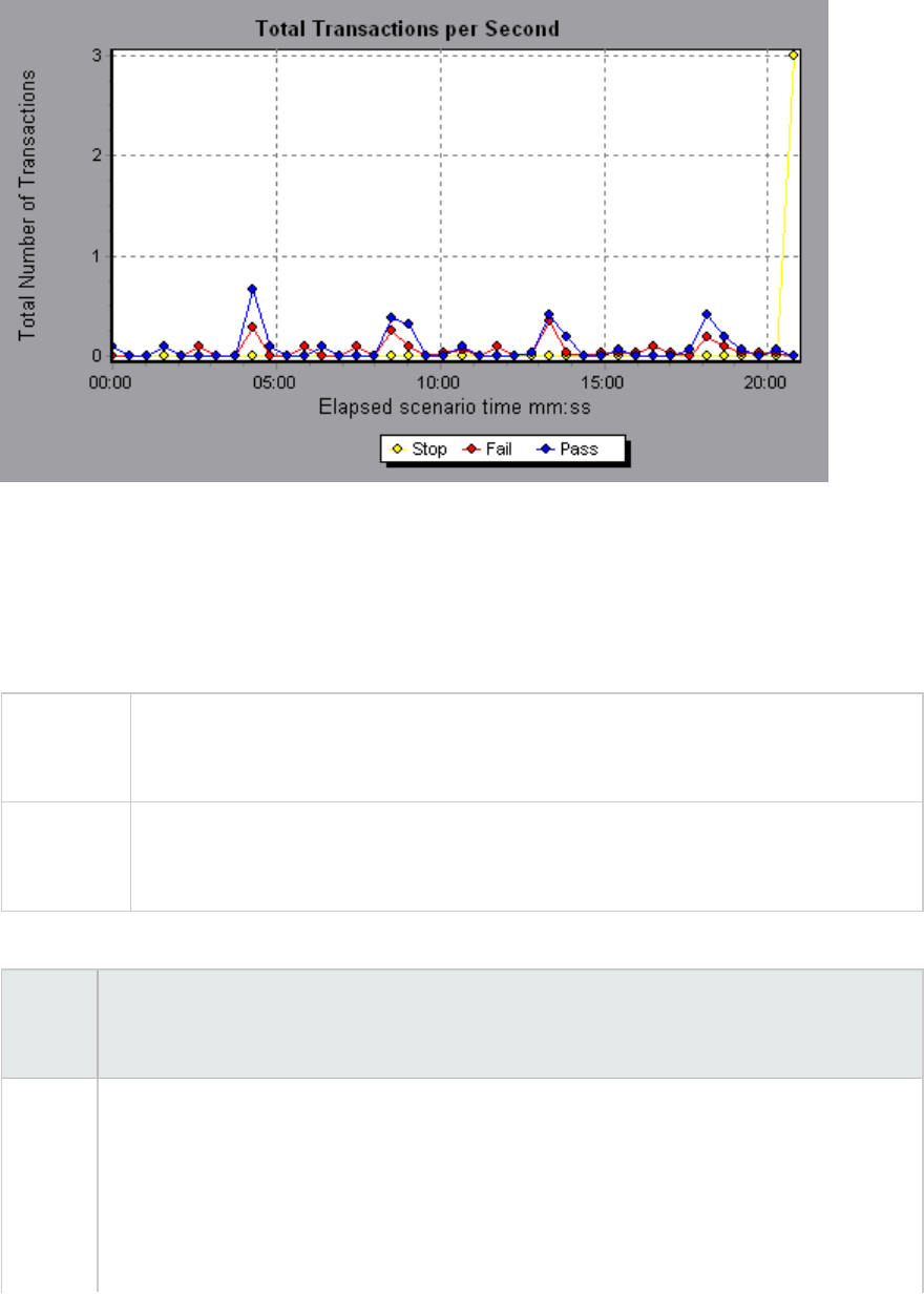
Example
Transaction Breakdown Tree
The Transaction Breakdown Tree displays a tree view of the transactions and sub-transactions in the
current session. From the tree, you can breakdown transactions and view the results of the breakdown
in either the Average Transaction Response Time or Transaction Performance Summary graph.
To access In either the Average Transaction Response Time or Transaction Performance
Summary graph, right-click in the graph and select Show Transaction Breakdown
Tree.
Important
information
After you breakdown a transaction, you can return to the original transaction graph by
reapplying the global filter (File > Set Global Filter) or by undoing your breakdown
actions using Edit > Undo Last Action.
User interface elements are described below (unlabeled elements are shown in angle brackets):
UI
Element
Description
<Right-
click
menu>
lBreak Down From Highest Level. Displays data for the highest level hierarchical path
of a transaction.
lBreak Down <transaction name>. Displays data for the sub-transactions in the
Average Transaction Response Time or Transaction Performance Summary graph.
lShow Only <transaction name>. Displays data only for the selected transaction/sub-
transaction.
User Guide
Analysis
HP LoadRunner (12.50) Page 138
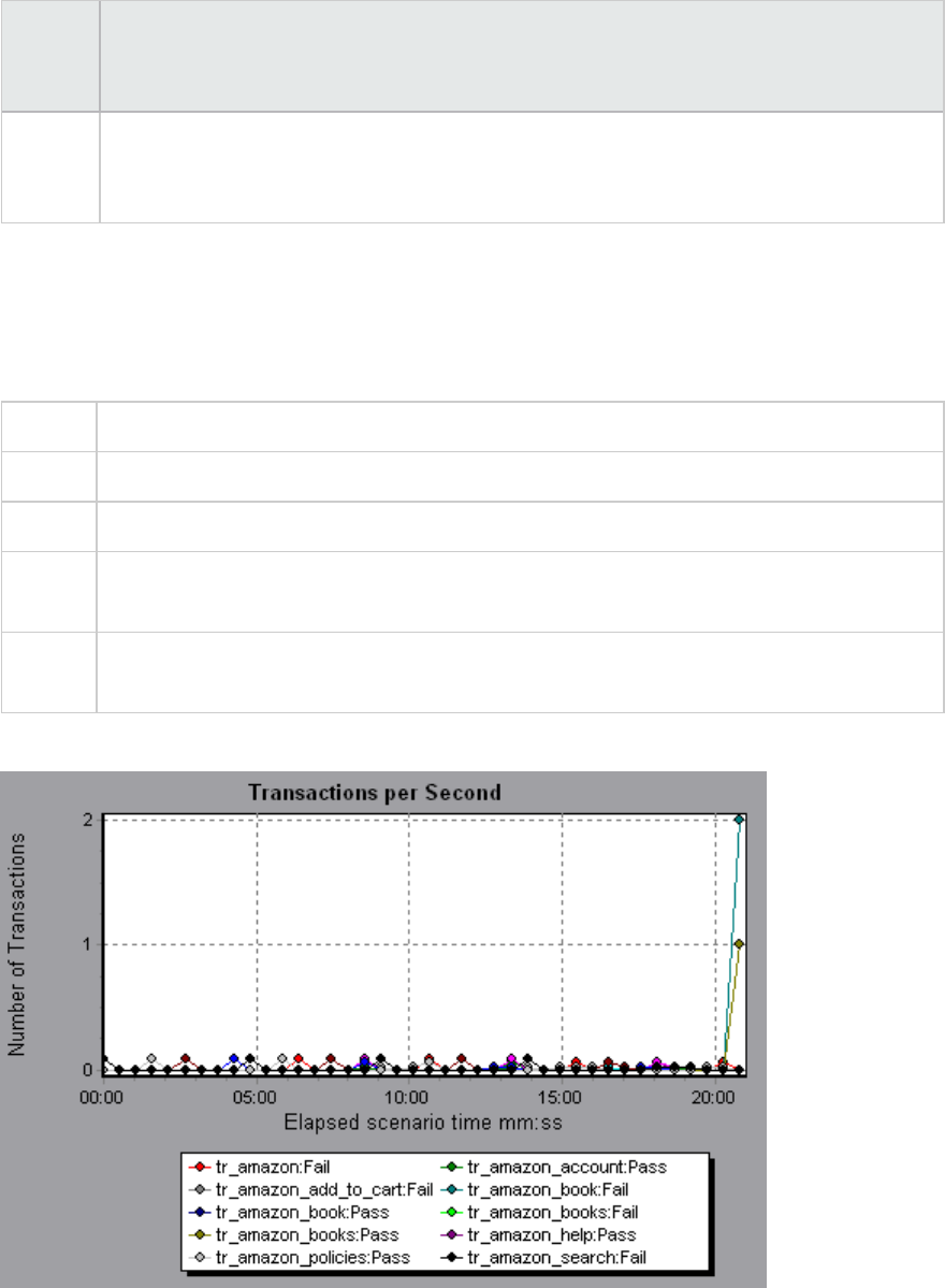
UI
Element
Description
lWeb Page Diagnostics for <page name>. Displays a breakdown of the Web page(s)
included in a transaction or sub-transaction in the Web Page Diagnostics graphs. For
details, see "Web Page Diagnostics Graphs" on page157.
Transactions per Second Graph
This graph displays, for each transaction, the number of times it passed, failed, and stopped during
each second of a load test scenario run.
Purpose Helps you determine the actual transaction load on your system at any given moment.
X-axis Elapsed time since the start of the run.
Y-axis Number of transactions performed during the scenario run.
Tips Compare with the Average Transaction Response Time Graph. Doing this helps you
analyze the effect of the amount of transactions upon the performance time.
See
also
"Transaction Graphs" on page135
Example
User Guide
Analysis
HP LoadRunner (12.50) Page 139
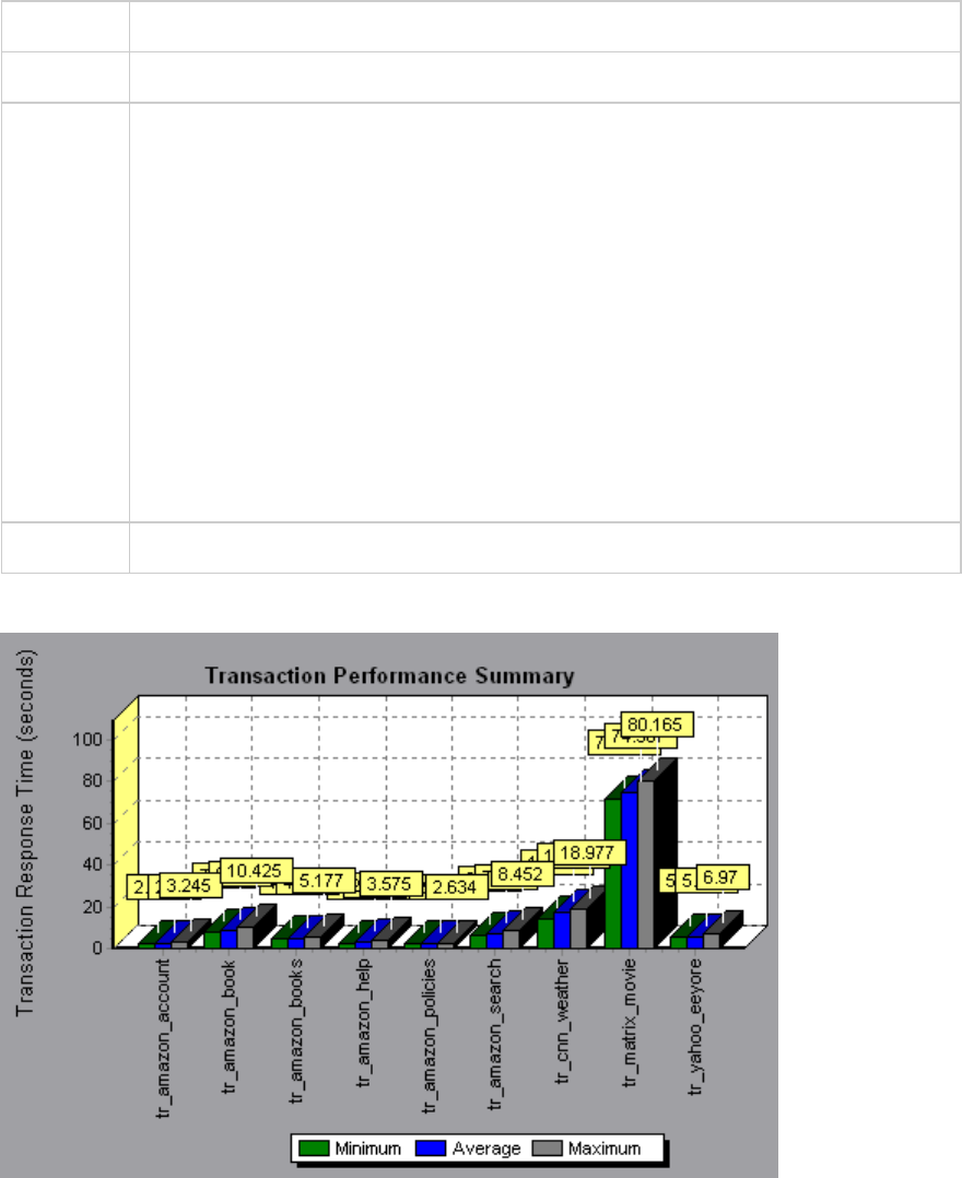
Transaction Performance Summary Graph
This graph displays the minimum, maximum and average performance time for all the transactions in
the load test scenario.
X-axis Name of the transaction.
Y-axis Response time—rounded off to the nearest second—of each transaction.
Breakdown
options
Transaction Breakdown
You can view breakdown of a transaction in the Transaction Performance Summary
graph by right-clicking the transaction in the graph and selecting Show Transaction
Breakdown Tree. In the Transaction Breakdown Tree, right-click the transaction you
want to break down, and select Break Down <transaction name>. The Transaction
Performance Summary graph displays data for the sub-transactions. For more
details, see "Transaction Breakdown Tree" on page138.
Web Page Breakdown
To view a breakdown of the Web page(s) included in a transaction or sub-transaction,
right-click it and select Web Page Diagnostics for <transaction name>. For more, see
"Web Page Diagnostics Graphs" on page157.
See also "Transaction Graphs" on page135
Example
User Guide
Analysis
HP LoadRunner (12.50) Page 140
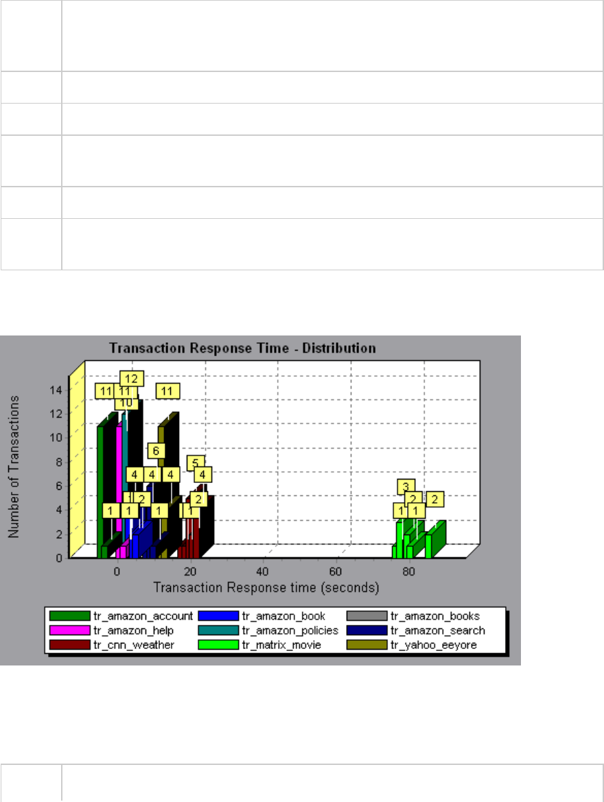
Transaction Response Time (Distribution) Graph
This graph displays the distribution of the time taken to perform transactions in a load test scenario.
Purpose If you have defined acceptable minimum and maximum transaction performance times,
you can use this graph to determine whether the performance of the server is within the
acceptable range.
X-axis Transaction response time (rounded down to the nearest second).
Y-axis Number of transactions executed during the scenario.
Tips Compare with Transaction Performance Summary Graph to see how the average
performance was calculated.
Note This graph can only be displayed as a bar graph.
See
also
"Transaction Graphs" on page135
Example
In the following example, most of the transactions had a response time of less than 20 seconds.
Transaction Response Time (Percentile) Graph
This graph analyzes the percentage of transactions that were performed within a given time range.
Purpose Helps you determine the percentage of transactions that met the performance criteria
User Guide
Analysis
HP LoadRunner (12.50) Page 141
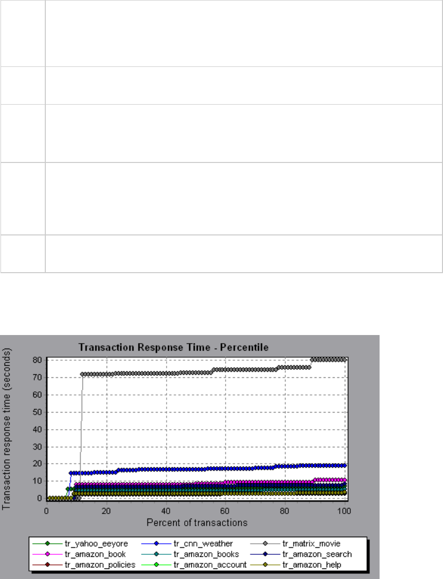
defined for your system. In many instances, you need to determine the percent of
transactions with an acceptable response time. The maximum response time may be
exceptionally long, but if most transactions have acceptable response times, the overall
system is suitable for your needs.
X-axis Percentage of the total number of transactions measured during the load test scenario
run.
Y-axis Maximum transaction response time (in seconds).
Note: Analysis approximates the transaction response time for each available percentage
of transactions. The y-axis values, therefore, may not be exact.
Tips Compare with the Average Response Time Graph.
A high response time for several transactions may raise the overall average. However, if
the transactions with a high response time occurred less than five percent of the time,
that factor may be insignificant.
See
also
"Transaction Graphs" on page135
Example
In the following example, fewer than 20 percent of the tr_matrix_movie transactions had a response
time less than 70 seconds.
User Guide
Analysis
HP LoadRunner (12.50) Page 142
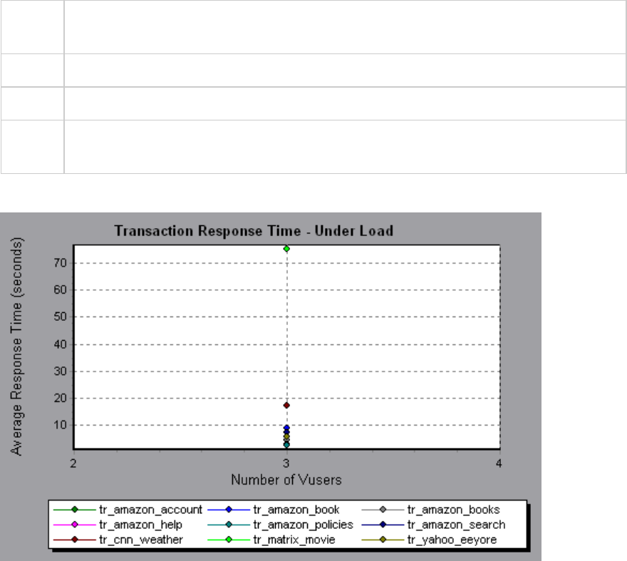
Transaction Response Time (Under Load) Graph
This graph is a combination of the Running Vusers and Average Transaction Response Time graphs and
indicates transaction times relative to the number of Vusers running at any given point during the load
test scenario.
Purpose Helps you view the general impact of Vuser load on performance time and is most useful
when analyzing a scenario with a gradual load.
X-axis Number of running Vusers
Y-axis Average response time (in seconds) of each transaction.
See
also
"Transaction Graphs" on page135
Example
Transaction Response Time by Location Graph
This graph indicates the transaction response times relative to the virtual locations in which they were
performed.
This graph is used in conjunction with Network Virtualization. Using HP Network Virtualization, you set up
a scenario that runs Vusers on several virtual locations. This graph lets you compare the transaction
response times of the various locations. For details, see Network Virtualization Integration.
User Guide
Analysis
HP LoadRunner (12.50) Page 143
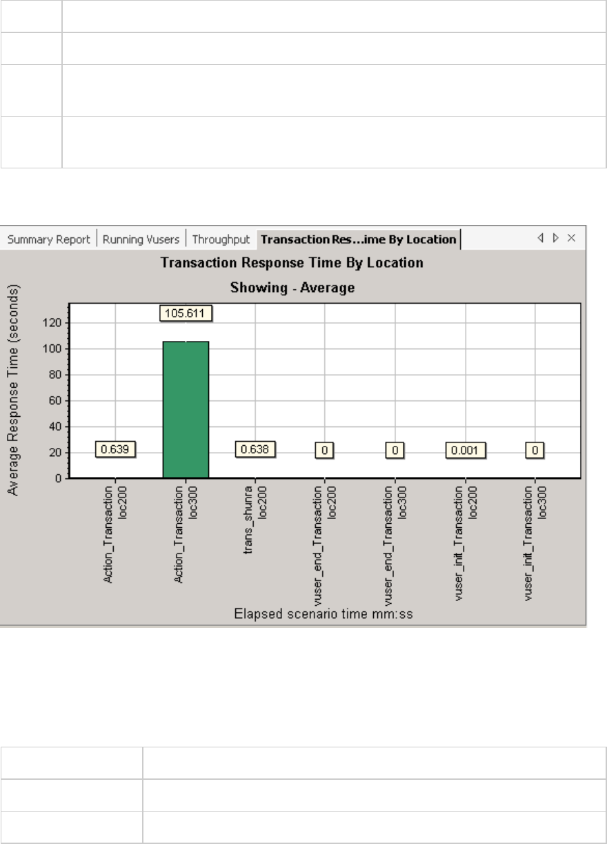
Purpose Helps you view the general impact of Vuser load on performance time per virtual location.
X-axis Elapsed scenario time in mm:ss
Y-axis Average response time (in seconds) of each transaction, per virtual location. A bar chart
and annotation, show the average response times.
See
also
"Transaction Graphs" on page135
The following example shows the transaction response time for several locations. It is evident that the
response time was excessive in location loc300.
Transaction Summary Graph
This graph summarizes the number of transactions in the load test scenario that failed, passed,
stopped, and ended in error.
X-axis Name of the transaction
Y-axis Number of transactions performed during the scenario run.
See also "Transaction Graphs" on page135
User Guide
Analysis
HP LoadRunner (12.50) Page 144
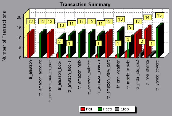
Example
Web Resources Graphs
Web Resources Graphs Overview
Web Resource graphs provide you with information about the performance of your Web server. You use
the Web Resource graphs to analyze the following data:
lThroughput on the Web server
lThe number of hits per second
lThe number of HTTP responses per second
lThe HTTP status codes returned from the Web server
lThe number of downloaded pages per second
lThe number of server retries per second
lA summary of the server retries during the load test scenario
lThe number of open TCP/IP connections
lThe number of TCP/IP connections per second
lThe number of new and reused SSL connections opened per second
User Guide
Analysis
HP LoadRunner (12.50) Page 145
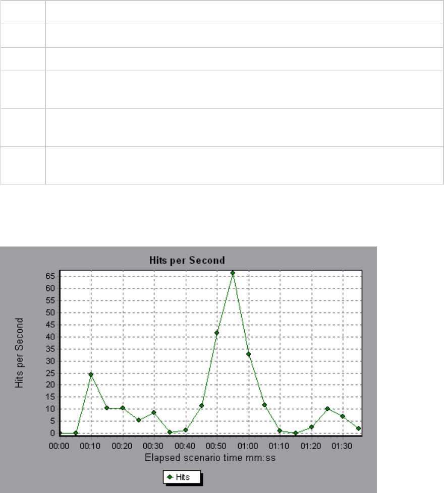
Hits per Second Graph
This graph shows the number of HTTP requests made by Vusers to the Web server during each second
of the load test scenario run.
Purpose Helps you evaluate the amount of load Vusers generate, in terms of the number of hits.
X-axis Elapsed time since the start of the run.
Y-axis Number of hits on the server.
Tips Compare to the Average Transaction Response Time graph to see how the number of hits
affects transaction performance.
Note You cannot change the granularity of the x-axis to a value that is less than the Web
granularity you defined in the General tab of the Options dialog box.
See
also
"Web Resources Graphs Overview" on the previous page
Example
In the following example, the most hits per second took place during the fifty-fifth second of the
scenario.
Throughput Graph
This graph shows the amount of throughput on the server during each second of the load test scenario
run. Throughput is measured in bytes or megabytes and represents the amount of data that the Vusers
User Guide
Analysis
HP LoadRunner (12.50) Page 146
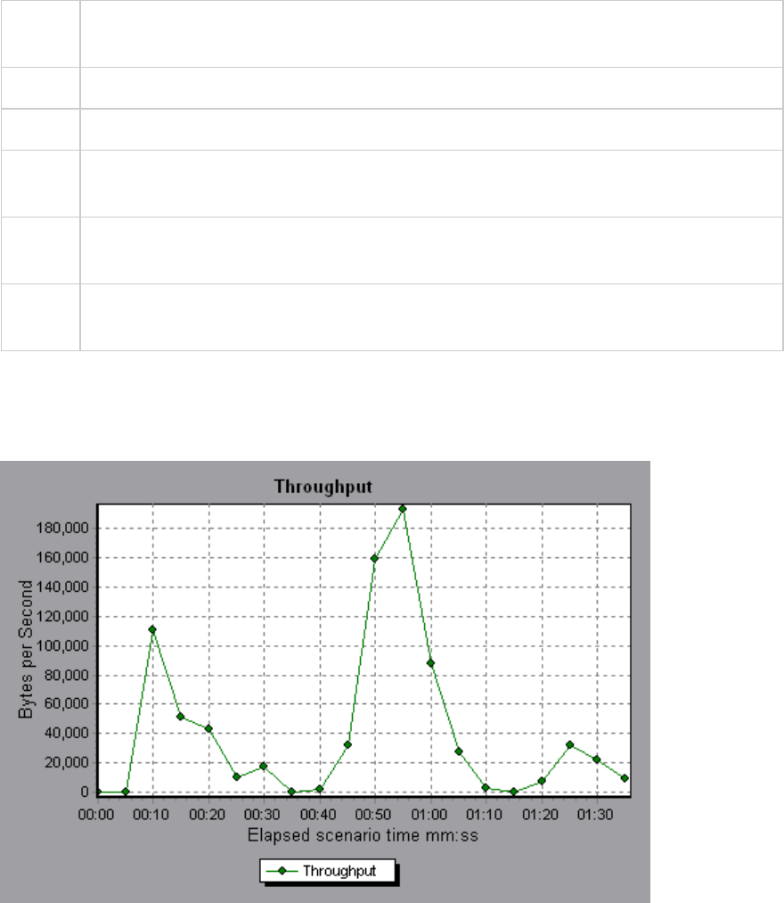
received from the server at any given second. To view throughput in megabytes, use the Throughput
(MB) graph.
Purpose Helps you evaluate the amount of load that Vusers generate, in terms of server
throughput.
X-axis Elapsed time since the start of the scenario run.
Y-axis Throughput of the server, in bytes or megabytes.
Tips Compare to the Average Transaction Response Time graph to see how the throughput
affects transaction performance.
Note You cannot change the granularity of the x-axis to a value that is less than the Web
granularity you defined in the General tab of the Options dialog box.
See
also
"Web Resources Graphs Overview" on page145
Example
In the following example, the highest throughput is 193,242 bytes during the fifty-fifth second of the
scenario.
HTTP Status Code Summary Graph
This graph shows the number of HTTP status codes returned from the Web server during the load test
scenario run, grouped by status code. HTTP status codes indicate the status of HTTP requests, for
example, "the request was successful","the page was not found".
User Guide
Analysis
HP LoadRunner (12.50) Page 147
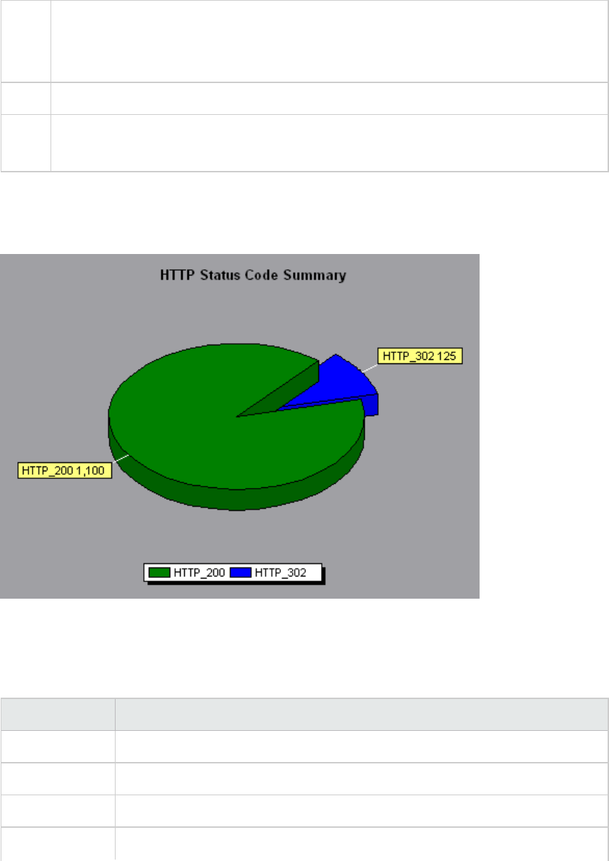
Tips Locate scripts which generated error codes
Use this graph together with the HTTP Responses per Second graph to locate those scripts
which generated error codes.
Note This graph can only be viewed as a pie.
See
also
l"Web Resources Graphs Overview" on page145
l"HTTP Status Codes" below
Example
In the following example, the graph shows that only the HTTP status codes 200 and 302 were generated.
Status code 200 was generated 1,100 times, and status code 302 was generated 125 times.
HTTP Status Codes
The following table displays a list of HTTP status codes:
Code Description
200 OK
201 Created
202 Accepted
203 Non-Authoritative Information
User Guide
Analysis
HP LoadRunner (12.50) Page 148
Code Description
204 No Content
205 Reset Content
206 Partial Content
300 Multiple Choices
301 Moved Permanently
302 Found
303 See Other
304 Not Modified
305 Use Proxy
307 Temporary Redirect
400 Bad Request
401 Unauthorized
402 Payment Required
403 Forbidden
404 Not Found
405 Method Not Allowed
406 Not Acceptable
407 Proxy Authentication Required
408 Request Timeout
409 Conflict
410 Gone
411 Length Required
412 Precondition Failed
413 Request Entity Too Large
414 Request - URI Too Large
415 Unsupported Media Type
User Guide
Analysis
HP LoadRunner (12.50) Page 149
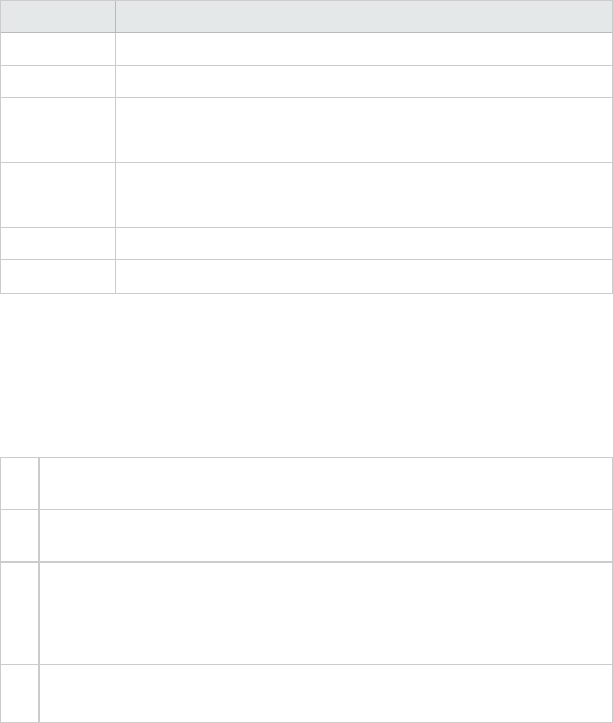
Code Description
416 Requested range not satisfiable
417 Expectation Failed
500 Internal Server Error
501 Not Implemented
502 Bad Gateway
503 Service Unavailable
504 Gateway Timeout
505 HTTP Version not supported
For more information on the above status codes and their descriptions, see http://www.w3.org.
HTTP Responses per Second Graph
This graph shows the number of HTTP status codes returned from the Web server during each second
of the load test scenario run, grouped by status code. HTTP status codes indicate the status of HTTP
requests, for example, "the request was successful", "the page was not found".
X-
axis
Elapsed time since the start of the run.
Y-
axis
Number of HTTP responses per second.
Tips Locate scripts which generated error codes
You can group the results shown in this graph by script (using the "Group By" function) to
locate scripts which generated error codes. For more information on the "Group By" function,
see "Filtering and Sorting Graph Data" on page103.
See
also
l"Web Resources Graphs Overview" on page145
l"HTTP Status Codes" on page148
Example
In the following example, the greatest number of 200 status codes, 60, was generated in the fifty-fifth
second of the scenario run. The greatest number of 302 codes, 8.5, was generated in the fiftieth second
of the scenario run.
User Guide
Analysis
HP LoadRunner (12.50) Page 150
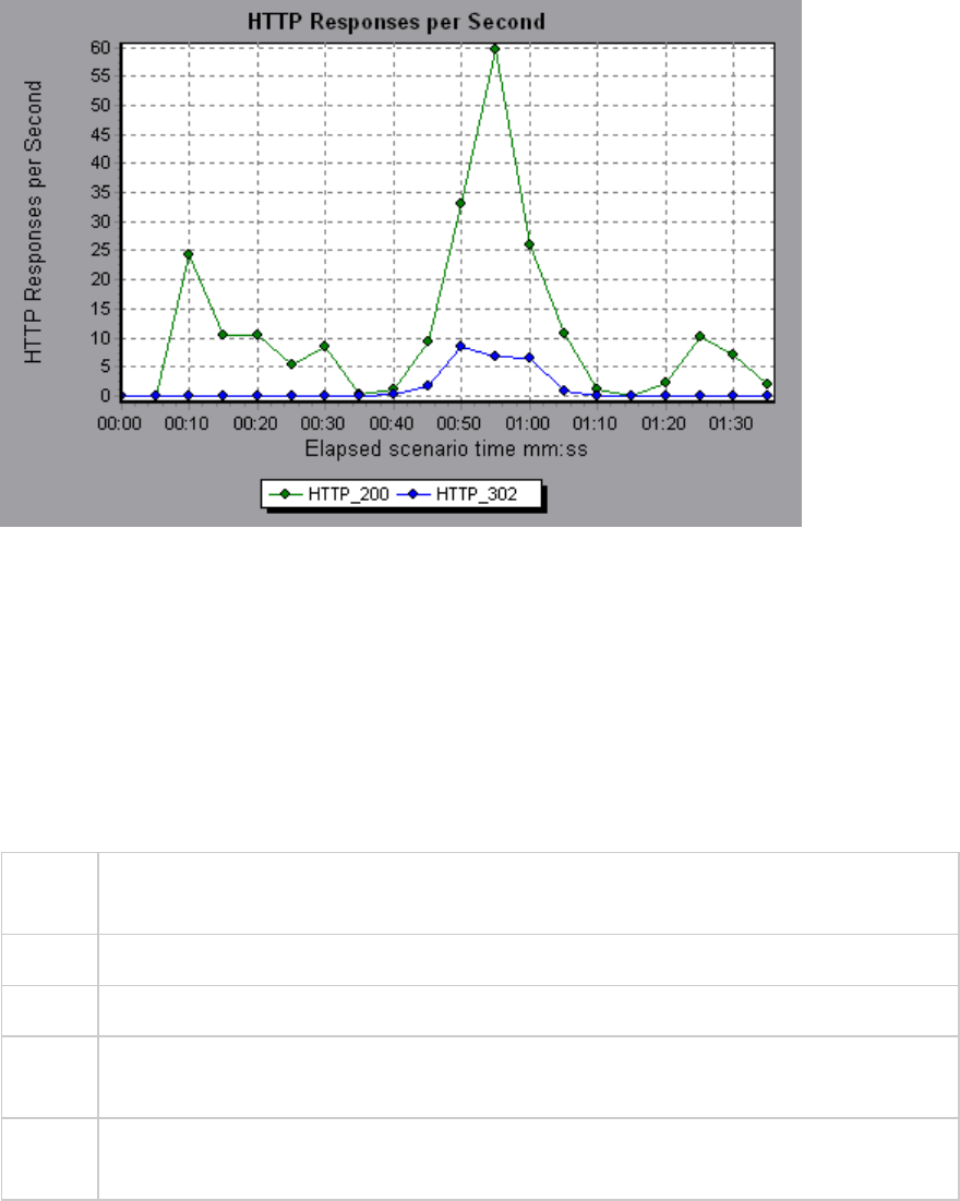
Pages Downloaded per Second Graph
This graph shows the number of Web pages downloaded from the server during each second of the load
test scenario run.
Like the Throughput graph, the Pages Downloaded per Second graph represents the amount of data
that the Vusers received from the server at any given second. However, the Throughput graph takes
into account each resource and its size (for example, the size of each .gif file, the size of each Web
page). The Pages Downloaded per Second graph takes into account only the number of pages.
Purpose Helps you evaluate the amount of load Vusers generate, in terms of the number of pages
downloaded.
X-axis Elapsed time since the start of the run.
Y-axis Number of Web pages downloaded from the server.
Note To view the Pages Downloaded per Second graph, you must select Pages per second (HTML
Mode only) from the runtime settings Preferences tab before running your scenario.
See
also
"Web Resources Graphs Overview" on page145
Example 1
In the following example, the greatest number of pages downloaded per second, about 7, occurred in
the fiftieth second of the scenario run.
User Guide
Analysis
HP LoadRunner (12.50) Page 151
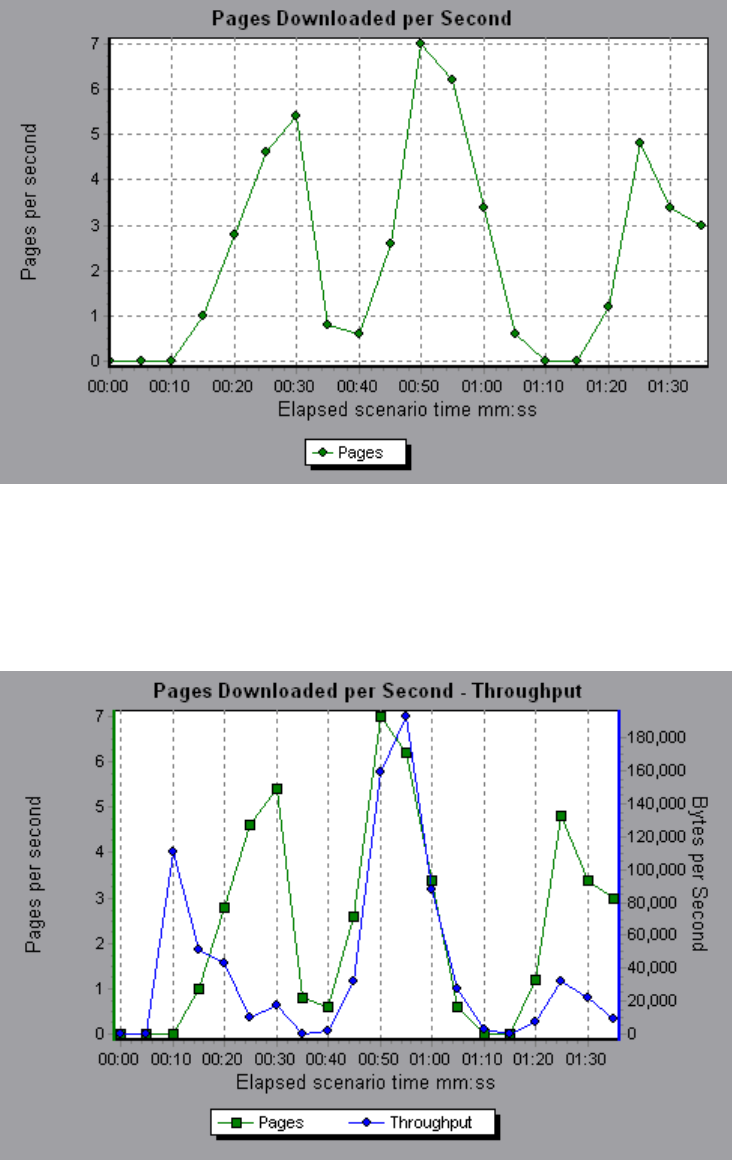
Example 2
In the following example, the Throughput graph is merged with the Pages Downloaded per Second
graph. It is apparent from the graph that throughput is not completely proportional to the number of
pages downloaded per second. For example, between 10 and 25 seconds into the scenario run, the
number of pages downloaded per second increased while the throughput decreased.
User Guide
Analysis
HP LoadRunner (12.50) Page 152
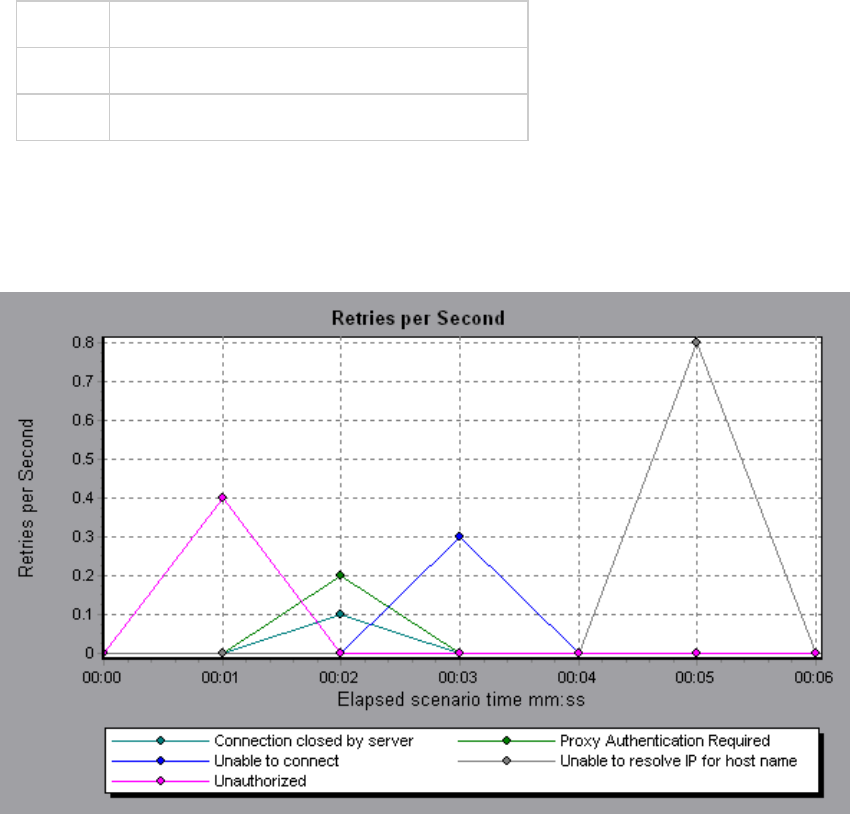
Retries per Second Graph
This graph displays the number of attempted server connections during each second of the load test
scenario run. A server connection is retried when:
lthe initial connection was unauthorized
lproxy authentication is required
lthe initial connection was closed by the server
lthe initial connection to the server could not be made
lwhen the server was initially unable to resolve the load generator's IP address
X-axis Elapsed time since the start of the run.
Y-axis Number of server retries per second.
See also "Web Resources Graphs Overview" on page145
Example
In the following example, the graph shows that during the first second of the scenario, the number of
retries was 0.4, whereas in the fifth second of the scenario, the number of retries per second rose to
0.8.
User Guide
Analysis
HP LoadRunner (12.50) Page 153
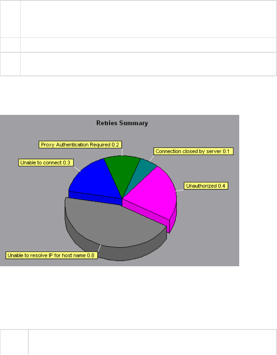
Retries Summary Graph
This graph shows the number of attempted server connections during the load test scenario run,
grouped by the cause of the retry.
Tips Determine when server retries were attempted
Use this graph together with the Retries per Second graph to determine at what point
during the scenario the server retries were attempted.
Note This graph may only be viewed as a pie.
See
also
"Web Resources Graphs Overview" on page145
Example
In the following example, the graph shows that the server's inability to resolve the load generator's IP
address was the leading cause of server retries during the scenario run.
Connections Graph
This graph shows the number of open TCP/IP connections (y-axis) at each point in time of the load test
scenario (x-axis). Depending on the emulated browser type, each Vuser may open several simultaneous
connections per Web server.
Purpose This graph is useful in indicating when additional connections are needed. For example, if
the number of connections reaches a plateau, and the transaction response time
User Guide
Analysis
HP LoadRunner (12.50) Page 154
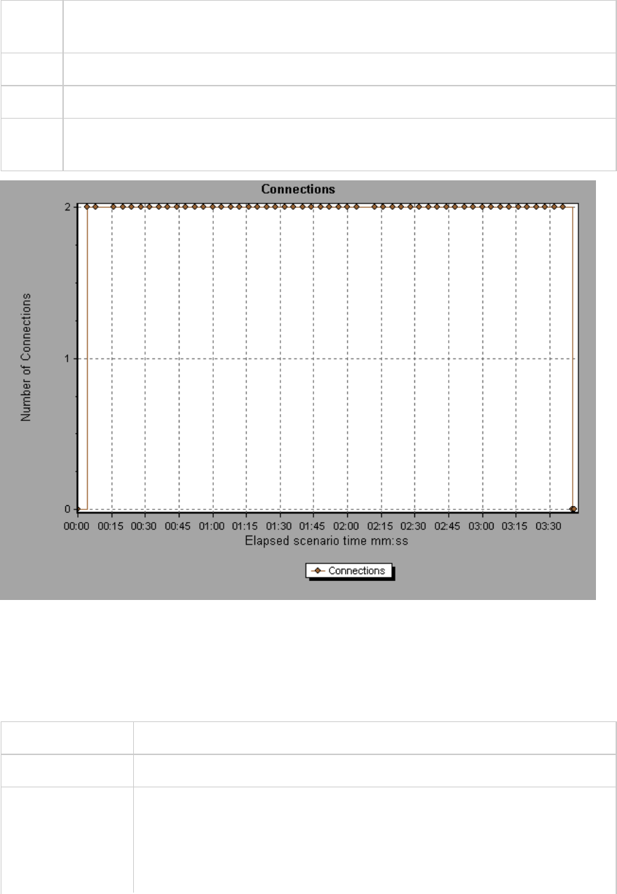
increases sharply, adding connections would probably cause a dramatic improvement in
performance (reduction in the transaction response time).
X-axis Elapsed time since the start of the run.
Y-axis Open TCP/IP connections.
See
also
"Web Resources Graphs Overview" on page145
Connections per Second Graph
This graph shows the number of new TCP/IP connections (y-axis) opened and the number of connections
that are shut down for each second of the load test scenario (x-axis).
X-axis Elapsed time since the start of the run.
Y-axis TCP/IP connections per second.
Tips New connections versus hits per second:
The number of new connections should be a small fraction of the number of
hits per second, because new TCP/IP connections are very expensive in terms
of server, router and network resource consumption. Ideally, many HTTP
User Guide
Analysis
HP LoadRunner (12.50) Page 155
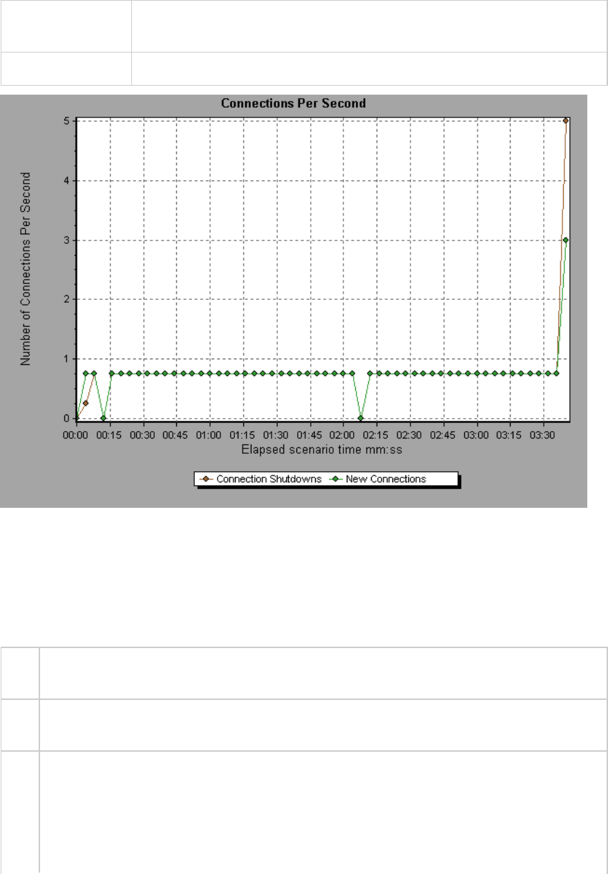
requests should use the same connection, instead of opening a new
connection for each request.
See also "Web Resources Graphs Overview" on page145
SSLs per Second Graph
This graph shows the number of new and reused SSL Connections (y-axis) opened in each second of the
load test scenario (x-axis). An SSL connection is opened by the browser after a TCP/IP connection has
been opened to a secure server.
X-
axis
Elapsed time since the start of the run.
Y-
axis
Number of SSL Connections
Tips Reduce SSL connections
Creating a new SSL connection entails heavy resource consumption. Therefore, you should
try to open as few new SSL connections as possible. Once you've established an SSL
connection, you should reuse it. There should be no more than one new SSL connection per
Vuser.
User Guide
Analysis
HP LoadRunner (12.50) Page 156
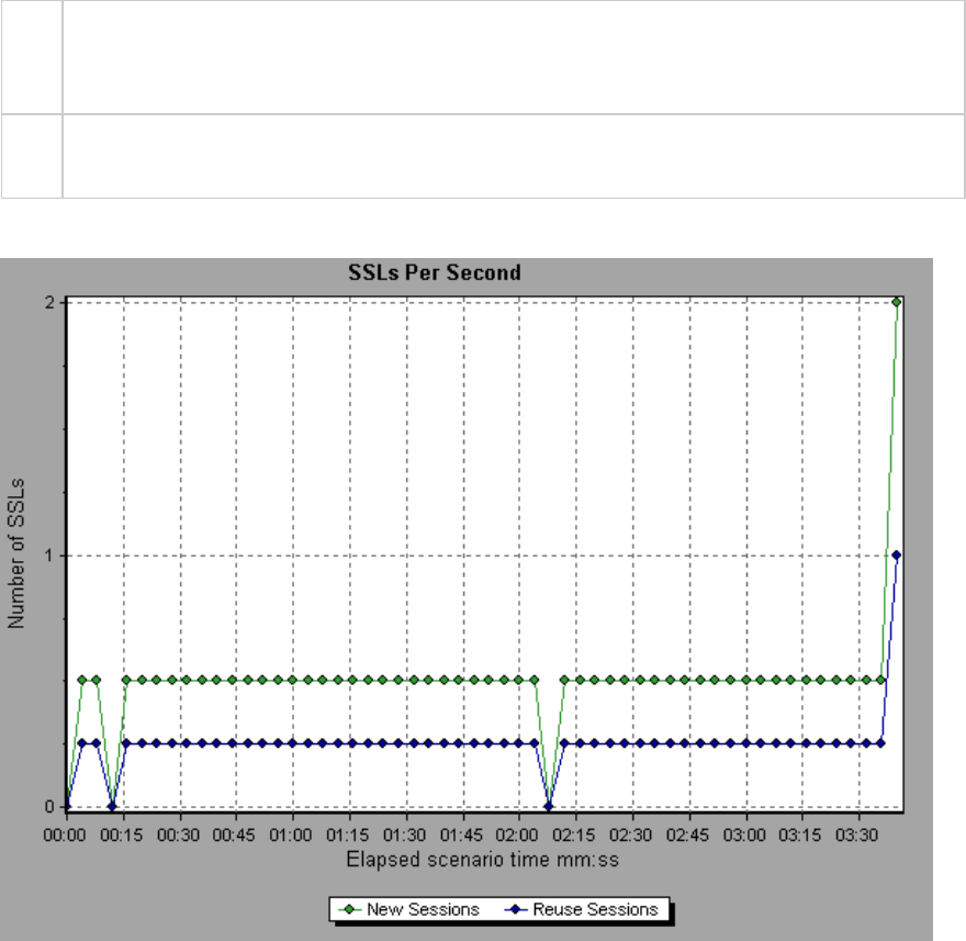
In cases where you reset TCP connections between iterations (VuGen Runtime Settings >
Browser Emulation node > Simulate a new user on each iteration), you should have no
more than one new SSL connection per iteration.
See
also
"Web Resources Graphs Overview" on page145
Example
Web Page Diagnostics Graphs
Web Page Diagnostics Tree View Overview
The Web Page Diagnostics tree view displays a tree view of the transactions, sub-transactions, and Web
pages for which you can view Web Page Diagnostics graphs. For more information about Web Page
Diagnostics graphs, see "Web Page Diagnostics Graph" on page161.
The Web Page Diagnostics graphs enable you to assess whether transaction response times were
affected by page content. Using the Web Page Diagnostics graphs, you can analyze problematic
elements—for example, images that download slowly, or broken links—of a Web site.
User Guide
Analysis
HP LoadRunner (12.50) Page 157
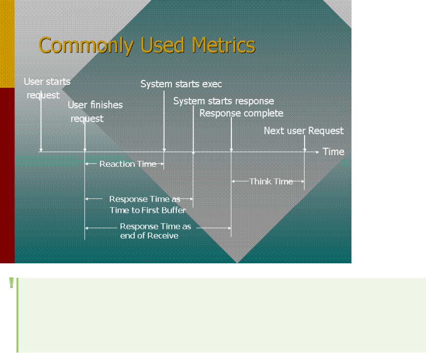
Web Page Diagnostics Graphs Overview
Web Page Diagnostics graphs provide you with performance information for each monitored Web page
in your script. You can view the download time of each page in the script and its components, and
identify at what point during download time problems occurred. In addition, you can view the relative
download time and size of each page and its components. Analysis displays both average download time
and download time over time data.
You correlate the data in the Web Page Diagnostics graphs with data in the Transaction Performance
Summary and Average Transaction Response Time graphs in order to analyze why and where problems
are occurring, and whether the problems are network- or server-related.
The following diagram illustrates the sequence of events from the time an HTTP request is sent:
Note: Because server time is being measured from the client, network time may influence this
measurement if there is a change in network performance from the time the initial HTTP
request is sent until the time the first buffer is sent. The server time displayed, therefore, is
estimated server time and may be slightly inaccurate.
You begin analyzing the Transaction Performance Summary and Average Transaction Response Time
graphs with the Web Page Diagnostics graph, which displays the average download time (in seconds) for
each monitored Web page during each second of the load test scenario run. The x-axis represents the
elapsed time from the beginning of the scenario run. The y-axis represents the average download time
(in seconds) for each Web page.
User Guide
Analysis
HP LoadRunner (12.50) Page 158
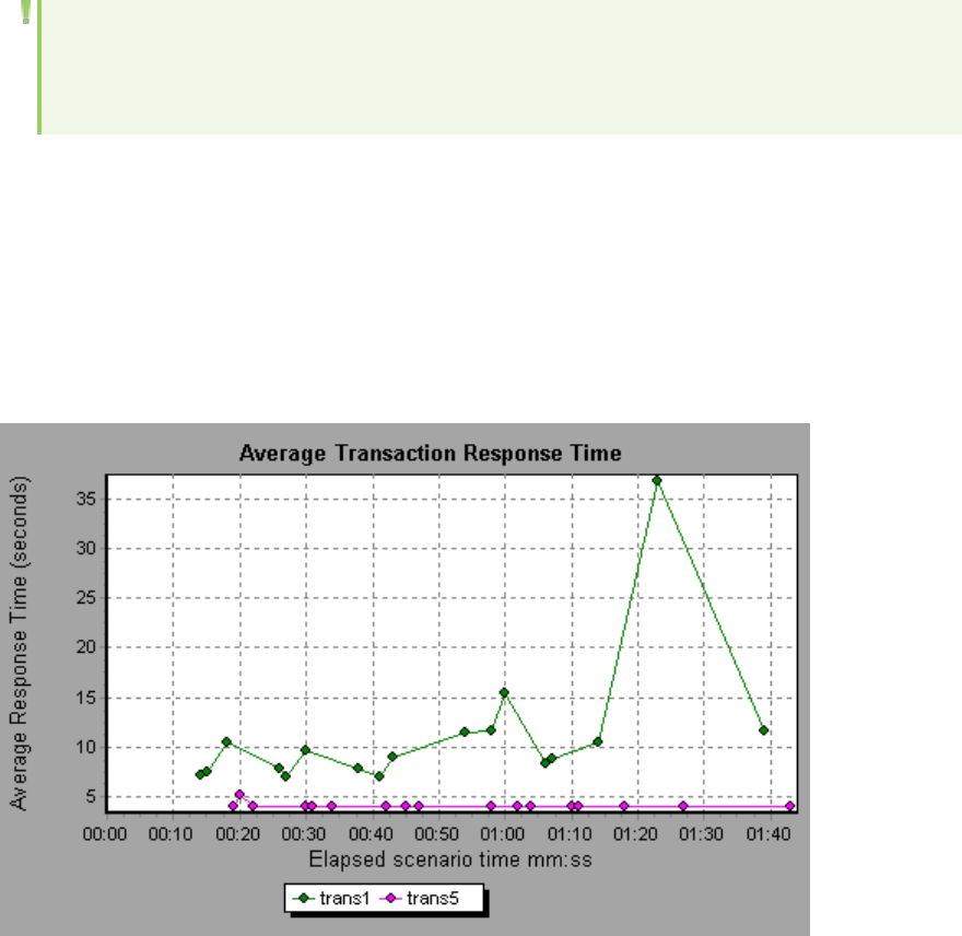
These graphs can also be used for analyzing mobile applications using the Mobile Application -
HTTP/HTML protocol.
In order for Analysis to generate Web Page Diagnostics graphs, you must enable the Web Page
Diagnostics feature in the Controller before running your scenario.
1. From the Controller menu, choose Diagnostics > Configuration and select the Enable the
following diagnostics check box.
2. In the Offline Diagnostics section, if the button to the right of Web Page Diagnostics (Max. Vuser
Sampling: 10%) says Enable, click it.
Note: When preparing a Web HTTP/HTML Vuser script for which you want to perform Web
diagnostics, it is recommended that you create an HTML-based script (using the Recording tab
in the Recording Options).
For more information on recording scripts, refer to the VuGen section in the LoadRunner User Guide.
How to View the Breakdown of a Transaction
The Web Page Diagnostics graphs are most commonly used to analyze a problem detected in the
Transaction Performance Summary or Average Transaction Response Time graphs. For example, the
Average Transaction Response Time graph below demonstrates that the average transaction response
time for the trans1 transaction was high.
Using the Web Page Diagnostics graphs, you can pinpoint the cause of the delay in response time for
the trans1 transaction.
This task describes how to breakdown a transaction.
User Guide
Analysis
HP LoadRunner (12.50) Page 159
1. Right-click trans1 and select Web Page Diagnostics for trans1. The Web Page Diagnostics graph
opens and the Web Page Diagnostics tree appear. An icon appears next to the page name
indicating the page content. See "Web Page Diagnostics Content Icons" below.
2. In the Web Page Diagnostics tree, right-click the problematic page you want to break down, and
select Break Down <component name>. Alternatively, select a page in the Select Page to Break
Down box that appears under the Web Page Diagnostics graph. The Web Page Diagnostics graph
for that page appears.
Note: You can open a browser displaying the problematic page by right-clicking the page in
the Web Page Diagnostics tree and selecting View page in browser.
3. Select one of the following available breakdown options:
lDownload Time. Displays a table with a breakdown of the selected page's download time. The
size of each page component (including the component's header) is displayed. See the "Page
Download Time Breakdown Graph" on page165 for more information about this display.
lComponent (Over Time). Displays the "Page Component Breakdown (Over Time) Graph" on
page164 for the selected Web page.
lDownload Time (Over Time). Displays the "Page Download Time Breakdown (Over Time) Graph"
on page167 for the selected Web page.
lTime to First Buffer (Over Time). Displays the "Time to First Buffer Breakdown (Over Time)
Graph" on page172 for the selected Web page.
To display the graphs in full view, click the button. You can also access these graphs, as well
as additional Web Page Diagnostics graphs, from the Open a New Graph dialog box.
Web Page Diagnostics Content Icons
The following icons appear in the Web Page Diagnostics tree. They indicate the HTTP content of the
page.
Name Description
Transaction. Specifies that the ensuing content is part of the transaction.
Page Content. Specifies that the ensuing content, which may include text, images, and so on,
is all part of one logical page.
Text content. Textual information. Plain text is intended to be displayed as-is. Includes HTML
text and style sheets.
Multipart content. Data consisting of multiple entities of independent data types.
Message content. An encapsulated message. Common subtypes are news, or external-body
User Guide
Analysis
HP LoadRunner (12.50) Page 160
Name Description
which specifies large bodies by reference to an external data source.
Application content. Some other kind of data, typically either uninterpreted binary data or
information to be processed by an application. An example subtype is Postscript data.
Image content. Image data. Two common subtypes are the jpeg and gif format.
Resource content. Other resources not listed above. Also, content that is defined as "not
available" is likewise included.
Web Page Diagnostics Graph
The Web Page Diagnostics graph provides you with performance information for each monitored Web
page in your script. You can view the download time of each page in the script and its components, and
identify at what point during download time problems occurred. In addition, you can view the average
download time of each page and its components.
Purpose This graph enables you to determine at what point during scenario execution a network
or server problem occurred, that may have affected access to the Web page.
X-axis Elapsed time from the beginning of the scenario run.
Y-axis The download time (in seconds) for each Web page in the download process.
Tips lChoose a page in the Select Page to Break Down drop-down box.
lTo isolate the most problematic components, you can sort the legend window
according to the average number of seconds taken to download a component. To
sort the legend by average, double-click the Average column heading.
Diagnostic
Options
You can choose one of the following options to drill down on the results. For sample
graphs, see below.
lDownload Time - as a bar graph
lComponent (Over Time) - as a line graph
lDownload Time (Over Time) - as an area graph
lTime to First Buffer (Over Time) - as an area graph
See also "Web Page Diagnostics Tree View Overview" on page157
Example
This graph enables you to monitor the download time during the scenario execution, to determine at
what point network or server problems occurred.
User Guide
Analysis
HP LoadRunner (12.50) Page 161
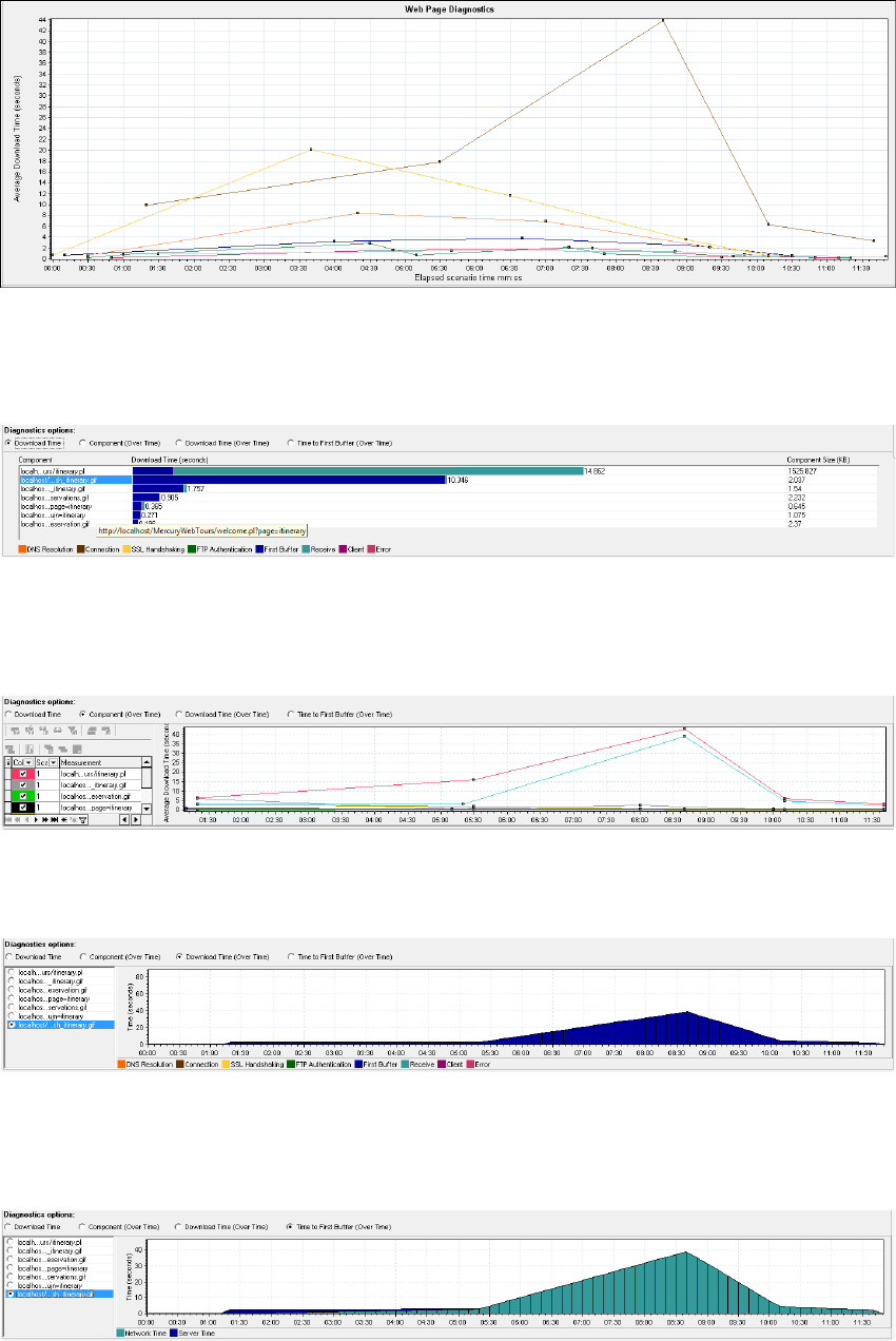
Download Time
In the following example, the download time for the itinerary.pl page was the greatest during the
Receive stage.
Component(Over Time)
In the following example, the download time for the itinerary.pl component was the greatest at
approximately 8:40 into the scenario.
Download Time (Over Time)
The following graph shows the download time for the itinerary.pl page as an area graph.
Time to First Buffer (Over Time)
In the following example, the download time for the splash_itinerary.gif file was the greatest
approximately 8:40 into the scenario.
User Guide
Analysis
HP LoadRunner (12.50) Page 162
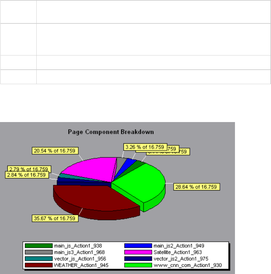
Page Component Breakdown Graph
This graph displays the average download time (in seconds) for each Web page and its components.
Breakdown
options
To ascertain which components caused the delay in download time, you can break down
the problematic URL by double-clicking it in the Web Page Diagnostics tree.
Tips To isolate problematic components, it may be helpful to sort the legend according to
the average number of seconds taken to download a component. To sort the legend by
average, click the Graph's Average column.
Note The graph can only be viewed as a pie.
See also "Web Page Diagnostics Graphs Overview" on page158
Example
The following graph demonstrates that the main cnn.com URL took 28.64% of the total download time,
compared to 35.67% for the www.cnn.com/WEATHER component.
Example
The graph shows that the main cnn.com/WEATHER component took the longest time to download
(8.98% of the total download time).
User Guide
Analysis
HP LoadRunner (12.50) Page 163
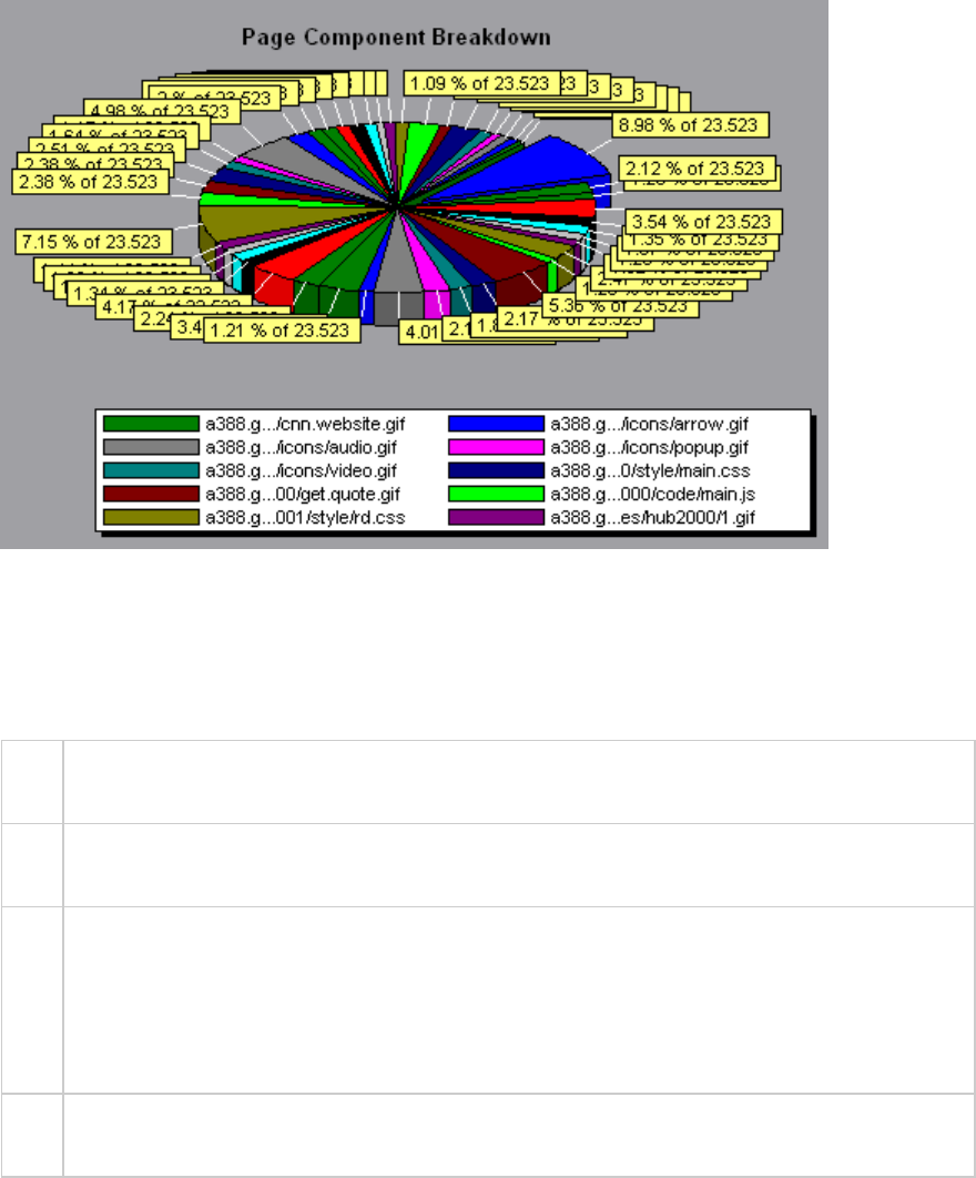
Page Component Breakdown (Over Time) Graph
This graph displays the average response time (in seconds) for each Web page and its components
during each second of the load test scenario run.
X-
axis
The elapsed time from the beginning of the scenario run.
Y-
axis
The average response time (in seconds) for each component.
Tips lTo isolate the most problematic components, it may be helpful to sort the legend window
according to the average number of seconds taken to download a component. To sort the
legend by average, double-click the Average column heading.
lTo identify a component in the graph, you can select it. The corresponding line in the legend
window is selected.
See
also
"Web Page Diagnostics Graphs Overview" on page158
Example
The following graph demonstrates that the response time for Satellite_Action1_963 was significantly
greater, throughout the scenario, than the response time for main_js_Action1_938.
User Guide
Analysis
HP LoadRunner (12.50) Page 164
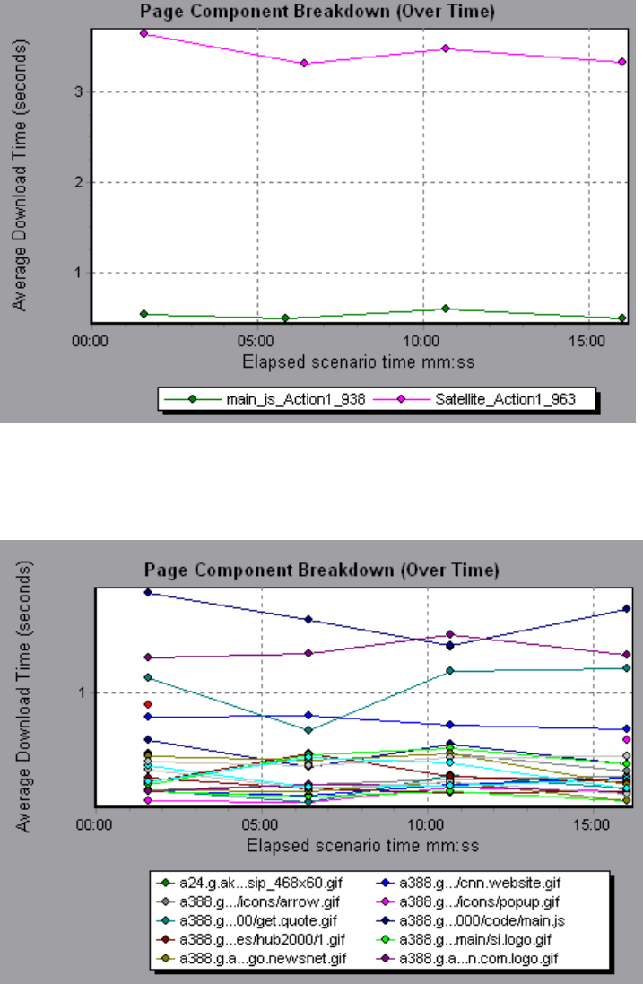
Example
Using the graph, you can track which components of the main component were most problematic, and
at which point(s) during the scenario the problem(s) occurred.
Page Download Time Breakdown Graph
This graph displays a breakdown of each page component's download time.
User Guide
Analysis
HP LoadRunner (12.50) Page 165
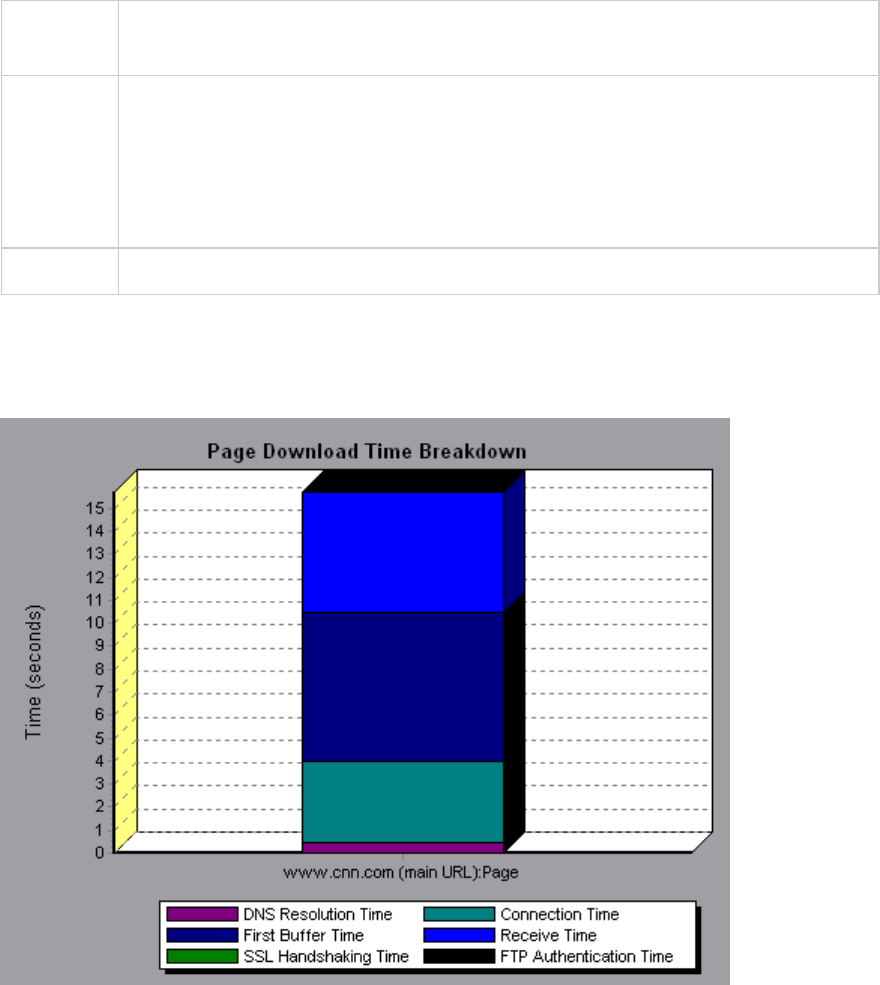
Purpose Enables you to determine whether slow response times are being caused by network or
server errors during Web page download.
Breakdown
options
For breakdown options, see "Page Download Time Breakdown Graph Breakdown
Options" on page169.
Note: Each measurement displayed on the page level is the sum of that measurement
recorded for each page component. For example, the Connection Time for
www.cnn.com is the sum of the Connection Time for each of the page's components.
See also "Web Page Diagnostics Graphs Overview" on page158
Example
The Page Download Time Breakdown graph demonstrates that receive time, connection time, and first
buffer time accounted for a large portion of the time taken to download the main cnn.com URL.
Example
If you break the cnn.com URL down further, you can isolate the components with the longest download
time, and analyze the network or server problems that contributed to the delay in response time.
Breaking down the cnn.com URL demonstrates that for the component with the longest download time
(the www.cnn.com component), the receive time accounted for a large portion of the download time.
User Guide
Analysis
HP LoadRunner (12.50) Page 166
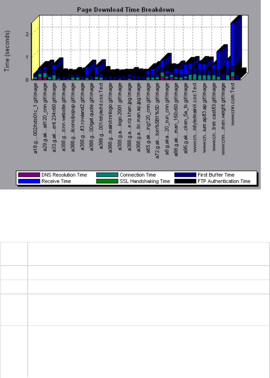
Page Download Time Breakdown (Over Time) Graph
The graph displays a breakdown of each page component's download time during each second of the
load test scenario run.
Purpose This graph enables you to determine at what point during scenario execution network or
server problems occurred.
X-axis Elapsed time from the beginning of the scenario run.
Y-axis Time (in seconds) taken for each step in the download process.
Tips To isolate the most problematic components, you can sort the legend window according to
the average number of seconds taken to download a component. To sort the legend by
average, double-click the Average column heading.
Notes lEach measurement displayed on the page level is the sum of that measurement
recorded for each page component. For example, the Connection Time for www.cnn.com
is the sum of the Connection Time for each of the page's components.
lWhen the Page Download Time Breakdown (Over Time) graph is selected from the Web
Page Diagnostics graph, it appears as an area graph.
User Guide
Analysis
HP LoadRunner (12.50) Page 167
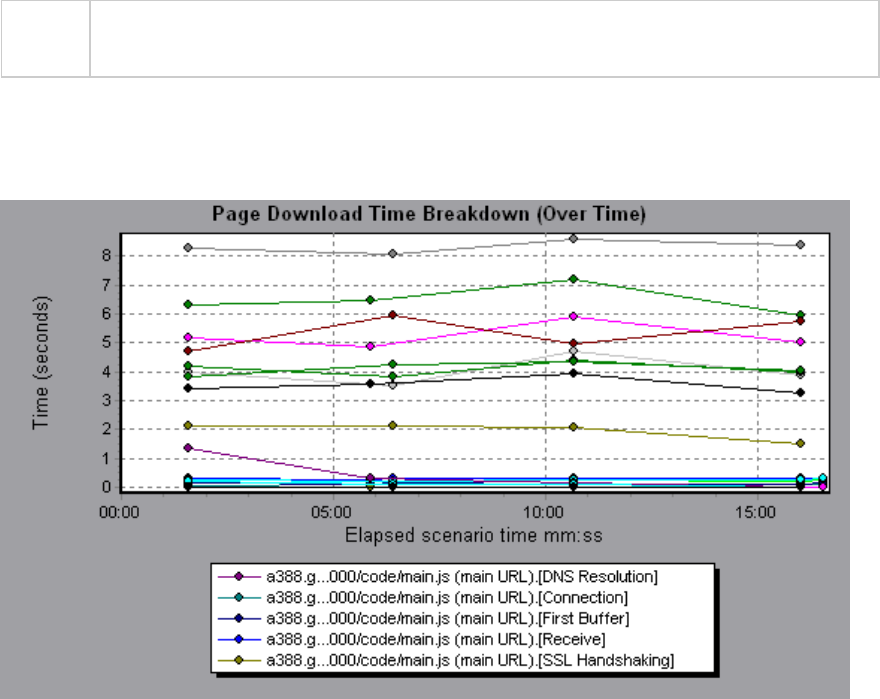
See
also
"Web Page Diagnostics Graphs Overview" on page158
Example
This graph enables you to determine at what point during scenario execution network or server
problems occurred.
Example
In the example in the previous section, it is apparent that cnn.com was the most problematic
component. If you examine the cnn.com component, the Page Download Time Breakdown (Over Time)
graph demonstrates that First Buffer and Receive time remained high throughout the scenario, and
that DNS Resolution time decreased during the scenario.
User Guide
Analysis
HP LoadRunner (12.50) Page 168
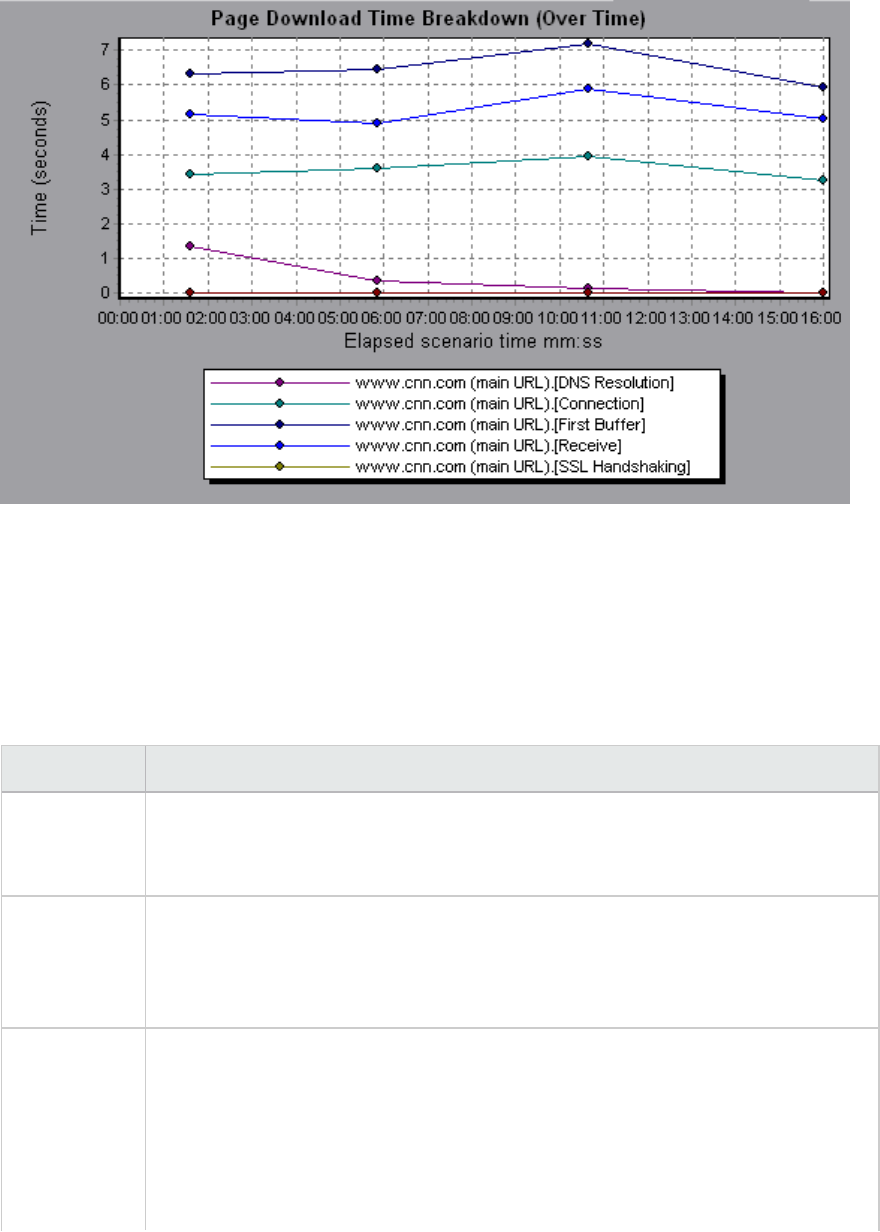
Page Download Time Breakdown Graph Breakdown Options
The Page Download Time Breakdown graph breaks down each component by DNS resolution time,
connection time, time to first buffer, SSL handshaking time, receive time, FTP authentication time,
client time, and error time.
These breakdowns are described below:
Name Description
DNS
Resolution
Displays the amount of time needed to resolve the DNS name to an IP address, using
the closest DNS server. The DNS Lookup measurement is a good indicator of
problems in DNS resolution, or problems with the DNS server.
Connection Displays the amount of time needed to establish an initial connection with the Web
server hosting the specified URL. The connection measurement is a good indicator
of problems along the network. It also indicates whether the server is responsive to
requests.
First Buffer Displays the amount of time that passes from the initial HTTP request (usually GET)
until the first buffer is successfully received back from the Web server. The first
buffer measurement is a good indicator of Web server delay as well as network
latency.
Note: Since the buffer size may be up to 8K, the first buffer might also be the time it
takes to completely download the element.
User Guide
Analysis
HP LoadRunner (12.50) Page 169
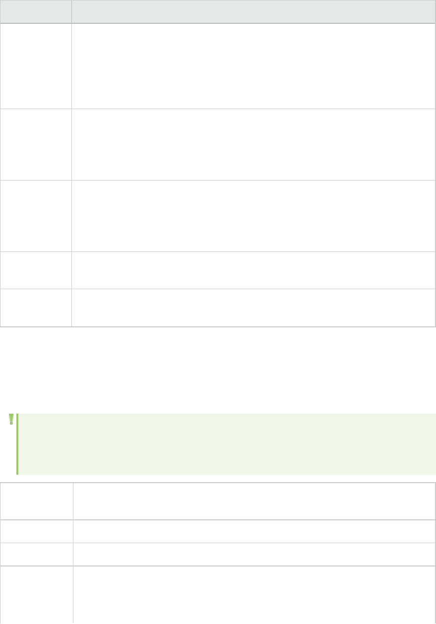
Name Description
SSL
Handshaking
Displays the amount of time taken to establish an SSL connection (includes the
client hello, server hello, client public key transfer, server certificate transfer, and
other—partially optional—stages). After this point, all the communication between
the client and server is encrypted.
The SSL Handshaking measurement is only applicable for HTTPS communications.
Receive Displays the amount of time that passes until the last byte arrives from the server
and the downloading is complete.
The Receive measurement is a good indicator of network quality (look at the
time/size ratio to calculate receive rate).
FTP
Authentication
Displays the time taken to authenticate the client. With FTP, a server must
authenticate a client before it starts processing the client's commands.
The FTP Authentication measurement is only applicable for FTP protocol
communications.
Client Time Displays the average amount of time that passes while a request is delayed on the
client machine due to browser think time or other client-related delays.
Error Time Displays the average amount of time that passes from the moment an HTTP
request is sent until the moment an error message (HTTP errors only) is returned.
Time to First Buffer Breakdown Graph
This graph displays each Web page component's relative server/network time (in seconds) for the
period of time until the first buffer is successfully received back from the Web server.
Note: This graph is only relevant when the load generator does not use a proxy to connect to
the application under test. If the load generator is connected through a proxy, this graph will
only show the proxy latency—not the AUT latency.
Purpose If the download time for a component is high, you can use this graph to determine
whether the problem is server- or network-related.
X-axis Specifies the name of the component.
Y-axis Shows the average network/server time (in seconds) for each component.
Measurements lNetwork time is defined as the average amount of time that passes from the
moment the first HTTP request is sent until receipt of ACK.
lServer time is defined as the average amount of time that passes from the
User Guide
Analysis
HP LoadRunner (12.50) Page 170
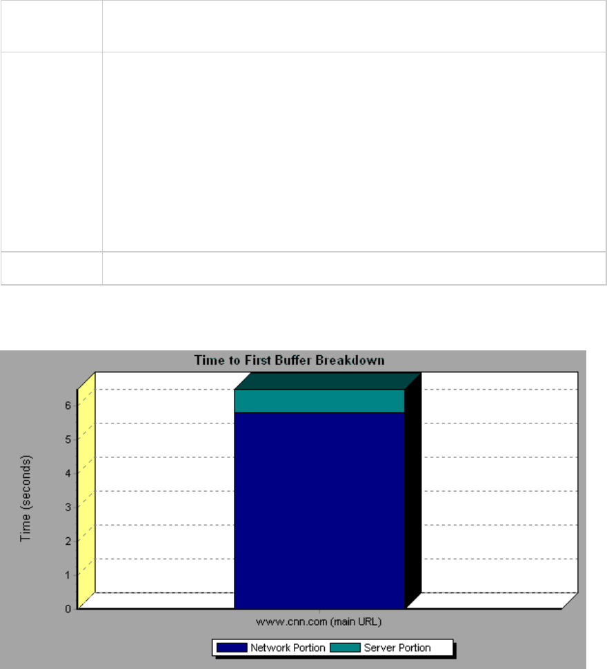
receipt of ACK of the initial HTTP request (usually GET) until the first buffer is
successfully received back from the Web server.
Note lEach measurement displayed on the page level is the sum of that measurement
recorded for each page component. For example, the network time for
www.cnn.com is the sum of the network time for each of the page's components.
lBecause server time is being measured from the client, network time may
influence this measurement if there is a change in network performance from
the time the initial HTTP request is sent until the time the first buffer is sent. The
server time displayed, therefore, is estimated server time and may be slightly
inaccurate.
lThe graph can only be viewed as a bar graph.
See also "Web Page Diagnostics Graphs Overview" on page158
Example
In the following example it is apparent that network time is greater than server time.
Example
In the following example shows that you can break the main cnn.com URL down further to view the time
to first buffer breakdown for each of its components. It is apparent that for the main cnn.com
component (the first component on the right), the time to first buffer breakdown is almost all network
time.
User Guide
Analysis
HP LoadRunner (12.50) Page 171
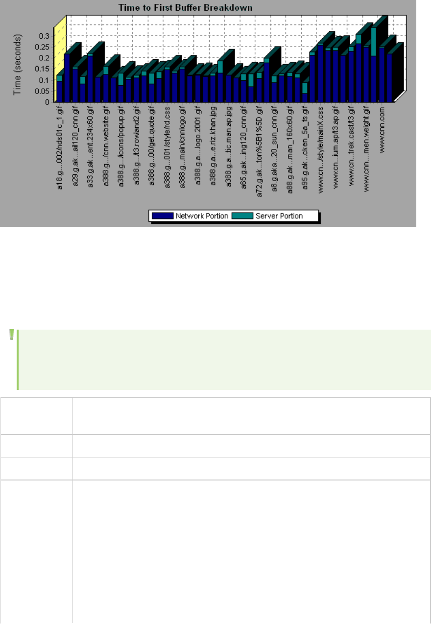
Time to First Buffer Breakdown (Over Time) Graph
This graph displays each Web page component's server and network time (in seconds) during each
second of the load test scenario run, for the period of time until the first buffer is successfully received
back from the Web server.
Note: This graph is only relevant when the load generator does not use a proxy to connect to
the application under test. If the load generator is connected through a proxy, this graph will
only show the proxy latency—not the AUT latency.
Purpose You can use this graph to determine when during the scenario run a server- or
network-related problem occurred.
X-axis Elapsed time from the beginning of the scenario run.
Y-axis Average network or server time (in seconds) for each component.
Measurements lNetwork time is defined as the average amount of time that passes from the
moment the first HTTP request is sent until receipt of ACK.
lServer time is defined as the average amount of time that passes from the
receipt of ACK of the initial HTTP request (usually GET) until the first buffer is
successfully received back from the Web server.
Note: Because server time is being measured from the client, network time may
influence this measurement if there is a change in network performance from the
time the initial HTTP request is sent until the time the first buffer is sent. The
server time displayed, therefore, is estimated server time and may be slightly
User Guide
Analysis
HP LoadRunner (12.50) Page 172
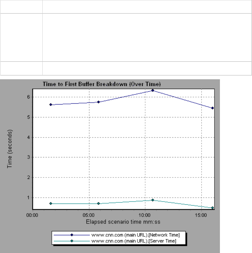
inaccurate.
Note lEach measurement displayed on the page level is the sum of that measurement
recorded for each page component. For example, the network time for
www.hp.com is the sum of the network time for each of the page's components.
lWhen the Time to First Buffer Breakdown (Over Time) graph is selected from the
Web Page Diagnostics graph, it appears as an area graph.
See also "Web Page Diagnostics Graphs Overview" on page158
User Guide
Analysis
HP LoadRunner (12.50) Page 173
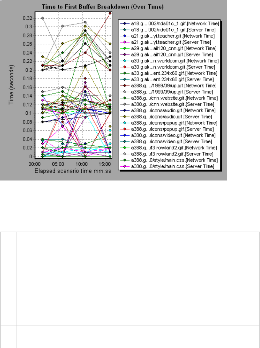
Example
In the following example you can break the main cnn.com URL down further to view the time to first
buffer breakdown for each of its components.
Client Side Breakdown (Over Time) Graph
This graph displays the client side breakdown of each transaction during each second of the load test
scenario run.
X-
axis
The elapsed time from the beginning of the scenario run.
Y-
axis
The average response time (in seconds) for each transaction.
Tips lTo isolate the most problematic transactions, it may be helpful to sort the legend window
according to the average number of seconds taken for the transaction to run. To sort the
legend by average, double-click the Average column heading.
lTo identify a transaction in the graph, you can select it. The corresponding line in the legend
window is selected.
See
also
"Web Page Diagnostics Graph" on page161
User Guide
Analysis
HP LoadRunner (12.50) Page 174
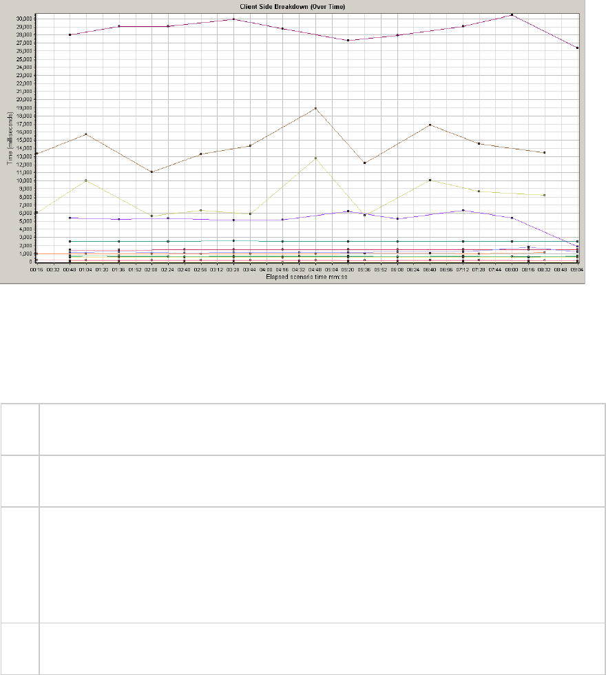
Example
Using the graph, you can track which transactions on the client side were most problematic, and at
which point(s) during the scenario the problem(s) occurred.
Client Side Java Script Breakdown (Over Time) Graph
This graph displays the client side breakdown of each JavaScript transaction during each second of the
load test scenario run.
X-
axis
The elapsed time from the beginning of the scenario run.
Y-
axis
The average response time (in seconds) for each transaction.
Tips lTo isolate the most problematic transactions, it may be helpful to sort the legend window
according to the average number of seconds taken for the transaction to run. To sort the
legend by average, double-click the Average column heading.
lTo identify a transaction in the graph, you can select it. The corresponding line in the legend
window is selected.
See
also
"Web Page Diagnostics Graph" on page161
Example
Using the graph, you can track which transactions on the client side were most problematic, and at
which point(s) during the scenario the problem(s) occurred.
User Guide
Analysis
HP LoadRunner (12.50) Page 175
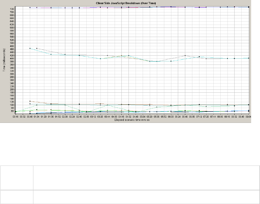
Downloaded Component Size Graph
This graph displays the size of each Web page component.
Note lThe Web page size is a sum of the sizes of each of its components.
lThe Downloaded Component Size graph can only be viewed as a pie graph.
See also "Web Page Diagnostics Graphs Overview" on page158
Example
In the following example the www.cnn.com/WEATHER component is 39.05% of the total size, whereas
the main cnn.com component is 34.56% of the total size.
User Guide
Analysis
HP LoadRunner (12.50) Page 176
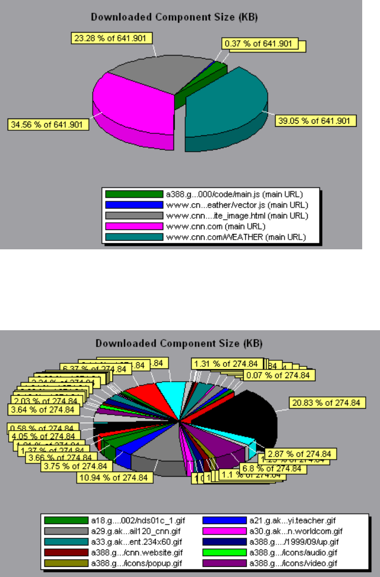
Example
In the following example the cnn.com component's size (20.83% of the total size) may have contributed
to the delay in its downloading. To reduce download time, it may help to reduce the size of this
component.
User-Defined Data Point Graphs
User Guide
Analysis
HP LoadRunner (12.50) Page 177

User-Defined Data Point Graphs Overview
The User-Defined Data Point graphs display the values of user-defined data points. You define a data
point in your Vuser script by inserting an lr_user_data_point function at the appropriate place (user_
data_point for GUI Vusers and lr.user_data_point for Java Vusers).
Action1()
{
lr_think_time(1);
lr_user_data_point ("data_point_1",1);
lr_user_data_point ("data_point_2",2);
return 0;
}
For Vuser protocols that support the graphical script representations such as Web and Oracle NCA, you
insert a data point as a User Defined step. Data point information is gathered each time the script
executes the function or step. For more information about data points, refer to the Function Reference.
Data points, like other Analysis data, are aggregated every few seconds, resulting in less data points
shown on the graph than actually recorded. For more information, see "Changing the Granularity of the
Data" on page91.
Data Points (Average) Graph
This graph shows the average values that were recorded for user-defined data points during the load
test scenario run.
Purpose This graph is typically used in cases where the actual value of the measurement is
required. Suppose that each Vuser monitors CPU utilization on its machine and records it
as a data point. In this case, the actual recorded value of CPU utilization is required. The
Average graph displays the average value recorded throughout the scenario.
X-axis Elapsed time since the start of the run.
Y-axis The average values of the recorded data point statements.
See
also
"User-Defined Data Point Graphs Overview" above
Example
In the following example, the CPU utilization is recorded as the data point user_data_point_val_1. It is
shown as a function of the elapsed scenario time.
User Guide
Analysis
HP LoadRunner (12.50) Page 178
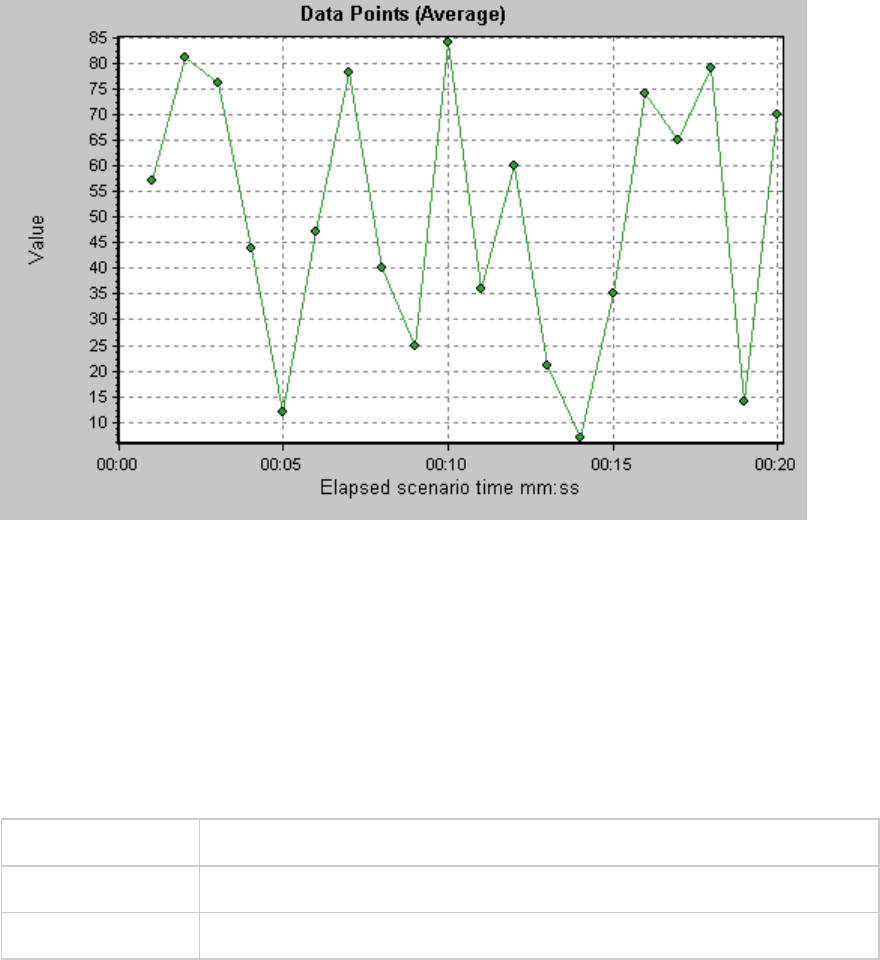
Data Points (Sum) Graph
This graph shows the sum of the values for user-defined data points throughout the load test scenario
run.
This graph typically indicates the total amount of measurements which all Vusers are able to generate.
For example, suppose only a certain set of circumstances allow a Vuser to call a server. Each time it
does, a data point is recorded. In this case, the Sum graph displays the total number of times that
Vusers call the function.
X-axis Elapsed time since the start of the run.
Y-axis The sum of the recorded data point values.
See also "User-Defined Data Point Graphs Overview" on the previous page
Example
In the following example, the call to the server is recorded as the data point user_data_point_val_1. It is
shown as a function of the elapsed scenario time.
User Guide
Analysis
HP LoadRunner (12.50) Page 179
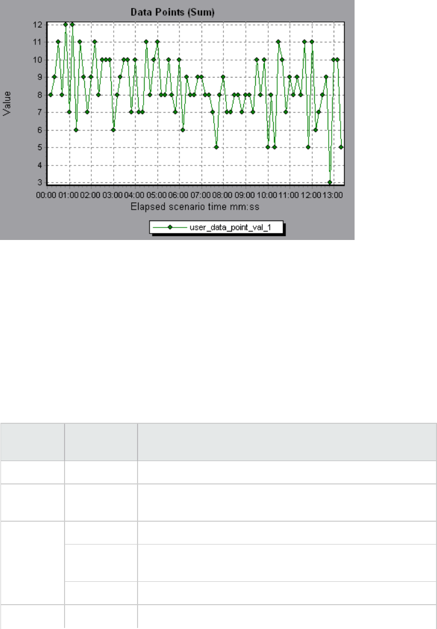
System Resource Graphs
System Resource graphs display the system resource usage measured by the online monitors during
the load test scenario run. These graphs require that you specify the resources you want to measure
before running the scenario. For more information, see the section on online monitors in the
LoadRunner Controller documentation.
Server Resources Performance Counters
The following table describes the available counters:
Monitor Measurements Description
CPU Monitor Utilization Measures CPU utilization.
Disk Space
Monitor
Disk space Measures the amount (in MB) free disk space and the percentage of
disk space used.
Memory
Monitor
MB free Measures the amount of free memory (in MB).
Pages/sec Measures the number of virtual memory pages that are moved
between main memory and disk storage.
Percent used Measures the percentage of memory and paging file space used.
Services Monitors processes locally or on remote systems. Can be used to
User Guide
Analysis
HP LoadRunner (12.50) Page 180
Monitor Measurements Description
Monitor verify that specific processes are running.
Linux Resources Default Measurements
The following default measurements are available for Linux machines:
Measurement Description
Average load Average number of processes simultaneously in `Ready' state during the
last minute.
Collision rate Collisions per second detected on the Ethernet.
Context switches rate Number of switches between processes or threads, per second.
CPU utilization Percent of time that the CPU is utilized.
Disk rate Rate of disk transfers.
Incoming packets error
rate
Errors per second while receiving Ethernet packets.
Incoming packets rate Incoming Ethernet packets per second.
Interrupt rate Number of device interrupts per second.
Outgoing packets errors
rate
Errors per second while sending Ethernet packets.
Outgoing packets rate Outgoing Ethernet packets per second.
Page-in rate Number of pages read to physical memory, per second.
Page-out rate Number of pages written to pagefile(s) and removed from physical
memory, per second.
Paging rate Number of pages read to physical memory or written to
pagefile(s), per second.
Swap-in rate The rate by which disk content is swapped into the machine's memory in
Kbps.
Swap-out rate The rate by which the machine's memory is being swapped out to disk in
Kbps.
System mode CPU Percent of time that the CPU is utilized in system mode.
User Guide
Analysis
HP LoadRunner (12.50) Page 181

Measurement Description
utilization
User mode CPU
utilization
Percent of time that the CPU is utilized in user mode.
Windows Resources Default Measurements
The following default measurements are available for Windows Resources:
Object Measurement Description
System % Total
Processor
Time
The average percentage of time that all the processors on the
system are busy executing non-idle threads. On a multi-processor
system, if all processors are always busy, this is 100%, if all
processors are 50% busy this is 50% and if 1/4 of the processors are
100% busy this is 25%. It can be viewed as the fraction of the time
spent doing useful work. Each processor is assigned an Idle thread in
the Idle process which consumes those unproductive processor
cycles not used by any other threads.
Processor % Processor
Time
The percentage of time that the processor is executing a non-idle
thread. This counter was designed as a primary indicator of
processor activity. It is calculated by measuring the time that the
processor spends executing the thread of the idle process in each
sample interval, and subtracting that value from 100%. (Each
processor has an idle thread which consumes cycles when no other
threads are ready to run.) It can be viewed as the percentage of the
sample interval spent doing useful work. This counter displays the
average percentage of busy time observed during the sample
interval. It is calculated by monitoring the time the service was
inactive, and then subtracting that value from 100%.
System File Data
Operations/sec
The rate at which the computer issues read and write operations to
file system devices. This does not include File Control Operations.
System Processor
Queue Length
The instantaneous length of the processor queue in units of
threads. This counter is always 0 unless you are also monitoring a
thread counter. All processors use a single queue in which threads
wait for processor cycles. This length does not include the threads
that are currently executing. A sustained processor queue length
greater than two generally indicates processor congestion. This is
an instantaneous count, not an average over the time interval.
User Guide
Analysis
HP LoadRunner (12.50) Page 182

Object Measurement Description
Memory Page
Faults/sec
This is a count of the page faults in the processor. A page fault
occurs when a process refers to a virtual memory page that is not in
its Working Set in the main memory. A page fault will not cause the
page to be fetched from disk if that page is on the standby list (and
hence already in main memory), or if it is in use by another process
with which the page is shared.
PhysicalDisk % Disk Time The percentage of elapsed time that the selected disk drive is busy
servicing read or write requests.
Memory Pool Nonpaged
Bytes
The number of bytes in the non-paged pool, a system memory area
where space is acquired by operating system components as they
accomplish their appointed tasks. Non-paged pool pages cannot be
paged out to the paging file. They remain in main memory as long as
they are allocated.
Memory Pages/sec The number of pages read from the disk or written to the disk to
resolve memory references to pages that were not in memory at
the time of the reference. This is the sum of Pages Input/sec and
Pages Output/sec. This counter includes paging traffic on behalf of
the system cache to access file data for applications. This value also
includes the pages to/from non-cached mapped memory files. This
is the primary counter to observe if you are concerned about
excessive memory pressure (that is, thrashing), and the excessive
paging that may result.
System Total
Interrupts/sec
The rate at which the computer is receiving and servicing hardware
interrupts. The devices that can generate interrupts are the system
timer, the mouse, data communication lines, network interface
cards, and other peripheral devices. This counter provides an
indication of how busy these devices are on a computer-wide basis.
See also Processor:Interrupts/sec.
Objects Threads The number of threads in the computer at the time of data
collection. Notice that this is an instantaneous count, not an average
over the time interval. A thread is the basic executable entity that
can execute instructions in a processor.
Process Private Bytes The current number of bytes that the process has allocated that
cannot be shared with other processes.
User Guide
Analysis
HP LoadRunner (12.50) Page 183
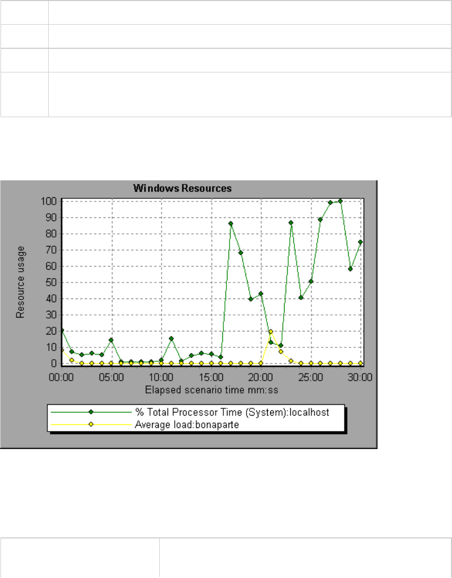
Server Resources Graph
This graph shows the resources (CPU, disk space, memory, or services) used on remote Linux servers
measured during the load test scenario.
Purpose This graph helps you determine the impact of Vuser load on the various system resources.
X-axis Elapsed time since the start of the run.
Y-axis The usage of resources on the Linux server.
See also "System Resource Graphs" on page180
"Server Resources Performance Counters" on page180
Example
In the following example, Windows resource utilization is measured during the load test scenario. It is
shown as a function of the elapsed scenario time.
Host Resources Graph
This graph displays a summary of the System Resources usage for each Windows based Performance
Center host (Controller and Load Generators). measured during the load test scenario.
Purpose This graph helps you determine the impact of Vuser load on the
various host resources.
User Guide
Analysis
HP LoadRunner (12.50) Page 184
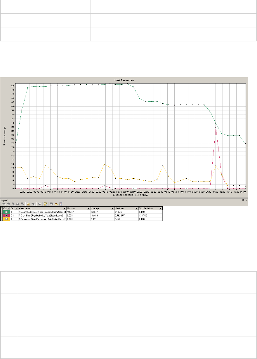
X-axis Elapsed time since the start of the run.
Y-axis The usage of resources on the Windows hosts.
See also "System Resource Graphs" on page180
Example
In the following example, you can see a peak in the usage of Disk Time and Processor Time as the
Memory Usage gets less towards the end of the load test.
SNMP Resources Graph
This graph shows statistics for machines running an SNMP agent, using the Simple Network
Management Protocol (SNMP).
X-
axis
Elapsed time since the start of the run.
Y-
axis
The usage of resources on a machine running the SNMP agent.
Note To obtain data for this graph, you need to enable the SNMP monitor (from the Controller) and
select the default measurements you want to display, before running the scenario.
See
also
"System Resource Graphs" on page180
Example
User Guide
Analysis
HP LoadRunner (12.50) Page 185
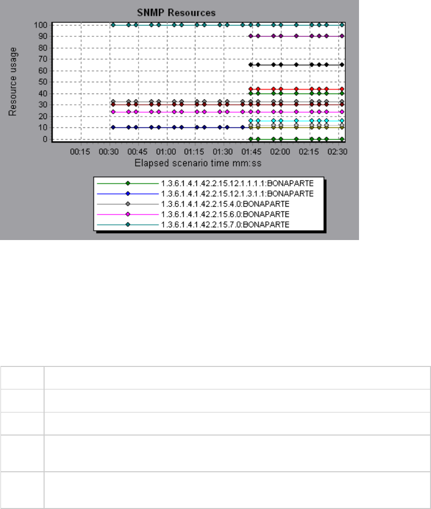
In the following example SNMP measurements are displayed for a machine called bonaporte.
Linux Resources Graph
This graph shows the Linux resources measured during the load test scenario. The Linux measurements
include those available by the rstatd daemon: average load, collision rate, context switch rate, CPU
utilization, incoming packets error rate, incoming packets rate, interrupt rate, outgoing packets error
rate, outgoing packets rate, page-in rate, page-out rate, paging rate, swap-in rate, swap-out rate,
system mode CPU utilization, and user mode CPU utilization.
Purpose This graph helps you determine the impact of Vuser load on the various system resources.
X-axis Elapsed time since the start of the run.
Y-axis The usage of resources on the Linux machine.
Note To obtain data for this graph, you need to select the desired measurements for the online
monitor (from the Controller) before running the scenario.
See
also
"Linux Resources Default Measurements" on page181
Example
In the following example Linux resources are measured during the load test scenario.
User Guide
Analysis
HP LoadRunner (12.50) Page 186
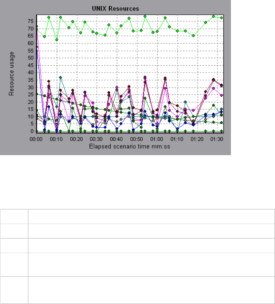
Windows Resources Graph
This graph shows the Windows resources measured during the load test scenario. The Windows
measurements correspond to the built-in counters available from the Windows Performance Monitor.
Purpose This graph helps you determine the impact of Vuser load on the various system resources.
X-axis Elapsed time since the start of the run.
Y-axis The usage of resources on the Windows machine running the load test scenario.
Note To obtain data for this graph, you need to select the desired measurements for the online
monitor (from the Controller) before running the scenario.
See
also
"System Resource Graphs" on page180
"Windows Resources Default Measurements" on page182
Example
In the following example Windows resources are measured on the server running the load test scenario.
User Guide
Analysis
HP LoadRunner (12.50) Page 187
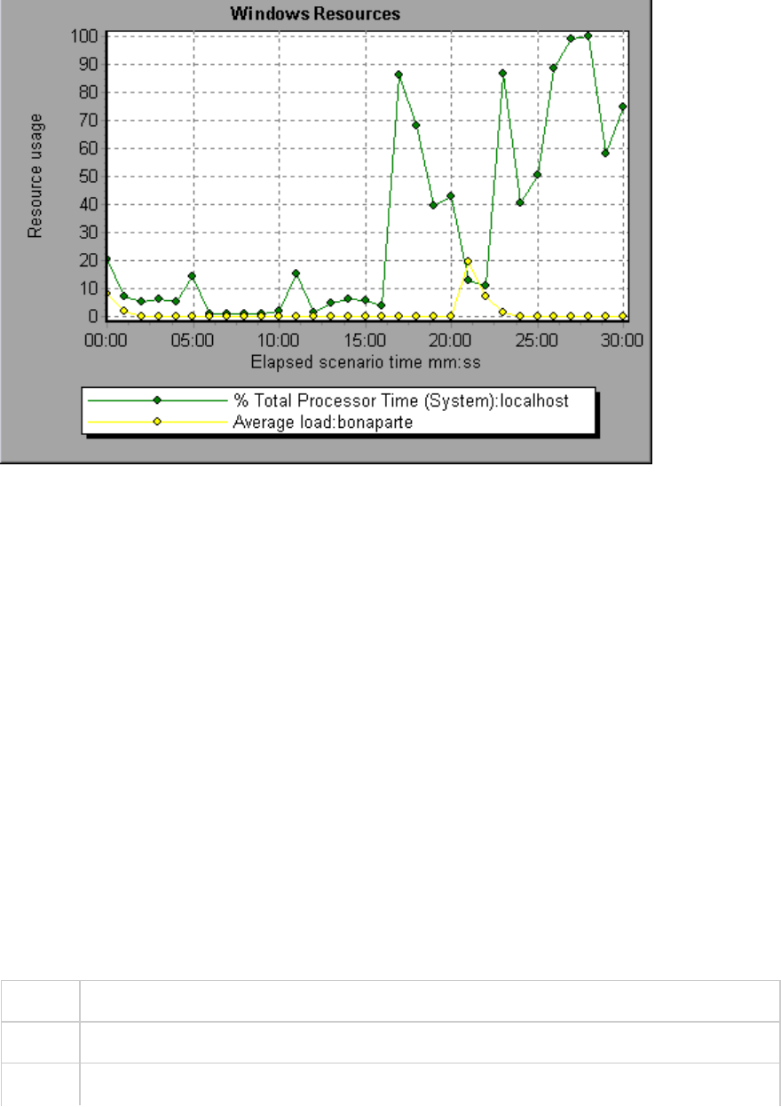
Network Virtualization Graphs
LoadRunner integrates with HP Network Virtualization. This enables you to test point-to-point
performance of WAN or other network deployed products under real-world network conditions. By
installing software on your load generators, you introduce highly probable effects such as latency,
packet loss, and link faults over your network. As a result of this, your scenario performs the test in an
environment that better represents the actual deployment of your application.
You can create more meaningful results by configuring multiple load generator machines or groups on a
single load generator with the same unique set of network effects, and by giving each set a unique
location name, such as NY- London. When viewing scenario results in Analysis, you can group the metrics
according to their location names.
Packet Loss Graph
This graph shows packets lost during the last second of the scenario run. Packet loss occurs when data
packets fail to reach their destination. It can result from gateway overload, signal degradation, channel
congestion, or faulty hardware.
Purpose Helps you understand how many data packets were lost over a specific time interval.
X-axis Elapsed time since the start of the run.
Y-axis The following measurements:
User Guide
Analysis
HP LoadRunner (12.50) Page 188
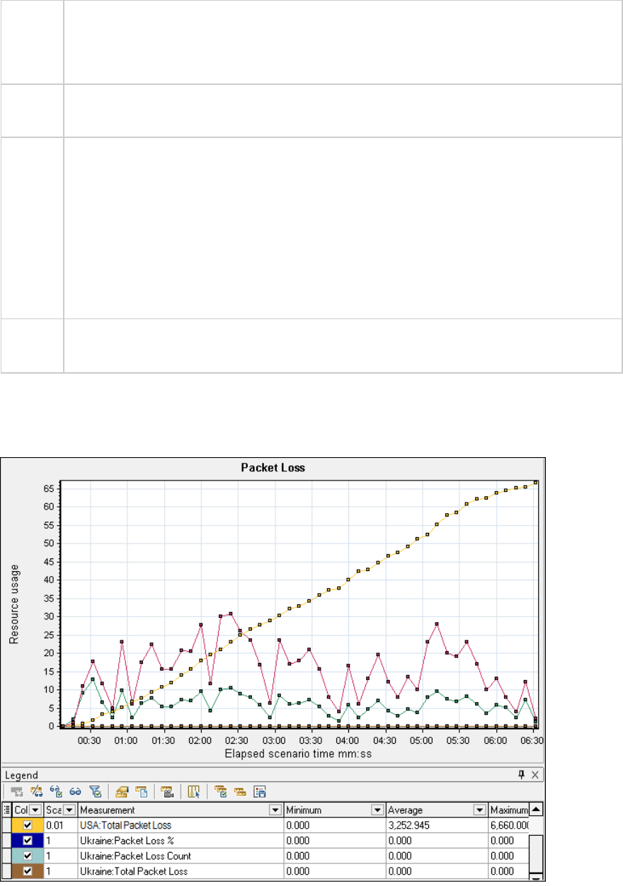
lThe percentage of lost packets from all packets that were sent.
lThe number of data packets that were lost over 60 seconds.
lThe total number of packets that were lost.
Note You cannot change the granularity of the x-axis to a value that is less than the Web
granularity you defined in the General tab of the Options dialog box.
Tip For LoadRunner Analysis (not applicable to monitoring graphs):
To view information for a specific location:
1. Click within the graph.
2. Select Set Filter/ Sort By from the right-click menu to open the Graph Settings dialog
box.
3. In the Filter condition section, select the Location Name row, and select the desired
location from the drop-down list.
See
also
"Network Virtualization Graphs" on the previous page
Example - Network Virtualization Per Group
The following example shows how the total of packet loss for the USA group increased as the scenario
progressed.
User Guide
Analysis
HP LoadRunner (12.50) Page 189
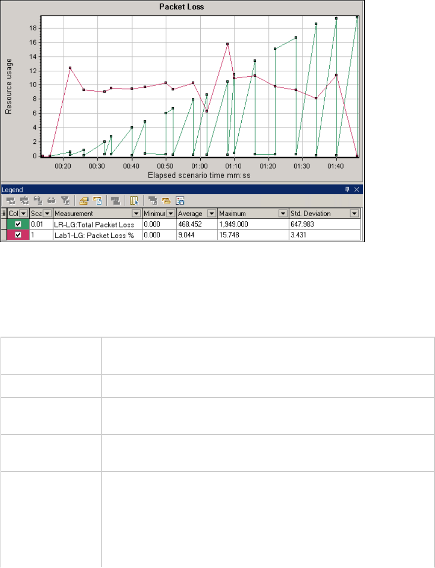
Example - Network Virtualization Per Load Generator
In the following example, you can see that the packet loss is grouped by load generator. This was the
mode selected when you enabled Network Virtualization for the scenario.
Average Latency Graph
This graph shows the average recorded time required for a packet of data to travel from the indicated
source point to the required destination, measured in milliseconds in the last 60 seconds.
Purpose Helps you evaluate the time required for a packet of data to travel over the
network.
X-axis Elapsed time since the start of the run.
Y-axis The average latency—the time in milliseconds required for a packet of data
to reach its destination, per 60 second intervals.
Note You cannot change the granularity of the x-axis to a value that is less than
the Web granularity you defined in the General tab of the Options dialog box.
Tips For LoadRunner Analysis (not applicable to monitoring graphs):
To view information for a specific location:
1. Click within the graph.
2. Select Set Filter/ Sort By from the right-click menu to open the Graph
Settings dialog box.
User Guide
Analysis
HP LoadRunner (12.50) Page 190
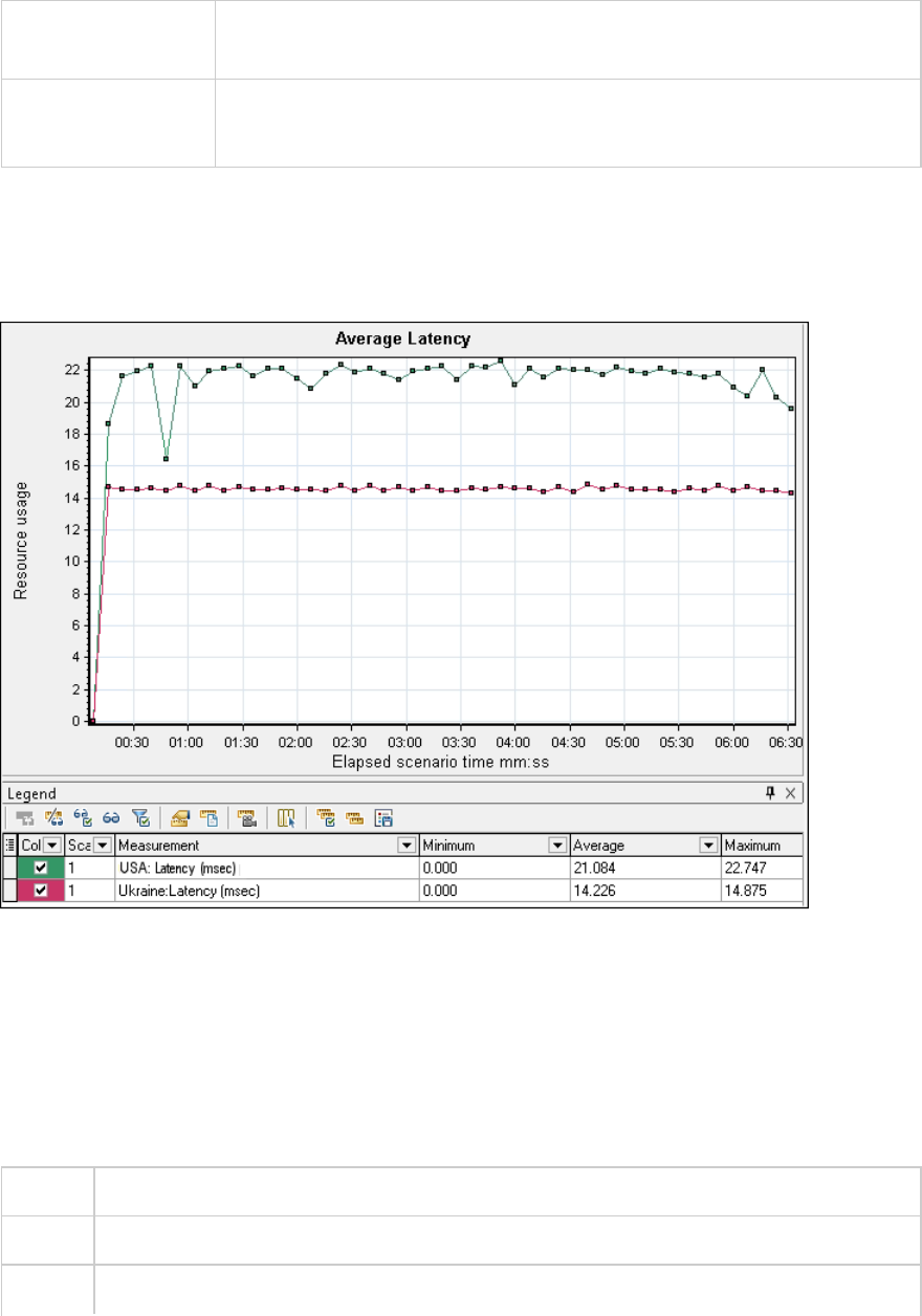
3. In the Filter condition section, select the Location Name row, and select
the desired location from the drop-down list.
See also l"Network Virtualization Graphs" on page188
l"Custom Filter Dialog Box" on page113
Example - Network Virtualization Per Group
In the following example, you can see that the latency for the USA group reached its peak at nearly 4
minutes into the scenario run, while the Ukraine group remained fairly constant at approximately 14
msec.
If you enabled Network Virtualization per load generator (and not per group), the graph shows the
measurements per load generator, as shown in the "Packet Loss Graph" on page188.
Average Bandwidth Utilization Graph
This graph shows the average bandwidth utilized by a virtual user or a virtualized location from the
maximal available bandwidth allocated for it during the last second, measured in percentages.
Purpose Helps you evaluate the bandwidth used over your network.
X-axis Elapsed time since the start of the run.
Y-axis The percentage of bandwidth utilization.
User Guide
Analysis
HP LoadRunner (12.50) Page 191
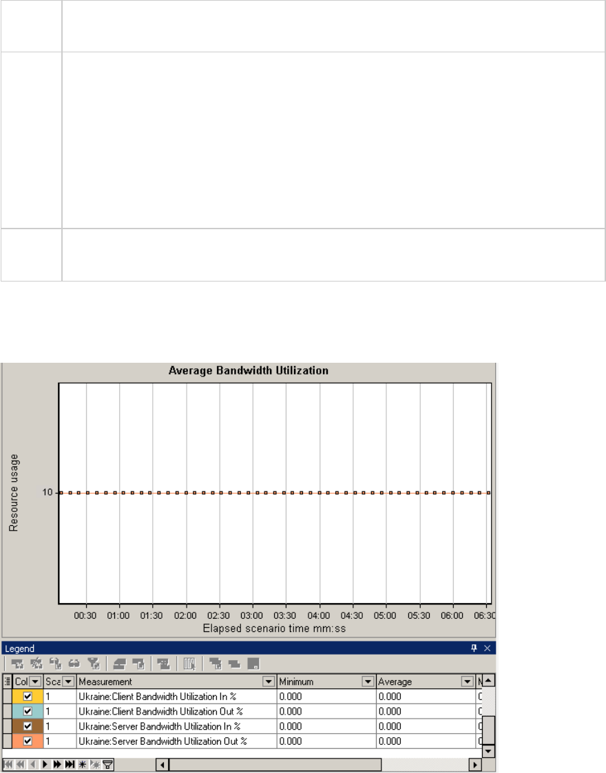
Note You cannot change the granularity of the x-axis to a value that is less than the Web
granularity you defined in the General tab of the Options dialog box.
Tips For LoadRunner Analysis (not applicable to monitoring graphs):
To view information for a specific location:
1. Click within the graph.
2. Select Set Filter/ Sort By from the right-click menu to open the Graph Settings dialog
box.
3. In the Filter condition section, select the Location Name row, and select the desired
location from the drop-down list.
See
also
"Network Virtualization Graphs" on page188
Example
In the following example, you can see that the bandwidth utilization for all locations and measurements,
was constant at 10%.
If you enabled Network Virtualization per load generator (and not per group), the graph shows the
measurements per load generator, as shown in the "Packet Loss Graph" on page188.
User Guide
Analysis
HP LoadRunner (12.50) Page 192
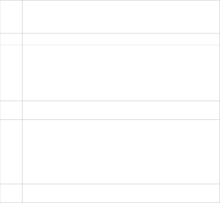
Average Throughput Graph
This graph shows the average data traffic passing to or from the virtualized location, measured in
kilobytes per second (kbps).
Purpose Helps you evaluate the amount of load Vusers generate, in terms of the number of server
and client throughput. The graph shows metrics for input and output traffic for both the
server and client machines. Use the legend below the graph to determine the line color for
each metric.
X-axis Elapsed time since the start of the run.
Y-axis The rate of data passing to and from the virtual location, in kbps for the following metrics
per group or load generator:
lInput to the client machine
lOutput from the client machine
lInput to the server machine
lOutput from the server machine
Note You cannot change the granularity of the x-axis to a value that is less than the Web
granularity you defined in the General tab of the Options dialog box.
Tips For LoadRunner Analysis (not applicable to monitoring graphs):
To view information for a specific location:
1. Click within the graph.
2. Select Set Filter/ Sort By from the right-click menu to open the Graph Settings dialog
box.
3. In the Filter condition section, select the Location Name row, and select the desired
location from the drop-down list.
See
also
"Total Throughput Graph" on the next page
User Guide
Analysis
HP LoadRunner (12.50) Page 193
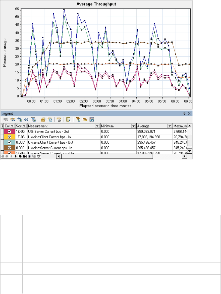
Example
In the following example, the average server input throughput was the lowest for the Ukraine group.
If you enabled Network Virtualization per load generator (and not per group), the graph shows the
measurements per load generator, as shown in the "Packet Loss Graph" on page188.
Total Throughput Graph
Displays the total data traffic passing to or from the virtualized location, measured in kilobytes.
Purpose Helps you evaluate the total amount of load that Vusers generate while running a scenario
with network virtualization.
The graph shows metrics for input and output traffic for both the server and client
machines. The legend below the graph indicates the line color for each of these metrics.
X-axis Elapsed time since the start of the run.
Y-axis Throughput of the server, in kilobytes per second (Kbps).
Note You cannot change the granularity of the x-axis to a value that is less than the Web
granularity you defined in the General tab of the Options dialog box.
User Guide
Analysis
HP LoadRunner (12.50) Page 194
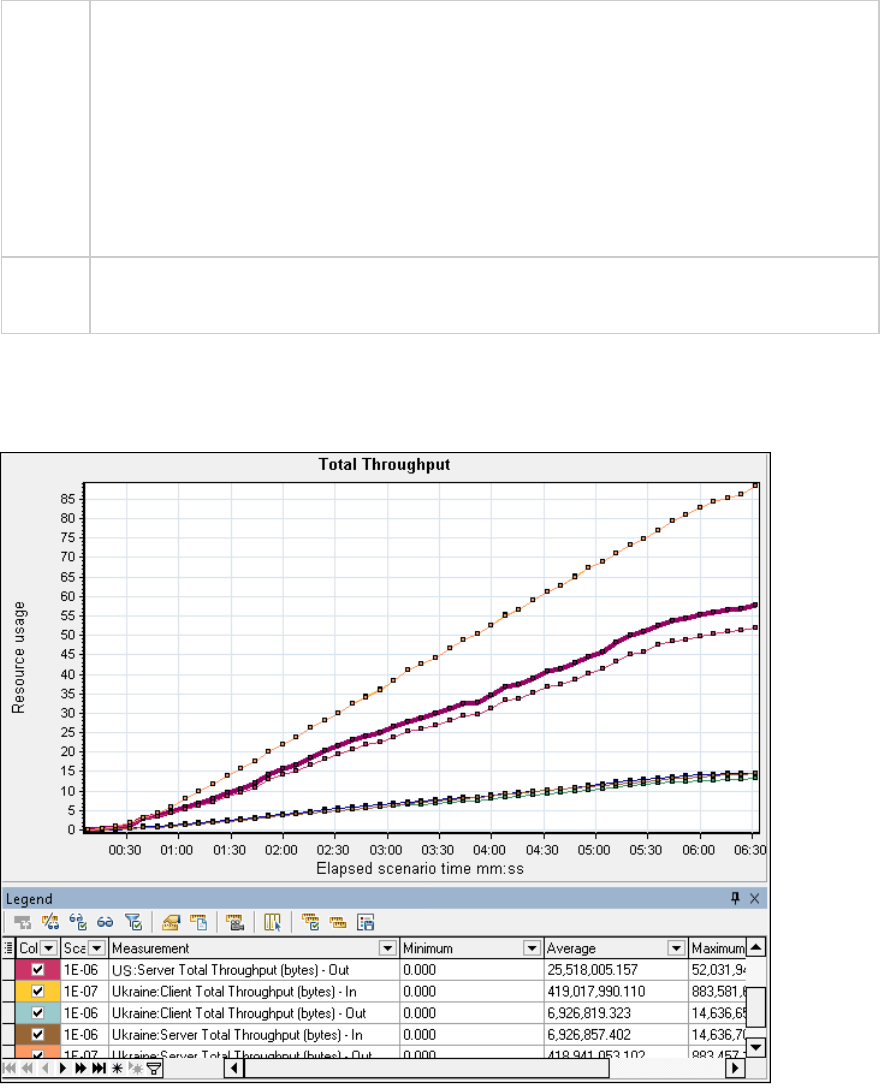
Tips For LoadRunner Analysis (not applicable to monitoring graphs):
To view information for a specific location:
1. Click within the graph.
2. Select Set Filter/ Sort By from the right-click menu to open the Graph Settings dialog
box.
3. In the Filter condition section, select the Location Name row, and select the desired
location from the drop-down list.
See
also
"Average Throughput Graph" on page193
Example
In the following example, the highest throughput level was for the input data to the client, for the
Ukraine group.
If you enabled Network Virtualization per load generator (and not per group), the graph shows the
measurements per load generator, as shown in the "Packet Loss Graph" on page188.
Network Monitor Graphs
User Guide
Analysis
HP LoadRunner (12.50) Page 195
Network Monitor Graphs Overview
Network configuration is a primary factor in the performance of applications and Web systems. A poorly
designed network can slow client activity to unacceptable levels. In an application, there are many
network segments. A single network segment with poor performance can affect the entire application.
The following diagram shows a typical network. To go from the server machine to the Vuser machine,
data must travel over several segments.
To measure network performance, the Network monitor sends packets of data across the network.
When a packet returns, the monitor calculates the time it takes for the packet to go to the requested
node and return.
The Network Sub-Path Time graph displays the delay from the source machine to each node along the
path. The Network Segment Delay graph displays the delay for each segment of the path. The Network
Delay Time graph displays the delay for the complete path between the source and destination
machines.
Using the Network Monitor graphs, you can determine whether the network is causing a bottleneck. If
the problem is network-related, you can locate the problematic segment so that it can be fixed.
In order for Analysis to generate Network monitor graphs, you must activate the Network monitor
before executing the load test scenario. In the Network monitor settings, you specify the path you want
to monitor. For information about setting up the Network monitor, see Network Delay Monitoring.
Network Delay Time Graph
This graph shows the delays for the complete path between the source and destination machines (for
example, the database server and Vuser load generator). The graph maps the delay as a function of the
elapsed load test scenario time.
Each path defined in the Controller is represented by a separate line with a different color in the graph.
X-
axis
Elapsed time since the start of the run.
User Guide
Analysis
HP LoadRunner (12.50) Page 196
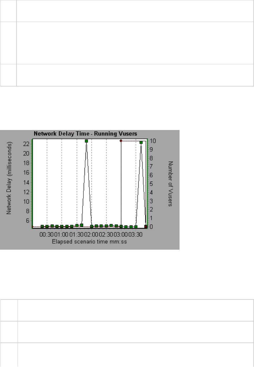
Y-
axis
Network delay time.
Tips Merge graphs to determine network bottleneck
You can merge various graphs to determine if the network is a bottleneck. For example,
using the Network Delay Time and Running Vusers graphs, you can determine how the
number of Vusers affects the network delay.
See
also
"Network Monitor Graphs Overview" on the previous page
Example
In the following example of a merged graph, the network delays are compared to the running Vusers.
The graph shows that when all 10 Vusers were running, a network delay of 22 milliseconds occurred,
implying that the network may be overloaded.
Network Segment Delay Graph
This graph shows the delay for each segment of the path according to the elapsed load test scenario
time. Each segment is displayed as a separate line with a different color.
X-
axis
Elapsed time since the start of the run.
Y-
axis
Network delay time.
Note The segment delays are measured approximately, and do not add up to the network path
delay which is measured exactly. The delay for each segment of the path is estimated by
User Guide
Analysis
HP LoadRunner (12.50) Page 197
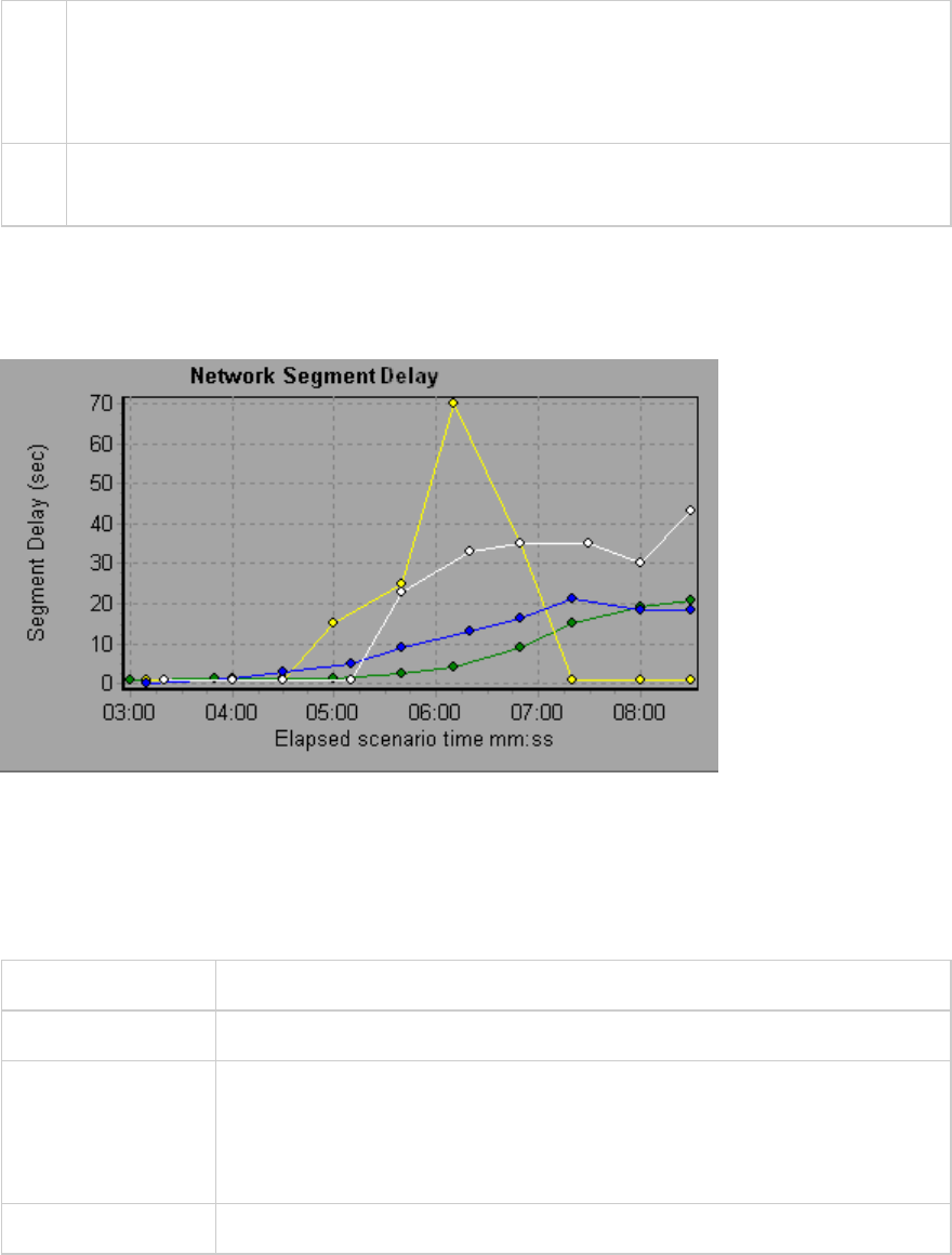
calculating the delay from the source machine to one node and subtracting the delay from the
source machine to another node. For example, the delay for segment B to C is calculated by
measuring the delay from the source machine to point C, and subtracting the delay from the
source machine to point B.
See
also
"Network Monitor Graphs Overview" on page196
Example
In the following example, four segments are shown. The graph indicates that one segment caused a
delay of 70 seconds in the sixth minute.
Network Sub-Path Time Graph
This graph displays the delay from the source machine to each node along the path according to the
elapsed load test scenario time. Each segment is displayed as a separate line with a different color.
X-axis Elapsed time since the start of the run.
Y-axis Network delay time.
Note The delays from the source machine to each of the nodes are measured
concurrently, yet independently. It is therefore possible that the delay from
the source machine to one of the nodes could be greater than the delay for
the complete path between the source and destination machines.
See also "Network Monitor Graphs Overview" on page196
Example
In the following example, four segments are shown. The graph indicates that one segment caused a
delay of 70 milliseconds in the sixth minute.
User Guide
Analysis
HP LoadRunner (12.50) Page 198
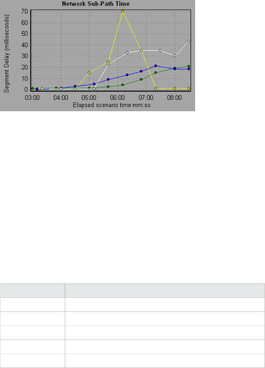
Web Server Resource Graphs
Web Server Resource Graphs Overview
Web Server Resource graphs provide you with information about the resource usage of the Apache and
Microsoft IIS Web servers. In order to obtain data for these graphs, you need to activate the online
monitor for the server and specify which resources you want to measure before running the load test
scenario. For information on activating and configuring the Web Server Resource monitors, see Web
Server Resource Monitoring Overview.
In order to display all the measurements on a single graph, Analysis may scale them. The Legend window
indicates the scale factor for each resource. To obtain the true value, multiply the scale factor by the
displayed value.
Apache Server Measurements
The following default measurements are available for the Apache server:
Measurement Description
# Busy Servers The number of servers in the Busy state
# Idle Servers The number of servers in the Idle state
Apache CPU Usage The percentage of time the CPU is utilized by the Apache server
Hits/sec The HTTP request rate
KBytes Sent/sec The rate at which data bytes are sent from the Web server
User Guide
Analysis
HP LoadRunner (12.50) Page 199
IIS Server Measurements
The following default measurements are available for the IIS server:
Object Measurement Description
Web
Service
Bytes Sent/sec The rate at which the data bytes are sent by the Web service.
Web
Service
Bytes
Received/sec
The rate at which the data bytes are received by the Web service.
Web
Service
Get
Requests/sec
The rate at which HTTP requests using the GET method are made. Get
requests are generally used for basic file retrievals or image maps,
though they can be used with forms.
Web
Service
Post
Requests/sec
The rate at which HTTP requests using the POST method are made. Post
requests are generally used for forms or gateway requests.
Web
Service
Maximum
Connections
The maximum number of simultaneous connections established with the
Web service.
Web
Service
Current
Connections
The current number of connections established with the Web service.
Web
Service
Current
NonAnonymous
Users
The number of users that currently have a non-anonymous connection
using the Web service.
Web
Service
Not Found
Errors/sec
The rate of errors due to requests that could not be satisfied by the
server because the requested document could not be found. These are
generally reported to the client as an HTTP 404 error code.
Process Private Bytes The current number of bytes that the process has allocated that cannot
be shared with other processes.
Apache Server Graph
This graph shows server statistics as a function of the elapsed load test scenario time.
X-
axis
Elapsed time since the start of the run.
Y-
axis
The resource usage on the Apache server during the scenario run.
Note To obtain data for this graph, you need to enable the Apache online monitor (from the
User Guide
Analysis
HP LoadRunner (12.50) Page 200
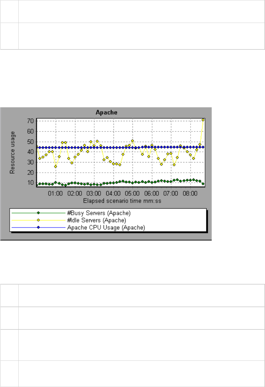
Controller) and select the default measurements you want to display, before running the
scenario.
See
also
"Web Server Resource Graphs Overview" on page199
"Apache Server Measurements" on page199
Example
In the following example, the CPU usage remained steady throughout the scenario. At the end of the
scenario, the number of idle servers increased. The number of busy servers remained steady at 1
throughout the scenario, implying that the Vuser only accessed one Apache server.
The scale factor for the Busy Servers measurement is 1/10 and the scale factor for CPU usage is 10.
Microsoft Information Internet Server (IIS) Graph
This graph shows server statistics as a function of the elapsed load test scenario time.
X-
axis
Elapsed time since the start of the run.
Y-
axis
The resource usage on the MS IIS.
Note To obtain data for this graph, you need to enable the MS IIS online monitor (from the
Controller) and select the default measurements you want to display, before running the
scenario.
See
also
"Web Server Resource Graphs Overview" on page199
"IIS Server Measurements" on the previous page
User Guide
Analysis
HP LoadRunner (12.50) Page 201
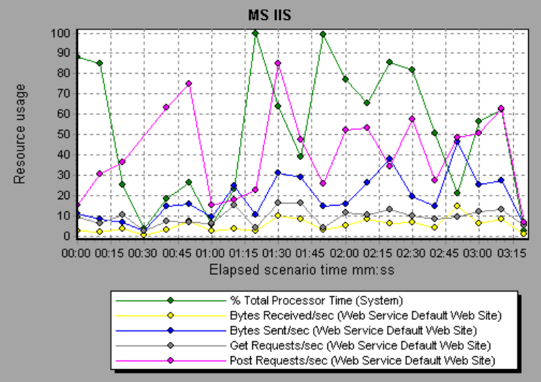
Example
In the following example the Bytes Received/sec and Get Requests/sec measurements remained fairly
steady throughout the scenario, while the % Total Processor Time,Bytes Sent/sec, and Post
Requests/sec measurements fluctuated considerably.
The scale factor for the Bytes Sent/sec and Bytes Received/sec measurements is 1/100, and the scale
factor for the Post Requests/sec measurement is 10.
Web Application Server Resource Graphs
Web Application Server Resource Graphs Overview
Web Application Server Resource graphs provide you with resource usage information about the Ariba,
ATG Dynamo, BroadVision, ColdFusion, Fujitsu INTERSTAGE, iPlanet (NAS), Microsoft ASP, Oracle9iAS
HTTP, SilverStream, WebLogic (SNMP), WebLogic (JMX), and WebSphere application servers.
In order to obtain data for these graphs, you need to activate the online monitor for the application
server and specify which resources you want to measure before running the load test scenario.
When you open a Web Application Server Resource graph, you can filter it to show only the relevant
application. When you need to analyze other applications, you can change the filter conditions and
display the desired resources.
In order to display all the measurements on a single graph, Analysis may scale them. The Legend window
indicates the scale factor for each resource. To obtain the true value, multiply the scale factor by the
User Guide
Analysis
HP LoadRunner (12.50) Page 202
displayed value. For more information on scaled measurements, see the example in "Web Server
Resource Graphs Overview" on page199.
Web Application Server Resource Graphs Measurements
Microsoft Active Server Pages (ASP) Measurements
The following default measurements are available for Microsoft Active Server Pages:
>Measurement Description
Errors per Second The number of errors per second.
Requests Wait Time The number of milliseconds the most recent request was waiting in the
queue.
Requests Executing The number of requests currently executing.
Requests Queued The number of requests waiting in the queue for service.
Requests Rejected The total number of requests not executed because there were insufficient
resources to process them.
Requests Not Found The number of requests for files that were not found.
Requests/sec The number of requests executed per second.
Memory Allocated The total amount of memory (in bytes) currently allocated by Active Server
Pages.
Errors During Script
Runtime
The number of failed requests due to runtime errors.
Sessions Current The current number of sessions being serviced.
Transactions/sec The number of transactions started per second.
Oracle9iAS HTTP Server Modules
The following table describes some of the modules that are available for the Oracle9iAS HTTP server:
Measurement Description
mod_mime.c Determines document types using file extensions.
mod_mime_
magic.c
Determines document types using "magic numbers".
User Guide
Analysis
HP LoadRunner (12.50) Page 203
Measurement Description
mod_auth_
anon.c
Provides anonymous user access to authenticated areas.
mod_auth_
dbm.c
Provides user authentication using DBM files.
mod_auth_
digest.c
Provides MD5 authentication.
mod_cern_
meta.c
Supports HTTP header metafiles.
mod_digest.c Provides MD5 authentication (deprecated by mod_auth_digest).
mod_
expires.c
Applies Expires: headers to resources.
mod_
headers.c
Adds arbitrary HTTP headers to resources.
mod_proxy.c Provides caching proxy abilities.
mod_
rewrite.c
Provides powerful URI-to-filename mapping using regular expressions.
mod_
speling.c
Automatically corrects minor typos in URLs.
mod_info.c Provides server configuration information.
mod_status.c Displays server status.
mod_
usertrack.c
Provides user tracking using cookies.
mod_dms.c Provides access to DMS Apache statistics.
mod_perl.c Allows execution of Perl scripts.
mod_
fastcgi.c
Supports CGI access to long-lived programs.
mod_ssl.c Provides SSL support.
mod_plsql.c Handles requests for Oracle stored procedures.
User Guide
Analysis
HP LoadRunner (12.50) Page 204
Measurement Description
mod_isapi.c Provides Windows ISAPI extension support.
mod_
setenvif.c
Sets environment variables based on client information.
mod_
actions.c
Executes CGI scripts based on media type or request method.
mod_imap.c Handles imagemap files.
mod_asis.c Sends files that contain their own HTTP headers.
mod_log_
config.c
Provides user-configurable logging replacement for mod_log_common.
mod_env.c Passes environments to CGI scripts.
mod_alias.c Maps different parts of the host file system in the document tree, and redirects
URLs.
mod_
userdir.c
Handles user home directories.
mod_cgi.c Invokes CGI scripts.
mod_dir.c Handles the basic directory.
mod_
autoindex.c
Provides automatic directory listings.
mod_
include.c
Provides server-parsed documents.
mod_
negotiation.c
Handles content negotiation.
mod_auth.c Provides user authentication using text files.
mod_
access.c
Provides access control based on the client host name or IP address.
mod_so.c Supports loading modules (.so on UNIX, .dll on Win32) at runtime.
mod_
oprocmgr.c
Monitors JServ processes and restarts them if they fail.
mod_jserv.c Routes HTTP requests to JServ server processes. Balances load across multiple
User Guide
Analysis
HP LoadRunner (12.50) Page 205
Measurement Description
JServs by distributing new requests in round-robin order.
mod_ose.c Routes requests to the JVM embedded in Oracle's database server.
http_core.c Handles requests for static Web pages.
Oracle9iAS HTTP Server Counters
The following table describes the counters that are available for the Oracle9iAS HTTP server:
Measurement Description
handle.minTime The minimum time spent in the module handler.
handle.avg The average time spent in the module handler.
handle.active The number of threads currently in the handle processing phase.
handle.time The total amount of time spent in the module handler.
handle.completed The number of times the handle processing phase was completed.
request.maxTime The maximum amount of time required to service an HTTP request.
request.minTime The minimum amount of time required to service an HTTP request.
request.avg The average amount of time required to service an HTTP request.
request.active The number of threads currently in the request processing phase.
request.time The total amount of time required to service an HTTP request.
request.completed The number of times the request processing phase was completed.
connection.maxTime The maximum amount of time spent servicing any HTTP connection.
connection.minTime The minimum amount of time spent servicing any HTTP connection.
connection.avg The average amount of time spent servicing HTTP connections.
connection.active The number of connections with currently open threads.
connection.time The total amount of time spent servicing HTTP connections.
connection.completed The number of times the connection processing phase was completed.
numMods.value The number of loaded modules.
User Guide
Analysis
HP LoadRunner (12.50) Page 206
Measurement Description
childFinish.count The number of times the Apache parent server started a child server, for
any reason.
childStart.count The number of times "children"finished "gracefully."There are some
ungraceful error/crash cases that are not counted in childFinish.count.
Decline.count The number of times each module declined HTTP requests.
internalRedirect.count The number of times that any module passed control to another module
using an "internal redirect".
cpuTime.value The total CPU time utilized by all processes on the Apache server (measured
in CPU milliseconds).
heapSize.value The total heap memory utilized by all processes on the Apache server
(measured in kilobytes).
pid.value The process identifier of the parent Apache process.
upTime.value The amount of time the server has been running (measured in
milliseconds).
WebLogic (SNMP) Server Table Measurements
The Server Table lists all WebLogic (SNMP) servers that are being monitored by the agent. A server must
be contacted or be reported as a member of a cluster at least once before it will appear in this table.
Servers are only reported as a member of a cluster when they are actively participating in the cluster,
or shortly thereafter.
Measurement Description
ServerState The state of the WebLogic server, as inferred by the SNMP agent. Up
implies that the agent can contact the server. Down implies that the
agent cannot contact the server.
ServerLoginEnable True if client logins are enabled on the server.
ServerMaxHeapSpace The maximum heap size for this server (in KB).
ServerHeapUsedPct The percentage of heap space currently in use on the server.
ServerQueueLength The current length of the server execute queue.
ServerQueueThroughput The current throughput of execute queue, expressed as the number
of requests processed per second.
User Guide
Analysis
HP LoadRunner (12.50) Page 207
Measurement Description
ServerNumEJBDeployment The total number of EJB deployment units known to the server.
ServerNumEJBBeansDeployed The total number of EJB beans actively deployed on the server.
WebLogic (SNMP) Listen Table Measurements
The Listen Table is the set of protocol, IP address, and port combinations on which servers are listening.
There will be multiple entries for each server: one for each (protocol, ipAddr, port) combination. If
clustering is used, the clustering-related MIB objects will assume a higher priority.
Measurement Description
ListenPort Port number.
ListenAdminOK True if admin requests are allowed on this (protocol, ipAddr, port) combination;
otherwise false.
ListenState Listening if the (protocol, ipAddr, port) combination is enabled on the server; Not
Listening if it is not. The server may be listening but not accepting new clients if its
server Login Enable state is false. In this case, existing clients will continue to
function, but new ones will not.
WebLogic (SNMP) ClassPath Table Measurements
The ClassPath Table is the table of classpath elements for Java, WebLogic (SNMP) server, and servlets.
There are multiple entries in this table for each server. There may also be multiple entries for each path
on a server. If clustering is used, the clustering-related MIB objects will assume a higher priority.
Measurement Description
CPType The type of CP element: Java, WebLogic, servlet. A Java CPType means the CP
element is one of the elements in the normal Java classpath. A WebLogic CPType
means the CP element is one of the elements in weblogic.class.path. A servlet CPType
means the CP element is one of the elements in the dynamic servlet classpath.
CPIndex The position of an element within its path. The index starts at 1.
Websphere Application Server Monitor Runtime Resource Measurements
Contains resources related to the Java Virtual Machine runtime, as well as the ORB.
User Guide
Analysis
HP LoadRunner (12.50) Page 208
Measurement Description
MemoryFree The amount of free memory remaining in the Java Virtual Machine.
MemoryTotal The total memory allocated for the Java Virtual Machine.
MemoryUse The total memory in use on the Java Virtual Machine.
Websphere Application Server Monitor BeanData Measurements
Every home on the server provides performance data, depending on the type of bean deployed in the
home. The top level bean data holds an aggregate of all the containers.
Measurement Description
BeanDestroys The number of times an individual bean object was destroyed. This applies
to any bean, regardless of its type.
StatelessBeanDestroys The number of times a stateless session bean object was destroyed.
StatefulBeanDestroys The number of times a stateful session bean object was destroyed.
Websphere Application Server Monitor BeanObjectPool Measurements
The server holds a cache of bean objects. Each home has a cache and there is therefore one
BeanObjectPoolContainer per container. The top level, BeanObjectPool, holds an aggregate of all the
containers data.
Measurement Description
NumGetFound The number of calls to the pool that resulted in finding an available bean.
NumPutsDiscarded The number of times releasing a bean to the pool resulted in the bean being
discarded because the pool was full.
Websphere Application Server Monitor OrbThreadPool Measurements
These are resources related to the ORB thread pool that is on the server.
Measurement Description
ActiveThreads The average number of active threads in the pool.
TotalThreads The average number of threads in the pool.
PercentTimeMaxed The average percent of the time that the number of threads in the pool
reached or exceeded the desired maximum number.
User Guide
Analysis
HP LoadRunner (12.50) Page 209
Websphere Application Server Monitor DBConnectionMgr Measurements
These are resources related to the database connection manager. The manager consists of a series of
data sources, as well as a top-level aggregate of each of the performance metrics.
Measurement Description
ConnectionWaitTime The average time (in seconds) of a connection grant.
ConnectionTime The average time (in seconds) that a connection is in use.
ConnectionPercentUsed The average percentage of the pool that is in use.
Websphere Application Server Monitor TransactionData Measurements
These are resources that pertain to transactions.
Measurement Description
NumTransactions The number of transactions processed.
ActiveTransactions The average number of active transactions.
TransactionRT The average duration of each transaction.
RolledBack The number of transactions rolled back.
Timeouts The number of transactions that timed out due to inactivity timeouts.
TransactionSuspended The average number of times that a transaction was suspended.
Websphere Application Server Monitor ServletEngine Measurements
These are resources that are related to servlets and JSPs.
Measurement Description
ServletErrors The number of requests that resulted in an error or an exception.
Websphere Application Server Monitor Session Measurements
These are general metrics regarding the HTTP session pool.
Measurement Description
SessionsInvalidated The number of invalidated sessions. May not be valid when using sessions in
the database mode.
User Guide
Analysis
HP LoadRunner (12.50) Page 210
Microsoft Active Server Pages (ASP) Graph
This graph displays statistics about the resource usage on the ASP server during the load test scenario
run.
X-
axis
Elapsed time since the start of the run.
Y-
axis
The resource usage on the ASP server.
Note To obtain data for this graph, you need to enable the Microsoft ASP online monitor (from the
Controller) and select the default measurements you want to display, before running the
scenario.
See
also
"Web Application Server Resource Graphs Overview" on page202
"Web Application Server Resource Graphs Measurements" on page203
Oracle9iAS HTTP Server Graph
This graph displays statistics about the resource usage on the Oracle9iAS HTTP server during the load
test scenario run.
X-
axis
Elapsed time since the start of the run.
Y-
axis
The resource usage on the Oracle9iAS HTTP server.
Note To obtain data for this graph, you need to enable the Oracle9iAS HTTP online monitor (from
the Controller), and select the default measurements you want to display, before running the
scenario.
See
also
"Web Application Server Resource Graphs Overview" on page202
"Web Application Server Resource Graphs Measurements" on page203
WebLogic (SNMP) Graph
This graph displays statistics about the resource usage on the WebLogic (SNMP) server (version 6.0 and
earlier) during the load test scenario run.
X-
axis
The elapsed time since the start of the run.
Y- The resource usage on the WebLogic (SNMP) server.
User Guide
Analysis
HP LoadRunner (12.50) Page 211
axis
Note To obtain data for this graph, you need to enable the WebLogic (SNMP) online monitor (from
the Controller) and select the default measurements you want to display, before running the
scenario.
See
also
"Web Application Server Resource Graphs Overview" on page202
"Web Application Server Resource Graphs Measurements" on page203
WebSphere Application Server Graph
This graph displays statistics about the resource usage on the WebSphere application server during the
load test scenario run.
X-
axis
Elapsed time since the start of the run.
Y-
axis
The resource usage on the WebSphere Application server.
Note To obtain data for this graph, you need to configure the WebSphere Application Server online
monitor (from the Controller) and select the default measurements you want to display,
before running the scenario.
See
also
"Web Application Server Resource Graphs Overview" on page202
"Web Application Server Resource Graphs Measurements" on page203
Database Server Resource Graphs
The Database Server Resource graphs show statistics for several database servers. Currently DB2,
Oracle, SQL server, and Sybase databases are supported. These graphs require that you specify the
resources you want to measure before running the load test scenario. For more information, see the
section on online monitors in the LoadRunner Controller documentation.
DB2 Database Manager Counters
Measurement Description
rem_cons_in The current number of connections initiated from remote clients to the instance of
the database manager that is being monitored.
rem_cons_
in_exec
The number of remote applications that are currently connected to a database and
are currently processing a unit of work within the database manager instance being
User Guide
Analysis
HP LoadRunner (12.50) Page 212
Measurement Description
monitored.
local_cons The number of local applications that are currently connected to a database within
the database manager instance being monitored.
local_cons_
in_exec
The number of local applications that are currently connected to a database within
the database manager instance being monitored and are currently processing a unit
of work.
con_local_
dbases
The number of local databases that have applications connected.
agents_
registered
The number of agents registered in the database manager instance that is being
monitored (coordinator agents and subagents).
agents_
waiting_on_
token
The number of agents waiting for a token so they can execute a transaction in the
database manager.
idle_agents The number of agents in the agent pool that are currently unassigned to an
application and are therefore "idle".
agents_
from_pool
The number of agents assigned from the agent pool.
agents_
created_
empty_pool
The number of agents created because the agent pool was empty.
agents_
stolen
The number of times that agents are stolen from an application. Agents are stolen
when an idle agent associated with an application is reassigned to work on a
different application.
comm_
private_mem
The amount of private memory that the instance of the database manager has
currently committed at the time of the snapshot.
inactive_gw_
agents
The number of DRDA agents in the DRDA connections pool that are primed with a
connection to a DRDA database, but are inactive.
num_gw_
conn_
switches
The number of times that an agent from the agents pool was primed with a
connection and was stolen for use with a different DRDA database.
sort_heap_
allocated
The total number of allocated pages of sort heap space for all sorts at the level
chosen and at the time the snapshot was taken.
post_ The number of sorts that have requested heaps after the sort heap threshold has
User Guide
Analysis
HP LoadRunner (12.50) Page 213
Measurement Description
threshold_
sorts
been reached.
piped_sorts_
requested
The number of piped sorts that have been requested.
piped_sorts_
accepted
The number of piped sorts that have been accepted.
DB2 Database Counters
Measurement Description
appls_cur_
cons
Indicates the number of applications that are currently connected to the database.
appls_in_db2 Indicates the number of applications that are currently connected to the database,
and for which the database manager is currently processing a request.
total_sec_
cons
The number of connections made by a sub-agent to the database at the node.
num_assoc_
agents
At the application level, this is the number of sub-agents associated with an
application. At the database level, it is the number of sub-agents for all applications.
sort_heap_
allocated
The total number of allocated pages of sort heap space for all sorts at the level
chosen and at the time the snapshot was taken.
total_sorts The total number of sorts that have been executed.
total_sort_
time
The total elapsed time (in milliseconds) for all sorts that have been executed.
sort_
overflows
The total number of sorts that ran out of sort heap and may have required disk
space for temporary storage.
active_sorts The number of sorts in the database that currently have a sort heap allocated.
total_hash_
joins
The total number of hash joins executed.
total_hash_
loops
The total number of times that a single partition of a hash join was larger than the
available sort heap space.
hash_join_ The number of times that hash join data exceeded the available sort heap space.
User Guide
Analysis
HP LoadRunner (12.50) Page 214
Measurement Description
overflows
hash_join_
small_
overflows
The number of times that hash join data exceeded the available sort heap space by
less than 10%.
pool_data_l_
reads
The number of logical read requests for data pages that have gone through the
buffer pool.
pool_data_p_
reads
The number of read requests that required I/O to get data pages into the buffer
pool.
pool_data_
writes
Indicates the number of times a buffer pool data page was physically written to disk.
pool_index_
l_reads
The number of logical read requests for index pages that have gone through the
buffer pool.
pool_index_
p_reads
The number of physical read requests to get index pages into the buffer pool.
pool_index_
writes
The number of times a buffer pool index page was physically written to disk.
pool_read_
time
The total amount of elapsed time spent processing read requests that caused data
or index pages to be physically read from disk to buffer pool.
pool_write_
time
The total amount of time spent physically writing data or index pages from the
buffer pool to disk.
files_closed The total number of database files closed.
pool_async_
data_reads
The number of pages read asynchronously into the buffer pool.
pool_async_
data_writes
The number of times a buffer pool data page was physically written to disk by either
an asynchronous page cleaner, or a pre-fetcher. A pre-fetcher may have written dirty
pages to disk to make space for the pages being pre-fetched.
pool_async_
index_writes
The number of times a buffer pool index page was physically written to disk by either
an asynchronous page cleaner, or a pre-fetcher. A pre-fetcher may have written dirty
pages to disk to make space for the pages being pre-fetched.
pool_async_
index_reads
The number of index pages read asynchronously into the buffer pool by a pre-
fetcher.
User Guide
Analysis
HP LoadRunner (12.50) Page 215
Measurement Description
pool_async_
read_time
The total elapsed time spent reading by database manager pre-fetchers.
pool_async_
write_time
The total elapsed time spent writing data or index pages from the buffer pool to disk
by database manager page cleaners.
pool_async_
data_read_
reqs
The number of asynchronous read requests.
pool_lsn_
gap_clns
The number of times a page cleaner was invoked because the logging space used
had reached a pre-defined criterion for the database.
pool_drty_
pg_steal_
clns
The number of times a page cleaner was invoked because a synchronous write was
needed during the victim buffer replacement for the database.
pool_drty_
pg_thrsh_
clns
The number of times a page cleaner was invoked because a buffer pool had reached
the dirty page threshold criterion for the database.
prefetch_
wait_time
The time an application spent waiting for an I/O server (pre-fetcher) to finish loading
pages into the buffer pool.
pool_data_
to_estore
The number of buffer pool data pages copied to extended storage.
pool_index_
to_estore
The number of buffer pool index pages copied to extended storage.
pool_data_
from_estore
The number of buffer pool data pages copied from extended storage.
pool_index_
from_estore
The number of buffer pool index pages copied from extended storage.
direct_reads The number of read operations that do not use the buffer pool.
direct_writes The number of write operations that do not use the buffer pool.
direct_read_
reqs
The number of requests to perform a direct read of one or more sectors of data.
direct_write_
reqs
The number of requests to perform a direct write of one or more sectors of data.
User Guide
Analysis
HP LoadRunner (12.50) Page 216
Measurement Description
direct_read_
time
The elapsed time (in milliseconds) required to perform the direct reads.
direct_write_
time
The elapsed time (in milliseconds) required to perform the direct writes.
cat_cache_
lookups
The number of times that the catalog cache was referenced to obtain table
descriptor information.
cat_cache_
inserts
The number of times that the system tried to insert table descriptor information into
the catalog cache.
cat_cache_
overflows
The number of times that an insert into the catalog cache failed due the catalog
cache being full.
cat_cache_
heap_full
The number of times that an insert into the catalog cache failed due to a heap-full
condition in the database heap.
pkg_cache_
lookups
The number of times that an application looked for a section or package in the
package cache. At a database level, it indicates the overall number of references
since the database was started, or monitor data was reset.
pkg_cache_
inserts
The total number of times that a requested section was not available for use and
had to be loaded into the package cache. This count includes any implicit prepares
performed by the system.
pkg_cache_
num_
overflows
The number of times that the package cache overflowed the bounds of its allocated
memory.
appl_
section_
lookups
Lookups of SQL sections by an application from its SQL work area.
appl_
section_
inserts
Inserts of SQL sections by an application from its SQL work area.
sec_logs_
allocated
The total number of secondary log files that are currently being used for the
database.
log_reads The number of log pages read from disk by the logger.
log_writes The number of log pages written to disk by the logger.
total_log_ The total amount of active log space currently used (in bytes) in the database.
User Guide
Analysis
HP LoadRunner (12.50) Page 217
Measurement Description
used
locks_held The number of locks currently held.
lock_list_in_
use
The total amount of lock list memory (in bytes) that is in use.
deadlocks The total number of deadlocks that have occurred.
lock_escals The number of times that locks have been escalated from several row locks to a
table lock.
x_lock_
escals
The number of times that locks have been escalated from several row locks to one
exclusive table lock, or the number of times an exclusive lock on a row caused the
table lock to become an exclusive lock.
lock_
timeouts
The number of times that a request to lock an object timed-out instead of being
granted.
lock_waits The total number of times that applications or connections waited for locks.
lock_wait_
time
The total elapsed time waited for a lock.
locks_
waiting
The number of agents waiting on a lock.
rows_deleted The number of row deletions attempted.
rows_
inserted
The number of row insertions attempted.
rows_
updated
The number of row updates attempted.
rows_
selected
The number of rows that have been selected and returned to the application.
int_rows_
deleted
The number of rows deleted from the database as a result of internal activity.
int_rows_
updated
The number of rows updated from the database as a result of internal activity.
int_rows_
inserted
The number of rows inserted into the database as a result of internal activity caused
by triggers.
User Guide
Analysis
HP LoadRunner (12.50) Page 218
Measurement Description
static_sql_
stmts
The number of static SQL statements that were attempted.
dynamic_
sql_stmts
The number of dynamic SQL statements that were attempted.
failed_sql_
stmts
The number of SQL statements that were attempted, but failed.
commit_sql_
stmts
The total number of SQL COMMIT statements that have been attempted.
rollback_sql_
stmts
The total number of SQL ROLLBACK statements that have been attempted.
select_sql_
stmts
The number of SQL SELECT statements that were executed.
uid_sql_
stmts
The number of SQL UPDATE, INSERT, and DELETE statements that were executed.
ddl_sql_
stmts
The number of SQL Data Definition Language (DDL) statements that were executed.
int_auto_
rebinds
The number of automatic rebinds (or recompiles) that have been attempted.
int_commits The total number of commits initiated internally by the database manager.
int_rollbacks The total number of rollbacks initiated internally by the database manager.
int_
deadlock_
rollbacks
The total number of forced rollbacks initiated by the database manager due to a
deadlock. A rollback is performed on the current unit of work in an application
selected by the database manager to resolve the deadlock.
binds_
precompiles
The number of binds and pre-compiles attempted.
DB2 Application Counters
Measurement Description
agents_
stolen
The number of times that agents are stolen from an application. Agents are stolen
when an idle agent associated with an application is reassigned to work on a
User Guide
Analysis
HP LoadRunner (12.50) Page 219
Measurement Description
different application.
num_assoc_
agents
At the application level, this is the number of sub-agents associated with an
application. At the database level, it is the number of sub-agents for all applications.
total_sorts The total number of sorts that have been executed.
total_sort_
time
The total elapsed time (in milliseconds) for all sorts that have been executed.
sort_
overflows
The total number of sorts that ran out of sort heap and may have required disk
space for temporary storage.
total_hash_
joins
The total number of hash joins executed.
total_hash_
loops
The total number of times that a single partition of a hash join was larger than the
available sort heap space.
hash_join_
overflows
The number of times that hash join data exceeded the available sort heap space
hash_join_
small_
overflows
The number of times that hash join data exceeded the available sort heap space by
less than 10%.
pool_data_l_
reads
The number of logical read requests for data pages that have gone through the
buffer pool.
pool_data_p_
reads
The number of read requests that required I/O to get data pages into the buffer
pool.
pool_data_
writes
The number of times a buffer pool data page was physically written to disk.
pool_index_
l_reads
The number of logical read requests for index pages that have gone through the
buffer pool.
pool_index_
p_reads
The number of physical read requests to get index pages into the buffer pool.
pool_index_
writes
The number of times a buffer pool index page was physically written to disk.
pool_read_
time
The total amount of elapsed time spent processing read requests that caused data
or index pages to be physically read from disk to buffer pool.
User Guide
Analysis
HP LoadRunner (12.50) Page 220
Measurement Description
prefetch_
wait_time
The time an application spent waiting for an I/O server (pre-fetcher) to finish loading
pages into the buffer pool.
pool_data_
to_estore
The number of buffer pool data pages copied to extended storage.
pool_index_
to_estore
The number of buffer pool index pages copied to extended storage.
pool_data_
from_estore
The number of buffer pool data pages copied from extended storage.
pool_index_
from_estore
The number of buffer pool index pages copied from extended storage.
direct_reads The number of read operations that do not use the buffer pool.
direct_writes The number of write operations that do not use the buffer pool.
direct_read_
reqs
The number of requests to perform a direct read of one or more sectors of data.
direct_write_
reqs
The number of requests to perform a direct write of one or more sectors of data.
direct_read_
time
The elapsed time (in milliseconds) required to perform the direct reads.
direct_write_
time
The elapsed time (in milliseconds) required to perform the direct writes.
cat_cache_
lookups
The number of times that the catalog cache was referenced to obtain table
descriptor information.
cat_cache_
inserts
The number of times that the system tried to insert table descriptor information into
the catalog cache.
cat_cache_
overflows
The number of times that an insert into the catalog cache failed due to the catalog
cache being full.
cat_cache_
heap_full
The number of times that an insert into the catalog cache failed due to a heap-full
condition in the database heap.
pkg_cache_
lookups
The number of times that an application looked for a section or package in the
package cache. At a database level, it indicates the overall number of references
since the database was started, or monitor data was reset.
User Guide
Analysis
HP LoadRunner (12.50) Page 221
Measurement Description
pkg_cache_
inserts
The total number of times that a requested section was not available for use and
had to be loaded into the package cache. This count includes any implicit prepares
performed by the system.
appl_
section_
lookups
Lookups of SQL sections by an application from its SQL work area.
appl_
section_
inserts
Inserts of SQL sections by an application from its SQL work area.
uow_log_
space_used
The amount of log space (in bytes) used in the current unit of work of the monitored
application.
locks_held The number of locks currently held.
deadlocks The total number of deadlocks that have occurred.
lock_escals The number of times that locks have been escalated from several row locks to a
table lock.
x_lock_
escals
The number of times that locks have been escalated from several row locks to one
exclusive table lock, or the number of times an exclusive lock on a row caused the
table lock to become an exclusive lock.
lock_
timeouts
The number of times that a request to lock an object timed-out instead of being
granted.
lock_waits The total number of times that applications or connections waited for locks.
lock_wait_
time
The total elapsed time waited for a lock.
locks_
waiting
The number of agents waiting on a lock.
uow_lock_
wait_time
The total amount of elapsed time this unit of work has spent waiting for locks.
rows_deleted The number of row deletions attempted.
rows_
inserted
The number of row insertions attempted.
rows_
updated
The number of row updates attempted.
User Guide
Analysis
HP LoadRunner (12.50) Page 222
Measurement Description
rows_
selected
The number of rows that have been selected and returned to the application.
rows_written The number of rows changed (inserted, deleted or updated) in the table.
rows_read The number of rows read from the table.
int_rows_
deleted
The number of rows deleted from the database as a result of internal activity.
int_rows_
updated
The number of rows updated from the database as a result of internal activity.
int_rows_
inserted
The number of rows inserted into the database as a result of internal activity caused
by triggers.
open_rem_
curs
The number of remote cursors currently open for this application, including those
cursors counted by `open_rem_curs_blk'.
open_rem_
curs_blk
The number of remote blocking cursors currently open for this application.
rej_curs_blk The number of times that a request for an I/O block at server was rejected and the
request was converted to non-blocked I/O.
acc_curs_blk The number of times that a request for an I/O block was accepted.
open_loc_
curs
The number of local cursors currently open for this application, including those
cursors counted by `open_loc_curs_blk'.
open_loc_
curs_blk
The number of local blocking cursors currently open for this application.
static_sql_
stmts
The number of static SQL statements that were attempted.
dynamic_
sql_stmts
The number of dynamic SQL statements that were attempted.
failed_sql_
stmts
The number of SQL statements that were attempted, but failed.
commit_sql_
stmts
The total number of SQL COMMIT statements that have been attempted.
rollback_sql_
stmts
The total number of SQL ROLLBACK statements that have been attempted.
User Guide
Analysis
HP LoadRunner (12.50) Page 223
Measurement Description
select_sql_
stmts
The number of SQL SELECT statements that were executed.
uid_sql_
stmts
The number of SQL UPDATE, INSERT, and DELETE statements that were executed.
ddl_sql_
stmts
This element indicates the number of SQL Data Definition Language (DDL)
statements that were executed.
int_auto_
rebinds
The number of automatic rebinds (or recompiles) that have been attempted.
int_commits The total number of commits initiated internally by the database manager.
int_rollbacks The total number of rollbacks initiated internally by the database manager.
int_
deadlock_
rollbacks
The total number of forced rollbacks initiated by the database manager due to a
deadlock. A rollback is performed on the current unit of work in an application
selected by the database manager to resolve the deadlock.
binds_
precompiles
The number of binds and pre-compiles attempted.
Oracle Server Monitoring Measurements
The following measurements are most commonly used when monitoring the Oracle server (from the
V$SYSSTAT table):
Measurement Description
CPU used by
this session
The amount of CPU time (in tens of milliseconds) used by a session between the time
a user call started and ended. Some user calls can be completed within 10
milliseconds and, as a result, the start- and end-user call time can be the same. In
this case, 0 milliseconds are added to the statistic. A similar problem can exist in the
operating system reporting, especially on systems that suffer from many context
switches.
Bytes
received via
SQL*Net from
client
The total number of bytes received from the client over Net8.
Logons
current
The total number of current logons.
User Guide
Analysis
HP LoadRunner (12.50) Page 224
Measurement Description
Opens of
replaced
files
The total number of files that needed to be reopened because they were no longer in
the process file cache.
User calls Oracle allocates resources (Call State Objects) to keep track of relevant user call
data structures every time you log in, parse, or execute. When determining activity,
the ratio of user calls to RPI calls gives you an indication of how much internal work is
generated as a result of the type of requests the user is sending to Oracle.
SQL*Net
roundtrips
to/from
client
The total number of Net8 messages sent to, and received from, the client.
Bytes sent
via SQL*Net
to client
The total number of bytes sent to the client from the foreground process(es).
Opened
cursors
current
The total number of current open cursors.
DB block
changes
Closely related to consistent changes, this statistic counts the total number of
changes that were made to all blocks in the SGA that were part of an update or
delete operation. These are changes that generate redo log entries and hence cause
permanent changes to the database if the transaction is committed. This statistic is
a rough indication of total database work and indicates (possibly on a per-
transaction level) the rate at which buffers are being dirtied.
Total file
opens
The total number of file opens being performed by the instance. Each process needs
a number of files (control file, log file, database file) in order to work against the
database.
SQL Server Default Counters
Measurement Description
% Total
Processor Time
The average percentage of time that all the processors on the system are busy
executing non-idle threads. On a multi-processor system, if all processors are
always busy, this is 100%, if all processors are 50% busy this is 50% and if 1/4 of
the processors are 100% busy this is 25%. It can be viewed as the fraction of the
time spent doing useful work. Each processor is assigned an Idle thread in the Idle
process which consumes those unproductive processor cycles not used by any
User Guide
Analysis
HP LoadRunner (12.50) Page 225
Measurement Description
other threads.
Cache Hit Ratio The percentage of time that a requested data page was found in the data cache
(instead of being read from disk).
I/O - Batch
Writes/sec
The number of pages written to disk per second, using Batch I/O. The checkpoint
thread is the primary user of Batch I/O.
I/O - Lazy
Writes/sec
The number of pages flushed to disk per second by the Lazy Writer.
I/O -
Outstanding
Reads
The number of physical reads pending.
I/O -
Outstanding
Writes
The number of physical writes pending.
I/O - Page
Reads/sec
The number of physical page reads per second.
I/O -
Transactions/sec
The number of Transact-SQL command batches executed per second.
User
Connections
The number of open user connections.
% Processor
Time
The percentage of time that the processor is executing a non-idle thread. This
counter was designed as a primary indicator of processor activity. It is calculated
by measuring the time that the processor spends executing the thread of the idle
process in each sample interval, and subtracting that value from 100%. (Each
processor has an idle thread which consumes cycles when no other threads are
ready to run). It can be viewed as the percentage of the sample interval spent
doing useful work. This counter displays the average percentage of busy time
observed during the sample interval. It is calculated by monitoring the time the
service was inactive, and then subtracting that value from 100%.
Sybase Server Monitoring Measurements
The following tables describe the measurements that can be monitored on a Sybase server:
Object Measurement Description
Network Average packet Reports the number of network packets received.
User Guide
Analysis
HP LoadRunner (12.50) Page 226
Object Measurement Description
size (Read)
Average packet
size (Send)
Reports the number of network packets sent.
Network bytes
(Read)
Reports the number of bytes received, over the sampling interval.
Network bytes
(Read)/sec
Reports the number of bytes received, per second.
Network bytes
(Send)
Reports the number of bytes sent, over the sampling interval.
Network bytes
(Send)/sec
Reports the number of bytes sent, per second.
Network packets
(Read)
Reports the number of network packets received, over the
sampling interval.
Network packets
(Read)/sec
Reports the number of network packets received, per second.
Network packets
(Send)
Reports the number of network packets sent, over the sampling
interval.
Network packets
(Send)/sec
Reports the number of network packets sent, per second.
Memory Memory Reports the amount of memory (in bytes) allocated for the page
cache.
Disk Reads Reports the number of reads made from a database device.
Writes Reports the number of writes made to a database device.
Waits Reports the number of times that access to a device had to wait.
Grants Reports the number of times access to a device was granted.
Engine Server is busy
(%)
Reports the percentage of time during which the Adaptive Server is
in a "busy" state.
CPU time Reports how much "busy" time was used by the engine.
Logical pages
(Read)
Reports the number of data page reads, whether satisfied from
cache or from a database device.
Pages from disk Reports the number of data page reads that could not be satisfied
User Guide
Analysis
HP LoadRunner (12.50) Page 227
Object Measurement Description
(Read) from the data cache.
Pages stored Reports the number of data pages written to a database device.
Stored
Procedures
Executed
(sampling
period)
Reports the number of times a stored procedure was executed,
over the sampling interval.
Executed
(session)
Reports the number of times a stored procedure was executed,
during the session.
Average
duration
(sampling
period)
Reports the time (in seconds) spent executing a stored procedure,
over the sampling interval.
Average
duration
(session)
Reports the time (in seconds) spent executing a stored procedure,
during the session.
Locks % Requests Reports the percentage of successful requests for locks.
Locks count Reports the number of locks. This is an accumulated value.
Granted
immediately
Reports the number of locks that were granted immediately,
without having to wait for another lock to be released.
Granted after
wait
Reports the number of locks that were granted after waiting for
another lock to be released.
Not granted Reports the number of locks that were requested but not granted.
Wait time (avg.) Reports the average wait time for a lock.
SqlSrvr Locks/sec Reports the number of locks. This is an accumulated value.
% Processor
time (server)
Reports the percentage of time that the Adaptive Server is in a
"busy" state.
Transactions Reports the number of committed Transact-SQL statement blocks
(transactions).
Deadlocks Reports the number of deadlocks.
Cache % Hits Reports the percentage of times that a data page read could be
satisfied from cache without requiring a physical page read.
Pages (Read) Reports the number of data page reads, whether satisfied from
User Guide
Analysis
HP LoadRunner (12.50) Page 228
Object Measurement Description
cache or from a database device.
Cache Pages (Read)
/sec
Reports the number of data page reads, whether satisfied from
cache or from a database device, per second.
Pages from disk
(Read)
Reports the number of data page reads that could not be satisfied
from the data cache.
Pages from disk
(Read)/sec
Reports the number of data page reads, per second, that could not
be satisfied from the data cache.
Pages (Write) Reports the number of data pages written to a database device.
Pages (Write)
/sec
Reports the number of data pages written to a database device,
per second.
Process % Processor
time (process)
Reports the percentage of time that a process running a given
application was in the "Running" state (out of the time that all
processes were in the "Running" state).
Locks/sec Reports the number of locks, by process. This is an accumulated
value.
% Cache hit Reports the percentage of times that a data page read could be
satisfied from cache without requiring a physical page read, by
process.
Pages (Write) Reports the number of data pages written to a database device, by
process.
Transaction Transactions Reports the number of committed Transact-SQL statement blocks
(transactions), during the session.
Transaction Rows (Deleted) Reports the number of rows deleted from database tables during
the session.
Inserts Reports the number of insertions into a database table during the
session.
Updates Reports the updates to database tables during the session.
Updates in place Reports the sum of expensive, in-place and not-in-place updates
(everything except updates deferred) during the session.
Transactions/sec Reports the number of committed Transact-SQL statement blocks
(transactions) per second.
Rows (Deleted) Reports the number of rows deleted from database tables, per
User Guide
Analysis
HP LoadRunner (12.50) Page 229
Object Measurement Description
/sec second.
Inserts/sec Reports the number of insertions into a database table, per
second.
Updates/sec Reports the updates to database tables, per second.
Updates in
place/sec
Reports the sum of expensive, in-place and not-in-place updates
(everything except updates deferred), per second.
DB2 Graph
This graph shows the resource usage on the DB2 database server machine as a function of the elapsed
load test scenario time.
X-
axis
Elapsed time since the start of the run.
Y-
axis
The resource usage on the DB2 database server.
Note In order to monitor the DB2 database server machine, you must first set up the DB2 monitor
environment. You then enable the DB2 monitor (from the Controller) by selecting the counters
you want the monitor to measure.
See
also
"Database Server Resource Graphs" on page212
"DB2 Database Manager Counters" on page212
"DB2 Database Counters" on page214
"DB2 Application Counters" on page219
Oracle Graph
This graph displays information from Oracle V$ tables: Session statistics, V$SESSTAT, system statistics,
V$SYSSTAT, and other table counters defined by the user in the custom query.
X-
axis
Elapsed time since the start of the run.
Y-
axis
The resource usage on the Oracle server.
Note To obtain data for this graph, you need to enable the Oracle online monitor (from the
Controller) and select the default measurements you want to display, before running the
User Guide
Analysis
HP LoadRunner (12.50) Page 230
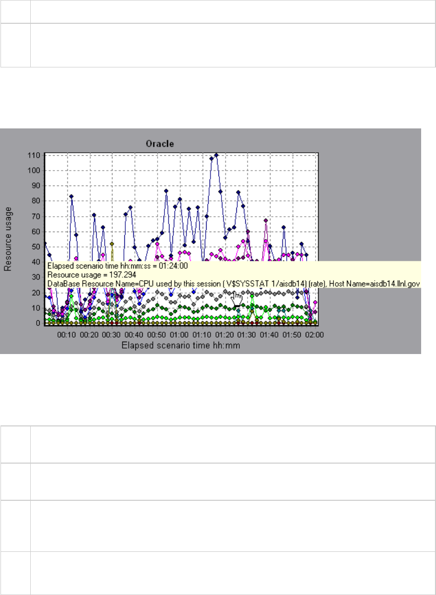
scenario.
See
also
"Database Server Resource Graphs" on page212
"Oracle Server Monitoring Measurements" on page224
Example
In the following example, the V$SYSSTAT resource values are shown as a function of the elapsed load
test scenario time:
SQL Server Graph
This graph shows the standard Windows resources on the SQL server machine.
X-
axis
Elapsed time since the start of the load test scenario run.
Y-
axis
Resource usage
Note To obtain data for this graph, you need to enable the SQL Server online monitor (from the
Controller) and select the default measurements you want to display, before running the
scenario.
See
also
"Database Server Resource Graphs" on page212
"SQL Server Default Counters" on page225
Example
User Guide
Analysis
HP LoadRunner (12.50) Page 231
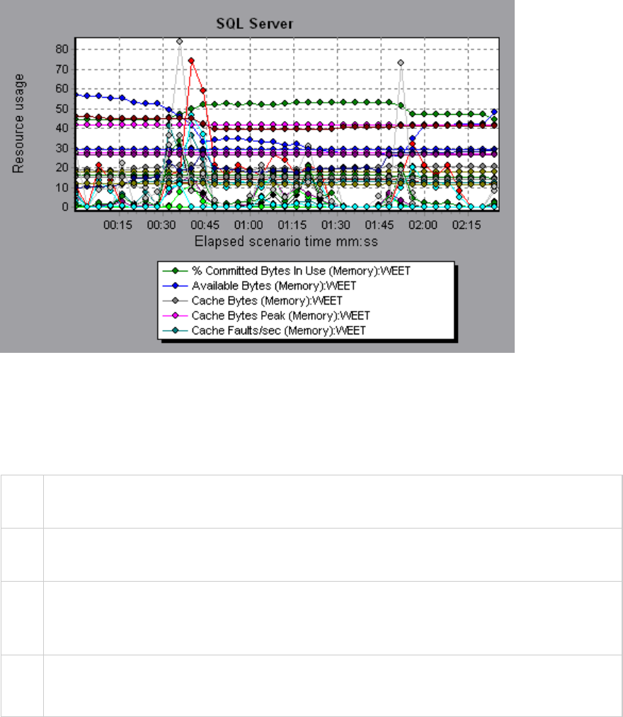
Sybase Graph
This graph shows the resource usage on the Sybase database server machine as a function of the
elapsed load test scenario time.
X-
axis
Elapsed time since the start of the run.
Y-
axis
The resource usage on the Sybase database server.
Note In order to monitor the Sybase database server machine, you must first set up the Sybase
monitor environment. You then enable the Sybase monitor (from the Controller) by selecting
the counters you want the monitor to measure.
See
also
"Database Server Resource Graphs" on page212
"SQL Server Default Counters" on page225
Streaming Media Graphs
Streaming Media Graphs Overview
Streaming Media Resource graphs provide you with performance information for the RealPlayer Client,
RealPlayer Server, Windows Media Server, and Media Player Client machines.
User Guide
Analysis
HP LoadRunner (12.50) Page 232
In order to obtain data for Streaming Media Resource graphs, you need to install the RealPlayer Client
and activate the online monitor for the RealPlayer Server or Windows Media Server before running the
load test scenario.
When you set up the online monitor for the RealPlayer Server or Windows Media Server, you indicate
which statistics and measurements to monitor. For more information on installing and configuring the
Streaming Media Resource monitors, see Media Player Client Performance Counters.
In order to display all the measurements on a single graph, Analysis may scale them. The Legend window
indicates the scale factor for each resource. To obtain the true value, multiply the scale factor by the
displayed value.
Media Player Client Monitoring Measurements
The following table describes the Media Player Client measurements that are monitored:
Measurement Description
Average
Buffering
Events
The number of times Media Player Client had to buffer incoming media data due to
insufficient media content.
Average
Buffering
Time (sec)
The time spent by Media Player Client waiting for sufficient amount of media data in
order to continue playing media clip.
Current
bandwidth
(Kbits/sec)
The number of kbits per second received.
Number of
Packets
The number of packets sent by server for a particular media clip.
Stream
Interruptions
The number of interruptions encountered by Media Player Client while playing a
media clip. This measurement includes the number of times Media Player Client had
to buffer incoming media data, and any errors that occurred during playback.
Stream
Quality
(Packet-
level)
The percentage ratio of packets received to total packets.
Stream
Quality
(Sampling-
level)
The percentage of stream samples received on time (no delays in reception).
Total number The number of lost packets that were recovered. This value is only relevant during
User Guide
Analysis
HP LoadRunner (12.50) Page 233
Measurement Description
of recovered
packets
network playback.
Total number
of lost
packets
The number of lost packets that were not recovered. This value is only relevant
during network playback.
RealPlayer Client Monitoring Measurements
The following table describes the RealPlayer Client measurements that are monitored:
Measurement Description
Current Bandwidth
(Kbits/sec)
The number of kilobytes in the last second.
Buffering Event Time (sec) The average time spent on buffering.
Network Performance The ratio (percentage) between the current bandwidth and the
actual bandwidth of the clip.
Percentage of Recovered
Packets
The percentage of error packets that were recovered.
Percentage of Lost Packets The percentage of packets that were lost.
Percentage of Late Packets The percentage of late packets.
Time to First Frame
Appearance (sec)
The time for first frame appearance (measured from the start of
the replay).
Number of Buffering Events The average number of all buffering events.
Number of Buffering Seek
Events
The average number of buffering events resulting from a seek
operation.
Buffering Seek Time The average time spent on buffering events resulting from a seek
operation.
Number of Buffering
Congestion Events
The average number of buffering events resulting from network
congestion.
Buffering Congestion Time The average time spent on buffering events resulting from network
congestion.
Number of Buffering Live
Pause Events
The average number of buffering events resulting from live pause.
User Guide
Analysis
HP LoadRunner (12.50) Page 234
Measurement Description
Buffering Live Pause Time The average time spent on buffering events resulting from live
pause.
RealPlayer Server Monitoring Measurements
The following table describes the RealPlayer Client measurements that are monitored:
Measurement Description
Current Bandwidth
(Kbits/sec)
The number of kilobytes in the last second.
Buffering Event Time (sec) The average time spent on buffering.
Network Performance The ratio (percentage) between the current bandwidth and the
actual bandwidth of the clip.
Percentage of Recovered
Packets
The percentage of error packets that were recovered.
Percentage of Lost Packets The percentage of packets that were lost.
Percentage of Late Packets The percentage of late packets.
Time to First Frame
Appearance (sec)
The time for first frame appearance (measured from the start of
the replay).
Number of Buffering Events The average number of all buffering events.
Number of Buffering Seek
Events
The average number of buffering events resulting from a seek
operation.
Buffering Seek Time The average time spent on buffering events resulting from a seek
operation.
Number of Buffering
Congestion Events
The average number of buffering events resulting from network
congestion.
Buffering Congestion Time The average time spent on buffering events resulting from network
congestion.
Number of Buffering Live
Pause Events
The average number of buffering events resulting from live pause.
Buffering Live Pause Time The average time spent on buffering events resulting from live
pause.
User Guide
Analysis
HP LoadRunner (12.50) Page 235

Windows Media Server Default Measurements
Measurement Description
Active Live
Unicast
Streams
(Windows)
The number of live unicast streams that are being streamed.
Active
Streams
The number of streams that are being streamed.
Active TCP
Streams
The number of TCP streams that are being streamed.
Active UDP
Streams
The number of UDP streams that are being streamed.
Aggregate
Read Rate
The total, aggregate rate (bytes/sec) of file reads.
Aggregate
Send Rate
The total, aggregate rate (bytes/sec) of stream transmission.
Connected
Clients
The number of clients connected to the server.
Connection
Rate
The rate at which clients are connecting to the server.
Controllers The number of controllers currently connected to the server.
HTTP
Streams
The number of HTTP streams being streamed.
Late Reads The number of late read completions per second.
Pending
Connections
The number of clients that are attempting to connect to the server, but are not yet
connected. This number may be high if the server is running near maximum capacity
and cannot process a large number of connection requests in a timely manner.
Stations The number of station objects that currently exist on the server.
Streams The number of stream objects that currently exist on the server.
Stream
Errors
The cumulative number of errors occurring per second.
User Guide
Analysis
HP LoadRunner (12.50) Page 236
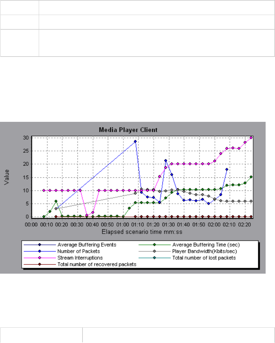
Media Player Client Graph
This graph shows statistics on the Windows Media Player client machine as a function of the elapsed
load test scenario time.
X-axis Elapsed time since the start of the run.
Y-axis The resource usage on the Windows Media Player client machine.
See also "Streaming Media Graphs Overview" on page232
"Media Player Client Monitoring Measurements" on page233
Example
In the following example the Total number of recovered packets remained steady during the first two
and a half minutes of the scenario. The Number of Packets and Stream Interruptions fluctuated
significantly. The Average Buffering Time increased moderately, and the Player Bandwidth increased
and then decreased moderately. The scale factor for the Stream Interruptions and Average Buffering
Events measurements is 10, and the scale factor for Player Bandwidth is 1/10.
Real Client Graph
This graph shows statistics on the RealPlayer client machine as a function of the elapsed load test
scenario time.
X-axis Elapsed time since the start of the run.
User Guide
Analysis
HP LoadRunner (12.50) Page 237
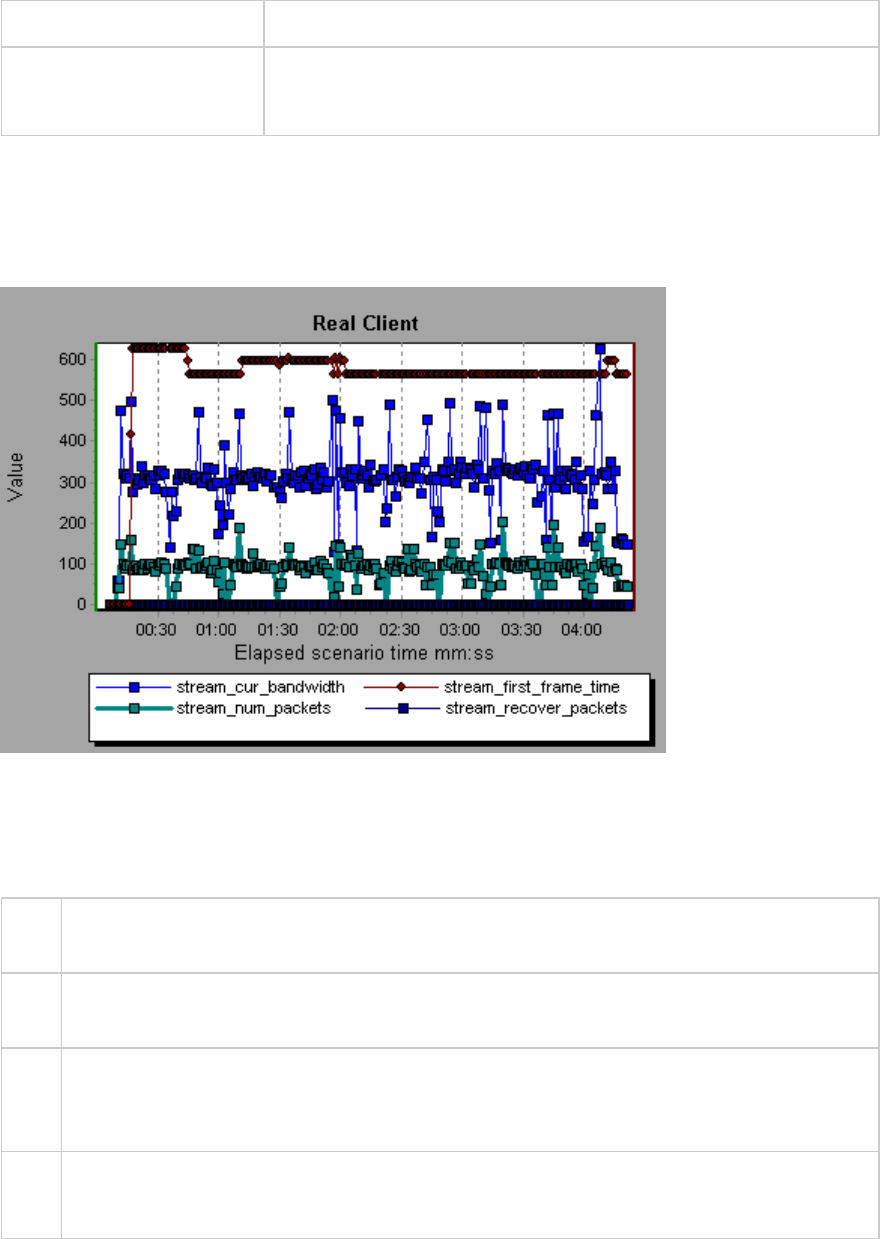
Y-axis The resource usage on the RealPlayer client machine.
See also "Streaming Media Graphs Overview" on page232
"RealPlayer Client Monitoring Measurements" on page234
Example
In the following example this graph displays the Total Number of Packets, Number of Recovered
Packets, Current Bandwidth, and First Frame Time measurements during the first four and a half
minutes of the scenario. The scale factor is the same for all of the measurements.
Real Server Graph
This graph shows RealPlayer server statistics as a function of the elapsed load test scenario time.
X-
axis
Elapsed time since the start of the run.
Y-
axis
The resource usage of the RealPlayer server machine.
Note To obtain data for this graph, you need to enable the RealPlayer Server online monitor (from
the Controller) and select the default measurements you want to display, before running the
scenario.
See
also
"Streaming Media Graphs Overview" on page232
"RealPlayer Server Monitoring Measurements" on page235
Example
User Guide
Analysis
HP LoadRunner (12.50) Page 238
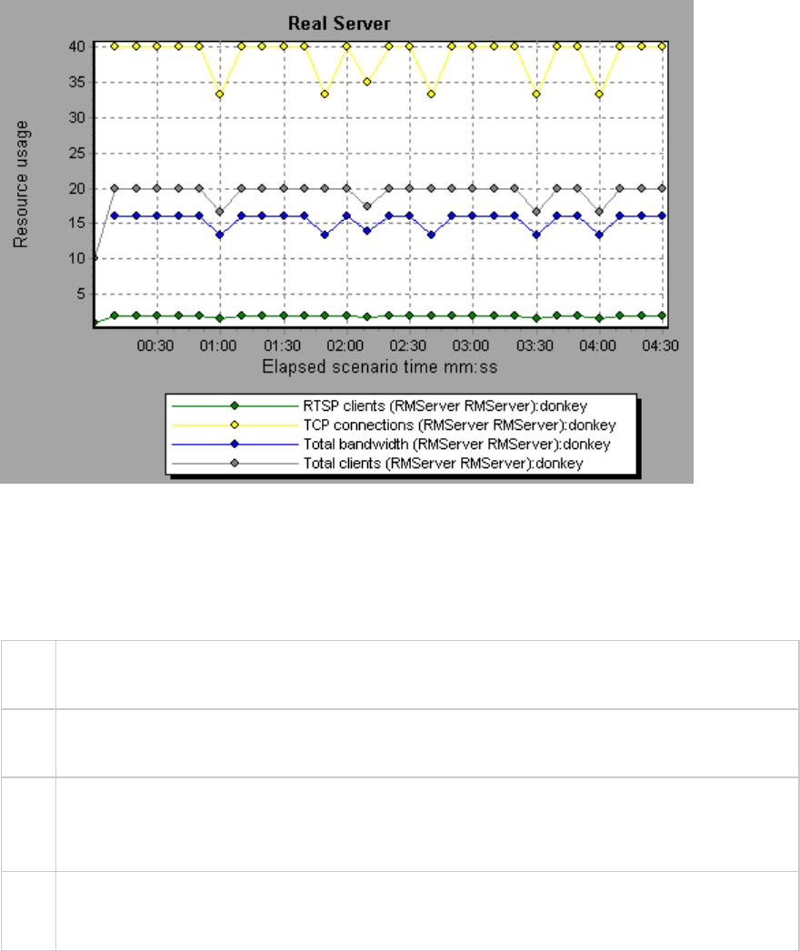
In the following example this graph displays the Total Number of Packets, Number of Recovered
Packets, Current Bandwidth, and First Frame Time measurements during the first four and a half
minutes of the scenario. The scale factor is the same for all of the measurements.
Windows Media Server Graph
This graph shows the Windows Media server statistics as a function of the elapsed load test scenario
time.
X-
axis
Elapsed time since the start of the run.
Y-
axis
Resource usage.
Note To obtain data for this graph, you need to enable the Windows Media Server online monitor
(from the Controller) and select the default measurements you want to display, before
running the scenario.
See
also
"Streaming Media Graphs Overview" on page232
"Windows Media Server Default Measurements" on page236
J2EE & .NET Diagnostics Graphs
User Guide
Analysis
HP LoadRunner (12.50) Page 239
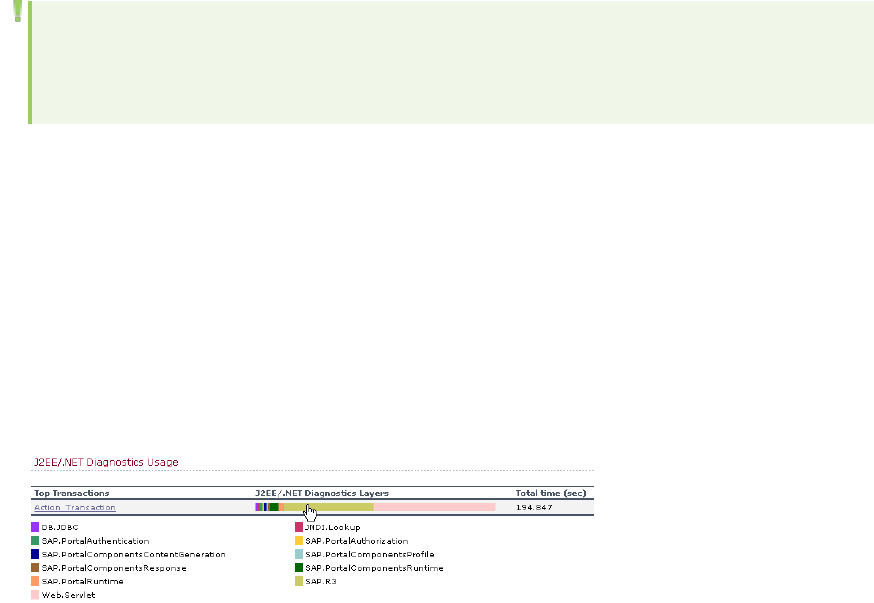
J2EE & .NET Diagnostics Graphs Overview
The J2EE & .NET Diagnostics graphs in LoadRunner Analysis enable you to trace, time, and troubleshoot
individual transactions and server requests through J2EE & .NET Web, application, and database
servers. You can also pinpoint problem servlets and JDBC calls to maximize business process
performance, scalability, and efficiency.
The J2EE & .NET Diagnostics graphs are comprised of two groups:
lJ2EE & .NET Diagnostics Graphs. These graphs show you the performance of requests and methods
generated by virtual user transactions. They show you the transaction that generated each request.
lJ2EE & .NET Server Diagnostics Graphs. These graphs show you the performance of all the requests
and methods in the application you are monitoring. These include requests generated by virtual user
transactions and by real users.
How to Enable Diagnostics for J2EE & .NET
To generate Diagnostics for J2EE & .NET data, you must first install HP Diagnostics.
Before you can use HP Diagnostics with LoadRunner, you need to ensure that you have specified the
Diagnostics Server details in LoadRunner. Before you can view Diagnostics for J2EE & .NET data in a
particular load test scenario, you need to configure the Diagnostics parameters for that scenario. For
more information, see the section on online monitors in the LoadRunner Controller documentation.
Note: To ensure that valid J2EE/.NET diagnostics data is generated during the scenario run, you
must manually mark the beginning and end of each transaction in the Vuser script, rather than
using automatic transactions.
Viewing J2EE to SAP R3 Remote Calls
The Remote Function Call (RFC) protocol in SAP allows communication to take place between SAP J2EE
and SAP R3 environments. When remote calls take place between SAP J2EE and SAP R3 environments,
Analysis displays information about the RFC functions, including the name of each function.
You view information about RFC functions by breaking down the SAP R3 layer. You can view the RFC
function information in a graph display or in the Chain Of Calls window.
1. Go to the J2EE/.NET Diagnostics Usage section of the Summary Report. Next to the relevant
transaction, click the color representing the SAP.R3 layer.
User Guide
Analysis
HP LoadRunner (12.50) Page 240
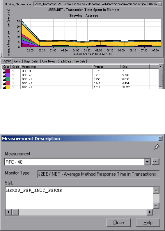
The J2EE/.NET - Transaction Time Spent in Element graph opens, representing the SAP.R3 layer.
2. Right click the graph and choose J2EE/.NET Diagnostics > Break down the class to methods.
3. Break down the graph further by right clicking the graph and choosing J2EE/.NET Diagnostics >
Break down the method to SQLs.
The graph is broken down into the different RFC functions.
4. To view the name of each RFC function, right click an RFC measurement in the Measurement
column in the graph legend and choose Show measurement description.
The Measurement Description dialog box opens. The name of the RFC function is displayed in the
SQL box.
View RFC function information in the Chain Of Calls window
1. Go to the J2EE/.NET Diagnostics Usage section of the Summary Report. Next to the relevant
transaction, click the color representing the SAP.R3 layer.
The J2EE/.NET - Transaction Time Spent in Element graph opens, representing the SAP.R3 layer.
2. Right click the graph and choose J2EE/.NET Diagnostics > Show chain of calls.
The Transaction chain of calls window opens. When you click any of the RFC functions, in the
Measurement column, the name of the function is displayed in the lower pane in the RFC Name tab.
User Guide
Analysis
HP LoadRunner (12.50) Page 241
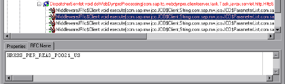
J2EE & .NET Diagnostics Data
The J2EE & .NET Diagnostics graphs provide an overview of the entire chain of activity on the server side
of the system. At the same time, you can break down J2EE/.NET layers into classes and methods to
enable you to pinpoint the exact location where time is consumed. In addition, you can view custom
classes or packages that you set the J2EE/.NET probe to monitor. You can also view the transaction
chain of calls and call stack statistics to track the percentage of time spent on each part of the
transaction.
You can correlate the end user response time with the Web server activity (Servlets and JSPs data),
application server activity (JNDIs), and back-end activity of database requests (JDBC methods and SQL
queries).
Example Transaction Breakdown
The following graphs illustrate the breakdown of a transaction to its layers, classes, and methods.
Transaction Level
The following figure shows the top level Average Transaction Response Time graph. The graph displays
several transactions: Birds,Bulldog,Checkout,Start, and so on.
User Guide
Analysis
HP LoadRunner (12.50) Page 242
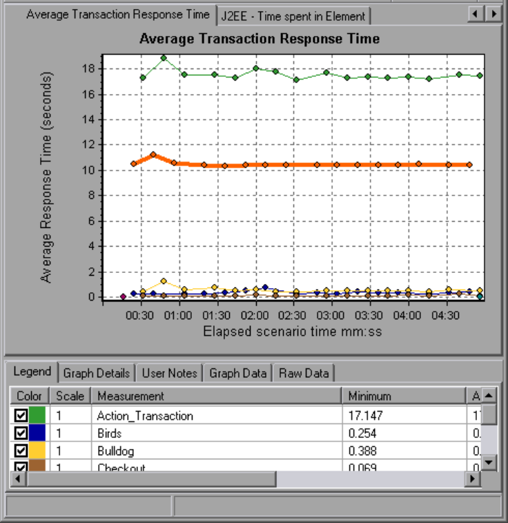
Layer Level
In the following figure, the Start transaction has been broken down to its layers (DB, EJB, JNDI, and
Web). In J2EE/.NET transactions, the Web layer is generally the largest.
User Guide
Analysis
HP LoadRunner (12.50) Page 243
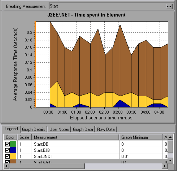
Class Level
In the following figure, the Web layer of the Start transaction has been broken down to its classes.
User Guide
Analysis
HP LoadRunner (12.50) Page 244
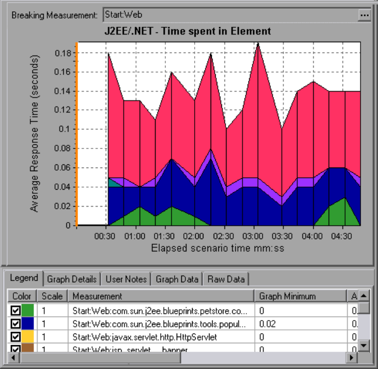
Method/Query Level
In the following figure, the weblogic.servlet.FileServlet component of the Web layer of the Start
transaction has been broken down to its methods.
User Guide
Analysis
HP LoadRunner (12.50) Page 245
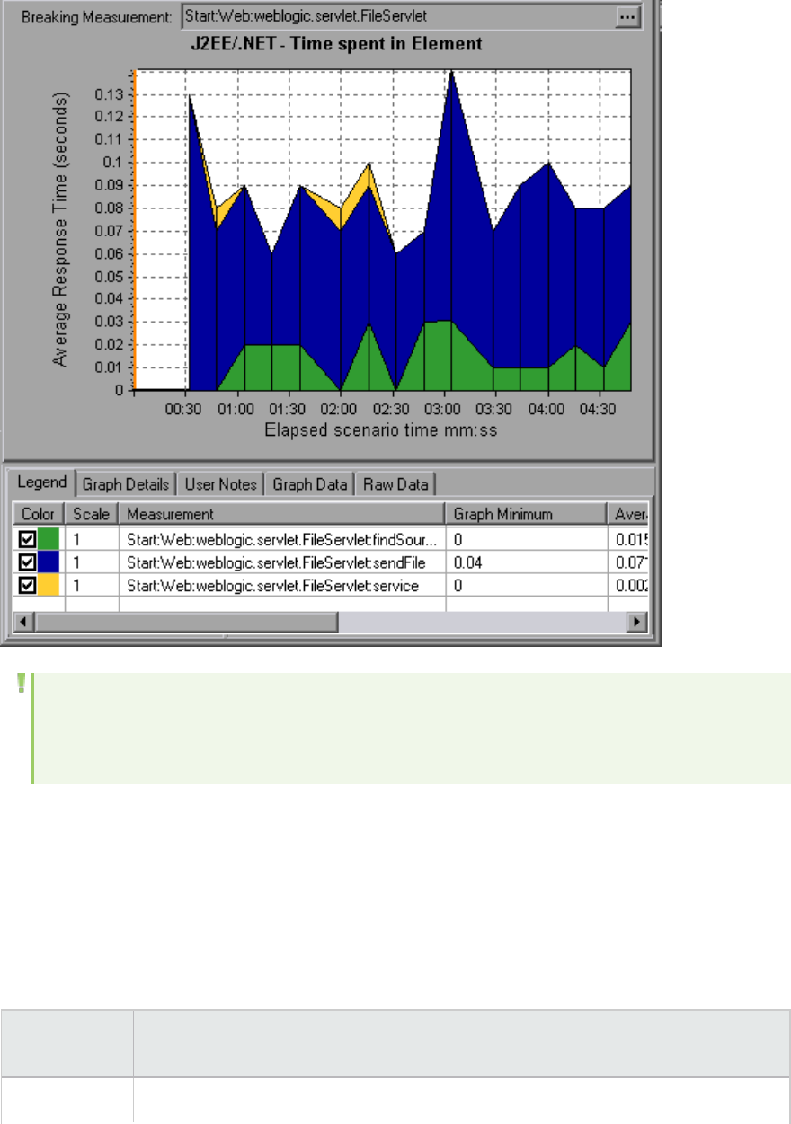
Note: Some JDBC methods can invoke SQLs which can be broken down further. In this case there
is another level of breakdown, that is SQL Statements. For the methods that can not be further
broken down into SQL statements when reaching this level of breakdown, you see NoSql.
Cross VM Analysis
When a server request makes a remote method invocation, the J2EE & .NET Diagnostics graphs display
certain measurements relating to the classes and methods involved in these requests. These
measurements are displayed at a layer, class and method level. The VM making the call is referred to as
the caller VM, and the VM that executes the remote call is the callee VM.
The measurements are described below:
Measurements Description
Cross VM A measurement that represents a dummy layer that integrates the data from the
User Guide
Analysis
HP LoadRunner (12.50) Page 246
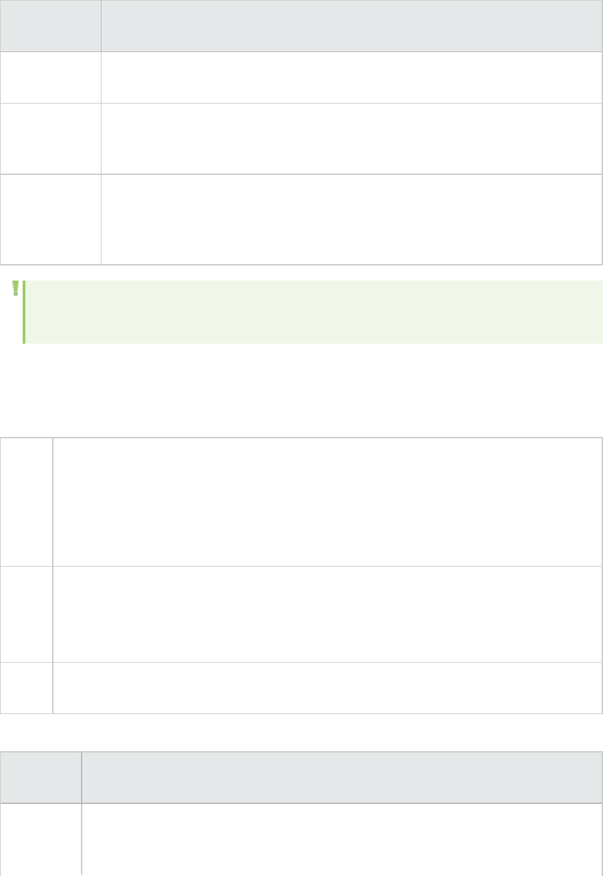
Measurements Description
Layer remote classes and methods in server requests that take place across two or more
virtual machines.
Remote-Class A measurement that represents a dummy class that integrates the data from the
remote methods in server requests that take place across two or more virtual
machines.
Remote-Class:
Remote
Method
A measurement that represents a dummy method. Remote-Class: Remote Method
measures the total time, call count, exclusive latency, minimum and maximum
values, standard deviation, and so on of the methods that are executed remotely,
relative to the caller virtual machine.
Note: Since this data is measured on the caller virtual machine the exclusive latency will include
all of the time required for making the remote method invocation such as network latency.
Using the J2EE & .NET Breakdown Options
J2EE & .NET breakdown options are described.
To
access
Use one of the following to access breakdown options:
l<J2EE & .NET Graphs> View > J2EE & .NET Diagnostics
l<J2EE & .NET Diagnostics Graphs> > select transaction >short-cut menu > J2EE & .NET
Diagnostics
lSee toolbar options for each breakdown level
Notes lThe breakdown menu options and buttons are not displayed until an element
(transaction, server request, layer) is selected.
lIf there is no URI in the SQL, URI-None appears in front of the full measurement
description in the Measurement Description dialog box.
See
also
"J2EE & .NET Diagnostics Graphs Overview" on page240
User interface elements are described below :
UI Element Description
<Right-
click>
Choose J2EE/.NET Diagnostics > Show Server Requests. A new graph opens showing the
breakdown of the selected transaction. The name of the transaction is displayed in the
Breaking Measurement box.
User Guide
Analysis
HP LoadRunner (12.50) Page 247
UI Element Description
transaction
in Average
Response
Time
Graph
You can view the full SQL statement for a selected SQL element by choosing Show
measurement description from the Legend window right-click menu. The
Measurement Description dialog box opens displaying the name of the selected
measurement and the full SQL statement.
To view transaction properties for the breakdown measurement, click the Breaking
Measurement button. To disable this feature, choose View > Display Options, and
clear the Show Breaking Measurement check box.
Select View>J2EE/.NET Diagnostics>Break down the server request to layers, or
click the measurement breakdown button in the toolbar above the graph.
Note: The option in the J2EE/.NETDiagnostics menu, and the tool tip of the
measurementbreakdown button, vary according to the element that you want to
break down. For example, when you select a server request, the menu option and tool
tip are Break down server request to layers.
Select View>J2EE/.NET Diagnostics>ShowVM, or click the Show VM button in the
toolbar above the graph. This breaks the data down to the application host name (VM).
Select View>J2EE/.NET Diagnostics>UndoBreak down the server request to
User Guide
Analysis
HP LoadRunner (12.50) Page 248
UI Element Description
layers, or click the Undo<MeasurementBreakdown>button in the toolbar above the
graph.
Note: The option in the J2EE/.NETDiagnostics menu, and the tool tip of the
measurementbreakdown button, vary according to the element whose breakdown you
want to undo. For example, when you select a layer, the menu option and tool tip are
Undo break down server request to layers.
Select View>J2EE/.NET Diagnostics>HideVM, or click the Hide VM button in the
toolbar above the graph.
Display the chain of call or call stack statistics in the measurements tree window: Drag
the orange time line on to the graph to the time specifying the end of the period for
which you want to view data, and select
View>J2EE/.NETDiagnostics>ShowChainofCalls, or click the ShowChainofCalls
button in the toolbar above the graph.
Note: A measurement that is broken down in the Average Method Response Time in
Transactions graph will be different from the same measurement broken down in the
J2EE/.NET - Transaction Time Spent in Element graph. This is because the J2EE/.NET -
Average Method Response Time in Transactions graph displays the average transaction
time, whereas the J2EE/.NET - Transaction Time Spent in Element graph displays the
average time per transaction event (sum of method execution time).
Viewing Chain of Calls and Call Stack Statistics
You can view the chain of calls for transactions and methods. The chain of calls answers the question
"Whom did I call?"
You can also view the call stack statistics for methods. Call stack statistics answer the question "Who
called me?"
Chain of call and call stack statistics data are shown in the measurements tree window. The title of the
window changes depending on which kind of data you are viewing.
lTo set the point to which the measurements tree window relates, you must drag the orange time line
to the desired spot.
lTo view transaction call chains, right-click a component and choose
J2EE/.NETDiagnostics>Show ChainofCalls. The ChainofCalls window opens displaying the chain
of calls from the parent transaction downwards.
lTo view method statistics, in the ChainofCalls window right-click a method and choose Show Method
Chain of Calls or Show Method Call Stack Statistics.
User Guide
Analysis
HP LoadRunner (12.50) Page 249
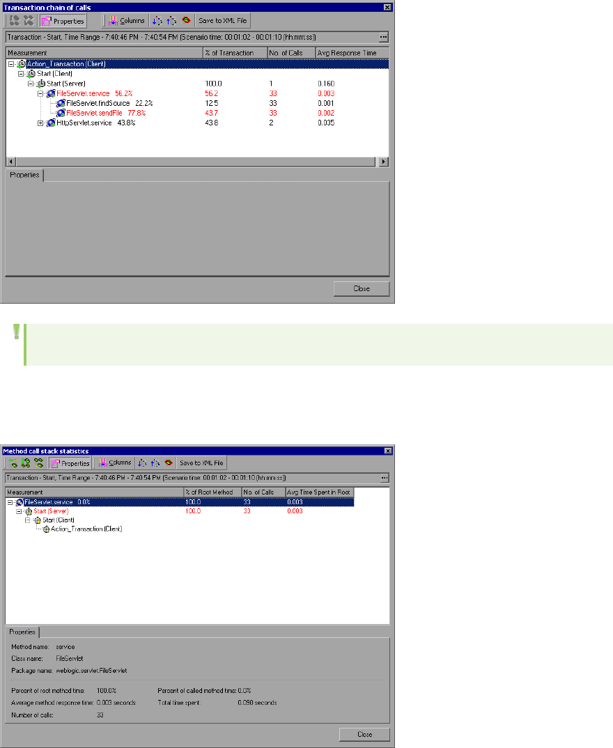
The Chain of Calls Windows
You use the Chain of Calls window to view the components that the selected transaction or method
called. In the following figure, all the calls in the critical path of the Start server-side transaction are
displayed.
Note: Each red node signifies the most time consuming child of its parent.
You use the Call Stack Statistics window to view which components called the selected component. In
the following figure, the FileServlet.service was called by Start (Server), which was called by Start
(Client), and so on, down to the transaction at the bottom of the chain.
User Guide
Analysis
HP LoadRunner (12.50) Page 250
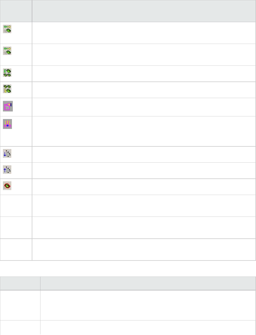
Understanding the Chain of Calls Window
User interface elements are described below:
UI
Element
Description
Switch to Method Chain of Calls. When the call stack statistics data is displayed,
displays the method chain of calls data (only if the root is a method).
Switch to Method Call Stack Statistics. When the method chain of calls data is
displayed, displays the method call stack statistics data (only if the root is a method).
Show Method Chain of Calls. Displays the Chain of Calls window.
Show Method Call Stack Statistics. Displays the Call Stack Statistics window.
Properties. Hides or displays the properties area (lower pane).
Columns. Enables you to select the columns shown in the Calls window. To display
additional fields, drag them to the desired location in the Calls window. To remove fields,
drag them from the Calls window back to the Columns chooser.
Expand All. Expands the entire tree.
Collapse All. Collapses the entire tree.
Expand Worst Path. Expands only the parts of the path on the critical path.
Save to
XML File
Saves the tree data to an XML file.
Method
Properties
Area.Displays the full properties of the selected method.
SQL Query Displays the SQL query for the selected method. (For Database only.)The following
columns are available in the Chain of Calls window:
The following columns are available in the Chain of Calls window:
Column Description
Measurement Name of the method, displayed as ComponentName:MethodName. In the case of a
database call, query information is also displayed. The percent shown indicates the
percentage of calls to this component from its parent.
% of Root Percentage of the total time of the method from the total time of the root tree item.
User Guide
Analysis
HP LoadRunner (12.50) Page 251
Column Description
Method
No of Calls Displays the amount of times this transaction or method was executed.
Avg
Response
Time
Response time is the time from the beginning of execution until the end. Average
response time is the total response time divided by the number of divided by the
number of instances of the method.
STD
Response
Time
The standard deviation response time.
Min
Response
Time
The minimum response time.
Max
Response
Time
The maximum response time.
% of Caller Displays the percentage of method time in relation the parent method time.
Total time Displays the total method execution time, including the child execution time.
The following columns are available in the Call Stack Statistics window:
Column Description
Measurement Name of the method, displayed as ComponentName.MethodName. In the case of a
database call, query information is also displayed. The percent shown indicates the
percentage of calls to this component from its child.
% of Root
Method
Percentage of the total time of the transaction (or method) from the total time of
the root tree item.
No. of Calls
to Root
Displays the amount of times this transaction or method was executed.
Avg Time
Spent in Root
Time spent in root is the time that the sub-area spent in the root sub-
area/area/transaction.
Average Time Spent in Root time is the total time spent in the root divided by the
number of instances of the method.
STD Time
Spent in Root
The standard deviation time spent in the root.
Min Time The minimum time spent in the root.
User Guide
Analysis
HP LoadRunner (12.50) Page 252
Column Description
Spent in Root
Max Time
Spent in Root
The maximum time spent in the root.
% of Called Displays the percentage of method time in relation the child method time.
Total Time
Spent in Root
Displays the total method execution time, including the child execution time.
Graph Filter Properties
You can filter the J2EE & .NET Diagnostics graphs so that the displayed data is more suitable to your
needs. You can filter using the following methods:
lBefore opening a graph, enter filter criteria in the Graph Properties box of the Open Graph dialog
box. For more information, see "Open a New Graph Dialog Box" on page125.
lFrom an open graph, enter filter criteria in the Filter condition fields in a filter dialog box. For more
information, see "Filter Dialog Boxes" on page114 and "Drilling Down in a Graph" on page90.
User interface elements are described below:
UI Element Description
Class Name Shows data for specified classes.
Layer
Name
Shows data for specified layers.
Scenario
Elapsed
Time
Shows data for transactions that ended during the specified time.
SQL Logical
Name
Shows data for specified SQL logical names. Due to the length of some SQL names,
after you choose an SQL statement it is assigned a "logical name." This logical name is
used in the filter dialog, legend, grouping, and other places in place of the full SQL
statement. You can view the full SQL statement in the Measurement Description dialog
box (View>Show Measurement Description).
Transaction
Name -
J2EE/.NET
Shows data for a specified transaction.
Some JDBC methods have the ability to invoke SQL's (each method can invoke several different SQL's)
so there is another level of breakdown which is the SQL statements.
User Guide
Analysis
HP LoadRunner (12.50) Page 253
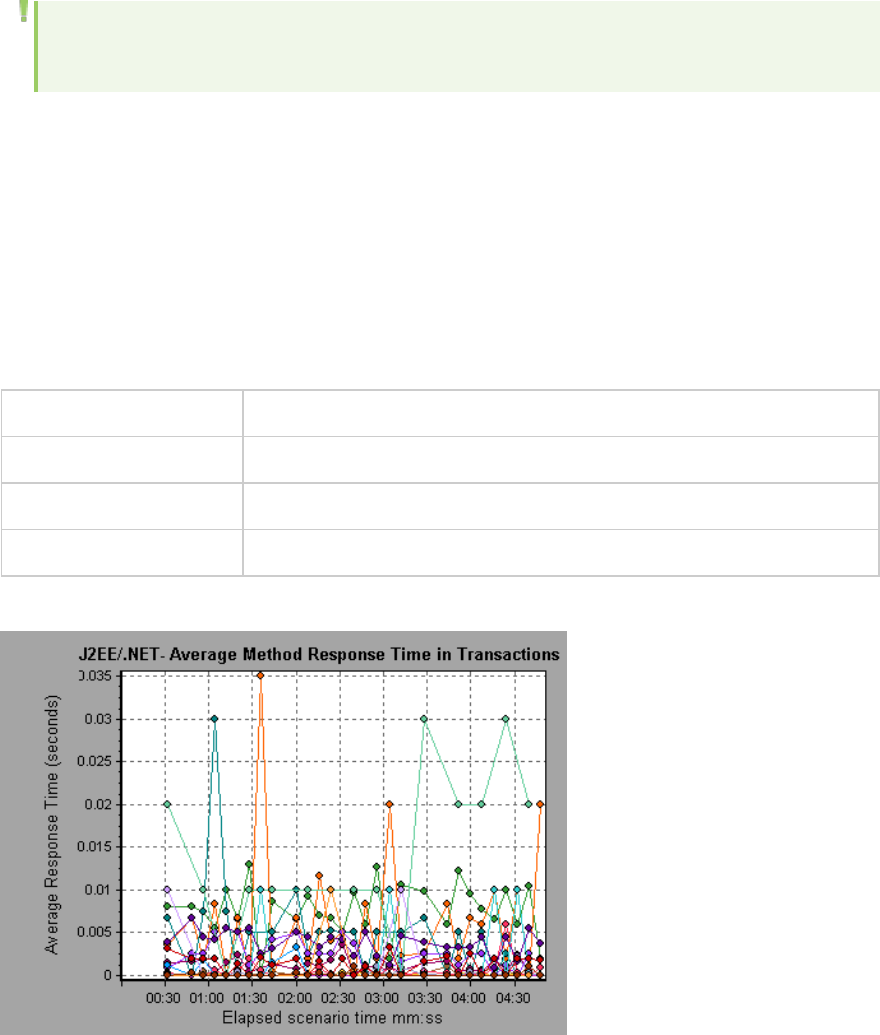
Note: For the methods that do not have SQL statement when reaching this level of breakdown
you see NoSql.
J2EE/.NET - Average Method Response Time in Transactions
Graph
This graph displays the average response time for the server side methods, computed as Total Method
Response Time/Number of Method calls. For example, if a method was executed twice by an instance of
transaction A and once by another instance of the same transaction, and it took three seconds for each
execution, the average response time is 9/3, or 3 seconds. The method time does not include calls made
from the method to other methods.
X-axis Elapsed time.
Y-axis Average response time (in seconds) per method
Breakdown options "Using the J2EE & .NET Breakdown Options" on page247
See also "J2EE & .NET Diagnostics Graphs Overview" on page240
Example
J2EE/.NET - Average Number of Exceptions in Transactions
Graph
This graph displays the average number of code exceptions per method, transaction, or request that
were monitored during the selected time range.
User Guide
Analysis
HP LoadRunner (12.50) Page 254
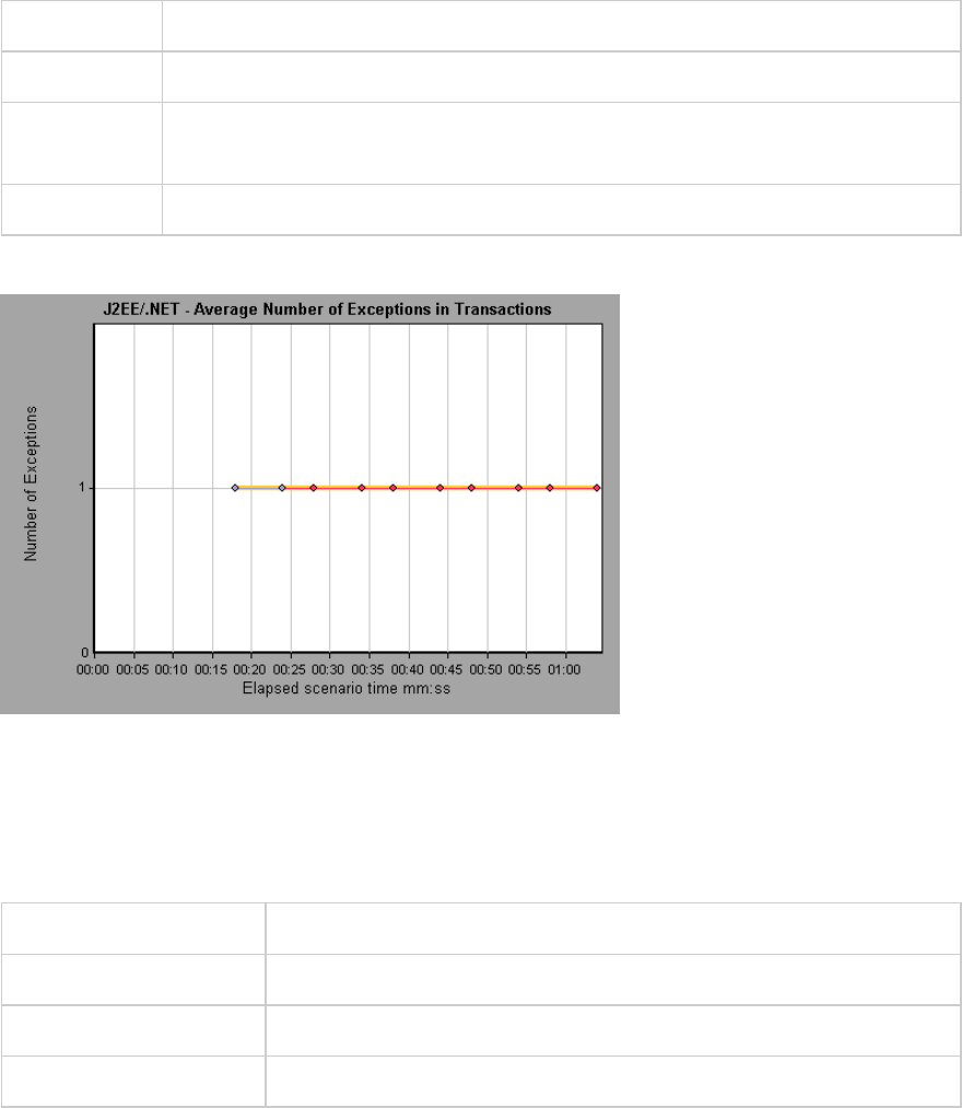
X-axis Elapsed time.
Y-axis Represents the number of events.
Breakdown
options
To break the displayed elements down further, see "Using the J2EE & .NET
Breakdown Options" on page247.
See also "J2EE & .NET Diagnostics Graphs Overview" on page240
Example
J2EE/.NET - Average Number of Exceptions on Server Graph
This graph displays the average number of code exceptions per method that were monitored during the
selected time range.
X-axis Elapsed time of the scenario run.
Y-axis Number of events.
Breakdown options "Using the J2EE & .NET Breakdown Options" on page247
See also "J2EE & .NET Diagnostics Graphs Overview" on page240
Example
User Guide
Analysis
HP LoadRunner (12.50) Page 255
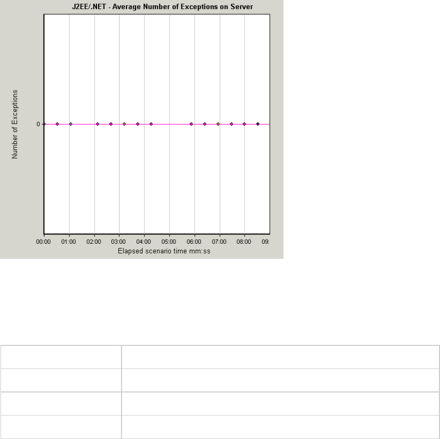
J2EE/.NET - Average Number of Timeouts in Transactions Graph
This graph displays the average number of timeouts per method, transaction, or request that were
monitored during the selected time range.
X-axis Elapsed time since the scenario run.
Y-axis Represents number of events.
Breakdown options "Using the J2EE & .NET Breakdown Options" on page247
See also "J2EE & .NET Diagnostics Graphs Overview" on page240
Example
User Guide
Analysis
HP LoadRunner (12.50) Page 256
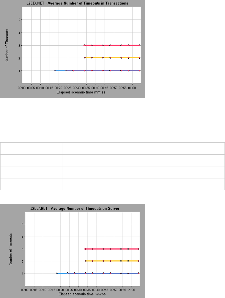
J2EE/.NET - Average Number of Timeouts on Server Graph
This graph displays the average number of timeouts per method that were monitored during the
selected time range.
X-axis Elapsed time since the scenario run.
Y-axis Number of events.
Breakdown options "Using the J2EE & .NET Breakdown Options" on page247
See also "J2EE & .NET Diagnostics Graphs Overview" on page240
Example
User Guide
Analysis
HP LoadRunner (12.50) Page 257
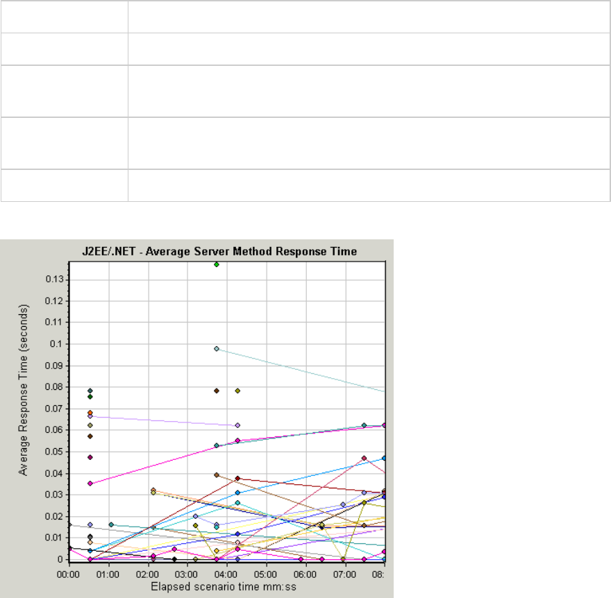
J2EE/.NET - Average Server Method Response Time Graph
This graph displays the average response time for the server side methods, computed as Total Method
Response Time/Number of Method calls.
X-axis Elapsed time since the scenario run.
Y-axis Average response time (in seconds) per method.
Breakdown
options
"Using the J2EE & .NET Breakdown Options" on page247
Note The method time does not include calls made from the method to other
methods.
See also "J2EE & .NET Diagnostics Graphs Overview" on page240
Example
J2EE/.NET - Method Calls per Second in Transactions Graph
This graph displays the number of completed sampled transactions during each second of a load test
scenario run.
The number of transactions included in the sample is determined by the sampling percentage set in the
Diagnostics Distribution dialog box in the Controller (Diagnostics >Configuration).
User Guide
Analysis
HP LoadRunner (12.50) Page 258
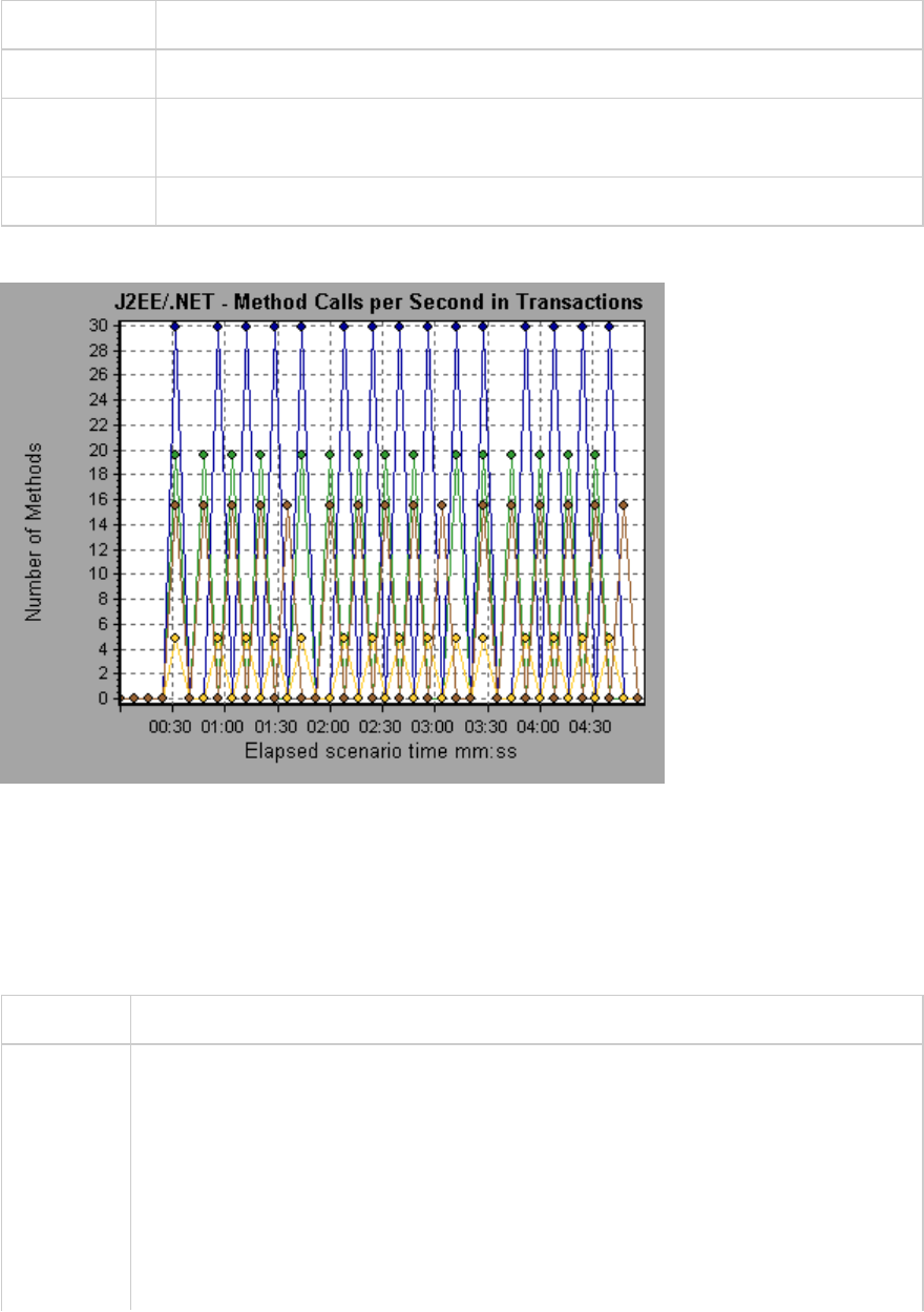
X-axis Elapsed time.
Y-axis Represents the number of completed sampled transactions per second.
Breakdown
options
To break the displayed elements down further, see "Using the J2EE & .NET
Breakdown Options" on page247.
See also "J2EE & .NET Diagnostics Graphs Overview" on page240
Example
J2EE/.NET - Probes Metrics Graph
This graph displays performance metrics collected by HP Diagnostics probes. Metrics include JVM
related data such as Heap usage and Garbage Collection, application server specific metrics, JDBC (Java
Database Connectivity) metrics, and more.
X-axis Elapsed time since the scenario run.
Y-axis Resource usage. The following probe metric data is provided for offline analysis:
lHeapUsed
lGC Collections/sec
lGC time Spent in Collections
To include additional Probe metric data in offline Analysis, you use the Diagnostics
configuration file, etc./offline.xml. For more information, see the HP Diagnostics
Server Installation and Administration Guide.
User Guide
Analysis
HP LoadRunner (12.50) Page 259
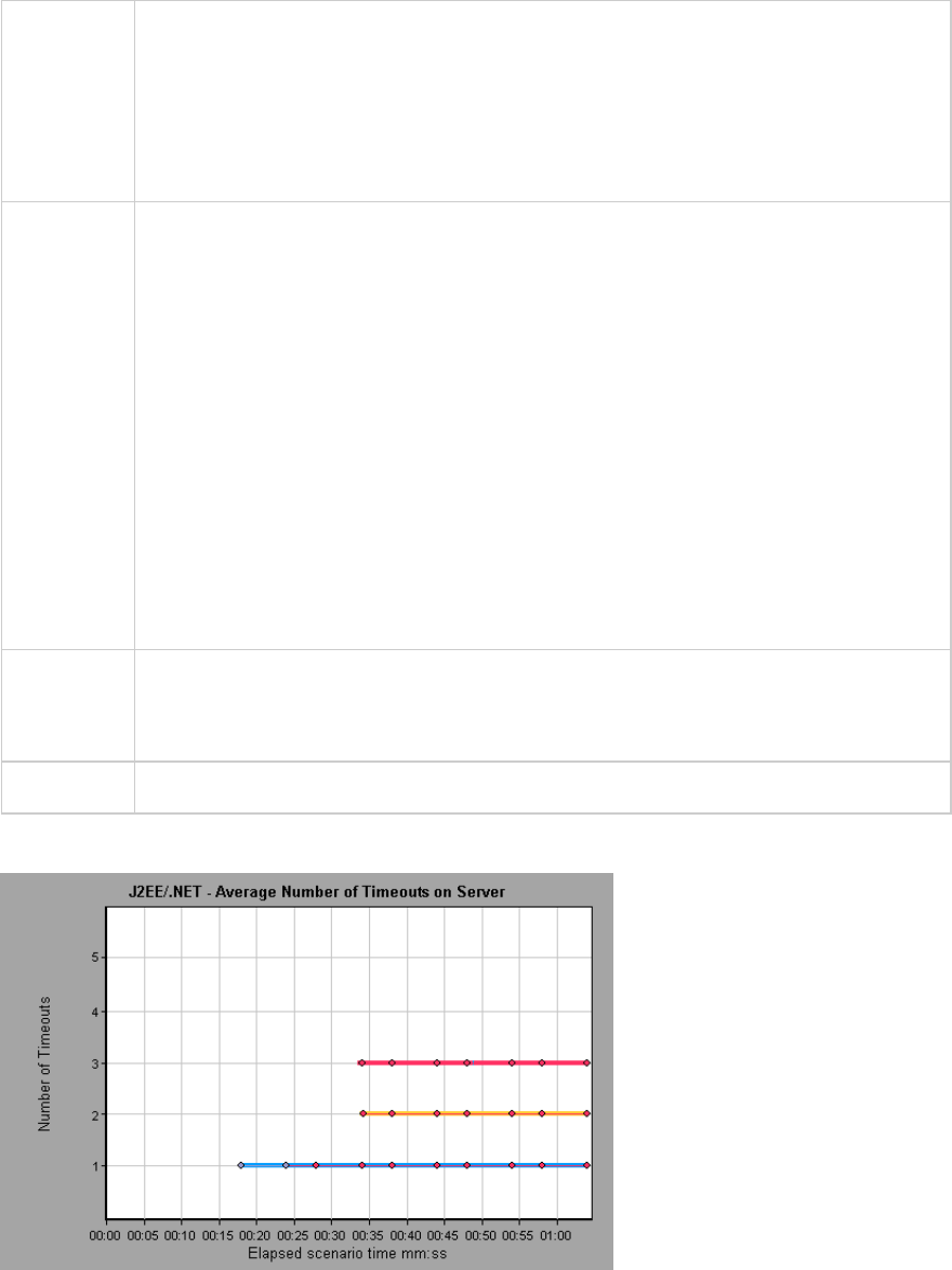
Data
Grouping
By default, the data in the graph is grouped by Category Name (the Diagnostics metric
category name) and Probe Name. As a result, the default format for the measurement
name is the graph is:
<Name of metric from Diagnostics (unit of metric)>:<Diagnostics metric category
name>:<Probe name>
If the measurement unit is a count, no unit name is displayed in parentheses.
Important
Information
By default, the following probe metric data is provided for offline analysis: HeapUsed,
GC Collections/sec, and GC time Spent in Collections. To include additional Probe
metric data in offline Analysis, you use the Diagnostics configuration file,
etc/offline.xml. For more information, see the HP Diagnostics LoadRunner and
Performance Center-Diagnostics Integration Guide .
For example, for the following measurement name:
lthe name of the metric is GC Time Spent in Collections.
lthe value is measured as a percentage.
lthe metric category name is GC.
lthe Probe name is MyJBossDev
In addition to the regular Analysis filter criteria, you can also filter and group by the
Diagnostics metrics collector name and the host name.
Note You need to synchronize the operating system time settings on the Controller machine
and the Diagnostics Servers to ensure accurate display of the elapsed scenario time in
the Probe Metrics graph.
See also "J2EE & .NET Diagnostics Graphs Overview" on page240
Example
User Guide
Analysis
HP LoadRunner (12.50) Page 260
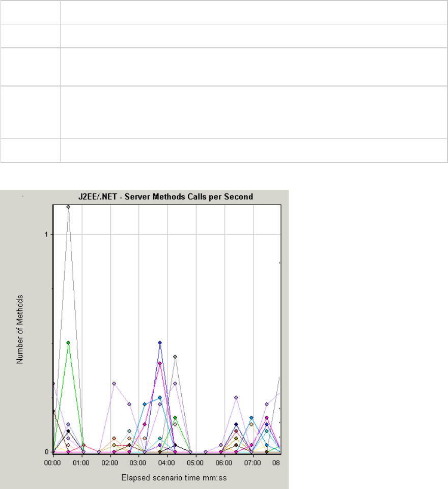
J2EE/.NET - Server Methods Calls per Second Graph
This graph displays the number of completed sampled methods during each second of a load test
scenario run.
X-axis Elapsed time of the scenario run.
Y-axis Number of completed sampled methods per second.
Breakdown
options
"Using the J2EE & .NET Breakdown Options" on page247
Note The number of methods included in the sample is determined by the sampling
percentage set in the Diagnostics Distribution dialog box in the Controller
(Diagnostics>Configuration).
See also "J2EE & .NET Diagnostics Graphs Overview" on page240
Example
J2EE/.NET - Server Requests per Second Graph
This graph displays the number of completed sampled requests during each second of a load test
scenario run.
User Guide
Analysis
HP LoadRunner (12.50) Page 261

X-axis Elapsed time of the scenario run.
Y-axis Number of completed sampled requests per second.
Breakdown
options
"Using the J2EE & .NET Breakdown Options" on page247
Note The number of requests included in the sample is determined by the sampling
percentage set in the Diagnostics Distribution dialog box in the Controller
(Diagnostics>Configuration). For more information, see the section on online
monitors in the LoadRunner Controller documentation.
See also "J2EE & .NET Diagnostics Graphs Overview" on page240
Example
J2EE/.NET - Server Request Response Time Graph
This graph displays the server response time of requests that include steps that cause activity on the
J2EE/.NET backend.
X-axis Elapsed time of the scenario time.
Y-axis Average time (in seconds) taken to perform each request.
User Guide
Analysis
HP LoadRunner (12.50) Page 262
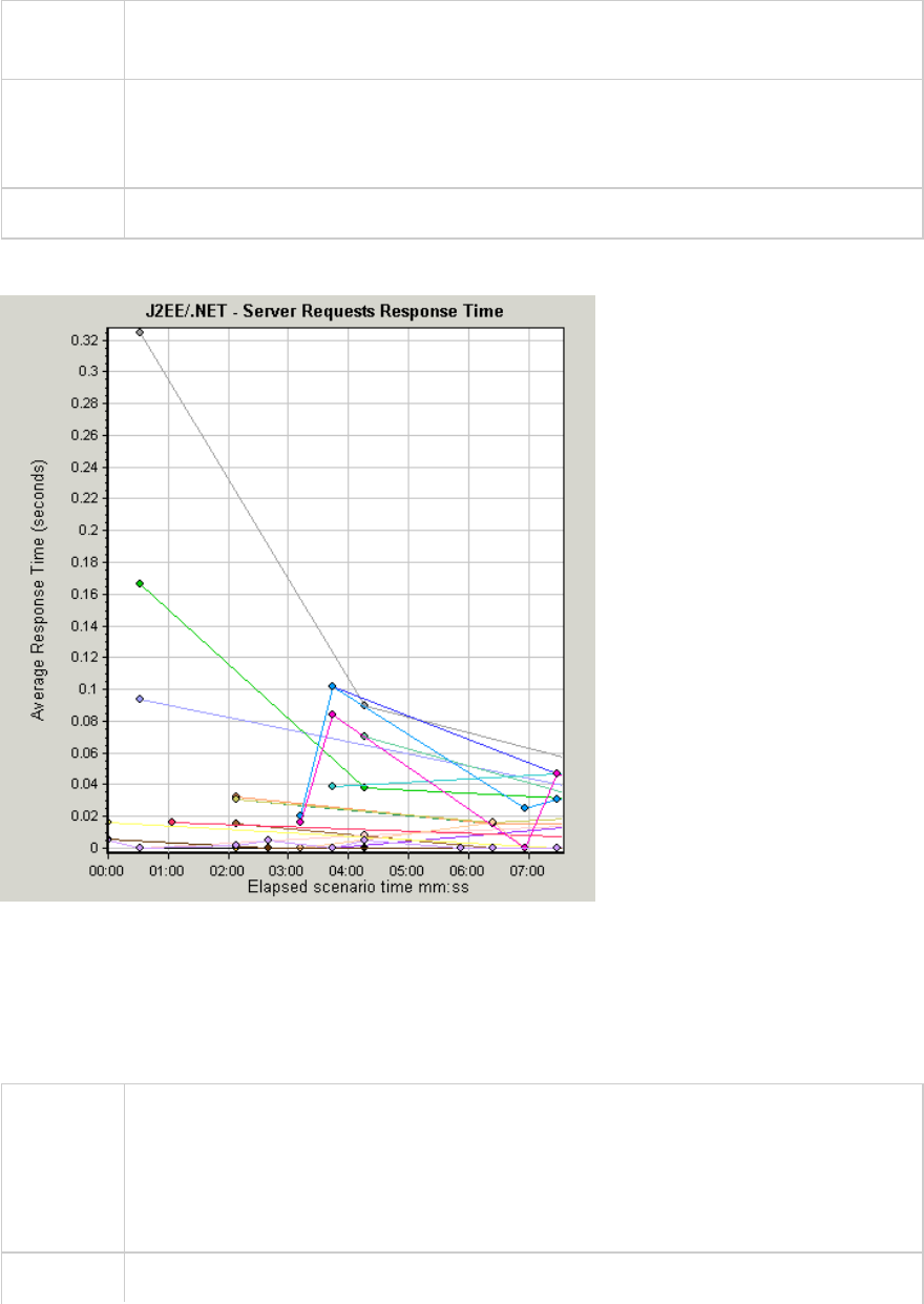
Breakdown
options
"Using the J2EE & .NET Breakdown Options" on page247
Note The reported times, measured from the point when the request reached the Web
server to the point it left the Web server, include only the time that was spent in the
J2EE/.NET backend.
See also "J2EE & .NET Diagnostics Graphs Overview" on page240
Example
J2EE/.NET - Server Request Time Spent in Element Graph
This graph displays the server response time for the selected element (layer, class, or method) within
each server request.
Purpose The time is computed as Total Response Time/Total Number of Server Requests. For
example, if a method was executed twice by an instance of server request A and once
by another instance of the same server request, and it took three seconds for each
execution, the average response time is 9/2, or 4.5 seconds. The server request time
does not include the nested calls from within each server request.
X-axis Elapsed time of the scenario run.
User Guide
Analysis
HP LoadRunner (12.50) Page 263

Y-axis Average response time (in seconds) per element within the server request.
Breakdown
options
"Using the J2EE & .NET Breakdown Options" on page247
Filtering
properties
The display of the graph is determined by the Graph Properties selected when the
graph is opened, as described:
None
lTime spent in each server request
Server request
lFiltered by server request. Grouped by layer.
Server request and layer
lFiltered by server request and layer. Grouped by class.
Server request, layer, and class
lFiltered by server request, layer, and class. Grouped by method.
Tips To obtain data for this graph, you must first install HP Diagnostics. Before you can view
Diagnostics for J2EE & .NET data in a particular load test scenario, you need to
configure the Diagnostics parameters for that scenario. For more information, see the
section on online monitors in the LoadRunner Controller documentation.
See also "J2EE & .NET Diagnostics Graphs Overview" on page240
Example
User Guide
Analysis
HP LoadRunner (12.50) Page 264
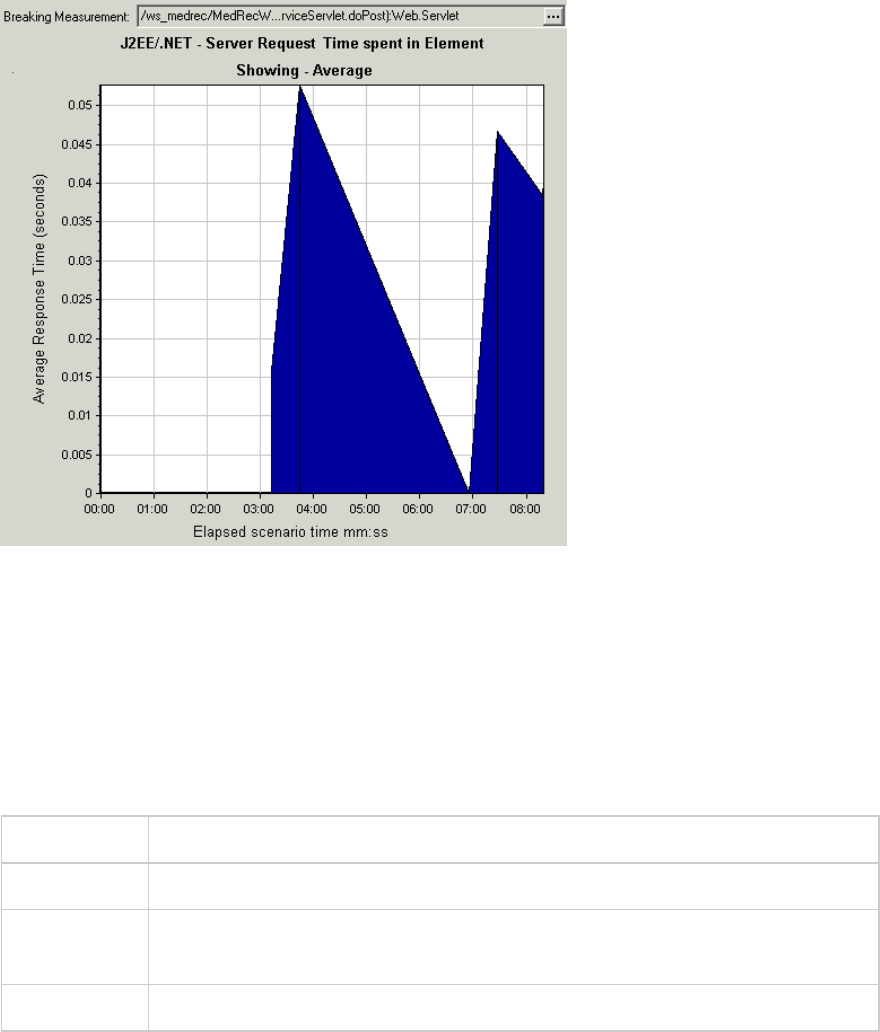
J2EE/.NET - Transactions per Second Graph
This graph displays the number of completed sampled transactions during each second of a load test
scenario run.
The number of transactions included in the sample is determined by the sampling percentage set in the
Diagnostics Distribution dialog box in the Controller (Diagnostics >Configuration). For more
information, see the section on online monitors in the LoadRunner Controller documentation.
X-axis Elapsed time.
Y-axis Number of completed sampled transactions per second
Breakdown
options
To break the displayed elements down further, see "Using the J2EE & .NET
Breakdown Options" on page247.
See also "J2EE & .NET Diagnostics Graphs Overview" on page240
Example
User Guide
Analysis
HP LoadRunner (12.50) Page 265
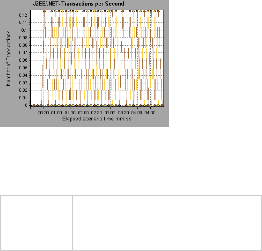
J2EE/.NET - Transaction Response Time Server Side Graph
This graph displays the transaction server response time of transactions that include steps that cause
activity on the J2EE/.NET backend. The reported times, measured from the point when the transaction
reached the Web server to the point it left the Web server, include only the time that was spent in the
J2EE/.NET backend.
X-axis Elapsed time.
Y-axis Average response time (in seconds) of each transaction.
Breakdown options "Using the J2EE & .NET Breakdown Options" on page247
See also "J2EE & .NET Diagnostics Graphs Overview" on page240
Example
User Guide
Analysis
HP LoadRunner (12.50) Page 266
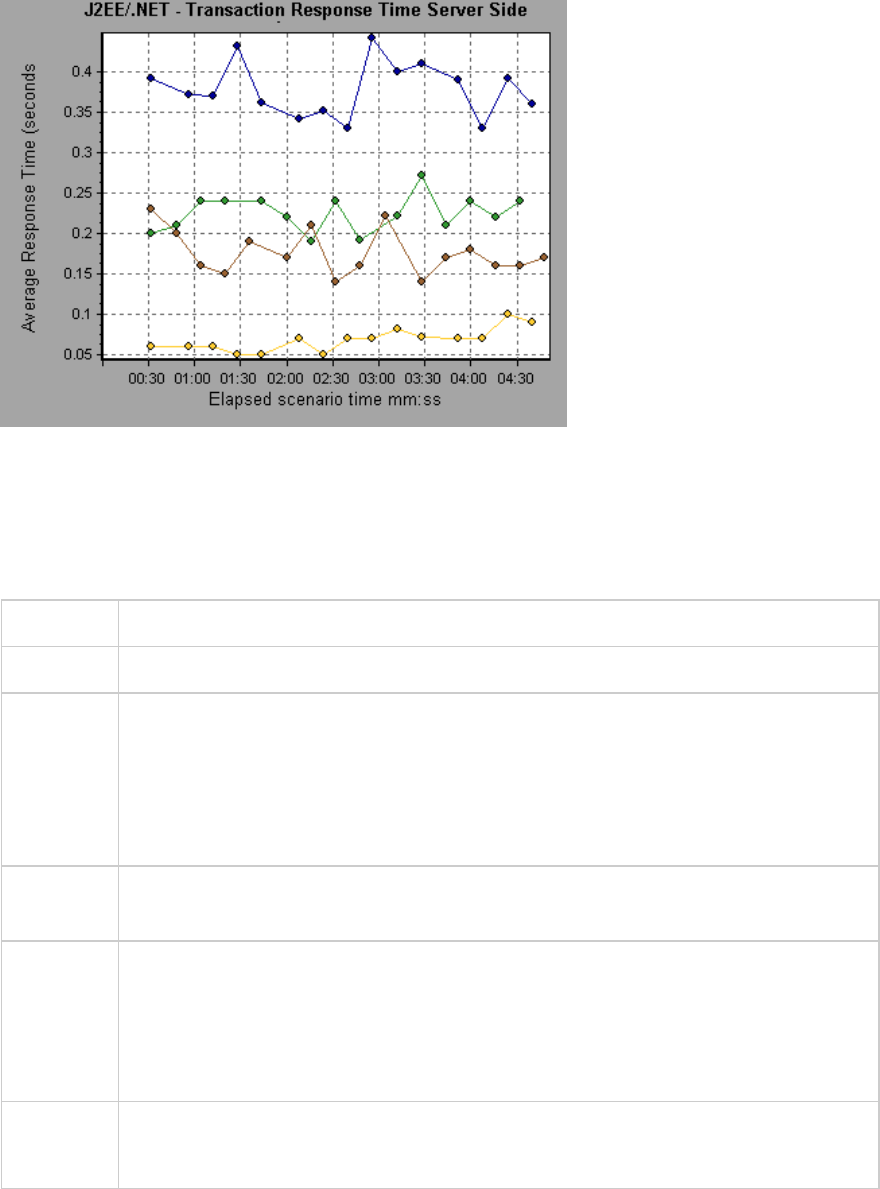
J2EE/.NET - Transaction Time Spent in Element Graph
This graph displays the server response time for the selected element (layer, class, or method) within
each transaction.
X-axis Elapsed time.
Y-axis Average response time (in seconds) per element within the transaction.
Breakdown
options
The display of graph data is determined by the graph properties selected when the
graph was opened, as described in the following table: For information on filtering on
graph data, see "Filtering Graph Data Overview" on page103.
You can break down the displayed elements. For more information, see "Using the J2EE
& .NET Breakdown Options" on page247.
Tips To obtain data for this graph, you must enable the J2EE & .NET Diagnostics module
(from the Controller) before running the load test scenario.
Note The time is computed as Total Response Time/Total Number of Transactions. For
example, if a method was executed twice by an instance of transaction A and once by
another instance of the same transaction, and it took three seconds for each
execution, the average response time is 9/2, or 4.5 seconds. The transaction time does
not include the nested calls from within each transaction.
See also "J2EE & .NET Diagnostics Graphs Overview" on page240
"Filtering and Sorting Graph Data" on page103
Example
User Guide
Analysis
HP LoadRunner (12.50) Page 267
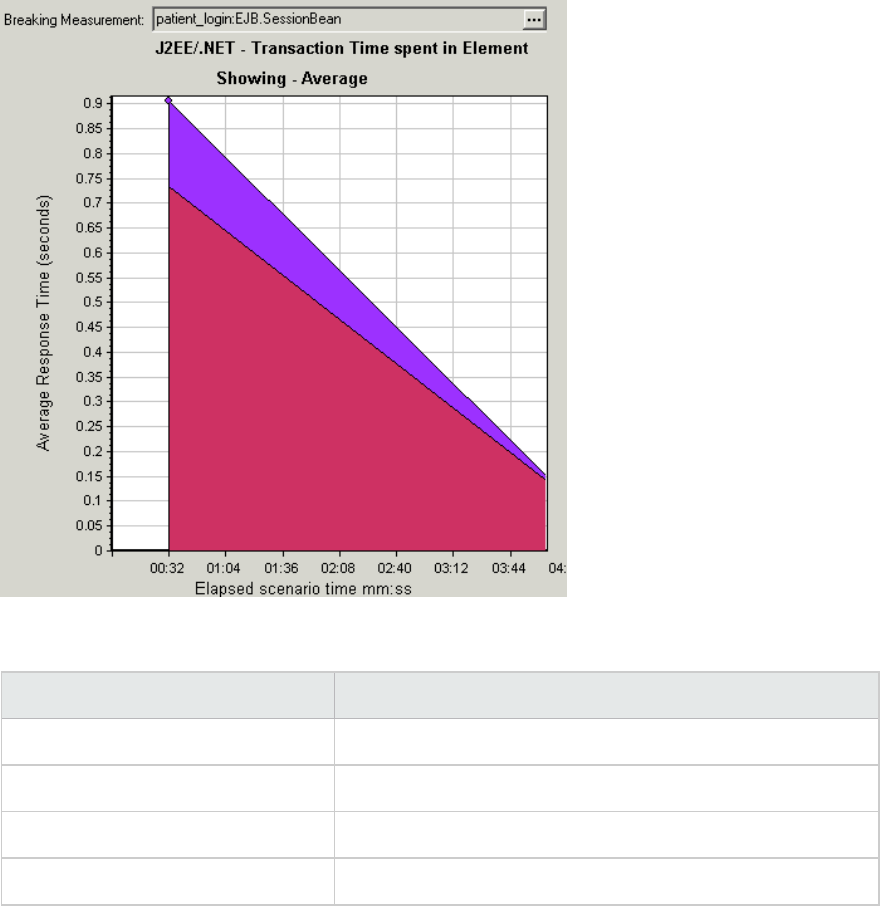
Graph Data Display
If you filter by these properties... The graph data is displayed like this
None Time spent in each transaction.
Transaction Filtered by transaction. Grouped by layer.
Transaction and layer Filtered by transaction and layer. Grouped by class.
Transaction, layer, and class Filtered by transaction, layer, and class. Grouped by method.
Application Component Graphs
Microsoft COM+ performance graphs provide you with performance information for COM+ interfaces
and methods.
To obtain data for these graphs, you need to activate the various Microsoft COM+ performance
monitors before running the load test scenario.
When you set up the Microsoft COM+ performance online monitors, you indicate which statistics and
measurements to monitor.
User Guide
Analysis
HP LoadRunner (12.50) Page 268
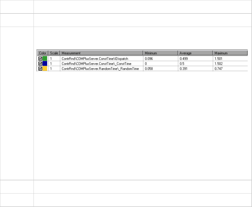
The .NET CLR performance graphs provide you with performance information for .NET classes and
methods. To obtain data for these graphs, you must activate the .NET CLR performance monitor before
running the load test scenario run.
Displayed measurements are specified using the .NET monitor.
For more information, see the section on online monitors in the LoadRunner Controller documentation.
COM+ Average Response Time Graph
This graph specifies the average time COM+ interfaces or methods take to perform during the load test
scenario.
X-axis Elapsed time from the beginning of the scenario run.
Y-axis Average response time of a COM+ interface or method.
Breakdown
options
Each interface or method is represented by a different colored line on the graph. The
legend frame (which is found below the graph) identifies the interfaces by color:
This legend shows that the blue colored line belongs to the COM+ interface _
ConstTime. Looking at the graph above, we see that this interface has higher response
times than all other COM+ interfaces. At 2:10 minutes into the scenario, it records an
average response time of 0.87 seconds.
Note: The 0.87 second data point is an average, taken from all data points recorded
within a 10 second interval (the default granularity). You can change the length of this
sample interval.
Viewing CON+ Methods
The table initially displays COM+ interfaces, but you can also view the list of COM+
methods by using drill-down or filtering techniques. For more information, see "Filtering
and Sorting Graph Data" on page103 and "Drilling Down in a Graph" on page90.
Tips To highlight a specific interface line in the graph, select the interface row in the legend.
See also "Application Component Graphs" on the previous page
User Guide
Analysis
HP LoadRunner (12.50) Page 269
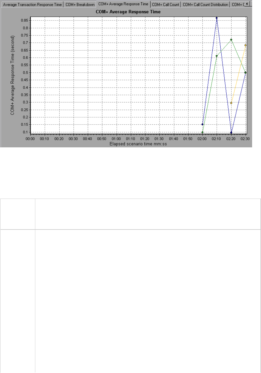
COM+ Breakdown Graph
This graph summarizes fundamental result data about COM+ interfaces or methods and presents it in
table format.
Purpose Using the COM+ Breakdown table, you can identify the COM+ interfaces or methods
which consume the most time during the test. The table can be sorted by column, and
the data can be viewed either by COM+ interface or COM+ method.
Breakdown
options
Average Response Time
The Average Response Time column shows how long, on average, an interface or
method takes to perform. The graphical representation of this column is the "COM+
Average Response Time Graph" on the previous page.
Call Count
The next column, Call Count, specifies the number of times the interface or method
was invoked. The graphical representation of this column is the "COM+ Average
Response Time Graph" on the previous page.
Total Response Time
The final column, Total Response Time, specifies how much time was spent overall on
the interface or method. It is calculated by multiplying the first two data columns
together. The graphical representation of this column is the "COM+ Average Response
Time Graph" on the previous page.
User Guide
Analysis
HP LoadRunner (12.50) Page 270

The graphical representations of each of these columns are the "COM+ Average
Response Time Graph" on page269, the "COM+ Call Count Distribution Graph" on the
next page and the "COM+ Total Operation Time Distribution Graph" on page275
Interfaces are listed in the COM+ Interface column in the form Interface:Host. In the
table above, the _ConstTime interface took an average of .5 seconds to execute and
was called 70 times. Overall, this interface took 34.966 seconds to execute.
Tips Sorting List
To sort the list by a column, click on the column heading. The list above is sorted by
Average Response Time which contains the triangle icon specifying a sort in
descending order.
Viewing COM+ Methods
The table initially displays COM+ interfaces, but you can also view the list of COM+
methods.
To view the methods of a selected interface, select the COM+ Methods option. You
can also double-click on the interface row to view the methods. The methods of the
specified interface are listed in the COM+ Method column.
See also "Application Component Graphs" on page268
User Guide
Analysis
HP LoadRunner (12.50) Page 271
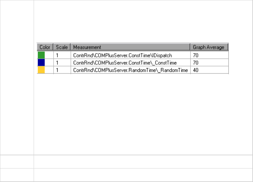
COM+ Call Count Distribution Graph
This graph shows the percentage of calls made to each COM+ interface compared to all COM+
interfaces. It can also show the percentage of calls made to a specific COM+ method compared to other
methods within the interface
Breakdown
options
The number of calls made to the interface or method is listed in the Call Count column
of the "COM+ Breakdown Graph" on page270 table.
Each interface or method is represented by a different colored area on the pie graph.
The legend frame (which is found below the graph) identifies the interfaces by color:
This legend shows that the green colored area belongs to the COM+ interface
IDispatch. Looking at the example graph below, we see that 38.89% of calls are made
to this interface. The actual figures can be seen in the Call Count column of the "COM+
Breakdown Graph" on page270 table.
Viewing COM+ Methods
The table initially displays COM+ interfaces, but you can also view the list of COM+
methods by using drill-down or filtering techniques. For more information, see "Filtering
and Sorting Graph Data" on page103 and "Drilling Down in a Graph" on page90.
Tips To highlight a specific interface line in the graph, select the interface row in the legend.
See also "Application Component Graphs" on page268
User Guide
Analysis
HP LoadRunner (12.50) Page 272
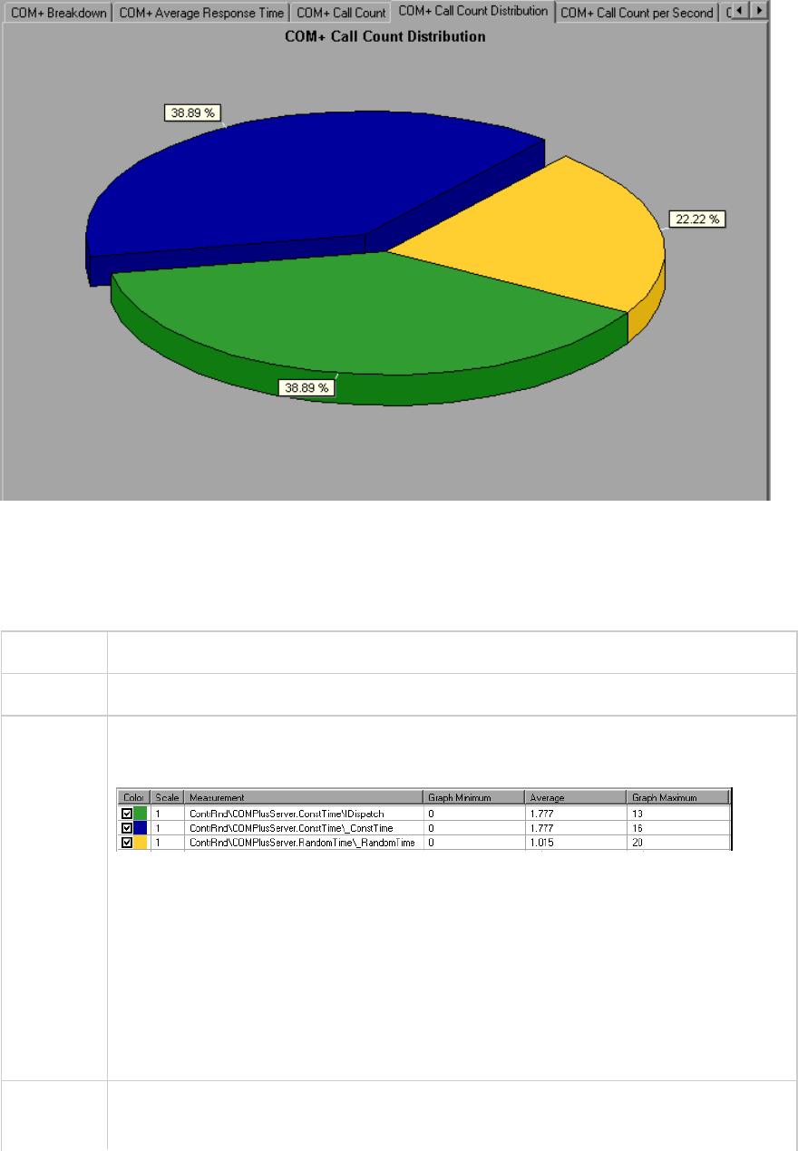
COM+ Call Count Graph
This graph displays the number of times COM+ interfaces and methods are invoked during the test.
X-axis Elapsed time from the beginning of the scenario run.
Y-axis How many calls were made to a COM+ interface or method.
Breakdown
options
Each interface or method is represented by a different colored line on the graph. The
legend frame (which is found below the graph) identifies the interfaces by color:
This legend shows that the yellow colored line belongs to the COM+ interface _
RandomTime. Looking at the graph above, we see that calls to this interface begin at
the beginning of the scenario run. There are 20 calls at the 2:20 minute point.
Viewing COM+ Methods
The table initially displays COM+ interfaces, but you can also view the list of COM+
methods by using drill-down or filtering techniques. For more information, see "Filtering
and Sorting Graph Data" on page103 and "Drilling Down in a Graph" on page90.
Note The call count is computed by multiplying the call frequency by a time interval. As a
result, the reported measurement may be rounded.
User Guide
Analysis
HP LoadRunner (12.50) Page 273
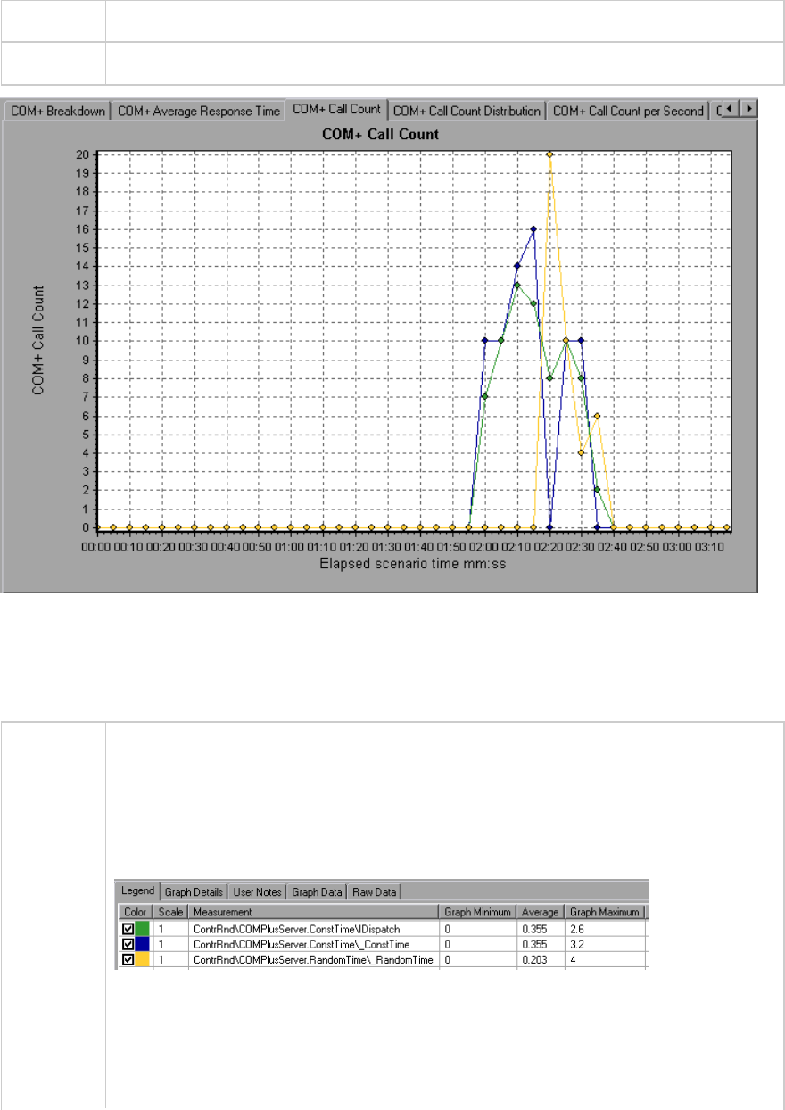
Tips To highlight a specific interface line in the graph, select the interface row in the legend.
See also "Application Component Graphs" on page268
COM+ Call Count Per Second Graph
This graph shows the number of times per second a COM+ interface or method is invoked.
Breakdown
options
This graph is similar to the "COM+ Call Count Graph" on the previous page except that
the y-axis indicates how many invocations were made to a COM+ interface or method
per second.
Each interface or method is represented by a different colored line on the graph. The
legend frame (which is found below the graph) identifies the interfaces by color:
This legend shows that the green colored line belongs to the COM+ interface IDispatch.
Looking at the graph above, we see that calls to this interface begins 1:55 minutes into
the scenario run. There is an average of 2.5 calls per second at the 2:10 minute mark.
Viewing COM+ Methods
User Guide
Analysis
HP LoadRunner (12.50) Page 274
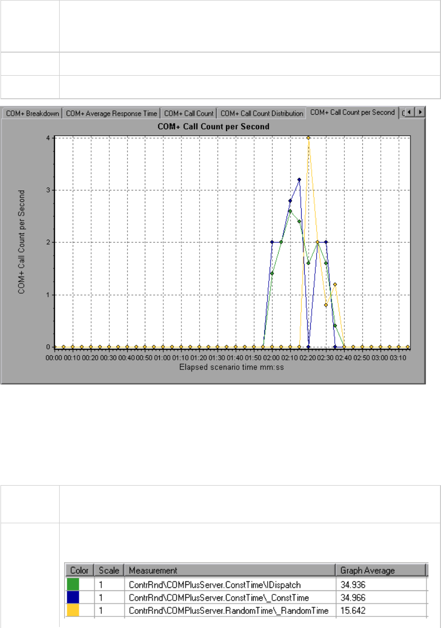
To view the average response time of the individual methods within a COM+ interface,
see "Filtering and Sorting Graph Data" on page103 and "Drilling Down in a Graph" on
page90.
Tips To highlight a specific interface line in the graph, select the interface row in the legend.
See also "Application Component Graphs" on page268
COM+ Total Operation Time Distribution Graph
This graph shows the percentage of time a specific COM+ interface takes to execute in relation to all
COM+ interfaces. It can also show the percentage of time a COM+ method takes to execute in relation
to all COM+ methods within the interface.
Purpose Use it to identify those interfaces or methods which take up an excessive amount of
time.
Breakdown
options
Each interface or method is represented by a different colored area on the pie graph.
The legend frame (which is found below the graph) identifies the interfaces by color:
User Guide
Analysis
HP LoadRunner (12.50) Page 275
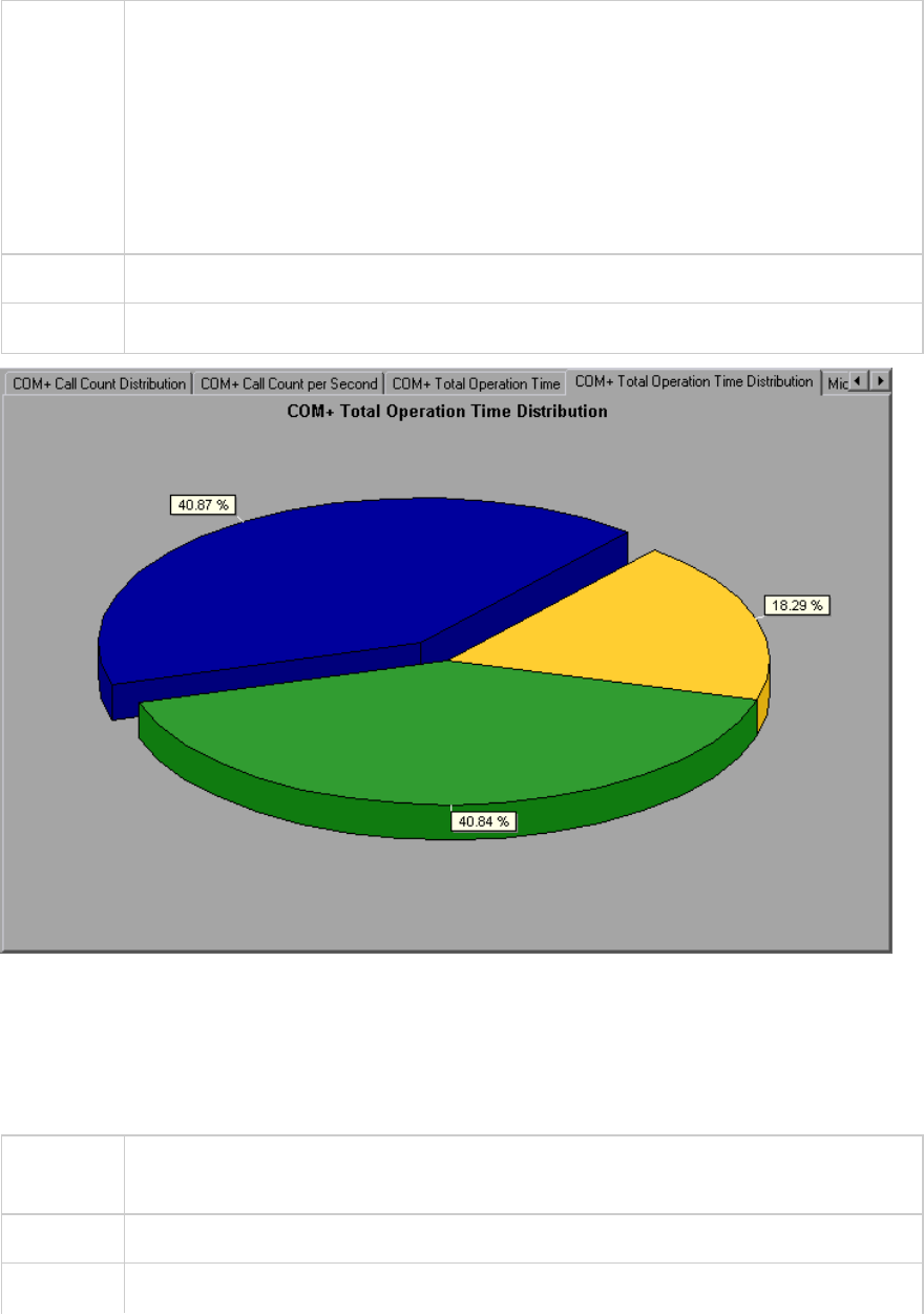
This legend shows that the green colored line belongs to the COM+ interface IDispatch.
Looking at the graph above, we see that this interface takes up 40.84% of the COM+
operational time.
Viewing COM+ Methods
To view the average response time of the individual methods within a COM+ interface,
see "Filtering and Sorting Graph Data" on page103 and "Drilling Down in a Graph" on
page90.
Tips To highlight a specific interface line in the graph, select the interface row in the legend.
See also "Application Component Graphs" on page268
COM+ Total Operation Time Graph
This graph displays the amount of time each COM+ interface or method takes to execute during the
test.
Purpose Use it to identify those interfaces or methods which take up an excessive amount of
time.
X-axis Elapsed time from the beginning of the scenario run.
Y-axis Total time a COM+ interface or method is in operation.
User Guide
Analysis
HP LoadRunner (12.50) Page 276
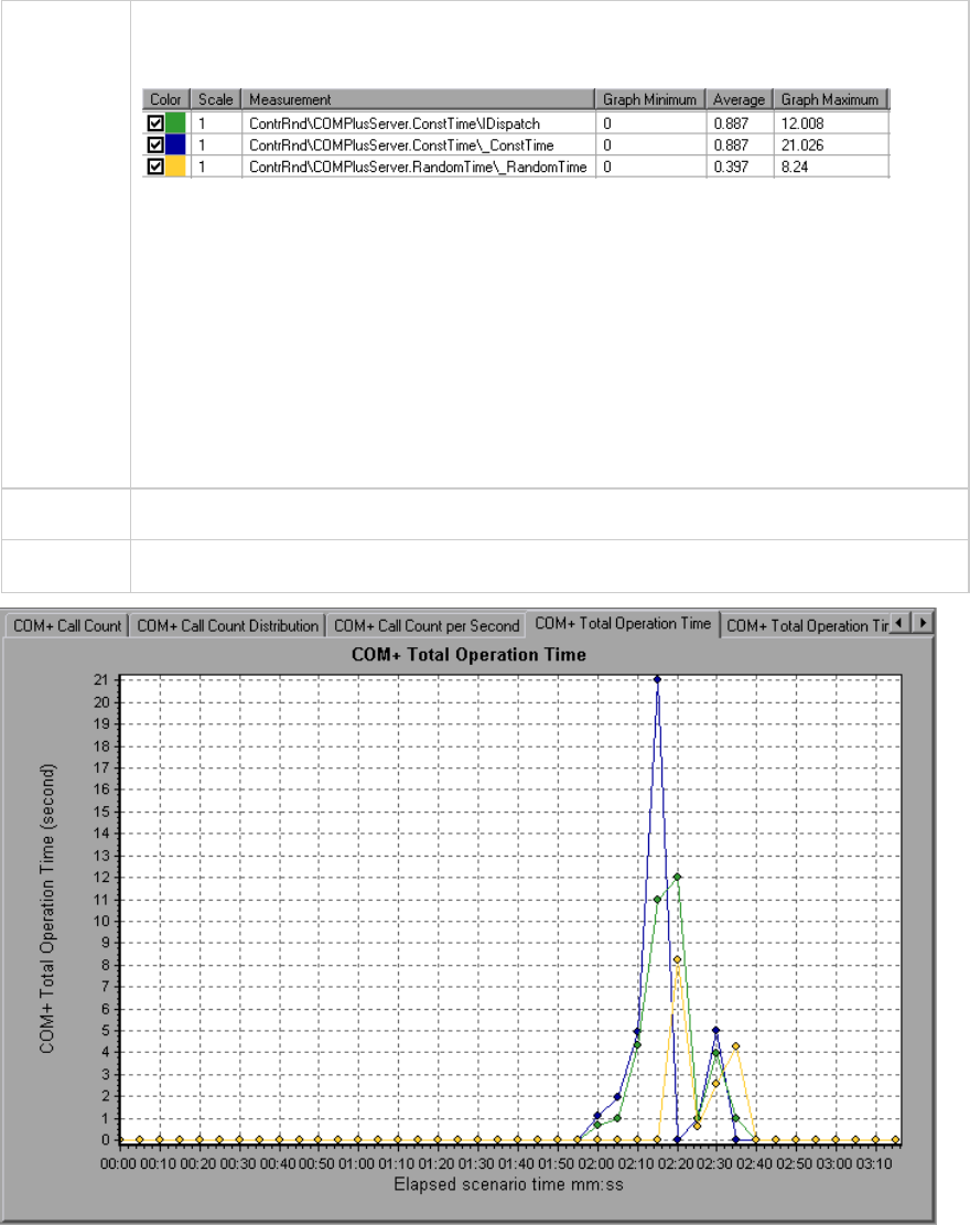
Breakdown
options
Each interface or method is represented by a different colored line on the graph. The
legend frame (which is found below the graph) identifies the interfaces by color:
This legend shows that the blue colored line belongs to the COM+ interface _
ConstTime. Looking at the graph above, we see that throughout the scenario, this
interface consumes more time than any other, especially at 2 minutes and 15 seconds
into the scenario run, where the calls to this interface take an average of 21 seconds.
Viewing COM+ Methods
The table initially displays COM+ interfaces, but you can also view the list of COM+
methods by using drill-down or filtering techniques. For more information, see "Filtering
and Sorting Graph Data" on page103 and "Drilling Down in a Graph" on page90.
Tips To highlight a specific interface line in the graph, select the interface row in the legend.
See also "Application Component Graphs" on page268
Microsoft COM+ Graph
This graph shows the resource usage of COM+ objects as a function of the elapsed load test scenario
time.
User Guide
Analysis
HP LoadRunner (12.50) Page 277
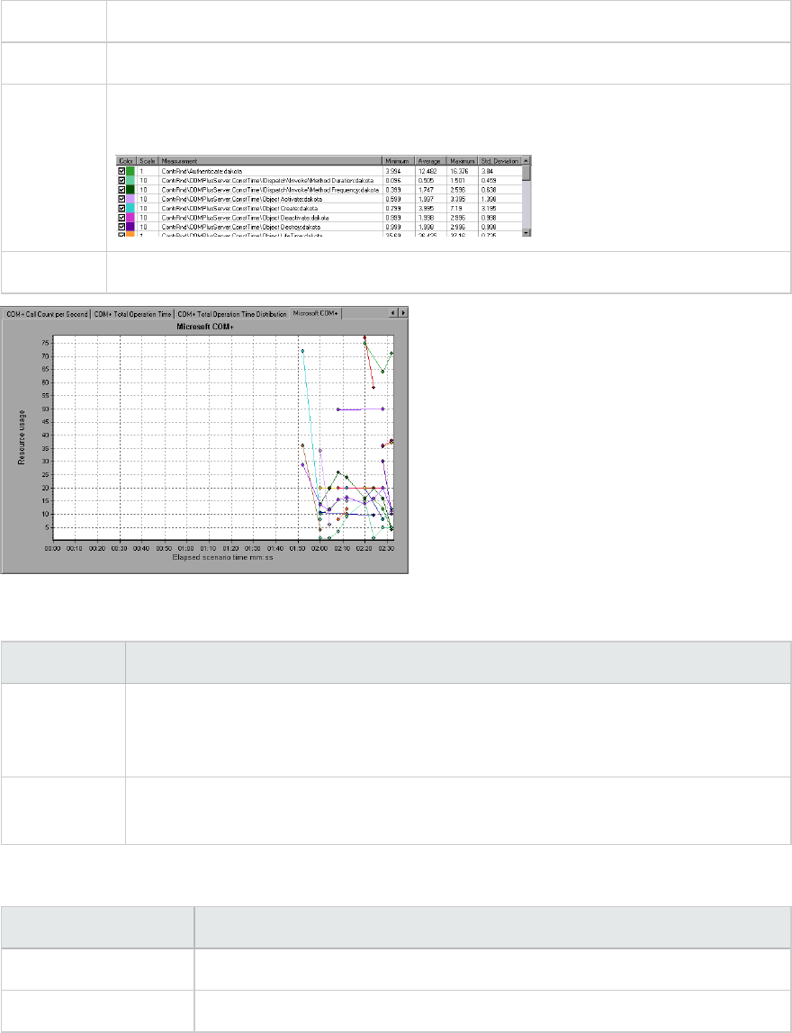
X-axis Elapsed time since the start of the run.
Y-axis The resource usage of COM+ objects.
Breakdown
Options
Each COM+ object is represented by a different colored line on the graph. The legend
frame (which is found below the graph) identifies the objects by color:
See also "Application Component Graphs" on page268
Authentication Metrics
Measurement Description
Authenticate Frequency of successful method call level authentication. When you set an
authentication level for an application, you determine what degree of authentication
is performed when clients call into the application.
Authenticate
Failed
Frequency of failed method call level authentication.
Application Event
Measurement Description
Activation Frequency of application activation or startup.
Shutdown Frequency of application shutdown or termination.
User Guide
Analysis
HP LoadRunner (12.50) Page 278
Thread Event
Measurement Description
Thread Start Rate at which single-threaded apartment (STA) thread for application have been
started.
Thread
Terminate
Rate at which single-threaded apartment (STA) thread for application have been
terminated.
Work Enque Event sent if a work is queued in single thread apartment object (STA). Note: These
events are not signaled/sent in Windows Server 2003 and later.
Work Reject Event sent if a work is rejected from single thread apartment object (STA). Note:
These events are not signaled/sent in Windows Server 2003 and later.
Transaction Events
Measurement Description
Transaction
Duration
Duration of COM+ transactions for selected application.
Transaction Start Rate at which transactions have started.
Transaction
Prepared
Rate at which transactions have completed the prepare phase of the two-
phase protocol.
Transaction
Aborted
Rate at which transactions have been aborted.
Transaction
Commit
Rate at which transactions have completed the commit protocol.
Object Events
Measurement Description
Object Life
Time
Duration of object existence (from instantiation to destruction).
Object Create Rate at which new instances of this object are created.
Object
Destroy
Rate at which instances of the object are destroyed.
User Guide
Analysis
HP LoadRunner (12.50) Page 279
Measurement Description
Object
Activate
Rate of retrieving instances of a new JIT-activated object.
Object
Deactivation
Rate of freeing JIT-activated object via SetComplete or SetAbort.
Disable
Commit
Rate of client calls to DisableCommit on a context. DisableCommit declares that the
object's transactional updates are inconsistent and can't be committed in their
present state.
Enable
Commit
Rate of client calls to EnableCommit on a context. EnableCommit declares that the
current object's work is not necessarily finished, but that its transactional updates
are consistent and could be committed in their present form.
Set Complete Rate of client calls to SetComplete on a context. SetComplete declares that the
transaction in which the object is executing can be committed, and that the object
should be deactivated on returning from the currently executing method call.
Set Abort Rate of client calls to SetAbort on a context. SetAbort declares that the transaction
in which the object is executing must be aborted, and that the object should be
deactivated on returning from the currently executing method call.
Method Events
Measurement Description
Method Duration Average duration of method.
Method Frequency Frequency of method invocation.
Method Failed Frequency of failed methods (i.e. methods that return error HRESULT codes).
Method Exceptions Frequency of exceptions thrown by selected method.
.NET Average Response Time Graph
This graph specifies the average time that .NET classes or methods took to perform during the load
test scenario run.
X-axis Elapsed time from the beginning of the scenario run.
Y-axis Average response time of a .NET class or method.
Breakdown The graph initially displays .NET classes, but you can also view the individual methods
User Guide
Analysis
HP LoadRunner (12.50) Page 280
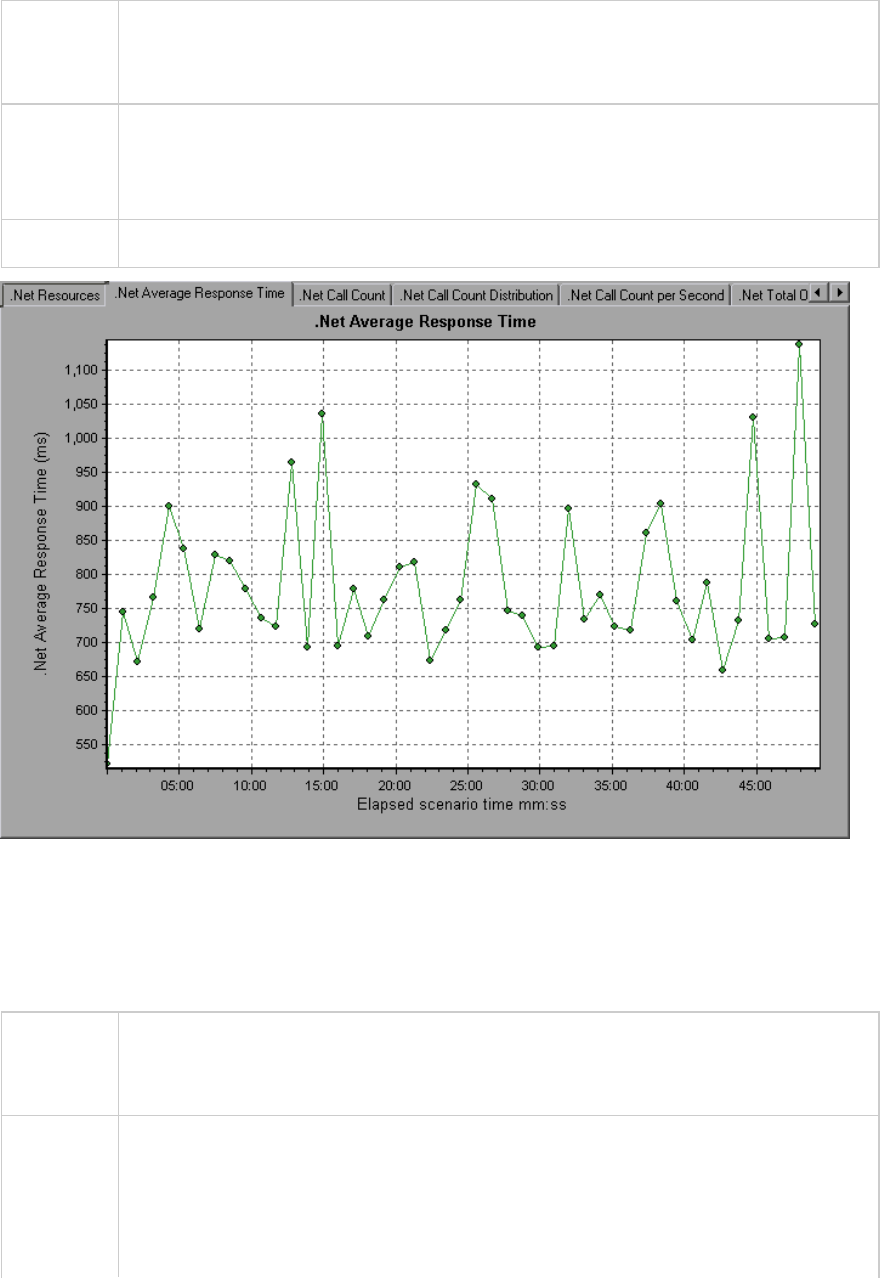
options within a .NET class by using drill-down or filtering techniques. For more information, see
"Filtering and Sorting Graph Data" on page103 and "Drilling Down in a Graph" on
page90.
Tips You can change the length of the sample interval.
Hint: To highlight a specific class line in the graph, select the class row in the legend
(displayed below the graph).
See also "Application Component Graphs" on page268
.NET Breakdown Graph
This graph summarizes fundamental result data about .NET classes or methods and presents it in table
format.
Purpose Using the .NET Breakdown table, you can identify the .NET classes or methods which
consume the most time during the test. The table can be sorted by column, and the
data can be viewed either by .NET class or .NET method.
Breakdown
options
The Average Response Time column shows how long, on average, a class or method
took to perform. The next column, Call Count, specifies the number of times the class
or method was invoked. The final column, Total Response Time, specifies how much
time was spent overall on the class or method. It is calculated by multiplying the results
from the first two columns together.
User Guide
Analysis
HP LoadRunner (12.50) Page 281
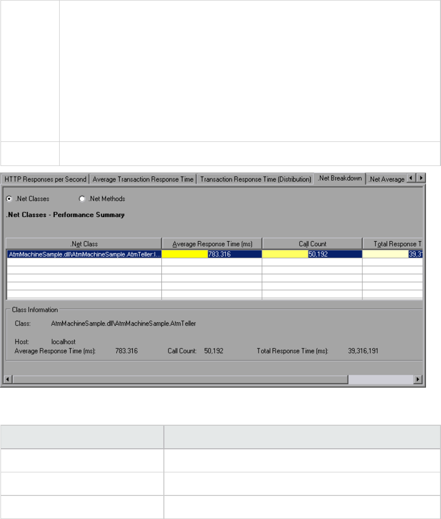
Classes are listed in the .NET Class column in the form Class:Host. In the table above,
the AtmMachineSample.AtmTeller class took an average of 783 seconds to execute
and was called 50,912 times. Overall, this class took 39,316 seconds to execute.
To sort the list by a column, click the column heading.
Each column in the .NET Breakdown graph is graphically represented by another graph.
The table initially displays .NET classes, but you can also view the list of .NET methods.
To view .NET methods, select the .NET Methods option, or double-click the class row.
The methods of the specified class are listed in the .NET Method column.
See also "Application Component Graphs" on page268
.NET Breakdown graph
.NET Breakdown Column Graphical Representation
Average Response Time .NET Average Response Time Graph.
Call Count .NET Call Count Graph.
Total Response Time .NET Total Operation Time Distribution Graph.
.NET Call Count Distribution Graph
This graph shows the percentage of calls made to each .NET class compared to all .NET classes. It can
also show the percentage of calls made to a specific .NET method compared to other methods within
the class
User Guide
Analysis
HP LoadRunner (12.50) Page 282
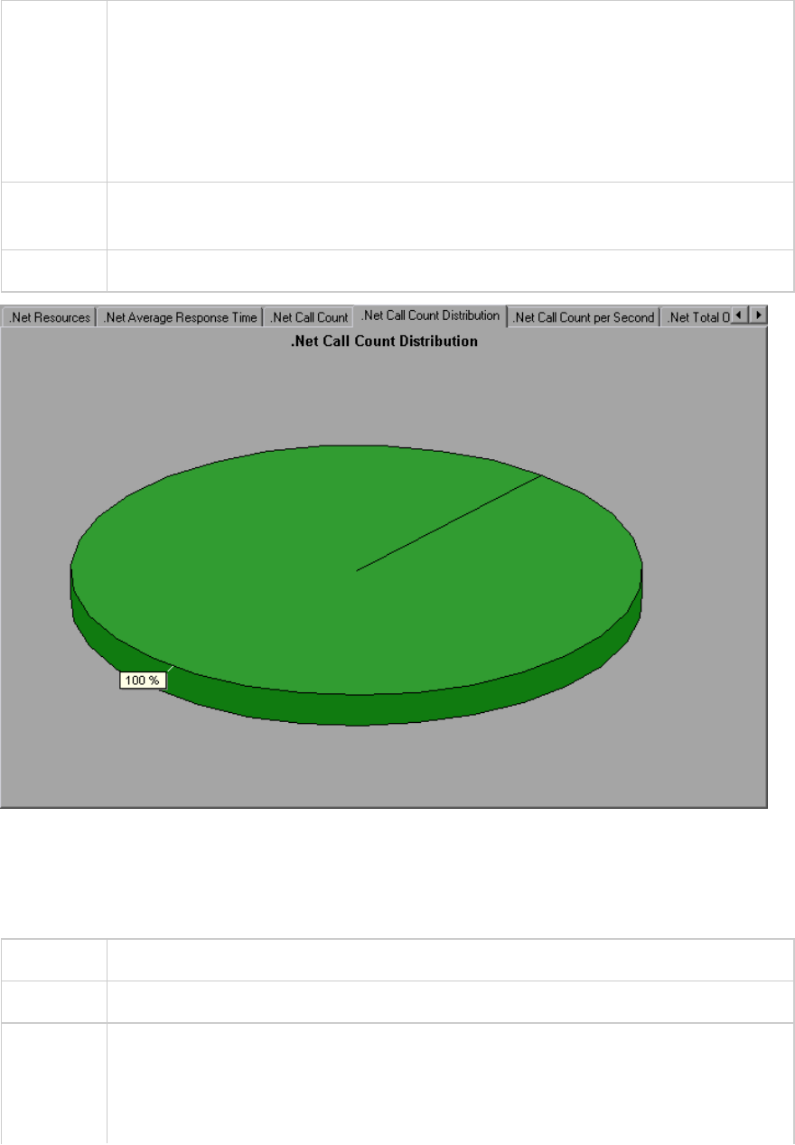
Breakdown
options
The number of calls made to the class or method is listed in the Call Count column of
the .NET Breakdown graph table.
The graph initially displays .NET classes, but you can also view the individual methods
within a .NET class by using drill-down or filtering techniques. For more information, see
"Filtering and Sorting Graph Data" on page103 and "Drilling Down in a Graph" on
page90.
Tips To highlight a specific class line in the graph, select the class row in the legend
(displayed below the graph).
See also "Application Component Graphs" on page268
.NET Call Count Graph
This graph displays the number of times that .NET classes and methods are invoked during the test.
X-axis Elapsed time from the beginning of the scenario run.
Y-axis Indicates how many calls were made to a .NET class or method.
Breakdown
options
The graph initially displays .NET classes, but you can also view the individual methods
within a .NET class by using drill-down or filtering techniques. For more information, see
"Filtering and Sorting Graph Data" on page103 and "Drilling Down in a Graph" on
page90.
User Guide
Analysis
HP LoadRunner (12.50) Page 283
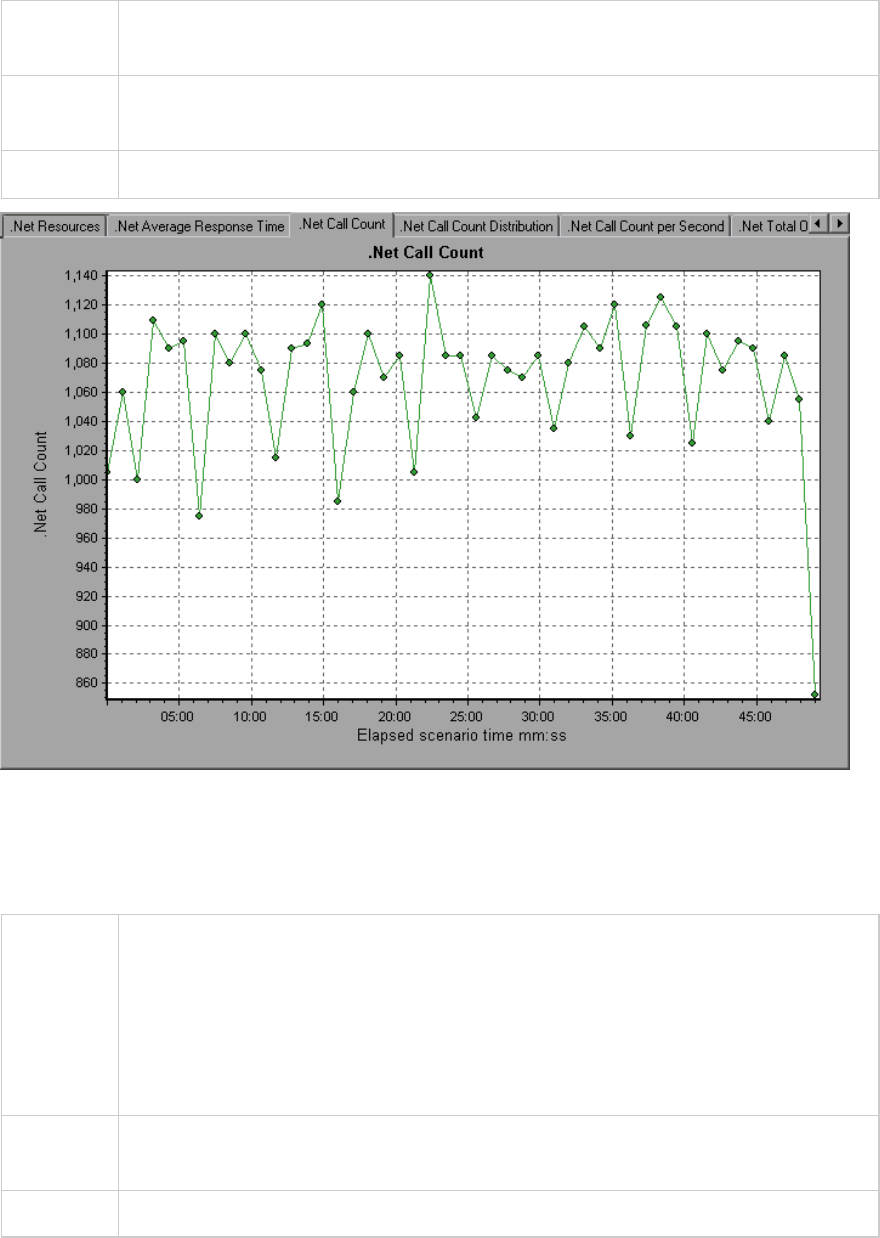
Tips To highlight a specific class line in the graph, select the class row in the legend
(displayed below the graph).
Note The call count is computed by multiplying the call frequency by a time interval. As a
result, the reported measurement may be rounded.
See also "Application Component Graphs" on page268
.NET Call Count per Second Graph
This graph shows the number of times per second that a .NET class or method is invoked.
Breakdown
options
This graph is similar to the .NET Call Count graph except that the y-axis indicates how
many invocations were made to a .NET class or method per second.
The graph initially displays .NET classes, but you can also view the individual methods
within a .NET class by using drill-down or filtering techniques. For more information, see
"Filtering and Sorting Graph Data" on page103 and "Drilling Down in a Graph" on
page90.
Tips To highlight a specific class line in the graph, select the class row in the legend
(displayed below the graph).
See also "Application Component Graphs" on page268
User Guide
Analysis
HP LoadRunner (12.50) Page 284
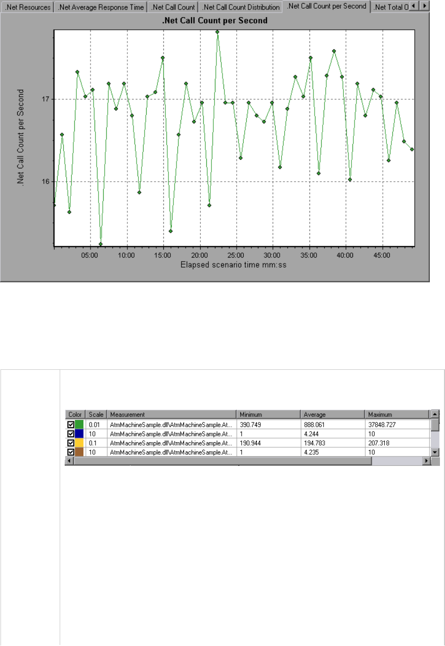
.NET Resources Graph
This graph shows the resource usage of .NET methods as a function of the elapsed load test scenario
time.
Breakdown
options
Each .NET method is represented by a different colored line on the graph. The legend
frame (located below the graph) identifies the methods by color:
You can monitor .NET counters at the application, assembly, class, and method levels.
Measurements that take place before the application is fully loaded (such as Assembly
Load Time, that measures the time it takes to load an assembly) will not be measured.
The following tables describe the counters that can be measured at each level. All
durations are reported in seconds, and all frequencies are reported per five-second
polling periods. For example, if 20 events occur in a 5 second polling period, the
reported frequency is 4.
l"Application Level" on the next page
l"Assembly Level" on page288
l"Class Level" on page288
User Guide
Analysis
HP LoadRunner (12.50) Page 285
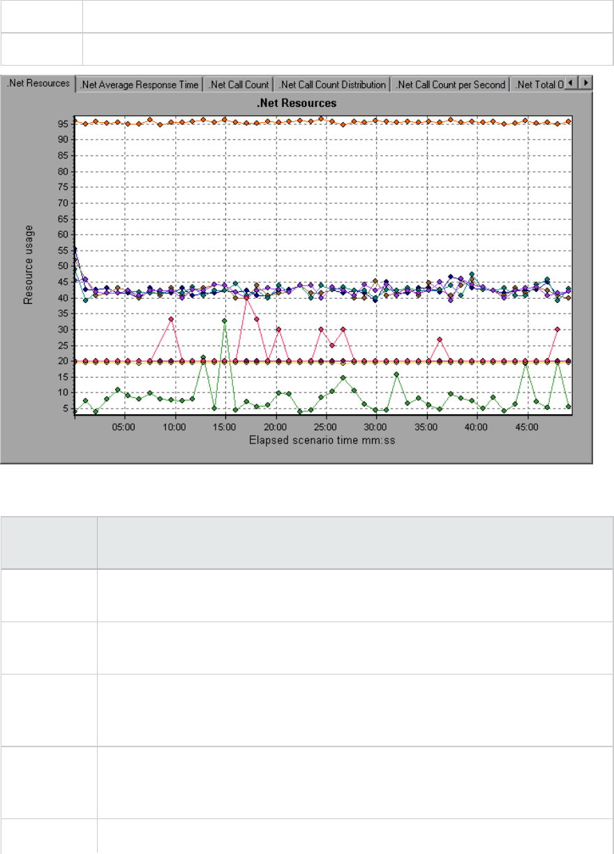
l"Method Level" on page288
See also "Application Component Graphs" on page268
Application Level
Measurement Description
Application
Lifetime
Monitors the duration of the application in seconds.
Exception
Frequency
Monitors the number of exceptions per second, in the five second polling period.
JIT (Just In
Time)
Duration
Monitors the time (in seconds) it takes for the JIT to compile code.
Thread
Creation
Frequency
Monitors the number of threads that are created in a polling period.
Thread Monitors the duration of threads.
User Guide
Analysis
HP LoadRunner (12.50) Page 286
Measurement Description
Lifetime
Domain
Creation
Frequency
Monitors the number of domain creations in a polling period. (Domains protect areas
of code. All applications run in a domain which keeps them encapsulated, so that they
cannot interfere with other applications outside the domain.)
Domain Load
Time
Monitors the time it takes to load a domain. (Domains protect areas of code. All
applications run in a domain which keeps them encapsulated, so that they cannot
interfere with other applications outside the domain).
Domain
Unload Time
Monitors the time it takes to unload a domain. (Domains protect areas of code. All
applications run in a domain which keeps them encapsulated, so that they cannot
interfere with other applications outside the domain).
Domain
Lifetime
Monitors the duration of a domain. (Domains protect areas of code. All applications
run in a domain which keeps them encapsulated, so that they cannot interfere with
other applications outside the domain).
Module
Creation
Frequency
Monitors the number of modules that get created in a polling period. (Modules are
groups of assemblies that make up a DLL or EXE).
Module Load
Time
Monitors the time it takes to load a module. (Modules are groups of assemblies that
make up a dll or exe).
Module
Unload Time
Monitors the time it takes to unload a module. (Modules are groups of assemblies
that make up a dll or exe).
Module
Lifetime
Monitors the duration of a module. (Modules are groups of assemblies that make up
a dll or exe).
Garbage
Collection
Duration
Monitors the duration between the start and stop of Garbage Collection.
Garbage
Collection
Frequency
Monitors the number of breaks for Garbage Collections in a polling period.
Unmanaged
Code
Duration
Monitors the duration of the calls to unmanaged code.
Unmanaged Monitors the number of calls to unengaged code in a polling period.
User Guide
Analysis
HP LoadRunner (12.50) Page 287
Measurement Description
Code
Frequency
Assembly Level
Measurement Description
Assembly Creation
Frequency
Monitors the number of assembly creations in a polling period. (Assemblies
hold the .NET byte code and metadata).
Assembly Load
Time
Monitors the time it takes to load an assembly. (Assemblies hold the .NET byte
code and metadata).
Assembly Unload
Time
Monitors the time it takes to unload an assembly. (Assemblies hold the .NET
byte code and metadata).
Assembly Lifetime Monitors the duration of an assembly. (Assemblies hold the .NET byte code and
metadata).
Class Level
Measurement Description
Class Lifetime Monitors the duration of a class.
Class Load Time Monitors the time it takes to load a class.
Class Unload Time Monitors the time it takes to unload a class.
Method Level
At the method level, the measured time is per method, exclusive of other methods, calls to unmanaged
code, and garbage collection time.
Measurement Description
Method Duration Monitors the duration of a method.
Method Frequency Monitors the number of methods called in a polling period.
.NET Total Operation Time Distribution Graph
This graph shows the percentage of time that a specific .NET class took to execute in relation to all the
.NET classes. It can also show the percentage of time that a .NET method took to execute in relation to
User Guide
Analysis
HP LoadRunner (12.50) Page 288
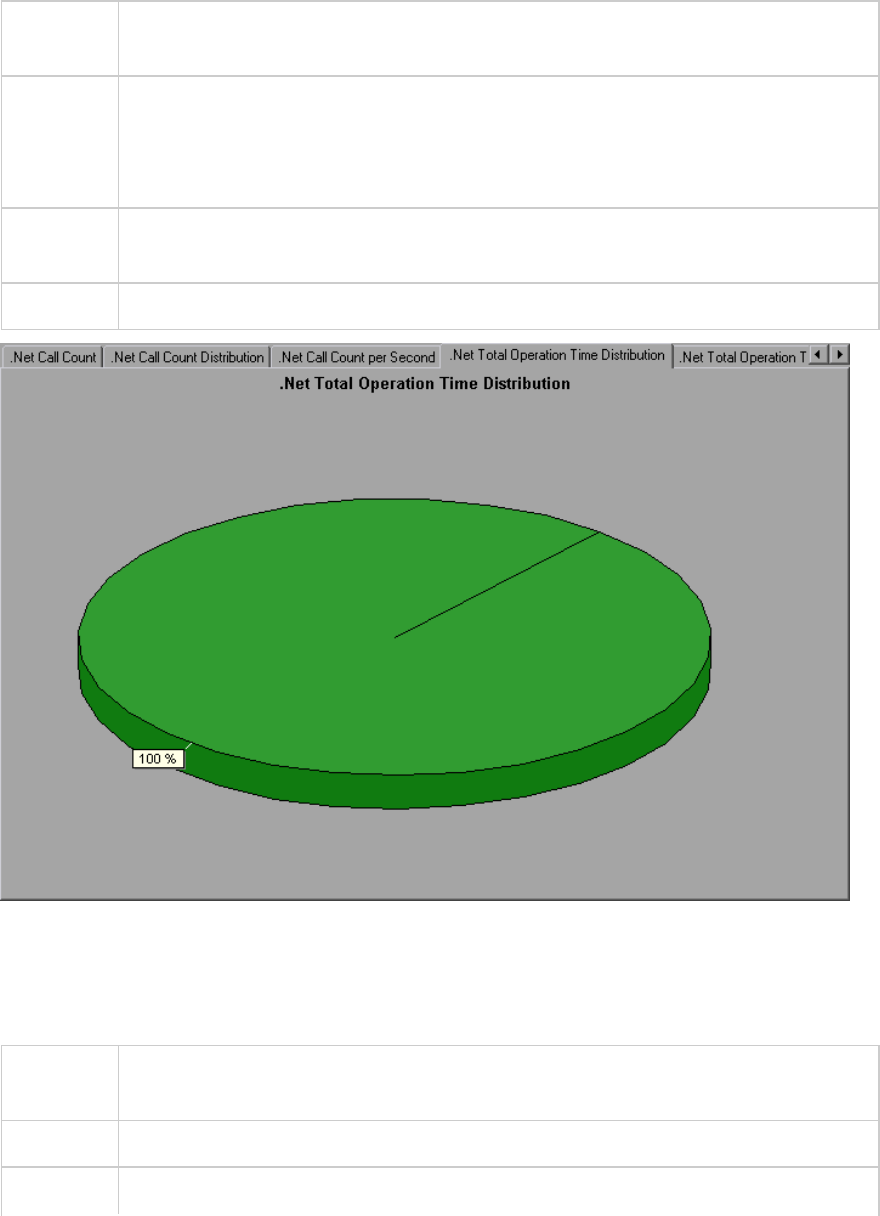
all the .NET methods within the class.
Purpose Use this graph to identify those classes or methods that take an excessive amount of
time.
Breakdown
options
The graph initially displays .NET classes, but you can also view the individual methods
within a .NET class by using drill-down or filtering techniques. For more information, see
"Filtering and Sorting Graph Data" on page103 and "Drilling Down in a Graph" on
page90.
Tips To highlight a specific class line in the graph, select the class row in the legend
(displayed below the graph).
See also "Application Component Graphs" on page268
.NET Total Operation Time Graph
This graph displays the amount of time that each .NET class or method took to execute during the test.
Purpose Use this graph to identify those classes or methods that take an excessive amount of
time.
X-axis Elapsed time from the beginning of the scenario run.
Y-axis Total time a .NET class or method is in operation.
User Guide
Analysis
HP LoadRunner (12.50) Page 289
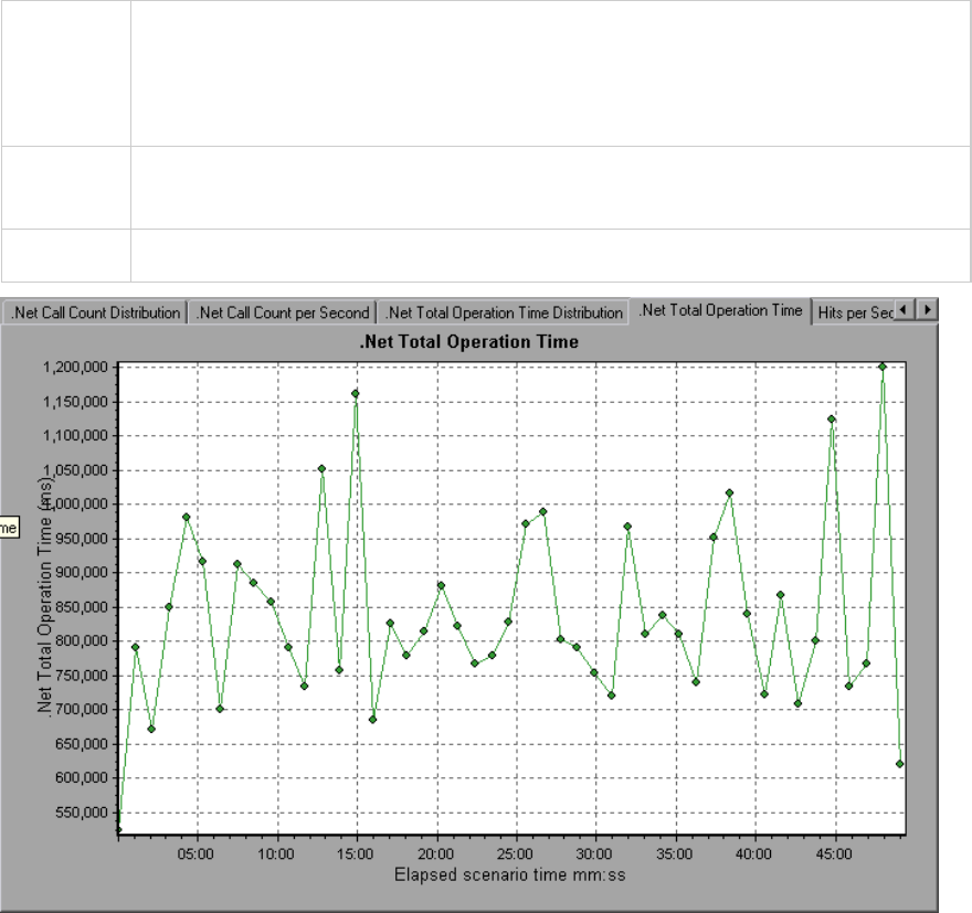
Breakdown
options
The graph initially displays .NET classes, but you can also view the individual methods
within a .NET class by using drill-down or filtering techniques. For more information, see
"Filtering and Sorting Graph Data" on page103 and "Drilling Down in a Graph" on
page90.
Tips To highlight a specific class line in the graph, select the class row in the legend
(displayed below the graph).
See also "Application Component Graphs" on page268
Application Deployment Solutions Graphs
LoadRunner's Citrix Server monitor provides you with information about the application deployment
usage of the Citrix server during a load test scenario execution. In order to obtain performance data,
before you execute the scenario you need to activate the online monitor for the server and specify
which resources you want to measure.
For more information on activating and configuring the Citrix monitors, see the section on online
monitors in the LoadRunner Controller documentation.
User Guide
Analysis
HP LoadRunner (12.50) Page 290

Citrix Measurements
Non-Virtual Counters
Measurement Description
% Disk Time The percentage of elapsed time that the selected disk drive services read or write
requests.
% Processor
Time
The percentage of time that the processor executes a non-Idle thread. This counter
is a primary indicator of processor activity. It is calculated by measuring the time
that the processor spends executing the thread of the Idle process in each sample
interval, and subtracting that value from 100%. (Each processor has an Idle thread
which consumes cycles when no other threads are ready to run.) It can be viewed as
the percentage of the sample interval spent doing useful work. This counter
displays the average percentage of busy time observed during the sample interval.
It is calculated by monitoring the time the service was inactive, and then
subtracting that value from 100%.
File data
Operations/sec
The rate that the computer issues Read and Write operations to file system
devices. It does not include File Control Operations.
Interrupts/sec The average number of hardware interrupts the processor receives and services
per second. It does not include DPCs, which are counted separately. This value is an
indirect indicator of the activity of devices that generate interrupts, such as the
system clock, the mouse, disk drivers, data communication lines, network interface
cards and other peripheral devices. These devices normally interrupt the processor
when they have completed a task or require attention. Normal thread execution is
suspended during interrupts. Most system clocks interrupt the processor every 10
milliseconds, creating a background of interrupt activity. This counter displays the
difference between the values observed in the last two samples, divided by the
duration of the sample interval.
Output Session
Line Speed
This value represents the line speed from server to client for a session in bps.
Input Session
Line Speed
This value represents the line speed from client to server for a session in bps.
Page
Faults/sec
A count of the Page Faults in the processor. A page fault occurs when a process
refers to a virtual memory page that is not in its Working Set in main memory. A
Page Fault will not cause the page to be fetched from disk if that page is on the
standby list, and hence already in main memory, or if it is in use by another process
with whom the page is shared.
User Guide
Analysis
HP LoadRunner (12.50) Page 291
Measurement Description
Pages/sec The number of pages read from the disk or written to the disk to resolve memory
references to pages that were not in memory at the time of the reference. This is
the sum of Pages Input/sec and Pages Output/sec. This counter includes paging
traffic on behalf of the system Cache to access file data for applications. This value
also includes the pages to/from non-cached mapped memory files. This is the
primary counter to observe if you are concerned about excessive memory pressure
(that is, thrashing), and the excessive paging that may result.
Pool Nonpaged
Bytes
The number of bytes in the Nonpaged Pool, a system memory area where space is
acquired by operating system components as they accomplish their appointed
tasks. Nonpaged Pool pages cannot be paged out to the paging file, but instead
remain in main memory as long as they are allocated.
Private Bytes The current number of bytes this process has allocated that cannot be shared with
other processes.
Processor
Queue Length
The instantaneous length of the processor queue in units of threads. This counter is
always 0 unless you are also monitoring a thread counter. All processors use a
single queue in which threads wait for processor cycles. This length does not include
the threads that are currently executing. A sustained processor queue length
greater than two generally indicates processor congestion. This is an instantaneous
count, not an average over the time interval.
Threads The number of threads in the computer at the time of data collection. Notice that
this is an instantaneous count, not an average over the time interval. A thread is
the basic executable entity that can execute instructions in a processor.
Latency –
Session
Average
The average client latency over the life of a session.
Latency – Last
Recorded
The last recorded latency measurement for this session.
Latency –
Session
Deviation
The difference between the minimum and maximum measured values for a
session.
Input Session
Bandwidth
The bandwidth (in bps) from client to server traffic for a session in bps.
Input Session
Compression
The compression ratio for client to server traffic for a session.
Output Session The bandwidth (in bps) from server to client traffic for a session.
User Guide
Analysis
HP LoadRunner (12.50) Page 292
Measurement Description
Bandwidth
Output Session
Compression
The compression ratio for server to client traffic for a session.
Output Session
Linespeed
The line speed (in bps) from server to client for a session.
Virtual Channel Counters
All the counters in the following table are measured in bytes per second (bps):
Measurement Description
Input Audio Bandwidth The bandwidth from client to server traffic on the audio mapping
channel.
Input Clipboard
Bandwidth
The bandwidth from client to server traffic on the clipboard mapping
channel.
Input COM1 Bandwidth The bandwidth from client to server traffic on the COM1 channel.
Input COM2 Bandwidth The bandwidth from client to server traffic on the COM2 channel.
Input COM Bandwidth The bandwidth from client to server traffic on the COM channel.
Input Control Channel
Bandwidth
The bandwidth from client to server traffic on the ICA control channel.
Input Drive Bandwidth The bandwidth from client to server traffic on the client drive mapping
channel.
Input Font Data
Bandwidth
The bandwidth from client to server traffic on the local text echo font
and keyboard layout channel.
Input Licensing
Bandwidth
The bandwidth from server to client traffic on the licensing channel.
Input LPT1 Bandwidth The bandwidth from client to server traffic on the LPT1 channel.
Input LPT2 Bandwidth The bandwidth from client to server traffic on the LPT2 channel.
Input Management
Bandwidth
The bandwidth from client to server traffic on the client management
channel.
Input PN Bandwidth The bandwidth from client to server traffic on the Program
Neighborhood channel.
User Guide
Analysis
HP LoadRunner (12.50) Page 293
Measurement Description
Input Printer Bandwidth The bandwidth from client to server traffic on the printer spooler
channel.
Input Seamless
Bandwidth
The bandwidth from client to server traffic on the Seamless channel.
Input Text Echo
Bandwidth
The bandwidth from client to server traffic on the local text echo data
channel.
Input Thinwire
Bandwidth
The bandwidth from client to server traffic on the Thinwire (graphics)
channel.
Input VideoFrame
Bandwidth
The bandwidth from client to server traffic on the VideoFrame channel.
Output Audio Bandwidth The bandwidth from server to client traffic on the audio mapping
channel.
Output Clipboard
Bandwidth
The bandwidth from server to client traffic on the clipboard mapping
channel.
Output COM1 Bandwidth The bandwidth from server to client traffic on the COM1 channel.
Output COM2 Bandwidth The bandwidth from server to client traffic on the COM2 channel.
Output COM Bandwidth The bandwidth from server to client traffic on the COM channel.
Output Control Channel
Bandwidth
The bandwidth from server to client traffic on the ICA control channel.
Output Drive Bandwidth The bandwidth from server to client traffic on the client drive channel.
Output Font Data
Bandwidth
The bandwidth from server to client traffic on the local text echo font
and keyboard layout channel.
Output Licensing
Bandwidth
The bandwidth from server to client traffic on the licensing channel.
Output LPT1 Bandwidth The bandwidth from server to client traffic on the LPT1 channel.
Output LPT2 Bandwidth The bandwidth from server to client traffic on the LPT2 channel.
Output Management
Bandwidth
The bandwidth from server to client traffic on the client management
channel.
Output PN Bandwidth The bandwidth from server to client traffic on the Program
Neighborhood channel.
User Guide
Analysis
HP LoadRunner (12.50) Page 294
Measurement Description
Output Printer
Bandwidth
The bandwidth from server to client traffic on the printer spooler
channel.
Output Seamless
Bandwidth
The bandwidth from server to client traffic on the Seamless channel.
Output Text Echo
Bandwidth
The bandwidth from server to client traffic on the local text echo data
channel.
Output Thinwire
Bandwidth
The bandwidth from server to client traffic on the Thinwire (graphics)
channel.
Output VideoFrame
Bandwidth
The bandwidth from server to client traffic on the VideoFrame channel.
Citrix Server Graph
This graph is an Application Deployment solution which delivers applications across networks. The Citrix
Server monitor is an Application Deployment Solution monitor, which provides performance information
for the Citrix server.
X-
axis
Elapsed time since the start of the run.
Y-
axis
The resource usage on the Citrix server.
Note To obtain data for this graph, you need to enable the Citrix Server monitor (from the
Controller) and select the default measurements you want to display, before running the
scenario.
See
also
"Application Deployment Solutions Graphs" on page290
"Citrix Measurements" on page291
User Guide
Analysis
HP LoadRunner (12.50) Page 295
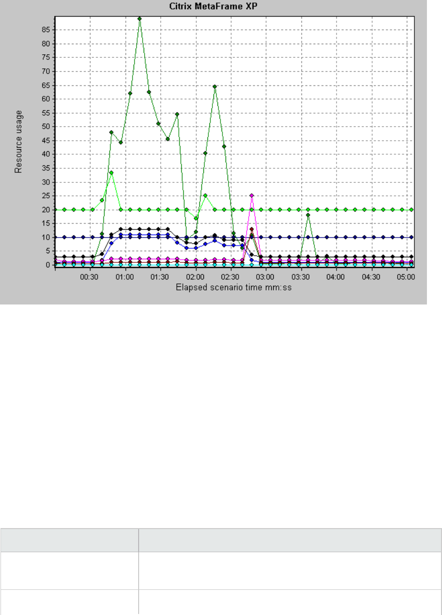
Middleware Performance Graphs
A primary factor in a transaction's response time is the middleware performance usage. LoadRunner's
Middleware Performance monitors provide you with information about the middleware performance
usage of the Tuxedo and IBM WebSphere MQ servers during a load test scenario execution. To obtain
performance data, you need to activate the online monitor for the server and specify which resources
you want to measure before executing the scenario.
For more information, see the section on online monitors in the LoadRunner Controller documentation.
IBM WebSphere MQ Counters
Queue Performance Counters
Measurement Description
Event - Queue Depth High
(events per second)
An event triggered when the queue depth reaches the configured
maximum depth.
Event - Queue Depth Low An event triggered when the queue depth reaches the configured
User Guide
Analysis
HP LoadRunner (12.50) Page 296
Measurement Description
(events per second) minimum depth.
Event - Queue Full (events
per second)
An event triggered when an attempt is made to put a message on a
queue that is full.
Event - Queue Service
Interval High (events per
second)
An event triggered when no messages are put to or retrieved from a
queue within the timeout threshold.
Event - Queue Service
Interval OK (events per
second)
An event triggered when a message has been put to or retrieved
from a queue within the timeout threshold.
Status - Current Depth The current count of messages on a local queue. This measurement
applies only to local queues of the monitored queue manager.
Status - Open Input Count The current count of open input handles. Input handles are opened
so that an application may "put" messages to a queue.
Status - Open Output Count The current count of open output handles. Output handles are
opened so that an application may "get" messages from a queue.
Channel Performance Counters
Measurement Description
Event - Channel
Activated
(events per
second)
An event generated when a channel, waiting to become active but inhibited from
doing so due to a shortage of queue manager channel slots, becomes active due
to the sudden availability of a channel slot.
Event - Channel
Not Activated
(events per
second)
An event generated when a channel attempts to become active but is inhibited
from doing so due to a shortage of queue manager channel slots.
Event - Channel
Started (events
per second)
An event generated when a channel is started.
Event - Channel
Stopped (events
per second)
An event generated when a channel is stopped, regardless of source of stoppage.
Event - Channel An event generated when a channel is stopped by a user.
User Guide
Analysis
HP LoadRunner (12.50) Page 297
Measurement Description
Stopped by User
(events per
second)
Status -
Channel State
The current state of a channel. Channels pass through several states from
stopped (inactive state) to running (fully active state). Channel states range from
0 (stopped) to 6 (running).
Status -
Messages
Transferred
The count of messages that have been sent over the channel. If no traffic is
occurring over the channel, this measurement will be zero. If the channel has not
been started since the queue manager was started, no measurement will be
available.
Status - Buffer
Received
The count of buffers that have been received over the channel. If no traffic is
occurring over the channel, this measurement will be zero. If the channel has not
been started since the queue manager was started, no measurement will be
available.
Status - Buffer
Sent
The count of buffers that have been sent over the channel. If no traffic is
occurring over the channel, this measurement will be zero. If the channel has not
been started since the queue manager was started, no measurement will be
available.
Status - Bytes
Received
The count of bytes that have been received over the channel. If no traffic is
occurring over the channel, this measurement will appear as zero. If the channel
has not been started since the queue manager was started, no measurement will
be available.
Status - Bytes
Sent
The count of bytes that have been sent over the channel. If no traffic is occurring
over the channel, this measurement will appear as zero. If the channel has not
been started since the queue manager was started, no measurement will be
available.
Tuxedo Resources Graph Measurements
The following table describes the default counters that can be measured. It is recommended to pay
particular attention to the following measurements: %Busy Clients, Active Clients, Busy Clients, Idle
Clients, and all the queue counters for relevant queues.
Monitor Measurements
Machine % Busy Clients. The percentage of active clients currently logged in to the Tuxedo
application server that are waiting for a response from the application server.
User Guide
Analysis
HP LoadRunner (12.50) Page 298
Monitor Measurements
Active Clients. The total number of active clients currently logged in to the Tuxedo
application server.
Busy Clients. The total number of active clients currently logged in to the Tuxedo
application server that are waiting for a response from the application server.
Current Accessers. The number of clients and servers currently accessing the
application either directly on this machine or through a workstation handler on this
machine.
Current Transactions. The number of in use transaction table entries on this machine.
Idle Clients. The total number of active clients currently logged in to the Tuxedo
application server that are not waiting for a response from the application server.
Workload Completed/second. The total workload on all the servers for the machine
that was completed, per unit time.
Workload Initiated/second. The total workload on all the servers for the machine that
was initiated, per unit time.
Queue % Busy Servers. The percentage of active servers currently handling Tuxedo
requests.
Active Servers. The total number of active servers either handling or waiting to
handle Tuxedo requests.
Busy Servers. The total number of active servers currently busy handling Tuxedo
requests.
Idle Servers. The total number of active servers currently waiting to handle Tuxedo
requests.
Number Queued. The total number of messages which have been placed on the queue.
Server Requests/second. The number of server requests handled per second.
Workload/second. The workload is a weighted measure of the server requests. Some
requests could have a different weight than others. By default, the workload is always
50 times the number of requests.
Workstation
Handler
(WSH)
Bytes Received/sec. The total number of bytes received by the workstation handler,
per second.
Bytes Sent/sec. The total number of bytes sent back to the clients by the workstation
handler, per second.
Messages Received/sec. The number of messages received by the workstation
User Guide
Analysis
HP LoadRunner (12.50) Page 299
Monitor Measurements
handler, per second.
Messages Sent/sec. The number of messages sent back to the clients by the
workstation handler, per second.
Number of Queue Blocks/sec. The number of times the queue for the workstation
handler blocked, per second. This gives an idea of how often the workstation handler
was overloaded.
IBM WebSphere MQ Graph
This graph shows the resource usage of IBM WebSphere MQ Server channel and queue performance
counters as a function of the elapsed load test scenario time.
X-
axis
Elapsed time since the start of the run.
Y-
axis
The resource usage of the IBM WebSphere MQ Server channel and queue performance
counters.
Note To obtain data for this graph, you need to enable the IBM WebSphere MQ monitor (from the
Controller) and select the default measurements you want to display, before running the
scenario.
See
also
"Middleware Performance Graphs" on page296
"IBM WebSphere MQ Counters" on page296
User Guide
Analysis
HP LoadRunner (12.50) Page 300
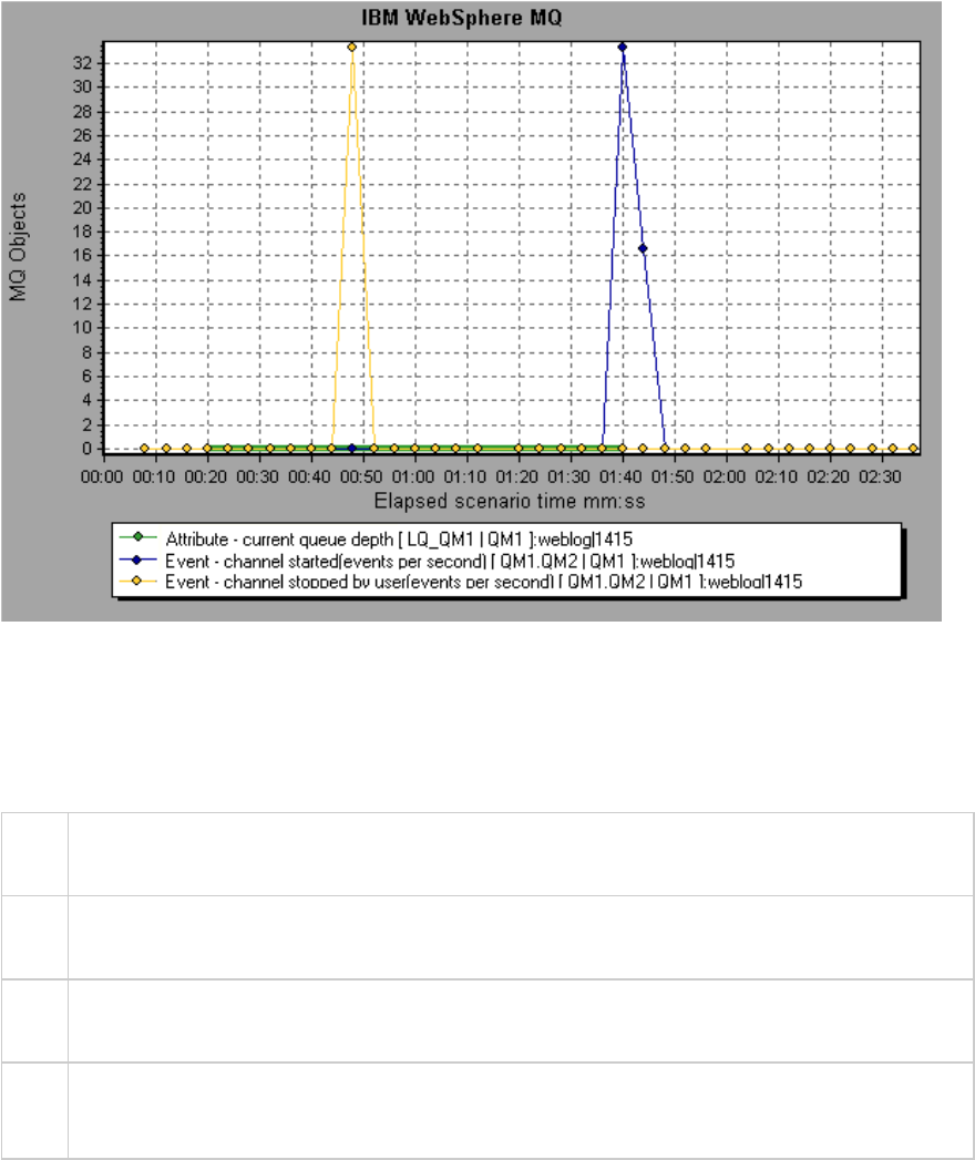
Tuxedo Resources Graph
This graph provides information about the server, load generator machine, workstation handler, and
queue in a Tuxedo system.
X-
axis
Elapsed time since the start of the run.
Y-
axis
The resource usage on the Tuxedo system.
Note To obtain data for this graph, you need to enable the TUXEDO monitor (from the Controller)
and select the default measurements you want to display, before running the scenario.
See
also
"Middleware Performance Graphs" on page296
"Tuxedo Resources Graph Measurements" on page298
User Guide
Analysis
HP LoadRunner (12.50) Page 301
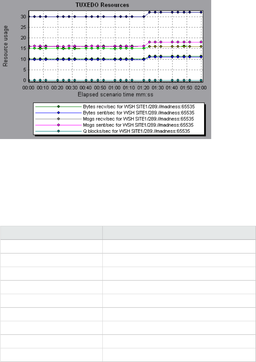
Infrastructure Resources Graphs
LoadRunner's Infrastructure Resources monitor provides you with information about the performance
of FTP, POP3, SMTP, IMAP, and DNS Vusers on the network client during load test scenario execution.
Network Client Measurements
Measurement Description
Pings per sec Number of pings per second.
Data transfer bytes per sec Number of data bytes transferred per second.
Data receive bytes per sec Number of data bytes received per second.
Connections per sec Number of connections per second.
Accept connections per sec Number of connections accepted per seconds.
SSL Connections per sec Number of SSL connections per second.
SSL Data transfer bytes per sec Number of SSL data bytes transferred per second.
SSL Data receive bytes per sec Number of SSL data bytes received per second.
SSL Accept connections per sec Number of SSL connections accepted per seconds.
User Guide
Analysis
HP LoadRunner (12.50) Page 302
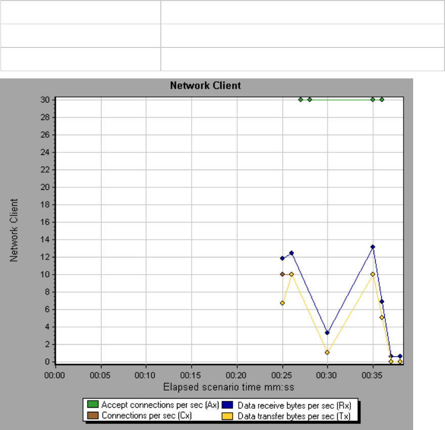
Network Client Graph
This graph displays network client data points for FTP, POP3, SMTP, IMAP, and DNS Vusers during a load
test scenario run.
X-axis Elapsed time since the start of the run.
Y-axis The resource value of the network client data points..
See also "Infrastructure Resources Graphs" on the previous page
HP Service Virtualization Graphs
The Service Virtualization graphs are similar to the corresponding monitors used by the LoadRunner
Controller. For details, see Service Virtualization Monitoring Overview.
User Guide
Analysis
HP LoadRunner (12.50) Page 303
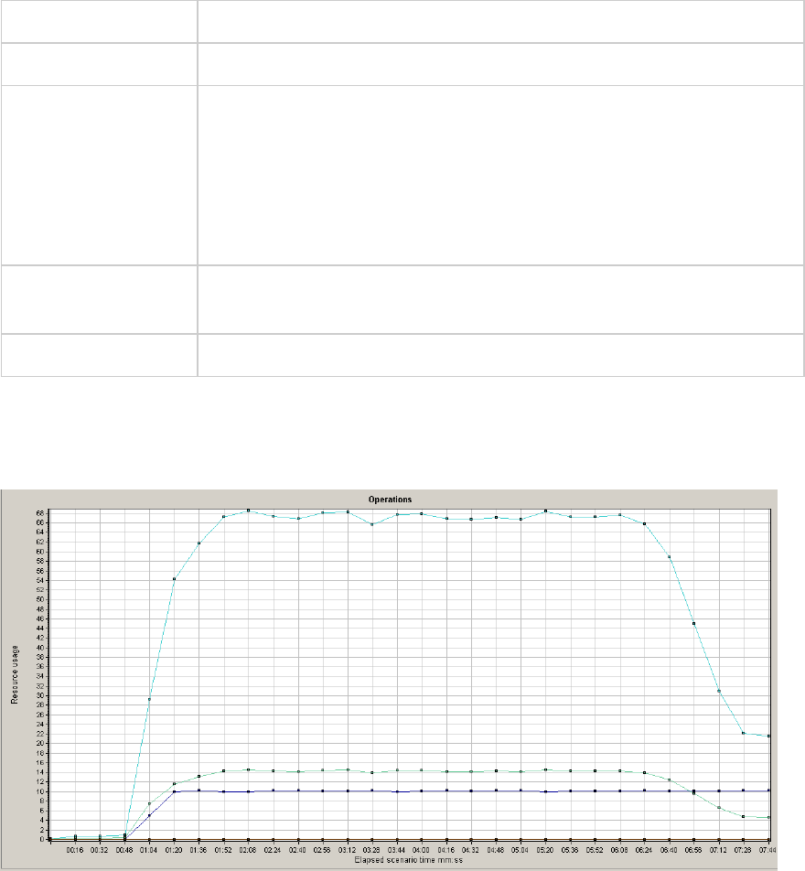
Service Virtualization Graphs Overview
The Service Virtualization graphs are similar to the corresponding monitors used by the LoadRunner
Controller. For details, see Service Virtualization Monitoring Overview.
HP Service Virtualization Operations Graph
This graph displays a summary for HP Service Virtualization - Operations.
X-axis The elapsed time from the beginning of the scenario run.
Y-axis The number of resources used.
Tips lTo isolate the measurement with the most problems, it may be helpful to
sort the legend window according to the average number of resources
used. To sort the legend by average, double-click the Average column
heading.
lTo identify a measurement in the graph, you can select it. The
corresponding line in the legend window is selected.
Note To use this graph, you must first open a Service Virtualization project in the
Controller.
See also Web Page Diagnostics Graph
Example
Using the graph, you can track which resources were most problematic, and at which point(s) during the
scenario the problem(s) occurred.
User Guide
Analysis
HP LoadRunner (12.50) Page 304

HP Service Virtualization Services Graph
This graph displays a summary for HP Service Virtualization - Services.
X-axis The elapsed time from the beginning of the scenario run.
Y-axis The number of resources used.
Tips lTo isolate the measurement with the most problems, it may be helpful to
sort the legend window according to the average number of resources
used. To sort the legend by average, double-click the Average column
heading.
lTo identify a measurement in the graph, you can select it. The
corresponding line in the legend window is selected.
Note To use this graph, you must first open a Service Virtualization project in the
Controller scenario.
See also Web Page Diagnostics Graph
Example
Using the graph, you can track which resources were most problematic, and at which point(s) during the
scenario the problem(s) occurred.
Flex Graphs
Flex graphs provide you with information about the performance of your Flex server. You use the Flex
graphs to analyze the following data:
User Guide
Analysis
HP LoadRunner (12.50) Page 305
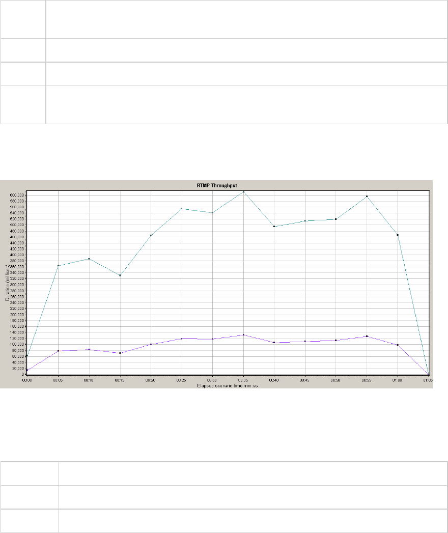
Flex RTMP Throughput Graph
This graph shows the amount of throughput (in bytes) on the RTMP/T server during each second of the
load test scenario run. The throughput represents the amount of data that the Vusers received from
the server or sent to the server at any given second.
Purpose Helps you evaluate the amount of load that Vusers generate, in terms of server
throughput.
X-axis Elapsed time since the start of the scenario run.
Y-axis Throughput of the server in bytes
Note You cannot change the granularity of the x-axis to a value that is less than the Web
granularity you defined in the General tab of the Options dialog box.
Example
In the following example, the highest throughput is over 600,000 bytes during the thirty-fifth second of
the scenario.
Flex RTMP Other Statistics Graph
This graph shows various statistics about Flex RTMP Vusers.
Purpose The graph shows the duration taken to perform various RTMP tasks.
X-axis Elapsed time since the start of the scenario run.
Y-axis Task duration (in milliseconds).
User Guide
Analysis
HP LoadRunner (12.50) Page 306
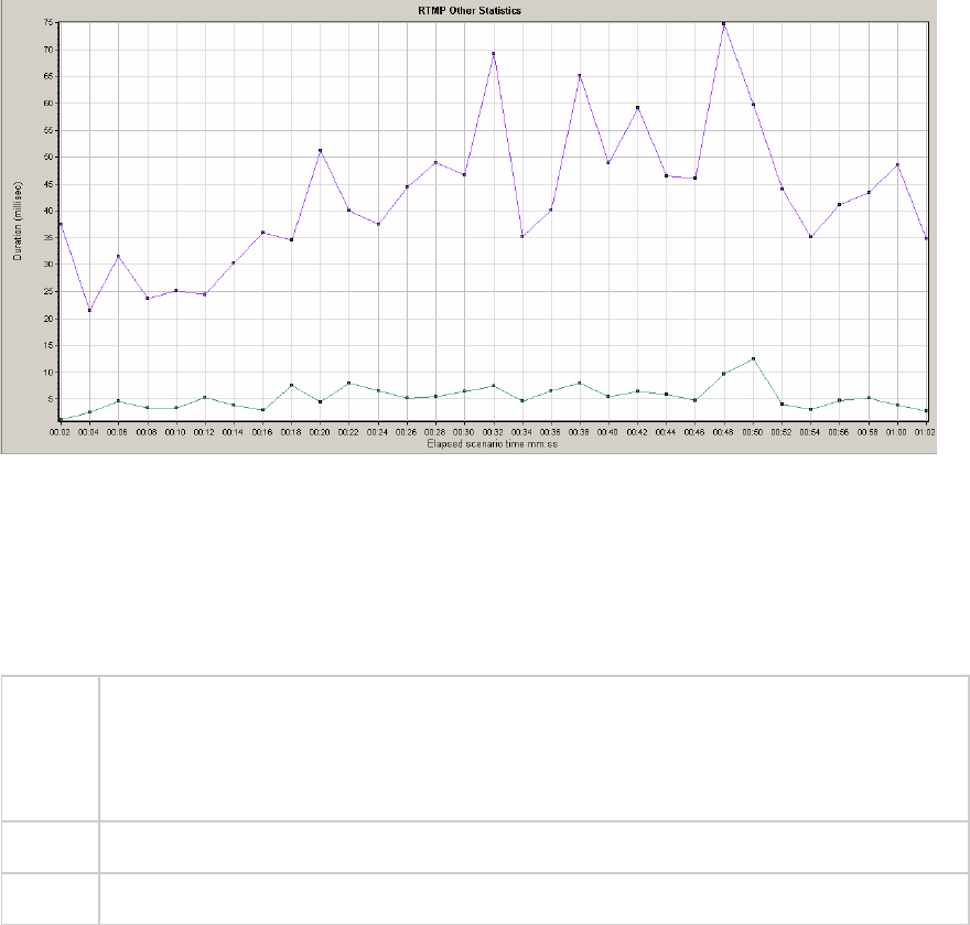
Example
In the following example,the RTMP Handshake has a duration of seventy five milliseconds at the forty
eighth second of the scenario.
Flex RTMP Connections Graph
This graph shows the number of open RTMP connections at any time during the load test scenario run.
The throughput represents the amount of data that the Vusers received from the server or sent to the
server at any given second.
Purpose This graph is useful in indicating when additional connections are needed. For example, if
the number of connections reaches a plateau, and the transaction response time
increases sharply, adding connections would probably cause a dramatic improvement in
performance (reduction in the transaction response time).
X-axis Elapsed time since the start of the scenario run.
Y-axis Number of connections.
Example
In the following example,between the forty-eighth second and the fifty-sixth second of the scenario
there are eighty open connections.
User Guide
Analysis
HP LoadRunner (12.50) Page 307
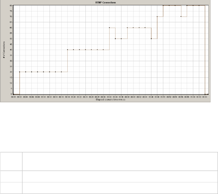
TruClient CPU Utilization Percentage Graph
This graph displays the total number of streams that were successfully delivered by the server. A
successful delivery is indicated when the server initiates a "NetStream.Stop" message at the end of the
requested stream.
Purpose Helps you evaluate the amount of load that Vusers generate, in terms of server
throughput.
X-axis Elapsed time since the start of the scenario run.
Y-axis Number of streams delivered
Example
In the following example, the graph rises at a forty five degree angle, indicating a constant number of
streams being delivered over time.
User Guide
Analysis
HP LoadRunner (12.50) Page 308
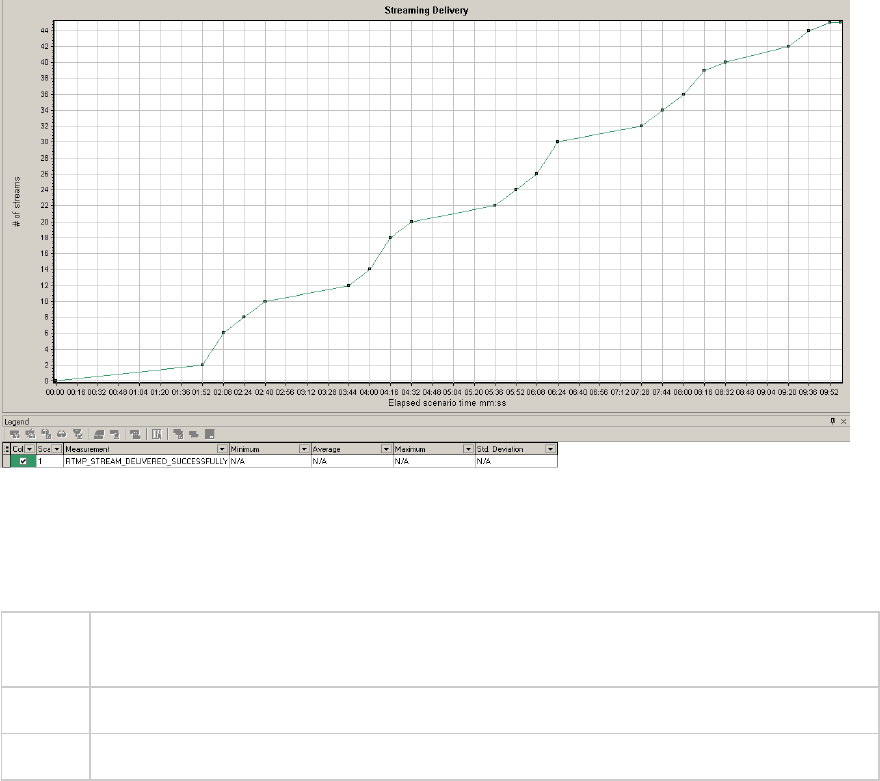
Flex Average Buffering Time Graph
This graph displays the average buffering time for RTMP streams.
Purpose Helps you evaluate the amount of load that Vusers generate, in terms of time spent for
streams in the buffer.
X-axis Elapsed time since the start of the scenario run.
Y-axis Buffering time in milliseconds
Example
In the following example, the buffering time reaches its lowest after 4 minutes and 32 seconds of the
scenario before climbing up to a peak again. You should compare it to other graphs to see what
happened at that time.
User Guide
Analysis
HP LoadRunner (12.50) Page 309
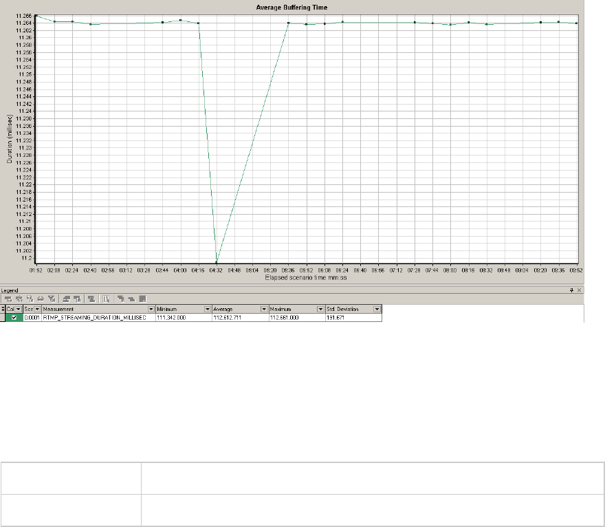
WebSocket Statistics Graphs
The WebSocket Statistics graphs provides you with statistics for the WebSocket data during the
scenario run, such as byte rate, connection status, and the number of messages.
X-axis Elapsed time since the start of the run.
Y-axis WebSocket per second throughout the whole scenario.
The WebSocket Statistics graphs are:
lWebSocket Bytes per second. This graph shows the number of bytes that were sent and received
per second.
lWebSocket Connections per second. This graph shows the number of new, failed, and closed
connections. I
lWebSocket Messages per second. This graph shows the number of WebSocket messages that were
sent, per second.
To gather these statistics, enable the WebSocket Statistics monitors before running your scenario.
Diagnostics Graphs
You can open Diagnostics graphs that were generated in earlier versions of LoadRunner.
User Guide
Analysis
HP LoadRunner (12.50) Page 310
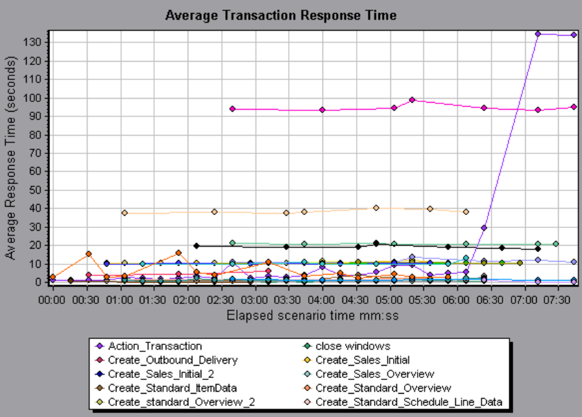
Siebel Diagnostics Graphs
Siebel Diagnostics Graphs Overview
Siebel Diagnostics graphs enable you to trace, time, and troubleshoot individual transactions through
Web, application, and database servers.
To analyze where problems are occurring, you correlate the data in the Siebel Diagnostics graphs with
data in the Transaction Response Time graphs.
You begin analyzing these graphs with the transaction graphs that display the average transaction
response time during each second of the load test scenario run. For example, the following Average
Transaction Response Time graph demonstrates that the average transaction response time for the
Action_Transaction transaction was high.
Using the Siebel Diagnostics graphs, you can pinpoint the cause of the delay in response time for this
transaction.
Alternatively, you can use the Summary Report to view individual transactions broken down into Web,
application, and database layers, and the total usage time for each transaction. For more information,
see "Siebel Diagnostics Graphs Summary Report" on page321.
User Guide
Analysis
HP LoadRunner (12.50) Page 311
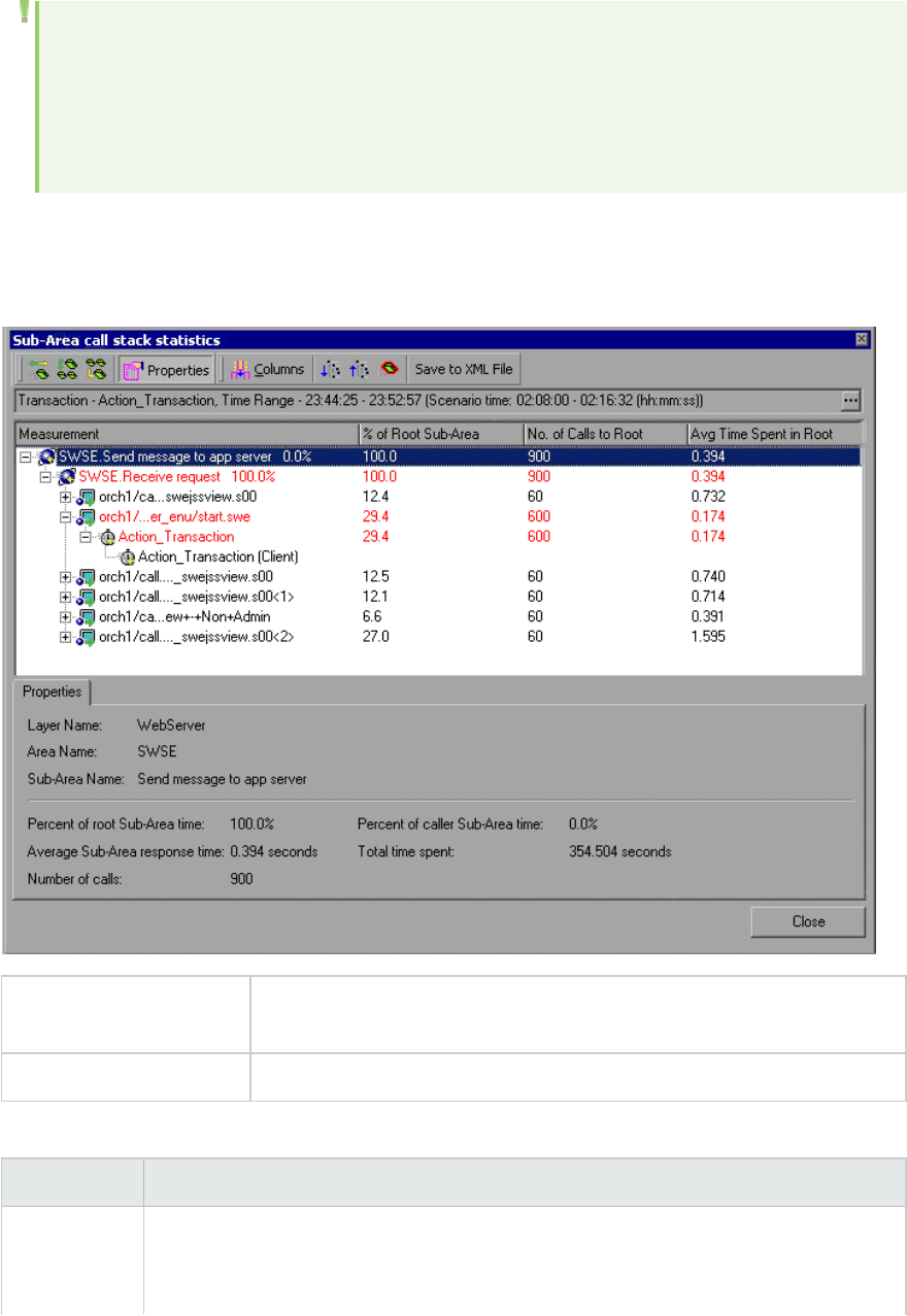
Note: A measurement that is broken down in the Average Transaction Response Time graph will
be different from the same measurement broken down in the Siebel Diagnostics graph. This is
because the Average Transaction Response Time graph displays the average transaction
response time, whereas the Siebel Diagnostics graph displays the average time per transaction
event (sum of Siebel Area response time).
Call Stack Statistics Window
This window enables you to view which components called the selected component.
To access Analysis window > <Siebel> graph > right click sub-area and select Siebel
Diagnostics > Show Sub-Area Call Stack Statistics
See also "Siebel Diagnostics Graphs Overview" on the previous page
User interface elements are described below:
UI Element Description
Measurement Name of the sub-area, displayed as AreaName:SubAreaName. In the case of a
database call, query information is also displayed. The percent shown indicates the
percentage of calls to this component from its child.
User Guide
Analysis
HP LoadRunner (12.50) Page 312
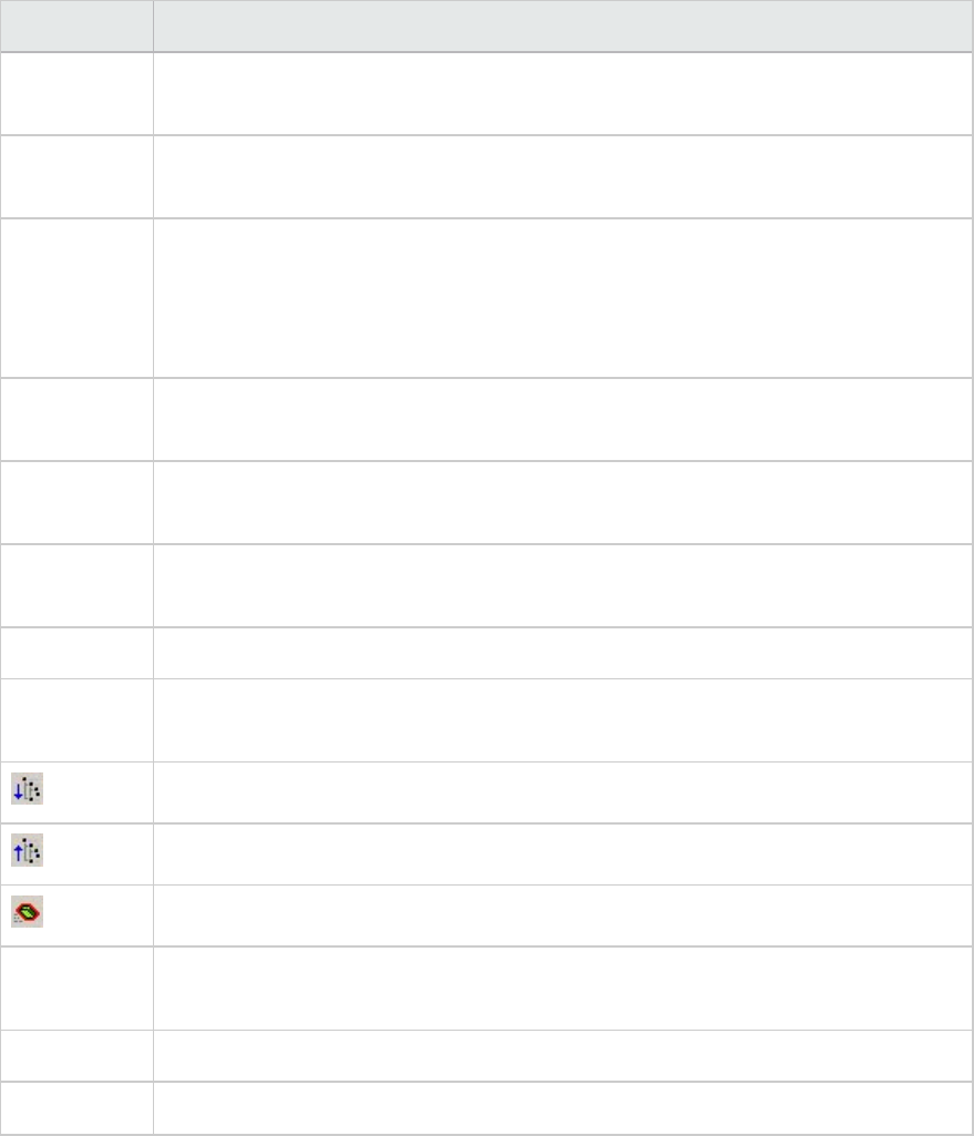
UI Element Description
% of Root
Sub-Area
Displays the percentage of sub-area time in relation the total root sub-area time.
No. of Calls
to Root
Displays the amount of times this transaction or sub-area was executed.
Avg Time
Spent in Root
Time spent in root is the time that the sub-area spent in the root sub-
area//transaction.
Average Time Spent in Root time is the total time spent in the root divided by the
number of instances of the sub-area.
STD Time
Spent in Root
The standard deviation time spent in the root.
Min Time
Spent in Root
The minimum time spent in the root.
Max Time
Spent in Root
The maximum time spent in the root.
% of Called Displays the percentage of sub-area time in relation the child sub-area time.
Total Time
Spent in Root
Displays the total sub-area execution time, including the child execution time.
Expand All. Expands the entire tree.
Collapse All. Collapses the entire tree.
Expand Worst Path. Expands only the parts of the path on the critical path.
Save to XML
File
Saves the tree data to an XML file.
Properties Properties Area.Displays the full properties of the selected sub-area.
SQL Query SQL Query. Displays the SQL query for the selected sub-area (For Database only).
Chain of Calls Window
This window enables you to view the components that the selected transaction or sub-area called. The
following figure shows all the calls in the critical path of the parent Action_Transaction server-side
transaction are displayed.
User Guide
Analysis
HP LoadRunner (12.50) Page 313
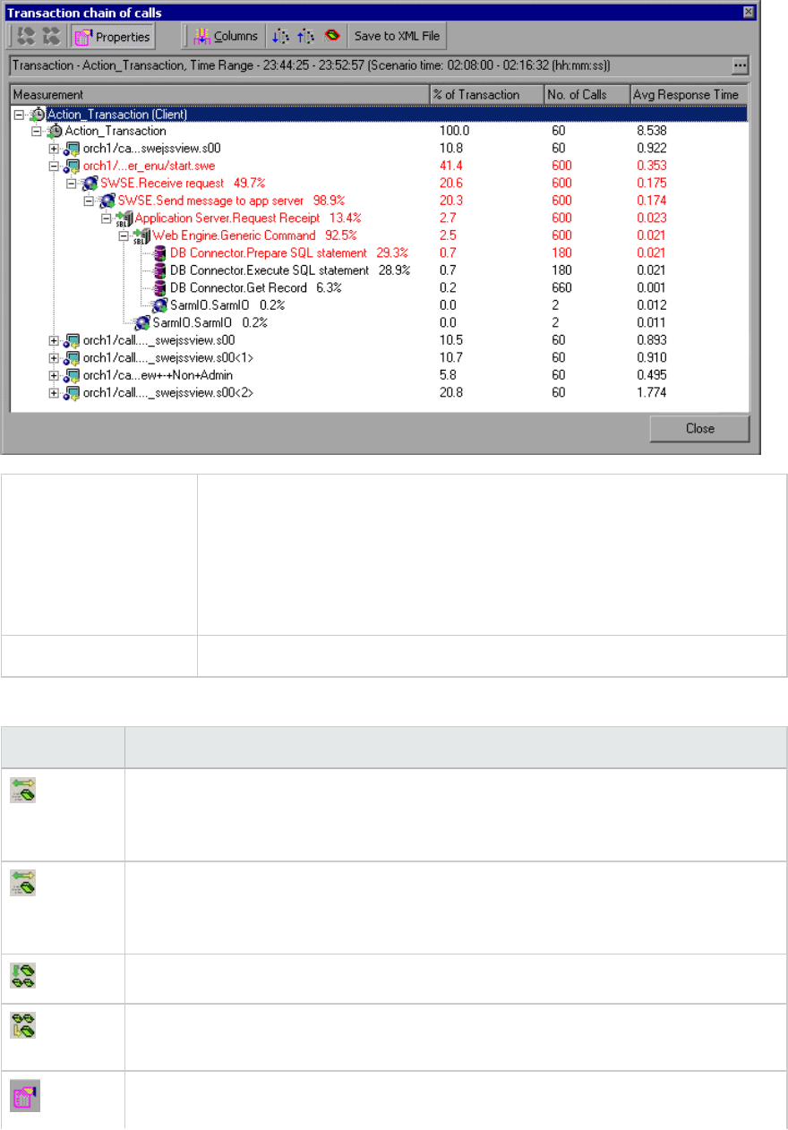
To access Use one of the following:
lTo view transaction call chains - right click a component and select
Siebel Diagnostics > Show Chain of Calls
lTo view sub-area statistics - right click sub-area and select Show Sub-
Area Chain of Calls
Note Each red node signifies the most time consuming child to its parent.
User interface elements are described below:
UI Element Description
Switch to Sub-Area Chain of Calls. When the sub-area call stack statistics data is
displayed, this displays the sub-area chain of calls data (only if the root is a sub-
area).
Switch to Sub-Area Call Stack Statistics. When the sub-area chain of calls data is
displayed, this displays the sub-area call stack statistics data (only if the root is a
sub-area).
Show Sub-Area Chain of Calls. Displays the Sub-Area Chain of Calls window.
Show Sub-Area Call Stack Statistics. Displays the Sub-Area Call Stack Statistics
window.
Properties. Hides or displays the properties area (lower pane).
User Guide
Analysis
HP LoadRunner (12.50) Page 314
UI Element Description
Columns. Enables you to select the columns shown in the Calls window. To display
additional fields, drag them to the desired location in the Calls window. To remove
fields, drag them from the Calls window back to the Columns chooser.
Measurement Name of the sub-area, displayed as AreaName:SubAreaName. In the case of a
database call, query information is also displayed. The percent shown indicates the
percentage of calls to this component from its parent.
% of
Transaction/
Root Sub-
Area
Displays the percentage of sub-area time in relation the total transaction/root sub-
area time.
No of Calls Displays the amount of times this transaction or sub-area was executed.
Avg
Response
Time
Response time is the time from the beginning of execution until the end. Average
response time is the total response time divided by the number of instances of the
area/sub-area.
STD
Response
Time
The standard deviation response time.
Min
Response
Time
The minimum response time.
Max
Response
Time
The maximum response time.
% of Caller Displays the percentage of sub-area time in relation the parent sub-area time.
Total time Displays the total sub-area execution time, including the child execution time.
Siebel Area Average Response Time Graph
This graph displays the average response time for the server side areas, computed as the total area
response time divided by the number of area calls.
Purpose For example, if an area was executed twice by one instance of transaction A, and once
by another instance of the same transaction, and it took three seconds for each
execution, then the average response time is 9/3, or 3 seconds. The area time does not
include calls made from the area to other areas.
User Guide
Analysis
HP LoadRunner (12.50) Page 315
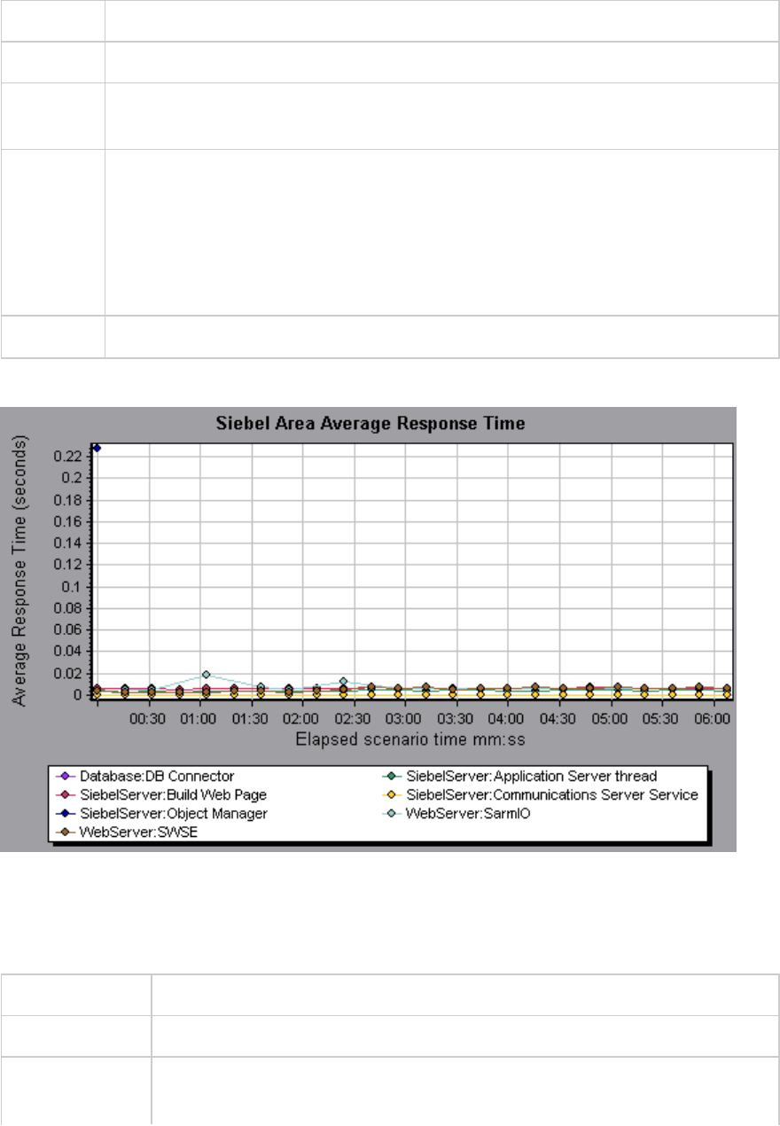
X-axis Elapsed time since the start of the run.
Y-axis Average response time (in seconds) per area.
Breakdown
options
For breakdown options, see "Siebel Breakdown Levels" on page318.
Tips You can filter the Siebel graphs by the following fields:
lTransaction Name. Shows data for the specified transaction.
lScenario Elapsed Time. Shows data for transactions that ended during the specified
time.
For more information on filtering, see "Filtering and Sorting Graph Data" on page103.
See also "Siebel Breakdown Levels" on page318
Example
Siebel Area Call Count Graph
This graph displays the number of times that each Siebel area is called.
X-axis Elapsed time since the start of the run.
Y-axis The call count.
Breakdown
options
For breakdown options, see "Siebel Breakdown Levels" on page318.
User Guide
Analysis
HP LoadRunner (12.50) Page 316
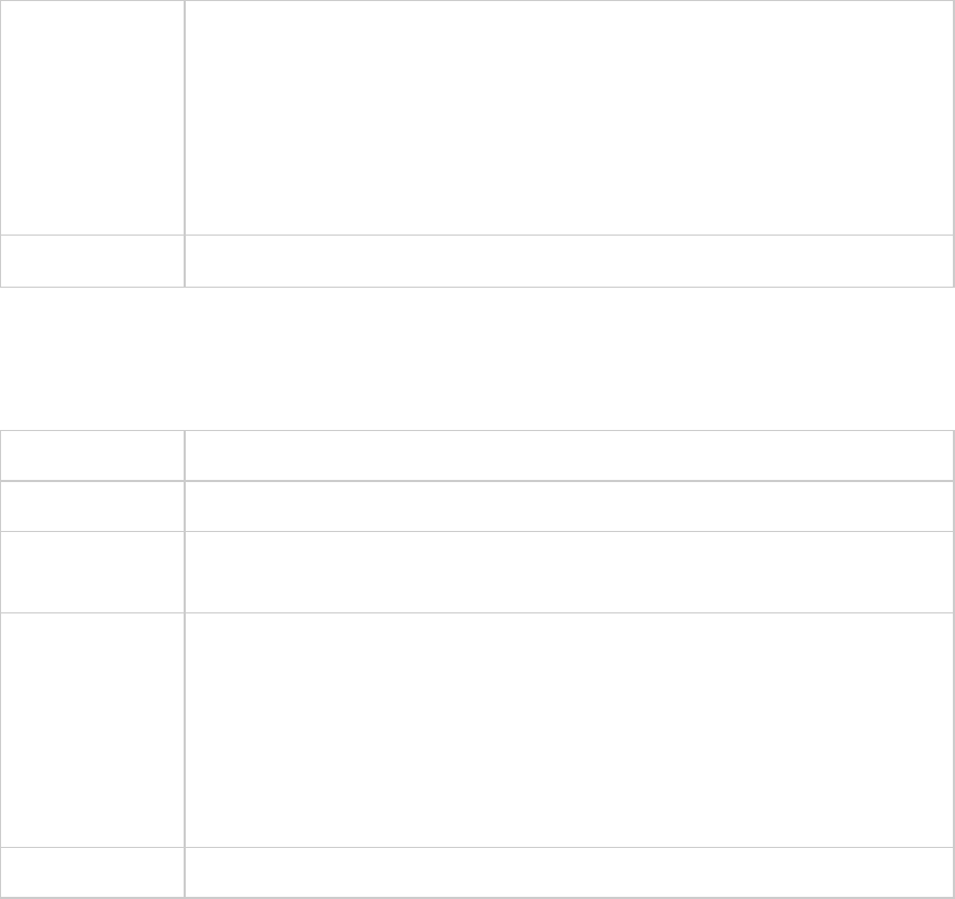
Tips You can filter the Siebel graphs by the following fields:
lTransaction Name. Shows data for the specified transaction.
lScenario Elapsed Time. Shows data for transactions that ended during the
specified time.
For more information on filtering, see "Filtering and Sorting Graph Data" on
page103.
See also "Siebel Diagnostics Graphs Overview" on page311
Siebel Area Total Response Time Graph
This graph displays the total response time of each Siebel area.
X-axis Elapsed time since the start of the run.
Y-axis Average response time (in seconds) per area.
Breakdown
options
For breakdown options, see "Siebel Breakdown Levels" on the next page.
Tips You can filter the Siebel graphs by the following fields:
lTransaction Name. Shows data for the specified transaction.
lScenario Elapsed Time. Shows data for transactions that ended during the
specified time.
For more information on filtering, see "Filtering and Sorting Graph Data" on
page103.
See also "Siebel Diagnostics Graphs Overview" on page311
Example
User Guide
Analysis
HP LoadRunner (12.50) Page 317
Siebel Breakdown Levels
You can break down Siebel layers into areas, sub-areas, servers, and scripts to enable you to pinpoint
the exact location where time is consumed.
To access Use one of the following to access breakdown options:
l<Siebel Diagnostics Graphs> > View > Siebel Diagnostics
l<Siebel Diagnostics Graphs> > select transaction >short-cut menu > Siebel
Diagnostics
See toolbar options for each breakdown level.
Important
Information
The breakdown menu options and buttons are not displayed until an element
(transaction, layer, area, sub-area) is selected.
See also "Siebel Diagnostics Graphs Overview" on page311
Siebel Breakdown Levels are described below:
Transaction
Level
The following figure displays the top level Average Transaction Response Time graph.
The graph displays several transactions.
User Guide
Analysis
HP LoadRunner (12.50) Page 318
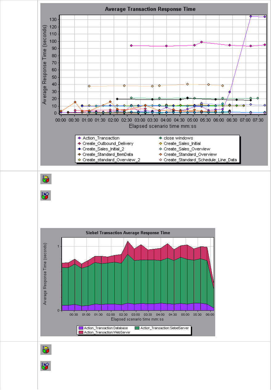
Layer Level Siebel Layer Breakdown button shows the breakdown of the selected transaction.
Undo Siebel Layer Breakdown returns the graph to the transaction level.
In the following figure, the Action_Transaction transaction has been broken down to its
layers (Siebel Database, Application, and Web).
Area Level Siebel Area Breakdown button breaks the data down to its Siebel areas.
Undo Siebel Area Breakdown button returns the graph to the layer level.
In the following figure, the Web layer of the Action_Transaction transaction has been
User Guide
Analysis
HP LoadRunner (12.50) Page 319

broken down to its Siebel areas.
Script
Level Siebel Script Breakdown button breaks the data down to its Siebel scripts. You can
only break down to the script level from the scripting engine area.
Undo Siebel Script Breakdown button returns the graph to the sub-area level.
You can break a transaction down further to its Siebel script level. You can only break
down to the script level from the scripting engine area.
Sub-Area
Level Siebel Sub-Area Breakdown button breaks the data down to its Siebel sub-areas.
You can only break down to the sub-area level from the area level.
Undo Siebel Sub-Area Breakdown button returns the graph to the area level.
In the following figure, the area level of the Action_Transaction transaction has been
broken down to its Siebel sub-area.
Server Siebel Server Breakdown button to group the data by Siebel server.
User Guide
Analysis
HP LoadRunner (12.50) Page 320
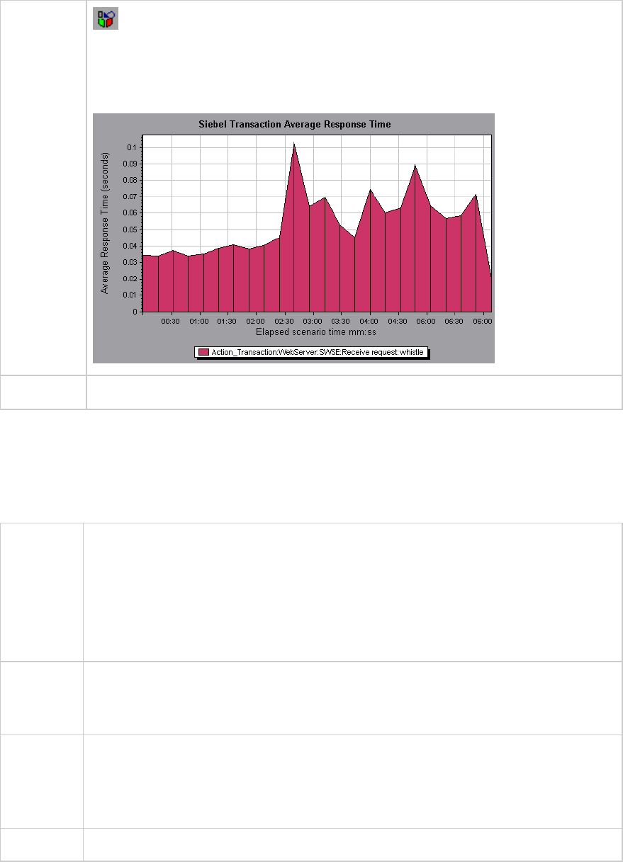
Level Undo Siebel Server Breakdown button ungroups data in the graph.
In the following figure, the Action_Transaction;WebServer:SWSE:Receive Request
transaction has been broken down to its Siebel servers. Server level breakdown is
usual for pin pointing overloaded servers and for load balancing.
See also "Siebel Diagnostics Graphs Overview" on page311
Siebel Diagnostics Graphs Summary Report
The Siebel Usage section of the Summary Report provides a usage chart for the Siebel layer breakdown.
This report is available from the Session Explorer or as a tab in the Analysis window.
Breakdown
options
The Siebel Layer Usage section breaks the individual transactions into:
lWeb Server
lSiebel Server
lDatabase Layers
lTotal usage time for each transaction
Tips To view server side diagnostics data from the Summary Report, click the Siebel layer on
which you want to perform transaction breakdown. The Siebel Transaction Response
Time graph opens displaying the breakdown of the selected transaction.
Note If you do not see diagnostics data on the Summary Report, check if you are using a
user-defined template. To view relevant data, choose a different template from the list
of templates, or create and apply a new template. For more information about using
templates, see "Apply/Edit Template Dialog Box" on page84.
See also "Siebel Diagnostics Graphs Overview" on page311
User Guide
Analysis
HP LoadRunner (12.50) Page 321
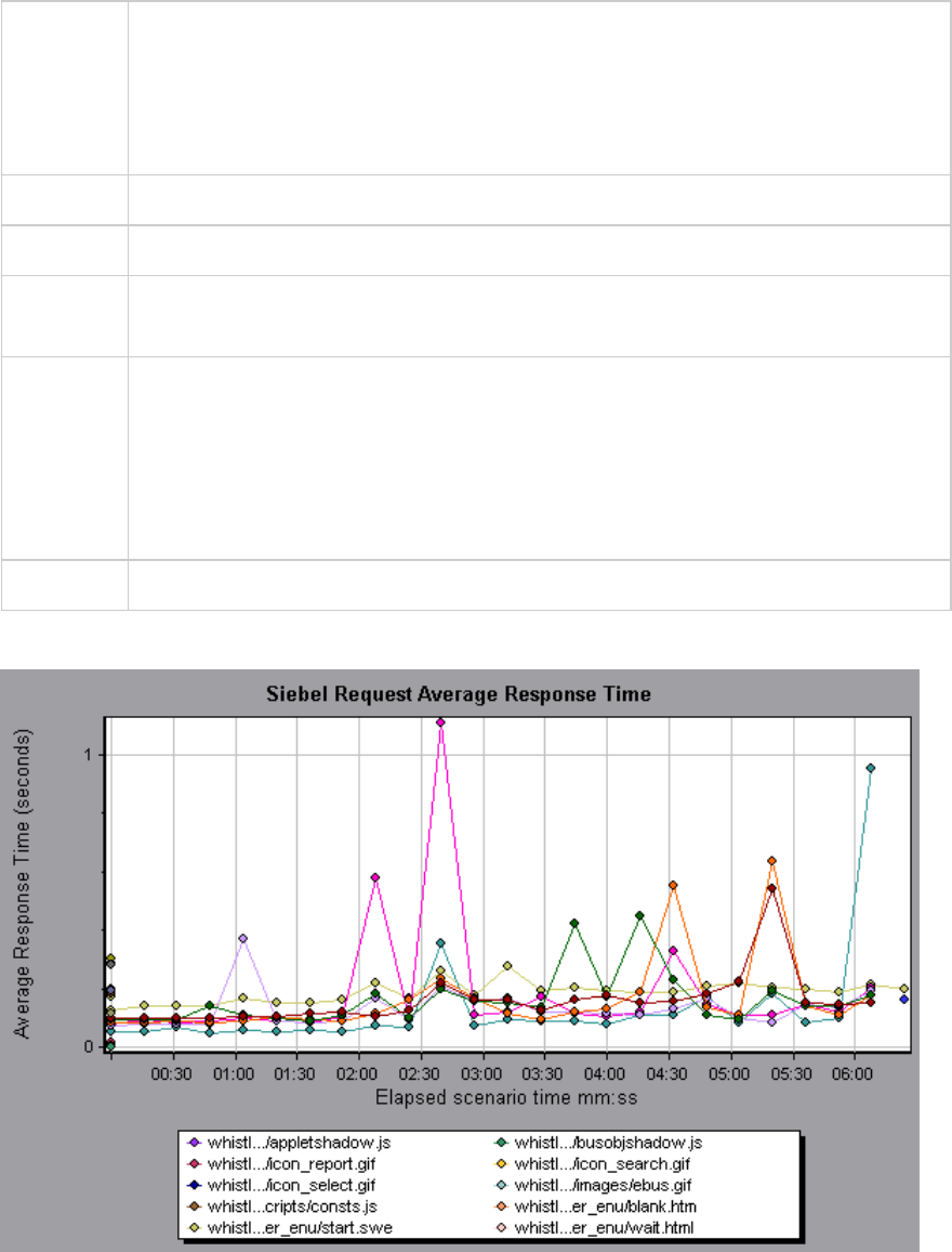
Siebel Request Average Response Time Graph
This graph displays the response time per HTTP request.
Purpose The time is computed as the total request response time divided by the total number of
instances of the specific request. For example, if a request was executed twice by one
instance of transaction A, and once by a second instance of transaction A, and it took
three seconds to execute each request, then the average response time is 9/3, or 3
seconds. The request time does not include the nested calls from within each request.
X-axis Elapsed time since the start of the run.
Y-axis Average response time (in seconds) per area.
Breakdown
options
For breakdown options, see "Siebel Breakdown Levels" on page318.
Tips You can filter the Siebel graphs by the following fields:
lTransaction Name. Shows data for the specified transaction.
lScenario Elapsed Time. Shows data for transactions that ended during the specified
time.
For more information on filtering, see "Filtering and Sorting Graph Data" on page103.
See also "Siebel Diagnostics Graphs Overview" on page311
Example
User Guide
Analysis
HP LoadRunner (12.50) Page 322
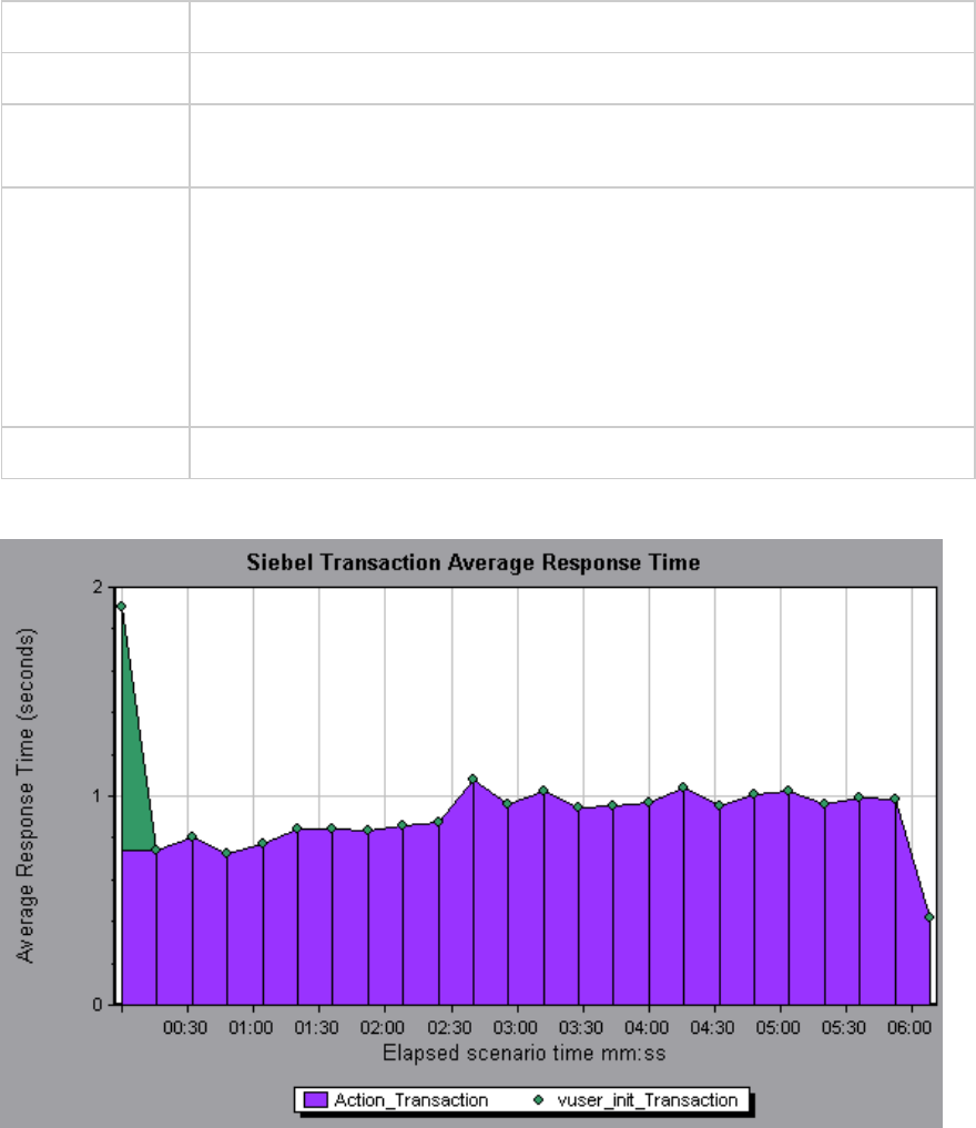
Siebel Transaction Average Response Time Graph
This graph displays the server response time for the selected area (layer, area, or sub-area) within each
transaction, computed as the total response time for that layer or area divided by the total number of
relevant transactions.
X-axis Elapsed time since the start of the run.
Y-axis Average response time (in seconds) per area.
Breakdown
options
For breakdown options, see "Siebel Breakdown Levels" on page318.
Tips You can filter the Siebel graphs by the following fields:
lTransaction Name. Shows data for the specified transaction.
lScenario Elapsed Time. Shows data for transactions that ended during the
specified time.
For more information on filtering, see "Filtering and Sorting Graph Data" on
page103.
See also "Siebel Breakdown Levels" on page318
Example
Siebel DB Diagnostics Graphs
User Guide
Analysis
HP LoadRunner (12.50) Page 323
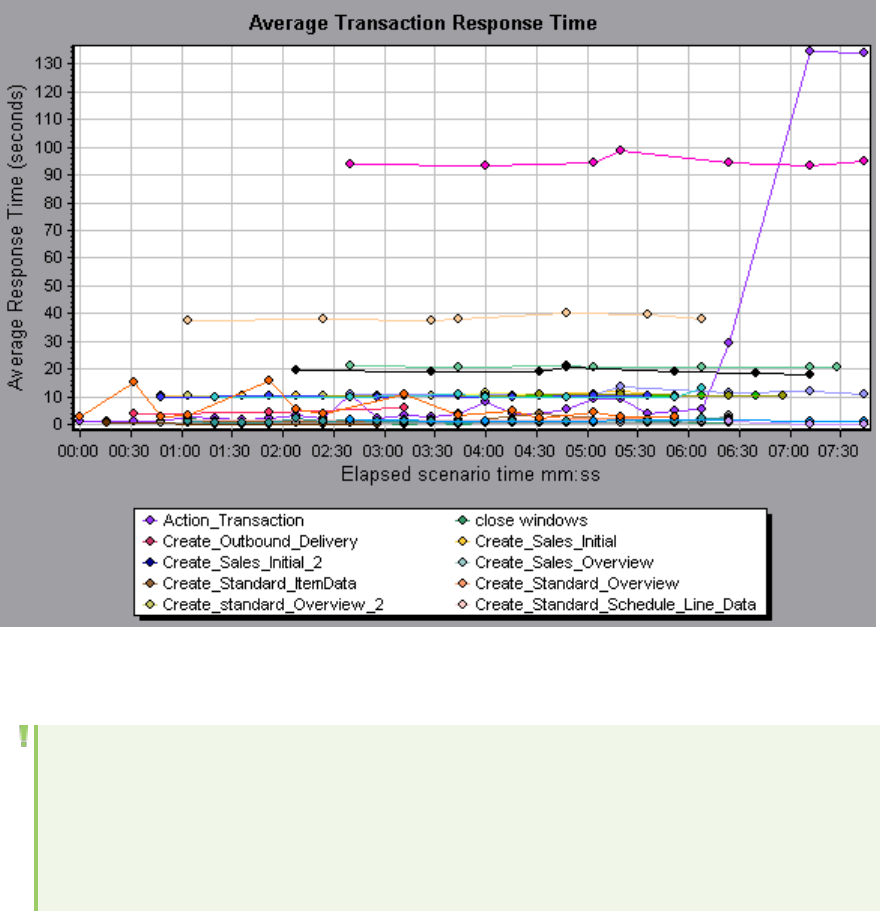
Siebel DB Diagnostics Graphs Overview
Siebel DB Diagnostics graphs provide you with performance information for SQLs generated by
transactions on the Siebel system. You can view the SQLs for each transaction, identify the problematic
SQL queries of each script, and identify at what point problems occurred.
To analyze where problems are occurring, you correlate the data in the Siebel DB Diagnostics graphs
with data in the Transaction Response Time graphs.
You begin analyzing these graphs with the transaction graphs that display the average transaction
response time during each second of the load test scenario run. For example, the following Average
Transaction Response Time graph demonstrates that the average transaction response time for the
query_for_contact transaction was high.
Using the Siebel DB Diagnostics graphs, you can pinpoint the cause of the delay in response time for this
transaction.
Note: A measurement that is broken down in the Average Transaction Response Time graph will
be different from the same measurement broken down in the Siebel DB Side Transactions
graph. This is because the Average Transaction Response Time graph displays the average
transaction time, whereas the Siebel DB Side Transactions graph displays the average time per
transaction event (sum of SQL component response times).
User Guide
Analysis
HP LoadRunner (12.50) Page 324
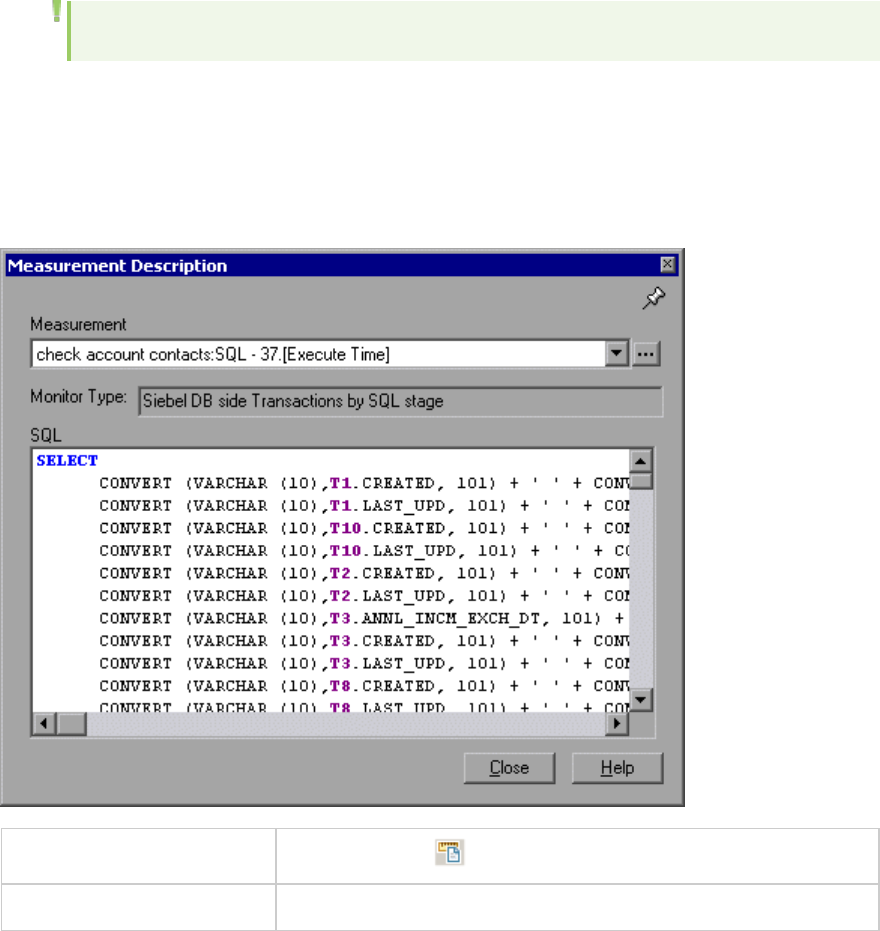
How to Synchronize Siebel Clock Settings
This task describes how to synchronize the Load Generator and Siebel application server clocks to
ensure that the correlation of SQLs to transactions is correct.
1. Choose Tools>Siebel Database Diagnostics Options.
2. Select Apply Application Server time settings.
3. Click Add and enter the information as described in "Siebel Database Diagnostics Options Dialog
Box" on page328.
4. Click OK to save the data and close the dialog box.
Note: You must reopen the results file for time synchronization to take effect.
Measurement Description Dialog Box
You can view the full SQL statement for a selected SQL element by choosing Show measurement
description from the Legend window. The Measurement Description dialog box opens displaying the
name of the selected measurement and the full SQL statement.
To access Legend window >
See also "Siebel Database Breakdown Levels" on the next page
User interface elements are described below:
User Guide
Analysis
HP LoadRunner (12.50) Page 325
UI Element Description
Break the data down to a lower level.
Return to the previous level.
To keep the focus on the Measurement Description dialog box, click the Stay on
Top button. This enables you to view the full SQL statement of any
measurement by selecting it in the Legend window. Click the button again to
remove the focus.
Click the Breaking Measurement button to display the Transaction Name and
SQL Alias Name of the selected measurement.
Siebel Database Breakdown Levels
You can break down Siebel layers into areas, sub-areas, servers, and scripts to enable you to pinpoint
the exact location where time is consumed.
To access Use one of the following to access breakdown options:
l<Siebel DB Diagnostics Graphs> > View > Siebel DB Diagnostics
l<Siebel DB Diagnostics Graphs> > select transaction >short-cut menu >
Siebel DB Diagnostics
lSee toolbar options for each breakdown level
Important
information
The breakdown menu options and buttons are not displayed until a transaction
is selected.
See also "Siebel DB Diagnostics Graphs Overview" on page324
Siebel Breakdown Levels are described below:
Transaction
Level
The following figure displays the top level Average Transaction Response Time
graph. The graph displays several transactions. You can break this graph down to
show the SQL statements and the SQL stages level.
User Guide
Analysis
HP LoadRunner (12.50) Page 326
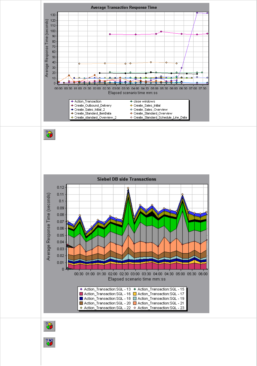
SQL
Statements
Level
Siebel SQL Statements Breakdown button shows the breakdown of the
selected transaction.
In the following figure, the Siebel DB Side Transactions graph displays the Action_
Transaction broken down to its SQL statements.
SQL Stages
Level Measurement Breakdown button breaks the data down to a lower level.
Undo Breakdown Measurement button returns to the previous level.
In the following figure, the Siebel DB Side Transactions by SQL Stage graph displays
User Guide
Analysis
HP LoadRunner (12.50) Page 327
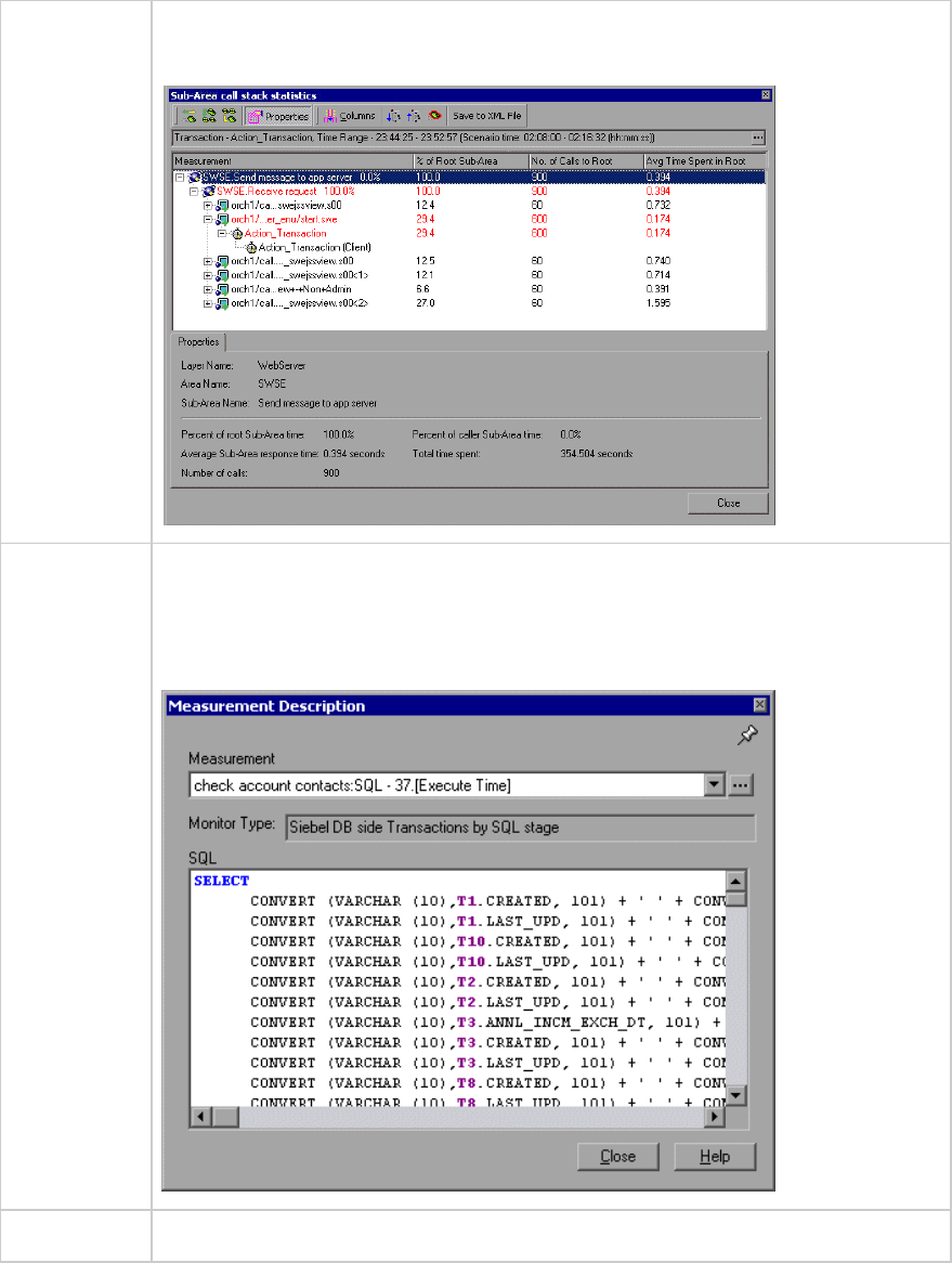
Action_Transaction:SQL-33 broken down to its SQL stage: Prepare, Execute, and
Initial Fetch.
Show
measurement
description
You can view the full SQL statement for a selected SQL element by choosing Show
measurement description from the Legend window. The Measurement Description
dialog box opens displaying the name of the selected measurement and the full SQL
statement.
See also "Siebel DB Diagnostics Graphs Overview" on page324
Siebel Database Diagnostics Options Dialog Box
This dialog box enables you to synchronize the Load Generator and Siebel application server clocks.
User Guide
Analysis
HP LoadRunner (12.50) Page 328
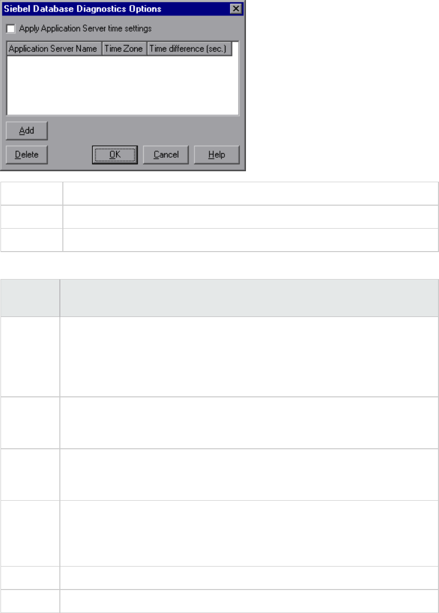
To access Tools > Siebel Database Diagnostics Options
Note You must reopen the results file for time synchronization to take effect.
See also "How to Synchronize Siebel Clock Settings" on page325
User interface elements are described below:
UI Element Description
Apply
Application
Server
time
settings
Enables the synchronized time settings option.
Application
Server
Name
Enter the name of the Siebel application server.
Time Zone Enter the time zone of the Siebel application server (GMT or Local). GMT means the
application server time is reported in GMT time, and local means the application server
time is reported in local time.
Time
Difference
(sec.)
Enter the time difference (in seconds) between the load generator and the Siebel
application server. Use the minus sign ("-") if the time on Siebel application server is
ahead of the load generator. For example, if the application server time is two minutes
ahead of the load generator time, enter -120 in the time difference field.
Add Enables you to add an application server's time settings to the list.
Delete Deletes the server breakdown time settings from the list.
User Guide
Analysis
HP LoadRunner (12.50) Page 329
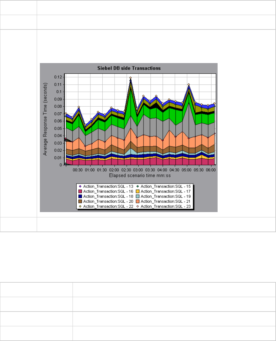
Siebel DB Side Transactions Graph
This graph displays the average transaction execution time in the Siebel database.
X-axis Elapsed time since the start of the run.
Y-axis Average response time (in seconds) of each transaction.
Breakdown
options
You can break down a transaction in the Siebel DB Side Transactions graph to view its
SQL statements. In the following figure, the Action_Transaction transaction is broken
down to its SQL statements.
See also "Siebel DB Diagnostics Graphs Overview" on page324
Siebel DB Side Transactions by SQL Stage Graph
This graph displays the time taken by each SQL, grouped by SQL stage: Prepare, Execute, and Initial
Fetch.
X-axis Elapsed time since the start of the run.
Y-axis Average time (in seconds) taken to perform each SQL stage.
Breakdown options "Siebel Database Breakdown Levels" on page326
See also "Siebel DB Diagnostics Graphs Overview" on page324
User Guide
Analysis
HP LoadRunner (12.50) Page 330

Siebel SQL Average Execution Time Graph
This graph displays the average execution time of each SQL performed in the Siebel database.
Purpose This enables you to identify problematic SQLs regardless of the transaction that
produced them. You can then choose Show measurement description from the Legend
window to view the full SQL statement. The SQL statements are listed by a numeric ID.
X-axis Elapsed time since the start of the run.
Y-axis Average response time (in seconds) of each SQL.
Breakdown
options
"Siebel Database Breakdown Levels" on page326
See also "Siebel DB Diagnostics Graphs Overview" on page324
Oracle - Web Diagnostics Graphs
Oracle - Web Diagnostics Graphs Overview
Oracle - Web Diagnostics graphs provide you with performance information for SQLs generated by
transactions on the Oracle NCA system. You can view the SQLs for each transaction, identify the
problematic SQL queries of each script, and identify at what point problems occurred.
To analyze where problems are occurring, you correlate the data in the Oracle - Web Diagnostics graphs
with data in the Transaction Response Time graphs.
You begin analyzing these graphs with the transaction graphs that display the average transaction
response time during each second of the load test scenario run. For example, the following Average
Transaction Response Time graph demonstrates that the average transaction response time for the
enter transaction was high.
User Guide
Analysis
HP LoadRunner (12.50) Page 331
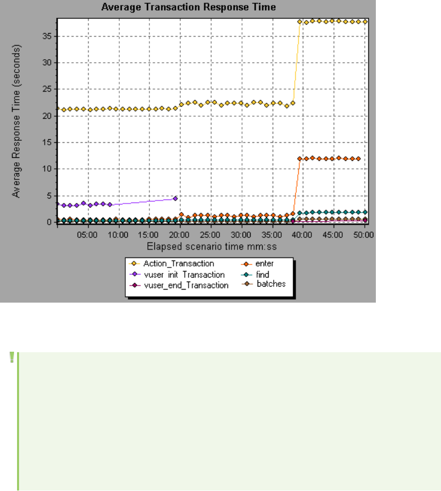
Using the Oracle - Web Diagnostics graphs, you can pinpoint the cause of the delay in response time for
this transaction.
Note:
lA measurement that is broken down in the Average Transaction Response Time graph will be
different from the same measurement broken down in the Oracle - Web(DB) Side
Transactions graph. This is because the Average Transaction Response Time graph displays
the average transaction time, whereas the Oracle - WebDB Side Transactions graph displays
the average time per transaction event (sum of SQL component response times).
lvuser_init and vuser_end actions in Oracle cannot be broken down.
Measurement Description Dialog Box
This dialog box enables you to view the full SQL statement for a selected SQL element.
User Guide
Analysis
HP LoadRunner (12.50) Page 332
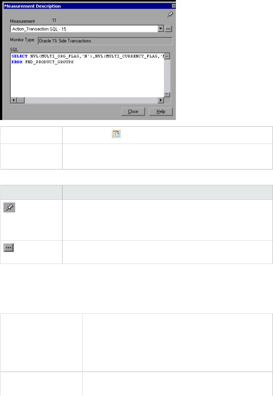
To access Legend window >
See also l"Oracle - Web Diagnostics Graphs Overview" on page331
l"Oracle Breakdown Levels" below
User interface elements are described below:
UI Element Description
To keep the focus on the Measurement Description dialog box, click the Stay
on Top button. This enables you to view the full SQL statement of any
measurement by selecting it in the Legend window. Click the button again to
remove the focus.
Click the Breaking Measurement button to display the Transaction Name and
SQL Alias Name of the selected measurement.
Oracle Breakdown Levels
After you have enabled Oracle - Web Diagnostics on the Controller machine and run the load test
scenario, you can view the diagnostics data.
To access Use one of the following to access breakdown options:
l<Oracle Diagnostics Graphs> > View > Oracle Diagnostics
l<Oracle Diagnostics Graphs> > select transaction >shortcut
menu > Oracle Diagnostics
lSee toolbar options for each breakdown level
Important Information The breakdown menu options and buttons are not displayed until a
transaction is selected.
User Guide
Analysis
HP LoadRunner (12.50) Page 333
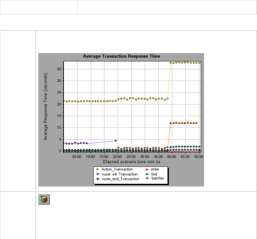
See also "Oracle - Web Diagnostics Graphs Overview" on page331
Oracle Breakdown Levels are described below:
Transaction
Level
The following figure illustrates the top level Average Transaction Response Time
graph. The graph displays several transactions.
SQL
Statements
Level
Oracle SQL Statement Breakdown button shows the breakdown of the selected
transaction.
In the following figure, the Oracle - WebDB Side Transactions graph displays the
Action_Transaction transaction broken down to its SQL statements.
User Guide
Analysis
HP LoadRunner (12.50) Page 334
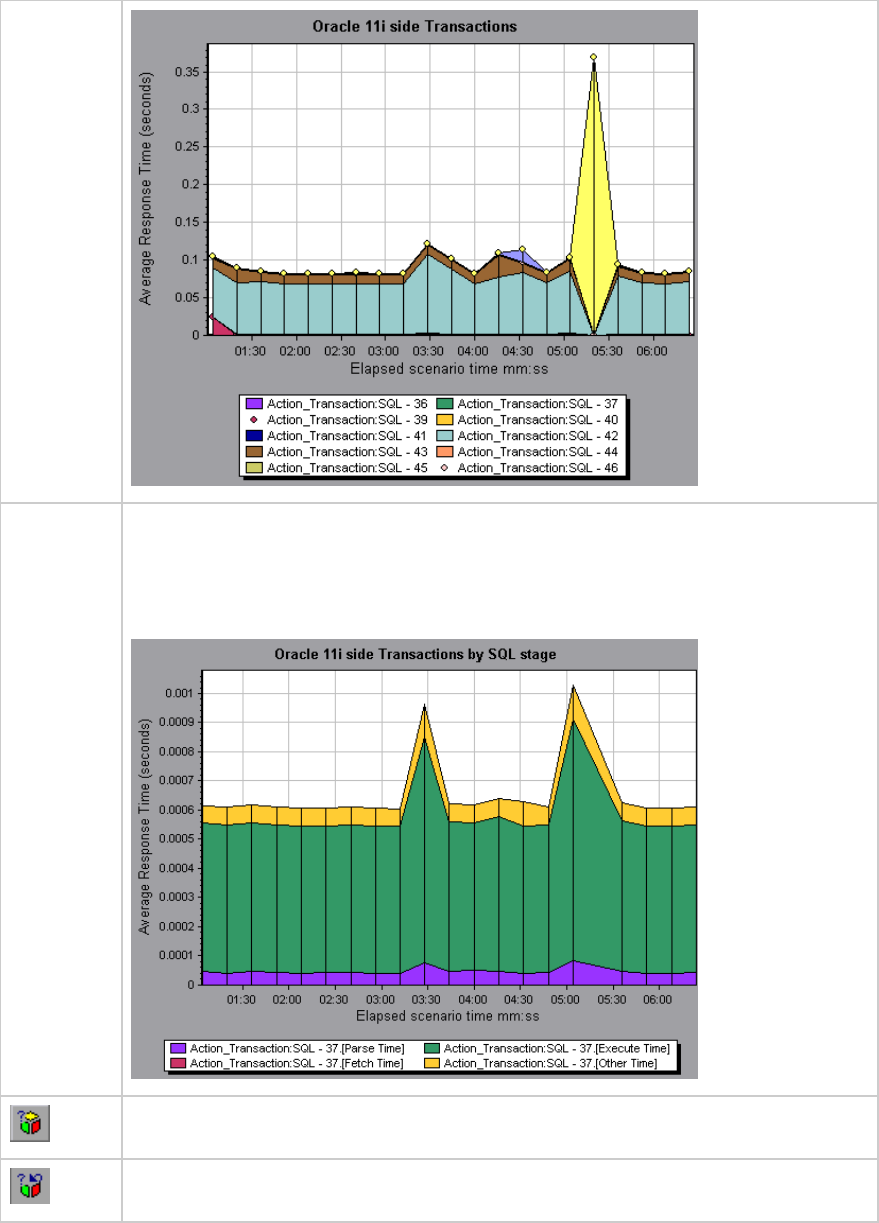
SQL Stages
Level
In the following figure, the Oracle - WebDB Side Transactions by SQL Stage graph
displays Action_Transaction:SQL-37 broken down to its SQL stages: Parse Time,
Execute Time, Fetch Time, and Other Time. Other Time includes other database time
such as bind time.
You can break the data down to a lower level.
Enables you to return to a previous level.
User Guide
Analysis
HP LoadRunner (12.50) Page 335
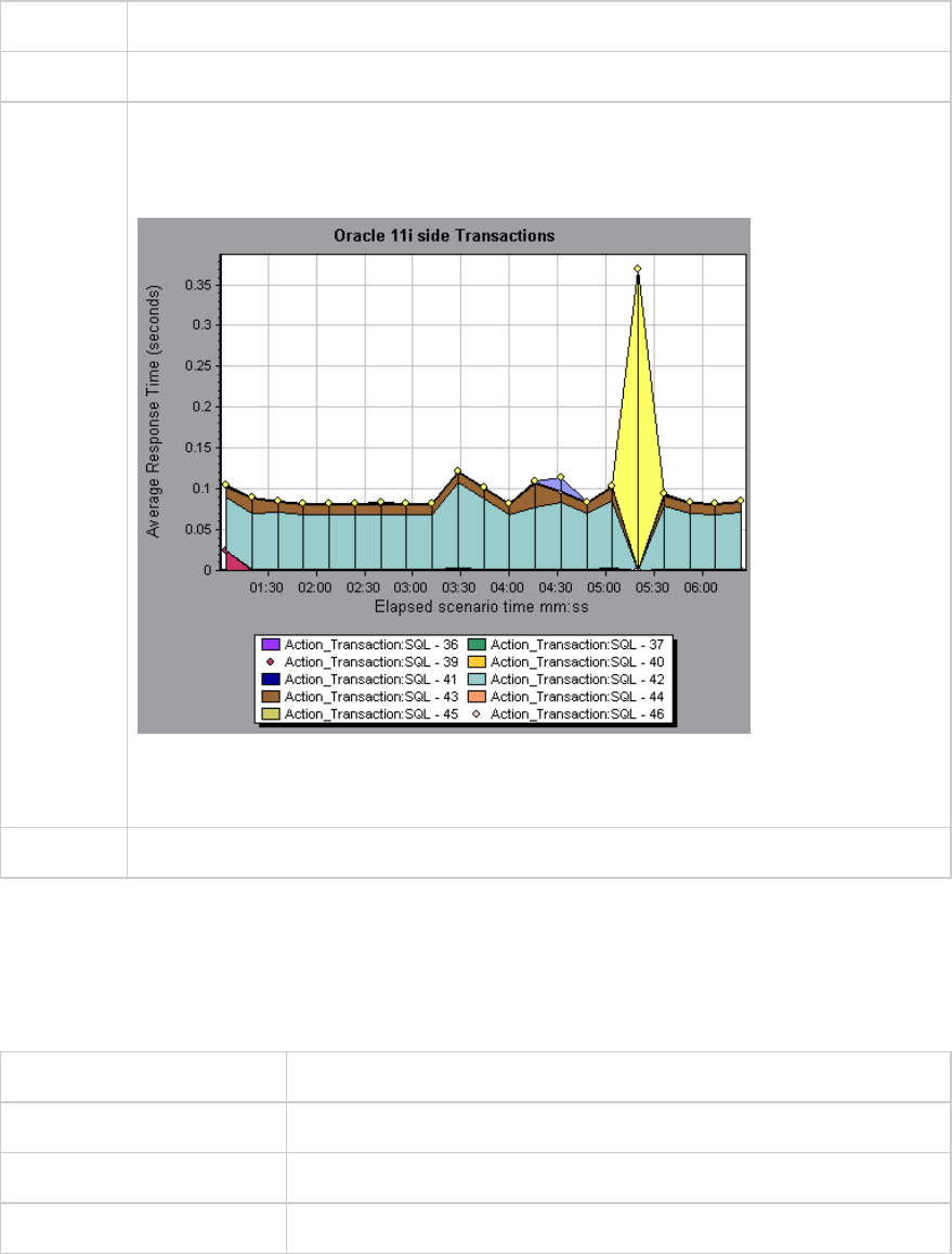
Oracle - WebDB Side Transactions Graph
This graph displays the average transaction execution time in the Oracle database.
X-axis Elapsed time of the scenario run.
Y-axis Response time (in seconds) of each transaction.
Breakdown
options
You can break down a transaction in the Oracle - WebDB Side Transactions graph to
view its SQL statements. In the following figure, the Action_Transaction transaction is
broken down to its SQL statements.
To break the displayed elements down further, see "Oracle Breakdown Levels" on
page333.
See also "Oracle - Web Diagnostics Graphs Overview" on page331
Oracle - WebDB Side Transactions by SQL Stage Graph
This graph displays the time taken by each SQL, divided by the SQL stages: Parse Time, Execute Time,
Fetch Time, and Other Time. Other Time includes other database time such as bind time.
X-axis Elapsed time since the scenario run.
Y-axis Average response time (in seconds) of each SQL stage.
Breakdown options "Oracle Breakdown Levels" on page333
See also "Oracle - Web Diagnostics Graphs Overview" on page331
User Guide
Analysis
HP LoadRunner (12.50) Page 336
Oracle - Web SQL Average Execution Time Graph
This graph displays the average execution time of each SQL performed in the Oracle database.
Purpose The graph enables you to identify problematic SQLs regardless of the transaction
that produced them.
X-axis Elapsed time since the scenario run.
Y-axis Average response time (in seconds) of each SQL.
Breakdown
options
"Oracle Breakdown Levels" on page333
Tips You can select Show measurement description from the Legend window to view
the full SQL statement.
Note The SQL statements are shortened to a numeric indicator.
See also "Oracle - Web Diagnostics Graphs Overview" on page331
SAP Diagnostics Graphs
SAP Diagnostics Graphs Overview
SAP Diagnostics enables you to pinpoint the root cause of a certain problem (for example, DBA, Network,
WAS, Application, OS/HW) quickly and easily, and engage with the relevant expert only, without having to
present the problem to a whole team of people.
Using SAP Diagnostics, you can create graphs and reports, which you can present to the relevant expert
when discussing the problems that occurred.
SAP Diagnostics also allow an SAP performance expert (in one of the areas of expertise) to perform the
required root-cause analysis more quickly and easily.
How to Configure SAP Alerts
SAP Diagnostics comes with a set of alert rules with pre-defined threshold values.
When you open a LoadRunner results file (.lrr) in Analysis, these alert rules are applied to the load test
scenario results, and if a threshold value is exceeded, Analysis generates an alert that there is a
problem.
Before opening a LoadRunner results file, you can define new threshold values for the alert rules using
the Alerts Configuration dialog box. Then, when you open the results file, the customized alert rules are
applied.
User Guide
Analysis
HP LoadRunner (12.50) Page 337
Note: When an Analysis session is open, the Alerts Configuration dialog box is not editable. To
edit thresholds in the Alerts Configuration dialog box, close all open sessions.
This task describes how to define threshold values for alert rules when analyzing load test scenario
results.
1. Close all open Analysis sessions.
2. From the Tools menu, select SAP Diagnostics Alerts Configuration.
3. The Generate alert if column lists the rules. Set the threshold for each rule in the Threshold
column.
4. By default, all pre-defined alert rules are enabled. To disable an alert rule, clear the check box next
to that rule.
5. Click OK to apply your changes and close the Alerts Configuration dialog box.
Note: Modifying the alert rules does not affect the results of a saved Analysis session. You need
to re-analyze the results in order for new settings to take effect.
SAP Diagnostics - Guided Flow Tab
You open the SAP Diagnostics graphs from the Analysis Summary Report or from Session Explorer >
Graphs > SAP Diagnostics - Guided Flow.
This tab remains open throughout the Analysis application flow, and its content varies according to the
breakdown flow.
User Guide
Analysis
HP LoadRunner (12.50) Page 338
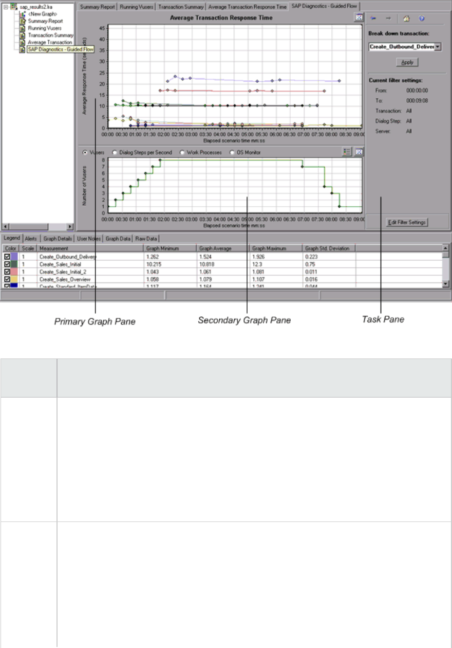
User interface elements are described below:
UI
Element
Description
Primary
Graph
Pane
The upper pane of the SAP Diagnostics - Guided Flow tab is referred to as the primary
graph pane. This pane displays graphs of the transactions and their broken down dialog
steps or components, and other associated resources.
You break down the graphs displayed in this pane using the breakdown options provided
in the right pane of the guided flow (see "SAP Breakdown Task Pane" on page346).
You can open the displayed graph in full view by clicking the Enlarge Graph button in the
top right corner of this pane. An enlarged version of the graph opens in a new tab.
Secondary
Graph
Pane
The lower pane of the SAP Diagnostics - Guided Flow tab is referred to as the secondary
graph pane and displays graphs showing secondary information supporting the graph
displayed in the primary graph pane.
To see the legend for the graph displayed in this pane, click the Graph Legend button in
the top right corner. To see all the data in the Legend, scroll along the horizontal scroll
bar.
You can open the displayed graph in full view by clicking the Enlarge Graph button in the
User Guide
Analysis
HP LoadRunner (12.50) Page 339
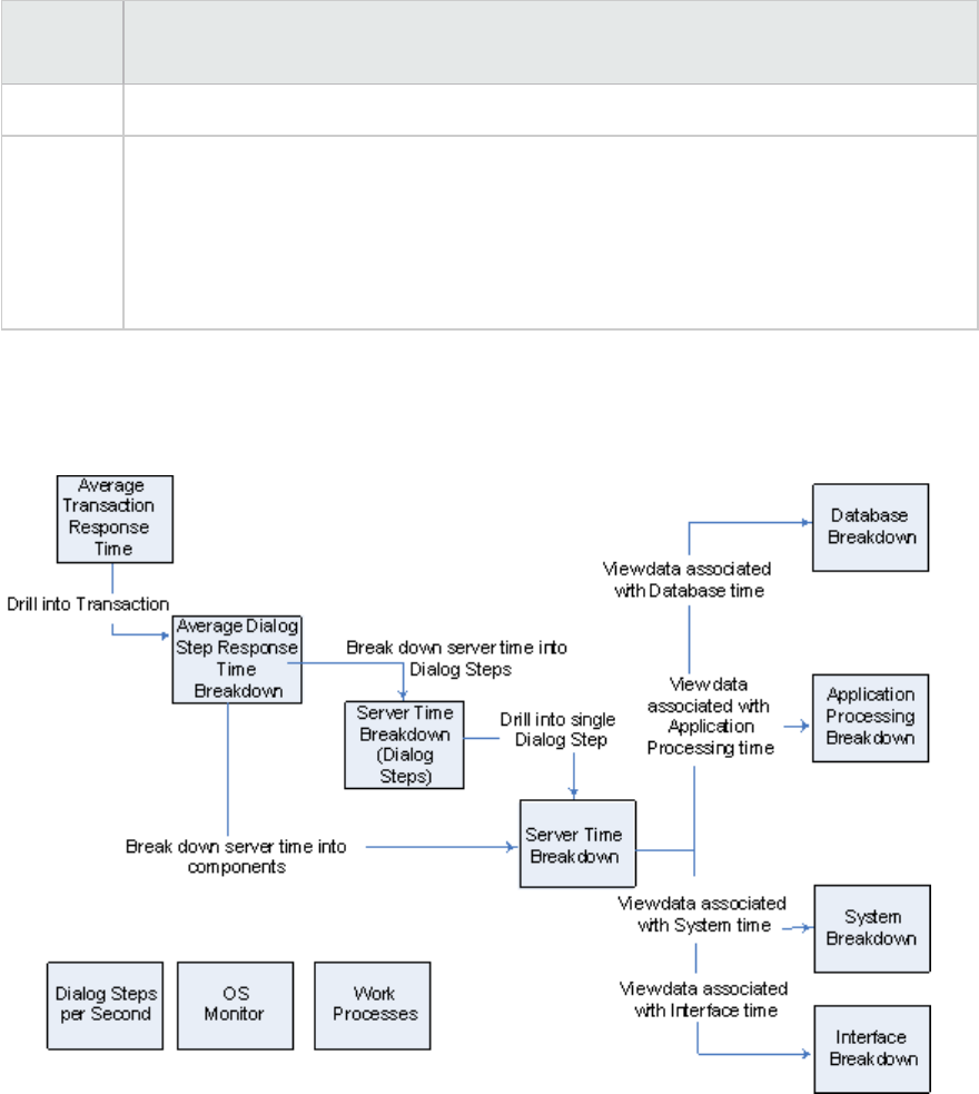
UI
Element
Description
top right corner of this pane. An enlarged version of the graph opens in a new tab.
Task Pane The pane on the right side of the SAP Diagnostics - Guided Flow tab is referred to as the
task pane. You use the task pane to choose the level of breakdown you want to view, to
filter and group transaction and server information, and to navigate backwards and
forwards through the broken down graphs.
For more information, see "SAP Breakdown Task Pane" on page346.
SAP Diagnostics Application Flow
The following diagram depicts the general flow of SAP Diagnostics:
The main view of SAP Diagnostics displays all of the transactions in a scenario run for which there is SAP
diagnostics data. Each transaction can be broken down into server-time components, or first into the
dialog steps that comprise a transaction, and then into server-time components. The server
components can further be broken down into sub-components or other related data.
There are three independent/parallel views: Dialog Steps per Second,OS Monitor, and Work Processes.
These do not generally participate in the breakdown flow, and you may choose to display or hide them.
User Guide
Analysis
HP LoadRunner (12.50) Page 340
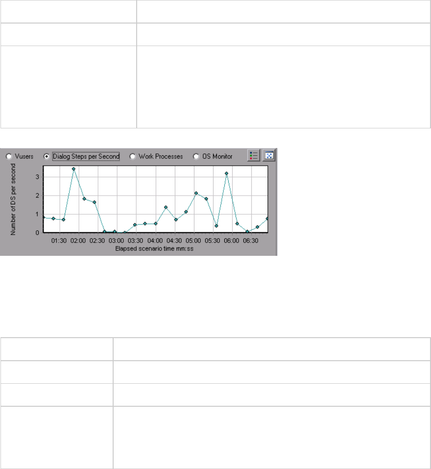
Dialog Steps per Second Graph
This graph represents the number of dialog steps that ran on all the servers during each second of the
load test scenario run.
X-axis Elapsed scenario time (in hh:mm:ss).
Y-axis Number of dialog steps per second.
See also "SAP Breakdown Task Pane" on page346
"Vuser Graphs" on page127
"Work Processes Graph" on page353
"OS Monitor Graph" below
Example
OS Monitor Graph
This graph represents the operating system resources that were measured throughout the load test
scenario run.
X-axis Elapsed scenario time (in hh:mm:ss).
Y-axis Resource value.
Note This graph is available only when a single server filter is applied.
See also "SAP Breakdown Task Pane" on page346
"Dialog Steps per Second Graph" above
"Work Processes Graph" on page353
Example
User Guide
Analysis
HP LoadRunner (12.50) Page 341
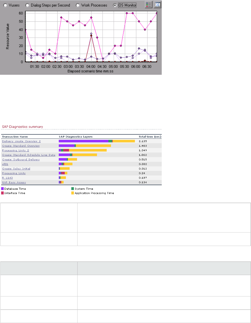
SAP Alerts Configuration Dialog box
This dialog box enables you to define threshold values for alert rules used when opening the results file
(.lrr) in Analysis.
Important information Modifying the alert rules does not affect the results of a saved
Analysis session. You need to re-analyze the results in order for new
settings to take effect.
See also "SAP Diagnostics Graphs Overview" on page337
User interface elements are described below:
UI Element Description
Enabled By default, all pre-defined alert rules are enabled. To disable an alert
rule, clear the check box next to that rule.
Generate alert if The Generate alert if column lists the rules.
Threshold Set the threshold for each rule in the Threshold column.
User Guide
Analysis
HP LoadRunner (12.50) Page 342
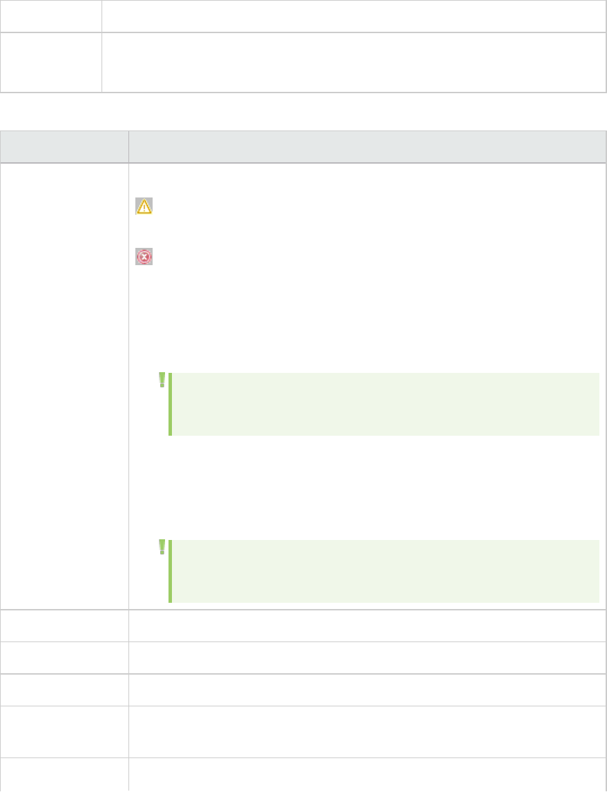
SAP Alerts Window
This Window displays a list of alerts related to the data displayed in the current graph(s) shown in the
Analysis window.
To access Windows > SAP Alerts
See also "SAP Alerts Configuration Dialog box" on the previous page
"How to Configure SAP Alerts" on page337
User interface elements are described below:
UI Element Description
Type Displays one of the following icons indicating the type of alert:
Standard Alert. This alert is generated in the context of a transaction
and/or server if the conditions of a pre-defined alert rule are met.
Major Alert. There are two types of alerts:
lGeneral Application Problem Alert. If a standard alert was generated in the
context of a transaction, and the same alert was generated in the context of
all other transactions running in the same time frame, then a major alert of
this type is generated, indicating that there is a general application problem.
Note: If a Dialog Step filter is applied (for a single dialog step), then
this alert is not generated.
lServer-Specific Problem Alert. This alert is generated for a specific server
if a certain measurement on that server exceeds its threshold, while the
overall server performance for that measurement is satisfactory. This type
of alert indicates that there is a server related problem.
Note: Server-Specific Problem alerts are generated only when the
current server context is "All Servers".
Time interval The time interval during which the problem occurred.
Transaction/Server The name of the transaction and server where problem occurred.
Description A description of the alert.
Recommended
Step
Recommends what to do in order to understand the problem on a deeper level.
Action A link to a graph representing the data described in the alert, allowing for a
User Guide
Analysis
HP LoadRunner (12.50) Page 343
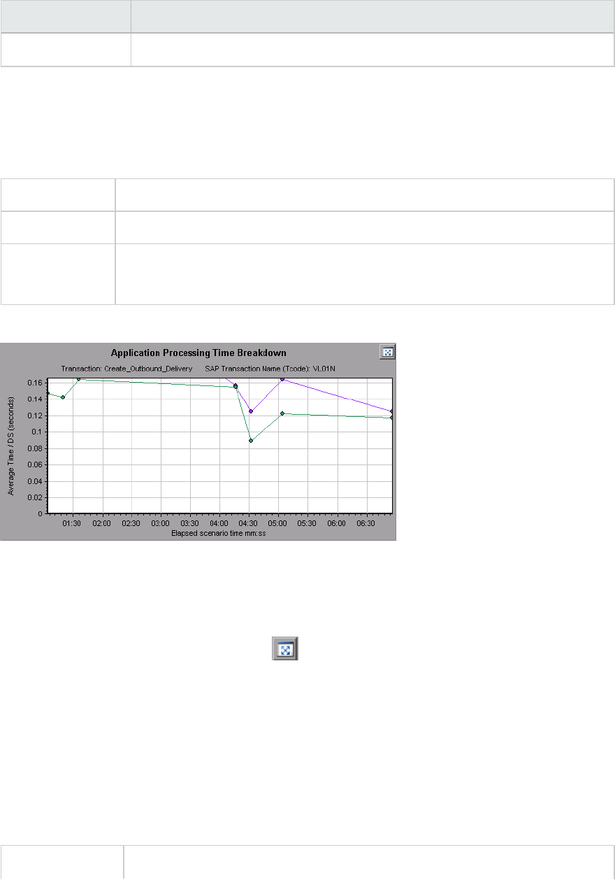
UI Element Description
more graphic display of the alert. Double-click the link to open the graph.
SAP Application Processing Time Breakdown Graph
This graph displays the behavior of resources associated with application processing time, namely ABAP
time and CPU time.
X-axis Elapsed load test scenario time (in hh:mm:ss).
Y-axis Average time per dialog step (in seconds).
See also "SAP Breakdown Task Pane" on page346
"SAP Secondary Graphs" on page353
Example
SAP Primary Graphs
You view the SAP Diagnostics graphs in the primary graph pane.
You can open the graph in full view by clicking in the top right corner of the primary graph pane. An
enlarged version of the graph opens in a new tab.
To filter or group data displayed in these graphs, see "SAP Breakdown Task Pane" on page346.
SAP Average Dialog Step Response Time Breakdown Graph
This graph represents a breakdown of the average dialog step response time of a specific transaction.
The graph displays the Network Time, Server Response Time, (including the GUI time), and Other Time
(the time taken for the client to process the dialog step) of a single transaction.
X-axis Elapsed time since the start of the run (in hh:mm:ss).
User Guide
Analysis
HP LoadRunner (12.50) Page 344
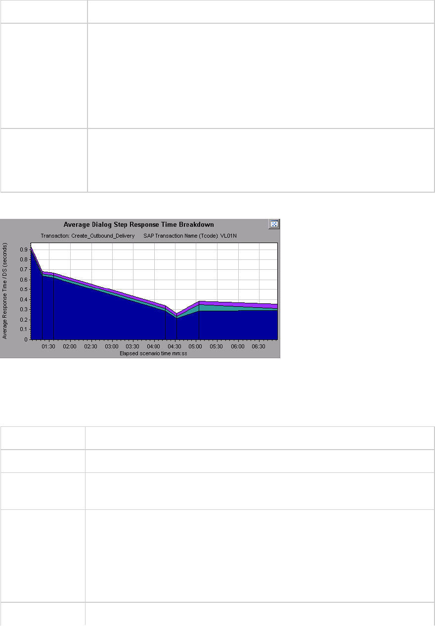
Y-axis The average response time divided by the number of dialog steps (in seconds).
Breakdown
options
Components
This option opens the "SAP Server Time Breakdown Graph" on page349
Dialog Steps
This option opens the "SAP Server Time Breakdown (Dialog Steps) Graphs" on
page348
See also "SAP Breakdown Task Pane" on the next page
"SAP Secondary Graphs" on page353
"SAP Breakdown Task Pane" on the next page
Example
SAP Average Transaction Response Time Graph
This graph displays all the SAP-related transactions in the load test scenario.
X-axis Elapsed time since the start of the run.
Y-axis Average response time (in seconds) of each transaction
Breakdown
graph
"SAP Average Dialog Step Response Time Breakdown Graph" on the previous
page
Tips Select a transaction in one of the following ways:
lSelect the transaction from the Breakdown transaction: list in the task pane.
lHighlight the transaction by selecting the line representing it in the graph.
lSelect the transaction from the graph legend. This highlights the line in the
graph.
See also "SAP Breakdown Task Pane" on the next page
User Guide
Analysis
HP LoadRunner (12.50) Page 345
"SAP Secondary Graphs" on page353
"SAP Breakdown Task Pane" below
SAP Breakdown Task Pane
The task pane enables you to choose the level of breakdown you want to view, to filter and group
transaction and server information, and to navigate backwards and forwards through the broken down
graphs.
To access Session Explorer > Graphs > SAP Diagnostics > SAP Diagnostics - Guided Flow
See also "SAP Diagnostics Graphs Overview" on page337
SAP Breakdown Toolbar
User interface elements are described below:
UI Element Description
Back. Click to view previous breakdown graph, or to ungroup grouped data.
Next. Click to view next breakdown graph.
Home. Click to return to the initial SAP Average Transaction Response Time
graph.
Help. Click to get help on the breakdown options.
Breakdown Options
To break down SAP diagnostics data, choose the breakdown and filter options from the task pane.
User interface elements are described below:
UI Element Description
Break down
transaction
Select a transaction from this list to display the average dialog step response
time breakdown.
Break down
server time into
Displays the breakdown options for the Average Dialog Step Response Time
Breakdown graph.
lSelect Components to view a breakdown of the transaction's server
components, namely database time, interface time, application processing
time, and system time.
User Guide
Analysis
HP LoadRunner (12.50) Page 346
UI Element Description
lSelect Dialog Steps to view a breakdown of the transaction's dialog steps.
Break down dialog
step <dialog step>
Break down a dialog step into its server-time components, namely database
time, interface time, application processing time, and system time.
View data
associated with
<component>
Break down a server-time component (database time; interface time;
application processing time; system time) to view data associated with it.
No available
breakdown
There are no further breakdown options.
Apply Click to apply the selected breakdown option.
Current filter settings
This section displays the filter/grouping settings of the graph currently displayed in the primary graph
pane.
User interface elements are described below:
UI Element Description
From/To Enter values (in hh:mm:ss) to filter the graph over a specified time interval.
Transaction Displays the name of the transaction represented in the graph.
Dialog Step Displays the name of the dialog step represented in the graph.
Server Displays the name of the server represented in the graph.
Edit filter settings
Click this button to modify filter or grouping settings. When you click Edit Filter Settings the
filter/grouping options become editable.
User interface elements are described below:
UI
Element
Description
Filter Use this option to filter the current graph by time interval, transaction, dialog step, and/or
server.
lFrom/To. Enter values (in hh:mm:ss) to filter the graph over a specified time interval.
lBy Transaction. Filter the graph to display information about a specific transaction by
User Guide
Analysis
HP LoadRunner (12.50) Page 347

UI
Element
Description
selecting the transaction from the list.
lBy Dialog Step. Filter the graph to display information about a specific dialog step by
selecting the dialog step from the list.
lBy Server. Filter the graph to display information about a server by selecting the server
name from the list.
Note: Only servers associated with the data displayed in the current graph are listed in the
By Server list
Group Use this option to group the data represented in the graph by transaction or by server.
Select a transaction, component or subcomponent from the list.
lBy Transaction. Select this check box to group by transaction.
lBy Server. Select this check box to group by server.
Note: After applying grouping to a graph, you need to ungroup the data in order to apply
further breakdown options. To ungroup grouped data, click the Back button on the
toolbar.
Important: When you open a saved session, the Back is disabled. If you have grouped data,
you need to click the Home button, or open a new SAP Diagnostics - Guided Flow tab to
restart SAP breakdown.
OK Click OK to apply the chosen filter/grouping settings. The Current filter settings area
displays the chosen settings in non-editable mode.
Notes:
lGlobal filtering is enabled when viewing SAP Diagnostics graphs (special SAP view) but
cannot be applied on these graphs.
lLocal filtering is disabled in the SAP Diagnostics - Guided Flow tab. To apply local filters
to a SAP Diagnostics graph displayed in the Guided Flow tab, open the graph in a new
tab by clicking the Enlarge Graph button.
SAP Server Time Breakdown (Dialog Steps) Graphs
This graph displays the dialog steps of a particular transaction.
X-axis Elapsed time since the start of the run (in hh:mm:ss).
Y-axis The average response time per dialog step (in seconds).
Breakdown graph "SAP Server Time Breakdown Graph" on the next page
User Guide
Analysis
HP LoadRunner (12.50) Page 348
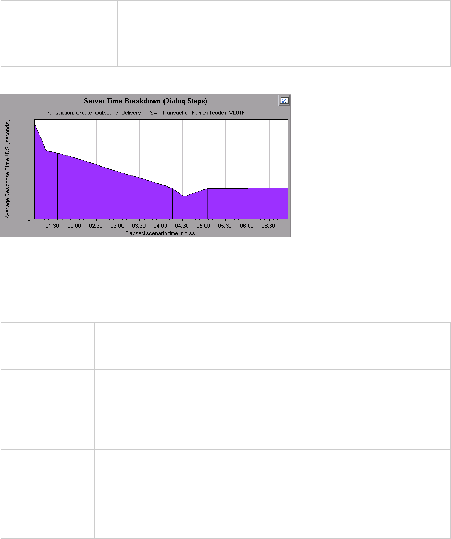
See also "SAP Breakdown Task Pane" on page346
"SAP Secondary Graphs" on page353
"SAP Breakdown Task Pane" on page346
Example
SAP Server Time Breakdown Graph
This graph represents the server-time components of a single transaction, namely database time,
application processing time, interface time, and system time.
X-axis Elapsed time since the start of the run (in hh:mm:ss).
Y-axis Represents the average response time per dialog step (in seconds).
Breakdown graphs l"SAP Database Time Breakdown Graph" on the next page
l"SAP Application Processing Time Breakdown Graph" on page344
l"SAP System Time Breakdown Graph" on page352
l"SAP Interface Time Breakdown Graph" on page352
Tips In the task pane, select a component from the View data associated with box.
See also "SAP Breakdown Task Pane" on page346
"SAP Secondary Graphs" on page353
"SAP Breakdown Task Pane" on page346
Example
User Guide
Analysis
HP LoadRunner (12.50) Page 349
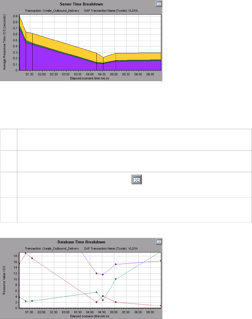
SAP Database Time Breakdown Graph
This graph displays the behavior of resources associated with database time, namely time taken to
access a record, database time, and the number of records accessed per dialog step.
X-
axis
Elapsed time since the start of the run (in hh:mm:ss).
Y-
axis
Represents the resource value per dialog step (in msec).
Tips You can open the graph in full view by clicking in the top right corner of the primary graph
pane. An enlarged version of the graph opens in a new tab.
See
also
"SAP Breakdown Task Pane" on page346
"SAP Secondary Graphs" on page353
Example
SAP Diagnostics Summary Report
This report displays a list of major alerts generated when opening the Analysis session, and a summary
of the SAP diagnostics data.
User Guide
Analysis
HP LoadRunner (12.50) Page 350
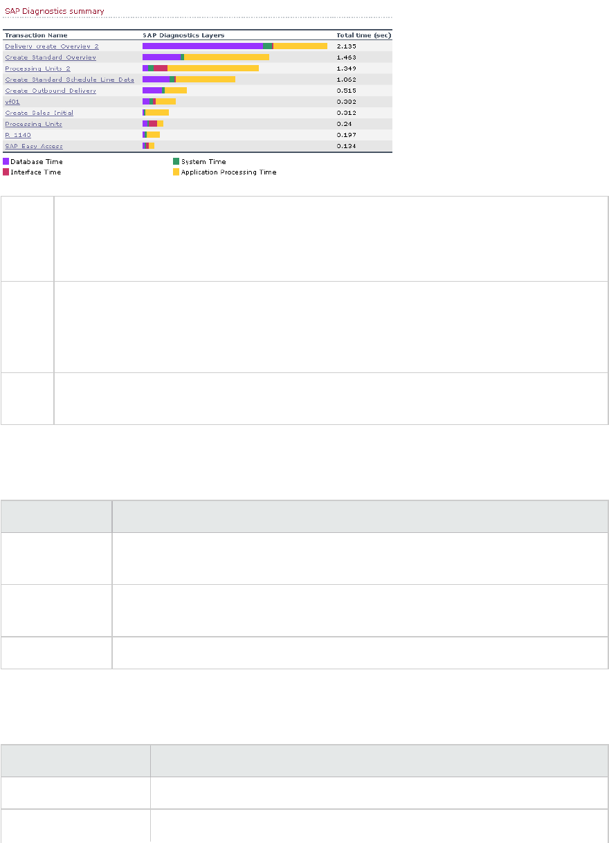
To
access
Use one of the following:
lSession Explorer > Reports > Summary Report > Major Alerts
lSession Explorer > Reports > Summary Report > SAP Diagnostics Summary
Note If you do not see diagnostics data on the Summary Report, check if you are using a user-
defined template. To view relevant data, choose a different template from the list of
templates, or create and apply a new template. For more information about using
templates, see "Apply/Edit Template Dialog Box" on page84.
See
also
"SAP Diagnostics Graphs Overview" on page337
SAP Diagnostics Summary
User interface elements are described below:
UI Element Description
Transaction Individual transactions. You can click a transaction name to display the server time
breakdown for that transaction.
SAP Diagnostics
Layers
Relative server-time breakdown in layers. Click a layer to display data associated
with the component.
Total time Total usage time for each transaction.
Major Alerts
User interface elements are described below:
UI Element Description
Time Interval The time during which the problem occurred.
Transaction/Server Which transaction and server were involved.
User Guide
Analysis
HP LoadRunner (12.50) Page 351
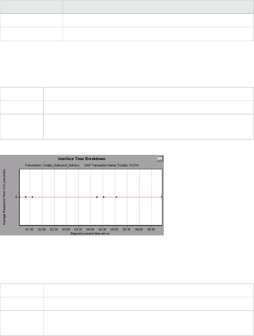
UI Element Description
Description A description of the alert.
Action This column provides a link to a graphic depiction of the problem.
SAP Interface Time Breakdown Graph
This graph displays the behavior of resources associated with interface time, namely GUI time, RFC
time, and roll-wait time.
X-axis Elapsed load test scenario time (in hh:mm:ss)
Y-axis Average response time per dialog step (in seconds).
See also "SAP Breakdown Task Pane" on page346
"SAP Secondary Graphs" on the next page
Example
SAP System Time Breakdown Graph
This graph displays the behavior of the sub-components of the system time component, namely the
dispatcher wait time, the load and generation time, and the roll-in and roll-out times.
X-axis Elapsed load test scenario time (in hh:mm:ss)
Y-axis Average response time per dialog step (in seconds)
See also "SAP Breakdown Task Pane" on page346
"Secondary Graph Pane" on page339
Example
User Guide
Analysis
HP LoadRunner (12.50) Page 352
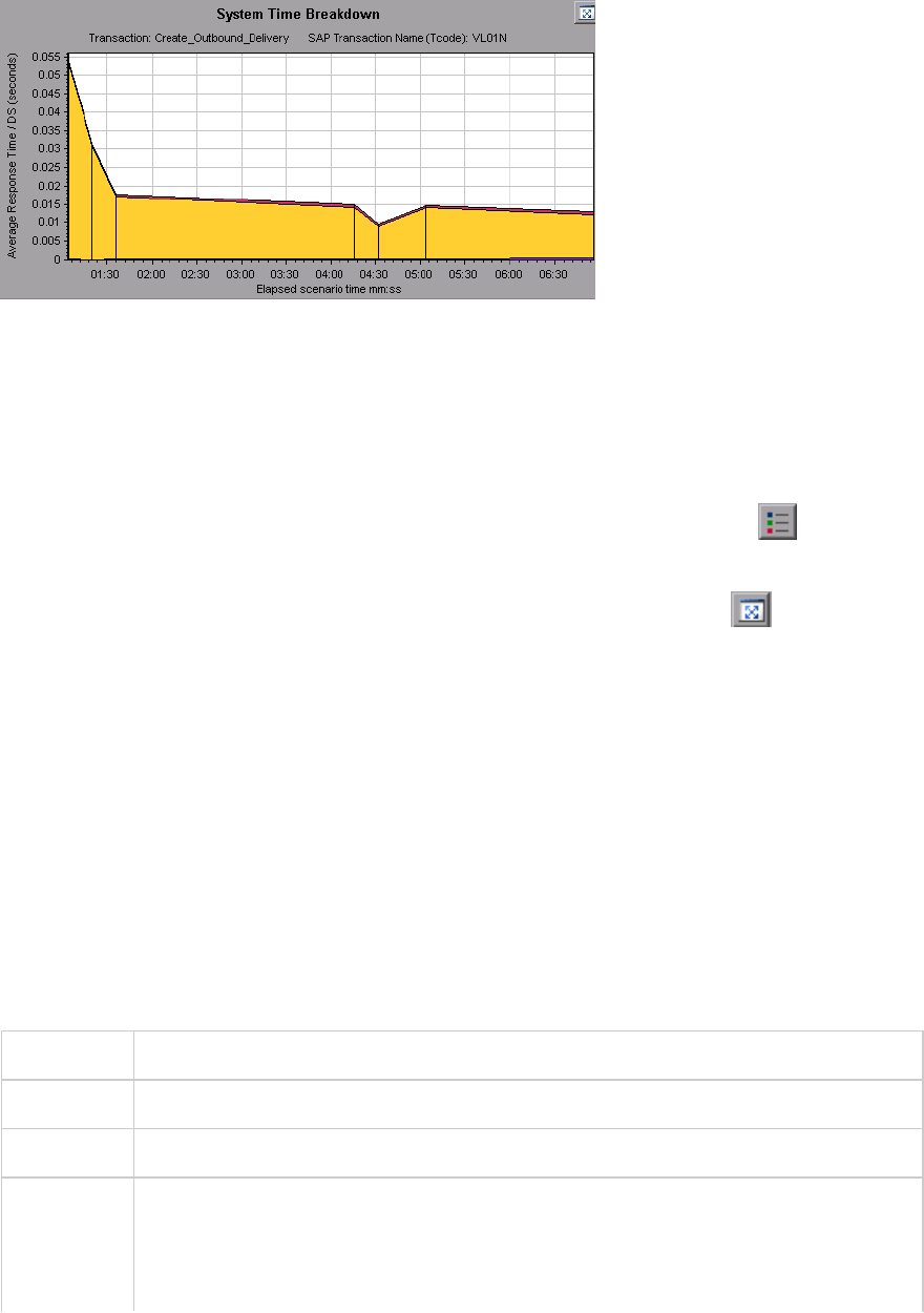
SAP Secondary Graphs
The secondary graph pane of the SAP Diagnostics - Guided Flow tab displays graphs that support the
graph displayed in the primary graph pane. You can correlate over time only one graph displayed in the
secondary graph pane.
To see the legend for the graph displayed in this pane, click the Graph Legend button in the top
right corner. To see all the data in the Legend, scroll along the horizontal scroll bar.
You can open the displayed graph in full view by clicking the Enlarge Graph button in the top right
corner of this pane. An enlarged version of the graph opens in a new tab.
You view the following graphs in the secondary graph pane:
l"Vuser Graphs" on page127
l"Dialog Steps per Second Graph" on page341
l"Work Processes Graph" below
l"OS Monitor Graph" on page341
Work Processes Graph
This graph represents the number and distribution of work processes that ran throughout the load test
scenario.
X-axis Elapsed scenario time (in hh:mm:ss).
Y-axis Number of work processes.
Note This graph is available only when a single server filter is applied.
See also "SAP Breakdown Task Pane" on page346
"Vuser Graphs" on page127
"Dialog Steps per Second Graph" on page341
User Guide
Analysis
HP LoadRunner (12.50) Page 353
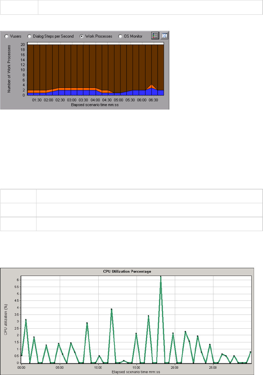
"OS Monitor Graph" on page341
Example
TruClient - Native Mobile Graphs
TruClient CPU Utilization Percentage Graph
This graph displays the percentage of the CPU utilized during the test run for TruClient Native Mobile
Vuser scripts.
Purpose Helps you evaluate the amount of CPU utilized by an application.
X-axis Elapsed time since the start of the scenario run.
Y-axis The percentage of the CPU utilized during the test run.
Example
In the following example, the CPU utilization peaked to approximately 6% at 18 minutes into the test
run.
User Guide
Analysis
HP LoadRunner (12.50) Page 354
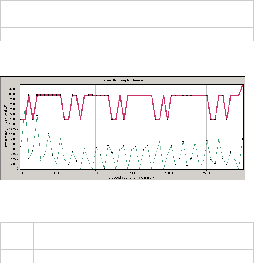
TruClient Free Memory In Device Graph
This graph displays the free memory on a mobile device as a function of time, for TruClient Native
Mobile scripts.
Purpose Helps you evaluate the amount of memory available on the device during the test run.
X-axis Elapsed time since the start of the scenario run.
Y-axis The amount of free memory in KBs.
Example
In the following example, the graph shows a free memory of over 33 MBs, at 30 minutes into the test
run for one of the transactions.
TruClient Memory Consumed by Application Graph
This graph displays the memory consumed by the application, as a function of time.
Purpose Helps you evaluate the amount of memory used by the application.
X-axis Elapsed time since the start of the scenario run.
Y-axis The memory consumed by the application in KBs.
Example
In the following example, the memory consumption peaked to 1337 KBs at 30 minutes into the test, for
one of the transactions.
User Guide
Analysis
HP LoadRunner (12.50) Page 355
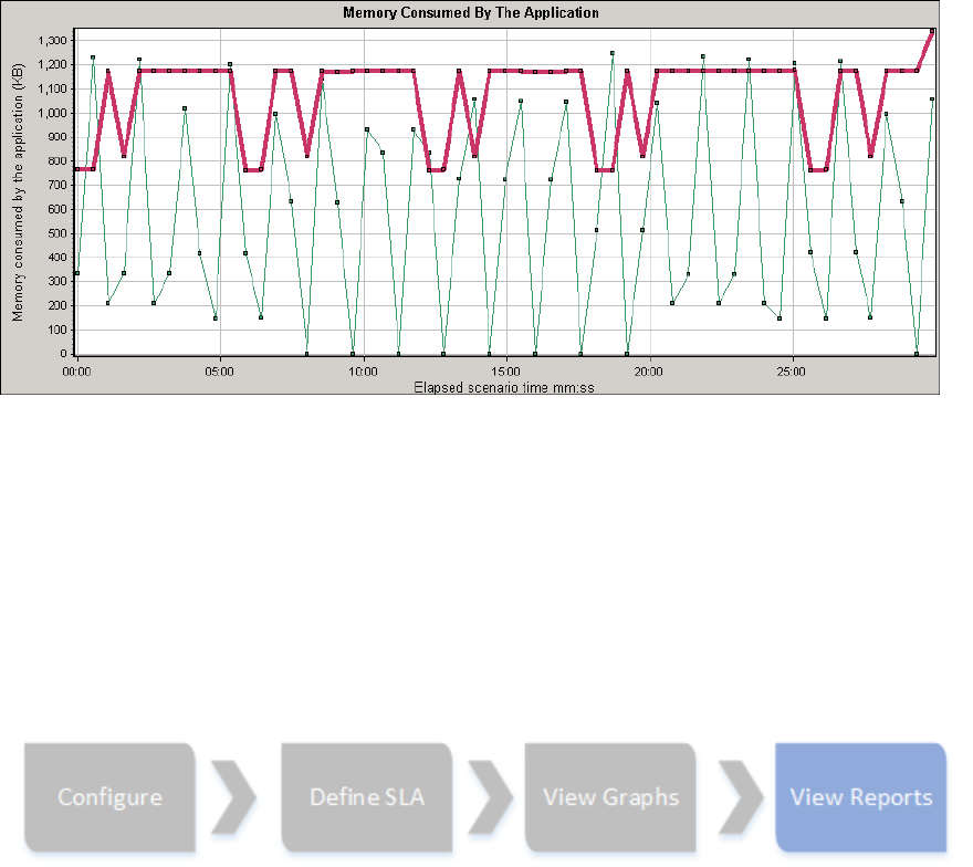
Analysis Reports
Understanding Analysis Reports
Analysis Reports Overview
After running a load test scenario, you can view reports that summarize your system's performance.
Analysis provides the following reporting tools:
l"Summary Report" on page369
l"SLA Reports" on page374
l"Transaction Analysis Report" on page375
l"HTML Reports" on page373
The Summary report provides general information about the scenario run. You can access the Summary
report at any time from the Session Explorer.
The SLA report provides an overview of the defined SLAs (Service Level Agreements) with succeeded or
failed status.
The Transaction Analysis report provides a detailed analysis of a specific transaction over a specific
time period.
User Guide
Analysis
HP LoadRunner (12.50) Page 356
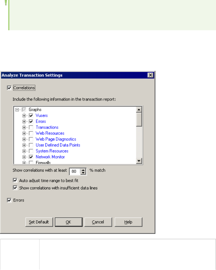
You can instruct Analysis to create an HTML report. The HTML report contains a page for each open
graph, the Summary report, the SLA report, and the Transaction Analysis report.
Transaction reports provide performance information about the transactions defined within the Vuser
scripts. These reports give you a statistical breakdown of your results and allow you to print and export
the data.
Note: SLA reports and Transaction Analysis reports are not available when generating Cross
Result graphs. For more information on Cross Result graphs, see "Cross Result and Merged
Graphs" on page120.
Analyze Transaction Settings Dialog Box
This dialog box enables you to configure the Transaction Analysis Report to show correlations between
the graph of the analyzed transaction and other graphs that you select.
To access Use one of the following:
lReports > Analyze Transaction > Settings
lTools > Options > Analyze Transaction Settings tab
User Guide
Analysis
HP LoadRunner (12.50) Page 357
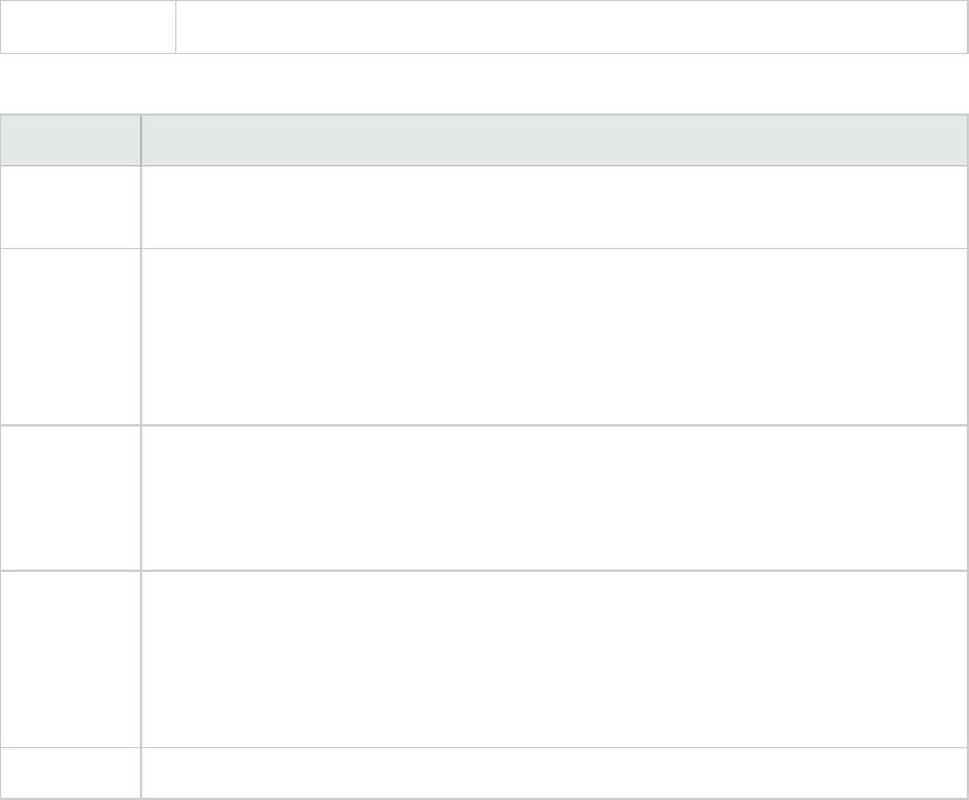
See also "Analyze Transactions Dialog Box" below
User interface elements are described below:
UI Element Description
Correlations Defines which graphs you want Analysis to match to the graph of the transaction you
selected. Graphs where data is available appear in blue.
Show
correlations
with at
least x%
match
The positive or negative percentage correlation between the graph of the analyzed
transaction and the graphs selected above. You can change the percentage by
entering a value in the box. The default is 20%.
Auto adjust
time range
to best fit
Analysis adjusts the selected time range to focus on the SLA violations within and
around that time period. This option only applies when the Transaction Analysis report
is generated directly from the Summary report (from the X Worst transactions or
Scenario behavior over time sections).
Show
correlations
with
insufficient
data lines
Displays correlations where one of the measurements contains less than 15 units of
granularity.
Errors Displays errors in the Transaction Analysis Report if selected.
Analyze Transactions Dialog Box
You use the Analyze Transaction dialog box to define the criteria that will be used to analyze the
selected transaction in the Transaction Analysis Report. You can analyze a transaction even if you have
not defined an SLA.
User Guide
Analysis
HP LoadRunner (12.50) Page 358
To
access
Reports > Analyze Transaction
Summary Report > right-click menu > Add New Item > Analyze Transaction
Toolbar >
Summary Report with no SLA > Statistics Summary section > Analyze Transaction tool
link
Note Analysis data (for example, transactions) that has been excluded by the Summary Filter will
not be available for analysis in the Transaction Analysis report.
See
also
"Filtering and Sorting Graph Data" on page103
User interface elements are described below (unlabeled elements are shown in angle brackets):
UI Element Description
Show time
ranges
based on
box
Select one of the display options:
lSuggestions. Lists all transactions and time ranges from the scenario run.
lSLA Violations. Lists only those transactions and time ranges where the
transaction exceeded the SLA. This option does not appear if there were no
transactions that exceeded the SLA.
Transaction Select the transaction to analyze from the Transaction tree.
<Time
Range>
Select the time range to analyze in one of the following ways:
lSelect the time range from the Transaction tree.
User Guide
Analysis
HP LoadRunner (12.50) Page 359
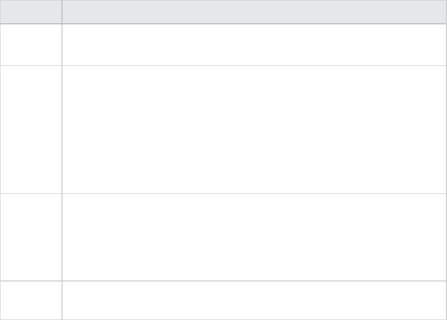
UI Element Description
lEnter the time range in the From and To boxes above the graph.
lSelect the time range by dragging the bars on the graph.
<Display
options>
Select one of the following:
lRunning Vusers
lThroughput
lHits per Second
The option you select is displayed on the graph and will appear on the snapshot of the
graph that appears on the Transaction Analysis Report. Note that your choice only
affects the display of the graph and not the calculation for correlations.
Settings Click Settings to define the Analyze Transaction settings in the Analyze Transaction
Settings dialog box. For more information, see "Analyze Transaction Settings Dialog
Box" on page357.
Note: You can also define the Analyze Transaction settings in the Analyze Transaction
Settings tab of the Options dialog box (Tools > Options).
Generate
report
The Transaction Analysis Report opens. Once the report has been created, you can
access it at any time from the Session Explorer.
New Report Dialog Box
This dialog box enables you to create a report based on the report template selected. You can adjust
the report template settings to generate a report that corresponds to the required report layout.
User Guide
Analysis
HP LoadRunner (12.50) Page 360
To access Reports > New Report
See also "Report Templates Dialog Box" on the next page
Note: This dialog box and the Report Templates dialog box utilize the same
components.
User interface elements are described below:
UI Element Description
Based on Template The template upon which to build the report. After you
select a template, the corresponding settings of the report
template appear.
General tab For user interface details, see "Report Templates - General
Tab" on page364.
Format tab For user interface details, see "Report Templates - Format
Tab" on page365.
Content tab For user interface details, see "Report Templates - Content
Tab" on page367.
Save As Template Prompts you for a template name that will be added to the
User Guide
Analysis
HP LoadRunner (12.50) Page 361
UI Element Description
report template list.
Generate Generates the report according to your settings.
Analysis Report Templates
Report Templates Overview
You can use Report Templates to create and customize templates which are used when generating
reports. Report templates can be used across similar scenario runs and saves time and effort on
recreating reports each time.
Using the Report Templates dialog box, you can record document details, define the format of the
report, and select the content items to include in the report and configure each content item
accordingly.
A list of report templates is displayed in the Templates dialog box, under Rich Reports. Select this
option if you want to generate the report in the load run session in word, excel, HTML or PDF format. For
more information on templates, see "Apply/Edit Template Dialog Box" on page84.
Report Templates Dialog Box
This dialog box enables you to add, modify, import, export, or duplicate a report template.
User Guide
Analysis
HP LoadRunner (12.50) Page 362
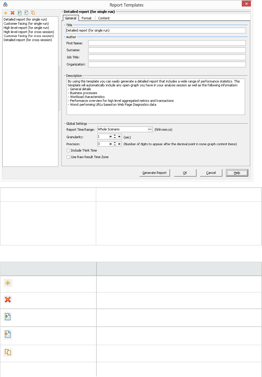
To access Reports > Report Templates
See also l"Report Templates Overview" on the previous page
l"New Report Dialog Box" on page360
Note: This dialog box and the New Report dialog box utilize the
same components.
User interface elements are described below:
UI Element Description
New. Adds a new report template.
Delete. Removes the selected template.
Import. Imports a report template from an XML file.
Export. Saves the selected template as an XML file.
Duplicate.Creates a copy of the selected template.
General tab For user interface details, see "Report Templates - General
User Guide
Analysis
HP LoadRunner (12.50) Page 363
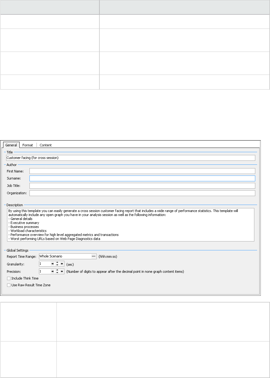
UI Element Description
Tab" on the next page.
Format tab For user interface details, see "Report Templates - Format
Tab" on the next page.
Content tab For user interface details, see "Report Templates - Content
Tab" on page367.
Generate Report button Generates the report according to your settings.
Report Templates - General Tab
This tab enables you to record document details, such as title, author name and title and set global
settings, such as Report Time Range and granularity.
To Access Reports >New Report… >General tab
or
Reports >Report Templates… >General tab
See also l"Report Templates Overview" on page362
l"New Report Dialog Box" on page360
l"Report Templates Dialog Box" on page362
User interface elements are described below:
User Guide
Analysis
HP LoadRunner (12.50) Page 364
UI Element Description
Title A description of the template.
First Name The first name of the person to display on the report.
Surname The last name of the person to display on the report.
Job title The job title of the person to display on the report.
Organization The name of the organization to display on the report.
Description You can enter a description and include details of the report template.
Report Time
Range
The default setting is Whole Scenario. Click to set the start and end time range
of the scenario runtime to display on the report.
Granularity Define granularity settings (in seconds).
Precision The number of digits to appear after the decimal point in none graph content
items.
Include Think
Time
Include think time when processing the Analysis data. This data is then used when
generating reports.
Use Raw Result
Time Zone
When creating the report, use the time zone that was generated in the raw data
results.
Report Templates - Format Tab
This tab enables you to define the format of report template.
User Guide
Analysis
HP LoadRunner (12.50) Page 365
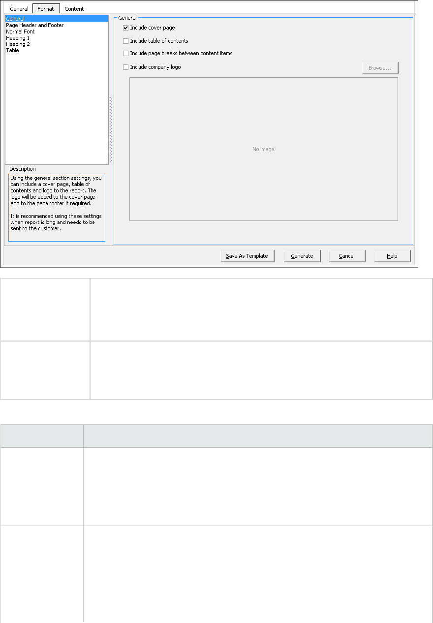
To access Reports >New Report… >Format tab
or
Reports >Report Templates… >Format tab
See also l"Report Templates Overview" on page362
l"New Report Dialog Box" on page360
l"Report Templates Dialog Box" on page362
User interface elements are described below:
UI Element Description
General General options such as:
linclude a cover page
linclude table of contents
linclude company logo
Page Header and
Footer
Header and footer options:
lFont type, size and color
lBold, italicize, or underline
lRight, center or left align
lYou can add tags, such as date, name or organization.
User Guide
Analysis
HP LoadRunner (12.50) Page 366
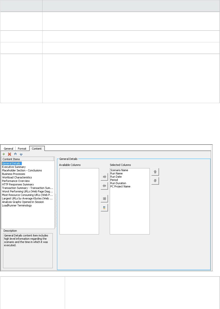
UI Element Description
lYou can include required details such as page count, date, name, and so forth
on the left, center or right column.
Normal Font The type of font to use in the report template.
Heading 1/2 The style for your headings.
Table Table format options:
lFont type, size and color
lBackground color
lBold, italicize, or underline
lRight, center or left align
Report Templates - Content Tab
This tab enables you to select the content items to include in the report and configure each item
accordingly.
To access Reports >New Report… >Content tab
or
Reports >Report Templates… >Content tab
User Guide
Analysis
HP LoadRunner (12.50) Page 367
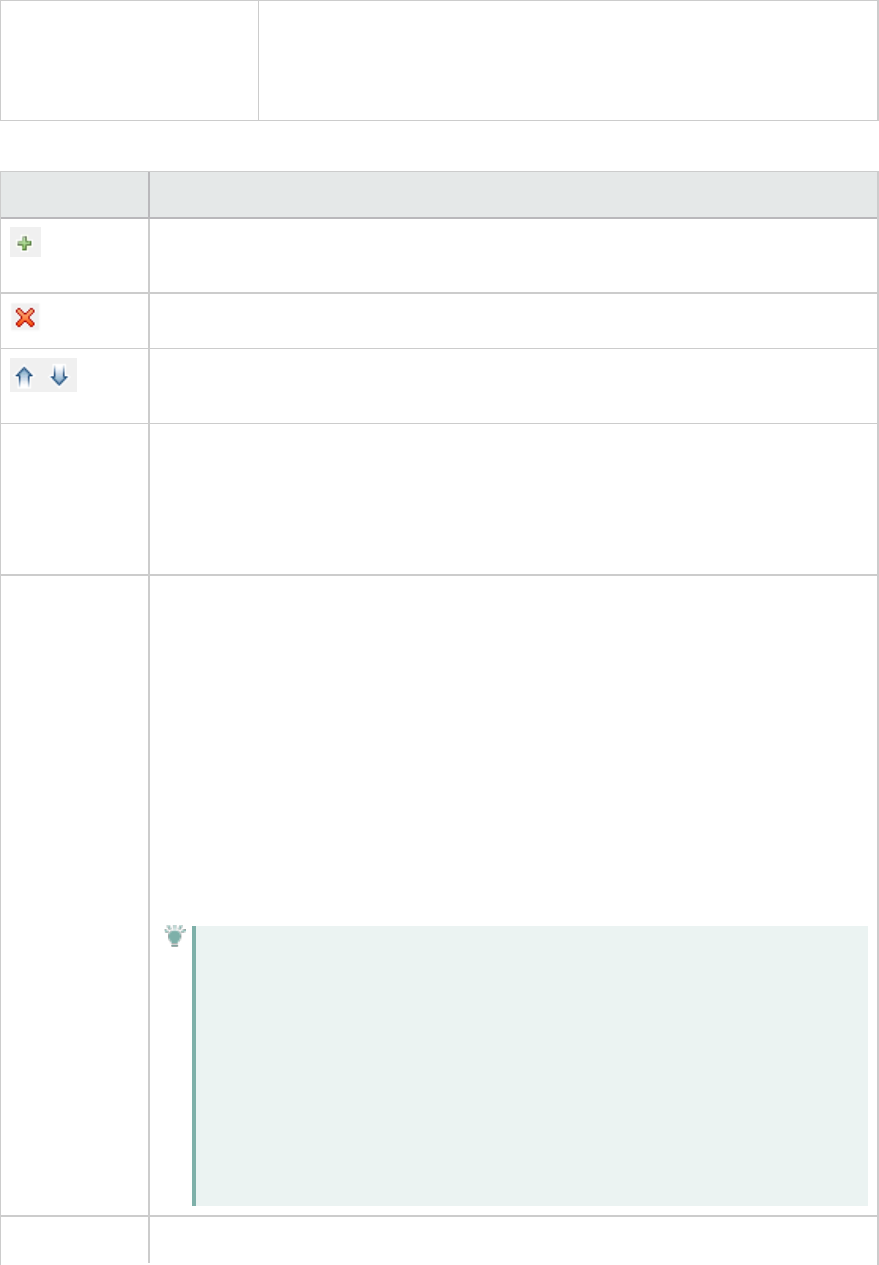
See also l"Report Templates Overview" on page362
l"New Report Dialog Box" on page360
l"Report Templates Dialog Box" on page362
User interface elements are described below:
UI Element Description
Add Content. Opens the Add Content Items pane. Select one or more items from
the grid and click OK.
Delete Content. Removes the selected items from the Content Items pane.
Reorder. Reorders the content items, determining how they will be shown in the
report.
Contents Item
pane
A list of the content items to be included in the report.
lTo add more items, click the Add Content button.
lTo learn about a content item, select it and view the information in the
Description pane beneath it.
<Configuration
pane>
Settings for the selected content item. The components and tabs in this pane vary,
based on the selected content item.
lParameters tab. Settings such as integer values for percentiles or number of
elements.
lColumns tab. Allows you to select the columns to include in the report. To include
a column, make sure it appears in the Selected Columns pane.
lFilter tab. Allows you to enter criteria for including a specific range of a
measurement.
lText area. A rich text box for enter free text, such as in a Placeholder Section or
an Executive Summary.
Tip: For the Performance Summary content item, you can retrieve
different information about transactions such as the total number of
passed or failed transactions. The item, Weighted Average of Transaction
Response timeis calculated based on the following formula: Round (Sum of
Average value in transaction response time / Sum of transactions). For
example if you have three transactions with the response times of 0.005,
0.004, and 0.003, the weighted Average of Transaction Response Time is
Round((0.005 + 0.004 + 0.003)/3) = 0.004
Generate Generates the report according to your settings.
User Guide
Analysis
HP LoadRunner (12.50) Page 368
UI Element Description
Report
Analysis Report Types
Summary Report Overview
The Summary report provides general information about load test scenario execution. This report is
always available from the Session Explorer or as a tab in the Analysis window.
The Summary report lists statistics about the scenario run and provides links to the following graphs:
Running Vusers, Throughput, Hits Per Second, HTTP Responses per Second, Transaction Summary, and
Average Transaction Response Time.
The appearance of the Summary report and the information displayed, will vary depending on whether
an SLA (Service Level Agreement) was defined.
An SLA defines goals for the scenario. LoadRunner measures these goals during the scenario run, and
analyzes them in the Summary report. For more information on defining an SLA, see "SLA Reports" on
page374
A Summary report is also provided for Cross Result graphs. For more information about Cross Result
graphs, see "Cross Result Graphs Overview" on page120.
Note: You can save the Summary reports to an Excel file by selecting View > Export Summary
to Excel or by clicking the Export Summary to Excel button on the toolbar.
Summary Report
The Summary report provides general information about load test scenario execution. It lists statistics
about the scenario run and provides links to the following graphs: Running Vusers, Throughput, Hits Per
Second, HTTP Responses per Second, Transaction Summary, and Average Transaction Response Time.
To access Session Explorer > Reports > Summary Report
Important
information
The Summary report for SAP Diagnostics, J2EE /.NET Diagnostics, and Siebel
Diagnostics provides a usage chart that links to and displays each individual
transaction's Web, application, and database layers, and provides the total usage time
for each transaction.
Relevant
tasks
You can save the Summary reports to an Excel file by selecting View > Export
Summary to Excel or by clicking on the toolbar.
User Guide
Analysis
HP LoadRunner (12.50) Page 369
See also The Summary reports for the various diagnostics environments are discussed in detail
in the following sections:
"SAP Diagnostics Summary Report" on page350
J2EE & .NET Diagnostics Graphs Summary Report
"Siebel Diagnostics Graphs Summary Report" on page321
Summary Report with No SLA
User interface elements are described below:
UI Element Description
Scenario
Details
Shows the basic details of the load test scenario being analyzed.
Statistics
Summary
This section shows a breakdown of the transaction statistics and also provides links to
the following:
lThe SLA configuration wizard. For more information on defining an SLA, see "SLA
Reports" on page374
lThe Analyze Transaction tool. For more information on analyzing transactions, see
"Analyze Transactions Dialog Box" on page358
Transaction
Summary
This section displays a table containing the load test scenario's diagnostics data.
Included in this data is a percentile column (x Percent). This column indicates the
maximum response time for that percentage of transactions performed during the
run.
Note: You can change the value in the percentile column in one of the following ways:
lOpen the Options dialog box (Tools > Options). Click the General tab and in the
Summary Report section enter the desired percentile in the Transaction Percentile
box.
lSelect View > Summary Filter or click on the toolbar. The Analysis Summary
Filter dialog box opens. In the Additional Settings area enter desired percentile.
HTTP
Responses
Summary
This section shows the number of HTTP status codes returned from the Web server
during the load test scenario, grouped by status code.
Note: There are additional Diagnostics sections that may appear at the end of the
Summary report, depending on the configuration of your system.
Summary Report with SLA
User interface elements are described below:
User Guide
Analysis
HP LoadRunner (12.50) Page 370

UI Element Description
Scenario
details
This section shows the basic details of the load test scenario being analyzed.
Statistics
Summary
This section shows a breakdown of the transaction statistics.
X Worst
Transactions
The X Worst Transactions table shows the worst transactions in terms of how often
the transactions exceeded the SLA boundary during the run, and by how much. Click
here to see an example of the 5 Worst transactions section of the summary report.
Note: You choose how many transactions are displayed in this table in the Summary
Report section on the General tab of the options dialog box. Open the dialog box
(Tools >Options) and enter the number of transactions to display. The default is 5.
You expand a transaction to get more information. When expanded, the following
information appears for each transaction:
Failure Ratio
lThe percentage of time intervals where the transaction exceeded the SLA. You
can see this graphically in the Scenario Behavior Over Time section below.
Failure Value
lThe average percentage by which the transaction exceeded the SLA over the
whole run.
Avg exceeding ratio
lThe average percentage by which the transaction exceeded the SLA over a
specific time interval. For example, in the first time interval in the screenshot
above, the figure is 4.25%. This means that during that time interval, the
transaction may have exceeded the SLA boundary several times, each time by a
different percentage margin, the average percentage being 4.25%.
Max exceeding ratio
lThe highest percentage by which the transaction exceeded the SLA over a
specific time interval. For example, using the same time interval as above, the
transaction may have exceeded the SLA several times, each time by a different
percentage margin. The highest percentage being 7.39%
Analysis allows you to analyze a specific transaction in more detail. You open the
Analyze Transaction tool from this section by clicking the Analyze Transaction
button. For more information on Transaction Analysis Reports, see "Analyze
Transactions Dialog Box" on page358.
User Guide
Analysis
HP LoadRunner (12.50) Page 371
)

UI Element Description
Scenario
Behavior
Over Time
This section shows how each transaction performed in terms of the SLA over time
intervals. The green squares show time intervals where the transaction performed
within the SLA boundary. Red squares show time intervals where the transaction
failed and gray squares show where no relevant SLA was defined.
Note: The time intervals displayed in the Scenario Behavior Over Time section may
vary for each interval. The time interval set in the tracking period of the SLA is only
the minimum time interval that will be displayed.
It is only the display that varies. The SLA is still determined over the time interval you
choose in the Advanced Settings section.
Analysis allows you to analyze a specific transaction in more detail. You open the
Analyze Transaction tool from the Scenario Behavior Over Time section in one of the
following ways:
lSelect the transaction to analyze from the list and enter the time interval in the
From and To boxes. Then click Analyze Transaction.
lDrag the mouse over the desired transaction and time range to analyze. Then click
Analyze Transaction.
For more information on Transaction Analysis Reports, see "Analyze Transactions
Dialog Box" on page358.
Transaction
Summary
This section displays a table containing the load test scenario's diagnostics data.
Included in this data is a percentile column (x Percent). This column indicates the
maximum response time for that percentage of transactions performed during the
run. For example, in the table below, the value in the 88 Percent column for browse
special books is 8.072. This means that the response time for 88% of the browse
special books transactions was less that 8.072 seconds. Click here to see an example
of a Transaction Summary.
Note: You can change the value in the percentile column in the Summary Report
section of the General tab of the Options dialog box. Open the dialog box (Tools >
Options) and enter the desired percentage.
Alternatively, you can also change the value in the Summary Filter (View > Summary
Filter) .
HTTP
Responses
Summary
This section shows the number of HTTP status codes returned from the Web server
during the load test scenario, grouped by status code.
Note: There are additional Diagnostics sections that may appear at the end of the
Summary report, depending on the configuration of your system.
User Guide
Analysis
HP LoadRunner (12.50) Page 372
)
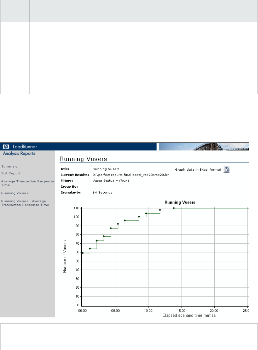
Summary reports for Cross Result Graphs
User interface elements are described below:
UI
Element
Description
<graphs> Displays summary information for the scenarios that you are comparing. The information
is displayed in a way that enables you to compare data from the different scenarios.
Includes the same type of information as the regular Summary report except for the
following:
lSLA information
lDiagnostics information
lScenario behavior over time
HTML Reports
Analysis enables you to create HTML reports for your load test scenario run. It creates a separate page
for each one of the open graphs and reports.
To
access
Use one of the following:
lReports > HTML Report
User Guide
Analysis
HP LoadRunner (12.50) Page 373
lToolbar >
Relevant
tasks
lOpen all graphs that you want to include in the report.
lSpecify a path and file name for the HTML report and click Save. Analysis saves a
Summary report which has the same name as the file in the selected folder. The rest
of the graphs are saved in a folder with the same name as the Summary report's file
name. When you create an HTML report, Analysis opens your default browser and
displays the Summary report.
lTo copy the HTML reports to another location, be sure to copy the filename and the
folder with the same name. For example, if you named your HTML report test1, copy
test1.html and the folder test1 to the desired location
User interface elements are described below:
UI Element Description
<Graphs> menu
left frame
Click the graph link to view an HTML report for that graph.
You can view an Excel file containing the graph data, by clicking the Graph data in
Excel format button on the relevant graph page.
SLA Reports
An SLA (Service Level Agreement) defines goals for the load test scenario. LoadRunner measures these
goals during the scenario run and analyzes them in the Summary report. The SLA Report shows the
succeeded or failed status of all SLAs that were defined for the scenario run.
Note: Analysis data (for example, transactions) that has been excluded by the Summary Filter
will not be available for analysis in the SLA report.
To access You create the SLA Report in one of the following ways:
Reports > Analyze SLA
Right-click the Summary pane > Add New Item > Analyze SLA
Summary Report >
Relevant tasks "Defining Service Level Agreements" on page51
User interface elements are described below:
User Guide
Analysis
HP LoadRunner (12.50) Page 374
UI Element Description
Display of SLA
statuses
SLA Status per goal definition
lWhere the SLA was defined over the whole run, the report displays a
single SLA status for each goal definition.
SLA status for each transaction per time interval
lWhere the SLA was defined per time interval within the run, the report
displays the status of the SLA for each transaction per time interval. The
green squares show time intervals where the transaction performed
within the SLA boundary. Red squares where the transaction failed and
gray squares show where no relevant SLA was defined.
SLA goal definitions
lWhere the SLA was defined per time interval within the run, a further
section appears detailing the goal definitions for the SLA.
Transaction Analysis Report
This report enables you to individually examine each of the transactions from the load test scenario run.
To access Reports > Analyze Transaction > Generate Report button
User interface elements are described below:
UI Element Description
Observations This section shows both positive and negative correlations between the graph of the
transaction being analyzed, and other graphs based on the settings you chose in the
Analyze Transaction Dialog Box. When two graphs are correlated, it means that their
behavior matches each other by a certain percentage.
To view the correlating graph, select one of the results and then click the View
Graph icon at the bottom of the section. The graph comparison opens.
You can return to the Transaction Analysis Report from the graph comparison at
anytime by clicking the Back to <transaction name> icon on the toolbar.
Note: The correlations are automatically calculated according to a default ratio of
20%. You can adjust this ratio by clicking the arrows next to the percentage. Then
click Recalculate.
Errors This section is divided into two sub-sections.
lApplication Under Test errors. Shows errors that occurred during the transaction
User Guide
Analysis
HP LoadRunner (12.50) Page 375
UI Element Description
that were direct results of Vuser activity.
lAll errors. Shows Application Under Test errors as well as errors that were not
related to Vuser activity, and which affected your system and not the application
under test.
Observation
Settings
This section displays a summary of the settings that were selected in the Advanced
Settings section of the Analyze Transaction dialog box.
Graph The Graph section displays a snapshot of selected transaction and time range for
analysis merged with the display option you selected (Running Vusers, Throughput, or
Hits per Second). Note that it is only a snapshot and can not be manipulated like
normal graphs.
Importing Data
What do you want to do?
lImport data
lDefine a custom file format
See also:
lSupported file types
lImport Data dialog box
Import Data Tool Overview
The LoadRunner Analysis Import Data tool enables you to import and integrate non-HP data into a
LoadRunner Analysis session. After the import procedure, you can view the data files as graphs within
the session, using all the capabilities of the Analysis tool.
Suppose an NT Performance Monitor runs on a server and measures its behavior. Following a
LoadRunner scenario on the server, you can retrieve the results of the Performance Monitor, and
integrate the data into LoadRunner's results. This enables you to correlate trends and relationships
between the two sets of data: LoadRunner's and the Performance Monitor's.
In this case, the results of the NT Performance Monitor are saved as a .csv file. You launch the Import
Data tool, direct it to the .csv file, and specify its format. LoadRunner reads the file and integrates the
results into its own Analysis session.
For a list of data formats that are supported, see "Supported File Types" on page378. To define your
own custom data files, see "How to Define Custom File Formats" on page378.
User Guide
Analysis
HP LoadRunner (12.50) Page 376
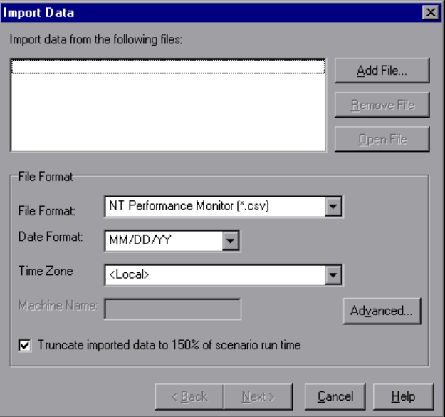
How to Use the Import Data Tool
This task describes how to import data files to integrate into your analysis session.
1. Choose Tools > External Monitors > Import Data. The Import Data dialog box opens.
2. Select the format of the external data file from the File format list box.
3. Click Add File. In the Select File to Import dialog box that opens, the Files of type list box shows
the type chosen in step 2.
4. Set other file format options, as described in "Import Data Dialog Box" on page383. You must
enter a machine name.
5. To specify character separators and symbols, click Advanced. For more information, see
"Advanced Settings Dialog Box (Import Data Dialog Box)" on page380.
6. Click Next. The Import Data dialog box opens.
7. Select the type of monitor that generated the external data file. If your monitor type does not
exist, you can add it, as described in How to Customize Monitor Types for Import.
When opening a new graph, you will see your monitor added to the list of available graphs under this
particular category. (See "Open a New Graph Dialog Box" on page125.)
8. Click Finish. LoadRunner Analysis imports the data file or files, and refreshes all graphs currently
displayed in the session.
User Guide
Analysis
HP LoadRunner (12.50) Page 377

Note: When importing data into a scenario with two or more cross results, the imported
data will be integrated into the last set of results listed in the File > Cross with Result
dialog box. For more information, see "How to Generate Merged Graphs" on page124.
How to Define Custom File Formats
This task describes how to define a custom format, if the file format of your import file is not
supported.
If the file format of your import file is not supported, you can define a custom format.
1. Choose Tools > External Monitors > Import Data. The Import Data dialog box opens.
2. From the File Format list, select <Custom File Format>. The Enter New Format Name dialog box
opens.
3. Enter a name for the new format (in this case, my_monitor_format).
4. Click OK. The Define External Format dialog box opens.
5. Specify the mandatory and optional data, as described in "Define External Format Dialog Box" on
page381.
6. Click Save.
Supported File Types
The following file types are supported:
NT Performance Monitor (.csv)
The default file type of the NT Performance monitor, in comma separated value (CSV) format.
For example:
Reported on \\WINTER
Date: 03/06/15
Time: 10:06:01 AM
Data: Current Activity
Interval: 1.000 seconds
,,% Privileged Time,% Processor Time,% User Time,
,,0,0,0,
,,,,,,
,,Processor,Processor,Processor,
Date,Time,\\WINTER,\\WINTER,
03/06/15,10:06:00 AM , 0.998, 1.174, 0.000,
User Guide
Analysis
HP LoadRunner (12.50) Page 378
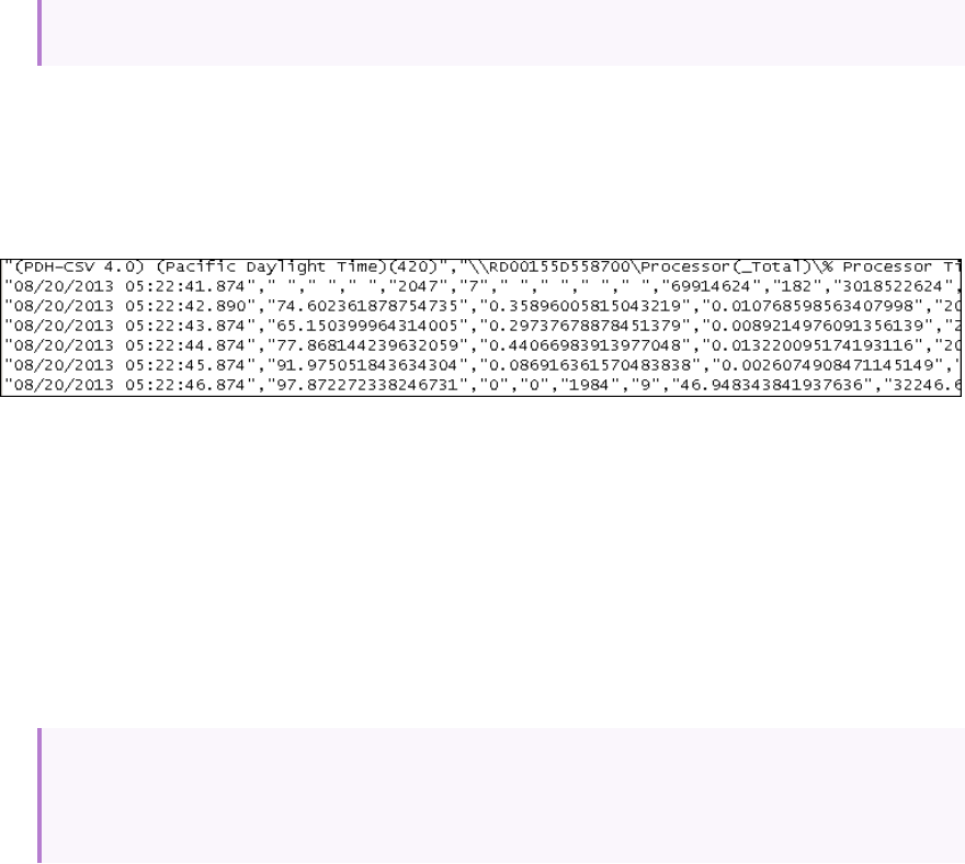
03/06/15,10:06:00 AM , 0.000, 0.275, 0,000,
Windows Performance Monitor (.csv)
The default file type for the Windows 2000, 2008 server, Windows 7, etc. performance monitor, in CSV
format.
For example:
Standard Comma Separated File (.csv)
This file type has the following format:
date, time, measurement_1,measurement_2, ...
where fields are comma separated and first row contains column titles.
The following example from a standard CSV file shows 3 measurements: an interrupt rate, a file IO rate
and a CPU usage. The first row shows an interrupt rate of 1122.19, an IO rate of 4.18, and a CPU busy
percentage of 1.59:
date, time, interrupt rate, File IO rate, CPU busy percent
03/06/15,10:06:01,1122.19,4.18,1.59
03/06/15,10:06:01,1123.7,6.43,1.42
Master-Detail Comma Separated File (.csv)
This file type is identical to Standard Comma Separated Files except for an additional Master column
which specifies that row's particular breakdown of a more general measurement. For example, a
Standard CSV file may contain data points of a machine's total CPU usage at a given moment:
Date,Time,CPU_Usage
However, if the total CPU usage can be further broken up into CPU time per-process, then a Master-
Detail CSV file can be created with an extra column ProcessName, containing the name of a process.
Each row contains the measurement of a specific process's CPU usage only. The format will be the
following:
Date,Time,ProcessName,CPU_Usage
as in the following example:
User Guide
Analysis
HP LoadRunner (12.50) Page 379
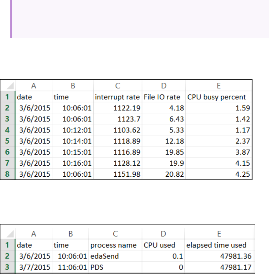
date, time, process name, CPU used, elapsed time used
03/06/15,10:06:01,edaSend,0.1,47981.36
03/06/15,10:06:01,PDS,0,47981.17
Microsoft Excel File (.xls)
Created by the Microsoft Excel application. The first row contains column titles. (.xlxs format is not
supported.)
Master-Detail Microsoft Excel file (.xls)
Created by Microsoft's Excel application. The first row contains column titles. It contains an extra
Master column. (.xlxs format is not supported.)
Advanced Settings Dialog Box (Import Data Dialog Box)
This dialog box enables you to define the data format of the imported file to settings other than of the
regional configuration.
User Guide
Analysis
HP LoadRunner (12.50) Page 380
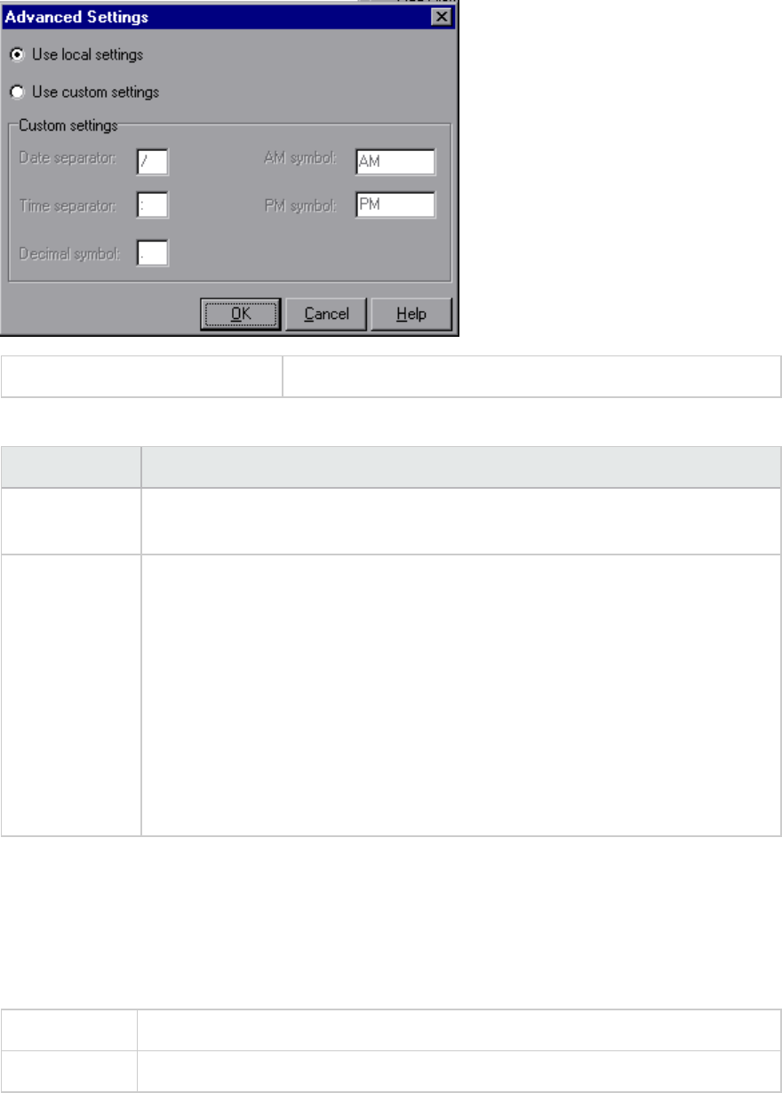
To access Tools > External Monitors > Import Data > Advanced
User interface elements are described below:
UI Element Description
Use local
settings
Keep default settings of the regional configuration. Disables the Custom Settings
area of the dialog box.
Use custom
settings
Define your own settings. Enables the Custom Settings area of the dialog box.
lDate Separator. Enter a custom symbol, for example, the slash (`/') character in
11/10/02
lTime Separator. Enter a custom symbol, for example, the colon `:' character in
9:54:19
lDecimal symbol. Enter a custom symbol, for example, the `.' character in the
number 2.5
lAM symbol. Enter a custom symbol for the hours between midnight and noon.
lPM symbol. Enter a custom symbol for the hours between noon and midnight.
Define External Format Dialog Box
This dialog box enables you to define a new file format for external data files not supported by Analysis.
The Define External Format dialog box is divided into mandatory and optional information.
To access Tools > External Monitors > Import data > File Format > <Custom File Format>
Relevant tasks "How to Define Custom File Formats" on page378
User Guide
Analysis
HP LoadRunner (12.50) Page 381
Mandatory tab
User interface elements are described below:
UI
Element
Description
Date
Column
Number
Enter the column that contains the date. If there is a master column (see "Supported File
Types" on page378), specify its number.
Time
Column
Number
Enter the column that contains the time.
Use
Master
Column
Select this if the data file contains a master column. A master column specifies the row's
particular breakdown of a more general measurement.
File
Extension
Enter the file suffix.
Field
Separator
Enter the character that separates a field in a row from its neighbor. To select a field
separator character, click Browse and select a character from the define Field Separator
dialog box.
Optional tab
User interface elements are described below:
UI Element Description
Date Format Specify the format of the date in the imported data file. For example, for European
dates with a 4 digit year, choose DD/MM/YYYY.
Time Zone Select the time zone where the external data file was recorded. LoadRunner Analysis
aligns the times in the file with local time zone settings to match LoadRunner results.
(LoadRunner does not alter the file itself).
Machine
Name
Specify the machine name the monitor runs on. This associates the machine name
with the measurement.
Exclude
Columns
Indicate which columns are to be excluded from the data import, such as columns
containing descriptive comments. When there is more than one column to be
excluded, specify the columns in a comma-separated list. For example, 1,3,8.
Convert file
from UNIX
Monitors often run on UNIX machines. Check this option to convert data files to
Windows format. A carriage return (Ascii character 13) is appended to all line feed
User Guide
Analysis
HP LoadRunner (12.50) Page 382
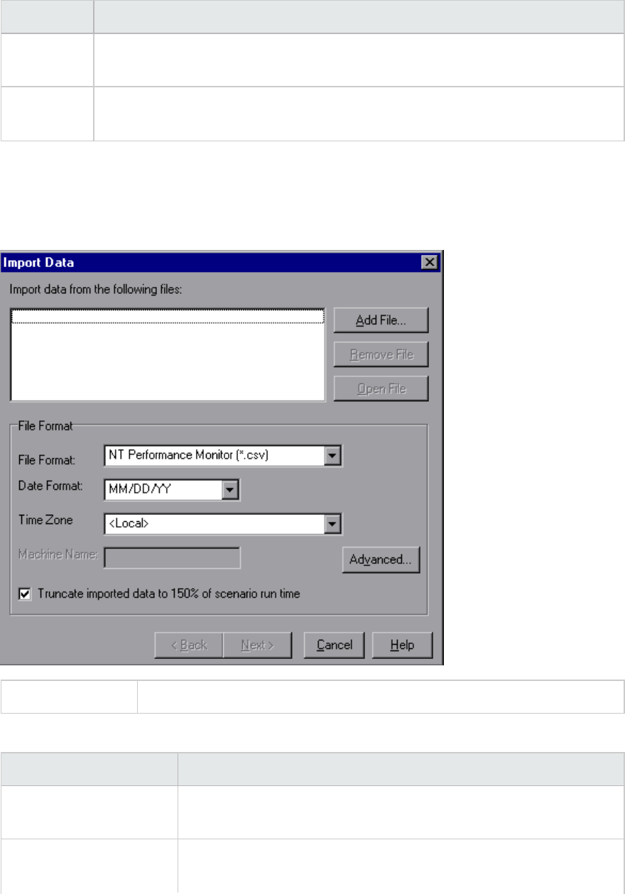
UI Element Description
to DOS
format
characters (Ascii character 10) in the UNIX file.
Skip the
first [] lines
Specify the number of lines at the start of the file to ignore before reading in data.
Typically, the first few lines in a file contain headings and sub-headings.
Import Data Dialog Box
This dialog box enables you to import and integrate non-HP data files into Analysis session.
To access Tools > External Monitors > Import Data
User interface elements are described below (unlabeled elements are shown in angle brackets):
UI Element Description
Import data from the
following files
Displays the files that you selected for import.
Add file Select an external data file to import. A dialog box opens to enable you
to select files.
User Guide
Analysis
HP LoadRunner (12.50) Page 383

UI Element Description
Remove file Delete an external data file from the list.
Open File Open an external data file using the associated application.
File Format Set the file format options.
lFile Format. Choose the format of the external data file. For an
explanation of available formats, see "Supported File Types" on
page378.
lDate Format. Specify the format of the date in the imported data
file. For example, for European dates with a 4 digit year, choose
DD/MM/YYYY.
Time Zone Select the time zone where the external data file was recorded.
LoadRunner Analysis compensates for the various international time
zones and aligns the times in the file with local time zone settings in
order to match LoadRunner results. If the times in the imported file are
erroneous by a constant offset, you can synchronize the time.
<Synchronize with
scenario start time>
Time Zone also contains the option <Synchronize with scenario start
time>. Choose this to align the earliest measurement found in the data
file to the start time of the LoadRunner scenario.
Machine Name Specify the machine name the monitor runs on. This associates the
machine name with the measurement. For example, a file IO rate on the
machine fender will be named File IO Rate:fender. This enables
you to apply Graph settings by the machine name. For more
information, see "Filtering and Sorting Graph Data" on page103.
Advanced For more information, see "Advanced Settings Dialog Box (Import Data
Dialog Box)" on page380.
Truncate imported data
to 150% of scenario
runtime
In certain cases, the external monitor may have collected data over a
time period that was larger than the actual load test. This option
deletes data that was collected while the load test was not running,
limiting the data collection period to 150% of the load testing period.
Troubleshooting and Limitations for Analysis
This section contains troubleshooting and limitations for Analysis.
User Guide
Analysis
HP LoadRunner (12.50) Page 384
General
lIf the behavior of Analysis is unpredictable and unexpected messages appear, this might be a result
of UAC Virtualization having been enabled for Analysis. You can disable UAC Virtualization on the
Analysis.exe process in the Windows Task Manager.
lAnalysis API works only on x86 platforms. If you are using Visual Studio, define the platform as x86 in
the project options.
lWhen analyzing results from a load test in which the Web Vusers accesses the AUT through a proxy
server, the Time to First Buffer Breakdown graph shows only zero values for Network Time and
Server Time. This is because the "time to first buffer" metric is turned off when working behind a
proxy, and the time values can only be calculated to the proxy server.
lLoad results that contain transactions with the '@' or ',' characters may conflict with existing
transactions. This is because Analysis attempts to replace those characters with the '_', and if this
results in a transaction name conflict, an error will occur.
Workaround: Avoid using the '@' and ',' characters in transaction names.
lThe following Analysis default settings have been modified: Include Think Time is disabled and
Display summary while generating complete data is enabled.
lWhen exporting Analysis reports to MS Word, the content load may affect the table format within the
document. The recommended format is RTF.
lIf the results take a long time to load, make sure that the Use cached file to store data option in
Tools > Options > General tab is disabled. You should only enable this for very large result files. For
details, see "General Tab (Options Dialog Box)" on page30.
Graphs
lWhen the Analysis results consists of a large number of similar measurements, you may experience
spikes in graphs, or an Out of memory message.
Workaround: For 64-bit Windows, make sure that you have 4 GB or more memory. F or 32-bit
Windows, Select Start > Run, and type msconfig. In the Boot tab, click Advanced Options. Select
Maximum memory and set it to the maximum value.
lAfter running a Language Pack, the Analysis data generated from the sample session (in the <LR
Installation>\tutorial folder) is displayed in English and filtering cannot be applied.
Workaround: Regenerate the graphs.
lThe Transaction Response Time (Percentile) graph may show inaccurate results.
Workaround: Follow these steps:
a. Close the Analysis application.
b. Open the C:\Program Files (x86)\HP\LoadRunner\bin\dat\percentile.def file
c. In the [Graph Definition] section, set BasicTableName to an empty string:
[Graph Definitions]
User Guide
Analysis
HP LoadRunner (12.50) Page 385
BasicTableName=
d. Open Analysis again and view the graph.
ALM Integration
lWhen trying to save an Analysis session to the ALM repository with CAC on IIS, you may encounter an
error message indicating that the session cannot be saved and that the connection is unavailable..
Workaround: Increase the size of the uploadReadAHeadSize parameter to 16 MB or higher, and
restart IIS. You can use the command line: C:\Windows\System32\inetsrv\appcmd.exe set
config "Default Web Site" -section:system.webServer/ServerRuntime
/uploadReadAheadSize:16777216 /commit:apphost
lAfter running a Language Pack, the Analysis data generated from the sample session (in the <LR
Installation>\tutorial folder) is displayed in English and filtering cannot be applied.
Workaround: Regenerate the graphs.
Microsoft SQL Server
lIf you are using your own policy in an MS SQL server, you may need to add your own account to the
Analysis database template (in the <LR Installation>\bin\dat folder).
lAnalysis may fail to load results created through an MS SQL database, if the decimal separator on the
Analysis machine is different from the decimal separator on the MS SQL Server machine (common on
non-English operating systems).
Workaround:Change the decimal separator on Analysis machine to be the same as the MS SQL Server
machine.
lFiltering of transactions for MS Access and SQL queries is limited to 100 transactions.
lIf you are using Microsoft SQL Server 2000, you need to either migrate Analysis data, or upgrade to
Microsoft SQL Server 2005. The following tasks describe how to migrate and upgrade.
To migrate legacy Analysis data to a SQL 2005 server:
1. From the SQL Server Management Studio, using Object Explorer, connect to an instance of SQL
Server Database Engine.
2. Expand Databases, right-click Analysis database, select Tasks\Copy Database.
3. Follow the instructions in the wizard.
To upgrade SQL 2000 to SQL 2005:
1. Uninstall SQL 2000.
2. Install SQL 2005.
3. Restore Analysis data from backup. (http://msdn.microsoft.com/en-us/library/ms177429
(SQL.90).aspx)
User Guide
Analysis
HP LoadRunner (12.50) Page 386

Analysis APIReference
The HP LoadRunner Analysis API set can be used for unattended creating of an Analysis session or for
custom extraction of data from the results of a test run under the Controller.
You can only view this help from a machine with LoadRunner. Go to Start > All Programs > HP Software
> HP LoadRunner > Documentation > Analysis API Reference. In icon-based desktops, such as
Windows 8, search for API and select Analysis API Reference from the results.
Note: The Analysis API is only supported for 32-bit environments. If you use Visual Studio to
develop your script, make sure to define x86 as the platform in the project options.
Send Us Feedback
Let us know how we can improve your experience with the User Guide.
Send your email to:sw-doc@hp.com
User Guide
Analysis APIReference
HP LoadRunner (12.50) Page 387
