Hadoop Beginner Guide
Hadoop%20%20Beginner%20Guide
Hadoop%20%20Beginner%20Guide
hadoop_-beginners-guide
Hadoop_%20Beginner's%20Guide
User Manual: Pdf
Open the PDF directly: View PDF ![]() .
.
Page Count: 398 [warning: Documents this large are best viewed by clicking the View PDF Link!]
- Cover
- Copyright
- Credits
- About the Author
- About the Reviewers
- www.PacktPub.com
- Table of Contents
- Preface
- Chapter 1: What It's All About
- Chapter 2: Getting Hadoop Up and Running
- Hadoop on a local Ubuntu host
- Time for action – checking the prerequisites
- Time for action – downloading Hadoop
- Time for action – setting up SSH
- Time for action – using Hadoop to calculate Pi
- Time for action – configuring the pseudo-distributed mode
- Time for action – changing the base HDFS directory
- Time for action – formatting the NameNode
- Time for action – starting Hadoop
- Time for action – using HDFS
- Time for action – WordCount, the Hello World of MapReduce
- Using Elastic MapReduce
- Time for action – WordCount on EMR using the management console
- Comparison of local versus EMR Hadoop
- Summary
- Chapter 3: Understanding MapReduce
- Key/value pairs
- The Hadoop Java API for MapReduce
- Writing MapReduce programs
- Time for action – setting up the classpath
- Time for action – implementing WordCount
- Time for action – building a JAR file
- Time for action – running WordCount on a local Hadoop cluster
- Time for action – running WordCount on EMR
- Time for action – WordCount the easy way
- Walking through a run of WordCount
- Time for action – WordCount with a combiner
- Time for action – fixing WordCount to work with a combiner
- Hadoop-specific data types
- Time for action – using the Writable wrapper classes
- Input/output
- Summary
- Chapter 4: Developing MapReduce Programs
- Using languages other than Java with Hadoop
- Time for action – WordCount using Streaming
- Analyzing a large dataset
- Time for action – summarizing the UFO data
- Time for action – summarizing the shape data
- Time for action – correlation of sighting duration to UFO shape
- Time for action – performing the shape/time analysis from the command line
- Time for action – using ChainMapper for field validation/analysis
- Time for action – using the Distributed Cache to improve location output
- Counters, status, and other output
- Time for action – creating counters, task states, and writing log output
- Summary
- Chapter 5: Advanced MapReduce Techniques
- Simple, advanced, and in-between
- Joins
- Time for action – reduce-side join using MultipleInputs
- Graph algorithms
- Time for action – representing the graph
- Time for action – creating the source code
- Time for action – the first run
- Time for action – The second run
- Time for action – the third run
- Time for action – the fourth and last run
- Using language-independent data structures
- Time for action – getting and installing Avro
- Time for action – defining the schema
- Time for action – creating the source Avro data with Ruby
- Time for action – consuming the Avro data with Java
- Time for action – generating shape summaries in MapReduce
- Time for action – examining the output data with Ruby
- Time for action – examining the output data with Java
- Summary
- Chapter 6: When Things Break
- Failure
- Time for action – killing a DataNode process
- Time for action – the replication factor in action
- Time for action – intentionally causing missing blocks
- Time for action – killing a TaskTracker process
- Time for action – killing the JobTracker
- Time for action – killing the NameNode process
- Starting a replacement NameNode
- The role of the NameNode in more detail
- File systems, files, blocks, and nodes
- The single most important piece of data in the cluster – fsimage
- DataNode startup
- Safe mode
- SecondaryNameNode
- So what to do when the NameNode process has a critical failure?
- BackupNode/CheckpointNode and NameNode HA
- Hardware failures
- Host failure
- Host corruption
- The risk of correlated failures
- Task failures due to software
- Starting a replacement NameNode
- Time for action – causing task failures
- Time for action – handling dirty data by using skip mode
- Summary
- Chapter 7: Keeping Things Running
- A note on EMR
- Hadoop configuration properties
- Time for action – browsing default properties
- Setting up a cluster
- Time for action – examining the default rack configuration
- Time for action – adding a rack awareness script
- Cluster access control
- Time for action – demonstrating the default security
- Managing the NameNode
- Time for action – adding an additional fsimage location
- Time for action – swapping to a new NameNode host
- Managing HDFS
- MapReduce management
- Time for action – changing job priorities and killing a job
- Scaling
- Summary
- Chapter 8: A Relational View on Data with Hive
- Overview of Hive
- Setting up Hive
- Time for action – installing Hive
- Using Hive
- Time for action – creating a table for the UFO data
- Time for action – inserting the UFO data
- Time for action – validating the table
- Time for action – redefining the table with the correct column separator
- Time for action – creating a table from an existing file
- Time for action - performing a join
- Time for action - using views
- Time for action – exporting query output
- Time for action – making a partitioned UFO sighting table
- Time for action – adding a new User Defined Function (UDF)
- Hive on Amazon Web Services
- Time for action – running UFO analysis on EMR
- Summary
- Chapter 9: Working with Relational Databases
- Common data paths
- Setting up MySQL
- Time for action – installing and setting up MySQL
- Time for action – configuring MySQL to allow remote connections
- Time for action – setting up the employee database
- Getting data into Hadoop
- Time for action – downloading and configuring Sqoop
- Time for action – exporting data from MySQL to HDFS
- Time for action – exporting data from MySQL into Hive
- Time for action – a more selective import
- Time for action – using a type mapping
- Time for action – importing data from a raw query
- Getting data out of Hadoop
- Time for action – importing data from Hadoop into MySQL
- Time for action – importing Hive data into MySQL
- Time for action – fixing the mapping and re-running the export
- AWS considerations
- Summary
- Chapter 10: Data Collection with Flume
- A note about AWS
- Data data everywhere
- Time for action – getting web server data into Hadoop
- Introducing Apache Flume
- Time for action – installing and configuring Flume
- Time for action – capturing network traffic to a log file
- Time for action – logging to the console
- Time for action – capturing the output of a command to a flat file
- Time for action – capturing a remote file to a local flat file
- Time for action – writing network traffic onto HDFS
- Time for action – adding timestamps
- Time for action – multi-level Flume networks
- Time for action – writing to multiple sinks
- The bigger picture
- Summary
- Chapter 11: Where to Go Next
- Appendix: Pop Quiz Answers
- Index


Hadoop Beginner's Guide
Copyright © 2013 Packt Publishing
All rights reserved. No part of this book may be reproduced, stored in a retrieval system,
or transmied in any form or by any means, without the prior wrien permission of the
publisher, except in the case of brief quotaons embedded in crical arcles or reviews.
Every eort has been made in the preparaon of this book to ensure the accuracy of the
informaon presented. However, the informaon contained in this book is sold without
warranty, either express or implied. Neither the author, nor Packt Publishing, and its dealers
and distributors will be held liable for any damages caused or alleged to be caused directly or
indirectly by this book.
Packt Publishing has endeavored to provide trademark informaon about all of the
companies and products menoned in this book by the appropriate use of capitals.
However, Packt Publishing cannot guarantee the accuracy of this informaon.
First published: February 2013
Producon Reference: 1150213
Published by Packt Publishing Ltd.
Livery Place
35 Livery Street
Birmingham B3 2PB, UK.
ISBN 978-1-84951-7-300
www.packtpub.com
Cover Image by Asher Wishkerman (a.wishkerman@mpic.de)
www.it-ebooks.info

Credits
Author
Garry Turkington
Reviewers
David Gruzman
Muthusamy Manigandan
Vidyasagar N V
Acquision Editor
Robin de Jongh
Lead Technical Editor
Azharuddin Sheikh
Technical Editors
Ankita Meshram
Varun Pius Rodrigues
Copy Editors
Brandt D'Mello
Aditya Nair
Laxmi Subramanian
Ruta Waghmare
Project Coordinator
Leena Purkait
Proofreader
Maria Gould
Indexer
Hemangini Bari
Producon Coordinator
Nitesh Thakur
Cover Work
Nitesh Thakur
www.it-ebooks.info

About the Author
Garry Turkington has 14 years of industry experience, most of which has been focused
on the design and implementaon of large-scale distributed systems. In his current roles as
VP Data Engineering and Lead Architect at Improve Digital, he is primarily responsible for
the realizaon of systems that store, process, and extract value from the company's large
data volumes. Before joining Improve Digital, he spent me at Amazon.co.uk, where he led
several soware development teams building systems that process Amazon catalog data for
every item worldwide. Prior to this, he spent a decade in various government posions in
both the UK and USA.
He has BSc and PhD degrees in Computer Science from the Queens University of Belfast in
Northern Ireland and an MEng in Systems Engineering from Stevens Instute of Technology
in the USA.
I would like to thank my wife Lea for her support and encouragement—not
to menon her paence—throughout the wring of this book and my
daughter, Maya, whose spirit and curiosity is more of an inspiraon than
she could ever imagine.
www.it-ebooks.info
About the Reviewers
David Gruzman is a Hadoop and big data architect with more than 18 years of hands-on
experience, specializing in the design and implementaon of scalable high-performance
distributed systems. He has extensive experse of OOA/OOD and (R)DBMS technology. He
is an Agile methodology adept and strongly believes that a daily coding roune makes good
soware architects. He is interested in solving challenging problems related to real-me
analycs and the applicaon of machine learning algorithms to the big data sets.
He founded—and is working with—BigDataCra.com, a bouque consulng rm in the area
of big data. Visit their site at www.bigdatacraft.com. David can be contacted at david@
bigdatacraft.com. More detailed informaon about his skills and experience can be
found at http://www.linkedin.com/in/davidgruzman.
Muthusamy Manigandan is a systems architect for a startup. Prior to this, he was a Sta
Engineer at VMWare and Principal Engineer with Oracle. Mani has been programming for
the past 14 years on large-scale distributed-compung applicaons. His areas of interest are
machine learning and algorithms.
www.it-ebooks.info

Vidyasagar N V has been interested in computer science since an early age. Some of his
serious work in computers and computer networks began during his high school days. Later,
he went to the presgious Instute Of Technology, Banaras Hindu University, for his B.Tech.
He has been working as a soware developer and data expert, developing and building
scalable systems. He has worked with a variety of second, third, and fourth generaon
languages. He has worked with at les, indexed les, hierarchical databases, network
databases, relaonal databases, NoSQL databases, Hadoop, and related technologies.
Currently, he is working as Senior Developer at Collecve Inc., developing big data-based
structured data extracon techniques from the Web and local informaon. He enjoys
producing high-quality soware and web-based soluons and designing secure and
scalable data systems. He can be contacted at vidyasagar1729@gmail.com.
I would like to thank the Almighty, my parents, Mr. N Srinivasa Rao and
Mrs. Latha Rao, and my family who supported and backed me throughout
my life. I would also like to thank my friends for being good friends and
all those people willing to donate their me, eort, and experse by
parcipang in open source soware projects. Thank you, Packt Publishing
for selecng me as one of the technical reviewers for this wonderful book.
It is my honor to be a part of it.
www.it-ebooks.info

www.PacktPub.com
Support les, eBooks, discount offers and more
You might want to visit www.PacktPub.com for support les and downloads related
to your book.
Did you know that Packt oers eBook versions of every book published, with PDF and ePub
les available? You can upgrade to the eBook version at www.PacktPub.com and as a
print book customer, you are entled to a discount on the eBook copy. Get in touch with
us at service@packtpub.com for more details.
At www.PacktPub.com, you can also read a collecon of free technical arcles, sign
up for a range of free newsleers and receive exclusive discounts and oers on Packt
books and eBooks.
http://PacktLib.PacktPub.com
Do you need instant soluons to your IT quesons? PacktLib is Packt's online digital book
library. Here, you can access, read and search across Packt's enre library of books.
Why Subscribe?
Fully searchable across every book published by Packt
Copy and paste, print and bookmark content
On demand and accessible via web browser
Free Access for Packt account holders
If you have an account with Packt at www.PacktPub.com, you can use this to access
PacktLib today and view nine enrely free books. Simply use your login credenals for
immediate access.
www.it-ebooks.info

Table of Contents
Preface 1
Chapter 1: What It's All About 7
Big data processing 8
The value of data 8
Historically for the few and not the many 9
Classic data processing systems 9
Liming factors 10
A dierent approach 11
All roads lead to scale-out 11
Share nothing 11
Expect failure 12
Smart soware, dumb hardware 13
Move processing, not data 13
Build applicaons, not infrastructure 14
Hadoop 15
Thanks, Google 15
Thanks, Doug 15
Thanks, Yahoo 15
Parts of Hadoop 15
Common building blocks 16
HDFS 16
MapReduce 17
Beer together 18
Common architecture 19
What it is and isn't good for 19
Cloud compung with Amazon Web Services 20
Too many clouds 20
A third way 20
Dierent types of costs 21
AWS – infrastructure on demand from Amazon 22
Elasc Compute Cloud (EC2) 22
Simple Storage Service (S3) 22
www.it-ebooks.info

Table of Contents
[ ii ]
Elasc MapReduce (EMR) 22
What this book covers 23
A dual approach 23
Summary 24
Chapter 2: Geng Hadoop Up and Running 25
Hadoop on a local Ubuntu host 25
Other operang systems 26
Time for acon – checking the prerequisites 26
Seng up Hadoop 27
A note on versions 27
Time for acon – downloading Hadoop 28
Time for acon – seng up SSH 29
Conguring and running Hadoop 30
Time for acon – using Hadoop to calculate Pi 30
Three modes 32
Time for acon – conguring the pseudo-distributed mode 32
Conguring the base directory and formang the lesystem 34
Time for acon – changing the base HDFS directory 34
Time for acon – formang the NameNode 35
Starng and using Hadoop 36
Time for acon – starng Hadoop 36
Time for acon – using HDFS 38
Time for acon – WordCount, the Hello World of MapReduce 39
Monitoring Hadoop from the browser 42
The HDFS web UI 42
Using Elasc MapReduce 45
Seng up an account on Amazon Web Services 45
Creang an AWS account 45
Signing up for the necessary services 45
Time for acon – WordCount in EMR using the management console 46
Other ways of using EMR 54
AWS credenals 54
The EMR command-line tools 54
The AWS ecosystem 55
Comparison of local versus EMR Hadoop 55
Summary 56
Chapter 3: Understanding MapReduce 57
Key/value pairs 57
What it mean 57
Why key/value data? 58
Some real-world examples 59
MapReduce as a series of key/value transformaons 59
www.it-ebooks.info

Table of Contents
[ iii ]
The Hadoop Java API for MapReduce 60
The 0.20 MapReduce Java API 61
The Mapper class 61
The Reducer class 62
The Driver class 63
Wring MapReduce programs 64
Time for acon – seng up the classpath 65
Time for acon – implemenng WordCount 65
Time for acon – building a JAR le 68
Time for acon – running WordCount on a local Hadoop cluster 68
Time for acon – running WordCount on EMR 69
The pre-0.20 Java MapReduce API 72
Hadoop-provided mapper and reducer implementaons 73
Time for acon – WordCount the easy way 73
Walking through a run of WordCount 75
Startup 75
Spling the input 75
Task assignment 75
Task startup 76
Ongoing JobTracker monitoring 76
Mapper input 76
Mapper execuon 77
Mapper output and reduce input 77
Paroning 77
The oponal paron funcon 78
Reducer input 78
Reducer execuon 79
Reducer output 79
Shutdown 79
That's all there is to it! 80
Apart from the combiner…maybe 80
Why have a combiner? 80
Time for acon – WordCount with a combiner 80
When you can use the reducer as the combiner 81
Time for acon – xing WordCount to work with a combiner 81
Reuse is your friend 82
Hadoop-specic data types 83
The Writable and WritableComparable interfaces 83
Introducing the wrapper classes 84
Primive wrapper classes 85
Array wrapper classes 85
Map wrapper classes 85
www.it-ebooks.info

Table of Contents
[ iv ]
Time for acon – using the Writable wrapper classes 86
Other wrapper classes 88
Making your own 88
Input/output 88
Files, splits, and records 89
InputFormat and RecordReader 89
Hadoop-provided InputFormat 90
Hadoop-provided RecordReader 90
Output formats and RecordWriter 91
Hadoop-provided OutputFormat 91
Don't forget Sequence les 91
Summary 92
Chapter 4: Developing MapReduce Programs 93
Using languages other than Java with Hadoop 94
How Hadoop Streaming works 94
Why to use Hadoop Streaming 94
Time for acon – WordCount using Streaming 95
Dierences in jobs when using Streaming 97
Analyzing a large dataset 98
Geng the UFO sighng dataset 98
Geng a feel for the dataset 99
Time for acon – summarizing the UFO data 99
Examining UFO shapes 101
Time for acon – summarizing the shape data 102
Time for acon – correlang sighng duraon to UFO shape 103
Using Streaming scripts outside Hadoop 106
Time for acon – performing the shape/me analysis from the command line 107
Java shape and locaon analysis 107
Time for acon – using ChainMapper for eld validaon/analysis 108
Too many abbreviaons 112
Using the Distributed Cache 113
Time for acon – using the Distributed Cache to improve locaon output 114
Counters, status, and other output 117
Time for acon – creang counters, task states, and wring log output 118
Too much informaon! 125
Summary 126
Chapter 5: Advanced MapReduce Techniques 127
Simple, advanced, and in-between 127
Joins 128
www.it-ebooks.info

Table of Contents
[ v ]
When this is a bad idea 128
Map-side versus reduce-side joins 128
Matching account and sales informaon 129
Time for acon – reduce-side joins using MulpleInputs 129
DataJoinMapper and TaggedMapperOutput 134
Implemenng map-side joins 135
Using the Distributed Cache 135
Pruning data to t in the cache 135
Using a data representaon instead of raw data 136
Using mulple mappers 136
To join or not to join... 137
Graph algorithms 137
Graph 101 138
Graphs and MapReduce – a match made somewhere 138
Represenng a graph 139
Time for acon – represenng the graph 140
Overview of the algorithm 140
The mapper 141
The reducer 141
Iterave applicaon 141
Time for acon – creang the source code 142
Time for acon – the rst run 146
Time for acon – the second run 147
Time for acon – the third run 148
Time for acon – the fourth and last run 149
Running mulple jobs 151
Final thoughts on graphs 151
Using language-independent data structures 151
Candidate technologies 152
Introducing Avro 152
Time for acon – geng and installing Avro 152
Avro and schemas 154
Time for acon – dening the schema 154
Time for acon – creang the source Avro data with Ruby 155
Time for acon – consuming the Avro data with Java 156
Using Avro within MapReduce 158
Time for acon – generang shape summaries in MapReduce 158
Time for acon – examining the output data with Ruby 163
Time for acon – examining the output data with Java 163
Going further with Avro 165
Summary 166
www.it-ebooks.info

Table of Contents
[ vi ]
Chapter 6: When Things Break 167
Failure 167
Embrace failure 168
Or at least don't fear it 168
Don't try this at home 168
Types of failure 168
Hadoop node failure 168
The dfsadmin command 169
Cluster setup, test les, and block sizes 169
Fault tolerance and Elasc MapReduce 170
Time for acon – killing a DataNode process 170
NameNode and DataNode communicaon 173
Time for acon – the replicaon factor in acon 174
Time for acon – intenonally causing missing blocks 176
When data may be lost 178
Block corrupon 179
Time for acon – killing a TaskTracker process 180
Comparing the DataNode and TaskTracker failures 183
Permanent failure 184
Killing the cluster masters 184
Time for acon – killing the JobTracker 184
Starng a replacement JobTracker 185
Time for acon – killing the NameNode process 186
Starng a replacement NameNode 188
The role of the NameNode in more detail 188
File systems, les, blocks, and nodes 188
The single most important piece of data in the cluster – fsimage 189
DataNode startup 189
Safe mode 190
SecondaryNameNode 190
So what to do when the NameNode process has a crical failure? 190
BackupNode/CheckpointNode and NameNode HA 191
Hardware failure 191
Host failure 191
Host corrupon 192
The risk of correlated failures 192
Task failure due to soware 192
Failure of slow running tasks 192
Time for acon – causing task failure 193
Hadoop's handling of slow-running tasks 195
Speculave execuon 195
Hadoop's handling of failing tasks 195
Task failure due to data 196
Handling dirty data through code 196
Using Hadoop's skip mode 197
www.it-ebooks.info

Table of Contents
[ vii ]
Time for acon – handling dirty data by using skip mode 197
To skip or not to skip... 202
Summary 202
Chapter 7: Keeping Things Running 205
A note on EMR 206
Hadoop conguraon properes 206
Default values 206
Time for acon – browsing default properes 206
Addional property elements 208
Default storage locaon 208
Where to set properes 209
Seng up a cluster 209
How many hosts? 210
Calculang usable space on a node 210
Locaon of the master nodes 211
Sizing hardware 211
Processor / memory / storage rao 211
EMR as a prototyping plaorm 212
Special node requirements 213
Storage types 213
Commodity versus enterprise class storage 214
Single disk versus RAID 214
Finding the balance 214
Network storage 214
Hadoop networking conguraon 215
How blocks are placed 215
Rack awareness 216
Time for acon – examining the default rack conguraon 216
Time for acon – adding a rack awareness script 217
What is commodity hardware anyway? 219
Cluster access control 220
The Hadoop security model 220
Time for acon – demonstrang the default security 220
User identy 223
More granular access control 224
Working around the security model via physical access control 224
Managing the NameNode 224
Conguring mulple locaons for the fsimage class 225
Time for acon – adding an addional fsimage locaon 225
Where to write the fsimage copies 226
Swapping to another NameNode host 227
Having things ready before disaster strikes 227
www.it-ebooks.info

Table of Contents
[ viii ]
Time for acon – swapping to a new NameNode host 227
Don't celebrate quite yet! 229
What about MapReduce? 229
Managing HDFS 230
Where to write data 230
Using balancer 230
When to rebalance 230
MapReduce management 231
Command line job management 231
Job priories and scheduling 231
Time for acon – changing job priories and killing a job 232
Alternave schedulers 233
Capacity Scheduler 233
Fair Scheduler 234
Enabling alternave schedulers 234
When to use alternave schedulers 234
Scaling 235
Adding capacity to a local Hadoop cluster 235
Adding capacity to an EMR job ow 235
Expanding a running job ow 235
Summary 236
Chapter 8: A Relaonal View on Data with Hive 237
Overview of Hive 237
Why use Hive? 238
Thanks, Facebook! 238
Seng up Hive 238
Prerequisites 238
Geng Hive 239
Time for acon – installing Hive 239
Using Hive 241
Time for acon – creang a table for the UFO data 241
Time for acon – inserng the UFO data 244
Validang the data 246
Time for acon – validang the table 246
Time for acon – redening the table with the correct column separator 248
Hive tables – real or not? 250
Time for acon – creang a table from an exisng le 250
Time for acon – performing a join 252
Hive and SQL views 254
Time for acon – using views 254
Handling dirty data in Hive 257
www.it-ebooks.info

Table of Contents
[ ix ]
Time for acon – exporng query output 258
Paroning the table 260
Time for acon – making a paroned UFO sighng table 260
Buckeng, clustering, and sorng... oh my! 264
User Dened Funcon 264
Time for acon – adding a new User Dened Funcon (UDF) 265
To preprocess or not to preprocess... 268
Hive versus Pig 269
What we didn't cover 269
Hive on Amazon Web Services 270
Time for acon – running UFO analysis on EMR 270
Using interacve job ows for development 277
Integraon with other AWS products 278
Summary 278
Chapter 9: Working with Relaonal Databases 279
Common data paths 279
Hadoop as an archive store 280
Hadoop as a preprocessing step 280
Hadoop as a data input tool 281
The serpent eats its own tail 281
Seng up MySQL 281
Time for acon – installing and seng up MySQL 281
Did it have to be so hard? 284
Time for acon – conguring MySQL to allow remote connecons 285
Don't do this in producon! 286
Time for acon – seng up the employee database 286
Be careful with data le access rights 287
Geng data into Hadoop 287
Using MySQL tools and manual import 288
Accessing the database from the mapper 288
A beer way – introducing Sqoop 289
Time for acon – downloading and conguring Sqoop 289
Sqoop and Hadoop versions 290
Sqoop and HDFS 291
Time for acon – exporng data from MySQL to HDFS 291
Sqoop's architecture 294
Imporng data into Hive using Sqoop 294
Time for acon – exporng data from MySQL into Hive 295
Time for acon – a more selecve import 297
Datatype issues 298
www.it-ebooks.info

Table of Contents
[ x ]
Time for acon – using a type mapping 299
Time for acon – imporng data from a raw query 300
Sqoop and Hive parons 302
Field and line terminators 302
Geng data out of Hadoop 303
Wring data from within the reducer 303
Wring SQL import les from the reducer 304
A beer way – Sqoop again 304
Time for acon – imporng data from Hadoop into MySQL 304
Dierences between Sqoop imports and exports 306
Inserts versus updates 307
Sqoop and Hive exports 307
Time for acon – imporng Hive data into MySQL 308
Time for acon – xing the mapping and re-running the export 310
Other Sqoop features 312
AWS consideraons 313
Considering RDS 313
Summary 314
Chapter 10: Data Collecon with Flume 315
A note about AWS 315
Data data everywhere 316
Types of data 316
Geng network trac into Hadoop 316
Time for acon – geng web server data into Hadoop 316
Geng les into Hadoop 318
Hidden issues 318
Keeping network data on the network 318
Hadoop dependencies 318
Reliability 318
Re-creang the wheel 318
A common framework approach 319
Introducing Apache Flume 319
A note on versioning 319
Time for acon – installing and conguring Flume 320
Using Flume to capture network data 321
Time for acon – capturing network trac to a log le 321
Time for acon – logging to the console 324
Wring network data to log les 326
Time for acon – capturing the output of a command in a at le 326
Logs versus les 327
Time for acon – capturing a remote le in a local at le 328
Sources, sinks, and channels 330
www.it-ebooks.info

Table of Contents
[ xi ]
Sources 330
Sinks 330
Channels 330
Or roll your own 331
Understanding the Flume conguraon les 331
It's all about events 332
Time for acon – wring network trac onto HDFS 333
Time for acon – adding mestamps 335
To Sqoop or to Flume... 337
Time for acon – mul level Flume networks 338
Time for acon – wring to mulple sinks 340
Selectors replicang and mulplexing 342
Handling sink failure 342
Next, the world 343
The bigger picture 343
Data lifecycle 343
Staging data 344
Scheduling 344
Summary 345
Chapter 11: Where to Go Next 347
What we did and didn't cover in this book 347
Upcoming Hadoop changes 348
Alternave distribuons 349
Why alternave distribuons? 349
Bundling 349
Free and commercial extensions 349
Choosing a distribuon 351
Other Apache projects 352
HBase 352
Oozie 352
Whir 353
Mahout 353
MRUnit 354
Other programming abstracons 354
Pig 354
Cascading 354
AWS resources 355
HBase on EMR 355
SimpleDB 355
DynamoDB 355
www.it-ebooks.info

Preface
This book is here to help you make sense of Hadoop and use it to solve your big data
problems. It's a really excing me to work with data processing technologies such as
Hadoop. The ability to apply complex analycs to large data sets—once the monopoly of
large corporaons and government agencies—is now possible through free open source
soware (OSS).
But because of the seeming complexity and pace of change in this area, geng a grip on
the basics can be somewhat inmidang. That's where this book comes in, giving you an
understanding of just what Hadoop is, how it works, and how you can use it to extract
value from your data now.
In addion to an explanaon of core Hadoop, we also spend several chapters exploring
other technologies that either use Hadoop or integrate with it. Our goal is to give you an
understanding not just of what Hadoop is but also how to use it as a part of your broader
technical infrastructure.
A complementary technology is the use of cloud compung, and in parcular, the oerings
from Amazon Web Services. Throughout the book, we will show you how to use these
services to host your Hadoop workloads, demonstrang that not only can you process
large data volumes, but also you don't actually need to buy any physical hardware to do so.
What this book covers
This book comprises of three main parts: chapters 1 through 5, which cover the core of
Hadoop and how it works, chapters 6 and 7, which cover the more operaonal aspects
of Hadoop, and chapters 8 through 11, which look at the use of Hadoop alongside other
products and technologies.
www.it-ebooks.info

Preface
[ 2 ]
Chapter 1, What It's All About, gives an overview of the trends that have made Hadoop and
cloud compung such important technologies today.
Chapter 2, Geng Hadoop Up and Running, walks you through the inial setup of a local
Hadoop cluster and the running of some demo jobs. For comparison, the same work is also
executed on the hosted Hadoop Amazon service.
Chapter 3, Understanding MapReduce, goes inside the workings of Hadoop to show how
MapReduce jobs are executed and shows how to write applicaons using the Java API.
Chapter 4, Developing MapReduce Programs, takes a case study of a moderately sized data
set to demonstrate techniques to help when deciding how to approach the processing and
analysis of a new data source.
Chapter 5, Advanced MapReduce Techniques, looks at a few more sophiscated ways of
applying MapReduce to problems that don't necessarily seem immediately applicable to the
Hadoop processing model.
Chapter 6, When Things Break, examines Hadoop's much-vaunted high availability and fault
tolerance in some detail and sees just how good it is by intenonally causing havoc through
killing processes and intenonally using corrupt data.
Chapter 7, Keeping Things Running, takes a more operaonal view of Hadoop and will be
of most use for those who need to administer a Hadoop cluster. Along with demonstrang
some best pracce, it describes how to prepare for the worst operaonal disasters so you
can sleep at night.
Chapter 8, A Relaonal View On Data With Hive, introduces Apache Hive, which allows
Hadoop data to be queried with a SQL-like syntax.
Chapter 9, Working With Relaonal Databases, explores how Hadoop can be integrated with
exisng databases, and in parcular, how to move data from one to the other.
Chapter 10, Data Collecon with Flume, shows how Apache Flume can be used to gather
data from mulple sources and deliver it to desnaons such as Hadoop.
Chapter 11, Where To Go Next, wraps up the book with an overview of the broader Hadoop
ecosystem, highlighng other products and technologies of potenal interest. In addion, it
gives some ideas on how to get involved with the Hadoop community and to get help.
What you need for this book
As we discuss the various Hadoop-related soware packages used in this book, we will
describe the parcular requirements for each chapter. However, you will generally need
somewhere to run your Hadoop cluster.
www.it-ebooks.info

Preface
[ 3 ]
In the simplest case, a single Linux-based machine will give you a plaorm to explore almost
all the exercises in this book. We assume you have a recent distribuon of Ubuntu, but as
long as you have command-line Linux familiarity any modern distribuon will suce.
Some of the examples in later chapters really need mulple machines to see things working,
so you will require access to at least four such hosts. Virtual machines are completely
acceptable; they're not ideal for producon but are ne for learning and exploraon.
Since we also explore Amazon Web Services in this book, you can run all the examples on
EC2 instances, and we will look at some other more Hadoop-specic uses of AWS throughout
the book. AWS services are usable by anyone, but you will need a credit card to sign up!
Who this book is for
We assume you are reading this book because you want to know more about Hadoop at
a hands-on level; the key audience is those with soware development experience but no
prior exposure to Hadoop or similar big data technologies.
For developers who want to know how to write MapReduce applicaons, we assume you are
comfortable wring Java programs and are familiar with the Unix command-line interface.
We will also show you a few programs in Ruby, but these are usually only to demonstrate
language independence, and you don't need to be a Ruby expert.
For architects and system administrators, the book also provides signicant value in
explaining how Hadoop works, its place in the broader architecture, and how it can be
managed operaonally. Some of the more involved techniques in Chapter 4, Developing
MapReduce Programs, and Chapter 5, Advanced MapReduce Techniques, are probably
of less direct interest to this audience.
Conventions
In this book, you will nd several headings appearing frequently.
To give clear instrucons of how to complete a procedure or task, we use:
Time for action – heading
1. Acon 1
2. Acon 2
3. Acon 3
Instrucons oen need some extra explanaon so that they make sense, so they are
followed with:
www.it-ebooks.info

Preface
[ 4 ]
What just happened?
This heading explains the working of tasks or instrucons that you have just completed.
You will also nd some other learning aids in the book, including:
Pop quiz – heading
These are short mulple-choice quesons intended to help you test your own
understanding.
Have a go hero – heading
These set praccal challenges and give you ideas for experimenng with what you
have learned.
You will also nd a number of styles of text that disnguish between dierent kinds of
informaon. Here are some examples of these styles, and an explanaon of their meaning.
Code words in text are shown as follows: "You may noce that we used the Unix command
rm to remove the Drush directory rather than the DOS del command."
A block of code is set as follows:
# * Fine Tuning
#
key_buffer = 16M
key_buffer_size = 32M
max_allowed_packet = 16M
thread_stack = 512K
thread_cache_size= 8
max_connections= 300
When we wish to draw your aenon to a parcular part of a code block, the relevant lines
or items are set in bold:
# * Fine Tuning
#
key_buffer = 16M
key_buffer_size = 32M
max_allowed_packet = 16M
thread_stack = 512K
thread_cache_size= 8
max_connections= 300
www.it-ebooks.info

Preface
[ 5 ]
Any command-line input or output is wrien as follows:
cd /ProgramData/Propeople
rm -r Drush
git clone --branch master http://git.drupal.org/project/drush.git
Newterms and important words are shown in bold. Words that you see on the screen, in
menus or dialog boxes for example, appear in the text like this: "On the Select Desnaon
Locaon screen, click on Next to accept the default desnaon."
Warnings or important notes appear in a box like this.
Tips and tricks appear like this.
Reader feedback
Feedback from our readers is always welcome. Let us know what you think about this
book—what you liked or may have disliked. Reader feedback is important for us to
develop tles that you really get the most out of.
To send us general feedback, simply send an e-mail to feedback@packtpub.com,
and menon the book tle through the subject of your message.
If there is a topic that you have experse in and you are interested in either wring or
contribung to a book, see our author guide on www.packtpub.com/authors.
Customer support
Now that you are the proud owner of a Packt book, we have a number of things to help you
to get the most from your purchase.
Downloading the example code
You can download the example code les for all Packt books you have purchased from
your account at http://www.packtpub.com. If you purchased this book elsewhere,
you can visit http://www.packtpub.com/support and register to have the les
e-mailed directly to you.
www.it-ebooks.info

Preface
[ 6 ]
Errata
Although we have taken every care to ensure the accuracy of our content, mistakes
do happen. If you nd a mistake in one of our books—maybe a mistake in the text or the
code—we would be grateful if you would report this to us. By doing so, you can save other
readers from frustraon and help us improve subsequent versions of this book. If you nd
any errata, please report them by vising http://www.packtpub.com/submit-errata,
selecng your book, clicking on the errata submission form link, and entering the details of
your errata. Once your errata are veried, your submission will be accepted and the errata
will be uploaded to our website, or added to any list of exisng errata, under the Errata
secon of that tle.
Piracy
Piracy of copyright material on the Internet is an ongoing problem across all media.
At Packt, we take the protecon of our copyright and licenses very seriously. If you come
across any illegal copies of our works, in any form, on the Internet, please provide us with
the locaon address or website name immediately so that we can pursue a remedy.
Please contact us at copyright@packtpub.com with a link to the suspected
pirated material.
We appreciate your help in protecng our authors, and our ability to bring you
valuable content.
Questions
You can contact us at questions@packtpub.com if you are having a problem with any
aspect of the book, and we will do our best to address it.
www.it-ebooks.info

1
What It's All About
This book is about Hadoop, an open source framework for large-scale data
processing. Before we get into the details of the technology and its use in later
chapters, it is important to spend a little time exploring the trends that led to
Hadoop's creation and its enormous success.
Hadoop was not created in a vacuum; instead, it exists due to the explosion
in the amount of data being created and consumed and a shift that sees this
data deluge arrive at small startups and not just huge multinationals. At the
same time, other trends have changed how software and systems are deployed,
using cloud resources alongside or even in preference to more traditional
infrastructures.
This chapter will explore some of these trends and explain in detail the specic
problems Hadoop seeks to solve and the drivers that shaped its design.
In the rest of this chapter we shall:
Learn about the big data revoluon
Understand what Hadoop is and how it can extract value from data
Look into cloud compung and understand what Amazon Web Services provides
See how powerful the combinaon of big data processing and cloud compung
can be
Get an overview of the topics covered in the rest of this book
So let's get on with it!
www.it-ebooks.info

What It’s All About
[ 8 ]
Big data processing
Look around at the technology we have today, and it's easy to come to the conclusion that
it's all about data. As consumers, we have an increasing appete for rich media, both in
terms of the movies we watch and the pictures and videos we create and upload. We also,
oen without thinking, leave a trail of data across the Web as we perform the acons of
our daily lives.
Not only is the amount of data being generated increasing, but the rate of increase is also
accelerang. From emails to Facebook posts, from purchase histories to web links, there are
large data sets growing everywhere. The challenge is in extracng from this data the most
valuable aspects; somemes this means parcular data elements, and at other mes, the
focus is instead on idenfying trends and relaonships between pieces of data.
There's a subtle change occurring behind the scenes that is all about using data in more
and more meaningful ways. Large companies have realized the value in data for some
me and have been using it to improve the services they provide to their customers, that
is, us. Consider how Google displays adversements relevant to our web surng, or how
Amazon or Nelix recommend new products or tles that oen match well to our tastes
and interests.
The value of data
These corporaons wouldn't invest in large-scale data processing if it didn't provide a
meaningful return on the investment or a compeve advantage. There are several main
aspects to big data that should be appreciated:
Some quesons only give value when asked of suciently large data sets.
Recommending a movie based on the preferences of another person is, in the
absence of other factors, unlikely to be very accurate. Increase the number of
people to a hundred and the chances increase slightly. Use the viewing history of
ten million other people and the chances of detecng paerns that can be used to
give relevant recommendaons improve dramacally.
Big data tools oen enable the processing of data on a larger scale and at a lower
cost than previous soluons. As a consequence, it is oen possible to perform data
processing tasks that were previously prohibively expensive.
The cost of large-scale data processing isn't just about nancial expense; latency is
also a crical factor. A system may be able to process as much data as is thrown at
it, but if the average processing me is measured in weeks, it is likely not useful. Big
data tools allow data volumes to be increased while keeping processing me under
control, usually by matching the increased data volume with addional hardware.
www.it-ebooks.info

Chapter 1
[ 9 ]
Previous assumpons of what a database should look like or how its data should be
structured may need to be revisited to meet the needs of the biggest data problems.
In combinaon with the preceding points, suciently large data sets and exible
tools allow previously unimagined quesons to be answered.
Historically for the few and not the many
The examples discussed in the previous secon have generally been seen in the form of
innovaons of large search engines and online companies. This is a connuaon of a much
older trend wherein processing large data sets was an expensive and complex undertaking,
out of the reach of small- or medium-sized organizaons.
Similarly, the broader approach of data mining has been around for a very long me but has
never really been a praccal tool outside the largest corporaons and government agencies.
This situaon may have been regreable but most smaller organizaons were not at a
disadvantage as they rarely had access to the volume of data requiring such an investment.
The increase in data is not limited to the big players anymore, however; many small and
medium companies—not to menon some individuals—nd themselves gathering larger
and larger amounts of data that they suspect may have some value they want to unlock.
Before understanding how this can be achieved, it is important to appreciate some of these
broader historical trends that have laid the foundaons for systems such as Hadoop today.
Classic data processing systems
The fundamental reason that big data mining systems were rare and expensive is that scaling
a system to process large data sets is very dicult; as we will see, it has tradionally been
limited to the processing power that can be built into a single computer.
There are however two broad approaches to scaling a system as the size of the data
increases, generally referred to as scale-up and scale-out.
Scale-up
In most enterprises, data processing has typically been performed on impressively large
computers with impressively larger price tags. As the size of the data grows, the approach is
to move to a bigger server or storage array. Through an eecve architecture—even today,
as we'll describe later in this chapter—the cost of such hardware could easily be measured in
hundreds of thousands or in millions of dollars.
www.it-ebooks.info

What It’s All About
[ 10 ]
The advantage of simple scale-up is that the architecture does not signicantly change
through the growth. Though larger components are used, the basic relaonship (for
example, database server and storage array) stays the same. For applicaons such as
commercial database engines, the soware handles the complexies of ulizing the
available hardware, but in theory, increased scale is achieved by migrang the same
soware onto larger and larger servers. Note though that the diculty of moving soware
onto more and more processors is never trivial; in addion, there are praccal limits on just
how big a single host can be, so at some point, scale-up cannot be extended any further.
The promise of a single architecture at any scale is also unrealisc. Designing a scale-up system
to handle data sets of sizes such as 1 terabyte, 100 terabyte, and 1 petabyte may conceptually
apply larger versions of the same components, but the complexity of their connecvity may
vary from cheap commodity through custom hardware as the scale increases.
Early approaches to scale-out
Instead of growing a system onto larger and larger hardware, the scale-out approach
spreads the processing onto more and more machines. If the data set doubles, simply use
two servers instead of a single double-sized one. If it doubles again, move to four hosts.
The obvious benet of this approach is that purchase costs remain much lower than for
scale-up. Server hardware costs tend to increase sharply when one seeks to purchase larger
machines, and though a single host may cost $5,000, one with ten mes the processing
power may cost a hundred mes as much. The downside is that we need to develop
strategies for spling our data processing across a eet of servers and the tools
historically used for this purpose have proven to be complex.
As a consequence, deploying a scale-out soluon has required signicant engineering eort;
the system developer oen needs to handcra the mechanisms for data paroning and
reassembly, not to menon the logic to schedule the work across the cluster and handle
individual machine failures.
Limiting factors
These tradional approaches to scale-up and scale-out have not been widely adopted
outside large enterprises, government, and academia. The purchase costs are oen high,
as is the eort to develop and manage the systems. These factors alone put them out of the
reach of many smaller businesses. In addion, the approaches themselves have had several
weaknesses that have become apparent over me:
As scale-out systems get large, or as scale-up systems deal with mulple CPUs, the
dicules caused by the complexity of the concurrency in the systems have become
signicant. Eecvely ulizing mulple hosts or CPUs is a very dicult task, and
implemenng the necessary strategy to maintain eciency throughout execuon
of the desired workloads can entail enormous eort.
www.it-ebooks.info

Chapter 1
[ 11 ]
Hardware advances—oen couched in terms of Moore's law—have begun to
highlight discrepancies in system capability. CPU power has grown much faster than
network or disk speeds have; once CPU cycles were the most valuable resource in
the system, but today, that no longer holds. Whereas a modern CPU may be able to
execute millions of mes as many operaons as a CPU 20 years ago would, memory
and hard disk speeds have only increased by factors of thousands or even hundreds.
It is quite easy to build a modern system with so much CPU power that the storage
system simply cannot feed it data fast enough to keep the CPUs busy.
A different approach
From the preceding scenarios there are a number of techniques that have been used
successfully to ease the pain in scaling data processing systems to the large scales
required by big data.
All roads lead to scale-out
As just hinted, taking a scale-up approach to scaling is not an open-ended tacc. There is
a limit to the size of individual servers that can be purchased from mainstream hardware
suppliers, and even more niche players can't oer an arbitrarily large server. At some point,
the workload will increase beyond the capacity of the single, monolithic scale-up server, so
then what? The unfortunate answer is that the best approach is to have two large servers
instead of one. Then, later, three, four, and so on. Or, in other words, the natural tendency
of scale-up architecture is—in extreme cases—to add a scale-out strategy to the mix.
Though this gives some of the benets of both approaches, it also compounds the costs
and weaknesses; instead of very expensive hardware or the need to manually develop
the cross-cluster logic, this hybrid architecture requires both.
As a consequence of this end-game tendency and the general cost prole of scale-up
architectures, they are rarely used in the big data processing eld and scale-out
architectures are the de facto standard.
If your problem space involves data workloads with strong internal
cross-references and a need for transaconal integrity, big iron
scale-up relaonal databases are sll likely to be a great opon.
Share nothing
Anyone with children will have spent considerable me teaching the lile ones that it's good
to share. This principle does not extend into data processing systems, and this idea applies to
both data and hardware.
www.it-ebooks.info

What It’s All About
[ 12 ]
The conceptual view of a scale-out architecture in parcular shows individual hosts, each
processing a subset of the overall data set to produce its poron of the nal result. Reality
is rarely so straighorward. Instead, hosts may need to communicate between each other,
or some pieces of data may be required by mulple hosts. These addional dependencies
create opportunies for the system to be negavely aected in two ways: bolenecks and
increased risk of failure.
If a piece of data or individual server is required by every calculaon in the system, there is
a likelihood of contenon and delays as the compeng clients access the common data or
host. If, for example, in a system with 25 hosts there is a single host that must be accessed
by all the rest, the overall system performance will be bounded by the capabilies of this
key host.
Worse sll, if this "hot" server or storage system holding the key data fails, the enre
workload will collapse in a heap. Earlier cluster soluons oen demonstrated this risk;
even though the workload was processed across a farm of servers, they oen used a
shared storage system to hold all the data.
Instead of sharing resources, the individual components of a system should be as
independent as possible, allowing each to proceed regardless of whether others
are ed up in complex work or are experiencing failures.
Expect failure
Implicit in the preceding tenets is that more hardware will be thrown at the problem
with as much independence as possible. This is only achievable if the system is built
with an expectaon that individual components will fail, oen regularly and with
inconvenient ming.
You'll oen hear terms such as "ve nines" (referring to 99.999 percent upme
or availability). Though this is absolute best-in-class availability, it is important
to realize that the overall reliability of a system comprised of many such devices
can vary greatly depending on whether the system can tolerate individual
component failures.
Assume a server with 99 percent reliability and a system that requires ve such
hosts to funcon. The system availability is 0.99*0.99*0.99*0.99*0.99 which
equates to 95 percent availability. But if the individual servers are only rated
at 95 percent, the system reliability drops to a mere 76 percent.
Instead, if you build a system that only needs one of the ve hosts to be funconal at any
given me, the system availability is well into ve nines territory. Thinking about system
upme in relaon to the cricality of each component can help focus on just what the
system availability is likely to be.
www.it-ebooks.info

Chapter 1
[ 13 ]
If gures such as 99 percent availability seem a lile abstract to you, consider
it in terms of how much downme that would mean in a given me period.
For example, 99 percent availability equates to a downme of just over 3.5
days a year or 7 hours a month. Sll sound as good as 99 percent?
This approach of embracing failure is oen one of the most dicult aspects of big data
systems for newcomers to fully appreciate. This is also where the approach diverges most
strongly from scale-up architectures. One of the main reasons for the high cost of large
scale-up servers is the amount of eort that goes into migang the impact of component
failures. Even low-end servers may have redundant power supplies, but in a big iron box,
you will see CPUs mounted on cards that connect across mulple backplanes to banks of
memory and storage systems. Big iron vendors have oen gone to extremes to show how
resilient their systems are by doing everything from pulling out parts of the server while it's
running to actually shoong a gun at it. But if the system is built in such a way that instead of
treang every failure as a crisis to be migated it is reduced to irrelevance, a very dierent
architecture emerges.
Smart software, dumb hardware
If we wish to see a cluster of hardware used in as exible a way as possible, providing hosng
to mulple parallel workows, the answer is to push the smarts into the soware and away
from the hardware.
In this model, the hardware is treated as a set of resources, and the responsibility for
allocang hardware to a parcular workload is given to the soware layer. This allows
hardware to be generic and hence both easier and less expensive to acquire, and the
funconality to eciently use the hardware moves to the soware, where the knowledge
about eecvely performing this task resides.
Move processing, not data
Imagine you have a very large data set, say, 1000 terabytes (that is, 1 petabyte), and you
need to perform a set of four operaons on every piece of data in the data set. Let's look
at dierent ways of implemenng a system to solve this problem.
A tradional big iron scale-up soluon would see a massive server aached to an equally
impressive storage system, almost certainly using technologies such as bre channel to
maximize storage bandwidth. The system will perform the task but will become I/O-bound;
even high-end storage switches have a limit on how fast data can be delivered to the host.
www.it-ebooks.info

What It’s All About
[ 14 ]
Alternavely, the processing approach of previous cluster technologies would perhaps see
a cluster of 1,000 machines, each with 1 terabyte of data divided into four quadrants, with
each responsible for performing one of the operaons. The cluster management soware
would then coordinate the movement of the data around the cluster to ensure each piece
receives all four processing steps. As each piece of data can have one step performed on the
host on which it resides, it will need to stream the data to the other three quadrants, so we
are in eect consuming 3 petabytes of network bandwidth to perform the processing.
Remembering that processing power has increased faster than networking or disk
technologies, so are these really the best ways to address the problem? Recent experience
suggests the answer is no and that an alternave approach is to avoid moving the data and
instead move the processing. Use a cluster as just menoned, but don't segment it into
quadrants; instead, have each of the thousand nodes perform all four processing stages on
the locally held data. If you're lucky, you'll only have to stream the data from the disk once
and the only things travelling across the network will be program binaries and status reports,
both of which are dwarfed by the actual data set in queson.
If a 1,000-node cluster sounds ridiculously large, think of some modern server form factors
being ulized for big data soluons. These see single hosts with as many as twelve 1- or
2-terabyte disks in each. Because modern processors have mulple cores it is possible to
build a 50-node cluster with a petabyte of storage and sll have a CPU core dedicated to
process the data stream coming o each individual disk.
Build applications, not infrastructure
When thinking of the scenario in the previous secon, many people will focus on the
quesons of data movement and processing. But, anyone who has ever built such a
system will know that less obvious elements such as job scheduling, error handling,
and coordinaon are where much of the magic truly lies.
If we had to implement the mechanisms for determining where to execute processing,
performing the processing, and combining all the subresults into the overall result, we
wouldn't have gained much from the older model. There, we needed to explicitly manage
data paroning; we'd just be exchanging one dicult problem with another.
This touches on the most recent trend, which we'll highlight here: a system that handles
most of the cluster mechanics transparently and allows the developer to think in terms of
the business problem. Frameworks that provide well-dened interfaces that abstract all this
complexity—smart soware—upon which business domain-specic applicaons can be built
give the best combinaon of developer and system eciency.
www.it-ebooks.info

Chapter 1
[ 15 ]
Hadoop
The thoughul (or perhaps suspicious) reader will not be surprised to learn that the
preceding approaches are all key aspects of Hadoop. But we sll haven't actually
answered the queson about exactly what Hadoop is.
Thanks, Google
It all started with Google, which in 2003 and 2004 released two academic papers describing
Google technology: the Google File System (GFS) (http://research.google.com/
archive/gfs.html) and MapReduce (http://research.google.com/archive/
mapreduce.html). The two together provided a plaorm for processing data on a very
large scale in a highly ecient manner.
Thanks, Doug
At the same me, Doug Cung was working on the Nutch open source web search
engine. He had been working on elements within the system that resonated strongly
once the Google GFS and MapReduce papers were published. Doug started work on the
implementaons of these Google systems, and Hadoop was soon born, rstly as a subproject
of Lucene and soon was its own top-level project within the Apache open source foundaon.
At its core, therefore, Hadoop is an open source plaorm that provides implementaons of
both the MapReduce and GFS technologies and allows the processing of very large data sets
across clusters of low-cost commodity hardware.
Thanks, Yahoo
Yahoo hired Doug Cung in 2006 and quickly became one of the most prominent supporters
of the Hadoop project. In addion to oen publicizing some of the largest Hadoop
deployments in the world, Yahoo has allowed Doug and other engineers to contribute to
Hadoop while sll under its employ; it has contributed some of its own internally developed
Hadoop improvements and extensions. Though Doug has now moved on to Cloudera
(another prominent startup supporng the Hadoop community) and much of the Yahoo's
Hadoop team has been spun o into a startup called Hortonworks, Yahoo remains a major
Hadoop contributor.
Parts of Hadoop
The top-level Hadoop project has many component subprojects, several of which we'll
discuss in this book, but the two main ones are Hadoop Distributed File System (HDFS)
and MapReduce. These are direct implementaons of Google's own GFS and MapReduce.
We'll discuss both in much greater detail, but for now, it's best to think of HDFS and
MapReduce as a pair of complementary yet disnct technologies.
www.it-ebooks.info

What It’s All About
[ 16 ]
HDFS is a lesystem that can store very large data sets by scaling out across a cluster of
hosts. It has specic design and performance characteriscs; in parcular, it is opmized
for throughput instead of latency, and it achieves high availability through replicaon
instead of redundancy.
MapReduce is a data processing paradigm that takes a specicaon of how the data will be
input and output from its two stages (called map and reduce) and then applies this across
arbitrarily large data sets. MapReduce integrates ghtly with HDFS, ensuring that wherever
possible, MapReduce tasks run directly on the HDFS nodes that hold the required data.
Common building blocks
Both HDFS and MapReduce exhibit several of the architectural principles described in the
previous secon. In parcular:
Both are designed to run on clusters of commodity (that is, low-to-medium
specicaon) servers
Both scale their capacity by adding more servers (scale-out)
Both have mechanisms for idenfying and working around failures
Both provide many of their services transparently, allowing the user to concentrate
on the problem at hand
Both have an architecture where a soware cluster sits on the physical servers and
controls all aspects of system execuon
HDFS
HDFS is a lesystem unlike most you may have encountered before. It is not a POSIX-
compliant lesystem, which basically means it does not provide the same guarantees as a
regular lesystem. It is also a distributed lesystem, meaning that it spreads storage across
mulple nodes; lack of such an ecient distributed lesystem was a liming factor in some
historical technologies. The key features are:
HDFS stores les in blocks typically at least 64 MB in size, much larger than the 4-32
KB seen in most lesystems.
HDFS is opmized for throughput over latency; it is very ecient at streaming
read requests for large les but poor at seek requests for many small ones.
HDFS is opmized for workloads that are generally of the write-once and
read-many type.
Each storage node runs a process called a DataNode that manages the blocks on
that host, and these are coordinated by a master NameNode process running on a
separate host.
www.it-ebooks.info

Chapter 1
[ 17 ]
Instead of handling disk failures by having physical redundancies in disk arrays or
similar strategies, HDFS uses replicaon. Each of the blocks comprising a le is
stored on mulple nodes within the cluster, and the HDFS NameNode constantly
monitors reports sent by each DataNode to ensure that failures have not dropped
any block below the desired replicaon factor. If this does happen, it schedules the
addion of another copy within the cluster.
MapReduce
Though MapReduce as a technology is relavely new, it builds upon much of the
fundamental work from both mathemacs and computer science, parcularly approaches
that look to express operaons that would then be applied to each element in a set of data.
Indeed the individual concepts of funcons called map and reduce come straight from
funconal programming languages where they were applied to lists of input data.
Another key underlying concept is that of "divide and conquer", where a single problem is
broken into mulple individual subtasks. This approach becomes even more powerful when
the subtasks are executed in parallel; in a perfect case, a task that takes 1000 minutes could
be processed in 1 minute by 1,000 parallel subtasks.
MapReduce is a processing paradigm that builds upon these principles; it provides a series of
transformaons from a source to a result data set. In the simplest case, the input data is fed
to the map funcon and the resultant temporary data to a reduce funcon. The developer
only denes the data transformaons; Hadoop's MapReduce job manages the process of
how to apply these transformaons to the data across the cluster in parallel. Though the
underlying ideas may not be novel, a major strength of Hadoop is in how it has brought
these principles together into an accessible and well-engineered plaorm.
Unlike tradional relaonal databases that require structured data with well-dened
schemas, MapReduce and Hadoop work best on semi-structured or unstructured data.
Instead of data conforming to rigid schemas, the requirement is instead that the data be
provided to the map funcon as a series of key value pairs. The output of the map funcon is
a set of other key value pairs, and the reduce funcon performs aggregaon to collect the
nal set of results.
Hadoop provides a standard specicaon (that is, interface) for the map and reduce
funcons, and implementaons of these are oen referred to as mappers and reducers.
A typical MapReduce job will comprise of a number of mappers and reducers, and it is not
unusual for several of these to be extremely simple. The developer focuses on expressing the
transformaon between source and result data sets, and the Hadoop framework manages all
aspects of job execuon, parallelizaon, and coordinaon.
www.it-ebooks.info

What It’s All About
[ 18 ]
This last point is possibly the most important aspect of Hadoop. The plaorm takes
responsibility for every aspect of execung the processing across the data. Aer the user
denes the key criteria for the job, everything else becomes the responsibility of the system.
Crically, from the perspecve of the size of data, the same MapReduce job can be applied
to data sets of any size hosted on clusters of any size. If the data is 1 gigabyte in size and on
a single host, Hadoop will schedule the processing accordingly. Even if the data is 1 petabyte
in size and hosted across one thousand machines, it sll does likewise, determining how best
to ulize all the hosts to perform the work most eciently. From the user's perspecve, the
actual size of the data and cluster are transparent, and apart from aecng the me taken to
process the job, they do not change how the user interacts with Hadoop.
Better together
It is possible to appreciate the individual merits of HDFS and MapReduce, but they are even
more powerful when combined. HDFS can be used without MapReduce, as it is intrinsically a
large-scale data storage plaorm. Though MapReduce can read data from non-HDFS sources,
the nature of its processing aligns so well with HDFS that using the two together is by far the
most common use case.
When a MapReduce job is executed, Hadoop needs to decide where to execute the code
most eciently to process the data set. If the MapReduce-cluster hosts all pull their data
from a single storage host or an array, it largely doesn't maer as the storage system is
a shared resource that will cause contenon. But if the storage system is HDFS, it allows
MapReduce to execute data processing on the node holding the data of interest, building
on the principle of it being less expensive to move data processing than the data itself.
The most common deployment model for Hadoop sees the HDFS and MapReduce clusters
deployed on the same set of servers. Each host that contains data and the HDFS component
to manage it also hosts a MapReduce component that can schedule and execute data
processing. When a job is submied to Hadoop, it can use an opmizaon process as much
as possible to schedule data on the hosts where the data resides, minimizing network trac
and maximizing performance.
Think back to our earlier example of how to process a four-step task on 1 petabyte of
data spread across one thousand servers. The MapReduce model would (in a somewhat
simplied and idealized way) perform the processing in a map funcon on each piece
of data on a host where the data resides in HDFS and then reuse the cluster in the reduce
funcon to collect the individual results into the nal result set.
A part of the challenge with Hadoop is in breaking down the overall problem into the best
combinaon of map and reduce funcons. The preceding approach would only work if the
four-stage processing chain could be applied independently to each data element in turn. As
we'll see in later chapters, the answer is somemes to use mulple MapReduce jobs where
the output of one is the input to the next.
www.it-ebooks.info

Chapter 1
[ 19 ]
Common architecture
Both HDFS and MapReduce are, as menoned, soware clusters that display common
characteriscs:
Each follows an architecture where a cluster of worker nodes is managed by a
special master/coordinator node
The master in each case (NameNode for HDFS and JobTracker for MapReduce)
monitors the health of the cluster and handle failures, either by moving data
blocks around or by rescheduling failed work
Processes on each server (DataNode for HDFS and TaskTracker for MapReduce) are
responsible for performing work on the physical host, receiving instrucons from
the NameNode or JobTracker, and reporng health/progress status back to it
As a minor terminology point, we will generally use the terms host or server to refer to the
physical hardware hosng Hadoop's various components. The term node will refer to the
soware component comprising a part of the cluster.
What it is and isn't good for
As with any tool, it's important to understand when Hadoop is a good t for the problem
in queson. Much of this book will highlight its strengths, based on the previous broad
overview on processing large data volumes, but it's important to also start appreciang
at an early stage where it isn't the best choice.
The architecture choices made within Hadoop enable it to be the exible and scalable data
processing plaorm it is today. But, as with most architecture or design choices, there are
consequences that must be understood. Primary amongst these is the fact that Hadoop is a
batch processing system. When you execute a job across a large data set, the framework will
churn away unl the nal results are ready. With a large cluster, answers across even huge
data sets can be generated relavely quickly, but the fact remains that the answers are not
generated fast enough to service impaent users. Consequently, Hadoop alone is not well
suited to low-latency queries such as those received on a website, a real-me system, or a
similar problem domain.
When Hadoop is running jobs on large data sets, the overhead of seng up the job,
determining which tasks are run on each node, and all the other housekeeping acvies
that are required is a trivial part of the overall execuon me. But, for jobs on small data
sets, there is an execuon overhead that means even simple MapReduce jobs may take a
minimum of 10 seconds.
www.it-ebooks.info

What It’s All About
[ 20 ]
Another member of the broader Hadoop family is HBase, an
open-source implementaon of another Google technology.
This provides a (non-relaonal) database atop Hadoop that
uses various means to allow it to serve low-latency queries.
But haven't Google and Yahoo both been among the strongest proponents of this method
of computaon, and aren't they all about such websites where response me is crical?
The answer is yes, and it highlights an important aspect of how to incorporate Hadoop into
any organizaon or acvity or use it in conjuncon with other technologies in a way that
exploits the strengths of each. In a paper (http://research.google.com/archive/
googlecluster.html), Google sketches how they ulized MapReduce at the me; aer a
web crawler retrieved updated webpage data, MapReduce processed the huge data set, and
from this, produced the web index that a eet of MySQL servers used to service end-user
search requests.
Cloud computing with Amazon Web Services
The other technology area we'll explore in this book is cloud compung, in the form
of several oerings from Amazon Web Services. But rst, we need to cut through some
hype and buzzwords that surround this thing called cloud compung.
Too many clouds
Cloud compung has become an overused term, arguably to the point that its overuse risks
it being rendered meaningless. In this book, therefore, let's be clear what we mean—and
care about—when using the term. There are two main aspects to this: a new architecture
opon and a dierent approach to cost.
A third way
We've talked about scale-up and scale-out as the opons for scaling data processing systems.
But our discussion thus far has taken for granted that the physical hardware that makes
either opon a reality will be purchased, owned, hosted, and managed by the organizaon
doing the system development. The cloud compung we care about adds a third approach;
put your applicaon into the cloud and let the provider deal with the scaling problem.
www.it-ebooks.info

Chapter 1
[ 21 ]
It's not always that simple, of course. But for many cloud services, the model truly is this
revoluonary. You develop the soware according to some published guidelines or interface
and then deploy it onto the cloud plaorm and allow it to scale the service based on the
demand, for a cost of course. But given the costs usually involved in making scaling systems,
this is oen a compelling proposion.
Different types of costs
This approach to cloud compung also changes how system hardware is paid for. By
ooading infrastructure costs, all users benet from the economies of scale achieved by
the cloud provider by building their plaorms up to a size capable of hosng thousands
or millions of clients. As a user, not only do you get someone else to worry about dicult
engineering problems, such as scaling, but you pay for capacity as it's needed and you
don't have to size the system based on the largest possible workloads. Instead, you gain the
benet of elascity and use more or fewer resources as your workload demands.
An example helps illustrate this. Many companies' nancial groups run end-of-month
workloads to generate tax and payroll data, and oen, much larger data crunching occurs at
year end. If you were tasked with designing such a system, how much hardware would you
buy? If you only buy enough to handle the day-to-day workload, the system may struggle at
month end and may likely be in real trouble when the end-of-year processing rolls around. If
you scale for the end-of-month workloads, the system will have idle capacity for most of the
year and possibly sll be in trouble performing the end-of-year processing. If you size for the
end-of-year workload, the system will have signicant capacity sing idle for the rest of the
year. And considering the purchase cost of hardware in addion to the hosng and running
costs—a server's electricity usage may account for a large majority of its lifeme costs—you
are basically wasng huge amounts of money.
The service-on-demand aspects of cloud compung allow you to start your applicaon
on a small hardware footprint and then scale it up and down as the year progresses.
With a pay-for-use model, your costs follow your ulizaon and you have the capacity
to process your workloads without having to buy enough hardware to handle the peaks.
A more subtle aspect of this model is that this greatly reduces the costs of entry for an
organizaon to launch an online service. We all know that a new hot service that fails to
meet demand and suers performance problems will nd it hard to recover momentum and
user interest. For example, say in the year 2000, an organizaon wanng to have a successful
launch needed to put in place, on launch day, enough capacity to meet the massive surge of
user trac they hoped for but did n't know for sure to expect. When taking costs of physical
locaon into consideraon, it would have been easy to spend millions on a product launch.
www.it-ebooks.info

What It’s All About
[ 22 ]
Today, with cloud compung, the inial infrastructure cost could literally be as low as a
few tens or hundreds of dollars a month and that would only increase when—and if—the
trac demanded.
AWS – infrastructure on demand from Amazon
Amazon Web Services (AWS) is a set of such cloud compung services oered by Amazon.
We will be using several of these services in this book.
Elastic Compute Cloud (EC2)
Amazon's Elasc Compute Cloud (EC2), found at http://aws.amazon.com/ec2/, is
basically a server on demand. Aer registering with AWS and EC2, credit card details are
all that's required to gain access to a dedicated virtual machine, it's easy to run a variety
of operang systems including Windows and many variants of Linux on our server.
Need more servers? Start more. Need more powerful servers? Change to one of the higher
specicaon (and cost) types oered. Along with this, EC2 oers a suite of complimentary
services, including load balancers, stac IP addresses, high-performance addional virtual
disk drives, and many more.
Simple Storage Service (S3)
Amazon's Simple Storage Service (S3), found at http://aws.amazon.com/s3/, is a
storage service that provides a simple key/value storage model. Using web, command-
line, or programmac interfaces to create objects, which can be everything from text les
to images to MP3s, you can store and retrieve your data based on a hierarchical model.
You create buckets in this model that contain objects. Each bucket has a unique idener,
and within each bucket, every object is uniquely named. This simple strategy enables an
extremely powerful service for which Amazon takes complete responsibility (for service
scaling, in addion to reliability and availability of data).
Elastic MapReduce (EMR)
Amazon's Elasc MapReduce (EMR), found at http://aws.amazon.com/
elasticmapreduce/, is basically Hadoop in the cloud and builds atop both EC2 and
S3. Once again, using any of the mulple interfaces (web console, CLI, or API), a Hadoop
workow is dened with aributes such as the number of Hadoop hosts required and the
locaon of the source data. The Hadoop code implemenng the MapReduce jobs is provided
and the virtual go buon is pressed.
www.it-ebooks.info

Chapter 1
[ 23 ]
In its most impressive mode, EMR can pull source data from S3, process it on a Hadoop
cluster it creates on EC2, push the results back into S3, and terminate the Hadoop cluster
and the EC2 virtual machines hosng it. Naturally, each of these services has a cost (usually
on per GB stored and server me usage basis), but the ability to access such powerful data
processing capabilies with no need for dedicated hardware is a powerful one.
What this book covers
In this book we will be learning how to write MapReduce programs to do some serious data
crunching and how to run them on both locally managed and AWS-hosted Hadoop clusters.
Not only will we be looking at Hadoop as an engine for performing MapReduce processing,
but we'll also explore how a Hadoop capability can t into the rest of an organizaon's
infrastructure and systems. We'll look at some of the common points of integraon, such as
geng data between Hadoop and a relaonal database and also how to make Hadoop look
more like such a relaonal database.
A dual approach
In this book we will not be liming our discussion to EMR or Hadoop hosted on Amazon EC2;
we will be discussing both the building and the management of local Hadoop clusters (on
Ubuntu Linux) in addion to showing how to push the processing into the cloud via EMR.
The reason for this is twofold: rstly, though EMR makes Hadoop much more accessible,
there are aspects of the technology that only become apparent when manually
administering the cluster. Though it is also possible to use EMR in a more manual mode,
we'll generally use a local cluster for such exploraons. Secondly, though it isn't necessarily
an either/or decision, many organizaons use a mixture of in-house and cloud-hosted
capacies, somemes due to a concern of over reliance on a single external provider, but
praccally speaking, it's oen convenient to do development and small-scale tests on local
capacity then deploy at producon scale into the cloud.
In some of the laer chapters, where we discuss addional products that integrate with
Hadoop, we'll only give examples of local clusters as there is no dierence in how the
products work regardless of where they are deployed.
www.it-ebooks.info

What It’s All About
[ 24 ]
Summary
We learned a lot in this chapter about big data, Hadoop, and cloud compung.
Specically, we covered the emergence of big data and how changes in the approach to
data processing and system architecture bring within the reach of almost any organizaon
techniques that were previously prohibively expensive.
We also looked at the history of Hadoop and how it builds upon many of these trends
to provide a exible and powerful data processing plaorm that can scale to massive
volumes. We also looked at how cloud compung provides another system architecture
approach, one which exchanges large up-front costs and direct physical responsibility
for a pay-as-you-go model and a reliance on the cloud provider for hardware provision,
management and scaling. We also saw what Amazon Web Services is and how its Elasc
MapReduce service ulizes other AWS services to provide Hadoop in the cloud.
We also discussed the aim of this book and its approach to exploraon on both
locally-managed and AWS-hosted Hadoop clusters.
Now that we've covered the basics and know where this technology is coming from
and what its benets are, we need to get our hands dirty and get things running,
which is what we'll do in Chapter 2, Geng Hadoop Up and Running.
www.it-ebooks.info

2
Getting Hadoop Up and Running
Now that we have explored the opportunities and challenges presented
by large-scale data processing and why Hadoop is a compelling choice,
it's time to get things set up and running.
In this chapter, we will do the following:
Learn how to install and run Hadoop on a local Ubuntu host
Run some example Hadoop programs and get familiar with the system
Set up the accounts required to use Amazon Web Services products such as EMR
Create an on-demand Hadoop cluster on Elasc MapReduce
Explore the key dierences between a local and hosted Hadoop cluster
Hadoop on a local Ubuntu host
For our exploraon of Hadoop outside the cloud, we shall give examples using one or
more Ubuntu hosts. A single machine (be it a physical computer or a virtual machine)
will be sucient to run all the parts of Hadoop and explore MapReduce. However,
producon clusters will most likely involve many more machines, so having even a
development Hadoop cluster deployed on mulple hosts will be good experience.
However, for geng started, a single host will suce.
Nothing we discuss will be unique to Ubuntu, and Hadoop should run on any Linux
distribuon. Obviously, you may have to alter how the environment is congured if
you use a distribuon other than Ubuntu, but the dierences should be slight.
www.it-ebooks.info

Geng Hadoop Up and Running
[ 26 ]
Other operating systems
Hadoop does run well on other plaorms. Windows and Mac OS X are popular choices
for developers. Windows is supported only as a development plaorm and Mac OS X is
not formally supported at all.
If you choose to use such a plaorm, the general situaon will be similar to other Linux
distribuons; all aspects of how to work with Hadoop will be the same on both plaorms
but you will need use the operang system-specic mechanisms for seng up environment
variables and similar tasks. The Hadoop FAQs contain some informaon on alternave
plaorms and should be your rst port of call if you are considering such an approach.
The Hadoop FAQs can be found at http://wiki.apache.org/hadoop/FAQ.
Time for action – checking the prerequisites
Hadoop is wrien in Java, so you will need a recent Java Development Kit (JDK) installed
on the Ubuntu host. Perform the following steps to check the prerequisites:
1. First, check what's already available by opening up a terminal and typing
the following:
$ javac
$ java -version
2. If either of these commands gives a no such file or directory or similar
error, or if the laer menons "Open JDK", it's likely you need to download the full
JDK. Grab this from the Oracle download page at http://www.oracle.com/
technetwork/java/javase/downloads/index.html; you should get the
latest release.
3. Once Java is installed, add the JDK/bin directory to your path and set the
JAVA_HOME environment variable with commands such as the following,
modied for your specic Java version:
$ export JAVA_HOME=/opt/jdk1.6.0_24
$ export PATH=$JAVA_HOME/bin:${PATH}
What just happened?
These steps ensure the right version of Java is installed and available from the command line
without having to use lengthy pathnames to refer to the install locaon.
www.it-ebooks.info

Chapter 2
[ 27 ]
Remember that the preceding commands only aect the currently running shell and the
sengs will be lost aer you log out, close the shell, or reboot. To ensure the same setup
is always available, you can add these to the startup les for your shell of choice, within
the .bash_profile le for the BASH shell or the .cshrc le for TCSH, for example.
An alternave favored by me is to put all required conguraon sengs into a standalone
le and then explicitly call this from the command line; for example:
$ source Hadoop_config.sh
This technique allows you to keep mulple setup les in the same account without making
the shell startup overly complex; not to menon, the required conguraons for several
applicaons may actually be incompable. Just remember to begin by loading the le at the
start of each session!
Setting up Hadoop
One of the most confusing aspects of Hadoop to a newcomer is its various components,
projects, sub-projects, and their interrelaonships. The fact that these have evolved over
me hasn't made the task of understanding it all any easier. For now, though, go to http://
hadoop.apache.org and you'll see that there are three prominent projects menoned:
Common
HDFS
MapReduce
The last two of these should be familiar from the explanaon in Chapter 1, What It's All
About, and common projects comprise a set of libraries and tools that help the Hadoop
product work in the real world. For now, the important thing is that the standard Hadoop
distribuon bundles the latest versions all of three of these projects and the combinaon is
what you need to get going.
A note on versions
Hadoop underwent a major change in the transion from the 0.19 to the 0.20 versions, most
notably with a migraon to a set of new APIs used to develop MapReduce applicaons. We
will be primarily using the new APIs in this book, though we do include a few examples of the
older API in later chapters as not of all the exisng features have been ported to the new API.
Hadoop versioning also became complicated when the 0.20 branch was renamed to 1.0.
The 0.22 and 0.23 branches remained, and in fact included features not included in the 1.0
branch. At the me of this wring, things were becoming clearer with 1.1 and 2.0 branches
being used for future development releases. As most exisng systems and third-party tools
are built against the 0.20 branch, we will use Hadoop 1.0 for the examples in this book.
www.it-ebooks.info

Geng Hadoop Up and Running
[ 28 ]
Time for action – downloading Hadoop
Carry out the following steps to download Hadoop:
1. Go to the Hadoop download page at http://hadoop.apache.org/common/
releases.html and retrieve the latest stable version of the 1.0.x branch; at the
me of this wring, it was 1.0.4.
2. You'll be asked to select a local mirror; aer that you need to download
the le with a name such as hadoop-1.0.4-bin.tar.gz.
3. Copy this le to the directory where you want Hadoop to be installed
(for example, /usr/local), using the following command:
$ cp Hadoop-1.0.4.bin.tar.gz /usr/local
4. Decompress the le by using the following command:
$ tar –xf hadoop-1.0.4-bin.tar.gz
5. Add a convenient symlink to the Hadoop installaon directory.
$ ln -s /usr/local/hadoop-1.0.4 /opt/hadoop
6. Now you need to add the Hadoop binary directory to your path and set
the HADOOP_HOME environment variable, just as we did earlier with Java.
$ export HADOOP_HOME=/usr/local/Hadoop
$ export PATH=$HADOOP_HOME/bin:$PATH
7. Go into the conf directory within the Hadoop installaon and edit the
Hadoop-env.sh le. Search for JAVA_HOME and uncomment the line,
modifying the locaon to point to your JDK installaon, as menoned earlier.
What just happened?
These steps ensure that Hadoop is installed and available from the command line.
By seng the path and conguraon variables, we can use the Hadoop command-line
tool. The modicaon to the Hadoop conguraon le is the only required change to
the setup needed to integrate with your host sengs.
As menoned earlier, you should put the export commands in your shell startup le
or a standalone-conguraon script that you specify at the start of the session.
Don't worry about some of the details here; we'll cover Hadoop setup and use later.
www.it-ebooks.info

Chapter 2
[ 29 ]
Time for action – setting up SSH
Carry out the following steps to set up SSH:
1. Create a new OpenSSL key pair with the following commands:
$ ssh-keygen
Generating public/private rsa key pair.
Enter file in which to save the key (/home/hadoop/.ssh/id_rsa):
Created directory '/home/hadoop/.ssh'.
Enter passphrase (empty for no passphrase):
Enter same passphrase again:
Your identification has been saved in /home/hadoop/.ssh/id_rsa.
Your public key has been saved in /home/hadoop/.ssh/id_rsa.pub.
…
2. Copy the new public key to the list of authorized keys by using the following
command:
$ cp .ssh/id _rsa.pub .ssh/authorized_keys
3. Connect to the local host.
$ ssh localhost
The authenticity of host 'localhost (127.0.0.1)' can't be
established.
RSA key fingerprint is b6:0c:bd:57:32:b6:66:7c:33:7b:62:92:61:fd:c
a:2a.
Are you sure you want to continue connecting (yes/no)? yes
Warning: Permanently added 'localhost' (RSA) to the list of known
hosts.
4. Conrm that the password-less SSH is working.
$ ssh localhost
$ ssh localhost
What just happened?
Because Hadoop requires communicaon between mulple processes on one or more
machines, we need to ensure that the user we are using for Hadoop can connect to each
required host without needing a password. We do this by creang a Secure Shell (SSH) key
pair that has an empty passphrase. We use the ssh-keygen command to start this process
and accept the oered defaults.
www.it-ebooks.info

Geng Hadoop Up and Running
[ 30 ]
Once we create the key pair, we need to add the new public key to the stored list of trusted
keys; this means that when trying to connect to this machine, the public key will be trusted.
Aer doing so, we use the ssh command to connect to the local machine and should expect
to get a warning about trusng the host cercate as just shown. Aer conrming this, we
should then be able to connect without further passwords or prompts.
Note that when we move later to use a fully distributed cluster, we will
need to ensure that the Hadoop user account has the same key set up
on every host in the cluster.
Conguring and running Hadoop
So far this has all been prey straighorward, just downloading and system administraon.
Now we can deal with Hadoop directly. Finally! We'll run a quick example to show Hadoop in
acon. There is addional conguraon and set up to be performed, but this next step will
help give condence that things are installed and congured correctly so far.
Time for action – using Hadoop to calculate Pi
We will now use a sample Hadoop program to calculate the value of Pi. Right now,
this is primarily to validate the installaon and to show how quickly you can get a
MapReduce job to execute. Assuming the HADOOP_HOME/bin directory is in your path,
type the following commands:
$ Hadoop jar hadoop/hadoop-examples-1.0.4.jar pi 4 1000
Number of Maps = 4
Samples per Map = 1000
Wrote input for Map #0
Wrote input for Map #1
Wrote input for Map #2
Wrote input for Map #3
Starting Job
12/10/26 22:56:11 INFO jvm.JvmMetrics: Initializing JVM Metrics
with processName=JobTracker, sessionId=
12/10/26 22:56:11 INFO mapred.FileInputFormat: Total input paths
to process : 4
12/10/26 22:56:12 INFO mapred.JobClient: Running job: job_
local_0001
www.it-ebooks.info

Chapter 2
[ 31 ]
12/10/26 22:56:12 INFO mapred.FileInputFormat: Total input paths
to process : 4
12/10/26 22:56:12 INFO mapred.MapTask: numReduceTasks: 1
…
12/10/26 22:56:14 INFO mapred.JobClient: map 100% reduce 100%
12/10/26 22:56:14 INFO mapred.JobClient: Job complete: job_
local_0001
12/10/26 22:56:14 INFO mapred.JobClient: Counters: 13
12/10/26 22:56:14 INFO mapred.JobClient: FileSystemCounters
…
Job Finished in 2.904 seconds
Estimated value of Pi is 3.14000000000000000000
$
What just happened?
There's a lot of informaon here; even more so when you get the full output on your screen.
For now, let's unpack the fundamentals and not worry about much of Hadoop's status
output unl later in the book. The rst thing to clarify is some terminology; each Hadoop
program runs as a job that creates mulple tasks to do its work.
Looking at the output, we see it is broadly split into three secons:
The start up of the job
The status as the job executes
The output of the job
In our case, we can see the job creates four tasks to calculate Pi, and the overall job result
will be the combinaon of these subresults. This paern should sound familiar to the one
we came across in Chapter 1, What It's All About; the model is used to split a larger job into
smaller pieces and then bring together the results.
The majority of the output will appear as the job is being executed and provide status
messages showing progress. On successful compleon, the job will print out a number of
counters and other stascs. The preceding example is actually unusual in that it is rare to see
the result of a MapReduce job displayed on the console. This is not a limitaon of Hadoop,
but rather a consequence of the fact that jobs that process large data sets usually produce a
signicant amount of output data that isn't well suited to a simple echoing on the screen.
Congratulaons on your rst successful MapReduce job!
www.it-ebooks.info

Geng Hadoop Up and Running
[ 32 ]
Three modes
In our desire to get something running on Hadoop, we sidestepped an important issue: in
which mode should we run Hadoop? There are three possibilies that alter where the various
Hadoop components execute. Recall that HDFS comprises a single NameNode that acts as
the cluster coordinator and is the master for one or more DataNodes that store the data. For
MapReduce, the JobTracker is the cluster master and it coordinates the work executed by one
or more TaskTracker processes. The Hadoop modes deploy these components as follows:
Local standalone mode: This is the default mode if, as in the preceding Pi example,
you don't congure anything else. In this mode, all the components of Hadoop, such
as NameNode, DataNode, JobTracker, and TaskTracker, run in a single Java process.
Pseudo-distributed mode: In this mode, a separate JVM is spawned for each of the
Hadoop components and they communicate across network sockets, eecvely
giving a fully funconing minicluster on a single host.
Fully distributed mode: In this mode, Hadoop is spread across mulple machines,
some of which will be general-purpose workers and others will be dedicated hosts
for components, such as NameNode and JobTracker.
Each mode has its benets and drawbacks. Fully distributed mode is obviously the only one
that can scale Hadoop across a cluster of machines, but it requires more conguraon work,
not to menon the cluster of machines. Local, or standalone, mode is the easiest to set
up, but you interact with it in a dierent manner than you would with the fully distributed
mode. In this book, we shall generally prefer the pseudo-distributed mode even when using
examples on a single host, as everything done in the pseudo-distributed mode is almost
idencal to how it works on a much larger cluster.
Time for action – conguring the pseudo-distributed mode
Take a look in the conf directory within the Hadoop distribuon. There are many
conguraon les, but the ones we need to modify are core-site.xml, hdfs-site.xml
and mapred-site.xml.
1. Modify core-site.xml to look like the following code:
<?xml version="1.0"?>
<?xml-stylesheet type="text/xsl" href="configuration.xsl"?>
<!-- Put site-specific property overrides in this file. -->
<configuration>
<property>
<name>fs.default.name</name>
www.it-ebooks.info

Chapter 2
[ 33 ]
<value>hdfs://localhost:9000</value>
</property>
</configuration>
2. Modify hdfs-site.xml to look like the following code:
<?xml version="1.0"?>
<?xml-stylesheet type="text/xsl" href="configuration.xsl"?>
<!-- Put site-specific property overrides in this file. -->
<configuration>
<property>
<name>dfs.replication</name>
<value>1</value>
</property>
</configuration>
3. Modify mapred-site.xml to look like the following code:
<?xml version="1.0"?>
<?xml-stylesheet type="text/xsl" href="configuration.xsl"?>
<!-- Put site-specific property overrides in this file. -->
<configuration>
<property>
<name>mapred.job.tracker</name>
<value>localhost:9001</value>
</property>
</configuration>
What just happened?
The rst thing to note is the general format of these conguraon les. They are obviously
XML and contain mulple property specicaons within a single conguraon element.
The property specicaons always contain name and value elements with the possibility for
oponal comments not shown in the preceding code.
We set three conguraon variables here:
The dfs.default.name variable holds the locaon of the NameNode and is
required by both HDFS and MapReduce components, which explains why it's in
core-site.xml and not hdfs-site.xml.
www.it-ebooks.info

Geng Hadoop Up and Running
[ 34 ]
The dfs.replication variable species how many mes each HDFS block should
be replicated. Recall from Chapter 1, What It's All About, that HDFS handles failures
by ensuring each block of lesystem data is replicated to a number of dierent
hosts, usually 3. As we only have a single host and one DataNode in the pseudo-
distributed mode, we change this value to 1.
The mapred.job.tracker variable holds the locaon of the JobTracker just
like dfs.default.name holds the locaon of the NameNode. Because only
MapReduce components need know this locaon, it is in mapred-site.xml.
You are free, of course, to change the port numbers used, though 9000
and 9001 are common convenons in Hadoop.
The network addresses for the NameNode and the JobTracker specify the ports on which
the actual system requests should be directed. These are not user-facing locaons, so don't
bother poinng your web browser at them. There are web interfaces that we will look at
shortly.
Conguring the base directory and formatting the lesystem
If the pseudo-distributed or fully distributed mode is chosen, there are two steps that need
to be performed before we start our rst Hadoop cluster.
1. Set the base directory where Hadoop les will be stored.
2. Format the HDFS lesystem.
To be precise, we don't need to change the default directory; but, as
seen later, it's a good thing to think about it now.
Time for action – changing the base HDFS directory
Let's rst set the base directory that species the locaon on the local lesystem under
which Hadoop will keep all its data. Carry out the following steps:
1. Create a directory into which Hadoop will store its data:
$ mkdir /var/lib/hadoop
2. Ensure the directory is writeable by any user:
$ chmod 777 /var/lib/hadoop
www.it-ebooks.info

Chapter 2
[ 35 ]
3. Modify core-site.xml once again to add the following property:
<property>
<name>hadoop.tmp.dir</name>
<value>/var/lib/hadoop</value>
</property>
What just happened?
As we will be storing data in Hadoop and all the various components are running on our local
host, this data will need to be stored on our local lesystem somewhere. Regardless of the
mode, Hadoop by default uses the hadoop.tmp.dir property as the base directory under
which all les and data are wrien.
MapReduce, for example, uses a /mapred directory under this base directory; HDFS uses
/dfs. The danger is that the default value of hadoop.tmp.dir is /tmp and some Linux
distribuons delete the contents of /tmp on each reboot. So it's safer to explicitly state
where the data is to be held.
Time for action – formatting the NameNode
Before starng Hadoop in either pseudo-distributed or fully distributed mode for the rst
me, we need to format the HDFS lesystem that it will use. Type the following:
$ hadoop namenode -format
The output of this should look like the following:
$ hadoop namenode -format
12/10/26 22:45:25 INFO namenode.NameNode: STARTUP_MSG:
/************************************************************
STARTUP_MSG: Starting NameNode
STARTUP_MSG: host = vm193/10.0.0.193
STARTUP_MSG: args = [-format]
…
12/10/26 22:45:25 INFO namenode.FSNamesystem: fsOwner=hadoop,hadoop
12/10/26 22:45:25 INFO namenode.FSNamesystem: supergroup=supergroup
12/10/26 22:45:25 INFO namenode.FSNamesystem: isPermissionEnabled=true
12/10/26 22:45:25 INFO common.Storage: Image file of size 96 saved in 0
seconds.
www.it-ebooks.info

Geng Hadoop Up and Running
[ 36 ]
12/10/26 22:45:25 INFO common.Storage: Storage directory /var/lib/hadoop-
hadoop/dfs/name has been successfully formatted.
12/10/26 22:45:26 INFO namenode.NameNode: SHUTDOWN_MSG:
/************************************************************
SHUTDOWN_MSG: Shutting down NameNode at vm193/10.0.0.193
$
What just happened?
This is not a very excing output because the step is only an enabler for our future use
of HDFS. However, it does help us think of HDFS as a lesystem; just like any new storage
device on any operang system, we need to format the device before we can use it. The
same is true for HDFS; inially there is a default locaon for the lesystem data but no
actual data for the equivalents of lesystem indexes.
Do this every me!
If your experience with Hadoop has been similar to the one I have had, there
will be a series of simple mistakes that are frequently made when seng
up new installaons. It is very easy to forget about the formang of the
NameNode and then get a cascade of failure messages when the rst Hadoop
acvity is tried.
But do it only once!
The command to format the NameNode can be executed mulple mes, but in
doing so all exisng lesystem data will be destroyed. It can only be executed
when the Hadoop cluster is shut down and somemes you will want to do it
but in most other cases it is a quick way to irrevocably delete every piece of
data on HDFS; it does take much longer on large clusters. So be careful!
Starting and using Hadoop
Aer all that conguraon and setup, let's now start our cluster and actually do something
with it.
Time for action – starting Hadoop
Unlike the local mode of Hadoop, where all the components run only for the lifeme of the
submied job, with the pseudo-distributed or fully distributed mode of Hadoop, the cluster
components exist as long-running processes. Before we use HDFS or MapReduce, we need to
start up the needed components. Type the following commands; the output should look as
shown next, where the commands are included on the lines prexed by $:
www.it-ebooks.info

Chapter 2
[ 37 ]
1. Type in the rst command:
$ start-dfs.sh
starting namenode, logging to /home/hadoop/hadoop/bin/../logs/
hadoop-hadoop-namenode-vm193.out
localhost: starting datanode, logging to /home/hadoop/hadoop/
bin/../logs/hadoop-hadoop-datanode-vm193.out
localhost: starting secondarynamenode, logging to /home/hadoop/
hadoop/bin/../logs/hadoop-hadoop-secondarynamenode-vm193.out
2. Type in the second command:
$ jps
9550 DataNode
9687 Jps
9638 SecondaryNameNode
9471 NameNode
3. Type in the third command:
$ hadoop dfs -ls /
Found 2 items
drwxr-xr-x - hadoop supergroup 0 2012-10-26 23:03 /tmp
drwxr-xr-x - hadoop supergroup 0 2012-10-26 23:06 /user
4. Type in the fourth command:
$ start-mapred.sh
starting jobtracker, logging to /home/hadoop/hadoop/bin/../logs/
hadoop-hadoop-jobtracker-vm193.out
localhost: starting tasktracker, logging to /home/hadoop/hadoop/
bin/../logs/hadoop-hadoop-tasktracker-vm193.out
5. Type in the h command:
$ jps
9550 DataNode
9877 TaskTracker
9638 SecondaryNameNode
9471 NameNode
9798 JobTracker
9913 Jps
www.it-ebooks.info

Geng Hadoop Up and Running
[ 38 ]
What just happened?
The start-dfs.sh command, as the name suggests, starts the components necessary for
HDFS. This is the NameNode to manage the lesystem and a single DataNode to hold data.
The SecondaryNameNode is an availability aid that we'll discuss in a later chapter.
Aer starng these components, we use the JDK's jps ulity to see which Java processes are
running, and, as the output looks good, we then use Hadoop's dfs ulity to list the root of
the HDFS lesystem.
Aer this, we use start-mapred.sh to start the MapReduce components—this me the
JobTracker and a single TaskTracker—and then use jps again to verify the result.
There is also a combined start-all.sh le that we'll use at a later stage, but in the early
days it's useful to do a two-stage start up to more easily verify the cluster conguraon.
Time for action – using HDFS
As the preceding example shows, there is a familiar-looking interface to HDFS that allows
us to use commands similar to those in Unix to manipulate les and directories on the
lesystem. Let's try it out by typing the following commands:
Type in the following commands:
$ hadoop -mkdir /user
$ hadoop -mkdir /user/hadoop
$ hadoop fs -ls /user
Found 1 items
drwxr-xr-x - hadoop supergroup 0 2012-10-26 23:09 /user/Hadoop
$ echo "This is a test." >> test.txt
$ cat test.txt
This is a test.
$ hadoop dfs -copyFromLocal test.txt .
$ hadoop dfs -ls
Found 1 items
-rw-r--r-- 1 hadoop supergroup 16 2012-10-26 23:19/user/hadoop/
test.txt
$ hadoop dfs -cat test.txt
This is a test.
$ rm test.txt
$ hadoop dfs -cat test.txt
www.it-ebooks.info

Chapter 2
[ 39 ]
This is a test.
$ hadoop fs -copyToLocal test.txt
$ cat test.txt
This is a test.
What just happened?
This example shows the use of the fs subcommand to the Hadoop ulity. Note that both
dfs and fs commands are equivalent). Like most lesystems, Hadoop has the concept of a
home directory for each user. These home directories are stored under the /user directory
on HDFS and, before we go further, we create our home directory if it does not already exist.
We then create a simple text le on the local lesystem and copy it to HDFS by using the
copyFromLocal command and then check its existence and contents by using the -ls and
-cat ulies. As can be seen, the user home directory is aliased to . because, in Unix, -ls
commands with no path specied are assumed to refer to that locaon and relave paths
(not starng with /) will start there.
We then deleted the le from the local lesystem, copied it back from HDFS by using the
-copyToLocal command, and checked its contents using the local cat ulity.
Mixing HDFS and local lesystem commands, as in the preceding example,
is a powerful combinaon, and it's very easy to execute on HDFS commands
that were intended for the local lesystem and vice versa. So be careful,
especially when deleng.
There are other HDFS manipulaon commands; try Hadoop fs -help for a detailed list.
Time for action – WordCount, the Hello World of MapReduce
Many applicaons, over me, acquire a canonical example that no beginner's guide should
be without. For Hadoop, this is WordCount – an example bundled with Hadoop that counts
the frequency of words in an input text le.
1. First execute the following commands:
$ hadoop dfs -mkdir data
$ hadoop dfs -cp test.txt data
$ hadoop dfs -ls data
Found 1 items
-rw-r--r-- 1 hadoop supergroup 16 2012-10-26 23:20 /
user/hadoop/data/test.txt
www.it-ebooks.info

Geng Hadoop Up and Running
[ 40 ]
2. Now execute these commands:
$ Hadoop Hadoop/hadoop-examples-1.0.4.jar wordcount data out
12/10/26 23:22:49 INFO input.FileInputFormat: Total input paths to
process : 1
12/10/26 23:22:50 INFO mapred.JobClient: Running job:
job_201210262315_0002
12/10/26 23:22:51 INFO mapred.JobClient: map 0% reduce 0%
12/10/26 23:23:03 INFO mapred.JobClient: map 100% reduce 0%
12/10/26 23:23:15 INFO mapred.JobClient: map 100% reduce 100%
12/10/26 23:23:17 INFO mapred.JobClient: Job complete:
job_201210262315_0002
12/10/26 23:23:17 INFO mapred.JobClient: Counters: 17
12/10/26 23:23:17 INFO mapred.JobClient: Job Counters
12/10/26 23:23:17 INFO mapred.JobClient: Launched reduce
tasks=1
12/10/26 23:23:17 INFO mapred.JobClient: Launched map tasks=1
12/10/26 23:23:17 INFO mapred.JobClient: Data-local map
tasks=1
12/10/26 23:23:17 INFO mapred.JobClient: FileSystemCounters
12/10/26 23:23:17 INFO mapred.JobClient: FILE_BYTES_READ=46
12/10/26 23:23:17 INFO mapred.JobClient: HDFS_BYTES_READ=16
12/10/26 23:23:17 INFO mapred.JobClient: FILE_BYTES_
WRITTEN=124
12/10/26 23:23:17 INFO mapred.JobClient: HDFS_BYTES_WRITTEN=24
12/10/26 23:23:17 INFO mapred.JobClient: Map-Reduce Framework
12/10/26 23:23:17 INFO mapred.JobClient: Reduce input groups=4
12/10/26 23:23:17 INFO mapred.JobClient: Combine output
records=4
12/10/26 23:23:17 INFO mapred.JobClient: Map input records=1
12/10/26 23:23:17 INFO mapred.JobClient: Reduce shuffle
bytes=46
12/10/26 23:23:17 INFO mapred.JobClient: Reduce output
records=4
12/10/26 23:23:17 INFO mapred.JobClient: Spilled Records=8
12/10/26 23:23:17 INFO mapred.JobClient: Map output bytes=32
12/10/26 23:23:17 INFO mapred.JobClient: Combine input
records=4
12/10/26 23:23:17 INFO mapred.JobClient: Map output records=4
12/10/26 23:23:17 INFO mapred.JobClient: Reduce input
records=4
www.it-ebooks.info

Chapter 2
[ 41 ]
3. Execute the following command:
$ hadoop fs -ls out
Found 2 items
drwxr-xr-x - hadoop supergroup 0 2012-10-26 23:22 /
user/hadoop/out/_logs
-rw-r--r-- 1 hadoop supergroup 24 2012-10-26 23:23 /
user/hadoop/out/part-r-00000
4. Now execute this command:
$ hadoop fs -cat out/part-0-00000
This 1
a 1
is 1
test. 1
What just happened?
We did three things here, as follows:
Moved the previously created text le into a new directory on HDFS
Ran the example WordCount job specifying this new directory and a non-existent
output directory as arguments
Used the fs ulity to examine the output of the MapReduce job
As we said earlier, the pseudo-distributed mode has more Java processes, so it may seem
curious that the job output is signicantly shorter than for the standalone Pi. The reason is
that the local standalone mode prints informaon about each individual task execuon to
the screen, whereas in the other modes this informaon is wrien only to logles on the
running hosts.
The output directory is created by Hadoop itself and the actual result les follow the
part-nnnnn convenon illustrated here; though given our setup, there is only one result
le. We use the fs -cat command to examine the le, and the results are as expected.
If you specify an exisng directory as the output source for a Hadoop job, it
will fail to run and will throw an excepon complaining of an already exisng
directory. If you want Hadoop to store the output to a directory, it must not exist.
Treat this as a safety mechanism that stops Hadoop from wring over previous
valuable job runs and something you will forget to ascertain frequently. If you are
condent, you can override this behavior, as we will see later.
www.it-ebooks.info

Geng Hadoop Up and Running
[ 42 ]
The Pi and WordCount programs are only some of the examples that ship with Hadoop. Here
is how to get a list of them all. See if you can gure some of them out.
$ hadoop jar hadoop/hadoop-examples-1.0.4.jar
Have a go hero – WordCount on a larger body of text
Running a complex framework like Hadoop ulizing ve discrete Java processes to count the
words in a single-line text le is not terribly impressive. The power comes from the fact that
we can use exactly the same program to run WordCount on a larger le, or even a massive
corpus of text spread across a mulnode Hadoop cluster. If we had such a setup, we would
execute exactly the same commands as we just did by running the program and simply
specifying the locaon of the directories for the source and output data.
Find a large online text le—Project Gutenberg at http://www.gutenberg.org is a good
starng point—and run WordCount on it by copying it onto the HDFS and execung the
WordCount example. The output may not be as you expect because, in a large body of text,
issues of dirty data, punctuaon, and formang will need to be addressed. Think about how
WordCount could be improved; we'll study how to expand it into a more complex processing
chain in the next chapter.
Monitoring Hadoop from the browser
So far, we have been relying on command-line tools and direct command output to see what
our system is doing. Hadoop provides two web interfaces that you should become familiar
with, one for HDFS and the other for MapReduce. Both are useful in pseudo-distributed
mode and are crical tools when you have a fully distributed setup.
The HDFS web UI
Point your web browser to port 50030 on the host running Hadoop. By default, the web
interface should be available from both the local host and any other machine that has
network access. Here is an example screenshot:
www.it-ebooks.info
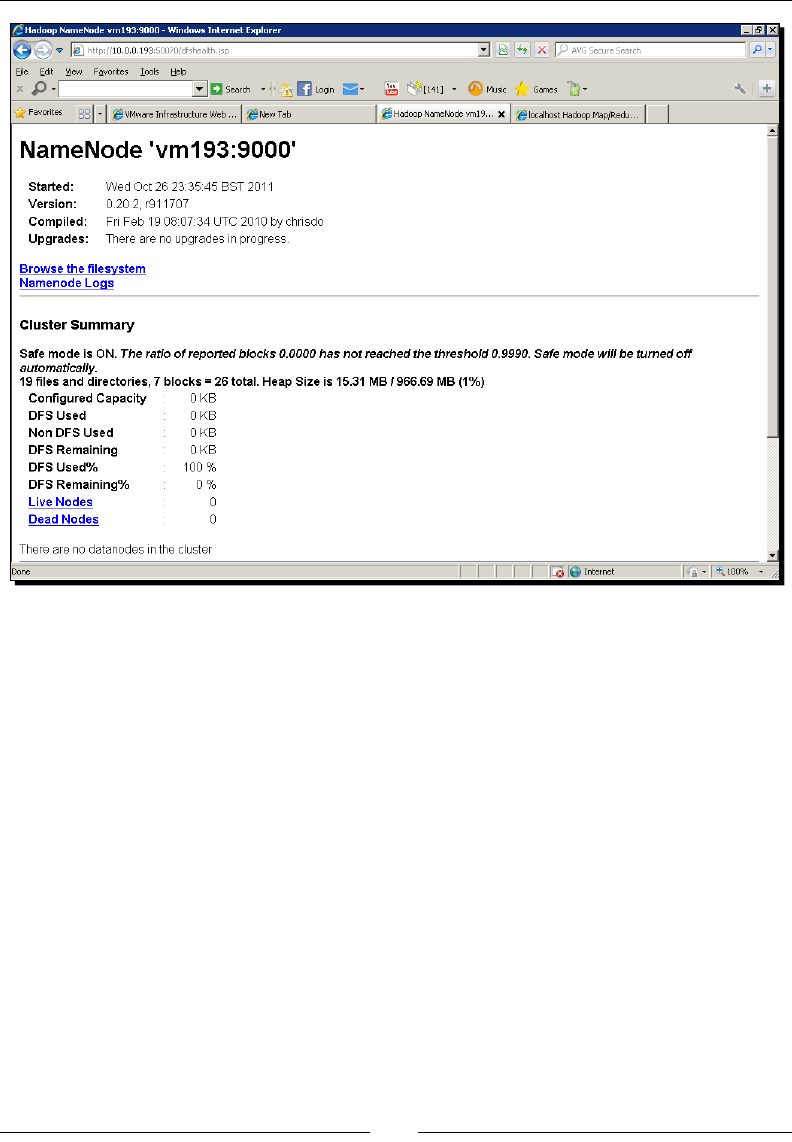
Chapter 2
[ 43 ]
There is a lot going on here, but the immediately crical data tells us the number of nodes
in the cluster, the lesystem size, used space, and links to drill down for more info and even
browse the lesystem.
Spend a lile me playing with this interface; it needs to become familiar. With a mulnode
cluster, the informaon about live and dead nodes plus the detailed informaon on their
status history will be crical to debugging cluster problems.
www.it-ebooks.info
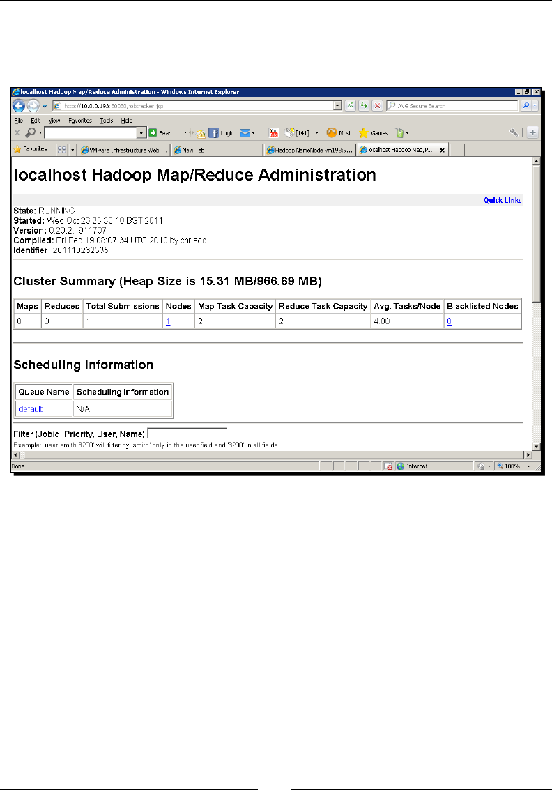
Geng Hadoop Up and Running
[ 44 ]
The MapReduce web UI
The JobTracker UI is available on port 50070 by default, and the same access rules stated
earlier apply. Here is an example screenshot:
This is more complex than the HDFS interface! Along with a similar count of the number
of live/dead nodes, there is a history of the number of jobs executed since startup and a
breakdown of their individual task counts.
The list of execung and historical jobs is a doorway to much more informaon; for every
job, we can access the history of every task aempt on every node and access logs for
detailed informaon. We now expose one of the most painful parts of working with any
distributed system: debugging. It can be really hard.
Imagine you have a cluster of 100 machines trying to process a massive data set where the
full job requires each host to execute hundreds of map and reduce tasks. If the job starts
running very slowly or explicitly fails, it is not always obvious where the problem lies. Looking
at the MapReduce web UI will likely be the rst port of call because it provides such a rich
starng point to invesgate the health of running and historical jobs.
www.it-ebooks.info

Chapter 2
[ 45 ]
Using Elastic MapReduce
We will now turn to Hadoop in the cloud, the Elasc MapReduce service oered by Amazon
Web Services. There are mulple ways to access EMR, but for now we will focus on the
provided web console to contrast a full point-and-click approach to Hadoop with the
previous command-line-driven examples.
Setting up an account in Amazon Web Services
Before using Elasc MapReduce, we need to set up an Amazon Web Services account and
register it with the necessary services.
Creating an AWS account
Amazon has integrated their general accounts with AWS, meaning that if you already have an
account for any of the Amazon retail websites, this is the only account you will need to use
AWS services.
Note that AWS services have a cost; you will need an acve credit card associated with the
account to which charges can be made.
If you require a new Amazon account, go to http://aws.amazon.com, select create a new
AWS account, and follow the prompts. Amazon has added a free er for some services, so
you may nd that in the early days of tesng and exploraon you are keeping many of your
acvies within the non-charged er. The scope of the free er has been expanding, so make
sure you know for what you will and won't be charged.
Signing up for the necessary services
Once you have an Amazon account, you will need to register it for use with the required
AWS services, that is, Simple Storage Service (S3), Elasc Compute Cloud (EC2), and Elasc
MapReduce (EMR). There is no cost for simply signing up to any AWS service; the process
just makes the service available to your account.
Go to the S3, EC2, and EMR pages linked from http://aws.amazon.com and click on the
Sign up buon on each page; then follow the prompts.
www.it-ebooks.info
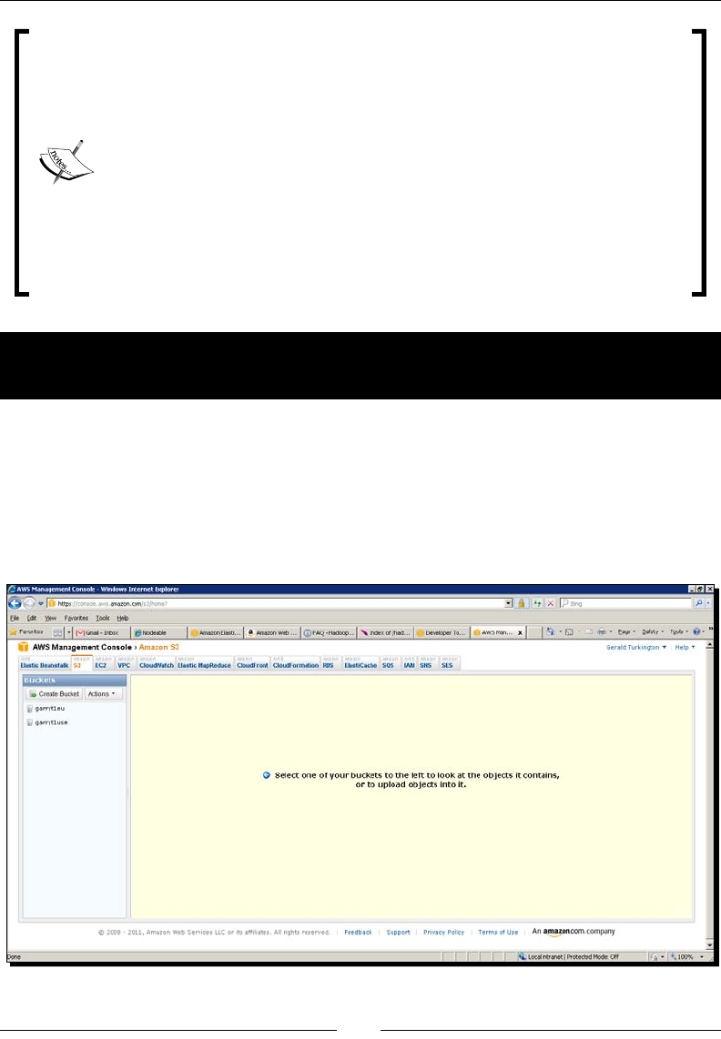
Geng Hadoop Up and Running
[ 46 ]
Cauon! This costs real money!
Before going any further, it is crical to understand that use of AWS services will
incur charges that will appear on the credit card associated with your Amazon
account. Most of the charges are quite small and increase with the amount of
infrastructure consumed; storing 10 GB of data in S3 costs 10 mes more than
for 1 GB, and running 20 EC2 instances costs 20 mes as much as a single one.
There are ered cost models, so the actual costs tend to have smaller marginal
increases at higher levels. But you should read carefully through the pricing
secons for each service before using any of them. Note also that currently
data transfer out of AWS services, such as EC2 and S3, is chargeable but data
transfer between services is not. This means it is oen most cost-eecve to
carefully design your use of AWS to keep data within AWS through as much of
the data processing as possible.
Time for action – WordCount on EMR using the management
console
Let's jump straight into an example on EMR using some provided example code. Carry out
the following steps:
1. Browse to http://aws.amazon.com, go to Developers | AWS Management
Console, and then click on the Sign in to the AWS Console buon. The default
view should look like the following screenshot. If it does not, click on Amazon S3
from within the console.
www.it-ebooks.info
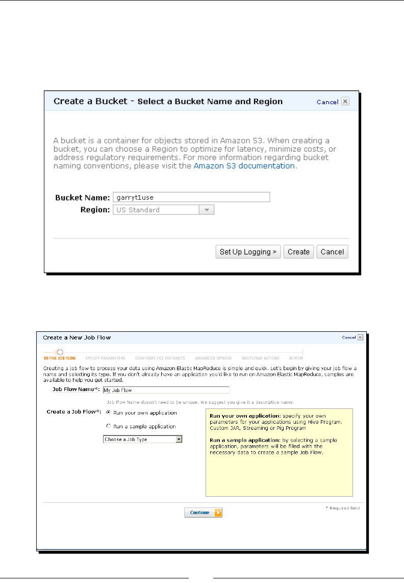
Chapter 2
[ 47 ]
2. As shown in the preceding screenshot, click on the Create bucket buon and enter
a name for the new bucket. Bucket names must be globally unique across all AWS
users, so do not expect obvious bucket names such as mybucket or s3test to
be available.
3. Click on the Region drop-down menu and select the geographic area nearest to you.
4. Click on the Elasc MapReduce link and click on the Create a new Job Flow buon.
You should see a screen like the following screenshot:
www.it-ebooks.info
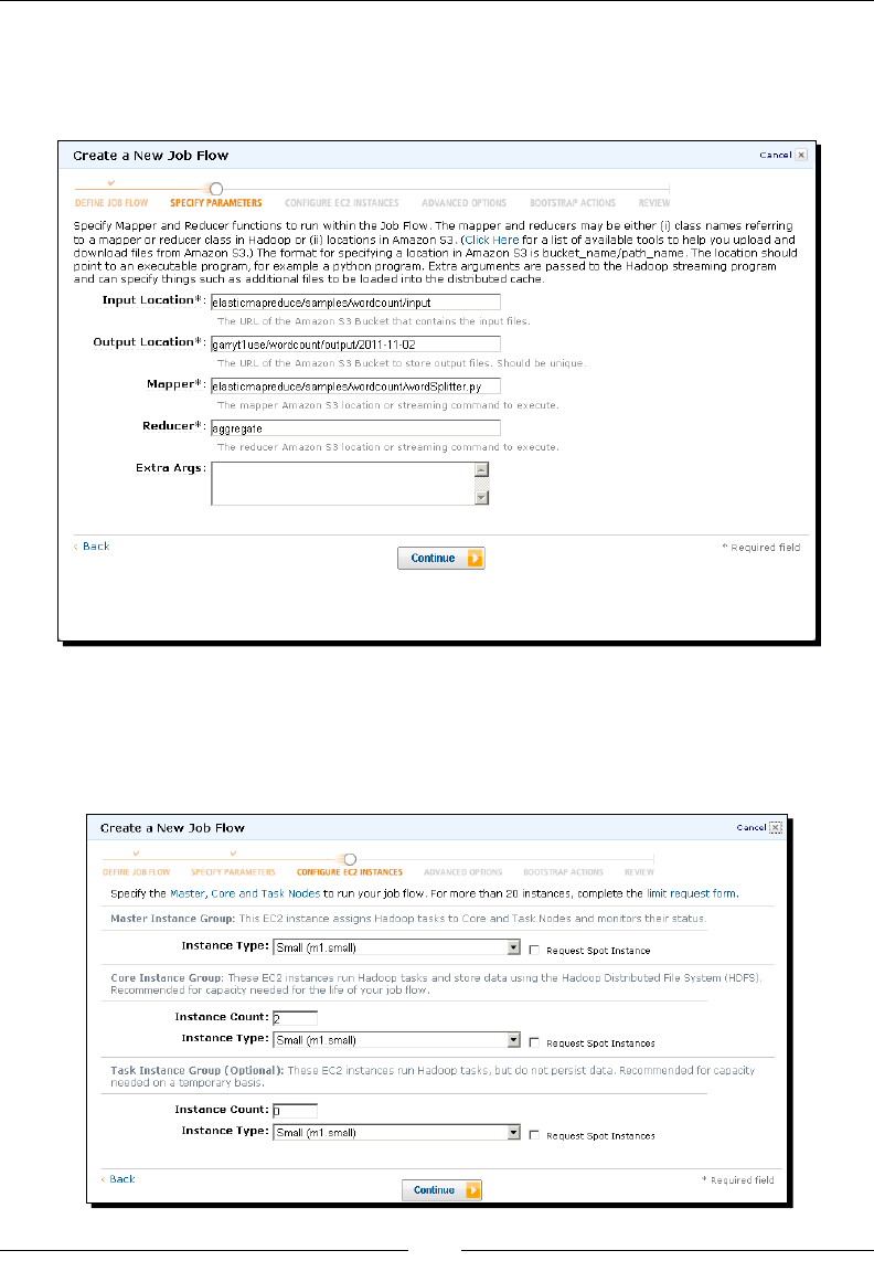
Geng Hadoop Up and Running
[ 48 ]
5. You should now see a screen like the preceding screenshot. Select the Run a sample
applicaon radio buon and the Word Count (Streaming) menu item from the
sample applicaon drop-down box and click on the Connue buon.
6. The next screen, shown in the preceding screenshot, allows us to specify the
locaon of the output produced by running the job. In the edit box for the output
locaon, enter the name of the bucket created in step 1 (garryt1use is the bucket
we are using here); then click on the Connue buon.
www.it-ebooks.info
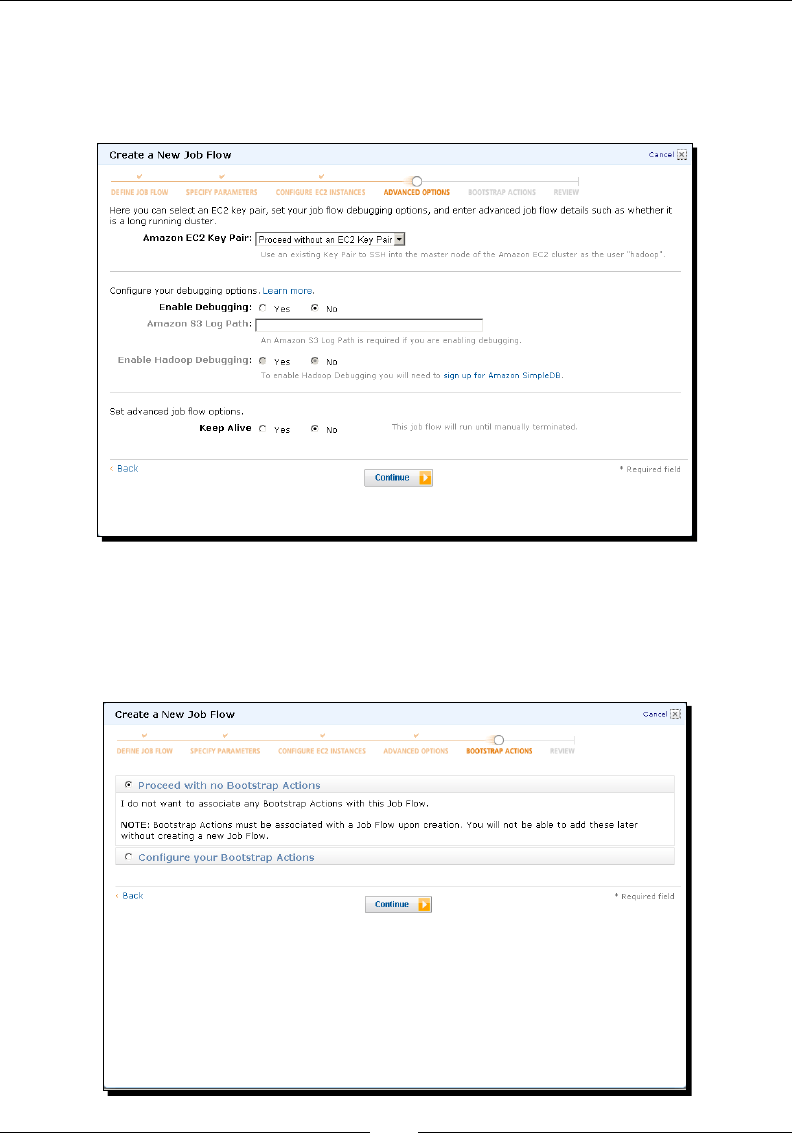
Chapter 2
[ 49 ]
7. The next screenshot shows the page where we can modify the number and size of
the virtual hosts ulized by our job. Conrm that the instance type for each combo
box is Small (m1.small), and the number of nodes for the Core group is 2 and for the
Task group it is 0. Then click on the Connue buon.
8. This next screenshot involves opons we will not be using in this example. For the
Amazon EC2 key pair eld, select the Proceed without key pair menu item and click
on the No radio buon for the Enable Debugging eld. Ensure that the Keep Alive
radio buon is set to No and click on the Connue buon.
www.it-ebooks.info
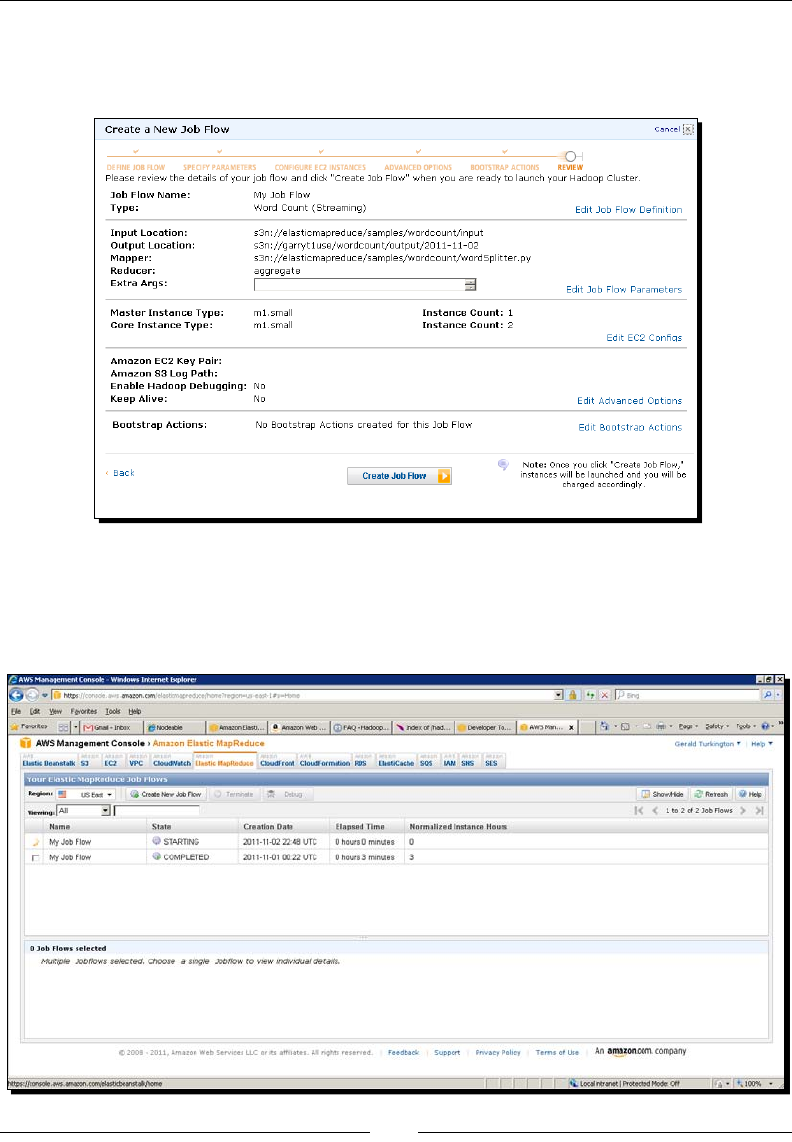
Geng Hadoop Up and Running
[ 50 ]
9. The next screen, shown in the preceding screenshot, is one we will not be doing
much with right now. Conrm that the Proceed with no Bootstrap Acons radio
buon is selected and click on the Connue buon.
10. Conrm the job ow specicaons are as expected and click on the Create Job Flow
buon. Then click on the View my Job Flows and check status buons. This will give
a list of your job ows; you can lter to show only running or completed jobs. The
default is to show all, as in the example shown in the following screenshot:
www.it-ebooks.info
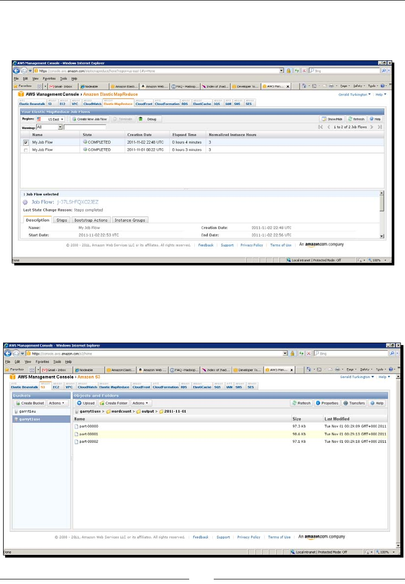
Chapter 2
[ 51 ]
11. Occasionally hit the Refresh buon unl the status of the listed job, Running or
Starng, changes to Complete; then click its checkbox to see details of the job ow,
as shown in the following screenshot:
12. Click the S3 tab and select the bucket you created for the output locaon. You will
see it has a single entry called wordcount, which is a directory. Right-click on that
and select Open. Then do the same unl you see a list of actual les following the
familiar Hadoop part-nnnnn naming scheme, as shown in the following screenshot:
www.it-ebooks.info

Geng Hadoop Up and Running
[ 52 ]
Right click on part-00000 and open it. It should look something like this:
a 14716
aa 52
aakar 3
aargau 3
abad 3
abandoned 46
abandonment 6
abate 9
abauj 3
abbassid 4
abbes 3
abbl 3
…
Does this type of output look familiar?
What just happened?
The rst step deals with S3, and not EMR. S3 is a scalable storage service that allows you to
store les (called objects) within containers called buckets, and to access objects by their
bucket and object key (that is, name). The model is analogous to the usage of a lesystem, and
though there are underlying dierences, they are unlikely to be important within this book.
S3 is where you will place the MapReduce programs and source data you want to process in
EMR, and where the output and logs of EMR Hadoop jobs will be stored. There is a plethora
of third-party tools to access S3, but here we are using the AWS management console, a
browser interface to most AWS services.
Though we suggested you choose the nearest geographic region for S3, this is not required;
non-US locaons will typically give beer latency for customers located nearer to them, but
they also tend to have a slightly higher cost. The decision of where to host your data and
applicaons is one you need to make aer considering all these factors.
Aer creang the S3 bucket, we moved to the EMR console and created a new job ow.
This term is used within EMR to refer to a data processing task. As we will see, this can
be a one-me deal where the underlying Hadoop cluster is created and destroyed on
demand or it can be a long-running cluster on which mulple jobs are executed.
We le the default job ow name and then selected the use of an example applicaon,
in this case, the Python implementaon of WordCount. The term Hadoop Streaming refers
to a mechanism allowing scripng languages to be used to write map and reduce tasks, but
the funconality is the same as the Java WordCount we used earlier.
www.it-ebooks.info

Chapter 2
[ 53 ]
The form to specify the job ow requires a locaon for the source data, program, map and
reduce classes, and a desired locaon for the output data. For the example we just saw, most
of the elds were prepopulated; and, as can be seen, there are clear similaries to what was
required when running local Hadoop from the command line.
By not selecng the Keep Alive opon, we chose a Hadoop cluster that would be created
specically to execute this job, and destroyed aerwards. Such a cluster will have a longer
startup me but will minimize costs. If you choose to keep the job ow alive, you will see
addional jobs executed more quickly as you don't have to wait for the cluster to start up.
But you will be charged for the underlying EC2 resources unl you explicitly terminate the
job ow.
Aer conrming, we do not need to add any addional bootstrap opons; we selected the
number and types of hosts we wanted to deploy into our Hadoop cluster. EMR disnguishes
between three dierent groups of hosts:
Master group: This is a controlling node hosng the NameNode and the JobTracker.
There is only 1 of these.
Core group: These are nodes running both HDFS DataNodes and MapReduce
TaskTrackers. The number of hosts is congurable.
Task group: These hosts don't hold HDFS data but do run TaskTrackers and can
provide more processing horsepower. The number of hosts is congurable.
The type of host refers to dierent classes of hardware capability, the details of which can
be found on the EC2 page. Larger hosts are more powerful but have a higher cost. Currently,
by default, the total number of hosts in a job ow must be 20 or less, though Amazon has a
simple form to request higher limits.
Aer conrming, all is as expected—we launch the job ow and monitor it on the console
unl the status changes to COMPLETED. At this point, we go back to S3, look inside the
bucket we specied as the output desnaon, and examine the output of our WordCount
job, which should look very similar to the output of a local Hadoop WordCount.
An obvious queson is where did the source data come from? This was one of the
prepopulated elds in the job ow specicaon we saw during the creaon process. For
nonpersistent job ows, the most common model is for the source data to be read from a
specied S3 source locaon and the resulng data wrien to the specied result S3 bucket.
That is it! The AWS management console allows ne-grained control of services such as S3
and EMR from the browser. Armed with nothing more than a browser and a credit card,
we can launch Hadoop jobs to crunch data without ever having to worry about any of the
mechanics around installing, running, or managing Hadoop.
www.it-ebooks.info

Geng Hadoop Up and Running
[ 54 ]
Have a go hero – other EMR sample applications
EMR provides several other sample applicaons. Why not try some of them as well?
Other ways of using EMR
Although a powerful and impressive tool, the AWS management console is not always
how we want to access S3 and run EMR jobs. As with all AWS services, there are both
programmac and command-line tools to use the services.
AWS credentials
Before using either programmac or command-line tools, however, we need to look at how
an account holder authencates for AWS to make such requests. As these are chargeable
services, we really do not want anyone else to make requests on our behalf. Note that as
we logged directly into the AWS management console with our AWS account in the
preceding example, we did not have to worry about this.
Each AWS account has several ideners that are used when accessing the various services:
Account ID: Each AWS account has a numeric ID.
Access key: Each account has an associated access key that is used to idenfy the
account making the request.
Secret access key: The partner to the access key is the secret access key. The access
key is not a secret and could be exposed in service requests, but the secret access
key is what you use to validate yourself as the account owner.
Key pairs: These are the key pairs used to log in to EC2 hosts. It is possible to either
generate public/private key pairs within EC2 or to import externally generated keys
into the system.
If this sounds confusing, it's because it is. At least at rst. When using a tool to access an
AWS service, however, there's usually a single up-front step of adding the right credenals
to a congured le, and then everything just works. However, if you do decide to explore
programmac or command-line tools, it will be worth a lile me investment to read the
documentaon for each service to understand how its security works.
The EMR command-line tools
In this book, we will not do anything with S3 and EMR that cannot be done from the AWS
management console. However, when working with operaonal workloads, looking to
integrate into other workows, or automang service access, a browser-based tool is not
appropriate, regardless of how powerful it is. Using the direct programmac interfaces to
a service provides the most granular control but requires the most eort.
www.it-ebooks.info

Chapter 2
[ 55 ]
Amazon provides for many services a group of command-line tools that provide a useful way
of automang access to AWS services that minimizes the amount of required development.
The Elasc MapReduce command-line tools, linked from the main EMR page, are worth a
look if you want a more CLI-based interface to EMR but don't want to write custom code
just yet.
The AWS ecosystem
Each AWS service also has a plethora of third-party tools, services, and libraries that can
provide dierent ways of accessing the service, provide addional funconality, or oer
new ulity programs. Check out the developer tools hub at http://aws.amazon.com/
developertools, as a starng point.
Comparison of local versus EMR Hadoop
Aer our rst experience of both a local Hadoop cluster and its equivalent in EMR, this is a
good point at which we can consider the dierences of the two approaches.
As may be apparent, the key dierences are not really about capability; if all we want is an
environment to run MapReduce jobs, either approach is completely suited. Instead, the
disnguishing characteriscs revolve around a topic we touched on in Chapter 1, What It's
All About, that being whether you prefer a cost model that involves upfront infrastructure
costs and ongoing maintenance eort over one with a pay-as-you-go model with a lower
maintenance burden along with rapid and conceptually innite scalability. Other than the
cost decisions, there are a few things to keep in mind:
EMR supports specic versions of Hadoop and has a policy of upgrading over me.
If you have a need for a specic version, in parcular if you need the latest and
greatest versions immediately aer release, then the lag before these are live on
EMR may be unacceptable.
You can start up a persistent EMR job ow and treat it much as you would a local
Hadoop cluster, logging into the hosng nodes and tweaking their conguraon. If
you nd yourself doing this, its worth asking if that level of control is really needed
and, if so, is it stopping you geng all the cost model benets of a move to EMR?
If it does come down to a cost consideraon, remember to factor in all the hidden
costs of a local cluster that are oen forgoen. Think about the costs of power,
space, cooling, and facilies. Not to menon the administraon overhead, which
can be nontrivial if things start breaking in the early hours of the morning.
www.it-ebooks.info

Geng Hadoop Up and Running
[ 56 ]
Summary
We covered a lot of ground in this chapter, in regards to geng a Hadoop cluster up and
running and execung MapReduce programs on it.
Specically, we covered the prerequisites for running Hadoop on local Ubuntu hosts.
We also saw how to install and congure a local Hadoop cluster in either standalone or
pseudo-distributed modes. Then, we looked at how to access the HDFS lesystem and
submit MapReduce jobs. We then moved on and learned what accounts are needed to
access Elasc MapReduce and other AWS services.
We saw how to browse and create S3 buckets and objects using the AWS management
console, and also how to create a job ow and use it to execute a MapReduce job on an
EMR-hosted Hadoop cluster. We also discussed other ways of accessing AWS services and
studied the dierences between local and EMR-hosted Hadoop.
Now that we have learned about running Hadoop locally or on EMR, we are ready to start
wring our own MapReduce programs, which is the topic of the next chapter.
www.it-ebooks.info

3
Understanding MapReduce
The previous two chapters have discussed the problems that Hadoop allows us
to solve, and gave some hands-on experience of running example MapReduce
jobs. With this foundation, we will now go a little deeper.
In this chapter we will be:
Understanding how key/value pairs are the basis of Hadoop tasks
Learning the various stages of a MapReduce job
Examining the workings of the map, reduce, and oponal combined stages in detail
Looking at the Java API for Hadoop and use it to develop some simple
MapReduce jobs
Learning about Hadoop input and output
Key/value pairs
Since Chapter 1, What It's All About, we have been talking about operaons that process
and provide the output in terms of key/value pairs without explaining why. It is me to
address that.
What it mean
Firstly, we will clarify just what we mean by key/value pairs by highlighng similar concepts
in the Java standard library. The java.util.Map interface is the parent of commonly used
classes such as HashMap and (through some library backward reengineering) even the
original Hashtable.
www.it-ebooks.info

Understanding MapReduce
[ 58 ]
For any Java Map object, its contents are a set of mappings from a given key of a specied
type to a related value of a potenally dierent type. A HashMap object could, for example,
contain mappings from a person's name (String) to his or her birthday (Date).
In the context of Hadoop, we are referring to data that also comprises keys that relate to
associated values. This data is stored in such a way that the various values in the data set
can be sorted and rearranged across a set of keys. If we are using key/value data, it will
make sense to ask quesons such as the following:
Does a given key have a mapping in the data set?
What are the values associated with a given key?
What is the complete set of keys?
Think back to WordCount from the previous chapter. We will go into it in more detail shortly,
but the output of the program is clearly a set of key/value relaonships; for each word
(the key), there is a count (the value) of its number of occurrences. Think about this simple
example and some important features of key/value data will become apparent, as follows:
Keys must be unique but values need not be
Each value must be associated with a key, but a key could have no values
(though not in this parcular example)
Careful denion of the key is important; deciding on whether or not the
counts are applied with case sensivity will give dierent results
Note that we need to dene carefully what we mean by keys being unique
here. This does not mean the key occurs only once; in our data set we may see
a key occur numerous mes and, as we shall see, the MapReduce model has
a stage where all values associated with each key are collected together. The
uniqueness of keys guarantees that if we collect together every value seen for
any given key, the result will be an associaon from a single instance of the key
to every value mapped in such a way, and none will be omied.
Why key/value data?
Using key/value data as the foundaon of MapReduce operaons allows for a powerful
programming model that is surprisingly widely applicable, as can be seen by the adopon of
Hadoop and MapReduce across a wide variety of industries and problem scenarios. Much
data is either intrinsically key/value in nature or can be represented in such a way. It is a
simple model with broad applicability and semancs straighorward enough that programs
dened in terms of it can be applied by a framework like Hadoop.
www.it-ebooks.info

Chapter 3
[ 59 ]
Of course, the data model itself is not the only thing that makes Hadoop useful; its real
power lies in how it uses the techniques of parallel execuon, and divide and conquer
discussed in Chapter 1, What It's All About. We can have a large number of hosts on which
we can store and execute data and even use a framework that manages the division of
the larger task into smaller chunks, and the combinaon of paral results into the overall
answer. But we need this framework to provide us with a way of expressing our problems
that doesn't require us to be an expert in the execuon mechanics; we want to express the
transformaons required on our data and then let the framework do the rest. MapReduce,
with its key/value interface, provides such a level of abstracon, whereby the programmer
only has to specify these transformaons and Hadoop handles the complex process of
applying this to arbitrarily large data sets.
Some real-world examples
To become less abstract, let's think of some real-world data that is key/value pair:
An address book relates a name (key) to contact informaon (value)
A bank account uses an account number (key) to associate with the account
details (value)
The index of a book relates a word (key) to the pages on which it occurs (value)
On a computer lesystem, lenames (keys) allow access to any sort of data,
such as text, images, and sound (values)
These examples are intenonally broad in scope, to help and encourage you to think that
key/value data is not some very constrained model used only in high-end data mining but
a very common model that is all around us.
We would not be having this discussion if this was not important to Hadoop. The boom line
is that if the data can be expressed as key/value pairs, it can be processed by MapReduce.
MapReduce as a series of key/value transformations
You may have come across MapReduce described in terms of key/value transformaons, in
parcular the inmidang one looking like this:
{K1,V1} -> {K2, List<V2>} -> {K3,V3}
We are now in a posion to understand what this means:
The input to the map method of a MapReduce job is a series of key/value pairs that
we'll call K1 and V1.
www.it-ebooks.info

Understanding MapReduce
[ 60 ]
The output of the map method (and hence input to the reduce method) is a series
of keys and an associated list of values that are called K2 and V2. Note that each
mapper simply outputs a series of individual key/value outputs; these are combined
into a key and list of values in the shuffle method.
The nal output of the MapReduce job is another series of key/value pairs, called K3
and V3.
These sets of key/value pairs don't have to be dierent; it would be quite possible to input,
say, names and contact details and output the same, with perhaps some intermediary format
used in collang the informaon. Keep this three-stage model in mind as we explore the Java
API for MapReduce next. We will rst walk through the main parts of the API you will need
and then do a systemac examinaon of the execuon of a MapReduce job.
Pop quiz – key/value pairs
Q1. The concept of key/value pairs is…
1. Something created by and specic to Hadoop.
2. A way of expressing relaonships we oen see but don't think of as such.
3. An academic concept from computer science.
Q2. Are username/password combinaons an example of key/value data?
1. Yes, it's a clear case of one value being associated to the other.
2. No, the password is more of an aribute of the username, there's no index-type
relaonship.
3. We'd not usually think of them as such, but Hadoop could sll process a series
of username/password combinaons as key/value pairs.
The Hadoop Java API for MapReduce
Hadoop underwent a major API change in its 0.20 release, which is the primary interface
in the 1.0 version we use in this book. Though the prior API was certainly funconal, the
community felt it was unwieldy and unnecessarily complex in some regards.
The new API, somemes generally referred to as context objects, for reasons we'll see later,
is the future of Java's MapReduce development; and as such we will use it wherever possible
in this book. Note that caveat: there are parts of the pre-0.20 MapReduce libraries that have
not been ported to the new API, so we will use the old interfaces when we need to examine
any of these.
www.it-ebooks.info

Chapter 3
[ 61 ]
The 0.20 MapReduce Java API
The 0.20 and above versions of MapReduce API have most of the key classes and interfaces
either in the org.apache.hadoop.mapreduce package or its subpackages.
In most cases, the implementaon of a MapReduce job will provide job-specic subclasses
of the Mapper and Reducer base classes found in this package.
We'll sck to the commonly used K1 / K2 / K3 / and so on terminology,
though more recently the Hadoop API has, in places, used terms such as
KEYIN/VALUEIN and KEYOUT/VALUEOUT instead. For now, we will
sck with K1 / K2 / K3 as it helps understand the end-to-end data ow.
The Mapper class
This is a cut-down view of the base Mapper class provided by Hadoop. For our own
mapper implementaons, we will subclass this base class and override the specied
method as follows:
class Mapper<K1, V1, K2, V2>
{
void map(K1 key, V1 value Mapper.Context context)
throws IOException, InterruptedException
{..}
}
Although the use of Java generics can make this look a lile opaque at rst, there is
actually not that much going on. The class is dened in terms of the key/value input
and output types, and then the map method takes an input key/value pair in its parameters.
The other parameter is an instance of the Context class that provides various mechanisms
to communicate with the Hadoop framework, one of which is to output the results of a map
or reduce method.
Noce that the map method only refers to a single instance of K1 and V1 key/
value pairs. This is a crical aspect of the MapReduce paradigm in which you
write classes that process single records and the framework is responsible
for all the work required to turn an enormous data set into a stream of key/
value pairs. You will never have to write map or reduce classes that try to
deal with the full data set. Hadoop also provides mechanisms through its
InputFormat and OutputFormat classes that provide implementaons
of common le formats and likewise remove the need of having to write le
parsers for any but custom le types.
www.it-ebooks.info

Understanding MapReduce
[ 62 ]
There are three addional methods that somemes may be required to be overridden.
protected void setup( Mapper.Context context)
throws IOException, Interrupted Exception
This method is called once before any key/value pairs are presented to the map method.
The default implementaon does nothing.
protected void cleanup( Mapper.Context context)
throws IOException, Interrupted Exception
This method is called once aer all key/value pairs have been presented to the map method.
The default implementaon does nothing.
protected void run( Mapper.Context context)
throws IOException, Interrupted Exception
This method controls the overall ow of task processing within a JVM. The default
implementaon calls the setup method once before repeatedly calling the map
method for each key/value pair in the split, and then nally calls the cleanup method.
Downloading the example code
You can download the example code les for all Packt books you have purchased
from your account at http://www.packtpub.com. If you purchased this
book elsewhere, you can visit http://www.packtpub.com/support
and register to have the les e-mailed directly to you.
The Reducer class
The Reducer base class works very similarly to the Mapper class, and usually requires only
subclasses to override a single reduce method. Here is the cut-down class denion:
public class Reducer<K2, V2, K3, V3>
{
void reduce(K1 key, Iterable<V2> values,
Reducer.Context context)
throws IOException, InterruptedException
{..}
}
Again, noce the class denion in terms of the broader data ow (the reduce method
accepts K2/V2 as input and provides K3/V3 as output) while the actual reduce method
takes only a single key and its associated list of values. The Context object is again the
mechanism to output the result of the method.
This class also has the setup, run, and cleanup methods with similar default
implementaons as with the Mapper class that can oponally be overridden:
www.it-ebooks.info

Chapter 3
[ 63 ]
protected void setup( Reduce.Context context)
throws IOException, InterruptedException
This method is called once before any key/lists of values are presented to the reduce
method. The default implementaon does nothing.
protected void cleanup( Reducer.Context context)
throws IOException, InterruptedException
This method is called once aer all key/lists of values have been presented to the reduce
method. The default implementaon does nothing.
protected void run( Reducer.Context context)
throws IOException, InterruptedException
This method controls the overall ow of processing the task within JVM. The default
implementaon calls the setup method before repeatedly calling the reduce method for as
many key/values provided to the Reducer class, and then nally calls the cleanup method.
The Driver class
Although our mapper and reducer implementaons are all we need to perform the
MapReduce job, there is one more piece of code required: the driver that communicates
with the Hadoop framework and species the conguraon elements needed to run a
MapReduce job. This involves aspects such as telling Hadoop which Mapper and Reducer
classes to use, where to nd the input data and in what format, and where to place the
output data and how to format it. There is an addional variety of other conguraon
opons that can be set and which we will see throughout this book.
There is no default parent Driver class as a subclass; the driver logic usually exists in the main
method of the class wrien to encapsulate a MapReduce job. Take a look at the following
code snippet as an example driver. Don't worry about how each line works, though you
should be able to work out generally what each is doing:
public class ExampleDriver
{
...
public static void main(String[] args) throws Exception
{
// Create a Configuration object that is used to set other options
Configuration conf = new Configuration() ;
// Create the object representing the job
Job job = new Job(conf, "ExampleJob") ;
// Set the name of the main class in the job jarfile
job.setJarByClass(ExampleDriver.class) ;
// Set the mapper class
job.setMapperClass(ExampleMapper.class) ;
www.it-ebooks.info

Understanding MapReduce
[ 64 ]
// Set the reducer class
job.setReducerClass(ExampleReducer.class) ;
// Set the types for the final output key and value
job.setOutputKeyClass(Text.class) ;
job.setOutputValueClass(IntWritable.class) ;
// Set input and output file paths
FileInputFormat.addInputPath(job, new Path(args[0])) ;
FileOutputFormat.setOutputPath(job, new Path(args[1]))
// Execute the job and wait for it to complete
System.exit(job.waitForCompletion(true) ? 0 : 1);
}
}}
Given our previous talk of jobs, it is not surprising that much of the setup involves operaons
on a Job object. This includes seng the job name and specifying which classes are to be
used for the mapper and reducer implementaons.
Certain input/output conguraons are set and, nally, the arguments passed to the main
method are used to specify the input and output locaons for the job. This is a very common
model that you will see oen.
There are a number of default values for conguraon opons, and we are implicitly using
some of them in the preceding class. Most notably, we don't say anything about the le
format of the input les or how the output les are to be wrien. These are dened through
the InputFormat and OutputFormat classes menoned earlier; we will explore them
in detail later. The default input and output formats are text les that suit our WordCount
example. There are mulple ways of expressing the format within text les in addion to
parcularly opmized binary formats.
A common model for less complex MapReduce jobs is to have the Mapper and Reducer
classes as inner classes within the driver. This allows everything to be kept in a single le,
which simplies the code distribuon.
Writing MapReduce programs
We have been using and talking about WordCount for quite some me now; let's actually
write an implementaon, compile, and run it, and then explore some modicaons.
www.it-ebooks.info

Chapter 3
[ 65 ]
Time for action – setting up the classpath
To compile any Hadoop-related code, we will need to refer to the standard
Hadoop-bundled classes.
Add the Hadoop-1.0.4.core.jar le from the distribuon to the Java classpath
as follows:
$ export CLASSPATH=.:${HADOOP_HOME}/Hadoop-1.0.4.core.jar:${CLASSPATH}
What just happened?
This adds the Hadoop-1.0.4.core.jar le explicitly to the classpath alongside the
current directory and the previous contents of the CLASSPATH environment variable.
Once again, it would be good to put this in your shell startup le or a standalone le
to be sourced.
We will later need to also have many of the supplied third-party libraries
that come with Hadoop on our classpath, and there is a shortcut to do this.
For now, the explicit addion of the core JAR le will suce.
Time for action – implementing WordCount
We have seen the use of the WordCount example program in Chapter 2, Geng Hadoop
Up and Running. Now we will explore our own Java implementaon by performing the
following steps:
1. Enter the following code into the WordCount1.java le:
Import java.io.* ;
import org.apache.hadoop.conf.Configuration ;
import org.apache.hadoop.fs.Path;
import org.apache.hadoop.io.IntWritable;
import org.apache.hadoop.io.Text;
import org.apache.hadoop.mapreduce.Job;
import org.apache.hadoop.mapreduce.Mapper;
import org.apache.hadoop.mapreduce.Reducer;
import org.apache.hadoop.mapreduce.lib.input.FileInputFormat;
import org.apache.hadoop.mapreduce.lib.output.FileOutputFormat;
www.it-ebooks.info

Understanding MapReduce
[ 66 ]
public class WordCount1
{
public static class WordCountMapper
extends Mapper<Object, Text, Text, IntWritable>
{
private final static IntWritable one = new IntWritable(1);
private Text word = new Text();
public void map(Object key, Text value, Context context
) throws IOException, InterruptedException {
String[] words = value.toString().split(" ") ;
for (String str: words)
{
word.set(str);
context.write(word, one);
}
}
}
public static class WordCountReducer
extends Reducer<Text,IntWritable,Text,IntWritable> {
public void reduce(Text key, Iterable<IntWritable> values,
Context context
) throws IOException, InterruptedException {
int total = 0;
for (IntWritable val : values) {
total++ ;
}
context.write(key, new IntWritable(total));
}
}
public static void main(String[] args) throws Exception {
Configuration conf = new Configuration();
Job job = new Job(conf, "word count");
job.setJarByClass(WordCount1.class);
www.it-ebooks.info

Chapter 3
[ 67 ]
job.setMapperClass(WordCountMapper.class);
job.setReducerClass(WordCountReducer.class);
job.setOutputKeyClass(Text.class);
job.setOutputValueClass(IntWritable.class);
FileInputFormat.addInputPath(job, new Path(args[0]));
FileOutputFormat.setOutputPath(job, new Path(args[1]));
System.exit(job.waitForCompletion(true) ? 0 : 1);
}
}
2. Now compile it by execung the following command:
$ javac WordCount1.java
What just happened?
This is our rst complete MapReduce job. Look at the structure and you should recognize the
elements we have previously discussed: the overall Job class with the driver conguraon in
its main method and the Mapper and Reducer implementaons dened as inner classes.
We'll do a more detailed walkthrough of the mechanics of MapReduce in the next secon,
but for now let's look at the preceding code and think of how it realizes the key/value
transformaons we talked about earlier.
The input to the Mapper class is arguably the hardest to understand, as the key is not
actually used. The job species TextInputFormat as the format of the input data and, by
default, this delivers to the mapper data where the key is the line number in the le and
the value is the text of that line. In reality, you may never actually see a mapper that uses
that line number key, but it is provided.
The mapper is executed once for each line of text in the input source and every me
it takes the line and breaks it into words. It then uses the Context object to output
(more commonly known as eming) each new key/value of the form <word, 1>.
These are our K2/V2 values.
We said before that the input to the reducer is a key and a corresponding list of values,
and there is some magic that happens between the map and reduce methods to collect
together the values for each key that facilitates this, which we'll not describe right now.
Hadoop executes the reducer once for each key and the preceding reducer implementaon
simply counts the numbers in the Iterable object and gives output for each word in the
form of <word, count>. This is our K3/V3 values.
www.it-ebooks.info

Understanding MapReduce
[ 68 ]
Take a look at the signatures of our mapper and reducer classes: the WordCountMapper
class gives IntWritable and Text as input and gives Text and IntWritable as output.
The WordCountReducer class gives Text and IntWritable both as input and output. This
is again quite a common paern, where the map method performs an inversion on the key and
values, and instead emits a series of data pairs on which the reducer performs aggregaon.
The driver is more meaningful here, as we have real values for the parameters.
We use arguments passed to the class to specify the input and output locaons.
Time for action – building a JAR le
Before we run our job in Hadoop, we must collect the required class les into a single JAR
le that we will submit to the system.
Create a JAR le from the generated class les.
$ jar cvf wc1.jar WordCount1*class
What just happened?
We must always package our class les into a JAR le before subming to Hadoop, be it
local or on Elasc MapReduce.
Be careful with the JAR command and le paths. If you include in a JAR le
class the les from a subdirectory, the class may not be stored with the path
you expect. This is especially common when using a catch-all classes directory
where all source data gets compiled. It may be useful to write a script to
change into the directory, convert the required les into JAR les, and move
the JAR les to the required locaon.
Time for action – running WordCount on a local Hadoop cluster
Now we have generated the class les and collected them into a JAR le, we can run the
applicaon by performing the following steps:
1. Submit the new JAR le to Hadoop for execuon.
$ hadoop jar wc1.jar WordCount1 test.txt output
2. If successful, you should see the output being very similar to the one we obtained
when we ran the Hadoop-provided sample WordCount in the previous chapter.
Check the output le; it should be as follows:
www.it-ebooks.info
Chapter 3
[ 69 ]
$ Hadoop fs –cat output/part-r-00000
This 1
yes 1
a 1
is 2
test 1
this 1
What just happened?
This is the rst me we have used the Hadoop JAR command with our own code. There are
four arguments:
1. The name of the JAR le.
2. The name of the driver class within the JAR le.
3. The locaon, on HDFS, of the input le (a relave reference to the /user/Hadoop
home folder, in this case).
4. The desired locaon of the output folder (again, a relave path).
The name of the driver class is only required if a main class has not
(as in this case) been specied within the JAR le manifest.
Time for action – running WordCount on EMR
We will now show you how to run this same JAR le on EMR. Remember, as always, that this
costs money!
1. Go to the AWS console at http://aws.amazon.com/console, sign in, and
select S3.
2. You'll need two buckets: one to hold the JAR le and another for the job output.
You can use exisng buckets or create new ones.
3. Open the bucket where you will store the job le, click on Upload, and add the wc1.
jar le created earlier.
4. Return to the main console home page, and then go to the EMR poron of the
console by selecng Elasc MapReduce.
www.it-ebooks.info
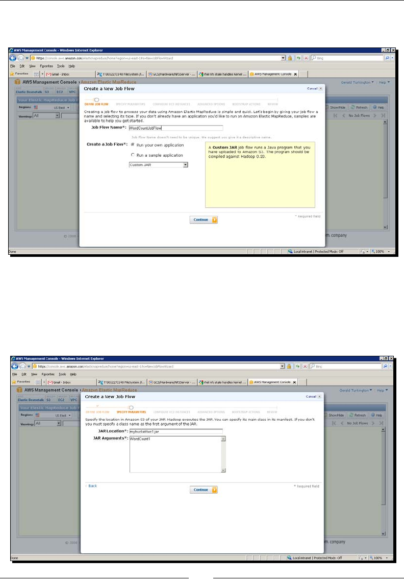
Understanding MapReduce
[ 70 ]
5. Click on the Create a New Job Flow buon and you'll see a familiar screen as
shown in the following screenshot:
6. Previously, we used a sample applicaon; to run our code, we need to perform
dierent steps. Firstly, select the Run your own applicaon radio buon.
7. In the Select a Job Type combobox, select Custom JAR.
8. Click on the Connue buon and you'll see a new form, as shown in the
following screenshot:
www.it-ebooks.info
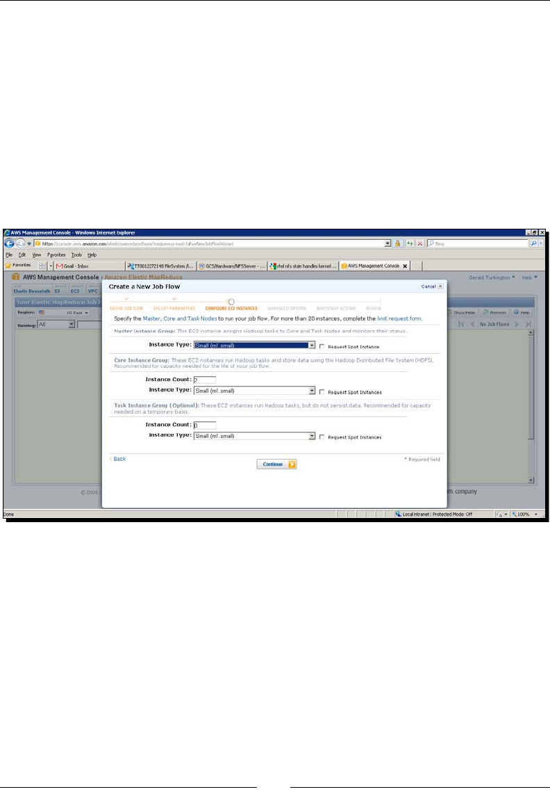
Chapter 3
[ 71 ]
We now specify the arguments to the job. Within our uploaded JAR le, our code—
parcularly the driver class—species aspects such as the Mapper and Reducer classes.
What we need to provide is the path to the JAR le and the input and output paths for the
job. In the JAR Locaon eld, put the locaon where you uploaded the JAR le. If the JAR le
is called wc1.jar and you uploaded it into a bucket called mybucket, the path would be
mybucket/wc1.jar.
In the JAR Arguments eld, you need to enter the name of the main class and the
input and output locaons for the job. For les on S3, we can use URLs of the form
s3://bucketname/objectname. Click on Connue and the familiar screen to specify
the virtual machines for the job ow appears, as shown in the following screenshot:
Now connue through the job ow setup and execuon as we did in Chapter 2, Geng
Hadoop Up and Running.
What just happened?
The important lesson here is that we can reuse the code wrien on and for a local Hadoop
cluster in EMR. Also, besides these rst few steps, the majority of the EMR console is the
same regardless of the source of the job code to be executed.
Through the remainder of this chapter, we will not explicitly show code being executed
on EMR and will instead focus more on the local cluster, because running a JAR le on
EMR is very easy.
www.it-ebooks.info

Understanding MapReduce
[ 72 ]
The pre-0.20 Java MapReduce API
Our preference in this book is for the 0.20 and above versions of MapReduce Java API, but
we'll need to take a quick look at the older APIs for two reasons:
1. Many online examples and other reference materials are wrien for the older APIs.
2. Several areas within the MapReduce framework are not yet ported to the new API,
and we will need to use the older APIs to explore them.
The older API's classes are found primarily in the org.apache.hadoop.mapred package.
The new API classes use concrete Mapper and Reducer classes, while the older API had this
responsibility split across abstract classes and interfaces.
An implementaon of a Mapper class will subclass the abstract MapReduceBase class and
implement the Mapper interface, while a custom Reducer class will subclass the same
MapReduceBase abstract class but implement the Reducer interface.
We'll not explore MapReduceBase in much detail as its funconality deals with job setup
and conguraon, which aren't really core to understanding the MapReduce model. But the
interfaces of pre-0.20 Mapper and Reducer are worth showing:
public interface Mapper<K1, V1, K2, V2>
{
void map( K1 key, V1 value, OutputCollector< K2, V2> output, Reporter
reporter) throws IOException ;
}
public interface Reducer<K2, V2, K3, V3>
{
void reduce( K2 key, Iterator<V2> values,
OutputCollector<K3, V3> output, Reporter reporter)
throws IOException ;
}
There are a few points to understand here:
The generic parameters to the OutputCollector class show more explicitly how
the result of the methods is presented as output.
The old API used the OutputCollector class for this purpose, and the Reporter
class to write status and metrics informaon to the Hadoop framework. The 0.20
API combines these responsibilies in the Context class.
www.it-ebooks.info

Chapter 3
[ 73 ]
The Reducer interface uses an Iterator object instead of an Iterable object;
this was changed as the laer works with the Java for each syntax and makes for
cleaner code.
Neither the map nor the reduce method could throw InterruptedException
in the old API.
As you can see, the changes between the APIs alter how MapReduce programs are wrien
but don't change the purpose or responsibilies of mappers or reducers. Don't feel obliged
to become an expert in both APIs unless you need to; familiarity with either should allow
you to follow the rest of this book.
Hadoop-provided mapper and reducer implementations
We don't always have to write our own Mapper and Reducer classes from scratch. Hadoop
provides several common Mapper and Reducer implementaons that can be used in our
jobs. If we don't override any of the methods in the Mapper and Reducer classes in the
new API, the default implementaons are the identy Mapper and Reducer classes, which
simply output the input unchanged.
Note that more such prewrien Mapper and Reducer implementaons may be added over
me, and currently the new API does not have as many as the older one.
The mappers are found at org.apache.hadoop.mapreduce.lib.mapper, and include
the following:
InverseMapper: This outputs (value, key)
TokenCounterMapper: This counts the number of discrete tokens in each line
of input
The reducers are found at org.apache.hadoop.mapreduce.lib.reduce, and currently
include the following:
IntSumReducer: This outputs the sum of the list of integer values per key
LongSumReducer: This outputs the sum of the list of long values per key
Time for action – WordCount the easy way
Let's revisit WordCount, but this me use some of these predened map and reduce
implementaons:
1. Create a new WordCountPredefined.java le containing the following code:
import org.apache.hadoop.conf.Configuration ;
import org.apache.hadoop.fs.Path;
www.it-ebooks.info

Understanding MapReduce
[ 74 ]
import org.apache.hadoop.io.IntWritable;
import org.apache.hadoop.io.Text;
import org.apache.hadoop.mapreduce.Job;
import org.apache.hadoop.mapreduce.lib.input.FileInputFormat;
import org.apache.hadoop.mapreduce.lib.output.FileOutputFormat;
import org.apache.hadoop.mapreduce.lib.map.TokenCounterMapper ;
import org.apache.hadoop.mapreduce.lib.reduce.IntSumReducer ;
public class WordCountPredefined
{
public static void main(String[] args) throws Exception
{
Configuration conf = new Configuration();
Job job = new Job(conf, "word count1");
job.setJarByClass(WordCountPredefined.class);
job.setMapperClass(TokenCounterMapper.class);
job.setReducerClass(IntSumReducer.class);
job.setOutputKeyClass(Text.class);
job.setOutputValueClass(IntWritable.class);
FileInputFormat.addInputPath(job, new Path(args[0]));
FileOutputFormat.setOutputPath(job, new Path(args[1]));
System.exit(job.waitForCompletion(true) ? 0 : 1);
}
}
2. Now compile, create the JAR le, and run it as before.
3. Don't forget to delete the output directory before running the job, if you want to
use the same locaon. Use the hadoop fs -rmr output, for example.
What just happened?
Given the ubiquity of WordCount as an example in the MapReduce world, it's perhaps not
enrely surprising that there are predened Mapper and Reducer implementaons that
together realize the enre WordCount soluon. The TokenCounterMapper class simply
breaks each input line into a series of (token, 1) pairs and the IntSumReducer class
provides a nal count by summing the number of values for each key.
There are two important things to appreciate here:
Though WordCount was doubtless an inspiraon for these implementaons, they
are in no way specic to it and can be widely applicable
This model of having reusable mapper and reducer implementaons is one thing to
remember, especially in combinaon with the fact that oen the best starng point
for a new MapReduce job implementaon is an exisng one
www.it-ebooks.info

Chapter 3
[ 75 ]
Walking through a run of WordCount
To explore the relaonship between mapper and reducer in more detail, and to expose
some of Hadoop's inner working, we'll now go through just how WordCount (or indeed
any MapReduce job) is executed.
Startup
The call to Job.waitForCompletion() in the driver is where all the acon starts. The
driver is the only piece of code that runs on our local machine, and this call starts the
communicaon with the JobTracker. Remember that the JobTracker is responsible for
all aspects of job scheduling and execuon, so it becomes our primary interface when
performing any task related to job management. The JobTracker communicates with the
NameNode on our behalf and manages all interacons relang to the data stored on HDFS.
Splitting the input
The rst of these interacons happens when the JobTracker looks at the input data and
determines how to assign it to map tasks. Recall that HDFS les are usually split into blocks
of at least 64 MB and the JobTracker will assign each block to one map task.
Our WordCount example, of course, used a trivial amount of data that was well within a
single block. Picture a much larger input le measured in terabytes, and the split model
makes more sense. Each segment of the le—or split, in MapReduce terminology—is
processed uniquely by one map task.
Once it has computed the splits, the JobTracker places them and the JAR le containing
the Mapper and Reducer classes into a job-specic directory on HDFS, whose path will be
passed to each task as it starts.
Task assignment
Once the JobTracker has determined how many map tasks will be needed, it looks at the
number of hosts in the cluster, how many TaskTrackers are working, and how many map
tasks each can concurrently execute (a user-denable conguraon variable). The JobTracker
also looks to see where the various input data blocks are located across the cluster and
aempts to dene an execuon plan that maximizes the cases when a TaskTracker processes
a split/block located on the same physical host, or, failing that, it processes at least one in the
same hardware rack.
This data locality opmizaon is a huge reason behind Hadoop's ability to eciently process
such large datasets. Recall also that, by default, each block is replicated across three dierent
hosts, so the likelihood of producing a task/host plan that sees most blocks processed locally
is higher than it may seem at rst.
www.it-ebooks.info

Understanding MapReduce
[ 76 ]
Task startup
Each TaskTracker then starts up a separate Java virtual machine to execute the tasks.
This does add a startup me penalty, but it isolates the TaskTracker from problems
caused by misbehaving map or reduce tasks, and it can be congured to be shared
between subsequently executed tasks.
If the cluster has enough capacity to execute all the map tasks at once, they will all be
started and given a reference to the split they are to process and the job JAR le. Each
TaskTracker then copies the split to the local lesystem.
If there are more tasks than the cluster capacity, the JobTracker will keep a queue of
pending tasks and assign them to nodes as they complete their inially assigned map tasks.
We are now ready to see the executed data of map tasks. If this all sounds like a lot of
work, it is; and it explains why when running any MapReduce job, there is always a
non-trivial amount of me taken as the system gets started and performs all these steps.
Ongoing JobTracker monitoring
The JobTracker doesn't just stop work now and wait for the TaskTrackers to execute all the
mappers and reducers. It is constantly exchanging heartbeat and status messages with the
TaskTrackers, looking for evidence of progress or problems. It also collects metrics from the
tasks throughout the job execuon, some provided by Hadoop and others specied by the
developer of the map and reduce tasks, though we don't use any in this example.
Mapper input
In Chapter 2, Geng Hadoop Up and Running, our WordCount input was a simple one-line
text le. For the rest of this walkthrough, let's assume it was a not-much-less trivial two-line
text le:
This is a test
Yes this is
The driver class species the format and structure of the input le by using TextInputFormat,
and from this Hadoop knows to treat this as text with the line number as the key and
line contents as the value. The two invocaons of the mapper will therefore be given the
following input:
1 This is a test
2 Yes it is.
www.it-ebooks.info

Chapter 3
[ 77 ]
Mapper execution
The key/value pairs received by the mapper are the oset in the le of the line and the line
contents respecvely because of how the job is congured. Our implementaon of the map
method in WordCountMapper discards the key as we do not care where each line occurred in
the le and splits the provided value into words using the split method on the standard Java
String class. Note that beer tokenizaon could be provided by use of regular expressions or
the StringTokenizer class, but for our purposes this simple approach will suce.
For each individual word, the mapper then emits a key comprised of the actual word itself,
and a value of 1.
We add a few opmizaons that we'll menon here, but don't worry
too much about them at this point. You will see that we don't create the
IntWritable object containing the value 1 each me, instead we
create it as a stac variable and re-use it in each invocaon. Similarly, we
use a single Text object and reset its contents for each execuon of the
method. The reason for this is that though it doesn't help much for our
ny input le, the processing of a huge data set would see the mapper
potenally called thousands or millions of mes. If each invocaon
potenally created a new object for both the key and value output, this
would become a resource issue and likely cause much more frequent
pauses due to garbage collecon. We use this single value and know the
Context.write method will not alter it.
Mapper output and reduce input
The output of the mapper is a series of pairs of the form (word, 1); in our example
these will be:
(This,1), (is, 1), (a, 1), (test., 1), (Yes, 1), (it, 1), (is, 1)
These output pairs from the mapper are not passed directly to the reducer. Between
mapping and reducing is the shue stage where much of the magic of MapReduce occurs.
Partitioning
One of the implicit guarantees of the Reduce interface is that a single reducer will be given
all the values associated with a given key. With mulple reduce tasks running across a cluster,
each mapper output must therefore be paroned into the separate outputs desned for
each reducer. These paroned les are stored on the local node lesystem.
www.it-ebooks.info

Understanding MapReduce
[ 78 ]
The number of reduce tasks across the cluster is not as dynamic as that of mappers, and
indeed we can specify the value as part of our job submission. Each TaskTracker therefore
knows how many reducers are in the cluster and from this how many parons the mapper
output should be split into.
We'll address failure tolerance in a later chapter, but at this point an obvious
queson is what happens to this calculaon if a reducer fails. The answer is
that the JobTracker will ensure that any failed reduce tasks are reexecuted,
potenally on a dierent node so a transient failure will not be an issue. A
more serious issue, such as that caused by a data-sensive bug or very corrupt
data in a split will, unless certain steps are taken, cause the whole job to fail.
The optional partition function
Within the org.apache.hadoop.mapreduce package is the Partitioner class, an
abstract class with the following signature:
public abstract class Partitioner<Key, Value>
{
public abstract int getPartition( Key key, Value value,
int numPartitions) ;
}
By default, Hadoop will use a strategy that hashes the output key to perform the
paroning. This funconality is provided by the HashPartitioner class within the org.
apache.hadoop.mapreduce.lib.partition package, but it is necessary in some cases
to provide a custom subclass of Partitioner with applicaon-specic paroning logic.
This would be parcularly true if, for example, the data provided a very uneven distribuon
when the standard hash funcon was applied.
Reducer input
The reducer TaskTracker receives updates from the JobTracker that tell it which nodes
in the cluster hold map output parons which need to be processed by its local reduce
task. It then retrieves these from the various nodes and merges them into a single le
that will be fed to the reduce task.
www.it-ebooks.info

Chapter 3
[ 79 ]
Reducer execution
Our WordCountReducer class is very simple; for each word it simply counts the number
of elements in the array and emits the nal (Word, count) output for each word.
We don't worry about any sort of opmizaon to avoid excess object creaon
here. The number of reduce invocaons is typically smaller than the number
of mappers, and consequently the overhead is less of a concern. However, feel
free to do so if you nd yourself with very ght performance requirements.
For our invocaon of WordCount on our sample input, all but one word have only one value
in the list of values; is has two.
Note that the word this and This had discrete counts because we did
not aempt to ignore case sensivity. Similarly, ending each sentence with
a period would have stopped is having a count of two as is would be
dierent from is.. Always be careful when working with textual data such
as capitalizaon, punctuaon, hyphenaon, paginaon, and other aspects, as
they can skew how the data is perceived. In such cases, it's common to have a
precursor MapReduce job that applies a normalizaon or clean-up strategy to
the data set.
Reducer output
The nal set of reducer output for our example is therefore:
(This, 1), (is, 2), (a, 1), (test, 1), (Yes, 1), (this, 1)
This data will be output to paron les within the output directory specied in the driver
that will be formaed using the specied OutputFormat implementaon. Each reduce task
writes to a single le with the lename part-r-nnnnn, where nnnnn starts at 00000 and is
incremented. This is, of course, what we saw in Chapter 2, Geng Hadoop Up and Running;
hopefully the part prex now makes a lile more sense.
Shutdown
Once all tasks have completed successfully, the JobTracker outputs the nal state of the job
to the client, along with the nal aggregates of some of the more important counters that
it has been aggregang along the way. The full job and task history is available in the log
directory on each node or, more accessibly, via the JobTracker web UI; point your browser
to port 50030 on the JobTracker node.
www.it-ebooks.info

Understanding MapReduce
[ 80 ]
That's all there is to it!
As you've seen, each MapReduce program sits atop a signicant amount of machinery
provided by Hadoop and the sketch provided is in many ways a simplicaon. As before,
much of this isn't hugely valuable for such a small example, but never forget that we can
use the same soware and mapper/reducer implementaons to do a WordCount on a much
larger data set across a huge cluster, be it local or on EMR. The work that Hadoop does for
you at that point is enormous and is what makes it possible to perform data analysis on such
datasets; otherwise, the eort to manually implement the distribuon, synchronizaon, and
parallelizaon of code will be immense.
Apart from the combiner…maybe
There is one addional, and oponal, step that we omied previously. Hadoop allows the
use of a combiner class to perform some early sorng of the output from the map method
before it is retrieved by the reducer.
Why have a combiner?
Much of Hadoop's design is predicated on reducing the expensive parts of a job that usually
equate to disk and network I/O. The output of the mapper is oen large; it's not infrequent
to see it many mes the size of the original input. Hadoop does allow conguraon opons
to help reduce the impact of the reducers transferring such large chunks of data across the
network. The combiner takes a dierent approach, where it is possible to perform early
aggregaon to require less data to be transferred in the rst place.
The combiner does not have its own interface; a combiner must have the same signature as
the reducer and hence also subclasses the Reduce class from the org.apache.hadoop.
mapreduce package. The eect of this is to basically perform a mini-reduce on the mapper
for the output desned for each reducer.
Hadoop does not guarantee whether the combiner will be executed. At mes, it may not be
executed at all, while at mes it may be used once, twice, or more mes depending on the
size and number of output les generated by the mapper for each reducer.
Time for action – WordCount with a combiner
Let's add a combiner to our rst WordCount example. In fact, let's use our reducer as
the combiner. Since the combiner must have the same interface as the reducer, this is
something you'll oen see, though note that the type of processing involved in the
reducer will determine if it is a true candidate for a combiner; we'll discuss this later.
Since we are looking to count word occurrences, we can do a paral count on the map
node and pass these subtotals to the reducer.
www.it-ebooks.info

Chapter 3
[ 81 ]
1. Copy WordCount1.java to WordCount2.java and change the driver class to add
the following line between the denion of the Mapper and Reducer classes:
job.setCombinerClass(WordCountReducer.class);
2. Also change the class name to WordCount2 and then compile it.
$ javac WordCount2.java
3. Create the JAR le.
$ jar cvf wc2.jar WordCount2*class
4. Run the job on Hadoop.
$ hadoop jar wc2.jar WordCount2 test.txt output
5. Examine the output.
$ hadoop fs -cat output/part-r-00000
What just happened?
This output may not be what you expected, as the value for the word is is now incorrectly
specied as 1 instead of 2.
The problem lies in how the combiner and reducer will interact. The value provided to the
reducer, which was previously (is, 1, 1), is now (is, 2) because our combiner did its
own summaon of the number of elements for each word. However, our reducer does not
look at the actual values in the Iterable object, it simply counts how many are there.
When you can use the reducer as the combiner
You need to be careful when wring a combiner. Remember that Hadoop makes no
guarantees on how many mes it may be applied to map output, it may be 0, 1, or more.
It is therefore crical that the operaon performed by the combiner can eecvely be
applied in such a way. Distribuve operaons such as summaon, addion, and similar
are usually safe, but, as shown previously, ensure the reduce logic isn't making implicit
assumpons that might break this property.
Time for action – xing WordCount to work with a combiner
Let's make the necessary modicaons to WordCount to correctly use a combiner.
Copy WordCount2.java to a new le called WordCount3.java and change the reduce
method as follows:
public void reduce(Text key, Iterable<IntWritable> values,
Context context) throws IOException, InterruptedException
www.it-ebooks.info

Understanding MapReduce
[ 82 ]
{
int total = 0 ;
for (IntWritable val : values))
{
total+= val.get() ;
}
context.write(key, new IntWritable(total));
}
Remember to also change the class name to WordCount3 and then compile, create the
JAR le, and run the job as before.
What just happened?
The output is now as expected. Any map-side invocaons of the combiner performs
successfully and the reducer correctly produces the overall output value.
Would this have worked if the original reducer was used as the combiner and
the new reduce implementaon as the reducer? The answer is no, though our
test example would not have demonstrated it. Because the combiner may be
invoked mulple mes on the map output data, the same errors would arise
in the map output if the dataset was large enough, but didn't occur here due
to the small input size. Fundamentally, the original reducer was incorrect, but
this wasn't immediately obvious; watch out for such subtle logic aws. This
sort of issue can be really hard to debug as the code will reliably work on a
development box with a subset of the data set and fail on the much larger
operaonal cluster. Carefully cra your combiner classes and never rely on
tesng that only processes a small sample of the data.
Reuse is your friend
In the previous secon we took the exisng job class le and made changes to it. This is a
small example of a very common Hadoop development workow; use an exisng job le as
the starng point for a new one. Even if the actual mapper and reducer logic is very dierent,
it's oen a mesaver to take an exisng working job as this helps you remember all the
required elements of the mapper, reducer, and driver implementaons.
Pop quiz – MapReduce mechanics
Q1. What do you always have to specify for a MapReduce job?
1. The classes for the mapper and reducer.
2. The classes for the mapper, reducer, and combiner.
www.it-ebooks.info

Chapter 3
[ 83 ]
3. The classes for the mapper, reducer, paroner, and combiner.
4. None; all classes have default implementaons.
Q2. How many mes will a combiner be executed?
1. At least once.
2. Zero or one mes.
3. Zero, one, or many mes.
4. It's congurable.
Q3. You have a mapper that for each key produces an integer value and the following set of
reduce operaons:
Reducer A: outputs the sum of the set of integer values.
Reducer B: outputs the maximum of the set of values.
Reducer C: outputs the mean of the set of values.
Reducer D: outputs the dierence between the largest and smallest values
in the set.
Which of these reduce operaons could safely be used as a combiner?
1. All of them.
2. A and B.
3. A, B, and D.
4. C and D.
5. None of them.
Hadoop-specic data types
Up to this point we've glossed over the actual data types used as the input and output
of the map and reduce classes. Let's take a look at them now.
The Writable and WritableComparable interfaces
If you browse the Hadoop API for the org.apache.hadoop.io package, you'll
see some familiar classes such as Text and IntWritable along with others with
the Writable sux.
www.it-ebooks.info

Understanding MapReduce
[ 84 ]
This package also contains the Writable interface specied as follows:
import java.io.DataInput ;
import java.io.DataOutput ;
import java.io.IOException ;
public interface Writable
{
void write(DataOutput out) throws IOException ;
void readFields(DataInput in) throws IOException ;
}
The main purpose of this interface is to provide mechanisms for the serializaon and
deserializaon of data as it is passed across the network or read and wrien from the
disk. Every data type to be used as a value input or output from a mapper or reducer
(that is, V1, V2, or V3) must implement this interface.
Data to be used as keys (K1, K2, K3) has a stricter requirement: in addion to Writable,
it must also provide an implementaon of the standard Java Comparable interface.
This has the following specicaons:
public interface Comparable
{
public int compareTO( Object obj) ;
}
The compare method returns -1, 0, or 1 depending on whether the compared object is less
than, equal to, or greater than the current object.
As a convenience interface, Hadoop provides the WritableComparable interface in the
org.apache.hadoop.io package.
public interface WritableComparable extends Writable, Comparable
{}
Introducing the wrapper classes
Fortunately, you don't have to start from scratch; as you've already seen, Hadoop provides
classes that wrap the Java primive types and implement WritableComparable. They are
provided in the org.apache.hadoop.io package.
www.it-ebooks.info

Chapter 3
[ 85 ]
Primitive wrapper classes
These classes are conceptually similar to the primive wrapper classes, such as Integer
and Long found in java.lang. They hold a single primive value that can be set either
at construcon or via a seer method.
BooleanWritable
ByteWritable
DoubleWritable
FloatWritable
IntWritable
LongWritable
VIntWritable – a variable length integer type
VLongWritable – a variable length long type
Array wrapper classes
These classes provide writable wrappers for arrays of other Writable objects. For example,
an instance of either could hold an array of IntWritable or DoubleWritable but not
arrays of the raw int or oat types. A specic subclass for the required Writable class will
be required. They are as follows:
ArrayWritable
TwoDArrayWritable
Map wrapper classes
These classes allow implementaons of the java.util.Map interface to be used as keys
or values. Note that they are dened as Map<Writable, Writable> and eecvely
manage a degree of internal-runme-type checking. This does mean that compile type
checking is weakened, so be careful.
AbstractMapWritable: This is a base class for other concrete Writable
map implementaons
MapWritable: This is a general purpose map mapping Writable keys to
Writable values
SortedMapWritable: This is a specializaon of the MapWritable class that
also implements the SortedMap interface
www.it-ebooks.info

Understanding MapReduce
[ 86 ]
Time for action – using the Writable wrapper classes
Let's write a class to show some of these wrapper classes in acon:
1. Create the following as WritablesTest.java:
import org.apache.hadoop.io.* ;
import java.util.* ;
public class WritablesTest
{
public static class IntArrayWritable extends ArrayWritable
{
public IntArrayWritable()
{
super(IntWritable.class) ;
}
}
public static void main(String[] args)
{
System.out.println("*** Primitive Writables ***") ;
BooleanWritable bool1 = new BooleanWritable(true) ;
ByteWritable byte1 = new ByteWritable( (byte)3) ;
System.out.printf("Boolean:%s Byte:%d\n", bool1, byte1.
get()) ;
IntWritable i1 = new IntWritable(5) ;
IntWritable i2 = new IntWritable( 17) ; System.
out.printf("I1:%d I2:%d\n", i1.get(), i2.get()) ;
i1.set(i2.get()) ;
System.out.printf("I1:%d I2:%d\n", i1.get(), i2.get()) ;
Integer i3 = new Integer( 23) ;
i1.set( i3) ;
System.out.printf("I1:%d I2:%d\n", i1.get(), i2.get()) ;
System.out.println("*** Array Writables ***") ;
ArrayWritable a = new ArrayWritable( IntWritable.class) ;
a.set( new IntWritable[]{ new IntWritable(1), new
IntWritable(3), new IntWritable(5)}) ;
IntWritable[] values = (IntWritable[])a.get() ;
for (IntWritable i: values)
www.it-ebooks.info

Chapter 3
[ 87 ]
System.out.println(i) ;
IntArrayWritable ia = new IntArrayWritable() ;
ia.set( new IntWritable[]{ new IntWritable(1), new
IntWritable(3), new IntWritable(5)}) ;
IntWritable[] ivalues = (IntWritable[])ia.get() ;
ia.set(new LongWritable[]{new LongWritable(1000l)}) ;
System.out.println("*** Map Writables ***") ;
MapWritable m = new MapWritable() ;
IntWritable key1 = new IntWritable(5) ;
NullWritable value1 = NullWritable.get() ;
m.put(key1, value1) ;
System.out.println(m.containsKey(key1)) ;
System.out.println(m.get(key1)) ;
m.put(new LongWritable(1000000000), key1) ;
Set<Writable> keys = m.keySet() ;
for(Writable w: keys)
System.out.println(w.getClass()) ;
}
}
2. Compile and run the class, and you should get the following output:
*** Primitive Writables ***
Boolean:true Byte:3
I1:5 I2:17
I1:17 I2:17
I1:23 I2:17
*** Array Writables ***
1
3
5
*** Map Writables ***
true
(null)
class org.apache.hadoop.io.LongWritable
class org.apache.hadoop.io.IntWritable
www.it-ebooks.info

Understanding MapReduce
[ 88 ]
What just happened?
This output should be largely self-explanatory. We create various Writable wrapper objects
and show their general usage. There are several key points:
As menoned, there is no type-safety beyond Writable itself. So it is possible to
have an array or map that holds mulple types, as shown previously.
We can use autounboxing, for example, by supplying an Integer object to methods
on IntWritable that expect an int variable.
The inner class demonstrates what is needed if an ArrayWritable class is to be
used as an input to a reduce funcon; a subclass with such a default constructor
must be dened.
Other wrapper classes
CompressedWritable: This is a base class to allow for large objects that
should remain compressed unl their aributes are explicitly accessed
ObjectWritable: This is a general-purpose generic object wrapper
NullWritable: This is a singleton object representaon of a null value
VersionedWritable: This is a base implementaon to allow writable classes
to track versions over me
Have a go hero – playing with Writables
Write a class that exercises the NullWritable and ObjectWritable classes in the same
way as it does in the previous examples.
Making your own
As you have seen from the Writable and Comparable interfaces, the required methods
are prey straighorward; don't be afraid of adding this funconality if you want to use your
own custom classes as keys or values within a MapReduce job.
Input/output
There is one aspect of our driver classes that we have menoned several mes without
geng into a detailed explanaon: the format and structure of the data input into and
output from MapReduce jobs.
www.it-ebooks.info

Chapter 3
[ 89 ]
Files, splits, and records
We have talked about les being broken into splits as part of the job startup and the data
in a split being sent to the mapper implementaon. However, this overlooks two aspects:
how the data is stored in the le and how the individual keys and values are passed to the
mapper structure.
InputFormat and RecordReader
Hadoop has the concept of an InputFormat for the rst of these responsibilies.
The InputFormat abstract class in the org.apache.hadoop.mapreduce
package provides two methods as shown in the following code:
public abstract class InputFormat<K, V>
{
public abstract List<InputSplit> getSplits( JobContext context) ;
RecordReader<K, V> createRecordReader(InputSplit split,
TaskAttemptContext context) ;
}
These methods display the two responsibilies of the InputFormat class:
To provide the details on how to split an input le into the splits required for
map processing
To create a RecordReader class that will generate the series of key/value
pairs from a split
The RecordReader class is also an abstract class within the org.apache.hadoop.
mapreduce package:
public abstract class RecordReader<Key, Value> implements Closeable
{
public abstract void initialize(InputSplit split, TaskAttemptContext
context) ;
public abstract boolean nextKeyValue()
throws IOException, InterruptedException ;
public abstract Key getCurrentKey()
throws IOException, InterruptedException ;
public abstract Value getCurrentValue()
throws IOException, InterruptedException ;
public abstract float getProgress()
throws IOException, InterruptedException ;
public abstract close() throws IOException ;
}
www.it-ebooks.info

Understanding MapReduce
[ 90 ]
A RecordReader instance is created for each split and calls getNextKeyValue to return a
Boolean indicang if another key/value pair is available and if so, the getKey and getValue
methods are used to access the key and value respecvely.
The combinaon of the InputFormat and RecordReader classes therefore are all
that is required to bridge between any kind of input data and the key/value pairs
required by MapReduce.
Hadoop-provided InputFormat
There are some Hadoop-provided InputFormat implementaons within the org.apache.
hadoop.mapreduce.lib.input package:
FileInputFormat: This is an abstract base class that can be the parent of any
le-based input
SequenceFileInputFormat: This is an ecient binary le format that will be
discussed in an upcoming secon
TextInputFormat: This is used for plain text les
The pre-0.20 API has addional InputFormats dened in the org.
apache.hadoop.mapred package.
Note that InputFormats are not restricted to reading from les;
FileInputFormat is itself a subclass of InputFormat. It is possible
to have Hadoop use data that is not based on the les as the input to
MapReduce jobs; common sources are relaonal databases or HBase.
Hadoop-provided RecordReader
Similarly, Hadoop provides a few common RecordReader implementaons, which are also
present within the org.apache.hadoop.mapreduce.lib.input package:
LineRecordReader: This implementaon is the default RecordReader class for
text les that present the line number as the key and the line contents as the value
SequenceFileRecordReader: This implementaon reads the key/value from the
binary SequenceFile container
Again, the pre-0.20 API has addional RecordReader classes in the org.apache.hadoop.
mapred package, such as KeyValueRecordReader, that have not yet been ported to the
new API.
www.it-ebooks.info

Chapter 3
[ 91 ]
OutputFormat and RecordWriter
There is a similar paern for wring the output of a job coordinated by subclasses of
OutputFormat and RecordWriter from the org.apache.hadoop.mapreduce
package. We'll not explore these in any detail here, but the general approach is similar,
though OutputFormat does have a more involved API as it has methods for tasks such
as validaon of the output specicaon.
It is this step that causes a job to fail if a specied output directory already
exists. If you wanted dierent behavior, it would require a subclass of
OutputFormat that overrides this method.
Hadoop-provided OutputFormat
The following OutputFormats are provided in the org.apache.hadoop.mapreduce.
output package:
FileOutputFormat: This is the base class for all le-based OutputFormats
NullOutputFormat: This is a dummy implementaon that discards the output and
writes nothing to the le
SequenceFileOutputFormat: This writes to the binary SequenceFile format
TextOutputFormat: This writes a plain text le
Note that these classes dene their required RecordWriter implementaons as inner
classes so there are no separately provided RecordWriter implementaons.
Don't forget Sequence les
The SequenceFile class within the org.apache.hadoop.io package provides an
ecient binary le format that is oen useful as an output from a MapReduce job. This
is especially true if the output from the job is processed as the input of another job. The
Sequence les have several advantages, as follows:
As binary les, they are intrinsically more compact than text les
They addionally support oponal compression, which can also be applied at
dierent levels, that is, compress each record or an enre split
The le can be split and processed in parallel
www.it-ebooks.info

Understanding MapReduce
[ 92 ]
This last characterisc is important, as most binary formats—parcularly those that are
compressed or encrypted—cannot be split and must be read as a single linear stream of
data. Using such les as input to a MapReduce job means that a single mapper will be used
to process the enre le, causing a potenally large performance hit. In such a situaon, it
is preferable to either use a splitable format such as SequenceFile, or, if you cannot avoid
receiving the le in the other format, do a preprocessing step that converts it into a splitable
format. This will be a trade-o, as the conversion will take me; but in many cases—especially
with complex map tasks—this will be outweighed by the me saved.
Summary
We have covered a lot of ground in this chapter and we now have the foundaon to explore
MapReduce in more detail. Specically, we learned how key/value pairs is a broadly applicable
data model that is well suited to MapReduce processing. We also learned how to write mapper
and reducer implementaons using the 0.20 and above versions of the Java API.
We then moved on and saw how a MapReduce job is processed and how the map
and reduce methods are ed together by signicant coordinaon and task-scheduling
machinery. We also saw how certain MapReduce jobs require specializaon in the form
of a custom paroner or combiner.
We also learned how Hadoop reads data to and from the lesystem. It uses the concept of
InputFormat and OutputFormat to handle the le as a whole and RecordReader and
RecordWriter to translate the format to and from key/value pairs.
With this knowledge, we will now move on to a case study in the next chapter, which
demonstrates the ongoing development and enhancement of a MapReduce applicaon
that processes a large data set.
www.it-ebooks.info

4
Developing MapReduce Programs
Now that we have explored the technology of MapReduce, we will spend
this chapter looking at how to put it to use. In particular, we will take a more
substantial dataset and look at ways to approach its analysis by using the tools
provided by MapReduce.
In this chapter we will cover the following topics:
Hadoop Streaming and its uses
The UFO sighng dataset
Using Streaming as a development/debugging tool
Using mulple mappers in a single job
Eciently sharing ulity les and data across the cluster
Reporng job and task status and log informaon useful for debugging
Throughout this chapter, the goal is to introduce both concrete tools and ideas about how
to approach the analysis of a new data set. We shall start by looking at how to use scripng
programming languages to aid MapReduce prototyping and inial analysis. Though it
may seem strange to learn the Java API in the previous chapter and immediately move to
dierent languages, our goal here is to provide you with an awareness of dierent ways to
approach the problems you face. Just as many jobs make lile sense being implemented
in anything but the Java API, there are other situaons where using another approach is
best suited. Consider these techniques as new addions to your tool belt and with that
experience you will know more easily which is the best t for a given scenario.
www.it-ebooks.info

Developing MapReduce Programs
[ 94 ]
Using languages other than Java with Hadoop
We have menoned previously that MapReduce programs don't have to be wrien in Java.
Most programs are wrien in Java, but there are several reasons why you may want or need
to write your map and reduce tasks in another language. Perhaps you have exisng code to
leverage or need to use third-party binaries—the reasons are varied and valid.
Hadoop provides a number of mechanisms to aid non-Java development, primary amongst
these are Hadoop Pipes that provides a nave C++ interface to Hadoop and Hadoop
Streaming that allows any program that uses standard input and output to be used
for map and reduce tasks. We will use Hadoop Streaming heavily in this chapter.
How Hadoop Streaming works
With the MapReduce Java API, both map and reduce tasks provide implementaons for
methods that contain the task funconality. These methods receive the input to the task as
method arguments and then output results via the Context object. This is a clear and type-
safe interface but is by denion Java specic.
Hadoop Streaming takes a dierent approach. With Streaming, you write a map task that
reads its input from standard input, one line at a me, and gives the output of its results to
standard output. The reduce task then does the same, again using only standard input and
output for its data ow.
Any program that reads and writes from standard input and output can be used in
Streaming, such as compiled binaries, Unixshell scripts, or programs wrien in a
dynamic language such as Ruby or Python.
Why to use Hadoop Streaming
The biggest advantage to Streaming is that it can allow you to try ideas and iterate on them
more quickly than using Java. Instead of a compile/jar/submit cycle, you just write the scripts
and pass them as arguments to the Streaming jar le. Especially when doing inial analysis
on a new dataset or trying out new ideas, this can signicantly speed up development.
The classic debate regarding dynamic versus stac languages balances the benets of swi
development against runme performance and type checking. These dynamic downsides also
apply when using Streaming. Consequently, we favor use of Streaming for up-front analysis and
Java for the implementaon of jobs that will be executed on the producon cluster.
We will use Ruby for Streaming examples in this chapter, but that is a personal preference.
If you prefer shell scripng or another language, such as Python, then take the opportunity
to convert the scripts used here into the language of your choice.
www.it-ebooks.info

Chapter 4
[ 95 ]
Time for action – implementing WordCount using Streaming
Let's og the dead horse of WordCount one more me and implement it using Streaming
by performing the following steps:
1. Save the following le to wcmapper.rb:
#/bin/env ruby
while line = gets
words = line.split("\t")
words.each{ |word| puts word.strip+"\t1"}}
end
2. Make the le executable by execung the following command:
$ chmod +x wcmapper.rb
3. Save the following le to wcreducer.rb:
#!/usr/bin/env ruby
current = nil
count = 0
while line = gets
word, counter = line.split("\t")
if word == current
count = count+1
else
puts current+"\t"+count.to_s if current
current = word
count = 1
end
end
puts current+"\t"+count.to_s
4. Make the le executable by execung the following command:
$ chmod +x wcreducer.rb
www.it-ebooks.info

Developing MapReduce Programs
[ 96 ]
5. Execute the scripts as a Streaming job using the datale from the previous chapter:
$ hadoop jar hadoop/contrib/streaming/hadoop-streaming-1.0.3.jar
-file wcmapper.rb -mapper wcmapper.rb -file wcreducer.rb
-reducer wcreducer.rb -input test.txt -output output
packageJobJar: [wcmapper.rb, wcreducer.rb, /tmp/hadoop-
hadoop/hadoop-unjar1531650352198893161/] [] /tmp/
streamjob937274081293220534.jar tmpDir=null
12/02/05 12:43:53 INFO mapred.FileInputFormat: Total input paths
to process : 1
12/02/05 12:43:53 INFO streaming.StreamJob: getLocalDirs(): [/var/
hadoop/mapred/local]
12/02/05 12:43:53 INFO streaming.StreamJob: Running job:
job_201202051234_0005
…
12/02/05 12:44:01 INFO streaming.StreamJob: map 100% reduce 0%
12/02/05 12:44:13 INFO streaming.StreamJob: map 100% reduce 100%
12/02/05 12:44:16 INFO streaming.StreamJob: Job complete:
job_201202051234_0005
12/02/05 12:44:16 INFO streaming.StreamJob: Output: wcoutput
6. Check the result le:
$ hadoop fs -cat output/part-00000
What just happened?
Ignore the specics of Ruby. If you don't know the language, it isn't important here.
Firstly, we created the script that will be our mapper. It uses the gets funcon to read a line
from standard input, splits this into words, and uses the puts funcon to write the word and
the value 1 to the standard output. We then made the le executable.
Our reducer is a lile more complex for reasons we will describe in the next secon.
However, it performs the job we would expect, it counts the number of occurrences for each
word, reads from standard input, and gives the output as the nal value to standard output.
Again we made sure to make the le executable.
Note that in both cases we are implicitly using Hadoop input and output formats discussed
in the earlier chapters. It is the TextInputFormat property that processes the source le
and provides each line one at a me to the map script. Conversely, the TextOutputFormat
property will ensure that the output of reduce tasks is also
correctly wrien as textual data. We can of course modify these if required.
www.it-ebooks.info

Chapter 4
[ 97 ]
Next, we submied the Streaming job to Hadoop via the rather cumbersome command line
shown in the previous secon. The reason for each le to be specied twice is that any le
not available on each node must be packaged up by Hadoop and shipped across the cluster,
which requires it to be specied by the -file opon. Then, we also need to tell Hadoop
which script performs the mapper and reducer roles.
Finally, we looked at the output of the job, which should be idencal to the previous
Java-based WordCount implementaons
Differences in jobs when using Streaming
The Streaming WordCount mapper looks a lot simpler than the Java version, but the reducer
appears to have more logic. Why? The reason is that the implied contract between Hadoop
and our tasks changes when we use Streaming.
In Java we knew that our map() method would be invoked once for each input key/value
pair and our reduce() method would be invoked for each key and its set of values.
With Streaming we don't have the concept of the map or reduce methods anymore, instead
we have wrien scripts that process streams of received data. This changes how we need to
write our reducer. In Java the grouping of values to each key was performed by Hadoop; each
invocaon of the reduce method would receive a single key and all its values. In Streaming,
each instance of the reduce task is given the individual ungathered values one at a me.
Hadoop Streaming does sort the keys, for example, if a mapper emied the following data:
First 1
Word 1
Word 1
A 1
First 1
The Streaming reducer would receive this data in the following order:
A 1
First 1
First 1
Word 1
Word 1
Hadoop sll collects the values for each key and ensures that each key is passed only to a
single reducer. In other words, a reducer gets all the values for a number of keys and they are
grouped together; however, they are not packaged into individual execuons of the reducer,
that is, one per key, as with the Java API.
www.it-ebooks.info

Developing MapReduce Programs
[ 98 ]
This should explain the mechanism used in the Ruby reducer; it rst sets empty default
values for the current word; then aer reading each line it determines if this is another value
for the current key, and if so, increments the count. If not, then there will be no more values
for the previous key and its nal output is sent to standard output and the counng begins
again for the new word.
Aer reading so much in the earlier chapters about how great it is for Hadoop to do so much
for us, this may seem a lot more complex, but aer you write a few Streaming reducers it's
actually not as bad as it may rst appear. Also remember that Hadoop does sll manage
the assignment of splits to individual map tasks and the necessary coordinaon that sends
the values for a given key to the same reducer. This behavior can be modied through
conguraon sengs to change the number of mappers and reducers just as with the
Java API.
Analyzing a large dataset
Armed with our abilies to write MapReduce jobs in both Java and Streaming, we'll now
explore a more signicant dataset than any we've looked at before. In the following secon,
we will aempt to show how to approach such analysis and the sorts of quesons Hadoop
allows you to ask of a large dataset.
Getting the UFO sighting dataset
We will use a public domain dataset of over 60,000 UFO sighngs. This is hosted by
InfoChimps at http://www.infochimps.com/datasets/60000-documented-ufo-
sightings-with-text-descriptions-and-metada.
You will need to register for a free InfoChimps account to download a copy of the data.
The data comprises a series of UFO sighng records with the following elds:
1. Sighng date: This eld gives the date when the UFO sighng occurred.
2. Recorded date: This eld gives the date when the sighng was reported, oen
dierent to the sighng date.
3. Locaon: This eld gives the locaon where the sighng occurred.
4. Shape: This eld gives a brief summary of the shape of the UFO, for example,
diamond, lights, cylinder.
5. Duraon: This eld gives the duraon of how long the sighng lasted.
6. Descripon: This eld gives free text details of the sighng.
Once downloaded, you will nd the data in a few formats. We will be using the .tsv (tab-
separated value) version.
www.it-ebooks.info

Chapter 4
[ 99 ]
Getting a feel for the dataset
When faced with a new dataset it is oen dicult to get a feel for the nature, breadth, and
quality of the data involved. There are several quesons, the answers to which will aect
how you approach the follow-on analysis, in parcular:
How big is the dataset?
How complete are the records?
How well do the records match the expected format?
The rst is a simple queson of scale; are we talking hundreds, thousands, millions, or more
records? The second queson asks how complete the records are. If you expect each record
to have 10 elds (if this is structured or semi-structured data), how many have key elds
populated with data? The last queson expands on this point, how well do the records
match your expectaons of format and representaon?
Time for action – summarizing the UFO data
Now we have the data, let's get an inial summarizaon of its size and how many records
may be incomplete:
1. With the UFO tab-separated value (TSV) le on HDFS saved as ufo.tsv, save the
following le to summarymapper.rb:
#!/usr/bin/env ruby
while line = gets
puts "total\t1"
parts = line.split("\t")
puts "badline\t1" if parts.size != 6
puts "sighted\t1" if !parts[0].empty?
puts "recorded\t1" if !parts[1].empty?
puts "location\t1" if !parts[2].empty?
puts "shape\t1" if !parts[3].empty?
puts "duration\t1" if !parts[4].empty?
puts "description\t1" if !parts[5].empty?
end
2. Make the le executable by execung the following command:
$ chmod +x summarymapper.rb
www.it-ebooks.info

Developing MapReduce Programs
[ 100 ]
3. Execute the job as follows by using Streaming:
$ hadoop jar hadoop/contrib/streaming/hadoop-streaming-1.0.3.jar
-file summarymapper.rb -mapper summarymapper.rb -file wcreducer.rb
-reducer wcreducer.rb -input ufo.tsv -output ufosummary
4. Retrieve the summary data:
$ hadoop fs -cat ufosummary/part-0000
What just happened?
Remember that our UFO sighngs should have six elds as described previously.
They are listed as follows:
The date of the sighng
The date the sighng was reported
The locaon of the sighng
The shape of the object
The duraon of the sighng
A free text descripon of the event
The mapper examines the le and counts the total number of records in addion to
idenfying potenally incomplete records.
We produce the overall count by simply recording how many disnct records are
encountered while processing the le. We idenfy potenally incomplete records
by agging those that either do not contain exactly six elds or have at least one
eld that has a null value.
Therefore, the implementaon of the mapper reads each line and does three things
as it proceeds through the le:
It gives the output of a token to be incremented in the total number of
records processed
It splits the record on tab boundaries and records any occurrence of lines which
do not result in six elds' values
www.it-ebooks.info

Chapter 4
[ 101 ]
For each of the six expected elds it reports when the values present are other than
an empty string, that is, there is data in the eld, though this doesn't actually say
anything about the quality of that data
We wrote this mapper intenonally to produce the output of the form (token, count).
Doing this allowed us to use our exisng WordCount reducer from our earlier implementaons
as the reducer for this job. There are certainly more ecient implementaons, but as this job is
unlikely to be frequently executed, the convenience is worth it.
At the me of wring, the result of this job was as follows:
badline324
description61372
duration58961
location61377
recorded61377
shape58855
sighted61377
total61377
We see from these gures that we have 61,300records. All of these provide values for the
sighted date, reported date, and locaon elds. Around 58,000-59,000 records have values
for shape and duraon, and almost all have a descripon.
When split on tab characters there were 372 lines found to not have exactly six elds.
However, since only ve records had no value for descripon, this suggests that the bad
records typically have too many tabs as opposed to too few. We could of course alter our
mapper to gather detailed informaon on this fact. This is likely due to tabs being used in
the free text descripon, so for now we will do our analysis expecng most records to have
correctly placed values for all the six elds, but not make any assumpons regarding further
tabs in each record.
Examining UFO shapes
Out of all the elds in these reports, it was shape that immediately interested us most,
as it could oer some interesng ways of grouping the data depending on what sort of
informaon we have in that eld.
www.it-ebooks.info

Developing MapReduce Programs
[ 102 ]
Time for action – summarizing the shape data
Just as we provided a summarizaon for the overall UFO data set earlier, let's now do a more
focused summarizaon on the data provided for UFO shapes:
1. Save the following to shapemapper.rb:
#!/usr/bin/env ruby
while line = gets
parts = line.split("\t")
if parts.size == 6
shape = parts[3].strip
puts shape+"\t1" if !shape.empty?
end
end
2. Make the le executable:
$ chmod +x shapemapper.rb
3. Execute the job once again using the WordCount reducer:
$ hadoop jar hadoop/contrib/streaming/hadoop-streaming-1.0.3.jarr
--file shapemapper.rb -mapper shapemapper.rb -file wcreducer.rb
-reducer wcreducer.rb -input ufo.tsv -output shapes
4. Retrieve the shape info:
$ hadoop fs -cat shapes/part-00000
What just happened?
Our mapper here is prey simple. It breaks each record into its constuent elds,
discards any without exactly six elds, and gives a counter as the output for any
non-empty shape value.
For our purposes here, we are happy to ignore any records that don't precisely match the
specicaon we expect. Perhaps one record is the single UFO sighng that will prove it once
and for all, but even so it wouldn't likely make much dierence to our analysis. Think about
the potenal value of individual records before deciding to so easily discard some. If you
are working primarily on large aggregaons where you care mostly about trends, individual
records likely don't maer. But in cases where single individual values could materially
aect the analysis or must be accounted for, an approach of trying to parse and recover
more conservavely rather than discard may be best. We'll talk more about this trade-o
in Chapter 6, When Things Break.
www.it-ebooks.info

Chapter 4
[ 103 ]
Aer the usual roune of making the mapper executable and running the job we produced,
data showing 29 dierent UFO shapes were reported. Here's some sample output tabulated
in compact form for space reasons:
changed1 changing1533 chevron758 cigar1774
circle5250 cone265 crescent2 cross177
cylinder981 delta8 diamond909 disk4798
dome1 egg661 fireball3437 flare1
flash988 formation1775 hexagon1 light12140
other4574 oval2859 pyramid1 rectangle957
round2 sphere3614 teardrop592 triangle6036
unknown4459
As we can see, there is a wide variance in sighng frequency. Some such as pyramid occur
only once, while light comprises more than a h of all reported shapes. Considering many
UFO sighngs are at night, it could be argued that a descripon of light is not terribly useful
or specic and when combined with the values for other and unknown we see that around
21000 of our 58000 reported shapes may not actually be of any use. Since we are not about
to run out and do addional research, this doesn't maer very much, but what's important
is to start thinking of your data in these terms. Even these types of summary analysis can
start giving an insight into the nature of the data and indicate what quality of analysis may be
possible. In the case of reported shapes, for example, we have already discovered that out of
our 61000 sighngs only 58000 reported the shape and of these 21000 are of dubious value.
We have already determined that our 61000 sample set only provides 37000 shape reports
that we may be able to work with. If your analysis is predicated on a minimum number of
samples, always be sure to do this sort of summarizaon up-front to determine if the data
set will actually meet your needs.
Time for action – correlating of sighting duration to UFO shape
Let's do a lile more detailed analysis in regards to this shape data. We wondered if there
was any correlaon between the duraon of a sighng to the reported shape. Perhaps
cigar-shaped UFOs hang around longer than the rest or formaons always appear for
the exact amount of me.
1. Save the following to shapetimemapper.rb:
#!/usr/bin/env ruby
pattern = Regexp.new /\d* ?((min)|(sec))/
while line = gets
parts = line.split("\t")
if parts.size == 6
www.it-ebooks.info

Developing MapReduce Programs
[ 104 ]
shape = parts[3].strip
duration = parts[4].strip.downcase
if !shape.empty? && !duration.empty?
match = pattern.match(duration)
time = /\d*/.match(match[0])[0]
unit = match[1]
time = Integer(time)
time = time * 60 if unit == "min"
puts shape+"\t"+time.to_s
end
end
end
2. Make the le executable by execung the following command:
$ chmod +x shapetimemapper.rb
3. Save the following to shapetimereducer.rb:
#!/usr/bin/env ruby
current = nil
min = 0
max = 0
mean = 0
total = 0
count = 0
while line = gets
word, time = line.split("\t")
time = Integer(time)
if word == current
count = count+1
total = total+time
min = time if time < min
max = time if time > max
else
puts current+"\t"+min.to_s+" "+max.to_s+" "+(total/count).to_s if
current
current = word
count = 1
total = time
min = time
max = time
end
end
puts current+"\t"+min.to_s+" "+max.to_s+" "+(total/count).to_s
www.it-ebooks.info

Chapter 4
[ 105 ]
4. Make the le executable by execung the following command:
$ chmod +x shapetimereducer.rb
5. Run the job:
$ hadoop jar hadoop/contrib/streaminghHadoop-streaming-1.0.3.jar
-file shapetimemapper.rb -mapper shapetimemapper.rb -file
shapetimereducer.rb -reducer shapetimereducer.rb -input ufo.tsv
-output shapetime
6. Retrieve the results:
$ hadoop fs -cat shapetime/part-00000
What just happened?
Our mapper here is a lile more involved than previous examples due to the nature of the
duraon eld. Taking a quick look at some sample records, we found values as follows:
15 seconds
2 minutes
2 min
2minutes
5-10 seconds
In other words, there was a mixture of range and absolute values, dierent formang and
inconsistent terms for me units. Again for simplicity we decided on a limited interpretaon
of the data; we will take the absolute value if present, and the upper part of a range if not.
We would assume that the strings min or sec would be present for the me units and
would convert all mings into seconds. With some regular expression magic, we unpack the
duraon eld into these parts and do the conversion. Note again that we simply discard
any record that does not work as we expect, which may not always be appropriate.
The reducer follows the same paern as our earlier example, starng with a default key
and reading values unl a new one is encountered. In this case, we want to capture the
minimum, maximum, and mean for each shape, so use numerous variables to track the
needed data.
Remember that Streaming reducers need to handle a series of values grouped into their
associated keys and must idenfy when a new line has a changed key, and hence indicates
the last value for the previous key that has been processed. In contrast, a Java reducer would
be simpler as it only deals with the values for a single key in each execuon.
www.it-ebooks.info

Developing MapReduce Programs
[ 106 ]
Aer making both les executable we run the job and get the following results, where we
removed any shape with less than 10 sighngs and again made the output more compact
for space reasons. The numbers for each shape are the minimum value, the maximum value,
and mean respecvely:
changing0 5400 670 chevron0 3600 333
cigar0 5400 370 circle0 7200 423
cone0 4500 498 cross2 3600 460
cylinder0 5760 380 diamond0 7800 519
disk0 5400 449 egg0 5400 383
fireball0 5400 236 flash0 7200 303
formation0 5400 434 light0 9000 462
other0 5400 418 oval0 5400 405
rectangle0 4200 352 sphere0 14400 396
teardrop0 2700 335 triangle0 18000 375
unknown0 6000 470
It is surprising to see the relavely narrow variance in the mean sighng duraon across all
shape types; most have the mean value between 350 and 430 seconds. Interesngly, we
also see that the shortest mean duraon is for reballs and the maximum for changeable
objects, both of which make some degree of intuive sense. A reball by denion wouldn't
be a long-lasng phenomena and a changeable object would need a lengthy duraon for its
changes to be noced.
Using Streaming scripts outside Hadoop
This last example with its more involved mapper and reducer is a good illustraon of how
Streaming can help MapReduce development in another way; you can execute the scripts
outside of Hadoop.
It's generally good pracce during MapReduce development to have a sample of the
producon data against which to test your code. But when this is on HDFS and you are
wring Java map and reduce tasks, it can be dicult to debug problems or rene complex
logic. With map and reduce tasks that read input from the command line, you can directly
run them against some data to get quick feedback on the result. If you have a development
environment that provides Hadoop integraon or are using Hadoop in standalone mode, the
problems are minimized; just remember that Streaming does give you this ability to try the
scripts outside of Hadoop; it may be useful some day.
While developing these scripts the author noced that the last set of records in his UFO
datale had data in a beer structured manner than those at the start of the le. Therefore,
to do a quick test on the mapper all that was required was:
$ tail ufo.tsv | shapetimemapper.rb
This principle can be applied to the full workow to exercise both the map and reduce script.
www.it-ebooks.info

Chapter 4
[ 107 ]
Time for action – performing the shape/time analysis from the
command line
It may not be immediately obvious how to do this sort of local command-line analysis,
so let's look at an example.
With the UFO datale on the local lesystem, execute the following command:
$ cat ufo.tsv | shapetimemapper.rb | sort| shapetimereducer.rb
What just happened?
With a single Unixcommand line, we produced output idencal to our previous full
MapReduce job. If you look at what the command line does, this makes sense.
Firstly, the input le is sent—a line at a me—to the mapper. The output of this is passed
through the Unix sort ulity and this sorted output is passed a line at a me to the reducer.
This is of course a very simplied representaon of our general MapReduce job workow.
Then the obvious queson is why should we bother with Hadoop if we can do equivalent
analysis at the command line. The answer of course is our old friend, scale. This simple
approach works ne for a le such as the UFO sighngs, which though non-trivial, is only
71MB in size. To put this into context we could hold thousands of copies of this dataset
on a single modern disk drive.
So what if the dataset was 71GB in size instead, or even 71TB? In the laer case, at least
we would have to spread the data across mulple hosts, and then decide how to split the
data, combine paral answers, and deal with the inevitable failures along the way. In other
words,we would need something like Hadoop.
However, don't discount the use of command-line tools like this, such approaches should
be well used during MapReduce development.
Java shape and location analysis
Let's return to the Java MapReduce API and consider some analysis of the shape and locaon
data within the reports.
However, before we start wring code, let's think about how we've been approaching the
per-eld analysis of this dataset. The previous mappers have had a common paern:
Discard records determined to be corrupt
Process valid records to extract the eld of interest
Output a representaon of the data we care about for the record
www.it-ebooks.info

Developing MapReduce Programs
[ 108 ]
Now if we were to write Java mappers to analyze locaon and then perhaps the sighng
and reported me columns, we would follow a similar paern. So can we avoid any of the
consequent code duplicaon?
The answer is yes, through the use of org.apache.hadoop.mapred.lib.ChainMapper.
This class provides a means by which mulple mappers are executed in sequence and it is
the output of the nal mapper that is passed to the reducer. ChainMapper is applicable not
just for this type of data clean-up; when analyzing parcular jobs, it is not an uncommon
paern that is useful to perform mulple map-type tasks before applying a reducer.
An example of this approach would be to write a validaon mapper that could be used by all
future eld analysis jobs. This mapper would discard lines deemed corrupt, passing only valid
lines to the actual business logic mapper that can now be focused on analyzing data instead
of worrying about coarse-level validaon.
An alternave approach here would be to do the validaon within a custom InputFormat
class that discards non-valid records; which approach makes the most sense will depend on
your parcular situaon.
Each mapper in the chain is executed within a single JVM so there is no need to worry about
the use of mulple mappers increasing our lesystem I/O load.
Time for action – using ChainMapper for eld validation/
analysis
Let's use this principle and employ the ChainMapper class to help us provide some record
validaon within our job:
1. Create the following class as UFORecordValidationMapper.java:
import java.io.IOException;
import org.apache.hadoop.io.* ;
import org.apache.hadoop.mapred.* ;
import org.apache.hadoop.mapred.lib.* ;
public class UFORecordValidationMapper extends MapReduceBase
implements Mapper<LongWritable, Text, LongWritable, Text>
{
public void map(LongWritable key, Text value,
OutputCollector<LongWritable, Text> output,
Reporter reporter) throws IOException
{
String line = value.toString();
www.it-ebooks.info

Chapter 4
[ 109 ]
if (validate(line))
output.collect(key, value);
}
private boolean validate(String str)
{
String[] parts = str.split("\t") ;
if (parts.length != 6)
return false ;
return true ;
}
}
2. Create the following as UFOLocation.java:
import java.io.IOException;
import java.util.Iterator ;
import java.util.regex.* ;
import org.apache.hadoop.conf.* ;
import org.apache.hadoop.fs.Path;
import org.apache.hadoop.io.* ;
import org.apache.hadoop.mapred.* ;
import org.apache.hadoop.mapred.lib.* ;
public class UFOLocation
{
public static class MapClass extends MapReduceBase
implements Mapper<LongWritable, Text, Text, LongWritable>
{
private final static LongWritable one = new LongWritable(1);
private static Pattern locationPattern = Pattern.compile(
"[a-zA-Z]{2}[^a-zA-Z]*$") ;
public void map(LongWritable key, Text value,
OutputCollector<Text, LongWritable> output,
Reporter reporter) throws IOException
{
String line = value.toString();
String[] fields = line.split("\t") ;
String location = fields[2].trim() ;
www.it-ebooks.info

Developing MapReduce Programs
[ 110 ]
if (location.length() >= 2)
{
Matcher matcher = locationPattern.matcher(location) ;
if (matcher.find() )
{
int start = matcher.start() ;
String state = location.substring(start,start+2);
output.collect(new Text(state.toUpperCase()),
One);
}
}
}
}
public static void main(String[] args) throws Exception
{
Configuration config = new Configuration() ;
JobConf conf = new JobConf(config, UFOLocation.class);
conf.setJobName("UFOLocation");
conf.setOutputKeyClass(Text.class);
conf.setOutputValueClass(LongWritable.class);
JobConf mapconf1 = new JobConf(false) ;
ChainMapper.addMapper( conf, UFORecordValidationMapper.class,
LongWritable.class, Text.class, LongWritable.class,
Text.class, true, mapconf1) ;
JobConf mapconf2 = new JobConf(false) ;
ChainMapper.addMapper( conf, MapClass.class,
LongWritable.class, Text.class,
Text.class, LongWritable.class, true, mapconf2) ;
conf.setMapperClass(ChainMapper.class);
conf.setCombinerClass(LongSumReducer.class);
conf.setReducerClass(LongSumReducer.class);
FileInputFormat.setInputPaths(conf,args[0]) ;
FileOutputFormat.setOutputPath(conf, new Path(args[1])) ;
JobClient.runJob(conf);
}
}
www.it-ebooks.info

Chapter 4
[ 111 ]
3. Compile both les:
$ javac UFORecordValidationMapper.java UFOLocation.java
4. Jar up the class les and submit the job to Hadoop:
$ Hadoop jar ufo.jar UFOLocation ufo.tsv output
5. Copy the output le to the local lesystem and examine it:
$ Hadoop fs -get output/part-00000 locations.txt
$ more locations.txt
What just happened?
There's quite a bit happening here, so let's look at it one piece at a me.
The rst mapper is our simple validaon mapper. The class follows the same interface as
the standard MapReduce API and the map method simply returns the result of a ulity
validaon method. We split this out into a separate method to highlight the funconality of
the mapper, but the checks could easily have been within the main map method itself. For
simplicity, we keep to our previous validaon strategy of looking for the number of elds
and discarding lines that don't break into exactly six tab-delimited elds.
Note that the ChainMapper class has unfortunately been one of the last components to be
migrated to the context object API and as of Hadoop 1.0, it can only be used with the older
API. It remains a valid concept and useful tool but unl Hadoop 2.0, where it will nally be
migrated into the org.apache.hadoop.mapreduce.lib.chain package, its current
use requires the older approach.
The other le contains another mapper implementaon and an updated driver in the main
method. The mapper looks for a two-leer sequence at the end of the locaon eld in a
UFO sighng report. From some manual examinaon of data, it is obvious that most locaon
elds are of the form city, state, where the standard two-character abbreviaon is used
for the state.
Some records, however, add trailing parenthesis, periods, or other punctuaon. Some others
are simply not in this format. For our purposes, we are happy to discard those records and
focus on those that have the trailing two-character state abbreviaon we are looking for.
The map method extracts this from the locaon eld using another regular expression and
gives the output as the capitalized form of the abbreviaon along with a simple count.
The driver for the job has the most changes as the previous conguraon involving a single
map class is replaced with mulple calls on the ChainMapper class.
www.it-ebooks.info

Developing MapReduce Programs
[ 112 ]
The general model is to create a new conguraon object for each mapper, then add the
mapper to the ChainMapper class along with a specicaon of its input and output,
and a reference to the overall job conguraon object.
Noce that the two mappers have dierent signatures. Both input a key of type
LongWritable and value of type Text which are also the output types of
UFORecordValidationMapper. UFOLocationMapper however outputs the
reverse with a key of type Text and a value of type LongWritable.
The important thing here is to match the input from the nal mapper in the chain
(UFOLocationMapper) with the inputs expected by the reduce class (LongSumReducer).
When using theChainMapper class the mappers in the chain can have dierent input and
output as long as the following are true:
For all but the nal mapper each map output matches the input of the subsequent
mapper in the chain
For the nal mapper, its output matches the input of the reducer
We compile these classes and put them in the same jar le. This is the rst me we have
bundled the output from more than one Java source le together. As may be expected,
there is no magic here; the usual rules on jar les, path, and class names apply. Because in
this case we have both our classes in the same package, we don't have to worry about an
addional import in the driver class le.
We then run the MapReduce job and examine the output, which is not quite as expected.
Have a go hero
Use the Java API and the previousChainMapper example to reimplement the mappers
previously wrien in Ruby that produce the shape frequency and duraon reports.
Too many abbreviations
The following are the rst few entries from our result le of the previous job:
AB 286
AD 6
AE 7
AI 6
AK 234
AL 548
AM 22
AN 161
…
www.it-ebooks.info

Chapter 4
[ 113 ]
The le had 186 dierent two-character entries. Plainly, our approach of extracng the nal
character digraph from the locaon eld was not suciently robust.
We have a number of issues with the data which becomes apparent aer a manual analysis
of the source le:
There is inconsistency in the capitalizaon of the state abbreviaons
A non-trivial number of sighngs are from outside the U.S. and though they
may follow a similar (city, area) paern, the abbreviaon is not one of
the 50 we'd expect
Some elds simply don't follow the paern at all, yet would sll be captured
by our regular expression
We need to lter these results, ideally by normalizing the U.S. records into correct state
output and by gathering everything else into a broader category.
To perform this task we need to add to the mapper some noon of what the valid U.S. state
abbreviaons are. We could of course hardcode this into the mapper but that does not seem
right. Although we are for now going to treat all non-U.S. sighngs as a single category, we
may wish to extend that over me and perhaps do a breakdown by country. If we hardcode
the abbreviaons, we would need to recompile our mapper each me.
Using the Distributed Cache
Hadoop gives us an alternave mechanism to achieve the goal of sharing reference data
across all tasks in the job, the Distributed Cache. This can be used to eciently make
available common read-only les that are used by the map or reduce tasks to all nodes.
The les can be text data as in this case but could also be addional jars, binary data, or
archives; anything is possible.
The les to be distributed are placed on HDFS and added to the DistributedCache within
the job driver. Hadoop copies the les onto the local lesystem of each node prior to job
execuon, meaning every task has local access to the les.
An alternave is to bundle needed les into the job jar submied to Hadoop. This does e
the data to the job jar making it more dicult to share across jobs and requires the jar to
be rebuilt if the data changes.
www.it-ebooks.info

Developing MapReduce Programs
[ 114 ]
Time for action – using the Distributed Cache to improve
location output
Let's now use the Distributed Cache to share a list of U.S. state names and abbreviaons
across the cluster:
1. Create a datale called states.txt on the local lesystem. It should have the state
abbreviaon and full name tab separated, one per line. Or retrieve the le from this
book's homepage. The le should start like the following:
AL Alabama
AK Alaska
AZ Arizona
AR Arkansas
CA California
…
2. Place the le on HDFS:
$ hadoop fs -put states.txt states.txt
3. Copy the previous UFOLocation.java le to UFOLocaon2.java le and make the
changes by adding the following import statements:
import java.io.* ;
import java.net.* ;
import java.util.* ;
import org.apache.hadoop.fs.Path;
import org.apache.hadoop.filecache.DistributedCache ;
4. Add the following line to the driver main method aer the job name is set:
DistributedCache.addCacheFile(new URI ("/user/hadoop/states.txt"),
conf) ;
5. Replace the map class as follows:
public static class MapClass extends MapReduceBase
implements Mapper<LongWritable, Text, Text, LongWritable>
{
private final static LongWritable one = new
LongWritable(1);
private static Pattern locationPattern = Pattern.compile(
"[a-zA-Z]{2}[^a-zA-Z]*$") ;
private Map<String, String> stateNames ;
@Override
www.it-ebooks.info

Chapter 4
[ 115 ]
public void configure( JobConf job)
{
try
{
Path[] cacheFiles = DistributedCache.
getLocalCacheFiles(job) ;
setupStateMap( cacheFiles[0].toString()) ;
} catch (IOException e)
{
System.err.println("Error reading state file.") ;
System.exit(1) ;
}
}
private void setupStateMap(String filename)
throws IOException
{
Map<String, String> states = new HashMap<String,
String>() ;
BufferedReader reader = new BufferedReader( new
FileReader(filename)) ;
String line = reader.readLine() ;
while (line != null)
{
String[] split = line.split("\t") ;
states.put(split[0], split[1]) ;
line = reader.readLine() ;
}
stateNames = states ;
}
public void map(LongWritable key, Text value,
OutputCollector<Text, LongWritable> output,
Reporter reporter) throws IOException
{
String line = value.toString();
String[] fields = line.split("\t") ;
String location = fields[2].trim() ;
if (location.length() >= 2)
{
Matcher matcher = locationPattern.matcher(location) ;
if (matcher.find() )
www.it-ebooks.info

Developing MapReduce Programs
[ 116 ]
{
int start = matcher.start() ;
String state = location.substring(start, start+2)
;
output.collect(newText(lookupState(state.
toUpperCase())), one);
}
}
}
private String lookupState( String state)
{
String fullName = stateNames.get(state) ;
return fullName == null? "Other": fullName ;
}
}
6. Compile these classes and submit the job to Hadoop. Then retrieve the result le.
What just happened?
We rst created the lookup le we will use in our job and placed it on HDFS. Files to be
added to the Distributed Cache must inially be copied onto the HDFS lesystem.
Aer creang our new job le, we added the required class imports. Then we modied the
driver class to add the le we want on each node to be added to the DistributedCache.
The lename can be specied in mulple ways, but the easiest way is with an absolute
path to the le locaon on HDFS.
There were a number of changes to our mapper class. We added an overridden configure
method, which we use to populate a map that will be used to associate state abbreviaons
with their full name.
The configure method is called on task startup and the default implementaon does
nothing. In our overridden version, we retrieve the array of les that have been added to the
Distributed Cache. As we know there is only one le in the cache we feel safe in using the
rst index in this array, and pass that to a utility method that parses the le and uses the
contents to populate the state abbreviaon lookup map. Noce that once the le reference
is retrieved, we can access the le with standard Java I/O classes; it is aer all just a le on
the local lesystem.
www.it-ebooks.info

Chapter 4
[ 117 ]
We add another method to perform the lookup that takes the string extracted from
the locaon eld and returns either the full name of the state if there is a match or
the string Other otherwise. This is called prior to the map result being wrien via the
OutputCollector class.
The result of this job should be similar to the following data:
Alabama 548
Alaska 234
Arizona 2097
Arkansas 534
California 7679
…
Other 4531…
…
This works ne but we have been losing some informaon along the way. In our validaon
mapper, we simply drop any lines which don't meet our six eld criteria. Though we don't
care about individual lost records, we may care if the number of dropped records is very
large. Currently, our only way of determining that is to sum the number of records for each
recognized state and subtract from the total number of records in the le. We could also try
to have this data ow through the rest of the job to be gathered in a special reduced key but
that also seems wrong. Fortunately, there is a beer way.
Counters, status, and other output
At the end of every MapReducejob, we see output related to counters such as the
following output:
12/02/12 06:28:51 INFO mapred.JobClient: Counters: 22
12/02/12 06:28:51 INFO mapred.JobClient: Job Counters
12/02/12 06:28:51 INFO mapred.JobClient: Launched reduce tasks=1
12/02/12 06:28:51 INFO mapred.JobClient: Launched map tasks=18
12/02/12 06:28:51 INFO mapred.JobClient: Data-local map tasks=18
12/02/12 06:28:51 INFO mapred.JobClient: SkippingTaskCounters
12/02/12 06:28:51 INFO mapred.JobClient: MapProcessedRecords=61393
…
It is possible to add user-dened counters that will likewise be aggregated from all tasks and
reported in this nal output as well as in the MapReduce web UI.
www.it-ebooks.info

Developing MapReduce Programs
[ 118 ]
Time for action – creating counters, task states, and writing log
output
We'll modify our UFORecordValidationMapper to report stascs about skipped records
and also highlight some other facilies for recording informaon about a job:
1. Create the following as the UFOCountingRecordValidationMapper.java le:
import java.io.IOException;
import org.apache.hadoop.io.* ;
import org.apache.hadoop.mapred.* ;
import org.apache.hadoop.mapred.lib.* ;
public class UFOCountingRecordValidationMapper extends
MapReduceBase
implements Mapper<LongWritable, Text, LongWritable, Text>
{
public enum LineCounters
{
BAD_LINES,
TOO_MANY_TABS,
TOO_FEW_TABS
} ;
public void map(LongWritable key, Text value,
OutputCollector<LongWritable, Text> output,
Reporter reporter) throws IOException
{
String line = value.toString();
if (validate(line, reporter))
Output.collect(key, value);
}
private boolean validate(String str, Reporter reporter)
{
String[] parts = str.split("\t") ;
if (parts.length != 6)
{
if (parts.length < 6)
{
www.it-ebooks.info

Chapter 4
[ 119 ]
reporter.incrCounter(LineCounters.TOO_FEW_TABS, 1) ;
}
else
{
reporter.incrCounter(LineCounters.TOO_MANY_TABS,
1) ;
}
reporter.incrCounter(LineCounters.BAD_LINES, 1) ;
if((reporter.getCounter(
LineCounters.BAD_LINES).getCounter()%10)
== 0)
{
reporter.setStatus("Got 10 bad lines.") ;
System.err.println("Read another 10 bad lines.") ;
}
return false ;
}
return true ;
}
}
2. Make a copy of the UFOLocation2.java le as the UFOLocation3.java le to
use this new mapper instead of UFORecordValidationMapper:
…
JobConf mapconf1 = new JobConf(false) ;
ChainMapper.addMapper( conf,
UFOCountingRecordValidationMapper.class,
LongWritable.class, Text.class, LongWritable.class,
Text.class,
true, mapconf1) ;
3. Compile the les, jar them up, and submit the job to Hadoop:
…
12/02/12 06:28:51 INFO mapred.JobClient: Counters: 22
12/02/12 06:28:51 INFO mapred.JobClient: UFOCountingRecordValida
tionMapper$LineCounters
12/02/12 06:28:51 INFO mapred.JobClient: TOO_MANY_TABS=324
12/02/12 06:28:51 INFO mapred.JobClient: BAD_LINES=326
12/02/12 06:28:51 INFO mapred.JobClient: TOO_FEW_TABS=2
12/02/12 06:28:51 INFO mapred.JobClient: Job Counters
www.it-ebooks.info
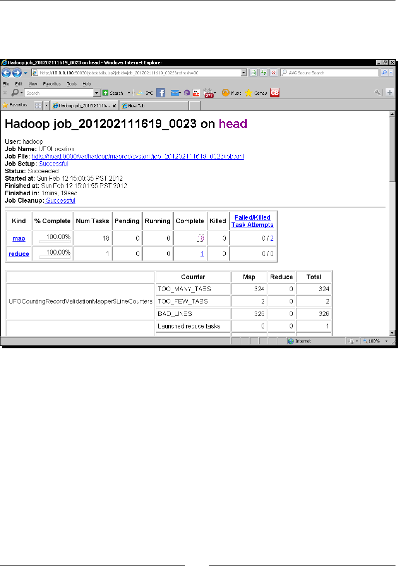
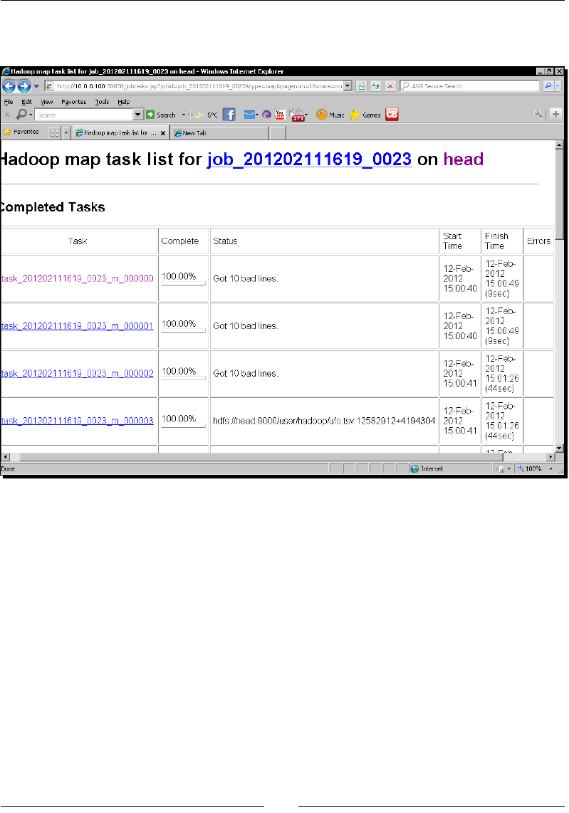
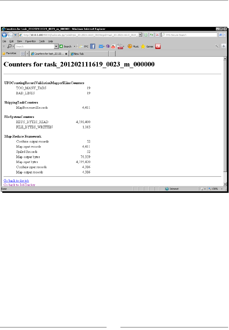
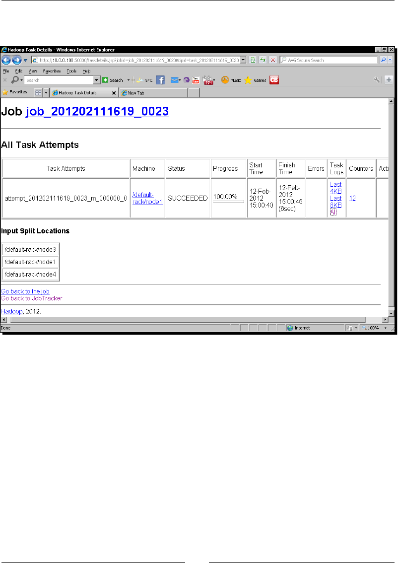
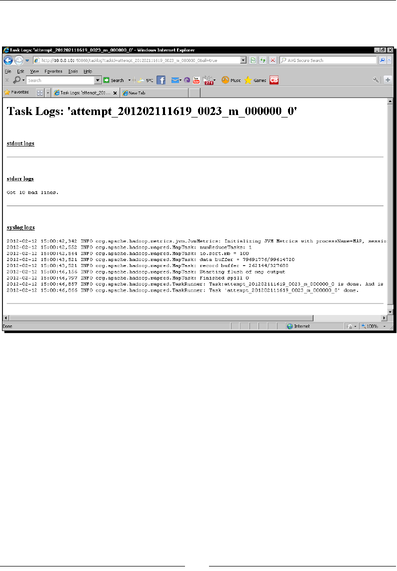
Developing MapReduce Programs
[ 124 ]
8. Under the Task Logs column are opons for the amount of data to be displayed.
Click on All and the following screenshot should be displayed:
9. Now log into one of the task nodes and look through the les stored under hadoop/
logs/userlogs. There is a directory for each task aempt and several les within
each; the one to look for is stderr.
What just happened?
The rst thing we need to do in order to add new counters is to create a standard Java
enumeraon that will hold them. In this case we created what Hadoop would consider a
counter group called LineCounters and within that there are three counters for the total
number of bad lines, and ner grained counters for the number of lines with either too
few or too many elds. This is all you need to do to create a new set of counters; dene
the enumeraon and once you start seng the counter values, they will be automacally
understood by the framework.
www.it-ebooks.info

Chapter 4
[ 125 ]
To add to a counter we simply increment it via the Reporter object, in each case here we
add one each me we encounter a bad line, one with fewer than six elds, and one with
more than six elds.
We also retrieve the BAD_LINE counter for a task and if it is a mulple of 10, do
the following:
Set the task status to reect this fact
Write a similar message to stderr with the standard Java System.err.println
mechanism
We then go to the MapReduce UI and validate whether we can see both the counter totals in
the job overview as well as tasks with the custom state message in the task list.
We then explored the web UI, looking at the counters for an individual job, then under the
detail page for a task we saw, we can click on through the log les for the task.
We then looked at one of the nodes to see that Hadoop also captures the logs from each
task in a directory on the lesystem under the {HADOOP_HOME}/logs/userlogs directory.
Under subdirectories for each task aempt, there are les for the standard streams as well
as the general task logs. As you will see, a busy node can end up with a large number of task
log directories and it is not always easy to idenfy the task directories of interest. The web
interface proved itself to be a more ecient view on this data.
If you are using the Hadoop context object API, then counters are accessed
through the Context.getCounter().increment() method.
Too much information!
Aer not worrying much about how to get status and other informaon out of our jobs,
it may suddenly seem like we've got too many confusing opons. The fact of the maer is
that when running a fully distributed cluster in parcular, there really is no way around the
fact that the data may be spread across every node. With Java code we can't as easily mock
its usage on the command line as we did with our Ruby Streaming tasks; so care needs to be
taken to think about what informaon will be needed at runme. This should include details
concerning both the general job operaon (addional stascs) as well as indicators of
problems that may need further invesgaon.
www.it-ebooks.info

Developing MapReduce Programs
[ 126 ]
Counters, task status messages, and good old-fashioned Java logging can work together. If
there is a situaon you care about, set it as a counter that will record each me it occurs and
consider seng the status message of the task that encountered it. If there is some specic
data, write that to stderr. Since counters are so easily visible, you can know prey quickly
post job compleon if the situaon of interest occurred. From this, you can go to the web UI
and see all the tasks in which the situaon was encountered at a glance. From here, you can
click through to examine the more detailed logs for the task.
In fact, you don't need to wait unl the job completes; counters and task status messages
are updated in the web UI as the job proceeds, so you can start the invesgaon as soon
as either counters or task status messages alert you to the situaon. This is parcularly
useful in very long running jobs where the errors may cause you to abort the job.
Summary
This chapter covered development of a MapReduce job, highlighng some of the issues
and approaches you are likely to face frequently. In parcular, we learned how Hadoop
Streaming provides a means to use scripng languages to write map and reduce tasks,
and how using Streaming can be an eecve tool for early stages of job prototyping and
inial data analysis.
We also learned that wring tasks in a scripng language can provide the addional
benet of using command-line tools to directly test and debug the code. Within the Java
API, we looked at the ChainMapper class that provides an ecient way of decomposing
a complex map task into a series of smaller, more focused ones.
We then saw how the Distributed Cache provides a mechanism for ecient sharing of data
across all nodes. It copies les from HDFS onto the local lesystem on each node, providing
local access to the data. We also learned how to add job counters by dening a Java
enumeraon for the counter group and using framework methods to increment their
values, and how to use a combinaon of counters, task status messages,
and debug logs to develop an ecient job analysis workow.
We expect most of these techniques and ideas to be the ones that you will encounter
frequently as you develop MapReduce jobs. In the next chapter, we will explore a series
of more advanced techniques that are less oen encountered but are invaluable when
they are.
www.it-ebooks.info
5
Advanced MapReduce Techniques
Now that we have looked at a few details of the fundamentals of MapReduce and its usage,
it's me to examine some more techniques and concepts involved in MapReduce. This
chapter will cover the following topics:
Performing joins on data
Implemenng graph algorithms in MapReduce
How to represent complex datatypes in a language-independent fashion
Along the way, we'll use the case studies as examples in order to highlight other aspects
such as ps and tricks and idenfying some areas of best pracce.
Simple, advanced, and in-between
Including the word "advanced" in a chapter tle is a lile dangerous, as complexity is a
subjecve concept. So let's be very clear about the material covered here. We don't, for even
a moment, suggest that this is the pinnacle of dislled wisdom that would otherwise take
years to acquire. Conversely, we also don't claim that some of the techniques and problems
covered in this chapter will have occurred to someone new to the world of Hadoop.
For the purposes of this chapter, therefore, we use the term "advanced" to cover things that
you don't see in the rst days or weeks, or wouldn't necessarily appreciate if you did. These
are some techniques that provide both specic soluons to parcular problems but also
highlight ways in which the standard Hadoop and related APIs can be employed to address
problems that are not obviously suited to the MapReduce processing model. Along the way,
we'll also point out some alternave approaches that we don't implement here but which
may be useful sources for further research.
Our rst case study is a very common example of this laer case; performing join-type
operaons within MapReduce.
www.it-ebooks.info

Advanced MapReduce Techniques
[ 128 ]
Joins
Few problems use a single set of data. In many cases, there are easy ways to obviate the need
to try and process numerous discrete yet related data sets within the MapReduce framework.
The analogy here is, of course, to the concept of join in a relaonal database. It is very
natural to segment data into numerous tables and then use SQL statements that join tables
together to retrieve data from mulple sources. The canonical example is where a main
table has only ID numbers for parcular facts, and joins against other tables are used to
extract data about the informaon referred to by the unique ID.
When this is a bad idea
It is possible to implement joins in MapReduce. Indeed, as we'll see, the problem is
less about the ability to do it and more the choice of which of many potenal strategies
to employ.
However, MapReduce joins are oen dicult to write and easy to make inecient. Work
with Hadoop for any length of me, and you will come across a situaon where you need
to do it. However, if you very frequently need to perform MapReduce joins, you may want
to ask yourself if your data is well structured and more relaonal in nature than you rst
assumed. If so, you may want to consider Apache Hive (the main topic of Chapter 8, A
Relaonal View on Data with Hive) or Apache Pig (briey menoned in the same chapter).
Both provide addional layers atop Hadoop that allow data processing operaons to be
expressed in high-level languages; in the case of Hive, through a variant of SQL.
Map-side versus reduce-side joins
That caveat out of the way, there are two basic approaches to join data in Hadoop and these
are given their names depending on where in the job execuon the join occurs. In either
case, we need to bring mulple data streams together and perform the join through some
logic. The basic dierence between these two approaches is whether the mulple data
streams are combined within the mapper or reducer funcons.
Map-side joins, as the name implies, read the data streams into the mapper and uses
logic within the mapper funcon to perform the join. The great advantage of a map-side
join is that by performing all joining—and more crically data volume reducon—within
the mapper, the amount of data transferred to the reduce stage is greatly minimized. The
drawback of map-side joins is that you either need to nd a way of ensuring one of the
data sources is very small or you need to dene the job input to follow very specic criteria.
Oen, the only way to do that is to preprocess the data with another MapReduce job whose
sole purpose is to make the data ready for a map-side join.
www.it-ebooks.info

Chapter 5
[ 129 ]
In contrast, a reduce-side join has the mulple data streams processed through the map
stage without performing any join logic and does the joining in the reduce stage. The
potenal drawback of this approach is that all the data from each source is pulled through
the shue stage and passed into the reducers, where much of it may then be discarded by
the join operaon. For large data sets, this can become a very signicant overhead.
The main advantage of the reduce-side join is its simplicity; you are largely responsible
for how the jobs are structured and it is oen quite straighorward to dene a reduce-side
join approach for related data sets. Let's look at an example.
Matching account and sales information
A common situaon in many companies is that sales records are kept separate from the
client data. There is, of course, a relaonship between the two; usually a sales record
contains the unique ID of the user account through which the sale was performed.
In the Hadoop world, these would be represented by two types of data les: one containing
records of the user IDs and informaon for sales, and the other would contain the full data
for each user account.
Frequent tasks require reporng that uses data from both these sources; say, for example,
we wanted to see the total number of sales and total value for each user but do not want
to associate it with an anonymous ID number, but rather with a name. This may be valuable
when customer service representaves wish to call the most frequent customers—data from
the sales records—but want to be able to refer to the person by name and not just a number.
Time for action – reduce-side join using MultipleInputs
We can perform the report explained in the previous secon using a reduce-side join by
performing the following steps:
1. Create the following tab-separated le and name it sales.txt:
00135.992012-03-15
00212.492004-07-02
00413.422005-12-20
003499.992010-12-20
00178.952012-04-02
00221.992006-11-30
00293.452008-09-10
0019.992012-05-17
www.it-ebooks.info

Advanced MapReduce Techniques
[ 130 ]
2. Create the following tab-separated le and name it accounts.txt:
001John AllenStandard2012-03-15
002Abigail SmithPremium2004-07-13
003April StevensStandard2010-12-20
004Nasser HafezPremium2001-04-23
3. Copy the datales onto HDFS.
$ hadoop fs -mkdir sales
$ hadoop fs -put sales.txt sales/sales.txt
$ hadoop fs -mkdir accounts
$ hadoop fs -put accounts/accounts.txt
4. Create the following le and name it ReduceJoin.java:
import java.io.* ;
import org.apache.hadoop.conf.Configuration;
import org.apache.hadoop.fs.Path;
import org.apache.hadoop.io.Text;
import org.apache.hadoop.mapreduce.*;
import org.apache.hadoop.mapreduce.lib.input.*;
import org.apache.hadoop.mapreduce.lib.input.*;
public class ReduceJoin
{
public static class SalesRecordMapper
extends Mapper<Object, Text, Text, Text>
{
public void map(Object key, Text value, Context context)
throws IOException, InterruptedException
{
String record = value.toString() ;
String[] parts = record.split("\t") ;
context.write(new Text(parts[0]), new
Text("sales\t"+parts[1])) ;
}
}
public static class AccountRecordMapper
extends Mapper<Object, Text, Text, Text>
{
www.it-ebooks.info

Chapter 5
[ 131 ]
public void map(Object key, Text value, Context context)
throws IOException, InterruptedException
{
String record = value.toString() ;
String[] parts = record.split("\t") ;
context.write(new Text(parts[0]), new
Text("accounts\t"+parts[1])) ;
}
}
public static class ReduceJoinReducer
extends Reducer<Text, Text, Text, Text>
{
public void reduce(Text key, Iterable<Text> values,
Context context)
throws IOException, InterruptedException
{
String name = "" ;
double total = 0.0 ;
int count = 0 ;
for(Text t: values)
{
String parts[] = t.toString().split("\t") ;
if (parts[0].equals("sales"))
{
count++ ;
total+= Float.parseFloat(parts[1]) ;
}
else if (parts[0].equals("accounts"))
{
name = parts[1] ;
}
}
String str = String.format("%d\t%f", count, total) ;
context.write(new Text(name), new Text(str)) ;
}
}
www.it-ebooks.info

Advanced MapReduce Techniques
[ 132 ]
public static void main(String[] args) throws Exception
{
Configuration conf = new Configuration();
Job job = new Job(conf, "Reduce-side join");
job.setJarByClass(ReduceJoin.class);
job.setReducerClass(ReduceJoinReducer.class);
job.setOutputKeyClass(Text.class);
job.setOutputValueClass(Text.class);
MultipleInputs.addInputPath(job, new Path(args[0]),
TextInputFormat.class, SalesRecordMapper.class) ;
MultipleInputs.addInputPath(job, new Path(args[1]),
TextInputFormat.class, AccountRecordMapper.class) ;
Path outputPath = new Path(args[2]);
FileOutputFormat.setOutputPath(job, outputPath);
outputPath.getFileSystem(conf).delete(outputPath);
System.exit(job.waitForCompletion(true) ? 0 : 1);
}
}
5. Compile the le and add it to a JAR le.
$ javac ReduceJoin.java
$ jar -cvf join.jar *.class
6. Run the job by execung the following command:
$ hadoop jar join.jarReduceJoin sales accounts outputs
7. Examine the result le.
$ hadoop fs -cat /user/garry/outputs/part-r-00000
John Allen 3 124.929998
Abigail Smith 3 127.929996
April Stevens 1 499.989990
Nasser Hafez 1 13.420000
What just happened?
Firstly, we created the datales to be used in this example. We created two small data sets as
this makes it easier to track the result output. The rst data set we dened was the account
details with four columns, as follows:
The account ID
The client name
www.it-ebooks.info

Chapter 5
[ 133 ]
The type of account
The date the account was opened
We then created a sales record with three columns:
The account ID of the purchaser
The value of the sale
The date of the sale
Naturally, real account and sales records would have many more elds than the ones
menoned here. Aer creang the les, we placed them onto HDFS.
We then created the ReduceJoin.java le, which looks very much like the previous
MapReduce jobs we have used. There are a few aspects to this job that make it special
and allow us to implement a join.
Firstly, the class has two dened mappers. As we have seen before, jobs can have mulple
mappers executed in a chain; but in this case, we wish to apply dierent mappers to each
of the input locaons. Accordingly, we have the sales and account data dened into the
SalesRecordMapper and AccountRecordMapper classes. We used the MultipleInputs
class from the org.apache.hadoop.mapreduce.lib.io package as follows:
MultipleInputs.addInputPath(job, new Path(args[0]),
TextInputFormat.class, SalesRecordMapper.class) ;
MultipleInputs.addInputPath(job, new Path(args[1]),
TextInputFormat.class, AccountRecordMapper.class) ;
As you can see, unlike in previous examples where we add a single input locaon, the
MultipleInputs class allows us to add mulple sources and associate each with a
disnct input format and mapper.
The mappers are prey straighorward; the SalesRecordMapper class emits an output of
the form <account number>, <sales value> while the AccountRecordMapper class
emits an output of the form <account number>, <client name>. We therefore have
the order value and client name for each sale being passed into the reducer where the
actual join will happen.
Noce that both mappers actually emit more than the required values.
The SalesRecordMapper class prexes its value output with sales while
the AccountRecordMapper class uses the tag account.
If we look at the reducer, we can see why this is so. The reducer retrieves each record for a
given key, but without these explicit tags we would not know if a given value came from the
sales or account mapper and hence would not understand how to treat the data value.
www.it-ebooks.info

Advanced MapReduce Techniques
[ 134 ]
The ReduceJoinReducer class therefore treats the values in the Iterator
object dierently, depending on which mapper they came from. Values from the
AccountRecordMapper class—and there should be only one—are used to populate
the client name in the nal output. For each sales record—likely to be mulple, as most
clients buy more than a single item—the total number of orders is counted as is the overall
combined value. The output from the reducer is therefore a key of the account holder name
and a value string containing the number of orders and the total order value.
We compile and execute the class; noce how we provide three arguments represenng
the two input directories as well as the single output source. Because of how the
MultipleInputs class is congured, we must also ensure we specify the directories
in the right order; there is no dynamic mechanism to determine which type of le is in
which locaon.
Aer execuon, we examine the output le and conrm that it does indeed contain the
overall totals for named clients as expected.
DataJoinMapper and TaggedMapperOutput
There is a way of implemenng a reduce-side join in a more sophiscated and object-
oriented fashion. Within the org.apache.hadoop.contrib.join package are classes
such as DataJoinMapperBase and TaggedMapOutput that provide an encapsulated
means of deriving the tags for map output and having them processed at the reducer. This
mechanism means you don't have to dene explicit tag strings as we did previously and then
carefully parse out the data received at the reducer to determine from which mapper the
data came; there are methods in the provided classes that encapsulate this funconality.
This capability is parcularly valuable when using numeric or other non-textual data. For
creang our own explicit tags as in the previous example, we would have to convert types
such as integers into strings to allow us to add the required prex tag. This will be more
inecient than using the numeric types in their normal form and relying on the addional
classes to implement the tag.
The framework allows for quite sophiscated tag generaon as well as concepts such as tag
grouping that we didn't implement previously. There is addional work required to use this
mechanism that includes overriding addional methods and using a dierent map base class.
For straighorward joins such as in the previous example, this framework may be overkill,
but if you nd yourself implemenng very complex tagging logic, it may be worth a look.
www.it-ebooks.info

Chapter 5
[ 135 ]
Implementing map-side joins
For a join to occur at a given point, we must have access to the appropriate records from
each data set at that point. This is where the simplicity of the reduce-side join comes into
its own; though it incurs the expense of addional network trac, processing it by denion
ensures that the reducer has all records associated with the join key.
If we wish to perform our join in the mapper, it isn't as easy to make this condion hold
true. We can't assume that our input data is suciently well structured to allow associated
records to be read simultaneously. We generally have two classes of approach here: obviate
the need to read from mulple external sources or preprocess the data so that it is amenable
for map-side joining.
Using the Distributed Cache
The simplest way of realizing the rst approach is to take all but one data set and make it
available in the Distributed Cache that we used in the previous chapter. The approach can
be used for mulple data sources, but for simplicity let's discuss just two.
If we have one large data set and one smaller one, such as with the sales and account info
earlier, one opon would be to package up the account info and push it into the Distributed
Cache. Each mapper would then read this data into an ecient data structure, such as a
hash table that uses the join key as the hash key. The sales records are then processed,
and during the processing of record each the needed account informaon can be
retrieved from the hash table.
This mechanism is very eecve and when one of the smaller data sets can easily t into
memory, it is a great approach. However, we are not always that lucky, and somemes the
smallest data set is sll too large to be copied to every worker machine and held in memory.
Have a go hero - Implementing map-side joins
Take the previous sales/account record example and implement a map-side join using the
Distributed Cache. If you load the account records into a hash table that maps account ID
numbers to client names, you can use the account ID to retrieve the client name. Do this
within the mapper while processing the sales records.
Pruning data to t in the cache
If the smallest data set is sll too big to be used in the Distributed Cache, all is not
necessarily lost. Our earlier example, for instance, extracted only two elds from each record
and discarded the other elds not required by the job. In reality, an account will be described
by many aributes, and this sort of reducon will limit the data size dramacally. Oen the
data available to Hadoop is this full data set, but what we need is only a subset of the elds.
www.it-ebooks.info

Advanced MapReduce Techniques
[ 136 ]
In such a case, therefore, it may be possible to extract from the full data set only the elds
that are needed during the MapReduce job, and in doing so create a pruned data set that is
small enough to be used in the cache.
This is a very similar concept to the underlying column-oriented databases.
Tradional relaonal databases store data a row at a me, meaning that
the full row needs to be read to extract a single column. A column-based
database instead stores each column separately, allowing a query to read
only the columns in which it is interested.
If you take this approach, you need to consider what mechanism will be used to generate
the data subset and how oen this will be done. The obvious approach is to write another
MapReduce job that does the necessary ltering and this output is then used in the
Distributed Cache for the follow-on job. If the smaller data set changes only rarely, you may
be able to get away with generang the pruned data set on a scheduled basis; for example,
refresh it every night. Otherwise, you will need to make a chain of two MapReduce jobs: one
to produce the pruned data set and the other to perform the join operaon using the large
set and the data in the Distributed Cache.
Using a data representation instead of raw data
Somemes, one of the data sources is not used to retrieve addional data but is instead
used to derive some fact that is then used in a decision process. We may, for example, be
looking to lter sales records to extract only those for which the shipping address was in a
specic locale.
In such a case, we can reduce the required data size down to a list of the applicable sales
records that may more easily t into the cache. We can again store it as a hash table, where
we are just recording the fact that the record is valid, or even use something like a sorted
list or a tree. In cases where we can accept some false posives while sll guaranteeing no
false negaves, a Bloom lter provides an extremely compact way of represenng such
informaon.
As can be seen, applying this approach to enable a map-side join requires creavity and not
a lile luck in regards to the nature of the data set and the problem at hand. But remember
that the best relaonal database administrators spend signicant me opmizing queries
to remove unnecessary data processing; so it's never a bad idea to ask if you truly need to
process all that data.
Using multiple mappers
Fundamentally, the previous techniques are trying to remove the need for a full cross data
set join. But somemes this is what you have to do; you may simply have very large data
sets that cannot be combined in any of these clever ways.
www.it-ebooks.info

Chapter 5
[ 137 ]
There are classes within the org.apache.hadoop.mapreduce.lib.join package that
support this situaon. The main class of interest is CompositeInputFormat, which applies
a user-dened funcon to combine records from mulple data sources.
The main limitaon of this approach is that the data sources must already be indexed based
on the common key, in addion to being both sorted and paroned in the same way. The
reason for this is simple: when reading from each source, the framework needs to know if
a given key is present at each locaon. If we know that each paron is sorted and contains
the same key range, simple iteraon logic can do the required matching.
This situaon is obviously not going to happen by accident, so again you may nd yourself
wring preprocess jobs to transform all the input data sources into the correct sort and
paron structure.
This discussion starts to touch on distributed and parallel join algorithms;
both topics are of extensive academic and commercial research. If you are
interested in the ideas and want to learn more of the underlying theory, go
searching on http://scholar.google.com.
To join or not to join...
Aer our tour of joins in the MapReduce world, let's come back to the original queson:
are you really sure you want to be doing this? The choice is oen between a relavely
easily implemented yet inecient reduce-side join, and more ecient but more complex
map-side alternaves. We have seen that joins can indeed be implemented in MapReduce,
but they aren't always prey. This is why we advise the use of something like Hive or Pig if
these types of problems comprise a large poron of your workload. Obviously, we can use
tools such as those that do their own translaon into MapReduce code under the hood
and directly implement both map-side and reduce-side joins, but it's oen beer to use
a well-engineered and well-opmized library for such workloads instead of building your
own. That is aer all why you are using Hadoop and not wring your own distributed
processing framework!
Graph algorithms
Any good computer scienst will tell you that the graph data structure is one of the
most powerful tools around. Many complex systems are best represented by graphs and
a body of knowledge going back at least decades (centuries if you get more mathemacal
about it) provides very powerful algorithms to solve a vast variety of graph problems. But
by their very nature, graphs and their algorithms are oen very dicult to imagine in a
MapReduce paradigm.
www.it-ebooks.info

Advanced MapReduce Techniques
[ 138 ]
Graph 101
Let's take a step back and dene some terminology. A graph is a structure comprising of
nodes (also called verces) that are connected by links called edges. Depending on the type
of graph, the edges may be bidireconal or unidireconal and may have weights associated
with them. For example, a city road network can be seen as a graph where the roads are
the edges, and intersecons and points of interest are nodes. Some streets are one-way
and some are not, some have tolls, some are closed at certain mes of day, and so forth.
For transportaon companies, there is much money to be made by opmizing the routes
taken from one point to another. Dierent graph algorithms can derive such routes by taking
into account aributes such as one-way streets and other costs expressed as weights that
make a given road more aracve or less so.
For a more current example, think of the social graph popularized by sites such as Facebook
where the nodes are people and the edges are the relaonships between them.
Graphs and MapReduce – a match made somewhere
The main reason graphs don't look like many other MapReduce problems is due to the
stateful nature of graph processing, which can be seen in the path-based relaonship
between elements and oen between the large number of nodes processed together
for a single algorithm. Graph algorithms tend to use noons of the global state to make
determinaons about which elements to process next and modify such global knowledge
at each step.
In parcular, most of the well-known algorithms oen execute in an incremental or reentrant
fashion, building up structures represenng processed and pending nodes, and working
through the laer while reducing the former.
MapReduce problems, on the other hand, are conceptually stateless and typically based
upon a divide-and-conquer approach where each Hadoop worker host processes a small
subset of the data, wring out a poron of the nal result where the total job output is
viewed as the simple collecon of these smaller outputs. Therefore, when implemenng
graph algorithms in Hadoop, we need to express algorithms that are fundamentally stateful
and conceptually single-threaded in a stateless parallel and distributed framework. That's
the challenge!
Most of the well-known graph algorithms are based upon search or traversal of the graph,
oen to nd routes—frequently ranked by some noon of cost—between nodes. The most
fundamental graph traversal algorithms are depth-rst search (DFS) and breadth-rst search
(BFS).The dierence between the algorithms is the ordering in which a node is processed in
relaonship to its neighbors.
www.it-ebooks.info
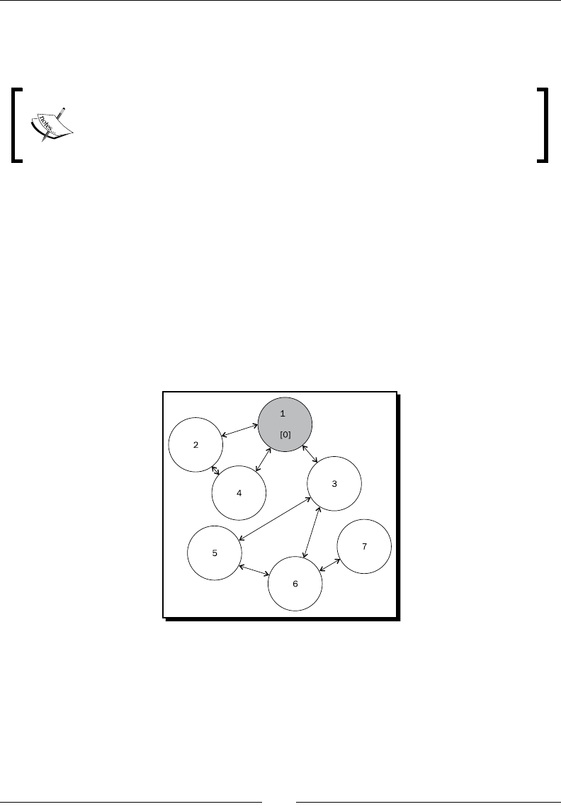
Chapter 5
[ 139 ]
We will look at represenng an algorithm that implements a specialized form of such a
traversal; for a given starng node in the graph, determine the distance between it and
every other node in the graph.
As can be seen, the eld of graph algorithms and theory is a huge one that
we barely scratch the surface of here. If you want to nd out more, the
Wikipedia entry on graphs is a good starng point; it can be found at http://
en.wikipedia.org/wiki/Graph_(abstract_data_type).
Representing a graph
The rst problem we face is how to represent the graph in a way we can eciently
process using MapReduce. There are several well-known graph representaons known
as pointer-based, adjacency matrix, and adjacency list. In most implementaons, these
representaons oen assume a single process space with a global view of the whole graph;
we need to modify the representaon to allow individual nodes to be processed in discrete
map and reduce tasks.
We'll use the graph shown here in the following examples. The graph does have some extra
informaon that will be explained later.
Our graph is quite simple; it has only seven nodes, and all but one of the edges is
bidireconal. We are also using a common coloring technique that is used in standard
graph algorithms, as follows:
White nodes are yet to be processed
Gray nodes are currently being processed
Black nodes have been processed
www.it-ebooks.info

Advanced MapReduce Techniques
[ 140 ]
As we process our graph in the following steps, we will expect to see the nodes move
through these stages.
Time for action – representing the graph
Let's dene a textual representaon of the graph that we'll use in the following examples.
Create the following as graph.txt:
12,3,40C
21,4
31,5,6
41,2
53,6
63,5
76
What just happened?
We dened a le structure that will represent our graph, based somewhat on the adjacency
list approach. We assumed that each node has a unique ID and the le structure has four
elds, as follows:
The node ID
A comma-separated list of neighbors
The distance from the start node
The node status
In the inial representaon, only the starng node has values for the third and fourth
columns: its distance from itself is 0 and its status is "C", which we'll explain later.
Our graph is direconal—more formally referred to as a directed graph—that is to say,
if node 1 lists node 2 as a neighbor, there is only a return path if node 2 also lists node 1
as its neighbor. We see this in the graphical representaon where all but one edge has an
arrow on both ends.
Overview of the algorithm
Because this algorithm and corresponding MapReduce job is quite involved, we'll explain
it before showing the code, and then demonstrate it in use later.
Given the previous representaon, we will dene a MapReduce job that will be executed
mulple mes to get the nal output; the input to a given execuon of the job will be the
output from the previous execuon.
www.it-ebooks.info

Chapter 5
[ 141 ]
Based on the color code described in the previous secon, we will dene three states
for a node:
Pending: The node is yet to be processed; it is in the default state (white)
Currently processing: The node is being processed (gray)
Done: The nal distance for the node has been determined (black)
The mapper
The mapper will read in the current representaon of the graph and treat each node
as follows:
If the node is marked as Done, it gives output with no changes.
If the node is marked as Currently processing, its state is changed to Done and gives
output with no other changes. Each of its neighbors gives output as per the current
record with its distance incremented by one, but with no neighbors; node 1 doesn't
know node 2's neighbors, for example.
If the node is marked Pending, its state is changed to Currently processing and it
gives output with no further changes.
The reducer
The reducer will receive one or more records for each node ID, and it will combine their
values into the nal output node record for that stage.
The general algorithm for the reducer is as follows:
A Done record is the nal output and no further processing of the values
is performed
For other nodes, the nal output is built up by taking the list of neighbors,
where it is to be found, and the highest distance and state
Iterative application
If we apply this algorithm once, we will get node 1 marked as Done, several more (its
immediate neighbors) as Current, and a few others as Pending. Successive applicaons of
the algorithm will see all nodes move to their nal state; as each node is encountered, its
neighbors are brought into the processing pipeline. We will show this later.
www.it-ebooks.info

Advanced MapReduce Techniques
[ 142 ]
Time for action – creating the source code
We'll now see the source code to implement our graph traversal. Because the code
is lengthy, we'll break it into mulple steps; obviously they should all be together in
a single source le.
1. Create the following as GraphPath.java with these imports:
import java.io.* ;
import org.apache.hadoop.conf.Configuration;
import org.apache.hadoop.fs.Path;
import org.apache.hadoop.io.Text;
import org.apache.hadoop.mapreduce.Job;
import org.apache.hadoop.mapreduce.*;
import org.apache.hadoop.mapreduce.lib.input.*;
import org.apache.hadoop.mapreduce.lib.output.*;
public class GraphPath
{
2. Create an inner class to hold an object-oriented representaon of a node:
// Inner class to represent a node
public static class Node
{
// The integer node id
private String id ;
// The ids of all nodes this node has a path to
private String neighbours ;
// The distance of this node to the starting node
private int distance ;
// The current node state
private String state ;
// Parse the text file representation into a Node object
Node( Text t)
{
String[] parts = t.toString().split("\t") ;
this.id = parts[0] ;
this.neighbours = parts[1] ;
if (parts.length<3 || parts[2].equals(""))
this.distance = -1 ;
else
this.distance = Integer.parseInt(parts[2]) ;
www.it-ebooks.info

Chapter 5
[ 143 ]
if (parts.length< 4 || parts[3].equals(""))
this.state = "P" ;
else
this.state = parts[3] ;
}
// Create a node from a key and value object pair
Node(Text key, Text value)
{
this(new Text(key.toString()+"\t"+value.toString())) ;
}
Public String getId()
{return this.id ;
}
public String getNeighbours()
{
return this.neighbours ;
}
public int getDistance()
{
return this.distance ;
}
public String getState()
{
return this.state ;
}
}
3. Create the mapper for the job. The mapper will create a new Node object for its
input and then examine it, and based on its state do the appropriate processing.
public static class GraphPathMapper
extends Mapper<Object, Text, Text, Text>
{
public void map(Object key, Text value, Context context)
throws IOException, InterruptedException
{
Node n = new Node(value) ;
if (n.getState().equals("C"))
www.it-ebooks.info

Advanced MapReduce Techniques
[ 144 ]
{
// Output the node with its state changed to Done
context.write(new Text(n.getId()), new
Text(n.getNeighbours()+"\t"+n.getDistance()+"\t"+"D")) ;
for (String neighbour:n.getNeighbours().
split(","))
{
// Output each neighbour as a Currently processing node
// Increment the distance by 1; it is one link further away
context.write(new Text(neighbour), new
Text("\t"+(n.getDistance()+1)+"\tC")) ;
}
}
else
{
// Output a pending node unchanged
context.write(new Text(n.getId()), new
Text(n.getNeighbours()+"\t"+n.getDistance()
+"\t"+n.getState())) ;
}
}
}
4. Create the reducer for the job. As with the mapper, this reads in a representaon
of a node and gives as output a dierent value depending on the state of the node.
The basic approach is to collect from the input the largest value for the state and
distance columns, and through this converge to the nal soluon.
public static class GraphPathReducer
extends Reducer<Text, Text, Text, Text>
{
public void reduce(Text key, Iterable<Text> values,
Context context)
throws IOException, InterruptedException
{
// Set some default values for the final output
String neighbours = null ;
int distance = -1 ;
String state = "P" ;
for(Text t: values)
{
Node n = new Node(key, t) ;
www.it-ebooks.info

Chapter 5
[ 145 ]
if (n.getState().equals("D"))
{
// A done node should be the final output; ignore the remaining
// values
neighbours = n.getNeighbours() ;
distance = n.getDistance() ;
state = n.getState() ;
break ;
}
// Select the list of neighbours when found
if (n.getNeighbours() != null)
neighbours = n.getNeighbours() ;
// Select the largest distance
if (n.getDistance() > distance)
distance = n.getDistance() ;
// Select the highest remaining state
if (n.getState().equals("D") ||
(n.getState().equals("C") &&state.equals("P")))
state=n.getState() ;
}
// Output a new node representation from the collected parts
context.write(key, new
Text(neighbours+"\t"+distance+"\t"+state)) ;
}
}
5. Create the job driver:
public static void main(String[] args) throws Exception
{
Configuration conf = new Configuration();
Job job = new Job(conf, "graph path");
job.setJarByClass(GraphPath.class);
job.setMapperClass(GraphPathMapper.class);
job.setReducerClass(GraphPathReducer.class);
job.setOutputKeyClass(Text.class);
job.setOutputValueClass(Text.class);
FileInputFormat.addInputPath(job, new Path(args[0]));
FileOutputFormat.setOutputPath(job, new Path(args[1]));
System.exit(job.waitForCompletion(true) ? 0 : 1);
}
}
www.it-ebooks.info

Advanced MapReduce Techniques
[ 146 ]
What just happened?
The job here implements the previously described algorithm that we'll execute in
the following secons. The job setup is prey standard, and apart from the algorithm
denion the only new thing here is the use of an inner class to represent nodes.
The input to a mapper or reducer is oen a aened representaon of a more complex
structure or object. We could just use that representaon, but in this case this would result
in the mapper and reducer bodies being full of text and string manipulaon code that would
obscure the actual algorithm.
The use of the Node inner class allows the mapping from the at le to object representaon
that is to be encapsulated in an object that makes sense in terms of the business domain.
This also makes the mapper and reducer logic clearer as comparisons between object
aributes are more semancally meaningful than comparisons with slices of a string
idened only by absolute index posions.
Time for action – the rst run
Let's now perform the inial execuon of this algorithm on our starng representaon of
the graph:
1. Put the previously created graph.txt le onto HDFS:
$ hadoop fs -mkdirgraphin
$ hadoop fs -put graph.txtgraphin/graph.txt
2. Compile the job and create the JAR le:
$ javac GraphPath.java
$ jar -cvf graph.jar *.class
3. Execute the MapReduce job:
$ hadoop jar graph.jarGraphPathgraphingraphout1
4. Examine the output le:
$ hadoop fs –cat /home/user/hadoop/graphout1/part-r00000
12,3,40D
21,41C
31,5,61C
41,21C
53,6-1P
63,5-1P
76-1P
www.it-ebooks.info
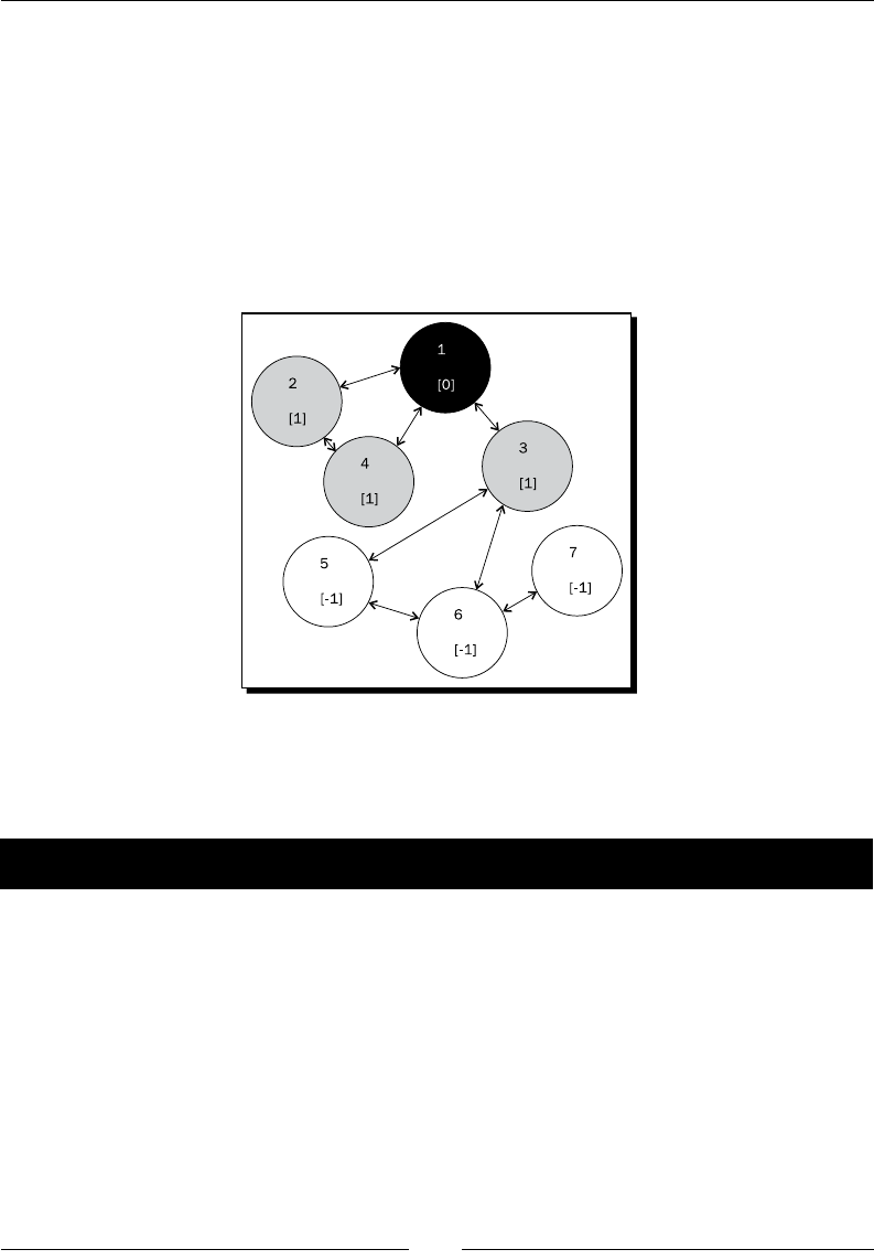
Chapter 5
[ 147 ]
What just happened?
Aer pung the source le onto HDFS and creang the job JAR le, we executed the job in
Hadoop. The output representaon of the graph shows a few changes, as follows:
Node 1 is now marked as Done; its distance from itself is obviously 0
Nodes 2, 3, and 4 – the neighbors of node 1 — are marked as Currently processing
All other nodes are Pending
Our graph now looks like the following gure:
Given the algorithm, this is to be expected; the rst node is complete and its neighboring
nodes, extracted through the mapper, are in progress. All other nodes are yet to
begin processing.
Time for action – the second run
If we take this representaon as the input to another run of the job, we would expect nodes
2, 3, and 4 to now be complete, and for their neighbors to now be in the Current state. Let's
see; execute the following steps:
1. Execute the MapReduce job by execung the following command:
$ hadoop jar graph.jarGraphPathgraphout1graphout2
2. Examine the output le:
$ hadoop fs -cat /home/user/hadoop/graphout2/part-r000000
12,3,40D
21,41D
www.it-ebooks.info
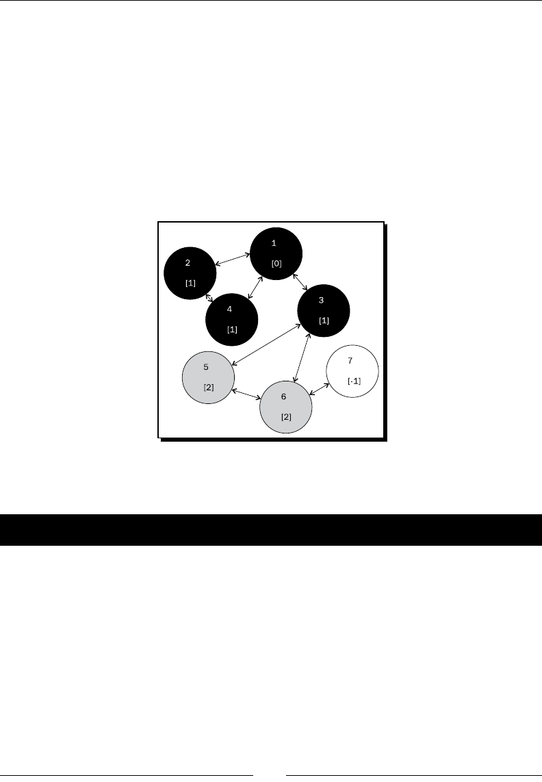
Advanced MapReduce Techniques
[ 148 ]
31,5,61D
41,21D
53,62C
63,52C
76-1P
What just happened?
As expected, nodes 1 through 4 are complete, nodes 5 and 6 are in progress, and node 7 is
sll pending, as seen in the following gure:
If we run the job again, we should expect nodes 5 and 6 to be Done and any unprocessed
neighbors to become Current.
Time for action – the third run
Let's validate that assumpon by running the algorithm for the third me.
1. Execute the MapReduce job:
$ hadoop jar graph.jarGraphPathgraphout2graphout3
2. Examine the output le:
$ hadoop fs -cat /user/hadoop/graphout3/part-r-00000
12,3,40D
21,41D
31,5,61D
www.it-ebooks.info
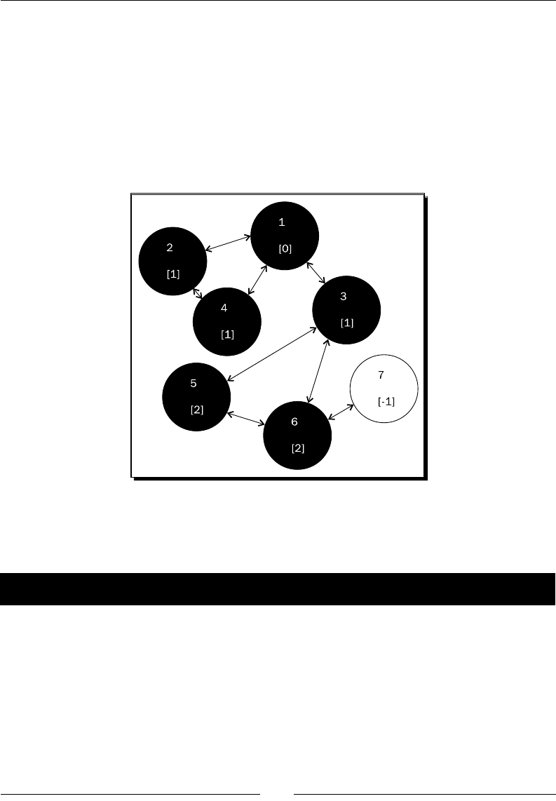
Chapter 5
[ 149 ]
41,21D
53,62D
63,52D
76-1P
What just happened?
We now see nodes 1 through 6 are complete. But node 7 is sll pending and no nodes are
currently being processed, as shown in the following gure:
The reason for this state is that though node 7 has a link to node 6, there is no edge in the
reverse direcon. Node 7 is therefore eecvely unreachable from node 1. If we run the
algorithm one nal me, we should expect to see the graph unchanged.
Time for action – the fourth and last run
Let's perform the fourth execuon to validate that the output has now reached its nal
stable state.
1. Execute the MapReduce job:
$ hadoop jar graph.jarGraphPathgraphout3graphout4
www.it-ebooks.info
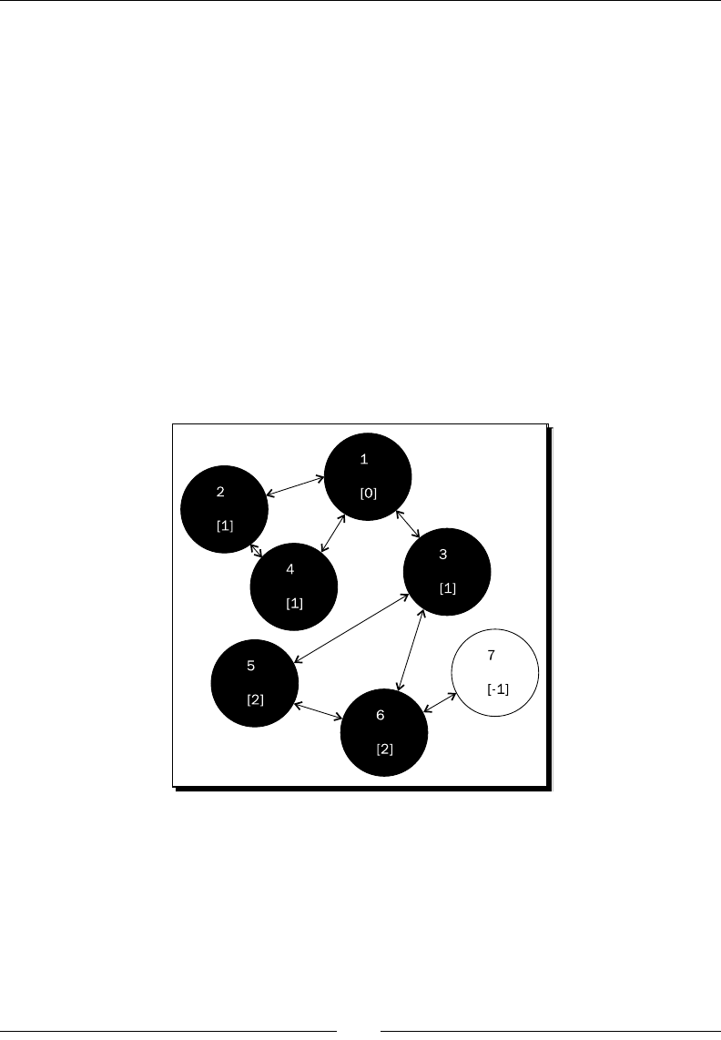
Advanced MapReduce Techniques
[ 150 ]
2. Examine the output le:
$ hadoop fs -cat /user/hadoop/graphout4/part-r-00000
12,3,40D
21,41D
31,5,61D
41,21D
53,62D
63,52D
76-1P
What just happened?
The output is as expected; since node 7 is not reachable by node 1 or any of its neighbors, it
will remain Pending and never be processed further. Consequently, our graph is unchanged
as shown in the following gure:
The one thing we did not build into our algorithm was an understanding of a terminang
condion; the process is complete if a run does not create any new D or C nodes.
The mechanism we use here is manual, that is, we knew by examinaon that the
graph representaon had reached its nal stable state. There are ways of doing this
programmacally, however. In a later chapter, we will discuss custom job counters; we
can, for example, increment a counter every me a new D or C node is created and only
reexecute the job if that counter is greater than zero aer the run.
www.it-ebooks.info

Chapter 5
[ 151 ]
Running multiple jobs
The previous algorithm is the rst me we have explicitly used the output of one MapReduce
job as the input to another. In most cases, the jobs are dierent; but, as we have seen, there
is value in repeatedly applying an algorithm unl the output reaches a stable state.
Final thoughts on graphs
For anyone familiar with graph algorithms, the previous process will seem very alien. This
is simply a consequence of the fact that we are implemenng a stateful and potenally
recursive global and reentrant algorithm as a series of serial stateless MapReduce jobs.
The important fact is not in the parcular algorithm used; the lesson is in how we can take
at text structures and a series of MapReduce jobs, and from this implement something
like graph traversal. You may have problems that at rst don't appear to have any way of
being implemented in the MapReduce paradigm; consider some of the techniques used
here and remember that many algorithms can be modeled in MapReduce. They may look
very dierent from the tradional approach, but the goal is the correct output and not an
implementaon of a known algorithm.
Using language-independent data structures
A cricism oen leveled at Hadoop, and which the community has been working
hard to address, is that it is very Java-centric. It may appear strange to accuse a project
fully implemented in Java of being Java-centric, but the consideraon is from a client's
perspecve.
We have shown how Hadoop Streaming allows the use of scripng languages to implement
map and reduce tasks and how Pipes provides similar mechanisms for C++. However, one
area that does remain Java-only is the nature of the input formats supported by Hadoop
MapReduce. The most ecient format is SequenceFile, a binary spliable container that
supports compression. However, SequenceFiles have only a Java API; they cannot be wrien
or read in any other language.
We could have an external process creang data to be ingested into Hadoop for MapReduce
processing, and the best way we could do this is either have it simply as an output of text
type or do some preprocessing to translate the output format into SequenceFiles to be
pushed onto HDFS. We also struggle here to easily represent complex data types; we either
have to aen them to a text format or write a converter across two binary formats, neither
of which is an aracve opon.
www.it-ebooks.info

Advanced MapReduce Techniques
[ 152 ]
Candidate technologies
Fortunately, there have been several technologies released in recent years that address
the queson of cross-language data representaons. They are Protocol Buers (created
by Google and hosted at http://code.google.com/p/protobuf), Thri (originally
created by Facebook and now an Apache project at http://thrift.apache.org), and
Avro (created by Doug Cung, the original creator of Hadoop). Given its heritage and ght
Hadoop integraon, we will use Avro to explore this topic. We won't cover Thri or Protocol
Buers in this book, but both are solid technologies; if the topic of data serializaon interests
you, check out their home pages for more informaon.
Introducing Avro
Avro, with its home page at http://avro.apache.org, is a data-persistence framework
with bindings for many programming languages. It creates a binary structured format
that is both compressible and spliable, meaning it can be eciently used as the input
to MapReduce jobs.
Avro allows the denion of hierarchical data structures; so, for example, we can create a
record that contains an array, an enumerated type, and a subrecord. We can create these
les in any programming language, process them in Hadoop, and have the result read by
a third language.
We'll talk about these aspects of language independence over the next secons, but this
ability to express complex structured types is also very valuable. Even if we are using only
Java, we could employ Avro to allow us to pass complex data structures in and out of
mappers and reducers. Even things like graph nodes!
Time for action – getting and installing Avro
Let's download Avro and get it installed on our system.
1. Download the latest stable version of Avro from http://avro.apache.org/
releases.html.
2. Download the latest version of the ParaNamer library from http://paranamer.
codehaus.org.
3. Add the classes to the build classpath used by the Java compiler.
$ export CLASSPATH=avro-1.7.2.jar:${CLASSPATH}
$ export CLASSPATH=avro-mapred-1.7.2.jar:${CLASSPATH}
$ export CLASSPATH=paranamer-2.5.jar:${CLASSPATH
www.it-ebooks.info

Chapter 5
[ 153 ]
4. Add exisng JAR les from the Hadoop distribuon to the build classpath.
Export CLASSPATH=${HADOOP_HOME}/lib/Jackson-core-asl-
1.8.jar:${CLASSPATH}
Export CLASSPATH=${HADOOP_HOME}/lib/Jackson-mapred-asl-
1.8.jar:${CLASSPATH}
Export CLASSPATH=${HADOOP_HOME}/lib/commons-cli-
1.2.jar:${CLASSPATH}
5. Add the new JAR les to the Hadoop lib directory.
$cpavro-1.7.2.jar ${HADOOP_HOME}/lib
$cpavro-1.7.2.jar ${HADOOP_HOME}/lib
$cpavro-mapred-1.7.2.jar ${HADOOP_HOME}/lib
What just happened?
Seng up Avro is a lile involved; it is a much newer project than the other Apache tools
we'll be using, so it requires more than a single download of a tarball.
We download the Avro and Avro-mapred JAR les from the Apache website. There is also
a dependency on ParaNamer that we download from its home page at codehaus.org.
The ParaNamer home page has a broken download link at the me of wring;
as an alternave, try the following link:
http://search.maven.org/remotecontent?filepath=com/
thoughtworks/paranamer/paranamer/2.5/paranamer-2.5.jar
Aer downloading these JAR les, we need to add them to the classpath used by our
environment; primarily for the Java compiler. We add these les, but we also need to
add to the build classpath several packages that ship with Hadoop because they are
required to compile and run Avro code.
Finally, we copy the three new JAR les into the Hadoop lib directory on each host
in the cluster to enable the classes to be available for the map and reduce tasks at
runme. We could distribute these JAR les through other mechanisms, but this is
the most straighorward means.
www.it-ebooks.info

Advanced MapReduce Techniques
[ 154 ]
Avro and schemas
One advantage Avro has over tools such as Thri and Protocol Buers, is the way it approaches
the schema describing an Avro datale. While the other tools always require the schema to be
available as a disnct resource, Avro datales encode the schema in their header, which allows
for the code to parse the les without ever seeing a separate schema le.
Avro supports but does not require code generaon that produces code tailored to a specic
data schema. This is an opmizaon that is valuable when possible but not a necessity.
We can therefore write a series of Avro examples that never actually use the datale schema,
but we'll only do that for parts of the process. In the following examples, we will dene a
schema that represents a cut-down version of the UFO sighng records we used previously.
Time for action – dening the schema
Let's now create this simplied UFO schema in a single Avro schema le.
Create the following as ufo.avsc:
{ "type": "record",
"name": "UFO_Sighting_Record",
"fields" : [
{"name": "sighting_date", "type": "string"},
{"name": "city", "type": "string"},
{"name": "shape", "type": ["null", "string"]},
{"name": "duration", "type": "float"}
]
}
What just happened?
As can be seen, Avro uses JSON in its schemas, which are usually saved with the .avsc
extension. We create here a schema for a format that has four elds, as follows:
The Sighng_date eld of type string to hold a date of the form yyyy-mm-dd
The City eld of type string that will contain the city's name where the
sighng occurred
The Shape eld, an oponal eld of type string, that represents the UFO's shape
The Duraon eld gives a representaon of the sighng duraon in
fraconal minutes
With the schema dened, we will now create some sample data.
www.it-ebooks.info

Chapter 5
[ 155 ]
Time for action – creating the source Avro data with Ruby
Let's create the sample data using Ruby to demonstrate the cross-language capabilies
of Avro.
1. Add the rubygems package:
$ sudo apt-get install rubygems
2. Install the Avro gem:
$ gem install avro
3. Create the following as generate.rb:
require 'rubygems'
require 'avro'
file = File.open('sightings.avro', 'wb')
schema = Avro::Schema.parse(
File.open("ufo.avsc", "rb").read)
writer = Avro::IO::DatumWriter.new(schema)
dw = Avro::DataFile::Writer.new(file, writer, schema)
dw<< {"sighting_date" => "2012-01-12", "city" => "Boston", "shape"
=> "diamond", "duration" => 3.5}
dw<< {"sighting_date" => "2011-06-13", "city" => "London", "shape"
=> "light", "duration" => 13}
dw<< {"sighting_date" => "1999-12-31", "city" => "New York",
"shape" => "light", "duration" => 0.25}
dw<< {"sighting_date" => "2001-08-23", "city" => "Las Vegas",
"shape" => "cylinder", "duration" => 1.2}
dw<< {"sighting_date" => "1975-11-09", "city" => "Miami",
"duration" => 5}
dw<< {"sighting_date" => "2003-02-27", "city" => "Paris", "shape"
=> "light", "duration" => 0.5}
dw<< {"sighting_date" => "2007-04-12", "city" => "Dallas", "shape"
=> "diamond", "duration" => 3.5}
dw<< {"sighting_date" => "2009-10-10", "city" => "Milan", "shape"
=> "formation", "duration" => 0}
dw<< {"sighting_date" => "2012-04-10", "city" => "Amsterdam",
"shape" => "blur", "duration" => 6}
dw<< {"sighting_date" => "2006-06-15", "city" => "Minneapolis",
"shape" => "saucer", "duration" => 0.25}
dw.close
4. Run the program and create the datale:
$ ruby generate.rb
www.it-ebooks.info

Advanced MapReduce Techniques
[ 156 ]
What just happened?
Before we use Ruby, we ensure the rubygems package is installed on our Ubuntu host.
We then install the preexisng Avro gem for Ruby. This provides the libraries we need
to read and write Avro les from, within the Ruby language.
The Ruby script itself simply reads the previously created schema and creates a datale
with 10 test records. We then run the program to create the data.
This is not a Ruby tutorial, so I will leave analysis of the Ruby API as an exercise for the
reader; its documentaon can be found at http://rubygems.org/gems/avro.
Time for action – consuming the Avro data with Java
Now that we have some Avro data, let's write some Java code to consume it:
1. Create the following as InputRead.java:
import java.io.File;
import java.io.IOException;
import org.apache.avro.file.DataFileReader;
import org.apache.avro.generic.GenericData;
import org.apache.avro. generic.GenericDatumReader;
import org.apache.avro.generic.GenericRecord;
import org.apache.avro.io.DatumReader;
public class InputRead
{
public static void main(String[] args) throws IOException
{
String filename = args[0] ;
File file=new File(filename) ;
DatumReader<GenericRecord> reader= new
GenericDatumReader<GenericRecord>();
DataFileReader<GenericRecord>dataFileReader=new
DataFileReader<GenericRecord>(file,reader);
while (dataFileReader.hasNext())
{
GenericRecord result=dataFileReader.next();
String output = String.format("%s %s %s %f",
result.get("sighting_date"), result.get("city"),
result.get("shape"), result.get("duration")) ;
www.it-ebooks.info
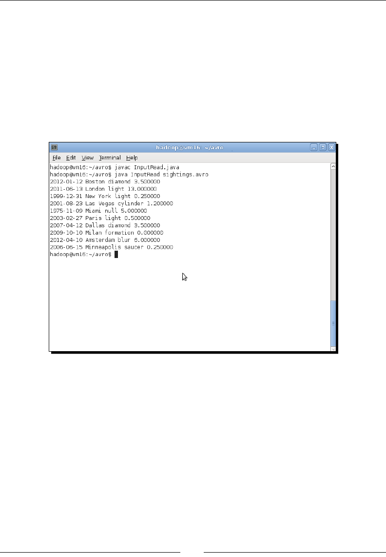
Chapter 5
[ 157 ]
System.out.println(output) ;
}
}
}
2. Compile and run the program:
$ javacInputRead.java
$ java InputReadsightings.avro
The output will be as shown in the following screenshot:
What just happened?
We created the Java class InputRead, which takes the lename passed as a
command-line argument and parses this as an Avro datale. When Avro reads
from a datale, each individual element is called a datum and each datum will
follow the structure dened in the schema.
In this case, we don't use an explicit schema; instead, we read each datum into the
GenericRecord class, and from this extract each eld by explicitly retrieving it by name.
The GenericRecord class is a very exible class in Avro; it can be used to wrap any record
structure, such as our UFO-sighng type. Avro also supports primive types such as integers,
oats, and booleans as well as other structured types such as arrays and enums. In these
examples, we'll use records as the most common structure, but this is only a convenience.
www.it-ebooks.info

Advanced MapReduce Techniques
[ 158 ]
Using Avro within MapReduce
Avro's support for MapReduce revolves around several Avro-specic variants of other
familiar classes, whereas we'd normally expect a new datale format to be supported
in Hadoop through new InputFormat and OutputFormat classes, we'll use AvroJob,
AvroMapper, and AvroReducer instead of the non-Avro versions. AvroJob expects Avro
datales as its input and output, so instead of specifying input and output format types,
we congure it with details of the input and output Avro schemas.
The main dierence for our mapper and reducer implementaons are the types used. Avro,
by default, has a single input and output, whereas we're used to our Mapper and Reducer
classes having a key/value input and a key/value output. Avro also introduces the Pair class,
which is oen used to emit intermediate key/value data.
Avro does also support AvroKey and AvroValue, which can wrap other types, but we'll not
use those in the following examples.
Time for action – generating shape summaries in MapReduce
In this secon we will write a mapper that takes as input the UFO sighng record we dened
earlier. It will output the shape and a count of 1, and the reducer will take this shape and
count records and produce a new structured Avro datale type containing the nal counts
for each UFO shape. Perform the following steps:
1. Copy the sightings.avro le to HDFS.
$ hadoopfs -mkdiravroin
$ hadoopfs -put sightings.avroavroin/sightings.avro
2. Create the following as AvroMR.java:
import java.io.IOException;
import org.apache.avro.Schema;
import org.apache.avro.generic.*;
import org.apache.avro.Schema.Type;
import org.apache.avro.mapred.*;
import org.apache.avro.reflect.ReflectData;
import org.apache.avro.util.Utf8;
import org.apache.hadoop.conf.*;
import org.apache.hadoop.fs.Path;
import org.apache.hadoop.mapred.*;
import org.apache.hadoop.mapreduce.Job;
import org.apache.hadoop.io.* ;
import org.apache.hadoop.util.*;
// Output record definition
www.it-ebooks.info

Chapter 5
[ 159 ]
class UFORecord
{
UFORecord()
{
}
public String shape ;
public long count ;
}
public class AvroMR extends Configured implements Tool
{
// Create schema for map output
public static final Schema PAIR_SCHEMA =
Pair.getPairSchema(Schema.create(Schema.Type.STRING),
Schema.create(Schema.Type.LONG));
// Create schema for reduce output
public final static Schema OUTPUT_SCHEMA =
ReflectData.get().getSchema(UFORecord.class);
@Override
public int run(String[] args) throws Exception
{
JobConfconf = new JobConf(getConf(), getClass());
conf.setJobName("UFO count");
String[] otherArgs = new GenericOptionsParser(conf, args).
getRemainingArgs();
if (otherArgs.length != 2)
{
System.err.println("Usage: avro UFO counter <in><out>");
System.exit(2);
}
FileInputFormat.addInputPath(conf, new Path(otherArgs[0]));
Path outputPath = new Path(otherArgs[1]);
FileOutputFormat.setOutputPath(conf, outputPath);
outputPath.getFileSystem(conf).delete(outputPath);
Schema input_schema =
Schema.parse(getClass().getResourceAsStream("ufo.avsc"));
AvroJob.setInputSchema(conf, input_schema);
AvroJob.setMapOutputSchema(conf,
Pair.getPairSchema(Schema.create(Schema.Type.STRING),
www.it-ebooks.info

Advanced MapReduce Techniques
[ 160 ]
Schema.create(Schema.Type.LONG)));
AvroJob.setOutputSchema(conf, OUTPUT_SCHEMA);
AvroJob.setMapperClass(conf, AvroRecordMapper.class);
AvroJob.setReducerClass(conf, AvroRecordReducer.class);
conf.setInputFormat(AvroInputFormat.class) ;
JobClient.runJob(conf);
return 0 ;
}
public static class AvroRecordMapper extends
AvroMapper<GenericRecord, Pair<Utf8, Long>>
{
@Override
public void map(GenericRecord in, AvroCollector<Pair<Utf8,
Long>> collector, Reporter reporter) throws IOException
{
Pair<Utf8,Long> p = new Pair<Utf8,Long>(PAIR_SCHEMA) ;
Utf8 shape = (Utf8)in.get("shape") ;
if (shape != null)
{
p.set(shape, 1L) ;
collector.collect(p);
}
}
}
public static class AvroRecordReducer extends
AvroReducer<Utf8,
Long, GenericRecord>
{
public void reduce(Utf8 key, Iterable<Long> values,
AvroCollector<GenericRecord> collector,
Reporter reporter) throws IOException
{
long sum = 0;
for (Long val : values)
{
sum += val;
}
GenericRecord value = new
GenericData.Record(OUTPUT_SCHEMA);
www.it-ebooks.info

Chapter 5
[ 161 ]
value.put("shape", key);
value.put("count", sum);
collector.collect(value);
}
}
public static void main(String[] args) throws Exception
{
int res = ToolRunner.run(new Configuration(), new AvroMR(),
args);
System.exit(res);
}
}
3. Compile and run the job:
$ javacAvroMR.java
$ jar -cvfavroufo.jar *.class ufo.avsc
$ hadoop jar ~/classes/avroufo.jarAvroMRavroinavroout
4. Examine the output directory:
$ hadoopfs -lsavroout
Found 3 items
-rw-r--r-- 1 … /user/hadoop/avroout/_SUCCESS
drwxr-xr-x - hadoopsupergroup 0 … /user/hadoop/
avroout/_logs
-rw-r--r-- 1 … /user/hadoop/avroout/part-00000.avro
5. Copy the output le to the local lesystem:
$ hadoopfs -get /user/hadoop/avroout/part-00000.avroresult.avro
What just happened?
We created the Job class and examined its various components. The actual logic within the
Mapper and Reducer classes is relavely straighorward: the Mapper class just extracts
the shape column and emits it with a count of 1; the reducer then counts the total number
of entries for each shape. The interesng aspects are around the dened input and output
types to the Mapper and Reducer classes and how the job is congured.
The Mapper class has an input type of GenericRecord and an output type of Pair. The
Reducer class has a corresponding input type of Pair and output type of GenericRecord.
www.it-ebooks.info

Advanced MapReduce Techniques
[ 162 ]
The GenericRecord class passed to the Mapper class wraps a datum that is the UFO
sighng record represented in the input le. This is how the Mapper class is able to retrieve
the Shape eld by name.
Recall that GenericRecords may or may not be explicitly created with a schema, and in
either case the structure can be determined from the datale. For the GenericRecord
output by the Reducer class, we do pass a schema but use a new mechanism for its creaon.
Within the previously menoned code, we created the addional UFORecord class and used
Avro reecon to generate its schema dynamically at runme. We were then able to use this
schema to create a GenericRecord class specialized to wrap that parcular record type.
Between the Mapper and Reducer classes we use the Avro Pair type to hold a key and
value pair. This allows us to express the same logic for the Mapper and Reducer classes
that we used in the original WordCount example back in Chapter 2, Geng Hadoop Up
and Running; the Mapper class emits singleton counts for each value and the reducer
sums these into an overall total for each shape.
In addion to the Mapper and Reducer classes' input and output, there is some
conguraon unique to a job processing Avro data:
Schema input_schema = Schema.parse(getClass().
getResourceAsStream("ufo.avsc")) ;
AvroJob.setInputSchema(conf, input_schema);
AvroJob.setMapOutputSchema(conf, Pair.getPairSchema(Schema.
create(Schema.Type.STRING), Schema.create(Schema.Type.LONG)));
AvroJob.setOutputSchema(conf, OUTPUT_SCHEMA);
AvroJob.setMapperClass(conf, AvroRecordMapper.class);
AvroJob.setReducerClass(conf, AvroRecordReducer.class);
These conguraon elements demonstrate the cricality of schema denion to Avro;
though we can do without it, we must set the expected input and output schema types. Avro
will validate the input and output against the specied schemas, so there is a degree of data
type safety. For the other elements, such as seng up the Mapper and Reducer classes,
we simply set those on AvroJob instead of the more generic classes, and once done, the
MapReduce framework will perform appropriately.
This example is also the rst me we've explicitly implemented the Tool interface. When
running the Hadoop command-line program, there are a series of arguments (such as -D)
that are common across all the mulple subcommands. If a job class implements the Tool
interface as menoned in the previous secon, it automacally gets access to any of these
standard opons passed on the command line. It's a useful mechanism that prevents lots of
code duplicaon.
www.it-ebooks.info

Chapter 5
[ 163 ]
Time for action – examining the output data with Ruby
Now that we have the output data from the job, let's examine it again using Ruby.
1. Create the following as read.rb:
require 'rubygems'
require 'avro'
file = File.open('res.avro', 'rb')
reader = Avro::IO::DatumReader.new()
dr = Avro::DataFile::Reader.new(file, reader)
dr.each {|record|
print record["shape"]," ",record["count"],"\n"
}
dr.close
2. Examine the created result le.
$ ruby read.rb
blur 1
cylinder 1
diamond 2
formation 1
light 3
saucer 1
What just happened?
As before, we'll not analyze the Ruby Avro API. The example created a Ruby script that
opens an Avro datale, iterates through each datum, and displays it based on explicitly
named elds. Note that the script does not have access to the schema for the datale;
the informaon in the header provides enough data to allow each eld to be retrieved.
Time for action – examining the output data with Java
To show that the data is accessible from mulple languages, let's also display the job output
using Java.
1. Create the following as OutputRead.java:
import java.io.File;
import java.io.IOException;
www.it-ebooks.info

Advanced MapReduce Techniques
[ 164 ]
import org.apache.avro.file.DataFileReader;
import org.apache.avro.generic.GenericData;
import org.apache.avro. generic.GenericDatumReader;
import org.apache.avro.generic.GenericRecord;
import org.apache.avro.io.DatumReader;
public class OutputRead
{
public static void main(String[] args) throws IOException
{
String filename = args[0] ;
File file=new File(filename) ;
DatumReader<GenericRecord> reader= new
GenericDatumReader<GenericRecord>();
DataFileReader<GenericRecord>dataFileReader=new
DataFileReader<GenericRecord>(file,reader);
while (dataFileReader.hasNext())
{
GenericRecord result=dataFileReader.next();
String output = String.format("%s %d",
result.get("shape"), result.get("count")) ;
System.out.println(output) ;
}
}
}
2. Compile and run the program:
$ javacOutputResult.java
$ java OutputResultresult.avro
blur 1
cylinder 1
diamond 2
formation 1
light 3
saucer 1
www.it-ebooks.info

Chapter 5
[ 165 ]
What just happened?
We added this example to show the Avro data being read by more than one language.
The code is very similar to the earlier InputRead class; the only dierence is that the
named elds are used to display each datum as it is read from the datale.
Have a go hero – graphs in Avro
As previously menoned, we worked hard to reduce representaon-related complexity in
our GraphPath class. But with mappings to and from at lines of text and objects, there
was an overhead in managing these transformaons.
With its support for nested complex types, Avro can navely support a representaon of
a node that is much closer to the runme object. Modify the GraphPath class job to read
and write the graph representaon to an Avro datale comprising of datums for each node.
The following example schema may be a good starng point, but feel free to enhance it:
{ "type": "record",
"name": "Graph_representation",
"fields" : [
{"name": "node_id", "type": "int"},
{"name": "neighbors", "type": "array", "items:"int" },
{"name": "distance", "type": "int"},
{"name": "status", "type": "enum",
"symbols": ["PENDING", "CURRENT", "DONE"
},]
]
}
Going forward with Avro
There are many features of Avro we did not cover in this case study. We focused only on its
value as an at-rest data representaon. It can also be used within a remote procedure call
(RPC) framework and can oponally be used as the default RPC format in Hadoop 2.0. We
didn't use Avro's code generaon facilies that produce a much more domain-focused API.
Nor did we cover issues such as Avro's ability to support schema evoluon that, for example,
allows new elds to be added to recent records without invalidang old datums or breaking
exisng clients. It's a technology you are very likely to see more of in the future.
www.it-ebooks.info

Advanced MapReduce Techniques
[ 166 ]
Summary
This chapter has used three case studies to highlight some more advanced aspects of
Hadoop and its broader ecosystem. In parcular, we covered the nature of join-type
problems and where they are seen, how reduce-side joins can be implemented with
relave ease but with an eciency penalty, and how to use opmizaons to avoid
full joins in the map-side by pushing data into the Distributed Cache.
We then learned how full map-side joins can be implemented, but require signicant input
data processing; how other tools such as Hive and Pig should be invesgated if joins are a
frequently encountered use case; and how to think about complex types like graphs and
how they can be represented in a way that can be used in MapReduce.
We also saw techniques for breaking graph algorithms into mulstage MapReduce jobs,
the importance of language-independent data types, how Avro can be used for both
language independence as well as complex Java-consumed types, and the Avro extensions
to the MapReduce APIs that allow structured types to be used as the input and output to
MapReduce jobs.
This now concludes our coverage of the programmac aspects of the Hadoop MapReduce
framework. We will now move on in the next two chapters to explore how to manage and
scale a Hadoop environment.
www.it-ebooks.info

6
When Things Break
One of the main promises of Hadoop is resilience to failure and an ability to
survive failures when they do happen. Tolerance to failure will be the focus
of this chapter.
In parcular, we will cover the following topics:
How Hadoop handles failures of DataNodes and TaskTrackers
How Hadoop handles failures of the NameNode and JobTracker
The impact of hardware failure on Hadoop
How to deal with task failures caused by soware bugs
How dirty data can cause tasks to fail and what to do about it
Along the way, we will deepen our understanding of how the various components
of Hadoop t together and idenfy some areas of best pracce.
Failure
With many technologies, the steps to be taken when things go wrong are rarely covered in
much of the documentaon and are oen treated as topics only of interest to the experts.
With Hadoop, it is much more front and center; much of the architecture and design of
Hadoop is predicated on execung in an environment where failures are both frequent
and expected.
www.it-ebooks.info

When Things Break
[ 168 ]
Embrace failure
In recent years, a dierent mindset than the tradional one has been described by the term
embrace failure. Instead of hoping that failure does not happen, accept the fact that it will
and know how your systems and processes will respond when it does.
Or at least don't fear it
That's possibly a stretch, so instead, our goal in this chapter is to make you feel more
comfortable about failures in the system. We'll be killing the processes of a running cluster,
intenonally causing the soware to fail, pushing bad data into our jobs, and generally
causing as much disrupon as we can.
Don't try this at home
Oen when trying to break a system, a test instance is abused, leaving the operaonal
system protected from the disrupon. We will not advocate doing the things given in this
chapter to an operaonal Hadoop cluster, but the fact is that apart from one or two very
specic cases, you could. The goal is to understand the impact of the various types of failures
so that when they do happen on the business-crical system, you will know whether it is a
problem or not. Fortunately, the majority of cases are handled for you by Hadoop.
Types of failure
We will generally categorize failures into the following ve types:
Failure of a node, that is, DataNode or TaskTracker process
Failure of a cluster's masters, that is, NameNode or JobTracker process
Failure of hardware, that is, host crash, hard drive failure, and so on
Failure of individual tasks within a MapReduce job due to soware errors
Failure of individual tasks within a MapReduce job due to data problems
We will explore each of these in turn in the following secons.
Hadoop node failure
The rst class of failure that we will explore is the unexpected terminaon of the individual
DataNode and TaskTracker processes. Given Hadoop's claims of managing system availability
through survival of failures on its commodity hardware, we can expect this area to be very
solid. Indeed, as clusters grow to hundreds or thousands of hosts, failures of individual
nodes are likely to become quite commonplace.
Before we start killing things, let's introduce a new tool and set up the cluster properly.
www.it-ebooks.info

Chapter 6
[ 169 ]
The dfsadmin command
As an alternave tool to constantly viewing the HDFS web UI to determine the cluster status,
we will use the dfsadmin command-line tool:
$ Hadoop dfsadmin
This will give a list of the various opons the command can take; for our purposes we'll
be using the -report opon. This gives an overview of the overall cluster state, including
congured capacity, nodes, and les as well as specic details about each congured node.
Cluster setup, test les, and block sizes
We will need a fully distributed cluster for the following acvies; refer to the setup
instrucons given earlier in the book. The screenshots and examples that follow use a
cluster of one host for the JobTracker and NameNode and four slave nodes for running
the DataNode and TaskTracker processes.
Remember that you don't need physical hardware for each node,
we use virtual machines for our cluster.
In normal usage, 64 MB is the usual congured block size for a Hadoop cluster. For
our tesng purposes, that is terribly inconvenient as we'll need prey large les to get
meaningful block counts across our mulnode cluster.
What we can do is reduce the congured block size; in this case, we will use 4 MB. Make the
following modicaons to the hdfs-site.xml le within the Hadoop conf directory:
<property>
<name>dfs.block.size</name>
<value>4194304</value>
;</property>
<property>
<name>dfs.namenode.logging.level</name>
<value>all</value>
</property>
The rst property makes the required changes to the block size and the second one increases
the NameNode logging level to make some of the block operaons more visible.
www.it-ebooks.info

When Things Break
[ 170 ]
Both these sengs are appropriate for this test setup but would rarely be
seen on a producon cluster. Though the higher NameNode logging may be
required if a parcularly dicult problem is being invesgated, it is highly
unlikely you would ever want a block size as small as 4 MB. Though the
smaller block size will work ne, it will impact Hadoop's eciency.
We also need a reasonably-sized test le that will comprise of mulple 4 MB blocks. We
won't actually be using the content of the le, so the type of le is irrelevant. But you should
copy the largest le you can onto HDFS for the following secons. We used a CD ISO image:
$ Hadoop fs –put cd.iso file1.data
Fault tolerance and Elastic MapReduce
The examples in this book are for a local Hadoop cluster because this allows some of the
failure mode details to be more explicit. EMR provides exactly the same failure tolerance
as the local cluster, so the failure scenarios described here apply equally to a local Hadoop
cluster and the one hosted by EMR.
Time for action – killing a DataNode process
Firstly, we'll kill a DataNode. Recall that the DataNode process runs on each host in the
HDFS cluster and is responsible for the management of blocks within the HDFS lesystem.
Because Hadoop, by default, uses a replicaon factor of 3 for blocks, we should expect a
single DataNode failure to have no direct impact on availability, rather it will result in some
blocks temporarily falling below the replicaon threshold. Execute the following steps to
kill a DataNode process:
1. Firstly, check on the original status of the cluster and check whether everything is
healthy. We'll use the dfsadmin command for this:
$ Hadoop dfsadmin -report
Configured Capacity: 81376493568 (75.79 GB)
Present Capacity: 61117323920 (56.92 GB)
DFS Remaining: 59576766464 (55.49 GB)
DFS Used: 1540557456 (1.43 GB)
DFS Used%: 2.52%
Under replicated blocks: 0
Blocks with corrupt replicas: 0
Missing blocks: 0
-------------------------------------------------
www.it-ebooks.info

Chapter 6
[ 171 ]
Datanodes available: 4 (4 total, 0 dead)
Name: 10.0.0.102:50010
Decommission Status : Normal
Configured Capacity: 20344123392 (18.95 GB)
DFS Used: 403606906 (384.91 MB)
Non DFS Used: 5063119494 (4.72 GB)
DFS Remaining: 14877396992(13.86 GB)
DFS Used%: 1.98%
DFS Remaining%: 73.13%
Last contact: Sun Dec 04 15:16:27 PST 2011
…
Now log onto one of the nodes and use the jps command to determine the process
ID of the DataNode process:
$ jps
2085 TaskTracker
2109 Jps
1928 DataNode
2. Use the process ID (PID) of the DataNode process and kill it:
$ kill -9 1928
3. Check that the DataNode process is no longer running on the host:
$ jps
2085 TaskTracker
4. Check the status of the cluster again by using the dfsadmin command:
$ Hadoop dfsadmin -report
Configured Capacity: 81376493568 (75.79 GB)
Present Capacity: 61117323920 (56.92 GB)
DFS Remaining: 59576766464 (55.49 GB)
DFS Used: 1540557456 (1.43 GB)
DFS Used%: 2.52%
Under replicated blocks: 0
Blocks with corrupt replicas: 0
Missing blocks: 0
www.it-ebooks.info

When Things Break
[ 172 ]
-------------------------------------------------
Datanodes available: 4 (4 total, 0 dead)
…
5. The key lines to watch are the lines reporng on blocks, live nodes, and the last
contact me for each node. Once the last contact me for the dead node is around
10 minutes, use the command more frequently unl the block and live node values
change:
$ Hadoop dfsadmin -report
Configured Capacity: 61032370176 (56.84 GB)
Present Capacity: 46030327050 (42.87 GB)
DFS Remaining: 44520288256 (41.46 GB)
DFS Used: 1510038794 (1.41 GB)
DFS Used%: 3.28%
Under replicated blocks: 12
Blocks with corrupt replicas: 0
Missing blocks: 0
-------------------------------------------------
Datanodes available: 3 (4 total, 1 dead)
…
6. Repeat the process unl the count of under-replicated blocks is once again 0:
$ Hadoop dfsadmin -report
…
Under replicated blocks: 0
Blocks with corrupt replicas: 0
Missing blocks: 0
-------------------------------------------------
Datanodes available: 3 (4 total, 1 dead)
…
What just happened?
The high-level story is prey straighorward; Hadoop recognized the loss of a node and
worked around the problem. However, quite a lot is going on to make that happen.
www.it-ebooks.info

Chapter 6
[ 173 ]
When we killed the DataNode process, the process on that host was no longer available to
serve or receive data blocks as part of the read/write operaons. However, we were not
actually accessing the lesystem at the me, so how did the NameNode process know this
parcular DataNode was dead?
NameNode and DataNode communication
The answer lies in the constant communicaon between the NameNode and DataNode
processes that we have alluded to once or twice but never really explained. This occurs through
a constant series of heartbeat messages from the DataNode reporng on its current state
and the blocks it holds. In return, the NameNode gives instrucons to the DataNode, such as
nocaon of the creaon of a new le or an instrucon to retrieve a block from another node.
It all begins when the NameNode process starts up and begins receiving status messages
from the DataNode. Recall that each DataNode knows the locaon of its NameNode and
will connuously send status reports. These messages list the blocks held by each DataNode
and from this, the NameNode is able to construct a complete mapping that allows it to relate
les and directories to the blocks from where they are comprised and the nodes on which
they are stored.
The NameNode process monitors the last me it received a heartbeat from each DataNode
and aer a threshold is reached, it assumes the DataNode is no longer funconal and marks
it as dead.
The exact threshold aer which a DataNode is assumed to be dead is
not congurable as a single HDFS property. Instead, it is calculated from
several other properes such as dening the heartbeat interval. As we'll
see later, things are a lile easier in the MapReduce world as the meout
for TaskTrackers is controlled by a single conguraon property.
Once a DataNode is marked as dead, the NameNode process determines the blocks which
were held on that node and have now fallen below their replicaon target. In the default
case, each block held on the killed node would have been one of the three replicas, so each
block for which the node held a replica will now have only two replicas across the cluster.
In the preceding example, we captured the state when 12 blocks were sll under-replicated,
that is they did not have enough replicas across the cluster to meet the replicaon target.
When the NameNode process determines the under-replicated blocks, it assigns other
DataNodes to copy these blocks from the hosts where the exisng replicas reside. In this
case we only had to re-replicate a very small number of blocks; in a live cluster, the failure of
a node can result in a period of high network trac as the aected blocks are brought up to
their replicaon factor.
www.it-ebooks.info

When Things Break
[ 174 ]
Note that if a failed node returns to the cluster, we have the situaon of blocks having
more than the required number of replicas; in such a case the NameNode process will
send instrucons to remove the surplus replicas. The specic replica to be deleted is
chosen randomly, so the result will be that the returned node will end up retaining
some of its blocks and deleng the others.
Have a go hero – NameNode log delving
We congured the NameNode process to log all its acvies. Have a look through these
very verbose logs and aempt to idenfy the replicaon requests being sent.
The nal output shows the status aer the under-replicated blocks have been copied
to the live nodes. The cluster is down to only three live nodes but there are no
under-replicated blocks.
A quick way to restart the dead nodes across all hosts is to use the
start-all.sh script. It will aempt to start everything but is smart
enough to detect the running services, which means you get the dead
nodes restarted without the risk of duplicates.
Time for action – the replication factor in action
Let's repeat the preceding process, but this me, kill two DataNodes out of our cluster
of four. We will give an abbreviated walk-through of the acvity as it is very similar to
the previous Time for acon secon:
1. Restart the dead DataNode and monitor the cluster unl all nodes are marked
as live.
2. Pick two DataNodes, use the process ID, and kill the DataNode processes.
3. As done previously, wait for around 10 minutes then acvely monitor the cluster
state via dfsadmin, paying parcular aenon to the reported number of under-
replicated blocks.
4. Wait unl the cluster has stabilized with an output similar to the following:
Configured Capacity: 61032370176 (56.84 GB)
Present Capacity: 45842373555 (42.69 GB)
DFS Remaining: 44294680576 (41.25 GB)
DFS Used: 1547692979 (1.44 GB)
DFS Used%: 3.38%
Under replicated blocks: 125
Blocks with corrupt replicas: 0
www.it-ebooks.info

Chapter 6
[ 175 ]
Missing blocks: 0
-------------------------------------------------
Datanodes available: 2 (4 total, 2 dead)
…
What just happened?
This is the same process as before; the dierence is that due to two DataNode failures
there were signicantly more blocks that fell below the replicaon factor, many going
down to a single remaining replica. Consequently, you should see more acvity in the
reported number of under-replicated blocks as it rst increase because nodes fail and
then drop as re-replicaon occurs. These events can also be seen in the NameNode logs.
Note that though Hadoop can use re-replicaon to bring those blocks with only a single
remaining replica up to two replicas, this sll leaves the blocks in an under-replicated
state. With only two live nodes in the cluster, it is now impossible for any block to
meet the default replicaon target of three.
We have been truncang the dfsadmin output for space reasons; in parcular, we have
been oming the reported informaon for each node. However, let's take a look at the
rst node in our cluster through the previous stages. Before we started killing any DataNode,
it reported the following:
Name: 10.0.0.101:50010
Decommission Status : Normal
Configured Capacity: 20344123392 (18.95 GB)
DFS Used: 399379827 (380.88 MB)
Non DFS Used: 5064258189 (4.72 GB)
DFS Remaining: 14880485376(13.86 GB)
DFS Used%: 1.96%
DFS Remaining%: 73.14%
Last contact: Sun Dec 04 15:16:27 PST 2011
Aer a single DataNode was killed and all blocks had been re-replicated as necessary, it
reported the following:
Name: 10.0.0.101:50010
Decommission Status : Normal
Configured Capacity: 20344123392 (18.95 GB)
DFS Used: 515236022 (491.37 MB)
Non DFS Used: 5016289098 (4.67 GB)
DFS Remaining: 14812598272(13.8 GB)
www.it-ebooks.info

When Things Break
[ 176 ]
DFS Used%: 2.53%
DFS Remaining%: 72.81%
Last contact: Sun Dec 04 15:31:22 PST 2011
The thing to note is the increase in the local DFS storage on the node. This shouldn't be a
surprise. With a dead node, the others in the cluster need to add some addional block
replicas and that will translate to a higher storage ulizaon on each.
Finally, the following is the node's report aer two other DataNodes were killed:
Name: 10.0.0.101:50010
Decommission Status : Normal
Configured Capacity: 20344123392 (18.95 GB)
DFS Used: 514289664 (490.46 MB)
Non DFS Used: 5063868416 (4.72 GB)
DFS Remaining: 14765965312(13.75 GB)
DFS Used%: 2.53%
DFS Remaining%: 72.58%
Last contact: Sun Dec 04 15:43:47 PST 2011
With two dead nodes it may seem as if the remaining live nodes should consume even more
local storage space, but this isn't the case and it's yet again a natural consequence of the
replicaon factor.
If we have four nodes and a replicaon factor of 3, each block will have a replica on three
of the live nodes in the cluster. If a node dies, the blocks living on the other nodes are
unaected, but any blocks with a replica on the dead node will need a new replica created.
However, with only three live nodes, each node will hold a replica of every block. If a second
node fails, the situaon will result into under-replicated blocks and Hadoop does not have
anywhere to put the addional replicas. Since both remaining nodes already hold a replica
of each block, their storage ulizaon does not increase.
Time for action – intentionally causing missing blocks
The next step should be obvious; let's kill three DataNodes in quick succession.
This is the rst of the acvies we menoned that you really should not do
on a producon cluster. Although there will be no data loss if the steps are
followed properly, there is a period when the exisng data is unavailable.
www.it-ebooks.info

Chapter 6
[ 177 ]
The following are the steps to kill three DataNodes in quick succession:
1. Restart all the nodes by using the following command:
$ start-all.sh
2. Wait unl Hadoop dfsadmin -report shows four live nodes.
3. Put a new copy of the test le onto HDFS:
$ Hadoop fs -put file1.data file1.new
4. Log onto three of the cluster hosts and kill the DataNode process on each.
5. Wait for the usual 10 minutes then start monitoring the cluster via dfsadmin unl
you get output similar to the following that reports the missing blocks:
…
Under replicated blocks: 123
Blocks with corrupt replicas: 0
Missing blocks: 33
-------------------------------------------------
Datanodes available: 1 (4 total, 3 dead)
…
6. Try and retrieve the test le from HDFS:
$ hadoop fs -get file1.new file1.new
11/12/04 16:18:05 INFO hdfs.DFSClient: No node available for
block: blk_1691554429626293399_1003 file=/user/hadoop/file1.new
11/12/04 16:18:05 INFO hdfs.DFSClient: Could not obtain block
blk_1691554429626293399_1003 from any node: java.io.IOException:
No live nodes contain current block
…
get: Could not obtain block: blk_1691554429626293399_1003 file=/
user/hadoop/file1.new
7. Restart the dead nodes using the start-all.sh script:
$ start-all.sh
8. Repeatedly monitor the status of the blocks:
$ Hadoop dfsadmin -report | grep -i blocks
Under replicated blockss: 69
Blocks with corrupt replicas: 0
Missing blocks: 35
www.it-ebooks.info

When Things Break
[ 178 ]
$ Hadoop dfsadmin -report | grep -i blocks
Under replicated blockss: 0
Blocks with corrupt replicas: 0
Missing blocks: 30
9. Wait unl there are no reported missing blocks then copy the test le onto
the local lesystem:
$ Hadoop fs -get file1.new file1.new
10. Perform an MD5 check on this and the original le:
$ md5sum file1.*
f1f30b26b40f8302150bc2a494c1961d file1.data
f1f30b26b40f8302150bc2a494c1961d file1.new
What just happened?
Aer restarng the killed nodes, we copied the test le onto HDFS again. This isn't strictly
necessary as we could have used the exisng le but due to the shuing of the replicas,
a clean copy gives the most representave results.
We then killed three DataNodes as before and waited for HDFS to respond. Unlike the
previous examples, killing these many nodes meant it was certain that some blocks would
have all of their replicas on the killed nodes. As we can see, this is exactly the result; the
remaining single node cluster shows over a hundred blocks that are under-replicated
(obviously only one replica remains) but there are also 33 missing blocks.
Talking of blocks is a lile abstract, so we then try to retrieve our test le which, as we
know, eecvely has 33 holes in it. The aempt to access the le fails as Hadoop could
not nd the missing blocks required to deliver the le.
We then restarted all the nodes and tried to retrieve the le again. This me it was
successful, but we took an added precauon of performing an MD5 cryptographic
check on the le to conrm that it was bitwise idencal to the original one — which it is.
This is an important point: though node failure may result in data becoming unavailable,
there may not be a permanent data loss if the node recovers.
When data may be lost
Do not assume from this example that it's impossible to lose data in a Hadoop cluster. For
general use it is very hard, but disaster oen has a habit of striking in just the wrong way.
www.it-ebooks.info

Chapter 6
[ 179 ]
As seen in the previous example, a parallel failure of a number of nodes equal to or greater
than the replicaon factor has a chance of resulng in missing blocks. In our example of
three dead nodes in a cluster of four, the chances were high; in a cluster of 1000, it would
be much lower but sll non-zero. As the cluster size increases, so does the failure rate and
having three node failures in a narrow window of me becomes less and less unlikely.
Conversely, the impact also decreases but rapid mulple failures will always carry a
risk of data loss.
Another more insidious problem is recurring or paral failures, for example, when
power issues across the cluster cause nodes to crash and restart. It is possible for
Hadoop to end up chasing replicaon targets, constantly asking the recovering hosts
to replicate under-replicated blocks, and also seeing them fail mid-way through the task.
Such a sequence of events can also raise the potenal of data loss.
Finally, never forget the human factor. Having a replicaon factor equal to the size of the
cluster—ensuring every block is on every node—won't help you when a user accidentally
deletes a le or directory.
The summary is that data loss through system failure is prey unlikely but is possible through
almost inevitable human acon. Replicaon is not a full alternave to backups; ensure that
you understand the importance of the data you process and the impact of the types of loss
discussed here.
The most catastrophic losses in a Hadoop cluster are actually caused by
NameNode failure and lesystem corrupon; we'll discuss this topic in
some detail in the next chapter.
Block corruption
The reports from each DataNode also included a count of the corrupt blocks, which we
have not referred to. When a block is rst stored, there is also a hidden le wrien to the
same HDFS directory containing cryptographic checksums for the block. By default, there
is a checksum for each 512-byte chunk within the block.
Whenever any client reads a block, it will also retrieve the list of checksums and compare
these to the checksums it generates on the block data it has read. If there is a checksum
mismatch, the block on that parcular DataNode will be marked as corrupt and the client
will retrieve a dierent replica. On learning of the corrupt block, the NameNode will
schedule a new replica to be made from one of the exisng uncorrupted replicas.
www.it-ebooks.info
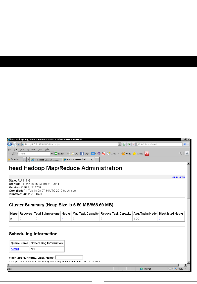
When Things Break
[ 180 ]
If the scenario seems unlikely, consider that faulty memory, disk drive, storage controller, or
numerous issues on an individual host could cause some corrupon to a block as it is inially
being wrien while being stored or when being read. These are rare events and the chances
of the same corrupon occurring on all DataNodes holding replicas of the same block
become exceponally remote. However, remember as previously menoned that replicaon
is not a full alternave to backup and if you need 100 percent data availability, you likely
need to think about o-cluster backup.
Time for action – killing a TaskTracker process
We've abused HDFS and its DataNode enough; now let's see what damage we can do to
MapReduce by killing some TaskTracker processes.
Though there is an mradmin command, it does not give the sort of status reports we are
used to with HDFS. So we'll use the MapReduce web UI (located by default on port 50070
on the JobTracker host) to monitor the MapReduce cluster health.
Perform the following steps:
1. Ensure everything is running via the start-all.sh script then point your browser
at the MapReduce web UI. The page should look like the following screenshot:
www.it-ebooks.info
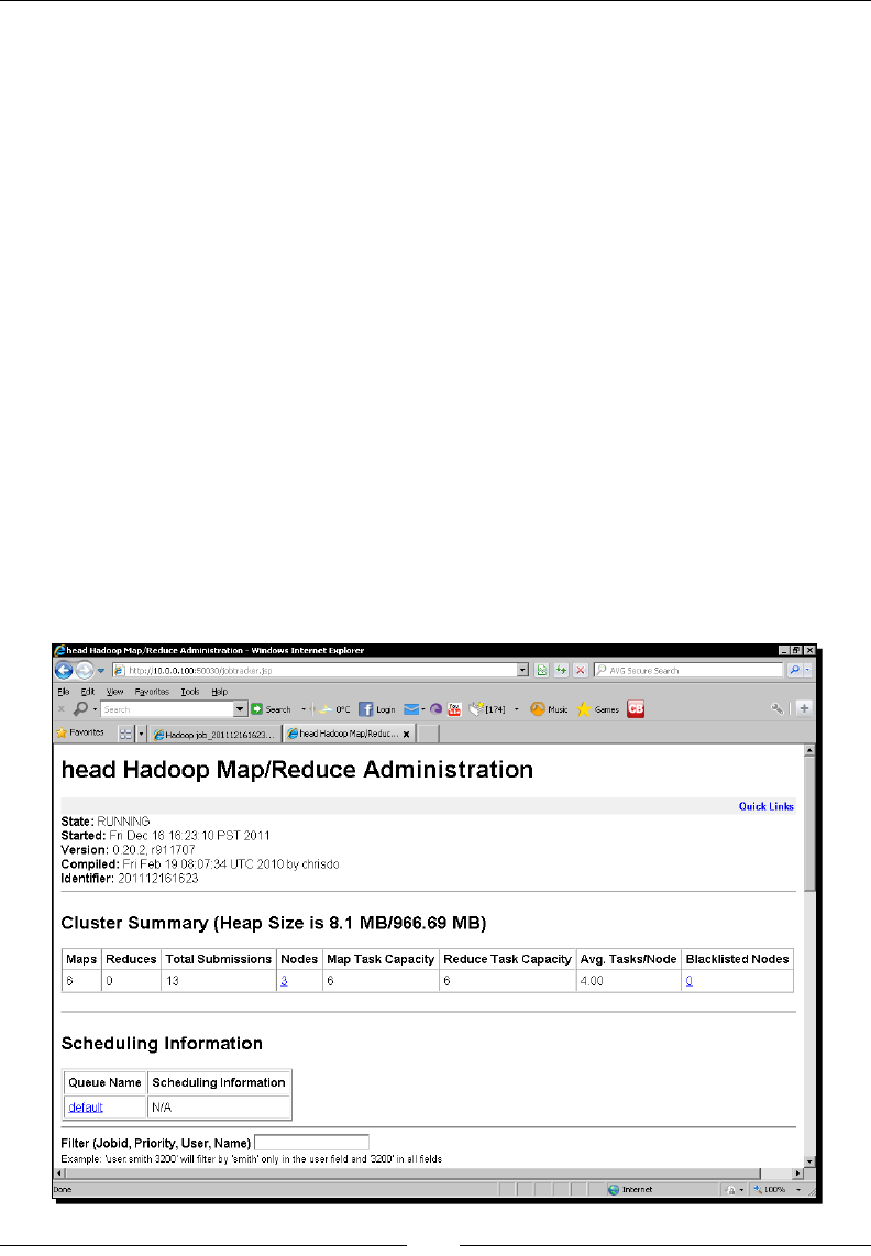
Chapter 6
[ 181 ]
2. Start a long-running MapReduce job; the example pi esmator with large values
is great for this:
$ Hadoop jar Hadoop/Hadoop-examples-1.0.4.jar pi 2500 2500
3. Now log onto a cluster node and use jps to idenfy the TaskTracker process:
$ jps
21822 TaskTracker
3918 Jps
3891 DataNode
4. Kill the TaskTracker process:
$ kill -9 21822
5. Verify that the TaskTracker is no longer running:
$jps
3918 Jps
3891 DataNode
6. Go back to the MapReduce web UI and aer 10 minutes you should see that
the number of nodes and available map/reduce slots change as shown in the
following screenshot:
www.it-ebooks.info
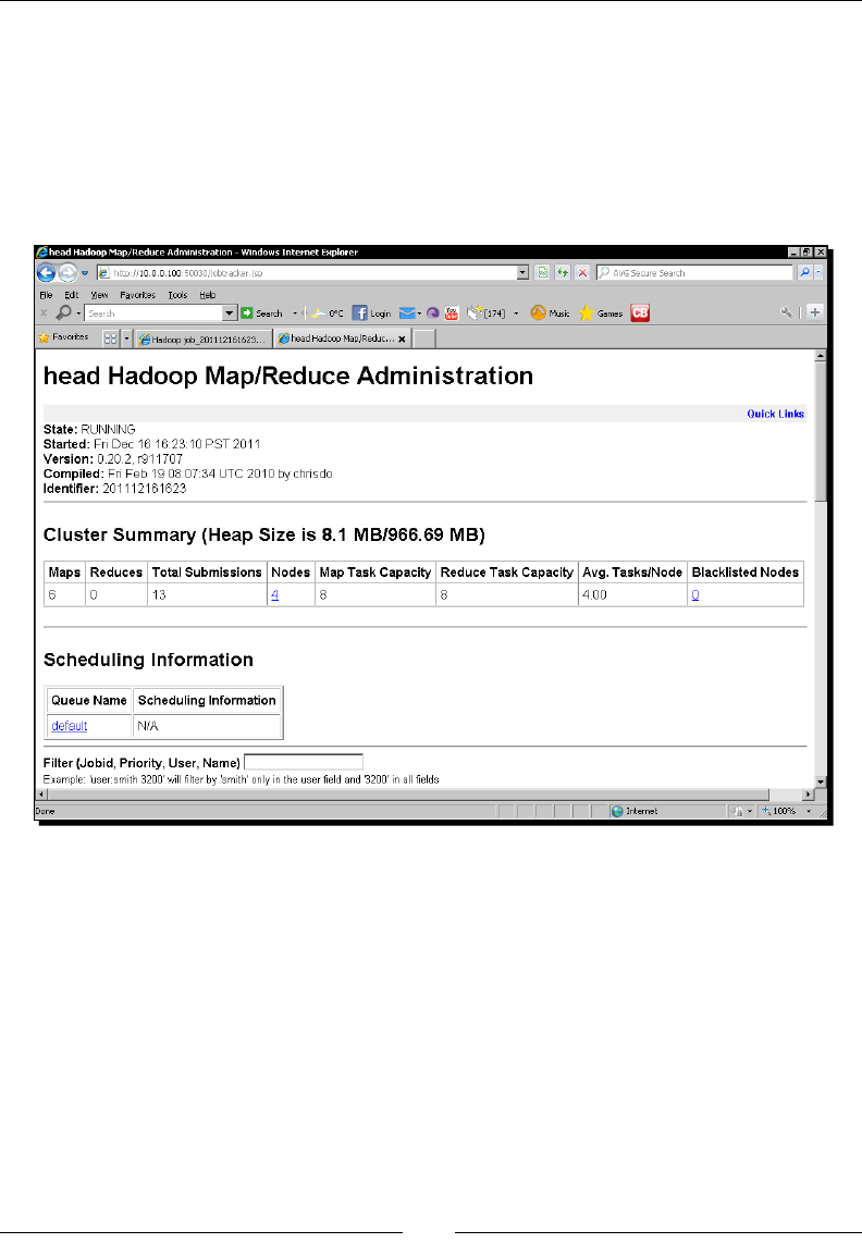
When Things Break
[ 182 ]
7. Monitor the job progress in the original window; it should be proceeding, even if
it is slow.
8. Restart the dead TaskTracker process:
$ start-all.sh
9. Monitor the MapReduce web UI. Aer a lile me the number of nodes should
be back to its original number as shown in the following screenshot:
What just happened?
The MapReduce web interface provides a lot of informaon on both the cluster as well
as the jobs it executes. For our interests here, the important data is the cluster summary
that shows the currently execung number of map and reduce tasks, the total number of
submied jobs, the number of nodes and their map and reduce capacity, and nally, any
blacklisted nodes.
The relaonship of the JobTracker process to the TaskTracker process is quite dierent
than that between NameNode and DataNode but a similar heartbeat/monitoring
mechanism is used.
www.it-ebooks.info

Chapter 6
[ 183 ]
The TaskTracker process frequently sends heartbeats to the JobTracker, but instead of status
reports of block health, they contain progress reports of the assigned task and available
capacity. Each node has a congurable number of map and reduce task slots (the default
for each is two), which is why we see four nodes and eight map and reduce slots in the
rst web UI screenshot.
When we kill the TaskTracker process, its lack of heartbeats is measured by the JobTracker
process and aer a congurable amount of me, the node is assumed to be dead and we
see the reduced cluster capacity reected in the web UI.
The meout for a TaskTracker process to be considered dead is modied by
the mapred.tasktracker.expiry.interval property, congured
in mapred-site.xml.
When a TaskTracker process is marked as dead, the JobTracker process also considers its
in-progress tasks as failed and re-assigns them to the other nodes in the cluster. We see
this implicitly by watching the job proceed successfully despite a node being killed.
Aer the TaskTracker process is restarted it sends a heartbeat to the JobTracker, which marks
it as alive and reintegrates it into the MapReduce cluster. This we see through the cluster node
and task slot capacity returning to their original values as can be seen in the nal screenshot.
Comparing the DataNode and TaskTracker failures
We'll not perform similar two or three node killing acvies with TaskTrackers as the task
execuon architecture renders individual TaskTracker failures relavely unimportant.
Because the TaskTracker processes are under the control and coordinaon of JobTracker,
their individual failures have no direct eect other than to reduce the cluster execuon
capacity. If a TaskTracker instance fails, the JobTracker will simply schedule the failed tasks on
a healthy TaskTracker process in the cluster. The JobTracker is free to reschedule tasks around
the cluster because TaskTracker is conceptually stateless; a single failure does not aect
other parts of the job.
In contrast, loss of a DataNode—which is intrinsically stateful—can aect the persistent data
held on HDFS, potenally making it unavailable.
This highlights the nature of the various nodes and their relaonship to the overall Hadoop
framework. The DataNode manages data, and the TaskTracker reads and writes that data.
Catastrophic failure of every TaskTracker would sll leave us with a completely funconal
HDFS; a similar failure of the NameNode process would leave a live MapReduce cluster that
is eecvely useless (unless it was congured to use a dierent storage system).
www.it-ebooks.info

When Things Break
[ 184 ]
Permanent failure
Our recovery scenarios so far have assumed that the dead node can be restarted on the
same physical host. But what if it can't due to the host having a crical failure? The answer is
simple; you can remove the host from the slave's le and Hadoop will no longer try to start a
DataNode or TaskTracker on that host. Conversely, if you get a replacement machine with a
dierent hostname, add this new host to the same le and run start-all.sh.
Note that the slave's le is only used by tools such as the start/stop and
slaves.sh scripts. You don't need to keep it updated on every node, but only
on the hosts where you generally run such commands. In pracce, this is likely to
be either a dedicated head node or the host where the NameNode or JobTracker
processes run. We'll explore these setups in Chapter 7, Keeping Things Running.
Killing the cluster masters
Though the failure impact of DataNode and TaskTracker processes is dierent, each
individual node is relavely unimportant. Failure of any single TaskTracker or DataNode is
not a cause for concern and issues only occur if mulple others fail, parcularly in quick
succession. But we only have one JobTracker and NameNode; let's explore what happens
when they fail.
Time for action – killing the JobTracker
We'll rst kill the JobTracker process which we should expect to impact our ability to execute
MapReduce jobs but not aect the underlying HDFS lesystem.
1. Log on to the JobTracker host and kill its process.
2. Aempt to start a test MapReduce job such as Pi or WordCount:
$ Hadoop jar wc.jar WordCount3 test.txt output
Starting Job
11/12/11 16:03:29 INFO ipc.Client: Retrying connect to server:
/10.0.0.100:9001. Already tried 0 time(s).
11/12/11 16:03:30 INFO ipc.Client: Retrying connect to server:
/10.0.0.100:9001. Already tried 1 time(s).
…
11/12/11 16:03:38 INFO ipc.Client: Retrying connect to server:
/10.0.0.100:9001. Already tried 9 time(s).
www.it-ebooks.info

Chapter 6
[ 185 ]
java.net.ConnectException: Call to /10.0.0.100:9001 failed on
connection exception: java.net.ConnectException: Connection
refused
at org.apache.hadoop.ipc.Client.wrapException(Client.java:767)
at org.apache.hadoop.ipc.Client.call(Client.java:743)
at org.apache.hadoop.ipc.RPC$Invoker.invoke(RPC.java:220)
…
3. Perform some HDFS operaons:
$ hadoop fs -ls /
Found 2 items
drwxr-xr-x - hadoop supergroup 0 2011-12-11 19:19 /user
drwxr-xr-x - hadoop supergroup 0 2011-12-04 20:38 /var
$ hadoop fs -cat test.txt
This is a test file
What just happened?
Aer killing the JobTracker process we aempted to launch a MapReduce job. From the
walk-through in Chapter 2, Geng Hadoop Up and Running, we know that the client on
the machine where we are starng the job aempts to communicate with the JobTracker
process to iniate the job scheduling acvies. But in this case there was no running
JobTracker, this communicaon did not happen and the job failed.
We then performed a few HDFS operaons to highlight the point in the previous secon;
a non-funconal MapReduce cluster will not directly impact HDFS, which will sll be
available to all clients and operaons.
Starting a replacement JobTracker
The recovery of the MapReduce cluster is also prey straighorward. Once the JobTracker
process is restarted, all the subsequent MapReduce jobs are successfully processed.
Note that when the JobTracker was killed, any jobs that were in ight are lost and need to
be restarted. Watch out for temporary les and directories on HDFS; many MapReduce jobs
write temporary data to HDFS that is usually cleaned up on job compleon. Failed jobs—
especially the ones failed due to a JobTracker failure—are likely to leave such data behind
and this may require a manual clean-up.
www.it-ebooks.info

When Things Break
[ 186 ]
Have a go hero – moving the JobTracker to a new host
But what happens if the host on which the JobTracker process was running has a fatal
hardware failure and cannot be recovered? In such situaons you will need to start a new
JobTracker process on a dierent host. This requires all nodes to have their mapred-site.
xml le updated with the new locaon and the cluster restarted. Try this! We'll talk about it
more in the next chapter.
Time for action – killing the NameNode process
Let's now kill the NameNode process, which we should expect to directly stop us from
accessing HDFS and by extension, prevent the MapReduce jobs from execung:
Don't try this on an operaonally important cluster. Though the impact will
be short-lived, it eecvely kills the enre cluster for a period of me.
1. Log onto the NameNode host and list the running processes:
$ jps
2372 SecondaryNameNode
2118 NameNode
2434 JobTracker
5153 Jps
2. Kill the NameNode process. Don't worry about SecondaryNameNode, it can keep
running.
3. Try to access the HDFS lesystem:
$ hadoop fs -ls /
11/12/13 16:00:05 INFO ipc.Client: Retrying connect to server:
/10.0.0.100:9000. Already tried 0 time(s).
11/12/13 16:00:06 INFO ipc.Client: Retrying connect to server:
/10.0.0.100:9000. Already tried 1 time(s).
11/12/13 16:00:07 INFO ipc.Client: Retrying connect to server:
/10.0.0.100:9000. Already tried 2 time(s).
11/12/13 16:00:08 INFO ipc.Client: Retrying connect to server:
/10.0.0.100:9000. Already tried 3 time(s).
11/12/13 16:00:09 INFO ipc.Client: Retrying connect to server:
/10.0.0.100:9000. Already tried 4
time(s).
…
Bad connection to FS. command aborted.
www.it-ebooks.info

Chapter 6
[ 187 ]
4. Submit the MapReduce job:
$ hadoop jar hadoop/hadoop-examples-1.0.4.jar pi 10 100
Number of Maps = 10
Samples per Map = 100
11/12/13 16:00:35 INFO ipc.Client: Retrying connect to server:
/10.0.0.100:9000. Already tried 0 time(s).
11/12/13 16:00:36 INFO ipc.Client: Retrying connect to server:
/10.0.0.100:9000. Already tried 1 time(s).
11/12/13 16:00:37 INFO ipc.Client: Retrying connect to server:
/10.0.0.100:9000. Already tried 2 time(s).
…
java.lang.RuntimeException: java.net.ConnectException: Call
to /10.0.0.100:9000 failed on connection exception: java.net.
ConnectException: Connection refused
at org.apache.hadoop.mapred.JobConf.getWorkingDirectory(JobConf.
java:371)
at org.apache.hadoop.mapred.FileInputFormat.
setInputPaths(FileInputFormat.java:309)
…
Caused by: java.net.ConnectException: Call to /10.0.0.100:9000
failed on connection exception: java.net.ConnectException:
Connection refused
…
5. Check the running processes:
$ jps
2372 SecondaryNameNode
5253 Jps
2434 JobTracker
Restart the NameNode
$ start-all.sh
6. Access HDFS:
$ Hadoop fs -ls /
Found 2 items
drwxr-xr-x - hadoop supergroup 0 2011-12-16 16:18 /user
drwxr-xr-x - hadoop supergroup 0 2011-12-16 16:23 /var
www.it-ebooks.info

When Things Break
[ 188 ]
What just happened?
We killed the NameNode process and tried to access the HDFS lesystem. This of course
failed; without the NameNode there is no server to receive our lesystem commands.
We then tried to submit a MapReduce job and this also failed. From the abbreviated
excepon stack trace you can see that while trying to set up the input paths for the
job data, the JobTracker also tried and failed to connect to NameNode.
We then conrmed that the JobTracker process is healthy and it was the NameNode's
unavailability that caused the MapReduce task to fail.
Finally, we restarted the NameNode and conrmed that we could once again access
the HDFS lesystem.
Starting a replacement NameNode
With the dierences idened so far between the MapReduce and HDFS clusters, it
shouldn't be a surprise to learn that restarng a new NameNode on a dierent host is
not as simple as moving the JobTracker. To put it more starkly, having to move NameNode
due to a hardware failure is probably the worst crisis you can have with a Hadoop cluster.
Unless you have prepared carefully, the chance of losing all your data is very high.
That's quite a statement and we need to explore the nature of the NameNode process to
understand why this is the case.
The role of the NameNode in more detail
So far we've spoken of the NameNode process as the coordinator between the DataNode
processes and the service responsible for ensuring the conguraon parameters, such as
block replicaon values, are honored. This is an important set of tasks but it's also very
operaonally focused. The NameNode process also has the responsibility of managing
the HDFS lesystem metadata; a good analogy is to think of it holding the equivalent
of the le allocaon table in a tradional lesystem.
File systems, les, blocks, and nodes
When accessing HDFS you rarely care about blocks. You want to access a given le at a
certain locaon in the lesystem. To facilitate this, the NameNode process is required to
maintain numerous pieces of informaon:
The actual lesystem contents, the names of all the les, and their
containing directories
Addional metadata about each of these elements, such as size,
ownership, and replicaon factor
www.it-ebooks.info

Chapter 6
[ 189 ]
The mapping of which blocks hold the data for each le
The mapping of which nodes in the cluster hold which blocks and from this, the
current replicaon state of each
All but the last of the preceding points is persistent data that must be maintained across
restarts of the NameNode process.
The single most important piece of data in the cluster – fsimage
The NameNode process stores two data structures to disk, the fsimage le and the edits
log of changes to it. The fsimage le holds the key lesystem aributes menoned in the
previous secon; the name and details of each le and directory on the lesystem and the
mapping of the blocks that correspond to each.
If the fsimage le is lost, you have a series of nodes holding blocks of data without any
knowledge of which blocks correspond to which part of which le. In fact, you don't even
know which les are supposed to be constructed in the rst place. Loss of the fsimage le
leaves you with all the lesystem data but renders it eecvely useless.
The fsimage le is read by the NameNode process at startup and is held and manipulated
in memory for performance reasons. To avoid changes to the lesystem being lost, any
modicaons made are wrien to the edits log throughout the NameNode's upme. The
next me it restarts, it looks for this log at startup and uses it to update the fsimage le
which it then reads into memory.
This process can be opmized by the use of the SecondaryNameNode
which we'll menon later.
DataNode startup
When a DataNode process starts up, it commences its heartbeat process by reporng to the
NameNode process on the blocks it holds. As explained earlier in this chapter, this is how the
NameNode process knows which node should be used to service a request for a given block.
If the NameNode process itself restarts, it uses the re-establishment of the heartbeats with
all the DataNode processes to construct its mapping of blocks to nodes.
With the DataNode processes potenally coming in and out of the cluster, there is lile use
in this mapping being stored persistently as the on-disk state would oen be out-of-date
with the current reality. This is why the NameNode process does not persist the locaon
of which blocks are held on which nodes.
www.it-ebooks.info

When Things Break
[ 190 ]
Safe mode
If you look at the HDFS web UI or the output of dfsadmin shortly aer starng an HDFS
cluster, you will see a reference to the cluster being in safe mode and the required threshold
of the reported blocks before it will leave safe mode. This is the DataNode block reporng
mechanism at work.
As an addional safeguard, the NameNode process will hold the HDFS lesystem in a read-
only mode unl it has conrmed that a given percentage of blocks meet their replicaon
threshold. In the usual case this will simply require all the DataNode processes to report in,
but if some have failed, the NameNode process will need to schedule some re-replicaon
before safe mode can be le.
SecondaryNameNode
The most unfortunately named enty in Hadoop is the SecondaryNameNode. When one
learns of the crical fsimage le for the rst me, this thing called SecondaryNameNode
starts to sound like a helpful migaon. Is it perhaps, as the name suggests, a second copy
of the NameNode process running on another host that can take over when the primary
fails? No, it isn't. SecondaryNameNode has a very specic role; it periodically reads in the
state of the fsimage le and the edits log and writes out an updated fsimage le with the
changes in the log applied. This is a major me saver in terms of NameNode startup. If the
NameNode process has been running for a signicant period of me, the edits log will be
huge and it will take a very long me (easily several hours) to apply all the changes to the old
fsimage le's state stored on the disk. The SecondaryNameNode facilitates a faster startup.
So what to do when the NameNode process has a critical failure?
Would it help to say don't panic? There are approaches to NameNode failure and this is such
an important topic that we have an enre secon on it in the next chapter. But for now, the
main point is that you can congure the NameNode process to write its fsimage le and
edits log to mulple locaons. Typically, a network lesystem is added as a second locaon
to ensure a copy of the fsimage le outside the NameNode host.
But the process of moving to a new NameNode process on a new host requires manual
eort and your Hadoop cluster is dead in the water unl you do. This is something you want
to have a process for and that you have tried (successfully!) in a test scenario. You really
don't want to be learning how to do this when your operaonal cluster is down, your CEO is
shoung at you, and the company is losing money.
www.it-ebooks.info

Chapter 6
[ 191 ]
BackupNode/CheckpointNode and NameNode HA
Hadoop 0.22 replaced SecondaryNameNode with two new components, BackupNode and
CheckpointNode. The laer of these is eecvely a renamed SecondaryNameNode; it is
responsible for updang the fsimage le at regular checkpoints to decrease the NameNode
startup me.
The BackupNode, however, is a step closer to the goal of a fully funconal hot-backup for
the NameNode. It receives a constant stream of lesystem updates from the NameNode
and its in-memory state is up-to-date at any point in me, with the current state held in the
master NameNode. If the NameNode dies, the BackupNode is much more capable of being
brought into service as a new NameNode. The process isn't automac and requires manual
intervenon and a cluster restart, but it takes some of the pain out of a NameNode failure.
Remember that Hadoop 1.0 is a connuaon of the Version 0.20 branch, so it does not
contain the features menoned previously.
Hadoop 2.0 will take these extensions to the next logical step: a fully automac NameNode
failover from the current master NameNode to an up-to-date backup NameNode. This
NameNode High Availability (HA) is one of the most long-requested changes to the Hadoop
architecture and will be a welcome addion when complete.
Hardware failure
When we killed the various Hadoop components earlier, we were—in most cases—using
terminaon of the Hadoop processes as a proxy for the failure of the hosng physical
hardware. From experience, it is quite rare to see the Hadoop processes fail without
some underlying host issue causing the problem.
Host failure
Actual failure of the host is the simplest case to consider. A machine could fail due to a
crical hardware issue (failed CPU, blown power supply, stuck fans, and so on), causing
sudden failure of the Hadoop processes running on the host. Crical bugs in system-level
soware (kernel panics, I/O locks, and so on) can also have the same eect.
Generally speaking, if the failure causes a host to crash, reboot, or otherwise become
unreachable for a period of me, we can expect Hadoop to act just as demonstrated
throughout this chapter.
www.it-ebooks.info

When Things Break
[ 192 ]
Host corruption
A more insidious problem is when a host appears to be funconing but is in reality producing
corrupt results. Examples of this could be faulty memory resulng in corrupon of data or
disk sector errors, resulng in data on the disk being damaged.
For HDFS, this is where the status reports of corrupted blocks that we discussed earlier come
into play.
For MapReduce there is no equivalent mechanism. Just as with most other soware, the
TaskTracker relies on data being wrien and read correctly by the host and has no means
to detect corrupon in either task execuon or during the shue stage.
The risk of correlated failures
There is a phenomenon that most people don't consider unl it bites them; somemes the
cause of a failure will also result in subsequent failures and greatly increase the chance of
encountering a data loss scenario.
As an example, I once worked on a system that used four networking devices. One of these
failed and no one cared about it; there were three remaining devices, aer all. Unl they all
failed in an 18-hour period. Turned out they all contained hard drives from a faulty batch.
It doesn't have to be quite this exoc; more frequent causes will be due to faults in the
shared services or facilies. Network switches can fail, power distribuon can spike, air
condioning can fail, and equipment racks can short-circuit. As we'll see in the next chapter
Hadoop doesn't assign blocks to random locaons, it acvely seeks to adopt a placement
strategy that provides some protecon from such failures in shared services.
We are again talking about unlikely scenarios, most oen a failed host is just that and not the
p of a failure-crisis iceberg. However, remember to never discount the unlikely scenarios,
especially when taking clusters to progressively larger scale.
Task failure due to software
As menoned earlier, it is actually relavely rare to see the Hadoop processes themselves
crash or otherwise spontaneously fail. What you are likely to see more of in pracce are
failures caused by the tasks, that is faults in the map or reduce tasks that you are execung
on the cluster.
Failure of slow running tasks
We will rst look at what happens if tasks hang or otherwise appear to Hadoop to have
stopped making progress.
www.it-ebooks.info

Chapter 6
[ 193 ]
Time for action – causing task failure
Let's cause a task to fail; before we do, we will need to modify the default meouts:
1. Add this conguraon property to mapred-site.xml:
<property>
<name>mapred.task.timeout</name>
<value>30000</value>
</property>
2. We will now modify our old friend WordCount from Chapter 3, Understanding
MapReduce. Copy WordCount3.java to a new le called WordCountTimeout.
java and add the following imports:
import java.util.concurrent.TimeUnit ;
import org.apache.hadoop.fs.FileSystem ;
import org.apache.hadoop.fs.FSDataOutputStream ;
3. Replace the map method with the following one:
public void map(Object key, Text value, Context context
) throws IOException, InterruptedException {
String lockfile = "/user/hadoop/hdfs.lock" ;
Configuration config = new Configuration() ;
FileSystem hdfs = FileSystem.get(config) ;
Path path = new Path(lockfile) ;
if (!hdfs.exists(path))
{
byte[] bytes = "A lockfile".getBytes() ;
FSDataOutputStream out = hdfs.create(path) ;
out.write(bytes, 0, bytes.length);
out.close() ;
TimeUnit.SECONDS.sleep(100) ;
}
String[] words = value.toString().split(" ") ;
for (String str: words)
{
word.set(str);
context.write(word, one);
}
}
}
www.it-ebooks.info

When Things Break
[ 194 ]
4. Compile the le aer changing the class name, jar it up, and execute it on
the cluster:
$ Hadoop jar wc.jar WordCountTimeout test.txt output
…
11/12/11 19:19:51 INFO mapred.JobClient: map 50% reduce 0%
11/12/11 19:20:25 INFO mapred.JobClient: map 0% reduce 0%
11/12/11 19:20:27 INFO mapred.JobClient: Task Id : attempt_2011121
11821_0004_m_000000_0, Status : FAILED
Task attempt_201112111821_0004_m_000000_0 failed to report status
for 32 seconds. Killing!
11/12/11 19:20:31 INFO mapred.JobClient: map 100% reduce 0%
11/12/11 19:20:43 INFO mapred.JobClient: map 100% reduce 100%
11/12/11 19:20:45 INFO mapred.JobClient: Job complete:
job_201112111821_0004
11/12/11 19:20:45 INFO mapred.JobClient: Counters: 18
11/12/11 19:20:45 INFO mapred.JobClient: Job Counters
…
What just happened?
We rst modied a default Hadoop property that manages how long a task can seemingly
make no progress before the Hadoop framework considers it for terminaon.
Then we modied WordCount3 to add some logic that causes the task to sleep for 100
seconds. We used a lock le on HDFS to ensure that only a single task instance sleeps.
If we just had the sleep statement in the map operaon without any checks, every
mapper would meout and the job would fail.
Have a go hero – HDFS programmatic access
We said we would not really deal with programmac access to HDFS in this book.
However, take a look at what we have done here and browse through the Javadoc
for these classes. You will nd that the interface largely follows the paerns for
access to a standard Java lesystem.
Then we compile, jar up the classes, and execute the job on the cluster. The rst task goes
to sleep and aer exceeding the threshold we set (the value was specied in milliseconds),
Hadoop kills the task and reschedules another mapper to process the split assigned to the
failed task.
www.it-ebooks.info

Chapter 6
[ 195 ]
Hadoop's handling of slow-running tasks
Hadoop has a balancing act to perform here. It wants to terminate tasks that have got
stuck or, for other reasons, are running abnormally slowly; but somemes complex tasks
simply take a long me. This is especially true if the task relies on any external resources
to complete its execuon.
Hadoop looks for evidence of progress from a task when deciding how long it has been
idle/quiet/stuck. Generally this could be:
Eming results
Wring values to counters
Explicitly reporng progress
For the laer, Hadoop provides the Progressable interface which contains one method
of interest:
Public void progress() ;
The Context class implements this interface, so any mapper or reducer can call context.
progress() to show it is alive and connuing to process.
Speculative execution
Typically, a MapReduce job will comprise of many discrete maps and reduce task execuons.
When run across a cluster, there is a real risk that a miscongured or ill host will cause its
tasks to run signicantly slower than the others.
To address this, Hadoop will assign duplicate maps or reduce tasks across the cluster
towards the end of the map or reduce phase. This speculave task execuon is aimed
at prevenng one or two slow running tasks from causing a signicant impact on the
overall job execuon me.
Hadoop's handling of failing tasks
Tasks won't just hang; somemes they'll explicitly throw excepons, abort, or otherwise
stop execung in a less silent way than the ones menoned previously.
Hadoop has three conguraon properes that control how it responds to task failures,
all set in mapred-site.xml:
mapred.map.max.attempts: A given map task will be retried this many mes
before causing the job to fail
www.it-ebooks.info

When Things Break
[ 196 ]
mapred.reduce.max.attempts: A given reduce task will be retried these many
mes before causing the job to fail
mapred.max.tracker.failures: The job will fail if this many individual task
failures are recorded
The default value for all of these is 4.
Note that it does not make sense for mapred.tracker.max.failures
to be set to a value smaller than either of the other two properes.
Which of these you consider seng will depend on the nature of your data
and jobs. If your jobs access external resources that may occasionally cause
transient errors, increasing the number of repeat failures of a task may be
useful. But if the task is very data-specic, these properes may be less
applicable as a task that fails once will do so again. However, note that a
default value higher than 1 does make sense as in a large complex system
various transient failures are always possible.
Have a go hero – causing tasks to fail
Modify the WordCount example; instead of sleeping, have it throw a RunmeExcepon
based on a random number. Modify the cluster conguraon and explore the relaonship
between the conguraon properes that manage how many failed tasks will cause the
whole job to fail.
Task failure due to data
The nal types of failure that we will explore are those related to data. By this, we mean
tasks that crash because a given record had corrupt data, used the wrong data types or
formats, or a wide variety of related problems. We mean those cases where the data
received diverges from expectaons.
Handling dirty data through code
One approach to dirty data is to write mappers and reducers that deal with data defensively.
So, for example, if the value received by the mapper should be a comma-separated list of
values, rst validate the number of items before processing the data. If the rst value should
be a string representaon of an integer, ensure that the conversion into a numerical type has
solid error handling and default behavior.
The problem with this approach is that there will always be some type of weird data input
that was not considered, no maer how careful you were. Did you consider receiving values
in a dierent unicode character set? What about mulple character sets, null values, badly
terminated strings, wrongly encoded escape characters, and so on?
www.it-ebooks.info

Chapter 6
[ 197 ]
If the data input to your jobs is something you generate and/or control, these possibilies
are less of a concern. However, if you are processing data received from external sources,
there will always be grounds for surprise.
Using Hadoop's skip mode
The alternave is to congure Hadoop to approach task failures dierently. Instead of
looking upon a failed task as an atomic event, Hadoop can instead aempt to idenfy which
records may have caused the problem and exclude them from future task execuons. This
mechanism is known as skip mode. This can be useful if you are experiencing a wide variety
of data issues where coding around them is not desirable or praccal. Alternavely, you may
have lile choice if, within your job, you are using third-party libraries for which you may not
have the source code.
Skip mode is currently available only for jobs wrien to the pre 0.20 version of API, which is
another consideraon.
Time for action – handling dirty data by using skip mode
Let's see skip mode in acon by wring a MapReduce job that receives the data that causes
it to fail:
1. Save the following Ruby script as gendata.rb:
File.open("skipdata.txt", "w") do |file|
3.times do
500000.times{file.write("A valid record\n")}
5.times{file.write("skiptext\n")}
end
500000.times{file.write("A valid record\n")}
End
2. Run the script:
$ ruby gendata.rb
3. Check the size of the generated le and its number of lines:
$ ls -lh skipdata.txt
-rw-rw-r-- 1 hadoop hadoop 29M 2011-12-17 01:53 skipdata.txt
~$ cat skipdata.txt | wc -l
2000015
4. Copy the le onto HDFS:
$ hadoop fs -put skipdata.txt skipdata.txt
www.it-ebooks.info

When Things Break
[ 198 ]
5. Add the following property denion to mapred-site.xml:
<property>
<name>mapred.skip.map.max.skip.records</name>
<value5</value>
</property>
6. Check the value set for mapred.max.map.task.failures and set it to 20
if it is lower.
7. Save the following Java le as SkipData.java:
import java.io.IOException;
import org.apache.hadoop.conf.* ;
import org.apache.hadoop.fs.Path;
import org.apache.hadoop.io.* ;
import org.apache.hadoop.mapred.* ;
import org.apache.hadoop.mapred.lib.* ;
public class SkipData
{
public static class MapClass extends MapReduceBase
implements Mapper<LongWritable, Text, Text, LongWritable>
{
private final static LongWritable one = new
LongWritable(1);
private Text word = new Text("totalcount");
public void map(LongWritable key, Text value,
OutputCollector<Text, LongWritable> output,
Reporter reporter) throws IOException
{
String line = value.toString();
if (line.equals("skiptext"))
throw new RuntimeException("Found skiptext") ;
output.collect(word, one);
}
}
public static void main(String[] args) throws Exception
{
Configuration config = new Configuration() ;
www.it-ebooks.info

Chapter 6
[ 199 ]
JobConf conf = new JobConf(config, SkipData.class);
conf.setJobName("SkipData");
conf.setOutputKeyClass(Text.class);
conf.setOutputValueClass(LongWritable.class);
conf.setMapperClass(MapClass.class);
conf.setCombinerClass(LongSumReducer.class);
conf.setReducerClass(LongSumReducer.class);
FileInputFormat.setInputPaths(conf,args[0]) ;
FileOutputFormat.setOutputPath(conf, new
Path(args[1])) ;
JobClient.runJob(conf);
}
}
8. Compile this le and jar it into skipdata.jar.
9. Run the job:
$ hadoop jar skip.jar SkipData skipdata.txt output
…
11/12/16 17:59:07 INFO mapred.JobClient: map 45% reduce 8%
11/12/16 17:59:08 INFO mapred.JobClient: Task Id : attempt_2011121
61623_0014_m_000003_0, Status : FAILED
java.lang.RuntimeException: Found skiptext
at SkipData$MapClass.map(SkipData.java:26)
at SkipData$MapClass.map(SkipData.java:12)
at org.apache.hadoop.mapred.MapRunner.run(MapRunner.java:50)
at org.apache.hadoop.mapred.MapTask.runOldMapper(MapTask.
java:358)
at org.apache.hadoop.mapred.MapTask.run(MapTask.java:307)
at org.apache.hadoop.mapred.Child.main(Child.java:170)
11/12/16 17:59:11 INFO mapred.JobClient: map 42% reduce 8%
...
11/12/16 18:01:26 INFO mapred.JobClient: map 70% reduce 16%
11/12/16 18:01:35 INFO mapred.JobClient: map 71% reduce 16%
11/12/16 18:01:43 INFO mapred.JobClient: Task Id : attempt_2011111
61623_0014_m_000003_2, Status : FAILED
java.lang.RuntimeException: Found skiptext
...
11/12/16 18:12:44 INFO mapred.JobClient: map 99% reduce 29%
11/12/16 18:12:50 INFO mapred.JobClient: map 100% reduce 29%
www.it-ebooks.info
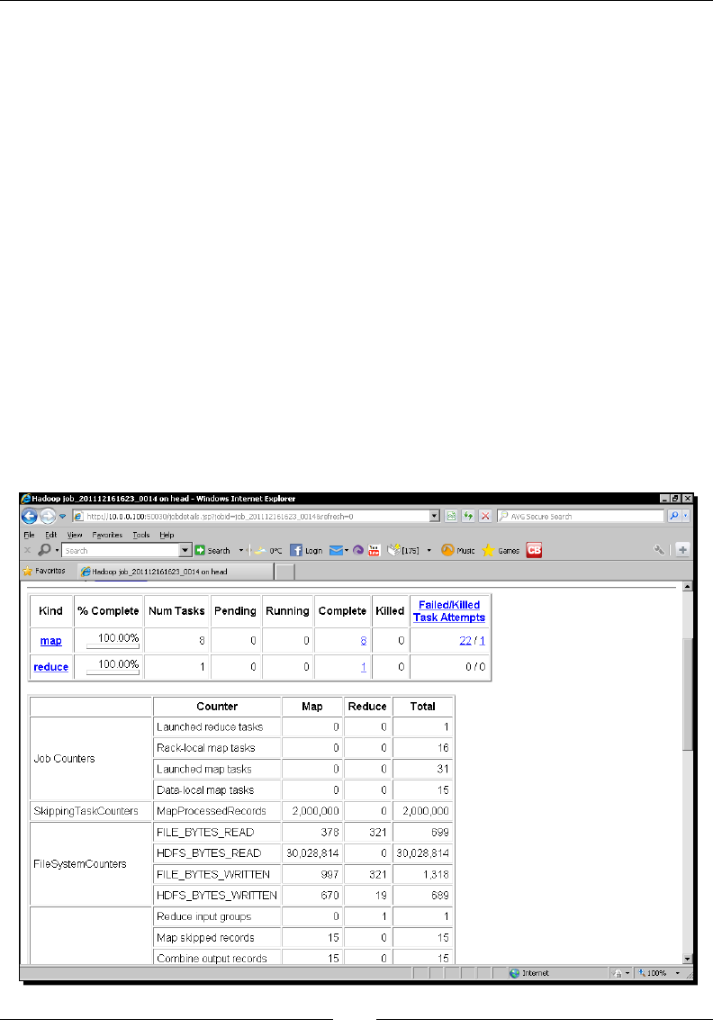
When Things Break
[ 200 ]
11/12/16 18:13:00 INFO mapred.JobClient: map 100% reduce 100%
11/12/16 18:13:02 INFO mapred.JobClient: Job complete:
job_201112161623_0014
...
10. Examine the contents of the job output le:
$ hadoop fs -cat output/part-00000
totalcount 2000000
11. Look in the output directory for skipped records:
$ hadoop fs -ls output/_logs/skip
Found 15 items
-rw-r--r-- 3 hadoop supergroup 203 2011-12-16 18:05 /
user/hadoop/output/_logs/skip/attempt_201112161623_0014_m_000001_3
-rw-r--r-- 3 hadoop supergroup 211 2011-12-16 18:06 /
user/hadoop/output/_logs/skip/attempt_201112161623_0014_m_000001_4
…
12. Check the job details from the MapReduce UI to observe the recorded stascs as
shown in the following screenshot:
www.it-ebooks.info

Chapter 6
[ 201 ]
What just happened?
We had to do a lot of setup here so let's walk through it a step at a me.
Firstly, we needed to congure Hadoop to use skip mode; it is disabled by default. The key
conguraon property was set to 5, meaning that we didn't want the framework to skip any
set of records greater than this number. Note that this includes the invalid records, and by
seng this property to 0 (the default) Hadoop will not enter skip mode.
We also check to ensure that Hadoop is congured with a suciently high threshold for
repeated task aempt failures, which we will explain shortly.
Next we needed a test le that we could use to simulate dirty data. We wrote a simple
Ruby script that generated a le with 2 million lines that we would treat as valid with three
sets of ve bad records interspersed through the le. We ran this script and conrmed that
the generated le did indeed have 2,000,015 lines. This le was then put on HDFS where it
would be the job input.
We then wrote a simple MapReduce job that eecvely counts the number of valid records.
Every me the line reads from the input as the valid text we emit an addional count of 1 to
what will be aggregated as a nal total. When the invalid lines are encountered, the mapper
fails by throwing an excepon.
We then compile this le, jar it up, and run the job. The job takes a while to run and as seen
from the extracts of the job status, it follows a paern that we have not seen before. The
map progress counter will increase but when a task fails, the progress will drop back then
start increasing again. This is skip mode in acon.
Every me a key/value pair is passed to the mapper, Hadoop by default increments a counter
that allows it to keep track of which record caused a failure.
If your map or reduce tasks process their input through mechanisms other
than directly receiving all data via the arguments to the map or reduce method
(for example, from asynchronous processes or caches) you will need to ensure
you explicitly update this counter manually.
When a task fails, Hadoop retries it on the same block but aempts to work around the
invalid records. Through a binary search approach, the framework performs retries across
the data unl the number of skipped records is no greater than the maximum value we
congured earlier, that is 5. This process does require mulple task retries and failures as the
framework seeks the opmal batch to skip, which is why we had to ensure the framework
was congured to be tolerant of a higher-than-usual number of repeated task failures.
www.it-ebooks.info

When Things Break
[ 202 ]
We watched the job connue following this back and forth process and on compleon
checked the contents of the output le. This showed 2,000,000 processed records, that
is the correct number of valid records in our input le. Hadoop successfully managed to
skip only the three sets of ve invalid records.
We then looked within the _logs directory in the job output directory and saw that
there is a skip directory containing the sequence les of the skipped records.
Finally, we looked at the MapReduce web UI to see the overall job status, which
included both the number of records processed while in skip mode as well as the
number of records skipped. Note that the total number of failed tasks was 22, which is
greater than our threshold for failed map aempts, but this number is aggregate failures
across mulple tasks.
To skip or not to skip...
Skip mode can be very eecve but as we have seen previously, there is a performance
penalty caused by Hadoop having to determine which record range to skip. Our test le was
actually quite helpful to Hadoop; the bad records were nicely grouped in three groups and
only accounted for a ny fracon of the overall data set. If there were many more invalid
records in the input data and they were spread much more widely across the le, a more
eecve approach may have been to use a precursor MapReduce job to lter out all the
invalid records.
This is why we have presented the topics of wring code to handle bad data and using
skip mode consecuvely. Both are valid techniques that you should have in your tool
belt. There is no single answer to when one or the other is the best approach, you need
to consider the input data, performance requirements, and opportunies for hardcoding
before making a decision.
Summary
We have caused a lot of destrucon in this chapter and I hope you never have to deal with
this much failure in a single day with an operaonal Hadoop cluster. There are some key
learning points from the experience.
In general, component failures are not something to fear in Hadoop. Parcularly with large
clusters, failure of some component or host will be prey commonplace and Hadoop is
engineered to handle this situaon. HDFS, with its responsibility to store data, acvely
manages the replicaon of each block and schedules new copies to be made when the
DataNode processes die.
www.it-ebooks.info

Chapter 6
[ 203 ]
MapReduce has a stateless approach to TaskTracker failure and in general simply schedules
duplicate jobs if one fails. It may also do this to prevent the misbehaving hosts from slowing
down the whole job.
Failure of the HDFS and MapReduce master nodes is a more signicant failure. In parcular,
the NameNode process holds crical lesystem data and you must acvely ensure you have
it set up to allow a new NameNode process to take over.
In general, hardware failures will look much like the previous process failures, but always
be aware of the possibility of correlated failures. If tasks fail due to soware errors, Hadoop
will retry them within congurable thresholds. Data-related errors can be worked around by
employing skip mode, though it will come with a performance penalty.
Now that we know how to handle failures in our cluster, we will spend the next chapter
working through the broader issues of cluster setup, health, and maintenance.
www.it-ebooks.info

7
Keeping Things Running
Having a Hadoop cluster is not all about writing interesting programs to do
clever data analysis. You also need to maintain the cluster, and keep it tuned
and ready to do the data crunching you want.
In this chapter we will cover:
More about Hadoop conguraon properes
How to select hardware for your cluster
How Hadoop security works
Managing the NameNode
Managing HDFS
Managing MapReduce
Scaling the cluster
Although these topics are operaonally focused, they do give us an opportunity to explore
some aspects of Hadoop we have not looked at before. Therefore, even if you won't be
personally managing the cluster, there should be useful informaon here for you too.
www.it-ebooks.info

Keeping Things Running
[ 206 ]
A note on EMR
One of the main benets of using cloud services such as those oered by Amazon Web Services
is that much of the maintenance overhead is borne by the service provider. Elasc MapReduce
can create Hadoop clusters ed to the execuon of a single task (non-persistent job ows) or
allow long-running clusters that can be used for mulple jobs (persistent job ows). When
non-persistent job ows are used, the actual mechanics of how the underlying Hadoop cluster
is congured and run are largely invisible to the user. Consequently, users employing non-
persistent job ows will not need to consider many of the topics in this chapter. If you are
using EMR with persistent job ows, many topics (but not all) do become relevant.
We will generally talk about local Hadoop clusters in this chapter. If you need to recongure
a persistent job ow, use the same Hadoop properes but set them as described in Chapter
3, Wring MapReduce Jobs.
Hadoop conguration properties
Before we look at running the cluster, let's talk a lile about Hadoop's conguraon
properes. We have been introducing many of these along the way, and there are a
few addional points worth considering.
Default values
One of the most mysfying things to a new Hadoop user is the large number of
conguraon properes. Where do they come from, what do they mean, and
what are their default values?
If you have the full Hadoop distribuon—that is, not just the binary distribuon—the
following XML les will answer your quesons:
Hadoop/src/core/core-default.xml
Hadoop/src/hdfs/hdfs-default.xml
Hadoop/src/mapred/mapred-default.xml
Time for action – browsing default properties
Fortunately, the XML documents are not the only way of looking at the default values; there
are also more readable HTML versions, which we'll now take a quick look at.
www.it-ebooks.info
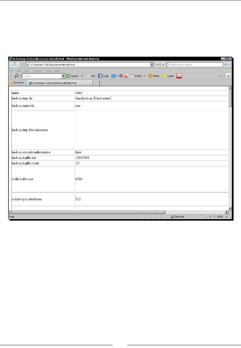
Chapter 7
[ 207 ]
These les are not included in the Hadoop binary-only distribuon; if you are using that,
you can also nd these les on the Hadoop website.
1. Point your browser at the docs/core-default.html le within your
Hadoop distribuon directory and browse its contents. It should look like
the next screenshot:
2. Now, similarly, browse these other les:
Hadoop/docs/hdfs-default.html
Hadoop/docs/mapred-default.html
What just happened?
As you can see, each property has a name, default value, and a brief descripon. You will
also see there are indeed a very large number of properes. Do not expect to understand
all of these now, but do spend a lile me browsing to get a avor for the type of
customizaon allowed by Hadoop.
www.it-ebooks.info

Keeping Things Running
[ 208 ]
Additional property elements
When we have previously set properes in the conguraon les, we have used an XML
element of the following form:
<property>
<name>the.property.name</name>
<value>The property value</value>
</property>
There are an addional two oponal XML elements we can add, description and final.
A fully described property using these addional elements now looks as follows:
<property>
<name>the.property.name</name>
<value>The default property value</value>
<description>A textual description of the property</description>
<final>Boolean</final>
</property>
The descripon element is self-explanatory and provides the locaon for the descripve text
we saw for each property in the preceding HTML les.
The final property has a similar meaning as in Java: any property marked final cannot be
overridden by values in any other les or by other means; we will see this shortly. Use this
for those properes where for performance, integrity, security, or other reasons, you wish to
enforce cluster-wide values.
Default storage location
You will see properes that modify where Hadoop stores its data on both the local disk and
HDFS. There's one property used as the basis for many others hadoop.tmp.dir, which is
the root locaon for all Hadoop les, and its default value is /tmp.
Unfortunately, many Linux distribuons—including Ubuntu—are congured to remove
the contents of this directory on each reboot. This means that if you do not override this
property, you will lose all your HDFS data on the next host reboot. Therefore,
it is worthwhile to set something like the following in core-site.xml:
<property>
<name>hadoop.tmp.dir</name>
<value>/var/lib/hadoop</value>
</property>
www.it-ebooks.info

Chapter 7
[ 209 ]
Remember to ensure the locaon is writable by the user who will start Hadoop, and that
the disk the directory is located on has enough space. As you will see later, there are a
number of other properes that allow more granular control of where parcular types
of data are stored.
Where to set properties
We have previously used the conguraon les to specify new values for Hadoop properes.
This is ne, but does have an overhead if we are trying to nd the best value for a property
or are execung a job that requires special handling.
It is possible to use the JobConf class to programmacally set conguraon properes on
the execung job. There are two types of methods supported, the rst being those that
are dedicated to seng a specic property, such as the ones we've seen for seng the job
name, input, and output formats, among others. There are also methods to set properes
such as the preferred number of map and reduce tasks for the job.
In addion, there are a set of generic methods, such as the following:
Void set(String key, String value);
Void setIfUnset(String key, String value);
Void setBoolean( String key, Boolean value);
Void setInt(String key, int value);
These are more exible and do not require specic methods to be created for each
property we wish to modify. However, they also lose compile me checking meaning
you can use an invalid property name or assign the wrong type to a property and will
only nd out at runme.
This ability to set property values both programmacally and in the
conguraon les is an important reason for the ability to mark a property as
final. For properes for which you do not want any submied job to have the
ability to override them, set them as nal within the master conguraon les.
Setting up a cluster
Before we look at how to keep a cluster running, let's explore some aspects of seng it up in
the rst place.
www.it-ebooks.info

Keeping Things Running
[ 210 ]
How many hosts?
When considering a new Hadoop cluster, one of the rst quesons is how much capacity to
start with. We know that we can add addional nodes as our needs grow, but we also want
to start o in a way that eases that growth.
There really is no clear-cut answer here, as it will depend largely on the size of the data sets
you will be processing and the complexity of the jobs to be executed. The only near-absolute
is to say that if you want a replicaon factor of n, you should have at least that many nodes.
Remember though that nodes will fail, and if you have the same number of nodes as the
default replicaon factor then any single failure will push blocks into an under-replicated
state. In most clusters with tens or hundreds of nodes, this is not a concern; but for very
small clusters with a replicaon factor of 3, the safest approach would be a ve-node cluster.
Calculating usable space on a node
An obvious starng point for the required number of nodes is to look at the size of the data
set to be processed on the cluster. If you have hosts with 2 TB of disk space and a 10 TB data
set, the temptaon would be to assume that ve nodes is the minimum number needed.
This is incorrect, as it omits consideraon of the replicaon factor and the need for
temporary space. Recall that the output of mappers is wrien to the local disk to be
retrieved by the reducers. We need to account for this non-trivial disk usage.
A good rule of thumb would be to assume a replicaon factor of 3, and that 25 percent of
what remains should be accounted for as temporary space. Using these assumpons, the
calculaon of the needed cluster for our 10 TB data set on 2 TB nodes would be as follows:
Divide the total storage space on a node by the replicaon factor:
2 TB/3 = 666 GB
Reduce this gure by 25 percent to account for temp space:
666 GB * 0.75 = 500 GB
Each 2 TB node therefore has approximately 500 GB (0.5 TB) of usable space
Divide the data set size by this gure:
10 TB / 500 GB = 20
So our 10 TB data set will likely need a 20 node cluster as a minimum, four mes our
naïve esmate.
This paern of needing more nodes than expected is not unusual and should be
remembered when considering how high-spec you want the hosts to be; see the
Sizing hardware secon later in this chapter.
www.it-ebooks.info

Chapter 7
[ 211 ]
Location of the master nodes
The next queson is where the NameNode, JobTracker, and SecondaryNameNode will
live. We have seen that a DataNode can run on the same host as the NameNode and the
TaskTracker can co-exist with the JobTracker, but this is unlikely to be a great setup for a
producon cluster.
As we will see, the NameNode and SecondaryNameNode have some specic resource
requirements, and anything that aects their performance is likely to slow down the enre
cluster operaon.
The ideal situaon would be to have the NameNode, JobTracker, and SecondaryNameNode
on their own dedicated hosts. However, for very small clusters, this would result in a
signicant increase in the hardware footprint without necessarily reaping the full benet.
If at all possible, the rst step should be to separate the NameNode, JobTracker, and
SecondaryNameNode onto a single dedicated host that does not have any DataNode or
TaskTracker processes running. As the cluster connues to grow, you can add an addional
server host and then move the NameNode onto its own host, keeping the JobTracker and
SecondaryNameNode co-located. Finally, as the cluster grows yet further, it will make sense
to move to full separaon.
As discussed in Chapter 6, Keeping Things Running, Hadoop 2.0 will split the
Secondary NameNode into Backup NameNodes and Checkpoint NameNodes.
Best pracce is sll evolving, but aiming towards having a dedicated host each
for the NameNode and at least one Backup NameNode looks sensible.
Sizing hardware
The amount of data to be stored is not the only consideraon regarding the specicaon
of the hardware to be used for the nodes. Instead, you have to consider the amount of
processing power, memory, storage types, and networking available.
Much has been wrien about selecng hardware for a Hadoop cluster, and once again there
is no single answer that will work for all cases. The big variable is the types of MapReduce
tasks that will be executed on the data and, in parcular, if they are bounded by CPU,
memory, I/O, or something else.
Processor / memory / storage ratio
A good way of thinking of this is to look at potenal hardware in terms of the CPU / memory
/ storage rao. So, for example, a quad-core host with 8 GB memory and 2 TB storage could
be thought of as having two cores and 4 GB memory per 1 TB of storage.
www.it-ebooks.info

Keeping Things Running
[ 212 ]
Then look at the types of MapReduce jobs you will be running, does that rao seem
appropriate? In other words, does your workload require proporonally more of one
of these resources or will a more balanced conguraon be sucient?
This is, of course, best assessed by prototyping and gathering metrics, but that isn't always
possible. If not, consider what part of the job is the most expensive. For example, some
of the jobs we have seen are I/O bound and read data from the disk, perform simple
transformaons, and then write results back to the disk. If this was typical of our workload,
we could likely use hardware with more storage—especially if it was delivered by mulple
disks to increase I/O—and use less CPU and memory.
Conversely, jobs that perform very heavy number crunching would need more CPU, and
those that create or use large data structures would benet from memory.
Think of it in terms of liming factors. If your job was running, would it be CPU-bound
(processors at full capacity; memory and I/O to spare), memory-bound (physical memory full
and swapping to disk; CPU and I/O to spare), or I/O-bound (CPU and memory to spare, but
data being read/wrien to/from disk at maximum possible speed)? Can you get hardware
that eases that bound?
This is of course a limitless process, as once you ease one bound another will manifest itself.
So always remember that the idea is to get a performance prole that makes sense in the
context of your likely usage scenario.
What if you really don't know the performance characteriscs of your jobs? Ideally, try
to nd out, do some prototyping on any hardware you have and use that to inform your
decision. However, if even that is not possible, you will have to go for a conguraon and
try it out. Remember that Hadoop supports heterogeneous hardware—though having
uniform specicaons makes your life easier in the end—so build the cluster to the
minimum possible size and assess the hardware. Use this knowledge to inform future
decisions regarding addional host purchases or upgrades of the exisng eet.
EMR as a prototyping platform
Recall that when we congured a job on Elasc MapReduce we chose the type of hardware
for both the master and data/task nodes. If you plan to run your jobs on EMR, you have
a built-in capability to tweak this conguraon to nd the best combinaon of hardware
specicaons to price and execuon speed.
However, even if you do not plan to use EMR full-me, it can be a valuable prototyping
plaorm. If you are sizing a cluster but do not know the performance characteriscs of
your jobs, consider some prototyping on EMR to gain beer insight. Though you may end
up spending money on the EMR service that you had not planned, this will likely be a lot less
than the cost of nding out you have bought completely unsuitable hardware for your cluster.
www.it-ebooks.info

Chapter 7
[ 213 ]
Special node requirements
Not all hosts have the same hardware requirements. In parcular, the host for the
NameNode may look radically dierent to those hosng the DataNodes and TaskTrackers.
Recall that the NameNode holds an in-memory representaon of the HDFS lesystem and
the relaonship between les, directories, blocks, nodes, and various metadata concerning
all of this. This means that the NameNode will tend to be memory bound and may require
larger memory than any other host, parcularly for very large clusters or those with a huge
number of les. Though 16 GB may be a common memory size for DataNodes/TaskTrackers,
it's not unusual for the NameNode host to have 64 GB or more of memory. If the NameNode
ever ran out of physical memory and started to use swap space, the impact on cluster
performance would likely be severe.
However, though 64 GB is large for physical memory, it's ny for modern storage, and
given that the lesystem image is the only data stored by the NameNode, we don't need
the massive storage common on the DataNode hosts. We care much more about NameNode
reliability so are likely to have several disks in a redundant conguraon. Consequently,
the NameNode host will benet from mulple small drives (for redundancy) rather than
large drives.
Overall, therefore, the NameNode host is likely to look quite dierent from the other
hosts in the cluster; this is why we made the earlier recommendaons regarding moving
the NameNode to its own host as soon as budget/space allows, as its unique hardware
requirements are more easily sased this way.
The SecondaryNameNode (or CheckpointNameNode and BackupNameNode
in Hadoop 2.0) share the same hardware requirements as the NameNode. You
can run it on a more generic host while in its secondary capacity, but if you do
ever need to switch and make it the NameNode due to failure of the primary
hardware, you may be in trouble.
Storage types
Though you will nd strong opinions on some of the previous points regarding the relave
importance of processor, memory, and storage capacity, or I/O, such arguments are usually
based around applicaon requirements and hardware characteriscs and metrics. Once we
start discussing the type of storage to be used, however, it is very easy to get into ame war
situaons, where you will nd extremely entrenched opinions.
www.it-ebooks.info

Keeping Things Running
[ 214 ]
Commodity versus enterprise class storage
The rst argument will be over whether it makes most sense to use hard drives aimed at
the commodity/consumer segments or those aimed at enterprise customers. The former
(primarily SATA disks) are larger, cheaper, and slower, and have lower quoted gures for
mean me between failures (MTBF). Enterprise disks will use technologies such as SAS or
Fiber Channel, and will on the whole be smaller, more expensive, faster, and have higher
quoted MTBF gures.
Single disk versus RAID
The next queson will be on how the disks are congured. The enterprise-class approach
would be to use Redundant Arrays of Inexpensive Disks (RAID) to group mulple disks into
a single logical storage device that can quietly survive one or more disk failures. This comes
with the cost of a loss in overall capacity and an impact on the read/write rates achieved.
The other posion is to treat each disk independently to maximize total storage and
aggregate I/O, at the cost of a single disk failure causing host downme.
Finding the balance
The Hadoop architecture is, in many ways, predicated on the assumpon that hardware will
fail. From this perspecve, it is possible to argue that there is no need to use any tradional
enterprise-focused storage features. Instead, use many large, cheap disks to maximize the
total storage and read and write from them in parallel to do likewise for I/O throughput.
A single disk failure may cause the host to fail, but the cluster will, as we have seen, work
around this failure.
This is a completely valid argument and in many cases makes perfect sense. What the
argument ignores, however, is the cost of bringing a host back into service. If your cluster
is in the next room and you have a shelf of spare disks, host recovery will likely be a quick,
painless, and inexpensive task. However, if you have your cluster hosted by a commercial
collocaon facility, any hands-on maintenance may cost a lot more. This is even more
the case if you are using fully-managed servers where you have to pay the provider for
maintenance tasks. In such a situaon, the extra cost and reduced capacity and I/O from
using RAID may make sense.
Network storage
One thing that will almost never make sense is to use networked storage for your primary
cluster storage. Be it block storage via a Storage Area Network (SAN) or le-based via
Network File System (NFS) or similar protocols, these approaches constrain Hadoop by
introducing unnecessary bolenecks and addional shared devices that would have a
crical impact on failure.
www.it-ebooks.info

Chapter 7
[ 215 ]
Somemes, however, you may be forced for non-technical reasons to use something like
this. It's not that it won't work, just that it changes how Hadoop will perform in regards to
speed and tolerance to failures, so be sure you understand the consequences if this happens.
Hadoop networking conguration
Hadoop's support of networking devices is not as sophiscated as it is for storage, and
consequently you have fewer hardware choices to make compared to CPU, memory, and
storage setup. The boom line is that Hadoop can currently support only one network device
and cannot, for example, use all 4-gigabit Ethernet connecons on a host for an aggregate
of 4-gigabit throughput. If you need network throughput greater than that provided by a
single-gigabit port then, unless your hardware or operang system can present mulple
ports as a single device to Hadoop, the only opon is to use a 10-gigabit Ethernet device.
How blocks are placed
We have talked a lot about HDFS using replicaon for redundancy, but have not explored
how Hadoop chooses where to place the replicas for a block.
In most tradional server farms, the various hosts (as well as networking and other devices)
are housed in standard-sized racks that stack the equipment vercally. Each rack will usually
have a common power distribuon unit that feeds it and will oen have a network switch
that acts as the interface between the broader network and all the hosts in the rack.
Given this setup, we can idenfy three broad types of failure:
Those that aect a single host (for example, CPU/memory/disk/motherboard failure)
Those that aect a single rack (for example, power unit or switch failure)
Those that aect the enre cluster (for example, larger power/network failures,
cooling/environmental outages)
Remember that Hadoop currently does not support a cluster that is spread
across mulple data centers, so instances of the third type of failure will
quite likely bring down your cluster.
By default, Hadoop will treat each node as if it is in the same physical rack. This implies that
the bandwidth and latency between any pair of hosts is approximately equal and that each
node is equally likely to suer a related failure as any other.
www.it-ebooks.info

Keeping Things Running
[ 216 ]
Rack awareness
If, however, you do have a mul-rack setup, or another conguraon that otherwise
invalidates the previous assumpons, you can add the ability for each node to report
its rack ID to Hadoop, which will then take this into account when placing replicas.
In such a setup, Hadoop tries to place the rst replica of a node on a given host, the second
on another within the same rack, and the third on a host in a dierent rack.
This strategy provides a good balance between performance and availability. When racks
contain their own network switches, communicaon between hosts inside the rack oen has
lower latency than that with external hosts. This strategy places two replicas within a rack
to ensure maximum speed of wring for these replicas, but keeps one outside the rack to
provide redundancy in the event of a rack failure.
The rack-awareness script
If the topology.script.file.name property is set and points to an executable script
on the lesystem, it will be used by the NameNode to determine the rack for each host.
Note that the property needs to be set and the script needs to exist only on the
NameNode host.
The NameNode will pass to the script the IP address of each node it discovers, so the script
is responsible for a mapping from node IP address to rack name.
If no script is specied, each node will be reported as a member of a single default rack.
Time for action – examining the default rack conguration
Let's take a look at how the default rack conguraon is set up in our cluster.
1. Execute the following command:
$ Hadoop fsck -rack
2. The result should include output similar to the following:
Default replication factor: 3
Average block replication: 3.3045976
Corrupt blocks: 0
Missing replicas: 18 (0.5217391 %)
Number of data-nodes: 4
Number of racks: 1
The filesystem under path '/' is HEALTHY
www.it-ebooks.info

Chapter 7
[ 217 ]
What just happened?
Both the tool used and its output are of interest here. The tool is hadoop fsck, which
can be used to examine and x lesystem problems. As can be seen, this includes some
informaon not dissimilar to our old friend hadoop dfsadmin, though that tool is focused
more on the state of each node in detail while hadoop fsck reports on the internals of the
lesystem as a whole.
One of the things it reports is the total number of racks in the cluster, which, as seen in the
preceding output, has the value 1, as expected.
This command was executed on a cluster that had recently been used for
some HDFS resilience tesng. This explains the gures for average block
replicaon and under-replicated blocks.
If a block ends up with more than the required number of replicas due to a
host temporarily failing, the host coming back into service will put the block
above the minimum replicaon factor. Along with ensuring that blocks have
replicas added to meet the replicaon factor, Hadoop will also delete excess
replicas to return blocks to the replicaon factor.
Time for action – adding a rack awareness script
We can enhance the default at rack conguraon by creang a script that derives the rack
locaon for each host.
1. Create a script in the Hadoop user's home directory on the NameNode host called
rack-script.sh, containing the following text. Remember to change the IP
address to one of your HDFS nodes.
#!/bin/bash
if [ $1 = "10.0.0.101" ]; then
echo -n "/rack1 "
else
echo -n "/default-rack "
fi
2. Make this script executable.
$ chmod +x rack-script.sh
3. Add the following property to core-site.xml on the NameNode host:
<property>
<name>topology.script.file.name</name>
<value>/home/Hadoop/rack-script.sh</value>
</property>
www.it-ebooks.info
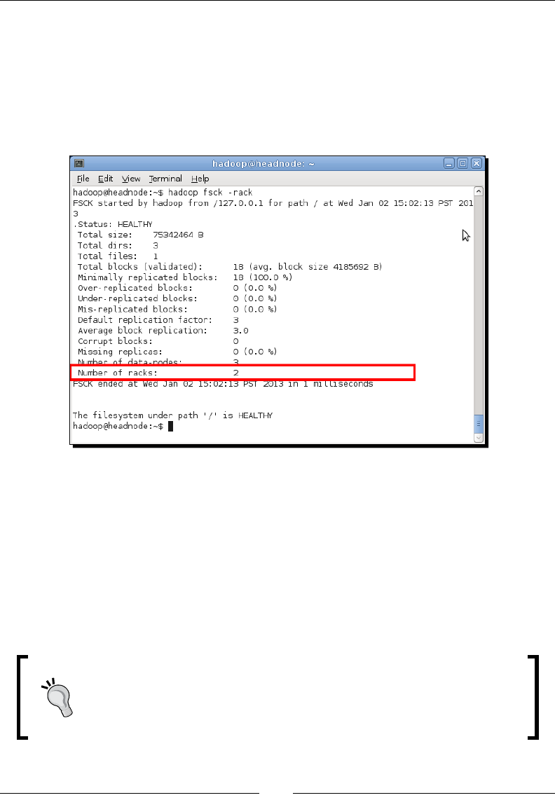
Keeping Things Running
[ 218 ]
4. Restart HDFS.
$ start-dfs.sh
5. Check the lesystem via fsck.
$ Hadoop fsck –rack
The output of the preceding command can be shown in the following screenshot:
What just happened?
We rst created a simple script that returns one value for a named node and a default value
for all others. We placed this on the NameNode host and added the needed conguraon
property to the NameNode core-site.xml le.
Aer starng HDFS, we used hadoop fsck to report on the lesystem and saw that
we now have a two-rack cluster. With this knowledge, Hadoop will now employ more
sophiscated block placement strategies, as described previously.
Using an external host le
A common approach is to keep a separate data le akin to the /etc/hosts
le on Unix and use this to specify the IP/rack mapping, one per line. This le
can then be updated independently and read by the rack-awareness script.
www.it-ebooks.info

Chapter 7
[ 219 ]
What is commodity hardware anyway?
Let's revisit the queson of the general characteriscs of the hosts used for your cluster, and
whether they should look more like a commodity white box server or something built for a
high-end enterprise environment.
Part of the problem is that "commodity" is an ambiguous term. What looks cheap
and cheerful for one business may seem luxuriously high-end for another. We suggest
considering the following points to keep in mind when selecng hardware and then
remaining happy with your decision:
With your hardware, are you paying a premium for reliability features that duplicate
some of Hadoop's fault-tolerance capabilies?
Are the higher-end hardware features you are paying for addressing the need or risk
that you have conrmed is realisc in your environment?
Have you validated the cost of the higher-end hardware to be higher than dealing
with cheaper / less reliable hardware?
Pop quiz – setting up a cluster
Q1. Which of the following is most important when selecng hardware for your new
Hadoop cluster?
1. The number of CPU cores and their speed.
2. The amount of physical memory.
3. The amount of storage.
4. The speed of the storage.
5. It depends on the most likely workload.
Q2. Why would you likely not want to use network storage in your cluster?
1. Because it may introduce a new single point of failure.
2. Because it most likely has approaches to redundancy and fault-tolerance that may
be unnecessary given Hadoop's fault tolerance.
3. Because such a single device may have inferior performance to Hadoop's use of
mulple local disks simultaneously.
4. All of the above.
www.it-ebooks.info

Keeping Things Running
[ 220 ]
Q3. You will be processing 10 TB of data on your cluster. Your main MapReduce job
processes nancial transacons, using them to produce stascal models of behavior
and future forecasts. Which of the following hardware choices would be your rst
choice for the cluster?
1. 20 hosts each with fast dual-core processors, 4 GB memory, and one 500 GB
disk drive.
2. 30 hosts each with fast dual-core processors, 8 GB memory, and two 500 GB
disk drives.
3. 30 hosts each with fast quad-core processors, 8 GB memory, and one 1 TB disk drive.
4. 40 hosts each with 16 GB memory, fast quad-core processors, and four 1 TB
disk drives.
Cluster access control
Once you have the shiny new cluster up and running, you need to consider quesons of
access and security. Who can access the data on the cluster—is there sensive data that
you really don't want the whole user base to see?
The Hadoop security model
Unl very recently, Hadoop had a security model that could, at best, be described as
"marking only". It associated an owner and group with each le but, as we'll see, did very
lile validaon of a given client connecon. Strong security would manage not only the
markings given to a le but also the idenes of all connecng users.
Time for action – demonstrating the default security
When we have previously shown lisngs of les, we have seen user and group names for
them. However, we have not really explored what that means. Let's do so.
1. Create a test text le in the Hadoop user's home directory.
$ echo "I can read this!" > security-test.txt
$ hadoop fs -put security-test.txt security-test.txt
2. Change the permissions on the le to be accessible only by the owner.
$ hadoop fs -chmod 700 security-test.txt
$ hadoop fs -ls
www.it-ebooks.info
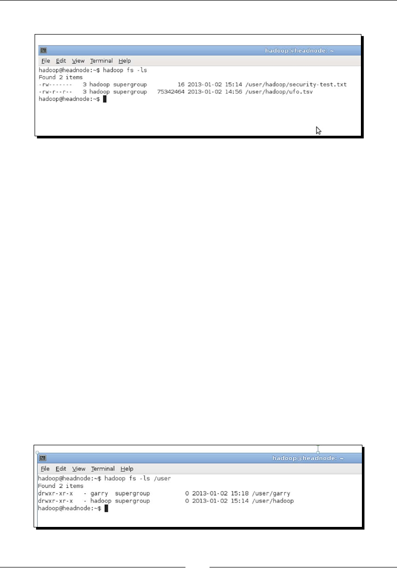
Chapter 7
[ 221 ]
The output of the preceding command can be shown in the following screenshot:
3. Conrm you can sll read the le.
$ hadoop fs -cat security-test.txt
You'll see the following line on the screen:
I can read this!
4. Connect to another node in the cluster and try to read the le from there.
$ ssh node2
$ hadoop fs -cat security-test.txt
You'll see the following line on the screen:
I can read this!
5. Log out from the other node.
$ exit
6. Create a home directory for another user and give them ownership.
$ hadoop m[Kfs -mkdir /user/garry
$ hadoop fs -chown garry /user/garry
$ hadoop fs -ls /user
The output of the preceding command can be shown in the following screenshot:
www.it-ebooks.info
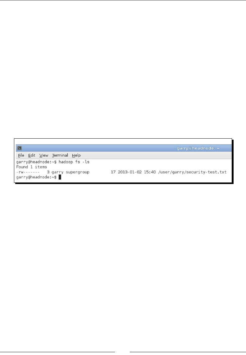
Keeping Things Running
[ 222 ]
7. Switch to that user.
$ su garry
8. Try to read the test le in the Hadoop user's home directory.
$ hadoop/bin/hadoop fs -cat /user/hadoop/security-test.txt
cat: org.apache.hadoop.security.AccessControlException: Permission
denied: user=garry, access=READ, inode="security-test.txt":hadoop:
supergroup:rw-------
9. Place a copy of the le in this user's home directory and again make it accessible
only by the owner.
$ Hadoop/bin/Hadoop fs -put security-test.txt security-test.txt
$ Hadoop/bin/Hadoop fs -chmod 700 security-test.txt
$ hadoop/bin/hadoop fs -ls
The output of the preceding command can be shown in following screenshot:
10. Conrm this user can access the le.
$ hadoop/bin/hadoop fs -cat security-test.txt
You'll see the following line on the screen:
I can read this!
11. Return to the Hadoop user.
$ exit
12. Try and read the le in the other user's home directory.
$ hadoop fs -cat /user/garry/security-test.txt
You'll see the following line on the screen:
I can read this!
www.it-ebooks.info

Chapter 7
[ 223 ]
What just happened?
We rstly used our Hadoop user to create a test le in its home directory on HDFS. We used
the -chmod opon to hadoop fs, which we have not seen before. This is very similar to the
standard Unix chmod tool that gives various levels of read/write/execute access to the le
owner, group members, and all users.
We then went to another host and tried to access the le, again as the Hadoop user. Not
surprisingly, this worked. But why? What did Hadoop know about the Hadoop user that
allowed it to give access to the le?
To explore this, we then created another home directory on HDFS (you can use any other
account on the host you have access to), and gave it ownership by using the -chown
opon to hadoop fs. This should once again look similar to standard Unix -chown. Then
we switched to this user and aempted to read the le stored in the Hadoop user's home
directory. This failed with the security excepon shown before, which is again what we
expected. Once again, we copied a test le into this user's home directory and made it only
accessible by the owner.
But we then muddied the waters by switching back to the Hadoop user and tried to access
the le in the other account's home directory, which, surprisingly, worked.
User identity
The answer to the rst part of the puzzle is that Hadoop uses the Unix ID of the user
execung the HDFS command as the user identy on HDFS. So any commands executed by a
user called alice will create les with an owner named alice and will only be able to read
or write les to which this user has the correct access.
The security-minded will realize that to access a Hadoop cluster all one needs to do is create
a user with the same name as an already exisng HDFS user on any host that can connect
to the cluster. So, for instance, in the previous example, any user named hadoop created
on any host that can access the NameNode can read all les accessible by the user hadoop,
which is actually even worse than it seems.
The super user
The previous step saw the Hadoop user access another user's les. Hadoop treats the user
ID that started the cluster as the super user, and gives it various privileges, such as the
ability to read, write, and modify any le on HDFS. The security-minded will realize even
more the risk of having users called hadoop randomly created on hosts outside the Hadoop
administrator's control.
www.it-ebooks.info

Keeping Things Running
[ 224 ]
More granular access control
The preceding situaon has caused security to be a major weakness in Hadoop since its
incepon. The community has, however, not been standing sll, and aer much work the
very latest versions of Hadoop support a more granular and stronger security model.
To avoid reliance on simple user IDs, the developers need to learn the user identy from
somewhere, and the Kerberos system was chosen with which to integrate. This does require
the establishment and maintenance of services outside the scope of this book, but if such
security is important to you, consult the Hadoop documentaon. Note that this support does
allow integraon with third-party identy systems such as Microso Acve Directory, so it is
quite powerful.
Working around the security model via physical access control
If the burden of Kerberos is too great, or security is a nice-to-have rather than an absolute,
there are ways of migang the risk. One favored by me is to place the enre cluster behind
a rewall with ght access control. In parcular, only allow access to the NameNode and
JobTracker services from a single host that will be treated as the cluster head node and
to which all users connect.
Accessing Hadoop from non-cluster hosts
Hadoop does not need to be running on a host for it to use the command-line
tools to access HDFS and run MapReduce jobs. As long as Hadoop is installed on
the host and its conguraon les have the correct locaons of the NameNode
and JobTracker, these will be found when invoking commands such as Hadoop
fs and Hadoop jar.
This model works because only one host is used to interact with Hadoop; and since this host
is controlled by the cluster administrator, normal users should be unable to create or access
other user accounts.
Remember that this approach is not providing security. It is pung a hard shell around a
so system that reduces the ways in which the Hadoop security model can be subverted.
Managing the NameNode
Let's do some more risk reducon. In Chapter 6, When Things Break, I probably scared
you when talking about the potenal consequences of a failure of the host running the
NameNode. If that secon did not scare you, go back and re-read it—it should have. The
summary is that the loss of the NameNode could see you losing every single piece of data on
the cluster. This is because the NameNode writes a le called fsimage that contains all the
metadata for the lesystem and records which blocks comprise which les. If the loss of the
NameNode host makes the fsimage unrecoverable, all the HDFS data is likewise lost.
www.it-ebooks.info

Chapter 7
[ 225 ]
Conguring multiple locations for the fsimage class
The NameNode can be congured to simultaneously write fsimage to mulple locaons.
This is purely a redundancy mechanism, the same data is wrien to each locaon and there
is no aempt to use mulple storage devices for increased performance. Instead, the policy
is that mulple copies of fsimage will be harder to lose.
Time for action – adding an additional fsimage location
Let's now congure our NameNode to simultaneously write mulple copies of fsimage to
give us our desired data resilience. To do this, we require an NFS-exported directory.
1. Ensure the cluster is stopped.
$ stopall.sh
2. Add the following property to Hadoop/conf/core-site.xml, modifying the
second path to point to an NFS-mounted locaon to which the addional copy of
NameNode data can be wrien.
<property>
<name>dfs.name.dir</name>
<value>${hadoop.tmp.dir}/dfs/name,/share/backup/namenode</value>
</property>
3. Delete any exisng contents of the newly added directory.
$ rm -f /share/backup/namenode
4. Start the cluster.
$ start-all.sh
5. Verify that fsimage is being wrien to both the specied locaons by running the
md5sum command against the two les specied before (change the following code
depending on your congured locaons):
$ md5sum /var/hadoop/dfs/name/image/fsimage
a25432981b0ecd6b70da647e9b94304a /var/hadoop/dfs/name/image/
fsimage
$ md5sum /share/backup/namenode/image/fsimage
a25432981b0ecd6b70da647e9b94304a /share/backup/namenode/image/
fsimage
What just happened?
Firstly, we ensured the cluster was stopped; though changes to the core conguraon les
are not reread by a running cluster, it's a good habit to get into in case that capability is ever
added to Hadoop.
www.it-ebooks.info

Keeping Things Running
[ 226 ]
We then added a new property to our cluster conguraon, specifying a value for the
data.name.dir property. This property takes a list of comma-separated values and writes
fsimage to each of these locaons. Note how the hadoop.tmp.dir property discussed
earlier is de-referenced, as would be seen when using Unix variables. This syntax allows us to
base property values on others and inherit changes when the parent properes are updated.
Do not forget all required locaons
The default value for this property is ${Hadoop.tmp.dir}/dfs/name.
When adding an addional value, remember to explicitly add the default
one also, as shown before. Otherwise, only the single new value will be
used for the property.
Before starng the cluster, we ensure the new directory exists and is empty. If the directory
doesn't exist, the NameNode will fail to start as should be expected. If, however, the
directory was previously used to store NameNode data, Hadoop will also fail to start as it will
idenfy that both directories contain dierent NameNode data and it does not know which
one is correct.
Be careful here! Especially if you are experimenng with various NameNode data locaons
or swapping back and forth between nodes; you really do not want to accidentally delete the
contents from the wrong directory.
Aer starng the HDFS cluster, we wait for a moment and then use MD5 cryptographic
checksums to verify that both locaons contain the idencal fsimage.
Where to write the fsimage copies
The recommendaon is to write fsimage to at least two locaons, one of which should be
the remote (such as a NFS) lesystem, as in the previous example. fsimage is only updated
periodically, so the lesystem does not need high performance.
In our earlier discussion regarding the choice of hardware, we alluded to other
consideraons for the NameNode host. Because of fsimage cricality, it may be useful
to ensure it is wrien to more than one disk and to perhaps invest in disks with higher
reliability, or even to write fsimage to a RAID array. If the host fails, using the copy wrien
to the remote lesystem will be the easiest opon; but just in case that has also experienced
problems, it's good to have the choice of pulling another disk from the dead host and using it
on another to recover the data.
www.it-ebooks.info

Chapter 7
[ 227 ]
Swapping to another NameNode host
We have ensured that fsimage is wrien to mulple locaons and this is the single most
important prerequisite for managing a swap to a dierent NameNode host. Now we need
to actually do it.
This is something you really should not do on a producon cluster. Absolutely not when
trying for the rst me, but even beyond that it's not a risk-free process. But do pracce
on other clusters and get an idea of what you'll do when disaster strikes.
Having things ready before disaster strikes
You don't want to be exploring this topic for the rst me when you need to recover the
producon cluster. There are several things to do in advance that will make disaster recovery
much less painful, not to menon possible:
Ensure the NameNode is wring the fsimage to mulple locaons, as done before.
Decide which host will be the new NameNode locaon. If this is a host currently
being used for a DataNode and TaskTracker, ensure it has the right hardware needed
to host the NameNode and that the reducon in cluster performance due to the loss
of these workers won't be too great.
Make a copy of the core-site.xml and hdfs-site.xml les, place them
(ideally) on an NFS locaon, and update them to point to the new host. Any me
you modify the current conguraon les, remember to make the same changes to
these copies.
Copy the slaves le from the NameNode onto either the new host or the NFS
share. Also, make sure you keep it updated.
Know how you will handle a subsequent failure in the new host. How quickly can
you likely repair or replace the original failed host? Which host will be the locaon
of the NameNode (and SecondaryNameNode) in the interim?
Ready? Let's do it!
Time for action – swapping to a new NameNode host
In the following steps we keep the new conguraon les on an NFS share mounted to /
share/backup and change the paths to match where you have the new les. Also use a
dierent string to grep; we use a poron of the IP address we know isn't shared with any
other host in the cluster.
www.it-ebooks.info

Keeping Things Running
[ 228 ]
1. Log on to the current NameNode host and shut down the cluster.
$ stop-all.sh
2. Halt the host that runs the NameNode.
$ sudo poweroff
3. Log on to the new NameNode host and conrm the new conguraon les have the
correct NameNode locaon.
$ grep 110 /share/backup/*.xml
4. On the new host, rst copy across the slaves le.
$ cp /share/backup/slaves Hadoop/conf
5. Now copy across the updated conguraon les.
$ cp /share/backup/*site.xml Hadoop/conf
6. Remove any old NameNode data from the local lesystem.
$ rm -f /var/Hadoop/dfs/name/*
7. Copy the updated conguraon les to every node in the cluster.
$ slaves.sh cp /share/backup/*site.xml Hadoop/conf
8. Ensure each node now has the conguraon les poinng to the new NameNode.
$ slaves.sh grep 110 hadoop/conf/*site.xml
9. Start the cluster.
$ start-all.sh
10. Check HDFS is healthy, from the command line.
$ Hadoop fs ls /
11. Verify whether HDFS is accessible from the web UI.
What just happened?
First, we shut down the cluster. This is a lile un-representave as most failures see the
NameNode die in a much less friendly way, but we do not want to talk about issues of
lesystem corrupon unl later in the chapter.
We then shut down the old NameNode host. Though not strictly necessary, it is a good way
of ensuring that nothing accesses the old host and gives you an incorrect view on how well
the migraon has occurred.
www.it-ebooks.info

Chapter 7
[ 229 ]
Before copying across les, we take a quick look at core-site.xml and hdfs-site.xml
to ensure the correct values are specied for the fs.default.dir property in
core-site.xml.
We then prepare the new host by rstly copying across the slaves conguraon le and
the cluster conguraon les and then removing any old NameNode data from the local
directory. Refer to the preceding steps about being very careful in this step.
Next, we use the slaves.sh script to get each host in the cluster to copy across the new
conguraon les. We know our new NameNode host is the only one with 110 in its IP
address, so we grep for that in the les to ensure all are up-to-date (obviously, you will
need to use a dierent paern for your system).
At this stage, all should be well; we start the cluster and access via both the command-line
tools and UI to conrm it is running as expected.
Don't celebrate quite yet!
Remember that even with a successful migraon to a new NameNode, you aren't done quite
yet. You decided in advance how to handle the SecondaryNameNode and which host would
be the new designated NameNode host should the newly migrated one fail. To be ready for
that, you will need to run through the "Be prepared" checklist menoned before once more
and act appropriately.
Do not forget to consider the chance of correlated failures. Invesgate the
cause of the NameNode host failure in case it is the start of a bigger problem.
What about MapReduce?
We did not menon moving the JobTracker as that is a much less painful process as
shown in Chapter 6, When Things Break. If your NameNode and JobTracker are running
on the same host, you will need to modify the preceding approach by also keeping a new
copy of mapred-site.xml, which has the locaon of the new host in the mapred.job.
tracker property.
Have a go hero – swapping to a new NameNode host
Perform a migraon of both the NameNode and JobTracker from one host to another.
www.it-ebooks.info

Keeping Things Running
[ 230 ]
Managing HDFS
As we saw when killing and restarng nodes in Chapter 6, When Things Break, Hadoop
automacally manages many of the availability concerns that would consume a lot of eort on
a more tradional lesystem. There are some things, however, that we sll need to be aware of.
Where to write data
Just as the NameNode can have mulple locaons for storage of fsimage specied via
the dfs.name.dir property, we explored earlier that there is a similar-appearing property
called dfs.data.dir that allows HDFS to use mulple data locaons on a host, which we
will look at now.
This is a useful mechanism that works very dierently from the NameNode property. If
mulple directories are specied in dfs.data.dir, Hadoop will view these as a series of
independent locaons that it can use in parallel. This is useful if you have mulple physical
disks or other storage devices mounted at disnct points on the lesystem. Hadoop will
use these mulple devices intelligently, maximizing not only the total storage capacity but
also by balancing reads and writes across the locaons to gain maximum throughput. As
menoned in the Storage types secon, this is the approach that maximizes these factors
at the cost of a single disk failure causing the whole host to fail.
Using balancer
Hadoop works hard to place data blocks on HDFS in a way that maximizes both performance
and redundancy. However, in certain situaons, the cluster can become unbalanced, with a
large discrepancy between the data held on the various nodes. The classic situaon that causes
this is when a new node is added to the cluster. By default, Hadoop will consider the new node
as a candidate for block placement alongside all other nodes, meaning that it will remain lightly
ulized for a signicant period of me. Nodes that have been out of service or have otherwise
suered issues may also have collected a smaller number of blocks than their peers.
Hadoop includes a tool called the balancer, started and stopped by the start-balancer.
sh and stop-balancer.sh scripts respecvely, to handle this situaon.
When to rebalance
Hadoop does not have any automac alarms that will alert you to an unbalanced lesystem.
Instead, you need to keep an eye on the data reported by both hadoop fsck and hadoop
fsadmin and watch for imbalances across the nodes.
www.it-ebooks.info

Chapter 7
[ 231 ]
In reality, this is not something you usually need to worry about, as Hadoop is very good at
managing block placement and you likely only need to consider running the balancer to remove
major imbalances when adding new hardware or when returning faulty nodes to service. To
maintain maximum cluster health, however, it is not uncommon to have the balancer run on a
scheduled basis (for example, nightly) to keep the block balancing within a specied threshold.
MapReduce management
As we saw in the previous chapter, the MapReduce framework is generally more tolerant of
problems and failures than HDFS. The JobTracker and TaskTrackers have no persistent data to
manage and, consequently, the management of MapReduce is more about the handling of
running jobs and tasks than servicing the framework itself.
Command line job management
The hadoop job command-line tool is the primary interface for this job management.
As usual, type the following to get a usage summary:
$ hadoop job --help
The opons to the command are generally self-explanatory; it allows you to start, stop,
list, and modify running jobs in addion to retrieving some elements of job history. Instead
of examining each individually, we will explore the use of several of these subcommands
together in the next secon.
Have a go hero – command line job management
The MapReduce UI also provides access to a subset of these capabilies. Explore the UI and
see what you can and cannot do from the web interface.
Job priorities and scheduling
So far, we have generally run a single job against our cluster and waited for it to complete.
This has hidden the fact that, by default, Hadoop places subsequent job submissions into a
First In, First Out (FIFO) queue. When a job nishes, Hadoop simply starts execung the next
job in the queue. Unless we use one of the alternave schedulers that we will discuss in later
secons, the FIFO scheduler dedicates the full cluster to the sole currently running job.
For small clusters with a paern of job submission that rarely sees jobs waing in the queue,
this is completely ne. However, if jobs are oen waing in the queue, issues can arise. In
parcular, the FIFO model takes no account of job priority or resources needed. A long-running
but low-priority job will execute before faster high-priority jobs that were submied later.
www.it-ebooks.info

Keeping Things Running
[ 232 ]
To address this situaon, Hadoop denes ve levels of job priority: VERY_HIGH, HIGH,
NORMAL, LOW, and VERY_LOW. A job defaults to NORMAL priority, but this can be changed
with the hadoop job -set-priority command.
Time for action – changing job priorities and killing a job
Let's explore job priories by changing them dynamically and watching the result of
killing a job.
1. Start a relavely long-running job on the cluster.
$ hadoop jar hadoop-examples-1.0.4.jar pi 100 1000
2. Open another window and submit a second job.
$ hadoop jar hadoop-examples-1.0.4.jar wordcount test.txt out1
3. Open another window and submit a third.
$ hadoop jar hadoop-examples-1.0.4.jar wordcount test.txt out2
4. List the running jobs.
$ Hadoop job -list
You'll see the following lines on the screen:
3 jobs currently running
JobId State StartTime UserName Priority SchedulingInfo
job_201201111540_0005 1 1326325810671 hadoop NORMAL NA
job_201201111540_0006 1 1326325938781 hadoop NORMAL NA
job_201201111540_0007 1 1326325961700 hadoop NORMAL NA
5. Check the status of the running job.
$ Hadoop job -status job_201201111540_0005
You'll see the following lines on the screen:
Job: job_201201111540_0005
file: hdfs://head:9000/var/hadoop/mapred/system/
job_201201111540_0005/job.xml
tracking URL: http://head:50030/jobdetails.
jsp?jobid=job_201201111540_000
map() completion: 1.0
reduce() completion: 0.32666665
Counters: 18
www.it-ebooks.info

Chapter 7
[ 233 ]
6. Raise the priority of the last submied job to VERY_HIGH.
$ Hadoop job -set-priority job_201201111540_0007 VERY_HIGH
7. Kill the currently running job.
$ Hadoop job -kill job_201201111540_0005
8. Watch the other jobs to see which begins processing.
What just happened?
We started a job on the cluster and then queued up another two jobs, conrming that the
queued jobs were in the expected order by using hadoop job -list. The hadoop job
-list all command would have listed both completed as well as the current jobs and
hadoop job -history would have allowed us to examine the jobs and their tasks in much
more detail. To conrm the submied job was running, we used hadoop job -status to get
the current map and reduce task compleon status for the job, in addion to the job counters.
We then used hadoop job -set-priority to increase the priority of the job currently
last in the queue.
Aer using hadoop job -kill to abort the currently running job, we conrmed the job
with the increased priority that executed next, even though the job remaining in the queue
was submied beforehand.
Alternative schedulers
Manually modifying job priories in the FIFO queue certainly does work, but it requires
acve monitoring and management of the job queue. If we think about the problem, the
reason we are having this diculty is the fact that Hadoop dedicates the enre cluster to
each job being executed.
Hadoop oers two addional job schedulers that take a dierent approach and share the
cluster among mulple concurrently execung jobs. There is also a plugin mechanism by
which addional schedulers can be added. Note that this type of resource sharing is one of
those problems that is conceptually simple but is in reality very complex and is an area of
much academic research. The goal is to maximize resource allocaon not only at a point in
me, but also over an extended period while honoring noons of relave priority.
Capacity Scheduler
The Capacity Scheduler uses mulple job queues (to which access control can be applied) to
which jobs are submied, each of which is allocated a poron of the cluster resources. You
could, for example, have a queue for large long-running jobs that is allocated 90 percent of
the cluster and one for smaller high-priority jobs allocated the remaining 10 percent. If both
queues have jobs submied, the cluster resources will be allocated in this proporon.
www.it-ebooks.info

Keeping Things Running
[ 234 ]
If, however, one queue is empty and the other has jobs to execute, the Capacity Scheduler
will temporarily allocate the capacity of the empty queue to the busy one. Once a job is
submied to the empty queue, it will regain its capacity as the currently running tasks
complete execuon. This approach gives a reasonable balance between the desired
resource allocaon and prevenng long periods of unused capacity.
Though disabled by default, the Capacity Scheduler supports job priories within each
queue. If a high priority job is submied aer a low priority one, its tasks will be scheduled
in preference to the other jobs as capacity becomes available.
Fair Scheduler
The Fair Scheduler segments the cluster into pools into which jobs are submied; there
is oen a correlaon between the user and the pool. Though by default each pool gets an
equal share of the cluster, this can be modied.
Within each pool, the default model is to share the pool across all jobs submied to that
pool. Therefore, if the cluster is split into pools for Alice and Bob, each of whom submit three
jobs, the cluster will execute all six jobs in parallel. It is possible to place total limits on the
number of concurrent jobs running in a pool, as too many running at once will potenally
produce a large amount of temporary data and provide overall inecient processing.
As with the Capacity Scheduler, the Fair Scheduler will over-allocate cluster capacity to
other pools if one is empty, and then reclaim it as the pool receives jobs. It also supports job
priories within a pool to preferenally schedule tasks of high priority jobs over those with a
lower priority.
Enabling alternative schedulers
Each of the alternave schedulers is provided as a JAR le in capacityScheduler and
fairScheduler directories within the contrib directory in the Hadoop installaon. To
enable a scheduler, either add its JAR to the hadoop/lib directory or explicitly place it on
the classpath. Note that each scheduler requires its own set of properes to congure its
usage. Refer to the documentaon for each for more details.
When to use alternative schedulers
The alternave schedulers are very eecve, but are not really needed on small clusters
or those with no need to ensure mulple job concurrency or execuon of late-arriving
but high-priority jobs. Each has mulple conguraon parameters and requires tuning
to get opmal cluster ulizaon. But for any large cluster with mulple users and varying
job priories, they can be essenal.
www.it-ebooks.info

Chapter 7
[ 235 ]
Scaling
You have data and you have a running Hadoop cluster; now you get more of the former and
need more of the laer. We have said repeatedly that Hadoop is an easily scalable system.
So let us add some new capacity.
Adding capacity to a local Hadoop cluster
Hopefully, at this point, you should feel prey underwhelmed at the idea of adding another
node to a running cluster. All through Chapter 6, When Things Break, we constantly killed
and restarted nodes. Adding a new node is really no dierent; all you need to do is perform
the following steps:
1. Install Hadoop on the host.
2. Set the environment variables shown in Chapter 2, Geng Up and Running.
3. Copy the conguraon les into the conf directory on the installaon.
4. Add the host's DNS name or IP address to the slaves le on the node from
which you usually run commands such as slaves.sh or cluster start/stop scripts.
And that's it!
Have a go hero – adding a node and running balancer
Try out the process of adding a new node and aerwards examine the state of HDFS. If it
is unbalanced, run the balancer to x things. To help maximize the eect, ensure there is a
reasonable amount of data on HDFS before adding the new node.
Adding capacity to an EMR job ow
If you are using Elasc MapReduce, for non-persistent clusters, the concept of scaling does
not always apply. Since you specify the number and type of hosts required when seng up
the job ow each me, you need only ensure that the cluster size is appropriate for the job
to be executed.
Expanding a running job ow
However, somemes you may have a long-running job that you want to complete more
quickly. In such a case, you can add more nodes to the running job ow. Recall that EMR has
three dierent types of node: master nodes for NameNode and JobTracker, core nodes for
HDFS, and task nodes for MapReduce workers. In this case, you could add addional task
nodes to help crunch the MapReduce job.
www.it-ebooks.info

Keeping Things Running
[ 236 ]
Another scenario is where you have dened a job ow comprising a series of MapReduce
jobs instead of just one. EMR now allows the job ow to be modied between steps in such
a series. This has the advantage of each job being given a tailored hardware conguraon
that gives beer control of balancing performance against cost.
The canonical model for EMR is for the job ow to pull its source data from S3, process that
data on a temporary EMR Hadoop cluster, and then write results back to S3. If, however,
you have a very large data set that requires frequent processing, the copying back and
forth of data could become too me-consuming. Another model that can be employed in
such a situaon is to use a persistent Hadoop cluster within a job ow that has been sized
with enough core nodes to store the needed data on HDFS. When processing is performed,
increase capacity as shown before by assigning more task nodes to the job ow.
These tasks to resize running job ows are not currently available from the AWS
Console and need to be performed through the API or command line tools.
Summary
This chapter covered how to build, maintain, and expand a Hadoop cluster. In parcular,
we learned where to nd the default values for Hadoop conguraon properes and how
to set them programmacally on a per-job level. We learned how to choose hardware for a
cluster and the value in understanding your likely workload before comming to purchases,
and how Hadoop can use awareness of the physical locaon of hosts to opmize its block
placement strategy through the use of rack awareness.
We then saw how the default Hadoop security model works, its weaknesses and how to
migate them, how to migate the risks of NameNode failure we introduced in Chapter
6, When Things Break, and how to swap to a new NameNode host if disaster strikes. We
learned more about block replica placement, how the cluster can become unbalanced,
and what to do if it does.
We also saw the Hadoop model for MapReduce job scheduling and learned how job
priories can modify the behavior, how the Capacity Scheduler and Fair Scheduler give
a more sophiscated way of managing cluster resources across mulple concurrent job
submissions, and how to expand a cluster with a new capacity.
This completes our exploraon of core Hadoop in this book. In the remaining chapters,
we will look at other systems and tools that build atop Hadoop to provide more sophiscated
views on data and integraon with other systems. We will start with a relaonal view on the
data in HDFS through the use of Hive.
www.it-ebooks.info

8
A Relational View on Data with Hive
MapReduce is a powerful paradigm which enables complex data processing
that can reveal valuable insights. However, it does require a different mindset
and some training and experience on the model of breaking processing
analytics into a series of map and reduce steps. There are several products that
are built atop Hadoop to provide higher-level or more familiar views on the
data held within HDFS. This chapter will introduce one of the most popular of
these tools, Hive.
In this chapter, we will cover:
What Hive is and why you may want to use it
How to install and congure Hive
Using Hive to perform SQL-like analysis of the UFO data set
How Hive can approximate common features of a relaonal database such
as joins and views
How to eciently use Hive across very large data sets
How Hive allows the incorporaon of user-dened funcons into its queries
How Hive complements another common tool, Pig
Overview of Hive
Hive is a data warehouse that uses MapReduce to analyze data stored on HDFS. In parcular,
it provides a query language called HiveQL that closely resembles the common Structured
Query Language (SQL) standard.
www.it-ebooks.info

A Relaonal View on Data with Hive
[ 238 ]
Why use Hive?
In Chapter 4, Developing MapReduce Programs, we introduced Hadoop Streaming and
explained that one large benet of Streaming is how it allows faster turn-around in the
development of MapReduce jobs. Hive takes this a step further. Instead of providing a
way of more quickly developing map and reduce tasks, it oers a query language based
on the industry standard SQL. Hive takes these HiveQL statements and immediately and
automacally translates the queries into one or more MapReduce jobs. It then executes
the overall MapReduce program and returns the results to the user. Whereas Hadoop
Streaming reduces the required code/compile/submit cycle, Hive removes it enrely
and instead only requires the composion of HiveQL statements.
This interface to Hadoop not only accelerates the me required to produce results from data
analysis, it signicantly broadens who can use Hadoop and MapReduce. Instead of requiring
soware development skills, anyone with a familiarity with SQL can use Hive.
The combinaon of these aributes is that Hive is oen used as a tool for business and data
analysts to perform ad hoc queries on the data stored on HDFS. Direct use of MapReduce
requires map and reduce tasks to be wrien before the job can be executed which means
a necessary delay from the idea of a possible query to its execuon. With Hive, the data
analyst can work on rening HiveQL queries without the ongoing involvement of a soware
developer. There are of course operaonal and praccal limitaons (a badly wrien query
will be inecient regardless of technology) but the broad principle is compelling.
Thanks, Facebook!
Just as we earlier thanked Google, Yahoo!, and Doug Cung for their contribuons to Hadoop
and the technologies that inspired it, it is to Facebook that we must now direct thanks.
Hive was developed by the Facebook Data team and, aer being used internally, it was
contributed to the Apache Soware Foundaon and made freely available as open source
soware. Its homepage is http://hive.apache.org.
Setting up Hive
In this secon, we will walk through the act of downloading, installing, and conguring Hive.
Prerequisites
Unlike Hadoop, there are no Hive masters, slaves, or nodes. Hive runs as a client applicaon
that processes HiveQL queries, converts them into MapReduce jobs, and submits these to a
Hadoop cluster.
www.it-ebooks.info

Chapter 8
[ 239 ]
Although there is a mode suitable for small jobs and development usage, the usual situaon
is that Hive will require an exisng funconing Hadoop cluster.
Just as other Hadoop clients don't need to be executed on the actual cluster nodes, Hive
can be executed on any host where the following are true:
Hadoop is installed on the host (even if no processes are running)
The HADOOP_HOME environment variable is set and points to the locaon of the
Hadoop installaon
The ${HADOOP_HOME}/bin directory is added to the system or user path
Getting Hive
You should download the latest stable Hive version from http://hive.apache.org/
releases.html.
The Hive geng started guide at http://cwiki.apache.org/confluence/display/
Hive/GettingStarted will give recommendaons on version compability, but as a
general principle, you should expect the most recent stable versions of Hive, Hadoop, and
Java to work together.
Time for action – installing Hive
Let's now set up Hive so we can start using it in acon.
1. Download the latest stable version of Hive and move it to the locaon to which you
wish to have it installed:
$ mv hive-0.8.1.tar.gz /usr/local
2. Uncompress the package:
$ tar –xzf hive-0.8.1.tar.gz
3. Set the HIVE_HOME variable to the installaon directory:
$ export HIVE_HOME=/usr/local/hive
4. Add the Hive home directory to the path variable:
$ export PATH=${HIVE_HOME}/bin:${PATH}
5. Create directories required by Hive on HDFS:
$ hadoop fs -mkdir /tmp
$ hadoop fs -mkdir /user/hive/warehouse
www.it-ebooks.info

A Relaonal View on Data with Hive
[ 240 ]
6. Make both of these directories group writeable:
$ hadoop fs -chmod g+w /tmp
$ hadoop fs -chmod g+w /user/hive/warehouse
7. Try to start Hive:
$ hive
You will receive the following response:
Logging initialized using configuration in jar:file:/opt/hive-
0.8.1/lib/hive-common-0.8.1.jar!/hive-log4j.properties
Hive history file=/tmp/hadoop/hive_job_log_
hadoop_201203031500_480385673.txt
hive>
8. Exit the Hive interacve shell:
$ hive> quit;
What just happened?
Aer downloading the latest stable Hive release, we copied it to the desired locaon
and uncompressed the archive le. This created a directory, hive-<version>.
Similarly, as we previously dened HADOOP_HOME and added the bin directory within
the installaon to the path variable, we then did something similar with HIVE_HOME
and its bin directory.
Remember that to avoid having to set these variables every me you log in,
add them to your shell login script or to a separate conguraon script that
you source when you want to use Hive.
We then created two directories on HDFS that Hive requires and changed their aributes
to make them group writeable. The /tmp directory is where Hive will, by default, write
transient data created during query execuon and will also place output data in this
locaon. The /user/hive/warehouse directory is where Hive will store the data
that is wrien into its tables.
Aer all this setup, we run the hive command and a successful installaon will give output
similar to the one menoned above. Running the hive command with no arguments enters
an interacve shell; the hive> prompt is analogous to the sql> or mysql> prompts familiar
from relaonal database interacve tools.
www.it-ebooks.info

Chapter 8
[ 241 ]
We then exit the interacve shell by typing quit;. Note the trailing semicolon ;. HiveQL is,
as menoned, very similar to SQL and follows the convenon that all commands must be
terminated by a semicolon. Pressing Enter without a semicolon will allow commands to
be connued on subsequent lines.
Using Hive
With our Hive installaon, we will now import and analyze the UFO data set introduced in
Chapter 4, Developing MapReduce Programs.
When imporng any new data into Hive, there is generally a three-stage process:
1. Create the specicaon of the table into which the data is to be imported.
2. Import the data into the created table.
3. Execute HiveQL queries against the table.
This process should look very familiar to those with experience with relaonal databases.
Hive gives a structured query view of our data and to enable that, we must rst dene the
specicaon of the table's columns and import the data into the table before we can execute
any queries.
We assume a general level of familiarity with SQL and will be focusing
more on how to get things done with Hive than in explaining parcular
SQL constructs in detail. A SQL reference may be handy for those with lile
familiarity with the language, though we will make sure you know what
each statement does, even if the details require deeper SQL knowledge.
Time for action – creating a table for the UFO data
Perform the following steps to create a table for the UFO data:
1. Start the Hive interacve shell:
$ hive
2. Create a table for the UFO data set, spling the statement across mulple lines for
easy readability:
hive> CREATE TABLE ufodata(sighted STRING, reported STRING,
sighting_location STRING, > shape STRING, duration STRING,
description STRING COMMENT 'Free text description')
COMMENT 'The UFO data set.' ;
www.it-ebooks.info

A Relaonal View on Data with Hive
[ 242 ]
You should see the following lines once you are done:
OK
Time taken: 0.238 seconds
3. List all exisng tables:
hive> show tables;
You will receive the following output:
OK
ufodata
Time taken: 0.156 seconds
4. Show tables matching a regular expression:
hive> show tables '.*data';
You will receive the following output:
OK
ufodata
Time taken: 0.065 seconds
5. Validate the table specicaon:
hive> describe ufodata;
You will receive the following output:
OK
sighted string
reported string
sighting_location string
shape string
duration string
description string Free text description
Time taken: 0.086 seconds
6. Display a more detailed descripon of the table:
hive> describe extended ufodata;
You will receive the following output:
OK
www.it-ebooks.info

Chapter 8
[ 243 ]
sighted string
reported string
…
Detailed Table Information Table(tableName:ufodata,
dbName:default, owner:hadoop, createTime:1330818664,
lastAccessTime:0, retention:0,
…
…location:hdfs://head:9000/user/hive/warehouse/
ufodata, inputFormat:org.apache.hadoop.mapred.
TextInputFormat, outputFormat:org.apache.hadoop.hive.ql.io.
HiveIgnoreKeyTextOutputFormat, compressed:false, numBuckets:-1,
What just happened?
Aer starng the interacve Hive interpreter, we used the CREATE TABLE command to
dene the structure of the UFO data table. As with standard SQL, this requires that each
column in the table has a name and datatype. HiveQL also oers oponal comments on
each column and on the overall table, as shown previously where we add one column
and one table comment.
For the UFO data, we use STRING as the data type; HiveQL, as with SQL, supports a variety
of datatypes:
Boolean types: BOOLEAN
Integer types: TINYINT, INT, BIGINT
Floang point types: FLOAT, DOUBLE
Textual types: STRING
Aer creang the table, we use the SHOW TABLES statement to verify that the table has
been created. This command lists all tables and in this case, our new UFO table is the only
one in the system.
We then use a variant on SHOW TABLES that takes an oponal Java regular expression to
match against the table name. In this case, the output is idencal to the previous command,
but in systems with a large number of tables—especially when you do not know the exact
name—this variant can be very useful.
We have seen the table exists but we have not validated whether
it was created properly. We next do this by using the DESCRIBE
TABLE command to display the specicaon of the named table.
We see that all is as specied (though note the table comment is
not shown by this command) and then use the DESCRIBE TABLE
EXTENDED variant to get much more informaon about the table.
www.it-ebooks.info

A Relaonal View on Data with Hive
[ 244 ]
We have omied much of this nal output though a few points of interest are present.
Note the input format is specied as TextInputFormat; by default, Hive will assume
any HDFS les inserted into a table are stored as text les.
We also see that the table data will be stored in a directory under the /user/hive/
warehouse HDFS directory we created earlier.
A note on case sensivity:
HiveQL, as with SQL, is not case sensive in terms of keywords, columns, or
table names. By convenon, SQL statements use uppercase for SQL language
keywords and we will generally follow this when using HiveQL within les, as
shown later. However, when typing interacve commands, we will frequently
take the line of least resistance and use lowercase.
Time for action – inserting the UFO data
Now that we have created a table, let us load the UFO data into it.
1. Copy the UFO data le onto HDFS:
$ hadoop fs -put ufo.tsv /tmp/ufo.tsv
2. Conrm that the le was copied:
$ hadoop fs -ls /tmp
You will receive the following response:
Found 2 items
drwxrwxr-x - hadoop supergroup 0 … 14:52 /tmp/hive-
hadoop
-rw-r--r-- 3 hadoop supergroup 75342464 2012-03-03 16:01 /tmp/
ufo.tsv
3. Enter the Hive interacve shell:
$ hive
4. Load the data from the previously copied le into the ufodata table:
hive> LOAD DATA INPATH '/tmp/ufo.tsv' OVERWRITE INTO TABLE
ufodata;
You will receive the following response:
Loading data to table default.ufodata
Deleted hdfs://head:9000/user/hive/warehouse/ufodata
www.it-ebooks.info

Chapter 8
[ 245 ]
OK
Time taken: 5.494 seconds
5. Exit the Hive shell:
hive> quit;
6. Check the locaon from which we copied the data le:
$ hadoop fs -ls /tmp
You will receive the following response:
Found 1 items
drwxrwxr-x - hadoop supergroup 0 … 16:10 /tmp/hive-
hadoop
What just happened?
We rst copied onto HDFS the tab-separated le of UFO sighngs used previously in Chapter
4, Developing MapReduce Programs. Aer validang the le's presence on HDFS, we started
the Hive interacve shell and used the LOAD DATA command to load the le into the
ufodata table.
Because we are using a le already on HDFS, the path was specied by INPATH alone.
We could have loaded directly from a le on the local lesystem (obviang the need
for the prior explicit HDFS copy) by using LOCAL INPATH.
We specied the OVERWRITE statement which will delete any exisng data in the table
before loading the new data. This obviously should be used with care, as can be seen
from the output of the command, the directory holding the table data is removed by
use of OVERWRITE.
Note the command took only a lile over ve seconds to execute, signicantly longer
than it would have taken to copy the UFO data le onto HDFS.
Though we specied an explicit le in this example, it is possible to load mulple
les with a single statement by specifying a directory as the INPATH locaon; in
such a case, all les within the directory will be loaded into the table.
Aer exing the Hive shell, we look again at the directory into which we copied the data le
and nd it is no longer there. If a LOAD statement is given a path to data on HDFS, it will not
simply copy this into /user/hive/datawarehouse, but will move it there instead. If you
want to analyze data on HDFS that is used by other applicaons, then either create a copy or
use the EXTERNAL mechanism that will be described later.
www.it-ebooks.info

A Relaonal View on Data with Hive
[ 246 ]
Validating the data
Now that we have loaded the data into our table, it is good pracce to do some quick
validang queries to conrm all is as expected. Somemes our inial table denion
turns out to be incorrect.
Time for action – validating the table
The easiest way to do some inial validaon is to perform some summary queries to validate
the import. This is similar to the types of acvies for which we used Hadoop Streaming in
Chapter 4, Developing MapReduce Programs.
1. Instead of using the Hive shell, pass the following HiveQL to the hive command-line
tool to count the number of entries in the table:
$ hive -e "select count(*) from ufodata;"
You will receive the following response:
Total MapReduce jobs = 1
Launching Job 1 out of 1
…
Hadoop job information for Stage-1: number of mappers: 1; number
of reducers: 1
2012-03-03 16:15:15,510 Stage-1 map = 0%, reduce = 0%
2012-03-03 16:15:21,552 Stage-1 map = 100%, reduce = 0%
2012-03-03 16:15:30,622 Stage-1 map = 100%, reduce = 100%
Ended Job = job_201202281524_0006
MapReduce Jobs Launched:
Job 0: Map: 1 Reduce: 1 HDFS Read: 75416209 HDFS Write: 6
SUCESS
Total MapReduce CPU Time Spent: 0 msec
OK
61393
Time taken: 28.218 seconds
2. Display a sample of ve values for the sighted column:
$ hive -e "select sighted from ufodata limit 5;"
You will receive the following response:
Total MapReduce jobs = 1
Launching Job 1 out of 1
www.it-ebooks.info

Chapter 8
[ 247 ]
…
OK
19951009 19951009 Iowa City, IA Man repts. witnessing
"flash, followed by a classic UFO, w/ a tailfin at
back." Red color on top half of tailfin. Became triangular.
19951010 19951011 Milwaukee, WI 2 min. Man on Hwy 43 SW
of Milwaukee sees large, bright blue light streak by his car,
descend, turn, cross road ahead, strobe. Bizarre!
19950101 19950103 Shelton, WA Telephoned Report:CA
woman visiting daughter witness discs and triangular ships over
Squaxin Island in Puget Sound. Dramatic. Written report, with
illustrations, submitted to NUFORC.
19950510 19950510 Columbia, MO 2 min. Man repts. son's
bizarre sighting of small humanoid creature in back yard. Reptd.
in Acteon Journal, St. Louis UFO newsletter.
19950611 19950614 Seattle, WA Anonymous caller repts.
sighting 4 ufo's in NNE sky, 45 deg. above horizon. (No
other facts reptd. No return tel. #.)
Time taken: 11.693 seconds
What just happened?
In this example, we use the hive -e command to directly pass HiveQL to the Hive tool
instead of using the interacve shell. The interacve shell is useful when performing a series
of Hive operaons. For simple statements, it is oen more convenient to use this approach
and pass the query string directly to the command-line tool. This also shows that Hive can
be called from scripts like any other Unix tool.
When using hive –e, it is not necessary to terminate the HiveQL string
with a semicolon, but if you are like me, the habit is hard to break. If
you want mulple commands in a single string, they must obviously be
separated by semicolons.
The result of the rst query is 61393, the same number of records we saw when analyzing
the UFO data set previously with direct MapReduce. This tells us the enre data set was
indeed loaded into the table.
We then execute a second query to select ve values of the rst column in the table, which
should return a list of ve dates. However, the output instead includes the enre record
which has been loaded into the rst column.
The issue is that though we relied on Hive loading our data le as a text le, we didn't take
into account the separator between columns. Our le is tab separated, but Hive, by default,
expects its input les to have elds separated by the ASCII code 00 (control-A).
www.it-ebooks.info

A Relaonal View on Data with Hive
[ 248 ]
Time for action – redening the table with the correct column
separator
Let's x our table specicaon as follows:
1. Create the following le as commands.hql:
DROP TABLE ufodata ;
CREATE TABLE ufodata(sighted string, reported string, sighting_
location string,
shape string, duration string, description string)
ROW FORMAT DELIMITED
FIELDS TERMINATED BY '\t' ;
LOAD DATA INPATH '/tmp/ufo.tsv' OVERWRITE INTO TABLE ufodata ;
2. Copy the data le onto HDFS:
$ hadoop fs -put ufo.tsv /tmp/ufo.tsv
3. Execute the HiveQL script:
$ hive -f commands.hql
You will receive the following response:
OK
Time taken: 5.821 seconds
OK
Time taken: 0.248 seconds
Loading data to table default.ufodata
Deleted hdfs://head:9000/user/hive/warehouse/ufodata
OK
Time taken: 0.285 seconds
4. Validate the number of rows in the table:
$ hive -e "select count(*) from ufodata;"
You will receive the following response:
OK
61393
Time taken: 28.077 seconds
www.it-ebooks.info

Chapter 8
[ 249 ]
5. Validate the contents of the reported column:
$ hive -e "select reported from ufodata limit 5"
You will receive the following response:
OK
19951009
19951011
19950103
19950510
19950614
Time taken: 14.852 seconds
What just happened?
We introduced a third way to invoke HiveQL commands in this example. In addion to
using the interacve shell or passing query strings to the Hive tool, we can have Hive
read and execute the contents of a le containing a series of HiveQL statements.
We rst created such a le that deletes the old table, creates a new one, and loads the
data le into it.
The main dierences with the table specicaon are the ROW FORMAT and FIELDS
TERMINATED BY statements. We need both these commands as the rst tells Hive
that the row contains mulple delimited elds, while the second species the actual
separator. As can be seen here, we can use both explicit ASCII codes as well as common
tokens such as \t for tab.
Be careful with the separator specicaon as it must be precise and is case
sensive. Do not waste a few hours by accidentally wring \T instead of
\t as I did recently.
Before running the script, we copy the data le onto HDFS again—the previous copy was
removed by the DELETE statement—and then use hive -f to execute the HiveQL le.
As before, we then execute two simple SELECT statements to rst count the rows in the
table and then extract the specic values from a named column for a small number of rows.
The overall row count is, as should be expected, the same as before, but the second
statement now produces what looks like correct data, showing that the rows are now
correctly being split into their constuent elds.
www.it-ebooks.info

A Relaonal View on Data with Hive
[ 250 ]
Hive tables – real or not?
If you look closely at the me taken by the various commands in the preceding example,
you'll see a paern which may at rst seem strange. Loading data into a table takes about as
long as creang the table specicaon, but even the simple count of all row statements takes
signicantly longer. The output also shows that table creaon and the loading of data do not
actually cause MapReduce jobs to be executed, which explains the very short execuon mes.
When loading data into a Hive table, the process is dierent from what may be expected with
a tradional relaonal database. Although Hive copies the data le into its working directory, it
does not actually process the input data into rows at that point. What it does instead is create
metadata around the data which is then used by subsequent HiveQL queries.
Both the CREATE TABLE and LOAD DATA statements, therefore, do not truly create
concrete table data as such, instead they produce the metadata that will be used when
Hive is generang MapReduce jobs to access the data conceptually stored in the table.
Time for action – creating a table from an existing le
So far we have loaded data into Hive directly from les over which Hive eecvely takes
control. It is also possible, however, to create tables that model data held in les external
to Hive. This can be useful when we want the ability to perform Hive processing over data
wrien and managed by external applicaons or otherwise required to be held in directories
outside the Hive warehouse directory. Such les are not moved into the Hive warehouse
directory or deleted when the table is dropped.
1. Save the following to a le called states.hql:
CREATE EXTERNAL TABLE states(abbreviation string, full_name
string)
ROW FORMAT DELIMITED
FIELDS TERMINATED BY '\t'
LOCATION '/tmp/states' ;
2. Copy the data le onto HDFS and conrm its presence aerwards:
$ hadoop fs -put states.txt /tmp/states/states.txt
$ hadoop fs -ls /tmp/states
You will receive the following response:
Found 1 items
-rw-r--r-- 3 hadoop supergroup 654 2012-03-03 16:54 /tmp/
states/states.txt
www.it-ebooks.info

Chapter 8
[ 251 ]
3. Execute the HiveQL script:
$ hive -f states.hql
You will receive the following response:
Logging initialized using configuration in jar:file:/opt/hive-
0.8.1/lib/hive-common-0.8.1.jar!/hive-log4j.properties
Hive history file=/tmp/hadoop/hive_job_log_
hadoop_201203031655_1132553792.txt
OK
Time taken: 3.954 seconds
OK
Time taken: 0.594 seconds
4. Check the source data le:
$ hadoop fs -ls /tmp/states
You will receive the following response:
Found 1 items
-rw-r--r-- 3 hadoop supergroup 654 … /tmp/states/states.
txt
5. Execute a sample query against the table:
$ hive -e "select full_name from states where abbreviation like
'CA'"
You will receive the following response:
Logging initialized using configuration in jar:file:/opt/hive-
0.8.1/lib/hive-common-0.8.1.jar!/hive-log4j.properties
Hive history file=/tmp/hadoop/hive_job_log_
hadoop_201203031655_410945775.txt
Total MapReduce jobs = 1
...
OK
California
Time taken: 15.75 seconds
www.it-ebooks.info

A Relaonal View on Data with Hive
[ 252 ]
What just happened?
The HiveQL statement to create an external table only diers slightly from the forms of
CREATE TABLE we used previously. The EXTERNAL keyword species that the table exists
in resources that Hive does not control and the LOCATION clause species where the source
le or directory are to be found.
Aer creang the HiveQL script, we copied the source le onto HDFS. For this table, we used
the data le from Chapter 4, Developing MapReduce Programs, which maps U.S. states to
their common two-leer abbreviaon.
Aer conrming the le was in the expected locaon on HDFS, we executed the query to
create the table and checked the source le again. Unlike previous table creaons that
moved the source le into the /user/hive/warehouse directory, the states.txt
le is sll in the HDFS locaon into which it was copied.
Finally, we executed a query against the table to conrm it was populated with the source
data and the expected result conrms this. This highlights an addional dierence with this
form of CREATE TABLE; for our previous non-external tables, the table creaon statement
does not ingest any data into the table, a subsequent LOAD DATA or (as we'll see later)
INSERT statement performs the actual table populaon. With table denions that include
the LOCATION specicaon, we can create the table and ingest data in a single statement.
We now have two tables in Hive; the larger table with UFO sighng data and a smaller one
mapping U.S. state abbreviaons to their full names. Wouldn't it be a useful combinaon to
use data from the second table to enrich the locaon column in the former?
Time for action – performing a join
Joins are a very frequently used tool in SQL, though somemes appear a lile inmidang
to those new to the language. Essenally a join allows rows in mulple tables to be logically
combined together based on a condional statement. Hive has rich support for joins which
we will now examine.
1. Create the following as join.hql:
SELECT t1.sighted, t2.full_name
FROM ufodata t1 JOIN states t2
ON (LOWER(t2.abbreviation) = LOWER(SUBSTR( t1.sighting_location,
(LENGTH(t1.sighting_location)-1))))
LIMIT 5 ;
2. Execute the query:
$ hive -f join.hql
www.it-ebooks.info

Chapter 8
[ 253 ]
You will receive the following response:
OK
20060930 Alaska
20051018 Alaska
20050707 Alaska
20100112 Alaska
20100625 Alaska
Time taken: 33.255 seconds
What just happened?
The actual join query is relavely straighorward; we want to extract the sighted date and
locaon for a series of records but instead of the raw locaon eld, we wish to map this into
the full state name. The HiveQL le we created performs such a query. The join itself is specied
by the standard JOIN keyword and the matching condion is contained in the ON clause.
Things are complicated by a restricon of Hive in that it only supports equijoins, that is,
those where the ON clause contains an equality check. It is not possible to specify a join
condion using operators such as >, ?, <, or as we would have preferred to use here, the
LIKE keyword.
Instead, therefore, we have an opportunity to introduce several of Hive's built-in funcons,
in parcular, those to convert a string to lowercase (LOWER), to extract a substring from a
string (SUBSTR) and to return the number of characters in a string (LENGTH).
We know that most locaon entries are of the form "city, state_abbreviaon." So we use
SUBSTR to extract the third and second from last characters in the string, using length to
calculate the indices. We convert both the state abbreviaon and extracted string to lower
case via LOWER because we cannot assume that all entries in the sighng table will correctly
use uniform capitalizaon.
Aer execung the script, we get the expected sample lines of output that indeed include
the sighng date and full state name instead of the abbreviaon.
Note the use of the LIMIT clause that simply constrains how many output rows will be
returned from the query. This is also an indicaon that HiveQL is most similar to SQL
dialects such as those found in open source databases such as MySQL.
This example shows an inner join; Hive also supports le and right outer joins as well as le
semi joins. There are a number of subtlees around the use of joins in Hive (such as the
aforemenoned equijoin restricon) and you should really read through the documentaon
on the Hive homepage if you are likely to use joins, especially when using very large tables.
www.it-ebooks.info

A Relaonal View on Data with Hive
[ 254 ]
This is not a cricism of Hive alone; joins are incredibly powerful tools but it
is probably fair to say that badly wrien joins or those created in ignorance
of crical constraints have brought more relaonal databases to a grinding
halt than any other type of SQL query.
Have a go hero – improve the join to use regular expressions
As well as the string funcons we used previously, Hive also has funcons such as RLIKE and
REGEXP_EXTRACT that provide direct support for Java-like regular expression manipulaon.
Rewrite the preceding join specicaon using regular expressions to make a more accurate
and elegant join statement.
Hive and SQL views
Another powerful SQL feature supported by Hive is views. These are useful when instead
of a stac table the contents of a logical table are specied by a SELECT statement and
subsequent queries can then be executed against this dynamic view (hence the name)
of the underlying data.
Time for action – using views
We can use views to hide the underlying query complexity such as the previous join example.
Let us now create a view to do just that.
1. Create the following as view.hql:
CREATE VIEW IF NOT EXISTS usa_sightings (sighted, reported,
shape, state)
AS select t1.sighted, t1.reported, t1.shape, t2.full_name
FROM ufodata t1 JOIN states t2
ON (LOWER(t2.abbreviation) = LOWER(substr( t1.sighting_location,
(LENGTH(t1.sighting_location)-1)))) ;
2. Execute the script:
$ hive -f view.hql
You will receive the following response:
Logging initialized using configuration in jar:file:/opt/hive-
0.8.1/lib/hive-common-0.8.1.jar!/hive-log4j.properties
Hive history file=/tmp/hadoop/hive_job_log_
hadoop_201203040557_1017700649.txt
OK
Time taken: 5.135 seconds
www.it-ebooks.info

Chapter 8
[ 255 ]
3. Execute the script again:
$ hive -f view.hql
You will receive the following response:
Logging initialized using configuration in jar:file:/opt/hive-
0.8.1/lib/hive-common-0.8.1.jar!/hive-log4j.properties
Hive history file=/tmp/hadoop/hive_job_log_
hadoop_201203040557_851275946.txt
OK
Time taken: 4.828 seconds
4. Execute a test query against the view:
$ hive -e "select count(state) from usa_sightings where state =
'California'"
You will receive the following response:
Logging initialized using configuration in jar:file:/opt/hive-
0.8.1/lib/hive-common-0.8.1.jar!/hive-log4j.properties
Hive history file=/tmp/hadoop/hive_job_log_
hadoop_201203040558_1729315866.txt
Total MapReduce jobs = 2
Launching Job 1 out of 2
…
2012-03-04 05:58:12,991 Stage-1 map = 0%, reduce = 0%
2012-03-04 05:58:16,021 Stage-1 map = 50%, reduce = 0%
2012-03-04 05:58:18,046 Stage-1 map = 100%, reduce = 0%
2012-03-04 05:58:24,092 Stage-1 map = 100%, reduce = 100%
Ended Job = job_201203040432_0027
Launching Job 2 out of 2
…
2012-03-04 05:58:33,650 Stage-2 map = 0%, reduce = 0%
2012-03-04 05:58:36,673 Stage-2 map = 100%, reduce = 0%
2012-03-04 05:58:45,730 Stage-2 map = 100%, reduce = 100%
Ended Job = job_201203040432_0028
MapReduce Jobs Launched:
Job 0: Map: 2 Reduce: 1 HDFS Read: 75416863 HDFS Write: 116
SUCESS
Job 1: Map: 1 Reduce: 1 HDFS Read: 304 HDFS Write: 5 SUCESS
Total MapReduce CPU Time Spent: 0 msec.
www.it-ebooks.info

A Relaonal View on Data with Hive
[ 256 ]
OK
7599
Time taken: 47.03 seconds
5. Delete the view:
$ hive -e "drop view usa_sightings"
You will receive the following output on your screen:
OK
Time taken: 5.298 seconds
What just happened?
We rstly created the view using the CREATE VIEW statement. This is similar to CREATE
TABLE but has two main dierences:
The column denions include only the name as the type, which will be determined
from the underlying query
The AS clause species the SELECT statement that will be used to generate the view
We use the previous join statement to generate the view, so in eect we are creang a table
that has the locaon eld normalized to the full state name without directly requiring the
user to deal with how that normalizaon is performed.
The oponal IF NOT EXISTS clause (which can also be used with CREATE TABLE) means
that Hive will ignore duplicate aempts to create the view. Without this clause, repeated
aempts to create the view will generate errors, which isn't always the desired behavior.
We then execute this script twice to both create the view and to demonstrate that the
inclusion of the IF NOT EXISTS clause is prevenng errors as we intended.
With the view created, we then execute a query against it, in this case, to simply count how
many of the sighngs took place in California. All our previous Hive statements that generate
MapReduce jobs have only produced a single one; this query against our view requires a
pair of chained MapReduce jobs. Looking at the query and the view specicaon, this isn't
necessarily surprising; it's not dicult to imagine how the view would be realized by the
rst MapReduce job and its output fed to the subsequent counng query performed as the
second job. As a consequence, you will also see this two-stage job take much longer than any
of our previous queries.
www.it-ebooks.info

Chapter 8
[ 257 ]
Hive is actually smarter than this. If the outer query can be folded into the view creaon,
then Hive will generate and execute only one MapReduce job. Given the me taken to hand-
develop a series of co-operang MapReduce jobs this is a great example of the benets
Hive can oer. Though a hand-wrien MapReduce job (or series of jobs) is likely to be much
more ecient, Hive is a great tool for determining which jobs are useful in the rst place. It
is beer to run a slow Hive query to determine an idea isn't as useful as hoped instead of
spending a day developing a MapReduce job to come to the same conclusion.
We have menoned that views can hide underlying complexity; this does oen mean that
execung views is intrinsically slow. For large-scale producon workloads, you will want
to opmize the SQL and possibly remove the view enrely.
Aer running the query, we delete the view through the DROP VIEW statement, which
demonstrates again the similarity between how HiveQL (and SQL) handle tables and views.
Handling dirty data in Hive
The observant among you may noce that the number of California sighngs reported by
this query is dierent from the number we generated in Chapter 4, Developing MapReduce
Programs. Why?
Recall that before running our Hadoop Streaming or Java MapReduce jobs in Chapter 4,
Developing MapReduce Programs, we had a mechanism to ignore input rows that were
malformed. Then while processing the data, we used more precise regular expressions to
extract the two-leer state abbreviaon from the locaon eld. However, in Hive, we did
no such pre-processing and relied on quite crude mechanisms to extract the abbreviaon.
On the laer, we could use some of Hive's previously menoned funcons that support
regular expressions but for the former, we'd at best be forced to add complex validaon
WHERE clauses to many of our queries.
A frequent paern is to instead preprocess data before it is imported into Hive, so for
example, in this case, we could run a MapReduce job to remove all malformed records
in the input le and another to do the normalizaon of the locaon eld in advance.
Have a go hero – do it!
Write MapReduce jobs (it could be one or two) to do this pre-processing of the input data
and generate a cleaned-up le more suited for direct importaon into Hive. Then write a
script to execute the jobs, create a Hive table, and import the new le into the table.
This will also show how easily and powerfully scriptable Hadoop and Hive can be together.
www.it-ebooks.info

A Relaonal View on Data with Hive
[ 258 ]
Time for action – exporting query output
We have previously either loaded large quanes of data into Hive or extracted very small
quanes as query results. We can also export large result sets; let us look at an example.
1. Recreate the previously used view:
$ hive -f view.hql
2. Create the following le as export.hql:
INSERT OVERWRITE DIRECTORY '/tmp/out'
SELECT reported, shape, state
FROM usa_sightings
WHERE state = 'California' ;
3. Execute the script:
$ hive -f export.hql
You will receive the following response:
2012-03-04 06:20:44,571 Stage-1 map = 100%, reduce = 100%
Ended Job = job_201203040432_0029
Moving data to: /tmp/out
7599 Rows loaded to /tmp/out
MapReduce Jobs Launched:
Job 0: Map: 2 Reduce: 1 HDFS Read: 75416863 HDFS Write: 210901
SUCESS
Total MapReduce CPU Time Spent: 0 msec
OK
Time taken: 46.669 seconds
4. Look in the specied output directory:
$ hadoop fs -ls /tmp/out
You will receive the following response:
Found 1 items
-rw-r--r-- 3 hadoop supergroup 210901 … /tmp/out/000000_1
5. Examine the output le:
$ hadoop fs -cat /tmp/out/000000_1 | head
www.it-ebooks.info

Chapter 8
[ 259 ]
You will receive the following output on your screen:
20021014_ light_California
20050224_ other_California
20021001_ egg_California
20030527_ sphere_California
20050813_ light_California
20040701_ other_California
20031007_ light_California
What just happened?
Aer reusing the previous view, we created our HiveQL script using the INSERT OVERWRITE
DIRECTORY command. This, as the name suggests, places the results of the subsequent
statement into the specied locaon. The OVERWRITE modier is again oponal and simply
determines if any exisng content in the locaon is to be rstly removed or not. The INSERT
command is followed by a SELECT statement which produces the data to be wrien to the
output locaon. In this example, we use a query on our previously created view which you
will recall is built atop a join, demonstrang how the query here can be arbitrarily complex.
There is an addional oponal LOCAL modier for occasions when the output data is to be
wrien to the local lesystem of the host running the Hive command instead of HDFS.
When we run the script, the MapReduce output is mostly as we have come to expect but
with the addion of a line stang how many rows have been exported to the specied
output locaon.
Aer running the script, we check the output directory and see if the result le is there
and when we look at it, the contents are as we would expect.
Just as Hive's default separator for text les in inputs is ASCII code
0001 ('\a'), it also uses this as the default separator for output les,
as shown in the preceding example.
The INSERT command can also be used to populate one table with the results of a query
on others and we will look at that next. First, we need to explain a concept we will use at
the same me.
www.it-ebooks.info

A Relaonal View on Data with Hive
[ 260 ]
Partitioning the table
We menoned earlier that badly wrien joins have a long and disreputable history of
causing relaonal databases to spend huge amounts of me grinding through unnecessary
work. A similar sad tale can be told of queries that perform full table scans (vising every
row in the table) instead of using indices that allow direct access to rows of interest.
For data stored on HDFS and mapped into a Hive table, the default situaon almost demands
full table scans. With no way of segmenng data into a more organized structure that allows
processing to apply only to the data subset of interest, Hive is forced to process the enre
data set. For our UFO le of approximately 70 MB, this really is not a problem as we see the
le processed in tens of seconds. However, what if it was a thousand mes larger?
As with tradional relaonal databases, Hive allows tables to be paroned based on the
values of virtual columns and for these values to then be used in query predicates later.
In parcular, when a table is created, it can have one or more paron columns and when
loading data into the table, the specied values for these columns will determine the
paron into which the data is wrien.
The most common paroning strategy for tables that see lots of data ingested on a daily basis
is for the paron column to be the date. Future queries can then be constrained to process
only that data contained within a parcular paron. Under the covers, Hive stores each
paron in its own directory and les, which is how it can then apply MapReduce jobs only on
the data of interest. Through the use of mulple paron columns, it is possible to create a rich
hierarchical structure and for large tables with queries that require only small subsets of data it
is worthwhile spending some me deciding on the opmal paroning strategy.
For our UFO data set, we will use the year of the sighng as the paron value but we have
to use a few less common features to make it happen. Hence, aer this introducon, let us
now make some parons!
Time for action – making a partitioned UFO sighting table
We will create a new table for the UFO data to demonstrate the usefulness of paroning.
1. Save the following query as createpartition.hql:
CREATE TABLE partufo(sighted string, reported string, sighting_
location string,shape string, duration string, description string)
PARTITIONED BY (year string)
ROW FORMAT DELIMITED
FIELDS TERMINATED BY '\t' ;
www.it-ebooks.info

Chapter 8
[ 261 ]
2. Save the following query as insertpartition.hql:
SET hive.exec.dynamic.partition=true ;
SET hive.exec.dynamic.partition.mode=nonstrict ;
INSERT OVERWRITE TABLE partufo partition (year)
SELECT sighted, reported, sighting_location, shape, duration,
description,
SUBSTR(TRIM(sighted), 1,4) FROM ufodata ;
3. Create the paroned table:
$ hive -f createpartition.hql
You will receive the following response:
Logging initialized using configuration in jar:file:/opt/hive-
0.8.1/lib/hive-common-0.8.1.jar!/hive-log4j.properties
Hive history file=/tmp/hadoop/hive_job_log_
hadoop_201203101838_17331656.txt
OK
Time taken: 4.754 seconds
4. Examine the created table:
OK
sighted string
reported string
sighting_location string
shape string
duration string
description string
year string
Time taken: 4.704 seconds
5. Populate the table:
$ hive -f insertpartition.hql
You will see the following lines on the screen:
Total MapReduce jobs = 2
…
…
www.it-ebooks.info

A Relaonal View on Data with Hive
[ 262 ]
Ended Job = job_201203040432_0041
Ended Job = 994255701, job is filtered out (removed at runtime).
Moving data to: hdfs://head:9000/tmp/hive-hadoop/hive_2012-03-
10_18-38-36_380_1188564613139061024/-ext-10000
Loading data to table default.partufo partition (year=null)
Loading partition {year=1977}
Loading partition {year=1880}
Loading partition {year=1975}
Loading partition {year=2007}
Loading partition {year=1957}
…
Table default.partufo stats: [num_partitions: 100, num_files: 100,
num_rows: 0, total_size: 74751215, raw_data_size: 0]
61393 Rows loaded to partufo
…
OK
Time taken: 46.285 seconds
6. Execute a count command against a paron:
$ hive –e "select count(*)from partufo where year = '1989'"
You will receive the following response:
OK
249
Time taken: 26.56 seconds
7. Execute a similar query on the non-paroned table:
$ hive –e "select count(*) from ufodata where sighted like
'1989%'"
You will receive the following response:
OK
249
Time taken: 28.61 seconds
8. List the contents of the Hive directory housing the paroned table:
$ Hadoop fs –ls /user/hive/warehouse/partufo
www.it-ebooks.info

Chapter 8
[ 263 ]
You will receive the following response:
Found 100 items
drwxr-xr-x - hadoop supergroup 0 2012-03-10 18:38 /
user/hive/warehouse/partufo/year=0000
drwxr-xr-x - hadoop supergroup 0 2012-03-10 18:38 /
user/hive/warehouse/partufo/year=1400
drwxr-xr-x - hadoop supergroup 0 2012-03-10 18:38 /
user/hive/warehouse/partufo/year=1762
drwxr-xr-x - hadoop supergroup 0 2012-03-10 18:38 /
user/hive/warehouse/partufo/year=1790
drwxr-xr-x - hadoop supergroup 0 2012-03-10 18:38 /
user/hive/warehouse/partufo/year=1860
drwxr-xr-x - hadoop supergroup 0 2012-03-10 18:38 /
user/hive/warehouse/partufo/year=1864
drwxr-xr-x - hadoop supergroup 0 2012-03-10 18:38 /
user/hive/warehouse/partufo/year=1865
What just happened?
We created two HiveQL scripts for this example. The rst of these creates the new
paroned table. As we can see, it looks very much like the previous CREATE TABLE
statements; the dierence is in the addional PARTITIONED BY clause.
Aer we execute this script, we describe the table and see that from a HiveQL perspecve
the table appears just like the previous ufodata table but with the addion of an extra
column for the year. This allows the column to be treated as any other when it comes to
specifying condions in WHERE clauses, even though the column data does not actually
exist in the on-disk data les.
We next execute the second script which performs the actual loading of data into the
paroned table. There are several things of note here.
Firstly, we see that the INSERT command can be used with tables just as we previously did
for directories. The INSERT statement has a specicaon of where the data is to go and a
subsequent SELECT statement gathers the required data from exisng tables or views.
The paroning mechanism used here is taking advantage of a relavely new feature in Hive,
dynamic parons. In most cases, the paron clause in this statement would include an
explicit value for the year column. But though that would work if we were uploading a day's
data into a daily paron, it isn't suitable for our type of data le where the various rows
should be inserted into a variety of parons. By simply specifying the column name with no
value, the paron name will be automacally generated by the value of the year column
returned from the SELECT statement.
www.it-ebooks.info

A Relaonal View on Data with Hive
[ 264 ]
This hopefully explains the strange nal clause in the SELECT statement; aer specifying all
the standard columns from ufodata, we add a specicaon that extracts a string containing
the rst four characters of the sighng column. Remember that because the paroned
table sees the year paron column as the seventh column, this means we are assigning the
year component of the sighted string to the year column in each row. Consequently, each
row is inserted into the paron associated with its sighng year.
To prove this is working as expected, we then perform two queries; one counts all records
in the paron for 1989 in the paroned table, the other counts the records in ufodata
that begin with the string "1989", that is, the component used to dynamically create the
parons previously.
As can be seen, both queries return the same result, verifying that our paroning strategy is
working as expected. We also note that the paroned query is a lile faster than the other,
though not by very much. This is likely due to the MapReduce start up mes dominang the
processing of our relavely modest data set.
Finally, we take a look inside the directory where Hive stores the data for the paroned
table and see that there is indeed a directory for each of the 100 dynamically-generated
parons. Any me we now express HiveQL statements that refer to specic parons,
Hive can perform a signicant opmizaon by processing only the data found in the
appropriate parons' directories.
Bucketing, clustering, and sorting... oh my!
We will not explore it in detail here, but hierarchical paron columns are not the full extent
of how Hive can opmize data access paerns within subsets of data. Within a paron,
Hive provides a mechanism to further gather rows into buckets using a hash funcon on
specied CLUSTER BY columns. Within a bucket, the rows can be kept in sorted order
using specied SORT BY columns. We could, for example, have bucketed our data based
on the UFO shape and within each bucket sorted on the sighng date.
These aren't necessarily features you'll need to use on day 1 with Hive, but if you nd
yourself using larger and larger data sets, then considering this type of opmizaon
may help query processing me signicantly.
User-Dened Function
Hive provides mechanisms for you to hook custom code directly into the HiveQL execuon.
This can be in the form of adding new library funcons or by specifying Hive transforms,
which work quite similarly to Hadoop Streaming. We will look at user-dened funcons in
this secon as they are where you are most likely to have an early need to add custom code.
Hive transforms are a somewhat more involved mechanism by which you can add custom
map and reduce classes that are invoked by the Hive runme. If transforms are of interest,
they are well documented on the Hive wiki.
www.it-ebooks.info

Chapter 8
[ 265 ]
Time for action – adding a new User Dened Function (UDF)
Let us show how to create and invoke some custom Java code via a new UDF.
1. Save the following code as City.java:
package com.kycorsystems ;
import java.util.regex.Matcher ;
import java.util.regex.Pattern ;
import org.apache.hadoop.hive.ql.exec.UDF ;
import org.apache.hadoop.io.Text ;
public class City extends UDF
{
private static Pattern pattern = Pattern.compile(
"[a-zA-z]+?[\\. ]*[a-zA-z]+?[\\, ][^a-zA-Z]") ;
public Text evaluate( final Text str)
{
Text result ;
String location = str.toString().trim() ;
Matcher matcher = pattern.matcher(location) ;
if (matcher.find())
{
result = new Text( location.
substring(matcher.start(), matcher.end()-2)) ;
}
else
{
result = new Text("Unknown") ;
}
return result ;
}
}
2. Compile this le:
$ javac -cp hive/lib/hive-exec-0.8.1.jar:hadoop/hadoop-1.0.4-core.
jar -d . City.java
3. Package the generated class le into a JAR le:
$ jar cvf city.jar com
www.it-ebooks.info

A Relaonal View on Data with Hive
[ 266 ]
You will receive the following response:
added manifest
adding: com/(in = 0) (out= 0)(stored 0%)
adding: com/kycorsystems/(in = 0) (out= 0)(stored 0%)
adding: com/kycorsystems/City.class(in = 1101) (out= 647)(deflated
41%)
4. Start the interacve Hive shell:
$ hive
5. Add the new JAR le to the Hive classpath:
hive> add jar city.jar;
You will receive the following response:
Added city.jar to class path
Added resource: city.jar
6. Conrm that the JAR le was added:
hive> list jars;
You will receive the following response:
file:/opt/hive-0.8.1/lib/hive-builtins-0.8.1.jar
city.jar
7. Register the new code with a funcon name:
hive> create temporary function city as 'com.kycorsystems.City' ;
You will receive the following response:
OK
Time taken: 0.277 seconds
8. Execute a query using the new funcon:
hive> select city(sighting_location), count(*) as total
> from partufo
> where year = '1999'
> group by city(sighting_location)
> having total > 15 ;
www.it-ebooks.info

Chapter 8
[ 267 ]
You will receive the following response:
Total MapReduce jobs = 1
Launching Job 1 out of 1
…
OK
Chicago 19
Las Vegas 19
Phoenix 19
Portland 17
San Diego 18
Seattle 26
Unknown 34
Time taken: 29.055 seconds
What just happened?
The Java class we wrote extends the base org.apache.hadoop.hive.exec.ql.UDF
(User Dened Funcon) class. Into this class, we dene a method for returning a city name
given a locaon string that follows the general paern we have seen previously.
UDF does not actually dene a series of evaluate methods based on type; instead, you are
free to add your own with arbitrary arguments and return types. Hive uses Java Reecon
to select the correct evaluaon method, and if you require a ner-grained selecon, you can
develop your own ulity class that implements the UDFMethodResolver interface.
The regular expression used here is a lile unwieldy; we wish to extract the name of the
city, assuming it will be followed by a state abbreviaon. However, inconsistency in how
the names are delineated and handling of mul-word names gives us the regular expression
seen before. Apart from this, the class is prey straighorward.
We compile the City.java le, adding the necessary JARs from both Hive and Hadoop
as we do so.
Remember, of course, that the specic JAR lenames may be dierent if
you are not using the same versions of both Hadoop and Hive.
We then bundle the generated class le into a JAR and start the Hive interacve shell.
Aer creang the JAR, we need to congure Hive to use it. This is a two-step process. Firstly,
we use the add jar command to add the new JAR le to the classpath used by Hive. Aer
doing so, we use the list jars command to conrm that our new JAR has been registered
in the system.
www.it-ebooks.info

A Relaonal View on Data with Hive
[ 268 ]
Adding the JAR only tells Hive that some code exists, it does not say how we wish to refer
to the funcon within our HiveQL statements. The CREATE FUNCTION command does
this—associang a funcon name (in this case, city) with the fully qualied Java class
that provides the implementaon (in this case, com.kycorsystems.City).
With both the JAR le added to the classpath and the funcon created, we can now refer
to our city() funcon within our HiveQL statements.
We next ran an example query that demonstrates the new funcon in acon. Going back to the
paroned UFO sighngs table, we thought it would be interesng to see where the most UFO
sighngs were occurring as everyone prepared for the end-of-millennium apocalypse.
As can be seen from the HiveQL statement, we can use our new funcon just like any other
and indeed the only way to know which funcons are built-in and which are UDFs is through
familiarity with the standard Hive funcon library.
The result shows a signicant concentraon of sighngs in the north-west and south-west of
the USA, Chicago being the only excepon. We did get quite a few Unknown results however,
and it would require further analysis to determine if that was due to locaons outside of the
U.S. or if we need to further rene our regular expression.
To preprocess or not to preprocess...
Let us re-visit an earlier topic; the potenal need to pre-process data into a cleaner
form before it is imported into Hive. As can be seen from the preceding example, we
could perform similar processing on the y through a series of UDFs. We could, for
example, add funcons called state and country that extract or infer the further
region and naon components from the locaon sighng string. There are rarely
concrete rules for which approach is best, but a few guidelines may help.
If, as is the case here, we are unlikely to actually process the full locaon string for
reasons other than to extract the disnct components, then preprocessing likely makes
more sense. Instead of performing expensive text processing every me the column is
accessed, we could either normalize it into a more predictable format or even break it
out into separate city/region/country columns.
If, however, a column is usually used in HiveQL in its original form and addional processing
is the exceponal case, then there is likely lile benet to an expensive processing step
across the enre data set.
Use the strategy that makes the most sense for your data and workloads. Remember that
UDFs are for much more than this sort of text processing, they can be used to encapsulate
any type of logic that you wish to apply to data in your tables.
www.it-ebooks.info

Chapter 8
[ 269 ]
Hive versus Pig
Search the Internet for arcles about Hive and it won't be long before you nd many
comparing Hive to another Apache project called Pig. Some of the most common quesons
around this comparison are why both exist, when to use one over the other, which is beer,
and which makes you look cooler when wearing the project t-shirt in a bar.
The overlap between the projects is that whereas Hive looks to present a familiar SQL-like
interface to data, Pig uses a language called Pig Lan that species dataow pipelines. Just
as Hive translates HiveQL into MapReduce which it then executes, Pig performs similar
MapReduce code generaon from the Pig Lan scripts.
The biggest dierence between HiveQL and Pig Lan is the amount of control expressed
over how the job will be executed. HiveQL, just like SQL, species what is to be done but
says almost nothing about how to actually structure the implementaon. The HiveQL query
planner is responsible for determining in which order to perform parcular parts of the
HiveQL command, in which order to evaluate funcons, and so on. These decisions are
made by Hive at runme, analogous to a tradional relaonal database query planner,
and this is also the level at which Pig Lan operates.
Both approaches obviate the need to write raw MapReduce code; they dier in the
abstracons they provide.
The choice of Hive versus Pig will depend on your needs. If having a familiar SQL interface
to the data is important as a means of making the data in Hadoop available to a wider
audience, then Hive is the obvious choice. If instead you have personnel who think in terms
of data pipelines and need ner-grained control over how the jobs are executed, then Pig
may be a beer t. The Hive and Pig projects are looking for closer integraon so hopefully
the false sense of compeon will decrease and instead both will be seen as complementary
ways of decreasing the Hadoop knowledge required to execute MapReduce jobs.
What we didn't cover
In this overview of Hive, we have covered its installaon and setup, the creaon and
manipulaon of tables, views, and joins. We have looked at how to move data into and out
of Hive, how to opmize data processing, and explored several of Hive's built-in funcons.
In reality, we have barely scratched the surface. In addion to more depth on the previous
topics and a variety of related concepts, we didn't even touch on topics such as the
MetaStore where Hive stores its conguraon and metadata or SerDe (serialize/deserialize)
objects, which can be used to read data from more complex le formats such as JSON.
www.it-ebooks.info

A Relaonal View on Data with Hive
[ 270 ]
Hive is an incredibly rich tool with many powerful and complex features. If Hive is something
that you feel may be of value to you, then it is recommended that aer running through the
examples in this chapter that you spend some quality me with the documentaon on the
Hive website. There you will also nd links to the user mailing list, which is a great source of
informaon and help.
Hive on Amazon Web Services
Elasc MapReduce has signicant support for Hive with some specic mechanisms to help its
integraon with other AWS services.
Time for action – running UFO analysis on EMR
Let us explore the use of EMR with Hive by doing some UFO analysis on the plaorm.
1. Log in to the AWS management console at http://aws.amazon.com/console.
2. Every Hive job ow on EMR runs from an S3 bucket and we need to select the
bucket we wish to use for this purpose. Select S3 to see the list of the buckets
associated with your account and then choose the bucket from which to run the
example, in the example below, we select the bucket called garryt1use.
3. Use the web interface to create three directories called ufodata, ufoout, and
ufologs within that bucket. The resulng list of the bucket's contents should
look like the following screenshot:
www.it-ebooks.info

Chapter 8
[ 271 ]
4. Double-click on the ufodata directory to open it and within it create two
subdirectories called ufo and states.
5. Create the following as s3test.hql, click on the Upload link within the ufodata
directory, and follow the prompts to upload the le:
CREATE EXTERNAL TABLE IF NOT EXISTS ufodata(sighted string,
reported string, sighting_location string,
shape string, duration string, description string)
ROW FORMAT DELIMITED
FIELDS TERMINATED BY '\t'
LOCATION '${INPUT}/ufo' ;
CREATE EXTERNAL TABLE IF NOT EXISTS states(abbreviation string,
full_name string)
ROW FORMAT DELIMITED
FIELDS TERMINATED BY '\t'
LOCATION '${INPUT}/states' ;
CREATE VIEW IF NOT EXISTS usa_sightings (sighted, reported, shape,
state)
AS SELECT t1.sighted, t1.reported, t1.shape, t2.full_name
FROM ufodata t1 JOIN states t2
ON (LOWER(t2.abbreviation) = LOWER(SUBSTR( t1.sighting_location,
(LENGTH(t1.sighting_location)-1)))) ;
CREATE EXTERNAL TABLE IF NOT EXISTS state_results ( reported
string, shape string, state string)
ROW FORMAT DELIMITED
FFIELDS TERMINATED BY '\t' LINES TERMINATED BY '\n'
STORED AS TEXTFILE
LOCATION '${OUTPUT}/states' ;
INSERT OVERWRITE TABLE state_results
SELECT reported, shape, state
FROM usa_sightings
WHERE state = 'California' ;
www.it-ebooks.info
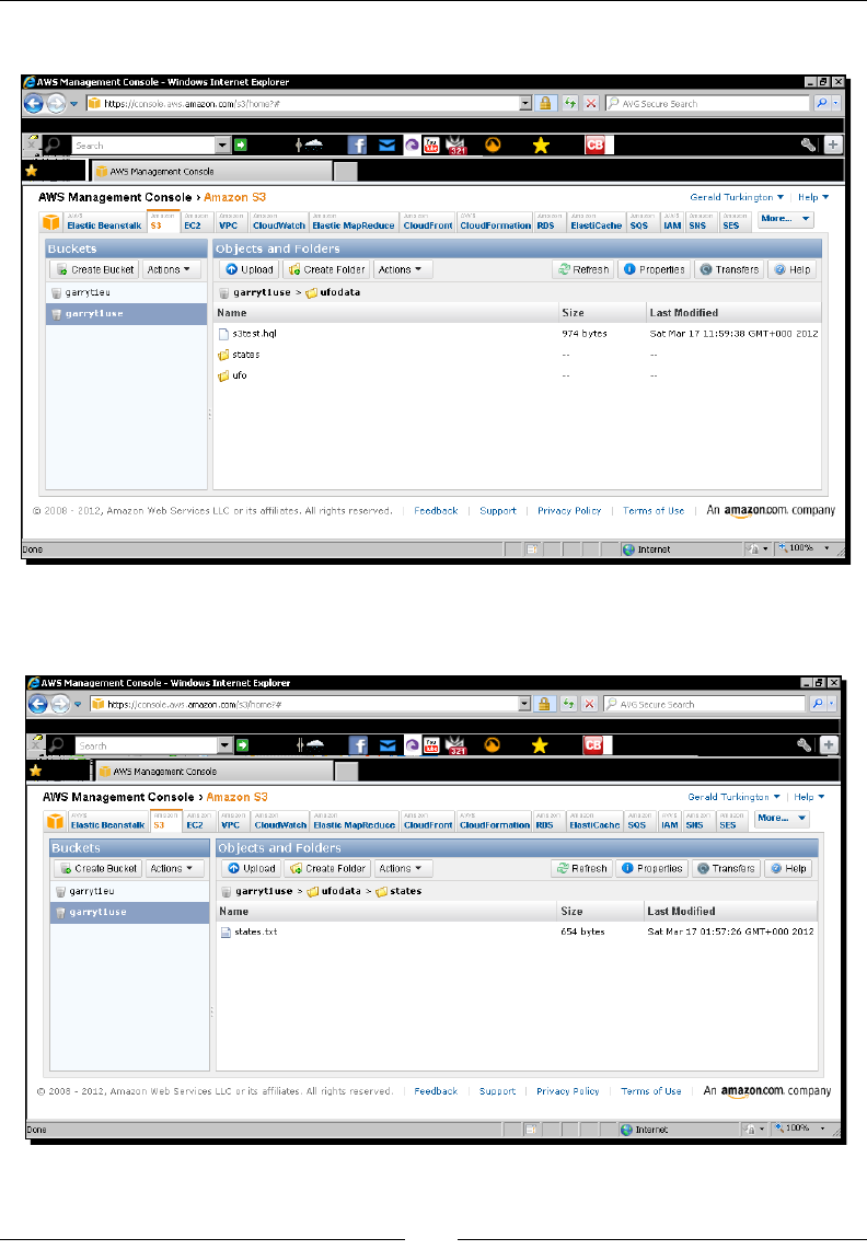
A Relaonal View on Data with Hive
[ 272 ]
The contents of ufodata should now look like the following screenshot:
6. Double-click the states directory to open it and into this, upload the states.txt
le used earlier. The directory should now look like the following screenshot:
7. Click on the ufodata component at the top of the le list to return to this directory.
www.it-ebooks.info
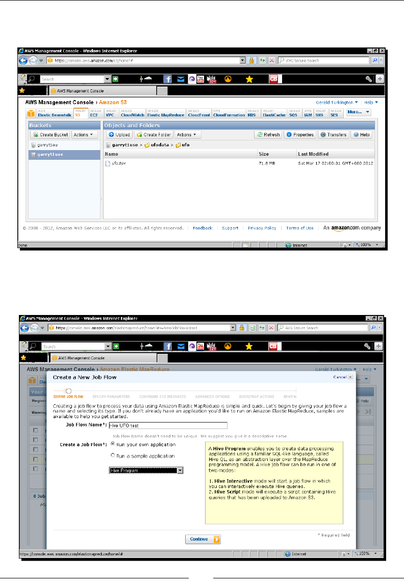
Chapter 8
[ 273 ]
8. Double-click on the ufo directory to open it and into this, upload the ufo.tsv le
used earlier. The directory should now look like the following screenshot:
9. Now select Elasc MapReduce and click on Create a New Job Flow. Then select
the opon Run your own applicaon and select a Hive applicaon, as shown in
the following screenshot:
www.it-ebooks.info
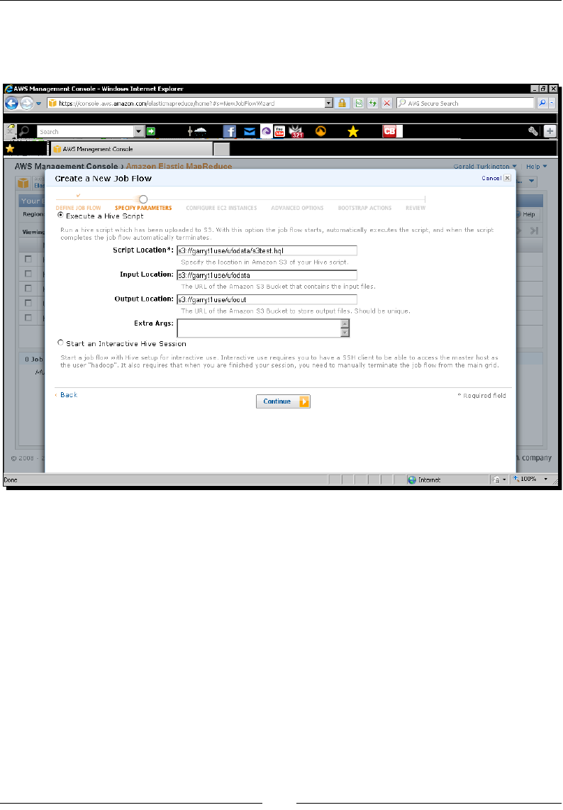
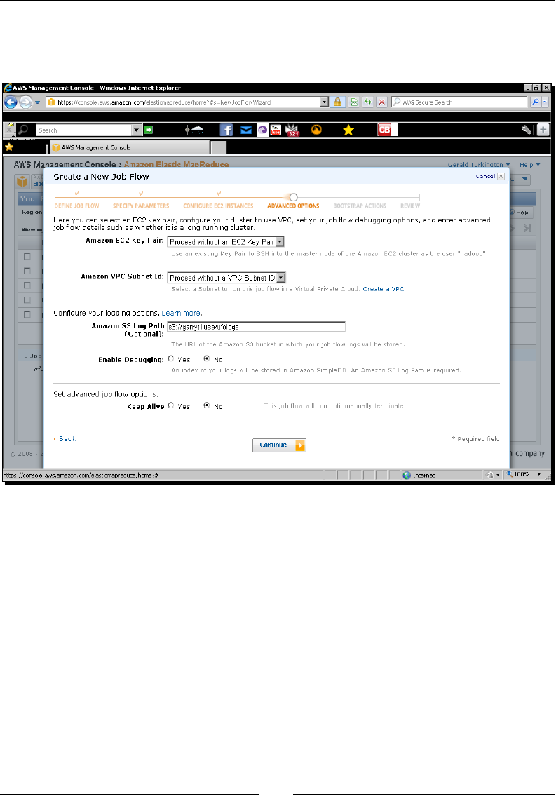

A Relaonal View on Data with Hive
[ 276 ]
12. Click on Connue. Then do the same through the rest of the job creaon process as
there are no other default opons that need to be changed for this example. Finally
start the job ow and monitor its progress from the management console.
13. Once the job has completed successfully, go back to S3 and double-click on the
ufoout directory. Within that should be a directory called states and within that,
a le named something like 0000000. Double-click to download the le and verify
that its contents look something like the following:
20021014 light California
20050224 other California
20021001 egg California
20030527 sphere California
What just happened?
Before we actually execute our EMR job ow, we needed to do a bit of setup in the
preceding example. Firstly, we used the S3 web interface to prepare the directory structure
for our job. We created three main directories to hold the input data, into which to write
results and one for EMR to place logs of the job ow execuon.
The HiveQL script is a modicaon of several of the Hive commands used earlier in this
chapter. It creates the tables for the UFO sighng data and state names as well as the
view joining them. Then it creates a new table with no source data and uses an INSERT
OVERWRITE TABLE to populate the table with the results of a query.
The unique feature in this script is the way we specify the LOCATION clauses for each
of the tables. For the input tables, we use a path relave to a variable called INPUT
and do likewise with the OUTPUT variable for the result table.
Note that Hive in EMR expects the locaon of table data to be a directory and not a le.
This is the reason for us previously creang subdirectories for each table into which we
uploaded the specic source le instead of specifying the table with the direct path to
the data les themselves.
Aer seng up the required le and directory structure within our S3 bucket, we went
to the EMR web console and started the job ow creaon process.
Aer specifying that we wish to use our own program and that it would be a Hive
applicaon, we lled in a screen with the key data required for our job ow:
The locaon of the HiveQL script itself
The directory containing input data
The directory to be used for output data
www.it-ebooks.info

Chapter 8
[ 277 ]
The path to the HiveQL script is an explicit path and does not require any explanaon.
However, it is important to realize how the other values are mapped into the variables
used within our Hive script.
The value for the input path is available to the Hive script as the INPUT variable and this
is how we then specify the directory containing the UFO sighng data as ${INPUT}/ufo.
Similarly, the output value specied in this form will be used as the OUTPUT variable within
our Hive script.
We did not make any changes to the default host setup, which will be one small master
and two small core nodes. On the next screen, we added the locaon into which we
wanted EMR to write the logs produced by the job ow execuon.
Though oponal, it is useful to capture these logs, parcularly in the early stages of running
a new script, though obviously S3 storage does have a cost. EMR can also write indexed log
data into SimpleDB (another AWS service), but we did not show that in acon here.
Aer compleng the job ow denion, we started it and on successful execuon, went
to the S3 interface to browse to the output locaon, which happily contained the data
we were expecng.
Using interactive job ows for development
When developing a new Hive script to be executed on EMR, the previous batch job execuon
is not a good t. There is usually a several minute latency between job ow creaon and
execuon and if the job fails, then the cost of several hours of EC2 instance me will have
been incurred (paral hours are rounded up).
Instead of selecng the opon to create an EMR job ow to run a Hive script, as in the
previous example, we can start a Hive job ow in interacve mode. This eecvely spins up a
Hadoop cluster without requiring a named script. You can then SSH into the master node as
the Hadoop user where you will nd Hive installed and congured. It is much more ecient
to do the script development in this environment and then, if required, set up the batch
script job ows to automacally execute the script in producon.
Have a go hero – using an interactive EMR cluster
Start up an interacve Hive job ow in EMR. You will need to have SSH credenals already
registered with EC2 so that you can connect to the master node. Run the previous script
directly from the master node, remembering to pass the appropriate variables to the script.
www.it-ebooks.info

A Relaonal View on Data with Hive
[ 278 ]
Integration with other AWS products
With a local Hadoop/Hive installaon, the queson of where data lives usually comes
down to HDFS or local lesystems. As we have seen previously, Hive within EMR gives
another opon with its support for external tables whose data resides in S3.
Another AWS service with similar support is DynamoDB (at http://aws.amazon.com/
dynamodb), a hosted NoSQL database soluon in the cloud. Hive job ows within EMR
can declare external tables that either read data from DynamoDB or use it as the
desnaon for query output.
This is a very powerful model as it allows Hive to be used to process and combine data
from mulple sources while the mechanics of mapping data from one system into Hive
tables happens transparently. It also allows Hive to be used as a mechanism for moving
data from one system to another. The act of geng data frequently into such hosted
services from exisng stores is a major adopon hurdle.
Summary
We have looked at Hive in this chapter and learned how it provides many tools and
features that will be familiar to anyone who uses relaonal databases. Instead of requiring
development of MapReduce applicaons, Hive makes the power of Hadoop available to a
much broader community.
In parcular, we downloaded and installed Hive, learning that it is a client applicaon that
translates its HiveQL language into MapReduce code, which it submits to a Hadoop cluster.
We explored Hive's mechanism for creang tables and running queries against these tables.
We saw how Hive can support various underlying data le formats and structures and how
to modify those opons.
We also appreciated that Hive tables are largely a logical construct and that behind the
scenes, all the SQL-like operaons on tables are in fact executed by MapReduce jobs on
HDFS les. We then saw how Hive supports powerful features such as joins and views
and how to paron our tables to aid in ecient query execuon.
We used Hive to output the results of a query to les on HDFS and saw how Hive is
supported by Elasc MapReduce, where interacve job ows can be used to develop
new Hive applicaons, and then ran automacally in batch mode.
As we have menoned several mes in this book, Hive looks like a relaonal database but is
not really one. However, in many cases you will nd exisng relaonal databases are part of
the broader infrastructure into which you need integrate. Performing that integraon and how
to move data across these dierent types of data sources will be the topic of the next chapter.
www.it-ebooks.info

9
Working with Relational Databases
As we saw in the previous chapter, Hive is a great tool that provides a relational
database-like view of the data stored in Hadoop. However, at the end of the
day, it is not truly a relational database. It does not fully implement the SQL
standard, and its performance and scale characteristics are vastly different
(not better or worse, just different) from a traditional relational database.
In many cases, you will find a Hadoop cluster sitting alongside and used with
(not instead of) relational databases. Often the business flows will require data
to be moved from one store to the other; we will now explore such integration.
In this chapter, we will:
Idenfy some common Hadoop/RDBMS use cases
Explore how we can move data from RDBMS into HDFS and Hive
Use Sqoop as a beer soluon for such problems
Move data with exports from Hadoop into an RDBMS
Wrap up with a discussion of how this can be applied to AWS
Common data paths
Back in Chapter 1, What It's All About, we touched on what we believe to be an arcial
choice that causes a lot of controversy; to use Hadoop or a tradional relaonal database.
As explained there, it is our contenon that the thing to focus on is idenfying the right
tool for the task at hand and that this is likely to lead to a situaon where more than one
technology is employed. It is worth looking at a few concrete examples to illustrate this idea.
www.it-ebooks.info

Working with Relaonal Databases
[ 280 ]
Hadoop as an archive store
When an RDBMS is used as the main data repository, there oen arises issues of scale
and data retenon. As volumes of new data increase, what is to be done with the older
and less valuable data?
Tradionally, there are two main approaches to this situaon:
Paron the RDBMS to allow higher performance of more recent data;
somemes the technology allows older data to be stored on slower and
less expensive storage systems
Archive the data onto tape or another oine store
Both approaches are valid, and the decision between the two oen rests on just whether or
not the older data is required for mely access. These are two extreme cases as the former
maximizes for access at the cost of complexity and infrastructure expense, while the laer
reduces costs but makes data less accessible.
The model being seen recently is for the most current data to be kept in the relaonal
database and the older data to be pushed into Hadoop. This can either be onto HDFS as
structured les or into Hive to retain the RDBMS interface. This gives the best of both worlds,
allowing the lower-volume, more recent data to be accessible by high-speed, low-latency
SQL queries, while the much larger volume of archived data will be accessed from Hadoop.
The data therefore remains available for use cases requiring either types of access; this
would be needed on a plaorm that does require addional integraon for any queries
that need to span both the recent and archive data.
Because of Hadoop's scalability, this model gives great future growth potenal; we know we
can connue to increase the amount of archive data being stored while retaining the ability
to run analycs against it.
Hadoop as a preprocessing step
Several mes in our Hive discussion, we highlighted opportunies where some preprocessing
jobs to massage or otherwise clean up the data would be hugely useful. The unfortunate
fact is that, in many (most?) big data situaons, the large volumes of data coming from
mulple sources mean that dirty data is simply a given. Although most MapReduce jobs
only require a subset of the overall data to be processed, we should sll expect to nd
incomplete or corrupt data across the data set. Just as Hive can benet from preprocessing
data, a tradional relaonal database can as well.
Hadoop can be a great tool here; it can pull data from mulple sources, combine them
for necessary transformaons, and clean up prior to the data being inserted into the
relaonal database.
www.it-ebooks.info

Chapter 9
[ 281 ]
Hadoop as a data input tool
Hadoop is not just valuable in that it makes data beer and is well suited to being ingested
into a relaonal database. In addion to such tasks, Hadoop can also be used to generate
addional data sets or data views that are then served from the relaonal database.
Common paerns here are situaons such as when we wish to display not only the primary
data for an account but to also display alongside it secondary data generated from account
history. Such views could be summaries of transacons against types of expenditure for the
previous months. This data is held within Hadoop, from which can be generated the actual
summaries that may be pushed back into the database for quicker display.
The serpent eats its own tail
Reality is oen more complex than these well-dened situaons, and it's not uncommon
for the data ow between Hadoop and the relaonal database to be described by circles
and arcs instead of a single straight line. The Hadoop cluster may, for example, do the
preprocessing step on data that is then ingested into the RDBMS and then receive frequent
transacon dumps that are used to build aggregates, which are sent back to the database.
Then, once the data gets older than a certain threshold, it is deleted from the database but
kept in Hadoop for archival purposes.
Regardless of the situaon, the ability to get data from Hadoop to a relaonal database and
back again is a crical aspect of integrang Hadoop into your IT infrastructure. So, let's see
how to do it.
Setting up MySQL
Before reading and wring data from a relaonal database, we need a running relaonal
database. We will use MySQL in this chapter because it is freely and widely available and
many developers have used it at some point in their career. You can of course use any
RDBMS for which a JDBC driver is available, but if you do so, you'll need to modify the
aspects of this chapter that require direct interacon with the database server.
Time for action – installing and setting up MySQL
Let's get MySQL installed and congured with the basic databases and access rights.
1. On an Ubuntu host, install MySQL using apt-get:
$ apt-get update
$ apt-get install mysql-server
2. Follow the prompts, and when asked, choose a suitable root password.
www.it-ebooks.info

Working with Relaonal Databases
[ 282 ]
3. Once installed, connect to the MySQL server:
$ mysql -h localhost -u root -p
4. Enter the root password when prompted:
Welcome to the MySQL monitor. Commands end with ; or \g.
Your MySQL connection id is 40
…
Mysql>
5. Create a new database to use for the examples in this chapter:
Mysql> create database hadooptest;
You will receive the following response:
Query OK, 1 row affected (0.00 sec)
6. Create a user account with full access to the database:
Mysql> grant all on hadooptest.* to 'hadoopuser'@'%' identified
by 'password';
You will receive the following response:
Query OK, 0 rows affected (0.01 sec)
7. Reload the user privileges to have the user changes take eect:
Mysql> flush privileges;
You will receive the following response:
Query OK, 0 rows affected (0.01 sec)
8. Log out as root:
mysql> quit;
You will receive the following response:
Bye
9. Log in as the newly created user, entering the password when prompted:
$ mysql -u hadoopuser -p
10. Change to the newly created database:
mysql> use hadooptest;
www.it-ebooks.info
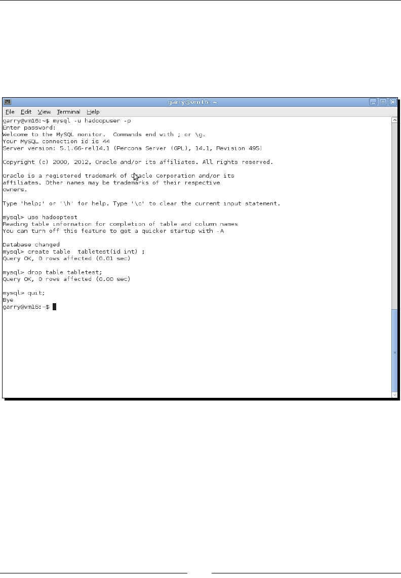
Chapter 9
[ 283 ]
11. Create a test table, drop it to conrm the user has the privileges in this database,
and then log out:
mysql> create table tabletest(id int);
mysql> drop table tabletest;
mysql> quit;
What just happened?
Due to the wonders of package managers such as apt, installing complex soware such
as MySQL is really very easy. We just use the standard process to install a package; under
Ubuntu (and most other distribuons in fact), requesng the main server package for MySQL
will bring along all needed dependencies as well as the client packages.
During the install, you will be prompted for the root password on the database. Even if this is
a test database instance that no one will use and that will have no valuable data, please give
the root user a strong password. Having weak root passwords is a bad habit, and we do not
want to encourage it.
www.it-ebooks.info

Working with Relaonal Databases
[ 284 ]
Aer MySQL is installed, we connect to the database using the mysql command-line ulity.
This takes a range of opons, but the ones we will use are as follows:
-h: This opon is used to specify the hostname of the database (the local machine is
assumed if none is given)
-u: This opon is used for the username with which to connect (the default is the
current Linux user)
-p: This opon is used to be prompted for the user password
MySQL has the concept of mulple databases, each of which is a collecve grouping
of tables. Every table needs be associated with a database. MySQL has several built-in
databases, but we use the CREATE DATABASE statement to create a new one called
hadooptest for our later work.
MySQL refuses connecons/requests to perform acons unless the requesng user has
explicitly been given the needed privileges to perform the acon. We do not want to do
everything as the root user (a bad pracce and quite dangerous since the root can modify/
delete everything), so we create a new user called hadoopuser by using the GRANT statement.
The GRANT statement we used actually does three disnct things:
Creates the hadoopuser account
Sets the hadoopuser password; we set it to password, which obviously you should
never do; pick something easy to memorize
Gives hadoopuser all privileges on the hadooptest database and all its tables
We issue the FLUSH PRIVILEGES command to have these changes take eect and then we
log out as root and connect as the new user to check whether all is working.
The USE statement here is a lile superuous. In future, we can instead add the database
name to the mysql command-line tool to automacally change to that database.
Connecng as the new user is a good sign, but to gain full condence, we create a new table
in the hadooptest database and then drop it. Success here shows that hadoopuser does
indeed have the requested privileges to modify the database.
Did it have to be so hard?
We are perhaps being a lile cauous here by checking every step of the process along
the way. However, I have found in the past that subtle typos, in the GRANT statement in
parcular, can result in really hard-to-diagnose problems later on. And to connue our
paranoia, let's make one change to the default MySQL conguraon that we won't need
quite yet, but which if we don't do, we'll be sorry later.
www.it-ebooks.info

Chapter 9
[ 285 ]
For any producon database, you would of course not have security-sensive statements,
such as GRANT, present that were typed in from a book. Refer to the documentaon of your
database to understand user accounts and privileges.
Time for action – conguring MySQL to allow remote
connections
We need to change the common default MySQL behavior, which will prevent us from
accessing the database from other hosts.
1. Edit /etc/mysql/my.cnf in your favorite text editor and look for this line:
bind-address = 127.0.0.1
2. Change it to this:
# bind-address = 127.0.0.1
3. Restart MySQL:
$ restart mysql
What just happened?
Most out-of-the-box MySQL conguraons allow access only from the same host on which
the server is running. This is absolutely the correct default from a security standpoint.
However, it can also cause real confusion if, for example, you launch MapReduce jobs that try
to access the database on that host. You may see the job fail with connecon errors. If that
happens, you re up the mysql command-line client on the host; this will succeed. Then,
perhaps, you will write a quick JDBC client to test connecvity. This will also work. Only when
you try these steps from one of the Hadoop worker nodes will the problem be apparent. Yes,
this has bit ten me several mes in the past!
The previous change tells MySQL to bind to all available interfaces and thus be accessible
from remote clients.
Aer making the change, we need to restart the server. In Ubuntu 11.10, many of the service
scripts have been ported to the Upstart framework, and we can use the handy restart
command directly.
If you are using a distribuon other than Ubuntu—or potenally even a dierent version of
Ubuntu—the global MySQL conguraon le may be in a dierent locaon; /etc/my.cnf,
for example, on CentOS and Red Hat Enterprise Linux.
www.it-ebooks.info

Working with Relaonal Databases
[ 286 ]
Don't do this in production!
Or at least not without thinking about the consequences. In the earlier example, we gave a
really bad password to the new user; do not do that. However, especially don't do something
like that if you then make the database available across the network. Yes, it is a test database
with no valuable data, but it is amazing how many test databases live for a very long me
and start geng more and more crical. And will you remember to remove that user with
the weak password aer you are done?
Enough lecturing. Databases need data. Let's add a table to the hadooptest database that
we'll use throughout this chapter.
Time for action – setting up the employee database
No discussion of databases is complete without the example of an employee table, so we will
follow tradion and start there.
1. Create a tab-separated le named employees.tsv with the following entries:
Alice Engineering 50000 2009-03-12
Bob Sales 35000 2011-10-01
Camille Marketing 40000 2003-04-20
David Executive 75000 2001-03-20
Erica Support 34000 2011-07-07
2. Connect to the MySQL server:
$ mysql -u hadoopuser -p hadooptest
3. Create the table:
Mysql> create table employees(
first_name varchar(10) primary key,
dept varchar(15),
salary int,
start_date date
) ;
4. Load the data from the le into the database:
mysql> load data local infile '/home/garry/employees.tsv'
-> into table employees
-> fields terminated by '\t' lines terminated by '\n' ;
www.it-ebooks.info
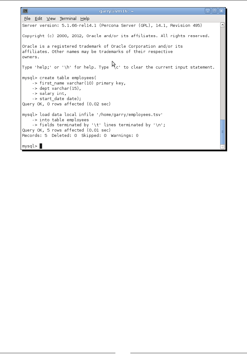
Chapter 9
[ 287 ]
What just happened?
This is prey standard database stu. We created a tab-separated data le, created the table
in the database, and then used the LOAD DATA LOCAL INFILE statement to import the
data into the table.
We are using a very small set of data here as it is really for illustraon purposes only.
Be careful with data le access rights
Don't omit the LOCAL part from the LOAD DATA statement; doing so sees MySQL try and
load the le as the MySQL user, and this usually results in access problems.
Getting data into Hadoop
Now that we have put in all that up-front eort, let us look at ways of bringing the data out
of MySQL and into Hadoop.
www.it-ebooks.info

Working with Relaonal Databases
[ 288 ]
Using MySQL tools and manual import
The simplest way to export data into Hadoop is to use exisng command-line tools and
statements. To export an enre table (or indeed an enre database), MySQL oers the
mysqldump ulity. To do a more precise export, we can use a SELECT statement of the
following form:
SELECT col1, col2 from table
INTO OUTFILE '/tmp/out.csv'
FIELDS TERMINATED by ',', LINES TERMINATED BY '\n';
Once we have an export le, we can move it into HDFS using hadoop fs -put or into
Hive through the methods discussed in the previous chapter.
Have a go hero – exporting the employee table into HDFS
We don't want this chapter to turn into a MySQL tutorial, so look up the syntax of the
mysqldump ulity, and use it or the SELECT … INTO OUTFILE statement to export
the employee table into a tab-separated le you then copy onto HDFS.
Accessing the database from the mapper
For our trivial example, the preceding approaches are ne, but what if you need to export
a much larger set of data, especially if it then is to be processed by a MapReduce job?
The obvious approach is that of direct JDBC access within a MapReduce input job that pulls
the data from the database and writes it onto HDFS, ready for addional processing.
This is a valid technique, but there are a few not-so-obvious gotchas.
You need to be careful how much load you place on the database. Throwing this sort of job
onto a very large cluster could very quickly melt the database as hundreds or thousands
of mappers try to simultaneously open connecons and read the same table. The simplest
access paern is also likely to see one query per row, which obviates the ability to use more
ecient bulk access statements. Even if the database can take the load, it is quite possible
for the database network connecon to quickly become the boleneck.
To eecvely parallelize the query across all the mappers, you need a strategy to paron
the table into segments each mapper will retrieve. You then need to determine how each
mapper is to have its segment parameters passed in.
If the retrieved segments are large, there is a chance that you will end up with long-running
tasks that get terminated by the Hadoop framework unless you explicitly report progress.
That is actually quite a lot of work for a conceptually simple task. Wouldn't it be much
beer to use an exisng tool for the purpose? There is indeed such a tool that we will
use throughout the rest of this chapter, Sqoop.
www.it-ebooks.info

Chapter 9
[ 289 ]
A better way – introducing Sqoop
Sqoop was created by Cloudera (http://www.cloudera.com), a company that provides
numerous services related to Hadoop in addion to producing its own packaging of the
Hadoop distribuon, something we will discuss in Chapter 11, Where to Go Next.
As well as providing this packaged Hadoop product, the company has also created a number
of tools that have been made available to the community, and one of these is Sqoop. Its
job is to do exactly what we need, to copy data between Hadoop and relaonal databases.
Though originally developed by Cloudera, it has been contributed to the Apache Soware
Foundaon, and its homepage is http://sqoop.apache.org.
Time for action – downloading and conguring Sqoop
Let's download and get Sqoop installed and congured.
1. Go to the Sqoop homepage, select the link for the most stable version that is
no earlier than 1.4.1, and match it with the version of Hadoop you are using.
Download the le.
2. Copy the retrieved le where you want it installed on your system; then uncompress
it:
$mv sqoop-1.4.1-incubating__hadoop-1.0.0.tar.gz_ /usr/local
$ cd /usr/local
$ tar –xzf sqoop-1.4.1-incubating__hadoop-1.0.0.tar.gz_
3. Make a symlink:
$ ln -s sqoop-1.4.1-incubating__hadoop-1.0.0 sqoop
4. Update your environment:
$ export SQOOP_HOME=/usr/local/sqoop
$ export PATH=${SQOOP_HOME}/bin:${PATH}
5. Download the JDBC driver for your database; for MySQL, we nd it at http://dev.
mysql.com/downloads/connector/j/5.0.html.
6. Copy the downloaded JAR le into the Sqoop lib directory:
$ cp mysql-connector-java-5.0.8-bin.jar /opt/sqoop/lib
7. Test Sqoop:
$ sqoop help
www.it-ebooks.info

Working with Relaonal Databases
[ 290 ]
You will see the following output:
usage: sqoop COMMAND [ARGS]
Available commands:
codegen Generate code to interact with database
records
…
version Display version information
See 'sqoop help COMMAND' for information on a specific command.
What just happened?
Sqoop is a prey straighorward tool to install. Aer downloading the required version from
the Sqoop homepage—being careful to pick the one that matches our Hadoop version—we
copied and unpacked the le.
Once again, we needed to set an environment variable and added the Sqoop bin directory
to our path so we can either set these directly in our shell, or as before, add these steps to a
conguraon le we can source prior to a development session.
Sqoop needs access to the JDBC driver for your database; for us, we downloaded the MySQL
Connector and copied it into the Sqoop lib directory. For the most popular databases, this
is as much conguraon as Sqoop requires; if you want to use something exoc, consult the
Sqoop documentaon.
Aer this minimal install, we executed the sqoop command-line ulity to validate that it is
working properly.
You may see warning messages from Sqoop telling you that addional
variables such as HBASE_HOME have not been dened. As we are not
talking about HBase in this book, we do not need this seng and will
be oming such warnings from our screenshots.
Sqoop and Hadoop versions
We were very specic in the version of Sqoop to be retrieved before; much more so than for
previous soware downloads. In Sqoop versions prior to 1.4.1, there is a dependency on an
addional method on one of the core Hadoop classes that was only available in the Cloudera
Hadoop distribuon or versions of Hadoop aer 0.21.
Unfortunately, the fact that Hadoop 1.0 is eecvely a connuaon of the 0.20 branch
meant that Sqoop 1.3, for example, would work with Hadoop 0.21 but not 0.20 or 1.0.
To avoid this version confusion, we recommend using version 1.4.1 or later, which removes
the dependency.
www.it-ebooks.info
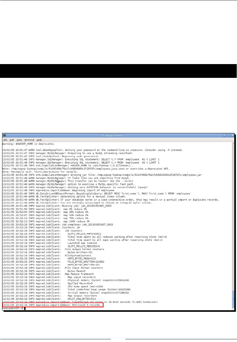
Chapter 9
[ 291 ]
There is no addional MySQL conguraon required; we would discover if the server had not
been congured to allow remote clients, as described earlier, through use of Sqoop.
Sqoop and HDFS
The simplest import we can perform is to dump data from a database table onto structured
les on HDFS. Let's do that.
Time for action – exporting data from MySQL to HDFS
We'll use a straighorward example here, where we just pull all the data from a single
MySQL table and write it to a single le on HDFS.
1. Run Sqoop to export data from MySQL onto HDFS:
$ sqoop import --connect jdbc:mysql://10.0.0.100/hadooptest
--username hadoopuser \ > --password password --table employees
www.it-ebooks.info

Working with Relaonal Databases
[ 292 ]
2. Examine the output directory:
$ hadoop fs -ls employees
You will receive the following response:
Found 6 items
-rw-r--r-- 3 hadoop supergroup 0 2012-05-21 04:10 /
user/hadoop/employees/_SUCCESS
drwxr-xr-x - hadoop supergroup 0 2012-05-21 04:10 /
user/hadoop/employees/_logs
-rw-r--r-- 3 … /user/hadoop/employees/part-m-00000
-rw-r--r-- 3 … /user/hadoop/employees/part-m-00001
-rw-r--r-- 3 … /user/hadoop/employees/part-m-00002
-rw-r--r-- 3 … /user/hadoop/employees/part-m-00003
3. Display one of the result les:
$ hadoop fs -cat /user/hadoop/employees/part-m-00001
You will see the following output:
Bob,Sales,35000,2011-10-01
Camille,Marketing,40000,2003-04-20
What just happened?
We did not need any preamble; a single Sqoop statement is all we require here. As can be
seen, the Sqoop command line takes many opons; let's unpack them one at a me.
The rst opon in Sqoop is the type of task to be performed; in this case, we wish to import
data from a relaonal source into Hadoop. The --connect opon species the JDBC URI for
the database, of the standard form jdbc:<driver>://<host>/<database>. Obviously,
you need to change the IP or hostname to the server where your database is running.
We use the --username and --password opons to specify those aributes and nally
use --table to indicate from which table we wish to retrieve the data. That is it! Sqoop
does the rest.
The Sqoop output is relavely verbose, but do read it as it gives a good idea of exactly what
is happening.
Repeated execuons of Sqoop may however include a nested error about
a generated le already exisng. Ignore that for now.
www.it-ebooks.info

Chapter 9
[ 293 ]
Firstly, in the preceding steps, we see Sqoop telling us not to use the --password opon
as it is inherently insecure. Sqoop has an alternave -P command, which prompts for the
password; we will use that in future examples.
We also get a warning about using a textual primary key column and that it's a very bad
idea; more on that in a lile while.
Aer all the setup and warnings, however, we see Sqoop execute a MapReduce job and
complete it successfully.
By default, Sqoop places the output les into a directory in the home directory of the
user who ran the job. The les will be in a directory of the same name as the source table.
To verify this, we used hadoop fs -ls to check this directory and conrmed that it
contained several les, likely more than we would have expected, given such a small
table. Note that we slightly abbreviated the output here to allow it to t on one line.
We then examined one of the output les and discovered the reason for the mulple
les; even though the table is ny, it was sll split across mulple mappers, and hence,
output les. Sqoop uses four map tasks by default. It may look a lile strange in this case,
but the usual situaon will be a much larger data import. Given the desire to copy data onto
HDFS, this data is likely to be the source of a future MapReduce job, so mulple les makes
perfect sense.
Mappers and primary key columns
We intenonally set up this situaon by somewhat arcially using a textual primary key
column in our employee data set. In reality, the primary key would much more likely be
an auto-incremenng, numeric employee ID. However, this choice highlighted the nature
of how Sqoop processes tables and its use of primary keys.
Sqoop uses the primary key column to determine how to divide the source data across
its mappers. But, as the warnings before state, this means we are reliant on string-based
comparisons, and in an environment with imperfect case signicance, the results may be
incorrect. The ideal situaon is to use a numeric column as suggested.
Alternavely, it is possible to control the number of mappers using the -m opon. If we use
-m 1, there will be a single mapper and no aempt will be made to paron the primary key
column. For small data sets such as ours, we can also do this to ensure a single output le.
This is not just an opon; if you try to import from a table with no primary key, Sqoop will
fail with an error stang that the only way to import from such a table is to explicitly set a
single mapper.
www.it-ebooks.info

Working with Relaonal Databases
[ 294 ]
Other options
Don't assume that Sqoop is all or nothing when it comes to imporng data. Sqoop has
several other opons to specify, restrict, and alter the data extracted from the database.
We will illustrate these in the following secons, where we discuss Hive, but bear in mind
that most can also be used when exporng into HDFS.
Sqoop's architecture
Now that we have seen Sqoop in acon, it is worthwhile taking a few moments to clarify its
architecture and see how it works. In several ways, Sqoop interacts with Hadoop in much
the same way that Hive does; both are single client programs that create one or more
MapReduce jobs to perform their tasks.
Sqoop does not have any server processes; the command-line client we run is all there is
to it. However, because it can tailor its generated MapReduce code to the specic tasks
at hand, it tends to ulize Hadoop quite eciently.
The preceding example of spling a source RDBMS table on a primary key is a good
example of this. Sqoop knows the number of mappers that will be congured in the
MapReduce job—the default is four, as previously menoned—and from this, it can
do smart paroning of the source table.
If we assume a table with 1 million records and four mappers, then each will process
2,50,000 records. With its knowledge of the primary key column, Sqoop can create four
SQL statements to retrieve the data that each use the desired primary key column range
as caveats. In the simplest case, this could be as straighorward as adding something like
WHERE id BETWEEN 1 and 250000 to the rst statement and using dierent id
ranges for the others.
We will see the reverse behavior when exporng data from Hadoop as Sqoop again
parallelizes data retrieval across mulple mappers and works to opmize the inseron of this
data into the relaonal database. However, all these smarts are pushed into the MapReduce
jobs executed on Hadoop; the Sqoop command-line client's job is to generate this code as
eciently as possible and then get out of the way as the processing occurs.
Importing data into Hive using Sqoop
Sqoop has signicant integraon with Hive, allowing it to import data from a relaonal
source into either new or exisng Hive tables. There are mulple ways in which this
process can be tailored, but again, let's start with the simple case.
www.it-ebooks.info
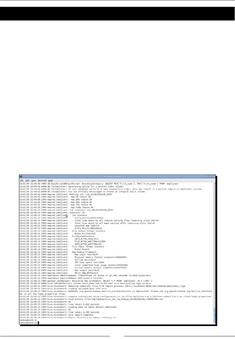
Chapter 9
[ 295 ]
Time for action – exporting data from MySQL into Hive
For this example, we'll export all the data from a single MySQL table into a correspondingly
named table in Hive. You will need Hive installed and congured as detailed in the
previous chapter.
1. Delete the output directory created in the previous secon:
$ hadoop fs -rmr employees
You will receive the following response:
Deleted hdfs://head:9000/user/hadoop/employees
2. Conrm Hive doesn't already contain an employees table:
$ hive -e "show tables like 'employees'"
You will receive the following response:
OK
Time taken: 2.318 seconds
3. Perform the Sqoop import:
$ sqoop import --connect jdbc:mysql://10.0.0.100/hadooptest
--username hadoopuser -P
--table employees --hive-import --hive-table employees
www.it-ebooks.info

Working with Relaonal Databases
[ 296 ]
4. Check the contents in Hive:
$ hive -e "select * from employees"
You will receive the following response:
OK
Alice Engineering 50000 2009-03-12
Camille Marketing 40000 2003-04-20
David Executive 75000 2001-03-20
Erica Support 34000 2011-07-07
Time taken: 2.739 seconds
5. Examine the created table in Hive:
$ hive -e "describe employees"
You will receive the following response:
OK
first_name string
dept string
salary int
start_date string
Time taken: 2.553 seconds
What just happened?
Again, we use the Sqoop command with two new opons, --hive-import to tell Sqoop
the nal desnaon is Hive and not HDFS, and --hive-table to specify the name of the
table in Hive where we want the data imported.
In actuality, we don't need to specify the name of the Hive table if it is the same as the
source table specied by the --table opon. However, it does make things more explicit,
so we will typically include it.
As before, do read the full Sqoop output as it provides great insight into what's going on,
but the last few lines highlight the successful import into the new Hive table.
We see Sqoop retrieving ve rows from MySQL and then going through the stages of
copying them to HDFS and imporng into Hive. We will talk about the warning re type
conversions next.
Aer Sqoop completes the process, we use Hive to retrieve the data from the new Hive table
and conrm that it is what we expected. Then, we examine the denion of the created table.
www.it-ebooks.info

Chapter 9
[ 297 ]
At this point, we do see one strange thing; the start_date column has been given a type
string even though it was originally a SQL DATE type in MySQL.
The warning we saw during the Sqoop execuon explains this situaon:
12/05/23 13:06:33 WARN hive.TableDefWriter: Column start_date had to be
cast to a less precise type in Hive
The cause of this is that Hive does not support any temporal datatype other than TIMESTAMP.
In those cases where imported data is of another type, relang to dates or mes, Sqoop
converts it to a string. We will look at a way of dealing with this situaon a lile later.
This example is a prey common situaon, but we do not always want to import an enre
table into Hive. Somemes, we want to only include parcular columns or to apply a
predicate to reduce the number of selected items. Sqoop allows us to do both.
Time for action – a more selective import
Let's see how this works by performing an import that is limited by a condional expression.
1. Delete any exisng employee import directory:
$ hadoop fs -rmr employees
You will receive the following response:
Deleted hdfs://head:9000/user/hadoop/employees
2. Import selected columns with a predicate:
sqoop import --connect jdbc:mysql://10.0.0.100/hadooptest
--username hadoopuser -P
--table employees --columns first_name,salary
--where "salary > 45000"
--hive-import --hive-table salary
You will receive the following response:
12/05/23 15:02:03 INFO hive.HiveImport: Hive import complete.
3. Examine the created table:
$ hive -e "describe salary"
You will receive the following response:
OK
first_name string
www.it-ebooks.info

Working with Relaonal Databases
[ 298 ]
salary int
Time taken: 2.57 seconds
4. Examine the imported data:
$ hive -e "select * from salary"
You will see the following output:
OK
Alice 50000
David 75000
Time taken: 2.754 seconds
What just happened?
This me, our Sqoop command rst added the --columns opon that species which
columns to include in the import. This is a comma-separated list.
We also used the --where opon that allows the free text specicaon of a WHERE clause
that is applied to the SQL used to extract data from the database.
The combinaon of these opons is that our Sqoop command should import only the names
and salaries of those with a salary greater than the threshold specied in the WHERE clause.
We execute the command, see it complete successfully, and then examine the table created
in Hive. We see that it indeed only contains the specied columns, and we then display the
table contents to verify that the where predicate was also applied correctly.
Datatype issues
In Chapter 8, A Relaonal View on Data with Hive, we menoned that Hive does not support
all the common SQL datatypes. The DATE and DATETIME types in parcular are not currently
implemented though they do exist as idened Hive issues; so hopefully, they will be added
in the future. We saw this impact our rst Hive import earlier in this chapter. Though the
start_date column was of type DATE in MySQL, the Sqoop import agged a conversion
warning, and the resultant column in Hive was of type STRING.
Sqoop has an opon that is of use here, that is, we can use --map-column-hive to
explicitly tell Sqoop how to create the column in the generated Hive table.
www.it-ebooks.info

Chapter 9
[ 299 ]
Time for action – using a type mapping
Let's use a type mapping to improve our data import.
1. Delete any exisng output directory:
$ hadoop fs -rmr employees
2. Execute Sqoop with an explicit type mapping:
sqoop import --connect jdbc:mysql://10.0.0.100/hadooptest
--username hadoopuser
-P --table employees
--hive-import --hive-table employees
--map-column-hive start_date=timestamp
You will receive the following response:
12/05/23 14:53:38 INFO hive.HiveImport: Hive import complete.
3. Examine the created table denion:
$ hive -e "describe employees"
You will receive the following response:
OK
first_name string
dept string
salary int
start_date timestamp
Time taken: 2.547 seconds
4. Examine the imported data:
$ hive -e "select * from employees";
You will receive the following response:
OK
Failed with exception java.io.IOException:java.lang.
IllegalArgumentException: Timestamp format must be yyyy-mm-dd
hh:mm:ss[.fffffffff]
Time taken: 2.73 seconds
www.it-ebooks.info

Working with Relaonal Databases
[ 300 ]
What just happened?
Our Sqoop command line here is similar to our original Hive import, except for the addion
of the column mapping specicaon. We specied that the start_date column should be
of type TIMESTAMP, and we could have added other specicaons. The opon takes a
comma-separated list of such mappings.
Aer conrming Sqoop executed successfully, we examined the created Hive table
and veried that the mapping was indeed applied and that the start_date column
has type TIMESTAMP.
We then tried to retrieve the data from the table and could not do so, receiving an error
about type format mismatch.
On reecon, this should not be a surprise. Though we specied the desired column type
was to be TIMESTAMP, the actual data being imported from MySQL was of type DATE, which
does not contain the me component required in a mestamp. This is an important lesson.
Ensuring that the type mappings are correct is only one part of the puzzle; we must also
ensure the data is valid for the specied column type.
Time for action – importing data from a raw query
Let's see an example of an import where a raw SQL statement is used to select the data
to be imported.
1. Delete any exisng output directory:
$ hadoop fs –rmr employees
2. Drop any exisng Hive employee table:
$ hive -e 'drop table employees'
3. Import data using an explicit query:
sqoop import --connect jdbc:mysql://10.0.0.100/hadooptest
--username hadoopuser -P
--target-dir employees
--query 'select first_name, dept, salary,
timestamp(start_date) as start_date from employees where
$CONDITIONS'
--hive-import --hive-table employees
--map-column-hive start_date=timestamp -m 1
4. Examine the created table:
$ hive -e "describe employees"
www.it-ebooks.info

Chapter 9
[ 301 ]
You will receive the following response:
OK
first_name string
dept string
salary int
start_date timestamp
Time taken: 2.591 seconds
5. Examine the data:
$ hive -e "select * from employees"
You will receive the following response:
OK
Alice Engineering 50000 2009-03-12 00:00:00
Bob Sales 35000 2011-10-01 00:00:00
Camille Marketing 40000 2003-04-20 00:00:00
David Executive 75000 2001-03-20 00:00:00
Erica Support 34000 2011-07-07 00:00:00
Time taken: 2.709 seconds
What just happened?
To achieve our goal, we used a very dierent form of the Sqoop import. Instead of specifying
the desired table and then either leng Sqoop import all columns or a specied subset, here
we use the --query opon to dene an explicit SQL statement.
In the statement, we select all the columns from the source table but apply the
timestamp() funcon to convert the start_date column to the correct type.
(Note that this funcon simply adds a 00:00 me element to the date). We alias
the result of this funcon, which allows us to name it in the type mapping opon.
Because we have no --table opon, we have to add --target-dir to tell Sqoop the
name of the directory it should create on HDFS.
The WHERE clause in the SQL is required by Sqoop even though we are not actually using it.
Having no --table opon does not just remove Sqoop's ability to auto-generate the name
of the export directory, it also means that Sqoop does not know from where data is being
retrieved, and hence, how to paron the data across mulple mappers. The $CONDITIONS
variable is used in conjuncon with a --where opon; specifying the laer provides Sqoop
with the informaon it needs to paron the table appropriately.
www.it-ebooks.info

Working with Relaonal Databases
[ 302 ]
We take a dierent route here and instead explicitly set the number of mappers to 1, which
obviates the need for an explicit paroning clause.
Aer execung Sqoop, we examine the table denion in Hive, which as before, has the
correct datatypes for all columns. We then look at the data, and this is now successful, with
the start_date column data being appropriately converted into the TIMESTAMP values.
When we menoned in the Sqoop and HDFS secon that Sqoop provided
mechanisms to restrict the data extracted from the database, we were
referring to the query, where, and columns opons. Note that these
can be used by any Sqoop import regardless of the desnaon.
Have a go hero
Though it truly is not needed for such a small data set, the $CONDITIONS variable is an
important tool. Modify the preceding Sqoop statement to use mulple mappers with an
explicit paroning statement.
Sqoop and Hive partitions
In Chapter 8, A Relaonal View on Data with Hive, we talked a lot about Hive parons
and highlighted how important they are in allowing query opmizaon for very large tables.
The good news is that Sqoop can support Hive parons; the bad news is that the support
is not complete.
To import data from a relaonal database into a paroned Hive table, we use the --hive-
partition-key opon to specify the paron column and the --hive-partition-
value opon to specify the value for the paron into which this Sqoop command will
import data.
This is excellent but does require each Sqoop statement to be imported into a single Hive
paron; there is currently no support for Hive auto-paroning. Instead, if a data set is
to be imported into mulple parons in a table, we need use a separate Sqoop statement
for inseron into each paron.
Field and line terminators
Unl now, we have been implicitly relying on some defaults but should discuss them at this
point. Our original text le was tab separated, but you may have noced that the data we
exported onto HDFS was comma-separated. If you go look in the les under /user/hive/
warehouse/employees (remember this is the default locaon on HDFS where Hive keeps
its source les), the records use ASCII code 001 as the separator. What is going on?
www.it-ebooks.info

Chapter 9
[ 303 ]
In the rst instance, we let Sqoop use its defaults, which in this case, means using a comma
to separate elds and using \n for records. However, when Sqoop is imporng into Hive, it
instead employs the Hive defaults, which include using the 001 code (^A) to separate elds.
We can explicitly set separators using the following Sqoop opons:
fields-terminated-by: This is the separator between elds
lines-terminated-by: The line terminator
escaped-by: Used to escape characters (for example, \)
enclosed-by: The character enclosing elds (for example, ")
optionally-enclosed-by: Similar to the preceding opon but not mandatory
mysql-delimiters: A shortcut to use the MySQL defaults
This may look a lile inmidang, but it's not as obscure as the terminology may suggest,
and the concepts and syntax should be familiar to those with SQL experience. The rst few
opons are prey self-explanatory; where it gets less clear is when talking of enclosing and
oponally enclosing characters.
This is really about (usually free-form) data where a given eld may include characters that
have special meanings. For example, a string column in a comma-separated le that includes
commas. In such a case, we could enclose the string columns within quotes to allow the
commas within the eld. If all elds need such enclosing characters, we would use the rst
form; if it was only required for a subset of the elds, it could be specied as oponal.
Getting data out of Hadoop
We said that the data ow between Hadoop and a relaonal database is rarely a linear
single direcon process. Indeed the situaon where data is processed within Hadoop
and then inserted into a relaonal database is arguably the more common case. We will
explore this now.
Writing data from within the reducer
Thinking about how to copy the output of a MapReduce job into a relaonal database,
we nd similar consideraons as when looking at the queson of data import into Hadoop.
www.it-ebooks.info

Working with Relaonal Databases
[ 304 ]
The obvious approach is to modify a reducer to generate the output for each key and its
associated values and then to directly insert them into a database via JDBC. We do not have
to worry about source column paroning, as with the import case, but do sll need to think
about how much load we are placing on the database and whether we need to consider
meouts for long-running tasks. In addion, just as with the mapper situaon, this approach
tends to perform many single queries against the database, which is typically much less
ecient than bulk operaons.
Writing SQL import les from the reducer
Oen, a superior approach is not to work around the usual MapReduce case of generang
output les, as with the preceding example, but instead to exploit it.
All relaonal databases have the ability to ingest data from source les, either through
custom tools or through the use of the LOAD DATA statement. Within the reducer,
therefore, we can modify the data output to make it more easily ingested into our relaonal
desnaon. This obviates the need to consider issues such as reducers placing load on the
database or how to handle long-running tasks, but it does require a second step external to
our MapReduce job.
A better way – Sqoop again
It probably won't come as a surprise—certainly not if you've looked at the output of Sqoop's
inbuilt help or its online documentaon—to learn that Sqoop can also be our tool of choice
for data export from Hadoop.
Time for action – importing data from Hadoop into MySQL
Let's demonstrate this by imporng data into a MySQL table from an HDFS le.
1. Create a tab-separated le named newemployees.tsv with the following entries:
Frances Operations 34000 2012-03-01
Greg Engineering 60000 2003-11-18
Harry Intern 22000 2012-05-15
Iris Executive 80000 2001-04-08
Jan Support 28500 2009-03-30
2. Create a new directory on HDFS and copy the le into it:
$hadoop fs -mkdir edata
$ hadoop fs -put newemployees.tsv edata/newemployees.tsv
3. Conrm the current number of records in the employee table:
$ echo "select count(*) from employees" |
www.it-ebooks.info

Chapter 9
[ 305 ]
mysql –u hadoopuser –p hadooptest
You will receive the following response:
Enter password:
count(*)
5
4. Run a Sqoop export:
$ sqoop export --connect jdbc:mysql://10.0.0.100/hadooptest
--username hadoopuser -P --table employees
--export-dir edata --input-fields-terminated-by '\t'
You will receive the following response:
12/05/27 07:52:22 INFO mapreduce.ExportJobBase: Exported 5
records.
5. Check the number of records in the table aer the export:
Echo "select count(*) from employees"
| mysql -u hadoopuser -p hadooptest
You will receive the following response:
Enter password:
count(*)
10
6. Check the data:
$ echo "select * from employees"
| mysql -u hadoopuser -p hadooptest
You will receive the following response:
Enter password:
first_name dept salary start_date
Alice Engineering 50000 2009-03-12
…
Frances Operations 34000 2012-03-01
Greg Engineering 60000 2003-11-18
Harry Intern 22000 2012-05-15
Iris Executive 80000 2001-04-08
Jan Support 28500 2009-03-30
www.it-ebooks.info

Working with Relaonal Databases
[ 306 ]
What just happened?
We rst created a data le containing informaon on ve more employees. We created a
directory for our data on HDFS into which we copied the new le.
Before running the export, we conrmed that the table in MySQL contained the original ve
employees only.
The Sqoop command has a similar structure as before with the biggest change being the use
of the export command. As the name suggests, Sqoop exported export data from Hadoop
into a relaonal database.
We used several similar opons as before, mainly to specify the database connecon, the
username and password needed to connect, and the table into which to insert the data.
Because we are exporng data from HDFS, we needed to specify the locaon containing any
les to be exported which we do via the --export-dir opon. All les contained within
the directory will be exported; they do not need be in a single le; Sqoop will include all les
within its MapReduce job. By default, Sqoop uses four mappers; if you have a large number
of les it may be more eecve to increase this number; do test, though, to ensure that load
on the database remains under control.
The nal opon passed to Sqoop specied the eld terminator used in the source les, in this
case, the tab character. It is your responsibility to ensure the data les are properly formaed;
Sqoop will assume there is the same number of elements in each record as columns in the
table (though null is acceptable), separated by the specied eld separator character.
Aer watching the Sqoop command complete successfully, we saw it reports that it exported
ve records. We check, using the mysql tool, the number of rows now in the database and
then view the data to conrm that our old friends are now joined by the new employees.
Differences between Sqoop imports and exports
Though similar conceptually and in the command-line invocaons, there are a number of
important dierences between Sqoop imports and exports that are worth exploring.
Firstly, Sqoop imports can assume much more about the data being processed; through
either explicitly named tables or added predicates, there is much informaon about both
the structure and type of the data. Sqoop exports, however, are given only a locaon of
source les and the characters used to separate and enclose elds and records. While Sqoop
imports into Hive can automacally create a new table based on the provided table name
and structure, a Sqoop export must be into an exisng table in the relaonal database.
www.it-ebooks.info

Chapter 9
[ 307 ]
Even though our earlier demonstraon with dates and mestamps showed there are some
sharp edges, Sqoop imports are also able to determine whether the source data complies
with the dened column types; the data would not have been possible to insert into the
database otherwise. Sqoop exports again only have access eecvely to elds of characters
with no understanding of the real datatype. If you have the luxury of very clean and
well-formaed data, this may never maer, but for the rest of us, there will be a need to
consider data exports and type conversions, parcularly in terms of null and default values.
The Sqoop documentaon goes into these opons in some detail and is worth a read.
Inserts versus updates
Our preceding example was very straighorward; we added an enre new set of data that
can happily coexist with the exisng contents of the table. Sqoop exports by default do a
series of appends, adding each record as a new row in the table.
However, what if we later want to update data when, for example, our employees get
increased salaries at the end of the year? With the database table dening first_name
as a primary key, any aempt to insert a new row with the same name as an exisng
employee will fail with a failed primary key constraint.
In such cases, we can set the Sqoop --update-key opon to specify the primary key, and
Sqoop will generate UPDATE statements based on this key (it can be a comma-separated list
of keys), as opposed to INSERT statements adding new rows.
In this mode, any record that does not match an exisng key value will
silently be ignored, and Sqoop will not ag errors if a statement updates
more than one row.
If we also want the opon of an update that adds new rows for non-exisng data, we can set
the --update-mode opon to allowinsert.
Have a go hero
Create another data le that contains three new employees as well as updated salaries for
two of the exisng employees. Use Sqoop in import mode to both add the new employees
as well as apply the needed updates.
Sqoop and Hive exports
Given the preceding example, it may not be surprising to learn that Sqoop does not currently
have any direct support to export a Hive table into a relaonal database. More precisely,
there are no explicit equivalents to the --hive-import opon we used earlier.
www.it-ebooks.info

Working with Relaonal Databases
[ 308 ]
However, in some cases, we can work around this. If a Hive table is storing its data in text
format, we could point Sqoop at the locaon of the table data les on HDFS. In case of tables
referring to external data, this may be straighorward, but once we start seeing Hive tables
with complex paroning, the directory structure becomes more involved.
Hive can also store tables as binary SequenceFiles, and a current limitaon is that Sqoop
cannot transparently export from tables stored in this format.
Time for action – importing Hive data into MySQL
Regardless of these limitaons, let's demonstrate that, in the right situaons, we can use
Sqoop to directly export data stored in Hive.
1. Remove any exisng data in the employee table:
$ echo "truncate employees" | mysql –u hadoopuser –p hadooptest
You will receive the following response:
Query OK, 0 rows affected (0.01 sec)
2. Check the contents of the Hive warehouse for the employee table:
$ hadoop fs –ls /user/hive/warehouse/employees
You will receive the following response:
Found 1 items
… /user/hive/warehouse/employees/part-m-00000
3. Perform the Sqoop export:
sqoop export --connect jdbc:mysql://10.0.0.100/hadooptest
--username hadoopuser –P --table employees \
--export-dir /user/hive/warehouse/employees
--input-fields-terminated-by '\001'
--input-lines-terminated-by '\n'
www.it-ebooks.info
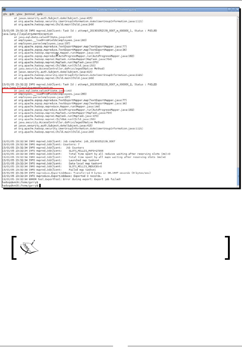
Chapter 9
[ 309 ]
What just happened?
Firstly, we truncated the employees table in MySQL to remove any exisng data and then
conrmed the employee table data was where we expected it to be.
Note that Sqoop may also create an empty le in this directory with the
sux _SUCCESS; if this is present it should be deleted before running
the Sqoop export.
www.it-ebooks.info

Working with Relaonal Databases
[ 310 ]
The Sqoop export command is like before; the only changes are the dierent source
locaon for the data and the addion of explicit eld and line terminators. Recall that
Hive, by default, uses ASCII code 001 and \n for its eld and line terminators, respecvely
(also recall, though, that we have previously imported les into Hive with other separators,
so this is something that always needs to be checked).
We execute the Sqoop command and watch it fail due to Java
IllegalArgumentExceptions when trying to create instances of java.sql.Date.
We are now hing the reverse of the problem we encountered earlier; the original type
in the source MySQL table had a datatype not supported by Hive, and we converted the
data to match the available type of TIMESTAMP. When exporng data back again, however,
we are now trying to create a DATE using a TIMESTAMP value, which is not possible without
some conversion.
The lesson here is that our earlier approach of doing a one-way conversion only worked
for as long as we only had data owing in one direcon. As soon as we need bi-direconal
data transfer, mismatched types between Hive and the relaonal store add complexity and
require the inseron of conversion rounes.
Time for action – xing the mapping and re-running the export
In this case, however, let us do what probably makes more sense—modifying the denion
of the employee table to make it consistent in both data sources.
1. Start the mysql ulity:
$ mysql -u hadoopuser -p hadooptest
Enter password:
2. Change the type of the start_date column:
mysql> alter table employees modify column start_date timestamp;
You will receive the following response:
Query OK, 0 rows affected (0.02 sec)
Records: 0 Duplicates: 0 Warnings: 0
www.it-ebooks.info

Chapter 9
[ 311 ]
3. Display the table denion:
mysql> describe employees;
4. Quit the mysql tool:
mysql> quit;
5. Perform the Sqoop export:
sqoop export --connect jdbc:mysql://10.0.0.100/hadooptest
--username hadoopuser –P –table employees
--export-dir /user/hive/warehouse/employees
--input-fields-terminated-by '\001'
--input-lines-terminated-by '\n'
You will receive the following response:
12/05/27 09:17:39 INFO mapreduce.ExportJobBase: Exported 10
records.
www.it-ebooks.info

Working with Relaonal Databases
[ 312 ]
6. Check the number of records in the MySQL database:
$ echo "select count(*) from employees"
| mysql -u hadoopuser -p hadooptest
You will receive the following output:
Enter password:
count(*)
10
What just happened?
Before trying the same Sqoop export as last me, we used the mysql tool to connect to
the database and modify the type of the start_date column. Note, of course, that such
changes should never be made casually on a producon system, but given that we have a
currently empty test table, there are no issues here.
Aer making the change, we re-ran the Sqoop export and this me it succeeded.
Other Sqoop features
Sqoop has a number of other features that we won't discuss in detail, but we'll highlight
them so the interested reader can look them up in the Sqoop documentaon.
Incremental merge
The examples we've used have been all-or-nothing processing that, in most cases, make the
most sense when imporng data into empty tables. There are mechanisms to handle addions,
but if we foresee Sqoop performing ongoing imports, some addional support is available.
Sqoop supports the concept of incremental imports where an import task is addionally
qualied by a date and only records more recent than that date are processed by the task.
This allows the construcon of long-running workows that include Sqoop.
Avoiding partial exports
We've already seen how errors can occur when exporng data from Hadoop into a relaonal
database. For us, it wasn't a signicant problem as the issue caused all exported records to
fail. But it isn't uncommon for only part of an export to fail and result in parally commied
data in the database.
www.it-ebooks.info

Chapter 9
[ 313 ]
To migate this risk, Sqoop allows the use of a staging table; it loads all the data into this
secondary table, and only aer all data is successfully inserted, performs the move into the
main table in a single transacon. This can be very useful for failure-prone workloads but
does come with some important restricons, such as the inability to support update mode.
For very large imports, there are also performance and load impacts on the RDBMS of a
single very long-running transacon.
Sqoop as a code generator
We've been ignoring an error during Sqoop processing that we casually brushed o a while
ago—the excepon thrown because the generated code required by Sqoop already exists.
When performing an import, Sqoop generates Java class les that provide a programmac
means of accessing the elds and records in the created les. Sqoop uses these classes
internally, but they can also be used outside of a Sqoop invocaon, and indeed, the
Sqoop codegen command can regenerate the classes outside of an export task.
AWS considerations
We've not menoned AWS so far in this chapter as there's been nothing in Sqoop that either
supports or prevents its use on AWS. We can run Sqoop on an EC2 host as easily as on a
local one, and it can access either a manually or EMR-created Hadoop cluster oponally
running Hive. The only possible quirk when considering use in AWS is security group access
as many default EC2 conguraons will not allow trac on the ports used by most relaonal
databases (3306 by default for MySQL). But, that's no more of an issue than if our Hadoop
cluster and MySQL database were to be located on dierent sides of a rewall or any other
network security boundary.
Considering RDS
There is another AWS service that we've not menoned before that does deserve an
introducon now. Amazon Relaonal Database Service (RDS) oers hosted relaonal
databases in the cloud and provides MySQL, Oracle, and Microso SQL Server opons.
Instead of having to worry about the installaon, conguraon, and management of a
database engine, RDS allows an instance to be started from either the console or command-
line tools. You then just point your database client tool at the database and start creang
tables and manipulang data.
RDS and EMR are a powerful combinaon, providing hosted services that take much of the
pain out of manually managing such services. If you need a relaonal database but don't
want to worry about its management, RDS may be for you.
www.it-ebooks.info

Working with Relaonal Databases
[ 314 ]
The RDS and EMR combinaon can be parcularly powerful if you use EC2 hosts to generate
data or store data in S3. Amazon has a general policy that there is no cost for data transfer
from one service to another within a single region. Consequently, it's possible to have a eet
of EC2 hosts generang large data volumes that get pushed into a relaonal database in RDS
for query access and are stored in EMR for archival and long-term analycs. Geng data into
the storage and processing systems is oen a technically challenging acvity that can easily
consume signicant expense if the data needs be moved across commercial network links.
Architectures built atop collaborang AWS services such as EC2, RDS, and EMR can minimize
both these concerns.
Summary
In this chapter, we have looked at the integraon of Hadoop and relaonal databases. In
parcular, we explored the most common use cases and saw that Hadoop and relaonal
databases can be highly complimentary technologies. We considered ways of exporng
data from a relaonal database onto HDFS les and realized that issues such as primary
key column paroning and long-running tasks make it harder than it rst seems.
We then introduced Sqoop, a Cloudera tool now donated to the Apache Soware Foundaon
and that provides a framework for such data migraon. We used Sqoop to import data from
MySQL into HDFS and then Hive, highlighng how we must consider aspects of datatype
compability in such tasks. We also used Sqoop to do the reverse—copying data from HDFS
into a MySQL database—and found out that this path has more subtle consideraons than
the other direcon, briey discussed issues of le formats and update versus insert tasks, and
introduced addional Sqoop capabilies, such as code generaon and incremental merging.
Relaonal databases are an important—oen crical—part of most IT infrastructures.
But, they aren't the only such component. One that has been growing in importance—oen
with lile fanfare—is the vast quanes of log les generated by web servers and other
applicaons. The next chapter will show how Hadoop is ideally suited to process and
store such data.
www.it-ebooks.info

10
Data Collection with Flume
In the previous two chapters, we've seen how Hive and Sqoop give a
relational database interface to Hadoop and allow it to exchange data with
"real" databases. Although this is a very common use case, there are, of course,
many different types of data sources that we may want to get into Hadoop.
In this chapter, we will cover:
An overview of data commonly processed in Hadoop
Simple approaches to pull this data into Hadoop
How Apache Flume can make this task a lot easier
Common paerns for simple through sophiscated, Flume setups
Common issues, such as the data lifecycle, that need to be considered
regardless of technology
A note about AWS
This chapter will discuss AWS less than any other in the book. In fact, we won't even menon
it aer this secon. There are no Amazon services akin to Flume so there is no AWS-specic
product that we could explore. On the other hand, when using Flume, it works exactly
the same, be it on a local host or EC2 virtual instance. The rest of this chapter, therefore,
assumes nothing about the environment on which the examples are executed; they will
perform idencally on each.
www.it-ebooks.info

Data Collecon with Flume
[ 316 ]
Data data everywhere...
In discussions concerning integraon of Hadoop with other systems, it is easy to think of it as
a one-to-one paern. Data comes out of one system, gets processed in Hadoop, and then is
passed onto a third.
Things may be like that on day one, but the reality is more oen a series of collaborang
components with data ows passing back and forth between them. How we build this
complex network in a maintainable fashion is the focus of this chapter.
Types of data
For the sake of the discussion, we will categorize data into two broad categories:
Network trac, where data is generated by a system and sent across a network
connecon
File data, where data is generated by a system and wrien to les on a
lesystem somewhere
We don't assume these data categories are dierent in any way other than how the data
is retrieved.
Getting network trafc into Hadoop
When we say network data, we mean things like informaon retrieved from a web server
via an HTTP connecon, database contents pulled by a client applicaon, or messages sent
across a data bus. In each case, the data is retrieved by a client applicaon that either pulls
the data across the network or listens for its arrival.
In several of the following examples, we will use the curl ulity to
either retrieve or send network data. Ensure that it is installed on your
system and install it if not.
Time for action – getting web server data into Hadoop
Let's take a look at how we can simpliscally copy data from a web server onto HDFS.
1. Retrieve the text of the NameNode web interface to a local le:
$ curl localhost:50070 > web.txt
2. Check the le size:
$ ls -ldh web.txt
www.it-ebooks.info

Chapter 10
[ 317 ]
You will receive the following response:
-rw-r--r-- 1 hadoop hadoop 246 Aug 19 08:53 web.txt
3. Copy the le to HDFS:
$ hadoop fs -put web.txt web.txt
4. Check the le on HDFS:
$ hadoop fs -ls
You will receive the following response:
Found 1 items
-rw-r--r-- 1 hadoop supergroup 246 2012-08-19 08:53 /
user/hadoop/web.txt
What just happened?
There shouldn't be anything that is surprising here. We use the curl ulity to retrieve a
web page from the embedded web server hosng the NameNode web interface and save
it to a local le. We check the le size, copy it to HDFS, and verify the le has been
transferred successfully.
The point of note here is not the series of acons—it is aer all just another use of the
hadoop fs command we have used since Chapter 2, Geng Up and Running—rather
the paern used is what we should discuss.
Though the data we wanted was in a web server and accessible via the HTTP protocol,
the out of the box Hadoop tools are very le-based and do not have any intrinsic support
for such remote informaon sources. This is why we need to copy our network data into a
le before transferring it to HDFS.
We can, of course, write data directly to HDFS through the programmac interface
menoned back in Chapter 3, Wring MapReduce Jobs, and this would work well.
This would, however, require us to start wring custom clients for every dierent
network source from which we need to retrieve data.
Have a go hero
Programmacally retrieving data and wring it to HDFS is a very powerful capability
and worth some exploraon. A very popular Java library for HTTP is the Apache
HTTPClient, within the HTTP Components project found at http://hc.apache.org/
httpcomponents-client-ga/index.html.
www.it-ebooks.info

Data Collecon with Flume
[ 318 ]
Use the HTTPClient and the Java HDFS interface to retrieve a web page as before and write it
to HDFS.
Getting les into Hadoop
Our previous example showed the simplest method for geng le-based data into Hadoop
and the use of the standard command-line tools or programmac APIs. There is lile else to
discuss here, as it is a topic we have dealt with throughout the book.
Hidden issues
Though the preceding approaches are good as far as they go, there are several reasons why
they may be unsuitable for producon use.
Keeping network data on the network
Our model of copying network-accessed data to a le before placing it on HDFS will
have an impact on performance. There is added latency due to the round-trip to disk,
the slowest part of a system. This may not be an issue for large amounts of data retrieved
in one call—though disk space potenally becomes a concern—but for small amounts of
data retrieved at high speed, it may become a real problem.
Hadoop dependencies
For the le-based approach, it is implicit in the model menoned before that the point at
which we can access the le must have access to the Hadoop installaon and be congured
to know the locaon of the cluster. This potenally adds addional dependencies in the
system; this could force us to add Hadoop to hosts that really need to know nothing about it.
We can migate this by using tools like SFTP to retrieve the les to a Hadoop-aware machine
and from there, copy onto HDFS.
Reliability
Noce the complete lack of error handling in the previous approaches. The tools we are
using do not have built-in retry mechanisms which means we would need to wrap a degree
of error detecon and retry logic around each data retrieval.
Re-creating the wheel
This last point touches on perhaps the biggest issue with these ad hoc approaches; it is
very easy to end up with a dozen dierent strings of command-line tools and scripts, each
of which is doing very similar tasks. The potenal costs in terms of duplicate eort and more
dicult error tracking can be signicant over me.
www.it-ebooks.info

Chapter 10
[ 319 ]
A common framework approach
Anyone with experience in enterprise compung will, at this point, be thinking that this
sounds like a problem best solved with some type of common integraon framework.
This is exactly correct and is indeed a general type of product well known in elds such
as Enterprise Applicaon Integraon (EAI).
What we need though is a framework that is Hadoop-aware and can easily integrate with
Hadoop (and related projects) without requiring massive eort in wring custom adaptors.
We could create our own, but instead let's look at Apache Flume which provides much of
what we need.
Introducing Apache Flume
Flume, found at http://flume.apache.org, is another Apache project with ght Hadoop
integraon and we will explore it for the remainder of this chapter.
Before we explain what Flume can do, let's make it clear what it is not. Flume is described
as a system for the retrieval and distribuon of logs, meaning line-oriented textual data. It is
not a generic data-distribuon plaorm; in parcular, don't look to use it for the retrieval or
movement of binary data.
However, since the vast majority of the data processed in Hadoop matches this descripon,
it is likely that Flume will meet many of your data retrieval needs.
Flume is also not a generic data serializaon framework like Avro that we used
in Chapter 5, Advanced MapReduce Techniques, or similar technologies such as
Thri and Protocol Buers. As we'll see, Flume makes assumpons about the
data format and provides no ways of serializing data outside of these.
Flume provides mechanisms for retrieving data from mulple sources, passing it to remote
locaons (potenally mulple locaons in either a fan-out or pipeline model), and then
delivering it to a variety of desnaons. Though it does have a programmac API that allows
the development of custom sources and desnaons, the base product has built-in support
for many of the most common scenarios. Let's install it and take a look.
A note on versioning
Flume has gone through some major changes in recent mes. The original Flume
(now renamed Flume OG for Original Generaon) is being superseded by Flume NG
(Next Generaon). Though the general principles and capabilies are very similar, the
implementaon is quite dierent.
www.it-ebooks.info

Data Collecon with Flume
[ 320 ]
Because Flume NG is the future, we will cover it in this book. For some me though, it
will lack several of the features of the more mature Flume OG, so if you nd a specic
requirement that Flume NG doesn't meet then it may be worth looking at Flume OG.
Time for action – installing and conguring Flume
Let's get Flume downloaded and installed.
1. Retrieve the most recent Flume NG binary from http://flume.apache.org/ and
download and save it to the local lesystem.
2. Move the le to the desired locaon and uncompress it:
$ mv apache-flume-1.2.0-bin.tar.gz /opt
$ tar -xzf /opt/apache-flume-1.2.0-bin.tar.gz
3. Create a symlink to the installaon:
$ ln -s /opt/apache-flume-1.2.0 /opt/flume
4. Dene the FLUME_HOME environment variable:
Export FLUME_HOME=/opt/flume
5. Add the Flume bin directory to your path:
Export PATH=${FLUME_HOME}/bin:${PATH}
6. Verify that JAVA_HOME is set:
Echo ${JAVA_HOME}
7. Verify that the Hadoop libraries are in the classpath:
$ echo ${CLASSPATH}
8. Create the directory that will act as the Flume conf directory:
$ mkdir /home/hadoop/flume/conf
9. Copy the needed les into the conf directory:
$ cp /opt/flume/conf/log4j.properties /home/hadoop/flume/conf
$ cp /opt/flume/conf/flume-env.sh.sample /home/hadoop/flume/conf/
flume-env.sh
10. Edit flume-env.sh and set JAVA_HOME.
www.it-ebooks.info

Chapter 10
[ 321 ]
What just happened?
The Flume installaon is straighorward and has similar prerequisites to previous tools we
have installed.
Firstly, we retrieved the latest version of Flume NG (any version of 1.2.x or later will do) and
saved it to the local lesystem. We moved it to the desired locaon, uncompressed it, and
created a convenience symlink to the locaon.
We needed to dene the FLUME_HOME environment variable and add the bin directory
within the installaon directory to our classpath. As before, this can be done directly on
the command line or within convenience scripts.
Flume requires JAVA_HOME to be dened and we conrmed this is the case. It also requires
Hadoop libraries, so we checked that the Hadoop classes are in the classpath.
The last steps are not strictly necessary for demonstraon though will be used in producon.
Flume looks for a conguraon directory within which are les dening the default logging
properes and environment setup variables (such as JAVA_HOME). We nd Flume performs
most predictably when this directory is properly set up, so we did this now and don't need
to change it much later.
We assumed /home/hadoop/flume is the working directory within which the
Flume conguraon and other les will be stored; change this based on what's
appropriate for your system.
Using Flume to capture network data
Now that we have Flume installed, let's use it to capture some network data.
Time for action – capturing network trafc in a log le
In the rst instance, let's use a simple Flume conguraon that will capture the network data
to the main Flume log le.
1. Create the following le as agent1.conf within your Flume working directory:
agent1.sources = netsource
agent1.sinks = logsink
agent1.channels = memorychannel
agent1.sources.netsource.type = netcat
agent1.sources.netsource.bind = localhost
agent1.sources.netsource.port = 3000
www.it-ebooks.info
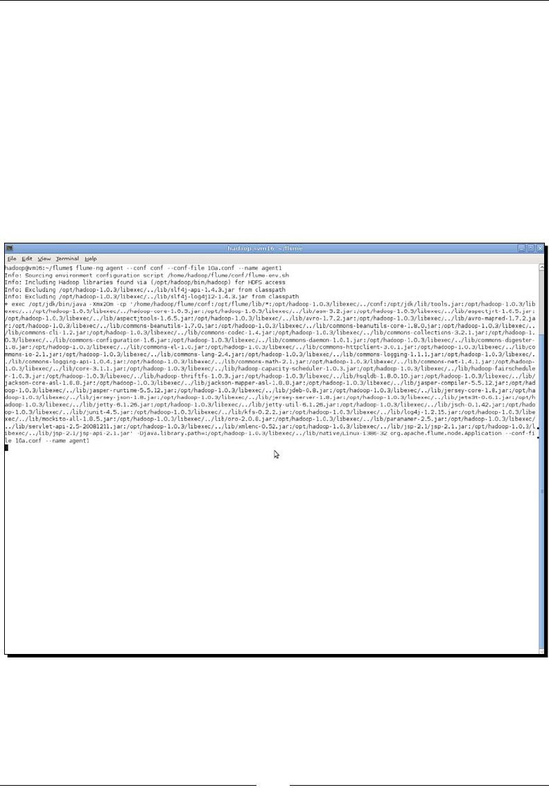
Data Collecon with Flume
[ 322 ]
agent1.sinks.logsink.type = logger
agent1.channels.memorychannel.type = memory
agent1.channels.memorychannel.capacity = 1000
agent1.channels.memorychannel.transactionCapacity = 100
agent1.sources.netsource.channels = memorychannel
agent1.sinks.logsink.channel = memorychannel
2. Start a Flume agent:
$ flume-ng agent --conf conf --conf-file 10a.conf --name agent1
The output of the preceding command can be shown in the following screenshot:
www.it-ebooks.info

Chapter 10
[ 323 ]
3. In another window, open a telnet connecon to port 3000 on the local host and
then type some text:
$ curl telnet://localhost:3000
Hello
OK
Flume!
OK
4. Close the curl connecon with Ctrl + C.
5. Look at the Flume log le:
$ tail flume.log
You will receive the following response:
2012-08-19 00:37:32,702 INFO sink.LoggerSink: Event: { headers:{}
body: 68 65 6C 6C 6F Hello }
2012-08-19 00:37:32,702 INFO sink.LoggerSink: Event: { headers:{}
body: 6D 65 Flume }
What just happened?
Firstly, we created a Flume conguraon le within our Flume working directory. We'll go
into this in more detail later, but for now, think of Flume receiving data through a component
called a source and wring it to a desnaon called a sink.
In this case, we create a Netcat source which listens on a port for network connecons.
You can see we congure it to bind to port 3000 on the local machine.
The congured sink is of the type logger which, not surprisingly, writes its output to a
log le. The rest of the conguraon le denes an agent called agent1, which uses this
source and sink.
We then start a Flume agent by using the flume-ng binary. This is the tool we'll use to
launch all Flume processes. Note that we give a few opons to this command:
The agent argument tells Flume to start an agent, which is the generic name
for a running Flume process involved in data movement
The conf directory, as menoned earlier
The parcular conguraon le for the process we are going to launch
The name of the agent within the conguraon le
www.it-ebooks.info

Data Collecon with Flume
[ 324 ]
The agent will start and no further output will appear on that screen. (Obviously, we would
run the process in the background in a producon seng.)
In another window, we open a telnet connecon to port 3000 on the local machine using
the curl ulity. The tradional way of opening such sessions is of course the telnet program
itself, but many Linux distribuons have curl installed by default; almost none use the older
telnet ulity.
We type a word on each line and hit Enter then kill the session with a Ctrl + C command.
Finally, we look at the flume.log le that is being wrien into the Flume working directory
and see an entry for each of the words we typed in.
Time for action – logging to the console
It's not always convenient to have to look at log les, parcularly when we already have the
agent screen open. Let's modify the agent to also log events to the screen.
1. Restart the Flume agent with an addional argument:
$ flume-ng agent --conf conf --conf-file 10a.conf --name agent1
-Dflume.root.logger=INFO,console
You will receive the following response:
Info: Sourcing environment configuration script /home/hadoop/
flume/conf/flume-env.sh
…
org.apache.flume.node.Application --conf-file 10a.conf --name
agent1
2012-08-19 00:41:45,462 (main) [INFO - org.apache.flume.lifecycle.
LifecycleSupervisor.start(LifecycleSupervisor.java:67)] Starting
lifecycle supervisor 1
2. In another window, connect to the server via curl:
$ curl telnet://localhost:3000
3. Type in Hello and Flume on separate lines, hit Ctrl + C, and then check the
agent window:
www.it-ebooks.info
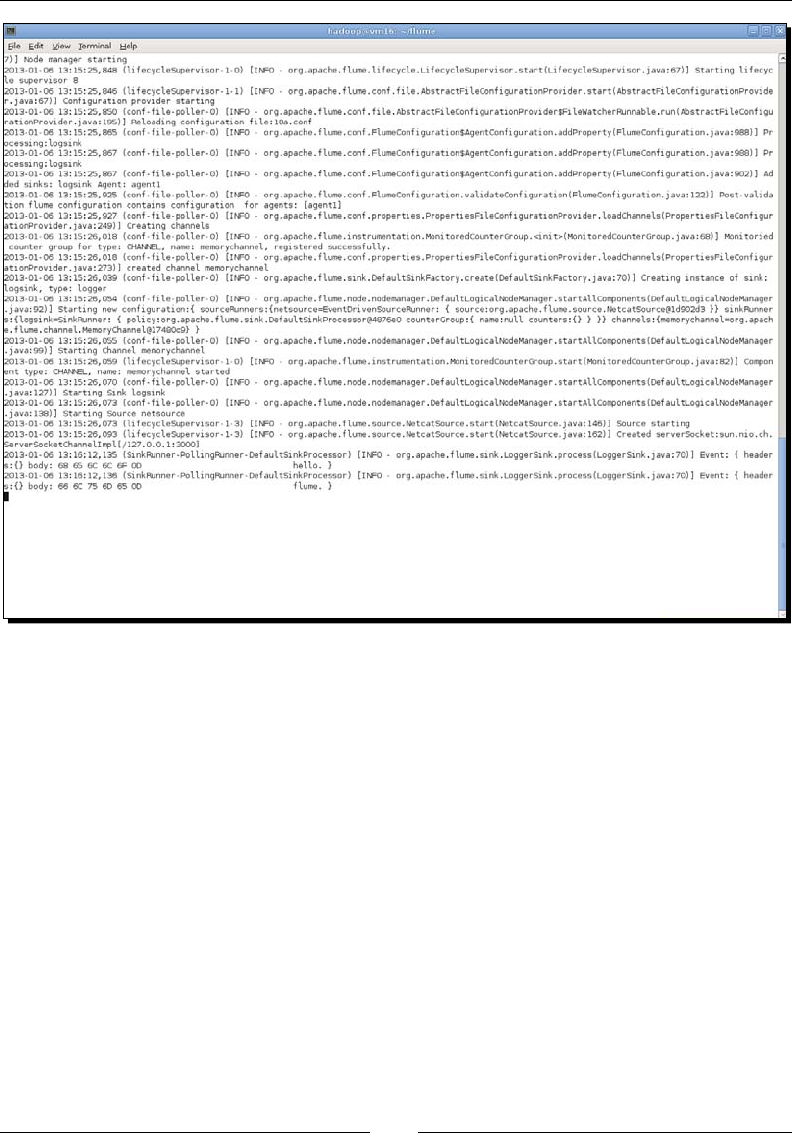
Chapter 10
[ 325 ]
What just happened?
We added this example as it becomes very useful when debugging or creang new ows.
As seen in the previous example, Flume will, by default, write its logs to a le on the
lesystem. More precisely, this is the default behavior as specied within the log4j property
le within our conf directory. Somemes we want more immediate feedback without
constantly looking at log les or having to change the property le.
By explicitly seng the flume.root.logger variable on the command line, we can override
the default logger conguraon and have the output sent directly to the agent window. The
logger is standard log4j, so the usual log levels such as DEBUG and INFO are supported.
www.it-ebooks.info

Data Collecon with Flume
[ 326 ]
Writing network data to log les
The default log sink behavior of Flume wring its received data into log les has some
limitaons, parcularly if we want to use the captured data in other applicaons.
By conguring a dierent type of sink, we can instead write the data into more
consumable data les.
Time for action – capturing the output of a command to a at le
Let's show this in acon, along the way demonstrang a new kind of source as well.
1. Create the following le as agent2.conf within the Flume working directory:
agent2.sources = execsource
agent2.sinks = filesink
agent2.channels = filechannel
agent2.sources.execsource.type = exec
agent2.sources.execsource.command = cat /home/hadoop/message
agent2.sinks.filesink.type = FILE_ROLL
agent2.sinks.filesink.sink.directory = /home/hadoop/flume/files
agent2.sinks.filesink.sink.rollInterval = 0
agent2.channels.filechannel.type = file
agent2.channels.filechannel.checkpointDir = /home/hadoop/flume/fc/
checkpoint
agent2.channels.filechannel.dataDirs = /home/hadoop/flume/fc/data
agent2.sources.execsource.channels = filechannel
agent2.sinks.filesink.channel = filechannel
2. Create a simple test le in the home directory:
$ echo "Hello again Flume!" > /home/hadoop/message
3. Start the agent:
$ flume-ng agent --conf conf --conf-file agent2.conf --name agent2
4. In another window, check le sink output directory:
$ ls files
$ cat files/*
www.it-ebooks.info

Chapter 10
[ 327 ]
The output of the preceding command can be shown in the following screenshot:
What just happened?
The previous example follows a similar paern as before. We created the conguraon le
for a Flume agent, ran the agent, and then conrmed it had captured the data we expected.
This me we used an exec source and a file_roll sink. The former, as the name suggests,
executes a command on the host and captures its output as the input to the Flume agent.
Although, in the previous case, the command is executed only once, this was for illustraon
purposes only. More common uses will use commands that produce an ongoing stream of
data. Note that the exec sink can be congured to restart the command if it does terminate.
The output of the agent is wrien to a le as specied in the conguraon le. By default,
Flume rotates (rolls) to a new le every 30 seconds; we disable this capability to make it
easier to track what's going on in a single le.
We see the le does indeed contain the output of the specied exec command.
Logs versus les
It may not be immediately obvious why Flume has both log and le sinks. Conceptually
both do the same thing, so what's the dierence?
The logger sink in reality is more of a debug tool than anything else. It doesn't just
record the informaon captured by the source, but adds a lot of addional metadata
www.it-ebooks.info

Data Collecon with Flume
[ 328 ]
and events. The le sink however records the input data exactly as it was received with
no alteraon—though such is possible if required as we will see later.
In most cases, you'll want the le sink to capture the input data but the log may also be of
use in non-producon situaons depending on your needs.
Time for action – capturing a remote le in a local at le
Let's show another example of capturing data to a le sink. This me we will use another
Flume capability that allows it to receive data from a remote client.
1. Create the following le as agent3.conf in the Flume working directory:
agent3.sources = avrosource
agent3.sinks = filesink
agent3.channels = jdbcchannel
agent3.sources.avrosource.type = avro
agent3.sources.avrosource.bind = localhost
agent3.sources.avrosource.port = 4000
agent3.sources.avrosource.threads = 5
agent3.sinks.filesink.type = FILE_ROLL
agent3.sinks.filesink.sink.directory = /home/hadoop/flume/files
agent3.sinks.filesink.sink.rollInterval = 0
agent3.channels.jdbcchannel.type = jdbc
agent3.sources.avrosource.channels = jdbcchannel
agent3.sinks.filesink.channel = jdbcchannel
2. Create a new test le as /home/hadoop/message2:
Hello from Avro!
3. Start the Flume agent:
$ flume-ng agent –conf conf –conf-file agent3.conf –name agent3
4. In another window, use the Flume Avro client to send a le to the agent:
$ flume-ng avro-client -H localhost -p 4000 -F /home/hadoop/
message
5. As before, check the le in the congured output directory:
$ cat files/*
www.it-ebooks.info

Chapter 10
[ 329 ]
The output of the preceding command can be shown in following screenshot:
What just happened?
As before, we created a new conguraon le and this me used an Avro source for the agent.
Recall from Chapter 5, Advanced MapReduce Techniques, that Avro is a data serializaon
framework; that is, it manages the packaging and transport of data from one point to another
across the network. Similarly to the Netcat source, the Avro source requires conguraon
parameters that specify its network sengs. In this case, it will listen on port 4000 on the local
machine. The agent is congured to use the le sink as before and we start it up as usual.
Flume comes with both an Avro source and a standalone Avro client. The laer can be used
to read a le and send it to an Avro source anywhere on the network. In our example, we
just use the local machine, but note that the Avro client requires the explicit hostname and
port of the Avro source to which it should send the le. So this is not a constraint; an Avro
client can send les to a listening Flume Avro source anywhere on the network.
The Avro client reads the le, sends it to the agent, and this gets wrien to the le sink. We
check this behavior by conrming that the le contents are in the le sink locaon as expected.
www.it-ebooks.info

Data Collecon with Flume
[ 330 ]
Sources, sinks, and channels
We intenonally used a variety of sources, sinks, and channels in the previous examples
just to show how they can be mixed and matched. However, we have not explored them—
especially channels—in much detail. Let's dig a lile deeper now.
Sources
We've looked at three sources: Netcat, exec, and Avro. Flume NG also supports a sequence
generator source (mostly for tesng) as well as both TCP and UDP variants of a source that
reads syslogd data. Each source is congured within an agent and aer receiving enough
data to produce a Flume event, it sends this newly created event to the channel to which the
source is connected. Though a source may have logic relang to how it reads data, translates
events, and handles failure situaons, the source has no knowledge of how the event is to be
stored. The source has the responsibility of delivering the event to the congured channel,
and all other aspects of the event processing are invisible to the source.
Sinks
In addion to the logger and le roll sinks we used previously, Flume also supports sinks for
HDFS, HBase (two types), Avro (for agent chaining), null (for tesng), and IRC (for an Internet
Relay Chat service). The sink is conceptually similar to the source but in reverse.
The sink waits for events to be received from the congured channel about whose inner
workings it knows nothing. On receipt, the sink handles the output of the event to its
parcular desnaon, managing all issues around me outs, retries, and rotaon.
Channels
So what are these mysterious channels that connect the source and sink? They are, as
the name and conguraon entries before suggest, the communicaon and retenon
mechanism that manages event delivery.
When we dene a source and a sink, there may be signicant dierences in how they read
and write data. An exec source may, for example, receive data much faster than a le roll sink
can write it or the source may have mes (such as when rolling to a new le or dealing with
system I/O congeson) that wring needs be paused. The channel, therefore, needs buer
data between the source and sink to allow data to stream through the agent as eciently
as possible. This is why the channel conguraon porons of our conguraon les include
elements such as capacity.
The memory channel is the easiest to understand as the events are read from the source
into memory and passed to the sink as it is able to receive them. But if the agent process
dies mid-way through the process (be it due to soware or hardware failure), then all the
events currently in the memory channel are lost forever.
www.it-ebooks.info

Chapter 10
[ 331 ]
The le and JDBC channels that we also used provide persistent storage of events to prevent
such loss. Aer reading an event from a source, the le channel writes the contents to a le
on the lesystem that is deleted only aer successful delivery to the sink. Similarly, the JDBC
channel uses an embedded Derby database to store events in a recoverable fashion.
This is a classic performance versus reliability trade-o. The memory channel is the fastest
but has the risk of data loss. The le and JDBC channels are typically much slower but
eecvely provide guaranteed delivery to the sink. Which channel you choose depends
on the nature of the applicaon and the values of each event.
Don't worry too much about this trade-o; in the real world, the answer
is usually obvious. Also be sure to look carefully at the reliability of the
source and sink being used. If those are unreliable and you drop events
anyway, do you gain much from a persistent channel?
Or roll your own
Don't feel limited by the exisng collecon of sources, sinks, and channels. Flume oers
an interface to dene your own implementaon of each. In addion, there are a few
components present in Flume OG that have not yet been incorporated into Flume NG
but may appear in the future.
Understanding the Flume conguration les
Now that we've talked through sources, sinks, and channels, let's take a look at one of
the conguraon les from earlier in a lile more detail:
agent1.sources = netsource
agent1.sinks = logsink
agent1.channels = memorychannel
These rst lines name the agent and dene the sources, sinks, and channels associated
with it. We can have mulple values on each line; the values are space separated:
agent1.sources.netsource.type = netcat
agent1.sources.netsource.bind = localhost
agent1.sources.netsource.port = 3000
These lines specify the conguraon for the source. Since we are using the Netcat source,
the conguraon values specify how it should bind to the network. Each type of source
has its own conguraon variables.
agent1.sinks.logsink.type = logger
www.it-ebooks.info

Data Collecon with Flume
[ 332 ]
This species the sink to be used is the logger sink which is further congured via the
command line or the log4j property le.
agent1.channels.memorychannel.type = memory
agent1.channels.memorychannel.capacity = 1000
agent1.channels.memorychannel.transactionCapacity = 100
These lines specify the channel to be used and then add the type
specific configuration values. In this case we are using the memory
channel and we specify its capacity but – since it is non-persistent –
no external storage mechanism.
agent1.sources.netsource.channels = memorychannel
agent1.sinks.logsink.channel = memorychannel
These last lines congure the channel to be used for the source and sink. Though we used
dierent conguraon les for our dierent agents, we could just as easily place all the
elements in a single conguraon le as the respecve agent names provide the necessary
separaon. This can, however, produce a prey verbose le which can be a lile inmidang
when you are just learning Flume. We can also have mulple ows within a given agent, we
could, for example, combine the rst two preceding examples into a single conguraon le
and agent.
Have a go hero
Do just that! Create a conguraon le that species the capabilies of both our previous
agent1 and agent2 from the preceding example in a single composite agent that contains:
A Netcat source and its associated logger sink
An exec source and its associated le sink
Two memory channels, one for each of the source/sink pairs menoned before
To get you started, here's how the component denions could look:
agentx.sources = netsource execsource
agentx.sinks = logsink filesink
agentx.channels = memorychannel1 memorychannel2
It's all about events
Let's discuss one more denion before we try another example. Just what is an event?
Remember that Flume is explicitly based around log les, so in most cases, an event equates
to a line of text followed by a new line character. That is the behavior we've seen with the
sources and sinks we've used.
www.it-ebooks.info

Chapter 10
[ 333 ]
This isn't always the case, however, the UDP syslogd source, for example, treats each packet
of data received as a single event, which gets passed through the system. When using these
sinks and sources, however, these denions of events are unchangeable and when reading
les, for example, we have no choice but to use line-based events.
Time for action – writing network trafc onto HDFS
This discussion of Flume in a book about Hadoop hasn't actually used Hadoop at all so far.
Let's remedy that by wring data onto HDFS via Flume.
1. Create the following le as agent4.conf within the Flume working directory:
agent4.sources = netsource
agent4.sinks = hdfssink
agent4.channels = memorychannel
agent4.sources.netsource.type = netcat
agent4.sources.netsource.bind = localhost
agent4.sources.netsource.port = 3000
agent4.sinks.hdfssink.type = hdfs
agent4.sinks.hdfssink.hdfs.path = /flume
agent4.sinks.hdfssink.hdfs.filePrefix = log
agent4.sinks.hdfssink.hdfs.rollInterval = 0
agent4.sinks.hdfssink.hdfs.rollCount = 3
agent4.sinks.hdfssink.hdfs.fileType = DataStream
agent4.channels.memorychannel.type = memory
agent4.channels.memorychannel.capacity = 1000
agent4.channels.memorychannel.transactionCapacity = 100
agent4.sources.netsource.channels = memorychannel
agent4.sinks.hdfssink.channel = memorychannel
2. Start the agent:
$ flume-ng agent –conf conf –conf-file agent4.conf –name agent4
3. In another window, open a telnet connecon and send seven events to Flume:
$ curl telnet://localhost:3000
4. Check the contents of the directory specied in the Flume conguraon le and
then examine the le contents:
$ hadoop fs -ls /flume
$ hadoop fs –cat "/flume/*"
www.it-ebooks.info
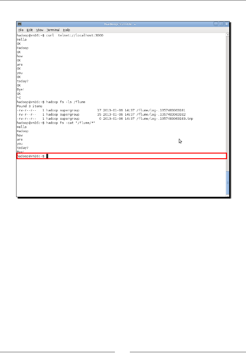
Data Collecon with Flume
[ 334 ]
The output of the preceding command can be shown in the following screenshot:
What just happened?
This me we paired a Netcat source with the HDFS sink. As can be seen from the
conguraon le, we need to specify aspects such as the locaon for the les, any le prex,
and the strategy for rolling from one le to another. In this case, we specied les within the
/flume directory, each starng with log- and with a maximum of three entries in each le
(obviously, such a low value is for tesng only).
Aer starng the agent, we use curl once more to send seven single word events to Flume.
We then used the Hadoop command-line ulity to look at the directory contents and verify
that our input data was being wrien to HDFS.
Note that the third HDFS le has a .tmp extension. Remember that we specied three
entries per le but only input seven values. We, therefore, lled up two les and started
on another. Flume gives the le currently being wrien a .tmp extension, which makes it
easy to dierenate the completed les from in-progress les when specifying which les to
process via MapReduce jobs.
www.it-ebooks.info

Chapter 10
[ 335 ]
Time for action – adding timestamps
We menoned earlier that there were mechanisms to have le data wrien in slightly more
sophiscated ways. Let's do something very common and write our data into a directory with
a dynamically-created mestamp.
1. Create the following conguraon le as agent5.conf:
agent5.sources = netsource
agent5.sinks = hdfssink
agent5.channels = memorychannel
agent5.sources.netsource.type = netcat
agent5.sources.netsource.bind = localhost
agent5.sources.netsource.port = 3000
agent5.sources.netsource.interceptors = ts
agent5.sources.netsource.interceptors.ts.type = org.apache.flume.
interceptor.TimestampInterceptor$Builder
agent5.sinks.hdfssink.type = hdfs
agent5.sinks.hdfssink.hdfs.path = /flume-%Y-%m-%d
agent5.sinks.hdfssink.hdfs.filePrefix = log-
agent5.sinks.hdfssink.hdfs.rollInterval = 0
agent5.sinks.hdfssink.hdfs.rollCount = 3
agent5.sinks.hdfssink.hdfs.fileType = DataStream
agent5.channels.memorychannel.type = memory
agent5.channels.memorychannel.capacity = 1000
agent5.channels.memorychannel.transactionCapacity = 100
agent5.sources.netsource.channels = memorychannel
agent5.sinks.hdfssink.channel = memorychannel
2. Start the agent:
$ flume-ng agent –conf conf –conf-file agent5.conf –name agent5
3. In another window, open up a telnet session and send seven events to Flume:
$ curl telnet://localhost:3000
4. Check the directory name on HDFS and the les within it:
$ hadoop fs -ls /
www.it-ebooks.info
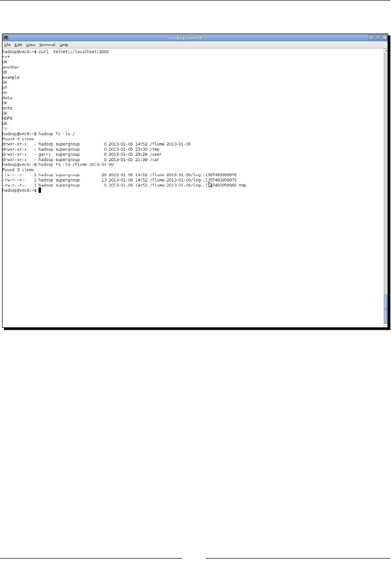
Data Collecon with Flume
[ 336 ]
The output of the preceding code can be shown in the following screenshot:
What just happened?
We made a few changes to the previous conguraon le. We added an
interceptor specicaon to the Netcat source and gave its implementaon
class as TimestampInterceptor.
Flume interceptors are plugins that can manipulate and modify events before they
pass from the source to the channel. Most interceptors either add metadata to the
event (as in this case) or drop events based on certain criteria. In addion to several
inbuilt interceptors, there is naturally a mechanism for user-dened interceptors.
We used the mestamp interceptor here which adds to the event metadata the Unix
mestamp at the me the event is read. This allows us to extend the denion of the
HDFS path into which events are to be wrien.
www.it-ebooks.info

Chapter 10
[ 337 ]
While previously we simply wrote all events to the /flume directory, we now specied the
path as /flume-%Y-%m-%d. Aer running the agent and sending some data to Flume, we
looked at HDFS and saw that these variables have been expanded to give the directory a
year/month/date sux.
The HDFS sink supports many other variables such as the hostname of the source and
addional temporal variables that can allow precise paroning to the level of seconds.
The ulity here is plain; instead of having all events wrien into a single directory that becomes
enormous over me, this simple mechanism can give automac paroning, making data
management easier but also providing a simpler interface to the data for MapReduce jobs. If,
for example, most of your MapReduce jobs process hourly data, then having Flume paron
incoming events into hourly directories will make your life much easier.
To be precise, the event passing through Flume has had a complete Unix mestamp added,
that is, accurate to the nearest second. In our example, we used only date-related variables
in the directory specicaon, if hourly or ner-grained directory paroning is required, then
the me-related variables would be used.
This assumes that the mestamp at the point of processing is sucient for
your needs. If les are being batched and then fed to Flume, then a le's
contents may have mestamps from the previous hour than when they are
being processed. In such a case, you could write a custom interceptor to set
the mestamp header based on the contents of the le.
To Sqoop or to Flume...
An obvious queson is whether Sqoop or Flume is most appropriate if we have data in a
relaonal database that we want to export onto HDFS. We've seen how Sqoop can perform
such an export and we could do something similar using Flume, either with a custom source
or even just by wrapping a call to the mysql command within an exec source.
A good rule of thumb is to look at the type of data and ask if it is log data or something
more involved.
Flume was created in large part to handle log data and it excels in this area. But in most
cases, Flume networks are responsible for delivering events from sources to sinks without
any real transformaon on the log data itself. If you have log data in mulple relaonal
databases, then Flume is likely a great choice, though I would queson the long-term
scalability of using a database for storing log records.
www.it-ebooks.info

Data Collecon with Flume
[ 338 ]
Non-log data may require data manipulaon that only Sqoop is capable of performing.
Many of the transformaons we performed in the previous chapter using Sqoop, such
as specifying subsets of columns to be retrieved, are really not possible using Flume. It's
also quite possible that if you are dealing with structured data that requires individual eld
processing, then Flume alone is not the ideal tool. If you want direct Hive integraon then
Sqoop is your only choice.
Remember, of course, that the tools can also work together in more complex workows.
Events could be gathered together onto HDFS by Flume, processed through MapReduce,
and then exported into a relaonal database by Sqoop.
Time for action – multi level Flume networks
Let's put together a few pieces we touched on earlier and see how one Flume agent can use
another as its sink.
1. Create the following le as agent6.conf:
agent6.sources = avrosource
agent6.sinks = avrosink
agent6.channels = memorychannel
agent6.sources.avrosource.type = avro
agent6.sources.avrosource.bind = localhost
agent6.sources.avrosource.port = 2000
agent6.sources.avrosource.threads = 5
agent6.sinks.avrosink.type = avro
agent6.sinks.avrosink.hostname = localhost
agent6.sinks.avrosink.port = 4000
agent6.channels.memorychannel.type = memory
agent6.channels.memorychannel.capacity = 1000
agent6.channels.memorychannel.transactionCapacity = 100
agent6.sources.avrosource.channels = memorychannel
agent6.sinks.avrosink.channel = memorychannel
2. Start an agent congured as per the agent3.conf le created earlier, that is, with
an Avro source and a le sink:
$ flume-ng client –conf conf –conf-file agent3.conf agent3
3. In a second window, start another agent; this one congured with the preceding le:
$ flume-ng client –conf conf –conf-file agent6.conf agent6
www.it-ebooks.info

Chapter 10
[ 339 ]
4. In a third window, use the Avro client to send a le to each of the Flume agents:
$ flume-ng avro-client –H localhost –p 4000 –F /home/hadoop/
message
$ flume-ng avro-client -H localhost -p 2000 -F /home/hadoop/
message2
5. Check the output directory for les and examine the le present:
What just happened?
Firstly, we dened a new agent with an Avro source and also an Avro sink. We've not used
this sink before; instead of wring the events to a local locaon or HDFS, this sink sends the
events to a remote source using Avro.
We start an instance of this new agent and then also start an instance of agent3 we used
earlier. Recall this agent has an Avro source and a le roll sink. We congure the Avro sink in
the rst agent to point to the host and port of the Avro sink in the second and by doing so,
build a data-roung chain.
www.it-ebooks.info

Data Collecon with Flume
[ 340 ]
With both agents running, we then use the Avro client to send a le to each and conrm that
both appear in the le locaon congured as the desnaon for the agent3 sink.
This isn't just technical capability for its own sake. This capability is the building block that
allows Flume to build arbitrarily complex distributed event collecon networks. Instead of
one copy of each agent, think of mulple agents of each type feeding events into the next
link in the chain, which acts as an event aggregaon point.
Time for action – writing to multiple sinks
We need one nal piece of capability to build such networks, namely, an agent that can write
to mulple sinks. Let's create one.
1. Create the following conguraon le as agent7.conf:
agent7.sources = netsource
agent7.sinks = hdfssink filesink
agent7.channels = memorychannel1 memorychannel2
agent7.sources.netsource.type = netcat
agent7.sources.netsource.bind = localhost
agent7.sources.netsource.port = 3000
agent7.sources.netsource.interceptors = ts
agent7.sources.netsource.interceptors.ts.type = org.apache.flume.
interceptor.TimestampInterceptor$Builder
agent7.sinks.hdfssink.type = hdfs
agent7.sinks.hdfssink.hdfs.path = /flume-%Y-%m-%d
agent7.sinks.hdfssink.hdfs.filePrefix = log
agent7.sinks.hdfssink.hdfs.rollInterval = 0
agent7.sinks.hdfssink.hdfs.rollCount = 3
agent7.sinks.hdfssink.hdfs.fileType = DataStream
agent7.sinks.filesink.type = FILE_ROLL
agent7.sinks.filesink.sink.directory = /home/hadoop/flume/files
agent7.sinks.filesink.sink.rollInterval = 0
agent7.channels.memorychannel1.type = memory
agent7.channels.memorychannel1.capacity = 1000
agent7.channels.memorychannel1.transactionCapacity = 100
agent7.channels.memorychannel2.type = memory
www.it-ebooks.info
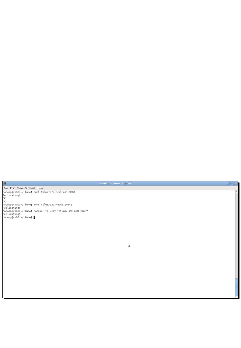
Chapter 10
[ 341 ]
agent7.channels.memorychannel2.capacity = 1000
agent7.channels.memorychannel2.transactionCapacity = 100
agent7.sources.netsource.channels = memorychannel1 memorychannel2
agent7.sinks.hdfssink.channel = memorychannel1
agent7.sinks.filesink.channel = memorychannel2
agent7.sources.netsource.selector.type = replicating
2. Start the agent:
$ flume-ng agent –conf conf –conf-file agent7.conf –name agent7
3. Open a telnet session and send an event to Flume:
$ curl telnet://localhost:3000
You will receive the following response:
Replicating!
Check the contents of the HDFS and file sinks:
$ cat files/*
$ hdfs fs –cat "/flume-*/*"
The output of the preceding command can be shown in the following screenshot:
www.it-ebooks.info

Data Collecon with Flume
[ 342 ]
What just happened?
We created a conguraon le containing a single Netcat source and both the le and HDFS
sink. We congured separate memory channels connecng the source to both sinks.
We then set the source selector type to replicating, which means events will be sent to
all congured channels.
Aer starng the agent as normal and sending an event to the source, we conrmed that
the event was indeed wrien to both the lesystem and HDFS sinks.
Selectors replicating and multiplexing
The source selector has two modes, replicang as we have seen here and mulplexing.
A mulplexing source selector will use logic to determine to which channel an event
should be sent, depending on the value of a specied header eld.
Handling sink failure
By their nature of being output desnaons, it is to be expected that sinks may fail or
become unresponsive over me. As with any input/output device, a sink may be saturated,
run out of space, or go oine.
Just as Flume associates selectors with sources to allow the replicaon and mulplexing
behavior we have just seen it also supports the concept of sink processors.
There are two dened sink processors, namely, the failover sink processor and the load
balancing sink processor.
The sink processors view the sinks as being within a group and, dependent on their type, react
dierently when an event arrives. The load balancing sink processor sends events to sinks one
at a me, using either a round-robin or random algorithm to select which sink to use next. If a
sink fails, the event is retried on another sink, but the failed sink remains in the pool.
The failover sink, in contrast, views the sinks as a priorized list and only tries a lower priority
sink if the ones above it have failed. Failed sinks are removed from the list and are only
retried aer a cooling-o period that increases with subsequent failures.
Have a go hero - Handling sink failure
Set up a Flume conguraon that has three congured HDFS sinks, each wring to dierent
locaons on HDFS. Use the load balancer sink processor to conrm events are wrien to
each sink, and then use the failover sink processor to show the priorizaon.
Can you force the agent to select a processor other than the highest priority one?
www.it-ebooks.info

Chapter 10
[ 343 ]
Next, the world
We have now covered most of the key features of Flume. As menoned earlier, Flume is a
framework and this should be considered carefully; Flume has much more exibility in its
deployment model than any other product we have looked at.
It achieves its exibility through a relavely small set of capabilies; the linking of sources
to sinks via channels and mulple variaons that allow mul-agent or mul-channel
conguraons. This may not seem like much, but consider that these building blocks can be
composed to create a system such as the following where mulple web server farms feed
their logs into a central Hadoop cluster:
Each node in each farm runs an agent pulling each local log le in turn.
These log les are sent to a highly-available aggregaon point, one within each farm
which also performs some processing and adds addional metadata to the events,
categorizing them as three types of records.
These rst level aggregators then send the events to one of the series of agents that
access the Hadoop cluster. The aggregators oer mulple access points and event
types 1 and 2 are sent to the rst, event type 3 to the second.
Within the nal aggregator, they write event type 1 and 2 to dierent locaons on
HDFS, with type 2 also being wrien to a local lesystem. Event type 3 is wrien
directly into HBase.
It is amazing how simple primives can be composed to build complex systems like this!
Have a go hero - Next, the world
As a thought experiment, try to work through the preceding scenario and determine what
sort of Flume setup would be required at each step in the ow.
The bigger picture
It's important to realize that "simply" geng data from one point to another is rarely the
extent of your data consideraons. Terms such as data lifecycle management have become
widely used recently for good reason. Let's briey look at some things to consider, ideally
before you have the data ooding across the system.
Data lifecycle
The main queson to be asked in terms of data lifecycle is for how long will the value you
gain from data storage be greater than the storage costs. Keeping data forever may seem
aracve but the costs of holding more and more data will increase over me. These costs
are not just nancial; many systems see their performance degrade as volumes increase.
www.it-ebooks.info

Data Collecon with Flume
[ 344 ]
This queson isn't—or at least rarely should be—decided by technical factors. Instead,
you need the value and costs to the business to be the driving factors. Somemes data
becomes worthless very quickly, other mes the business cannot delete it for either
compeve or legal reasons. Determine the posion and act accordingly.
Remember of course that it is not a binary decision between keeping or deleng data;
you can also migrate data across ers of storage that decrease in cost and performance
as they age.
Staging data
On the other side of the process, it is oen worthwhile to think about how data is fed into
processing plaorms such as MapReduce. With mulple data sources, the last thing you
oen want is to have all the data arrive on a single massive volume.
As we saw earlier, Flume's ability to parameterize the locaon to which it writes on HDFS is a
great tool to aid this problem. However, oen it is useful to view this inial drop-o point as
a temporary staging area to which data is wrien prior to processing. Aer it is processed, it
may be moved into the long-term directory structure.
Scheduling
At many points in the ows, we have discussed that there is an implicit need for an external
task to do something. As menoned before, we want MapReduce to process les once they
are wrien to HDFS by Flume, but how is that task scheduled? Alternavely, how do we
manage the post-processing, the archival or deleon of old data, even the removal of log
les on the source hosts?
Some of these tasks, such as the laer, are likely managed by exisng systems such as
logrotate on Linux but the others may be things you need to build. Obvious tools such as
cron may be good enough, but as system complexity increases, you may need to invesgate
more sophiscated scheduling systems. We will briey menon one such system with ght
Hadoop integraon in the next chapter.
www.it-ebooks.info

Chapter 10
[ 345 ]
Summary
This chapter discussed the problem of how to retrieve data from across the network
and make it available for processing in Hadoop. As we saw, this is actually a more general
challenge and though we may use Hadoop-specic tools, such as Flume, the principles are
not unique. In parcular, we covered an overview of the types of data we may want to write
to Hadoop, generally categorizing it as network or le data. We explored some approaches
for such retrieval using exisng command-line tools. Though funconal, the approaches
lacked sophiscaon and did not suit extension into more complex scenarios.
We looked at Flume as a exible framework for dening and managing data (parcularly
from log les) roung and delivery, and learned the Flume architecture which sees data
arrive at sources, be processed through channels, and then wrien to sinks.
We then explored many of Flume's capabilies such as how to use the dierent
types of sources, sinks, and channels. We saw how the simple building blocks could
be composed into very complex systems and we closed with some more general
thoughts on data management.
This concludes the main content of this book. In the next chapter, we will sketch out a
number of other projects that may be of interest and highlight some ways of engaging
the community and geng support.
www.it-ebooks.info

11
Where to Go Next
This book has, as the title suggests, sought to give a beginner to Hadoop
in-depth knowledge of the technology and its application. As has been seen
on several occasions, there is a lot more to the Hadoop ecosystem than the
core product itself. We will give a quick highlight of some potential areas of
interest in this chapter.
In this chapter we will discuss:
What we covered in this book
What we didn't cover in this book
Upcoming Hadoop changes
Alternave Hadoop distribuons
Other signicant Apache projects
Alternave programming abstracons
Sources of informaon and help
What we did and didn't cover in this book
With our focus on beginners, the aim of this book was to give you a strong grounding in the
core Hadoop concepts and tools. In addion, we provided experiences with some other tools
that help you integrate the technology into your infrastructure.
www.it-ebooks.info

Where to Go Next
[ 348 ]
Though Hadoop started as the single core product, it's fair to say that the ecosystem
surrounding Hadoop has exploded in recent years. There are alternave distribuons
of the technology, some providing commercial custom extensions. There are a plethora
of related projects and tools that build upon Hadoop and provide specic funconality
or alternave approaches to exisng ideas. It's a really excing me to get involved with
Hadoop; let's take a quick tour of what is out there.
Note, of course, that any overview of the ecosystem is both skewed by the
author's interests and preferences and outdated the moment it is wrien.
In other words, don't for a moment think this is all that's available; consider
it a wheng of the appete.
Upcoming Hadoop changes
Before discussing alternave Hadoop distribuons, let's look at some changes to Hadoop
itself in the near future. We've already discussed the HDFS changes coming in Hadoop 2.0,
parcularly the high availability of NameNode enabled by the new BackupNameNode and
CheckpointNameNode services. This is a signicant capability for Hadoop as it will make
HDFS much more robust, greatly enhancing its enterprise credenals and streamlining
cluster operaons. The impact of NameNode HA is hard to exaggerate; it will almost
certainly become one of those capabilies that no one will be able to remember how
we lived without in a few years' me.
MapReduce is not standing sll while all this is going on, and in fact, the changes
being introduced may not have as much immediate impact but are actually much
more fundamental.
These changes were inially developed under the name MapReduce 2.0 or MRV2.
However, the name now being used is YARN (Yet Another Resource Negoator), which is
more accurate as the changes are much more about Hadoop as a plaorm than MapReduce
itself. The goal of YARN is to build a framework on Hadoop that allows cluster resources to be
allocated to given applicaons and for MapReduce to be only one of these applicaons.
If you consider the JobTracker today, it is responsible for two quite dierent tasks:
managing the progress of a given MapReduce job (but also idenfying which cluster
resources are available at any point in me) and allocang the resources to the various
stages of the job. YARN separates these out into disnct roles; a global ResourceManager
that uses NodeManagers on each host to manage the cluster's resources and a disnct
ApplicaonManager (the rst example of which is MapReduce) that communicates with the
ResourceManager to get the resources it needs for its job.
www.it-ebooks.info

Chapter 11
[ 349 ]
The MapReduce interface in YARN will be unchanged, so from a client perspecve, all exisng
code will sll run on the new plaorm. But as new ApplicaonManagers are developed, we
will start to see Hadoop being used more as a generic task processing plaorm with mulple
types of processing models supported. Early examples of other models being ported to YARN
are stream-based processing and a port of the Message Passing Interface (MPI), which is
broadly used in scienc compung.
Alternative distributions
Way back in Chapter 2, Geng Up and Running, we went to the Hadoop homepage from
which we downloaded the installaon package. Odd as it may seem, this is far from the only
way to get Hadoop. Odder sll may be the fact that most producon deployments don't use
the Apache Hadoop distribuon.
Why alternative distributions?
Hadoop is open source soware. Anyone can, providing they comply with the Apache
Soware License that governs Hadoop, make their own release of the soware. There
are two main reasons alternave distribuons have been created.
Bundling
Some providers seek to build a pre-bundled distribuon containing not only Hadoop but
also other projects, such as Hive, HBase, Pig, and many more. Though installaon of most
projects is rarely dicult—with the excepon of HBase, which has historically been more
dicult to set up by hand—there can be subtle version incompabilies that don't arise
unl a parcular producon workload hits the system. A bundled release can provide a
pre-integrated set of compable versions that are known to work together.
The bundled release can also provide the distribuon not only in a tarball le but also in
packages that are easily installed through package managers such as RPM, Yum, or APT.
Free and commercial extensions
Being an open source project with a relavely liberal distribuon license, creators are also
free to enhance Hadoop with proprietary extensions that are made available either as free
open source or commercial products.
This can be a controversial issue as some open source advocates dislike any
commercializaon of successful open source projects; to them it appears that the
commercial enty is freeloading by taking the fruits of the open source community without
having to build it for themselves. Others see this as a healthy aspect of the exible Apache
license; the base product will always be free and individuals and companies can choose to
go with commercial extensions or not. We do not pass judgment either way, but be aware
that this is a controversy you will almost certainly encounter.
www.it-ebooks.info

Where to Go Next
[ 350 ]
Given the reasons for the existence of alternave distribuons, let's look at a few popular
examples.
Cloudera Distribution for Hadoop
The most widely used Hadoop distribuon is the Cloudera Distribuon for Hadoop,
referred to as CDH. Recall that Cloudera is the company that rst created Sqoop and
contributed it back to the open source community and is where Doug Cung now works.
The Cloudera distribuon is available at http://www.cloudera.com/hadoop and
contains a large number of Apache products, from Hadoop itself, Hive, Pig, and HBase
through tools such as Sqoop and Flume, to other lesser-known products such as Mahout
and Whir. We'll talk about some of these later.
CDH is available in several package formats and deploys the soware in a ready-to-go
fashion. The base Hadoop product, for example, is separated into dierent packages
for the components such as NameNode, TaskTracker, and so on, and for each, there is
integraon with the standard Linux service infrastructure.
CDH was the rst widely available alternave distribuon, and its breadth of available
soware, proven level of quality, and free cost has made it a very popular choice.
Cloudera does also oer addional commercial-only products, such as a Hadoop
management tool, in addion to training, support, and consultancy services. Details
are available on the company webpage.
Hortonworks Data Platform
In 2011, the Yahoo division responsible for so much of the development of Hadoop was
spun o into a new company called Hortonworks. They have also produced their own
pre-integrated Hadoop distribuon, called the Hortonworks Data Plaorm (HDP) and
available at http://hortonworks.com/products/hortonworksdataplatform/.
HDP is conceptually similar to CDH, but both products have dierences in their focus.
Hortonworks makes much of the fact that HDP is fully open source, including the
management tool. They also have posioned HDP as a key integraon plaorm through
support for tools such as Talend Open Studio. Hortonworks does not oer commercial
soware; its business model focuses instead on oering professional services and support
for the plaorm.
Both Cloudera and Hortonworks are venture-backed companies with signicant engineering
experse; both companies employ many of the most prolic contributors to Hadoop. The
underlying technology is however the same Apache projects; the dierences are how they
are packaged, the versions employed, and the addional value-added oerings provided by
the companies.
www.it-ebooks.info

Chapter 11
[ 351 ]
MapR
A dierent type of distribuon is oered by MapR Technologies, though the company and
distribuon are usually referred to simply as MapR. Available at http://www.mapr.com,
the distribuon is based on Hadoop but has added a number of changes and enhancements.
One main MapR focus is on performance and availability, for example, it was the rst
distribuon to oer a high-availability soluon for the Hadoop NameNode and JobTracker,
which you will remember (from Chapter 7, Keeping Things Running) is a signicant weakness
in core Hadoop. It also oers nave integraon with NFS le systems, which makes
processing of exisng data much easier; MapR replaced HDFS with a full POSIX-compliant
lesystem that can easily be mounted remotely.
MapR provides both a community and enterprise edion of its distribuon; not all the
extensions are available in the free product. The company also oers support services
as part of the enterprise product subscripon, in addion to training and consultancy.
IBM InfoSphere Big Insights
The last distribuon we'll menon here comes from IBM. The IBM InfoSphere Big Insights
distribuon is available at http://www-01.ibm.com/software/data/infosphere/
biginsights/ and (like MapR) oers commercial improvements and extensions to the
open source Hadoop core.
Big Insights comes in two versions, the free IBM InfoSphere Big Insights Basic Edion and the
commercial IBM InfoSphere Big Insights Enterprise Edion. Big Insights, big names! The basic
edion is an enhanced set of Apache Hadoop products, adding some free management and
deployment tools as well as integraon with other IBM products.
The Enterprise Edion is actually quite dierent from the Basic Edion; it is more of a layer
atop Hadoop, and in fact, can be used with other distribuons such as CDH or HDP. The
Enterprise Edion provides an array of data visualizaon, business analysis, and processing
tools. It also has deep integraon with other IBM products such as InfoSphere Streams, DB2,
and GPFS.
Choosing a distribution
As can be seen, the available distribuons (and we didn't cover them all) range from
convenience packaging and integraon of fully open source products through to enre
bespoke integraon and analysis layers atop them. There is no overall best distribuon;
think carefully about your needs and consider the alternaves. Since all the previous
distribuons oer a free download of at least a basic version, it's also good to simply
have a try and experience the opons for yourself.
www.it-ebooks.info

Where to Go Next
[ 352 ]
Other Apache projects
Whether you use a bundled distribuon or sck with the base Apache Hadoop download,
you will encounter many references to other, related Apache projects. We have covered
Hive, Sqoop, and Flume in this book; we'll now highlight some of the others.
Note that this coverage seeks to point out the highlights (from my perspecve) as well
as give a taste of the wide range of the types of projects available. As before, keep looking
out; there will be new ones launching all the me.
HBase
Perhaps the most popular Apache Hadoop-related project that we didn't cover in this
book is HBase; its homepage is at http://hbase.apache.org. Based on the BigTable
model of data storage publicized by Google in an academic paper (sound familiar?),
HBase is a non-relaonal data store sing atop HDFS.
Whereas both MapReduce and Hive tasks focus on batch-like data access paerns, HBase
instead seeks to provide very low latency access to data. Consequently, HBase can, unlike
the already menoned technologies, directly support user-facing services.
The HBase data model is not the relaonal approach we saw used in Hive and all other
RDBMSs. Instead, it is a key-value, schemaless soluon that takes a column-oriented view
of data; columns can be added at run-me and depend on the values inserted into HBase.
Each lookup operaon is then very fast as it is eecvely a key-value mapping from the row
key to the desired column. HBase also treats mestamps as another dimension on the data,
so one can directly retrieve data from a point in me.
The data model is very powerful but does not suit all use cases, just as the relaonal
model isn't universally applicable. But if you have a need for structured low-latency views
on large-scale data stored in Hadoop, HBase is absolutely something you should look at.
Oozie
We have said many mes that Hadoop clusters do not live in a vacuum and need to integrate
with other systems and into broader workows. Oozie, available at http://oozie.
apache.org, is a Hadoop-focused workow scheduler that addresses this laer scenario.
In its simplest form, Oozie provides mechanisms to schedule the execuon of MapReduce
jobs based either on a me-based criteria (for example, do this every hour) or on data
availability (for example, do this when new data arrives in this locaon). It allows the
specicaon of mul-stage workows that can describe a complete end-to-end process.
www.it-ebooks.info

Chapter 11
[ 353 ]
In addion to straight-forward MapReduce jobs, Oozie can also schedule jobs that run
Hive or Pig commands as well as tasks enrely outside of Hadoop (such as sending emails,
running shell scripts, or running commands on remote hosts).
There are many ways of building workows; a common approach is with Extract Transform
and Load (ETL) tools such as Pentaho Kele (http://kettle.pentaho.com) and Spring
Batch (http://static.springsource.org/spring-batch). These, for example, do
include some Hadoop integraon but the tradional dedicated workow engines may not.
Consider Oozie if you are building workows with signicant Hadoop interacon and you
do not have an exisng workow tool with which you have to integrate.
Whir
When looking to use cloud services such as Amazon AWS for Hadoop deployments, it is
usually a lot easier to use a higher-level service such as ElascMapReduce as opposed to
seng up your own cluster on EC2. Though there are scripts to help, the fact is that the
overhead of Hadoop-based deployments on cloud infrastructures can be involved. That is
where Apache Whir from http://whir.apache.org comes in.
Whir is not focused on Hadoop; it is about supplier-independent instanaon of cloud
services of which Hadoop is a single example. Whir provides a programmac way of
specifying and creang Hadoop-based deployments on cloud infrastructures in a way that
handles all the underlying service aspects for you. And it does this in a provider-independent
fashion so that once you've launched on, say, EC2, you can use the same code to create the
idencal setup on another provider such as Rackspace or Eucalyptus. This makes vendor
lock-in—oen a concern with cloud deployments—less of an issue.
Whir is not quite there yet. Today it is limited in what services it can create and only supports
a single provider, AWS. However, if you are interested in cloud deployment with less pain, it
is worth watching its progress.
Mahout
The previous projects are all general-purpose in that they provide a capability that is
independent of any area of applicaon. Apache Mahout, located at http://mahout.
apache.org, is instead a library of machine learning algorithms built atop Hadoop and
MapReduce.
The Hadoop processing model is oen well suited for machine learning applicaons
where the goal is to extract value and meaning from a large dataset. Mahout provides
implementaons of such common ML techniques as clustering and recommenders.
If you have a lot of data and need help nding the key paerns, relaonships, or just the
needles in the haystack, Mahout may be able to help.
www.it-ebooks.info

Where to Go Next
[ 354 ]
MRUnit
The nal Apache Hadoop project we will menon also highlights the wide range of what
is available. To a large extent, it does not maer how many cool technologies you use and
which distribuon if your MapReduce jobs frequently fail due to latent bugs. The recently
promoted MRUnit from http://mrunit.apache.org can help here.
Developing MapReduce jobs can be dicult, especially in the early days, but tesng and
debugging them is almost always hard. MRUnit takes the unit test model of its namesakes
such as JUnit and DBUnit and provides a framework to help write and execute tests that
can help improve the quality of your code. Build up a test suite, integrate with automated
test, and build tools, and suddenly, all those soware engineering best pracces that you
wouldn't dream of not following when wring non-MapReduce code are available here also.
MRUnit may be of interest, well, if you ever write any MapReduce jobs. In my humble
opinion, it's a really important project; please check it out.
Other programming abstractions
Hadoop is not just extended by addional funconality; there are tools to provide enrely
dierent paradigms for wring the code used to process your data within Hadoop.
Pig
We menoned Pig (http://pig.apache.org) in Chapter 8, A Relaonal View on Data
with Hive, and won't say much else about it here. Just remember that it is available and
may be useful if you have processes or people for whom a data ow denion of the
Hadoop processes is a more intuive or beer t than wring raw MapReduce code or
HiveQL scripts. Remember that the major dierence is that Pig is an imperave language
(it denes how the process will be executed), while Hive is more declarave (denes the
desired results but not how they will be produced).
Cascading
Cascading is not an Apache project but is open source and is available at
http://www.cascading.org. While Hive and Pig eecvely dene dierent languages
with which to express data processing, Cascading provides a set of higher-level abstracons.
Instead of thinking of how mulple MapReduce jobs may process and share data with
Cascading, the model is a data ow using pipes and mulple joiners, taps, and similar
constructs. These are built programmacally (the core API was originally Java, but there are
numerous other language bindings), and Cascading manages the translaon, deployment,
and execuon of the workow on the cluster.
www.it-ebooks.info

Chapter 11
[ 355 ]
If you want a higher-level interface to MapReduce and the declarave style of Pig and Hive
doesn't suit, the programmac model of Cascading may be what you are looking for.
AWS resources
Many Hadoop technologies can be deployed on AWS as part of a self-managed cluster.
But just as Amazon oers support for Elasc MapReduce, which handles Hadoop as a
managed service, there are a few other services that are worth menoning.
HBase on EMR
This isn't really a disnct service per se, but just as EMR has nave support for Hive and Pig,
it also now oers direct support for HBase clusters. This is a relavely new capability, and
it will be interesng to see how well it works in pracce; HBase has historically been quite
sensive to the quality of the network and system load.
SimpleDB
Amazon SimpleDB (http://aws.amazon.com/simpledb) is a service oering an
HBase-like data model. This isn't actually implemented atop Hadoop, but we'll menon
this and the following service as they do provide hosted alternaves worth considering
if a HBase-like data model is of interest. The service has been around for several years
and is very mature with well understood use cases.
SimpleDB does have some limitaons, parcularly on table size and the need to manually
paron large datasets, but if you have a need for an HBase-type store at smaller volumes,
it may be a good t. It's also easy to set up and can be a nice way of having a go at the
column-based data model.
DynamoDB
A more recent service from AWS is DynamoDB, available at http://aws.amazon.com/
dynamodb. Though its data model is again very similar to that of SimpleDB and HBase, it is
aimed at a very dierent type of applicaon. Where SimpleDB has quite a rich search API
but is very limited in terms of size, DynamoDB provides a more constrained API but with a
service guarantee of near-unlimited scalability.
The DynamoDB pricing model is parcularly interesng; instead of paying for a certain number
of servers hosng the service, you allocate a certain read/write capacity and DynamoDB
manages the resources required to meet this provisioned capacity. This is an interesng
development as it is a purer service model, where the mechanism of delivering the desired
performance is kept completely opaque to the service user. Look at DynamoDB if you need
a much larger scale of data store than SimpleDB can oer, but do consider the pricing model
carefully as provisioning too much capacity can become very expensive very quickly.
www.it-ebooks.info

Where to Go Next
[ 356 ]
Sources of information
You don't just need new technologies and tools, no maer how cool they are. Somemes,
a lile help from a more experienced source can pull you out of a hole. In this regard you
are well covered; the Hadoop community is extremely strong in many areas.
Source code
It's somemes easy to overlook, but Hadoop and all the other Apache projects are aer
all fully open source. The actual source code is the ulmate source (pardon the pun) of
informaon about how the system works. Becoming familiar with the source and tracing
through some of the funconality can be hugely informave, not to menon helpful, when
you hit unexpected behavior.
Mailing lists and forums
Almost all the projects and services listed earlier have their own mailing lists and/or forums;
check out the homepages for the specic links. If using AWS, make sure to check out the
AWS developer forums at https://forums.aws.amazon.com.
Remember to always read posng guidelines carefully and understand the expected
equee. These are tremendous sources of informaon, and the lists and forums are
oen frequently visited by the developers of the parcular project. Expect to see the
core Hadoop developers on the Hadoop lists, Hive developers on the Hive list, EMR
developers on the EMR forums, and so on.
LinkedIn groups
There are a number of Hadoop and related groups on the professional social network, LinkedIn.
Do a search for your parcular areas of interest, but a good starng point may be the general
Hadoop Users group at http://www.linkedin.com/groups/Hadoop-Users-988957.
HUGs
If you want more face-to-face interacon, look for a Hadoop User Group (HUG) in your
area; most should be listed at http://wiki.apache.org/hadoop/HadoopUserGroups.
These tend to arrange semi-regular get-togethers that combine things such as quality
presentaons, the ability to discuss technology with like-minded individuals, and oen
pizza and drinks.
No HUG near where you live? Consider starng one!
www.it-ebooks.info

Chapter 11
[ 357 ]
Conferences
Though it's a relavely new technology, Hadoop already has some signicant
conference acon involving the open source, academic, and commercial worlds.
Events such as the Hadoop Summit are prey big; it and and other events are
linked to via http://wiki.apache.org/hadoop/Conferences.
Summary
In this chapter, we took a quick gallop around the broader Hadoop ecosystem.
We looked at the upcoming changes in Hadoop, parcularly HDFS high availability
and YARN, why alternave Hadoop distribuons exist and some of the more popular
ones, and other Apache projects that provide capabilies, extensions, or Hadoop
supporng tools.
We also looked at the alternave ways of wring or creang Hadoop jobs and sources
of informaon and how to connect with other enthusiasts.
Now go have fun and build something amazing!
www.it-ebooks.info

Pop Quiz Answers
Chapter 3, Understanding MapReduce
Pop quiz – key/value pairs
Q1 2
Q2 3
Pop quiz – walking through a run of WordCount
Q1 1
Q2 3
Q3 2. Reducer C cannot be used because if such reduction were to
occur, the final reducer could receive from the combiner a series
of means with no knowledge of how many items were used to
generate them, meaning the overall mean is impossible to calculate.
Reducer D is subtle as the individual tasks of selecting a maximum
or minimum are safe for use as combiner operations. But if the goal
is to determine the overall variance between the maximum and
minimum value for each key, this would not work. If the combiner
that received the maximum key had values clustered around it, this
would generate small results; similarly for the one receiving the
minimum value. These subranges have little value in isolation and
again the final reducer cannot construct the desired result.
www.it-ebooks.info

Pop Quiz Answers
[ 360 ]
Chapter 7, Keeping Things Running
Pop quiz – setting up a cluster
Q1 5. Though some general guidelines are possible and you may need to
generalize whether your cluster will be running a variety of jobs, the best
fit depends on the anticipated workload.
Q2 4. Network storage comes in many flavors but in many cases you may
find a large Hadoop cluster of hundreds of hosts reliant on a single
(or usually a pair) of storage devices. This adds a new failure scenario
to the cluster and one with a less uncommon likelihood than many
others. Where storage technology does look to address failure mitigation
it is usually through disk-level redundancy. These disk arrays can be
highly performant but will usually have a penalty on either reads or
writes. Giving Hadoop control of its own failure handling and allowing
it full parallel access to the same number of disks is likely to give higher
overall performance.
Q3 3. Probably! We would suggest avoiding the first configuration as,
though it has just enough raw storage and is far from underpowered,
there is a good chance the setup will provide little room for growth.
An increase in data volumes would immediately require new hosts and
additional complexity in the MapReduce job could require additional
processor power or memory.
Configurations B and C both look good as they have surplus storage for
growth and provide similar head-room for both processor and memory.
B will have the higher disk I/O and C the better CPU performance.
Since the primary job is involved in financial modelling and forecasting,
we expect each task to be reasonably heavyweight in terms of CPU
and memory needs. Configuration B may have higher I/O but if the
processors are running at 100 percent utilization it is likely the extra disk
throughput will not be used. So the hosts with greater processor power
are likely the better fit.
Configuration D is more than adequate for the task and we don’t choose
it for that very reason; why buy more capacity than we know we need?
www.it-ebooks.info
Index
Symbols
0.20 MapReduce Java API
about 61
driver class 63, 64
Mapper class 61, 62
Reducer class 62, 63
A
AccountRecordMapper class 133
add jar command 267
advanced techniques, MapReduce
about 127
graph algorithms 137
joins 128
language-independent data structures, using
151
agent
about 323
wring, to mulple sinks 340-342
alternave distribuons
about 349
bundling 349
Cloudera Distribuon 350
free and commercial extensions 349
Hortonworks Data Plaorm 350
IBM InfoSphere Big Insights 351
MapR 351
reasons 349
selecng 351
Amazon Web Services. See AWS
Amazon Web Services account. See AWS ac-
count
Apache projects
HBase 352
Mahout 353
MRUnit 354
Oozie 352
Whir 353
Apache Soware Foundaon 289
ApplicaonManager 348
array wrapper classes
about 85
ArrayWritable 85
TwoDArrayWritable 85
aternave schedulers, MapReduce management
Capacity Scheduler 233
enabling 234
Fair Scheduler 234
using 234
Avro
about 152, 330
advantages 154
Avro data, consuming with Java 156, 157
downloading 152, 153
features 165
graphs 165
installing 153
schema, dening 154
schemas 154
seng up 153
source Avro data, creang with Ruby 155, 156
URL 152
using, within MapReduce 158
www.it-ebooks.info

[ 362 ]
Avro client 329
Avro code 153
Avro data
consuming, with Java 156, 157
creang, with Ruby 155, 156
AvroJob 158
AvroKey 158
AvroMapper 158
Avro-mapred JAR les 153
AvroReducer 158
AvroValue 158
Avro, within MapReduce
output data, examining with Java 163, 165
output data, examining with Ruby 163
shape summaries, generang 158-162
AWS
about 22, 315
consideraons 313
Elasc Compute Cloud (EC2) 22
Elasc MapReduce (EMR) 22
Simple Storage Service (S3) 22
AWS account
creang 45
management console 46
needed services, signing up 45
AWS credenals
about 54
access key 54
account ID 54
key pairs 54
secret access key 54
AWS developer forums
URL 356
AWS ecosystem
about 55
URL 55
AWS management console
URL 270, 273-276
used, for WordCount on EMR 46-51
AWS resources
about 355
DynamoDB 355
HBase on EMR 355
SimpleDB 355
B
BackupNameNode 348
base HDFS directory
changing 34
big data processing
about 8
aspects 8
dierent approach 11-14
historical trends 9
Bloom lter 136
breadth-rst search (BFS) 138
C
candidate technologies
about 152
Avro 152
Protocol Buers 152
Thri 152
capacity
adding, to EMR job ow 235
adding, to local Hadoop cluster 235
Capacity Scheduler 233
capacityScheduler directory 234
Cascading
about 354
URL 354
CDH 350
ChainMapper class
using 108, 109
channels 330, 331
CheckpointNameNode 348
C++ interface
using 94
city() funcon 268
classic data processing systems
about 9
scale-out approach 10
scale-up 9, 10
Cloud compung, with AWS
about 20
third approach 20
types of cost 21
www.it-ebooks.info

[ 363 ]
Cloudera
about 289
URL 289
Cloudera Distribuon
about 350
URL 350
Cloudera Distribuon for Hadoop. See CDH
cluster access control
about 220
Hadoop security model 220
cluster masters, killing
BackupNode 191
blocks 188
CheckpointNode 191
DataNode start-up 189
les 188
lesystem 188
fsimage 189
JobTracker, killing 184, 185
JobTracker, moving 186
NameNode failure 190
NameNode HA 191
NameNode process 188
NameNode process, killing 186, 187
nodes 189
replacement JobTracker, starng 185
replacement NameNode, starng 188
safe mode 190
SecondaryNameNode 190
column-oriented databases 136
combiner class
about 80
adding, to WordCount 80, 81
features 80
command line job management 231
command output
capturing, to at le 326, 327
commodity hardware 219
commodity versus enterprise class storage 214
common architecture, Hadoop
about 19
advantages 19
disadvantages 20
CompressedWritable wrapper class 88
conferences
about 357
URL 357
conguraon les, Flume 331, 332
conguraon, Flume 320, 321
conguraon, MySQL
for remote connecons 285
conguraon, Sqoop 289, 290
consideraons, AWS 313
correlated failures 192
counters
adding 117
CPU / memory / storage rao, Hadoop cluster
211, 212
CREATE DATABASE statement 284
CREATE FUNCTION command 268
CREATE TABLE command 243
curl ulity 316, 317, 344
D
data
about 316
copying, from web server into HDFS 316, 317
exporng, from MySQL into Hive 295-297
exporng, from MySQL to HDFS 291-293
geng, into Hadoop 287
geng, out of Hadoop 303
hidden issues 318, 319
imporng, from Hadoop into MySQL 304-306
imporng, from raw query 300, 301
imporng, into Hive 294
lifecycle 343
scheduling 344
staging 344
types 316
wring, from within reducer 303
database
accessing, from mapper 288
data import
improving, type mapping used 299, 300
data input/output formats
about 88
les 89
Hadoop-provided input formats 90
www.it-ebooks.info

[ 364 ]
Hadoop-provided OutputFormats 91
Hadoop-provided record readers 90
InputFormat 89
OutputFormats 91
RecordReaders 89
records 89
RecordWriters 91
Sequence les 91
splits 89
DataJoinMapperBase class 134
data lifecycle management 343
DataNode 211
data paths 279
dataset analysis
Java shape and locaon analysis 107
UFO sighng dataset 98
datatype issues 298
data, types
le data 316
network trac 316
datatypes, HiveQL
Boolean types 243
Floang point types 243
Integer types 243
Textual types 243
datum 157
default properes
about 206
browsing 206, 207
default security, Hadoop security model
demonstrang 220-222
default storage locaon, Hadoop conguraon
properes 208
depth-rst search (DFS) 138
DESCRIBE TABLE command 243
descripon property element 208
dfs.data.dir property 230
dfs.default.name variable 33
dfs.name.dir property 230
dfs.replicaon variable 34
dierent approach, big data processing 11
dirty data, Hive tables
handling 257
query output, exporng 258, 259
Distributed Cache
used, for improving Java locaon data
output 114-116
driver class, 0.20 MapReduce Java API 63, 64
dual approach 23
DynamoDB
about 278, 355
URL 278, 355
E
EC2 314
edges 138
Elasc Compute Cloud (EC2)
about 22, 45
URL 22
Elasc MapReduce (EMR)
about 22, 45, 206, 313, 314
as, prototyping plaorm 212
benets 206
URL 22
using 45
employee database
seng up 286, 287
employee table
exporng, into HDFS 288
EMR command-line tools 54, 55
EMR Hadoop
versus, local Hadoop 55
EMR job ow
capacity, adding 235
expanding 235
Enterprise Applicaon Integraon (EAI) 319
ETL tools
about 353
Pentaho Kele 353
Spring Batch 353
evaluate methods 267
events 332
exec 330
export command 310
Extract Transform and Load. See ETL tools
F
failover sink processor 342
failure types, Hadoop
about 168
cluster masters, killing 184
Hadoop node failures 168
Fair Scheduler 234
www.it-ebooks.info

[ 365 ]
fairScheduler directory 234
features, Sqoop
code generator 313
incremental merge 312
paral exports, avoiding 312
le channel 331
le data 316
FileInputFormat 90
FileOutputFormat 91
le_roll sink 327
les
geng, into Hadoop 318
versus logs 327
nal property element 208
First In, First Out (FIFO) queue 231
at le
command output, capturing to 326, 327
Flume
about 319, 337, 350
channels 330, 331
conguraon les 331, 332
conguring 320, 321
features 343
installing 320, 321
logging, into console 324, 325
network data, wring to log les 326, 327
sink failure, handling 342
sinks 330
source 330
mestamps, adding 335-337
URL 319
used, for capturing network data 321-323
versioning 319
Flume NG 319
Flume OG 319
ume.root.logger variable 325
FLUSH PRIVILEGES command 284
fsimage class 225
fsimage locaon
adding, to NameNode 225
fully distributed mode 32
G
GenericRecord class 157
Google File System (GFS)
URL 15
GRANT statement 284
granular access control, Hadoop security
model 224
graph algorithms
about 137
adjacency list representaons 139
adjacency matrix representaons 139
black nodes 139
common coloring technique 139
nal thoughts 151
rst run 146, 147
fourth run 149, 150
Graph 101 138
graph nodes 139
graph, represenng 139, 140
Graphs and MapReduce 138
iterave applicaon 141
mapper 141
mulple jobs, running 151
nodes 138
overview 140
pointer-based representaons 139
reducer 141
second run 147, 148
source code, creang 142-145
states, for node 141
third run 148, 149
white nodes 139
graphs, Avro 165
H
Hadoop
about 15
alternave distribuons 349
architectural principles 16
as archive store 280
as data input tool 281
as preprocessing step 280
base folder, conguring 34
base HDFS directory, changing 34
common architecture 19
common building blocks 16
components 15
conguring 30
data, geng into 287
data paths 279
www.it-ebooks.info

[ 366 ]
downloading 28
embrace failure 168
failure 167
failure, types 168
les, geng into 318
lesystem, formang 34
HDFS 16
HDFS and MapReduce 18
HDFS, using 38
HDFS web UI 42
MapReduce 17
MapReduce web UI 44
modes 32
monitoring 42
NameNode, formang 35
network trac, geng into 316, 317
on local Ubuntu host 25
on Mac OS X 26
on Windows 26
prerequisites 26
programming abstracons 354
running 30
scaling 235
seng up 27
SSH, seng up 29
starng 36, 37
used, for calculang Pi 30
versions 27, 290
web server data, geng into 316, 317
WordCount, execung on larger body
of text 42
WordCount, running 39
Hadoop changes
about 348
MapReduce 2.0 or MRV2 348
YARN (Yet Another Resource Negoator) 348
Hadoop cluster
commodity hardware 219
EMR, as prototyping plaorm 212
hardware, sizing 211
hosts 210
master nodes, locaon 211
networking conguraon 215
node and running balancer, adding 235
processor / memory / storage rao 211, 212
seng up 209
special node requirements 213
storage types 213
usable space on node, calculang 210
Hadoop community
about 356
conferences 357
HUGs 356
LinkedIn groups 356
mailing lists and forums 356
source code 356
Hadoop conguraon properes
about 206
default properes 206
default storage locaon 208
property elements 208
seng 209
Hadoop dependencies 318
Hadoop Distributed File System. See HDFS
Hadoop failure
correlated failures 192
hardware failures 191
host corrupon 192
host failures 191
Hadoop FAQ
URL 26
hadoop fs command 317
Hadoop, into MySQL
data, imporng from 304, 306
Hadoop Java API, for MapReduce
0.20 MapReduce Java API 61
about 60
hadoop job -history command 233
hadoop job -kill command 233
hadoop job -list all command 233
hadoop job -set-priority command 232, 233
hadoop job -status command 233
hadoop/lib directory 234
Hadoop networking conguraon
about 215
blocks, placing 215
default rack conguraon, examining 216
rack-awareness script 216
rack awareness script, adding 217, 218
Hadoop node failures
block corrupon 179
block sizes 169, 170
cluster setup 169
data loss 178, 179
www.it-ebooks.info

[ 367 ]
DataNode and TaskTracker failures,
comparing 183
DataNode process, killing 170-173
dfsadmin command 169
Elasc MapReduce 170
fault tolerance 170
missing blocks, causing intenonally 176-178
NameNode and DataNode communicaon 173,
174
NameNode log delving 174
permanent failure 184
replicaon factor 174, 175
TaskTracker process, killing 180-183
test les 169
Hadoop Pipes 94
Hadoop-provided input formats
about 90
FileInputFormat 90
SequenceFileInputFormat 90
TextInputFormat 90
Hadoop-provided OutputFormats
about 91
FileOutputFormat 91
NullOutputFormat 91
SequenceFileOutputFormat 91
TextOutputFormat 91
Hadoop-provided record readers
about 90
LineRecordReader 90
SequenceFileRecordReader 90
Hadoop security model
about 220
default security, demonstrang 220-222
granular access control 224
user identy 223
working around, via physical access control 224
Hadoop-specic data types
about 83
wrapper classes 84
Writable interface 83, 84
Hadoop Streaming
about 94
advantages 94, 97, 98
using, in WordCount 95, 96
working 94
Hadoop Summit 357
Hadoop User Group. See HUGs
Hadoop versioning 27
hardware failure 191
HBase
about 20, 330, 352
URL 352
HBase on EMR 355
HDFS
about 16
and Sqoop 291
balancer, using 230
data, wring 230
employee table, exporng into 288
features 16
managing 230
network trac, wring onto 333, 334
rebalancing 230
using 38, 39
HDFS web UI 42
HDP. See Hortonworks Data Plaorm
hidden issues, data
about 318
common framework approach 319
Hadoop dependencies 318
network data, keeping on network 318
reliability 318
historical trends, big data processing
about 9
classic data processing systems 9
liming factors 10, 11
Hive
about 237
benets 238
buckeng 264
clustering 264
data, imporng into 294
data, validang 246
downloading 239
features 270
installing 239, 240
overview 237
prerequisites 238
seng up 238
sorng 264
table for UFO data, creang 241-243
table, validang 246, 247
www.it-ebooks.info

[ 368 ]
UFO data, adding to table 244, 245
user-dened funcons 264
using 241
versus, Pig 269
Hive and SQL views
about 254
using 254, 256
Hive data
imporng, into MySQL 308-310
Hive exports
and Sqoob 307, 308
Hive, on AWS
interacve EMR cluster, using 277
interacve job ows, using for development
277
UFO analysis, running on EMR 270-276
Hive parons
about 302
and Sqoop 302
HiveQL
about 243
datatypes 243
HiveQL command 269
HiveQL query planner 269
Hive tables
about 250
creang, from exisng le 250-252
dirty data, handling 257
join, improving 254
join, performing 252, 253
paroned UFO sighng table, creang 260-
264
paroning 260
Hive transforms 264
Hortonworks 350
Hortonworks Data Plaorm
about 350
URL 350
host failure 191
HTTPClient 317, 318
HTTP Components 317
HTTP protocol 317
HUGs 356
I
IBM InfoSphere Big Insights
about 351
URL 351
InputFormat class 89, 158
INSERT command 263
insert statement
versus update statement 307
installaon, Flume 320, 321
installaon, MySQL 282-284
installaon, Sqoop 289, 290
interacve EMR cluster
using 277
interacve job ows
using, for development, 277
Iterator object 134
J
Java Development Kit (JDK) 26
Java HDFS interface 318
Java IllegalArgumentExcepons 310
Java shape and locaon analysis
about 108
ChainMapper, using for record validaon 108,
111, 112
Distributed Cache, using 113, 114
issues, with output data 112, 113
java.sql.Date 310
JDBC 304
JDBC channel 331
JobConf class 209
job priories, MapReduce management
changing 231, 233
scheduling 232
JobTracker 211
JobTracker UI 44
joins
about 128
account and sales informaon, mtaching 129
disadvantages 128
limitaons 137
map-side joins, implemenng 135
map-side, versus reduce-side joins 128
reduce-side join, implemenng 129
www.it-ebooks.info

[ 369 ]
K
key/value data
about 58, 59
MapReduce, using 59
real-world examples 59
key/value pairs
about 57, 58
key/value data 58
L
language-independent data structures
about 151
Avro 152
candidate technologies 152
large-scale data processing. See big data pro-
cessing
LineCounters 124
LineRecordReader 90
LinkedIn groups
about 356
URL 356
list jars command 267
load balancing sink processor 342
LOAD DATA statement 287
local at le
remote le, capturing to 328, 329
local Hadoop
versus, EMR Hadoop 55
local standalone mode 32
log le
network trac, capturing to 321-323
logrotate 344
logs
versus les 327
M
Mahout
about 353
URL 353
mapper
database, accessing from 288
mapper and reducer implementaons 73
Mapper class, 0.20 MapReduce Java API
about 61, 62
cleanup method 62
map method 62
setup method 62
mappers 17, 293
MapR
about 351
URL 351
mapred.job.tracker property 229
mapred.job.tracker variable 34
mapred.map.max.aempts 195
mapred.max.tracker.failures 196
mapred.reduce.max.aempts 196
MapReduce
about 16, 17, 237, 344
advanced techniques 127
features 17
Hadoop Java API 60
used, as key/value transformaons 59, 60
MapReduce 2.0 or MRV2 348
MapReducejob analysis
developing 117-124
MapReduce management
about 231
alternave schedulers 233
alternave schedulers, enabling 234
alternave schedulers, using 234
command line job management 231
job priories 231
scheduling 231
MapReduce programs
classpath, seng up 65
developing 93
Hadoop-provided mapper and reducer
implementaons 73
JAR le, building 68
pre-0.20 Java MapReduce API 72
WordCount, implemenng 65-67
WordCount, on local Hadoop cluster 68
WordCount, running on EMR 69-71
wring 64
MapReduce programs development
counters 117
counters, creang 118
job analysis workow, developing 117
languages, using 94
large dataset, analyzing 98
status 117
task states 122, 123
www.it-ebooks.info

[ 370 ]
MapReduce web UI 44
map-side joins
about 128
data pruning, for ng cache 135
data representaon, using 136
implemenng, Distributed Cache used 135
mulple mappers, using 136
map wrapper classes
AbstractMapWritable 85
MapWritable 85
SortedMapWritable 85
master nodes
locaon 211
mean me between failures (MTBF) 214
memory channel 330
Message Passing Interface (MPI) 349
MetaStore 269
modes
fully distributed mode 32
local standalone mode 32
pseudo-distributed mode 32
MRUnit
about 354
URL 354
mul-level Flume networks 338-340
MulpleInputs class 133
mulple sinks
agent, wring to 340-342
mulplexing 342
mulplexing source selector 342
MySQL
conguring, for remote connecons 285
Hive data, imporng into 308-310
installing 282-284
seng up 281-284
mysql command-line ulity
about 284, 337
opons 284
mysqldump ulity 288
MySQL, into Hive
data, exporng from 295-297
MySQL, to HDFS
data, exporng from 291-293
MySQL tools
used, for exporng data into Hadoop 288
N
NameNode
about 211
formang 35
fsimage copies, wring 226
fsimage locaon, adding 225
host, swaping 227
managing 224
mulple locaons, conguring 225
NameNode host, swapping
disaster recovery 227
swapping, to new NameNode host 227, 228
Netcat 323, 330
network
network data, keeping on 318
network data
capturing, Flume used 321-323
keeping, on network 318
wring, to log les 326, 327
Network File System (NFS) 214
network storage 214
network trac
about 316
capturing, to log le 321-323
geng, into Hadoop 316, 317
wring, onto HDFS 333, 334
Node inner class 146
NullOutputFormat 91
NullWritable wrapper class 88
O
ObjectWritable wrapper class 88
Oozie
about 352
URL 352
Open JDK 26
OutputFormat class 91
P
paroned UFO sighng table
creang 260-263
Pentaho Kele
URL 353
www.it-ebooks.info

[ 371 ]
Pi
calculang, Hadoop used 30
Pig
about 269, 354
URL 354
Pig Lan 269
pre-0.20 Java MapReduce API 72
primary key column 293
primive wrapper classes
about 85
BooleanWritable 85
ByteWritable 85
DoubleWritable 85
FloatWritable 85
IntWritable 85
LongWritable 85
VIntWritable 85
VLongWritable 85
process ID (PID) 171
programming abstracons
about 354
Cascading 354
Pig 354
Project Gutenberg
URL 42
property elements
about 208
descripon 208
nal 208
Protocol Buers
about 152, 319
URL 152
pseudo-distributed mode
about 32
conguraon variables 33
conguring 32, 33
Q
query output, Hive
exporng 258, 259
R
raw query
data, imporng from 300, 301
RDBMS 280
RDS
considering 313
real-world examples, key/value data 59
RecordReader class 89
RecordWriters class 91
ReduceJoinReducer class 134
reducer
about 17
data, wring from 303
SQL import les, wring from 304
Reducer class, 0.20 MapReduce Java API
about 62, 63
cleanup method 63
reduce method 62
run method 62
setup method 62
reduce-side join
about 129
DataJoinMapper class 134
implemenng 129
implemenng, MulpleInputs used 129-132
TaggedMapperOutput class 134
Redundant Arrays of Inexpensive Disks (RAID)
214
Relaonal Database Service. See RDS
remote connecons
MySQL, conguring for 285
remote le
capturing, to local at le 328, 329
remote procedure call (RPC) framework 165
replicang 342
ResourceManager 348
Ruby API
URL 156
S
SalesRecordMapper class 133
scale-out approach
about 10
benets 10
scale-up approach
about 9
advantages 10
scaling
capacity, adding to EMR job ow 235
capacity, adding to local Hadoop cluster 235
www.it-ebooks.info

[ 372 ]
schemas, Avro
City eld 154
dening 154
Duraon eld 154
Shape eld 154
Sighng_date eld 154
SecondaryNameNode 211
selecve import
performing 297, 298
SELECT statement 288
SequenceFile class 91
SequenceFileInputFormat 90
SequenceFileOutputFormat 91
SequenceFileRecordReader 90
SerDe 269
SimpleDB 277
about 355
URL 355
Simple Storage Service (S3)
about 22, 45
URL 22
single disk versus RAID 214
sink 323, 330
sink failure
handling 342
skip mode 197
source 323, 330
source code 356
special node requirements, Hadoop cluster 213
Spring Batch
URL 353
SQL import les
wring, from reducer 304
Sqoop
about 289, 337, 338, 350
and HDFS 291
and Hive exports 307, 308
and Hive parons 302
architecture 294
as code generator 313
conguring 289, 290
downloading 289, 290
export, re-running 310-312
features 312, 313
eld and line terminators 303
installing 289, 290
mappers 293
mapping, xing 310-312
primary key columns 293
URL, for homepage 289
used, for imporng data into Hive 294
versions 290
sqoop command-line ulity 290
Sqoop exports
versus Sqoop imports 306, 307
Sqoop imports
versus Sqoop exports 306, 307
start-balancer.sh script 230
stop-balancer.sh script 230
Storage Area Network (SAN) 214
storage types, Hadoop cluster
about 213
balancing 214
commodity, versus enterprise class storage 214
network storage 214
single disk, versus RAID 214
Streaming WordCount mapper 97
syslogd 330
T
TaggedMapperOutput class 134
task failures, due to data
about 196
dirty data, handling by skip mode 197-201
dirty data, handling through code 196
skip mode, using 197
task failures, due to soware
about 192
failing tasks, handling 195
HDFS programmac access 194
slow running tasks 192, 194
slow-running tasks, handling 195
speculave execuon 195
TextInputFormat 90
TextOutputFormat 91
Thri
about 152, 319
URL 152
www.it-ebooks.info

[ 373 ]
mestamp() funcon 301
TimestampInterceptor class 336
mestamps
adding 335-337
used, for wring data into directory 335-337
tradional relaonal databases 136
type mapping
used, for improving data import 299, 300
U
Ubuntu 283
UDFMethodResolver interface 267
UDP syslogd source 333
UFO analysis
running, on EMR 270-273
ufodata 264
UFO dataset
shape data, summarizing 102, 103
shape/me analysis, performing from com-
mand line 107
sighng duraon, correlang to UFO shape
103-105
Streaming scripts, using outside Hadoop 106
UFO data, summarizing 99-101
UFO shapes, examining 101
UFO data table, Hive
creang 241-243
data, loading 244, 245
data, validang 246, 247
redening, with correct column
separator 248, 249
UFO sighng dataset
geng 98
UFO sighng records
descripon 98
duraon 98
locaon date 98
recorded date 98
shape 98
sighng date 98
Unix chmod 223
update statement
versus insert statement 307
user-dened funcons (UDF)
about 264
adding 265-267
user identy, Hadoop security model
about 223
super user 223
USE statement 284
V
VersionedWritable wrapper class 88
versioning 319
W
web server data
geng, into Hadoop 316, 317
WHERE clause 301
Whir
about 353
URL 353
WordCount example
combiner class, using 80, 81
execung 39-42
xing, to work with combiner 81, 82
implemenng, Streaming used 95, 96
input, spling 75
JobTracker monitoring 76
mapper and reducer implementaons, using
73, 74
mapper execuon 77
mapper input 76
mapper output 77
oponal paron funcon 78
paroning 77, 78
reduce input 77
reducer execuon 79
reducer input 78
reducer output 79
reducer, using as combiner 81
shutdown 79
start-up 75
task assignment 75
task start-up 76
www.it-ebooks.info

[ 374 ]
WordCount example, on EMR
AWS management console used 46-50, 51
wrapper classes
about 84
array wrapper classes 85
CompressedWritable 88
map wrapper classes 85
NullWritable 88
ObjectWritable 88
primive wrapper classes 85
VersionedWritable 88
writable wrapper classes 86, 87
writable wrapper classes
about 86, 87
exercises 88
Y
Yet Another Resource Negoator (YARN) 348
www.it-ebooks.info

Thank you for buying
Hadoop Beginner's Guide
About Packt Publishing
Packt, pronounced 'packed', published its rst book "Mastering phpMyAdmin for Eecve
MySQL Management" in April 2004 and subsequently connued to specialize in publishing
highly focused books on specic technologies and soluons.
Our books and publicaons share the experiences of your fellow IT professionals in adapng
and customizing today's systems, applicaons, and frameworks. Our soluon based books
give you the knowledge and power to customize the soware and technologies you're
using to get the job done. Packt books are more specic and less general than the IT books
you have seen in the past. Our unique business model allows us to bring you more focused
informaon, giving you more of what you need to know, and less of what you don't.
Packt is a modern, yet unique publishing company, which focuses on producing quality,
cung-edge books for communies of developers, administrators, and newbies alike. For
more informaon, please visit our website: www.packtpub.com.
About Packt Open Source
In 2010, Packt launched two new brands, Packt Open Source and Packt Enterprise, in order
to connue its focus on specializaon. This book is part of the Packt Open Source brand,
home to books published on soware built around Open Source licences, and oering
informaon to anybody from advanced developers to budding web designers. The Open
Source brand also runs Packt's Open Source Royalty Scheme, by which Packt gives a royalty
to each Open Source project about whose soware a book is sold.
Writing for Packt
We welcome all inquiries from people who are interested in authoring. Book proposals
should be sent to author@packtpub.com. If your book idea is sll at an early stage and you
would like to discuss it rst before wring a formal book proposal, contact us; one of our
commissioning editors will get in touch with you.
We're not just looking for published authors; if you have strong technical skills but no wring
experience, our experienced editors can help you develop a wring career, or simply get
some addional reward for your experse.
www.it-ebooks.info
Hadoop MapReduce Cookbook
ISBN: 978-1-84951-728-7 Paperback: 308 pages
Recipes for analyzing large and complex data sets
with Hadoop MapReduce
1. Learn to process large and complex data sets,
starng simply, then diving in deep
2. Solve complex big data problems such as
classicaons, nding relaonships, online
markeng and recommendaons
3. More than 50 Hadoop MapReduce recipes,
presented in a simple and straighorward manner,
with step-by-step instrucons and real world
examples
Hadoop Real World Solutions Cookbook
ISBN: 978-1-84951-912-0 Paperback: 325 pages
Realisc, simple code examples to solve problems at
scale with Hadoop and related technologies
1. Soluons to common problems when working in the
Hadoop environment
2. Recipes for (un)loading data, analycs, and
troubleshoong
3. In depth code examples demonstrang various
analyc models, analyc soluons, and common
best pracces
Please check www.PacktPub.com for information on our titles
www.it-ebooks.info

HBase Administration Cookbook
ISBN: 978-1-84951-714-0 Paperback: 332 pages
Master HBase conguraon and administraon for
opmum database performance
1. Move large amounts of data into HBase and learn
how to manage it eciently
2. Set up HBase on the cloud, get it ready for
producon, and run it smoothly with high
performance
3. Maximize the ability of HBase with the Hadoop eco-
system including HDFS, MapReduce, Zookeeper, and
Hive
Cassandra High Performance Cookbook
ISBN: 978-1-84951-512-2 Paperback: 310 pages
Over 150 recipes to design and opmize large-scale
Apache Cassandra deployments
1. Get the best out of Cassandra using this ecient
recipe bank
2. Congure and tune Cassandra components to
enhance performance
3. Deploy Cassandra in various environments and
monitor its performance
4. Well illustrated, step-by-step recipes to make all
tasks look easy!
Please check www.PacktPub.com for information on our titles
www.it-ebooks.info
