INTO CPS Toolchain User Manual
INTO-CPS_toolchain_User_Manual
User Manual: Pdf
Open the PDF directly: View PDF ![]() .
.
Page Count: 170 [warning: Documents this large are best viewed by clicking the View PDF Link!]
- Introduction
- Overview of the INTO-CPS Tool Chain
- The INTO-CPS Application
- Modelio and SysML
- Using the Separate Modelling and Simulation Tools
- Design Space Exploration
- Test Automation and Model Checking
- Traceability Support
- Code Generation
- Issue handling
- Conclusions
- List of Acronyms
- Background on the Individual Tools
- Underlying Principles

INtegrated TOol chain for model-based design of CPSs
INTO-CPS Tool Chain User Manual
Version: 1.1
Date: February, 2018
The INTO-CPS Association
http://into-cps.org

INTO-CPS Tool Chain User Manual (Public)
Contributors:
Victor Bandur, AU
Peter Gorm Larsen, AU
Kenneth Lausdahl, AU
Casper Thule, AU
Carl Gamble, UNEW
Richard Payne, UNEW
Adrian Pop, LIU
Etienne Brosse, ST
Jörg Brauer, VSI
Florian Lapschies, VSI
Marcel Groothuis, CLP
Tom Bokhove, CLP
Christian Kleijn, CLP
Luis Diogo Couto, UTRC
Editors:
Peter Gorm Larsen, AU
©The INTO-CPS Association
2

INTO-CPS Tool Chain User Manual (Public)
Document History
Ver Date Author Description
0.01 11-01-2017 Victor Bandur Initial version.
0.02 30-10-2017 Victor Bandur Updates for internal review.
0.03 30-10-2017 Marcel Groothuis Added 20-sim 4C FMI import/-
export manual.
0.04 12-12-2017 Marcel Groothuis Address internal review com-
ments 20-sim and 20-sim 4C sec-
tions.
1.0 18-12-2017 Victor Bandur Final version inside the INTO-
CPS project.
1.1 26-02-2018 Peter Gorm Larsen First version in the INTO-CPS
association.
3

INTO-CPS Tool Chain User Manual (Public)
Abstract
This user manual for the INTO-CPS tool chain, an update of Deliverable
D4.3a [BLL+17] that was developed inside the INTO-CPS H2020 project
and it is now taken further inside the INTO-CPS association. It is targeted
at those wishing to make use of the INTO-CPS technology to design and
validate cyber-physical systems. This user manual is concerned with those
aspects of the tool chain relevant to end-users, so it is necessarily high-level.
Other deliverables from the INTO-CPS project discuss finer details of in-
dividual components, including theoretical foundations (Deliverables D4.3b
[PBL+17], D4.2c [BQ16], D4.3c [Bro17], D2.3a [ZCWO17], D2.2b [FCC+16],
D2.3b [CFT+17], D2.3c [ZFC+17]), methods and guidelines (Deliverables
D3.3a [FGP17] and D3.6 [MGP+17]) and software design decisions (Deliv-
erables D4.3d [KLN+17], D5.2a [PLM16], D5.3c [BH17], D5.3d [BHPG17],
D5.3e [Gam17]).
4

INTO-CPS Tool Chain User Manual (Public)
Contents
1 Introduction 7
2 Overview of the INTO-CPS Tool Chain 9
3 The INTO-CPS Application 11
3.1 Introduction............................ 11
3.2 Projects .............................. 12
3.3 Multi-Models ........................... 15
3.4 Co-simulations .......................... 20
3.5 Additional Features . . . . . . . . . . . . . . . . . . . . . . . . 24
3.6 The Co-Simulation Orchestration Engine . . . . . . . . . . . . 25
4 Modelio and SysML 30
4.1 Creating a New Project . . . . . . . . . . . . . . . . . . . . . 31
4.2 INTO-CPS SysML modelling . . . . . . . . . . . . . . . . . . 32
4.3 DSEModelling .......................... 37
4.4 Behavioural Modelling . . . . . . . . . . . . . . . . . . . . . . 39
5 Using the Separate Modelling and Simulation Tools 41
5.1 Overture.............................. 41
5.2 20-sim ............................... 50
5.3 20-sim4C ............................. 55
5.4 OpenModelica........................... 69
5.5 Unity................................ 74
5.6 AutoFOCUS3........................... 80
6 Design Space Exploration 83
6.1 Installing DSE Scripts . . . . . . . . . . . . . . . . . . . . . . 83
6.2 How to Launch a DSE . . . . . . . . . . . . . . . . . . . . . . 83
6.3 ResultsofaDSE ......................... 84
6.4 How to Edit a DSE Configuration . . . . . . . . . . . . . . . . 86
7 Test Automation and Model Checking 114
7.1 Installation of RT-Tester RTT-MBT . . . . . . . . . . . . . . 114
7.2 TestAutomation .........................115
7.3 ModelChecking..........................122
7.4 Modeling Guidelines (for TA and MC purposes) . . . . . . . . 130
8 Traceability Support 132
8.1 Overview..............................132
5

INTO-CPS Tool Chain User Manual (Public)
8.2 INTO-CPS Application . . . . . . . . . . . . . . . . . . . . . . 132
8.3 Modelio ..............................133
8.4 Overture..............................134
8.5 OpenModelica...........................136
8.6 20-sim ...............................139
8.7 RTTester .............................141
8.8 Retrieving Traceability Information . . . . . . . . . . . . . . . 143
9 Code Generation 146
9.1 Overture..............................146
9.2 20-sim ...............................149
9.3 OpenModelica...........................149
9.4 RT-Tester/RTT-MBT . . . . . . . . . . . . . . . . . . . . . . 149
10 Issue handling 150
11 Conclusions 151
A List of Acronyms 157
B Background on the Individual Tools 159
B.1 Modelio ..............................159
B.2 Overture..............................160
B.3 20-sim ...............................162
B.4 OpenModelica...........................163
B.5 RT-Tester .............................164
C Underlying Principles 167
C.1 Co-simulation...........................167
C.2 Design Space Exploration . . . . . . . . . . . . . . . . . . . . 167
C.3 Model-Based Test Automation . . . . . . . . . . . . . . . . . . 169
C.4 CodeGeneration .........................169
6

INTO-CPS Tool Chain User Manual (Public)
1 Introduction
The tool chain supports the development and verification of Cyber-Physical
Systems (CPSs) through collaborative modelling (co-modelling) and co-si-
mulation [GTB+17]. Development of CPSs with the INTO-CPS technology
proceeds with the development of constituent models using established and
mature modelling tools. Development also benefits from support for De-
sign Space Exploration (DSE). The analysis phase is primarily based on
co-simulation of heterogeneous models compliant with version 2.0 of the
Functional-Mockup Interface (FMI) standard for co-simulation [Blo14]. Other
verification features supported by the tool chain include hardware- and software-
in-the-loop (HiL and SiL) simulation and model-based testing through Linear
Temporal Logic model checking.
All INTO-CPS tools can be obtained from
http://into-cps-association.github.io
This is the primary source of information and help for users of the INTO-
CPS tool chain. The structure of the website follows the natural flow of CPS
development with INTO-CPS, and serves as a natural aid in getting started
with the technology. In case access to the individual tools is required, pointers
to each are also provided.
Please note: This user manual assumes that the reader has a good under-
standing of the FMI standard. We therefore strongly encourage the reader to
become familiar with Section 2 of Deliverable 4.1d [LLW+15] for background,
concepts and terminology related to FMI.
The rest of this manual is structured as follows:
•Section 2 provides an overview of the different features and components
of the INTO-CPS tool chain.
•Section 3 explains the different features of the main user interface of
the INTO-CPS tool chain, called the INTO-CPS Application.
•Section 4 explains the relevant parts of the Modelio SysML modelling
tool.
•Section 5 describes the separate modelling and simulation tools used
to build and analyse the different constituent models of a multi-model.
•Section 6 describes Design Space Exploration (DSE) for INTO-CPS
multi-models.
7

INTO-CPS Tool Chain User Manual (Public)
•Section 7 describes model-based test automation and model checking
in the INTO-CPS context.
•Section 8 describes traceability along the INTO-CPS tool chain.
•Section 9 provides a short overview of code generation in the INTO-
CPS context.
•Section 10 describes how issues with the INTO-CPS tool chain are
reported and handled.
•Section 11 presents concluding remarks.
•The appendices are structured as follows:
–Appendix A lists the acronyms used throughout this document.
–Appendix B gives background information on the individual tools
making up the INTO-CPS tool chain.
–Appendix C gives background information on the various princi-
ples underlying the INTO-CPS tool chain.
8
INTO-CPS Tool Chain User Manual (Public)
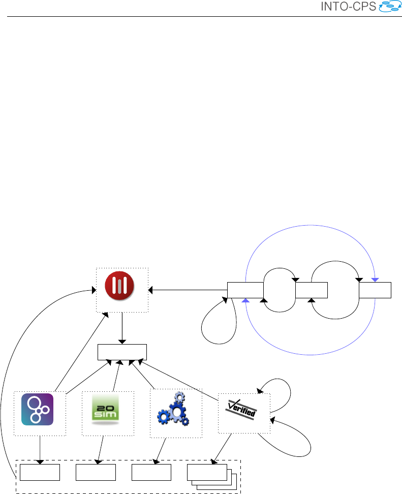
2 Overview of the INTO-CPS Tool Chain
The INTO-CPS tool chain consists of several special-purpose tools from a
number of different providers. Note that this is an open tool chain, so it is
possible to incorporate other tools that also support the FMI standard for co-
simulation. We have already tested this with numerous external tools (both
commercial as well as open-source). The constituent tools are dedicated to
the different phases of collaborative modelling activities. They are discussed
individually through the course of this manual. An overview of the tool chain
is shown in Figure 1. The main interface to INTO-CPS is the INTO-CPS
Modelio
Model Description
Overture 20-sim OpenModelica RT-Tester
FMU FMU FMU FMU
Export part
Import
Import
Import
Import
Export
Export
Export
Export
FMU Import
UML Model Exchange
INTO-CPS
App DSE COE
FMU Model Check
Co-sim Model Check
Co-sim
config
Optimal
co-sim
config
Co-sim
config
Co-sim
config
Live Update
Obtain co-sim config
Figure 1: Overview of the structure of the INTO-CPS tool chain.
Application. This is where the user can design co-simulations from scratch,
assemble them using existing FMUs and configure how simulations are exe-
cuted. The result is a multi-model. The multi-model can then be analysed
through co-simulation, model checking and model-based testing.
The design of a multi-model is carried out visually using the Modelio SysML
tool, in accordance with the SysML/INTO-CPS profile described in D2.3a
[ZCWO17]. Here one can either design a multi-model from scratch by specify-
9

INTO-CPS Tool Chain User Manual (Public)
ing the characteristics and connection topology of Functional Mockup Units
(FMUs) yet to be developed, or import existing FMUs so that the con-
nections between them may be laid out visually. The result is a SysML
architecture model of the multi-model, expressed in the SysML/INTO-CPS
profile. In the former case, where no FMUs exist yet, a number of model
Description.xml files are generated from this multi-model which serve
as the starting point for constituent model construction inside each of the
individual simulation tools, leading to the eventual FMUs.
Once a multi-model has been designed and populated with concrete FMUs,
the Co-simulation Orchestration Engine (COE) can be invoked to execute
a co-simulation. The COE controls all the individual FMUs in order to
carry out the co-simulation. In the case of tool-wrapper FMUs, the model
inside each FMU is simulated by its corresponding simulation tool. The
tools involved are Overture [LBF+10], 20-sim [Con13] and OpenModelica
[Lin15]. RT-Tester is not under the direct control of the COE at co-simulation
time, as its purpose is to carry out testing and model checking rather than
simulation. The user can configure a co-simulation, for instance by running
it with different simulation parameter values and observing the effect of the
different values on the co-simulation outcome.
Alternatively, the user has the option of exploring optimal simulation pa-
rameter values by entering a DSE phase. In this mode, ranges are defined
for various parameters which are explored, in an intelligent way, by a design
space exploration engine that searches for optimal parameter values based
on defined optimization conditions. This engine interacts directly with the
COE and itself controls the conditions under which the co-simulation is ex-
ecuted.
10

INTO-CPS Tool Chain User Manual (Public)
3 The INTO-CPS Application
This section describes the INTO-CPS Application, the primary gateway to
the INTO-CPS tool chain. Section 3.1 gives an introductory overview of the
INTO-CPS Application. Section 3.2 describes how the INTO-CPS Applica-
tion can be used to create new INTO-CPS co-simulation projects. Section
3.3 describes how multi-models can be assembled. Section 3.4 describes how
co-simulations are configured, executed and visualized. Section 3.5 lists some
additional useful features of the INTO-CPS Application, while Section 3.6
describes how the co-simulation engine itself can be started manually, for
specialist use.
3.1 Introduction
The INTO-CPS Application is the front-end of the entire INTO-CPS tool
chain. The INTO-CPS Application defines a common INTO-CPS project and
it is the easiest way to configure and execute co-simulations. Certain features
in the tool chain are only accessible through the INTO-CPS Application.
Those features will be explained in their own sections of the user manual.
This section introduces the INTO-CPS Application and its basic features
only.
Releases of the INTO-CPS Application can be downloaded from:
https://into-cps-association.github.io/into-cps/
download
Five variants are available:
•-darwin-x64.zip – MacOS version
•-linux-ia32.zip – Linux 32-bit version
•-linux-x64.zip – Linux 64-bit version
•-win32-ia32.zip – Windows 32-bit version
•-win32-x64.zip – Windows 64-bit version
The INTO-CPS Application itself has no dependencies and requires no in-
stallation. Simply unzip it and run the executable. However, certain INTO-
11

INTO-CPS Tool Chain User Manual (Public)
CPS Application features require Git1, Java 82and Python 23to be already
installed.
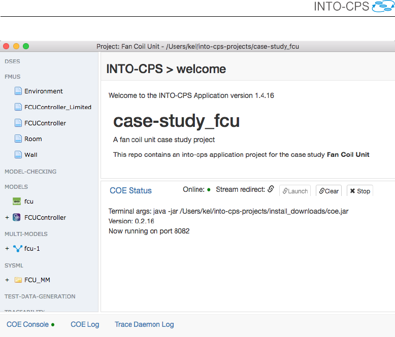
The main window of the INTO-CPS Application, with a project already
loaded, is shown in Figure 2. The left panel shows the INTO-CPS project
explorer. The central area of the window displays the contents of the current
project’s README file. The bottom of the main INTO-CPS Application
window contains two navigation tabs. When clicked, their content is dis-
played immediately above. Figure 2 shows this for the “COE Console” tab.
Elements of the main window are discussed in further detail below. The tabs
are as follows:
•“COE Console” shows the output of the COE process and log messages
with a log level of “error” or “warning”. Furthermore, a dot shows
whether the COE is online or offline. If the dot is green then the COE
is online, whereas the dot is red when the COE is offline. The “Launch”
and “Stop” buttons start and stop the COE process, respectively. If
“Stream Redirect” is followed by a link icon ( ) then the output of
the COE is shown in this part of the main window, otherwise no COE
output is shown.
•“COE log” shows the co-simulation log output according to the co-
simulation configuration.
3.2 Projects
An INTO-CPS project contains all the artifacts used and produced by the
tool chain. The project artifacts are grouped into folders. You can create
as many folders as you want and they will all be displayed in the project
browser. The default set of folders for a new project, shown in Figure 3, is:
DSES Scripts and configuration files for performing DSE experiments.
FMUs FMUs for the constituent models of the project.
Model-Checking Configuration files for performing Model Checking exper-
iments.
1https://git-scm.com/
2http://www.oracle.com/technetwork/java/javase/overview/
java8-2100321.html
3http://www.python.org/downloads/
12
INTO-CPS Tool Chain User Manual (Public)
Figure 2: INTO-CPS Application main window.
Models Sources for the constituent models of the project.
Multi-Models The multi-models of the project, using the project FMUs.
This folder also holds configuration files for performing co-simulations.
SysML Sources for the SysML model that defines the architecture and con-
nections of the project multi-model.
Test-Data-Generation Configuration files for performing test data gener-
ation experiments.
Traceability Traceability-specific files plus context menu for traceability
information.
userMetricScripts Data analysis scripts.
In order to create a new project, select File →New Project, as shown in
Figure 4a. This opens the dialog shown in Figure 4b, where you must choose
the project name and location – the chosen location will be the root of the
project, so you should manually create a new folder for it. To open an existing
13
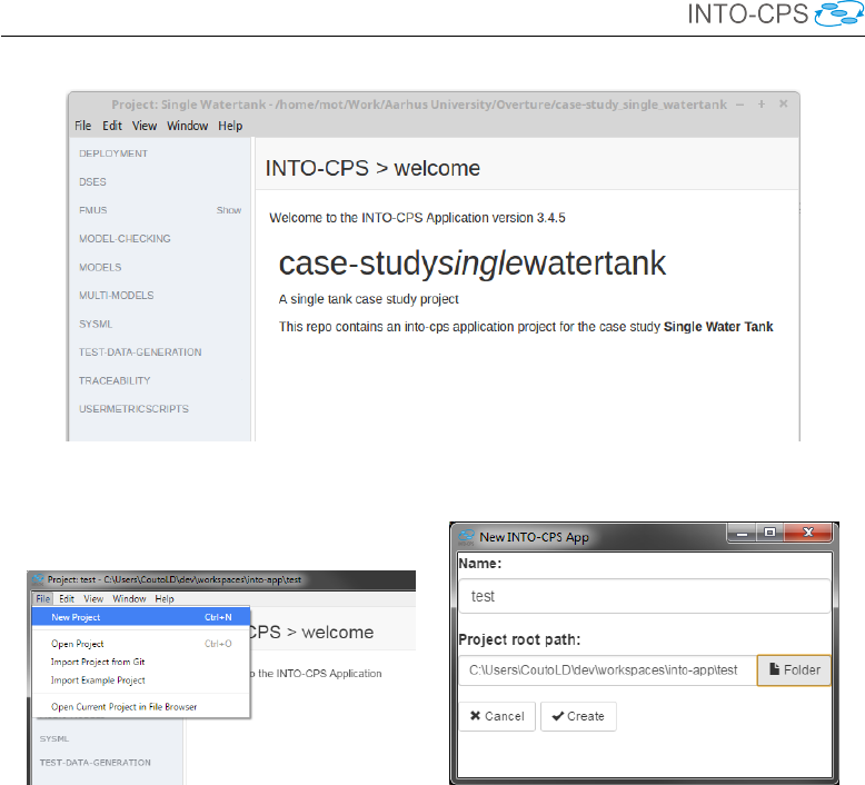
INTO-CPS Tool Chain User Manual (Public)
Figure 3: INTO-CPS project shown in the project browser.
(a) New Project menu entry. (b) New Project dialog.
Figure 4: Creating a new INTO-CPS project.
project, select File →Open Project, then navigate to the project’s root folder
and open it.
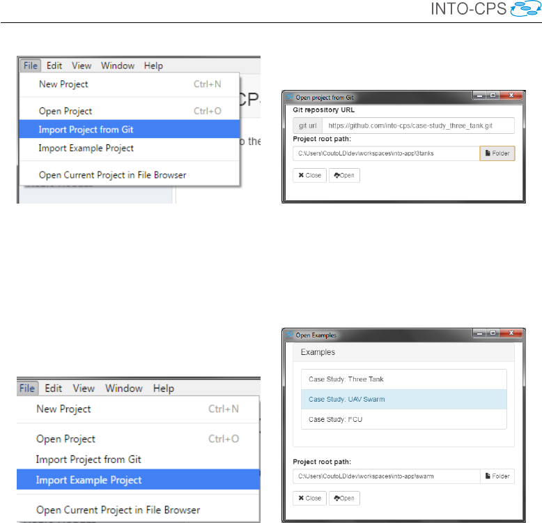
To import a project stored in the Git version control system, select File →
Import Project from Git, as shown in Figure 5a. This opens the dialog shown
in Figure 5b, where you must choose the project location and also provide
the Git URL. The project is checked out using Git, so any valid Git URL
will work. You must also have Git available in your PATH environment
variable in order for this feature to work. It is possible to import several
public example projects that show off the various features of the INTO-CPS
tool chain. These examples are described in Deliverable D3.6 [MGP+17]. To
import an example, select File →Import Example Project, as shown in Figure
6a. This opens the dialog box shown in Figure 6b, where you must select
which example to import and a project location. The example is checked out
via Git, so you must have Git available in your path in order for this feature
14
INTO-CPS Tool Chain User Manual (Public)
(a) Import Git Project menu entry. (b) Import Git Project dialog.
Figure 5: Importing a Git project.
to work. For both Git projects and examples, once you begin the import
(a) Import Example Project menu. (b) Import Example Project dialog.
Figure 6: Importing examples.
process, a process dialog is displayed, as shown in Figure 7.
3.3 Multi-Models
For any given project, the INTO-CPS Application allows you to create and
edit multi-models and co-simulation configurations. To create a new multi-
model, right click the Multi-models node in the project browser and select
New multi-model, as shown in Figure 8. After creation, the new multi-model
is automatically opened for editing. To select an existing multi-model for
editing, double-click it. Once a multi-model is open, the multi-model view,
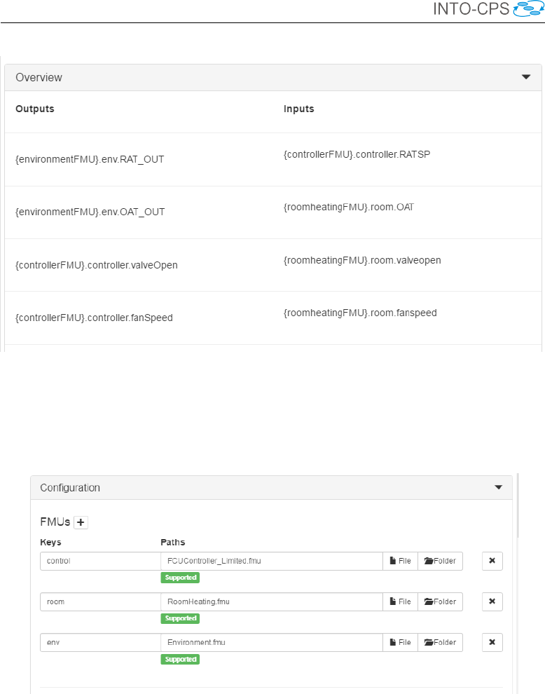
shown in Figure 9 is displayed. The top box, Overview, displays an overview
of the input and output variables in the FMUs, as shown in Figure 10. The
bottom box, Configuration, enables the user to configure the multi-model. In
15

INTO-CPS Tool Chain User Manual (Public)
Figure 7: Progress of project imports through Git.
Figure 8: Creating a new multi-model.
Figure 9: Main multi-model view.
order to configure a multi-model, it must first be unlocked for editing by click-
ing the Edit button at the bottom of the Configuration box. There are four
main areas dedicated to configuring various aspects of a multi-model.
The FMUs area, shown in Figure 11, allows you to remove or add FMUs
and to associate the FMUs with their files by browsing to, or typing, the
path of the FMU file. For each FMU file a marker is displayed indicating
16
INTO-CPS Tool Chain User Manual (Public)
Figure 10: Multi-model overview.
whether the FMU is supported by the INTO-CPS Application and can be
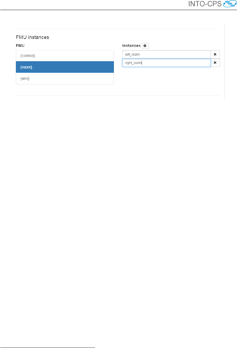
used for co-simulation on the current platform. The FMU instances area,
Figure 11: FMUs configuration.
shown in Figure 12, allows you to create or remove FMU instances and name
them. A multi-model consists of one or more interconnected instances of
various FMUs. More than one instance may be created for a given FMU.
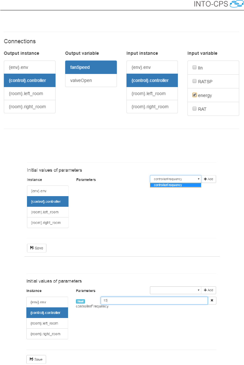
As a convenient workflow shortcut, the Connections area, shown in Figure
13, allows you to connect output variables from an FMU instance into input
variables of another:
17
INTO-CPS Tool Chain User Manual (Public)
Figure 12: FMU instances configuration.
1. Click the desired output FMU instance in the first column. The output
variables for the selected FMU appear in the second column.
2. Click the desired output variable in the second column. The input
instances appear in the third column.
3. Click the desired FMU input instance in the third column. The input
variables for the selected FMU appear in the fourth column.
4. Check the box for the desired input variable in the fourth column.
This facility makes it unnecessary to return to Modelio whenever small
changes must be made to the connection topology of the multi-model4. The
Initial values of parameters area, shown in Figure 14, allows you to set the
initial values of any parameters defined in the FMUs:
1. Click the desired FMU instance in the Instance Column.
2. Select the desired parameter in the Parameters dropdown box and click
Add.
3. Type the parameter value in the box that appears.
Once the multi-model configuration is complete, click the Save button at the
bottom of the Configuration box.
4Changes made to a multi-model or FMU outside of the INTO-CPS Application will
cause internal CRC checks to fail. If this route is taken, it will be necessary to open
the multi-model configuration again in the INTO-CPS Application and go through the
edit-save procedure without making any changes. This will re-validate the multi-model
configuration.
18
INTO-CPS Tool Chain User Manual (Public)
Figure 13: Connections configuration.
(a) Parameter selection.
(b) Parameter value input.
Figure 14: Initial values of parameters configuration.
19
INTO-CPS Tool Chain User Manual (Public)
3.4 Co-simulations
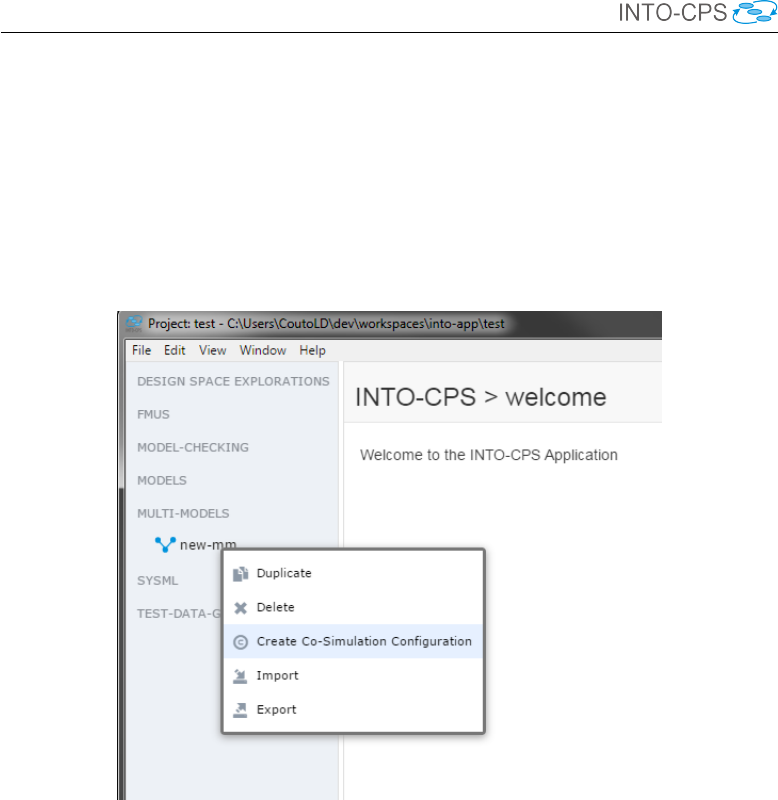
To execute co-simulations of a multi-model, a co-simulation configuration is
needed. To create a co-simulation configuration, right click the desired multi-
model and select Create Co-Simulation Configuration, as shown in Figure
15. After creation, the new configuration automatically opens for editing.
To select an existing co-simulation configuration, double-click it. Once a
Figure 15: Creating a co-simulation configuration.
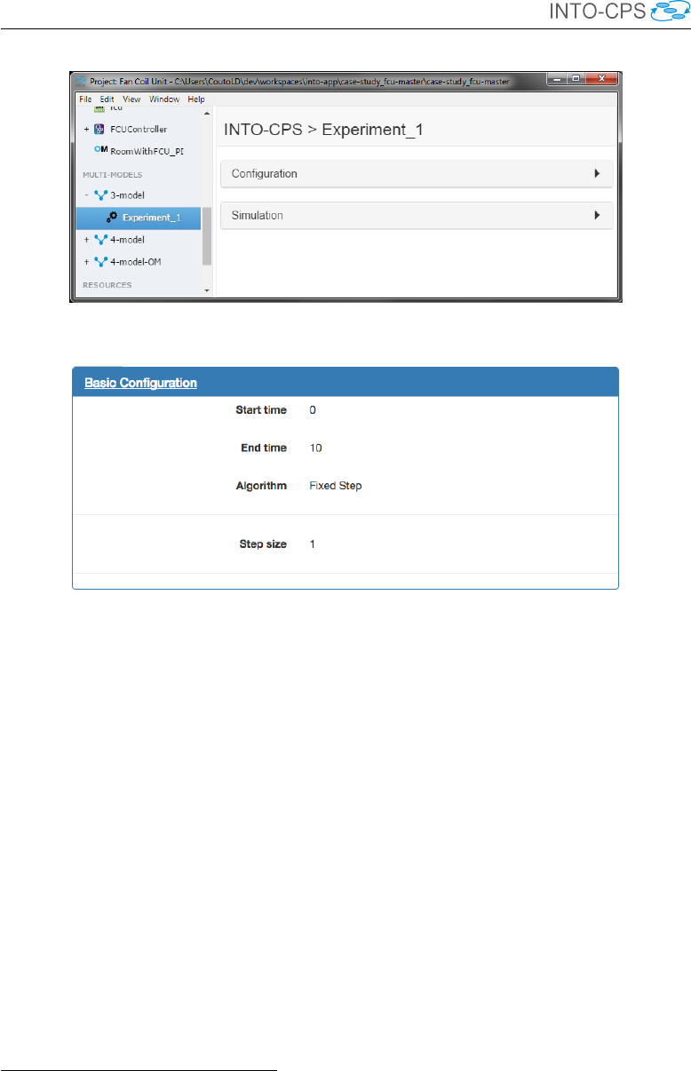
configuration is open, the co-simulation configuration, shown in Figure 16, is
displayed. The top box, Configuration, lets you configure the co-simulation.
The bottom box, Simulation, lets you execute the co-simulation. In order to
configure a co-simulation, the configuration must first be unlocked for editing
by clicking the Edit button at the bottom of the Configuration box. There
are seven things to configure for a co-simulation, discussed next.
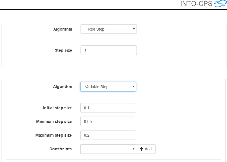
Basic Configuration, shown in Figure 17, allows you to select the start and
end time for the co-simulation as well as the master algorithm to be used. For
every algorithm, there are configuration parameters that can be set. These
are displayed below the top area, as shown in Figure 18. These parameters
differ with the master algorithm chosen. Parameters are further documented
in Deliverable D4.3b [PBL+17].
20
INTO-CPS Tool Chain User Manual (Public)
Figure 16: Main co-simulation configuration view.
Figure 17: Start/End time and master algorithm configuration.
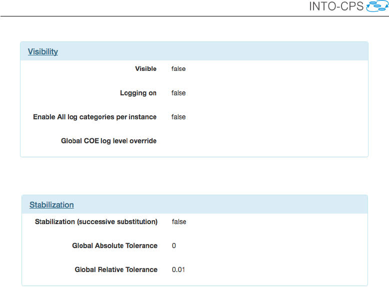
The Visibility area, shown in Figure 19, controls loggable FMU output. Vis-
ible indicates whether the FMU gives any visible feedback, e.g. graphs. Log-
ging on indicates whether the FMU should use the logging system and send
log info back to the COE. Enable all log categories per instance enables all
log categories listed inside each FMU. Global coe log level override enables
the user to override the pre-set log level in the COE. This is for debugging
failing simulations and should be left unset or at “error” or “warning” level.
The Stabilization area, shown in Figure 20, allows the user to enable the
global co-simulation stabilization feature. These parameters are passed to
the NumPy isclose() function5.
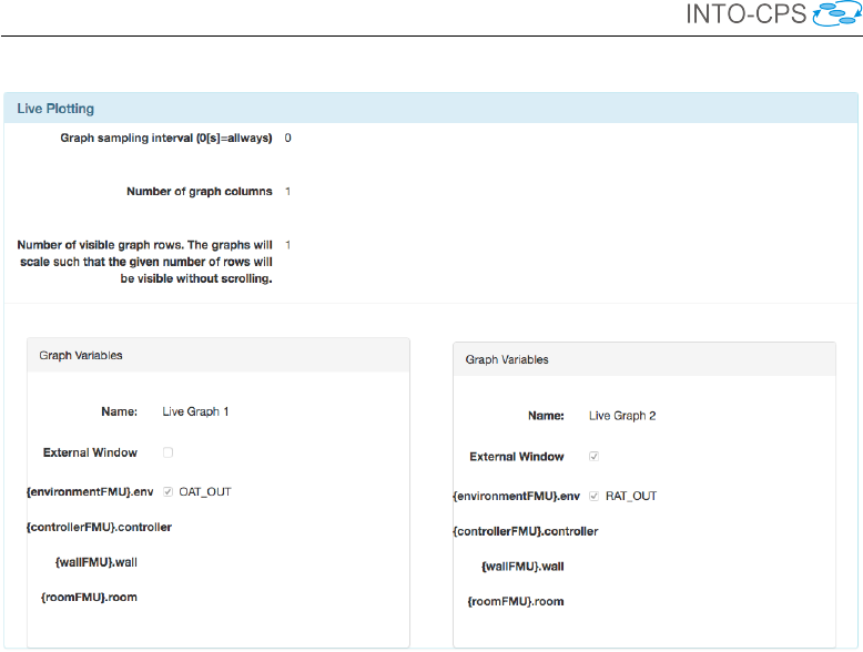
The Live Plotting area, shown in Figure 21, enables the user to define multiple
graphs (currently this comes at a relatively high display cost.) Each graph
can either be external (in its own window) or internal (embedded). The
5https://docs.scipy.org/doc/numpy-1.13.0/reference/generated/
numpy.isclose.html
21
INTO-CPS Tool Chain User Manual (Public)
(a) Fixed step size.
(b) Variable step size.
Figure 18: Master algorithm configuration.
internal graphs are arranged in a configurable grid. The aim of the grid
layout is to eliminate the need for scrolling. Additional rows are added if no
space is left, but these introduce scrolling. When configuring the graphs, it
is possible to use a filter on all available scalar variables to find the ones of
interest.
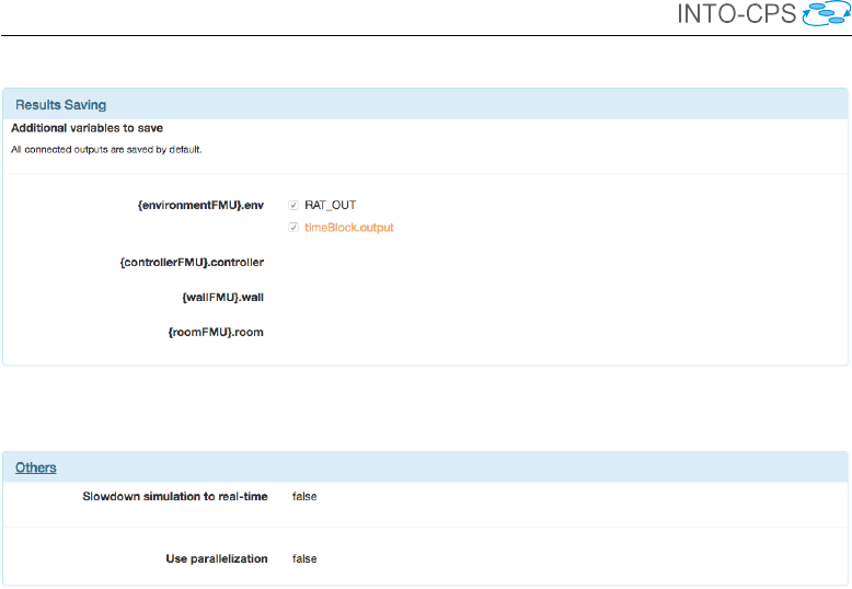
The Results Saving area, shown in Figure 22, allows the user to select addi-
tional FMU variables to log in the global CSV log file. All connected variables
are logged by default.
The Others area, shown in Figure 23, allows the user to slow the co-simulation
down to wall time and to enable co-simulation parallelisation. Please note
that parallelising a co-simulation does not always result in a speed-up [TL16].
The final area, Post-Processing, shown in Figure 24, allows the user to attach
a post-processing script written in Python that can be executed at the end
of co-simulations.
Once the co-simulation configuration is complete, click the Save button at
the bottom of the Configuration box.
22
INTO-CPS Tool Chain User Manual (Public)
Figure 19: Visibility configuration.
Figure 20: Stabilization configuration.
The Simulation box, shown in Figure 25, allows you to launch a co-simulation.
To run a co-simulation, the COE must be online. The area at the top of the
Simulation box displays the status of the COE. If the COE is offline, you
may click the Launch button to start it. Once a co-simulation is in progress,
any variables chosen for live plotting are plotted in real time in the simula-
tion box, as shown in Figure 26. A progress bar is also displayed. When the
simulation is complete, the live stream plot can be explored or exported as
a PNG image. In addition, an outputs.csv file is created containing the
values of every variable marked for logging. This file can be double-clicked
and it will open with the default system program for CSV files. It can also
be imported into programs such as R, MATLAB or Excel for more complex
analysis. Furthermore, it is possible to add a post-processing script that
receives the CSV file name and the total simulation time respectively as ar-
guments. It is also possible to configure the amount of logging performed by
the COE.
23
INTO-CPS Tool Chain User Manual (Public)
Figure 21: Live plotting configuration.
3.5 Additional Features
The INTO-CPS Application has several secondary features, most of them
accessible through the Window menu, as shown in Figure 27. They are
briefly explained below.
Show Settings Displays a settings page where various default paths and
other options can be set. Development mode can also be enabled from
this page, but this feature is primarily meant to be used by developers
for testing. Documentation for each setting is found here.
Show Download Manager Displays a page where installers can be down-
loaded for the various tools of the INTO-CPS tool chain, including the
COE.
Show FMU Builder Displays a page that links to a service where source
code FMUs can be uploaded and cross-compiled for various platforms.
Note that this is not a secure service and users are discouraged from
uploading proprietary FMUs.
24
INTO-CPS Tool Chain User Manual (Public)
Figure 22: Results logging configuration.
Figure 23: Miscellaneous configuration options.
3.6 The Co-Simulation Orchestration Engine
The heart of the INTO-CPS Application is the Co-Simulation Orchestration
Engine (COE). This is the engine that orchestrates the various simulation
tools (described below), carrying out their respective roles in the overall co-
simulation. It runs as a stand-alone server hosting the co-simulation API on
port 8080. It can be started from the INTO-CPS Application, but it may be
started manually at the command prompt for testing and specialist purposes
by executing:
java -jar coe.jar 8082
TCP port 8082 will be chosen by default if it is omitted in the command
above. The COE is entirely hidden from the end user of the INTO-CPS Ap-
plication, but parts of it are transparently configured through the main inter-
face. The design of the COE is documented in Deliverable D4.1d [LLW+15].
The COE is controlled using simple HTTP requests. These are documented
in the API manual, which can be obtained directly from the COE by navi-
gating to http://localhost:8082, once the COE is running. Port 8082
should be changed to that specified when the COE is started.
Following the protocol detailed in the API document, a co-simulation session
can be controlled manually from the command prompt using, for example,
25
INTO-CPS Tool Chain User Manual (Public)
Figure 24: Attaching a post-processing script.
(a) COE offline. (b) COE online.
Figure 25: Launching a co-simulation.
the curl utility, as demonstrated in the following example.
With the COE running, a session must first be created:
curl http://localhost:8082/createSession
This command will return a sessionID that is used in the following com-
mands.
Next, assuming a COE configuration file called coeconf.json has been
created as described in the API manual, the session must be initialized:
curl -H "Content-Type: application/json"
--data @coeconf.json
http://localhost:8082/initialize/sessionID
Assuming start and end time information has been saved to a file, say
startend.json, the co-simulation can now be started:
curl -H "Content-Type: application/json"
--data @startend.json
http://localhost:8082/simulate/sessionID
Once the co-simulation run ends, the results can be obtained as follows:
curl -o results.zip
http://localhost:8082/result/sessionID/zip
The session can now be terminated:
curl http://localhost:8082/destroy/sessionID
26

INTO-CPS Tool Chain User Manual (Public)
Figure 26: Live stream variable plot.
Figure 27: Additional features.
The INTO-CPS Application fundamentally controls the COE in this way.
Distributed co-simulations Presently the INTO-CPS Application can
only control the COE in this way for non-distributed co-simulations. In
27

INTO-CPS Tool Chain User Manual (Public)
order to run a distributed co-simulation, a distributed version of the COE,
dcoe, must be controlled from the command prompt manually, as illustrated
above. The distributed COE can be downloaded using the App’s Download
Manager.
In a distributed co-simulation the COE and (some) FMUs execute on physi-
cally different compute nodes. The FMUs local to the COE computing node
are handled in the same way as in standard co-simulations.
Each FMU on the remote nodes is served externally by a daemon process.
This process must be started on the remote node manually as follows:
java -jar daemon*-jar-with-dependencies.jar -host
<public-ip> -ip4
Here, <public-ip> is the IPv4 address of the compute node.
Next, the distributed COE process must be started manually from the com-
mand prompt on its own node, with options specific to distributed co-simulation:
java -Dcoe.fmu.custom.factory=
org.intocps.orchestration.coe.distribution.
DistributedFmuFactory
-jar dcoe*-jar-with-dependencies.jar
The second difference is the way in which the location of the remote FMUs is
specified. For a standard co-simulation, the fmus clause of the co-simulation
configuration file (coeconf.json, in our example) contains elements of the
form
“file://fmu-1-path.fmu”
These must be modified for each remote FMU to the following URI scheme:
“uri://<public-ip>/FMU/#file://local-fmu-path.fmu”
The COE configuration file can, of course, be written manually in its entirety,
but it is possible to take a faster route, as follows.
This configuration file is only generated when a co-simulation is executed.
It is therefore possible to assemble a “dummy” co-simulation that is similar
to the desired distributed version, but with a local FMU topology. Since
it is likely that the remote FMUs are not supported on the COE platform
itself, it is necessary here to construct “dummy” FMUs with the same inter-
face. If this local co-simulation is then executed briefly, a COE configuration
file will be emitted that can be easily modified as described above. The
INTO-CPS Application will name this file config.json and emit it to the
28

INTO-CPS Tool Chain User Manual (Public)
Multi-models folder under each co-simulation run. This modified config-
uration can then be used to execute the distributed co-simulation.
29
INTO-CPS Tool Chain User Manual (Public)
4 Modelio and SysML
The INTO-CPS tool chain supports a model-based approach to the develop-
ment and validation of CPS. The Modelio tool and its SysML/INTO-CPS
profile extension provide the diagramming starting point. This section de-
scribes the Modelio extension that provides INTO-CPS-specific modelling
functionality to the SysML modelling approach.
The INTO-CPS extension module is based on the Modelio SysML extension
module, and extends it in order to fulfill INTO-CPS modelling requirements
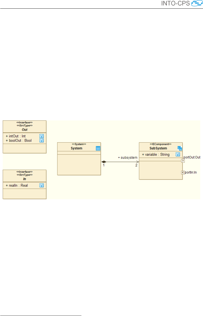
and needs. Figure 28 shows an example of a simple INTO-CPS Architecture
Structure Diagram under Modelio. This diagram shows a System, named
Figure 28: Example INTO-CPS multi-model.
“System”6, composed of two EComponents of kind Subsystem, named “Sub-
System”7. These Subsystems have an internal Variable called “variable” of
type String and expose two FlowPorts named “portIn” and “portOut”. The
type of data going through these ports is respectively defined by types In
and Out of kind StrtType. More details on the SysML/INTO-CPS profile
can be found in Deliverable D2.3a [ZCWO17].
Figure 29 illustrates the main graphical interface after Modelio and the
INTO-CPS extension have been installed. Of all the panes, the following
three are most useful in the INTO-CPS context.
1. The Modelio model browser, which lists all the elements of your model
in tree form.
6An abstract description of an INTO-CPS multi-model.
7Abstract descriptions of INTO-CPS constituent models.
30
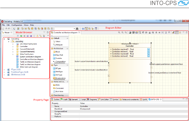
INTO-CPS Tool Chain User Manual (Public)
Figure 29: Modelio for INTO-CPS.
2. The diagram editor, which allows you to create INTO-CPS design ar-
chitectures and connection diagrams.
3. The INTO-CPS property page, in which values for properties of INTO-
CPS subsystems are specified.
4.1 Creating a New Project
In the INTO-CPS Modelling workflow described in Deliverable D3.3a [FGP17],
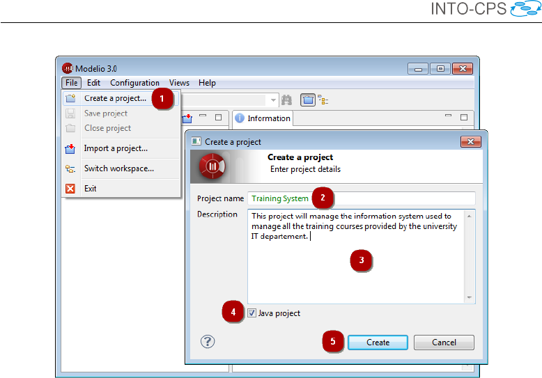
the first step will be to create, as depicted in Figure 30, a Modelio project:
1. Launch Modelio.
2. Click on File →Create a project....
3. Enter the name of the project.
4. Enter the description of the project.
5. If it is envisaged that the project will be connected to a Java develop-
ment workflow in the future (unrelated to INTO-CPS), you can choose
to include the Java Designer module by selecting Java Project, other-
wise de-select this option.
6. Click on Create to create and open the project.
31
INTO-CPS Tool Chain User Manual (Public)
Figure 30: Creating a new Modelio project.
Once you have successfully created a Modelio project, you have to install
the Modelio extensions required for INTO-CPS modelling, i.e. both Modelio
SysML and INTO-CPS extensions, as described at
http://into-cps-association.github.io
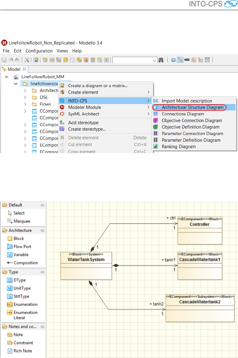
If both modules have been correctly installed, you should be able to create,
under any package, an INTO-CPS Architecture Structure Diagram in order
to model the first subsystem of your multi-model. For that, in the Modelio
model browser, right click on a Package element then in the INTO-CPS
entry, choose Architecture Structure Diagram as shown in Figure 31. Once
you are sure that the modules have been correctly installed. You are able to
start your INTO-CPS SysML modelling.
4.2 INTO-CPS SysML modelling
INTO-CPS SysML modelling activitIES can be succinctly described as the
creation and population of INTO-CPS SysML diagrams. Figure 31 shows
you how to create an Architecture Structure Diagram. Figure 32 represents
an example of an Architecture Structure Diagram. Besides creating an Ar-
chitecture Structure Diagram from scratch and specifying by hand the blocks
of your system, the INTO-CPS extension allows the user to create a block
32
INTO-CPS Tool Chain User Manual (Public)
Figure 31: Creating an Architecture Structure diagram.
Figure 32: Example Architecture Structure diagram.
33
INTO-CPS Tool Chain User Manual (Public)
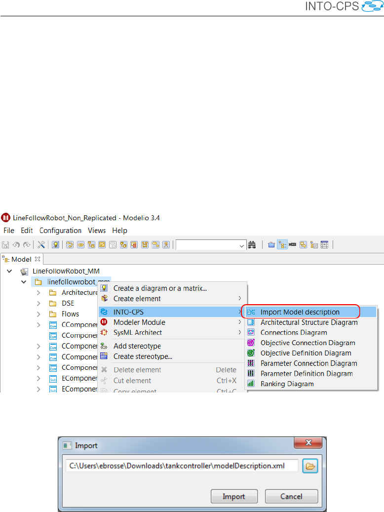
from an existing modelDescription.xml file . A modelDescription
.xml file is an artifact defined in the FMI standard which specifies, in XML
format, the public interface of an FMU. To import a modelDescription
.xml file,
1. Right click in the Modelio model browser on a Package element, then
in the INTO-CPS entry choose Import Model description, as shown in
Figure 33.
2. Select the desired modelDescription.xml file (or the .fmu file
that should contain a modelDescription.xml file ) in your instal-
lation and click on Import (Figure 34).
Figure 33: Importing an existing model description.
Figure 34: Model description selection.
This import command creates an Architecture Structure Diagram describing
the interface of an INTO-CPS block corresponding to the modelDescrip-
tion.xml file imported, cf. Figure 35. Once you have created several such
blocks, either from scratch or by importing modelDescription.xml files,
you must eventually connect instances of them in an INTO-CPS Connection
34
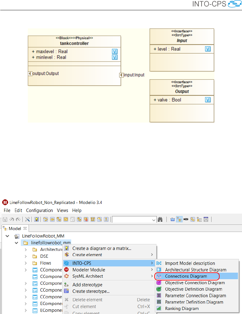
INTO-CPS Tool Chain User Manual (Public)
Figure 35: Result of model description import.
Diagram. To create an INTO-CPS Connection diagram, as for an INTO-
CPS Architecture Structure Diagram, right click on a Package element, then
in the INTO-CPS entry choose Connection Diagram, as shown in Figure 36.
Figure 37 shows the result of creating such a diagram. Once you have created
Figure 36: Creating a Connection diagram.
all desired block instances and their ports by using the dedicated command in
the Connection Diagram palette, you will be able to model their connections
by using the connector creation command (Figure 38). At this point your
blocks have been defined and the connections have been set. The next step is
to simulate your multi-model using the INTO-CPS Application. For that you
must first generate a configuration file from your Connection diagram. Select
35

INTO-CPS Tool Chain User Manual (Public)
Figure 37: Unpopulated Connection diagram.
Figure 38: Populated Connection diagram.
36
INTO-CPS Tool Chain User Manual (Public)
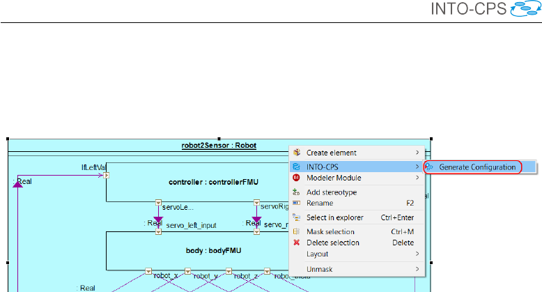
the top element in the desired Connection diagram, right click on it and in
the INTO-CPS entry choose Generate configuration, as shown in Figure 39.
In the final step, choose a relevant name and click on Generate.
Figure 39: Generating a configuration file.
The SysML Connection diagram defines the components of the system and
their connections. The internals of these block instances are created in
the various modeling tools and exported as FMUs. The modeling tools
Overture, 20-sim and OpenModelica support importing the interface def-
inition (ports) of the blocks in the Connection diagram by importing a
modelDescription.xml file containing the block name and its interface
definition.
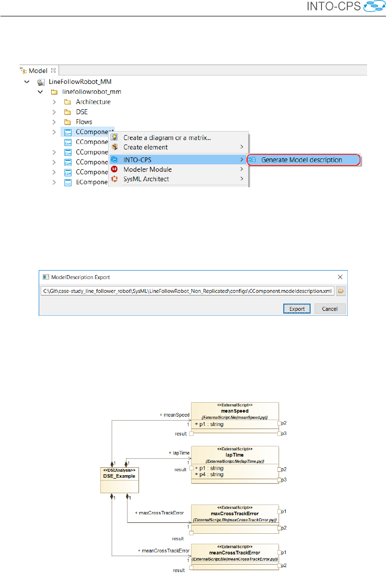
Follow these steps to export a modelDescription.xml file from Mode-
lio:
1. In Modelio, right-click on the model block in the tree.
2. Select INTO-CPS →Generate Model Description (see Figure 40).
3. Choose a file name containing the text “modelDescription.xml” and
click Export (see Figure 41).
4.3 DSE Modelling
For design space exploration (DSE) purposes, a DSE model can be con-
structed in Modelio as well. This modelling is done by specifying mainly a
DSE analysis, its parameters, its objectives and a ranking method. Figure 42
depicts an example of a DSE objective definition. More details and examples
can be found in Deliverable D4.2c [BQ16].
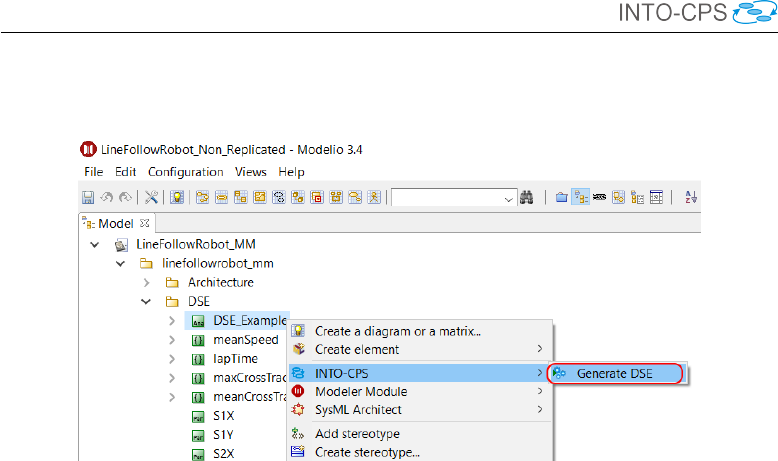
Once the DSE model has been created, the DSE analysis can be exported
to the INTO-CPS Application. To do so, right-click on DSE Analysis in the
37
INTO-CPS Tool Chain User Manual (Public)
Figure 40: Exporting a modelDescription.xml file.
Figure 41: Naming the model description file.
Figure 42: DSE Objective definition.
38
INTO-CPS Tool Chain User Manual (Public)
model tree as depicted in Figure 43. In the final step, choose a relevant name
Figure 43: DSE Export command.
and click on Export.
4.4 Behavioural Modelling
For test generation and/or model-checking analysis, a behavioural model of
the system is required. This is usually referred to as test model in order to
indicate its purpose. It is typically not identical to the design model, because
it can omit or abstract implementation details. The test model needs to cap-
ture all inputs and outputs and describe the system’s reactions to inputs by
means of one or more deterministic state machine diagram. Timing behaviour
should be included by means of timers and timer-guarded transitions. For
more details and examples refer to the RTT-MBT Manual [Ver15b].
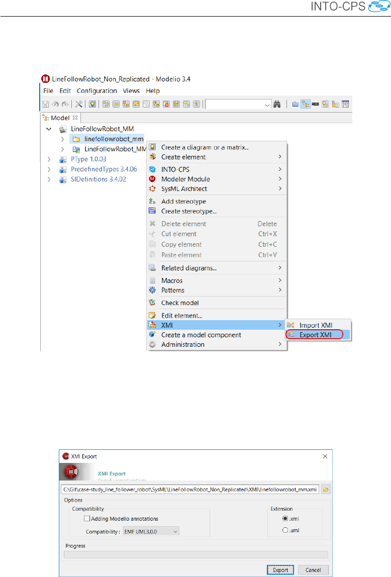
Once the behavioural model has been specified, the entire model must be
exported in XMI format. To do so, right-click on the top package in the
model tree as depicted in Figure 44. Then select the file path by using the
XMI export window, as shown in Figure 45. Note that compatibility must
be set to "EMG UML 3.0.0" and the file extension to ".xmi".
39
INTO-CPS Tool Chain User Manual (Public)
Figure 44: XMI Export command.
Figure 45: XMI export windows.
40

INTO-CPS Tool Chain User Manual (Public)
5 Using the Separate Modelling and Simula-
tion Tools
This section provides a tutorial introduction to the FMI-specific functionality
of each of the modelling and simulation tools. This functionality is centered
on the role of FMUs for each tool. For more general descriptions of each tool,
please refer to Appendix B.
5.1 Overture
Overture implements export of both tool-wrapper as well as standalone FMUs.
It also has the ability to import a modelDescription.xml file in order to
facilitate creating an FMI-compliant model from scratch. A typical workflow
in creating a new FMI-compliant VDM-RT model starts with the import
of a modelDescription.xml file created using Modelio. This results in
a minimal project that can be exported as an FMU. The desired model is
then developed in this context. This section discusses the complete work-
flow.
5.1.1 Installing the FMI import/export plugin for Overture
In order to use the FMI integration in Overture it is necessary to install a
plugin. Below is a guide to install the plugin:
1. Open Overture.
2. Select Help -> Install New Software.
3. Click Add...
4. In the Name: field write Overture FMU.
5. In the Location: field there are two options:
INTO-CPS Application: Download the Overture FMU Import / Ex-
porter - Overture FMI Support using the Download Manager men-
tioned in Section 3.5. Locate the file using the Archive... button
next to the Location: field.
Update site: Enter the following URL in the Location: field:
http://overture.au.dk/into-cps/vdm-tool-wrapper/master/latest.
41
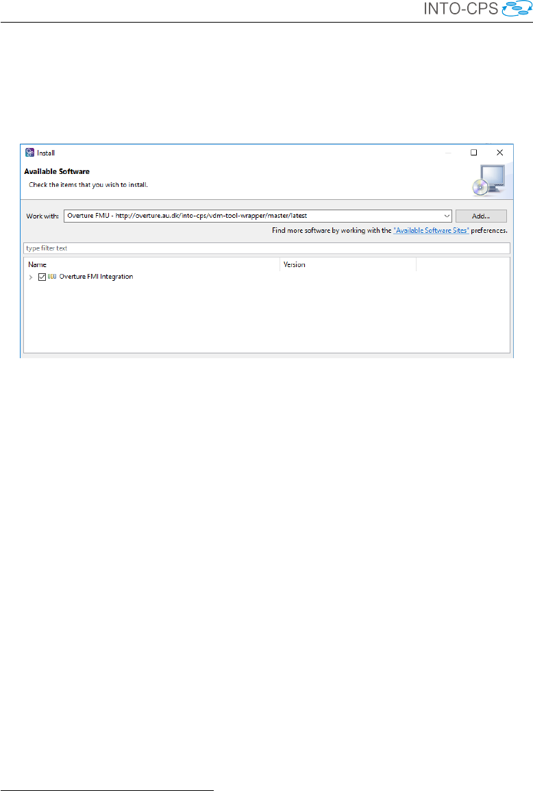
INTO-CPS Tool Chain User Manual (Public)
6. Check the box next to Overture FMI Integration as shown in Figure
46.
7. Click Next or Finish to accept and install.
Figure 46: Installing Overture FMI Integration.
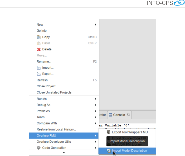
5.1.2 Import of modelDescription.xml File
AmodelDescription.xml file is easily imported into an existing, typ-
ically blank, VDM-RT project from the project explorer context menu as
shown in Figure 47. This results in the project being populated with the
classes necessary for FMU export:
•A VDM-RT system class named “System” containing the system def-
inition. The corresponding “System” class for the water tank controller
FMU is shown in Listing 48.
•A standard VDM-RT class named “World”. This class is conventional
and only provides an entry point into the model. The corresponding
“World” class for the water tank controller FMU is shown in Listing 49.
•A standard VDM-RT class named “HardwareInterface”. This class con-
tains the definition of the input and output ports of the FMU. Its struc-
ture is enforced, and a self-documenting annotation scheme8is used
such that the “HardwareInterface” class may be hand-written. The
8The annotation scheme is documented on the INTO-CPS website
into-cps-association.github.io under “Constituent Model Development →
Overture →FMU Import/Export.
42

INTO-CPS Tool Chain User Manual (Public)
system System
instance variables
-- Hardware interface variable required by FMU Import/Export
public static hwi: HardwareInterface := new
HardwareInterface();
instance variables
public levelSensor : LevelSensor;
public valveActuator : ValveActuator;
public static controller : [Controller] := nil;
cpu1 : CPU := new CPU(<FP>, 20);
operations
public System : () ==> System
System () ==
(
levelSensor := new LevelSensor(hwi.level);
valveActuator := new ValveActuator(hwi.valveState);
controller := new Controller(levelSensor, valveActuator);
cpu1.deploy(controller,"Controller");
);
end System
Figure 48: “System” class for water tank controller.
44

INTO-CPS Tool Chain User Manual (Public)
class World
operations
public run : () ==> ()
run() ==
(start(System‘controller);
block();
);
private block : () ==>()
block() ==
skip;
sync
per block => false;
end World
Figure 49: “World” class for water tank controller.
class HardwareInterface
values
-- @ interface: type = parameter, name="minlevel";
public minlevel : RealPort = new RealPort(1.0);
-- @ interface: type = parameter, name="maxlevel";
public maxlevel : RealPort = new RealPort(2.0);
instance variables
-- @ interface: type = input, name="level";
public level : RealPort := new RealPort(0.0);
instance variables
-- @ interface: type = output, name="valve";
public valveState : BoolPort := new BoolPort(false);
end HardwareInterface
Figure 50: “HardwareInterface” class for water tank controller.
45

INTO-CPS Tool Chain User Manual (Public)
The port structure used in the “HardwareInterface” class is a simple inheri-
tance structure, with a top-level generic “Port”, subclassed by ports for spe-
cific values: booleans, reals, integers and strings. The hierarchy is shown in
Listing 51. When a model is developed without the benefit of an existing
modelDescription.xml file, this library file can be added to the project
from the project context menu, also under the category “Overture FMU”.
With all the necessary FMU scaffolding in place, the VDM-RT model can be
developed as usual.
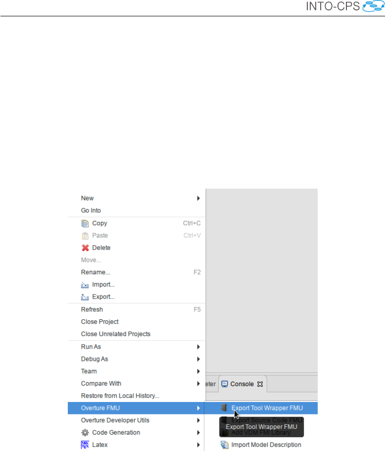
5.1.3 Tool-Wrapper FMU Export
Models exported as tool-wrapper FMUs require the Overture tool to sim-
ulate. Export is implemented such that the VDM interpreter and its FMI
interface are included in the exported FMU. Overture tool-wrapper FMUs
currently support Win32, Win64, Linux64, Darwin64 and require Java 1.7
to be installed and available in the PATH environment variable.
A tool-wrapper FMU is easily exported from the project context menu as
shown in Figure 52. The FMU will be placed in the generated folder.
46

INTO-CPS Tool Chain User Manual (Public)
class Port
types
public String = seq of char;
public FmiPortType = bool |real |int | String;
operations
public setValue : FmiPortType ==> ()
setValue(v) == is subclass responsibility;
public getValue : () ==> FmiPortType
getValue() == is subclass responsibility;
end Port
class IntPort is subclass of Port
instance variables
value: int:=0;
operations
public IntPort: int ==> IntPort
IntPort(v)==setValue(v);
public setValue : int ==> ()
setValue(v) ==value :=v;
public getValue : () ==> int
getValue() == return value;
end IntPort
class BoolPort is subclass of Port
instance variables
...
Figure 51: Excerpt of “Fmi.vdmrt” library file defining FMI interface port
hierarchy.
47
INTO-CPS Tool Chain User Manual (Public)
Figure 52: Exporting a tool-wrapper FMU.
48
INTO-CPS Tool Chain User Manual (Public)
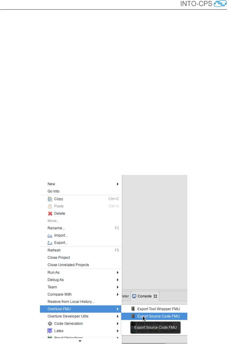
5.1.4 Standalone FMU Export
In contrast to tool-wrapper FMUs, models exported as standalone FMUs
do not require Overture in order to simulate. Instead, they are first passed
through Overture’s C code generator such that a standalone implementation
of the model is first obtained. Once compiled, this executable model then
replaces the combination of VDM interpreter and model, and the FMU ex-
ecutes natively on the co-simulation platform. Currently Mac OS, Windows
and Linux are supported.
The export process consists of two steps. First, a source code FMU is ob-
tained from Overture as shown in Figure 53. Second, the INTO-CPS Appli-
cation must be used to upload the resulting FMU to the FMU compilation
server using the built-in facility described in Section 3.5. This is accessed by
navigating to Window →Show FMU Builder.
Please note that only some features of VDM-RT are currently supported by
the C code generator. This is discussed in more detail in Section 9.
Figure 53: Exporting a standalone FMU.
49
INTO-CPS Tool Chain User Manual (Public)
5.2 20-sim
This section explains the FMI and INTO-CPS related features of 20-sim9.
We focus on the import of modelDescription.xml files, standalone and
tool-wrapper FMU export (FMU slave), 3D visualization of FMU operation
and an experimental FMU import (FMU master) feature. The complete
20-sim tool documentation can be found in the 20-sim Reference Manual
[KGD16].
5.2.1 Import of modelDescription.xml File
20-sim can automatically generate an empty 20-sim submodel 10 from a mo-
delDescription.xml file. To use the modelDescription.xml im-
port, you will need to use the special “4.6.4-intocps” version of 20-sim11. A
modelDescription.xml file can be imported into 20-sim by using Win-
dows Explorer to drag the modelDescription.xml file onto your 20-sim
model (see Figure 54). This creates a new empty submodel with a blue icon
that has the same inputs and outputs as defined in the modelDescription
.xml file.
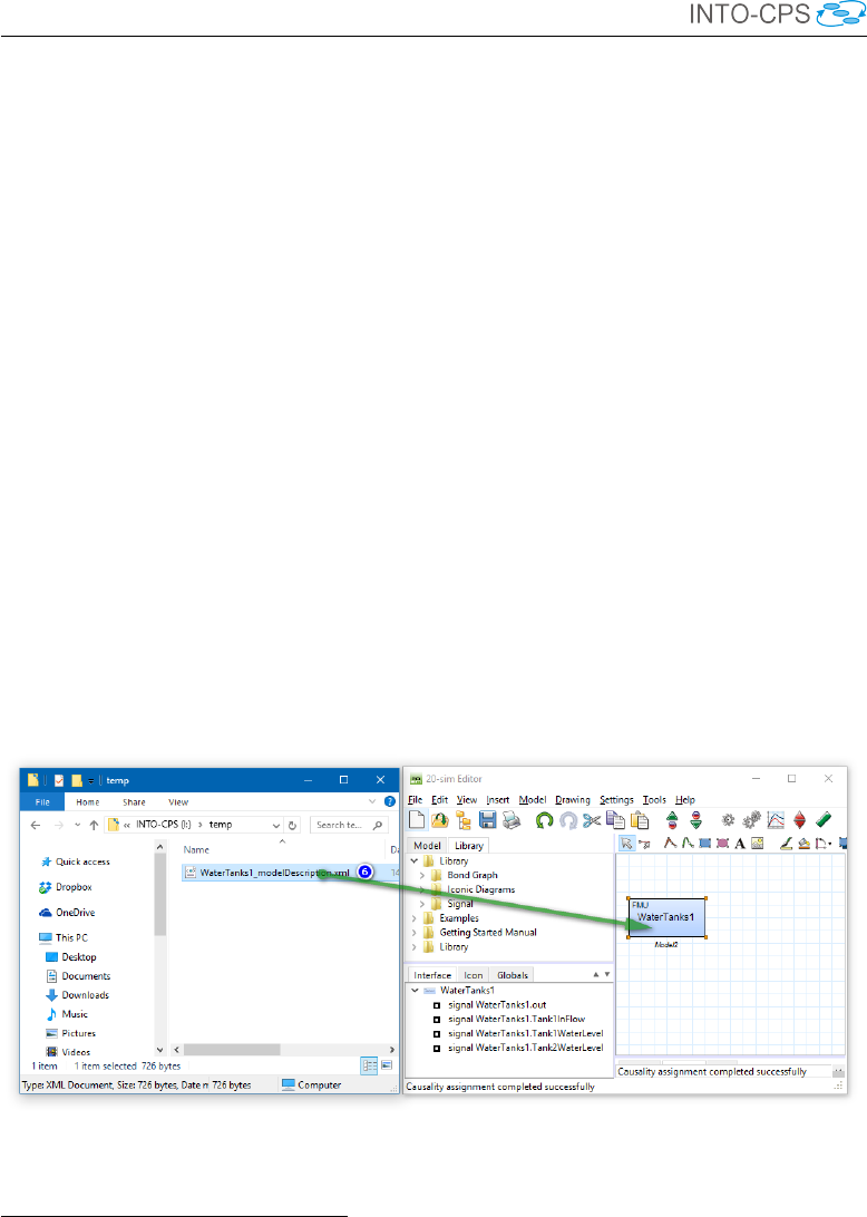
Figure 54: Import a Model Description in 20-sim.
9Note that 20-sim is Windows-only. However, it can run fine using Wine [Win16] on
other platforms. For details on using 20-sim under Wine, contact Controllab.
10Note that the term “submodel” here should not be confused with the INTO-CPS notion
of a “constituent model”. A submodel here is a part in a graphical 20-sim model.
11You can download the INTO-CPS version of 20-sim using the Download Manager in
the INTO-CPS Application.
50

INTO-CPS Tool Chain User Manual (Public)
5.2.2 Tool-wrapper FMU Export
A tool-wrapper FMU is a communication FMU that opens the original
model in the modelling tool and takes care of remotely executing the co-
simulation steps inside the modelling tool using some tool-supported com-
munication mechanism. 20-sim supports co-simulation using the XML-RPC-
based DESTECS co-simulation interface [LRVG11]. The generation of a
tool-wrapper FMU involves two steps that will be explained below:
1. Extend the model with co-simulation inputs, outputs and shared design
parameters.
2. Generate a model-specific tool-wrapper FMU.
The tool-wrapper approach involves communication between the co-simula-
tion engine (COE) and the 20-sim model through the tool-wrapper FMU.
The 20-sim model should be extended with certain variables that can be
set or read by the COE. These variables are the co-simulation inputs and
outputs. They can be defined in the model in an equation section called
externals:
externals
real global export mycosimOutput;
real global import mycosimInput;
To make it possible to set or read a parameter by the co-simulation engine,
it should be marked as ’shared’:
parameters
// shared design parameters
real mycosimParameter (’shared’) = 1.0;
The next step is to generate a tool-wrapper FMU for the prepared model.
This requires at least the “4.6.3-intocps” version of 20-sim12. This version of
20-sim comes with a Python script that generates a tool-wrapper FMU for
the loaded model.
To generate the tool-wrapper FMU:
1. Make sure that the tool-wrapper prepared 20-sim model is saved at
a writable location. The tool-wrapper FMU will be generated in the
same folder as the model.
12You can download the INTO-CPS version of 20-sim using the Download Manager in
the INTO-CPS Application.
51
INTO-CPS Tool Chain User Manual (Public)
2. Open the prepared 20-sim model in 20-sim.
3. In the 20-sim Editor window, open the menu Tools and select the menu
option Generate Toolwrapper FMU.
4. You can find the generated tool-wrapper FMU as <modelname>.fmu
in the same folder as your model.
5.2.3 Standalone FMU Export
Starting with 20-sim version 4.6, the tool has a built-in option to generate
standalone co-simulation FMUs for both FMI 1.0 and 2.0.
To export a 20-sim submodel as a standalone FMU, make sure that the part
of the model that you want to export as an FMU is contained in a submodel
and simulate your model to confirm that it behaves as desired.
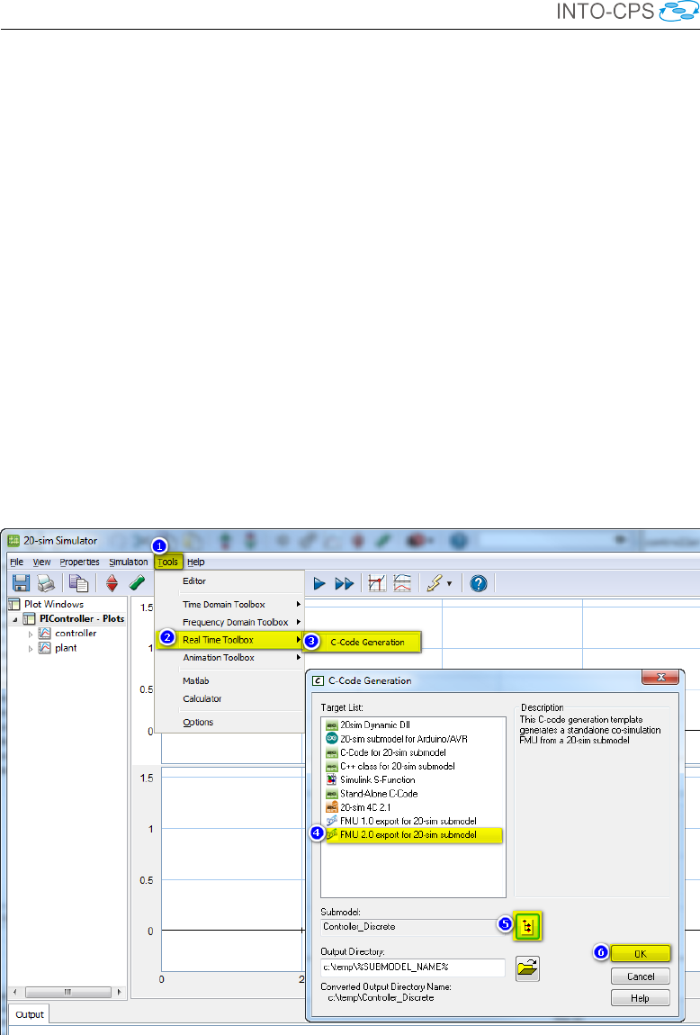
Next, follow these steps (see also Figure 55):
Figure 55: Export an FMU from 20-sim.
1. In the Simulator window, choose from the menu: Tools.
52

INTO-CPS Tool Chain User Manual (Public)
2. Select Real Time Toolbox.
3. Click C-Code Generation.
4. Select the FMU 2.0 export for 20-sim submodel target.
5. Select the submodel to export as an FMU.
6. Click OK to generate the FMU. This will pop-up a blue window.
Note that to automatically compile the FMU, you will need the Microsoft
Visual C++ 2010, 2013 or 2015 compiler installed (normally included with
Microsoft Visual Studio, either Express or Community edition). If 20-sim
can find one of the supported VC++ compilers, it starts the compilation
and reports where you can find the newly generated FMU. The 20-sim FMU
export also generates a Makefile that allows you to compile the FMU on
Windows using Cygwin, MinGW, MinGW64 or on Linux or MacOS X.
20-sim can currently export only a subset of the supported modelling lan-
guage elements as standalone C-code. Full support for all 20-sim features is
only possible through the tool-wrapper FMU approach (described shortly in
Section 5.2.2). The original goal for the 20-sim code generator was to export
control systems into ANSI-C code to run the control system under a real-
time operating system. As a consequence, 20-sim currently only allows code
generation for discrete-time submodels or continuous-time submodels using
a fixed-step integration method. Support for variable step size integration
methods is not yet included by default in the official 20-sim 4.6 release, but it
is already included in the 20-sim “4.6.2-intocps” release and on GitHub (see
below). Other language features that are not supported, (or are only partly
supported) for code generation, are:
•Hybrid models: Models that contain both discrete- and continuous-
time sections cannot be generated at once. However, it is possible to
export the continuous and discrete blocks separate.
•File I/O: The 20-sim “Table2D” block is supported; the “datafromfile”
block is not yet supported.
•External code: Calls to external code are not supported. Examples
are: DLL(),DLLDynamic() and the MATLAB functions.
•Variable delays: The tdelay() function is not supported due to
the requirement for dynamic memory allocation.
•Event functions: timeevent(),frequencyevent() statements
are ignored in the generated code.
53

INTO-CPS Tool Chain User Manual (Public)
•Fixed-step integration methods: Euler,Runge-Kutta 2 and Runge-
Kutta 4 are supported.
•Implicit models: Models that contain unsolved algebraic loops are
not supported.
•Variable-step integration methods: Vode-Adams and Modified Back-
ward Differential Formula (MeBDF) are available on GitHub (see below
for the link).
The FMU export feature of 20-sim is being improved continuously based on
feedback from INTO-CPS members and other customers. To benefit from
bug fixes and to try the latest FMU export features like variable step size
integration methods (e.g. Vode-Adams and MeBDF), you can download the
latest version of the 20-sim FMU export template from:
https://github.com/controllab/fmi-export-20sim
Detailed instructions for the installation of the GitHub version of the 20-sim
FMU export template can be found on this GitHub page. The GitHub FMU
export template can be installed alongside the existing built-in FMU export
template.
5.2.4 FMI 2.0 Import
The “4.6.4-intocps” version of 20-sim has an experimental option to import
an FMU directly in 20-sim for co-simulation within 20-sim itself. This is
useful for quickly testing exported FMUs without the need to set-up a full
co-simulation experiment in the INTO-CPS application. Presently it can
only import FMI 1.0 and 2.0 co-simulation FMUs can be imported.
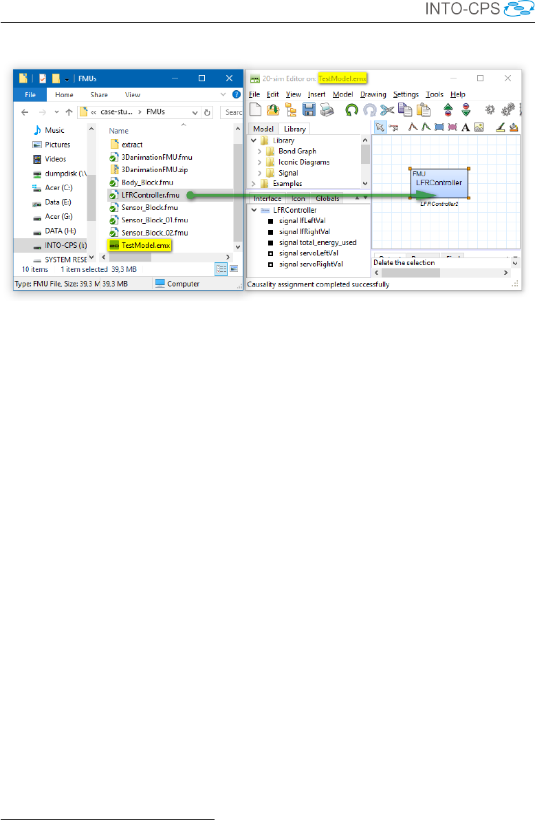
The procedure for importing an FMU as 20-sim submodel is similar to im-
porting a modelDescription.xml file. Follow these steps to import an
FMU in 20-sim:
1. Copy/move the FMU to the same folder as your model. This is not
required but recommended to prevent embedding hardcoded paths in
your model.
2. Using Windows Explorer, drag the FMU file on your 20-sim model (see
Figure 56).
This creates a new submodel with a blue icon that acts as an FMU wrap-
per. FMU inputs and outputs are translated into 20-sim submodel input
54
INTO-CPS Tool Chain User Manual (Public)
Figure 56: Importing an FMU in 20-sim.
and output signals. FMU parameters (scalar variables with causality “pa-
rameter”) are also available in 20-sim. This means that you can alter the
default values of these FMU parameters in 20-sim. The altered FMU param-
eters are transferred to the FMU during the initialization mode phase of the
FMU.
5.3 20-sim 4C
This section describes the features of 20-sim 4C [Con17] 13 developed specifi-
cally in support of INTO-CPS and FMI. 20-sim 4C is a rapid prototyping tool
that facilitates running C code on hardware to control machines and systems.
20-sim 4C imports models (as generated C code) from multiple sources (e.g.
20-sim) and runs them on hardware targets such as embedded ARM boards
(e.g. Raspberry Pi), PCs running real-time Linux and industrial PLCs.
One of the goals of the INTO-CPS project is to extend the capabilities of
the INTO-CPS tool chain toward executing part of a co-simulation on real
hardware in real-time. This is known as Hardware-in-the-Loop (HiL) sim-
ulation. This section explains how the FMI import and export features of
20-sim 4C can be used to execute source code FMUs on hardware targets
in co-simulation under the control of the COE. The complete 20-sim tool
documentation can be found in the 20-sim 4C Reference Manual [Kle13]. All
13Note that 20-sim 4C is Windows-only, but it can be executed using Wine [Win16] on
other platforms.
55
INTO-CPS Tool Chain User Manual (Public)
details of the implementation of FMI support in 20-sim 4C can be found in
Deliverable D4.3b [PBL+17].
5.3.1 Source Code FMU Import
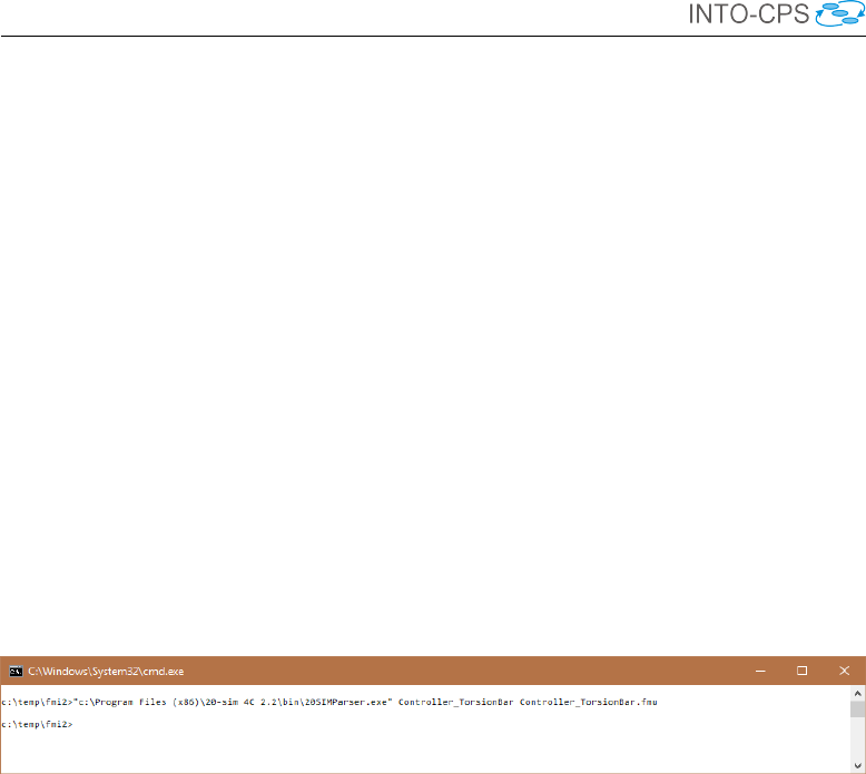
To import an FMU in 20-sim 4C, it must first be converted to a valid 20-sim
4C project. This is currently done via a command line call at the Windows
Command prompt. The command to import a source code FMU in 20-sim
4C is:
C:\Program Files (x86)\20-sim 4C 2.2\bin\
20simparser.exe newfmuProjectName fmuFilename.fmu
where newfmuProjectName is the name of a new directory in which 20-sim
4C will generate the new project. This directory is created as a subdirectory
of the current directory. An example is shown in Figure 57. This example cre-
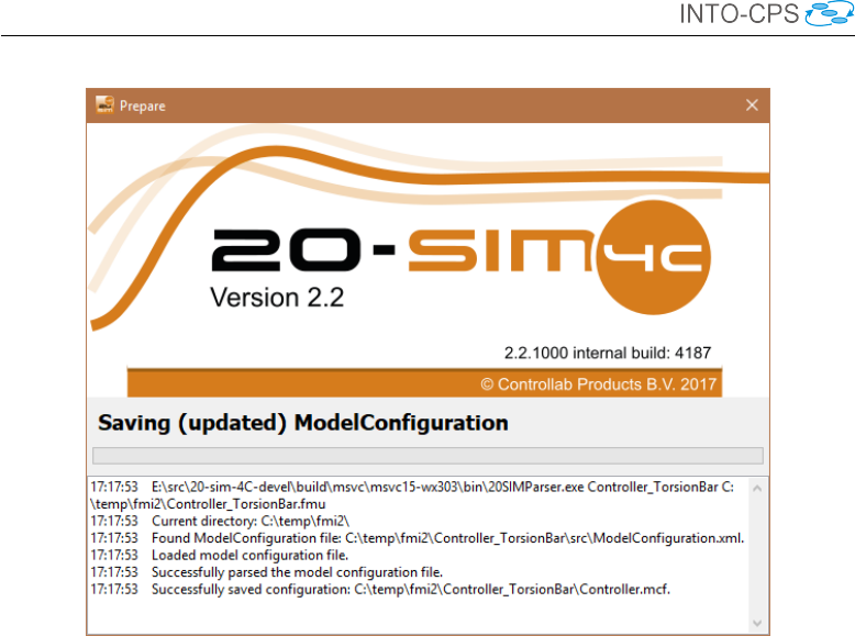
Figure 57: Import a source code FMU in 20-sim 4C.
ates a new directory in C:\Temp\fmi2 named Controller_TorsionBar
and briefly shows the import dialog from Figure 58. After successfully ex-
tracting and importing the FMU, 20-sim 4C will start.
Source code FMUs are deployed to a real-time target as follows:
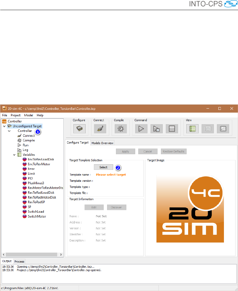
1. The 20-sim 4C window (Figure 59) shows the name of the FMU and
its public variables and parameters in the tree at the left side.
2. Use the Select button in the Target Template Selection box to select
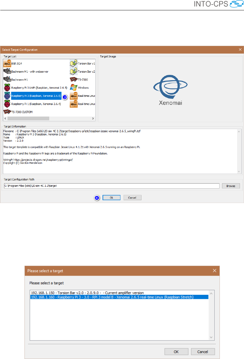
the hardware target for the FMU. This shows the Select Target Con-
figuration dialog (Figure 60.)
3. Select the Raspberry Pi 3 (Raspbian, Xenomai 2.6.5) target.
4. Press the OK button to confirm. This will automatically trigger a
network scan to find the Raspberry Pi on the network.
5. In case multiple targets are found, select the desired target in the Please
select a target dialog (Figure 61) and press OK.
56
INTO-CPS Tool Chain User Manual (Public)
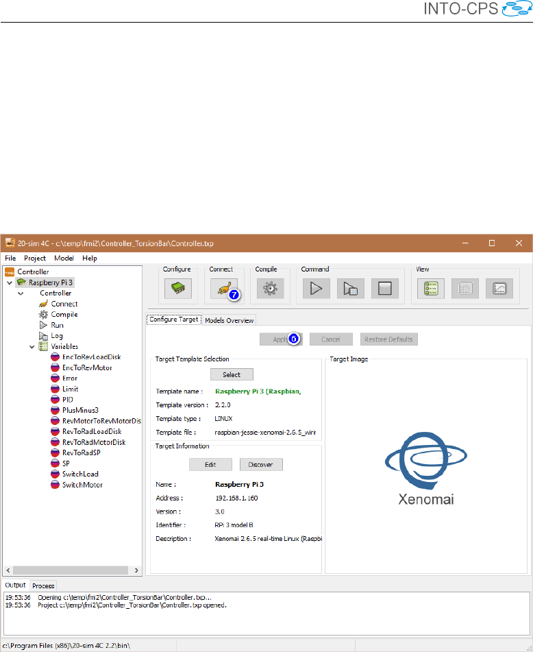
Figure 58: 20-sim 4C FMU importer.
6. In the main 20-sim 4C window, press Apply to confirm the target set-
tings. 20-sim 4C will now try to connect to the Raspberry Pi. When
the connection is successful, the Configure button will turn green. See
Figure 62.
7. Click the Connect button to go to the connection phase. This will
show the inputs and outputs of the FMU and 20-sim 4C allows you to
connect them to the on-board I/O pins.
8. To connect an input or output, select the signal and press the Con-
nect button or double-click the signal (Figure 63.) This will show the
Connection dialog as shown in Figure 64.
9. The connection dialog allows you to select an I/O component (e.g.
GPIO for digital I/O or PWM; see Figure 64) and a port within this
component (typically a physical pin or connector on the target device;
see Figure 65). Select OK to confirm the connection. The I/O available
depends on the selected target device. The Raspberry Pi 3 provides by
default only digital inputs and outputs and 2 PWM outputs. Extension
boards are needed for other I/O.
Note: In case you would like to use an extension board or external
I2C or SPI based I/O chip or other I/O, feel free to ask Controllab for
57
INTO-CPS Tool Chain User Manual (Public)
Figure 59: 20-sim 4C project with imported FMU.
58
INTO-CPS Tool Chain User Manual (Public)
Figure 60: Select the Raspberry Pi target.
Figure 61: Select the right target.
59
INTO-CPS Tool Chain User Manual (Public)
Figure 62: Accept target settings and go to the connection phase.
60
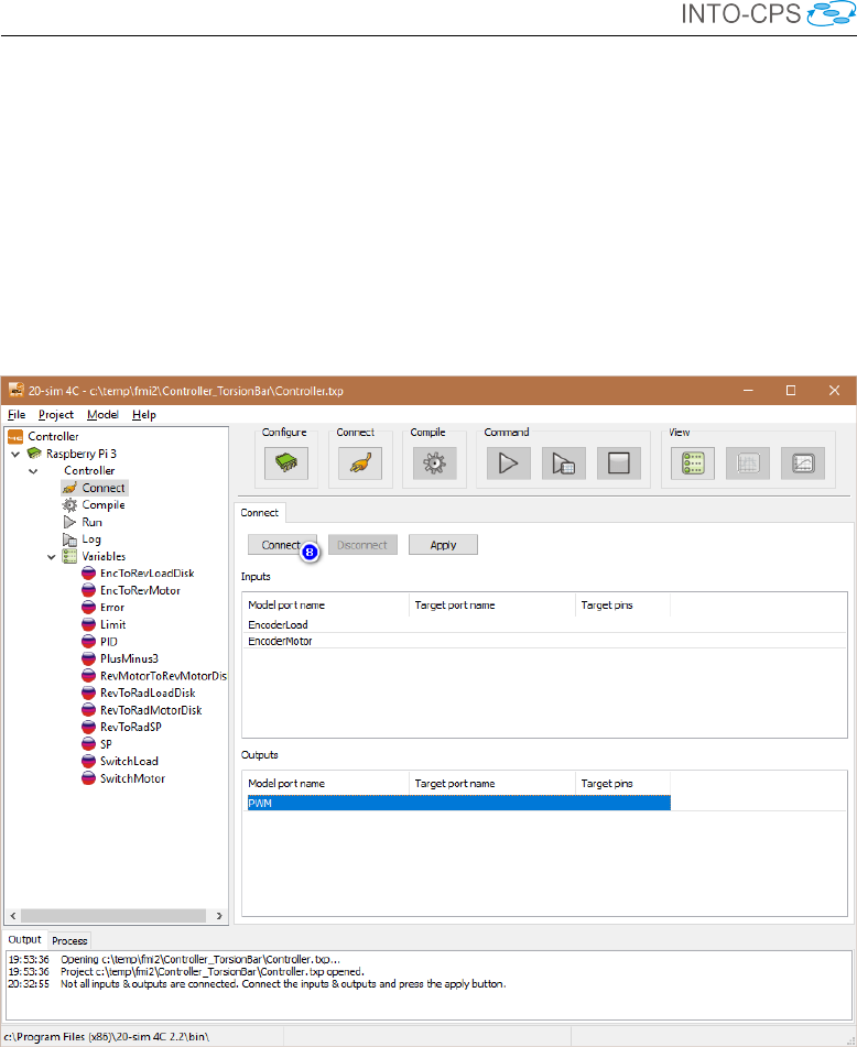
INTO-CPS Tool Chain User Manual (Public)
Figure 63: Select an input or output and press Connect.
61
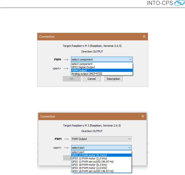
INTO-CPS Tool Chain User Manual (Public)
options to support this in 20-sim 4C.
Figure 64: Select a component.
Figure 65: Select a port.
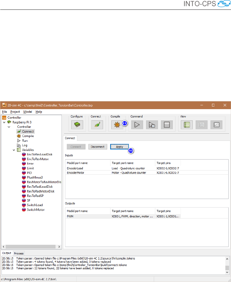
10. When you have connected all desired inputs and outputs to the I/O,
press the Apply button (Figure 66.) The Connect button will turn
green and 20-sim 4C will extend the FMU source code with additional
files to provide support for the Raspberry Pi Xenomai real-time Linux
and the Raspberry Pi I/O.
Note: It is not required to connect all inputs and outputs to real I/O.
20-sim 4C will show a warning when some inputs or outputs are not
connected. Unconnected inputs will read a zero (0) value by default. A
special real-time toolwrapper FMU can be generated from 20-sim 4C
that will allow you to write to unconnected inputs from a co-simulation
experiment (see section 5.3.2). This toolwrapper FMU will also allow
you to read all FMU exported variables including all inputs and out-
puts even when inputs and outputs are connected to the I/O. This
toolwrapper FMU is the basis for INTO-CPS HiL simulation with the
Raspberry Pi as the real-time target.
62
INTO-CPS Tool Chain User Manual (Public)
Figure 66: Apply the connections and compile the code.
63
INTO-CPS Tool Chain User Manual (Public)
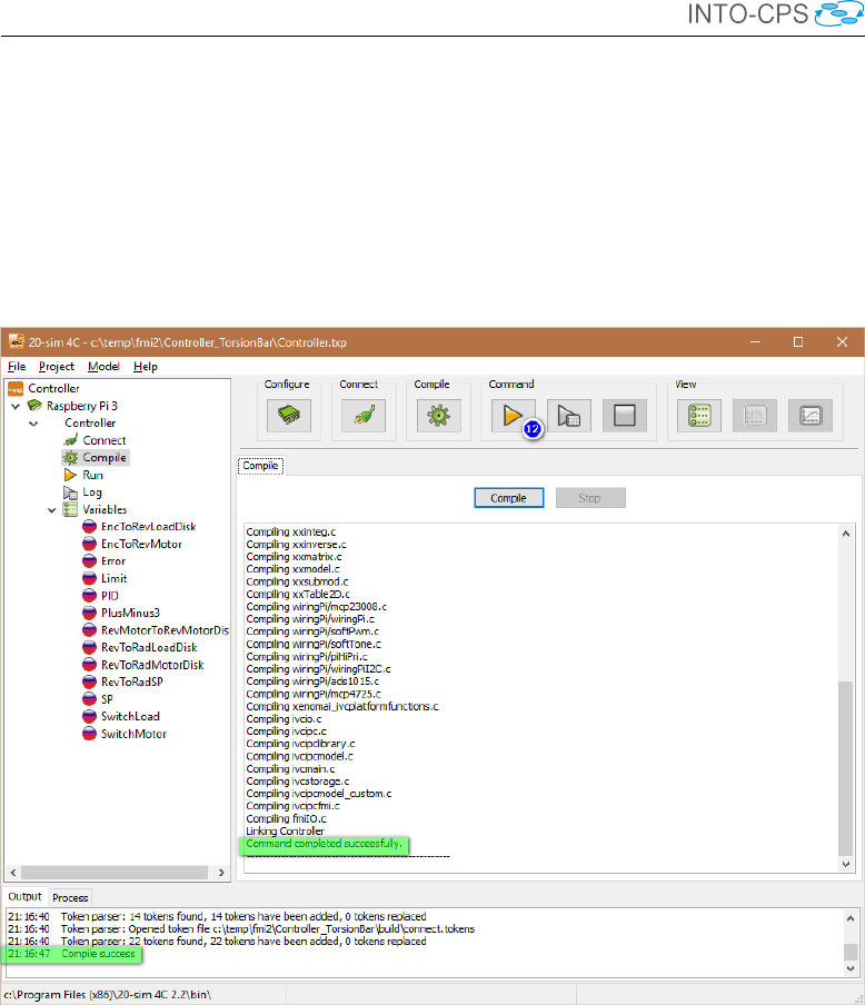
11. Press the orange Compile button (Figure 66) to go to the Compile
phase. This will compile the FMU source code and the additional 20-
sim 4C source code into a real-time application.
12. When the compilation process is ready and successful, click the orange
Command button to configure the last task settings before uploading
the compiled FMU to the Raspberry Pi (Figure 67.)
Figure 67: Compilation phase.
13. On the Configure Run tab (Figure 68), you can specify the finish time of
the FMU or disable it if it should run forever (until reboot/shutdown).
Ensure that the Discrete Time Interval has a step size larger than 0.
This value is used as the time (step size) between two FMU “doStep”
calls and determines the FMU calculation frequency. The Raspberry
Pi 3 is able to support step sizes as low as 0.00005 (20 kHz), but this
depends on the FMU computation load and number of connected I/O
pins.
14. Press the Apply button to store the run settings. The Command button
64
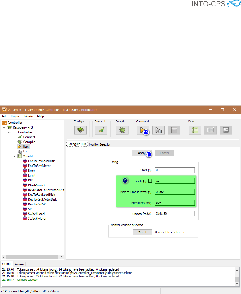
INTO-CPS Tool Chain User Manual (Public)
Figure 68: Configure task run settings.
65
INTO-CPS Tool Chain User Manual (Public)
will turn green.
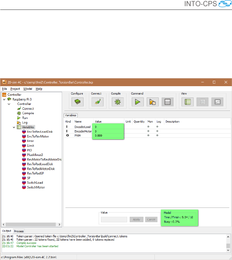
15. Click the Command button to upload and start your FMU on the
Raspberry Pi. If everything is configured correctly, the FMU will start
and 20-sim 4C will monitor its progress and the current value of the
FMU variables.
Figure 69: FMU is running.
16. It is also possible to show selected variables in a monitor plot. You
can enable monitoring of a signal by toggling the dot icon in the Mon
column to a monitor icon.
17. Click the large monitor icon on the button bar to show the monitor
plot. An example of the monitor plot with three I/O signals is shown
in Figure 70.
66
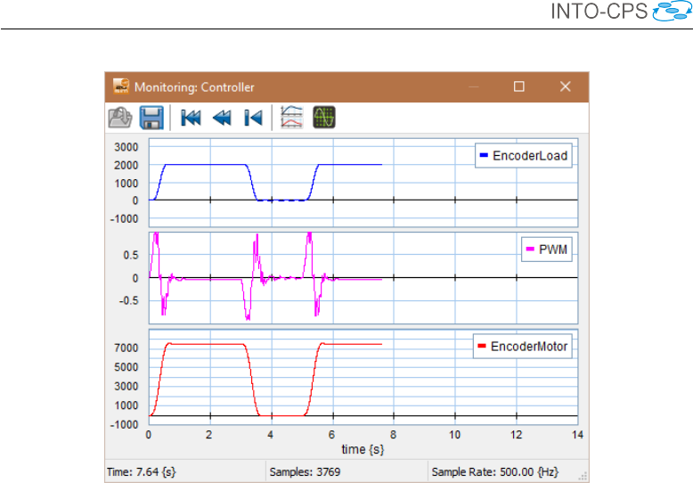
INTO-CPS Tool Chain User Manual (Public)
Figure 70: Variable monitor.
5.3.2 Real-time toolwrapper FMU export
For HiL simulation with a Raspberry Pi, 20-sim 4C is extended with FMU
export functionality. The 20-sim 4C FMU export option generates a real-
time toolwrapper FMU for the currently loaded 20-sim 4C project. This
FMU can be used in the COE to interface the real-time FMU running on
the Raspberry Pi with a standard COE co-simulation experment. Assuming
a running application on the Raspberry Pi, FMU export can be performed
as follows:
1. Co-simulation using a toolwrapper FMU uses the unconnected 20-sim
4C inputs. Make sure that the desired co-simulation inputs are not
connected during the 20-sim 4C Connect phase (Figure 66).
2. Export an FMU using the FMU Export menu item. Make sure that the
“Raspberry Pi 3” target, or the 20-sim 4C project (your FMU name,)
is selected in the left tree. This is required so that the FMU exporter
can find the right 20-sim 4C project.
3. Select Export FMU from the Project menu item. See Figure 71.
4. A command-line window will be displayed showing status information
of the FMU toolwrapper creation process. See Figure 72.
67
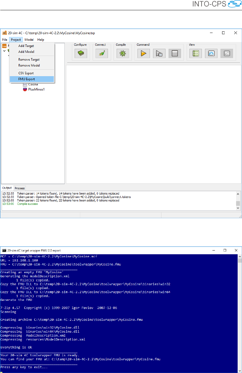
INTO-CPS Tool Chain User Manual (Public)
Figure 71: Export toolwrapper FMU.
Figure 72: Toolwrapper FMU status.
68

INTO-CPS Tool Chain User Manual (Public)
5. This window can be closed after noting the location of the generated
FMU.
6. The newly created FMU can be used in 32-bit and 64-bit Windows FMI
co-simulators like the INTO-CPS COE. Linux and MacOS X compat-
ible versions are not yet available.
5.4 OpenModelica
This section explains the FMI and INTO-CPS related features of Open-
Modelica. The focus is on import of modelDescription.xml files and
standalone and tool-wrapper FMU export.
5.4.1 Import of modelDescription.xml Files
OpenModelica can import modelDescription.xml interface files cre-
ated using Modelio and create Modelica models from them. To use the
modelDescription.xml import feature, you will need to use OpenMod-
elica nightly-builds versions, as this extension is new. Nightly builds can be
obtained through the main INTO-CPS GitHub site:
http://into-cps-association.github.io
To import a modelDescription.xml file in OpenModelica one can use:
1. The OpenModelica Connection Editor GUI (OMEdit): FMI →Import
FMI Model Description.
2. A MOS script, i.e. script.mos, see below.
// start script.mos
// import the FMU modelDescription.xml
importFMUModeldescription("path/to/modelDescription.xml");
getErrorString();
// end script.mos
The MOS script can be executed from command line via:
// on Linux and Mac OS
> path/to/omc script.mos
// on Windows
> %OPENMODELICAHOME%\bin\omc script.mos
69

INTO-CPS Tool Chain User Manual (Public)
The result is a generated file with a Modelica model containing the inputs
and outputs specified in modelDescription.xml. For instance:
model Modelica_Blocks_Math_Gain_cs_FMU "Output the product
of a gain value with the input signal"
Modelica.Blocks.Interfaces.RealInput u "Input signal
connector" annotation(Placement(transformation(extent
={{-120,60},{-100,80}})));
Modelica.Blocks.Interfaces.RealOutput y "Output signal
connector" annotation(Placement(transformation(extent
={{100,60},{120,80}})));
end Modelica_Blocks_Math_Gain_cs_FMU;"
5.4.2 FMU Export
All FMUs exported from OpenModelica are standalone. There are two ways
to export an FMU:
1. From a command prompt.
2. From OMEdit (OpenModelica Connection Editor).
FMU export from a command prompt To export an FMU for co-
simulation from a Modelica model, a Modelica script file generateFMU.mos
containing the following calls to the OMC compiler can be used:
// load Modelica library
loadModel(Modelica); getErrorString();
// load other libraries if needed
// loadModel(OtherLibrary); getErrorString();
// generate the FMU: PathTo.MyModel.fmu
translateModelFMU(PathTo.MyModel, "2.0","cs");
getErrorString();
Next, the OMC compiler must be invoked on the generateFMU.mos script:
// on Linux and Mac OS
> path/to/omc generateFMU.mos
// on Windows
> %OPENMODELICAHOME%\bin\omc generateFMU.mos
70
INTO-CPS Tool Chain User Manual (Public)
FMU export from OMEdit One can also use OMEdit to export an
FMU, as detailed in the figures below.
•Open OMEdit (see Figure 73.)
•Load the model in OMEdit (see Figure 74.)
•Open the model in OMEdit (see Figure 75.)
•Use the menu to export the FMU (see Figure 76.)
•The FMU is now generated (see Figure 77.)
Figure 73: Opening OMEdit.
The generated FMU will be saved to %TEMP%\OpenModelica\OMEdit.
71
INTO-CPS Tool Chain User Manual (Public)
Figure 74: Loading the Modelica model in OMEdit.
Figure 75: Opening the Modelica model in OMEdit.
72

INTO-CPS Tool Chain User Manual (Public)
Figure 76: Exporting the FMU.
Figure 77: Final step of FMU export.
73

INTO-CPS Tool Chain User Manual (Public)
5.5 Unity
This section describes the 3D visualisation functionality of the INTO-CPS
tool chain. This capability is encapsulated into a Unity-based FMU that
is configured and loaded into co-simulations in the usual manner. Unity is
a professional game engine. It can be downloaded from the Unity website
[Tec16].
5.5.1 Importing the Unity Package into Unity
To create a 3D animation FMU using Unity, first create a new project or open
an existing Unity project. A Unity package was made by CLP that can be
imported into Unity to expand Unity with FMU export options. This Unity
package can be downloaded via the Download Manager in the INTO-CPS
application or by contacting CLP. First, drag-and-drop this package into the
Assets folder in Unity (in the Project tab). See Figure 78 on how to import
the package from the explorer into Unity. A pop-up will open, like the one
shown in Figure 79. Press the Import button, as shown in Figure 79. Since
the package contains scripts that will modify the Unity editor, it is necessary
to restart the Unity project after importing the package.
5.5.2 Importing the FMUBuilder gameobject
After restarting Unity, go to the Hierarchy tab. Right click within the blank
part of the hierarchy (i.e. do not select any objects in the hierarchy) and
select FMU →FMUBuilder (see Figure 80). This will create a new object in
the hierarchy named FMUBuilder. When selecting this FMUBuilder object
in the hierarchy, a few options will be shown in the Inspector (see Figure 81).
There are three components visible: Transform,FMU Builder (Script) and
Scenery Conversion (Script). The latter two are unique to the INTO-CPS
Unity FMU package. FMU Builder (Script) is the component that will even-
tually build the 3D animation FMU, which will be covered later in this sec-
tion. The other component, Scenery Conversion (Script), is used to convert
existing 20-sim sceneries into Unity sceneries. This will also be covered later
in this section.
74
INTO-CPS Tool Chain User Manual (Public)
Figure 78: Importing the Unity package into Unity.
5.5.3 Assigning FMU Variables to Unity gameobjects
To be able to connect variables from a co-simulation to an object in Unity,
agameobject is needed. For example, as shown in Figure 80, a cube object
can be created by right-clicking in the hierarchy tab in a blank space of the
hierarchy, but now selecting 3D Object →Cube. When the newly created
object is selected in the hierarchy, all components currently attached to this
cube can be seen in the Inspector tab. At the bottom of this tab there is a
button named Add Component. Press this button, go to FMU variables and
choose between 20-sim coordinates or Unity coordinates. The first one means
that the axes are part of a right-handed frame, that the Z-axis is pointing
up, and that the order of rotation for Euler angles is X-Y-Z. The latter is the
Unity convention, in which the frame is left-handed, the Y-axis is pointing
up, and the rotation for Euler angles is Z-X-Y. See Figure 82 on how to
do this. If there is doubt about which of the two types of variables should
be chosen, choose the 20-sim option, as this is the reference frame used in
75
INTO-CPS Tool Chain User Manual (Public)
Figure 79: Summary of what will be imported into the Unity project.
most modeling tools like 20-sim. Once one is selected, two additional scripts
become available in the Inspector tab. These are GUID (Script) and either
Twenty Sim Variable (Script) or Unity Variable (Script). The GUID script
should not be touched. The Variable script, however, is the script that will
describe the interface variables of the to-be-generated FMU. Choose an FMU
variable name and an axis, and press the Add Axis button. Multiple axes
can be defined for one gameobject. Figure 83 shows the axes dropdown menu
and the Twenty Sim Variable (Script) and GUID (Script) components.
5.5.4 Converting a 20-sim Scenery into a Unity Scenery
If a 20-sim scenery already exists, then it is possible to import it into Unity.
If there is a 3D animation window in the 20-sim model, then double click the
plot to open the 3D Properties window. Then go to File →Save Scene (see
Figure 84). If 20-sim asks to save the whole scenery, select Yes. Remember
where the scenery file is located and go back to Unity. Go to the hierarchy
tab, select FMUBuilder and enter under the Scene Conversion (Script) the
location of the scenery file, by pressing Find scenery. Afterwards, press
the Build scenery button and the 20-sim scene will be loaded underneath the
FMUBuilder object in the hierarchy (this can be drag-dropped to other places
in the hierarchy if needed), see Figure 85 for the hierarchy that is created.
Note that the Cube seen in Figure 84 in the hierarchy is now created in Unity
as well. Furthermore, the Default Lights and Cameras frame is converted into
Unity, which is a default set of lights and cameras in every 20-sim 3D scene.
76
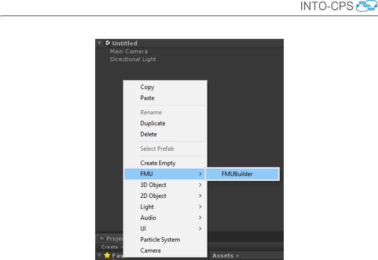
INTO-CPS Tool Chain User Manual (Public)
Figure 80: Creating the FMUBuilder gameobject in the hierarchy tab.
5.5.5 Exporting an FMU
The final step in the process of creating a 3D animation FMU in Unity is
the build process itself. The variables that were added by manually assigning
FMU variables to gameobjects and by importing 20-sim scenery files will now
be used to generate the FMU itself. Every variable name (either the ones
manually entered, or automatically generated by the import 20-sim scenery
option) will be the input variables of this FMU. Select the FMUBuilder in
the hierarchy and go to the Inspector tab. Under FMU Builder (Script)
select the export location and the name of the to-be-exported FMU, then
press Build FMU. Once the build process is done, the FMU will be present
in the export location selected, with the given name. Note that for larger
Unity scenes this can take a while to build.
77
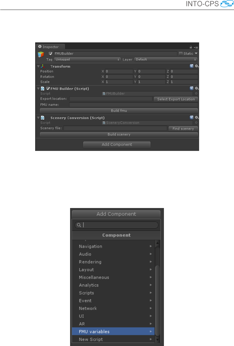
INTO-CPS Tool Chain User Manual (Public)
Figure 81: Components of the FMUBuilder in the Inspector tab in Unity.
Figure 82: Adding new FMU variables to the Unity scene.
78
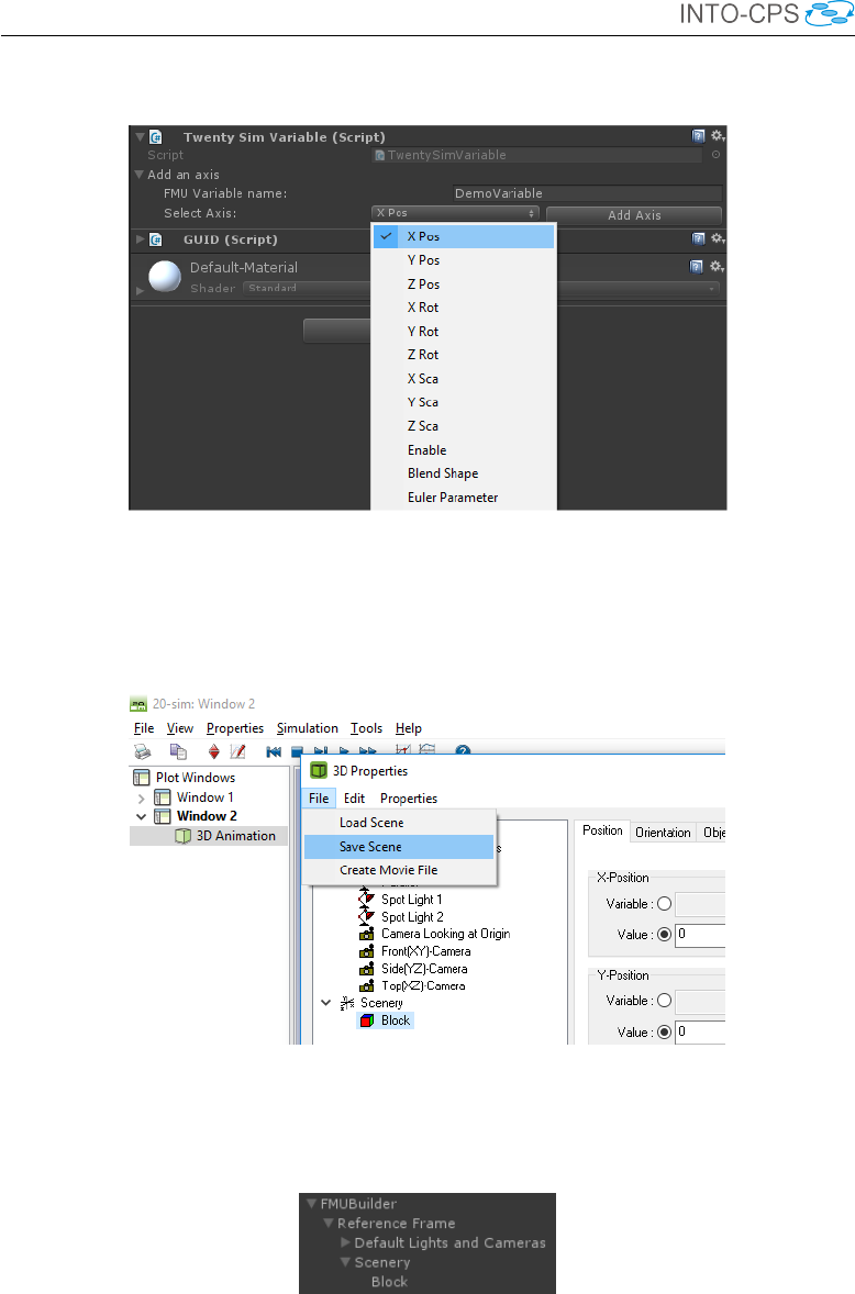
INTO-CPS Tool Chain User Manual (Public)
Figure 83: Adding the variable named "DemoVariable" for the x-position
axis to the newly generated cube object.
Figure 84: Exporting a 20-sim 3D scenery from a 3D animation plot.
Figure 85: Importing a 20-sim scenery file into Unity.
79

INTO-CPS Tool Chain User Manual (Public)
5.6 AutoFOCUS3
AutoFOCUS3 (AF3) is an open source model based development tool for dis-
tributed, reactive and embedded software systems. It uses models to develop
systems. From the requirements to the hardware architecture, passing by
the design of the logical architecture, the deployment and the scheduling. It
provides advanced features to support the user ensuring the quality of their
system: formal analyses, synthesis methods, space exploration visualization,
etc.
Co-simulation feature supports for now only Functional Mockup Unit (FMU)
export satisfying the following constraints:
•FMI 2.0
•32/64bit
•GCC compilation
•Input and output values cannot carry NoVal but instead contain de-
fault values (0 for integers and reals, false for booleans, first item for
enumerations) Note: This behavior is different from AF3 simulation
FMI export is done at the level of component with logical architecture (in the
future, we might implement this feature for deployments as well). To export
your component with logical architecture to the FMU, right-click on it in the
model navigator and select "Export to FMU2.0" as shown in Figure 86.
AF3 works with logical time, however co-simulation is generally achieved
with tools modeling reality and therefore working with real time. Therefore,
the FMI standard requires that AF3 notion of time is translated to real time.
Consequently, you will have to define the sampling time (in seconds) for the
component as a function with name "samplingTime()" in the data dictionary
as shown in Figure 87. Otherwise, you will be asked to provide the frequency
of the component in Hertz as shown in Figure 88.
80
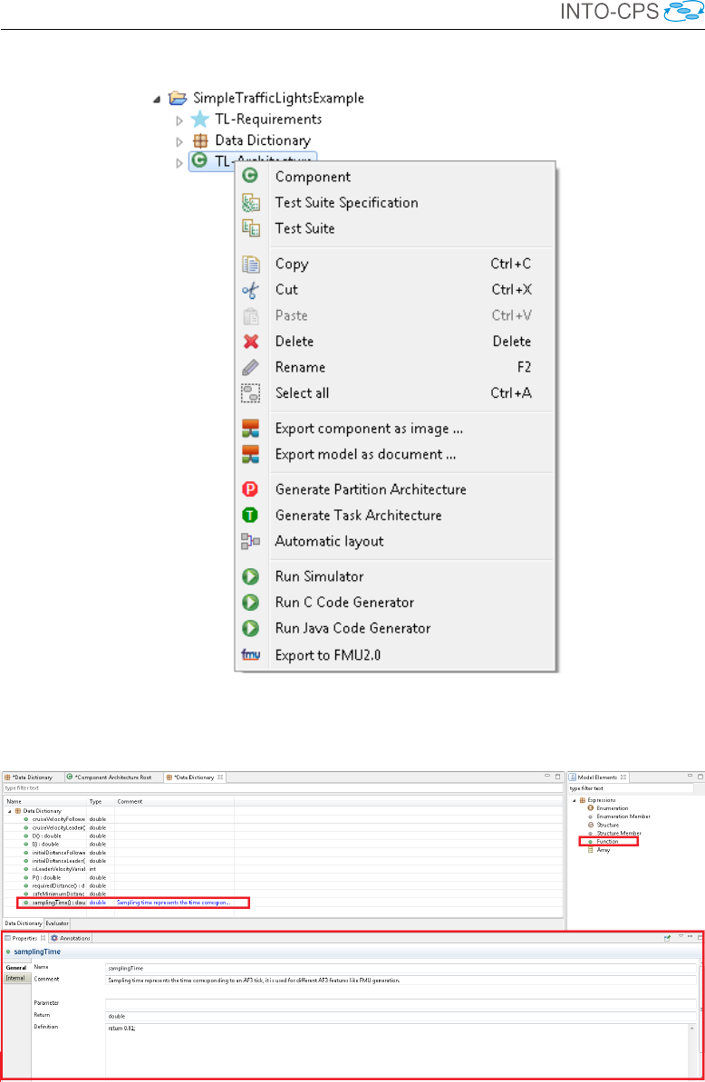
INTO-CPS Tool Chain User Manual (Public)
Figure 86: Exporting component architecture to FMU.
Figure 87: Defining the sampling time function in data dictionary.
81
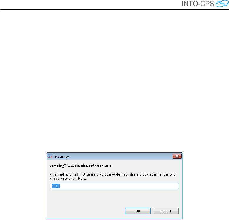
INTO-CPS Tool Chain User Manual (Public)
Figure 88: Providing the component frequency in case of samplingtime()
function not defined.
82

INTO-CPS Tool Chain User Manual (Public)
6 Design Space Exploration
This section provides a description of INTO-CPS tool chain support for de-
sign space exploration (DSE.) This section is split into four parts. In Sec-
tion 6.1 the installation procedure is outlined. Section 6.2 describes how
the INTO-CPS Application can be used to launch a DSE using an existing
configuration file and Section 6.3 describes how the results from DSE are
generated and stored. Section 6.4 describes the structure of the DSE config-
uration file, giving enough detail for the user to be able to edit one for their
purposes.
6.1 Installing DSE Scripts
Before we launch a DSE, we must install the DSE scripts for the various
search algorithms and objective evaluation. In the INTO-CPS Application,
select Window →Show Download Manager. This opens the download man-
ager as shown in Figure 89. Select the most recent release and download
Design Space Exploration - Scripts for generating and analysing multiple co-
simulations. Python version 2.7 must be installed, along with the matplotlib
library.
This will download a Zip archive – extract this into the directory in which
the archive was downloaded. DSEs may now be launched.
6.2 How to Launch a DSE
To launch a DSE we need to provide the INTO-CPS Application with the
path to two files. The first is the DSE configuration, defining the parameters
of the design space, how it should be searched, measured and the results
compared. The second is the multi-model configuration, defining the base
model that will be used for the search. A DSE configuration is selected by
double clicking on one of the configurations listed in the DSES section of
the INTO-CPS Application project explorer; these configurations are iden-
tified with the ( ) icon. Hint: several of the downloadable examples have
predefined DSE configurations.
To launch the DSE, we must first select the multi-model to use. One can be
selected by clicking the Set multi-model button and selecting one from the
drop-down list, as shown in Figures 90 and 91. Once selected, your choice
83
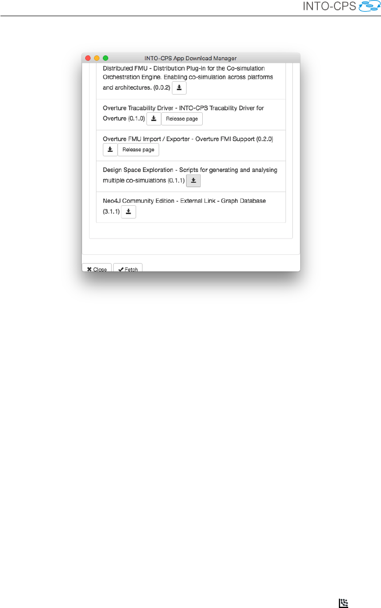
INTO-CPS Tool Chain User Manual (Public)
Figure 89: Download Manager.
must be saved to parse the DSE configuration with respect to the multi-
model of choice by clicking on the Save multi-model choice button, as shown
in Figure 91.
If the COE is not already running, the bottom of the DSE page is shown
with a red “Co-Simulation Engine offline. No connection at localhost:8082 ”
status, as shown in Figure 92. If this is the case, click on the Launch button to
start the COE. This results in a green co-simulation engine status (see Figure
93). Pressing the Simulate button starts the DSE background process.
6.3 Results of a DSE
The DSE scripts store their results in a folder named for the date and time
at which the DSE was started. This folder may be found underneath the
name of the DSE script selected, as shown in Figure 94. When the DSE
has finished, we can find both a graphs folder and an HTML results page
inside the results folder. It may be necessary to refresh the project view to
see these new items. The results HTML file is identified by the ( ) icon,
84

INTO-CPS Tool Chain User Manual (Public)
Figure 90: Selecting a multi-model.
Figure 91: Setting a multi-model.
85
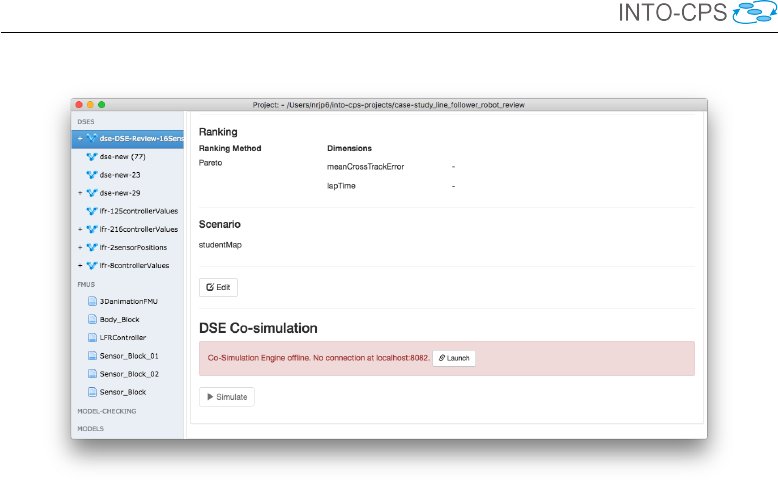
INTO-CPS Tool Chain User Manual (Public)
Figure 92: Status when COE is not running.
and double clicking on it opens the results page in the computer’s default
browser.
The results, shown in Figure 95, contain two elements. The first element is
a Pareto graph showing the results of all simulations on a single plot, with
each point on the graph representing a single simulation. The best designs,
referred to as the non-dominated set, are shown in blue, with ranks of progres-
sively worse designs coloured alternately red and yellow. The second element
is a table of these results, with the rank in the left hand column, followed
by the objective values and finally the design parameters that produced the
result.
6.4 How to Edit a DSE Configuration
A DSE configuration comprises several elements. In Section 6.4.1 we outline
the content of each element and their role in a DSE. There are three methods
for producing DSE configurations; through the use of the INTO-SysML DSE
profile (Section 6.4.2), through the INTO-CPS Application (this method may
also be used to edit an existing configuration) (Section 6.4.3), or manually
editing a text configuration document (Section 6.4.13). In this section we
outline each approach.
86
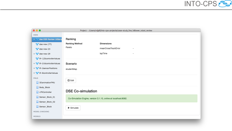
INTO-CPS Tool Chain User Manual (Public)
Figure 93: Status when COE is running.
6.4.1 DSE Configuration Overview
A DSE configuration comprises several elements: the search algorithm to
use; parameters; parameter constraints; objectives; objective constraints; a
ranking; and a set of scenarios.
Search Algorithm
The algorithm section allows a user to choose between DSE search algorithms
implemented in INTO-CPS. There are two options at present: exhaustive
and genetic. The exhaustive approach will simulate the whole design space
as dictated by the choice of parameters and scenarios. The genetic algorithm
uses an approach to selecting the designs to simulate based upon genetic
breeding and mutations. For more information on the search algorithms, see
Deliverable D3.2a [FGPP16].
Parameters
The parameters section is used to define a list of values for each parameter
to be explored. If a parameter is included in the DSE configuration file, then
it must have at least one value defined. The order of the values in the list is
not important.
87
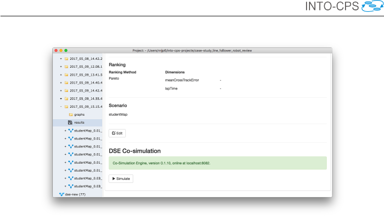
INTO-CPS Tool Chain User Manual (Public)
Figure 94: Icon shown when DSE results are ready.
Parameter Constraints
It may be the case that not all combinations of the parameter values defined
in the previous section are valid. So, it is necessary to be able to define con-
straints over the design parameters such that no time is wasted simulating
invalid designs. For example, in the Line Follower Robot project [MGP+17]
we define ranges for the x and y co-ordinates of the left and right sensors
separately, and running all combinations of these leads to asymmetric de-
signs that do not have the same turning behaviour on left and right turns.
To prevent this we can define boolean expressions based upon the design
parameters and evaluate these before a simulation is launched.
Objective Definitions: Internal
There are two means for defining the objectives used to assess the perfor-
mance of a simulated model. The first of these, described here, is using the
internal functions included in the DSE scripts. This is a set of simple func-
tions that can be applied to any of the values recorded by the COE during
simulation. The current set of internal functions is:
max Returns the maximum value of a variable during a simulation.
min Returns the minimum value of a variable during a simulation.
mean Returns the mean value of a variable during a simulation (n.b., a fixed
simulation step size is assumed.)
88

INTO-CPS Tool Chain User Manual (Public)
Figure 95: A page of DSE results.
Objective Definitions: External Scripts
The second form of objective definition makes use of user-defined Python
scripts to allow bespoke analysis of simulation results to be launched auto-
matically and results recorded using the common format. The definition has
two parts: the construction of the Python script to perform the analysis and
the definition of the script’s required parameters in the DSE configuration
file. These two steps are described below.
Construction of the Script The outline functionality of an analysis script
is that, at the appropriate times, a DSE script calls it, passing four or more
arguments. The script uses these arguments to locate a raw simulation re-
89
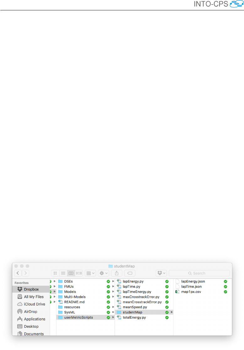
INTO-CPS Tool Chain User Manual (Public)
sults file (results.csv), process those results and then write the objective
values into an objectives file (objectives.json) for that simulation.
The first three arguments sent to the script are common to all scripts. These
are listed below.
argv 1 The absolute path to the folder containing the results.csv re-
sults file. This is also the path where the script finds the
objectives.json file.
argv 2 The name of the objective. This is the key against which the script
should save its results in the objectives file.
argv 3 The name of the scenario.
With this information the script can find the raw simulation data and also
determine where to save its results. The name of the scenario allows the script
to locate any data files it needs relating to the scenario. For example, in the
case of the script measuring cross track error for the line following robot,
the script makes use of a data file that contains a series of coordinates that
represent the line to be followed. The name of this data file is map1px.csv.
It is placed into a folder with the same name as the scenario, which in this
case is studentMap. That folder is located in the userMetricScripts
folder, as shown in Figure 96. Using this method, the developer of an external
analysis script needs only to define the name of the data file they will need and
know that at runtime the script will be passed a path to a folder containing
the data file suitable for the scenario under test.
Figure 96: External analysis script data files for the “studentMap” scenario.
Figure 97 shows an example of an external analysis script. In this case it
computes the cumulative deviation of the water level from some target level.
90

INTO-CPS Tool Chain User Manual (Public)
Figure 97: External analysis script to calculate cumulative deviation in the
Water Tank example.
91

INTO-CPS Tool Chain User Manual (Public)
There are two distinct sections in the file, we shall refer to them as the
“common” and “script specific” sections.
The common section contains core functions that are common to all ex-
ternal scripts. It reads in the three arguments that are common to all
scripts, and contains functions to help the user retrieve the data needed
by the analysis script, and to write the computed objective value into the
objectives.json file. It is recommended that this section be copied to
form the basis of any new external analysis scripts.
The second part of the example script shown is specific to the analysis to
be performed. The purpose of this section is to actually compute the value
of the objective from the results of a simulation. Generally it will have
three parts: reading in any analysis specific arguments such as the ID of
data in the results that it needs, using the data in results.csv to cal-
culate the value of the objective and finally write the objective value into
objectives.json.
In the ‘Script Specific Section’ of Figure 97 we see the example of the script
calculating the cumulative deviation of the water level from a target level in
the water tank model. It starts by reading a further two arguments passed
when the script is launched and initializes the variables. The script then it-
erates through all rows of data in results.csv to calculate the cumulative
deviation which is then written to the objectives.json file in the final
line.
Ranking
The final part of a DSE configuration file concerns the placing of designs in
a partial order according to their performance. The DSE currently supports
a Pareto method of ranking, as was shown earlier in Figure 95. The purpose
of the ranking section of the configuration is to define the pair of objectives
that will be used to rank the designs, and whether to maximise or minimise
each.
Scenario List
The DSE scripts currently have limited support for scenarios referring to a
specific set of conditions against which the multi-model is to be tested. In
the example of the line following robot, the scenario refers to the map the
robot has to follow, along with its starting co-ordinates. For instance, in
92
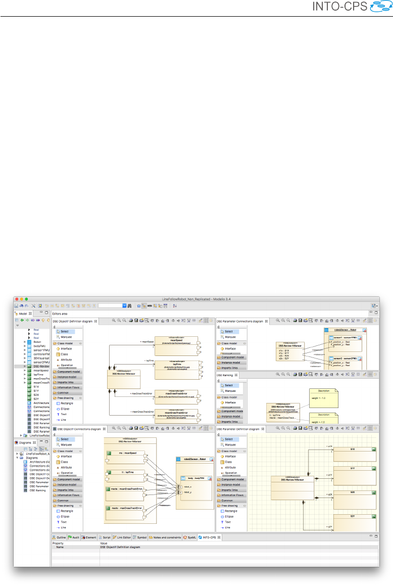
INTO-CPS Tool Chain User Manual (Public)
one scenario the robot would go around a circular track in one direction,
predominantly turning left, whereas in a different scenario the same track
would be followed in the opposite direction, predominantly turning right. In
both scenarios the map of the track is the same.
6.4.2 Using the INTO-SysML DSE Profile
The INTO-CPS DSE SysML profile is defined in Deliverable D4.2c [BQ16],
with an example of its use in Deliverable D3.3a [FGP17]. Here we describe
the steps to export the configuration from Modelio and import it into the
INTO-CPS Application.
Given a complete DSE SysML model, as shown in Figure 98, we generate
a DSE configuration by right-clicking on the DSEAnalysis object in the
model browser and selecting INTO-CPS →GenerateDSE, as in Figure 99.
Figure 98: SysML model of DSE analysis experiment.
93

INTO-CPS Tool Chain User Manual (Public)
Figure 99: Menu option for generating DSE configuration.
Simply supply an appropriate name and select Export (Figure 100). When
the export is complete, click OK (Figure 101).
Figure 100: Enter DSE configuration name.
Figure 101: Export complete.
Moving to the INTO-CPS Application, we start to import the configuration.
Expand the generated configurations in project’s SysML model: Model →
configs, right click on the configuration name as defined above and select
Create DSE Configuration (see Figure 102). When complete, the configu-
ration screen is displayed, and can be launched according to instructions in
Section 6.2.
94
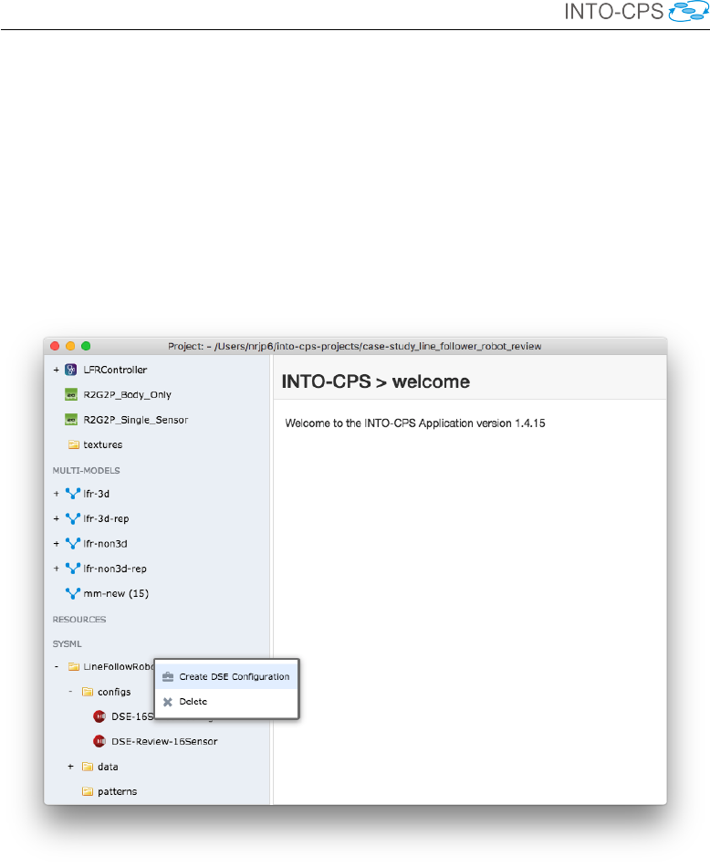
INTO-CPS Tool Chain User Manual (Public)
Figure 102: Create configuration in INTO-CPS Application.
95
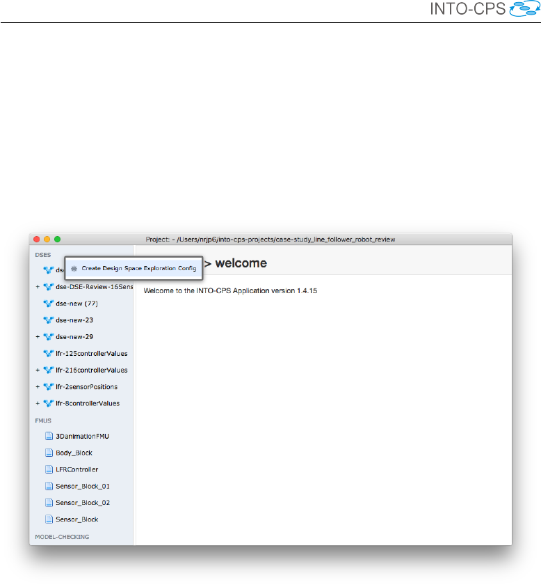
INTO-CPS Tool Chain User Manual (Public)
6.4.3 Using the INTO-CPS Application DSE Editor
To create a new DSE configuration in the INTO-CPS Application, right click
on the DSES section of the project browser and select Create Design Space
Exploration Config, as in Figure 103. This will create a new configuration
with a name in the form dse-new(xx) with a random number. This can
be renamed by right-clicking on the new config in the project browser. When
Figure 103: Create new DSE configuration.
opened, one must first select the multi-model to use. Follow the same steps
as given earlier for launching a DSE (Figures 90 and 91). When selected, the
DSE configuration may be edited.
6.4.4 Search Algorithm
The first element to define is the search algorithm. A choice is given between
Exhaustive and Genetic searches, as shown in Figure 104. The exhaustive
option has no further options, whist a genetic search requires data concerning:
the initial population;initial population distribution;mutation probability;
96
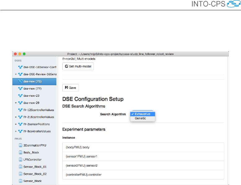
INTO-CPS Tool Chain User Manual (Public)
parent selection strategy; and maximum generations without improvement –
these are shown in Figure 105.
Figure 104: Choosing the DSE search algorithm.
6.4.5 Parameters
Design parameters may be defined in a multi-model. In addition, a DSE
configuration may define a range of values to be used in the DSE. The DSE
editor allows users to browse the multi-model parameters (Figure 106) and
edit those parameters defined in the multi-model (Figure 107).
Parameters may be removed from the DSE configuration (they will not be re-
moved from the multi-model) by clicking the Remove DSE Parameter button
– see Figure 108. Additional DSE parameters may be added by selecting the
parameter name from the drop down and clicking the Add DSE Parameter
button – see Figure 109.
97
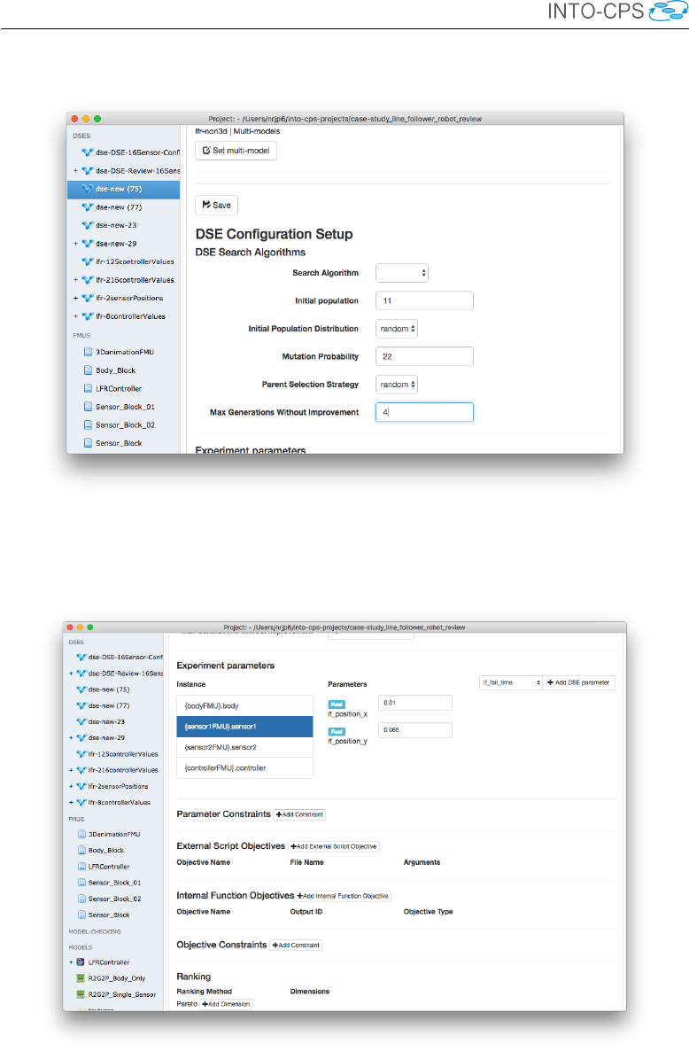
INTO-CPS Tool Chain User Manual (Public)
Figure 105: Options for the genetic algorithm.
Figure 106: Browsing the multi-model parameters.
98
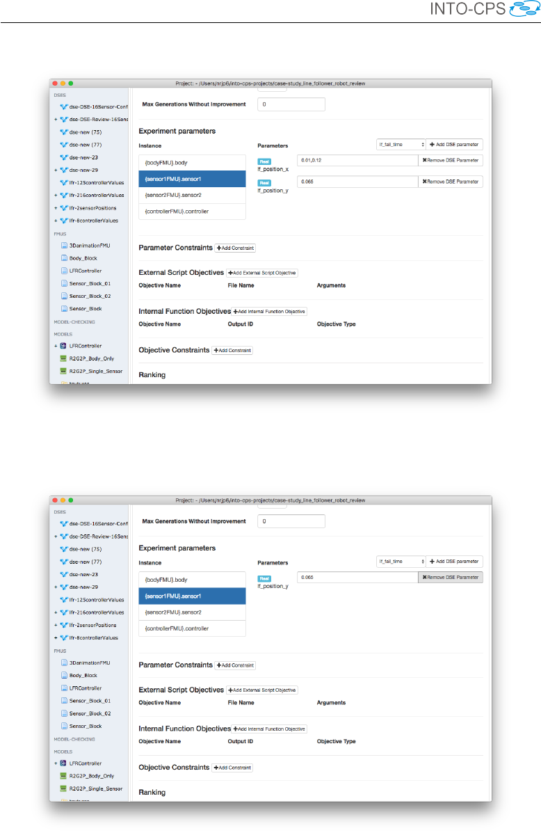
INTO-CPS Tool Chain User Manual (Public)
Figure 107: Editing parameters for DSE run.
Figure 108: Removing a DSE parameter.
99
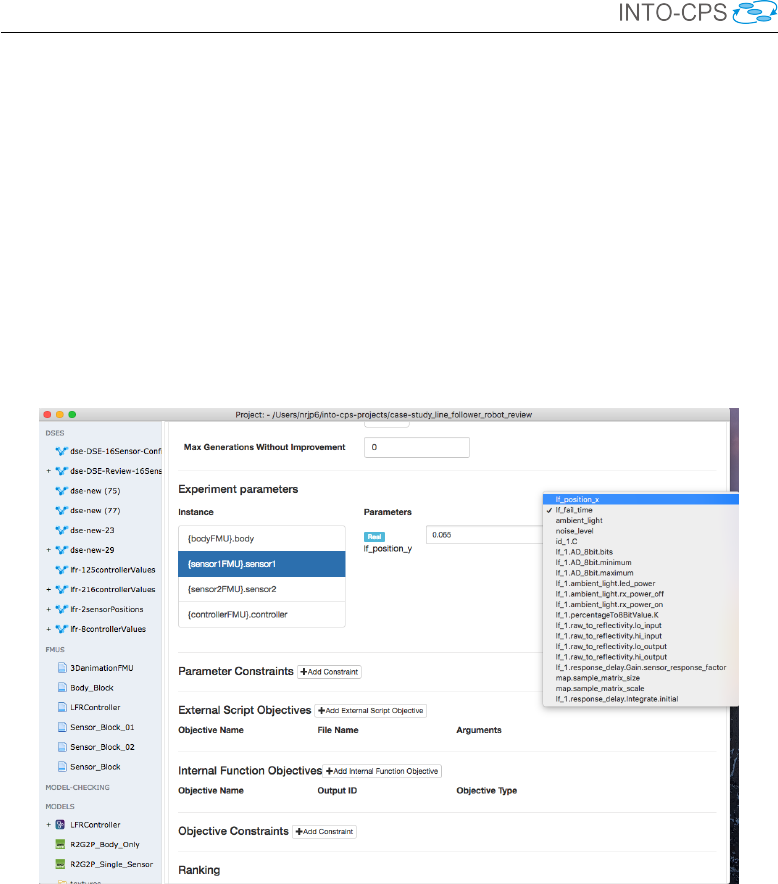
INTO-CPS Tool Chain User Manual (Public)
Figure 109: Add a model parameter for DSE.
100
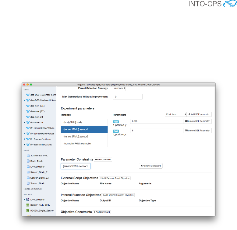
INTO-CPS Tool Chain User Manual (Public)
6.4.6 Parameter Constraints
Clicking the Add Constraint button in the Parameter Constraints section
adds a text box where free text may be added, shown in Figure 110. The con-
straint must be defined according to the description in Section 6.4.16.
Figure 110: Defining a parameter constraint.
6.4.7 Objective Definitions: External Scripts
An external script can be added by clicking the Add External Script Objective
button. Two text boxes are added; first a name for the objective and the
file name of the objective script. In Figure 111, the new objective is given
the name lapTime and uses the lapTime.py Python script. Note: external
scripts must be included in the userMetricScripts folder of the INTO-CPS
project.
Once added, the required arguments must be given. Clicking the Add Ar-
gument button adds several elements (shown in Figure 112) – the first text
box indicates the argument order; the second drop down indicates the type
of value, which is either a model output (refers to an output port of a con-
stituent element of the multi-model), a simulation value (either step-size
101

INTO-CPS Tool Chain User Manual (Public)
Figure 111: Adding a new external script.
or time), or some constant; the third is the argument to pass to the script.
The argument may be a user defined constant value, or one of the predefined
values depending on the type selected. A complete definition is shown in
Figure 113.
6.4.8 Objective Definitions: Internal Functions
Internal functions are added by clicking the Add Internal Function Objective
button. This adds a text box to provide the name of the objective, a drop
down to specify which model output to use (this refers to an output port
of a constituent element of the multi-model) and a drop down to select the
type of function. Currently three exist: max,min and mean. This is shown
in Figure 114.
6.4.9 Objective Constraints
Objective constraints are similar to parameter constraints. A constraint is
added by clicking the Add Constraint button in the Objective Constraints
102
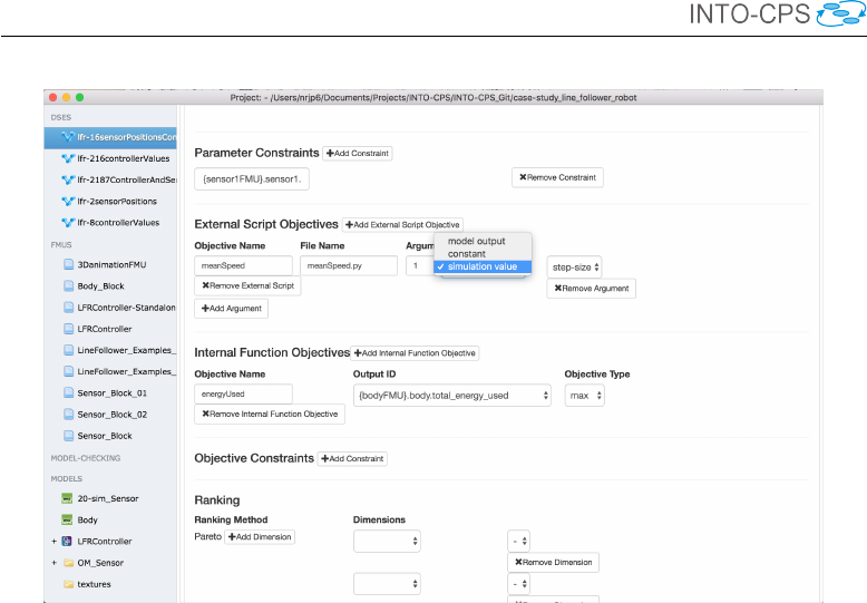
INTO-CPS Tool Chain User Manual (Public)
Figure 112: Add argument to external script.
section. This adds a text box where free text may be added, shown in
Figure 115. The constraint must be expressed in valid Python code.
6.4.10 Ranking
At present, DSE uses only 2-way Pareto rankings. As such, a maximum of
two dimensions may be added by clicking the Add Dimension button. When
clicked, the user may select one of the defined objectives and a direction –
either +or −. This is shown in Figure 116.
6.4.11 Scenario List
The support for scenarios is currently limited. At present the user may define
a collection of named scenarios, which are passed to all external scripts (the
external scripts need not use this). This is shown in Figure 117.
6.4.12 Saving the Configuration
When the configuration editing is finished, it may be saved by clicking the
Save button at the top or bottom of the configuration description, as in Fig-
103
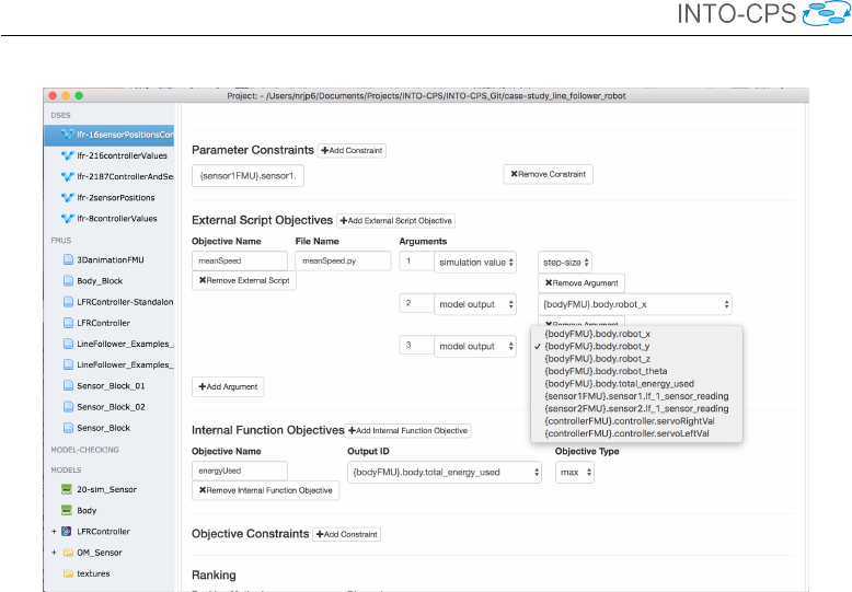
INTO-CPS Tool Chain User Manual (Public)
Figure 113: Complete external script.
ure 118. Note this will overwrite the previous version of the json configuration
file – any non-DSE tags will be lost.
6.4.13 Manual Configuration Creation
The recommended procedure for creating a new configuration is to make a
copy of an existing one and then to edit the required sections. The individ-
ual configurations are located in their own folders within the Design Space
Exploration folder of the INTO-CPS Application project directory, such as
the pilot study with the line following robot “LFR-2SensorPositions” config-
uration shown in Figure 119 (see [PGP+16]). Using your OS’s file browser,
create a new folder under DSEs and then copy in and rename a DSE configu-
ration. The names of the new folder and configuration folder can be chosen at
will, but the configuration file must have the extension .dse.json .
6.4.14 Algorithm
The algorithm section dictates the DSE search algorithm to employ in a DSE.
There are two types (although if no algorithm is defined, it is assumed to be
an exhaustive search):
104
INTO-CPS Tool Chain User Manual (Public)
Figure 114: Defining an internal function.
Exhaustive No further values are required.
Genetic The genetic approach requires several additional values; initialPop-
ulation (number); initialPopulationDistribution (currently only “ran-
dom” is supported); mutationProbablity (number – 0-100); parentSe-
lectionStrategy (currently only “random” is supported); and maxGen-
erationsWithoutImprovement (number).
An example is given in Figure 120.
6.4.15 Parameters
The parameters section is used to define a list of values for each parameter to
be explored. Figure 121 shows the definition of four parameters, each with
two values. If a parameter is included in the DSE configuration file, then it
must have at least one value defined. The order of the values in the list is
not important. If a parameter that is to be explored is not in the list, its ID
may be found in the three ways listed below.
1. If the parameter is listed in the multi-model configuration, then copy
it from there.
2. If the parameter is not in the multi-model parameters list then its name
105
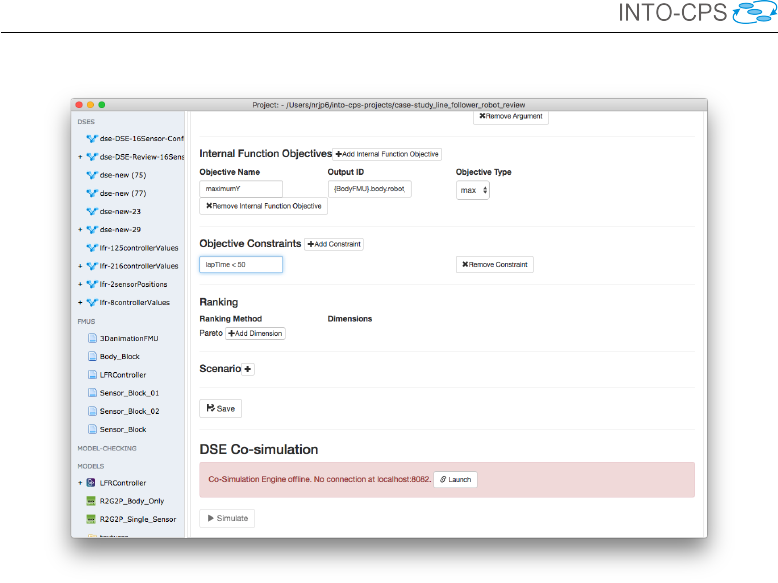
INTO-CPS Tool Chain User Manual (Public)
Figure 115: Defining an objective constraint.
may be found by examining the model description file in the associated
FMU. In this case it will be necessary to prepend the parameter ID
with the ID for the FMU and the instance ID of the FMU, for example
in “{sensor1FMU}.sensor1.lf_position_x”.
•the ID of the FMU is {sensor1FMU}.
•the instance ID of the FMU in the multi-model is sensor1.
•the parameter ID is lf_position_x.
3. The IDs for each parameter may also be found on the Architecture
Structure Diagram in the SysML models of the system. The full name
for use in the multi-model may then be constructed as above.
6.4.16 Parameter Constraints
Figure 122 shows two constraints defined for the line follower DSE experiment
that ensure only symmetrical designs are allowed. The first constraint ensures
the y co-ordinates of both sensors are the same, while the second constraint
ensures that the x co-ordinate of the left sensor is the same, but negated as
106
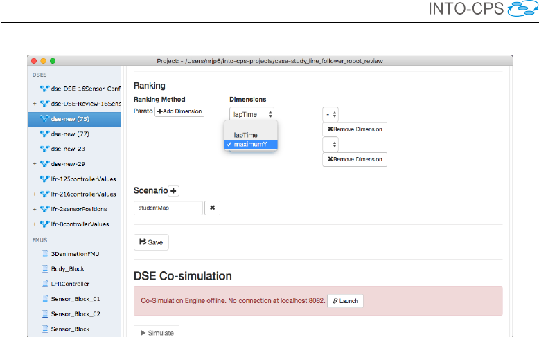
INTO-CPS Tool Chain User Manual (Public)
Figure 116: Defining the Pareto ranking.
the x co-ordinate of the right sensor. Note that the names used when defining
such constraints have the same FMU_ID.instance_ID.parameter_ID
format as used when defining a parameter range (see Section 6.4.15)
Since the constraints are processed using the Python eval function, any
boolean expression compatible with this may be used here.
6.4.17 Objective Definitions: Internal
Defining an internal objective requires three pieces of information:
name This is the name that the objective value will be stored under in the
objectives file.
type This selects the function to be applied. The key objectiveType is
used in the DSE configuration file.
variable This defines the variable to which the function is to be applied.
The key columnID is used to denote this parameter in the DSE con-
figuration file.
Figure 123 shows the definition of an objective named energyConsumed,
which records the maximum value of the variable
{bodyFMU}.body.total_energy_used. This objective is recorded and
may be used later, primarily for the purpose of ranking designs, but it could
107
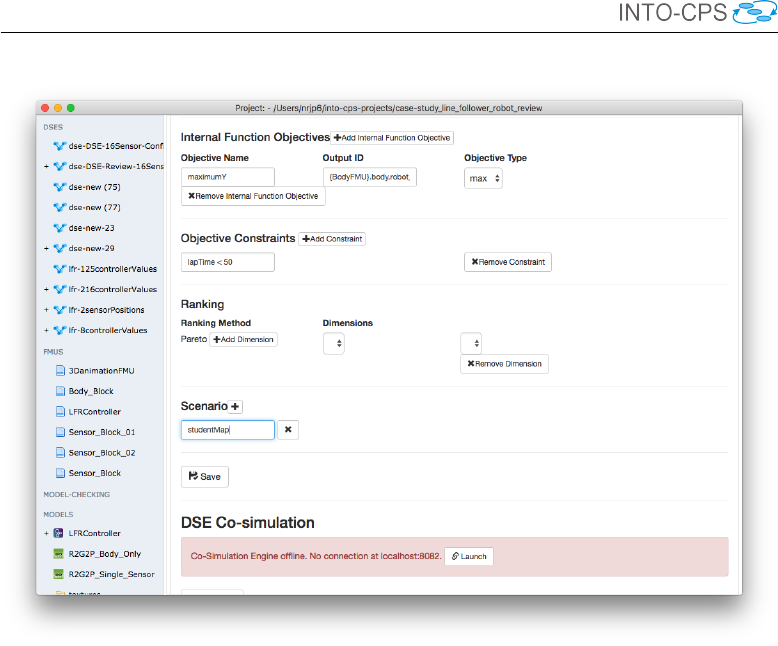
INTO-CPS Tool Chain User Manual (Public)
Figure 117: Adding a DSE scenario.
also be used for any other analysis required.
6.4.18 Objective Definitions: External Scripts
Using external scripts in a configuration requires three parts; a name for
the objective, the file name of the script and a list of arguments to pass.
The name given to the objective allows it to be referenced in the objectives
constraints and ranking sections of the DSE configuration. The file name tells
the DSE scripts which script to launch and the arguments define additional
data (over the standard three arguments described earlier) that the script
needs, such as the names of data it needs or constant values.
In Figure 124 we find the definition of the external analysis used in the
Three Water Tank example. There are two analyses defined, the first is
named “cumulativeDeviation” and the second is “vCount”. In each there are
two parameters defined: “scriptFile” contains the file name of the script file
to run in each case, while “scriptParameters” contains the list of additional
arguments each needs.
108
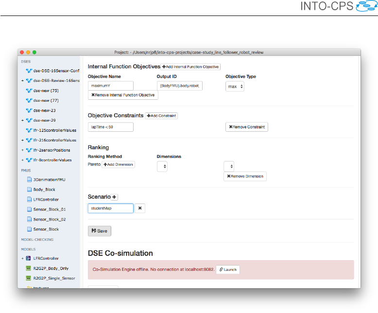
INTO-CPS Tool Chain User Manual (Public)
Figure 118: Save DSE configuration.
The purpose of both internal and external analysis functions is to populate
the objectives.json file with values that characterise the performance
of the designs being explored. Figure 125 shows an example objectives file
generated during a DSE of the Three Water Tank example. There is an
instance of the objectives file created for each simulation in DSE, its primary
use being to inform the ranking of designs, but it may be used for any other
analysis a user wishes to define.
6.4.19 Ranking
Figure 126 shows an example of a ranking definition from the line following
robot example. Here the user has specified that the lap time and mean cross
track error objectives will be used for ranking. The use of ’-’ after each
indicates that the aim is to minimise both, whereas a ’+’ indicates the desire
to maximise.
109
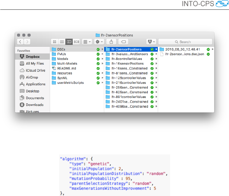
INTO-CPS Tool Chain User Manual (Public)
Figure 119: Location of DSE configurations.
Figure 120: Example genetic algorithm.
6.4.20 Scenario List
Changing a scenario may involve changing one or more different parts of the
multi-model and its analysis, such as the specific FMUs used, parameters
passed to an FMU, the multi-model the DSE is based upon, along with any
data files used by the objective scripts (Section 6.4.18) to evaluate perfor-
mance. This feature is currently under development and so only the objective
data file selection is implemented presently. As such, scenarios are simply
passed to objectives.
Combining all these sections results in a complete DSE configuration, as
shown in Figure 127.
110
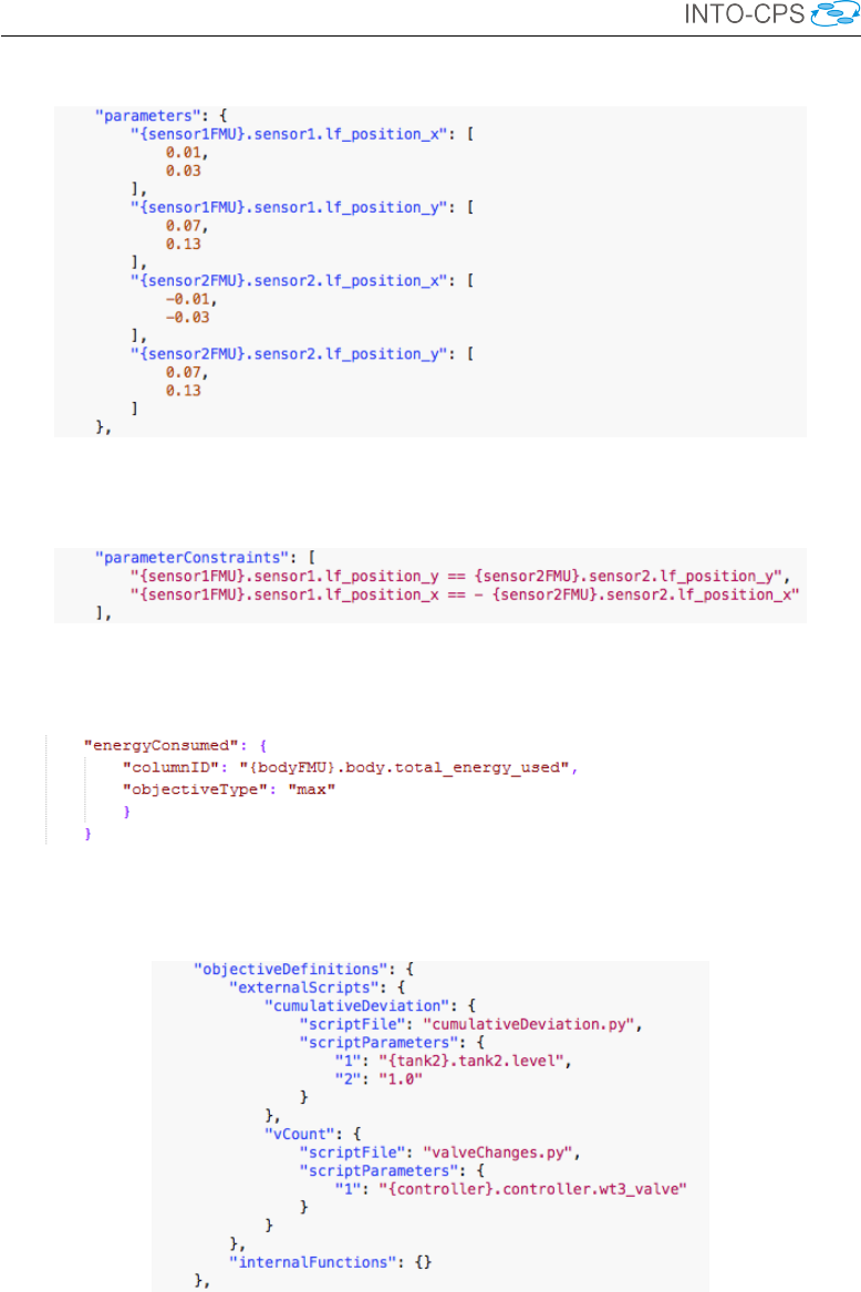
INTO-CPS Tool Chain User Manual (Public)
Figure 121: Example parameter definitions.
Figure 122: Example parameter constraints.
Figure 123: Definition of an internal objective.
Figure 124: Definition of the external analysis functions for the Three Water
Tank model.
111
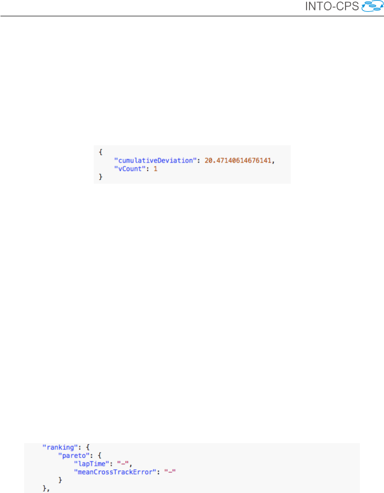
INTO-CPS Tool Chain User Manual (Public)
Figure 125: Contents of objectives.json file for a single simulation of
the Three Water Tank model.
Figure 126: Defining parameters and their preferred directions for ranking.
112

INTO-CPS Tool Chain User Manual (Public)
Figure 127: A complete DSE configuration for the Line Follower Robot ex-
ample.
113

INTO-CPS Tool Chain User Manual (Public)
7 Test Automation and Model Checking
Test Automation and Model Checking for INTO-CPS is provided by the RT-
Tester RTT-MBT tool. This section first describes installation and configu-
ration of RT-Tester MBT in Section 7.1. It then describes test automation
in Section 7.2 and model checking in Section 7.3. Note, that these features
are explained in more detail in the deliverables D5.2a [PLM16] and D5.3c
[BH17], respectively. Section 7.4 describes modelling guidelines for model
checking and model-based testing.
7.1 Installation of RT-Tester RTT-MBT
In order to use RTT-MBT, a number of software packages must be installed.
These software packages have been bundled into two installers:
•VSI tools dependencies bundle:
This bundle is required on the Windows platform and installs the fol-
lowing third party software:
–Python 2.7.
–GCC 4.9 compiler suite, used to compile FMUs.
•VSI tools – VSI Test Tool Chain:
–RT-Tester 6.0, a stripped version of the RT-Tester core test system
that contains the necessary functionality for INTO-CPS.
–RT-Tester MBT 9.0, the model-based testing extension of RT-
Tester.
–RTTUI 3.9, the RT-Tester graphical user interface.
–Utility scripts to run RTT-MBT.
–Examples for trying out RTT-MBT.
These bundles can be downloaded via the download manager of the INTO-
CPS Application.
7.1.1 Setup of the RT-Tester User Interface
When the RT-Tester User Interface (RTTUI) is first started, a few configu-
ration settings must be made.
114
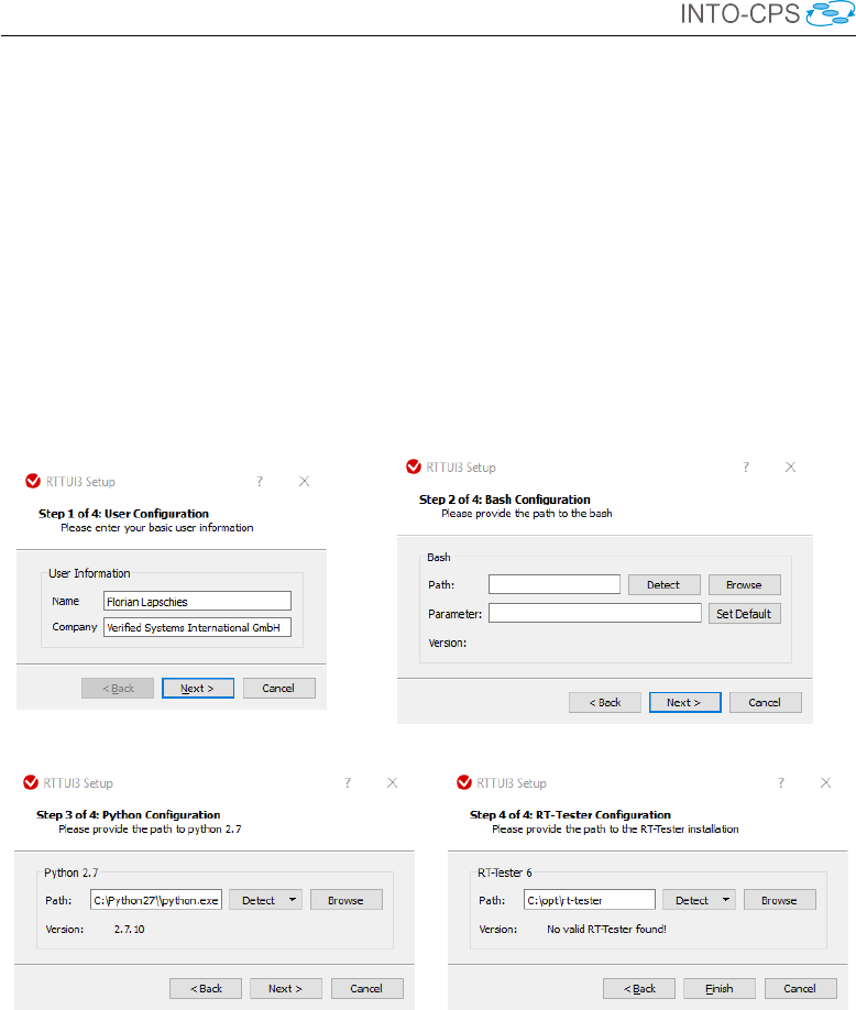
INTO-CPS Tool Chain User Manual (Public)
•User name and company name (Figure 128a).
•Location of Bash shell (Figure 128b). This step can be safely skipped
by clicking Next.
•Path to Python 2.7 executable (Figure 128c): Click Detect and then
Installation Path for auto-detection, or Browse to select manually.
•Location of RT-Tester (Figure 128d): Click Browse to select the direc-
tory of your RT-Tester installation. Note that if you did not specify
the Bash shell location in step 7.1.1, the version number might not be
detected properly.
(a) Configuring user. (b) Configuring Bash.
(c) Configuring Python. (d) Configuring RT-Tester.
Figure 128: RT-Tester GUI configuration.
7.2 Test Automation
Configuring and using a Test Project involves several activities. These are:
•Creating a test project.
•Defining tests.
115
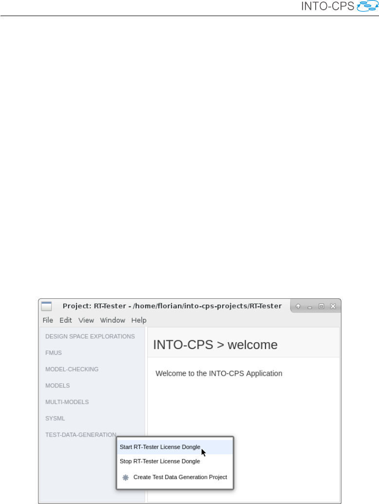
INTO-CPS Tool Chain User Manual (Public)
•Compiling test driver FMUs.
•Setting up test runs.
•Running tests.
•Evaluating test results.
These activities can be performed either solely using the RT-Tester graphical
user interface, or using a combination of the INTO-CPS Application and the
RT-Tester GUI. In this section we focus on describing the latter, since it
supports the complete set of features necessary for test automation. A more
comprehensive description of the test automation workflow can be found in
Deliverable D5.2a [PLM16].
In the INTO-CPS Application, test automation functionality can be found
below the main activity Test-Data-Generation in the project browser. Before
using most of the test automation utilities, the license management process
has to be started. To this end, right-click on Test-Data-Generation and select
Start RT-Tester License Dongle (see Figure 129).
Figure 129: Starting the license management process.
After developing the behavioural model in Modelio and exporting it to an
XMI file (see section 4.4), test automation projects can be created from
the INTO-CPS Application. Such a project is then added as a sub-project
within a containing INTO-CPS Application project. To create a project, do
the following:
116
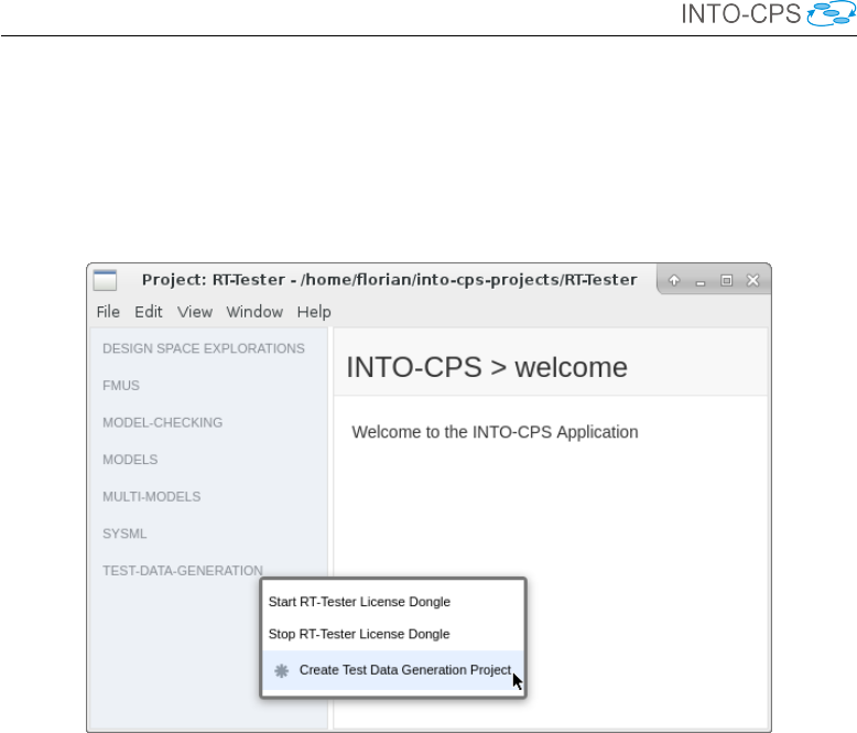
INTO-CPS Tool Chain User Manual (Public)
1. Right-click on Test-Data-Generation in the project browser and select
Create Test Data Generation Project (see Figure 130).
2. Specify a name for the project, select the XMI file containing the test
model and press Create, as shown in Figure 131.
Figure 130: Creating a test automation project.
The newly created sub-project and its directory hierarchy is displayed in the
project browser. The following two folders are of special significance:
•TestProcedures contains symbolic test procedures where test objec-
tives are specified in an abstract way, for example by specifying Linear
Temporal Logic (LTL) formulas.
•From these symbolic test procedures, concrete executable (RT-Tester 6)
test procedures are generated, which then reside in the folder RTT_
TestProcedures.
The specification of test objectives is done using the RT-Tester GUI. The
relevant files can be opened in the RT-Tester GUI directly from the INTO-
CPS Application by double-clicking them:
•conf/generation.mbtconf allows you to specify the overall test
objectives of the test procedure. Test objectives can be specified as
LTL formulas, which must then be fulfilled during a test run. Test
goals can also be specified by selecting structural elements from a tree
representation of the test model and then choosing a coverage metric
117
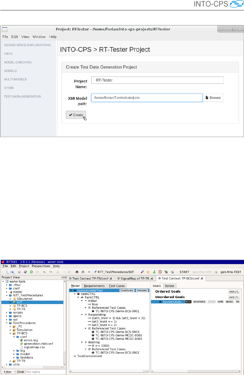
INTO-CPS Tool Chain User Manual (Public)
Figure 131: Test automation project specifics.
for that element. For example, the user might select a sub-component
of the System Under Test (SUT) and specify that all Basic Control
States (BCS) must be reached (see Figure 132), or that all transitions
must be exercised (TR) in a test run.
•conf/signalmap.csv allows you to configure the input and output
signals of the system under test (see Figure 133). This includes defining
the admissible signal latencies for checking the SUT’s outputs in a test
run. This file also allows you to restrict the range of the signals in order
to constrain these values during test data generation.
Figure 132: Configuring a test goal.
118

INTO-CPS Tool Chain User Manual (Public)
Figure 133: Configuring signals.
More details on the definition of tests can be found in Deliverable D5.2a
[PLM16].
After defining the test objectives, a concrete test case can be created by right-
clicking on the symbolic test case under TestProcedures and then selecting
Solve (see Figure 134).
Figure 134: Generating a concrete test procedure.
119
INTO-CPS Tool Chain User Manual (Public)
A solver component then computes the necessary timed inputs to realize the
test objectives. A concrete test procedure is generated that feeds a system
under test with these inputs and observes its outputs against expected results
derived from the test model. This test procedure will be placed in RTT_
TestProcedures and has the same name as the symbolic test procedure.
Figure 135 shows how test generation progresses.
Figure 135: Test data generation progress.
A generated test procedure can be cast into an FMU, which can then be
run in a co-simulation against the system under test. To this end, right
click on the concrete test procedure and select Generate Test FMU (see
Figure 136). In cases where a real and perhaps physical system under test is
not available, a simulation of the system under test can be generated from
the behavioural model. To generate such an FMU, right-click on Simulation
an select Generate Simulation FMU as depicted in Figure 137.
In order to run a test, right-click on the test procedure and select Run Test
120
INTO-CPS Tool Chain User Manual (Public)
Figure 136: Generating a test FMU.
Figure 137: Generating a simulation FMU.
(see Figure 138). Then, the FMUs that constitute the system under test
must be added by pressing the respective Add FMU button. When running
a test, this list of FMUs is further augmented by an FMU representing the
test driver. The connections between these FMUs are automatically derived
by matching the names of inputs and outputs. The duration of the test
is derived during test data generation and does not need to be manually
specified. However, an appropriate step size must be set. Finally, after
making sure the COE is running, press Run to start the test (see Figure 139).
Every test execution yields as its result an evaluation of test cases, i.e., each is
121
INTO-CPS Tool Chain User Manual (Public)
Figure 138: Running a test.
associated with a verdict of PASS, FAIL, or INCONCLUSIVE.14 The details
are found in the test log files below the folder testdata. See the RT-Tester
user manual [Ver15a] for details.
The file testcase_tags.txt gives a condensed record of test case, ver-
dict, and point in a *.log file where a corresponding PASS, FAIL, or—
in case of INCONCLUSIVE—test case occurrence without assertion can
be found. The project-wide test-case verdict summary as well the require-
ment verdict summary can be found in the folder RTT_TestProcedures/
verification. More details on the evaluation of test runs can be found
in Deliverable D5.2a [PLM16].
7.3 Model Checking
This section describes how to use the INTO-CPS Application as a front-
end to the LTL model checker of RT-Tester RTT-MBT. More details on the
algorithms used and the syntax of LTL formulas can be found in Deliverable
D5.3c [BH17].
Once an INTO-CPS project has been created (see Section 3.2), model check-
ing functionality can be found under the top-level activity Model Checking in
14The verdict can also be NOT TESTED. This means a test case has been included in
a test procedure, but a run that reaches it is still missing.
122
INTO-CPS Tool Chain User Manual (Public)
Figure 139: Configuring a test.
the project browser. Before getting started, the RT-Tester license manage-
ment process must be launched. To this end, right-click on Model Checking
and select Start RT-Tester License Dongle (see Figure 140). Model checking
projects are presented as sub-projects of INTO-CPS Application projects. In
order to add a new project,
1. Right-click on the top-level activity Model Checking in the project
browser and select Create Model Checking Project (see Figure 141).
2. Provide a project name and the behavioural model that has been ex-
ported to XMI from Modelio (see section 4.4).
123
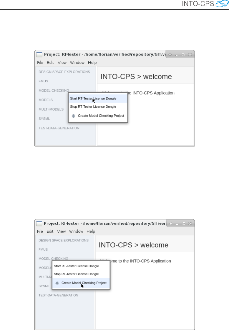
INTO-CPS Tool Chain User Manual (Public)
Figure 140: Starting the RT-Tester license dongle.
Figure 141: Creating a model checking project.
124
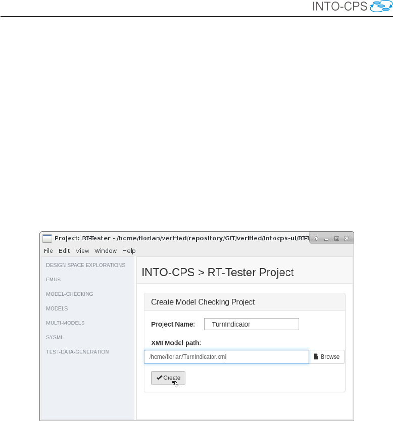
INTO-CPS Tool Chain User Manual (Public)
Figure 142: Specifying the model checking project.
125
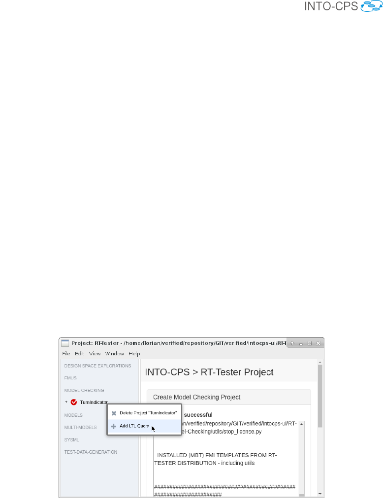
INTO-CPS Tool Chain User Manual (Public)
After pressing Create, a new node representing the model checking project is
added to the project browser.
The next step is to add LTL queries to the project:
1. Right click on the project and select Add LTL Query (see Figure 143).
2. Enter a name for the new query (see Figure 144).
3. To edit the LTL query, double click on the corresponding node in the
project browser (see Figure 145). The LTL formula can then be edited
in a text field. In addition to all variables occurring in the model a
special variable called _stable which is true iff the system resides in a
stable state is available. This variable can be used to rule out spurious
counter-examples involving transient states that are immediately left in
zero time. Note that the editor supports auto-completion for variable
names and LTL operators (see Figure 146).
4. Specify a comma-separated list of requirements and select whether a
model checking result should be linked to either verify or violate these
requirements in the traceability database.
5. Provide the upper bound for the bounded model checking query.
Figure 143: Adding an LTL formula.
To check the query, press Save & Check. After a while the tool either reports
that the query holds within the specified number of steps or it prints a coun-
terexample to demonstrate that the property does not hold — as depicted in
Figure 147. The user then has to manually inspect the model-checking result
for spurious counter examples that might have been introduced by abstrac-
tions that are too coarse. Finally, if the user is satisfied with the result, the
126
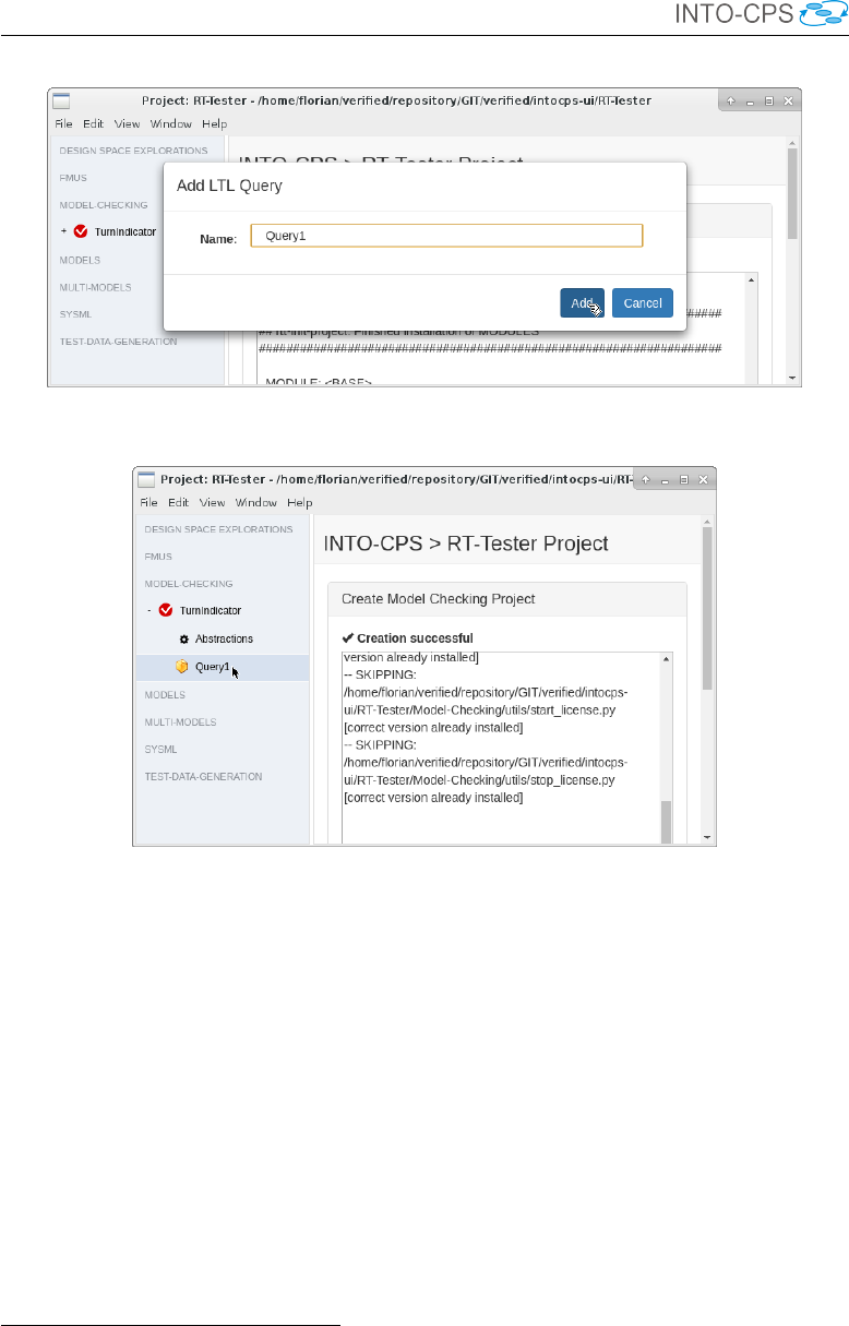
INTO-CPS Tool Chain User Manual (Public)
Figure 144: Naming the new LTL formula.
Figure 145: Opening the LTL formula editor.
traceability information associated with the result can be committed to the
traceability database by pressing Commit Traceability Data.
It is possible to configure abstractions15 for a particular model checking
project. To do so, double-click on the corresponding Abstractions node below
that project in the project browser. It is then possible to choose an abstrac-
tion method for each output variable of an environment component along
with making the associated setting. In Figure 148 the interval abstraction
has been selected for the output variable voltage. This abstraction has
further been configured to restrict the variable’s value within the interval
[10,12]. After pressing Save, this abstraction is applied to all model checking
queries in the current model checking project.
15Information on abstractions and their associated configuration items can be found in
Deliverable D5.2b [BLM16].
127
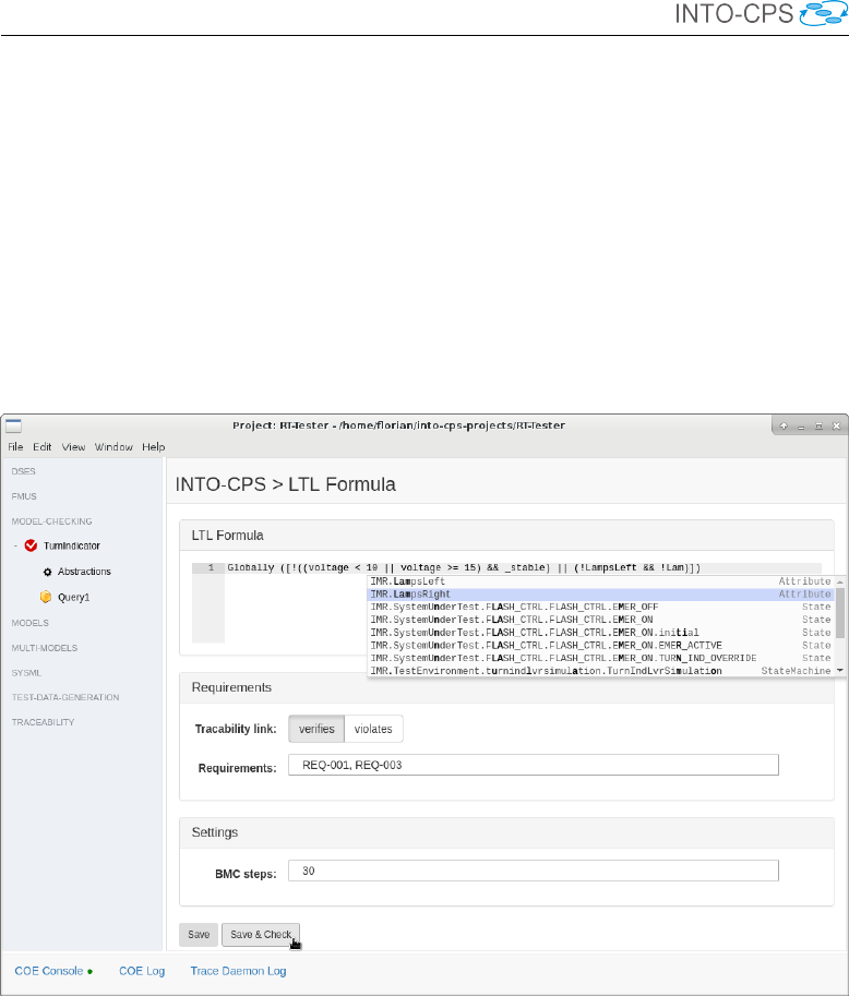
INTO-CPS Tool Chain User Manual (Public)
Figure 146: LTL formula editor.
128
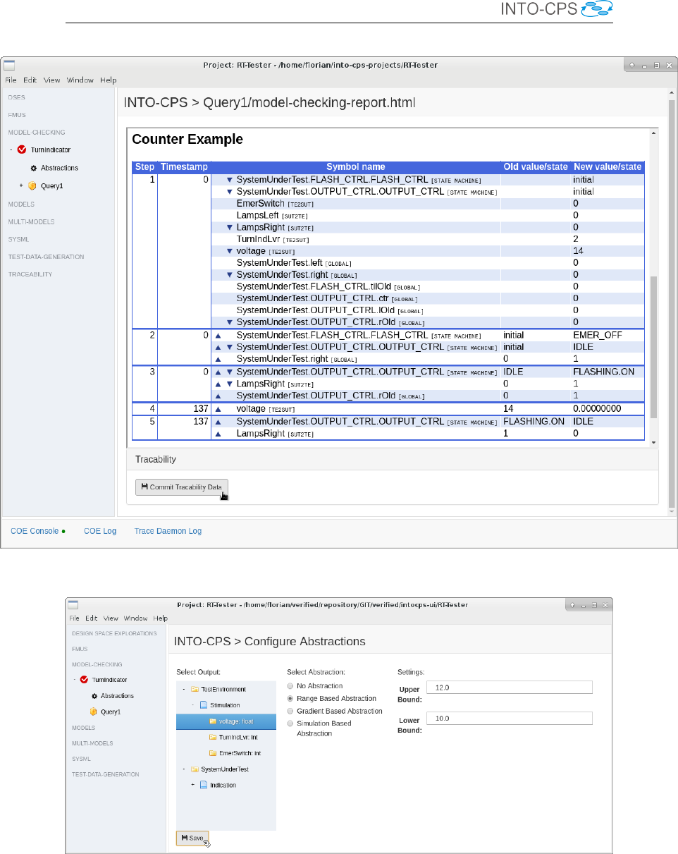
INTO-CPS Tool Chain User Manual (Public)
Figure 147: Model checking result.
Figure 148: Configuring abstractions.
129

INTO-CPS Tool Chain User Manual (Public)
7.4 Modeling Guidelines (for TA and MC purposes)
When creating a model for test automation (TA) or model checking (MC),
it is important to keep in mind that it will be input to a solver that explores
the state space of the model. It is not helpful to have a very precise state
machine model which the solver cannot handle.16
A“good” model tries to find a balance between precision and solver time, i.e.,
it aims to represent all important logical aspects (that may contain design
errors,) but abstract away from details where the implementation can be
trusted to handle data correctly. This section contains some guidelines on
how to avoid common modelling pitfalls.
(G.1) Model independent parts as separate machines. When you
can think of two parts of the system as individual entities, then you should
have one state machine for each part. This is much easier to maintain than
a state machine that “merges” two (or more) behaviours.
(G.2) Reset auxiliary variables. If you use “auxiliary” variables in your
model (e.g. to remember some situation) then they should have a limited
lifetime where they can be of relevance. Reset them (to “0”) when they have
fulfilled their purpose. This modelling trick will not influence the relevant
behaviour of your model, but make the solver’s task easier.
(G.3) Keep the diameter of state machines small (if possible). The
number of steps that are necessary to reach a certain situation can be a serious
limitation in finding solutions. If your state machine includes long sequences
of transitions that need to be taken in order to reach a certain situation,
consider simplifying it by
•breaking this state machine down into several state machines
•“merging” several similar states along this path into a single, more
abstract state (i.e. make your model less precise)
(G.4) Use abstractions whenever specific (payload) data is of no
interest. If the logical state depends on input data, try to model this as
16I.e., resources on time, memory or user patience will be depleted before completion of
the “solving” task.
130

INTO-CPS Tool Chain User Manual (Public)
simply as possible. Consider omitting data sanitation steps (like plausibility
checks, interpolation of values, data sanitation) that may exist in your specific
system but only serve as countermeasures to unreliable sensor inputs. In the
modelling world, inputs are always “perfect” and “reliable”. Example: When
modelling a protocol, avoid modelling the payload. Also, do not put payload
and addressing (housekeeping) information in the same variable.
(G.5) Try to think of “logical states” rather than of “data driven
states”. Variables can be used to “encode” the states of your system. Try to
find a balance where state machine states actually represent “logical states”
(that are distinguished by their behaviour). This will make the guard condi-
tions smaller and more maintainable.
(G.6) Keep a list of modelling parameters. Keep an overview on what
immutable “parameters” your modelling depends on, i.e., what values they
have and where they are used. This will make it easier to revise your model
consistently when required.
(G.7) Dare to approximate complex values. In particular continuous
flows may need to be broken down into manageable components. Example:
A physical accumulator can be approximated by a scalar value. Using a
(scaled) integer instead of a floating-point number may be good enough and
make the task of the solver much easier.
(G.8) Dare to approximate complex behaviour. A common mod-
elling mistake is to “model as precise as possible”. In particular, capturing
continuous states can be very expensive (in terms of state space). Whenever
possible, you should consider simplifying things, even if this means sacrific-
ing precision. Remember that testing aims to find “logical errors” and not to
“represent the most precise approximation of the system”. Example: When
modelling a water tank with (continuous) in-flow and state change, it may
suffice to create a “coarse” model of it which changes state only once per sec-
ond, based in input value, water level, and maximal output capacity.
(G.9) Start with small versions of your system. Do not start mod-
elling with a full-blown version of a complete system. Rather start with one
relevant component, say, one controller and explore testing a small system
before moving to “many controllers, many other components”.
131

INTO-CPS Tool Chain User Manual (Public)
8 Traceability Support
This section describes tool support for traceability along the INTO-CPS tool
chain.
8.1 Overview
Traceability support is divided into two steps: sending data from the tools
to the Neo4J traceability database, and retrieving information from the
database. In the following we first describe how information is sent to the
database and then how it is retrieved.
It shall be noted that the traceability features of INTO-CPS require Git17
to be installed. Furthermore, the project folder must be under Git version
control.
8.2 INTO-CPS Application
Information is stored in the traceability database via the traceability dae-
mon. The traceability daemon is integrated in the INTO-CPS Application
and it starts automatically when the Application is started. Only Neo4J
has to be downloaded, which can be done through the Download Man-
ager. When downloaded, Neo4J must be extracted by hand into the folder
<user_home>/into-cps-projects/install (the archive file is lo-
cated at <user_home>/into-cps-projects/install_downloads af-
ter download.) Note that Neo4J is a singleton, so ensure all other instances
of Neo4J are down before starting the INTO-CPS Application.
Please note: the daemon only runs while the INTO-CPS Application is run-
ning. Therefore, to record traceability data while using any of the other
tools, the INTO-CPS Application must be running.
Treaceability information is captured by the traceability daemon and stored
in a Neo4J database. The database is project-specific and is deployed on
project change within the INTO-CPS Application. When running, Neo4J
is accessible at http://localhost:7474. Here one can view the cur-
rent traceability graph. Username and password of the databases are al-
ways:
17https://git-scm.com/
132
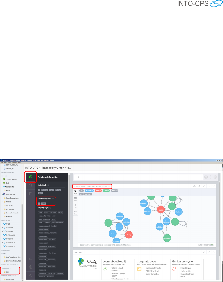
INTO-CPS Tool Chain User Manual (Public)
username = intoCPSApp
password = KLHJiK8k2378HKsg823jKKLJ89sjklJHBNf8j8JH7FxE
To view the raw data from the database, right-click on Traceability in the
INTO-CPS Application project browser and select View Traceability Graph
(see Figure 149). Select the database symbol and click under Relation-
ship types click on Trace. This shows the graph database. By default,
the view is limited to 25 entries. To change this, edit the line MATCH
p=()-[r:Trace]->() RETURN p LIMIT 25 and set the limit to a dif-
ferent value. When starting the INTO-CPS Application, Neo4J needs to be
started as well. Sometimes this is very slow and the startup operation is
aborted. To force the Neo4J database to start, repeat the View Traceability
Graph action until the Neo4J view shows, as illustrated in Figure 149. Alter-
natively, start the INTO-CPS Application from the command line to monitor
the status of the Neo4J database. Please note: this view of traceability rela-
Figure 149: Current view of traceability in the INTO-CPS Application.
tionships is not meant for end users, but rather for developers.
8.3 Modelio
The latest Modelio module can be downloaded here: http://forge.
modelio.org/projects/intocps-modelio34/files. Note that cur-
133

INTO-CPS Tool Chain User Manual (Public)
rently the INTO-CPS module is only compatible with Modelio 3.4. Modelio
currently (INTO-CPS module 1.3.15) supports traceability for the following
modelling activities:
•Model creation
•Model modification
•Model Description export
•Configuration export
•Requirements creation
To install the module go to Configuration →Modules, select INTO-CPS and
set the parameters for:
•The daemon connection, i.e. the daemon IP address and its connection
port (7474). By default these values are, respectively, 127.0.0.1 and
8083
•The Git user identification, i.e. its Git ID, the related e-mail address
and the path to the local Git repository (i.e. the path to the location
of the .git folder).
The traceability information is sent automatically to the daemon, either right
after performing a traced action (Model Description Export and Configura-
tion Export) or after closing the project.
Regarding requirements tracing, currently only the relations Satisfy and Ver-
ify are supported for traceability, as shown in Figure 151. Hint: To push an
older model (i.e., one made before the deployment of the traceabilty feature)
to the traceability database, you can use the following Jython script inside
the Modelio Script tab as depicted in Figure 152.
peerModule = Modelio.getInstance().getModuleService().
getPeerModule(IINTOCPSPeerModule.MODULE_NAME);
peerModule.pushModel();
8.4 Overture
The latest version of the Overture traceability driver can be found on the
GitHub site18 or in the download manager of the INTO-CPS Application.
18see https://github.com/overturetool/intocps-tracability-driver/
releases
134
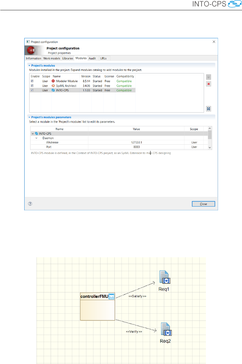
INTO-CPS Tool Chain User Manual (Public)
Figure 150: Configuration of traceability features in Modelio.
Figure 151: Requirements related to a SysML Block in Modelio.
135
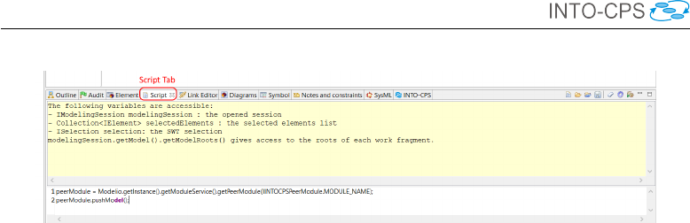
INTO-CPS Tool Chain User Manual (Public)
Figure 152: Pushing Jython script.
All traces can be extracted from the traceability driver and sent to the dae-
mon. To do so, please follow the description on the GitHub site above.
8.5 OpenModelica
The latest INTO-CPS targeted nightly builds of OpenModelica support trace-
ability. They can be downloaded from https://build.openmodelica.
org/omc/builds/windows/nightly-builds/intocps/. OpenMod-
elica supports tracing the following modeling activities:
•Model creation
•Model modification
•FMU export
•FMU import
•Model description XML import
As a prerequisite for traceability support, Git should be installed in the sys-
tem. To configure traceability support, go to Tools →Options →Traceability,
select the traceability checkbox and set all the fields, the traceability daemon
IP address and port (7474) (see Figure 153). By default, the port is 8083.
Then, go to Tools →Options →General and set the working directory to
which you would like to export the FMU (see Figure 154). Create a Modelica
model via File →New Modelica Class or load a model via File →Open Mod-
el/LibraryFile(s), as in Figure 155. After modification of the model/class,
click the File →Save button, press Ctrl-s or click the Save button from
the menu bar, as shown in Figure 156. A dialog as shown below in Figure
157 will appear to enter the commit description. To trace the export of an
FMU, load the Modelica model or create a new model, then go to FMI →
Export FMU (see Figure 158). OpenModelica generates the FMU, commits
and sends the traceability information to the daemon automatically.
136
INTO-CPS Tool Chain User Manual (Public)
Figure 153: Traceability settings in OpenModelica.
Figure 154: FMU export directory in OpenModelica.
137
INTO-CPS Tool Chain User Manual (Public)
Figure 155: Create or open a Class in OpenModelica.
Figure 156: Save a model in OpenModelica.
Figure 157: The commit message in OpenModelica.
138
INTO-CPS Tool Chain User Manual (Public)
Figure 158: FMU export in OpenModelica.
To import a modelDescription.xml file, go to FMI →Import FMU
Model Description. A dialog as shown in Figure 159 will appear. Select the
modelDescription.xml file and the output directory then press OK.
The Modelica model with SysML block inputs and outputs will be generated
and automatically loaded (see the left part of Figure 159). To visualize the
Figure 159: FMI model description import in OpenModelica.
traceability graph, click the Traceability perspective button as shown below.
8.6 20-sim
To record traceability information from within 20-sim, 20-sim 4.6.3-intocps or
higher is required. A version of 20-sim that supports traceability can be found
139
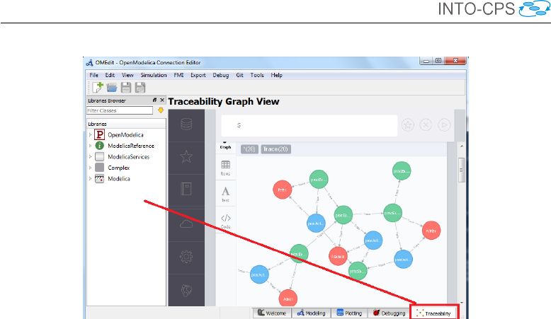
INTO-CPS Tool Chain User Manual (Public)
Figure 160: View traceability data in OpenModelica.
in the INTO-CPS application download manager. Please keep the checkbox
to install Python enabled during the installation process of 20-sim.
When the installation process of 20-sim is done, open 20-sim. The traceability
settings dialog can be found by going to Tools →Version Control Toolbox
→Traceability (see Figure 161). A window will pop up, like the one shown
in Figure 162. If no changes have been made with respect to traceability
within the settings of the INTO-CPS Application, then these are the default
settings that should be used. Please note that the Git Repository can be
changed to another folder on your PC. Furthermore, GIT username and
GIT email address should be altered to match the Git user account and Git
email address with which the commit should be made. For an explanation of
all options that are available in this dialog, please refer to Deliverable D4.3d
[KLN+17].
20-sim has support for several traceable actions:
•Model creation
•Model modification
•FMU export
•FMU import
•Model description XML import
Performing any of these actions will automatically trigger a trace event.
Model creation and model modification are triggered by a Save As action and
140
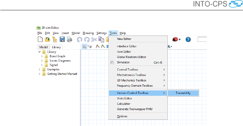
INTO-CPS Tool Chain User Manual (Public)
Figure 161: Opening the traceability dialog in 20-sim.
Save action respectively in the 20-sim GUI. FMU import and modelDes-
cription.xml import are triggered when respectively an FMU or model-
Description.xml file is dragged from the Windows Explorer onto the
canvas in 20-sim. See also subsubsection 5.2.4 for more information on how
to import an FMU in 20-sim, and subsubsection 5.2.1 on how to import a
model description XML file into 20-sim. An FMU export event is triggered
when an FMU is exported from 20-sim (see subsubsection 5.5.5 on how to
export an FMU from within 20-sim). To read more about what actions are
performed during a trace event in 20-sim, please refer to Deliverable D4.3d
[KLN+17].
8.7 RT Tester
For Windows, download the latest release bundle of RT-Tester from
https://secure.verified.de/f5x1hks4/into-cps/one-click/
VSI_bundle.exe. Alternatively, you can use the INTO-CPS download
manager. RT-Tester supports tracing the following modelling activities.
•Define test model
•Define test objectives
•Run test
Prerequisites Git should be installed in the system, as well as the fol-
lowing Python packages: requests,jsonschema,gitpython.Note:
141
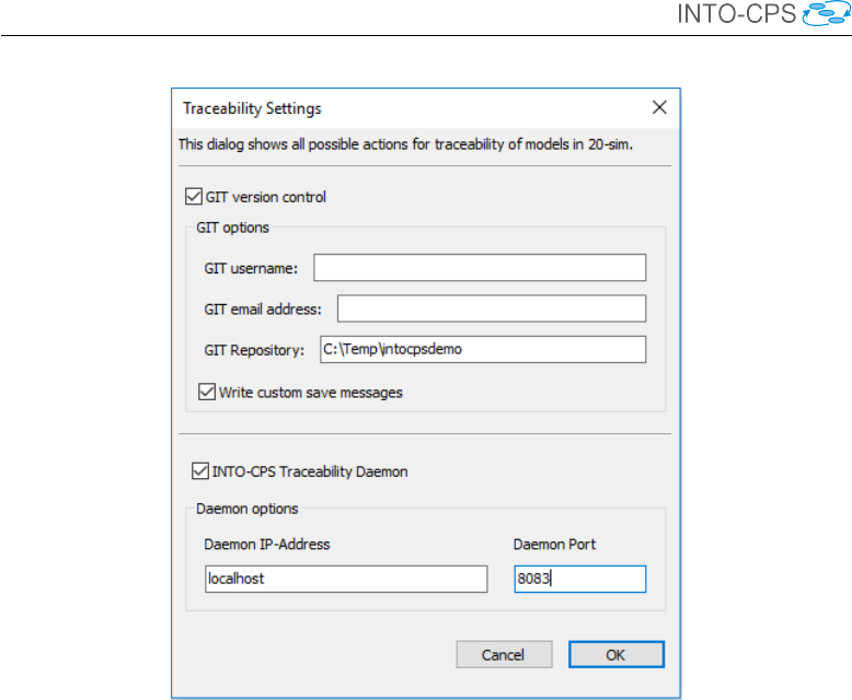
INTO-CPS Tool Chain User Manual (Public)
Figure 162: Opening the traceability dialog in 20-sim.
The VSI_bundle.exe installation process this will check whether these
are installed; if not, it will be attempted to install them using pip.
Configuration of remote OSLC server. If the traceability daemon runs
on the same system as your RT-Tester, then you have nothing to configure.
The actions will already be identified and traced. If the daemon is running
somewhere else, you can configure this by setting the environment variable
OSLC_SERVER. For example, you can do this from the RTTUI3 as indicated
in Figure 163:
1. In the menu bar, select Project →Project Settings
2. Go to the Local Environment tab
3. Click Add →Add a New Variable
4. Set Name to OSLC_SERVER and Value to the host IP or URL
5. Click OK to close the Add Variable dialog
142
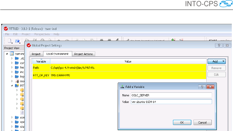
INTO-CPS Tool Chain User Manual (Public)
Figure 163: Configure variable OSLC_SERVER in RTTUI3.
6. Click Save to close the Global Project Settings dialog
8.8 Retrieving Traceability Information
The following traces can be queried from within the INTO-CPS Applica-
tion:
•FMUs and the related requirements
•Users and related activities and artifacts
•Simulation results and the files that were used to produce a certain
result
•Requirements and related test cases
To get an overview in the Application, right-click on the Traceability entry
in the project browser and select Trace Objects. A page will appear as shown
in Figure 164.
Requirements related to FMUs In the first tab of the traceability page
(FMUs) of the INTO-CPS Application (see Figure 164), all the FMUs in the
traceability database are listed. The FMUs are traced once they are exported
from the modelling tool. To each FMU, the related requirements can then
be traced, to give the user a quick and easy overview of which requirements
143
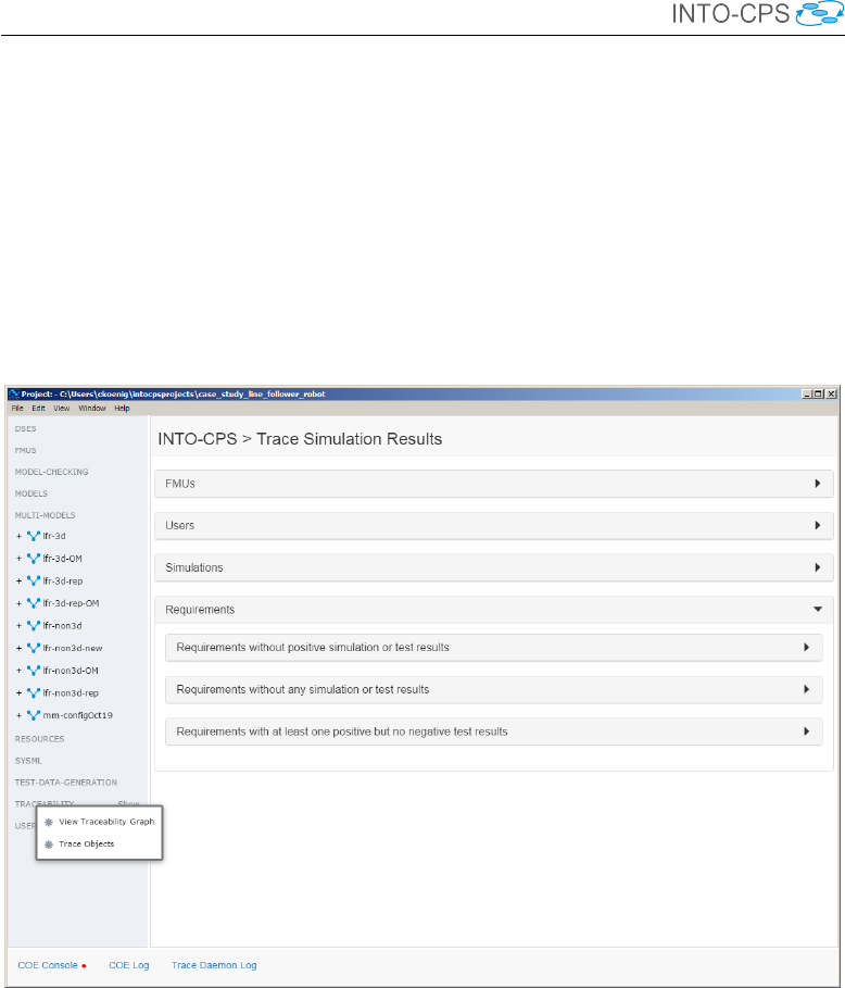
INTO-CPS Tool Chain User Manual (Public)
Figure 164: Overview of the different queries as they are implemented in the
INTO-CPS Application.
144

INTO-CPS Tool Chain User Manual (Public)
are generally linked to a certain FMU, originating from requirements linking
in Modelio.
Activities and artifacts related to users The second tab (Users) lists
all the users that have performed traceability-related actions, as identified
by their e-mail address. For each user, artifacts (e.g. simulation results,
configuration files, modelDescription.xml files etc.) and activities (e.g.
exporting an FMU, importing a modelDescription.xml file, running
a simulation etc.) can be found, along with the time stamp. This allows
evaluating which user created which file, to understand responsibilities in a
complex project.
Files used to create a simulation result The third tab (Simulations)
lists all the simulation results that were created by the INTO-CPS Applica-
tion. For each result, the files and the version of the INTO-CPS Application
used to create the result can be found. This allows understanding the simu-
lation result and can give confidence, since they can be reconstructed.
Test cases and requirements The fourth tab (Requirements) is sub-
divided into three queries. The first, requirements without positive simu-
lation or test results indicates those requirements that have not yet been
validated. The second, requirements without any simulation or test result,
shows requirements which are not yet covered by a test case, neither posi-
tive nor negative. The third, requirements with at least one positive but no
negative test result shows those requirements that have had a positive test
or simulation result, and can therefore be regarded as fulfilled.
145

INTO-CPS Tool Chain User Manual (Public)
9 Code Generation
The INTO-CPS tools Overture, OpenModelica and 20-sim have the ability,
to varying degrees, to translate models into platform-independent C source
code. Overture can moreover translate VDM models written in the exe-
cutable subset of VDM++ [LLB11] (itself a subset of VDM-RT) to Java,
but C is the language of interest for the INTO-CPS technology.
The purpose of translating models into source code is twofold. First, the
source code can be compiled and wrapped as standalone FMUs for co-
simulation, such that the source tool is not required. Second, with the aid of
existing C compilers, the automatically generated source code can be com-
piled for specific hardware targets.
The INTO-CPS approach is to use 20-sim 4C to compile and deploy the code
to hardware targets, since the tool incorporates the requisite knowledge re-
garding compilers, target configuration etc. This is usually done for control
software modelled in one of the high-level modelling notations, after valida-
tion through the INTO-CPS tool chain. Deployment to target hardware is
also used for SiL and HiL validation and prototyping.
For each of the modelling and simulation tools of the INTO-CPS tool chain,
code generation is a standalone activity. As such, the reader should refer to
the tool-specific documentation referenced in Appendix B for guidance on
code generation. Deliverable D5.1d [HLG+15] contains the details of how
each tool approaches code generation.
The remainder of this section lists information about the code generation
capabilities of each tool. Extensive guidance on how to tailor models for
problem-free translation to code can be found in the tools’ individual user
manuals, as referenced in Appendix B. Further references are given herein.
9.1 Overture
Overture provides a code generator for VDM-RT that is geared toward resource-
constrained embedded platforms. Of these, PIC32 and ATmega microcon-
trollers have been tested, as well as Raspberry Pi and typical Intel-based
computers. A complete description of Overture’s C code generator can be
found in Deliverable D5.3d [BHPG17] and in the Overture User Manual,
which is accessible through Overture’s Help system. As a quick-start guide,
this section only provides an introduction to invoking the C code generator,
146
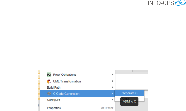
INTO-CPS Tool Chain User Manual (Public)
and an overview of the features of VDM-RT that are stable from a code
generation point of view. Please note that exporting a source code FMU
with Overture (Section 5.1) automatically invokes the code generator and
packages the result as an FMU.
The C code generator is invoked from the context menu in the Project Ex-
plorer as shown in Figure 165. The code generator currently supports the
Figure 165: Invoking the code generator.
following VDM-RT language features:
•Basic data types and operations: integers, reals, booleans, etc.
•The is_ type test
•Quote types
•Token types
•let expressions
•Pattern matching (partial support)
•For and while loops
•case expressions
•Record types
•Union types
•Product types
•Aggregate types and operations: sets, sequences and maps
•Object-oriented features
•The time expression
•Pre-condition checks
•Quantifiers
147

INTO-CPS Tool Chain User Manual (Public)
•Distributed architectures
The following language features are not supported:
•Lambda expressions.
•Post-conditions and invariants.
•File I/O via the I/O library.
A key feature of the C code generator is the use of a garbage collector for
memory management. Generating a VDM-RT model to C code via the con-
text menu results in a main.c file containing a skeletal main() function.
This function contains calls to vdm_gc_init() and vdm_gc_shutdown(),
the garbage collector initialization and shutdown functions. The collector
proper can not be invoked automatically, so calls to the essential function
vdm_gc() must be inserted manually in the main code, for instance after
each repetition of a cyclic task. The source code FMU exporter, on the other
hand, can handle automatic invocation of the garbage collector, so no man-
ual intervention is required. Please note that it is generally unsafe to insert
calls to vdm_gc() in the generated code. The following is a typical main()
function:
#include <Vdm.h>
extern void periodic_task();
extern void other_init();
extern void other_shutdown();
extern int keep_going;
int main()
{
vdm_gc_init();
other_init();
while(keep_going != 0)
{
periodic_task();
vdm_gc();
}
vdm_gc_shutdown();
other_shutdown();
return 0;
}
148

INTO-CPS Tool Chain User Manual (Public)
9.2 20-sim
20-sim supports ANSI-C and C++ code generation through the use of ex-
ternal and user-modifiable code-generation templates. Only a subset of the
supported 20-sim modelling language elements can be exported as ANSI-C
or C++ code. The exact supported features depend on the chosen template
and its purpose and are discussed in Section 5.2.
The main purpose of the 20-sim code generator is to export control systems.
Therefore the focus in on running code on limited embedded targets (e.g.
Arduino) with no operating system, or as a real-time task on a real-time
operating system. The code generated by 20-sim does not contain any target-
related or operating system specific code. The exported code is generated
such that it can be embedded in an external software project. To run 20-
sim generated code on a target, you can use 20-sim 4C. This is a tool that
extends the 20-sim generated code with target code based on target templates
[Con17].
9.3 OpenModelica
OpenModelica supports code generation from Modelica to source code target-
ing both ANSI-C and C++. From the generated source code, co-simulation
and model-exchange FMUs can be built. The only supported solver in the
generated co-simulation FMUs is forward Euler. Additional solvers will be
supported in the future.
9.4 RT-Tester/RTT-MBT
When generating test FMUs from SysML discrete-event state-chart specifi-
cations using RTTester/RTT-MBT, the user should be aware of the following
sources of errors:
•Livelock resulting from a transition cycle in the state-chart specification
in which all transition guards are true simultaneously. This can be
checked separately using a livelock checker.
•Race conditions arising from parallel state-charts assigning different
values to the same variable. Model execution in this case will deadlock.
•State-charts specifying a replacement SUT must be deterministic.
149

INTO-CPS Tool Chain User Manual (Public)
10 Issue handling
Should you experience an issue while using one or more of the INTO-CPS
tools, please take the time to report the issue to the INTO-CPS project team,
so we can help you resolve it as soon as possible.
Before you go any further with your current issue, please check that the
INTO-CPS version you are using is the newest. The version number is part
of the file name of the INTO-CPS Application. To find the list of released
INTO-CPS Applications, and to see what the current version of INTO-CPS
is, please visit
https://github.com/into-cps-association/intocps-ui/
releases/
If your issue is not listed on the Issues tab, please report it there.
150

INTO-CPS Tool Chain User Manual (Public)
11 Conclusions
The tool chain supports model-based design and validation of CPSs, with an
emphasis on multi-model co-simulation.
Several independent simulation tools are orchestrated by a custom co-simu-
lation orchestration engine, which implements both fixed and variable step
size co-simulation semantics. A multi-model thus co-simulated can be fur-
ther verified through automated model-based testing and bounded model
checking.
The tool chain benefits from a cohesive management interface, the INTO-
CPS Application, the main gateway to modelling and validation with the
INTO-CPS technology. Following the manual should give a new user of the
INTO-CPS tool chain an understanding of all the elements of the INTO-CPS
vision for co-simulation. This manual is accompanied by tutorial material
and guidance on the main INTO-CPS tool chain website at
http://into-cps-association.github.io
151

INTO-CPS Tool Chain User Manual (Public)
References
[BH17] Jörg Brauer and Miran Hasanagic. Implementation of a model-
checking component. Technical report, INTO-CPS Deliverable,
D5.3c, December 2017.
[BHJ+06] Armin Biere, Keijo Heljanko, Tommi A. Juntilla, Timo Latvala,
and Viktor Schuppan. Linear encodings of bounded LTL model
checking. Logical Methods in Computer Science, 2(5), 2006.
[BHPG17] Victor Bandur, Miran Hasanagic, Adrian Pop, and Marcel
Groothuis. FMI-Compliant Code Generation in the INTO-CPS Tool
Chain. Technical report, INTO-CPS Deliverable, D5.3d, December
2017.
[BLL+17] Victor Bandur, Peter Gorm Larsen, Kenneth Lausdahl, Casper
Thule, Anders Franz Terkelsen, Carl Gamble, Adrian Pop, Etienne
Brosse, Jörg Brauer, Florian Lapschies, Marcel Groothuis, Christian
Kleijn, and Luis Diogo Couto. INTO-CPS Tool Chain User Manual.
Technical report, INTO-CPS Deliverable, D4.3a, December 2017.
[BLM16] Jörg Brauer, Florian Lapschies, and Oliver Möller. Implementation
of a Model-Checking Component. Technical report, INTO-CPS De-
liverable, D5.2b, December 2016.
[Blo14] Torsten Blochwitz. Functional Mock-up Interface for Model Ex-
change and Co-Simulation. https://www.fmi-standard.
org/downloads, July 2014.
[BQ16] Etienne Brosse and Imran Quadri. SysML and FMI in INTO-CPS.
Technical report, INTO-CPS Deliverable, D4.2c, December 2016.
[Bro97] Jan F. Broenink. Modelling, Simulation and Analysis with 20-Sim.
Journal A Special Issue CACSD, 38(3):22–25, 1997.
[Bro17] Etienne Brosse. SysML and FMI in INTO-CPS. Technical report,
INTO-CPS Deliverable, D4.3c, December 2017.
[CFT+17] Ana Cavalcanti, Simon Foster, Bernhard Thiele, Jim Woodcock,
and Frank Zeyda. Final Semantics of Modelica. Technical report,
INTO-CPS Deliverable, D2.3b, December 2017.
[Con13] Controllab Products B.V. http://www.20sim.com/, January 2013.
20-sim official website.
152

INTO-CPS Tool Chain User Manual (Public)
[Con17] Controllab Products B.V. http://www.20sim4C.com/, August
2017. 20-sim 4C official website.
[Fav05] Jean-Marie Favre. Foundations of Model (Driven) (Reverse) Engi-
neering : Models – Episode I: Stories of The Fidus Papyrus and of
The Solarus. In Language Engineering for Model-Driven Software
Development, March 2005.
[FCC+16] Simon Foster, Ana Cavalcanti, Samuel Canham, Ken Pierce, and
Jim Woodcock. Final Semantics of VDM-RT. Technical report,
INTO-CPS Deliverable, D2.2b, December 2016.
[FE98] Peter Fritzson and Vadim Engelson. Modelica - A Unified Object-
Oriented Language for System Modelling and Simulation. In EC-
COP ’98: Proceedings of the 12th European Conference on Object-
Oriented Programming, pages 67–90. Springer-Verlag, 1998.
[FGP17] John Fitzgerald, Carl Gamble, and Ken Pierce. Method Guidelines
3. Technical report, INTO-CPS Deliverable, D3.3a, December 2017.
[FGPP16] John Fitzgerald, Carl Gamble, Richard Payne, and Ken Pierce.
Method Guidelines 2. Technical report, INTO-CPS Deliverable,
D3.2a, December 2016.
[Fri04] Peter Fritzson. Principles of Object-Oriented Modeling and Simula-
tion with Modelica 2.1. Wiley-IEEE Press, January 2004.
[Gam17] Carl Gamble. Comprehensive DSE Support. Technical report,
INTO-CPS Deliverable, D5.3e, December 2017.
[GFR+12] Anand Ganeson, Peter Fritzson, Olena Rogovchenko, Adeel As-
ghar, Martin Sjölund, and Andreas Pfeiffer. An OpenModelica
Python interface and its use in pysimulator. In Martin Otter and
Dirk Zimmer, editors, Proceedings of the 9th International Model-
ica Conference. Linköping University Electronic Press, September
2012.
[GTB+17] Cláudio Gomes, Casper Thule, David Broman, Peter Gorm
Larsen, and Hans Vangheluwe. Co-simulation: State of the art.
Technical report, feb 2017.
[HLG+15] Miran Hasanagić, Peter Gorm Larsen, Marcel Groothuis, Despina
Davoudani, Adrian Pop, Kenneth Lausdahl, and Victor Bandur.
Design Principles for Code Generators. Technical report, INTO-
CPS Deliverable, D5.1d, December 2015.
153

INTO-CPS Tool Chain User Manual (Public)
[KG16] C. Kleijn and M.A. Groothuis. Getting Started with 20-sim 4.5.
Controllab Products B.V., 2016.
[KGD16] C. Kleijn, M.A. Groothuis, and H.G. Differ. 20-sim 4.6 Reference
Manual. Controllab Products B.V., 2016.
[Kle13] C. Kleijn. 20-sim 4C 2.1 Reference Manual. Controllab Products
B.V., 2013.
[KLN+17] Christian König, Kenneth Lausdahl, Peter Niermann, Jos
Höll, Carl Gamble, Oliver Mölle, Etienne Brosse, Tom Bokhove,
Luis Diogo Couto, and Adrian Pop. INTO-CPS Traceability Imple-
mentation. Technical report, INTO-CPS Deliverable, D4.3d, De-
cember 2017.
[KR68] D.C. Karnopp and R.C. Rosenberg. Analysis and Simulation of
Multiport Systems: the bond graph approach to physical system dy-
namic. MIT Press, Cambridge, MA, USA, 1968.
[KS08] Daniel Kroening and Ofer Strichman. Decision Procedures - An
Algorithmic Point of View. Texts in Theoretical Computer Science.
An EATCS Series. Springer, 2008.
[LBF+10] Peter Gorm Larsen, Nick Battle, Miguel Ferreira, John Fitzgerald,
Kenneth Lausdahl, and Marcel Verhoef. The Overture Initiative –
Integrating Tools for VDM. SIGSOFT Softw. Eng. Notes, 35(1):1–6,
January 2010.
[Lin15] Linköping University. http://www.openmodelica.org/, August
2015. OpenModelica official website.
[LLB11] Kenneth Lausdahl, Peter Gorm Larsen, and Nick Battle. A Deter-
ministic Interpreter Simulating A Distributed real time system using
VDM. In Shengchao Qin and Zongyan Qiu, editors, Proceedings of
the 13th international conference on Formal methods and software
engineering, volume 6991 of Lecture Notes in Computer Science,
pages 179–194, Berlin, Heidelberg, October 2011. Springer-Verlag.
ISBN 978-3-642-24558-9.
[LLJ+13] Peter Gorm Larsen, Kenneth Lausdahl, Peter Jørgensen, Joey
Coleman, Sune Wolff, and Nick Battle. Overture VDM-10 Tool
Support: User Guide. Technical Report TR-2010-02, The Overture
Initiative, www.overturetool.org, April 2013.
[LLW+15] Kenneth Lausdahl, Peter Gorm Larsen, Sune Wolf, Victor Ban-
dur, Anders Terkelsen, Miran Hasanagić, Casper Thule Hansen, Ken
154

INTO-CPS Tool Chain User Manual (Public)
Pierce, Oliver Kotte, Adrian Pop, Etienne Brosse, Jörg Brauer, and
Oliver Möller. Design of the INTO-CPS Platform. Technical report,
INTO-CPS Deliverable, D4.1d, December 2015.
[LRVG11] Kenneth G. Lausdahl, Augusto Ribeiro, Peter Visser, and Frank
Groen. D3.2b co-simulation. DESTECS Deliverable D3.2b, The
DESTECS Project (INFSO-ICT-248134), January 2011.
[MGP+17] Martin Mansfield, Carl Gamble, Ken Pierce, John Fitzgerald,
Simon Foster, Casper Thule, and Rene Nilsson. Examples Com-
pendium 3. Technical report, INTO-CPS Deliverable, D3.6, De-
cember 2017.
[Ope] Open Source Modelica Consortium. OpenModelica User’s Guide.
[PBL+17] Adrian Pop, Victor Bandur, Kenneth Lausdahl, Marcel Groothuis,
and Tom Bokhove. Final Integration of Simulators in the INTO-
CPS Platform. Technical report, INTO-CPS Deliverable, D4.3b,
December 2017.
[PGP+16] Richard Payne, Carl Gamble, Ken Pierce, John Fitzgerald, Simon
Foster, Casper Thule, and Rene Nilsson. Examples Compendium 2.
Technical report, INTO-CPS Deliverable, D3.5, December 2016.
[PLM16] Adrian Pop, Florian Lapschies, and Oliver Möller. Test automation
module in the INTO-CPS Platform. Technical report, INTO-CPS
Deliverable, D5.2a, December 2016.
[Pnu77] Amir Pnueli. The Temporal Logic of Programs. In 18th Sympo-
sium on the Foundations of Computer Science, pages 46–57. ACM,
November 1977.
[Tec16] Unity Technologies. Unity. https://unity3d.com/, December
2016.
[TL16] Casper Thule and Peter Gorm Larsen. Investigating concurrency in
the co-simulation orchestration engine for into-cps. Proceedings of
the Institute for System Programming of the RAS, 28(2):139–156,
2016.
[Ver13] Verified Systems International GmbH. RTT-MBT Model-Based
Test Generator - RTT-MBT Version 9.0-1.0.0 User Manual. Tech-
nical Report Verified-INT-003-2012, Verified Systems International
GmbH, 2013. Available on request from Verified System Interna-
tional GmbH.
155

INTO-CPS Tool Chain User Manual (Public)
[Ver15a] Verified Systems International GmbH, Bremen, Germany. RT-
Tester 6.0: User Manual, 2015. https://www.verified.de/
products/rt-tester/, Doc. Id. Verified-INT-014-2003.
[Ver15b] Verified Systems International GmbH, Bremen, Germany. RT-
Tester Model-Based Test Case and Test Data Generator – RTT-
MBT: User Manual, 2015. https://www.verified.de/
products/model-based-testing/, Doc. Id. Verified-INT-
003-2012.
[Win16] Wine community. https://www.winehq.org/, November 2016. Wine
website.
[ZCWO17] Frank Zeyda, Ana Cavalcanti, Jim Woodcock, and Julien Ouy.
SysML Foundations: Case Study. Technical report, INTO-CPS
Deliverable, D2.3a, December 2017.
[ZFC+17] Frank Zeyda, Simon Foster, Ana Cavalcanti, Jim Woodcock, and
Julien Ouy. A Mechanised FMI Semantics. Technical report, INTO-
CPS Deliverable, D2.3c, December 2017.
156

INTO-CPS Tool Chain User Manual (Public)
A List of Acronyms
20-sim Software package for modelling and simulation of dynamic systems
API Application Programming Interface
AST Abstract Syntax Tree
AU Aarhus University
BCS Basic Control States
CLE ClearSy
CLP Controllab Products B.V.
COE Co-simulation Orchestration Engine
CORBA Common Object Request Broker Architecture
CPS Cyber-Physical Systems
CT Continuous-Time
DE Discrete Event
DESTECS Design Support and Tooling for Embedded Control Software
DSE Design Space Exploration
FMI Functional Mockup Interface
FMI-Co Functional Mockup Interface – for Co-simulation
FMI-ME Functional Mockup Interface – Model Exchange
FMU Functional Mockup Unit
HiL Hardware-in-the-Loop
HMI Human Machine Interface
HW Hardware
ICT Information Communication Technology
IDE Integrated Design Environment
LTL Linear Temporal Logic
M&S Modelling and Simulation
MARTE Modeling and Analysis of Real-Time and Embedded Systems
MBD Model-based Design
MBT Model-based Testing
MC/DC Modified Decision/Condition Coverage
MDE Model Driven Engineering
MiL Model-in-the-Loop
MIWG Model Interchange Working Group
OMG Object Management Group
OS Operating System
PID Proportional Integral Derivative
PROV-N The Provenance Notation
RPC Remote Procedure Call
RTT Real-Time Tester
157

INTO-CPS Tool Chain User Manual (Public)
SiL Software-in-the Loop
SMT Satisfiability Modulo Theories
ST Softeam
SUT System Under Test
SVN Subversion
SysML Systems Modelling Language
TA Test Automation
TE Test Environment
TR TRansitions
TRL Technology Readiness Level
TWT TWT GmbH Science & Innovation
UML Unified Modelling Language
UNEW University of Newcastle upon Tyne
UTP Unifying Theories of Programming
UTRC United Technologies Research Center
UY University of York
VDM Vienna Development Method
VSI Verified Systems International
WP Work Package
XML Extensible Markup Language
158

INTO-CPS Tool Chain User Manual (Public)
B Background on the Individual Tools
This appendix provides background information on each of the independent
tools of the INTO-CPS tool chain.
B.1 Modelio
Modelio is a comprehensive MDE [Fav05] workbench tool which supports
the UML2.x standard. Modelio adds modern Eclipse-based graphical envi-
ronment to the solid modelling and generation know-how obtained with the
earlier Softeam MDE workbench, Objecteering, which has been on the mar-
ket since 1991. Modelio provides a central repository for the local model,
which allows various languages (UML profiles) to be combined in the same
model, abstraction layers to be managed and traceability between different
model elements to be established. Modelio makes use of extension modules,
enabling the customization of this MDE environment for different purposes
and stakeholders. The XMI module allows models to be exchanged between
different UML modelling tools. Modelio supports the most popular XMI
UML2 flavors, namely EMF UML2 and OMG UML 2.3. Modelio is one of
the leaders in the OMG Model Interchange Working Group (MIWG), due to
continuous work on XMI exchange improvements.
Among the extension modules, some are dedicated to IT system architects.
For system engineering, SysML or MARTE modules can be used. They
provide dedicated modelling support for dealing with general, software and
hardware aspects of embedded or cyber physical systems. In addition, sev-
eral utility modules are available, such as the Document Publisher which
provides comprehensive support for the generation of different types of doc-
ument.
Modelio is highly extendable and can be used as a platform for building
new MDE features. The tool enables users to build UML2 Profiles, and to
combine them with a rich graphical interface for dedicated diagrams, model
element property editors and action command controls. Users can use several
extension mechanisms: light Python scripts or a rich Java API, both of which
provide access to Modelio‘s model repository and graphical interface.
159

INTO-CPS Tool Chain User Manual (Public)
B.2 Overture
The Overture platform [LBF+10] is an Eclipse-based integrated development
environment (IDE) for the development and validation of system specifica-
tions in three dialects of the specification language of the Vienna Develop-
ment Method. Overture is distributed with a suite of examples and step-by-
step tutorials which demonstrate the features of the three dialects. A user
manual for the platform itself is also provided [LLJ+13], which is accessible
through Overture’s help system. Although certain features of Overture are
relevant only to the development of software systems, VDM itself can be used
for the specification and validation of any system with distinct states, known
as discrete-event systems, such as physical plants, protocols, controllers (both
mechanical and software) etc., and Overture can be used to aid in validation
activities in each case.
Overture supports the following activities:
•The definition and elaboration of syntactically correct specifications in
any of the three dialects, via automatic syntax and type validation.
•The inspection and assay of automatically generated proof obligations
which ensure correctness in those aspects of specification validation
which can not be automated.
•Direct interaction with a specification via an execution engine which
can be used on those elements of the specification written in an exe-
cutable subset of the language.
•Automated testing of specifications via a custom test suite definition
language and execution engine.
•Visualization of test coverage information gathered from automated
testing.
•Visualization of timing behaviours for specifications incorporating tim-
ing information.
•Translation to/from UML system representations.
•For specifications written in the special executable subset of the lan-
guage, obtaining Java implementations of the specified system auto-
matically.
For more information and tutorials, please refer to the documentation dis-
tributed with Overture.
160

INTO-CPS Tool Chain User Manual (Public)
The following is a brief introduction to the features of the three dialects of
the VDM specification language.
VDM-SL This is the foundation of the other two dialects. It supports the
development of monolithic state-based specifications with state transition
operations. Central to a VDM-SL specification is a definition of the state
of the system under development. The meaning of the system and how it
operates is conveyed by means of changes to the state. The nature of the
changes is captured by state-modifying operations. These may make use of
auxiliary functions which do not modify state. The language has the usual
provisions for arithmetic, new dependent types, invariants, pre- and post-
conditions etc. Examples can be found in the VDM-SL tutorials distributed
with Overture.
VDM++ The VDM++ dialect supports a specification style inspired by
object-oriented programming. In this specification paradigm, a system is
understood as being composed of entities which encapsulate both state and
behaviour, and which interact with each other. Entities are defined via tem-
plates known as classes. A complete system is defined by specifying instances
of the various classes. The instances are independent of each other, and they
may or may not interact with other instances. As in object-oriented program-
ming, the ability of one component to act directly on any other is specified
in the corresponding class as a state element. Interaction is naturally carried
out via precisely defined interfaces. Usually a single class is defined which
represents the entire system, and it has one instance, but this is only a con-
vention. This class may have additional state elements of its own. Whereas a
system in VDM-SL has a central state which is modified throughout the life-
time of the system, the state of a VDM++ system is distributed among all of
its components. Examples can be found in the VDM++ tutorials distributed
with Overture.
VDM-RT VDM-RT is a small extension to VDM++ which adds two pri-
mary features:
•The ability to define how the specified system is envisioned to be allo-
cated on a distributed execution platform, together with the commu-
nication topology.
•The ability to specify the timing behaviours of individual components,
as well as whether certain behaviours are meant to be cyclical.
161
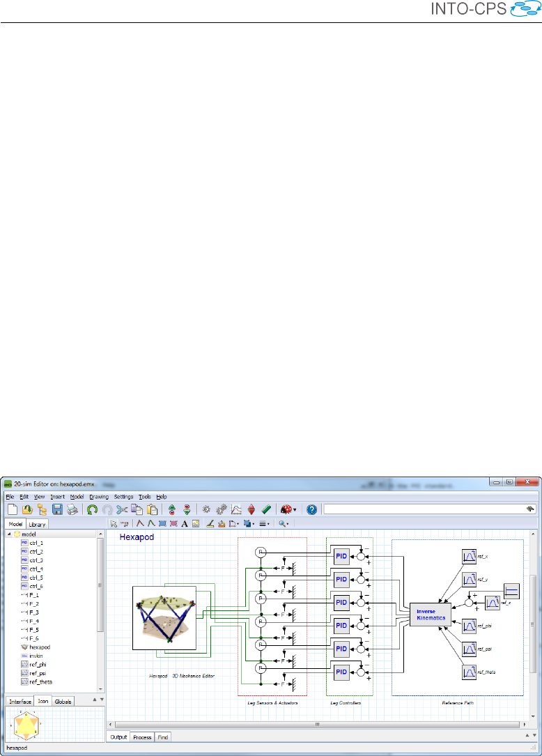
INTO-CPS Tool Chain User Manual (Public)
Finer details can be specified, such as execution synchronization and mu-
tual exclusion on shared resources. A VDM-RT specification has the same
structure as a VDM++ specification, only the conventional system class of
VDM++ is mandatory in VDM-RT. Examples can be found in the VDM-RT
tutorials distributed with Overture.
B.3 20-sim
20-sim [Con13, Bro97] is a commercial modelling and simulation software
package for mechatronic systems. With 20-sim, models can be created graph-
ically, similar to drawing an engineering scheme. With these models, the
behaviour of dynamic systems can be analyzed and control systems can be
designed. 20-sim models can be exported as C-code to be run on hardware
for rapid prototyping and HiL-simulation. 20-sim includes tools that allow
an engineer to create models quickly and intuitively. Models can be cre-
ated using equations, block diagrams, physical components and bond graphs
[KR68]. Various tools give support during the model building and simulation.
Other toolboxes help to analyze models, build control systems and improve
system performance. Figure 166 shows 20-sim with a model of a controlled
Figure 166: Example of a hexapod model in 20-sim.
hexapod. The mechanism is generated with the 3D Mechanics Toolbox and
connected with standard actuator and sensor models from the mechanics li-
brary. The hexapod is controlled by PID controllers which are tuned in the
162

INTO-CPS Tool Chain User Manual (Public)
frequency domain. Everything that is required to build and simulate this
model and generate the controller code for the real system is included inside
the package.
The 20-sim Getting Started manual [KG16] contains examples and step-by-
step tutorials that demonstrate the features of 20-sim. More information on
20-sim can be found at http://www.20sim.com and in the user manual
at http://www.20sim.com/webhelp [KGD16]. The integration of 20-
sim into the INTO-CPS tool-chain is realized via the FMI standard.
B.4 OpenModelica
OpenModelica [Fri04] is an open-source Modelica-based modelling and sim-
ulation environment. Modelica [FE98] is an object-oriented, equation based
language to conveniently model complex physical systems containing, e.g.,
mechanical, electrical, electronic, hydraulic, thermal, control, electric power
or process-oriented subcomponents. The Modelica language (and OpenMod-
elica) supports continuous, discrete and hybrid time simulations. OpenMod-
elica already compiles Modelica models into FMU, C or C++ code for simula-
tion. Several integration solvers, both fixed and variable step size, are avail-
able in OpenModelica: euler, rungekutta, dassl (default), radau5, radau3,
radau1.
OpenModelica can be interfaced to other tools in several ways as described
in the OpenModelica user’s manual [Ope]:
•via command line invocation of the omc compiler
•via C API calls to the omc compiler dynamic library
•via the CORBA interface
•via OMPython interface [GFR+12]
OpenModelica has its own scripting language, Modelica script (mos files),
which can be used to perform actions via the compiler API, such as load-
ing, compilation, simulation of models or plotting of results. OpenModelica
supports Windows, Linux and Mac Os X.
The integration of OpenModelica into the INTO-CPS tool chain is realized
via compliance with the FMI standard, and is described in Deliverable D4.3b
[PBL+17].
163

INTO-CPS Tool Chain User Manual (Public)
B.5 RT-Tester
The RT-Tester [Ver15a] is a test automation tool for automatic test gener-
ation, test execution and real-time test evaluation. Key features include a
strong C/C++-based test script language, high performance multi-threading,
and hard real-time capability. The tool has been successfully applied in avion-
ics, rail automation, and automotive test projects. In the INTO-CPS tool
chain, RT-Tester is responsible for model-based testing, as well as for model
checking. This section gives some background information on the tool from
these two perspectives.
B.5.1 Model-based Testing
The RT-Tester Model Based Test Case and Test Data Generator (RTT-
MBT) [Ver15b] supports model-based testing (MBT), that is, automated
generation of test cases, test data, and test procedures from UML/SysML
models. A number of common modelling tools can be used as front-ends for
this. The most important technical challenge in model-based test automation
is the extraction of test cases from test models. RTT-MBT combines an SMT
solver with a technique akin to bounded model checking so as to extract finite
paths through the test model according to some predefined criterion. This
criterion can, for instance, be MC/DC coverage, or it can be requirements
coverage (if the requirements are specified as temporal logic formulae within
the model). A further aspect is that the environment can be modelled within
the test model. For example, the test model may contain a constraint such
that a certain input to the system-under-test remains in a predefined range.
This aspect becomes important once test automation is lifted from single test
models to multi-model cyber-physical systems. The derived test procedures
use the RT-Tester Core as a back-end, allowing the system under test to be
provided on real hardware, software only, or even just simulation to aid test
model development.
Further, RTT-MBT includes requirement tracing from test models down to
test executions and allows for powerful status reporting in large scale testing
projects.
B.5.2 Model Checking of Timed State Charts
RTT-MBT applies model checking to behavioural models that are specified
as timed state charts in UML and SysML, respectively. From these models,
164

INTO-CPS Tool Chain User Manual (Public)
a transition relation is extracted and represented as an SMT formula in bit-
vector theory [KS08], which is then checked against LTL formulae [Pnu77]
using the algorithm of Biere et al. [BHJ+06]. The standard setting of RTT-
MBT is to apply model checking to a single test model, which consists of the
system specification and an environment.
•A component called TestModel that is annotated with stereotype TE.
•A component called SystemUnderTest that is annotated with stereo-
type SUT.
RTT-MBT uses the stereotypes to infer the role of each component. The in-
teraction between these two parts is implemented via input and output inter-
faces that specify the accessibility of variables using UML stereotypes.
•A variable that is annotated with stereotype SUT2TE is written by
the system model and readable by the environment.
•A variable that is annotated with stereotype TE2SUT is written by
the environment and read by the system model as an input.
A simple example is depicted in Figure 167, which shows a simple composite
structure diagram in Modelio for a turn indication system. The purpose
of the system is to control the lamps of a turn indication system in a car.
Further details are given in [Ver13]. The test model consists of the two
aforementioned components and two interfaces:
•Interface1 is annotated with stereotype TE2SUT and contains three
variables voltage,TurnIndLvr and EmerSwitch. These variables
are controlled by the environment and fed to the system under test as
inputs.
•Interface2 is annotated with stereotype SUT2TE and contains two
variables LampsLeft and LampsRight. These variables are con-
trolled by the system under test and can be read by the environment.
Observe that the two variables LampsLeft and LampsRight have type
int, but should only hold values 0or 1to indicate states on or off. A
straightforward system property that could be verified would thus be that
LampsLeft and LampsRight indeed are only assigned 0or 1, which could
be expressed by the following LTL specification:
G(0 ≤LampsLeft ≤1∧0≤LampsRight ≤1)
A thorough introduction with more details is given in the RTT-MBT user
manual [Ver13].
165

INTO-CPS Tool Chain User Manual (Public)
Figure 167: Simple model that highlights interfaces between the environment
and the system-under-test.
166

INTO-CPS Tool Chain User Manual (Public)
C Underlying Principles
The INTO-CPS tool chain facilitates the design and validation of CPSs
through its implementation of results from a number of underlying principles.
These principles are co-simulation, design space exploration, model-based
test automation and code generation. This appendix provides an introduc-
tion to these concepts.
C.1 Co-simulation
Co-simulation refers to the simultaneous simulation of individual models
which together make up a larger system of interest, for the purpose of ob-
taining a simulation of the larger system. A co-simulation is performed by a
co-simulation orchestration engine. This engine is responsible for initializing
the individual simulations as needed; for selecting correct time step sizes such
that each constituent model can be simulated successfully for that duration,
thus preventing time drift between the constituent simulations; for asking
each individual simulation to perform a simulation step; and for synchro-
nizing information between models as needed after each step. The result of
one such round of simulations is a single simulation step for the complete
multi-model of the system of interest.
As an example, consider a very abstract model of a nuclear power plant. This
consists of a nuclear reactor core, a controller for the reactor, a water and
steam distribution system, a steam-driven turbine and a standard electrical
generator. All these individual components can be modelled separately and
simulated, but when composed into a model of a nuclear power plant, the
outputs of some become the inputs of others. In a co-simulation, outputs
are matched to inputs and each component is simulated one step at a time
in such a way that when each model has performed its simulation step, the
overall result is a simulation step of the complete power plant model. Once
the correct information is exchanged between the constituent models, the
process repeats.
C.2 Design Space Exploration
During the process of developing a CPS, either starting from a completely
blank canvas or constructing a new system from models of existing compo-
nents, the architects will encounter many design decisions that shape the
167

INTO-CPS Tool Chain User Manual (Public)
final product. The activity of investigating and gathering data about the
merits of the different choices available is termed Design Space Exploration.
Some of the choices the designer will face could be described as being the
selection of parameters for specific components of the design, such as the
exact position of a sensor, the diameter of wheels or the parameters affecting
a control algorithm. Such parameters are variable to some degree and the
selection of their value will affect the values of objectives by which a design
will be measured. In these cases it is desirable to explore the different values
each parameter may take and also different combinations of these parameter
values if there are more than one parameter, to find a set of designs that best
meets its objectives. However, since the size of the design space is the prod-
uct of the number of parameters and the number of values each may adopt,
it is often impractical to consider performing simulations of all parameter
combinations or to manually assess each design.
The purpose of an automated DSE tool is to help manage the exploration
of the design space, and it separates this problem into three distinct parts:
the search algorithm, obtaining objective values and ranking the designs
according to those objectives. The simplest of all search algorithms is the
exhaustive search, and this algorithm will methodically move through each
design, performing a simulation using each and every one. This is termed
an open loop method, as the simulation results are not considered by the
algorithm at all. Other algorithms, such as a genetic search, where an initial
set of randomly generated individuals are bred to produce increasingly good
results, are closed loop methods. This means that the choice of next design
to be simulated is driven by the results of previous simulations.
Once a simulation has been performed, there are two steps required to close
the loop. The first is to analyze the raw results output by the simulation to
determine the value for each of the objectives by which the simulations are
to be judged. Such objective values could simply be the maximum power
consumed by a component or the total distance traveled by an object, but
they could also be more complex measures, such as the proportion of time
a device was operating in the correct mode given some conditions. As well
as numerical objectives, there can also be constraints on the system that
are either passed or failed. Such constraints could be numeric, such as the
maximum power that a substation must never exceed, or they could be based
on temporal logic to check that undesirable events do not occur, such as all
the lights at a road junction not being green at the same time.
The final step in a closed loop is to rank the designs according to how well
each performs. The ranking may be trivial, such as in a search for a design
168

INTO-CPS Tool Chain User Manual (Public)
that minimizes the total amount of energy used, or it may be more complex
if there are multiple objectives to optimize and trade off. Such ranking
functions can take the form of an equation that returns a score for each
design, where the designs with the highest/lowest scores are considered the
best. Alternatively, if the relationship between the desired objectives is not
well understood, then a Pareto approach can be taken to ranking, where
designs are allocated to ranks of designs that are indistinguishable from each
other, in that each represents an optimum, but there exist different tradeoffs
between the objective values.
C.3 Model-Based Test Automation
The core fragment of test automation activities is a model of the desired
system behaviour, which can be expressed in SysML. This test model in-
duces a transition relation, which describes a collection of execution paths
through the system, where a path is considered a sequence of timed data
vectors (containing internal data, inputs and outputs). The purpose of a test
automation tool is to extract a subset of these paths from the test model
and turn these paths into test cases, respectively test procedures. The test
procedures then compare the behaviour of the actual system-under-test to
the path, and produce warnings once discrepancies are observed.
C.4 Code Generation
Code generation refers to the translation of a modelling language to a com-
mon programming language. Code generation is commonly employed in con-
trol engineering, where a controller is modelled and validated using a tool
such as 20-sim, and finally translated into source code to be compiled for
some embedded execution platform, which is its final destination.
The relationship that must be maintained between the source model and
translated program must be one of refinement, in the sense that the trans-
lated program must not do anything that is not captured by the original
model. This must be considered when translating models written in high-
level specification languages, such as VDM. The purpose of such languages
is to allow the specification of several equivalent implementations. When
a model written in such a language is translated to code, one such imple-
mentation is essentially chosen. In the process, any non-determinism in the
specification, the specification technique that allows a choice of implemen-
169

INTO-CPS Tool Chain User Manual (Public)
tations, must be resolved. Usually this choice is made very simple by re-
stricting the modelling language to an executable subset, such that no such
non-determinism is allowed in the model. This restricts the choice of imple-
mentations to very few, often one, which is the one into which the model is
translated via code generation.
170
