1 Instructor's Solutions Manual Marion
Stephen%20T.(Stephen%20T.%20Thornton)%20Thornton%2C%20Jerry%20B.%20Marion%20-%20Classical%20Dynamics%20of%20Particles%20and%20Sy
User Manual: Pdf
Open the PDF directly: View PDF ![]() .
.
Page Count: 496 [warning: Documents this large are best viewed by clicking the View PDF Link!]

CHAPTER 0
Contents
Preface v
Problems Solved in Student Solutions Manual vii
1 Matrices, Vectors, and Vector Calculus 1
2 Newtonian Mechanics—Single Particle 29
3 Oscillations 79
4 Nonlinear Oscillations and Chaos 127
5 Gravitation 149
6 Some Methods in The Calculus of Variations 165
7 Hamilton’s Principle—Lagrangian and Hamiltonian Dynamics 181
8 Central-Force Motion 233
9 Dynamics of a System of Particles 277
10 Motion in a Noninertial Reference Frame 333
11 Dynamics of Rigid Bodies 353
12 Coupled Oscillations 397
13 Continuous Systems; Waves 435
14 Special Theory of Relativity 461
iii
iv CONTENTS

CHAPTER 0
Pre
f
ace
This Instructor’s Manual contains the solutions to all the end-of-chapter problems (but not the
appendices) from Classical Dynamics of Particles and Systems, Fifth Edition, by Stephen T.
Thornton and Jerry B. Marion. It is intended for use only by instructors using Classical Dynamics
as a textbook, and it is not available to students in any form. A Student Solutions Manual
containing solutions to about 25% of the end-of-chapter problems is available for sale to
students. The problem numbers of those solutions in the Student Solutions Manual are listed on
the next page.
As a result of surveys received from users, I continue to add more worked out examples in
the text and add additional problems. There are now 509 problems, a significant number over
the 4th edition.
The instructor will find a large array of problems ranging in difficulty from the simple
“plug and chug” to the type worthy of the Ph.D. qualifying examinations in classical mechanics.
A few of the problems are quite challenging. Many of them require numerical methods. Having
this solutions manual should provide a greater appreciation of what the authors intended to
accomplish by the statement of the problem in those cases where the problem statement is not
completely clear. Please inform me when either the problem statement or solutions can be
improved. Specific help is encouraged. The instructor will also be able to pick and choose
different levels of difficulty when assigning homework problems. And since students may
occasionally need hints to work some problems, this manual will allow the instructor to take a
quick peek to see how the students can be helped.
It is absolutely forbidden for the students to have access to this manual. Please do not
give students solutions from this manual. Posting these solutions on the Internet will result in
widespread distribution of the solutions and will ultimately result in the decrease of the
usefulness of the text.
The author would like to acknowledge the assistance of Tran ngoc Khanh (5th edition),
Warren Griffith (4th edition), and Brian Giambattista (3rd edition), who checked the solutions of
previous versions, went over user comments, and worked out solutions for new problems.
Without their help, this manual would not be possible. The author would appreciate receiving
reports of suggested improvements and suspected errors. Comments can be sent by email to
stt@virginia.edu, the more detailed the better.
Stephen T. Thornton
Charlottesville, Virginia
v
vi PREFACE
CHAPTER 1
Matrices, Vectors,
and Vector Calculus
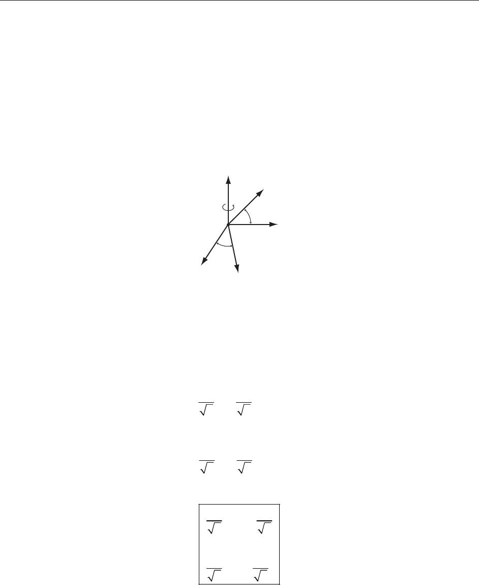
1-1.
x
2
= x
2
′
x
1
′
45˚
x
1
x
3
′
x
3
45˚
Axes and lie in the plane.
1
x′3
x′13
xx
The transformation equations are:
11 3
cos 45 cos 45xx x
=
°− °
′
22
xx
=
′
33 1
cos 45 cos 45xx x
=
°+ °
′
11
11
22
xx=−
′3
x
22
xx
=
′
31
11
22
xx=−
′3
x
So the transformation matrix is:
11
0
22
01 0
11
0
22
−
1
2 CHAPTER 1
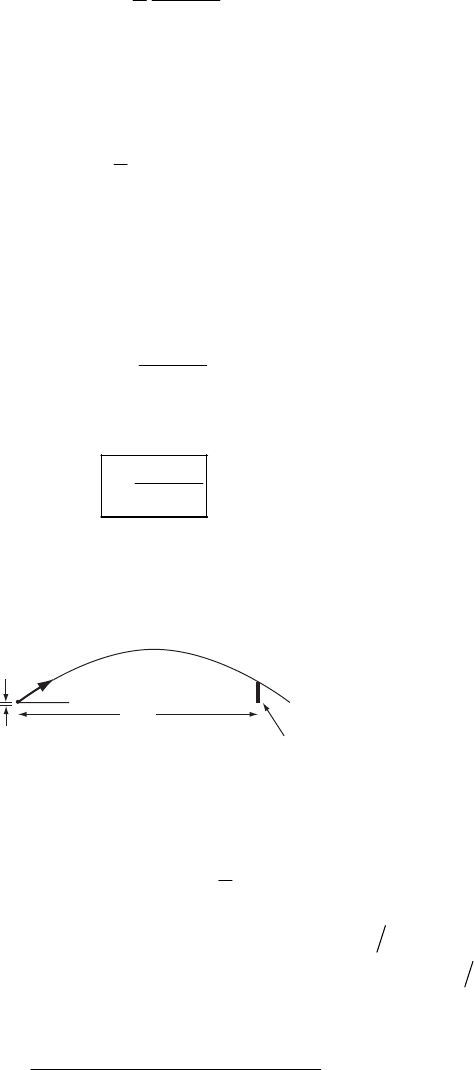
1-2.
a)
x
1
A
B
C
D
α
β
γ
O
E
x
2
x
3
From this diagram, we have
cosOE OA
α
=
cosOE OB
β
= (1)
cosOE OD
γ
=
Taking the square of each equation in (1) and adding, we find
2
222
cos cos cos OA OB OD
αβγ
++ =++
222
OE
(2)
But
22
OA OB OC+=
2
(3)
and
22
OC OD OE+=
2
(4)
Therefore,
22 2
OA OB OD OE++ =
2
(5)
Thus,
222
cos cos cos 1
αβγ
+
+= (6)
b)
x
3
AA′
x
1
x
2
O
E
D
C
B
θ
C′
B′
E′
D′
First, we have the following trigonometric relation:
22
2cosOE OE OE OE EE
θ
2
′
′
+− =
′
(7)
MATRICES, VECTORS, AND VECTOR CALCULUS 3
But,
22 2
2
22
2
cos cos cos cos
cos cos
EE OB OB OA OA OD OD
OE OE OE OE
OE OE
β
βα
γγ
′′ ′ ′
=−+− + −
′′
=−+−
′′
′
+−
′
α
(8)
or,
22 2
222 222
22
cos cos cos cos cos cos
2 cos cos cos cos cos cos
2 cos cos cos cos cos cos
EE OE OE
OE OE
OE OE OE OE
α
βγ αβ
αα ββ γγ
γ
α
αββγ
′′
=+++++
′′′
′
−++
′′′
′
=+− + +
′′′
γ
′
(9)
Comparing (9) with (7), we find
cos cos cos cos cos cos cos
θ
αα ββ γγ
=++
′
′′
(10)
1-3.
x
1
e
3
′
x
2
x
3
O
e
1
e
2
e
3
Ae
2
′
e
1
′
e
2
e
1
e
3
Denote the original axes by , , , and the corresponding unit vectors by e,, . Denote
the new axes by , , and the corresponding unit vectors by
1
x2
x3
x1 2
e3
e
1
x′2
x′3
x′1
′
e, 2
′
e, e. The effect of the
rotation is ee, , e. Therefore, the transformation matrix is written as:
3
′
13
′
→21
′
ee→3
→2
′
e
(
)
(
)
(
)
()()()
()()()
11 12 13
21 22 23
31 32 33
cos , cos , cos , 010
cos , cos , cos , 0 0 1
100
cos , cos , cos ,
′′′
λ
′′′
==
′′′
ee ee ee
ee ee ee
ee ee ee
1-4.
a) Let C = AB where A, B, and C are matrices. Then,
i
j
ik k
j
k
CA=B
∑
(1)
(
)
t
j
i
j
kki ki
j
k
ij kk
CC AB BA== =
∑
∑
4 CHAPTER 1
Identifying
(
)
t
ki ik
B=B and
(
)
t
jk k
j
AA=,
(
)
(
)
(
)
tt
i
t
j
ik k
j
k
CBA=
∑
(2)
or,
(
)
t
t
CABBA==
tt
(3)
b) To show that
(
)
111
A
BBA
−−−
=,
(
)
(
)
11 11
A
BB A I B A AB
−− −−
== (4)
That is,
(
)
11 1 1
A
BB A AIA AA I
−− − −
=
== (5)
(
)
(
)
11 1 1
BA AB BIB BB I
−− − −
=
== (6)
1-5. Take
λ
to be a two-dimensional matrix:
11 12
11 22 12 21
21 22
λλ
λ
λλ λλ
λλ
==− (1)
Then,
(
)
(
)
()()()
()()
()
222 22 22 22 22 22
11 22 11 22 12 21 12 21 11 21 12 22 11 21 12 22
22 2 22 2 22 22
22 11 12 21 11 12 11 21 11 22 12 21 12 22
2
2222
11 12 22 21 11 21 12 22
2
2
λ
λλ λλλλ λλ λλ λλ λλ λλ
λ λ λ λ λ λ λλ λλλλ λλ
λλλλ λλλλ
=− ++ + − +
=+++−+ +
=+ +− + (2)
But since
λ
is an orthogonal transformation matrix, i
j
k
j
ik
j
λ
λδ
=
∑
.
Thus,
22 22
11 12 21 22
11 21 12 22
1
0
λλλλ
λλ λλ
+
=+=
+= (3)
Therefore, (2) becomes
21
λ
=
(4)
1-6. The lengths of line segments in the
j
x and
j
x
′
systems are
2
j
j
Lx=
∑
; 2
i
i
L=x
′
′
∑
(1)
MATRICES, VECTORS, AND VECTOR CALCULUS 5
If , then LL=′
22
j
i
ji
xx=
′
∑
∑ (2)
The transformation is
ii
jj
j
x
λ
=
′x
∑
(3)
Then,
(4)
2
,
jikk
jik
kiki
ki
xx
xx
λλ
λλ
=
=
∑∑∑ ∑
∑∑
AA
A
AA
A
i
x
But this can be true only if
ik i k
i
λ
λδ
=
∑AA
(5)
which is the desired result.
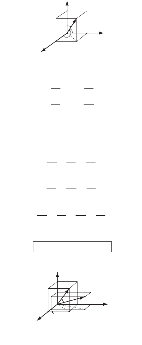
1-7.
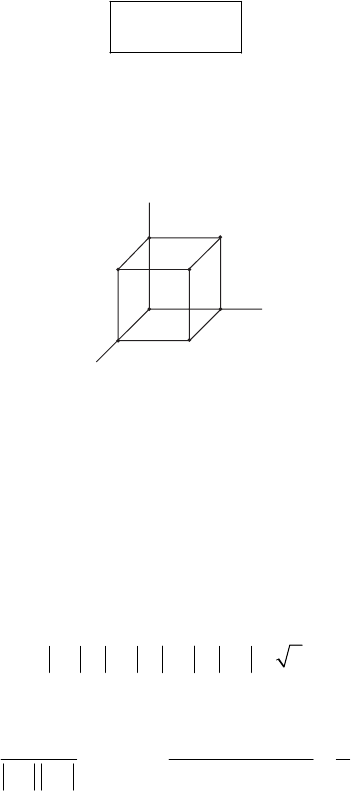
x
1
(1,0,1)
x
3
x
2
(1,0,0) (1,1,0)
(0,1,0)
(1,1,1)
(0,0,1) (0,1,1)
(0,0,0)
There are 4 diagonals:
1
D, from (0,0,0) to (1,1,1), so (1,1,1) – (0,0,0) = (1,1,1) = D;
1
2
D, from (1,0,0) to (0,1,1), so (0,1,1) – (1,0,0) = (–1,1,1) = ;
2
D
3
D, from (0,0,1) to (1,1,0), so (1,1,0) – (0,0,1) = (1,1,–1) = ; and
3
D
4
D, from (0,1,0) to (1,0,1), so (1,0,1) – (0,1,0) = (1,–1,1) = D.
4
The magnitudes of the diagonal vectors are
1234
3====DDDD
The angle between any two of these diagonal vectors is, for example,
(
)
(
)
12
12
1,1,1 1,1,1 1
cos 33
θ
⋅−
⋅
=
==
DD
DD
6 CHAPTER 1
so that
11
cos 70.5
3
θ
−
=
=°
Similarly,
13 23 34
14 24
13 14 23 24 34
1
3
⋅⋅⋅
⋅⋅
=====
DD DD DD
DD DD
DD DD DD DD DD ±
1-8. Let
θ
be the angle between A and r. Then, 2
A
⋅
=Ar can be written as
2
cos
A
rA
θ
=
or,
cos
rA
θ
=
(1)
This implies
2
QPO
π
=
(2)
Therefore, the end point of r must be on a plane perpendicular to A and passing through P.
1-9. 2=+ −Ai jk 23=− + +Bijk
a) 32−= −−AB ij k
() ( )
12
222
31(2)
−= +− +−
AB
14−=AB
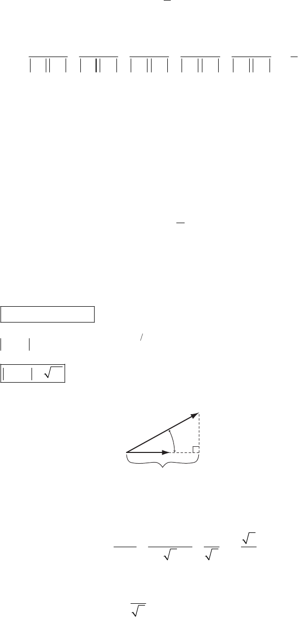
b)
component of B along A
B
A
θ
The length of the component of B along A is B cos
θ
.
cos
A
B
θ
⋅
=AB
261 3 6
cos or 2
66
A
θ
⋅−+−
== =
AB
B
The direction is, of course, along A. A unit vector in the A direction is
()
12
6
+
−ijk
MATRICES, VECTORS, AND VECTOR CALCULUS 7
So the component of B along A is
()
12
2+−ijk
c) 33
cos 614 27
AB
θ
⋅
== =
AB ; 13
cos 27
θ
−
=
71
θ
°
d) 21 1 1 12
12 1 31 21 23
23 1
−−
×= −= − +
−−
−
ijk
AB i j k
57×= ++AB ij k
e) 32−= −−AB ij k 5
+
=− +AB i j
()()
31
15 0
−×+= −−
−
ijk
AB AB 2
()()
10 2 14−× += ++AB AB i j k
1-10. 2sin cosbtb t
ω
ω
=+rij
a) 22
2cos sin
2sin cos
btbt
btbt
ωω ωω
2
ω
ωωω ω
== −
==− − =−
vr i j
av i j r
12
22 2 22 2
12
22
speed 4 cos sin
4cos sin
btb
btt
ωωωω
ωωω
t
== +
=+
v
12
2
speed 3 cos 1bt
ωω
=+
b) At 2t
π
ω
=, sin 1t
ω
=, cos 0t
ω
=
So, at this time, b
ω
=−vj,
2
2b
ω
=−ai
So,
90
θ
°
8 CHAPTER 1
1-11.
a) Since
(
)
i
j
k
j
k
i
jk
A
B
ε
×=
∑
AB , we have
()()
()
()
,
123 32 213 31 312 21
123 123 123
123 123 123
123 123 123
() ijk j k i
ijk
ABC
CAB AB CAB AB CAB AB
CCC AAA AAA
AAA CCC B B B
BBB BBB CCC
ε
×⋅=
=−−−+−
==−==⋅
∑∑
ABC
ABC
×
(1)
We can also write
(
123 123
123 123
123 123
()
CCC BBB
BBB CCC
AAA AAA
×⋅=− = =⋅×ABC BCA
)
(2)
We notice from this result that an even number of permutations leaves the determinant
unchanged.
b) Consider vectors A and B in the plane defined by e, . Since the figure defined by A, B,
C is a parallelepiped, area of the base, but
1
3
2
e
3
×= ×ABe
⋅
=eC altitude of the parallelepiped.
Then,
(
)
(
)
3area of the base
= altitude area of the base
= volume of the parallelepiped
⋅×=⋅×
×
CAB Ce
1-12.
O
A
B
C
h
a
b
c
a – c
c – b
b – a
The distance h from the origin O to the plane defined by A, B, C is
MATRICES, VECTORS, AND VECTOR CALCULUS 9
(
)
(
)
()()
()
h⋅−×−
=−×−
⋅×−×+×
=×−×+×
⋅×
=×+×+×
aba cb
ba cb
abcacab
bcacab
ab c
abbcca (1)
The area of the triangle ABC is:
()()()( )()()
111
222
×−=−×−=−×−ba cb ac ba cb acA=− (2)
1-13. Using the Eq. (1.82) in the text, we have
(
)
(
)
(
)
2
A
φ
×= × × = ⋅ − ⋅ = −A AX XAA AAX A XAB
from which
(
)
2
A
×+
=BA A
X
φ
1-14.
a)
12 12 1 0 1 21
03 1 0 12 1 29
201 113 533
−−
=−=
AB
−
Expand by the first row.
29 19 1 2
121
33 53 53
−
−
=++
AB
104=−AB
b)
12 121 9 7
03 1 43 139
20 1 10 5 2
−
==
AC
97
13 9
52
=
AC
10 CHAPTER 1
c)
()
12 1 8 5
03 1 2 3
20 1 9 4
−
== −−
ABC A BC
55
35
25 14
−−
=−
ABC
d) ?
tt
−
=AB B A
121
129 (from part )
533
201 102 1 15
111230 223
023 111 1 93
tt
−
=−
=− =−−
−
AB a
BA
034
30 6
460
tt
−−
−=
−
AB B A
1-15. If A is an orthogonal matrix, then
2
2
1
100100 100
00 01
00 00
10 0 100
02 0 010
002 001
t
aa a a
aa a a
a
a
=
−=
−
0
1
=
AA
1
2
a=
MATRICES, VECTORS, AND VECTOR CALCULUS 11
1-16.
x3P
r
θ
x2
x1
a
r
θa
r cos θ
constant
⋅
=ra
cos constantra
θ
=
It is given that a is constant, so we know that
cos constantr
θ
=
But cosr
θ
is the magnitude of the component of r along a.
The set of vectors that satisfy all have the same component along a; however, the
component perpendicular to a is arbitrary.
constant⋅=
ra
Th
is
us the surface represented by constant
a plane perpendicular to .
⋅=ra
a
1-17.
a
A
θb
B
c
C
Consider the triangle a, b, c which is formed by the vectors A, B, C. Since
()(
2
22
2
)
A
B
=
−
=
−⋅ −
=
−⋅+
CAB
CABAB
AB
(1)
or,
222
2cosAB AB
θ
=+−C (2)
which is the cosine law of plane trigonometry.
1-18. Consider the triangle a, b, c which is formed by the vectors A, B, C.
A
αC
Bγβb
c
a
12 CHAPTER 1
=
−CAB (1)
so that
(
)
×
=−×CB AB B (2)
but the left-hand side and the right-hand side of (2) are written as:
3
sinBC
α
×
=CB e (3)
and
(
)
3
sinAB
γ
− ×=×−×=×=AB BABBBAB e (4)
where e is the unit vector perpendicular to the triangle abc. Therefore,
3
sin sinBC AB
α
γ
=
(5)
or,
sin sin
CA
γ
α
=
Similarly,
sin sin sin
CAB
γ
αβ
== (6)
which is the sine law of plane trigonometry.
1-19.
x2
a
α
x1
a2
b2
a1b1
b
β
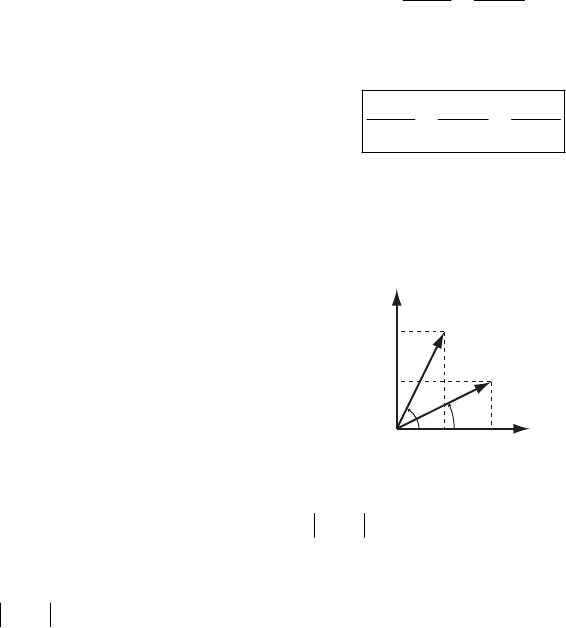
a) We begin by noting that
(
)
222
2cosab ab
α
β
−=+− −ab (1)
We can also write that
(
)
(
)
()()
()()
()
()
22
2
11 22
22
22 2 22 2
22
cos cos sin sin
sin cos sin cos 2 cos cos sin sin
2coscos sinsin
ab ab
ab ab
ab ab
ab ab
αβ αβ
α
αββαβα
αβ αβ
−=− +−
=− +−
=+++− +
=+− +
ab
β
(2)
MATRICES, VECTORS, AND VECTOR CALCULUS 13
Thus, comparing (1) and (2), we conclude that
()
cos cos cos sin sin
α
βαβα
−= +
β
(3)
b) Using (3), we can find
(
)
sin
α
β
−:
() ()
()()
()
2
22 22
222 2
22 22
2
sin 1 cos
1 cos cos sin sin 2cos sin cos sin
1 cos 1 sin sin 1 cos 2cos sin cos sin
sin cos 2sin sin cos cos cos sin
sin cos cos sin
αβ αβ
αβ αβ ααββ
α
βα β ααβ
αβ αβαβ αβ
αβ αβ
−=− −
=− − −
=− − − − −
=− +
=−
β
(4)
so that
()
sin sin cos cos sin
α
βαβα
−= −
β
j
(5)
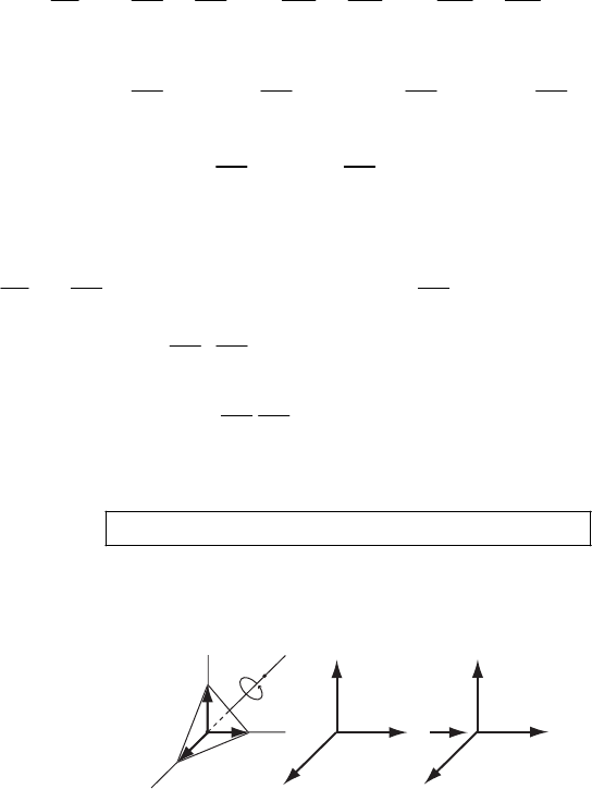
1-20.
a) Consider the following two cases:
When i≠0
ij
δ
= but 0
ijk
ε
≠.
When i=j0
ij
δ
≠ but 0
ijk
ε
=.
Therefore,
0
ijk ij
ij
εδ
=
∑ (1)
b) We proceed in the following way:
When j = k, 0
ijk ijj
ε
ε
==
.
Terms such as 11 11 0
j
ε
ε
=
A. Then,
12 12 13 13 21 21 31 31 32 32 23 23ijkjkiiiiii
jk
ε
εεεεεεεεεεεεε
=+++++
∑AAAAAA A
=
Now, suppose i, then, 1==A
123 123 132 132 112
jk
εε εε
=+=+
∑

14 CHAPTER 1
for , . For
2
i==A213 213 231 231 112
jk
εε εε
=+=+
∑=3i
=
=A, 312 312 321 321 2
jk
εε εε
=
+=
∑
. But i = 1,
gives . Likewise for i = 2,
2
=A0
jk
=
∑1
=
A; i = 1, 3
=
A; i = 3, 1
=
A; i = 2, A; i = 3, .
Therefore,
3=2=A
,
2
i
j
k
j
ki
jk
ε
εδ
=
∑AA
(2)
c)
()()()()()()()()
123 123 312 312 321 321 132 132 213 213 231 231
1111 11 11 1111
ijk ijk
ijk
ε
εεεεεεεεεεεεε
=+++++
= ⋅ + ⋅ +− ⋅− +− ⋅− +− ⋅− + ⋅
∑
or,
6
ijk ijk
ijk
εε
=
∑ (3)
1-21.
(
)
i
j
k
j
k
i
jk
A
B
ε
×=
∑
AB (1)
(
)
i
j
k
j
ki
ijk
A
BC
ε
×⋅=
∑∑
ABC (2)
By an even permutation, we find
i
j
ki
j
k
ijk
A
BC
ε
=∑
ABC (3)
1-22. To evaluate i
j
kmk
k
ε
ε
∑A we consider the following cases:
a)
: 0 for all , ,
ijk mk iik mk
kk
ij i m
εε εε
===
∑∑
AA A
b)
:1 for
0 for
ijk mk ijk imk
kk
ij
jm
εε εε
====
=≠
∑∑
A
A and,mkij≠
ij
i
c) :0 for
1 for and ,
ijk mk ijk ik
kk
im j
jk
εε εε
===≠
=− = ≠
∑∑
AA A
A
d) :0 for
1 for and ,
ijk mk ijk jmk
kk
jm
mi kij
εε εε
===≠
=− = ≠
∑∑
A
A

MATRICES, VECTORS, AND VECTOR CALCULUS 15
e) :0 for
1 for and ,
ijk mk ijk jk
kk
jm i
ik
εε εε
===≠
== ≠
∑∑
AA A
Aij
jk
m
f)
: 0 for all , ,
ijk mk ijk k
kk
mi
εε εε
===
∑∑
AAA
A
g) : This implies that i = k or i = j or m = k. or i≠A
Then, for all
0
ijk mk
k
εε
=
∑A, , ,ij mA
h) for all
or : 0
ijk mk
k
jm
εε
≠=
∑A
A, , ,ij mA
Now, consider i
j
mim
j
δ
δδδ
−
AA
and examine it under the same conditions. If this quantity
behaves in the same way as the sum above, we have verified the equation
i
j
kmk i
j
mim
j
k
ε
εδδδδ
=−
∑AA A
a) : 0 for all , ,
iim imi
ij i m
δ
δδδ
=−=
AA A
b) : 1 if , ,
0 if
ii jm im ji
ij
jm
mijm
δ
δδδ
=−==≠
=≠
A
c) : 1 if , ,
0 if
iji iij
im j ij
j
δ
δδδ
=−=−=
=≠
AA AA
A
≠
mi
d) : 1 if ,
0 if
im im
ji
im
δ
δδδ
=−=−=
=≠
AA AA
AA≠
e) : 1 if ,
0 if
imm imm
jm i m
i
δ
δδδ
=−==
=≠
AA
AA
A
≠
all,,j
f) :0 for
ij ilj
mi
δ
δδδ
=−=
AA A
AA
g) , : 0 for all , , ,
ijm imj
im ijm
δ
δδδ
≠−=
AA
AA
h) ,: 0 for all ,,,
ijm imi
jm ijm
δ
δδδ
≠−=
AA
AA
Therefore,
i
j
kmk i
j
mim
j
k
ε
εδδδδ
=−
∑AA A
(1)
Using this result we can prove that
(
)
(
)
(
)
××=⋅ −⋅ABC ACBABC

16 CHAPTER 1
First
(
)
i
j
k
j
k
i
jk
BC
ε
×=
∑
BC . Then,
(
)
[
]
(
)
()
()()
mn m mn m njk j k
n
mn mn jk
mn njk m j k mn jkn m j k
jkmn jkmn
lmn jkn m j k
jkm n
jl km k jm m j k
jkm
mm mm mm mm
mm m m
ABC A BC
ABC ABC
ABC
ABC
A
BC A B C B A C C A B
BC
εεε
εε εε
εε
δδ δ δ
×× = × =
==
=
=−
=−= −
=⋅ −⋅
∑∑∑
∑∑
∑∑
∑
∑∑ ∑ ∑
ABC
AC AB
AA
A
AA
A
AAAA
AA
Therefore,
()()()
××= ⋅ −⋅ABC ACBABC (2)
1-23. Write
(
)
j
mm
j
m
A
B
ε
×=
∑
AB AA
A
(
)
krs r s
k
rs
CD
ε
×=
∑
CD
Then,

MATRICES, VECTORS, AND VECTOR CALCULUS 17
()()
[]
()
()
ijk j m m krs r s
ijk m rs
ijk j m krs m r s
jk mrs
j m ijk rsk m r s
jmrs k
j m ir js is jr m r s
jmrs
jm m i j m i j
jm
jm j m i jm
jm j
AB CD
AB CD
AB CD
AB CD
AB CD AB DC
DAB C
εε ε
εε ε
εεε
εδδδδ
ε
εε
××× =
=
=
=−
=−
=−
∑∑ ∑
∑
∑∑
∑
∑
∑
AB CD AA
A
AA
A
AA
A
AA
A
AA A
A
AA A
A
()()
j
mi
m
ii
CAB D
CD
=−
∑
ABD ABC
A
A
Therefore,
[
()()
]
()()××× = −AB CD ABDC ABCD
1-24. Expanding the triple vector product, we have
(
)
(
)
(
)
×
×= ⋅− ⋅eAeAeeeAe (1)
But,
(
)
⋅
=Aee A (2)
Thus,
() ( )
=
⋅+× ×AeAeeAe (3)
e(A · e) is the component of A in the e direction, while e × (A × e) is the component of A
perpendicular to e.
18 CHAPTER 1
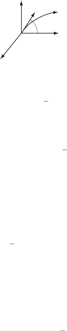
1-25.
e
r
e
φ
e
θ
θ
φ
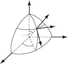
The unit vectors in spherical coordinates are expressed in terms of rectangular coordinates by
(
)
()
()
cos cos , cos sin , sin
sin , cos , 0
sin cos , sin sin , cos
r
θ
φ
θ
φθφ θ
φφ
θφθφ θ
=−
=−
=
e
e
e
(1)
Thus,
(
)
cos sin sin cos , cos cos sin sin , cos
θ
φ
θφθθφφθφθθφθθ
=− − − −e
cos
r
φ
θ
φθ
+e
=− (2) e
Similarly,
(
)
cos , sin , 0
φ
φφφφ
=− −e
cos sin r
θ
φ
θφθ
−e
=− (3) e
sin
r
φ
θ
φ
θθ
=+ee
e (4)
Now, let any position vector be x. Then,
r
r
=
xe (5)
(
)
sin
sin
rr
r
rrr r
rrr
φθ
φθ
φθ θ
φθ θ
=+= + +
=++
xe e e e e
eee
r
(6)
(
)
(
)
()()
()
22 2
2
sin cos sin sin
2 sin 2 cos sin sin
2sincos
rr
r
rr r r rrrr
rrr rr r
rrr
φφ θθ
φ
θ
φθθφθφθ φθ θθ θ
φθ θφθφθ φ θθ
θθφ θ θ
=+ + + +++++
=+ + +−−
++−
xeee
ee
e
r
eee
(7)
or,
MATRICES, VECTORS, AND VECTOR CALCULUS 19
()
()
222 2 2
22
1
sin sin cos
1sin
sin
r
d
rr r r r
rdt
dr
rdt
θ
φ
θφ θ θφ θθ
φθ
θ
== − − + −
+
xa e e
e
(8)
1-26. When a particle moves along the curve
(
)
1cosrk
θ
=+ (1)
we have
2
sin
cos sin
rk
rk
θθ
θ
θθ θ
=−
=− +
(2)
Now, the velocity vector in polar coordinates is [see Eq. (1.97)]
r
rr
θ
θ
=+ve e
(3)
so that
()
2
2222
22 2 2 2 2
22
sin 1 2 cos cos
22cos
vrr
kk
k
θ
θ
θθ
θθ
==+
=+++
=+
v
θθ
)
(4)
and is, by hypothesis, constant. Therefore,
2
v
(
2
2
21cos
v
k
θ
θ
=+
(5)
Using (1), we find
2
v
kr
θ
=
(6)
Differentiating (5) and using the expression for r, we obtain
()
22
2
22
sin sin
441cos
vv
rk
θθ
θ
θ
==
+
(7)
The acceleration vector is [see Eq. (1.98)]
(
)
(
)
22
r
rr r r
θ
θθθ
=− + +ae
e
(8)
so that
20 CHAPTER 1
()
()
()
()
()
()
2
22
22
22
2
2
2
cos sin 1 cos
sin
cos 1 cos
21 cos
1cos
2cos 1
21 cos
31cos
2
rrr
kk
k
k
k
θ
θθθθ θθ
θθ
θ
θθ
θ
θ
θθ θ
θθ
⋅=−
=− + − +
=− + + +
+
−
=− + +
+
+
ae
θ
=− (9)
or,
2
3
4
r
v
k
⋅=−
ae (10)
In a similar way, we find
2sin
3
41cos
v
k
θ
θ
θ
⋅=− +
ae (11)
From (10) and (11), we have
()
()
2
2
r
θ
=⋅+⋅aae ae (12)
or,
2
32
41cos
v
k
θ
=+
a (13)
1-27. Since
(
)
(
)
(
)
×
×=⋅ −⋅rvr rrvrvr
we have
()
[]
() ( )
[]
() ()()( )()
()
()
22
2
dd
dt dt
rv
×× = ⋅ −⋅
=⋅ + ⋅ −⋅ − ⋅ −⋅
=+⋅ − +⋅
rvr rrvrvr
rra rvv rvv vvr rar
arvvr ra (1)
Thus,
()
[]
()
()
2
r
dt ×× = +⋅ − ⋅+
rvr arvvrrav
2
d (2)
MATRICES, VECTORS, AND VECTOR CALCULUS 21
1-28.
() ()
ln ln i
ii
x
∂
=∂
∑
grad r r e (1)
where
2
i
i
x=
∑
r (2)
Therefore,
()
2
2
1
ln i
ii
i
i
x
xx
x
∂
=
∂
=
∑
rr
r (3)
so that
()
2
1
ln ii
i
x
=
∑
grad r e
r
(4)
or,
()
2
ln r
=r
grad r (5)
1-29. Let describe the surface S and
29r=1
21xyz
+
+= describe the surface S. The angle
θ
between and at the point (2,–2,1) is the angle between the normals to these surfaces at the
point. The normal to is
2
1
S2
S
1
S
(
)
(
)
(
)
()
222
1
1232,2,1
123
99
222
442
xyz
Sr xyz
xyz
===
=−=++
=++
=−+
grad grad grad
eee
eee
2
−
(1)
In , the normal is:
2
S
(
)
(
)
()
2
2
12 3 2,2,
12 3
1
2
2
x1
y
z
Sxyz
z
=
=− =
=++−
=++
=++
grad grad
ee e
ee e
(2)
Therefore,
22 CHAPTER 1
(
)
(
)
() ()
()()
12
12
123123
cos
442 2
66
SS
SS
θ
⋅
=
−+ ⋅++
=
grad grad
grad grad
eeeeee
(3)
or,
4
cos 66
θ
= (4)
from which
16
cos 74.2
9
θ
−
=
=° (5)
1-30.
()
(
)
3
1
ii
ii
ii
ii
ii
ii
xx
xx
φψ ψφ
i
x
φ
ψφ
ψφ
φψ
=
ψ
∂∂∂
==+
∂∂∂
∂∂
=+
∂∂
∑∑
∑∑
grad e e
ee
Thus,
(
)
φ
ψφ ψψ φ
=+grad grad grad
1-31.
a)
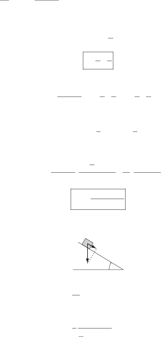
()
12
3
2
1
1
2
2
1
2
2
2
22
n
nn
ii j
ij
ii
n
ii j
ij
n
ii j
ij
n
ii
i
r
rx
xx
n
xx
xn x
xnr
=
−
−
−
∂∂
==
∂∂
=
=
=
∑∑∑
∑∑
∑∑
∑
grad e e
e
e
e (1)
Therefore,
()
2
n
n
rnr
−
=grad r (2)
MATRICES, VECTORS, AND VECTOR CALCULUS 23
b)
()
(
)
(
)
()
()
33
11
12
2
12
2
ii
ii
ii
ij
ij
i
ii j
ij
i
i
i
fr fr r
fr xr
fr
x
xr
fr
xx r
f
x
rdr
==
−
∂∂
x
∂
==
∂
∂∂
∂
∂
=
∂∂
∂
=∂
∂
=
∑∑
∑∑
∑∑
∑
grad e e
e
e
e (3)
Therefore,
()
()
f
r
fr rr
∂
=
∂
r
grad (4)
c)
()
()()
()
()
12
22
22
22
12
2
12
2
1
2
21
22
2
22
2
ln
ln ln
12
2
2
1
23
j
ij
ii
ij
j
ii
j
j
ij
ij
i
i
ii j j
ijij
i
j
i
r
rx
xx
xx
x
x
xx
x
x
xx x x
x
xr r
−
−
−
−
−
∂∂
==
∂∂
⋅
∂
=
∂
∂
=
∂
∂
=− +
∂
=− +
∑∑∑
∑
∑
∑
∑∑
∑∑∑∑
∑
∇
2
422
231r
rrr
=− + = (5)
or,
()
2
2
1
ln rr
=∇ (6)
24 CHAPTER 1
1-32. Note that the integrand is a perfect differential:
() (
22 dd
aba b
dt dt
⋅+ ⋅= ⋅ + ⋅rr rr rr rr
)
(1)
Clearly,
()
22
22 conabdtarbr⋅+ ⋅ = + +
∫rr rr
st. (2)
1-33. Since
2
drr
dtrrr
2
r
r
−
==−
rrrrr
(1)
we have
2
rd
dt dt
rr dtr
−=
∫∫
rr r
(2)
from which
2
rdt
rr r
−
=+
∫rr rC
(3)
where C is the integration constant (a vector).
1-34. First, we note that
()
d
dt
×
=×+×AA AAAA
(1)
But the first term on the right-hand side vanishes. Thus,
()()
d
dt dt
dt
×= ×
∫∫
AA AA
(2)
so that
(
)
dt
×
=×+
∫AA AAC
(3)
where C is a constant vector.
MATRICES, VECTORS, AND VECTOR CALCULUS 25
1-35.
x
z
y
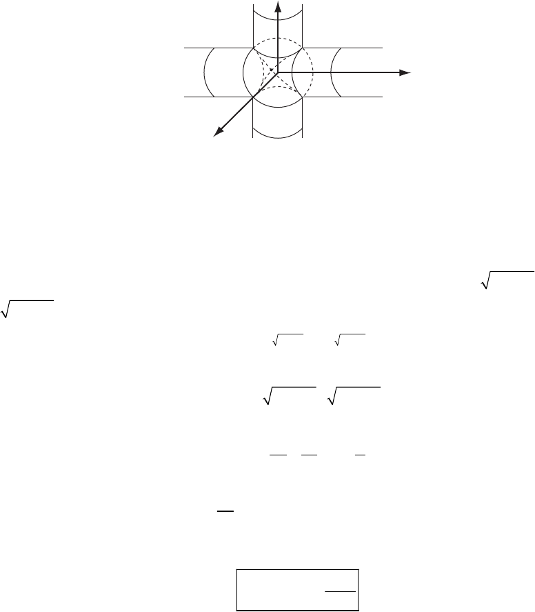
We compute the volume of the intersection of the two cylinders by dividing the intersection
volume into two parts. Part of the common volume is that of one of the cylinders, for example,
the one along the y axis, between y = –a and y = a:
(
)
2
122Vaa
3
a
π
π
== (1)
The rest of the common volume is formed by 8 equal parts from the other cylinder (the one
along the x-axis). One of these parts extends from x = 0 to x = a, y = 0 to 2
yax=−
2
, z = a to
22
z
ax=−. The complementary volume is then
22 22
200
22 22
0
33
21
0
33
8
8
8sin
32
16 2
3
aax ax
a
a
a
Vdxdydz
dxax axa
xa x
ax a
aa
π
−−
−
=
=−−−
=−−
=−
∫∫ ∫
∫
(2)
Then, from (1) and (2):
3
12
16
3
a
VV V
=+= (3)
26 CHAPTER 1
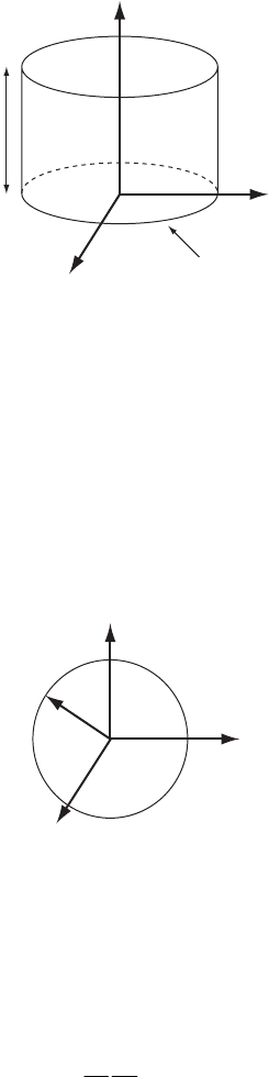
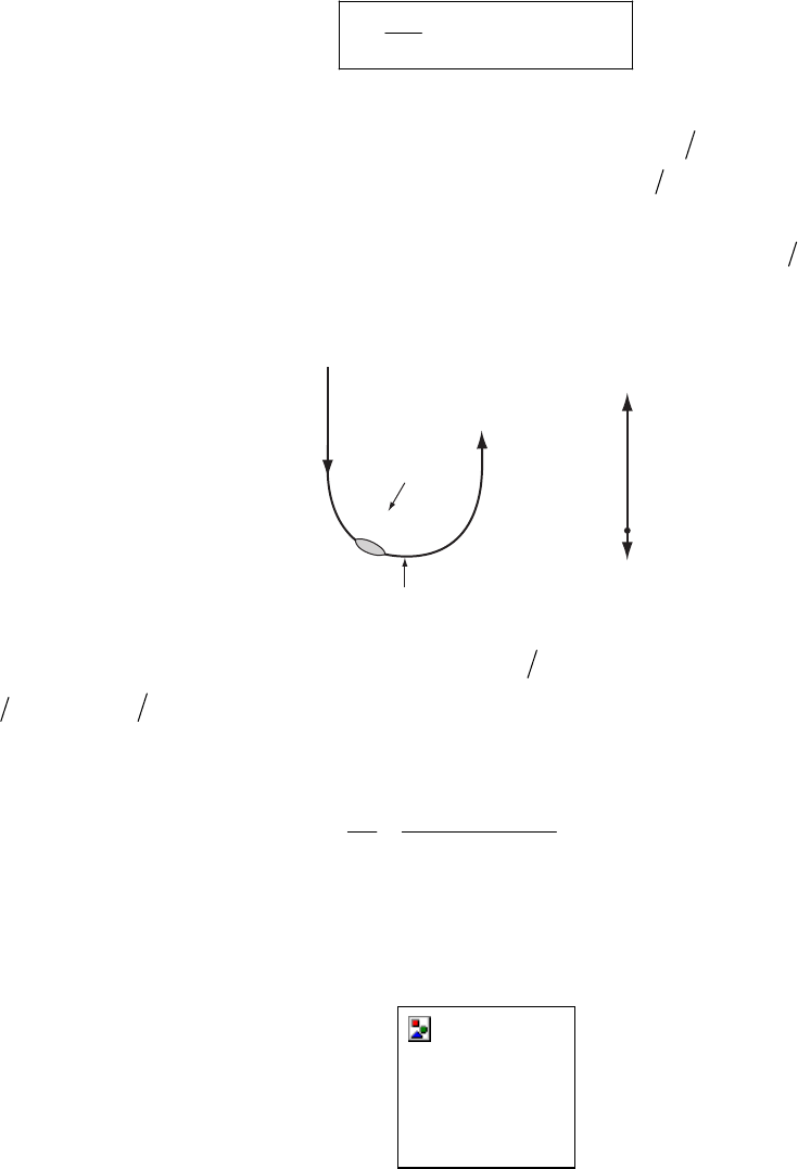
1-36.
d
z
x
y
c2 = x2 + y2
The form of the integral suggests the use of the divergence theorem.
(1)
SV
d⋅=∇⋅
∫∫
Aa Adv
Since ∇⋅ , we only need to evaluate the total volume. Our cylinder has radius c and height
d, and so the answer is
1=A
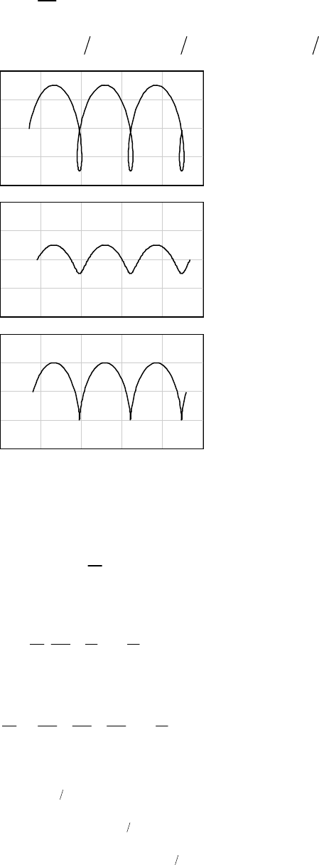
(2)
2
Vdv c d
π
=
∫
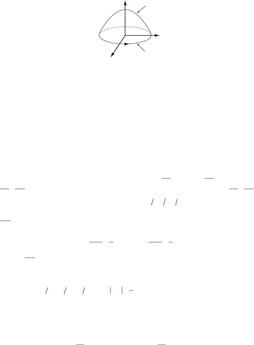
1-37.
z
y
x
R
To do the integral directly, note that A, on the surface, and that .
3
r
R=e
5
r
dda=ae
332
44
SS
dRdaR R R
π
π
⋅= = × =
∫∫
Aa (1)
To use the divergence theorem, we need to calculate
∇
⋅A. This is best done in spherical
coordinates, where A. Using Appendix F, we see that
3
r
r=e
()
2
2
15
r
r
rr
2
r
∂
∇⋅ = =
∂
AA (2)
Therefore,
(
)
222
000
sin 5 4
R
Vdv d d r r dr R
ππ
5
θ
θφ π
∇⋅ = =
∫∫
A
∫∫ (3)
Alternatively, one may simply set dv in this case.
2
4r dr
π
=
MATRICES, VECTORS, AND VECTOR CALCULUS 27
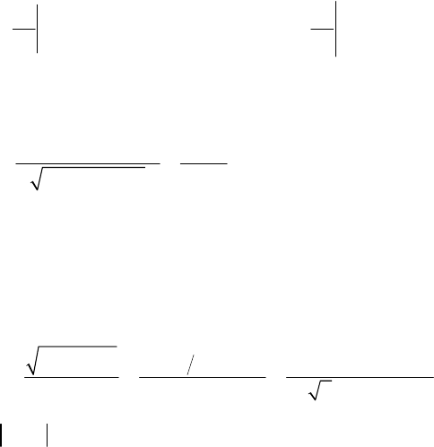
1-38.
x
z
y
C
x
2
+ y
2
= 1
z = 1 – x
2
– y
2
By Stoke’s theorem, we have
()
S
d
C
d
∇
×⋅= ⋅
∫∫
Aa As (1)
The curve C that encloses our surface S is the unit circle that lies in the xy plane. Since the
element of area on the surface da is chosen to be outward from the origin, the curve is directed
counterclockwise, as required by the right-hand rule. Now change to polar coordinates, so that
we have dd
θ
θ
=se and sin cos
θ
θ
=+Aik on the curve. Since sin
θ
θ
⋅
=−ei and 0
θ
⋅=ek , we
have
(
)
22
0sin
Cd
π
d
θ
θπ
⋅
=− =−
∫∫
As (2)
1-39.
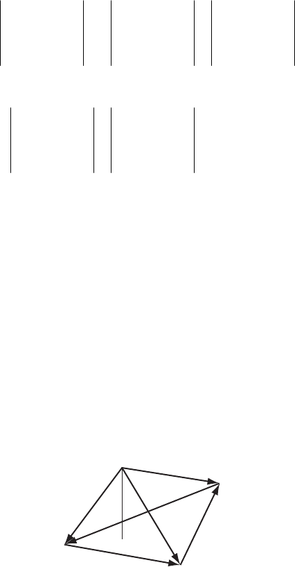
a) Let’s denote A = (1,0,0); B = (0,2,0); C = (0,0,3). Then (1,2,0)=−AB ; (1,0,3)=−AC ; and
(6,3,2)×=AB AC . Any vector perpendicular to plane (ABC) must be parallel to ×AB AC , so
the unit vector perpendicular to plane (ABC) is (6 7,3 7,2 7)
=
n
b) Let’s denote D = (1,1,1) and H = (x,y,z) be the point on plane (ABC) closest to H. Then
(1, 1,1xyz=− − −DH ) is parallel to n given in a); this means
162
13
x
y
−
=
=
− and 163
12
x
z
−
=
=
−
Further, (1,,xy=− )zAH is perpendicular to n so one has 6( 1) 3 2 0xyz
−
++=.
Solving these 3 equations one finds
H ( , , ) (19 49,34 49, 39 49)xyz== and 5
7
DH
=
1-40.
a) At the top of the hill, z is maximum;
02 and
6
zyx
x
∂
==−−
∂18 028
zxy
y28
∂
=
=−+
∂
28 CHAPTER 1
so x = –2 ; y = 3, and the hill’s height is max[z]= 72 m. Actually, this is the max value of z,
because the given equation of z implies that, for each given value of x (or y), z describes an
upside down parabola in term of y ( or x) variable.
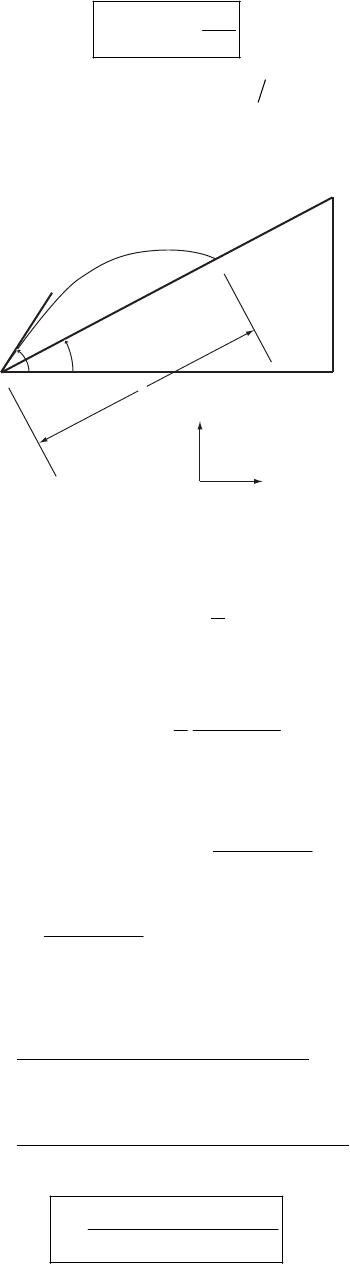
b) At point A: x = y = 1, z = 13. At this point, two of the tangent vectors to the surface of the
hill are
1
(1,1)
(1, 0, ) (1, 0, 8)
z
x
∂=
∂
t= and −
2
(1,1)
(0,1, ) (0,1,22)
z
y
∂
==
∂
t
Evidently tt is perpendicular to the hill surface, and the angle
12
(8, 22,1)×= −
θ
between this
and Oz axis is
222
(0,0,1) (8, 22,1) 1
s23.43
8221
⋅−
++
co
θ
= so
θ
= 87.55 degrees.
=
c) Suppose that in the
α
direction ( with respect to W-E axis), at point A = (1,1,13) the hill is
steepest. Evidently, dy = (tan
α
)dx and
d2 2 6 8 18 28 22(tan 1)
z xdy ydx xdx ydy dx dy dx
α
=+ −−−+= −
then
22 cos 1
22(tan 1) 22 2 cos ( 45)
dx dy dx
dz dx
α
αα
+−
=
−+
tan
β
==
The hill is steepest when tan
β
is minimum, and this happens when
α
= –45 degrees with
respect to W-E axis. (note that
α
= 135 does not give a physical answer).
1-41.
2( 1)aa
⋅
=−AB
then if only a = 1 or a = 0.
0⋅=
AB

CHAPTER 2
Newtonian Mechanics
—
Sin
g
le Particle
2-1. The basic equation is
ii
F
mx
=
(1)
a)
(
)
(
)
(
)
,
ii
Fx t f x gt mx==
ii
: Not integrable (2)
b)
(
)
(
)
(
)
,
ii
Fx t f x gt mx==
ii
()
()
i
ii
dx
mfxg
dt =
t
()
(
)
i
ii
gt
dx dt
fx m
=
: Integrable (3)
c)
(
)
(
)
(
)
,
ii i i i
Fx x f x gx mx==
i
: Not integrable (4)
2-2. Using spherical coordinates, we can write the force applied to the particle as
rr
F
FF
θ
θφφ
=
++Fe e e
(1)
But since the particle is constrained to move on the surface of a sphere, there must exist a
reaction force that acts on the particle. Therefore, the total force acting on the particle is
rr
F−e
total
F
Fm
θθ φφ
=
+=Fee
r
(2)
The position vector of the particle is
r
R
=
re (3)
where R is the radius of the sphere and is constant. The acceleration of the particle is
r
R
=
=ar e
(4)
29

30 CHAPTER 2
We must now express in terms of ,
r
e
r
e
θ
e, and
φ
e. Because the unit vectors in rectangular
coordinates, e, , e, do not change with time, it is convenient to make the calculation in
terms of these quantities. Using Fig. F-3, Appendix F, we see that
1 2
e3
123
123
12
sin cos sin sin cos
cos cos cos sin sin
sin cos
r
θ
φ
θ
φθφθ
θ
φθφ
φφ
=++
θ
=+−
=− +
ee e e
e e
ee e
ee (5)
Then
(
)
(
)
12
sin sin cos cos cos sin sin cos sin
sin
r
φθ
3
φ
θφθθφ θθφφθφ θ
φθ θ
=− + + + −
=+
ee e e
ee
θ
(6)
Similarly,
cos
r
θφ
θ
φ
=− +eee
θ
(7)
sin cos
r
φθ
φ
θφ
=− −ee e
θ
(8)
And, further,
(
)
(
)
(
)
22 2 2
sin sin cos 2 cos sin
rr
θφ
φ
θθ θφ θ θ θφ θφ θ
=− + + − + +ee e e
(9)
which is the only second time derivative needed.
The total force acting on the particle is
total r
mmR
=
=Fr
e (10)
and the components are
(
)
()
2sin cos
2cos sin
FmR
FmR
θ
φ
θ
φθθ
θ
φθφθ
=−
=+
(11)
NEWTONIAN MECHANICS—SINGLE PARTICLE 31
2-3.
y
x
v
0
P
β
α
The equation of motion is
m
=
Fa (1)
The gravitational force is the only applied force; therefore,
0
x
y
Fmx
F
my mg
==
==−
(2)
Integrating these equations and using the initial conditions,
(
)
()
0
0
0cos
0sin
xt v
yt v
α
α
==
==
(3)
We find
(
)
()
0
0
cos
sin
xt v
yt v gt
α
α
=
=−
(4)
So the equations for x and y are
(
)
()
0
2
0
cos
1
sin 2
xt vt
yt vt gt
α
α
=
=−
(5)
Suppose it takes a time t to reach the point P. Then,
0
00
2
00 0
cos cos
1
sin sin 2
vt
vt gt
βα
βα
=
=−
(6)
Eliminating between these equations,
00
00
2sin 2
1cos tan 0
2
vv
tgg
ααβ
gt
−
+
=
(7)
from which
32 CHAPTER 2
()
0
0
2sin cos tan
v
tg
α
αβ
=− (8)
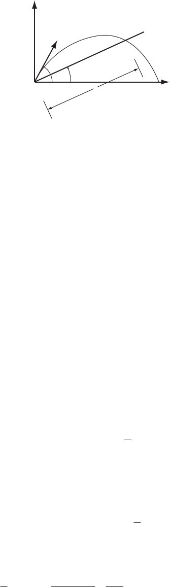
2-4. One of the balls’ height can be described by 2
00 2yy vtgt=+ − . The amount of time it
takes to rise and fall to its initial height is therefore given by 0
2vg. If the time it takes to cycle
the ball through the juggler’s hands is 0.9 s
τ
=
, then there must be 3 balls in the air during that
time
τ
. A single ball must stay in the air for at least 3
τ
, so the condition is 0
23vg
τ
≥, or
.
1
013.2 m sv−
≥⋅
2-5.
mg
N
point of maximum
acceleration
flightpath
plane
er
a) From the force diagram we have
(
)
2
r
mmvR−=Ng e. The acceleration that the pilot feels is
(
)
2
r
mmvR=+Ng e, which has a maximum magnitude at the bottom of the maneuver.
b) If the acceleration felt by the pilot must be less than 9g, then we have
(
)
1
2
2
3330ms 12.5 km
889.8ms
v
Rg
−
−
⋅⋅
≥=⋅⋅
(1)
A circle smaller than this will result in pilot blackout.
2-6.
Let the origin of our coordinate system be at the tail end of the cattle (or the closest cow/bull).
a) The bales are moving initially at the speed of the plane when dropped. Describe one of
these bales by the parametric equations
00
xx vt
=
+ (1)
NEWTONIAN MECHANICS—SINGLE PARTICLE 33
2
0
1
2
yy gt=− (2)
where , and we need to solve for . From (2), the time the bale hits the ground is
080 my=0
x
0
2yg
τ
=. If we want the bale to land at
(
)
30 mx
τ
=
−, then
(
)
0
xx v
0
τ
τ
=
−. Substituting
and the other values, this gives
-1
s
044.4 mv=⋅ 0210x m
−
. The rancher should drop the bales
210 m behind the cattle.
b) She could drop the bale earlier by any amount of time and not hit the cattle. If she were late
by the amount of time it takes the bale (or the plane) to travel by 30 m in the x-direction, then
she will strike cattle. This time is given by
(
)
0
30 m 0.68 sv.
2-7. Air resistance is always anti-parallel to the velocity. The vector expression is:
2
11
22
w
cAv cAv
v
ρ
=−=−
v
W
w
ρ
v
a
(1)
Including gravity and setting , we obtain the parametric equations
net m=F
2
xbxxy=− +
2
(2)
22
ybyxyg
=
−+
− (3)
where 2
wAmbc
ρ
=. Solving with a computer using the given values and , we
find that if the rancher drops the bale 210 m behind the cattle (the answer from the previous
problem), then it takes 4.44 s to land 62.5 m behind the cattle. This means that the bale
should be dropped at 178 m behind the cattle to land 30 m behind. This solution is what is
plotted in the figure. The time error she is allowed to make is the same as in the previous
problem since it only depends on how fast the plane is moving.
-3
1.3 kg m
ρ
=⋅
–200 –180 –160 –140 –120 –100 –80 –60 –40
0
20
40
60
80
With air resistance
No air resistance
x (m)
y (m)
34 CHAPTER 2
2-8.
PQ
x
y
v
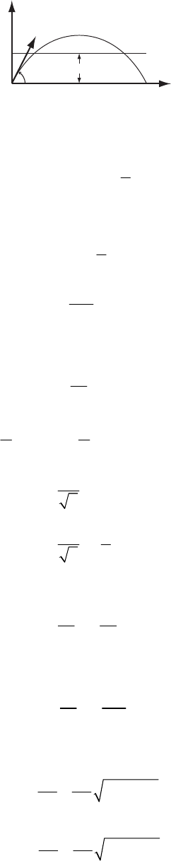
0
αh
From problem 2-3 the equations for the coordinates are
0cosxvt
α
=
(1)
2
0
1
sin 2
yvt gt
α
=− (2)
In order to calculate the time when a projective reaches the ground, we let y = 0 in (2):
2
0
1
sin 0
2
vt gt
α
−
= (3)
0
2sin
v
tg
α
= (4)
Substituting (4) into (1) we find the relation between the range and the angle as
2
0sin 2
v
xg
α
= (5)
The range is maximum when 22
π
α
=, i.e., 4
π
α
=
. For this value of α the coordinates become
0
2
0
2
1
2
2
v
xt
v
xtgt
=
=−
(6)
Eliminating t between these equations yields
22
200
0
vv
xxy
gg
−
+= (7)
We can find the x-coordinate of the projectile when it is at the height h by putting y = h in (7):
22
200
0
vvh
xx
gg
−
+= (8)
This equation has two solutions:
22
2
00
10
22
2
00
20
4
22
4
22
vv
xv
gg
vv
xv
gg
=− −
gh
gh
=+ −
(9)
NEWTONIAN MECHANICS—SINGLE PARTICLE 35
where corresponds to the point P and to Q in the diagram. Therefore,
1
x2
x
2
0
21 0
4
v
dx x v gh
g
=−= − (10)
2-9.
a) Zero resisting force ( ): 0
r
F=
The equation of motion for the vertical motion is:
dv
F
ma m mg
dt
== =− (1)
Integration of (1) yields
0
vgtv
=
−+ (2)
where v is the initial velocity of the projectile and t = 0 is the initial time.
0
The time required for the projectile to reach its maximum height is obtained from (2). Since
corresponds to the point of zero velocity,
m
t
m
t
(
)
0
0
m
vt v gt== − m
, (3)
we obtain
0
m
v
tg
= (4)
b) Resisting force proportional to the velocity
(
)
r
F
kmv=− :
The equation of motion for this case is:
dv
F
mmgk
dt
==−−mv (5)
where –kmv is a downward force for m
tt
<
′
and is an upward force for m
tt>
′
. Integrating, we
obtain
()
0kt
gkv g
vt e
kk
−
+
=− + (6)
For t, v(t) = 0, then from (6),
m
t=
()
01
m
kt
g
ve
k
=
− (7)
which can be rewritten as
0
ln 1
m
kv
kt g
=+
(8)
Since, for small z (z 1) the expansion
36 CHAPTER 2
()
2
11
ln 1 23
3
z
zz z+=− + (9)
is valid, (8) can be expressed approximately as
2
00 0
1
1232
m
vkv kv
tgg g
=−+ −
… (10)
which gives the correct result, as in (4) for the limit k → 0.
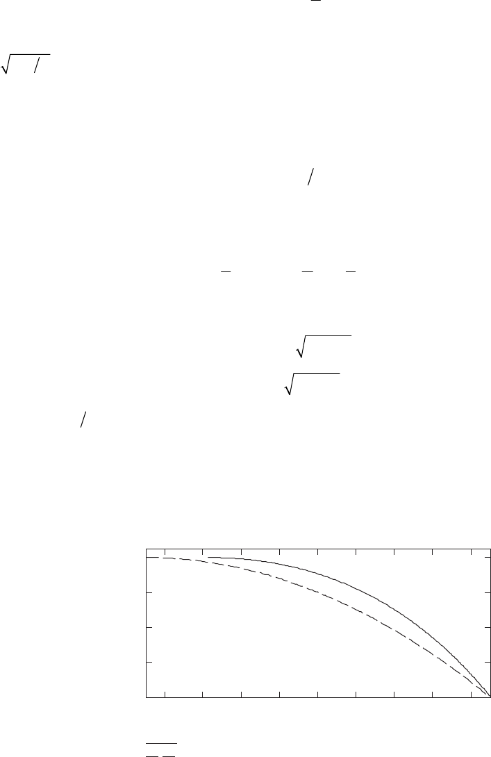
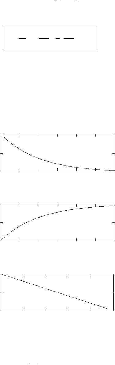
2-10. The differential equation we are asked to solve is Equation (2.22), which is .
Using the given values, the plots are shown in the figure. Of course, the reader will not be able
to distinguish between the results shown here and the analytical results. The reader will have to
take the word of the author that the graphs were obtained using numerical methods on a
computer. The results obtained were at most within 10
xk=−
x
8
−
of the analytical solution.
0 5 10 15 20 25 30
5
10 v vs t
t (s)
v (m/s)
0 20406080
0
5
10
100
v vs x
x (m)
v (m/s)
0 5 10 15 20 25 30
0
50
100 x vs t
t (s)
x (m)
2-11. The equation of motion is
2
2
2
dx
m kmv mg
dt =− + (1)
This equation can be solved exactly in the same way as in problem 2-12 and we find
NEWTONIAN MECHANICS—SINGLE PARTICLE 37
2
0
2
1log
2
gkv
xkgkv
−
=
−
(2)
where the origin is taken to be the point at which v0
v
=
so that the initial condition is
(
)
00xv v==. Thus, the distance from the point 0
vv
=
to the point v1
v
=
is
()
2
0
01 2
1
1log
2
gkv
sv v kgkv
−
→=
−
(3)
2-12. The equation of motion for the upward motion is
2
2
2
dx
mmkv
dt =− −mg (1)
Using the relation
2
2
d x dv dv dx dv
v
dt dt dx dt dx
== = (2)
we can rewrite (1) as
2
vdv dx
kv g
=
−
+ (3)
Integrating (3), we find
()
2
1log
2kv g x C
k
+
=− + (4)
where the constant C can be computed by using the initial condition that when x = 0:
0
vv=
()
2
0
1log
2
Ckv
kg
=
+ (5)
Therefore,
2
0
2
1log
2
kv g
xkkvg
+
=
+
(6)
Now, the equation of downward motion is
2
2
2
dx
mmkv
dt =− +mg
(7)
This can be rewritten as
2
vdv dx
kv g =
−+ (8)
Integrating (8) and using the initial condition that x = 0 at v = 0 (w take the highest point as the
origin for the downward motion), we find
38 CHAPTER 2
2
1log
2
g
xkgkv
=− (9)
At the highest point the velocity of the particle must be zero. So we find the highest point by
substituting v = 0 in (6):
2
0
1log
2
h
kv g
xkg
+
= (10)
Then, substituting (10) into (9),
2
0
2
11
log log
22
kv g g
kgkgk
+=−v
(11)
Solving for v,
2
0
2
0
gv
k
vg
vk
=
+
(12)
We can find the terminal velocity by putting x → ∞ in(9). This gives
t
g
vk
= (13)
Therefore,
0
22
0
t
t
vv
vvv
=+ (14)
2-13. The equation of motion of the particle is
()
32
dv
mmkva
dt =− + v
(1)
Integrating,
()
22
dv kdt
vv a =−
+
∫
∫ (2)
and using Eq. (E.3), Appendix E, we find
2
222
1ln
2
vkt C
aav
=
−+
+
(3)
Therefore, we have
2
22
A
t
vCe
av
−
=′
+ (4)
NEWTONIAN MECHANICS—SINGLE PARTICLE 39
where 2
2
A
ak≡
0
vv=
and where C′ is a new constant. We can evaluate C′ by using the initial
condition, at t = 0:
2
0
2
0
v
Cav
=
′2
+
(5)
Substituting (5) into (4) and rearranging, we have
12
2
1
At
At
aCe dx
vCe dt
−
−
′
=
−′
=
(6)
Now, in order to integrate (6), we introduce
A
t−
≡ue so that du = –Au dt. Then,
12 12
2
2
11
At
At
aCe a Cu du
xdt
Ce A Cu u
aC du
ACu u
−
−
′′
==
−−
′′
′
−+
′
∫∫
=−
∫
(7)
Using Eq. (E.8c), Appendix E, we find
()
1
sin 1 2
a
xCuC
A
−
=−+
′
′′ (8)
Again, the constant C″ can be evaluated by setting x = 0 at t = 0; i.e., x = 0 at u = 1:
(
1
sin 1 2
a
C
)
C
A
−
=− −
′
′′
(9)
Therefore, we have
()
()
11
sin 2 1 sin 2 1
At
ae CxC
A
−− −
=−+−−+
′′
Using (4) and (5), we can write
22
22
11
0
22 22
0
1sin sin
2
va
va
ak va va
−−
x
−+
−+ −
=
++
(10)
From (6) we see that v → 0 as t → ∞. Therefore,
22
1
22
lim sin sin (1) 2
t
va
va
1
π
−−
→∞
−+
=
=
+
(11)
Also, for very large initial velocities,
()
0
22
11
0
22
0
lim sin sin 1 2
v
va
va
π
−−
→∞
−+
=
−=−
+
(12)
Therefore, using (11) and (12) in (10), we have
40 CHAPTER 2
()
2
xt ka
π
→∞ = (13)
and the particle can never move a distance greater than 2ka
π
for any initial velocity.
2-14.
y
x
d
αβ
a) The equations for the projectile are
0
2
0
cos
1
sin 2
xv t
yv t gt
α
α
=
=−
Solving the first for t and substituting into the second gives
2
22
0
1
tan 2cos
gx
yx v
α
α
=−
Using x = d cos
β
and y = d sin
β
gives
22
22
0
2
22
0
cos
sin cos tan 2cos
cos
0costan
2cos
gd
dd v
gd
dv
β
ββα α
β
sin
β
αβ
α
=−
=−+
Since the root d = 0 is not of interest, we have
(
)
()
22
0
2
2
0
2
2cos tan sin cos
cos
2cos sincos cossin
cos
v
dg
v
g
βα β α
β
α
αβ αβ
β
−
=
−
=
()
2
0
2
2cossin
cos
v
dg
α
αβ
β
−
= (1)
NEWTONIAN MECHANICS—SINGLE PARTICLE 41
b) Maximize d with respect to
α
()
() ()(
2
0
2
2
0sinsincoscoscos2
cos
v
dd
dg
)
α
αβ α αβ αβ
αβ
== − − + − −
(
)
cos 2 0
αβ
−
=
22
π
αβ
−
=
42
π
β
α
=
+
c) Substitute (2) into (1)
2
0
max 2
2cos sin
cos 4 2 4 2
v
g
d
π
βπβ
β
=+
−
Using the identity
()()
11
n sin 2 cos sin
22
si
A
BABA−= + −B
we have
22
00
max 22
sin sin 1sin
22
cos 2 1 sin
vv
gg
d
π
β
β
β
β
−
−
=⋅ =
−
()
2
0
max 1sin
v
dg
β
=+
2-15.
mg θ
mg sin θ
The equation of motion along the plane is
2
sin
dv
mmg km
dt
θ
=−v (1)
Rewriting this equation in the form
2
1
sin
dv dt
g
kv
k
θ
=
−
(2)
42 CHAPTER 2
We know that the velocity of the particle continues to increase with time (i.e., 0dv dt >), so that
(
)
2
singk v
θ
>. Therefore, we must use Eq. (E.5a), Appendix E, to perform the integration. We
find
1
11tanh
sin sin
vtC
kgg
kk
θθ
−
=
+
(3)
The initial condition v(t = 0) = 0 implies C = 0. Therefore,
()
sin tanh sin
gdx
vgk
kd
θθ
=t
t
= (4)
We can integrate this equation to obtain the displacement x as a function of time:
()
sin tanh sin
g
xgk
k
θθ
=∫tdt
Using Eq. (E.17a), Appendix E, we obtain
(
)
ln cosh sin
sin sin
gk t
g
kgk
θ
θθ
=
xC
+
′
(5)
The initial condition x(t = 0) = 0 implies C′ = 0. Therefore, the relation between d and t is
()
1ln cosh sindgk
kt
θ
= (6)
From this equation, we can easily find
(
)
1
cosh
sin
dk
e
tgk
θ
−
= (7)
2-16. The only force which is applied to the article is the component of the gravitational force
along the slope: mg sin
α
. So the acceleration is g sin
α
. Therefore the velocity and displacement
along the slope for upward motion are described by:
(
)
0sinvv g t
α
=− (1)
(
2
0
1sin
2
xvt g t
)
α
=− (2)
where the initial conditions
(
)
0
0v==vt and
(
)
0xt 0
=
= have been used.
At the highest position the velocity becomes zero, so the time required to reach the highest
position is, from (1),
0
0sin
v
tg
α
= (3)
At that time, the displacement is
NEWTONIAN MECHANICS—SINGLE PARTICLE 43
2
0
0
1
2sin
v
xg
α
= (4)
For downward motion, the velocity and the displacement are described by
(
)
sinvg t
α
= (5)
(
2
1sin
2
xg
α
=
)
t
(6)
where we take a new origin for x and t at the highest position so that the initial conditions are
v(t = 0) = 0 and x(t = 0) = 0.
We find the time required to move from the highest position to the starting position by
substituting (4) into (6):
0
sin
v
tg
α
=
′ (7)
Adding (3) and (7), we find
0
2
sin
v
tg
α
= (8)
for the total time required to return to the initial position.
2-17.
v
0
Fence
35˚
0.7 m
60 m
The setup for this problem is as follows:
0cosxvt
θ
=
(1)
2
00
1
sin 2
yy vt gt
θ
=+ − (2)
where and . The ball crosses the fence at a time
35
θ
=
007 my=.
(
)
0cosRv
τ
θ
=, where
R = 60 m. It must be at least h = 2 m high, so we also need 2
00
sinv g
τθτ
−2hy−= . Solving for
, we obtain
0
v
()
2
2
0
0
2 cos sin cos
gR
vRhy
θ
θθ
=
−−
(3)
which gives v.
1
025 4 m s−
.⋅
44 CHAPTER 2
2-18.
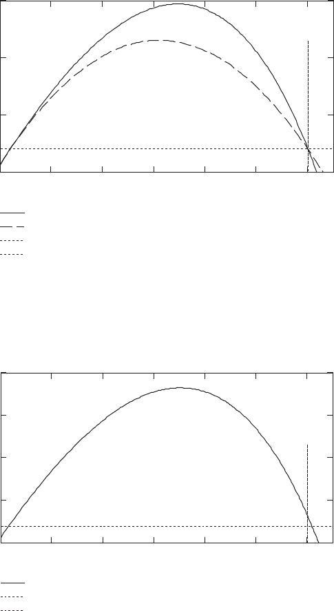
a) The differential equation here is the same as that used in Problem 2-7. It must be solved for
many different values of v in order to find the minimum required to have the ball go over the
fence. This can be a computer-intensive and time-consuming task, although if done correctly is
easily tractable by a personal computer. This minimum is
0
0
v1
35.2 m s
−
⋅
3
m
, and the trajectory is
shown in Figure (a). (We take the density of air as 13 kg
ρ
−
=. ⋅ .)
0102030405060
0
5
10
15
With air resistance
No air resistance
fence height
fence range
x (m)
y (m)
b) The process here is the same as for part (a), but now we have v fixed at the result just
obtained, and the elevation angle
θ
must be varied to give the ball a maximum height at the
fence. The angle that does this is 0.71 rad = 40.7°, and the ball now clears the fence by 1.1 m.
This trajectory is shown in Figure (b).
0
0102030405060
0
5
10
15
20
Flight Path
fence height
fence range
x (m)
y (m)
NEWTONIAN MECHANICS—SINGLE PARTICLE 45
2-19. The projectile’s motion is described by
(
)
()
0
2
0
cos
1
sin 2
xv t
yv t gt
α
α
=
=−
(1)
where v is the initial velocity. The distance from the point of projection is
0
2
rxy=+
2
(2)
Since r must always increase with time, we must have : 0r>
0
xx yy
rr
+
=
>
(3)
Using (1), we have
()
23 2 2
0
13
sin
22
yy g t g v t v t
α
+= − +
0
xx (4)
Let us now find the value of t which yields 0xx yy
+
=
(i.e., 0r
=
):
2
00
sin
39sin 8
22
vv
tgg
α
α
=± − (5)
For small values of
α
, the second term in (5) is imaginary. That is, r = 0 is never attained and the
value of t resulting from the condition 0r
=
is unphysical.
Only for values of
α
greater than the value for which the radicand is zero does t become a
physical time at which does in fact vanish. Therefore, the maximum value of
α
that insures
for all values of t is obtained from
r
0r>
2
max
9sin 8 0
α
−
= (6)
or,
max
22
sin 3
α
= (7)
so that
max 70.5
α
≅
° (8)
2-20. If there were no retardation, the range of the projectile would be given by Eq. (2.54):
2
0
0
sin 2
v
Rg
θ
= (1)
The angle of elevation is therefore obtained from

46 CHAPTER 2
()
()
()
02
0
2
2
sin 2
1000 m 9.8 m/sec
140 m/sec
0.50
Rg
v
θ
=
×
=
= (2)
so that
015
θ
=
° (3)
Now, the real range R′, in the linear approximation, is given by Eq. (2.55):
2
00
4
13
sin 2 4 sin
13
kV
RR g
vkv
gg
θ
θ
=−
′
=−
(4)
Since we expect the real angle
θ
to be not too different from the angle 0
θ
calculated above, we
can solve (4) for
θ
by substituting 0
θ
for
θ
in the correction term in the parentheses. Thus,
200
0
sin 2 4sin
13
gR
kv
vg
θ
θ
′
=
−
(5)
Next, we need the value of k. From Fig. 2-3(c) we find the value of km by measuring the slope of
the curve in the vicinity of v = 140 m/sec. We find
(
)
(
)
110 N 500 m/s 0.22 kg/skm
≅
≅. The
curve is that appropriate for a projectile of mass 1 kg, so the value of k is
1
0.022 seck
−
(6)
Substituting the values of the various quantities into (5) we find 17.1
θ
=
°. Since this angle is
somewhat greater than 0
θ
, we should iterate our solution by using this new value for 0
θ
in (5).
We then find 17.4
θ
=°. Further iteration does not substantially change the value, and so we
conclude that
17.4
θ
=
°
If there were no retardation, a projectile fired at an angle of 17.4° with an initial velocity of
140 m/sec would have a range of
(
)
2
2
140 m/sec sin 34.8
9.8 m/sec
1140 m
R°
=
NEWTONIAN MECHANICS—SINGLE PARTICLE 47
2-21.
x3
α
v0
x2
x1
Assume a coordinate system in which the projectile moves in the 2
xx
3
−
plane. Then,
20
2
30
cos
1
sin 2
xvt
xvt gt
α
α
=
=−
(1)
or,
()
22 33
2
020
1
cos sin 2
xx
vt vt gt
αα
=+
=+−
re e
e3
e
(2)
The linear momentum of the projectile is
(
)
(
)
020
cos sinmmv v gt
αα
3
== + −
e e
pr (3)
and the angular momentum is
(
)
(
)
(
)
(
)
2
020 3020
cos sin cos sinvt vt gt m v v gt
αα αα
3
=× = + − × + −
Lrp e e e e (4)
Using the property of the unit vectors that 3i
j
i
j
k
ε
×
=eee , we find
()
2
0
1cos
2mg v t
α
=L1
e (5)
This gives
(
)
0
cosmg v t
α
=−L
1
e (6)
Now, the force acting on the projectile is
3
mg
=
−Fe (7)
so that the torque is
() ()
()
2
020 3
01
1
cos sin 2
cos
vt vt gt mg
mg v t
αα
α
=× = + − −
=−
NrF e e e
e
3
which is the same result as in (6).
48 CHAPTER 2
2-22.
x
y
z
e
B
E
Our force equation is
(
)
q
=
+×FEvB (1)
a) Note that when E = 0, the force is always perpendicular to the velocity. This is a centripetal
acceleration and may be analyzed by elementary means. In this case we have also so that
⊥
vB
vB×=vB .
2
centripetal
mv
ma qvB
r
== (2)
Solving this for r
c
mv v
rqB
ω
== (3)
with cqB m
ω
≡/.
b) Here we don’t make any assumptions about the relative orientations of v and B, i.e. the
velocity may have a component in the z direction upon entering the field region. Let
, with
xyz=++
rijk
=
vr
and . Let us calculate first the v × B term. =ar
(
00
xyz By x
B
×= = −
ijk
vB i j
)
(4)
The Lorentz equation (1) becomes
(
)
y
z
m qBy q E Bx qE== + − +Fr i j
k (5)
Rewriting this as component equations:
c
qB
xy
my
ω
==
(6)
y
c
qE E
qB
yx x
mm B
ω
=− + =− −
y
(7)
z
qE
zm
=
(8)
NEWTONIAN MECHANICS—SINGLE PARTICLE 49
The z-component equation of motion (8) is easily integrable, with the constants of integration
given by the initial conditions in the problem statement.
()
2
002
z
qE
z
tzzt t
m
=+ +
(9)
c) We are asked to find expressions for and , which we will call and x
y
x
v
y
v, respectively.
Differentiate (6) once with respect to time, and substitute (7) for
y
v
2
y
xcy cx
E
vv v
B
ωω
==− −
(10)
or
22
y
xcxc
E
vv B
ωω
+=
(11)
This is an inhomogeneous differential equation that has both a homogeneous solution (the
solution for the above equation with the right side set to zero) and a particular solution. The
most general solution is the sum of both, which in this case is
() ()
12
cos sin
y
xc c
E
vC tC t B
ωω
=++ (12)
where C and C are constants of integration. This result may be substituted into (7) to get
1 2
y
v
(
)
(
)
12
cos sin
ycc c
CtC
vc
t
ω
ωωω
=− −
(13)
(
)
(
)
12
sin cos
yc c
vC tC t
ωω
=− + +K (14)
where K is yet another constant of integration. It is found upon substitution into (6), however,
that we must have K = 0. To compute the time averages, note that both sine and cosine have an
average of zero over one of their periods 2c
T
π
ω
≡
.
0
y
E
xy
B
=
,=
(15)
d) We get the parametric equations by simply integrating the velocity equations.
() ()
12
sin cos y
cc
cc
E
CC
t
B
ωω
ωω
=−+
x
tD
+
xt (16)
() ()
12
cos sin
cc
y
cc
CC
yt t
ωω
ωω
=+ D+ (17)
where, indeed, D and
x
y
D are constants of integration. We may now evaluate all the C’s and
D’s using our initial conditions
(
)
0c
xA
ω
=
−,
(
)
0y
xEB
=
,
(
)
00y
=
,
(
)
0y=
A. This gives us
, and gives the correct answer
1xy
CDD== 0=2
C=A
()
()
cos
y
c
c
E
A
xt t t
B
ω
ω
−
=+ (18)
50 CHAPTER 2
(
() sin c
c
A
yt t
)
ω
ω
= (19)
These cases are shown in the figure as (i) y
A
EB>, (ii) y
A
EB
<
, and (iii) y
A
EB=.
(i)
(ii)
(iii)
2-23.
(
)
(
)
at
F
tmatkte
−
== (1)
with the initial conditions x(t) = v(t) = 0. We integrate to get the velocity. Showing this explicitly,
()
()
(0) 0
vt t t
v
k
at dt te dt
m
α
−
=
∫∫
(2)
Integrating this by parts and using our initial conditions, we obtain
2
11 1
() t
k
vt t e
m
α
αα α
−
=−+
(3)
By similarly integrating v(t), and using the integral (2) we can obtain x(t).
()
322
211 2 t
k
xt t e
m
α
ααα α
−
=−++ +
(4)
To make our graphs, substitute the given values of m = 1 kg, 1
1 N sk
−
=
⋅, and .
1
0.5 s
α
−
=
(
)
2t
xt te
−
= (5)
(
)
(
)
2
42 2 t
vt t e
−
=− + (6)
(
)
(
)
2
16 4 4 4 t
ttt
α
−
=− + + + e (7)
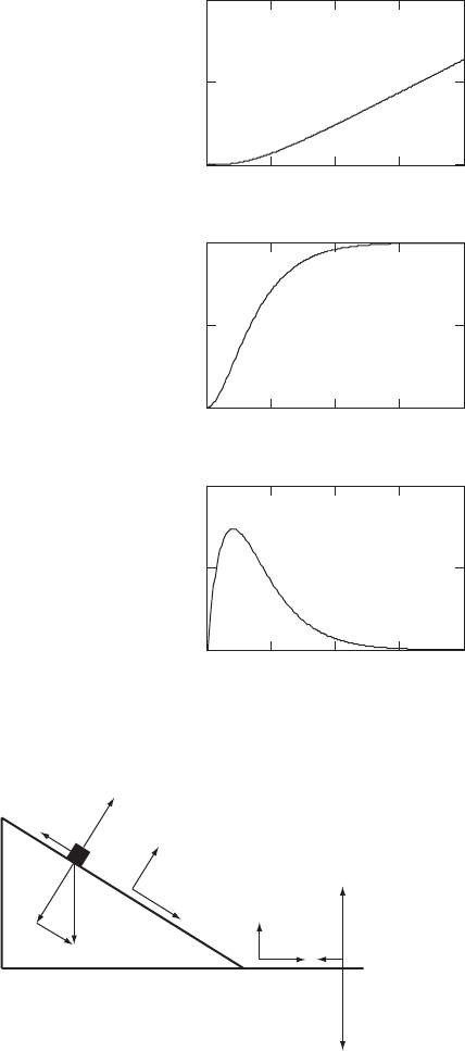
NEWTONIAN MECHANICS—SINGLE PARTICLE 51
0 5 10 15 20
0
50
100
t
x(t)
0 5 10 15 20
0
2
4
t
v(t)
0 5 10 15 20
0
0.5
1
t
a(t)
2-24.
mg
mg
Ff
FfN
B
N′
d= length of incline
s= distance skier travels
along level ground
θx
mg sin θ
mg cos θ
y
y
x
While on the plane:
FN
∑ so Nm
cos 0
ymg my
θ
=− = =
cosg
θ
=
sin
x
f
Fm
∑; g F
θ
=− cos
f
F
Nmg
µ
µθ
=
=
sin cosmg mg mx
θ
µθ
−
=
So the acceleration down the plane is:
(
)
1sin cos constantag
θµ θ
=−=
52 CHAPTER 2
While on level ground: ; Nm=
′gg
f
Fm
µ
=
−
So becomes
x
Fm=
∑
xmg mx
µ
−=
The acceleration while on level ground is
2constantag
µ
=
−=
For motion with constant acceleration, we can get the velocity and position by simple
integration:
xa
=
0
vxatv
=
=+
(1)
2
00
1
2
xx vt at−= + (2)
Solving (1) for t and substituting into (2) gives:
0
vv t
a
−
=
(
)
(
)
2
00 0
0
1
2
vvv vv
xx aa
−−
−= +⋅
or
(
)
22
00
2ax x v v
−
=−
Using this equation with the initial and final points being the top and bottom of the incline
respectively, we get:
2 = speed at bottom of incline
2
1B
ad V=B
V
Using the same equation for motion along the ground:
2
2
2B
as V
=
− (3)
Thus
ad
1
as=− 2
(
)
1sin cosag
θ
µ
=−
θ
2
ag
µ
=
−
So
(
)
sin cosgd gs
θ
µθµ
−=
Solving for
µ
gives
sin
cos
d
ds
θ
µθ
=
+
Substituting
θ
= 17°, d = 100 m, s = 70 m gives
0.18
µ
=
Substituting this value into (3):
NEWTONIAN MECHANICS—SINGLE PARTICLE 53
2
2B
gs V
µ
−
=−
2
B
Vgs
µ
=
15.6 m/sec
B
V=
2-25.
a) At A, the forces on the ball are:
N
mg
The track counters the gravitational force and provides centripetal acceleration
2
NmgmvR−=
Get v by conservation of energy:
0
top top top
ETU mgh
=
+=+
2
10
2
AA A
ETU mv
=
+= +
2
top A
EEv g=→= h
So
2NmgmghR
=
+
2
1h
Nmg R
=+
b) At B the forces are:
mg
N
45˚
2
2
cos 45
2
NmvRmg
mv R mg
=
+°
=+ (1)
Get v by conservation of energy. From a), total
Emgh
=
.
At B, 2
1
2vmgh=+
′
Em
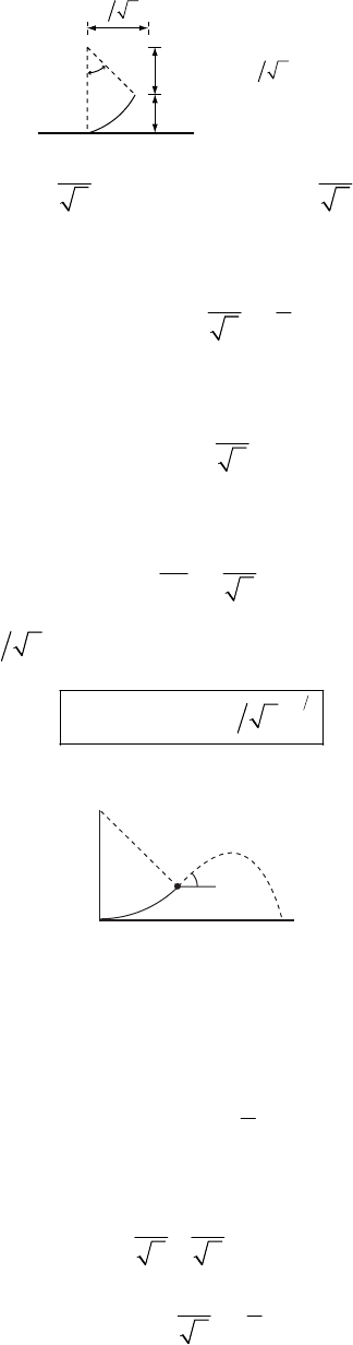
54 CHAPTER 2
R
R
h′
45˚
RRcos 45 2˚=
R2
2
R
R=+h
′
or 1
12
hR
=−
′
So becomes:
total B B
ETU=+
2
11
12
2
mgh mgR mv
=−+
Solving for
2
v
2
1
21
2
gh gR v
−
−=
Substituting into (1):
23
2
2
h
Nmg
R
=+−
c) From b) 222
BhRR
=−+
vg
()
12
22vghRR
=−+
d) This is a projectile motion problem
45˚
45˚
B
A
Put the origin at A.
The equations:
00x
xx vt
=
+
2
00
1
2
y
yy vt gt=+ −
become
22
B
vR
x=+t (2)
2
1
2
2
B
v
yh t gt=+ −
′ (3)
Solve (3) for t when y = 0 (ball lands).
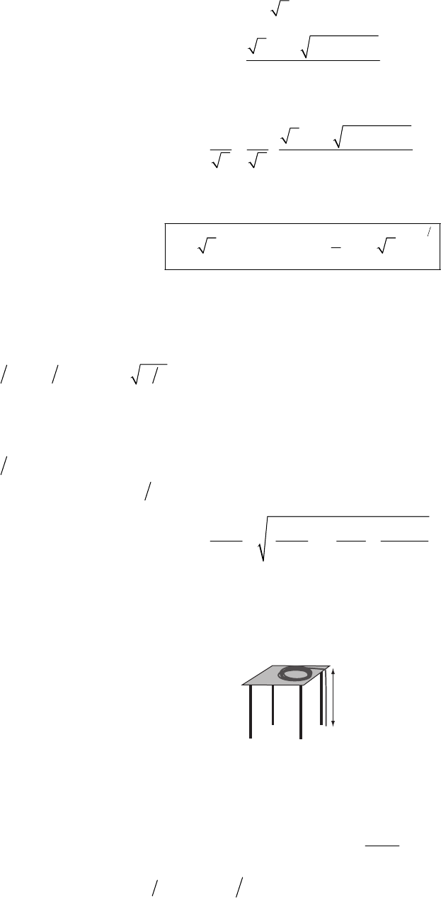
NEWTONIAN MECHANICS—SINGLE PARTICLE 55
222
B
gt v t h 0
−
−=
′
2
228
2
BB
vvg
tg
±+h
′
=
We discard the negative root since it gives a negative time. Substituting into (2):
2
228
2
22
BB
Bvvgh
vR
xg
±+
′
=+
Using the previous expressions for and h′ yields
B
v
()
12
22 2
3
21 2
2
hhRRxR
=−++− +
e) , with , so Ux has the shape of the track. () ()Ux mgyx=(0)yh=( )
2-26. All of the kinetic energy of the block goes into compressing the spring, so that
22
22mv kx=, or 23 mxvmk=., where x is the maximum compression and the given
values have been substituted. When there is a rough floor, it exerts a force kmg
µ
in a direction
that opposes the block’s velocity. It therefore does an amount of work kmgd
µ
in slowing the
block down after traveling across the floor a distance d. After 2 m of floor, the block has energy
22k
mv mgd
µ
−, which now goes into compressing the spring and still overcoming the friction
on the floor, which is 22k
kx mgx
µ
+. Use of the quadratic formula gives
222mg mg mgd
mv
kkkk
µµ µ
=− + + −
x (1)
Upon substitution of the given values, the result is 1.12 m.
2-27.
0.6 m
To lift a small mass dm of rope onto the table, an amount of work
(
)
(
)
0
dW dm g z z
=
− must be
done on it, where 006 m
z
=. is the height of the table. The total amount of work that needs to be
done is the integration over all the small segments of rope, giving
0
2
0
0
0()( )2
zgz
Wdzgzz
µ
µ
=−=
∫ (1)
When we substitute
(
)
(
)
04 kg 4 mmL
µ
==. , we obtain 0 18 JW
.
.
56 CHAPTER 2
2-28.
m
M
v
v
v4
v3
before
collision
after
collision
The problem, as stated, is completely one-dimensional. We may therefore use the elementary
result obtained from the use of our conservation theorems: energy (since the collision is elastic)
and momentum. We can factor the momentum conservation equation
11 22 13 2 4
mv mv mv mv
+
=+ (1)
out of the energy conservation equation
222
11 22 13 24
1111
2222
mv mv mv mv+=+
2
4
(2)
and get
13 2
vvvv
+
=+ (3)
This is the “conservation” of relative velocities that motivates the definition of the coefficient of
restitution. In this problem, we initially have the superball of mass M coming up from the
ground with velocity 2g=v, while the marble of mass m is falling at the same velocity.
Conservation of momentum gives
h
(
)
34
M
vmv Mv mv
+
−= + (4)
and our result for elastic collisions in one dimension gives
3
()vv v v
4
+
=− + (5)
solving for and and setting them equal to
3
v4
v2item
gh , we obtain
2
3
1
marble
h
α
α
−h
=
+
(6)
2
13
1
superball
h
α
α
−h
=
+
(7)
where mM
α
≡. Note that if 13
α
<, the superball will bounce on the floor a second time after
the collision.
NEWTONIAN MECHANICS—SINGLE PARTICLE 57
2-29.
mg cos θ
mg sin θ
mg
F
f
N
y
x
θ
1
tan 0.08 4.6
cos
0
cos
sin
cos
y
xf
f
FNmg
my
Nmg
Fmg F
mx
FNmg
θ
θ
θ
θ
µ
µθ
−
=
=°
=−
==
=
=−
=
==
∑
∑
so
()
sin cos
sin cos
mx mg mg
xg
θ
µθ
θµ θ
=
−
=−
Integrate with respect to time
(
)
0
sin cosxgt x
θµ θ
=
−
+
(1)
Integrate again:
(
2
00
1sin cos
2
xx xt gt
)
θ
µθ
=+ + −
(2)
Now we calculate the time required for the driver to stop for a given (initial speed) by
solving Eq. (1) for t with .
0
x
0x=
()
1
0sin cos
x
tg
θ
µθ
−
=− −
′
Substituting this time into Eq. (2) gives us the distance traveled before coming to a stop.
()
()
()()
()
2
00
22
11
00
2
21
0
1sin cos
2
1
sin cos sin cos
2
cos sin
2
xx xt gt
xx
xg
gg
x
xg
θµ θ
θ
µθ θµθ
µθ θ
−
−
−
−= + −
′′′
− − + −
∆= −
∆=
58 CHAPTER 2
We have 4.6
θ
=°, 0.45
µ
=, .
2
9.8 m/secg=
For , .
025 mph 11.2 m/secx==
17.4 metersx∆=
If the driver had been going at 25 mph, he could only have skidded 17.4 meters.
Therefore, he was speeding
How fast was he going?
gives .
30 metersx∆≥ 032.9 mphx≥
2-30. 1
Tt t
2
=
+ (1)
where T = total time = 4.021 sec.
= the time required for the balloon to reach the ground.
1
t
= the additional time required for the sound of the splash to reach the first
student.
2
t
We can get t from the equation
1
2
00
1
2
yy yt gt=+ −
; 00
0yy
=
=
When , y = –h; so (h = height of building)
1
tt=
2
1
1
2
h−gt−= or 1
2h
g
=t
distance sound travels
speed of sound
h
v
t==
Substituting into (1):
2hh
gv
+T= or 20
hh
T
vg
+
−=
This is a quadratic equation in the variable h. Using the quadratic formula, we get:
224
2
11
22
T
ggv gT
v
V
g
v
−±+
h
−±==+
Substituting 331 m/secV=
2
9.8 m/secg=
4.021 sec
T=
and taking the positive root because it is the physically acceptable one, we get:
NEWTONIAN MECHANICS—SINGLE PARTICLE 59
12
8.426 mh=
h = 71 meters
2-31. For , example 2.10 proceeds as is until the equations following Eq. (2.78).
Proceeding from there we have
00x≠
00Bx
α
=
≠
0
A
z
α
=
so
()
00
0cos sin
zx
xx t t
α
α
αα
−= +
(
)
00
yy yt−=
()
00
0cos sin
xz
z
ztt
α
α
αα
−=− +
Note that
()()
22
22
00
00
22
z
x
xx zz
α
α
−+−=+
Thus the projection of the motion onto the x–z plane is a circle of radius
()
12
22
00
1xz
α
+
.
()
12
22
00
0
So the motion is unchanged except for a change in the
the helix. The new radius is .
mxz
qB +
radius of
2-32.
The forces on the hanging mass are
T
mg
The equation of motion is (calling downward positive)
mg T ma
−
= or
(
)
Tmga
=
− (1)
The forces on the other mass are
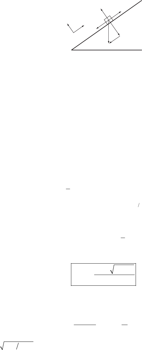
60 CHAPTER 2
yxF
f
NT
θ
2mg
2mg cos θ
2mg sin θ
The y equation of motion gives
2cosNmg my0
θ
−=
=
or
2cosNmg
θ
=
The x equation of motion gives
(
)
2cos
fk k
FNmg
µ
µθ
==
2sin 2 cos
k
Tmg mg ma
θ
µθ
−− = (2)
Substituting from (1) into (2)
2sin 2 cos 2
k
mg mg mg ma
θ
µθ
−− =
When 0
θ
θ
=, a = 0. So
00
2sin 2 cos 0
k
gg g
θ
µθ
−− =
()
00
12
2
00
1sin cos
2
sin 1 sin
k
k
θµ θ
θµ θ
=+
=+−
Isolating the square root, squaring both sides and rearranging gives
()
22 2
00
1
1sin sin
4
kk
µθθµ
+−−
0
=
Using the quadratic formula gives
()
2
02
134
sin 21
kk
k
µ
µ
θµ
±+
=+
2-33. The differential equation to solve is
2
2
1
2
W
t
cAv v
ygg
mv
ρ
=
−= −
(1)
where 2
t
gc
w
Avm
ρ
= is the terminal velocity. The initial conditions are , and
. The computer integrations for parts (a), (b), and (c) are shown in the figure.
0100 my=
00v=
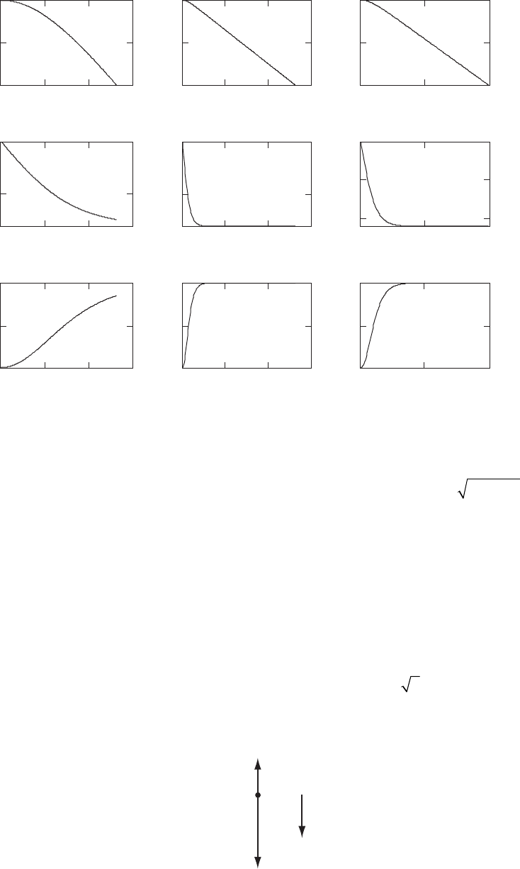
NEWTONIAN MECHANICS—SINGLE PARTICLE 61
05
0
50
100
10
t (s)
05
–10
–5
0
10
t (s)
05
–5
0
10
t (s)
0246
0
50
100
t (s)
y (m)
0246
–20
0
t (s)
v (m/s)
0246
–5
0
t (s)
a (m/s
2
)
0 5 10 15
0
50
100
t (s)
0 5 10 15
–5
0
t (s)
0 5 10 15
–5
0
t (s)
d) Taking as the density of air, the terminal velocities are 32.2, 8.0, and 11.0 (all
) for the baseball, ping-pong ball, and raindrop, respectively. Both the ping-pong ball and
the raindrop essentially reach their terminal velocities by the time they hit the ground. If we
rewrite the mass as average density times volume, then we find that
3
13 kg m
ρ
−
=. ⋅
-1
ms⋅
tmaterial
vR
ρ
∝. The
differences in terminal velocities of the three objects can be explained in terms of their densities
and sizes.
e) Our differential equation shows that the effect of air resistance is an acceleration that is
inversely proportional to the square of the terminal velocity. Since the baseball has a higher
terminal velocity than the ping-pong ball, the magnitude of its deceleration is smaller for a
given speed. If a person throws the two objects with the same initial velocity, the baseball goes
farther because it has less drag.
f) We have shown in part (d) that the terminal velocity of a raindrop of radius 0.004 m will be
larger than for one with radius 0.002 m ( -1
90 m s
.
⋅) by a factor of 2.
2-34.
FR
y
mg
Take the y-axis to be positive downwards. The initial conditions are 0yy
=
=
at t = 0.
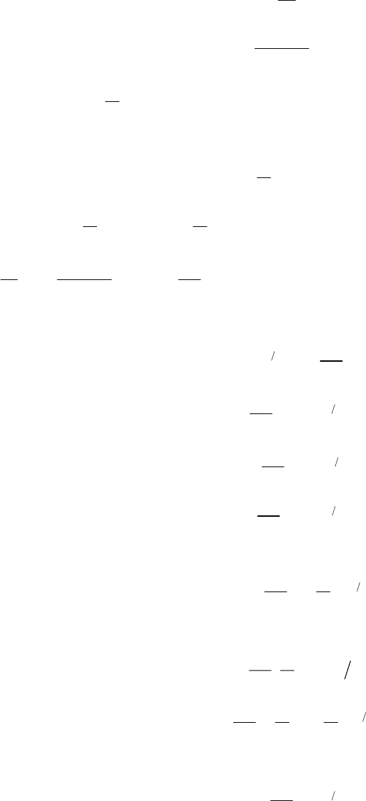
62 CHAPTER 2
a) R
F
v
α
=
The equation of motion is
dv
my m mg v
dt
α
==−
mdv dt
mg v
α
=
−
Integrating gives:
()
ln
mmg v t C
α
α
−−=+
Evaluate C using the condition v = 0 at t = 0:
()
ln
mmg C
α
−
=
So
()()
ln ln
mm
mg v mg t
α
αα
−−+ =
or ln ln 1
mg v
tv
mmg
α
αα
−= −
mg
−=
Take the exponential of both sides and solve for v:
1
rm v
emg
α
α
−=−
1tm
ve
mg
α
α
−
=−
(
1tm
mg
ve
α
α
−
=−
)
(1)
()
1tm
mg
dy e dt
α
α
−
=−
Integrate again:
tm
mg m
yC t e
α
αα
−
+= +
y = 0 at t = 0, so:
22
mg m
Cmg
α
αα
==
tm
mg mm
yte
α
αα α
−
=−++
(2)
Solve (3) for t and substitute into (4):
1tm
ve
mg
α
α
−
−= (3)
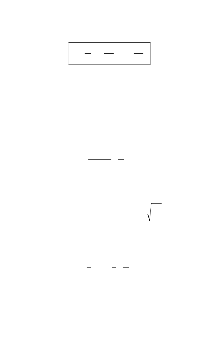
NEWTONIAN MECHANICS—SINGLE PARTICLE 63
ln 1
mv
tmg
α
α
=− −
ln 1 1 ln 1
mg mg
mm v m v vm v
ymg mg g mg
αα
ααα α α α
=−− −+− =−− −
α
(4)
ln 1
mg
mv
yv mg
α
αα
=− + −
b) 2
R
Fv
β
=
The equation of motion becomes:
2
dv
mmg
dt v
β
=−
2
mdv dt
mg v
β
=
−
Integrate and apply the initial condition v = 0 at t = 0:
2
dv dt
mg m
v
β
β
=
−
∫
∫
From integral tables 1
22
1tanh
dx x
ax a a
−
=
−
∫; so
1
1tanh vtC
aam
β
−
=
+ where mg
a
β
≡
1
1tanh000C
α
−
=
=+
so:
1
1tanh vt
aam
β
−=
Solving for v:
tanh at
va m
β
= (5)
tanh
dy at
a
dt m
β
=
From integral tables
tanh ln cosh
udu u=
∫
So ln cosh
ma
yC m
t
β
β
+=
64 CHAPTER 2
Apply the conditions at y = 0 and t = 0
()
ln cosh 0 ln 1 0
mm
C
ββ
=
==
So
ln cosh
ma
ym
t
β
β
= (6)
Solving (5) for t:
1
tanh
mv
ta
αβ
−
=
Substituting into (6):
1
ln cosh tanh
mv
ya
β
−
=
Use the identity: 11
2
1
tanh cosh 1
uu
−−
=−, where 1u
<
.
(In our case 1u< as it should be because
2
vv
amg
β
=; and the condition that 1u< just says that
gravity is stronger than the retarding force, which it must be.) So
()
12
12
2
1
ln cosh cosh ln 1
1
mm
vmg
β
ββ
β
−
−
==
−
yv
mg
−
()
2
ln 1
2
m
yv
β
β
=− − mg
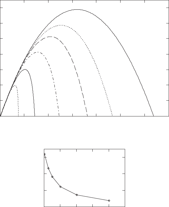
NEWTONIAN MECHANICS—SINGLE PARTICLE 65
2-35.
0 5 10 15 20 25 30 35
0
2
4
6
8
10
12
14
x (km)
y (km)
0 0.02 0.04 0.06 0.08
0
10
20
30
k (1/s)
Range (km)
We are asked to solve Equations (2.41) and (2.42), for the values k = 0, 0.005, 0.01, 0.02, 0.04, and
0.08 (all in ), with initial speed v
1
s−1
0600 m s
−
=
⋅ and angle of elevation 60
θ
=°. The first figure
is produced by numerical solution of the differential equations, and agrees closely with Figure
2-8. Figure 2-9 can be most closely reproduced by finding the range for our values of k, and
plotting them vs. k. A smooth curve could be drawn, or more ranges could be calculated with
more values of k to fill in the plot, but we chose here to just connect the points with straight
lines.
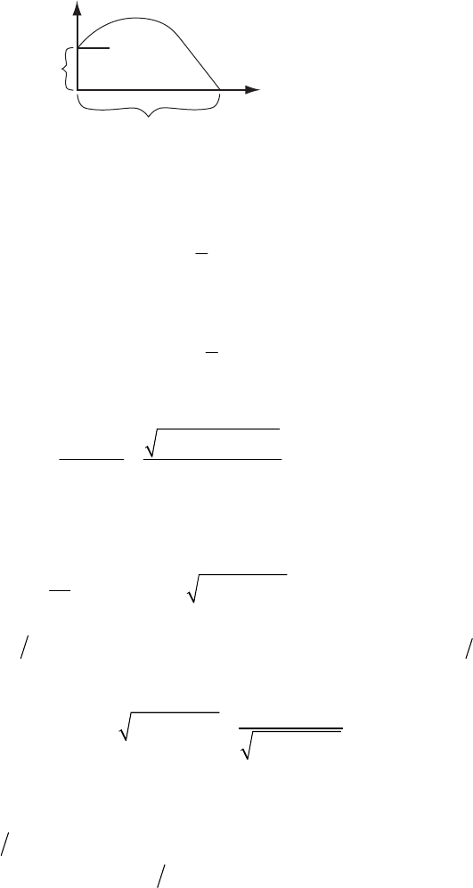
66 CHAPTER 2
2-36.
θ
h
y
x
R
Put the origin at the initial point. The equations for the x and y motion are then
(
)
0cosxv t
θ
=
()
2
0
1
sin 2
yv t gt
θ
=−
Call
τ
the time when the projectile lands on the valley floor. The y equation then gives
()
2
0
1
sin 2
hv g
θ
ττ
−= −
Using the quadratic formula, we may find
τ
22
0
0sin 2
sin vg
v
gg
θ
θ
τ
+
=+ h
(We take the positive since 0
τ
>.) Substituting
τ
into the x equation gives the range R as a
function of
θ
.
2
2
0cos sin sin
v
R
g
θθ θ
=+
2
x
+ (1)
where we have defined 2
0
2xghv≡2
. To maximize R for a given h and , we set
0
v0dR d
θ
=
. The
equation we obtain is
2
22 22
22
sin cos
os sin sin sin 0
sin
xx
θθ
θθθθ θ
−− ++ +
c (2) =
Although it can give
(
)
xx
θ
=, the above equation cannot be solved to give ( )x
θ
θ
= in terms of
the elementary functions. The optimum
θ
for a given x is plotted in the figure, along with its
respective range in units of 2
0
vg. Note that x = 0, which among other things corresponds to
h = 0, gives the familiar result
θ
= 45° and 2
0
Rvg=.
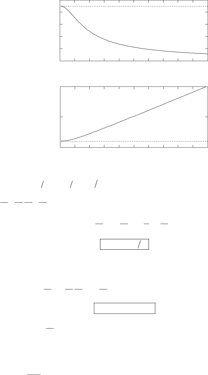
NEWTONIAN MECHANICS—SINGLE PARTICLE 67
0123456789
0
10
20
30
40
50
10
x
θ
0123456789
0
5
10
10
x
R/(v
02
/g)
45˚
1
2-37. vx
α
= 2
dv dx x
α
=−
Since dv dv dx dv v
dt dx dt dx
== then
2
dv dv
Fm mv m
dt dx x x
α
α
== = −
()
23
F
xmx
α
=−
2-38.
(
)
n
vx ax
−
=
a)
()()
1nn
dv dv dx dv
Fm m mv max nax
dt dx dt dx
−−
== = = −
−
()
()
21
2n
Fx mna x
−+
=−
b)
()
n
dx
vx ax
dt
−
==
n
xdx adt=
Integrate:
1
1
n
xat C
n
+
=+
+ C = 0 using given initial conditions
68 CHAPTER 2
(
)
11
n
xn
+=+ at
()
[]
()
11
1n
xn at
+
=+
c) Substitute x(t) into F(x):
() ( )
{}
()
(
)
21
11
21
n
n
Ft mna n at
−
+
+
=− +
() ( )
[]
()()
21 1
21nn
Ft mna n at−+ +
=− +
2-39.
a) v
Fe
β
α
=−
v
dv e
dt m
β
α
=−
v
edv d
m
β
t
α
−=−
∫
∫
1v
et
m
β
C
α
β
−
−
=− +
0
vv= at t = 0, so
0
1v
eC
β
β
−
−
=
()
0
1v
v
ee m
β
β
t
α
β
−
−
−−=−
Solving for v gives
()
0
1ln v
t
vt e
m
β
αβ
β
−
=− +
b) Solve for t when v = 0
01
v
te
m
β
α
β
−
+
=
0
1v
m
te
β
αβ
−
=−
c) From a) we have
0
1ln v
t
dx e dt
m
β
αβ
β
−
=− +
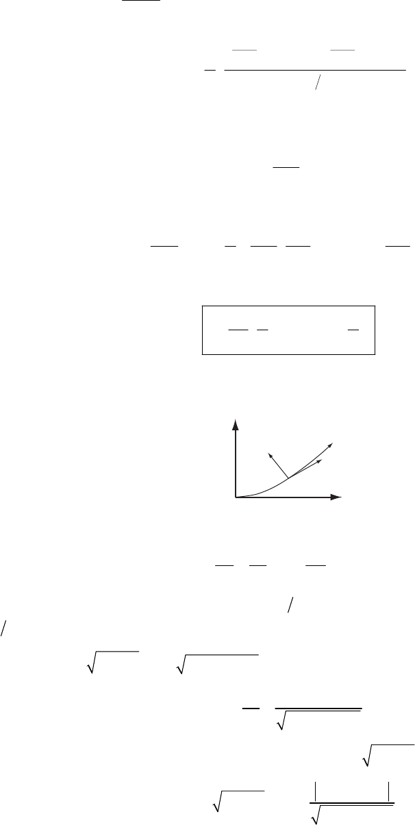
NEWTONIAN MECHANICS—SINGLE PARTICLE 69
Using
() ()
ln ln
ax b
ax b dx ax b x
a
+
+= +−
∫ we obtain
00
ln
1
vv
tt
ee
mm
t
m
ββ
αβ αβ
βαβ
−−
xC
++
+=− −
Evaluating C using x = 0 at t = 0 gives
0
0v
vm
Ce
β
αβ
−
=
So
00
0
2ln
vv
mv tm t t
e e
mm
ββ
αβ αβ
αβ β αβ
−−
0
v
β
−
xe
=− + − + +
Substituting the time required to stop from b) gives the distance required to stop
00
11
v
m
xev
β
α
ββ β
−
=− +
2-40.
y
anat
(x(t),y(t))
x
Write the velocity as v(t) = v(t)T(t). It follows that
()
tn
ddv d
tva
dt dt dt
==+=+
vT
aTT
a
N
(1)
where N is the unit vector in the direction of ddTt. That N is normal to T follows from
(
)
0ddt=⋅TT. Note also is positive definite.
n
a
a) We have 2
254cos
y
vA
xt
α
α
=+= −
. Computing from the above equation,
2
2sin
54cos
t
A
t
dv
adt t
α
α
α
==− (2)
We can get from knowing a in addition to . Using
n
at
a22
2y
aA
x
α
=+=
, we get
22 2
2cos 1
54cos
nt
t
aaaA t
α
α
α
−
=−= − (3)
b) Graphing versus t shows that it has maxima at
n
atn
α
π
=
, where 2
n
aA
α
=.
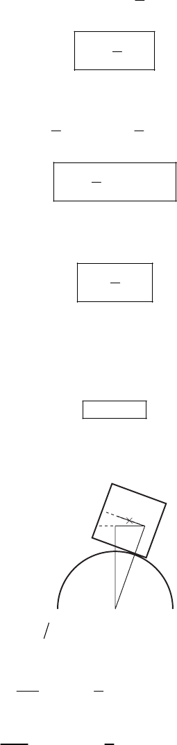
70 CHAPTER 2
2-41.
a) As measured on the train:
0
i
T
=
; 2
1
2
f=Tm v
2
1
2
Tmv∆=
b) As measured on the ground:
2
1
2
i
Tm=u;
()
2
1
2
f
Tmvu=+
2
1
2
Tmvmv∆= + u
c) The woman does an amount of work equal to the kinetic energy gain of the ball as
measured in her frame.
2
1
2
Wmv=
d) The train does work in order to keep moving at a constant speed u. (If the train did no
work, its speed after the woman threw the ball would be slightly less than u, and the speed of
the ball relative to the ground would not be u + v.) The term mvu is the work that must be
supplied by the train.
Wmvu=
2-42.
Rθ
θ
θ
b
R
From the figure, we have () ( 2)cos sinhRb R
θ
θθ
=+ +
θ
, and the potential is Um( ) ( )gh
θ
θ
=.
Now compute:
sin cos
2
dU b
mg R
d
θ
θθ
θ
=− +
(1)
2
2cos sin
2
dU b
mg R R
d
θ
θθ
θ
=− −
(2)
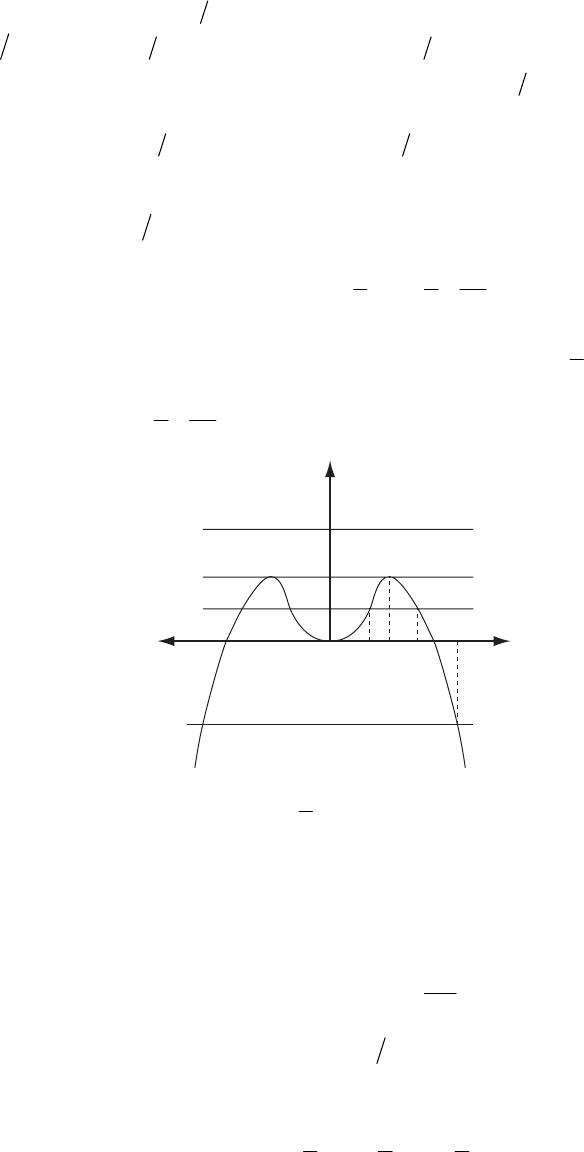
NEWTONIAN MECHANICS—SINGLE PARTICLE 71
The equilibrium point (where 0ddU
θ
=
) that we wish to look at is clearly
θ
= 0. At that point,
we have
(
)
22 2dU d mg R b
θ
=−, which is stable for 2>Rb and unstable for Rb. We can
use the results of Problem 2-46 to obtain stability for the case
2</
2Rb
=
, where we will find that
the first non-trivial result is in fourth order and is negative. We therefore have an equilibrium at
θ
= 0 which is stable for 2Rb> and unstable for 2Rb
≤
.
2-43. 32
Fkxkx
α
=− +
()
4
2
2
11
24
x
Ux Fdx kx k
α
=− = −
∫
To sketch U(x), we note that for small x, U(x) behaves like the parabola 2
1
2kx . For large x, the
behavior is determined by
4
2
1
4
x
k
α
−
U(x)
E
0
E
1
E
2
E
3
= 0
E
4
x
1
x
2
x
3
x
4
x
5
x
()
2
1
2
EmvUx=+
For E, the motion is unbounded; the particle may be anywhere.
0
E=
For E (at the maxima in U(x)) the particle is at a point of unstable equilibrium. It may
remain at rest where it is, but if perturbed slightly, it will move away from the equilibrium.
1
E=
What is the value of ? We find the x values by setting
1
E0
dU
dx
=
.
32
0kx kx
α
=−
x = 0, ±
α
are the equilibrium points
()
22
1
111
244
UEkkk
2
α
αα
±== − =
α
For E, the particle is either bounded and oscillates between
2
E=2
x
−
and ; or the particle
comes in from ±∞ to ± and returns to ±∞.
2
x
3
x
72 CHAPTER 2
For E, the particle is either at the stable equilibrium point x = 0, or beyond .
30=4
xx=±
For E, the particle comes in from ±∞ to
4 5
x
±
and returns.
2-44.
m
1
T
m
1
g
m
2
TT
m
2
g
θ
From the figure, the forces acting on the masses give the equations of motion
1
11
mmg
xT
=
−
(1)
2
22
2cosmmgT
x
θ
=
−
(2)
where is related to by the relation
2
x1
x
()
2
12
24
bx
x
−d
=
− (3)
and
(
)
1
cos 2dbx
θ
=−
. At equilibrium, 12
0
xx
=
=
and Tm
1g
=
. This gives as the equilibrium
values for the coordinates
1
10 2
12
4
4
md
xb mm
=− −2
(4)
2
20 2
12
4
md
xmm
=−2
(5)
We recognize that our expression is identical to Equation (2.105), and has the same
requirement that
10
x
21
2mm< for the equilibrium to exist. When the system is in motion, the
descriptive equations are obtained from the force laws:
(
)
21
1
1
2
() (
4
mbx
mg
x
x
−
2
)g
x
−
=
−
0
(6)
To examine stability, let us expand the coordinates about their equilibrium values and look at
their behavior for small displacements. Let 111
xx
ξ
≡
− and 222
xx
0
ξ
≡
−. In the calculations,
take terms in 1
ξ
and 2
ξ
, and their time derivatives, only up to first order. Equation (3) then
becomes 212
(mm 1
)
ξ
ξ
−. When written in terms of these new coordinates, the equation of
motion becomes
(
)
()
32
22
12
1
1
12 1 2
4
4
gm m
mm m m d
ξ
ξ
−
=− +
(7)
NEWTONIAN MECHANICS—SINGLE PARTICLE 73
which is the equation for simple harmonic motion. The equilibrium is therefore stable, when it
exists.
2-45. and 2-46. Expand the potential about the equilibrium point
()
10
1
!
i
i
i
in
du
Ux x
idx
∞
=+
=
∑ (1)
The leading term in the force is then
(1)
(1)
0
1
()
n
n
n
dU d U
Fx x
dx n dx
+
+
=− =−
!
(2)
The force is restoring for a stable point, so we need
(
)
0Fx><0 and
(
)
0Fx 0
<
>. This is never
true when n is even (e.g., Uk), and is only true for odd when
3
x=n(1) (nn
dUdx
+1)
00
+
<.
2-47. We are given
(
)
0
() U ax xa=+Ux for . Equilibrium points are defined by 0x>
0dU dx =, with stability determined by 2
dU 2
dx at those points. Here we have
02
1dU a
U
dx x a
=−+
(1)
which vanishes at x = a. Now evaluate
20
3
2
20
a
U
dU
a
dx
=
>
(2)
indicating that the equilibrium point is stable.
0 0.5 1 1.5 2
0
5
10
15
20
25
x/a
U(x)/U
0
74 CHAPTER 2
2-48. In the equilibrium, the gravitational force and the eccentric force acting on each star
must be equal
32
22
2
2
/2 2
Gm mv mG d d
v
dd d v mG
ππ
τ
=⇒= ⇒==
2-49. The distances from stars to the center of mass of the system are respectively
2
1
12
dm
rmm
=+ and 1
2
12
dm
rmm
=+
At equilibrium, like in previous problem, we have
32
22
12 11 2 1
1
2
1121
12
22
() ()
m m v Gm r d
v
dr dmm v
Gm m
ππ
τ
=⇒= ⇒==
++
Gm
The result will be the same if we consider the equilibrium of forces acting on 2nd star.
2-50.
a) 000
222
02
0
222
()
111
t
mv mv mv
dF
Fd Ftvt
dt vvv
m
ccc
=⇒ = = ⇒ =
−−−
∫22
2
t
Ft
c
+
222
2
00
2
0
() ()
tcFt
xt vtdt m m
Fc
= + −
∫
⇒=
b)
t
v
c) From a) we find
0
2
2
1
vm
tv
Fc
=
−
Now if
0
10
F
m=, then
NEWTONIAN MECHANICS—SINGLE PARTICLE 75
when 2=vc, we have 0.55 year
10 3
c
t==
when v = 99% c, we have 99 6.67 years
10 199
c
==t
2-51.
a) 20
2
0
() mv
dv dv b
mbv dtvt
dt v m btv m
=− ⇒ =− ⇒ =
+
∫∫
Now let v(t) = v0/1000 , one finds
0
999 138.7 hours
m
tvb
== .
t
v
b) 0
0
() ln
tbtv m
m
x t vdt bm
+
==
∫
We use the value of t found in question a) to find the corresponding distance
( ) ln(1000) 6.9 km
m
xt b
==
2-52.
a)
2
0
22
4
() 1
Ux
dU x
Fx dx a a
=− =− −
b)
x
U
When F = 0, there is equilibrium; further when U has a local minimum (i.e. 0dF dx <) it is
stable, and when U has a local maximum (i.e. 0dF dx >) it is unstable.
76 CHAPTER 2
So one can see that in this problem x = a and x = –a are unstable equilibrium positions, and x = 0
is a stable equilibrium position.
c) Around the origin, 00
22
44Ux U
k
Fkx
am
ω
≈− ≡− ⇒ = = ma
d) To escape to infinity from x = 0, the particle needs to get at least to the peak of the potential,
2
0
min
max 0 min
2
2
U
mv UUv m
==⇒=
e) From energy conservation, we have
2222
00
min
22
21
22
Ux U
mv dx x
v
adtm
+= ⇒== −
mv
a
We note that, in the ideal case, because the initial velocity is the escape velocity found in d),
ideally x is always smaller or equal to a, then from the above expression,
0
2
2
2
00
00
22
8
exp 1
ln ( )
28 8
1exp 1
x
U
at
ma
mdx maax
t
UUax
xU
t
ama
−
+
==⇒=
−
−
+
∫
tx
t
x
2-53.
F is a conservative force when there exists a non-singular potential function U(x) satisfying
F(x) = –grad(U(x)). So if F is conservative, its components satisfy the following relations
y
x
F
F
yx
∂
∂=
∂
∂
and so on.
a) In this case all relations above are satisfied, so F is indeed a conservative force.
2
1(,)
2
x
Ubx
ayz bx c U ayzx cx f y z
x
∂= + + ⇒ =− − − +
∂
F=− (1)
where is a function of only y and z
1(,)fyz
2(,)
y
Uaxz bz U ayzx byz f x z
y
∂= + ⇒ =− − +
∂
F=− (2)
NEWTONIAN MECHANICS—SINGLE PARTICLE 77
where is a function of only x and z
2(,)fxz
3(,)
Uaxy by c U ayzx byz f y z
z
F
z
∂= + + ⇒ =− − +
∂
=− (3)
then from (1), (2), (3) we find that
2
2
2
bx
U axyz byz cx C=− − − − +
where C is a arbitrary constant.
b) Using the same method we find that F in this case is a conservative force, and its potential
is
exp( ) lnUz xyzC
=
−−−+
c) Using the same method we find that F in this case is a conservative force, and its potential
is ( using the result of problem 1-31b):
lnUar
=
−
2-54.
a) Terminal velocity means final steady velocity (here we assume that the potato reaches this
velocity before the impact with the Earth) when the total force acting on the potato is zero.
mg = kmv and consequently 1000 m/skvg
=
=.
b)
0
0
0
()
x
v
F dx dv vdv
gkv dt dx
dt m v g kv g kv
−+ ⇒ ==− ⇒ =− ⇒
++
∫∫
dv ==
0
max 2
0
ln 679.7 m
gg
v
xkk gkv
=+ =
+ where v is the initial velocity of the potato.
0
2-55. Let’s denote and
0x
v0
y
v the initial horizontal and vertical velocity of the pumpkin.
Evidently, 0x0
y
vv= in this problem.
0xx
f
xx
xx f
xx
vv
dv dv
dx
mkv dt x
dt v kv k
mF
−
==− ⇒− =−= ⇒= (1)
where the suffix f always denote the final value. From the second equality of (1), we have
0
f
kt
x
xf x
x
dv
dt v v e
kv
−
−= ⇒ = (2)
Combining (1) and (2) we have
(
01f
kt
x
f
v
x
k
−
=−
)
e (3)
78 CHAPTER 2
Do the same thing with the y-component, and we have
0
2
0
0ln
yyyfyyf
yy f
yy y
dv dv g kv v v
dy g
m F mg mkv dt y
dt v g kv k g kv k
+
−
==− − ⇒− =−= ⇒== +
++
(4)
and
()
0
f
kt
y
yf f
y
dv
dt g kv g kv e
gkv
−
⇒+ = +
+
−= (5)
From (4) and (5) with a little manipulation, we obtain
0
1f
kt f
y
gkt
egkv
−
−=
+ (6)
(3) and (6) are 2 equations with 2 unknowns,
f
t and k. We can eliminate
f
t, and obtain an
equation of single variable k.
()
()
(
)
00
01fyx
kt g kv gv
x
f
v
xe
k
−+
=−
Putting and
142 m
f
x=0
00 38.2 m/s
2
xy
v
===vv we can numerically solve for k and obtain
K= 0.00246 1
s
−
.
CHAPTER 3
Oscillations
3-1.
a)
421
02
gram cm
10 dyne/cm
11 10 10
sec cm sec
2210 gram2gram2
k
m
ππ π π
−
⋅
⋅
= =
ν
==
or,
01.6 Hz
ν
≅ (1)
0
0
12
sec
10
π
τν
==
or,
00.63 sec
τ
≅ (2)
b) 242
11
10 3 dyne-cm
22
EkA==××
so that
4
4.5 10 ergE=× (3)
c) The maximum velocity is attained when the total energy of the oscillator is equal to the
kinetic energy. Therefore,
24
max
4
max
14.5 10 erg
2
24.510
v100
mv =×
××
=
79
80 CHAPTER 3
or,
max 30 cm/secv= (4)
3-2.
a) The statement that at a certain time 1
tt
=
the maximum amplitude has decreased to one-
half the initial value means that
1
0
1
2
t
en
xAe A
β
−
==
0
(1)
or,
11
2
t
e
β
−
=
(2)
so that
11
ln 2 0.69
tt
β
== (3)
Since ,
110 sect=
2
6.9 10 sec
β
1
−
−
=× (4)
b) According to Eq. (3.38), the angular frequency is
2
10
2
ω
ωβ
=− (5)
where, from Problem 3-1, 1
010 sec
ω
−
=. Therefore,
()
()
()
2
22
1
261
10 6.9 10
1
10 1 6.9 10 sec
2
ω
−
−
−
=−×
≅− ×
(6)
so that
5
1
10 (1 2 40 10 ) sec
2
νπ
1
−
−
=−.× (7)
which can be written as
(
)
10
1
ν
νδ
=
− (8)
where
5
2.40 10
δ
−
=× (9)
That is, 1
ν
is only slightly different from 0
ν
.
OSCILLATIONS 81
c) The decrement of the motion is defined to be e1
β
τ
where 1
11
τ
ν
=
. Then,
11.0445e
βτ
3-3. The initial kinetic energy (equal to the total energy) of the oscillator is 2
0
1
2mv , where
m = 100 g and v.
01 cm/sec=
a) Maximum displacement is achieved when the total energy is equal to the potential energy.
Therefore,
22
00
11
22
mv kx
=
2
00
4
10 1
1 c
10 10
m
xv
k
==×=m
or,
0
1cm
10
x= (1)
b) The maximum potential energy is
24
max 0
11
10 10
22
Ukx 2
−
==××
or,
max 50 ergsU= (2)
3-4.
a) Time average:
The position and velocity for a simple harmonic oscillator are given by
0
sinxA t
ω
=
(1)
0
cosxA 0
t
ω
ω
=
(2)
where 0km
ω
=
The time average of the kinetic energy is
2
11
2
t
t
Tmx
τ
τ
+
=∫dt
(3)
where
0
2
π
τ
ω
= is the period of oscillation.
82 CHAPTER 3
By inserting (2) into (3), we obtain
22 2
0
1cos
2
t
t
TmA t
τ
ωω
τ
+
=∫0
dt (4)
or,
22
0
4
mA
T
ω
= (5)
In the same way, the time average of the potential energy is
2
22
0
2
11
2
1sin
2
4
t
t
t
t
Ukxdt
kA t dt
kA
τ
τ
τ
ω
τ
+
+
=
=
=
∫
∫
(6)
and since 2
0km
ω
=, (6) reduces to
22
0
4
mA
U
ω
= (7)
From (5) and (7) we see that
TU= (8)
The result stated in (8) is reasonable to expect from the conservation of the total energy.
ETU
=
+ (9)
This equality is valid instantaneously, as well as in the average. On the other hand, when T and
U are expressed by (1) and (2), we notice that they are described by exactly the same function,
displaced by a time 2
τ
:
22
2
0
0
2
2
0
0
cos
2
sin
2
mA
Tt
mA t
Ut
ωω
ωω
=
=
(10)
Therefore, the time averages of T and U must be equal. Then, by taking time average of (9), we
find
2
E
TU
=
= (11)
b) Space average:
The space averages of the kinetic and potential energies are
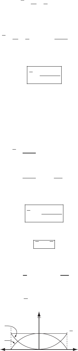
OSCILLATIONS 83
2
0
11
2
A
Tmx
A
=∫dx (12)
and
2
2
0
00
11
22
AA
m
Ukxdxx
AA
ω
==
∫2
dx
∫
(13)
(13) is readily integrated to give
22
0
6
mA
U
ω
= (14)
To integrate (12), we notice that from (1) and (2) we can write
(
)
()
2222 22 2
000
22 2
0
cos 1 sinxA tA
Ax
0
t
ω
ωω ω
ω
==−
=−
(15)
Then, substituting (15) into (12), we find
2
22
0
0
23
3
0
2
23
A
m
TAx
A
mA
A
A
ω
ω
dx
=−
=−
∫
(16)
or,
22
0
26
mA
T
ω
= (17)
From the comparison of (14) and (17), we see that
2TU= (18)
To see that this result is reasonable, we plot T = T(x) and U = U(x):
2
22
02
22
0
11
2
1
2
x
TmA A
Umx
ω
ω
=−
=
(19)
U = U(x)
T = T(x)
A
Energy
–AO x
mA2
0
2
ω
EmA==const. 1
2
2
0
2
ω
And the area between T(x) and the x-axis is just twice that between U(x) and the x-axis.
84 CHAPTER 3
3-5. Differentiating the equation of motion for a simple harmonic oscillator,
0
sinxA t
ω
=
(1)
we obtain
00
cosxA tt
ω
ω
∆
=∆ (2)
But from (1)
0
sin x
t
A
ω
=
(3)
Therefore,
()
2
0
cos 1tx
ω
=−A (4)
and substitution into (2) yields
22
0
x
t
A
x
ω
∆
∆= − (5)
Then, the fraction of a complete period that a simple harmonic oscillator spends within a small
interval ∆x at position x is given by
22 22
02
tx x
A
xA
τωτ π
∆∆ ∆
==
−−x
(6)
–A
1
–A
2
–A
3
A
3
A
2
A
1
∆t⁄τ
x
This result implies that the harmonic oscillator spends most of its time near x = ±A, which is
obviously true. On the other hand, we obtain a singularity for t
τ
∆
at x = ±A. This occurs
because at these points x = 0, and (2) is not valid.
3-6.
x
1
x
2
k
x
m1m2
Suppose the coordinates of m and are and x and the length of the spring at
equilibrium is . Then the equations of motion for m and are
1 2
m1
x2
1
2
m
(
)
11 1 2
mx k x x
=
−−+
(1)
(
)
22 2 1
mx k x x
=
−−+
(2)
OSCILLATIONS 85
From (2), we have
(
1222
1
xmxkxk
k
=+−
)
(3)
Substituting this expression into (1), we find
()
2
122 1 2 2
20
dmmx m m kx
dt
+
+
=
(4)
from which
12
2
12
mm
x
mm 2
kx
+
=−
(5)
Therefore, oscillates with the frequency
2
x
12
12
mm
k
mm
ω
+
= (6)
We obtain the same result for . If we notice that the reduced mass of the system is defined as
1
x
12
11 1
mm
µ
=+ (7)
we can rewrite (6) as
k
ω
µ
= (8)
k
µ
This means the system oscillates in the same way as a system consisting of a single mass
µ
.
Inserting the given values, we obtain
µ
66.7 g and 1
2.74 rad s
ω
−
⋅
.
3-7.
A
h
b
h
s
Let A be the cross-sectional area of the floating body, its height, the height of its
submerged part; and let
ρ
and
b
hs
h
0
ρ
denote the mass densities of the body and the fluid,
respectively.
The volume of displaced fluid is therefore Vs
Ah
=
. The mass of the body is b
M
Ah
ρ
=.

86 CHAPTER 3
There are two forces acting on the body: that due to gravity (Mg), and that due to the fluid,
pushing the body up ( 00s
gV gh A
ρ
ρ
−−= ).
The equilibrium situation occurs when the total force vanishes:
0
0
0
b
Mg gV
gAh gh A
s
ρ
ρρ
=
−
=− (1)
which gives the relation between and :
s
hb
h
0
sb
hh
ρ
ρ
= (2)
For a small displacement about the equilibrium position ( ), (1) becomes
ss
hh→+x
(
)
0bbs
M
xAhxgAh ghx
ρρρ
==−+
A (3)
Upon substitution of (1) into (3), we have
0b
A
h x gxA
ρ
ρ
=
−
(4)
or,
00
b
xg x
h
ρ
ρ
+
=
(5)
Thus, the motion is oscillatory, with an angular frequency
20
bs
ggA
ghh V
ρ
ωρ
=== (6)
where use has been made of (2), and in the last step we have multiplied and divided by A. The
period of the oscillations is, therefore,
22V
gA
π
τπ
ω
== (7)
Substituting the given values, 018 s
τ
..
3-8.
y
Om
s
2a
2a
x
The force responsible for the motion of the pendulum bob is the component of the gravitational
force on m that acts perpendicular to the straight portion of the suspension string. This
component is seen, from the figure (a) below, to be
cos
F
ma mv mg
α
=
==−
(1)
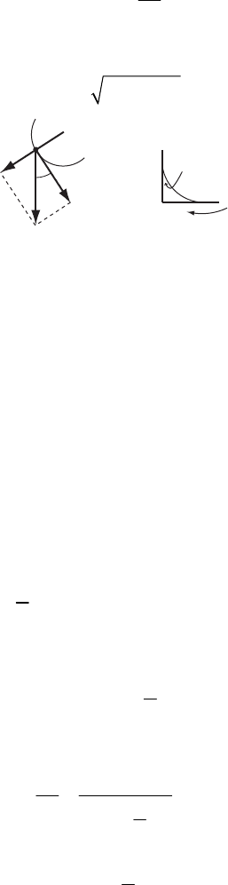
OSCILLATIONS 87
where
α
is the angle between the vertical and the tangent to the cycloidal path at the position of
m. The cosine of
α
is expressed in terms of the differentials shown in the figure (b) as
cos dy
ds
α
= (2)
where
2
ds dx dy=+
2
(3)
α
α
m
mg
Fdx
dy
S
ds
(a) (b)
The differentials, dx and dy, can be computed from the defining equations for x(
φ
) and y(
φ
)
above:
(
)
1cos
sin
dx a d
dy a d
φ
φ
φφ
=−
=−
(4)
Therefore,
() ()
222
2
2222
22 2
1cos sin 2 1cos
in
2
ds dx dy
ada
ad
2
d
4s
φ
φφ φφ
φφ
=+
=− + =−
= (5)
so that
2sin
2
ds a d
φ
φ
= (6)
Thus,
sin
2sin
2
cos cos
2
dy a d
ds ad
φ
φ
φφ
φ
α
−
=
=− = (7)
The velocity of the pendulum bob is
88 CHAPTER 3
2sin
2
4cos
2
ds d
va
dt dt
d
adt
φ
φ
φ
==
=−
(8)
from which
2
2
4cos
2
d
va
dt
φ
=−
(9)
Letting cos 2
z
φ
≡ be the new variable, and substituting (7) and (9) into (1), we have
4maz mgz
−
=
(10)
or,
0
4
g
zz
a
+
=
(11)
which is the standard equation for simple harmonic motion,
2
00zz
ω
+
=
(12)
If we identify
0
g
ω
= (13)
where we have used the fact that .
4a=
Thus, the motion is exactly isochronous, independent of the amplitude of the oscillations. This
fact was discovered by Christian Huygene (1673).
3-9. The equation of motion for 0
0tt
≤
≤ is
(
)
(
)
0
mx k x x F kx F kx=− − + =− + +
0
(1)
while for , the equation is
0
tt≥
(
)
0
mx k x x kx kx=−−=−+
0
(2)
It is convenient to define
0
xx
ξ
=
−
which transforms (1) and (2) into
mk
ξξ
F
=
−+
; 0
0tt
≤
≤ (3)
mk
ξ
ξ
=
−
; (4)
0
tt≥
OSCILLATIONS 89
The homogeneous solutions for both (3) and (4) are of familiar form
(
)
it it
tAe Be
ω
ω
ξ
−
=+ , where
km
ω
=. A particular solution for (3) is
F
k
ξ
=
. Then the general solutions for (3) and (4) are
it it
F
A
eBe
k
ω
ω
ξ
−
−=+ + ; 0
0tt
≤
≤ (5)
it it
Ce De
ω
ω
ξ
−
+=+ ; t (6)
0
t≥
To determine the constants, we use the initial conditions:
(
)
0
0xt x
=
= and x(t = 0) = 0. Thus,
(
)
(
)
00tt
ξξ
−−
0
=
===
(7)
The conditions give two equations for A and B:
()
0
0
F
A
B
k
iAB
ω
=++
=−
(8)
Then
2
F
AB k
==−
and, from (5), we have
()
01cos
F
xx t
k
ξ
ω
−=− = − ; 0
0tt
≤
≤ (9)
Since for any physical motion, x and must be continuous, the values of
x
(
)
0
tt
ξ
−= and
(
)
0
tt
ξ
−=
are the initial conditions for
(
)
t
ξ
+ which are needed to determine C and D:
()
()
()
00
00
00
00
1cos
sin
it it
it it
F
tt t Ce De
k
F
tt t i Ce De
k
ωω
ωω
ξω
ξωωω
−
+
−
+
== − = +
== = −
(10)
The equations in (10) can be rewritten as:
()
00
00
0
0
1cos
sin
it it
it it
F
Ce De t
k
iF
Ce De t
k
ωω
ωω
ω
ω
−
−
+=−
−
−=
(11)
Then, by adding and subtracting one from the other, we obtain
()
()
00
00
1
2
1
2
it it
it it
F
Ce e
k
F
De e
k
ωω
ωω
−
−
=−
=−
(12)
90 CHAPTER 3
Substitution of (12) into (6) yields
()()
() ()
()
00
00
0
11
2
2
cos cos
it it it it
itt itt
it it
Feeee
k
Feee e
k
Ftt t
k
ωωω ω
ωω
ωω
ξ
ωω
−−
+
−−−
−
=−+−
=−+−
=−−
(13)
Thus,
()
00
cos cos ;
Ftt ttt
k
ωω
−= −− ≥
0
xx (14)
3-10. The amplitude of a damped oscillator is expressed by
(
)
(
)
1
cos
t
xt Ae t
β
ω
δ
−
=
+ (1)
Since the amplitude decreases to 1 after n periods, we have e
1
21nT n
π
ββ
ω
=
= (2)
Substituting this relation into the equation connecting 1
ω
and 0
ω
(the frequency of undamped
oscillations), 22
10
2
ω
ωβ
=−, we have
2
22 2
1
01 1 22
1
1
24nn
ω
ωω ω
ππ
=+ = +
(3)
Therefore,
12
1
22
0
1
14n
ω
ωπ
−
=+
(4)
so that
1
22
2
1
18n
ω
ωπ
≅−
3-11. The total energy of a damped oscillator is
() () ()
2
11
22
Et mxt kxt=+
2
(1)
where
(
)
(
)
1
cos
t
xt Ae t
β
ω
δ
−
=
− (2)
(
)
(
)
(
)
111
cos sin
t
Ae t t
β
xt
β
ωδω ωδ
−
=− −− −
(3)
OSCILLATIONS 91
22
10
ω
ωβ
=−, 0
k
m
ω
=
Substituting (2) and (3) into (1), we have
()
()
() ()
()()
2
22 2 22
111
11 1
cos sin
2sin cos
t
A
Et e m k t m t
mt t
β
2
β
ωδ ω ωδ
β
ωωδωδ
−
=+−+
+−
−
−
(4)
Rewriting (4), we find the expression for E(t):
()
() ()
2
22 22 2
10 1
cos 2 sin 2
2
t
mA e t t
β
βωδβωβωδω
−
=−+−
0
−+
Et (5)
Taking the derivative of (5), we find the expression for dE
dt :
()
()
()
2
223
01
222 2
01
0
24cos2
4sin22
t
dE mA et
t
ββω β ω δ
βωβ ω δ βω
−
=−−
−− −−
2
dt (6)
The above formulas for E and dE reproduce the curves shown in Figure 3-7 of the text. To
find the average rate of energy loss for a lightly damped oscillator, let us take
dt
0
β
ω
. This
means that the oscillator has time to complete some number of periods before its amplitude
decreases considerably, i.e. the term 2t
e
β
− does not change much in the time it takes to complete
one period. The cosine and sine terms will average to nearly zero compared to the constant term
in dE dt , and we obtain in this limit
222
0
t
dE mAe
dt
β
βω
−
− (7)
3-12.
mg
mg sin θ
θ
The equation of motion is
sinmmg
θ
θ
−=
(1)
sin
g
θ
θ
=−
(2)
If θ is sufficiently small, we can approximate sin
θ
θ
≅
, and (2) becomes
92 CHAPTER 3
g
θ
θ
=−
(3)
which has the oscillatory solution
(
)
0
cost
0
t
θ
θω
=
(4)
where 0g
ω
= and where 0
θ
is the amplitude. If there is the retarding force 2mg
θ
, the
equation of motion becomes
sin 2mmg mg
θ
θ
−= +
θ
(5)
or setting sin
θ
θ
≅ and rewriting, we have
2
00
2
θωθωθ
0
+
+=
(6)
Comparing this equation with the standard equation for damped motion [Eq. (3.35)],
2
0
2xxx
βω
0
+
+=
(7)
we identify 0
ω
β
=. This is just the case of critical damping, so the solution for
θ
(t) is [see
Eq. (3.43)]
(
)
(
)
0t
tABte
ω
θ
−
=+ (8)
For the initial conditions
(
)
0
0
θ
θ
= and
θ
(0) = 0, we find
()
()
0
00
1t
tt
ω
θθω
−
=+e
3-13. For the case of critical damping, 0
β
ω
=
. Therefore, the equation of motion becomes
2
2xxx
ββ
0
+
+=
(1)
If we assume a solution of the form
(
)
(
)
t
xt yte
β
−
= (2)
we have
2
2
tt
tt
xye ye
xye ye ye
ββ
ββ
β
ββ
−−
−−−
=−
t
β
=− +
(3)
Substituting (3) into (1), we find
ye
(4)
22
222
tttt tt
ye ye ye ye ye
ββββ ββ
ββ β β β
−−−− −−
−++− +
2
0=
0
or,
y
=
(5)
Therefore,
(
)
yt A Bt
=
+ (6)
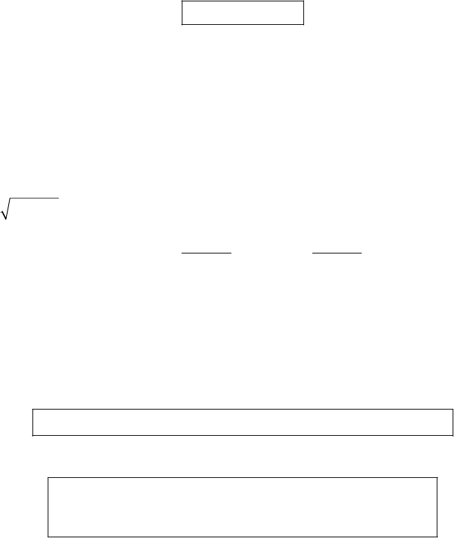
OSCILLATIONS 93
and
() ( )
t
xt A Bte
β
−
=+ (7)
which is just Eq. (3.43).
3-14. For the case of overdamped oscillations, x(t) and
(
)
xt
are expressed by
(
)
2
12
tt
xt e Ae Ae
βω
−−2
t
ω
=+
(1)
()
(
)
(
)
22 2
12 1222
tt t
e Ae Ae A e A e
ωω ω
βω
−−
−+++ −
2
t
ω
ω
−
t
xt
β
(2)
where 2
2
2
0
ω
βω
=−. Hyperbolic functions are defined as
cosh 2
yy
ee
y
−
+
=, sinh 2
yy
ee
y
−
−
= (3)
or,
cosh sinh
cosh sinh
y
y
ey
ey
−
=+
y
y
=−
(4)
Using (4) to rewrite (1) and (2), we have
()
(
)
() ()
12 2 12 2
cosh sinh cosh sinht t A A t A A t
ββ ω ω
xt
=− + +−
(5)
and
()
()
()
()
()
()
12 1 2 2
222 2 2
cosh sinh cosh sinh
cosh sinh
xt t t A A t t
A
At
ββωβω ω
βω ω ω
=− − +
−+ −
t
(6)
3-15. We are asked to simply plot the following equations from Example 3.2:
(
)
(
)
1
cos
t
Ae t
β
xt
ω
δ
−
=− (1)
(
)
(
)
111
() cos sin
t
Ae t t
β
vt
β
ωδω ωδ
−
=− − + −
(2)
with the values A = 1 cm,1
01 rad s
ω
−
=⋅, 1
01 s
β
−
=. , and
δ
=
π
rad. The position goes through
x = 0 a total of 15 times before dropping to 0.01 of its initial amplitude. An exploded (or
zoomed) view of figure (b), shown here as figure (B), is the best for determining this number, as
is easily shown.
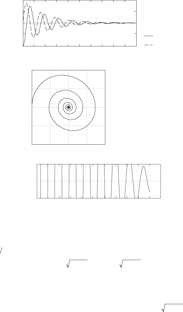
94 CHAPTER 3
–1 –0.5 0 0.5 1
–1
–0.5
0
0.5
1
x (cm)
v (cm/s)
0 5 10 15 20 25 30 35 40 45 50
–1
0
1
0.5
–0.5 x(t) (cm)
v(t) (cm/s)
t (s)
(b)
(c)
0 5 10 15 20 25 30 35 40 45 50 55
0
t (s)
x (cm)
0.01
–0.01
(B)
3-16. If the damping resistance b is negative, the equation of motion is
2
0
2xxx
βω
0
−
+=
(1)
where 2bm0
β
≡− > because b < 0. The general solution is just Eq. (3.40) with
β
changed to –
β
:
()
(
)
(
)
22 22
102
exp exp
t
e A t A t
β
βω βω
=−+−
0
−
xt (2)
From this equation, we see that the motion is not bounded, irrespective of the relative values of
2
β
and 2
0
ω
.
The three cases distinguished in Section 3.5 now become:
a) If 2
0
2
ω
β
>, the motion consists of an oscillatory solution of frequency 22
10
ω
ωβ
=−,
multiplied by an ever-increasing exponential:
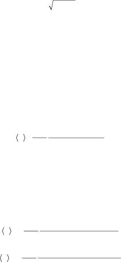
OSCILLATIONS 95
(
)
1
12
tit it
xt e Ae Ae
βω
−1
ω
=+
(3)
b) If 2
0
2
ω
β
=, the solution is
(
)
(
)
t
xt A Bte
β
=+ (4)
which again is ever-increasing.
c) If 2
0
2
ω
β
<, the solution is:
(
)
2
12
tt
xt e Ae Ae
βω
−2
t
ω
=+
(5)
where
22
20
ω
βω β
=
−≤ (6)
This solution also increases continuously with time.
The tree cases describe motions in which the particle is either always moving away from its
initial position, as in cases b) or c), or it is oscillating around its initial position, but with an
amplitude that grows with the time, as in a).
Because b < 0, the medium in which the particle moves continually gives energy to the particle
and the motion grows without bound.
3-17. For a damped, driven oscillator, the equation of motion is
2
0
2cxxxAost
β
ω
=+=
ω
(1)
and the average kinetic energy is expressed as
()
22
2
22 2
0
44
mA
T
ω
2
ω
ωω
=−+
β
(2)
Let the frequency n octaves above 0
ω
be labeled 1
ω
and let the frequency n octaves below 0
ω
be labeled 2
ω
; that is
10
20
2
2
n
n
ω
ω
ω
ω
−
=
= (3)
The average kinetic energy for each case is
()
1
22
2
0
2
222 22
00 0
2
42(4)2
n
nn
mA
ω
ω
2
T
ω
ωω
=−+
β
(4)
()
2
22
2
0
2
222 22
00 0
2
42(4)2
n
nn
mA
ω
ω
2
T
ω
ωω
−
−−
=−+
β
(5)
Multiplying the numerator and denominator of (5) by , we have
4
2n
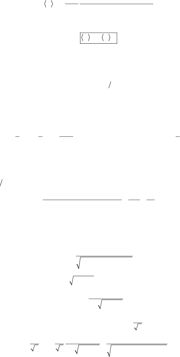
96 CHAPTER 3
()
2
22
2
0
2
222 22
00 0
2
42(4)2
n
nn
mA
ω
ω
2
T
ω
ωω
=−+
β
Hence, we find
1
TT
ω
=2
ω
(6)
and the proposition is proven.
3-18. Since we are near resonance and there is only light damping, we have 0R
ω
ωω
,
where
ω
is the driving frequency. This gives 02Q
ω
β
. To obtain the total energy, we use the
solution to the driven oscillator, neglecting the transients:
(
)
(
)
cosxt D t
ω
δ
=
− (1)
We then have
()
2
22 22 22 2
0
11 1
sin ( ) cos
22 2 2
mD
Emx kx t t mD
ωωδω ωδ ω
=+= −+ −
2
0
(2)
The energy lost over one period is
()
()
2
022
Tmx xdt m D
β
πωβ
⋅=
∫ (3)
where 2T
π
ω
=. Since 0
ω
ω
, we have
0
energy lost over one period 4 2
EQ
ω
π
βπ
(4)
which proves the assertion.
3-19. The amplitude of a damped oscillator is [Eq. (3.59)]
()
2
22 2
04
A
D
2
ω
ωω
=
−+
β
(1)
At the resonance frequency, 2
0
R
2
ω
ωωβ
== −, D becomes
22
0
2
R
A
D
β
ωβ
=− (2)
Let us find the frequency,
ω
=
ω
′, at which the amplitude is 1
2R
D:
()
22 2
22 2
00
11
22
24
R
AA
D
βω β
ω
ωωβ
2
==
−−+
′′
(3)
Solving this equation for
ω
′, we find
OSCILLATIONS 97
12
2
22 2
00
2
0
22 1
β
ωω β βω ω
=− ± −
′
(4)
For a lightly damped oscillator,
β
is small and the terms in 2
β
can be neglected. Therefore,
22
0
20
ω
ωβ
≅±
′
ω
(5)
or,
0
0
1
β
ωω
ω
≅±
′
(6)
which gives
(
)
(
)
00
2
ω
ωβ ωβ
∆= + − − =
β
(7)
We also can approximate R
ω
for a lightly damped oscillator:
22
0
2
R0
ω
ωβω
=−≅ (8)
Therefore, Q for a lightly damped oscillator becomes
00
2
Q
ω
ω
β
ω
≅≅
∆
(9)
3-20. From Eq. (3.66),
()
(
2
22 22
0
sin
4
A
x
)
t
ω
ω
δ
ωω ωβ
−
=
−+
−
(1)
Therfore, the absolute value of the velocity amplitude v is given by
()
02
22 2
04
A
v
2
ω
ω
ωω
=
−+
β
(2)
The value of
ω
for v a maximum, which is labeled
0v
ω
, is obtained from
00
v
v
ωω
ω
=
∂
=
∂ (3)
and the value is 0v
ω
ω
=.
Since the Q of the oscillator is equal to 6, we can use Eqs. (3.63) and (3.64) to express
β
in terms
of 0
ω
:
2
20
146
ω
β
= (4)
We need to find two frequencies, 1
ω
and 2
ω
, for which 0max
2vv=, where
(
)
max 0 0
vv
ω
ω
==.
We find
98 CHAPTER 3
()
max
2
22 2
0
222 4
vAA
2
ω
β
ω
ωω
==
−+
β
(5)
Substituting for
β
in terms of 0
ω
from (4), and by squaring and rearranging terms in (5), we
obtain
()()
2
22 22
01,2 1,20
20
73
ωω ωω
−
−= (6)
from which
22
0 1,2 1,2 0 1,2 0
21
73 6
ω
ωωωω
−=± ≅±
ω
(7)
Solving for 1
ω
, 2
ω
we obtain
0
1,2 0
12
ω
ω
ω
≅
±±
(8)
It is sufficient for our purposes to consider 1
ω
, 2
ω
positive: then
0
10
12
ω
ω
ω
≅
+; 0
2
12 0
ω
ω
ω
≅
−+ (9)
so that
0
12
6
ω
ωω ω
∆= − = (10)
A graph of vs.
ω
for Q = 6 is shown.
0
v
vA
max
=2
β
A
22
βω
0
12
1
6
0
ω
ω
0
12
ω
0
v0
∆
ω
3-21. We want to plot Equation (3.43), and its derivative:
(
)
(
)
t
xt A Bte
β
−
=+ (1)
(
)
(
)
[
]
t
vt B A Bt e
β
β
−
=− + (2)
where A and B can be found in terms of the initial conditions
0
A
x
=
(3)
0
Bv x
0
β
=
+ (4)
OSCILLATIONS 99
The initial conditions used to produce figure (a) were
(
)
(
)
00 24xv
,
=−, , (1 4)
,
, , ( ,
, and , where we take all x to be in cm, all v in cm
(4 1),− 1 4),−
(1 4)−,− ( 4 0)−, 1
s
−
⋅
, and . Figure (b) is a
magnified view of figure (a). The dashed line is the path that all paths go to asymptotically as
t → ∞. This can be found by taking the limits.
1
1 s−
β
=
lim ( ) t
tvt Bte
β
β
−
→∞ =− (5)
lim ( ) t
txt Bte
β
−
→∞ = (6)
so that in this limit, v = –
β
x, as required.
–4 –2 0 2 4
–4
–3
–2
–1
0
1
2
3
4
x (cm)
v (cm/s)
–0.5 –0.25 0 0.25 0.5
–0.4
–0.2
0
0.2
0.4
x (cm)
v (cm/s)
(a)
(b)
3-22. For overdamped motion, the position is given by Equation (3.44)
(
)
1
12
t
xt Ae Ae 2
t
β
β
−
=+
−
(1)
100 CHAPTER 3
The time derivative of the above equation is, of course, the velocity:
(
)
1
11 22
t
vt A e A e 2
t
β
β
ββ
−
=− − −
2
(2)
a) At t = 0:
01
xAA
=
+ (3)
0112
vAA
2
β
β
=
−− (4)
The initial conditions and v can now be used to solve for the integration constants
0
x0 1
A
and
2
A
.
b) When 10
A
=, we have vx
020
β
=− and
(
)
(
)
2
vt xt
β
=
− quite easily. For 10
A
≠, however, we
have
(
)
1t
e
β
11
A1
xvt
β
β
−=−→− as t → ∞ since 12
β
β
<
.
3-23. Firstly, we note that all the
δ
=
π
solutions are just the negative of the
δ
= 0 solutions.
The 2
δ
π
= solutions don’t make it all the way up to the initial “amplitude,”
A
, due to the
retarding force. Higher
β
means more damping, as one might expect. When damping is high,
less oscillation is observable. In particular, 209
β
=
. would be much better for a kitchen door
than a smaller
β
, e.g. the door closing (
δ
= 0), or the closed door being bumped by someone who
then changes his/her mind and does not go through the door ( 2
δ
π
=
).
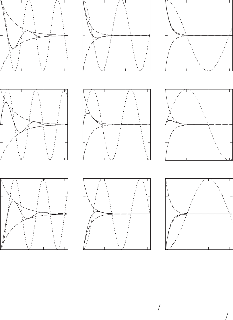
OSCILLATIONS 101
–1
–0.5
0
0.5
1β2 = 0.1, δ = π/2
β2 = 0.9, δ = 0
β2 = 0.9, δ = π/2
0 5 10 15
β2 = 0.9, δ = π
β2 = 0.5, δ = 0
β2 = 0.5, δ = π/2
0 5 10 15
–1
0.5
0
0.5
1β2 = 0.1, δ = π
0 5 10 15
β2 = 0.5, δ = π
–0.5
0
0.5
1β2 = 0.1, δ = 0
–1
3-24. As requested, we use Equations (3.40), (3.57), and (3.60) with the given values to
evaluate the complementary and particular solutions to the driven oscillator. The amplitude of
the complementary function is constant as we vary
ω
, but the amplitude of the particular
solution becomes larger as
ω
goes through the resonance near 1
096 rad s
−
.
⋅, and decreases as
ω
is increased further. The plot closest to resonance here has 111
ω
ω
=
., which shows the least
distortion due to transients. These figures are shown in figure (a). In figure (b), the 16
ω
ω
=
plot from figure (a) is reproduced along with a new plot with 2
20 m s
p
A−
=
⋅.
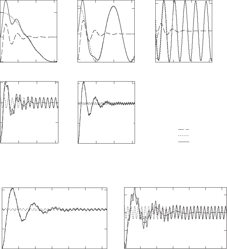
102 CHAPTER 3
–1
0
1
ω/ω
1
= 1/3
0102030
–1
–0.5
0
0.5
0102030
ω/ω
1
= 6
t (s)
–1
–0.5
0
0.5
ω/ω
1
= 3
0102030
t (s)
–2
0
2
ω/ω
1
= 1.1
01020
t (s)
30
–1
0
1
ω/ω
1
= 1/9
0102030
xc
xp
x
Legend:
(a)
0 5 10 15 20 25 30
–1
–0.5
0
0.5
0 5 10 15 20 25 30
–1
–0.5
0
0.5
(b)
A
p
= 1 A
p
= 20
3-25. This problem is nearly identical to the previous problem, with the exception that now
Equation (3.43) is used instead of (3.40) as the complementary solution. The distortion due to
the transient increases as
ω
increases, mostly because the complementary solution has a fixed
amplitude whereas the amplitude due to the particular solution only decreases as
ω
increases.
The latter fact is because there is no resonance in this case.
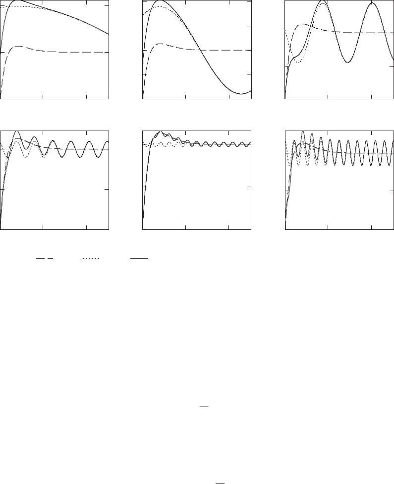
OSCILLATIONS 103
0510
–1
0
1
ω/ω
1
= 1/9
0510
–1
–0.5
0
0.5
1
ω/ω
1
= 1/3
0510
–1
–0.5
0
ω/ω
1
= 1.1
0510
–1
–0.5
0
ω/ω
1
= 3
0510
–1
–0.5
0
ω/ω
1
= 6
0510
–1
–0.5
0
ω/ω
1
= 6, A
p
= 6
xc xp x
Legend:
3-26. The equations of motion of this system are
(
)
()
11 1 1 1 2
22 22 1 2 1
cosmx kx b x x F t
mx bx b x x
ω
=− − − +
=− − −
(1)
The electrical analog of this system can be constructed if we substitute in (1) the following
equivalent quantities:
mL;
11
→1
kC
→; ; x → q
1
bR→1
mL;
22
→0
F
ε
→;
22
bR→
Then the equations of the equivalent electrical circuit are given by
()
()
11 1 1 2 1 0
22 22 1 2 1
1cos
0
Lq R q q q t
C
Lq Rq R q q
εω
+−+=
++ −=
(2)
Using the mathematical device of writing exp(i
ω
t) instead of cos
ω
t in (2), with the
understanding that in the results only the real part is to be considered, and differentiating with
respect to time, we have
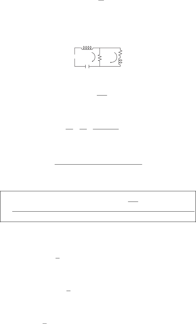
104 CHAPTER 3
()
()()
1
11 1 1 2 0
22 2 2 1 2 1 0
it
I
LI R I I i e
C
LI R I R I I
ω
ωε
+−+=
++−=
(3)
Then, the equivalent electrical circuit is as shown in the figure:
ε
0
cos ωt
L
1
L
2
R
1
R
2
I
1
(t)I
2
(t)
12
C
The impedance of the system Z is
1
1
ZiL i Z
C
ωω
1
=
−+ (4)
where is given by
1
Z
112
11 1
ZRRiL
2
ω
=++ (5)
Then,
(
)
()
22
122 1 2 21
1222
12 2
RRR R L iLR
ZRR L
ωω
ω
++ +
=++ (6)
and substituting (6) into (4), we obtain
() ()
()
()
2
22 22
122 1 2 12 1 1 2 2
222
12 2
1
RRR R L iRL L R R L
C
ZRR L
ωωω ω
ω
ω
++ + + − + +
=++ (7)
3-27. From Eq. (3.89),
()
(
0
1
1cos sin
2nn
n
a a n t b n t
)
Ft
ω
ω
∞
=
=+ +
∑ (1)
We write
()
(
0
1
1cos
2n
n
Ft a c n t
)
n
ω
φ
∞
=
=+ −
∑ (2)
which can also be written using trigonometric relations as
()
0
1
1cos cos sin sin
2nn
n
t a c nt nt n
F
ω
φω
∞
=
=+ +
φ
∑ (3)
Comparing (3) with (2), we notice that if there exists a set of coefficients c such that
n
OSCILLATIONS 105
cos
sin
nnn
nnn
ca
cb
φ
φ
=
=
(4)
then (2) is equivalent to (1). In fact, from (4),
222
tan
nnn
n
n
n
cab
b
a
φ
=+
=
(5)
with and b as given by Eqs. (3.91).
n
an
3-28. Since F(t) is an odd function, F(–t) = –F(t), according to Eq. (3.91) all the coefficients
vanish identically, and the b are given by
n
a
n
()
()
0
0
0
0
sin
sin sin
11
cos cos
2cos 0 cos
4 for odd
0 for even
n
bFtntdt
ntdt ntdt
nt nt
nn
n
n
n
n
n
π
ωπ
ω
π
ω
π
ω
π
ω
π
ω
ωω
π
ωωω
π
ωωω
πω ω
π
π
π
−
−
−
=′′′
=− +
′′ ′′
=+−
′′
=−
∫
∫∫
= (1)
Thus,
()
()
()
21
2
4
21 0, 1, 2,
0
n
n
bnn
b
π
+
=
+=
=
… (2)
Then, we have
()
44 4
sin sin 3 sin 5
35
t t t
ωωω
ππ π
=++ …
Ft (3) +
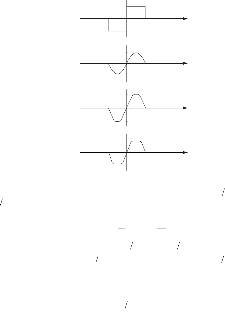
106 CHAPTER 3
F(t)
t
–1
1
–π⁄ω
π⁄ω
Terms 1 + 2
t
–0.849
0.849
–π⁄ω
π⁄ω
Terms 1 + 2 + 3
t
–1.099
1.099
–π⁄ω
π⁄ω
Terms 1 + 2 + 3 + 4
t
–0.918
0.918
–π⁄ω
π⁄ω
3-29. In order to Fourier analyze a function of arbitrary period, say 2P
τ
ω
=
instead of
2
π
ω
, proportional change of scale is necessary. Analytically, such a change of scale can be
represented by the substitution
t
xP
π
= or Px
t
π
= (1)
for when t = 0, then x = 0, and when 2Pt
τ
ω
=
=, then 2x
π
ω
=
.
Thus, when the substitution tPx
π
= is made in a function F(t) of period 2P
ω
′, we obtain the
function
()
Px
F
fx
π
=
(2)
and this, as a function of x, has a period of 2
π
ω
. Now, f(x) can, of course, be expanded
according to the standard formula, Eq. (3.91):
()
(
0
1
1cos sin
2nn
n
a a nx b nx
)
fx
ω
ω
∞
=
=+ +
∑ (3)
where

OSCILLATIONS 107
()
()
2
0
2
0
cos
sin
n
n
afxnxd
bfxnxd
π
ω
π
ω
ωω
π
ωω
π
=x
x
′
′′
=
′
′′
∫
∫
(4)
If, in the above expressions, we make the inverse substitutions
t
xP
π
= and dx dt
P
π
= (5)
the expansion becomes
()
0
1
cos sin
2nn
n
t t nt nt
a
PFt a b
PP P P
π π ωπ ωπ
π
∞
=
fF
=⋅==+ +
∑ (6)
and the coefficients in (4) become
()
()
2
0
2
0
cos
sin
P
n
P
n
nt
aFt
PP
nt
bFt d
PP
ω
ω
ωπ
ω
ωπ
ω
′
=dt
t
′
′
′
=
′
′
∫
∫
(7)
For the case corresponding to this problem, the period of F(t) is 4
π
ω
, so that P = 2
π
. Then,
substituting into (7) and replacing the integral limits 0 and
τ
by the limits 2
τ
− and 2
τ
+, we
obtain
()
()
2
2
2
2
cos
22
sin
22
n
n
nt
aFt
nt
bFt
π
ωπ
ω
π
ωπ
ω
ω
ω
π
ω
ω
π
−
−
′
=dt
dt
′
′
′
=
′
′
∫
∫
(8)
and substituting into (6), the expansion for F(t) is
()
0
1
cos sin
22
nn
n
nt nt
aa b
ωω
∞
=2
Ft
=+ +
∑ (9)
Substituting F(t) into (8) yields
2
0
2
0
sin cos
22
sin sin
22
n
n
nt
at
nt
bt
π
ω
π
ω
ω
ωω
π
ω
ωω
π
′
=dt
dt
′
′
′
=
′
′
∫
∫
(10)
Evaluation of the integrals gives
108 CHAPTER 3
()
()
2
01
2
1;0for 2
2
0 eve
02
4odd
4
n
n
bb n
n
aa an n
n
π
== ≠
n
== ≥=
−
−
(11)
and the resulting Fourier expansion is
()
357
14 4 4 4
sin cos cos cos cos
23252212452
tt t
Ft t
ωω ω ω
ωππ π π
=+ − − − …
t
+ (12)
3-30. The output of a full-wave rectifier is a periodic function F(t) of the form
()
sin ; 0
sin ; 0
tt
Ft
tt
π
ωω
π
ω
ω
−
−<≤
=
<
<
(1)
The coefficients in the Fourier representation are given by
()
()
0
0
0
0
sin cos sin cos
sin sin sin sin
n
n
atntdttn
btntdttn
π
ω
π
ω
π
ω
π
ω
ωωω ωω
π
ωωω ωω
π
−
−
=− + tdt
tdt
′
′′ ′ ′′
=− +
′
′′ ′ ′′
∫∫
∫∫
(2)
Performing the integrations, we obtain
()
()
2
4;if even or 0
1
0; if odd
0for all
n
n
n
n
a
n
bn
π
−
=
=
(3)
The expansion for F(t) is
()
24 4
cos 2 cos 4
315
t t
ω
ππ π
=− − …Ft (4)
ω
The exact function and the sum of the first three terms of (4) are shown below.
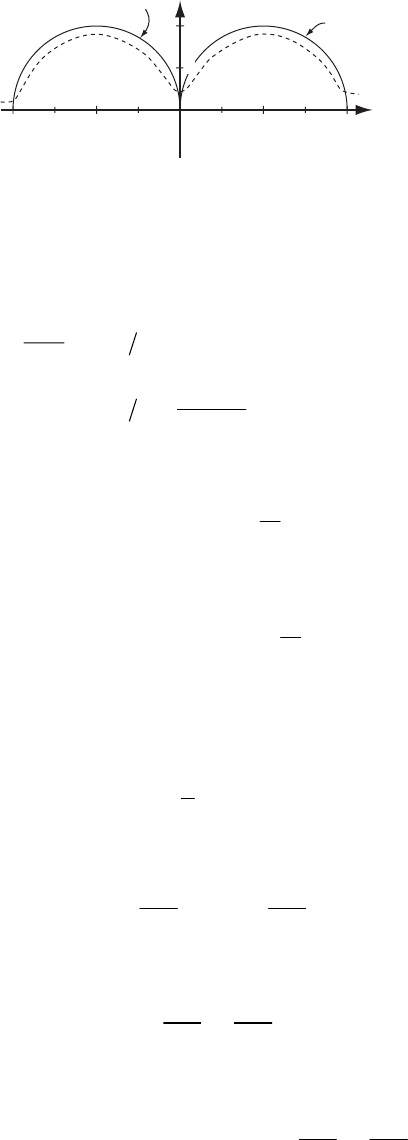
OSCILLATIONS 109
Sum of first
three terms F(t)sin ωt
ωt
–π⁄2π⁄2
1
–ππ
.5
3-31. We can rewrite the forcing function so that it consists of two forcing functions for t >
τ
:
()
()
()
()
00
0
t
Ft at t
m
at
at t
τ
τ
τ
ττ
τ
<
=
−
−>
<<
(1)
During the interval 0 < t <
τ
, the differential equation which describes the motion is
2
0
2at
xxx
βω
τ
+
+=
(2)
The particular solution is , and substituting this into (2), we find
p
xCt=+D
22
00
2at
CCtD
βω ω
τ
+
+= (3)
from which
2
0
2
0
20
0
CD
a
C
βω
ωτ
+=
−=
(4)
Therefore, we have
4
00
2,
a
DC
2
a
β
ω
τω
=− =
τ
(5)
which gives
2
00
2
p
aa
xt
4
β
ω
τω
=−
τ
(6)
Thus, the general solution for 0 < t <
τ
is
()
11
2
00
2
cos sin
taa
e A t B t t
β
4
xt
β
ωω
ω
τω
−
=++
τ
−
(7)
and then,
110 CHAPTER 3
()
111 1 1
2
0
cos sin sin cos
tt
a
xt e A t B t e A t B t
ββ
βωωω ωω
ω
τ
−−
=− + + − + +
(8)
The initial conditions, x(0) = 0,
(
)
0x0
=
, implies
4
0
2
22
10 0
2
21
a
A
a
B
β
ωτ
β
ωωτ ω
=
=−
(9)
Therefore, the response function is
()
2
11
22 2 2
00 10 0
22
cos 1 sin
t
t
ae
e t t t
β
β
2
xt
β
ββ
ωω
ω
τω ω ω ω
−
−
=+−
+−
(10)
For the forcing function
(
)
at
τ
τ
−
− in (1), we have a response similar to (10). Thus, we add these
two equations to obtain the total response function:
() ()
()
()
2
11
22 2
00 10
11
22
cos cos 1
sin sin
t
tt
t
ae
xt e t e t
te t
β
ββ
β
ββ
ωωτ
ω ω ω
ωωττ
−
−
ωτ
=
−−+
−
×+− −+
(11)
When
τ
→ 0, we can approximate e
β
τ
as 1 +
βτ
, and also 11
sin
ω
τωτ
≅
, co 1
s 1
ω
τ
≅. Then,
()
()
()
()
()
2
1111
22 2
0
00 10
1111
3
1
11
222
00110
22
cos 1 cos sin 1
sin 1 sin cos
22
1cos sin
t
t
tt
ae
xt e t t t
ttt
aete t
β
β
τ
ββ
ββ
ωβτωωτω
ωτ ω ω ω
ωβτωωτωτ
βω ββ
ωω
ωωωωω
−
−
→
−−
→−+++
−
×−+ − +
=− − −+
2
(12)
If we use 22
10
ω
ωβ
=−, the coefficient of 1
sin
t
e
β
t
ω
− becomes 1
β
ω
. Therefore,
()
1
2
0
01
1cos sin
tt
ae t e t
−−
→1
xt
→− −
ββ
τ
β
ω
ωω
ω
(13)
This is just the response for a step function.
3-32.
a) Response to a Step Function:
From Eq. (3.100)
(
)
0
H
t is defined as
OSCILLATIONS 111
()
0
0
10
0,
,
tt
Ht
att
<
=>
(1)
With initial conditions
(
)
00xt = and
(
)
00xt
=
, the general solution to Eq. (3.102) (equation of
motion of a damped linear oscillator) is given by Eq. (3.105):
()
()
()
()
()
()
0
0
10 10 0
2
01
0
1 cos sin for
0f
tt
tt
ae
xt e t t t t t t
xt t t
β
ββ
ωω
ωω
−−
−−
=− −− − >
=<
or
(2)
where 22
10
ω
ωβ
=−.
For the case of overdamping, 2
0
2
ω
β
<, and consequently 2
1
i2
0
ω
βω
=− is a pure imaginary
number. Hence,
(
)
1
cos tt
ω
−0
and
(
)
10
tt
ω
−sin are no longer oscillatory functions; instead,
they are transformed into hyperbolic functions. Thus, if we write 2
20
2
ω
βω
=− (where 2
ω
is
real),
(
)
(
)
(
)
() () ()
10 20 20
10 20 20
cos cos cosh
sin sin sinh
tt i tt tt
tt i tt i tt
ωω ω
ωω ω
−= −= −
−= −= −
(3)
The response is given by [see Eq. (3.105)]
()
()
()
()
()
()
0
0
20 10 0
2
02
0
1 cosh sinh for
0f
tt
tt
ae
xt e t t t t t t
xt t t
β
ββ
ωω
ωω
−−
−−
=− −− − >
=<
or
(4)
For simplicity, we choose t, and the solution becomes
00=
() ()
2
2
02
01cosh sinh
t
t
He
e t t
β
ββ
ω
ωω
−
−
2
ω
xt
=− −
(5)
This response is shown in (a) below for the case 0
5
β
ω
=.
b) Response to an Impulse Function (in the limit
τ
→ 0):
From Eq. (3.101) the impulse function
(
)
01
,It t is defined as
()
0
01 0 1
1
0
,
0
tt
It t a t t t
tt
<
=
<<
>
(6)
For tt
12 0
τ
−=→ in such a way that a
τ
is constant = b, the response function is given by
Eq. (3.110):
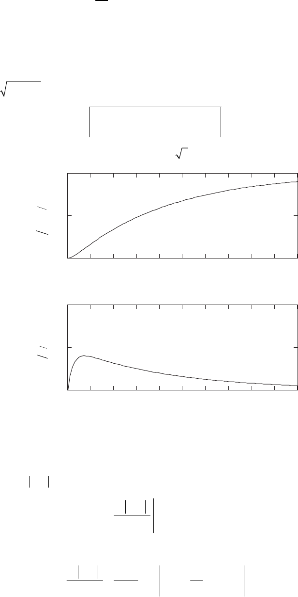
112 CHAPTER 3
()
()
()
0
10
1
sin for
tt
be t t t t
βω
ω
−−
=−
0
>
xt (7)
Again taking the “spike” to be at t = 0 for simplicity, we have
() ()
1
1
sin for 0
t
b
xt e t t
βω
ω
−
=
> (8)
For 2
12
ii 2
0
ω
ωβ
== −
ω
(overdamped oscillator), the solution is
()
2
2
sinh ; 0
t
b
xt e t t
βω
ω
−
=
> (9)
This response is shown in (b) below for the case 0
5
β
ω
=.
0123456789
0
0.5
1
10
ω0t
xH00
2
()
ω
0123456789
0
0.5
1
10
ω0t
()
xb
ω
2
(a)
(b)
3-33.
a) In order to find the maximum amplitude of the response function shown in Fig. 3-22, we
look for such that
1
t
(
)
xt given by Eq. (3.105) is maximum; that is,
()
(
)
1
0
tt
xt
t=
∂
=
∂ (1)
From Eq. (3.106) we have
(
)
(
)
()
2
1
2
01
0sin
t
xt He
t
ββ
1
t
ω
ω
ωω
−
∂
=+
∂ (2)
OSCILLATIONS 113
For 0
0.2
β
ω
=, 22
10 0.98 0
ω
ωβ ω
=−= . Evidently, 11
t
π
ω
=
makes (2) vanish. (This is the
absolute maximum, as can be seen from Fig. 3-22.)
Then, substituting into Eq. (3.105), the maximum amplitude is given by
()
()
1
12
max
0
1
a
xt xt e
βπ
ω
ω
−
== +
(3)
or,
()
12
0
1.53 a
xt
ω
≅ (4)
b) In the same way we find the maximum amplitude of the response function shown in Fig.
3-24 by using x(t) given in Eq. (3.110); then,
()
(
)
()
() ()
0
1
1
10 10
1
cos sin
tt
tt
tt
xt be t t t t
t
ββ
ωω
ω
−−
=
=
∂
=−−−
∂
(5)
If (5) is to vanish, is given by
1
t
()
11
1
10
11
11
tan tan 4.9
ω
1
1.37
tt
ω
βω ω
−−
−= = =
(6)
Substituting (6) into Eq. (3.110), we obtain (for 0
0.2
β
ω
=
)
()
()
(
1
1.37
1
max
0
sin 1.37
0.98
b
xt e
β
ω
ω
−×
==
)
xt (7)
or,
()
1
0
0.76 a
xt
τ
ω
≅ (8)
3-34. The response function of an undamped (
β
= 0) linear oscillator for an impulse function
I(0,
τ
), with
0
2
π
τ
ω
=, can be obtained from Eqs. (3.105) and (3.108) if we make the following
substitutions:
10
01
0
0;
2
0;tt
βωω
π
τω
==
===
(1)
(For convenience we have assumed that the impulse forcing function is applied at t = 0.)
Hence, after substituting we have
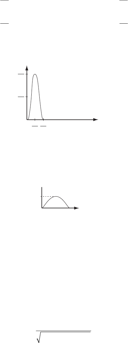
114 CHAPTER 3
(
)
()
()
()
0
2
00
00
2
00
00
2
1cos 0
2
cos 2 cos 0
xt t
at t
a
xt wt wt t
xt
π
ω
ωω
π
πτ
ωω
=<
=− <<
=−−=>=
(2)
This response function is shown below. Since the oscillator is undamped, and since the impulse
lasts exactly one period of the oscillator, the oscillator is returned to its equilibrium condition at
the termination of the impulse.
t
0
2
a
ω
2
0
π
ω
0
π
ω
2
0
2
a
ω
3-35. The equation for a driven linear oscillator is
(
)
0
2
2xxwxf
β
++=
t
where f(t) is the sinusoid shown in the diagram.
f(t)
I II III
t
a
Region I: x = 0 (1)
Region II:
xx
2
0
2xasint
β
ω
++=
ω
0
(2)
Region III:
xx
2
0
2x
βω
+
+=
(3)
The solution of (2) is
(
)
11
sin cos
t
P
xe A tB t x
βωω
−
=++ (4)
in which
(
)
sin
P
xDa t
ω
δ
=
− (5)
where
()
22 2
0
1
4
D2
ω
ωβω
=−+ (6)

OSCILLATIONS 115
1
2
0
2
tan 2
β
ω
δ
ω
ω
−
=− (7)
Thus,
(
)
(
)
11
sin cos sin
tA tB t Da t
β
xe
ω
ωω
−
=++
δ
− (8)
The initial condition x(0) = 0 gives
sin
BaD
δ
=
(9)
and
(
)
00x=
1cos 0BADa
β
ωωδ
−+ + =
or,
()
1
sin cos aD
A
βδωδ
ω
=− (10)
The solution of (3) is
(
)
1
sin cos
t
xt e A t B t
β
1
ω
ω
−
=+
′′
(11)
We require that
(
)
xt and
(
)
xt for regions II and III match at
t
π
ω
=
. The condition that
II III
xx
π
π
ω
ω
=
gives
(
)
(
)
(
)
sin cos sin sin cosB Da eA B
βπ ω βπ ω
eA
φ
φπδ φ
−−
++ −= +
′′
φ
where 1
ω
φ
π
ω
= or,
sin
cot cot sin
aD
AB eAB
β
πω
δ
φφ
φ
+=++
′′ (12)
The condition that II III
xx
π
π
ω
ω
=
gives
(
)
(
)
(
)
()()
11
11
sin cos cos cos sin
sin cos cos sin
eA B aD eA B
eA B eA B
βπ ω βπ ω
βπ ω βπ ω
β
φφωπδ ωφω
βφφωφωφ
−−
−−
−++−+ −
=− + + −
′′ ′ ′
φ
or,
(
)
(
)
()()
11
11
cos sin sin cos
sin cos sin cos cos
AB
ABe
βπ ω
ωφβφ ωφβφ
aD
β
φω φ ω φβ φ ω δ
−− +
′′
=− + − + −
or,
11
111
sin cos sin cos cos
cos sin cos sin cos sin
Da
AB AB e
βπ ω
ω φβφ ω φβφ ω δ
ω
φβ φ ω φβ φ ω φβ φ
++
−=−−
′′
−−
−
(13)

116 CHAPTER 3
Substituting into (13) from (12), we have
(
)
(
)
()
()()
()
11
1
11
1 1
cos sin cos sin cos sin
cos sin sin
cos sin cos sin cos sin sin cos
cos sin sin sin cos sin
B
aDe
βπ ω
ωφβφφωφβφφ
ωφβφφ
ωφβφφωφβφφ δωδ
ω
φβ φ φ φω φβ φ
−++
′−
−++
=++
−−
(14)
from which
()
1
1
sin sin cos sin cos sin
a
D De
βπ ω
Ba
δ
δω φ β φ ω δ φ
ω
=+ −+
′
(15)
Using (12), we can find A′:
sin
cot cot
sin
aD e
B B
βπ ω
δ
AA
φ
φ
φ
=+ + −
′′
(16)
Substituting for A, B, and B′ from (10), (9), and (15), we have
()
11 1
cos
sin cos sin 1 cos
aD
AaD e e
βπ ω βπ ω
ωδ
ββ
δ
φφ
ωω ω
=+ +−+
′
φ
(17)
Thus, we obtained all constants giving us the response functions explicitly.
3-36. With the initial conditions,
(
)
0
xt x
0
=
and
(
)
0
xt x
0
=
, the solution for a step function for
given by Eq. (3.103) yields
0
tt>
00
10 2
2
011
;xx
aa
Ax A 2
01
β
β
ω
ωωωω
=− = + −
(1)
Therefore, the response to
(
)
0
H
t for the initial conditions above can be expressed as
()
()
() ()
()
()
()
()
0
00
00
010 10
11
10 10
2
01
cos sin
1 cos sin for
tt
tt tt
xx
xt e x tt tt
aettett
β
ββ
β
ωω
ωω
β
ωω
ωω
−−
−− −−
=−++−
+− −− − >
0
tt
(2)
The response to an impulse function
(
)
(
)
01 1
,It t Ht=, for the above initial conditions will then be
given by (2) for tt and by a superposition of solutions for
0
t<<
1
(
)
0
H
t and for
(
)
1
H
t
1
t>
(
taken
individually for . We must be careful, however, because the solution for t must be
equal that given by (2) for . This can be insured by using as a solution for
1
tt>
1
tt=
)
1
H
t Eq. (3.103)
with initial conditions
(
)
00=x,
(
)
00x
=
, and using t instead of t in the expression.
1 0
The solution for t is then
1
t>
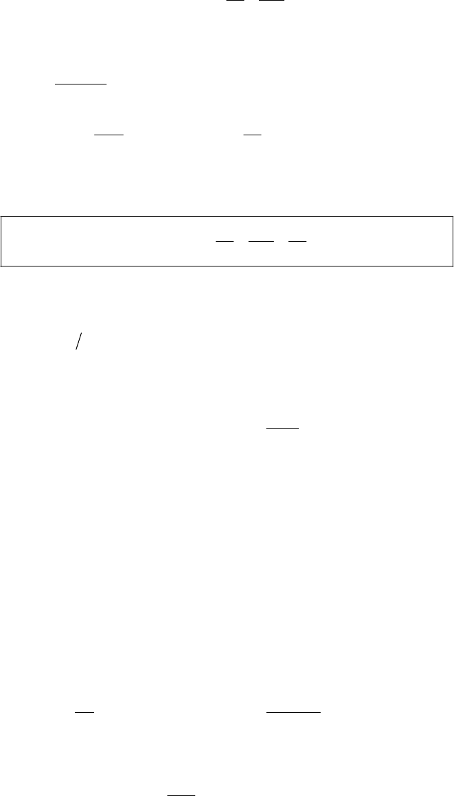
OSCILLATIONS 117
()
()
() ()
()
000
010 101
11
cos sin
tt xx
t e x tt tt xt
β
β
ωω
ωω
−−
=−++−
x (3) +
where
()
(
)
() ()
() ()
0
1
11010
2
0
10 10
11
cos cos
sin sin for
tt
ae
xt e t t t t
ett t t
e
tt
β
βτ
βτ
βτ
ωτω
ω
ββ
ωτ
β
ω
ωω
ω
−−
=−−−−+
+−−−−
1
>
(4)
We now allow a → ∞ as
τ
→ 0 in such a way that a
τ
= b = constant; expanding (3) for this
particular case, we obtain
()
()
() ()
000
010 10
111
cos sin
tt xx
b
xt e x t t t t t t
β
β
ωω
ωωω
−−
=−+++−
0
> (5)
which is analogous to Eq. (3.119) but for initial conditions given above.
3-37. Any function
(
)
Ft m can be expanded in terms of step functions, as shown in the figure
below where the curve is the sum of the various (positive and negative) step functions.
In general, we have
(
)
()
2
0
2n
n
n
n
F
t
xxx m
H
t
βω
∞
=−∞
∞
=−∞
++=
=
∑
∑
(1)
where
()
(
)
0
nn
n
n
at tt n
Ht
tt n
τ
τ
>=
=<=
(2)
Then, since (1) is a linear equation, the solution to a superposition of functions of the form given
by (2) is the superposition of the solutions for each of those functions.
According to Eq. (3.105), the solution for
(
)
n
H
t for is
n
tt>
()
()
()
()
(
1
2
01
1cos sin
n
n
tt
tt
n
nn
ae
e tt tt
β
β
β
ω
ωω
−−
−−
=− −− −
)
1
n
ω
xt (3)
then, for
(
)
()
n
n
Ft
H
t
m
∞
=−∞
=∑ (4)
the solution is
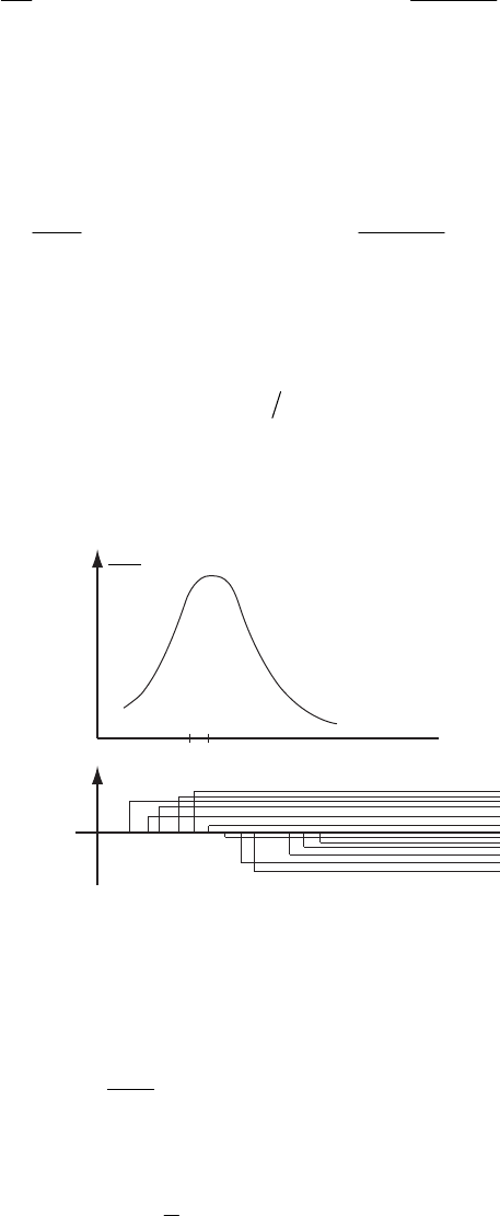
118 CHAPTER 3
() ()
()
()
()
()
() () () ()
11
2
01
11cos sin
n
n
tt
tt
nn
n
nn nn
nn
e
xt H t e t t t t
mH tG t F tG t
β
β
β
ωω
ωω
−−
∞−−
=−∞
∞∞
=−∞ =−∞
=−−−
==
∑
∑∑
n
−
(5)
where
()
()
()
()
()
11
2
01
11cos sin ;
0
n
n
tt
tt
nn
n
n
e
ett tt
m
Gt
tt
β
β
β
ωω
ωω
−−
−−
−−− −
=
<
n
tt
≥
(6)
or, comparing with (3)
()
(
)
,
0
nn
n
n
xtma tt
Gt
tt
≥
=
n
<
(7)
Therefore, the Green’s function is the response to the unit step.
Hn(t)
Ft
m
()
tn+1
tnt
3-38. The solution for x(t) according to Green’s method is
() ( ) ( )
()
()
0
1
0
1
,
sin sin
t
tttt
xt Ft Gtt dt
Fete tt
m
γβ
ωω
ω
−∞
−−−
′′
=′′′
dt
−=
′
′
∫
∫′
(1)
Using the trigonometric identity,
()
() ()
1111
1
sin sin cos cos
2
ttt tt t
ωω ωωω ωωω
1
t
−= + − − − +
′′ ′ ′
(2)
we have
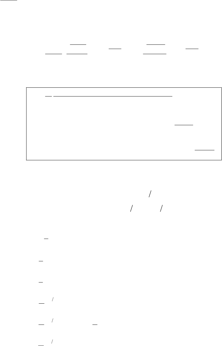
OSCILLATIONS 119
()
()
()
()
()
0
11 11
100
cos cos
2
tt
t
tt
Fe
xt dte t t dte t t
m
ββγ βγ
ωω ω ωω ω
ω
−−−
′′
=+−−−
′′′
∫∫
+
′
(3)
Making the change of variable,
(
)
11
z
tt
ω
ωω
=+ −
′, for the first integral and
(
)
11
ytt
ω
ωω
=− +
′
for the second integral, we find
()
() () () ()
11
11
1
11
0
11 1
cos cos
2
tt
zy
tt
t
tt
Fe ee
dze z dye y
m
βγω βγω
βγ βγ
ωω
βωω ωω
ωω ωω
ωω
ωωω ωω
−−−
−−
−+−
+
−
=−
+−
∫∫
1
−
xt (4)
After evaluating the integrals and rearranging terms, we obtain
()
()
()
()
()
()
[]
()
()
[]
()
0
22
22
11
222
1
222 1
11
sin
2cos
sin
2cos
t
t
F
xt m
t
et
t
et
γ
β
ω
βγ ωω βγ ωω
ω
γβ ω βγ ω ω ω
ω
βγ ω βγ ω ω ω
−
−
=
−++ −+−
×−+−+−
+− +−+−
(5)
3-39.
()
sin 0
02
tt
Ft
t
ωπω
π
ωπ
<<
=<<
ω
From Equations 3.89, 3.90, and 3.91, we have
()
()
0
1
1cos sin
2nn
n
Ft a a n t b n t
ω
ω
∞
=
=+ +
∑
()
0
2cos
n
aFtnt
τ
ω
τ
=′′
∫dt
′
()
0
2sin
n
bFtnt
τ
ω
τ
=′′
∫dt
′
0sin cos
n
atn
πω
tdt
ω
ωω
π
=′′
∫′
00
2
sinat
πω
dt
ω
ω
π
π
==
′′
∫
10sin cos 0att
πω
dt
ω
ωω
π
==
′′′
∫
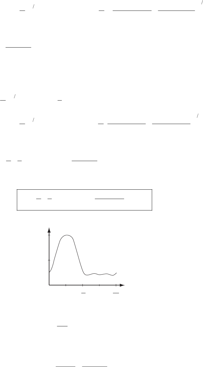
120 CHAPTER 3
() ()
()
()
()
0
0
cos 1 cos 1
2sincos 21 21
n
nt nt
an t ntdt nn
π
ω
πω
ωω
ωω
ωω
ππωω
−+
′
≥= = − −
′′′
−+
∫
Upon evaluating and simplifying, the result is
()
2
2 even
1
0 o
n
n
n
a
n
π
−
=
dd
n = 0,1,2,…
00 by inspectionb=
2
10
1
sin 2
bt
πω
dt
ω
ω
π
==
′′
∫
() ()
()
()
()
0
0
sin 1 sin 1
2sinsin 21 21
n
nt nt
bn t ntdt nn
πω
πω
ωω
ωω
ωω
ππω
−+
′′
≥= = − =
′′′
−+
∫0
ω
So
()
()
2
2
2,4,6,
11 2
sin cos
21
n
Ft t n t
n
ω
ω
ππ
∞
=
=+ + −
∑
…
or, letting n → 2n
()
()
2
1,2,
11 2
sin cos 2
214
n
t n t
n
Ft
ω
ω
ππ
∞
=
=+ + −
∑
…
The following plot shows how well the first four terms in the series approximate the function.
Sum of first
four terms
t
π
ω
2
π
ω
1.0
0.5
3-40. The equation describing the car’s motion is
()
2
2sin
dy
mkya
dt t
ω
=− −
where y is the vertical displacement of the car from its equilibrium position on a flat road, a is
the amplitude of sine-curve road, and
k = elastic coefficient = 100 9.8 98000 N/m
0.01
dm g
dy
×
×
==
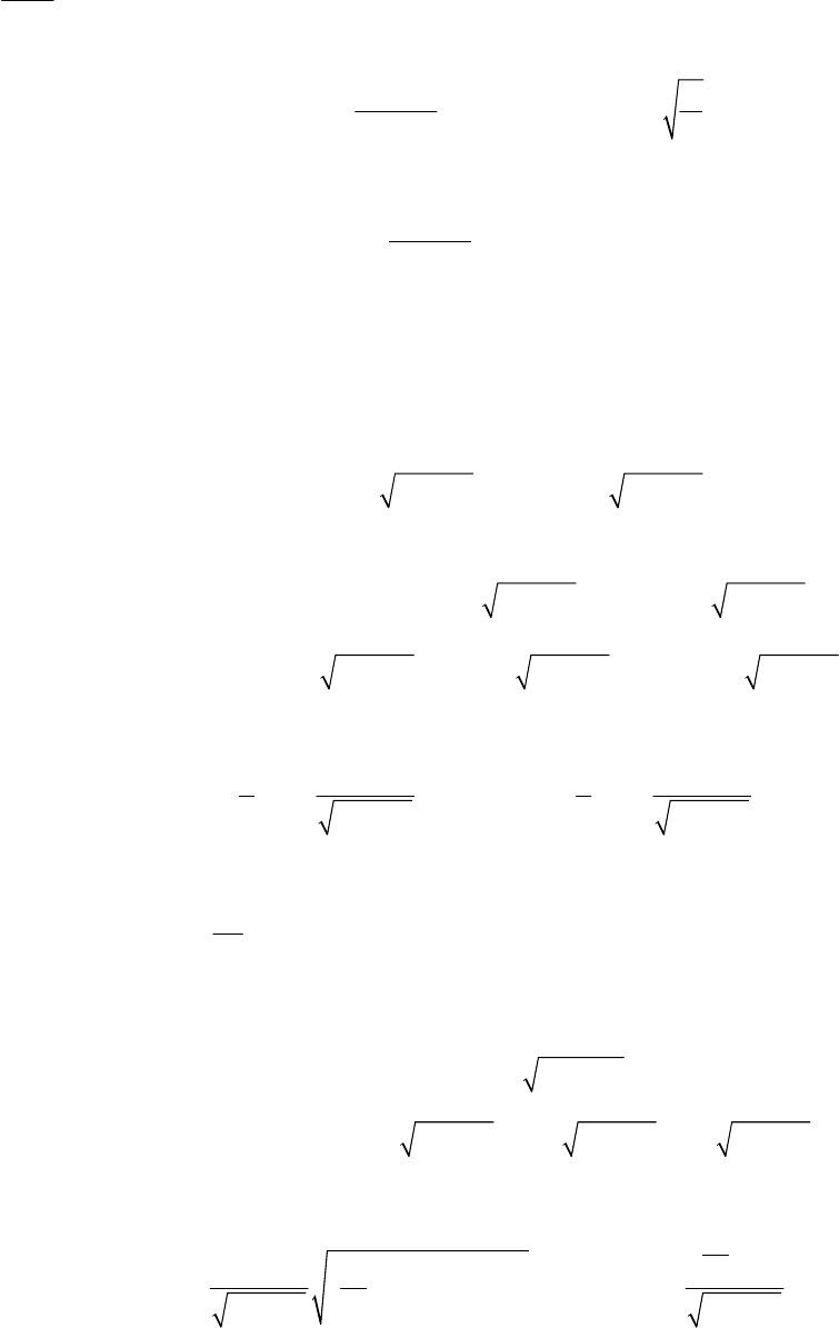
OSCILLATIONS 121
0
2174
v
π
ωλ
== rad/s with and
λ
being the car’s speed and wavelength of sine-curve road.
The solution of the motion equation can be cast in the form
0
v
()
()
2
0
022
0
cos sin
a
yt B t t
ω
ω
βω
ωω
=++
− with 09.9 rad/s
k
m
ω
==
We see that the oscillation with angular frequency
ω
has amplitude
2
0
22
0
0.16 mm
a
A
ω
ωω
==−
−
The minus sign just implies that the spring is compressed.
3-41.
a) The general solution of the given differential equation is (see Equation (3.37))
()
()
(
)
(
)
22 22
102
exp exp expxt t A t A t
ββω β
=− −+ −−
0
ω
and
()
()
(
)
(
)
()
()()
22 22
102
22 22 22
01 0 2 0
() exp exp exp
exp exp exp
vt x t t A t A t
tAt At
β β βω βω
ββω βω βω
0
==− − −+ −−
′
+− − −− −−
at t = 0, , vt
0
()xt x=0
() v=⇒
00
10
22
0
1
2
vx
β
Ax
β
ω
+
=+
−
and 00
10
22
0
1
2
vx
Ax
β
βω
+
=−
−
(1)
b)
i) Underdamped, 0
2
ω
β
=
In this case, instead of using above parameterization, it is more convenient to work with the
following parameterization
()
(
)
22
0
() exp cosxt A t t
β
ωβδ
=− −− (2)
()
(
)
(
)
22 22 22
000
() exp cos sinvt A t t t
β
β ωβδ ωβ ωβδ
=− − − − + − − −
(3)
Using initial conditions of x(t) and v(t), we find
2
2
00
0
22 0
0
xv
x
2
A
β
ωβ
ωβ
++
−
= −
and
0
0
22
0
tan ( )
v
x
β
δ
ω
β
+
=−
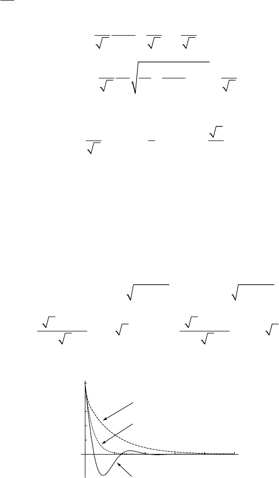
122 CHAPTER 3
In the case 0
2
ω
β
=, and using (6) below we have
0
00
211 30
333
v
x
=+=−⇒=−
δδ
ω
tan
°
2
2
00 00
00
2
00 0
22
33
xvv
A
x
xx
ωω
ω
=++=
so finally
00 0
21 3
() exp cos 30
22
3x t t
=− +
ωω
xt (4)
°
ii) Critically damped, 0
β
ω
=, using the same parameterization as in i) we have from (2) and
(3):
(
)
(
)
0
() exp expxt A t x t
0
β
ω
=
−= − (5)
and 00 0 0 00
() () exp(vt x t x t v x
ω
ω
==− −⇒=−
′
ω
(6)
iii) Overdamped, 0
β
ω
=, returning to the original parameterization (1) we have (always
using relation (6)),
()
()
(
)
(
)
() ()
()
() ()
(
22 22
102 0
00
0
exp exp exp
31 31
exp 3 2 exp 3 2
23 23
xt t A t A t
xx
t
ββω βω
)
0
t
ω
ω
=− −+ −−
+−
+−=− + (7)
Below we show sketches for equations (4), (5), (7)
t
x
Underdamped
Critically damped
Overdamped
3-42.
a)
(
)
2
00
sin 0mx x F t
ωω
+
−
′′ = (1)
The most general solution is
00
( ) sin cos sinxt a t b t A t
ω
ωω
=++
where the last term is a particular solution.
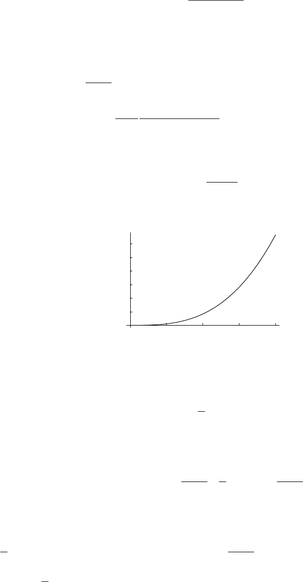
OSCILLATIONS 123
To find A we put this particular solution (the last term) into (1) and find
()
0
22
0
F
Am
ω
ω
=−
At t = 0, x = 0, so we find b = 0, and then we have
xt 000
() sin sin () cos cosa t A t vt a t A t
ω
ωωωω
=+ ⇒= +
ω
At t = 0, 0
0a
vA
ω
ω
−
=⇒ = ⇒
()()
()
0
00
00 0
1
() sin sin
Ft t
m
xt
ω
ωω ω
ωω ωω ω
=−
+−
b) In the limit 0
ω
ω
→ one can see that
3
00
() 6
Ft
xt m
ω
→
The sketch of this function is shown below.
t
x
3-43.
a) Potential energy is the elastic energy:
2
1
() ( )
2
Ur kr a=−,
where m is moving in a central force field. Then the effective potential is (see for example,
Chapter 2 and Equation (8.14)):
22
2
22
1
() () ( )
22 2
eff
ll
Ur kra
mr mr
=+ = −+Ur
where lm 2
vrmr
ω
== is the angular momentum of m and is a conserved quantity in this
problem. The solid line below is U; at low values of r, the dashed line represents
()
eff r
2
1( )
2kr a=−()Ur , and the solid line is dominated by
2
2
2
l
mr . At large values of r,
2
( )
kra−
1
() () 2
eff
UrUr≅= .
124 CHAPTER 3
Potential energy
r
Ur kr a() ( )=−
1
2
2
l
mr
2
2
2
Ur
eff
()
b) In equilibrium circular motion of radius , we have
0
r
() ()
0
2
0000
0
kr a
a m r mr
ωω
kr
−
−= ⇒ =
c) For given (and fixed) angular momentum l, V(r) is minimal at r0, because 0
() 0
rr=
Vr
=
′, so
we make a Taylor expansion of V(r) about ;
0
r
22
200 0
000 00
3( ) ( )
1
() () ( ) () ( ) () ...
22
mrr Krr
Vr Vr r r V r r r V r
ω
−−
=+− +− +≈ =
′′′
2
2
where 2
0
3Km
ω
=, so the frequency of oscillation is
0
0
0
3( )
3kr a
K
mm
ωω
r
−
== =
3-44. This oscillation must be underdamped oscillation (otherwise no period is present).
From Equation (3.40) we have
(
)
(
)
1
() exp cosxt A t t
β
ωδ
=
−−
so the initial amplitude (at t = 0) is A.
Now at
1
8
4tT
π
ω
==
1
8
(4 ) exp cos (8 )xT A
π
β
πδ
ω
=
−−
The amplitude now is
1
8
expA
π
β
ω
−
, so we have
OSCILLATIONS 125
1
8
exp 1
A
A
e
π
βω
−
=
and because 2
0
2
1
β
ωω
=−, we finally find
1
2
0
8
64 1
ω
π
ωπ
=
+
3-45. Energy of a simple pendulum is 2
2
mgl
θ
where
θ
is the amplitude.
For a slightly damped oscillation ( ) exp( )tt
θ
θβ
≈
−.
Initial energy of pendulum is 2
2
mgl
θ
.
Energy of pendulum after one period, 2l
g
π
=T, is
22
() exp(2 )
22
mgl mgl
TT
θ
θβ
=−
So energy lost in one period is
()
()
22
1exp2 2
22
mgl mgl
TTmg
2
lT
θ
βθβθ
−− ≈ =
β
So energy lost after 7 days is
22
(7 days) (7 days)mgl T mgl
T
θβ θβ
=
This energy must be compensated by potential energy of the mass M as it falls h meters:
21
2
(7 days) 0.01 s
(7 days)
Mh
h mgl ml
θβ β θ
Mg
−
=⇒ ==
Knowing
β
we can easily find the coefficient Q (see Equation (3.64))
2
22
0
2
2178
22 2
R
g
l
β
ωβ
ω
ββ β
−
−
== = =
Q
126 CHAPTER 3
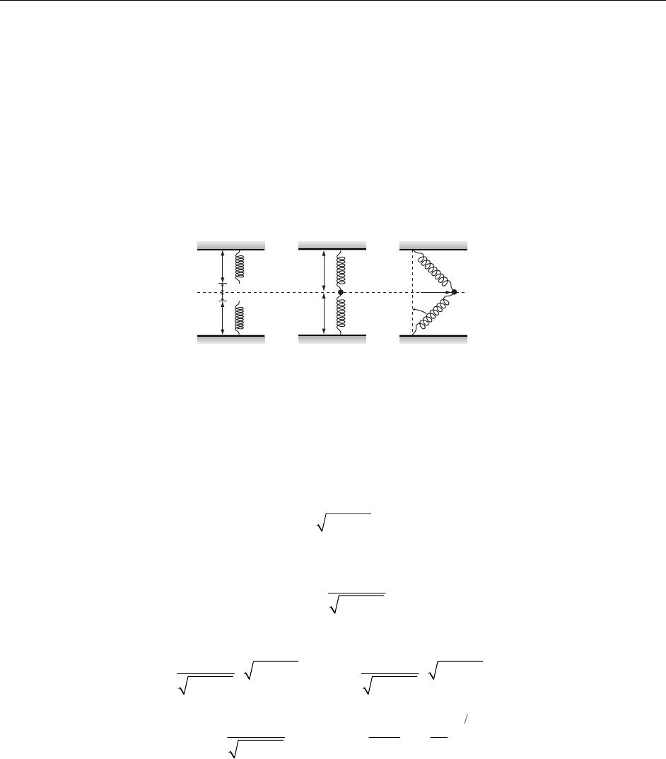
CHAPTER 4
Nonlinear Oscillations
and Chaos
4-1.
d
d
0
0
(a) (b) (c)
=
0
+ d
=
0
+ d
mm
s
x
θ
The unextended length of each spring is , as shown in (a). In order to attach the mass m, each
spring must be stretched a distance d, as indicated in (b). When the mass is moved a distance x,
as in (c), the force acting on the mass (neglecting gravity) is
0
(
)
0
2siFks n
θ
=− − (1)
where
2
s2
x
=
+ (2)
and
2
sin x
x
θ
=+2
(3)
Then,
()
()
22 22
0
22 22
12
2
2
22
22
21 21 1
kx kx
Fx x x d
xx
ddx
kx kx
x
−
=− + − =− + − −
++
−−
− =− − +
+
=− (4)
127
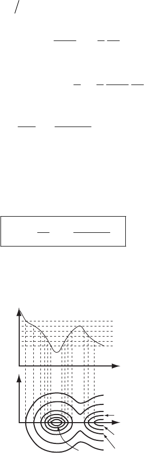
128 CHAPTER 4
Expanding the radical in powers of 22
x and retaining only the first two terms, we have
()
()
2
2
2
2
3
3
1
21 1
2
1
211 2
2
dx
Fx kx
dd
kx
kd
kd xx
−
≅− − −
x
−
=− − − +
−
=− −
(5)
The potential is given by
(6)
() ()
Ux Fxdx=−∫
so that
()
(
)
2
3
4
kd
kd
Ux x x
−
=+
4
(7)
4-2. Using the general procedure explained in Section 4.3, the phase diagram is constructed
as follows:
·
x
x
x
E
1
U(x)
E
6
E
5
E
4
E
3
E
2
E
6
E
5
E
4
E
3
E
2
E
1
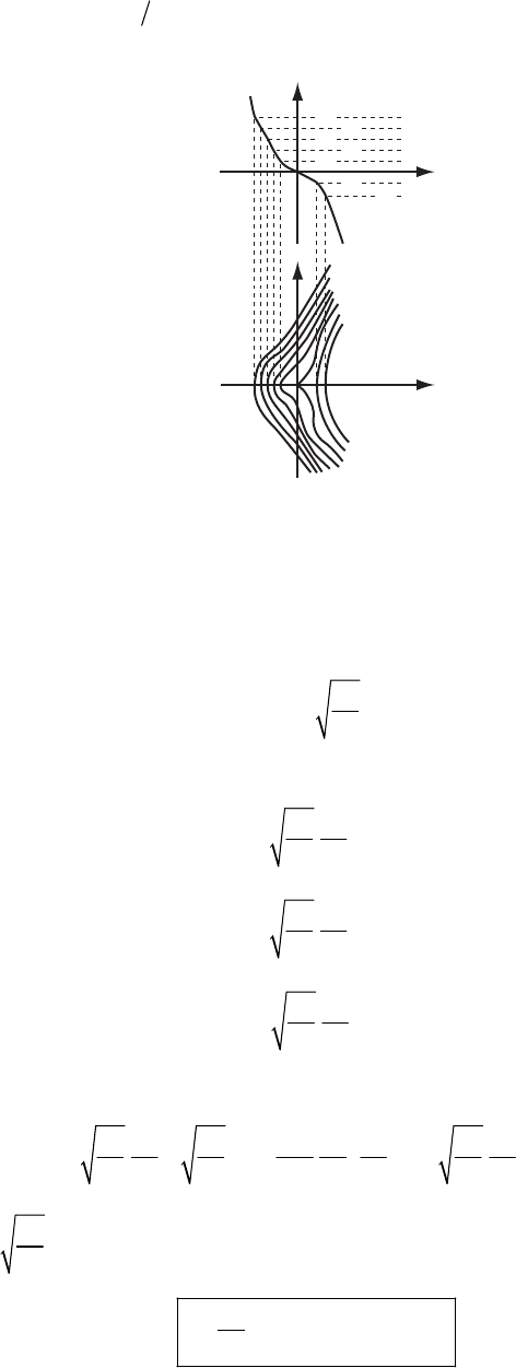
NONLINEAR OSCILLATIONS AND CHAOS 129
4-3. The potential
()
(
)
3
3x
λ
=−Ux has the form shown in (a) below. The corresponding phase
diagram is given in (b):
x
x
·
x
U(x)
E
5
E
4
E
2
E
1
E
2
E
3
E
1
(a)
(b)
4-4. Differentiation of Rayleigh’s equation above yields
(
)
22
0
3xabxx x
ω
0
−
−+
= (1)
The substitution,
0
3b
yy x
a
= (2)
implies that
0
0
0
3
3
3
y
a
xby
y
a
xby
y
a
xby
=
=
=
(3)
When these expressions are substituted in (1), we find
2
2
0
2
000
30
33 3
yyy
aaba a
a
by b b y y by
ω
−− +
0
y
=
(4)
Multiplying by 0
3b
ya and rearranging, we arrive at van der Pol’s equation:
()
22 2
00
2
0
0
a
yyyyy
y
ω
−
−+=
(5)
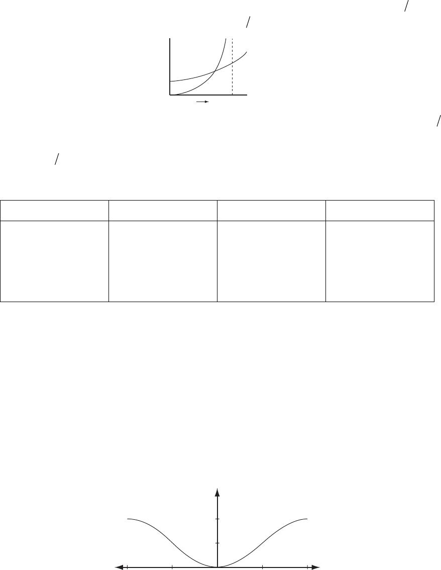
130 CHAPTER 4
4-5.
a) A graph of the functions
(
)
2
11fx x x=++ and
(
)
2tanfx x
=
in the region 0x2
π
≤≤ shows
that there is an intersection (i.e., a solution) for 1
x38
π
≅
.
tan x
Ox π⁄2
x2 + x +1
The procedure is to use this approximate solution as a starting point and to substitute 138x
π
=
into
(
)
1
fx and then solve for
(
)
1
11
tanxf
−x
=
. If the result is within some specified amount,
say 10 , of
4−38
π
, then this is our solution. If the result is not within this amount of the starting
value, then use the result as a new starting point and repeat the calculation. This procedure
leads to the following values:
1
x
(
)
2
11 1 11fx x x=++
(
)
1
11
tan fx
−
Difference
1.1781 3.5660 1.2974 0.11930
1.2974 3.9806 1.3247 0.02728
1.3247 4.0794 1.3304 0.00573
1.3304 4.1004 1.3316 0.00118
1.3316 4.1047 1.3318 0.00024
1.3318 4.1056 1.3319 0.00005
Thus, the solution is x = 1.3319.
Parts b) and c) are solved in exactly the same way with the results:
b) x = 1.9151
c) x = 0.9271
4-6. For the plane pendulum, the potential energy is
1cosumg
θ
=−
(1)
If the total energy is larger than , all values of
θ
are allowed, and the pendulum revolves
continuously in a circular path. The potential energy as a function of
θ
is shown in (a) below.
2mg
U
2mg
mg
–π–π⁄2π⁄2
O
θ
π
(a)
Since T = E – U(
θ
), we can write
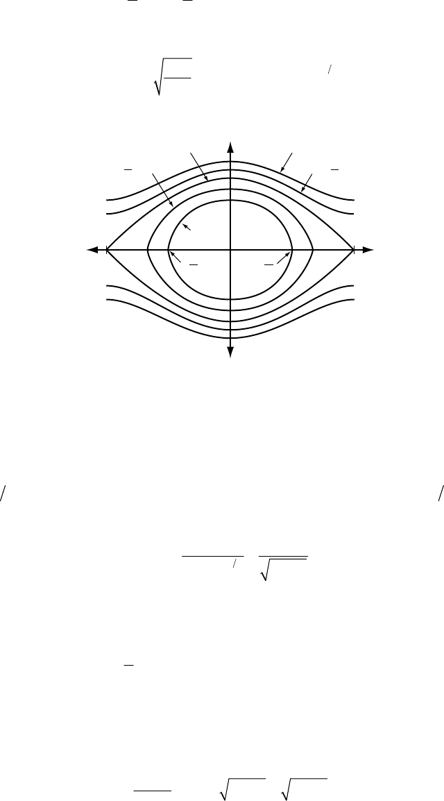
NONLINEAR OSCILLATIONS AND CHAOS 131
(
222
11 1cos
22
v m Emg
)
Tm
θ
θ
== =−−
(2)
and, therefore, the phase paths are constructed by plotting
()
12
2
21cosEmg
m
θθ
=−−
(3)
versus
θ
. The phase diagram is shown in (b) below.
E = 2mgE = 3mg
E = mg
θ
·
θ
–ππ
−
π
2
π
2
Emg=3
2
Emg=5
2
(b)
4-7. Let us start with the equation of motion for the simple pendulum:
2
0sin
θ
ω
=−
θ
(1)
where 2g≡
ω
. Put this in terms of the horizontal component by setting sinyx≡=
θ
.
Solving for
θ
and taking time derivatives, we obtain
2
32
22
(1 ) 1
yy y
yy
θ
=+
−−
(2)
Since we are keeping terms to third order, we need to get a better handle on the term. Help
comes from the conservation of energy:
2
y
22
0
1cos cos
2mmg mg−=−
θ
θθ
(3)
where 0
θ
is the maximum angle the pendulum makes, and serves as a convenient parameter
that describes the total energy. When written in terms of , the above equation becomes (with
the obvious definition for )
y
0
y
(
)
2
22
0
221 1
1
yy
y
ω
=−−−
−
2
0
y
(4)
Substituting (4) into (2), and the result into (1) gives
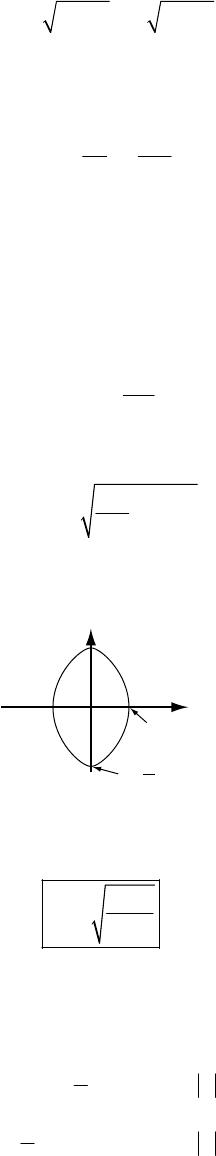
132 CHAPTER 4
(
)
222
0
31 21 0yy y y
ω
+−−−
0
=
(5)
Using the binomial expansion of the square roots and keeping terms up to third order, we can
obtain for the x equation of motion
2
2
0
023
3
1
2
g
x
xx x
3
0
+
+− =
ω
(6)
4-8. For x > 0, the equation of motion is
0
mx F
=
−
(1)
If the initial conditions are
(
)
0xA=,
(
)
0x0
=
, the solution is
()
2
0
2
F
xt A t
m
=− (2)
For the phase path we need
(
)
xxx=
, so we calculate
()
0
2(
F
xx A x
m)
=
±
− (3)
Thus, the phase path is a parabola with a vertex on the x-axis at x = A and symmetrical about
both axes as shown below.
t = 0
·
x
Ax
t=1
4
τ
Because of the symmetry, the period
τ
is equal to 4 times the time required to move from x = A
to x = 0 (see diagram). Therefore, from (2) we have
0
2
4mA
F
τ
= (4)
4-9. The proposed force derives from a potential of the form
()
()
2
2
1
2
1
2
kx x a
Ux
xxaxxa
δδ
<
=
+
−>
which is plotted in (a) below.
NONLINEAR OSCILLATIONS AND CHAOS 133
U(x)
x
a
–aO
E
3
E
2
E
1
E
7
E
6
E
5
E
4
(a)
For small deviations from the equilibrium position (x = 0), the motion is just that of a harmonic
oscillator.
For energies , the particle cannot reach regions with x < –a, but it can reach regions of
x > a if . For the possibility exists that the particle can be trapped near x = a.
6
EE<
4
EE>4
EEE<<
2
A phase diagram for the system is shown in (b) below.
(b)
·
x
x
E
1
E
3
E
4
E
2
E
7
…
4-10. The system of equations that we need to solve are
0.05 sin 0.7 cos
xy
yyx t
ω
=
−−+
(1)
The values of
ω
that give chaotic orbits are 0.6 and 0.7. Although we may appear to have chaos
for other values, construction of a Poincaré plot that samples at the forcing frequency show that
they all settle on a one period per drive cycle orbit. This occurs faster for some values of
ω
than
others. In particular, when
ω
= 0.8 the plot looks chaotic until it locks on to the point
. The phase plot for
ω
= 0.3 shown in the figure was produced by numerical
integration of the system of equations (1) with 100 points per drive cycle. The box encloses the
point on the trajectory of the system at the start of a drive cycle. In addition, we also show
Poincaré plot for the case
ω
= 0.6 in figure, integrated over 8000 drive cycles with 100 points per
cycle.
( 2.50150, 0.236439)−
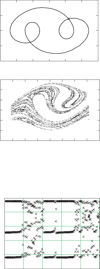
134 CHAPTER 4
–1.5 –1 -0.5 0 0.5 1 1.5
–1
-0.5
0
0.5
1
–4
–3 –3 –2 –1 0 1 2 3 4
–2
–1
0
1
2
3
4-11. The three-cycle does indeed occur where indicated in the problem, and does turn
chaotic near the 80th iteration. This value is approximate, however, and depends on the
precision at which the calculations are performed. The behavior returns to a three-cycle near the
200th iteration, and stays that way until approximately the 270th iteration, although some may
see it continue past the 300th.
100 200 300 400 500
0
0.2
0.4
0.6
0.8
1
x
iteration
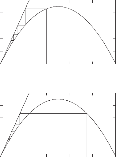
NONLINEAR OSCILLATIONS AND CHAOS 135
4-12.
0 0.2 0.4 0.6 0.8 1
0
0.1
0.05
0.2
0.25
0.15
x1 = 0.4
x1 = 0.75
0 0.2 0.4 0.6 0.8 1
0
0.1
0.2
0.05
0.25
0.15
These plots are created in the manner described in the text. They are created with the logistic
equation
(
)
10.9 1
nn
xx
+=⋅ −
n
x (1)
The first plot has the seed value as asked for in the text. Only one additional seed has
been done here ( ) as it is assumed that the reader could easily produce more of these
plots after this small amount of practice.
10.4x=
10.75x=
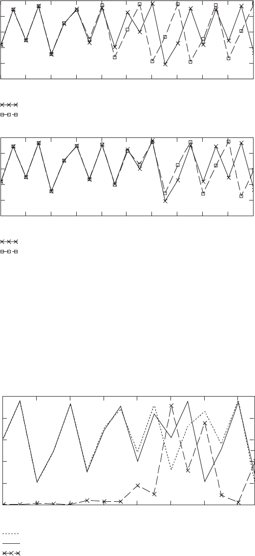
136 CHAPTER 4
4-13.
30 32 34 36 38 40 42 44 46 48 50
0
0.2
0.4
0.6
0.8
1
x
1
= 0.7
x
1
= 0.700000001
iteration
30 32 34 36 38 40 42 44 46 48 50
0
1
x
1
= 0.7
x
1
= 0.7000000001
iteration
0.2
0.4
0.6
0.8
The plots are created by iteration on the initial values of (i) 0.7, (ii) 0.700000001, and (iii)
0.7000000001, using the equation
(
)
2
12.5 1
nn
xx
+=⋅ −
n
x (1)
A subset of the iterates from (i) and (ii) are plotted together, and clearly diverge by n = 39. The
plot of (i) and (iii) clearly diverge by n = 43.
4-14.
20 22 24 26 28 30 32 34
0
0.2
0.4
0.6
0.8
1
x
1
= 0.9
x
1
= 0.9000001
fractional difference
iteration
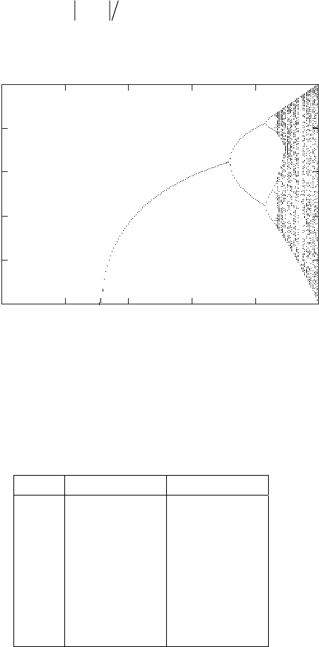
NONLINEAR OSCILLATIONS AND CHAOS 137
The given function with the given initial values are plotted in the figure. Here we use the
notation and , with
10.9x=10.9000001y=
(
)
1nn
xfx
+= and
(
)
1n
yfy
+=n
where the function is
(
)
(
)
2
2.5 1fx x x=⋅− (1)
The fractional difference is defined as xyx−, and clearly exceeds 30% when n = 30.
4-15. A good way to start finding the bifurcations of the function f(
α
,x) =
α
sin
π
x is to plot its
bifurcation diagram.
0 0.2 0.4 0.6 0.8 1
0
0.2
0.4
0.6
0.8
1
α
x
One can expand regions of the diagram to give a rough estimate of the location of a bifurcation.
Its accuracy is limited by the fact that the map does not converge very rapidly near the
bifurcation point, or more precisely, the Lyapunov exponent approaches zero. One may
continue undaunted, however, with the help of a graphical fractal generating software
application, to estimate quite a few of the period doublings n
α
.Using Fractint for Windows, and
Equation (4.47) to compute the Feigenbaum constant, we can obtain the following:
n
α
δ
1 0.71978
2 0.83324 4.475
3 0.85859 4.611
4 0.86409 4.699
5 0.86526 4.680
6 0.86551 4.630
7 0.865564 4.463
8 0.8655761
One can see that although we should obtain a better value of
δ
as n increases, numerical
precision and human error quickly degrade the quality of the calculation. This is a perfectly
acceptable answer to this question.
One may compute the n
α
to higher accuracy by other means, all of which are a great deal more
complicated. See, for example, Exploring Mathematics with Mathematica, which exploits the
vanishing Lyapunov exponent. Using their algorithm, one obtains the following:
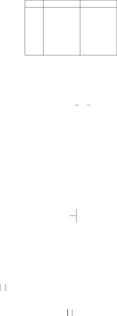
138 CHAPTER 4
n
α
δ
1 0.719962
2 0.833266 4.47089
3 0.858609 4.62871
4 0.864084 4.66198
5 0.865259 4.65633
6 0.865511 5.13450
7 0.865560
Note that these are shown here only as reference, and the student may not necessarily be
expected to perform to this degree of sophistication. The above values are only good to about
, but this time only limited by machine precision. Another alternative in computing the
Feigenbaum constant, which is not requested in the problem, is to use the so-called
”supercycles,” or super-stable points , which are defined by
6
10−
n
R
()
1
211
,22
n
n
fR
−
=
The values obey the same scaling as the bifurcation points, and are much easier to compute
since these points converge faster than for other
α
(the Lyapunov exponent goes to –∞). See, for
example, Deterministic Chaos: An Introduction by Heinz Georg Schuster or Chaos and Fractals: New
Frontiers of Science by Peitgen, Jürgens and Saupe. As a result, the estimates for
δ
obtained in
this way are more accurate than those obtained by calculating the bifurcation points.
n
R
4-16. The function y = f(x) intersects the line y = x at 0
xx
=
, i.e. is defined as the point
where
0
x
(
)
0
xfx=0
. Now expand f(x) in a Taylor series, so that near we have
0
x
(
)
(
)
(
)
(
)
0000
f
xfx xx x xx
ββ
+−=+− (1)
where
0
x
df
dx
β
≡ (2)
Now define 0nn
xx
ε
≡−. If we have very close to , then
1
x0
x1
ε
should be very small, and we
may use the Taylor expansion. The equation of iteration
(
)
1x
+n
xf=n
n
becomes
1n
ε
βε
+ (3)
If the approximation (1) remains valid from the initial value, we have 11
n
n
ε
βε
+.
a) The values xx
0nn
ε
−= form the geometric sequence .
2
11 1
, , ,
εβεβε
…
b) Clearly, when 1
β
< we have stability since
lim 0
n
n
ε
→∞
=
Similarly we have a divergent sequence when 1
β
>, although it will not really be exponentially
divergent since the approximation (1) becomes invalid after some number of iterations, and
normally the range of allowable is restricted to some subset of the real numbers.
n
x
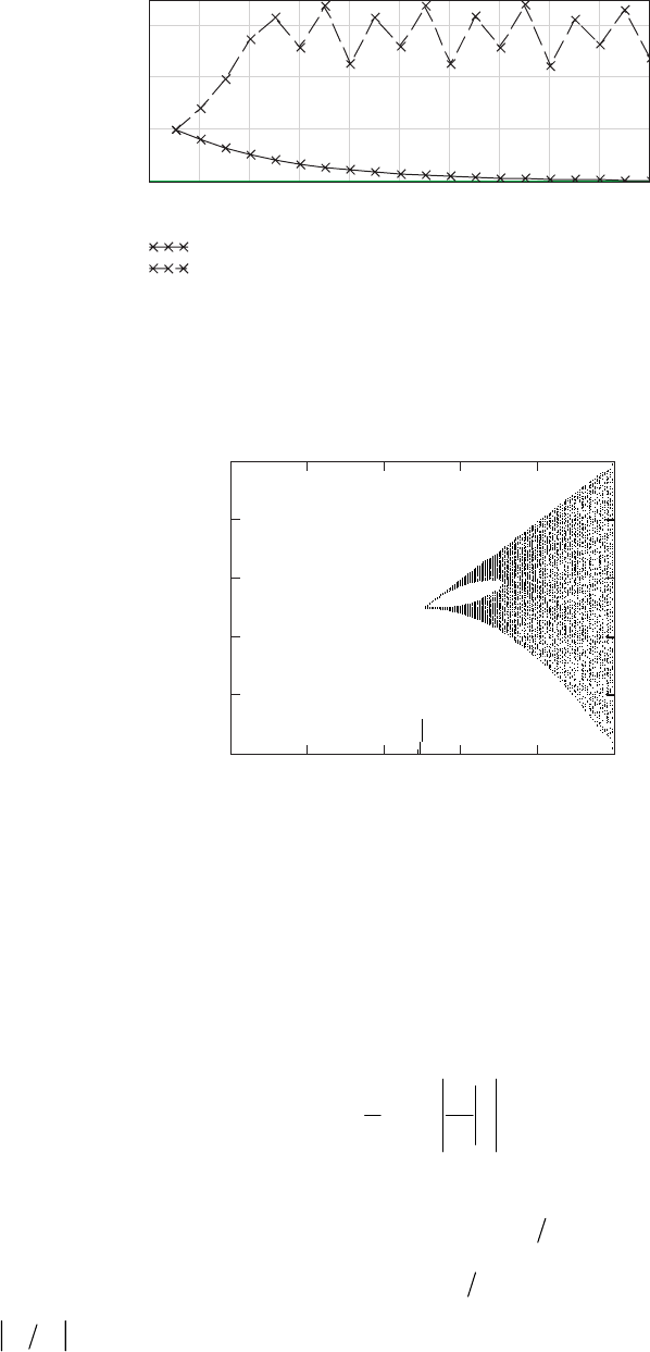
NONLINEAR OSCILLATIONS AND CHAOS 139
4-17.
024681012141618
0
0.2
0.4
0.6
20
α = 0.4
α = 0.7
iteration
The first plot (with
α
= 0.4) converges rather rapidly to zero, but the second (with
α
= 0.7) does
appear to be chaotic.
4-18.
0 0.2 0.4 0.6 0.8 1
0
0.2
0.4
0.6
0.8
1
α
x
The tent map always converges to zero for
α
< 0.5. Near
α
= 0.5 it takes longer to converge, and
that is the artifact seen in the figure. There exists a “hole” in the region 0.5 <
α
< 0.7 (0.7 is
approximate), where the iterations are chaotic but oscillate between an upper and lower range
of values. For
α
> 0.7, there is only a single range of chaos, which becomes larger until it fills the
range (0,1) at
α
= 1.
4-19. From the definition in Equation (4.52) the Lyapunov exponent is given by
1
0
1
lim ln
i
n
nix
df
ndx
λ
−
→∞ =
=∑ (1)
The tent map is defined as
() ()
2for 0
21 for 12 1
xx
fx
xx
α
α
<<
=
12
−
<<
(2)
This gives 2df dx
α
=, so we have
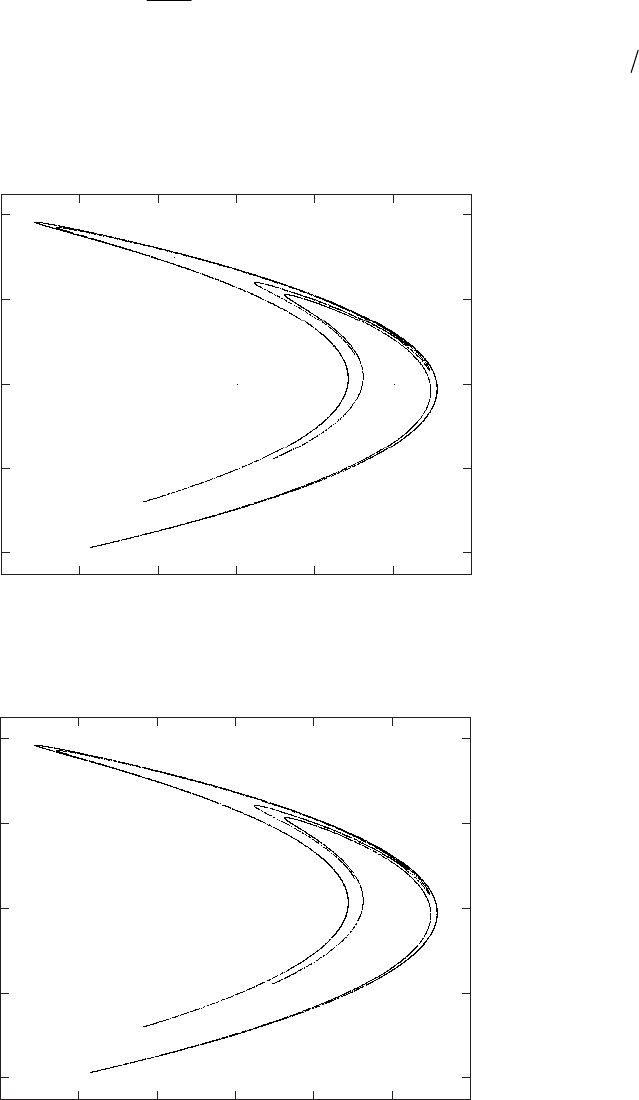
140 CHAPTER 4
() (
1
lim ln 2 ln 2
n
n
n
)
λ
α
→∞
α
−
=
=
(3)
As indicated in the discussion below Equation (4.52), chaos occurs when
λ
is positive: 12
α
>
for the tent map.
4-20.
–1.5 –1 –0.5 0 0.5 1 1.5
–0.4
–0.2
0
0.2
0.4
x
y
4-21.
–1.5 –1 –0.5 0 0.5 1 1.5
–0.4
–0.2
0
0.2
0.4
x
y
The shape of this plot (the attractor) is nearly identical to that obtained in the previous problem.
In Problem 4-20, however, we can clearly see the first few iterations (0,0), (1,0), (–0.4,0.3),
NONLINEAR OSCILLATIONS AND CHAOS 141
whereas the next iteration (1.076,–0.12) is almost on the attractor. In this problem the initial
value is taken to be on the attractor already, so we do not see any transient points.
4-22. The following. system of differential equations were integrated numerically
(1)
3
0.1 cos
xy
yyxB
=
−−+
t
using different values of B in the range [9.8,13.4], and with a variety of initial conditions. The
integration range is over a large number of drive cycles, throwing away the first several before
starting to store the data in order to reduce the effects of the transient response. For the case
B = 9.8, we have a one period per three drive cycle orbit. The phase space plot (line) and
Poincaré section (boxes) for this case are overlaid and shown in figure (a). All integrations are
done here with 100 points per drive cycle. One can experiment with B and determine that the
system becomes chaotic somewhere between 9.8 and 9.9. The section for B = 10.0, created by
integrating over 8000 drive cycles, is shown in figure (b). If one further experiments with
different values of B, and one is also lucky enough to have the right initial conditions, (0,0) is
one that works, then a transition will be found for B in the range (11.6,11.7). As an example of
the different results one can get depending on the initial conditions, we show two plots in
figure (c). One is a phase plot, overlaid with its section, for B = 12.0 and the initial condition
(0,0). Examination of the time evolution reveals that it has one period per cycle. The second plot
is a Poincaré section for the same B but with the initial condition (10,0), clearly showing chaotic
motion. Note that the section looks quite similar to the one for B = 10.0. Another transition is in
the range (13.3,13.4), where the orbits become regular again, with one period per drive cycle,
regardless of initial conditions. The phase plot for B = 13.4 looks similar to the one with B = 12.0
and initial condition (0,0).
To summarize, we may enumerate the above transition points by B, , and .
Circumventing the actual task of computing where these transition points are, we do know that
, 11 , and 13.3
1 2
B3
B
1
9.8 9.9B<< 2
.6 11.7B<< 313.4B
<
<. We can then describe the behavior of the
system by region.
• : one period per three drive cycles
1
BB<
• : chaotic
1
BBB<<
2
3
• : mixed chaotic/one period per drive cycle (depending on initial conditions)
2
BBB<<
• : one period per drive cycle
3
BB<
We should remind ourselves, though, that the above list only applies for B in the range we have
examined here. We do not know the behavior when B < 9.8 and B > 13.4, without going beyond
the scope of this problem.
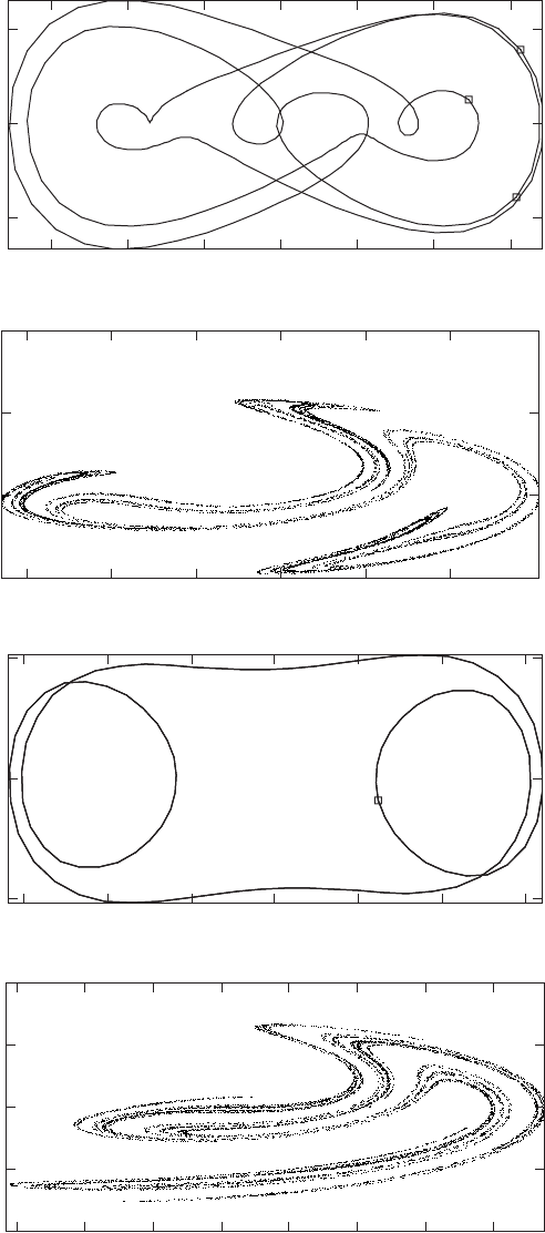
142 CHAPTER 4
–3 –2 –1 0 1 2 3
–5
0
5
x
y
(a)
2.4 2.6 2.8 3 3.2 3.4 3.6
–5
0
5
10
x
y
(b)
–3 –2 –1 0 1 2 3
–5
0
5
x
y
(c)
2.4 2.6 2.8 3 3.2 3.4 3.6 3.8
–10
–5
0
5
10
x
y
(d)
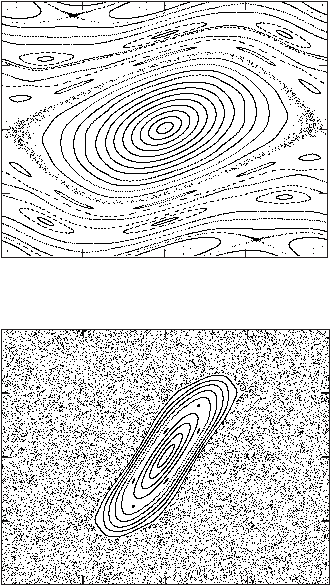
NONLINEAR OSCILLATIONS AND CHAOS 143
4-23. The Chirikov map is defined by
1sin
nn
ppK
+n
q
=
− (1)
1nnn
qqp
1
+
+
=
− (2)
The results one should get from doing this problem should be some subset of the results shown
in figures (a), (b), and (c) (for K = 0.8, 3.2, and 6.4, respectively). These were actually generated
using some not-so-random initial points so that a reasonably complete picture could be made.
What look to be phase paths in the figures are actually just different points that come from
iterating on a single initial condition. For example, in figure (a), an ellipse about the origin (just
pick one) comes from iterating on any one of the points on it. Above the ellipses is chaotic orbit,
then a five ellipse orbit (all five come from a single initial condition), etc. The case for K = 3.2 is
similar except that there is an orbit outside of which the system is always undergoing chaotic
motion. Finally, for K = 6.4 the entire space is filled with chaotic orbits, with the exception of
two small lobes. Inside of these lobes are regular orbits (the ones in the left are separate from the
ones in the right).
–1 –0.5 0 0.5 1
–1
–0.5
0
0.5
1
q⁄π
p⁄π
(a)
–1 –0.5 0 0.5 1
–1
–0.5
0
0.5
1
q⁄π
p⁄π
(b)
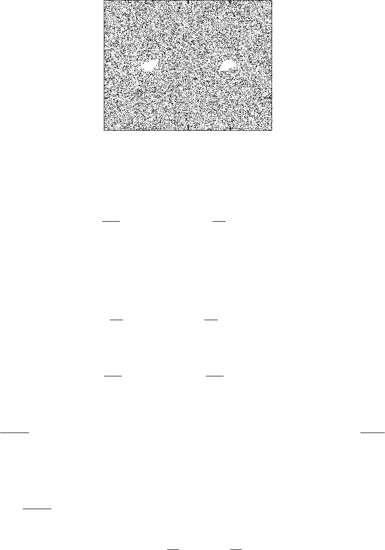
144 CHAPTER 4
–1 –0.5 0 0.5 1
–1
–0.5
0
0.5
1
q⁄π
p⁄π
(c)
4-24.
a) The Van de Pol equation is
()
2
222
0
2
dx dx
xax
dt dt
ωµ
+=−
Now look for solution in the form
0
() cos ()xt b t ut
ω
=
+ (1)
we have
00
sin
dx du
bt
dt dt
ωω
=− +
and
22
2
00
22
cos
dx du
bt
dt dt
ωω
=− +
Putting these into the Van de Pol equation, we obtain
{}
{
}
2
22 2 2
00 000
2
() ()
( ) cos ( ) 2 ( ) cos sin
dut dut
ut b t u t but t a b t
dt dt
ωµ ω ω ωω
+=− ++ −− +
From this one can see that u(t) is of order
µ
(i.e. ~ ( )uO
µ
), which is assumed to be small here.
Keeping only terms up to order
µ
, the above equation reads
{}
2
322
00000
2
22
2
00
() ( ) sin cos sin
sin sin 3
44
dut ut b t t ab t
dt
bb
ba t t
ωµωωωωω
µω ω ω
+=−− +
=− − −
0
0
0
t
(where we have used the identity 2
00 0
4 sin cos sin sin 3tt t
ω
ωω
=+
ω
)
This equation has 2 frequencies ( 0
ω
and 30
ω
), and is complicated. However, if then the
term
2b=a
0
sin t
ω
disappears and the above equation becomes
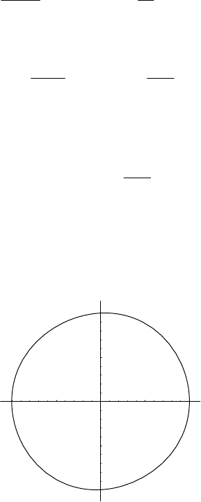
NONLINEAR OSCILLATIONS AND CHAOS 145
23
00
2
() () sin3
4
dut b
ut t
dt 0
ω
µω ω
+=
We let , and the solution for this equation is
2
b=a
33
00
00
() sin3 sin3
32 4
ba
t t
µµ
ut
ω
ω
ωω
=− =−
So, finally putting this form of u(t) into (1), we obtain one of the exact solutions of Van de Pol
equation:
3
00
0
() 2 cos sin3
4
a
ut a t t
µ
ω
ω
ω
=−
b) See phase diagram below. Since 0.05
µ
=
is very small, then actually the second term in the
expression of u(t) is negligible, and the phase diagram is very close to a circle of radius
b = 2a = 2.
x
–2
–1
1
2
.
x
–2 –1 1 2
4-25. We have used Mathematica to numerically solve and plot the phase diagram for the van
de Pol equation. Because 0.07
µ
= is a very small value, the limit cycle is very close to a circle of
radius b = 2a = 2.
a) In this case, see figure a), the phase diagram starts at the point (x = 1, x′ = 0) inside the limit
cycle, so the phase diagram spirals outward to ultimately approach the stable solution
presented by the limit cycle (see problem 4-24 for exact expression of stable solution).
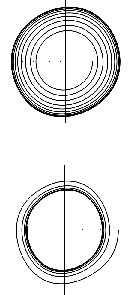
146 CHAPTER 4
x
.
x
–2 –1 1 2
–2
–1
1
2
–2 –1 1 2 3
–2
–1
1
2
b) In this case, see figure b), the phase diagram starts at the point (x = 3, x′ = 0) outside the
limit cycle, so the phase diagram spirals inward to ultimately approaches the stable solution
presented by the limit cycle (see problem 4-24 for exact expression of stable solution).
x
.
x
4-26. We have used Mathematica to numerically solve and plot the phase diagram for the van
de Pol equation. Because 0.5
µ
= is not a small value, the limit cycle is NOT close to a circle (see
problem 4-24 above).
a) In this case, see figure a), the phase diagram starts at the point (x = 1, x′ = 0) inside the limit
cycle, so the phase diagram spirals outward to ultimately approach the stable solution
presented by the limit cycle (see problem 4-24 for exact expression of stable solution).
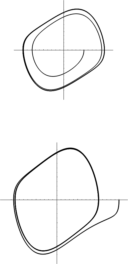
NONLINEAR OSCILLATIONS AND CHAOS 147
x
.
x
–2 –1 1 2
–2
–1
1
2
–2 –1 1 2 3
–2
–1
1
2
b) In this case (see figure below), the phase diagram starts at the point (x = 3, x′ = 0) outside
the limit cycle, so the phase diagram spirals inward to ultimately approaches the stable solution
presented by the limit cycle (see problem 4-24 for exact expression of stable solution).
x
.
x
148 CHAPTER 4
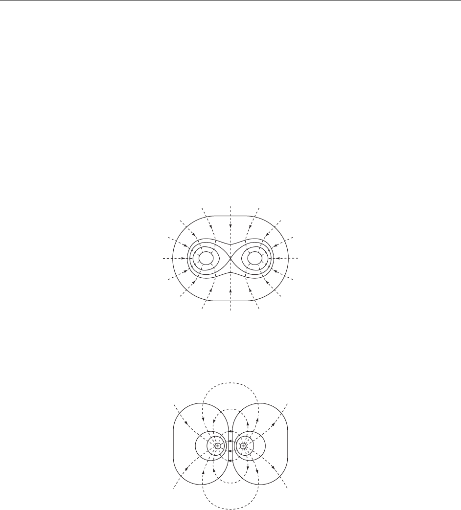
CHAPTER 5
Gravitation
5-1.
a) Two identical masses:
The lines of force (dashed lines) and the equipotential surfaces (solid lines) are as follows:
b) Two masses, +M and –M:
In this case the lines of force do not continue outward to infinity, as in a), but originate on the
“negative” mass and terminate on the positive mass. This situation is similar to that for two
electrical charges, +q and –q; the difference is that the electrical lines of force run from +q to –q.
149
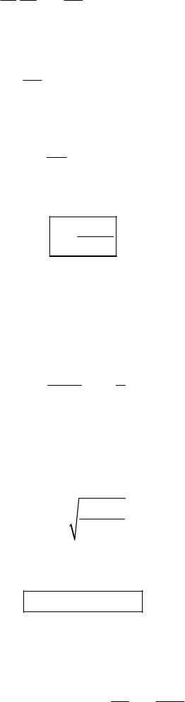
150 CHAPTER 5
5-2. Inside the sphere the gravitational potential satisfies
(
)
24Gr
φ
πρ
∇= (1)
Since
ρ
(r) is spherically symmetric,
φ
is also spherically symmetric. Thus,
()
2
2
14rG
rr r
φπρ
∂∂
=
∂∂
r
(2)
The field vector is independent of the radial distance. This fact implies
r
φ
∂
∂
= constant ≡ C (3)
Therefore, (2) becomes
24
CG
r
π
ρ
= (4)
or,
2
C
Gr
ρπ
= (5)
5-3. In order to remove a particle from the surface of the Earth and transport it infinitely far
away, the initial kinetic energy must equal the work required to move the particle from e
rR
=
to r = ∞ against the attractive gravitational force:
2
0
2
1
2
e
e
R
Mm
Gdrm
r
∞=
∫v
(1)
where e
M
and are the mass and the radius of the Earth, respectively, and is the initial
velocity of the particle at .
e
R0
v
e
rR=
Solving (1), we have the expression for :
0
v
0
2e
e
GM
vR
= (2)
Substituting G, , , we have
11 3 2
6.67 10 m /kg s
−
=× ⋅ 24
5.98 10 kg
e
M=× 6
6.38 10 m
e
R=×
011.2 km/secv≅ (3)
5-4. The potential energy corresponding to the force is
2
2
3
2
dx mk
UFdxmk
xx
=− = =−
∫∫
2
(1)
The central force is conservative and so the total energy is constant and equal to the potential
energy at the initial position, x = d:
GRAVITATION 151
22
2
2
11 1
constant 22 2
k
xm
xd
==−=−
2
k
mEm (2)
Rewriting this equation in integrable form,
00
22
2
22
11
dd
dx d x dx
kdx
kxd
=− =− −
−
∫∫
dt (3)
where the choice of the negative sign for the radical insures that x decreases as t increases.
Using Eq. (E.9), Appendix E, we find
0
22
d
d
tdx
k
=− (4)
or
2
d
tk
=
5-5. The equation of motion is
2
Mm
mx G x
=−
(1)
Using conservation of energy, we find
2
11
2xGM E GM
xx
1
∞
−==−
(2)
11
2
dx GM
dt x x∞
=− −
(3)
where is some fixed large distance. Therefore, the time for the particle to travel from
x∞x
∞
to x
is
()
1
2
11
2
xx
xx
xx
dx
xx
GM
GM xx
∞∞
∞
∞
∞
=− =− −
−
∫∫
td
x
Making the change of variable, , and using Eq. (E.7), Appendix E, we obtain
2
xy→
()
1
sin
2
x
x
xx
xxx
GM x
tx
∞
−
∞∞∞
∞
=−−
(4)
If we set x = 0 and 2xx
∞
= in (4), we can obtain the time for the particle to travel the total
distance and the first half of the distance.
152 CHAPTER 5
32
0
0
1
2
x
x
Tdt
GM
∞
∞
==
∫ (5)
232
12
11
22
x
x
x
Tdt
GM
π
∞
∞
∞
== +
∫ (6)
Hence,
12
0
12
T
T
π
π
+
=
Evaluating the expression,
12
0
0.818
T
T= (7)
or
12
0
9
11
T
T≅ (8)
5-6.
α
θ
φ
z
x
y
r
s
P
r
2
drd(cos θ)dφ
Since the problem has symmetry around the z-axis, the force at the point P has only a
z-component. The contribution to the force from a small volume element is
()
2
2cos cos
z
dg G r dr d d
s
ρ
θ
φ
=−
α
(1)
where
ρ
is the density. Using cos
cos zr
s
θ
α
−
= and integrating over the entire sphere, we have
()
()
12
2
32
22
01 0
cos
cos 2cos
a
z
zr
rdrd d
rz rz
π
θ
ρθφ θ
+
−
−
=− +−
∫∫ ∫
gG (2)
Now, we can obtain the integral of cos
θ
as follows:
GRAVITATION 153
()
()
()
()
1
32
22
1
112
22
1
cos cos
2cos
2cos cos
zr
Id
rz rz
rz rz d
z
θθ
θ
θ
θ
+
−
+
−
−
=+−
∂
=− + −
∂
∫
∫
Using Eq. (E.5), Appendix E, we find
()
1
12
22
1
2
12cos
22
Irzrz
zrz
zz z
θ
+
−
∂
=− − + −
∂
∂
=− =
∂ (3)
Therefore, substituting (3) into (2) and performing the integral with respect to r and
φ
, we have
3
2
3
2
22
3
41
3
z
a
gG z
Ga
z
ρ
π
πρ
=
−⋅
=− (4)
But 3
4
3a
π
ρ
is equal to the mass of the sphere. Thus,
2
1
z
gGM
z
=− (5)
Thus, as we expect, the force is the same as that due to a point mass M located at the center of
the sphere.
5-7.
dx
P
R
s
x
The contribution to the potential at P from a small line element is
dG
sdx
ρ
Φ=− (1)
where M
ρ
=
is the linear mass density. Integrating over the whole rod, we find the potential
2
22
2
1M
G
xR
−
Φ=− +
∫
dx
(2)
154 CHAPTER 5
Using Eq. (E.6), Appendix E, we have
2
2
2
22
2
22
24
ln ln
24
R
MGM
GxxR
R
−
++
− + + =−
Φ=
−+ +
22
22
4
ln 4
GM R
R
++
Φ=−
+−
(3)
5-8.
z
z
y
x
r
a
rdrdθdz
z
0
θ
αrzz
2
0
2
+−
()
Since the system is symmetric about the z-axis, the x and y components of the force vanish and
we need to consider only the z-component of the force. The contribution to the force from a
small element of volume at the point (r,
θ
,z) for a unit mass at (0,0, 0
z
) is
()
()
()
2
2
0
0
32
2
2
0
cos
z
rdrd dz
dg G rzz
z
zrdrddz
G
rzz
θ
ρ
α
θ
ρ
=− +−
−
=−
+−
(1)
where
ρ
is the density of the cylinder and where we have used
(
)
()
0
2
2
0
cos zz
rzz
α
−
=+− . We can
find the net gravitational force by integrating (1) over the entire volume of the cylinder. We find
()
2
0
32
2
2
000 0
a
z
zz
rdrddz
rzz
π
ρθ
−
=−gG
+−
∫∫∫
Changing the variable to , we have
0
xz z=−
0
0
32
22
0
2
z
a
z
z
xdx
gGrdr
rx
πρ
−
=
+
∫∫
(2)
Using the standard integral,
GRAVITATION 155
()
32
22
1xdx
ax
ax 2
−
=±
±
∫ (3)
we obtain
()
222
2
00
0
2
a
z
rr
dr rz
rz
πρ
gG
=− −
+
+−
∫
(4)
Next, using Eq. (E.9), Appendix E, we obtain
()
2
22
0
2
zaz az
πρ
2
0
gG
=− + − − + +
(5)
Now, let us find the force by first computing the potential. The contribution from a small
element of volume is
()
2
2
0
rdrd dz
dG
rzz
θ
ρ
Φ=− +− (6)
Integrating over the entire volume, we have
()
2
2
2
000 0
ar
dGdzddr
rzz
π
ρθ
Φ=− +−
∫∫∫
(7)
Using Eq. (E.9), Appendix E, again, we find
()(
2
2
00
0
2dzazzz
πρ
)
zdG
Φ=− + − − −
∫
(8)
Now, we use Eqs. (E.11) and (E.8a), Appendix E, and obtain
(
)
() ()()
2
22
02 2
000
2
22 22 2
0
0000
2ln2
22
1
ln 2 2
22 2
za
Gaz zz
za
az z za z
πρ
−2a
Φ=− − + − + − − + − +
++−−++−+
Thus, the force is
156 CHAPTER 5
() ()
()
()
()()
0
2
22
2
20
0
2
022
22
0000
0
22
22
0
22 0
022 22
000
1
11
222 2
1
11
22 2
z
z
za
za
gGaz
zaz z z a
z
za
za
az az z za
πρ
−
−
−+
−
∂Φ
=− =− + − + +
∂+− −−+ −+
−
+
−+− − +
+−++
(9)
or,
()
2
22
0
2
zaz az
πρ
2
0
gG
=− + − − + +
(10
and we obtain the same result as in (5).
In this case, it is clear that it is considerably easier to compute the force directly. (See the
remarks in Section 5.4.)
5-9.
θP
r
R
a
The contribution to the potential at the point P from a small line element d is
d
Gr
ρ
Φ=−
∫
(1)
where
ρ
is the linear mass density which is expressed as 2
M
a
ρ
π
=
. Using
22
2cosrRa aR
θ
=+− and d = ad
θ
, we can write (1) as
2
22
0
22cos
GM d
Ra aR
π
θ
π
θ
Φ=− +−
∫ (2)
This is the general expression for the potential.
If R is much greater than a, we can expand the integrand in (2) using the binomial expansion:
12
2
2
22
2
22
22
11
12cos
2cos
13
12cos 2cos
28
aa
RRR
Ra aR
aa aa
RR RRR
θ
θ
θθ
−
=− −
+−
=+ − + − +
…
1
(3)
GRAVITATION 157
If we neglect terms of order
3
a
R
and higher in (3), the potential becomes
222
2
22
0
22
22
3
1cos cos
222
3
2
22
GM a a a d
RRR
GM a a
RR
π
θ
θθ
π
ππ π
π
Φ=− + − +
− +
∫
=− (4)
or,
()
2
2
1
14
GM a
RRR
Φ≅− +
(5)
We notice that the first term in (5) is the potential when mass M is concentrated in the center of
the ring. Of course this is a very rough approximation and the first correction term is
2
3
4
GMa
R
−.
5-10.
P
R
x
r
a
R sin θ
R cos θ
θ
φ
Using the relations
()
22
sin 2 sin cosxR aaR
θ
θ
=+−
φ
(1)
222 22
cos 2 sin cosR Ra aRrx
θ
θ
=+ =+−
φ
(2)
2
M
a
ρ
π
=
(the linear mass density), (3)
the potential is expressed by
2
2
0
2
212sincos
dGM d
GrR aa
RR
−
− =Φ=
−−
∫∫
π
ρφ
πθφ
(4)
If we expand the integrand and neglect terms of order
(
)
3
aR and higher, we have
12
22
22
22
13
1 2 sin cos 1 sin cos sin cos
22
aaa aa
RRR RR
2
2
θ
φθφ
−
−−≅+−+
θφ
(5)
Then, (4) becomes
158 CHAPTER 5
22
2
22
13
22 sin
222
GM a a
RRR
π
ππ
πθ
− − +Φ≅
Thus,
()
2
2
2
13
11sin
22
GM a
RRR
θ
− − −Φ≅
(6)
5-11.
P
a
r
z
dm
θ
The potential at P due to a small mass element dm inside the body is
22
2cos
dm dm
dG G
rza za
θ
Φ=− =− +− (1)
Integrating (1) over the entire volume and dividing the result by the surface area of the sphere,
we can find the average field on the surface of the sphere due to dm:
2
222
0
2sin
1
42cos
ave
ad
dm
aza za
π
πθθ
π
dG
θ
Φ= −
+−
∫ (2)
Making the variable change cos
θ
= x, we have
()
1
22
1
22
ave
Gdx
ddm
z
a zax
+
−
Φ=− +−
∫ (3)
Using Eq. (E.5), Appendix E, we find
()()
()()
22 22
11
22
2
2
ave
G
ddmzazaza
za za
za za
Gdm za
Gdm
za
z
Φ=− − + − + + +
−−++
=−
=− (4)
This is the same potential as at the center of the sphere. Since the average value of the potential
is equal to the value at the center of the sphere at any arbitrary element dm, we have the same
relation even if we integrate over the entire body.
GRAVITATION 159
5-12.
O
P
dm
R
r
r'
Let P be a point on the spherical surface. The potential dΦ due to a small amount of mass dm
inside the surface at P is
Gdm
dr
Φ=− (1)
The average value over the entire surface due to dm is the integral of (1) over dΩ divided by 4
π
.
Writing this out with the help of the figure, we have
2
02
2sin
42cos
ave
d
Gdm
RrR
r
π
d
π
θθ
π
θ
Φ=− +−
′
′
∫ (2)
Making the obvious change of variable and performing the integration, we obtain
1
2
12
42
ave
Gdm du Gdm
R
RrRu
r
π
−
Φ=− =−
+−
′
′
∫
d (3)
We can now integrate over all of the mass and get ave Gm R
Φ
=− . This is a mathematical
statement equivalent to the problem’s assertion.
5-13.
R1
R2
R0
ρ2
ρ1
0
R= position of particle. For , we calculate the force by assuming that all mass for
which is at r = 0, and neglect mass for which . The force is in the radially inward
direction ( −).
10
RRR<<
2
0
rR<
e
0
rR>
r
The magnitude of the force is
2
0
GMm
FR
=
where M = mass for which
0
rR<
160 CHAPTER 5
()
33
11 0 1 2
44
33
MR RR
3
π
ρπ
=+−
ρ
So
()
333
11 20 21
2
0
4
3r
Gm RRR
R
π
ρρρ
=− + −Fe
()
3
121
20
2
0
4
3r
R
Gm R
R
ρρ
πρ
−
=− +
Fe
5-14. Think of assembling the sphere a shell at a time (r = 0 to r = R).
For a shell of radius r, the incremental energy is dU = dm
φ
where
φ
is the potential due to the
mass already assembled, and dm is the mass of the shell.
So
2
22
33
33
44
4
MM
r dr r dr
RR
ρπ π
π
== =
rdr
dm
Gm
r
φ
=− where
3
3
r
mM
R
=
So
22
33
0
2
4
6
0
3
3
R
r
R
Udu
M
rdr GMr
RR
GM rdr
R
=
=
=−
=−
∫
∫
∫
2
3
5
GM
UR
=−
5-15. When the mass is at a distance r from the center of the Earth, the force is in the inward
radial direction and has magnitude r
F
:
m
r
3
2
4
3
r
Gm
F
rr
π
ρ
=
where
ρ
is the mass density of the Earth. The equation of motion is
GRAVITATION 161
3
2
4
3
r
Gm
Fmr r
r
π
ρ
==−
or
where
20rr
ω
+=
24
3
G
π
ρ
ω
=
This is the equation for simple harmonic motion. The period is
23
TG
π
π
ω
ρ
==
Substituting in values gives a period of about 84 minutes.
5-16.
z
y
x
M
h
r
θrh
22
+
For points external to the sphere, we may consider the sphere to be a point mass of mass M. Put
the sheet in the x-y plane.
Consider force on M due to the sheet. By symmetry, 0
xy
F
F
=
=
()
22
0
cos
zz
r
GMdm
FdF rh
θ
∞
=
== +
∫∫
With 2
s
dm rdr
ρ
π
= and 22
sh
rh
θ
=+
co
we have
()
()
32
22
0
12
22
0
2
1
2
2
zs
r
zs
zs
rdr
FGMh
rh
FGMh
rh
FGM
πρ
πρ
πρ
∞
=
∞
=+
=−
+
=
∫
Th
e sphere attracts the sheet in the -direction
with a force of magnitude 2 s
z
GM
πρ
162 CHAPTER 5
5-17.
y
x
Earth
moon
(not to scale)
water
Start with the hint given to us. The expression for and
x
g
y
g are given by
33
2me
x
GM x GM x
DR
g=−; 3
m
y
GM y GM y
gDR
=− − 3
e
(1)
where the first terms come from Equations (5.54) and the second terms come from the standard
assumption of an Earth of uniform density. The origin of the coordinate system is at the center
of the Earth. Evaluating the integrals:
max 2
max
33
0
2
2
xme
x
GM GM x
gdx DR
=−
∫; max
2
max
33
02
yme
y
y
GM GM
gdy DR
=− −
∫
(2)
To connect this result with Example 5.5, let us write (1) in the following way
()
2
22
max
max max max
33
22
me
yGM
xx
DR
+= −
2
y
GM (3)
The right-hand side can be factored as
()()
()
()
max max max max
32
22
e
GM GM
xyxy Rhg
RR
+−=
3
e
h=
2
R
(4)
If we make the approximation on the left-hand side of (3) that , we get exactly
Equation (5.55). Turning to the exact solution of (3), we obtain
22
max max
xy
33 3 3
33 3 3
2
22
em e
em e
MM M M
RD R D
hR
MM M M
RD R D
+− −
=
++ −
m
m
(5)
Upon substitution of the proper values, the answer is 0.54 m, the same as for Example 5.5.
Inclusion of the centrifugal term in does not change this answer significantly.
x
g
GRAVITATION 163
5-18. From Equation (5.55), we have with the appropriate substitutions
2
3
3
moon
2
sun
3
3
2
3
2
m
mes
ss
es
GM r
gD
hM
GM r
hM
gR
R
D
==
(1)
Substitution of the known values gives
3
22 11
moon
30 8
sun
7350 10 kg 1 495 10 m 22
1 993 10 kg 3 84 10 m
h
h
.× .×
=
.× .×
.
(2)
5-19.
ω
earth
ω
moon
Because the moon’s orbit about the Earth is in the same sense as the Earth’s rotation, the
difference of their frequencies will be half the observed frequency at which we see high tides.
Thus
tides earth moon
111
2TTT
=− (1)
which gives T 12 hours, 27 minutes.
tides
5-20. The differential potential created by a thin loop of thickness dr at the point (0,0,z) is
(
)
()
2
22
22 2
22 22
22
() () ()
GrdrMGMdr GM
dz z dz z R z
RR R
zr zr
π
π
−− −
Φ= = ⇒Φ=Φ= + −
++
∫
Then one can find the gravity acceleration,
22
222
2
ˆˆ
() dGMzR
k k
dz R zR
z
gz
Φ
+−
=− =−
+
where is the unit vector in the z-direction.
ˆ
k

164 CHAPTER 5
5-21. (We assume the convention that D > 0 means m is not sitting on the rod.)
The differential force dF acting on point mass m from the element of thickness dx of the rod,
which is situated at a distance x from m, is
(
)
22
()
LD
D
GMLmdx GMm dx GMm
dF F dF
xLx
+
=⇒===
+
∫∫
DLD
And that is the total gravitational force acting on m by the rod.
CHAPTER 6
Some Methods in the
Calculus o
f
Variations
6-1. If we use the varied function
(
)
(
)
,sin1yxx x
α
απ
=
+− (1)
Then
(
1cos1
dy x
dx
απ π
)
=
−− (2)
Thus, the total length of the path is
() ()
2
1
0
112
22 2
0
1
2 cos 1 cos 1
dy
Sdx
dx
xx
απ π α π π
=+
−+ −
∫
∫2
=− (3)
dx
Setting
(
)
1xu
π
−≡, the expression for S becomes
12
22 2
0
11
21 cos cos
2
π
απ α π
π
=−+
∫
Su (4)
udu
The integral cannot be performed directly since it is, in fact, an elliptic integral. Because
α
is a
small quantity, we can expand the integrand and obtain
2
22 2 22 2
0
21 1 1 1
1 cos cos cos cos
22 82
Suuuu
π
απ α π απ α π
π
=− − − − +
∫…du
(5)
If we keep the terms up to co and perform the integration, we find
2
su
22
2
216
S
π
α
=+ (6)
which gives
165
166 CHAPTER 6
2
2
8
S
π
α
α
∂=
∂ (7)
Therefore
0
0
a
S
α
=
∂
=
∂ (8)
and S is a minimum when
α
= 0.
6-2. The element of length on a plane is
2
dS dx dy=+
2
(1)
from which the total length is
()
(
)
22 2
11 1
,2
22
,
1
xy x
xy x
dy
Sdxdy dx
=+=+
∫∫
dx
(2)
If S is to be minimum, f is identified as
2
1dy
fdx
=+
(3)
Then, the Euler equation becomes
2
1
dd y
dx dy
0
+
=
′
′ (4)
where dy
ydx
=
′. (4) becomes
20
1
y
d
dx y
′
=
+′
(5)
or,
2
1
y
y
′
+
′
= constant ≡ C (6)
from which we have
2
2
1
C
yC
=
′− = constant ≡ a (7)
Then,
yaxb
=
+ (8)
This is the equation of a straight line.
SOME METHODS IN THE CALCULUS OF VARIATIONS 167
6-3. The element of distance in three-dimensional space is
22
dS dx dy dz=++
2
(1)
Suppose x, y, z depends on the parameter t and that the end points are expressed by
(
)
(
)
(
)
(
)
11 11 11
,,xt yt zt ,
(
)
(
)
(
)
(
)
22 22 22
,,xt yt zt . Then the total distance is
2
1
2
22
t
t
dy
dx dz
S
dt dt dt
=++
∫dt
(2)
The function f is identified as
222
f
xyz
=
++
(3)
Since 0
fff
xyz
∂∂∂
===
∂∂∂ , the Euler equations become
0
0
0
f
d
dt x
f
d
dt y
f
d
dt z
∂=
∂
∂
=
∂
∂
=
∂
(4)
from which we have
1
222
2
222
3
222
constant
constant
constant
xC
xyz
yC
xyz
zC
xyz
=≡
++
=≡
++
=≡
++
(5)
From the combination of these equations, we have
12
23
y
x
CC
y
z
CC
=
=
(6)
If we integrate (6) from t to the arbitrary t, we have
1
168 CHAPTER 6
1
1
12
11
23
yy
xx
CC
yy
z
z
CC
−
−
=
−−
=
(7)
On the other hand, the integration of (6) from to gives
1
t2
t
21
21
12
21 21
23
yy
xx
CC
yy
z
z
CC
−
−
=
−−
=
(8)
from which we find the constants , C, and C. Substituting these constants into (7), we find
1
C2 3
1
1
21 21 21
yy
xx zz
xx yy zz
−
−−
==
−−−
1
(9)
This is the equation expressing a straight line in three-dimensional space passing through the
two points
(
)
111
,,xyz,
(
)
222
,,xyz.
6-4.
x
y
z
1
2dS
φ
ρ
The element of distance along the surface is
22
dS dx dy dz=++
2
(1)
In cylindrical coordinates (x,y,z) are related to (
ρ
,
φ
,z) by
cos
sin
x
y
zz
ρ
φ
ρ
φ
=
=
=
(2)
from which
sin
cos
dx d
dy d
dz dz
ρ
φφ
ρφφ
=−
=
=
(3)
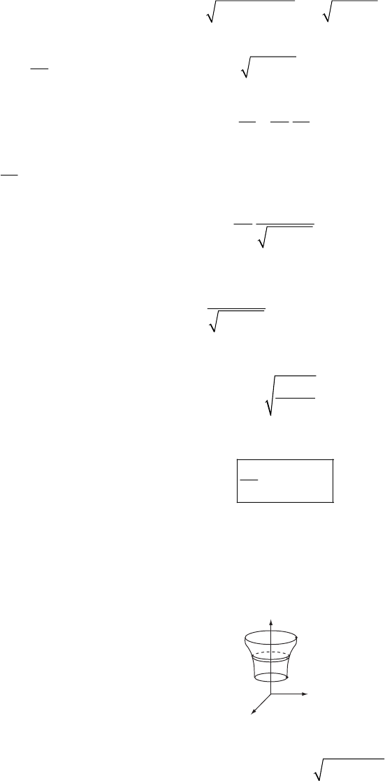
SOME METHODS IN THE CALCULUS OF VARIATIONS 169
Substituting (3) into (1) and integrating along the entire path, we find
2
1
2
22 2 2 2
1
Sddz z
φ
φ
d
ρ
φρ
=+=+
∫∫
φ
(4)
where dz
zd
φ
=
. If S is to be minimum, 22
f
z
ρ
≡
+ must satisfy the Euler equation:
0
ff
zz
φ
∂
∂
∂
−
=
∂∂∂
(5)
Since 0
f
z
∂=
∂, the Euler equation becomes
22
0
z
z
φρ
∂
=
∂+
(6)
from which
22
z
z
ρ
+
= constant ≡ C (7)
or,
2
2
1
C
zC
ρ
=−
(8)
Since
ρ
is constant, (8) means
constant
dz
d
φ
=
and for any point along the path, z and
φ
change at the same rate. The curve described by this
condition is a helix.
6-5.
ds
(x
1
,y
1
)
(x
2
,y
2
)
y
x
z
The area of a strip of a surface of revolution is
2
22dA ds dx dy
ππ
=×=× +
2
(1)
Thus, the total area is
170 CHAPTER 6
2
1
2
21
x
x
A
xy
π
=+
∫dx (2)
where dy
ydx
=
. In order to make A a minimum, 2
1
f
xy≡+
must satisfy equation (6.39). Now
2
2
1
1
fy
x
f
xy
yy
∂
=+
∂
∂=
∂+
Substituting into equation (6.39) gives
()
()
2
22
22
12
22
2
11
11
11
1
xy
dd
yxy
dx dx
yy
y xydydx y
y
−
x
+= +− =
++
+− +
=+
Multiplying by 2
1y+ and rearranging gives
()
2
1
dy
dx
xyy
−= +
Integration gives
2
2
1
ln ln ln
21
y
xa y
−+=
+
where ln a is a constant of integration. Rearranging gives
()
2
22
1
1
yxa
=
−
Integrating gives
1
cosh x
yba a
−
=+
or
cosh yb
xa a
−
=
which is the equation of a catenary.
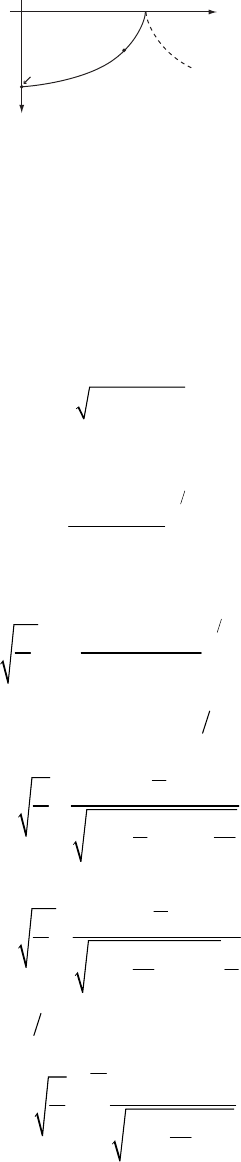
SOME METHODS IN THE CALCULUS OF VARIATIONS 171
6-6.
(x
1
,y
1
)
(x
2
,y
2
)
2a
0
θ = 0
θ = π
x
y
If we use coordinates with the same orientation as in Example 6.2 and if we place the minimum
point of the cycloid at (2a,0) the parametric equations are
(
)
()
1cos
sin
xa
ya
θ
θ
θ
=+
=+
(1)
Since the particle starts from rest at the point
(
)
11
,xy, the velocity at any elevation x is [cf. Eq.
6.19]
(
)
1
2vgxx=− (2)
Then, the time required to reach the point
(
)
22
,xy is [cf. Eq. 6.20]
()
2
1
12
2
1
1
2
x
x
y
t
gx x
+′
=
−
∫dx
(3)
Using (1) and the derivatives obtained therefrom, (3) can be written as
1
2
12
1
0
1cos
cos cos
a
t
g
θ
θ
θ
d
θ
θθ
=
+
=
−
∫
(4)
Now, using the trigonometric identity, 2
cos 2 cos 21
θ
θ
+= , we have
1
1
22
1
0
22
1
0
cos 2
cos cos
22
cos 2
sin sin
22
d
a
tg
d
a
g
θ
θ
θ
θ
θ
θ
θθ
θ
θ
=
−
=
−
∫
∫ (5)
Making the change of variable, sin 2
z
θ
=, the expression for t becomes
1
sin 2
22
1
0
2
sin 2
adz
tg
z
θ
θ
=
−
∫ (6)
The integral is now in standard form:
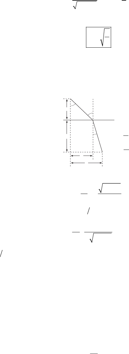
172 CHAPTER 6
1
22
sin
dx x
a
ax
−
=
=
∫ (7)
Evaluating, we find
a
tg
π
= (8)
Thus, the time of transit from
(
)
11
,xy to the minimum point does not depend on the position of
the starting point.
6-7.
vc
n
1
1
=
vc
n
2
2
=
n
1
n
2
θ
1
θ
1
θ
2
(n
2
> n
1
)
d
b
x
a
The time to travel the path shown is (cf. Example 6.2)
2
1y
ds
t
vv
+′
==
∫∫ dx
(1)
Although we have v = v(y), we only have 0dv dy
≠
when y = 0. The Euler equation tells us
20
1
y
d
dx vy
′
=
+′
(2)
Now use vcn= and y′ = –tan
θ
to obtain
n sin
θ
= const. (3)
This proves the assertion. Alternatively, Fermat’s principle can be proven by the method
introduced in the solution of Problem 6-8.
6-8. To find the extremum of the following integral (cf. Equation 6.1)
(
)
,
J
fyxdx=∫
we know that we must have from Euler’s equation
0
f
y
∂
=
∂
This implies that we also have
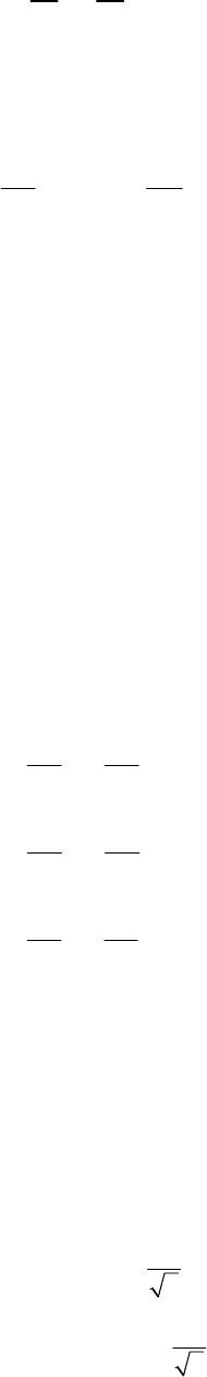
SOME METHODS IN THE CALCULUS OF VARIATIONS 173
0
f
Jdx
yy
∂
∂
=
=
∂∂
∫
giving us a modified form of Euler’s equation. This may be extended to several variables and to
include the imposition of auxiliary conditions similar to the derivation in Sections 6.5 and 6.6.
The result is
()
0
j
j
j
ii
g
Jx
yy
λ
∂
∂
+
=
∂∂
∑
when there are constraint equations of the form
(
)
,0
ji
gyx
=
a) The volume of a parallelepiped with sides of lengths , b, is given by
1
a11
c
111
Vabc
=
(1)
We wish to maximize such a volume under the condition that the parallelepiped is
circumscribed by a sphere of radius R; that is,
(2)
222
111
4abc R++= 2
We consider , , c as variables and V is the function that we want to maximize; (2) is the
constraint condition:
1
a1
b1
{
}
111
,, 0gabc
=
(3)
Then, the equations for the solution are
11
11
11
0
0
0
g
V
aa
g
V
bb
g
V
cc
λ
λ
λ
∂
∂+=
∂∂
∂
∂
+=
∂∂
∂
∂
+=
∂∂
(4)
from which we obtain
11 1
11 1
11 1
20
20
20
bc a
ac b
ab c
λ
λ
λ
+=
+=
+=
(5)
Together with (2), these equations yield
111
2
3
abc R=== (6)
Thus, the inscribed parallelepiped is a cube with side 2
3R.
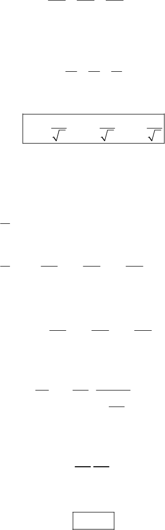
174 CHAPTER 6
b) In the same way, if the parallelepiped is now circumscribed by an ellipsoid with semiaxes
a, b, c, the constraint condition is given by
222
111
222
1
444
abc
abz
=
== (7)
where , , c are the lengths of the sides of the parallelepiped. Combining (7) with (1) and
(4) gives
1
a1
b1
22
11
22
abc
abc
2
1
2
=
= (8)
Then,
111
22
,,
33
aa bb cc===
2
3
(9)
6-9. The average value of the square of the gradient of
(
)
123
,,xxx
φ
within a certain volume V
is expressed as
()
2
123
2
22
12
123
1
1
Idxdxdx
V
Vxxx
φ
φφφ
=∇
∂∂∂
=+ +
∂∂∂
∫∫∫
∫∫∫ 3
dxdxdxv (1)
In order to make I a minimum,
2
22
12
fxxx
3
φ
φφ
∂∂∂
=++
∂∂∂
must satisfy the Euler equation:
3
1
0
ii
i
ff
x
x
φφ
=
∂∂
∂
−
=
∂∂
∂
∂
∂
∑ (2)
If we substitute f into (2), we have
3
1
0
iii
xx
φ
=
∂∂
=
∂∂
∑ (3)
which is just Laplace’sequation:
20
φ
∇
= (4)
Therefore,
φ
must satisfy Laplace’s equation in order that I have a minimum value.
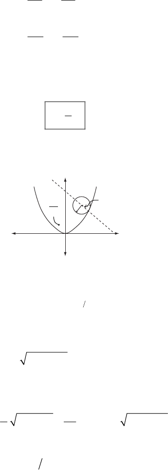
SOME METHODS IN THE CALCULUS OF VARIATIONS 175
6-10. This problem lends itself to the method of solution suggested in the solution of Problem
6-8. The volume of a right cylinder is given by
(1)
2
VR
π
=H
The total surface area A of the cylinder is given by
(
)
2
bases side 22 2
A
AA RRHRR
ππ π
=+ = +H=+ (2)
We wish A to be a minimum. (1) is the constraint condition, and the other equations are
0
0
g
A
RR
g
A
HH
λ
λ
∂
∂
+=
∂∂
∂
∂
+=
∂∂
(3)
where .
20gV RH
π
=− =
The solution of these equations is
1
2
RH= (4)
6-11.
y
ds
Rθ
}
1
2a
The constraint condition can be found from the relation ds = Rd
θ
(see the diagram), where ds is
the differential arc length of the path:
(
)
12
22
ds dx dy Rd
θ
=+ = (1)
which, using , yields
2
yax=
22
14ax dx Rd
θ
+= (2)
If we want the equation of constraint in other than a differential form, (2) can be integrated to
yield
(
)
2
1
41ln2 4
24
xax ax ax
a
θ
+= ++ + +
22
1
AR (3)
where A is a constant obtained from the initial conditions. The radius of curvature of a parabola,
, is given at any point (x,y) by
2
yax=012≥r. The condition for the disk to roll with one and
only one point of contact with the parabola is
a
0
Rr
<
; that is,
176 CHAPTER 6
1
2
Ra
< (4)
6-12. The path length is given by
22
1sds y zd== ++
′′
∫∫ x (1)
and our equation of constraint is
(
)
2222
,, 0gxyz x y z
ρ
=
++−= (2)
The Euler equations with undetermined multipliers (6.69) tell us that
22 2
1
ydg
dy
dx dy
yz
λ
λ
′
==
++
′′
(3)
with a similar equation for z. Eliminating the factor
λ
, we obtain
22 22
0
11
y
ddz
ydx zdx
yz yz
′′
11
−
=
++ ++
′′ ′′
(4)
This simplifies to
(
)
(
)
(
)
(
)
22 22
11zy y z y yy zz yz y z z yy zz
++ − + − ++ − + =
′′ ′ ′ ′ ′ ′′ ′ ′′ ′′ ′ ′ ′ ′ ′′ ′ ′′
0
(5)
(
)
(
)
0yy zz z y yz yy zz y z−−+ =
′′ ′ ′ ′ ′′ ′′ ′ ′ ′ ′′
zy ++ (6)
and using the derivative of (2),
(
)
(
)
z
xz y y xy z−=−
′
′′ ′ ′′ (7)
This looks to be in the simplest form we can make it, but is it a plane? Take the equation of a
plane passing through the origin:
A
xByz
+
= (8)
and make it a differential equation by taking derivatives (giving A + By′ = z′ and By″ = z″) and
eliminating the constants. The substitution yields (7) exactly. This confirms that the path must
be the intersection of the sphere with a plane passing through the origin, as required.
6-13. For the reason of convenience, without lost of generality, suppose that the closed curve
passes through fixed points A(-a,0) and B(a,0) (which have been chosen to be on axis Ox). We
denote the part of the closed curve above and below the Ox axis as and respectively.
(note that and )
1()yx 2()yx
10y>20y<
The enclosed area is
()
12 1 2 1 2 12
(, ) () () () () (, )
aa a a
aa a a
J
yy yxdx yxdx yx yxdx fyydx
−− − −
=−=−=
∫∫∫ ∫
SOME METHODS IN THE CALCULUS OF VARIATIONS 177
The total length of closed curve is
() () () () ()
{
}
()
22 22
12 1 2 1 1 12
,1 1 1 1 ,
aa a a
aa a a
Ky y y dx y dx y y dx gy y dx
−− − −
=+ ++ = + ++ =
′′ ′ ′ ′ ′ ′′
∫∫∫ ∫
Then the generalized versions of Eq. (6.78) (see textbook) for this case are
1
2
1111 1
01 1()
ffgg y
dd d
ydxy ydxy dx y
λλ
∂∂∂∂ ′
−+− =⇒−
∂∂∂∂
′′
+′
0
=
(1)
2
2
2222 2
01 1( )
ffgg y
dd d
ydxy ydxy dx y
λλ
∂∂∂∂ ′
−+− =⇒−
∂∂∂∂
′′
+′
0
=
(2)
Analogously to Eq. (6.85);
from (1) we obtain
(
)
(
)
222
112
xA y A
λ
−
+− = (3)
from (2) we obtain
(
)
(
)
222
122
xB y B
λ
−
+− = (4)
where constants A’s, B’s can be determined from 4 initial conditions
(
)
1
,0xay=± = and
(
)
2
,0xay
=
±=
We note that and , so actually (3) and (4) altogether describe a circular path of
radius
10y<20y>
λ
. And this is the sought configuration that renders maximum enclosed area for a given
path length.
6-14. It is more convenient to work with cylindrical coordinates (r,
φ
,z) in this problem. The
constraint here is z = 1 – r , then dz = –dr
(
)
22222 22
2s dr r d dz dr r d 2
d
φ
β
=+ += +
where we have introduced a new angular coordinate 2
φ
β
=
In this form of , we clearly see that the space is 2-dimensional Euclidean flat, so the shortest
line connecting two given points is a straight line given by:
2
ds
()
00
0
0
cos cos 2
rr
r
φ
φ
ββ
==
−
−
this line passes through the endpoints (r = 1, 2
π
φ
=
±) , then we can determine unambiguously
the shortest path equation
cos 22
()
cos 2
r
π
φ
φ
=
and z = 1 – r
178 CHAPTER 6
Accordingly, the shortest connecting length is
22
2
2
222sin
22
dr r
d
π
π
ld
π
φφ
−
=+=
∫
6-15.
2
1
2
0
[] dy
Iy y dx
dx
=−
∫
a) Treating I[y] as a mechanical action, we find the corresponding Euler-Lagrange equation
2
2
() dy
yx dx
=−
Combining with the boundary conditions (x = 0, y = 0) and (x = 1, y = 1), we can determine
unambiguously the functional form of () (sin )(sin1)yx x
=
.
b) The corresponding minimum value of the integral is
2
11
2
2
00
1
[ ] cos 2 cot (1) 0.642
sin 1
dy y dx dx x
dx
=−= ==
∫∫
Iy
c) If x = y then I[y] = ( 2 3 ) = 0.667.
6-16.
a) S is arc length
22
2
222 9
11
4
dy dy
dz
S dxdydz dx dx x Ld
dx dx dx
=++=++=++=
∫∫ ∫ x
∫
Treating S and L like a mechanical action and Lagrangian respectively, we find the canonical
momentum associated with coordinate y
2
9
14
dy
Ldx
pdy dy
x
dx dx
δ
δ
==
++
Because L does not depend on y explicitly, then E-L equation implies that p is constant
(i.e. 0dp dx =), then the above equation becomes
32
22
9
199
411
11 44
x
dy p
p
ydxxAx
dx p p
+
= +=+
−−
∫B
+=⇒
where A and B are constants. Using boundary conditions (x = 0, y = 0) and (x = 1, y = 1) one can
determine the arc equation unambiguously
SOME METHODS IN THE CALCULUS OF VARIATIONS 179
32
32
89
() 1 1
13 8 4 xyx
=+−
−
and 32
z
x=
b)
z
x
y
0
0.25
0.5
0.75
1
0
0.25
0.5
0.75
1
0
0.25
0.5
0.75
1
0
0.25
0.5
0.
1
0
6-17.
a) Equation of a ellipse
2
2
22
1
y
x
ab
+
=
which implies
2
ab
xy ≤ because
2
2
22
2xy y
x
ab a b
≤+
so the maximal area of the rectangle, whose corners lie on that ellipse, is
Max[A] = Max[4xy] = 2 iab.
This happens when
2
a
x= and 2
b
y=
b) The area of the ellipse is 0
A
ab
π
=; so the fraction of rectangle area to ellipse area is then
0
[] 2Max A
A
π
=
6-18. One can see that the surface xy = z is “locally” symmetric with respect to the line
xy=− = −z where x > 0, y < 0, z < 0. This line is a parabola. This implies that if the particle
starts from point (1,-1,-1) (which belongs to the symmetry line) under gravity ideally will move
downward along this line. Its velocity at altitude z (z < –1) can be found from the conservation
of energy.
() 2( 1)vz gz
=
−+
180 CHAPTER 6
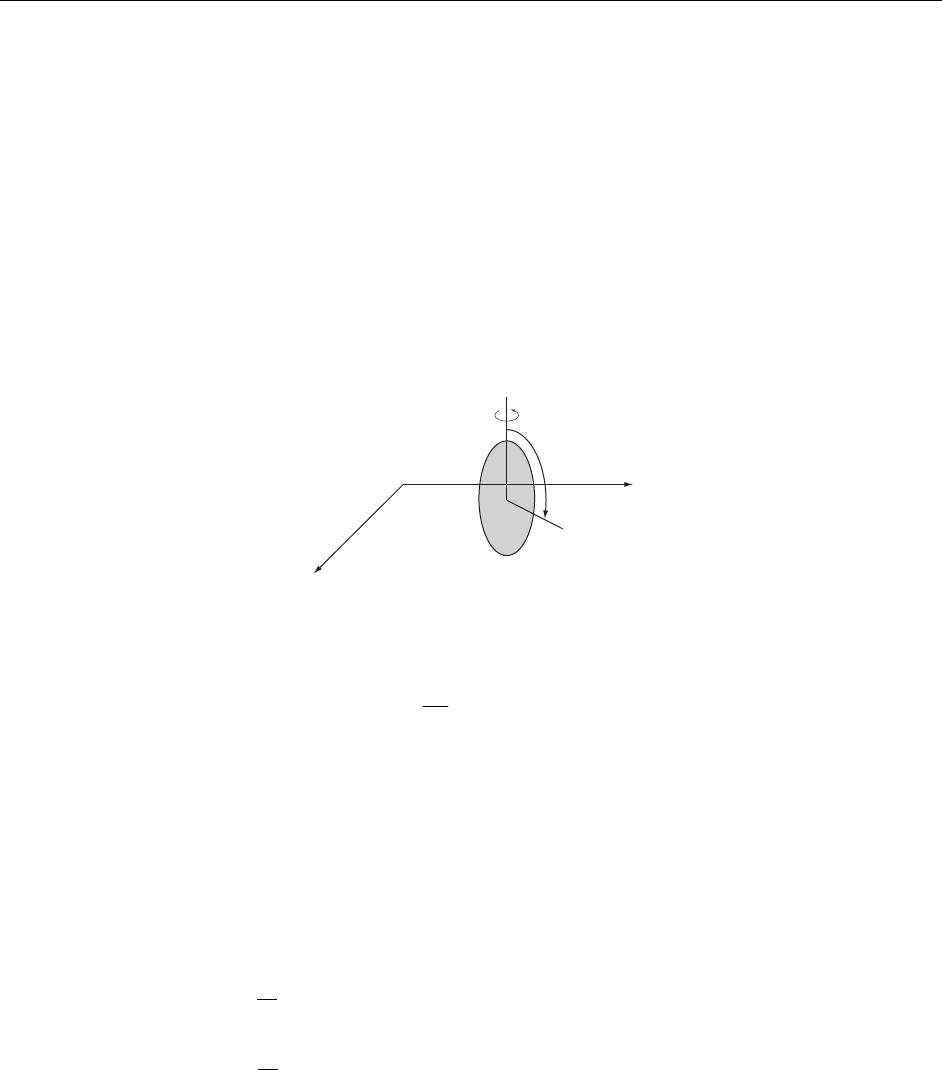
CHAPTER 7
Hamilton’s Principle
—
Lagrangian and
H
amiltonian D
y
namics
7-1. Four coordinates are necessary to completely describe the disk. These are the x and y
coordinates, the angle
θ
that measures the rolling, and the angle
φ
that describes the spinning
(see figure).
φ
θ
x
y
Since the disk may only roll in one direction, we must have the following conditions:
cos sindx dy R d
φ
φθ
+
= (1)
tan
dy
dx
φ
= (2)
These equations are not integrable, and because we cannot obtain an equation relating the
coordinates, the constraints are nonholonomic. This means that although the constraints relate
the infinitesimal displacements, they do not dictate the relations between the coordinates
themselves, e.g. the values of x and y (position) in no way determine
θ
or
φ
(pitch and yaw),
and vice versa.
7-2. Start with the Lagrangian
()()
22
0cos sin cos
2
mat mgLv
θ
θθθ
=++ + +
θ
(1)
()()
222
00
2cos
2
mvat vat mgcos
θ
θθ
++ ++
θ
=+ (2)
181
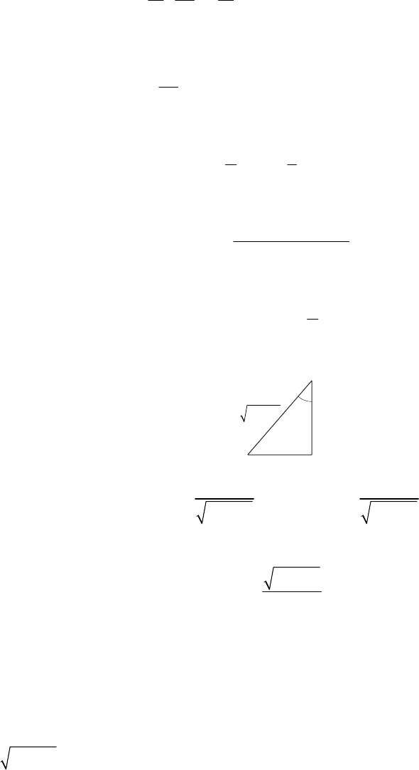
182 CHAPTER 7
Now let us just compute
()
2
0cos
dL d
mv at m
dt dt
θ
θ
θ
∂
=+ +
∂
(3)
(
)
2
0
cos sinma m v at m
θ
θθ
=−− +
θ
(4)
()
0sin sin
Lmv at mg
θ
θ
θ
∂+ −
∂
θ
=− (5)
According to Lagrange’s equations, (4) is equal to (5). This gives Equation (7.36)
sin cos 0
ga
θθθ
=
+
=
(6)
To get Equation (7.41), start with Equation (7.40)
cos sin
e
ga
e
θ
θ
η
η
−
=−
(7)
and use Equation (7.38)
tan e
a
g
θ
=
− (8)
to obtain, either through a trigonometric identity or a figure such as the one shown here,
g
a
θ
e
ga
22
+
22
sg
ga
+
co e
θ
= 22
sin e
a
ga
θ
=+ (9)
Inserting this into (7), we obtain
22
ag
η
η
+
=−
(10)
as desired.
We know intuitively that the period of the pendulum cannot depend on whether the train is
accelerating to the left or to the right, which implies that the sign of a cannot affect the
frequency. From a Newtonian point of view, the pendulum will be in equilibrium when it is in
line with the effective acceleration. Since the acceleration is sideways and gravity is down, and
the period can only depend on the magnitude of the effective acceleration, the correct form is
clearly 22
ag+.
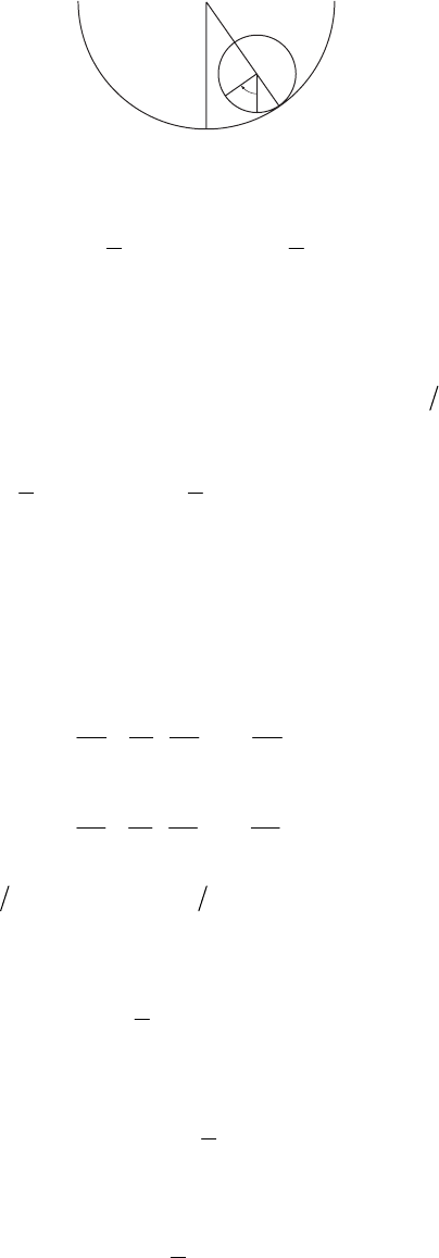
HAMILTON’S PRINCIPLE—LAGRANGIAN AND HAMILTONIAN DYNAMICS 183
7-3.
θ
ρφθ
R
If we take angles
θ
and
φ
as our generalized coordinates, the kinetic energy and the potential
energy of the system are
()
22
1
22
TmR I
1
ρ
θ
=−+
φ
(1)
(
)
cosURR m
ρθ
=−−
g
(2)
where m is the mass of the sphere and where U = 0 at the lowest position of the sphere. I is the
moment of inertia of sphere with respect to any diameter. Since
(
)
2
25Im
ρ
=, the Lagrangian
becomes
() ()
2222
11 cos
25
U mR m R R mg
ρθ ρφ ρ θ
=−= − + − − −
LT (3)
When the sphere is at its lowest position, the points A and B coincide. The condition A0 = B0
gives the equation of constraint:
(
)
(
)
,fR
θφ ρθ ρφ
0
=
−−= (4)
Therefore, we have two Lagrange’s equations with one undetermined multiplier:
0
0
f
Ld L
dt
f
Ld L
dt
λ
θθ
θ
λ
φφφ
∂
∂∂
−+=
∂∂
∂
∂
∂∂
−+=
∂∂∂
(5)
After substituting (3) and fR
θ
ρ
∂∂=− and f
φ
ρ
∂
∂=− into (5), we find
(
)
(
)
(
)
2
sin 0Rmg mR R
ρθ ρθλρ
− − + −=
−− (6)
2
20
5m
ρφ λρ
−
−=
(7)
From (7) we find
λ
:
2
5m
λ
ρφ
=− (8)
or, if we use (4), we have
()
2
5mR
λ
ρθ
=− − (9)
Substituting (9) into (6), we find the equation of motion with respect to
θ
:
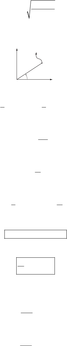
184 CHAPTER 7
2sin
θ
ω
=−
θ
)
(10)
where
ω
is the frequency of small oscillations, defined by
(
5
7
g
R
ω
ρ
=− (11)
7-4.
y
m
x
r
θ
If we choose (r,
θ
) as the generalized coordinates, the kinetic energy of the particle is
()
()
22 222
11
22
Tmxy mrr
θ
=+=+
(1)
Since the force is related to the potential by
U
fr
∂
=−
∂
(2)
we find
A
Ur
α
α
= (3)
where we let U(r = 0) = 0. Therefore, the Lagrangian becomes
()
222
1
2
A
Lmrr r
α
θα
=+−
(4)
Lagrange’s equation for the coordinate r leads to
21
0mr mr Ar
α
θ
−
−
+=
(5)
Lagrange’s equation for the coordinate
θ
leads to
()
20
dmr
dt
θ
=
(6)
Since is identified as the angular momentum, (6) implies that angular momentum is
conserved. Now, if we use , we can write (5) as
2
mr
θ
=
2
1
30mr Ar
mr
α
−
−
+=
(7)
Multiplying (7) by , we have
r
2
1
30
r
mrr Ar r
mr
α
−
−
+
= (8)
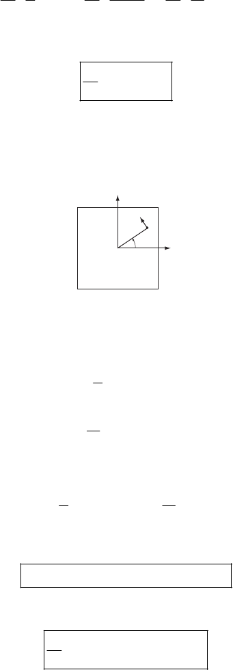
HAMILTON’S PRINCIPLE—LAGRANGIAN AND HAMILTONIAN DYNAMICS 185
which is equivalent to
2
2
2
10
22
dddA
mr r
dt dt mr dt
α
α
+
+
= (9)
Therefore,
()
0
dTU
dt
+
= (10)
and the total energy is conserved.
7-5.
φx
y
rm
Let us choose the coordinate system so that the x-y plane lies on the vertical plane in a
gravitational field and let the gravitational potential be zero along the x axis. Then the kinetic
energy and the potential energy are expressed in terms of the generalized coordinates (r,
φ
) as
(
222
1
2
Tmrr
)
φ
=+
(1)
sin
A
Urmgr
α
φ
α
=+ (2)
from which the Lagrangian is
()
222
1sin
2
A
U mr r r mgr
α
LT
φ
φ
α
=−= + − −
(3)
Therefore, Lagrange’s equation for the coordinate r is
21
sin 0mr mr Ar mg
α
φ
−
φ
−
++ =
(4)
Lagrange’s equation for the coordinate
φ
is
()
2cos 0
dmr mgr
dt
φφ
+
=
(5)
Since 2
mr
φ
is the angular momentum along the z axis, (5) shows that the angular momentum is
not conserved. The reason, of course, is that the particle is subject to a torque due to the
gravitational force.
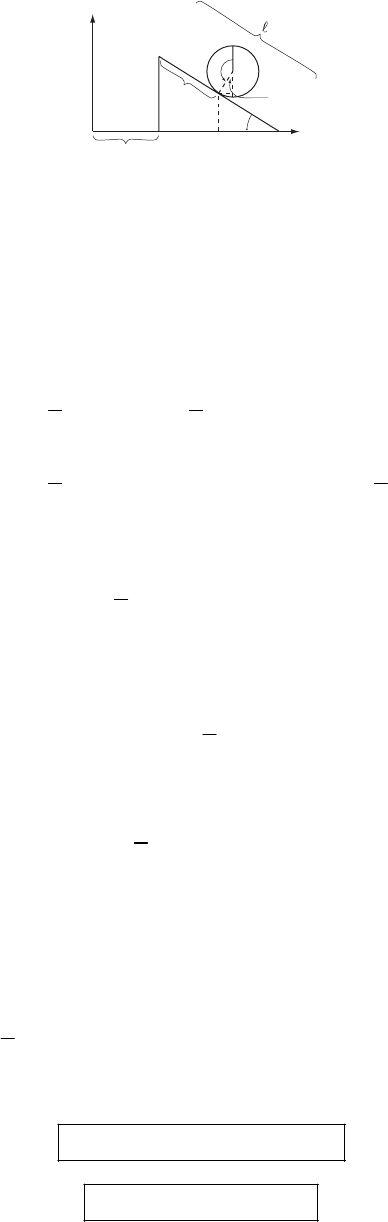
186 CHAPTER 7
7-6.
y
M
S
m
α
α
φ
ξ
x
Let us choose
ξ
,S as our generalized coordinates. The x,y coordinates of the center of the hoop
are expressed by
()
cos sin
cos sin
xS r
yr S
ξαα
α
α
=+ +
=+−
(1)
Therefore, the kinetic energy of the hoop is
()
()
()
22 2
hoop
222
11
22
11
cos sin
22
TmxyI
mS S I
=++
=+ +− +
φ
ξ
ααφ
(2)
Using and
2
Imr=Sr
φ
=, (2) becomes
22
hoop
122cos
2
TmS S
ξ
ξα
=++
(3)
In order to find the total kinetic energy, we need to add the kinetic energy of the translational
motion of the plane along the x-axis which is
2
plane
1
2
TM
ξ
= (4)
Therefore, the total kinetic energy becomes
()
2
21cos
2
TmS mM mS
ξ
ξ
=++ +
α
(5)
The potential energy is
(
)
cos sinUmgymgr S
α
α
== +−
(6)
Hence, the Lagrangian is
() ()
2
21cos cos sin
2
S mM mS mgr Slm
ξ
ξα α
=++ + − +−
α
(7)
from which the Lagrange equations for
ξ
and S are easily found to be
2cossinmS m mg
ξα α
0
+
−
= (8)
()
cos 0mM mS
ξα
+
+
= (9)
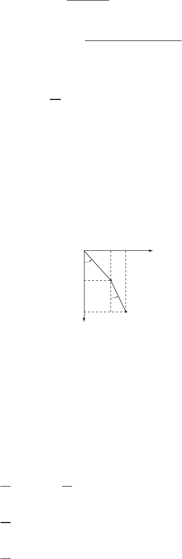
HAMILTON’S PRINCIPLE—LAGRANGIAN AND HAMILTONIAN DYNAMICS 187
or, if we rewrite these equations in the form of uncoupled equations by substituting for
ξ
and
, we have S
()
2
2
cos
2si
sin cos
2cos
mSg
mM
mg
mM m
αα
αα
ξ
n0
α
−−=
+
=−
+−
(10)
Now, we can rewrite (9) as
()
cos 0
dmM mS
dt
ξα
+
+
=
(11)
where we can interpret
(
)
mM
ξ
+ as the x component of the linear momentum of the total
system and cosmS
α
as the x component of the linear momentum of the hoop with respect to
the plane. Therefore, (11) means that the x component of the total linear momentum is a
constant of motion. This is the expected result because no external force is applied along the
x-axis.
7-7.
x
1
y
1
y
2
x
2
m
y
m
x
φ
1
φ
2
If we take
(
)
12
,
φ
φ
as our generalized coordinates, the x,y coordinates of the two masses are
11
11
cos
sin
x
y
φ
φ
=
=
(1)
21
21
cos cos
sin sin
x
y
2
2
φ
φ
φφ
=+
=+
(2)
Using (1) and (2), we find the kinetic energy of the system to be
()()
()
()
22 22
11 22
2222
112 12 1 2 1 2
222
12 12 12
22
2sinsincoscos
2
22cos
2
mm
Txy xy
m
m
φ
φφ φφ φ φ φ φ
φφ φφ φφ
=+++
= +++ +
+ −
=+ (3)
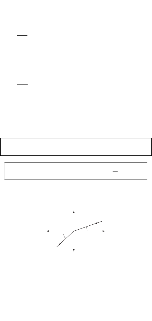
188 CHAPTER 7
The potential energy is
Um
12 1
2cos cosgxmgx mg 2
φ
φ
=− − =− +
(4)
Therefore, the Lagrangian is
()
22 2
1212 12 1
1cos 2 cos cos
2mg 2
Lm
φ
φφφ φφ φ φ
=++ −+ +
(5)
from which
()
()
()
()
2
12 1 2 1
1
22
1212
1
2
12 1 2 2
2
22
2112
2
sin 2 sin
2cos
sin sin
cos
Lmm
Lmm
Lmmg
Lmm
g
φ
φφφ φ
φ
φφφφ
φ
φ
φφφ φ
φ
φφφφ
φ
∂
=−−
∂
∂
=+ −
∂
∂
=− − −
∂
∂=+ −
∂
(6)
The Lagrange equations for 1
φ
and 2
φ
are
() ()
2
12 12 2 12 1
cos sin 2 sin 0
g
φφ φ φφ φ
+−+−+
2
φφ
(7)
=
() ()
2
21 12 1 12 2
cos sin sin 0
g
φφ φφ φ φφ φ
+−−−+
=
(8)
7-8.
v
1
v
2
θ
2
θ
1
U
1
U
2
y
x
Let us choose the x,y coordinates so that the two regions are divided by the y axis:
()
1
2
0
0
Ux
Ux
Ux
<
=>
If we consider the potential energy as a function of x as above, the Lagrangian of the particle is
()
()
22
1
2
LmxyUx=+−
(1)
Therefore, Lagrange’s equations for the coordinates x and y are
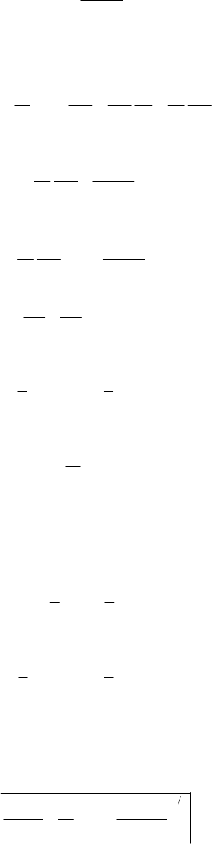
HAMILTON’S PRINCIPLE—LAGRANGIAN AND HAMILTONIAN DYNAMICS 189
(
)
0
dU x
mx dx
+
=
(2)
0my
=
(3)
Using the relation
x
xx x
dp
dP dP P
ddx
mx mx
dt dt dx dt m dx
=== =
(4)
(2) becomes
(
)
0
xx
dU x
PdP
mdx dx
+
= (5)
Integrating (5) from any point in the region 1 to any point in the region 2, we find
(
)
22
11
0
xx dU x
PdPdx dx
mdx dx
+
=
∫∫ (6)
21
22
21
0
22
xx
PP
UU
mm
−
+−= (7)
or, equivalently,
22
11 2
11
22
mx U mx U+= +
2
(8)
Now, from (3) we have
0
dmy
dt
=
and is constant. Therefore, my
1
my my2
=
(9)
From (9) we have
2
1
11
22
my my=
2
2
(10)
Adding (8) and (10), we have
2
11 2
11
22
mv U mv U+= +
2
2
2
(11)
From (9) we also have
11 2
sin sinmv mv
θ
θ
=
(12)
Substituting (11) into (12), we find
12
1212
21 1
sin 1
sin
vUU
vT
θ
θ
−
==+
(13)
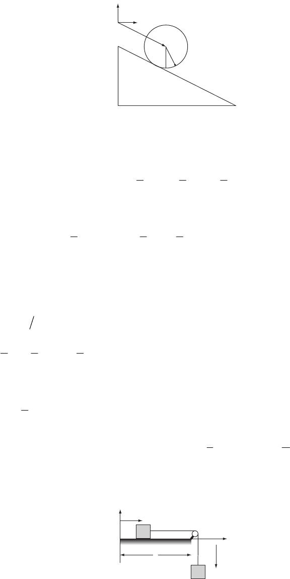
190 CHAPTER 7
This problem is the mechanical analog of the refraction of light upon passing from a medium of
a certain optical density into a medium with a different optical density.
7-9.
Ox
y
M
m
φ
α
ξ
Using the generalized coordinates given in the figure, the Cartesian coordinates for the disk are
(
ξ
cos
α
, –
ξ
sin
α
), and for the bob they are ( sin
φ
+
ξ
cos
α
, – cos
φ
–
ξ
sin
α
). The kinetic
energy is given by
()
22 22
disk bob bob bob
111
222
T M I mx y
ξθ
=+= + + +
TT (1)
Substituting the coordinates for the bob, we obtain
()
(
22 22
111 cos
222
m I m m
ξθ φφξφ
=++ + + +
)
a
TM (2)
The potential energy is given by
(
)
disk bob disk bob sin cosU U Mgy mgy M m g mgU
ξ
α
= + =−+ −
φ
=+ (3)
Now let us use the relation
ξ
= R
θ
to reduce the degrees of freedom to two, and in addition
substitute 22IMR= for the disk. The Lagrangian becomes
()
()
222
31 1 cos sin cos
42 2
LTU M m m m a Mmg mg
ξ
φφξφ ξα
=−= + + + + + + +
φ
(4)
The resulting equations of motion for our two generalized coordinates are
()
() ()
2
3sin cos sin 0
2Mm Mmg m
ξαφφαφφ
+−+ + +− +=
α
(5)
()
1cos sin 0
g
φξ φα φ
+
++ =
(6)
7-10.
MM
MM
yx
x
–y
S

HAMILTON’S PRINCIPLE—LAGRANGIAN AND HAMILTONIAN DYNAMICS 191
Let the length of the string be so that
(
)
Sx y
−
−= (1)
Then,
xy
=
−
(2)
a) The Lagrangian of the system is
22 2
11
22
Mx My Mgy My Mgy=+−=−
L (3)
Therefore, Lagrange’s equation for y is
2
dL L My Mg
dt y y 0
∂
∂
−
=+=
∂∂
(4)
from which
2
g
y
=
−
(5)
Then, the general solution for y becomes
()
2
1
4
g
yt t Ct C
2
=
−++ (6)
If we assign the initial conditions
(
)
0yt 0
=
= and
(
)
0yt 0
=
=
, we find
()
2
4
g
yt t
=− (7)
b) If the string has a mass m, we must consider its kinetic energy and potential energy. These
are
2
string
1
2
T=
my (8)
2
string 22
ymg
m
Uyg
=− =−
y
(9)
Adding (8) and (9) to (3), the total Lagrangian becomes
22
1
22
mg
LMy Mgy my y
=−+ +
2
(10)
Therefore, Lagrange’s equation for y now becomes
()
2
mg
Mmy yMg0
+
−+=
(11)
In order to solve (11), we arrange this equation into the form
()
2mg M
Mmy y m
+= −
(12)
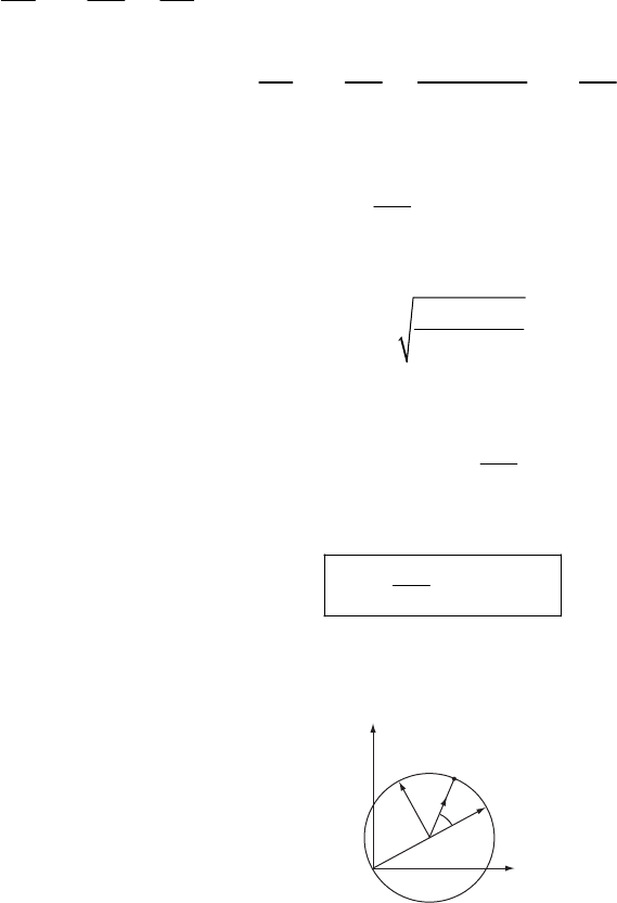
192 CHAPTER 7
Since
22
2
dMd
y
dt m dt
−=
2
y
, (12) is equivalent to
()
2
22
mg
dM M
y
dt m M m m
−= −
+
y
(13)
which is solved to give
t
M
yAeB
m
t
e
γ
γ
−
−= +
(14)
where
()
2
mg
Mm
γ
=+
(15)
If we assign the initial condition
(
)
00yt
=
=;
(
)
0yt 0
=
=
, we have
2
M
AB m
=+ =−
Then,
()
()
1cosh
M
yt t
m
γ
=−
(16)
7-11.
x
x′
m
y
y′
φ
e
r
′
The x,y coordinates of the particle are
(
)
()
cos cos
sin sin
xR tR t
yR tR t
ωφω
ωφω
=++
=++
(1)
Then,
(
)
(
)
()
()
sin sin
cos cos
xR tR t
yR tR t
ω ω φω φω
ω ω φω φω
=− − + +
=+++
(2)
Since there is no external force, the potential energy is constant and can be set equal to zero. The
Lagrangian becomes
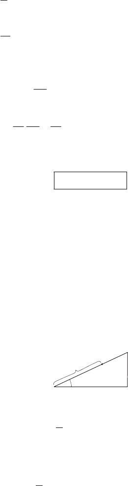
HAMILTON’S PRINCIPLE—LAGRANGIAN AND HAMILTONIAN DYNAMICS 193
()
() ()
22
2
22 2 2
1
2
2c
2
Lmxy
mRR R os
ω
φω ωφω φ
=+
+++
=+ (3)
from which
()
2sin
LmR
ω
φω φ
φ
∂
=− +
∂ (4)
(
2cos
dL d
mR
dt dt
)
φ
ωω φ
φ
∂
=++
∂
(5)
Therefore, Lagrange’s equation for
φ
becomes
2sin 0
φω φ
+
=
(6)
which is also the equation of motion for a simple pendulum. To make the result appear
reasonable, note that we may write the acceleration felt by the particle in the rotating frame as
(
)
2
r
R
ω
=+
′
′
aie (7)
where the primed unit vectors are as indicated in the figure. The part proportional to r
′
e does
not affect the motion since it has no contribution to the torque, and the part proportional to i′ is
constant and does not contribute to the torque in the same way a constant gravitational field
provides a torque to the simple pendulum.
7-12.
r
m
θ
Put the origin at the bottom of the plane
()
222
1sin
2
U mr r mgrLT
θ
θ
=−= + −
;
t
θ
αθα
=
=
()
2
22
1sin
2
Lmr rmgr t
α
α
=+−
Lagrange’s equation for r gives
2sinmr m r mg t
α
α
=−
or
2sinrrg t
α
α
−=−
(1)
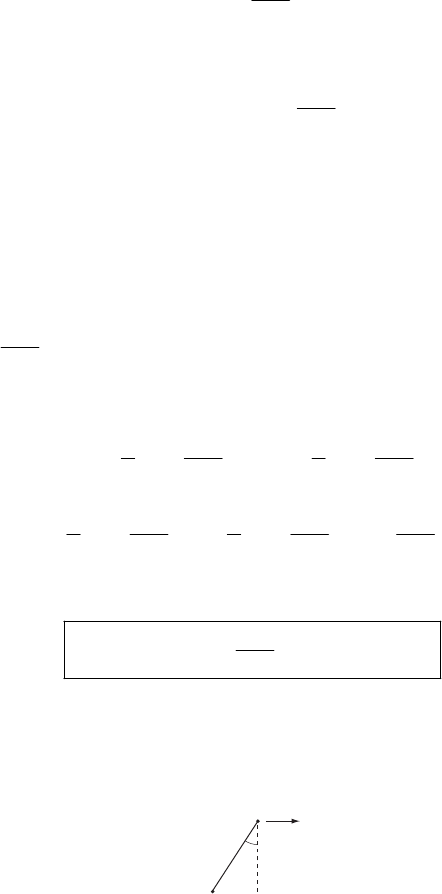
194 CHAPTER 7
The general solution is of the form
p
h
rrr
=
+ where is the general solution of the
homogeneous equation and
h
r
20rr
α
−=
p
r is a particular solution of Eq. (1).
So
tt
h
rAe Be
α
α
−
=+
For
p
r, try a solution of the form rC
sin
pt
α
=. Then 2sin
p
rC t
α
α
=−
. Substituting into (1) gives
22
sin sin sinCtC tgt
α
ααα
−− =−
α
2
2
g
C
α
=
So
()
2sin
2
tt
g
r t Ae Be t
αα
α
α
−
=+ +
We can determine A and B from the initial conditions:
(
)
0
0rr
=
(2)
(
)
00r
=
(3)
(2) implies
0
rA=+B
(3) implies 2
2
g
AB
0
α
=−+
Solving for A and B gives:
00
22
11
22 22
gg
Ar Br
α
α
=− =+
()
00
22
11 sin
22 22 2
tt
ggg
r e r e t
αα
2
rt
α
ααα
−
=− ++ +
or
()
()
02
cosh sin sinh
2
g
r t t trt
α
αα
α
=+ −
7-13.
a)
θ
a
b
m
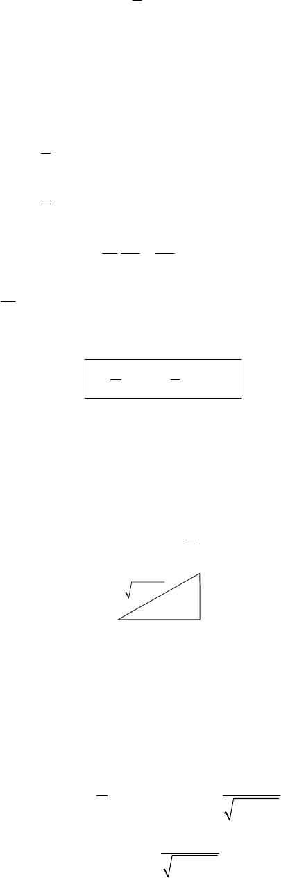
HAMILTON’S PRINCIPLE—LAGRANGIAN AND HAMILTONIAN DYNAMICS 195
2
1sin
2
cos
cos
sin
xatb
yb
xatb
yb
θ
θ
θ
θ
θθ
=−
=−
=−
=
()
()
22
22 2 2
1
2
12cos cos
2
Lmxymgy
mat atb b mgb
θ
θθ
=+−
=− ++
θ
dL L
dt
θ
θ
∂
∂
=
∂
∂ gives
2
cos sin sinmat b mb mat b mgb
dt
d
θ
θθθ
−+= −
θ
This gives the equation of motion
sin cos 0
ga
bb
θθθ
+
−=
b) To find the period for small oscillations, we must expand sin
θ
and cos
θ
about the
equilibrium point 0
θ
. We find 0
θ
by setting 0
θ
=
. For equilibrium,
00
sin cosga
θ
θ
=
or
0
tan a
g
θ
=
g
a
θ
0
ag
22
+
Using the first two terms in a Taylor series expansion for sin
θ
and cos
θ
gives
(
)
(
)
(
)
(
)
0
00
ff f
θθ
θ
θθθ
=
+−
′
θ
(
)
00
sin sin cos 0
θ
θθθ θ
+−
(
)
00
cos cos sin 0
θ
θθθ θ
−−
0
tan a
g
θ
=
implies 022
sin a
ag
θ
=+,
022
cos g
ag
θ
=+
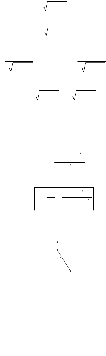
196 CHAPTER 7
Thus
()
0
22
1
sin ag g
ag
θ
θθ
+−
+
()
0
22
1
cos ga a
ag
θ
θθ
−+
+
Substituting into the equation of motion gives
() ()
00
22 22
ga
ag g ga a
ba g ba g
0
θ
θθ θθ
+ − − − +
++
=+
This reduces to
22 22
0
ga ga
bb
θ
θθ
++
+=
The solution to this inhomogeneous differential equation is
0cos sin
A
B
θ
θωθωθ
=
++
where
(
)
14
22
12
ga
b
ω
+
=
Thus
()
12
14
22
2
2b
Tga
π
π
ω
==+
7-14.
θ
a
b
m
2
sin
1cos
2
cos
sin
xb
yatb
xb
yatb
θ
θ
θθ
θ
θ
=
=−
=
=+
()
()
22 2222
11 2sin
22
xy mb atabtTm
θ
θθ
=+= ++
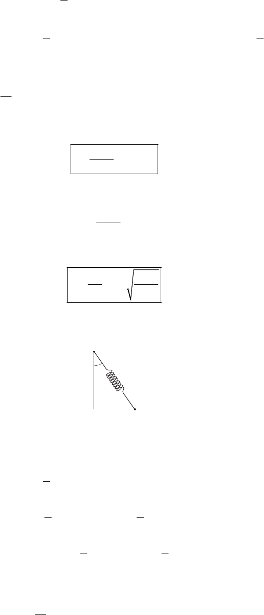
HAMILTON’S PRINCIPLE—LAGRANGIAN AND HAMILTONIAN DYNAMICS 197
2
1cos
2
gymg at bUm
θ
== −
()
22 22 2
11
2sin cos
22
U mb at abt mgb at
θθθθ
=−= + + + −
LT
Lagrange’s equation for
θ
gives
2sin cos sin
dmb mabt mabt mgb
dt
θ
θθθ
+= −
θ
ba
2sin cos cos sinb abt abt gb
θ
θθθθθ
++ = −
θ
sin 0
ag
b
θθ
+
+
=
For small oscillations, sin
θ
θ
0
ag
b
θθ
+
+
=
.
Comparing with gives
20
θωθ
+=
22b
Tag
ππ
ω
==
+
7-15.
k
m
θ
b = unextended length of spring
= variable length of spring
()
222
1
2
Tm
θ
=+
() ()
22
11
cos
22
bmgykbmgUk
θ
=−+=−−
()
()
2
222
11
cos
22
U m b mgLT
θ
θ
=−= + − − +
Taking Lagrange’s equations for and
θ
gives
()
2
:c
dmm kbmg
dt os
θ
θ
=−−+
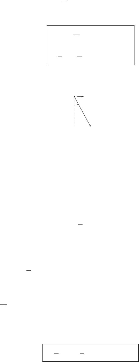
198 CHAPTER 7
2
:s
dmmg
dt in
θ
θθ
=−
This reduces to
()
2cos 0
2sin 0
kbg
m
g
θθ
θθ θ
−+ −− =
++ =
7-16.
θ
m
b
x = a sin ωt
For mass m:
sin sin
cos
cos cos
sin
xa tb
yb
xa tb
yb
ω
θ
θ
ω
ωθ
θθ
θ
=
+
=−
=+
=
Substitute into
()
22
1
2
Tmxy=+
Umgy
=
and the result is
()
22 2 22
1cos 2 cos cos cos
2
LTU ma t ab t b mgb
ω
ωωθωθθ
=−= + + +
θ
Lagrange’s equation for
θ
gives
(
co
d
)
2
s cos cos sin sinmab t mb mabw t mgb
dt
ω
ωθ θ θωθ
+=− −
θ
22
sin cos cos sin cos sin sinab t ab t b ab t gb
ω
ωθωθωθθ ωθωθ
−− +=− −
θ
or
2
sin sin cos 0
gat
bb
θθωωθ
+−
=
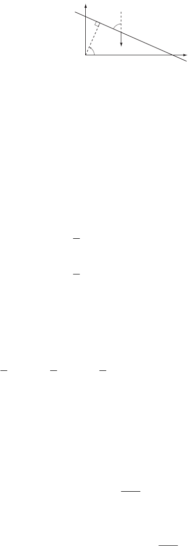
HAMILTON’S PRINCIPLE—LAGRANGIAN AND HAMILTONIAN DYNAMICS 199
7-17.
θ
θ
A
B
C
y
h
mg
q
Using q and
θ
(=
ω
t since
θ
(0) = 0), the x,y coordinates of the particle are expressed as
(
)
()
cos sin cos sin
sin cos sin cos
xh q h tqt t
yh q h tqt t
θ
θω ω
θ
θω ω
=+= +
=−= −
(1)
from which
sin cos sin
cos sin cos
xh tq tq t
yh tq tq t
ω
ωωω ω
ωωωω ω
=− + +
=+−
(2)
Therefore, the kinetic energy of the particle is
()
()
22
22 22 2
1
2
1
2
Tmxy
mh q q mh q
ω
ω
=+
=++−
ω
(3)
The potential energy is
(
)
sin cosUmgymgh tq t
ω
ω
== − (4)
Then, the Lagrangian for the particle is
22 22 2
111 sin cos
222
mh mq mq mgh t mgq t mh qL
ω
ωωω
+− + −
ω
t
=+ (5)
Lagrange’s equation for the coordinate is
2cosqqg
ω
ω
−=
(6)
The complementary solution and the particular solution for (6) are written as
(
)
(
)
()
2
cos
cos
2
c
P
qt A it
g
qt t
ω
δ
ω
ω
=+
=−
(7)
so that the general solution is
()
()
2
cos cos
2
g
qt A i t t
ω
δ
ω
=+−
ω
(8)
Using the initial conditions, we have
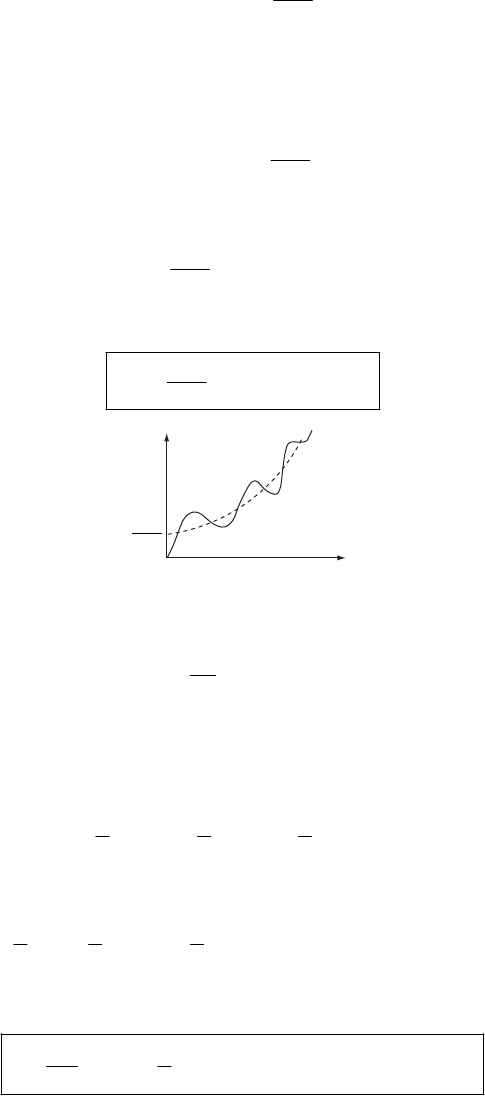
200 CHAPTER 7
()
()
2
0cos 0
2
0sin0
g
qA
qiA
δω
ωδ
=−=
=− =
(9)
Therefore,
δ
= 0, 2
2
g
A
ω
= (10)
and
()
(
2cos cos
2
g
qt i t t
)
ω
ω
ω
=− (11)
or,
()
()
2cosh cos
2
g
qt t t
ω
ω
ω
=− (12)
q(t)
t
g
22
ω
In order to compute the Hamiltonian, we first find the canonical momentum of q. This is
obtained by
L
p
mq m h
q
ω
∂
==−
∂ (13)
Therefore, the Hamiltonian becomes
222222
111 sin cos
222
HpqL
mq m hq m h m q mq mgh t mgq t m qh
ω
ωω ω ω
=−
=− − − − + − +
ω
so that
22222
11 1 sin cos
22 2
H
mq m h m q mgh t mgq t
ω
ωω
− + −
ω
=− (14)
Solving (13) for and substituting gives q
2
22
1sin cos
22
p
H
hp m q mgh t mgq t
m
ω
ωω
− + −
ω
=+ (15)
The Hamiltonian is therefore different from the total energy, T + U. The energy is not conserved
in this problem since the Hamiltonian contains time explicitly. (The particle gains energy from
the gravitational field.)
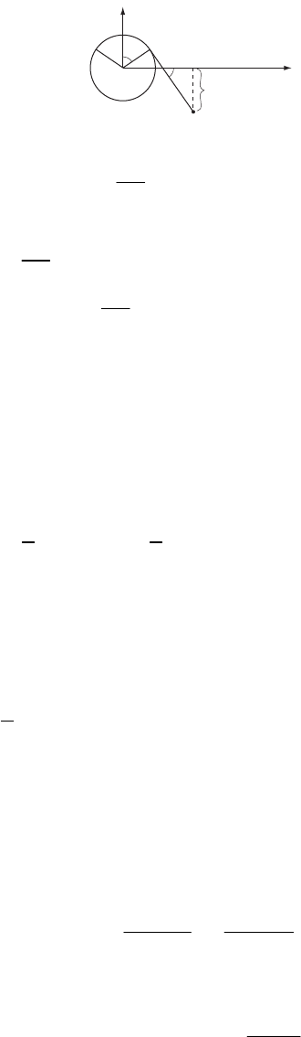
HAMILTON’S PRINCIPLE—LAGRANGIAN AND HAMILTONIAN DYNAMICS 201
7-18.
θ
θ
y
S
RO
A
B
C
m
x
–y
x
From the figure, we have the following relation:
A
CsR
θ
=−=− (1)
where
θ
is the generalized coordinate. In terms of
θ
, the x,y coordinates of the mass are
()
()
cos sin cos sin
cos sin cos sin
xAC R R R
yR AC R R
θ
θθθθ
θ
θθθ
=+=−+
θ
=− =−−
(2)
from which
sin sin
cos cos
xR
yR
θ
θθθθ
θ
θθθθ
=−
=−
(3)
Therefore, the kinetic energy becomes
()
2 2 22 222 2
11 2
22
xy m R RTm
θ
θθ θθ
=+= +−
(4)
The potential energy is
(
)
cos singymgR RUm
θ
θ
== −−
θ
(5)
Then, the Lagrangian is
()
22 222 2
12cos
2
LTU m R R mgR Rsin
θ
θθ θθ θ θ θ
=−= + − − −−
(6)
Lagrange’s equation for
θ
is
(
)
2cos 0RRg
θθ θ θ
−
−− =
(7)
Now let us expand about some angle 0
θ
, and assume the deviations are small. Defining
0
ε
θθ
≡− , we obtain
0
00
sin cosgg
RR
0
θ
θ
εε
θ
θ
+=
−−
(8)
The solution to this differential equation is
()
0
0
cos
sin sin
At
θ
εωδ
θ
=++ (9)
where A and
δ
are constants of integration and
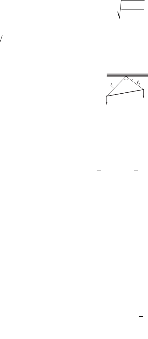
202 CHAPTER 7
0
0
sing
R
θ
ω
θ
≡− (10)
is the frequency of small oscillations. It is clear from (9) that
θ
extends equally about 0
θ
when
02
θ
π
=.
7-19.
PP
m
1
m
2
m
2
g
m
1
g
d
θφ
Because of the various constraints, only one generalized coordinate is needed to describe the
system. We will use
φ
, the angle between a plane through P perpendicular to the direction of the
gravitational force vector, and one of the extensionless strings, e.g., , as our generalized
coordinate.
2
The, the kinetic energy of the system is
() ()
2
11 22
11
22
Tm m 2
φ
φ
=+
(1)
The potential energy is given by
(
)
(
)
11 22
sin sing mgUm
π
φθ φ
=− − + − (2)
from which the Lagrangian has the form
()
()
222
11 22 1 1 2 2
1sin sin
2
U m m mg mgLT
φ
φθ φ
=−= + + + +
(3)
The Lagrangian equation for
φ
is
(
)
(
)
22
22 11 11 22
cos cos 0mg m m
φφθ
++−+
mg (4)
φ
=
This is the equation which describes the motion in the plane .
12
,,mmP
To find the frequency of small oscillations around the equilibrium position (defined by 0
φ
φ
=
),
we expand the potential energy U about 0
φ
:
()
() () ()
()
2
00 0
2
0
1
2
1
2
UU U U
U
φ φ φφ φφ
φφ
=+ + +
′′′
=′′
…
(5)
where the last equality follows because we can take
(
)
00
φ
U
=
and because
(
)
00
φ
=
′
U.
From (4) and (5), the frequency of small oscillations around the equilibrium position is
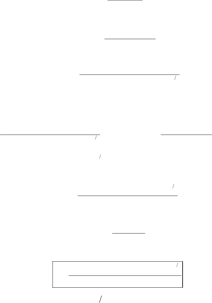
HAMILTON’S PRINCIPLE—LAGRANGIAN AND HAMILTONIAN DYNAMICS 203
(
)
0
2
2
11 22
U
mm
φ
ω
′′
=+
2
(6)
The condition
(
)
00
φ
=
′
U gives
22 11
0
11
cos
tan sin
mm
m
θ
φθ
+
=
(7)
or,
()
22 11
012
22 22
11 22 1 212
cos
n2cos
mm
mm mm
si
θ
φθ
+
=++
(8)
Then from (2), (7), and (8),
(
)
0
U
φ
′′ is found to be
(
)
(
)
()
()
()
0 0 22 11 11 0
22 2
22 11 11
22 11
12
22 22 22 11
11 2 2 2 121
12
22 22
11 2 2 2 121
sin cos sin cot
cos sin
cos cos
2cos
2cos
Ugmm m
gm m m
mm mm
mm mm
gm m mm
φφ θ θφ
θθ
θ
θ
θ
θ
=++
′′
+
=++
+
++
=++
(9)
Finally, from (6) and (9), we have
(
)
()
12
22 22
11 22 1 212
2
22
11 22
2cosmm mm
gmm
θ
++
=+
ω
(10)
which, using the relation,
22
12
12
cos 2
d
θ
2
+
−
=
(11)
can be written as
()
()
()
12
222
121122 12
22
11 22
gm m m m dmm
mm
++−
=+
2
ω
(12)
Notice that 2
ω
degenerates to the value g appropriate for a simple pendulum when d → 0
(so that ).
12
=
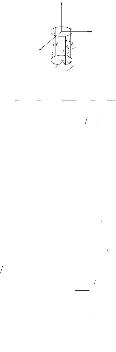
204 CHAPTER 7
7-20. The x-y plane is horizontal, and A, B, C are the fixed points lying in a plane above the
hoop. The hoop rotates about the vertical through its center.
z
AB
B′
y
x
R
C
C′
A′
θ′
θ
The kinetic energy of the system is given by
2
2
22 2
11 1
22 2 2
MR z
Mz M 2
TI
ω
θ
θ
∂
=+ = +
∂
θ
(1)
For small
θ
, the second term can be neglected since
(
)
00z
θ
θ
=
∂
∂=
The potential energy is given by
UMgz
=
(2)
where we take U = 0 at z = –.
Since the system has only one degree of freedom we can write z in terms of θ. When
θ
= 0,
z
=−. When the hoop is rotated thorough an angle
θ
, then
(
)
(
)
2
22 cos sinzRR R
2
θ
θ
=−− − (3)
so that
(
)
12
22
2cos1zR
θ
=− + −
(4)
and the potential energy is given by
(
)
12
22
2cos1UMg R
θ
=− + −
(5)
for small
θ
, 2
s 1 2
θθ
−≅−co ; then,
12
22
2
22
2
1
12
R
UMg
R
Mg
θ
θ
≅− −
≅− −
(6)
From (1) and (6), the Lagrangian is
22
22
2
11
22
R
U MR MgLT
θ
θ
=−= + −
, (7)
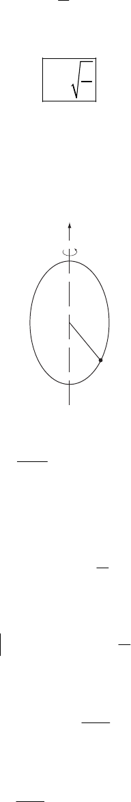
HAMILTON’S PRINCIPLE—LAGRANGIAN AND HAMILTONIAN DYNAMICS 205
for small
θ
. The Lagrange equation for
θ
gives
0
g
θθ
+
=
(8)
where
g
ω
= (9)
which is the frequency of small rotational oscillations about the vertical through the center of
the hoop and is the same as that for a simple pendulum of length .
7-21.
ω
θ
From the figure, we can easily write down the Lagrangian for this system.
()
2
222
sin
2
mR
T
θ
ω
=+
θ
(1)
cos
UmgR
θ
=
− (2)
The resulting equation of motion for
θ
is
2sin cos sin 0
g
R
θω θ θ θ
−+
= (3)
The equilibrium positions are found by finding the values of
θ
for which
0
2
0
0cos
g
R
θθ
0
sin
θ
ωθ
=
== −
θ
(4)
Note first that 0 and
π
are equilibrium, and a third is defined by the condition
02
cos g
R
θω
= (5)
To investigate the stability of each of these, expand using 0
ε
θθ
=
−
(
2
000
2
cos sin sin cos
g
R
)
0
ε
ωθ εθ θε
ω
− +
θ
=−
(6)
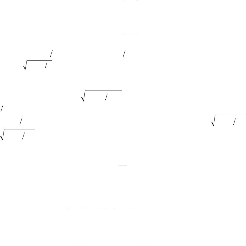
206 CHAPTER 7
For 0
θ
π
=, we have
2
2
1g
R
ε
ω
ω
=+
ε
(7)
indicating that it is unstable. For 00
θ
=
, we have
2
2
1g
R
ε
ω
ω
=−
ε
(8)
which is stable if 2gR
ω
< and unstable if 2gR
ω
>. When stable, the frequency of small
oscillations is 2gR
ω
−. For the final candidate,
22
0
sin
ε
ωθ
=−
ε
(9)
with a frequency of oscillations of
()
2
2gR
ωω
−, when it exists. Defining a critical frequency
2
cgR
ω
≡, we have a stable equilibrium at 00
θ
=
when c
ω
ω
<
, and a stable equilibrium at
(
)
12 2
0cos c
θ
ωω
−
= when c
ω
ω
≥. The frequencies of small oscillations are then
()
2
1c
ω
ωω
−
and
()
4
1c
ω
ωω
−, respectively.
To construct the phase diagram, we need the Hamiltonian
L
H
L
θθ
∂
≡
−
∂
(10)
which is not the total energy in this case. A convenient parameter that describes the trajectory
for a particular value of H is
22
2
22
1sin cos
2
ccc
H
mR
θω
K
θ
θ
ωωω
− −
≡= (11)
so that we’ll end up plotting
()
22
2
2cos sin
cc
K
θω
θ
θ
ωω
=+ +
(12)
for a particular value of
ω
and for various values of K. The results for c
ω
ω
<
are shown in
figure (b), and those for c
ω
ω
> are shown in figure (c). Note how the origin turns from an
attractor into a separatrix as
ω
increases through c
ω
. As such, the system could exhibit chaotic
behavior in the presence of damping.
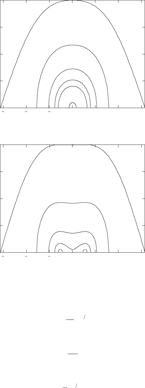
HAMILTON’S PRINCIPLE—LAGRANGIAN AND HAMILTONIAN DYNAMICS 207
3 2 101 2
0
0.5
1
1.5
2
3
K
θ
(b)
3 2 101 2
0
0.5
1
1.5
2
3
K
θ
(c)
7-22. The potential energy U which gives the force
()
()
2
,t
k
Fxt e
x
τ
−
= (1)
must satisfy the relation
U
Fx
∂
=−
∂
(2)
we find
t
k
Ue
x
τ
−
= (3)
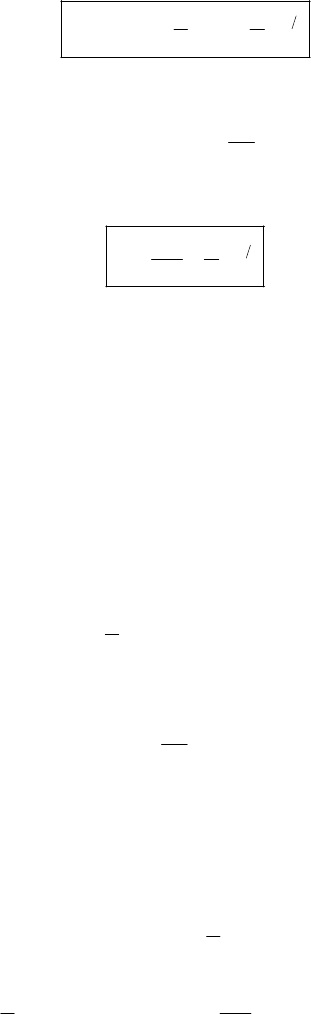
208 CHAPTER 7
Therefore, the Lagrangian is
2
1
2
t
k
LTU mx e
x
τ
−
=−= −
(4)
The Hamiltonian is given by
x
L
H
px L x L
x
∂
=
−= −
∂
(5)
so that
2
2
t
x
pk
H
mx
e
τ
−
=+ (6)
The Hamiltonian is equal to the total energy, T + U, because the potential does not depend on
velocity, but the total energy of the system is not conserved because H contains the time
explicitly.
7-23. The Hamiltonian function can be written as [see Eq. (7.153)]
jj
j
H
pq L
=
−
∑
(1)
For a particle which moves freely in a conservative field with potential U, the Lagrangian in
rectangular coordinates is
()
222
1
2
LmxyzU
=
++ −
and the linear momentum components in rectangular coordinates are
x
y
z
L
p
mx
x
pmy
pmz
∂
==
∂
=
=
(2)
()
()
()
222 222
222 222
1
2
11
22
xyz
H
mx my mz m x y z U
mx y z U p p p
m
=++− ++−
++=++
=+ (3)
which is just the total energy of the particle. The canonical equations are [from Eqs. (7.160) and
(7.161)]
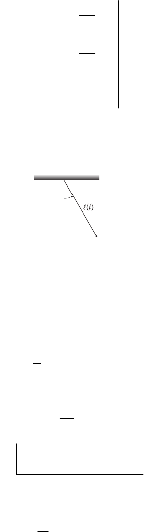
HAMILTON’S PRINCIPLE—LAGRANGIAN AND HAMILTONIAN DYNAMICS 209
xx
yy
z
z
U
p
mx F
x
U
p
my F
y
U
p
mz F
z
∂
==− =
∂
∂
==− =
∂
∂
==− =
∂
(4)
These are simply Newton’s equations.
7-24.
θ
m
The kinetic energy and the potential energy of the system are expressed as
()()
222 222
11
22
cos
Tm m
Umg
θαθ
θ
=+= +
=−
(1)
so that the Lagrangian is
()
222
1cos
2
U m mgLT
α
θ
=−= + +
θ
(2)
The Hamiltonian is
2
2
2
1cos
22
L
Hp L L
pmmg
m
θ
θ
θθ
θ
α
θ
∂
=−= −
∂
=− −
(3)
which is different from the total energy, T + U. The total energy is not conserved in this system
because work is done on the system and we have
()
0
dTU
dt
+
≠ (4)
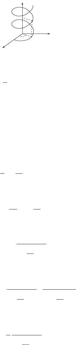
210 CHAPTER 7
7-25.
z
m
zr
y
x
θ
In cylindrical coordinates the kinetic energy and the potential energy of the spiraling particle
are expressed by
2222
1
2
Tmrr z
Umgz
θ
=++
=
(1)
Therefore, if we use the relations,
i.e.,
const.
z
kzk
r
θ
θ
==
=
(2)
the Lagrangian becomes
2
22
2
1
2
r
Lmzzmg
k
=+−
z
(3)
Then the canonical momentum is
2
21
z
Lr
p
m
zkz
∂
== +
∂
(4)
or,
2
21
z
p
zr
mk
=
+
(5)
The Hamiltonian is
2
22
22
12 1
zz
zz
pp
H
pz L p mgz
rr
mm
kk
= − +
++
=− (6)
or,
2
2
2
1
21
z
p
H
mgz
r
mk
=
+
+ (7)
Now, Hamilton’s equations of motion are
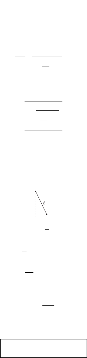
HAMILTON’S PRINCIPLE—LAGRANGIAN AND HAMILTONIAN DYNAMICS 211
z
H
p
z
∂
−
=
∂;
z
H
z
p
∂
=
∂ (8)
so that
z
Hmg p
z
∂
−
=− =
∂ (9)
2
21
z
z
p
H
z
pr
mk
∂
=
=
∂
+
(10)
Taking the time derivative of (10) and substituting (9) into that equation, we find the equation
of motion of the particle:
2
21
g
zr
k
=
+
(11)
It can be easily shown that Lagrange’s equation, computed from (3), gives the same result as
(11).
7-26.
a)
θ
m
22
1
2
LTU m mgy
θ
=−= −
22
1cos
2
Lm mg
θ
θ
=+
2
L
pm
θ
θ
θ
∂
==
∂
so
2
p
m
θ
θ
=
Since U is velocity-independent and the coordinate transformations are time-independent, the
Hamiltonian is the total energy
2
2cos
2
p
HTU mg
m
θ
θ
=+= −
The equations of motion are
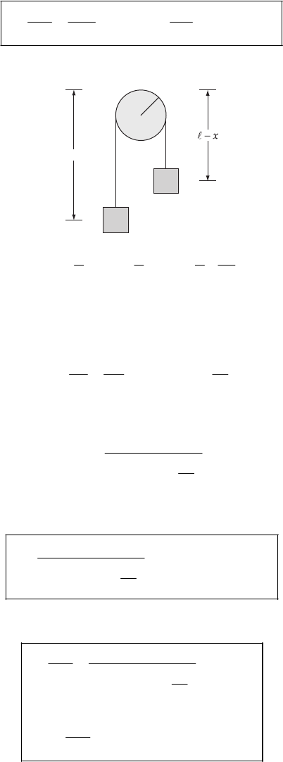
212 CHAPTER 7
2and sin
p
HH
pmg
pm
θθ
θ
θ
θ
θ
∂∂
= =− =−
∂∂
=
b)
a
m2
m2
m1
m1
x
2
22
12 2
111
222
x
TmxmxI
a
=++
where I = moment of inertia of the pulley
(
)
12
Umgxmg x
=
−− −
12
2
x
LT I
p
mm x
xx a
∂
∂
=== ++
∂∂
So
12
2
x
p
xI
mm a
=
++
H = T + U
()
2
12
12
2
2
x
p
H
mgx mg x
I
mm a
=−−
++
−
The equations of motion are
()
12
2
12 12
2
x
x
x
x
p
H
xI
pmm a
H
p
mg mg g m m
p
∂
==
∂
++
∂
=− = − = −
∂
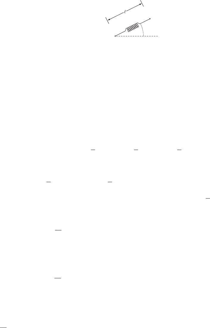
HAMILTON’S PRINCIPLE—LAGRANGIAN AND HAMILTONIAN DYNAMICS 213
7-27.
a)
m
2
m
1
k,b
θ
, coordinates of
ii
xy m
i
=
Using ,
θ
as polar coordinates
21cosxx
θ
=
+
21sinyy
θ
=
+
21cos sinxx
θ
θ
=+ −
θ
(1)
21sin cosyy
θ
θ
=+ +
θ
(2)
If we substitute (1) and (2) into
()()
()
2
22 22
11 1 22 2
111
222
U mx y mx y k b=−= + + + − −
LT
the result is
()
()
()
()()
()
22 222
1211 2
2
21 1 2 1 1
11
22
1
cos sin cos sin 2
Lmmxy m
mx y m y x k b
θ
θθθθθ
=+ ++ +
+++ −−
−
The equations of motion are
()
11212 2
11 22
:cossin0
x
d
xmmxm m
dt
mx mx p
θθθ
++ − =
=
+=
So = constant
x
p
()
11212 2
11 22
:sincos0
y
d
ymmym m
my my p
θθθ
++ + =
dt
=
+=
So
y
p
= constant
()
()
()
2
221 1 2 21 1
: cos sin cos sin
dmmx y m kbmy x
dt
θ
θθ θθ
++=−−+ −
θ
which reduces to
214 CHAPTER 7
()
2
11
2
cos sin 0
k
xy b
m
θθθ
−+ + + −=
()
()(
2
221 1
21 1 2 1 1
:cossin
sin cos cos sin
dmmy x
dt
mx y m x y
θθ θθ
)
θ
θθ θ
+−
=− − + − −
θ
which reduces to
11
cos sin
20yx
θθ
θθ
++ − =
b) As was shown in (a)
1
constant
x
Lp
x
∂==
∂
1
constant
y
Lp
y
∂==
∂ (total linear momentum)
c) Using L from part (a)
()
11212 2
1
cos sin
x
L
pmmxmm
x
θ
θθ
∂
==+ + −
∂
()
11212 2
1
sin cos
y
L
pmmymm
y
θ
θθ
∂
==+ + −
∂
21 21 2
cos sin
L
p
mx my m
θθ
∂
== + +
∂
2
21 21 2
sin cospmx my m
θ
θ
θθ
=− + +
Inverting these equations gives (after much algebra)
1
1
1
sin
1cos
x
xpp
mp
θ
θ
θ
=− +
1
1
1
cos
1sin
y
ypp
mp
θ
θ
θ
=−−
11
12
12
1cos sin
xy
mm
p
pp
mm
θθ
+
=− − +
11
12
12
1sin cos
xy
mm
p
pp
mm
θ
θθθ
+
=−+
Since the coordinate transformations are time independent, and U is velocity independent,
H
TU
=
+
Substituting using the above equations for in terms of gives
i
q
i
p

HAMILTON’S PRINCIPLE—LAGRANGIAN AND HAMILTONIAN DYNAMICS 215
()
()
()
11 1 1
11
2
22 2
12
2
12
2
12cos sin
2
1
2sincos
2
xy x y
xy
p
mm
Hpp p pp p
mm
p
p
pk
θ
θ
θθ
θθ
+
=++ +− +
+−+
b
−
The equations of motion are
1
1
1
1
sin
1cos
x
x
H
xpp
pm p
θ
θ
θ
∂
== − +
∂
1
1
1
1
cos
1sin
y
y
H
ypp
pm p
θ
θ
θ
∂
== − −
∂
11
12
12
1cos sin
xy
mmHpp p
pm m
θ
θ
+∂
== − −
∂
11
12
12
1sin cos
xy
mmHpp p
pm m
θ
θ
θ
θθ
+∂
== + −
∂
11
11
00
xy
HH
pp
xy
∂∂
=− = =− =
∂∂
(
)
()
()
11
2
12
32
12 1
sin cos
xy
mmp p
H
p
pp k
mm m
θθ
θθ
+
∂
=− = + − − −
∂
b
()
11 1 1
11
sin cos cos sin
xy x y
pp
H
ppppp
mm
θ
θ
θ
θθ
θ
∂
θ
=− = − + − +
∂
Note: This solution chooses as its generalized coordinates what the student would most likely
choose at this point in the text. If one looks ahead to Section 8.2 and 8.3, however, it would
show another choice of generalized coordinates that lead to three cyclic coordinates ( , ,
and
θ
), as shown in those sections.
CM
xCM
y
7-28. so
2
Fkr
−
=− 1
Ukr
−
=−
()
222
1
2
k
LTU mr r r
θ
=−= + +
so r
r
p
L
pmrr
rm
∂
== =
∂
2
2
so
p
L
pmr mr
θ
θ
θθ
θ
∂
== =
∂
Since the coordinate transformations are independent of t, and the potential energy is velocity-
independent, the Hamiltonian is the total energy.
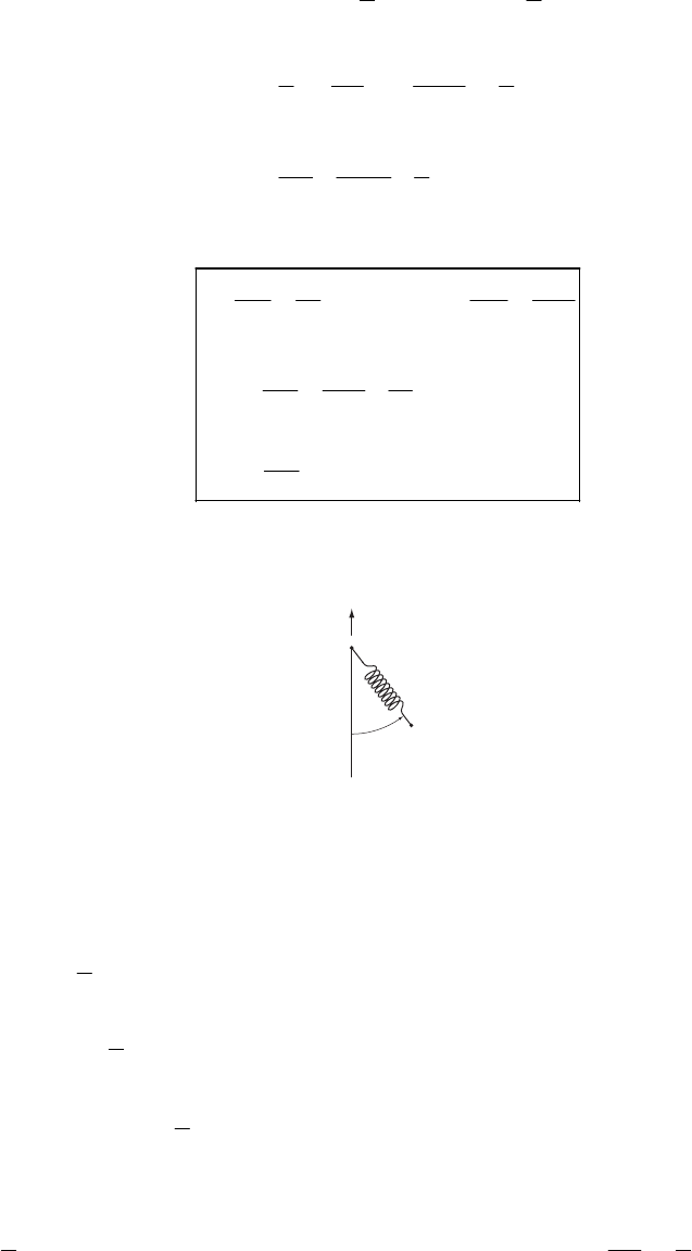
216 CHAPTER 7
()
222
22
2
224
22
2
1
2
1
2
22
r
r
k
HTU mr r r
pp
k
mr
mmrr
pp
k
Hmmrr
θ
θ
θ
=
+= + −
=+ −
=+ −
Hamilton’s equations of motion are
2
2
32
0
r
r
r
p
p
HH
r
p
mp
p
Hk
prmr r
H
p
θ
θ
θ
θ
θ
θ
∂∂
== ==
∂∂
∂
=− = −
∂
∂
=− =
∂
mr
7-29.
a
k
m
θ
b = unextended length of spring
= variable length of spring
a) sin sin cosxx
θ
θθ
==
θ
+
2
1cos cos sin
2
yat yat
θ
θθ
=− =− +
θ
Substituting into
()
()
22
2
1
2
1
2
Tmxy
Umgy k b
=+
=+ −
gives
()
()
22
22222
12sincos cos
22
at k
LTU m at at mg b
θθθθθ
=−= + + + − + − − −
2
Lagrange’s equations give:
HAMILTON’S PRINCIPLE—LAGRANGIAN AND HAMILTONIAN DYNAMICS 217
()
2
: cos sin cos
dmamt m mat mg k b
dt
θθ θθ θ
−=++−
−
2
: sin sin sin cos
dmmat mat mg mat
dt
θ
θθ θθθ
+=−+
θ
Upon simplifying, the equations of motion reduce to:
()
()
2cos 0
2sin 0
k
ag b
m
ag
θθ
θθ θ
−−+ + −=
+
+
+=
b) cos or cos
p
L
pmmat at
m
θ
θ
∂
==− =+
∂
(1)
2sin
L
pmmat
θ
θ
θ
θ
∂
== +
∂
or
2
sinpat
m
θ
θ
θ
=−
(2)
Since the transformation equations relating the generalized coordinates to rectangular
coordinates are not time-independent, the Hamiltonian is not the total energy.
ii
HpqLpp
θ
θ
L
=
−= + −
∑
Substituting (1) and (2) for and
θ
and simplifying gives
()
22 22
2
11
sin cos cos
22 2 2
pp
at
Hpatpkbmgatm
mm
θθ
g
θ
θθ
=+ − + + −+ −
The equations for
θ
and are
2sin
cos agreeing with (1) and (2)
p
Hat
pm
p
Hat
pm
θ
θ
θθ
θ
∂
== −
∂
∂
==+
∂
The equations for and
p
p
θ
are
()
2
23
sin cos
p
Hat kbmg
m
pp
θ
θ
θθ
∂
=− =− − − + +
∂
or
()
2
23
sin cos 0
p
at kbmg m
θ
θ
θθ
++−−+
pp =
cos sin sin
Hat atpmg
θθ
pp
θ
θθ
θ
∂
=− =− + −
∂
218 CHAPTER 7
or
cos sin sin 0
at atp mg
θθ
θθθ
−−+
pp =
c)
2
sin , cos 1 2
θ
θθ θ
−
Substitute into Lagrange’s equations of motion
()
()
2
210
2
20
k
ag b
m
ag at
θ
θ
θ
θθ θ
−−+ −+ −=
+
+
+−
=
For small oscillations, . Dropping all second-order terms gives
1, 1, 1
θθ
0
kk
ag b
mm
ag
θθ
+=++
+
+=
For
θ
,
22Tag
θ
ππ
ω
==
+
The solution to the equation for is
()
homogeneous particular
cos sin
kkm
A
tB t ag b
mmk
=+
=+++
+
So for ,
22m
Tk
ππ
ω
==
7-30.
a) From the definition of a total derivative, we can write
k
kkk
dg g g q g p
dt t q t p t
k
∂∂∂∂∂
=+ +
∂
∂∂ ∂∂
∑ (1)
Using the canonical equations
HAMILTON’S PRINCIPLE—LAGRANGIAN AND HAMILTONIAN DYNAMICS 219
k
k
k
k
k
k
qH
q
tp
p
H
p
tq
∂∂
==
∂∂
∂∂
==−
∂∂
(2)
we can write (1) as
kkk kk
dg g g g
H
H
dt t q p p q
∂∂ ∂
∂∂
=+ −
∂∂∂∂∂
∑ (3)
or
,
dg g gH
dt t
∂
=+
∂ (4)
b) j
j
j
q
H
qtp
∂
∂
==
∂
∂
(5)
According to the definition of the Poisson brackets,
,jj
j
kkk kk
qg
H
H
qH qp pq
∂∂
∂∂
=−
∂∂ ∂∂
∑ (6)
but
j
j
k
k
q
q
δ
∂
=
∂ and 0
j
k
q
p
∂
=
∂ for any j,k (7)
then (6) can be expressed as
,
jj
j
H
qH q
p
∂
=
=
∂ (8)
In the same way, from the canonical equations,
j
j
H
pq
∂
=−
∂
(9)
so that
,jj
j
kkk kk
pp
H
H
pH qp pq
∂∂
∂∂
=−
∂∂ ∂∂
∑ (10)
but
j
j
k
k
p
p
δ
∂=
∂ and 0
j
k
p
q
∂
=
∂ for any j,k (11)
then,
220 CHAPTER 7
,
jj
j
H
p
pH
q
∂
=− =
∂
(12)
c) ,
jj
kk
kj
p
p
pp
pp qp pq
∂∂
∂∂
=−
∂∂ ∂∂
∑
(13)
since,
0
k
p
q
∂
=
∂
for any k, (14)
the right-hand side of (13) vanishes, and
,
kj
pp
0
=
(15)
In the same way,
,
jj
kk
kj
qq
qq
qq qp pq
∂∂
∂∂
=−
∂∂ ∂∂
∑
(16)
since
0
j
q
p
∂
=
∂
for any j, (17)
the right-hand side of (16) vanishes and
,
kj
qq
0
=
(18)
d)
,
jj
kk
kj
kj
p
p
qq
qp qp pq
δδ
∂∂
∂∂
=−
∂∂ ∂∂
=
∑
∑
(19)
or,
,
k
j
k
j
qp
δ
=
(20)
e) Let
(
)
,
kk
gp q be a quantity that does not depend explicitly on the time. If
(
)
,
kk
gp q
commutes with the Hamiltonian, i.e., if
,gH 0
=
(21)
then, according to the result in a) above,
0
dg
dt
=
(22)
and g is a constant of motion.
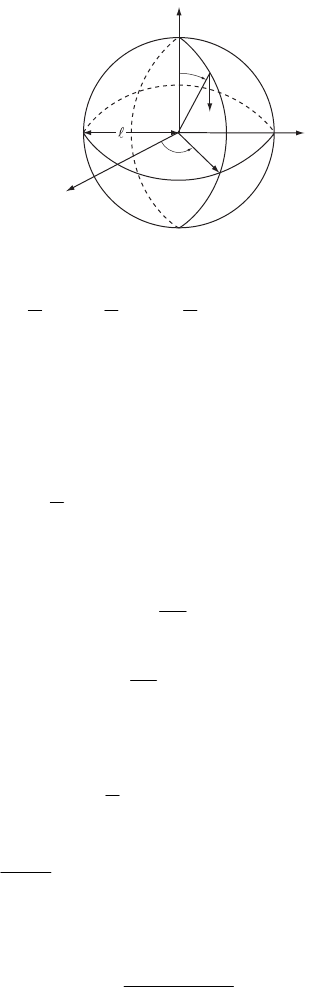
HAMILTON’S PRINCIPLE—LAGRANGIAN AND HAMILTONIAN DYNAMICS 221
7-31. A spherical pendulum can be described in terms of the motion of a point mass m on the
surface of a sphere of radius , where corresponds to the length of the pendulum support rod.
The coordinates are as indicated below.
θ
φ
y
mg
x
z
The kinetic energy of the pendulum is
()
22222
12
111 sin
222
I m 2
TI
φ
θφθ
=+= +
θ
(1)
and the potential energy is
cosUmg
θ
=
(2)
The Lagrangian is
()
22 2 2
1sin cos
2
Lm mg
φ
θθ θ
=+−
(3)
so that the momenta are
2
L
pm
θ
θ
θ
∂
==
∂
(4)
22
sin
L
pm
φ
φ
θ
φ
∂
==
∂
(5)
The Hamiltonian then becomes
()
()
22 2 2
2
2
1sin cos
2
,
2
Hp p m mg
pVp
m
θφ
θφ
θ
φφθθ
θ
=+− ++
=+
θ
(6)
which is just the total energy of the system and where the effective potential is
()
2
22
,
2sin
p
Vp mg
m
θ
φ
cos
θ
θ
θ
=+
(7)
When 0
p
φ
=, V(
θ
,0) is finite for all
θ
, with a maximum at
θ
= 0 (top of the sphere) and a
minimum at
θ
=
π
(bottom of the sphere); this is just the case of the ordinary pendulum. For
different values of
p
φ
, the V–
θ
diagram has the appearance below:
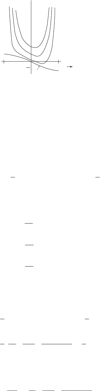
222 CHAPTER 7
V
P
φ
= 0
0π
π
2
θ
When 0
p
φ
>, the pendulum never reaches
θ
= 0 or
θ
=
π
because V is infinite at these points.
The V–
θ
curve has a single minimum and the motion is oscillatory about this point. If the total
energy (and therefore V) is a minimum for a given
p
φ
,
θ
is a constant, and we have the case of a
conical pendulum.
For further details, see J. C. Slater and N. H. Frank, Mechanics, McGraw-Hill, New York, 1947,
pp. 79–86.
7-32. The Lagrangian for this case is
()
2222 22
1sin
2
k
U mr r r r
θθφ
=−= + + +
LT (1)
where spherical coordinates have been used due to the symmetry of U.
The generalized coordinates are r,
θ
, and
φ
, and the generalized momenta are
r
L
p
mr
r
∂
==
∂
(2)
2
L
p
mr
θ
θ
θ
∂
==
∂
(3)
22
sin
L
pmr
φ
φ
θ
φ
∂
==
∂
(4)
The Hamiltonian can be constructed as in Eq. (7.155):
()
22222 2
2
22
222
1sin
2
1
2sin
r
r
Hprp p L
k
mr r r r
p
pp k
mmr mr r
θφ
φ
θ
θφ
θφ θ
θ
=++ −
=++
=++ −
−
(5)
Eqs. (7.160) applied to H as given in (5) reproduce equations (2), (3), and (4). The canonical
equations of motion are obtained applying Eq. (7.161) to H:
2
2
2332
sin
r
p
p
Hk
prrmrmr
φ
θ
θ
∂
=− =− + +
∂
(6)
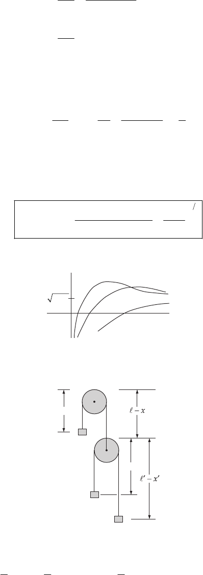
HAMILTON’S PRINCIPLE—LAGRANGIAN AND HAMILTONIAN DYNAMICS 223
2
22
cot
sin
p
H
pmr
φ
θ
θ
θ
θ
∂
=− =
∂
(7)
0
H
p
φ
φ
∂
=− =
∂
(8)
The last equation implies that const
p
φ
=, which reduces the number of variables on which H
depends to four: , , ,
r
rpp
θ
θ
:
2
2
222
1const
2sin
r
pk
Hp
mrr
θ
θ
=++
r
−
(9)
For motion with constant energy, (9) fixes the value of any of the four variables when the other
three are given.
From (9), for a given constant value of H = E, we obtain
12
22
22
sin 2
2sin
r
pconst
mk
Err
θ
θ
θ
+
=− +
pm (10)
and so the projection of the phase path on the rr
p
−
plane are as shown below.
p
r
θ
3
θ
2
θ
1
θ
1
< θ
2
< θ
3
2mE
7-33.
m
1
m
2
m
3
x′
x
Neglect the masses of the pulleys
() ()
22
2
12 3
11 1
22 2
x mxx mxx=+ −+−−Tm
′
′
(
)
(
)
12 3
mgx mg x x mg x x=− − − + − − + −U
′
′′

224 CHAPTER 7
()() (
()()
22
123 23 32
123 23
11
constant
mmx mmxxxmm
gm m m x gm m x
=++ ++ + −
′′
+−−+− +
′
)
22
Lm
We redefine the zero in U such that the constant in L = 0.
()(
123 32x
L
)
p
mmmxmmx
x
∂
== ++ + −
′
∂
(1)
()(
32 23x
L
)
p
mmxmmx
x
′
∂
==− ++
′
∂
′
(2)
Solving (1) and (2) for and gives
x
px
p′
(
)
(
)
1
23 23xx
xD m mp m mp
−
′
=++−
(
)
(
)
1
23 123xx
xD mmp mmmp
−
′
=++++
′
where Dm
13 12 23
4m mm mm=++
()()()
()(
22
123 23 32
123 23
11
22
)
H
TU
mmmx mmx mmxx
gm m m x gm m x
=+
+ ++ +−
′
−−− − −′
=+
Substituting for and and simplifying gives
x
x′
() ()
() ( )()
12 12
23 123
1
23 123 23
13 12 23
11
22
where 4
xx
xx
HmmDp mmmDp
mmDpp gmmmxgmmx
Dmm mm mm
−−
′
−
′
=+ +++
− −+ − − ′
=++
+−
The equations of motion are
() ()
() ( )
()
()
11
23 23
11
23 123
123
23
xx
x
xx
x
x
x
H
x m mD p m mD p
p
H
xmmDpmmmD
p
H
pgmmm
x
H
pgmm
x
−−
′
−−
p
′
′
′
′
∂
==+ +−
∂
∂
==− +++
′∂
∂
=− = − −
∂
∂
=− = −
∂′
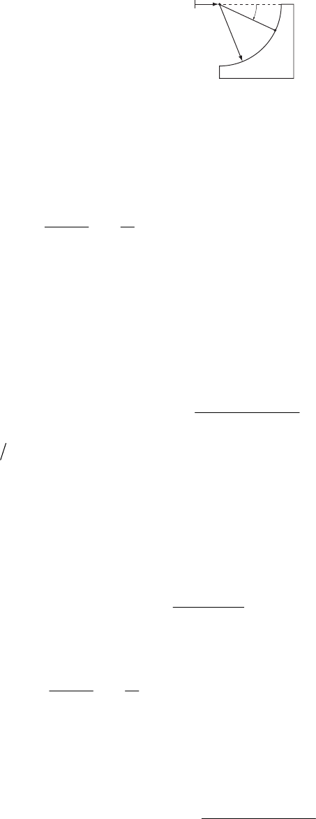
HAMILTON’S PRINCIPLE—LAGRANGIAN AND HAMILTONIAN DYNAMICS 225
7-34.
x
R
rm
M
θ
The coordinates of the wedge and the particle are
cos
0s
Mm
Mm
xx xr
yyr
in
x
θ
θ
==
==−
+
(1)
The Lagrangian is then
()
2222
2cos 2 sin sin
2
Mm m
L x r r xr xr mgr
r
θ
θθθ
+
=+++− +
θ
(2)
Note that we do not take r to be constant since we want the reaction of the wedge on the
particle. The constraint equation is
(
)
,, 0fx r r R
θ
=
−=.
a) Right now, however, we may take r = R and 0rr
=
=
to get the equations of motion for x
and
θ
. Using Lagrange’s equations,
(
)
2
sin cosxaR
θ
θθ θ
=+
(3)
sin cosxg
R
θ
θ
θ
+
=
(4)
where
(
)
amMm≡+.
b) We can get the reaction of the wedge from the Lagrange equation for r
2
cos sinmx mR mg
λ
θθ
=−−
θ
(5)
We can use equations (3) and (4) to express in terms of
θ
and x
θ
, and substitute the resulting
expression into (5) to obtain
()
2
2
1sin
1sin
aRg
a
λ
θ
θ
−
=+
−
θ
(6)
To get an expression for
θ
, let us use the conservation of energy
()
222
0
2 sin sin sin
22
Mm m
HxRxRmgRmgR
θ
θθ θ θ
+
=+− − =−
(7)
where 0
θ
is defined by the initial position of the particle, and 0
sinmgR
θ
−
is the total energy of
the system (assuming we start at rest). We may integrate the expression (3) to obtain
si
Rn
xa
θ
θ
=
, and substitute this into the energy equation to obtain an expression for
θ
(
)
()
0
2
2
2sin sin
1sin
g
Ra
θ
θ
θ
θ
−
=−
(8)
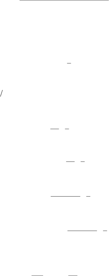
226 CHAPTER 7
Finally, we can solve for the reaction in terms of only
θ
and 0
θ
(
)
()
()
3
0
2
2
3 sin sin 2 sin
1sin
mMg a
Mm a
θ
θθ
θ
−−
=− +−
λ
(9)
7-35. We use i
z
and as our generalized coordinates, the subscript i corresponding to the
ith particle. For a uniform field in the z direction the trajectories z = z(t) and momenta p = p(t)
are given by
i
p
2
00
0
1
2
ii i
ii
z
zvt gt
pp mgt
=+ −
=−
(1)
where 0i
z
, , and
0i
p00ii
vp=m are the initial displacement, momentum, and velocity of the ith
particle.
Using the initial conditions given, we have
2
0
10
1
2
pt
z
z
m
=+ −gt
t
(2a)
10
ppmg
=
− (2b)
2
0
20 0
1
2
pt
z
zz g
m
=+∆+ − t
t
(2c)
20
ppmg
=
− (2d)
(
)
00 2
30
1
2
ppt
z
z
m
+∆
=+ −
gt
t
(2e)
30 0
pp pmg
=
+∆ − (2f)
(
)
00 2
40 0
1
2
ppt
z
zZ g
m
+∆
=+∆+ − t
t
(2g)
40 0
pp pmg
=
+∆ − (2h)
The Hamiltonian function corresponding to the ith particle is
2
2
const.
22
i
i
iii i i
p
mz
V mgz mgz
m
=+= + = + =
HT (3)
From (3) the phase space diagram for any of the four particles is a parabola as shown below.
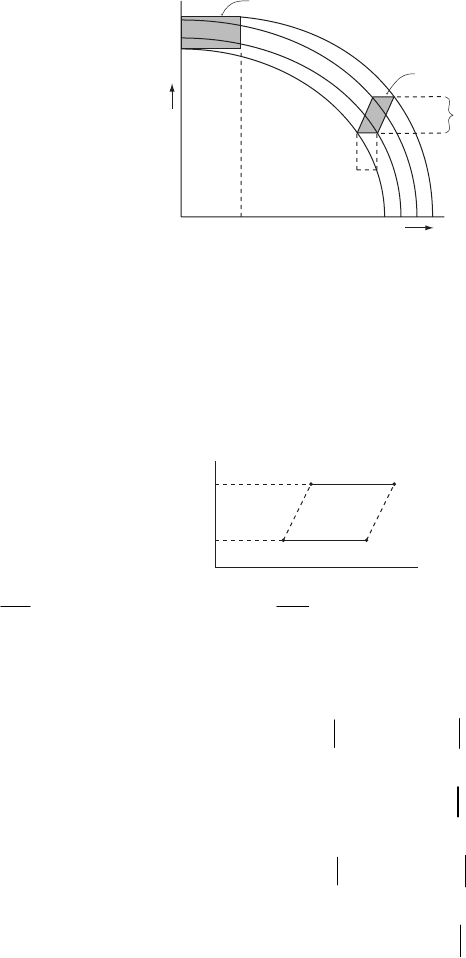
HAMILTON’S PRINCIPLE—LAGRANGIAN AND HAMILTONIAN DYNAMICS 227
p
0
+ ∆p
0
z
0
+ ∆z
0
p
0
Area at t = 0
Area at t = t
1
∆p
0
z
0
∆z
0
p
z
1234
From this diagram (as well as from 2b, 2d, 2f, and 2h) it can be seen that for any time t,
1
pp
2
=
(4)
3
pp
4
=
(5)
Then for a certain time t the shape of the area described by the representative points will be of
the general form
p
z
12
34
(p
1
,z
1
)(p
2
,z
2
)
(p
3
,z
3
)(p
4
,z
4
)
where the base 1 must parallel to the top 2 3 4 . At time t = 0 the area is given by 00
z
p∆∆ , since
it corresponds to a rectangle of base 0
z
∆
and height 0
p
∆
. At any other time the area will be
given by
()
{
()
}
()
{
()
}
11
1
11
1
21
43 0
31
42 0
00
base of parallelogram
height of parallelogram
=
tt tt
tt
tt tt
tt
Azz
z
zz
xpp
p
pp
pz
==
=
==
=
==−
=− =∆
=−
=− =∆
∆∆ (6)
Thus, the area occupied in the phase plane is constant in time.
7-36. The initial volume of phase space accessible to the beam is
2
00
VRp
2
0
π
π
= (1)
After focusing, the volume in phase space is
22
11
VRp
1
π
π
= (2)
228 CHAPTER 7
where now is the resulting radius of the distribution of transverse momentum components
of the beam with a circular cross section of radius . From Liouville’s theorem the phase space
accessible to the ensemble is invariant; hence,
1
p
1
R
22 2
00011
VRpVRp
2
1
π
ππ
===
π
(3)
from which
00
1
1
Rp
pR
= (4)
If , then , which means that the resulting spread in the momentum distribution
has increased.
1
RR<001
pp>
This result means that when the beam is better focused, the transverse momentum components
are increased and there is a subsequent divergence of the beam past the point of focus.
7-37. Let’s choose the coordinate system as shown:
x
1
m
1
m
2
m
3
x
3
x
2
The Lagrangian of the system is
()
2
22
3
12
12 3 1122
1
2
dx
dx dx
LTU m m m gmx mx mx
dt dt dt
=−= + + + + +
33
12
with the constraints
and
1
xyl+= 23
xyxyl
−
+−=
which imply
2
22
3
12
123 12 222
2(2)02 dx
dx dx
xxx ll dt dt dt
++− +=⇒ + + =
0
(1)
The motion equations (with Lagrange multiplier
λ
) are
HAMILTON’S PRINCIPLE—LAGRANGIAN AND HAMILTONIAN DYNAMICS 229
2
1
11
22
dx
mg m dt
λ
0
−
+= (2)
2
2
22
20
dx
mg m dt
λ
−
+= (3)
2
3
33
20
dx
mg m dt
λ
−
+= (4)
Combining (1)–(4) we find
12
4
411
g
mmm
λ
3
−
=
++
Finally, the string tension that acts on m is (see Eq. (2))
1
2
1
11 1
2
12
8
2411
g
dx
gm
dt
mmm
λ
=− =−=
++
3
Tm
7-38. The Hamiltonian of the system is
22
24 2
1
22422
p
dx kx bx kx bx
U m
dt m
=+= + + = + +
4
4
HT
The Hamiltonian motion equations that follow this Hamiltonian are
p
dx H
dt p m
∂
=
=
∂
3
()
dp Hkx bx
dt x
∂
=− =− +
∂
7-39.
z
The Lagrangian of the rope is
22
2
11
222
mgz
dz mz z dz
U m g m
dt b dt b
=−= −− = +
2
LT
230 CHAPTER 7
from which follows the equation of motion
2
2
mgz
LdL dz
m
z
dt z b dt
∂∂
=⇒=
∂∂
7-40.
m
m
2 mx
θ
2
θ
1
We choose the coordinates for the system as shown in the figure.
The kinetic energy is
222
211
1
22
12 12
12 1
11
22cos
22
1cos cos sin sin
2
dddx dx dx
Tm mb b
dt dt dt dt dt
dd dddx
mb b b b
dt dt dt dt dt
=+ ++
++ + + +
θθ
θ
θθ θθ
θθ θ
2
θ
2
The potential energy is
Um 11
cos ( cos cos )gb mgb b
θ
θθ
=− − +
And the Lagrangian is
222
22
11 2
1
2
212
2121
1
22cos
2
cos cos ( ) 2 cos cos
dd d
dx dx
L T U m mb mb mb
dt dt dt dt dt
ddddx
mb mb mgb mgb
dt dt dt dt
=−= + + +
++ −++
θθ θ
θ
θθθ
2
θ
θθ θ θ
From this follow 3 equations of motion
222
12
12
22 2
22
12
12
04 2 cos cos
2sin sin
ddLdL dx
b
x dt x dt dt dt
dd
bdt dt
∂∂
=⇒=+ +
∂∂
−+
θθ
θ
θ
θθ
θθ

HAMILTON’S PRINCIPLE—LAGRANGIAN AND HAMILTONIAN DYNAMICS 231
222
12
11
22 2
11
2
2
12
2sin 2 2 cos cos( )
sin( )
dd
LdL dx
gb b
dt dt dt dt
d
bdt
∂∂
=⇒−=+ + −
∂∂
+−
θθ
12
θ
θθ
θθ
θθθ
θ
22
2
222
211
2212
22 2
sin cos cos ( ) sin ( )
LdL
dt
dd ddx
gb b b
dt dt dt dt
θθ
θθθ
12
θ
θθθ θ
∂∂
=⇒
∂∂
−=+ + −− −
θ
7-41. For small angle of oscillation
θ
we have
22
2
11
22
dd
b m
dt dt
θ
=+
b
Tm and Umcosgb
θ
=
−
So the Lagrangian reads
22
2
11 cos
22
ddb
U mb m mgb
dt dt
θ
LT
θ
=−= + +
from which follow 2 equations of motion
22
2
cos
LdL d db d
bg
bdt dt dt dt
b
∂∂
=⇒ +==−
∂∂
θ
α
θ
22
22
22
sin 2 2
LdL dbd d d d
mgb mb mb mb mb
dt dt dt dt dt dt
θ
θθ
θα
θθ
∂∂
=⇒− = + =− +
∂∂
θ
232 CHAPTER 7
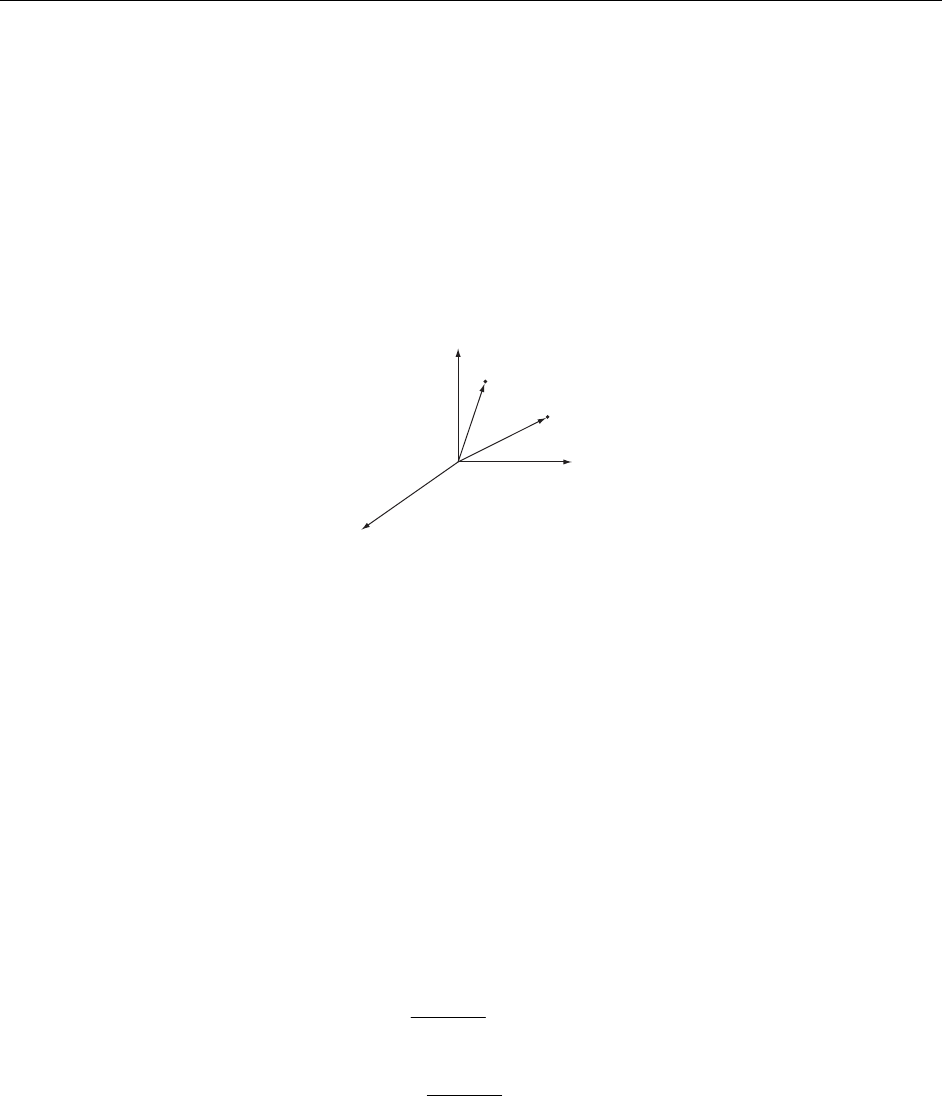
CHAPTER 8
Central-
F
orce Motion
8-1.
x
3
m
2
m
1
x
2
r
1
r
2
x
1
In a uniform gravitational field, the gravitational acceleration is everywhere constant. Suppose
the gravitational field vector is in the x direction; then the masses and have the
gravitational potential energies:
1 1
m2
m
() () () ()
() () () ()
111 1
111
222 2
121
g
g
UFxmx
UFxmx
α
α
=− =−
=− =−
(1)
where
() () ()
(
)
111
1123
,,xxx=r and where
α
is the constant gravitational acceleration. Therefore,
introducting the relative coordinate r and the center of mass coordinate R according to
()
12
11 22 1 2
mm mm
=−
+=+
rr r
rr R
(2)
we can express r and r in terms of r and R by
1 2
2
1
12
1
2
12
m
mm
m
mm
=+
+
=− +
+
rr
rr
R
R
(3)
233
234 CHAPTER 8
which differ from Eq. (8.3) in the text by R. The Lagrangian of the two-particle system can now
be expressed in terms of r and R:
()
() ()
()
22 12
11 22
22
21
12
12 12
21
12
12 12
11
22
11
22
gg
Lm m U UU
mm
mmUr
mm mm
mm
mxXm x
mm mm
αα
=+−−−
+−+−
++
X
=+
+++−
+
++
rrr
rR rR
(4)
where x and X are the components of r and R, respectively. Then, (4) becomes
1
x
()
()
()
2
2
22
21
121
12 12
12 12
12
12
111
2
mm
Lm m mm
mm mm
mm mm
Ur x m m X
mm
αα
=++
++
−
−+ ++
+
rr
2
+R
22 (5)
Hence, we can write the Lagrangian in the form
()
()()
2
2
12 12
11
22
rmmmmLU X
µ
α
=−++ ++rR
(6)
where
µ
is the reduced mass:
12
12
mm
mm
µ
=+ (7)
Therefore, this case is reducible to an equivalent one-body problem.
8-2. Setting 1u=r, Eq. (8.38) can be rewritten as
2
22
22
du
Ek
uu
θµµ
=−
+−
∫
(1)
where we have used the relation
(
)
2
1du r dr=− . Using the standard form of the integral [see
Eq. (E.8c), Appendix E]:
1
22
12
sin const.
4
dx ax b
a
ax bx c b ac
−
−+
=
−
++ −
+
∫ (2)
we have
2
1
2
22
22
const. sin
28
k
r
kE
µ
θµµ
−
−+
+=
+
(3)
CENTRAL-FORCE MOTION 235
or, equivalently,
()
2
2
22
22
sin const.
28
k
r
kE
µ
θ
µ
µ
−+
+=
+
(4)
We can choose the point from which
θ
is measured so that the constant in (4) is 2
π
−. Then,
2
2
2
11
cos 2
1
kr
E
k
µ
θ
µ
−
=
+
(5)
which is the desired expression.
8-3. When 2kk→, the potential energy will decrease to half its former value; but the kinetic
energy will remain the same. Since the original orbit is circular, the instantaneous values of T
and U are equal to the average values, T and U. For a 2
r1 force, the virial theorem states
1
2
T=− U (1)
Hence,
11
22
ETU UU U=+=− += (2)
Now, consider the energy diagram
ED
C
A
r
–k/r
B
where
CB E= original total energy
CA U= original potential energy
C
CD U= original centrifugal energy
The point B is obtained from CB CA CD=−. According to the virial theorem,
(
)
12=EU or
(
)
12 .CB CA= Therefore,
CD CB BA==
236 CHAPTER 8
Hence, if U suddenly is halved, the total energy is raised from B by an amount equal to
(
)
12CA
or by CB . Thus, the total energy point is raised from B to C; i.e., E(final) = 0 and the orbit is
parabolic.
8-4. Since the particle moves in a central, inverse-square law force field, the potential energy
is
k
Ur
=
− (1)
so that the time average is
0
1k
U
r
τ
τ
=− dt
∫
(2)
Since this motion is a central motion, the angular momentum is a constant of motion. Then,
(3)
2.rco
µθ
≡=
nst
from which
2
r
dt d
µ
θ
= (4)
Therefore, (2) becomes
22
2
00
1kr k
Ud
r
ππ
µµ
rd
θ
θ
ττ
=− =−
∫
∫
(5)
Now, substituting 1cosr
α
εθ
=
+ and
(
)
32
2a
τµπα
=, (5) becomes
2
32
0
1
21cos
k
U
a
π
α
d
θ
πε
=− +
∫
θ
(6)
where a is the semimajor axis of the ellipse. Using the standard integral [see Eq. (E.15),
Appendix E],
2
2
0
1
1cos 1
d
π
2
π
θ
εθ
ε
=
+−
∫ (7)
and the relation,
(
)
2
1a
α
ε
=− (8)
(6) becomes
k
Ua
=
− (9)
The kinetic energy is
CENTRAL-FORCE MOTION 237
2
2
2
1
22
Tr
r
µ
µ
=− +
(10)
and the time average is
2
2
3
00
11
2
k
TTdt Tr
a
τπ
µ
d
θ
τπ
=− =
∫∫
(11)
Part of this integral is trivial,
()
22
2
3
0
1
22
k
Trrd
a
π
µµ π
θ
π
µ
=+
∫
(12)
To evaluate the integral above, substitute the expression for r and make a change of variable
()
()
()
22
22 1
22
2
2
00 1
sin 1
22 1
1cos
dx
rr d x
ππ
θθ
εε
θµµ
ε
εθ
−
−
==
+
+∫
2
dx
11
∫∫ (13)
The reader is invited to evaluate this integral in either form. The solution presented here is to
integrate by parts twice, which gives a third integral that can be looked up in a table:
() () ()
1
11
22
22
11
1
111
1
111
xdx xdx
x
x
xxx
εε ε
ε
ε
−−
−
−−
=− −
+
+−+
∫∫ (14)
()
11
11
2
1
1
sin sin
1
11
xx xd
xx
εε ε
−−
−
−
x
=− −
++
∫ (15)
()()
()()
1
11
22
1
11
12
sin tan 11
1
x
xx
ε
εε
ε
−−
−
−−
=− + ++
−
(16)
22
1
11
π
ε
ε
=−+
−
(17)
Substituting this into (13) and then into (12), we obtain the desired answer,
2
k
Ta
= (18)
This explicitly verifies the virial theorem, which states that for an inverse-square law force,
1
2
T=− U (19)
238 CHAPTER 8
8-5.
a
m
1
m
2
Suppose two particles with masses and move around one another in a circular orbit with
radius a. We can consider this motion as the motion of one particle with the reduced mass
µ
moving under the influence of a central force
1
m2
m
2
12
Gmm a . Therefore, the equation of motion
before the particles are stopped is
212
2
mm
aG
a
µω
= (1)
where
12
11 1
mm
µ
=+, 2
π
ω
τ
= (2)
The radius of circular motion is
13
2
12
2
4
Gmm
a
τ
πµ
=
(3)
After the circular motion is stopped, the particle with reduced mass
µ
starts to move toward the
force center. We can find the equation of motion from the conservation of energy:
2
12 12
1
2
mm mm
GxG
ax
µ
−=−
(4)
or,
12
12
211
Gmm
xxa
µ
=−
(5)
Therefore, the time elapsed before the collision is
0
12
211
a
dx
tdt Gmm
xa
µ
==−
−
∫∫ (6)
where the negative sign is due to the fact that the time increases as the distance decreases.
Rearranging the integrand, we can write
0
12
2a
ax
t
Gmm ax
µ
=− −
∫dx
(7)
Setting
(
)
22xydx ydy≡=, the integral in (7) becomes
00
2
2
2
aa
y
x
Idx
ax ay
==
−−
∫∫
dy
CENTRAL-FORCE MOTION 239
Using Eq. (E.7), Appendix E, we find
0
2
1
2sin
22 a
yay y
aa
a2
I
π
−
−
+ =−
(8)
=−
Therefore,
12
22
aa
tGmm
µ
π
=
or,
42
t=
τ
(9)
8-6.
m1m2
x1x2
O
r
rxx=−
21
When two particles are initially at rest separated by a distance , the system has the total
energy
0
r
12
0
0
mm
EG
r
=− (1)
The coordinates of the particles, and , are measured from the position of the center of
mass. At any time the total energy is
1
x2
x
22
12
11 22
11
22
mm
Emx mxG
r
=+−
(2)
and the linear momentum, at any time, is
11 2 2 0pmx mx
=
+=
(3)
From the conservation of energy we have E0
E
=
, or
22
12 12
11 22
0
11
22
mm mm
GmxmxG
rr
−=+−
(4)
Using (3) in (4), we find
11 2
0
12 1
0
211
211
G
xvmMr r
G
xv m
M
rr
== −
==− −
(5)
240 CHAPTER 8
8-7. Since
(
)
Fr kr=− is a central force, angular momentum is conserved and the areal velocity,
2dA dt
µ
=, is trivially constant (see Section 8.3). In order to compute U, we start with
2
2
2
2
dr
dt
EU r
µµ
=
−−
(1)
and
2
2
kr
U= (2)
The time average of the potential energy becomes
max
min
0
3
42
2
1
2
22
22
r
r
UUdt
kr dr
kr
Er
τ
τ
τ
µ
µ
=
=
−−
∫
∫
(3)
Substituting
21
2
r x dr dx
r
== (4)
(4) becomes
2
max
2
min 2
2
22
22
r
r
xdx
k
Uk
Ex x
µ
τ
µ
=
−+−
∫
(5)
Using the integrals in Eqs. (E.9) and (E.8c), Appendix E,
21
22
1
sin
24
xdx bax
ax bx c
aaa
ax bx c b ac
−2
b
+
=+++
−
++ −
∫ (6)
(5) becomes
max
min
12 22
14
12
2
2
22
sin
22 2 2
r
r
kE Ekr k
Ur
kk k
k
E
µ
τµ
µ
−
−
=− −−+−
−
2
Er
(7)
But and were originally defined as the roots of
max
rmin
r
2
2
2
EU r
µ
−−
. Hence, the second term
vanishes at both limits of integration. On the other hand,
CENTRAL-FORCE MOTION 241
max
min
max
min
2
2
2
42
2
2
2
2
22
r
r
r
r
dr
EU r
rdr
krEr
τ
µµ
µ
µ
=
−−
=
−+−
∫
∫
(8)
or, using (5),
2
max
2
min
max
min
2
2
12 2
1
12
2
2
2
22
2sin
2
r
r
r
r
dx
kxEx
Ekr
kk
E
µ
τ
µ
µ
µ
−
=
−+−
−
=−
−
∫
(9)
Using (9) to substitute for
τ
in (7), we have
2
E
U
=
(10)
Now,
2
E
TEU
=
−= (11)
The virial theorem states:
1
2
n
TU
+
= when Uk1n
r
+
= (12)
In our case n = 1, therefore,
2
E
TU
=
= (13)
8-8. The general expression for
θ
(r) is [see Eq. (8.17)]
()
(
)
2
2
2
22
rdr
r
EU r
θ
µµ
=
−−
∫
(1)
where 22rdrkr=− =−
∫
Uk in the present case. Substituting 2
xr
=
and dx = 2r dr into (1), we
have
242 CHAPTER 8
()
2
22
1
221
dx
rkE
xx x
θµµ
=
+
−
∫
(2)
Using Eq. (E.10b), Appendix E,
1
2
12
sin 4
dx bx c
c
xax bx c x b ac
−
2
+
=
−
++ −
∫ (3)
and expressing again in terms of r, we find
()
2
2
1
0
22
2
42
1
1sin
2
Er
rEk
r
µ
θ
θ
µµ
−
−
=
+
+
(4)
or,
()
2
02
2
22
1
n 2
11
E
r
kk
EE
µ
θθ
µµ
1
−= −
++
2
si (5)
In order to interpret this result, we set
2
2
2
1k
E
E
ε
µ
α
µ
+≡
′
≡
′
(6)
and specifying 04
θ
π
=, (5) becomes
21cos2
r
α
ε
θ
′=+′ (7)
or,
(
)
222 2
cos sinrr
α
εθ
=+ −
′′
θ
(8)
Rewriting (8) in x-y coordinates, we find
(
)
22 22
xy xy
αε
=++ −
′′
(9)
or,
2
2
1
11
y
x
α
α
ε
ε
=+
′
′
+
−
′
′
(10)
Since a′ > 0,
ε
′ > 1 from the definition, (10) is equivalent to
CENTRAL-FORCE MOTION 243
2
2
1
11
y
x
αα
ε
ε
=+
′
′
+−
′
′
(11)
which is the equation of a hyperbola.
8-9.
(a) By the virial theorem, 2U=−T for a circular orbit.
The firing of the rocket doesn’t change U, so
f
i
UU
=
But
()
22
12
2
f
i
Tmvv=+=T
So
20
fii ii
ETUUU
=
+=−+=
0
f
i
E
E
=
The firing of the rocket doesn’t change the angular momentum since it fires in a radial direction.
1
f
i
=
(b) E = 0 means the orbit is parabolic. The satellite will be lost.
() ()
0es
GM m
Er Ur r
==−
()
es
GM m
Tr E U r
=− =
() ()
22
22
22
es
GM m
Vr Ur rrr
µ
µ
=+ =− +
Behavior of V(r) is determined by
22
2 for small
for large
es
rr
GM m r r
µ
−
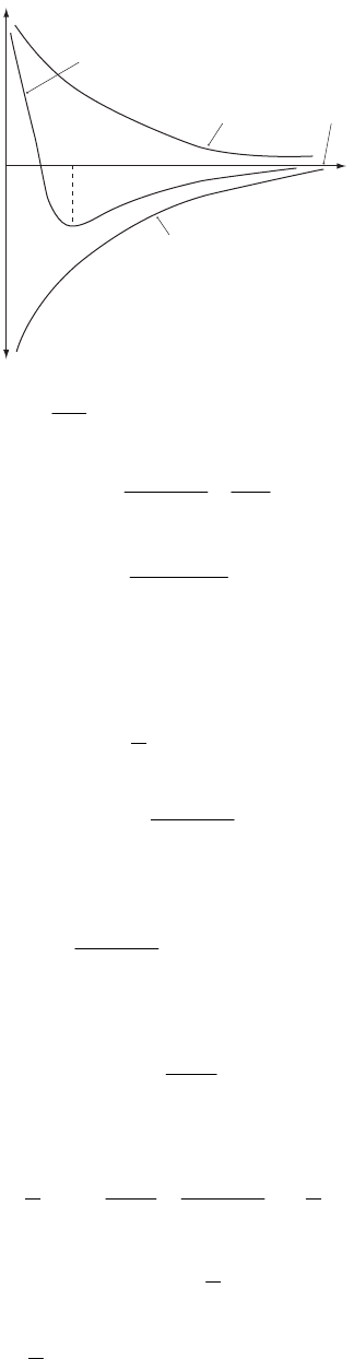
244 CHAPTER 8
Energy
V(r)
U(r)
T(r)E(r) = 0
r0
Minimum in V(r) is found by setting 0
dV
dr
=
at 0
rr
=
2
23
00
0es
GM m
rr
µ
=− +
2
0
es
rGM m
µ
=−
8-10. For circular motion
22
1
2ee
Tm
ω
=r
se
e
GM m
Ur
=−
We can get 2
ω
by equating the gravitational force to the centripetal force
2
2
se
ee
e
GM m mr
r
ω
=
or
2
3
s
e
GM
r
ω
=
So
2
3
11
22
se
s
ee
ee
GM m
GM
Tmr
rr
=⋅= =−
2
U
1
2
ETU U=+ =
If the sun’s mass suddenly goes to 1
2 its original value, T remains unchanged but U is halved.
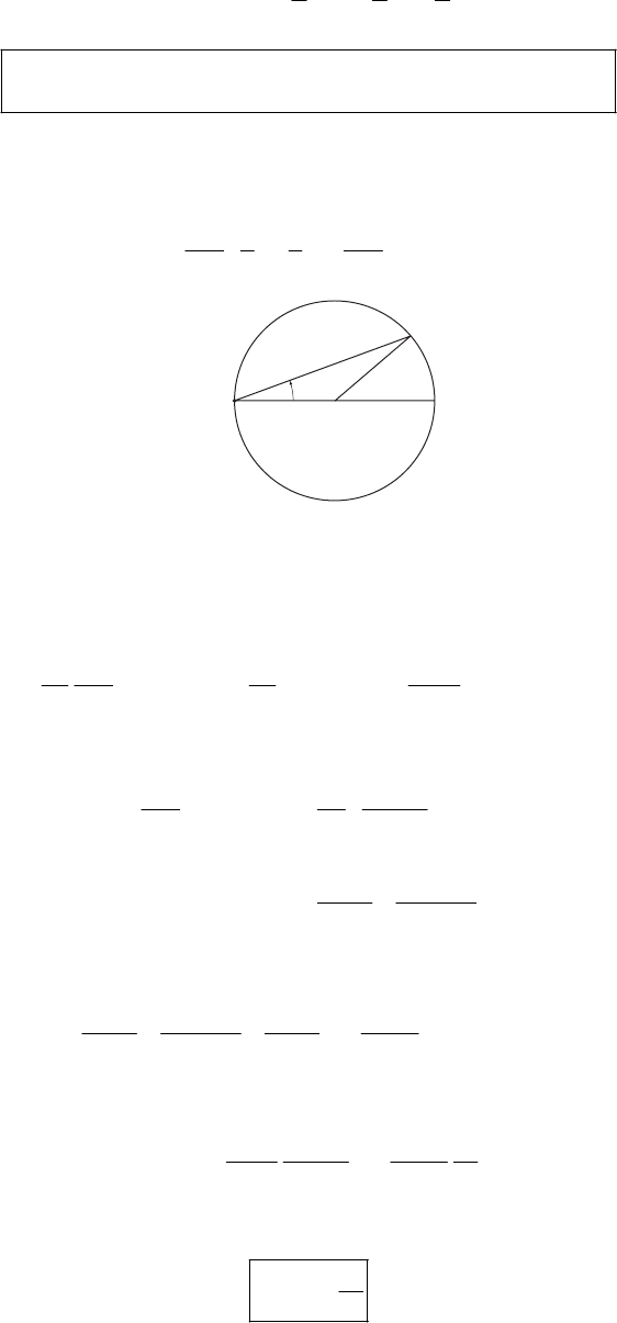
CENTRAL-FORCE MOTION 245
111
0
222
UT U U U=+ =+ =− + =
′′′
ET
T
or
he energy is 0, so the orbit is a parabola. For a parabolic
bic, the earth will escape the solar system.
8-11. For central-force motion the equation of orbit is [Eq. (8.21)]
()
22
22
11dr
F
r
drr
µ
θ
+=−
(1)
force
center
ra
θ
In our case the equation of orbit is
2cos
ra
θ
=
(2)
Therefore, (1) becomes
() ()
()
22
11 2
2
4
cos cos cos
22
dFr
ad a
µ
2
a11
θ
θ
θ
−−
+=−
θ
(3)
But we have
()
21
22
2
3
sin
cos cos
2sin
1
cos cos
dd
dd
θ
θ
θθθ
θ
θ
θ
−
=
=+ (4)
Therefore, we have
()
23
2
32
2sin 8
11 cos
cos cos cos
aFr
θµ
θ
θθθ
++=−
(5)
or,
()
22
35
28
8cos
a
Fr ar
µθ µ
=− =−
2
5
1
(6)
so that
()
5
k
Fr r
=− (7)
246 CHAPTER 8
8-12.
βr
e
r
e
The orbit of the comet is a parabola (
ε
= 1), so that the equation of the orbit is
1cos
r
α
θ
=+ (1)
We choose to measure
θ
from perihelion; hence
(
)
0E
rr
θ
β
=
= (2)
Therefore,
2
2E
r
k
α
β
µ
==
(3)
Since the total energy is zero (the orbit is parabolic) and the potential energy is Uk=− r, the
time spent within the orbit of the Earth is
()
2
2
2
2
2
2
22
2
3
E
E
E
E
E
E
r
r
r
rE
r
E
E
r
dr
T
k
rr
rdr
krr
rrrr
k
β
β
µµ
µ
β
β
µβ
Β
=
−
=−
−−
=− −
∫
∫
(4)
from which
()
32
22 211
3E
Tr
k
µ
β
β
=+−
(5)
Now, the period and the radius of the Earth are related by
2
2
4E
E
r
k
πµ
τ
=3
E
′
(6)
or,
CENTRAL-FORCE MOTION 247
32
2
E
E
E
k
r
τ
µ
π
′
= (7)
Substituting (7) into (5), we find
()
22 211
32
E
E
k
Tk
τµ
β
β
µπ
′
=+−
(8)
where s
kGM
µ
= and sE
kGM
µ
=
′. Therefore,
()()
121 1 2
3E
T
β
βτ
π
=−+ (9)
where 1 year
E
τ
=. Now, Mercury 0.387
E
rr
β
==. Therefore,
()()
12 1 0.387 1 2 0.387 365 days
3
π
+××T=−
so that
76 daysT= (10)
8-13. Setting 1≡u we can write the force as r
2
23
k3
F
ku u
rr
λ
λ
=− − =− − (1)
Then, the equation of orbit becomes [cf. Eq. (8.20)]
()
2
2
222
1du uku
du
µλ
θ
+=− − −
3
u
(2)
from which
2
22
1
du k
u
d2
µ
λµ
θ
+− =
(3)
or,
2
222
2
1
1
1
du k
u
d
µλ µ
µλ
θ
0
+
−−
−
=
(4)
If we make the change of variable,
2
2
1
1
k
vu
µ
µ
λ
=−
−
(5)
we have
2
22
1
dv v
d
µλ
θ
0
+
−
=
(6)
248 CHAPTER 8
or,
2
2
20
dv v
d
β
θ
+
= (7)
where 22
1
βµλ
=− . This equation gives different solutions according to the value of
λ
. Let us
consider the following three cases:
i) 2
λ
µ
<:
For this case and the solution of (7) is
20
β
>
(
)
cosvA
β
θδ
=
−
By proper choice of the position
θ
= 0, the integration constant
δ
can be made to equal zero.
Therefore, we can write
2
1cos k
A
r
µ
βθ
µ
λ
=+
− (9)
When
β
= 1 (
λ
= 0), this equation describes a conic section. Since we do not know the value of
the constant A, we need to use what we have learned from Kepler’s problem to describe the
motion. We know that for
λ
= 0,
()
2
11cos
k
r
µ
ε
θ
=+
and that we have an ellipse or circle (0 ≤
ε
< 1) when E < 1, a parabola (
ε
= 1) when E = 0, and a
hyperbola otherwise. It is clear that for this problem, if E ≥ 0, we will have some sort of
parabolic or hyperbolic orbit. An ellipse should result when E < 0, this being the only bound
orbit. When
β
≠ 1, the orbit, whatever it is, precesses. This is most easily seen in the case of the
ellipse, where the two turning points do not have an angular separation of
π
. One may obtain
most constants of integration (in particular A) by using Equation (8.17) as a starting point, a
more formal approach that confirms the statements made here.
ii) 2
λ
µ
=
For this case and (3) becomes
20
β
=
2
2
du k
d2
µ
θ
= (10)
so that
2
2
1
2
k
u
r
µθθ
AB
=
=++
(11)
from which we see that r continuously decreases as
θ
increases; that is, the particle spirals in
toward the force center.
CENTRAL-FORCE MOTION 249
iii) 2
λ
µ
>
For this case and the solution (7) is
20
β
<
(
)
2
coshvA
β
θδ
=
−−
(12)
δ
may be set equal to zero by the proper choice of the position at which
θ
= 0. Then,
(
)
2
2
1cosh k
A
r
µ
βθ
µ
λ
=−+
−
(13)
Again, the particle spirals in toward the force center.
8-14. The orbit equation for the central-force field is [see Eq. (8.17)]
242
2
2
2
dr r EU
dr
µ
θµ
2
=−−
(1)
But we are given the orbit equation:
2
rk
θ
= (2)
from which
2
22
4
dr k
d
θ
θ
=
(3)
Substituting (2) into (3), we have
2
2
44
dr r
k
dk
θ
==
kr
(4)
From (1) and (4), we find the equation for the potential U:
42
2
2
42
r
kr E U r
µ
µ
2
=−−
(5)
from which
22
3
21
2
k
UE rr
µµ
=− −
2
1
(6)
and
(
)
Fr U r=−∂ ∂ . Therefore,
()
2
43
61k
Fr rr
µ
=− +
(7)
250 CHAPTER 8
8-15.
AB
r
P
m
θ
b2
Let us denote by v the velocity of the particle when it is infinitely far from P and traveling along
the line AB. The angular momentum is
2
kmvb vb
b
== =2 (1)
where we have used m = 1. Therefore,
2
2
k
vb
= (2)
The total energy E of the particle is equal to the initial kinetic energy:
2
4
1
24
k
Ev b
== (3)
The general orbit equation for a force,
(
)
5
F
rkr=− , is
22
42
242
dr
drk
Err
θ
=
+−
(4)
Substituting for and E from (1) and (3), we have
()
2
442
4224
2
22
1
22
22
2
kdr
dbr kkk
brbr
dr
brbrb
dr
b
rb
θ
=
+−
=−+
=
−
2
or,
2
2dr
db
rb
θ
=− 2
−
(5)
where we have taken the negative square root because r decreases as
θ
increases (see the diagram).
We can now use the integral [see Eq. (E.4b), Appendix E]
CENTRAL-FORCE MOTION 251
1
22 2
1coth
dx ax
ax b ab b
−
=−
−
∫ (6)
from which we obtain
1
0
2coth r
b
θ
θ
−
=
+
(7)
or,
0
coth 2
rb
θ
θ
−
=
(8)
Now, coth
φ
→ ∞ as
φ
→ 0, since r → ∞ as
θ
→ 0, we must have 00
θ
=
. Thus,
(
)
coth 2rb
θ
= (9)
Notice that r is always greater than b (because coth
φ
→ 1 as
φ
→ ∞), so that the denominator in
(5) never equals zero nor changes sign. Thus, r always decreases as
θ
increases. This is, the
particle spirals in toward P but never approaches closer than a distance b.
8-16. The total energy of the particle is
ETU
=
+ (1)
a principle that by no means pushes the philosophical envelope of physical interpretation. The
impulse that causes v → v +
δ
v changes the kinetic energy, not the potential energy. We
therefore have
2
1
2
E T mv mv v
δ
δδ δ
== =
(2)
By the virial theorem, for a nearly circular orbit we have
2
1
2
Em=− v (3)
so that
2Ev
Ev
δ
δ
=
− (4)
where we have written –E since E < 0. The major and minor axes of the orbit are given by
22
k
ab
EE
µ
=− = −
(5)
Now let us compute the changes in these quantities. For a we have
2
22
kkE E
a
EE E
a
δ
δ
δδ
=− = =
−
(6)
and for b we have
252 CHAPTER 8
3
1
22
22
2
E
bE
EE
EEb
δ
δδ
δ
µµ
µ
δδ
==+−=−
−−
−
(7)
Easily enough, we can show that vv
δ
δ
=
and therefore
2abE
ab Ev
v
δ
δδ δ
== =
− (8)
8-17. The equation of the orbit is
1cos
r
α
ε
θ
=+ (1)
from which
1cos
r
α
ε
θ
=+ (2)
where 2k
α
µ
= and
2
2
2
1E
mk
ε
=+. Therefore, the radial distance r can vary from the
maximum value
(
)
1
α
ε
− to the minimum value
(
)
1
α
ε
+
. Now, the angular velocity of the
particle is given by
2
r
ω
µ
= (3)
Thus, the maximum and minimum values of
ω
become
max 2
2
min
min 2
2
max
1
1
r
r
ωµα
µε
ωµα
µε
==
+
==
−
(4)
Thus,
2
max
min
1
1n
ωε
ωε
+
=
=
−
(5)
from which we find
1
1
n
n
ε
−
=
+
(6)
8-18. Kepler’s second law states that the areal velocity is constant, and this implies that the
angular momentum L is conserved. If a body is acted upon by a force and if the angular
momentum of the body is not altered, then the force has imparted no torque to the body; thus,
CENTRAL-FORCE MOTION 253
the force must have acted only along the line connecting the force center and the body. That is,
the force is central.
Kepler’s first law states that planets move in elliptical orbits with the sun at one focus. This
means the orbit can be described by Eq. (8.41):
1cos with 0
r1
α
εθ ε
=+ << (1)
On the other hand, for central forces, Eq. (8.21) holds:
()
22
22
11dr
F
r
drr
µ
θ
+=−
(2)
Substituting 1 from (1) into the left-hand side of (2), we find r
()
2
2
1rFr
a
µ
=− (3)
which implies, that
()
2
2
Fr r
αµ
=− (4)
8-19. The semimajor axis of an orbit is defined as one-half the sum of the two apsidal
distances, and [see Eq. (8.44)], so
max
rmin
r
[]
max min 2
11
2211
rr 1
α
αα
ε
εε
+= + =
+
−−
(1)
This is the same as the semimajor axis defined by Eq. (8.42). Therefore, by using Kepler’s Third
Law, we can find the semimajor axis of Ceres in astronomical units:
2
2
2
2
4
4
C
C
CC
E
EE
E
k
a
k
a
τ
πµ
τ
πµ
=
(2)
where cs
kMm
c
γ
=, and
111
cs
Mm
µ
=+
c
Here, s
M
and are the masses of the sun and Ceres, respectively. Therefore, (2) becomes
c
m
13
2
Cscc
EseE
aMm
aMm
τ
τ
+
=
+
(3)
from which
254 CHAPTER 8
()
13
2
1
333, 480 8,000 4.6035
333, 480 1
C
E
a
a
+
=
+
(4)
so that
2.767
C
E
a
a≅ (5)
The period of Jupiter can also be calculated using Kepler’s Third Law:
12
2
312
3
2
3
4
4
J
J
JJ J
sE
E
Es
E
E
a
ka
Mm
Mma
a
k
πµ
τ
πµ
τ
JE
+
==
+
(6)
from which
()
12
3
333, 480 1 5.2028
333, 480 318.35
J
E
τ
τ
+
=
+
(7)
Therefore,
11.862
J
E
τ
τ
≅ (8)
The mass of Saturn can also be calculated from Kepler’s Third law, with the result
95.3
s
e
m
m≅ (9)
8-20. Using Eqs. (8.42) and (8.41) for a and r, we have
4
4
2
0
1cos
1
cos cos
1
adt
r
τ
εθ
θ
θ
τε
+
=
−
∫ (1)
From Kepler’s Second Law, we can find the relation between t and
θ
:
()
2
2
1
21cos
dt dA d
ab ab
ττ α
θ
ππ εθ
== + (2)
since
(
)
2
12dA r d
θ
=. Therefore, (1) becomes
()
(
42
22
4
20
11
cos cos 1 cos
2
1
aa
d
rab
π
τ
)
θ
θεθ
τπ
ε
=
−∫
θ
+
(3)
It is easily shown that the value of the integral is 2
πε
. Therefore,
CENTRAL-FORCE MOTION 255
()
4
2
4
2
11
cos 1
a
rab
θ
αε
ε
=
− (4)
After substituting a and b in terms of
ε
and
α
[see Eqs. (8.42) and (8.43)], we obtain
()
4
52
2
cos 1
a
r
ε
θε
=
− (5)
8-21. If we denote the total energy and the potential of the family of orbits by E and U(r), we
have the relation
()
2
2
2
1
22
rUr
r
µµ
E
+
+=
(1)
from which
()
22 1
22
rEUr r
µ
=−−
2
µ
(2)
Here, E and U(r) are same for all orbits, and the different values of result from different values
of
(
)
2
12 r
µ
. For stable circular motion, 0r
=
, but for all other motions, 0r
≠
. Therefore, for non-
circular motions, and is smaller than for the circular case. That is, the angular
momentum of the circular orbit is the largest among the family.
20r>
8-22. For the given force,
(
)
3
Fr kr=− , the potential is
()
2
2
k
Ur r
=− (1)
and the effective potential is
()
2
2
11
2
Vr k r
µ
=−
(2)
The equation of the orbit is [cf. Eq. (8.20)]
()
2
3
222
du u
du
µ
θ
+=− −
ku (3)
or,
2
22
1
du k u
d
µ
θ
0
+
−
=
(4)
Let us consider the motion for various values of .
256 CHAPTER 8
i) 2k
µ
=:
In this case the effective potential V(r) vanishes and the orbit equation is
2
20
du
d
θ
=
(5)
with the solution
1
uA
r
θ
B
=
=+ (6)
and the particle spirals toward the force center.
ii) 2k
µ
>:
In this case the effective potential is positive and decreases monotonically with increasing r. For
any value of the total energy E, the particle will approach the force center and will undergo a
reversal of its motion at ; the particle will then proceed again to an infinite distance.
0
rr=
V(r)
E
r
r
0
Setting 22
k
µβ
−≡1, (4) becomes 0>
2
2
20
du u
d
β
θ
+
= (7)
with the solution
()
1cosuA
r
β
θδ
== − (8)
Since the minimum value of u is zero, this solution corresponds to unbounded motion, as
expected from the form of the effective potential V(r).
iii) 2k
µ
<:
For this case we set 22
1kG
µ
−≡ >0, and the orbit equation becomes
2
2
20
du Gu
d
θ
−
= (9)
with the solution
()
1coshuA
r
β
θδ
== − (10)
so that the particle spirals in toward the force center.
CENTRAL-FORCE MOTION 257
In order to investigate the stability of a circular orbit in a 3
r1 force field, we return to Eq. (8.83)
and use
(
)
3
gr k r
µ
=. Then, we have
() ()
2
3
23 3
11
k
xx
µρ ρ µρ ρ
−=−
3
x
++
(11)
or,
()
2
3
3
10
1
xk
x
µµρ ρ
+− ⋅ =
+
(12)
Since 0
rp
r==
, Eq. (8.87) shows that 2
k
µ
=. Therefore, (12) reduces to
0x
=
(13)
so that the perturbation x increases uniformly with the time. The circular orbit is therefore not
stable.
We can also reach the same conclusion by examining the basic criterion for stability, namely,
that
2
2
0 and 0
rr
VV
rr
ρρ
==
∂∂
=
>
∂∂
The first of these relations requires 2
k
µ
= while the second requires 2k
µ
>. Since these
requirements cannot be met simultaneously, no stable circular orbits are allowed.
8-23. Start with the equation of the orbit:
1cos
r
α
ε
θ
=+ (1)
and take its time derivative
2
sin sin
r
rr
2
ε
ε
θ
θ
ααµ
==
θ
(2)
Now from Equation (8.45) and (8.43) we have
2
22
1
a
ab
µ
πµ α
τπ
ε
=⋅ = −
(3)
so that from (2)
max 2
2
1
a
r
ε
πε
µα
τ
ε
=⋅= −
(4)
as desired.
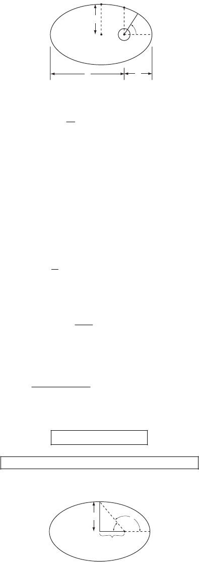
258 CHAPTER 8
8-24.
r
(b) (a)
θ
b
r
a
r
p
a) With the center of the earth as the origin, the equation for the orbit is
1cox
r
α
ε
θ
=+ (1)
Also we know
(
)
min 1ra
ε
=
− (2)
(
)
max 1ra
ε
=
+
6
min 300 km 6.67 10 m
pe
rr r== += ×
rr
6
max 3500 km 9.87 10 m
ae
r== += ×
()
6
18.27 10 m
2ap
arr=+=×
Substituting (2) gives
ε
= 0.193. When
θ
= 0,
min
1
a
r
ε
=
+
which gives . So the equation of the orbit is
6
7.96 10 m
α
=×
6
7.96 10 m 1 0.193 cos
r
θ
×=+
When
θ
= 90°,
6
7.96 10 mr
α
== ×
T he satellite is 1590 km above the earth.
b)
b
a – r
min
βθ
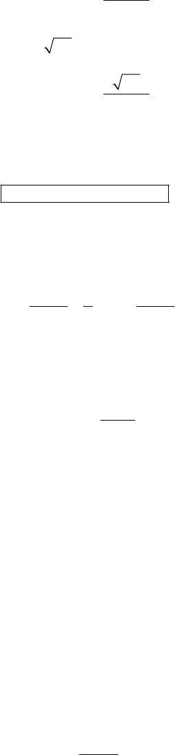
CENTRAL-FORCE MOTION 259
1
min
1
min
tan
Using
tan 101
b
ar
ba
a
ar
θ
πβ
π
α
α
θπ
−
−
=
−
=− −
=
=
−°
−
Substituting into (1) gives
; which is
6
8.27 10 mr=×
1900 km above the earth
8-25. Let us obtain the major axis a by exploiting its relationship to the total energy. In the
following, let M be the mass of the Earth and m be the mass of the satellite.
2
1
22
p
p
GMm GMm
Emv
ar
=− = = (1)
where
p
r and
p
v are the radius and velocity of the satellite’s orbit at perigee. We can solve for a
and use it to determine the radius at apogee by
1
2
2
2
app
pp
GM
rarr
rv 1
−
=−= −
(2)
Inserting the values
11 2 2
6.67 10 N m kgG
−
−
=× ⋅⋅ (3)
(4)
24
5.976 10 kgM=×
(5)
6
6.59 10 m
p
r=×
3
7.797 10 m s
p
v1
−
=
×⋅ (6)
we obtain , or 288 km above the earth’s surface. We may get the
speed at apogee from the conservation of angular momentum,
6
1.010 6.658 10 m
ap
rr=×
aa
pp
mr v mr v
=
(7)
giving . The period can be found from Kepler’s third law
1
27,780 km hr
a
v−
=⋅
23
24a
tGM
π
= (8)
Substitution of the value of a found from (1) gives
τ
= 1.49 hours.

260 CHAPTER 8
8-26.
r
r
a
r
p
First, consider a velocity kick applied along the direction of travel at an arbitrary place in
the orbit. We seek the optimum location to apply the kick.
v∆
()
1
2
2
2
initial energy
1
2
final energy
1
2
E
GMm
mv r
E
GMm
mv v r
=
=−
=
=+∆−
We seek to maximize the energy gain EE
21
−
:
()
2
21
12
2
EE mvv v−= ∆+∆
For a given , this quantity is clearly a maximum when v is a maximum; i.e., at perigee. v∆
Now consider a velocity kick applied at perigee in an arbitrary direction: V∆
∆v
v
2
v
1
The final energy is
2
2
1
2p
GMm
mv r
=
This will be a maximum for a maximum 2
v; which clearly occurs when and are along
the same direction.
1
v∆v
Thus, the most efficient way to change the energy of
elliptical orbit (for a single engine thrust) is by
firing along the direction of travel at perigee.
an
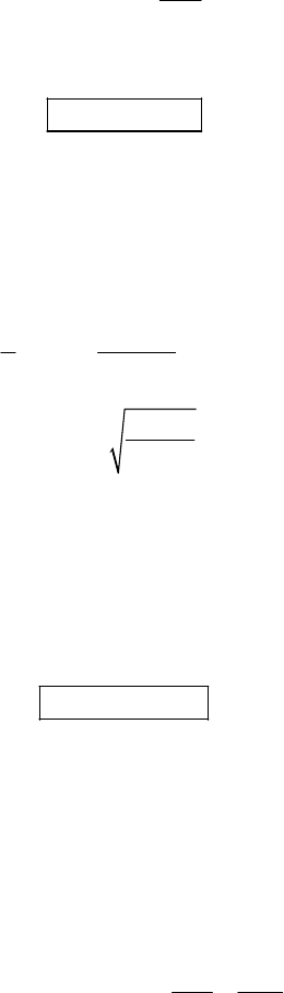
CENTRAL-FORCE MOTION 261
8-27. By conservation of angular momentum
aa
pp
pp
a
a
mr v mr v
rv
or v r
=
=
Substituting gives
1608 m/s
a
v=
8-28. Use the conservation of energy for a spacecraft leaving the surface of the moon with
just enough velocity to reach r = ∞:
esc
v
ii
ff
TU T U
+
=+
2m
esc
GM100
2m
m
mv r
−
=+
esc
2m
m
GM
vr
=
where
M
22
mass of the moon 7.36 10 kg
m==×
×
r
6
radius of the moon 1.74 10 m
m==
Substituting gives
esc 2380 m/sv=
8-29. max 0 min 0
,vvvvvv
=
+=−
From conservation of angular momentum we know
aa bb
mv r mv r
=
or
max max
max min min max
min min
;rv
vr vr rv
==
(1)
Also we know
(
)
min 1rae
=
− (2)
(
)
max 1rae
=
+ (3)
Dividing (3) by (2) and setting the result equal to (1) gives
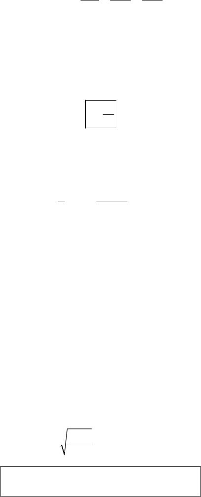
262 CHAPTER 8
() ()
()
()
max max
min min
min max
min max max min
0
1
1
11
22
rv
e
rev
vev
ev v v v
ev v
e
+
==
−
+= −
+=−
=
0
v
ev
=
8-30. To just escape from Earth, a velocity kick must be applied such that the total energy E is
zero. Thus
2
2
10
2
e
GM m
mv r
−
= (1)
where
2
24
11 2 2
6
6
velocity after kick
5.98 10 kg
6.67 10 Nm /kg
200 km
200 km 6.37 10 m
6.57 10 m
e
e
v
M
G
rr
−
=
=×
=×
=+
=+×
=×
Substituting into (1) gives v.
211.02 km/sec=
For a circular orbit, the initial velocity v is given by Eq. (8.51)
1
17.79 km/sec
e
GM
vr
==
Thus, to escape from the earth, a velocity
ck of 3.23 km/sec must be applied.ki
CENTRAL-FORCE MOTION 263
Since E = 0, the trajectory is a parabola.
parabolic
escape
orbit
circular orbit
Earth
8-31. From the given force, we find
(
)
()
3
24
dF r kk
Fr
dr r r5
′
==+
′ (1)
Therefore, the condition of stability becomes [see Eq. (8.93)]
()
()
()
()
2
5
2
4
22
30
1
kk
F
Fkk
ρ
ρρ
ρρ ρ
ρ
ρ
+′
′3
+
=
−+
′
+> (2)
or,
()
2
20
kk
kk
ρ
ρρ
−′>
+′ (3)
Therefore, if , the orbit is stable.
2kk
ρ
>′
8-32. For this force, we have
(
)
()
32
3
2
2
ra ra
ra
dF r kk
F
re e
dr r ar
kr
e
ra
−−
−
== +
′
=+
(1)
Therefore, the condition of stability [see Eq. (8.93)] becomes
()
()
23
30
r
Fr a
Fr r r
−+ +
′
+
=> (2)
This condition is satisfied if r < a.
264 CHAPTER 8
8-33. The Lagrangian of the particle subject to a gravitational force is written in terms of the
cylindrical coordinates as
()
2222
1
2
LTU mr r z mgz
θ
=−= + + −
(1)
From the constraint , we have
24ra=z
2
rr
za
=
(2)
Therefore, (1) becomes
2
222
2
11
24 4
mg
r
Lm rr r
aa
θ
=++−
2
(3)
Lagrange’s equation for
θ
is
()
20
LdL d
mr
dt dt
θ
θθ
∂∂
−
=− =
∂∂
(4)
This equation shows that the angular momentum of the system is constant (as expected):
(5)
2const.mr
θ
==
Lagrange’s equation for r is
2
22
2
1
424
mg
LdL m d r
rr mr r m r
rdtr a a dt a
θ
∂∂
−= +−− + =
∂∂
2
0
(6)
from which
2
22 2
22
1
4242
mg
mr
rr mr r m r rr
aaaa
θ
+−−+ − =
2
0
m
(7)
After rearranging, this equation becomes
22
2
22 3
1
1
44 2
mg
rm
rrr
aa amr
++ +−
0
=mr (8)
For a circular orbit, we must have 0rr
=
=
or, r =
ρ
= constant. Then,
2
3
2
mg
am
ρ
ρ
= (9)
or,
2
2
2
mg
a
4
ρ
= (10)
Equating this with 224
m2
ρ
θ
=
, we have
2
242 4
2
mg
ma
ρ
θ
=
ρ
(11)
CENTRAL-FORCE MOTION 265
or,
2
2
g
a
θ
=
(12)
Applying a perturbation to the circular orbit, we can write
where 1
x
rx
ρρ
→+ (13)
This causes the following changes:
22
33
2
13
1
rx
x
r
rx
rx
ρ
ρ
ρ
ρ
→+
−
→
→
→
(14)
from which, we have
(
)
()
22
22 2
0, in lowest order
2, in lowest ord
rr x x
rr xx x
ρ
ρρ ρ
→+ ≅
er
→+ ≅
(15)
Thus, (8) becomes
()
2
2
23
1
1
42
mg x
x
aam
ρρ
ρρ
+++−−
130
=
mx (16)
But
2
3
2
mg
am
ρ
ρ
= (17)
so that (16) becomes
22
2
3
1
42
mg
mxxx
aam
ρ
ρ
4
0
+
++ =
(18)
Substituting (17) into (18), we find
2
2
2
1
4
mg
mxx
aa
ρ
0
+
+
= (19)
or,
2
20
4
g
xx
aa
ρ
+
=
+
(20)
266 CHAPTER 8
Therefore, the frequency of small oscillations is
0
2g
az
ω
=+ (21)
where
2
04
za
ρ
=
8-34. The total energy of the system is
()
2222 2
1cot cot
2rr r mgrEm
θ
α
=++ +
α
(1)
or,
()
22 22
11
1cot cot
22
r mr mgrEm
α
θ
=+ + +
α
(2)
Substituting 2
mr
θ
=
, we have
()
2
22
2
11cot cot
22
r mgr
mr
Em
α
α
=+ ++
(3)
Therefore, the effective potential is
()
2
2cot
2
Vr mgr
mr
α
=+
(4)
At the turning point we have , and (3) becomes a cubic equation in r:
0r=
2
32
cot 0
2
mgr Er m
α
−
+=
(5)
Energy
mgr cot a
r
2
r
1
E
r
V(r)
This cubic equation has three roots. If we attempt to find these roots graphically from the
intersections of E = const. and
(
)
22
2cmr mgr otVr
α
=+, we discover that only two of the roots
are real. (The third root is imaginary.) These two roots specify the planes between which the
motion takes place.
CENTRAL-FORCE MOTION 267
8-35. If we write the radial distance r as
,corx nst.
ρ
ρ
=
+= (1)
then x obeys the oscillatory equation [see Eqs. (8.88) and (8.89)]
2
00xx
ω
+
=
(2)
where
(
)
()
0
3gg
ρ
ω
ρ
ρ
=+
′
(3)
The time required for the radius vector to go from any maximum value to the succeeding
minimum value is
0
2
t
τ
∆= (4)
where 0
0
2
π
τ
ω
=, the period of x. Thus,
0
t
π
ω
∆= (5)
The angle through which the particle moves during this time interval is
0
t
π
ω
φω
ω
=∆= (6)
where
ω
is the angular velocity of the orbital motion which we approximate by a circular
motion. Now, under the force
(
)
(
)
Fr gr
µ
=− ,
ω
satisfies the equation
(
)
(
)
2Fr g
µ
ρω µ ρ
=− = (7)
Substituting (3) and (7) into (6), we find for the apsidal angle
()
() () ()
()
033
g
gg
gg
ρ
πρ
πω π
ω
φ
ρ
ρ
ρρ
ρ
ρ
== = ′
++
′
(8)
Using
()
1
n
k
gr r
µ
=, we have
(
)
()
gn
g
ρ
ρ
ρ
′
=
− (9)
Therefore, (8) becomes
3n
φπ
=
− (10)
268 CHAPTER 8
In order to have the closed orbits, the apsidal angle must be a rational fraction of 2
π
. Thus, n
must be
2, 1, 6,n
=
−−…
n = 2 corresponds to the inverse-square-force and n = –1 corresponds to the harmonic oscillator
force.
8-36. The radius of a circular orbit in a force field described by
()
2
ra
k
F
re
r
−
=− (1)
is determined by equating F(r) to the centrifugal force:
2
2
a
ke
rm
ρ
3
ρ
−= (2)
Hence, the radius
ρ
of the circular orbit must satisfy the relation
2
a
emk
ρ
ρ
−= (3)
Since the orbit in which we are interested is almost circular, we write
(
)
(
)
[
]
1r
θ
ρδθ
=+ (4)
where
(
)
1
δ
θ
for all values of
θ
. (With this description, the apsides correspond to the
maximum and minimum values of
δ
.)
We can express the following quantities in terms of
δ
by using (4):
(
11
1ur
)
δ
ρ
=
=− (5a)
22
2
11dd
dr d
2
δ
θ
ρθ
=−
(5b)
(
)
()
(
1
2
2
21
1
au
a
Fu kue
ke a
ρ
ρδ
ρδ
−
−
=−
≅− −
+
)
(5c)
Then, substitution into Eq. (8.20) yields
()
(
2
22
11
11
a
dmke
)
p
a
d
ρ
δδ
ρθ ρ
−
−= −
δ
−+ (6)
Multiplying by
ρ
, using (3) and simplifying, (6) reduces to
()
2
21
da
d
δρδ
θ
0
+
−= (7)
CENTRAL-FORCE MOTION 269
This equation obviously has two types of solution depending on whether a
ρ
is larger than or
smaller than 1; we consider only
ρ
< a. (In fact, there is no stable circular orbit for
ρ
> a.)
For the initial condition, we choose 0
δ
δ
=
to be a maximum (i.e., an apside) at
θ
= 0. Then, we
have
(
)
12
0cos 1 , for a
δδ ρ θ ρ
=− a< (8)
This solution describes an orbit with well-defined apsides. The advance of the apsides can be
found from (8) by computing for what value of
θ
is
δ
again a maximum. Thus,
2
1a
π
θ
ρ
=− (9)
The advance of the apside is given by
(
)
12
2211 a
θππ ρ
−
∆= − = − −
(10)
In the particular case in which
ρ
a we obtain, by extending (10),
221
2a
ρ
ππ
∆≅ − +
(11)
so that
a
π
ρ
∆≅ (12)
8-37. From the equations in Section 8.8 regarding Hohmann transfers:
∆=
12
vv v∆ +∆
∆=
12
12tt
vv v v v− + −
2
11 2 1 2 21 2
2rkkkk
vmr r r mr mr mr r r
− + −
++
1
2r
∆= (1)
Substituting
()()
11 2 2 24
1
2
6
6.67 10 Nm /kg 5.98 10 kg
initial height above center of Earth 2
final height above center of Earth 3
radius of the Earth 6.37 10 m
e
e
e
e
kGM
m
rr
rr
r
−
==× ×
==
==
==×
gives
1020 m/sv∆
270 CHAPTER 8
8-38. Substitute the following into Eq. (1) of problem 8-37:
()()
11 2 2 30
11
1
11
2
6.67 10 Nm /kg 1.99 10 kg
mean Earth-sun distance 1.50 10 m
mean Venus-sun distance 1.08 10 m
s
kGM
m
r
−
==× ×
=×
r=×
The result is . The answer is negative because 5275 m/sv∆=− 2
rr
1
<
; so the rocket must be fired
in the direction opposite to the motion (the satellite must be slowed down).
5275 m/s; opposite to direction of motion.v∆=
From Eq. (8.58), the time is given by
32
32 12
2
t
rr
mm
Ta
kk
ππ
+
==
(1)
Substituting gives
148 days
τ
8-39. We must calculate the quantity 1
v
∆
for transfers to Venus and Mars. From Eqs. (8.54),
(8.53), and (8.51):
1
11
2
11 2 1
2
t
vv v
rkk
mr r r mr
∆= −
=−
+
where
()()
11 3 2 30
9
1
9
2
6.67 10 m /s -kg 1.99 10 kg
mean Earth-sun distance 150 10 m
Venus 108
mean sun distance 10 m
Mars 228
s
kGM
m
r
−
==× ×
×
=−=
r==
×
Substituting gives
Venus
Mars
2.53 km/sec
2.92 km/sec
v
v
∆
=−
∆=
where the negative sign for Venus means the velocity kick is opposite to the Earth’s orbital
motion.
Th us, a Mars flyby requires a larger than a Venus flyby.v∆
CENTRAL-FORCE MOTION 271
8-40. To crash into the sun, we calculate 1
v
∆
from Eq. (8.54) with r = mean distance from
sun to Earth, and = radius of the sun. Using Eqs. (8.54), (8.53), and (8.51) we have
1
2
r
()
2
1sun
112 1
2ss
GM GM
r
vrrr r
∆= −
+
Substituting
11 2 2
30
11
1
8
2sun
6.67 10 Nm /kg
1.99 10 kg
1.5 10 m
6.96 10 m
s
se
G
M
rr
rr
−
=×
=×
== ×
== ×
gives
(
)
1sun 26.9 km/secv∆=−
To escape from the solar system, we must overcome the gravitational pull of both the sun and
Earth. From conservation of energy ( final 0E
=
) we have:
2
10
2
se
se e
GM m GM m mv
rr
−−+=
Substituting values gives
43500 m/sv
=
Now
()
()
escape
43500 29700 m/s
13.8 km/s
i
s
se
vvv
GM
vr
v
∆
=−
=−
=−
∆=
To
les
send the waste out of the solar system requires
s energy than crashing it into the sun.
8-41. From the equations in Section 8.8 regarding Hohmann transfers
12
12
12
tt
vv v
vvvv
∆
=∆ +∆
=
−+−
where
272 CHAPTER 8
1
2
1
11 2 1
2;
t
rkk
vv
mr r r mr
==
+
2
1
1
21 2 2
2;
t
rkk
vv
mr r r mr
==
+
Substituting
()()
11 2 2 24
65
1
8
2
6.67 10 Nm /kg 5.98 10 kg
200 km 6.37 10 m 2 10 m
mean Earth-moon distance 3.84 10 m
e
e
kGM
m
r
−
==× ×
=+=×+×
==
rr
×
gives
3966 m/sv∆=
From Eq. (8.58), the time of transfer is given by
32
32 12
2
t
rr
mm
Ta
kk
τπ
+
==
Substituting gives
429,000 sec. 5 days
τ
=
8-42.
r=×
11 2 2
24
56
1
2
8
3
6.67 10 Nm /kg
5.98 10 kg
2 10 m 6.37 10 m
?
mean Earth-moon distance 3.84 10 m
e
G
M
r
r
−
=×
=×
+ ×
=
==×
We can get from Kepler’s Third Law (with
τ
= 1 day)
2
r
13
2
7
224.225 10 m
4
e
GM
r
τ
π
==×
We know 2EGMm=− r
CENTRAL-FORCE MOTION 273
So
()
()
()
11
1
1
10
2
9
3
3.04 10 J
2
4.72 10 J
5.19 10 J
e
GM m
Er r
Er
Er
=− =− ×
=− ×
=− ×
To place the satellite in a synchronous orbit would require a minimum energy of
(
)
(
)
21
Er Er
−
=
11
2.57 10 J×
8-43. In a circular orbit, the velocity v of satellite is given by
0
2
0
0
2
mv GMm GM
v
RR R
=⇒=
where M is the Earth’s mass.
Conservation of energy implies
22
12
22
mv mv
GMm GMm
RR
−=−
2
Conservation of angular momentum gives
12
2mRv m Rv
=
From these equations, we find
1
4
3
GM
vR
=
so the velocity need to be increased by a factor 4 3 to change the orbit.
8-44. The bound motion means that
2
0
2
mv
EV
=
+<
where ra
k
r
−
=−
Ve
.
The orbit of particle moving in this central force potential is given by
274 CHAPTER 8
()
(
)
min
min
2
2
2
22
2
/
22
1
2
2
r
r
r
ra
r
rdr
r
EV r
dr
rke
Err
θ
µµ
µ
µ
−
=
−
=
+−
∫
∫
In first order of , this is ( / )ra
() 22
22
22
22
22
r
dr dr
kk kk
rE r E
rra arr
µµ
θ
µ
µ
+− − − +−
∫∫
≈=
Now effectively, this is the orbit of particle of total energy k
Ea
−
moving in potential
k
r
−
. It is
well known that this orbit is given by (see Chapter 8)
1cos
r
α
ε
θ
=+
where
2
k
α
µ
= and
2
2
2
1k
E
ka
εµ
=+ −
If 0 1
ε
<<, the orbit is ellipsoid; if 0
ε
=
, the orbit is circular.
8-45.
a) In equilibrium, for a circular orbit of radius r0,
20
00
0
F
Fmr mr
φφ
ωω
=⇒=
b) The angular momentum (which is conserved) of a particle in circular orbit is
2
0
Lmr
φ
ω
=3
0
mFr=
The force acting on a particle, which is placed a distance r (r is very close to equilibrium position
) from the center of force is
o
r
() ()()
3
2
00
3
32 2
00 0 0
32 4
00 0
33
L
FmrF F
mr
LL L
rr F rr krr
mr mr mr
φ
ω
=−=−
≈− −−=− −=−−
CENTRAL-FORCE MOTION 275
where . So the frequency of oscillation is
2
0
3/kLmr≡4
2
0
24
00
3
3
r
F
kL
mmr mr
ω
== =
8-46. In equilibrium circular orbit,
22
22
44
M
vGM GM
R
RR
=⇒=
v
where M is the Sun’s mass.
The period is
32
7
24 2 910yr
RRR D
vGM GM
ππ π
== = ≈×
T
where
D is the separation distance of 2 stars.
2
=R
8-47. In equilibrium circular orbit of 1st star
2
11 1 2
12
M
vGMM
LL
= where 2
1
12
LM
LMM
=+ is the distance from 1st star to the common center of
mass.
The corresponding velocity is
2
21 2
12
12
()
GM L GM
vLLMM
==
+
Finally, the period is
32
8
1
112
22 1.2 10 yr.
()
LL
vGM M
ππ
== =×
+
T
276 CHAPTER 8
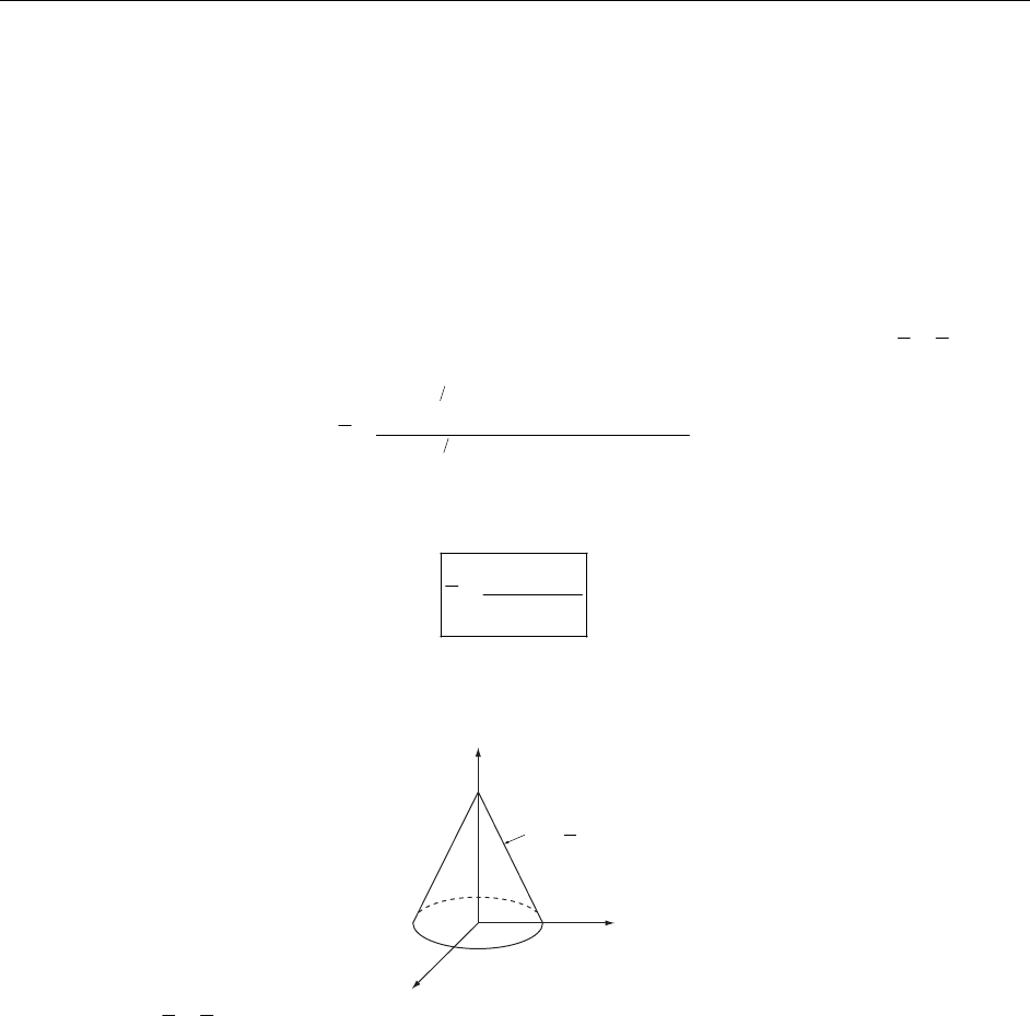
CHAPTER 9
D
y
namics o
f
a
System o
f
Particles
9-1. Put the shell in the z > 0 region, with the base in the x-y plane. By symmetry, 0xy==.
2
1
2
1
22 2
00
22 2
00
sin
sin
r
rr
r
rr
z
rdr dd
z
rdr dd
ππ
φθ
ππ
φθ
ρ
θθφ
ρ
θθφ
== =
===
=∫∫∫
∫∫∫
Using z = r cos
θ
and doing the integrals gives
(
)
()
44
21
33
21
3
8
rr
zrr
−
=−
9-2.
z
h
x
y
a
zh
ah=− +
ρ
By symmetry, 0xy==.
Use cylindrical coordinates
ρ
,
φ
, z.
0mass density
ρ
=
277
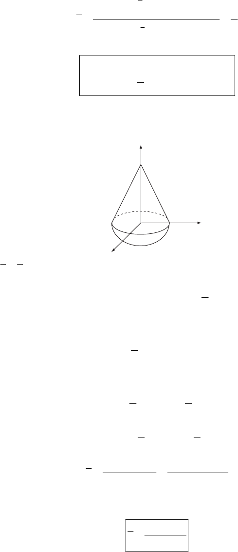
278 CHAPTER 9
2
0
000
240
000
4
h
ah
a
z
h
ah
z
zdddz h
z
dddz
πρ
φρ
πρ
φρ
ρρρφ
ρρρφ
−+
===
−+
===
==
∫∫∫
∫∫∫
The center of mass is on the axis
3
of the cone from the vertex.
4h
9-3.
z
h
x
y
a
By symmetry, 0xy==.
From problem 9-2, the center of mass of the cone is at 1
4
z
h=.
From problem 9-1, the center of mass of the hemisphere is at
()
21
3,0
8
zarar
=
−==
So the problem reduces to
2
111
11
;
43
z
hm a h
ρπ
==i
3
222
32
;
83
z
am a
ρ
π
=− =i
()
22
11 22 1 2
12 1 2
3
42
mz mz h a
zmm h a
ρρ
ρ
ρ
+−
==
++
for 12
ρ
ρ
=
()
23
3
42
ha
zah
−
=+
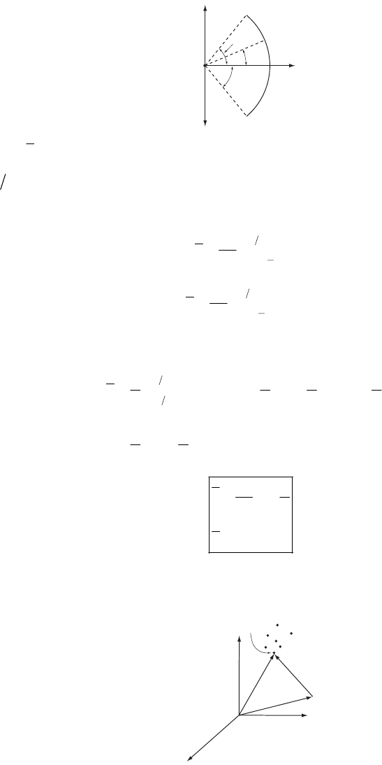
DYNAMICS OF A SYSTEM OF PARTICLES 279
9-4.
θ′
θ/2
θ/2
y
x
a
a
By symmetry, 0y=.
If mass length
σ
= then
M
a
σ
θ
=
So
2
2
1
x xdm
M
θ
θ
θ
=−
′
=∫
2
2
1
xx
M
θ
θ
θ
ad
σ
θ
=−
′
=
′
∫
Using
M
a
σ
θ
= and cosxa
θ
=′,
2
2
1cos sin sin
22
2sin 2
a
xad
a
θ
θ
θ
θ
θθ
θθ
θ
θ
−
==−
′′
−
=
∫
2sin 2
0
a
x
y
θ
θ
=
=
9-5.
r
i
– r
0
r
0
r
i
m
i

280 CHAPTER 9
th
th
1
position of the particle
mass of the particle
total mass
constant gravitational field
i
i
i
mi
Mm
=
=
==
=
∑
r
g
Calculate the torque about
0
r
()
()
()()
()
0
0
10
0
0
i
ii
ii
ii
ii i
ii
m
mm
mm
mM
ττ
=
=−×
=−×
=×−×
=×−
=×−×
×
∑
∑
∑
∑∑
∑∑
∑
rr F
rr g
rgrg
rg r
rg rg
g
Now if the total torque is zero, we must have
0ii
mM=
∑
rr
or
0
1
ii
m
M
=
∑
rr
which is the definition of the center of mass. So
0CM
0 about
or center of gravity center of mass.
τ
==
=
rr
9-6. Since particle 1 has F = 0, , then
00
0==rv 10
=
r. For particle 2
0
20
ˆˆ
then
F
Fr
m
==Fx x
Integrating twice with gives
00
0==rv
2
0
2ˆ
2
F
rt
m
=x
2
0
11 22
CM
12
ˆ
4
F
mm t
mm m
+
==
+
rr
rx

DYNAMICS OF A SYSTEM OF PARTICLES 281
2
0
CM
0
CM
0
CM
ˆ
4
ˆ
2
ˆ
2
Ft
m
Ft
m
F
m
=
=
=
rx
vx
ax
9-7.
O
y
a
a
H
H
x
52˚
52˚
By symmetry 0y=
016
H
mm=
Let
0
,16
H
mmm==m
Then
3
1
1
ii
xm
M
=∑x
()
cos 52
12cos52
18 9
a
xma
m
°
=°=
0.068xa=
9-8. By symmetry, 0x=. Also, by symmetry, we may integrate over the x > 0 half of the
triangle to get y.
σ
= mass/area
22
00
22
00
32
aa
x
xy
aa
x
xy
ydydx a
y
dy dx
σ
σ
−
==
−
==
==
∫∫
∫∫
32
a
y=
282 CHAPTER 9
9-9.
POW!
45˚
z
y
m
1
m
2
v
1
v
y
v
z
Let the axes be as shown with the projectile in the y-z plane. At the top just before the explosion,
the velocity is in the y direction and has magnitude 0
02
y
v
v=.
0
12
00
0
12
2
22
y
E
mm
vE
vmm
+
== = +
where and are the masses of the fragments. The initial momentum is
1
m2
m
()
0
12
12
0, , 0
i
E
pmm mm
=+
+
The final momentum is
12f
p
pp
=
+
(
)
11 1
0,0,
p
mv=
(
)
22
,,
x
y
z
p
mvvv=
The conservation of momentum equations are
2
:0
xx
vorv==0
x
pm
() ()
01 2 2 01 2
2
1
:
yyy
p
Em m mv or v Em m
m
+= = +
2
11 2 1
1
or :0
z
zz
m
p
mv mv v v
m
=+ =−
The energy equation is
()
()
22
0
12 0 11 2
12
1
222
2
11
y
z
E
mm E mv mvv
mm
++=+
++
or
(
)
22
0112
32
y
z
Emvmvv=+ +
Substituting for
y
v and v gives
1
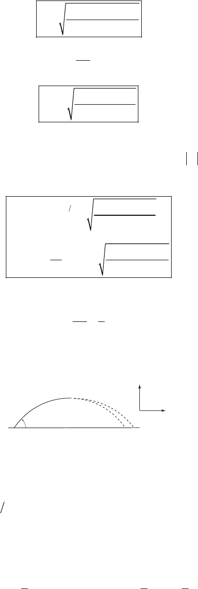
DYNAMICS OF A SYSTEM OF PARTICLES 283
()
()
01 2 1
2
21 2
2
z
Em m m
vmm m
−
=+
2
1
1
z
m
vv
m
=− gives
()
()
021
1
11 2
2Emm
vmm m
−
=− +
So
travels straight down with speed =
1
m1
v
travels in the y-z plane
2
m
()
()
()
()
()
12 012
22
2
21 2
121
11
12
4
2
tan tan
yz
z
y
Emm
vvv mm m
mmm
v
vm
θ
−−
+
=+ = +
−
== +m
The mass is the largest it can be when
1
m10v
=
, meaning 2
2mm
1
=
and the mass ratio is
1
2
1
2
m
m
=
9-10.
x2
x1
x
y
B
A
θ
First, we find the time required to go from A to B by examining the motion. The equation for the
y-component of velocity is
0sin
y
vv gt
θ
=
− (1)
At B, v; thus
0
y=0sin
B
tv g
θ
=. The shell explodes giving m and horizontal velocities v
and (in the original direction). We solve for and using conservation of momentum and
energy.
1 2
m1
2
v1
v2
v
(
)
120 112
os
x2
:c
p
mmv mvmv
θ
+=+ (2)
()
22 2
120 11 2
11
:cos
22
mv Emv
θ
++=+
2
2
1
2
mvEm (3)
Solving for in (2) and substituting into (3) gives an equation quadratic in v. The solution is
2
v1
284 CHAPTER 9
()
2
10
11 2
cos mE
vv mm m
θ
2
=± + (4)
and therefore we also must have
()
1
20
21 2
cos mE
vv mm m
θ
2
=+
∓ (5)
Now we need the positions where m and m land. The time to fall to the ocean is the same as
the time it took to go from A to B. Calling the location where the shell explodes x = 0 gives for
the positions of and upon landing:
1 2
1
m2
m
11 2 2
;
B
xvt xvt
B
=
= (6)
Thus
0
12 12
sinv
xx vv
g
θ
−= − (7)
Using (4) and (5) and simplifying gives
01
12
12 2 1
sin 2
vmmE
gmmmm
θ
2
xx
−= +
+
(8)
9-11. The term in question is
b
α
β
αβ
α
≠
∑
∑f
For n = 3, this becomes
(
)
(
)
(
)
12 13 21 23 31 32 12 21 13 31 23 32
+++++=+++++ffff ff ff ffff
But by Eq. (9.1), each quantity in parentheses is zero. Thus
33
11
0
αβ
αβ
αβ
==
≠
=
∑∑f
9-12.
a) 0
0ln m
vv u m
=+
Assuming , we have
00v=
m10
100 ln
s9
v
=
0
8
2.02 m/s; yes, he runs out of gas.v=
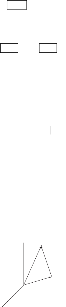
DYNAMICS OF A SYSTEM OF PARTICLES 285
b) Relative to Stumblebum’s original frame of reference we have:
Before throwing tank
98 kg
2.02 m/s→
After throwing the tank we want Stumblebum’s velocity to be slightly greater than 3 m/s (so
that he will catch up to the orbiter).
8 kg 90 kg
3m/sV←→
Conservation of momentum gives
(
)
(
)
(
)
(
)
(
)
98 kg 2.02 m/s 90 kg 3 m/s 8 kg
9 m/s
v
v
=−
=
(This velocity is relative to Stumblebum’s original reference frame; i.e., before he fires his
pressurized tank.) Since Stumblebum is traveling towards the orbiter at 2.02 m/s, he must
throw the tank at v = 9 m/s + 2.02 m/s
11 m/sv=
9-13. From Eq. (9.9), the total force is given by
()e
α
αβ
ααβ
αβ
≠
+
∑
∑∑
Ff
As shown in Section 9.3, the second term is zero. So the total force is
()e
α
α
∑
F
It is given that this quantity is zero.
Now consider two coordinate systems with origins at 0 and 0′
O
O′
m
α
r
α
′
r
α
r
0
where
is a vector from 0 to 0′
0
r
α
r is the position vector of m
α
in 0
286 CHAPTER 9
α
′
r is the position vector of m
α
in 0′
We see that 0a
α
=+
′
rrr
The torque in 0 is given by
()e
α
α
α
τ
=×
∑
rF
The torque in 0′ is
()
()
()
0
() ()
0
()
0
e
e
ee
e
αα
α
αα
α
α
αα
αα
α
α
τ
τ
=×
′′
=−×
=×−×
=− ×
∑
∑
∑∑
∑
rF
rr F
rF rF
rF
But it is given that
() 0
e
α
α
=
∑F
Thus
τ
τ
=
′
9-14. Neither Eq. (9.11) or Eq. (9.31) is valid for a system of particles interacting by magnetic
forces. The derivations leading to both of these equations assumes the weak statement of
Newton’s Third Law [Eq. (9.31) assumes the strong statement of the Third Law also], which is
α
ββα
=
−ff
That this is not valid for a system with magnetic interactions can be seen by considering two
particles of charge and moving with velocities and :
1
q2
q1
v2
v
q1
q2
v2
f21
v1
f12
Now
i
j
ii i
j
q
=
×fvB
where i
j
B is the magnetic field at due to the motion of
i
q
j
q.
DYNAMICS OF A SYSTEM OF PARTICLES 287
Since i
j
f is perpendicular to both and
i
vi
j
B (which is either in or out of the paper), i
j
f can only
be parallel to
j
i
f if and
i
v
j
v are parallel, which is not true in general.
Thus, equations (9.11) and (9.31) are not valid for
ystem of particles with magnetic interactions.a s
9-15.
σ
= mass/length
dp
Fdt
= becomes
mg mv mv
=
+
where m is the mass of length x of the rope. So
;
mxmx
σ
σ
=
=
2
2
dv
xg x xv
dt
dv dx
xg x v
dx dt
dv
xg xv v
dx
σσ σ
=+
=+
=+
Try a power law solution:
1
;
nn
dv
vax nax
dx
−
==
Substituting,
(
)
(
)
122nn
xg x ax nax a x
−
=+
n
or
(
)
22
1n
xg a n x=+
Since this must be true for all x, the exponent and coefficient of x must be the same on both sides
of the equation.
Thus we have: 1 = 2n or 1
2
n=
()
22
1 or 3
g
gan a
=+ =
So
2
3
gx
v=
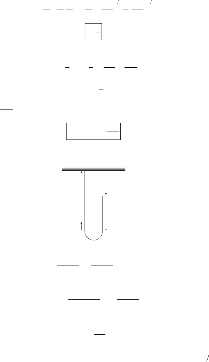
288 CHAPTER 9
12 12
22
333
gx g gx
dv dv dx dv
dt dx dt dx
−
av
== = =
3
g
a
=
TU
00(0 on t
ii
y===
able)
22
11
223
f
gL mgL
Tmvm
== =
3
2
f
L
Umghmg==−
So 0; 6
if
mgL
EE==−
Energy lost 6
mgL
=
9-16.
T1T2
T
x
The equation of motion for the falling side of the chain is, from the figure,
(
)
(
)
2
22
bx bx
xg
ρρ
−−
T
=
+
(1)
From Example 9.2, we have for the energy conservation case
(
)
() ()
22
2
2
2
2
gbxx x
xg g bx
bx
−
=− =+
−
−
(2)
Substitution gives us
2
24
x
T
ρ
= (3)
To find the tension on the other side of the bend, change to a moving coordinate system in
which the bend is instantaneously at rest. This frame moves downward at a speed 2ux= with
respect to the fixed frame. The change in momentum at the bend is
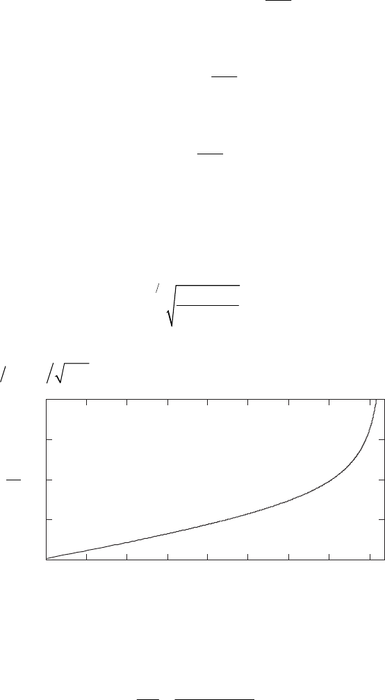
DYNAMICS OF A SYSTEM OF PARTICLES 289
()
()
2
2
22 2
x
p
xu ut
ρ
ρρ
∆= ∆ ⋅ = ∆= ∆
t (4)
Equating this with the net force gives
2
12 2
x
TT
ρ
+=
(5)
Using equation (3), we obtain
2
14
x
T
ρ
= (6)
as required. Note that equation (5) holds true for both the free fall and energy conservation
cases.
9-17. As the problem states, we need to perform the following integral
()
12 12
21 d
ε
α
τ
α
αα
−
=−
∫ (1)
Our choice of
ε
is 10 for this calculation, and the results are shown in the figure. We plot the
natural velocity
4−
2dd x gb
ατ
= vs. the natural time
τ
.
0 0.1 0.2 0.3 0.4 0.5 0.6 0.7 0.8
0
0.5
1
1.5
2
τ
d
d
α
τ
9-18. Once we have solved Problem 9-17, it becomes an easy matter to write the expression
for the tension (Equation 9.18):
()
2
12 6
21 2
T
mg
α
α
α
+−
=− (1)
This is plotted vs. the natural time using the solution of Problem 9-17.
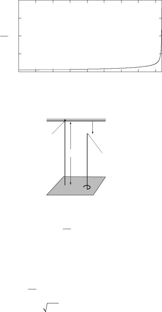
290 CHAPTER 9
0 0.1 0.2 0.3 0.4 0.5 0.6 0.7 0.8
0
5
10
15
20
τ
T
mg
9-19.
released at
t = 0
x
at time t
ceiling
table
b
The force that the tabletop exerts on the chain counteracts the force due to gravity, so that we
may write the change in momentum of the center of the mass of the chain as
dp bg F
dt
ρ
=
− (1)
We can write out what the momentum is, though:
(
)
p
bxx
ρ
=
− (2)
which has a time derivative
()
(
23
dp xbxx bggx
dt
ρρ
=−+− = −
)
(3)
where we have used and
xg=
2xg=
x
3
. Setting this last expression equal to (1) gives us
F
gx
ρ
=
(4)
Although M. G. Calkin (personal communication) has found that experimentally the time of fall
for this problem is consistently less than the value one would obtain in the above treatment by
about 1.5%, he also finds evidence that suggests the free fall treatment is more valid if the table
is energy absorbing.
DYNAMICS OF A SYSTEM OF PARTICLES 291
9-20.
a – x
a + x
Let
ρ
= mass/length
The force on the rope is due to gravity
(
)
(
)
2
F
ax g ax g
xg
ρ
ρ
ρ
=
+−−
=
2
dp dv dv
ma
dt dt dt
ρ
==
So dp
Fdt
= becomes
dv
xg a dt
=
Now
dv dv dx dv
v
dt dx dt dx
=⋅=
So
dv
xg av dx
=
or
g
vdv xdx
a
=
Integrating yields
22
1
22
g
vx
ac
=
+
Since v = 0 when x = 0, c = 0.
Thus
22
g
vx
a
=
When the rope clears the nail, x = a. Thus
vga=
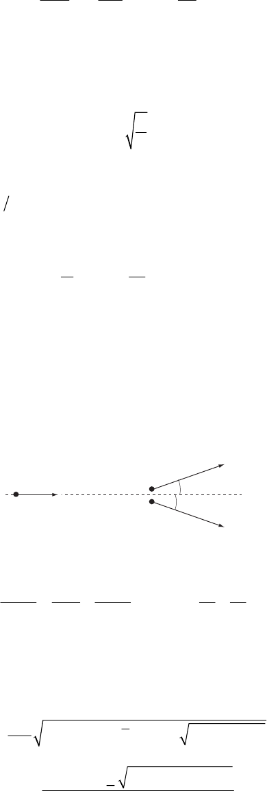
292 CHAPTER 9
9-21. Let us call the length of rope hanging over the edge of the table, and the total
length of the rope. The equation of motion is
x L
2
2
mgx gx
dx
mx
Ldt
=⇒=
L
Let us look for solution of the form
tt
xAe Be
ω
ω
−
=+
Putting this into equation of motion, we find
g
L
ω
=
Initial conditions are ;
(0) 0 0.3 m
t
xx
=== (0) 0m/s
t
v=
=
.
From these we find 02
A
Bx== .
Finally 0cosh ( )xx t
ω
=. When , the corresponding time is xL=
1
0
1cosh 0.59 s.
L
tx
ω
−
==
9-22. Let us denote (see figure)
m and 2m mass of neutron and deuteron respectively
0
v velocity of deuteron before collision
1
v and v velocity of neutron and deuteron, respectively after collision
2
2m
2mν
0
ν
2
ν
1
mα
ψ
a) Conservation of energy:
222 2
2
012 1
0
2
222 2
mv mv mv v v
v=+ ⇒=+
2
2
2
2
Conservation of momentum is
22 222
021 20102
44 8cosmv mv v v v v v v
ψ
=+⇒+=+
Solving these equations, we obtain 2 sets of solutions
22
0
1
26 4 cos 2 cos 4 cos 3
3
v
ψψ ψ
+
v=− −
22
00
2
2 cos 4 cos 3
3
vv
v
ψψ
+−
=
2
0
v
DYNAMICS OF A SYSTEM OF PARTICLES 293
or numerically
15.18 km/sv=214.44 km/sv
=
and
119.79 km/sv=25.12 km/sv
=
b) Let us call
α
the lab scattering angle of the neutron, then from the sine theorem we have
12 2
1
2sin 2 sin
sin sin
mv mv v
v
α
ψ
ψα
=⇒=
74.84 and 5.16
α
α
⇒= ° = °
c) From a) we see that
22
02
02
44
cos 8
vvv
vv
ψ
2
1
+
−
=
22
0
02
max
02
26 330 30
82
vv
vv
ψψ
+⇒≤⇒==≥ °
9-23. Conservation of momentum requires
f
v to be in the same direction as u (component
of
1
f
v ⊥ to must be zero).
1
u
11i
pmu
=
(
)
12
ff
p
mmv=+
1
1
12
if f
m
p
pv
mm
=→= +u
The fraction of original kinetic energy lost is
()
()
22
211
11 1 2 2
12
2
11
2
1
1
12
1
2
12
11
22
1
2
if
i
mu
mu m m
KK mm
Kmu
m
mmm
m
m
mm
−+
−+
=
−+
=
=+
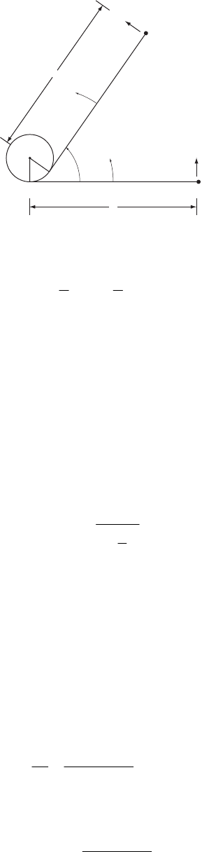
294 CHAPTER 9
9-24.
ω
0
b
v
0
x
ω
v
m
a
O
θθ
The energy of the system is, of course, conserved, and so we have the following relation
involving the instantaneous velocity of the particle:
2
0
11
22
mv mv=2
(1)
The angular momentum about the center of the cylinder is not conserved since the tension in
the string causes a torque. Note that although the velocity of the particle has both radial and
angular components, there is only one independent variable, which we chose to be
θ
. Here
ω
θ
= is the angular velocity of the particle about the point of contact, which also happens to be
the rate at which the point of contact is rotating about the center of the cylinder. Hence we may
write
(
)
00 0
;vb vba
ω
ωθ
=
=− (2)
From (1) and (2), we can solve for the angular velocity after turning through an angle
θ
0
1a
b
ω
ω
θ
=
−
(3)
The tension will then be (look at the point of contact)
(
)
2
0
Tm ba m b
ω
θωω
=−= (4)
9-25. The best elements are those that will slow down the neutrons as much as possible. In a
collision between (the neutron) and (moderator atom), we would thus want to minimize
(kinetic energy of the neutron after the collision); or alternatively, maximize T (kinetic
energy of the moderator atom after the collision). From Eq. (9.88)
1
m2
m
1
T2
()
2
212
2
012
4cos
Tmm
Tmm
ζ
=+
Since one cannot control the angle
ζ
, we want to maximize the function
()
12
2
12
mm
fmm
=+
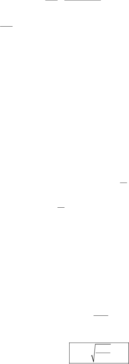
DYNAMICS OF A SYSTEM OF PARTICLES 295
with respect to . ( m = constant)
2
m1
(
)
()
22
11 2
12
4
212
0 when
mm m
df mm
dm mm
−
==
+=
By evaluating
12
2
2
2mm
df
dm =
12
mm=
one can show that the equilibrium point is a maximum. Thus, is a
maximum for . Back to reactors, one would want elements whose mass is as close as
possible to the neutron mass (thus, as light as possible). Naturally, there are many other factors
to consider besides mass, but in general, the lower the mass of the moderator, the more energy
is lost per collision by the neutrons.
2
T
9-26. The internal torque for the system is
112221
=
×+×Nr f r f (1)
where f is the force acting on the first particle due to the second particle. Now
12
21 12
=
−ff
(2)
Then,
(
)
()()()
()()
12 12
12 21 21
0
12 12
0
r
kv
kr
v
=−×
=−×−− −
=−×−
Nrr f
rr rr rr
rr rr
(3)
This is not zero in general because
(
)
12
−rr and
(
)
12
−rr
are not necessarily parallel. The
internal torque vanishes only if the internal force is directed along the line joining two particles.
The system is not conservative.
9-27. The equation for conservation of
y
p
in the lab system is (see fig. 9-10c):
11 22
0sin simv mv n
ψζ
=
−
Thus
11
22
sin sin
mv
mv
ζ
ψ
=
or
11
22
sin sin
mT
mT
ζ
ψ
=
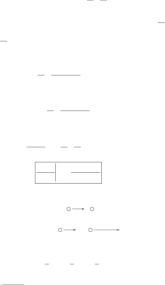
296 CHAPTER 9
9-28. Using the notation from the chapter:
10
:,
if
mTTTT
1
=
=
22
:0;
if
mT TT
=
=
Thus
1
012
00
1TT
TTTor TT
=+ = +
2
(1)
If we want the kinetic energy loss for to be a maximum, we must minimize
1
m1
0
T
T or,
equivalently, maximize 2
0
T
T.
From Eq. (9.88):
()
2
212
2
012
4cos
Tmm
Tmm
ζ
=+
To maximize this,
ζ
= 0 (it can’t = 180°).
()
21
2
012
4Tmm
Tmm
=+
2
1
The kinetic energy loss for is T. The fraction of kinetic energy loss is thus
1
m0
T−
01 1
00
1
TT TT
TT
2
0
T
−
=− = (from (1))
()
01 12
2
012
max
4
TT mm
Tmm
−=+
ζ
= 0 implies
ψ
= 0, 180° (conservation of ). So the reaction is as follows
v
p
Before:
After:
m
1
v
1
m
2
m
1
v
1
m
2
v
2
1112
:
x
pmvmvmv
2
=
+
22
111
111
:222
Emv mvm=+
2
22
v
Solving for gives
1
v12
1
12
mm
vv
mm
−
=+
So
travels in + x direction
2
m
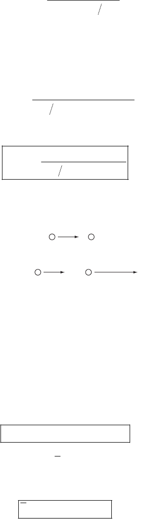
DYNAMICS OF A SYSTEM OF PARTICLES 297
m travels in
1
12
12
direction if
direction if
xm
xm
+>
−<
m
m
9-29. From Eq. (9.69)
()
12
sin
tan cos mm
θ
ψθ
=+
From Eq. (9.74)
2
θ
π
ζ
=
−
Substituting gives
(
)
()
()
12
sin 2
tan cos 2mm
πζ
ψ
πζ
−
=+−
or
()
()
()
12
sin 2
tan cos 2mm
ζ
ψ
ζ
=−
9-30.
Before:
After:
m
1
v
1
m
2
m
1
v
1
m
2
v
2
a)
(
)
(
)
0.06 kg 16 m/s cos 15 8 m/s cos 45
1.27 N sec
y
p∆= °−− °
=⋅
(
)
(
)
0.06 kg 16 m/s cos 15 8 m/s sin 45
0.09 N sec
x
p∆= °− °
=− ⋅
The impulse P is the change in momentum.
So
(
)
0.09 1.27 N sec=− + ⋅Pxy
b) dt t
=
=∆
∫
PF F
So
(
)
9127 N=− +Fxy
298 CHAPTER 9
9-31. From Eq. (9.69)
1
2
sin
tan
cos
m
m
θ
ψ
θ
=
−
From Eq. (9.74)
θ
πφ
=
−
Substituting gives
1
2
sin
tan
cos
m
m
φ
ψ
φ
=
−
9-32. 1i
pmu
=
12
2
f
p
mv mv
=
+
Conservation of momentum gives
11 2 11
22uv vorvu v
2
=
+=−
()
222
112
22 2
11122
2
12 2
11
22
11 44
22
23
Tmu mvmv
mu m u u v v mv
mu v mv
∆= − −
=− −+−
=−
2
2
(
)
1
12 2
2
0 implies 2 6 or 3
dT u
uv v
dv
∆===
(
)
2
2
2
0, so this is a maximum
dT
dv
∆<
1
11 2
23
u
vu v=− =
1
12
3
u
vv==
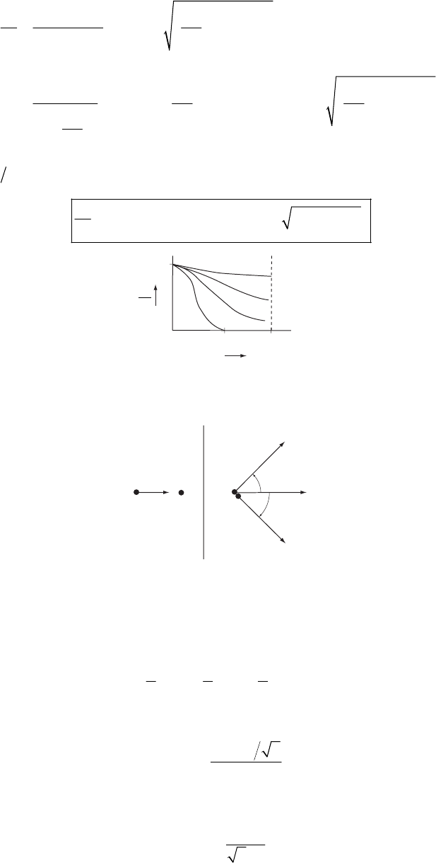
DYNAMICS OF A SYSTEM OF PARTICLES 299
9-33. From Eq. (9.87b) in the text, we have
()
2
2
2
2
11 2
2
01
12
22
22
22
2
11
2
1
cos sin
1cos sin 2 cos sin
1
Tm m
Tm
mm
mm
mm
m
m
ψψ
2
ψ
ψψ
=+−
+
=+−+−
+
ψ
Substituting 21
mm
α
≡ and cos
ψ
≡ y we have
()
222 22
1
0
12 12
Tyyy
T
αα α
−1
+ −+ + −=+
(1)
α = 12
α = 4
α = 2
α = 1
π/2
ψ
π
1
0
T
T
1
0
9-34.
Before After
45˚
mm
m
x
m
v
2
v
1
u
1
θ
Cons. of
z
p: 11 2
cos 45 cosmu mv mv
θ
=°+ (1)
Cons. of
y
p
: 12
0sin45 simv mv n
θ
=°− (2)
Cons. of energy (elastic collision)
22
11
111
222
mu mv mv=−
2
2
(3)
Solve (1) for cos
θ
:
11
2
2
cos uv
v
θ
−
=
Solve (2) for sin
θ
:
1
2
sin 2
v
v
θ
=
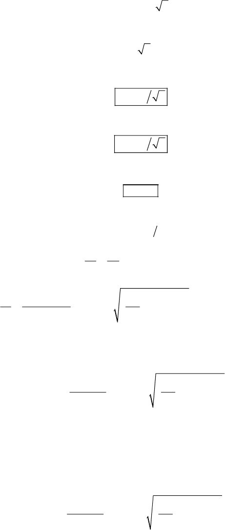
300 CHAPTER 9
Substitute into , simplify, and the result is
22
cos sin 1
θθ
+=
222
121 1
2uvv uv=−+ 1
Combining this with (3) gives
2
11
22vu=1
v
We are told v, hence
10≠
11
2vu=
Substitute into (3) and the result is
21
2vu=
Since v, (2) implies
1
v=2
045
=
°
9-35. From the following two expressions for 10
TT,
2
11
2
01
Eq. (9.82)
Tv
Tu
=
()
2
2
2
2
11 2
2
1
12
cos sin Eq. (9.87b)
m
Tm
mm
ψψ
=±−
+
Tm
we can find the expression for the final velocity of in the lab system in terms of the
scattering angle
ψ
:
1
v1
m
2
2
11 2
1
12 1
cos sin
mu m
mm m
v
ψ
ψ
=±−
+
(1)
If time is to be constant on a certain surface that is a distance r from the point of collision, we
have
10
rvt
=
(2)
Thus,
2
2
110 2
12 1
cos sin
mut m
mm m
r
ψ
ψ
=±−
+
(3)
This is the equation of the required surface. Let us consider the following cases:
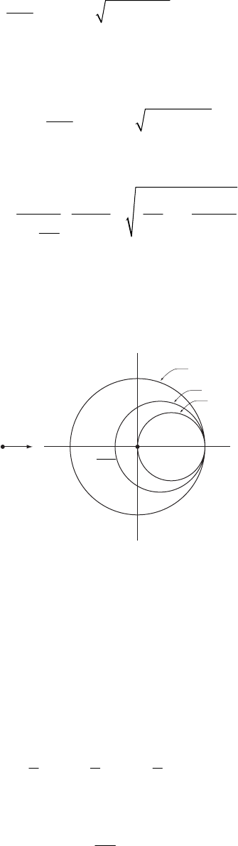
DYNAMICS OF A SYSTEM OF PARTICLES 301
i) :
21
mm=
2
10
10
cos 1 sin cos
2
ut
rut
ψ
ψ
=±−=
ψ
(4)
(The possibility r = 0 is uninteresting.)
iI) :
21
2mm=
2
10 cos 4 sin
3
ut
r
ψ
ψ
=±−
(5)
iII) : Rewriting (3) as
2
m=∞
22
110
2
1212
2
cos sin
1
1
mut
mmmm
m
r
ψ
ψ
=±−
+
(6)
and taking the limit , we find
2
m→∞
10
rut
=
(7)
All three cases yield spherical surfaces, but with the centers displaced:
v
1
t
0
–v
1
t
0
m
2
= 2m
1
m
2
= ∞
m
1
= m
2
m
2
m
1
O
−vt
10
3
This result is useful in the design of a certain type of nuclear detector. If a hydrogenous material
is placed at 0 then for neutrons incident on the material, we have the case . Therefore,
neutrons scattered from the hydrogenous target will arrive on the surface A with the same time
delay between scattering and arrival, independent of the scattering angle. Therefore, a
coincidence experiment in which the time delay is measured can determine the energies of the
incident neutrons. Since the entire surface A can be used, a very efficient detector can be
constructed.
1
mm=2
9-36. Since the initial kinetic energies of the two particles are equal, we have
222
11 22 21
111
222
mu mu mu
α
== 2
(1)
or,
2
1
2
m
m
α
=
(2)
302 CHAPTER 9
Now, the kinetic energy of the system is conserved because the collision is elastic. Therefore,
222
11 2 2 11 22
11 1
22 2
mu mu mu mv===
2
(3)
since v. Momentum is also conserved, so we can write
10=
(
)
11 22 1 2 1 22
mu mu m m u mv
α
+=+ = (4)
Substituting the second equality in (4) into (3), we find
2
2
12
11 2 1
2
1
2
mm
mu m u
m
α
+
=
2
(5)
or,
2
1
12
2
1
2
m
mm
m
α
=+
(6)
Using 2
12
mm
α
=, (6) becomes
(
)
2
22
2
α
αα
=+ (7)
solving for
α
, we obtain
2
12; 32
αα
=− =∓2∓ (8)
This gives us
()
12
21
:0
322; 1 2 with :
mu
mu 0
α
α
+
<
=± =−±
−
>
(9)
9-37.
()
()
3
610 72
0
73
33
Impulse
360 10
10
360 6 10 6 10 N s
3
t
Fdt
tdt
−
×
=
−−
=
=−
=⋅×−⋅×
∫
∫
⋅
kg m
Impulse 1.44 s
=
Since the initial velocity is zero,
f
vv=∆
Impulse Pmv
=
∆= ∆
So
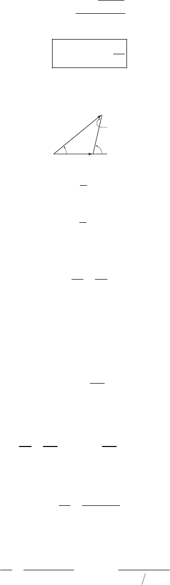
DYNAMICS OF A SYSTEM OF PARTICLES 303
kg m
1.44 s
0.003 kg
f
v=
muzzle
m
480 s
v=
9-38.
v
1
′
v
1
V
θ
θ − ψ
ψ
2
011
2
111
1
2
1
2
Tmu
Tmv
=
=
(1)
Thus,
2
1
2
01
Tv
Tu
=1
(2)
Now, from the diagram above, we have
(
)
11
cos cosvV v
ψ
θψ
=+−
′ (3)
Using Eq. (9.68) in the text, this becomes
(
2
1
1
cos cos
m
vV m
)
ψ
θψ
=+ −
(4)
Thus,
()
2
22
12
22
11 1
cos
vmV
uu m
ψθψ
=+−
(5)
Using Eq. (9.84) in the text,
1
11
mV
umm
=+2
(6)
Therefore, we find
()
()
()
2
2
11
2
01
12
cos
cos
Tm
Tm
mm
θψ
ψ
2
m
−
=+
+
(7)
If we define
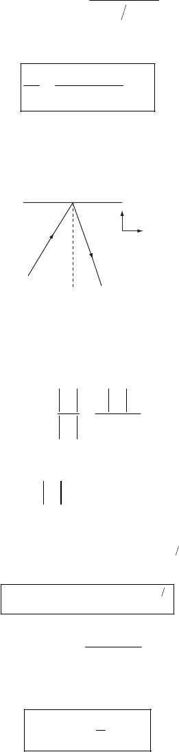
304 CHAPTER 9
(
)
()
12
cos
cosSmm
θ
ψ
ψ
−
≡+ (8)
we have
()
2
2
11
2
012
TmS
Tmm
=
+× (9)
as desired.
9-39.
θ′
θ
u
v
y
x
As explained in Section 9.8, the component of velocity parallel to the wall is unchanged. So
sin
x
vu
θ
=
y
v is given by
cos
yy
y
vv
u
u
ε
θ
==
or
cos
y
vu
ε
θ
=
Thus
12
22 22 2
sin cosvu u
θε θ
=+
12
222
sin cosvu
θε θ
=+
sin
tan cos
u
u
θ
θ
ε
θ
=
′
or
11
tan tan
θ
θ
ε
−
=
′
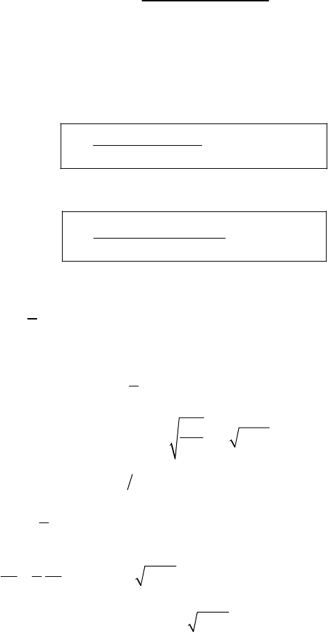
DYNAMICS OF A SYSTEM OF PARTICLES 305
9-40. Because of the string, is constrained to move in a circle of radius a. Thus, initially,
will move straight up (taken to be the y direction). Newton’s rule applies to the velocity
component along . The perpendicular component of velocity (which is zero) is unchanged.
Thus will move in the original direction after the collision.
2
m
2
m
1
u
1
m
From conservation of
y
p
we have
11 11 22
sin sinmu mv mv
α
α
=
+ (1)
From Newton’s rule we have
(
)
21
1
cos 90vv
u
α
ε
°− −
=
or
12
sinvv u
1
α
ε
=
− (2)
Substituting (2) into (1) and solving for gives
2
v
()
11
22
12
1sin straight up
sin
mu
mm
εα
α
+
=+
v
(2) then gives
(
)
2
11 2
11
2
12
sin along
sin
um m
mm
αε
α
−
=+u
v
9-41. Using 2
0
1
2
yvt gt=− and vv , we can get the velocities before and after the
collision:
0gt=−
Before: 2
11 1
1
where 2
ugt h g=− = 1
t
So 1
11
22
h
ug gh
g
=− =−
After: 02 20
0orvgt tv=− = g
2
202 2
22
00
02
1
2
1or 2
2
hvt gt
vv vg
gg
=−
=− = h
So 12
2vg=h
306 CHAPTER 9
Thus
2
21
21 1
2
2
gh
vv
uu gh
ε
−
==
−
2
1
h
h
ε
=
lost i
f
TTT
=
−
22
11 12
2
11
Fraction lost
1
if
i
TT
T
uv hh h
uh
−
=
−−
===−
2
1
h
2
1
if
i
TT
T
ε
−=−
9-42.
y
x
30˚
5 m/s
θ
As explained in Section 9.8, the velocity component in the y-direction is unchanged.
m
5 sin 30 2.5 m/s
s
yy
vu
== °=
For the x component we have
0.8 m3m
5cos30 5
s2s
xxx
x
vvv
u
== =
°
m
23s
x
v=
1
173 4.3 m/s
2
2.5
tan 36
23
f
v
θ
−
=
=
°
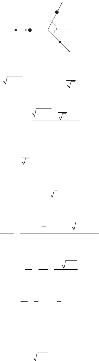
DYNAMICS OF A SYSTEM OF PARTICLES 307
9-43.
α
T0
v2
v1
45˚
4mm
m
4m
Conservation of gives
x
p
02
1
24cos
2
mT mv mv
α
=+
1
or
01
2
1
22
cos 4
mT mv
mv
α
−
=
Conservation of
y
p
gives
12
1
04
2mv mv sin
α
=−
or
1
2
sin 42
v
v
α
=
Substituting into si gives
22
n cos 1
αα
+=
22
201 0
1
222
22
1
22
2
32 16
mT m v mT mv
v
vmv
+−
=+ 1
1
Simplifying gives
2
10
20
1
216 8 8
vTm
T
v
vmm
=+ − (1)
The equation for conservation of energy is
()
22
0
01
11
4
62 2
T
Tmv−= + 2
mv
2
2
or
(2)
2
01
53 12Tmv mv=+
Substituting (1) into (2) gives a quadratic in :
1
v
2
1010
15 6 14 0mv T m v T
−
−=
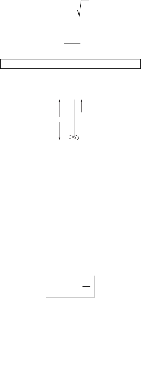
308 CHAPTER 9
Using the quadratic formula (taking the positive sign since v) gives:
10>
0
11.19 T
vm
=
Substituting this into the previous expressions for cos
α
and sin
α
and dividing gives
sin
tan 1.47
cos
α
αα
==
Thu s , the recoil angle of the helium, is 55.8 .
α
°
9-44.
v
0
x
grav
impulse 0 0
where mass/length
, since , 0.
Fmgxg
F mvmvmv vvv
µ
µ
== =
=++ = =
We have
()
0
ddx
mx
dt dt v
µ
µµ
===
So the total force is
(
)
2
0
F
xxgv
µ
µ
=+
We want F(x = a)
(
)
2
0
F
aagv
µ
µ
=+
or
2
0
1v
Fag ag
µ
=+
9-45. Since the total number of particles scattered into a unit solid angle must be the same in
the lab system as in the CM system [cf. Eq. (9.124) in the text],
(
)
(
)
2sin 2sindd
σ
θπ θθσψ π ψψ
=⋅ (1)
Thus,
()
()
sin
sin
d
d
ψ
ψ
σθ σψ
θ
θ
= (2)
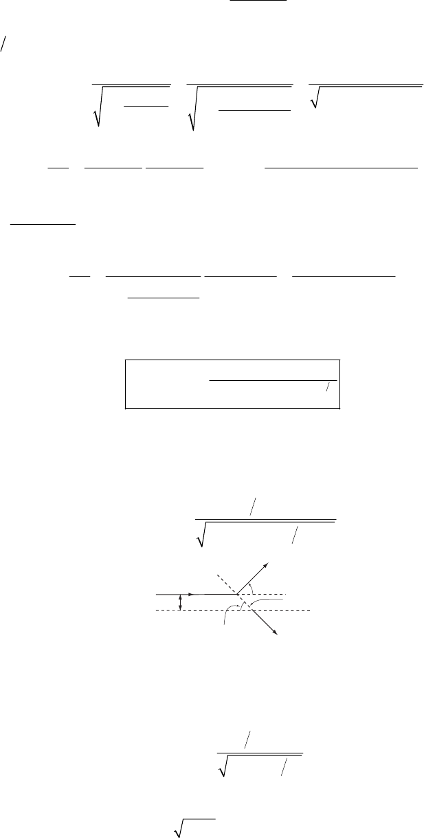
DYNAMICS OF A SYSTEM OF PARTICLES 309
The relation between
θ
and
ψ
is given by Eq. (9.69), which is
sin
tan cos x
θ
ψθ
=
+
(3)
where 1
xmm=2
. Using this relation, we can eliminate
ψ
from (2):
()
2
22
sin
11
n112cos
cos
11
tan sin
xx
x2
si
θ
ψ
== (4)
θ
θ
ψθ
=
++
+
++
()
(
)
(
)
()
2
2
2
tan cos cos sin
cos
tan cos
dx
dd d x
dd
ψ
θθ
ψψ ψ
θψθ θ
++
== +
θ
(5)
Since 2
2
1
s1tan
ψ
co
ψ
=+, (5) becomes
()
()
22 2
2
1cos 1cos
1
sin 12cos
cos
1cos
xx
dx
x
x
d
x
θ
θ
ψ
θ
θθ
θ
θ
+
+
=
++
+
++
= (6)
Substituting (4) and (6) into (2), we find
()
()
()
32
2
1cos
12cos
x
xx
θ
σθ σψ θ
+
=++
(7)
9-46. The change in angle for a particle of mass
µ
moving in a central-force field is [cf. Eq.
(9.121)]. Let
ψ
= capital
θ
here.
(
)
()
max
min
2
22
22
r
r
rdr
EU r
ψµµ
∆= −−
∫
(1)
b
a
rmin
θ
ψ
In the scattering from an impenetrable sphere, is the radius of that sphere. Also, we can see
from the figure that
min
r
2
θ
πψ
=− .
For , U = 0. Thus (1) becomes
min
rr>
(
)
2
22
2
a
rdr
Er
ψµ
∞
∆= −
∫
(2)
Substituting
0
2;bT ET
µ
0
=
=
′
′
(3)
310 CHAPTER 9
(2) becomes
2
21
dr
r
rb
α
ψ
∞
∆=
−
∫ (4)
This integral can be solved by using Eq. (E. 10b), Appendix E:
1
2
2
sin 4
a
rb
ψ
∞
−−
=
(5)
Thus,
sin b
a
=
ψ
(6)
Therefore, we can find the relation between
θ
and b by substituting
(
)
2
θ
πψ
=− into (6). We
have
cos 2
ba
θ
= (7)
Now, the differential cross section is given by Eq. (9.120):
()
sin
bdb
d
σθ
θ
θ
= (8)
From (7), we have
()
2
1cos sin
sin 2 2 2 4
a
a
θθ
σθ θ
=×
a
= (9)
Total cross section is given by
()
2
4
4
t
a
d
σ
σθ π
=
Ω= ⋅
∫ (10)
so that
2
ta
σ
π
= (11)
9-47. The number of recoil particles scattered into unit solid angle in each of the two systems,
lab and CM, are the same. Therefore,
(
)
(
)
sin sindd
σ
φφφσ
ζζζ
= (1)
where
φ
and
ζ
are the CM and lab angles, respectively, of the recoil particle. From (1) we can
write [cf. Eq. (9.125) in the text]
(
)
()
sin
sin
d
d
σφ ζ
ζ
σζ
φφ
= (2)

DYNAMICS OF A SYSTEM OF PARTICLES 311
Now, in general, 2
φζ
= [see Eq. (9.74)]. Hence,
sin sin 1
sin sin 2 2 cos
ζζ
φζ ζ
== (3)
and
1
2
d
d
ζ
φ
=
(4)
Using (3) and (4) in (2), we have
(
)
()
1
4cos
σφ
σζ ζ
= (5)
For , the Rutherford scattering cross section is [Eq. (9.141)]
1
mm=2
()
()
2
24
0
1
4sin
k
T
σθ θ
=× 2
(6)
Also for this case, we have [Eqs. (9.71) and (9.75)]
2
2
θ
ψ
π
ψζ
=
=−
(7)
Hence,
sin sin sin cos
22
θ
π
ψζζ
== −=
(8)
and since the CM recoil cross section
σ
(
φ
) is the same as the CM scattering cross section ( )
σ
θ
,
(6) becomes
()
2
24
0
1
4cos
k
T
σφ
ζ
=× (9)
Using (5) to express
σ
(
ζ
), we obtain
(
)
(
)
4cos
σζ
σφ
ζ
=× (10)
or,
()
2
23
0
1
cos
k
T
σζ
ζ
=× (11)

312 CHAPTER 9
9-48. In the case , the scattering angle
ψ
for the incident particle measured in the lab
system is very small for all energies. We can then anticipate that
σ
(
ψ
) will rapidly approach
zero as
ψ
increases.
1
mm2
Eq. (9.140) gives the Rutherford cross section in terms of the scattering angle in the CM system:
()
()
()
2
CM 24
0
1
sin 2
4
k
T
σθ θ
=′ (1)
From Eq. (9.79) we see that for ,
12
mm
2
00
12 1
mm
TT
mm m
=≅
′+
2
0
T (2)
Furthermore, from Eq. (9.69),
2
11
2
sin
tan sin
cos
m
mm
m
θ
ψ
θ
θ
=≅
+
(3)
and therefore, since
ψ
is expected to be small for all cases of interest,
1
22
sin tan
mm
mm
1
θ
ψ
≅≅
ψ
(4)
Then,
2
1
2
cos 1 m
m
θψ
=−
(5)
and
()
2
21
2
1
sin 2 1 1
2
m
m
θψ
=−−
(6)
(Notice that 1
ψ
, but since m, the quantity
1
m21
mm
2
ψ
is not necessarily small compared
to unity.)
With the help of (2) and (6), we can rewrite the CM cross section in terms of
ψ
as
()
2
1
CM 2
2
20
1
2
1
2
11
mk
mT m
m
ψ
=
σψ
−−
(7)
According to Eq. (9.129),
DYNAMICS OF A SYSTEM OF PARTICLES 313
()
()
2
2
11
22
LAB CM 2
1
2
cos 1 sin
1sin
mm
mm
m
m
+−
=
−
ψψ
σθ
ψ
σψ
(8)
We can compute
(
)
LAB
σ
ψ
with the help of (7) and the simplifications introduced in the right-
hand side of (8) by the fact that 1
ψ
:
()
2
2
11
222
1
LAB 2
22
20
11
22
1
2
11 1
mm
mm
mk
mT mm
mm
+−
≅
−− −
ψ
ψψ
σψ
(9)
and so,
()
()
2
22
120
LAB 2
22
11
22
2
11 1
mk mT
mm
mm
≅
−− −
ψψ
σψ
(10)
This expression shows that the cross section has a second-order divergence at
ψ
= 0. For values
of 2
mm
1
ψ
>, (9) gives complex values for lab
σ
. This result is due to the approximations
involved in its derivation, making our result invalid for angles larger than 21
mm.
9-49. The differential cross section for Rutherford scattering in the CM system is [cf. Eq.
(9.140) in the text]
()
2
24
0
1
16 sin 2
k
T
σθ
θ
=′ (1)
where [cf. Eq. (9.79)]
2
0
12
m
T
mm
=
′+0
T
(2)
314 CHAPTER 9
Thus,
()
2
2
12
24
02
2
2
1
24
02
1
16 sin 2
11
16 sin 2
mm
k
Tm
mk
Tm
σθ θ
θ
+
=
=+
(3)
Since 121mm, we expand
2
11
22
112
mm
mm
+
≅+ +
… (4)
Thus, to the first order in 1
mm
2
, we have
()
2
1
24
02
112
16 sin 2
m
k
Tm
σθ θ
=+
(5)
This result is the same as Eq. (9.140) except for the correction term proportional to 12
mm.
9-50. The potential for the given force law is
()
2
2
k
Ur r
= (1)
First, we make a change of variable, 1
z
r
=
. Then, from Eq. (9.123), we can write
max
12
2
max 2
0
0
22
2
0
1
2max 0
2
0
2
2
0
1
sin
2
2
z
k
zb
mu
bdz
k
bz
mu
bz
z
k
bmu
b
k
bmu
θ
π
−
=+
−
=
−+
=
+
=
+
∫
(2)
Solving (2) for b = b(
θ
),
222
0
2
4
k
bmu
θ
θ
π
θ
=− (3)
DYNAMICS OF A SYSTEM OF PARTICLES 315
According to Fig. 9-22 and Eq. (9.122),
(
1
2
)
θ
πθ
=
− (4)
so that b(
θ
) can be rewritten as (
θ
):
() ()
2
02
k
bmu
πθ
θ
θ
πθ
−
=
−
(5)
The differential cross section can now be computed from Eq. (9.120):
()
sin
bdb
d
σθ
θ
θ
= (6)
with the result
() ()
()
2
2
22
02sin
k
mu
ππθ
σθ
θ
πθ θ
−
=− (7)
9-51.
θ
φ = π − θ
p
n
In the CM system, whenever the neutron is scattered through the angle
θ
, the proton recoils at
the angle
φ
=
π
–
θ
. Thus, the neutron scattering cross section is equal to the recoil cross section
at the corresponding angles:
()
()
p
ndN
dN
dd
θ
φ
=
ΩΩ
(1)
Thus,
()
()
pp
n
p
dN dT
dN
ddTd
θ
φ
=
ΩΩ
(2)
where
pp
dN dT is the energy distribution of the recoil protons. According to experiment,
pp
dN dT = const. Since
p
n
mm≅,
p
T is expressed in terms of the angle
ψ
by using Eq. (9.89b):
2
0sin
p
TT
ψ
= (3)
We also have 2
θ
ψ
= for the case
p
n
mm
≅
. Thus,
()
()
2
0
1sin
2sin
p
dT dT
dd
ψ
φπφφ
=
Ω (4)
316 CHAPTER 9
or,
()
2
0
0
sin
2sin 2
sin cos
2sin 2 2 4
p
dT Td
dd
TT
0
π
φ
φπφφ
φφ
π
φπ
−
=
Ω
== (5)
Therefore, we find for the angular distribution of the scattered neutron,
()
0
4
p
n
p
dN
dN T
ddT
θ
π
=⋅
Ω (6)
Since
pp
dN dT = const., n
dN dΩ is also constant. That is, the scattering of neutrons by protons
is isotropic in the CM system.
9-52. Defining the differential cross section
σ
(
θ
) in the CM system as in Eq. (9.116), the
number of particles scattered into the interval from
θ
to
θ
+ d
θ
is proportional to
(
)
(
)
(
)
sin cosdN d d
σ
θθθσθ
∝=−
θ
2
(1)
From Eq. (9.87a) and the assumption of elastic collisions (i.e., TT
01
T
=
+), we obtain
()
(
212
2
012
21cos
Tmm
Tmm
)
θ
=−
+ (2)
or, solving for cos
θ
,
2
2
cos m
m
TT
T
θ
−
= (3)
where
()
12
0
2
12
4
m
mm
mm
=+
T is the maximum energy attainable by the recoil particle in the lab
system. Then, (1) can be rewritten as
T
()
2
2
m
dT
dN T
σθ
∝ (4)
and consequently, we obtain the desired result for the energy distribution:
()
2
dN
dT
σ
θ
∝ (5)
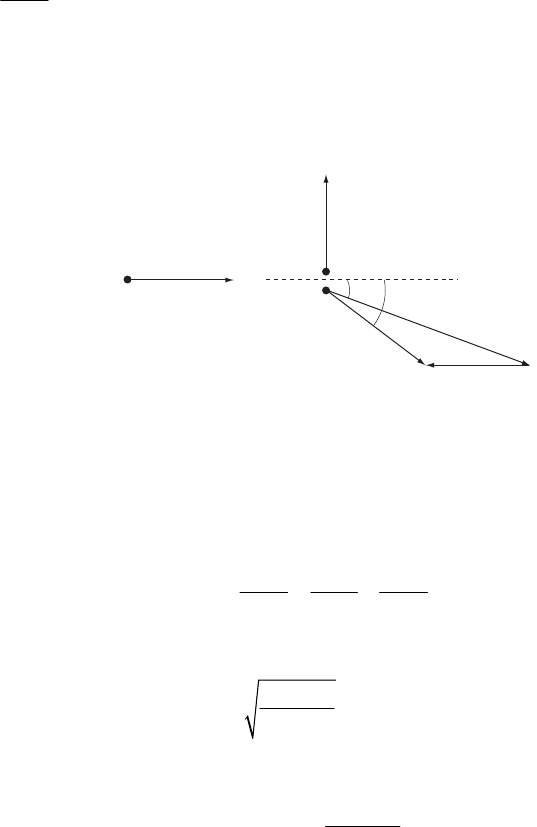
DYNAMICS OF A SYSTEM OF PARTICLES 317
9-53.
1
m=mass of particle 1
α
, mass of
2
m=238 U
1
,uu
′
1
: velocity of particle
α
in LAB and CM before collision
1
,vv
′
1
2
2
: velocity of particle in LAB and CM after collision ∝
2
,uu
′: velocity of in LAB and CM before collision
238 U
2
,vv
′” velocity of in LAB and CM after collision
238 U
20u=,
2
11
17.7MeV
2
mu
T==
90
ψ
=° is angle through which particle
α
is deflected in LAB
θ
is angle through which particle
α
and are deflected in CM
238 U
ζ is recoil angle of in LAB
238 U
m1u1
v1
v
v2′–vCM
m1
m2ζθ
2
a) Conservation of momentum in LAB:
11 22
11
11 22
cos tan
sin
mu mv u
mv mv v
ζ
ζ
ζ
==
=⇒
Conservation of energy in LAB:
22
11 11 22
222
mu mv mv
=+
2
From these equations we obtain the recoil scattering angle of
238 U
tan
21
21
44.52
mm
mm
−
=
⇒=
+°
ζζ
b) The velocity of CM of system is
11
CM
12
mu
vmm
=+
The velocity of in CM after collision is vv
238 U'
22C
v=−
M
. From the above figure we can obtain
the scattering angle of particle in CM to be
238 U
318 CHAPTER 9
22
221
2
21
sin
n 89.04
cos cm
vmm
vvm
ζ
ζ
−
==⇒=
−
ta
θθ
°
In CM, clearly after collision, particle
α
moves in opposite direction of that of 23 .
8U
c) The kinetic energy of particle after collision in LAB is
238 U
2
222
10
22 2 11 1
1
21212
20.25 MeV
22cos
mv
m mu m T
mmmmm
ζ
====
++
mv
Evidently, conservation of energy is satisfied.
d) The impact parameter in CM is given in Section 9.10.
0
cot
22
k
bT
θ
=
′
where 12
0
9
qq
k
π
ε
= and
()
2
0112
1
2umu=+
′′
2
2
′
Tm is the total energy of system in CM,
so 14
12 12
2
0121
cot 1.8 10 m
42
qq mm
bmmu
θ
πε
−
+
==
×
We note that b is the impact parameter of particle
α
with respect to CM, so the impact
parameter of particle
α
with respect to is
238 U
(
)
12 14
2
1.83 10 m.
mmb
m
−
+=×
e) In CM system, the orbit equation of particle
α
is
()
1cos
r
α
ε
θ
=+
′ where 0
θ
=
corresponds to rr
min
=
min 1
r
α
ε
⇒=
′+ is closest distance from particle
α
to the center of mass, and
(
)
2
2
11
0
112 1
4mub
mk qq m
πε
α
′
==
and
()
()
2
2
11
0
112
2
11
20
11
12 1
4
12 12
4
1
mub
EE
mk qq m
mub
mu qq m
πε
ε
πε
1
′
=+ =+
′
=+ ′
But the actual minimum distance between particles is
14
12
min min
2
0.93 10 m.
mm
rr
m
−
+
==×
′
DYNAMICS OF A SYSTEM OF PARTICLES 319
f) Using formula
()
()
(
)
2
22
LAB CM 22
cos 1 sin
1sin
xx
x
ψ
ψ
σθ ψ
+−
=−
σψ
where 1
2
m
xm
=, 90
ψ
=°,
()
()
2
CM 24
0
1
4sin 2
k
T
σθ
θ
=
′
We find this differential cross section in LAB at
ψ
= 90°:
(
)
28 2
LAB 90 3.16 10 m
σψ
−
=°= ×
g) Since d()sin d d
N
N
σ
θψψ
=
φ
we see that the ratio of probability is
(
)
()
sin 11.1
'sin
σψ ψ
σψ ψ
=
′
9-54. Equation 9.152 gives the velocity of the rocket as a function of mass:
()
00
00
0
ln ln 0
ln
mm
vv u v
mm
m
pmvmu m
µ
=+ = =
==
To maximize p, set 0
dp
dm =
0
0ln
dp m
u
dm m 1
=
=−
1
00
0
1
mm m
eor e
mm m
ln
−
== =
To check that we have a maximum, examine
1
0
22
22
mme
dp dp u
dm dm m
−
=
=
−
1
0
2
2
0
0
mme
dp ue
dm m
−
=
=
−<
, so we have a maximum.
1
0
me
m
−
=
320 CHAPTER 9
9-55. The velocity equation (9.165) gives us:
() ()
0
ln m
vt gt u mt
=− +
(1)
where
(
)
0
mt m t
α
=−, the burn rate 0
910m
α
τ
=
, the burn time 300 s
τ
=
, and the exhaust
velocity u. These equations are good only from t = 0 to t =
τ
. First, let us check that
the rocket does indeed lift off at t = 0: the thrust
-1
4500 m s=⋅
2
00
910 suum mm
ατ
−
==⋅⋅>
0
g135 m., as
required. To find the maximum velocity of the rocket, we need to check it at the times t = 0 and
t =
τ
, and also check for the presence of any extrema in the region 0 < t <
τ
. We have v(0) = 0,
, and calculate
1
( ) 0 m s−
=− ⋅ln 10vgu
ττ
+ =740
() ()
10
dv u u
gg
dt mt mtg
αα
=− + = − >
(2)
The inequality follows since
(
)
0
umgmtg
α
>>
1
00 m s−
⋅
. Therefore the maximum velocity occurs at t =
τ
,
where vg . A similar single-stage rocket cannot reach the moon since ln 10 74u
τ
=− + =
()
(
)
1
10 4 m s
0
ln ln 10
final
u m m uvt
−
<=.⋅, which is less than escape velocity and independent of
fuel burn rate.
9-56.
a) Since the rate of change of mass of the droplet is proportional to its cross-sectional area, we
have
2
dm kr
dt
π
= (1)
If the density of the droplet is
ρ
,
3
4
3
mr
π
ρ
= (2)
so that
2
4
dm dm dr dr
r
dt dr dt dt
πρ π
== =
2
kr (3)
Therefore,
4
dr k
dt
ρ
= (4)
or,
04
k
rr t
ρ
=+ (5)
as required.
DYNAMICS OF A SYSTEM OF PARTICLES 321
b) The mass changes with time, so the equation of motion is
()
ddvdm
Fmvmv m
dt dt dt
= =+=g (6)
Using (1) and (2) this becomes
32
44
33
dv
rkrv
dt
3
rg
π
π
ρπ ρ
+= (7)
or,
3
4
dv k vg
dt r
ρ
+
= (8)
Using (5) this becomes
0
3
4
4
dv k v g
k
dt rt
ρ
ρ
+
=
+
(9)
If we set 3
4
k
A
ρ
= and 4
k
B
ρ
=, this equation becomes
0
dv A vg
dt r Bt
+
=
+ (10)
and we recognize a standard form for a first-order differential equation:
() ()
dv Ptv Qt
dt += (11)
in which we identify
()
0
A
Pt rBt
=+; Q(t) = g (12)
The solution of (11) is
vt
()
() ()
constant
Pt dt Pt dt
e e Qdt
−
∫∫
=+
∫ (13)
Now,
()
()
()
0
0
3
0
ln
ln
AA
P t dt dt r Bt
rBt B
rBt
==
+
=+
∫∫ +
(14)
since 3
A
B=. Therefore,
(15)
(
3
0
Pdt
erB
∫=+
)
t
322 CHAPTER 9
Thus,
()
()()
()()
33
00
34
00
constant
4
vt r Bt r Bt gdt
g
rBt rBt C
B
−
−
=+ + +
=+ + +
∫
(16)
The constant C can be evaluated by setting
(
)
0
0vt v
=
=:
()
4
00
3
0
1
4
g
vr
rB C
=+
(17)
so that
3
00 0
4
g
Cvr r
B
=−4
(18)
We then have
()
()
()
43
000
3
0
1
44
gg
r Bt vr r
BB
rBt
4
0
vt
=++−
+ (19)
or,
() () ()
()
43
0
3
10
4
g
vt Bt r
B
Bt
=+
(20)
where
(
)
3
0
r0 means “terms of order and higher.” If is sufficiently small so that we can
neglect these terms, we have
3
0
r0
r
()
vt t
∝
(21)
as required.
9-57. Start from our definition of work:
dp
W F dx dx v dp
dt
== =
∫
∫∫
(1)
We know that for constant acceleration we must have v = at (zero initial velocity). From
Equation (9.152) this means
0
at u
mme
−
= (2)
We can then compute dp:
() ( )
01
at u at
d mv d mat ma dt at dm m ae dt
u
−
dp
=+= −==
(3)
This makes our expression for the work done on the rocket
()( )
0
0
tat u
r
ma
Watuate
u
−
=−
∫dt
(4)
DYNAMICS OF A SYSTEM OF PARTICLES 323
The work done on the exhaust, on the other hand, is given with v → (v – u) and
, so that
(
exhaust
dp dm v u→)
−
()
2
0
0
tat u
e
ma
Watue
u
−
=−
∫dt
(5)
The upper limit on the integrals is the burnout time, which we can take to be the final velocity
divided by the acceleration. The total work done by the rocket engines is the sum of these two
quantities, so that
()
()
22
0
0
00
1
va vu
at u x
ma u uat e dt m u x e dx
u
−−
=−
∫∫
W=− (6)
where the obvious substitution was made in the last expression. Upon evaluating the integral
we find
0
vu
W m uve muv
−
== (7)
where m is the mass of the rocket after its engines have turned off and v is its final velocity.
9-58. From Eq. (9.165) the velocity is
0
ln
dy m
vgtu
dt m
==−+
0
ln m
dy gt u dt
m
=−+
∫∫
Since m
dt
α
=− , dt dm
α
=−
20
1ln
2
m
u
yC gt dm
m
α
+=− −∫
ln 1 ln
aa
dx x
xx
=+
∫
, so we have
20
1ln
2
m
u
yC gt mm m
α
+=− − +
Evaluate C using y = 0 when t = 0, 0
mm
=
0
um
C
α
=−
(
)
020
1ln
2
um m m
mu
t
m
αα
−
=−−yg; 0
mm t
α
−
=
20
1ln
2
m
mu
yut gt m
α
=− −
At burnout, ,
B
yy=B
tt=
324 CHAPTER 9
20
1ln
2
BB B
m
mu
yut gt m
α
=− −
After burnout, the equations are
2
00
1
2
yy vt gt=+ − and vv
0gt
=
−
Calling the top of the path the final point
0
f
B
f
vv== −gt
or fB
tvg
=
22
022
BB
vv v
yy gg
−= − =
2
B
g
; 00y
=
2
2
B
v
yg
=
9-59. In order to immediately lift off, the thrust must be equal in magnitude to the weight of
the rocket. From Eq. (9.157):
Thru 0
st v
α
= 0velocity of fuelv
=
So
0
vmg
α
=
or
0
vmg
α
=
9-60. The rocket will lift off when the thrust just exceeds the weight of the rocket.
Thrust dm
uu
dt
α
=− =
(
)
0
Weight mg m t g
α
== −
Set thrust = weight and solve for t:
(
)
0
umt
αα
=−g; 0
mu
tg
α
=
−
With ,
070000 kgm=250 kg/s
α
=, 2500 m/su
=
,
2
9.8 m/sg=
25 sect
The design problem is that there is too much fuel on board. The rocket sits on the ground
burning off fuel until the thrust equals the weight. This is not what happens in an actual launch.
A real rocket will lift off as soon as the engines reach full thrust. The time the rocket sits on the
ground with the engines on is spent building up to full thrust, not burning off excess fuel.
DYNAMICS OF A SYSTEM OF PARTICLES 325
9-61. From Eq. (9.153), the velocity after the first state is:
10 lnvvuk
=
+
After the second stage:
21 0
ln 2 lnvvukv uk
=
+=+
After the third stage:
32 0
ln 3 lnvvukv uk
=
+=+
After the n stages:
10
ln ln
nn
v v ukvnuk
−
=
+=+
0ln
n
vvnuk=+
9-62. To hover above the surface requires the thrust to counteract the gravitational force of
the moon. Thus:
1
6
6
dm
um
dt
udm dt
gm
−=
−=
g
Integrate from m to 0.8 and t = 0 to T:
0
m=0
m
(
)
2
6 2000 m/s
6ln 0.8 ln 0.8
9.8 m/s
u
Tg
=− =−
273 secT=
9-63.
a) With no air resistance and constant gravity, the problem is simple:
2
0
1
2mv mgh= (1)
giving the maximum height of the object as 2
021800 kmhv g=. The time it takes to do this is
0610 svg.
b) When we add the expression for air resistance, the differential equation that describes the
projectile’s ascent is
2
2
11
2W
t
dv v
mg c Av mg
dt v
ρ
Fm
==−− =−+ (2)
326 CHAPTER 9
where 1
225 k
tW
gcA
ρ
−
=.
13 kg
ms⋅vm would be the terminal velocity if the object were falling
from a sufficient height (using 3
m
−
.⋅ as the density of air). Solution of this differential
equation gives
()
10
tan tan
t
tt
gt
v
vt v vv
−
=− (3)
This gives v = 0 at time
(
)
(
)
1
0
tan 300 s
tt
vg vv
τ
−
=. The velocity can in turn be integrated to
give the y-coordinate of the projectile on the ascent. The height it reaches is the y-coordinate at
time
τ
:
2
2
0
ln 1
2
t
t
vv
hgv
=+ (4)
which is 600 km.
c) Changing the acceleration due to gravity from –g to
(
)
(
)
2
2
ee ee
GMRy gRRy
−+=−+
changes our differential equation for y to
2
2
e
te
yR
yg
vRy
=− +
+
(5)
Using the usual numerical techniques, we find that the projectile reaches a height of 630 km in
a flight time of 330 s.
d) Now we must replace the
ρ
in the air resistance equation with ( )y
ρ
. Given the dependence
of on
ρ
, we may write the differential equation
t
v
()
2
2
0
e
te
yyR
yg vRy
ρ
ρ
=− +
+
(6)
where we use log and
5
10 ( ) 0 11 (5 10 )y
ρ
−
=. − × y
013
ρ
=
., with the
ρ
’s in and y in meters.
The projectile then reaches a height of 2500 km in a flight time of 940 s. This is close to the
height to which the projectile rises when there is no air resistance, which is 2600 km.
3
kg m−
⋅
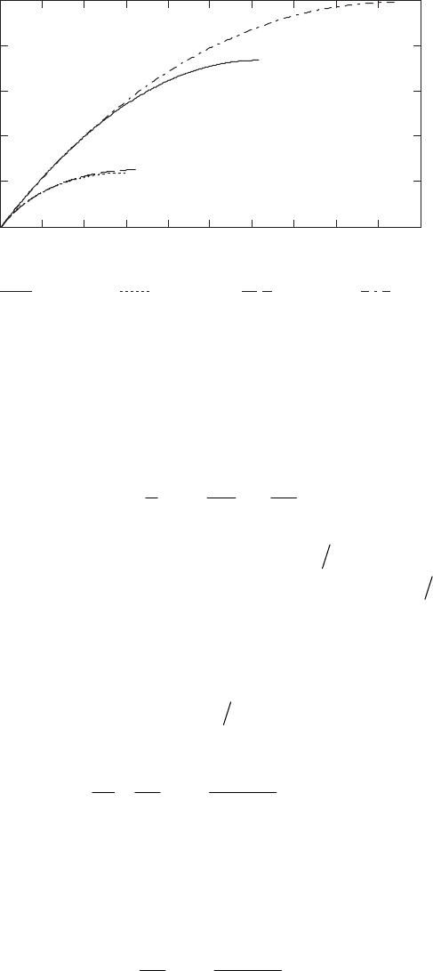
DYNAMICS OF A SYSTEM OF PARTICLES 327
0 0.1 0.2 0.3 0.4 0.5 0.6 0.7 0.8 0.9 1
0
0.5
1
1.5
2
2.5
(a) (b) (c) (d)
t (1000 s)
height (1000 km)
9-64. We start with the equation of motion for a rocket influenced by an external force, Eq.
(9.160), with including gravity, and later, air resistance.
ext
F
a) There is only constant acceleration due to gravity to worry about, so the problem can be
solved analytically. From Eq. (9.166), we can obtain the rocket’s height at burnout
20
1ln
2
bb b
b
m
mu
yut gt m
α
=− −
(1)
where is the mass of the rocket at burnout and
b
m
(
)
0b
mmt
α
=− b
. Substitution of the given
values gives . After burnout, the rocket travels an additional
250 km
b
y22
b
v, where is the
rocket velocity at burnout. The final height the rocket ends up being 3700 km, after everything
is taken into account.
gb
v
b) The situation, and hence the differential equation, becomes more complicated when air
resistance is added. Substituting 22
ext W
FmgcAv
ρ
=− − (with ) into Equation
(9.160), we obtain
3
13 kg m
ρ
−
=. ⋅
2
2
W
cAv
dv u g
dt m m
ρ
α
=−− (2)
We must remember that the mass m is also a function of time, and we must therefore include it
also in the system of equations. To be specific, the system of equations we must use to do this by
computer are
2
2
W
v
ycAv
u
vg
mm
m
ρ
α
α
=−−
−
(3)
These must be integrated from the beginning until the burnout time, and therefore must be
integrated with the substitution α = 0. Firstly, we get the velocity and height at burnout to be
and . We can numerically integrate to get the second part of the
1
7000 m s
b
v−
⋅230 km
b
y
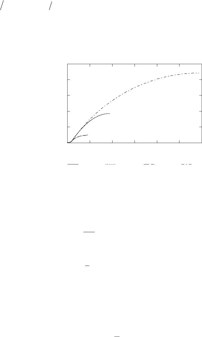
328 CHAPTER 9
journey, or use the results of Problem 9-63(b) to help us get the additional distance travelled
with air resistance, analytically. The total height to which the rocket rises is 890 km in a total
flight time of 410 s.
c) The variation in the acceleration of gravity is taken into account by substituting
(
)
(
)
2
2
ee ee
GMRy gRRy
+= +
1
6900 m s
b
v−
⋅230 km
b
y
for g in the differential equation in part (b). This gives
, , with total height 950 km and time-of-flight 460 s.
d) Now one simply substitutes the given expression for the air density,
ρ
(y) for
ρ
, into the
differential equation from part (c). This gives v1
8200 m s
b
−
⋅
, , and total height
8900 km with time-of-flight 2900 s.
250 km
b
y
0 0.5 1 1.5 2 2.5 3
0
2
4
6
8
10
height (km)
(a) (b) (c) (d)
t (1000 s)
9-65.
Total impulse 8.5 N sP=⋅
Total mass
00.054 kgm=
Burn time
1.5 s
f
t=
Rocket cross section area
2
42
4.5 10 m
4
d
S
π
−
==×
Drag coefficient
0.75
w
c=
Drag force 22 42
1210 N
2w
DcSvKv v
ρ
−
===×
where
1.2
ρ
= is density of air
3
kg/m
and v is rocket’s speed
Rocket exhaust speed u = 800 m/s
a) The total mass of propellant is
0.0106 kg
P
mu
∆= =
DYNAMICS OF A SYSTEM OF PARTICLES 329
Since , we will assume that the rocket’s mass is approximately constant in this
problem. The equation of motion of rocket is
0
~20%mm
2
0o
dv
mmgu
dt
α
=− + −Kv
(where 3
7.1 10 kg/s
f
m
t
α
−
∆
==× is fuel burn rate)
()
0
2
0
mdv dt
umgKv
α
⇒=
−−
Using the initial condition at t = 0, v = 0, we find
() ()
00
2
0
() tanh
umg Kumg
Km
αα
vt
−−
=
At burn-out, , we find
1.5 s
f
tt==
( ) 114.3 m/s
ff
vvt
=
=
The height accordingly is given by
()
0
0
2
0
0
() ()d ln cosh ku mg
m
vt t t
km
α
ht
−
==
∫
At burn out,
f
tt=, we find the burn-out height
( ) 95.53 m
ff
hht
=
=
b) After the burn-out, the equation of motion is
20
00 2
0
d
dd
d
mv
vgKv
tmg
=− − ⇒ =−
+
mm t
Kv
with solution
0
0
() tan
mg Kg
vt t C
Km
=− −
Using the initial condition at
f
tt=,
()
f
tvv
=
, we find the constant C = –1.43 rad, so
0
0
() tan 1.43
mg Kg
vt t
Km
=− −
and the corresponding height
0
0
( ) ( ) d 0.88 ln cos 1.43
f
t
ff
t
Kg
m
h vt t h t
Km
ht
=+ + −=+
∫
330 CHAPTER 9
When the rocket reaches its maximum height (at tt
max
=
) the time t can be found by setting
We then find And the maximum height the rocket can reach is
max
max
()vt =0. max 7.52 s.t=
max max
()334 mhht
=
=
c) Acceleration in burn-out process is (see v(t) in a))
()
0
00
2
2
0
d1
() d
cosh
umg
v
tm ku mg
tm
at
α
α
−
==
−
Evidently, the acceleration is maximum when t = 0 and
2
0
0
(0) 95.4 m/s
max
umg
aat m
α
−
=== =
d) In the fall-down process, the equation of motion is
2
0
0
d
d
mv mg Kv
t=−,
With the initial condition tt , v = 0, we find
max
=
(
)
max
tt≥
()
0
max
0
() tanh
mg Kg
vt t t
Km
=− −
(v(t) is negative for , because then the rocket falls downward)
max
tt≥
The height of the rocket is
()
max
0
max max max
0
() ln cosh
t
t
Kg
m
vtdth tt
Km
hh
=+ =− −
∫
To find the total flight-time, we set h = 0 and solve for t. We find total 17.56 st
=
e) Putting into the expression of V in part d), we find the speed at ground impact to
be
total
tt=
()
t
()
0
max
0
tanh 49.2 m/s
gtotal
mg Kg
t
Km
=− − =−
vt
9-66. If we take into account the change of the rocket’s mass with time 0
mm t
α
=−, where
α
is the fuel burn rate,
3
7.1 10 kg/s
α
−
=×
as calculated in problem 9-65.
The equation of motion for the rocket during boost phase is
DYNAMICS OF A SYSTEM OF PARTICLES 331
()
2
02
0
dd
d
vv
mt uKv
tKvu
αα αα
−=−⇒ =
−−
dt
tm
Integrating both sides we obtain finally
()
()
2
0
2
0
1
()
1
Ku
Ku
Ctm u
vt K
Ctm
α
α
α
α
α
+−
=
−−
where C is a constant. Using the initial condition ( ) 0 at 0vt t
=
=, we can find C and the velocity
is
2
0
2
0
11
()
11
Ku
Ku
t
m
u
vt Kt
m
α
α
α
∝
∝
−−
=
+−
a) The rocket speed at burn-out is (note t1.5 s
f
=
).
( ) 131.3 m/s
ff
vvt
=
=
b) The distance the rocket has traveled to the burn-out is
( ) 108.5 m
f
t
f
hvtdt
θ
==
∫
9-67. From Equation (9.167) we have
(
)
2
0
0
2
0
ln
2
ff
bo
ff
gm m m
u
H
mm
m
αα
−m
+ + −=−
Using numerical values from Example 9.12
4
1.42 10 kg/s
α
=− ×
6
02.8 10 kgm=×
6
0.7 10 kg
f
m=×
2.600 m/su=
we find 97.47 km
bo
H
=.
From Equation (9.168) we find
0
()
ln
fo
bo
f
gm m m
vu
m
α
−
=− +
2125 m/s
bo
v
=
332 CHAPTER 9
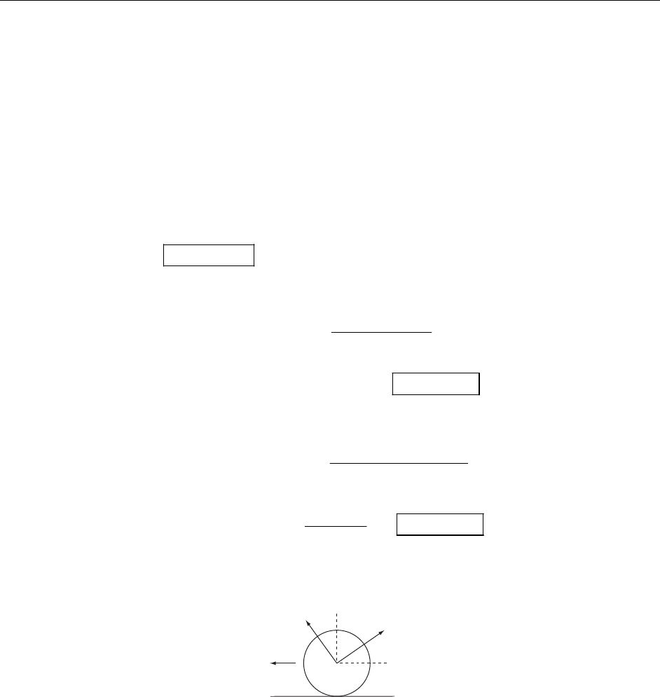
CHAPTER 10
Motion in a
Noninertial Re
f
erence Frame
10-1. The accelerations which we feel at the surface of the Earth are the following:
(1) Gravitational : 2
980 cm/sec
(2) Due to the Earth’s rotation on its own axis:
()
()()
2
28
2
85
2 rad/day
6.4 10 cm 86400 sec/day
6.4 10 7.3 10 3.4 cm/sec
r
π
ω
−
=× ×
=××× = 2
(3) Due to the rotation about the sun:
()
()
2
213
2
5
13 2
2 rad/year
1.5 10 cm 86400 365 sec/day
7.3 10
1.5 10 0.6 cm/sec
365
r
π
ω
−
=× ×
×
×
=× × =
10-2. The fixed frame is the ground.
y
aθ
x
The rotating frame has the origin at the center of the tire and is the frame in which the tire is at
rest.
From Eqs. (10.24), (10.25):
(
)
2
ff
rr
= + +×+× ×+ ×a r r v
ωωω ωaR
333
334 CHAPTER 10
Now we have
0
00
cos sin
0
f
rr
aa
r
Va
rr
θθ
=− +
=
==
==
Ri
ri va
kk
ωω
j
Substituting gives
2
0
cos sin
f
v
aaa
r
θθ
=− + + −aijji
(
2
0
cos sin 1
f
va
r
θθ
=− + + +
ai j
)
a (1)
We want to maximize
f
a, or alternatively, we maximize 2
f
a:
42
222 2 2 22
2
00
42
222
2
00
2
cos cos 2 sin sin
2
2cossin
f
vav
aaa
rr
vav
aa
rr
a
θ
θθ
θθ
=+ + ++ +
=+ + +
a
θ
22
2
0
0
2
2cos 2 cos
0 when tan
f
dav a
dr
ar
v
θ
θ
θ
θ
=− +
==
a
(Taking a second derivative shows this point to be a maximum.)
2
0
222 4
0
n implies cos
ar v
var v
θθ
==
+
ta
and
0
22 4
0
sin ar
ar v
θ
=+
Substituting into (1)
22
0
22 4 22 4
000
1
f
ar
vav a
rar v ar v
=− + + +
++
j
ai
This may be written as
242
0faavr=+ +a
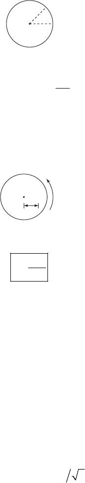
MOTION IN A NONINERTIAL REFERENCE FRAME 335
θ
A
This is the maximum acceleration. The point which experiences this acceleration is at A:
where
0
2
ar
v
tan
θ
=
10-3. We desire . From Eq. (10.25) we have
eff 0=F
(
)
eff 2
f
r
mm m m=− −×−××− ×r r v
ωωω ωFFR
r0ω
The only forces acting are centrifugal and friction, thus 2
smg m r
µ
ω
=, or
2
sg
r
µ
ω
=
10-4. Given an initial position of (–0.5R,0) the initial velocity (0,0.5
ω
R) will make the puck
motionless in the fixed system. In the rotating system, the puck will appear to travel clockwise
in a circle of radius 0.5R. Although a numerical calculation of the trajectory in the rotating
system is a great aid in understanding the problem, we will forgo such a solution here.
10-5. The effective acceleration in the merry-go-round is given by Equation 10.27:
22xxy
ω
ω
=+
(1)
22yyx
ω
ω
=−
(2)
These coupled differential equations must be solved with the initial conditions
(
)
00 0.5 mxx≡=− ,
(
)
000 myy≡=, and
(
)
(
)
1
0
00 2 msxyv
−
=
=
0
v
⋅, since we are given in the
problem that the initial velocity is at an angle of 45° to the x-axis. We will vary over some
range that we know satisfies the condition that the path cross over . We can start by
looking at Figures 10-4e and 10-4f, which indicate that we want . Trial and error
can find a trajectory that does loop but doesn’t cross its path at all, such as
0
v
1
⋅
0.
00
(,)xy
0.47 m>s−
0
v1
53 m s
−
=⋅.
From here, one may continue to solve for different values of v until the wanted crossing is
eyeball-suitable. This may be an entirely satisfactory answer, depending on the inclinations of
the instructor. An interpolation over several trajectories would show that an accurate answer to
the problem is , which exits the merry-go-round at 3.746 s. The figure shows
this solution, which was numerically integrated with 200 steps over the time interval.
0
1
0.512 m s−
=⋅
0
v
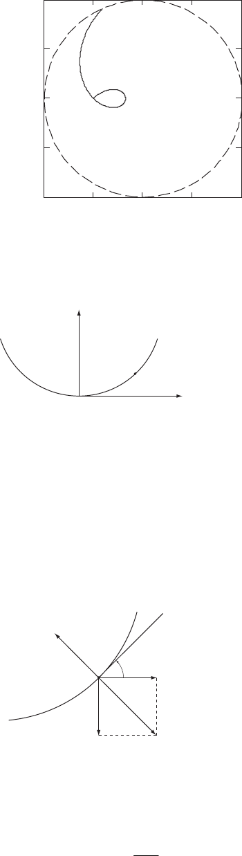
336 CHAPTER 10
–0.5 0 0.5 1
0.5
0
0.5
x (m)
y (m)
1
–1
–1
10-6.
z
m
r
z = f(r)
Consider a small mass m on the surface of the water. From Eq. (10.25)
(
)
eff 2
f
r
mm m rm=− −×−××− ×r v
ωωω ωFFR
In the rotating frame, the mass is at rest; thus, eff 0
=
F. The force F will consist of gravity and the
force due to the pressure gradient, which is normal to the surface in equilibrium. Since
, we now have
0
fr
== =Rv
ω
(
)
0p
mm
=
+− × ×gF r
ω
ω
where
p
F is due to the pressure gradient.
F
p
mg
mω
2
r
θ′
θ
Since F, the sum of the gravitational and centrifugal forces must also be normal to the
surface.
eff 0=
Thus
θ
′ =
θ
.
2
tan tan r
g
ω
θθ
==
′
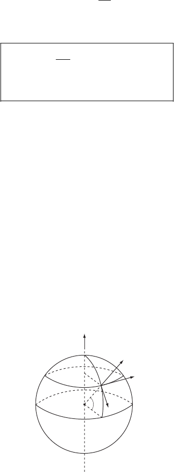
MOTION IN A NONINERTIAL REFERENCE FRAME 337
but
tan dz
dr
θ
=
Thus
2
2constant
2
The shape is a circular paraboloid.
zr
g
ω
=+
10-7. For a spherical Earth, the difference in the gravitational field strength between the poles
and the equator is only the centrifugal term:
2
poles equator
gg R
ω
−=
For and R = 6370 km, this difference is only 34
5
7.3 10 rad s
ω
−
=× ⋅
1−2
mm s−
⋅
. The disagreement
with the true result can be explained by the fact that the Earth is really an oblate spheroid,
another consequence of rotation. To qualitatively describe this effect, approximate the real Earth
as a somewhat smaller sphere with a massive belt about the equator. It can be shown with more
detailed analysis that the belt pulls inward at the poles more than it does at the equator. The
next level of analysis for the undaunted is the “quadrupole” correction to the gravitational
potential of the Earth, which is beyond the scope of the text.
10-8.
x
y
z
λ
ω
Choose the coordinates x, y, z as in the diagram. Then, the velocity of the particle and the
rotation frequency of the Earth are expressed as
(
)
()
0,0,
cos , 0, sin
z
ω
λω λ
=
=−
v
ω (1)
so that the acceleration due to the Coriolis force is
(
)
220,cosz
ω
=− × = −ar
ω,0
λ
(2)
338 CHAPTER 10
This acceleration is directed along the y axis. Hence, as the particle moves along the z axis, it
will be accelerated along the y axis:
2cosyz
ω
λ
=
−
(3)
Now, the equation of motion for the particle along the z axis is
0
z
vgt
=
−
(4)
2
0
1
2
z
vt gt=− (5)
where v is the initial velocity and is equal to
02gh if the highest point the particle can reach is
h:
02v=gh
c
(6)
From (3), we have
2cosyz
ω
λ
=
−
+ (7)
but the initial condition
(
)
0yz==
0 implies c = 0. Substituting (5) into (7) we find
()
2
0
22
0
1
2cos 2
cos 2
yvt
gt v t
ωλ
ωλ
=− −
=−
gt
(8)
Integrating (8) and using the initial condition y(t = 0) = 0, we find
22
0
1
cos 3
ygt
ωλ
vt
=−
(9)
From (5), the time the particle strikes the ground (z = 0) is
0
1
02
vgt
=−
t
so that
0
2v
tg
= (10)
Substituting this value into (9), we have
32
00
0
32
3
0
2
84
1
cos 3
4cos
3
vv
ygv
gg
v
g
ωλ
ωλ
=−
=− (11)
If we use (6), (11) becomes
MOTION IN A NONINERTIAL REFERENCE FRAME 339
3
4
cos
3
h
yg
ωλ
=− 8
(12)
The negative sign of the displacement shows that the particle is displaced to the west.
10-9. Choosing the same coordinate system as in Example 10.3 (see Fig. 10-9), we see that the
lateral deflection of the projectile is in the x direction and that the acceleration is
(
)
(
)
0
22sincos
xzy
ax v V
ω
ωλ α
== =
(1)
Integrating this expression twice and using the initial conditions,
(
)
0x0
=
and
(
)
0x=0, we
obtain
(
)
2
0cos sinxt Vt
ω
α
=
λ
(2)
Now, we treat the z motion of the projectile as if it were undisturbed by the Coriolis force. In
this approximation, we have
()
2
0
1
sin 2
z
tVt gt
α
=− (3)
from which the time T of impact is obtained by setting z = 0:
0
2sinV
Tg
α
= (4)
Substituting this value for T into (2), we find the lateral deflection at impact to be
()
3
2
0
2
4sin cos sin
V
xT g
ω
λ
α
=
α
(5)
10-10. In the previous problem we assumed the z motion to be unaffected by the Coriolis
force. Actually, of course, there is an upward acceleration given by 2x
y
v
ω
−
so that
0
2coscos
z
Vg
ω
αλ
=
−
(1)
from which the time of flight is obtained by integrating twice, using the initial conditions, and
then setting z = 0:
0
0
2sin
2coscos
V
TgV
α
ω
αλ
=
′− (2)
Now, the acceleration in the y direction is
()(
0
2
2cos sin
yxz
ay v
V
)
gt
ω
ωλ α
=
=
=− −
(3)
Integrating twice and using the initial conditions,
(
)
0
0cosyV
α
=
and
(
)
00y=, we have
340 CHAPTER 10
()
32
0
1cos cos sin cos
3
t gt Vt Vt
0
y
ω
λω λ α α
=− + (4)
Substituting (2) into (4), the range R′ is
()()
33 33 2
000
32
0
00
sin cos 4 sin cos 2 cos cos
8
32
2 cos cos 2 cos cos
Vg V V
RgV
gV gV coscos
ω
αλ ω αλ αλ
ω
αλ
ωαλ ωαλ
=−+
′−
−− (5)
We now expand each of these three terms, retaining quantities up to order
ω
but neglecting all
quantities proportional to 2
ω
and higher powers of
ω
. In the first two terms, this amounts to
neglecting 0
2coscVos
ω
αλ
compared to g in the denominator. But in the third term we must
use
22
000
0
3
2
0
02
2cossin 22
cos sin 1 cos cos
2
1coscos
4sin cos cos
VVV
gg
V
gg
V
Rg
αα ω
α
αα
ωαλ
ωααλ
λ
≅+
−
=+
′ (6)
where is the range when Coriolis effects are neglected [see Example 2.7]:
0
R′
2
0
0
2cos sin
V
Rg
α
α
=
′ (7)
The range difference, , now becomes
0
RRR∆= −
′′′
3
2
0
2
41
cos sin cos sin
3
V
Rg
ω
3
λ
αα α
−
′
∆= (8)
Substituting for in terms of from (7), we have, finally,
0
V0
R′
12 32
0
21
cos cot tan
3
R
Rg
ω
λα
′
−
′
α
∆= (9)
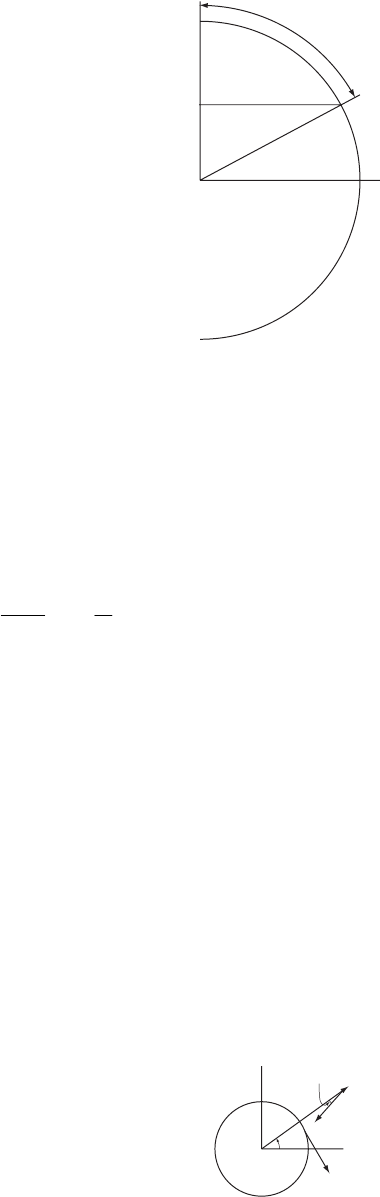
MOTION IN A NONINERTIAL REFERENCE FRAME 341
10-11.
θ
R sin θ
d = Rθ
This problem is most easily done in the fixed frame, not the rotating frame. Here we take the
Earth to be fixed in space but rotating about its axis. The missile is fired from the North Pole at
some point on the Earth’s surface, a direction that will always be due south. As the missile
travels towards its intended destination, the Earth will rotate underneath it, thus causing it to
miss. This distance is:
∆ = (transverse velocity of Earth at current latitude) × (missile’s time of flight)
sinRT
ω
θ
=× (1)
sin
dR d
vR
ω
=
(2)
Note that the actual distance d traveled by the missile (that distance measured in the fixed
frame) is less than the flight distance one would measure from the Earth. The error this causes
in ∆ will be small as long as the miss distance is small. Using R = 6370 km, 5
7.27 10
ω
−
=×
rad⋅, we obtain for the 4800 km, T = 600 s flight a miss distance of 190 km. For a 19300 km
flight the missile misses by only 125 km because there isn’t enough Earth to get around, or
rather there is less of the Earth to miss. For a fixed velocity, the miss distance actually peaks
somewhere around d = 12900 km.
1
s−
Doing this problem in the rotating frame is tricky because the missile is constrained to be in a
path that lies close to the Earth. Although a perturbative treatment would yield an order of
magnitude estimate on the first part, it is entirely wrong on the second part. Correct treatment
in the rotating frame would at minimum require numerical methods.
10-12.
z
Fs
r0
x
λ
ε
342 CHAPTER 10
Using the formula
(
)
eff 2
f
r
mm m=−××− ×Fa r v
ω
ωω (1)
we try to find the direction of when
eff
F
f
ma (which is the true force) is in the direction of the z
axis. Choosing the coordinate system as in the diagram, we can express each of the quantities in
(1) as
0
0
(cos,0,sin)
(0,0, )
(0,0, )
r
f
R
mmg
ω
λω λ
=
=−
=
=−
v
r
a
ω
(2)
Hence, we have
cos
y
R
ω
λ
×
=re
ω
(3)
and (1) becomes
eff 0 cos 0 sin
0cos0
xy
z
mg m
R
z
ω
λω
ωλ
=− − −
eee
λ
22
Fe (4)
from which, we have
2
eff 0 sin cos cos
z
x
mg mR mR z
ω
λλ ω λ
=− + +eFe (5) e
Therefore,
2
22
0
() sincos
() cos
fx
fz
FmR
FmgmR
ωλλ
ω
λ
=
=− +
(6)
The angular deviation is given by
2
22
0
() sin cos
tan cos
()
fx
fz
FR
gR
F
ω
λλ
ε
ω
λ
==
− (7)
Since
ε
is very small, we can put
ε
ε
≅. Then, we have
2
22
0
sin cos
cos
R
gR
ω
λλ
ε
ω
λ
=− (8)
It is easily shown that
ε
is a maximum for 45
λ
°.
Using , , , the maximum deviation is
8
6.4 10 cmR=× 51
7.3 10 sec
ω
−−
=× 2
980 cm/secg=
1.7 0.002 rad
980
ε
≅≅ (9)
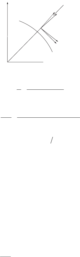
MOTION IN A NONINERTIAL REFERENCE FRAME 343
10-13.
ω
λ
ε
z′
z
x
x′
Earth
The small parameters which govern the approximations that need to be made to find the
southerly deflection of a falling particle are:
height of fall
radius of Earth
h
R
δ
≡= (1)
and
2
0
centrifugal force
purely gravitational force
R
g
ω
α
≡= (2)
The purely gravitational component is defined the same as in Problem 10-12. Note that
although both
δ
and
α
are small, the product 2
0
hg
δα ω
= is still of order 2
ω
and therefore
expected to contribute to the final answer.
Since the plumb line, which defines our vertical direction, is not in the same direction as the
outward radial from the Earth, we will use two coordinate systems to facilitate our analysis. The
unprimed coordinates for the Northern Hemisphere-centric will have its x-axis towards the
south, its y-axis towards the east, and its z-axis in the direction of the plumb line. The primed
coordinates will share both its origin and its y′-axis with its unprimed counterpart, with the z′-
and x′-axes rotated to make the z′-axis an outward radial (see figure). The rotation can be
described mathematically by the transformation
cos sin
xx z
ε
ε
=+
′′
(3)
(4) yy=′
sin cos
z
xz
ε
ε
=− +
′
′ (5)
where
2
sin cos
R
g
ω
ε
λ
≡
λ
(6)
as found from Problem 10-12.
a) The acceleration due to the Coriolis force is given by
2
X
≡
−×
′
av
ω
(7)
Since the angle between
ω
and the z′-axis is
π
–
λ
, (7) is most appropriately calculated in the
primed coordinates:
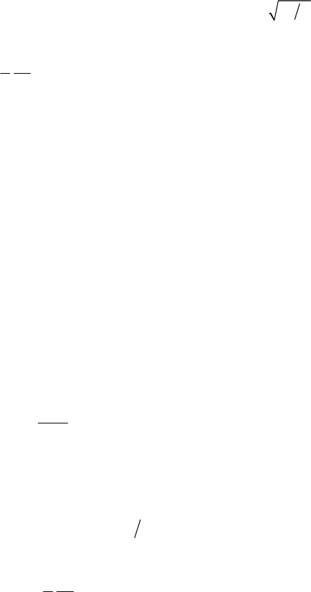
344 CHAPTER 10
2sin
xy
ω
λ
=
′′
(8)
(
)
2cos sinyz x
ω
λ
=− +
′′ ′
λ
(9)
2cos
zy
ω
λ
=
′′
(10)
In the unprimed coordinates, the interesting component is
(
)
2sincoscossinxy
ω
λε λ
=+
ε
(11)
At our level approximation this becomes
2sinxy
ω
λ
(12)
Using the results for and
y
z
, which is correct to order
ω
(also found from Example 10.3),
22
2sincosxgt
ω
λ
λ
(13)
Integrating twice and using the zeroth order result for the time-of-fall, 2h=t, we obtain for
the deflection
g
2
2
2sin cos
3
X
h
dg
ω
λ
=
λ
(14)
b) The centrifugal force gives us an acceleration of
(
)
c≡− × ×
′
arωω (15)
The component equations are then
(
)
2sin sin cosxxRz
ω
λλ
=++
′′ ′
λ
(16)
(17)
2
y
ω
=
′
y
′
(
)
2
0
cos sin cos
z
xRz
ωλ λ λ
=++
′′′
g−
(18)
where we have included the pure gravitational component of force as well. Now transform to
the unprimed coordinates and approximate
(
)
2
0
sin cos sinxRz g
ω
λλ
+−
ε
(19)
We can use Problem 10-12 to obtain sin
ε
to our level of approximation
2
0
sin sin cos
R
g
ω
ε
ελ
λ
(20)
The prompts a cancellation in equation (19), which becomes simply
2sin cosxz
ω
λ
λ
(21)
Using the zeroth order result for the height, 22
z
hgt=− , and for the time-of-fall estimates the
deflection due to the centrifugal force
2
2
5sin cos
6
c
h
dg
ω
λ
λ
(22)
MOTION IN A NONINERTIAL REFERENCE FRAME 345
c) Variation in gravity causes the acceleration
0
3
g
GM g
r
≡− +ark (23)
where
(
)
xy Rz=+++
′′ ′
jri is the vector pointing to the particle from the center of the
spherical Earth. Near the surface
k
(
)
2
222 2
2rx y zR R Rz=+++ +
′
′′ ′
(24)
so that (23) becomes, with the help of the binomial theorem,
(
02
g
gxy z
R
−+−
)
′
′′
aijk (25)
Transform and get the x component
()
0cos 2 sin
g
xx z
R
ε
ε
−+
′′
(26)
()(
0cos sin cos 2 sin cos sin
gxz xz
R
)
ε
εε ε ε
=− − + +
ε
(27)
(
03sin
gxz
R
)
ε
−+ (28)
Using (20),
2
3sincosxz
ω
λ
λ
(29)
where we have neglected the x term. This is just thrice the part (b) result, R
2
2
5sin cos
2
g
h
dg
ω
λ
λ
(30)
Thus the total deflection, correct to order 2
ω
, is
2
2
4sincos
h
dg
ω
λ
λ
(31)
(The solution to this and the next problem follow a personal communication of Paul Stevenson,
Rice University.)
10-14. The solution to part (c) of the Problem 10-13 is modified when the particle is dropped
down a mineshaft. The force due to the variation of gravity is now
0
0g
gg
R
≡− +ark (1)
As before, we approximate r for near the surface and (1) becomes
(
0
g
gxyz
R
−++
)
′
′′
aijk (2)
In the unprimed coordinates,
346 CHAPTER 10
0
x
xg
R
−
(3)
To estimate the order of this term, as we probably should have done in part (c) of Problem
10-13, we can take 22
~xh g
ω
, so that
2
~h
xh
R
ω
×
(4)
which is reduced by a factor hR from the accelerations obtained previously. We therefore have
no southerly deflection in this order due to the variation of gravity. The Coriolis and centrifugal
forces still deflect the particle, however, so that the total deflection in this approximation is
2
2
3sin cos
2
h
dg
ω
λ
λ
(5)
10-15. The Lagrangian in the fixed frame is
()
2
1
2
ff
LmvUr=− (1)
where
f
v and
f
r are the velocity and the position, respectively, in the fixed frame. Assuming
we have common origins, we have the following relation
f
rr
=
+×vv r
ω
(2)
where v and are measured in the rotating frame. The Lagrangian becomes
r r
r
()() (
2
22
2rr r r
mU
=+⋅×+×−
vr rωω
)
r
r
Lv (3)
The canonical momentum is
(
rr
r
Lmm
)
r
∂
≡
=+ ×
∂
pv
vωr (4)
The Hamiltonian is then
() (
2
2
11
22
rr r r r
mvUrm≡⋅−= − − ×vp rω
)
HL (5)
H is a constant of the motion since 0Lt∂∂=, but H ≠ E since the coordinate transformation
equations depend on time (see Section 7.9). We can identify
(
2
1
2
c
Um=− ×rω
)
r
(6)
as the centrifugal potential energy because we may find, with the use of some vector identities,
()
2
22
2
cr
m
Ur
ω
r
−∇ = ∇ − ⋅
rω (7)
(
)
2
rr
m
ω
=−⋅
rr
ω
ω (8)

MOTION IN A NONINERTIAL REFERENCE FRAME 347
(
)
r
m
=
−×⋅rωω (9)
which is the centrifugal force. Computing the derivatives of (3) required in Lagrange’s
equations
r
r
dmm
dt
∂
r
=
+×
∂
La
vωv (10)
()
(
rr c
r
m
∂
=∇ × ⋅ −∇ +
∂
Lvr
rω
)
UU (11)
(
)
(
)
rr
mm U
=
−×−××−∇vrωωω (12)
The equation of motion we obtain is then
(
)
(
)
2
rr
m m=−∇ − × × − ×arωω ω r
v
a
mU (13)
If we identify F and F, then we do indeed reproduce the equations of motion
given in Equation 10.25, without the second and third terms.
eff r
m=U=−∇
10-16. The details of the forces involved, save the Coriolis force, and numerical integrations
in the solution of this problem are best explained in the solution to Problem 9-63. The only thing
we do here is add an acceleration caused by the Coriolis force, and re-work every part of the
problem over again. This is conceptually simple but in practice makes the computation three
times more difficult, since we now also must include the transverse coordinates in our
integrations. The acceleration we add is
(
)
2sin sin cos cos
cy x z y
vvv v
ω
λλλ
=−++
j
λ
kai (1)
where we have chosen the usual coordinates as shown in Figure 10-9 of the text.
a) Our acceleration is
C
g
=
−+aka (2)
As a check, we find that the height reached is 1800 km, in good agreement with the result of
Problem 9-63(a). The deflection at this height is found to be 77 km, to the west.
b) This is mildly tricky. The correct treatment says that the equation of motion with air
resistance is (cf. equation (2) of Problem 9-63 solution)
2C
t
v
gv
=
−+ +
akva (3)
The deflection is calculated to be 8.9 km.
c) Adding the vaiation due to gravity gives us a deflection of 10 km.
d) Adding the variation of air density gives us a deflection of 160 km.
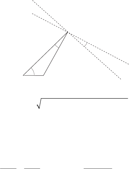
348 CHAPTER 10
Of general note is that the deflection in all cases was essentially westward. The usual small
deflection to the north did not contribute significantly to the total transverse deflection at this
precision. All of the heights obtained agreed well with the answers from Problem 9-63.
Inclusion of the centrifugal force also does not change the deflections to a significant degree at
our precision.
10-17. Due to the centrifugal force, the water surface of the lake is not exactly perpendicular
to the Earth’s radius (see figure).
mg
C
B
ββ
Water surface
Tangent to Earth surface
α
A
The length BC is (using cosine theorem)
22
()2 cos
α
=+−AC mg ACmgBC
where AC is the centrifugal force 2cos
ω
α
=AC m R with
α
= 47° and Earth’s radius
, 6400 kmR≅
The angle
β
that the water surface is deviated from the direction tangential to the Earth’s surface
is
5
sin
sin 4.3 10
sin sin
α
β
αβ
−
=⇒ = =×
BC AC AC
BC
So the distance the lake falls at its center is sin
β
=
hr where r = 162 km is the lake’s radius.
So finally we find h = 7 m.
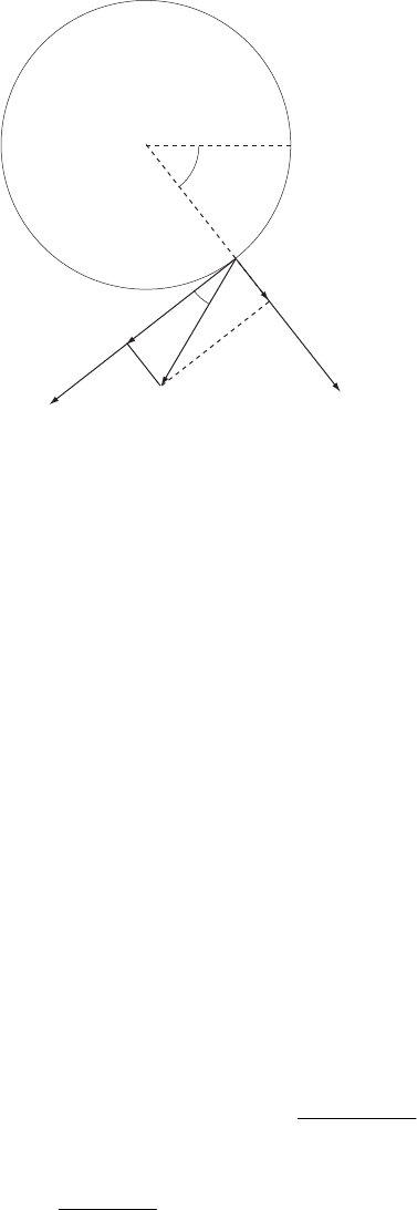
MOTION IN A NONINERTIAL REFERENCE FRAME 349
10-18. Let us choose the coordinate system Oxyz as shown in the figure.
O
νx
νy
ν
β
α
x
y
The projectile’s velocity is
vv where
β
= 37°
0
0
cos
sin
00
β
β
== −
Gx
y
vv
v gt
The Earth’s angular velocity is
cos
sin
0
ω
α
ω
ωα
−
=−
G
where
α
= 50°
So the Coriolis acceleration is
(
)
()
00
2 2 cos sin 2 sin cos
ωωβα βωα
=×=− + −
G
GG
c z
v v gt eav
The velocity generated by Coriolis force is
()
2
0
0
2 cos sin sin cos cos
ω
βα βα ω
− −
∫
t
cc
a dt v t gt
α
==v
And the distance of deviation due to the Coriolis force is
()
3
2
0
0
cos
sin 3
ω
α
ωαβ
==− −−
∫
t
cc
gt
dtvtzv
The flight time of the projectile is 0
2sin
2
β
=v
t. If we put this into , we find the deviation
distance due to Coriolis force to be
c
z
~ 260 m
c
z
350 CHAPTER 10
10-19. The Coriolis force acting on the car is
22sin
ω
ωα
=×⇒=
GG
G
G
cc
Fmv F mv
where
α
= 65°, m = 1300 kg, v = 100 km/hr.
So 4.76 N.
c
F=
G
10-20. Given the Earth’s mass, M, the magnitude of the gravitational field
vector at the poles is
24
5.976 10 kg=×
2
29.866 m/s==
pole
pole
GM
gR
The magnitude of the gravitational field vector at the equator is
22
e
2R 9.768 m/s
ω
=− =
eq q
eq
GM
gR
where
ω
is the angular velocity of the Earth about itself.
If one use the book’s formula, we have
at the poles
2
( 90 ) 9.832 m/s
λ
=°=g
and
g at the equator
2
( 0 ) 9.780 m/s
λ
=°=
10-21. The Coriolis acceleration acting on flowing water is
22sin
ω
ωα
=× ⇒ =
G
GG G
cc
av a v
Due to this force, the water is higher on the west bank. As in problem 10-17, the angle
β
that the
water surface is deviated from the direction tangential to Earth’s surface is
5
22 2 222
2sin 2.5 10
4sin
ωα
ωα
sin
β
−
== =×
++ ∝
c
c
av
ga g v
The difference in heights of the two banks is
3
sin 1.2 10 m
β
−
∆= = ×Ah
where Am is the river’s width. 47=
10-22. The Coriolis acceleration is 2
c
av
ω
=
×
G
GG
. This acceleration c
a
G
pushes lead bullets
eastward with the magnitude 2 coscos 2
ω
αω
G
cgt
α
==av , where
α
= 42°.
The velocity generated by the Coriolis force is
MOTION IN A NONINERTIAL REFERENCE FRAME 351
2
() cos
ω
α
==
∫
c
vt adt gt
and the deviation distance is
3
() cos
3
ω
α
∆= =
∫
cc
gt
xvtdt
The falling time of the bullet is 2=ht . So finally g
3
3
8cos 2.26 10 m
3
ωα
−
∆= = ×
c
h
xg
352 CHAPTER 10

CHAPTER 11
D
y
namics
of Rigid Bodies
11-1. The calculation will be simplified if we use spherical coordinates:
sin cos
sin sin
cos
xr
yr
zr
θ
φ
θ
φ
θ
=
=
=
(1)
z
y
x
Using the definition of the moment of inertia,
()
2
ij ij k i j
k
Ir xxx
ρδ
dv
=−
∑
∫ (2)
we have
(
)
()
()
22
33
22 2 2
cos cos
Irzdv
rr rdrd d
ρ
ρ
θθ
=−
=−
∫
∫
φ
(3)
or,
()
()
12
42
33
01 0
5
1cos cos
4
253
R
Irdr d
R
+
−
=−
=⋅
∫∫ ∫
π
d
ρ
θθ
πρ
φ
(4)
353
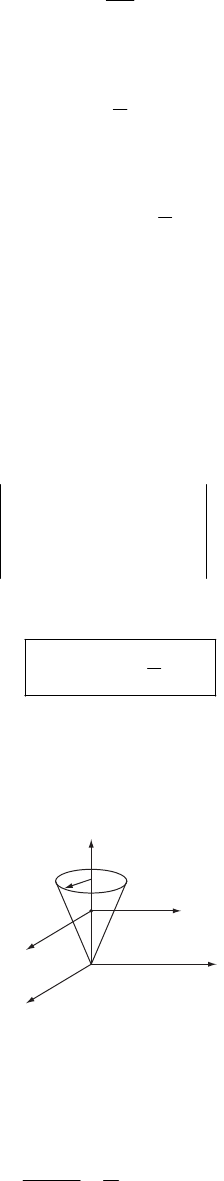
354 CHAPTER 11
The mass of the sphere is
3
4
3
M=R
π
ρ
(5)
Therefore,
2
33 5
IMR
2
= (6)
Since the sphere is symmetrical around the origin, the diagonal elements of {I} are equal:
2
11 22 33
2
5
III MR=== (7)
A typical off-diagonal element is
(
)
()
12
22 2
sin sin cos cos
Ixydv
rrdrd
ρ
d
ρ
θφφ θ
=−
=−
∫
∫
φ
(8)
This vanishes because the integral with respect to
φ
is zero. In the same way, we can show that
all terms except the diagonal terms vanish. Therefore, the secular equation is
11
22
33
00
00
00
II
II
II
−
0
−
=
−
(9)
From (9) and (7), we have
2
123
2
5
III MR=== (10)
11-2.
a) Moments of inertia with respect to the x axes:
i
x
3
= x
3
′
R
h
CM
x
1
x
1
′x
2
x
2
′
It is easily seen that for i ≠ j. Then the diagonal elements become the principal
moments I, which we now calculate.
0
ij
I=ii
I
i
The computation can be simplified by noting that because of the symmetry, . Then,
12
III=≠
3
()
222
12
12 3 1 2
2
22
II xxxdII v
ρ
+
== = ++
∫ (1)
DYNAMICS OF RIGID BODIES 355
which, in cylindrical coordinates, can be written as
()
222
12 000 2
2
hRzh
d dz r zrd
π
II r
ρ
φ
== +
∫∫∫ (2)
where
2
3MM
VR
ρπ
== h
(3)
Performing the integration and substituting for
ρ
, we find
()
2
12
34
20
II MR h
== +2
(4)
3
I is given by
(
)
22 2
312
Ixxdvrrdrddz
ρ
ρ
=+=⋅
∫∫
φ
(5)
from which
2
3
3
10
IMR= (6)
b) Moments of inertia with respect to the xi
′
axes:
Because of the symmetry of the body, the center of mass lies on the 3
x
′
axis. The coordinates of
the center of mass are (0 0
,0, )
z
, where
3
0
3
4
xdv
z
h
dv
′
==
∫
∫ (7)
Then, using Eq. (11.49),
2
i
j
i
j
i
j
i
j
IIMa aa
δ
=− −
′
(8)
In the present case, and
12
0aa==
(
)
334a=h, so that
22
11
22
22
2
33
93 1
16 20 4
93 1
16 20 4
3
10
II Mh MR h
II Mh MR h
II MR
=− = +
′
=− = +
′
=−
′
2
2
11-3. The equation of an ellipsoid is
2
22
3
12
222
1
x
xx
abc
+
+= (1)
356 CHAPTER 11
which can be written in normalized form if we make the following substitutions:
12 3
,,xa xb xc
ξ
η
ζ
=
== (2)
Then, Eq. (1) reduces to
222
1
ξηζ
+
+= (3)
This is the equation of a sphere in the (
ξ
,
η
,
ζ
) system.
If we denote by dv the volume element in the system and by d
τ
the volume element in the
(
ξ
,
η
,
ζ
) system, we notice that the volume of the ellipsoid is
i
x
123
4
3
Vdvdxdxdxabcddd
abc d abc
ξ
η
ζ
τπ
== =
==
∫∫ ∫
∫
(4)
because d
τ
∫ is just the volume of a sphere of unit radius.
The rotational inertia with respect to the passing through the center of mass of the
ellipsoid (we assume the ellipsoid to be homogeneous), is given by
3-axisx
()
(
22
312
22
22
M
Ixxdv
V
Mabc a b d
V
=+
=+
∫
∫
)
ξ
ητ
(5)
In order to evaluate this integral, consider the following equivalent integral in which z = r cos
θ
:
(
)
22 22
21
22
00 0
2
2
sin
cos sin
21
235
4
15
R
azdv az rdrr dd
ad d rd
a
a
=
=
=
=× ××
=
∫∫
∫∫ ∫
ππ
θθφ
φθθθ
π
π
4
r
(6)
Therefore,
()
()
22
22 2
4
15
abd ab
2
π
ξητ
+=+
∫ (7)
and
()
22
3
1
5
IMab=+ (8)
Since the same analysis can be applied for any axis, the other moments of inertia are
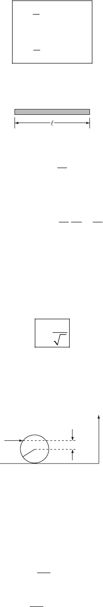
DYNAMICS OF RIGID BODIES 357
()
()
22
1
22
2
1
5
1
5
IMbc
IMac
=+
=+
(9)
11-4.
The linear density of the rod is
m
ρ
=
AA (1)
For the origin at one end of the rod, the moment of inertia is
3
2
033
mm
Ixdx
ρ
===
∫
A
A
AA
A
2
(2)
If all of the mass were concentrated at the point which is at a distance a from the origin, the
moment of inertia would be
(3)
2
Ima=
Equating (2) and (3), we find
3
a=A (4)
This is the radius of gyration.
11-5.
JM
a
Q
z – a
z
a) The solid ball receives an impulse J; that is, a force F(t) is applied during a short interval of
time
τ
so that
()
tdt=
′
′
∫
JF (1)
The equations of motion are
d
dt
=
pF (2)
d
dt
=
×
LrF
(3)
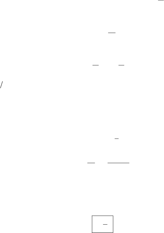
358 CHAPTER 11
which, for this case, yield
()
tdt
∆
==
′
′
∫
pF J (4)
()
tdt
∆
=× =×
′′
∫
LrF rJ (5)
Since p(t = 0) = 0 and L(t = 0) = 0, after the application of the impulse, we have
()
CM 0
;IzaJ
ω
====×=−V J L rJpM
ω
ω (6)
so that
CM =
J
VM (7)
and
()
0
Jza
I
ω
=−
ω
ω (8)
where
(
)
2
025IM=a.
The velocity of any point a on the ball is given by Eq. (11.1):
CM
α
α
=
+×vV r
ω
(9)
For the point of contact Q, this becomes
()
CM
5
12
QaJ
J
za
Ma
=−
−
=−
J
vV
ω
(10)
Then, for rolling without slipping, 0
Q
=
v, and we have
(
)
25aza
=
− (11)
so that
7
5
z
a= (12)
b) Many billiard tricks are performed by striking the ball at different heights and at different
angles in order to impart slipping and spinning motion (“English”). For the table not to
introduce spurious effects, the rail must be at such a height that the ball will be “reflected” upon
collision.
Consider the case in which the ball is incident normally on the rail, as in the diagram. We have
the following relationships:
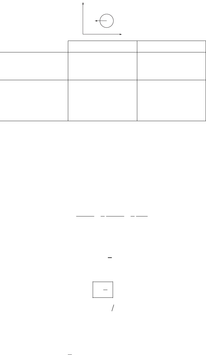
DYNAMICS OF RIGID BODIES 359
y
x
V
CM
Before Collision After Collision
Linear Momentum CM
0
x
y
p
MV
p
=
−
=
CM
0
x
y
p
MV
p
=
+
′
=
′
Angular Momentum 0
*
0
x
y
z
L
L
L
=
=
=
0
0
x
y
z
L
LL
L
y
=
′
=
−
′
=
′
* The relation between and depends on whether or not slipping occurs.
y
LCM
V
Then, we have
CM
22
x
ppJMV
∆
=− = = (13)
(
)
0
22
y
LLI Jza
ω
∆=− = = − (14)
so that
(
)
0CM
22IMVza
ω
=
− (15)
from which
22
0
CM CM CM
22
55
I
M
aa
za MV MV V
ω
ω
ω
−= = = (16)
If we assume that the ball rolls without slipping before it contacts the rail, then V
CM a
ω
=, and
we obtain the same result as before, namely,
2
5
z
a−= a (17)
or,
7
5
z
a= (18)
Thus, the height of the rail must be at a height of
(
)
25a above the center of the ball.
11-6. Let us compare the moments of inertia for the two spheres for axes through the centers
of each. For the solid sphere, we have
2
2(see Problem 11-1)
5
s
IMR= (1)
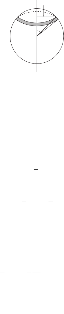
360 CHAPTER 11
For the hollow sphere,
θ
R sin θ
()
222
00
43
0
4
sin sin
2sin
8
3
h
IdR R
Rd
R
ππ
π
d
σ
φθ θ
πσ θ θ
πσ
=
=
=
∫∫
∫
θ
or, using , we have
2
4RM
πσ
=
2
2
3
h
IM=R (2)
Let us now roll each ball down an inclined plane. [Refer to Example 7.9.] The kinetic energy is
2
11
22
TMy I
2
θ
=+
(3)
where y is the measure of the distance along the plane. The potential energy is
(
)
sinUMg y
α
=−A (4)
where A is the length of the plane and
α
is the angle of inclination of the plane. Now, y = R
θ
, so
that the Lagrangian can be expressed as
22
2
11 sin
22
I
LMy yMgy
R
α
=+ + (5)
where the constant term in U has been suppressed. The equation of motion for y is obtained in
the usual way and we find
2
2
singMR
y
M
RI
α
=+
(6)
Therefore, the sphere with the smaller moment of inertia (the solid sphere) will have the greater
acceleration down the plane.
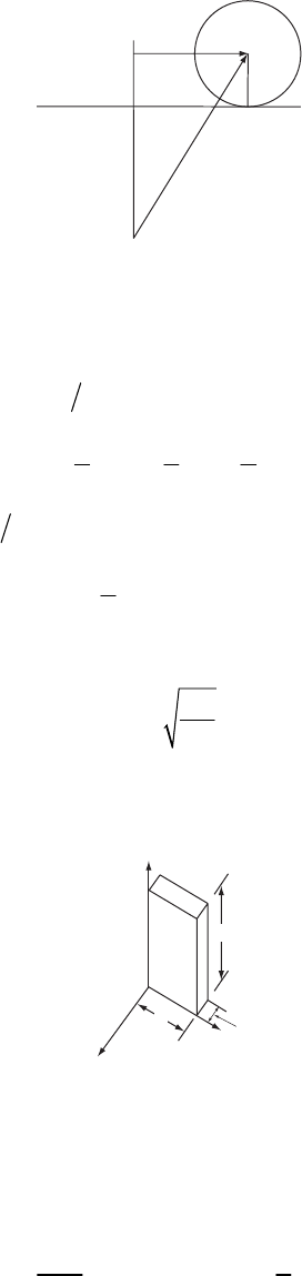
DYNAMICS OF RIGID BODIES 361
11-7.
R
d
x
r
φ
θ
The force between the force center and the disk is, from the figure
k
=
−Fr (1)
Only the component along x does any work, so that the effective force is sin
x
F
kr kx
φ
=− =− .
This corresponds to a potential 22x=Uk . The kinetic energy of the disk is
22
113
224
TMx I Mx
θ
=+=
2
(2)
where we use the result 22IMR= for a disk and dx = R d
θ
. Lagrange’s equations give us
30
2Mx kx
+
=
(3)
This is simple harmonic motion about x = 0 with an angular frequency of oscillations
2
3
k
m
ω
= (4)
11-8.
x
3
′
x
1
′x
2
′d
h
w
We let be the vertical axis in the fixed system. This would be the axis (i.e., the hinge line) of
the door if it were properly hung (no self-rotation), as indicated in the diagram. The mass of the
door is M=
ρ
whd.
3
x′
The moment of inertia of the door around the x3
′
axis is
2
3
00
1
3
hw
m
Idhwddw
whd
=
′′ ′
∫∫ 2
Mw=
(1)
where the door is considered to be a thin plate, i.e., d w,h.
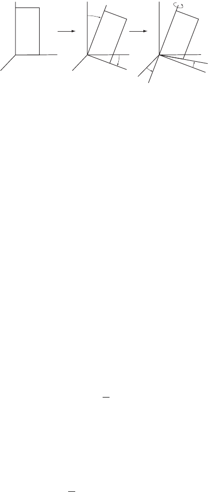
362 CHAPTER 11
The initial position of the self-closing door can be expressed as a two-step transformation,
starting with the position in the diagram above. The first rotation is around the through
an angle
θ
and the second rotation is around the
1-axisx′
1-axisx
′
′ through an angle
ψ
:
w
h
x3′
x2′
x1′
x3′x3″
x2′
x2″
x1′ = x1″
θ
θ
x3′x3 = x3″
w3 = w
x2′
x2
x2″
x1″x1
ψψ
The -axes are the fixed-system axes and the are the body system (or rotating) axes
which are attached to the door. Here, the Euler angle
φ
is zero.
1
x′-axes
i
x
The rotation matrix that transforms the fixed axes into the body axes
(
)
i
xx→
′i
is just Eq. (11.99)
with
φ
= 0 and
θ
→ –
θ
since this rotation is performed clockwise rather than counterclockwise
as in the derivation of Eq. (11.99):
cos cos sin sin sin
sin cos cos sin cos
0sin cos
ψ
θψ θψ
ψ
θψ θψ
θθ
−
=− −
λ (2)
The procedure is to find the torque acting on the door expressed in the fixed coordinate system
and then to obtain the component, i.e., the component in the body system. Notice that when
the door is released from rest at some initial angle
3
x
0
ψ
, the rotation is in the direction to decrease
ψ
. According to Eq. (11.119),
33 3 3
INI
ω
ψ
=
=
(3)
where 12
0
ω
ω
== since . 0
φθ
==
In the body ( system the coordinates of the center of mass of the door are
)
i
x
0
1
2
Rw
h
=
(4)
where we have set the thickness equal to zero. In the fixed ( )
i
x
′
system, these coordinates are
obtained by applying the inverse transformation 1
λ
−
to R; but 1t
λ
λ
−
=
, so that
sin
1cos cos sin
2sin cos cos
t
w
wh
wh
ψ
θ
ψθ
θ
ψθ
−
== +
′
−+
λRR (5)
Now, the gravitational force acting on the door is downward, and in the coordinate system
is
i
x′
3
M
g
=
−
′
′
Fe (6)
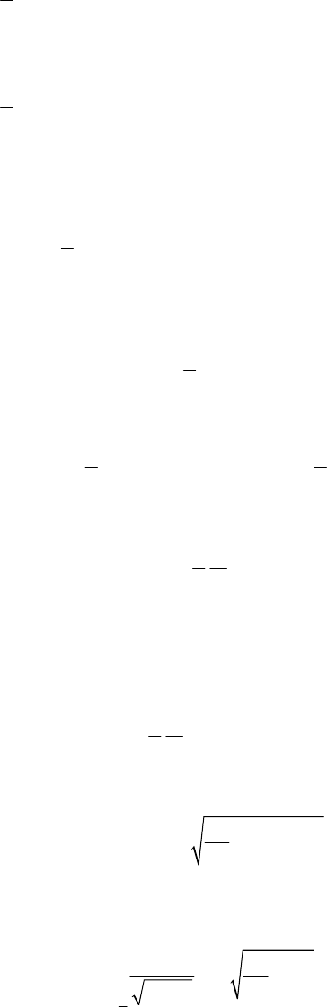
DYNAMICS OF RIGID BODIES 363
There the torque on the door, expressed in the fixed system, is
12 3
1sin cos cos sin sin cos cos
200 1
cos cos sin
1sin
20
Mg w w h w h
wh
Mg w
=×
′′′
′′ ′
=− − + − +
+
=−
NRF
ee e
ψ
θψ θ θψ θ
θψ θ
ψ
(7)
so that in the body system we have
22
cos cos sin cos cos sin
1sin sin
2sin sin
whw
Mg h
w
θ
ψθψ θ
θψ
θψ
++
==− −
′′
λ
ψ
NN (8)
Thus,
3
1sin sin
2
NMgw
θ
ψ
−= (9)
and substituting this expression into Eq. (3), we have
2
3
11
sin sin
23
Mgw I Mw
θ
ψψ
==
ψ
− (10)
where we have used Eq. (1) for . Solving for
3
I
ψ
,
3sin sin
2
g
w
ψ
θ
=−
ψ
(11)
This equation can be integrated by first multiplying by
ψ
:
2
13
sin sin
22
3sin cos
2
g
dt dt
w
g
w
==−
=
∫∫
ψψ ψ θ ψψ
θψ
(12)
where the integration constant is zero since cos 0
ψ
=
when 0
ψ
=
. Thus,
3sin cos
g
w
ψ
θ
=±
ψ
(13)
We must choose the negative sign for the radical since 0
ψ
<
when cos 0
ψ
>. Integrating again,
from
ψ
= 90° to
ψ
= 0°,
0
0
2
3sin
cos
T
g
ddt
w
π
ψθ
ψ
=−
∫∫
(14)
364 CHAPTER 11
where T = 2 sec. Rewriting Eq. (14),
2
0
3sin
cos
g
dTw
π
ψ
θ
ψ
=
∫ (15)
Using Eq. (E. 27a), Appendix E, we find
2
12
0
1
4
cos 3
2
4
d
π
π
ψψ
−
Γ
=
Γ
∫ (16)
From Eqs. (E.20) and (E.23),
11 1
1 0.906
44 4
13.624
4
Γ=Γ =
Γ=
(17)
And from Eqs. (E.20) and (E.24),
33 3
1 0.919
44 4
31.225
4
Γ=Γ =
Γ=
(18)
Therefore,
2
0
3.624 2.62
21.225
cos
d
π
ψπ
ψ
==
∫ (19)
Returning to Eq. (15) and solving for sin
θ
,
(
2
2
sin 2.62
3
w
gT
θ
=×
)
(20)
Inserting the values for g, w(= 1m), and T(= 2 sec), we find
(
)
1
sin 0.058
θ
−
=
or,
3.33
θ
≅
° (21)
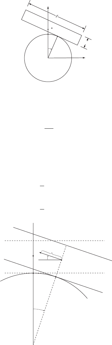
DYNAMICS OF RIGID BODIES 365
11-9.
a
O
R
QP
CC′
θ
y
x
The diagram shows the slab rotated through an angle
θ
from its equilibrium position. At
equilibrium the contact point is Q and after rotation the contact point is P. At equilibrium the
position of the center of mass of the slab is C and after rotation the position is C′.
Because we are considering only small departures from
θ
= 0, we can write
QP R
θ
≅ (1)
Therefore, the coordinates of C′ are (see enlarged diagram below)
=
+
′
rOAAC (2)
so that
sin cos
2
cos sin
2
a
xR R
a
yR R
θ
θθ
θ
θθ
=+ −
=+ +
(3)
C
Q
C′
Rθ
Rθ
P
O
A
θ
θ
Consequently,
366 CHAPTER 11
cos cos sin
2
cos sin
2
sin cos sin
2
sin cos
2
a
xR R R
aR
a
yR R R
aR
θ
θθθθ
θθθθ
θ
θθ θ
θθ θθ
=+ − +
=+
=− + + +
=− +
θ
from which
2
22 22
4
a
xy R 2
θ
θ
+= +
(4)
The kinetic energy is
()
22
11
22
TMxy I
2
θ
=++
(5)
where I is the moment of inertia of the slab with respect to an axis passing through the center of
mass and parallel to the z-axis:
()
22
1
12
IMa=+A (6)
Therefore,
()
2
1
1
2
Tf
θ
θ
= (7)
where
()
2
22
14
a
f
MR
θ
I
θ
=
+
+
(8)
The potential energy is
(
)
2
UMgy f
θ
=
=− (9)
where
()
2cos sin
2
a
fMgR R
θ
θθθ
=− + +
(10)
and where Eq. (3) has been used for y.
The Lagrangian is
() ()
2
1
1
2
Lf f
2
θ
θ
=+
θ
(11)
The Lagrange equation for
θ
is
DYNAMICS OF RIGID BODIES 367
0
dL L
dt
θ
θ
∂
∂
−
=
∂
∂ (12)
Now,
()
1
Lf
θ
θ
θ
∂
=
∂
() ()
11
2
22 2 2
2
4
dL ff
dt
a
MR IMR
∂=+
∂
=+++
θθ θθ
θ
θ
θθθ
(13)
() ()
2
12
22
1
2
sin cos sin
2
Lff
a
MR Mg R R R
∂=+
′′
∂
+−−
=+
θθ θ
θ
θ
θθθθθ
(14)
Combining, we find
2
22 2 2 sin cos sin 0
42
aa
MR IMR MgR R R
θθ θθ θθθ θ
+++ − + − −
=
(15)
For the case of small oscillations, 2
θ
θ
and 2
θ
θ
, so that Eq. (15) reduces to
2
20
4
a
Mg R
Ma I
θ
−
θ
+
=
+
(16)
The system is stable for oscillations around
θ
= 0 only if
2
2
20
4
a
Mg R
Ma I
ω
−
=
>
+
(17)
This condition is satisfied if 20Ra−>, i.e.,
2
a
R> (18)
Then, the frequency is
()
2
22
2
1
412
a
Mg R
Ma Ma
ω
−
=
++
A
(19)
Simplifying, we have
368 CHAPTER 11
()
22
12 2
4
a
gR
a
ω
−
=+
A (20)
According to Eqs. (9) and (10), the potential energy is
()
cos sin
2
a
UMgR R
θ
θθθ
=+ +
(21)
This function has the following forms for 2Ra> and 2Ra
<
:
U(θ)U(θ)
θ
−π/2 π/2
Ra
>2
Ra
<2
Mg R a
+
2
θ
To verify that a stable condition exists only for 2Ra>, we need to evaluate 2
U2
θ
∂∂ at
θ
= 0:
sin cos
2
Ua
Mg R
θ
θθ
θ
∂
=− +
∂
(22)
2
2cos cos sin
2
Ua
Mg R R
θ
θθθ
θ
∂
=− + −
∂
(23)
and
2
2
02
U
Mg R
θ
θ
=
∂
=−
∂
a
(24)
so that
2
20 if 2
U
R
θ
∂>>
∂
a
(25)
11-10.
z
m
R
θ
When the mass m is at one pole, the z component of the angular momentum of the system is
2
2
5
z
LI MR
ω
ω
== (1)
After the mass has moved a distance vt = R
θ
along a great circle on the surface of the sphere,
the z component of the angular momentum of the system is
DYNAMICS OF RIGID BODIES 369
222
2sin
5
z
LMRmR
θ
φ
=+
(2)
where
φ
is the new angular velocity. Since there is no external force acting on the system,
angular momentum must be conserved. Therefore, equating (1) and (2), we have
2
222
2
5
2sin
5
MR
MR mR
ω
φ
θ
=
+
(3)
Substituting vt R
θ
= and integrating over the time interval during which the mass travels from
one pole to the other, we have
()
2
222
0
2
5
2sin
5
R
tV
t
MR
dt
MR mR vt R
π
ω
φ
=
=
=
+
∫ (4)
Making the substitutions,
(
)
,vt R u dt R v du≡= (5)
we can rewrite (4) as
2
222
0
2
2
0
2
5
2sin
5
2
1sin
MR Rdu
v
MR mR u
Rdu
vu
=
+
=+
∫
∫
π
π
ω
φ
ω
β
(6)
where 52mM
β
≡ and where we have used the fact that the integrand is symmetric around
2u
π
= to write
φ
as twice the value of the integral over half the range. Using the identity
(
21
sin 1 cos 2
2
u=−
)
u (7)
we express (6) as
2
0
2
11
1c
22
Rdu
vu
π
ω
φ
ββ
=
+−
∫os2
(8)
or, changing the variable to x = 2u,
011
1c
22
Rdx
vx
π
os
ω
φ
ββ
=
+−
∫ (9)
Now, we can use Eq. (E.15), Appendix E, to obtain
370 CHAPTER 11
()
()
1
0
1tan2
2tan
11
2
25
2
25
x
R
v
RM
vMm
M
TMm
−
+
=
++
=+
=+
π
β
ω
φββ
πω
ω
(10)
where TRv
π
= is the time required for the particle to move from one pole to the other.
If m = 0, (10) becomes
(
)
0mT
φ
ω
=
= (11)
Therefore, the angle of retardation is
(
)
(
)
0mm
α
φφ
=
=− (12)
or,
2
125
M
TMm
αω
=−
+
(13)
11-11.
a) No sliding:
P
P
2
2
From energy conservation, we have
2
C.M.
11
22 2
2
mg mg mv I 2
ω
=+ +
AA (1)
where v is the velocity of the center of mass when one face strikes the plane; v is related
to
ω
by
CM C.M.
CM 2
v=A
ω
(2)
I is the moment of inertia of the cube with respect to the axis which is perpendicular to one face
and passes the center:
2
1
6
Im=A (3)
Then, (1) becomes
DYNAMICS OF RIGID BODIES 371
()
22
22
11 1
21
22263
2
mg m
m
ω
2
m
ω
ω
−= + =
AAA A (4)
from which, we have
()
2321
2
g
ω
=
−
A (5)
b) Sliding without friction:
In this case there is no external force along the horizontal direction; therefore, the cube slides so
that the center of mass falls directly downward along a vertical line.
P
θ
P
While the cube is falling, the distance between the center of mass and the plane is given by
cos
2
y
θ
=A (6)
Therefore, the velocity of center of mass when one face strikes the plane is
04 4
11
sin 22
2
==
=− =− =−
A
A
πθπ
yA
θ
θθω
(7)
From conservation of energy, we have
2
2
11 11
22 2 26
2mg m m 2
mg
ω
ω
=+− +
AA AA (8)
from which we have
()
212 21
5
g
ω
=
−
A (9)
11-12. According to the definition of the principal moments of inertia,
(
)
(
)
()
22 22
22 2
2
2
2
jk i k i j
jk i
ii
I I x x dv x x dv
xxdv xdv
Ixdv
+= + + +
=++
=+
∫∫
∫∫
∫
ρρ
ρρ
ρ
(1)
since
20
i
xdv
ρ
>
∫
we have

372 CHAPTER 11
j
ki
III
+
≥ (2)
11-13. We get the elements of the inertia tensor from Eq. 11.13a:
(
)
()()()
22
11 ,2 ,3
222
342213
Imxx
mb m b mb mb
αα α
α
=+
=+ +=
∑
2
bb
2
Likewise and
2
22 16Im=2
33 15Im=
()()
12 21 ,1 ,2
22
42 2
II mxx
mb m b mb
αα α
α
==−
=− − − =−
∑
Likewise
2
13 31
IImb==
and
II
2
23 32 4mb==
Thus the inertia tensor is
{}
2
13 2 1
216 4
1415
Imb
−
=−
The principal moments of inertia are gotten by solving
2
13 2 1
216 4
1415
mb
λ
λ
λ
−−
0
−
−=
−
Expanding the determinant gives a cubic equation in
λ
:
32
44 622 2820 0
λλ λ
−
+−=
Solving numerically gives
1
2
3
10.00
14.35
19.65
λ
λ
λ
=
=
=
2
1
2
2
2
3
Thus the principal moments of inertia are 10
14.35
19.65
Imb
Imb
Imb
=
=
=
To find the principal axes, we substitute into (see example 11.3):
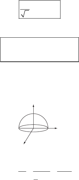
DYNAMICS OF RIGID BODIES 373
(
)
()
()
123
12
12 3
13 2 0
26 4
415 0
ii i i
iiii
ii ii
−−+=
−+1− + =
++− =
λω ω ω
ωλωω
ωω λω
3
0
For i = 1, we have
(
)
110
λ
=
11 21 31
11 21 31
11 21 31
32 0
264
450
0
ω
ωω
ωωω
ωωω
−
+=
−
−+=
−+=
Solving the first for 31
ω
and substituting into the second gives
11 21
ω
ω
=
Substituting into the third now gives
31 21
ω
ω
=
−
or
11 21 31
: : 1:1: 1
ω
ωω
=
−
So, the principal axis associated with is
1
I
()
1
3xyz
+
−
Proceeding in the same way gives the other two principal axes:
2 : .81 .29 .52
3 : .14 .77 .63
i
i
=−+−
=−++
xy
xy
z
z
We note that the principal axes are mutually orthogonal, as they must be.
11-14.
z
y
x
Let the surface of the hemisphere lie in the x-y plane as shown. The mass density is given by
3
3
3
22
3
M
MM
Vb
b
ρ
π
π
== =
First, we calculate the center of mass of the hemisphere. By symmetry
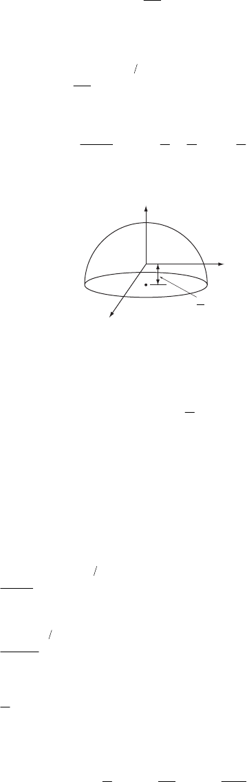
374 CHAPTER 11
CM CM
CM
0
1
v
xy
z
zdv
M
ρ
=
=
=∫
Using spherical coordinates 2
(cos, sin )
z
rdvrdrdd
θ
θθ
==
φ
we have
()
2
2
3
CM
00 0
4
3
sin cos
3113
2
2248
b
r
z
dd
M
bb
b
π
π
φθ
ρφθθθ
π
π
== =
=
==
∫∫ ∫
rdr
We now calculate the inertia tensor with respect to axes passing through the center of mass:
z′ = z
x′
y′
3
8b
By symmetry, . Thus the axes shown are the principal axes.
12 21 13 31 23 32 0IIIIII======
Also, by symmetry I. We calculate I using Eq. 11.49:
11 22
I=11
2
11 11
3
8
IJMv
=−
(1)
where 11
J
= the moment of inertia with respect to the original axes
(
)
()
()
()
22
11
22 2 2 2 2
22
4222
3
000
2
2
32
0
2
sin sin cos sin
3sin sin cos sin
2
3sin 2 cos sin
10
2
5
v
v
b
r
Jyzdv
rrrdrdd
Mrdr d d
b
Mb d
Mb
ππ
θφ
π
θ
ρ
θφ θ θθφ
θ
φθφθ
π
πθπθθθ
π
===
=
=+
=+
=+
=
∫
∫
∫∫∫
∫
θ
=+
Thus, from (1)
22
11 22
29 83
564320
I I Mb Mb Mb== − = 2
Also, from Eq. 11.49
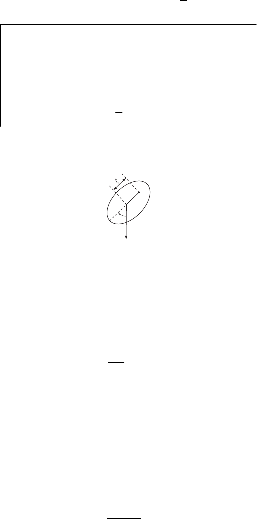
DYNAMICS OF RIGID BODIES 375
(
)
33 33 33
0IJM J
=
−=
( should be obvious physically)
33 33
IJ=
So
(
)
22
33
43 2
sin 5
v
v
Ixydv
rdrddM
ρ
ρθθφ
=+
==
∫
∫2
b
2
11 22
2
33
Thus, the principal axes are the primed axes shown
in the figure. The principal moments of inertia are
83
I320
2
I5
IMb
Mb
==
=
11-15.
θ
P
g
We suspend the pendulum from a point P which is a distance A from the center of mass. The
rotational inertia with respect to an axis through P is
(1)
2
0
IMR M=+A2
where is the radius of gyration about the center of mass. Then, the Lagrangian of the system
is
0
R
(
2
1cos
2
I
LTU Mg
θ
)
θ
=−= − −
A (2)
Lagrange’s equation for
θ
gives
sin 0IMg
θθ
+
=
A (3)
For small oscillation, sin
θ
θ
≅. Then,
0
Mg
I
θθ
+
=
A
(4)
or,
22
0
0
g
R
θθ
+
=
+
A
A (5)
376 CHAPTER 11
from which the period of oscillation is
22
0
22R
g
π
τπ
ω
+
== A
A (6)
If we locate another point P′ which is a distance A′ from the center of mass such that the period
of oscillation is also
τ
, we can write
22 2
00
RR
gg
++
2
′
=
′
A
AA
A
(7)
from which . Then, the period must be
2
0
R=′
AA
2
2g
τπ
+
′
=AA A
A (8)
or,
2g
τπ
+
′
=AA (9)
This is the same as the period of a simple pendulum of the length A + A′
1
. Using this method, one
does not have to measure the rotational inertia of the pendulum used; nor is one faced with the
problem of approximating a simple pendulum physically. On the other hand, it is necessary to
locate the two points for which
τ
is the same.
11-16. The rotation matrix is
()
cos sin 0
sin cos 0
00
θθ
θθ
=−
λ (1)
The moment of inertia tensor transforms according to
(
)
(
)
(
)
(
)
t
=
′
Ι
λΙλ (2)
That is
()
()()
()()
110
22
cos sin 0 cos sin 0
11
sin cos 0 0 sin cos 0
22
001 00
00
AB AB
IABAB
C
θθ θ θ
θθ θ θ
+−
−
=− − +
′
1
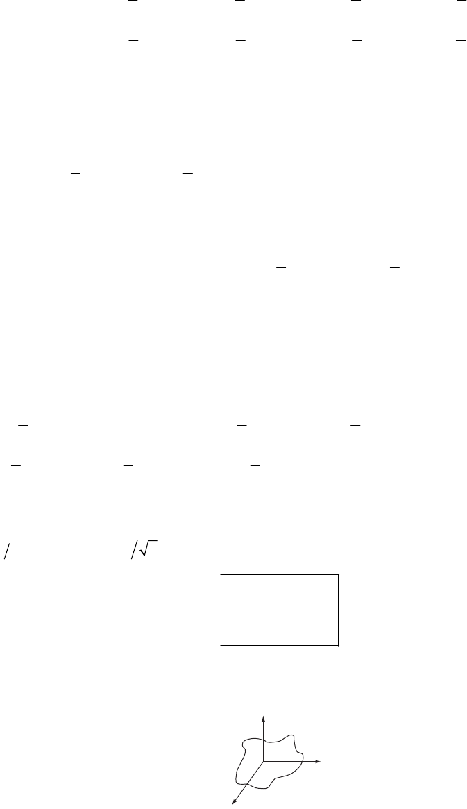
DYNAMICS OF RIGID BODIES 377
() () () ()
() () () ()
11 11
cos sin sin cos 0
22 22
cos sin 0 11 11
sin cos 0 cos sin sin cos 0
22 22
001 00
AB AB AB AB
AB AB AB AB
C
θθ θ
θθ
θθ θ θ θ θ
++− −++−
=− − + + − − + +
θ
() () ()
() ()
() ()
() () ()
22
22
22
22
11
cos cos sin sin
22
11
sin cos
22
0
11
cos sin 0
22
11
sin sin cos cos 0
22
0
AB AB AB
AB AB
AB AB
AB AB AB
C
++− ++
=−−+−
−−−
+−− ++
θθθ θ
θθ
θθ
θθθ θ
or
()
()() () ()
() () ()()
22
22
111
cos sin cos sin 0
222
11 1
sin cos cos sin 0
22 2
00
AB AB AB AB
AB AB AB AB
C
θθ θ θ
θθ θθ
++ − − − −
=− − + − + − −
′
I (3)
If 4
θ
π
=, sin cos 1 2
θθ
==. Then,
()
00
00
00
A
B
C
=
′
I (4)
11-17.
x
3
x
2
x
1

378 CHAPTER 11
The plate is assumed to have negligible thickness and the mass per unit area is s
ρ
. Then, the
inertia tensor elements are
(
)
22
11 1 1 2
sxdx
ρ
=−
∫
Ir dx
(
)
22 2
2312 212ss
xxdxdx xdxdxA
ρρ
= ≡
∫∫
=+ (1)
(
)
22 2
22 2 1 2 1 1 2ss
xdxdxxdxdx
ρρ
=− =
∫∫
Ir (2) B≡
(
)
(
)
22 22
33 312 121ss
r xdxdx x xdxdx
ρρ
=− =+
∫∫
2
B
I (3)
Defining A and B as above, becomes
33
I
33
IA
=
+ (4)
Also,
(
)
12 1 2 1 2s
Ixxdxdx
ρ
C
=
−
∫≡− (5)
(
)
21 2 1 1 2s
Ixxdxdx
ρ
C
=
−
∫=− (6)
(
)
13 1 3 1 2 31
0
s
Ixxdxdx
ρ
I
=
−=
∫= (7)
(
)
23 2 3 1 2 32
0
s
Ixxdxdx
ρ
I
=
−=
∫= (8)
Therefore, the inertia tensor has the form
{}
0
0
00
AC
CB
A
B
−
=−
+
I (9)
11-18. The new inertia tensor
{
}
′
I is obtained from
{
}
I by a similarity transformation [see
Eq. (11.63)]. Since we are concerned only with a rotation around the , the transformation
matrix is just
3-axisx
φ
λ, as defined in Eq. (11.91). Then,
1
φ
φ
−
=
′
II
λ
λ (1)
where
1t
φ
φ
−
=
λ
λ (2)
Therefore, the similarity transformation is
=−
I
cos sin 0 0 cos sin 0
sin cos 0 0 sin cos 0
00100 00
AC
CB
AB
θθ θ θ
θθ θ θ
−−
−
′
+
1
Carrying out the operations and simplifying, we find
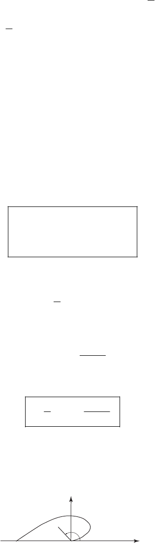
DYNAMICS OF RIGID BODIES 379
{}
()
()
22
22
1
cos sin 2 sin cos 2 sin 2 0
2
1
cos 2 sin 2 sin sin 2 cos 0
2
00
ACB C BA
CBAACB
A
B
θθθ θ θ
θθθθθ
−+ −+−
=− + − + +
′
+
I (3)
Making the identifications stipulated in the statement of the problem, we see that
11 22
12 21
,IAIB
II C
==
′
′′ ′
==−
′′ ′
(4)
and
33
IABAB
=
+= +
′
′′
(5)
Therefore
{}
0
0
00
AC
CB
AB
−
′′
=−
′′′
+
′
′
I (6)
In order that and be principal axes, we require C′ = 0:
1
x2
x
()
1
cos 2 sin 2 0
2
CBA
θθ
−
−= (7)
or,
2
tan 2 C
BA
θ
=
−
(8)
from which
1
12
tan
2
C
BA
θ
−
=
−
(9)
Notice that this result is still valid if A = B. Why? (What does A = B mean?)
11-19.
θ = 0
x2
x
ηθ
θ = π
θ = π/2
1
The boundary of the plate is given by rke
α
θ
=. Any point (
η
,
θ
) has the components
1
2
cos
sin
x
x
η
θ
η
θ
=
=
(1)

380 CHAPTER 11
The moments of inertia are
2
12
00
23
00
sin
ke
ke
IA xdd
dd
αθ
αθ
π
π
ρ
ηηθ
ρ
θθ η η
==
=
∫∫
∫∫
The integral over
θ
can be performed by using Eq. (E.18a), Appendix E, with the result
4
12
k
IA P
==
ρ
α
(2)
where
()
4
2
1
16 1 4
e
P
πα
α
−
=+ (3)
In the same way,
2
21
00
2
00
cos
ke
ke
IB xdd
d
==
=
∫∫
∫∫
αθ
αθ
π
π
3
d
ρ
ηηθ
ρ
θθ η η
(4)
Again, we use Eq. (E.18a) by writing co 2
s 1 sin2
θ
θ
=− , and we find
()
4
2
218
2
k
IB P
ρ
α
α
== + (5)
Also
12 1 2
00
3
00
cos sin
ke
ke
IC xxdd
dd
αθ
αθ
π
π
ρ
ηηθ
ρ
θθθ η
=− =−
=−
∫∫
∫∫
η
(6)
In order to evaluate the integral over
θ
in this case we write
(
)
cos sin 1 2 sin 2
θ
θθ
= and use
Eq. (E.18), Appendix E. We find
(7)
4
12
ICk
ρ
=− = P
Using the results of problem 11-17, the entire inertia tensor is now known.
According to the result of Problem 11-18, the angle through which the coordinates must be
rotated in order to make
{
}
I diagonal is
1
12
tan
2
C
BA
θ
−
=
−
(8)
Using Eqs. (2), (5), and (7) for A, B, C, we find
21
2
C
BA
α
=
− (9)
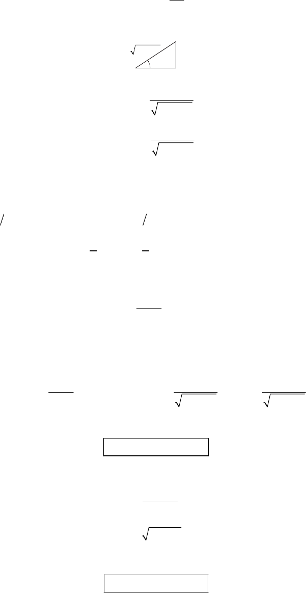
DYNAMICS OF RIGID BODIES 381
so that
1
tan 2 2
θ
α
= (10)
Therefore, we also have
2θ
2α
1
14
2
+α
2
2
1
sin 2 14
2
cos 2 14
θα
α
θα
=
+
=
+
(11)
Then, according to the relations specified in Problem 11-18,
2
1cos sin 2 sinIAA C B2
θ
θ
== − +
′′
θ
(12)
Using
(
)
(
)
2
cos 1 2 1 cos 2
θ
θ
=+ and
(
)
(
)
2
sin 1 2 1 cos 2
θ
θ
=− , we have
()()
1
11
cos 2 sin 2
22
AB AB CIA
θ
θ
== ++ − −
′′ (13)
Now,
()
4
2
4
14
4
kP
AB
AB kP
ρα
α
αρ
+= +
−=−
(14)
Thus,
()
4
24 4
122
21
14 2
214 14
kP kP kP
ρα
ααρ ρ
α
IA
α
α
== + − × − ×
′′ ++
(15)
or,
()
4
1
IA kPQR
ρ
== −
′′ (16)
where
2
2
14
2
14
Q
Ra
α
α
+
=
=+
(17)
Similarly,
()
4
2
IB kPQR
ρ
== +
′′ (18)
and, of course,
382 CHAPTER 11
3
IABII
12
=
+=+
′
′′′′
(19)
We can also easily verify, for example, that I
12 0C
=
−=
′
′.
11-20. We use conservation of energy. When standing upright, the kinetic energy is zero.
Thus, the total energy is the potential energy
12
b
EU mg==
(2
b is the height of the center of mass above the floor.)
When the rod hits the floor, the potential energy is zero. Thus
2
2
1
2
ET I
ω
==
where I is the rotational inertia of a uniform rod about an end. For a rod of length b,
mass/length
σ
:
23
end
0
11
33
b
Ixdxb
σσ
===
∫2
mb
Thus
22
2
1
6
Tmb
ω
=
By conservation of energy
12
UT
=
22
1
26
b
mg mb
ω
=
3g
b
ω
=
11-21. Using I to denote the matrix whose elements are those of
{
}
I, we can write
=
LI
ω
(11.54)
=
′
′′
LI
ω
(11.54a)
We also have and and therefore we can express L and ω as =
′
xλx′
x
t
=
′
xλ
t
=
′
LL
λ
(11.55a)
t
=
′
ω
λω (11.55b)
substituting these expressions into Eq. (11.54), we have

DYNAMICS OF RIGID BODIES 383
tt
=
′
′
LI
λ
λω
and multiplying on the left by λ,
tt
=
′
′
LI
λ
λλλω
or
(
)
t
=
′
′
LI
λ
λω
by virture of Eq. (11.54a), we identify
t
=
′
II
λ
λ (11.61)
11-22. According to Eq. (11.61),
1
,
i
j
ik k
j
kl
II
λ
λ
−
=
′
∑
AA
(1)
Then,
{
}
1
,
1
,
,
ii ik k i
iik
kiik
ki
kk kk
kk
tr I I
I
II
−
−
==
′′
=
==
∑
∑∑
∑∑
∑∑
IAA
A
AA
A
AA
A
λ
λ
λλ
δ
(2)
so that
{} {}
tr tr=
′
II (3)
This relation can be verified for the examples in the text by straightforward calculations.
Note: A translational transformation is not a similarity transformation and, in general,
{
}
tr is not
invariant under translation. (For example,
I
{
}
tr I will be different for inertia tensors expressed in
coordinate system with different origins.)
11-23. We have
1
−
=
′
II
λ
λ (1)
Then,
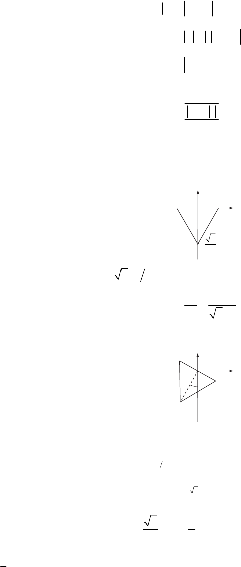
384 CHAPTER 11
1
1
1
−
−
−
=
′
=××
=×
II
I
I
λλ
λ
λ
λλ
so that,
=
′
II (2)
This result is easy to verify for the various examples involving the cube.
11-24.
–a/2 a/2
x
2
x
1
−3
2a
The area of the triangle is 2
34
A
a=, so that the density is
2
4
3
MM
Aa
ρ
== (1)
a) The rotational inertia with respect to an axis through the point of suspension (the origin) is
x2
x1
θ
(
)
()
()
1
22
31212
20
22
112
032
2
42
2
31
24 6
a
ax
Ixxdxdx
dx x x dx
aMa
−−
=+
=+
==
∫
∫∫
ρ
ρ
ρ
2
(2)
When the triangle is suspended as shown and when
θ
= 0, the coordinates of the center of mass
are 2
(0, ,0)x, where
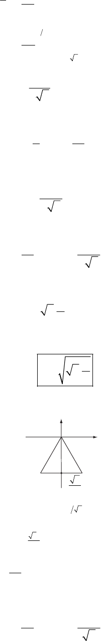
DYNAMICS OF RIGID BODIES 385
()
1
2 212
20
12
032
1
2
23
a
ax
x x dx dx
M
dx x dx
M
a
−−
=
=
=−
∫
∫∫
ρ
ρ
2
(3)
The kinetic energy is
2
3
11
212
TI Ma
22
θ
θ
==
(4)
and the potential energy is
(
1cos
23
Mga
U
)
θ
=− (5)
Therefore,
22
1cos
12 23
Mga
LMa
θ
θ
=+
(6)
where the constant term has been suppressed. The Lagrange equation for
θ
is
3sin 0
g
a
θθ
+
=
(7)
and for oscillations with small amplitude, the frequency is
3g
a
ω
= (8)
b) The rotational inertia for an axis through the point of suspension for this case is
x
2
x
1
−3
2a
()
23
0
22
3212
0
3
2
2
2
5
12
x
a
Idxxx
Ma
−
−
=+
′
=
∫∫
ρ
1
dx
(9)
The Lagrangian is now
22
5cos
24 3
Mga
LMa
θ
θ
=+
(10)
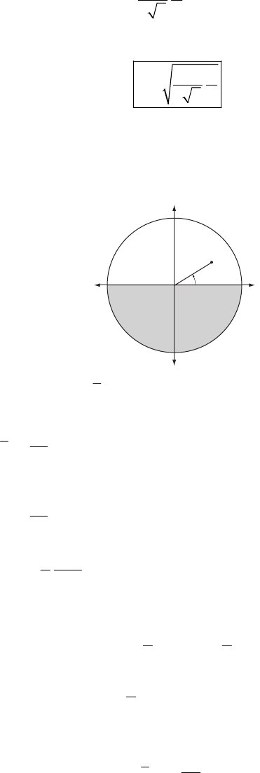
386 CHAPTER 11
and the equation of motion is
12 sin 0
53
g
a
θθ
+
=
(11)
so that the frequency of small oscillations is
12
53
g
a
ω
= (12)
which is slightly smaller than the previous result.
11-25.
x
2
x
1
R
r
2ρ
ρ
θ
The center of mass of the disk is 2
(0, )x, where
() ()
2 212 212
lower upper
semicircle semicircle
2
00 0
3
2
sin 2 sin
2
3
RR
xxdxdxxdxdx
M
r rdrd r rdrd
M
R
M
=+
=⋅+
∫∫
∫∫ ∫∫
ππ
π
ρ
ρ
⋅
=−
θ
θθ
ρ
θ
(1)
Now, the mass of the disk is
22
2
11
2
22
3
2
MR
R
=⋅ + ⋅
=
R
ρ
πρπ
ρπ
(2)
so that
2
4
9
xR
π
=− (3)
The direct calculation of the rotational inertia with respect to an axis through the center of mass
is tedious, so we first compute I with respect to the and then use Steiner’s theorem.
3-axisx
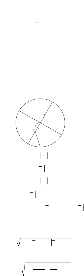
DYNAMICS OF RIGID BODIES 387
2
22
300 0
42
2
31
42
RR
Irrdrdrrd
RMR
=⋅+⋅
==
∫∫ ∫∫
ππ
π
rd
ρ
θθ
πρ
(4)
Then,
2
03 2
22
2
2
2
11
281
132
1
281
IIMx
6
M
RM R
MR
=−
=−⋅
=−
π
π
(5)
When the disk rolls without slipping, the velocity of the center of mass can be obtained as
follows:
Thus
R
CM
θ
θ
CM 2
CM 2
sin
cos
xRx
yRx
θ
θ
θ
=−
=−
2ρ
ρ
x
2
CM 2
CM 2
cos
sin
xRx
yx
θ
θθ
θθ
=−
=
(
)
22 222222
CM CM 2 2
2coxy VR x Rxs
θ
θθ
+==+ −
θ
2
22
Va
θ
= (6)
where
22
22
2cosaRx Rx
θ
=+− (7)
Using (3), a can be written as
2
16 8
1
81 9
aR cos
θ
ππ
=+ − (8)
The kinetic energy is
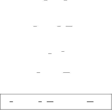
388 CHAPTER 11
trans rot
2
0
11
22
TT T
Mv I 2
=
+
=+
θ
(9)
Substituting and simplifying yields
22
138
cos
229
TMR
θ
θ
π
=−
(10)
The potential energy is
2
1cos
2
18
1cos
29
UMg Rx
MgR
=+
=−
θ
θ
π
(11)
Thus the Lagrangian is
2
138 8
cos 1 cos
229 9
RR gLM
θ
θ
ππ
θ
=−−−
(12)
11-26. Since =
φ
φ
ω lies along the fixed 3-axisx
′
, the components of
φ
ω
along the body axes
are given by the application of the transformation matrix λ [Eqs. (11.98) and (11.99)]:
()
i
x
(
)
()
()
11
2
2
3
3
0
0
φ
φ
φ
ωφ
ωφ
φ
φ
ω
==
λ (1)
Carrying out the matrix multiplication, we find
(
)
()
()
1
2
3
sin sin
cos sin
cos
φ
φ
φ
ω
ψ
θ
ω
φψ
θ
ω
θ
=
(2)
which is just Eq. (11.101a).
The direction of =
θ
θ
ω coincides with the line of nodes and lies along the axis. The
components of
1
x′′′
θ
ω
along the body axes are therefore obtained by the application of the
transformation matrix
ψ
λ
which carries the xi
′
′′ system into the system:
i
x
(
)
()
()
1
2
3
cos
0sin
00
θ
θψ
θ
ω
θψ
ω
θ
ω
ψ
==−
λ (3)
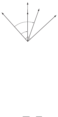
DYNAMICS OF RIGID BODIES 389
which is just Eq. (11.101b).
Finally, since
ψ
ω lies along the body , no transformation is required:
3-axisx
(
)
()
()
1
2
3
0
0
1
ψ
ψ
ψ
ω
ωψ
ω
=
(4)
which is just Eq. (11.101c).
Combining these results, we obtain
(
)
()
(
)
()
()
()
()
()
()
1
11
2
22
3
33
sin sin cos
cos sin sin
cos
++
++
++
+
=−
+
φθψ
φθψ
φθψ
ωωω
ωωω
ωωω
φ
ψθθψ
φ
φψθθψ
θθψ
ω=
(5)
which is just Eq. (11.02).
11-27.
L
α
θ
ω
x3x2
x3′
Initially:
111
2121
3333
0
sin sin
cos
LI
LL I I
LLxos I I
ω
θ
ωωα
θ
ωωα
=
=
===
===
Thus
21
33
tan tan
LI
LI
θ
α
== (1)
From Eq. (11.102)
3cos
ω
φθψ
=
+
Since 3cos
ω
ω
=
α
, we have
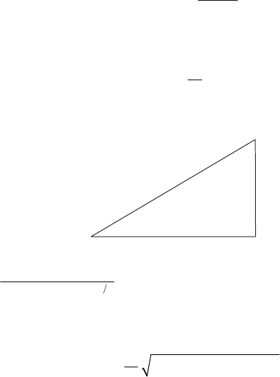
390 CHAPTER 11
cos cos
φ
θω αψ
=
−
(2)
From Eq. (11.131)
31
3
1
II
I
ψ
ω
−
=−Ω=−
(2) becomes
3
1
cos cos
I
I
=
φ
θωα
(3)
From (1), we may construct the following triangle
I
3
I
3
tan α
θ
from which 3
12
22 2
31
stan
I
II
θα
=
+
co
Substituting into (3) gives
22 2 2
13
1
sin cosII
I
ω
φ
αα
=+
11-28. From Fig. 11-7c we see that
=
φ
φ
ω is along the 3-axisx
′
,
=
θ
θ
ω is along the line of
nodes, and =
ψ
ψ
ω is along the . Then,
3-axxis
3
φ
φ
=
′
′
e
ω (1)
whee is the unit vector in the direction.
3
′
e3
x′
Projecting the lines of nodes into the 1-x
′
and 2-axesx
′
, we obtain
(
)
12
cos sin
θ
θ
φ
=+
′′ ′
ee
ω
φ
(2)
ψ
ω
′ has components along all three of the xi
′
axes. First, we write
ψ
′
ω
in terms of a component
along the x and a component normal to this axis:
3-axis
′
(
)
12 3
sin cos
ψ
ψ
θ
=+
′′ ′
ee
ω
θ
(3)
where
12 1 2
sin cos
φ
φ
=
−
′
′′
ee e (4)
Then,
(
)
12 3
sin sin sin cos cos
ψ
ψ
θφ θφ θ
=−+
′′ ′ ′
ee e
ω (5)

DYNAMICS OF RIGID BODIES 391
Collecting the various components, we have
1
2
3
cos sin sin
sin sin cos
cos
ω
θφψθφ
ω
θφψθ
ωψ θφ
=+
′
=−
′
=+
′
φ
(6)
11-29. When the motion is vertical
θ
= 0. Then, according to Eqs. (11.153) and (11.154),
(
)
3
PI P
φ
ψ
φψ
=
+=
(1)
and using Eq. (11.159), we see that
33
PPI
ψφ
ω
=
= (2)
Also, when
θ
= 0 (and ), the energy is [see Eq. (11.158)] 0
θ
=
2
33
1
2
EI Mg
ω
=+h (3)
Furthermore, referring to Eq. (11.160),
2
33
1
2
EE I Mgh
ω
=− =
′ (3)
If we wish to examine the behavior of the system near
θ
= 0 in order to determine the conditions
for stability, we can use the values of P
ψ
, P
φ
, and E′ for
θ
= 0 in Eq. (11.161). Thus,
(
)
2
22
33
2
12 2
12
1cos
1cos
22sin
I
I Mgh
I
ωθ
Mgh
θ
θ
θ
−
=+ +
(5)
Changing the variable to z = cos
θ
and rearranging, Eq. (5) becomes
() ()
2
2
12 3 3
2
12
121
z22
z
Mgh I z I w
I
−
=+−
(6)
The questions concerning stability can be answered by examining this expression. First, we note
that for physically real motion we must have 20
z
≥
. Now, suppose that the top is spinning very
rapidly, i.e., that 3
ω
is large. Then, the term in the square brackets will be negative. In such a
case, the only way to maintain the condition 20
z
≥
is to have z = 1, i.e.,
θ
= 0. Thus, the motion
at
θ
= 0 will be stable as long as
22
12 3 3
4Mgh I I
ω
0
−
< (7)
or,
12
22
33
41
Mgh I
I
ω
<
(8)
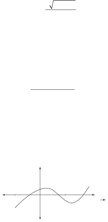
392 CHAPTER 11
Suppose now that the top is set spinning with
θ
= 0 but with 3
ω
sufficiently small that the
condition in Eq. (8) is not met. Any small disturbance away from
θ
= 0 will then give
z
a
negative value and
θ
will continue to increase; i.e., the motion is unstable. In fact,
θ
will
continue until z reaches a value 0
z
that again makes the square brackets equal to zero. This is a
turning point for the motion and nutation between z = 1 and 0
z
z
=
will result.
From this discussion it is evident that there exists a critical value for the angular velocity, c
ω
,
such that for 3c
ω
ω
> the motion is stable and for c
ω
ω
<
there is nutation:
12
3
2
c
Mgh I
I
ω
= (9)
If the top is set spinning with 3c
ω
ω
> and
θ
= 0, the motion will be stable. But as friction slows
the top, the critical angular velocity will eventually be reached and nutation will set in. This is
the case of the “sleeping top.”
11-30. If we set , Eq. (1.162) becomes 0
θ
=
()
(
)
()
2
2
12
cos cos
21cos
PP Mgh
I
φψ θ
EV
θ
θ
θ
−
== +
′− (1)
Re-arranging, this equation can be written as
(
)
(
)
(
)
(
)
322
12 12 12 12
2 cos 2 cos 2 cos 2 0Mgh I E I P P P Mgh I E I P
ψφψ
θθ θ
−+ +− +−
′′
2
φ
= (2)
which is cubic in cos
θ
.
V(
θ
) has the form shown in the diagram. Two of the roots occur in the region 1cos 1
θ
−≤ , and
one root lies outside this range and is therefore imaginary.
≤
V(θ)
cos θ
–1
+1
DYNAMICS OF RIGID BODIES 393
11-31. The moments of inertia of the plate are
()
12
2
312
2
2
2
cos 2
1cos2
2cos
II
I
III
I
I
α
α
α
=
=+
=+
=
=
(1)
We also note that
(
)
12 2
2
2
1cos2
2sin
II I
I
α
α
−=− −
=−
(2)
Since the plate moves in a force-free manner, the Euler equations are [see Eq. (11.114)]
(
)
()
()
121233
232311
313122
0
0
0
II I
II I
II I
ωω ω
ωω ω
ωω ω
−−=
−−=
−−=
(3)
Substituting (1) and (2) into (3), we find
(
)
(
)
()()
22
2122 3
22321
231 22
2sin 2cos 0
cos 2 cos 2 0
0
II
II
II
αωω αω
αωω αω
ωω ω
−−=
−−=
−=
(4)
These equations simplify to
2
312
123
231
tan
=−
=−
=
ω
ωω α
ωωω
ωωω
(5)
From which we can write
2
123221133
cot
ω
ωω ωω ωω ωω α
==−=−
(6)
Integrating, we find
(
)
(
)
(
)
22 22 22 2 2
22 11 3 3
0 0 cot 0 cot
ω
ωωωωαω
−=−+=− +
α
(7)
Now, the initial conditions are
394 CHAPTER 11
(
)
()
()
1
2
3
0cos
00
0sin
ω
α
ω
ω
α
=Ω
=
=Ω
(8)
Therefore, the equations in (7) become
2
2222 22 2
21 3
cos cot cos
α
ωω
(9)
αω α
=− +Ω =− +Ω
From (5), we can write
22
23
2
1
ω
ωω
=
(10)
and from (9), we have 222
13
cot
ω
ω
=
α
. Therefore, (10) becomes
2
23
cot
ω
ω
=
α
(11)
and using 222 22
32
sin tan
ω
αω α
=Ω − from (9), we can write (11) as
2
22 22
2
cot
tan sin
ω
α
ωα α
=−
−Ω
(12)
Since 22
ddt
ω
ω
=
, we can express this equation in terms of integrals as
2
22 22
2
cot
tan sin
ddt
ω
α
ωα α
=−
−Ω
∫∫
(13)
Using Eq. (E.4c), Appendix E, we find
()( )
12tan
1tanh cot
tan sin sin t
ωα
α
αα α
−
ΩΩ
−=− (14)
Solving for 2
ω
,
()
(
)
2cos tanh sintt
ω
α
=Ω Ω
α
(15)
11-32.
a) The exact equation of motion of the physical pendulum is
sin 0IMgL
+
=
θθ
where , so we have
2
IMk=
2sin
gL
k
=−
θ
θ
or
()
(
)
2
dcos
d
dd
gL
tk
=
θ
θθ
or
DYNAMICS OF RIGID BODIES 395
()
()
2
ddco
gL
k
=
s
θ
θθ
so
2
2
2cos
gL a
k
=
+
θθ
where a is a constant determined by the initial conditions. Suppose that at t, 0=0
=
θ
θ
and at
that initial position the angular velocity of the pendulum is zero, we find 0
2
2
ak
−
=cos
gl
θ
. So
finally
()
0
2
2cos cos
gl
k
=−
θ
θθ
b) One could use the conservation of energy to find the angular velocity of the pendulum at
any angle
θ
, but it is exactly the result we obtained in a), so at 0
1
=
θ
, we have
()
1
0
2
2cos cos 53.7 s
gL
k
−
== − =
ωθ θ θ
11-33. Cats are known to have a very flexible body that they can manage to twist around to a
feet-first descent while falling with conserved zero angular momentum. First they thrust their
back legs straight out behind their body and at the same time they tuck their front legs in.
Extending their back legs helps to resist spinning, since rotation velocity evidently is inversely
proportional to inertia momentum. This allows the cat to twist their body differently to preserve
zero angular momentum: the front part of the body twisting more than the back. Tucking the
front legs encourages spinning to a downward direction preparing for touchdown and as this
happens, cats can easily twist the rear half of their body around to catch up with the front.
However, whether or not cats land on their feet depends on several factors, notably the distance
they fall, because the twist maneuver takes a certain time, apparently around 0.3 sec. Thus the
minimum height required for cats falling is about 0.5m.
11-34. The Euler equation, which describes the rotation of an object about its symmetry axis,
say 0x, is
(
)
xx
y
z
y
zx
III−− =
ωωω
N
x
where x
Nb=−
ω
is the component of torque along Ox. Because the object is symmetric about
Ox, we have
y
z
II= , and the above equation becomes
0
d
d
x
x
xxx
bt
I
Ib e
t
−
=− ⇒ =
ω
x
ω
ωω
396 CHAPTER 11
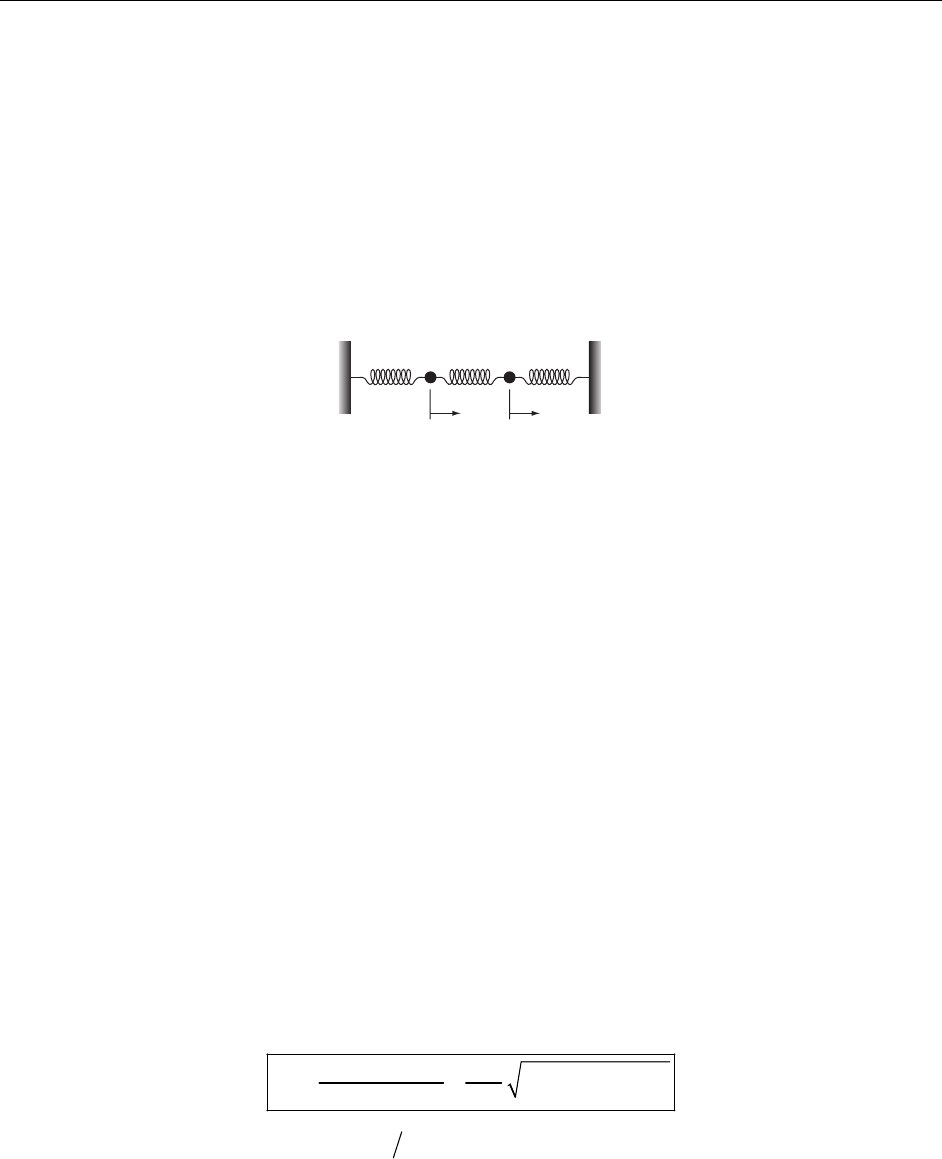
CHAPTER 12
Cou
p
led Oscillations
12-1.
m
1
= M
k
1
x
1
k
12
k
2
m
2
= M
x
2
The equations of motion are
(
)
()
11121122
22122121
0
0
Mx x x
Mx x x
κκ κ
κκ κ
++ − =
++ − =
(1)
We attempt a solution of the form
()
()
11
22
it
it
xt Be
xt Be
ω
ω
=
=
(2)
Substitution of (2) into (1) yields
(
)
()
2
112 1122
2
12 1 2 12 2
0
0
MB B
BMB
κκ ω κ
κκκω
+− − =
−++− =
(3)
In order for a non-trivial solution to exist, the determinant of coefficients of and must
vanish. This yields
1
B2
B
(
)
(
)
22
1 12 2 12 12
MM
κκ ωκκ ω κ
+− +− =
2
(4)
from which we obtain
()
2
12 12
12 12
214
22
MM
κκ κ
22
ω
κκ κ
++
=±−+ (5)
This result reduces to
(
)
2
12 12
M
ωκκκ
=+ ± for the case 12
κ
κκ
=
= (compare Eq. (12.7)].
397
398 CHAPTER 12
If were held fixed, the frequency of oscillation of m would be
2
m1
(
2
01 1 12
1
M
)
ω
κκ
=+ (6)
while in the reverse case, would oscillate with the frequency
2
m
(
2
02 2 12
1
M
)
ω
κκ
=+ (7)
Comparing (6) and (7) with the two frequencies,
ω
+
and
ω
−
, given by (5), we find
()
2
22
12 12 12 12
124
2M
κκκκκ
+
=+++−+
ωκ
()()
2
12 12 12 112 0
11
2
2MM
κκ κ κκ κκ ω
++−=+=
1
>+ (8)
so that
01
ω
ω
+> (9)
Similarly,
()
2
22
12 12 12 12
124
2M
κκκκκ
−
=++−−+
ωκ
()()
2
12 12 12 212 0
11
2
2MM
κκ κ κκ κκ ω
+−−=+=
2
<+ (10)
so that
02
ω
ω
−
<
(11)
If , then the ordering of the frequencies is
1
κκ
>2
01 02
ω
ωωω
+
−
>>> (12)
12-2. From the preceding problem we find that for 12 1 2
,
κ
κκ
112 212
12
;
MM
κ
κκ
ωω
++
≅≅
κ
(1)
If we use
1
01 02
;
MM
2
κ
κ
ωω
== (2)
then the frequencies in (1) can be expressed as
COUPLED OSCILLATIONS 399
()
()
12
101 01 1
1
12
202 02 2
2
11
11
κ
ωω ω ε
κ
κ
ωω ω ε
κ
=+≅+
=+≅+
(3)
where
12 12
12
12
;
22
κ
κ
εε
κ
κ
== (4)
For the initial conditions [Eq. 12.22)],
(
)
(
)
(
)
(
)
1 212
0 , 00, 00, 00x x x===
,=xD (5)
the solution for
(
)
1
xt is just Eq. (12.24):
()
12 12
1cos cos
22
D t txt
ω
ωωω
+
−
=
(6)
Using (3), we can write
(
)
(
)
1 2 01 02 1 01 2 02
22
ωω ω ω εω εω
ε
++
+= + + +
≡Ω+ (7)
(
)
(
)
1 2 01 02 1 01 2 02
22
ω
ωωω εωεω
ε
−−
−=−+ −
≡Ω+ (8)
Then,
(
)
(
)
(
)
1cos cosxt D t t t t
ε
ε
++ −−
=Ω+ Ω+ (9)
Similarly,
()
()(
12 12
2sin sin
22
sin sin
xt D t t
Dtt t
++ −−
+−
)
t
=
=Ω+ Ω+
ωω ωω
ε
ε
(10)
Expanding the cosine and sine functions in (9) and (10) and taking account of the fact that
ε
+
and
ε
− are small quantities, we find, to first order in the
ε
’s,
(
)
1cos cos sin cos cos sinD t t t t t t t t
εε
+ −++ −− +
≅ΩΩ−ΩΩ−ΩΩ
xt (11)
−
(
)
2sin sin cos sin sin cosD t t t t t t t t
εε
+−++−−+
≅ΩΩ+ ΩΩ+ΩΩ
xt (12)
−
When either
(
)
1
xt or
(
)
2
xt reaches a maximum, the other is at a minimum which is greater
than zero. Thus, the energy is never transferred completely to one of the oscillators.
400 CHAPTER 12
12-3. The equations of motion are
2
1201
2
2202
0
0
m
xxx
M
m
xxx
M
ω
ω
++=
++=
(1)
We try solutions of the form
(
)
(
)
11 22
;
it it
xt Be xt Be
ω
ω
== (2)
We require a non-trivial solution (i.e., the determinant of the coefficients of B and equal to
zero), and obtain
1 2
B
()
2
2
22 4
00
m
M
ωω ω
−
−
= (3)
so that
22 2
0
m
M
ωω ω
−=± (4)
and then
2
20
1m
M
ω
ω
=
±
(5)
Therefore, the frequencies of the normal modes are
2
0
1
2
0
2
1
1
m
M
m
M
ω
ω
ω
ω
=
+
=
−
(6)
where 1
ω
corresponds to the symmetric mode and 2
ω
to the antisymmetric mode.
By inspection, one can see that the normal coordinates for this problem are the same as those for
the example of Section 12.2 [i.e., Eq. (12.11)].
12-4. The total energy of the system is given by
()()
()
2
22 22
12 12 1221
111
222
ETU
M
xx xx xx
κκ
=+
=++++ −
(1)
Therefore,
COUPLED OSCILLATIONS 401
()()()()
() ()
() ()
11 22 11 22 12 2 1 2 1
1112211 221221
1121122121211222
dE Mxxxx xxxx xxxx
dt
Mx x x x x Mx x x x x
Mx x x x Mx x x x
=++++−−
=+− − +++ −
+ − +−++
κκ
κκ κκ
κκ κ κ κκ
2
=+ (2)
which exactly vanishes because the coefficients of and are the left-hand sides of Eqs.
(12.1a) and (12.1b).
1
x
2
x
An analogous result is obtained when T and U are expressed in terms of the generalized
coordinates 1
η
and 2
η
defined by Eq. (12.11):
()
22
12
1
4
TM
η
η
=+
(3)
()
22
12 12
11
42
U2
1
κ
ηη κη
=++ (4)
Therefore,
()
[
1 121 1 2 22
dE MM
dt
]
22
η
κκηη ηκηη
⋅= ++ + +
(5)
which exactly vanishes by virtue of Eqs. (12.14).
When expressed explicitly in terms of the generalized coordinates, it is evident that there is only
one term in the energy that has as a coefficient (namely,
12
κ
2
12 1
κ
η
1
), and through Eq. (12.15) we
see that this implies that such a term depends on the ’s and
1
C
ω
, but not on the ’s and
2
C2
ω
.
To understand why this is so, it is sufficient to recall that 1
η
is associated with the
anitsymmetrical mode of oscillation, which obviously must have 12
κ
as a parameter. On the
other hand, 2
η
is associated to the symmetric mode,
(
)
(
)
12
xt xt
=
,
(
)
(
)
12
xt xt
=
, in which both
masses move as if linked together with a rigid, massless rod. For this mode, therefore, if the
spring connecting the masses is changed, the motion is not affected.
12-5. We set . Then, the equations of motion are
1212
κκκ
== ≡
κ
11 1 2
22 2 1
20
20
mx x x
mx x x
κκ
κκ
+−=
+−=
(1)
Assuming solutions of the form
()
()
11
22
it
it
xt Be
xt Be
ω
ω
=
=
(2)
we find that the equations in (1) become
402 CHAPTER 12
(
)
()
2
112
2
122
20
20
mBB
BmB
κω κ
κκω
−−=
−+− =
(3)
which lead to the secular equation for 2
ω
:
(
)
(
)
22
12
22mm
2
κ
ωκ ωκ
−
−= (4)
Therefore,
2
12
3
11
mm
κµ
ωµ
=±−
+
(5)
where
(
)
12 1 2
mm m m
µ
=+
12
=
is the reduced mass of the system. Notice that (5) agrees with Eq.
(12.8) for the case mm and M=12
κ
κ
=
. Notice also that 2
ω
is always real and positive since
the maximum value of
(
)
1
m+2
3m
µ
is 3 4 . (Show this.)
Inserting the values for 1
ω
and 2
ω
into either of the equations in (3), we find1
1
11 21
12
3
211
maa
mm
µ
µ
−+− =
+
(6)
and
1
12 22
12
3
211
m
a
mm
µ
µ
=− −−
+
a
(7)
Using the orthonormality condition produces
11
1
1
aD
= (8)
()
12 12
2
212
21
1
3
211
mm mm
mmm
D
a
+
−+−
+
= (9)
where
()
()
()
2
22
1
121 12 2
22 12
3
2
22 1
mm
m mm
mm mm
≡−++ − −
+
12
m
Dm (10)
The second eigenvector has the components
()
12 12
2
212
12
2
3
211
mm mm
mmm
D
a
+
−−−
+
= (11)
1 Recall that when we use 1
ω
ω
=, we call the coefficients
(
)
11
a
βω ω
11
=
= and
(
)
21
a
βω ω
==
21
, etc.
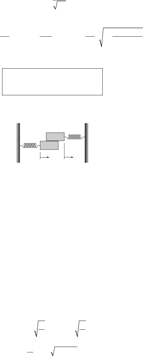
COUPLED OSCILLATIONS 403
22
2
1
aD
= (12)
where
()
222
111
21 2 1 2
22 2
22 2
12
33
21 1 21 1
mmmm
m m
mm m
mm
≡++−+− −
+
12
m
Dm (13)
The normal coordinates for the case in which
(
)
0
j
q0
=
are
()
()
()
()
11111022120
21121022220
cos
cos
tmaxmax t
tmaxmax
1
2
t
η
ω
η
ω
=+
=+ (14)
12-6.
mm
mm
k
k
x
1
x
2
If the frictional force acting on mass 1 due to mass 2 is
(
)
12
f
xx
β
=− −
(1)
then the equations of motion are
(
)
()
1121
2212
0
0
mx x x x
mx x x x
+−+=
+−+=
βκ
βκ
(2)
Since the system is not conservative, the eigenfrequencies will not be entirely real as in the
previous cases. Therefore, we attempt a solution of the form
(
)
(
)
11 22
;
t
xt Be xt Be
t
α
α
== (3)
where i
α
λω
=+ is a complex quantity to be determined. Substituting (3) into (1), we obtain the
following secular equation by setting the determinant of the coefficients of the B’s equal to zero:
(
)
2
2
m22
α
βα κ β α
++= (4)
from which we find the two solutions
()
11
2
2
;
1
imm
m
m
κ
κ
αω
αββκ
=± =±
=−± −
(5)
The general solution is therefore
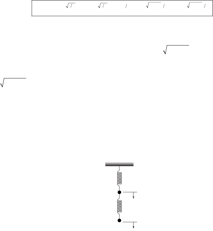
404 CHAPTER 12
()
(
)
22
111 11 12 12
imt imt mtm mtm
tm
Be Be e Be Be
κκ βκ βκ
β
−−
+−−+ −
=++ +xt (6)
and similarly for
(
)
2
xt.
The first two terms in the expression for
(
)
1
xt are purely oscillatory, whereas the last two terms
contain the damping factor t
e
β
−. (Notice that the term
(
)
2
12 expBmt
β
κ
+− increases with time if
2m
β
κ
>, but is not required to vanish in order to produce physically realizable motion
because the damping term, exp(–
β
t), decreases with time at a more rapid rate; that is
12
B+
2
ββ
−+ 0
κ
<m−.)
To what modes do 1
α
and 2
α
apply? In Mode 1 there is purely oscillating motion without
friction. This can happen only if the two masses have no relative motion. Thus, Mode 1 is the
symmetric mode in which the masses move in phase. Mode 2 is the antisymmetric mode in which
the masses move out of phase and produce frictional damping. If 2m
β
κ
<, the motion is one of
damped oscillations, whereas if 2m
β
κ
>, the motion proceeds monotonically to zero amplitude.
12-7.
m
k
m
k
x
1
x
2
We define the coordinates and as in the diagram. Including the constant downward
gravitational force on the masses results only in a displacement of the equilibrium positions and
does not affect the eigenfrequencies or the normal modes. Therefore, we write the equations of
motion without the gravitational terms:
1
x2
x
112
221
20
0
mx x x
mx x x
κκ
κκ
+−=
+−=
(1)
Assuming a harmonic time dependence for
(
)
1tx and
(
)
2
xt in the usual way, we obtain
(
)
()
2
12
2
12
20
0
mB B
BmB
κω κ
κκω
−−=
−+− =
(2)
Solving the secular equation, we find the eigenfrequencies to be
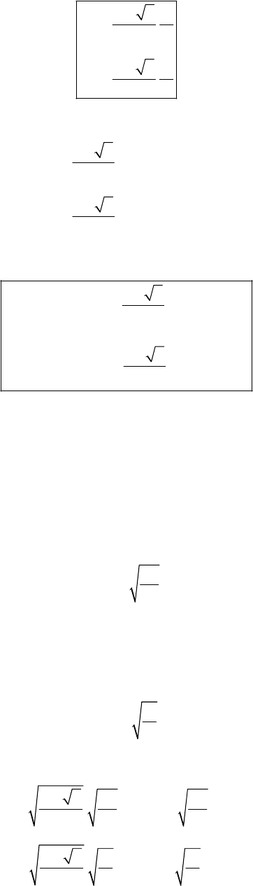
COUPLED OSCILLATIONS 405
2
1
2
2
35
2
35
2
m
m
κ
ω
κ
ω
+
=
−
=
(3)
Substituting these frequencies into (2), we obtain for the eigenvector components
11 21
12 22
15
2
15
2
aa
aa
−=
+
=
(4)
For the initial conditions
(
)
(
)
12
00xx==
0, the normal coordinates are
()
()
11110 20
21210 20
15 cos
2
15 cos
2
tmax x t
tmax x t
ηω
ηω
−
=+
+
=+
1
2
(5)
Therefore, when ,
10 20
1.6180xx=−
(
)
20t
η
=
and the system oscillates in Mode 1, the
antisymmetrical mode. When ,
10 2
0.6180xx=0
(
)
10t
η
=
and the system oscillates in Mode 2, the
symmetrical mode.
When mass 2 is held fixed, the equation of motion of mass 1 is
11
2mx x 0
κ
+
=
(6)
and the frequency of oscillation is
10
2
m
κ
ω
= (7)
When mass 1 is held fixed, the equation of motion of mass 2 is
22
0mx x
κ
+
=
(8)
and the frequency of oscillation is
20 m
κ
ω
= (9)
Comparing these frequencies with 1
ω
and 2
ω
we find
11
22
352 2
1.1441
4
35 0.6180
4
mm
mm
κκ
ωω
κκ
ωω
+
== 0
0
>
−
==<
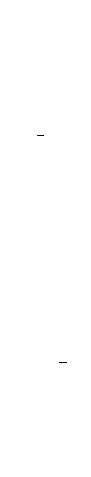
406 CHAPTER 12
Thus, the coupling of the oscillators produces a shift of the frequencies away from the
uncoupled frequencies, in agreement with the discussion at the end of Section 12.2.
12-8. The kinetic and potential energies for the double pendulum are given in Problem 7-7. If
we specialize these results to the case of small oscillations, we have
(
222
12 12
122
2
Tm
)
φ
φφφ
=++
A (1)
()
22
12
12
2
Umg
φ
φ
=A+ (2)
where 1
φ
refers to the angular displacement of the upper pendulum and 2
φ
to the lower
pendulum, as in Problem 7-7. (We have also discarded the constant term in the expression for
the potential energy.)
Now, according to Eqs. (12.34),
,
1
2
j
k
j
k
jk
Tmq=∑
q (3)
,
1
2
j
k
j
k
jk
UAq=∑q (4)
Therefore, identifying the elements of
{
}
m and
{
}
A, we find
{}
221
11
m
=
mA (5)
{}
20
01
mg
=
AA (6)
and the secular determinant is
22
22
22
0
g
g
ωω
ωω
−−
=
−−
A
A
(7)
or,
224
22
gg
ωωω
0
−
−−=
AA (8)
Expanding, we find
2
42
42
gg
ωω
0
−
+
AA
= (9)
which yields
COUPLED OSCILLATIONS 407
()
222
g
ω
=± A (10)
and the eigenfrequencies are
1
2
22 1.848
22 0.765
gg
gg
ω
ω
=+ =
=− =
AA
AA
(11)
To get the normal modes, we must solve
(
)
20
jk r jk jr
j
Ama
ω
−
=
∑
For k = 1, this becomes:
(
)
(
)
22
11 11 1 21 21 2 0
rr r r
AmaAma
ωω
−+−=
For r = 1:
() ()
22
11 21
2222 22
gg
mg m a m a−+ −+ =
AA A
AA
0
Upon simplifying, the result is
21 11
2aa=−
Similarly, for r = 2, the result is
22 12
2aa=
The equations
111112
221122
xa a
xa a
2
2
η
η
η
η
=
+
=+
can thus be written as
1111 22
1
2
xa a2
η
η
=+
1 11 1 22 2
2xaa
η
η
=− +
Solving for 1
η
and 2
η
:
12 1
12
22
11
22
;2
22
xx xx
a
a
ηη
−+
==
2
408 CHAPTER 12
2
12 1
2
211
occurs when 0; i.e. when 2
occurs when 0; i.e. when 2
x
x
x
x
ηη
ηη
==
==
−
Mode 2 is therefore the symmetrical mode in which both pendula are always deflected in the
same direction; and Mode 1 is the antisymmetrical mode in which the pendula are always
deflected in opposite directions. Notice that Mode 1 (the antisymmetrical mode), has the higher
frequency, in agreement with the discussion in Section 12.2.
12-9. The general solutions for
(
)
1
xt and
(
)
2
xt are given by Eqs. (12.10). For the initial
conditions we choose oscillator 1 to be displaced a distance D from its equilibrium position,
while oscillator 2 is held at , and both are released from rest:
20x=
(
)
(
)
(
)
(
)
1212
0 , 00, 00, 0x x x===
0=xD (1)
Substitution of (1) into Eq. (12.10) determines the constants, and we obtain
()
(
11
cos cos
2
D
xt t t
)
2
ω
ω
=+ (2)
()
(
22
cos cos
2
D
xt t t
)
1
ω
ω
=− (3)
where
12
12
2
MM
κκ
κ
ωω
+>= (4)
As an example, take 12
1.2
ω
ω
=;
(
)
1
xt vs.
(
)
2
xt is plotted below for this case.
It is possible to find a rotation in configuration space such that the projection of the system
point onto each of the new axes is simple harmonic.
By inspection, from (2) and (3), the new coordinates must be
112 1
cosxxxD t
ω
≡
−=
′
(5)
212 2
cosxxxD t
ω
≡
+=
′
(6)
These new normal axes correspond to the description by the normal modes. They are
represented by dashed lines in the graph of the figure.
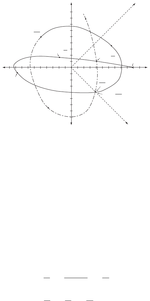
COUPLED OSCILLATIONS 409
0.2
0.2
–0.5
0.4
0.6
0.8
1.0 0.4 0.6 0.8 1.0
ωπ
2
5
2
t=
ωπ
2
3
2
t=
ωπ
2
3
t=
ωπ
2
2
t=
7π
2
x
2
(t)/Dx
2
′
x
1
′
x
1
(t)/D
ω
2
t = π
3π
4π
ω
2
t = 2π
ω
1
= 1.2 ω
2
ω
2
t = 0
12-10. The equations of motion are
(
)
()
11 1211220
22 122121
cos
0
mx bx x x F t
mx bx x x
κ
κκ ω
κκ κ
+++ − =
+++ − =
(1)
The normal coordinates are the same as those for the undamped case [see Eqs. (12.11)]:
112 21
;xx xx
2
η
η
=
−=+ (2)
Expressed in terms of these coordinates, the equations of motion become
(
)
(
)
(
)
(
)
(
)
()()()()()
21 21 1221 1221 0
21 21 1221 1221
2cos
0
mb F
mb
t
η
ηηηκκηηκηη ω
ηη ηη κκ ηη κηη
++ +++ +− −=
−+ −++ −− +=
(3)
By adding and subtracting these equations, we obtain the uncoupled equations:
0
12
11 1
0
222
2cos
cos
F
bt
mmm
F
bt
mmm
κκ
ηη η ω
κ
ηηη ω
+
++ =
++=
(4)
With the following definitions,
410 CHAPTER 12
212
1
2
2
0
2
2
b
m
m
m
F
Am
β
κκ
ω
κ
ω
=
+
=
=
=
(5)
the equations become
2
1111
2
2222
2c
2c
os
os
A
t
A
t
η
βη ω η ω
η
βη ω η ω
++=
++=
(6)
Referring to Section 3.6, we see that the solutions for
(
)
1t
η
and
(
)
2t
η
are exactly the same as
that given for x(t) in Eq. (3.62). As a result
(
)
1t
η
exhibits a resonance at 1
ω
ω
= and
(
)
2t
η
exhibits a resonance at 2
ω
ω
=.
12-11. Taking a time derivative of the equations gives
(
)
qI
=
1
12
0
I
LI MI
C
+
+=
2
21
0
I
LI MI
C
+
+=
Assume 11
it
IBe
ω
=, 22
it
IBe
ω
=; and substitute into the previous equations. The result is
22
11 2
10
it it it
LB e B e M B e
C
ωω ω
ωω
−+− =
22
22 1
10
it it it
LB e B e M B e
C
ωω ω
ωω
−+− =
These reduce to
()
22
12
10BLBM
C
ωω
−
+− =
()
22
12
10BM B L
C
ωω
−
+−=
This implies that the determinant of coefficients of B and must vanish (for a non-trivial
solution). Thus
1 2
B
COUPLED OSCILLATIONS 411
22
22
1
0
1
LM
C
ML
C
ωω
ωω
−−
=
−−
()
22
22
10LM
C
ωω
−
−=
22
1LM
C
ω
ω
−=±
or
()
21
CL M
ω
=±
Thus
()
()
1
2
1
1
CL M
CL M
ω
ω
=+
=−
12-12. From problem 12-11:
112
10LI I MI
C
+
+=
(1)
221
10LI I MI
C
+
+=
(2)
Solving for in (1) and substituting into (2) and similarly for I
, we have
1
I2
2
11 2
2
22 1
10
10
MM
LIII
LCCL
MM
LIII
LCCL
−+−=
−+−=
(3)
If we identify
2
12
11
M
mL L
M
LC
M
CL
κ
κ
=−
=
=−
(4)
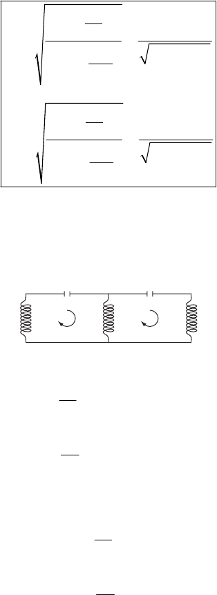
412 CHAPTER 12
then the equations in (3) become
(
)
()
1121122
2122121
0
0
mI I I
mI I I
κκ κ
κκ κ
++ − =
++ − =
(5)
which are identical in form to Eqs. (12.1). Then, using Eqs. (12.8) for the characteristic
frequencies, we can write
()
()
12
22
11
11
M
L
MCL M
CL L
M
L
MCL M
CL L
ω
ω
+
==
−
−
−
==
+
−
(6)
which agree with the results of the previous problem.
12-13.
I
1
C
1
q
1
I
2
C
2
q
2
L
1
L
12
L
2
The Kirchhoff circuit equations are
()
()
1
11 12 1 2
1
2
22 12 2 1
2
0
0
q
LI L I I
C
q
LI L I I
C
++ −=
++ −=
(1)
Differentiating these equations using qI
=
, we can write
()
()
1121 1122
1
2122 2121
2
10
10
LLI ILI
C
LLI ILI
C
++−=
++−=
(2)
As usual, we try solutions of the form
(
)
(
)
11 22
;
it it
It Be It Be
ω
ω
== (3)
which lead to
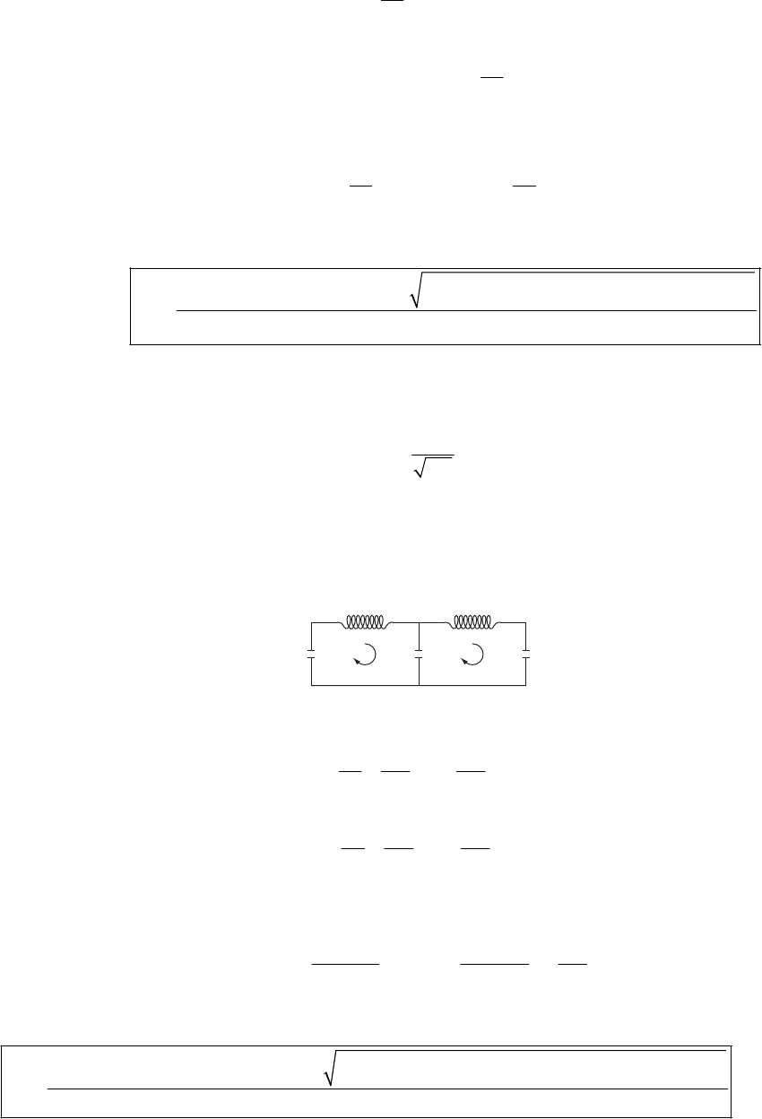
COUPLED OSCILLATIONS 413
()
()
22
112 112 2
1
22
12 1 2 12 2
1
10
10
LL BL B
C
LB LL B
C
ωω
ωω
+− − =
−++−=
(4)
Setting the determinant of the coefficients of the B’s equal to zero, we obtain
() ()
22
112 212 1
12
11
LL LL L
CC
ωω
+− +−=
42
2
ω
(5)
with the solution
()()()()
()()
22
1121 2122 1121 2122 1212
2
2
12 1 12 2 12 12
4
2
LLC LLC LLC LLC LCC
CC L L L L L
ω
+++±+−+ +
=
++−
(6)
We observe that in the limit of weak coupling
(
)
12 0L→ and 12
LLL
=
=, CC , the
frequency reduces to
12
C==
1
LC
ω
= (7)
which is just the frequency of uncoupled oscillations [Eq. (3.78)].
12-14.
I
1
C
1
C
12
I
2
C
2
L
1
L
2
The Kirchhoff circuit equations are (after differentiating and using qI
=
)
11 1 2
112 12
22 2 1
212 12
11 1 0
11 1 0
LI I I
CC C
LI I I
CC C
++ − =
++ − =
(1)
Using a harmonic time dependence for
(
)
1
It and
(
)
2tI , the secular equation is found to be
22
112 212
12 2
112 212 12
1CC CC
LL
CC CC C
ωω
++
−−
=
(2)
Solving for the frequency,
()() ()()
222
11 2 12 22 1 12 11 2 12 22 1 12 1 212
2
12 1 2 12
4
2
CL C C CL C C CL C C CL C C CCLL
LLCCC
ω
++ +± +− + +
= (3)
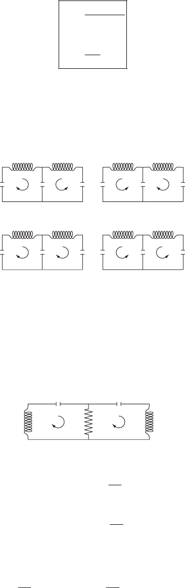
414 CHAPTER 12
Because the characteristic frequencies are given by this complicated expression, we examine the
normal modes for the special case in which 12
LLL
=
= and CC
12
C
=
=. Then,
212
1
12
2
2
2
1
CC
LCC
LC
ω
ω
+
=
=
(4)
Observe that 2
ω
corresponds to the case of uncoupled oscillations. The equations for this
simplified circuit can be set in the same form as Eq. (12.1), and consequently the normal modes
can be found in the same way as in Section 12.2. There will be two possible modes of oscillation:
(1) out of phase, with frequency 1
ω
, and (2) in phase, with frequency 2
ω
.
Mode 1 corresponds to the currents and oscillating always out of phase:
1
I2
I
;
I
1
I
2
I
1
I
2
Mode 2 corresponds to the currents and oscillating always in phase:
1
I2
I
;
I
1
I
2
I
1
I
2
(The analogy with two oscillators coupled by a spring can be seen by associating case 1 with
Fig. 12-2 for 1
ω
ω
= and case 2 with Fig. 12-2 for 2
ω
ω
=
.) If we now let and , we
do not have pure symmetrical and antisymmetrical symmetrical modes, but we can associate
1
LL≠221
CC≠
2
ω
with the mode of highest degree of symmetry and 1
ω
with that of lowest degree of
symmetry.
12-15.
I
1
C
1
I
2
C
2
L
1
RL
2
Setting up the Kirchhoff circuit equations, differentiating, and using qI
=
, we find
()
()
11 1 2 1
1
22 2 1 2
2
10
10
LI R I I I
C
LI R I I I
C
+−+ =
+−+ =
(1)
Using a harmonic time dependence for
(
)
1
It and
(
)
2tI , the secular equation is
22
12
12
110LiRL iRR
CC
ωωωωω
−− −− + =
22
(2)
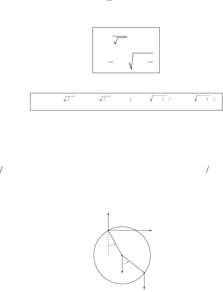
COUPLED OSCILLATIONS 415
From this expression it is clear that the oscillations will be damped because
ω
will have an
imaginary part. (The resistor in the circuit dissipates energy.) In order to simplify the analysis,
we choose the special case in which 12
LLL
=
= and 12
CCC
=
=. Then, (2) reduces to
2
2
10LiR R
C
ωωω
22
−
−+
=
(3)
which can be solved as in Problem 12-6. We find
1
2
2
1
LC
iL
RR
LC
ω
ω
=±
=±−
(4)
The general solution for is
()
1
It
()
22
11
111 11 12 12
i LCt i LCt R LCtL R LCtL
Rt L
Be Be e Be Be
−−−
−
+− + −
It −
=+ + +
(5)
and similarly for . The implications of these results follow closely the arguments presented
in Problem 12-6.
()
2
It
Mode 1 is purely oscillatory with no damping. Since there is a resistor in the circuit, this means
that and flow in opposite senses in the two parts of the circuit and cancel in R. Mode 2 is the
mode in which both currents flow in the same direction through R and energy is dissipated. If
1
I2
I
2C<RL, there will be damped oscillations of and , whereas if
1
I2
I2
RLC>, the currents will
decrease monotonically without oscillation.
12-16.
O
y
x
R
P
R
Mg Q(x,y)
Mg
θ
φ
Let O be the fixed point on the hoop and the origin of the coordinate system. P is the center of
mass of the hoop and Q(x,y) is the position of the mass M. The coordinates of Q are
(
)
()
sin sin
cos cos
xR
yR
θφ
θ
φ
=+
=− +
(1)
The rotational inertia of the hoop through O is
416 CHAPTER 12
(2)
2
OCM 2II MR MR=+ = 2
The potential energy of the system is
()
hoop mass
2cos cos
UU U
MgR
θ
φ
=
+
=− + (3)
Since
θ
and
φ
are small angles, we can use 2
s 1 2xx≅−co . Then, discarding the constant term in
U, we have
()
22
12
2
UMgR
θ
φ
=+ (4)
The kinetic energy of the system is
()
hoop mass
222
O
22 2 2 2
11
22
12
2
TT T
IMxy
MR MR
=+
=+ +
=+ ++
θ
θ
θφ θφ
(5)
where we have again used the small-angle approximations for
θ
and
φ
. Thus,
222
132
2
TMR
θ
φθφ
=++
(6)
Using Eqs. (12.34),
,
1
2
j
k
j
k
jk
Tmq=∑
q (7)
,
1
2
j
k
j
k
jk
UAq=∑q (8)
we identify the elements of
{
}
m and
{
}
A:
{}
231
11
MR
=
m (9)
{}
20
01
MgR
=
A (10)
The secular determinant is
22
22
23
0
g
R
g
R
ωω
ωω
−−
=
−−
(11)
from which
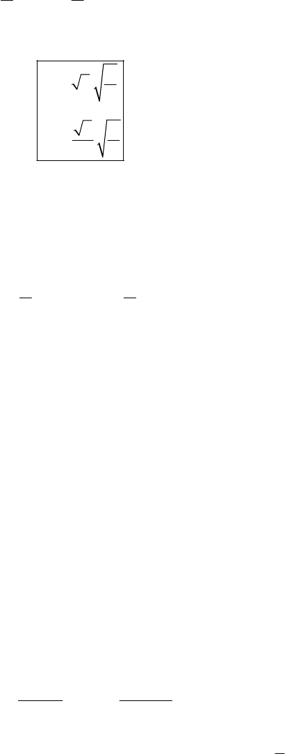
COUPLED OSCILLATIONS 417
224
23
gg
RR
ωωω
0
−
−−=
(12)
Solving for the eigenfrequencies, we find
1
2
2
2
2
g
R
g
R
ω
ω
=
=
(13)
To get the normal modes, we must solve:
(
)
20
jk r jk jr
j
Ama
ω
−
=
∑
For k = r = 1, this becomes:
22
11 21
223 2
gg
mgR mR a mR a
RR
0
−
−=
or
21 11
2aa
=
−
For k = 1, r = 2, the result is
12 22
aa
=
Thus the equations
111112
221122
xa a
xa a
2
2
η
η
η
η
=
+
=+
can be written as
1111222
211122
2
xa a
xa a
2
η
η
η
η
=
+
=− +
Solving for 1
η
, 2
η
12 1
11
11 22
2
;
33
xx xx
aa
ηη
2
−
+
==
1
η
occurs when the initial conditions are such that 20
η
=
; i.e., 10 20
1
2
xx=−
This is the antisymmetrical mode in which the CM of the hoop and the mass are on opposite
sides of the vertical through the pivot point.
2
η
occurs when the initial conditions are such that 10
η
=
; i.e., 10 20
xx
=
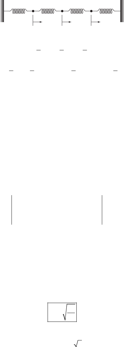
418 CHAPTER 12
This is the symmetrical mode in which the pivot point, the CM of the hoop, and the mass
always lie on a straight line.
12-17.
kk mk
mk
m
x
1
x
2
x
3
Following the procedure outlined in section 12.6:
22
12
111
222
Tmxmxm=++
2
3
x
()
()
2
2
22
121 32
222
1231223
11 1 1
22 2 2
Ukx kxx kxx kx
kx x x xx xx
=+ −+ −+
=++−−
3
Thus
00
00
00
m
m
m
=
m
20
2
02
kk
kkk
kk
−
=
−−
−
A
Thus we must solve
2
2
2
20
20
02
km k
kkmk
kkm
ω
ω
ω
−−
−− −
−−
=
This reduces to
(
)
(
)
3
222
222km kkm
ωω
0
−
−−=
or
(
)
(
)
2
222
22 2kmkm k
ωω
−−−
0
=
If the first term is zero, then we have
1
2k
m
ω
=
If the second term is zero, then
2
22km
ω
−=±k
COUPLED OSCILLATIONS 419
which leads to
() ()
23
22 22
;
kk
mm
+−
==
ωω
To get the normal modes, we must solve
(
)
20
jk r jk jr
j
Ama
ω
−
=
∑
For k = 1 this gives:
(
)
(
)
2
12
20
rr r
kma ka
ω
−
+− =
Substituting for each value of r gives
(
)
()
()
11 21 21
12 22 22 12
13 23 23 13
1: 2 2 0 0
2: 2 0 2
3: 2 0 2
rkkakaa
akaa
rkakaaa
=−−=→=
=− −=→=−
=−=→=
rk
a
Doing the same for k = 2 and 3 yields
11 31 21
12 32 22 32
13 33 23 33
0
2
2
aa a
aa a a
aa a a
=
−=
==−
==
The equations
111112213
221122223
331132233
xa a a
xa a a
xa a a
3
3
3
η
ηη
η
ηη
η
ηη
=
++
=++
=++
can thus be written as
1111 222333
2222 333
3111 22233
1
2
2
1
2
xa a a
xa a
xa a a
3
η
ηη
ηη
η
ηη
=− +
=+
=− − +
We get the normal modes by solving these three equations for 1
η
, 2
η
, 3
η
:
420 CHAPTER 12
13
1
11
12
2
22
2
2
22
xx
a
xx
a
η
η
3
x
−
=
−+ −
=
and
12
3
33
2
4
xx
a
η
3
x
+
+
=
The normal mode motion is as follows
11
22
3 213
:
:2
:2
xx
xx
xxx
η
η
•→ • ←• =−
←• •→←• =− =−
•→ •→ •→ = =
3
13
2
2
x
η
12-18.
x
1
y
1
m
b
x
MM
θ
11
11
sin ; cos
cos ; sin
xxb xxb
ybb yb
θ
θθ
θθθ
=+ =+
=− =
Thus
()
()
()
222
11
2222
1
11
22
11 2cos
22
1cos
TMx mxy
Mx m x b b x
Umgy mgb
θ
θθ
θ
=+ +
=+ ++
== −
For small
θ
,
2
cos 1 2
θ
θ
−. Substituting and neglecting the term of order 2
θ
θ
gives

COUPLED OSCILLATIONS 421
()
()
222
2
11
2
22
2
TMmxmb bx
mgb
U
θ
θ
θ
=++ +
=
Thus
2
M
mmb
mb mb
+
=
m
00
0mgb
=
A
We must solve
(
)
22
22
0
Mm mb
mb mgb mb
ωω
ωω
−+ −
2
=
−−
which gives
(
)
(
)
()
22242
22 2
0
0
M m mb mgb m b
Mb mgb m M
ωω ω
ωω
+−−
−+=
2
=
Thus
()
1
2
0
gMm
mb
ω
ω
=
=+
(
)
20
jk r jk jr
j
Ama
ω
−
=
∑
Substituting into this equation gives
(
)
()
()
21
12 22
02
2, 2
ak
bm
aak
mM
==
=− = =
+
,1r
r
=
Thus the equations
11 1 12 2
21 1 22 2
xa a
aa
η
η
θ
ηη
=
+
=+
become
()
11 1 22 2
mb
xa a
mM
η
η
=−
+

422 CHAPTER 12
22 2
a
θ
η
=
Solving for 1
η
, 2
η
:
()
2
22
1
11
a
bm
xmM
na
θ
η
θ
=
++
=
()
12
21
occurs when 0; or 0
occurs when 0; or
nn
bm
nnx
mM
θ
θ
==
==−
+
12-19. With the given expression for U, we see that
{
}
A
has the form
{}
12 13
12 23
13 23
1
1
1
ε
ε
ε
ε
εε
−−
=− −
−−
A (1)
The kinetic energy is
()
222
123
1
2
T
θ
θθ
=++
(2)
so that
{
}
m is
{}
100
010
001
=
m (3)
The secular determinant is
2
12 13
2
12 23
2
13 23
1
1
1
ωε ε
εωε
εε ω
−− −
0
−
−−=
−− −
(4)
Thus,
(
)
(
)
(
)
3
2 2222
12 13 23 12 13 23
11 2
ωωεεεεεε
−−− ++− =0 (5)
This equation is of the form (with 12x
−
≡
ω
)
32 2
32xx 0
−
−=
αβ
(6)
which has a double root if and only if
(
)
32
22
α
β
=
(7)
COUPLED OSCILLATIONS 423
Therefore, (5) will have a double root if and only if
32
222
12 13 23
12 13 23
3
εεε
ε
εε
++ =
(8)
This equation is satisfied only if
12 13 23
ε
εε
== (9)
Consequently, there will be no degeneracy unless the three coupling coefficients are identical.
12-20. If we require , then Eq. (12.122) gives
11 21
2aa=31 21
3aa
=
−, and from Eq. (12.126) we
obtain 21 114a=. Therefore,
1
21 3
,,
14 14 14
=−
a (1)
The components of can be readily found by substituting the components of above into Eq.
(12.125) and using Eqs. (12.123) and (12.127):
2
a1
a
2
451
,,
42 42 42
−
=
a (2)
These eigenvectors correspond to the following cases:
a1a2
12-21. The tensors
{
}
A and
{
}
m are:
{}
13
32 3
31
10
2
1
22
1
02
κκ
1
κ
κκ
κκ
=
A (1)
{}
00
0
00
m
m
m
0
=
m (2)
thus, the secular determinant is
424 CHAPTER 12
2
13
2
32 3
2
31
10
2
11
0
22
1
02
m
m
m
κω κ
κκω κ
κκω
−
−
=
−
(3)
from which
()()()
2
2222
12 31
10
2
mm m
κω κκω
−−−−
κω
(4) =
In order to find the roots of this equation, we first set
(
)
2
31
12 2
κ
κκ
= and then factor:
(
)
(
)
(
)
(
κω
(5)
)
()
()
()
222
11212
224 2
112
22 2
112
0
0
0
mmm
mm m
mmm
κωκωκωκκ
ωκκω
κωωωκκ
−−−−
−−+=
−−+=
=
Therefore, the roots are
1
1
12
2
30
m
m
κ
ω
κ
κ
ω
ω
=
+
=
=
(6)
Consider the case 30
ω
=. The equation of motion is
2
333
0
+
=
ηωη
(7)
so that
30
η
=
(8)
with the solution
(
)
3tatb
η
=
+ (9)
That is, the zero-frequency mode corresponds to a translation of the system with oscillation.
COUPLED OSCILLATIONS 425
12-22. The equilibrium configuration is shown in diagram (a) below, and the non-
equilibrium configurations are shown in diagrams (b) and (c).
12
43
x
1
x
2
x
3
O
2A2B
(a)
1
2
x
3
x
x
3
O
O′
A
AAθ
θ
2
}
(b)
1
4
x
3
x
x
3
O
O′
B
B
Bφ
φ
2
{
(c)
The kinetic energy of the system is
22
31 2
111
222
TMx I I
2
θ
φ
=++
(1)
where
(
)
2
113IM=A and
(
)
2
213IM=B.
The potential energy is
()()()()
()
2222
3333
22222
3
1
2
144 4
2
UxABxABxABxAB
xA B
=−−++−++++−+
=++
κθφθφθφθ
κθφ
φ
(2)
Therefore, the tensors
{
}
m and
{
}
A are
{}
2
2
00
1
0
3
1
00
3
M
MA 0
M
B
=
m (3)
{}
2
2
40 0
04 0
004
A
B
κ
κ
κ
=
A (4)
The secular equation is
426 CHAPTER 12
()
22 222 22
11
44 4
33
MAMA BMB
κωκ ωκ ω
−− −
0
=
(5)
Hence, the characteristic frequencies are
1
2
32
2
3
2
3
2
M
M
M
κ
ω
κ
ω
κ
ω
ω
=
=
==
(6)
We see that 23
ω
ω
=, so the system is degenerate.
The eigenvector components are found from the equation
(
)
20
jk r jk jr
j
Ama
ω
−
=
∑
(7)
Setting to remove the indeterminacy, we find
32 0a=
2
12 3
2
0
10
0; 3 ; 0
00
3
M
MA
MB
== =
aaa (8)
The normal coordinates are (for
(
)
(
)
(
)
3000x
θφ
0
=
==
)
()
()
()
130 1
0
2
0
33
cos
cos
3
cos
3
tx M t
AM
t
BM
tt
ηω
θ
2
t
η
ω
φ
ηω
=
=
=
(9)
Mode 1 corresponds to the simple vertical oscillations of the plate (without tipping). Mode 2
corresponds to rotational oscillations around the axis, and Mode 3 corresponds to rotational
oscillations around the -axis.
1
x
2
x
The degeneracy of the system can be removed if the symmetry is broken. For example, if we
place a bar of mass m and length 2A along the of the plate, then the moment of inertia
around the is changed:
2-axisx
1-axisx
()
2
1
1
3
IMm=+
′A (10)
The new eigenfrequencies are
COUPLED OSCILLATIONS 427
1
2
3
2
3
2
3
2
M
M
m
M
κ
ω
κ
ω
κ
ω
=
=+
=
(11)
and there is no longer any degeneracy.
12-23. The total energy of the r-th normal mode is
22
11
22
rr r
rr
ETU
2
r
η
ωη
=
+
=+
(1)
where
r
it
rr
e=
ω
ηβ
(2)
Thus,
r
it
rrr
ie=
ω
ηωβ
(3)
In order to calculate T and U, we must take the squares of the real parts of
r r r
η
and r
η
:
() ( )
()
2
2
2
2
Re Re cos sin
cos sin
rr rrrr r
rr r r r r
ii ti
tt
t
== + +
−
ηη ωµνω ω
ων ω ωµ ω
=− (4)
so that
2
2
1cos sin
2
rrrrrr
Tt
ων ω µ ω
=+t
(5)
Also
() ( )
()
2
2
2
2
Re Re cos sin
cos sin
rr rrr r
rrrr
iti
tt
t
==+ +
ηη µνω ω
µωνω
=− (6)
so that
2
2
1cos
2
rrrrrr
Ut
ωµ ω ν ω
=−xint
(7)
Expanding the squares in T and U, and then adding, we find
r r
428 CHAPTER 12
()
22 2
1
2
rr r
rr r
ETU
ω
µν
=
+
=+
Thus,
2
2
1
2
rrr
E
ωβ
= (8)
So that the total energy associated with each normal mode is separately conserved.
For the case of Example 12.3, we have for Mode 1
()
11020
cos
2
Mxx 1
t
η
ω
=− (9)
Thus,
()
11 1020
sin
2
Mxx 1
t
η
ω
=− −
ω
(10)
Therefore,
22
11 1
11
22
E2
1
η
ωη
=+
(11)
But
212
1
2
M
κ
κ
ω
+
= (12)
so that
() ()
()
()
22
22
12 12
110201 1020
2
12 10 20
2211
sin cos
22 22
12
4
MM
Exxtxx
MM
xx
++
=−+−
=+ −
κκ κκ
1
t
ω
ω
κκ
(13)
which is recognized as the value of the potential energy at t = 0. [At t = 0, , so that the
total energy is
12
0xx==
(
)
10=Ut .]
12-24. Refer to Fig. 12-9. If the particles move along the line of the string, the equation of
motion of the j-th particle is
(
)
(
)
1jjj j
mx xx xx
κκ
−
=− − − −
1j+
(1)
Rearranging, we find
()
1
2
jjjj
xxxx
m1
κ
−
=−+
+
(2)
which is just Eq. (12.131) if we identify md
τ
with m
κ
.
COUPLED OSCILLATIONS 429
12-25. The initial conditions are
(
)
(
)
(
)
() () ()
123
123
000
0000
qqqa
qqq
===
===
(1)
Since the initial velocities are zero, all of the r
ν
[see Eq. (12.161b)] vanish, and the r
µ
are given
by [see Eq. (12.161a)]
3
sin sin sin
24 2 4
r
ar r r
π
ππ
µ
=++
(2)
so that
1
2
3
21
2
0
21
2
a
a
µ
µ
µ
+
=
=
−
=
(3)
The quantities
(
)
si are the same as in Example 12.7 and are given in Eq. (12.165).
The displacements of the particles are
n 1jr n
π
+
()
()()
()
()(
()
)
()()
113 1
2131
313 1
12
cos cos cos cos
24
21
cos cos cos cos
22
12
cos cos cos cos
24
qt a t t a t t
a t t a t t
qt a t t a t t
ωω ωω
ωω ωω
ωω ωω
=++ −
=−++
=−+ +
3
3
3
qt (4)
where the characteristic frequencies are [see Eq. (12.152)]
2sin,1,2
8
r
rr
md
τπ
ω
=
,3
=
(5)
Because all three particles were initially displaced, there can exist no normal modes in which
any one of the particles is located at a node. For three particles on a string, there is only one
normal mode in which a particle is located at a node. This is the mode 2
ω
ω
=
(see Figure 12-11)
and so this mode is absent.
12-26. Kinetic energy
()
[]
2
2
222 2
123
2
2
mb
mb
mb
Tmmb
=++⇒=
+
θθθ
Potential energy
430 CHAPTER 12
()()()()()
()()
[]
22
2
123 213
2
222 2 22
123 1 23 12 23
22
222
22
1cos 1cos 1cos sin sin sin sin
2
222
22
0
0
k
Umgb b
mgb kb
mgb kb kb
A kb mgb kb kb
kb mgb kb
2
= − +− +− + − + −
≈+++++−−
+−
⇒=− + −
−+
θθθ θθθ
θθθ θ θθ θθ θθ
θ
The proper frequencies are solutions of the equation
[] []
()(
)
()()
222 2
22222
22
0
0Det Det 2
0
mgb kb mb kb
Am kb mgbkbmb kb
kb mgb kb mb
+− −
=−= − +− −
−+−
ω
ωω
ω
2
22
We obtain 3 different proper frequencies
2
11
2
22
2
33
4.64 rad/s
33
4.81 rad/s
4.57 rad/s
mg kb mg kb
mb mb
mg kb mg kb
mb mb
mg g
mb f
++
=⇒==
++
=⇒==
=⇒==
ωω
ωω
ωω
Actually those values are very close to one another, because k is very small.
12-27. The coordinates of the system are given in the figure:
L
1
m
1
m
2
θ
1
θ
2
L
2
Kinetic energy:
()
()
()
222 22 2 2
1 1 1 2 1 1 2 2 1212 1 2
22 2 22
1 11 21 222 21212
11 2cos
22
11 1
22 2
j
k
j
k
jk
TmL mL L LL
mL mL mL mLL m
=+ +− −
≈++− =
∑
θθθθθθ
θ
θ
θθθ θθ
COUPLED OSCILLATIONS 431
(
)
2
121 212
2
212 22
jk
mmL mLL
mmLL mL
+−
⇒=
−
Potential energy:
(
)
(
)
(
)
()
11 1 2 1 1 2 2
22
12
121 22
1cos 1cos 1cos
1
222
jk j k
jk
UmgL mgL L
mmgL mgL A
=−+ −+−
≈+ + =
∑
θ
θθ
θθ θθ
(
)
121
22
0
0
jk
mmgL
AmgL
+
⇒=
Proper oscillation frequencies are solutions of the equation
[
]
[
]
(
)
2
Det 0Am
−
=
ω
()()()()()
22
2
12 12 12 112 212
1,2
112
2
mmgLL mmgmLL mLL
mLL
++++ −++
⇒=
ω
The eigenstate corresponding to 1
ω
is 11
21
a
a
where
()
( )()( )()()
121 12
21 11
22
2
12 12 12 12 112 212
2
1
mmL gm L
a a
mL mmgLL mmgmLL mLL
+
=−
++++ −++
×
The eigenstate corresponding to 2
ω
is 12
22
a
a
where
()
()()()()()
121 12
22 12
22
2
12 12 12 12 112 212
2
1
mmL gm L
a a
mL mmgLL mmgmLL mLL
+
=−
++−+ −++
×
These expressions are rather complicated; we just need to note that and have the same
sign
11
a21
a
11
21
0
a
a
>
while and have opposite sign
12
a22
a11
21
0
a
a
<
.
The relationship between coordinates
(
)
12
,
θ
θ
and normal coordinates 12
,
η
η
are
12
11
1111122 22
2211222 11
21
21
~
~
a
aa a
aa a
a
−
=+
⇔
=+−
2
2
η
θθ
θηη
θηη
η
θθ
432 CHAPTER 12
To visualize the normal coordinate 1
η
, let 20
=
η
. Then to visualize the normal coordinate 2
η
,
we let 10=
η
. Because 11
21
0
a
a> and 12
22
a
a0
<
, we see that these normal coordinates describe two
oscillation modes. In the first one, the two bobs move in opposite directions and in the second,
the two bobs move in the same direction.
12-28. Kinetic energy:
[]
2
2
22 22
11 22 2
2
0
11
22 0
mb
Tmb mb m mb
=+ ⇒=
θθ
Potential energy:
()()()
[]
1122 1
22
1
22
2
1cos 1cos sin sin
2
k
Umgb mgb b b
mgb kb kb
Akb m gb kb
=−+−+ −
+−
⇒≈
−+
2
θ
θθθ
Solving the equation,
[
]
[
]
(
)
2
Det 0Am−
ω
=, gives us the proper frequencies of oscillation,
22
1
ω
25 (rad/s)
g
b
== 22
2
12
25.11(rad/s)
gkk
bm m
=+ + =
ω
The eigenstate corresponding to 1
ω
is 11
22
a
a
with 21 11
7.44aa
=
The eigenstate corresponding to 2
ω
is 12
22
a
a
with 22 12
8.55aa
=
From the solution of problem 12-27 above, we see that the normal coordinates are
12
11 21
22
~0
a
a
−=+2
.12
η
θθθ θ
11
21 21
21
~0
a
a
−=+2
.13
η
θθθ θ
Evidently 1
η
then characterizes the in-phase oscillation of two bobs, and 2
η
characterizes the
out-of-phase oscillation of two bobs.
Now to incorporate the initial conditions, let us write the most general oscillation form:
(
)
()
()
11 22
11 22
11 22
111 12
221 22
11 12
Re
Re
Re 7.44 8.35
iti iti
iti iti
iti iti
ae ae
ae ae
ae ae
−−
−−
−−
=+
=+
=−
ωδ ωδ
ωδ ωδ
ωδ ωδ
θα α
α
αα
θα
where
α
is a real normalization constant. The initial conditions helps to determine parameters
α
’s, a’s,
δ
’s.

COUPLED OSCILLATIONS 433
()
(
)
()
()
1111122
211112
Re 0 7 cos cos 0.122 rad
Re 0 0 7.44 cos 8.35 cos 0
taa
taa
°
==− ⇒ + =−
==°⇒ + =
θαδαδ
θαδα
2
δ
=
11
sin sin 0⇒=
δ
δ
. Then
()
111 1 12 2 1 2
2111 122 2
cos cos 0.065 cos 0.057 cos
7.44 cos 8.35 cos 0.48 cos cos
atat t
atat t
=+=− −
=+=−
1
t
θ
αωαω ω ω
θ
αω αω ω ω
where 15.03 rad/s=
ω
, 24.98 rad/s=
ω
(found earlier)
Approximately, the maximum angle 2
θ
is 0.096 rad and it happens when
2
1
cos 1
cos 1
t
t
=
=
−
ω
ω
which gives
()
21
12
221
21 2
tn k
tk n
=
+
⇒=
=+
ωπ ω
ωπ
ω
because 1
2
101
100
=
ω
ω
we finally find 50kn
=
= and
2
100 63 s
t==
π
ω
.
Note: 2max 0.96 rad=
θ
and at this value the small-angle approximation breaks down, and
the value 2max
θ
we found is just a rough estimate.
434 CHAPTER 12
CHAPTER 13
Continuous S
y
stems;
Waves
13-1. The initial velocities are zero and so all of the r
ν
vanish [see Eq. (13.8b)]. The r
µ
are
given by [see Eq. (13.8a)]
0
3
23
sin sin
L
r
r
Axrx
dx
LLL
A
ππ
µ
δ
=
=
∫ (1)
so that
3
0, 3
r
A
r
µ
µ
=
=≠
(2)
The characteristic frequency 3
ω
is [see Eq. (13.11)]
3
3
L
π
τ
ω
ρ
= (3)
and therefore,
()
33
,cos sin
x
qxt A t
LL
πτ π
ρ
=
(4)
For the particular set of initial conditions used, only one normal mode is excited. Why?
13-2.
L
3
h
L
435
436 CHAPTER 13
The initial conditions are
()
()
3,0 3
,0
3,
23
hL
xx
L
qx
hL
Lx xL
L
≤≤
=
−
≤≤
(1)
(
)
,0 0qx
=
(2)
Because
(
)
,0 0qx =
, all of the r
ν
vanish. The r
µ
are given by
()
3
22
03
22
63
sin sin
9sin 3
LL
r
L
hrxh rx
xdxLx
LLL L
hr
r
=+−
∫∫
ππ
µ
π
π
dx
= (3)
We see that 0
r
µ
= for r = 3, 6, 9, etc. The displacement function is
()
12
2
93 12 1 4
, sin cos sin cos sin cos
2416
hxx x
qxt t t t
LL L
=+×−
…
ππ π
ωω
π
4
−
ω
(4)
where
r
r
L
π
τ
ω
ρ
= (5)
The frequencies 3
ω
, 6
ω
, 9
ω
, etc. are absent because the initial displacement at 3L prevents
that point from being a node. Thus, none of the harmonics with a node at 3L are excited.
13-3. The displacement function is
(
)
13
2
,13 1 5
sin cos sin cos sin cos
8925
qxt xx x
tt
hL L L
ππ π
ωω
π
+…
5
t
ω
+=− (1)
where
1
1
r
L
r
π
τ
ω
ρ
ωω
=
=
(2)
For t = 0,
(
)
2
,0 13 1 5
sin sin sin
8925
xx x
hLL L
=− + +…
ππ π
π
qx (3)
The figure below shows the first term, the first two terms, and the first three terms of this
function. It is evident that the triangular shape is well represented by the first three terms.
CONTINUOUS SYSTEMS; WAVES 437
1 term
L
1
0
2 terms
L
1
0
3 terms
L
1
0
The time development of q(x,t) is shown below at intervals of 1 of the fundamental period. 8
t = 0, T
tT=1
8
7
8
,T
tT=1
4
3
4
,T
tT=3
8
5
8
,T
tT=1
2
13-4. The coefficients r
ν
are all zero and the r
µ
are given by Eq. (13.8a):
()
()
2
0
33
8sin
16 11
L
r
r
rx
xL x dx
LL
r
=−
=−−
∫
π
µ
π
(1)
so that
3
0, even
32 , odd
3
r
r
r
r
µ
π
=
(2)
Since
438 CHAPTER 13
()
,sincos
r
r
rx
qxt t
Lr
π
µ
ω
=∑ (3)
the amplitude of the n-th mode is just n
µ
.
The characteristic frequencies are given by Eq. (13.11):
n
n
L
π
τ
ω
ρ
= (4)
13-5. The initial conditions are
(
)
()
0
,0 0
1
,2
,
0, otherwise
qx
vx s
qxt
=
−≤
=
(1)
The r
µ
are all zero and the r
ν
are given by [see Eq. (13.8b)]
()
(
)
2
0
2
0
2sin
4sin sin
2
Ls
r
rLs
r
rx
vd
LL
vrrs
rL
+
−
=−
=
∫
π
νω
ππ
πω
x
(2)
from which
()
()
12
0
0, even
41sin, od
rr
r
r
vrs r
rL
π
πω
−
=−−
d
ν
(3)
(Notice that the even modes are all missing, as expected from the symmetrical nature of the
initial conditions.)
Now, from Eq. (13.11),
1L
π
τ
ω
ρ
= (4)
and 1rr
ω
ω
=. Therefore,
()
()
12
0
2
1
41sin, od
r
r
vrs r
rL
d
π
νπω
−
−
=− (5)
According to Eq. (13.5),
CONTINUOUS SYSTEMS; WAVES 439
()
,sin
sin sin
r
it
r
r
rr
r
rx
qxt e L
rx
tL
=
=−
∑
∑
ω
π
β
π
νω
(6)
Therefore,
()
0
13
1
4133
, sin sin sin sin sin sin
9
vsx s x
t t t
LL L L
ππ π π
ωω
πω
=−
…
qx (7) +
Notice that some of the odd modes—those for which
(
)
sin 3 0sL
π
=
—are absent.
13-6. The initial conditions are
(
)
()
0
0
,0 0
404
4
,0 24
02
qx
vL
xx
L
vLL
qx x x
L
LxL
2
L
=
≤≤
=−≤≤
≤≤
(1)
The velocity at t = 0 along the string,
(
)
,0
qx , is shown in the diagram.
v
L
v
0
L
4
L
2
3
4
L
The r
µ
are identically zero and the r
ν
are given by:
()
10
0
32
1
2,0 sin
8sin 2 sin
24
L
r
rx
qx dx
rL L
vr
r
=−
r
=−
∫
π
νω
π
π
πω
(2)
Observe that for r = 4n, r
ν
is zero. This happens because at t = 0 the string was struck at 4L,
and none of the harmonics with modes at that point can be excited.
Evaluation of the first few r
ν
gives
440 CHAPTER 13
0
14
2
1
0
25
2
11
00
36
22
11
8
0.414 0
8
12.41
4125
88
2.414 2
27 216
v
v
vv
νν
πω
ν
πω πω
νν
πω πω
=− ⋅ =
0
2
8
4
v
ν
=− ⋅ = ⋅
=− ⋅ = ⋅
(3)
and so,
()
0
12
2
1
35
812
, 0.414 sin sin sin sin
4
2.414 3 2.414 5
sin sin sin sin
27 135
vxx
qxt t t
LL
xx
tt
LL
=+
+−
…
ππ
ωω
πω
ππ
ωω
−
(4)
From these amplitudes we can find how many db down the fundamental are the various
harmonics:
Second harmonic:
2
0.250
10 log 4.4 db
0.414
=−
(5)
Third harmonic:
2
2.414 27
10 log 13.3 db
0.414
=−
(6)
These values are much smaller than those found for the case of example (13.1). Why is this so?
(Compare the degree of symmetry of the initial conditions in each problem.)
13-7.
3
7L
3
7L
h
h
L
O
Since
(
)
,0 0qx =
, we know that all of the r
ν
are zero and the r
µ
are given by Eq. (13.8a):
()
0
2,0 sin
L
r
rx
qx dx
LL
π
µ
=∫ (1)
The initial condition on
(
)
,qxt is
CONTINUOUS SYSTEMS; WAVES 441
() ()
()
73
,0
37
73
,0 2 , 77
74
,
37
hxx
L
hx L L x L
L
hLx LxL
L
4
L
qx
−≤≤
=− ≤≤
−≤≤
(2)
Evaluating the r
µ
we find
22
98 4 3
sin sin
37
r
hr r
r7
π
π
µπ
=−
(3)
Obviously, 0
r
µ
= when 47r and 37r simultaneously are integers. This will occur when r is
any multiple of 7 and so we conclude that the modes with frequencies that are multiples of 1
7
ω
will be absent.
13-8. For the loaded string, we have [see Eq. (12.152)]
()
2sin
21
r
r
md n
τπ
ω
=
+
(1)
Using md
ρ
= and
(
)
1Ln=+d, we have
()
()
()
2sin 21
21 sin 21
r
r
dn
nr
Ln
=+
+
=
+
τπ
ωρ
τ
π
ρ
(2)
The function
() ()
1sin
21
2
rr
nn
L
ωπ
τ
ρ
=+
+
(3)
is plotted in the figure for n = 3, 5, and 10. For comparison, the characteristic frequency for a
continuous string is also plotted:
2
2
rr
L
ω
π
τ
ρ
= (4)
442 CHAPTER 13
0
024 6 8 10
2
4
6
8
10
12
Continuous string
n = 10
n = 5
n = 3
ω
τ
ρ
r
L
2
Of course, the curves have meaning only at the points for which r is an integer.
13-9. From Eq. (13.49), we have:
22
2
0
;
2
Ds
b
π
τ
βω
ρ
ρ
== (1)
From section 3.5, we know that underdamped motion requires:
22
0
β
ω
<
Using (1) this becomes
222
2
4
Ds
b
π
τ
ρ
ρ
<
22
2
22
2
22
2
4
or underdamped
4
ise critically damped
4overdamped
s
Db
s
Db
s
Db
ρπτ
ρπτ
ρπτ
<
=
>
Likew
The complementary solution to Eq. (13.48) for underdamped motion can be written down using
Eq. (3.40). The result is:
(
)
(
)
1
cos
t
ss
tCe t
β
s
η
ωφ
−
=−
CONTINUOUS SYSTEMS; WAVES 443
where 22
10
2
ω
ωβ
=−, 0
ω
and
β
are as defined in (1), and C and
s s
φ
are arbitrary constants
depending on the initial conditions. The complete solution to Eq. (13.48) is the sum of the
particular and complementary solutions (analogous to Eq. (13.50)):
()
() ()
0
122
22
2sin cos
2
cos
s
t
ss s
s
Ft
tCe t
sD
bb
β
π
ω
δ
φ
πτ
ηω
ρ
ωω
ρρ
−
−
=−+
−+
where
1
22
2
tan
s
D
s
b
ω
δπτ
ρ
ω
ρ
−
=
−
From Eq. (13.40):
() ()
,sin
r
r
rx
qxt t b
π
η
=∑
Thus
()
()
22 2 0
222
22
2sin cos
2
,expcos sin
24
(underdamped)
r
rr
r
r
Ft
Dt s D r x
qxt C t
bb
rD
bb
−
=− −−+
−+
∑
πωδ
π
τπ
φ
ρρρ πτ
ρωω
ρρ
13-10. From Eq. (13.44) the equation for the driving Fourier coefficient is:
() ( )
0
,sin
b
s
sx
ft Fxt dx
b
π
=∫
If the point x is a node for normal coordinate s, then
where is an integer
xn ns
bs
=≤
(This comes from the fact that normal mode s has s-half wavelengths in length b.)
For xn
bs
=,
()
sin sin 0; hence 0
s
sx nf
bt
=
==
π
π

444 CHAPTER 13
Thus, if the string is driven at an arbitrary point,
al modes with nodes at the driving
point will be excited.
none of the norm
13-11. From Eq. (13.44)
() ( )
0
,sin
b
s
sx
ft Fxt dx
b
π
=∫ (1)
where
(
)
,Fxt is the driving force, and
(
)
s
ft is the Fourier coefficient of the Fourier expansion of
(
)
,Fxt. Eq. (13.45) shows that is the component of
()
s
ft
(
)
,
F
xt effective in driving normal
coordinate s. Thus, we desire
(
)
,Fxt such that
(
)
0for
0for
s
ft s n
sn
=
≠
≠
=
From the form of (1), we are led to try a solution of the form
() ()
,sin
nx
Fxt gt b
=
π
where g(t) is a function of t only.
Thus
() ()
0
sin sin
b
s
nx sx
ft gt dx
bb
=∫
ππ
For n ≠ s, the integral is proportional to
()
0
sin
b
x
nsx
b
π
=
±
; hence
(
)
0
s
ft
=
for s ≠ n.
For n = s, we have
() () ()
2
0
sin 0
2
b
s
nx b
f t gt dx gt
b
==
∫
π
≠
Only the n normal coordinate will be driven.
th
() ()
th
Thus, to drive the harmonic only,
,sin
n
nx
Fxt gt b
=
π
CONTINUOUS SYSTEMS; WAVES 445
13-12. The equation to be solved is
22
0
ss s
Ds
b
πτ
ηη η
ρρ
+
+
= (1)
Compare this equation to Eq. (3.35):
2
0
20xx x
βω
+
+=
The solution to Eq. (3.35) is Eq. (3.37):
()
(
)
(
)
22 22
102
exp exp
t
e A t A t
−
+−
β
βω βω
0
xt =− −
Thus, by analogy, the solution to (1) is
()
22
22 22
2
12
22
exp exp
44
Dt
s
Ds Ds
nt e A t A t
bb
−
=−+−−
ρ
πτ πτ
ρρ ρρ
13-13. Assuming k is real, while
ω
and v are complex, the wave function becomes
()
(
)
()
,ititkx
tkx t
xt Ae
A
ee
+−
−
−
=
=
αβ
α
β
ψ
(1)
whose real part is
(
)
(
)
,cos
t
xt Ae t kx
β
ψ
−
=
α
− (2)
and the wave is damped in time, with damping coefficient
β
.
From the relation
2
2
2
kv
ω
= (3)
we obtain
(4)
()
(
22
2
ikuiw
αβ
+= +
)
By equating the real and imaginary part of this equation we can solve for
α
and
β
in terms of u
and w:
2
kuw
α
β
= (5)
and
(6)
kw
iku
β
=
Since we have assumed
β
to be real, we choose the solution
446 CHAPTER 13
kw
β
= (7)
Substituting this into (5), we have
ku
α
= (8)
as expected.
Then, the phase velocity is obtained from the oscillatory factor in (2) by its definition:
Re
Vkk
ω
α
=
= (9)
That is,
Vu
=
13-14.
V
n+2
V
n–2
L′
C′
I
n
V
n–1
L′
I
n+1
V
n
L′
I
n+2
V
n+1
Q
n–1
C′
Q
n
C′
Q
n+1
C′
Q
n+2
C′
Q
n–2
L′
I
n–2
Consider the above circuit. The circuit in the inductor is I, and the voltage above ground
at the point between the elements is V. Thus we have
th
nn
th
nn
n
n
Q
VC
=
′
and
1
1
n
nn
n
dI
LVV
dt
QQ
CC
−
−
=−
′
=−
n
′
′ (1)
We may also write
1
n
nn
dQ II
dt
+
=− (2)
Differentiating (1) with respect to time and using (2) gives
[
2
1
2
12
n
nnn
dI
LII
dt C
]
1
I
−
+
=−+
′
′
(3)
or
[
2
1
2
12
n
nnn
dI III
dt L C −
=−+
]
1
+
′
′ (4)
CONTINUOUS SYSTEMS; WAVES 447
Let us define a parameter x which increases by x
∆
in going from one loop to the next (this will
become the coordinate x in the continuous case), and let us also define
;
LC
LC
xx
′
′
≡≡
∆
∆ (5)
which will become the inductance and the capacitance, respectively, per unit length in the limit
. 0x∆→
From the above definitions and
1rr
II I
+r
∆
=− (6)
(4) becomes
(
2
1
2
10
n
nn
dI II
dt L C −
)
+
∆−∆=
′
′ (7)
or,
(
)
2
20
n
nI
dI
dt L C
∆∆
−
=
′
′ (8)
Dividing by
(
)
2
x∆, and multiplying by (–L′C′), we find
(
)
()
2
220
nn
IdI
LC dt
x
∆∆
−
=
∆ (9)
But by virtue of the above definitions, we can now pass to the continuous limit expressed by
(
)
(
)
,
n
It Ixt→ (10)
Then,
(
)
(
)
(
)
2
22
,,0
Ixt Ixt
LC
xt
∆∆ ∂
−
=
∆∂
(11)
and for , we obtain 0x∆→
22
222
10
II
xvt
∂∂
−
=
∂∂
(12)
where
1
vLC
= (13)
13-15. Consider the wave functions
()
()
()
()
1
2
exp
exp
Aitkx
Bi tkkx
ψω
ψωω
=−
=+∆−+∆
(1)
where ; kk
ω
ω
∆∆. A and B are complex constants:
448 CHAPTER 13
(
)
()
exp
exp
a
b
AA i
BB i
φ
φ
=
=
(2)
The superposition of 1
ψ
and 2
ψ
is given by
() ()
12
22
exp exp exp
22
tkx tkx
i
ab
k
itkxAieBie
ω
i
ω
ψ
ψψ
ω
ωφ
∆−∆ ∆−∆
φ
−
=+
∆∆
=+−+× +
(3)
which can be rewritten as
2
exp 222
ab ba
tkx tkx
ii
ab
k
iw t k x Ae Be
ωφφ ωφφ
φφ
ω
ψ
∆−∆−+ ∆−∆+−
2
−
+
∆∆
=+−++× +
(4)
Define
ba
txk
ω
δ
φ
φα
∆−∆≡
−≡
(5)
and
(
)
(
)
22ii i
A
eBe
δα δα
e
θ
−+ +
+=Γ (6)
Therefore,
(
)
22
22
A
BΓ= + (7)
()
(
)
12
22
cos cos 2
2
a
AB
AB
δ
θ
+
+
=
+
(8)
()
(
)
12
22
sin sin 2
2
a
BA
AB
δ
θ
+
−
=
+
(9)
That is,
θ
is a function of
(
)
(
)
tk∆−∆x
ω
. Using (6) and (7) – (9), we can rewrite (4) as
exp 222
i
ab
k
itkxe
θ
φφ
ω
+
∆∆
=Γ + − + +
ψω
(10)
and then,
Re cos cos
22 2
sin sin
22 2
ab
ab
k
tk x
k
tk x
+
∆∆
=Γ + − + +
+
∆∆
−+−+ +
φφ
ω
ψω θ
φφ
ω
ωθ
(11)
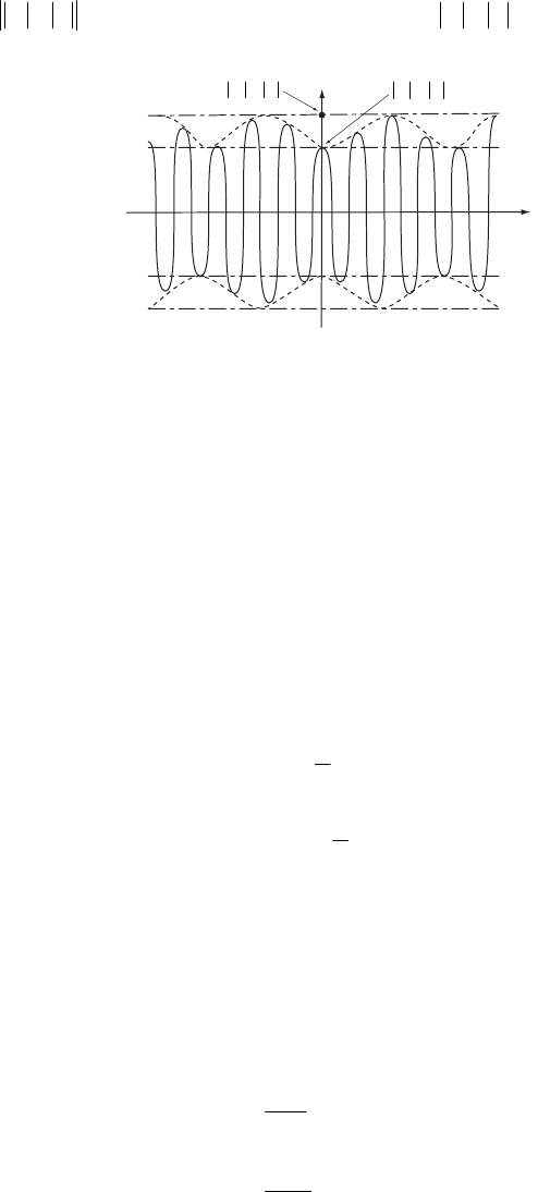
CONTINUOUS SYSTEMS; WAVES 449
From this expression we see that the wave function is modulated and that the phenomenon of
beats occurs, but for A ≠ B, the waves never beat to zero amplitude; the minimum amplitude is,
from Eq. (11),
A
B−, and the maximum amplitude is
A
B
+
. The wave function has the form
shown in the figure.
AB+
AB−
Reψ
wt – kx
13-16. As explained at the end of section 13.6, the wave will be reflected at and will
then propagate in the –x direction.
0
xx=
13-17. We let
,2
,2
j
mjn
m
mjn
=
′
=1
=
+
′′
(1)
where n is an integer.
Following the procedure in Section 12.9, we write
(
22 2122
2
nn nnn
Fmq q qq
d−
== −+
′
)
1+
τ
(2a)
(
21 21 2 21 22
2
nnnn
Fmq qqq
d
++ +
==−+
′′
)
n+
τ
(2b)
Assume solutions of the form
(
)
2
2
it nkd
n
qAe
ω
−
= (3a)
()
[
]
21
21
it n kd
n
qBe
ω
−+
+= (3b)
Substituting (3a,b) into (2a,b), we obtain
()
()
2
2
2
2
ikd ikd
ikd ikd
ABeABe
md
BAeBAe
md
τ
ω
τ
ω
−
−
−= −+
′
−= −+
′′
(4)
from which we can write
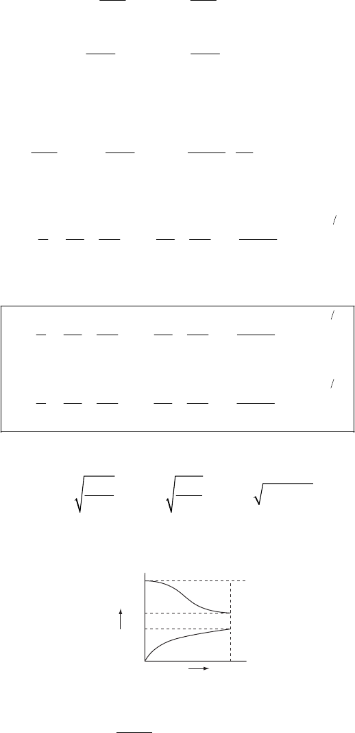
450 CHAPTER 13
2
2
22
cos 0
22
cos 0
ABkd
md md
AkdB
md md
ττ
ω
ττ
ω
−− =
′′
−+−
=
′′ ′′
(5)
The solution to this set of coupled equations is obtained by setting the determinant of the
coefficients equal to zero. We then obtain the secular equation
2
22
22 12
cos 0kd
md m d mm d
ττ τ
ωω
−−−
′′′ ′′′
=
(6)
Solving for
ω
, we find
12
2
11 11 4
sin kd
dmm mm mm
τ
2
ω
2
=+±+−
′′′ ′′′ ′′′
(7)
from which we find the two solutions
12
2
22
1
12
2
22
2
11 11 4
sin
11 11 4
sin
kd
dmm mm mm
kd
dmm mm mm
τ
ω
τ
ω
=+++−
′′′ ′′′ ′′′
=+−+−
′′′ ′′′ ′′′
(8)
If m′ < m″, and if we define
2
22
,,
abc
md md
ττ
2
ab
ω
ωωω
≡≡=
′′ ′
ω
+ (9)
Then the
ω
vs. k curve has the form shown below in which two branches appear, the lower
branch being similar to that for m′ = m″ (see Fig. 13-5).
ωa
ωb
ωc
0k
ω
π/2d
Using (9) we can write (6) as
()
()
2
2222
22
sin ab
ab
kd W
ω
ω
ωω ω
ωω
=+−≡ (10)
From this expression and the figure above we see that for c
ω
ω
> and for ab
ω
ωω
<< , the wave
number k is complex. If we let , we then obtain from (10) k
κ
=+i
β
(
)
(
)
22222
sin sin cosh cos sinh 2 sin cos sinh coshid d d d d i d d d dW
κβ κ β κ β κ κ β β ω
+= − + = (11)
Equating the real and imaginary parts, we find
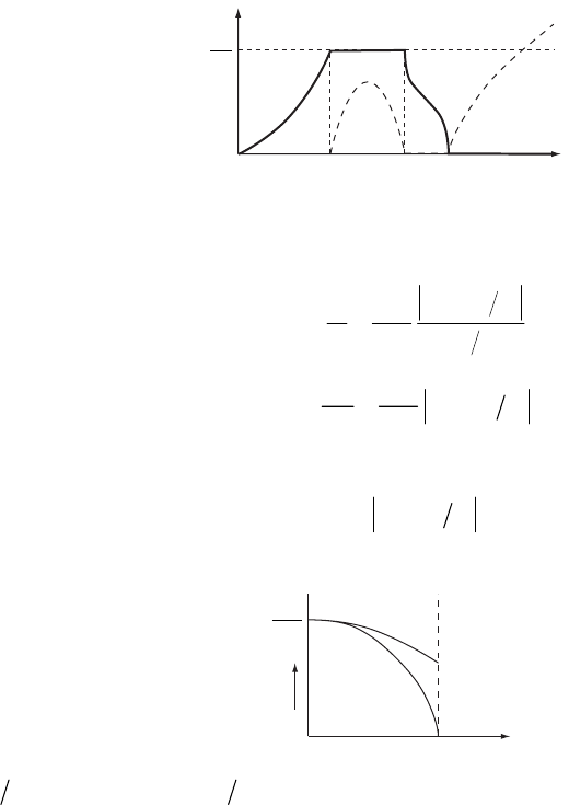
CONTINUOUS SYSTEMS; WAVES 451
()
22 22
sin cos sinh cosh 0
sin cosh cos sinh
dd d d
ddddW
κκ β β
κβκβ
=
ω
−=
(12)
We have the following possibilities that will satisfy the first of these equations:
a) sin
κ
d = 0, which gives
κ
= 0. This condition also means that cos
κ
d = 1; then β is
determined from the second equation in (12):
(
)
2
sinh dW
β
ω
−= (13)
Thus, c
ω
ω
>, and
κ
is purely imaginary in this region.
b) cos
κ
d = 0, which gives
κ
=
π
/2d. Then, sin
κ
d = 1, and
(
)
2
cosh dW
β
ω
=. Thus, ab
ω
ωω
<
<,
and
κ
is constant at the value
π
/2d in this region.
c) sinh
β
d = 0, which gives
β
= 0. Then,
(
)
2
ndWsi
κ
ω
=. Thus, a
ω
ω
<
or bc
ω
ωω
<< , and
κ
is
real in this region.
Altogether we have the situation illustrated in the diagram.
k
κ
κ
κ
κ
ω
a
ω
b
ω
c
ω
β
β
π
2d
13-18. The phase and group velocities for the propagation of waves along a loaded string are
()
(
)
sin 2
22
ckd
d
Vk kkd
ω
ω
== (1)
()
()
cos 2
2
cd
d
Uk kd
dk
ω
ω
== (2)
where
(
)
sin 2
ckd
ωω
= (3)
The phase and group velocities have the form shown below.
V,UU(k)
V(k)
0k
π/d
ω
c
d
2
When kd
π
=, U = 0 but cdV
ω
π
=. In this situation, the group (i.e., the wave envelope) is
stationary, but the wavelets (i.e., the wave structure inside the envelope) move forward with the
velocity V.
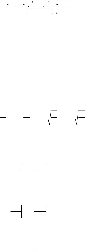
452 CHAPTER 13
13-19. The linear mass density of the string is described by
1
21
if 0;
if 0
xx
xL
L
<
>
=><<
ρ
ρρρ
III III
0
x
ρ1ρ1
ρ2
Consider the string to be divided in three different parts: I for x < 0, II for 0 < x < L, and III for
x > L.
Let be a wave train, oscillating with frequency
ω
, incident from the left on II. We can write
for the different zones the corresponding wave functions as follows:
(
1
itkx
Ae
ω
φ
−
=
)
II
ψ
() ()
() ()
()
11 11
22 22
1
itkx itkx it ikx ikx
I
itkx itkx it ikx ikx
itkx
III
Ae Be e Ae Be
Ce De e Ce De
Ee
ωω
ω
ωω
ω
ω
ψ
ψ
−+ −
−+ −
−
=+= +
= +=+
=
(1)
Where
12 1 2
12 1
,, ,V V
VV 2
kk
ω
ωτ τ
ρ
ρ
=== = (2)
and where
τ
is the tension in the string (constant throughout). To solve the problem we need to state first
the boundary conditions; these will be given by the continuity of the wave function and its derivative at
the boundaries x = 0 and x = L. For x = 0, we have
(
)
(
)
III
III
00
00
xx
xx
xx
==
== =
∂∂
=
∂∂
ψψ
ψψ
(3)
and for x = L, the conditions are
(
)
(
)
II III
II III
0
xL xL
xx
xx
==
== =
L
∂∂
=
∂∂
ψψ
ψψ
(4)
Substituting
ψ
as given by (1) into (3) and (4), we have
()
2
1
ABCD
k
A
BCD
k
+
=+
−+= −+
(5)
and
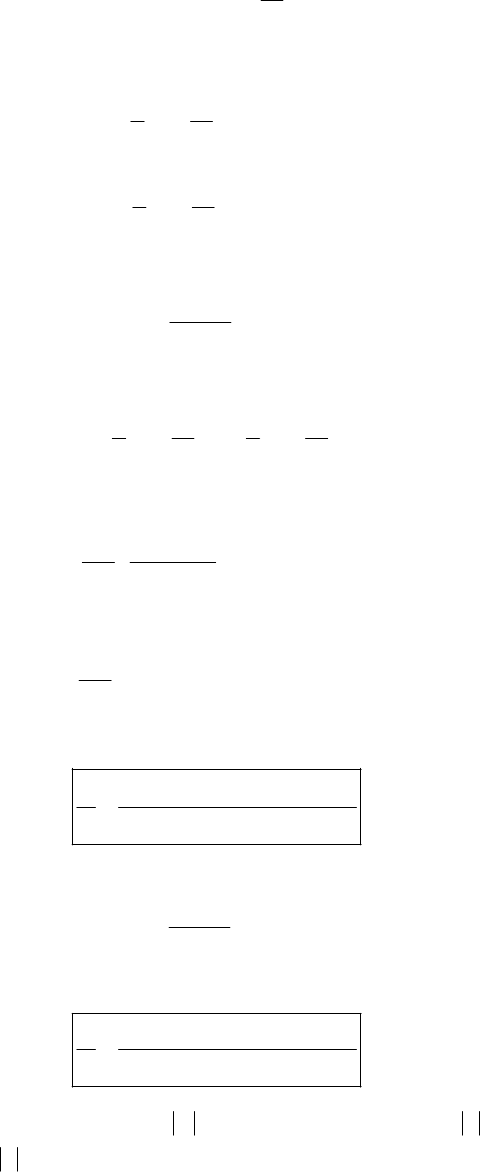
CONTINUOUS SYSTEMS; WAVES 453
22 1
22 1
1
2
ik L ik L ik L
ik L ik L ik L
Ce De Ee
k
Ce De Ee
k
−−
−−
+=
−+=−
(6)
From (6) we obtain
()
()
21
21
1
2
1
2
11
2
11
2
ik k L
ik k L
k
CEe
k
k
DEe
k
−
−+
=+
=−
(7)
Hence,
2
2
21
21
ikL
kk
Ce
kk D
+
=− (8)
From (5) we have
2
11
11
11
22
kk
2
A
C
kk
=+ +−
D (9)
Using (7) and rearranging the above equation
()
() ()
2
2
12 2
21
121
1
2
ikL
kk
A
ekk
kkk D
+
=−−
−
(10)
In the same way
() ()
2
2
21 12
1
1
2
ikL
Bkkekk
kD
=−+ ++
(11)
From (10) and (11) we obtain
(
)
() ()
2
2
22 2
12
2
2
12 12
1
ikL
ikL
kke
B
Akke kk
−−
=+−−
2
(12)
On the other hand, from (6) and (8) we have
()
21
2
21
2ik k L
kD
Ee
kk
+
=− (13)
which, together with (10) gives
()
() ()
12
2
12
2
2
12 12
4ik k L
ikL
kk e
E
Akke kk
+
=+−−
2
(14)
Since the incident intensity is proportional to
0
I2
A
, the reflected intensity is 2
r
IB=, and the total
transmitted intensity is 2
tEI=, we can write
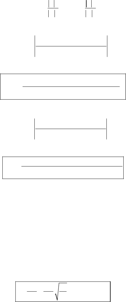
454 CHAPTER 13
22
0
2
,
rt
BE
II II
0
2
A
A
==
(15)
Substituting (12) and (14) into (15), we have, for the reflected intensity,
(
)
() ()
2
2
2
22 2
12
02
2
12 12
1
ikL
rikL
kke
II
kke kk
−−
=+−−
2
(16)
From which
()
()
()
2
22
12 2
02
44 22 22
12 12 12 2
1 cos 2
6 cos 2
r
kk kL
kk kk kk kL
−−
=
++ − −
II (17)
and for the transmitted intensity, we have
()
() ()
12
2
2
12
02
2
12 12
4ik k L
tikL
kk e
IIkke kk
+
=+−−
2
(18)
so that
()
22
12
02
44 22 22
12 12 12 2
8
62 cos2
t
kk
kk kk kk kL
=++ − −
II (19)
We observe that II , as it must.
0rt
I+=
For maximum transmission we need minimum reflection; that is, the case of best possible transmission is
that in which
0
0
t
r
II
I
=
=
(20)
In order that , (17) shows that L must satisfy the requirement 0
r
I=
2
1cos2 0kL
−
= (21)
so that we have
22
,0,1,2,
mm
Lm
k
ππτ
ωρ
== = … (22)
The optical analog to the reflection and transmission of waves on a string is the behavior of light
waves which are incident on a medium that consists of two parts of different optical densities
(i.e., different indices of refraction). If a lens is given a coating of precisely the correct thickness
of a material with the proper index of refraction, there will be almost no reflected wave.
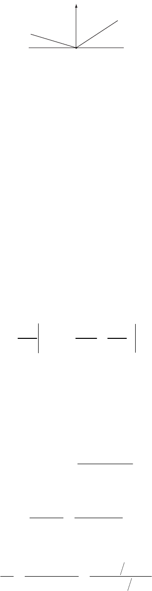
CONTINUOUS SYSTEMS; WAVES 455
13-20.
III
M
0
y
We divide the string into two zones:
I: 0
II: 0
x
x
<
>
Then,
() ()
()
I1 1
II 2
itkx itkx
itkx
Ae Be
Ae
−+
−
=+
=
ωω
ω
ψ
ψ
(1)
The boundary condition is
(
)
(
)
III
0xx0
=
==
ψ
ψ
(2)
That is, the string is continuous at x = 0. But because the mass M is attached at x = 0, the
derivative of the wave function will not be continuous at this point. The condition on the
derivative is obtained by integrating the wave equation from x = –
ε
to x = +
ε
and then taking
the limit
ε
→ 0.
Thus,
2
II I
2
0
0x
x
Mtxx
=
=
∂∂∂
=−
∂∂∂
ψψψτ
2
(3)
Substituting the wave functions from (1), we find
11
A
BA
+
= (4)
(
)
2
211
ik A A B MA
τ
−+− =− 2
ω
(5)
which can be rewritten as
(
)
2
11 2
ik M
ABA ik
−
−=
τω
τ
(6)
From (4) and (6) we obtain
11
2
11
AB ik
A
Bik M
τ
τω
+
=
−−
(7)
from which we write
2
2
1
22
1
2
212
M
ik
BM
A
ik M M ik
ω
τ
ω
τ
ωω
==
−−
τ
(8)
Define
456 CHAPTER 13
2
tan
2
MP
k
ω
θ
τ
== (9)
Then, we can rewrite (8) as
1
11
BiP
A
iP
−
=
+
(10)
And if we substitute this result in (4), we obtain a relation between 1
A
and 2
A
:
2
1
1
1
A
A
iP
=
+
(11)
The reflection coefficient,
2
1
1
B
R
A
=, will be, from (10),
22
2
1
2
1
tan
11tan
BP
RAP 2
θ
θ
== =
++ (12)
or,
2
sinR
θ
= (13)
and the transmission coefficient,
2
2
1
A
T
A
=, will be from (10)
2
2
2
1
11
11tan
A
TAP 2
θ
== =
++ (14)
or,
2
cosT
θ
= (15)
The phase changes for the reflected and transmitted waves can be calculated directly from (10)
and (11) if we substitute
11 1
11 1
22 2
i
i
i
BBeB
AAeA
A
AeA
φ
φ
φ
=
=
=
(16)
Then,
()
()
1
11 tan 1
1
1
2
11 1
A
ii
B
BP
e
AA P
φφ
−
−
==
+
BP
e
(17)
and
()
()
1
21
2tan
2
2
11
1
1
AA
ii
A
Ae
AA P
φφ
−
−−
==
+
P
e
(18)

CONTINUOUS SYSTEMS; WAVES 457
Hence, the phase changes are
()
()
()
11
21
11
11
1
tan tan cot
tan tan tan
BA
AA
P
P
φφ θ
φ
φθ
−−
−−
−= =
−=− =− =−
θ
(19)
13-21. The wave function can be written as {see Eq. (13.111a)]
(1)
()
()
()
,itkx
xt Ak e dk
ω
ψ
+∞
−
−∞
=∫
Since A(k) has a non-vanishing value only in the vicinity of 0
kk
=
, (1) becomes
(2)
()
()
0
0
,
kk
itkx
kk
xt e dk
ω
ψ
+∆
−
−∆
=∫
According to Eq. (13.113),
(
)
00 0
kk
ωω ω
=+ −
′ (3)
Therefore, (2) can now be expressed as
()
() ()
()
()()()()
()
()() ()
0
000 0
0
00 00
000
000 0 0
0
0
,
2
2
kk
iwkt itxk
kk
ik k t x ik k t x
ikt
i k t i tx k i tx k
xt e e dk
ee
eitx
eee
tx i
+∆
−−
′′
−∆
+∆ − −∆ −
′′
−′
−−∆−∆
′′ ′
=
−
=
−
′
−
=
−
′
∫
ωω
ωω
ωω
ωω ω ω
ψ
ω
ω
(4)
and writing the term in the brackets as a sine, we have
()
()
()
00
0
0
2sin
,itkx
txk
xt e
tx
ω
ω
ψω
−
−∆
′
=−
′ (5)
The real part of the wave function at t = 0 is
()
(
)
0
2sin
Re ,0 cos
xk
x
x
ψ
∆
=kx (6)
If ∆, the cosine term will undergo many oscillations in one period of the sine term. That
is, the sine term plays the role of a slowly varying amplitude and we have the situation in the
figure below.
0
kk
458 CHAPTER 13
x
ReΨ(x,0)
13-22.
a) Using Eq. (13.111a), we can write (for t = 0)
(1)
()
()
()
() ()
2
0
2
00
0
2
0
,0 ikx
kk ikx
kk ikk x
ik x
ik x uiux
xAkedk
Be e dk
Be e e dk
Be e e du
+∞
−
−∞
+∞ −− −
−∞
+∞ −− −−
−
−∞
+∞
−−−
−∞
=
=
=
=
∫
∫
∫
∫
σ
σ
σ
ψ
This integral can be evaluated by completing the square in the exponent:
2
2
22
2
2
2
2
44
2
4
b
ax x
ax bx a
bb b
ax x
aaa
b
bax a
a
eedx e dx
ee
ee dx
+∞ +∞
−−
−
−∞ −∞
+∞ −−+
−∞
+∞
−−
−∞
=
=
=
∫∫
∫
∫
dx
(2)
and letting 2yxba=− , we have
2
2
24
b
ay
ax bx a
e e dx e e dy
+∞ +∞
−
−
−∞ −∞
=
∫∫
(3)
Using Eq. (E.18c) in Appendix E, we have
2
24
b
ax bx a
eedx e
a
π
+∞
−
−∞
=
∫ (4)
Therefore,
CONTINUOUS SYSTEMS; WAVES 459
()
2
04
,0 x
ik x
xBee
σ
π
ψσ
−
−
= (5)
The form of
(
)
,0x
ψ
(the wave packet) is Gaussian with a 1 width of e4
σ
, as indicated in the
diagram below.
−2σ2σ
1
e⋅Bπ
σ
Bπ
σ
Ψx,0
()
x
b) The frequency can be expressed as in Eq. (13.113a):
(
)
(
)
00 0
kkk
ωωω
=
+−+
′… (6)
and so,
(7)
()
()
()
()
()
() () ()()
() ()
00 0
200 0
00 0
2
00 0
,itkx
it kktkx
ikktkkx
itkx kk
itkx itxu
u
xt Ak e dk
Ak e dk
Be e e dk
Be e e du
+∞
−
−∞
+∞
+−−
′
−∞
+∞
−−−
′
−−−
−∞
+∞
−−
′
−
−∞
=
=
=
=
∫
∫
∫
∫
ω
ωω
ω
ωσ
ωω
σ
ψ
Using the same integral as before, we find
()
()()
2
00 0 4
,itkx tx
xt B e e
−−−
′
=
ω
ω
π
ψσ
σ
(8)
c) Retaining the second-order term in the Taylor expansion of
ω
(k), we have
()
() ()
2
00 0 0 0
1
2
kkkkk
ω ω
=+ −+ − +
′′′
…
ωω
(9)
Then,
()
()
()
() ()()
() ()
2
00 00 0
00
2
0
00 0
1
2
2
,ikkt kktkkx
itkx
t
iu
itkx iwtxu
xt e Ake dk
Be e e du
+∞
−+ − −−
′′′
−
−∞
′′
+∞ −−
−−
′
−∞
=
=
∫
∫
ωω
ω
ω
σ
ω
ψ
(10)
We notice that if we make the change 02it
σ
ωσ
−
→
′
′, then (10) becomes identical to (7).
Therefore,
460 CHAPTER 13
()
()
()
00 ,
0
2
,2
itkx xt
xt B i e
iw t
ωα
π
ψσ
−−
=−′′ (11)
where
()
()
()
2
00
2
22
0
1
2
,4
tx it
xt t
ωσω
ασω
−+
′
′′
=+′′ (12)
The 1 width of the wave packet will now be e
()
()
2
22
0
1
4
2
e
t
wt
σω
σ
+′′
= (13)
or,
()
2
0
141
2
e
t
Wt
ω
σσ
′
′
=+
(14)
In first order, 1e
W, shown in the figure above, does not depend upon the time, but in second
order, 1e
W depends upon t through the expression (14). But, as can be seen from (8) and (11),
the group velocity is 0
ω
′
, and is the same in both cases. Thus, the wave packet propagates with
velocity 0
ω
′ but it spreads out as a function of time, as illustrated below.
Ox
t = t
1
t = 0
Ψxt,
()
CHAPTER 14
The S
p
ecial Theor
y
of Relativit
y
14-1. Substitute Eq. (14.12) into Eqs. (14.9) and (14.10):
11
v
xxx
c
γ
=−
′
1
(1)
(
111
v
xxx
c
=+ =
)
′
′
′
γ
γγ
(2)
From (1)
1
1
1
xv
xc
γ
′
=−
From (2)
1
1
1
1
x
v
x
c
γ
′=
+
So
1
1
1
v
v
c
c
γ
γ
−=
+
or
22
1
1vc
γ
=−
461
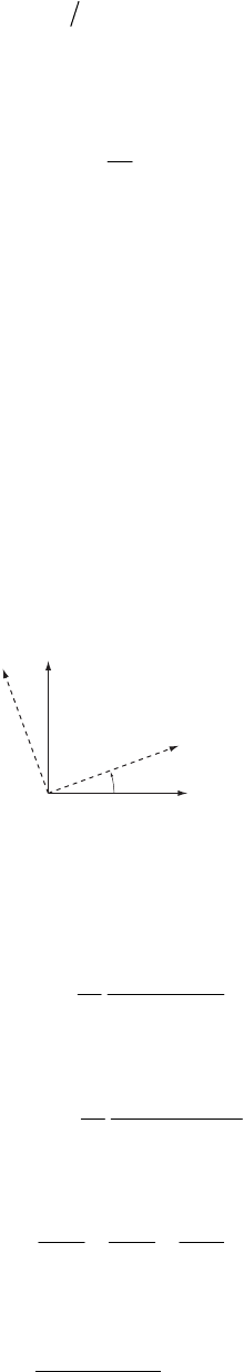
462 CHAPTER 14
14-2. We introduce cosh , sinhyyvc
α
α
≅≅ and substitute these expressions into Eqs.
(14.14); then
11
1
22 33
cosh sinh
cosh sinh
;
xx ct
x
tt ac
xx xx
α
α
α
=
−
′
=−
′
==
′′
(1)
Now, if we use cosh
α
= cos (i
α
) and i sinh
α
= sin (i
α
), we can rewrite (1) as
(
)
(
)
() ()
11
1
cos sin
sin cos
xx i ict i
ict x i ict i
αα
α
α
=+
′
=− +
′
(2)
Comparing these equations with the relation between the rotated system and the original
system in ordinary three-dimensional space,
11 2
21 2
33
cos sin
sin cos
xx x
xx x
xx
θθ
θ
θ
=+
′
=− +
′
=
′
(3)
x
2
x
2
′
x
1
x
1
′
θ
We can see that (2) corresponds to a rotation of the 1
xict
−
plane through the angle i
α
.
14-3. If the equation
()
(
)
2
2
22
,
1
,
xict
xict ct
ψ
ψ
∂
∇−
∂0
=
(1)
is Lorentz invariant, then in the transformed system we must have
()
(
)
2
2
22
,
1
,
xict
xict ct
ψ
ψ
∂′′
∇−
′′′ ∂0
=
′
(2)
where
22
2
22
xyz
2
2
∂
∂∂
∇= + +
′
∂
∂∂
′
′′
(3)
We can rewrite (2) as
(
)
2
4
2
1
,0
xict
x
µµ
ψ
=
∂′′
=
∂′
∑ (4)
THE SPECIAL THEORY OF RELATIVITY 463
Now, we first determine how the operator
2
2
x
µ
µ
∂
∂
′
∑ is related to the original operator
2
2
x
µ
µ
∂
∂
∑.
We know the following relations:
xx
µ
µν ν
ν
λ
=
′
∑
(5)
xx
ν
µν µ
µ
λ
=
′
∑
(6)
µ
νµλ νλ
µ
λ
λδ
=
∑
(7)
Then,
x
xxx
νµν
νν
x
µ
νµ
λ
ν
∂
∂∂
==
∂∂∂ ∂
′′
∑∑
∂
(8)
2
2
xxx x
µν µλ µν µλ
νλ νλ
x
µ
νλ ν
λλ λλ
∂∂∂ ∂
∂∂∂ ∂
′∑∑ ∑∑ (9)
λ
∂
==
∂
Therefore,
2
2
2
2
xx
xx
x
∂∂
=
∂∂
′
∂∂
=∂∂
∂
=∂
∑∑∑∑
∑∑
∑
µν µλ
µνλµ
x
∂
∂
µ
νλ
νλ
νλ νλ
λ
λλ
δ
(10)
Since
µ
and
λ
are dummy indices, we see that the operator 2
x2
µ
∂
∂
∑
is invariant under a
Lorentz transformation. So we have
(
)
2
2
,0
xict
x
µµ
ψ
∂′′
=
∂′
∑ (11)
This equation means that the function
ψ
taken at the transformed point (x′,ict′) satisfies the
same equation as the original function
ψ
(x,ict) and therefore the equation is invariant. In a
Galilean transformation, the coordinates become
x
y
z
xxvt
yyvt
z
zvt
tt
=−
′
=−
′
=−
′
=
′
(12)
Using these relations, we have
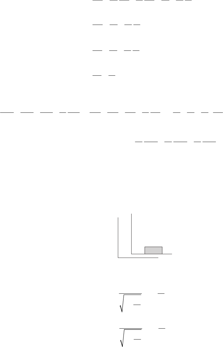
464 CHAPTER 14
1
1
1
x
y
z
xt
xxxtxxvt
yyvt
zyvt
tt
∂∂∂∂∂ ∂ ∂
=+=−
∂∂∂∂∂∂ ∂
′′′
∂∂ ∂
=−
∂∂ ∂
′
∂∂ ∂
=−
∂∂ ∂
′
∂∂
=
∂∂
′
(13)
Therefore,
222 2 222 2
2222 22222 222
222
1 1 111
2
111
2
xyz
xyz
x y zct xyzct vvvt
vxtvytvzt
∂∂∂ ∂ ∂∂∂ ∂ ∂
++− = ++− +++
∂∂∂ ∂ ∂∂∂ ∂ ∂
′′′ ′
2
2
∂∂∂
−++
∂∂ ∂∂ ∂∂
(14)
This means that the function
ψ
(x′,ict′) does not satisfy the same form of equation as does
(, )xict
ψ
, and the equation is not invariant under a Galilean transformation.
14-4. In the K system the rod is at rest with its ends at and . The K′ system moves with a
velocity v (along the x axis) relative to K.
1
x2
x
K
K′
x
1
x
2
If the observer measures the time for the ends of the rod to pass over a fixed point in the K′
system, we have
11
2
2
2
22
2
2
2
1
1
1
1
v
tt
c
v
c
v
tt
c
v
c
=−
′
1
2
x
x
−
=−
′
−
(1)
where t and t are measured in the K′ system. From (1), we have
1
′2
′
THE SPECIAL THEORY OF RELATIVITY 465
()
(
12 12 1 2
2
2
2
1
1
v
tt xx
c
v
c
)
tt
−= − − −
′′
−
(2)
We also have
12
xx
−
=A (3)
(
)
12
vt t
−
=A (4)
(
)
12
vt t
−
=
′
′
A′
(5)
Multiplying (2) by v and using (3), (4), and (5), we obtain the FitzGerald-Lorentz contraction:
2
2
1v
c
=−
′
AA (6)
14-5. The “apparent shape” of the cube is that shape which would be recorded at a certain
instant by the eye or by a camera (with an infinitesimally short shutter speed!). That is, we must
find the positions that the various points of the cube occupy such that light emitted from these
points arrives simultaneously at the eye of the observer. Those parts of the cube that are farther
from the observer must then emit light earlier than those parts that are closer to the observer. An
observer, looking directly at a cube at rest, would see just the front face, i.e., a square.
When in motion, the edges of the cube are distorted, as indicated in the figures below, where
the observer is assumed to be on the line passing through the center of the cube. We also note
that the face of the cube in (a) is actually bowed toward the observer (i.e., the face appears
convex), and conversely in (b).
(a) Cube moving toward the
observer.
(a) Cube moving away from the
observer.
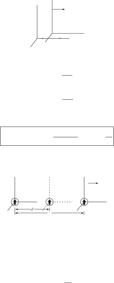
466 CHAPTER 14
14-6.
K′
v
x
1
x
2
K
We transform the time t at the points and in the K system into the K′ system. Then,
1
x2
x
1
12
2
22
vx
tt
c
vx
tt
c
=−
′
=−
′
γ
γ
(1)
From these equations, we have
()
12
12 2
1
xx
ttt v vx
cc
−
− =− =− ∆
′′′
γγ
2
∆= (2)
14-7.
KK′
v
x
Suppose the origin of the K′ system is at a distance x from the origin of the K system after a time
t measured in the K system. When the observer sees the clock in the K′ system at that time, he
actually sees the clock as it was located at an earlier time because it takes a certain time for a
light signal to travel to 0. Suppose we see the clock when it is a distance A from the origin of the
K system and the time is t in K and
1 1
t
′
in K′. Then we have
()
11
2
1
1
v
tt
c
ct t
tv x
tv
γ
=−
′
−=
=
=
A
A
A
(1)
We eliminate A, t, and x from these equations and we find
1
THE SPECIAL THEORY OF RELATIVITY 467
11v
t
c
γ
t
=−
′
(2)
This is the time the observer reads by means of a telescope.
14-8. The velocity of a point on the surface of the Earth at the equator is
(
)
8
4
4
26.3810 cm
2
8.64 10 sec
4.65 10 cm/sec
e
R
v
π
π
τ
××
== ×
=×
(1)
which gives
4
6
10
4.65 10 cm/sec 1.55 10
310 cm/sec
v
c
−
×
== = ×
×
β
(2)
According to Eq. (14.20), the relationship between the polar and equatorial time intervals is
2
2
1
12
1
t
tt
β
β
∆
∆= ≅∆ +
′
−
(3)
so that the accumulated time difference is
2
1
2
tt
β
t
∆
=∆ −∆ = ∆
′ (4)
Supplying the values, we find
()()()
67
11.55 10 3.156 10 sec/yr 10 yr
2
−
× × × × 2
∆= × (5)
Thus,
0.0038 sec∆= (6)
14-9.
w
dm′m + dm
v + dv
The unsurprising part of the solution to the problem of the relativistic rocket requires that we
apply conservation of momentum, as was done for the nonrelativistic case. The surprising, and
key, part of the solution is that we not assume the mass of the ejected fuel is the same as the
mass lost from the rocket. Hence
(
)
(
)
(
)
w
p
mv d m dm v dv dm w
γγγ γ
+ + ++==
′
(1)
where –dm is the mass lost from the rocket, dm′ is the mass of the ejected fuel,
(
)
(
)
2
1wvV vVc≡− − is the velocity of the exhaust with respect to the inertial frame, and
22
11
wwc
γ
≡− . One can easily calculate 3
dd
γ
γβ β
=, ad after some algebra one obtains
468 CHAPTER 14
2wdm
mdv vdm w
γ
γγ
′
++ (2)
where we of course keep infinitesimals only to first order. The additional unknown dm′ is
unalarming because of another conservation law
(
)
(
)
22
w
c dmdmc dmc
γγγ γ
==+ + + 2
Em
′
(3)
Subsequent substitution of dm′ into (2) gives, in one of its many intermediate forms
()
21
w
mdv dm v w
c
β
γ
0
−
+−=
(4)
and will finally come to its desired form after dividing by dt
()
2
1
dv dm
mV
dt dt
β
0
+
−= (5)
The quantity dt can be measured in any inertial frame, but would presumably only make sense
for the particular one in which we measure v. Interestingly, it is not important for the ejected
fuel to have an especially large kinetic energy but rather that it be near light speed, a nontrivial
distinction. For such a case, a rocket can reach 0.6c by ejecting half its mass.
14-10. From Eq. (14.14)
(
)
11
xxv
γ
=−
′t (1)
1
2
v
ttx
c
γ
=−
′
(2)
Solving (1) for and substituting into (2) gives
1
x
1
2
xv
tt vt
c
γγ
′
=− +
′
2
1
22
vv
txt t
cc
γγ
t
γ
+
=− =
′′
1
2
v
tt x
c
γ
=+
′
′
Solving (2) for t and substituting into (1) gives
11 1
2
tv
xxv x
c
γγ
′
=−+
′
or
(
)
11
xxvt
γ
=+
′
′
THE SPECIAL THEORY OF RELATIVITY 469
14-11.
θx1
From example 14.1 we know that, to an observer in motion relative to an object, the dimensions
of objects are contracted by a factor of 22
1vc− in the direction of motion. Thus, the 1
x
′
component of the stick will be
22
cos 1 vc
θ
−A
while the perpendicular component will be unchanged:
sin
θ
A
So, to the observer in K′, the length and orientation of the stick are
(
)
12
2222
sin 1 cosvc
θθ
=+−
′
AA
1
22
sin
tan cos 1 vc
θ
θθ
−
=
′
−
or
12
2
2
2
cos
sin
tan tan
θ
θγ
θγ θ
=+
′
=
′
AA
14-12. The ground observer measures the speed to be
8
100 m 2.5 10 m/s
.4 sec
v
µ
==×
The length between the markers as measured by the racer is
22
2
1
2.5
100 m 1 55.3 meters
3
vc=−
′
=−=
AA
The time measured in the racer’s frame is given by
470 CHAPTER 14
()
()
()
1
2
8
2
2
2.5 10 m/s 100 m
.4 sec
12.53
.22 sec
v
ttx
c
c
γ
µ
µ
=−
′
×
−
=
−
=
The speed observed by the racer is
8
2.5 10 m/svtt
′
=== ×
′
AA
14-13.
()
12
2
1.5 s
1 0.999 22.4
tt
t
γ
µ
γ
−
∆=∆
′
∆=
=−
Therefore 34 st
µ
∆′.
14-14.
KK′
receiver
v
source
In K, the energy and momentum of each photon emitted are
0
0and h
Eh p c
ν
ν
==
Using Eq. (14.92) to transform to K′:
()
0
11
00
;h
Eh Evp p c
v
hh
c
ν
νγ
γν ν
== − =−
′
=+
THE SPECIAL THEORY OF RELATIVITY 471
So
0
00
2
1
11
1
1
v
c
=+
+
+
==
−
−
ννγ
β
β
νν
β
β
which agrees with Eq. (14.31).
14-15. From Eq. (14.33)
0
1
1
β
ν
ν
β
−
=+
Since c
λ
ν
=
0
1
1
β
λ
λ
β
−
=+
or
0
1
1
β
λ
λ
β
−
=+
With 0656.3 nm
λ
= and
4
8
410
310
β
×
=×,
λ
= 656.4 nm.
S o the shift is 0.1 nm toward the red (longer wavelength).
14-16.
θ
θ′
Earth
star
v
K′
K
Consider a photon sent from the star to the Earth. From Eq. (14.92)
(
)
1
EEvp
γ
=−
′
also
(
)
1
EEvp
γ
=+
′
′
472 CHAPTER 14
Now
0
01 1
, , cos , cos
h
h
E h p p
cc
Eh
ν
ν
ν
νθ
= = =− =−
′′
θ
′
Substituting yields
(
)
01cos
ν
νγ β θ
=+
and
(
)
01cos
ν
γν β θ
=−
′
Thus
(
)
(
)
2
1 cos 1 cos
β
θβθγ
−
+−
′=
122
cos cos cos cos 1
β
θβ θ β θ θ β
+− − =−
′′
cos cos cos cos
θ
θβ θ θ β
−
−=
′′
−
Solving for cos
θ
yields
cos
cos 1cos
θ
β
θ
β
θ
−
′
=−
′
where
angle in earth’s frame
angle in star’s frame
vc
β
θ
θ
=
=
=
′
14-17. From Eq. (14.33)
0
1
1
β
ν
ν
β
−
=+
Since
c
ν
λ
=
,
0
1
1
β
λ
λ
β
+
=−
We have 0
1.5
λ
λ
=. This gives 5
13
β
=
or
8
1.2 10 m/secv=×
THE SPECIAL THEORY OF RELATIVITY 473
14-18.
θ
observer
source
light
v
K′
K
Proceeding as in example 14.11, we treat the light as a photon of energy h
ν
.
In 0
0
:,
h
hp c
KE
ν
ν
==
′′ ′
In
(
)
1
:h E p
νγ ν
== +
′
KE
For the source approaching the observer at an early time we have
0
1
h
pc
ν
=
Thus
000
1
1
v
c
β
νγν ν ν
β
+
=+ =
−
For the source receding from the observer (at a much later time) we have
0
1
h
pc
ν
=−
and
0
1
1
β
νν
β
−
=
+
So
0
0
1source approaching observer
1
1source receding from observer
1
β
νν β
β
νν β
+
=−
−
=+
474 CHAPTER 14
14-19.
θ
observer
source
v
K
K′
Proceeding as in the previous problem, we have
In
122
:
cos r
rt
KEh
hh
pcc
ν
βνν
θ
β
β
=
′′
=− =−
′+
In
(
)
10
:KE E p h
γ
νν
=+=
′′
So
22
022 22
1
1
r
rt
rt rt
h
c
c
νβ
ννββ
ββ ββ
hh
=−+
−− +
or
(
)
022
1
1
r
rt
−
=−−
ν
β
ν
β
β
22
0
0
1
1
rt
r
β
β
λ
ν
νλ β
−−
== −
For 0
λ
λ
>, we have
(
)
222
11
rrt
β
ββ
−
>− −
22
22
trr
β
ββ
>−
()
221
tr r
β
ββ
>−
14-20. As measured by observers on Earth, the entire trip takes
4 lightyears 80
2 y
0.3 c 3
=
ears
The people on earth age 80
3 years. The astronaut’s clock is ticking slower by a factor of
γ
. Thus,
the astronaut ages
THE SPECIAL THEORY OF RELATIVITY 475
2
80 80
1 0.3 0.95 years
33
−=
So
Those on Earth age 26.7 years.
The astronaut ages 25.4 years.
14-21.
()
()
()
0
032
22
2
032
22
12
2
11
1
11
m
d
Fm
dt
m
β
β
ββ
β
ββ
ββ
−−
==+
−−
−
=+
−−
vvv
vv
(1)
If we take (this does not mean vv
11
v=ve 23
0
=
=
), we have
()()
11
10
1
10 1
32 32
222
111
vv
vm
vcc vmv
βββ
=+==
−−−
A
1
Fm (2)
0
22
2
1t
m
2
F
vmv
β
==
−
(3)
0
33
2
1t
m
3
F
vmv
β
==
−
(4)
14-22. The total energy output of the sun is
()
32
1.4 10 W m 4
dE R
dt
−
=× ⋅ ×2
π
(1)
where is the mean radius of the Earth’s orbit around the sun. Therefore,
11
1.50 10 mR=×
26
3.96 10 W
dE
dt × (2)
The corresponding rate of mass decrease is
9
2
14.4 10 kg s
dm dE
dt c dt
1
−
=
×⋅ (3)
The mass of the sun is approximately 1. , so this rate of mass decrease can continue
for a time
30
99 10 kg×
476 CHAPTER 14
30
13
91
1.99 10 yr 1.4 10 yr
4.4 10 kg s
T−
×
=
×⋅
×
(4)
Actually, the lifetime of the sun is limited by other factors and the sun is expected to expire
about years from now.
9
4.5 10×
14-23. From Eq. (14.67)
()
22 2 2
0
22
00
2
0
22 2 2
2
2
pc E E
ET E
ET T
p
cTmcT
=−
=
+−
=+
=+
14-24. The minimum energy will occur when the four particles are all at rest in the center of
the mass system after the collision.
Conservation of energy gives (in the CM system)
2
24
pp
Emc=
or
2
,CM 0
22
pp
Emc==E
which implies
γ
= 2 or 32
β
=
To find the energy required in the lab system (one proton at rest initially), we transform back to
the lab
(
)
1
EEvp
γ
=+
′
′ (1)
The velocity of K′(CM) with respect to K(lab) is just the velocity of the proton in the K′ system.
So u = v.
Then
(
)
(
)
22
1CM
v p v mu mv mc 2
vp
γ
γγ
== ==
′
β
Since
γ
= 2, 32
β
=,
10
3
2
vp E=
′
Substituting into (1)
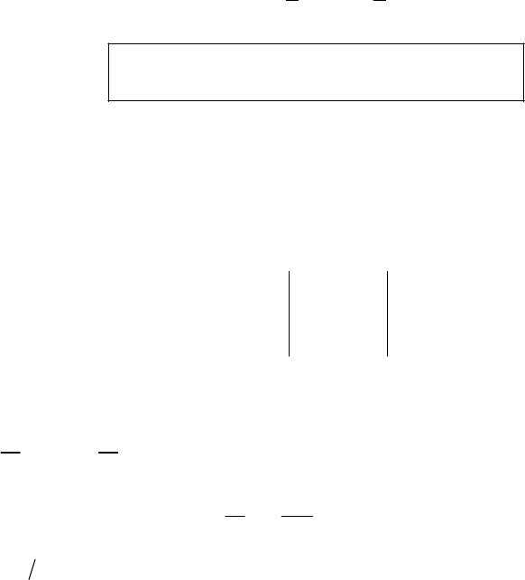
THE SPECIAL THEORY OF RELATIVITY 477
lab 0 0 0 0
37
22
22
EEE E
γ
=+= =
7E
2 2
The minimum proton energy in the lab system
7 , of which 6 is kinetic energy.
pp
mc
is mc
14-25. Let Bz
0
B=
x
y
vv
=
+vij
Then
0
00
0
00
xy
yx
qqvv
B
qvB vB
×=
=−
ijk
vB
ij
()
()
dd
qm
dt dt
γ
=×= =FvB p v gives
()
0
yx
qB
dvv
dt m
=−vi
γ
j
Define 0
qB m
ω
γ
≡
Thus
and
x
yy
x
vv v v
ω
ω
=
=−
or
2
x
y
x
vv
ωω
==−
v
and
2
y
x
y
vv
ωω
=− =−
v
t
t
So
cos sin
cos sin
x
y
vA tB
vC tD
ω
ω
ω
ω
=
+
=+
Take
(
)
0
x
vv=,
(
)
0
y
v=0. Then A = v, C = 0. Then
(
)
(
)
00
xy
0vv
ω
=
=
(
)
(
)
00
0,
yx
vv
BDv
=− =−
→= =−
v
ω
ω
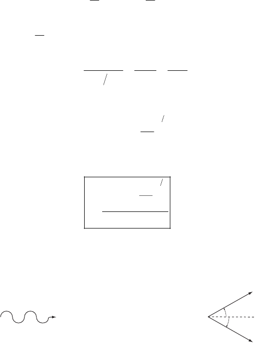
478 CHAPTER 14
Thus
cos sinvtvt
=
−vi j
ω
ω
Then
sin cos
vv
tt
=+ri j
ω
ω
ωω
The path is a circle of radius v
ω
000
p
vmv
rqB m qB qB
γ
γ
===
From problem 14-22
12
2
2
2T
pTm
c
=+
So
12
2
2
0
2T
Tm c
rqB
+
=
14-26. Suppose a photon traveling in the x-direction is converted into an e and as shown
below
−e+
before after
e
+
e
–
θ
θ
Cons. of energy gives
2
p
e
p
cE
=
where
momentum of the photon
energy of energy of
p
e
p
Ee e
+
−
=
==
Cons. of gives
x
p
(
)
2 cos momentum of ,
pe e
p
pp e
θ
e
+
−
==
Dividing gives

THE SPECIAL THEORY OF RELATIVITY 479
cos
pe
pe
p
cE
c
pp
θ
==
or
22 2 2
cos
ee
p
c
θ
E
=
(1)
But , so (1) cannot be satisfied for
22
ee
Epc>22
cos 1
θ
≤
.
An isolated photon cannot be converted
to an electron-positron pair.in
This result can also be seen by transforming to a frame where 0
x
p
=
after the collision. But,
before the collision, 0
xp
p
pc=≠
in any frame moving along the x-axis. So, without another
object nearby, momentum cannot be conserved; thus, the process cannot take place.
14-27. The minimum energy required occurs when the p and p are at rest after the collision.
By conservation of energy
(
)
0
22938 MeV
938 MeV
e
e
E
ET
=
E
=
=+
Since
E,
0.5 MeV
e=
937.5 MeV
ee
TT
+−
==
14-28. 2
classical
1
2
Tm=v
(
)
2
rel classical
1TmcT
γ
=− ≥
We desire
rel classical
rel
0.01
TT
T
−
≤
()
2
2
1
2
10
1
mv
mc
γ
−≤
−.01
()
2
2
1
20.99
1
v
c
γ
≥
−
2
1.98
1
β
γ
≥
−
Putting
(
)
12
2
1
γβ
−
=− and solving gives
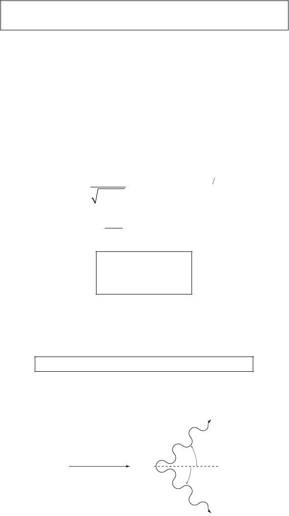
480 CHAPTER 14
0.115vc
≤
7
The classical kinetic energy will be within 1% of the correct
for 0 3.5 10 m/sec, independent of mass.
v×
value ≤≤
14-29. 0
EE
γ
=
For
()
9
6
0
4
12
2
2
10
2
30 10 eV
0.51 10 eV,
5.88 10
1or 1
1
1
111.410
2
E
E
γ
γβ
β
βγ
−
−
=×
×
×
==
−
−=−×
γ
−
(
)
10
11.410 c
0.99999999986 c
v−
=− ×
=
14-30. A neutron at rest has an energy of 939.6 MeV. Subtracting the rest energies of the
proton (938.3 MeV) and the electron (0.5 MeV) leaves 0.8 MeV.
Ot her than rest energies 0.8 MeV is available.
14-31.
0.98c θ
θ
Conservation of energy gives
2
p
EE
π
=
where E energy of each photon (Cons. of
p=
y
p
implies that the photons have the same energy).
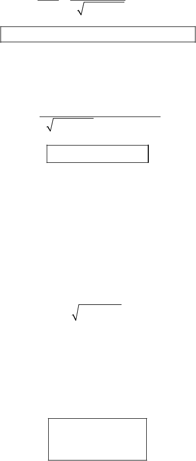
THE SPECIAL THEORY OF RELATIVITY 481
Thus
02
p
EE
γ
=
0
2
135 MeV 339 MeV
22 1 0.98
p
E
E
γ
== =
−
Th e energy of each photon is 339 MeV.
Conservation of gives
x
p
mv 2 cos where momentum of each photon
pp
p p
γ
θ
==
(
)
()
()
2
2
135 Mev/c 0.98 c
s 0.98
2 1 0.98 339 MeV/c
==
−
θ
co
1
cos 0.98 11.3
θ
−
=
=°
14-32. From Eq. (14.67) we have
222
0
EEpc−= 2
2
With , this reduces to
0
EE T=+
22
0
2ET T pc+=
Using the quadratic formula (taking the + root since T ≥ 0) gives
222
00
TEpcE
=
+−
Substituting pc = 1000 MeV
(
)
0electron 0.5 MeVE
=
(
)
0proton 938 MeVE=
gives
electron
proton
999.5 MeV
433 MeV
T
T
=
=
482 CHAPTER 14
14-33.
120˚
120˚
afterbefore
p
e
n
ν
Conservation of
y
p
gives
sin 60 sin 60 or
ee
pp pp
ν
ν
°= ° =
Conservation of gives
x
p
cos 60 cos 60
p
ee
p
pp
ν
p
=
°+ °=
So
ep
p
pp
ν
p
=
=≡
Conservation of energy gives
0nep
EEEE
ν
=
++
222 222
00 0
ne p
EEpcEpc=++++pc (1)
Substituting
0939.6 MeV
n
E
=
0938.3 MeV
p
E
=
00.5 MeV
e
E
=
and solving for pc gives
p = 0.554 MeV/c
0.554 MeV/c
pe
ppp
ν
===
Substituting into
0
222
00
TEE
EpcE
=
−
=
+−
gives
(
)
00E
ν
=
4
0.554 MeV
2 10 MeV, or 200 eV
0.25 MeV
p
e
T
T
T
ν
−
=
=×
=
THE SPECIAL THEORY OF RELATIVITY 483
14-34. 2 22222
12
sctxxx∆=− +++
3
′
′′′′
Using the Lorentz transformation this becomes
22
22 1222
1
2
22
11
23
22 22
22 2
2222
1
122
22
23
22
22222
123
22
11
1
vx
ct xvt xvt xvt
c
sx
vc vc
vx v
xctt
cc
xx
vc
ct x x x
−− + +−
∆= + ++
′−−
−−−
+
−
=− + + +
2
x
=+
So
22
ss
∆
=∆
′
14-35. Let the frame of Saturn be the unprimed frame, and let the frame of the first spacecraft
be the primed frame. From Eq. (14.17a) (switch primed and unprimed variables and change the
sign of v)
1
11
2
1
uv
uuv
c
+
′
=
′
+
Substituting v = 0.9 c
10.2uc
=
′
gives
10.93uc=
14-36. Since
()
123
and , , ,
ddX Xxxxi
dd
==
µµ
µ
ττ
Fm
ct
we have
()
2
11
12
2
2
3
2
23
22
2
42
dx d x
d
Fm m
dd d
dx
dx
Fm Fm
dd
dict
dd
Fm icm
dd d
ττ τ
t
τ
τ
τ
ττ
==
==
==
484 CHAPTER 14
Thus
()
()
()
22
1
11
22
22
1
14
22
22
22
22
22
1
422
22
1
22
41
;
dx d
Fm m xvt
dd
dx dt
mmv Fi
dd
dx dx
Fm m F FF
dd
vxd
Ficm t
dc
dxdt
icm i m
dd
FiF
=− −
′
′
== =+
′
=== =
′′
=−
′
=−
=−
γ
ττ
γγ γ
ττ
ττ
γ
τ
γγβ
ττ
γβ
33
F
β
Th us the required transformation equations are shown.
14-37. From the Lagrangian
(
)
22
1
11 2
Lmc kx
β
=−−−
2
(1)
we compute
Lkx
x
∂
=
−
∂ (2)
2
1
LL
mc
vv
β
β
β
β
∂
∂∂
==
∂∂∂ − (3)
Then, from (2) and (3), the Lagrange equation of motion is
20
1
dmc kx
dt
β
β
+
=
−
(4)
from which
()
32
20
1
mc kx
β
β
+
=
−
(5)
Using the relation
dv dv dx dv
c
dt dx dt dx
β
== =
v
(6)
we can rewrite (4) as
THE SPECIAL THEORY OF RELATIVITY 485
()
2
32
20
1
mc d kx
dx
ββ
β
+
=
− (7)
This is easily integrated to give
2
2
2
1
2
1
mc kx E
β
+
=
− (8)
where E is the constant of integration.
The value of E is evaluated for some particular point in phase space, the easiest being x = a;
β
= 0:
2
1
2
Emc ka=+2
(9)
From (8) and (9),
2
22
2
11
22
1
mc kx mc ka
β
+=+
−
2
(10)
Eliminating 2
β
from (10), we have
()
()()
()
24
2
2
222
222
22
2
222
11
2
4
2
mc
mc k a x
k
mc a x
ka x k
mc a x
=−
+−
+−
=−
+−
β
(11)
and, therefore,
(
)
(
)
()
22 2 22
222
4
1
2
ka x mc ka x
dx
cdt mc k a x
−+−
+−
β
== (12)
The period will then be four times the integral of dt = dt(x) from x = 0 to x = a:
()
()
22
2
22 22
0
2
12
4
14
a
kax
mmc dx
kk
ax ax
mc
+−
−+ −
∫
τ
= (13)
Since x varies between 0 and a, the variable xa takes on values in the interval 0 to 1, and
therefore, we can define
sin x
a
φ
=
(14)
from which
486 CHAPTER 14
22
cos ax
a
φ
−
= (15)
and
22
dx a x d
φ
=− (16)
We also define the dimensionless parameter,
2
2
ak
mc
≡
κ
(17)
Using (14) – (17), (13) transforms into
(
)
22
2
22
0
12 cos
2
1cos
ad
c
+
=+
∫
π
κφ
τ
φ
κκφ
(18)
Since 22
1ka mc for the weakly relativistic case, we can expand the integrand of (18) in a
series of powers of
κ
:
(
)
()()
22 2
22 2
12
22
22
22
12 cos 1 2 cos 1 cos
2
1cos
1
12 cos
2
3
1cos
2
+
≅+ −
+
≅+ −
=+
κφ κ
κ
φφ
κφ
κφ
κφ
(19)
Substitution of (19) into (18) yields
2
22
0
2
0
23
1cos
2
31
sin 2
22
ad
c
aa
cc
≅+
=+ +
∫
π
π
τ
κφ
κ
πκφφ
κ
φ
(20)
Evaluating (20) and substituting the expression for
κ
from (17), we obtain
2
2
3
28
ma
kc
π
τπ
=+k
m
(21)
or,
2
02
3
116
ka
mc
ττ
=+
(22)
THE SPECIAL THEORY OF RELATIVITY 487
14-38.
()
()
(for constant)
dp d
Fmu
dt dt
d
mu m
dt
γ
γ
==
==
22
1
du
mdt uc
=
−
()()
()
12 12
22 22
2
22
11
1
u
uc u uc du
c
mdt
uc
−
−−−−
−
=
()
32
22
1du
muc dt
−
=−
Thus
()
32
22
1
du
Fm uc
dt
−
=−
14-39. The kinetic energy is
22 24 2
00
Tpcmcmc=+− (1)
For a momentum of 100 MeV/c,
()
2
4
proton 10 931 931 936 931 5 MeV=+ −≅−=T (2)
()
2
4
electron 10 0.51 0.51 100 0.5 99.5 MeV=+ −≅−=T (3)
In order to obtain
γ
and
β
, we use the relation
2
22
0
02
1
mc
Emc mc
γ
β
== =
− (4)
so that
2
0
E
mc
γ
= (5)
and
2
1
1
β
γ
=− (6)
electron
100 200
0.51
γ
=≅ (7)
488 CHAPTER 14
2
electron
1
10.99
200
β
=− ≅
9988
(8)
This is a relativistic velocity.
proton
936 1.0054
931
γ
=≅ (9)
2
proton
1
1
1.0053
β
=− ≅
0.1
(10)
This is a nonrelativistic velocity.
14-40. If we write the velocity components of the center-of-mass system as
j
v, the
transformation of ,
j
p
α
into the center-of-mass system becomes
,,
2
j
jj
vE
pp
c
α
αα
γ
=−
′
(1)
where 2
2
1
1
j
v
c
γ
=
−
. Since in the center-of-mass system, ,0
j
p
=
′
∑
α
α
must be satisfied, we have
,,
20
j
jj
vE
pp
c
=
−=
′
∑∑
α
αα
αα
γ
(2)
or,
,j
j
p
c
v
cE
α
α
α
α
=∑
∑ (3)
14-41. We want to compute
2
10
1
2
000
Emc
T
TEmc
−
=− (1)
where T and E represent the kinetic and total energy in the laboratory system, respectively, the
subscripts 0 and 1 indicate the initial and final states, and is the rest mass of the incident
particle.
0
m
The expression for in terms of
0
E1
γ
is
2
00
Emc
1
γ
− (2)
1
E can be related to (total energy of particle 1 in the center of momentum reference frame
after the collision) through the Lorentz transformation [cf. Eq. (14.92)] (remembering that for the
inverse transformation we switch the primed and unprimed variables and change the sign of v):
1
E′
THE SPECIAL THEORY OF RELATIVITY 489
(
)
111 11
cosEEcp
γ
β
=+
′′ ′′
θ
1
(3)
where 101
pmc
β
γ
=
′′
and Em
2
10
c
1
γ
=
′′
:
(
)
22 2
101 1
1cosEmc
γ
β
=+
′′
θ
(4)
Then, from (1), (2), and (4),
222
111
1
01
cos 1
1
T
T
γγβ θ
γ
+
−
′′′
=− (5)
For the case of collision between two particles of equal mass, we have, from Eq. (14.127),
21
1
1
2
γ
γ
+
=
′ (6)
and, consequently,
22 2 1
11 1
1
12
γ
γβ γ
−
=−=
′′ ′ (7)
Thus, with the help of (6) and (7), (5) becomes
(
)
()
11
1
01
11co
21
1cos
2
T
T
−+ −
=−
+
=
s
γ
γθ
γ
θ
(8)
We must now relate the scattering angle
θ
in the center of momentum system to the angle
ψ
in
the lab system.
Squaring Eq. (14.128), which is valid only for 1
mm
2
=
, we obtain an equation quadratic in cos
θ
.
Solving for cos
θ
in terms of tan2
ψ
, we obtain
2
1
2
1
1tan 1
2
cos 1
1tan
2
γ
ψ
θγ
ψ
+
−
±
=+
+
(9)
One of the roots given in (9) corresponds to
θ
=
π
, i.e., the incident particle reverses its path and
is projected back along the incident direction. Substitution of the other root into (8) gives
()
2
1
2
2
1
01
2cos
1
12cos 1 sin
1tan
2
T
T
ψ
γ
2
ψ
γψ
ψ
+++
+
== (10)
An elementary manipulation with the denominator of (10), namely,
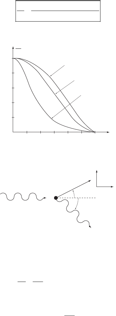
490 CHAPTER 14
(
)
(
)
()()
22222
11
22 22
11
22
11
2
11
2 cos 1 sin 2 cos 1 cos sin
sin cos cos cos
1cos cos
11cos
++ = + − +
=+ + − +
=+− +
=+−−
ψγ ψ ψγ ψ ψ
γ
ψψγψ
γγψ ψ
γγ ψ
ψ
(11)
provides us with the desired result:
()()
2
1
2
01 1
2cos
11cos
T
T
ψ
γ
γψ
=+− − (12)
Notice that the shape of the curve changes when Tm, i.e., when
2
10
c>12
γ
>.
0.2
00˚ 30˚ 60˚ 90˚
0.4
0.6
0.8
1.0
T
T
1
0
T
1
= 0.1 GeV
T
1
= 1 GeV
T
1
= 10 GeV
ψ
14-42.
φ
θ
hν
hν′
γmec2
y
x
From conservation of energy, we have
22
ee
hmc mch
ν
γ
ν
+= +
′
(1)
Momentum conservation along the x axis gives
cos cos
e
hh mv
cc
ν
ν
θ
γ
′
=+
φ
(2)
Momentum conservation along the y axis gives
sin sin
e
h
mv c
ν
γ
φ
′
=
θ
(3)
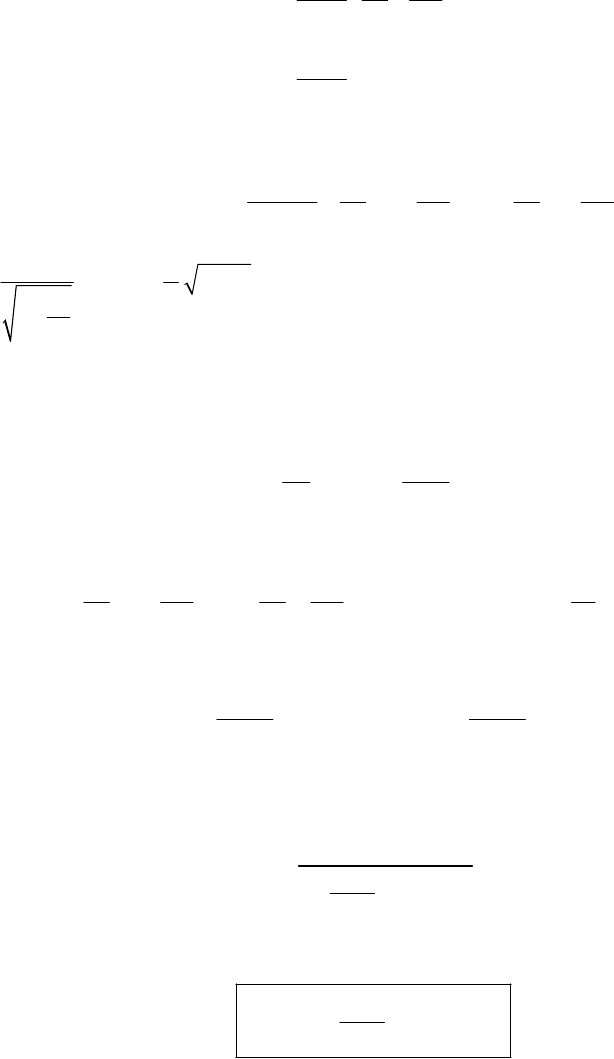
THE SPECIAL THEORY OF RELATIVITY 491
In order to eliminate
φ
, we use (2) and (3) to obtain
1
cos cos
sin sin
e
e
hh
mv c c
h
mv
νν
φ
θ
γ
ν
φθ
γ
′
=−
′
=
(4)
Then,
22
22
222
1
s sin 1 2 cos
e
hh hh
mv c c c c
νν νν
co
φ
φθ
γ
′′
+== + − +
(5)
Since 2
2
1
1v
c
γ
=
−
and 21
c
v
γ
γ
=− we have
(
)
22 2 2 1vc
γγ
=
− (6)
Substituting γ from (1) into (6), we have
() (
22
22
22
2
ee
hh
vmmc
=−+ −
)
′
′
γ
νν νν
(7)
From (5) and (7), we can find the equation for
ν
′:
()(
22 22
2
2cos2
e
hh hh h
hm
cc cc c
νν νν
)
θ
νν νν
′′
+− = −+−
′
′
(8)
or,
()
22
2
21cos
e
mc mc
hh
2
e
ν
θν ν
+− =
′
(9)
Then,
()
2
1
11cos
e
h
mc
ν
ν
νθ
=
′
+−
(10)
or,
()
1
2
11cos
e
E
EE mc
θ
−
=+ −
′
(11)
The kinetic energy of the electron is
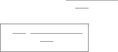
492 CHAPTER 14
()
22
2
1
1
11cos
ee
e
cmchh E E
mc
γνν
Tm
θ
=−=−=−
′
+−
()
2
2
2
1cos
11cos
e
e
E
TE
mc
mc
θ
θ
−
=
+−
(12)
