J Ops Manual

User Manual: Pdf

Open the PDF directly: View PDF .
Page Count: 46

J_Ops

Contents

1 Introduction 3

1.1 Installation ................................................. 3

1.1.1 NUKE_PATH Considerations .................................. 3

1.2 Versioning .................................................. 3

1.3 Thanks/Contributions ........................................... 3

2Plug-ins 5

2.1 J_3Way ................................................... 5

2.1.1 Introduction ............................................ 5

2.1.2 Usage ................................................ 5

2.1.3 ASC CDL File I/O Framework .................................. 6

2.1.4 Knobs ................................................ 8

2.2 J_GeoManager ............................................... 10

2.2.1 Introduction ............................................ 10

2.2.2 Usage ................................................ 10

2.2.3 Knobs ................................................ 11

2.3 J_GotSomeID ............................................... 12

2.3.1 Introduction ............................................ 12

2.3.2 Usage ................................................ 12

2.3.3 Knobs ................................................ 13

2.4 J_ICCkyProﬁle ............................................... 13

2.4.1 Introduction ............................................ 13

2.4.2 Usage ................................................ 13

2.4.3 Knobs ................................................ 14

2.5 J_MergeHDR ................................................ 14

2.5.1 Introduction ............................................ 14

2.5.2 Usage ................................................ 15

2.5.3 Knobs ................................................ 16

2.6 J_Mullet .................................................. 21

2.7 J_MulletBody ............................................... 22

2.8 J_MulletCompound ............................................ 23

2.9 J_MulletConstraint ............................................ 23

2.10 J_MulletForce ............................................... 24

2.11 J_MulletSolver ............................................... 25

2.12 J_rawReader ................................................ 26

2.12.1 Introduction ............................................ 26

2.12.2 Usage ................................................ 26

2.12.3 Knobs ................................................ 27

2.13 J_Scopes .................................................. 29

2.13.1 Introduction ............................................ 29

2.13.2 Usage ................................................ 29

2.13.3 Knobs ................................................ 30

2.14 J_ZMaths .................................................. 31

2.14.1 Introduction ............................................ 31

2.14.2 Usage ................................................ 31

2.14.3 Knobs ................................................ 32

2.15 J_ZKeyer .................................................. 32

2.15.1 Introduction ............................................ 32

2.15.2 Usage ................................................ 33

2.15.3 Knobs ................................................ 33

3 Python Scripts 34

3.1 Improved Drag & Drop .......................................... 34

3.2 DAG Bookmarks .............................................. 34

4 Release Notes 35

4.1 Known Issues/Requests .......................................... 35

4.1.1 J_3Way ............................................... 35

4.1.2 J_Scopes .............................................. 35

4.1.3 Scripts ................................................ 35

4.2 Historical .................................................. 35

4.2.1 2.3v1: ................................................ 35

4.2.2 2.2v1: ................................................ 35

4.2.3 2.1v1: ................................................ 35

4.2.4 2.0v1: ................................................ 36

4.2.5 1.0v1a9: ............................................... 38

4.2.6 1.0v1a8: ............................................... 38

4.2.7 1.0v1a7: ............................................... 39

4.2.8 1.0v1a6: ............................................... 39

4.2.9 1.0v1a5: ............................................... 40

4.2.10 1.0v1a4: ............................................... 40

4.2.11 1.0v1a3: ............................................... 40

4.2.12 1.0v1a2: ............................................... 40

4.2.13 1.0v1a1: ............................................... 41

5 3rd Party Licenses 42

5.1 VXL ..................................................... 42

5.2 LibRaw ................................................... 42

5.3 Bullet .................................................... 46

5.4 jpeglib .................................................... 46

5.5 Little CMS ................................................. 46

1 Introduction

J_Ops are a few Nuke plug-ins and python scripts which I’ve found handy and ﬁgured others might as well. More

information on them (outside of this manual), and on what’s in the pipeline can be got from the development blog

http://major-kong.blogspot.com.Anycommentsyoumayhave,bestoﬀcommunicatingviatheNuke-Users

list, or to jackbinks at googlemail.com.

Disclaimer: Although I work at the Foundry, I’m not a developer by trade, and this is something I’ve done

entirely outside of work - so don’t go to them with any issues you ﬁnd! In addition, if one of the Foundry devs

did this, I’m sure they’d do a much better job! By downloading and using the J_Ops bundle you are accepting

responsbility for any issues that may arise from their use or presence.

1.1 Installation

Grab the binary package for your platform and version of Nuke oﬀthe dev blog. Note that NDK plug-ins are

very version speciﬁc; if you get the wrong version all bets are oﬀ.

Once you’ve downloaded the resultant archive, decompress it by double clicking to extract the underlying

installer (executable on windows and linux, pkg on OSX). Double clicking that will ﬁre up a standard installer

which’ll place the ﬁles included into the standard NDK plug-in locations, as introduced in Nuke6.1.

Platform Install Location

OSX 64bit /Library/Application Support/Nuke/x.x/plugins/

Linux 64bit /usr/local/Nuke/x.x/plugins/

Windows 64bit /Program Files/Common Files/Nuke/x.x/plugins/

Where x.x is the Nuke major.minor version numbers.

Note that earlier versions installed into your .nuke directory (as Nuke 6.0 and before did not have the concept

of a standard centralised NDK plug-in location). To ensure later versions get picked up it’s best to go into your

.nuke directory and manually remove the previous version.

1.1.1 NUKE_PATH Considerations

If you install to the default directory then the related version of Nuke you launch will ﬁnd the plug-ins on start

up. If you choose a custom location in the installers, or if you use the manual install process in the OSX and

linux bundles, you will need to ensure that Nuke is able to pick up the plug-ins from that location. To do this you

need to set the NUKE_PATH environment variable appropriately. See the Nuke manual for more information

on how to do this.

Once you’re successful you should see a new ’J_Ops’ entry on the Nuke toolbar.

1.2 Versioning

J_Ops versioning has changed since the 2.0 release. Previously it followed the same manner as the Foundry’s prod-

ucts, namely: <Major>.<Minor>v<Vnumber>a/b<Alpha/Betanumber>. Now it follows the more restricted

and Nukepedia friendly <Major>.<Minor>, with a v number in use in builds themselves.

You can see you current J_Ops version by adding one of the nodes and bringing up the help. It should list

both the version and the build date and time.

1.3 Thanks/Contributions

•Everyone at the Foundry, for building the world’s best compositor, lighting tool, texture paint engine,

conform station, high tech plug-ins, and being all round excellent colleagues.

•The guys responsible for all the third party libraries in use in J_Ops (see Appendix B). I’m standing on

the shoulders of giants, without whom J_Ops would not have been possible.

•Rhys D at Filament VFX for the testing and documentation ﬁsheye shots used for J_MergeHDR.

•Matt Brealey for material used in the J_Mullet documentation and videos.

•Thorsten Kaufmann for development and test depth and ID renders.

•Andrew Hake & Rob Elphick for the Op icons.

2 Plug-ins

2.1 J_3Way

2.1.1 Introduction

J_3Way is an NDK plug-in oﬀering quick, artist friendly grading via an on screen control system, grade

interchange via the ASC CDL format, and an extensible python framework for writing extra I/O modules.

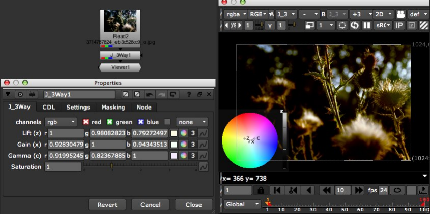
2.1.2 Usage

The J_3Way control system was designed to give you direct control over the grade whilst remaining in the viewer.

This association of control with the image canvas allows you to see the context of every decision without having

to refer back and forth between control panel and viewer.

There are three main control system interaction methods:

1. Via the virtual colour wheel interface, present in every area of the viewer except the actual colour wheel.

2. Via the actual colour wheel interface in the viewer.

3. Via conventional Nuke control panel interaction

The Virtual Colour Wheel Interface The recommended way of setting up a grade is via 1. the virtual

colour wheel interface, which can be thought of as a kind of ’poor man’s control surface’, if you will. To use this,

click over any part of the screen other than the colour wheel. At this point you can enter one of three modes -

lift, gain or gamma - by pressing z, x or c respectively.

When in a mode any cursor movement will be interpreted as a movement on a virtual colour wheel, with

origin at the cursor position from which you entered the mode. Indeed, you can check out how the resultant

move looks on the actual colour wheel interface present in the lower left of the viewer window. Releasing the

current mode key again will toggle you out of that mode, and pressing a diﬀerent mode key will toggle you out

of the current mode and into the new mode associated with that key. Depressing multiple mode keys will keep

you in the current mode, and add you into the new mode as well. At this point any movement will be translated

as a move on both the mode’s colour wheels. This swift method of mode shifting allows you to rapidly bounce

between the lift, gain and gamma parameters, tweaking each so as to balance other and obtain the desired grade.

When in any mode, a number of modiﬁer keys can be held down so as to alter the impact of the current move,

namely:

Shift - to gear up the change caused by the mouse movement, ie making a mouse move have a greater impact

on the colour change

Ctrl/Cmd - to gear down the change caused by the mouse movement, ie making a mouse move have a lesser

impact on the colour change

Ctrl/Cmd+Shift - to temporarily ignore all mouse moves. Useful when you’re getting close to the edge of the

Viewer and want to continue adjusting the colour.

Alt - to interpret the mouse move as a luminance shift, rather than a hue/saturation colour wheel shift. Vertical

moves are taken into account.

For you keyboard junkies, when in a particular mode you can also use the standard Nuke nudge keys (ie the

numpad), coupled with the above modiﬁers, in place of the mouse to cause colour adjustments.

I’d thoroughly recommend a trackball when working with J_3Way and the virtual colour wheel interface, it

just feels better!

Note, due to the overlay capturing all input mouse action when the J_3Way control panel is open, there is

shift compared to general Nuke plug-in overlays in that the virtual colour wheel will only capture mouse input

when the J_3Way control panel is currently selected. This means if you have multiple control panels open you

can still interact with the other panel’s in viewer controls by deselecting J_3Way. To return selection, either click

on the control panel, or click on the actual colour wheel drawn in the Viewer.

The Actual Colour Wheel Interface As you’ve probably noticed, you can also pick up the handles in the

hue/saturation colour wheel and the luminance slider present in the Viewer when the J_3Way control panel

is open. This allows direct interaction, and the ability to set a handle to a particular colour. The handles are

identiﬁed by the mode hotkey printed next to them, and highlighted in the selected colour speciﬁed in the settings

when selected via a mode hotkey.

GPU Engine J_3Way implements a gpu engine inside of the Nuke glslang framework, meaning if you can

satisfy the caveats following you can set up Nuke so that J_3Way gives you lightning fast feedback.

•You need a meaty enough gfx card in your machine. If you see an error message in the terminal regarding

your graphics card not supporting ﬂoat or half ﬂoat it means you probably don’t.

•J_3Way needs to be the last thing in the tree, ie, hook it up directly to the Viewer. Anything inbetween

J_3Way and the viewer will break the gpu concatenation inside of Nuke, and the gpu engine will not be

called.

•You need an early adopters mindset :) . This is a very new part of Nuke (read: quite shonky) and you’ll

intermittently get things like the Viewer not updating when it should. If this happens kill the viewer and

open a new one.

To use the gpu engine, hook up J_3Way to the viewer as described, open the viewer settings and switch bit depth

to half-ﬂoat, and toggle on ’use GPU for viewer...’ and ’use GPU for inputs...’.

Using J_3Way as part of Viewer Lookups If you’ve been communicated a look/grade via a cdl ﬁle you

may wish to employ J_3Way in some form of viewer lookup conﬁguration. Check out the Nuke manual regarding

VIEWER_INPUT and ViewerProcess handling for more information on the standard Nuke methods to do this.

2.1.3 ASC CDL File I/O Framework

J_3Way implements an extensible python framework, allowing for import and export of ASC CDL ﬁles. Currently

it supports CDL and CCC XML ﬁle import, and thanks to the framework you can extend this to any ﬁle type

which you can parse via python. Obviously it’s taken a bit of eﬀort to implement this in such a manner, rather

than simply hiding it underneath the hood, so what I do ask is if you do add support for new ﬁle types and are

able to share it, then drop the amended/new python ﬁles in an email on the Nuke-Users list. It’ll give you a warm

fuzzy feeling of contributing back, and I’ll of course credit to you in the documentation. Also, feel free to clean

up my frankly shocking python code and drop that back :)

To import a CCC or a CDL ﬁle, simply go to the CDL tab, select the ﬁlename in the ﬁle knob, then hit ’Import’.

Note this’ll overwrite your current J_3Way settings, but if you decide the import was a bad idea, a judicious

undo will get you back to pretty much where you started. Note that the ASC CDL does not deﬁne a source

colour space explicitly, so you’ll need to check the description ﬁeld for if the grade conveyed should be applied

to the footage in question in Nuke’s linear space, or some other colourspace. Often toggling on raw/switching to

linear on the source read will get you the result expected.

Implementing your own CDL Import/Export The python framework for J_3Way is all contained within

the /J_Ops/py/J_Ops/J_3Way/ directory, situated wherever you chose to install the plug-ins. The following is

a breakdown of what the existing ﬁles do:

J_3Way.py contains the main entry functions from the plug-in. J_3Way will call either importCDL() or ex-

portCDL() within here in response to an appropriate button push on it’s control panel.

parseCCC.py implements the simple colour correction import XML parser. It’s a good starting point to look at

if you want to write your own I/O module.

parseCDL.py implements the somewhat more complex colour deicision list XML parser. This makes use of

the CCC parser when it hits a ColourCorrectionRef entry, which if you’re looking to implement

EDL/ALE/FLEX parsing is probably something you’ll hit

CDLUtils.py provides a general dialogue panel, as used by parseCCC and parseCDL, providing the user with the

ability to select the appropriate ColorCorrection/ColorDecision entry. It also implements the parent

class of both parseCCC and parseCDL, containing a number of shared functions.

__init.py__ contains module import functions

The following is the basic order of events:

1. J_3Way calls importCDL() or exportCDL() in J_3Way.py in response to a button push by the user. It

grabs the extension and picks a parsing module based on that.

2. J_3Way.py creates an instance of the parser (from parseXXX.py), calling the parse() main entry function,

passing it the ﬁlename entered.

3. parseXXX.py grabs the set of colour correction identiﬁers out of the ﬁle and stores them in a local dictionary

called ’colourcorrectionvalues’

4. parseXXX.py creates an instance of the parseDialogue in CDLUtils. The dialogue grabs the list of identiﬁers

from the parser and displays as an enumerated list

5. The parseDialogue calls the parseXXX.py’s parseElement method, passing the currently selected ColorCor-

rection identiﬁer. The parser then goes back to the ﬁle and ﬁgures out the description and colour correction

settings related to that identiﬁer. It pops these in the colourcorrectionvalues dict also, and returns to the

parseDialogue which grabs the values and displays them.

6. The dialogue awaits input. On an identiﬁer change it calls the parser again, as in step 5. On an ’ok’ or

’cancel’ click it returns to the parser, which, if necessary, sets the target knob values.

There’s a few more shennanigans involved to get the CCC by ref id, and corresponding knobs working, which can

be checked out in more depth in the code itself. So, to create your own module you’ll need to:

1. Create a new python module, named in line with the others and add to the relevant imports.

2. Edit J_3Way.py to cause your module to be called by the appropriate ﬁle extension is found.

3. Implement the parse, parseID and parseElement functions.

4. Fiddle around with it til it works.

More information on the ASC CDL formats and speciﬁcation is available from the very friendly people over at

the ASC on asc-cdl at theasc.com

2.1.4 Knobs

J_3Way Tab Contains common knobs for driving the look of the grade applied.

channels - Channel selector, inherited from NukeWrapper. Allows you to pick which channel the grade is

applied to. Note that the gpu engine does not support this, and will always apply its grade to the base

RGB channel, so if you’re working on a non base layer you’ll need to switch oﬀthe gpu processing

path in your viewer settings.

Mapping - Drop down list which speciﬁes how the lift, gamma and gain knobs are translated to the ASC

CDL values used by the underlying transfer function. The ’Lift/Gamma/Gain’ option uses the DI

standard mapping found on most grading systems, the ’ASC direct’ option maps directly (so lift=oﬀset,

gain=slope, and gamma=1/power), so oﬀering more ’compositor’ style interaction.

Clamp - Bool knob (checkbox) governs whether the underlying algorithm performs the clamps speciﬁed

by the ASC CDL speciﬁcation. Their transfer functions include clamps which limit pixel values to the

0.0 to 1.0 range after both the SOP (Slope, Oﬀset, Power) and the Sat operations. This toggle allows

you to switch oﬀthese clamps so as not the clamp the pixel data. Bear in mind, with this switched

oﬀthe result is not CDL compliant!

Lift/Gamma/Gain - Colour knobs to specify your grade. They are translated to ASC CDL values as

listed on the CDL tab, which are then used to calculate the resultant image via the CDL speciﬁed

transfer functions. There are three main ways of altering the values of these: -Using Nuke standard

<childish snigger> knob manipulation </childish snigger> actions, such as typing directly into the

value box, dragging sliders, alt+numerical drag and cursor keys. -Using the on screen colour wheel.

When the J_3Way control panel is open all three values are depicted in the viewer colour wheel and

luminance slider overlay. They are identiﬁed by the letters associated with them on the parameter

panel (ie lift=z, gain=x, gamma=c), and can be picked up and dropped at will. -Using the on screen

interaction tools, which is the recommended way of altering the parameters. Once the viewer has focus

(ie click on it) you can then toggle into lift, gain or gamma mode by pressing the associated mode

hotkey. For example, press z to toggle into lift mode, at which point any mouse move will be interpreted

as a movement on a virtual colour wheel (ie Hue and Saturation change), updating the image, and the

colourwheel overlay, as you go to show you the result of the current colour grade. Pressing z again will

toggle you out of lift mode. Alternatively, you can press x to switch to gain, or shift+z to add gain

to the current virtual colour wheel, so as to alter lift and gain simultaneously. Whilst in a particular

mode you can use the following modiﬁers to alter the action of the mouse move: -Shift - gear up speed

of move -Ctrl (win/linux)/Cmd (OSX) - gear down speed of move -Ctrl/Cmd + Shift - any mouse

move should not be translated to a parameter change. Use to temporarily move the cursor around the

screen without altering the params. -Alt - interpret vertical move as a luminance change Instead of

using the mouse, you can also use the keyboard nudge keys (ie numpad) to alter the current mode in

a particular direction, again using shift and ctrl/cmd keys to gear up and down.

Saturation - Float slider. speciﬁes the saturation change to your image. Directly linked to the ASC CDL

saturation knob on the CDL tab, and only supported by ASC CDL rev 1.2 and above. Single value

slider as the ASC CDL only speciﬁes a single value saturation function. Valid when >= 0.

CDL Tab Contains knobs related to the ASC CDL I/O handling and the underlying algorithm.

CDL File File knob used to specify the source/destination ﬁle for the import/export operations.

Import Python script knob which ﬁres oﬀthe python import framework. Currently supports CCC and

CDL XML formats. See the Python I/O framework section for more information on extending this.

Export Python script knob which ﬁres oﬀthe python export framework. Currently unimplemented. See

the python I/O framework section for more information on extending this.

Oﬀset/Slope/Power - Colour knobs specifying the underlying CDL grade. Translated from lift/gain/gamma

parameters as a result of any changes. Can be set manually, which’ll correspondingly set the lift/gain/gamma

params.

Saturation - Float knob specifying the saturation change to your image. Directly linked to the saturation

knob on the front tab. Single value slider as the ASC CDL only speciﬁes a single value saturation

function. Valid when >= 0

Settings Tab This tab contains params which alter the operation of the J_3Way node. If you want to make

any changes persistent, make use of Nuke’s Knob_Default functionality, which is documented in the Nuke

manual.

Trackball/Mouse Group Contains knobs related to tweaking the operation of the mouse driven on screen

virtual colour wheels.

Sensitivity - Float slider specifying the ratio between mouse moves and the corresponding move on

the virtual colour wheel/slider . If you’re ﬁnding you don’t have enough precision, or indeed, too

much precision, use this to alter it to your needs.

Gear Up - Float slider specifying the additional ratio invoked by holding down shift whilst altering

the grade via the virtual colour wheel.

Gear Down - Float slider specifying the additional ratio invoked by holding down ctrl/cmd whilst

altering the grade via the virtual colour wheel.

Keyboard Group Contains knobs related to tweaking the operation of the keyboard driven on screen

virtual colour wheels.

Nudge Group Contains knobs related to tweaking the sensitivity of the keyboard nudge keys.

Sensitivity - Float slider specifying the ratio between nudges and the corresponding move on the

virtual colour wheel/slider . If you’re ﬁnding you don’t have enough precision, or indeed, too

much precision, use this to alter it to your needs.

Gear Up - Float slider specifying the additional ratio invoked by holding down shift whilst al-

tering the grade via the virtual colour wheel.

Gear Down - Float slider specifying the additional ratio invoked by holding down ctrl/cmd whilst

altering the grade via the virtual colour wheel.

Interface Group Contains knobs related to tweaking the appearance and behaviour of the colour wheel/luminance

slider overlay.

Backdrop - Colour knob altering the colour of the background box.

Selected - Colour knob specifying the colour to draw the point(s) currently selected via their mode

hotkey.

Unselected - Colour knob specifying the colour to draw the point(s) currently not selected via their

mode hotkey,

Size - Float knob specifying the size of the colour wheel interface in the Viewer.

Colour Wheel Rotate - Float slider specifying how much to rotate the hue on the colour wheel

overlay. This allows you to match the Hue/Saturation wheel to other packages. It defaults to 0.7

which matches the standard vectorscope graticle (such as that in J_Scopes), 0 makes it match

Nuke. Valid 0.0 -> 1.0.

Viewer Exit Toggle - Bool knob (checkbox) governing whether J_3Way toggles out of any current

virtual colour wheel mode when the cursor leaves the Viewer. For example, if you are in z (lift)

mode, then move the cursor out of the viewer, if the Viewer Exit Toggle is on, it’ll cause the lift

mode to switch oﬀ. If it the Viewer Exit Toggle is oﬀthen you’ll stay in lift mode, and whenever

the cursor re enters the viewer it’ll return to making changes to the lift knob.

Masking Tab Nuke standard masking knobs, inherited from NukeWrapper. See the Nuke manual for more

details.

Node Tab Nuke standard node knobs. See the Nuke manual for more details.

2.2 J_GeoManager

2.2.1 Introduction

J_GeoManager is a 3D utility tool providing both information on the fed in 3D scene and enabling stripping

of objects and/or attributes from the stream, from the point of view of troubleshooting badly rendering or heavy

scenes. For example, in the circumstance where you’re reading in all objects in an fbx (to get the full transform

tree), but don’t actually need most of them, J_GeoManager will allow you to strip out those you don’t want

fed further downstream. Info provided includes point and vertex counts, presence of materials, transforms and

attributes including, but not limited to, the various object’s normals and UVs.

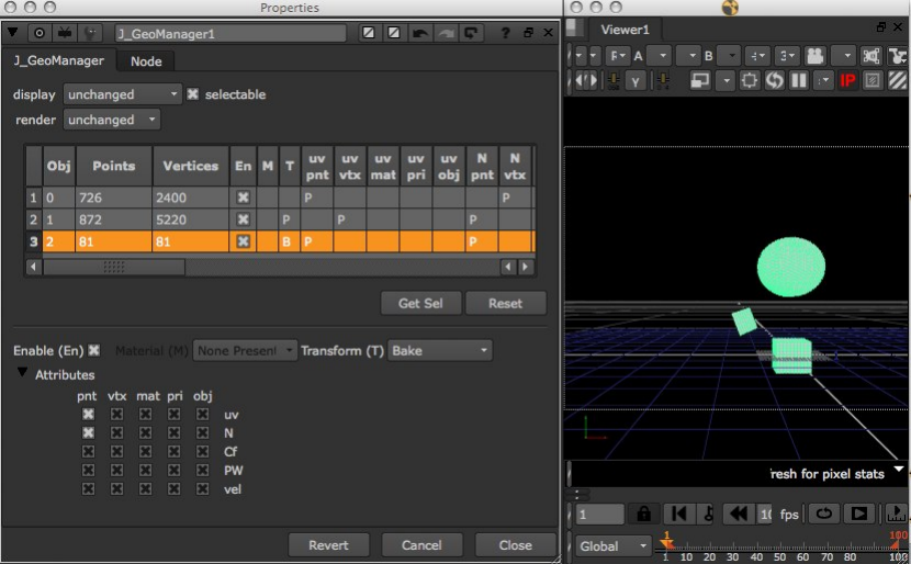
2.2.2 Usage

Basic usage involves adding the node after the 3d nodes for which you wish to see the resultant info from and/or

strip data. Ensure the viewer is hooked up downstream to pull data through the node, which’ll in turn populate

the main table knob geolist.

Nuke Objects & Attributes The geolist knob is the heart of the GeoManager plug-in, displaying data on

both the incoming scene and on the settings made to alter it, where each row equates to an object in the scene.

In Nuke, an object will have a variety of semi static data associated with it (it’s point and vertex data, whether it

has a material or a transformation matrix associated and so on), as well as an arbitrary array of ’attribute’ data.

Attributes are associated with one of the object’s semi static data groups (ie the attributes can be attributable

to the point data, the transformation matrix, etc), and have a name label. So, for example, the UV data on an

object can be present on the points or the vertices, dependant on the level of complexity required. J_GeoManager

shows the 5 standard Nuke attributes (N - normals, UV - uv texture, Cf - colour, PW - world position, and vel

for velocity) and each one can be attributable to up to 5 of the groups (namely 25 diﬀerent combinations). The

geolist table contain columns for everything from object IDs, point and vertex data counts, through the range

of attributes to the presence of materials and transformation data.

Editing Scene Data & Stripping Objects & Attributes Using the checkbox toggles in the En column of

the geoinfo table knob it is possible to selectively remove objects, however more detailed or selective changes

require use of the ’per row’ knobs found under the table. These are selectively enabled and disabled depending

on the current row selection in the geoinfo table. For example, to disable multiple objects simultaneously, select

their respective rows in the table and then toggle oﬀthe Enable (En) knob in the per row knobs (see below info

on how to select these by selecting their in viewer representations). Similarly, if you want to zero out a particular

attribute (an attribute in Nuke town being a piece of arbitrary data associated with one of the either the object’s

points, vertices, etc - for example an object’s UVs), you’d select the object’s row in the table, go down to the per

row knobs and toggle oﬀthe respective checkbox in the attribute table. If you cock something up you can easily

reset one or more rows by selecting them and using the Reset button.

Baking Transform Data For the ma jority of the scene data that can b e aﬀected (ob jects, attributes, ma-

terials, etc) the options are either to allow it through (ie Passthrough, or P) or to strip it (ie Zero, or 0). If

an item is not present in the incoming stream it’ll be signiﬁed either with None present or a blank space. For

transform data you can additionally elect to Bake, or B, the matrix. By default a transform associated with an

object will be carried as an extra local-to-world transform matrix alongside the point data - by baking this data

you’re able to set this extra matrix to identity and pre-emptively apply it’s previous transform data onto the

mesh points themselves. This can be handy in those circumstances where the matrix data isn’t being accounted

for, for whatever reason.

Selecting Table Rows From Viewer Selections By default it can be tricky to relate rows of object data

back against the object representations seen in the viewer. To make this much easier, ﬂip the viewer geo selection

tool into object mode, toggle on the object(s) in question you want highlighted in the geolist table knob and

then hit the Geo Sel button on the param panel.

2.2.3 Knobs

Are all documented through Nuke’s extensive tooltip system. Fire up the tool and hover over the knob in question

to get more information.

2.3 J_GotSomeID

2.3.1 Introduction

J_GotSomeID is a utility tool allowing fast and easy extraction of mattes and premulted channelsets from

ID/Object passes from 3D, taking into account a range of encodings of ID and coverage/aliasing data.

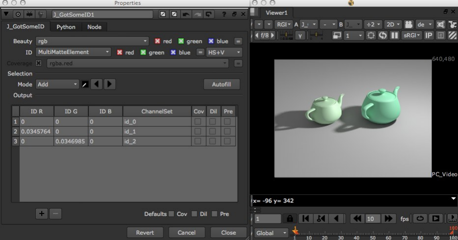
2.3.2 Usage

To get started, hook up the node to your 3d imp ort and in the ID channelset knob select the incoming ID/Object

pass. Pick its encoding in the Type drop down, then optionally pick the coverage channel in the Coverage drop

down. At this point you can start either picking a few objects manually, or use the Autoﬁll button to create

output passes for each and every object in the incoming stream and frame range. Note that if you have a lot

of IDs and you only want to grab one or two the latter unlikely to be wise, since it’ll create a lot of unrequired

channelsets and take some time.

To manually pick which objects you want channels for hook up a viewer ensure the picker is selected and

mode is set to add, then cmd/ctrl click on the objects in the scene you want output passes for. The picker will

grab the ID from the selected ID channelset automatically (regardless of what channel the viewer is set to) and

create an entry in the idlist with the selected ID, an autogenerated channelset name, and checkbox defaults taken

from the default knobs at the panel footer.

If you picked the wrong object select the entry, ﬂip the mode to edit and cmd/ctrl click on the viewer again,

thus altering its ID values in the idlist.Youcanalsoaltertheidlist values, such as the channelset name,

manually by double clicking and typing directly. To alter multiple output passes checkbox values, select the items

on the list and toggle the checkboxes at the panel footer. To ﬁnd a certain entry based on an object, ﬂip the

mode to ﬁnd and cmd/ctrl click on the object in the viewer. If a matching output pass is found it’ll be sleected

in the idlist.Finally,toaddordeleteentriesusethe+and-buttonsatthebottomoftheidlist.

Coverage passes allow aliasing data to be passed to the compositor. The most prevalent technique is to encode

aliasing data into a separate output channel called the coverage pass. This can be used in J_GotSomeID by setting

type to a Cov type, then checking the Cov checkbox on the required output pass. Where object aliasing crosses

others this may look slightly wrong since aliasing data from one object is crossing another. Enabling Dil for an

output pass attempts to ﬁx this by dilating a fringe from the current object, ﬂipping the aliasing data found and

using this as additional falloﬀaliasing for the current object. Occasionally you may also see an ID pass where the

ID are stashed around the Hue/Saturation wheel. More occasionally in these circumstances you may ﬁnd that the

aliasing data has been stashed in the ID pass V data, as opposed to separate pass. Both of these circumstances

can be handled by selecting the appropriate entry from the type drop down.

Nuke’s channel system does not allow channelsets to be removed from the current session, thus if you add

alotofchannelsandremovethem,oralternativerenamechannelsetsalotyou’llﬁndthechannellistsbecome

populated with a lot of now defunct channelsets. Those not used in the current channel are removed when killing

the current session and reloading the script. Additionally, channelset names should be alphanumeric.

2.3.3 Knobs

Are all documented through Nuke’s extensive tooltip system. Fire up the tool and hover over the knob in question

to get more information.

2.4 J_ICCkyProﬁle

2.4.1 Introduction

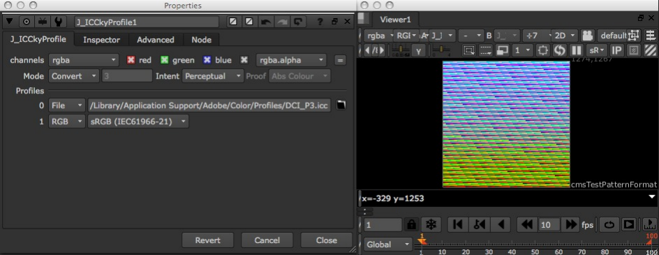
J_ICCkyProﬁle allows ICC based colourspace conversions to be applied within Nuke. This is not a magic

wand ’here’s an ICC based colour managed workﬂow inside of Nuke,’ any more than Nuke’s own Colorspace node

oﬀers a linear colour managed workﬂow; the workﬂow step requires a whole bunch of wrapping that Iop’s can’t

directly do inside of Nuke. Rather, think of it as oﬀering low level control of ICC colour conversions. To use

it eﬀectively you’ll need to have an understanding of ICC in general, as well as of Nuke’s underlying rgb linear

toolset. J_ICCkyProﬁle additionally oﬀers a proﬁle inspector, which can be used to judge what information is

being conveyed in a particular ICC ﬁle.

J_ICCkyProﬁle is based upon the lcms2 library.

2.4.2 Usage

Colour conversions inside of J_ICCkyProﬁle can be one of 4 modes - apply,convert,chain and proof.Convert

is the most standard, and allows you to specify two colour spaces, which the plug-in then converts the image data

between. Apply only oﬀers a single patch - it assumes the other colourspace is RGB linear (gamma 1.0) and

attempts to guess whether the proﬁle you specify should be used as the input or the output colourspace, based

on its metadata tags. Chain allows multiple conversions to be chained together, which can be occasionally useful

for devicelink type proﬁles. The ﬁnal, proof, allows an input output proﬁle pair, as in convert,inadditiontoa

prooﬁng proﬁle to be employed, so as to judge how the output of a particular process (which the proﬁling proﬁle

represents) will look.

Individual proﬁle patches can either be speciﬁed by an ICC ﬁle on disk (ICC direct, not embedded inside

an image ﬁle’s metadata), or from a number of RGB proﬁle presets provided directly. For further colourspace

options, such as CIEXYZ, feed through to RGB linear then employ Nuke’s own Colorspace node for the ﬁnal

step.

An ICC conversion also requires an intent to be deﬁned (or in the case of a prooﬁng transform, 2 intents).

This alters what image aspects are deemed most important, and so what the conversion attempts to preserve.

The inspector tab allows you to inspect ICC ﬁles directly, showing information on what ICC tags are

contained therein. This is very useful for troubleshooting in particular, but requires relatively speciﬁc ICC

knowledge. If you intend on using this tool extensively, and haven’t already done so, then the ICC spec, as well

as the lcms documentation are well worth a read.

Bear in mind that images are colour managed by Nuke by default, so to get close to Adobe’s colour management

you may need to switch Nuke’s to raw and use this op to manually apply such colour corrections. Also bear in

mind that this uses a diﬀerent colorimetric engine (namely lcms) to Adobe’s, since theirs is proprietary, so results

will never 100% match.

For ease of use it may be worth modelling the desired icc proﬁle by feeding a cmsTestPattern through this op

and writing out a Nuke readable 3D LUT.

2.4.3 Knobs

Are all documented through Nuke’s extensive tooltip system. Fire up the tool and hover over the knob in question

to get more information.

2.5 J_MergeHDR

2.5.1 Introduction

J_MergeHDR is a compiled NDK plug-in oﬀering a fast and eﬃcient route for combining multiple low dynamic

range images into a high dynamic range radiance map, for example, merging mirror ball shots for use in lighting

setup.

It implements:

•Debevec et al’s “Recovering High Dynamic Range Radiance Maps from Photographs,” for the response

estimation functionality.

•Greg Ward’s “Fast, Robust Image Registration for Compositing High Dynamic Range Photographs from

Handheld Exposures,” for the alignment estimation functionality.

2.5.2 Usage

Typically, a general J_MergeHDR workﬂow consists of three main steps:

1. Setting up source and target exposures.

2. Aligning the source images.

3. Estimating a camera response.

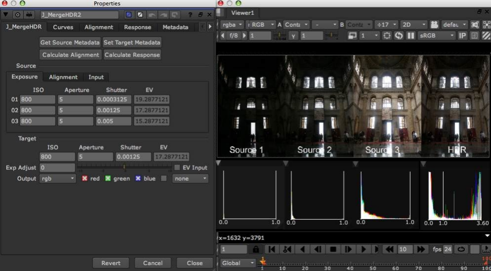
Source & Target Exposures Once you’ve hooked up the node to the various LDR images, you need to tell

J_MergeHDR what the rough exposure data for the source streams is. For any modern camera this should be

present in the metadata read in, so the ﬁrst order of the day is to hit the ’Get Source Metadata’ button. This’ll

query the source stream’s metadata looking for the keys set in the ’Metadata’ tab’s search strings. In most

circumstances the defaults should be ﬁne and you’ll now see that the source exposure parameters have been ﬁlled

in. If the search has been unsuccessful the op with error and will tell you on which inputs it was unable to ﬁnd

the metadata key strings speciﬁed. This could be down to either

a) the metadata string being wrong, in which case use a ViewMetadata node to see what the string should be,

amend it and hit ’Get Source Metadata’ again.

b) there being no metadata of the exposure data present in the source. In this circumstance you’ll have to enter

the data manually into the source ’Exposure’ panel params. Note that shutter speed is expected in seconds

(and you’re probably used to seeing it in 1/ notation). In this case simply go into the appropriate shutter

speed knob and type in ’1/<your value>’ and hit enter for Nuke to evaluate for you. If you simply dont

have the data at all you can dial in values manually by eye. In this case it’s generally easiest to switch on

’EV Input’ which allows you to dial in the EV knob directly (conventionally it’s contributed to by ISO,

shutter and aperture separately, but since you don’t know that data, you might as well cut it right out of

the loop).

The ﬁrst thing you’ll probably notice, having ﬁlled in the source metadata, is that the output’s got very white.

That’s because the target exposure default is set to unity, and in most normal circumstances your exposure

values are going to be way in excess of that. To sort that out either manually tweak down, or hit the ’Set Target

Metadata’ button. This’ll set the target exposure values to be the median of the input range, which is normally

aprettygoodstartingpoint. Youcannowmanuallydialupordownthedesiredtargetusingthe’ExpAdjust’

slider.

Occasionally this is all that is required to get an acceptable, and usable, result.

Alignment Often you’ll get source images which aren’t perfectly registered. If you’re one of the lucky ones who’s

images are already aligned then skip this stage, otherwise read on. The Alignment panel on the J_MergeHDR

tab allows you to dial in oﬀsets, in pixels, for each image in turn. Hitting ’Calculate Alignment’ will ﬁre oﬀa

process which’ll attempt to ﬁgure out these oﬀsets automatically. If the results aren’t perfect they’re normally

better, and form a good basis to subsequently tweak.

If the results are way out of whack there are a couple of params you can try tweaking on the ’Alignment’

tab. First up, ’Exclusion’ allows you to set the range of data around the image median value which is ignored

when comparing sources too each other. A higher ignore range will have the eﬀect of rejecting more noise, so if

you have particularly noisy or grainy images you can try tweaking this up. Note that going too far means it less

likely to ﬁnd a registration, so your better bet is probably to run a noise reduction pass on the images ﬁrst (note

that the response estimation is also aﬀected adversely by noise, so a reduction pass ﬁrst is probably a good idea

there as well). Max oﬀset allows you to deﬁne the search range. Great ranges take longer, and are likely to be

less robust. If you’re looking >50 pixel mark then buy a tripod, or manually set the alignment oﬀsets.

The alignment functionality only deals with translation oﬀsets. If there are rotational diﬀerences between the

frames then you’ll often ﬁnd that ﬁxing their translational oﬀsets will have the eﬀect of pushing the rotational

disparity to the edge of the frame, where it’s not particularly noticeable. If it’s still getting to you, hook up a

transform node on the aﬄicted input and ﬁx it manually. Greg Ward’s papaer, mentioned before, is a good read

if you’re looking to get more in depth with the alignment estimation functionality, in particular looking at the

diagnostic views and what they mean.

You’ll often ﬁnd that if something goes wrong, it’ll be only on one or two inputs, and ﬁnding out which ones

is tricky. On the ’Input’ panel on the ’J_MergeHDR’ tab you’ll ﬁnd a series of ’enable’ checkboxes. These’ll

allow you to selectively switch on and oﬀwhich inputs are rendering (and having the alignment estimation run

on them) and so ﬁnd the oﬀending culprits.

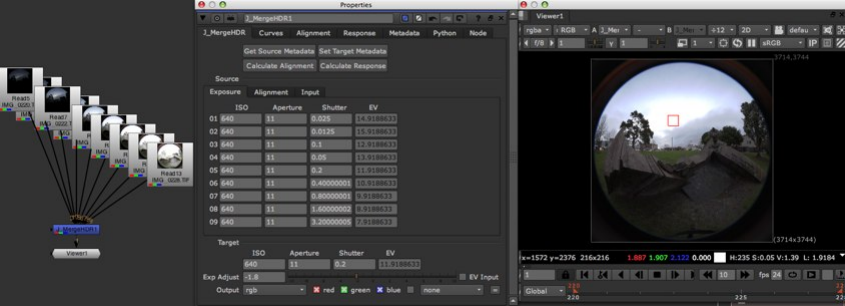
Response The ﬁnal step, if necessary, is to estimate the response curve of the camera with which a scene

was shot. Camera manufacturers (and models, and lenses, and chips, and ad inﬁnitum) have their own ideas

of what makes a perfect way to reproduce the range of data in the image down to a low dynamic range, where

direct mapping of intensity data to resultant value is generally of rather low importance. If you’re lucky the

work done thus far is enough to give a result which is suﬃcient for your needs, otherwise we’re going to have

to look at ﬁguring out a reverse of whatever mapping was applied. Now, by it’s very nature this is only ever

an approximation. Often, parts of the ’special sauce’ camera manufacturers apply can be spatially localised

dependent on surrounding luminance conditions, and a lookup mapping such as we’re trying to use to invert it

can only get so far.

The curves tab contains 4 curves. 3 for the diﬀerent colour channels of the logarithmic camera response, and 1

for the weighting curve applied both when estimating the response, and when recombining the exposures. Hitting

’Calculate Response’ will ﬁre oﬀthe algorithm described in Debevec’s ’Radiance Maps’ paper as mentioned earlier,

which’ll attempt to estimate these curves for us. The result will be used to render immediately, so you’ll get an

idea of if it’s what you need. Bear in mind you’ll likely need to tonemap the data down, or apply something like

J_Scopes, to get an idea of the resultant intensity distribution.

There are two main means by which we can impact the results. The algorithm initially picks a series of samples

from the source images (which is why it’s important they align), and then passes these sampled pixels values into

the actual solve phase. To impact the feature selection, use the knobs in the ’Response’ tab’s ’Feature’s’ group.

Check out where the features lie and if many sit on clipped, or noisy, image data try altering the seed or changing

the total number to avoid these regions. To alter the solve use the ’Response’ tab’s ’Solve’ knobs. If you have

an excessively spikey response try increasing lambda (and vica versa). If your response is too high on it’s upper

limit, try increasing the unity point up (in the range 0 to 1), and vica versa.

2.5.3 Knobs

J_MergeHDR Tab This tab contains the most commonly used knobs when setting up a HDR merge. Often,

for a basic merge, you can get away without switching away from this tab.

Get Source Metadata - a button which’ll kick oﬀa scan through the input streams current toggled on in

the channels setting and attempt to read back the source exposure metadata. It’ll report errors where

the set metadata strings cannot be found in the source stream; either alter the metadata strings to

match what is present or enter the data manually.

Set Target Metadata - a button to set the target metadata based on the median of the input data set

in ’Get Source Metadata.’

Calculate Alignment - a button which’ll execute an alignment estimation pass. This’ll attempt to calcu-

late the closest position oﬀsets for each input, needed to align it to the median exposure image in the

series. This only does a translation oﬀset, but even in the case of rotational diﬀerences, this’ll have the

impact of pushing the rotation oﬀsets to the edges of the frame. Note that results will vary, so some

manual ﬁx up may be required. Don’t run on an already registered sequence!

Calculate Response - a button which’ll execute a response calculation pass. This’ll attempt to ﬁgure out

the response curve of the camera with which the shots were originally taken. This may be taken care

of to a suitable amount via the built in Nuke linearisation, however if it’s not looking good you may be

able to improve matters by setting up a response curve in J_MergeHDR. If you do so, it is often good

to read in the shots in question as raw, and use J_MergeHDR to model the overall camera response

and linearise.

Source Divider - a grouping of knobs which largely control the data about the incoming image streams.

Exposure Panel - a grouping of knobs related to the exposure data for the incoming image streams.

ISO - a series of ﬂoat knobs, one per input, which deﬁne the ISO value for the image on the

same numbered input. This contributes to the input’s overall EV exposure value, visible in

the associated EV knob, and which can alternatively be entered directly by toggling on EV

Input.

Aperture - a series of ﬂoat knobs, one per input, which deﬁne the aperture value, in f-stops, for

the image on the same numbered input. This contributes to the input’s overall EV exposure

value, visible in the associated EV knob, and which can alternatively be entered directly by

toggling on EV Input.

Shutter - a series of ﬂoat knobs, one per input, which deﬁne the shutter speed, in seconds, for

the image on the same numbered input. Note that shutter speeds are conventionally given in

1/ speeds, as opposed to the decimals seen here. To easily enter in such a value, simply type

it directly into the knob (ie ’1/250’), and equally, invert the result to get back to your start

point. When set from metadata, this knob is set via an expression to the fraction, presuming

that it is fractional in the source metadata (as opposed to it being evaluated at set time to

a decimal). This allows you to see the original fractional value by either hovering over to

see the tooltip, or by bringing up the expression entry dialog for the knob in question. This

contributes to the input’s overall EV exposure value, visible in the associated EV knob, and

which can alternatively be entered directly by toggling on EV Input.

EV - a series of ﬂoat knobs, one per input, which deﬁne the overall exposure for the image of the

same numbered input, in EV. This can either be used as a point of reference for judging expo-

sure based on ISO, aperture and shutter measures, or can be used to enter such values directly,

bypassing the aforementioned three parameters, by toggling on the EV Input checkbox.

Alignment Panel - a grouping of knobs related to the translation oﬀsets applied to the incoming

image streams.

Input Oﬀset - a series of XY position knobs, one per input, which deﬁnes a translation oﬀset

for the input image of the same number, in pixels. Use to align images which have been

shot without a tripod. Purely translational, however setting this will also have the impact of

pushing rotational misalignments to the edge of the frame. If this isn’t suﬃcient, manually

hook up transforms to the inputs, or buy yourself a tripod. Also see the Calculate Alignment

button for setting these values automagickally.

Input Panel - a grouping of knobs related to the incoming image stream pixel data.

Enable - a series of checkboxes, one per input, which allow you to easily enable and disable that

input, and thus in turn to easily judge the impact a particular input is having on a ﬁnal

result. This is also used when calculating alignments and response functions, so if you have

a particular image which is throwing oﬀcalculations, but which you want in your ﬁnal HDR

then toggle it oﬀhere whilst working, then turn it back on at the end and do ﬁnal integration

work.

Input Channelset - a series of channelset knobs, one per input, which deﬁne what channelset

the incoming image data is living in.

Target Divider - a grouping of knobs which cover setting the related output data for the generated HDR

image.

ISO - a ﬂoat knob which deﬁnes the desired output image’s ISO, in the sense of how it contributes to

the overall target EV. Set automatically when running Set Target Metadata.

Aperture - a ﬂoat knob which deﬁnes the desired output image’s aperture value, in the sense of how

it contributes to the overall target EV. Given in f-stops and set automatically when running Set

Target Metadata.

Shutter - a ﬂoat knob which deﬁnes the desired output image’s shutter speed, in the sense of how

it contributes to the overall target EV. Given in seconds and set automatically when running Set

Target Metadata.

EV - a ﬂoat knob which deﬁnes the desired output image’s overall exposure value. The result of the

target ISO, shutter & aperture combined, as point of reference. Toggling on EV Input allows

this to be manually entered, skipping setting the consitutent parts individually, however if you’re

simply looking to manually tweak the target exposure up and down, you’re generally best oﬀusing

Exp Adjust. Set as a result of the target ISO, aperture and shutter being set when running Set

Target Metadata.

Exp Adjust - a ﬂoat knob with slider which allows you to tweak the target exposure up and down

manually, in EVs.

EV Input - a checkbox to enable or disable inputting EV values for source and target exposures

manually, as opposed to enforcing input of sets of ISO, aperture and shutter values.

Output - a channelset knob which deﬁnes the channelset to which the output high dynamic range

merge is sent.

Curves Tab This tab contains a curves graph interface, for viewing and manipulating the response estimate

calculated, and associated buttons.

Calculate Response - a button which’ll execute a response calculation pass. This’ll attempt to ﬁgure out

the response curve of the camera with which the shots were originally taken. This may be taken care

of to a suitable amount via the built in Nuke linearisation, however if it’s not looking good you may be

able to improve matters by setting up a response curve in J_MergeHDR. If you do so, it is often good

to read in the shots in question as raw, and use J_MergeHDR to model the overall camera response

and linearise.

Reset Response - a button which’ll reset the response curve, in the situation that it’s actually worse post

analysis than before, or when you’ve buggered up the response curves beyond belief by ﬁddling with

them manually.

Reset Weight - a button which’ll reset the weigh curve used in the response estimation function, and in

the high dynamic range merging. Default follows that used by Paul Debevec in ’Recovering Radiance

Maps’, however subsequent papers have advocated use of gaussian curves to soften roll oﬀ.

Curves - a lookup knob which interfaces to the response and weighting curves for the camera function and

the high dynamic range merge. Weight is used to roll oﬀthe data used in both response estimation,

and in exposure merging. Red/Green/Blue are the logarithmic response curves of the camera, used to

precorrect the exposures when merging.

Alignment Tab This tab contains params related to the alignment estimation and pre-merge translation.

Calculate Alignment - a button which’ll execute an alignment estimation pass. This’ll attempt to calcu-

late the closest position oﬀsets for each input, needed to align it to the median exposure image in the

series. This only does a translation oﬀset, but even in the case of rotational diﬀerences, this’ll have the

impact of pushing the rotation oﬀsets to the edges of the frame. Note that results will vary, so some

manual ﬁx up may be required. Don’t run on an already registered sequence!

Reset Alignment - a button which’ll reset all the inputs alignment oﬀset values to zero.

Variables Divider - a grouping of knobs related to values passed into the alignment process, both for

estimation and for translation.

Exclusion - a ﬂoat knob with slider which deﬁnes the range around the input’s median value which

is ignored when calculating a best ﬁt alignment. Higher values have the eﬀect of rejecting greater

amounts of noise, so if you have a noise sequence which isn’t aligning, try increasing this. Failing

that run a noise reduction algorithm ﬁrst (probably required as the noise’ll also throw oﬀthe

response calculation), or dial alignment oﬀsets in manually.

Max Oﬀset - an int knob deﬁning the maximum distance in pixels which you expect your images

to need to be moved to align them. Increasing will increase the time required for calculating the

alignment signiﬁcantly. Note that this is used to deﬁne the max oﬀset at the top of the underlying

image pyramid, so the ﬁnal oﬀset could be up to twice this.

Black Outside - a checkbox to insert black outsides after the incoming oﬀsets have been done. This

causes the edge repeat pixels otherwise seen in oﬀset images to be removed, and instead the

combination happens against black. Either way it’s likely you’ll have to crop the resultant image

to remove these regions.

Diagnostics Divider - a grouping of knobs allowing you to see and tweak a series of diagnostic view

renders on the underlying alignment process. Read Greg Ward’s ’Fast Robust Image Registration’

paper for more detail on what the underlying views show.

Show - a drop down and checkbox, where the checkbox toggles the diagnostic view rendering on and

oﬀ, and the drop down allows you to pick the desired view. The diagnostic views allow you to

tweak your alignment params by studying the impact of the params at the various levels of the

alignment calculation chain. MTB - Median Threshold Bitmap - red shows the selected input

partitioned around its median value, green shows the exclusion bitmap, namely the selected input

within the exclusion range, blue shows the greyscale input. XOR - red - shows the XORed MTBs

of the two source images against each other, and ignoring the exclusion range, green - shows the

exclusion bitmap, blue - shows the greyscale input.

MTB Input - an int knob enabled when MTB diagnostic view is selected. This deﬁnes which input

to show through the MTB process. Out of range or non-hooked up inputs will cause an error.

XOR Input 1 & 2 - a pair of int knobs enabled when XOR diagnostic view is selected. These deﬁne

the pair of inputs to run through the MTB to XOR process. Out of range or non-hooked up inputs

will cause an error.

Response Tab This tab contains params related to the response estimation and merge look ups. Generally you

need to work with this tab in conjunction with the curves tab to see the results of the changes you make.

Calculate Response - a button which’ll execute a response calculation pass. This’ll attempt to ﬁgure out

the response curve of the camera with which the shots were originally taken. This may be taken care

of to a suitable amount via the built in Nuke linearisation, however if it’s not looking good you may be

able to improve matters by setting up a response curve in J_MergeHDR. If you do so, it is often good

to read in the shots in question as raw, and use J_MergeHDR to model the overall camera response

and linearise.

Reset Response - a button which’ll reset the response curve, in the situation that it’s actually worse post

analysis than before, or when you’ve buggered up the response curves beyond belief by ﬁddling with

them manually.

Reset Weight - a button which’ll reset the weigh curve used in the response estimation function, and in

the high dynamic range merging. Default follows that used by Paul Debevec in ’Recovering Radiance

Maps’, however subsequent papers have advocated use of gaussian curves to soften roll oﬀ.

Features Divider - a grouping of knobs allowing you to see and tweak the feature points used in the

response estimation.

Preview Features - a checkbox to enable and disable the feature preview overlay which draws crosses

wherever a point has been picked for use in the response estimation calculation. Use this to judge

if any points have been placed badly (such as in clipped or noisy source regions) and alter the seed

to ensure this doesn’t occur.

Cross Size - an int knob deﬁning the size of the feature preview overlay crosses.

Seed - an int knob deﬁning the randomisation seed value used to place the feature samples. Alter this

to change where the samples are located.

Number - an int knob deﬁning the total number of samples used in the response calculation. More

is slower, but results in an estimate closer to the original.

Max Search - an int knob deﬁning the number of times an algorithm can ignore a selected position

if it thinks the underlying data could be poor. Set this to higher if the algorithm is picking up

ﬂat, or clipped regions. The greater the number the longer the sample setup time may take.

Solve Divider - a grouping of knobs allowing you to tweak the values passed into the response calculation

function, along with the selected feature point data.

Lambda - an ﬂoat knob deﬁning a the smoothing function run over the response estimate. The higher

the number the smoother the result, but the less likely to match the original function. Increase if

you’re seeing rough spiking, decrease if the result is overly ﬂat.

Unity Point -anintknobdeﬁningthesolveﬁxpoint. Whensolving,weneedtoarbitrarilyﬁxa

certain value on the response function to be 1. The default is modelled on Debevec’s selection in

his Radiance estimation function. Increase this if the resultant response curve upper limits are too

great, decrease if they’re too low.

Threshold Divider - a grouping of knobs allowing you to deﬁne intensity ranges of data to ignore when

both estimating the response function and when merging. Occasionally you see images with signiﬁcant

amounts of clipping, which the existing weighting curve and feature selection prediliction functions

don’t account for. For example, Debevec’s Memorial Church sequence imports to Nuke with some blue

channel clipping which throws oﬀthe resultant calculations. Using the thresholds vastly cleans up the

results.

Min - a ﬂoat knob with slider deﬁning the minimum intensity value on a per channel basis. Out of

range pixels are ignored.

Max - a ﬂoat knob with slider deﬁning the maximum intensity value on a per channel basis. Out of

range pixels are ignored.

Metadata Tab This tab contains params related to the metadata searching functions.

Get Source Metadata - a button which’ll kick oﬀa scan through the input streams current toggled on in

the channels setting and attempt to read back the source exposure metadata. It’ll report errors where

the set metadata strings cannot be found in the source stream; either alter the metadata strings to

match what is present or enter the data manually.

Reset Source Metadata - a button which’ll reset the source exposure params to their default values.

Get Target Metadata - a button to set the target metadata based on the median of the input data set

in ’Get Source Metadata.’

Reset Target Metadata - a button which’ll reset the target exposure params to their default values.

Search Divider - a grouping of knobs deﬁning the strings searched for in the source metadata.

ISO - a string knob deﬁning what metadata key value is searched for to set the ISO params for the

incoming streams.

Ap - a string knob deﬁning what metadata key value is searched for to set the aperture params for

the incoming streams.

Exp - a string knob deﬁning what metadata key value is searched for to set the exposure params for

the incoming streams.

Python Tab Nuke standard python callback knobs, found on any executable node. See the Nuke manual for

more details.

Node Tab Nuke standard node knobs. See the Nuke manual for more details.

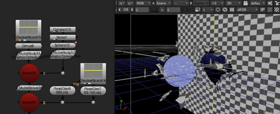
2.6 J_Mullet

J_Mullet is a suite of 5 plug-ins oﬀering rigid body physics simulation inside of Nuke, based upon the Bullet

engine. The J_MulletSolver is the core of the toolkit, performing the actual calculations, whilst the remainder

allow you to deﬁne the properties of your scene by inserting metadata into a Nuke 3D stream. At minimum you

need to add a J_MulletBody node to a geometry stream, followed up by a J_MulletSolver node. The Mullet

toolkit is mainly aimed at quick and easy physics simulations in the context of compositing, as opposed to hero

shot physics simulations. It is limited to working on a constant number of objects per scene, as well as working

on objects with properties within an order of magnitude of each other.

•J_MulletSolver. The core engine tool of the Mullet toolkit, this performs the heavy lifting when it comes

to calculating the scene interactions - every simulation needs one. It additionally allows for calculations to

be baked down to matrix knobs, so that they need not be performed again and again.

•J_MulletBody. Deﬁnes the presence of a piece of geometry within the physics scene, and allows you to

specify a range of properties, including the shape with which it should be represented (its collision shape),

the body’s weight, center of mass and more.

•J_MulletCompound. Allows physics bodies to be built from multiple pieces of geometry.

•J_MulletConstraint. Allows physics bodies to be connected to each other via a variety of joints. Addition-

ally, joints can be conﬁgured to break as a result of collisions and other force interactions. This should be

used to build more complicated networks of geometry connections that break when hit by another object,

or by a force within the scene.

•J_MulletForce. Allows forces to be added to the physics scene, and conﬁgured to act on all, or a subset of

the objects within the physics scene.

Standard usage generally consists of bringing in your scene geometry (prefractured where you want to explode or

otherwise break items), setting up a scene using the solver calculating on the ﬂy, then baking down the resultant

simulation once you’re happy with it, or when it starts to get too slow to work with. All the Mullet nodes are

extensively tooltipped, so the following per node sections are more of an introduction - see the knob tooltips for

more extensive discussions of the options available.

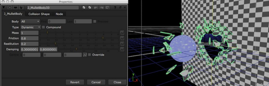
2.7 J_MulletBody

J_MulletBody is part of the Mullet toolset which oﬀers rigid body dynamics simulation within Nuke’s 3D

scene. J_MulletBody inserts metadata into the stream conveying an object’s desired characteristics. To have any

aﬀect it needs to be followed with a J_MulletSolver node which will actually does the heavy lifting of simulating

the scene together. Each incoming object selected can either be individually set to be a physics world body, or

they can be grouped together to become a single compound body which interacts together as a group.

Abodyinthephysicsworldisrepresentedbyasetofcharacteristicsroughlyapproximatedtorealworld

physical properties (such as mass and friction) along with a collision shape. Generally the collision shape is a

simpliﬁed version of the actual object, allowing faster simulation of interactions.

Body Characteristics The ﬁrst tab allows you to select a range of incoming objects and deﬁne whether each

or all represent a single body and whether than body is a dynamic,kinematic,orstatic.Foreaseofscript

reading the current body type is automatically shown on the node’s label. A dynamic body is subject to all

applied forces, constraints and interactions, whilst kinematics and statics are simply part of the scene with which

dynamic objects can collide. Kinematic bodies will update their position to match the source, whilst statics are

stuck at their initial position at the simulation start frame.

Additional characteristics include the body’s mass, centre of mass, friction, damping and bounciness.

Collision Shape The second tab governs the body’s collision shape. An object can be modelled as a sphere,

cube or convex hull, where complexity of shape is traded oﬀagainst speed of simulation. Again, for ease of

script reading the selected type is shown on the node’s label by default. J_MulletBody defaults to convex hull,

for ease of setup, however if you can mimix your object by one of the simpler options you should. Convex hulls

can also (and are by default) be automatically decimated for speed. Spheres and cubes use the bounding box to

deﬁne their sizing, however this can be overridden.

AcollisionshapeadditionallydeﬁnesaMargin, deﬁning when it starts to collide with surrounding objects.

Often to get a good looking interaction between objects you need to override and tweak this for both objects

involved with the collision.

If you are seeing odd interactions between objects it is possible that your collision shape is not closely enough

mimicking your object. Try switching on J_MulletSolver’s troubleshooting overlay, looking at the wireframes in

particular to see how closely they match the actual object.

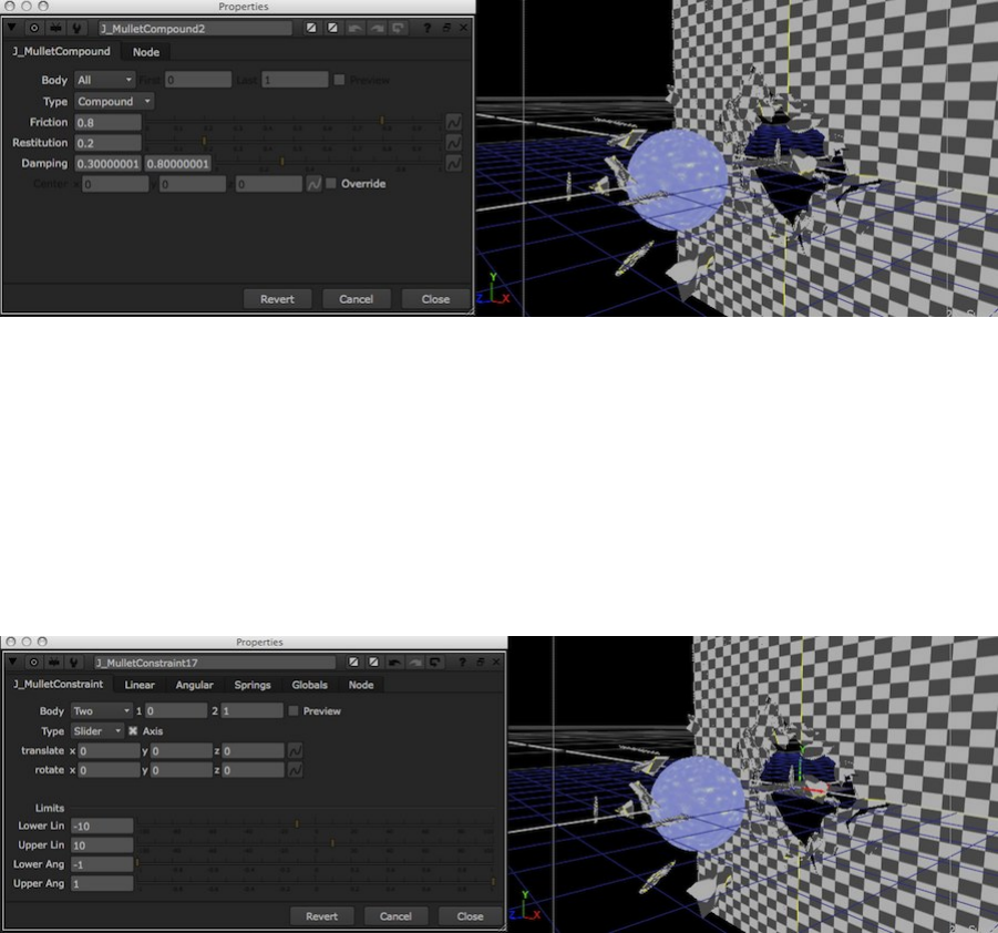
2.8 J_MulletCompound

J_MulletCompound is part of the Mullet toolset which oﬀers rigid body dynamics simulation within Nuke’s 3D

scene. J_MulletCompound inserts metadata into the stream conveying how objects should be grouped together.

To have any aﬀect it needs to be followed with a J_MulletSolver node which will actually does the heavy lifting

of simulating the scene together.

Incoming objects need to have already been deﬁned as bodies inside the physics scene, using J_MulletBody,

and indeed, in many cases J_MulletBody is capable of performing the compound grouping as well.

J_MulletCompound is of use when you want to group together multiple groups with diﬀerent collision shapes

in a single compound (though note that they must all be of a dynamic body type).

2.9 J_MulletConstraint

J_MulletConstraint is part of the Mullet toolset which oﬀers rigid body dynamics simulation within Nuke’s

3D scene. J_MulletConstraint inserts metadata into the stream conveying data about linkages between objects,

allowing them to be coupled together, or to absolute positions within the scene. To have any aﬀect it needs

to be followed with a J_MulletSolver node which will actually does the heavy lifting of simulating the body

interactions, as well as with relevant bodies on which to act.

Body Pairing A single J_MulletConstraint node can be conﬁgured to ﬁx a single object to an absolute position

in the scene (One), a pair of objects to each other (Two), all objects to their positions in the world (All-Lone),

or set up a network of linkages between each object and it’s nearest x neighbours (All-Pair).

Fix Positions Depending on the Body pairing a constraint may require an absolute position to be deﬁned

to act as the point to which the body is ﬁxed (using translate,rotate and/or the on screen widget), it may

dynamically calculate the position from the midpoints of the objects involved, or it may oﬀer you the choice of

either via Axis.

Constraint Types A constraint can be one of a number of types, which oﬀer increasing levels of control over

the degrees in which the attached objects can move around each other, and have motors or springs applied. See

the Type tooltip for a full breakdown. For script legibility the currently selected type is shown in the node’s

label.

Motors & Springs Motors allow a constraint to act as an engine, driving movement into a scene. They can

be conﬁgured to act along or around axes of motion (depending on the constraint Type). Springs, as you would

expect, allow the axes of movement some degree of ﬂexibility, and are only available on the 6DOF constraint

Type

Breakable Constraints Often it is desirable to allow a network of constraints to hold a set of objects together

until a certain collision occurs, or level of force is applied. Breakable constraints allow exactly this, and the

breaking point can be deﬁned with both a Break threshold and an additional level of random Varianceto

introduce realistic looking delays in splitting into larger constraint networks.

Compound Bodies J_MulletConstraint is set up to operate on scene objects rather than physics world bodies.

As such the body selection dialog’s 1and 2work in object IDs. If you have already combined multiple objects

into a single compound body then any constraint set up between individual objects in that body will be ignored.

2.10 J_MulletForce

J_MulletForce is part of the Mullet toolset which oﬀers rigid body dynamics simulation within Nuke’s 3D

scene. J_MulletForce inserts metadata into the stream conveying data about forces within the scene. To have any

aﬀect it needs to be followed with a J_MulletSolver node which will actually does the heavy lifting of simulating

the body interactions.

Force Types J_MulletForce allows you to deﬁne a force from a number of diﬀerent types, including direc-

tional,point,turbulence,rotational and positional, with a varying array of controls for each. All force

types include an animatable Strength parameter which allows for easy varying forces. A number of force types

also expose an in viewer widget allowing the force to be quickly and easily altered by directly operating on your

scene. For script readability the currently selected force type is shown on the node’s label.

Inputs Plugging a J_MulletForce into a physics scene by default means it’ll aﬀect every object within the

scene. You can opt to Filter,meaningthattheforceisonlyappliedtotheobjectspresentontheprimaryinput

which are fed through to the scene.

By deﬁning a scene on the Vol,orvolume,inputyouareabletolimittheforcetoonlybeappliedinsidea

certain spacial volume.

The Pnt,orpoint,inputisoptionallyusedbyanumberoftheforcetypestodeﬁneapositionin3dspace(for

example to source the force from). It expects an Axis or an Axis derived node (such as Camera) for its input.

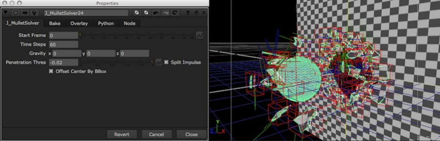
2.11 J_MulletSolver

J_MulletSolver is the engine tool of the Mullet toolkit, allowing rigid body dynamics simulation within Nuke’s

3D engine. The remaining tools in the suite simply insert metadata into the stream which is utilised by the solver

to govern how the object interaction takes place. No J_MulletSolver in your scene means no simulation will take

place, as does no metadata inserting tool, such as J_MulletBody, since the solver will not know that a dynamic

body exists.

A scene can contain dynamic, kinematic and static rigid bodies, which can be connected together (or to

absolute positions in the scene) via systems of constraints, and acted on by forces. Bodies can be arranged into

compounds, which enable them to behave as a single entity.

The Mullet toolkit is mainly aimed at quick and easy physics simulations in the context of compositing, as

opposed to hero shot physics simulations. It is also limited to working on a constant number of objects per scene.

Introducing or removing objects during the simulation range will result in undeﬁned behaviour; don’t do it. If

you need to allow an object to interact only after a certain range of time there are a number of options, including

suspending it out of shot on a kinematic body which is moved out the way, on a breakable constraint which is

broken using a suitably sized force, or applying an invisible texture up to a certain frame.

The Mullet toolkit uses the Bullet physics simulation library underneath the hood, which establishes a number

of limitations on the type of scene that it can model. The simulation engine is designed to simulate interactions

between bodies of size and mass within an order of magnitude of each other. As such it will not provide a realistic

representation, for example, of a tiny, light, fast moving body (for example a bullet) hitting a slow, heavy, large

object (such as a tank)

Controls Overall scene characteristics are controlled via the front panel. Baking,orpositioncaching,is

available through the second tab, and a Debug overlay, showing the scene as constructed by the engine so as to

allow easy troubleshooting is available on the third.

Baking By default the engine is run dynamically, at render time, by the solver node. For large scenes, or where

the resultant scene and render is being extensively worked with, this can prove to be a large overhead. In most

normal circumstances once you’ll want to start baking down the results either during or soon after completing

your dynamics simulation.

IDs & Hashing Nuke uses hashes to track the ’ﬁngerprint’ of the current node graph, and so to ﬁgure out

when knobs/reads/etc change and a rerender is required. For 2D there’s a single hash, but for 3D there are a

range, depending on which part of the 3D structure (point positions, object positions, UVs, etc) need to change.

Unfortunately some of these 3D hashes, depending on the ops in use, are not the most stable and may change from

one script load to the next. J_MulletSolver identiﬁes whether the current Bake cache is valid using combinations

of these hashes as an ID. If the solver simply used the relevant hashes you’d unfortunately ﬁnd that, thanks to

the lack of robust hash consistency, it would randomly start reporting the Bake cache as invalid from one script

load to the next. Instead, the Bake ID Strategy group oﬀers control over how various parts of the incoming

scene and settings are combined.

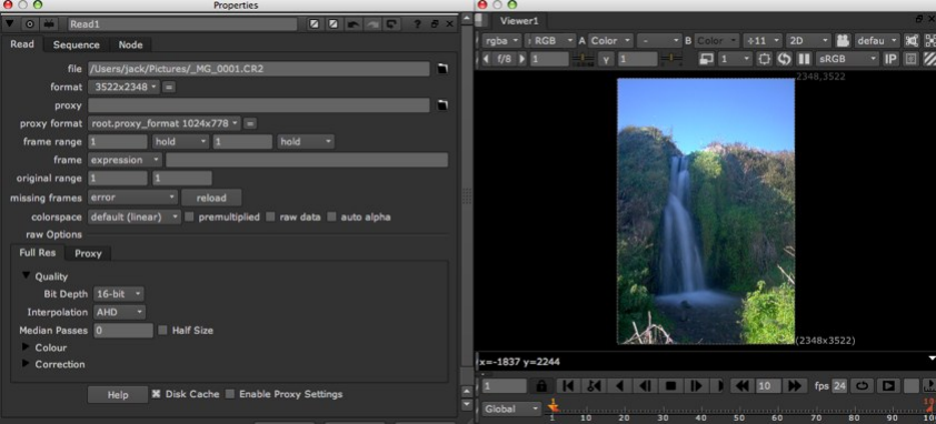
2.12 J_rawReader

2.12.1 Introduction

J_rawReader is a rewrite of the NDK example crwReader which supports the reading of a variety of SLR raw

camera formats. Whilst the crwReader utilises the third party DCRaw command line application thus requiring

additional tools to be installed, J_rawReader uses the rather awesome LibRaw to do the heavy lifting, making

it faster and more robust than the crwReader. Additionally, J_rawReader implements a ﬂexible RAM and disk

caching system to speed up your workﬂow, along with a progress feedback system to keep you up to date with

what its doing. Additionally it injects metadata from the raw ﬁle into the stream, allows extensive control over

the underlying raw negative development process, and adds redirects (ie support) for Nikon and Panasonic raw

formats plus Adobe DNG, in addition to the already present Canon support.

2.12.2 Usage

First oﬀ, note that a link to create a ’J_rawReader’ doesn’t appear in the J_Ops toolbar; as with any other

ﬁlereader in Nuke it is created by adding a read node and attempting to read a ﬁle of the type supported by the

reader. Currently ﬁles of the types ’crw’ ’cr2’ ’dng’ ’nrw’ ’nef’ and ’rw2’ will cause a J_rawReader to be used.

If there is another ﬁle type which you know can be read by DCRaw, and which you want to use, then drop a

request onto the nuke users list asking me to add a redirect.

Debayering is a slow process, however J_rawReader’s RAM and disk caching system should ensure that it

only happens when required. When you see a progress bar appear it’s likely that it’s having to go through this

process. Note that the disk caching mechanism is fairly disk hungry, so the larger you’re able to set your cache

preferences, the better it’ll perform.

The disk cache may occasionally get confused (particularly when the cache is shared between platforms).

You may see errors pop up about not being able to read or write the cache. In this circumstance, use the

Render->Clear Disk Cache function, followed by a reload on the Read node itself.

J_rawReader will attempt to read metadata from the input ﬁle and insert it into the metadata in the stream.

It’ll use the exif namespace for data which maps to an exif counterpart (currently limited to the exposure data

used by J_MergeHDR), and a raw namespace for all remaining data it is able to extract. Append a viewmetadata

to see the resultant data.

J_rawReader exposes a range of knobs to allow you to tune to underlying raw negative development process

to your needs, even to the extent of setting up proxy decode parameters separately to full res. LibRaw is based on

DCRaw, so if you’re familiar with the DCRaw ﬂags you’ll ﬁnd they largely have direct mappings to the LibRaw

controls exposed. The development controls are divided into three main groups - quality, colour (inc white balance,

histogram based corrections and manual corrections) and artefact correction. The knobs are described in more

depth in the following section. For more information on DCRaw, the tool upon which LibRaw is based, and the

ﬂags available see the DCRaw homepage available at http://www.cybercom.net/~dcoffin/dcraw/.

2.12.3 Knobs

Read Tab Contains the standard read knobs, followed by

raw options separator

Full Res/Proxy tabs duplicated tab groups, allowing the underlying raw development parameters to be

set diﬀerently. You’ll need to use the ’Enable Proxy Settings’ checkbox to enable the Proxy tab controls.

Quality group grouping of knobs related to the quality of the underlying raw development process.

Bit Depth enumeration knob allowing to pick 8 or 16 bit processing. Note both are ﬁxed integer

types; ﬂoat buﬀers in the underlying development process are not currently supported by the

underlying LibRaw engine. Equivalent to DCRaw’s -6 ﬂag.

Interpolation enumeration knobs specifying the debayering interpolation method, in rough order

of decreasing speed and increasing quality. Equivalent to DCRaw’s -q ﬂag.

DCB:Iterations int knob enabled when interpolation is set to DCB, specifying the number of

DCB correction passes to be run. Default of -1 equates to no impact. Note additional correction

passes can take a long time. No DCRaw equivalent.

DCB:Enhance checkbox enabled when interpolation is set to DCB, specifying whether to run

DCB colour enhancement interpolation. No DCRaw equivalent.

Median Passes int knob specifying the number of iterations of a 3x3 median ﬁlter to run on the

R-G and B-G channels to help clean up colour artefacts. Equivalent to DCRaw’s -m ﬂag.

Half Size checkbox allowing the underlying development to be run at half size, to increase speed.

Only recommended for use in the proxy tab. Equivalent to DCRaw’s -h ﬂag.

Colour group grouping of knobs related to the colour processing run during the underlying raw

development process.

White Balance divider grouping of knobs related to the white balance processing carried out

during the underlying raw development process.

White Balance Mode enumeration knob specifying where to source the white balance cor-

rection carried out on the negative. Default uses DCRaw’s ﬁxed white balance based on a

colour chart illuminated at D65. From Camera attempts to read the white balance setting

from the metadata, falling back to default if none is present. Auto from full frame builds

an average from the image data an uses that. Auto from region builds an average from a

region you specify and uses that. Eqiuvalent to DCRaw’s -w -a and -A ﬂags.

White Balance Region area box with on screen widgets, enabled when White Balance

Mode is in Auto from region mode. Equivalent to DCRaw’s -A ﬂag.

User White Balance speciﬁes a manual white balance oﬀset (additional to any other auto

white balance oﬀset). Note the 4th channel is not the alpha, but rather the second green

channel used in the debayer process. Equivalent to DCRaw’s -r ﬂag.

Histogram divider grouping of knobs controlling the auto colour correction applied based on

the image histogram.

Auto Brightness Threshold ﬂoat knob and checkbox. Enabling the checkbox turns on an

automatic brightness correction applied in the underlying development process. The ﬂoat

knob speciﬁes the threshold used in the calculation, essentially governing the proportion of

pixels clipped. Checkbox is equivalent to DCRaw’s -W ﬂag. No direct equivalent for the

ﬂoat knob.

Highlight Clip Mode enumeration knob specifying the highlight processing. Clip, as the

name suggestions, clips them out to solid white. Unclipped leaves the highlights unclipped

in various shades of pink. Blend blends the clipped and unclipped versions together for a

gradual fade to white. Reconstruct rebuilds the highlights according to the reconstruction

int knob value set. Equivalent to DCRaw’s -H ﬂag.

Reconstruct int knob enabled when Highlight Clip Mode is set to ’Reconstruct. Controls

how the reconstruction algorithm operations. Lower numbers favour whites, higher numbers

favour colours. Recommended start point is 2 as a compromise. If you need to push higher,

it’s generally good practice to matt a high reconstruction value read node’s highlights over

one with a reconstruct of 0. Equivalent to DCRaw’s -H ﬂag.

Manual divider grouping of knobs allow manual colour correction to be applied during the raw

development process.

Gamma Power ﬂoat knob allowing the gamma curve’s power value to be set. Default is

1 which gives a linear decode, inline with the default lookup speciﬁed by the reader. Use

1/2.222 to correspond to a BT709 power curve, and 1/2.4 to correspond to the power value

of the sRGB curve. Equivalent to DCRaw’s -g ﬂag.

Gamma Toe ﬂoat knob allowing the toe slope of the gamma curve’s toe slope to be set.

Default is 1 which gives a linear decode, inline with the default lookup speciﬁed by the

reader. Use 4.5 to correspond to a BT709 toe slope, and 12.92 to correspond to an sRGB

toe slope. Equivalent to DCRaw’s -g ﬂag.

User Brightness int knob setting the brightness value by which the white point is divided.

Equivalent to DCRaw’s -b ﬂag.

User Black int knob setting a user deﬁned black level. Increase this is the shadows appear

foggy. The default of -1 means none speciﬁed. Equivalent to DCRaw’s -k ﬂag.

User Saturation int knob setting a user deﬁned saturation level. Increase this value when

the highlights start to appear pink. The default of -1 means none speciﬁed. Equivalent to

DCRaw’s -S ﬂag.

Correction group grouping of knobs related to artefaction compression techniques which can be

applied as part of the raw development process.

Aberration Correction R-G & B-G two ﬂoat knobs allowing the red and green layers respec-

tively to be scaled to correct for chromatic aberrations. Generally ranges from 0.999 to 1.001.

Equivalent to DCRaw’s -C ﬂag.

Noise Reduction: Threshold ﬂoat knob specifying the amount of noise reduction to apply.

Equivalent to DCRaw’s -n ﬂag.

Noise Reduction: Pre-Debayer enumeration knob specifying how heavy an FBDD denoise

pass to run on the data prior to debayering. No DCRaw equivalent.

Help button. Workaround for Nuke not supporting the standard Help function on Reader op types. Pops

up information speciﬁc to the rawReader, ncluding the version number of the included build of LibRaw

(useful when troubleshooting, and when checking whether a camera is supported).

Disk Cache checkbox. Allows you to specify if the disk caching mechanism is used. RAM caching is

always used, but it will not maintain data when changing frames, so a debayer will happen. Only use

this if you’re having problems with the disk caching mechanism, or if the amount of disk used oﬀends

your sensibilities.

Enable Proxy Settings checkbox. Enable to allow the proxy settings to be used. With this oﬀthe full

res settings are use when run in proxy mode.

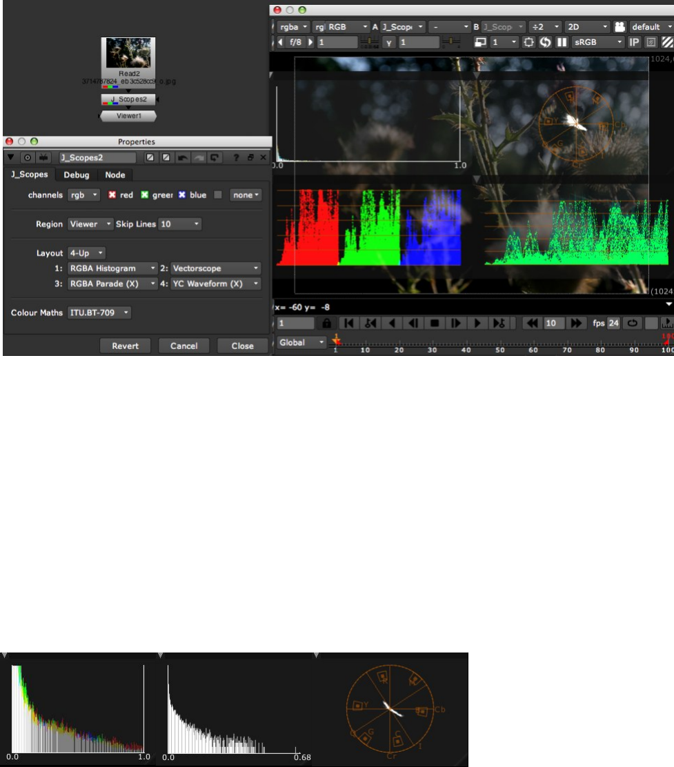
2.13 J_Scopes

2.13.1 Introduction

J_Scopes analyses your image data and draws a variety of histograms, parades and waveforms as overlays to

the viewer.

2.13.2 Usage

The ﬁrst thing to know about using this plugin is that the scopes will only be drawn when the node control panel

is open. This is simply part of the Nuke architecture, and something you’ll have to work with. Individual controls

have tooltips, so check them out if you’re still lacking information after reading this.

Add a Read node pointing at the image you want to see a Histogram of, append a J_Scopes node to it, and

make sure the node control panel is open. This should show the default display of an RGBAHistogram over the

entire image. You can alter the displayed scope type using the ’1’ drop down. To add more scopes to the display,

alter the ’layout’ drop down. The default ’1 Up’ only displays the one scope, ’2 Up’ will display 2 and so on up

to 4. Of course, as you add more layout slots for scopes, you can change the type of scope in them using the 1,

2, 3 and 4 dropdowns which will become enabled or disabled based on the number of slots selected.

Scope Types The following is a breakdown of the scope types available inside J_Scopes. Images illustrate the

scopes in order of description.

RGBA_Histogram: Maps the range of colour values in the input image against the frequency of their occu-

rance. Alpha, if enabled in the channel selector, weights the pixel value with which it is associated. You

can alter the Y Scaling using the ’Histogram Y Scale Type’ drop down in the Debug tab.

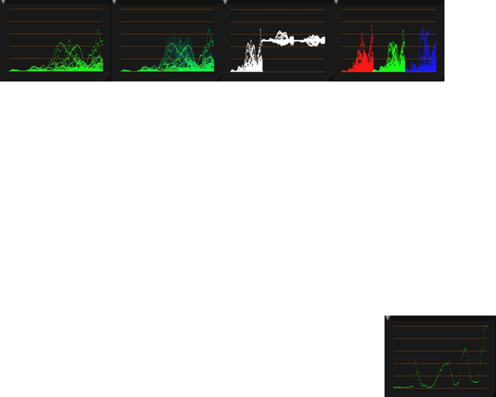
Luma_Histogram: As RGBA, but maps ITU.BT-701 Y against frequency of occurance. Requires all 3 colour

channels to be present in source.

Vectorscope: Maps ITU-BT-701 Cb against Cr, so providing a plot of hue against chrominance intensity. I’ve

adjusted the target graticle to match Nuke colour bars at 0.75 intensity. Requires all 3 colour channels to

be present in source.

Each of the following is available in an X and Y variety - X maps against the horiztonal axis, Y against the

vertical (note when using Y scopes you’ll probably want to set the skip lines to 1, otherwise you’re immediately

chopping out lines of data). Each has a graticle of 5 lines, running from 0 (lowest, or most left) to 1 (highest, or

most right), at 0.2 intensity increments. Note intensity is measured in the 0 to 1 range for visible data, rather

than IRE scales. Out of range data is also plotted:

Y_Waveform: Plots luminance (calculated using the selected maths) against the X or Y axis.

YC_Waveform: Plots luminance and chrominance against the X or Y axis. Y is calculated using the selected

maths. C is a hypot of the selected CbCr maths, riding on the Y data.

YCbCr_Parade: Plots the Y Cb and Cr signals alongside each other against the selected axis. Since Cb and

Cr signals roam from +0.5 to -0.5 (when calculated from RGB data in the 0-1 range), both chrominance

channels have their 0 point at 0.5 on the intensity axis.

RGB_Parade: Plots the R, G and B signals alongside each other against the selected axis.

For the scop es displayed, you can move them round on the screen by clicking and dragging on the title bar, resize

them by clicking and dragging on the triangle in the lower right of the scope display, and minimise/maximise

them using the arrow on the top right of the title bar.

You can use the plugin as a VIEWER_INPUT. This allows you to get it inserted just before the viewer,

regardless of what the viewer is hooked up to, or which input is active. Check the Nuke manual for how to do

this. Set ’input process order’ to ’after viewer process’ to see the result of the LUTTing/gamma/gain viewer

operations in reﬂected in the scope data.

Specifying What Data To Show You can use the source region drop down to specify

the area sampled by the plug-in. Viewer, the default, means show me the data from the

lines being pulled through the viewer, and so doesn’t add too much of a compute burden.

ROI means show me the data from within a certain region (defaults to entire image, so

can be computationally more expensive), and slice allows you to graph just the data on

alinebetweentwopoints(alatheslicetoolofapopularcompositingbible).

Additionally, for the ﬁrst two modes, you can specify a certain ratio of lines to skip,

so as to speed up the calculation at the expensive of accuracy.

2.13.3 Knobs

Hover over the knob in question in the J_Scopes param panel for live tooltip help!

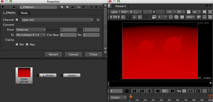
2.14 J_ZMaths

2.14.1 Introduction

J_ZMaths is a utility tool allowing quick and easy conversion between a variety of depth channel encodings,

as output by the range of 3D packages and renderers.

2.14.2 Usage

Pick the channel containing your depth data if it diﬀerents from the default Nuke z chan, then pick the source

and target depth encodings from the following options.

Distance: (ZBlur equivalent: Depth). z - linear representation.\nPixel value is absolute depth in front of the

camera.

Inverted Distance: (ZBlur equivalent: Far=0) .1/z - inverse representation. Pixel value is the inverse of the

depth. Used by Nuke’s 3D system & PRMan.

Normalised 0->1: (ZBlur equivalent: Far=1). z ranges 0 to 1 (near to far). Pixel value is mapped to the 0 to

1range. UsedbyOpenGL.

Normalised 1->0: (No ZBlur equivalent). z ranges 1 to 0 (near to far). Pixel value is mapped to the 1 to 0

range. Used by VRay.

Neg Distance: (ZBlur equivalent: -Depth). -z - negative linear representation. Pixel value is the negative of

the absolute depth infront of the camera.

Neg Inv Distance: (ZBlur equivalent: Far=-0). -1/z - negative inverse representation. Pixel value is the

negative of the invert of the depth. Used by Maya.

Normalised -1->0: (ZBlur equivalent: Far=-1). z ranges -1 to 0 (near to far). Pixel value is mapped to the -1

to 0 range.

Normalised 0->-1: (No ZBlur equivalent). z ranges 0 to -1 (near to far). Pixel value is mapped to the 0 to -1

range.

Some depth encodings normalise the underlying depth data, thus losing the absolute depth values. In the circum-

stance that you pick such an encoding the tool will enable additional Clip Near and Clip Far knobs, allowing the

resultant conversion to be scaled to take into account the normalisation. Depending on how you limited the range

in your 3D package, either enter the clips from the source camera, or use the range limits imposed in your render

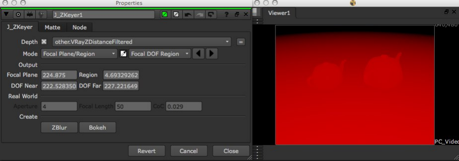
pass conﬁguration. If you don’t care about the absolute values (or wish to scale the data manually using other

Nuke tools) then opt for the defaults. If you select an normalised encoding for the target then the two clamp

checkboxes will enable, allowing you to force clamp the resultant depth map to the notional range imposed.

2.14.3 Knobs

Channel a drop down channel selector, designating which channel contains the depth data, and thus which

channel to operate on.

Convert separator

From a drop down enumeration list, designating the source depth data’s encoding type. The depth types

selectable are covered in the usage section above.

Clip Near a ﬂoat knob enabled when the From encoding is set to a normalised type. This, coupled with

the Clip Far knob, deﬁnes how to scale the depth data to recover the absolute depth values.

Clip Far a ﬂoat knob enabled when the From encoding is set to a normalised type. This, coupled with

the Clip Near knob, deﬁnes how to scale the depth data to recover the absolute depth values.

To a drop down enumeration list, designating the desired/target depth data’s encoding type. The depth

types selectable are covered in the usage section above.

Clip Near a ﬂoat knob enabled when the To encoding is set to a normalised type. This, coupled with the

Clip Far knob, deﬁnes how to scale the depth data into the normalised encoding space. Generally use

the min and max of the linear depth.

Clip Far a ﬂoat knob enabled when the To encoding is set to a normalised type. This, coupled with the

Clip Near knob, deﬁnes how to scale the depth data into the normalised encoding space. Generally

use the min and max of the linear depth.

Clamp separator

Min a checkbox enabled when the To encoding is set to a normalised type. This enables the resultant depth

map to be clamped to the min of the notional range speciﬁed by the selected normalised encoding.

Max a checkbox enabled when the To encoding is set to a normalised type. This enables the resultant depth

map to be clamped to the max of the notional range speciﬁed by the selected normalised encoding.

2.15 J_ZKeyer

2.15.1 Introduction

J_ZKeyer is a utility tool allowing easy extraction of mattes and depth of ﬁeld representations from a z-depth

pass, via a number of diﬀerent interfaces, but primarily a quick and intuitive eyedropper based system. The node

is additionally able to setup other depth related nodes (such as ZBlur) with matching conﬁguration, once a region

has been selected.

2.15.2 Usage

Hook up a J_ZKeyer node to an image stream with a z-depth pass, switching the node’s Depth knob to the

appropriate channel if the pass doesn’t reside in the usual depth.z. Now use the mode drop down to elect whether

you wish to pick the region from the central focal plane and one of it’s extremes (Focal Plane/Region),pickthe

front and back speciﬁcally (DOF Near/Far),orpickthefocalplaneandusearealworldcameraapproximation

to deﬁne the depth region (Focal Plane/Real World).

If you picked either Focal Plane/Region or DOF Near/Far you’ll now get a pick mode drop down from

which you can specify which of the two you’ll be colour picking, and then use standard viewer sampling hotkeys

to grab samples from the desired area. For example, if you’re looking to setup a ZBlur to throw out of focus the

background, but leave the foreground, you’d pick the Focal Plane by sampling the foreground object, and the

Region by sampling from some object just behind the foreground. Note that the sample will always be taken

from the elected depth channel, regardless of what channel the viewer is conﬁgured to use, so you’re easily able

to sample from the actual scene beauty pass itself.

Once you’ve sampled as required you’ll notice that the Output section knobs are now ﬁlled in with the data,

and you can now either use the provided buttons to create an appropriate setup ZBlur node (or Peregrine Lab’s

Bokeh if you have this installed). Additionally you’re able to ﬂip over to the Matte tab and use the controls

there to generate a matte based on the region elected. Note that sane people don’t anti alias their depth passes,

so of course the same aliasing will be present in mattes generated from it. By default the matte will be binary

- 0 for pixels not in the region, and 1 for those that are. You can elect to use the proﬁle curves option so as

to provide a roll oﬀto the edges, and there’s a number of such curves available as predeﬁned buttons below the

curve knob itself.

The Real World section knobs, enabled when the mode is set to Focal Plane/Real World, allows a region

depth to be approximated using idealised real world camera parameters - namely the focal length and aperture.

Additionally the circle of confusion for this idealised imaging system can be altered, but it’s generally best left

on default unless you know what you’re doing. This requires the depth pass to be encoded as Distance; use

J_ZMaths if required to convert if necessary.

2.15.3 Knobs

Are all documented through Nuke’s extensive tooltip system. Fire up the tool and hover over the knob in question

to get more information.

3 Python Scripts

J_Ops bundles a number of utility python scripts, in addition to the nodes detailed above. These provide useful

base level functionality, are generally implemented in the bundled menu.py script and can be enabled, disabled

and otherwise controlled in the J_Ops preferences tab. This can be found in your usual Nuke preferences, and

non-default settings are stored in the associated preferences<ver number>.nk script found in your .nuke directory.

3.1 Improved Drag & Drop

The improved drag and drop script builds on Nuke’s bundled drop functionality to add creation of ReadGeo,

Camera, Light and Vectorﬁeld nodes when geometry or LUT ﬁles are dropped on them as appropriate. In the

circumstance that a folder is dropped on the DAG then a per sequence node is created, and optionally (controlled

in the J_Ops preferences) the script will recurse into sub directories creating nodes for each sequence found

therein. This functionality can be enabled and disabled in the J_Ops preferences.

3.2 DAG Bookmarks

DAG bookmarks have been removed as of 2.1, due to inclusion of similar functionality natively inside of Nuke

7.0.

4 Release Notes

4.1 Known Issues/Requests

4.1.1 J_3Way

•Make the mouse wheel do luminance up and down shifts. Can’t be done currently due to bug 9634 in Nuke

(namely mousewheel events never making it into Qt Nuke builds). Pester Jon and the team to ﬁx this, if

you want to work in this manner.

4.1.2 J_Scopes

•Results aren’t cached.

•Previous frame results dropped when calculating current frame, making scope appear blank whilst calcu-

lating.

•No way of locking scope to a particular data range.

4.1.3 Scripts

•Improved drag and drop: does not observe Nuke’s preference setting for hash or regex type ﬁlename use.

This is due to the underling Nuke function being used not observing this setting.

4.2 Historical

4.2.1 2.3v1:

Maintenace release of J_Ops for Nuke9.0. Platforms: Windows XP64, Centos5.4 64bit, MacOSX 10.8 64bit

•J_rawReader:

–Retired DNG reader redirects due to native support.

4.2.2 2.2v1:

Maintenace release of J_Ops for Nuke8.0. Platforms: Windows XP64, Centos5.4 64bit, MacOSX 10.8 64bit

•J_rawReader:

–Updated to libraw 0.16. Added support for substantial number of cameras, various speed optimisations

and more.

–Added fall back to main image support for ﬁle browser rendering - if no thumbnail found, it’ll use the

full render path.

4.2.3 2.1v1:

Feature release of J_Ops for Nuke7.0. Platforms: Windows XP64, Centos5.4 64bit, MacOSX 10.6 64bit.

•J_ICCkyProﬁle added. J_ICCkyProﬁle allows ICC based colourspace conversions to be applied within

Nuke. This is not a magic wand ’here’s an ICC based colour managed workﬂow inside of Nuke,’ any

more than Nuke’s own Colorspace node oﬀers a linear colour managed workﬂow; the workﬂow step requires

a whole bunch of wrapping that Iop’s can’t directly do inside of Nuke. Rather, think of it as oﬀering

low level control of ICC colour conversions. To use it eﬀectively you’ll need to have an understanding of

ICC in general, as well as of Nuke’s underlying rgb linear toolset. J_ICCkyProﬁle additionally oﬀers a

proﬁle inspector, which can be used to judge what information is being conveyed in a particular ICC ﬁle.

J_ICCkyProﬁle is based upon the lcms2 library.

•J_Mullet:

–Added new collision shape type - the tri mesh. The tri mesh supports both convex and concave

underlying shapes, at the expense of longer processing times. Static tri meshes use a diﬀerent, faster,

body type than dynamic or kinematic bodies, best suited to modelling complex environments and the

like. The collision shape is available in the J_MulletBody collision shape type drop down.

–Added initial velocity controls to the J_MulletBody and J_MulletCompound ops for both linear and

angular control. These can be used to give the body an initial movement speed within the scene.

The J_MulletCompound initial velocities will override any upstream J_MulletBody settings for those

bodies, as per other compound settings.

–Added ’optimise’ control to the J_MulletBody and J_MulletCompound ops, allowing control over

whether Bullet can optimise the scene for faster simulation by allowing static bodies to deactivate.

Previously this was always on for dynamic bodies. Occasionally, particularly with the new dynamic

tri mesh shapes, a body can deactivate before it should, so stopping moving. If you see this sort of

behaviour experiment with toggling this control oﬀ.

–Added progress bars to simulation phase, which has in turn been moved out to Nuke 7.0’s updated

prevalidate phase. This allows reliable use of progress bars within geometry ops and similar. The

progress bars report both current stage (as %age) and current simulation fps, as well as oﬀering the

ability to cancel the calculation.

•J_rawReader:

–added thumbnail decompression for jpeg and bitmap based raw thumbnails when in the ﬁle browser.

The resultant image dimensions will be reported incorrectly, but the preview is signiﬁcantly faster.

–added ability to read embedded ICC proﬁle and apply to the image data.

–ﬁxed bug which intermittently made decoded images report incorrect size. Resultant image data would

only be for part of the frame.

–removed ARRIRAW tcl redirect script since Nuke 7.0 features native ARRIRAW reading, which is

signiﬁcantly better than the DCRaw based implementation. If you need it back for whatever crazy

reason, copy and rename one of the other tcl redirects to J_rawReader (for example the cr2Reader.tcl

script).

•All plug-ins and their library dependencies have been rebuilt with VS2010 on windows (and gcc4.1 on linux

for those libraries which hadn’t been for 2.0), in line with Nuke 7.0.

•Moved documentation to using compressed jpgs to reduce build and install size.

•Removed bookmarking script, due to Nuke 7.0’s inclusion of similar functionality.

•Made drag and drop improved script handle extensions in varying case.

•Bundled a ’manual install’ directory in windows build, at user request.

4.2.4 2.0v1:

Feature release of J_Ops for Nuke6.3. Platforms: Windows XP64, Centos5.4 64bit, MacOSX 10.6 64bit.

•J_Mullet added. J_Mullet is a suite of 5 plug-ins oﬀering rigid body physics simulation inside of Nuke, based

upon the Bullet engine. The J_MulletSolver is the core of the toolkit, performing the actual calculations,

whilst the remainder allow you to deﬁne the properties of your scene by inserting metadata into a Nuke

3D stream. At minimum you need to add a J_MulletBody node to a geometry stream, followed up by

a J_MulletSolver node. The Mullet toolkit is mainly aimed at quick and easy physics simulations in the

context of compositing, as opposed to hero shot physics simulations. It is limited to working on a constant

number of objects per scene, as well as working on objects with properties within an order of magnitude of

each other.

–J_MulletSolver added. The core engine tool of the Mullet toolkit, this performs the heavy lifting when

it comes to calculating the scene interactions - every simulation needs one. It additionally allows for

calculations to be baked down to matrix knobs, so that they need not be performed again and again.

–J_MulletBody added. Deﬁnes the presence of a piece of geometry within the physics scene, and allows

you to specify a range of properties, including the shape with which it should be represented (its

collision shape), the body’s weight, center of mass and more.

–J_MulletCompound added. Allows physics bodies to be built from multiple pieces of geometry.

–J_MulletConstraint added. Allows physics bodies to be connected to each other via a variety of joints.

Additionally, joints can be conﬁgured to break as a result of collisions and other force interactions.

–J_MulletForce added. Allows forces to be added to the physics scene, and conﬁgured to act on all, or

a subset of the objects within the physics scene.

•Added improved drag and drop python script, meaning that when geometry and LUT ﬁles are dropped

on the DAG the ReadGeo, Light, Camera and/or Vectorﬁeld node appropriate to their use is created

(rather than the Read node created previously). Additionally the script can be conﬁgured to recurse into

sub directories when folders are dropped. This functionality can be enabled and disabled in the J_Ops

preferences tab.

•Added DAG bookmarking python script, allowing node graph positions to be saved and recalled via the

menu entries, the TAB selector or their associated hotkeys. This functionality can be enabled and disabled

in the J_Ops preferences tab.

•Added J_Ops preferences tab to main Nuke preferences, to allow control of J_Ops python script conﬁgu-

ration.

•J_rawReader: updated libraw for optimisations and bug ﬁxes as well as to add support for newer cameras,

including the Canon 5D mk3. Additionally added experimental support for ARRIRAW. This’ll updoubtedly

be done better by the Foundry at some point, but it may get you out of a pickle in the meantime. Note

that the colour handling for arri is all rather strange.

•J_rawReader: exposed control over output colourspace from the process (equivalent to output_color in

libRaw and the DCRaw -o ﬂag). This chains with NUKE’s read colourspace, so the two need to be set in

tandem.

•J_rawReader: changed defaults for full res to use linear interpolation on the debayer, based on user feed-

back that linear is more than suﬃcient most of the time, making the extra compute time spent in AHD

interpolation unnecessary.

•J_rawReader: ﬁxed crash when executing in terminal mode with disk caching switched on.

•J_rawReader: ﬁxed circumstance where bit depth may not be read correctly out of disk cache.

•J_rawReader: ﬁxed ﬁle handle leak that could cause session to become unstable when using long sequences

or large numbers of raw ﬁles.

•J_MergeHDR: allow animation of alignment knobs, so that hdr sequences can be merged with their align-

ment oﬀsets animated.

•J_MergeHDR: added a number of weight curve presets as buttons. Some users have been seeing banding

in the extreme highlights and lowlights of merges. Diﬀerent weighting curves often mitigate or eliminate

these.

•J_MergeHDR: changed weight curve default, again to mitigate banding some users have seen.

•J_MergeHDR: ﬁxed preview overlay intermittently not working due to Nuke 6.2 changes.

•J_MergeHDR: ﬁxed metadata get and reset buttons not working in terminal mode (these can now be called

by their python execute methods, to allow scripting of HDR merge setups).

•J_3Way: the Nuke guys recently added button release events (thanks guys!), which means that the colour

corrector mode can now be set on a button depress, and unset on button release. This is how I always

wanted the corrector to work, so have changed the defaults to do so. The old modal operation is still

available by toggling the Release knob in the Interface group of the Settings tab.

•Added manual install folder to linux install bundle at user request.

•Shifted versioning to more nukepedia friendly shortened form.

4.2.5 1.0v1a9:

Feature release of J_Ops for Nuke6.3v1. Platforms: Windows XP64, Centos4.5 64bit, MacOSX 10.5 64bit.

•J_ZMaths added. J_ZMaths is a precompiled NDK utility plug-in, allowing easy conversion between a

variety of depth pass encodings.

•J_ZKeyer added. J_ZKeyer is a precompiled NDK utility plug-in, allowing fast generation of depth regions

and mattes from z-depth passes via an intuitive eyedropper based interface.

•J_GotSomeID added. J_GotSomeID is a precompiled NDK utility plug-in designed to speed up working

with object ID and coverage passes.

•J_GeoManager added. J_GeoManager is a precompiled NDK 3d plug-in providing access to information

about 3D scene’s not otherwise available and allowing ﬁltering out/removal of objects from the stream.

•Icons added, many thanks to Andrew Hake.

•J_rawReader has been updated with latest LibRaw, providing faster decoding and support for new cameras

including the Canon 60D and 1100D. Additional functionality provided by new library has been exposed

including further noise reduction tools and exposure compensation.

•Windows XP32 and MacOSX 10.5 32bit support dropped, inline with supported Nuke 6.3 platforms.

4.2.6 1.0v1a8:

Feature release of J_Ops for Nuke6.2v1. Platforms: Windows XP32, Windows XP64, Centos4.5 64bit, MacOSX

10.5 32bit, MacOSX 10.5 64bit. Date 12/10.

•Centos4.5 32bit platform dropped, inline with Nuke’s supported platforms.

•J_rawReader: rewritten to use the rather awesome LibRaw, under CDDL license. New version has:

–No external dependancy on DCRaw, so nothing extra to install or conﬁgure.

–Signiﬁcantly improved performance, thanks to LibRaw and new internal RAM and disk caching mech-

anism.

–Additional decode features present in LibRaw not available in DCRaw (at time of inclusion for example,

DCB debayer interpolation and FBDD pre-debayer denoising)

–Progress feedback.

–Improved interface, presenting underlying options as series of knobs, as opposed to the ﬂag knob on

the previous build.

–Inserts metadata into the stream in a more compliant manner. Direct matches to exif data go into the

exif namespace, and the remainder into a new raw namespace.

–Note that the defaults now use the camera metadata for white balance, as opposed to the DCRaw

default illumination. Coupled with the change in knobs note that this makes this build incompatible

with scripts saved from the previous build.

•J_rawReader: ﬁxed bug when using a forced reader type (ie putting ’raw:’ at the start of the ﬁlename).

This technique should now successfully work to force use of the rawReader when attempting to read in a

ﬁle format for which no redirect has been included. Of course, if you ﬁnd yourself often doing this, let me

know on the nuke users list and I’ll add support natively.

•J_MergeHDR: altered to set shutter speed from metadata as an expression, as opposed to evaluating the

fraction. This allows you to hover over the relevant knob to show tooltip, or pop up the expression box, to

see the fractional representation of the value (ie 1/20 as opposed to 0.05).

•J_3Way: set up knob_changed to handle animated GLG knobs.

•Appended icon search path to init.py, to ensure icon found when running from a custom path.

•Added some J_MergeHDR bracketed set screengrabs to the docs, kindly provided by Rhys of Filament

VFX.

4.2.7 1.0v1a7:

Feature release of J_Ops for Nuke6.1v1. Platforms: Windows XP32, Windows XP64, Centos4.5 32bit, Centos4.5

64bit, MacOSX 10.5 32bit, MacOSX 10.5 64bit. Date 09/10.

•J_MergeHDR added. J_MergeHDR is a precompiled NDK plug-in intended to simply the task of putting

a together a high dynamic range radiance map from a series of low dynamic range exposures. It performs a

number of functions, namely, querying the source LDR metadata streams for exposure data, calculating a

series of translation oﬀsets to align the source LDR images, and estimating a response curve for the camera

used to shoot the images. It also has functionality such that should automatic estimations prove oﬀ, they

can be tweaked, or entirely created, manually.

•J_rawReader retained. Nuke6.1 adds some of the features of J_rawReader, but there are a number left

which mean it still has value. Also added Panasonic RAW format redirects.

•Changed installers to install into the new common location searched by Nuke6.1. You may need to remove

older versions from your .nuke directory to enable the new builds to be picked up. Rejigged python support

scripts appropriately.

•J_Scopes: ﬁxed issue with Vectorscope when viewer run in ﬂoat or half ﬂoat modes. It was leaving the

gl buﬀer in a bad state, which could cause the VIEWER PROCESS to fail when being run on graphics

hardware.

•Added 64-bit OSX builds.

4.2.8 1.0v1a6:

Feature release of J_Ops for Nuke6.0v1. Platforms: Windows XP32, Windows XP64, Centos4.5 32bit, Centos4.5

64bit, MacOSX 10.5 32bit. Date: 02/10.

•J_rawReader added. J_rawReader is a precompiled NDK plug-in based on the NDK crwReader example

which uses DCRaw to read in a variety of SLR raw formats. J_rawReader adds, over the top of crwReader,

controls to allow the user to tweak the ﬂags passed to DCRaw (with control over the ﬂags between full res

and proxy mode), and it inserts metadata extracted from the raw ﬁle (again via DCRaw) into the stream.

crwReader redirects from canon raw formats only (crw & cr2). J_rawReader additionally redirects from

Nikon (sorry, I said a bad word) raw formats and Adobe DNG.

•Split menu.py into init.py for plugin path setup and menu.py for toolbars. As it should have been in the

ﬁrst place.

4.2.9 1.0v1a5:

First public release of J_Ops package, ﬁxing a number of bugs present in 1.0v1a4 and tweaking J_3Way’s interface

and interaction somewhat. Built for Nuke6.0v1. platforms: Windows XP32, Windows XP64, Centos4.5 32bit,

Centos4.5 64bit, MacOSX 10.5 32bit. Date: 02/10.

•J_Scopes: ﬁxed crashing immediately on instantiation on Windows XP64.

•J_3Way: moved CDL clamp parameter from settings to the front page.

•J_3Way: added a mapping drop down, to allow the user to specify a DI grader type of interaction, or a

more compositor style of interaction.

•Added various build ﬂags to optimise and speed up tools on XP32, Linux 32bit and Linux 64bit. Requires

aminimumofSSE2instructionsupportonchipset.

4.2.10 1.0v1a4:

Feature release of J_Ops (renamed from J_Scopes) for Nuke6.0v1. Platforms: Windows XP32, Windows XP64,

Centos4.5 32bit, Centos4.5 64bit, MacOSX 10.5 32bit. Date: 01/10.

•J_3Way added (hence renaming of bundle). J_3Way is a precompiled NDK plug-in providing gain/lift/gamma

style colour grading functionality. It has on screen controls allowing grade creation whilst interacting di-

rectly on the image canvas in an artist friendly manner, and a gpu implementation for rapid feedback of

results. It also implements a python based framework for importing and exporting ASC CDL data, allowing

exchange with other packages. At this time CCC and CDL import has been implemented, and a framework

provided for allowing extension to other ﬁle types. See the ?? J_3Way section for more information.

•Installers, menu, icon and nicer documentation added.

4.2.11 1.0v1a3:

Feature and bug ﬁx release of J_Scopes for Nuke6.0v1b6. Platforms: Windows XP32, Windows XP64, Centos4.5

32bit, Centos4.5 64bit, MacOSX 10.5 32bit. Date: 10/09.

•Added a source region selector. This allows you to pick exactly what data the plugin is drawing scopes of.

The options are:

–Viewer - this matches what the plugin was previously doing. With ’Skip Lines’ set to none any lines

being drawn by the viewer are drawn by the scopes.

–ROI - This draws every line (per the ’Skip Lines’ setting) of the region selected in the Viewer. The

ROI defaults to the format of the clip initially plugged into it.

–Slice - This draws the scopes for the line speciﬁed by the two terminating points now drawn in the

viewer. The X and Y Parade and Waveform tools will now draw the distance as against the length of the

line in question, rather than against their respective axes, thus performing ’slicetool’ type functionality.

•Set up core to use zero time close calls, making handle drawing on completion much more robust.

4.2.12 1.0v1a2:

Feature and bug ﬁx release of J_Scopes for Nuke5.2v1. Platforms: Windows XP32, Windows XP64, Centos4.5

32bit, Centos4.5 64bit, MacOSX 10.5 32bit. Date: 09/09.

•Added full vectorscope graticle - amending major target box to +/- 7 degrees, and adding minor target box

at +/- 2 degrees plus crosshair. Added labels for targets and axes.

•Recoded vectorscope data storage for lower memory overhead and greater speed.

•Added a knob to allow switching of maths used to calculate Y Cb Cr from RGB from ITU.BT-701 to

ITU.BT601. This doesnt change the scope frameworks (ie graticles) however. Calculation has been shifted

from scope classes to iop itself for additional speed when dealing with multiple scopes using YCbCr data.

•Lowered memory footprint of dispatching in some circumstances

•Add the following Parade and Waveform scopes, each of which is available in an X and Y variety - X maps

against the horiztonal axis, Y against the vertical (note when using Y scopes you’ll probably want to set

the skip lines to 1, otherwise you’re immediately chopping out lines of data). Each has a graticle of 5 lines,

running from 0 (lowest, or most left) to 1 (highest, or most right), at 0.2 intensity increments. Note intensity

is measured in the 0 to 1 range for visible data, rather than IRE scales. Out of range data is also plotted:

–YWaveform-plotsluminance(calculatedusingtheselectedmaths)againsttheXorYaxis.

–YC Waveform - plots luminance and chrominance against the X or Y axis. Y is calculated using the

selected maths. C is a hypot of the selected CbCr maths, riding on the Y data.

–YCbCr Parade - plots the Y Cb and Cr signals alongside each other against the selected axis. Since

Cb and Cr signals roam from +0.5 to -0.5 (when calculated from RGB data in the 0-1 range), both

chrominance channels have their 0 point at 0.5 on the intensity axis.

–RGB Parade - plots the R, G and B signals alongside each other against the selected axis. -Rewrote

plugin core to make begin and end frame calls robust. Moved forced refresh button to debug panel as

aresultofthis.

4.2.13 1.0v1a1:

Initial release of J_Scopes for Nuke5.1. Platforms: Windows XP32, Centos4.5 32bit, Centos4.5 64bit, Mac OSX

10.4 32bit. Date: 04/09

5 3rd Party Licenses

This section lists third party libraries used in J_Ops, along with their licenses.

5.1 VXL

GE Corporate Research and Development (GE CRD)

1 Research Circle

Niskayuna, NY 12309

Reproduction rights limited as described below.

Permission to use, copy, modify, distribute, and sell this software and its documentation for any purpose is

hereby granted without fee, provided that (i) the above copyright notice and this permission notice appear in

all copies of the software and related documentation, (ii) the name TargetJr Consortium (represented by GE

CRD), may not be used in any advertising or publicity relating to the software without the speciﬁc, prior written

permission of GE CRD, and (iii) any modiﬁcations are clearly marked and summarized in a change history log.

THE SOFTWARE IS PROVIDED "AS IS" AND WITHOUT WARRANTY OF ANY KIND, EXPRESS, IM-

PLIED OR OTHERWISE, INCLUDING WITHOUT LIMITATION, ANY WARRANTY OF MERCHANTABIL-

ITY OR FITNESS FOR A PARTICULAR PURPOSE. IN NO EVENT SHALL THE TARGETJR CONSOR-

TIUM BE LIABLE FOR ANY SPECIAL, INCIDENTAL, INDIRECT OR CONSEQUENTIAL DAMAGES OF

ANY KIND OR ANY DAMAGES WHATSOEVER RESULTING FROM LOSS OF USE, DATA OR PROFITS,

WHETHER OR NOT ADVISED OF THE POSSIBILITY OF SUCH DAMAGES, OR ON ANY THEORY OF

LIABILITY ARISING OUT OF OR IN CONNECTION WITH THE USE OR PERFORMANCE OF THIS

SOFTWARE.

5.2 LibRaw

Note LibRaw used without modiﬁcation. Source code available from the project site on www.libraw.org.

COMMON DEVELOPMENT AND DISTRIBUTION LICENSE (CDDL) Version 1.0

1. Deﬁnitions.

1.1. Contributor means each individual or entity that creates or contributes to the creation of Modiﬁcations.

1.2. Contributor Version means the combination of the Original Software, prior Modiﬁcations used by a

Contributor (if any), and the Modiﬁcations made by that particular Contributor.

1.3. Covered Software means (a) the Original Software, or (b) Modiﬁcations, or (c) the combination of ﬁles

containing Original Software with ﬁles containing Modiﬁcations, in each case including portions thereof.

1.4. Executable means the Covered Software in any form other than Source Code.

1.5. Initial Developer means the individual or entity that ﬁrst makes Original Software available under this

License.

1.6. Larger Workmeans a work which combines Covered Software or portions thereof with code not governed

by the terms of this License.

1.7. License means this document.

1.8. Licensable means having the right to grant, to the maximum extent possible, whether at the time of the

initial grant or subsequently acquired, any and all of the rights conveyed herein.

1.9. Modiﬁcations means the Source Code and Executable form of any of the following: A. Any ﬁle that

results from an addition to, deletion from or modiﬁcation of the contents of a ﬁle containing Original Software or

previous Modiﬁcations; B. Any new ﬁle that contains any part of the Original Software or previous Modiﬁcation;

or C. Any new ﬁle that is contributed or otherwise made available under the terms of this License.

1.10. Original Software means the Source Code and Executable form of computer software code that is

originally released under this License.

1.11. Patent Claims means any patent claim(s), now owned or hereafter acquired, including without limitation,

method, process, and apparatus claims, in any patent Licensable by grantor.

1.12. Source Code means (a) the common form of computer software code in which modiﬁcations are made

and (b) associated documentation included in or with such code.

1.13. You (or Your) means an individual or a legal entity exercising rights under, and complying with all of

the terms of, this License. For legal entities, You includes any entity which controls, is controlled by, or is under

common control with You. For purposes of this deﬁnition, control means (a) the power, direct or indirect, to

cause the direction or management of such entity, whether by contract or otherwise, or (b) ownership of more

than ﬁfty percent (50%) of the outstanding shares or beneﬁcial ownership of such entity.

2. License Grants.

2.1. The Initial Developer Grant. Conditioned upon Your compliance with Section 3.1 below and subject

to third party intellectual property claims, the Initial Developer hereby grants You a world-wide, royalty-free,

non-exclusive license:

(a) under intellectual property rights (other than patent or trademark) Licensable by Initial Developer, to

use, reproduce, modify, display, perform, sublicense and distribute the Original Software (or portions thereof),

with or without Modiﬁcations, and/or as part of a Larger Work; and

(b) under Patent Claims infringed by the making, using or selling of Original Software, to make, have made,

use, practice, sell, and oﬀer for sale, and/or otherwise dispose of the Original Software (or portions thereof);

or otherwise makes the Original Software available to a third party under the terms of this License;

(d) Notwithstanding Section 2.1(b) above, no patent license is granted: (1) for code that You delete from the

Original Software, or (2) for infringements caused by: (i) the modiﬁcation of the Original Software, or (ii) the

combination of the Original Software with other software or devices.

2.2. Contributor Grant. Conditioned upon Your compliance with Section 3.1 below and subject to third

party intellectual property claims, eachKnown Issues/Requests Contributor hereby grants You a world-wide,

royalty-free, non-exclusive license:

(a) under intellectual property rights (other than patent or trademark) Licensable by Contributor to use,

reproduce, modify, display, perform, sublicense and distribute the Modiﬁcations created by such Contributor (or

portions thereof), either on an unmodiﬁed basis, with other Modiﬁcations, as Covered Software and/or as part

of a Larger Work; and

(b) under Patent Claims infringed by the making, using, or selling of Modiﬁcations made by that Contributor

either alone and/or in combination with its Contributor Version (or portions of such combination), to make,

use, sell, oﬀer for sale, have made, and/or otherwise dispose of: (1) Modiﬁcations made by that Contributor

(or portions thereof); and (2) the combination of Modiﬁcations made by that Contributor with its Contributor

Version (or portions of such combination).

otherwise makes the Modiﬁcations available to a third party.

(d) Notwithstanding Section 2.2(b) above, no patent license is granted: (1) for any code that Contributor has

deleted from the Contributor Version; (2) for infringements caused by: (i) third party modiﬁcations of Contributor

Version, or (ii) the combination of Modiﬁcations made by that Contributor with other software (except as part

of the Contributor Version) or other devices; or (3) under Patent Claims infringed by Covered Software in the

absence of Modiﬁcations made by that Contributor.

3. Distribution Obligations.

3.1. Availability of Source Code. Any Covered Software that You distribute or otherwise make available in

Executable form must also be made available in Source Code form and that Source Code form must be distributed

only under the terms of this License. You must include a copy of this License with every copy of the Source Code

form of the Covered Software You distribute or otherwise make available. You must inform recipients of any such

Covered Software in Executable form as to how they can obtain such Covered Software in Source Code form in

areasonablemanneronorthroughamediumcustomarilyusedforsoftwareexchange.

3.2. Modiﬁcations. The Modiﬁcations that You create or to which You contribute are governed by the terms

of this License. You represent that You believe Your Modiﬁcations are Your original creation(s) and/or You have

suﬃcient rights to grant the rights conveyed by this License.

3.3. Required Notices. You must include a notice in each of Your Modiﬁcations that identiﬁes You as

the Contributor of the Modiﬁcation. You may not remove or alter any copyright, patent or trademark notices

contained within the Covered Software, or any notices of licensing or any descriptive text giving attribution to

any Contributor or the Initial Developer.

3.4. Application of Additional Terms. You may not oﬀer or impose any terms on any Covered Software in

Source Code form that alters or restricts the applicable version of this License or the recipients rights hereunder.

You may choose to oﬀer, and to charge a fee for, warranty, supp ort, indemnity or liability obligations to one or

more recipients of Covered Software. However, you may do so only on Your own behalf, and not on behalf of

the Initial Developer or any Contributor. You must make it absolutely clear that any such warranty, support,

indemnity or liability obligation is oﬀered by You alone, and You hereby agree to indemnify the Initial Developer

and every Contributor for any liability incurred by the Initial Developer or such Contributor as a result of

warranty, support, indemnity or liability terms You oﬀer.

3.5. Distribution of Executable Versions. You may distribute the Executable form of the Covered Software

under the terms of this License or under the terms of a license of Your choice, which may contain terms diﬀerent

from this License, provided that You are in compliance with the terms of this License and that the license for the

Executable form does not attempt to limit or alter the recipients rights in the Source Code form from the rights

set forth in this License. If You distribute the Covered Software in Executable form under a diﬀerent license, You

must make it absolutely clear that any terms which diﬀer from this License are oﬀered by You alone, not by the

Initial Developer or Contributor. You hereby agree to indemnify the Initial Developer and every Contributor for

any liability incurred by the Initial Developer or such Contributor as a result of any such terms You oﬀer.

3.6. Larger Works. You may create a Larger Work by combining Covered Software with other code not

governed by the terms of this License and distribute the Larger Work as a single product. In such a case, You

must make sure the requirements of this License are fulﬁlled for the Covered Software.

4. Versions of the License.

4.1. New Versions. Sun Microsystems, Inc. is the initial license steward and may publish revised and/or new

versions of this License from time to time. Each version will be given a distinguishing version number. Except as

provided in Section 4.3, no one other than the license steward has the right to modify this License.

4.2. Eﬀect of New Versions. You may always continue to use, distribute or otherwise make the Covered

Software available under the terms of the version of the License under which You originally received the Covered

Software. If the Initial Developer includes a notice in the Original Software prohibiting it from being distributed

or otherwise made available under any subsequent version of the License, You must distribute and make the

Covered Software available under the terms of the version of the License under which You originally received the

Covered Software. Otherwise, You may also choose to use, distribute or otherwise make the Covered Software

available under the terms of any subsequent version of the License published by the license steward.

4.3. Modiﬁed Versions. When You are an Initial Developer and You want to create a new license for Your

Original Software, You may create and use a modiﬁed version of this License if You: (a) rename the license and

remove any references to the name of the license steward (except to note that the license diﬀers from this License);

and (b) otherwise make it clear that the license contains terms which diﬀer from this License.

5. DISCLAIMER OF WARRANTY. COVERED SOFTWARE IS PROVIDED UNDER THIS LICENSE

ON AN AS IS BASIS, WITHOUT WARRANTY OF ANY KIND, EITHER EXPRESSED OR IMPLIED, IN-

CLUDING, WITHOUT LIMITATION, WARRANTIES THAT THE COVERED SOFTWARE IS FREE OF

DEFECTS, MERCHANTABLE, FIT FOR A PARTICULAR PURPOSE OR NON-INFRINGING. THE EN-

TIRE RISK AS TO THE QUALITY AND PERFORMANCE OF THE COVERED SOFTWARE IS WITH

YOU. SHOULD ANY COVERED SOFTWARE PROVE DEFECTIVE IN ANY RESPECT, YOU (NOT THE

INITIAL DEVELOPER OR ANY OTHER CONTRIBUTOR) ASSUME THE COST OF ANY NECESSARY

SERVICING, REPAIR OR CORRECTION. THIS DISCLAIMER OF WARRANTY CONSTITUTES AN ES-

SENTIAL PART OF THIS LICENSE. NO USE OF ANY COVERED SOFTWARE IS AUTHORIZED HERE-

UNDER EXCEPT UNDER THIS DISCLAIMER.

6. TERMINATION.

6.1. This License and the rights granted hereunder will terminate automatically if You fail to comply with

terms herein and fail to cure such breach within 30 days of becoming aware of the breach. Provisions which, by

their nature, must remain in eﬀect beyond the termination of this License shall survive.

6.2. If You assert a patent infringement claim (excluding declaratory judgment actions) against Initial Devel-

oper or a Contributor (the Initial Developer or Contributor against whom You assert such claim is referred to as

Participant) alleging that the Participant Software (meaning the Contributor Version where the Participant is a

Contributor or the Original Software where the Participant is the Initial Developer) directly or indirectly infringes

any patent, then any and all rights granted directly or indirectly to You by such Participant, the Initial Developer

(if the Initial Developer is not the Participant) and all Contributors under Sections 2.1 and/or 2.2 of this License

shall, upon 60 days notice from Participant terminate prospectively and automatically at the expiration of such

60 day notice period, unless if within such 60 day period You withdraw Your claim with respect to the Participant

Software against such Participant either unilaterally or pursuant to a written agreement with Participant.

6.3. In the event of termination under Sections 6.1 or 6.2 above, all end user licenses that have been validly

granted by You or any distributor hereunder prior to termination (excluding licenses granted to You by any

distributor) shall survive termination.

7. LIMITATION OF LIABILITY. UNDER NO CIRCUMSTANCES AND UNDER NO LEGAL THEORY,

WHETHER TORT (INCLUDING NEGLIGENCE), CONTRACT, OR OTHERWISE, SHALL YOU, THE INI-

TIAL DEVELOPER, ANY OTHER CONTRIBUTOR, OR ANY DISTRIBUTOR OF COVERED SOFTWARE,

OR ANY SUPPLIER OF ANY OF SUCH PARTIES, BE LIABLE TO ANY PERSON FOR ANY INDI-

RECT, SPECIAL, INCIDENTAL, OR CONSEQUENTIAL DAMAGES OF ANY CHARACTER INCLUDING,

WITHOUT LIMITATION, DAMAGES FOR LOST PROFITS, LOSS OF GOODWILL, WORK STOPPAGE,

COMPUTER FAILURE OR MALFUNCTION, OR ANY AND ALL OTHER COMMERCIAL DAMAGES OR

LOSSES, EVEN IF SUCH PARTY SHALL HAVE BEEN INFORMED OF THE POSSIBILITY OF SUCH

DAMAGES. THIS LIMITATION OF LIABILITY SHALL NOT APPLY TO LIABILITY FOR DEATH OR

PERSONAL INJURY RESULTING FROM SUCH PARTYS NEGLIGENCE TO THE EXTENT APPLICA-

BLE LAW PROHIBITS SUCH LIMITATION. SOME JURISDICTIONS DO NOT ALLOW THE EXCLUSION

OR LIMITATION OF INCIDENTAL OR CONSEQUENTIAL DAMAGES, SO THIS EXCLUSION AND LIM-

ITATION MAY NOT APPLY TO YOU.

8. U.S. GOVERNMENT END USERS. The Covered Software is a commercial item, as that term is deﬁned

in 48 C.F.R. 2.101 (Oct. 1995), consisting of commercial computer software (as that term is deﬁned at 48 C.F.R.

252.227-7014(a)(1)) and commercial computer software documentation as such terms are used in 48 C.F.R. 12.212

(Sept. 1995). Consistent with 48 C.F.R. 12.212 and 48 C.F.R. 227.7202-1 through 227.7202-4 (June 1995), all U.S.

Government End Users acquire Covered Software with only those rights set forth herein. This U.S. Government

Rights clause is in lieu of, and supersedes, any other FAR, DFAR, or other clause or provision that addresses

Government rights in computer software under this License.

9. MISCELLANEOUS. This License represents the complete agreement concerning subject matter hereof.

If any provision of this License is held to be unenforceable, such provision shall be reformed only to the extent

necessary to make it enforceable. This License shall be governed by the law of the jurisdiction speciﬁed in a

notice contained within the Original Software (except to the extent applicable law, if any, provides otherwise),

excluding such jurisdictions conﬂict-of-law provisions. Any litigation relating to this License shall be subject to the

jurisdiction of the courts located in the jurisdiction and venue speciﬁed in a notice contained within the Original

Software, with the losing party responsible for costs, including, without limitation, court costs and reasonable

attorneys fees and expenses. The application of the United Nations Convention on Contracts for the International

Sale of Goods is expressly excluded. Any law or regulation which provides that the language of a contract shall

be construed against the drafter shall not apply to this License. You agree that You alone are responsible for

compliance with the United States export administration regulations (and the export control laws and regulation

of any other countries) when You use, distribute or otherwise make available any Covered Software.

10. RESPONSIBILITY FOR CLAIMS. As between Initial Developer and the Contributors, each party is

responsible for claims and damages arising, directly or indirectly, out of its utilization of rights under this License

and You agree to work with Initial Developer and Contributors to distribute such responsibility on an equitable

basis. Nothing herein is intended or shall be deemed to constitute any admission of liability.

—————————————————————-

NOTICE PURSUANT TO SECTION 9 OF THE COMMON DEVELOPMENT AND DISTRIBUTION LI-

CENSE (CDDL): This code is released under the CDDL and shall be governed by the laws of the State of

California (excluding conﬂict-of-law provisions). Any litigation relating to this License shall be subject to the

jurisdiction of the Federal Courts of the Northern District of California and the state courts of the State of

California, with venue lying in Santa Clara County, California.Known Issues/Requests

—————————————————————-

5.3 Bullet

This software is provided ’as-is’, without any express or implied warranty. In no event will the authors be

held liable for any damages arising from the use of this software. Permission is granted to anyone to use this

software for any purpose, including commercial applications, and to alter it and redistribute it freely, subject to

the following restrictions:

1. The origin of this software must not be misrepresented; you must not claim that you wrote the original

software. If you use this software in a product, an acknowledgment in the product documentation would be

appreciated but is not required.

2. Altered source versions must be plainly marked as such, and must not be misrepresented as being the

original software.

3. This notice may not be removed or altered from any source distribution.

5.4 jpeglib

This software is based in part on the work of the Independent JPEG Group.

5.5 Little CMS

Permission is hereby granted, free of charge, to any person obtaining a copy of this software and associated

documentation ﬁles (the "Software"), to deal in the Software without restriction, including without limitation

the rights to use, copy, modify, merge, publish, distribute, sublicense, and/or sell copies of the Software, and to

permit persons to whom the Software is furnished to do so, subject to the following conditions:

The above copyright notice and this permission notice shall be included in all copies or substantial portions

of the Software.

THE SOFTWARE IS PROVIDED "AS IS", WITHOUT WARRANTY OF ANY KIND, EXPRESS OR IM-

PLIED, INCLUDING BUT NOT LIMITED TO THE WARRANTIES OF MERCHANTABILITY, FITNESS

FOR A PARTICULAR PURPOSE AND NONINFRINGEMENT. IN NO EVENT SHALL THE AUTHORS OR

IN AN ACTION OF CONTRACT, TORT OR OTHERWISE, ARISING FROM, OUT OF OR IN CONNEC-

TION WITH THE SOFTWARE OR THE USE OR OTHER DEALINGS IN THE SOFTWARE.

J Ops Manual

Navigation menu

Versions of this User Manual:

Views

Navigation