Java 9 Data Structures And Algorithms: A Step By Guide To Algorithms
User Manual: Pdf
Open the PDF directly: View PDF ![]() .
.
Page Count: 340 [warning: Documents this large are best viewed by clicking the View PDF Link!]
- Cover
- Copyright
- Credits
- About the Author
- About the Reviewer
- www.PacktPub.com
- Customer Feedback
- Table of Contents
- Preface
- Chapter 1: Why Bother? – Basic
- Chapter 2: Cogs and Pulleys – Building Blocks
- Chapter 3: Protocols – Abstract Data Types
- Chapter 4: Detour – Functional Programming
- Chapter 5: Efficient Searching – Binary Search and Sorting
- Chapter 6: Efficient Sorting – Quicksort and Merge Sort
- Chapter 7: Concepts of Tree
- Chapter 8: More About Search – Search Trees and Hash Tables
- Chapter 9: Advanced General Purpose Data Structures
- Chapter 10: Concepts of Graph
- What is a graph?
- The graph ADT
- Representation of a graph in memory
- Traversal of a graph
- Cycle detection
- Spanning tree and minimum spanning tree
- Finding the minimum spanning tree
- Summary
- Chapter 11: Reactive Programming
- Index

Java 9 Data Structures and
Algorithms
A step-by-step guide to data structures and algorithms
Debasish Ray Chawdhuri
BIRMINGHAM - MUMBAI
Java 9 Data Structures and Algorithms
Copyright © 2017 Packt Publishing
All rights reserved. No part of this book may be reproduced, stored in a retrieval
system, or transmitted in any form or by any means, without the prior written
permission of the publisher, except in the case of brief quotations embedded in
critical articles or reviews.
Every effort has been made in the preparation of this book to ensure the accuracy
of the information presented. However, the information contained in this book is
sold without warranty, either express or implied. Neither the author, nor Packt
Publishing, and its dealers and distributors will be held liable for any damages
caused or alleged to be caused directly or indirectly by this book.
Packt Publishing has endeavored to provide trademark information about all of the
companies and products mentioned in this book by the appropriate use of capitals.
However, Packt Publishing cannot guarantee the accuracy of this information.
First published: April 2017
Production reference: 1250417
Published by Packt Publishing Ltd.
Livery Place
35 Livery Street
Birmingham B3 2PB, UK.
ISBN 978-1-78588-934-9
www.packtpub.com

Credits
Author
Debasish Ray Chawdhuri
Reviewer
Miroslav Wengner
Commissioning Editor
Kunal Parikh
Acquisition Editor
Chaitanya Nair
Content Development Editor
Nikhil Borkar
Technical Editor
Madhunikita Sunil Chindarkar
Copy Editor
Muktikant Garimella
Project Coordinator
Vaidehi Sawant
Proofreader
Sas Editing
Indexer
Mariammal Chettiyar
Graphics
Abhinash Sahu
Production Coordinator
Nilesh Mohite
Cover Work
Nilesh Mohite

About the Author
Debasish Ray Chawdhuri is an established Java developer and has been in the
industry for the last 8 years. He has developed several systems, right from CRUD
applications to programming languages and big data processing systems. He
had provided the rst implementation of extensible business reporting language
specication, and a product around it, for the verication of company nancial data
for the Government of India while he was employed at Tata Consultancy Services
Ltd. In Talentica Software Pvt. Ltd., he implemented a domain-specic programming
language to easily implement complex data aggregation computation that would
compile to Java bytecode. Currently, he is leading a team developing a new high-
performance structured data storage framework to be processed by Spark. The
framework is named Hungry Hippos and will be open sourced very soon. He also
blogs at http://www.geekyarticles.com/ about Java and other computer science-
related topics.
He has worked for Tata Consultancy Services Ltd., Oracle India Pvt. Ltd., and
Talentica Software Pvt. Ltd.
I would like to thank my dear wife, Anasua, for her continued
support and encouragement, and for putting up with all my
eccentricities while I spent all my time writing this book. I would also
like to thank the publishing team for suggesting the idea of this book
to me and providing all the necessary support for me to nish it.

About the Reviewer
Miroslav Wengner has been a passionate JVM enthusiast ever since he
joined SUN Microsystems in 2002. He truly believes in distributed system
design, concurrency, and parallel computing. One of Miro's biggest hobby is
the development of autonomic systems. He is one of the coauthors of and main
contributors to the open source Java IoT/Robotics framework Robo4J.
Miro is currently working on the online energy trading platform for enmacc.de
as a senior software developer.
I would like to thank my family and my wife, Tanja, for big support
during reviewing this book.

www.PacktPub.com
eBooks, discount offers, and more
Did you know that Packt offers eBook versions of every book published, with PDF
and ePub les available? You can upgrade to the eBook version at www.PacktPub.
com and as a print book customer, you are entitled to a discount on the eBook copy.
Get in touch with us at customercare@packtpub.com for more details.
At www.PacktPub.com, you can also read a collection of free technical articles, sign
up for a range of free newsletters and receive exclusive discounts and offers on Packt
books and eBooks.
https://www.packtpub.com/mapt
Get the most in-demand software skills with Mapt. Mapt gives you full access to all
Packt books and video courses, as well as industry-leading tools to help you plan
your personal development and advance your career.
Why subscribe?
• Fully searchable across every book published by Packt
• Copy and paste, print, and bookmark content
• On demand and accessible via a web browser
Customer Feedback
Thanks for purchasing this Packt book. At Packt, quality is at the heart of our
editorial process. To help us improve, please leave us an honest review on this book's
Amazon page at https://www.amazon.com/dp/1785889346.
If you'd like to join our team of regular reviewers, you can e-mail us at
customerreviews@packtpub.com. We award our regular reviewers with free
eBooks and videos in exchange for their valuable feedback. Help us be relentless in
improving our products!
[ i ]
Table of Contents
Preface vii
Chapter 1: Why Bother? – Basic 1
The performance of an algorithm 2
Best case, worst case and the average case complexity 3
Analysis of asymptotic complexity 4
Asymptotic upper bound of a function 4
Asymptotic upper bound of an algorithm 8
Asymptotic lower bound of a function 8
Asymptotic tight bound of a function 9
Optimization of our algorithm 10
Fixing the problem with large powers 10
Improving time complexity 11
Summary 13
Chapter 2: Cogs and Pulleys – Building Blocks 15
Arrays 16
Insertion of elements in an array 16
Insertion of a new element and the process of appending it 18
Linked list 20
Appending at the end 21
Insertion at the beginning 23
Insertion at an arbitrary position 24
Looking up an arbitrary element 25
Removing an arbitrary element 27
Iteration 28
Doubly linked list 30
Insertion at the beginning or at the end 31
Insertion at an arbitrary location 32
Removing the rst element 33
Removing an arbitrary element 34
Table of Contents
[ ii ]
Removal of the last element 36
Circular linked list 37
Insertion 38
Removal 38
Rotation 39
Summary 40
Chapter 3: Protocols – Abstract Data Types 41
Stack 42
Fixed-sized stack using an array 43
Variable-sized stack using a linked list 45
Queue 47
Fixed-sized queue using an array 48
Variable-sized queue using a linked list 50
Double ended queue 52
Fixed-length double ended queue using an array 53
Variable-sized double ended queue using a linked list 55
Summary 56
Chapter 4: Detour – Functional Programming 57
Recursive algorithms 58
Lambda expressions in Java 60
Functional interface 60
Implementing a functional interface with lambda 61
Functional data structures and monads 62
Functional linked lists 62
The forEach method for a linked list 65
Map for a linked list 66
Fold operation on a list 67
Filter operation for a linked list 70
Append on a linked list 74
The atMap method on a linked list 74
The concept of a monad 76
Option monad 76
Try monad 82
Analysis of the complexity of a recursive algorithm 86
Performance of functional programming 89
Summary 90
Chapter 5: Efcient Searching – Binary Search and Sorting 91
Search algorithms 92
Binary search 93
Complexity of the binary search algorithm 96

Table of Contents
[ iii ]
Sorting 98
Selection sort 98
Complexity of the selection sort algorithm 101
Insertion sort 102
Complexity of insertion sort 104
Bubble sort 105
Inversions 106
Complexity of the bubble sort algorithm 107
A problem with recursive calls 108
Tail recursive functions 109
Non-tail single recursive functions 112
Summary 114
Chapter 6: Efcient Sorting – quicksort and mergesort 115
quicksort 115
Complexity of quicksort 120
Random pivot selection in quicksort 122
mergesort 123
The complexity of mergesort 126
Avoiding the copying of tempArray 127
Complexity of any comparison-based sorting 129
The stability of a sorting algorithm 133
Summary 134
Chapter 7: Concepts of Tree 135
A tree data structure 136
The traversal of a tree 139
The depth-rst traversal 140
The breadth-rst traversal 142
The tree abstract data type 143
Binary tree 145
Types of depth-rst traversals 147
Non-recursive depth-rst search 149
Summary 153
Chapter 8: More About Search – Search Trees and Hash Tables 155
Binary search tree 156
Insertion in a binary search tree 158
Invariant of a binary search tree 160
Deletion of an element from a binary search tree 162
Complexity of the binary search tree operations 167
Self-balancing binary search tree 168
AVL tree 171
Complexity of search, insert, and delete in an AVL tree 176

Table of Contents
[ iv ]
Red-black tree 177
Insertion 179
Deletion 183
The worst case of a red-black tree 188
Hash tables 190
Insertion 191
The complexity of insertion 193
Search 193
Complexity of the search 194
Choice of load factor 194
Summary 194
Chapter 9: Advanced General Purpose Data Structures 195
Priority queue ADT 195
Heap 196
Insertion 197
Removal of minimum elements 198
Analysis of complexity 199
Serialized representation 200
Array-backed heap 201
Linked heap 204
Insertion 206
Removal of the minimal elements 207
Complexity of operations in ArrayHeap and LinkedHeap 209
Binomial forest 209
Why call it a binomial tree? 211
Number of nodes 212
The heap property 212
Binomial forest 214
Complexity of operations in a binomial forest 221
Sorting using a priority queue 221
In-place heap sort 222
Summary 223
Chapter 10: Concepts of Graph 225
What is a graph? 226
The graph ADT 228
Representation of a graph in memory 229
Adjacency matrix 230
Complexity of operations in a sparse adjacency matrix graph 234
More space-efcient adjacency-matrix-based graph 235
Complexity of operations in a dense adjacency-matrix-based graph 243
Table of Contents
[ v ]
Adjacency list 244
Complexity of operations in an adjacency-list-based graph 250
Adjacency-list-based graph with dense storage for vertices 251
Complexity of the operations of an adjacency-list-based graph with dense storage
for vertices 258
Traversal of a graph 259
Complexity of traversals 264
Cycle detection 264
Complexity of the cycle detection algorithm 267
Spanning tree and minimum spanning tree 267
For any tree with vertices V and edges E, |V| = |E| + 1 268
Any connected undirected graph has a spanning tree 269
Any undirected connected graph with the property |V| = |E| + 1 is a tree 269
Cut property 269
Minimum spanning tree is unique for a graph that has all the edges
whose costs are different from one another 271
Finding the minimum spanning tree 272
Union nd 273
Complexity of operations in UnionFind 277
Implementation of the minimum spanning tree algorithm 277
Complexity of the minimum spanning tree algorithm 279
Summary 280
Chapter 11: Reactive Programming 281
What is reactive programming? 282
Producer-consumer model 283
Semaphore 283
Compare and set 284
Volatile eld 285
Thread-safe blocking queue 286
Producer-consumer implementation 289
Spinlock and busy wait 296
Functional way of reactive programming 301
Summary 313
Index 315

[ vii ]
Preface
Java has been one of the most popular programming languages for enterprise
systems for decades now. One of the reasons for the popularity of Java is its platform
independence, which lets one write and compile code on any system and run it on
any other system, irrespective of the hardware and the operating system. Another
reason for Java's popularity is that the language is standardized by a community
of industry players. The latter enables Java to stay updated with the most recent
programming ideas without being overloaded with too many useless features.
Given the popularity of Java, there are plenty of developers actively involved in Java
development. When it comes to learning algorithms, it is best to use the language
that one is most comfortable with. This means that it makes a lot of sense to write an
algorithm book, with the implementations written in Java. This book covers the most
commonly used data structures and algorithms. It is meant for people who already
know Java but are not familiar with algorithms. The book should serve as the rst
stepping stone towards learning the subject.
What this book covers
Chapter 1, Why Bother? – Basic, introduces the point of studying algorithms and data
structures with examples. In doing so, it introduces you to the concept of asymptotic
complexity, big O notation, and other notations.
Chapter 2, Cogs and Pulleys – Building Blocks, introduces you to array and the different
kinds of linked lists, and their advantages and disadvantages. These data structures
will be used in later chapters for implementing abstract data structures.
Chapter 3, Protocols – Abstract Data Types, introduces you to the concept of abstract
data types and introduces stacks, queues, and double-ended queues. It also covers
different implementations using the data structures described in the previous chapter.

Preface
[ viii ]
Chapter 4, Detour – Functional Programming, introduces you to the functional
programming ideas appropriate for a Java programmer. The chapter also introduces
the lambda feature of Java, available from Java 8, and helps readers get used to the
functional way of implementing algorithms. This chapter also introduces you to the
concept of monads.
Chapter 5, Efcient Searching – Binary Search and Sorting, introduces efcient searching
using binary searches on a sorted list. It then goes on to describe basic algorithms
used to obtain a sorted array so that binary searching can be done.
Chapter 6, Efcient Sorting – Quicksort and Mergesort, introduces the two most popular
and efcient sorting algorithms. The chapter also provides an analysis of why this is
as optimal as a comparison-based sorting algorithm can ever be.
Chapter 7, Concepts of Tree, introduces the concept of a tree. It especially introduces
binary trees, and also covers different traversals of the tree: breadth-rst and
depth-rst, and pre-order, post-order, and in-order traversal of binary tree.
Chapter 8, More About Search – Search Trees and Hash Tables, covers search using
balanced binary search trees, namely AVL, and red-black trees and hash-tables.
Chapter 9, Advanced General Purpose Data Structures, introduces priority queues and
their implementation with a heap and a binomial forest. At the end, the chapter
introduces sorting with a priority queue.
Chapter 10, Concepts of Graph, introduces the concepts of directed and undirected
graphs. Then, it discusses the representation of a graph in memory. Depth-rst and
breadth-rst traversals are covered, the concept of a minimum-spanning tree is
introduced, and cycle detection is discussed.
Chapter 11, Reactive Programming, introduces the reader to the concept of reactive
programming in Java. This includes the implementation of an observable pattern-
based reactive programming framework and a functional API on top of it. Examples
are shown to demonstrate the performance gain and ease of use of the reactive
framework, compared with a traditional imperative style.
What you need for this book
To run the examples in this book, you need a computer with any modern popular
operating system, such as some version of Windows, Linux, or Macintosh. You
need to install Java 9 in your computer so that javac can be invoked from the
command prompt.

Preface
[ ix ]
Who this book is for
This book is for Java developers who want to learn about data structures and
algorithms. A basic knowledge of Java is assumed.
Conventions
In this book, you will nd a number of text styles that distinguish between different
kinds of information. Here are some examples of these styles and an explanation of
their meaning.
Code words in text, database table names, folder names, lenames, le extensions,
pathnames, dummy URLs, user input, and Twitter handles are shown as follows:
"We can include other contexts through the use of the include directive."
A block of code is set as follows:
public static void printAllElements(int[] anIntArray){
for(int i=0;i<anIntArray.length;i++){
System.out.println(anIntArray[i]);
}
}
When we wish to draw your attention to a particular part of a code block, the
relevant lines or items are set in bold:
public static void printAllElements(int[] anIntArray){
for(int i=0;i<anIntArray.length;i++){
System.out.println(anIntArray[i]);
}
}
Any command-line input or output is written as follows:
# cp /usr/src/asterisk-addons/configs/cdr_mysql.conf.sample
/etc/asterisk/cdr_mysql.conf
New terms and important words are shown in bold. Words that you see on the
screen, for example, in menus or dialog boxes, appear in the text like this: "Clicking
the Next button moves you to the next screen."
Preface
[ x ]
Warnings or important notes appear in a box like this.
Tips and tricks appear like this.
Reader feedback
Feedback from our readers is always welcome. Let us know what you think about
this book—what you liked or disliked. Reader feedback is important for us as it helps
us develop titles that you will really get the most out of.
To send us general feedback, simply e-mail feedback@packtpub.com, and mention
the book's title in the subject of your message.
If there is a topic that you have expertise in and you are interested in either writing
or contributing to a book, see our author guide at www.packtpub.com/authors.
Customer support
Now that you are the proud owner of a Packt book, we have a number of things to
help you to get the most from your purchase.
Downloading the example code
You can download the example code les for this book from your account at http://
www.packtpub.com. If you purchased this book elsewhere, you can visit http://www.
packtpub.com/support and register to have the les e-mailed directly to you.
You can download the code les by following these steps:
1. Log in or register to our website using your e-mail address and password.
2. Hover the mouse pointer on the SUPPORT tab at the top.
3. Click on Code Downloads & Errata.
4. Enter the name of the book in the Search box.
5. Select the book for which you're looking to download the code les.
6. Choose from the drop-down menu where you purchased this book from.
7. Click on Code Download.

Preface
[ xi ]
You can also download the code les by clicking on the Code Files button on the
book's webpage at the Packt Publishing website. This page can be accessed by
entering the book's name in the Search box. Please note that you need to be logged in
to your Packt account.
Once the le is downloaded, please make sure that you unzip or extract the folder
using the latest version of:
• WinRAR / 7-Zip for Windows
• Zipeg / iZip / UnRarX for Mac
• 7-Zip / PeaZip for Linux
The code bundle for the book is also hosted on GitHub at https://github.com/
PacktPublishing/Java-9-Data-Structures-and-Algorithms. We also have other
code bundles from our rich catalog of books and videos available at https://github.
com/PacktPublishing/Java9DataStructuresandAlgorithm. Check them out!
Downloading the color images of this book
We also provide you with a PDF le that has color images of the screenshots/
diagrams used in this book. The color images will help you better understand the
changes in the output. You can download this le from http://www.packtpub.
com/sites/default/fles/downloads/Java9DataStructuresandAlgorithms_
ColorImages.pdf.
Errata
Although we have taken every care to ensure the accuracy of our content, mistakes
do happen. If you nd a mistake in one of our books—maybe a mistake in the text or
the code—we would be grateful if you could report this to us. By doing so, you can
save other readers from frustration and help us improve subsequent versions of this
book. If you nd any errata, please report them by visiting http://www.packtpub.
com/submit-errata, selecting your book, clicking on the Errata Submission Form
link, and entering the details of your errata. Once your errata are veried, your
submission will be accepted and the errata will be uploaded to our website or added
to any list of existing errata under the Errata section of that title.
To view the previously submitted errata, go to https://www.packtpub.com/books/
content/support and enter the name of the book in the search eld. The required
information will appear under the Errata section.

Preface
[ xii ]
Piracy
Piracy of copyrighted material on the Internet is an ongoing problem across all
media. At Packt, we take the protection of our copyright and licenses very seriously.
If you come across any illegal copies of our works in any form on the Internet, please
provide us with the location address or website name immediately so that we can
pursue a remedy.
Please contact us at copyright@packtpub.com with a link to the suspected
pirated material.
We appreciate your help in protecting our authors and our ability to bring you
valuable content.
Questions
If you have a problem with any aspect of this book, you can contact us at
questions@packtpub.com, and we will do our best to address the problem.
[ 1 ]
Why Bother? – Basic
Since you already know Java, you have of course written a few programs, which
means you have written algorithms. "Well then, what is it?" you might ask.
An algorithm is a list of well-dened steps that can be followed by a processor
mechanically, or without involving any sort of intelligence, which would produce
a desired output in a nite amount of time. Well, that's a long sentence. In simpler
words, an algorithm is just an unambiguous list of steps to get something done. It
kind of sounds like we are talking about a program. Isn't a program also a list of
instructions that we give the computer to follow, in order to get a desired result?
Yes it is, and that means an algorithm is really just a program. Well not really, but
almost. An algorithm is a program without the details of the particular programming
language that we are coding it in. It is the basic idea of the program; think of it as
an abstraction of a program where you don't need to bother about the program's
syntactic details.
Well, since we already know about programming, and an algorithm is just a
program, we are done with it, right? Not really. There is a lot to learn about
programs and algorithms, that is, how to write an algorithm to achieve a particular
goal. There are, of course, in general, many ways to solve a particular problem and
not all ways may be equal. One way may be faster than another, and that is a very
important thing about algorithms. When we study algorithms, the time it takes to
execute is of utmost importance. In fact, it is the second most important thing about
them, the rst one being their correctness.
In this chapter, we will take a deeper look into the following ideas:
• Measuring the performance of an algorithm
• Asymptotic complexity
• Why asymptotic complexity matters
• Why an explicit study of algorithms is important

Why Bother? – Basic
[ 2 ]
The performance of an algorithm
No one wants to wait forever to get something done. Making a program run faster
surely is important, but how do we know whether a program runs fast? The rst
logical step would be to measure how many seconds the program takes to run.
Suppose we have a program that, given three numbers, a, b, and c, determines the
remainder when a raised to the power b is divided by c.
For example, say a=2, b=10, and c = 7, a raised to the power b = 210 = 1024,
1024 % 7 = 2. So, given these values, the program needs to output 2. The
following code snippet shows a simple and obvious way of achieving this:
public static long computeRemainder(long base, long power, long
divisor){
long baseRaisedToPower = 1;
for(long i=1;i<=power;i++){
baseRaisedToPower *= base;
}
return baseRaisedToPower % divisor;
}
We can now estimate the time it takes by running the program a billion times and
checking how long it took to run it, as shown in the following code:
public static void main(String [] args){
long startTime = System.currentTimeMillis();
for(int i=0;i<1_000_000_000;i++){
computeRemainder(2, 10, 7);
}
long endTime = System.currentTimeMillis();
System.out.println(endTime - startTime);
}
On my computer, it takes 4,393 milliseconds. So the time taken per call is 4,393
divided by a billion, that is, about 4.4 nanoseconds. Looks like a very reasonable time
to do any computation. But what happens if the input is different? What if I pass
power = 1000? Let's check that out. Now it takes about 420,000 milliseconds to run
a billion times, or about 420 nanoseconds per run. Clearly, the time taken to do this
computation depends on the input, and that means any reasonable way to talk about
the performance of a program needs to take into account the input to the program.
Okay, so we can say that the number of nanoseconds our program takes to run is
0.42 X power, approximately.

Chapter 1
[ 3 ]
If you run the program with the input (2, 1000, and 7), you will get an output of 0,
which is not correct. The correct output is 2. So, what is going on here? The answer is
that the maximum value that a long type variable can hold is one less than 2 raised to
the power 63, or 9223372036854775807L. The value 2 raised to the power 1,000 is, of
course, much more than this, causing the value to overow, which brings us to our
next point: how much space does a program need in order to run?
In general, the memory space required to run a program can be measured in terms
of the bytes required for the program to operate. Of course, it requires the space to
at least store the input and the output. It may as well need some additional space to
run, which is called auxiliary space. It is quite obvious that just like time, the space
required to run a program would, in general, also be dependent on the input.
In the case of time, apart from the fact that the time depends on the input, it also
depends on which computer you are running it on. The program that takes 4 seconds
to run on my computer may take 40 seconds on a very old computer from the nineties
and may run in 2 seconds in yours. However, the actual computer you run it on only
improves the time by a constant multiplier. To avoid getting into too much detail
about specifying the details of the hardware the program is running on, instead of
saying the program takes 0.42 X power milliseconds approximately, we can say the
time taken is a constant times the power, or simply say it is proportional to the power.
Saying the computation time is proportional to the power actually makes it so non-
specic to hardware, or even the language the program is written in, that we can
estimate this relationship by just looking at the program and analyzing it. Of course,
the running time is sort of proportional to the power because there is a loop that
executes power number of times, except, of course, when the power is so small that
the other one-time operations outside the loop actually start to matter.
Best case, worst case and the average case
complexity
In general, the time or space required for an algorithm to process a certain input
depends not only on the size of the input, but also on the actual value of the input. For
example, a certain algorithm to arrange a list of values in increasing order may take
much less time if the input is already sorted than when it is an arbitrary unordered
list. This is why, in general, we must have a different function representing the time or
space required in the different cases of input. However, the best case scenario would
be where the resources required for a certain size of an input take the least amount
of resources. The would also be a worst case scenario, in which the algorithm needs
the maximum amount of resources for a certain size of input. An average case is an
estimation of the resources taken for a given size of inputs averaged over all values of
the input with that size weighted by their probability of occurrence.

Why Bother? – Basic
[ 4 ]
Analysis of asymptotic complexity
We seem to have hit upon an idea, an abstract sense of the running time. Let's spell it
out. In an abstract way, we analyze the running time of and the space required by a
program by using what is known as the asymptotic complexity.
We are only interested in what happens when the input is very large because it really
does not matter how long it takes for a small input to be processed; it's going to be
small anyway. So, if we have x3 + x2, and if x is very large, it's almost the same as x3.
We also don't want to consider constant factors of a function, as we have pointed
out earlier, because it is dependent on the particular hardware we are running the
program on and the particular language we have implemented it in. An algorithm
implemented in Java will perform a constant times slower than the same algorithm
written in C. The formal way of tackling these abstractions in dening the complexity
of an algorithm is called an asymptotic bound. Strictly speaking, an asymptotic
bound is for a function and not for an algorithm. The idea is to rst express the time
or space required for a given algorithm to process an input as a function of the size of
the input in bits and then looking for an asymptotic bound of that function.
We will consider three types of asymptotic bounds—an upper bound, a lower bound
and a tight bound. We will discuss these in the following sections.
Asymptotic upper bound of a function
An upper bound, as the name suggests, puts an upper limit of a function's growth.
The upper bound is another function that grows at least as fast as the original
function. What is the point of talking about one function in place of another? The
function we use is in general a lot more simplied than the actual function for
computing running time or space required to process a certain size of input. It is a lot
easier to compare simplied functions than to compare complicated functions.
For a function f, we dene the notation O, called big O, in the following ways:
1. f(x) = O(f(x)).
°For example, x3 = O(x3).
2. If f(x) = O(g(x)), then k f(x) = O(g(x)) for any non-zero constant k.
°For example, 5x3 = O(x3) and 2 log x = O(log x) and -x3 = O(x3)
(taking k= -1).
Chapter 1
[ 5 ]
3. If f(x) = O(g(x)) and |h(x)|<|f(x)| for all sufciently large x, then f(x) + h(x) =
O(g(x)).
°For example, 5x3 - 25x2 + 1 = O(x3) because for a sufficiently large x,
|- 25x2 + 1| = 25x2 - 1 is much less that | 5x3| = 5x3. So, f(x) + g(x) =
5x3 - 25x2 + 1 = O(x3) as f(x) = 5x3 = O(x3).
°We can prove by similar logic that x3 = O( 5x3 - 25x2 + 1).
4. if f(x) = O(g(x)) and |h(x)| > |g(x)| for all sufciently large x, then f(x) =
O(h(x)).
°For example, x3 = O(x4), because if x is sufficiently large, x4 > x3.
Note that whenever there is an inequality on functions, we are only interested in
what happens when x is large; we don't bother about what happens for small x.
To summarize the above denition, you can drop constant
multipliers (rule 2) and ignore lower order terms (rule 3). You
can also overestimate (rule 4). You can also do all combinations
for those because rules can be applied any number of times.
We had to consider the absolute values of the function to cater to the case when
values are negative, which never happens in running time, but we still have it for
completeness.
There is something about the sign = that is not usual. Just
because f(x) = O(g(x)), it does not mean, O(g(x)) = f(x). In fact,
the last one does not even mean anything.
It is enough for all purposes to just know the preceding denition of the big
O notation. You can read the following formal denition if you are interested.
Otherwise you can skip the rest of this subsection.
The preceding idea can be summarized in a formal way. We say the expression f(x)
= O(g(x)) means that positive constants M and x0 exist, such that |f(x)| < M|g(x)|
whenever x > x0. Remember that you just have to nd one example of M and x0 that
satisfy the condition, to make the assertion f(x) = O(g(x)).
Why Bother? – Basic
[ 6 ]
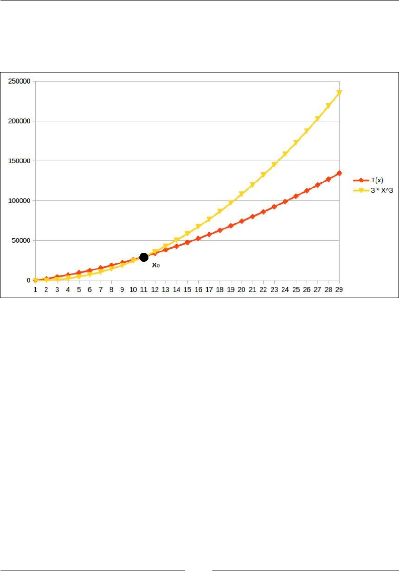
For example, Figure 1 shows an example of a function T(x) = 100x2+2000x+200. This
function is O(x2), with some x0 = 11 and M = 300. The graph of 300x2 overcomes the
graph of T(x) at x=11 and then stays above T(x) up to innity. Notice that the function
300x2 is lower than T(x) for smaller values of x, but that does not affect our conclusion.
Figure 1. Asymptotic upper bound
To see that it's the same thing as the previous four points, rst think of x0 as the
way to ensure that x is sufciently large. I leave it up to you to prove the above four
conditions from the formal denition.
I will, however, show some examples of using the formal denition:
• 5x2 = O(x2) because we can say, for example, x0 = 10 and M = 10 and thus f(x)
< Mg(x) whenever x > x0, that is, 5x2 < 10x2 whenever x > 10.
• It is also true that 5x2 = O(x3) because we can say, for example, x0 = 10 and M
= 10 and thus f(x) < Mg(x) whenever x > x0, that is, 5x2 < 10x3 whenever x >
10. This highlights a point that if f(x) = O(g(x)), it is also true that f(x) = O(h(x))
if h(x) is some functions that grows at least as fast as f(x).

Chapter 1
[ 7 ]
• How about the function f(x) = 5x2 - 10x + 3? We can easily see that when x is
sufficiently large, 5x2 will far surpass the term 10x. To prove my point, I can
simply say x>5, 5x2 > 10x. Every time we increment x by one, the increment
in 5x2 is 10x + 1 and the increment in 10x is just a constant, 10. 10x+1 > 10 for
all positive x, so it is easy to see why 5x2 is always going to stay above 10x as
x goes higher and higher.
In general, any polynomial of the form anxn + an-1xn-1 + an-2xn-2 + … + a0 = O(xn). To
show this, we will rst see that a0 = O(1). This is true because we can have x0 = 1 and
M = 2|a0|, and we will have |a0| < 2|a0| whenever x > 1.
Now, let us assume it is true for some n. Thus, anxn + an-1xn-1 + an-2xn-2 + … + a0 = O(xn).
What it means, of course, is that some Mn and x0 exist, such that |anxn + an-1xn-1 + an-
2xn-2 + … + a0 | < Mnxn whenever x>x0. We can safely assume that x0 >2, because if it is
not so, we can simply add 2 to it to get a new x0 , which is at least 2.
Now, |anxn + an-1xn-1 + an-2xn-2 + … + a0| < Mnxn implies |an+1xn+1 + anxn + an-1xn-1 + an-2xn-2
+ … + a0| ≤ |an+1xn+1| + |anxn + an-1xn-1 + an-2xn-2 + … + a0| < |an+1xn+1| + Mnxn.
This means |an+1xn+1| + Mnxn > |anxn + an-1xn-1 + an-2xn-2 + … + a0|.
If we take Mn+1= |an+1| + Mn, we can see that Mn+1 xn+1 = |an+1| xn+1 + Mn xn+1 =|an+1
xn+1| + Mn xn+1> |an+1 xn+1| + Mn xn > |an+1 xn+1 + anxn + an-1xn-1 + an-2xn-2 + … + a0|.
That is to say, |an+1 xn+1 + an-1xn-1 + an-2xn-2 + … + a0 |< Mn+1 xn+1 for all x > x0, that is, an+1
xn+1 + anxn + an-1xn-1 + an-2xn-2 + … + a0 = O(xn+1).
Now, we have it true for n=0, that is, a0 = O(1). This means, by our last conclusion,
a1x + a0 = O(x). This means, by the same logic, a2 x2 + a1x + a0 = O(x2), and so
on. We can easily see that this means it is true for all polynomials of positive
integral degrees.

Why Bother? – Basic
[ 8 ]
Asymptotic upper bound of an algorithm
Okay, so we gured out a way to sort of abstractly specify an upper bound on
a function that has one argument. When we talk about the running time of a
program, this argument has to contain information about the input. For example,
in our algorithm, we can say, the execution time equals O(power). This scheme of
specifying the input directly will work perfectly ne for all programs or algorithms
solving the same problem because the input will be the same for all of them.
However, we might want to use the same technique to measure the complexity of
the problem itself: it is the complexity of the most efcient program or algorithm that
can solve the problem. If we try to compare the complexity of different problems,
though, we will hit a wall because different problems will have different inputs.
We must specify the running time in terms of something that is common among
all problems, and that something is the size of the input in bits or bytes. How
many bits do we need to express the argument, power, when it's sufciently large?
Approximately log2 (power). So, in specifying the running time, our function needs
to have an input that is of the size log2 (power) or lg (power). We have seen that the
running time of our algorithm is proportional to the power, that is, constant times
power, which is constant times 2 lg(power) = O(2x),where x= lg(power), which is the
the size of the input.
Asymptotic lower bound of a function
Sometimes, we don't want to praise an algorithm, we want to shun it; for example,
when the algorithm is written by someone we don't like or when some algorithm
is really poorly performing. When we want to shun it for its horrible performance,
we may want to talk about how badly it performs even for the best input. An a
symptotic lower bound can be dened just like how greater-than-or-equal-to can be
dened in terms of less-than-or-equal-to.
A function f(x) = Ω(g(x)) if and only if g(x) = O(f(x)). The following list shows a
few examples:
• Since x3 = O(x3), x3 = Ω(x3)
• Since x3 = O(5x3), 5x3 = Ω(x3)
• Since x3 = O(5x3 - 25x2 + 1), 5x3 - 25x2 + 1 = Ω(x3)
• Since x3 = O(x4), x4 = O(x3)
Again, for those of you who are interested, we say the expression f(x) = Ω(g(x))
means there exist positive constants M and x0, such that |f(x)| > M|g(x)| whenever
x > x0, which is the same as saying |g(x)| < (1/M)|f(x)| whenever x > x0 , that is, g(x)
= O(f(x)).

Chapter 1
[ 9 ]
The preceding denition was introduced by Donald Knuth, which was a stronger
and more practical denition to be used in computer science. Earlier, there was a
different denition of the lower bound Ω that is more complicated to understand and
covers a few more edge cases. We will not talk about edge cases here.
While talking about how horrible an algorithm is, we can use an asymptotic lower
bound of the best case to really make our point. However, even a criticism of the
worst case of an algorithm is quite a valid argument. We can use an asymptotic
lower bound of the worst case too for this purpose, when we don't want to nd out
an asymptotic tight bound. In general, the asymptotic lower bound can be used to
show a minimum rate of growth of a function when the input is large enough
in size.
Asymptotic tight bound of a function
There is another kind of bound that sort of means equality in terms of asymptotic
complexity. A theta bound is specied as f(x) = Ͽ(g(x)) if and only if f(x) = O(g(x)) and
f(x) = Ω(g(x)). Let's see some examples to understand this even better:
• Since 5x3=O(x3) and also 5x3=Ω(x3), we have 5x3=Ͽ(x3)
• Since 5x3 + 4x2=O(x3) and 5x3 + 4x2=Ω(x3), we have 5x3 + 4x2=O(x3)
• However, even though 5x3 + 4x2 =O(x4), since it is not Ω(x4), it is also
not Ͽ(x4)
• Similarly, 5x3 + 4x2 is not Ͽ(x2) because it is not O(x2)
In short, you can ignore constant multipliers and lower order terms while
determining the tight bound, but you cannot choose a function which grows either
faster or slower than the given function. The best way to check whether the bound is
right is to check the O and the condition separately, and say it has a theta bound only
if they are the same.
Note that since the complexity of an algorithm depends on the particular input, in
general, the tight bound is used when the complexity remains unchanged by the
nature of the input.

Why Bother? – Basic
[ 10 ]
In some cases, we try to nd the average case complexity, especially when the upper
bound really happens only in the case of an extremely pathological input. But since
the average must be taken in accordance with the probability distribution of the
input, it is not just dependent on the algorithm itself. The bounds themselves are just
bounds for particular functions and not for algorithms. However, the total running
time of an algorithm can be expressed as a grand function that changes it's formula
as per the input, and that function may have different upper and lower bounds.
There is no sense in talking about an asymptotic average bound because, as we
discussed, the average case is not just dependent on the algorithm itself, but also on
the probability distribution of the input. The average case is thus stated as a function
that would be a probabilistic average running time for all inputs, and, in general, the
asymptotic upper bound of that average function is reported.
Optimization of our algorithm
Before we dive into actually optimizing algorithms, we need to rst correct our
algorithm for large powers. We will use some tricks to do so, as described below.
Fixing the problem with large powers
Equipped with all the toolboxes of asymptotic analysis, we will start optimizing our
algorithm. However, since we have already seen that our program does not work
properly for even moderately large values of power, let's rst x that. There are two
ways of xing this; one is to actually give the amount of space it requires to store all
the intermediate products, and the other is to do a trick to limit all the intermediate
steps to be within the range of values that the long datatype can support. We will
use binomial theorem to do this part.
As a reminder, binomial theorem says (x+y)n = xn + nC1xn-1y + nC2xn-2y2 + nC3xn-3y3 +
nC4xn-4y4 + … nCn-1x1yn-1 + yn for positive integral values of n. The important point here
is that all the coefcients are integers. Suppose, r is the remainder when we divide a
by b. This makes a = kb + r true for some positive integer k. This means r = a-kb, and rn
= (a-kb)n.
If we expand this using binomial theorem, we have rn = an - nC1 an-1.kb + nC2an-2.(kb)2 -
nC3an-3.(kb)3 + nC4an-4.(kb)4 + … nCn-1a1.(kb)n-1 ± (kb)n.
Note that apart from the rst term, all other terms have b as a factor. Which means
that we can write rn = an + bM for some integer M. If we divide both sides by b now
and take the remainder, we have rn % b = an % b, where % is the Java operator for
nding the remainder.

Chapter 1
[ 11 ]
The idea now would be to take the remainder by the divisor every time we raise the
power. This way, we will never have to store more than the range of the remainder:
public static long computeRemainderCorrected(long base, long
power, long divisor){
long baseRaisedToPower = 1;
for(long i=1;i<=power;i++){
baseRaisedToPower *= base;
baseRaisedToPower %= divisor;
}
return baseRaisedToPower;
}
This program obviously does not change the time complexity of the program; it
just xes the problem with large powers. The program also maintains a constant
space complexity.
Improving time complexity
The current running time complexity is O(2x), where x is the size of the input as we
have already computed. Can we do better than this? Let's see.
What we need to compute is (basepower) % divisor. This is, of course, the same as
(base2)power/2 % divisor. If we have an even power, we have reduced the number of
operations by half. If we can keep doing this, we can raise the power of base by 2n in
just n steps, which means our loop only has to run lg(power) times, and hence, the
complexity is O(lg(2x)) = O(x), where x is the number of bits to store power. This is a
substantial reduction in the number of steps to compute the value for large powers.
However, there is a catch. What happens if the power is not divisible by 2? Well, then
we can write (basepower)% divisor = (base ((basepower-1))%divisor = (base ((base2)power-1)%divisor,
and power-1 is, of course, even and the computation can proceed. We will write up this
code in a program. The idea is to start from the most signicant bit and move towards
less and less signicant bits. If a bit with 1 has n bits after it, it represents multiplying
the result by the base and then squaring n times after this bit. We accumulate this
squaring by squaring for the subsequent steps. If we nd a zero, we keep squaring for
the sake of accumulating squaring for the earlier bits:
public static long computeRemainderUsingEBS(long base, long power,
long divisor){
long baseRaisedToPower = 1;
long powerBitsReversed = 0;
int numBits=0;

Why Bother? – Basic
[ 12 ]
First reverse the bits of our power so that it is easier to access them from the least
important side, which is more easily accessible. We also count the number of bits
for later use:
while(power>0){
powerBitsReversed <<= 1;
powerBitsReversed += power & 1;
power >>>= 1;
numBits++;
}
Now we extract one bit at a time. Since we have already reversed the order of bit,
the rst one we get is the most signicant one. Just to get an intuition on the order,
the rst bit we collect will eventually be squared the maximum number of times and
hence will act like the most signicant bit:
while (numBits-->0){
if(powerBitsReversed%2==1){
baseRaisedToPower *= baseRaisedToPower * base;
}else{
baseRaisedToPower *= baseRaisedToPower;
}
baseRaisedToPower %= divisor;
powerBitsReversed>>>=1;
}
return baseRaisedToPower;
}
We test the performance of the algorithm; we compare the time taken for the same
computation with the earlier and nal algorithms with the following code:
public static void main(String [] args){
System.out.println(computeRemainderUsingEBS(13, 10_000_000, 7));
long startTime = System.currentTimeMillis();
for(int i=0;i<1000;i++){
computeRemainderCorrected(13, 10_000_000, 7);
}
long endTime = System.currentTimeMillis();
System.out.println(endTime - startTime);
startTime = System.currentTimeMillis();
for(int i=0;i<1000;i++){
computeRemainderUsingEBS(13, 10_000_000, 7);
}
endTime = System.currentTimeMillis();
System.out.println(endTime - startTime);
}

Chapter 1
[ 13 ]
The rst algorithm takes 130,190 milliseconds to complete all 1,000 times execution
on my computer and the second one takes just 2 milliseconds to do the same. This
clearly shows the tremendous gain in performance for a large power like 10 million.
The algorithm for squaring the term repeatedly to achieve exponentiation like we did
is called... well, exponentiation by squaring. This example should be able to motivate
you to study algorithms for the sheer obvious advantage it can give in improving the
performance of computer programs.
Summary
In this chapter, you saw how we can think about measuring the running time of
and the memory required by an algorithm in seconds and bytes, respectively. Since
this depends on the particular implementation, the programming platform, and
the hardware, we need a notion of talking about running time in an abstract way.
Asymptotic complexity is a measure of the growth of a function when the input is
very large. We can use it to abstract our discussion on running time. This is not to say
that a programmer should not spend any time to make a run a program twice as fast,
but that comes only after the program is already running at the minimum asymptotic
complexity.
We also saw that the asymptotic complexity is not just a property of the problem
at hand that we are trying to solve, but also a property of the particular way we
are solving it, that is, the particular algorithm we are using. We also saw that two
programs solving the same problem while running different algorithms with
different asymptotic complexities can perform vastly differently for large inputs.
This should be enough motivation to study algorithms explicitly.
In the following chapters, we will study the most used algorithmic tricks and
concepts required in daily use. We will start from the very easy ones that are also
the building blocks for the more advanced techniques. This book is, of course, by no
means comprehensive; the objective is to provide enough background to make you
comfortable with the basic concepts and then you can read on.
[ 15 ]
Cogs and Pulleys – Building
Blocks
We discussed algorithms in the previous chapter, but the title of the book also
includes the term "data structure." So what is a data structure? A data structure is
an organization of data in memory that is generally optimized so it can be used by
a particular algorithm. We have seen that an algorithm is a list of steps that leads to
a desired outcome. In the case of a program, there is always some input and output.
Both input and output contain data and hence must be organized in some way or
another. Therefore, the input and output of an algorithm are data structures. In fact,
all the intermediate states that an algorithm has to go through must also be stored in
some form of a data structure. Data structures don't have any use without algorithms
to manipulate them, and algorithms cannot work without data structures. It's
because this is how they get input and emit output or store their intermediate states.
There are a lot of ways in which data can be organized. Simpler data structures are
also different types of variables. For example, int is a data structure that stores one
4-byte integer value. We can even have classes that store a set of specic types of
values. However, we also need to think about how to store a collection of a large
number of the same type of values. In this book, we will spend the rest of the time
discussing a collection of values of the same type because how we store a collection
determines which algorithm can work on them. Some of the most common ways
of storing a collection of values have their own names; we will discuss them in this
chapter. They are as follows:
• Arrays
• Linked lists
• Doubly linked lists
• Circular linked lists

Cogs and Pulleys – Building Blocks
[ 16 ]
These are the basic building blocks that we will use to build more complex data
structures. Even if we don't use them directly, we will use their concepts.
Arrays
If you are a Java programmer, you must have worked with arrays. Arrays are the
basic storage mechanisms available for a sequence of data. The best thing about
arrays is that the elements of an array are collocated sequentially and can be accessed
completely and randomly with single instructions.
The traversal of an array element by an element is very simple. Since any element
can be accessed randomly, you just keep incrementing an index and keep accessing
the element at this index. The following code shows both traversal and random
access in an array:
public static void printAllElements(int[] anIntArray){
for(int i=0;i<anIntArray.length;i++){
System.out.println(anIntArray[i]);
}
}
Insertion of elements in an array
All the elements in an array are stored in contiguous memory. This makes it possible
to access any element in a constant amount of time. A program simply needs to
compute the offset that corresponds to an index, and it reads the information
directly. But this means they are also limited and have a xed size. If you want to
insert a new element into an array, you will need to create a new array with one
more element and copy the entire data from the original data along with the new
value. To avoid all this complexity, we will start with moving an existing element
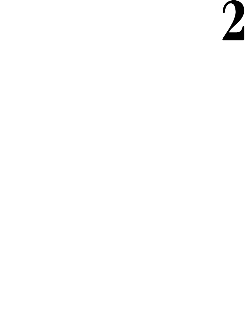
to a new position. What we are looking to do is to take an element out, shift all the
elements up to the target position to make space in this position, and insert the value
we extracted in the same place.
Chapter 2
[ 17 ]
Figure 1: Insertion of an existing array element into a new location
The preceding gure explains what we mean by this operation. The thin black
arrows show the movement of the element that is being reinserted, and the thick
white arrow shows the shift of the elements of the array. In each case, the bottom
gure shows the array after the reinsertion is done. Notice that the shifting is done
either to the left or right, depending on what the start and end index are. Let's put
this in code:
public static void insertElementAtIndex(int[] array,
int startIndex, int targetIndex){
int value = array[startIndex];
if(startIndex==targetIndex){
return;
}else if(startIndex < tarGetIndex){
for(int i=startIndex+1;i<=targetIndex;i++){
array[i-1]=array[i];
}
array[targetIndex]=value;
}else{
for(int i=startIndex-1;i>=targetIndex;i--){
array[i+1]=array[i];
}
array[targetIndex]=value;
}
}
Cogs and Pulleys – Building Blocks
[ 18 ]
What would be the running time complexity of the preceding algorithm? For all our
cases, we will only consider the worst case. When does an algorithm perform worst?
To understand this, let's see what the most frequent operation in an algorithm is. It is
of course the shift that happens in the loop. The number of shifts become maximum
when startIndex is at the beginning of the array and targetIndex at the end or
vice versa. This is when all but one element has to be shifted one by one. The running
time in this case must be some constant times the number of elements of the array
plus some other constant to account for the non-repeating operations. So it is T(n) =
K(n-1)+C for some constants K and C, where n is the number of elements in the array
and T(n) is the running time of the algorithm. This can be expressed as follows:
T(n) = K(n-1)+C = Kn + (C-K)
The following steps explain the expression:
1. As per rule 1 of the denition of big O, T(n) = O(Kn + (C-K)).
2. As per rule 3, T(n) = O(Kn).
3. We know |-(C-K)| < |Kn + (C-K)| is true for sufciently large n. Therefore,
as per rule 3, since T(n) = O(Kn + (C-K)), it means T(n) = O(Kn + (C-K) + (-(C-
K))), that is, T(n) = O(Kn).
4. And, nally, as per rule 2, T(n) = O(n).
Now since the array is the major input in the algorithm, the size of the input is
represented by n. So we will say, the running time of the algorithm is O(n), where n
is the size of the input.
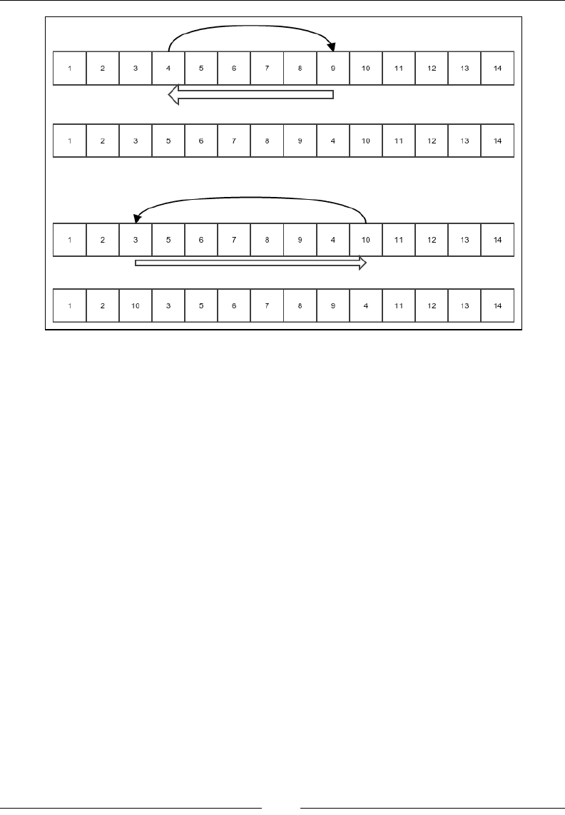
Insertion of a new element and the process of
appending it
Now we move on to the process of insertion of a new element. Since arrays are xed
in size, insertion requires us to create a new array and copy all the earlier elements
into it. The following gure explains the idea of an insertion made in a new array:
Figure 2: Insertion of a new element into an array

Chapter 2
[ 19 ]
The following code does exactly that:
public static int [] insertExtraElementAtIndex(int[] array,
int index, int value){
int [] newArray = new int[array.length+1];
First, you copy all the elements before the targeted position as they are in the
original array:
for(int i=0;i<index;i++){
newArray[i] = array[i];
}
Then, the new value must be put in the correct position:
newArray[index]=value;
In the end, copy the rest of the elements in the array by shifting their position by one:
for(int i=index+1;i<newArray.length;i++){
newArray[i]=array[i-1];
}
return newArray;
}
When we have the code ready, appending it would mean just inserting it at the end,
as shown in the following code:
public static int[] appendElement(int[] array, int value){
return insertExtraElementAtIndex(array, array.length, value);
}
What is the running time complexity of the preceding algorithm? Well, no matter
what we do, we must copy all the elements of the original array to the new array,
and this is the operation in the loop. So the running time is T(n) = Kn + C for some
constants K and C, and n is the size of the array, which is the size of the input. I leave
it to you to verify the steps in order to gure out this: T(n) = O(n).
Cogs and Pulleys – Building Blocks
[ 20 ]
Linked list
Arrays are great for storing data. We have also seen that any element of an array
can be read in O(1) time. But arrays are xed in size. Changing the size of an array
means creating a new array and copying all the elements to the original array. The
simplest recourse to the resizing problem is to store each element in a different object
and then hold a reference in each element to the next element. This way, the process
of adding a new element will just involve creating the element and attaching it at
the end of the last element of the original linked list. In another variation, the new
element can be added to the beginning of the existing linked list:
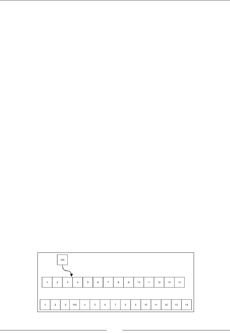
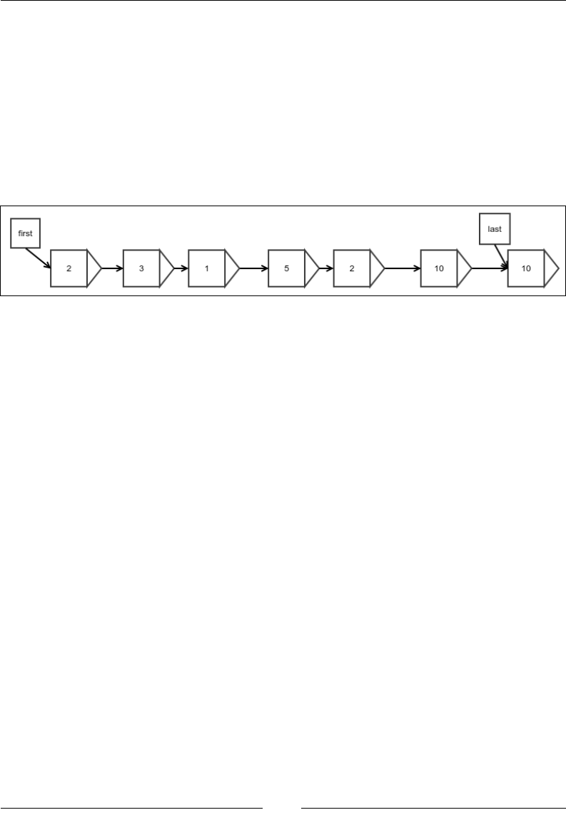
Figure 3: An example of a linked list
Figure 3 shows an example of a linked list. The arrows represent a reference. Each
element is stored in a wrapper object that also holds a reference to the next element
wrapper. There are two additional references to the rst and last elements, which are
required for any operation to start. The last reference is optional, but it improves the
performance of appending to the end vastly, as we shall see.
To begin the discussion, let's create a linked list node in the following way:
public class LinkedList<E> implements Iterable<E>, Visualizable {
First, we create a Node class inside the LinkedList class, which will act as a wrapper
for the elements and also hold the reference to the next node:
protected static class Node<E> {
protected E value;
protected Node next;
public String toString(){
return value.toString();
}
}
int length = 0;
Node<E>[] lastModifiedNode;
Chapter 2
[ 21 ]
Then, we must have references for the rst and last elements:
Node<E> first;
Node<E> last;
Finally, we create a method called getNewNode() that creates a new empty node. We
will need this if we want to use a different class for a node in any of the subclasses:
protected Node<E> getNewNode() {
Node<E> node = new Node<>();
lastModifiedNode = new Node[]{node};
return node;
}
}
At this point, the unnished class LinkedList will not be able to store any element;
let's see how to do this, though. Notice that we have implemented the Iterable
interface. This will allow us to loop through all the elements in an advanced for loop.
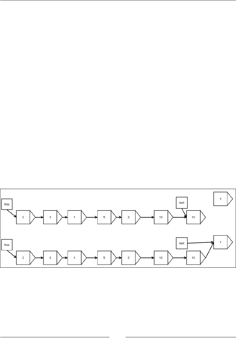
Appending at the end
Appending at the end is achieved by simply creating a link from the last element
of the original linked list to the new element that is being appended and then
reassigning the reference to the last element. The second step is required because the
new element is the new last element. This is shown in the following gure:
Figure 4: Appending at the end of a linked list
Cogs and Pulleys – Building Blocks
[ 22 ]
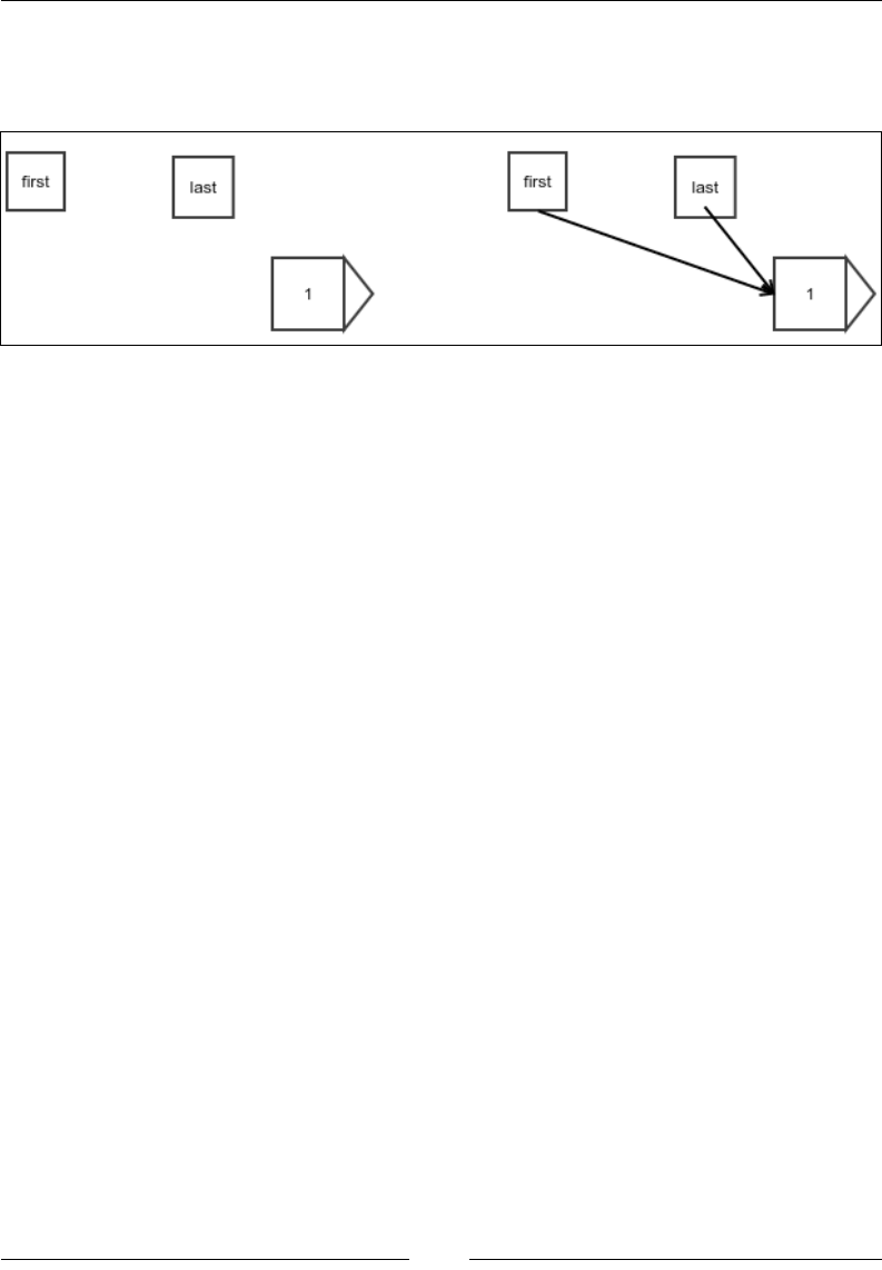
There is a small difference when you append an element to a linked list that is empty
to start with. At this point, the rst and last references are null, and this case must be
handled separately. The following gure explains this case:
Figure 5: Appending to an empty linked list
We will achieve this by using the following simple code as is. We return the node
that has just been added. This is helpful to any class that is extending this class. We
will do the same in all cases, and we will see the use of this while discussing doubly
linked lists:
public Node<E> appendLast(E value) {
Node node = getNewNode();
node.value = value;
We try to update the reference of the current last node only if the list is not empty:
if (last != null)
last.next = node;
Then, we must update the last reference as the new element is not going to be the
last element:
last = node;
Finally, if the list is empty, the new element must also be the rst new element and
we must update the rst reference accordingly, as shown in the preceding gure:
if (first == null) {
first = node;
}
length++;
return node;
}

Chapter 2
[ 23 ]
Notice that we also keep track of the current length of the list. This is not essential,
but if we do this, we do not have to traverse the entire list just to count how many
elements are in the list.
Now, of course, there is this important question: what is the time complexity of
appending to a linked list? Well, if we do it the way we have done it before—that is,
by having a special reference to the last element—we don't need any loop, as we can
see in the code. If the program does not have any loops, all operations would be one-
time operations, hence everything is completed in constant time. You can verify that
a constant function has this complexity: O(1). Compare this with what was appended
at the end of an array. It required the creation of a new array and also had O(n)
complexity, where n was the size of the array.
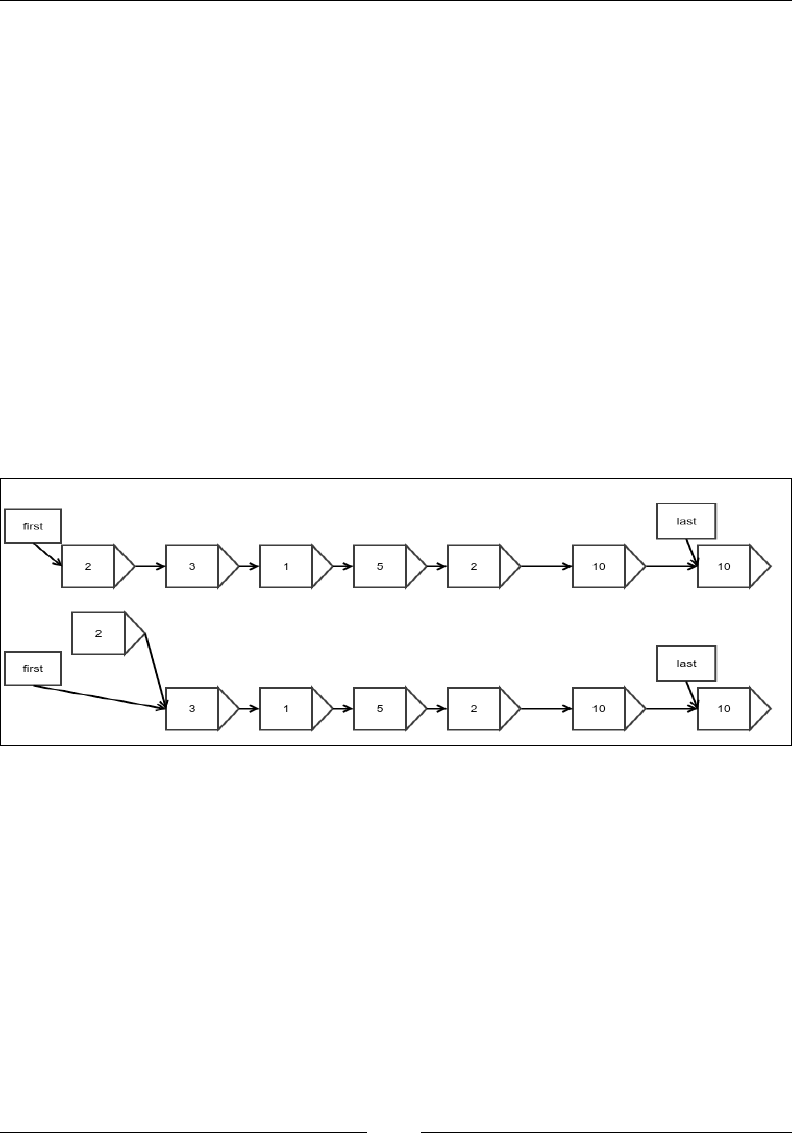
Insertion at the beginning
Inserting an element at the beginning of a list is very similar to appending it at the
end. The only difference is that you need to update the rst reference instead of the
last reference:
public Node<E> appendFirst(E value) {
Node node = getNewNode();
node.value = value;
node.next = first;
first = node;
if (length == 0)
last = node;
length++;
return node;
}
Cogs and Pulleys – Building Blocks
[ 24 ]
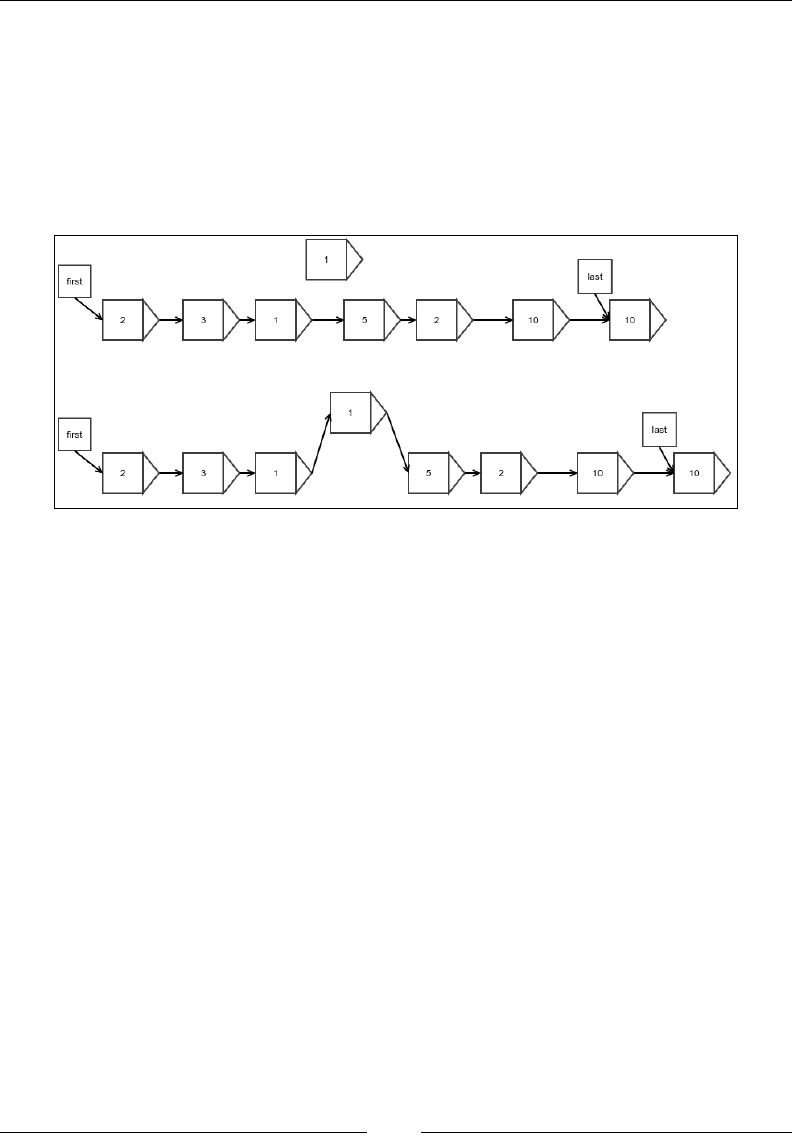
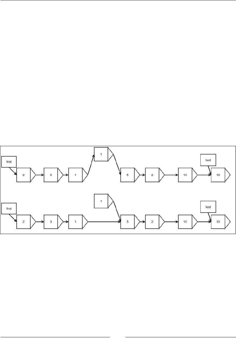
Insertion at an arbitrary position
Insertion at an arbitrary position can be achieved in the same way we perform an
insertion in the rst element, except that we update the reference of the previous
element instead of the rst reference. There is, however, a catch; we need to nd the
position where we need to insert the element. There is no way to nd it other than
to start at the beginning and walk all the way to the correct position while counting
each node we step on.
Figure 6: Insertion of an arbitrary element into a linked list
We can implement the idea as follows:
public Node<E> insert(int index, E value) {
Node<E> node = getNewNode();
First, we take care of the special cases:
if (index < 0 || index > length) {
throw new IllegalArgumentException("Invalid
index for insertion");
} else if (index == length) {
return appendLast(value);
} else if (index == 0) {
return appendFirst(value);
} else {
As mentioned earlier, we walk all the way to the desired position while counting the
nodes, or in this case, counting the index in the opposite direction:
Node<E> result = first;
while (index > 1) {
index--;
result = result.next;
}

Chapter 2
[ 25 ]
Finally, we update the references:
node.value = value;
node.next = result.next;
result.next = node;
length++;
return node;
}
}
What is the complexity of this algorithm? There is a loop that must run as many
times as the index. This algorithm seems to have a running time that is dependent
on the value of the input and not just its size. In this case, we are only interested in
the worst case. What is the worst case then? It is when we need to step on all the
elements of the list, that is, when we have to insert the element at the end of the list,
except for the last element. In this case, we must step on n-1 elements to get there
and do some constant work. The number of steps would then be T(n) = C(n-1)+K for
some constants C and K. So, T(n) = O(n).
Looking up an arbitrary element
Finding the value of an arbitrary element has two different cases. For the rst and
last element, it is simple. Since we have direct references to the rst and last element,
we just have to traverse that reference and read the value inside it. I leave this for
you to see how it could be done.
However, how do you read an arbitrary element? Since we only have forward
references, we must start from the beginning and walk all the way, traversing
references while counting steps until we reach the element we want.
Let's see how we can do this:
public E findAtIndex(int index) {
We start from the rst element:
Node<E> result = first;
while (index >= 0) {
if (result == null) {
throw new NoSuchElementException();
} else if (index == 0) {
Cogs and Pulleys – Building Blocks
[ 26 ]
When the index is 0, we would have nally reached the desired position, so
we return:
return result.value;
} else {
If we are not there yet, we must step onto the next element and keep counting:
index--;
result = result.next;
}
}
return null;
}
Here too, we have a loop inside that has to run an index a number of times. The
worst case is when you just need to remove one element but it is not the last one;
the last one can be found directly. It is easy to see that just like you insert into an
arbitrary position, this algorithm also has running time complexity of O(n).
Figure 7: Removing an element in the beginning
Removing an element in the beginning means simply updating the reference to the
rst element with that of the next element. Note that we do not update the reference
in the element that has just been removed because the element, along with the
reference, would be garbage-collected anyway:
public Node<E> removeFirst() {
if (length == 0) {
throw new NoSuchElementException();
}
Chapter 2
[ 27 ]
Assign the reference to the next element:
Node<E> origFirst = first;
first = first.next;
length--;
If there are no more elements left, we must also update the last reference:
if (length == 0) {
last = null;
}
return origFirst;
}
Removing an arbitrary element
Removing an arbitrary element is very similar to removing an element from the
beginning, except that you update the reference held by the previous element instead
of the special reference named rst. The following gure shows this:
Figure 8: Removing an arbitrary element
Notice that only the link in the linked list is to be reassigned to the next element. The
following code does what is shown in the preceding gure:
protected Node<E> removeAtIndex(int index) {
if (index >= length || index < 0) {
throw new NoSuchElementException();
}

Cogs and Pulleys – Building Blocks
[ 28 ]
Of course, removing the rst element is a special case:
if (index == 0) {
Node<E> nodeRemoved = first;
removeFirst();
return nodeRemoved;
}
First, nd out the element just before the one that needs to be removed because this
element would need its reference updated:
Node justBeforeIt = first;
while (--index > 0) {
justBeforeIt = justBeforeIt.next;
}
Update the last reference if the last element is the one that is being removed:
Node<E> nodeRemoved = justBeforeIt.next;
if (justBeforeIt.next == last) {
last = justBeforeIt.next.next;
}
Update the reference held by the previous element:
justBeforeIt.next = justBeforeIt.next.next;
length--;
return nodeRemoved;
}
It is very easy to see that the running time worst case complexity of this algorithm is
O(n)—which is similar to nding an arbitrary element—because this is what needs
to be done before removing it. The operation of the actual removal process itself
requires only a constant number of steps.
Iteration
Since we are working in Java, we prefer to implement the Iterable interface. It lets
us loop through the list in a simplied for loop syntax. For this purpose, we rst
have to create an iterator that will let us fetch the elements one by one:
protected class ListIterator implements Iterator<E> {
protected Node<E> nextNode = first;
@Override

Chapter 2
[ 29 ]
public boolean hasNext() {
return nextNode != null;
}
@Override
public E next() {
if (!hasNext()) {
throw new IllegalStateException();
}
Node<E> nodeToReturn = nextNode;
nextNode = nextNode.next;
return nodeToReturn.value;
}
}
The code is self-explanatory. Every time it is invoked, we move to the next element
and return the current element's value. Now we implement the iterator method of
the Iterable interface to make our list an iterable:
@Override
public Iterator<E> iterator() {
return new ListIterator();
}
This enables us to use the following code:
for(Integer x:linkedList){
System.out.println(x);
}
The preceding code assumes that the variable linkedList was
LinkedList<Integer>. Any list that extends this class will also get this
property automatically.
Cogs and Pulleys – Building Blocks
[ 30 ]
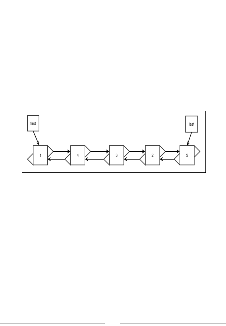
Doubly linked list
Did you notice that there is no quick way to remove the element from the end of a
linked list? This is because even if there is a quick way to nd the last element, there
is no quick way to nd the element before it whose reference needs to be updated.
We must walk all the way from the beginning to nd the previous element. Well
then, why not just have another reference to store the location of the last but one
element? This is because after you remove the element, how would you update the
reference otherwise? There would be no reference to the element right before that.
What it looks like is that to achieve this, we have to store the reference of all the
previous elements up to the beginning. The best way to do this would be to store the
reference of the previous element in each of the elements or nodes along with the
reference to the next element. Such a linked list is called a doubly linked list since
the elements are linked both ways:
Figure 9: Doubly linked list
We will implement a doubly linked list by extending our original linked list because
a lot of the operations would be similar. We can create the barebones class in the
following manner:
public class DoublyLinkedList<E> extends LinkedList<E> {
We create a new Node class extending the original one and adding a reference for the
previous node:
protected static class DoublyLinkedNode<E> extends Node<E> {
protected DoublyLinkedNode<E> prev;
}
Of course, we need to override the getNode() method to use this node:
@Override
protected Node<E> getNewNode() {
return new DoublyLinkedNode<E>();
}
}
Chapter 2
[ 31 ]
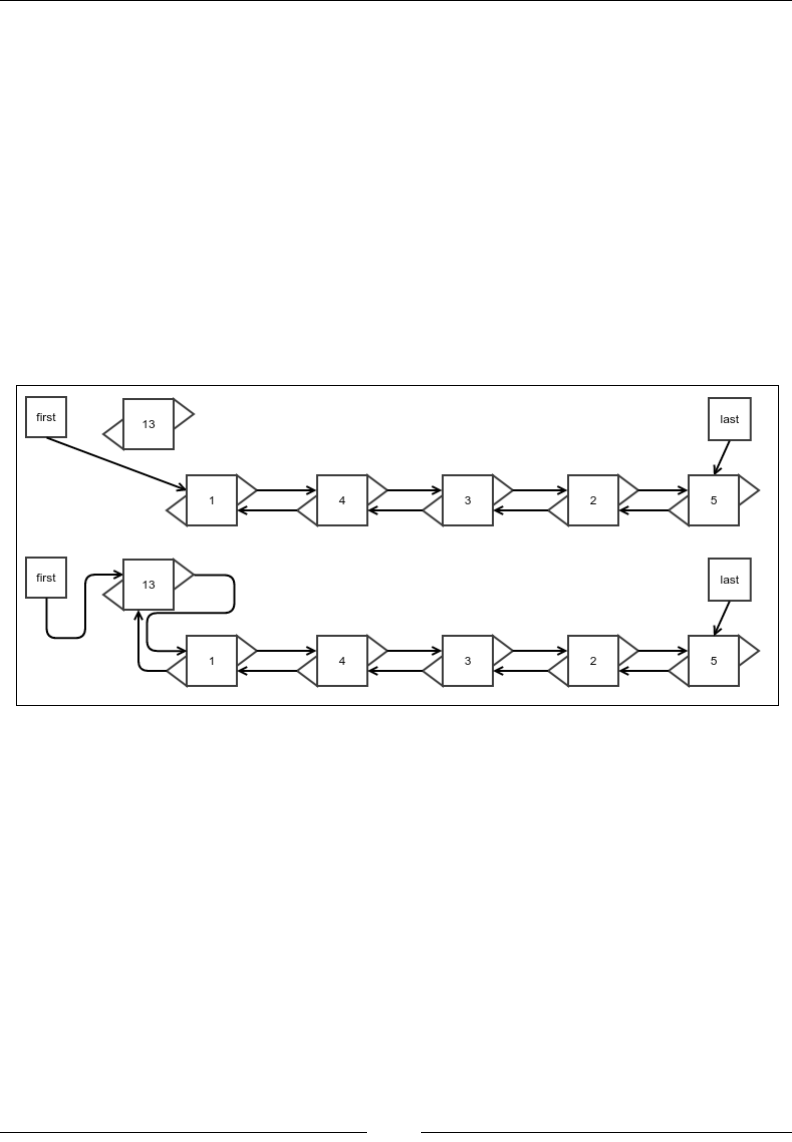
Insertion at the beginning or at the end
Insertion at the beginning is very similar to that of a singly linked list, except that
we must now update the next node's reference for its previous node. The node being
inserted does not have a previous node in this case, so nothing needs to be done:
public Node<E> appendFirst(E value) {
Node<E> node = super.appendFirst(value);
if (first.next != null)
((DoublyLinkedNode<E>) first.next).prev =
(DoublyLinkedNode<E>) first;
return node;
}
Pictorially, it can be visualized as shown in the following gure:
Figure 10: Insertion at the beginning of a doubly linked list
Appending at the end is very similar and is given as follows:
public Node<E> appendLast(E value) {
DoublyLinkedNode<E> origLast = (DoublyLinkedNode<E>)
this.last;
Node<E> node = super.appendLast(value);
If the original list were empty, the original last reference would be null:
if (origLast == null) {
origLast = (DoublyLinkedNode<E>) first;
}
((DoublyLinkedNode<E>) this.last).prev = origLast;
return node;
}
Cogs and Pulleys – Building Blocks
[ 32 ]
The complexity of the insertion is the same as that of a singly linked list. In fact, all
the operations on a doubly linked list have the same running time complexity as that
of a singly linked list, except the process of removing the last element. We will thus
refrain from stating it again until we discuss the removal of the last element. You
should verify that the complexity stays the same as with a singly linked list in all
other cases.
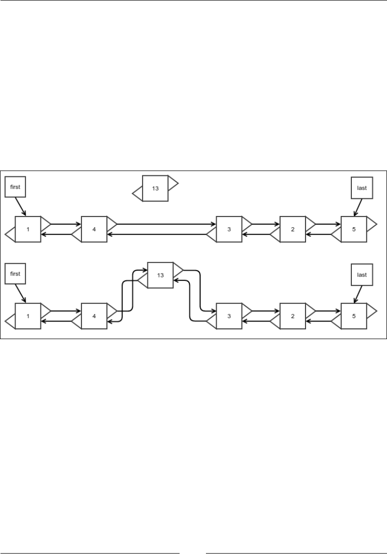
Insertion at an arbitrary location
As with everything else, this operation is very similar to the process of making
an insertion at an arbitrary location of a singly linked list, except that you need to
update the references for the previous node.
Figure 11: Insertion at an arbitrary location of a doubly linked list
The following code does this for us:
public Node<E> insert(int index, E value) {
DoublyLinkedNode<E> inserted = (DoublyLinkedNode<E>)
super.insert(index, value);

Chapter 2
[ 33 ]
In the case of the rst and last element, our overridden methods are invoked
anyway. Therefore, there is no need to consider them again:
if(index!=0 && index!=length) {
if (inserted.next != null) {
This part needs a little bit of explaining. In Figure 11, the node being inserted is 13.
Its previous node should be 4, which was originally the previous node of the next
node 3:
inserted.prev = ((DoublyLinkedNode<E>)
inserted.next).prev;
The prev reference of the next node 3 must now hold the newly inserted node 13:
((DoublyLinkedNode<E>) inserted.next).prev = inserted;
}
}
return inserted;
}
Removing the rst element
Removing the rst element is almost the same as that for a singly linked list. The
only additional step is to set the prev reference of the next node to null. The
following code does this:
public Node<E> removeFirst() {
super.removeFirst();
if (first != null) {
((DoublyLinkedNode<E>) first).prev = null;
}
return first;
}
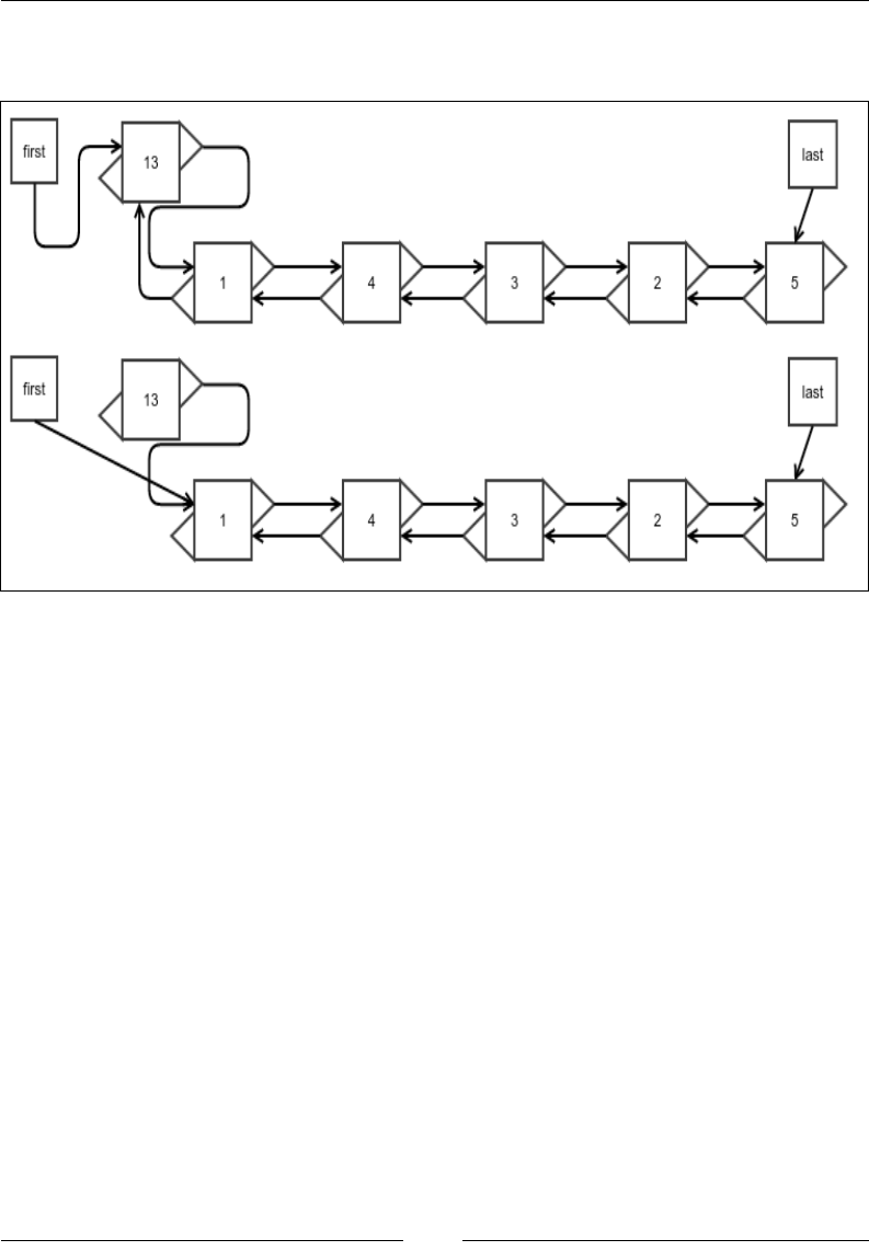
Cogs and Pulleys – Building Blocks
[ 34 ]
The following gure shows what happens. Also, note that nding an element does
not really need an update:
Figure 12: Removal of the first element from a doubly linked list
There can be an optimization to traverse backward from the last element to the rst
in case the index we are looking for is closer toward the end; however, it does not
change the asymptotic complexity of the nd operation. So we leave it at this stage. If
interested, you would be able to easily gure out how to do this optimization.
Removing an arbitrary element
Just like other operations, removal is very similar to removal of elements in the case
of a singly linked list, except that we need to update the prev reference:
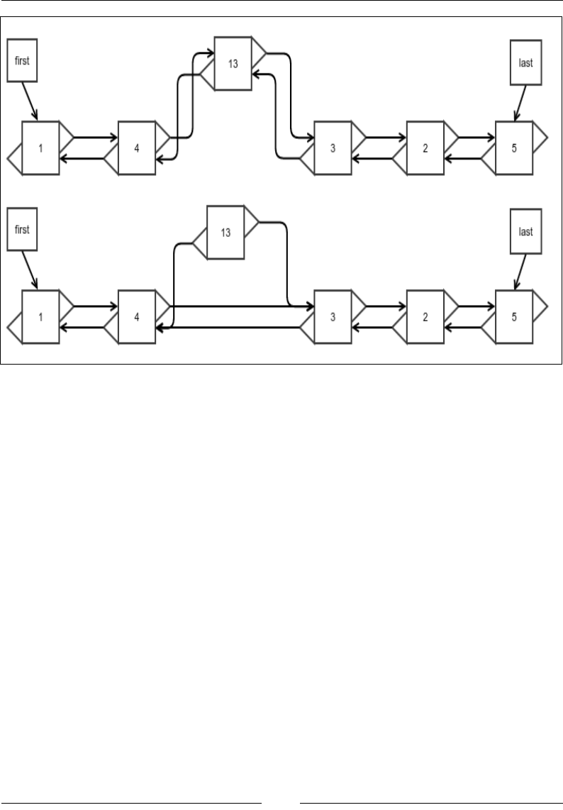
Chapter 2
[ 35 ]
Figure 13: Removal of an arbitrary element from a doubly linked list
The following code will help us achieve this:
public Node<E> removeAtIndex(int index) {
if(index<0||index>=length){
throw new NoSuchElementException();
}
This is a special case that needs extra attention. A doubly linked list really shines
while removing the last element. We will discuss the removeLast() method in the
next section:
if(index==length-1){
return removeLast();
}

Cogs and Pulleys – Building Blocks
[ 36 ]
The rest of the code is fairly easy to gure out:
DoublyLinkedNode<E> nodeRemoved
= (DoublyLinkedNode<E>) super.removeAtIndex(index);
if ((DoublyLinkedNode<E>) nodeRemoved.next != null)
((DoublyLinkedNode<E>) nodeRemoved.next).prev
= nodeRemoved.prev;
return nodeRemoved;
}
Removal of the last element
This is where a doubly linked list really shines. This is the reason we got started with
a doubly linked list. And it's not even a lot of code. Check this out:
public Node<E> removeLast() {
Node<E> origLast = last;
if(last==null){
throw new IllegalStateException
("Removing element from an empty list");
}
Just use the fact that we have access to the previous node's reference and we can
update the last reference very easily:
last = ((DoublyLinkedNode<E>)last).prev;
If the list is not empty after removal, set the next reference of the new last element to
null. If the new list is empty instead, update the rst element as well:
if(last!=null){
last.next = null;
} else{
first = null;
}
Don't forget to update the length:
length--;
return origLast;
}
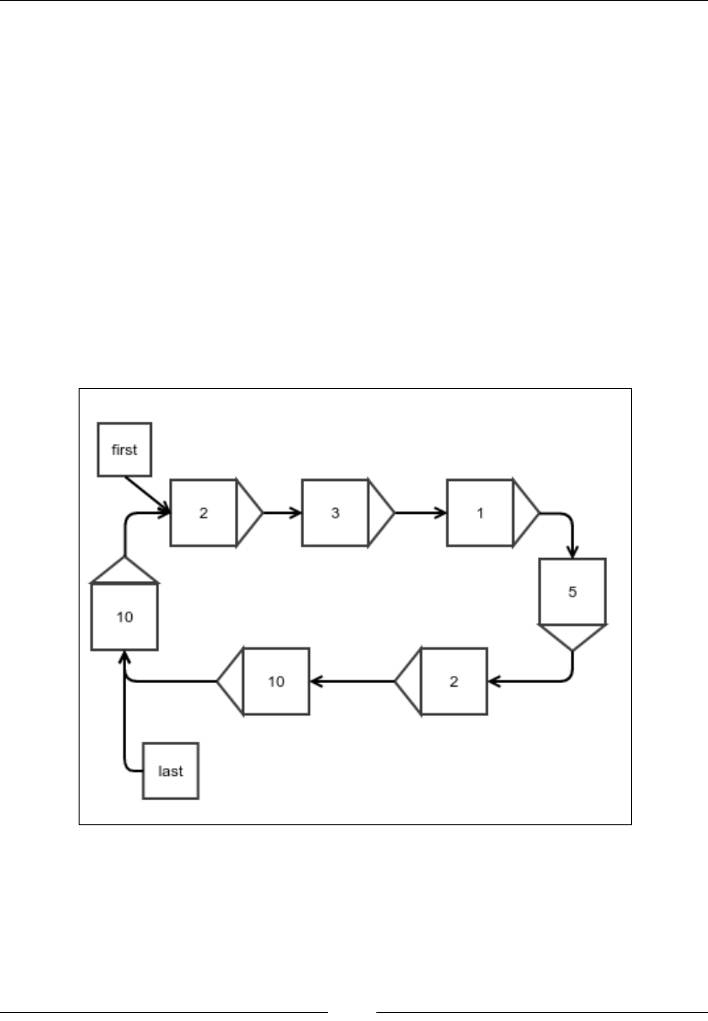
Chapter 2
[ 37 ]
We don't need a new gure to understand the update of the references as they are
really similar to the removal process of the rst element. The only difference from the
singly linked list is that in the case of a singly linked list, we need to walk all the way
to the end of the list to nd the previous element of the list. However, in the case of a
doubly linked list, we can update it in one step because we always have access to the
previous node's reference. This drastically reduces the running time from O(n) in the
case of a singly linked list to O(1) in the case of a doubly linked list.
Circular linked list
A circular linked list is an ordinary linked list, except that the last element holds the
reference to the rst element as its next element. This, of course, justies its name. It
would be useful when, for example, you are holding a list of players in a list and they
play in turn in a round robin fashion. The implementation is simplied if you use a
circular linked list and just keep rotating as the players complete their turn:
Figure 14: A circular linked list

Cogs and Pulleys – Building Blocks
[ 38 ]
The basic structure of a circular linked list is the same as that of a simple linked list;
no more elds or methods are required:
public class CircularLinkedList<E> extends LinkedList<E>{
}
Insertion
This is the same as the insertion for a simple linked list, except that you assign the
last references next to the rst:
@Override
public Node<E> appendFirst(E value) {
Node<E> newNode = super.appendFirst(value);
last.next = first;
return newNode;
}
From this, it is not hard to guess how it would be to append at the end:
@Override
public Node<E> appendLast(E value) {
Node<E> newNode = super.appendLast(value);
last.next = first;
return newNode;
}
Insertion at any other index, of course, remains the same as that for a simple linked
list; no more changes are required. This means the complexity of the insertion stays
the same as with that for a simple linked list.
Removal
Removal also only changes when you remove the rst or the last element. In any
case, just updating the last element's next reference solves the purpose. The only
place where we need to change this is when we remove the rst element. This is
because the same operation we used for a simple linked list does not update the
previous element's next reference, which we need to do:
@Override
public Node<E> removeFirst() {
Node<E> newNode = super.removeFirst();
last.next = first;
return newNode;
}
Nothing else needs to be done in removal.
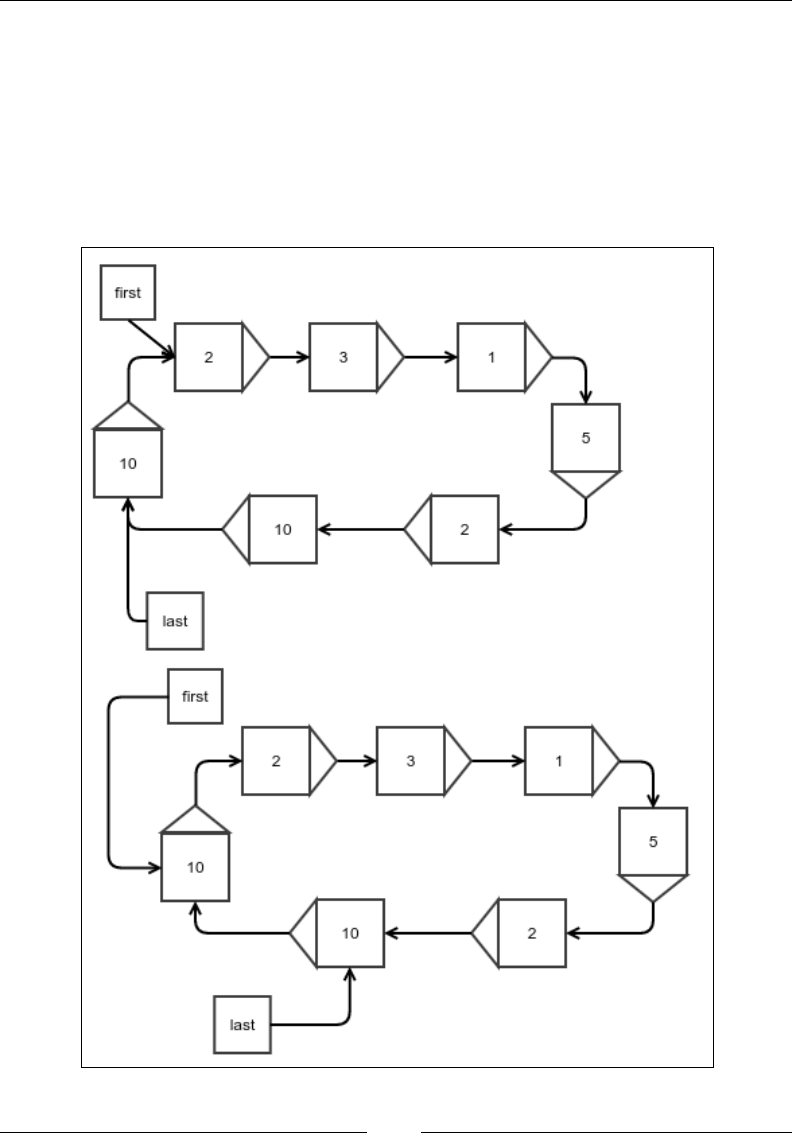
Chapter 2
[ 39 ]
Rotation
What we are doing here is just bringing the next element of the rst element to the
rst position. This is exactly what the name "rotation" would imply:
public void rotate(){
last = first;
first = first.next;
}
Figure 15: Rotation of a circular linked list
Cogs and Pulleys – Building Blocks
[ 40 ]
Doing the same with a simple linked list would require no more than assigning one
more reference. You should be able to gure out how to do this with a simple linked
list. But this operation looks more natural for a circular linked list, as conceptually,
there is no rst element.
The real power of a circular linked list is the iterator, which never ends. If the list is
non-empty, the iterator will have hasNext(), which always returns true. This means
you can simply keep calling the next() method on the iterator and keep processing
the elements in a round robin fashion. The following code should make it clear what
I mean:
for(int i=0;i<30;i++){
System.out.print(" "+ linkedList.first);
linkedList.rotate();
}
Note that if you try to use the enhanced for loop with a circular
linked list, you will run into an innite loop.
Summary
We covered a few basic data structures and the algorithms for manipulating them.
In addition to this, we also found out their running time complexities. To summarize
this, an array provides you with the fastest random access there is with this time
complexity: O(1). But arrays cannot change size; the only modication they allow is
to change the value of an element. A linked list allows fast append at the end and
insertion at the beginning at O(1) time. However, O(1) removal is only available for
removing the rst element. This is resolved by a doubly linked list that also allows
O(1) removal from the end. A circular linked list holds a reference to the rst element
in the next reference of the last element. This makes the list a circular structure that
allows one to loop indenitely.
In the upcoming chapters, we will discuss the abstraction of data structures called
abstract data types. We will use the data structures we have seen in this chapter to
implement the abstract data types, which in turn will be used in later chapters.
[ 41 ]
Protocols – Abstract
Data Types
In the last chapter, we saw a few basic data structures and some algorithms to
manipulate them. However, sometimes we may want to hide the implementation
details of a data structure and only want to know how they interact with other
algorithms. We may want to specify a few operations that they must allow and forget
about how they are achieved. This is not very different from abstraction of a part of a
program in any large software application. For example, in Java, we create interfaces
that only dene the methods of an object that its class must implement, and then
we use this interface type, being condent that they will be implemented properly.
We do not want to think about how an implementation class would provide their
implementation. Such interfaces of data structure are called abstract data types. To
put this another way, an abstract data type (ADT) is a description of what a data
structure should do for its user. It is a list of operations that any implementation
must support and the complete description of what these operations are supposed to
do. A few of these have very frequent usage and have names given to them. We will
discuss a few of these here.
In this chapter, you will learn about the following concepts:
• The definition of some common ADTs and their operations
• How to implement these ADTs using both simple arrays and the data
structures you learned in the last chapter
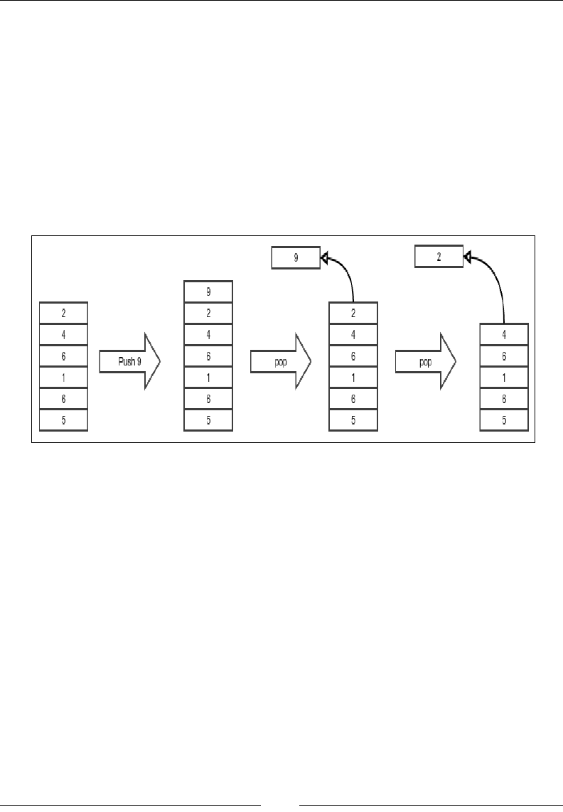
Protocols – Abstract Data Types
[ 42 ]
Stack
A stack is a very commonly used ADT. It is so named because it resembles a stack
of plates used in a restaurant. In such a stack, a plate that has been washed and put
last would stay on top. This would be the rst plate to be picked up when a plate is
needed. The plate that went in rst would be at the bottom of the stack and would be
picked last. So, the last plate to be placed in the stack is the rst plate to get out, we
can also call this last in rst out (LIFO).
Similarly, a stack ADT has a protocol where the last value that is put in it must be
returned on the rst attempt to get a value out, and the value that went in rst must
come out last. The following gure will make it more clear:
The operation of putting a new value in a stack is called push, and the operation of
retrieving a value from a stack is called pop. The element that was pushed last must
be popped rst. The operation that allows one to see what the next pop will return is
called peek. The peek operation returns the top element without modifying the stack.
We expect all stack implementations to have all operations implemented in the time
complexity of O(1). This is also part of our stack protocol.
The stack ADT has the following operations:
• Push: This adds an element at the top of the stack
• Pop: This removes the element at the top of the stack
• Peek: This checks the next value to be popped

Chapter 3
[ 43 ]
Since we know that ADTs are to data structures what interfaces are to classes, we
will code an ADT as an interface. The following is our interface for a stack:
public interface Stack<E> {
void push(E value);
E pop();
E peek();
}
Of course, we will not leave it at this. We will see how a stack can actually be
implemented. To this end, we will see both a xed-sized stack using an array to store
it's data, and a growing stack using a linked list for storing data. We will start with
the rst.
Fixed-sized stack using an array
A xed-sized stack uses a pre-allocated array to store values, that is when this stack
has used up the entire array, it can no longer accept new values until the old ones
are popped. This is not very different from an actual stack of plates, which most
certainly has a maximum height that it can handle.
As always, we start with the basic structure of the class, as follows:
public class StackImplArray<E> implements Stack<E> {
We need an array to store the elements, and we need to remember where the top of
the stack is in that array. The top always marks the index of the element that will be
popped next. When there are no more elements to be popped, it is set to -1. Why -1?
Because this is the natural choice as it does not require any special handling when
the rst element is inserted:
protected E[] array;
int top=-1;
public StackImplArray(int size){
array = (E[])new Object[size];
}
}
The push operation in a stack can be to simply put the value in the array right next
to the current top and then set the top to the new position, as illustrated in the
following code:
@Override
public void push(E value) {

Protocols – Abstract Data Types
[ 44 ]
We rst check whether the stack is already full or the current top is equal to the
maximum index possible, like this:
if(top == array.length-1){
throw new NoSpaceException("No more space in stack");
}
Now, we set the top to the new position and put the value we need to store in there
as follows:
top++;
array[top] = value;
}
The exception we used is a custom exception for this purpose. The code of the
exception is simple as shown in the following code:
public class NoSpaceException extends RuntimeException{
public NoSpaceException(String message) {
super(message);
}
}
The pop operation is just the opposite. We need to rst take the value of the current
top and then update the top to the new position, which is one less than the current
position, as shown in the following code:
@Override
public E pop() {
We rst check whether the stack is already empty, in which case we return a special
value, null. This is shown in the following code:
if(top==-1){
return null;
}
Then we update the top and return the value at the current top as follows:
top--;
return array[top+1];
}

Chapter 3
[ 45 ]
The peek operation does not change the state of the stack, and hence is even simpler:
@Override
public E peek() {
Just like the pop operation, we return null if the stack is empty:
if(top==-1){
return null;
}
Otherwise, we return the top element, as follows:
return array[top];
}
It is in fact possible to have a stack without an upper limit backed up by an array.
What we really need to do is that whenever we run out of space, we can resize the
array. Array actually cannot be resized, so the operation would be to create a new
array with a higher size (maybe twice as much as the original size), and copy all the
old elements into this array. Since this involves copying all the n elements to the new
array one by one, the complexity of this operation is O(n).
Variable-sized stack using a linked list
The problem with an array-based implementation is that since arrays are xed in size,
the stacks cannot grow beyond a xed-size. To resolve this, we have to do what we did
to x the same problem for an array, that is, use a linked list instead. We start such an
implementation with the following bare bone class. The linked list will store the values.
Instead of assigning a new linked list to it, we do so using an overridable method
getNewLinkedList(). This will be useful in the class that extends from this one:
public class StackImplLinkedList<E> implements Stack<E> {
protected LinkedList<E> list = getNewLinkedList();
protected LinkedList<E> getNewLinkedList(){
return new LinkedList<>();
}
}

Protocols – Abstract Data Types
[ 46 ]
To see which end of the linked list must be used as the top of the stack, we need
to remember that our stack protocol expects the operations to be O(1), so we must
choose an end that allows both insertion and removal in O(1) time. That end is of
course the front of the list as we saw in the last chapter. This makes the following
code for the push operation self-explanatory:
@Override
public void push(E value) {
list.appendFirst(value);
}
Note that this time, we did not check whether the stack is full because this
implementation of the stack is never full, it grows as it needs and the underlying
linked list takes care of that.
The pop operation, however, does need to check whether the stack is empty and
return null at that point. The following code for the pop operation is also quite
self-explanatory:
@Override
public E pop() {
if(list.getLength()==0){
return null;
}
E value = list.getFirst();
list.removeFirst();
return value;
}
The peek operation is, of course, the same, except it does not remove the top element:
@Override
public E peek() {
if(list.getLength()==0){
return null;
}
return list.getFirst();
}
This concludes our linked list-based implementation of a stack. In the next section,
we will check out another ADT called a queue.

Chapter 3
[ 47 ]
Queue
What is the opposite of a stack? This may be a weird question. However, a stack follows
LIFO, last in rst out. The opposite of that is rst-in-rst-out (FIFO). So, in some sense,
a FIFO ADT can be considered as the opposite of a stack. This is not very different from
a queue of people waiting for a bus or at a doctor's clinic. The rst person to show up
gets the rst chance to get onto the bus or to get to see the doctor. The second person
gets the second chance. No wonder, such an abstract data type is called a queue.
Appending to the end of a queue is called enqueuing and removing from it is called
dequeuing. The contract is, of course, that the rst value that is enqueued would be the
rst to be dequeued. The following gure illustrates this operation:
The queue ADT has the following operations:
• Enqueue: This adds an element at the back of the queue
• Dequeue: This removes an element from the front of the queue
• Peek: This checks the element that would be dequeued next
The queue will be represented by the following interface:
public interface Queue<E> {
void enqueue(E value);
E dequeue();
E peek();
}
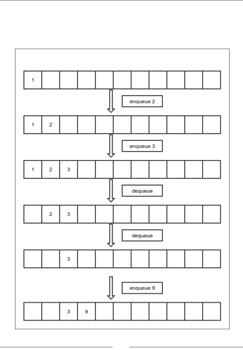
Protocols – Abstract Data Types
[ 48 ]
Fixed-sized queue using an array
Just like the stack, we have an array-based implementation of a queue. However,
since a queue receives new values and removes old values from opposite sides, the
body of the queue moves as it does. The following gure will illustrate this point:

Chapter 3
[ 49 ]
This means that after a sequence of a few such operations, the end of the queue will
reach the end of the array, and there will be space left at the beginning of the array.
At this point, we don't want to stop receiving new values as there is space left, so we
roll over to the beginning of the array. That is to say, we continue adding the new
values at the beginning of the array.
To do all these manipulations, we must have separate variables storing the indexes
of the beginning and the end of the queue. Also, since due to roll over, sometimes
the end is smaller than the beginning, we store the length separately to avoid
confusion. We start with the bare bone implementation of the class just as before. The
start represents the index of the element that would be dequeued next and the end
represents the position of the next value that would be enqueued. This is illustrated
in the following code:
public class QueueImplArray<E> implements Queue<E>{
protected E[] array;
protected int start=0;
protected int end=0;
protected int length=0;
public QueueImplArray(int size){
array = (E[]) new Object[size];
}
}
The enqueue operation does not change the start position. The new value is put at
the end position of the array and the end is incremented by one. The end, of course,
needs to be rolled over in case it goes beyond the maximum index of the array, as
shown in the following code:
@Override
public void enqueue(E value) {
if(length>=array.length){
throw new NoSpaceException("No more space to add an element");
}
array[end] = value;
The modulo operator will make sure that the index goes to the beginning of the array
when it hits the end of the array, as follows:
end = (end+1) % array.length;
length++;
}

Protocols – Abstract Data Types
[ 50 ]
The dequeue operation does not change the end position. We read from the start
index and then increment the start index with rollover, as follows:
@Override
public E dequeue() {
if(length<=0){
return null;
}
E value = array[start];
start = (start+1) % array.length;
length--;
return value;
}
The peek operation lets us see the element that would be dequeued next, without
removing it. It is, of course, simpler. We just return the next element to be dequeued.
This is shown in the following code:
@Override
public E peek() {
if(length<=0){
return null;
}
return array[start];
}
A queue backed up by an array can be resized in a similar manner as described for
the case of a stack, and this too will be O(n), since we must copy all the old elements
to the newly allocated array one by one.
Variable-sized queue using a linked list
Just like a stack, we want to implement a queue using a linked list. We need to
remember that all operations must be O(1) in running time. If we enqueue by
appending new elements at the beginning of the linked list, we will need to remove
elements from the end of the list during dequeuing. This will not work as removal of
an element from the end of a linked list is O(n). But appending at the end of a linked
list is O(1) and so is removing from the beginning of the list. Hence, the end of the
queue, where new elements are enqueued, would be the end of the list. And the start
of the queue, where the elements are dequeued from, would be the beginning of the
linked list.

Chapter 3
[ 51 ]
Given this, the implementation of a queue using a linked list is straightforward.
Again, we create an instance of the list only using a getNewLinkedList() method,
which can be overridden by a subclass to use a different linked list, as follows:
public class QueueImplLinkedList<E> implements Queue<E>{
protected LinkedList<E> list = getNewLinkedList();
protected LinkedList<E> getNewLinkedList(){
return new LinkedList<>();
}
The enqueue operation simply appends at the end of the list as follows:
@Override
public void enqueue(E value) {
list.appendLast(value);
}
The dequeue operation rst checks if the list is empty so it can return null, and then
it simply removes the rst element from the list. It must also return the element that
it just removed:
@Override
public E dequeue() {
if(list.getLength()==0){
return null;
}
E value = list.getFirst();
list.removeFirst();
return value;
}
Just like the dequeue operation, the peek operation rst needs to check whether the
list is empty, in which case it has to return a null value, otherwise it simply returns
the element at the beginning of the list that would be dequeued on the next dequeue
operation, as shown in the following code:
@Override
public E peek() {
if(list.getLength()==0){
return null;
}
return list.getFirst();
}
}

Protocols – Abstract Data Types
[ 52 ]
Double ended queue
A double ended queue is a combination of a stack and a queue. The idea is that you
are allowed to insert and remove elements at both ends of the queue. If you remove
elements from the side you have inserted, it will behave like a stack. On the other
hand, if you insert and remove on opposite ends, it will behave like a queue. You can
mix these operations and use them in any order you like. The following gure shows
a few operations to clarify this idea:
A double ended queue has the following operations all with a complexity of O(n):
• Push: This inserts an element at the beginning
• Pop: This removes an element from the beginning
• Inject: This inserts an element at the end
• Eject: This removes an element from the end
• Peek: This checks the first element
• PeekLast: This checks the last element

Chapter 3
[ 53 ]
A double ended queue will be represented by the following interface:
public interface DoubleEndedQueue<E> extends Stack<E> {
void inject(E value);
E eject();
E peekLast();
}
Note that since a double ended queue has push and pop operations just like a stack and
it preserves the same meaning, we create this interface extending the Stack interface.
Fixed-length double ended queue using
an array
Since we have created the double ended queue as an extension of a stack, one would
expect its implementation to extend a stack implementation as well. However,
remember that a double ended queue is both a stack and a queue. The array-based
implementation for a queue was more complex than that for a stack due to rollover
of the indexes. We don't want to reprogram those, so we choose to extend a queue
implementation instead of a stack implementation, as shown in the following code:
public class DoubleEndedQueueImplArray<E> extends
QueueImplArray<E> implements DoubleEndedQueue<E> {
We initialize the queue to the xed length, as follows:
public DoubleEndedQueueImplArray(int size) {
super(size);
}
This is appended at the end of the double ended queue, which is the same as the
enqueue operation of a queue:
@Override
public void inject(E value) {
enqueue(value);
}
The eject operation is the removal of an element from the end of the double ended
queue. We don't have an equivalent operation in a simple queue. So, we must code
for it as follows:
@Override
public E eject() {
if (length <= 0) {
return null;
}

Protocols – Abstract Data Types
[ 54 ]
The end has to decrement by one with a provision for rollover. But if the end is
already at zero, it will become negative, which will not work well with the modulo
operator, because it will return a negative value. To always keep it positive, we add
the length of the array to it. Note that it does not change the remainder when divided
by the length of the array. This is shown in the following code:
end = (end + array.length - 1) % array.length;
E value = array[end];
length--;
return value;
}
The peekLast operation simply needs to return the element that would have been
returned by the eject operation without modifying anything, as shown in the
following code:
@Override
public E peekLast() {
if (length <= 0) {
return null;
}
return array[(end + array.length - 1) % array.length];
}
The push operation is the insertion of an element at the beginning of the double
ended queue. There is no equivalent operation in a simple queue. Hence, we need to
code for it as follows:
@Override
public void push(E value) {
if (length >= array.length) {
throw new NoSpaceException("No more space to add an
element");
}
This operation is very similar to updating the end index eject operation, as shown
in the following code:
start = (start + array.length - 1) % array.length;
array[start] = value;
length++;
}

Chapter 3
[ 55 ]
The pop operation is the removal of the element at the beginning of the queue, which
is the same as the dequeue operation of an ordinary queue. This is illustrated in the
following code:
@Override
public E pop() {
return dequeue();
}
}
Note that we don't write any code for the peek operation, which should return the
element at the beginning of the double ended queue, as it is the same as the peek
operation for a simple queue.
The array-based implementation is, of course, xed in size and cannot hold more
elements than it's xed size. Next, we develop a linked list-based implementation.
Variable-sized double ended queue using a
linked list
We had earlier used a simple linked list to implement both a queue and a stack.
However, remember again that all operations must be O(1). Now, we must both
add and remove elements at both ends of the underlying linked list. We know that
removal from the end of a singly linked list is O(n) and we cannot use it. So, we must
use a doubly linked list instead.
This time we do not have to worry about rollovers and so we will extend the linked list
implementation of a stack, which is the natural choice. We will replace its singly linked
list with a doubly linked list by overriding the getLinkedList() method, as follows:
public class DoubleEndedQueueImplLinkedList<E> extends
StackImplLinkedList<E> implements DoubleEndedQueue<E> {
@Override
protected LinkedList<E> getNewLinkedList() {
return new DoublyLinkedList<E>();
}
The inject operation inserts a new element at the end of the list as shown in the
following code:
@Override
public void inject(E value) {
list.appendLast(value);
}

Protocols – Abstract Data Types
[ 56 ]
The eject operation must remove and return the last element of the list. This is
illustrated in the following code:
@Override
public E eject() {
if(list.getLength()==0){
return null;
}
E value = list.getLast();
list.removeLast();
return value;
}
Finally, the peekLast() method will just return the last element of the doubly linked
list as follows:
@Override
public E peekLast() {
if(list.getLength()==0){
return null;
}
return list.getLast();
}
}
We only had to implement the inject(), eject(), and peekLast() methods as the
other methods are already implemented by the stack we extend.
Summary
In this chapter, we saw that an abstract data type or ADT is an abstraction of a data
structure. It is a contract that an underlying data structure is supposed to adhere to.
The contract involves different operations on the data structure and their specic
behavior. We then saw a few simple ADTs as examples. These ADTs are, however,
extremely useful as we will see in the course of this book when we encounter other
algorithms. Abstraction allows different implementations of the structures. We will
also see more ADTs in the course of this book and their implementations.
In the next chapter, we will take a detour into a new area of algorithms called
functional programming. Remember that an algorithm is a sequence of steps that
may be followed to achieve a desired processing; it turns out that there is another
way of looking at it, which we will explore in the next chapter.
[ 57 ]
Detour – Functional
Programming
In the beginning of this book, we saw that an algorithm is a sequence of steps
to achieve a result. This way of solving a problem by following a sequence of
instructions is called imperative programming. Each statement in the program can be
thought of as an imperative sentence asking the computer to do something. However,
this is not the only way of looking at it. Functional programming sees an algorithm as
a composition of components rather than as a sequence of steps. A problem to solve is
seen as a composition of smaller-sized problems. Instead of using a loop, we combine
smaller versions of the same problem. Functional programming uses recursion as a
basic component. A recursion is nothing but solving the same problem for a smaller
size and then composing the result with something else to get the solution for the
given size of the problem. This has a far-reaching implication in how easy it is to read
and understand a program. This makes it very important to study.
There are really two worlds in the programming paradigm. The imperative style
of programming is favored by C-like languages, such as C, C++, and Java. On the
purely functional side, there are languages such as Lisp, Haskell, and Scheme. Apart
from these, some languages try to have the best of both worlds, such as Python or
Scala. This is easier said than done; trying to mix both ideas in a language means you
have features to support both, but to use them effectively is truly an art.
So, if Java is imperative in nature, why are we talking about functional programming
in this book? Well, as I pointed out, sometimes, it is better to mix both concepts and
get the best of both worlds. Recently, the Java community has taken note of this fact
and has introduced a feature lambda from Java version 8 to provide some level of
functional programming support. So, our intention is not to program completely in
functional style, as that is not the preferred programming style of Java, but we will
do it just enough to make our programs more beautiful and to aid our understanding
of algorithms.

Detour – Functional Programming
[ 58 ]
This chapter will introduce this rather foreign concept to you and provide some
basic tools that are commonly used in functional programming. You will learn the
following concepts:
• Recursive algorithms and the immutability of variables
• Monads
• Aggregations on monads
• Java's support for functional programming, that is, lambda.
Recursive algorithms
As I have already pointed out, recursive algorithms are a different way of thinking
about solving a problem. For example, say our problem is to write a program that,
given a positive integer n, returns the sum of numbers from zero to n. The known
imperative way of writing it is simple:
public int sum_upto(int n){
int sum=0;
for(int i=0;i<=n;i++){
sum+=i;
}
return sum;
}
The following would be the functional version of the problem:
public int sum_upto_functional(int n){
return n==0?0:n+sum_upto_functional(n-1);
}
That's it–just a one-liner! This is probably nothing new to Java programmers, as they
do understand recursive functions. However, an imperative programmer would use
recursion only when nothing else worked. But this is a different way of thinking.
How do we justify that it is equivalent to solving the problem for a smaller input and
then composing it with something else? Well, we are certainly rst computing the
same function for an input that is smaller by one and then just adding n to it. There is
one more thing to note here: in the imperative version, we are updating the variable
called sum for each value of the loop variable i. However, in the functional version,
we are not updating any variable. What do we achieve by that? When a variable is
updated multiple times in a program, it is hard to understand or debug it because
you need to keep track of the latest value. When this does not happen, it is far easier
to understand what is happening. In fact, it makes it simpler in such a way that we
can even prove the correctness of the program completely formally, which is rather
hard to do for imperative programs where variables change values.

Chapter 4
[ 59 ]
Let's check out another example. This one is about choosing r objects from n objects,
where the order does not matter. Let's have a set A of a nite amount of objects. Let
the number of objects in this set be n. How many subsets B of this set A have exactly
r elements? Of course, the maximum number of elements any subset of A can have
is n; hence r ≤ n. We will call this function choose. So, we write this as choose(n,r).
Now, the only subset that has an equal number of elements as A is A itself. So,
choose(n,n) equals 1.
How do we break this problem into subproblems of a similar nature but with smaller
input? To nd out how many subsets B have r elements, we rst think of the set A as
a combination of a subset C with n-1 elements and one particular element a. So, we
can say A = C ⋃ {a}. Now, we consider two disjoint cases: the element a is a member
of the subset B and when it is not a member of the subset B. When a is not a member
of the subset B, B is also a subset of C. The number of such subsets B with exactly
r elements is choose(n-1,r), since C has n-1 elements. On the other hand, when
a is a member of the set B, then B can be thought of as a union of two sets – a set D
that has all the elements of B except a, and the other is just {a}. So, B = D ⋃ {a}. Now,
you can see that D is a subset of C that we dened. How many such subsets D are
there of C? There are choose(n-1,r-1) subsets, since C has n-1 elements and D has
r-1 elements. So, the number of such subsets B is choose(n-1,r-1). This means
that the total number of sets B with or without a as an element is choose(n-1,r) +
choose(n-1,r-1). If we put this in recursive calls, the r and n will get reduced until
r equals zero or n equals r. We have already considered the case when n equals r,
that is, choose(n,n). When r equals zero, it means B is the null set. Since there is
only one null set, choose(n,0) equals 1. Now, we put this in code:
public long choose(long n, long r){
if(n<r){
return 0;
}else if(r==0){
return 1;
}else if(n==r){
return 1;
}else{
return choose(n-1,r) + choose(n-1,r-1);
}
}
That was a little complex, but note that not only did we compute the value of the
choose function, we also sort of proved that it will work. The choose function is the
binomial coefcient function for integral exponents.

Detour – Functional Programming
[ 60 ]
The aforementioned implementation is not efcient. To see why, just consider
what each recursive call of the choose function will evaluate to when they both fall
in the nal else case: choose(n-1,r) = choose(n-2,r) + choose(n-2,r-1)
and choose(n-1,r-1) = choose(n-2,r-1) + choose(n-2,r-2). Now note that
choose(n-2,r-1) is being evaluated in both cases, which then would have its own
recursive calls. This actually signicantly increases the asymptotic complexity. We'll
defer the analysis of this complexity to the end of this chapter.
Lambda expressions in Java
Before moving on, we need to learn about a feature in Java called Lambda. Many
of you may already know about it. However, since the feature was only introduced
in version 8, it is better to get familiar with it if you aren't already. It lets you pass a
block of code, called a lambda expression, as an argument to another function. To
talk about lambda, we must rst see what a functional interface is.
Functional interface
A functional interface is an interface that has only one unimplemented method, that
is to say, a class that implements it needs to implement exactly one method. The
functional interface may have more than one method declared or inherited, but as
long as we can implement it by implementing exactly one method, it is a functional
interface. The following example shows one such interface:
@FunctionalInterface
public interface SampleFunctionalInterface {
int modify(int x);
}
Note that we also marked it as a functional interface with an annotation, but it is not
necessary. Marking it ensures that Java will show a compile-time error if the interface
does not have exactly one method that needs to be implemented. The following
example shows another valid functional interface:
public interface AnotherFunctionalInterface{
public void doSomething(int x);
public String toString();
}
There are two methods in it. However, since the toString() method is already
implemented in the object class, you need to implement only one method.

Chapter 4
[ 61 ]
Similarly, an interface with more than one method can be a functional interface if all
but one has a default implementation. For example, look at the following interface.
@FunctionalInterface
public interface FunctionalInterfaceWithDefaultMethod {
int modify(int x);
default int modifyTwice(int x){return modify(modify(x));}
}
Even though this interface has two methods, only one needs to be implemented by
any implementation. This makes it a functional interface.
Implementing a functional interface with
lambda
So, what happens if we have a functional interface? We can provide an inline
implementation of it using a cool syntax called lambda, as follows:
SampleFunctionalInterface sfi = (x)->x+1;
int y = sfi.modify(1);
Take note of the parentheses and the arrow sign. The parentheses contain all the
parameters. The types of parameters are not specied because they are already
specied in the interface method. There can be zero or more parameters.
There are two kinds of lambda syntax–one that has an expression as the body and
one that has one or more steps as the body. These lambdas look a bit different from
each other. A lambda that is implemented as a one liner looks like the one we just
saw. This is called an expression syntax. The expression syntax can be used if the
lambda expression is a one liner. For multi-line code, we use the block syntax as
shown below:
Thread t = new Thread(()->{for(int i=0;i<500;i++)
System.out.println(i);});
One can use block syntax for functions that return a value as well, especially when
using multiple lines of code. In that case, one just needs to use a return statement to
return a value.
Detour – Functional Programming
[ 62 ]
Since in a functional program all variables must not ever be
reassigned, we should declare them nal to avoid accidentally
modifying them. However, since typing final for every
variable clutters the code a bit, we avoid doing so. In a purely
functional language, the variables are immutable by default.
Even in a semifunctional language, such as Scala, it is so if
it generally encourages the functional style. However, since
Java mostly prefers an imperative style, the final keyword is
necessary, causing a little clutter.
Now that we know about lambda, we can start learning about functional
data structures.
Functional data structures and monads
Functional data structures are data structures that follow the principle of immutability
and inductive (or recursive) denition. Immutability means that any modication of
the data structure would result in a new data structure, and any old reference to the
original version would still have access to the original version. Inductive denition
means that the denition of the structure is dened as a composition of smaller
versions of the same data structure. Take, for example, our linked list. When we add
an element to or remove an element from the beginning of the list, it will modify
the linked list. That means any reference to the linked list will now hold a reference
to the modied linked list. This doesn't conform to the principle of immutability. A
functional linked list would make sure that the older references still held reference to
an unmodied version. We will discuss how to do it in the next section.
Functional linked lists
To make a linked list that is immutable, we consider a linked list to be made of
two parts:
• A head containing the first element of the list
• A tail containing another linked list containing the rest of the elements
Note that we have now dened the linked list recursively, being true to our
functional design. This recursion says that a linked list is:
• Either an empty list
• Or a set of two objects, as follows:
°A head containing one element of its element type
°A tail containing another linked list of the same type

Chapter 4
[ 63 ]
This version of the denition is the same as the previous simplied one, except
that we have now specied how we represent where the list terminates. The list
terminates where there are no more elements, that is, when the tail is an empty list.
Let's put all these in code.
First, we dene a version according to the simplied denition:
public class LinkedList<E> {
private E head;
private LinkedList<E> tail;
private LinkedList(){
}
private LinkedList(E head, LinkedList<E> tail){
this.head = head;
this.tail = tail;
}
public E head(){
return head;
}
public LinkedList<E> tail(){
return tail;
}
This is the core of immutability for our linked list. Note that every time we add a
new value to our linked list, we create a new linked list so that the old references still
hold references to the unmodied list:
public LinkedList<E> add(E value){
return new LinkedList<E>(value,this);
}
}
The code is self-explanatory, now that we already know how we think about our
linked list. But note that we have made the constructors private. We don't want
people to create inconsistent versions of our linked lists, such as a null tail or
something. We insist that everyone creates our linked list by rst creating an empty
linked list and then adding elements to it. So, we add the following EmptyList class
and add() method:
public static final class EmptyList<E> extends LinkedList<E>{
@Override
public E head() {

Detour – Functional Programming
[ 64 ]
throw new NoValueException("head() invoked on empty list");
}
@Override
public LinkedList<E> tail() {
throw new NoValueException("tail() invoked on empty list");
}
}
public static <E> LinkedList<E> emptyList(){
return new EmptyList<>();
}
Now we can use the linked list as follows:
LinkedList<Integer> linkedList = LinkedList.<Integer>emptyList()
.add(5).add(3).add(0);
while(!(linkedList instanceof LinkedList.EmptyList)){
System.out.println(linkedList.head());
linkedList = linkedList.tail();
}
But wait, did we just modify the linkedList variable in the while loop? Yes, but
that does not comply with the principle of immutability. To solve this, let's see what
we would mostly want to do with a list. In general, we would want to perform the
following operations:
• Do something for each element of the list. For example, print all the elements
to the console.
• Get a new list where each element is transformed using a function that is
provided.
• Compute a function of all the elements in the list. This is an aggregation of
the elements. For example, find the sum of all the elements.
• Create a new list containing only selected elements of the list. This is
called filtering.
We will deal with them one by one. At the end of the next section, you will be
prepared to learn about monads as well.

Chapter 4
[ 65 ]
The forEach method for a linked list
The forEach() method on a linked list would do something for each element of
the list. This something would be passed as a lambda. For this purpose, we will
rst create a functional interface that consumes one parameter but does not return
anything:
@FunctionalInterface
public interface OneArgumentStatement<E> {
void doSomething(E argument);
}
With this interface available, we will dene the forEach() method for a list,
as follows:
public class LinkedList<E> {
…
public static class EmptyList<E> extends LinkedList<E>{
…
@Override
public void forEach(OneArgumentStatement<E> processor) {}
}
…
public void forEach(OneArgumentStatement<E> processor){
processor.doSomething(head());
tail().forEach(processor);
}
}
The ellipsis represent more code that we have already discussed and need not be
repeated. The forEach() method simply processes the head and then recursively
calls itself on the tail. Note again that, true to our philosophy of recursion, we have
implemented the forEach() method using recursion. Of course, this will not work
on an empty list because the head and tail are null. The empty list represents when
the method needs to stop calling itself. We achieve this by overriding the forEach()
method in the EmptyList class to not do anything.
Now we can print all the elements using the following code:
linkedList.forEach((x) -> {System.out.println(x);});

Detour – Functional Programming
[ 66 ]
We pass a lambda that, given any element x, calls System.out.println on x. But, if
you see, this lambda just works as a delegation to the System.out.println method
that already has the required form of the lambda. Java allows you to use a method as
a lambda with the following syntax. The :: operator is used to tell the compiler that
you are not looking for a eld with that name; instead you are looking for a method
with that name:
linkedList.forEach(System.out::println);
Note that this time we did not even modify the list while printing the elements,
unlike last time, when we did it using a loop.
Map for a linked list
Now we move on to the next thing we want to do with a list, which is to create a new
list where all the elements are transformed according to a lambda that is provided.
What I mean is that we want to do the following:
LinkedList<Integer> tranformedList = linkedList.map((x)->x*2);
We need to implement the map() method in a way that transformedList holds all
the elements of linkedList multiplied by 2, in the same order. The following is the
implementation of the map() method:
public class LinkedList<E> {
…
public static class EmptyList<E> extends LinkedList<E>{
…
@Override
public <R> LinkedList<R> map(OneArgumentExpression<E,
R> transformer) {
return LinkedList.emptyList();
}
}
…
public <R> LinkedList<R> map(OneArgumentExpression<E,R> transformer){
return new LinkedList<>(transformer.compute(head()),
tail.map(transformer));
}
}

Chapter 4
[ 67 ]
As usual, the method is dened recursively. The transformed list is just the head
transformed followed by the tail transformed. We have also overridden the method
in the EmptyList class to return an empty list because an empty list transformed
is just another empty list of a possibly different type. With this implementation in
place, we can do the following:
LinkedList<Integer> tranformedList = linkedList.map((x)->x*2);
tranformedList.forEach(System.out::println);
This should print a list with all the values multiplied by 2. You can even change the
type of the elements by transformation, such as the following:
LinkedList<String> tranformedListString
= linkedList.map((x)->"x*2
= "+(x*2));
tranformedListString.forEach(System.out::println);
The tranformedListString list is a list of strings, and printing each element on the
next line shows the strings obtained.
Now we move on to the next thing we want to do with a list, which is to compute
some function that uses all the values in the list. This is called an aggregation
operation. But before looking at a general case, we will concentrate on a specic one,
called a fold operation.
Fold operation on a list
A fold operation on a list is an aggregation operation that can be done element by
element. For example, if we want to compute the sum of all the elements of a list, we
can do it by taking each element of the list and adding it to a moving sum, so when
we are done with processing all the elements, we will have the sum of all elements.
There are two operations that suit this purpose: foldLeft and foldRight. The
foldLeft operation aggregates the head rst and moves on to the tail. The
foldRight method aggregates the tail rst and then moves on to the head. Let's
start with foldLeft. But before doing anything, we need a functional interface that
represents an expression of two parameters:
@FunctionalInterface
public interface TwoArgumentExpression<A,B,R> {
R compute(A lhs, B rhs);
}

Detour – Functional Programming
[ 68 ]
With this interface available, we dene the foldLeft method in the following way:
public class LinkedList<E> {
…
…
public static class EmptyList<E> extends LinkedList<E>{
…
@Override
public <R> R foldLeft(R initialValue, TwoArgumentExpression<R,
E, R> computer) {
return initialValue;
}
}
…
public <R> R foldLeft(R initialValue,
TwoArgumentExpression<R,E,R> computer){
R newInitialValue = computer.compute(initialValue, head());
return tail().foldLeft(newInitialValue, computer);
}
}
We compute a new value from initialValue and the head using the lambda
passed, and then we use this updated value to compute foldLeft on the tail. The
empty list overrides this method to just return the initialValue itself because it just
marks the end of the list. Now we can compute the sum of all elements as follows:
int sum = linkedList.foldLeft(0,(a,b)->a+b);
System.out.println(sum);
We have passed 0 as the initial value and the lambda that sums up the values passed.
This looks complicated until you get used to this idea, but once you get used to it, it
is very simple. Let's see what is happening step by step; the list from head to tail is
{0,3,5}:
1. In the rst invocation, we pass the initial value 0. The computed
newInitialValue is 0+0 = 0. Now, we pass this newInitialValue to the
tail to foldLeft, which is {3,5}.
2. The {3,5} has a head 3 and tail {5}. 3 is added to the initialValue 0 to
give a newInitialValue 0+3=3. Now, this new value 3 is passed to the tail
{5} to foldLeft.

Chapter 4
[ 69 ]
3. The {5} has a head 5 and tail and empty list. 5 is added to the
initialValue 3 to get 8. Now this 8 is passed as initialValue to the tail,
which is an empty list.
4. The empty list, of course, just returns the initial value for a foldLeft
operation. So it returns 8, and we get the sum.
Instead of computing one value, we can even compute a list as a result. The
following code reverses a list:
LinkedList<Integer> reversedList =
linkedList.foldLeft(LinkedList.emptyList(),(l,b)->l.add(b) );
reversedList.forEach(System.out::println);
We have simply passed an empty list as an initial operation, and then our operation
simply adds a new element to the list. In the case of foldLeft, the head will be
added before the tail, causing it to be placed more in the tail side in the newly
constructed list.
What if we want to process the right-most end (or away from the head) rst and
move to the left? This operation is called foldRight. This can be implemented in a
very similar manner, as follows:
public class LinkedList<E> {
…
public static class EmptyList<E> extends LinkedList<E>{
…
@Override
public <R> R foldRight(TwoArgumentExpression<E, R,
R> computer, R initialValue) {
return initialValue;
}
}
…
public <R> R foldRight(TwoArgumentExpression<E,R,R> computer,
R initialValue){
R computedValue = tail().foldRight(computer, initialValue);
return computer.compute(head(), computedValue);
}
}

Detour – Functional Programming
[ 70 ]
We have switched the order of the arguments to make it intuitive that the
initialValue is being combined from the right end of the list. The difference from
foldLeft is that we compute the value on the tail rst, calling a foldRight on it.
Then we return the result of the computed value from the tail being combined with
the head to get the result. In the case of computing a sum, it does not make any
difference which fold you invoke because sum is commutative, that is, a+b always
equals b+a. We can call the foldRight operation for the computation of sum in the
following way, which will give the same sum:
int sum2 = linkedList.foldRight((a,b)->a+b, 0);
System.out.println(sum2);
However, if we use an operator that is not commutative, we will get a different
result. For example, if we try reversing the list with the foldRight method, it will
give the same list instead of being reversed:
LinkedList<Integer> sameList = linkedList.foldRight((b,l)-
>l.add(b), LinkedList.emptyList());
sameList.forEach(System.out::println);
The nal thing we wanted to do with a list was ltering. You will learn it in the
next subsection.
Filter operation for a linked list
Filter is an operation that takes a lambda as a condition and creates a new list that
has only those elements that satisfy the condition. To demonstrate this, we will create
a utility method that creates a list of a range of elements.
First, we create a helper method that appends a range of numbers to the head of an
existing list. This method can call itself recursively:
private static LinkedList<Integer> ofRange(int start, int end,
LinkedList<Integer> tailList){
if(start>=end){
return tailList;
}else{
return ofRange(start+1, end, tailList).add(start);
}
}

Chapter 4
[ 71 ]
Then we use the helper method to generate a list of a range of numbers:
public static LinkedList<Integer> ofRange(int start, int end){
return ofRange(start,end, LinkedList.emptyList());
}
This will let us create a list of a range of integers. The range includes the start and
excludes the end. For example, the following code will create a list of numbers from
1 to 99 and then print the list:
LinkedList<Integer> rangeList = LinkedList.ofRange(1,100);
rangeList.forEach(System.out::println);
We now want to create a list of all even numbers, say. For that, we create a filter
method in the LinkedList class:
public class LinkedList<E> {
…
public static class EmptyList<E> extends LinkedList<E>{
…
@Override
public LinkedList<E> filter(OneArgumentExpression<E,
Boolean> selector) {
return this;
}
}
…
public LinkedList<E> filter(OneArgumentExpression<E,
Boolean> selector){
if(selector.compute(head())){
return new LinkedList<E>(head(), tail().filter(selector));
}else{
return tail().filter(selector);
}
}
}

Detour – Functional Programming
[ 72 ]
The filter() method checks whether the the condition is met. If yes, then it includes
the head and calls the filter() method on the tail. If not, then it just calls the
filter() method on the tail. The EmptyList of course needs to override this method
to just return itself because all we need is an empty list. Now, we can do the following:
LinkedList<Integer> evenList =
LinkedList.ofRange(1,100).filter((a)->a%2==0);
evenList.forEach(System.out::println);
This will print all the even numbers between 1 and 99. Let's go through some more
examples in order to get used to all this stuff. How do we add all numbers from 1 to
100? The following code will do that:
int sumOfRange = LinkedList.ofRange(1,101).foldLeft(0, (a,b)-
>a+b);
System.out.println(sumOfRange);
Note that we have used the range of (1,101) because the end number is not
included in the generated linked list.
How do we compute the factorial of a number using this? We dene a factorial
method as follows:
public static BigInteger factorial(int x){
return LinkedList.ofRange(1,x+1)
.map((a)->BigInteger.valueOf(a))
.foldLeft(BigInteger.valueOf(1),(a,b)->a.multiply(b));
}
We have used Java's BigInteger class because factorials grow too fast and an int
or a long cannot hold much. This code demonstrates how we converted the list of
integers to a list of BigIntegers using the map method before multiplying them
with the foldLeft method. We can now compute the factorial of 100 with the
following code:
System.out.println(factorial(100));
This example also demonstrates the idea that we can combine the methods we
developed to solve more complicated problems. Once you get used to this, reading
a functional program and understanding what it does is a lot simpler than doing
the same for their imperative versions. We have even used one-character variable
names. Actually, we could use meaningful names, and in some cases, we should. But
here the program is so simple and the variables used are so close to where they are
dened that it's not even necessary to name them descriptively.

Chapter 4
[ 73 ]
Let's say we want to repeat a string. Given an integer, n, and a string, we want
the resultant string to be a repetition of the original string n number of times.
For example, given an integer 5 and a string Hello, we want the output to be
HelloHello HelloHello Hello. We can do this with the following function:
public static String repeatString(final String seed, int count){
return LinkedList.ofRange(1,count+1)
.map((a)->seed)
.foldLeft("",(a,b)->a+b);
}
What we are doing here is rst creating a list of length count and then replacing all
its elements with the seed. This gives us a new list with all the elements equal to the
seed. This can be folded to get the desired repeated string. This is easy to understand
because it is very much like the sum method, except we are adding strings instead
of integers, which causes repetition of the string. But we don't even need to do this.
We can do this even without creating a new list with all the elements replaced. The
following will do it:
public static String repeatString2(final String seed, int count){
return LinkedList.ofRange(1,count+1)
.foldLeft("",(a,b)->a+seed);
}
Here, we just ignore the integer in the list and add the seed instead. In the rst
iteration, a would be set to the initial value, which is an empty string. Every time, we
just ignore the content and instead add the seed to this string. Note that in this case,
variable a is of the String type and variable b is of the Integer type.
So, we can do a lot of things using a linked list, using its special methods with
lambda parameters. This is the power of functional programming. What we are
doing with lambda, though, is that we are passing the implementation of interfaces
as pluggable code. This is not a new concept in an object-oriented language.
However, without the lambda syntax, it would take a lot of code to dene an
anonymous class to do the equivalent, which would clutter the code a lot, thus
undermining the simplicity. What has changed though is the immutability, leading
to chaining of methods and other concepts. We are not thinking about state while
analyzing the programs; we are simply thinking of it as a chain of transformations.
The variables are more like variables in algebra, where the value of x stays the same
throughout a formula.

Detour – Functional Programming
[ 74 ]
Append on a linked list
We have completed all the things that were in the list of the things we wanted to
do. There may be a few more. One important thing, for example, is append. This
operation sticks one list to another. This can be done using the foldRight method
that we have already dened:
public LinkedList<E> append(LinkedList<E> rhs){
return this.foldRight((x,l)->l.add(x),rhs);
}
Now, we perform the following:
LinkedList<Integer> linkedList =
LinkedList.<Integer>emptyList().add(5).add(3).add(0);
LinkedList<Integer> linkedList2 =
LinkedList.<Integer>emptyList().add(6).add(8).add(9);
linkedList.append(linkedList2).forEach(System.out::print);
This will output 035986, which is the rst list stuck in front of the second list.
To understand how it works, rst remember what a foldRight operation does. It
starts with an initial value–in this case, the right hand side (RHS). Then it takes one
element at a time from the tail end of the list and operates on that with the initial
list using the provided operation. In our case, the operation simply adds an element
to the head of the initial list. So, in the end, we get the entire list appended to the
beginning of the RHS.
There is one more thing that we want to do with a list, but we have not talked about
it until now. This concept requires an understanding of the earlier concepts. This is
called a flatMap operation, and we will explore it in the next subsection.
The atMap method on a linked list
The flatMap operation is just like the map operation, except we expect the operation
passed to return a list itself instead of a value. The job of the flatMap operation is to
atten the lists thus obtained and append them one after another. Take for example
the following code:
LinkedList<Integer> funnyList
=LinkedList.ofRange(1,10)
.flatMap((x)->LinkedList.ofRange(0,x));

Chapter 4
[ 75 ]
The operation passed returns a range of numbers starting from 0 to x-1. Since we
started the flatMap on a list of numbers from 1 to 9, x will get values from 1 to 9.
Our operation will then return a list containing 0,x-1 for each value of x. The job
of the flatMap operation is to then atten all these lists and stick them one after
another. Take a look at the following line of code, where we print funnyList:
funnyList.forEach(System.out::print);
It will print 001012012301234012345012345601234567012345678 on the output.
So, how do we implement the flatMap operation? Let's have a look:
public class LinkedList<E> {
public static class EmptyList<E> extends LinkedList<E>{
…
@Override
public <R> LinkedList<R> flatMap(OneArgumentExpression<E,
LinkedList<R>> transformer) {
return LinkedList.emptyList();
}
}
…
public <R> LinkedList<R> flatMap(OneArgumentExpression<E,
LinkedList<R>> transformer){
return transformer.compute(head())
append(tail().flatMap(transformer));
}
}
So what is happening here? First, we compute the list obtained by the head and
the result of the flatMap operation on the tail. Then we append the result of the
operation on the head of the list in front of the list obtained by flatMap on the tail. In
case of an empty list, the flatMap operation just returns an empty list because there
is nothing for the transformation to be called on.

Detour – Functional Programming
[ 76 ]
The concept of a monad
In the previous section, we saw quite a few operations for a linked list. A few of
them, namely map and flatMap, are a common theme in many objects in functional
programming. They have a meaning outside of the list. The map and flatMap
methods, and a method to construct a monad from a value are what make such a
wrapper object a monad. A monad is a common design pattern that is followed
in functional programming. It is a sort of container, something that stores objects
of some other class. It can contain one object directly as we will see; it can contain
multiple objects as we have seen in the case of a linked list, it can contain objects
that are only going to be available in the future after calling some function, and
so on. There is a formal denition of monad, and different languages name its
methods differently. We will only consider the way Java denes the methods. A
monad must have two methods, called map() and flatMap(). The map() method
accepts a lambda that works as a transformation for all the contents of the monad.
The flatMap method also takes a method, but instead of returning the transformed
value, it returns another monad. The flatMap() method then extracts the output
from the monad and creates a transformed monad. We have already seen an example
of a monad in the form of a linked list. But the general theme does not become clear
until you have seen a few examples instead of just one. In the next section, we will
see another kind of monad: an option monad.
Option monad
An option monad is a monad containing a single value. The whole point of this is to
avoid handling null pointers in our code, which sort of masks the actual logic. The
point of an option monad is to be able to hold a null value in a way that null checks
are not required in every step. In some way, an option monad can be thought of as
a list of zero or one objects. If it contains just zero objects, then it represents a null
value. If it contains one object, then it works as the wrapper of that object. The map
and flatMap methods then behave exactly like they would behave in the case of a
one-argument list. The class that represents an empty option is called None. First, we
create an abstract class for an option monad. Then, we create two inner classes called
Some and None to represent an Option containing a value and one without a value,
respectively. This is a more general pattern for developing a monad and can cater to
the fact that the non-empty Option has to store a value. We could do this with a list
as well. Let's rst see our abstract class:
public abstract class Option<E> {
public abstract E get();
public abstract <R> Option<R> map(OneArgumentExpression<E,R>
transformer);
public abstract <R> Option<R> flatMap(OneArgumentExpression<E,
Option<R>> transformer);

Chapter 4
[ 77 ]
public abstract void forEach(OneArgumentStatement<E> statement);
…
}
A static method optionOf returns the appropriate instance of the Option class:
public static <X> Option<X> optionOf(X value){
if(value == null){
return new None<>();
}else{
return new Some<>(value);
}
}
We now dene the inner class, called None:
public static class None<E> extends Option<E>{
@Override
public <R> Option<R> flatMap(OneArgumentExpression<E,
Option<R>> transformer) {
return new None<>();
}
@Override
public E get() {
throw new NoValueException("get() invoked on None");
}
@Override
public <R> Option<R> map(OneArgumentExpression<E, R> transformer) {
return new None<>();
}
@Override
public void forEach(OneArgumentStatement<E> statement) {
}
}
We create another class, Some, to represent a non-empty list. We store the value as a
single object in the class Some, and there is no recursive tail:
public static class Some<E> extends Option<E>{
E value;
public Some(E value){

Detour – Functional Programming
[ 78 ]
this.value = value;
}
public E get(){
return value;
}
…
}
The map and flatMap methods are pretty intuitive. The map method accepts a
transformer and returns a new Option where the value is transformed. The flatMap
method does the same, except it expects the transformer to wrap the returned value
inside another Option. This is useful when the transformer can sometimes return a
null value, in which case the map method will return an inconsistent Option. Instead,
the transformer should wrap it in an Option, for which we need to use a flatMap
operation. Have a look at the following code:
public static class Some<E> extends Option<E>{
…
public <R> Option<R> map(OneArgumentExpression<E,R> transformer){
return Option.optionOf(transformer.compute(value));
}
public <R> Option<R> flatMap(OneArgumentExpression<E,
Option<R>> transformer){
return transformer.compute(value);
}
public void forEach(OneArgumentStatement<E> statement){
statement.doSomething(value);
}
}
To understand the usage of an Option monad, we will rst create a JavaBean. A
JavaBean is an object exclusively intended to store data. It is the equivalent of a
structure in C. However, since encapsulation is a dening principle of Java, the
members of the JavaBean are not accessed directly. They are instead accessed
through special methods called getters and setters. However, our functional style
dictates that the beans be immutable, so there won't be any setter methods. The
following set of classes gives a few examples of JavaBeans:
public class Country {
private String name;
private String countryCode;
public Country(String countryCode, String name) {
this.countryCode = countryCode;

Chapter 4
[ 79 ]
this.name = name;
}
public String getCountryCode() {
return countryCode;
}
public String getName() {
return name;
}
}
public class City {
private String name;
private Country country;
public City(Country country, String name) {
this.country = country;
this.name = name;
}
public Country getCountry() {
return country;
}
public String getName() {
return name;
}
}
public class Address {
private String street;
private City city;
public Address(City city, String street) {
this.city = city;
this.street = street;
}
public City getCity() {
return city;
}
public String getStreet() {
return street;

Detour – Functional Programming
[ 80 ]
}
}
public class Person {
private String name;
private Address address;
public Person(Address address, String name) {
this.address = address;
this.name = name;
}
public Address getAddress() {
return address;
}
public String getName() {
return name;
}
}
There is not much to understand in these four classes. They are there to store a
person's data. In Java, it is not very uncommon to hit a case where you will hit a very
similar kind of object.
Now, let's say, given a variable person of type Person, we want to print the name of
the country he/she lives in. If the case is that any of the state variables can be null,
the correct way to do it with all null checks would look like the following:
if(person!=null
&& person.getAddress()!=null
&&
person.getAddress().getCity()!=null
&&
person.getAddress().getCity().getCountry()!=null){
System.out.println(person.getAddress().getCity().getCountry());
}
This code would work, but let's face it–it's a whole bunch of null checks. We can get
a hold of the address simply by using our Options class, as follows:
String countryName = Option.optionOf(person)
.map(Person::getAddress)
.map(Address::getCity)
.map(City::getCountry)
.map(Country::getName).get();

Chapter 4
[ 81 ]
Note that if we just print this address, there is a chance that we will print null. But it
would not result in a null-pointer exception. If we don't want to print null, we need a
forEach method just like the one in our linked list:
public class Option<E> {
public static class None<E> extends Option<E>{
…
@Override
public void forEach(OneArgumentStatement<E> statement) {
}
}
…
public void forEach(OneArgumentStatement<E> statement){
statement.doSomething(value);
}
}
The forEach method just calls the lambda passed on the value it contains, and the
None class overrides it to do nothing. Now, we can do the following:
Option.optionOf(person)
.map(Person::getAddress)
.map(Address::getCity)
.map(City::getCountry)
.map(Country::getName)
.forEach(System.out::println);
This code will now not print anything in case of a null name in country.
Now, what happens if the Person class itself is functionally aware and returns
Options to avoid returning null values? This is where we need a flatMap. Let's
make a new version of all the classes that were a part of the Person class. For brevity,
I will only show the modications in the Person class and show how it works. You
can then check the modications on the other classes. Here's the code:
public class Person {
private String name;
private Address address;
public Person(Address address, String name) {
this.address = address;
this.name = name;

Detour – Functional Programming
[ 82 ]
}
public Option<Address> getAddress() {
return Option.optionOf(address);
}
public Option<String> getName() {
return Option.optionOf(name);
}
}
Now, the code will be modied to use flatMap instead of map:
Option.optionOf(person)
.flatMap(Person::getAddress)
.flatMap(Address::getCity)
.flatMap(City::getCountry)
.flatMap(Country::getName)
.forEach(System.out::println);
The code now fully uses the Option monad.
Try monad
Another monad we can discuss is the Try monad. The point of this monad is to make
exception handing a lot more compact and avoid hiding the details of the actual
program logic. The semantics of the map and flatMap methods are self-evident.
Again, we create two subclasses, one for success and one for failure. The Success
class holds the value that was computed, and the Failure class holds the exception
that was thrown. As usual, Try is an abstract class here, containing one static method
to return the appropriate subclass:
public abstract class Try<E> {
public abstract <R> Try<R> map(
OneArgumentExpressionWithException<E, R> expression);
public abstract <R> Try<R> flatMap(
OneArgumentExpression<E, Try<R>> expression);
public abstract E get();
public abstract void forEach(
OneArgumentStatement<E> statement);
public abstract Try<E> processException(

Chapter 4
[ 83 ]
OneArgumentStatement<Exception> statement);
…
public static <E> Try<E> of(
NoArgumentExpressionWithException<E> expression) {
try {
return new Success<>(expression.evaluate());
} catch (Exception ex) {
return new Failure<>(ex);
}
}
…
}
We need a new NoArgumentExpressionWithException class and a
OneArgumentExpressionWithException class that allows exceptions in its body.
They are as follows:
@FunctionalInterface
public interface NoArgumentExpressionWithException<R> {
R evaluate() throws Exception;
}
@FunctionalInterface
public interface OneArgumentExpressionWithException<A,R> {
R compute(A a) throws Exception;
}
The Success class stores the value of the expression passed to the of() method.
Note that the of() method already executes the expression to extract the value.
protected static class Success<E> extends Try<E> {
protected E value;
public Success(E value) {
this.value = value;
}
The fact is that this is a class that represents the success of the earlier expression;
the flatMap has to only handle exceptions in the following expression, which the
following Try passed to it handles itself, so we can just return that Try instance itself:
@Override
public <R> Try<R> flatMap(
OneArgumentExpression<E, Try<R>> expression) {
return expression.compute(value);
}

Detour – Functional Programming
[ 84 ]
The map() method, however, has to execute the expression passed. If there is an
exception, it returns a Failure; otherwise it returns a Success:
@Override
public <R> Try<R> map(
OneArgumentExpressionWithException<E, R> expression) {
try {
return new Success<>(
expression.compute(value));
} catch (Exception ex) {
return new Failure<>(ex);
}
}
The get() method returns the value as expected:
@Override
public E get() {
return value;
}
The forEach() method lets you run another piece of code on the value without
returning anything:
@Override
public void forEach(
OneArgumentStatement<E> statement) {
statement.doSomething(value);
}
This method does not do anything. The same method on the Failure class runs
some code on the exception:
@Override
public Try<E> processException(
OneArgumentStatement<Exception> statement) {
return this;
}
}
Now, let's look at the Failure class:
protected static class Failure<E> extends Try<E> {
protected Exception exception;
public Failure(Exception exception) {
this.exception = exception;
}

Chapter 4
[ 85 ]
Here, in both the flatMap() and map() methods, we just change the type of
Failure, but return one with the same exception:
@Override
public <R> Try<R> flatMap(
OneArgumentExpression<E, Try<R>> expression) {
return new Failure<>(exception);
}
@Override
public <R> Try<R> map(
OneArgumentExpressionWithException<E, R> expression) {
return new Failure<>(exception);
}
There is no value to be returned in the case of a Failure:
@Override
public E get() {
throw new NoValueException("get method invoked on Failure");
}
We don't do anything in the forEach() method because there is no value to be
worked on, as follows:
@Override
public void forEach(
OneArgumentStatement<E> statement) {
…
}
The following method runs some code on the exception contained in the
Failure instance:
@Override
public Try<E> processException(
OneArgumentStatement<Exception> statement) {
statement.doSomething(exception);
return this;
}
}

Detour – Functional Programming
[ 86 ]
With this implementation of the Try monad, we can now go ahead and write some
code that involves handing exceptions. The following code will print the rst line of
the le demo if it exists. Otherwise, it will print the exception. It will print any other
exception as well:
Try.of(() -> new FileInputStream("demo"))
.map((in)->new InputStreamReader(in))
.map((in)->new BufferedReader(in))
.map((in)->in.readLine())
.processException(System.err::println)
.forEach(System.out::println);
Note how it removes the clutter in handling exceptions. You should, at this stage,
be able to see what is going on. Each map() method, as usual, transforms a value
obtained earlier, only, in this case, the code in the map() method may throw an
exception and that would be gracefully contained. The rst two map() methods
create a BufferedReader in from a FileInputStream, while the nal map() method
reads a line from the Reader.
With this example, I am concluding the monad section. The monadic design pattern
is ubiquitous in functional programming and it's important to understand this
concept. We will see a few more monads and some related ideas in the next chapter.
Analysis of the complexity of a recursive
algorithm
Throughout the chapter, I have conveniently skipped over the complexity analysis
of the algorithms I have discussed. This was to ensure that you grasp the concepts of
functional programming before being distracted by something else. Now is the time
to get back to it.
Analyzing the complexity of a recursive algorithm involves rst creating an
equation. This is naturally the case because the function is dened in terms of itself
for a smaller input, and the complexity is also expressed as a function of itself being
calculated for a smaller input.
For example, let's say we are trying to nd the complexity of the foldLeft operation.
The foldLeft operation is actually two operations, the rst one being a xed operation
on the current initial value and the head of the list, and then a foldLeft operation on
the tail. Suppose T(n) represents the time taken to run a foldLeft operation on a list of
length n. Now, let's assume that the xed operation takes a time A. Then, the denition
of the foldLeft operation suggests that T(n) = A + T(n-1). Now, we would try to nd a
function that solves this equation. In this case, it is very simple:
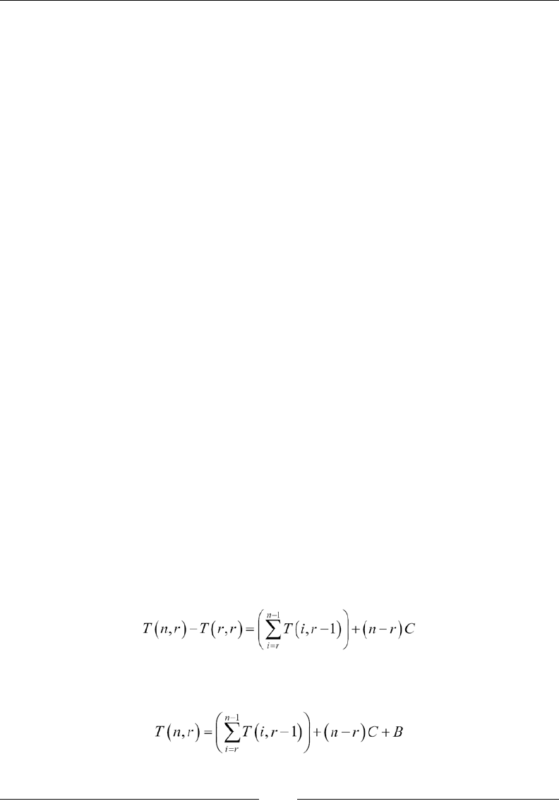
Chapter 4
[ 87 ]
T(n) = A + T(n-1)
=> T(n) – T(n-1) = A
This means T(n) is an arithmetic progression and thus can be represented as
T(n) = An + C, where C is the initial starting point, or T(0).
This means T(n) = O(n). We have already seen how the foldLeft operation works in
linear time. Of course, we have assumed that the the operation involved is constant
with time. A more complex operation will result in a different complexity.
You are advised to try to compute the complexity of the other algorithms, which are
not very different from this one. However, I will provide a few more of these.
Earlier in this chapter, we implemented the choose function as follows:
choose(n,r) = choose(n-1,r) + choose(n-1, r-1)
If we assume that the time taken is given by the function T(n,r), then T(n,r) =
T(n-1,r) + T(n-1,r-1) + C, where C is a constant. Now we can do the following:
T(n,r) = T(n-1,r) + T(n-1,r-1) + C
=>T(n,r) - T(n-1,r) = T(n-1,r-
1) + C
Similarly, T(n-1,r) - T(n-2,r) = T(n-2,r-1) + C, by simply having n-1 in
place of n. By stacking such values, we have the following:
T(n,r) - T(n-1,r) = T(n-1,r-1) + C
T(n-1,r) - T(n-2,r) = T(n-2,r-1) + C
T(n-2,r) - T(n-3,r) = T(n-3,r-1) + C
…
T(r+1,r) - T(r,r) = T(r,r-1) + C
The preceding equation considers n-r such steps in total. If we sum both sides of the
stack, we have the following:
Of course, T(r,r) is constant time. Let's call it B. Hence, we have the following:
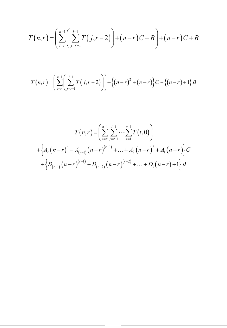
Detour – Functional Programming
[ 88 ]
Note that we can apply the same formula to T(i,r-1) too. This will give us the
following:
This gives the the following after simplication:
We can continue this way and we will eventually get an expression with multiple
nested summations, as follows:
Here A's and D's are also constants. When we are talking about asymptotic
complexity, we need to assume that a variable is sufciently large. In this case,
there are two variables, with the condition that r is always less than or equal to n.
So, rst we consider the case where r is xed and n is being increased and being
made sufciently large. In this case, there would be a total of r summations nested
in one another. T(t,0) is a constant time. The summation has r depth, each having a
maximum of (n-r) elements, so it is O((n-r)r). The other terms are O((n-r)r). Hence we
can say the following:
T(n,r) = O((n-r)r) = O(nr)
The size of the input is of course not n; it is log n = u (say). Then, we have the
complexity of computation of T(n,r) = O(2sr).
Another interesting case would be when we increase both r and n while also
increasing the difference between them. To do that, we may want a particular ratio
between the two, we assume r/n= k , k<1 always. Then we can see the asymptotic
growth of the function T(n, kn). But computing this requires calculus and is outside
the scope of this book.

Chapter 4
[ 89 ]
This shows that even though the analysis of algorithms in functional form can
be easier, the analysis of the time complexity can be fairly difcult. It is easy to
understand why it is more difcult to compute the complexity of a functional
algorithm. At the end of the day, computing complexity involves counting the
number of steps required to do the computation. In the imperative style, steps of
computation are direct, so it is easy to count them. On the other hand, a recursive
style is a higher level of abstraction, and hence, counting the number of steps is
harder. In the succeeding chapters, we will see more of these analyses.
Performance of functional programming
If we think about it, the whole point of functional programming is to have
immutability and recursive denitions (or inductive denitions) of programs so
that they can be analyzed easily. In general, adding additional constraints on your
program would make it simpler to analyze but would reduce what you can do with
it. Functional programming, of course, adds additional constraints on imperative
programming in the form of immutability, that is, you are no longer allowed
to reassign a variable. This is done so that the analysis of the program, that is,
understanding how the program works, is now simpler. It is also simpler to prove
theorems about the programs. However, we also lose some of the things that we
could do without such restrictions. It turns out that any program can be rewritten in
a functional style in a way to produce the same results. However, no guarantees are
made about their performance or complexity in general. So, a functional version of a
program can be a lot less efcient than its imperative counterpart. And indeed, in real
life, we face many such scenarios. So, it is really a tradeoff between performance and
simplicity. The general direction should then be that when working with a large input
size, it is better to do away with restrictions in order to be able to optimize more. On
the other hand, when the input sizes are small, it makes sense to stick to a functional
style because the performance is probably not affected much by it.
There are some cases, though, where the functional version has the same running
time complexity as the imperative version. In such a case, a functional version might
be preferred because of its simplicity. It should be noted that since Java does not
provide any explicit way of garbage collection and really, it happens by chance or
outside the control of the programmer, a functional programming style will ll up
the heap very quickly because of being immutable and thus being thrown away right
after being created. So, it will not be advisable to use them where performance is
really a problem.

Detour – Functional Programming
[ 90 ]
This would seem really contrary to the fact that many large data processing systems,
such as Spark, use a functional programming style. However, these systems only
have a specialized language that gives an appearance of a functional programming
style; they get translated to an almost non-functional form before they are even
executed. To elaborate a little more, a map method in a monad may not evaluate
anything at all; instead, it may just create a new object that contains this operator.
A general program can then analyze these structures and construct an imperative
program that does the same work. This provides a simple interface to the person
using the framework as well as keeping the resource usage under control. In the next
chapter, we will explore some of these ideas.
Summary
In this chapter, we learned a new way of looking at algorithms. The functional style
of writing a program can simplify the analysis of its correctness, that is, you can
easily understand why the program produces correct output. We saw a few patterns
in functional programming, especially monads. We also saw how Java provides
support for the functional style of programming through the syntax called lambda,
which has existed from version 9 of Java. Finally, we saw how to use lambda
effectively for functional programming.
Functional programs are, in general, easier to verify for correctness, but it is harder
to compute their complexity. They generally perform either at the same speed as
or slower than their imperative counterparts. It is a trade-off between development
effort and computational efciency. For smaller inputs, it is thus desirable to have
a functional style of programming, whereas for processing large inputs, imperative
style may be preferred.

[ 91 ]
Efcient Searching – Binary
Search and Sorting
What is searching? Searching is trying to locate a given value in a collection of
values. For example, you are given an array of integers, and your problem is to check
whether the integer 5 is in that array. This is a search problem. In addition to just
deciding whether the element 5 is in the array, we may be interested in its location as
well when it is found. This is also a search problem.
Another interesting take on it would be to imagine a dictionary, that is, an array of
values and associated values. For example, you have an array of names of students
and their marks, as shown in the following table:
Name Marks
Tom 63
Harry 70
Merry 65
Aisha 85
Abdullah 72
… ...
The list continues. Suppose, our system lets the student view his/her own marks.
They would type their name and the system would show their marks. For simplicity,
let's assume that there are no duplicate names. Now, we have to search for the name
provided and return the corresponding values. This is, thus, another search problem.
As we will see, search problems are quite ubiquitous in programming.

Efcient Searching – Binary Search and Sorting
[ 92 ]
In this chapter, you will learn the following:
• Search algorithms
• Efficient searching in a sorted list
• Some sorting algorithms
Search algorithms
Suppose you are given an array of values and you are required to check whether a
particular value is in that array, what is the most natural way to nd that element?
Well, it seems that the natural way is to go through each element one by one and
check whether they match the given value. If any one does, we have found that
element and we can return the index; if not, we can return -1 at the end of processing
all the elements to report that such an element could not be found. This is what we
would call a linear search. The following demonstrates a linear search algorithm in
an array:
public static <E, F extends E> int linearSearch(E[] values,
valueToLookup) {
for (int i = 0; i < values.length; i++) {
if (values[i].equals(valueToLookup)) {
return i;
}
}
return -1;
}
The function linearSearch takes an array of values and a value to search in it,
and returns the index if the value is found. If not, it returns a special value, -1. The
program simply goes through each element and checks whether the current element
matches with the value to lookup; if it does, then it just returns the current index,
otherwise it keeps looking. At the end of the array, it returns the special value, -1.
Now the following piece of code should return -1 in the rst case and the value 5 in
the second case:
Integer[] integers = new Integer[]{232,54,1,213,654,23,
6,72,21};
System.out.println(ArraySearcher.linearSearch(integers,5));
System.out.println(ArraySearcher.linearSearch(integers,23));

Chapter 5
[ 93 ]
Now, if we want to solve the student-marks problem described in the introduction
of this chapter, we just need to have the marks of the students stored in a different
array in the same order, as follows:
static String[] students = new String[]{"Tom","Harry",
"Merry","Aisha", "Abdullah"};
static int[] marks = new int[]{63,70, 65, 85, 72};
Now we can write a function to search for a name:
public static Integer marksForName(String name){
int index = linearSearch(students, name);
if(index>=0){
return marks[index];
}else{
return null;
}
}
First, we look for the name of the students in the list of students. If the name is
found, the corresponding index would be assigned to the variable index and the
value would be greater than or equal to zero. In such a case, we return the marks
stored in the same index as of the marks array. If it is not found, we return null. To
lookup the marks for Merry, for example, we call as shown here:
System.out.println(marksForName("Merry"));
We correctly obtain her marks, that are, 65.
What is the complexity of linear search? We have a for loop that moves through
each element of an array of length n (say); in the worst case, we would go through
all the elements, so the worst case complexity is θ(n). Even on an average, we would
be visiting half the elements before we hit the correct element, so the average case
complexity is θ(n/2) = θ(n).
Binary search
Is a linear search the best we can do? Well, it turns out that if we are looking at an
arbitrary array, this is what we have to do. After all, in an arbitrary array, there is no
way to know whether an element is there without potentially looking at all of them.
More specically, we cannot say for sure that some element does not exist, without
verifying all the elements. The reason is that the value of one element does not say
anything about the values of the other elements.
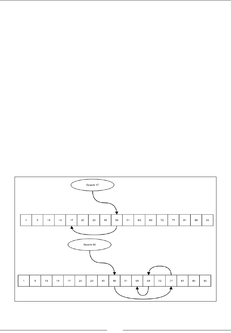
Efcient Searching – Binary Search and Sorting
[ 94 ]
But, what information can one element have about other elements in an array? One
way to make elements have information about the other elements is to have a sorted
array instead of just an arbitrary array. What is a sorted array? A sorted array is an
array that has all the elements arranged in order of their values. When an array is
sorted, every element contains the information that everything on the left is smaller
than that particular element, and everything on the right is bigger (or the other way
round if the order of the elements is opposite, but we will consider the arrays that
are sorted in an increasing order from left to right). This information can, amazingly,
make this search a lot faster. Here is what we do:
• Check the middle element of the array. If it matches the element we are
searching for, we are done.
• If the middle element is smaller than the value we are searching for, search
on the subarray on the right of the current array. This is because everything
on the left is even smaller.
• If the middle element is bigger than the value we are searching for, search
only in the left sub-array.
To avoid creating copies of the array while creating a sub-array, we just pass on the
whole array, but we remember the start and end positions we are looking at. The
start is included in the range and end is excluded. So, only elements on the right of
the start position and the left of the end position are included in the subarray being
searched. The following gure gives a visual understanding of binary search:
Figure 1: Binary Search.
An arrow representing moving one element to another during the search.

Chapter 5
[ 95 ]
But, before implementing this algorithm, we need to understand the concept of
Comparable. Comparable is an interface in the Java standard library that looks
like this:
package java.lang;
public interface Comparable<T> {
public int compareTo(T o);
}
Any class implementing this interface has to compare a different object with itself. It
is required that the type parameter, T, must be instantiated with the same class that
implements it, like this:
public class Integer implements Comparable<Integer>{
public int compareTo(Integer o){
…
}
}
The compareTo method intends to compare an object of the same type. If the current
object (the one that the this reference refers to) is smaller than the object passed,
compareTo must return a negative value. If the object passed is smaller, the method
must return a positive value. Otherwise, if they are equal, it must return 0. The
following conditions are required to be fullled by the compareTo method:
• If a.compareTo(b) == 0, then a.equals(b) must be true
• If a.compareTo(b) < 0 and b.compareTo(c) < 0, then a.compareTo(c) <0
• If a.compareTo(b) <0, then b.compareTo(a) > 0
• If b.equals(c) is true and a.compareTo(b) <0, then a.compareTo(c) <0
• If b.equals(c) is true and a.compareTo(b) >0, then a.compareTo(c) >0
Basically, the conditions are the same for a total order where equality is represented
by the equals method. It basically generalizes the concept of the < and <= operators,
which are there for numbers. Of course, the compareTo method for the Wrapper
objects are implemented exactly as the < and <= operators are on the primitives
inside them.
Now, we write the search function to do the search, as per the preceding steps:
private static <E extends Comparable<E>,
F extends E> int binarySearch( E[] sortedValues,
F valueToSearch, int start, int end) {
if(start>=end){
return -1;
}

Efcient Searching – Binary Search and Sorting
[ 96 ]
int midIndex = (end+start)/2;
int comparison = sortedValues[midIndex].compareTo(
valueToSearch);
if(comparison==0){
return midIndex;
}else if(comparison>0){
return binarySearch(sortedValues, valueToSearch,
start, midIndex);
}else{
return binarySearch(sortedValues, valueToSearch,
midIndex+1, end);
}
}
Note that in this case, we have mandated that the objects in the array must be
comparable so that we can know if an object is greater than or less than another
object. It does not matter exactly how this relationship is determined; the array must
be sorted using the same comparison – that the comparison between two consecutive
elements will make sure the element on the left is smaller than the one on the right,
as provided by Comparable.
The rst if condition checks whether the array passed is empty, if so, obviously the
element to be searched is not found and we return -1 to represent this. Then, we nd
the midIndex and recursively search for the element in either the left or the right
subarray. Once we have this function, we create another wrapper function to run the
search without having to mention the start and the end positions:
public static <E extends Comparable<E>, F extends E>
int binarySearch(
E[] sortedValues, F valueToSearch) {
return binarySearch(sortedValues, valueToSearch, 0,
sortedValues.length);
}
Complexity of the binary search algorithm
In every step, we are partitioning the total array into two parts, barring the one element
that we are comparing. In the worst case, that is, the case where the element searched
is not present in the array, we will have to get down all the way to the point where we
are dealing with an empty array, in which case we return -1 and stop recursing. We
must have had an array of only one element in the previous step. For our analysis, we
will consider this step as the last step. So, let's have a sorted array of n elements and
T(.) is the time required for searching in the array. So, we have the following:
T(n) = T((n-1)/2) + C, where C is a constant.

Chapter 5
[ 97 ]
In general, the two search branches in every step would be of different sizes, one
potentially being of size one less than that of the other part. But we will ignore these
small differences, which hardly matter for a large n. Hence, we will work with the
following equation:
T(n) = T(n/2) + C
Now, let's assume that n is an integral power of 2 so that n = 2m for some integer m.
So, we have this:
T(2m) = T(2m-1) + C
Now we take another function S(.), such that S(m) = T(2m) for all m. Then, we have:
S(m) = S(m-1) + C
This is the formula for an arithmetic progression. And hence, we have this:
S(m) = mC + D, where D is also a constant.
=> T(2m) = mC + D
=> T(n) = C lg(n) + D
So, we have the asymptotic complexity of T(n):
T(n) = O(lg(n))
The function, T(n), grows only as fast as the logarithm of the size of the array passed,
which is really slow. This makes binary search an extremely efcient algorithm.
To sort of eld test the algorithms, we run both linear and binary search algorithms
on an array of a hundred million elements with the following code:
int arraySize = 100000000;
Long array[] = new Long[arraySize];
array[0] = (long)(Math.random()*100);
for(int i=1;i<array.length;i++){
array[i] = array[i-1] + (long)(Math.random()*100);
}
//let us look for an element using linear and binary search
long start = System.currentTimeMillis();
linearSearch(array, 31232L);
long linEnd = System.currentTimeMillis();
binarySearch(array, 31232L);
long binEnd = System.currentTimeMillis();
System.out.println("linear search time :=" + (linEnd -start));
System.out.println("binary search time :=" +
(binEnd -linEnd));

Efcient Searching – Binary Search and Sorting
[ 98 ]
On my computer, the linear search took 282 milliseconds and binary search took
0 milliseconds. Also, note that the value we are looking for is expected to be quite
near to the beginning of the array; in case of values near the middle, a binary search
would have an even higher advantage.
Sorting
Okay, so we are convinced that if we have a sorted array, it takes a lot less time
to nd an element in it. But how do we get a sorted array? An arbitrary array is
unlikely to be sorted. The algorithm of getting a sorted array out of an arbitrary
array while keeping all the elements same, that is, by only rearranging the elements
of an input array, is called sorting. There are a lot of algorithms for sorting. But in
this chapter, we will start with a few simple ones that are not efcient. In the next
chapter, we will explore efcient sorting algorithms.
Selection sort
This is the most natural algorithm for sorting. We choose each position of the array
and nd the element in the array that belongs in that position. The functional
denition of selection sort is as follows:
• Find the minimum element in an array
• Swap this element with the first element of the array
• Sort the rest of the array after the first element recursively
Finding the minimum element has the functional structure as follows:
• Consider the array as a composition of the first element and the rest of
the array.
• Find the index of the minimum element in the rest of the array.
• Compare this element with the first element. If this element is smaller
than the first element, then it is the minimum element in the entire array.
Otherwise, the first element is the minimum element.
Instead of making copies of the array, we represent subarrays by simply storing the
starting index we want to consider, and then we work on the index recursively.
First, we write a function to nd the index of the minimum element in a given array,
starting from a position:
public static <E extends Comparable<E>> int findMin(E[] array,
int start){

Chapter 5
[ 99 ]
Then, we check whether the start position is the last position in the array, in which
case we just simply return the start position as there are no more elements:
if(start==array.length-1){
return start;
}
We nd the index of the minimum element in the array to the right of the current
start position and compare that element with the current start element. We return
whichever has the minimum element, as demonstrated in the following:
int restMinIndex = findMin(array, start+1);
E restMin = array[restMinIndex];
if(restMin.compareTo(array[start])<0){
return restMinIndex;
}else {
return start;
}
}
The swap function swaps or interchanges two elements in the array at the given
positions. This function is pretty straightforward:
public static <E> void swap(E[] array, int i, int j){
if(i==j)
return;
E temp = array[i];
array[i]=array[j];
array[j] = temp;
}
With the findMin and swap functions in our repository, we can nally put down the
selectionSort algorithm. We start off by passing the position zero as the value of
the start parameter:
public static <E extends Comparable<E>> void selectionSort(
E[] array, int start){
Firstly, there is no sorting to be done if the array is empty:
if(start>=array.length){
return;
}
Efcient Searching – Binary Search and Sorting
[ 100 ]
Now, we just nd the index of the minimum element and swap the current position
with the index of the minimum position. This will put the minimum element in the
current position:
int minElement = findMin(array, start);
swap(array,start, minElement);
Then, we recursively sort the rest of the array:
selectionSort(array, start+1);
}
Now, we can write a wrapper function to just do selectionSort without having to
pass a start index:
public static <E extends Comparable<E>> void selectionSort(
E[] array) {
selectionSort(array, 0);
}
We can test our code by creating an arbitrary array and then sorting it using
our algorithm:
Integer[] array = new Integer[]{10, 5, 2, 3, 78, 53, 3};
selectionSort(array);
System.out.println(Arrays.toString(array));
And the output would be as follows:
[2, 3, 3, 5, 10, 53, 78]
Note how all the elements are repositioned in ascending order, which means that the
array is sorted.
The form of selection sort shown is not functional in a strict
sense because we are modifying the contents of an array. A truly
functional sort of an array will make a copy of the array on every
modication. However, this is very expensive. On the other hand,
thinking of the algorithm in terms of smaller versions of the same
problem, like we have done, does make the algorithm simpler to
understand. I tried to hit a sweet spot where I have the simplicity
of the recursive algorithm, but don't have to keep creating copies
of the array.

Chapter 5
[ 101 ]
Complexity of the selection sort algorithm
To compute the complexity of the selection sort algorithm, rst we have to compute
the complexity of the findMin and swap functions. Let's start with the findMin
function. As with any recursive function, we start with assuming that with an array of
length n (in this case, the effective length of the array, starting from the start position),
it takes us T(n) time to compute the findMin function. While recursively calling itself,
it passes on an effective array of length n-1. So, we have the following equation:
T(n) = T(n-1) + A where A is a constants
=> T(n) – T(n-1) = A, so it is an arithmetic progression
=> T(n) = An + B where B is a constant
=> T(n) = θ(n)
Now, let's move on to the swap function. It has no recursion and no loops, so the
complexity is constant or θ(1).
Finally, we are ready to compute the complexity of the function selectionSort.
Say, for an effective length n of an array, the time taken is T(n). It calls itself with
effective length n-1, it also calls findMin and swap functions, which are θ(n) and θ(1),
respectively. So, we have this:
T(n) = T(n-1) + θ(n) + θ(1)
Note that some expressions that are θ (n) have been written as θ (n) itself. It should
be read as, "Some function of n that has the asymptotic complexity, θ (n)." It turns out, for
computing complexity of T(n), we don't have to actually know the actual expression,
we can simply put Cn and D for functions that are θ (n) and θ (1), respectively, where
C and D are constants. So, we form the following equation:
T(n) = T(n-1) + Cn + D
=> T(n) – T(n-1) = Cn + D
Similarly, T(n-1) - T(n-2) = C(n-1) + D and so on. If we stack these equations, we get
the following:
T(n) – T(n-1) = Cn + D
T(n-1) – T(n-2) = C(n-1) + D
T(n-2) – T(n-3) = C(n-2) + D
T(n-3) – T(n-4) = C(n-3) + D
…
T(1) – T(0) = C(1) + D
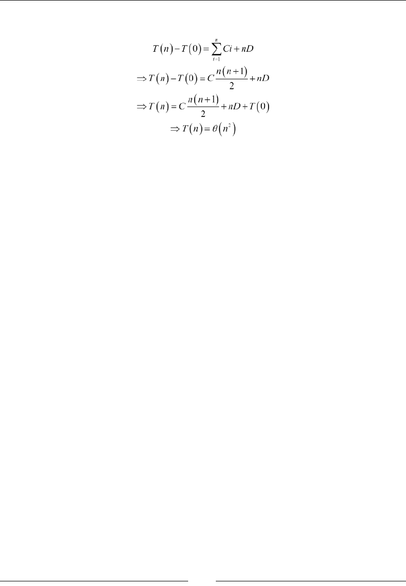
Efcient Searching – Binary Search and Sorting
[ 102 ]
Adding both sides, we get this:
So, the selection sort has a complexity of θ(n2), where n is the size of the array being
sorted. Now, we will see the next sorting algorithm, which is the insertion sort.
Insertion sort
In selection sort, we rst selected a position and then found the element that should
sit there. In the insertion sort, we do the opposite; we rst select an element and then
insert the element into position where it should sit. So, for every element, we rst
nd out where it should be and then we insert the element in the right place. So, we
rst see how to insert an element into a sorted array. The idea is that we are given an
array of sorted elements and we are supposed to insert another element in the correct
position, so that the resulting array remains sorted. We will consider a simpler
problem. We are given an array that is sorted except for the last element. Our job is
to insert the last element in the correct position. The recursive way to achieve this
insertion is as follows:
• If the element to be inserted is bigger than the end element of the sorted
array, it belongs in the end and the insertion is complete.
• Otherwise, we swap the last element with the element to be inserted and
recursively insert this element in the rest of the smaller array in front of it.
We do it with the following function. The function takes an array and a position that
represents this last position:
public static <E extends Comparable<E>> void insertElementSorted(
E[] array, int valueIndex) {
if (valueIndex > 0 && array[valueIndex].compareTo(
array[valueIndex - 1]) < 0) {
swap(array, valueIndex, valueIndex - 1);

Chapter 5
[ 103 ]
insertElementSorted(array, valueIndex - 1);
}
}
If the last position or the valueIndex is 0, there is nothing to be done, as the element
is already in the correct position, that is, 0. There is no array to the left of valueIndex
in this case. If not, we compare the last element to the previous element. Since the
array on the left is presumed to be sorted, the previous element is the largest element
in the sorted part of the array. If the last element is bigger than even this one, there
is nothing more to be done. If not, we swap the last element with the previous one
and run the insertion recursively on the array with one less element. The last element
has moved to the previous position and it must now be compared with the element
before that, and so on.
With the insertion function available for sorted arrays, we are now ready to write
the algorithm for an insertion sort. In every step of the insertion sort, we consider
a boundary in the array. Everything on the left of the boundary has already been
sorted. Our job in the current step is to insert the element at the boundary index into
the left sorted array, which we achieve using the insertElementSorted function.
We implement this sort with the following simple strategy. In any step, we do
the following:
• We first sort the left-hand side of the boundary so that our assumption about
it being sorted is achieved
• Then we invoke the insertElementSorted function to insert the current
boundary element in the sorted array
Of course, when boundary is zero, it means that there is no array to be sorted and we
simply return:
public static <E extends Comparable<E>> void insertionSort(
E[] array, int boundary) {
if(boundary==0){
return;
}
insertionSort(array, boundary-1);
insertElementSorted(array, boundary);
}
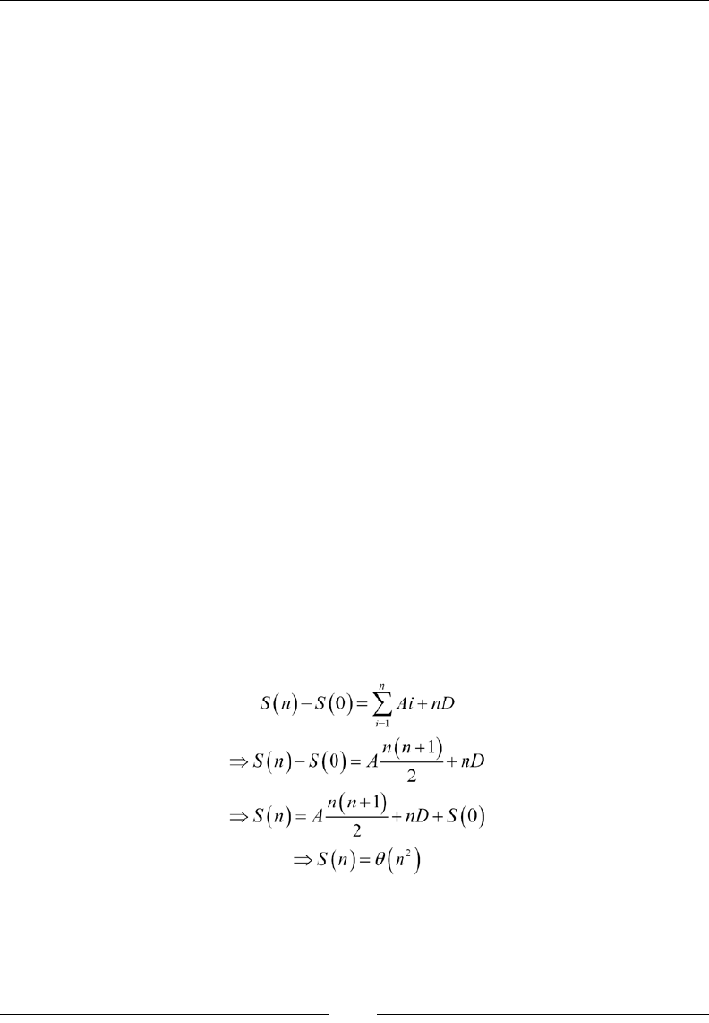
Efcient Searching – Binary Search and Sorting
[ 104 ]
Complexity of insertion sort
To compute the complexity of insertion sort, we must rst compute it for the
insertElementSorted function. Let the time taken for an array of effective length
(that is, from zero to boundary-1), n be T(n). From there, we recursively call it with
n-1. So, we have the following:
T(n) = T(n-1) + C where C is a constant
=> T(n) = θ(n)
Let's now assume that the time taken for sorting an array of n elements is S(n).
Apart from the base case, it calls itself with one less argument and then calls the
insertElementSorted function with an array of effective length n-1. Thus, we
have this:
S(n) = S(n-1) + T(n) + D where D is a constant.
Again, when n is large, T(n) = θ(n); hence, it can be approximated by An where A is a
constant. So, we have this:
S(n) = S(n-1) + An + D
=> S(n) – S(n-1) = An + D,
Since this is true for all n, we have:
S(n) – S(n-1) = An + D
S(n-1) – S(n-2) = A(n-1) + D
S(n-2) – S(n-3) = A(n-2) + D
…
S(1) – S(0) = A + D
Summing both sides, we get the following:
Thus, insertion sort has the same asymptotic complexity as selection sort.

Chapter 5
[ 105 ]
Bubble sort
Another interesting sorting algorithm is a bubble sort. Unlike the previous
algorithms, this one works at a very local level. The strategy is as follows:
• Scan through the array, searching pairs of consecutive elements that are
ordered wrongly. Then find a j, such that array[j+1] < array[j].
• Whenever such a pair is found, swap them and continue searching until the
end of the array and then back from the beginning again.
• Stop when a scan through the entire array does not even find a single
pair.
The code that does this is as follows:
public static <E extends Comparable<E>> void bubbleSort(
E[] array) {
boolean sorted = false;
while (!sorted) {
sorted = true;
for (int i = 0; i < array.length - 1; i++) {
if (array[i].compareTo(array[i + 1]) > 0) {
swap(array, i, i + 1);
sorted = false;
}
}
}
}
The ag, sorted, keeps track of whether any inverted pairs were found during a
scan. Each iteration of the while loop is a scan through the entire array, the scan
being done inside the for loop. In the for loop, we are, of course, checking each pair
of elements, and if an inverted pair is found, we swap them. We stop when sorted is
true, that is, when we have not found a single inverted pair in the entire array.
To see that this algorithm will indeed sort the array, we have to check two things:
• When there are no inverted pairs, the array is sorted. This justifies our
stopping condition.
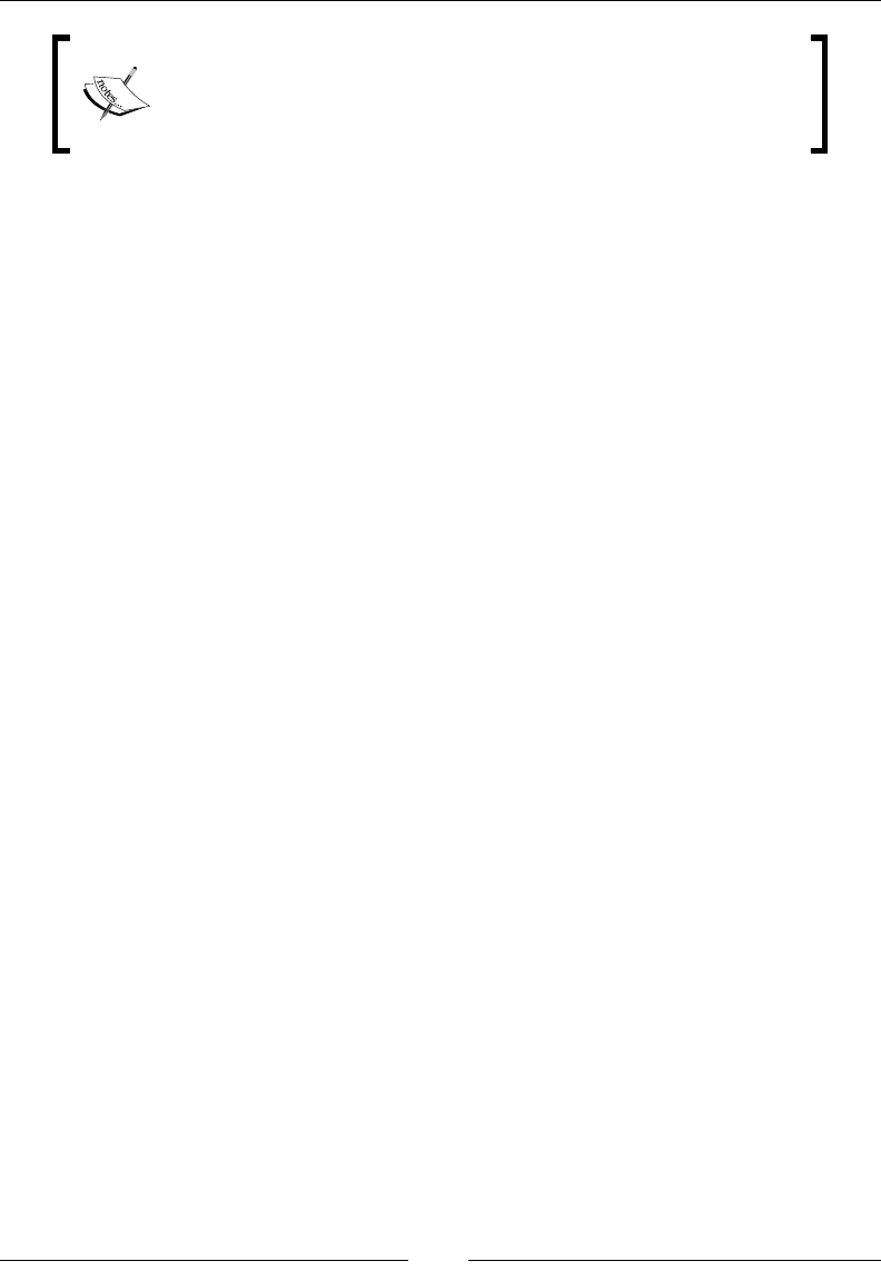
Efcient Searching – Binary Search and Sorting
[ 106 ]
This is, of course, true because when there are no inverted pairs,
we have that for all j< array.length-1, we have array[j+1]>=array[j].
This is the definition of an array being in an increasing order, that
is, the array being sorted.
• Irrespective of the input, the program will eventually reach the preceding
condition after a finite number of steps. That is to say that we need the
program to finish in a finite number of steps. To see this, we need to
understand the concept of inversions. We will explore them in the next section.
Inversions
Inversion in an array is a pair of elements that are wrongly ordered. The pair may be
close together or very far apart in the array. For example, take the following array:
Integer[] array = new Integer[]{10, 5, 2, 3, 78, 53, 3};
How many inversions does the array have? Let us count:
10>5, 10>2, 10>3, 10<78, 10<53, 10>3
5>2, 5>3, 5<78, 5<53, 5>3
, 2<3, 2<78, 2<53, 2<3
, 3<78, 3<53, 3=3
, 78>53, 78>3
53>3
In this listing, every element is compared with the elements following it. There is an
inversion when there is a greater-than sign, highlighted by bold characters. Counting
the bold ones, we see there are 10 inversions.
For any input array, there is a number of inversions. In a sorted array, the number
of inversions would be zero. Now, think about what happens to the number
of inversions when a swap is made. A swap interchanges a pair of consecutive
elements, thus breaking one inversion (the swap happens only when there is an
inversion between consecutive elements). To see this more clearly, consider the
following case of a swap between j and j+1 indexes:
…......., j, j+1, …....

Chapter 5
[ 107 ]
Let's take the jth element rst. Let it have x number of inversions with the left part of the
array. Since these elements are on the left, all inversions of this type are with elements
greater than the jth element. When the jth element moves to the (j+1)th position, they
still remain to the left, and the only element added to the left of the jth element is the
element it is swapped with. Hence, no changes to the number of inversion happens
to the jth element, other than the one due to the (j+1)th element. The same logic can be
applied to the inversions with it in the right part of the array, and also to both sides of
the array for the (j+1)th element. Because of the swap, one inversion is broken between
jth and (j+1)th elements. Hence, the number of inversions reduce by exactly one in each
inversion. This means the number of swaps in bubble sort would be exactly equal
to the number of inversions in the input array, which is nite. And since each scan
through the array requires a swap in the previous scan, the total number of scans is
at most one more that the number of swaps; this is nite too. This makes sure that the
algorithm always nishes.
Complexity of the bubble sort algorithm
To understand the complexity of a bubble sort, we have to count the number of
steps. Is the number of steps equal to the number of swaps? The answer is, not
really. In case of asymptotic analysis, we must always count the step that happens
a maximum number of times. In this case, that step is comparison. How many
comparisons are there per scan of the array? n-1 of course. So, now the analysis of
complexity is reduced to the number of scans we need to sort the array.
Let's see what happens to the maximum element after the rst scan. Let's say the
maximum element is at the index j. So, it will be compared with the element at
j+1. For simplicity, let's assume that all elements are different. Now, since it is the
maximum element, the element at the j+1 position will be less than it, and hence it
will be swapped. Now the maximum element is at the position, j+1, and is being
compared with the element at position, j+2, and the same thing happens. It will
continue until the maximum element is at the end of the array. If the elements are
not unique, the same will happen to the rightmost maximum element. In the next
cycle, the maximum element will already be at the end of the array, and we will hit
the second maximum (or another maximum element) somewhere in the array. Now,
since one maximum element is at the end of the array, we can think of the rest of the
array apart from the last element. In this array, the current maximum is the maximum
and it will reach the end of the current part of the array at the end of the current scan.

Efcient Searching – Binary Search and Sorting
[ 108 ]
This shows that at the end of each scan, at least one element reaches the correct
nal position without altering the correct positions of the ones that got there before
the scan, which means that at the end of n scans, all of the elements would be in
the correct position and the array would be sorted. That is to say that after at most
n scans, the bubble sort would be complete. In each of those scans, there are O(n)
operations. So, the worst case complexity of bubble sort is O(n2).
This is not the end of this analysis; we still have to show that there is a case that takes
that many steps, and only then can we have a theta bound on the worst case. We take
the case where all the elements are sorted in the opposite order, that is, they are in a
decreasing order and are all distinct. In such a case, every element has an inversion
with all the others. This means that each one of the n elements have an inversion
with n-1 other elements, that is, n(n-1) inversions in total. But since each inversion
would be counted twice, once from each of the elements that are members of the
inversion, it is actually n(n-1)/2. Now, note that the maximum number of swaps that
can be done in one scan is n-1, which will happen if every comparison results in a
swap because there are n-1 comparisons per scan. So, we will need at least (n(n-1)/2)/
(n-1) = n/2 scans to complete all the swaps, each requiring n-1 comparisons. So, the
complexity is at least n(n-1)/2 = Ω(n2). Of course then, the worst case is at least this
much complex because the worst case is, by denition, the most complex case.
So, the worst case is both O(n2) and Ω(n2), that is to say that it is θ(n2).
A problem with recursive calls
A problem with recursive calls is that they are expensive; a method invocation entails
considerable overhead on the processor. It is, in general, better to avoid invoking
methods if you want to improve performance to the last bit. On top of that, there is
a limit to the depth of function calls that you can go to, before the program breaks.
This is because a program has a stack to enable method invocation semantics, that
actually gets a new element containing all variables and the position of the current
instruction to the stack. This stack does not grow indenitely, but instead is xed in
size; usually, it can hold a few thousand values, which means that if your method
invocation is deeper than that, it will break and the program will exit with an error.
This means that our insertion sort will break for an array containing more than a few
thousand entries. On the other hand, it is generally easier to explain an algorithm
in a functional form. To balance between these two aspects, we need to be able to
convert to and from the recursive and non-recursive versions of the same algorithm.
We will do this step by step from the simplest form to the more complicated form.

Chapter 5
[ 109 ]
Tail recursive functions
A recursive function is called a tail recursive function if all the recursive calls to itself
in the function are the last operations. I say it like there are multiple calls and all of
them must be the last operations. How is that possible? I mean there can be different
calls from different conditional branches of the code inside the function. However,
whenever the function calls itself that must be the last operation in that conditional
branch of the function. For example, take our binary search algorithm again:
private static <E extends Comparable<E>, F extends E>
int binarySearch(
E[] sortedValues, F valueToSearch, int start, int end) {
if(start>=end){
return -1;
}
int midIndex = (end+start)/2;
int comparison = sortedValues[midIndex]
.compareTo(valueToSearch);
if(comparison==0){
return midIndex;
}else if(comparison>0){
return binarySearch(sortedValues, valueToSearch,
start, midIndex);
}else{
return binarySearch(sortedValues, valueToSearch,
midIndex+1, end);
}
}
Note that the function calls itself in two different conditional branches. However, in
each branch, the recursive call is the last operation. There is nothing to be done after
the call to itself. This is a tail recursive function.
Tail recursive functions can be turned into a loop absolutely mechanically. In fact, all
functional language compilers do this automatically during compiler optimization.
The Java compiler, however, does not do this because Java generally prefers loops
over recursion in the code, at least until very recently. But we can do this conversion
by ourselves.
The idea is that since there are no more operations after the recursive call, the
program does not have to remember the values of the variables of the calling
function. So, they can simply be overwritten by the values of the same variables
of the called function instead, and we just have to process the code of the function
again. So, the following is the mechanical procedure to achieve this:
Wrap the entire content in an innite while loop.

Efcient Searching – Binary Search and Sorting
[ 110 ]
Replace all recursive calls by updating the values of the parameters to the values that
are passed in the recursive calls.
The following shows this update in the binary search algorithm:
private static <E extends Comparable<E>, F extends E>
int binarySearchNonRecursive(
E[] sortedValues, F valueToSearch, int start, int end) {
while(true) {
if (start >= end) {
return -1;
}
int midIndex = (end + start) / 2;
int comparison = sortedValues[midIndex]
.compareTo(valueToSearch);
if (comparison == 0) {
return midIndex;
} else if (comparison > 0) {
end = midIndex;
} else {
start = midIndex + 1;
}
}
}
Note that we updated only those arguments that changed, which is only one update
per branch in this case. This will produce the exact same result as the earlier function,
but now it would not cause a stack overow. This conversion is not really required
in case of a binary search though, because you need only lg n steps to search an array
of length n. So, if your allowed depth of invocation is 1000, then you can search in an
array of maximum size of 21000 elements. This number is way more than the total
number of atoms in the entire universe, and hence we will never be able to store an
array of that enormous size. But the example shows the principle of converting a tail
recursion into a loop.
Another example is the insertElementSorted function, used in our insertion
sort algorithm:
public static <E extends Comparable<E>> void
insertElementSorted(
E[] array, int valueIndex) {
if (valueIndex > 0 && array[valueIndex]
.compareTo(array[valueIndex - 1]) < 0) {
swap(array, valueIndex, valueIndex - 1);
insertElementSorted(array, valueIndex - 1);

Chapter 5
[ 111 ]
}
}
Note that there is no operation pending after the recursive call to itself. But we need
to be a little more careful here. Note that the invocation only happens inside a code
branch. The else case is implicit here, which is else { return; }. We need to make
it explicit in our code rst, as shown below:
public static <E extends Comparable<E>> void insertElementSorted(
E[] array, int valueIndex) {
if (valueIndex > 0 && array[valueIndex].compareTo(
array[valueIndex - 1]) < 0) {
swap(array, valueIndex, valueIndex - 1);
insertElementSorted(array, valueIndex - 1);
} else{
return;
}
}
Now we can use our old technique to make it non-recursive, that is, to wrap it in an
innite loop and replace recursive calls with argument updates:
public static <E extends Comparable<E>> void
insertElementSortedNonRecursive(
E[] array, int valueIndex) {
while(true) {
if (valueIndex > 0 && array[valueIndex].compareTo(
array[valueIndex - 1]) < 0) {
swap(array, valueIndex, valueIndex - 1);
valueIndex = valueIndex – 1;
}else{
return;
}
}
}

Efcient Searching – Binary Search and Sorting
[ 112 ]
This gives the exact same result as the previous recursive version of the function. So,
the corrected steps would be as follows:
1. First, make all implicit branches explicit and all implicit returns explicit.
2. Wrap the entire content in an innite while loop.
3. Replace all recursive calls by updating the values of the parameters to the
values that are passed in the recursive calls.
Non-tail single recursive functions
By single recursion, I mean that the function invokes itself at most once per
conditional branch of the function. They may be tail-recursive, but they are not
always so. Consider the example of the recursion of our insertion sort algorithm:
public static <E extends Comparable<E>> void insertionSort(
E[] array, int boundary) {
if(boundary==0){
return;
}
insertionSort(array, boundary-1);
insertElementSorted(array, boundary);
}
Note that the function calls itself only once, so it is a single recursion. But since we
have a call to insertElementSorted after the recursive call to itself, it is not a tail
recursive function, which means that we cannot use the earlier method. Before doing
this though, let's consider a simpler example. Take the factorial function:
public static BigInteger factorialRecursive(int x){
if(x==0){
return BigInteger.ONE;
}else{
return factorialRecursive(x-1).multiply(
BigInteger.valueOf(x));
}
}
First, note that the function is singly recursive, because there is at most one recursive
call per branch of the code. Also, note that it is not tail recursive because you have to
do a multiplication after the recursive call.

Chapter 5
[ 113 ]
To convert this into a loop, we must rst gure out the actual order of the numbers
being multiplied. The function calls itself until it hits 0, at which point, it returns 1.
So, the multiplication actually starts from 1 and then accumulates the higher values.
Since it accumulates the values on its way up, we need an accumulator (that is
a variable storing one value) to collect this value in a loop version. The steps are
as follows:
1. First, make all implicit branches explicit and all implicit returns explicit.
2. Create an accumulator of the same type as the return type of the function.
This is to store intermediate return values. The starting value of the
accumulator is the value returned in the base case of the recursion.
3. Find the starting value of the recursion variable, that is, the one that is getting
smaller in each recursive invocation. The starting value is the value that
causes the next recursive call to fall in the base case.
4. The exit value of the recursion variable is the same as the one passed to the
function originally.
5. Create a loop and make the recursion variable your loop variable. Vary it
from the start value to the end value calculated earlier in a way to represent
how the value changes from higher depth to lower depth of recursion. The
higher depth value comes before the lower depth value.
6. Remove the recursive call.
What is the initial value of the accumulator prod? It is the same as the value that is
returned in the exit branch of the recursion, that is, 1. What is the highest value being
multiplied? It is x. So we can now convert it to the following loop:
public static BigInteger factorialRecursiveNonRecursive(int x){
BigInteger prod = BigInteger.ONE;
for(int i=1;i<=x;i++){
prod = prod.multiply(BigInteger.valueOf(x));
}
return prod;
}

Efcient Searching – Binary Search and Sorting
[ 114 ]
Now let's consider the insertionSort algorithm. What is the accumulator? It is the
same thing that would be the nal output, that is, an array of sorted elements. What
is the starting value? It is the same that is returned in the recursive version in the exit
branch. This is an array of length zero. What is the nal value? The array of sorted
elements of the length provided to sort. Again, just like our recursive version, we
represent these partial arrays with, simply, a boundary value. So, the code is as follows:
public static <E extends Comparable<E>> void
insertionSortNonRecursive(
E[] array) {
for(int boundary = 0;boundary<array.length;boundary++) {
insertElementSortedNonRecursive(array, boundary);
}
}
Note that in this case, the function return type is void. But what we are really
returning is the sorted array; we just resorted to modifying the same array to avoid
creating duplicate arrays.
The most general case is the multiple recursion, that is, the function calls itself multiple
times in the same conditional branch of the function. This case cannot be done without
a stack. In case of a recursive call, we use the method-invocation stack. Otherwise, we
can even use an external stack. Since we do not have such an example in this chapter,
we defer its explanation to the next chapter, where we will have an example.
Summary
In this chapter, we saw how to do an efcient search in an ordered array. This search is
called a binary search. You also learned some methods of obtaining an ordered array
out of an unordered one. This process is called sorting. We saw three basic algorithms
of sorting. Although they are not particularly efcient, they are simple to understand
the concept. You also learned how to convert a recursive algorithm to a non-recursive
one that uses a loop. In the next chapter, we will see efcient sorting algorithms.

[ 115 ]
Efcient Sorting – quicksort
and mergesort
In the last chapter, we explored a few simple sorting algorithms. The problem with
those is that they are not efcient enough. In this chapter, we will cover two efcient
sorting algorithms and we will also see how they are efcient.
In this chapter, you will learn the following topics:
• quicksort
• mergesort
• Optimality of efficiency in sorting algorithms
quicksort
We want to develop an algorithm that sorts an array of elements efciently. Our
strategy will be simple; we will somehow try to divide the array into two halves
in such a way that sorting each half will complete the sorting. If we can achieve
this, we can recursively call the sorting algorithm this way. We already know that
the number of levels of recursive call will be of the order of lg n where lg m is the
logarithm of m with the base 2. So, if we can manage to cut the array in a time in the
order of n, we will still have a complexity of O(n lg n) This is much better than O(n2),
which we saw in the previous chapter. But how do we cut the array that way? Let's
try to cut the following array as follows:
10, 5, 2, 3, 78, 53, 3,1,1,24,1,35,35,2,67,4,33,30
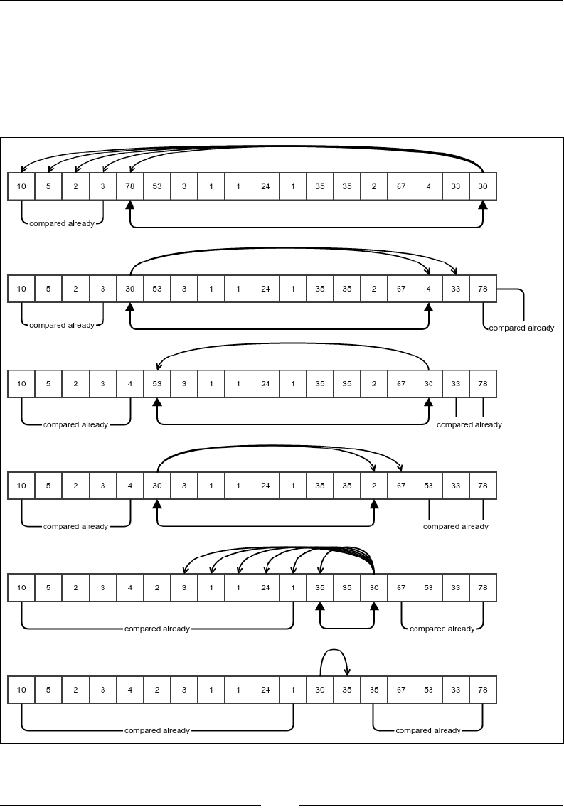
Efcient Sorting – quicksort and mergesort
[ 116 ]
If we trivially cut this array, each part will contain all sorts of values. Sorting these
individual parts would then not cause the entire array to be sorted. Instead, we have
to cut the array in such a way that all the elements in the left part are less than all
the elements in the right part. If we can achieve this, sorting the parts will achieve
sorting the whole. But, of course, we need to make some swaps for us to be able to
cut the array in such a way. So, we use the following trick:

Chapter 6
[ 117 ]
This is an example of pivot positioning in quicksort. The one headed arrows
represent comparison and double headed arrows represent swap.
We rst choose the last element and call it pivot. Our aim is to make all the elements
that are less than the pivot to be on its left and all the elements that are greater
than the pivot to be on its right. Note that this means that the pivot is already at
the correct position of the array. The preceding gure shows how to do it with an
example. In the gure, our pivot is 30. We start comparing with the rst element and
move on. The moment we nd an inversion, we swap the pivot with that element
and keep comparing in the opposite direction. We continue this way, swapping
every time there is an inversion and reversing the direction of comparison each time.
We stop when all the elements have been compared. Note that after this process, all
the elements less than the pivot are on its left, and all the elements greater than the
pivot are on its right. Why does this work? Let's take a closer look.
Suppose we start comparing from the left. After the rst swap, the pivot is at the
position of the element that was found to be greater than it. All the elements that
were on the left of it have already been compared with the pivot and found to be
less than it. The previous gure shows the parts that have already been compared.
Now it starts comparing from its earlier position in the opposite direction. After the
second swap, it sits in the position of the element that it has been swapped with. All
the elements on the right have already been compared with it and found to be greater
than it. We keep going in the same way, always ensuring that the parts that have
already been compared follow the rule that the part on the left of the pivot contains
only elements that are less than or equal to it and the part on the right of the pivot
contains only elements that are greater than or equal to it. So, when we are done with
the comparisons, we still hold this condition, thus achieving the result. Once we know
that all the elements on the left of the pivot are less than or equal to all the elements
that are on its right, we can sort these parts separately and the entire array will be
sorted as a result. Of course, we sort these parts recursively in the same way.
However, before we dive into the code, I would like to introduce a different interface
for comparison. It is called java.util.Comparator and allows us to specify any
comparison logic while sorting, thus providing more exibility. Here is how it looks:
@FunctionalInterface
public interface Comparator<T> {
int compare(T o1, T o2);
}

Efcient Sorting – quicksort and mergesort
[ 118 ]
This is, of course, a very simplied version of the actual interface but has got all
that we care about. As you can see, this is a functional interface and thus can be
implemented using a lambda. It should return the same value that is conceptually
similar to the value returned by o1.compareTo(o2), but a different sorting can use
a different comparison lambda. The compare method has to follow the same rules
that are there for the compareTo method in the java.util.Comparable interface we
studied in the previous chapter.
Now let's jump into the code for quicksort. We know we don't have to sort any more
when the array to be processed is empty, which would be our base case. Otherwise,
We create two indexes i and j, one storing the current end of the left part and the
other storing the current beginning of the right part that has already been compared
with the pivot at any given point of time, while the pivot is being placed in its correct
position. Both the index variables store the indexes that are to be compared next. At
any given point of time, one of these variables holds the position of the pivot and the
other stores the current value being compared with it. The variable that currently
stores the position of the pivot is agged by the Boolean variable, movingI. If it is
true, it means that we are currently moving i and hence, j is pointing to the pivot.
We update the position variables and keep comparing, in a loop, until both indexes
point to the pivot, when the comparison suggests that there is an inversion, we
swap and reverse the direction of movement. We reverse the direction of movement
because the pivot has moved to the position indexed by the opposite variable,
marked by movingI switching its value. Otherwise, we just keep updating the
appropriate position variable.
When movingI is false, it means that i is storing the position of the pivot. And
nally, when the pivot is at the correct position and all the elements on its left are
less than or equal to all the elements on its right, we recursively call quicksort on
each part:
public static <E> void quicksort(E[] array, int start, int end,
Comparator<E> comparator) {
if (end - start <= 0) {
return;
}
int i = start;
int j = end - 1;
boolean movingI = true;
while (i < j) {

Chapter 6
[ 119 ]
if (comparator.compare(array[i], array[j]) > 0) {
swap(array, i, j);
movingI = !movingI;
} else {
if (movingI) {
i++;
} else {
j--;
}
}
}
quicksort(array, start, i, comparator);
quicksort(array, i + 1, end, comparator);
}
We can wrap this method to avoid having to pass the start and end parameters:
public static <E> void quicksort(E[] array, Comparator<E> comparator){
quicksort(array, 0, array.length, comparator);
}
We can use this method to sort an array. Let's see how to sort an integer array:
Integer[] array =
new Integer[]{10, 5, 2, 3, 78, 53, 3, 1, 1, 24, 1, 35,
35, 2, 67, 4, 33, 30};
quicksort(array, (a, b) -> a - b);
System.out.println(Arrays.toString(array));
The following would be the output:
[1, 1, 1, 2, 2, 3, 3, 4, 5, 10, 24, 30, 33, 35, 35, 53, 67, 78]
Note how we passed the simple comparator using a lambda. If we pass a lambda
(a,b)->b-a instead, we will get the array reversed. In fact, this exibility lets us
sort arrays containing complex objects according to any comparison we like. For
example, it is easy to sort an array of Person objects by age using the lambda, (p1,
p2)->p1.getAge() - p2.getAge().

Efcient Sorting – quicksort and mergesort
[ 120 ]
Complexity of quicksort
Like always, we will try to gure out the worst case of quicksort. To begin with,
we notice that after the pivot has been positioned correctly, it is not positioned in
the middle of the array. In fact, its nal position depends on what value it has with
respect to the other elements of the array. Since it is always positioned as per its
rank, its rank determines the nal position. We also notice that the worst case for
quicksort would be when the pivot does not cut the array at all, that is, when all the
other elements are either to its left or to its right. This will happen when the pivot is
the largest or the smallest element. This will happen when the highest or the lowest
element is at the end of the array. So, for example, if the array is already sorted, the
highest element would be at the end of the array in every step, and we will choose
this element as our pivot. This gives us the counter intuitive conclusion that an array
that is already sorted would be the worst case for the quicksort algorithm. An array
that is sorted in the opposite direction is also one of the worst cases.
So, what is the complexity if the worst case happens? Since it is the worst case where
every step is made out of two recursive calls, one of which is with an empty array
and thus needing a constant time to process, and another having an array with one
less element. Also, in each step, the pivot is compared with every other element, thus
taking time proportional to (n-1) for an n-element step. So, we have the recursive
equation for the time T(n) as follows:
T(n) = T(n-1) + a(n-1) + b where a and b are some constants.
=> T(n) – T(n-1) = a(n-1) + b
Since this is valid for all values of n, we have:
T(n) – T(n-1) = a(n-1) + b
T(n-1) – T(n-2) = a(n-2) + b
T(n-2) – T(n-3) = a(n-3) + b
...
T(2) – T(1) = a(1) + b
Summing both sides, we have the following:
T(n) – T(1) = a (1+2+3+...+(n-1)) + (n-1)b
=> T(n) – T(1) = an(n-1)/2 + (n-1)b
=> T(n) = an(n-1)/2 + (n-1)b + T(1)
=> T(n) = O(n2)

Chapter 6
[ 121 ]
This is not very good. It is still O(n2). Is it really an efcient algorithm? Well,
to answer that, we need to consider the average case. The average case is the
probabilistically weighted average of the complexities for all possible inputs. This is
quite complicated. So, we will use something that we can call a typical case, which
is sort of the complexity of the usual case. So, what would happen in a typical
randomly unsorted array, that is, where the input array is arranged quite randomly?
The rank of the pivot will be equally likely to be any value from 1 to n, where n is the
length of the array. So, it will sort of split the array near the middle in general. So,
what is the complexity if we do manage to cut the array in halves? Let's nd out:
T(n) = 2T((n-1)/2) + a(n-1) + b
This is a little difcult to solve, so we take n/2 instead of (n-1)/2, which can only
increase the estimate of complexity. So, we have the following:
T(n) = 2T(n/2) + a(n-1) + b
Let m = lg n and S(m) = T(n), and hence, n = 2m. So, we have this:
S(m) = 2S(m-1) + a 2m + (b-a)
Since this is valid for all m, we can apply the same formula for S(m-1) as well. So, we
have the following:
S(m) = 2(2S(m-2) + a 2m-1 + (b-a)) + a 2m + (b-a)
=> S(m) = 4 S(m-2) + a (2m + 2m) + (b-a)(2+1)
Proceeding similarly, we have this:
S(m) = 8 S(m-3) + a (2m + 2m + 2m) + (b-a)(4+2+1)
…
S(m) = 2m S(0) + a (2m + 2m + 2m + 2m) + (b-a)(2m-1+ 2m-2+ … + 2+1)
=>S(m) = 2m S(0) + a m . 2m+ (b-a) (2m – 1)
=> T(n) = nT(1) + a . (lg n) . n + (b-a) (n-1)
=> T(n) = θ(n lg n)
This is pretty good. In fact, this is way better than the quadratic complexity we saw
in the previous chapter. In fact, n lg n grows so slow that n lg n = O(na) for any a
greater than 1. That is to say that the function n1.000000001 grows faster than n lg n.
So, we have found an algorithm that performs quite well in most cases. Remember
that the worst case for quicksort is still O(n2). We will try to address this problem in
the next subsection.

Efcient Sorting – quicksort and mergesort
[ 122 ]
Random pivot selection in quicksort
The problem with quicksort is that it performs really badly if the array is already
sorted or sorted in the reverse direction. This is because we would be always
choosing the pivot to be the smallest or the largest element of the array. If we can
avoid that, we can avoid the worst case time as well. Ideally, we want to select the
pivot that is the median of all the elements of the array, that is, the middle element
when the array is sorted. But it is not possible to compute the median efciently
enough. One trick is to choose an element randomly among all the elements and
use it as a pivot. So, in each step, we randomly choose an element and swap it with
the end element. After this, we can perform the quicksort as we did earlier. So, we
update the quicksort method as follows:
public static <E> void quicksort(E[] array, int start, int end,
Comparator<E> comparator) {
if (end - start <= 0) {
return;
}
int pivotIndex = (int)((end-start)*Math.random()) + start;
swap(array, pivotIndex, end-1);
//let's find the pivot.
int i = start;
int j = end - 1;
boolean movingI = true;
while (i < j) {
if (comparator.compare(array[i], array[j]) > 0) {
swap(array, i, j);
movingI = !movingI;
} else {
if (movingI) {
i++;
} else {
j--;
}
}
}
quicksort(array, start, i, comparator);
quicksort(array, i + 1, end, comparator);
}
Even now we can be very unlucky and pick the end element every time, but it is
very unlikely to happen. In this case, we will almost always get an n lg n complexity,
as desired.
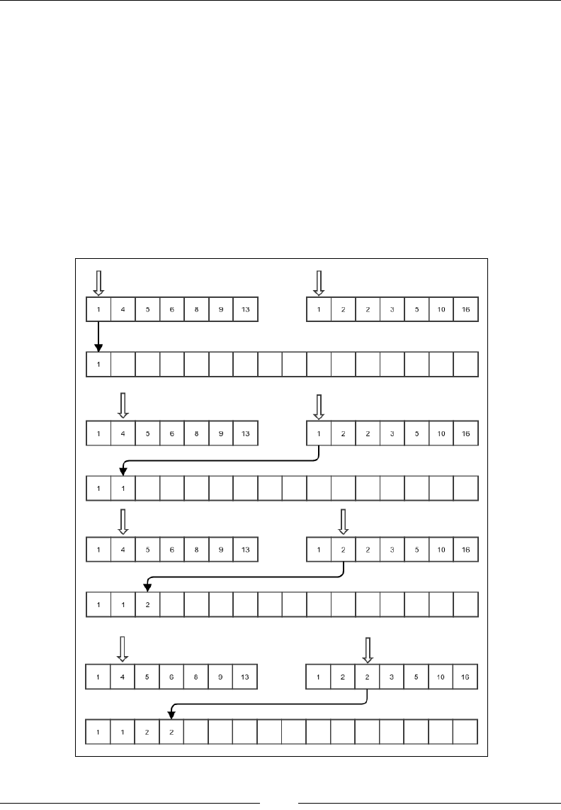
Chapter 6
[ 123 ]
mergesort
In the previous section, we tried to divide the array in such a way that when we sort each
part, the entire array is sorted. We faced the problem that when we try to do that, the two
parts are not equal in size causing the algorithm to sometimes take a quadratic amount of
time. What if, instead of trying to divide the array in a way that sorting the parts would
sort the whole, we just divide the array into two equal halves? Of course then, sorting the
parts will not sort the entire array. However, if we have two array parts sorted on their
own, can we merge them together to produce a sorted array as a whole? If we can do this
efciently enough, we would have an algorithm guaranteed to be efcient. As it turns
out, it is possible. But we need to think about where the merged array will be stored.
Since the values are being copied from the source array, the result needs to be stored in a
separate place. So, we will need another storage of equal size for mergesort.
.
Merge of sorted arrays

Efcient Sorting – quicksort and mergesort
[ 124 ]
The preceding gure shows a part of the merging operation. We keep the current
position of each of the arrays. In each step, we compare the values in the current
positions in both the input sorted arrays.
We copy whichever of them is smaller to the target location and increment the
corresponding current position. We keep doing this until we nish one of the arrays,
after which the elements of the other array can just be copied over. The following
shows the code for the merge operation. One thing to note is that, since the merge
will be used for a mergesort, it presumes both the input arrays to be the same array
with different indexes and the target arrays to have the same size. The source has
three indexes: start, mid, and end. It is assumed that the source parts are residing
side by side in the source array. The variable start points to the start of the rst
part. The integer mid stores the index of the start of the second part and also acts as
the end of the rst part, as the parts are contiguous. Finally, the end variable stores
the end of the second array:
private static <E> void merge(E[] array, int start, int mid,
int end, E[] targetArray, Comparator<E> comparator) {
int i = start;
int j = mid;
int k = start;
while (k < end) {
The rst two cases are for the time when one of the source arrays has been
exhausted:
if (i == mid) {
targetArray[k] = array[j];
j++;
} else if (j == end) {
targetArray[k] = array[i];
i++;
}
If none of the arrays are exhausted, copy from the correct array:
else if (comparator.compare(array[i], array[j]) > 0) {
targetArray[k] = array[j];
j++;
} else {
targetArray[k] = array[i];
i++;
}

Chapter 6
[ 125 ]
Finally, the target location must also be incremented:
k++;
}
}
With this merge function available to us, we can now proceed to do the mergesort. It
involves the following steps:
1. Divide the array into two equal parts.
2. Mergesort the parts.
3. Merge the sorted parts into a full sorted array.
Of course, we do not need to do anything for an array with zero or one element. So,
that will be our exit case:
public static <E> void mergeSort(E[] sourceArray, int start,
int end, E[] tempArray, Comparator<E> comparator) {
Just return to the calling function for an array of zero or one element. This is our
base case:
if (start >= end - 1) {
return;
}
For any array of size bigger than 1, divide the array into two halves–start to mid
and mid to end. Then merge-sort them separately, and then merge the two sorted
subarrays to a combined sorted array in tempArray, which is an auxiliary space that
we are using:
int mid = (start + end) / 2;
mergeSort(sourceArray, start, mid, tempArray, comparator);
mergeSort(sourceArray, mid, end, tempArray, comparator);
merge(sourceArray, start, mid, end, tempArray, comparator);

Efcient Sorting – quicksort and mergesort
[ 126 ]
Finally, copy the contents of tempArray to sourceArray so that the source is
now sorted:
System.arraycopy(tempArray, start, sourceArray, start,
end - start);
}
The complexity of mergesort
Let's start from the complexity of the merge operation. The merge operation is
not recursive. In every step, it increments either i or j. When both these variables
reach the end of the respective arrays, the merge ends. The comparison happens at
most once per any of these increments. This means that there are at most as many
comparisons as there are elements in both the sub-arrays combined. The copying
of the contents of tempArray to sourceArray also, of course, takes operations
proportional to the number of elements in tempArray, which is the same as the
number of elements in the sourceArray. So, the number of operations in each step
is proportional to n, apart from the recursive call. The recursive call works on both
parts of the array, which are themselves half the size of the entire array. Thus, if T(n)
is the time taken, we have the following:
T(n) = 2T(n/2) + an + b
Here, a and b are constants.
This is the same equation as the one obtained for the typical case of the quicksort
algorithm, and we know that the solution gives us T(n) = θ(n lg n). This is the
estimate for the both the average case and the worst case because, in both cases, the
array will always be divided into two equal halves irrespective of the contents of
the array. In fact, the worst case is when all the copying also requires a comparison,
which is the case we considered.
In the best case, one of the arrays will have all its elements copied before even
the rst element of the second array is copied, thus requiring only half as many
comparisons. But this case gives the same complexity of T(n) = θ(n lg n). So,
irrespective of the actual contents of the array we started with, mergesort will always
have the same asymptotic complexity.

Chapter 6
[ 127 ]
Avoiding the copying of tempArray
In our rather simplistic example, we rst merged the subarrays into tempArray,
and then we copied it back to sourceArray. Can the copying be avoided? Can we
use tempArray itself as the result of the merge? It turns out that we can. In this case,
both sourceArray and tempArray would be used rather symmetrically, the only
difference being that sourceArray holds the original input array. Otherwise, they
are two pre-allocated arrays of the same size. However, the code will get a little
more complicated.
Let us rst consider what would happen if we do not copy the contents of tempArray
to sourceArray and try to use tempArray itself as the content of the sorted array.
Then, in each step, sourceArray and tempArray would need to be swapped, that is,
tempArray would become sourceArray and vice versa. Since in each step, tempArray
and sourceArray are getting swapped, the actual array that holds the result depends
on whether the number of steps required to sort the array is odd or even.
Now, if the array we started with had a number of elements equal to an exact
integral power of 2, the source array could always be divided into two sub-arrays of
the exact same size. This means, the number of steps required to sort each of these
sub-arrays would be exactly the same. This means that the actual array that holds the
sorted result would be the same after sorting either sub-array. However, in reality,
the number of elements in the array is not an exact power of 2 most of the time,
and hence, one sub-array is a little bigger than the other. This results in a different
number of steps being required to sort either sub-array, causing them to potentially
store the resultant sorted array in different arrays. We have to consider these cases
as well. So, when the result of sorting either sub-array is stored in the same array, we
store the output of the merge in the other array. If not, we always store the output of
the merge in the array that holds the result of sorting the second part of the array.
First, we change the merge function to handle two different arrays holding the
contents of two different inputs:
private static <E> void merge(E[] arrayL, E[] arrayR,
int start, int mid, int end, E[] targetArray,
Comparator<E> comparator) {
int i = start;
int j = mid;
int k = start;
while (k < end) {
if (i == mid) {
targetArray[k] = arrayR[j];

Efcient Sorting – quicksort and mergesort
[ 128 ]
j++;
} else if (j == end) {
targetArray[k] = arrayL[i];
i++;
} else if (comparator.compare(arrayL[i], arrayR[j]) > 0) {
targetArray[k] = arrayR[j];
j++;
} else {
targetArray[k] = arrayL[i];
i++;
}
k++;
}
}
With this merge function available, we write our efcient mergesort in the following
way. Note that we need some way to inform the calling function about which pre-
allocated array contains the result, so we return that array:
public static <E> E[] mergeSortNoCopy(E[] sourceArray, int start,
int end, E[] tempArray, Comparator<E> comparator) {
if (start >= end - 1) {
return sourceArray;
}
First, split and merge-sort the sub-arrays as usual:
int mid = (start + end) / 2;
E[] sortedPart1 =
mergeSortNoCopy(sourceArray, start, mid, tempArray,
comparator);
E[] sortedPart2 =
mergeSortNoCopy(sourceArray, mid, end, tempArray,
comparator);
If both the sorted sub-arrays are stored in the same pre-allocated array, use the other
pre-allocated array to store the result of the merge:
if (sortedPart2 == sortedPart1) {
if (sortedPart1 == sourceArray) {
merge(sortedPart1, sortedPart2, start, mid, end,
tempArray, comparator);

Chapter 6
[ 129 ]
return tempArray;
} else {
merge(sortedPart1, sortedPart2, start, mid, end,
sourceArray, comparator);
return sourceArray;
}
} else {
In this case, we store the result in sortedPart2 because it has the rst portion empty:
merge(sortedPart1, sortedPart2, start, mid, end,
sortedPart2, comparator);
return sortedPart2;
}
}
Now we can use this mergesort as follows:
Integer[] anotherArray = new Integer[array.length];
array = mergeSortNoCopy(array, 0, array.length, anotherArray,
(a, b)->a-b);
System.out.println(Arrays.toString(array));
Here is the output:
[1, 1, 1, 2, 2, 3, 3, 4, 5, 10, 24, 30, 33, 35, 35, 53, 67, 78]
Note that this time, we had to ensure that we use the output returned by the method
as, in some cases, anotherArray may contain the nal sorted values. The efcient
no-copy version of the mergesort does not have any asymptotic performance
improvement, but it improves the time by a constant. This is something worth doing.
Complexity of any comparison-based
sorting
Now that we have seen two algorithms for sorting that are more efcient than the
ones described in the previous chapter, how do we know that they are as efcient
as a sorting can be? Can we make algorithms that are even faster? We will see in
this section that we have reached our asymptotic limit of efciency, that is, a
comparison-based sorting will have a minimum time complexity of θ(m lg m),
where m is the number of elements.

Efcient Sorting – quicksort and mergesort
[ 130 ]
Suppose we start with an array of m elements. For the time being, let's assume they
are all distinct. After all, if such an array is a possible input, we need to consider this
case as well. The number of different arrangements possible with these elements
is m!. One of these arrangements is the correct sorted one. Any algorithm that will
sort this array using comparison will have to be able to distinguish this particular
arrangement from all others using only comparison between pairs of elements. Any
comparison divides the arrangements into two sets–one that causes an inversion as
per the comparison between those two exact values and one that does not. This is
to say that given any two values a and b from the arrays, a comparison that returns
a<b will divide the set of arrangements into two partitions; the rst set will contain
all the arrangements where b comes before a, and the second set will contain all
the arrangements where a comes before b. The sorted arrangement is, of course, a
member of the second set. Any algorithm that sorts based on comparisons will have
to do enough of them to pin down on the single correct arrangement, that is, the
sorted arrangement. Basically, it will rst perform a comparison, choose the correct
subset, then perform another comparison and choose the correct subset of the subset,
and so on, until it reaches a set of arrangements containing just one arrangement.
This particular arrangement is the sorted version of the array. What is the minimum
number of comparisons that are required to nd one particular arrangement out
of m! arrangements? This is the same as asking how many times you have to halve
a set of m! elements to reach a set of only one element. It is, of course, lg (m!). This
is a rough estimation; in fact, the number of comparisons required would be a bit
more than this because the two subsets that each comparison creates may not be
equal in size. But we know that the number of comparisons required is lg (m!) at
the minimum.
Now, how much is lg m!? Well, it is (ln (m!)) (lg e), where ln (x) is the natural
logarithm of x. We will nd a simpler asymptotic complexity for the function ln(m!).
It requires a little bit of calculus.
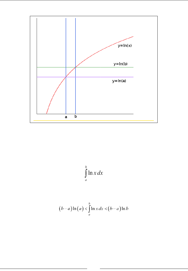
Chapter 6
[ 131 ]
Let's look at the following gure:
Area under the curve y = ln x.
The diagram shows some plots. We know that the integral measures the area under
the curve of a function. Now, the area under the curve y=ln b between a and b is (b-a)
ln b, and the area under the curve y=ln a is (b-a) ln a. The area under the curve y=lg x
in the same interval is as follows:
From the graph in the preceding gure, the following is clear:
Efcient Sorting – quicksort and mergesort
[ 132 ]
In particular, having b=a+1, we get the following:
So, we set a = 1 and move up to a = m-1, to get the following set of inequalities:
Adding respective sides, we get the following:
Now, of course we know the following:
So, we have the following inequalities:
Chapter 6
[ 133 ]
In the left inequality, if we put m instead of m-1, we will have the following:
This, combined with the right inequality, gives the following relations:
This gives a pretty good upper bound and lower bound on the value of ln(m!). Both
the upper bound and lower bound are θ(m ln m). So, we can conclude that ln(m!) =
θ(m ln m). This means that lg(m!) = (ln (m!))(lg e) is also θ(m ln m) = θ(m lg m) because
lg(m) = (ln m )(lg e).
So, the minimum time complexity of a comparison-based sorting algorithm would
have to be at least θ(m lg m) just because of the minimum number of comparisons
that would be needed to do this. Therefore, mergesort and the typical case of
quicksort are asymptotically optimal.
The stability of a sorting algorithm
The stability of a sorting algorithm is the property that the elements that compare
to be equal preserve their original order after sorting. For example, if we have an
array of objects containing the ID number and the age of some people and we want
to sort them in increasing order of age, a stable sorting algorithm will preserve the
original order of the people with the same age. This can be helpful if we are trying
to sort multiple times. For example, if we want the IDs to be in increasing order for
people with the same age, we can rst sort the array by ID and then sort it again
by age. If the sorting algorithm is stable, it will ensure that the nal sorted array is
in increasing order of age, and for the same age, it is in increasing order of ID. Of
course, this effect can also be achieved by having a more complex comparison with
a single sorting operation. Quicksort is not stable, but mergesort is. It is easy to see
why mergesort is stable. During merging, we preserve the order, that is, values from
the left half precede values from the right half when they compare as equal.

Efcient Sorting – quicksort and mergesort
[ 134 ]
Summary
In this chapter, we explored two efcient sorting algorithms. The basic principle, in
both cases, was to divide the array and to sort the parts separately. If we ensure that
sorting the parts will cause the entire array to be sorted by readjusting the elements,
it is quicksort. If we just divide the array into two equal parts rst and–after sorting
each part–merge the results to cause the entire array to be sorted, it is a mergesort.
This way of dividing the input into smaller parts, solving the problem for the smaller
parts and then combining the results to nd the solution for the entire problem is a
common pattern in solving computational problems, and it is called the divide and
conquer pattern.
We have also seen an asymptotic lower bound for any sorting algorithm that works
using comparisons. Both quicksort and mergesort achieve this lower bound and
hence, are asymptotically optimal. In the next chapter, we will move to a different
kind of data structures called trees.

[ 135 ]
Concepts of Tree
We have already seen data structures such as linked list and array. They represent
data stored in a linear fashion. In this chapter, we will discuss a new kind of data
structure, called a tree. A tree is a generalization of a linked list. While a linked list
node has one reference to the next node, a tree node has references to possibly more
than one next node. These next nodes are called children of the node, and the node
holding the references to the children is called a parent node. In this chapter, we will
explore the following topics:
• Concept of a tree as a data structure
• Concept of a tree as an ADT
• Binary trees
• Different kinds of tree traversals
• Tree search algorithms
So, let's jump into it right away.
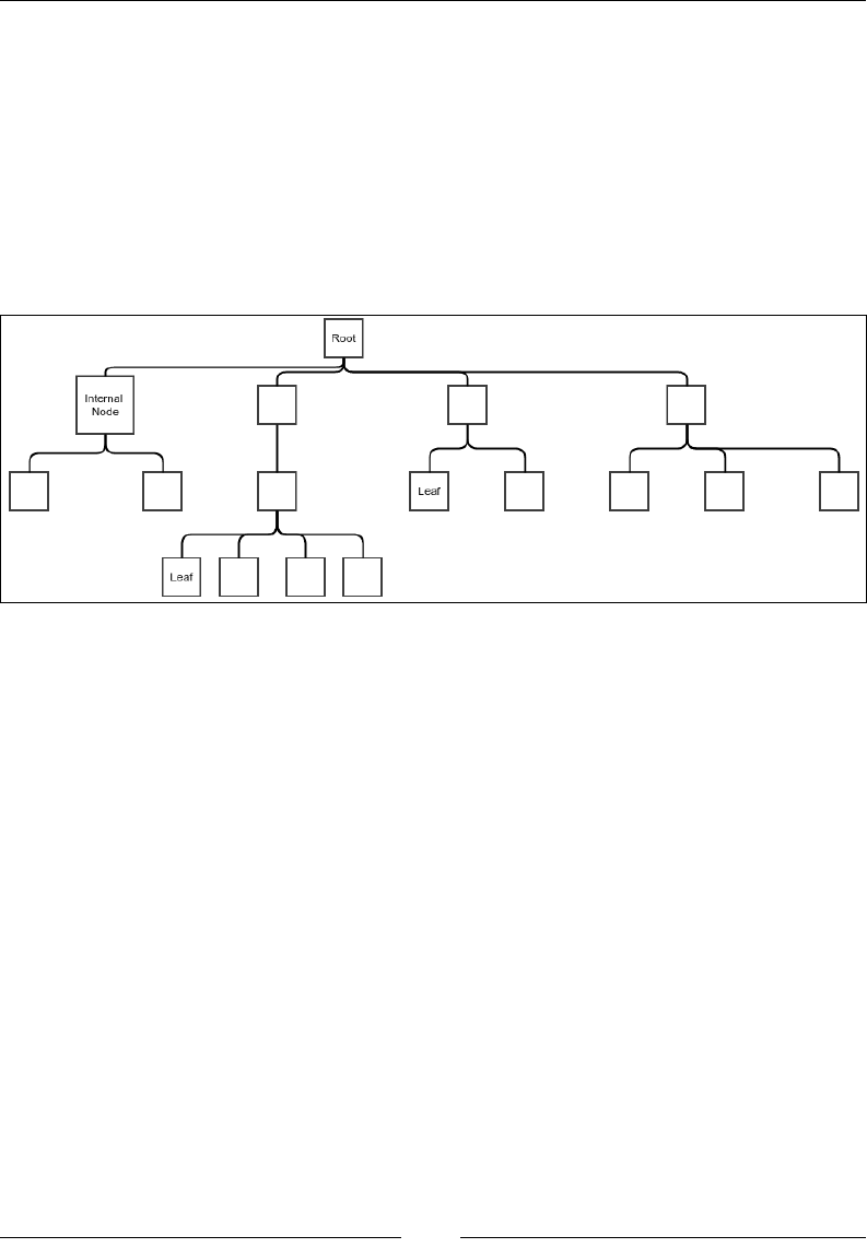
Concepts of Tree
[ 136 ]
A tree data structure
A tree data structure looks very much like a real tree, the kind you can see in a
garden or by the roadside. If we look at a tree, we will see that it has a root that
makes the stem outside of the ground. The stem splits into branches, and at the end
of the branches, we nd leaves. In our tree data structure, we start from the root.
The root is the node that does not have any parent. The children can be thought of
as being attached to the stem by lines just like the branches of a real tree. At the end,
we nd some nodes that have no children and hence are called leaves. The following
gure shows an example of a tree:
An example tree
Note that the tree is drawn upside down. The root is at the top and the leaves
are below. This is just a convention that most people prefer. Think of this as the
reection of a tree on water.
A tree can be represented in many ways, but we will get started with the idea of
generalization of a linked list. In the case of a linked list, a node stores a single
reference that points to the next node. In a tree, a node needs to store the references
to all its children. Multiple children could be stored in an array, but since we have
access to our own class LinkedList, we will use that. We will use our non-functional
version of the linked list because our rst tree will be non-functional and will
allow modication.
We start with the following class:
public class Tree<E> {
public static class Node<E>{
private E value;
private LinkedList<Node<E>> children;
private Tree<E> hostTree;
private Node<E> parent;

Chapter 7
[ 137 ]
public LinkedList<Node<E>> getChildren() {
return children;
}
public E getValue() {
return value;
}
private Node(LinkedList<Node<E>> children, Tree<E> hostTree,
E value, Node<E> parent) {
this.children = children;
this.hostTree = hostTree;
this.value = value;
this.parent = parent;
}
}
...
}
We have dened our Node class as an inner class. Apart from remembering the value
it stores inside and the list of children, it also stores the parent and the tree that it is
a member of. Once we create an instance of a tree, we must be able to store a node
in it. The node that does not have a parent is called the root of the tree. So, we add
an addRoot method to add a root to the tree. The tree, itself, only has to store the
reference of the root node as all the other nodes can be reached from this node by
traversing the references:
private Node<E> root;
public void addRoot(E value){
if(root == null){
root = new Node<>(new LinkedList<>(), this, value, null );
}else{
throw new IllegalStateException(
"Trying to add new node to a non empty tree");
}
}
Note that we test whether the tree already has a root node, in which case, we throw
an exception.

Concepts of Tree
[ 138 ]
Okay, now that we have a way of adding a root node, we need to have a method for
adding nodes as we like. The method takes a parent node and a value in order to add
a new node. This method will return the newly added node so that we keep adding
more nodes as its children:
public Node<E> addNode(Node<E> parent, E value){
if(parent==null){
throw new NullPointerException("Cannot add child
to null parent");
}else if(parent.hostTree != this){
throw new IllegalArgumentException(
"Parent node not a part of this tree");
}else{
Node<E> newNode = new Node<>(new LinkedList<>(),
this, value, parent);
parent.getChildren().appendLast(newNode);
return newNode;
}
}
In the preceding code, we rst check whether the parent is null or whether the
parent is the node of a different tree instance. In either case, an exception must be
thrown. Otherwise, we just add a new node as the child of the parent node passed
as an argument.
But wait a second! How would we ever be able to pass a parent node if we do not
have a reference to the root node in the calling code? So, we add a method, getRoot,
to access the root node of the Tree:
public Node<E> getRoot() {
return root;
}
Okay, now let's create a Tree instance:
public static void main(String [] args){
Tree<Integer> tree = new Tree<>();
tree.addRoot(1);
Node<Integer> node1 = tree.getRoot();
Node<Integer> node2 = tree.addNode(node1, 5);
Node<Integer> node3 = tree.addNode(node1, 1);
Node<Integer> node4 = tree.addNode(node2, 2);
Node<Integer> node5 = tree.addNode(node2, 5);
Node<Integer> node6 = tree.addNode(node2, 9);
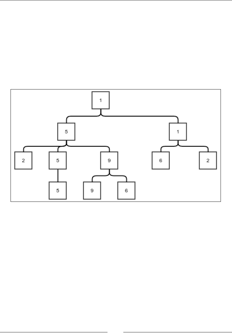
Chapter 7
[ 139 ]
Node<Integer> node7 = tree.addNode(node3, 6);
Node<Integer> node8 = tree.addNode(node3, 2);
Node<Integer> node9 = tree.addNode(node5, 5);
Node<Integer> node10 = tree.addNode(node6, 9);
Node<Integer> node11 = tree.addNode(node6, 6);
}
The code is self-explanatory. We just create a tree by adding the nodes one by
one. But how do we see what the tree looks like? For that, we will have to learn
about the traversal of a tree. The preceding code will create the tree shown in the
following gure:
Example tree
The traversal of a tree
Tree traversal is an algorithm to visit or to process all nodes of a tree exactly once.
This obviously involves recursively looking into the children of the nodes. The order
in which the children are processed depends on the particular algorithm we use. The
simplest algorithm for traversing a tree is the depth-rst traversal.
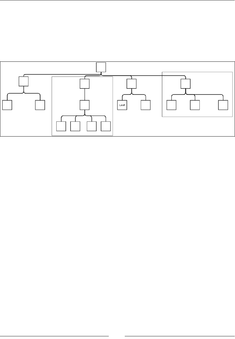
Concepts of Tree
[ 140 ]
The depth-rst traversal
In the depth-rst traversal, we process every child of a node recursively and wait for
it to nish with all its descendants before proceeding to the next child. To understand
the depth-rst search, we have to understand what a subtree is. A subtree is a node
with all its descendants up to the leaves. The following gure shows some examples
of subtrees.
Examplesubtrees
Now, if you think about it, each node not only stores references to the children,
but also sort of holds references to entire subtrees rooted at the child nodes. So, the
depth-rst traversal algorithm is nothing but the following steps:
1. Process the value in the current node.
2. For each child node of the current node, recursively traverse the entire
subtree rooted at the child node.
The following method does exactly this:
protected void traverseDepthFirst(OneArgumentStatement<E> processor,
Node<E> current){
processor.doSomething(current.value);
current.children.forEach((n)-> traverseDepthFirst(processor, n));
}
The method takes a lambda and a node to traverse. All this method does is rst
run the lambda on the current value and then call itself recursively on each of the
subtrees. Now, we can write a wrapper method without the parent node argument:
public void traverseDepthFirst(OneArgumentStatement<E> processor){
traverseDepthFirst(processor, getRoot());
}

Chapter 7
[ 141 ]
It is still not clear, though, why this way of traversing is called a depth-rst traversal.
If you think about the order in which the nodes are processed, you can see that since
the complete subtree root at any child node must be entirely processed before the
next child is processed, the depth of the tree will be covered before the breadth.
We have used a recursive function to do our depth-rst search. Alternatively, we can
use a stack to do the trick:
public void traverseDepthFirstUsingStack(
OneArgumentStatement<E> processor){
Stack<Node<E>> stack = new StackImplLinkedList<>();
stack.push(getRoot());
while(stack.peek()!=null){
Node<E> current = stack.pop();
processor.doSomething(current.value);
current.children.forEach((n)->stack.push(n));
}
}
Let's see what is happening in the preceding piece of code. We rst push the root
into the stack and go in a loop that continues until all the stack elements have been
cleared. Every time we pop a node, we process it and push all its children into
the stack. Now, since the stack is last in rst out (LIFO), all these children will
be popped and processed before any other node can be processed. However, the
moment the rst of these children is popped, its children will be pushed into the
stack and would be processed before anything else is processed. This will go on until
we hit the leaf nodes, which would not have any more children. This, in effect, is
almost the same as the recursive version.
There is a slight difference between the outputs of this code and the recursive
version, although both are indeed depth-rst. However, please note that in the case
of the recursive version, the child that is near the head of the linked list is processed
rst. In the case of the stack version, we push the children in the same order, but
since the stack is LIFO, we pop the children in the reverse order. To reverse this
order, we can store the list of children in the opposite order in a temporary list before
pushing them into the stack, as shown in the following code:
public void traverseDepthFirstUsingStack(
OneArgumentStatement<E> processor){
Stack<Node<E>> stack = new StackImplLinkedList<>();
stack.push(getRoot());
while(stack.peek()!=null){
Node<E> current = stack.pop();

Concepts of Tree
[ 142 ]
processor.doSomething(current.value);
LinkedList<Node<E>> reverseList = new LinkedList<>();
current.children.forEach((n)->reverseList.appendFirst(n));
reverseList.forEach((n)->stack.push(n));
}
}
The list is reversed by storing in a temporary list, called reverseList, by
appending the elements to its beginning. Then, the elements are pushed into
the stack from reverseList.
The breadth-rst traversal
Breadth-rst traversal is the opposite of the depth-rst traversal, in the sense that
depth-rst traversal processes children before siblings and breadth-rst traversal
processes the nodes of the same level before it processes any node of the succeeding
level. In other words, in a breadth-rst traversal, the nodes are processed level by
level. This is simply achieved by taking the stack version of the depth-rst traversal
and replacing the stack with a queue. That is all that is needed for it:
public void traverseBreadthFirst(OneArgumentStatement<E> processor){
Queue<Node<E>> queue = new QueueImplLinkedList<>();
queue.enqueue(getRoot());
while(queue.peek()!=null){
Node<E> current = queue.dequeue();
processor.doSomething(current.value);
current.children.forEach((n)->queue.enqueue(n));
}
}
Note that everything else remains exactly the same as that of the depth-rst traversal.
We still take one element from the queue, process its value and then enqueue
the children.
To understand why the use of a queue lets us process nodes level by level, we need
the following analysis:
• Root is pushed in the beginning, so root is dequeued first and processed.
• When the root is processed, the children of root, that is the nodes in level 1,
get enqueued. This means the level 1 nodes would be dequeued before any
further levels are dequeued.

Chapter 7
[ 143 ]
• When any node in level 1 is dequeued next, its children, which are the nodes
of level 2, will all get enqueued. However, since all the nodes in level 1 are
enqueued in the previous step, the nodes of level 2 will not be dequeued
before the nodes of level 1 are dequeued. When all the nodes of level 1 are
dequeued and processed, all the level 2 nodes would be enqueued because
they are all children of level 1 nodes.
• This means all the level 2 nodes would be dequeued and processed before
any nodes of higher levels are processed. When all the level 2 nodes are
already processed, all the level 3 nodes would be enqueued.
• In a similar manner, in all further levels, all the nodes in a particular level
will be processed before all the nodes of the next level are processed. In other
words, the nodes will be process level by level.
The tree abstract data type
Now that we have some idea of the tree, we can dene the tree ADT. A tree ADT can
be dened in multiple ways. We will check out two. In an imperative setting, that is,
when trees are mutable, we can dene a tree ADT as having the following operations:
• Get the root node
• Given a node, get its children
This is all that is required to have a model for a tree. We may also include some
appropriate mutation methods.
The recursive denition for the tree ADT can be as follows:
• A tree is an ordered pair containing the following:
°a value
°a list of other trees, which are meant to be it's subtrees
We can develop a tree implementation in exactly the same way as it is dened in the
functional tree ADT:
public class FunctionalTree<E> {
private E value;
private LinkedList<FunctionalTree<E>> children;

Concepts of Tree
[ 144 ]
As dened in the ADT, the tree is an ordered pair of a value and a list of other trees,
as follows:
public FunctionalTree(E value, LinkedList
<FunctionalTree<E>> children) {
this.children = children;
this.value = value;
}
public LinkedList<FunctionalTree<E>> getChildren() {
return children;
}
public E getValue() {
return value;
}
public void traverseDepthFirst(OneArgumentStatement<E> processor){
processor.doSomething(value);
children.forEach((n)-> n.traverseDepthFirst(processor));
}
}
The implementation is quite simple. The depth-rst traversal can be achieved
using recursive calls to the children, which are indeed subtrees. A tree without
any children needs to have an empty list of children. With this, we can create the
functional version of the same tree that we had created for an imperative version:
public static void main(String [] args){
LinkedList<FunctionalTree<Integer>> emptyList =
LinkedList.emptyList();
FunctionalTree<Integer> t1 = new FunctionalTree<>(5, emptyList);
FunctionalTree<Integer> t2 = new FunctionalTree<>(9, emptyList);
FunctionalTree<Integer> t3 = new FunctionalTree<>(6, emptyList);
FunctionalTree<Integer> t4 = new FunctionalTree<>(2, emptyList);
FunctionalTree<Integer> t5 = new FunctionalTree<>(5,
emptyList.add(t1));
FunctionalTree<Integer> t6 = new FunctionalTree<>(9,
emptyList.add(t3).add(t2));
FunctionalTree<Integer> t7 = new FunctionalTree<>(6, emptyList);
FunctionalTree<Integer> t8 = new FunctionalTree<>(2, emptyList);
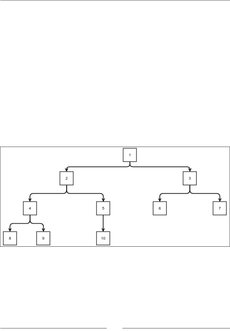
Chapter 7
[ 145 ]
FunctionalTree<Integer> t9 = new FunctionalTree<>(5,
emptyList.add(t6).add(t5).add(t4));
FunctionalTree<Integer> t10 = new FunctionalTree<>(1,
emptyList.add(t8).add(t7));
FunctionalTree<Integer> tree = new FunctionalTree<>(1,
emptyList.add(t10).add(t9));
At the end, we can do a depth-rst traversal to see if it outputs the same tree
as before:
tree.traverseDepthFirst(System.out::print);
}
Binary tree
A binary tree is a tree that has a maximum of two children per node. The two
children can be called the left and the right child of a node. The following gure
shows an example of a binary tree:
Example binary tree
This particular tree is important mostly because of its simplicity. We can create a
BinaryTree class by inheriting the general tree class. However, it will be difcult to
stop someone from adding more than two nodes and will take a lot of code just to
perform the checks. So, instead, we will create a BinaryTree class from scratch:
public class BinaryTree<E> {

Concepts of Tree
[ 146 ]
The Node has a very obvious implementation just like the generic tree:
public static class Node<E>{
private E value;
private Node<E> left;
private Node<E> right;
private Node<E> parent;
private BinaryTree<E> containerTree;
protected Node(Node<E> parent,
BinaryTree<E> containerTree, E value) {
this.value = value;
this.parent = parent;
this.containerTree = containerTree;
}
public E getValue(){
return value;
}
}
Adding the root is exactly the same as that for a generic tree, except for the fact
that we don't check for the existence of the root. This is just to save space; you can
implement as required:
private Node<E> root;
public void addRoot(E value){
root = new Node<>(null, this, value);
}
public Node<E> getRoot(){
return root;
}
The following method lets us add a child. It takes a Boolean parameter that is true
when the child to be added is the left child and false otherwise:
public Node<E> addChild(Node<E> parent, E value, boolean left){
if(parent == null){
throw new NullPointerException("Cannot add node to
null parent");
}else if(parent.containerTree != this){
throw new IllegalArgumentException
("Parent does not belong to this tree");
}else {

Chapter 7
[ 147 ]
Node<E> child = new Node<E>(parent, this, value);
if(left){
parent.left = child;
}else{
parent.right = child;
}
return child;
}
}
We now create two wrapper methods for specically adding either the left or the
right child:
public Node<E> addChildLeft(Node<E> parent, E value){
return addChild(parent, value, true);
}
public Node<E> addChildRight(Node<E> parent, E value){
return addChild(parent, value, false);
}
}
Of course, the traversal algorithms for a generic tree would also work for this
special case. However, for a binary tree, the depth-rst traversal can be of three
different types.
Types of depth-rst traversals
The depth-rst traversal of a binary tree can be of three types according to when the
parent node is processed with respect to when the child subtrees are processed. The
orders can be summarized as follows:
• Pre-order traversal:
1. Process the parent.
2. Process the left subtree.
3. Process the right subtree.
• In-order traversal:
1. Process the left subtree.
2. Process the parent.
3. Process the right subtree.

Concepts of Tree
[ 148 ]
• Post-order traversal:
1. Process the left subtree.
2. Process the right subtree.
3. Process the parent.
These different traversal types will produce a slightly different ordering when
traversing:
public static enum DepthFirstTraversalType{
PREORDER, INORDER, POSTORDER
}
public void traverseDepthFirst(OneArgumentStatement<E> processor,
Node<E> current, DepthFirstTraversalType tOrder)
{
if(current==null){
return;
}
if(tOrder == DepthFirstTraversalType.PREORDER){
processor.doSomething(current.value);
}
traverseDepthFirst(processor, current.left, tOrder);
if(tOrder == DepthFirstTraversalType.INORDER){
processor.doSomething(current.value);
}
traverseDepthFirst(processor, current.right, tOrder);
if(tOrder == DepthFirstTraversalType.POSTORDER){
processor.doSomething(current.value);
}
}
We have created an enum DepthFirstTraversalType to pass to the
traverseDepthFirst method. We process the current node according to its value.
Note that the only thing that changes is when the processor is called to process a node.
Let's create a binary tree and see how the results differ in the case of each ordering:
public static void main(String [] args){
BinaryTree<Integer> tree = new BinaryTree<>();
tree.addRoot(1);
Node<Integer> n1 = tree.getRoot();
Node<Integer> n2 = tree.addChild(n1, 2, true);
Node<Integer> n3 = tree.addChild(n1, 3, false);
Node<Integer> n4 = tree.addChild(n2, 4, true);
Node<Integer> n5 = tree.addChild(n2, 5, false);
Node<Integer> n6 = tree.addChild(n3, 6, true);
Node<Integer> n7 = tree.addChild(n3, 7, false);

Chapter 7
[ 149 ]
Node<Integer> n8 = tree.addChild(n4, 8, true);
Node<Integer> n9 = tree.addChild(n4, 9, false);
Node<Integer> n10 = tree.addChild(n5, 10, true);
tree.traverseDepthFirst(System.out::print, tree.getRoot(),
DepthFirstTraversalType.PREORDER);
System.out.println();
tree.traverseDepthFirst(System.out::print, tree.getRoot(),
DepthFirstTraversalType.INORDER);
System.out.println();
tree.traverseDepthFirst(System.out::print, tree.getRoot(),
DepthFirstTraversalType.POSTORDER);
System.out.println();
}
We have created the same binary tree as shown in the previous gure. The following
is the output of the program. Try to relate how the positions are getting affected:
1 2 4 8 9 5 10 3 6 7
8 4 9 2 10 5 1 6 3 7
8 9 4 10 5 2 6 7 3 1
You can take a note of the following points while matching the program output:
• In the case of a pre-order traversal, in any path starting from the root to any
leaf, a parent node will always be printed before any of the children.
• In the case of an in-order traversal, if we look at any path from the root to
a particular leaf, whenever we move from the parent to the left child, the
parent's processing is postponed. But whenever we move from the parent to
the right child, the parent is immediately processed.
• In the case of a post-order traversal, all the children are processed before any
parent is processed.
Non-recursive depth-rst search
The depth-rst search we have seen for the general tree is pre-order in the sense that
the parent node is processed before any of the children are processed. So, we can use
the same implementation for the pre-order traversal of a binary tree:
public void traversePreOrderNonRecursive(
OneArgumentStatement<E> processor) {
Stack<Node<E>> stack = new StackImplLinkedList<>();
stack.push(getRoot());
Concepts of Tree
[ 150 ]
while (stack.peek()!=null){
Node<E> current = stack.pop();
processor.doSomething(current.value);
if(current.right!=null)
stack.push(current.right);
if(current.left!=null)
stack.push(current.left);
}
}
We have to check whether the children are null. This is
because the absence of children is expressed as null references
instead of an empty list, as in the case of a generic tree.
Implementation of the in-order and post-order traversals is a bit tricky. We need to
suspend processing of the parent node even when the children are expanded and
pushed to the stack. We can achieve this by pushing each node twice. Once, we
push it when it is rst discovered due to its parent being expanded, and the next
time we do it when its own children are expanded. So, we must remember which of
these pushes caused it to be in the stack when it's popped. This is achieved using an
additional ag, which is then wrapped up in a class called StackFrame. The in-order
algorithm is as follows:
public void traverseInOrderNonRecursive(
OneArgumentStatement<E> processor) {
class StackFame{
Node<E> node;
boolean childrenPushed = false;
public StackFame(Node<E> node, boolean childrenPushed) {
this.node = node;
this.childrenPushed = childrenPushed;
}
}
Stack<StackFame> stack = new StackImplLinkedList<>();
stack.push(new StackFame(getRoot(), false));
while (stack.peek()!=null){
StackFame current = stack.pop();
if(current.childrenPushed){
processor.doSomething(current.node.value);
}else{
if(current.node.right!=null)
stack.push(new StackFame(current.node.right, false));
stack.push(new StackFame(current.node, true));

Chapter 7
[ 151 ]
if(current.node.left!=null)
stack.push(new StackFame(current.node.left, false));
}
}
}
Note that the stack is LIFO, so the thing that needs to be popped later must be
pushed earlier. The post-order version is extremely similar:
public void traversePostOrderNonRecursive(OneArgumentStatement<E>
processor) {
class StackFame{
Node<E> node;
boolean childrenPushed = false;
public StackFame(Node<E> node, boolean childrenPushed) {
this.node = node;
this.childrenPushed = childrenPushed;
}
}
Stack<StackFame> stack = new StackImplLinkedList<>();
stack.push(new StackFame(getRoot(), false));
while (stack.peek()!=null){
StackFame current = stack.pop();
if(current.childrenPushed){
processor.doSomething(current.node.value);
}else{
stack.push(new StackFame(current.node, true));
if(current.node.right!=null)
stack.push(new StackFame(current.node.right, false));
if(current.node.left!=null)
stack.push(new StackFame(current.node.left, false));
}
}
}
Note that the only thing that has changed is the order of pushing the children and
the parent. Now we write the following code to test these out:
public static void main(String [] args){
BinaryTree<Integer> tree = new BinaryTree<>();
tree.addRoot(1);
Node<Integer> n1 = tree.getRoot();
Node<Integer> n2 = tree.addChild(n1, 2, true);
Node<Integer> n3 = tree.addChild(n1, 3, false);

Concepts of Tree
[ 152 ]
Node<Integer> n4 = tree.addChild(n2, 4, true);
Node<Integer> n5 = tree.addChild(n2, 5, false);
Node<Integer> n6 = tree.addChild(n3, 6, true);
Node<Integer> n7 = tree.addChild(n3, 7, false);
Node<Integer> n8 = tree.addChild(n4, 8, true);
Node<Integer> n9 = tree.addChild(n4, 9, false);
Node<Integer> n10 = tree.addChild(n5, 10, true);
tree.traverseDepthFirst((x)->System.out.print(""+x),
tree.getRoot(), DepthFirstTraversalType.PREORDER);
System.out.println();
tree.traverseDepthFirst((x)->System.out.print(""+x),
tree.getRoot(), DepthFirstTraversalType.INORDER);
System.out.println();
tree.traverseDepthFirst((x)->System.out.print(""+x),
tree.getRoot(), DepthFirstTraversalType.POSTORDER);
System.out.println();
System.out.println();
tree.traversePreOrderNonRecursive((x)->System.out.print(""+x));
System.out.println();
tree.traverseInOrderNonRecursive((x)->System.out.print(""+x));
System.out.println();
tree.traversePostOrderNonRecursive((x)->System.out.print(""+x));
System.out.println();
}
We preserved the recursive versions as well so that we can compare the output,
which is as follows:
1 2 4 8 9 5 10 3 6 7
8 4 9 2 10 5 1 6 3 7
8 9 4 10 5 2 6 7 3 1
1 2 4 8 9 5 10 3 6 7
8 4 9 2 10 5 1 6 3 7
8 9 4 10 5 2 6 7 3 1
The rst three lines are the same as the last three, showing that they produce the
same result.

Chapter 7
[ 153 ]
Summary
In this chapter, you learned what a tree is. We started out with an actual
implementation and then designed an ADT out of it. You also learned about a binary
tree, which is just a tree with a maximum of two children per node. We also saw
different traversal algorithms for a generic tree. They are depth-rst and breadth-rst
traversals. In the case of a binary tree, a depth-rst traversal can be done in three
different ways: pre-order, in-order, and post-order. Even in the case of a generic tree,
we can nd equivalents of the pre-order and post-order traversals for a depth-rst
traversal. However, it is difcult to point to any particular equivalent of an in-order
traversal as it is possible to have more than two children.
In the next chapter, we will see the use of a binary tree in searching, and we will see
some other ways of searching as well.

[ 155 ]
More About Search – Search
Trees and Hash Tables
In the previous chapters, we had a look at both binary search and trees. In this
chapter, we will see how they are related and how this helps us create some more
exible, searchable data structures. We will also look at a different kind of searchable
structure called a hash table. The reason for using these structures is that they allow
mutation and still remain searchable. Basically, we need to be able to insert and
delete elements from the data structures with ease while still being able to conduct
a search efciently. These structures are relatively complicated, so we need to take a
step-by-step approach toward understanding it.
We'll cover the following topics in this chapter:
• Binary search trees
• Balanced binary search trees
• Hash tables
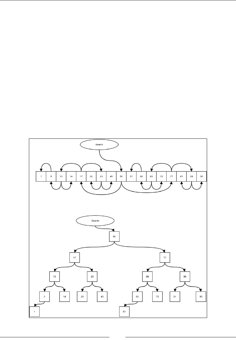
More About Search – Search Trees and Hash Tables
[ 156 ]
Binary search tree
You already know what binary search is. Let's go back to the sorted array from an
earlier chapter and study it again. If you think about binary search, you know you
need to start from the middle of the sorted array. Depending on the value to be
searched, either we return if the middle element is the search item, or move to the
left or right based on whether the search value is greater than or less than the middle
value. After this, we continue the same process recursively. This means the landing
points in each step are quite xed; they are the middle values. We can draw all the
search paths as in the next gure. In each step, the arrows connect to the mid points
of both the right half and left half, considering the current position. In the bottom
part, we disassemble the array and spread out the elements while keeping the
sources and targets of the arrows similar. As one can see, this gives us a binary tree.
Since each edge in this tree moves from the midpoint of one step to the midpoint of
the next step in the binary search, the same search can be performed in the tree by
simply following its edges. This tree is quite appropriately called a binary search
tree. Each level of this tree represents a step in binary search:
Binary search tree

Chapter 8
[ 157 ]
Say we want to search for item number 23. We start from the original midpoint,
which is the root of the tree. The root has the value 50. 23 is less than 50, so we must
check the left-hand side; in the case of our tree, follow the left edge. We arrive at the
value 17. 23 is greater than 17, so we must follow the right edge and arrive at the
value 23. We just found the element we have been searching for. This algorithm can
be summarized as follows:
1. Start at the root.
2. If the current element is equal to the search element, we are done.
3. If the search element is less than the current element, we follow the left edge
and start again from 2.
4. If the search element is greater than the current element, we follow the right
edge and start again from 2.
To code this algorithm, we must rst create a binary search tree. Create a
BinarySearchTree class extending the BinaryTree class and then put your
algorithm inside it:
public class BinarySearchTree<E extends Comparable<E>> extends
BinaryTree<E> {
protected Node<E> searchValue(E value, Node<E> root){
if(root==null){
return null;
}
int comp = root.getValue().compareTo(value);
if(comp == 0){
return root;
}else if(comp>0){
return searchValue(value, root.getLeft());
}else{
return searchValue(value, root.getRight());
}
}
Now wrap the method so that you don't need to pass the root. This method also
checks whether the tree is an empty tree and fails the search if that is the case:
public Node<E> searchValue(E value){
if(getRoot()==null){
return null;
}else{

More About Search – Search Trees and Hash Tables
[ 158 ]
return searchValue(value, getRoot());
}
}
…
}
So what exactly is the point of modifying an array in a binary tree? After all, are we
not doing the same exact search still? Well, the point is that when we have this in a
tree form, we can easily insert new values in the tree or delete some values. In the
case of an array, insertion and deletion have linear time complexity and cannot go
beyond the preallocated array size.
Insertion in a binary search tree
Insertion in a binary search tree is done by rst searching for the value to be inserted.
This either nds the element or ends the search unsuccessfully, where the new value
is supposed to be if it were in that position. Once we reach this position, we can
simply add the element to the tree. In the following code, we rewrite the search
again because we need access to the parent node once we nd the empty spot to
insert our element:
protected Node<E> insertValue(E value, Node<E> node){
int comp = node.getValue().compareTo(value);
Node<E> child;
if(comp<=0){
child = node.getRight();
if(child==null){
return addChild(node,value,false);
}else{
return insertValue(value, child);
}
}else if(comp>0){
child = node.getLeft();
if(child==null){
return addChild(node,value,true);
}else{
return insertValue(value, child);
}
}else{
return null;
}
}
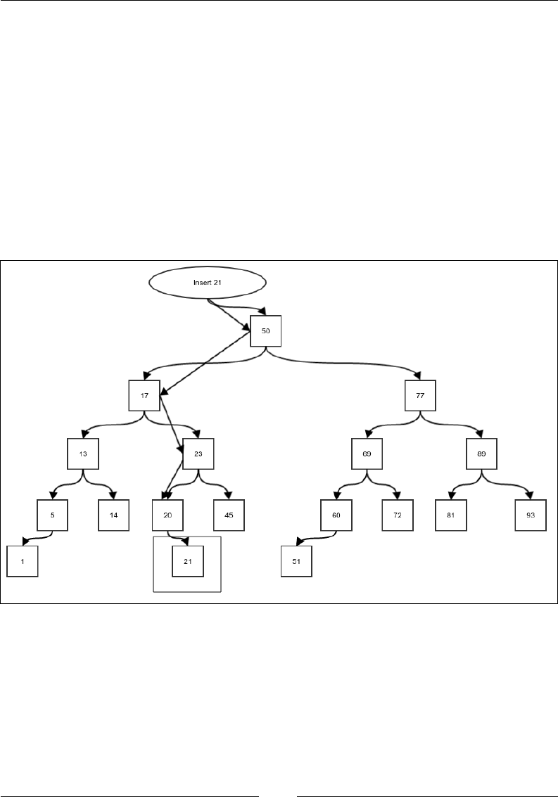
Chapter 8
[ 159 ]
We can wrap this up into a method that does not need a starting node. It also makes
sure that when we insert into an empty tree, we just add a root:
public Node<E> insertValue(E value){
if(getRoot()==null){
addRoot(value);
return getRoot();
}else{
return insertValue(value, getRoot());
}
}
Suppose in our earlier tree, we want to insert the value 21. The following gure
shows the search path using arrows and how the new value is inserted:
Insertion of a new value into a binary tree
Now that we have the means to insert elements in the tree, we can build the tree
simply by a successive insertion. The following code creates a random tree with 20
elements and then does an in-order traversal of it:
BinarySearchTree<Integer> tree = new BinarySearchTree<>();
for(int i=0;i<20;i++){
int value = (int) (100*Math.random());
More About Search – Search Trees and Hash Tables
[ 160 ]
tree.insertValue(value);
}
tree.traverseDepthFirst((x)->System.out.print(""+x),
tree.getRoot(), DepthFirstTraversalType.INORDER);
If you run the preceding code, you will always nd that the elements are sorted.
Why is this the case? We will see this in the next section.
What to do if the element inserted is the same as the element already present in the
search tree? It depends on that particular application. Generally, since we search by
value, we don't want duplicate copies of the same value. For simplicity, we will not
insert a value if it is already there.
Invariant of a binary search tree
An invariant is a property that stays the same irrespective of the modications
made in the structure it is related to. An in-order traversal of a binary search tree
will always result in the traversal of the elements in a sorted order. To understand
why this happens, let's consider another invariant of a binary tree: all descendants
of the left child of a node have a value less than or equal to the value of the node,
and all descendants of the right child of a node have a value greater than the value
of the node. It is understandable why this is true if you think about how we formed
the binary search tree using the binary search algorithm. This is why when we see
an element bigger than our search value, we always move to the left child. This is
because all the values that are descendants of the right child are bigger than the
left child so there is no point investing time in checking them. We will use this to
establish that an in-order traversal of a binary search tree will traverse elements in a
sorted order of the values in the nodes.
We will use induction to argue for this. Suppose we have a tree with only one node.
In this case, any traversal could be easily sorted. Now let's consider a tree with only
three elements, as shown in the following gure:
A binary search tree with three nodes
Chapter 8
[ 161 ]
An in-order traversal of this tree will rst process the left child, then the parent, and
nally, the right child. Since the search tree guarantees that the left child has a value
that is less than or equal to the parent and the right child has a value greater than or
equal to the value of the parent, the traversal is sorted.
Now let's consider our general case. Suppose this invariant we discussed is true for
trees with maximum h-levels. We will prove that, in such a case, it is also true for
trees with maximum h+1 levels. We will consider a general search tree, as shown in
the following gure:
A general binary search tree
The triangles represent subtrees with maximum n levels. We assume that the
invariant holds true for subtrees. Now, an in-order traversal would rst traverse
the left subtree in sorted order, then the parent, and nally, the right subtree in the
same order. The sorted order traversal of the subtrees is implied by the assumption
that the invariant holds true for these subtrees. This will result in the order [traversal
of left descendants in sorted order][traversal of parents][traversal of right descendants in
sorted order]. Since the left descendants are all less than or equal to the parent and
right descendants are all greater than or equal to the parent, the order mentioned is
actually a sorted order. So a tree of the maximum level h+1 can be drawn, as shown
in the preceding gure, with each sub-tree having n levels maximum. If this the case
and the invariant is true for all trees with level h, it must also be true for trees with
level h+1.
We already know that the invariant is true for trees with maximum level 1 and 2.
However, it must be true for trees with maximum level 3 as well. This implies it must
be true for trees with maximum level 4 and so on up to innity. This proves that the
invariant is true for all h and is universally true.
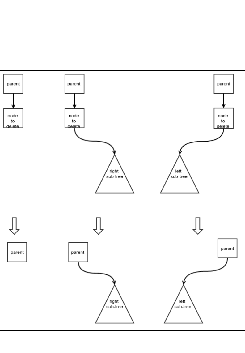
More About Search – Search Trees and Hash Tables
[ 162 ]
Deletion of an element from a binary search
tree
We are interested in all the modications of a binary search tree where the resultant
tree will remain a valid binary search tree. Other than insertion, we need to be able
to carry out deletion as well. That is to say, we need to be able to remove an existing
value from the tree:
Three simple cases of deletion of nodes

Chapter 8
[ 163 ]
The main concern is to know what to do with the children of the deleted node.
We don't want to lose those values from the tree, and we still want to make sure
the tree remains a search tree. There are four different cases we need to consider.
The relatively easier three cases are shown in the preceding gure. Here's a brief
description of these cases:
• The first case is where there is no child. This is the easiest case; we just delete
the node.
• The second case is where there is only a right subtree. In this case, the subtree
can take the place of the deleted node.
• The third case is very similar to the second case, except it is about the
left subtree.
The fourth case is, of course, when both the children are present for the node to be
deleted. In this case, none of the children can take the place of the node that is to be
deleted as the other one would also need to be attached somewhere. We resolve this
by replacing the node that needs to be deleted by another node that can be a valid
parent of both the children. This node is the least node of the right subtree. Why is
this the case? It is because if we delete this node from the right subtree, the remaining
nodes of the right subtree would be greater than or equal to this node. And this node
is also, of course, greater than all the nodes of the left subtree. This makes this node a
valid parent.
The next question is this: what is the least node in the right subtree? Remember that
when we move to the left child of a node, we always get a value that is less than or
equal to the current node. Hence, we must keep traversing left until we nd no more
left child. If we do this, we will reach the least node eventually. The least node of
any subtree cannot have any left child, so it can be deleted using the rst case or the
second case of deletion. The delete operation of the fourth case is thus used to:
• Copy the value of the least node in the right subtree to the node to be deleted
• Delete the least node in the right subtree
To write the deletion code, we need to rst add a few methods to our BinaryTree
class, which is meant for deleting nodes and rewriting node values. The method
deleteNodeWithSubtree simply deletes a node along with all its descendants. It
simply forgets about all the descendants. It also has certain checks to conrm the
validity of the input. Deletion of a root, as usual, must be handled separately:
public void deleteNodeWithSubtree(Node<E> node){
if(node == null){
throw new NullPointerException("Cannot delete to
null parent");
}else if(node.containerTree != this){

More About Search – Search Trees and Hash Tables
[ 164 ]
throw new IllegalArgumentException(
"Node does not belong to this tree");
}else {
if(node==getRoot()){
root=null;
return;
}else{
Node<E> partent = node.getParent();
if(partent.getLeft()==node){
partent.left = null;
}else{
partent.right = null;
}
}
}
}
Now we add another method to the BinaryTree class for rewriting the value in a
node. We don't allow this class to use public methods in the node class to maintain
encapsulation:
public void setValue(Node<E> node, E value){
if(node == null){
throw new NullPointerException("Cannot add node to
null parent");
}else if(node.containerTree != this){
throw new IllegalArgumentException(
"Parent does not belong to this tree");
}else {
node.value = value;
}
}
The preceding code is self-explanatory. Finally, we write a method to replace a
node's child with another node from the same tree. This is useful for cases 2 and 3:
public Node<E> setChild(Node<E> parent, Node<E> child,
boolean left){
if(parent == null){
throw new NullPointerException("Cannot set node
to null parent");
}else if(parent.containerTree != this){
throw new IllegalArgumentException(
"Parent does not belong to this tree");
}else {
if(left){

Chapter 8
[ 165 ]
parent.left = child;
}else{
parent.right = child;
}
if(child!=null) {
child.parent = parent;
}
return child;
}
}
Finally, we add a method to BinarySearchTree to nd the least node in the subtree.
We walk keeping to the left until there is no more child on the left-hand side:
protected Node<E> getLeftMost(Node<E> node){
if(node==null){
return null;
}else if(node.getLeft()==null){
return node;
}else{
return getLeftMost(node.getLeft());
}
}
Now we can implement our deletion algorithm. First, we create a deleteNode
method that deletes a node. We can then use this method to delete a value:
private Node<E> deleteNode(Node<E> nodeToBeDeleted) {
boolean direction;
if(nodeToBeDeleted.getParent()!=null
&& nodeToBeDeleted.getParent().getLeft()==nodeToBeDeleted){
direction = true;
}else{
direction = false;
}
Case 1: There are no children. In this case, we can simply delete the node:
if(nodeToBeDeleted.getLeft()==null &&
nodeToBeDeleted.getRight()==null){
deleteNodeWithSubtree(nodeToBeDeleted);
return nodeToBeDeleted;
}

More About Search – Search Trees and Hash Tables
[ 166 ]
Case 2: There is only a right child. The right child can take the place of the
deleted node:
else if(nodeToBeDeleted.getLeft()==null){
if(nodeToBeDeleted.getParent() == null){
root = nodeToBeDeleted.getRight();
}else {
setChild(nodeToBeDeleted.getParent(),
nodeToBeDeleted.getRight(), direction);
}
return nodeToBeDeleted;
}
Case 3: There is only a left child. The left child can take the place of the deleted node:
else if(nodeToBeDeleted.getRight()==null){
if(nodeToBeDeleted.getParent() == null){
root = nodeToBeDeleted.getLeft();
}else {
setChild(nodeToBeDeleted.getParent(),
nodeToBeDeleted.getLeft(), direction);
}
return nodeToBeDeleted;
}
Case 4: Both left child and right child are present. In this case, rst we copy the value
of the leftmost child in the right subtree (or the successor) to the node that needs to
be deleted. Once we do this, we delete the leftmost child in the right subtree:
else{
Node<E> nodeToBeReplaced = getLeftMost(
nodeToBeDeleted.getRight());
setValue(nodeToBeDeleted, nodeToBeReplaced.getValue());
deleteNode(nodeToBeReplaced);
return nodeToBeReplaced;
}
}
The process of deleting a node turned out to be a little more complicated, but it is
not difcult. In the next section, we will discuss the complexity of the operations of a
binary search tree.

Chapter 8
[ 167 ]
Complexity of the binary search tree
operations
The rst operation we will consider is the search operation. It starts at the root and
moves down one level every time we move from one node to either of its children.
The maximum number of edges we have to traverse during the search operation
must be equivalent to the maximum height of the tree—that is, the maximum
distance between any node and root. If the height of the tree is h, then the complexity
of search is O(h).
Now what is the relation between the number of nodes n of a tree and the height h
of a tree? It really depends on how the tree is built. Any level would require at least
one node in it, so in the worst case scenario, h = n and the search complexity is O(n).
What is our best case? Or rather, what do we want h to be in relation to n? In other
words, what is the minimum h, given a particular n. To answer this, we rst ask,
what is the maximum n we can t in a tree with height h?
The root is just a single element. The children of the root make a complete level
adding two more nodes for a tree of height 2. In the next level, we will have two
children for any node in this level. So the next level or level three has a total of 2X2=4
nodes. It can be easily seen that the level h of the tree has a total of 2(h-1) nodes. The
total number of nodes that a tree of height h can then have is as follows:
n = 1 + 2 + 4+ … + 2(h-1) = 2h – 1
=> 2h = (n+1)
=> h = lg (n+ 1)
This is our ideal case where the complexity of the search is O(lg n). This kind of a tree
where all the levels are full is called a balanced binary tree. Our aim is to maintain
the balanced nature of the tree even when insertion or deletion is carried out.
However, in general, the tree would not remain balanced in the case of an arbitrary
order of insertion of elements.
Insertion simply requires searching the element; once this is done, adding a new
node is just a constant time operation. Therefore, it has the same complexity as that
of a search. Deletion actually requires a maximum of two searches (in the fourth
case), so it also has the same complexity as that of a search.
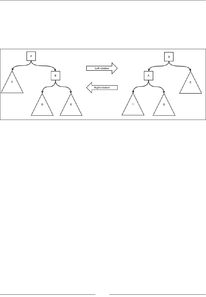
More About Search – Search Trees and Hash Tables
[ 168 ]
Self-balancing binary search tree
A binary search tree that remains balanced to some extent when insertion and
deletion is carried out is called a self-balancing binary search tree. To create a
balanced version of an unbalanced tree, we use a peculiar operation called rotation.
We will discuss rotation in the following section:
Rotation of a binary search tree
This gure shows the rotation operation on nodes A and B. Left rotation on A creates
the right image, and right rotation on B creates the left image. To visualize a rotation,
rst think about pulling out the subtree D. This subtree is somewhere in the middle.
Now the nodes are rotated in either the left or right direction. In the case of the left
rotation, the right child becomes the parent and the parent becomes the left child
of the original child. Once this rotation is done, the D subtree is added to the right
child's position of the original parent. The right rotation is exactly the same but in the
opposite direction.
How does it help balance a tree? Notice the left-hand side of the diagram. You'll
realize that the right side looks heavier, however, once you perform left rotation, the
left-hand side will appear heavier. Actually, a left rotation decreases the depth of the
right subtree by one and increases that of the left subtree by one. Even if, originally,
the right-hand side had a depth of 2 when compared to the left-hand side, you could
x it using left rotation. The only exception is the subtree D since the root of D
remains at the same level; its maximum depth does not change. A similar argument
will hold true for the right rotation as well.

Chapter 8
[ 169 ]
Rotation keeps the search-tree property of the tree unchanged. This is very important
if we are going to use it to balance search trees. Let's consider the left rotation. From
the positions, we can conclude the following inequalities:
• Each node in C ≤ A
• A ≤ B
• A ≤ Each node in D ≤ B
• B ≤ Each node in E
After we perform the rotation, we check the inequalities the same way and we nd
they are exactly the same. This proves the fact that rotation keeps the search-tree
property unchanged. A very similar argument can be made for the right rotation
as well. The idea of the algorithm of a rotation is simple: rst take the middle
subtree out, do the rotation, and reattach the middle subtree. The following is the
implementation in our BinaryTree class:
protected void rotate(Node<E> node, boolean left){
First, let's do some parameter value checks:
if(node == null){
throw new IllegalArgumentException("Cannot rotate
null node");
}else if(node.containerTree != this){
throw new IllegalArgumentException(
"Node does not belong to the current tree");
}
Node<E> child = null;
Node<E> grandchild = null;
Node<E> parent = node.getParent();
boolean parentDirection;
The child and grandchild we want to move depend on the direction of the rotation:
if(left){
child = node.getRight();
if(child!=null){
grandchild = child.getLeft();
}
}else{
child = node.getLeft();
if(child!=null){
grandchild = child.getRight();
}
}

More About Search – Search Trees and Hash Tables
[ 170 ]
The root node needs to be treated differently as usual:
if(node != getRoot()){
if(parent.getLeft()==node){
parentDirection = true;
}else{
parentDirection = false;
}
if(grandchild!=null)
deleteNodeWithSubtree(grandchild);
if(child!=null)
deleteNodeWithSubtree(child);
deleteNodeWithSubtree(node);
if(child!=null) {
setChild(parent, child, parentDirection);
setChild(child, node, left);
}
if(grandchild!=null)
setChild(node, grandchild, !left);
}else{
if(grandchild!=null)
deleteNodeWithSubtree(grandchild);
if(child!=null)
deleteNodeWithSubtree(child);
deleteNodeWithSubtree(node);
if(child!=null) {
root = child;
setChild(child, node, left);
}
if(grandchild!=null)
setChild(node, grandchild, !left);
root.parent = null;
}
}
We now can look at our rst self-balancing binary tree called the AVL tree.
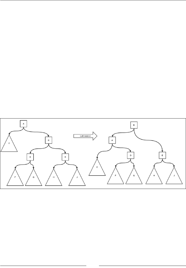
Chapter 8
[ 171 ]
AVL tree
AVL tree is our rst self-binary search tree. The idea is simple: keep every subtree
as balanced as possible. An ideal scenario would be for both the left and right
subtrees, starting from every node, to have exactly the same height. However,
since the number of nodes are not in the form of 2p-1, where p is a positive integer,
we cannot always achieve this. Instead, we allow a little bit of wiggle room. It's
important that the difference between the height of the left subtree and the right
subtree must not be greater than one. If, during any insert or delete operation, we
happen to break this condition, we will apply rotations to x this. We only have
to worry about a difference of two between the heights as we are only thinking of
insertion and deletion of one element at a time, and inserting one element or deleting
it cannot change the height by more than one. Therefore, our worst case is that there
was already a difference of one and the new addition or deletion created one more
difference requiring a rotation.
The simplest kind of rotation is shown in the following gure. The triangles
represent subtrees of equal heights. Notice that the height of the left subtree is two
less than the height of the right subtree:
AVL tree – simple rotation
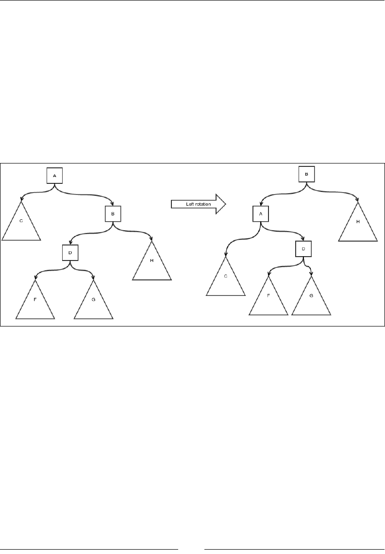
More About Search – Search Trees and Hash Tables
[ 172 ]
So we do a left rotation to generate the subtree of the structure, as shown in the
preceding diagram. You can see that the heights of the subtrees follow our condition.
The simple right rotation case is exactly the same, just in the opposite direction. We
must do this for all the ancestors of the node that were either inserted or deleted as
the heights of subtrees rooted by these nodes were the only ones affected by it. Since
rotations also cause heights to change, we must start from the bottom and walk our
way up to the root while doing rotations.
There is one more kind of case called a double rotation. Notice that the height of the
subtree rooted by the middle grandchild does not change due to the rotation. So, if
this is the reason for the imbalance, a simple rotation will not x it. It is shown in the
following gure:
Simple rotation does not fix this kind of imbalance
Here, the subtree that received an insertion is rooted by D or a node is deleted from
the subtree C. In the case of an insertion, notice that there would be no rotation on B
as the left subtree of B has a height of only one more than that of its right subtree. A is
however unbalanced. The height of the left subtree of A is two less than that of its right
subtree. However, if we do a rotation on A, as shown in the preceding gure, it does
not x the problem; only the left-heavy condition is transformed into a right-heavy
condition. To resolve this, we need a double rotation, as shown in the next gure.
First, we do an opposite direction rotation of the middle grandchild so that it is not
unbalanced in the opposite direction. A simple rotation after this will x the imbalance.
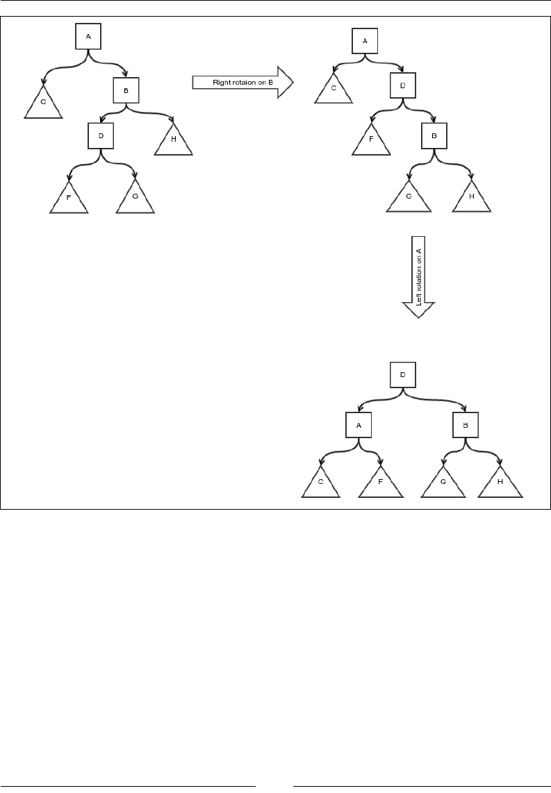
Chapter 8
[ 173 ]
AVL tree double rotation
So we create an AVL tree class, and we add an extra eld to the Node class to store
the height of the subtree rooted by it:
public class AVLTree<E extends Comparable<E>>
extends BinarySearchTree<E>{
public static class Node<E extends Comparable<E>>
extends BinaryTree.Node{
protected int height = 0;
public Node(BinaryTree.Node parent,
BinaryTree containerTree, E value) {
super(parent, containerTree, value);
}
}

More About Search – Search Trees and Hash Tables
[ 174 ]
We must override the newNode method to return our extended node:
@Override
protected BinaryTree.Node<E> newNode(
BinaryTree.Node<E> parent, BinaryTree<E> containerTree, E value) {
return new Node(parent, containerTree, value);
}
We use a utility method to retrieve the height of a subtree with a null check.
The height of a null subtree is zero:
private int nullSafeHeight(Node<E> node){
if(node==null){
return 0;
}else{
return node.height;
}
}
First, we include a method to compute and update the height of the subtree rooted
by a node. The height is one more than that of the maximum height of its children:
private void nullSafeComputeHeight(Node<E> node){
Node<E> left = (Node<E>) node.getLeft();
Node<E> right = (Node<E>) node.getRight();
int leftHeight = left==null? 0 : left.height;
int rightHeight = right==null? 0 :right.height;
node.height = Math.max(leftHeight, rightHeight)+1;
}
We also override the rotate method in BinaryTree to update the height of the
subtrees after the rotation:
@Override
protected void rotate(BinaryTree.Node<E> node, boolean left) {
Node<E> n = (Node<E>) node;
Node<E> child;
if(left){
child = (Node<E>) n.getRight();
}else{
child = (Node<E>) n.getLeft();
}
super.rotate(node, left);
if(node!=null){
nullSafeComputeHeight(n);
}
if(child!=null){
nullSafeComputeHeight(child);

Chapter 8
[ 175 ]
}
}
With the help of these methods, we implement the rebalancing of a node all the way
up to the root, as described in the preceding code. The rebalancing bit is done by
checking the difference in the height of the left and right subtrees. If the difference is
0, 1, or -1, nothing needs to be done. We simply move up the tree recursively. When
the height difference is 2 or -2, this is when we need to rebalance:
protected void rebalance(Node<E> node){
if(node==null){
return;
}
nullSafeComputeHeight(node);
int leftHeight = nullSafeHeight((Node<E>) node.getLeft());
int rightHeight = nullSafeHeight((Node<E>) node.getRight());
switch (leftHeight-rightHeight){
case -1:
case 0:
case 1:
rebalance((Node<E>) node.getParent());
break;
case 2:
int childLeftHeight = nullSafeHeight(
(Node<E>) node.getLeft().getLeft());
int childRightHeight = nullSafeHeight(
(Node<E>) node.getLeft().getRight());
if(childRightHeight > childLeftHeight){
rotate(node.getLeft(), true);
}
Node<E> oldParent = (Node<E>) node.getParent();
rotate(node, false);
rebalance(oldParent);
break;
case -2:
childLeftHeight = nullSafeHeight(
(Node<E>) node.getRight().getLeft());
childRightHeight = nullSafeHeight(
(Node<E>) node.getRight().getRight());
if(childLeftHeight > childRightHeight){
rotate(node.getRight(), false);
}
oldParent = (Node<E>) node.getParent();
rotate(node, true);
rebalance(oldParent);
break;
}
}

More About Search – Search Trees and Hash Tables
[ 176 ]
Once the rotation is implemented, implementing the insert and delete operations is
very simple. We rst do a regular insertion or deletion, followed by rebalancing. A
simple insertion operation is as follows:
@Override
public BinaryTree.Node<E> insertValue(E value) {
Node<E> node = (Node<E>) super.insertValue(value);
if(node!=null)
rebalance(node);
return node;
}
The delete operation is also very similar. It only requires an additional check
conrming that the node is actually found and deleted:
@Override
public BinaryTree.Node<E> deleteValue(E value) {
Node<E> node = (Node<E>) super.deleteValue(value);
if(node==null){
return null;
}
Node<E> parentNode = (Node<E>) node.getParent();
rebalance(parentNode);
return node;
}
Complexity of search, insert, and delete in an
AVL tree
The worst case of an AVL tree is when it has maximum imbalance. In other words,
the tree is worst when it reaches its maximum height for a given number of nodes.
To nd out how much that is, we need to ask the question differently, given a
height h: what is the minimum number of nodes (n) that can achieve this? Let the
minimum number of nodes required to achieve this be f(h). A tree of height h will
have two subtrees, and without any loss of generality, we can assume that the left
subtree is higher than the right subtree. We would like both these subtrees to also
have a minimum number of nodes. So the height of the left subtree would be f(h-1).
We want the height of the right subtree to be minimum, as this would not affect the
height of the entire tree. However, in an AVL tree, the difference between the heights
of two subtrees at the same level can differ by a maximum of one. The height of this
subtree is h-2. So the number of nodes in the right subtree is f(h-2). The entire tree
must also have a root, hence the total number of nodes:
f(h) = f(h-1) + f(h-2) + 1

Chapter 8
[ 177 ]
It almost looks like the formula of the Fibonacci sequence, except for the +1 part. Our
starting values are 1 and 2 because f(1) = 1 (only the root) and f(2) = 2 (just one child).
This is greater than the starting values of the Fibonacci sequence, which are 1 and
1. One thing is of course clear that the number of nodes would be greater than the
corresponding Fibonacci number. So, the following is the case:
f(h) ≥ Fh where Fh is the hth Fibonacci number.
We know that for a large enough h, Fh ≈ φFh-1 holds true; here φ is the golden
ratio (1 + √5)/2. This means Fh = C φ h, where C is some constant. So, we have
the following:
f(h) ≥ C φ h
=>n ≥ C φ h
=> log φn ≥ h + log φ C
=> h = O( log φn) = O(lg n)
This means even the worst height of an AVL tree is logarithmic, which is what
we wanted. Since an insertion processes one node in each level until it reaches the
insertion site, the complexity of an insertion is O(lg n); it is the same for performing
search and delete operations, and it holds true for the same reason.
Red-black tree
An AVL tree guarantees logarithmic insertion, deletion, and search. But it makes
a lot of rotations. In most applications, insertions are randomly ordered and so are
deletions. So, the trees would sort of balance out eventually. However, since the AVL
tree is too quick to rotate, it may make very frequent rotations in opposite directions
even when it would be unnecessary, had it been waiting for the future values to be
inserted. This can be avoided using a different approach: knowing when to rotate a
subtree. This approach is called a red-black tree.
In a red-black tree, the nodes have a color, either black or red. The colors can be
switched during the operations on the node, but they have to follow these conditions:
• The root has to be black
• A red node cannot have a black child
• The black height of any subtree rooted by any node is equal to the black
height of the subtree rooted by the sibling node
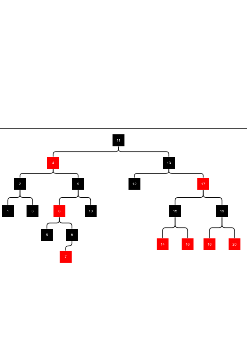
More About Search – Search Trees and Hash Tables
[ 178 ]
Now what is the black height of a subtree? It is the number of black nodes found
from the root to the leaf. When we say leaf, we really mean null children, which are
considered black and allow a parent to be red without violating rule 2. This is the
same no matter which path we take. This is because of the third condition. So the
third condition can also be restated as this: the number of black nodes in the path
from the root of any subtree to any of its leaves is the same, irrespective of which
leave we choose.
For ease of manipulation, the null children of the leaves are also considered sort of
half nodes; null children are always considered black and are the only ones really
considered as leaves as well. So leaves don't contain any value. But they are different
from the conventional leaves in other red-black trees. New nodes can be added to the
leaves but not in a red-black tree; this is because the leaves here are null nodes. So we
will not draw them out explicitly or put them in the code. They are only helpful to
compute and match black heights:
An example of a red-black tree
In our example of the red-black tree of height 4, the null nodes are black, which are
not shown (in print copy, the light-colored or gray nodes are red nodes and dark-
colored nodes are black nodes).
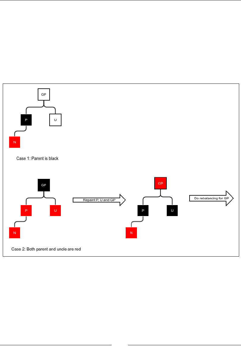
Chapter 8
[ 179 ]
Both insertion and deletion are more complicated than the AVL tree, as there are
more cases that we need to handle. We will discuss this in the following sections.
Insertion
Insertion is done in the same way we do it with BST. After an insertion is complete,
the new node is colored red. This preserves the black height, but it can result in a red
node being a child of another red node, which would violate condition 2. So we do
some manipulation to x this. The following two gures show four cases of insertions:
Case 1 and 2 of red-black tree insertion
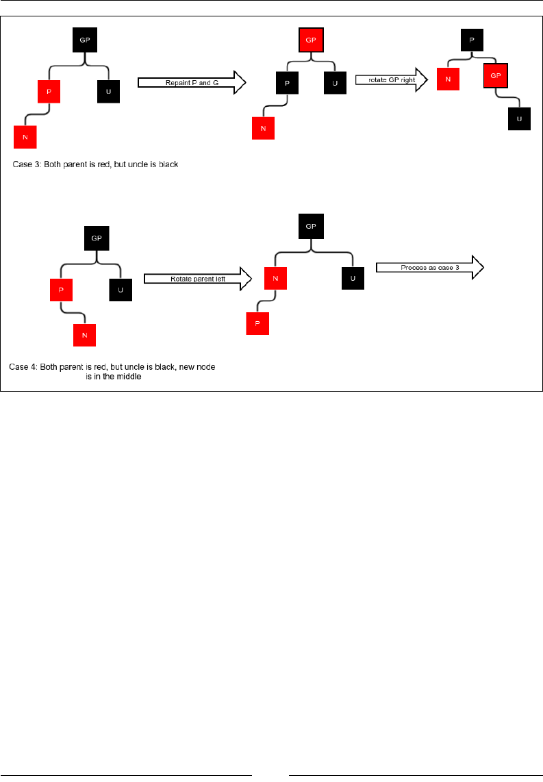
More About Search – Search Trees and Hash Tables
[ 180 ]
Case 3 and 4 of red-black tree insertion
Let's discuss the insertions case by case. Notice that the trees in the diagram look
black and unbalanced. But this is only because we have not drawn the entire tree;
it's just a part of the tree we are interested in. The important point is that the black
height of none of the nodes change because of whatever we do. If the black height
must be increased to t the new node, it must be at the top level; so we simply move
it up to the parent. The four cases are as follows:
1. The parent is black. In this case, nothing needs to be done as it does not
violate any of the constraints.
2. Both parent and uncle are red. In this case, we repaint parent, uncle, and
grandparent and the black heights are still unchanged. Notice now that no
constraints are violated. If, however, the grandparent is the root, keep it
black. This way, the entire tree's black height is increased by 1.
3. The parent is red and uncle is black. The newly added node is on the same
side of the parent as the parent is of the grandparent. In this case, we make
a rotation and repaint. We rst repaint the parent and grandparent and then
rotate the grandparent.

Chapter 8
[ 181 ]
4. This is the case that is similar to case 3, except the newly added node is on the
opposite side of the parent as the parent is of the grandparent. Case 3 cannot
be applied here because doing so will change the black height of the newly
added node. In this case, we rotate the parent to make it the same as case 3.
5. Note that all the cases can happen in the opposite direction, that is, in mirror
image. We will handle both the cases the same way.
Let's create our RedBlackTree class extending the BinarySearchTree class. We have
to again extend the Node class and include a ag to know whether the node is black:
public class RedBlackTree<E extends Comparable<E>> extends
BinarySearchTree<E>{
public static class Node<E> extends BinaryTree.Node<E>{
protected int blackHeight = 0;
protected boolean black = false;
public Node(BinaryTree.Node parent,
BinaryTree containerTree, E value) {
super(parent, containerTree, value);
}
}
@Override
protected BinaryTree.Node<E> newNode(
BinaryTree.Node<E> parent, BinaryTree<E> containerTree, E value) {
return new Node(parent, containerTree, value);
}
...
}
We now add a utility method that returns whether a node is black. As explained
earlier, a null node is considered black:
protected boolean nullSafeBlack(Node<E> node){
if(node == null){
return true;
}else{
return node.black;
}
}

More About Search – Search Trees and Hash Tables
[ 182 ]
Now we're ready to dene the method of rebalancing after we do an insertion.
This method works as described in the four cases earlier. We maintain a
nodeLeftGrandChild ag that stores whether the parent is the left child of the
grand parent or its right child. This helps us nd the uncle and also rotate in the
correct direction:
protected void rebalanceForInsert(Node<E> node){
if(node.getParent() == null){
node.black = true;
}else{
Node<E> parent = (Node<E>) node.getParent();
if(parent.black){
return;
}else{
Node<E> grandParent = (Node<E>) parent.getParent();
boolean nodeLeftGrandChild = grandParent
.getLeft()== parent;
Node<E> uncle = nodeLeftGrandChild?
(Node<E>) grandParent.getRight()
: (Node<E>) grandParent.getLeft();
if(!nullSafeBlack(uncle)){
if(grandParent!=root)
grandParent.black = false;
uncle.black = true;
parent.black = true;
rebalanceForInsert(grandParent);
}else{
boolean middleChild = nodeLeftGrandChild?
parent.getRight() == node:parent.getLeft()
== node;
if (middleChild){
rotate(parent, nodeLeftGrandChild);
node = parent;
parent = (Node<E>) node.getParent();
}
parent.black = true;
grandParent.black = false;
rotate(grandParent, !nodeLeftGrandChild);
}
}
}
}
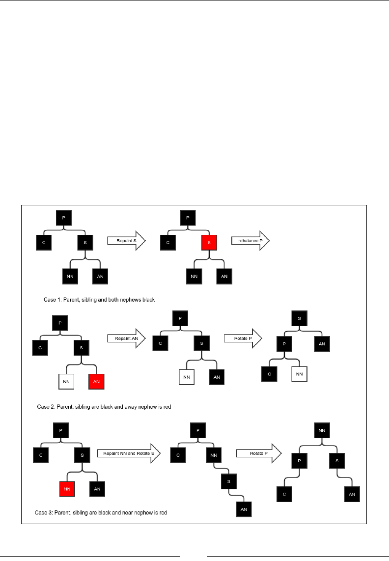
Chapter 8
[ 183 ]
The insertion is now done as follows:
@Override
public BinaryTree.Node<E> insertValue(E value) {
Node<E> node = (Node<E>) super.insertValue(value);
if(node!=null)
rebalanceForInsert(node);
return node;
}
Deletion
Deletion starts with a normal binary search tree deletion. If you remember, this
always involves deletion of a node with at most one child. Deletion of an internal
node is done by rst copying the value of the leftmost node of the right subtree and
deleting it. So we will consider only this case:
Case 1, 2, and 3 of deletion in a red-black tree

More About Search – Search Trees and Hash Tables
[ 184 ]
After the deletion is done, the parent of the deleted node either has no child or has
one child, which was originally its grandchild. During the insertion, the problem
we needed to solve was a red child of a red parent. In a deletion process, this cannot
happen. But it can cause the black height to change.
One simple case is that if we delete a red node, the black height does not change
anything, so we don't have to do anything. Another simple case is that if the deleted
node were black and the child red, we can simply repaint the child black in order to
restore the black height.
A black child cannot really happen because that would mean the original tree
was black and unbalanced, as the deleted node had a single black child. But since
recursion is involved, a black child can actually arise while moving up the path
with recursive rebalancing. In the following discussion, we only look at cases where
the deleted node was black and the child was also black (or null child, which is
considered black). Deletion is done as per the following cases, as shown in the
gures Case 1 and 2 and 3 of deletion in a red-black tree and Case 4, 5 and 6 of deletion from
a red-black tree:
1. The rst case we have is when the parent, sibling, and both the nephews
are black. In this case, we can simply repaint the sibling to red, which will
make the parent black and balanced. However, the black height of the
whole subtree will reduce by one; hence, we must continue rebalancing
from the parent.
2. This is the case when the parent and sibling are black, but the away nephew
is red. In this case, we cannot repaint the sibling as this would cause the red
sibling to have a red child, violating constraint 2. So we rst repaint the red
nephew to black and then rotate to x the black height of the nephew while
xing the black height of the child.
3. When the near nephew is red instead of the away nephew, the rotation does
not restore the black height of the near nephew that has been repainted. So,
we repaint NN but do a double rotation instead.
4. Now consider what happens when the sibling is red. We rst repaint the
parent and sibling using opposite colors and rotating P. But this does not
change the black height of any node; it reduces the case to case 5 or 6,
which we will discuss now. So we simply call the rebalancing code
again recursively.
5. We are now done with all the cases where the parent was black. This is a
case where the parent is red. In this case, we consider the near nephew to be
black. Simply rotating the parent xes the black height.
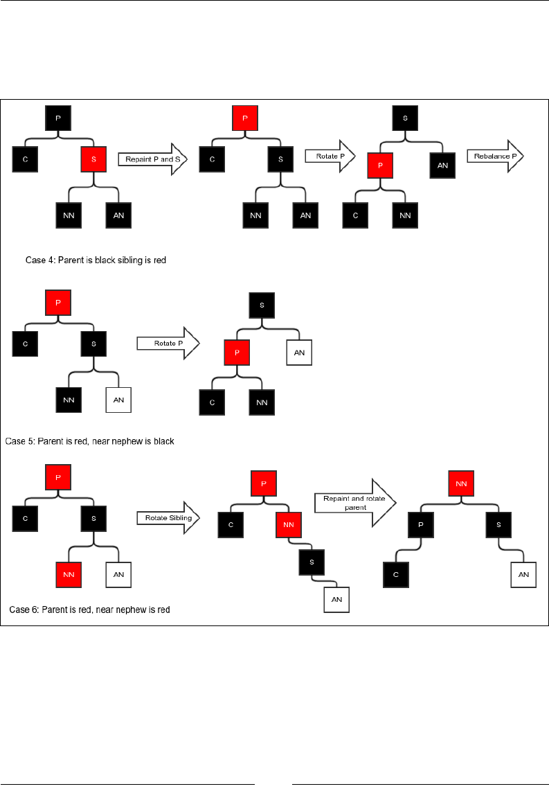
Chapter 8
[ 185 ]
6. Our nal case is when the parent is red and the near nephew is red. In this
case, we recolor the parent and do a double rotation. Notice that the top node
remains red. This is not a problem because the original top node, which is the
parent node, was also red and hence its parent must be black.
Case 4, 5, and 6 of deletion from a red-black tree
Now we can dene the rebalanceForDelete method coding all the preceding cases:
protected void rebalanceForDelete(Node<E> parent, boolean
nodeDirectionLeft){
if(parent==null){
return;

More About Search – Search Trees and Hash Tables
[ 186 ]
}
Node<E> node = (Node<E>) (nodeDirectionLeft?
parent.getLeft(): parent.getRight());
if(!nullSafeBlack(node)){
node.black = true;
return;
}
Node<E> sibling = (Node<E>) (nodeDirectionLeft?
parent.getRight(): parent.getLeft());
Node<E> nearNephew = (Node<E>) (nodeDirectionLeft?
sibling.getLeft():sibling.getRight());
Node<E> awayNephew = (Node<E>) (nodeDirectionLeft?
sibling.getRight():sibling.getLeft());
if(parent.black){
if(sibling.black){
if(nullSafeBlack(nearNephew) && nullSafeBlack(
awayNephew)){
sibling.black = false;
if(parent.getParent()!=null){
rebalanceForDelete (
(Node<E>) parent.getParent(),
parent.getParent().getLeft() == parent);
}
}else if(!nullSafeBlack(awayNephew)){
awayNephew.black = true;
rotate(parent, nodeDirectionLeft);
}else{
nearNephew.black = true;
rotate(sibling, !nodeDirectionLeft);
rotate(parent, nodeDirectionLeft);
}
}else{
parent.black = false;
sibling.black = true;
rotate(parent, nodeDirectionLeft);
rebalanceForDelete(parent, nodeDirectionLeft);
}
}else{

Chapter 8
[ 187 ]
if(nullSafeBlack(nearNephew)){
rotate(parent, nodeDirectionLeft);
}else{
parent.black = true;
rotate(sibling, !nodeDirectionLeft);
rotate(parent, nodeDirectionLeft);
}
}
}
Now we override the deleteValue method to invoke rebalancing after the deletion.
We only need to rebalance if the deleted node was black. We rst check that. Then,
we need to gure out whether the deleted child was a left child of the parent or the
right child. After that, we can invoke the rebalanceForDelete method:
@Override
public BinaryTree.Node<E> deleteValue(E value) {
Node<E> node = (Node<E>) super.deleteValue(value);
if(node !=null && node.black && node.getParent()!=null){
Node<E> parentsCurrentChild = (Node<E>) (
node.getLeft() == null ? node.getRight():
node.getLeft());
if(parentsCurrentChild!=null){
boolean isLeftChild = parentsCurrentChild
.getParent().getLeft() == parentsCurrentChild;
rebalanceForDelete(
(Node<E>) node.getParent(), isLeftChild);
}else{
boolean isLeftChild = node.getParent()
.getRight()!=null;
rebalanceForDelete(
(Node<E>) node.getParent(), isLeftChild);
}
}
return node;
}
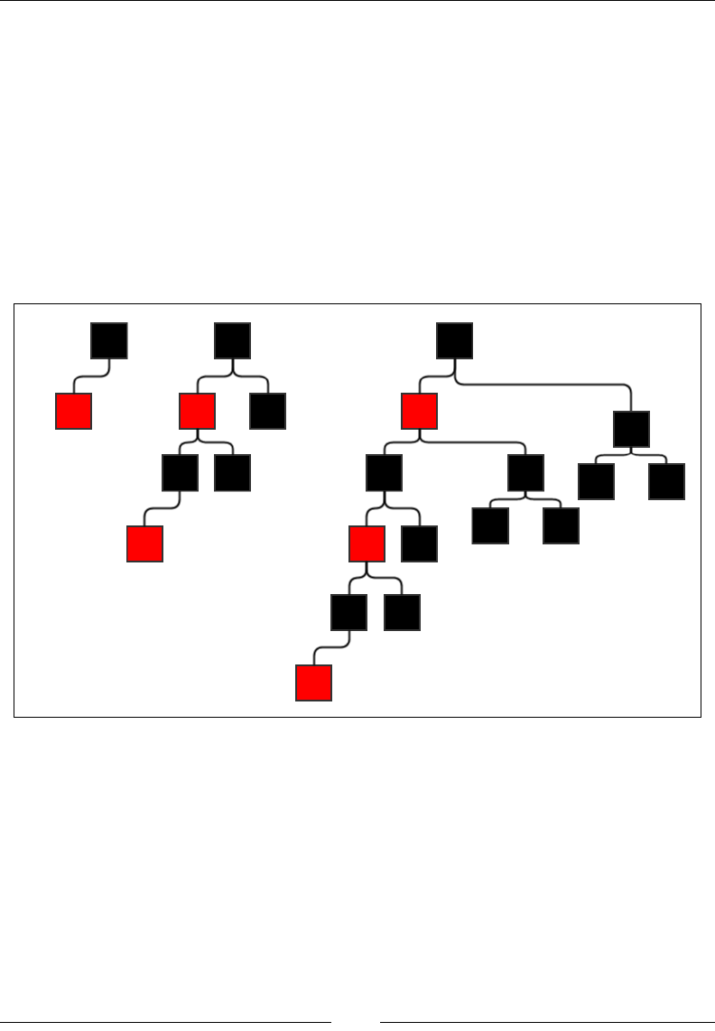
More About Search – Search Trees and Hash Tables
[ 188 ]
The worst case of a red-black tree
What is the worst possible red-black tree? We try to nd out the same way we did in
the case of the AVL tree. This one is a little more complicated, though. To understand
the worst tree, we must take into account the black height. To t the minimum
number of nodes n into height h, we need to rst choose a black height. Now it is
desirable to have as few black nodes as possible so that we don't have to include
black nodes for balancing the black height in the siblings of the nodes we are trying
to stretch the height with. Since a red node cannot be the parent of another, we must
have alternate black nodes. We consider height h and an even number so that the
black height is h/2 = l. For simplicity, we don't count the black null nodes for either the
height or the black height. The next gure shows some examples of the worst trees:
Worst red-black trees
The general idea is, of course, to have one path with the maximum possible height.
This path should be stuffed with the maximum number of red nodes and the other
paths lled with the least number of nodes, that is, with only black nodes. The
general idea is shown in the next gure.
The number of nodes in a full black tree of height l-1 is of course 2l-1 – 1. So, if the
number of nodes for height h = 2l is f(l), then we have the recursive formula:
f(l) = f(l-1) + 2 ( 2l-1 – 1) + 2
=> f(l) = f(l-1) + 2l
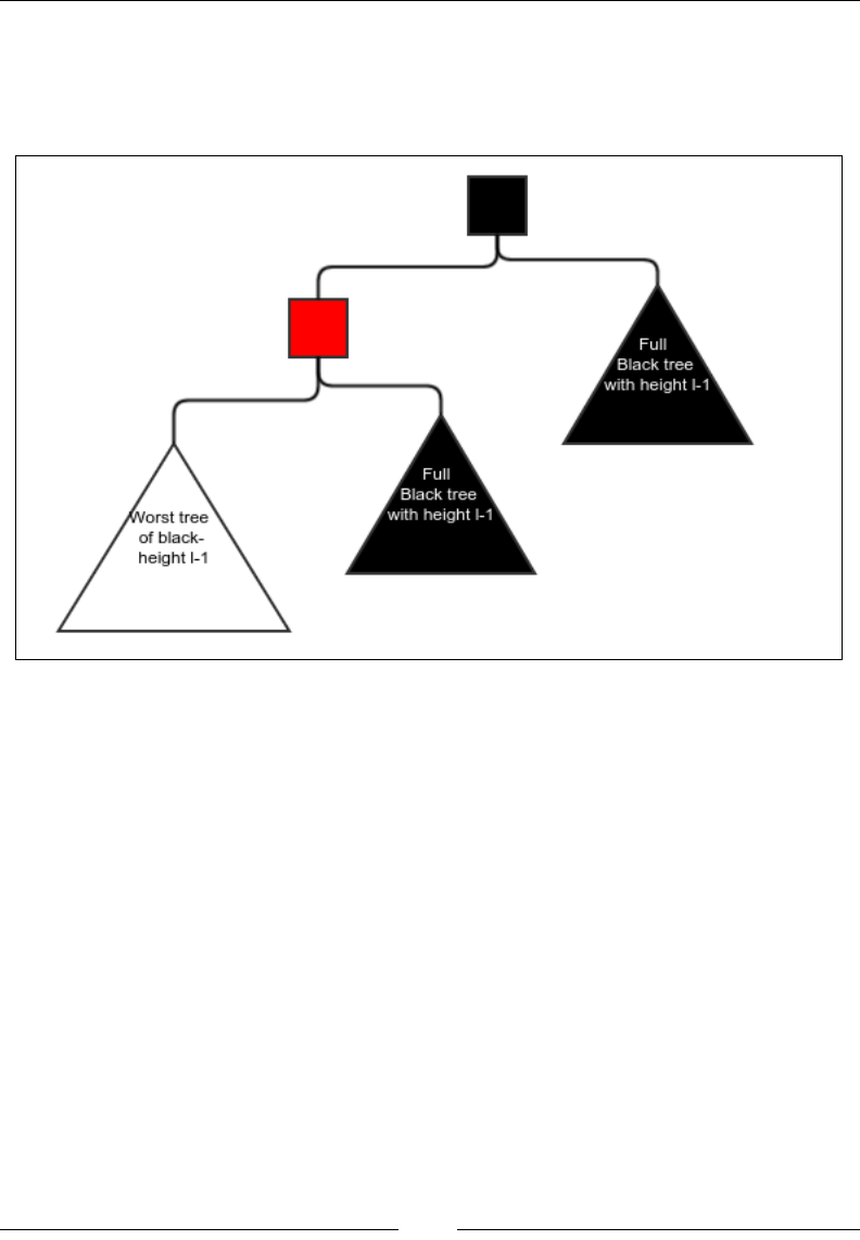
Chapter 8
[ 189 ]
Now, from the preceding gure, we can already see that f(1) = 2, f(2) = 6, and f(3) =
14. It looks like the formula should be f(l) = 2l+1 -2. We already have the base cases. If
we can prove that if the formula is true for l, then it is also true for l+1, we would be
able to prove the formula for all l by induction. This is what we will try to do:
General idea of the worst red-black tree
We already have f(l+1) = f(l) + 2l+1 and we also assume f(l) = 2l+1-2. So this is the
case: f(l+1) = 2l+1-2 + 2l+1 = 2l+2-2. Hence, if the formula holds true for l, it also
holds true for l+1; therefore, it is proved by induction.
So the minimum number of nodes is as follows:
n = f(l) = 2l+2-2.
=> lg n = lg ( 2l+2-2)
=> lg n > lg ( 2l+1)
=> lg n > l+1
=> l + 1< lg n
=> l < lg n
=> l = O (lg n)
Therefore, a red-black tree has a guaranteed logarithmic height; from this, it is not
hard to derive that the search, insertion, and deletion operations are all logarithmic.

More About Search – Search Trees and Hash Tables
[ 190 ]
Hash tables
A hash table is a completely different kind of searchable structure. The idea starts
from what is called a hash function. It is a function that gives an integer for any value
of the desired type. For example, the hash function for strings must return an integer
for every string. Java requires every class to have a hashcode() method. The object
class has one method implemented by default, but we must override the default
implementation whenever we override the equals method. The hash function holds
the following properties:
• Same values must always return the same hash value. This is called
consistency of the hash. In Java, this means if x and y are two objects and
x.equals(y) is true, then x.hashcode() == y.hashcode().
• Different values may return the same hash, but it is preferred that they don't.
• The hash function is computable in constant time.
A perfect hash function will always provide a different hash value for different
values. However, such a hash function cannot be computed in constant time in
general. So, we normally resort to generating hash values that look seemingly
random but are really complicated functions of the value itself. For example,
hashcode of the String class looks like this:
public int hashCode() {
int h = hash;
if (h == 0 && value.length > 0) {
char val[] = value;
for (int i = 0; i < value.length; i++) {
h = 31 * h + val[i];
}
hash = h;
}
return h;
}
Notice that it is a complicated function that is computed from constituent characters.
A hash table keeps an array of buckets indexed by the hash code. The bucket can
have many kinds of data structures, but here, we will use a linked list. This makes
it possible to jump to a certain bucket in constant time and then the bucket is kept
small enough so that the search within the bucket, even a linear search, will not cost
that much.

Chapter 8
[ 191 ]
Let's create a skeleton class for our hash table:
public class HashTable<E> {
protected LinkedList<E> [] buckets;
protected double maximumLoadFactor;
protected int totalValues;
public HashTable(int initialSize, double maximumLoadFactor){
buckets = new LinkedList[initialSize];
this.maximumLoadFactor = maximumLoadFactor;
}
…
}
We accept two parameters. InitialSize is the initial number of buckets we want to
start with, and our second parameter is the maximum load factor.
What is load factor? Load factor is the average number of values per bucket. If the
number of buckets is k and the total number of values in it is n, then load factor is n/k.
Insertion
Insertion is done by rst computing the hash and picking up the bucket in that
index. Now rstly, the bucket is searched linearly for the value. If the value is found,
insertion is not carried out; otherwise, the new value is added to the end of the bucket.
First we create a function for inserting in a given array of buckets and then using it to
perform the insertion. This would be useful when you are dynamically growing your
hash table:
protected boolean insert(E value, int arrayLength,
LinkedList<E>[] array) {
int hashCode = value.hashCode();
int arrayIndex = hashCode % arrayLength;
LinkedList<E> bucket = array[arrayIndex];
if(bucket == null){
bucket = new LinkedList<>();
array[arrayIndex] = bucket;
}
for(E element: bucket){
if(element.equals(value)){
return false;
}
}
bucket.appendLast(value);
totalValues++;
return true;
}

More About Search – Search Trees and Hash Tables
[ 192 ]
Note that effective hash code is computed by taking the remainder of the actual
hash code divided by the number of buckets. This is done to limit the number of
hash code.
There is one more thing to be done here and that is rehashing. Rehashing is the
process of dynamically growing the hash table as soon as it exceeds a predened
load factor (or in some cases due to other conditions, but we will use load factor in
this text). Rehashing is done by creating a second array of buckets of a bigger size
and copying each element to the new set of buckets. Now the old array of buckets is
discarded. We create this function as follows:
protected void rehash(){
double loadFactor = ((double)(totalValues))/buckets.length;
if(loadFactor>maximumLoadFactor){
LinkedList<E> [] newBuckets = new LinkedList[
buckets.length*2];
totalValues = 0;
for(LinkedList<E> bucket:buckets){
if(bucket!=null) {
for (E element : bucket) {
insert(element, newBuckets.length,
newBuckets);
}
}
}
this.buckets = newBuckets;
}
}
Now we can have our completed insert function for a value:
public boolean insert(E value){
int arrayLength = buckets.length;
LinkedList<E>[] array = buckets;
boolean inserted = insert(value, arrayLength, array);
if(inserted)
rehash();
return inserted;
}

Chapter 8
[ 193 ]
The complexity of insertion
It is easy to see that the insert operation is almost constant time unless we have to
rehash it; in this case, it is O(n). So how many times do we have to rehash it? Suppose
the load factor is l and the number of buckets is b. Say we start from an initialSize
B. Since we are doubling every time we rehash, the number of buckets will be b =
B.2R; here R is the number of times we rehashed. Hence, the total number of elements
can be represented as this: n = bl = Bl. 2R. Check this out:
lg n = R + lg(Bl) .
=> R = ln n – lg (Bl) = O(lg n)
There must be about lg n number of rehashing operations, each with complexity
of O(n). So the average complexity for inserting n elements is O(n lg n). Hence,
the average complexity for inserting each element is O(lg n). This, of course,
would not work if the values are all clustered together in a single bucket that we are
inserting into. Then, each insert would be O(n), which is the worst case complexity
of an insertion.
Deletion is very similar to insertion; it involves deletion of elements from the buckets
after they are searched.
Search
Search is simple. We compute the hash code, go to the appropriate bucket, and do a
linear search in the bucket:
public E search(E value){
int hash = value.hashCode();
int index = hash % buckets.length;
LinkedList<E> bucket = buckets[index];
if(bucket==null){
return null;
}else{
for(E element: bucket){
if(element.equals(value)){
return element;
}
}
return null;
}
}

More About Search – Search Trees and Hash Tables
[ 194 ]
Complexity of the search
The complexity of the search operation is constant time if the values are evenly
distributed. This is because in this case, the number of elements per bucket would
be less than or equal to the load factor. However, if all the values are in the same
bucket, search is reduced to a linear search and it is O(n). So the worst case is linear.
The average case of search is constant time in most cases, which is better than that of
binary search trees.
Choice of load factor
If the load factor is too big, each bucket would hold a lot of values that would output
a bad linear search. But if the load factor is too small, there would be a huge number
of unused buckets causing wastage of space. It is really a compromise between
search time and space. It can be shown that for a uniformly distributed hash code,
the fraction of buckets that are empty can be approximately expressed as e-l, where
l is the load factor and e is the base of a natural logarithm. If we use a load factor of
say 3, then the fraction of empty buckets would be approximately e-3 = 0.0497 or 5
percent, which is not bad. In the case of a non-uniformly distributed hash code (that
is, with unequal probabilities for different ranges of values of the same width), the
fraction of empty buckets would always be greater. Empty buckets take up space in
the array, but they do not improve the search time. Therefore, they are undesirable.
Summary
In this chapter, we saw a collection of searchable and modiable data structures. All
of these allowed you to insert new elements or delete elements while still remaining
searchable and that too quite optimally. We saw binary search trees in which a
search follows the paths of the tree from the root. Binary search trees can be modied
optimally while still remaining searchable if they are of the self-balancing type. We
studied two different kinds of self-balancing trees: AVL trees and red-black trees.
Red-black trees are less balanced than AVL trees, but they involve a fewer number
of rotations than AVL trees. In the end, we went through the hash table, which is a
different kind of searchable structure. Although the worst case complexity of search
or insertion is O(n), hash tables provide constant time search and average time
insertion (O(lg n)) in most cases. If a hash table does not keep growing, the average
insertion and deletion operations will also be constant time.
In the next chapter, we will see some more important general purpose data
structures.

[ 195 ]
Advanced General Purpose
Data Structures
In this chapter, we will take a look at some more interesting data structures that are
commonly used. We will start with the concept of a priority queue. We will see some
efcient implementations of a priority queue. In short, we will cover the following
topics in this chapter:
• Priority queue ADT
• Heap
• Binomial forest
• Sorting using a priority queue and heap
Priority queue ADT
A priority queue is like a queue in that you can enqueue and dequeue elements.
However, the element that gets dequeued is the one with the minimum value of
a feature, called its priority. We will use a comparator to compare elements and
learn which one has the lowest priority. We will use the following interface for the
priority queue:
public interface PriorityQueue<E> {
E checkMinimum();
E dequeueMinimum();
void enqueue(E value);
}
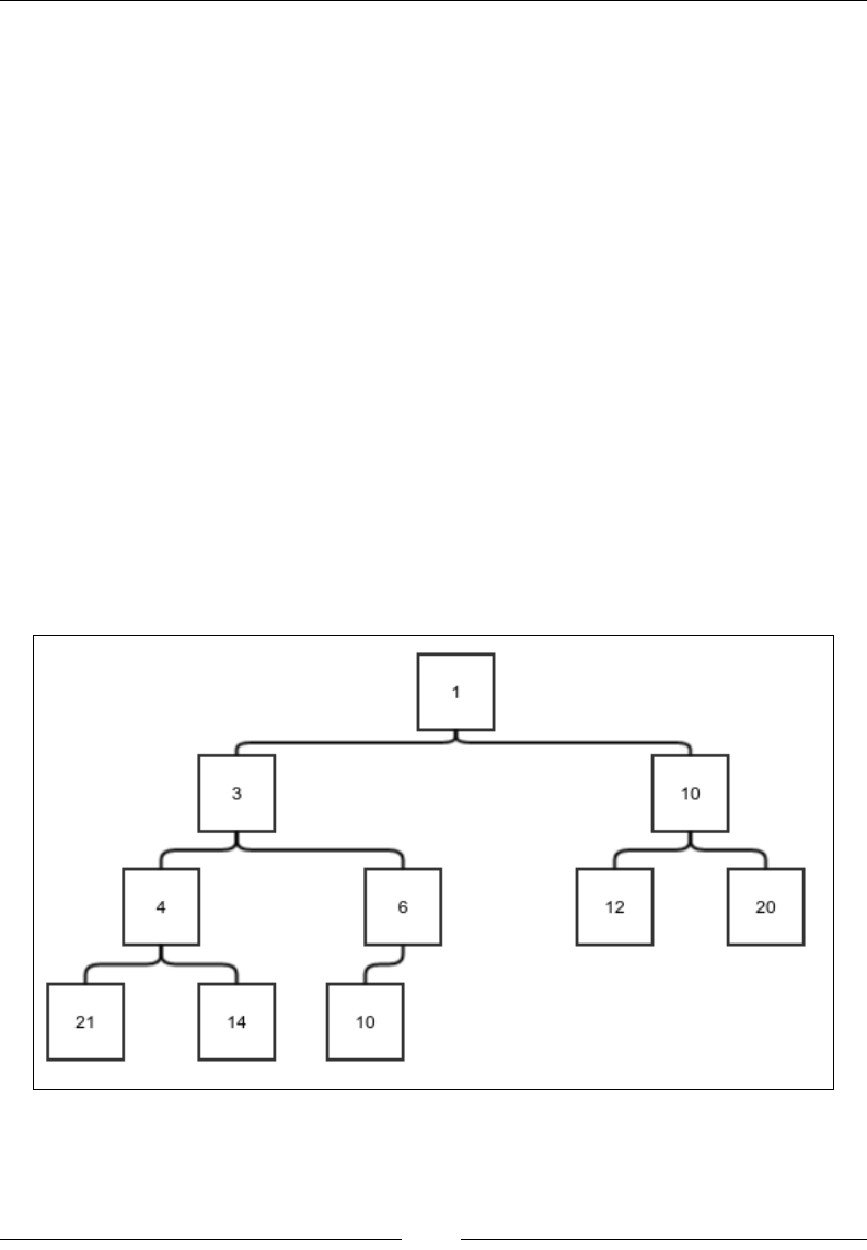
Advanced General Purpose Data Structures
[ 196 ]
We require the following set of behaviors from the methods:
• checkMinimum: This method must return the next value to be dequeued
without dequeuing it. If the queue is empty, it must return null.
• dequeueMinimum: This must dequeue the element with the minimum priority
and return it. It should return null when the queue is empty.
• enqueue: This should insert a new element in the priority queue.
We would also like to do these operations as efciently as possible. We will see two
different ways to implement it.
Heap
A heap is a balanced binary tree that follows just two constraints:
• The value in any node is less than the value in either of the children. This
property is also called the heap property.
• The tree is as balanced as possible—in the sense that any level is completely
filled before a single node is inserted in the next level.
The following gure shows a sample heap:
Figure 1. A sample heap
It would not be really clear until we actually discuss how to insert elements and
remove the least element. So let's jump into it.
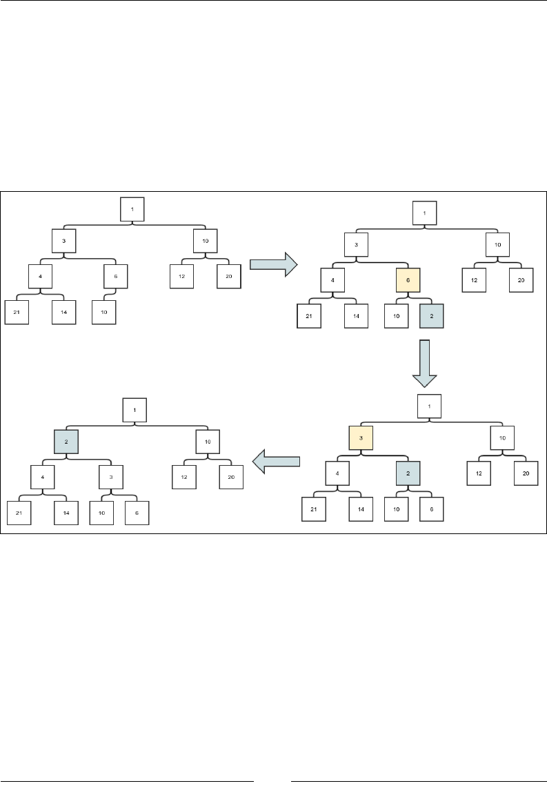
Chapter 9
[ 197 ]
Insertion
The rst step of insertion is to insert the element in the next available position. The
next available position is either another position in the same level or the rst position
in the next level; of course, this applies when there is no vacant position in the
existing level.
The second step is to iteratively compare the element with its parent and keep
switching until the element is bigger than the parent, thus restoring the constraints.
The following gure shows the steps of an insertion:
Figure 2. Heap insertion
The gray box represents the current node, and the yellow box represents the parent
node, whose value is larger than the current node. First, the new element is inserted
in the next available spot. It must be swapped until the constraint is satised. The
parent is 6, which is bigger than 2, so it is swapped. If the parent is 3, which is also
larger than 2, it is swapped. If the parent is 1, which is less than 2, we stop and the
insertion is complete.
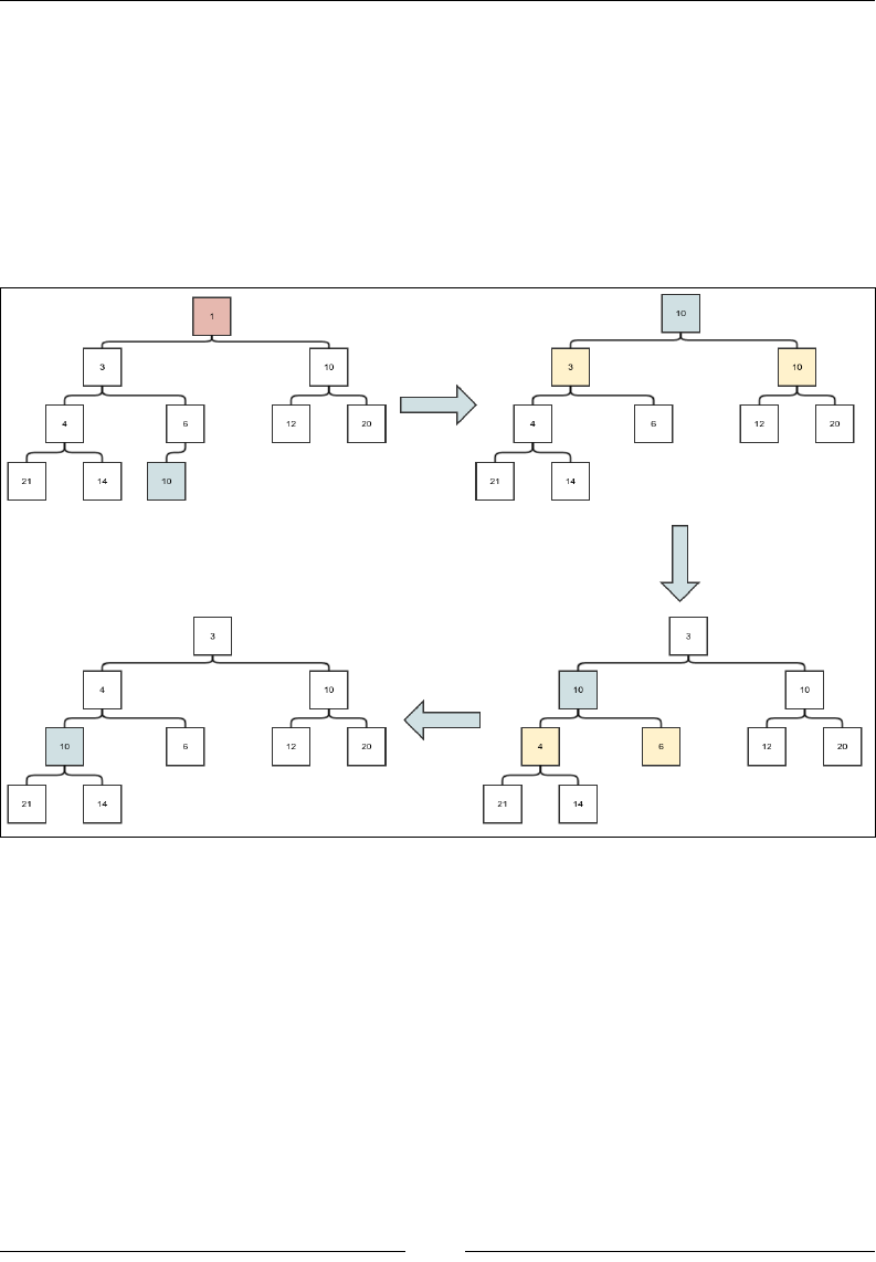
Advanced General Purpose Data Structures
[ 198 ]
Removal of minimum elements
The constraint that the parent is always less than or equal to the children guarantees
that the root is the element with the least value. This means the removal of the least
element leads only to the removal of the top element. However, the empty space of the
root must be lled, and elements can only be deleted from the last level to maintain
the constraint 2. To ensure this, the last element is rst copied to the root and then
removed. We must now iteratively move the new root element downward until the
constraint 1 is satised. The following gure shows an example of a delete operation:
Heap deletion
There is one question though, since any parent can have two children: which one
should we compare and swap with? The answer is simple. We need the parent to
be less than both the children; this means we must compare and swap with the
minimum value of the children.

Chapter 9
[ 199 ]
Analysis of complexity
First, let's check out the height of a heap for a given number of nodes. The rst layer
contains just the root. The second layer contains a maximum of two nodes. The
third layer contains four. Indeed, if any layer contains m elements, the next layer
will contain, at the maximum, the children of all these m elements. Since each node
can have two children, the maximum number of elements in the next layer will be
2m. This shows that the number of elements in layer l is 2l-1. So, a full heap of height
h will have total 1+2+4+...+ 2h-1 = 2h-1 nodes. Therefore, a heap of height h can have
maximum 2h+1-1 nodes. What is the minimum number of nodes in a heap of height
h. Well, since only the last level can have unlled positions, the heap must be full,
except the last layer. The last layer can have one node minimum. So, the minimum
number of nodes in a heap of height h is (2h-1 -1) + 1 = 2h-1. Hence, if the number of
nodes is n, then we have this:
2h-1 ≤ n ≤ 2h –1
=> h-1 ≤ lg n ≤ lg(2h –1) <lg( 2h)
=> h-1 ≤ lg n < h
We also have the following:
2h-1 ≤ n ≤ 2h –1
=> 2h≤ n ≤ 2h+1 –1
=>h ≤ lg (2n)< h+1
Combining the preceding two expressions, we get this:
lg n < h ≤ lg (2n)
=> h = θ(lg n)
Now, let's assume that adding a new element to the end of the heap is a constant
time operation or θ(lg n). We will see that this operation can be made this efcient.
Now we deal with the complexity of a trickle up operation. Since in each compare-
and-swap operation, we only compare with the parent and never backtrack, the
maximum number of swaps that can happen in a trickle up operation equals the
height of the heap h. Hence, the insertion is O(lg n). This means that the insert
operation itself is O(lg n).
Similarly, for the trickle down operation, we can only do as many swaps as the
height of the heap. So trickling down is also O(lg n). Now if we assume that
removing the root node and copying the last element to the root is at the maximum
O(lg n), we can conclude that the delete operation is also O(lg n).
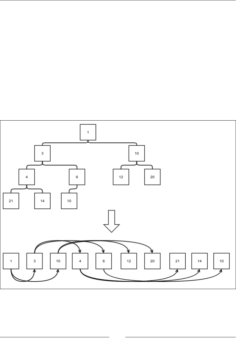
Advanced General Purpose Data Structures
[ 200 ]
Serialized representation
A heap can be represented as a list of numbers without any blanks in the middle.
The trick is to list the elements in order after each level. Positions from 1 through n
for an n element heap adopt the following conventions:
• For any element at index j, the parent is at index j/2, where '/' represents an
integer division. This means divide j by two and ignore the remainder if any.
• For any element at index j, the children are j*2 and j*2+1. One can verify that
this is the same as the first formula written the other way round.
The representation of our example tree is shown in the following gure. We have
just attened the process of writing a tree one entire level before another. We
retained the tree edges, and one can see that the parent-child relationships work as
described previously:
Array representation of a heap
With the knowledge of the array-based storage function of a heap, we can proceed to
implement our heap.

Chapter 9
[ 201 ]
Array-backed heap
An array-backed heap is a xed-sized heap implementation. We start with a partial
implementation class:
public class ArrayHeap<E> implements PriorityQueue<E>{
protected E[] store;
protected Comparator<E> comparator;
int numElements = 0;
public ArrayHeap(int size, Comparator<E> comparator){
store = (E[]) new Object[size];
this.comparator = comparator;
}
Given any index of the array (starting from 0), nd the index of the parent element.
It involves converting the index to 1 based form (so add 1), dividing by 2, and then
converting it back to 0 (so subtract 1):
protected int parentIndex(int nodeIndex){
return ((nodeIndex+1)/2)-1;
}
Find the index of the left child using this:
protected int leftChildIndex(int nodeIndex){
return (nodeIndex+1)*2 -1;
}
Swap the elements in the two indexes provided using this:
protected void swap(int index1, int index2){
E temp = store[index1];
store[index1] = store[index2];
store[index2] = temp;
}
…
}
To implement the insertion, rst implement a method that would trickle the value
up until constraint 1 is satised. We compare the current node with the parent,
and if the value of the parent is larger, then do a swap. We keep moving upwards
recursively:
protected void trickleUp(int position){
int parentIndex = parentIndex(position);

Advanced General Purpose Data Structures
[ 202 ]
if(position> 0 && comparator.compare(store[parentIndex],
store[position])>0){
swap(position, parentIndex);
trickleUp(parentIndex);
}
}
Now we can implement the insertion. The new element is always added to the end of
the current list. A check is done to ensure that when the heap is full, an appropriate
exception is thrown:
public void insert(E value){
if(numElements == store.length){
throw new NoSpaceException("Insertion in a full heap");
}
store[numElements] = value;
numElements++;
trickleUp(numElements-1);
}
Similarly, for deletion, we rst implement a trickle down method that compares an
element with its children and makes appropriate swaps until constraint 1 is restored.
If the right child exists, the left child must also exist. This happens because of the
balanced nature of a heap. In this case, we must compare only with a minimum of
two children and swap them if it is necessary. When the left child exists but the right
child does not, we only need to compare it with one element:
protected void trickleDown(int position){
int leftChild = leftChildIndex(position);
int rightChild = leftChild+1;
if(rightChild<numElements) {
if (comparator.compare(store[leftChild],
store[rightChild]) < 0) {
if (comparator.compare(store[leftChild],
store[position]) < 0) {
swap(position, leftChild);
trickleDown(leftChild);
}
} else {
if (comparator.compare(store[rightChild],
store[position]) < 0) {
swap(position, rightChild);
trickleDown(rightChild);
}
}
}else if(leftChild<numElements){

Chapter 9
[ 203 ]
if (comparator.compare(store[leftChild],
store[position]) < 0) {
swap(position, leftChild);
trickleDown(leftChild);
}
}
}
With the trickleDown method available, removing the minimum element is simple.
We rst save the current root as the minimum element, then copy the last element to
the root position. We then call the trickleDown method to restore constraint 1:
public E removeMin(){
if(numElements==0){
return null;
}else{
E value = store[0];
store[0] = store[numElements-1];
numElements--;
trickleDown(0);
return value;
}
}
Now we only have to use it as an implementation of the priority queue. So we
implement the relevant methods using our insert and removemin:
@Override
public E checkMinimum() {
if(numElements==0){
return null;
}else{
return store[0];
}
}
@Override
public E dequeueMinimum() {
return removeMin();
}
@Override
public void enqueue(E value) {
insert(value);
}

Advanced General Purpose Data Structures
[ 204 ]
This completes our array-based heap implementation. It has the same problem
as our array-based queue implementation, that is, we need to know its maximum
size beforehand. Next, we will have an implementation of a heap that has an
implementation in the form of a linked binary tree.
Linked heap
A linked heap is an actual binary tree where every node holds references to its
children. We rst create a skeleton structure for our heap:
public class LinkedHeap<E> implements PriorityQueue<E>{
protected static class Node<E>{
protected E value;
protected Node<E> left;
protected Node<E> right;
protected Node<E> parent;
public Node(E value, Node<E> parent){
this.value = value;
this.parent = parent;
}
}
…
}
To keep track of the next position, each position is given a number, just like we did
in our array-based representation. We have the same calculation for the index of
the parent and children. But, in this case, looking up the value at a particular index
requires a traversal from the root to that node. We create a method to do this. Note
that since we are not using an array, the position starts from 1. We start by nding the
parent node recursively. The parent node is of course the node at the position that is
half the value of the children. The remainder, when divided by 2, is the bit that tells us
whether the node is to the left or right of the parent. We return the node accordingly:
protected Node<E> findNodeAtPostion(int position){
if(position == 1){
return root;
}else{
int side = position % 2;
int parentPosition = position / 2;
Node<E> parent = findNodeAtPostion(parentPosition);
switch (side){
case 0:
return parent.left;

Chapter 9
[ 205 ]
case 1:
return parent.right;
}
}
return null;
}
Next, we turn to swapping. In the case of an array-based heap, we could swap the
values between any two indexes. However, this general implementation would
require multiple traversals in this case. We only need to swap the values between
a node and its parent. The swapWithParent takes the parent node as an argument.
Another argument is to know whether the current node is the left or right child of
the parent and switch references appropriately:
protected void swapWithParent(Node<E> parent, boolean left){
Node<E> node = left? parent.left:parent.right;
Node<E> leftChild = node.left;
Node<E> rightChild = node.right;
Node<E> sibling = left? parent.right:parent.left;
Node<E> grandParent = parent.parent;
parent.left = leftChild;
if(leftChild!=null){
leftChild.parent = parent;
}
parent.right = rightChild;
if(rightChild!=null){
rightChild.parent = parent;
}
parent.parent = node;
if(left){
node.right = sibling;
node.left = parent;
}else{
node.left = sibling;
node.right = parent;
}
node.parent = grandParent;
if(sibling!=null)
sibling.parent = node;
if(parent == root){
root = node;
}else{
boolean parentLeft = grandParent.left==parent;
if(parentLeft){

Advanced General Purpose Data Structures
[ 206 ]
grandParent.left = node;
}else{
grandParent.right = node;
}
}
}
Insertion
Insertion involves inserting a new element at the end rst and then trickling it in
the upward direction. First, we create a trickle up method, similar to the one in the
ArrayHeap class:
protected void trickleUp(Node<E> node){
if(node==root){
return;
}else if(comparator.compare(node.value, node.parent.value)<0){
swapWithParent(node.parent, node.parent.left == node);
trickleUp(node);
}
}
Now, we implement the insert method. If the tree is empty, we just have to add a
root. Otherwise, the position of the new element is (numElements+1). In this case, it's
parent must be ((numElements+1)/2). Whether it should be the left or right child of
its parent is determined by the value of ( (numElements+1)%2). A new node is then
created and added to the parent as a child. Finally, numElements is incremented to
keep track of the number of elements:
public void insert(E value){
if(root==null){
root = new Node<>(value, null);
}else{
Node<E> parent = findNodeAtPostion((numElements+1)/2);
int side = (numElements+1)%2;
Node<E> newNode = new Node<>(value, parent);
switch (side){
case 0:
parent.left = newNode;
break;
case 1:
parent.right = newNode;
break;
}

Chapter 9
[ 207 ]
trickleUp(newNode);
}
numElements++;
}
Removal of the minimal elements
Similar to the array-based heap, we need to implement a trickle down method. Since
the left child must exist if the right child does, if the left child is null, the node does
not have any child. But, if the right child is null and the left child is not, we only need
to compare the current node's value with that of the left child. Otherwise, compare
and swap with the child that has the minimum value:
protected void trickleDown(Node<E> node){
if(node==null){
return;
}
if(node.left == null){
return;
}else if(node.right == null){
if(comparator.compare(node.left.value, node.value)<0){
swapWithParent(node, true);
trickleDown(node);
}
}else{
if(comparator.compare(node.left.value,
node.right.value)<0){
if(comparator.compare(node.left.value, node.value)<0){
swapWithParent(node, true);
trickleDown(node);
}
}else{
if(comparator.compare(node.right.value, node.value)<0){
swapWithParent(node, false);
trickleDown(node);
}
}
}
}

Advanced General Purpose Data Structures
[ 208 ]
Now we can implement the method to remove the minimum element. If the root
is null, it means the queue is empty. If the last element is the root, there is only one
element and we just remove and return it. Otherwise, we copy the value of the root
to a temporary variable, then copy the value of the last element to the root, and
nally, trickle down the root:
public E removeMin(){
if(root==null){
return null;
}
Node<E> lastElement = findNodeAtPostion(numElements);
if(lastElement==root){
root = null;
numElements--;
return lastElement.value;
}
E value = root.value;
root.value = lastElement.value;
Node<E> parent = lastElement.parent;
if(parent.left==lastElement){
parent.left = null;
}else{
parent.right=null;
}
numElements--;
trickleDown(root);
return value;
}
Finally, we implement the methods required to make it a valid priority queue:
@Override
public E checkMinimum() {
return root==null? null : root.value;
}
@Override
public E dequeueMinimum() {
return removeMin();
}
@Override
public void enqueue(E value) {
insert(value);
}
This completes our priority queue implementation using heaps. We will now
introduce a different way of implementing a priority queue. It is called a binomial
forest, which comprises our next section.
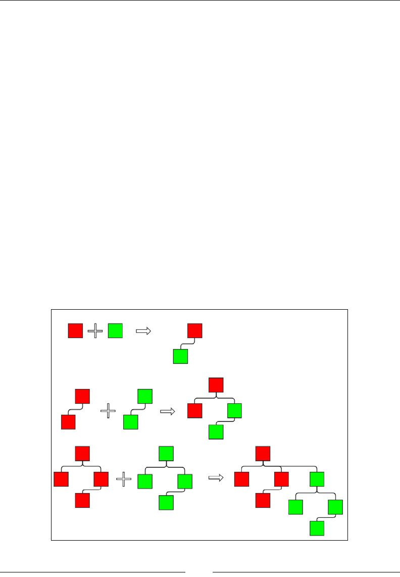
Chapter 9
[ 209 ]
Complexity of operations in ArrayHeap and
LinkedHeap
We have already seen that if we can append an element to the end of a heap in at most
O(lg n), where n is the number of elements already in the heap, we can perform both
insertion and removal of the minimum element θ(lg n) times. In the case of ArrayHeap,
insertion of a new element implies just setting the value of an element in an array at a
known index. This is a constant time operation. So, in ArrayHeap, both the insertion
and removal of minimum element are θ(lg n). Checking the minimum element is just
the check the value at index zero of the array and hence is constant time.
In the case of LinkedHeap, insertion of a new element at the end involves traversing
the tree to the end position. Since the height of the tree is θ(lg n), this operation is also
θ(lg n). This means, the insertion and deletion operation in LinkedHeap is also θ(lg n).
Checking the minimum element means just checking the value at the root, and this
operation is constant time.
Binomial forest
A binomial forest is a very interesting data structure. But, to discuss it, we need to
rst start with a binomial tree. A binomial tree is a tree in which a combination of
two smaller binomial trees of the same size are combined in a particular way:
Binomial tree
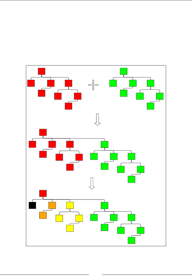
Advanced General Purpose Data Structures
[ 210 ]
The preceding gure shows how binomial trees combine to create larger binomial
trees. In the rst row, two binomial trees of height 1 combine to create a new
binomial tree of height 2. In the second row, two binomial trees of height 2 combine
to create a new binomial tree of height 3. In the nal example, two binomial trees
of height 3 combine to create a binomial tree of height 4, and it continues. The two
trees that are combined together are not treated symmetrically. Instead, the root of
one becomes the parent of the other. The next gure shows one more step in the
sequence and then shows a different way to look at a binomial tree. In the last row,
I have highlighted the subtrees differently. Notice how:
Figure 6. The other way of thinking about a binomial tree
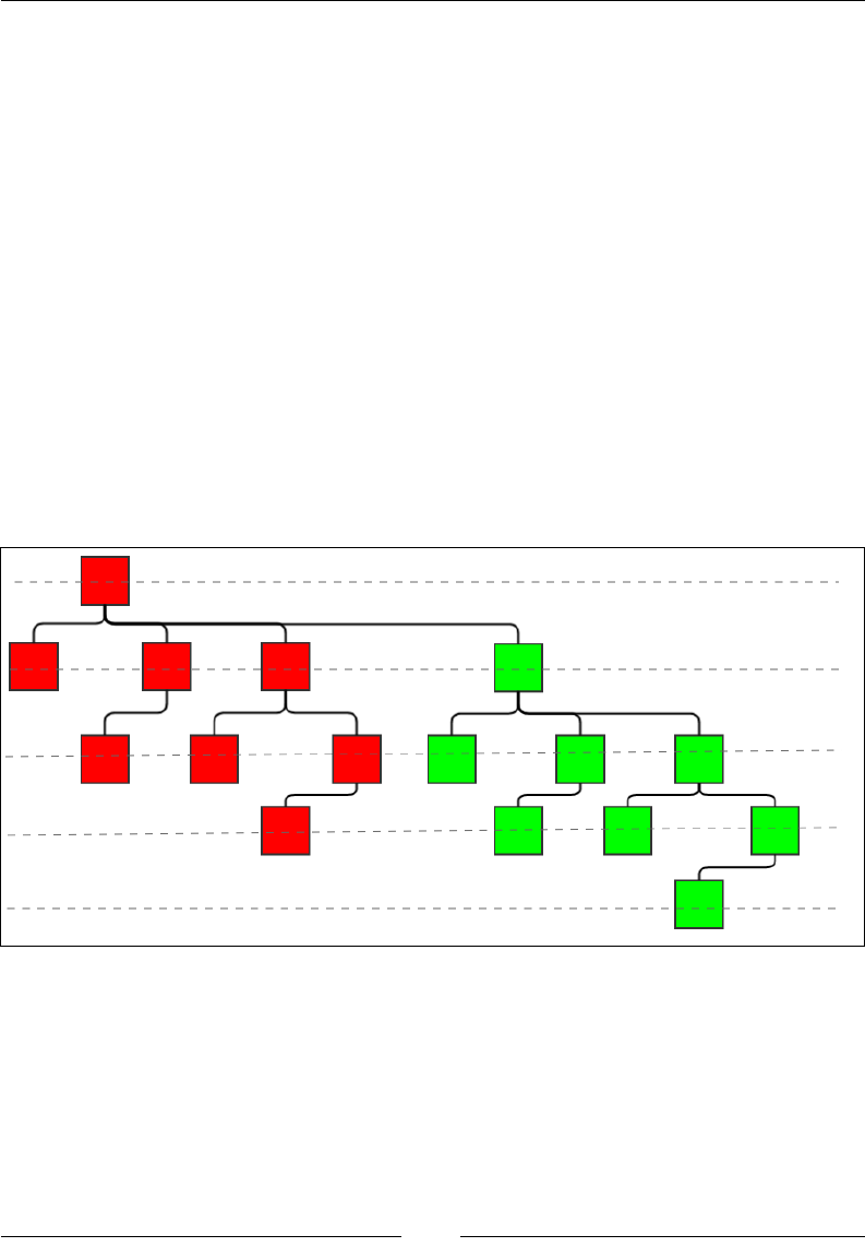
Chapter 9
[ 211 ]
Each subtree is a binomial tree. Not only that, the rst subtree is a binomial tree of
height 1, the second one of height 2, third one of height 3, and so on. So, another way
of thinking about a binomial tree is that it is a root and a sequence of subtrees that
are binomial trees of consecutive heights up to one less than the height of the entire
tree. Both these views are required in our discussion. The rst view is needed when
analyzing the idea and the second when implementing it.
Why call it a binomial tree?
Remember the choose function we discussed in Chapter 4, Detour - Functional
Programming? There, I pointed out that it is also called the binomial coefcient. Let's
see how it is related to a binomial tree. Suppose we have a binomial tree of height h
and we want to nd out the number of nodes at level l. Let's assume that for a tree of
height h, the number of nodes is f(t,r), where t=h-1 and r = l-1. The reason for taking
a variable that is one less than the height and level will become clearer a little later.
Basically, t is the height of the tree that starts from 0 instead of 1, and r is the level
that starts from zero. Now this tree is obviously a tree of only one element or it is
made up of two trees of height h-1 = t:
Figure 7. The rationale for naming it a binomial tree

Advanced General Purpose Data Structures
[ 212 ]
We will call these two subtrees this: red subtree and green subtree. This is because
they are colored this way in the preceding gure. The levels are highlighted using
dashed lines. It is clear from the picture that the nodes at the level r in the complete
tree is either at level r in the red tree or at level r-1 in the green tree. Both the red and
green trees are trees of height h-1. This means the following: f(t,r) = f(t-1,r) + f(t-1,r-1).
This equation is the same as what we have for the choose function we have already
discussed. The only thing we have to check is the boundary conditions. The top level
(that is t=0) always has only one node, so f(t,0) = 1. We also know that the number of
levels in the tree has to be less than or equal to the height of the tree, so we have f(t,r)
= 0 if t <r. So, f(t,t) = f(t-1,t) + f(t-1,t-1) = 0 + f(t-1,t-1) = f(t-1,t-1) for any t. In the same
way, f(t-1,t-1) = f(t-2,t-2) = f(t-3,t-3) = … = f(0,0) = 1 (because f(t,0) = 1). Therefore, all
the conditions of the choose function are satised; hence we can see f(t,r) = choose(t,r)
= choose(h-1, l-1). Since the choose function is also called the binomial coefcient, this
gives the binomial tree its name.
Number of nodes
What is the number of nodes n in a binomial tree of height h? When h=1, we only
have one node. A tree of height 2 is made up of two trees of height 1, a tree of height
3 is made up of two trees of height 2, and so on. So, for the increment of 1 in height,
the number of nodes must be twice as much as the original number. That is, when
h=1, n=1; h=2, n=2; h=3, n=4 ,... In general, this should be the case: n = 2h-1= 2t. Here t
is the height starting from zero.
Notice also that we can say that the number of nodes n in a tree is the sum of the
number of nodes in each level, which is choose(t, r), where r is the level starting
from 0 to t. The two formulas must be equal, so the sum choose(t, 0) + choose(t, 1) +
choose(t, 2) + … + choose(t, t) equals 2t. This is a proof of this relationship. There are
other proofs as well, but this is a valid proof too.
The heap property
Of course, with only this structure, we have no way of making sure of having
some easy way of guring out the minimum element. So, we also enforce the heap
property on a binomial tree:
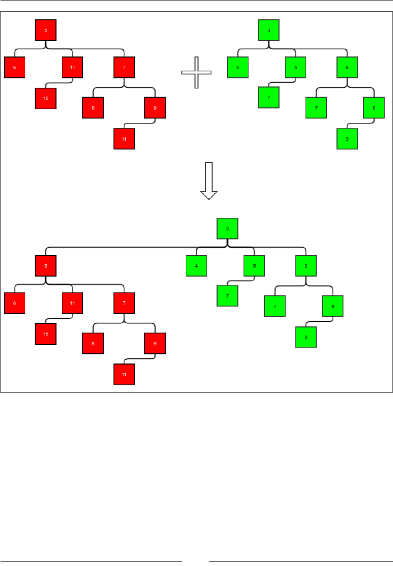
Chapter 9
[ 213 ]
Figure 8. Preserving heap property while merging.
This is the property: the value of any node is smaller than the value of each of its
children. When merging two trees to make one, the only thing we need to do to
preserve the heap property is to use the heap with the lesser value at its top node as
the top subtree and the one with the higher value at its top node as the subordinate
subtree. This is shown in the preceding gure. The red tree happens to have a higher
value in the root node than that of the green tree. Hence, the red tree must be the
subordinate tree. The heap property ensures that the root of any binomial tree holds
the minimum element.

Advanced General Purpose Data Structures
[ 214 ]
Binomial forest
So how do we make a queue out of this? Firstly, note that any tree will have nodes
with at least the power of 2. But, in a queue, we want an arbitrary number of
elements. So we store these elements in more than one tree. Any number can be
expressed as the sum of the power of 2 because any number can be expressed in
binary form. Suppose we need to store 20 nodes. The number 20 in binary is 10100.
So we need two binomial trees: one with height 5 and 16 nodes and one with height
3 and four nodes. A queue is built using a collection of binomial trees to store the
nodes. Hence it is called a binomial forest.
Before we discuss how to insert new elements and remove the minimum element,
we need to understand how to merge two binomial forests. We have already seen
that the numbers of elements are represented according to binary form. Just write
the number in binary form, and if 1 exists, it means there is a tree of height that is
equal to one plus its position from right to left. When we merge two forests, the
number of elements of the merged forest is the sum of the number of elements in the
forests that need to be merged. This means the result will have trees of sizes where
the binary representation of the sum will have the number 1. We can nd this binary
representation by performing a binary addition of the binary representations of the
node's source number. For example, let's merge two forests: one with 12 elements
and one with 10 elements. Their binary representations will be 1100 and 1010,
respectively. If we do a binary addition, we have 1100 + 1010 = 10110. This means
the original trees had trees of heights 3, 5 and 4, 5 and the result must have trees
of heights 3, 4, and 6. The merge happens the same way we do a binary addition.
The trees are stored in sequence, and we have empty places that represent zeros in
the binary representation. While merging, each tree represents a bit and it has the
number of nodes that the bit represents. We take the corresponding bit from each
forest and also consider a carry. All these trees must either be empty or have exactly
the same number of nodes. Then, we merge them to create the resulting bits.
To do any binary addition, we have input of three bits for each bit: one from each of
the input and a carry. We need to compute both the output bit and the next carry.
Similarly, while merging two trees, we need to compute the output tree and the carry
tree from the given input trees (two) and a carry tree. Once the merging is done,
inserting and removing min is simple.
The insert simply merges a forest with a single tree using a single node. Removing
the minimum element is a little more complicated operation. The rst step is to nd
out the minimum. We know every tree has the minimum element at its root. So we
need to walk through all the trees while comparing the root elements to nd the
minimum element and the tree that has it. Removing it is simply taking the root off,
leaving a list of subtrees that make a forest of consecutive heights of trees. Therefore,
we can merge the subtrees in the main forest to complete the removal process.

Chapter 9
[ 215 ]
Let's see the implementation. First, we create a skeleton class. A binomial tree
has a root, which contains a value and a list of subtrees. The list of subtrees is
like a dense forest. The list of trees in the forest is stored in a linked list. We use
DoublyLinkedList because we need to remove the last element:
public class BinomialForest<E> implements PriorityQueue<E>{
protected Comparator<E> comparator;
protected static class BinomialTree<E>{
E value;
LinkedList<BinomialTree<E>> subTrees = new LinkedList<>();
public BinomialTree(E value){
this.value = value;
}
}
public BinomialForest(Comparator<E> comparator){
this.comparator = comparator;
}
DoublyLinkedList<BinomialTree<E>> allTrees =
new DoublyLinkedList<>();
…
}
As discussed earlier, we will start with the merge operation now. First we need to
merge two trees, which we will use to merge two forests. Merging two trees is a
simple constant time operation. Merging with a null tree does not change the tree. The
two trees being merged should be of the same size. We need to simply compare the
root elements. The tree with the smaller value in its root will get the other as a child:
protected BinomialTree<E> merge(BinomialTree<E> left,
BinomialTree<E> right){
if(left==null){
return right;
}else if(right==null){
return left;
}
if(left.subTrees.getLength() != right.subTrees.getLength()){
throw new IllegalArgumentException(
"Trying to merge two unequal trees of sizes " +

Advanced General Purpose Data Structures
[ 216 ]
left.subTrees.getLength() + " and " +
right.subTrees.getLength());
}
if(comparator.compare(left.value, right.value)<0){
left.subTrees.appendLast(right);
return left;
}else{
right.subTrees.appendLast(left);
return right;
}
}
Since we want to check the minimum element in constant time, just like in a heap, we
will store the minimum element in a state variable. We will also store its position in
the allTrees list:
BinomialTree<E> minTree = null;
int minTreeIndex = -1;
We will dene a method to nd out and update the variables. Since the smallest
element in any tree is the root, we only have to go through the root to nd the
minimum element:
protected void updateMinTree(){
if(allTrees.getLength()==0){
minTree = null;
minTreeIndex = -1;
}
E min = null;
int index = 0;
for(BinomialTree<E> tree:allTrees){
if(tree==null){
index++;
continue;
}
if(min == null || comparator.compare(min, tree.value)>0){
min = tree.value;
minTree = tree;
minTreeIndex = index;
}
index++;
}
}

Chapter 9
[ 217 ]
To implement the merging of two forests, we need to rst implement how to
compute the output and carry the tree out of the two input trees and a carry tree.
These methods are fairly simple. We need to understand that both the input and the
carry must be of the same size if they are not null. The height of the output must be
the same as the height of the output, and the height of the carry must be one more
than the height of the input:
protected BinomialTree<E> computeOutputWithoutCarry(
BinomialTree<E> lhs, BinomialTree<E> rhs, BinomialTree<E> carry){
if(carry==null){
if(lhs==null){
return rhs;
}else if(rhs==null){
return lhs;
}else{
return null;
}
}else{
if(lhs==null && rhs==null){
return carry;
}else if(lhs == null){
return null;
}else if(rhs == null){
return null;
}else{
return carry;
}
}
}
protected BinomialTree<E> computeCarry(
BinomialTree<E> lhs, BinomialTree<E> rhs, BinomialTree<E> carry)
{
if(carry==null){
if(lhs!=null && rhs!=null){
return merge(lhs, rhs);
}else{
return null;
}
}else{
if(lhs==null && rhs==null){
return null;
}else if(lhs == null){
return merge(carry, rhs);
}else if(rhs == null){

Advanced General Purpose Data Structures
[ 218 ]
return merge(carry, lhs);
}else{
return merge(lhs, rhs);
}
}
}
We also need to enhance the ListIterator class in our imperative LinkedList
implementation so that we can modify the value of any node while iterating through
it. We use the following implementation to do this:
public class ListIterator implements Iterator<E> {
protected Node<E> nextNode = first;
protected Node<E> currentNode = null;
protected Node<E> prevNode = null;
@Override
public boolean hasNext() {
return nextNode != null;
}
@Override
public E next() {
if (!hasNext()) {
throw new IllegalStateException();
}
prevNode = currentNode;
currentNode = nextNode;
nextNode = nextNode.next;
return currentNode.value;
}
@Override
public void remove() {
if(currentNode==null || currentNode == prevNode){
throw new IllegalStateException();
}
if(currentNode==first){
first = nextNode;
}else{
prevNode.next = nextNode;
}
currentNode=prevNode;
}

Chapter 9
[ 219 ]
public void setValue(E value){
currentNode.value = value;
}
}
With these methods available, we can implement the merging of two forests or two
lists of trees:
protected void merge(LinkedList<BinomialTree<E>> rhs){
LinkedList<BinomialTree<E>>.ListIterator lhsIter
= (LinkedList<BinomialTree<E>>.ListIterator)allTrees
.iterator();
Iterator<BinomialTree<E>> rhsIter = rhs.iterator();
BinomialTree<E> carry = null;
while(lhsIter.hasNext() || rhsIter.hasNext()){
boolean lhsHasValue = lhsIter.hasNext();
BinomialTree<E> lhsTree = lhsHasValue?
lhsIter.next():null;
BinomialTree<E> rhsTree = rhsIter.hasNext()?
rhsIter.next():null;
BinomialTree<E> entry = computeOutputWithoutCarry(
lhsTree, rhsTree, carry);
carry = computeCarry(lhsTree, rhsTree, carry);
if(lhsHasValue) {
lhsIter.setValue(entry);
}else{
this.allTrees.appendLast(entry);
}
}
if(carry!=null){
this.allTrees.appendLast(carry);
}
updateMinTree();
}
The Insert method is very simple to implement with the merge available. Just
merge a list containing one tree with the value 1:
public void insert(E value){
BinomialTree<E> newTree = new BinomialTree<E>(value);
DoublyLinkedList<BinomialTree<E>> newList
= new DoublyLinkedList<>();
newList.appendLast(newTree);
merge(newList);
}

Advanced General Purpose Data Structures
[ 220 ]
Removal of the minimum element is a little more complex. It involves removing the
tree with the minimum value and then considering its root as the minimum element.
Once this is done, the subtrees need to be merged with the original forest. If the last
tree is being removed, we must actually remove it from the list. This is the same as
not writing a leading zero in binary representation. Otherwise, we only set the value
to null so that we know it is a zero bit:
public E removeMin(){
if(allTrees.getLength()==0){
return null;
}
E min = minTree.value;
if(minTreeIndex==allTrees.getLength()-1){
allTrees.removeLast();
}else {
allTrees.setValueAtIndex(minTreeIndex, null);
}
merge(minTree.subTrees);
return min;
}
Finally, we can implement the methods required to use it as a priority queue:
@Override
public E dequeueMinimum() {
return removeMin();
}
@Override
public void enqueue(E value) {
insert(value);
}
@Override
public Iterator<E> iterator() {
return null;
}
This completes our implementation of a binomial queue.

Chapter 9
[ 221 ]
Complexity of operations in a binomial forest
We already know that the number of nodes in a binomial tree of height h is 2h-1.
The question is, if we want to store n elements, what should be the maximum height
of the trees in the forest? We have seen that the trees we need are as per the binary
expression of the integer n. The most signicant bit of the binary representation of
n is the oor of (lg n), that is the greatest integer less than or equal to lg n. We will
write this as lg n. The height of the tree representing this bit is 1 + lg n. The length of
the list holding the trees in the forest is also 1 + lg n= θ(lg n). Both in the case of an
insertion and removal of a new element, a merge operation is involved. The merge
operation is constant time for each pair of input trees and one carry. So, the number
of operations for a merge operation of two forests is this: constant times the number of
trees in the largest forest = θ(lg n), where n is the number of trees in the largest forest.
At the time of insertion, we just merge a new forest of only one tree and one element.
So this operation is θ(lg n), where n is the number of elements in the original forest.
The removal process involves two steps. The rst is to remove the minimum
element. This involves a constant time operation, which is used to remove the tree
with the minimum element, and a merge operation, which is θ(lg n), as seen already.
The second step/operation is to update the tree with the minimum element. This
involves scanning the roots of all the trees; therefore, it is θ(lg n), just like the merge
operation. So, as a whole, the removal process is also θ(lg n).
Checking the minimum element is of course constant time, as we have it
referenced already.
Sorting using a priority queue
Since a priority queue always returns the minimum element, if we insert all input
elements and then keep dequeuing them, they would be dequeued in sorted order.
This can be used to sort a list of elements. In our example, we will add a new method
called the LinkedList implementation. This implementation sorts the elements
using PriorityQueue. First insert all the elements into the priority queue. Then,
dequeue the elements and append them back to the linked list:
public void sort(Comparator<E> comparator){
PriorityQueue<E> priorityQueue = new LinkedHeap<E>(comparator);
while (first!=null){
priorityQueue.enqueue(getFirst());
removeFirst();
}

Advanced General Purpose Data Structures
[ 222 ]
while (priorityQueue.checkMinimum()!=null){
appendLast(priorityQueue.dequeueMinimum());
}
}
Both enqueue and dequeue have θ(lg n) complexity, and we have to enqueue and
dequeue each of the elements. We have already seen this: lg 1 + lg 2 + … + lg n = θ(n
lg n). So, the enqueueing and dequeueing of the elements is θ(n lg n), which means
the sort is θ(n lg n), which is asymptotically optimal.
In-place heap sort
We can use an array-based heap implementation to do an in-place sort of the
elements of an array. The trick is to use the same array for backing the heap. In the
beginning, we simply insert the elements in the heap from the beginning of the array.
We achieve this by replacing the array in the heap, except the one that is passed.
Since the heap also uses the space from the beginning, it does not overwrite the
elements we are still to insert. While dequeuing the elements, we start saving them
from the end of the array, as this is the part that is being freed up by the heap. This
means we want the largest element to be dequeued rst. This is achieved by simply
using a comparator that is the opposite of the one that is passed. We add this static
method to our ArrayHeap class:
public static <E> void heapSort(E[] array, Comparator<E> comparator){
ArrayHeap<E> arrayHeap = new ArrayHeap<E>(0,
(a,b) -> comparator.compare(b,a));
arrayHeap.store = array;
for(int i=0;i<array.length;i++){
arrayHeap.insert(array[i]);
}
for(int i=array.length-1;i>=0;i--){
array[i] = arrayHeap.removeMin();
}
}
This is actually a sort using a priority queue as shown before, except that here we
are sharing the array with the priority queue. Hence, this sort is also θ(n lg n), just
as before.

Chapter 9
[ 223 ]
Summary
In this chapter, we discussed priority queues and their implementation. Priority
queues are important data structures that are used in a lot of problems. We saw two
implementations of a priority queue, a heap, and a binomial forest. We also saw how
to use priority queues for sorting, which is asymptotically optimal. A variation of
this allowed us to sort an array in place using an array-based heap.
In the next chapter, we will discuss the concept of graphs, which are very useful,
almost ubiquitous ADTs, and data structures that are used in many real-life
applications.
[ 225 ]
Concepts of Graph
A graph is a generalization of a tree. In a tree, every node has one parent. In a graph,
a node can have multiple parents. The most common way to think about a graph is
as a set of vertices and edges. Vertices are like points and edges are like lines that
connect the points. In the generic notion of a graph, there is no restriction on which
vertices can be connected by edges. This allows graphs to model a versatile category
of real-life concepts. The Internet, for example, is a graph where the vertices are the
web pages and the edges the hyperlinks between the pages. A social networking
site, such as Facebook, has a graph of proles in which the vertices are the proles
and the edges the friendships between the proles. Each software has a graph of
dependencies, called a dependency graph, in which the vertices are the different
software libraries used and the edges the dependencies between the software
libraries. There is no end to examples of graphs. In this chapter, we will discuss the
following topics:
• Different types of graphs
• The ADT graph
• Representation of graphs in memory
• Traversal of a graph
• Cycle detection
• Spanning trees
• Minimum spanning trees
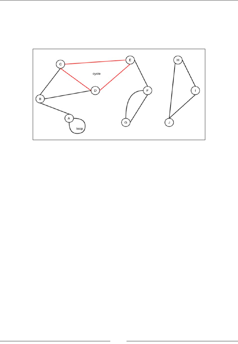
Concepts of Graph
[ 226 ]
What is a graph?
A graph is a collection of vertices and edges that connect the vertices. Figure 1 gives a
visual representation of an example of a graph. There are a few features to note here,
which we will discuss next:
Figure 1: Example of an undirected graph
• Undirected graph: An undirected graph is a graph in which the edges have
no direction, as shown in Figure 1.
• Directed graph: This is a graph in which the edges have a direction.
• Path: A path is a sequence of edges that connects a set of vertices that are
distinct from one another, except the first and the last vertices as they may
be the same. For example, in Figure 1, the edges AB, BD, and DE represent
a path. It can also be described as the ABDE path, which does not repeat its
vertices. In the case of a directed graph, the edges must traverse only in the
specified direction to form the sequence of edges required to make a path.
• Cycle: A cycle is a path with at least two vertices involved; it starts and ends
on the same vertex. For example, in Figure 1, the path DCED is a cycle.
• Loop: A loop is an edge that connects a node to itself. In Figure 1, vertex
A has a loop.
• Subgraph: The subgraph of a graph is another type of graph where all the
edges and vertices are the same as the edges and vertices of the original
graph. For example, in Figure 1, the nodes A, B, and C along with the edges
AB and BC represent a subgraph.
• Connected graph: A connected graph is a graph in which there exists a path
that starts from any arbitrary vertex and ends in any arbitrary, but different
vertex. The graph in Figure 1 is not connected. But, the subgraph with vertices
H, I, and J and the edges HI, IJ, and JH represent a connected subgraph:
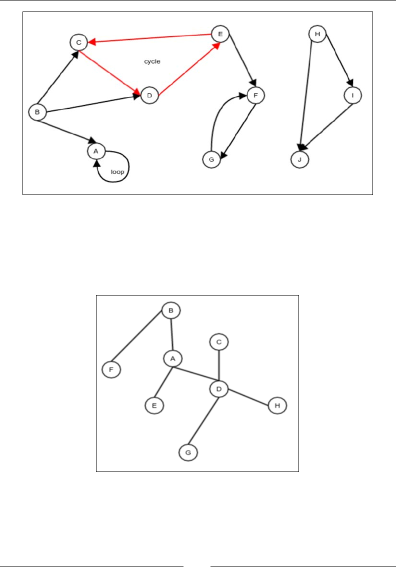
Chapter 10
[ 227 ]
Figure 2. Example directed graph
• Tree: A tree is a connected but undirected graph with no cycles and loops.
Figure 3 shows an example of a tree. Note that this is slightly different from
the tree we have studied earlier. This tree does not have any particular root.
The nodes in this tree do not have any particular parent, and any node can
act as a root:
Figure 3. Example tree
• Forest: A forest is an unconnected, undirected graph with no cycles or loops.
You can think of a forest as a collection of trees. A single tree is also a forest.
In other words, a forest is a collection of zero or more trees.
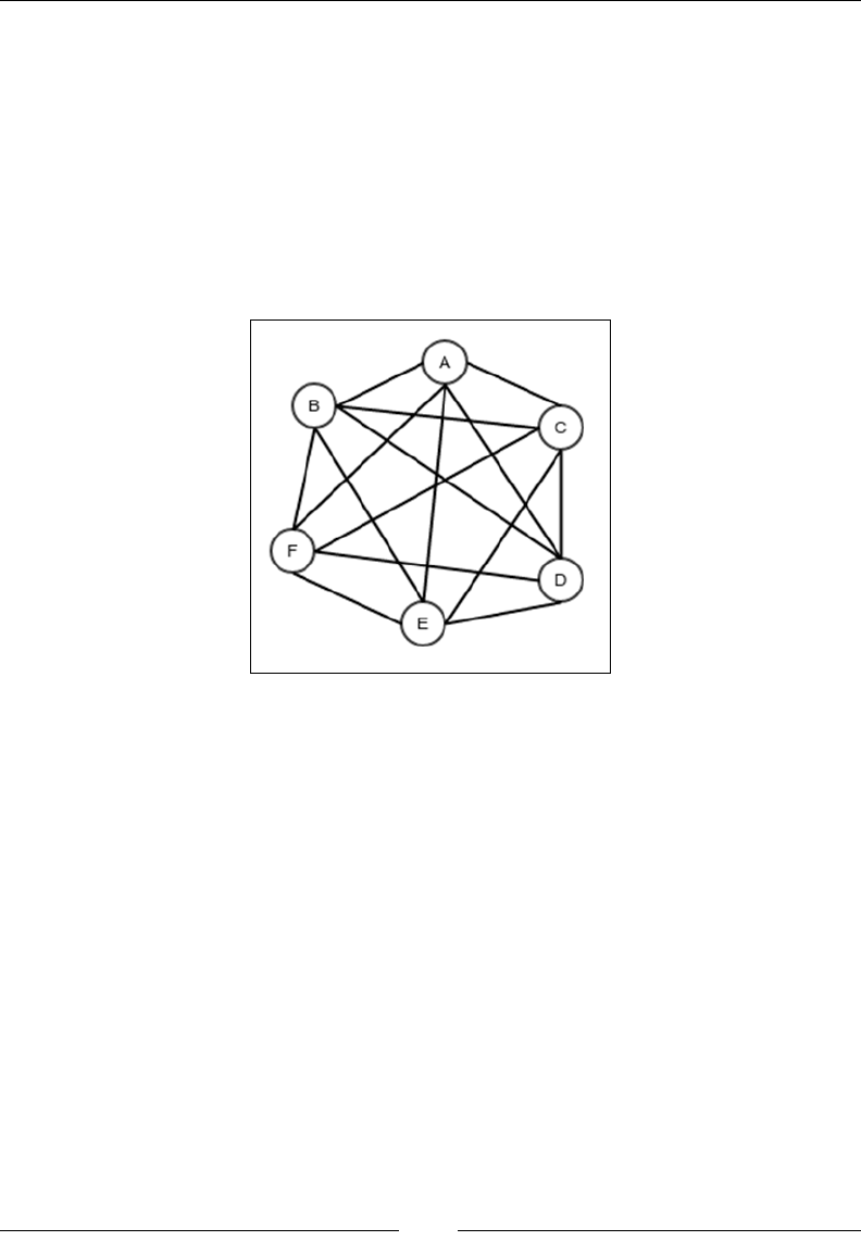
Concepts of Graph
[ 228 ]
• Complete graph: A complete graph is an undirected graph that has the
maximum number of edges, given a certain number of vertices. It also has
constraints as per which there can only be one edge between two given
vertices, with no loops. Figure 4 shows an example of a complete graph. For
a complete graph with the set of vertices V and the set of edges E, |E| = |V|
( |V| - 1) / 2. It is easy to see why this is the case. Each vertex will have an
edge between itself and other |V| - 1 nodes. That makes a total of |V| ( |V|
- 1) edges. However, in this approach, each edge is counted twice, once for
each of its two vertices. So, the actual number of edges in a complete graph is
|V| ( |V| - 1) / 2:
Figure 4. A complete graph
The graph ADT
We will now dene what a data structure representing a graph should do. Later, we
will discuss the different implementations of this ADT. A graph must support the
following operations:
• Add Vertex: This adds a new vertex
• Remove Vertex: This removes a vertex
• Add edge: This adds a new edge; in our graph, we will allow a maximum of
one edge between two vertices for simplicity
• Remove edge: This removes an edge
• Adjacent: This checks whether the two given vertices are adjacent to each
other, that is, whether there is an edge between the given nodes

Chapter 10
[ 229 ]
• Neighbors: This returns a list of vertices that are adjacent to the given vertex
• Get Vertex Value: This gets the value stored in a vertex
• Set Vertex Value: This stores a value in a vertex
• Get Edge Value: This gets the value stored in an edge
• Set Edge Value: This sets the value stored in an edge
• Is undirected: This returns whether the graph is undirected
• Get all vertices: This returns a self-balancing binary search tree containing all
the vertices
• Max Vertex ID: This returns the highest ID of the vertices
Our algorithms will depend on the above operations being available in a graph data
structure. The following Java interface is a realization of this ADT:
public interface Graph<V, E> {
int addVertex();
void removeVertex(int id);
void addEdge(int source, int target);
void removeEdge(int source, int target);
boolean isAdjacent(int source, int target);
LinkedList getNeighbors(int source);
void setVertexValue(int vertex, V value);
V getVertexValue(int vertex);
void setEdgeValue(int source, int target, E value);
E getEdgeValue(int source, int target);
boolean isUndirected();
BinarySearchTree<Integer> getAllVertices();
int maxVertexID();
}
We identify each vertex by an ID; edges are identied by a source vertex and a
target vertex. In the case of an undirected graph, the source and target could be
interchanged. But, in the case of a directed graph, they are noninterchangeable.
Now that we have an ADT, we would like to have an implantation. To implement a
graph data structure, we need to choose a representation in memory.
Representation of a graph in memory
A graph can be represented mainly in three different ways: adjacency matrix,
adjacency list, and incidence matrix.
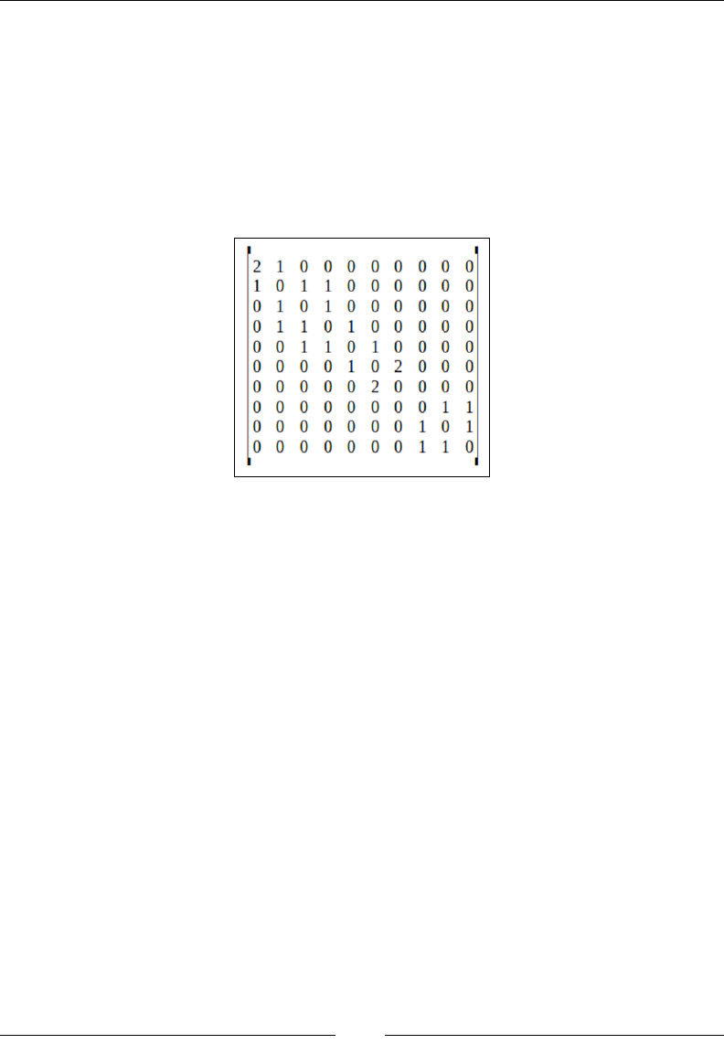
Concepts of Graph
[ 230 ]
Adjacency matrix
An adjacency matrix is a matrix, a table of values, where each value represents an
edge and both the rows are the columns that represent the vertices. The values in
a matrix can be the members of the entry. The values of the edges can be stored in
the matrix itself. There could also be a special value for representing the absence
of an edge. The following image shows an adjacency matrix for the graph in
Figure 1, where the value of the edge represents the number of edges between the
corresponding vertices:
The following things can be noted about an adjacency matrix:
• Rows are used to represent the sources and columns to represent the targets
of the edges
• In the case of an undirected graph, the source and target are
indistinguishable, so the adjacency matrix is symmetric
The following code provides an implementation of the graph ADT with the
adjacency matrix. We use a two-dimensional array to store the matrix. The ID of
any vertex is directly used as the index of the array. This is true for both the array
to store the values stored within the vertices and the values stored in the edges, or
even the existence of the edges. When we remove a vertex, we don't free its space; we
do this so that the IDs of the newer vertices don't get shifted. This improves lookup
performance but is wasteful in terms of resources:
public class AdjacencyMatrixGraphWithSparseVertex<V,E>
implements Graph<V, E> {
private static class NullEdgeValue{};

Chapter 10
[ 231 ]
We create two special objects to signify an edge and a vertex; these objects do not yet
hold a value. A null reference refers to the edge or vertex that does not exist:
private NullEdgeValue nullEdge = new NullEdgeValue();
private NullEdgeValue nullVertex = new NullEdgeValue();
Object [][] adjacencyMatrix = new Object[0][];
Object[] vertexValues = new Object[0];
A ag determines whether the graph is undirected:
boolean undirected;
public AdjacencyMatrixGraphWithSparseVertex(boolean undirected){
this.undirected = undirected;
}
Adding a vertex involves creating a new matrix and an array of vertex values and
copying all the older values into it:
@Override
public int addVertex() {
int numVertices = adjacencyMatrix.length;
Object [][] newAdjacencyMatrix = new Object[numVertices+1][];
for(int i=0;i<numVertices;i++){
newAdjacencyMatrix[i] = new Object[numVertices+1];
System.arraycopy(adjacencyMatrix[i],0,
newAdjacencyMatrix[i], 0, numVertices);
}
newAdjacencyMatrix[numVertices] = new Object[numVertices+1];
adjacencyMatrix = newAdjacencyMatrix;
Object [] vertexValuesNew = new Object[vertexValues.length+1];
System.arraycopy(vertexValues,0, vertexValuesNew, 0,
vertexValues.length);
vertexValuesNew[vertexValues.length] = nullVertex;
vertexValues = vertexValuesNew;
return numVertices;
}

Concepts of Graph
[ 232 ]
Since we don't free any space, removing a vertex simply involves setting values to
null. Note that removing a vertex has to be accompanied by the removal of all the
associated edges, which is done in a loop:
@Override
public void removeVertex(int id) {
vertexValues[id] = null;
for(int i=0;i<adjacencyMatrix.length;i++){
adjacencyMatrix[id][i] = null;
adjacencyMatrix[i][id] = null;
}
}
Adding an edge involves setting a particular position in the adjacency matrix. If the
graph is undirected, there will be two updates. This is because the source and target
could be interchanged and the adjacency matrix is always symmetric:
@Override
public void addEdge(int source, int target) {
if(adjacencyMatrix[source][target] == null){
adjacencyMatrix[source][target] = nullEdge;
if(undirected){
adjacencyMatrix[target][source] = nullEdge;
}
}else{
throw new IllegalArgumentException("Edge already exists");
}
}
The following operation is the simplest of all as it involves setting only one edge to
null. In the case of an undirected graph, there would be a corresponding update that
would interchange the source and target:
@Override
public void removeEdge(int source, int target) {
adjacencyMatrix[source][target] = null;
if(undirected){
adjacencyMatrix[target][source] = null;
}
}
The following is a trivial operation of checking the adjacency matrix:
@Override
public boolean isAdjacent(int source, int target) {
return adjacencyMatrix[source][target] != null;
}

Chapter 10
[ 233 ]
For any given source, nd all the edges in the same row of the matrix and add them
to a linked list that we can return. Note that in a directed graph, it traverses the edges
only in the forward direction:
@Override
public LinkedList getNeighbors(int source) {
LinkedList<Integer> neighborList = new LinkedList<>();
for(int i=0;i<adjacencyMatrix.length;i++){
if(adjacencyMatrix[source][i]!=null){
neighborList.appendLast(i);
}
}
return neighborList;
}
We store all the values of the vertices in a different array:
@Override
public void setVertexValue(int vertex, V value) {
vertexValues[vertex] = value;
}
@Override
public V getVertexValue(int vertex) {
if(vertexValues[vertex]!=nullVertex)
return (V)vertexValues[vertex];
else
throw new IllegalArgumentException("Vertex "+vertex
+" does not exist");
}
The values stored in the edges can be stored in the adjacency matrix itself:
@Override
public void setEdgeValue(int source, int target, E value) {
adjacencyMatrix[source][target] = value;
if(undirected){
adjacencyMatrix[target][source] = value;
}
}
@Override
public E getEdgeValue(int source, int target) {
if(adjacencyMatrix[source][target] != nullEdge) {

Concepts of Graph
[ 234 ]
return (E) adjacencyMatrix[source][target];
}else {
return null;
}
}
@Override
public boolean isUndirected() {
return undirected;
}
@Override
public BinarySearchTree<Integer> getAllVertices() {
BinarySearchTree<Integer> allVertices = new RedBlackTree<>();
for(int i=0;i<vertexValues.length;i++){
if(vertexValues[i]!=null){
allVertices.insertValue(i);
}
}
return allVertices;
}
@Override
public int maxVertexID() {
return vertexValues.length-1;
}
}
Complexity of operations in a sparse adjacency
matrix graph
Now let's analyze the complexity of the operations we have already discussed:
• Add vertex: Adding a vertex requires us to create a new two-dimensional
array with length and w the complexities of the idth |V| and then copy the
entire old content to the new array. Here, |V| represents the cardinality of
the set V of the vertices. What is the size of the adjacency matrix then? It's a
square matrix whose length or width equals |V|, so its size is |V|2. Hence,
adding a new edge has this complexity: θ(|V|2).

Chapter 10
[ 235 ]
• Remove Vertex: Removing a vertex involves removing all the edges that
correspond to the given vertex. The maximum number of edges that can be
associated with a single vertex is |V|, which is the length of a row or column
in the adjacency matrix. We must set all the values in the row and column
containing the vertex being deleted, so the number of values that need to be
changed is calculated as 2|V| - 1. The "minus one" part comes from the fact
that the row and column have one edge in common, the edge representing a
loop on the node that is being deleted. The common edge is counted twice,
both in the row and the column. So one of them must be stopped. Therefore,
the complexity of this operation is θ(2|V| - 1) = θ(|V|).
• Add edge and Remove edge: Adding an edge is as simple as setting a special
value at a single entry in the adjacency matrix. It has this complexity: θ(1).
Removing an edge is just setting null at the same position.
• Adjacent: This operation involves checking whether an edge exists between
the given source and target. It checks one entry in the adjacency matrix,
hence this complexity: θ(1).
• Neighbors: This operation requires reading all the values in the row of an
adjacency matrix. So it requires reading |V| values and possibly adding
them to a linked list. Therefore, the complexity of this operation is θ( |V| ).
• Setting and getting values at vertices and edges: These operations require
reading/setting a single value into/from the adjacency matrix. These
operations are all θ(1).
• Get all vertices: This involves scanning through all the vertices and inserting
them in a binary search tree. So this operation is θ( |V| lg |V|).
More space-efcient adjacency-matrix-based
graph
The trouble with the above graph implementation is that we are unable to recover
any space when vertices are deleted. The problem with recovering space is that it
changes the indexes of the vertices that are added later. To avoid this, we can choose
to have an ID of a vertex that is separate from its index position in the arrays. If we
do this, we need to be able to search the index of a vertex with the given ID. This
mapping can be done with a self-balancing binary search tree, which is what we are
going to do here.

Concepts of Graph
[ 236 ]
First, we create a separate class that represents a graph vertex. The idea is to allow a
comparison to exist on the ID of a vertex. Different graph implementations can then
extend this class to accommodate additional data in the graph vertex:
public class GraphVertex<V> implements Comparable<GraphVertex<V>>{
int id;
V value;
public GraphVertex(int id, V value) {
this.id = id;
this.value = value;
}
public int getId() {
return id;
}
public void setId(int id) {
this.id = id;
}
public V getValue() {
return value;
}
public void setValue(V value) {
this.value = value;
}
@Override
public boolean equals(Object o) {
if (this == o) return true;
if (o == null || getClass() != o.getClass()) return false;
GraphVertex<?> that = (GraphVertex<?>) o;
return id == that.id;
}
@Override
public int hashCode() {
return id;
}
@Override
public int compareTo(GraphVertex<V> o) {
return id - o.id;
}
}

Chapter 10
[ 237 ]
With this class available, we can implement our adjacency-matrix-based graph
implementation with a dense vertex and edge representation:
public class AdjacencyMatrixGraphWithDenseVertex<V,E> implements
Graph<V, E> {
First, we extend the GraphVertex class to include an addition eld that stores the
index of a vertex in the adjacency matrix as well as in the array meant for storing the
values of the vertices:
class Vertex extends GraphVertex<V>{
int internalIndex;
public Vertex(int id, V value, int internalIndex) {
super(id, value);
this.internalIndex = internalIndex;
}
public int getInternalIndex() {
return internalIndex;
}
public void setInternalIndex(int internalIndex) {
this.internalIndex = internalIndex;
}
}
The nextId variable is used to store the next ID that would be used:
private int nextId;
Special values to represent empty vertices and edges:
private static class NullValue {};
private NullValue nullEdge = new NullValue();
Object [][] adjacencyMatrix = new Object[0][];
The following is the binary search tree that stores the vertices with their indexes in
the arrays:
RedBlackTree<GraphVertex<V>> vertices = new RedBlackTree<>();
boolean undirected;
public AdjacencyMatrixGraphWithDenseVertex(boolean undirected){
this.undirected = undirected;
}

Concepts of Graph
[ 238 ]
The process of adding involves the same operations as before apart from the extra
operation of generating a new ID and storing an entry in the search tree:
@Override
public int addVertex() {
int id = nextId++;
int numVertices = adjacencyMatrix.length;
Object [][] newAdjacencyMatrix = new Object[numVertices+1][];
for(int i=0;i<numVertices;i++){
newAdjacencyMatrix[i] = new Object[numVertices+1];
System.arraycopy(adjacencyMatrix[i],0,
newAdjacencyMatrix[i], 0, numVertices);
}
newAdjacencyMatrix[numVertices] = new Object[numVertices+1];
vertices.insertValue(new Vertex(id, null,
adjacencyMatrix.length));
adjacencyMatrix = newAdjacencyMatrix;
return numVertices;
}
The removal of a vertex now actually involves creating a smaller adjacency matrix and
copying all the edges, except the ones associated with the vertex that is being deleted:
@Override
public void removeVertex(int id) {
BinaryTree.Node<GraphVertex<V>> node = vertices.searchValue(
new GraphVertex<V>(id, null));
if(node!=null){
int internalId = ((Vertex)(node.getValue()))
.getInternalIndex();
int numVertices = adjacencyMatrix.length;
Object [][] newAdjacencyMatrix = new Object[
numVertices-1][];
First, copy all the rows before the one for the vertex being deleted:
for(int i=0;i<internalId;i++){
newAdjacencyMatrix[i] = new Object[numVertices-1];
System.arraycopy(adjacencyMatrix[i],0,
newAdjacencyMatrix[i], 0, internalId);

Chapter 10
[ 239 ]
System.arraycopy(adjacencyMatrix[i],internalId+1,
newAdjacencyMatrix[i], internalId,
numVertices-internalId-1);
}
Then, copy all the rows after the one for the vertex being deleted:
for(int i=internalId+1;i<numVertices;i++){
newAdjacencyMatrix[i-1] = new Object[numVertices-1];
System.arraycopy(adjacencyMatrix[i],0,
newAdjacencyMatrix[i-1], 0, internalId);
System.arraycopy(adjacencyMatrix[i],internalId+1,
newAdjacencyMatrix[i-1], internalId,
numVertices-internalId-1);
}
adjacencyMatrix = newAdjacencyMatrix;
Now adjust all the indexes of the vertices added after the one that is deleted. We do
this by traversing the tree in preorder and updating only when appropriate:
vertices.traverseDepthFirstNonRecursive((gv)->{
if(((Vertex)gv).getInternalIndex()>internalId)
((Vertex)gv).setInternalIndex(((
Vertex)gv).getInternalIndex()-1);
}, BinaryTree.DepthFirstTraversalType.PREORDER);
vertices.deleteValue(new GraphVertex<>(id, null));
}else{
throw new IllegalArgumentException("Vertex with id "+id
+" does not exist");
}
}
Adding an edge involves setting an entry in the adjacency matrix. However, before
doing this, we need to look up the index of the vertex:
@Override
public void addEdge(int source, int target) {
BinaryTree.Node<GraphVertex<V>> sNode = vertices.searchValue(
new GraphVertex<V>(source, null));
BinaryTree.Node<GraphVertex<V>> tNode = vertices.searchValue(
new GraphVertex<V>(target, null));
if(sNode!=null && tNode!=null) {
int s = ((Vertex)(sNode.getValue())).getInternalIndex();
int t = ((Vertex)(tNode.getValue())).getInternalIndex();

Concepts of Graph
[ 240 ]
if(adjacencyMatrix[s][t] == null){
adjacencyMatrix[s][t] = nullEdge;
if(undirected){
adjacencyMatrix[t][s] = nullEdge;
}
}else{
throw new IllegalArgumentException("Edge
already exists");
}
}else{
throw new IllegalArgumentException("Non-existent ID");
}
}
This is the same as adding an edge, other than the fact that we change the
corresponding entry in the adjacency matrix to null:
@Override
public void removeEdge(int source, int target) {
BinaryTree.Node<GraphVertex<V>> sNode = vertices.searchValue(
new GraphVertex<V>(source, null));
BinaryTree.Node<GraphVertex<V>> tNode = vertices.searchValue(
new GraphVertex<V>(target, null));
if(sNode!=null && tNode!=null) {
int s = ((Vertex)(sNode.getValue())).getInternalIndex();
int t = ((Vertex)(tNode.getValue())).getInternalIndex();
adjacencyMatrix[s][t] = null;
}else{
throw new IllegalArgumentException("Non-existent ID");
}
}
Checking whether two vertices are adjacent involves looking up a value in the
adjacency matrix like before. But again, we must rst look up the indexes of the vertices:
@Override
public boolean isAdjacent(int source, int target) {
BinaryTree.Node<GraphVertex<V>> sNode = vertices.searchValue(
new GraphVertex<V>(source, null));
BinaryTree.Node<GraphVertex<V>> tNode = vertices.searchValue(
new GraphVertex<V>(target, null));
if(sNode!=null && tNode!=null) {
int s = ((Vertex)(sNode.getValue())).getInternalIndex();
int t = ((Vertex)(tNode.getValue())).getInternalIndex();

Chapter 10
[ 241 ]
return adjacencyMatrix[s][t] != null;
}else{
throw new IllegalArgumentException("Non-existent ID");
}
}
Getting the list of neighbors is a little trickier. We don't have a search mechanism that
lets us search by index to look up the ID. So instead of reading a row in the adjacency
matrix, we simply preorder traverse the search tree and check whether there is an
edge for the vertex in the adjacency matrix. We add a vertex only when there is an
edge between the source vertex and the vertex in question:
@Override
public LinkedList<Integer> getNeighbors(int source) {
BinaryTree.Node<GraphVertex<V>> node = vertices.searchValue(
new GraphVertex<V>(source, null));
if(node!=null){
LinkedList<Integer> neighborsList = new LinkedList<>();
int sourceInternalIndex = ((Vertex)
node.getValue()).getInternalIndex();
vertices.traverseDepthFirstNonRecursive((gv)->{
int targetInternalIndex = ((Vertex) gv)
.getInternalIndex();
if(adjacencyMatrix[sourceInternalIndex]
[targetInternalIndex]!=null)
neighborsList.appendLast(gv.getId());
}, BinaryTree.DepthFirstTraversalType.INORDER);
return neighborsList;
}else{
throw new IllegalArgumentException("Vertex with
id "+source+" does not exist");
}
}
The process of setting and getting values into/from the edges and vertices is the
same as before, except that we need to look up the index from the ID of the vertex
before using it:
@Override
public void setVertexValue(int vertex, V value) {
BinaryTree.Node<GraphVertex<V>> node =
vertices.searchValue(
new GraphVertex<V>(vertex, null));
if(node!=null){
node.getValue().setValue(value);

Concepts of Graph
[ 242 ]
}else{
throw new IllegalArgumentException("Vertex with
id "+vertex+" does not exist");
}
}
@Override
public V getVertexValue(int vertex) {
BinaryTree.Node<GraphVertex<V>> node =
vertices.searchValue(
new GraphVertex<V>(vertex, null));
if(node!=null){
return node.getValue().getValue();
}else{
throw new IllegalArgumentException("Vertex with
id "+vertex+" does not exist");
}
}
@Override
public void setEdgeValue(int source, int target, E value) {
BinaryTree.Node<GraphVertex<V>> sNode = vertices.searchValue(
new GraphVertex<V>(source, null));
BinaryTree.Node<GraphVertex<V>> tNode = vertices.searchValue(
new GraphVertex<V>(target, null));
if(sNode!=null && tNode!=null) {
int s = ((Vertex)(sNode.getValue())).getInternalIndex();
int t = ((Vertex)(tNode.getValue())).getInternalIndex();
adjacencyMatrix[s][t] = value;
if (undirected) {
adjacencyMatrix[t][s] = value;
}
}else{
throw new IllegalArgumentException("Non-existent ID");
}
}
@Override
public E getEdgeValue(int source, int target) {
BinaryTree.Node<GraphVertex<V>> sNode = vertices.searchValue(
new GraphVertex<V>(source, null));
BinaryTree.Node<GraphVertex<V>> tNode = vertices.searchValue(
new GraphVertex<V>(target, null));
if(sNode!=null && tNode!=null) {

Chapter 10
[ 243 ]
int s = ((Vertex)(sNode.getValue())).getInternalIndex();
int t = ((Vertex)(tNode.getValue())).getInternalIndex();
return (E) adjacencyMatrix[s][t];
}else{
throw new IllegalArgumentException("Non-existent ID");
}
}
@Override
public boolean isUndirected() {
return undirected;
}
@Override
public BinarySearchTree<Integer> getAllVertices() {
BinarySearchTree<Integer> allVertices = new RedBlackTree<>();
vertices.traverseDepthFirstNonRecursive(
(v) -> allVertices.insertValue(v.getId()),
BinaryTree.DepthFirstTraversalType.PREORDER);
return allVertices;
}
@Override
public int maxVertexID() {
return nextId-1;
}
}
Complexity of operations in a dense adjacency-
matrix-based graph
The following are the complexities of the operations we just discussed in a dense
adjacency-matrix-based graph:
• Add vertex: Addition still has the same θ(|V|2) operation for creating a new
adjacency matrix and copying all the old values. The additional operation of
inserting a new vertex in the search tree is θ(lg |V|). So the entire operation
is still θ(|V|2).
• Remove vertex: The removal of a vertex here follows the same operation
of recreating an adjacency matrix and copying all the old values, which
is θ(|V|2). The operation of removing a vertex from the search tree is
θ(lg |V|). So the entire operation is θ(|V|2).

Concepts of Graph
[ 244 ]
• Add edge and remove edge: The operation of updating an entry in the
adjacency matrix is still θ(1). However, now we need to have two lookups in
the search tree to figure out the indexes of the source and target. Both these
searches are θ(lg |V|). So the entire operation is θ(lg |V|).
• Adjacent: This is also θ(lg |V|) due to the same reason mentioned in the
preceding bullet point.
• Neighbors: Traversing the search tree is θ(|V|), and for each of the vertices
thus traversed, we create a constant number of operations. Looking up the
index of the source vertex is θ(lg |V|). Hence, the entire operation is still
θ(|V|).
• Setting and getting values at vertices and edges: These operations require
a fixed number of lookups (one or two) and then a constant time operation
for setting or getting the appropriate value. The lookups are θ(lg |V|), so the
entire operations are also θ(lg |V|).
• Get all vertices: Just like the previous implementation, this operation is θ(
|V| lg |V|).
Adjacency list
An adjacency list is a more space-efcient graph representation of sparse graphs.
A sparse graph is a graph that has a very few edges as compared to the number of
edges in a complete graph with the same number of vertices. A complete graph has
|V| ( |V| - 1) / 2 = θ (|V|2) edges, and the memory space required to store a graph
as an adjacency matrix is also θ (|V|2). So, in the case of a dense (almost complete)
graph, it makes sense to store it as an adjacency matrix. However, this is not true for
a sparse graph.
In an adjacency list representation, vertices are stored in an array or some other
data structure, and edges are stored along with the vertices in some list or some
other structure. First, we will consider an adjacency-list-based representation where
the vertices are stored in an array indexed by their IDs, as in the case of a sparse
adjacency matrix representation. It has the same problem: we cannot reduce the
size of the array of vertices when a vertex is deleted. However, in this case, the
list of edges are deleted, and this makes it way more space-efcient than what we
encountered in an adjacency matrix:
public class AdjacencyListGraphWithSparseVertex<V,E> implements
Graph<V,E> {
boolean undirected;
public AdjacencyListGraphWithSparseVertex(boolean undirected) {
this.undirected = undirected;
}

Chapter 10
[ 245 ]
The Edge class stores the details of the target and the value of an edge originating
from a vertex. The vertex stores a collection of the associated edges. We make the
edge comparable based of the ID of the target so that we can store them in a binary
search tree to easily look it up based on the ID:
class Edge implements Comparable<Edge>{
E value;
int target;
To improve the performance of the getNeighbors operation, we store a list of
neighbors in the node. We store a pointer in the node that corresponds to the target
of this node in the targetNode state variable:
DoublyLinkedList.DoublyLinkedNode<Integer> targetNode;
public Edge(int target) {
this.target = target;
}
@Override
public boolean equals(Object o) {
if (this == o) return true;
if (o == null || getClass() != o.getClass()) return false;
Edge edge = (Edge) o;
return target == edge.target;
}
@Override
public int hashCode() {
return target;
}
@Override
public int compareTo(Edge o) {
return target - o.target;
}
}
The Vertex class is used to store a vertex along with its associated edges. The edges
are stored in a red black tree:
class Vertex extends GraphVertex<V>{
RedBlackTree<Edge>
edges = new RedBlackTree<>();

Concepts of Graph
[ 246 ]
DoublyLinkedList<Integer> neighbors =
new DoublyLinkedList<>();
public Vertex(int id, V value) {
super(id, value);
}
}
The vertices are then stored in an array:
Object[] vertices = new Object[0];
Adding a vertex does not require us to copy any edges; it just ensures that the
vertices are copied to a newly created array of bigger size:
@Override
public int addVertex() {
Object[] newVertices = new Object[vertices.length+1];
System.arraycopy(vertices, 0, newVertices, 0,
vertices.length);
newVertices[vertices.length] = new Vertex(
vertices.length, null);
vertices=newVertices;
return newVertices.length-1;
}
Removing a vertex requires that you rst set the vertex to null at its position.
However, you must also remove all the edges from all the other vertices for which
the deleted vertex was the target:
@Override
public void removeVertex(int id) {
Vertex sVertex = (Vertex) vertices[id];
if(sVertex==null){
throw new IllegalArgumentException("Vertex "+
id +" does not exist");
}
LinkedList<Integer> neighbors = getNeighbors(id);
Edge dummyEdgeForId = new Edge(id);
We must remove all the edges associated with the vertex being deleted:
for(int t:neighbors){
Edge e = ((Vertex)vertices[t]).edges.deleteValue(
dummyEdgeForId).getValue();
((Vertex)vertices[t]).neighbors.removeNode(e.targetNode);
}
vertices[id] = null;
}

Chapter 10
[ 247 ]
Adding an edge requires making corresponding entries in the vertices associated
with it:
@Override
public void addEdge(int source, int target) {
Vertex sVertex = (Vertex) vertices[source];
Edge sEdge = sVertex.edges.insertValue(new
Edge(target)).getValue();
sEdge.targetNode = (DoublyLinkedList.DoublyLinkedNode<Integer>)
sVertex.neighbors.appendLast(sEdge.target);
if(undirected){
Vertex tVertex = (Vertex) vertices[target];
Edge tEdge = tVertex.edges.insertValue(
new Edge(source)).getValue();
tEdge.targetNode = (DoublyLinkedList
.DoublyLinkedNode<Integer>)
tVertex.neighbors.appendLast(tEdge.target);
}
}
Removing an edge requires removing the corresponding entries in the associated
vertices:
@Override
public void removeEdge(int source, int target) {
Vertex sVertex = (Vertex) vertices[source];
Edge deletedEdge = sVertex.edges.deleteValue(
new Edge(target)).getValue();
sVertex.neighbors.removeNode(deletedEdge.targetNode);
if(undirected){
Vertex tVertex = (Vertex) vertices[target];
deletedEdge = tVertex.edges.deleteValue(
new Edge(source)).getValue();
tVertex.neighbors.removeNode(deletedEdge.targetNode);
}
}

Concepts of Graph
[ 248 ]
Checking adjacency involves looking up the source vertex rst and then looking up
an edge for the target in the corresponding red black tree:
@Override
public boolean isAdjacent(int source, int target) {
Vertex sVertex = (Vertex) vertices[source];
return sVertex.edges.searchValue(new Edge(target))!=null;
}
We have the list of neighbors precomputed, so we simply return this list:
@Override
public LinkedList<Integer> getNeighbors(int source) {s
Vertex sVertex = (Vertex) vertices[source];
return sVertex.neighbors;
}
The process of setting and getting the values of a vertex or an edge are self-
explanatory:
@Override
public void setVertexValue(int vertex, V value) {
Vertex sVertex = (Vertex) vertices[vertex];
if(sVertex==null){
throw new IllegalArgumentException("Vertex "+ vertex
+ "does not exist");
}else{
sVertex.setValue(value);
}
}
@Override
public V getVertexValue(int vertex) {
Vertex sVertex = (Vertex) vertices[vertex];
if(sVertex==null){
throw new IllegalArgumentException("Vertex "+ vertex
+ "does not exist");
}else{
return sVertex.getValue();
}
}
@Override
public void setEdgeValue(int source, int target, E value) {
Vertex sVertex = (Vertex) vertices[source];
Vertex tVertex = (Vertex) vertices[target];

Chapter 10
[ 249 ]
if(sVertex==null){
throw new IllegalArgumentException("Vertex "+ source
+ "does not exist");
}else if(tVertex==null){
throw new IllegalArgumentException("Vertex "+ target
+ "does not exist");
}else{
BinaryTree.Node<Edge> node = sVertex.edges.searchValue(
new Edge(target));
if(node==null){
throw new IllegalArgumentException(
"Edge between "+ source + "and" + target
+ "does not exist");
}else{
node.getValue().value = value;
}
}
}
@Override
public E getEdgeValue(int source, int target) {
Vertex sVertex = (Vertex) vertices[source];
Vertex tVertex = (Vertex) vertices[target];
if(sVertex==null){
throw new IllegalArgumentException("Vertex "+ source
+ "does not exist");
}else if(tVertex==null){
throw new IllegalArgumentException("Vertex "+ target
+ "does not exist");
}else{
BinaryTree.Node<Edge> node =
sVertex.edges.searchValue(new Edge(target));
if(node==null){
throw new IllegalArgumentException(
"Edge between "+ source + "and" + target
+ "does not exist");
}else{
return node.getValue().value;
}
}
}
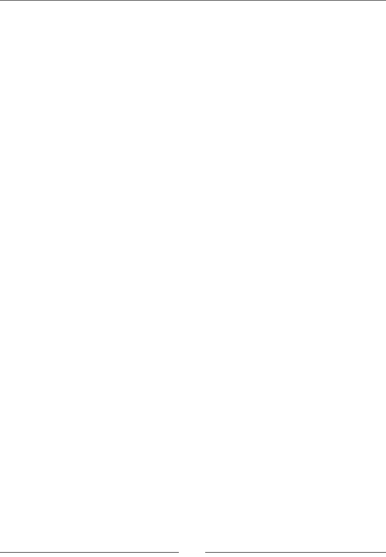
Concepts of Graph
[ 250 ]
@Override
public boolean isUndirected() {
return undirected;
}
@Override
public BinarySearchTree<Integer> getAllVertices() {
BinarySearchTree<Integer> allVertices = new RedBlackTree<>();
for(int i=0;i<vertices.length;i++){
if(vertices[i]!=null){
allVertices.insertValue(i);
}
}
return allVertices;
}
@Override
public int maxVertexID() {
return vertices.length-1;
}
}
Complexity of operations in an adjacency-list-based
graph
The following lists the complexities of the operations we have discussed in an
adjacency-list-based graph:
• Add vertex: Addition of a vertex requires that you create a new array first
and then copy all the vertices to it. So it is θ(|V|).
• Remove Vertex: The removal process does not change the array of the
vertices. However, this operation involves checking each vertex to remove
the edges which has the vertex being deleted as the target. So this operation
is θ(|V|) as well.
• Add edge and remove edge: The first step of this operation is to look up the
source vertex, which is constant time. The second step is to add or remove an
edge in a red black tree, so it is θ(lg |V|). So the entire operation of adding/
deleting an edge is θ(lg |V|).
• Adjacent: The first step of this operation is to look up the source vertex,
which is constant time. The second step is to look up the edge in a red black
tree, so it is θ(lg |V|). So the entire operation of adding/deleting an edge is
θ(lg |V|).

Chapter 10
[ 251 ]
• Neighbors: Since the list of neighbors is precomputed, the complexity is the
same as that for looking up a vertex, which is constant time.
• Setting and Getting values at vertices: These operations require looking up
the vertex first, which is constant time. The second step is setting/getting the
value. These operations are θ(1).
• Setting and Getting values at edges: These operations require looking up
the source vertex first and then looking up the particular edge. The first is
θ(1) and the second is θ(lg |V|). At the end, setting or getting the value of an
edge is θ(l). Hence, the total operation is θ(lg |V|).
• Get all vertices: This operation is θ( |V| lg |V| ), just like the previous
implementations.
Adjacency-list-based graph with dense
storage for vertices
Just as in the case of an adjacency-matrix-based graph, dense storage of vertices can
be done using a search tree instead of an array. This allows us to recover space when
we delete a vertex without affecting the IDs of the other vertices. Everything else
remains the same as the array-based storage of the vertices:
public class AdjacencyListGraphWithDenseVertex<V,E> implements
Graph<V,E> {
The nextId variable stores the value that would be the ID of the next vertex that
is inserted:
int nextId;
boolean undirected;
We have the Edge and Vertex class as before:
class Edge implements Comparable<Edge>{
E value;
int target;
DoublyLinkedList.DoublyLinkedNode<Integer> targetNode;
public Edge(int target) {
this.target = target;
}
@Override
public boolean equals(Object o) {
if (this == o) return true;

Concepts of Graph
[ 252 ]
if (o == null || getClass() != o.getClass())
return false;
Edge edge = (Edge) o;
return target == edge.target;
}
@Override
public int hashCode() {
return target;
}
@Override
public int compareTo(Edge o) {
return target - o.target;
}
}
class Vertex extends GraphVertex<V>{
RedBlackTree<Edge> edges = new RedBlackTree<Edge>();
DoublyLinkedList<Integer> neighbors
= new DoublyLinkedList<>();
public Vertex(int id, V value) {
super(id, value);
}
}
public AdjacencyListGraphWithDenseVertex(boolean undirected) {
this.undirected = undirected;
}
Now, instead of using an array to store the vertices, use a red black tree:
RedBlackTree<GraphVertex<V>> vertices = new RedBlackTree<>();
Adding a new vertex means inserting a new one in the red black tree:
@Override
public int addVertex() {
vertices.insertValue(new Vertex(nextId++, null));
return nextId;
}

Chapter 10
[ 253 ]
The removal process, as before, involves not only removing the vertex but also going
through all the other vertices and deleting every edge that has the vertex that is
being deleted as the target:
@Override
public void removeVertex(int id) {
vertices.deleteValue(new GraphVertex<V>(id, null));
vertices.traverseDepthFirstNonRecursive((gv)->{
BinaryTree.Node<Edge> edgeNode = ((
Vertex) gv).edges.deleteValue(new Edge(id));
if(edgeNode!=null){
Edge edge = edgeNode.getValue();
((Vertex) gv)
.neighbors.removeNode(edge.targetNode);
}
},
BinaryTree.DepthFirstTraversalType.INORDER);
}
The rst step is to nd the source and the target node to conrm that they exist.
After this, add an edge to the collection of edges of the source node. If the graph is
undirected, add an edge to the collection of edges in the target node as well:
@Override
public void addEdge(int source, int target) {
BinaryTree.Node<GraphVertex<V>> sNode =
vertices.searchValue(new GraphVertex<V>(source, null));
BinaryTree.Node<GraphVertex<V>> tNode =
vertices.searchValue(
new GraphVertex<V>(target, null));
if(sNode == null){
throw new IllegalArgumentException("Vertex ID "
+source+" does not exist");
}else if(tNode == null){
throw new IllegalArgumentException("Vertex ID "
+target+" does not exist");
}else{
Vertex sVertex = (Vertex) sNode.getValue();
Vertex tVertex = (Vertex) tNode.getValue();
Edge tEdge = new Edge(target);
sVertex.edges.insertValue(tEdge);
tEdge.targetNode = (DoublyLinkedList
.DoublyLinkedNode<Integer>) sVertex.neighbors
.appendLast(tVertex.getId());

Concepts of Graph
[ 254 ]
if(undirected) {
Edge sEdge = new Edge(source);
tVertex.edges.insertValue(sEdge);
sEdge.targetNode = (DoublyLinkedList
.DoublyLinkedNode<Integer>) tVertex.neighbors
.appendLast(sVertex.getId());
}
}
}
The rst step is the same as that of the previous one. After this, the edge is removed
from the collection of the edges of the source node. If the graph is undirected, the
edge is also removed from the collection of edges in the target node:
@Override
public void removeEdge(int source, int target) {
BinaryTree.Node<GraphVertex<V>> sNode =
vertices.searchValue(
new GraphVertex<V>(source, null));
BinaryTree.Node<GraphVertex<V>> tNode =
vertices.searchValue(
new GraphVertex<V>(target, null));
if(sNode == null){
throw new IllegalArgumentException("Vertex ID "
+source+" does not exist");
}else if(tNode == null){
throw new IllegalArgumentException("Vertex ID "
+target+" does not exist");
}else{
Vertex sVertex = (Vertex) sNode.getValue();
Edge deletedEdge = sVertex.edges.deleteValue(
new Edge(target)).getValue();
sVertex.neighbors.removeNode(deletedEdge.targetNode);
if(undirected) {
Vertex tVertex = (Vertex) tNode.getValue();
deletedEdge = tVertex.edges.deleteValue(
new Edge(source)).getValue();
tVertex.neighbors.removeNode(deletedEdge.targetNode);
}
}
}

Chapter 10
[ 255 ]
The rst step is the same as that of the previous one. After this, the edge with the
correct target is looked up. If the edge is found, the vertices are adjacent:
@Override
public boolean isAdjacent(int source, int target) {
BinaryTree.Node<GraphVertex<V>> sNode =
vertices.searchValue(
new GraphVertex<V>(source, null));
BinaryTree.Node<GraphVertex<V>> tNode =
vertices.searchValue(
new GraphVertex<V>(target, null));
if(sNode == null){
throw new IllegalArgumentException("Vertex ID "
+source+" does not exist");
}else if(tNode == null){
throw new IllegalArgumentException("Vertex ID "
+target+" does not exist");
}else{
Vertex sVertex = (Vertex) sNode.getValue();
return sVertex.edges.searchValue(
new Edge(target)) != null;
}
}
We just look up the vertex and then return our precomputed list of neighbors:
@Override
public LinkedList<Integer> getNeighbors(int source) {
BinaryTree.Node<GraphVertex<V>> sNode =
vertices.searchValue(
new GraphVertex<V>(source, null));
if(sNode == null){
throw new IllegalArgumentException(
"Vertex ID "+source+" does not exist");
}else{
Vertex sVertex = (Vertex) sNode.getValue();
return sVertex.neighbors;
}
}

Concepts of Graph
[ 256 ]
The process of setting and getting values is the same as before, except that we need
to look up the vertex/vertices in the red black tree instead of the array before setting
up the values:
@Override
public void setVertexValue(int vertex, V value) {
BinaryTree.Node<GraphVertex<V>> sNode =
vertices.searchValue(
new GraphVertex<V>(vertex, null));
if(sNode == null){
throw new IllegalArgumentException("Vertex ID "
+vertex+" does not exist");
}else{
Vertex sVertex = (Vertex) sNode.getValue();
sVertex.setValue(value);
}
}
@Override
public V getVertexValue(int vertex) {
BinaryTree.Node<GraphVertex<V>> sNode =
vertices.searchValue(
new GraphVertex<V>(vertex, null));
if(sNode == null){
throw new IllegalArgumentException("Vertex ID "
+vertex+" does not exist");
}else{
Vertex sVertex = (Vertex) sNode.getValue();
return sVertex.getValue();
}
}
@Override
public void setEdgeValue(int source, int target, E value) {
BinaryTree.Node<GraphVertex<V>> sNode =
vertices.searchValue(
new GraphVertex<V>(source, null));
BinaryTree.Node<GraphVertex<V>> tNode =
vertices.searchValue(
new GraphVertex<V>(target, null));
if(sNode == null){
throw new IllegalArgumentException("Vertex ID
"+source+" does not exist");
}else if(tNode == null){
throw new IllegalArgumentException("Vertex ID
"+target+" does not exist");

Chapter 10
[ 257 ]
}else{
Vertex sVertex = (Vertex) sNode.getValue();
BinaryTree.Node<Edge> edgeNode =
sVertex.edges.searchValue(new Edge(target));
if(edgeNode!=null) {
edgeNode.getValue().value = value;
if (undirected) {
Vertex tVertex = (Vertex) tNode.getValue();
edgeNode = tVertex.edges
.searchValue(new Edge(source));
edgeNode.getValue().value = value;
}
}else{
throw new IllegalArgumentException(
"No edge exists between the vertices "
+ source + " and " + target);
}
}
}
@Override
public E getEdgeValue(int source, int target) {
BinaryTree.Node<GraphVertex<V>> sNode =
vertices.searchValue(
new GraphVertex<V>(source, null));
BinaryTree.Node<GraphVertex<V>> tNode =
vertices.searchValue(
new GraphVertex<V>(target, null));
if(sNode == null){
throw new IllegalArgumentException("Vertex ID
"+source+" does not exist");
}else if(tNode == null){
throw new IllegalArgumentException("Vertex ID
"+target+" does not exist");
}else{
Vertex sVertex = (Vertex) sNode.getValue();
BinaryTree.Node<Edge> edgeNode =
sVertex.edges.searchValue(new Edge(target));
if(edgeNode!=null) {
return edgeNode.getValue().value;
}else{
throw new IllegalArgumentException(
"No edge exists between the vertices "
+ source + " and " + target);

Concepts of Graph
[ 258 ]
}
}
}
@Override
public boolean isUndirected() {
return undirected;
}
@Override
public BinarySearchTree<Integer> getAllVertices() {
BinarySearchTree<Integer> allVertices
= new RedBlackTree<>();
vertices.traverseDepthFirstNonRecursive(
(v) -> allVertices.insertValue(v.getId()),
BinaryTree.DepthFirstTraversalType.PREORDER);
return allVertices;
}
@Override
public int maxVertexID() {
return nextId -1;
}
}
Complexity of the operations of an adjacency-list-
based graph with dense storage for vertices
The complexity of the operations of an adjacency-list-based graph is as follows:
• Add vertex: Addition of a vertex requires insertion of one in the red black
tree. So this operation is θ(lg |V|).
• Remove Vertex: The removal process requires deletion of the vertex from the
red black tree, which is θ(lg |V|). However, this operation involves checking
each vertex to remove the edges which has the vertex being deleted as the
target. So this operation is θ(|V|) as well.
• Add edge and remove edge: The first step of this operation is to look up the
source vertex, which is θ(lg |V|). The second step is to add or remove an
edge to/from a red black tree, so this is also θ(lg |V|). Therefore, the entire
operation of adding/deleting an edge is θ(lg |V|).

Chapter 10
[ 259 ]
• Adjacent: The first step of this operation is to look up the source vertex,
which is θ(lg |V|). The second step is to look up the edge in a red black tree,
which is θ(lg |V|) too. Therefore, the entire operation of adding/deleting an
edge is θ(lg |V|).
• Neighbors: The list of neighbors is precomputed, so the complexity of this
operation is the same as that of searching a vertex, which is θ(lg |V|).
• Setting and getting values at vertices: These operations require you to first
look up the vertex, which is θ(lg |V|). The second step is to set/get the value.
These operations are θ(lg |V|).
• Setting and getting values at edges: These operations require you to
first look up the source vertex and then the particular edge. Both of these
operations are θ(lg |V|). At the end, setting or getting the value of an edge is
θ(l). Hence, the total operation is θ(lg |V|).
• Get all vertices: Here too, this operation is θ( |V| lg |V|).
Traversal of a graph
The traversal of a graph is the graph's equivalent of the traversal of a tree, as
discussed in an earlier chapter. Just as in the case of a tree, we can traverse either
breadth-rst or depth-rst. However, unlike a tree, a graph can reach all the vertices
without going through the edges. This makes it necessary to consider the traversal of
all the edges and vertices separately. Another thing is that a graph has no designated
root, so we can start from any particular vertex. Finally, since a graph may not be
connected, we may not be able to traverse all the vertices/edges, starting from one
single vertex. This is achieved by performing the traversal repeatedly, starting each
time from any vertex that has not been visited yet already. This is a simple extension
of the basic breadth-rst or depth-rst traversal that we are going to discuss here.
First, let's discuss visiting vertices using both the breadth-rst and depth-rst search.
It involves maintaining two collections of vertices: one that stores all the vertices that
are discovered but are yet to be visited/explored and another that stores a Boolean
array that checks whether a vertex has already been explored/visited.
The collection of vertices that are discovered but yet to be explored can be of two
types: if it is a stack, we have a depth-rst traversal, and if it is a queue, we have a
breadth-rst traversal.

Concepts of Graph
[ 260 ]
To implement both depth-rst and breadth-rst searches in a single method, we
need to create a super interface of our Stack and Queue interfaces. We will need to
dene three methods in it:
public interface OrderedStore<E> {
void insert(E value);
E pickFirst();
E checkFirst();
}
Now implement these methods in the Stack and Queue interfaces as default methods
to delegate to their appropriate methods:
public interface Stack<E> extends OrderedStore<E>{
void push(E value);
E pop();
E peek();
@Override
default E checkFirst(){
return peek();
}
@Override
default void insert(E value){
push(value);
}
@Override
default E pickFirst(){
return pop();
}
}
public interface Queue<E> extends OrderedStore<E>{
void enqueue(E value);
E dequeue();
E peek();
@Override
default E checkFirst(){
return peek();
}
@Override
default void insert(E value){
enqueue(value);

Chapter 10
[ 261 ]
}
@Override
default E pickFirst(){
return dequeue();
}
}
This allows us to use the OrderedStore interface to hold both a stack and a queue.
We also create a new functional interface that represents a lambda that takes two
arguments and does not return anything:
public interface TwoArgumentStatement<E,F> {
void doSomething(E e, F f);
}
We implement this search as a default method in the Graph interface itself.
enum TraversalType{
DFT, BFT
}
In the beginning, we only insert the starting vertex to the collection of vertices that
are not yet explored. Then, we loop until all the vertices that can be discovered in
the search are processed and there are no more elements in the collection of vertices.
We avoid processing each vertex from the collection of vertices if it has already been
processed. Otherwise, we mark it as "being processed" and invoke the visitor on
it. Finally, we expand this vertex by inserting all its neighbors to the collection of
elements that have to be processed:
default void visitAllConnectedVertices(int startingNode,
TwoArgumentStatement<Integer, V> visitor, TraversalType type) {
OrderedStore<Integer> toBeProcessed = null;
boolean doneProcessing[] = new boolean[maxVertexID()+1];
switch (type){
case BFT:
toBeProcessed = new QueueImplLinkedList<Integer>();
break;
case DFT:
toBeProcessed = new StackImplLinkedList<Integer>();
break;
}
toBeProcessed.insert(startingNode);

Concepts of Graph
[ 262 ]
while(toBeProcessed.checkFirst()!=null){
int currentVertex = toBeProcessed.pickFirst();
if(doneProcessing[currentVertex]){
continue;
}
doneProcessing[currentVertex] = true;
visitor.doSomething(currentVertex,
getVertexValue(currentVertex));
for(int neighbor:getNeighbors(currentVertex)){
if(doneProcessing[neighbor]==false){
toBeProcessed.insert(neighbor);
}
}
}
}
The process of traversal of edges is also very similar; we can follow either the
breadth-rst or depth-rst traversal. In this case, the visitor needs access to both the
source and target of the edges, which makes it necessary to store both of them in the
stack or queue we use. For this purpose, we create a class named Edge. The class is
comparable so that edges can be stored in a binary search tree for easy search ability:
class Edge implements Comparable<Edge>{
int source;
int target;
public Edge(int source, int target) {
this.source = source;
this.target = target;
}
@Override
public boolean equals(Object o) {
if (this == o) return true;
if (o == null || getClass() != o.getClass())
return false;
Edge edge = (Edge) o;
if (source != edge.source) return false;
return target == edge.target;

Chapter 10
[ 263 ]
}
@Override
public int hashCode() {
int result = source;
result = 31 * result + target;
return result;
}
@Override
public int compareTo(Edge o) {
if(source!=o.source){
return source - o.source;
}else {
return target - o.target;
}
}
}
Now we can implement the process of traversal of edges using the breadth-rst and
depth-rst traversal:
default void visitAllConnectedEdges(int startingNode,
ThreeArgumentStatement<Integer, Integer, E> visitor,
TraversalType type){
OrderedStore<Edge> toBeProcessed = null;
boolean doneProcessing[] = new boolean[maxVertexID()+1];
switch (type){
case BFT: toBeProcessed = new QueueImplLinkedList<Edge>();
break;
case DFT: toBeProcessed = new StackImplLinkedList<Edge>();
break;
}
toBeProcessed.insert(new Edge(-1, startingNode));
while (toBeProcessed.checkFirst()!=null){
Edge edge = toBeProcessed.pickFirst();
LinkedList<Integer> neighbors = getNeighbors(edge.target);
if(edge.source>=0) {
visitor.doSomething(edge.source, edge.target,
getEdgeValue(edge.source, edge.target));
}
if(doneProcessing[edge.target]){
continue;
}

Concepts of Graph
[ 264 ]
for(int target: neighbors){
if(isUndirected() && doneProcessing[target]){
continue;
}
Edge nextEdge = new Edge(edge.target, target);
if(nextEdge.target!=edge.source)
toBeProcessed.insert(nextEdge);
}
doneProcessing[edge.target] = true;
}
}
Complexity of traversals
For each traversal, either all vertices or edges, all edges must be traversed. This is
true even if you just want to visit the vertices. The actual complexity depends on the
particular map implementation, so we will use that the complexity of the operation
getNeighbors method is θ(g(|V|)).
If you're visiting either the edges or vertices, ensure that each vertex is expanded
only once. This operation is done |V| times, each of which is θ(g(|V|)). So
the complexity, due to the expansion of the vertex, to nd out the neighbors is
θ(|V|g(|V|)). When expanded, they are visited once, and for each edge, we have
one neighbor. Some of these neighbors have been visited before; however, we need
to perform constant time to verify this. So each vertex is visited once and each
neighbor is checked once. This changes the complexity to θ(|V|g(|V|) + |E| ). Since
we have seen an implementation of a graph that has the constant time getNeighbors
method, we can have a traversal in θ(|V| + |E| ).
Cycle detection
One of the uses of a traversal is cycle detection. A connected undirected graph
without any cycle is a tree. A directed graph without any cycle is called a directed
acyclic graph (DAG). Cycle detection in graphs can be done in a very similar manner.
In the case of an undirected graph, if we do a DFS and the same node is visited twice
as the target of an edge, there is a cycle. Since the edge is undirected, we are satised
if either the source or the target has not been seen before.

Chapter 10
[ 265 ]
In the case of a directed graph, visiting the same node twice is not enough if you
want to know whether there is a cycle; we should also consider the direction of the
edges. This means while traversing the edges, we need to know whether we can
reach the same node we started with. This requires us to remember the entire path
while doing a DFS. This is why we use a recursive helper method to detect a cycle
in a directed graph. We create the helper method for the directed cycle rst. The
checkDirectedCycleFromVertex method takes the path and binary search tree of
the vertices. The list of vertices is the one that stores all the vertices, and the ones
already visited must be removed so that they are not used as the starting point of
cycle detection later. The list of integers is the path from the starting point in a depth-
rst traversal. If a vertex is repeated in the same path, it means a cycle exists:
default void checkDirectedCycleFromVertex(
com.example.functional.LinkedList<Integer> path,
BinarySearchTree<Integer> allVertices){
The head of the list is the deepest vertex in the path; we need to expand this:
int top = path.head();
allVertices.deleteValue(top);
LinkedList<Integer> neighbors = getNeighbors(top);
Now if any neighbor is already present in the path, a cycle exists, which is what we
check. If a cycle is found, we throw an instance of a custom exception:
for(int n:neighbors){
com.example.functional.LinkedList<Integer>
pathPart = path;
while (!pathPart.isEmpty()){
int head = pathPart.head();
if(head == n){
throw new CycleDetectedException(
"Cycle detected");
}
pathPart = pathPart.tail();
}
checkDirectedCycleFromVertex(path.add(n), allVertices);
}
}

Concepts of Graph
[ 266 ]
Now we create the method for detection of cycles in either type of graph. Go through
all the vertices as there might be unconnected parts of the graph. A directed graph
may have connected vertices that cannot be reached from a particular starting vertex
due to the directionality of the edges. However, once a vertex is visited in any
traversal, it does not need to be visited again. This is taken care of by having all the
vertices in a binary search tree and removing the ones that have been visited already:
default boolean detectCycle(){
First, we get a list of all the vertices. We get it directly by understanding how the
vertices are stored inside the graphs:
BinarySearchTree<Integer> allVertices = getAllVertices();
try {
if (isUndirected()) {
while (allVertices.getRoot() != null) {
int start = allVertices.getRoot().getValue();
RedBlackTree<Integer> metAlready
= new RedBlackTree<>();
metAlready.insertValue(start);
allVertices.deleteValue(start);
visitAllConnectedEdges(start, (s, t, v) -> {
if(metAlready.searchValue(t) == null) {
metAlready.insertValue(t);
allVertices.deleteValue(t);
}else if(metAlready.searchValue(s)== null){
metAlready.insertValue(s);
allVertices.deleteValue(s);
}else{
throw new CycleDetectedException(
"found "+t);
}
}, TraversalType.DFT);
}
} else {
while (allVertices.getRoot() != null) {
checkDirectedCycleFromVertex(
com.example.functional.LinkedList
.<Integer>emptyList().add(allVertices
.getRoot().getValue()), allVertices);
}
}
}catch (CycleDetectedException ex){
return true;
}
return false;
}
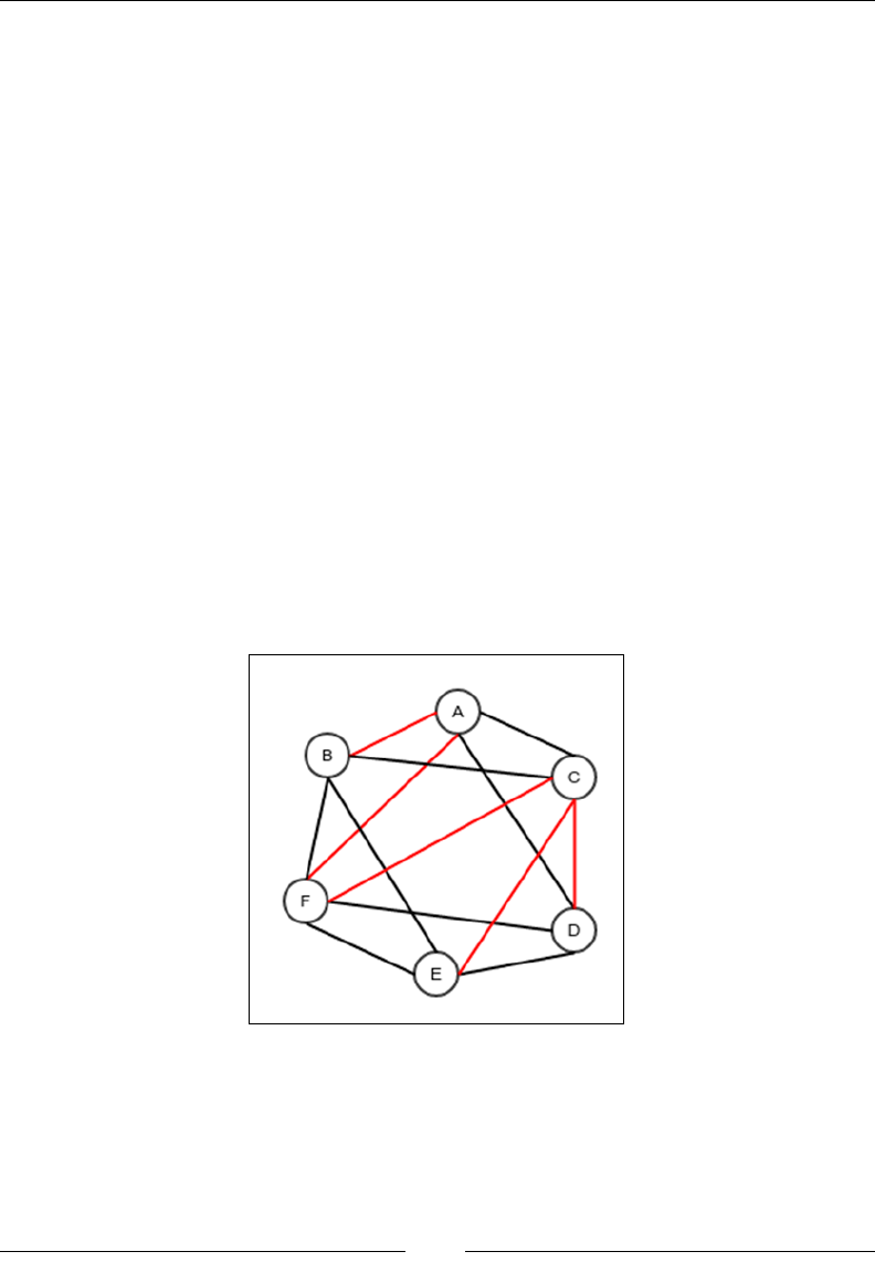
Chapter 10
[ 267 ]
Complexity of the cycle detection algorithm
First, let's check out the complexity of cycle detection in an undirected graph. The
complexity of getAllVertices is Ө(|V| lg |V|). Looking up a vertex in the search
tree of vertices that have already been visited is Ө( lg |V| ). We do this twice for
every edge. We also have to insert a new vertex in the metAlready search tree and
delete a vertex from the allVertices search tree; the complexity of these operations
for each edge is Ө( lg |V| ). So the total complexity is Ө(|E| lg |V| ).
Now let's consider the complexity of cycle detection in a directed graph. Here, we
traverse each edge once. However, for each edge, we have to look through the entire
path to know whether the current vertex is seen in the path. The path can potentially
be of this length: |V| - 1. So when we check it for each edge, the complexity is
O(|E||V|); this is a lot higher than O(|E|lg |V|).
Spanning tree and minimum
spanning tree
A spanning tree in a connected graph is a subgraph consisting of all the vertices and
some edges. So, a subgraph is a tree; it is a connected graph with no loops or cycles.
Figure 5 shows an example of a spanning tree in a graph:
Figure 5. A spanning tree of a graph (shown in red)

Concepts of Graph
[ 268 ]
A tree has minimum number of edges required to keep the vertices connected.
Removing any edge from a tree will disconnect the graph. This can be useful in
a map of roads that connect different places and has a minimal number of roads.
With this motivation, we would really be interested in a spanning tree that has a
minimum total length of roads. This may be important because constructing roads
is a costly affair. Alternatively, we could design a bus route map for a city and have
all the important places connected without creating too many routes; also, shorter
routes are better. Such a spanning tree is called a minimum spanning tree. Finding
a minimum spanning tree is an important problem. But before we discuss the
algorithm, let's see some of the properties of a minimum spanning tree.
For any tree with vertices V and edges
E, |V| = |E| + 1
First, let's consider this proposition: removing any edge from a tree will create two
trees with no connection between them. Let's assume the opposite. We have a graph
with two vertices A and B and an edge X between them. Let's assume that even if
we remove X, the tree still remains connected. This means a path P exists between A
and B even if you delete X. This means in the original graph, we can walk from A to
B through P and use X to come back to A. This means the original graph has a cycle.
But the original graph was assumed to be a tree, so this is impossible. Therefore, my
original proposition that removing any edge from the tree will create two trees with
no connection between them is true.
Now let's start with a graph G that has a set of edges E and vertices V. If we remove
all the edges, we would of course be left with only V. These set of vertices without
edges are actually single vertex trees with no connections between themselves.
We start with one tree, say G, and remove one edge. Now we have two trees. We
can now remove another edge, and this will split one of these trees into two so we
have three trees. This way, after the removal of each edge, we will have one more
tree. Therefore, after the removal of all the edges, we will have |E| + 1 trees (because
there was one tree before any edge was removed). These must be |V| single vertex
trees. So, it is either |V| = |E|+1 or |E| = |V| - 1.

Chapter 10
[ 269 ]
Any connected undirected graph has a
spanning tree
Let's take an undirected graph. If there are loops and cycles. First, we simply delete
all the loops. Consider A and B as two vertices that are neighbors and part of a
cycle. This means if we walk through the edge from A to B, we can use another path:
B to A (this is what makes it a cycle). So if we delete the B to A edge, we will still
have a connected graph. We do this operation for every cycle. At the end of these
operations, we will have a connected graph with no loops or cycles; this is a tree.
This tree connects all the vertices, so it is a spanning tree.
Any undirected connected graph with the
property |V| = |E| + 1 is a tree
Now let's check the reverse of the preceding theorem. Suppose there is a connected
graph where |V| = |E| + 1. We assume it is not a tree. This graph must have a
spanning tree, which is a subgraph, with fewer edges. This spanning tree will have
the same number of vertices (because we never deleted any vertices) but fewer
edges. Therefore, if the spanning tree has the set of edges E1, we have | E1|| < |E|
=> | E1|| + 1 < |E| + 1 => | E1|| + 1 < |V|. But this is not possible because the
new graph is a tree. So the original proposition that any undirected connected graph
with the property |V| = |E| +1 is a tree.
Cut property
Cut refers to a minimum set of edges that when removed would split a connected
undirected graph into two separate connected graphs with no connections between
them. There can be many cuts in a given graph.
The cut property can be dened as this: if an edge is an element of a cut and has a
minimum cost associated with it within the cut, it is part of the minimum spanning
tree of the graph. To check this out, rst note that for any cut of an undirected
connected graph, a spanning tree will always have exactly one member of the
cut in it.

Concepts of Graph
[ 270 ]
Let's have a cut X that divides the graph G into subgraphs H and J. Let G have a
spanning tree called S. Since G is a connected graph and X is a cut, this means H and
J are connected with each other. If X is empty, it means G was not connected; this is
not possible. Now we have the Y subset of X where all the members of Y are part of
the spanning tree S. If Y is empty, the vertices of H and J will be disconnected in S,
so this is impossible. Now as a contradiction to |Y| = 1, let's assume |Y| > 1. This
means there is more than one edge in S, between H and J. Let's pick two of them.
Let the rst is between vertex A in H and vertex B in J, and the second one between
vertex C in H and vertex D in J. Now since the spanning tree S has all the vertices of
H and J connected, there is a path from A to C and D to B in S outside of Y. So we
have a cycle from A to C and C to D using one of our selected edges and we have D
to B and B to A using the other selected edge. This means S has a cycle and hence S is
not a tree, which is a contradiction. Therefore, |Y| = 1. Thus, the spanning tree has
exactly one member of any cut in an undirected connected graph.
If S is the minimum spanning tree of G and X is a cut in G dividing G into H and
J, S has exactly one member for X, as proved in the preceding section. Let it be any
edge other than the one with minimum cost. Since S is a spanning tree, if we remove
the edge that is in X, we will have two disconnected subtrees, which are spanning
trees of H and J. If we insert any other edge from X now, this new edge will connect
these subtrees back to the single spanning tree. This is because all the edges of X are
between one vertex in H and another in J. So we can replace the edge in S that is a
member of X along with the edge in X with minimum cost, and we can thus create
another spanning tree of G. But the edges of the new tree will be the same as in S,
except the one that has a lesser cost than the one in S. So the sum of the costs of edges
of the new spanning tree must be lesser than that of S, which is a contradiction as S
is a minimum spanning tree. Therefore, the minimum spanning tree S must have an
edge with the least cost within the cut X.

Chapter 10
[ 271 ]
Minimum spanning tree is unique for a
graph that has all the edges whose costs are
different from one another
Let's assume that we have a connected undirected graph G for which there are two
different minimum spanning trees, namely S and T. Since S and T are different and
have the same number of edges (because for a spanning tree, the calculation is |V|
= |E| + 1), there is an edge E in S that is not in T. Let this edge be there between the
vertices A and B. Now let's create a partition of the set of vertices in G so that there
are two partitions: Y and Z. Create this such that A belongs to Y, B belongs to Z,
and Y and Z are disjointed and together contain all the vertices. Let X be the cut that
would divide G into two subgraphs with vertices in Y and Z. Since A belongs to Y
and B belongs to Z, the edge E between A and B belongs to X. Since X is a cut and S
is a spanning tree, there must be exactly one edge in X that is part of S; in this case, it
has to be the edge E. Now, since T is also a spanning tree and E is not a member of T,
there must be another member of X that is in T; let it be f.
If we remove the edge E from S, we will have two different trees, which would be
joined again if we insert f. This is because f is an edge between the vertices in Y and
Z, and the two parts are already trees. So now we are left with another spanning tree.
All the costs are different; the cost of E is different from the cost of f. If the cost of f
is lower than that of E, the total cost of the new spanning tree is lower than that of S.
Although, this is not possible because S is a minimum spanning tree. So, the cost of f
is higher than that of E.
We can do this for every edge in S that is not in T; S will transform into T when
no more edges are available. In every step of this process, the total cost of edges
will increase. This means the total cost of edges in T must be higher than that in S.
However, this is impossible because S and T are both minimum spanning trees. So
our original assumption that there can be two different minimum spanning trees is
wrong. Therefore, each minimum spanning tree is unique in a graph where all the
costs of the edges are different.

Concepts of Graph
[ 272 ]
Finding the minimum spanning tree
With the properties we just discussed, we can now dene an algorithm for nding
the minimum spanning tree of a graph. Suppose a set of edges F is already given
and they are members of the minimum spanning tree G. Now we are trying to nd
another edge that is also a member of the minimum spanning tree. First, we choose
an edge e whose cost is minimum when compared to the rest of the edges, E and F in
this case. Since some of the edges are already given, some of the vertices are already
connected. If the chosen edge e is between two vertices that are already connected, we
simply reject this edge and nd the next edge with minimum cost. We do this until
we nd an edge f between two vertices that are not already connected. Our claim is
that f is a new member of the minimum spanning tree. To conrm this, let's assume
that f is between the vertices A and B. From the description of our procedure, A and
B are not connected. Let's make two partitions of the vertices: H and J. Let's have all
the vertices that are connected to A, including A in H, and all the vertices connected
to B, including B in J. The rest of the vertices are assigned to the set H. Since H and J
are partitions of the vertices in the original graph G, we have a cut X in the original
graph G that splits the graph G in a way that all the vertices in H are placed in one
of the subgraphs and all the vertices in J in the other. We know that the member of
X that has the minimum cost is a member of the minimum spanning tree G. Now, of
course, f is a member of X as it connects A to B. It is also the edge with the minimum
cost among all the edges in X. This is because all the edges in X are in the remaining
edges (otherwise some vertices in H and some in J would be connected, which cannot
be true because of the way we have created the two sets), and f is the minimum
cost in all the remaining edges. This means f is a new member of the spanning tree.
Therefore, we use the following steps to build the minimum spanning tree:
1. Start with an empty set of edges as the spanning tree.
2. If more edges are remaining and all the vertices are not connected, choose the
one with the minimum cost.
3. If the edge is between two connected vertices, discard it and go back to
step 2.
4. Otherwise, add the edge to the set of edges of the minimum spanning tree.
5. Repeat from step 1.
The problem now is how to efciently know whether the two vertices are connected.
The solution is a data structure called a union set forest.

Chapter 10
[ 273 ]
Union nd
The purpose of union nd is to be able to tell whether the two given objects are
members of the same set. This data structure allows you to rst specify all the
members of a universal set and then specify which ones are members of the same
partition, thus joining the two partitions to make a single partition. It represents
a collection of partitions of the universal set, and it lets us query whether the two
members of the universal set are members of the same partition.
A tree is kept in an opposite pointer form, that is, the child knows its parent;
however, the parent does not have any pointers to the children. The idea is to have
connected values in the same tree. Each tree in a forest has a representative node
that is its root. If two nodes have the same representative roots, they are in the same
partition; otherwise, they are not.
This data structure has three important operations:
• Add a new object to the universal set.
• Union two objects: This will result in the partitions those objects belong to
joining together to make a single partition.
• Find: This will return the representative object of the partition that the object
passed belongs to. If the result of the find operations of two different objects
is the same, the object would belong to the same partition.
The following is an implementation of a Union nd that can hold comparable objects:
public class UnionFind<E extends Comparable<E>> {
Each node holds a reference to its parent. If there is no parent, that is, if the node is
the root of its tree, the parent is null. All nodes also store its rank, which is the height
of the tree rooted by itself:
private class Node implements Comparable<Node>{
Node parent;
E object;
int rank;
public Node(E object) {
this.object = object;
rank = 0;
}
@Override

Concepts of Graph
[ 274 ]
public int compareTo(Node o) {
return object.compareTo(o.object);
}
}
All the nodes are stored in a red black tree so they have a logarithmic search:
BinarySearchTree<Node> allNodes = new RedBlackTree<>();
Additionally, we want to keep a count of the number of partitions available:
int partitionCount;
The add operation adds a new object to the universal set, which is implemented
using a red black tree:
public void add(E object){
Node n = new Node(object);
allNodes.insertValue(n);
partitionCount++;
}
This is an internal method that traverses the parents one by one until it nds the root
of the tree that the object passed belongs to:
Node findRoot(Node n){
if(n.parent==null){
return n;
}else{
return findRoot(n.parent);
}
}
Chapter 10
[ 275 ]
Figure 6. Union operation in a union find forest. The partitions it represents are shown on the side.

Concepts of Graph
[ 276 ]
The union operation merges two trees. This is achieved by setting one of the roots
of the two trees as the parent of the root of the other tree. When merging two trees
of unequal height, the root of the taller tree is set as the parent of the root of the
shorter tree; otherwise, any one of the two is chosen as the root. The rank of the root
increases only when two equal trees are merged. When unequal trees are merged,
the height of the merged tree is the same as the height of the taller tree. Figure 6
shows the union operation:
public void union(E o1, E o2){
BinaryTree.Node<Node> node1 = allNodes.searchValue(
new Node(o1));
BinaryTree.Node<Node> node2 = allNodes.searchValue(
new Node(o2));
if(node1==null || node2==null){
throw new IllegalArgumentException("Objects not found");
}
Node n1 = node1.getValue();
Node n2 = node2.getValue();
Node p1 = findRoot(n1);
Node p2 = findRoot(n2);
if(p1==p2){
return;
}
int r1 = n1.rank;
int r2 = n2.rank;
if(r1>r2){
p2.parent = p1;
}else if(r2>r1){
p1.parent = p2;
}else{
p2.parent = p1;
p1.rank++;
}
partitionCount--;
}
The find operation involves looking up the node related to the object rst and then
nding the root node. The object contained in the root node is returned:
public E find(E object){
BinaryTree.Node<Node> node1 = allNodes.searchValue(
new Node(object));
if(node1==null){
throw new IllegalArgumentException("Objects not found");
}
Node n = node1.getValue();
return findRoot(n).object;
}
}

Chapter 10
[ 277 ]
Complexity of operations in UnionFind
First, let's consider the complexity of nding the root node of any node; this is an
internal operation. The complexity of this operation is θ(h), where h is the height
of the tree. Now what is the upper bound of the height of the tree? Let f(h) be the
minimum number of nodes in a tree of height h. Trees are always created by merging
two smaller trees. If the trees being merged have unequal heights, the height of the
merged tree is the same as the taller of the two initial trees, and now it has more nodes
than the original taller tree. This is not the way to create the worst tree, which is the
tree with minimum nodes with the same height. The worst tree must be created by
merging two equal trees, both of which are worst trees themselves. After you merge
them, the height of the merged tree is one more than the height of either of the trees
being merged. So, for creating a worst tree of height h+1, we must merge two worst
trees of height h. The operation to do this is f(h+1) = 2 f(h). So, if f(0) = C, where C is
some constant, f(1) = 2C, f(2)=4C, … , f(h) = 2h C. Therefore, if the number of nodes is
n, then n ≥ f(h) = 2h C => lg n ≥ lg (2h C) = h + lg C => h ≤ lg n – lg C => h = O(lg n). This
means the complexity of nding the root of a given node is also O(lg n).
• Adding a new object involves inserting a new node in the red black tree, so
the complexity is θ(lg n).
• Find: This operation involves looking up the node that corresponds to the
object first. This is a search operation in the red black tree; hence it is θ(lg n).
After this, it involves looking up the root of this node, which is O(lg n). And
at the end, we return the object in the node, which is constant time. Hence,
the complexity of the entire find operation is θ(lg n).
• Union involves three operations. The first is to search the nodes for the
objects, which is θ(lg n). The second is to find the roots of each of the trees
associated with the nodes, which is also O(lg n). And finally, it involves the
merging of the trees, which is a constant time operation. So the complexity of
the entire operation is θ(lg n).
Implementation of the minimum spanning tree
algorithm
Now we can implement our minimum spanning tree algorithm. First, we create a class
that we will use for the implantation. The CostEdge class represents an edge along
with its cost. The compareTo method is overridden to compare the costs instead of IDs:
class CostEdge extends Edge{
Integer cost;
public CostEdge(int source, int target, int cost) {

Concepts of Graph
[ 278 ]
super(source, target);
this.cost = cost;
}
@Override
public int compareTo(Edge o) {
return cost - ((CostEdge)o).cost;
}
}
The argument costFinder is a lambda that returns the cost of an edge from the value
that is stored in it. edgeQueue is a priority queue that lets us consider the edges in the
order of their costs. We can dequeue the edge with the minimum cost every time, as
our algorithm requires. The purpose of unionFind is to keep track of which vertices
are connected after some edges are already chosen. First, we traverse through all
the edges and enqueue them to the priority queue, then we traverse through all the
vertices to add them to unionFind. After this, as described in our algorithm, we pick
the edges in the order of their costs and add them only when they are not between the
vertices that are already connected. The unionFind keeps track of which vertices are
connected. The edges of the spanning tree are returned in a linked list:
default LinkedList<Edge> minimumSpanningTree(OneArgumentExpression<E,I
nteger> costFinder){
if(!isUndirected()){
throw new IllegalStateException(
"Spanning tree only applicable to undirected trees");
}
LinkedList<Edge> subGraph = new LinkedList<>();
PriorityQueue<CostEdge> edgeQueue = new
LinkedHeap<>((x, y)->x.compareTo(y));
UnionFind<Integer> unionFind = new UnionFind<>();
this.visitAllConnectedEdges(getAllVertices()
.getRoot().getValue(), (s,t,v)-> edgeQueue.enqueue(
new CostEdge(s,t,costFinder.compute(v))),
TraversalType.DFT);
this.getAllVertices().traverseDepthFirstNonRecursive(
(x)->unionFind.add(x),
BinaryTree.DepthFirstTraversalType.PREORDER);

Chapter 10
[ 279 ]
while((unionFind.getPartitionCount()>1
&& edgeQueue.checkMinimum()!=null){
Edge e = edgeQueue.dequeueMinimum();
int sGroup = unionFind.find(e.source);
int tGroup = unionFind.find(e.target);
if(sGroup!=tGroup){
subGraph.appendLast(e);
unionFind.union(e.source, e.target);
}
}
return subGraph;
}
Complexity of the minimum spanning tree
algorithm
Visiting all the edges and adding them to the priority queue can be as low as Ө(|V|
+ |E| + |E| lg |E|) because traversing through the edges is Ө(|V| + |E| ) and
adding all of them to the priority queue is Ө(|E| lg |E|). Since a connected graph
has |E| ≥|V| -1, Ө(|V| + |E| + |E| lg |E|) = Ө(|E| lg |E|). Inserting all the
vertices to the union nd is done through Ө(|V| lg |V|) because adding each vertex
has the complexity Ө(lg |V|).
Now let's consider the core of the algorithm. For each edge, dequeueing the
minimum edge is Ө(lg |E|), nding each of the source and the target in unionFind
is Ө(lg |V|), adding to the linked list is constant time, and doing a union on union
find is Ө(lg |V|). So, for each edge, the complexity is Ө(lg |V| + lg |E|). This is
Ө(lg |E|) for each edge, as |E| ≥|V| -1. Therefore, the complexity of the core part is
Ө(|V| lg |E|) because we stop after |V| - 1 number of edges are added and all the
vertices are already connected.
Adding the complexity of all the preceding steps, we get the total complexity of the
minimum spanning tree algorithm as Ө(|E| lg |E|) + Ө(lg |V|) + Ө(|V| lg |E|) =
Ө(|E| lg |E| + |V| lg |V|) = Ө(|E| lg |E| ) as |E| ≥|V| -1.
This algorithm is called Kruskal's algorithm, invented by Joseph Kruskal. Kruskal's
algorithm works with the complexity Ө(|V| lg |E| ) if a sorted list of edges is
already available. Since we have checked until all the edges are processed, if a graph
is passed that is not connected, it will give a set of minimum spanning trees, one for
each connected subgraph.

Concepts of Graph
[ 280 ]
Summary
In this chapter, we saw what a graph is and some real-world scenarios where they
can be applicable. We saw a few ways of implementing a graph data structure in
memory. We then studied ways to traverse a graph, in both BFT and DFT. We used
traversals to detect cycles in a graph. Finally, we saw what spanning trees are, what
minimum spanning trees are, and how to nd them in a graph.
In the next chapter, we will drift a bit to explore a simple and elegant way of
implementing some concurrent programming, called reactive programming.
[ 281 ]
Reactive Programming
This chapter is a little detour to reactive programming. It lets us handle the
concurrency requirements of an application in some cases. It provides an abstraction
to handle concurrency. Even though the concepts are old, it has gained interest in
recent years due to the beginning of large inow of data. In modern times, billions
of devices generate data every day. Tapping into this data is essential for the growth
of business; in some cases, processing the data to statistically analyze it or feeding it
to some machine learning algorithm may be the entire business in itself. This makes
it essential to support the processing of this large in-ow of data, provide a quick
response, and be resilient to failures. Of course, one can do these things even using
a traditional or imperative programming paradigm, just as one can, in theory, build
any application using an assembly language. However, this makes the application
extremely complex to maintain and impossible to modify according to business
needs. In this chapter, we will discuss the following topics:
• Basic idea of reactive programming
• Building an example reactive framework
• Building example programs using our framework

Reactive Programming
[ 282 ]
What is reactive programming?
Suppose we have a web server that lets us query some data or save it. This web
server serves multiple requests at the same time, and each request is a short task that
involves some computation. What is the usual way of achieving this? Well, the naive
way would be to spawn a new thread for each request. But one can easily realize
that this leads to an explosion in the number of threads in the application. Plus, the
creation and deletion of threads are heavyweight activities; they slow down the
entire application.
Next, you can use a thread pool so the same threads can be used over and over to
avoid the overhead of creation and deletion of threads. However, if you want to
serve thousands of requests at the same time, this will require a thread pool with
thousands of threads. Thread scheduling in an operating system is complex and
involves a lot of logic, including priority and so on. Operating systems do not expect
threads to just run short bursts of computation; they are not optimized that way.
Therefore, the solution is to use the same thread for multiple simultaneous requests.
This can, in general, be done if we stop blocking for IO and use the same thread for
another task when one task is waiting for I/O. Managing these things, however,
is extremely complicated. Hence, we would need a framework to carry out these
activities for us. Such a framework can be called a reactive framework.
Reactive programming takes care of the following:
• Scalability: This property is the capability of the application to cater to
proportional number of requests as the number of available resources
increases. If one processor serves 500 requests per second, two processors
should do 1,000.
• Responsiveness: We want the application to be responsive; for example, it
should show a status when it is computing some result or fetching it from
some other place.
• Resilience: Since we use the same thread for multiple tasks, handling errors
is more complicated than usual. How do we let the user know of an error?
So instead of propagating the exceptions back down the call stack, we move
forward and explicitly tackle the error situations.
There are different techniques for using reactive programming; it depends on the
actual problem we are trying to solve. We will not discuss all of them but will focus
on the commonly used ones.

Chapter 11
[ 283 ]
Producer-consumer model
A producer-consumer model is a design that divides processing into small
components that send messages to other components. One produces a message and
the other consumes and acts on it. It provides an abstraction to easily implement an
application optimized to utilize all the resources. A producer-consumer model starts
with a queue of messages. Producers publish messages in this queue and consumers
receive them. This queue is different from the queues we have studied so far in a
few ways. We want this queue to be thread-safe, which is required for the queue to
work correctly in a multithreaded environment. We do not need to worry about the
exact order of the messages being dequeued. After all, the order of messages does
not matter when they are being received by different threads. In these conditions, we
optimize the delivery of the messages. Before implementing this queue, let's discuss
a few thread synchronization techniques beyond what we have learned so far using
the synchronized keyword. These techniques are required for more optimal usage of
resources while maintaining the correctness of the program.
Semaphore
A semaphore is a special variable that lets us limit the number of threads that can
use a particular resource. The following code shows an example of a semaphore that
gives us a thread-safe counter:
public class SemaphoreExample {
volatile int threadSafeInt = 0;
Semaphore semaphore = new Semaphore(1);
public int incremementAndGet() throws InterruptedException{
semaphore.acquire();
int previousValue = threadSafeInt++;
semaphore.release();
return previousValue;
}
}
Here, the semaphore has been initialized to 1, which means it will allow only
one thread to acquire it. No other thread can acquire it until it is released. Unlike
synchronization, there is no requirement here that the same thread has to call the
release method that had acquired it, which makes it particularly exible.
A call to the acquire method of a semaphore will be blocked until it successfully
acquires it. This means that the calling thread will be taken off the thread scheduler
and put aside in such a way that the operating system's thread scheduler will not
be able to see it. Once the semaphore is ready to be acquired, this thread will be put
back in place for the thread scheduler to see it.
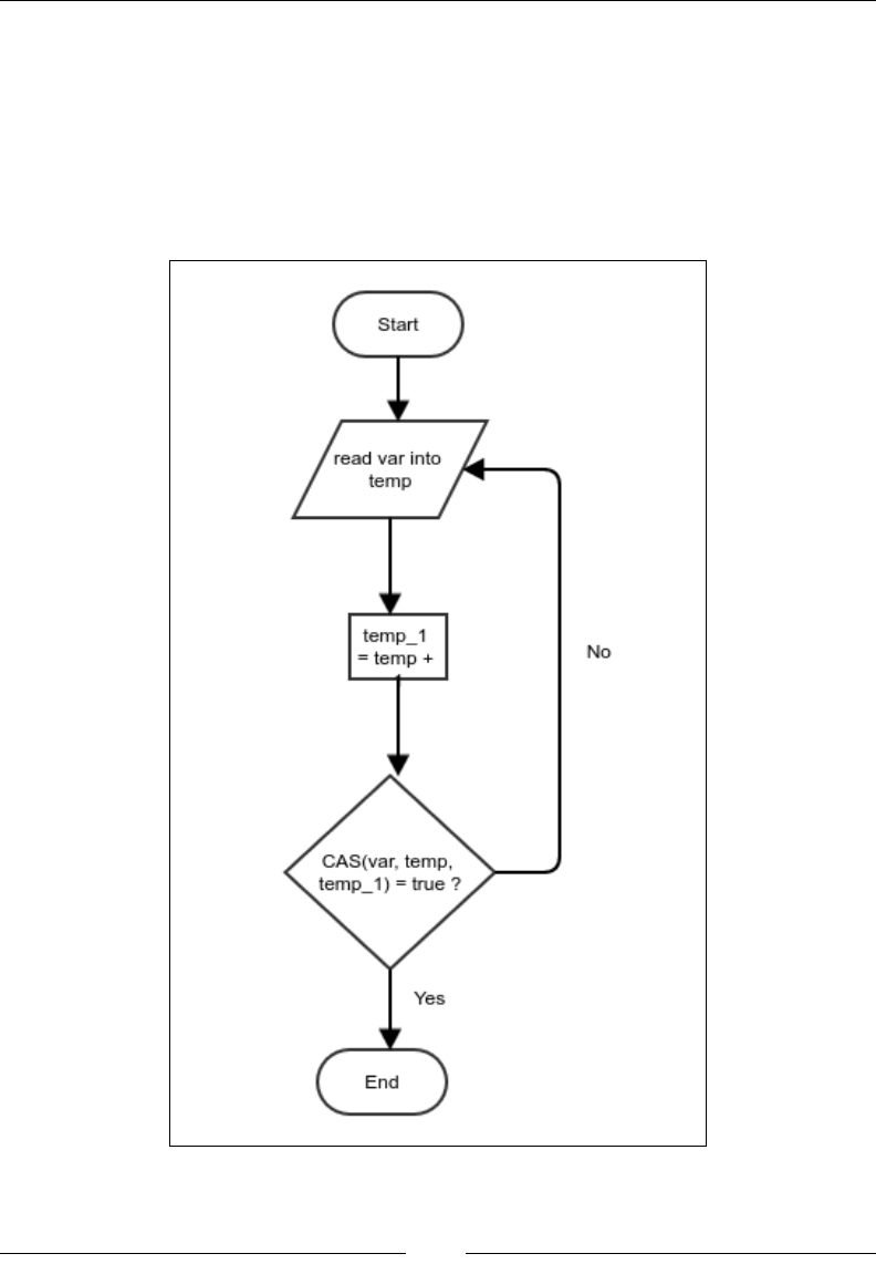
Reactive Programming
[ 284 ]
Compare and set
Compare and set is an atomic operation that lets you update the value of a variable
if and only if the existing value matches a specic value. This enables us to update
a variable based on its previous value. The CAS operation returns a Boolean. If the
comparison is a match, which means the set operation is successful, it returns true;
otherwise, it returns false. The idea is to keep trying until this set operation is
successful. The following diagram shows the basic strategy:
Figure 1: Atomic update using the compare and set operation

Chapter 11
[ 285 ]
In Figure 1, we are trying to increment the value of the shared variable var. The
operation requires us to read the value in a thread-specic temporary location, then
increment the temporary value and reassign it to the shared variable. However,
this operation can cause problems if there are multiple threads trying to perform
the update simultaneously. It can happen that both the threads read the value
simultaneously in order to get the same temp value. Both these threads can update
the shared variable with the incremented value. This will increment the value only
once, but it should have actually caused two increments. To avoid this, we check
whether the value of var is still the same and update only when it is so; otherwise,
we read the value of var again and repeat the process. Since this compare and set
operation is atomic, it guarantees that no increments will be lost. The following is the
Java code that does the exact same thing:
public class ThreadSafeCounter {
AtomicInteger counter;
public int incrementAndGet(){
while (true){
int value = counter.get();
if(counter.compareAndSet(value, value+1)){
return value;
}
}
}
}
To use any atomic operation, we need to use classes from the java.util.
concurrent.atomic package. AtomicInteger is a class that encapsulates an integer
and enables the compareAndSet operation on it. There are other utility methods as
well. In particular, it has methods to perform atomic increments and decrements, just
like the one we have implemented here.
Volatile eld
Suppose we have a eld that is being written to and read from multiple threads. If
all the threads run on the same single CPU, the writes can simply happen on the
CPU cache; they need not be synced to the main memory often. This would not be
a problem as the value could also be read from the same cache. However, multiple
CPUs can have their own caches, and in such a case, a write to a cache from one CPU
will not be visible from another thread running on a different CPU. Most programs
accept this and work accordingly. Java, for example, maintains a separate copy of a
shared variable for each thread, which is occasionally synced. If we, however, want
to mandate that the writes from one thread should be visible from another thread,
we need to declare the eld volatile. All elds involved in atomic operations are
declared volatile.

Reactive Programming
[ 286 ]
Thread-safe blocking queue
Now we are ready to implement our thread-safe blocking queue. Thread-safe means
that multiple threads can share the same queue; blocking means that if a thread tries
to dequeue an element and the queue is currently empty, the call to dequeue will be
blocked until some other thread enqueues an element. Similarly, if a thread tries to
enqueue a new element and the queue is full, the call to the queue will be blocked
until another thread dequeues an element and frees some space.
Our queue will store elements in a xed length array and maintain two counters
that would store the next index for queuing and dequeuing. Two semaphores block
threads when the queue is either empty or full. Along with this, each array position
is provided with two semaphores that ensure that enqueuing and dequeuing
operations do not overwrite or repeat any elements. It does this by ensuring that
once a new element is enqueued in a particular position, it is not overwriten before
it is dequeued. Similarly, once a particular array index is dequeued, it is never
dequeued again before another enqueue stores another element in it:
public class ThreadSafeFixedLengthBlockingQueue<E> {
The underflowSemaphore ensures that dequeues are blocked when the queue
is empty, and overflowSemaphore ensures that enqueues are blocked when the
queue is full:
Semaphore underflowSemaphore;
Semaphore overflowSemaphore;
AtomicInteger nextEnqueueIndex;
AtomicInteger nextDequeueIndex;
The array store is the space that holds the elements:
E[] store;
Both enqueueLocks and dequeueLocks are individual position-based locks that
allow only a dequeue after an enqueue and vice versa:
Semaphore [] enqueueLocks;
Semaphore [] dequeueLocks;
int length;
The alive ag can be used by the dequeuing threads to know when they can stop
running, and no more elements would be expected. This ag needs to be set by the
enqueuing threads:
boolean alive = true;

Chapter 11
[ 287 ]
All initializations are pretty much self-evident:
public ThreadSafeFixedLengthBlockingQueue(int length){
this.length = length;
store = (E[]) new Object[length];
nextEnqueueIndex = new AtomicInteger();
nextDequeueIndex = new AtomicInteger();
underflowSemaphore = new Semaphore(length);
overflowSemaphore = new Semaphore(length);
underflowSemaphore.acquireUninterruptibly(length);
enqueueLocks = new Semaphore[length];
dequeueLocks = new Semaphore[length];
for(int i=0;i<length;i++){
enqueueLocks[i] = new Semaphore(1);
dequeueLocks[i] = new Semaphore(1);
dequeueLocks[i].acquireUninterruptibly();
}
}
The enqueue operation rst makes sure that the queue is not full by acquiring
overflowSemaphore:
public void enqueue(E value) throws InterruptedException {
overflowSemaphore.acquire();
The nextEnqueueIndex is then incremented and the previous value is returned,
which is then used to compute the index in the array where the element would
be stored. The seemingly complicated expression ensures that the index rolls over
properly even after the nextEnqueueIndex integer rolls over, provided the length of
the queue is an integer power of 2:
int index = (length + nextEnqueueIndex.getAndIncrement()
% length)
% length;
Once the index is selected, we must acquire an enqueue lock on the position, store
the value, and then release the dequeue lock to mark this position as ready for
dequeuing. At the end, we release one count on underflowSemaphore to mark the
fact that there is one more element in the queue to be dequeued:
enqueueLocks[index].acquire();
store[index] = value;
dequeueLocks[index].release();
underflowSemaphore.release();
}

Reactive Programming
[ 288 ]
The dequeue operation is very similar to the enqueue operation, just the role of the
semaphores are reversed. There is slightly more complicated code before the actual
operation starts. This is to enable the dequeuing threads to quit when no more
elements are available:
public E dequeue() throws InterruptedException {
Instead of directly acquiring underflowSemaphore, we use tryAcquire, which
will wake up the thread after 1 second if there are no elements are available to be
dequeued. This gives us a chance to check the value of the alive Boolean ag and
quit the dequeue operation in case it is no longer alive. If the queue is no longer
alive, we interrupt the current thread and exit. Otherwise, we compute the index and
dequeue the element to the enqueue operation in a similar manner:
while (alive && !underflowSemaphore.tryAcquire(1,
TimeUnit.SECONDS));
if(!alive){
Thread.currentThread().interrupt();
}
int index = (length + nextDequeueIndex.getAndIncrement()
% length)
% length;
dequeueLocks[index].acquire();
E value = store[index];
enqueueLocks[index].release();
overflowSemaphore.release();
return value;
}
This is a utility method to return the current number of elements in the queue.
This is useful for knowing when to kill the queue (set the alive ag to false) in a
producer-consumer setup:
public int currentElementCount(){
return underflowSemaphore.availablePermits();
}
public void killDequeuers(){
alive = false;
}
}

Chapter 11
[ 289 ]
Producer-consumer implementation
We can now implement a producer-consumer setup using the queue we have created.
In simple words, the producer-consumer queue is a queue of events that the producers
produce and the consumers consume. There are three kinds of events. The INVOCATION
type refers to the regular events that propagate processing. The ERROR type event is
raised when an exception needs to be propagated. The COMPLETION event is produced
when it is required that the dequeue threads need to be terminated and the queue
needs to be closed. The ProcerConsumer queue takes Consumer as input:
public interface Consumer<E> {
void onMessage(E message);
default void onError(Exception error){
error.printStackTrace();
}
default void onComplete(){
}
}
public class ProducerConsumerQueue<E> {
enum EventType{
INVOCATION, ERROR, COMPLETION
}
The Event class represents single events. Depending on the type, it can have a value
or exception:
class Event{
E value;
Exception error;
EventType eventType;
}
ThreadSafeFixedLengthBlockingQueue<Event> queue;
boolean alive = true;
Thread [] threads;
The constructor of ProducerConsuerQueue creates consumer threads. It also takes
consumer code as input. The consumer must implement the Consumer interface:
public ProducerConsumerQueue(int bufferSize, int threadCount,
Consumer<E> consumer){
queue = new ThreadSafeFixedLengthBlockingQueue<>(bufferSize);
threads = new Thread[threadCount];

Reactive Programming
[ 290 ]
The consumer thread runs code that dequeues events and calls the methods on
consumerCode as per the event type in the loop. The loop ends when the termination
event is received and no more events are there in the queue to be processed:
Runnable consumerCode = ()->{
try{
while(alive || queue.currentElementCount()>0){
Event e = queue.dequeue();
switch (e.eventType) {
case INVOCATION:
consumer.onMessage(e.value);
break;
case ERROR:
consumer.onError(e.error);
break;
case COMPLETION:
alive = false;
consumer.onComplete();
}
}
} catch (InterruptedException e) {
} finally{
}
};
Consumer threads are spawned:
for(int i=0;i<threadCount;i++) {
threads[i] = new Thread(consumerCode);
threads[i].start();
}
}
The produce method is invoked from a producer thread. Notice that the queue does
not manage producer threads; they need to be managed separately:
public void produce(E value) throws InterruptedException {
Event event = new Event();
event.value = value;
event.eventType = EventType.INVOCATION;
queue.enqueue(event);
}

Chapter 11
[ 291 ]
Once a producer thread marks the stream of events to be completed, no more new
events could be generated and the dequeuing threads will be terminated after they
process all the events:
public void markCompleted() throws InterruptedException {
Event event = new Event();
event.eventType = EventType.COMPLETION;
queue.enqueue(event);
}
This is to propagate an exception:
public void sendError(Exception ex) throws InterruptedException {
Event event = new Event();
event.error = ex;
event.eventType = EventType.ERROR;
queue.enqueue(event);
}
If we need to wait for all the dequeuing threads to terminate, we use this:
public void joinThreads() throws InterruptedException {
for(Thread t: threads){
t.join();
}
}
}
To see how to use this producer-consumer queue to actually solve a problem, we will
consider a dummy problem. We will work on a le—com-orkut.ungraph.txt—that
is open to public and contains all the friendships between users in Orkut, which
was a social networking site in the past. The le can be downloaded from https://
snap.stanford.edu/data/bigdata/communities/com-orkut.ungraph.txt.
gz. To protect privacy, all the users are simply referenced by some arbitrary ID and
the mapping with the actual users is not shared. We will also use another le called
ulist that would contain the list of user IDs we are interested in. Our task is to nd
the number of friends that each user in the second le has. The following commands
show how the two les look:
$ head com-orkut.ungraph.txt
1 2
1 3
1 4
1 5
1 6

Reactive Programming
[ 292 ]
1 7
1 8
1 9
1 10
1 11
$ head ulist
2508972
1081826
2022585
141678
709419
877187
1592426
1013109
1490560
623595
Each line in com-orkut.ungraph.txt has two IDs that are separated by a
whitespace. The meaning is that there is friendship between these two users. It
is given that each friendship is mentioned only once in the le and is undirected.
Note that this means each line should increase the friend count for both the IDs.
Each line in ulist has a single ID. All IDs are unique, and we must nd the friend
count of each of these IDs. Note that some of these have no friends and thus are not
mentioned in com-orkut.ungraph.txt.
We will rst create a utility class that will let us read integer IDs from the les. The
purpose of this class is to read integer values from any text le so that not too many
objects are created in the process. This is just to reduce garbage collection to some
extent. In this case, we used le-channel-based logic that uses ByteBuffer as a buffer:
public class FileReader {
ByteBuffer buf= ByteBuffer.allocate(65536);
FileChannel channel;
The readCount variable keeps track of how many characters are left in the buffer:
int readCount = 0;
public FileReader(String filename) throws FileNotFoundException {
channel = new FileInputStream(filename).getChannel();
buf.clear();
}

Chapter 11
[ 293 ]
To read an int, keep reading the bytes in a loop until you hit a byte that is not a digit.
In the meantime, keep computing the integer that the string of characters represents:
public int readIntFromText() throws IOException {
int value = 0;
while(true){
First check whether the buffer is empty; if yes, rell it by reading from the le:
if(readCount<=0){
buf.clear();
readCount = channel.read(buf);
If no more bytes are available in the le, don't care to ip the buffer:
if(readCount<0){
break;
}
buf.flip();
}
We read a byte and decrement readCount because now the buffer has one less byte:
byte nextChar = buf.get();
readCount--;
If the character is a digit, keep computing the integer; otherwise, break the loop and
return the calculated integer value:
if(nextChar>='0' && nextChar<='9') {
value = value * 10 + (nextChar - '0');
}else{
break;
}
}
return value;
}
}
With the help of this, we will create a program to create a le output, which will
contain the user IDs provided in ulist along with the corresponding friend count.
The idea is that reading the le is made asynchronous by computing the friend
count. Since the counting involves a binary search, we want two threads doing it
instead of one:
public class FriendCountProblem {
private static final String USER_LIST_FILE = "ulist";

Reactive Programming
[ 294 ]
private static final String EDGES_PATH = "com-orkut.ungraph.txt";
private static final String OUTPUT_FILE_PATH = "output";
public static void main(String [] args)
throws Exception {
FileReader userListReader = new FileReader(USER_LIST_FILE);
First, we simply count the number of lines present in ulist. This will let us create
the correct size array:
int count = 0;
while(true){
int lineValue = userListReader.readIntFromText();
if(lineValue==0){
break;
}
count++;
}
We create two arrays: one containing the keys and the other containing the friend
count of each of the keys. The counts are stored in AtomicInteger objects so that
they can be incremented from multiple threads:
Integer [] keys = new Integer[count];
AtomicInteger [] values = new AtomicInteger[count];
We read userIDs from ulist in an array:
userListReader = new FileReader(USER_LIST_FILE);
int index = 0;
while(true){
int uid = userListReader.readIntFromText();
if(uid==0){
break;
}
keys[index] = uid;
values[index] = new AtomicInteger(0);
index++;
}

Chapter 11
[ 295 ]
Now we sort the array of userID so that we can perform binary search on it:
ArraySorter.quicksort(keys,(a,b)->a-b);
The job of our consumers is to search for each user encountered in com-orkut.
ungraph.txt and increment the corresponding count in the array values. Note that
creating ProducerConsumerQueue does not start any processing; only consumer
threads are created through this. Processing will start only when we produce events,
which we will do after reading from com-orkut.ungraph.txt:
ProducerConsumerQueue<Integer> queue
= new ProducerConsumerQueue<>(4092, 2, (v)->{
int pos = ArraySearcher.binarySearch(keys,v);
if(pos<0){
return;
}
values[pos].incrementAndGet();
});
We use the main thread for producing the events. We use the same FileReader
class for reading each user ID separately. This is because both the users in a line in
com-orkut.ungraph.txt have a friend (which is the other one in the same line) for
each line in the le. So we simply read the users and post them as events so that the
consumers can process them:
FileReader edgeListFileReader = new FileReader(EDGES_PATH);
while(true){
int val = edgeListFileReader.readIntFromText();
if(val == 0){
break;
}
queue.produce(val);
}
Once we are done processing the entire com-orkut.ungraph.txt le, we simply
mark the queue as completed and wait for the consumer threads to be terminated:
queue.markCompleted();
queue.joinThreads();

Reactive Programming
[ 296 ]
Now all the counts must be updated in the values array. So we simply read them one
by one and output them in the le output:
PrintStream out = new PrintStream(OUTPUT_FILE_PATH);
for(int i=0;i<count;i++){
out.println(keys[i] +" : "+values[i].get());
}
out.flush();
}
}
The preceding example demonstrates how an actual problem can be solved using
the reactive technique of producer-consumer. Now we will discuss another way of
implementing our event queue; it does not involve blocking on semaphores.
Spinlock and busy wait
A semaphore normally blocks a thread before the thread acquires it. This blocking
is achieved by the operating system by removing the thread from the list of threads
that are ready to be scheduled for processing time on the CPU. The list of threads
ready to be scheduled are called running threads. Every semaphore has a list of
threads waiting on it, and these threads are removed from the list of running threads.
Once the semaphore is released, threads from the list attached to the semaphore are
removed and put back on the list of the running threads. This operation is somewhat
heavyweight and requires processing time. Another way to stop a thread from
accessing a shared resource is to use a spinlock. A spinlock is generally implemented
using an atomic variable and compare and set operation. A thread in a spinlock
simply tries to perform compare and set on a variable in a loop; it does so until it
succeeds. To the operating system, this thread is as good as a running thread and
is scheduled just like any other thread. The thread itself, however, keeps trying a
compare and set operation and consumes processor time. This is why it is called a
busy wait. The thread can proceed to do something meaningful once the compare
and set operation is successful. Spinlocks are useful when the resource would not be
available only for a short period of time. It simply does not make sense to do all the
heavy lifting of removing the thread from the list of running thread and blocking on
a semaphore if the resource is unavailable for a brief period of time.

Chapter 11
[ 297 ]
We can implement our thread-safe queue with spinlocks instead of semaphores as
shown in the following code. Each array location for storing the queue elements
is protected by two AtomicBoolean variables, stored in the enqueueLocks and
dequeueLocks arrays. The only thing we want to make sure is that after each
dequeue, there should only be a single enqueue, and after each enqueue, there
should only be a single dequeue for a particular array location. Different array
locations should be independent of one another:
public class ThreadSafeFixedLengthSpinlockQueue<E> {
int nextEnqueueIndex;
int nextDequeueIndex;
E[] store;
AtomicBoolean[] enqueueLocks;
AtomicBoolean[] dequeueLocks;
AtomicInteger currentElementCount = new AtomicInteger(0);
int length;
volatile boolean alive = true;
public ThreadSafeFixedLengthSpinlockQueue(int length){
this.length = length;
store = (E[]) new Object[length];
enqueueLocks = new AtomicBoolean[length];
dequeueLocks = new AtomicBoolean[length];
When enqueueLocks[i] is false, it means there is no element being stored at the
position i. When dequeueLock[i] is true, it means the same thing. The reason we
need both is for protection when an element is in the process of being enqueued
or dequeued:
for(int i=0;i<length;i++){
enqueueLocks[i] = new AtomicBoolean(false);
dequeueLocks[i] = new AtomicBoolean(true);
}
}

Reactive Programming
[ 298 ]
Here is the core of the lock. We simply take the next index to enqueue and try to
get enqueueLock. If it is false, which means nothing is already enqueued, it is
atomically set to true and it starts the enqueue process; otherwise, we keep doing
the same thing in a busy loop until the compare and set operation is successful. Once
the process is complete, we release dequeueLock by simply setting it to false. A
compare and set operation is not necessary here because it is guaranteed to be true.
The number of elements are maintained using another atomic variable:
public void enqueue(E value) throws InterruptedException {
while (true) {
int index = nextEnqueueIndex;
nextEnqueueIndex = (nextEnqueueIndex+1) % length;
if(enqueueLocks[index].compareAndSet(false,true)){
currentElementCount.incrementAndGet();
store[index] = value;
dequeueLocks[index].set(false);
return;
}
}
}
The dequeue operation is very similar, just that the enqueue and dequeue locks have
switched places:
public E dequeue() throws InterruptedException {
while(alive) {
int index = nextDequeueIndex;
nextDequeueIndex = (nextDequeueIndex+1) % length;
if(dequeueLocks[index].compareAndSet(false,true)){
currentElementCount.decrementAndGet();
E value = store[index];
enqueueLocks[index].set(false);
return value;
}
}
throw new InterruptedException("");
}

Chapter 11
[ 299 ]
The rest of the code is self-evident:
public int currentElementCount(){
return currentElementCount.get();
}
public void killDequeuers(){
alive = false;
}
}
We can simply replace the queue in the ProducerConsumerQueue class to use this
spinlock-based queue. In the case of our example problem, the spinlock version of
the queue performs better.
Let's solve another problem using ProducerConsumerQueue. Our problem is to nd
all the perfect numbers between 2 and 500,000. What is a perfect number? A perfect
number is a number that is the sum of all its divisors, excluding itself. The rst perfect
number is 6. 6 has three divisors excluding itself, namely 1, 2, and 3 and 6=1+2+3.
This is what makes 6 a perfect number. To nd all the perfect numbers between 2 and
500,000, we will check whether each number in the range is a perfect number. We can
write the following code to gure out whether a given number is a perfect number.
For every number div, we check whether the number x is divisible by div; if so, we
add it to the sum. In such a case, if we divide x by div, we will of course get another
divisor of x as a result stored in the variable quotient. This must also be added to the
sum, unless it is equal to div. We stop this process when we pass through the square
root of x, that is, when div is bigger than the quotient we get when x is divided by div.
Since we, originally, exclude 1 as a divisor to avoid adding the number itself, we add
1 to the sum at the end and check whether it is equal to x; if so, x is a perfect number:
public static boolean isPerfect(long x){
long div = 2;
long sum=0;
while(true){
long quotient = x/div;
if(quotient<div){
break;
}
if(x%div==0){
sum+=div;
if(quotient!=div){

Reactive Programming
[ 300 ]
sum+=quotient;
}
}
div++;
}
return 1+sum==x;
}
As you can see, checking whether a given number is a perfect number is a
computationally expensive operation, which makes it desirable to use all the CPUs
to compute it. We will use our producer-consumer framework to do this. The code
is self-explanatory. Our consumer code simply checks whether a given number is a
perfect number and then prints the number if it is so. The producer simply generates
and queues all the numbers. Since the consumer is run in multiple threads and it
is the part that is computationally intensive, it should work faster than the single-
threaded version:
public static void findPerfectNumberWithProducerConsumer() throws
InterruptedException{
long start = System.currentTimeMillis();
ProducerConsumerQueue<Long> queue
= new ProducerConsumerQueue<>(4096, 4, (x)->{
if(isPerfect(x)){
System.out.println(x);
}
});
for(long i=2;i<5_00_000;i++){
queue.produce(i);
}
queue.markCompleted();
queue.joinThreads();
System.out.println("Time in ms: "+(
System.currentTimeMillis()-start));
}
Since my computer has four CPU cores, I used four threads to do the heavy lifting.
On my computer, this program takes 1,596 milliseconds as compared to 4,002
milliseconds for the single-threaded program, as shown in the following code:
public static void findPerfectNumberWithSingleThread(){
long start = System.currentTimeMillis();
for(long i=2;i<5_00_000;i++){
if(isPerfect(i)){

Chapter 11
[ 301 ]
System.out.println(i);
}
}
System.out.println("Time in ms: "+(
System.currentTimeMillis()-start));
}
Functional way of reactive programming
Most reactive programming frameworks provide functional APIs for reactive
programming, which makes it even easier to work with. In this section, we will
build a functional reactive API and solve a problem with it. The idea is to use the
concept of a stream. A stream is a data generator or source that can provide input
when requested. Functional APIs provide map, lter, and consume operations on
the stream. The map and the lter operations create a new stream, and the consume
operation gives a EventConsumer instance. The idea is that when EventConsumer is
asked to start processing, it would spawn its own producer threads and consumer
threads and treat each map, lter, or consume operations as a separately scheduled
operation in a producer-consumer queue. This is just to highlight what we are really
trying to achieve.
For example, I will put the code to use the functional API to solve the same perfect
number problem. We will replace the pseudo-method someWayCreateAStream with
the actual code to create a stream later. The point is to show how an event stream
can be manipulated using the map, lter, and consume method. The processing
really starts when the process method is called, and in each step of map, lter, and
consume are decoupled processing steps and are potentially run in different threads:
public static void findPerfectNumbersWithFunctionalAPI(){
EventStream<Long> stream = someWayCreateAStream();
stream.filter((x)->x>1)
.filter(EventStream::isPerfect)
.consume((x)->{System.out.println(x);})
.onError((x)->System.out.println(x))
.process(4096,1,4);
}

Reactive Programming
[ 302 ]
When we create an instance of EventStream or EventConsumer, no processing
happens; only metadata is created. It is when the method process is invoked that the
processing starts. This is done by the process method spawning the producer and
consumer threads. The producer threads create and enqueue events that contain
the initial value and the processing code (like map, lter, or consume operations). A
dequeuer runs the rst piece of processing and enqueues another event for the next
level of processing; it does this for map and lter operations. A consume operation
is the end of the processing chain, and it does not return any value. This is when no
more events are scheduled.
This requires that a dequeuer thread must also do some enqueue operations. What
can be a problem with this? There are two kinds of threads that enqueue. One of
these threads is responsible for dequeueing too. These threads may get blocked
while trying to perform enqueue operations when the queue is full. But this would
mean that they would not be able to do any dequeue operation either; this is
because if they do this, the queue would never have more space again. This situation
is a deadlock; all the threads are blocked and are expecting other threads to do
something to unblock them.
To see why this deadlock happens, let's imagine a queue with length 4. Suppose
there are two dequeuing threads that also perform an enqueue operation once
in some cases. Let's have another enqueuer thread too. Since the threads can run
in any order, it is possible that the enqueuer runs rst and enqueues four new
elements to make the queue full. Now say two dequeuers run, each dequeuing one
element. Before these threads get a chance to enqueue once more, the enqueuer
thread is run again, and this time it enqueues two new elements to ll the queue.
Now the dequeuer threads are run, but they are blocked because the queue is full.
They cannot even dequeue any element because they are themselves blocked from
enqueuing more elements. This is a deadlock situation. Figure 2 shows this situation:
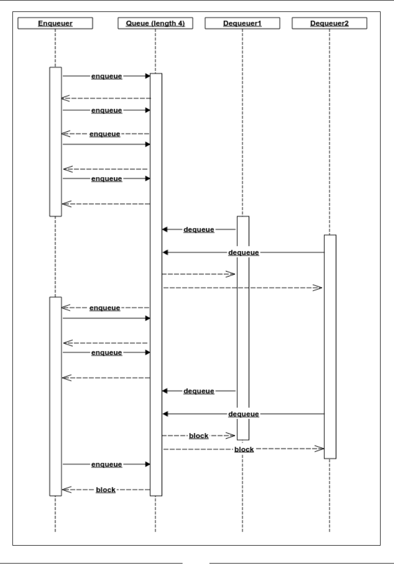
Chapter 11
[ 303 ]

Reactive Programming
[ 304 ]
What we really want is threads that will not only perform the enqueue operation,
but also block the queue before it is completely full. This is so that the dequeueing
threads can use some space to keep dequeuing and enqueuing until they reach a
point where they will not have to enqueue anymore (because they have reached the
last step of the processing chain). Eventually, the queue gets empty and the enqueuer
threads can be unblocked again. To do this, we need to have two different kinds
of enqueue operations. One that does not block until the queue is full, and another
that blocks once the queue is half or more full. We can implement the second type
using the following code in the ThreadSafeFixedLengthSpinlockQueue class. The
enqueueProducerOnly method is just like the enqueue method, except it performs
an atomic check of the currentElementCount variable instead of just incrementing
it. If, while enqueueing, it is seen that the queue is already full, we release the
enqueue lock and restart. The thread that does only enqueue operations and no
dequeue operation must use this method instead of the regular enqueue method:
public void enqueueProducerOnly(E value ) throws InterruptedException{
int halfLength = length/2;
while (true) {
int index = nextEnqueueIndex;
nextEnqueueIndex = (nextEnqueueIndex+1) % length;
if(enqueueLocks[index].compareAndSet(false,true)){
int numberOfElements = currentElementCount.get();
if(numberOfElements>=halfLength
|| (!currentElementCount.compareAndSet(
numberOfElements, numberOfElements+1))){
enqueueLocks[index].set(false);
continue;
}
store[index] = value;
dequeueLocks[index].set(false);
return;
}
}
}

Chapter 11
[ 305 ]
We can now use this method to implement a corresponding method in the
ProducerConsumerQueue class. This method is exactly the same as the produce
method, except that here, the call to enqueue has been replaced by a call to the
enqueueProducerOnly method:
public void produceExternal(E value) throws InterruptedException {
Event event = new Event();
event.value = value;
event.eventType = EventType.INVOCATION;
queue.enqueueProducerOnly(event);
}
Now let's see the EventStream class. The whole point of the EventStream class is
to create metadata in a functional way. It is an abstract class with only one abstract
method called read(). A call to the read method should return the next object that
needs to be processed. The class maintains a pointer to the previous EventStream
on which this EventStream will work. This means that the operation represented
by EventStream will work on the data obtained after all the previous EventStream
have been processed. It is really a linked list of EventStream. Depending on the kind
of operation the current EventStream represents, it either has a mapper, a lter, or
nothing. The read method is applicable only to the rst EventStream that generates
the data. Both the map lter methods return another EventStream that represents
the corresponding processing. After all the map and lter calls, the list linked by
EventStream will store all the operations from the last to the rst:
public abstract class EventStream<E> {
EventStream previous;
OneArgumentExpressionWithException mapper;
OneArgumentExpressionWithException filter;
public <R> EventStream<R> map(
OneArgumentExpressionWithException<E,R> mapper){
EventStream<R> mapped = new EventStream<R>() {
@Override
public R read() {
return null;
}
};
mapped.mapper = mapper;
mapped.previous = this;
return mapped;
}
public EventStream<E> filter(OneArgumentExpressionWithException<E,
Boolean> filter){

Reactive Programming
[ 306 ]
EventStream<E> mapped = new EventStream<E>() {
@Override
public E read() {
return null;
}
};
mapped.filter = filter;
mapped.previous = this;
return mapped;
}
The consume method, however, returns an instance of EventConsumer. This is
the terminal processing in any chain that does not compute a new value. The
EventConsumer class, as would be shown a little later, contains all of the logic to
actually start the processing:
public EventConsumer<E> consume(
OneArgumentStatementWithException<E> consumer){
EventConsumer eventConsumer = new EventConsumer(
consumer, this) {
};
return eventConsumer;
}
public abstract E read();
}
Since we need to store the details of the processing inside an EventConsumer
instance, we will rst make a few classes to store this information. The rst one is a
Task interface that represents any of the map, lter, or consume operation:
public interface Task {
}
This interface is implemented by three classes that represent each kind of operation.
To store the code, we need two additional functional interfaces that represent an
expression and a statement that would allow you to throw exceptions:
@FunctionalInterface
public interface OneArgumentExpressionWithException<A,R> {
R compute(A a) throws Exception;
}
@FunctionalInterface
public interface OneArgumentStatementWithException<E> {
void doSomething(E input) throws Exception;
}

Chapter 11
[ 307 ]
The following classes implement the Task interface:
public class MapperTask implements Task {
OneArgumentExpressionWithException mapper;
Task nextTask;
public MapperTask(
OneArgumentExpressionWithException mapper,
Task nextTask) {
this.mapper = mapper;
this.nextTask = nextTask;
}
}
public class FilterTask implements Task{
OneArgumentExpressionWithException filter;
Task nextTask;
public FilterTask(
OneArgumentExpressionWithException filter,
Task nextTask) {
this.filter = filter;
this.nextTask = nextTask;
}
}
Both MapperTask and FilterTask have a pointer to the next task because they
are intermediate operations. They also store the piece of code associated with the
processing. The ProcessorTask represents the terminal operation, so it does not
have a pointer to the next task:
public class ProcessorTask<E> implements Task{
OneArgumentStatementWithException<E> processor;
public ProcessorTask(
OneArgumentStatementWithException<E> processor) {
this.processor = processor;
}
}

Reactive Programming
[ 308 ]
We will now create the EventConsumer class that will create a task chain and run it:
public abstract class EventConsumer<E> {
OneArgumentStatementWithException consumptionCode;
EventStream<E> eventStream;
Task taskList = null;
private ProducerConsumerQueue<StreamEvent> queue;
private OneArgumentStatement<Exception> errorHandler =
(ex)->ex.printStackTrace();
A StreamEvent is a processing request that is an element of the producer-consumer
queue. It stores value as Object and task. The task can have more tasks pointed to
by its next reference:
class StreamEvent{
Object value;
Task task;
}
An EventStream stores its previous operation—that is to say that if we read the
head of the list, which would be the last operation. Of course, we need to arrange
the operations in the order of execution and not in reverse order. This is what the
eventStreamToTask method does. A MapperTask or FilterTask stores the next
operation, so the head of the list is the rst operation to be carried out:
private Task eventStreamToTask(EventStream stream){
Task t = new ProcessorTask(consumptionCode);
EventStream s = stream;
while(s.previous !=null){
if(s.mapper!=null)
t = new MapperTask(s.mapper, t);
else if(s.filter!=null){
t = new FilterTask(s.filter, t);
}
s = s.previous;
}
return t;
}
The constructor is package-accessible; it is intended to be initialized only from inside
the consume method of an EventStream:
EventConsumer(
OneArgumentStatementWithException consumptionCode,
EventStream<E> eventStream) {
this.consumptionCode = consumptionCode;
this.eventStream = eventStream;

Chapter 11
[ 309 ]
taskList = eventStreamToTask(eventStream);
}
The following is the piece of code responsible for actually carrying out the
operations. The ConsumerCodeContainer class implements Consumer and acts as the
consumer of the producer-consumer queue for processing events:
class ConsumerCodeContainer implements Consumer<StreamEvent>{
@Override
public void onError(Exception error) {
errorHandler.doSomething(error);
}
The onMessage method is invoked for every event in the producer-consumer
queue. Based on the actual task, it takes the corresponding action. Notice that for
MapperTask and FilterTask, a new event is enqueued with the next operation:
@Override
public void onMessage(StreamEvent evt) {
The ProcessorTask is always the end of a processing chain. The operation is simply
invoked on the value and no new event is queued:
if(evt.task instanceof ProcessorTask){
try {
((ProcessorTask) evt.task).processor
.doSomething(evt.value);
} catch (Exception e) {
queue.sendError(e);
}
}
For a FilterTask, the event with the next task is enqueued only if the condition is
satised:
else if(evt.task instanceof FilterTask){
StreamEvent nextEvent = new StreamEvent();
try {
if((Boolean)((FilterTask) evt.task)
.filter.compute(evt.value)) {
nextEvent.task =
((FilterTask) evt.task).nextTask;
nextEvent.value = evt.value;
queue.produce(nextEvent);

Reactive Programming
[ 310 ]
}
} catch (Exception e) {
queue.sendError(e);
}
}
For a MapperTask, the next task is enqueued with the value computed by the current
map operation:
else if(evt.task instanceof MapperTask){
StreamEvent nextEvent = new StreamEvent();
try {
nextEvent.value = ((MapperTask) evt.task).mapper
.compute(evt.value);
nextEvent.task = ((MapperTask) evt.task).nextTask;
queue.produce(nextEvent);
} catch (Exception e) {
queue.sendError(e);
}
}
}
}
The process method is responsible for kicking the actual processing of the tasks.
It uses a ProducerConsumerQueue to schedule events that are processed by the
consumer previously discussed:
public void process(int bufferSize, int numberOfProducerThreads,
int numberOfConsumerThreads) {
queue = new ProducerConsumerQueue<>(bufferSize,
numberOfConsumerThreads, new ConsumerCodeContainer());
Only the original EventStream on which map and lter were called has the read
method implemented. So we simply get a reference to the original EventStream:
EventStream s = eventStream;
while(s.previous !=null){
s = s.previous;
}
The startingStream variable points to the original EventStream:
EventStream startingStream = s;

Chapter 11
[ 311 ]
The producer code also runs in separate threads. The Runnable producerRunnable
contains the producer code. It simply keeps calling the read method of the
EventStream until null is returned (which marks the end of the stream) and
enqueues a StreamEvent with the value and the task chain we have created with the
help of the eventStreamToTask method:
Runnable producerRunnable = ()->{
while(true){
Object value = startingStream.read();
if(value==null){
break;
}
StreamEvent nextEvent = new StreamEvent();
try {
nextEvent.value = value;
nextEvent.task = taskList;
queue.produceExternal(nextEvent);
} catch (Exception e) {
queue.sendError(e);
}
}
try {
queue.markCompleted();
} catch (InterruptedException e) {
e.printStackTrace();
}
};
Now we spawn the producer threads and wait for them to nish with the join calls:
Thread [] producerThreads = new Thread[
numberOfProducerThreads];
for(int i=0;i<numberOfProducerThreads;i++){
producerThreads[i] = new Thread(producerRunnable);
producerThreads[i].start();
}
for(int i=0;i<numberOfProducerThreads;i++){
try {
producerThreads[i].join();
} catch (InterruptedException e) {
e.printStackTrace();
}
}
}

Reactive Programming
[ 312 ]
This is a method to register a custom error handler and return a new
EventConsumer:
public EventConsumer<E> onError(
OneArgumentStatement<Exception> errorHandler){
EventConsumer<E> consumer
= new EventConsumer<E>(consumptionCode, eventStream) {};
consumer.taskList = taskList;
consumer.errorHandler = errorHandler;
return consumer;
}
}
Going back to our original problem of perfect numbers, all we have to do now is
to dene an EventStream with a read method that generates all the numbers and
then does maps and lters on them as follows. Notice that the EventStream.read()
method may be invoked by multiple threads simultaneously if we use more than one
producer thread, so it is better for it to be thread-safe.
The read method simply increments an AtomicLong and returns the previous value,
unless the previous value is greater than 5_00_000L; in this case, it returns null,
marking the end of the stream. We have already seen the rest of the code:
public static void findPerfectNumbersWithFunctionalAPI(){
long start = System.currentTimeMillis();
EventStream<Long> stream = new EventStream<Long>() {
AtomicLong next = new AtomicLong(0L);
@Override
public Long read() {
Long ret = next.incrementAndGet();
if(ret<=5_00_000L){
return ret;
}
return null;
}
};
stream.filter((x)->x>1)
.filter(EventStream::isPerfect)
.consume((x)->{System.out.println(x);})
.onError((x)->System.out.println(x))
.process(4096,1,4);
System.out.println("Time in ms: "+(
System.currentTimeMillis()-start));
}

Chapter 11
[ 313 ]
This code runs for almost the same time as the previous reactive version without a
functional API. I will leave it up to you to use the functional API to implement the
friend count solution, as it is fairly simple as one gets the hang of it. All you need to
think about is how to implement the read method to return the integers from the le.
Summary
In this chapter, we learned how to do advanced thread synchronization using
volatile elds, atomic operations, and semaphores. We used these to create our own
reactive programming framework and also created a functional API for reactive
programming. We used our frameworks to solve sample problems and saw how
multithreaded scalable apps can be written easily with a reactive framework.
There are many reactive programming frameworks available, such as RxJava,
Akka, and many more. They are slightly different in their implementation and
features. They all provide a lot more features than the one we used. This chapter is
just an introduction to the topic; interested readers can learn more about reactive
programming from the books dedicated to this subject.
In this book, I tried to give you a head start in the world of algorithms, with
implementations in Java. Algorithms are a vast eld of study. Every computation
problem needs to be solved by an algorithm. A further study would include
complexity classes of algorithms, equivalence of algorithms, and approximate
algorithms for highly complex problems. A complex problem is a problem that
guarantees that any algorithm that solves it must have a certain amount of
complexity. This gives rise to the concept of the complexity classes of problems.
There are also formal/mathematical ways of proving the correctness of algorithms.
All these areas can be pursued by you.
The book also covers functional and reactive programming a little bit. This should
work as a head start in those areas; you can learn more about them in the books
dedicated to these topics.

[ 315 ]
Index
A
abstract data type (ADT) 41
adjacency list 244-248
adjacency-list-based graph
operations, complexity 250, 251
with dense storage for vertices 251-255
with dense storage for vertices, operations
complexity 258, 259
adjacency matrix
about 230-233
sparse adjacency matrix graph,
operations complexity 234, 235
adjacency-matrix-based graph 235-241
aggregation operation 67
algorithm
asymptotic complexity, analyzing 4
average case, complexity 3
best case, complexity 3
optimizing 10
performance 2, 3
worst case, complexity 3
append operation
implementing, for functional linked lists 74
array-backed heap 201-204
ArrayHeap
operations, complexity 209
arrays
about 16
elements, inserting 16-18
new elements, appending 18, 19
new elements, inserting 18, 19
asymptotic analysis 10
asymptotic complexity
algorithm, upper bound 8
analyzing 4
function, lower bound 8, 9
function, tight bound 9
function, upper bound 4-7
AVL tree
about 171-176
complexity 176
element, deleting 176
element, inserting 176
element, searching 176
B
binary search
about 93-96
complexity 96, 97
binary search tree
about 156-158
element, deleting 162-166
element, inserting 158-160
invariant 160, 161
operation complexity 167
binary tree
about 145-147
depth-rst traversal, types 147-149
non-recursive depth-rst search 149-152
binomial forest
about 209-219
heap property 212, 213
number of nodes 212
operations, complexity 221
uses 211, 212
breadth-rst traversal 142, 143
bubble sort
about 105
complexity 107, 108
inversions 106

[ 316 ]
C
CAS operation 284, 285
children node 135
circular linked list
about 37
element, inserting 38
element, removing 38
element, rotating 39, 40
comparison based sorting
complexity 129-133
connected graph 226
cut property 269, 270
cycle 226
cycle detection
about 264-266
complexity 267
D
data structure 15
dense adjacency-matrix-based graph
operations, complexity 243, 244
depth-rst traversal
about 140-142
in-order traversal 147
post-order traversal 148
pre-order traversal 147
types 147-149
dequeuing 47
directed graph 226
double ended queue
about 52, 53
eject operation 52
xed length double ended queue,
using with array 53-55
inject operation 52
peekLast operation 52
peek operation 52
pop operation 52
push operation 52
variable size double ended queue,
using with linked list 55, 56
doubly linked list
about 30
arbitrary element, removing 34, 35
element, inserting at arbitrary
location 32, 33
element, inserting at beginning 31, 32
element, inserting at end 31, 32
rst element, removing 33, 34
last element, removing 36
E
enqueuing 47
expression syntax 61
F
ltering 64
lter operation
implementing, for functional
linked lists 70-73
nal keyword 62
rst-in-rst-out (FIFO) 47
xed length double ended queue
using, with array 53-55
xed-sized queue
using, with array 48-51
xed-sized stack
using, with array 43-45
using, with linked list 45, 46
atMap method
implementing, for functional
linked lists 74, 75
fold operation
implementing, for functional
linked lists 67-70
forEach method
implementing, for functional linked lists 65
forest 227
functional data structures
about 62
functional linked lists 62-64
functional interface
about 60, 61
implementing, with lambda 61
functional linked lists
about 62-64
append operation 74
lter operation 70-73
atMap method 74, 75
fold operation 67-70
forEach method 65
map() method 66, 67

[ 317 ]
functional programming
about 57
performance 89
G
graph
about 226
adjacency list 244-248
adjacency-list-based graph 251-256
adjacency matrix 230-233
adjacency-matrix-based graph,
space-efcient 235-241
complete graph 228
connected graph 226
directed graph 226
representing 229
subgraph 226
traversal 259-261
traversals, complexity 264
undirected graph 226
graph ADT
about 228
operations 228, 229
H
hash function
about 190
properties 190
hash table
about 190
complexity, of insertion 193
complexity, of search 194
element, inserting 191, 192
element, searching 193
load factor 194
heap
about 196
array-backed heap 201-204
complexity, analysis 199
insertion 197
linked heap 204, 205
minimum elements, removing 198
serialized representation 200
I
imperative programming 57
in-place heap sort 222
insertion sort
about 102, 103
complexity 104
invariant, binary search tree 160, 161
inversions 106
J
Java
lambda expression 60
JavaBean 78
L
lambda expression
about 60
functional interface 60, 61
functional interface, implementing 61
last in rst out (LIFO) 42
linear search 92
linked heap
about 204, 205
insertion 206
minimal elements, removal 207, 208
linked list
about 20, 21, 136
arbitrary element, removing 27, 28
arbitrary element, searching 25-27
element, appending at end 21, 22
element, inserting at arbitrary
position 24, 25
element, inserting at beginning 23
iteration 28, 29
loop 226
M
map() method
implementing, for functional
linked lists 66, 67
mergesort
about 123-125
complexity 126
tempArray copy, avoiding 127-129

[ 318 ]
minimum spanning tree, nding
about 272
complexity 279
implementation 277
unionFind 273-276
unionFind, operations complexity 277
monads
about 62, 76
option monad 76-81
Try monad 82-86
N
non-recursive depth-rst search 149-152
non-tail single recursive functions 112, 114
O
option monad 76-81
P
parent node 135
path 226
priority queue
used, for sorting 221, 222
priority queue ADT 195
producer-consumer model
about 283
compare and set 284, 285
implementing 289-296
semaphore 283
spinlock and busy wait 296-300
thread-safe blocking queue 286-288
volatile eld 285
Q
queue
about 46, 47
dequeue operation 47
enqueue operation 47
xed-sized queue, using with array 48-51
peek operation 47
quicksort
about 115-119
complexity 120, 121
random pivot selection 122
R
random pivot selection
in quicksort 122
reactive programming
about 282
functional way 301-312
uses 282
recursion 57
recursive algorithms
about 58-60
complexity analysis 86-88
recursive calls
non-tail single recursive functions 112-114
problem 108
tail recursive function 109-111
red-black tree
about 177, 178
element, deleting 183-187
element, inserting 179-183
worst case scenario 188, 189
right hand side (RHS) 74
rotation operation
using, with self-balancing binary
search tree 168-170
S
search algorithms
about 92, 93
binary search 93-96
searching 91
selection sort
about 98-100
complexity 101, 102
self-balancing binary search tree
about 168
AVL tree 171-176
rotation operation, using 168-170
semaphore 283
sorting
about 98
bubble sort 105
insertion sort 102, 103
selection sort 98-100
sorting algorithm
stability 133

[ 319 ]
spanning tree
about 267, 268
connected undirected graph 269
cut property 269, 270
minimum spanning tree 271
minimum spanning tree, nding 272
undirected connected graph 269
with vertices V and edges E 268
stack
about 42, 43
xed-sized stack, using with array 43-45
peek operation 42
pop operation 42
push operation 42
variable sized stack, using with
linked list 45, 46
subgraph 226
T
tail recursive functions 109-111
Thread-safe blocking queue 286-288
time complexity
improving 11, 12
tree 135, 227
tree abstract data type 143-145
tree data structure 136-139
tree traversal
about 139
breadth-rst traversal 142, 143
depth-rst traversal 140-142
Try monad 82-86
U
undirected graph 226
V
variable size double ended queue
using, with linked list 55, 56
W
wrapper object 20
