MANUAL
MANUAL
User Manual: Pdf
Open the PDF directly: View PDF ![]() .
.
Page Count: 11
Tips on how to generate digital outcrop using
SfM-MVS and extract attitudes of
discontinuities using ply2atti and scanline 1
VIANA C.D.
camila.duelis@gmail.com
Institute of Geosciences / University of Sao Paulo
ENDLEIN A.
endarthur@gmail.com
Institute of Geosciences / University of Sao Paulo
January 22, 2018
1This document contains additional information and modifications of the al-
gorithms presented in ”DUELIS VIANA, C. et al. Algorithms for extraction of
structural attitudes from 3D outcrop models. Computers and Geosciences, v. 90,
p. 112-122, 2016”. The reader should address the same for more information.
Contents
1 Introduction 2
2 System requirements 3
3 Workflow 3
3.1 Image Acquisition ......................... 3
3.2 Generating the digital model and georeferencing ........ 4
3.3 Selecting planes .......................... 6
3.4 Ply2atti and Scanline ....................... 9
3.4.1 ply2atti .......................... 9
3.4.2 scanline .......................... 10
4 Troubleshooting 10
4.1 The mesh is distorted or loaded in “slices” on Meshlab . . . . 11
4.2 The attitudes of the reference planes are different from the
ones measured on the model ................... 11
4.3 Ply2atti can’t process the mesh ................. 11
4.4 Ply2atti returned no data .................... 11
1 Introduction
In this guide we try to detail the procedures adopted for digital model gen-
eration, from photo acquisition to georeferencing, and structural attitudes
extraction as shown on “Algorithms for extraction of structural attitudes
from 3D outcrop models” (Computers & Geosciences, Volume 90, Part A,
May 2016, Pages 112–122), available HERE.
A test model (Validation Model, referred as Site 1 on the paper), con-
sisting of wooden planes is used as an example. The instructions emphasize
the necessary cautions when building 3D models from rock slopes and on
the selection of planes and discontinuities from these models. The scripts
used in this work are also available ( you can download ply2atti here and
scanline here or install directly from the PyPI) . We present short manuals
on how to use them and solutions to some of the issues that may arise during
processing.
2
2 System requirements
All instructions contained on this manual refer to commands used on a Win-
dows 10 PC, tough both scripts should work on Linux and Mac. For the
generation of complex models it is recommended to use a PC with an Intel
Core i7 processor or higher and at least 8 GB of RAM, being 32 GB preferred.
The following components must be installed for the workflow:
•Python (2.7.x or 3.x): Python is an easy to use but powerful object
oriented language. Available at www.python.org/downloads.
•Numpy: numeric package for python that greatly facilitates and ac-
celerate operations between vectors and matrices. Available at www.
numpy.org.
•NetworkX: a python package for creation, manipulation and analysis
of graphs. Available at http://networkx.github.io.
Both Numpy and NetworkX can also be installed by using the following
commands from the command line:
pip install numpy networkx
3 Workflow
3.1 Image Acquisition
The acquisition of photographs for SfM processing is relatively simple, as the
the placement of control points is not necessary for scene restitution. In the
specific case of the ply2atti-scanline workflow the control points (GCP) are
used for georeferencing, orienting and scaling the model. That said, some
guidelines must be followed to increase the processing efficiency and reduce
the noise on the resulting model, making necessary some planning according
to the target application.
We used Agisoft Photoscan software (Professional edition, version 1.0.1)
for digital model generation. To maximize processing efficiency and reduce
noise, Agisoft provides some guidelines that must be followed. For our ap-
plication, the following instructions are the most relevant:
•5Mpx minimal resolution. Great results obtained with 12Mpx;
•Avoid fish-eye and wide angle lenses;
3
•Pictures must be taken at maximal resolution;
•Use of RAW images losslessy converted to TIFF (Tagged Image File
Format). We used XnConvert software (available here ), but this step
may be taken in any image processing package that supports this con-
version without any quality loss;
•Number of ”blind-zones” should be minimized since PhotoScan is able
to reconstruct only geometry visible from at least three cameras.
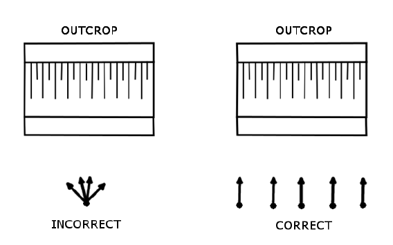
Camera positioning is another issue that requires attention. When pho-
tographing outcrops, Figure 1represent advice on appropriate capturing sce-
nario.
Figure 1: Correct and incorrect camera positioning.
3.2 Generating the digital model and georeferencing
The software Photoscan by Agisoft was chosen for the generation of the
digital models. This is a commercial package, but it offers a 30 day test
license and academic licenses. Other software can be used for this part, as
the opensource VisualSFM, tough the model quality can vary from those
obtained in this work (available at ccwu.me/vsfm/install.html).
Photoscan has a very simple interface and an easy to use workflow. The
tools used here are available on the Professional version. First it is necessary
to load the images on the system, which can be done either by creating
a chunk (Add Chunk) and inserting the images (Add Photos), or directly
on the Workspace pane. Working in chunks allows creating parts of the
4
model separately, making the workload lighter (speeding up processing) and
generating parts that can be merged in a single model afterwards.
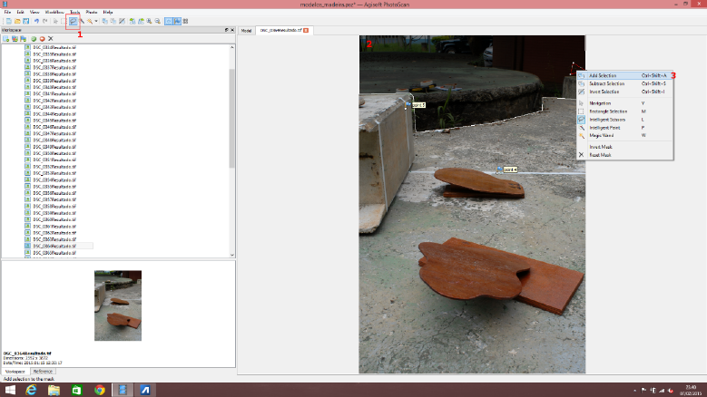
The next step, masking, is used to remove unnecessary parts of the scene.
It is not required for the system to work, but it is recommended as it might
enhance the model and processing speed. By double clicking on each picture,
a new tab is opened with the selected photograph. Using the tool Intelligent
Scissors the user selects a polygon that must be deleted (like trees, sky,
objects, people) and then this selection is added to the mask with the tool
Add Selection (Ctrl+Shift+A). The selected part is grayed out and will be
ignored in the following steps of the processing (Fig. 2).
Figure 2: To mask undesirable areas, use Inteligent Scissors (1), select the
area (2) and click Add Selection (3).
From this point it is necessary to follow the enabled operations in or-
der in the menu Workflow. First the software will align the images (Align
Photos) according to the features that are automatically extracted from the
images and build a sparse point cloud together with the relative positions
of the camera. Then the options Build Dense Cloud and Generate Mesh
are enabled. Even though it is possible to reconstruct the mesh from sparse
data, the quality of the surface might not be enough for geotechnical ap-
plications, especially if the software cannot recognize many features from
the images (for example, in a rock with low variations of color). The tool
Dense Cloud generates a high quality and high-density point cloud, compa-
rable with those obtainable with LIDAR. The software uses the calculated
5
positions of the camera to build a depth map for each image and from these
build a new cloud. The next step consists of generating a triangular mesh
using the chosen point cloud (Generate Mesh). The dense cloud should be
used for geotechnical applications, as it is more detailed. At last, the Build
Texture tool adds color and textures to the faces generated in the previous
step.
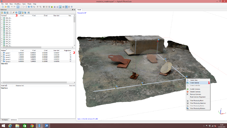
The georeferencing can be made at the final stage – locating each GCP
at the model – or at the beginning, locating them on each image. In both
cases the procedure is made right-clicking on the GCP and selecting Create
Marker. The point is automatically created at a table on the Reference
pane, where its coordinates can be edited with a double click on the cell. To
attribute the coordinates, click the Update button (Fig. 3).
Figure 3: To add GCPs, right-click the desired point and select Create
Marker (1). To insert coordinates, double click the cell at the Reference
pane(2). Click Update (3) to update georeferencing.
3.3 Selecting planes
The model built on Photoscan must be exported in either the .obj (wavefront
obj file) or .stl (StereoLithography) (File>Export Model) formats and then
loaded on Meshlab (File >Import Mesh), which is an opensource 3D Mesh
and Point Cloud processing software that can process even large files. It is
available at meshlab.sourceforge.net.
6
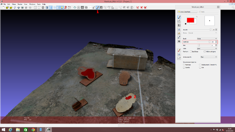
The user should then paint the planes to be measured using the ZPainting
tool, with maximum hardness to obtain a pure color and reducing the brush
size for better painting precision (Fig. 4). The structures can be separated
with different colors and the user must take note of the RBG values of the
used colors for the next step. The selection must be careful as not to make
different planes with the same color share a vertex, which would make the
script recognize these as the same plane.
The model with the painted planes should be exported in the .ply format
(Stanford Polygon) with binary encoding and no texture coordinates (Fig.
5).
Figure 4: For plane selection use the ZPainting tool (1), place the hardness at
its maximum value. Color in the surface (2), controlling brush size according
to the need.
In cases where planes are visible only by their traces, the placement of
a virtual scanline is made manually on MeshLab using the PickPoints tool.
First, the start-end points of the line are placed by right clicking on their
respective locations. Afterwards, for each individual recognizable surface
and trace along the scanline that crosses it, three points are placed: two
at start-end and one mid-point. The points can be labeled on the tool, by
giving them the same name for each plane. The digital surface texture and
high point density ensures that, even for traces, the three selected points for
each feature are extremely unlikely to be collinear, allowing a “three-point
problem” solution. The selected points are then exported on a XML file with
7
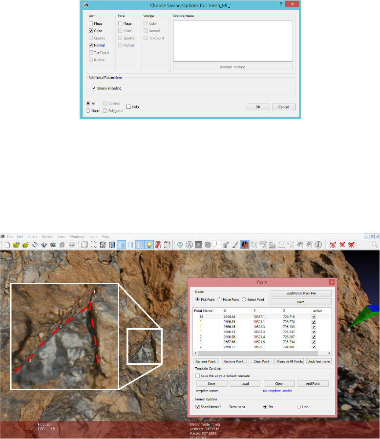
Figure 5: Selected options to export a .ply on MeshLab.
.pp termination by clicking Save on the PickPoints tool window. The .pp file
stores X, Y, and Z coordinates of all the selected points – being scanline
start-end points and three points per discontinuity – and point names (Fig.
6).
Figure 6: Screenshot of sampling procedure using PickPoints tool on Mesh-
Lab. The green prism indicates the scanline start point. On the zoomed
image the dashed lines indicate the discontinuities and the white numbers
(“1” and “2” indexes) show the three selected points for each plane, as they
appear on the screen. To select a feature, use the Pick Points tool. Select
start-end points (S1 and S2) and three points for each trace, right click-
ing them. Use the Rename Point button to assign an index to the feature.
Export the points by clicking Save.
8
3.4 Ply2atti and Scanline
Both scripts are on the PyPi, the python package index, and can be installed
using
pip install ply2atti scanline
This will download the scripts and add them to the scripts folder of the
python installation, allowing them to be called from any command line if
python was installed on the system path. Details on invoking the scripts
might be seen by using the -h (--help) option:
> ply2atti -h
> scanline -h
3.4.1 ply2atti
To use the ply2atti script on a .ply file that contain painted planes the fol-
lowing command can be used:
> ply2atti -f INFILE R1,G1,B1 R2,G2,B2 ...
Being INFILE the filename of the .ply file and R,G,B the RBG tuple of
each color used to paint the planes. For example:
> ply2atti -f example.ply 255,0,0 0,255,0
Will extract the planes painted with pure red (255,0,0) and pure green
(0,255,0) from the mesh. Two files will be output, one containing only the
attitudes of each plane and the other with full information, including the
attitude, centroid and estimated persistence of the plane. All colors will be
put together in the same file by default, but the option -split allows each
color to be output to a different file set.
To visualize the centroids of the calculated planes the CloudCompare soft-
ware (available at http://www.danielgm.net/cc/) can be used. First the
base .ply file should be opened (File>Open). Then, on the Open ASCII File
window, set the first dropdown menu to coord. X (Fig. 7). Automatically
the heading of the next columns will be replaced by coord. Y and coord. Z.
Click OK. At the right pane (DB Tree) it is possible to visualize both files.
You can chance point size clicking on the .txt file at the DB Tree pane and
choosing the Point size option at the Properties window.
9
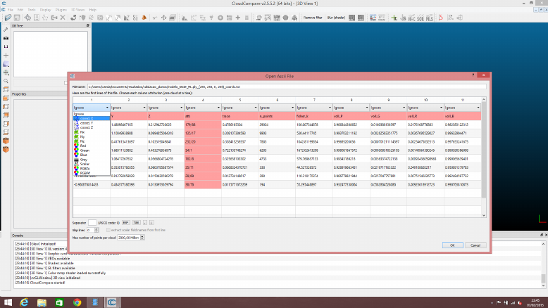
Figure 7: Loading the coordinates .txt file on Cloud Compare.
3.4.2 scanline
The scanline script can be used as follow:
> scanline INFLINE
Using the default settings, the points named S1 and S2 will be used as the
beginning and end of the scanline, respectively, and each trio of points with
the same name will be used as a plane. As default, the results are output to
the screen, which can either be copy/pasted or redirected to a text file as:
> scanline example.pp > example\_out.csv
Or the output filename can be given with the -out option, followed by the
output filename.
4 Troubleshooting
Aside from the errors that have solutions directly suggested by the software,
some issues that may happen during processing must be highlighted. Their
description and possible solutions are:
10
4.1 The mesh is distorted or loaded in “slices” on
Meshlab
If the model generated on Photoscan is not being correctly loaded on Meshlab
the solution might be by reducing the large coordinates used for georeferenc-
ing. UTM coordinates are large and might not load correctly. On the tests
that were made, cutting the first two numbers of each coordinate solved the
problem. This solution does not alter neither the attitudes nor the scale of
the model, only its geographical location. That way, to load the results on a
GIS software or Google Earth it is recommended that the model be directly
exported as a KMZ file from Meshlab.
4.2 The attitudes of the reference planes are different
from the ones measured on the model
In case the attitudes of the selected planes are not similar to the ones mea-
sured in the field, a possible solution might lie on the previous issue. For very
large meshes Meshlab can’t load large coordinates, and as such it reduces
them. In this process, the axes might be swapped, altering the attitudes.
Ply2atti adopts the coordinate system where the X, Y and Z axis correspond
to East, North and Up. It is possible to check the axis alignment on Mesh-
lab by using the option View>Trackball>Reset TrackBall, or the shortcut
Ctrl+H. That will make the program reset to the standard view, where X is
the horizontal axis, positive to the right, Y is vertical, positive up, and Z is
the orthogonal axis, positive out of the computer screen. If the axis do not
coincide, it is recommended to change the coordinates, as explained above.
4.3 Ply2atti can’t process the mesh
An error that was observed during testing that can be easily corrected. If
ply2atti shows an error message and don’t process the mesh the issue must
be with the file exported from Meshlab. Meshlab associates a texture to
the .ply file when the model is exported, and to prevent that the TexCoord
checkbox must be unchecked on the Wedge box on the export dialog.
4.4 Ply2atti returned no data
If the output file contains no data, it is possible that the reference colors
given to the script are incorrect, and as such it can’t locate the planes. It is
important to check the RGB values of the colors used to paint the planes.
11
