MANUAL SACTA Lib
User Manual: Pdf
Open the PDF directly: View PDF ![]() .
.
Page Count: 29
SACTA%LIBRARY%FOR%MATLAB%
1. INTRODUCTION
The SACTA library allows to access a transponder antenna to get information about air traffic
and representing a radar presentation in a SACTA monitor or Google Earth.
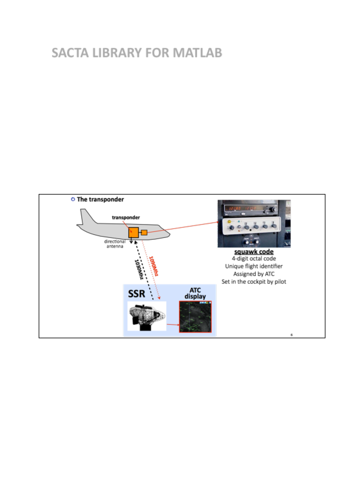
THE TRANSPONDER ANTENNA
The system gets the information from the signals of planes equipped with mode-S transponders
(figure 1).
Figure 1: the transponder
Transponders transmit a response to an interrogation of a Secondary Surveillance Radar (SSR). But
it also broadcasts an SQUITTER signal every two seconds with the information shown in figure 2. This
response signal can be also freely captured with a transponder antenna.
The information provided by the transponders can be used to produce a Radar Presentation like
the one of figure 3. The information of a mode-S transponder includes different data taken from the
Flight Manager Computer (FMC) including longitude, latitude, altitude, ground speed, track angle,
vertical rate, ICAO hex identifier, squawk code, and others.
1
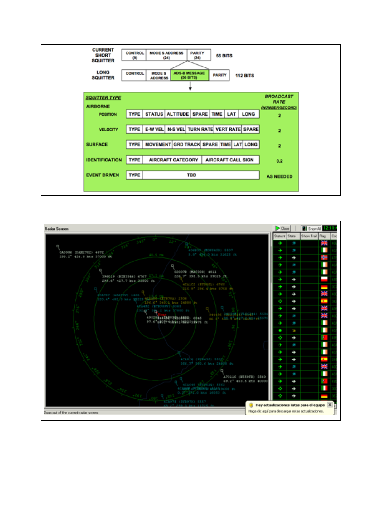
Figure 2: the transponder data frame
Figure 3: radar presentation
In the UPV there exists a computer equipped with an antenna that receives the transponder
signal. This computer has a retransmitter program that distributes this information via TCP/IP to other
computers in the UPVNET (UPV network).
2
This information is available inside the UPVNET network and also outside the UPV through the
UPV VPN (Virtual Private Network). The host with the transponder antenna in our case uses the
following IP address and port:
host: 158.42.40.150 , port=2220
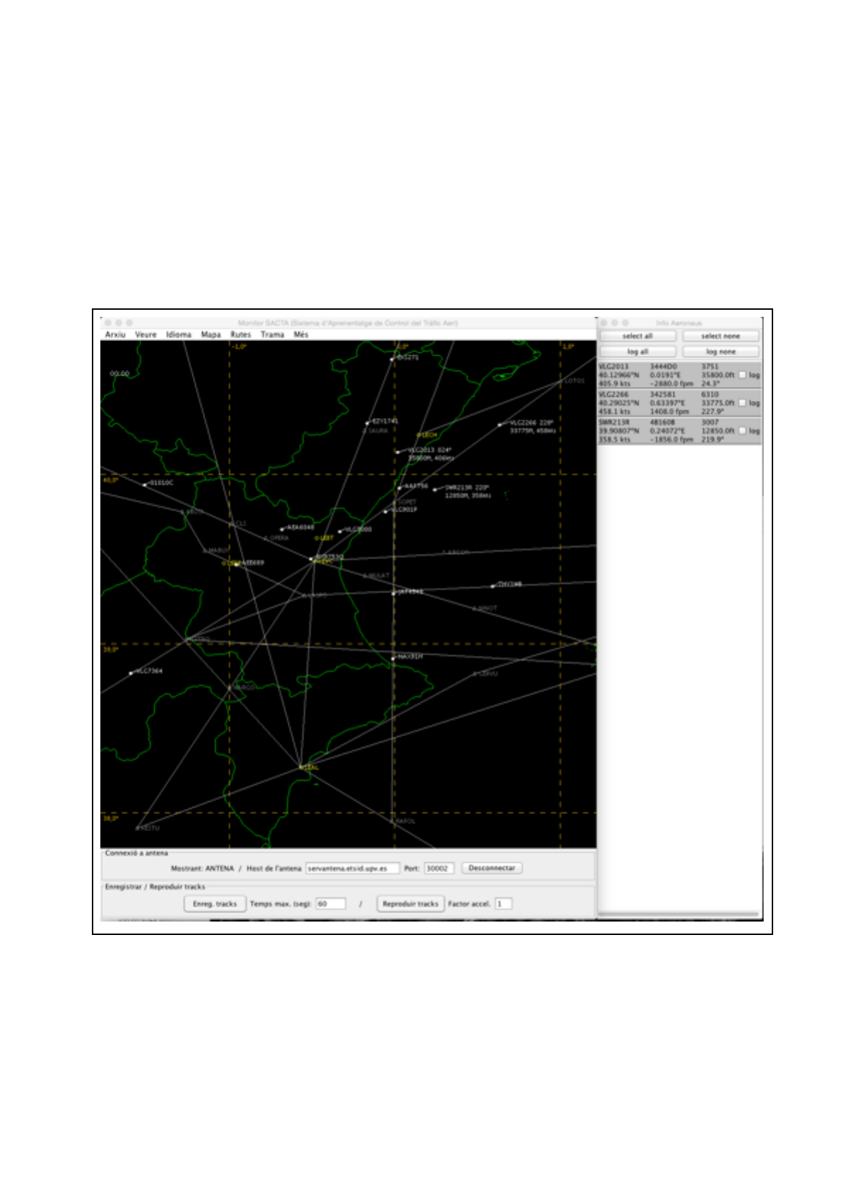
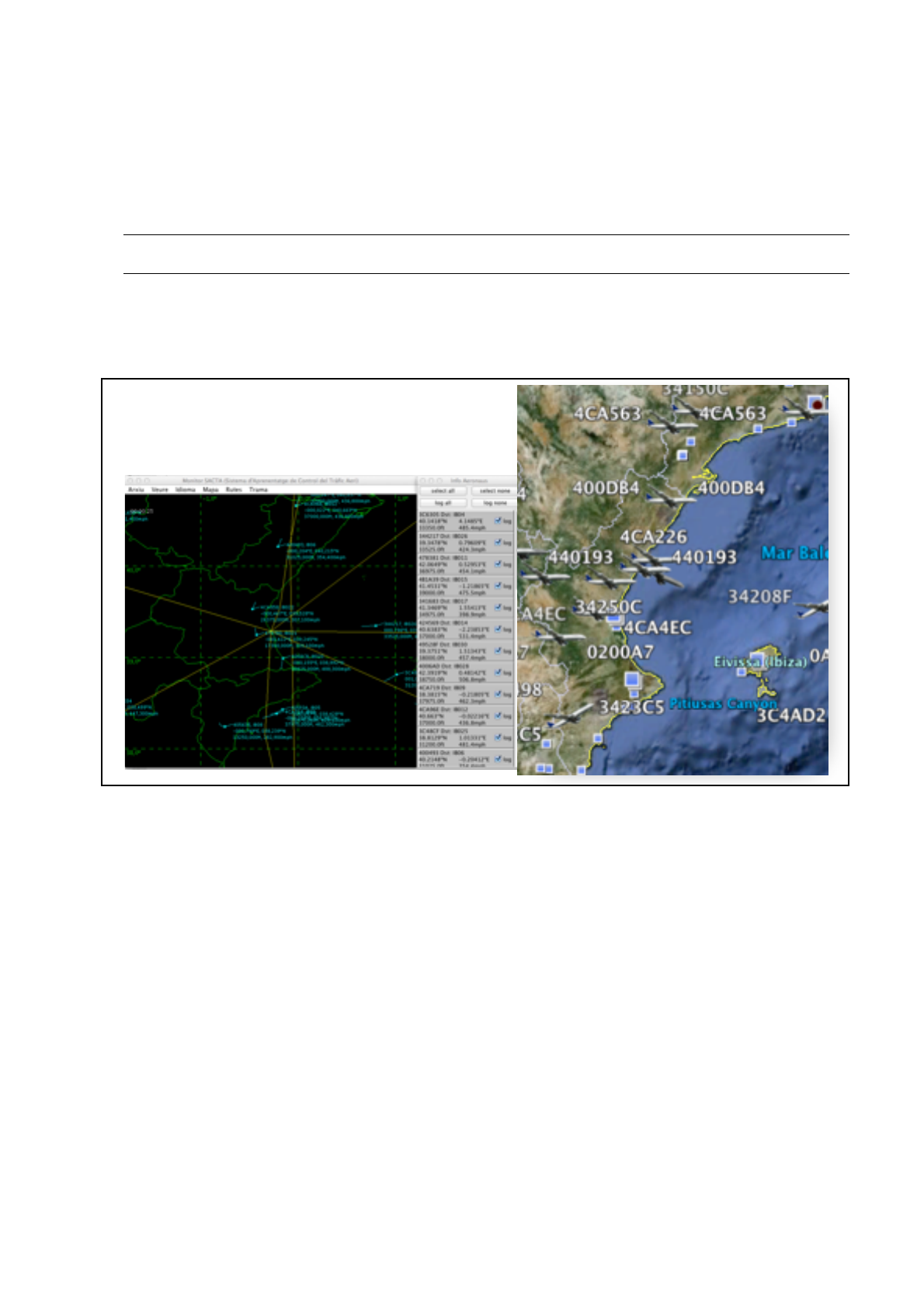
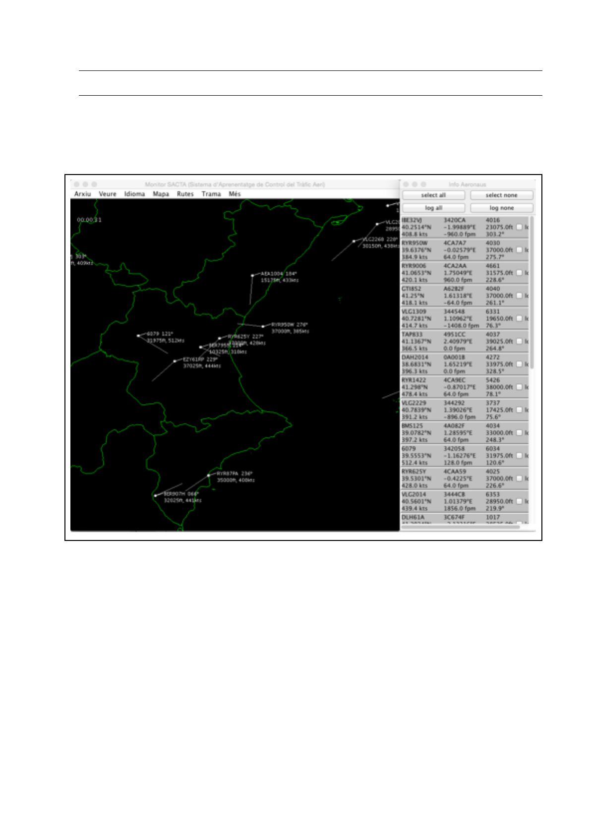
THE SACTA MONITOR
The SACTA monitor is a java executable file named monitor.jar contained in the SACTA
directory. When it is executed it displays the two windows of figure 4.
Figure 4: The SACTA monitor
One of the windows shows a list of traffics in text form. The other one presents it in graphically.
Once it is started, the SACTA monitor is listening to MATLAB (or some other program) to send
traffic information. However, using menu “More” and option “Panel Antenna/Tracks” you can display
the bottom panels to get the traffic from some other data sources.
3

Panel “Antenna connection” allows to connect to a host with a transponder antenna and get
real-time traffic.
Panel “Record/Play tracks” allows to record tracks in a .txt file or to play previously recorded
tracks. Recorded traffic can be played using an accelerator factor.
In summary, you can get traffic information from three sources: a Matlab program, the
transponder antenna or a previously recorded track. The source is indicated aftre the “Displaying”
label in the “Antenna connection” panel. Recording traffic takes the traffic from the currently used
traffic data source.!
4
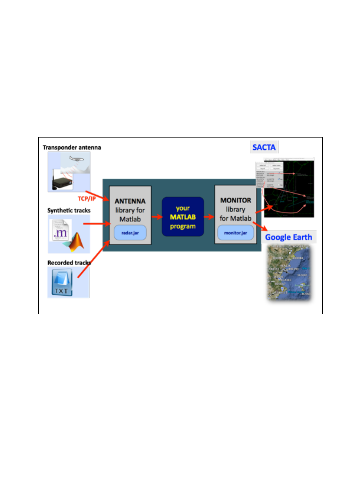
2. THE SACTA EDUCATIONAL SYSTEM
The SACTA educational system has the structure of figure 5. Basically, it is a system that allows
MATLAB to get the traffic from a transponder antenna and represent it graphically on a map. The
system consists of two main MATLAB libraries in jar format:
I. ANTENNA (radar.jar): it provides access to the transponder antenna in order to get
traffic data.
II. MONITOR (monitor.jar): it provides access to a radar screen in order to represent
traffics.
Figure 5: The SACTA system
The basic idea is to be able to write MATLAB programs (Your MATLAB program) that read
traffic from the ANTENNA, process this traffic, and display this information in the MONITOR. For
example, you can write a Matlab program to read traffic information from the ANTENNA, detecting
potential collisions (this is processing) and show the conflicting traffics in the MONITOR in red color.
The SACTA system allows several possibilities for getting traffic data and for the Radar
Presentations in the monitor.
RADAR PRESENTATIONS
Three possible Radar Presentations or display options are available SACTA. Two of them are
graphical and are shown in figure 6. The other one is in text form. These three options are:
1. Graphical presentation on the SACTA monitor
5
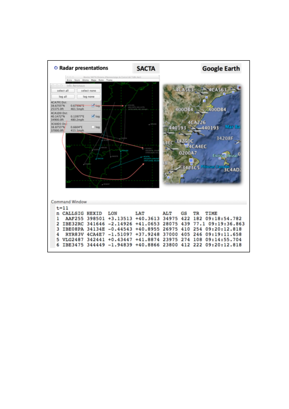
2. Graphical presentation in GoogleEarth
3. Text presentation on the MATLAB console
Figure 6: SACTA display options
This is easy to configure through library function !"#$%"&'()*+,-./0. The visualization is
performed in all cases using library function !"#$%"&'1,23456%/5++,78
DATA SOURCES
Three possible data sources for air traffic are available SACTA. They allow to get different traffics:
real-time, synthetic, perviously recorded. The traffic source is easy to configure through library
function 9#%:##9'()*+,-./0. Reading the traffic is performed using library function
9#%:##9'&05;<in all cases8
The different options for the traffic sources are shown in figure 7. They are also described below:
MATLAB%console%
6
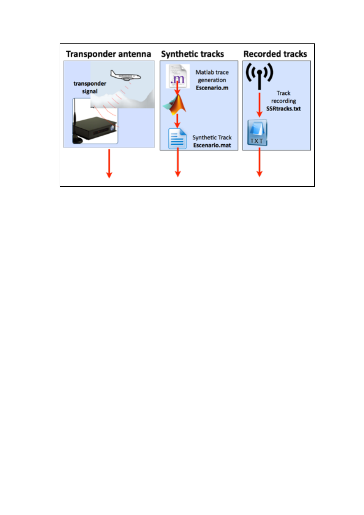
Figure 6: SACTA options for data sources
a. The Transponder antenna
b. Synthetic tracks
c. Recorded tracks
The firs option (Transponder antenna) provides real-time traffic in the Valencia area as detected
by the transponder antenna.<
The second option uses synthetic tracks that can be generated using a simple Matlab program.
This is especially useful when the real-time traffic does not provide scenarios or situations that you
want to test, as for example collision detection scenarios, which (thank God…) are highly improbable.
So if you want to test this scenarios you can generate them synthetically using a Matlab program and
saving it in a 8=5> file. This is an example:
% Generates a synthetic scenario with planes flying specified routes.
% 1 degree latitude = 110 km
% 1 degree longitude = 111 km
% 1 hour = 3600 s.
% Some airways:
% A33 = [ -3.17 40.22; -0.28 39.29; 2.45 39.26 ];
% A34 = [ 0.33 42.41; -0.1 40.15; -0.19 39.53; -0.28 39.29; -0.34
38.16; 0.012 36.52];
% B28 = [ 2.06 41.18; -0.28 39.29; -2.13 38.21];
% G30 = [ -0.28 39.29; 1.28 38.54];
% N609 = [ -0.012 36.52; -0.08 40.13; 0.059 42.46];
clc; clear all;
7

% Traffic through airway N609
plane(1).callsign = 'IB001';
plane(1).hexId = 'A00001';
plane(1).aicraftId = 'B757';
plane(1).flightId = '9191';
plane(1).squawk = '6001';
plane(1).color = 1;
plane(1).trace = [-0.042, 38, 5000, 0 ;
-0.08, 40.13, 6000, 1200;
0.059, 42.46, 4000, 3000];
% Traffic through airway G30
plane(2).callsign = 'BMI702';
plane(2).hexId = 'A00002';
plane(2).aicraftId = 'A319';
plane(2).flightId = '8151';
plane(2).squawk = '6002';
plane(2).color = 1;
plane(2).trace = [ -0.28 39.29, 0, 0 ;
-0.28 39.29, 0, 600 ;
-0.275 39.295 5000, 650 ;
1.28 38.54, 5000,1800 ];
% Traffic through airway A33 A33 = [ -3.17 40.22; -0.28 39.29; 2.45
39.26 ];
plane(3).callsign = 'RYR002';
plane(3).hexId = 'A00003';
plane(3).aicraftId = 'B737';
plane(3).flightId = '6196';
plane(3).squawk = '6003';
plane(3).color = 1;
plane(3).trace = [ -3.17, 40.22, 10000, 0 ;
-0.28, 39.29, 10000, 1000;
2.45, 39.26, 10000, 2000 ];
% OVNI
plane(4).callsign = 'OVNI';
plane(4).hexId = '????';
plane(4).aicraftId = 'OVNI';
plane(4).flightId = '0000';
plane(4).squawk = '0000';
plane(4).color = 3;
plane(4).trace = [ 1.5, 41, 1000, 0 ;
1, 38, 10000, 200 ;
0.5, 41, 1000, 300 ;
0 , 38, 10000, 400 ;
-0.5, 41, 1000, 500 ;
-1 , 38, 1000, 600 ;
-1.5, 41, 1000, 700 ;
2, 38, 1000, 800 ];
save 'scenario1' plane
8

The rule for generating a plane trace is creating an structure with the following mandatory fields:
callsign, hexId, aircraftId, flightId, squawk, color and trace. the field trace defines the trajectory
in 4D, i.e., 3D position and time. It consists of a matrix, with each row of the matrix defining a 4D
point:
?4)*-,>.;0@A<45>,>.;0@A<54>,>.;0@A<>,=0@B<
<4)*-,>.;0CA<45>,>.;0CA<54>,>.;0CA<>,=0CB<
0>78<<
DB<
The system will generate a trace that goes through the 4D points at the specified times. The
system will also linearly interpolate during the simulation intermediate points between two specified
points of the trace.!
9

3. THE ANTENNA LIBRARY FUNCTIONS
The ANTENNA library contains the following functions:
These functions are described next.
+.*7>,)*<!"#$""!%&'()*+,-.E2)./70A<2,=2300;A<,3'+,40A<3/)>)7)4A<3)/>F<
It configures the radar to get data from the following sources:
• The transponder antenna which is connected via TCP/IP
• .mat files: synthetic traces generated using Matlab
• .txt files: previously recorded tracks from the transponder
INPUT PARAMETERS
source: string that specifies the kind of source for traffic data. The two following strings are possible
• 'file' for simulating a track recorded in a .txt or .mat file
• 'ip' for a transponder antenna via TCP/IP
simspeed: Factor used to accelerate simulation traces. It does not affect real-time transponder
antenna
ip_file: string that specifies the specific file or ip address for the traffic source. Examples:
if source==ip' -> ip_file= '158.42.40.150'
ip_file= '226.1.1.1' for multicast
if source==file' -> ip_file= 'e1.mat' or
ip_file= 'SSRtracks_2015_enero_29-05-44.txt'
protocol: TCP/UDP protocol used to connect to the transponder antenna. This parameter is not
necessary for simulating file recorded tracks. Usual value is 3, which corresponds to TCP raw. All
possible valuesare:
0 - TCP (Java Objects) (incompatible Freemat)
1 - UDP (Java Objects)(incompatible Freemat)
!"#$""!%&'()*+,-.E2)./70A<2,=2300;A<,3'+,40A<3/)>)7)4A<3)/>F
?>/5++,72A<>2,=A</054'>,=0D<G<!"#$""!%/.01EF
10

2 - Multicast
3 - TCP (char) (server compatible Freemat)
4 - UDP (char) (server compatible Freemat)
port : integer to specify the antenna port. This parameter is not necessary for simulating file recorded
tracks. The usual port is 2220 for TCP and 2221 for multicast.
RETURN VALUES
none
+.*7>,)*<?>/5++,72A<>2,=A</054'>,=0D<G<!"#$""!%/.01EF<
It reads the information from the traffic source established by ANTENNA_Configure and returns
the corresponding traffic information.nThis information consists of an array of planes detected by the
radar. It delays one second two succesive reads from the traffic source.
INPUT PARAMETERS
none
RETURN VALUES
tsim: a double specifying the simulation time elapsed from the start of the simulation. If the simulation
is accelerated by a factor of A, the returned value is the previous value + A*dt.
real_time: It is current time for the transponder and matlab sythetic traces. For recorded tracks it
returns the time when the traffic was recorded.
traffics: an array of traffics or planes detected by the transponder. Each traffic is represented a struct
of the form
>/5++,72E,F8+,04;<
where the following fields are provided:!
11

H,04;<<<<<<<<<<<<<<<<<<%630<<<<1027/,3>,)*<
GGGGGGGGGGGGGGGGGGGGGGGGGGGGGGGGGGGGGGGGGGGGGGGGGGGGGGGGGGGGGGGGGGGGGGGGG<
>/5++,72E,F80*2-0)341<<string<<15>5I520<9,/7/5+></07)/;<*.=I0/8<
>/5++,72E,F8)5*+6341<<<string<<15>5I520<H4,-J></07)/;<*.=I0/8<
>/5++,72E,F86.741<<<<<<string<<9,/7/5+><!);0<K<J0L5;07,=54<7);08<
>/5++,72E,F820558*+(<<<2>/,*-<<9*<0,-J><;,-,><+4,-J><$18<$><75*<I0<5<+4,-J><*.=I0/<<
<<<<<<<<<<<<<<<<<<<<<<<<<<<<<<<)/</0-,2>8<E)/<0M0*<*)>J,*-F<
>/5++,72E,F889,0:;<<<<<string<<922,-*0;<!);0<9<2N.5OP<7);08<
>/5++,72E,F85'(<<<<<<<<double<<Q)*-,>.;0<,*<;0-/0028<:52><3)2,>,M0A<R02><*0-5>,M08<
>/5++,72E,F8503<<<<<<<<double<<Q5>,>.;0<,*<;0-/002<#)/>J<3)2,>,M0A<K).>J<*0-5>,M08<
>/5++,72E,F8053<<<<<<<<double<<!);0<(<54>,>.;0<,*<+00>8<S0,-J></045>,M0<>)<@T@U8C=I<,*<<
<<<<<<<<<<<<<<<<<<<<<<<<<<<<<<+00>8<EH4,-J><Q0M04F8<#)><J0,-J><9!KQ88<
>/5++,72E,F8+8<..1<<<<<double<<VK<K300;<)M0/<-/).*;<,*<#!<E*)><,*;,75>0;<5,/2300;F<
>/5++,72E,F83-02;<<<<<<double<<%/57P<)+<5,/7/5+><,*<;0-/002<E*)><J05;,*-F8<<
<<<<<<<<<<<<<<<<<<<<<<<<<<<<<<<10/,M0;<+/)=<>J0<M04)7,>6<:WR<5*;<#WK8<
>/5++,72E,F8=.-3/03.<<<double<<X0/>,754</5>0<,*<+3=8<YZ+></02)4.>,)*8<
>/5++,72E,F805.-3<<<<<<string<<H45-<>)<,*;,75>0<2N.5OP<J52<7J5*-0;8<
>/5++,72E,F8.>.-+.(2?<<string<<H45-<>)<,*;,75>0<0=0/-0*76<7);0<J52<I00*<20>8<
>/5++,72E,F8@A4<<<<<<<<string<<H45-<>)<,*;,75>0<>/5*23)*;0/<$;0*><J52<I00*<57>,M5>0;8<
>/5++,72E,F8*8B(C-',(1<string<<H45-<>)<,*;,75>0<-/).*;<2N.5><2O,>7J<,2<57>,M08<
>/5++,72E,F8103.<<<<<<<string<<15>0<OJ0*<=0225-0<O52<-0*0/5>0;8<
>/5++,72E,F83*>.<<<<<<<string<<%,=0<OJ0*<=0225-0<O52<-0*0/5>0;8<
>/5++,72E,F82'5'-<<<<<<;).I40<<9*<,*>0-0/<,*</5*-0<?@88[D<>)<20><>J0<7)4)/<+)/</5;5/<
<<<<<<<<<<<<<<<<<<<<<<<<<<<<<<<3/020*>5>,)*8<<K00<&:91!:87)4)/28<
>/5++,72E,F8*2'(<<<<<<string--\5M,)*83*-\<$7)*<+,40<+)/<V))-40<:5/>J</03/020*>5>,)*<
>/5++,72E,F82'>>.(38<<string<<()==0*>2<+)/<V))-40<:5/>J</03/020*>5>,)*!
12

4. THE MONITOR LIBRARY FUNCTIONS
The MONITOR library contains the following functions which are common to all monitors.
These functions are described next.
+.*7>,)*<2>5>.2<G<DB"4#B/%&'()*+,-.E=);0A<I05=F<
It establishes the monitor that will be used for the radar presentation. The refreshing period of
the information in the monitor is 1 second. It also tries to launch the selected monitor automatically. If
due to some problem the monitor could not be automatically launched, please execute the following
command to launch it:
K9(%9W=)*,>)/8]5/8<
INPUT PARAMETERS
mode: it is double specifying the monitor:
• 1: SACTA monitor
• 2: GOOGLE EARTH representation
• 3: CONSOLE table
beam: it simulates a rotating radar beam on SACTA if this is enabled in the corresponding menu of
the monitor: Show->Beam. Just for fun... This is not really a primary rada so the beam makes no sense,
…
OUTPUT PARAMETERS
status indicates if the corresponding monitor was successfully launched:
•~= -1: success
•-1: failed
+.*7>,)*<DB"4#B/%E*8<50?#-0))*2E>/5++,72A<>F<
It displays a traffic array and the simulation time in the monitor specified by
MONITOR_Configure (SACTA/Google Earth/Matlab console).
INPUT PARAMETERS
,&0><G<DB"4#B/%&'()*+,-.E=);0A<I05=F
DB"4#B/%E*8<50?#-0))*2E>/5++,72A<>F
13

t: Time to be displayed.
traffics: an array of structs of the form traffics(i).field where a number of fields are mandatory for
each monitor type. It is recommended to use an array of structs as the one returned by
ANTENNA_Read.
Mandatory fields for ALL monitors: hexId, callsign, squawk, lon, lat, alt, gspeed, track, time.
Additional mandatory fields for SACTA and Google Earth: vertRate, color
Additional mandatory fields for Google Earth: icon,comments
14

5. THE SACTA LIBRARY FUNCTIONS
The SACTA library contains the functions which are specific to the SACTA monitor.
These functions are described next.
+.*7>,)*<@!&#!%E*8<50?F0?<'*(38EO3>2F<
It displays a set of waypoints in the SACTA monitor.
INPUT PARAMETERS
wpts: an array of waypoints. A waypoint is an struct with the following fields:
wpts(i).name<<K>/,*-<
wpts(i).lon<<<;).I40<
wpts(i).lat<<<;).I40<
wpts(i).color<,*>0-0/<,*</5*-0<?@88@TD8<K00<&:91!:87)4)/2<
O3>2E,F8,7)*<<K>/,*-<<
RETURN VALUES
It returns an "0" if success and different error codes otherwise.
+.*7>,)*<8303,8GHG@!&#!%E*8<50?I*(.8E4,*02A7)4)/F<
It draws a set of lines in the SACTA monitor.
INPUT PARAMETERS
lines: this parameter is defined by a cell array of lines:
2>5>.2<G<@!&#!%E*8<50?F0?<'*(38EO3>2F
2>5>.2<G<@!&#!%E*8<50?I*(.8E4,*02A7)4)/F
2>5>.2<G<@!&#!%E*8<50?/',3.8E3&).>02F
2>5>.2<G<@!&#!%E*8<50?#-0))*2E>A<>/5+<A<I05=A<577H57>)/F
2>5>.2<G<@!&#!%E*8<50?D0<E3!53F
2>5>.2<G<@!&#!%E*8<50?C-*1E3Q)*A<3Q5>F
2>5>.2<G<@!&#!%@.3&''-1E3Q)*RA<3Q)*:A<3Q5>#A<3Q5>KF
2>5>.2<G<@!&#!%A*(+EF
15

4,*02G^4,*0@A<4,*0CA<4,*0U_<
Each line is defined by two points:
4,*0@<G<?<4)*@A<45>@B<4)*CA<45>CDB<
4,*0C<G<?<4)*UA<45>UB<4)*ZA<45>ZDB<
4,*0U<G<?<4)*`A<45>`B<4)*YA<45>YDB<
2'5'-a<5<*.=0/,7<M54.0<,*<>J0</5*-0<?@88@TD8<K00<&:91!:87)4)/28<<
RETURN VALUES
It returns an "0" if success and different error codes otherwise.
+.*7>,)*<@!&#!%E*8<50?/',3.8E3&).>02F<
It draws a set of airways in the SACTA monitor.
INPUT PARAMETERS
pRoutes: is a cell array of routes. Each cell consists of an array of size Nx2 where N is the number of
waypoints that define the route. Each row of the array defines a waypoint of the route and it consists
of two columns: longitude and latitude.
Example:
/).>0@<G<?<bT8`<Z@8TB<T8T<U[B<T8`<Uc<DB<
/).>0C<G<?<C<U[8@B<T<U[8@DB<
/).>0U<G<?<T<U[8@B<bC<U[8`DB<
/).>02<G<^</).>0@</).>0C</).>0U<_B<
RETURN VALUES
It returns an "0" if success and different error codes otherwise.
+.*7>,)*<@!&#!%E*8<50?#-0))*2E>A<>/5+A<I05=A<577H57>)/F<
It displays the traffic specified in the traffic array “traf" and the simulation time. It also represents the
radar beam on the monitor if beam=true
INPUT PARAMETERS
t: Time to be displayed.
16

traf: an array of structs of the form traffics(i).field where a number of fields are mandatory for each
monitor type. It is recomended to use an array of structs as the one returned by ANTENNA_Read.
beam: Boolean indicating whether the radar beam should be represented. The Show -> Beam option
on SACTA menu bar must be checked.
accFactor: Factor to accelerate the beam accordingly to the simulation speed.
RETURN VALUES
It returns an "0" if success and different error codes otherwise.
+.*7>,)*<@!&#!%E*8<50?D0<E3!53F<
It draws a map in the SACTA monitor.
INPUT PARAMETERS
pMap: a two column array (longitude, latitude) of points. An Inf value denotes that the previous
coordinate is not linked to the next one. In other words, lifting the pencil from the paper.
Example
$*+<$*+<
b@8TTTTZ`< Ud8`cZ`Y`<
b@8TTCU[C< Ud8`cZ`Y`<
b@8TTUCdC< Ud8`c`ZZ`<
b@8TTYd[C< Ud8`c`ZZ`<
$*+<$*+<
b@8TTdYdC< Ud8`cYUC`<
b@8TTd[YY< Ud8`c`dUc<
b@8TTd[YY< Ud8`cZc`c<
RETURN VALUES
It returns an "0" if success and different error codes otherwise.
+.*7>,)*<@!&#!%E*8<50?C-*1E3Q)*A<3Q5>F<
It sets a grid of meridians and parallels on the SACTA monitor.
INPUT PARAMETERS
17

pLon: array with the longitudes of each meridian
pLat: array with the longitudes of each parallel
Example
Q)*V/,;<G<?bC8T<b@8T<T<@8T<C8TDB<
Q5>V/,;<G<?Ud8T<Uc8T<U[8T<ZT8T<Z@8TDB<
RETURN VALUES
It returns an "0" if success and different error codes otherwise.
+.*7>,)*<@!&#!%@.3&''-1E3Q)*RA<3Q)*:A<3Q5>#A<3Q5>KF<
It sets the coordinates of the limits of the SACTA monitor.
INPUT PARAMETERS
pLonW: longitude of the WEST limit
pLonE: longitude of the EAST limit
pLonN: latitude of the NORTH limit
pLonS: latitude of the SOUTH limit
RETURN VALUES
It returns an "0" if success and different error codes otherwise.
+.*7>,)*<@!&#!%A*(+EF<
It sends a ping to the SACTA monitor to check it is alive.
RETURN VALUES
It returns an "0" if the monitor is alive.!
18

6. THE TRACK LIBRARY FUNCTIONS
The MONITOR library contains the following functions for writing and reading tracks in .txt file.
The format of a track file is:
15>0<
%,=0<e')+'>/5++,72<
>/5++,7@<
>/5++,7C<
>/5++,7U<
<888<
%,=0<e')+'>/5++,72<
>/5++,7@<
>/5++,7C<
>/5++,7U<
f<
The fields for each traffic line are:
See function ANTENNA_Read for a description of these fields.
Example:
T`b=5/bCT@`<
@TaUZaZ[8dYY<U<
CTcZZ<CZZc[dY<UZZ`Zc<XQVcZY@<ZddZ<bC8YUdTU<ZT8[dCcY<UcTTT8T<ZTY8C<d`8[<@[C8T<T<T<T<T<CT@`WTUWT`<@TaUZaZC8[`c<
YU<CZZc[Z[<Zg@9`:<:hK[cV:<``U@<C8U`ddU<U[8@dZCC<UcTTT8T<ZUZ8C<dT8c<bYZ8T<T<T<T<T<CT@`WTUWT`<@TaUZaZU8[dU<
ZcY<CZZc[UZ<T9TT@g<T9TT@g<``ZU<@8CYC[[<ZT8ZcTUZ<UYTTT8T<UUc8[<U`U8[<YZ8T<T<T<T<T<CT@`WTUWT`<@TaUZaZC8`[c<
@TaUZa`T8dd@<Z<
CTcZZ<CZZc[dY<UZZ`Zc<XQVcZY@<ZddZ<bC8YUdTU<ZT8[dCcY<UcTTT8T<ZTY8C<d`8[<@[C8T<T<T<T<T<CT@`WTUWT`<@TaUZaZC8[`c<
YU<CZZc[Z[<Zg@9`:<:hK[cV:<``U@<C8U`[[@<U[8@dZcd<UcTTT8T<ZUZ8C<dT8c<bYZ8T<T<T<T<T<CT@`WTUWT`<@TaUZaZU8[dU<
ZcY<CZZc[UZ<T9TT@g<T9TT@g<``ZU<@8CYCcd<ZT8Zc@Cd<UYTTT8T<UUc8[<U`U8[<YZ8T<T<T<T<T<CT@`WTUWT`<@TaUZaZC8`[c<
@YTYZ<CZZc[dT<UZZC[d<9:9CYYC<UdCC<b@8TUUZU<Uc8YcdCY<UYTTT8T<UYc8Y<Cc8C<T8T<T<T<T<T<CT@`WTUWT`<@TaUZaZC8`[c<
aicraftId
flightId
hexId
callsign
squawk
lon
lat
alt
gspeed
track
vertRate
alert
emergency
SPI
isOnGround
date
time
19

+.*7>,)*<#/!&J%:-*3.E+,40A>/5++,7A>,=0F<
It appends a line to a trace file with the data at time t of a traffic array that is passed as an argument.
INPUT PARAMETERS
file: an output .txt file located in the SACTA/tracks directory
time: simulation time
traffic: traffic structure as defined in by ANTENNA_Read.
+.*7>,)*<?>/5++,72A<>2,=A</054'>,=0DG#/!&J%-.01E+,40F<
It reads an instant of time of recorded set of tracks from a .txt file. and returns the traffic information,
i.e., a set of planes detected by the antenna. The first call opens the file, reads the information for the
first instant of time and leaves the file open. Subsequent calls read the following instants of time, until
the eof is reached. The the file is closed and tsim returns intmax.
INPUT PARAMETERS
file: Name (string) of the .txt file of the recorded track
OUTPUT PARAMETERS
traffics : array of traffics for the instant of time real_time. See ANTENNA_Read for a description
of such array.
real_time : time when the trace was recorded.
tsim: simulation time for which the traffic read has to be performed.
+.*7>,)*<,G3-0))*2%)*(1E>/5++,72AJ0L7);0F<
It looks for a traffic with a specified hexcode in an array of traffic structs
INPUT PARAMETERS
>/5++,72: array of traffic structs
J0L7);0: hexcode to look for.
OUTPUT PARAMETERS
,: index of the traffic we are looking for. The value i=0 if not found.!
20
7. EXAMPLES OF USE
The following examples show different applications of the SACTA library. Examples are
thoroughly commented so they are self-explicative. Source code for each example is provided in the
SACTA distribution.
MAIN_1: READ ANTENNA TRAFFIC, PROCESS IT, AND DISPLAY IT
This example introduces how to use the basic ANTENNA and MONITOR library functions. It
configures the ANTENNA and then it also configures the MONITOR to display in one of the
available monitors, as shown below:
The SACTA monitor or Google Earth are automatically started. It then performs a loop where it
reads the antenna traffic data and it displays it in the selected monitor.
Before displaying the traffic information in the monitor, this information can be processed using
functions like:
[traffics]=PROCESS_UpperLower(traffics);
[traffics]=PROCESS_ClimbDescend(traffics);
[traffics]=PROCESS_Collision(traffics);
Function PROCESS_UpperLower processes the traffic array in such a way that traffics in upper
airspace are colored in cyan and traffics in lower airspace are colored in yellow. This implies changing
the attribute >/5++,72E,F8()4)/.
Function PROCESS_ClimbDescend processes the traffic array in such a way that traffics
climbing are colored in red, traffics descending are colored in green, and traffics leveled are colored in
cyan. This also implies changing the attribute >/5++,72E,F8()4)/8<There are two methods to
21

find out if a traffic is climbing or descending. The simplest one consists of examining the sign of the
vertRate attribute. The other one is based on memorizing the traffic array in a previous instant of time
using a persistent variable and comparing the values of the alt attribute.
Function PROCESS_Collision detects potential collisions and colors the traffics properly. Red
color means collision alert. Based on checking the horizontal distance and vertical distance between
every pair of traffics The security cylinder has a horizontal radio of 5NM and a height of1000 ft. Use
the synthetic tracks of scenario3.mat to get a scenario with potential collisions.
function MAIN_1
% 1) READ ANTENNA TRAFFIC
% 2) PROCESS IT (optional) AND
% 3) DISPLAY IT ON:
% 1.- SACTA, 2.- GOOGLE EARTH OR 3.-CONSOLE
clc; clear all; close all;
addpath('SACTA','lib/kml','lib/geo');
%------------------------------------------------------------------
% Variables and constants
%------------------------------------------------------------------
%% ANTENNA PARAMETERS
ANTENNA='ip'; % SELECT ANTENNA
IP_FILE='158.42.40.150'; % IP of the host with the antenna
PORT=2220; % Port of the antenna host
PROTOCOL= 3; % TCP(char)=3 UDP(char)=4
% % Multicast=2 IP_FILE='226.1.1.1' PORT=2221
%% SIMULATION FILES
%ANTENNA='file'; % SELECT FILE
%IP_FILE = 'scenario3.mat'; %SYNTHETIC TRACE
%IP_FILE = 'SSRtracks_2015_enero_29-05-44.txt'; %RECORDED SCENARIO
%PORT ='';
%PROTOCOL=0;
%
SIM_SPEED = 1; % Factor used to accelerate simulation traces
%
%% MONITOR PARAMETERS
MONITOR= 1; % SACTA=1 Google_Earth = 2 Console=3;
BEAM= true; % Paint the rotating beam on the screen. Just for fun.
% It does not affect real-time transponder antenna
t=0; % Time elapsed since the beginning of the program
TMAX=2000; % Max (real or simulated) time executing the program
22

%---------------------------------------------------------
%% ANTENNA configuration
% Set traffic_data_source = ANTENNA_IP or TRACE_FILE .mat
%------------------------------------------------------------------
ANTENNA_Configure(ANTENNA,SIM_SPEED,IP_FILE,PROTOCOL,PORT);
%---------------------------------------------------------
%% MONITOR configuration
% MONITOR = SACTA, GOOGLE EARTH, or CONSOLE
%---------------------------------------------------------
if MONITOR_Configure(MONITOR,BEAM) ~= 0
fprintf(2,'\n Monitor not started\n');
return;
end
%---------------------------------------------------------
%% PERIODIC LOOP
%-------------------------------------------------------------------
while t<TMAX
%------------------------------------------------------------------
% READ the ANTENNA
%------------------------------------------------------------------
[traffics, t, real_time] = ANTENNA_Read();
fprintf('t=%s\n',real_time);
%------------------------------------------------------------------
% PROCESS the information from the ANTENNA
%------------------------------------------------------------------
% Process traffic array (a separated function is recommended to do
that)
% Uncomment the desired processing action
%[traffics]=PROCESS_UpperLower(traffics);
%[traffics]=PROCESS_ClimbDescend2(traffics);
%[traffics]=PROCESS_Collision(traffics);
%------------------------------------------------------------------
% Display Traffic in MONITOR
%------------------------------------------------------------------
MONITOR_DisplayTraffic(traffics, t);
end
end
23

MAIN_2: WRITE TRACKS IN A FILE
This example introduces how to save tracks in a file. It based on the use of library function
TRACK_write.
The example saves all traffic tracks in a file:
+,40G?\KK&>/57P2b\A;5>0A\8>L>\DB<<i>/57P<+,40<+)/<544<>/5++,72<
and also selects a single traffic and saves its track in another file:
+,40CG?J0LA\b\A;5>0A\8>L>\DB<<i>/57P<+,40<+)/<)*0<>/5++,7<
Filtering a single traffic is performed using function traffic_find.
Note that a traffic with a given hexcode may appear in different positions of the array traffics in two
consecutive readings of the antenna. This function can be used to look for the new position.
24
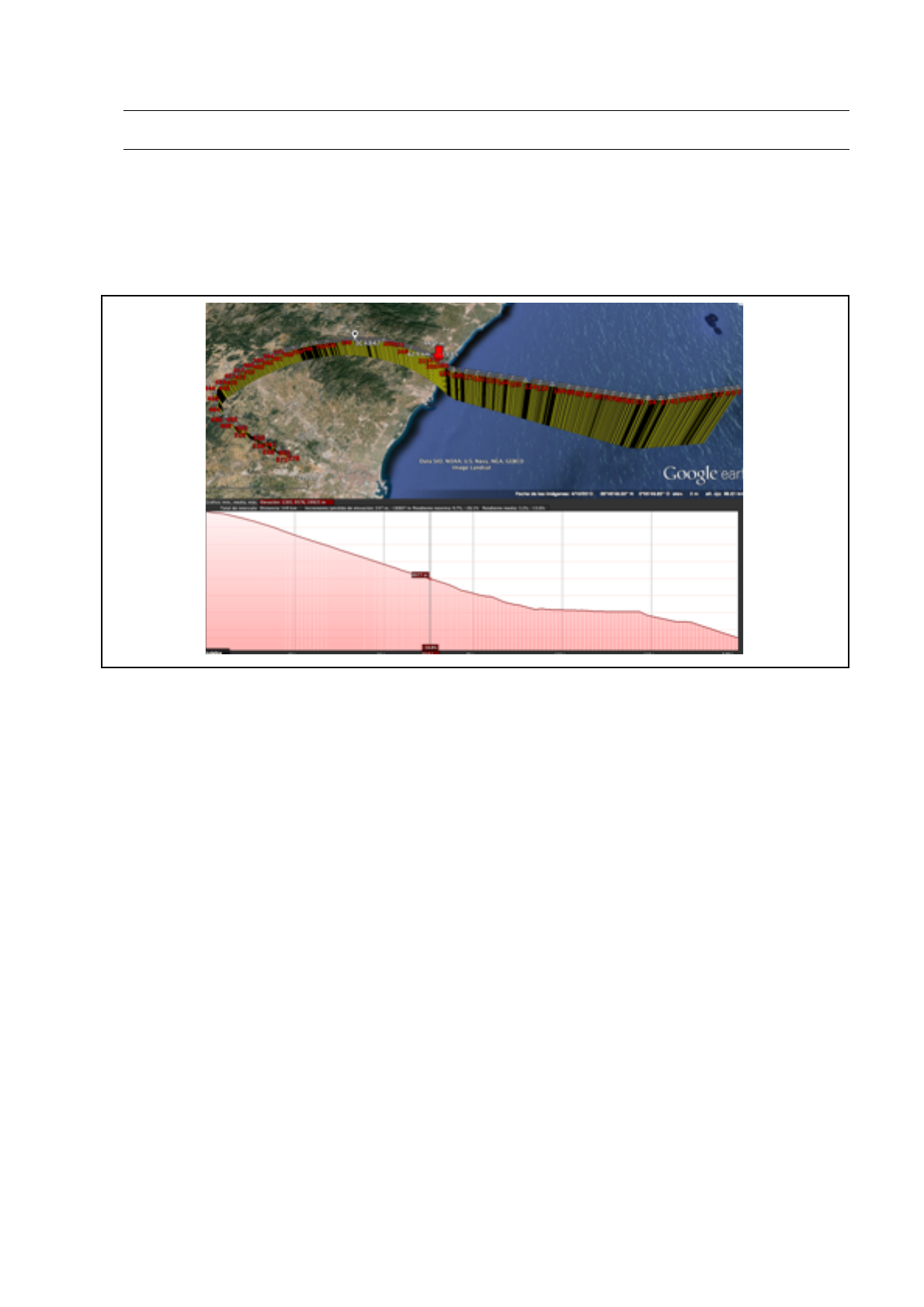
MAIN_3: READ A TRAFFIC TRACK AND REPRESENT IT IN GOOGLE EARTH
This example introduces the use of function TRACK_read. This function is used to read a trace
previously stored in a file.
Google Earth representation is based on the use of the kmlwrite_polyline library function. See
library lib/kml.
25
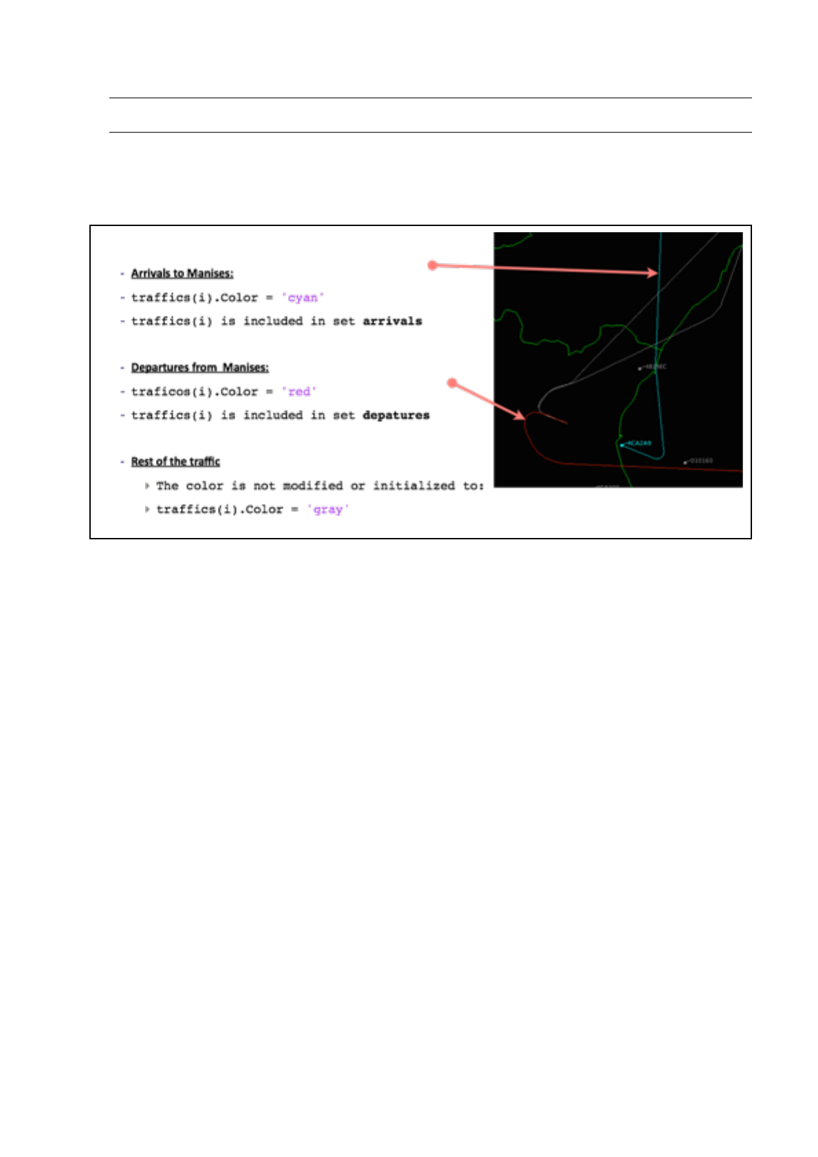
MAIN_4: DETECT AND LOG MANISES DEPARTURES AND ARRIVALS
This example is very much similar to MAIN_1. The only remarkable difference is the use of
function PROCESS_DepArr to guess the departures and arrivals from Valencia airport. Traffics are
colored in different ways according if they are departures, arrivals or they are overflying the airport.
Function PROCESS_DepArr identifies Departures and Arrivals to an Airport and represents
them in different colors: departures in red and arrivals in cyan.
It returns:
DepTraffic: array of departure traffics
ArrTraffic: array of arrival traffics
traffics : array of all traffics with the color attribute properly set
This function needs two phases to detect departures and arrivals.
1st PHASE:
DEPARTURE candidate: 94>,>.;0< j< UTTT< kk< < 5I2EQ)*-,>.;0b9,/3)/>84)*FjT8TY< kk<
5I2EQ5>,>.;0b9,/3)/>845>FjT8TY<
ARRIVAL candidate: 94>,>.;0<j<CTTTT<kk<<5I2EQ)*-,>.;b9,/3)/>84)*Fj@8C<kk<5I2EQ5>,>.;b
9,/3)/>845>Fj@8C<
26

2nd PHASE:
DEPARTURE:
• a) Departure candidate && Altitude increases && Distance increases
• b) Departure && 5I2EQ)*-,>.;0b9,/3)/>84)*Fj@8C<kk<5I2EQ5>,>.;0b9,/3)/>845>Fj@8C
ARRIVAL
• a) Arrival candidate && Altitude decreases && Distance decreases
• b) Arrival && 5I2EQ)*-,>.;0b9,/3)/>84)*FlT8Y<kk<5I2EQ5>,>.;0<b9,/3)/>845>FlT8Y
27
MAIN_5: DRAW FLIGHT VECTORS IN SACTA MONITOR
This example draws the flight vectors of each traffic in order to easily estimate future estimated
positions.
It introduces the use of function SACTA_DisplayLines to draw the vectors.
Function PROCESS_Vectors calculates the flight vectors (sable) of an array of traffics and
returns it as cell array of lines. The flight vector (sable) is a line that goes from the nose of the plane to
the calculated future position at a time t_future from current time t. This position is calculated by
extrapolation using the ground speed, the vertical speed and the track angle.!
28
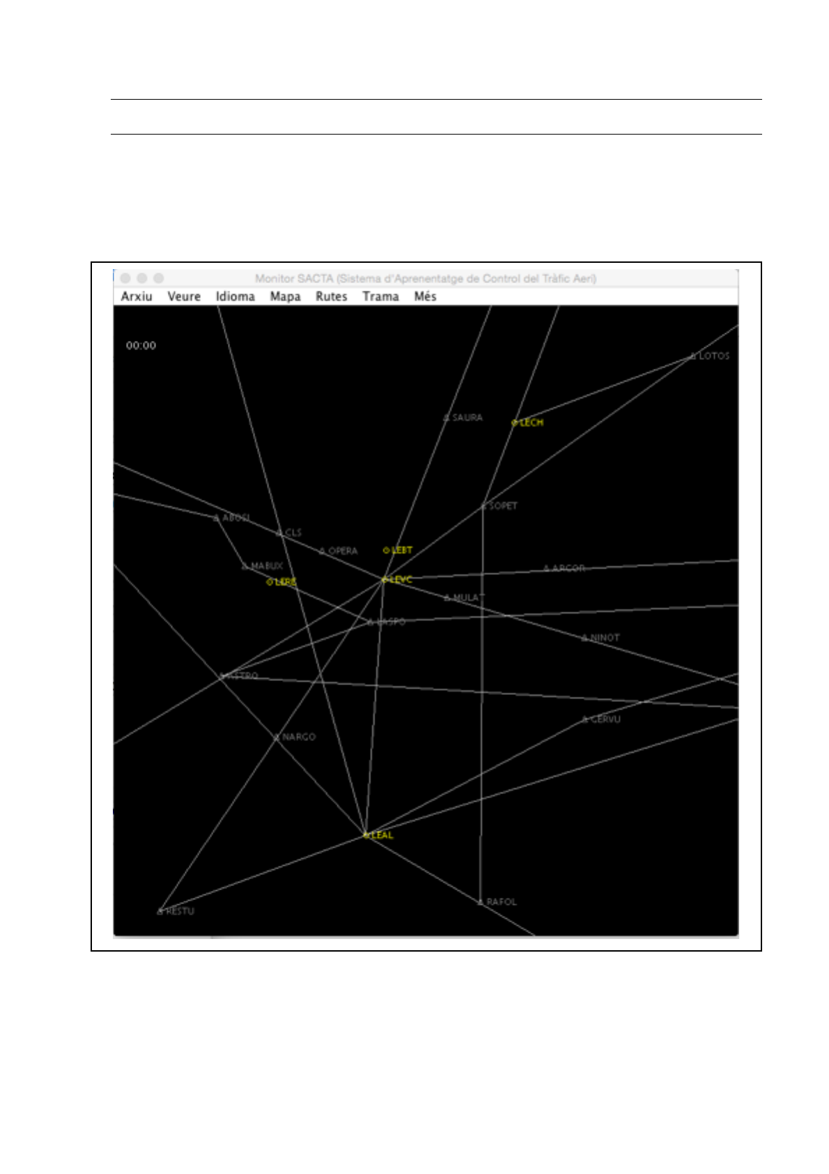
MAIN_6: DRAW ROUTES AND FIXES IN SACTA MONITOR
This example draws the airways and most important waypoints in the Valencia airspace.
It introduces the use of function SACTA_DisplayRoutes to draw the airways.
It introduces the use of function SACTA_DisplayWaypoints to draw the waypoints.
29
