MOEAFramework 2.6 Manual
User Manual: Pdf
Open the PDF directly: View PDF ![]() .
.
Page Count: 220 [warning: Documents this large are best viewed by clicking the View PDF Link!]
- Introduction
- I Beginner's Guide - Installing and Using the MOEA Framework
- Installation Instructions
- Executor, Instrumenter, Analyzer
- Diagnostic Tool
- Defining New Problems
- Representing Decision Variables
- Example: Knapsack Problem
- II Advanced Guide - Large-Scale Experiments, Parallelization, and other Advanced Topics
- Comparative Studies
- What are Comparative Studies?
- Executing Commands
- Parameter Description File
- Generating Parameter Samples
- Evaluation
- Check Completion
- Reference Set Generation
- Metric Calculation
- Averaging Metrics
- Analysis
- Set Contribution
- Sobol Analysis
- Example Script File (Unix/Linux)
- PBS Job Scripting (Unix)
- Conclusion
- Troubleshooting
- Optimization Algorithms
- Parallelization
- Advanced Topics
- Comparative Studies
- III Developer's Guide - Extending and Contributing to the MOEA Framework
MOEA Framework User Guide
A Free and Open Source Java Framework for Multiobjective Optimization
David Hadka
Version 2.6
ii

Copyright 2011-2015 David Hadka. All Rights Reserved.
Permission is granted to copy, distribute and/or modify this document un-
der the terms of the GNU Free Documentation License, Version 1.3 or any
later version published by the Free Software Foundation; with the Invariant
Section being the section entitled “Preface”, no Front-Cover Texts, and no
Back-Cover Texts. A copy of the license is included in the section entitled
“GNU Free Documentation License”.
iii
iv

Permission is granted to copy, distribute and/or modify the program code
contained in this document under the terms of the GNU Lesser General
Public License, Version 3 or any later version published by the Free Software
Foundation. Attach the following notice to any program code copied or
modified from this document:
Copyright 2011-2015 David Hadka. All Rights Reserved.
The MOEA Framework is free software: you can redistribute it
and/or modify it under the terms of the GNU Lesser General
Public License as published by the Free Software Foundation, ei-
ther version 3 of the License, or (at your option) any later version.
The MOEA Framework is distributed in the hope that it will
be useful, but WITHOUT ANY WARRANTY; without even the
implied warranty of MERCHANTABILITY or FITNESS FOR A
PARTICULAR PURPOSE. See the GNU Lesser General Public
License for more details.
You should have received a copy of the GNU Lesser General
Public License along with the MOEA Framework. If not, see
<http://www.gnu.org/licenses/>.
v
vi
Preface
Thank you for your interest in the MOEA Framework. Development of
the MOEA Framework started in 2009 with the idea of providing a single,
consistent framework for designing, testing, and experimenting with multi-
objective evolutionary algorithms (MOEAs). In late 2011, the software was
open-sourced and made available to the general public. Since then, a large
user base from the MOEA research community has formed, with thousands
of users from over 112 countries. We are indebted to the many individuals
who have contributed to this project through feedback, bug reporting, code
development, and testing.
As of September 2013, we have reached the next major milestone in the
development and maturity of the MOEA Framework. Version 2.0 brings with
it significant changes aimed to improve both the functionality and ease-of-use
of this software. We plan to implement more algorithms within the MOEA
Framework, which will improve the reliability, performance, and flexibility of
the algorithms. Doing so places the responsibility of ensuring the correctness
of the MOEA implementations on our shoulders, and we will continuously
work to ensure results obtained using the MOEA Framework meet the stan-
dards of scientific rigor.
We also want to reach out to the community of researchers developing
new, state-of-the-art MOEAs and ask that they consider providing reference
implementations of their MOEAs within the MOEA Framework. Doing so
not only disseminates your work to a wide user base, but you can take advan-
tage of the many resources and functionality already provided by the MOEA
Framework. Please contact contribute@moeaframework.org if we can
assist in any way.
vii
viii
Citing the MOEA Framework
Please include a citation to the MOEA Framework in any academic publi-
cations which used or are based on results from the MOEA Framework. For
example, you can use the following citation:
Hadka, David (2015). MOEA Framework User Guide. Version
2.6, available at http://www.moeaframework.org/.
ix
x
Contributing to this Document
This document is a work in progress. Please be mindful of this fact
when reading this document. If you encounter any spelling or grammat-
ical errors, confusing or unclear wording, inaccurate instructions, incom-
plete sections or missing topics, please notify us by sending an e-mail to
contribute@moeaframework.org. Please provide 1) the manual ver-
sion number, 2) the location of the error, and 3) a description of the error.
You may alternatively send an annotated version of the PDF file. With your
help, we can provide a complete and accurate user manual for this product.
xi
xii
Contents
1 Introduction 1
1.1 KeyFeatures ........................... 2
1.2 Other Java Frameworks . . . . . . . . . . . . . . . . . . . . . 3
1.2.1 Watchmaker Framework . . . . . . . . . . . . . . . . . 3
1.2.2 ECJ ............................ 4
1.2.3 jMetal ........................... 5
1.2.4 Opt4J ........................... 5
1.2.5 Others........................... 6
1.3 ReportingBugs .......................... 6
1.4 GettingHelp ........................... 7
I Beginner’s Guide - Installing and Using the
MOEA Framework 9
2 Installation Instructions 11
2.1 Understanding the License . . . . . . . . . . . . . . . . . . . . 11
2.2 Which Distribution is Right for Me? . . . . . . . . . . . . . . 11
2.3 ObtainingaCopy......................... 12
2.4 Installing Dependencies . . . . . . . . . . . . . . . . . . . . . . 12
2.4.1 Java 6+ (Required) . . . . . . . . . . . . . . . . . . . . 13
2.4.2 Eclipse or NetBeans (Optional) . . . . . . . . . . . . . 14
2.4.3 Apache Ant (Optional) . . . . . . . . . . . . . . . . . . 14
2.5 Importing into Eclipse . . . . . . . . . . . . . . . . . . . . . . 14
2.6 Importing into NetBeans . . . . . . . . . . . . . . . . . . . . . 15
2.7 Testing your Installation . . . . . . . . . . . . . . . . . . . . . 15
2.8 Distribution Contents . . . . . . . . . . . . . . . . . . . . . . . 17
2.8.1 Compiled Binary Contents . . . . . . . . . . . . . . . . 17
xiii
xiv CONTENTS
2.8.2 Source Code Contents . . . . . . . . . . . . . . . . . . 18
2.9 Resolving Dependencies with Maven . . . . . . . . . . . . . . 19
2.10 A Note on Running Examples . . . . . . . . . . . . . . . . . . 20
2.11Conclusion............................. 20
3 Executor, Instrumenter, Analyzer 21
3.1 Executor.............................. 21
3.2 Instrumenter ........................... 25
3.3 Analyzer.............................. 29
3.4 Conclusion............................. 32
4 Diagnostic Tool 33
4.1 Running the Diagnostic Tool . . . . . . . . . . . . . . . . . . . 33
4.2 LayoutoftheGUI ........................ 34
4.3 Quantile Plots vs Individual Traces . . . . . . . . . . . . . . . 35
4.4 Viewing Approximation Set Dynamics . . . . . . . . . . . . . 35
4.5 Statistical Results . . . . . . . . . . . . . . . . . . . . . . . . . 39
4.6 Improving Performance and Memory Efficiency . . . . . . . . 41
4.7 Conclusion............................. 42
5 Defining New Problems 43
5.1 Java ................................ 44
5.2 C/C++ .............................. 46
5.3 Scripting Language . . . . . . . . . . . . . . . . . . . . . . . . 51
5.4 Conclusion............................. 53
6 Representing Decision Variables 55
6.1 Floating-Point Values . . . . . . . . . . . . . . . . . . . . . . . 55
6.2 Integers .............................. 57
6.3 BooleanValues .......................... 58
6.4 BitStrings............................. 59
6.5 Permutations ........................... 60
6.6 Programs (Expression Trees) . . . . . . . . . . . . . . . . . . . 61
6.7 Grammars............................. 63
6.8 Variation Operators . . . . . . . . . . . . . . . . . . . . . . . . 65
6.8.1 Initialization........................ 65
6.8.2 Variation (Mutation & Crossover) . . . . . . . . . . . . 65
6.9 Conclusion............................. 67
CONTENTS xv
7 Example: Knapsack Problem 69
7.1 DataFiles............................. 70
7.2 Encoding the Problem . . . . . . . . . . . . . . . . . . . . . . 71
7.3 Implementing the Problem . . . . . . . . . . . . . . . . . . . . 72
7.4 Solving the Problem . . . . . . . . . . . . . . . . . . . . . . . 78
7.5 Conclusion............................. 79
II Advanced Guide - Large-Scale Experiments, Par-
allelization, and other Advanced Topics 81
8 Comparative Studies 83
8.1 What are Comparative Studies? . . . . . . . . . . . . . . . . . 83
8.2 Executing Commands . . . . . . . . . . . . . . . . . . . . . . . 85
8.3 Parameter Description File . . . . . . . . . . . . . . . . . . . . 86
8.4 Generating Parameter Samples . . . . . . . . . . . . . . . . . 86
8.5 Evaluation............................. 87
8.6 Check Completion . . . . . . . . . . . . . . . . . . . . . . . . 88
8.7 Reference Set Generation . . . . . . . . . . . . . . . . . . . . . 89
8.8 Metric Calculation . . . . . . . . . . . . . . . . . . . . . . . . 89
8.9 Averaging Metrics . . . . . . . . . . . . . . . . . . . . . . . . . 90
8.10Analysis .............................. 90
8.10.1 Best ............................ 91
8.10.2 Attainment ........................ 91
8.10.3 Efficiency ......................... 92
8.11SetContribution ......................... 92
8.12SobolAnalysis........................... 93
8.13 Example Script File (Unix/Linux) . . . . . . . . . . . . . . . . 95
8.14 PBS Job Scripting (Unix) . . . . . . . . . . . . . . . . . . . . 98
8.15Conclusion.............................100
8.16 Troubleshooting . . . . . . . . . . . . . . . . . . . . . . . . . . 100
9 Optimization Algorithms 105
9.1 Native Algorithms . . . . . . . . . . . . . . . . . . . . . . . . 105
9.1.1 CMA-ES..........................105
9.1.2 DBEA...........................108
9.1.3 -MOEA..........................109
9.1.4 -NSGA-II.........................110
xvi CONTENTS
9.1.5 GDE3 ...........................112
9.1.6 IBEA ...........................112
9.1.7 MOEA/D .........................113
9.1.8 NSGA-II..........................114
9.1.9 NSGA-III .........................115
9.1.10 OMOPSO.........................116
9.1.11 PAES ...........................117
9.1.12 PESA-II..........................118
9.1.13 Random Search . . . . . . . . . . . . . . . . . . . . . . 119
9.1.14 SMPSO ..........................119
9.1.15 SMS-EMOA........................120
9.1.16 SPEA2...........................121
9.1.17 VEGA...........................122
9.2 JMetal Algorithms . . . . . . . . . . . . . . . . . . . . . . . . 123
9.2.1 AbYSS...........................124
9.2.2 CellDE...........................124
9.2.3 DENSEA .........................125
9.2.4 FastPGA .........................126
9.2.5 MOCell ..........................127
9.2.6 MOCHC..........................127
9.3 PISAAlgorithms .........................128
9.3.1 Adding a PISA Selector . . . . . . . . . . . . . . . . . 130
9.3.2 Troubleshooting . . . . . . . . . . . . . . . . . . . . . . 131
9.4 BorgMOEA............................133
9.5 Conclusion.............................133
10 Parallelization 135
10.1 Master-Slave Parallelization . . . . . . . . . . . . . . . . . . . 135
10.2 Island-Model Parallelization . . . . . . . . . . . . . . . . . . . 141
10.3 Hybrid Parallelization . . . . . . . . . . . . . . . . . . . . . . 144
10.4Conclusion.............................145
11 Advanced Topics 147
11.1 Configuring Hypervolume Calculation . . . . . . . . . . . . . . 147
11.2 Storing Large Datasets . . . . . . . . . . . . . . . . . . . . . . 148
11.2.1 Writing Result Files . . . . . . . . . . . . . . . . . . . 149
11.2.2 Extract Information from Result Files . . . . . . . . . 150
11.3 Dealing with Maximized Objectives . . . . . . . . . . . . . . . 151
CONTENTS xvii
11.4Checkpointing...........................152
11.5 Referencing the Problem . . . . . . . . . . . . . . . . . . . . . 153
11.5.1 ByClass..........................153
11.5.2 By Class Name . . . . . . . . . . . . . . . . . . . . . . 154
11.5.3 ByName .........................155
11.5.4 With a ProblemProvider . . . . . . . . . . . . . . . . . 155
11.5.5 With the global.properties File . . . . . . . . . 157
III Developer’s Guide - Extending and Contribut-
ing to the MOEA Framework 159
12 Developer Guide 161
12.1VersionNumbers .........................161
12.2ReleaseCycle ...........................162
12.3 API Deprecation . . . . . . . . . . . . . . . . . . . . . . . . . 162
12.4CodeStyle.............................163
12.5Licensing..............................167
12.6WebPresence...........................167
12.7 Ways to Contribute . . . . . . . . . . . . . . . . . . . . . . . . 168
12.7.1 Translations........................168
13 Errors and Warning Messages 171
13.1Errors ...............................171
13.2Warnings .............................183
Credits 187
GNU Free Documentation License 189
References 201
xviii CONTENTS
Chapter 1
Introduction
The MOEA Framework is a free and open source Java library for developing
and experimenting with multiobjective evolutionary algorithms (MOEAs)
and other general-purpose optimization algorithms. A number of algo-
rithms are provided out-of-the-box, including NSGA-II, -MOEA, GDE3 and
MOEA/D. In addition, the MOEA Framework provides the tools necessary
to rapidly design, develop, execute and statistically test optimization algo-
rithms.
This user manual is divided into the following three parts:
Beginner’s Guide - Provides an introduction to the MOEA Framework for
new users. Topics discussed include installation instructions, walking
through some introductory examples, and solving user-specified prob-
lems.
Advanced Guide - Introduces features provided by the MOEA Framework
intended for academic researchers and other advanced users. Topics
include performing large-scale experimentation, statistically comparing
algorithms, and advanced configuration options.
Developer’s Guide - Intended for software developers, this part details
guidelines for contributing to the MOEA Framework. Topics covered
include the development of new optimization algorithms, software cod-
ing guidelines and other policies for contributors.
1

2CHAPTER 1. INTRODUCTION
Throughout this manual, you will find paragraphs marked with a red ex-
clamation as shown on the left-hand side of this page. This symbol indicates
important advice to help troubleshoot common problems.
Additionally, paragraphs marked with the lightbulb, as shown to the left,
provide helpful suggestions and other advice. For example, here is perhaps
the best advice we can provide: throughout this manual, we will refer you
to the “API documentation” to find additional information about a feature.
The API documentation is available at http://moeaframework.org/
javadoc/index.html. This documentation covers every aspect and every
feature of the MOEA Framework in detail, and it is the best place to look
to find out how something works.
1.1 Key Features
The following features of the MOEA Framework distinguish it from available
alternatives (detailed in the next section).
Fast, reliable implementations of many state-of-the-art multiob-
jective evolutionary algorithms. The MOEA Framework contains in-
ternally NSGA-II, -MOEA, -NSGA-II, GDE3 and MOEA/D. These algo-
rithms are optimized for performance, making them readily available for high
performance applications. By also supporting the JMetal and PISA libraries,
the MOEA Framework provides access to 24 multiobjective optimization al-
gorithms.
Extensible with custom algorithms, problems and operators. The
MOEA Framework provides a base set of algorithms, test problems and
search operators, but can also be easily extended to include additional com-
ponents. Using a Service Provider Interface (SPI), new algorithms and prob-
lems are seamlessly integrated within the MOEA Framework.
Modular design for constructing new optimization algorithms from
existing components. The well-structured, object-oriented design of the
MOEA Framework library allows combining existing components to con-
struct new optimization algorithms. And if needed functionality is not avail-
able in the MOEA Framework, you can always extend an existing class or
add new classes to support any desired feature.

1.2. OTHER JAVA FRAMEWORKS 3
Permissive open source license. The MOEA Framework is licensed un-
der the free and open GNU Lesser General Public License, version 3 or (at
your option) any later version. This allows end users to study, modify, and
distribute the MOEA Framework freely.
Fully documented source code. The source code is fully documented
and is frequently updated to remain consistent with any changes. Further-
more, an extensive user manual is provided detailing the use of the MOEA
Framework in detail.
Extensive support available online. As an actively maintained project,
bug fixes and new features are constantly added. We are constantly striving
to improve this product. To aid this process, our website provides the tools
to report bugs, request new features, or get answers to your questions.
Over 1100 test cases to ensure validity. Every release of the MOEA
Framework undergoes extensive testing and quality control checks. And, if
any bugs are discovered that survive this testing, we will promptly fix the
issues and release patches.
1.2 Other Java Frameworks
There exist a number of Java optimization framework developed over the
years. This section discusses the advantages and disadvantages of each frame-
work. While we appreciate your interest in the MOEA Framework, it is al-
ways useful to be aware of the available tools which may suit your specific
needs better.
1.2.1 Watchmaker Framework
The Watchmaker Framework is one of the most pop-
ular open source Java libraries for single objective
optimization. Its design is non-invasive, allowing
users to evolve objects of any type. Most other
frameworks (including the MOEA Framework) re-
quire the user to encode their objects using pre-
defined decision variable types. However, giving the users this freedom also
4CHAPTER 1. INTRODUCTION
increases the burden on the user to develop custom evolutionary operators
for their objects.
Homepage: http://watchmaker.uncommons.org
License: Apache License, Version 2.0
Advantages:
•Very clean API
•Fully documented source code
•Flexible decision variable representation
•Large collection of interesting example problems (Mona
Lisa, Sudoku, Biomorphs)
Disadvantages:
•Single objective only
•Much of the implementation burden is placed on the
developer
•Infrequently updated (the last release, 0.7.1, was in Jan-
uary 2010)
1.2.2 ECJ
ECJ is a research-oriented Java library developed at the George Mason Uni-
versity’s Evolutionary Computation Laboratory. Now in existence for nearly
fourteen years, ECJ is a mature and stable framework. It features a range of
evolutionary paradigms, including both single and multiobjective optimiza-
tion, master/slave and island-model parallelization, coevolution, parsimony
pressure techniques, with extensive support for genetic programming.
Homepage: http://cs.gmu.edu/˜eclab/projects/
ecj/
License: Academic Free License, Version 3.0
Advantages:
•Quickly setup and execute simple EAs without touching
any source code
•One of the most sophisticated open source libraries, par-
ticular in its support for various GP tree encodings
1.2. OTHER JAVA FRAMEWORKS 5
•Provides an extensive user manual, tutorials, and other
developer tools
Disadvantages:
•Focused on single-objective optimization, providing
only older MOEAs (NSGA-II and SPEA2)
•Configuring EAs using ECJs configuration file can be
cumbersome and error prone
•Appears to lack any kind of automated testing or quality
assurance
1.2.3 jMetal
jMetal is a framework focused on the development, experimentation and
study of metaheuristics. As such, it includes the largest collection of meta-
heuristics of any framework discussed here. If fact, the MOEA Framework
incorporates the jMetal library for this very reason. The jMetal authors have
more recently started developing C++ and C# versions of the jMetal library.
Homepage: http://jmetal.sourceforge.net
License: GNU Lesser General Public License, Version 3 or later
Advantages:
•Focused on multiobjective optimization
•Implementations of 15 state-of-the-art MOEAs
•Provides an extensive user manual
Disadvantages:
•Not currently setup as a library; several places have
hard-coded paths to resources located on the original
developers computer
•Appears to lack any kind of automated testing or quality
assurance
•Source code is not fully documented
1.2.4 Opt4J

6CHAPTER 1. INTRODUCTION
Opt4J provides perhaps the cleanest MOEA imple-
mentation. It takes modularity to the extreme, using
aspect-oriented programming to automatically stitch
together program modules to form a complete, work-
ing optimization algorithm. A helpful GUI for constructing experiments is
also provided.
Homepage: http://opt4j.sourceforge.net/
License: GNU Lesser General Public License, Version 3 or later
Advantages:
•Focused on multiobjective optimization
•Uses aspect-oriented programming (AOP) via Google
Guice to manage dependencies and wire all the compo-
nents together
•Well documented source code
•Frequently updated
Disadvantages:
•Only a limited number of MOEAs provided
1.2.5 Others
For completeness, we also acknowledge JGAP and JCLEC, two stable and
maintained Java libraries for evolutionary computation. These two libraries,
like the Watchmaker Framework, are specialized for single-objective opti-
mization. They do provide basic support for multiobjective optimization,
but not to the extent of JMetal, Opt4J, and the MOEA Framework. If you
are dealing with only single-objective optimization problems, we encourage
you to explore these libraries that specialize in single-objective optimization.
1.3 Reporting Bugs
The MOEA Framework is not bug-free, nor is any other software application,
and reporting bugs to developers is the first step towards improving the relia-
bility of software. Critical bugs will often be addressed within days. If during
its use you encounter error messages, crashes, or other unexpected behav-
ior, please file a bug report at http://moeaframework.org/support.
1.4. GETTING HELP 7
html. In the bug report, describe the problem encountered and, if known,
the version of the MOEA Framework used.
1.4 Getting Help
This user guide is the most comprehensive resource for learning about the
MOEA Framework. However, as this manual is still a work in progress, you
may need to turn to some other resources to find answers to your questions.
Our website at http://www.moeaframework.org contains links to the
API documentation, which provides access to the detailed source code doc-
umentation. This website also has links to file bugs or request new features.
If you still can not find an answer to your question, feel free to contact us at
support@moeaframework.org.
8CHAPTER 1. INTRODUCTION
Part I
Beginner’s Guide - Installing
and Using the MOEA
Framework
9
Chapter 2
Installation Instructions
This chapter details the steps necessary to download and install the MOEA
Framework on your computer.
2.1 Understanding the License
Prior to downloading, using, modifying or distributing the MOEA Frame-
work, developers should make themselves aware of the conditions of the GNU
Lesser General Public License (GNU LGPL). While the GNU LGPL is a free
software license, it does define certain conditions that must be followed in or-
der to use, modify and distribute the MOEA Framework library. These condi-
tions are enacted to ensure that all recipients of the MOEA Framework (in its
original and modified forms) are granted the freedoms to use, modify, study
and distribute the MOEA Framework so long as the conditions of the GNU
LGPL are met. Visit http://www.gnu.org/licenses/lgpl.html to
read the full terms of this license.
2.2 Which Distribution is Right for Me?
The MOEA Framework is currently distributed in three forms: 1) the com-
piled binaries; 2) the source code; and 3) the demo application. The following
text describes each distribution and its intended audience.
Compiled Binaries The compiled binaries distribution contains a fully-
working MOEA Framework installation. All required third-party libraries,
11

12 CHAPTER 2. INSTALLATION INSTRUCTIONS
data files and documentation are provided. This download is recommended
for developers integrating the MOEA Framework into an existing project.
Source Code The source code distribution contains all source code, unit
tests, documentation and data files. This distribution gives users full control
over the MOEA Framework, as any component can be modified as needed.
As such, this download is recommended for developers wishing to contribute
to or study the inner workings of the MOEA Framework.
Demo Application The demo application provides several interactive de-
mos of the MOEA Framework launched by double-clicking the downloaded
JAR file or running the command java - jar MOEAFramework-2.6-
Demo.jar. This download is intended for first-time users to quickly learn
about the MOEA Framework and its capabilities.
2.3 Obtaining a Copy
The various MOEA Framework distributions can be downloaded from our
website at http://www.moeaframework.org/. The compiled binaries
and source code distributions are packaged in a compressed tar (.tar.gz)
file. Unix/Linux/Mac users can extract the file contents using the following
command:
tar -xzf MOEAFramework-2.6.tar.gz
Windows users must use an unzip utility like 7-Zip to extract the file
contents. 7-Zip is a free, open source program which can be downloaded
from http://www.7-zip.org/.
2.4 Installing Dependencies
The software packages listed below are required or recommended in order
to use the MOEA Framework. Any software package marked as required
MUST be installed on your computer in order to use the MOEA Framework.
Software marked as optional is not required to be installed, but will generally
2.4. INSTALLING DEPENDENCIES 13
make your life easier. This manual will often provide instructions specific to
these optional software packages.
2.4.1 Java 6+ (Required)
Java 6, or any later version, is required for any system running the MOEA
Framework. If downloading the compiled binaries or demo application, you
only need to install the Java Runtime Environment (JRE). The source code
download requires the Java Development Kit (JDK), which contains the com-
piler and other developer tools. We recommend one of the following vendors
(most are free):
Oracle -http://www.oracle.com/technetwork/java/javase/
•For Windows, Linux and Solaris
JRockit JDK -http://www.oracle.com/technetwork/
middleware/jrockit/
•For Windows, Linux and Solaris
•May provide better performance and scalability on Intel 32 and
64-bit architectures
OpenJDK -http://openjdk.java.net/
•For Ubuntu 8.04 (or later), Fedora 9 (or later), Red Hat Enterprise
Linux 5, openSUSE 11.1, Debian GNU/Linux 5.0 and OpenSolaris
IBM -http://www.ibm.com/developerworks/java/jdk/
•For AIX, Linux and z/OS
Apple -http://support.apple.com/kb/DL1572
Please follow the installation instruction accompanying your chosen JRE
or JDK.

14 CHAPTER 2. INSTALLATION INSTRUCTIONS
2.4.2 Eclipse or NetBeans (Optional)
Eclipse and NetBeans are two development environments for writing, debug-
ging, testing, and running Java programs. Eclipse can be downloaded for free
from http://www.eclipse.org/, and NetBeans can be obtained from
http://netbeans.org/.
The installation of Eclipse is simple — just extract the compressed file
to a folder of your choice and run the Eclipse executable from this folder.
First-time users of Eclipse may be prompted to select a workspace location.
The default location is typically fine. Click the checkbox to no longer show
this dialog and click Ok.
To install NetBeans, simply run the executable. Once installed, you can
launch NetBeans by clicking the NetBeans link in your start menu.
2.4.3 Apache Ant (Optional)
Apache Ant is a Java tool for automatically compiling and packaging projects,
similar to the Make utility on Unix/Linux. Individuals working with the
source code distribution should consider installing Apache Ant, as it helps
automate building and testing the MOEA Framework. Apache Ant can be
downloaded from http://ant.apache.org/. The installation instruc-
tions provided by Ant should be followed.
Note that Eclipse contains Ant, so it is not necessary to install Eclipse
and Ant together.
2.5 Importing into Eclipse
When working with the source code distribution, it is necessary to properly
configure the Java environment to ensure all resources are available. To assist
in this process, the source code distribution includes the necessary files to
import directly into Eclipse.
To import the MOEA Framework project into Eclipse, first start Eclipse
and select File →Import... from the menu. A popup window will ap-
pear. Ensure the General →Existing Projects into Workspace item is se-
lected and click Next. A new window will appear. In this new window,
locate the Set Root Directory entry. Using the Browse button, select the
MOEAFramework-2.6 folder. Finally, click Finish. The MOEA Frame-
work will now be properly configured in Eclipse.

2.6. IMPORTING INTO NETBEANS 15
2.6 Importing into NetBeans
If you downloaded the source code, you can import the MOEA Framework
into NetBeans as follows. In NetBeans, select New Project from the File
menu. In the screen that appears, select the “Java” category and “Java
Project with Existing Sources”. Click Next.
Specify the project name as “MOEA Framework”. Set the project folder
by clicking the Browse button and selecting the MOEAFramework-2.6
folder. Click Next.
Add the src and examples folders as Source Package Folders.
Click Finish. The MOEA Framework project should now appear in the
Projects window.
Finally, we need to add the third-party libraries used by the MOEA
Framework. Right-click the MOEA Framework project in the Projects win-
dow and select Properties. In the window that appears, click Libraries in
the left-hand panel. On the right-side of the window, click the button “Add
Jars/Folder”. Browse to the MOEAFramework-2.6/lib folder, high-
light all the JAR files (using shift or alt to select multiple files), and click
Ok. Be sure that you select each individual JAR file and not the folder con-
taining the JAR files. Click the “Add Jars/Folder” button again. Navigate
to and select the root MOEAFramework-2.6 folder, and click Ok. You
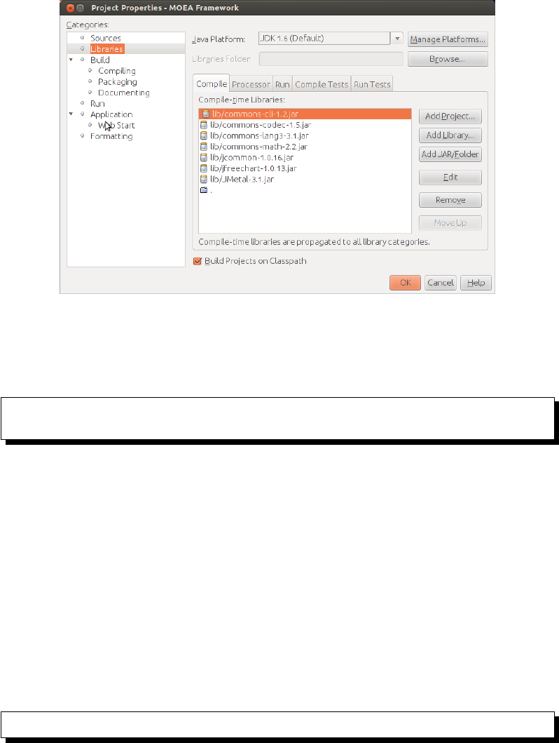
should now see 8 items in the compile-time libraries list. There should be 7
entries referencing .jar files the “ .” as the last entry. Your screen should
look like Figure 2.1. Click Ok when finished.
Test your NetBeans install by running Example1. You can run an ex-
ample by expanding the examples folder in the Project window, right-
clicking Example1, and selecting Run File from the popup menu.
2.7 Testing your Installation
Having finished installing the MOEA Framework and its dependencies, it
is useful to run the MOEA Diagnostic Tool to test if the installation was
successful. If the diagnostic tool appears and you can run any algorithm,
then the installation was successful.
Compiled Binaries Run the launch-diagnostic-tool.bat file on Windows.
You can manually run the diagnostic tool with the following command:
16 CHAPTER 2. INSTALLATION INSTRUCTIONS
Figure 2.1: How the NetBeans properties window should appear in the
MOEA Framework is properly configured.
java -Djava.ext.dirs=lib
org.moeaframework.analysis.diagnostics.LaunchDiagnosticTool
Source Code Inside Eclipse, navigate to the src →org →moeaframework
→analysis →diagnostic package in the Package Explorer window. Right-
click the file LaunchDiagnosticTool.java and select the Run as →
Java Application option in the popup menu.
Demo Program Double-click the downloaded JAR file. If the demo win-
dow does not appear, try to manually launch the tool with with the following
command:
java -jar MOEAFramework-2.6-Demo.jar

2.8. DISTRIBUTION CONTENTS 17
2.8 Distribution Contents
This section describes the contents of the compiled binaries and source code
distribution downloads.
2.8.1 Compiled Binary Contents
javadoc/ contains the MOEA Framework API, which is a valuable re-
source for software developers as it provides descriptions of all classes,
methods and variables available in the MOEA Framework. The API
may be viewed in a web browser by opening the index.html file.
lib/ contains the compiled libraries required to use the MOEA Frame-
work. This includes the MOEA Framework compiled libraries and all
required third-party libraries.
licenses/ contains the complete text of all open source software licenses
for the MOEA Framework and third-party libraries. In order to comply
with the licenses, this folder should always be distributed alongside the
compiled libraries in the lib folder.
pf/ contains the Pareto front files for the test problems provided by de-
fault in the MOEA Framework.
global.properties is the configuration file for the MOEA Frame-
work. Default settings are used unless the settings are provided in
this file.
HELP provides a comprehensive list of errors and warning messages en-
countered when using the MOEA Framework. When available, infor-
mation about the cause and ways to fix errors are suggested.
launch-diagnostic-tool.bat launches the diagnostic tool GUI
that allows users to run algorithms and display runtime information
about the algorithms. This file is for Windows systems only.
LICENSE lists the open source software licenses in use by the MOEA
Framework, contributor code and third-party libraries.

18 CHAPTER 2. INSTALLATION INSTRUCTIONS
NEWS details all important changes made in the current release and prior
releases. This includes critical bug fixes, changes, enhancements and
new features.
README provides information about obtaining, installing, using, distribut-
ing, licensing and contributing to the MOEA Framework.
2.8.2 Source Code Contents
auxiliary/ contains an assortment of files and utilities used by the
MOEA Framework, but are not required in a build. For instance, this
folder contains example C/C++ code for interfacing C/C++ problems
with the MOEA Framework.
examples/ contains examples using the MOEA Framework. These ex-
amples are also available on the website.
lib/ contains all required third-party libraries used by the MOEA Frame-
work.
manual/ contains the LaTeX files and figures for generating this user
manual.
META-INF/ contains important files which are packaged with the com-
piled binaries. Such files include the service provider declarations, li-
censing information, etc.
pf/ contains the Pareto front files for the test problems provided by de-
fault in the MOEA Framework.
src/ contains all source code in use by the core MOEA Framework li-
brary.
test/ contains all JUnit unit tests used to ensure the correctness of the
MOEA Framework source code.
website/ contains all files used to generate the website.
build.xml contains the Apache Ant build scripts for compiling and/or
building the MOEA Framework library.

2.9. RESOLVING DEPENDENCIES WITH MAVEN 19
global.properties is the configuration file for the MOEA Frame-
work. Default settings are used unless the settings are provided in
this file.
HELP provides a comprehensive list of errors and warning messages en-
countered when using the MOEA Framework. When available, infor-
mation about the cause and ways to fix errors are suggested.
LICENSE lists the open source software licenses in use by the MOEA
Framework, contributor code and third-party libraries.
NEWS details all important changes made in the current release and prior
releases. This includes critical bug fixes, changes, enhancements and
new features.
README provides information about obtaining, installing, using, distribut-
ing, licensing and contributing to the MOEA Framework.
test.xml contains the Apache Ant testing scripts used to automatically
run all JUnit unit tests and provide a human-readable report of the
test results.
TODO lists all planned changes for the MOEA Framework source code.
This file is a starting point for individuals wishing to contribute modi-
fications to the MOEA Framework.
2.9 Resolving Dependencies with Maven
As of version 2.4, the MOEA Framework and its dependencies can be resolved
using the Maven dependency management system. Maven is available from
http://maven.apache.org/. To add the MOEA Framework to your
Maven project, add the following dependency to your pom.xml file:
<dependency>
<groupId>org.moeaframework</groupId>
<artifactId>moeaframework</artifactId>
<version>2.6</version>
</dependency>
20 CHAPTER 2. INSTALLATION INSTRUCTIONS
2.10 A Note on Running Examples
Several example applications are provided with the MOEA Framework in
the MOEAFramework-2.6/examples/ folder. Details on these ex-
amples can be found on our website at http://moeaframework.org/
examples.html. In general, you will want to compile and run these ex-
amples from the MOEAFramework-2.6 folder, with a command similar
to:
javac -cp "examples;lib/*" examples/Example1.java
java -cp "examples;lib/*" Example1
If you receive an error saying “no reference set available”, that is because
the MOEA Framework is unable to locate the Pareto sets for the example
problems, typically located in MOEAFramework-2.6/pf/. To resolve
this error, you will need to add the root MOEAFramework-2.6 folder to
your classpath, such as:
java -cp "C:/path/to/MOEAFramework-2.4;C:/path/to/MOEAFramework
-2.4/lib/*;C:/path/to/MOEAFramework-2.4/examples" Example1
2.11 Conclusion
This chapter described each of the MOEA Framework distributions. At this
point, you should have a working MOEA Framework distribution which you
can use to run the examples in subsequent chapters.

Chapter 3
Executor, Instrumenter,
Analyzer
The Executor, Instrumenter and Analyzer classes provide most of the func-
tionality provided by the MOEA Framework. This chapter walks through
several introductory examples using these classes.
3.1 Executor
The Executor class is responsible for constructing and executing runs of an
algorithm. A single run requires three pieces of information: 1) the problem;
2) the algorithm used to solve the problem; and 3) the number of objec-
tive function evaluations allocated to solve the problem. The following code
snippet demonstrates how these three pieces of information are passed to the
Executor.
1NondominatedPopulation result = new Executor()
2.withProblem("UF1")
3.withAlgorithm("NSGAII")
4.withMaxEvaluations(10000)
5.run();
Line 1 creates a new Executor instance. Lines 2, 3 and 4 set the problem,
algorithm and maximum number of objective function evaluations, respec-
tively. In this example, we are solving the two-objective UF1 test problem
21

22 CHAPTER 3. EXECUTOR, INSTRUMENTER, ANALYZER
using the NSGA-II algorithm. Lastly, line 5 runs this experiment and returns
the resulting approximation set.
Note how, on lines 2 and 3, the problem and algorithm are specified using
strings. There exist a number of pre-defined problems and algorithms which
are available in the MOEA Framework. Furthermore, the MOEA Framework
can be easily extended to provide additional problems and algorithms which
can be instantiated in a similar manner.
Once the run is complete, we can access the result. Line 1 above shows
that the approximation set, which is a NondominatedPopulation, gets
assigned to a variable named result. This approximation set contains all
Pareto optimal solutions produced by the algorithm during the run. For
example, the code snippet below prints out the two objectives to the console.
1for (Solution solution : result) {
2System.out.println(solution.getObjective(0) + ""+
3solution.getObjective(1));
4}
Line 1 loops over each solution in the result. A solution stores the decision
variables, objectives, constraints and any relevant attributes. Lines 2 and 3
demonstrate how the objective values can be retrieved from a solution.
Putting all this together and adding the necessary boilerplate Java code,
the complete code snippet is shown below.
1import java.util.Arrays;
2import org.moeaframework.Executor;
3import org.moeaframework.core.NondominatedPopulation;
4import org.moeaframework.core.Solution;
5
6public class Example1 {
7
8public static void main(String[] args) {
9NondominatedPopulation result = new Executor()
10 .withProblem("UF1")
11 .withAlgorithm("NSGAII")
12 .withMaxEvaluations(10000)
13 .run();
14
15 for (Solution solution : result) {
16 System.out.println(solution.getObjective(0)

3.1. EXECUTOR 23
17 +""+ solution.getObjective(1));
18 }
19 }
20
21 }
Since line 6 defines the class name to be Example1, this code snippet
must be saved to the file Example1.java. Compiling and running this
file will produce output similar to:
0.44231379762506046 0.359116256460771
0.49221581122496827 0.329972177772519
0.8024234727753593 0.11620643510507386
0.7754123383456428 0.14631335018878214
0.4417794310706653 0.3725544250337767
0.11855110357018901 0.6715178312971422
...
The withProblem and withAlgorithm methods allow us to specify
the problem and algorithm by name. Changing the problem or algorithm
is as simple as changing the string passed to these methods. For example,
replacing line 11 in the code snippet above to withAlgorithm("GDE3")
will now allow you to run the Generalized Differential Evolution 3 (GDE3)
algorithm. Most existing MOEA libraries require users to instantiate and
configure each algorithm manually. In the MOEA Framework, such details
are handled by the Executor.
The MOEA Framework is distributed with a number of built-in problems
and algorithms. See the API documentation for StandardProblems
and StandardAlgorithms to see the list of problems and al-
gorithms available, respectively. This documentation is available
online at http://www.moeaframework.org/javadoc/org/
moeaframework/problem/StandardProblems.html and http:
//www.moeaframework.org/javadoc/org/moeaframework/
algorithm/StandardAlgorithms.html.
When specifying only the problem, algorithm and maximum evaluations,
the Executor assumes default parameterizations for the internal components
of the algorithm. For instance, NSGA-II parameters include the population
size, the simulated binary crossover (SBX) rate and distribution index, and

24 CHAPTER 3. EXECUTOR, INSTRUMENTER, ANALYZER
the polynomial mutation (PM) rate and distribution index. Changing the
parameter settings from their defaults is possible using the setProperty
methods. Each parameter is identified by a key and is assigned a numeric
value. For example, all of NSGA-II’s parameters are set in the following code
snippet:
1NondominatedPopulation result = new Executor()
2.withProblem("UF1")
3.withAlgorithm("NSGAII")
4.withMaxEvaluations(10000)
5.withProperty("populationSize", 50)
6.withProperty("sbx.rate", 0.9)
7.withProperty("sbx.distributionIndex", 15.0)
8.withProperty("pm.rate", 0.1)
9.withProperty("pm.distributionIndex", 20.0)
10 .run();
Each algorithm defines its own parameters. Refer to the API documen-
tation for the exact parameter keys. Any parameters not explicitly defined
using the withProperty methods will be set to their default values.
The Executor also provides many advanced features. One such feature is
the ability to distribute objective function evaluations across multiple pro-
cessing cores or computers. Distributing evaluations can significantly speed
up a run through parallelization. The simplest way to enable paralleliza-
tion is through the distributeOnAllCores method. This will distribute
objective function evaluations across all cores on your local computer. Note
that not all algorithms can support parallelization. In such cases, the MOEA
Framework will still run the algorithm, but it will not be parallelized. The
code snippet below extends our example with distributed evaluations.
1NondominatedPopulation result = new Executor()
2.withProblem("UF1")
3.withAlgorithm("NSGAII")
4.withMaxEvaluations(10000)
5.withProperty("populationSize", 50)
6.withProperty("sbx.rate", 0.9)
7.withProperty("sbx.distributionIndex", 15.0)
8.withProperty("pm.rate", 0.1)
9.withProperty("pm.distributionIndex", 20.0)
10 .distributeOnAllCores()

3.2. INSTRUMENTER 25
11 .run();
3.2 Instrumenter
In addition to supporting a multitude of algorithms and test problems, the
MOEA Framework also contains a comprehensive suite of tools for analyzing
the performance of algorithms. The MOEA Framework supports both run-
time dynamics and end-of-run analysis. Run-time dynamics capture the
behavior of an algorithm throughout the duration of a run, recording how
its solution quality and other elements change. End-of-run analysis, on the
other hand, focuses on the result of a complete run and comparing the relative
performance of various algorithms. Run-time dynamics will be introduced in
this section using the Instrumenter; end-of-run analysis will be discussed in
the following section using the Analyzer.
The Instrumenter gets its name from its ability to add instrumentation,
which are pieces of code that record information, to an algorithm. A range
of data can be collected using the Instrumenter, including:
1. Elapsed time
2. Population size / archive size
3. The approximation set
4. Performance metrics
5. Restart frequency
The Instrumenter works hand-in-hand with the Executor to collect its
data. The Executor is responsible for configuring and running the algo-
rithm, but it allows the Instrumenter to record the necessary data while the
algorithm is running. To start collecting run-time dynamics, we first create
and configure an Instrumenter instance.
1Instrumenter instrumenter = new Instrumenter()
2.withProblem("UF1")
3.withFrequency(100)
4.attachAll();

26 CHAPTER 3. EXECUTOR, INSTRUMENTER, ANALYZER
First, line 1 creates the new Instumenter instance. Next, line 2 specifies
the problem. This allows the instrumenter to access the known reference
set for this problem, which is necessary for evaluating performance metrics.
Third, line 3 sets the frequency at which the data is recorded. In this exam-
ple, data is recorded every 100 evaluations. Lastly, line 4 indicates that all
available data should be collected.
Next, we create and configure the Executor instance with the following
code snippet:
1NondominatedPopulation result = new Executor()
2.withProblem("UF1")
3.withAlgorithm("NSGAII")
4.withMaxEvaluations(10000)
5.withInstrumenter(instrumenter)
6.run();
This code snippet is similar to the previous examples of the Executor, but
includes the addition of line 5. Line 5 tells the executor that all algorithms
it executes will be instrumented with our Instrumenter instance. Once the
instrumenter is set and the algorithm is configured, we can run the algorithm
on line 6.
When the run completes, we can access the data collected by the instru-
menter. The data is stored in an Accumulator object. The Accumulator for
the run we just executed can be retrieved with the following line:
1Accumulator accumulator = instrumenter.getLastAccumulator();
An Accumulator is similar to a Map in that it stores key-value pairs.
The key identifies the type of data recorded. However, instead of storing
a single value, the Accumulator stores many values, one for each datapoint
collected by the Instrumenter. Recall that in this example, we are recording
a datapoint every 100 evaluations (i.e., the frequency). The data can be
extracted from an Accumulator with a loop similar to the following:
1for (int i=0; i<accumulator.size("NFE"); i++) {

3.2. INSTRUMENTER 27
2System.out.println(accumulator.get("NFE",i)+"\t" +
3accumulator.get("GenerationalDistance", i));
4}
In this code snippet, we are printing out two columns of data: the num-
ber of objective function evaluations (NFE) and the generational distance
performance indicator. Including all the boilerplate Java code, the complete
example is provided below.
1import java.io.IOException;
2import java.io.File;
3import org.moeaframework.core.NondominatedPopulation;
4import org.moeaframework.Instrumenter;
5import org.moeaframework.Executor;
6import org.moeaframework.analysis.collector.Accumulator;
7
8public class Example2 {
9
10 public static void main(String[] args) throws IOException {
11 Instrumenter instrumenter = new Instrumenter()
12 .withProblem("UF1")
13 .withFrequency(100)
14 .attachAll();
15
16 NondominatedPopulation result = new Executor()
17 .withProblem("UF1")
18 .withAlgorithm("NSGAII")
19 .withMaxEvaluations(10000)
20 .withInstrumenter(instrumenter)
21 .run();
22
23 Accumulator accumulator = instrumenter.getLastAccumulator();
24
25 for (int i=0; i<accumulator.size("NFE"); i++) {
26 System.out.println(accumulator.get("NFE",i)+"\t" +
27 accumulator.get("GenerationalDistance", i));
28 }
29 }
30
31 }
Since line 8 defines the class name to be Example2, this code snippet
28 CHAPTER 3. EXECUTOR, INSTRUMENTER, ANALYZER
must be saved to the file Example2.java. Compiling and running this
file will produce output similar to:
100 0.6270289757162074
200 0.5843583367503041
300 0.459146246330144
400 0.36799025371209954
500 0.3202295846482732
600 0.2646381449859231
...
This shows how NSGA-II experiences rapid convergence early in a run.
In the first 600 evaluations, the generational distance decreases to 33% of its
starting value. Running for longer, you should see the speed of convergence
begin to level off. This type of curve is commonly seen when using MOEAs.
They often experience a rapid initial convergence that quickly levels off. You
can confirm this behavior by running this example on different algorithms.
There are a few things to keep in mind when using the Instrumenter.
First, instrumenting an algorithm and recording all the data will slow down
the execution of algorithms and significantly increase their memory usage.
For this reason, we strongly recommend limiting the data collected to what
you consider important. To limit the data collected, simply replace the
attachAll method with one or more specific attach methods, such as
attachGenerationalDistanceCollector. Changing the collection
frequency is another way to reduce the performance and memory usage.
Second, if the memory usage exceeds that which is allocated to Java, you
will receive an OutOfMemoryException. The immediate solution is to
increase the amount of memory allocated to Java by specifying the -Xmx
command-line option when starting a Java application. For example, the
following command will launch a Java program with 512 MBs of available
memory.
java -Xmx512m ...rest of command...
If you have set the -Xmx option to include all available memory on your
computer and you still receive an OutOfMemoryException, then you need
to decrease the collection frequency or restrict what data is collected.
Third, the Instrumenter only collects data which is pro-
vided by the algorithm. For instance, an Instrumenter with

3.3. ANALYZER 29
attachAdaptiveTimeContinuationCollector will work per-
fectly fine on an algorithm that does support adaptive time continuation.
The Instrumenter examines the composition of the algorithm and only
collects data for the components it finds. This also implies that the Instru-
menter will work on any algorithm, including any provided by third-party
providers.
3.3 Analyzer
The Analyzer provides end-of-run analysis. This analysis focuses on the
resulting Pareto approximation set and how it compares against a known
reference set. The Analyzer is particularly useful for statistically comparing
the results produced by two or more algorithms, or possibly the same algo-
rithm with different parameter settings. To start using the Analyzer, we first
create and configure a new instance, as shown below.
1Analyzer analyzer = new Analyzer()
2.withProblem("UF1")
3.includeAllMetrics()
4.showStatisticalSignificance();
First, we construct a new Analyzer on line 1. Next, on line 2 we set the
problem in the same manner as required by the Executor and Instrumenter.
Line 3 tells the Analyzer to evaluate all available performance metrics. Lastly,
line 4 enables the statistical comparison of the results.
Next, the code snippet below shows how the Executor is used to run
NSGA-II and GDE3 for 50 replications and store the results in the Analyzer.
Running for multiple replications, or seeds, is important when generating
statistical results.
1Executor executor = new Executor()
2.withProblem("UF1")
3.withMaxEvaluations(10000);
4
5analyzer.addAll("NSGAII",
6executor.withAlgorithm("NSGAII").runSeeds(50));
7
8analyzer.addAll("GDE3",
9executor.withAlgorithm("GDE3").runSeeds(50));

30 CHAPTER 3. EXECUTOR, INSTRUMENTER, ANALYZER
Lines 1-3 create the Executor, similar to the previous examples except we
do not yet specify the algorithm. Lines 5-6 run NSGA-II. Note how we first
set the algorithm to NSGA-II, run it for 50 seeds, and add the results from
the 50 seeds to the analyzer. Similarly, on lines 8-9 we run GDE3 and add
its results to the analyzer. Note how lines 5 and 8 pass a string as the first
argument to addAll. This gives a name to the samples collected, which can
be any string and not necessarily the algorithm name as is the case in this
example.
Lastly, we can display the results of the analysis with the following line.
1analyzer.printAnalysis();
Putting all of this together and adding the necessary boilerplate Java
code results in:
1import java.io.IOException;
2import org.moeaframework.Analyzer;
3import org.moeaframework.Executor;
4
5public class Example3 {
6
7public static void main(String[] args) throws IOException {
8Analyzer analyzer = new Analyzer()
9.withProblem("UF1")
10 .includeAllMetrics()
11 .showStatisticalSignificance();
12
13 Executor executor = new Executor()
14 .withProblem("UF1")
15 .withMaxEvaluations(10000);
16
17 analyzer.addAll("NSGAII",
18 executor.withAlgorithm("NSGAII").runSeeds(50));
19
20 analyzer.addAll("GDE3",
21 executor.withAlgorithm("GDE3").runSeeds(50));
22
23 analyzer.printAnalysis();
24 }

3.3. ANALYZER 31
25
26 }
The output of which will look similar to:
GDE3:
Hypervolume:
Min: 0.4358713988821755
Median: 0.50408587891491
Max: 0.5334024567416756
Count: 50
Indifferent: []
...
NSGAII:
Hypervolume:
Min: 0.3853879478063566
Median: 0.49033837779756184
Max: 0.5355927774923894
Count: 50
Indifferent: []
...
Observe how the results are organized by the indenting. It starts with
the sample names, GDE3 and NSGAII in this example. The first indentation
level shows the different metrics, such as Hypervolume. The second indenta-
tion level shows the various statistics for the metric, such as the minimum,
median and maximum values.
The indifferent field show the statistical significance of the results. The
Analyzer applies the Mann-Whitney and Kruskal-Wallis tests for statistical
significance. If the medians are significantly different, then the indifferent
columns shows empty brackets (i.e., []). However, if the medians are in-
different, then the samples which are indifferent will be shown within the
brackets. For example, if GDE3’s indifferent field was [NSGAII], then that
indicates there is no statistical difference in performance between GDE3 and
NSGA-II.
Statistical significance is important when comparing multiple algorithms,
particularly when the results will be reported in scientific papers. Running
an algorithm will likely produce different results each time it is run. This is
because many algorithms are stochastic (meaning that they include sources of
32 CHAPTER 3. EXECUTOR, INSTRUMENTER, ANALYZER
randomness). Because of this, it is a common practice to run each algorithm
for multiple seeds, with each seed using a different random number sequence.
As a result, an algorithm does not produce a single result. It produces a dis-
tribution of results. When comparing algorithms based on their distributions,
it is necessary to use statistical tests. Statistical tests allow us to determine
if two distributions (i.e., two algorithms) are similar or different. This is ex-
actly what is provided when enabling showStatisticalSignificance
and viewing the Indifferent entries in the output from Analyzer.
In the example above, we called includeAllMetrics to include all
performance metrics in the analysis. This includes hypervolume, genera-
tional distance, inverted generational distance, spacing, additive -indicator,
maximum Pareto front error and reference set contribution. It is possible to
enable specific metrics by calling their corresponding include method, such
as includeGenerationalDistance.
3.4 Conclusion
This chapter introduced three of the high-level classes: the Executor, In-
strumenter and Analyzer. The examples provided show the basics of using
these classes, but their functionality is not limited to what was demonstrated.
Readers should explore the API documentation for these classes to discover
their more sophisticated functionality.

Chapter 4
Diagnostic Tool
The MOEA Framework provides a graphical interface to quickly run and
analyze MOEAs on a number of test problems. This chapter describes the
diagnostic tool in detail.
4.1 Running the Diagnostic Tool
The diagnostic tool is launched in a number of ways, depending on which
version of the MOEA Framework you downloaded. Follow the instructions
below for your version to launch the diagnostic tool.
Compiled Binaries Run launch-diagnostic-tool.bat on Win-
dows. You can manually run the diagnostic tool with the following command:
java -Djava.ext.dirs=lib
org.moeaframework.analysis.diagnostics.LaunchDiagnosticTool
Source Code Inside Eclipse, navigate to the src →org →moeaframework
→analysis →diagnostic package in the Package Explorer window. Right-
click the file LaunchDiagnosticTool.java and select the Run as →
Java Application option in the popup menu.
Demo Application Double-click the downloaded JAR file. If the demo
window does not appear, you can try to manually launch the tool with the
33
34 CHAPTER 4. DIAGNOSTIC TOOL
Figure 4.1: The main window of the diagnostic tool.
following command:
java -jar MOEAFramework-2.6-Demo.jar
Locate the Diagnostic Tool in the list of available demos and click Run
Example.
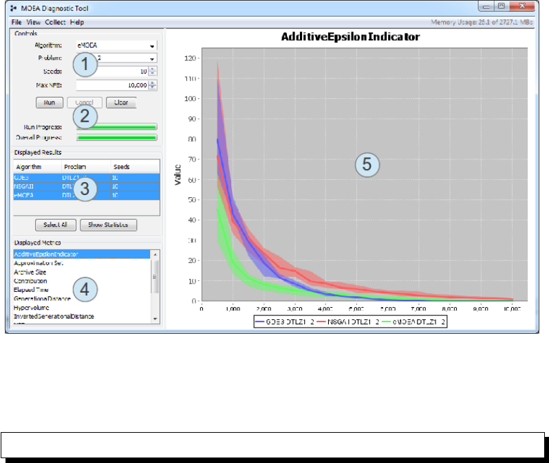
4.2 Layout of the GUI
Figure 4.1 provides a screenshot of the diagnostic tool window. This window
is composed of the following sections:
1. The configuration panel. This panel lets you select the algorithm, prob-
lem, number of repetitions (seeds), and maximum number of function
evaluations (NFE).
2. The execution panel. Clicking run will execute the algorithm as config-
ured in the configuration panel. Two progress bars display the individ-

4.3. QUANTILE PLOTS VS INDIVIDUAL TRACES 35
ual run progress and the total progress for all seeds. Any in-progress
runs can be canceled.
3. The displayed results table. This table displays the completed runs.
The entries which are selected/highlighted are displayed in the charts.
You can click an individual line to show the data for just that entry,
click while holding the Alt key to select multiple entries, or click the
Select All button to select all entries.
4. The displayed metrics table. Similar to the displayed results table, the
selected metrics are displayed in the charts. You can select one metric
or multiple metrics by holding the Alt key while clicking.
5. The actual charts. A chart will be generated for each selected metric.
Thus, if two metrics are selected, then two charts will be displayed
side-by-side. See Figure 4.2 for an example.
Some algorithms do not provide certain metrics. When selecting a specific
metric, only those algorithms that provide that metric will be displayed in
the chart.
4.3 Quantile Plots vs Individual Traces
By default, the charts displayed in the diagnostic tool show the statistical
25%, 50% and 75% quantiles. The 50% quantile is the thick colored line, and
the 25% and 75% quantiles are depicted by the colored area. This quantile
view allows you to quickly distinguish the performance between multiple
algorithms, particularly when there is significant overlap between two or
more algorithms.
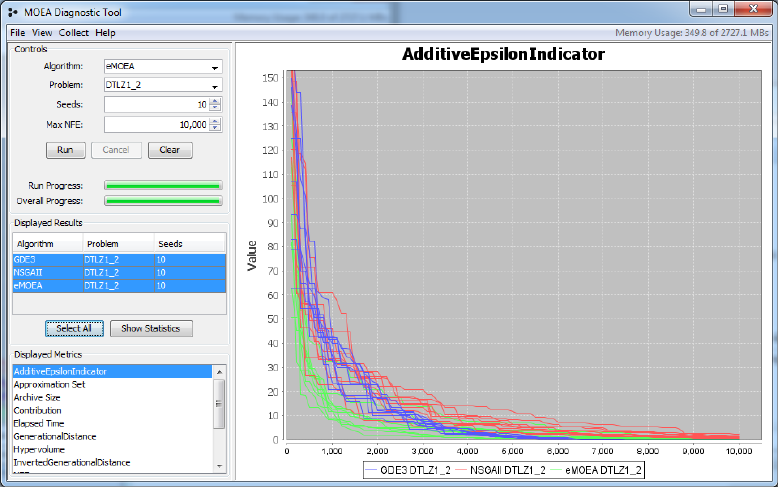
You can alternatively view the raw, individual traces by selecting ’Show
Individual Traces’ in the View menu. Each colored line represents one seed.
Figure 4.3 provides an example of plots showing individual traces. You can
always switch back to the quantile view using the View menu.
4.4 Viewing Approximation Set Dynamics
Another powerful feature of the diagnostic tool is the visualization of ap-
proximation set dynamics. The approximation set dynamics show how the
36 CHAPTER 4. DIAGNOSTIC TOOL
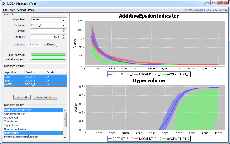
Figure 4.2: Screenshot of the diagnostic tool displaying two side-by-side met-
rics. You can select as many metrics to display by holding down the Alt key
and clicking a row in the displayed metrics table.
4.4. VIEWING APPROXIMATION SET DYNAMICS 37
Figure 4.3: Screenshot of the diagnostic tool displaying the individual traces
rather than the quantile view. The individual traces provide access to the
raw data, but the quantile view is often easier to interpret.
38 CHAPTER 4. DIAGNOSTIC TOOL
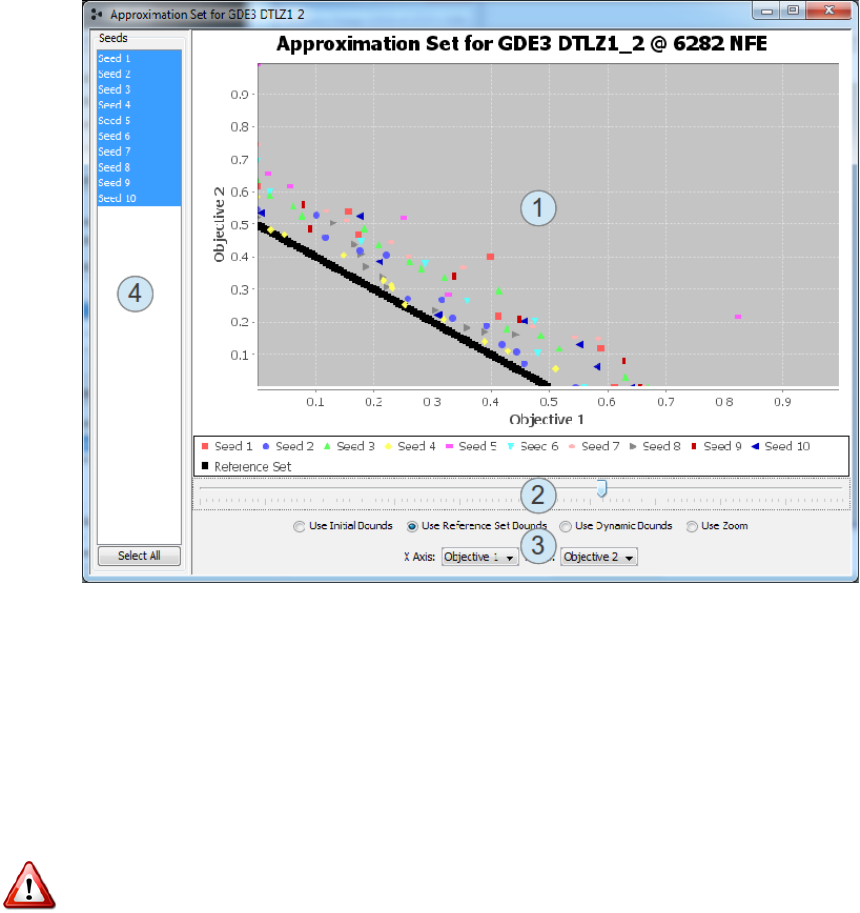
Figure 4.4: Screenshot of the approximation set viewer. This allows you to
view the approximation set at any point in the algorithm’s execution.
algorithm’s result (its approximation set) evolved throughout the run. To
view the approximation set dynamics, right-click on one of the rows in the
displayed results table. A menu will appear with the option to show the
approximation set. A window similar to Figure 4.4 will appear.
This menu will disappear if you disable collecting the approximation set
using the Collect menu. Storing the approximation set data tends to be
memory intensive, and it is sometimes useful to disable collecting the ap-
proximation sets if they are not needed.
This window displays the following items:
1. The approximation set plot. This plot can only show two dimensions.
If available, the reference set for the problem will be shown as black
points. All other points are the solutions produced by the algorithm.
Different seeds are displayed in different colors.

4.5. STATISTICAL RESULTS 39
2. The evolution slider. Dragging the slider to the left or right will show
the approximation set from earlier or later in the evolution.
3. The display controls. These controls let you adjust how the data is
displayed. Each of the radio buttons switches between different scaling
options. The most common option is ’Use Reference Set Bounds’, which
scales the plot so that the reference set fills most of the displayed region.
4. The displayed seeds table. By default, the approximation sets for all
seeds are displayed and are distinguished by color. You can also downs-
elect to display one or a selected group of seeds by selecting entries in
this table. Multiple entries can be selected by holding the Alt key while
clicking.
You can manually zoom to any portion in these plots (both in the ap-
proximation set viewer and the plots in the main diagnostic tool window) by
positioning the cursor at the top-left corner of the zoom region, pressing and
holding down the left-mouse button, dragging the cursor to the bottom-right
corner of the zoom region, and releasing the left-mouse button. You can reset
the zoom by pressing and holding the left-mouse button, dragging the cursor
to the top-left portion of the plot, and releasing the left-mouse button.
4.5 Statistical Results
The diagnostic tool also allows you to exercise the statistical testing tools
provided by the MOEA Framework with the click of a button. If you have
two or more entries selected in the displayed results table, the ’Show Statis-
tics’ button will become enabled. Figure 4.5 shows the example output from
clicking this button. The data is formatted as YAML. YAML uses indenta-
tion to indicate the relationship among entries. For example, observe that
the first line is not indented and says ’GDE3:’. All entries shown below that
are indented. Thus, the second line, which is ’Hypervolume:’, indicates that
this is the hypervolume for the GDE3 algorithm. The third line says ’Aggre-
gate: 0.4894457739242269’, and indicates that the aggregate hypervolume
produced by GDE3 was 0.489.
Displayed for each metric are the min, median and max values for the
specific metric. It is important to note that these values are calculated from
the end-of-run result. No intermediate results are used in the statistical tests.
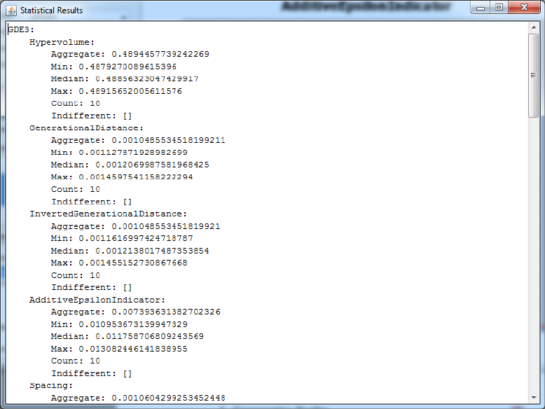
40 CHAPTER 4. DIAGNOSTIC TOOL
Figure 4.5: Screenshot of the statistics output by the diagnostic tool.

4.6. IMPROVING PERFORMANCE AND MEMORY EFFICIENCY 41
The aggregate value is the metric value resulting when the result from all
seeds are combined into one. The count is the number of seeds.
The indifferent entries are of particular importance and will be explained
in detail. When comparing two data sets using statistical tools, it is not
sufficient to simply compare their average or median values. This is because
such results can be skewed by randomness. For example, suppose we are
calculating the median values of ten seeds. If one algorithm gets “lucky”
and happens to use more above-average seeds, the estimated median will
be skewed. Therefore, it is necessary to check the statistical significance of
results. This is exactly what the indifferent entries are displaying. To deter-
mine statistical significance, the MOEA Framework uses the Kruskal-Wallis
and Mann-Whitney U tests with 95% confidence intervals. If an algorithm’s
median value for a metric is statistically different from another algorithm,
the indifferent entry will contain an empty list (e.g., ’Indifferent: []’). How-
ever, if its results are not statistically different, then the indifferent entry
will list the algorithms producing statistically similar results (e.g., ’Indiffer-
ent: [NSGAII]’). This list may contain more than one algorithm if multiple
algorithms are indifferent.
The show statistics button also requires each of the selected entries to use
the same problem. The button will remain disabled unless this condition is
satisfied. If the button is disabled, please ensure you have two or more rows
selected and all selected entries are using the same problem.
4.6 Improving Performance and Memory Ef-
ficiency
By default, the diagnostic tool collects and displays all available data. If
you know ahead of time that certain pieces of data are not needed for your
experiments, you can often increase the performance and memory efficiency
of the program by disabling unneeded data. You can enable or disable the
collection of data by checking or unchecking the appropriate item in the
Collect menu.

42 CHAPTER 4. DIAGNOSTIC TOOL
4.7 Conclusion
This chapter provided an introduction to the MOEA Diagnostic Tool, which
is a GUI that allows users to experiment running various MOEAs on different
problems. Readers are encouraged to experiment with this GUI when first
using the MOEA Framework as it should provide insight into how MOEAs
operate. As an exercise, try running all of the available MOEAs on the
DTLZ2 2 problem. Do the performance metrics (e.g., generational distance)
converge to roughly the same value? Does one MOEA converge to this value
faster than the others? Repeat this experiment with different problems and
see if you get the same result.

Chapter 5
Defining New Problems
The real value of the MOEA Framework comes not from the algorithms and
tools it provides, but the problems that it solves. As such, being able to
introduce new problems into the MOEA Framework is an integral aspect of
its use.
Throughout this chapter, we will show how a simple multiobjective prob-
lem, the Kursawe problem, can be defined in Java, C/C++, and in scripting
languages. The formal definition for the Kursawe problem is provided below.
minimize
x∈RLF(x)=(f1(x), f2(x))
where f1(x) =
L−1
X
i=0 −10e−0.2√x2
i+x2
i+1 ,
f2(x) =
L
X
i=0 |xi|0.8+ 5 sin x3
i.
(5.1)
The MOEA Framework only works on minimization problems. If any ob-
jectives in your problem are to be maximized, you can negate the objective
value to convert from maximization into minimization. In other words, by
minimizing the negated objective, your are maximizing the original objec-
tive. See section 11.3 for additional details on dealing with maximization
objectives.
43

44 CHAPTER 5. DEFINING NEW PROBLEMS
5.1 Java
Defining new problems in Java is the most direct and straightforward way
to introduce new problems into the MOEA Framework. All problems in the
MOEA Framework implement the Problem interface. The Problem inter-
face defines the methods for characterizing a problem, defining the problem’s
representation, and evaluating solutions to the problem. In practice, you
should never need to implement the Problem interface directly, but can ex-
tend the more convenient AbstractProblem class. AbstractProblem
provides default implementations for many of the methods required by the
Problem interface. The code example below shows the Kursawe problem
defined by extending the AbstractProblem class.
1import org.moeaframework.core.Solution;
2import org.moeaframework.core.variable.EncodingUtils;
3import org.moeaframework.core.variable.RealVariable;
4import org.moeaframework.problem.AbstractProblem;
5
6public class Kursawe extends AbstractProblem {
7
8public Kursawe() {
9super(3, 2);
10 }
11
12 @Override
13 public Solution newSolution() {
14 Solution solution = new Solution(numberOfVariables,
15 numberOfObjectives);
16
17 for (int i = 0; i < numberOfVariables; i++) {
18 solution.setVariable(i, new RealVariable(-5.0, 5.0));
19 }
20
21 return solution;
22 }
23
24 @Override
25 public void evaluate(Solution solution) {
26 double[] x = EncodingUtils.getReal(solution);
27 double f1 = 0.0;
28 double f2 = 0.0;
29
30 for (int i = 0; i < numberOfVariables - 1; i++) {

5.1. JAVA 45
31 f1 += -10.0 *Math.exp(-0.2 *Math.sqrt(
32 Math.pow(x[i], 2.0) + Math.pow(x[i+1], 2.0)));
33 }
34
35 for (int i = 0; i < numberOfVariables; i++) {
36 f2 += Math.pow(Math.abs(x[i]), 0.8) +
37 5.0 *Math.sin(Math.pow(x[i], 3.0));
38 }
39
40 solution.setObjective(0, f1);
41 solution.setObjective(1, f2);
42 }
43
44 }
Note on line 9 in the constructor, we call super(3, 2) to set the num-
ber of decision variables (3) and number of objectives (2). All that remains
is defining the newSolution and evaluate methods.
The newSolution method is responsible for instantiating new instances
of solutions for the problem, and in doing so defines the decision variable
types and bounds. In the newSolution method, we start by creating a
new Solution instance on lines 14-15. Observe that we must pass the
number of decision variables and objectives to the Solution constructor.
Next, we define each of the decision variables and specify their bounds on
lines 17-19. For the Kursawe problem, all decision variables are real values
ranging between −5.0 and 5.0, inclusively. Finally, we complete this method
by returning the Solution instance.
The evaluate method is responsible for evaluating solutions to the
problem. A solution which has been generated by an optimization algorithm
is passed as an argument to the evaluate method. The decision variables
contained in this solution are set to the values specified by the optimization
algorithm. The evaluate method must extract these values, evaluate the
problem, and set the objective values.
Since the Kursawe problem contains all real-valued decision variables, we
can cast the decision variables to an array using the helpful methods of the
EncodingUtils class on line 26. Use of EncodingUtils is encouraged
for extracting the decision variables from a solution. Then on lines 27 to 38,
we use those decision variables to evaluate the Kursawe problem. Finally, on
lines 40-41, we assign the two objectives for this problem.

46 CHAPTER 5. DEFINING NEW PROBLEMS
At this point, the problem is completely defined and can be used
with the MOEA Framework. To use this problem with the Executor,
Instrumenter and Analyzer classes introduced in Chapter 3, you pass
a direct references to the problem class using the withProblemClass
method. For example, we can optimize the Kursawe problem we just de-
fined with the following code:
1new Executor()
2.withProblemClass(Kursawe.class)
3.withAlgorithm("NSGAII")
4.withMaxEvaluations(10000)
5.run();
Note how we pass the reference to the problem with Kursawe.class
. The name of the class, Kursawe, is followed by .class. The MOEA
Framework then calls the constructor for the problem class, which in this
case is the empty (no argument) constructor, and proceed to optimize the
problem.
Problems can also define constructors with arguments. For example, con-
sider a problem that needs to load data from a file. For this to work, define
a constructor in the problem class that accepts the desired inputs. In this
case, our constructor would be called public ProblemWithArgument(
File dataFile).... You can then solve this problem as shown below.
1new Executor()
2.withProblemClass(ProblemWithArgument.class,
3new File("inputFile.txt"))
4.withAlgorithm("NSGAII")
5.withMaxEvaluations(10000)
6.run();
5.2 C/C++
It is often the case that the problem / model / computer simulation you
are working with is written in a different programming language, such as
C/C++. With a little work, it is possible to connect that C/C++ problem to
the MOEA Framework and optimize its inputs / parameters. In the following

5.2. C/C++ 47
example, we will demonstrate how to connect the MOEA Framework to a
simple C program. We continue using the Kursawe problem, which if written
in C would appear as follows:
1#include <math.h>
2
3int nvars = 3;
4int nobjs = 2;
5
6void evaluate(double*vars, double*objs) {
7int i;
8objs[0] = 0.0;
9objs[1] = 0.0;
10
11 for (i = 0; i < nvars - 1; i++) {
12 objs[0] += -10.0 *exp(-0.2 *sqrt(
13 pow(vars[i], 2.0) + pow(vars[i+1], 2.0)));
14 }
15
16 for (i = 0; i < nvars; i++) {
17 objs[1] += pow(abs(vars[i]), 0.8) +
18 5.0 *sin(pow(vars[i], 3.0));
19 }
20 }
Note how the evaluate method takes two arguments, vars and objs
, which coincide with the inputs (the decision variables) and the outputs
(the objective values). Now we need to define how the evaluate method
connects to the MOEA Framework. This connection is established using the
following code.
1#include <stdlib.h>
2#include "moeaframework.h"
3
4int main(int argc, char*argv[]) {
5double vars[nvars];
6double objs[nobjs];
7
8MOEA_Init(nobjs, 0);
9
10 while (MOEA_Next_solution() == MOEA_SUCCESS) {
11 MOEA_Read_doubles(nvars, vars);

48 CHAPTER 5. DEFINING NEW PROBLEMS
12 evaluate(vars, objs);
13 MOEA_Write(objs, NULL);
14 }
15
16 MOEA_Finalize();
17 return EXIT_SUCCESS;
18 }
First, line 2 includes the moeaframework.h file. This header is pro-
vided by the MOEA Framework and defines all the functions needed to com-
municate with the MOEA Framework. All such functions begin with the
prefix MOEA_. You can find the moeaframework.h file in the source
code distribution in the folder examples/ along with additional exam-
ples.
Lines 4-18 define the main loop for the C/C++ program. Lines 5-6
initialize the storage arrays for the decision variables and objectives. Line 8
calls MOEA_Init to initialize the communication between C/C++ and the
MOEA Framework. The MOEA_Init method takes the number of objectives
and constraints as arguments. Once initialized, we can begin reading and
evaluating solutions. Line 10 loops as long as we successfully read the next
solution using MOEA_Next_solution(). Line 11 extracts the real valued
decision variables, filling the array vars. Line 12 invokes the evaluate
method to evaluate the problem. This results in the array objs being filled
with the resulting objective values. Line 13 writes the objectives back to the
MOEA Framework. The second argument to MOEA_Write is NULL in this
example, since the Kursawe problem is unconstrained. This loop repeats until
no more solutions are read. At this point, the C/C++ program terminates
by invoking MOEA_Finalize() and exiting. The complete source code is
shown below.
1#include <stdlib.h>
2#include <math.h>
3#include "moeaframework.h"
4
5int nvars = 3;
6int nobjs = 2;
7
8void evaluate(double*vars, double*objs) {
9int i;
10 objs[0] = 0.0;

5.2. C/C++ 49
11 objs[1] = 0.0;
12
13 for (i = 0; i < nvars - 1; i++) {
14 objs[0] += -10.0 *exp(-0.2 *sqrt(
15 pow(vars[i], 2.0) + pow(vars[i+1], 2.0)));
16 }
17
18 for (i = 0; i < nvars; i++) {
19 objs[1] += pow(abs(vars[i]), 0.8) +
20 5.0 *sin(pow(vars[i], 3.0));
21 }
22 }
23
24 int main(int argc, char*argv[]) {
25 double vars[nvars];
26 double objs[nobjs];
27
28 MOEA_Init(nobjs, 0);
29
30 while (MOEA_Next_solution() == MOEA_SUCCESS) {
31 MOEA_Read_doubles(nvars, vars);
32 evaluate(vars, objs);
33 MOEA_Write(objs, NULL);
34 }
35
36 MOEA_Finalize();
37 return EXIT_SUCCESS;
38 }
You can save this C code to kursawe.c and compile it into an exe-
cutable. If using the GNU C Compiler (gcc), you can compile this code with
the following command on Linux or Windows. Note that you will need both
moeaframework.h and moeaframework.c in the same directory as
kursawe.c.
1gcc -o kursawe.exe kursawe.c moeaframework.c -lm
At this point, we now switch back to Java and define the prob-
lem class by extending the ExternalProblem class. We extend the
ExternalProblem class instead of the AbstractProblem class since
ExternalProblem understands how to communicate with the executable

50 CHAPTER 5. DEFINING NEW PROBLEMS
we just compiled. The code snippet below shows the complete Java class for
this example.
1import org.moeaframework.core.Solution;
2import org.moeaframework.core.variable.RealVariable;
3import org.moeaframework.problem.ExternalProblem;
4
5public class ExternalKursawe extends ExternalProblem {
6
7public ExternalKursawe() {
8super("kursawe.exe");
9}
10
11 public int getNumberOfVariables() {
12 return 3;
13 }
14
15 public int getNumberOfObjectives() {
16 return 2;
17 }
18
19 public int getNumberOfConstraints() {
20 return 0;
21 }
22
23 @Override
24 public Solution newSolution() {
25 Solution solution = new Solution(getNumberOfVariables(),
26 getNumberOfObjectives(), getNumberOfConstraints());
27
28 for (int i = 0; i < numberOfVariables; i++) {
29 solution.setVariable(i, new RealVariable(-5.0, 5.0));
30 }
31
32 return solution;
33 }
34
35 }
Note how we still need to define the number of variables, objectives, and
constraints in addition to defining the newSolution method. However,
we no longer include the evaluate method. Instead, we reference the
executable we previously created on line 8. The MOEA Framework will
5.3. SCRIPTING LANGUAGE 51
launch the executable and use it to evaluate solutions to the problem.
Our work is now complete. We can now solve this “external” version of
the Kursawe problem just like the pure Java implementation shown earlier
in this chapter.
1new Executor()
2.withProblemClass(ExternalKursawe.class)
3.withAlgorithm("NSGAII")
4.withMaxEvaluations(10000)
5.run();
It is helpful to test the C/C++ program manually prior to running it with
the MOEA Framework. Tests can be performed by launching the C/C++
program and manually typing in inputs. In this example, the program re-
quires 3 real values entered on a single line.
-2.5 1.25 0.05
Once the enter key is pressed, the program will output the two objectives
to the console:
-13.504159423733775 6.966377092192072
Additional inputs can be provided, or press Ctrl+D to terminate the
program.
5.3 Scripting Language
Problems can also be defined in one of the many scripting languages avail-
able via the Java Scripting API. Supported languages include Javascript,
Python, Ruby, Scheme, Groovy and BeanShell. Java SE 6 includes Rhino,
a Javascript scripting engine, out-of-the-box. The following code snippet
shows the Rhino Javascript code for defining the Kursawe problem.
1importPackage(java.lang);
2importPackage(Packages.org.moeaframework.core);
3importPackage(Packages.org.moeaframework.core.variable);

52 CHAPTER 5. DEFINING NEW PROBLEMS
4
5function getName() {
6return "Kursawe";
7}
8
9function getNumberOfVariables() {
10 return 3;
11 }
12
13 function getNumberOfObjectives() {
14 return 2;
15 }
16
17 function getNumberOfConstraints() {
18 return 0;
19 }
20
21 function evaluate(solution) {
22 x = EncodingUtils.getReal(solution);
23 f1 = 0.0;
24 f2 = 0.0;
25
26 for (i = 0; i < getNumberOfVariables() - 1; i++) {
27 f1 += -10.0 *Math.exp(-0.2 *Math.sqrt(
28 Math.pow(x[i], 2.0) + Math.pow(x[i+1], 2.0)));
29 }
30
31 for (i = 0; i < getNumberOfVariables(); i++) {
32 f2 += Math.pow(Math.abs(x[i]), 0.8) +
33 5.0 *Math.sin(Math.pow(x[i], 3.0));
34 }
35
36 solution.setObjective(0, f1);
37 solution.setObjective(1, f2);
38 }
39
40 function newSolution() {
41 solution = new Solution(getNumberOfVariables(),
42 getNumberOfObjectives());
43
44 for (i = 0; i < getNumberOfVariables(); i++) {
45 solution.setVariable(i, new RealVariable(-5.0, 5.0));
46 }
47
48 return solution;

5.4. CONCLUSION 53
49 }
50
51 function close() {
52
53 }
Note how all methods defined by the Problem interface appear in this
code. Also note how we can invoke Java methods and constructors through
the scripting language. The specifics of how to implement functions and
invoke existing methods are specific to the scripting language chosen. Refer
to the documentation for the scripting language for details.
Save this script to an appropriate file with the correct file extension for
the scripting language. Since the script in this example is written in the
Rhino Javascript language, we save the file to kursawe.js. Solving this
Javascript version of the Kursawe problem is nearly identical to all previous
examples, as shown below.
1new Executor()
2.withProblemClass(ScriptedProblem.class,
3new File("kursawe.js"))
4.withAlgorithm("NSGAII")
5.withMaxEvaluations(10000)
6.run();
The only difference is on lines 2-3, where we specify the problem class as
ScriptedProblem.class and pass as an argument the file kursawe.
js. The ScriptedProblem class loads the file, determines the appropriate
scripting engine, and uses that scripting engine to evaluate solutions to the
problem.
5.4 Conclusion
This chapter introduced the various means for introducing new problems
to the MOEA Framework. This includes implementing problems in Java,
C/C++, and in one of the many supported scripting languages. Care must
be taken when choosing which language to use, as each method has differ-
ent advantages and drawbacks. One key consideration is the speed of each
method. The table below shows the wall-clock time for the three methods

54 CHAPTER 5. DEFINING NEW PROBLEMS
discussed in this chapter. These times were produced on an Intel c
CoreTM2
Duo @ 2.13 GHz.
Method Time (Seconds)
Java 1.218
C/C++ 4.011
Scripted (Javascript) 24.874
Observe that using C/C++ incurs an overhead of approximately 0.000278
seconds per evaluation. For the simple Kursawe problem used as the example
throughout this chapter, the overhead outweighs the evaluation time. One
would expect, however, that larger and more complex problems will bene-
fit from potentially faster C/C++ implementations. Furthermore, as one
would expect, the scripted implementation in Javascript incurs a significant
performance penalty.

Chapter 6
Representing Decision
Variables
In Chapter 5 we saw various ways to define new problems using real-valued
(floating-point) decision variables. In addition to floating-point values, the
MOEA Framework allows problems to be encoded using integers, bit strings,
permutations, programs (expression trees), and grammars. This chapter de-
tails the use of each of these decision variables and their supported variation
operators. This chapter also details the use of the EncodingUtils class,
which provides many helper methods for creating, reading and modifying
different types of decision variables.
6.1 Floating-Point Values
Floating-point values, also known as real-valued decision variables, provide
a natural way to represent numeric values. Floating-point decision variables
are represented using RealVariable decision variables. When creating
a new real-valued decision variable, one must specify the lower and upper
bounds that the value can represent.
To create real-valued decision variables, use the EncodingUtils.
newReal(lowerBound, upperBound) method. Note how the lower
and upper bounds must be defined. The example code below demonstrates
creating a solution with three different real-valued decision variables.
1public Solution newSolution() {
55

56 CHAPTER 6. REPRESENTING DECISION VARIABLES
2Solution solution = new Solution(3, 2);
3solution.setVariable(0, EncodingUtils.newReal(-1.0, 1.0));
4solution.setVariable(1, EncodingUtils.newReal(0, Math.PI));
5solution.setVariable(2, EncodingUtils.newReal(10.0, 100.0));
6return solution;
7}
Inside the evaluate method, we can extract the decision variable val-
ues from the solution using the EncodingUtils.getReal(...) method.
Continuing the previous code example, we extract the values of the three de-
cision variables below.
1public void evaluate(Solution solution) {
2double x = EncodingUtils.getReal(solution.getVariable(0));
3double y = EncodingUtils.getReal(solution.getVariable(1));
4double z = EncodingUtils.getReal(solution.getVariable(2));
5
6// TODO: evaluate the solution given the values of x, y,
7// and z
8}
Alternatively, if the solution contains exclusively floating-point values,
then we can read out all of the variables into an array using a single call.
Note that we pass the entire solution to the EncodingUtils.getReal
(...) method below.
1public void evaluate(Solution solution) {
2double[] x = EncodingUtils.getReal(solution);
3
4// TODO: evaluate the solution given the values of x[0],
5// x[1], and x[2]
6}
The EncodingUtils class handles all the type checking and cast-
ing needed to ensure variables are read properly. Attempting to read or
write a decision variable that is not the correct type will result in an
IllegalArgumentException. If you see this exception, check all your
decision variables to ensure they are the types you expect.

6.2. INTEGERS 57
6.2 Integers
Integer-valued decision variables can be constructed in a similar way as
floating-point values. For instance, below we construct the solution using
calls to EncodingUtils.newInt(lowerBound, upperBound). As
we saw with floating-point values, we must specify the lower and upper
bounds of the decision variables.
1public Solution newSolution() {
2Solution solution = new Solution(3, 2);
3solution.setVariable(0, EncodingUtils.newInt(-1, 1));
4solution.setVariable(1, EncodingUtils.newInt(0, 100));
5solution.setVariable(2, EncodingUtils.newInt(-10, 10));
6return solution;
7}
Similarly, the values stored in the decision variables can be read using the
EncodingUtils.getInt(...) method, as demonstrated below.
1public void evaluate(Solution solution) {
2int x = EncodingUtils.getInt(solution.getVariable(0));
3int y = EncodingUtils.getInt(solution.getVariable(1));
4int z = EncodingUtils.getInt(solution.getVariable(2));
5
6// TODO: evaluate the solution given the values of x, y,
7// and z
8}
And as we saw with floating-point values, if the solution is exclusively
represented by integer-valued decision variables, we can likewise extract all
values with a single call to EncodingUtils.getInt(...). Note again
that this method is passed the entire solution instead of the individual deci-
sion variables as before.
1public void evaluate(Solution solution) {
2int[] x = EncodingUtils.getInt(solution);
3
4// TODO: evaluate the solution given the values of x[0],
5// x[1], and x[2]
6}
58 CHAPTER 6. REPRESENTING DECISION VARIABLES
The integer representation can be used to represent any other kind of
discrete value. For example, suppose we wanted to represent all even num-
bers between 0 and 100. We can accomplish this using EncodingUtils
.newInt(0, 50) and reading the value with 2*EncodingUtils.
getInt(variable). Integers are also useful for selecting a single item
from a group. In this scenario, the integer-valued decision variable repre-
sents the index of the item in an array.
Internally, integers are stored as floating-point values. This allows the
same variation operators to be applied to both real-valued and integer-
valued decision variables. When working with integers, always use the
EncodingUtils.newInt(...) and EncodingUtils.getInt(...)
methods. This will ensure the internal floating-point representation is cor-
rectly converted into an integer.
6.3 Boolean Values
Boolean values represent simple binary choices, such as “yes / no” or “on /
off”. Use the EncodingUtils.newBoolean() method to create boolean
decision variables, as shown below. Note also how we can combine multiple
decision variable types in a single solution.
1public Solution newSolution() {
2Solution solution = new Solution(2, 2);
3solution.setVariable(0, EncodingUtils.newBoolean());
4solution.setVariable(1, EncodingUtils.newInt(0, 100));
5return solution;
6}
Boolean values can be read using EncodingUtils.getBoolean
(...), as demonstrated below.
1public void evaluate(Solution solution) {
2boolean b = EncodingUtils.getBoolean(
3solution.getVariable(0));
4int x = EncodingUtils.getInt(solution.getVariable(1));
5

6.4. BIT STRINGS 59
6// TODO: evaluate the solution given the values of b and x
7}
The boolean decision variable works well when the problem has a single
choice. If the problem involves more than one choice, it is more convenient
and efficient to use bit strings (an array of booleans) instead. Bit strings are
introduced in the following section.
6.4 Bit Strings
Many problems involve making choices. For example, the famous knapsack
problem involves choosing which items to place in a knapsack to maximize
the value of the items carried without exceeding the weight capacity of the
knapsack. If Nitems are available, we can represent the decision to include
each item using a bit string with Nbits. Each bit in the string corresponds to
an item, and is set to 1if the item is included and 0if the item is excluded.
For instance, the bit string 00110 would place items 3 and 4 inside the
knapsack, excluding the rest.
The MOEA Framework supports fixed-length bit strings. The example
code below produces a solution with a single decision variable representing
a bit string with length 100. Again, note how the entire bit string is stored
within a single decision variable.
1public Solution newSolution() {
2Solution solution = new Solution(1, 2);
3solution.setVariable(0, EncodingUtils.newBinary(100));
4return solution;
5}
When evaluating the solution, the bit string can be read into an array of
boolean values, as demonstrated below.
1public void evaluate(Solution solution) {
2boolean[] values = EncodingUtils.getBinary(
3solution.getVariable(0));
4
5//TODO: evaluate the solution given the boolean values
6}

60 CHAPTER 6. REPRESENTING DECISION VARIABLES
6.5 Permutations
Permutation decision variables appear in many combinatorial and job
scheduling problems. In the famous traveling salesman problem (TSP), a
salesman must travel to every city with the condition that they visit each city
exactly once. The order in which the salesman visits each city is conveniently
represented as a permutation. For example, the permutation 0,3,1,2 states
that the salesman visits the first city first (0 represents the first city), travels
to the fourth city (3), then travels to the second city (1), and finally arrives
at the third city (2).
The code example below demonstrates the creation of a permutation of
25 elements.
1public Solution newSolution() {
2Solution solution = new Solution(1, 2);
3solution.setVariable(0, EncodingUtils.newPermutation(25));
4return solution;
5}
The permutation is read out into an array of int values. If the permu-
tation is over Nelements, the array length will be Nand the values stored
will range from 0 to N−1. Each distinct value will appear only once in the
array (by definition of a permutation).
1public void evaluate(Solution solution) {
2int[] permutation = EncodingUtils.getPermutation(
3solution.getVariable(0));
4
5//TODO: evaluate the solution given the permutation
6}

6.6. PROGRAMS (EXPRESSION TREES) 61
6.6 Programs (Expression Trees)
The first step towards evolving programs using evolutionary algorithms in-
volves defining the rules for the program (i.e., the syntax and semantics).
The MOEA Framework comes enabled with over 45 pre-defined program el-
ements for defining constants, variables, arithmetic operators, control struc-
tures, functions, etc. When defining the rules, two important properties
should be kept in mind: closure and sufficiency.
The closure property requires all program element to be able to accept
as arguments any value and data type that could possibly be returned by
any other function or terminal. All programs generated or evolved by the
MOEA Framework are strongly typed. No program produced by the MOEA
Framework will pass an argument to a function that is an incorrect type.
Furthermore, all functions guard against invalid inputs. For example, the
log of a negative number is undefined. Rather then causing an error, the
log method will guard itself and return 0.0. This allows the rest of the
calculation to continue unabated. With these two behaviors built into the
MOEA Framework, the closure property is guaranteed.
The sufficiency property states that the rule set must contain all the neces-
sary functions and terminals necessary to produce a solution to the problem.
Ensuring this property holds is more challenging as it will depend on the
problem domain. For instance, the operators And,Or and Not are suffi-
cient to produce all boolean expressions. It may not be so obvious in other
problem domains which program elements are required to ensure sufficiency.
Additionally, it is often helpful to restrict the rule set to those program ele-
ments that are sufficient, thus reducing the search space for the evolutionary
algorithm.
Below, we construct a rule set using several arithmetic operators. One
terminal is included, the variable x. We will assign this variable later when
evaluating the program. The last setting required is the return type of the
program. In this case, the program will return a number.
1//first, establish the rules for the program
2Rules rules = new Rules();
3rules.add(new Add());
4rules.add(new Multiply());
5rules.add(new Subtract());
6rules.add(new Divide());
7rules.add(new Sin());

62 CHAPTER 6. REPRESENTING DECISION VARIABLES
8rules.add(new Cos());
9rules.add(new Exp());
10 rules.add(new Log());
11 rules.add(new Get(Number.class,"x"));
12 rules.setReturnType(Number.class);
The second step is constructing the solution used by the evolutionary
algorithm. Here, we define one decision variable that is a program following
the rule set we previously defined.
1public Solution newSolution() {
2Solution solution = new Solution(1, 1);
3solution.setVariable(0, new Program(rules));
4return solution;
5}
Lastly, we evaluate the program. The program executes inside an envi-
ronment. The environment holds all of the variables and other identifiers
that the program can access throughout its execution. Since we previously
defined the variable x(with the Get node), we want to initialize the value of
xin the environment. Once the environment is initialized, we evaluate the
program. Since we set the return type to be a number in the rule set, we
cast the output from the program’s evaluation to a number.
1public void evaluate(Solution solution) {
2Program program = (Program)solution.getVariable(0);
3
4// initialize the variables used by the program
5Environment environment = new Environment();
6environment.set("x", 15);
7
8// evaluate the program
9double result = (Number)program.evaluate(
10 environment)).doubleValue();
11
12 // TODO: use the result to set the objective value
13 }

6.7. GRAMMARS 63
6.7 Grammars
Grammars are very similar to programs, but differ slightly in their definition
and how the derived programs are generated. Whereas the program required
us to define a set of program elements (the rules) used for constructing the
program, the grammar defines these rules using a context free grammar.
The text below shows an example grammar. The format of this grammar is
Backus-Naur form.
<expr> ::= <func> | (<expr> <op> <expr>) | <value>
<func> ::= <func-name> ( <expr> )
<func-name> ::= Math.sin | Math.cos | Math.exp | Math.log
<op> ::= + | *|-|/
<value> ::= x
You should note that this grammar defines the same functions and ter-
minals as the example in the previous section. This also demonstrates an
important difference between programs and grammars in the MOEA Frame-
work. The grammar explicitly defines where each problem element can ap-
pear. This is in contrast to programs, whose structure is determined by the
type system. As a result, grammars require more setup time but offer more
control over programs. We will now demonstrate the use of grammars in the
MOEA Framework.
First, we must parse the context free grammar. In the example below,
the grammar is read from a file. It is also possible to pass a string containing
the grammar using a StringReader in place of the FileReader.
1ContextFreeGrammar grammar = Parser.load(
2new FileReader("grammar.bnf"));
Second, we construct the grammar variable that will be evolved by the
evolutionary algorithm. Note how the Grammar object is passed an integer.
Grammatical evolution uses a novel representation of the decision variable.
Internally, it uses an integer array called a codon. The codon does not define
the program itself, but provides instructions for deriving the program using
the grammar. The integer argument to Grammar specifies the length of the
codon. We defer a detailed explanation of this derivation to the grammatical
evolution literature.

64 CHAPTER 6. REPRESENTING DECISION VARIABLES
1public Solution newSolution() {
2Solution solution = new Solution(1, 1);
3solution.setVariable(0, new Grammar(10));
4return solution;
5}
Finally, we can evaluate a solution by first extracting the codon and de-
riving the program. Unlike programs that can be evaluated directly, the
grammar produces a string (the derivation). While it is common for gram-
mars to produce program code, this is not a requirement. This is the second
major difference between grammars and programs in the MOEA Framework
— the behavior of programs is defined explicitly, whereas the behavior of
grammars depend on how the grammar is interpreted. In this case, we are
producing program code and will need a scripting language to evaluate the
program. Using Java’s Scripting API and having defined the grammar so
that it produces a valid Groovy program, we can evaluate the derivation
using the Groovy scripting language. In the code below, we instantiate a
ScriptEngine for Groovy, initialize the variable x, and evaluate the pro-
gram.
1public void evaluate(Solution solution) {
2int[] codon = ((Grammar)solution.getVariable(0)).toArray();
3
4// derive the program using the codon
5String program = grammar.build(codon);
6
7if (program == null) {
8// if null, the codon did not produce a valid grammar
9// TODO: penalize the objective value
10 }else {
11 ScriptEngineManager sem = new ScriptEngineManager();
12 ScriptEngine engine = sem.getEngineByName("groovy");
13
14 // initialize the variables used by the program
15 Bindings b = new SimpleBindings();
16 b.put("x", 15);
17
18 double result = ((Number)engine.eval(program, b))
19 .doubleValue();
20
21 // TODO: use the result to set the objective value

6.8. VARIATION OPERATORS 65
22 }
23 }
In order to compile and run this example, the Groovy scripting lan-
guage must be installed. To install Groovy, download the binary release
from http://groovy.codehaus.org/, extract the embeddable\
groovy-all-2.0.1.jar file into the lib folder in your MOEA Frame-
work installation, and add this jar file onto the Java classpath when launching
this example.
6.8 Variation Operators
The MOEA Framework contains a number of variation operators (initializa-
tion, mutation, crossover, etc.) tailored for each representation type. This
section provides a brief overview of the available operators and details their
use.
6.8.1 Initialization
The start of all evolutionary algorithms is the construction of an initial popu-
lation. This population is important since, in general, all future solutions are
derived from members of this initial population. Ensuring this initial popu-
lation provides a diverse and representative set of individuals is paramount.
The floating-point, integer, binary, permutation and grammar variables
are all initialized uniformly at random. This ensures the values, bit strings,
etc. are distributed uniformly throughout the search space.
Programs require a slightly more complicated initialization to ensure the
initial population contains a diverse sampling of potential programs. The
MOEA Framework provides the ramped half-and-half initialization method,
which is one of the most popular initialization techniques for programs. We
refer readers to the genetic programming literature for a detailed description
of ramped half-and-half initialization.
6.8.2 Variation (Mutation & Crossover)
After the initial population is generated, an evolutionary algorithm evolves
the population using individual or combinations of variation operators.

66 CHAPTER 6. REPRESENTING DECISION VARIABLES
Table 6.1: List of Supported Variation Operators
Representation Type Abbr.
Real / Integer Simulated Binary Crossover SBX
Real / Integer Polynomial Mutation PM
Real / Integer Differential Evolution DE
Real / Integer Parent-Centric Crossover PCX
Real / Integer Simplex Crossover SPX
Real / Integer Unimodal Normal Distribution Crossover UNDX
Real / Integer Uniform Mutation UM
Real / Integer Adaptive Metropolis AM
Binary Half-Uniform Crossover HUX
Binary Bit Flip Mutation BF
Permutation Partially-Mapped Crossover PMX
Permutation Element Insertion Insertion
Permutation Element Swap Swap
Grammar Single-Point Crossover for Grammars GX
Grammar Uniform Mutation for Grammars GM
Program Branch (Subtree) Crossover BX
Program Point Mutation PTM
Any Single-Point Crossover 1X
Any Two-Point Crossover 2X
Any Uniform Crossover UX
Variation operators are classified into two forms: crossover and mutation.
Crossover involves combining two or more parents to create an offspring.
Mutation involves a single parent. Mutations generally produce only small
changes, but this is not mandatory.
Table 6.1 lists the supported variation operators in the MOEA Frame-
work. The table highlights the decision variable representation and type of
each variation operator.
The abbreviation column lists the keyword used in the MOEA Frame-
work for referencing each operator. The example code below shows how we
can specify the operator used by an algorithm and also any parameters for
the operator. In this example, we are using parent-centric crossover (PCX)
and setting two of its parameters, pcx.eta and pcx.zeta. Refer to the
OperatorFactory class documentation for a complete list of the operators
and their parameters.

6.9. CONCLUSION 67
1NondominatedPopulation result = new Executor()
2.withProblem("UF1")
3.withAlgorithm("NSGAII")
4.withProperty("operator","pcx")
5.withProperty("pcx.eta", 0.1)
6.withProperty("pcx.zeta", 0.1)
7.withMaxEvaluations(10000)
8.run();
It is also possible to combine certain variation operators using the +sym-
bol. In the example below, we combine differential evolution with polynomial
mutation (de+pm), and we can set the parameters for both of these operators
as shown.
1NondominatedPopulation result = new Executor()
2.withProblem("UF1")
3.withAlgorithm("NSGAII")
4.withProperty("operator","de+pm")
5.withProperty("de.rate", 0.5)
6.withProperty("pm.rate", 0.1)
7.withMaxEvaluations(10000)
8.run();
Not all combinations of operators are supported. In general, combining a
crossover operator with a mutation operator is ok. If you request an invalid
operator combination, you will see an exception with the message invalid
number of parents. See the CompoundVariation class documentation for
more details on what operators can be combined.
6.9 Conclusion
This chapter introduced the various decision variable representations sup-
ported by the MOEA Framework. Look at these different representations
as the building blocks for your problem. If you can construct your problem
using these building blocks, the problem will seamlessly integrate with the
MOEA Framework.
We close this chapter by commenting that the MOEA Framework is not
limited to these representations. New representations are periodically in-
68 CHAPTER 6. REPRESENTING DECISION VARIABLES
troduced in the literature. This fact influenced the design of the MOEA
Framework to allow new representations and variation operators. Interested
readers should stay turned for future updates to this user manual that will
discuss such extensions in detail.
Chapter 7
Example: Knapsack Problem
In this chapter, we will walk through a complete example of creating a new
optimization problem and solving it using the MOEA Framework. This ex-
ample serves as a review of the topics learned thus far. We will also introduce
several new concepts such as constraint handling.
The problem we will be solving is the multiobjective version of the
knapsack problem. The knapsack problem (discussed in much detail at
http://en.wikipedia.org/wiki/Knapsack_problem) is a famous
combinatorial problem that involves choosing which items to place in a knap-
sack to maximize the value of the items carried without exceeding the weight
capacity of the knapsack. More formally, we are given Nitems. Each item
has a profit, P(i), and weight, W(i), for i= 1,2, . . . , N. Let d(i) represent
our decision to place the i-th item in the knapsack, where d(i) = 1 if the
item is put into the knapsack and d(i) = 0 otherwise. If the knapsack has a
weight capacity of C, then the knapsack problem is defined as:
Maximize
N
X
i=1
d(i)∗P(i) such that
N
X
i=1
d(i)∗W(i)≤C
The summation on the left (which we are maximizing) calculates the total
profit we gain from the items placed in the knapsack. The summation on
the right side is a constraint that ensures the items placed in the knapsack
do not exceed the weight capacity of the knapsack.
The multiobjective knapsack problem that we will be solving in this sec-
tion is very similar, except that we now have 2 knapsacks to hold the items.
Additionally, the profit and weights vary depending on which knapsack is
69

70 CHAPTER 7. EXAMPLE: KNAPSACK PROBLEM
holding each item. For example, an item will have a profit of $25 and a
weight of 5 pounds in the first knapsack, but will have a profit of $15 and
a weight of 8 pounds in the second knapsack. (It may seem unusual that
the weight changes, but that is how the problem is defined in the litera-
ture.) Thus, profit is now defined by P(i, j) and weight by W(i, j), where
the j= 1,2 term is the knapsack index. Lastly, each knapsack defines its
own capacity, C1and C2. Combining all of this, the multiobjective knapsack
problem is formally defined as:
Maximize PN
i=1 d(i)∗P(i, 1) such that PN
i=1 d(i)∗W(i, 1) ≤C1and
Maximize PN
i=1 d(i)∗P(i, 2) such that PN
i=1 d(i)∗W(i, 2) ≤C2
Once we have a firm understanding of the optimization problem, we
can now work on solving this problem. You can find all of the code
for this example in the examples/org/moeaframework/examples/
ga/knapsack folder in the source code distribution.
7.1 Data Files
We begin by developing a way to store all of the information re-
quired by the knapsack problem — profits, weights, capacities — in
a text file. This will let us quickly generate and run new in-
puts for this problem. Fortunately, two researchers, Eckart Zitzler
and Marco Laumanns, have already created a file format for multi-
objective knapsack problems at http://www.tik.ee.ethz.ch/sop/
download/supplementary/testProblemSuite/. For example, a
simple 5 item problem instance would appear as follows.
knapsack problem specification (2 knapsacks, 5 items)
=
knapsack 1:
capacity: +251
item 1:
weight: +94
profit: +57
item 2:
weight: +74
profit: +94
item 3:

7.2. ENCODING THE PROBLEM 71
weight: +77
profit: +59
item 4:
weight: +74
profit: +83
item 5:
weight: +29
profit: +82
=
knapsack 2:
capacity: +190
item 1:
weight: +55
profit: +20
item 2:
weight: +10
profit: +19
item 3:
weight: +97
profit: +20
item 4:
weight: +73
profit: +66
item 5:
weight: +69
profit: +48
We will re-use this file format in this example. One ad-
vantage is that you can download any of the example knap-
sack problems from http://www.tik.ee.ethz.ch/sop/download/
supplementary/testProblemSuite/ and solve them with the pro-
gram we are writing. Go ahead and save this example input file to
knapsack.5.2. We will then load and solve this data file later in this
chapter.
7.2 Encoding the Problem
The next step is to decide upon the encoding for the decision variables.
Observe that we are deciding which items to place in the knapsacks. Recalling
Chapter 6, the bit string representation works well for situation where we are
making many yes/no decisions. For example, if N= 5, we can represent the

72 CHAPTER 7. EXAMPLE: KNAPSACK PROBLEM
decision to include each item using a bit string with 5 bits. Each bit in the
string corresponds to an item, and is set to 1if the item is included and 0if
the item is excluded. For instance, the bit string 00110 would place items
3 and 4 inside the knapsacks, excluding the rest.
7.3 Implementing the Problem
Having decided upon an encoding, we can now implement the knapsack prob-
lem as shown below.
1import java.io.File;
2import java.io.FileReader;
3import java.io.IOException;
4import java.io.InputStream;
5import java.io.InputStreamReader;
6import java.io.Reader;
7import java.util.regex.Matcher;
8import java.util.regex.Pattern;
9
10 import org.moeaframework.core.Problem;
11 import org.moeaframework.core.Solution;
12 import org.moeaframework.core.variable.BinaryVariable;
13 import org.moeaframework.core.variable.EncodingUtils;
14 import org.moeaframework.util.Vector;
15 import org.moeaframework.util.io.CommentedLineReader;
16
17 /**
18 *Multiobjective 0/1 knapsack problem.
19 */
20 public class Knapsack implements Problem {
21
22 /**
23 *The number of sacks.
24 */
25 private int nsacks;
26
27 /**
28 *The number of items.
29 */
30 private int nitems;
31
32 /**
33 *Entry {@code profit[i][j]} is the profit from including

7.3. IMPLEMENTING THE PROBLEM 73
34 *item {@code j} in sack {@code i}.
35 */
36 private int[][] profit;
37
38 /**
39 *Entry {@code weight[i][j]} is the weight incurred from
40 *including item {@code j} in sack {@code i}.
41 */
42 private int[][] weight;
43
44 /**
45 *Entry {@code capacity[i]} is the weight capacity of sack
46 *{@code i}.
47 */
48 private int[] capacity;
49
50 /**
51 *Constructs a multiobjective 0/1 knapsack problem instance
52 *loaded from the specified file.
53 *
54 *@param file the file containing the knapsack problem
55 *instance
56 *@throws IOException if an I/O error occurred
57 */
58 public Knapsack(File file) throws IOException {
59 this(new FileReader(file));
60 }
61
62 /**
63 *Constructs a multiobjective 0/1 knapsack problem instance
64 *loaded from the specified input stream.
65 *
66 *@param inputStream the input stream containing the knapsack
67 *problem instance
68 *@throws IOException if an I/O error occurred
69 */
70 public Knapsack(InputStream inputStream) throws IOException {
71 this(new InputStreamReader(inputStream));
72 }
73
74 /**
75 *Constructs a multiobjective 0/1 knapsack problem instance
76 *loaded from the specified reader.
77 *
78 *@param reader the reader containing the knapsack problem

74 CHAPTER 7. EXAMPLE: KNAPSACK PROBLEM
79 *instance
80 *@throws IOException if an I/O error occurred
81 */
82 public Knapsack(Reader reader) throws IOException {
83 super();
84
85 load(reader);
86 }
87
88 /**
89 *Loads the knapsack problem instance from the specified
90 *reader.
91 *
92 *@param reader the file containing the knapsack problem
93 *instance
94 *@throws IOException if an I/O error occurred
95 */
96 private void load(Reader reader) throws IOException {
97 Pattern specificationLine = Pattern.compile("knapsack
problem specification \\((\\d+) knapsacks, (\\d+) items
\\)");
98 Pattern capacityLine = Pattern.compile(" capacity: \\+(\\d+)
");
99 Pattern weightLine = Pattern.compile(" weight: \\+(\\d+)");
100 Pattern profitLine = Pattern.compile(" profit: \\+(\\d+)");
101
102 CommentedLineReader lineReader = null;
103 String line = null;
104 Matcher matcher = null;
105
106 try {
107 lineReader = new CommentedLineReader(reader);
108 line = lineReader.readLine(); // problem specification
109 matcher = specificationLine.matcher(line);
110
111 if (matcher.matches()) {
112 nsacks = Integer.parseInt(matcher.group(1));
113 nitems = Integer.parseInt(matcher.group(2));
114 }else {
115 throw new IOException("knapsack data file " +
116 "not properly formatted: invalid specification " +
117 "line");
118 }
119
120 capacity = new int[nsacks];

7.3. IMPLEMENTING THE PROBLEM 75
121 profit = new int[nsacks][nitems];
122 weight = new int[nsacks][nitems];
123
124 for (int i = 0; i < nsacks; i++) {
125 line = lineReader.readLine(); // line containing "="
126 line = lineReader.readLine(); // knapsack i
127 line = lineReader.readLine(); // the knapsack capacity
128 matcher = capacityLine.matcher(line);
129
130 if (matcher.matches()) {
131 capacity[i] = Integer.parseInt(matcher.group(1));
132 }else {
133 throw new IOException("knapsack data file " +
134 "not properly formatted: invalid capacity line");
135 }
136
137 for (int j = 0; j < nitems; j++) {
138 line = lineReader.readLine(); // item j
139 line = lineReader.readLine(); // the item weight
140 matcher = weightLine.matcher(line);
141
142 if (matcher.matches()) {
143 weight[i][j] = Integer.parseInt(matcher.group(1));
144 }else {
145 throw new IOException("knapsack data file " +
146 "not properly formatted: invalid weight line");
147 }
148
149 line = lineReader.readLine(); // the item profit
150 matcher = profitLine.matcher(line);
151
152 if (matcher.matches()) {
153 profit[i][j] = Integer.parseInt(matcher.group(1));
154 }else {
155 throw new IOException("knapsack data file " +
156 "not properly formatted: invalid profit line");
157 }
158 }
159 }
160 }finally {
161 if (lineReader != null) {
162 lineReader.close();
163 }
164 }
165 }

76 CHAPTER 7. EXAMPLE: KNAPSACK PROBLEM
166
167 @Override
168 public void evaluate(Solution solution) {
169 boolean[] d = EncodingUtils.getBinary(
170 solution.getVariable(0));
171 double[] f = new double[nsacks];
172 double[] g = new double[nsacks];
173
174 // calculate the profits and weights for the knapsacks
175 for (int i = 0; i < nitems; i++) {
176 if (d[i]) {
177 for (int j = 0; j < nsacks; j++) {
178 f[j] += profit[j][i];
179 g[j] += weight[j][i];
180 }
181 }
182 }
183
184 // check if any weights exceed the capacities
185 for (int j = 0; j < nsacks; j++) {
186 if (g[j] <= capacity[j]) {
187 g[j] = 0.0;
188 }else {
189 g[j] = g[j] - capacity[j];
190 }
191 }
192
193 // negate the objectives since Knapsack is maximization
194 solution.setObjectives(Vector.negate(f));
195 solution.setConstraints(g);
196 }
197
198 @Override
199 public String getName() {
200 return "Knapsack";
201 }
202
203 @Override
204 public int getNumberOfConstraints() {
205 return nsacks;
206 }
207
208 @Override
209 public int getNumberOfObjectives() {
210 return nsacks;

7.3. IMPLEMENTING THE PROBLEM 77
211 }
212
213 @Override
214 public int getNumberOfVariables() {
215 return 1;
216 }
217
218 @Override
219 public Solution newSolution() {
220 Solution solution = new Solution(1, nsacks, nsacks);
221 solution.setVariable(0, EncodingUtils.newBinary(nitems));
222 return solution;
223 }
224
225 @Override
226 public void close() {
227 //do nothing
228 }
229
230 }
It is not vitally important to understand all of the code. Much of the
code is for loading the data file discussed in the previous section. The key
sections of the code you should pay attention to are the evaluate method
starting on line 168 and the newSolution method on line 219. Starting
with the newSolution method, notice how line 220 creates a solution using
the three-argument constructor, new Solution(1, nsacks, nsacks)
. The three argument constructor is used to define constraints. In this
example, we are defining a problem with 1decision variable, nsacks objec-
tives, and nsacks constraints — one objective and one constraint for each
knapsack. Then on line 221 we set the one decision variable to be a bit string
(binary encoding) with nitems bits.
The evaluate method on line 168 is where the knapsack equations from
the beginning of this chapter are calculated. We extract the bit string from
the solution we are evaluating on line 169. When the bit is set to 1, the
corresponding item is placed in both knapsacks. Lines 175-182 sum up the
profit and weight in each knapsack. Lines 185-191 then check if any of the
weights exceeds the capacity of any knapsack. If the weight is less than
the capacity, then the constraint is satisfied as we set the constraint value
to 0 (line 187). However, if the capacity is exceeded, then the constraint is

78 CHAPTER 7. EXAMPLE: KNAPSACK PROBLEM
violated and we set the constraint to a non-zero value (line 189). To reiterate,
constraints that are satisfied have a value of zero; violated constraints have
non-zero values (both positive and negative).
Lastly, we set the objective values on line 194 and the constraint values on
line 195. Note on line 194 how we negate the objective values. This is because
we are trying to maximize the objectives (the profits). See Section 11.3 for
additional details on maximizing objectives.
7.4 Solving the Problem
With the problem implemented in Java, we can now solve the multiobjective
knapsack problem using the optimization algorithms provided by the MOEA
Framework. In this example, we will use the NSGA-II algorithm as shown
below.
1import java.io.File;
2import java.io.IOException;
3import java.io.InputStream;
4import org.moeaframework.Executor;
5import org.moeaframework.core.NondominatedPopulation;
6import org.moeaframework.core.Solution;
7import org.moeaframework.util.Vector;
8
9/**
10 *Example of binary optimization using the {@link Knapsack}
11 *problem
12 */
13 public class KnapsackExample {
14
15 /**
16 *Starts the example running the knapsack problem.
17 *
18 *@param args the command line arguments
19 *@throws IOException if an I/O error occurred
20 */
21 public static void main(String[] args) throws IOException {
22 // solve using NSGA-II
23 NondominatedPopulation result = new Executor()
24 .withProblemClass(Knapsack.class,
25 new File("knapsack.5.2"))
26 .withAlgorithm("NSGAII")
27 .withMaxEvaluations(50000)

7.5. CONCLUSION 79
28 .distributeOnAllCores()
29 .run();
30
31 // print the results
32 for (int i = 0; i < result.size(); i++) {
33 Solution solution = result.get(i);
34 double[] objectives = solution.getObjectives();
35
36 // negate objectives to return them to their maximized
37 // form
38 objectives = Vector.negate(objectives);
39
40 System.out.println("Solution " + (i+1) + ":");
41 System.out.println(" Sack 1 Profit: " + objectives[0]);
42 System.out.println(" Sack 2 Profit: " + objectives[1]);
43 System.out.println(" Binary String: " +
44 solution.getVariable(0));
45 }
46 }
47
48 }
Here, we are using the Executor to configure and solve the Knapsack
problem. Please refer to Chapter 3 for more details. You can now run this
example code. If all goes well, you will see output similar to:
Solution 1:
Sack 1 Profit: 259.0
Sack 2 Profit: 133.0
Binary String: 01011
In this case, only one Pareto optimal solution was found. You can see
the profits for each knapsack as well as identify which items were selected in
this solution from the binary string being displayed.
7.5 Conclusion
This chapter walked you through a complete example of defining a new prob-
lem and solving it using the MOEA Framework. You should now have a gen-
eral understanding of using the MOEA Framework. We recommend walking

80 CHAPTER 7. EXAMPLE: KNAPSACK PROBLEM
through the other examples in the examples folder provided in the source
code distribution.
Part II
Advanced Guide - Large-Scale
Experiments, Parallelization,
and other Advanced Topics
81
Chapter 8
Comparative Studies
One of the primary purposes of the MOEA Framework is facilitating
large-scale comparative studies and sensitivity analysis. Such studies de-
mand large computational resources and generate massive amounts of data.
The org.moeaframework.analysis.sensitivity package contains
a suite of tools for performing large-scale comparative studies. This chapter
motivates the use of comparative studies and provides the necessary details
to use the tools provided by the MOEA Framework.
Academic uses of this work should cite the following paper:
Hadka, D. and Reed, P. “Diagnostic Assessment of Search Con-
trols and Failure Modes in Many-Objective Evolutionary Opti-
mization.” Evolutionary Computation, 20(3):423-452, 2012.
8.1 What are Comparative Studies?
Is algorithm A better than algorithm B? This is the fundamental question
answered by comparative studies. Many early studies would select a problem,
solve it using algorithms A and B, and compare their results to determine
which produced the best result. There are many factors at play, however,
that effect the outcome of such studies.
Problem Domain The performance of an algorithm can vary widely de-
pending on the problem being solved. Metaheuristics are intended to be
applicable over a large number of problems with varying characteristics. Se-
lecting a suite of test problems that capture a range of problem characteristics
83
84 CHAPTER 8. COMPARATIVE STUDIES
is important. Several such test suites have been developed in the literature
and are provided by the MOEA Framework. These include the ZDT, DTLZ,
WFG and CEC 2009 test problem suites.
Goals of Optimization In multiobjective optimization, there is no single
measure of performance. Additionally, the definition of good performance
may vary from person to person. In general, the three main goals of multi-
objective optimization is proximity, diversity, and consistency. An algorithm
that produces results satisfying all three goals is ideal. Results produced by
such an algorithm will be close to the ideal result (proximity), capture the
tradeoffs among competing objectives (diversity), and discover all regions of
the ideal result (consistency).
To analytically capture these various goals, we use a number of perfor-
mance metrics from the literature. These include hypervolume, generational
distance, inverted generational distance, spacing, and additive -indicator.
See the reference text by Coello Coello et al. (2007) for details of each per-
formance metric.
Parameterization The parameters used to configure optimization algo-
rithms, and in particular MOEAs, can significantly impact their behavior.
Early comparative studies used the suggested parameters from the litera-
ture, but more recent theoretical and experimental results have shown that
the ideal parameterization changes across problems. To eliminate any as-
sumptions or bias, the strategy used by the MOEA Framework is to sample
across all feasible parameterizations. Doing so allows us to 1) determine the
best parameterization for each problem; 2) determine the volume of the pa-
rameterization “sweet spot”; and 3) analyze the sensitivities of the various
parameters and their impact on the overall behavior of an algorithm.
Algorithm Selection Lastly, it is important to use relevant, state-of-the-
art algorithms in comparative studies. The MOEA Framework provides both
older, baseline algorithms and an assortment of modern, state-of-the-art
MOEAs. If you are proposing a new optimization algorithm, you should
consider performing a large-scale comparative study against a number of
state-of-the-art optimization algorithms to assess its performance relative to
established algorithms.
8.2. EXECUTING COMMANDS 85
Once the experimental design is set, you can begin running the experi-
ments and collecting data. The MOEA Framework provides all of the tools
for these analyses. For large-scale comparative studies, one should consider
the available computing resources. The MOEA Framework can run in nearly
any computing environment, from desktop computers to massive supercom-
puters. Regardless of the computing environment, the following sections walk
through all the steps needed to perform a complete comparative study.
8.2 Executing Commands
In the examples below, we provide commands which are to be executed in
the terminal or command prompt. For clarity, we left out certain parts of
the command and split the command across multiple lines. The basic syntax
for commands throughout this chapter is:
java CommandName
--argument1 value1
--argument2 value2
When typing these commands into the terminal or command prompt,
the command should be typed on a single line. Furthermore, Java requires
two additional arguments. First, add -Djava.ext.dirs=lib to specify
the location of the MOEA Framework libraries. Second, add -Xmx512m
to specify the amount of memory allocated to Java. In this example, 512
MBs are allocated. 512 MBs is typically sufficient, but you may decrease
or increase the allocated memory as required. The full command would be
typed into the terminal or command prompt as follows:
java -Djava.ext.dirs=lib -Xmx512m CommandName
--argument1 value1
--argument2 value2
All commands provided by the MOEA Framework support the --help
flag, which when included will print out documentation detailing the use of
the command. Use the --help flag to see what arguments are available and
the format of the argument values, if any. For example, type the following
for any command to see its help documentation.

86 CHAPTER 8. COMPARATIVE STUDIES
java -Djava.ext.dirs=lib -Xmx512m CommandName --help
All arguments have long and short versions. The long version is preceded
by two dashes, such as --input. The short version is a single dash followed
by a single character, such as -i. See the --help documentation for the
long and short versions for all arguments.
The end of this chapter includes a complete Unix script for executing all
commands discussed throughout this chapter.
8.3 Parameter Description File
The parameter description file describes, for each algorithm, the parameters
to be sampled and their feasible ranges. Each row in the file lists the name
of the parameter, its minimum value and its maximum value. For example,
the parameter description file for NSGA-II looks like:
maxEvaluations 10000 1000000
populationSize 10 1000
sbx.rate 0.0 1.0
sbx.distributionIndex 0.0 500.0
pm.rate 0.0 1.0
pm.distributionIndex 0.0 500.0
The parameter names must match the parameters listed in the doc-
umentation for the algorithm. For this example, this file is located at
NSGAII_Params.
8.4 Generating Parameter Samples
Next, the parameter sample file must be generated. The parameter sample
file contains the actual parameterizations used when executing an algorithm.
For example, 1000 Latin hypercube samples can be generated for our NSGA-
II example with the following command:
java org.moeaframework.analysis.sensitivity.SampleGenerator
--method latin

8.5. EVALUATION 87
--numberOfSamples 1000
--parameterFile NSGAII_Params
--output NSGAII_Latin
If you are planning on performing Sobol global variance decomposition
(discussed later), then the saltelli sampling method must be used. Oth-
erwise, latin is the recommended method.
8.5 Evaluation
Evaluation is the time-consuming step, as each parameter sample must be
executed by the algorithm. The evaluation process reads each line from the
parameter file, configures the algorithm with those parameters, executes the
algorithm and saves the results to a result file. This result file contains the
approximation sets produced by each run of the algorithm. Entries in the
result file align with the corresponding parameter sample. For example, since
we generated 1000 parameter samples in the prior step, the result file will
contain 1000 approximation sets when evaluation completes.
Furthermore, to improve the statistical quality of the results, it is a com-
mon practice to repeat the evaluation of each parameter sample multiple
times using different pseudo-random number generator seeds. Stochastic
search algorithms like MOEAs require randomness in several key areas, in-
cluding 1) generating the initial search population; 2) selecting the parent
individuals from the search population; 3) determining which decision vari-
ables to modify and the extent of the modification; and 4) determining which
offspring survive to the next generation. In some cases, these sources of ran-
domness can significantly impact the algorithms behavior. Replicating the
evaluations using multiple random seeds increases the statistical robustness
of the results.
The following command runs a single seed. Note the naming convention
used for the output files. The overall filename format used in these examples
for result files is {algorithm} {problem} {seed}with the .set exten-
sion to indicate result files containing approximation sets. It is not necessary
to follow this convention, but doing so is extremely helpful for organizing the
files.
java org.moeaframework.analysis.sensitivity.Evaluator

88 CHAPTER 8. COMPARATIVE STUDIES
--parameterFile NSGAII_Params
--input NSGAII_Latin
--seed 15
--problem DTLZ2_2
--algorithm NSGAII
--output NSGAII_DTLZ2_2_15.set
This command will be invoked once for each seed, changing the --seed
value and the --output filename each time. Using at least 50 seeds is
recommended unless the computational demands are prohibitive.
8.6 Check Completion
Double-checking that all result files are complete (all parameter samples have
been successfully evaluated) is an important step to prevent analyzing incom-
plete data sets. The following command prints out the number of approxi-
mation sets contained in each result file.
java org.moeaframework.analysis.sensitivity.ResultFileInfo
--problem DTLZ2_2
NSGAII_DTLZ2_2_*.set
Since our example used 1000 parameter samples, each result file should
contain 1000 approximation sets.
NSGAII_DTLZ2_2_0.set 1000
NSGAII_DTLZ2_2_1.set 1000
NSGAII_DTLZ2_2_2.set 952
NSGAII_DTLZ2_2_3.set 1000
...
In this example, we see that NSGAII_DTLZ2_2_2.set is incomplete
since the result file only contains 952 entries. Incomplete files occur when
the evaluation step is interrupted, such as when the evaluation process is
terminated when it exceeds its allocated wall-clock time. The evaluation
process supports resuming execution for this very reason. Simply call the
Evaluator command again on the incomplete seed, and it will automatically
resume evaluation where it left off.

8.7. REFERENCE SET GENERATION 89
8.7 Reference Set Generation
Many performance metrics require the Pareto optimal set. For example,
a metric may measure the distance of the approximation set produced by
an algorithm to the Pareto optimal set. A smaller distance indicates the
algorithm finds closer approximations of the Pareto optimal set.
If the true Pareto optimal set for a problem is known a priori, then this
step may be skipped. Many real-world problems, however, do not have a
defined true Pareto optimal set. For such cases, it is a common practice to
use the best known approximation of the Pareto optimal set as the reference
set. This best known approximation consists of all Pareto optimal solutions
produced by the optimization algorithms.
Continuing with our example, the best known approximation for the ref-
erence set can be produced by combining the approximation sets produced
by all algorithms, NSGA-II and GDE3 in this example, across all seeds.
java org.moeaframework.analysis.sensitivity.ResultFileMerger
--problem DTLZ2_2
--output DTLZ2_2.reference
NSGAII_DTLZ2_2_*.set GDE3_DTLZ2_2_*.set
When using the true Pareto optimal set when calculating performance
metrics (discussed in the following section), the results are said to be absolute.
Using the best known approximation produces relative performance metrics.
8.8 Metric Calculation
Given the reference set for the problem, we can now calculate the perfor-
mance metrics. Recall that the result file contains an approximation set for
each parameter sample. By calculating the performance metrics for each
approximation set, we deduce the absolute or relative performance for each
parameter sample. The following command would be invoked for each seed
by varying the input and output filenames appropriately.
java org.moeaframework.analysis.sensitivity.ResultFileEvaluator
--reference DTLZ2_2.reference
--input NSGAII_DTLZ2_2_15.set
--problem DTLZ2_2

90 CHAPTER 8. COMPARATIVE STUDIES
--output NSGAII_DTLZ2_2_15.metrics
Note the use of our filename convention with the .metrics extension
to indicate a file containing performance metric results. Each row in this
file contains the performance metrics for a single approximation set. The
performance metrics on each line appear in the order:
Column Performance Metric
0 Hypervolume
1 Generational Distance
2 Inverted Generational Distance
3 Spacing
4 Additive -Indicator
5 Maximum Pareto Front Error
8.9 Averaging Metrics
When multiple seeds are used, it is useful to aggregate the performance
metrics across all seeds. For this example, we compute the average of per-
formance metrics with the following command.
java org.moeaframework.analysis.sensitivity.SimpleStatistics
--mode average
--output NSGAII_DTLZ2_2.average
NSGAII_DTLZ2_2_*.metrics
8.10 Analysis
Finally, we can begin analyzing the data. The first analytical step is to
generate descriptive statistics for the data. Three common statistics are the
best achieved result, probability of attainment, and efficiency. The following
command is used to calculate these statistics.
java org.moeaframework.analysis.sensitivity.Analysis
--parameterFile NSGAII_Params

8.10. ANALYSIS 91
--parameters NSGAII_Latin
--metric 1
--threshold 0.75
--efficiency
NSGAII_DTLZ2_2.average
Note that the --metric argument specifies which of the six performance
metrics are used when calculating the results. In this example, --metric
1selects the generational distance metric. The output of this command will
appear similar to:
NSGAII_DTLZ2_2.average:
Best: 0.98
Attainment: 0.53
Efficiency: 0.38
The interpretation of each statistic is explained in detail below.
8.10.1 Best
The best attained value measures the absolute best performance observed
across all parameters. The value is normalized so that 1.0 indicates the best
possible result and 0.0 indicates the worst possible result. In the example
output, a best achieved value of 0.98 indicates at least one parameter setting
produced a near-optimal generational distance (within 2% of the optimum).
8.10.2 Attainment
While an optimization algorithm may produce near-optimal results, it will
be useless unless it can consistently produce good results. The probability of
attainment measures the reliability of an algorithm. Recall that we used
the --threshold 0.75 argument when invoking the command above.
The probability of attainment measures the percentage of parameter samples
which meet or exceed this threshold. The threshold can be varied from 0.0
to 1.0. In the example output, a probability of attainment of 0.53 indicates
only half of the parameter samples reached or exceeded the 75% threshold.

92 CHAPTER 8. COMPARATIVE STUDIES
8.10.3 Efficiency
Another important consideration is the computational resources required by
an optimization algorithm. An algorithm which can quickly produce near-
optimal results is preferred over an algorithm that runs for an eternity. Ef-
ficiency is a measure of the number of function evaluations (NFE) required
to reach the threshold with high likelihood. Efficiency values are normalized
so that 1.0 represents the most efficient algorithm and 0.0 indicates the least
efficient.
In this example, NSGA-II reports an efficiency of 0.38. Recall that we
set the upper bound for maxEvaluations to 1000000 in the parameter
description file for NSGA-II. This implies that it requires at least (1.0−0.38)∗
1000000 = 620000 NFE to reach the 75% threshold with high likelihood.
Since the efficiency calculation may be time consuming, you must
specify the --efficiency flag in order to calculate efficiency. There
is a fourth statistic called controllability, which is enabled by the
--controllability flag, but its use is outside the scope of this man-
ual.
8.11 Set Contribution
If multiple algorithms were executed, it is possible to calculate what percent-
age of the reference set was contributed by each algorithm. Optimization
algorithms that contribute more to the reference set are considered better,
as such algorithms are producing the best known solutions to the problem.
First, we generate the combined approximation set for each algorithm.
This combined approximation set is similar to the reference set, but is gener-
ated for a single algorithm. It represents the best known approximation set
that each algorithm is capable of producing. For our example, the following
two commands produce the combined approximation sets for NSGA-II and
GDE3, respectively.
java org.moeaframework.analysis.sensitivity.ResultFileMerger
--problem DTLZ2_2
--output NSGAII_DTLZ2_2.set
NSGAII_DTLZ2_2_*.combined
java org.moeaframework.analysis.sensitivity.ResultFileMerger
--problem DTLZ2_2

8.12. SOBOL ANALYSIS 93
--output GDE3_DTLZ2_2.set
GDE3_DTLZ2_2_*.combined
Next, invoke the following command to determine the percentage of the
reference set each algorithm contributed.
java org.moeaframework.analysis.sensitivity.SetContribution
--reference DTLZ2_2.reference
NSGAII_DTLZ2_2.combined GDE3_DTLZ2_2.combined
For example, the following output indicates NSGA-II contributed 71% of
the approximation set and GDE3 contributed 29%.
NSGAII_DTLZ2_2.combined 0.71
GDE3_DTLZ2_2.combined 0.29
Note that it is possible for the percentages to sum to more than 1 if the
contributions of each optimization algorithm overlap.
8.12 Sobol Analysis
The last type of analysis provided by the MOEA Framework is Sobol global
variance decomposition. Sobol global variance decomposition is motivated by
the need to understand the factors which control the behavior of optimization
algorithms. The outcome of optimization is ultimately controlled by four
factors:
1. the problem being solved;
2. the fundamental characteristics of the optimization algorithm;
3. the parameters used to configure the optimization algorithm; and
4. random seed effects.
The impact of the problem is largely outside our control. Harder problems
are simply harder to solve. But, its impact can be mitigated by selecting an
appropriate optimization algorithm and carefully configuring its parameters.

94 CHAPTER 8. COMPARATIVE STUDIES
How an optimization algorithm works, the way it stochastically samples
the search space, how its decision variables are encoded, and its ability to
cope with different search landscapes can greatly impact the outcome of op-
timization. Selecting an optimization algorithm appropriate for the problem
domain is important. This selection is generally left to the end user, but
should be influenced by results from comparative studies.
Once an appropriate optimization algorithm is selected, it can be fine-
tuned by controlling its various parameters. Understanding how parameters
impact an algorithm is important. Poor parameterization will lead to poor
performance. For example, too small a population size can lead to precon-
vergence and loss of diversity, whereas too large of a population size may
unnecessarily slow search by wasting resources.
The last factor to impact optimization algorithms are random seed effects.
An algorithm whose performance varies widely across different random seeds
is unreliable, and will require many replications in order to guarantee high-
quality results. This is why we recommend using at least 50 seeds when
performing any type of comparative study, as averaging across many seeds
mitigates the impact of random seed effects.
Sobol global variance decomposition helps us understand the impact of
parameterization. It identifies which parameters are important (i.e., which
parameters cause the largest variation in performance). Additionally, it iden-
tifies interactions between parameters. For example, using a larger popula-
tion size may increase the NFE needed to achieve high-quality results. This is
a second-order interaction (involving two parameters) that can be identified
using Sobol global variance decomposition.
In order to perform Sobol global variance decomposition, you must use
the saltelli sampling method when generating the parameter samples
(see Section 8.4 for details).
Similar to the earlier analysis method, the performance metric must be
specified with the --metric argument. In this example, we use --metric
0to select the hypervolume metric. The following command calculates the
parameter sensitivities for NSGA-II.
java org.moeaframework.analysis.sensitivity.SobolAnalysis
--parameterFile NSGAII_Params
--input NSGAII_DTLZ2_2.average
--metric 0

8.13. EXAMPLE SCRIPT FILE (UNIX/LINUX) 95
The output from this command will appear similar to the following.
First-Order Effects
populationSize 0.15 [0.04]
maxEvaluations 0.45 [0.03]
...
Total-Order Effects
populationSize 0.49 [0.06]
maxEvaluations 0.83 [0.05]
...
Second-Order Effects
populationSize *maxEvaluations 0.21 [0.04]
...
Three groupings are reported: first-order effects, second-order effects,
and total-order effects. First-order effects describe the sensitivities of each
parameter in isolation. Second-order effects describe the pairwise interaction
between parameters. Total-order effects describe the sum of all sensitivities
attributed to each parameter. Each row lists the parameter(s), its sensitivity
as a percentage, and the bootstrap confidence interval for the sensitivities in
brackets.
In this example, we see maxEvaluations has the largest impact, ac-
counting for nearly half (45%) of the first-order sensitivities. The large
total-order effects (83%) indicate maxEvaluations interacts strongly
with other parameters. There is a moderate level of interaction between
populationSize and maxEvaluations (21%). Note that this analysis
does not tell us how the parameters interact, it simply indicates the existence
of interaction. To see the interactions in more detail, it is often helpful to
generate a contour plot with the x and y-axes representing two parameters
and the height/color representing performance.
8.13 Example Script File (Unix/Linux)
The following script demonstrates how the commands introduced throughout
this chapter work together. All that is needed to start using this script is
creating the NSGAII_Params and GDE3_Params parameter descrip-
tion files. Note, however, that since the number of samples (NSAMPLES) and
number of replications (NSEEDS) are large, this script will take a while to

96 CHAPTER 8. COMPARATIVE STUDIES
run. You may also modify the parameter sampling method (METHOD), the
problem being tested (PROBLEM), and the list of algorithms being compared
(ALGORITHMS).
1NSAMPLES=1000
2NSEEDS=50
3METHOD=Saltelli
4PROBLEM=UF1
5ALGORITHMS=( NSGAII GDE3 )
6
7SEEDS=$(seq 1 ${NSEEDS})
8JAVA_ARGS="-Djava.ext.dirs=lib -Xmx512m"
9set -e
10
11 # Clear old data
12 echo -n "Clearing old data (if any)..."
13 rm *_${PROBLEM}_*.set
14 rm *_${PROBLEM}_*.metrics
15 echo "done."
16
17 # Generate the parameter samples
18 echo -n "Generating parameter samples..."
19 for ALGORITHM in ${ALGORITHMS[@]}
20 do
21 java ${JAVA_ARGS}
org.moeaframework.analysis.sensitivity.SampleGenerator -m
${METHOD} -n ${NSAMPLES} -p ${ALGORITHM}_Params -o
${ALGORITHM}_${METHOD}
22 done
23 echo "done."
24
25 # Evaluate all algorithms for all seeds
26 for ALGORITHM in ${ALGORITHMS[@]}
27 do
28 echo "Evaluating ${ALGORITHM}:"
29 for SEED in ${SEEDS}
30 do
31 echo -n " Processing seed ${SEED}..."
32 java ${JAVA_ARGS}
org.moeaframework.analysis.sensitivity.Evaluator -p
${ALGORITHM}_Params -i ${ALGORITHM}_${METHOD} -b
${PROBLEM} -a ${ALGORITHM} -s ${SEED} -o
${ALGORITHM}_${PROBLEM}_${SEED}.set
33 echo "done."
34 done

8.13. EXAMPLE SCRIPT FILE (UNIX/LINUX) 97
35 done
36
37 # Generate the combined approximation sets for each algorithm
38 for ALGORITHM in ${ALGORITHMS[@]}
39 do
40 echo -n "Generating combined approximation set for
${ALGORITHM}..."
41 java ${JAVA_ARGS}
org.moeaframework.analysis.sensitivity.ResultFileMerger -b
${PROBLEM} -o ${ALGORITHM}_${PROBLEM}.combined
${ALGORITHM}_${PROBLEM}_*.set
42 echo "done."
43 done
44
45 # Generate the reference set from all combined approximation
sets
46 echo -n "Generating reference set..."
47 java ${JAVA_ARGS} org.moeaframework.util.ReferenceSetMerger -o
${PROBLEM}.reference *_${PROBLEM}.combined > /dev/null
48 echo "done."
49
50 # Evaluate the performance metrics
51 for ALGORITHM in ${ALGORITHMS[@]}
52 do
53 echo "Calculating performance metrics for ${ALGORITHM}:"
54 for SEED in ${SEEDS}
55 do
56 echo -n " Processing seed ${SEED}..."
57 java ${JAVA_ARGS}
org.moeaframework.analysis.sensitivity.ResultFileEvaluator
-b ${PROBLEM} -i ${ALGORITHM}_${PROBLEM}_${SEED}.set -r
${PROBLEM}.reference -o
${ALGORITHM}_${PROBLEM}_${SEED}.metrics
58 echo "done."
59 done
60 done
61
62 # Average the performance metrics across all seeds
63 for ALGORITHM in ${ALGORITHMS[@]}
64 do
65 echo -n "Averaging performance metrics for ${ALGORITHM}..."
66 java ${JAVA_ARGS}
org.moeaframework.analysis.sensitivity.SimpleStatistics -m
average -o ${ALGORITHM}_${PROBLEM}.average
${ALGORITHM}_${PROBLEM}_*.metrics

98 CHAPTER 8. COMPARATIVE STUDIES
67 echo "done."
68 done
69
70 # Perform the analysis
71 echo ""
72 echo "Analysis:"
73 for ALGORITHM in ${ALGORITHMS[@]}
74 do
75 java ${JAVA_ARGS}
org.moeaframework.analysis.sensitivity.Analysis -p
${ALGORITHM}_Params -i ${ALGORITHM}_${METHOD} -m 1
${ALGORITHM}_${PROBLEM}.average
76 done
77
78 # Calculate set contribution
79 echo ""
80 echo "Set contribution:"
81 java ${JAVA_ARGS}
org.moeaframework.analysis.sensitivity.SetContribution -r
${PROBLEM}.reference *_${PROBLEM}.combined
82
83 # Calculate Sobol sensitivities
84 if [ ${METHOD} == "Saltelli" ]
85 then
86 for ALGORITHM in ${ALGORITHMS[@]}
87 do
88 echo ""
89 echo "Sobol sensitivities for ${ALGORITHM}"
90 java ${JAVA_ARGS}
org.moeaframework.analysis.sensitivity.SobolAnalysis -p
${ALGORITHM}_Params -i ${ALGORITHM}_${PROBLEM}.average
-m 1
91 done
92 fi
8.14 PBS Job Scripting (Unix)
It is possible to speed up the execution of a comparative study if you have
access to a cluster or supercomputer. The following script demonstrates
automatically submitting jobs to a Portable Batch System (PBS). PBS is a
program which manages job execution on some clusters and supercomputers

8.14. PBS JOB SCRIPTING (UNIX) 99
and allows us to distribute the workload across multiple processors.
1for ALGORITHM in ${ALGORITHMS[@]}
2do
3for SEED in ${SEEDS}
4do
5NAME=${ALGORITHM}_${PROBLEM}_${SEED}
6PBS="\
7#PBS -N ${NAME}\n\
8#PBS -l nodes=1\n\
9#PBS -l walltime=96:00:00\n\
10 #PBS -o output/${NAME}\n\
11 #PBS -e error/${NAME}\n\
12 cd \$PBS_O_WORKDIR\n\
13 java ${JAVA_ARGS}
org.moeaframework.analysis.sensitivity.Evaluator -p
${ALGORITHM}_Params -i ${ALGORITHM}_${METHOD} -b ${PROBLEM}
-a ${ALGORITHM} -s ${SEED} -o ${NAME}.set"
14 echo -e $PBS | qsub
15 done
16 done
Note that the above script sets a walltime of 96 hours. You should adjust
this value according to the walltime limit on your particular PBS queue. Jobs
will be terminated by the PBS system if their wall-clock time exceeds this
time limit. After all jobs terminate, use ResultFileInfo to check if the
results are complete. If any results are incomplete, simply rerun the script
above. The Evaluator automatically resumes processing where it left off.
In summary, the execution of a comparative study using PBS will gener-
ally follow these steps:
1. Create the parameter description files
2. Generate the parameter samples
3. Submit the evaluation jobs to PBS and wait for them to finish
4. Check if the results are complete
(a) If complete, continue to step 5
(b) If incomplete, repeat step 3
100 CHAPTER 8. COMPARATIVE STUDIES
5. Generate approximation sets
6. Generate reference set (if one is not available)
7. Calculate the performance metrics
8. Analyze the results
8.15 Conclusion
This chapter introduced techniques for performing comparative studies be-
tween two or more optimization algorithms. Using these techniques is
strongly encouraged since they ensure results are rigorous and statistically
sound. The final section in this chapter, Section 8.16, includes troubleshoot-
ing steps if you encounter issues while using any of the tools discussed in this
chapter.
8.16 Troubleshooting
The Evaluator or Analysis command throws an error saying “maxEvaluations
not defined.”
The Evaluator requires the maxEvaluations parameter to be
defined. maxEvaluations can either be included in the param-
eter sampling by including an entry in the parameter description
file, or by setting maxEvaluations to a fixed value for all sam-
ples using the -x maxEvaluations={value}argument.
The Analysis command throws an error saying “requires hypervolume op-
tion.”
When analyzing results using the hypervolume met-
ric (--metric 0), it is necessary to also include the
--hypervolume {value}argument to set the maximum
hypervolume for the problem.
The Evaluator or ResultFileEvaluator command throws an error saying “in-
put appears to be newer than output.”
8.16. TROUBLESHOOTING 101
The Evaluator and ResultFileEvaluator read entries in an input
file and write the corresponding outputs to a separate output file.
If the last modified date on the input file is newer than the date
on the output file, this error is thrown. This error suggests that
the input file has been modified unexpectedly, and attempting
to resume with a partially evaluated output file may result in
inconsistent results.
If you can confirm that the input file has not been changed, then
add the --force flag to the command to override this check.
However, if the input file has been modified, then you must delete
the output file and restart evaluation from the beginning. Do not
attempt to resume evaluation if the input file has changed.
The Evaluator or ResultFileEvaluator command throws an error saying “out-
put has more entries than input.”
This error occurs when the output file contains more entries than
the input file, which indicates an inconsistency between the two
files. The output file should never have more entries than the
input file. You must delete the output file and restart evaluation
from the beginning.
I get an error saying “no reference set available.”
Several of the commands described in this section require a ref-
erence set. Some problems provide a default reference set. If
a reference set is required and the problem does not provide a
default reference set, then you will see this error. You must man-
ually provide a reference set using the --reference argument.
See Section 8.7 for details.
I get an error saying “unable to load reference set.”
This error occurs when the reference set file is missing, could not
be accessed, or is corrupted. The error message should include
additional details describing the cause of the error. Typically,
you will need to change the --reference argument to point to
a valid reference set file.
102 CHAPTER 8. COMPARATIVE STUDIES
Sobol global variance decomposition is reporting large bootstrap confidence
intervals.
Small bootstrap confidence intervals (5% or less) are desired. A
large bootstrap confidence interval often indicates that an insuf-
ficient number of samples were used. Increasing the number of
parameter samples will likely shrink the confidence intervals and
improve the reliability of the results.
Large bootstrap confidence intervals may also arise under certain
conditions which cause numerical instability, such as division by
values near zero. Addressing this source of error is outside the
scope of this manual.
I received one of the following errors: “insufficient number of entries in row,”
“invalid entry in row,” or “parameter out of bounds.”
These errors indicate issues with the parameter samples. If any of
these errors occurs, it likely indicates that the parameter descrip-
tion file has been modified and is no longer consistent with the
parameter samples. “Insufficient number of entries in row” oc-
curs when the number of parameters in the parameter description
file and the parameter samples file do not match (e.g., there are
missing parameters). “Invalid entry in row” indicates one of the
parameter samples could not be parsed and is likely corrupted.
“Parameter out of bounds” indicates one of the parameter sam-
ples contained a value that exceeded the bounds defined in the
parameter description file.
If you intentionally modified the parameter description file, then
you will need to delete the old parameter samples (and any old
result files) and restart from the beginning.
If you did not recently modify the parameter description file,
then the data is likely corrupted. Revert to a backup if possible;
otherwise, you will need to delete the old parameter samples (and
any old result files) and restart from the beginning.
I get an error saying “expected only three items per line.”
8.16. TROUBLESHOOTING 103
The parameter description file is improperly formatted. Each row
in the file should contain exactly three items separated by whites-
pace. The items in order are the parameter name, its minimum
bound and its maximum bound. The parameter name must be a
single word (no whitespace).
The SimpleStatistics command throws one of the following errors: “requires
at least one file,” “empty file,” “unbalanced rows,” or “unbalanced columns.”
SimpleStatistics aggregates results across multiple files. In order
to correctly aggregate the results, a number of conditions must
be met. First, there must be at least one data file to aggregate,
otherwise the “requires at least one file” error occurs. Second,
each file must contain an equal number of rows and columns. If
any file does not satisfy this condition, one of the “empty file,”
“unbalanced rows,” or “unbalanced columns” errors will occur.
The error message identifies the responsible file.
The occurrence of any of these errors indicates that one of the
evaluation steps was either skipped or did not complete fully.
Generally, you can correct this error by resuming the evaluation
of any incomplete files.
104 CHAPTER 8. COMPARATIVE STUDIES
Chapter 9
Optimization Algorithms
The MOEA Framework supports the 26 optimization algorithms listed in
Table 9.1. Table 9.1 also indicates which of the decision variable representa-
tions from Chapter 6 are supported by each algorithm. The remainder of this
chapter introduces each of these algorithms and details their use within the
MOEA Framework. Please refer to the literature cited with each algorithm
for details.
9.1 Native Algorithms
The native algorithms listed in Table 9.1 are implemented within the MOEA
Framework, and thus support all functionality provided by the MOEA
Framework. This section details all of the native algorithms.
Note that in the following descriptions, we list the parameters for real-
valued operators. If Table 9.1 indicates that other representations are sup-
ported, then the real-valued operator parameters should be replaced for the
other default operators. For more details on the parameters for the various
operators, see the Javadoc documentation for the OperatorFactory class.
9.1.1 CMA-ES
CMA-ES is a sophisticated covariance matrix adaptation evolution strat-
egy algorithm for real-valued global optimization problems. The MOEA
Framework supports both the single and multiobjective versions. The single-
objective version is described in:
105
106 CHAPTER 9. OPTIMIZATION ALGORITHMS
Table 9.1: List of available optimization algorithms.
Algorithm Type Real Binary Permutation Grammar Program Constraints Provider
AbYSS Scatter Search Yes No No No No Yes JMetal
CellDE Differential Evolution Yes No No No No Yes JMetal
CMA-ES Evolutionary Strategy Yes No No No No Yes Native
DBEA Decomposition Yes Yes Yes Yes Yes Yes Native
DENSEA Genetic Algorithm Yes Yes Yes No No Yes JMetal
ECEA Genetic Algorithm Yes Yes Yes Yes Yes No PISA
eMOEA -Dominance Yes Yes Yes Yes Yes Yes Native
eNSGAII -Dominance Yes Yes Yes Yes Yes Yes Native
FastPGA Genetic Algorithm Yes Yes Yes No No Yes JMetal
FEMO Genetic Algorithm Yes Yes Yes Yes Yes No PISA
GDE3 Differential Evolution Yes No No No No Yes Native
HypE Indicator-Based Yes Yes Yes Yes Yes No PISA
IBEA Indicator-Based Yes Yes Yes Yes Yes No Native
MOCell Cellular Yes Yes Yes No No Yes JMetal
MOCHC CHC Algorithm No Yes No No No Yes JMetal
MOEAD Decomposition Yes No No No No Yes Native
NSGAII Genetic Algorithm Yes Yes Yes Yes Yes Yes Native
NSGAIII Reference Point Yes Yes Yes Yes Yes Yes Native
OMOPSO Particle Swarm Yes No No No No Yes Native
PAES Evolutionary Strategy Yes Yes Yes Yes Yes Yes Native
PESA2 Genetic Algorithm Yes Yes Yes Yes Yes Yes Native
Random Random Search Yes Yes Yes Yes Yes Yes Native
SEMO2 Genetic Algorithm Yes Yes Yes Yes Yes No PISA
SHV Indicator-Based Yes Yes Yes Yes Yes No PISA
SIBEA Indicator-Based Yes Yes Yes Yes Yes No PISA
SMPSO Particle Swarm Yes No No No No Yes Native
SMSEMOA Indicator-Based Yes Yes Yes Yes Yes Yes Native
SPAM Indicator-Based Yes Yes Yes Yes Yes No PISA
SPEA2 Genetic Algorithm Yes Yes Yes Yes Yes Yes Native
VEGA Genetic Algorithm Yes Yes Yes Yes Yes No Native

9.1. NATIVE ALGORITHMS 107
Hansen and Kern (2004). “Evaluating the CMA Evolution Strat-
egy on Multimodal Test Functions.” In Proceedings of the Eighth
International Conference on Parallel Problem Solving from Na-
ture PPSN VIII, pp. 282-291, Berlin: Springer.
and the multiobjective extension is introduced in:
Igel, C., N. Hansen, and S. Roth (2007). “Covariance Ma-
trix Adaptation for Multi-objective Optimization.” Evolutionary
Computation, 15(1):1-28.
Use the string "CMA-ES" when creating instances of this algorithm with
the Executor. The following parameters are available:
Parameters Description
lambda The offspring population size
cc The cumulation parameter
cs The step size of the cumulation parameter
damps The damping factor for the step size
ccov The learning rate
ccovsep The learning rate when in diagonal-only mode
sigma The initial standard deviation
diagonalIterations The number of iterations in which only the covariance
diagonal is used
indicator Either "hypervolume" or "epsilon" to specify
the use of the hypervolume or additive-epsilon indica-
tor. If neither is defined, crowding distance is used
initialSearchPoint Initial guess at the starting location (comma-
separated values)
and the default values for these parameters are:

108 CHAPTER 9. OPTIMIZATION ALGORITHMS
Parameters Default Values
lambda 100
cc Derived value (see reference paper)
cs Derived value (see reference paper)
damps Derived value (see reference paper)
ccov Derived value (see reference paper)
ccovsep Derived value (see reference paper)
sigma 0.5
diagonalIterations 0
indicator Unset (crowding distance)
initialSearchPoint Unset
9.1.2 DBEA
DBEA is the improved Decomposition-Based Evolutionary Algorithm, using
reference directions to direct solutions towards a diverse set. DBEA shares
many similarities with NSGA-III. Full details are described in:
Asafuddoula, M., T. Ray, and R. Sarker. “A Decomposition-
Based Evolutionary Algorithm for Many-Objective Optimiza-
tion.” IEEE Transaction on Evolutionary Computation,
19(3):445-460, 2015.
Use the string "DBEA" when creating instances of this algorithm with the
Executor. The following parameters are available:
Parameter Description
populationSize The size of the population
divisions The number of divisions
sbx.rate The crossover rate for simulated binary crossover
sbx.distributionIndex The distribution index for simulated binary
crossover
pm.rate The mutation rate for polynomial mutation
pm.distributionIndex The distribution index for polynomial mutation
and the default values for these parameters are:

9.1. NATIVE ALGORITHMS 109
Parameter Default Values
populationSize 100
divisions 4
sbx.rate 1.0
sbx.distributionIndex 15.0
pm.rate 1/N
pm.distributionIndex 20.0
The divisions parameter governs the number of reference directions, H,
for an Mobjective problem with the following equation:
H=M+divisions −1
divisions (9.1)
DBEA also supports the two-layer approach used by NSGA-III where an
outer and inner division number is specified. To use the two-layer ap-
proach, replace the divisions parameter with divisionsOuter and
divisionsInner.
9.1.3 -MOEA
-MOEA is a steady-state MOEA that uses -dominance archiving to record
a diverse set of Pareto optimal solutions. Full details of this algorithm are
available in the following technical report:
Deb, K. et al. “A Fast Multi-Objective Evolutionary Algorithm
for Finding Well-Spread Pareto-Optimal Solutions.” KanGAL
Report No 2003002, Feb 2003.
Use the string "eMOEA" when creating instances of this algorithm with the
Executor. The following parameters are available:

110 CHAPTER 9. OPTIMIZATION ALGORITHMS
Parameter Description
populationSize The size of the population
epsilon The values used by the -dominance archive,
which can either be a single value or a comma-
separated array
sbx.rate The crossover rate for simulated binary crossover
sbx.distributionIndex The distribution index for simulated binary
crossover
pm.rate The mutation rate for polynomial mutation
pm.distributionIndex The distribution index for polynomial mutation
and the default values for these parameters are:
Parameter Default Value
populationSize 100
epsilon Problem dependent
sbx.rate 1.0
sbx.distributionIndex 15.0
pm.rate 1/N where Nis the number of decision variables
pm.distributionIndex 20.0
9.1.4 -NSGA-II
-NSGA-II is an extension of NSGA-II that uses an -dominance archive and
randomized restart to enhance search and find a diverse set of Pareto optimal
solutions. Full details of this algorithm are given in the following paper:
Kollat, J. B., and Reed, P. M. “Comparison of Multi-Objective
Evolutionary Algorithms for Long-Term Monitoring Design.”
Advances in Water Resources, 29(6):792-807, 2006.
Use the string "eNSGAII" when creating instances of this algorithm with
the Executor. The following parameters are available:

9.1. NATIVE ALGORITHMS 111
Parameter Description
populationSize The size of the population
epsilon The values used by the -dominance archive,
which can either be a single value or a comma-
separated array
sbx.rate The crossover rate for simulated binary
crossover
sbx.distributionIndex The distribution index for simulated binary
crossover
pm.rate The mutation rate for polynomial mutation
pm.distributionIndex The distribution index for polynomial mutation
injectionRate Controls the percentage of the population after
a restart this is “injected”, or copied, from the
-dominance archive
windowSize Frequency of checking if a randomized restart
should be triggered (number of iterations)
maxWindowSize The maximum number of iterations between
successive randomized restarts
minimumPopulationSize The smallest possible population size when in-
jecting new solutions after a randomized restart
maximumPopulationSize The largest possible population size when in-
jecting new solutions after a randomized restart
and the default values for these parameters are:
Parameter Default Values
populationSize 100
epsilon Problem dependent
sbx.rate 1.0
sbx.distributionIndex 15.0
pm.rate 1/N
pm.distributionIndex 20.0
injectionRate 0.25
windowSize 100
maxWindowSize 100
minimumPopulationSize 100
maximumPopulationSize 10000

112 CHAPTER 9. OPTIMIZATION ALGORITHMS
9.1.5 GDE3
GDE3 is the extension of differential evolution for multiobjective problems.
It was originally introduced in the following technical report:
Kukkonen and Lampinen (2005). “GDE3: The Third Evolution
Step of Generalized Differential Evolution.” KanGAL Report
Number 2005013.
Use the string "GDE3" when creating instances of this algorithm with the
Executor. The following parameters are available:
Parameter Description
populationSize The size of the population
de.crossoverRate The crossover rate for differential evolution
de.stepSize Control the size of each step taken by differential evo-
lution
and the default values for these parameters are:
Parameter Default Values
populationSize 100
de.crossoverRate 0.1
de.stepSize 0.5
9.1.6 IBEA
IBEA is a indicator-based MOEA that uses the hypervolume performance
indicator as a means to rank solutions. IBEA was introduced in the following
paper:
Zitzler, E. and K¨unzli, S. “Indicator-based selection in multiob-
jective search.” In Parallel Problem Solving from Nature (PPSN
VIII), Lecture Notes in Computer Science, pages 832842, Berlin
/ Heidelberg, Springer, 2004.
Use the string "IBEA" when creating instances of this algorithm with the
Executor. The following parameters are available:

9.1. NATIVE ALGORITHMS 113
Parameter Description
populationSize The size of the population
sbx.rate The crossover rate for simulated binary crossover
sbx.distributionIndex The distribution index for simulated binary
crossover
pm.rate The mutation rate for polynomial mutation
pm.distributionIndex The distribution index for polynomial mutation
indicator The indicator function (e.g., hypervolume, epsilon,
crowding)
with the default parameter values:
Parameter Default Values
populationSize 100
sbx.rate 1.0
sbx.distributionIndex 15.0
pm.rate 1/N
pm.distributionIndex 20.0
indicator hypervolume
9.1.7 MOEA/D
MOEA/D is a relatively new optimization algorithm based on the concept
of decomposing the problem into many single-objective formulations. Two
versions of MOEA/D exist in the literature. The first, based on the paper
cited below, is the original incarnation:
Li, H. and Zhang, Q. “Multiobjective Optimization problems
with Complicated Pareto Sets, MOEA/D and NSGA-II.” IEEE
Transactions on Evolutionary Computation, 13(2):284-302, 2009.
An extension to the original MOEA/D algorithm introduced a utility func-
tion that aimed to reduce the amount of “wasted” effort by the algorithm.
Full details of this extension are available in the following paper:
Zhang, Q., et al. “The Performance of a New Version of
MOEA/D on CEC09 Unconstrained MOP Test Instances.” IEEE
Congress on Evolutionary Computation, 2009.
Use the string "MOEAD" when creating instances of this algorithm with the
Executor. The parameters listed below are available. Note that if the

114 CHAPTER 9. OPTIMIZATION ALGORITHMS
updateUtility parameter is NOT defined, then the original MOEA/D
implementation is used. If updateUtility is set, then the utility-based
extension is enabled.
Parameter Description
populationSize The size of the population
de.crossoverRate The crossover rate for differential evolution
de.stepSize Control the size of each step taken by differential
evolution
pm.rate The mutation rate for polynomial mutation
pm.distributionIndex The distribution index for polynomial mutation
neighborhoodSize The size of the neighborhood used for mating,
given as a percentage of the population size
delta The probability of mating with an individual from
the neighborhood versus the entire population
eta The maximum number of spots in the population
that an offspring can replace, given as a percentage
of the population size
updateUtility The frequency, in generations, at which utility val-
ues are updated
and the default values for these parameters are:
Parameter Default Values
populationSize 100
de.crossoverRate 0.1
de.stepSize 0.5
pm.rate 1/N
pm.distributionIndex 20.0
neighborhoodSize 0.1
delta 0.9
eta 0.01
updateUtility Unset
9.1.8 NSGA-II
NSGA-II is one of the most widely used MOEAs and was introduced in the
following paper:

9.1. NATIVE ALGORITHMS 115
Deb, K. et al. “A Fast Elitist Multi-Objective Genetic Algo-
rithm: NSGA-II.” IEEE Transactions on Evolutionary Compu-
tation, 6:182-197, 2000.
Use the string "NSGAII" when creating instances of this algorithm with
the Executor. The following parameters are available:
Parameter Description
populationSize The size of the population
sbx.rate The crossover rate for simulated binary crossover
sbx.distributionIndex The distribution index for simulated binary
crossover
pm.rate The mutation rate for polynomial mutation
pm.distributionIndex The distribution index for polynomial mutation
and the default values for these parameters are:
Parameter Default Values
populationSize 100
sbx.rate 1.0
sbx.distributionIndex 15.0
pm.rate 1/N
pm.distributionIndex 20.0
9.1.9 NSGA-III
NSGA-III is the many-objective successor to NSGA-II, using reference points
to direct solutions towards a diverse set. Full details are described in:
Deb, K. and Jain, H. ”An Evolutionary Many-Objective Op-
timization Algorithm Using Reference-Point-Based Nondomi-
nated Sorting Approach, Part I: Solving Problems With Box
Constraints.” IEEE Transactions on Evolutionary Computation,
18(4):577-601, 2014.
Use the string "NSGAIII" when creating instances of this algorithm with
the Executor. The following parameters are available:

116 CHAPTER 9. OPTIMIZATION ALGORITHMS
Parameter Description
populationSize The size of the population
divisions The number of divisions
sbx.rate The crossover rate for simulated binary crossover
sbx.distributionIndex The distribution index for simulated binary
crossover
pm.rate The mutation rate for polynomial mutation
pm.distributionIndex The distribution index for polynomial mutation
and the default values for these parameters are:
Parameter Default Values
populationSize 100
divisions 4
sbx.rate 1.0
sbx.distributionIndex 15.0
pm.rate 1/N
pm.distributionIndex 20.0
The divisions parameter governs the number of reference points,
H, for an Mobjective problem with the following equation:
H=M+divisions −1
divisions (9.2)
Deb and Jain also propose a two-layer approach for divisions for many-
objective problems where an outer and inner division number is specified.
To use the two-layer approach, replace the divisions parameter with
divisionsOuter and divisionsInner.
9.1.10 OMOPSO
OMOPSO is a multiobjective particle swarm optimization algorithm that
includes an -dominance archive to discover a diverse set of Pareto optimal
solutions. OMOPSO was originally introduced at the following conference:
Sierra, M. R. and Coello Coello, C. A. “Improving PSO-based
multi-objective optimization using crowding, mutation and -
dominance.” Evolutionary Multi-Criterion Optimization, Berlin,
Germany, 505-519, 2005.

9.1. NATIVE ALGORITHMS 117
Use the string "OMOPSO" when creating instances of this algorithm with the
Executor. OMOPSO defines its own parameters for its search operators
as listed below:
Parameter Description
populationSize The size of the population
archiveSize The size of the archive
maxEvaluations The maximum number of evaluations for adapting
non-uniform mutation
mutationProbability The mutation probability for uniform and non-
uniform mutation
perturbationIndex Controls the shape of the distribution for uniform
and non-uniform mutation
epsilon The values used by the -dominance archive
with the default parameter values:
Parameter Default Values
populationSize 100
archiveSize 100
maxEvaluations 25000
mutationProbability 1/N
perturbationIndex 0.5
epsilon Problem dependent
9.1.11 PAES
PAES is a multiobjective version of evolution strategy. PAES tends to under-
perform when compared to other MOEAs, but it is often used as a baseline
algorithm for comparisons. PAES was introduced in the following conference
proceedings:
Knowles, J. and Corne, D. “The Pareto Archived Evolution Strat-
egy: A New Baseline Algorithm for Multiobjective Optimiza-
tion.” Proceedings of the 1999 Congress on Evolutionary Com-
putation, Piscataway, NJ, 98-105, 1999.
Use the string "PAES" when creating instances of this algorithm with the
Executor. The following parameters are available:

118 CHAPTER 9. OPTIMIZATION ALGORITHMS
Parameter Description
archiveSize The size of the archive
bisections The number of bisections in the adaptive grid
archive
pm.rate The mutation rate for polynomial mutation
pm.distributionIndex The distribution index for polynomial mutation
with the default parameter values:
Parameter Default Values
archiveSize 100
bisections 8
pm.rate 1/N
pm.distributionIndex 20.0
9.1.12 PESA-II
PESA-II is another multiobjective evolutionary algorithm that tends to un-
derperform other MOEAs but is often used as a baseline algorithm. PESA-II
was introduced in the following paper:
Corne, D. W., et al. “PESA-II: Region-based Selection in Evo-
lutionary Multiobjective Optimization.” Proceedings of the Ge-
netic and Evolutionary Computation Conference, 283-290, 2001.
Use the string "PESA2" when creating instances of this algorithm with the
Executor. The following parameters are available:
Parameter Description
populationSize The size of the population
archiveSize The size of the archive
bisections The number of bisections in the adaptive grid
archive
sbx.rate The crossover rate for simulated binary crossover
sbx.distributionIndex The distribution index for simulated binary
crossover
pm.rate The mutation rate for polynomial mutation
pm.distributionIndex The distribution index for polynomial mutation
with the default parameter values:

9.1. NATIVE ALGORITHMS 119
Parameter Default Values
populationSize 10
archiveSize 100
bisections 8
sbx.rate 1.0
sbx.distributionIndex 15.0
pm.rate 1/N
pm.distributionIndex 20.0
9.1.13 Random Search
The random search algorithm simply randomly generates new solutions uni-
formly throughout the search space. It is not intended as an “optimization
algorithm” per se, but as a way to compare the performance of other MOEAs
against random search. If an optimization algorithm can not beat random
search, then continued use of that optimization algorithm should be ques-
tioned.
Use the string "Random" when creating instances of this algorithm with
the Executor. The following parameters are available:
Parameter Description
populationSize This parameter only has a use when parallelizing evalua-
tions; it controls the number of solutions that are gener-
ated and evaluated in parallel
epsilon The values used by the -dominance archive, which can
either be a single value or a comma-separated array (this
parameter is optional)
and the default values for these parameters are:
Parameter Default Values
populationSize 100
epsilon Problem dependent
9.1.14 SMPSO
SMPSO is a multiobjective particle swarm optimization algorithm that was
originally presented at the following conference:

120 CHAPTER 9. OPTIMIZATION ALGORITHMS
Nebro, A. J., et al. “SMPSO: A New PSO-based Metaheuristic
for Multi-objective Optimization.” 2009 IEEE Symposium on
Computational Intelligence in Multicriteria Decision-Making, 66-
73, 2009.
Use the string "SMPSO" when creating instances of this algorithm with the
Executor. SMPSO defines its own parameters for its operators as listed
below:
Parameter Description
populationSize The size of the population
archiveSize The size of the archive
pm.rate The mutation rate for polynomial mutation
pm.distributionIndex The distribution index for polynomial mutation
with the default parameter values:
Parameter Default Values
populationSize 100
archiveSize 100
pm.rate 1/N
pm.distributionIndex 20.0
9.1.15 SMS-EMOA
SMS-EMOA is an indicator-based MOEA that uses the volume of the dom-
inated hypervolume to rank individuals. SMS-EMOA is discussed in detail
in the following paper:
Beume, N., et al. “SMS-EMOA: Multiobjective selection based
on dominated hypervolume.” European Journal of Operational
Research, 181(3):1653-1669, 2007.
Use the string "SMS-EMOA" when creating instances of this algorithm with
the Executor. The following parameters are available:

9.1. NATIVE ALGORITHMS 121
Parameter Description
populationSize The size of the population
offset The reference point offset for computing hypervol-
ume
sbx.rate The crossover rate for simulated binary crossover
sbx.distributionIndex The distribution index for simulated binary
crossover
pm.rate The mutation rate for polynomial mutation
pm.distributionIndex The distribution index for polynomial mutation
with the default parameter values:
Parameter Default Values
populationSize 100
offset 100.0
sbx.rate 1.0
sbx.distributionIndex 15.0
pm.rate 1/N
pm.distributionIndex 20.0
9.1.16 SPEA2
SPEA2 is an older but popular benchmark MOEA that uses the so-called
“strength-based” method for ranking solutions. SPEA2 was introduced in
the following conference proceedings:
Zitzler, E., et al. “SPEA2: Improving the Strength Pareto Evo-
lutionary Algorithm For Multiobjective Optimization. CIMNE,
Barcelona, Spain, 2002.
Use the string "SPEA2" when creating instances of this algorithm with the
Executor. The following parameters are available:

122 CHAPTER 9. OPTIMIZATION ALGORITHMS
Parameter Description
populationSize The size of the population
offspringSize The number of offspring generated every iteration
k Crowding is based on the distance to the k-th near-
est neighbor
sbx.rate The crossover rate for simulated binary crossover
sbx.distributionIndex The distribution index for simulated binary
crossover
pm.rate The mutation rate for polynomial mutation
pm.distributionIndex The distribution index for polynomial mutation
with the default parameter values:
Parameter Default Values
populationSize 100
offspringSize 100
k 1
sbx.rate 1.0
sbx.distributionIndex 15.0
pm.rate 1/N
pm.distributionIndex 20.0
9.1.17 VEGA
VEGA is considered the earliest documented MOEA. While we provide sup-
port for VEGA, other MOEAs should be preferred as they exhibit better
performance. VEGA is provided for its historical significance. SPEA2 was
introduced in the following conference proceedings:
Schafffer, D. (1985). “Multiple Objective Optimization with Vec-
tor Evaluated Genetic Algorithms.” Proceedings of the 1st Inter-
national Conference on Genetic Algorithms, pp. 93-100.
Use the string "VEGA" when creating instances of this algorithm with the
Executor. The following parameters are available:

9.2. JMETAL ALGORITHMS 123
Parameter Description
populationSize The size of the population
sbx.rate The crossover rate for simulated binary crossover
sbx.distributionIndex The distribution index for simulated binary
crossover
pm.rate The mutation rate for polynomial mutation
pm.distributionIndex The distribution index for polynomial mutation
with the default parameter values:
Parameter Default Values
populationSize 100
sbx.rate 1.0
sbx.distributionIndex 15.0
pm.rate 1/N
pm.distributionIndex 20.0
9.2 JMetal Algorithms
Many of the optimization algorithms that can be executed within the MOEA
Framework are provided by the JMetal library. JMetal supports only the
real-valued, binary, and permutation encodings. Each of the descriptions
below will indicate which of these encodings, if any, the algorithm supports.
For each encoding, a different set of parameters are available. For real-valued
encodings, the additional parameters are:
Parameter Description
sbx.rate The crossover rate for simulated binary crossover
sbx.distributionIndex The distribution index for simulated binary
crossover
pm.rate The mutation rate for polynomial mutation
pm.distributionIndex The distribution index for polynomial mutation
For binary encodings, the additional parameters are:
Parameter Description
1x.rate The crossover rate for single-point crossover
bf.rate The mutation rate for bit flip mutation
For permutation encodings, the additional parameters are:

124 CHAPTER 9. OPTIMIZATION ALGORITHMS
Parameter Description
pmx.rate The crossover rate for PMX crossover
swap.rate The mutation rate for the swap operator
9.2.1 AbYSS
AbYSS is a hybrid scatter search algorithm that uses genetic algorithm op-
erators. It was originally introduced in the following paper:
Nebro, A. J., et al. “AbYSS: Adapting Scatter Search to Mul-
tiobjective Optimization.” IEEE Transactions on Evolutionary
Computation, 12(4):349-457, 2008.
Use the string "AbYSS" when creating instances of this algorithm with
the Executor. Only real-valued decision variables are supported. The
following parameters are available:
Parameter Description
populationSize The size of the population
archiveSize The size of the archive
refSet1Size The size of the first reference set
refSet2Size The size of the second reference set
improvementRounds The number of iterations that the local search op-
erator is applied
with the default parameter values:
Parameter Default Values
populationSize 20
archiveSize 100
refSet1Size 10
refSet2Size 10
improvementRounds 1
9.2.2 CellDE
CellDE is a hybrid cellular genetic algorithm (meaning mating only occurs
among neighbors) combined with differential evolution. CellDE was intro-
duced in the following study:

9.2. JMETAL ALGORITHMS 125
Durillo, J. J., et al. “Solving Three-Objective Optimization Prob-
lems Using a new Hybrid Cellular Genetic Algorithm.” Parallel
Problem Solving from Nature - PPSN X, Springer, 661-370, 2008.
Use the string "CellDE" when creating instances of this algorithm with the
Executor. CellDE defines its own parameters for its real-valued operators
as listed below:
Parameter Description
populationSize The size of the population
archiveSize The size of the archive
feedBack Controls the number of solutions from the archive that
are fed back into the population
de.crossoverRate The crossover rate for differential evolution
de.stepSize Control the size of each step taken by differential evo-
lution
with the default parameter values:
Parameter Default Values
populationSize 100
archiveSize 100
feedBack 20
de.crossoverRate 0.1
de.stepSize 0.5
9.2.3 DENSEA
DENSEA is the duplicate elimination non-domination sorting evolutionary
algorithm discussed in the following paper:
D. Greiner, et al. “Enhancing the multiobjective optimum de-
sign of structural trusses with evolutionary algorithms using
DENSEA.” 44th AIAA (American Institute of Aeronautics and
Astronautics) Aerospace Sciences Meeting and Exhibit, AIAA-
2006-1474, 2006.
Use the string "DENSEA" when creating instances of this algorithm with
the Executor. DENSEA supports real-valued, binary, and permutation
encodings. The following parameters are available:

126 CHAPTER 9. OPTIMIZATION ALGORITHMS
Parameter Description
populationSize The size of the population
with the default parameter values:
Parameter Default Values
populationSize 100
9.2.4 FastPGA
FastPGA is a genetic algorithm that uses adaptive population sizing to solve
time-consumping problems more efficiencly. It was introduced in the follow-
ing paper:
Eskandari, H., et al. “FastPGA: A Dynamic Population Siz-
ing Approach for Solving Expensive Multiobjective Optimiza-
tion Problems.” Evolutionary Multi-Criterion Optimization,
Springer, 141-155, 2007.
Use the string "FastPGA" when creating instances of this algorithm with
the Executor. FastPGA supports real-valued, binary, and permutation
encodings. The following parameters are available:
Parameter Description
maxPopSize The maximum size of the population
initialPopulationSize The initial size of the population
a Constant controlling the population size
b Multiplier controlling the population size
c Constant controlling the number of offspring
d Multiplier controlling the number of offspring
termination If 0, the algorithm terminates early if all solutions
like on the Pareto optimal front
with the default parameter values:

9.2. JMETAL ALGORITHMS 127
Parameter Default Values
maxPopSize 100
initialPopulationSize 100
a 20.0
b 1.0
c 20.0
d 0.0
termination 1
9.2.5 MOCell
MOCell is the multiobjective version of a cellular genetic algorithm. It was
originally introduced at the following workshop:
Nebro, A. J., et al. “A Cellular Genetic Algorithm for Multi-
objective Optimization.” Proceedings of the Workshop on Na-
ture Inspired Cooperative Strategies for Optimization, Granada,
Spain, 25-36, 2006.
Use the string "MOCell" when creating instances of this algorithm with
the Executor. MOCell supports real-valued, binary, and permutation
encodings. The following parameters are available:
Parameter Description
populationSize The size of the population
archiveSize The size of the archive
feedBack Controls the number of solutions from the archive that
are fed back into the population
with the default parameter values:
Parameter Default Values
populationSize 100
archiveSize 100
feedBack 20
9.2.6 MOCHC
MOCHC is a genetic algorithm that combines a conservative selection strat-
egy with highly disruptive recombination, which unlike traditional MOEAs

128 CHAPTER 9. OPTIMIZATION ALGORITHMS
aims to produce offspring that are maximally different from both parents. It
was introduced in the following conference proceedings:
Nebro, A. J., et al. “Optimal Antenna Placement using a New
Multi-objective CHC Algorithm.” Proceedings of the 9th Annual
Conference on Genetic and Evolutionary Computation, London,
England, 876-883, 2007.
Use the string "MOCHC" when creating instances of this algorithm with the
Executor. MOCHC defines its own parameters for its search operators as
listed below:
Parameter Description
initialConvergenceCount The threshold (as a percent of the number of
bits in the encoding) used to determine similar-
ity between solutions
preservedPopulation The percentage of the population that does not
undergo cataclysmic mutation
convergenceValue The convergence threshold that determines
when cataclysmic mutation is applied
populationSize The size of the population
hux.rate The crossover rate for the highly disruptive re-
combination operator
bf.rate The mutation rate for bit-flip mutation
with the default parameter values:
Parameter Default Values
initialConvergenceCount 0.25
preservedPopulation 0.05
convergenceValue 3
populationSize 100
hux.rate 1.0
bf.rate 0.35
9.3 PISA Algorithms
The MOEA Framework has been extensively tested with the PISA algorithms
listed in Table 9.1. PISA algorithms are provided by a third-party and are
9.3. PISA ALGORITHMS 129
not distributed by the MOEA Framework, but the MOEA Framework can
be configured to run such optimization algorithms. This section describes
how to connect the MOEA Framework to a PISA algorithm.
The Platform and Programming Language Independent Interface for
Search Algorithms (PISA), available at http://www.tik.ee.ethz.ch/
pisa/, is a language-neutral programming interface for creating search and
optimization algorithms. PISA specifies three components required for search
algorithms:
1. selectors, which define the optimization algorithms;
2. variators, which define the optimization problems; and
3. a communication scheme using plaintext files.
This design offers several benefits. First, it clearly demarcates the respon-
sibilities of algorithm experts from those of application engineers. The algo-
rithm experts focus on designing and improving the behavior of optimization
algorithms (i.e., selectors), whereas application engineers are responsible for
encoding the details of their problem (i.e., variators). Second, the file-based
communication scheme employed by PISA permits selectors and variators
to be written in nearly any programming language, which may be paired
with a selector/variator written in a completely different language. Third,
the standardized communication scheme enables plug-and-play integration,
allowing one module to be swapped out for another with little to no effort.
For instance, one selector may be replaced by another simply by changing
which executable is run.
The fundamental drawback of PISA is a result of its reliance on a file-
based communication scheme. File access on modern computers remains
a (relatively) slow operation, which is further exacerbated by the need to
constantly poll the communication files for changes. Nonetheless, PISA opens
the door to a number of optimization algorithms, including:
1. Set Preference Algorithm for Multiobjective Optimization (SPAM)
2. Sampling-Based Hypervolume-Oriented Algorithm (SHV)
3. Simple Indicator-Based Evolutionary Algorithm (SIBEA)
4. Hypervolume Estimation Algorithm for Multiobjective Optimization
(HypE)

130 CHAPTER 9. OPTIMIZATION ALGORITHMS
5. Simple Evolutionary Multiobjective Optimizer (SEMO2)
6. Fair Evolutionary Multiobjective Optimizer (FEMO)
7. Epsilon-Constraint Evolutionary Algorithm (ECEA)
8. Multiple Single Objective Pareto Sampling (MSOPS)
For this reason, the MOEA Framework provides the support necessary
to integrate with the PISA library. The PISAAlgorithm class acts as a
variator, which knows how to communicate with a PISA selector using the
file-based communication protocol.
9.3.1 Adding a PISA Selector
A standardized method for adding PISA selectors to the MOEA Framework
is provided. The steps required to add a new PISA selector are:
1. Download and extract a PISA selector
2. Edit global.properties
(a) Add the name of the selector, NAME, to the comma-separated
list of available PISA selectors in org.moeaframework.
algorithm.pisa.algorithms
(b) Add the property org.moeaframework.algorithm.pisa.
NAME.command, which points to the program executable which
starts the PISA selector
(c) Provide a list of parameters, in the order required by the PISA
selector, with the property org.moeaframework.algorithm
.pisa.NAME.parameters
(d) For each of the listed parameters, PARAM, add the prop-
erty org.moeaframework.algorithm.pisa.NAME.PARAM
to set the default value for the parameter. It is not necessary to
list the seed parameter
For example, if we install the HypE selector, we would first down-
load the HypE binaries from http://www.tik.ee.ethz.ch/pisa/.
These binaries are typically packaged as a compressed file (.zip or .tar.gz).

9.3. PISA ALGORITHMS 131
Next, extract the contents of this compressed file into the MOEA Frame-
work installation folder. In this example, we extracted the contents to
the folder pisa/hype_win. Finally, add the following lines to the
global.properties file:
org.moeaframework.algorithm.pisa.algorithms=HypE
org.moeaframework.algorithm.pisa.HypE.command = ./pisa/hype_win/
hype.exe
org.moeaframework.algorithm.pisa.HypE.parameters = seed,
tournament, mating, bound, nrOfSamples
org.moeaframework.algorithm.pisa.HypE.parameter.tournament = 5
org.moeaframework.algorithm.pisa.HypE.parameter.mating = 1
org.moeaframework.algorithm.pisa.HypE.parameter.bound = 2000
org.moeaframework.algorithm.pisa.HypE.parameter.nrOfSamples = -1
Once completed, you should be able to run the diagnostic tool and confirm
that HypE appears in the list of available algorithms. Additionally, HypE
may be referenced throughout the MOEA Framework wherever the algorithm
is specified as a string, such as:
1new Executor()
2.withProblem("Kursawe")
3.withAlgorithm("HypE")
4.withMaxEvaluations(10000)
5.withProperty("bound", 1000)
6.withProperty("tournament", 2)
7.run();
9.3.2 Troubleshooting
I’m attempting to run the PISA algorithm, but nothing is happening. The
task manager shows the PISA executable is running, but shows 0% CPU
usage.
The MOEA Framework uses your system’s default temporary di-
rectory as the location of the files used to communicate with the
PISA selector. Some PISA selectors do not support paths con-
taining spaces, and the path to the default temporary directory

132 CHAPTER 9. OPTIMIZATION ALGORITHMS
on older versions of Windows contains spaces. This causes a mis-
communication between the MOEA Framework and PISA, which
generally causes the MOEA Framework and PISA executables to
stall.
The easiest workaround is to override the temporary directory
location so that the space is removed. This can be accomplished
by editing the global.properties file and adding the line:
java.io.tmpdir = C:/temp/
PISA runs fine for a while, but eventually crashes with the message “Asser-
tion failed: fp != null”.
Some antivirus software is known to interfere with the file-based
communication protocol used by PISA. Antivirus programs which
actively monitor files for changes may lock the file during a scan,
potentially blocking access by the PISA selector. Most PISA
selectors will crash with the obscure message “Assertion failed:
fp != null”.
To verify this as the cause, you may temporarily disable your
antivirus software and re-run the program. Once verified, a per-
manent solution involves adding an exception to the antivirus
software to prevent scanning the PISA communication files. To
implement this solution, first define the location of temporary
files by adding the following line to the global.properties file:
java.io.tmpdir = C:/temp/
Then add an exception to your antivirus software to disable scan-
ning files located in this directory.
(Note: Disabling an antivirus program from scanning a folder
will leave its contents unprotected. Follow these steps at your
own risk.)
9.4. BORG MOEA 133
9.4 Borg MOEA
The Borg MOEA is a state-of-the-art MOEA built with auto-adaptive mul-
tioperator search, -progress to monitor search progress, and randomized
restarts triggered by a lack of -progress. These features enable the Borg
MOEA to solve challenging, real-world problems that cause other MOEAs
to fail. The Borg MOEA was first introduced in the following paper:
Hadka, D. and P. Reed (2013). “Borg: An Auto-Adaptive Many-
Objective Evolutionary Computing Framework.” Evolutionary
Computation, 21(2):231-259.
Since the Borg MOEA is restricted to non-commercial and academic users,
the Borg MOEA is not distributed with the MOEA Framework. How-
ever, version 1.8 of the Borg MOEA includes a plugin for the MOEA
Framework, allowing it to be called from within the MOEA Framework
like any other optimization algorithm. See the user manual accompany-
ing the Borg MOEA for further details. The Borg MOEA can be down-
loaded from http://borgmoea.org/. Commercial users should visit
http://decisionvis.com to license the Borg MOEA for use with com-
mercial applications.
9.5 Conclusion
This chapter provided an overview of the optimization algorithms that are
known to work with and extensively tested within the MOEA Framework.
By following the parameterization guidance provided in this chapter and the
information in Table 9.1, you can apply any of these algorithms to solve your
optimization problems.
134 CHAPTER 9. OPTIMIZATION ALGORITHMS
Chapter 10
Parallelization
When we first introduced the Executor class in Chapter 3, we demonstrated
the distributeOnAllCores() method as a way to automatically and
seamlessly distribute the evaluation across all cores in your local computer.
This section shows how to expand this simple distributed computing methods
to large-scale cloud and high-performance computing systems.
We will explore three classes of parallelization: master-slave, island-
model, and hybrid. The master-slave approach will increase computing speed
(decrease computing time) by spreading the function evaluations across mul-
tiple processors or computers. The island-model approach improves conver-
gence properties of the algorithm by running multiple concurrent instances of
the MOEA, periodically sharing candidate solutions between islands (called
migrations). Lastly, the hybrid approach combines the master-slave and
island-model to provide the benefits of both techniques.
10.1 Master-Slave Parallelization
The “master-slave” parallelization strategy is a parallelization technique to
reduce computing by spreading the workload across multiple processing cores,
either on the same computer or on multiple computers connected by a net-
work. The MOEA is run on a single node called the master, and all function
evaluations are distributed to one or more slave nodes for processing.
In order for this form of parallelization to work, the algorithm must
be naturally parallelizable. To be naturally parallelizable, the algorithm
must avoid querying the evaluation results (i.e., the objectives and con-
135
136 CHAPTER 10. PARALLELIZATION
straint values) prior to evaluating all solutions. This is typically achieved
by designing an algorithm to invoke the evaluateAll(...) method. If
this condition holds, then the MOEA Framework will automatically de-
tect that the algorithm is parallelizable and enable master-slave processing.
A simple way to determine if an algorithm is parallelizable is to use the
distributeOnAllCores() method in the Executor and checking the
CPU usage of each core on your local computer. Many of the algorithms pro-
vided by the MOEA Framework are parallelizable (e.g., NSGA-II, -NSGA-II,
NSGA-III, GDE3) but others like are not (e.g., -MOEA, MOEA/D).
The MOEA Framework relies on third-party “grid
computing” or “parallel processing” libraries to enable
the distribution of work across multiple computers. One
such library is JPPF. This section demonstrates config-
uring and running a master-slave MOEA using the MOEA Framework and
JPPF. This example was tested using JPPF version 4.2.5. For the purposes
of this exercise, we will run all slave nodes on a single computer. Please refer
to the JPPF documentation for information on running nodes on multiple
computers.
To begin, first download the Server/Driver, Node, and Applica-
tion Template distributions from http://www.jppf.org/ and un-
zip the files to any location on your computer. Next, create a new
project in your Java development environment (e.g., Eclipse or Net-
Beans). Add to the project the MOEA Framework and JPPF JAR
files located in the MOEAFramework-2.6/lib and JPPF-4.2.
5-application-template/lib folders, respectively. If using Eclipse,
the project folder should appear similar to Figure 10.1.
In this example, we will create a simple test problem and artificially make
it computationally expensive by adding a long-running loop. Create a new
Java class called ParallelProblem.java with the following code:
1import java.io.Serializable;
2
3import org.moeaframework.core.Problem;
4import org.moeaframework.core.Solution;
5import org.moeaframework.core.variable.EncodingUtils;
6
7public class ParallelProblem implements Problem, Serializable {
8
9private static final long serialVersionUID =
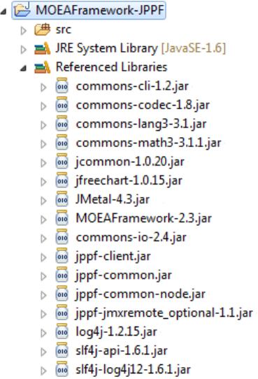
10.1. MASTER-SLAVE PARALLELIZATION 137
Figure 10.1: Screenshot of an Eclipse project with the JPPF and MOEA
Framework JAR files included.

138 CHAPTER 10. PARALLELIZATION
5790638151819130066L;
10
11 @Override
12 public String getName() {
13 return "ParallelProblem";
14 }
15
16 @Override
17 public int getNumberOfVariables() {
18 return 1;
19 }
20
21 @Override
22 public int getNumberOfObjectives() {
23 return 2;
24 }
25
26 @Override
27 public int getNumberOfConstraints() {
28 return 0;
29 }
30
31 @Override
32 public void evaluate(Solution solution) {
33 long start = System.currentTimeMillis();
34 double x = EncodingUtils.getReal(solution.getVariable(0));
35
36 // simulate time-consuming evaluation
37 for (long i = 0; i < 500000000; i++);
38
39 solution.setObjective(0, Math.pow(x, 2.0));
40 solution.setObjective(1, Math.pow(x - 2.0, 2.0));
41
42 System.out.println("Elapsed time: " +
43 (System.currentTimeMillis() - start));
44 }
45
46 @Override
47 public Solution newSolution() {
48 Solution solution = new Solution(1, 2);
49 solution.setVariable(0, EncodingUtils.newReal(-10.0, 10.0));
50 return solution;
51 }
52
53 @Override
10.1. MASTER-SLAVE PARALLELIZATION 139
54 public void close() {
55 //do nothing
56 }
57
58 }
Note that this class implements the Serializable interface. This is
a required step for parallelization. Implementing the Serializable in-
terface allows the Java class to be encoded and transmitted across a net-
work. To make a serializable class, all one needs to do is add implements
Serializable after the class name, as shown in this example.
Next, create another Java class called JPPFExample.java with the
following code:
1import org.jppf.client.JPPFClient;
2import org.jppf.client.concurrent.JPPFExecutorService;
3import org.moeaframework.Executor;
4import org.moeaframework.core.NondominatedPopulation;
5
6public class JPPFExample {
7
8public static void main(String[] args) {
9JPPFClient jppfClient = null;
10 JPPFExecutorService jppfExecutor = null;
11
12 try {
13 jppfClient = new JPPFClient();
14 jppfExecutor = new JPPFExecutorService(jppfClient);
15
16 // setting the batch size is important, as JPPF will only
17 // run one job at a time from a client; the batch size
18 // lets us group multiple evaluations (tasks) into a
19 // single job
20 jppfExecutor.setBatchSize(100);
21 jppfExecutor.setBatchTimeout(100);
22
23 long start = System.currentTimeMillis();
24
25 NondominatedPopulation result = new Executor()
26 .withProblemClass(ParallelProblem.class)
27 .withAlgorithm("NSGAII")
28 .withMaxEvaluations(10000)
29 .distributeWith(jppfExecutor)

140 CHAPTER 10. PARALLELIZATION
30 .run();
31
32 System.out.println("Solutions found: " + result.size());
33 System.out.println("Total elapsed time: " +
34 ((System.currentTimeMillis() - start) / 1000) +
35 " seconds");
36 }catch(Exception e) {
37 e.printStackTrace();
38 }finally {
39 if (jppfExecutor != null) {
40 jppfExecutor.shutdown();
41 }
42
43 if (jppfClient != null) {
44 jppfClient.close();
45 }
46 }
47 }
48
49 }
Line 20 is where we configure the Executor to distribute function evalua-
tions using JPPF. Also of importance is lines 20-21, where we set the JPPF
batch size and timeout. It is best if the batch size is equal to the population
size in this example (the default population size of 100).
With these two files created, we can now test this example. Prior to
running the Java code we just created, you will need to start the JPPF
driver and one or more JPPF nodes. To start the driver, run the JPPF-4.
2.5-driver/startDriver.bat program. To start a local node, run
the JPPF-4.2.5-node/startNode.bat program. You should see two
command prompt windows appear. If using Unix/Linux, use the files with
the .sh extension instead. Once the driver and node(s) are started, run the
JPPFExample class we just created. If all works as intended, your computer
should now be running at or near 100% CPU utilization as it is distributing
work to all nodes.
During our testing, we found that running this example on a single local
core with no parallelization takes approximately 1,687 seconds while running
on four local cores takes approximately 545 seconds. This results in a speedup
of 3.1x. We lose some speedup due to communication overhead between the
master and slave nodes, but still obtain a reasonable speedup.

10.2. ISLAND-MODEL PARALLELIZATION 141
10.2 Island-Model Parallelization
Rather than run a single algorithm and distribute the problem evaluations
to many cores, the island-model approach runs multiple instances of the al-
gorithm in parallel. This method of parallelization does not speed up the
algorithm itself, but allows running multiple algorithms in parallel. Period-
ically, solutions migrate from one population to another. These migration
events distribute genetic information to other islands, which in practice im-
proves convergence properties. For example, if one island gets stuck at a local
optima, a migration event may introduce new genetic material that helps the
island escape the local optima and continue searching for the global optimum.
The MOEA Framework can support island-model parallelization with
some additional coding. The developer is responsible for instantiating each
algorithm/island and processing the migrations. Below is a simple island-
model example where migration events occur every 10,000 evaluations. A
random solution from each island population is selected (the emigrant) and
sent to one of the neighboring islands. Special care is needed to ensure the
code is correctly synchronized to avoid race conditions. In this example,
we use a semaphore to ensure mutual exclusion while obtaining locks (i.e.,
the synchronized (oldIsland) and synchronized (newIsland)
lines) to avoid the possibility of deadlocks. Additionally, the majority of Java
and MOEA Framework classes are not thread safe, and any modifications
must be carefully synchronized.
1import java.util.HashMap;
2import java.util.Map;
3import java.util.Properties;
4import java.util.concurrent.Semaphore;
5
6import org.apache.commons.math3.random.MersenneTwister;
7import org.apache.commons.math3.random.RandomAdaptor;
8import org.apache.commons.math3.random.
SynchronizedRandomGenerator;
9import org.moeaframework.algorithm.NSGAII;
10 import org.moeaframework.algorithm.PeriodicAction;
11 import org.moeaframework.algorithm.PeriodicAction.FrequencyType;
12 import org.moeaframework.core.NondominatedPopulation;
13 import org.moeaframework.core.PRNG;
14 import org.moeaframework.core.Population;
15 import org.moeaframework.core.Problem;
16 import org.moeaframework.core.spi.AlgorithmFactory;

142 CHAPTER 10. PARALLELIZATION
17 import org.moeaframework.core.spi.ProblemFactory;
18
19 public class IslandExample {
20
21 public static void main(String[] args) {
22 final int numberOfIslands = 4;
23 final int maxEvaluations = 1000000;
24 final int migrationFrequency = 10000;
25 final Problem problem = ProblemFactory.getInstance()
26 .getProblem("DTLZ2_2");
27 final Map<Thread, NSGAII> islands = new HashMap<Thread,
28 NSGAII>();
29
30 // this semaphore is used to synchronize locking
31 // to prevent deadlocks
32 final Semaphore semaphore = new Semaphore(1);
33
34 // need to use a synchronized random number generator
35 // instead of the default
36 PRNG.setRandom(new RandomAdaptor(
37 new SynchronizedRandomGenerator(
38 new MersenneTwister())));
39
40 // create the algorithm run on each island
41 for (int i = 0; i < numberOfIslands; i++) {
42 final NSGAII nsgaii = (NSGAII)AlgorithmFactory
43 .getInstance().getAlgorithm(
44 "NSGAII",
45 new Properties(),
46 problem);
47
48 // create a periodic action for handling migration events
49 final PeriodicAction migration = new PeriodicAction(
50 nsgaii,
51 migrationFrequency,
52 FrequencyType.EVALUATIONS) {
53
54 @Override
55 public void doAction() {
56 try {
57 Thread thisThread = Thread.currentThread();
58
59 for (Thread otherThread : islands.keySet()) {
60 if (otherThread != thisThread) {
61 semaphore.acquire();

10.2. ISLAND-MODEL PARALLELIZATION 143
62
63 Population oldIsland = islands.get(thisThread)
64 .getPopulation();
65 Population newIsland = islands.get(otherThread)
66 .getPopulation();
67
68 synchronized (oldIsland) {
69 synchronized (newIsland) {
70 int emigrant = PRNG.nextInt(oldIsland.size()
);
71 newIsland.add(oldIsland.get(emigrant));
72
73 System.out.println("Sending solution " +
74 emigrant + " from " +
75 Thread.currentThread().getName() +
76 "to"+ otherThread.getName());
77 }
78 }
79
80 semaphore.release();
81 }
82 }
83 }catch (InterruptedException e) {
84 // ignore
85 }
86 }
87
88 };
89
90 // start each algorithm its own thread so they run
91 // concurrently
92 Thread thread = new Thread() {
93
94 public void run() {
95 while (migration.getNumberOfEvaluations() <
96 maxEvaluations) {
97 migration.step();
98 }
99 }
100
101 };
102
103 islands.put(thread, nsgaii);
104 }
105

144 CHAPTER 10. PARALLELIZATION
106 // start the threads
107 for (Thread thread : islands.keySet()) {
108 thread.start();
109 }
110
111 // wait for all threads to finish and aggregate the result
112 NondominatedPopulation result =
113 new NondominatedPopulation();
114
115 for (Thread thread : islands.keySet()) {
116 try {
117 thread.join();
118 result.addAll(islands.get(thread).getResult());
119 }catch (InterruptedException e) {
120 System.out.println("Thread " + thread.getId() +
121 " was interrupted!");
122 }
123 }
124
125 System.out.println("Found " + result.size() +
126 " solutions!");
127 }
128
129 }
10.3 Hybrid Parallelization
Combining the island-model and master-slave parallelization strategies, the
hybrid parallelization approach inherits the benefits of both strategies. It
gains speedup from the master-slave strategy by distributing function eval-
uations across many cores, and the benefit of operating multiple, concur-
rent algorithms in the island-model strategy. Since we are not using the
Executor in the island-model example, we instead use the underlying
DistributedProblem class. To enable the hybrid strategy, wrap the
problem created on lines 25-26 to either distribute work across multiple local
cores:
1problem = new DistributedProblem(problem,
2Runtime.getRuntime().availableProcessors());

10.4. CONCLUSION 145
or on multiple computers across a network using JPPF:
1problem = new DistributedProblem(problem, jppfExecutor);
Above, jppfExecutor is the JPPF executor service created in Sec-
tion 10.1. Note that all of the requirements outlined in Section 10.1 must be
followed when using JPPF.
10.4 Conclusion
This chapter provided an introduction to parallel computing with the MOEA
Framework. We explored the master-slave, island-model, and hybrid paral-
lelization strategies. Using parallelization, we can help decrease computing
time by distributing the workload across multiple computers and/or improve
convergence properties by running multiple concurrent algorithms.
146 CHAPTER 10. PARALLELIZATION

Chapter 11
Advanced Topics
11.1 Configuring Hypervolume Calculation
The hypervolume calculation is an important tool when comparing the per-
formance of MOEAs. This section details the available configuration options
for the hypervolume calculation.
The hypervolume calculation computes the volume of the space domi-
nated between the Pareto front and the nadir point. The nadir point is
set to the extremal objective values of the reference set plus some delta.
A non-zero delta is necessary to ensure such extremal values contribute a
non-zero volume. This delta is configurable by adding the following line to
global.properties:
org.moeaframework.core.indicator.hypervolume_delta = 0.01
The hypervolume calculation is computationally expensive. Use of the
built-in hypervolume calculator may become prohibitive on Pareto fronts
with 4 or more objectives. For this reason, it may be beneficial to use
third-party hypervolume calculators instead. A number of researchers have
released C/C++ implementations of high-performance hypervolume calcula-
tors, including those listed below.
•http://ls11-www.cs.uni-dortmund.de/rudolph/
hypervolume/start
•http://iridia.ulb.ac.be/˜manuel/hypervolume/
147

148 CHAPTER 11. ADVANCED TOPICS
•http://www.wfg.csse.uwa.edu.au/hypervolume/1
Such hypervolume calculators can be used by the MOEA Framework by
following two steps. First, download and compile the desired hypervolume
code. This should result in an executable file, such as hyp.exe. Second,
configure the MOEA Framework to use this executable by adding a line
similar to the following to the global.properties file.
org.moeaframework.core.indicator.hypervolume = hyp.exe {0} {1}
{2} {3}
This property is specifying the executable and any required arguments.
The arguments are configurable by using the appropriate variable, such as
{0}. The complete list of available variables are shown in the table below.
Variable Description
{0}Number of objectives
{1}Approximation set size
{2}File containing the approximation set
{3}File containing the reference point
{4}The reference point, separated by spaces
If all else fails, the hypervolume calculation can be disabled. When dis-
abled, the hypervolume will be reported as NaN. To disable all hypervolume
calculations, add the following line to global.properties:
org.moeaframework.core.indicator.hypervolume_enabled = false
11.2 Storing Large Datasets
When dealing with large datasets, proper data organization and management
is key to avoiding headaches. A number of tools are provided by the MOEA
Framework for storing and manipulating large datasets. The two key classes
1Some source code editing is necessary to modify the input and output format to be
compatible with the MOEA Framework.

11.2. STORING LARGE DATASETS 149
are the ResultFileWriter and ResultFileReader. A result file is a
collection of one or more approximation sets. Each entry in the result file is
the approximation set, including the decision variables and objectives for all
solutions in the approximation set, and any additional metadata you provide.
Note that this approximation set does not contain any constraints, as only
feasible solutions are written in a result file.
11.2.1 Writing Result Files
The ResultFileWriter class is used to write result files. The example
code below demonstrates running the UF1 problem and recording the ap-
proximation set at each generation. In addition, two pieces of metadata are
stored: the current number of objective function evaluations (NFE) and the
elapsed time.
1Problem problem = null;
2Algorithm algorithm = null;
3ResultFileWriter writer = null;
4long startTime = System.currentTimeMillis();
5
6try {
7problem = ProblemFactory.getInstance().getProblem("UF1");
8algorithm = AlgorithmFactory.getInstance().getAlgorithm(
9"NSGAII",new Properties(), problem);
10
11 try {
12 writer = new ResultFileWriter(problem, new File("result.set"
));
13
14 //run the algorithm
15 while (!algorithm.isTerminated() &&
16 (algorithm.getNumberOfEvaluations() < 10000)) {
17 algorithm.step(); //run one generation of the algorithm
18
19 TypedProperties properties = new TypedProperties();
20 properties.setInt("NFE", algorithm.getNumberOfEvaluations
());
21 properties.setLong("ElapsedTime", System.currentTimeMillis
()-start);
22
23 writer.append(new ResultEntry(algorithm.getResult(),
properties));
150 CHAPTER 11. ADVANCED TOPICS
24 }
25 }finally {
26 //close the result file writer
27 if (writer != null) {
28 writer.close();
29 }
30 }
31 }finally {
32 //close the problem to free any resources
33 if (problem != null) {
34 problem.close();
35 }
36 }
If the file you are saving already exists, the ResultFileWriter ap-
pends any new data to the end of the file. If you do not want to append to
any existing data, delete any old file first.
11.2.2 Extract Information from Result Files
The ExtractData command line utility is an extremely useful tool for
extracting information from a result file. It can extract any properties from
the file as well as calculate specific performance indicators, and outputs this
data in a clean, tabular format which can be read into spreadsheet software,
such as LibreOffice Calc or Microsoft Excel. When only extracting metadata,
you need only specify the input file and the property keys to extract. For
instance, continuing the example from above, we can extract the NFE and
ElapsedTime properties with the following command:
java org.moeaframework.analysis.sensitivity.ExtractData
--problem UF1
--input result.set
NFE ElapsedTime
The output of this command will appear similar to:
#NFE ElapsedTime
100 125
200 156
300 172

11.3. DEALING WITH MAXIMIZED OBJECTIVES 151
400 187
500 203
...
Performance indicators can be calculated using one of the “plus op-
tions.” The options for the supported performance indicators include +
hypervolume for hypervolume, +generational for generational dis-
tance, +inverted for inverted generational distance, +epsilon for ad-
ditive -indicator, +error for maximum Pareto front error, +spacing for
spacing, and +contribution for reference set contribution/coverage. In
addition, you must specify the problem, reference set, and optionally the
values to use when calculating contribution. For example:
java org.moeaframework.analysis.sensitivity.ExtractData
--problem UF1
--input result.set
--reference ./pf/UF1.dat
NFE ElapsedTime +hypervolume +epsilon +coverage
The added performance indicators will appear alongside the other prop-
erties:
#NFE ElapsedTime +hypervolume +epsilon +contribution
100 125 0.0 1.287951 0.0
200 156 0.0 1.149751 0.0
300 172 0.0 1.102796 0.0
400 187 0.0 1.083581 0.0
500 203 0.0 0.959353 0.0
...
Additional command line options allow you to format the output, such
as removing the column header line or specifying the column separator char-
acter.
11.3 Dealing with Maximized Objectives
The MOEA Framework is setup to minimize objectives; it can not by itself
maximize objectives. This simplifies the program and increases its perfor-
152 CHAPTER 11. ADVANCED TOPICS
mance considerably. By only allowing minimization objectives, the MOEA
Framework can avoid the overhead of constantly determining the optimiza-
tion direction whenever calculating the Pareto dominance relation.
This approach, however, puts the burden on the user to make the ap-
propriate adjustments to their problem definition to allow maximization ob-
jectives. The easiest way to allow maximization objectives is to negate the
objective value, as demonstrated below:
1solution.setObjective(0, obj1);
2solution.setObjective(1, -obj2); //negate the original objective
value
By minimizing the negated objective value, we are maximizing the orig-
inal objective value. These negated objective values will be carried through
to any output files produced by the MOEA Framework. The help assist in
managing these output files, version 1.13 includes the Negater command
line utility. The Negater tool processes any output file produced by the
MOEA Framework and negates any specified objective. For example, with-
out the two objective example above, we can remove the negation in any
output file with the following command. Specifying a direction of 1 will
negate the corresponding objective values in the processed file.
java org.moeaframework.analysis.sensitivity.Negater
--direction 0,1
output.set
It is best to wait until all post-processing is complete before negating the
objectives back to their original, maximized form as any calculations on the
maximized form will be invalid. You can always apply the Negater a second
time to undo the change. It is the responsibility of the user to manage their
data files accordingly.
11.4 Checkpointing
The MOEA Framework provides checkpointing functionality. As an algo-
rithm is running, checkpoint files will be periodically saved. The checkpoint
file stores the current state of the algorithm. If the run is interrupted, such as
11.5. REFERENCING THE PROBLEM 153
during a power outage, the run can be resumed at the last saved checkpoint.
The setCheckpointFile sets the file location for the checkpoint file, and
checkpointEveryIteration or setCheckpointFrequency control
how frequently the checkpoint file is saved.
Resuming a run from a checkpoint occurs automatically. If the checkpoint
file does not exist, a run starts from the beginning. However, if the checkpoint
file exists, then the run is automatically resumed at that checkpoint. For this
reason, care must be taken when using checkpoints as they can be a source
of confusion for new users. For instance, using the same checkpoint file from
an unrelated run can cause unexpected behavior or an error. For this reason,
checkpoints are recommended only when solving time-consuming problems.
The code snippet below demonstrates the use of checkpointing.
1NondominatedPopulation result = new Executor()
2.withProblem("UF1")
3.withAlgorithm("NSGAII")
4.withMaxEvaluations(1000000)
5.checkpointEveryIteration()
6.withCheckpointFile(new File("UF1_NSGAII.chkpt"))
7.run();
Checkpoint files are never deleted by the MOEA Framework. Each
time you run this example, it will resume from its last save point. If you
want to run this example from the beginning, you must delete the check-
point file manually. In this example, the checkpoint file is saved in the
MOEAFramework-2.6 folder.
11.5 Referencing the Problem
Once a new problem is defined in Java, it can be referenced by the MOEA
Framework in a number of ways. This section details the various methods
for referencing problems.
11.5.1 By Class
The Executor,Instrumenter and Analyzer classes introduced in
Chapter 3 all accept direct references to the problem class using the
withProblemClass method. For example, following the previous example

154 CHAPTER 11. ADVANCED TOPICS
with the Kursawe problem, we can optimize this problem with the following
code:
1new Executor()
2.withProblemClass(Kursawe.class)
3.withAlgorithm("NSGAII")
4.withMaxEvaluations(10000)
5.run();
Note how the Kursawe problem is specified by name followed by .class.
This passes a direct reference to the Kursawe class we created in the previous
chapter.
Problems can also define constructors with arguments. For example, con-
sider a problem that needs to load data from a file. For this to work, define
a constructor in the problem class that accepts the desired inputs. In this
case, our constructor would be called public ProblemWithArgument(
File dataFile).... You can then solve this problem as shown below.
1new Executor()
2.withProblemClass(ProblemWithArgument.class,new File("
inputFile.txt"))
3.withAlgorithm("NSGAII")
4.withMaxEvaluations(10000)
5.run();
11.5.2 By Class Name
As of version 1.11, problems can be referenced by their fully-qualified class
name. The fully-qualified class name includes the Java package in which
the class is defined. For example, the Schaffer problem’s fully-qualified class
name is org.moeaframework.problem.misc.Schaffer. The prob-
lem must have an empty (no argument) constructor.
The class name can be used to run problems anywhere the MOEA Frame-
work accepts a string representation of the problem. This includes but is not
limited to
1. The withProblem method in Executor,Instrumenter and
Analyzer
11.5. REFERENCING THE PROBLEM 155
2. Any command line utilities with a problem argument
3. The problem selection combo box in the MOEA Diagnostic Tool
11.5.3 By Name
The MOEA Framework also provides the option to reference problems
by name. There are two advantages to using this approach. First,
this approach allows the use of short, meaningful names. For example,
rather than specifying the fully-qualified class name for the Schaffer prob-
lem, org.moeaframework.problem.misc.Schaffer, one can use the
name Schaffer instead. Second, a reference set for named problems can
optionally be defined. This reference set will be automatically used wherever
a reference set is required. Without this, a reference set must be manually
specified by the user or programmer each time it is required.
The disadvantage to this approach is that some additional configuration
is necessary to provide the mapping from the problem name to the prob-
lem class. As such, this approach is recommended for third-party library
developers who are developing new problems to be used with the MOEA
Framework. The remainder of this section describes two such methods for
referencing problems by name.
The problem name can be used to run problems anywhere the MOEA
Framework accepts a string representation of the problem. This includes but
is not limited to
1. The withProblem method in Executor,Instrumenter and
Analyzer
2. Any command line utilities with a problem argument
3. The problem selection combo box in the MOEA Diagnostic Tool
11.5.4 With a ProblemProvider
The first way to reference problems by name is to define a
ProblemProvider. The ProblemProvider uses the Java Service
Provider Interface (SPI). The SPI allows the MOEA Framework to
load all available providers from the classpath. This approach allows
third-party software vendors to distribute compiled JAR files containing

156 CHAPTER 11. ADVANCED TOPICS
ProblemProvider instances that are automatically loaded by the MOEA
Framework. To create a new ProblemProvider, first create a subclass of
the ProblemProvider class. To do so, you must define two methods:
1. Problem getProblem(String name)
2. NondominatedPopulation getReferenceSet(String name
)
Both methods are provided the problem name as the argument. The
getProblem method should return a new instance of the specified prob-
lem, or null if the provider does not support the given problem name.
Likewise, the getReferenceSet method should return the reference set
of the specified problem if one is available, or null otherwise. Returning
null when the problem is not supported by the provider is important, as
the Java SPI will scan all available ProblemProvider instances until it
finds a suitable provider.
1import org.moeaframework.core.NondominatedPopulation;
2import org.moeaframework.core.Problem;
3import org.moeaframework.core.spi.ProblemProvider;
4
5public class ExampleProblemProvider extends ProblemProvider {
6
7public Problem getProblem(String name) {
8if (name.equalsIgnoreCase("kursawe")) {
9return new Kursawe();
10 }else {
11 return null;
12 }
13 }
14
15 public NondominatedPopulation getReferenceSet(String name) {
16 return null;
17 }
18
19 }
Lastly, a special configuration file used by the SPI must be created. The
file is located at META-INF/services/org.moeaframework.core.
spi.ProblemProvider. Each line of this file must contain the fully-
qualified class name for each of the ProblemProviders being introduced.

11.5. REFERENCING THE PROBLEM 157
When bundling the compiled class files into a JAR, be sure that this config-
uration file is also copied into the JAR.
Once packaged as a JAR, the provider is ready to be used. Place the JAR
on the classpath used by the MOEA Framework. Once on the classpath, the
Java SPI mechanism used by the MOEA Framework will be able to scan and
load all providers contained in all available JAR files.
11.5.5 With the global.properties File
The second way to reference problems by name is to add the problem defini-
tion to the global.properties file. This global.properties file
contains the configuration options for the MOEA Framework. This file usu-
ally accompanies a MOEA Framework distribution, but in the event it does
not exist, you can just create a new empty text file. Adding a new problem
is as simple as adding the following two lines to global.properties:
org.moeaframework.problem.problems = Kursawe
org.moeaframework.problem.Kursawe.class = Kursawe
Line 1 lists all problems configured in the global.properties file.
The string provided here becomes the problem name. This is the name you
would subsequently provide to any of the MOEA Framework tools to instan-
tiate the problem. More than one problem can be specified by separating the
problem names with commas.
Line 2 identifies the class for the specified problem. Note that this entry
follows the naming convention org.moeaframework.problem.NAME.
class = value. The NAME used must match the problem name defined
in line 1. The value is the fully-qualified Java classname. In this case, the
class is located in the default package. If this class were located, for example,
in the package foo.bar, the value must be set to foo.bar.Kursawe.
The reference set file for the problem can be optionally specified as well.
If a reference set is available for the problem, add the following line to
global.properties:
org.moeaframework.problem.Kursawe.referenceSet = kursawe.ref
158 CHAPTER 11. ADVANCED TOPICS
Part III
Developer’s Guide - Extending
and Contributing to the MOEA
Framework
159
Chapter 12
Developer Guide
This chapter outlines the coding practices to be used by contributors to the
core MOEA Framework library. In addition, many of the internal policies
used by MOEA Framework administrators, managers and developers are
outlined.
Much of the strategies used by the developers and managers are discussed
in detail in the open book Producing Open Source Software by Karl Fogel.
This book can be viewed or downloaded from http://producingoss.
com/.
12.1 Version Numbers
Amajor.minor version numbering scheme is used for all releases of the
MOEA Framework. Compatibility between two versions of the software can
be determined by comparing the version numbers.
•In general, downgrading to an older version should never be allowed.
The older version likely includes bugs or is missing features potentially
used by the newer version.
•Compatibility is guaranteed when upgrading to a newer version that
shares the same major version.
•Compatibility is NOT guaranteed when upgrading to a new version
with a different major version number. Deprecated API is removed
when the major version is incremented, and programs relying on dep-
recated API will not function with the new version.
161
162 CHAPTER 12. DEVELOPER GUIDE
12.2 Release Cycle
The MOEA Framework is a research tool, and as such experiences rapid peri-
ods of development. To provide these updates in a timely manner, new minor
versions are released approximately every six months, but more frequent re-
leases may occur to fix bugs. New releases are immediately available for
download from http://www.moeaframework.org and are announced
on http://www.freecode.com.
Prior to every release, the MOEA Framework must pass all testing code to
ensure it functions as expected. Furthermore, the code must pass a number
of code quality and code style checks.
Major version increments will occur approximately every four to five
years. The decision to release a new major version will depend on the state
of the codebase. Major releases serve as a time for spring cleaning, allowing
developers to remove old, deprecated API.
12.3 API Deprecation
Throughout the lifetime of a software project, certain API elements may be
deemed unused, redundant or flawed by the developers and users. A process
is established to facilitate the identification, cleanup and removal of such
API elements. Once a consensus is reached that a certain API element is to
be removed, it will be marked as @Deprecated in the next release. This
annotation serves as a reminder to all developers and users that the marked
class, variable, constructor or method should be avoided in all client code.
Deprecated API elements can be identified in a number of ways. First,
the Java compiler will emit warning messages whenever deprecated API is
referenced. Second, most IDEs will highlight all uses of deprecated API
with warning messages. Lastly, the published Javadoc comments will clearly
identify any deprecated method. These Javadoc comments will typically also
explain the reason for deprecation, specify the version when the API element
will be removed, and provide the alternatives (if any) that should be used to
replace the deprecated API.
In order to maintain backwards compatibility between minor releases,
deprecated API elements will only be removed during the next major version
release. In addition, an API element must be deprecated for at least three
months prior to removal.

12.4. CODE STYLE 163
12.4 Code Style
Clean and easy-to-understand code is of the utmost importance. While no
official code style standard is enforced, there are a number of guidelines
contributors should follow to help produce clean code.
•Every source code file should begin with a comment containing a copy-
right and license notice.
•Avoid using the asterisk to import all classes in a package. Instead,
add an import line for each class.
Bad:
1import java.util.*;
Good:
1import java.util.List;
2import java.util.ArrayList;
•Remove any import statements for classes not in use.
•Always add braces in loops or conditionals, even if the code block is
only one line.
Bad:
1for (int i=0; i<array.length; i++)
2array[i] = 0.0;
Good:
1for (int i=0; i<array.length; i++) {
2array[i] = 0.0;
3}

164 CHAPTER 12. DEVELOPER GUIDE
•Never write an empty block of code. At the minimum, include a com-
ment indicating why the block is empty.
Bad:
1try {
2Thread.sleep(1000);
3}catch (InterruptedException e) {}
Good:
1try {
2Thread.sleep(1000);
3}catch (InterruptedException e) {
4//sleep was interrupted, continue processing
5}
•Add the @Override annotation to overriding methods.
•If you override the equals(Object obj) method, always override
the hashCode() method as well. For this project, the Apache Com-
mons Lang library is used to build these methods. For example:
1@Override
2public int hashCode() {
3return new HashCodeBuilder()
4.append(algorithm)
5.append(problem)
6.toHashCode();
7}
8
9@Override
10 public boolean equals(Object obj) {
11 if (obj == this) {
12 return true;
13 }else if ((obj == null) || (obj.getClass() !=
getClass())) {
14 return false;
15 }else {
16 ResultKey rhs = (ResultKey)obj;

12.4. CODE STYLE 165
17
18 return new EqualsBuilder()
19 .append(algorithm, rhs.algorithm)
20 .append(problem, rhs.problem)
21 .isEquals();
22 }
23 }
•Avoid unnecessary whitespace unless the whitespace improves the clar-
ity or readability of the code.
Bad:
1List< String > grades = Arrays.asList( "A","B","C
","D","F" );
2
3for ( String grade : grades ) {
4...
5}
Good:
1List<String> grades = Arrays.asList("A","B","C",
"D","F");
2
3for (String grade : grades) {
4...
5}
•Never compare strings with == or !=. Use equals or
equalsIgnoreCase instead.
Bad:
1if ("yes" == inputTextField.getText()) {
2...
3}

166 CHAPTER 12. DEVELOPER GUIDE
Good:
1if ("yes".equals(inputTextField.getText()) {
2...
3}
•Avoid overriding clone() and finalize(). If you must override
these methods, always invoke super.clone() or super.finalize
() in the method.
•Write only one statement per line. Avoid multiple variable declarations
on one line. Also, initialize variables at their declaration whenever
possible.
Bad:
1double sum, product;
2...
3sum = 0.0;
4product = 1.0;
Good:
1double sum = 0.0;
2double product = 1.0;
•Fully document every variable, constructor and method. The only
place documentation is not necessary is on overridden methods if the
inherited documentation is sufficient.
•Follow standard Java naming conventions. Constants should be in
ALL_CAPS, variables and methods in camelCase, etc.
•Class variables should never be publicly visible. If the value is mutable,
add the appropriate getter/setter methods.
Bad:

12.5. LICENSING 167
1public int size;
Good:
1private int size;
2
3public int getSize() {
4return size;
5}
6
7public void setSize(int size) {
8this.size = size;
9}
12.5 Licensing
The MOEA Framework is licensed under the GNU Lesser General Public
License, version 3 or later. In order to ensure contributions can be legally
released as part of the MOEA Framework, all contributions must be licensed
under the GNU Lesser General Public License, version 3.
Modifications which are not licensed under the GNU Lesser General Pub-
lic License, version 3, can still be bundled with the MOEA Framework library
or distributed as a third-party extension. In fact, the GNU Lesser General
Public License specifically grants users of the MOEA Framework the right
to bundle the library with an application released under any license of their
choosing.
12.6 Web Presence
The following webpages are officially managed by the MOEA Framework
development team.
http://www.moeaframework.org - The main website for the MOEA
Framework, providing the latest downloads and documentation.

168 CHAPTER 12. DEVELOPER GUIDE
https://github.com/MOEAFramework/MOEAFramework - The web
host, where the source code, issue tracker, and other material is stored.
http://sourceforge.net/projects/moeaframework - The old
web host, no longer in use. Archival versions of the software are avail-
able here.
http://www.freecode.com/projects/moea-framework - An-
nounces new releases and other news to the open source community.
http://www.openhatch.org/+projects/MOEA%20Framework
- Provides information for individuals wishing to contribute to the
MOEA Framework.
12.7 Ways to Contribute
12.7.1 Translations
Version 1.14 introduced support for internationalization and localization (of-
ten referred to as i18n and l10n). Throughout the source folder, you will
find properties files with the name LocalStrings.properties. These
properties files contain the default text messages displayed in the GUI, com-
mand line tools, and other user-facing interfaces. If you are fluent in a foreign
language, you can contribute by providing translations of these text messages.
To provide a translation, first determine the target locale. You can
target a specific language or even a specific country. See http://www.
loc.gov/standards/iso639-2/php/English_list.php to deter-
mine your target locale’s two-character language code. For example, Spanish
is represented by the code es.
Next, create a copy of the LocalStrings.properties file and ap-
pend the language code (and optionally the country code). For example,
the Spanish translations will be stored in the file LocalStrings_es.
properties.
Lastly, replace the default English text messages with your translations.
For most strings, a direct translation is sufficient. However, some strings are
parametric, such as "Objective {0}". The parameter {0} is replaced in
this case by a number, producing the strings Objective 1,Objective 2
, etc. In general, you need only translate the text and place the parameter at

12.7. WAYS TO CONTRIBUTE 169
the correct position in the message. More advanced formatting of parameters
is possible. See the MessageFormat class for details.
The current LocalStrings.properties files are located in
the folders src/org/moeaframework/analysis/diagnostics,
src/org/moeaframework/analysis/sensitivity, and src/
org/moeaframework/util. We currently have complete English and
Italian translations.
170 CHAPTER 12. DEVELOPER GUIDE
Chapter 13
Errors and Warning Messages
This chapter provides a comprehensive list of errors and warning messages
that may be encountered when using the MOEA Framework. The error or
warning message is shown in italic text, followed by details and possible fixes
for the issue.
13.1 Errors
Errors halt the execution of the program and produce an error message to
the standard error stream (i.e., the console). Most errors can be corrected
by the user.
Exception in thread ”main” java.lang.NoClassDefFoundError: <class>
Thrown when Java is starting but is unable to find the specified class.
Ensure the specified class is located on the Java classpath. If the class
is located in a JAR file, use
java -classpath "$CLASSPATH:/path/to/library.
jar" ...
If the class is an individual .class file in a folder, use
java -classpath "$CLASSPATH:/path/to/folder/"
Also ensure you are using the correct classpath separator. Linux users
will use the colon (:) as the above examples demonstrate. Windows
and Cygwin users should use the semi-colon (;).
171
172 CHAPTER 13. ERRORS AND WARNING MESSAGES
Error occurred during initialization of VM or
Too small initial heap for new size specified
This Java error occurs when the initial heap size (allocated memory) is
too small to instantiate the Java virtual machine (VM). This error is
likely caused by the -Xmx command line option requesting less memory
than is necessary to start the VM. Increasing the -Xmx value may re-
solve this issue. Also ensure the -Xmx argument is properly formatted.
For instance, use -Xmx128m and NOT -Xmx128.
Error occurred during initialization of VM or
Could not reserve enough space for object heap or
Could not create the Java virtual machine
This Java error occurs when there is insufficient heap size (allocated
memory) to instantiate the Java virtual machine (VM). This error is
likely caused by the -Xmx command line option requesting more mem-
ory than is available on the host system. This error may also occur if
other running processes consume large quantities of memory. Lowering
the -Xmx value may resolve this issue.
Exception in thread “main” java.lang.OutOfMemoryError: GC overhead
limit exceeded
Java relies on a garbage collector to detect and free memory which is no
longer in use. This process is usually fast. However, if Java determines
it is spending too much time performing garbage collection (98% of
the time) and is only recovering a small amount of memory (2% of
the heap), this error is thrown. This is likely caused when the in-use
memory approaches the maximum heap size, leaving little unallocated
memory for temporary objects. Try increasing the maximum heap size
with the -Xmx command line argument.
Assertion failed: fp != NULL, file <filename>, line <linenumber>
PISA modules communicate using the file system. Some anti-virus soft-
ware scans the contents of files before read and after write operations.
This may cause one of the PISA communication files to become inac-
cessible and cause this error. To test if this is the cause, try disabling
your anti-virus and re-run the program.

13.1. ERRORS 173
A more permanent and secure solution involves adding an exception to
the anti-virus software to prevent active monitoring of PISA communi-
cation files. For example, first add the line
java.io.tmpdir=<folder>
to global.properties and set <folder> to some temporary
folder where the PISA communication files will be stored. Then con-
figure your anti-virus software to ignore the contents of <folder>.
problem does not have an analytical solution
Attempted to use SetGenerator to produce a reference set for a
problem which does not implement AnalyticalProblem. Only
AnalyticalProblems, which provide a method for generating
Pareto optimal solutions, can be used with SetGenerator.
input appears to be newer than output
Several of the command line utilities read entries in an input file and
write the corresponding outputs to a separate output file. If the last
modified date on the input file is newer than the date on the output
file, this exception is thrown. This suggests that the input file has
been modified unexpectedly, and attempting to resume with a partially
evaluated output file may result in incorrect results. To resolve:
1. If the input file is unchanged, use the --force command line
option to override this check.
2. If the input file is changed, delete the output file and restart eval-
uation from the beginning.
no reference set available
Several of the command line utilities require a reference set. The
reference set either is provided by the problem (through the
ProblemProvider), or supplied by the user via a command line ar-
gument. This exception occurs if neither approach provides a reference
set.
unable to load reference set
174 CHAPTER 13. ERRORS AND WARNING MESSAGES
Indicates that a reference set is specified, but it could not be loaded.
The error message should contain additional information about the
underlying cause for the load failure.
output has more entries than input
Thrown by the Evaluator or ResultFileEvaluator command
line utilities when attempting to resume evaluation of a partially eval-
uated file, but the output file contains more entries than the input file.
This implies the input file was either modified, or a different input file
was supplied than originally used to produce the output file. Unless the
original input file is found, do not attempt to recover from this excep-
tion. Delete the output file and restart evaluation from the beginning.
maxEvaluations not defined
Thrown by the Evaluator command line utility if the
maxEvaluations property has not been defined. This prop-
erty must either be defined in the parameter input file or through the
-x maxEvaluations=<value> command line argument.
unsupported decision variable type
Thrown when the user attempts to use an algorithm that does not
support the given problem’s decision variable encoding. For instance,
GDE3 only supports real-valued encodings, and will throw this excep-
tion if binary or permutation encoded problems are provided.
not enough bits or
not enough dimensions
The Sobol sequence generator supports up to 21000 dimensions and can
produce up to 2147483647 samples (231 −1). While unlikely, if either
of these two limits are exceeded, these exceptions are thrown.
invalid number of parents
Attempting to use CompoundVariation in a manner inconsistent
with its API specification will result in this exception. Refer to the
API documentation and the restrictions on the number of parents for
a variation operator.
13.1. ERRORS 175
binary variables not same length or
permutations not same size
Thrown by variation operators which require binary variables or per-
mutations of equal length, but the supplied variables differ in length.
invalid bit string
Thrown by ResultFileReader if either of the following two cases
occurs:
1. The binary variable length differs from that specified in the prob-
lem definition.
2. The string encoding in the file contains invalid characters.
In either case, the binary variable stored in the result file could not be
read.
invalid permutation
Thrown by ResultFileReader if either of the following two cases
occurs: 1) the permutation length differs from that specified in the
problem definition; and 2) the string encoding in the file does not rep-
resent a valid permutation. In either case, the permutation stored in
the result file could not be read.
no provider for <name>
Thrown by the service provider interface (org.moeaframework.core.spi)
codes when no provider for the requested service is available. Check
the following:
1. If a nested exception is reported, the nested exception will identify
the failure.
2. Ensure <name> is in fact provided by a built-in or third-party
provider. Check spelling and case sensitivity.
3. If <name> is supplied by a third-party provider, ensure the
provider is located on the Java classpath. If the provider is in
a JAR file, use
176 CHAPTER 13. ERRORS AND WARNING MESSAGES
java -classpath "$CLASSPATH:/path/to/
provider.jar" ...
If the provider is supplied as class files in a folder, use
java -classpath "$CLASSPATH:/path/to/
folder/"
Also ensure you are using the correct classpath separator. Linux
users will use the colon (:) as the above examples demonstrate.
Windows and Cygwin users should use the semi-colon (;).
error sending variables to external process or
error receiving variables from external process
Thrown when communicating with an external problem, but an I/O er-
ror occurred that disrupted the communication. Numerous situations
may cause this exception, such as the external process terminating un-
expectedly.
end of stream reached when response expected
Thrown when communicating with an external process, but the connec-
tion to the external process closed. This is most likely the result of an
error on the external process side which caused the external process to
terminate unexpectedly. Error messages printed to the standard error
stream should appear in the Java error stream.
response contained fewer tokens than expected
Thrown when communicating with an external problem, and the exter-
nal process has returned an unexpected number of entries. This is most
likely a configuration error where the defined number of objectives or
constraints differs from what is actually returned by the external pro-
cess.
unable to serialize variable
Attempted to serialize a decision variable to send to an external prob-
lem, but the decision variable is not one of the supported types. Only
real variables are supported.
restart not supported
13.1. ERRORS 177
PISA supports the ability to reuse a selector after a run has completed.
The MOEA Framework currently does not support this feature. This
exception is thrown if the PISA selector attempts to reset.
expected END on last line or
unexpected end of file or
invalid selection length
These exceptions are thrown when communicating with PISA processes,
and the files produced by the PISA process appear to be incomplete
or malformed. Check the implementation of the PISA codes to ensure
they follow the correct protocol and syntax.
invalid variation length
This exception is caused by an incorrect configuration of PISA. The
following equality must hold
children ∗(mu/parents) = lambda,
where mu is the number of parents selected by the PISA process, par-
ents is the number of parent solutions required by the variation opera-
tor, children is the number of offspring produced by a single invocation
of the variation operator, and lambda is the total number of offspring
produced during a generation.
no digest file
Thrown when attempting to validate a data file using a digest file, but
no such digest file exists. Processing of the data file should cease imme-
diately for sensitive applications where data integrity is essential. If the
digest file simply hasn’t yet been produced but the file contents are ver-
ified, the FileProtection command line utility can optionally generate
digest files.
invalid digest file
Thrown when attempting to validate a date file using a digest file, but
the digest file is corrupted or does not contain a valid digest. Processing
of the data file should cease immediately for sensitive applications where
data integrity is essential.
178 CHAPTER 13. ERRORS AND WARNING MESSAGES
digest does not match
Thrown when attempting to validate a data file using a digest file, but
the actual digest of the data file does not match the expected digest
contained in the digest file. This indicates that the data file or the digest
file are corrupted. Processing of the data file should cease immediately
for sensitive applications where data integrity is essential.
unexpected rule separator or
rule must contain at least one production or
invalid symbol or
rule must start with non-terminal or
rule must contain at least one production or
codon array is empty
Each of these exceptions originates in the grammatical evolution code,
and indicate specific errors when loading or processing a context free
grammar. The specific error message details the cause.
unable to mkdir ¡directory¿
For an unknown reason, the underlying operating system was unable
to create a directory. Check to ensure the location of the directory is
writable. One may also manually create the directory.
no scripting engine for extension ¡ext¿
Attempted to use the Java Scripting APIs, but no engine for the spec-
ified file extension could be found. To resolve:
1. Check that the extension is valid. If not, supply the file extension
for the scripting language required.
2. Ensure the scripting language engine is listed on the classpath.
The engine, if packaged in a JAR, can be specified with
java -classpath "$CLASSPATH:/path/to/
engine.jar"
Also ensure you are using the correct classpath separator. Linux
users will use the colon (:) as the above example demonstrates.
Windows and Cygwin users should use the semi-colon (;).
13.1. ERRORS 179
no scripting engine for ¡name¿
Attempted to use the Java Scripting APIs, but no engine with the
specified name was found.
1. Check that the name is valid. If not, supply the correct name for
the scripting language engine as required.
2. Ensure the scripting language engine is listed on the classpath.
The engine, if packaged in a JAR, can be specified with
java -classpath "$CLASSPATH:/path/to/
engine.jar"
Also ensure you are using the correct classpath separator. Linux
users will use the colon (:) as the above example demonstrates.
Windows and Cygwin users should use the semi-colon (;).
file has no extension
Attempted to use a script file with ScriptedProblem, but the file-
name does not contain a valid extension. Either supply the file exten-
sion for the scripting language required, or use the constructor which
accepts the engine name as an argument.
scripting engine not invocable
Thrown when using a scripting language engine which does not im-
plement the Invocable interface. The scripting language does not
support methods or functions, and thus can not be used as intended.
requires two or more groups
Attempted to use one of the n-ary statistical tests which require at least
two groups. Either add a second group to compare against, or remove
the statistical test.
could not locate resource ¡name¿
Thrown when attempting to access a resource packages within the
MOEA Framework, but the resource could not be located. This is
an error with the distribution. Please contact the distributor to correct
this issue.
180 CHAPTER 13. ERRORS AND WARNING MESSAGES
insufficient number of entries in row
Attempted to read a data file, but the row was missing one or more
entries. The exact meaning depends on the specific data file, but gen-
erally this error means the file is incomplete, improperly formatted or
corrupted. See the documentation on the various file types to determine
if this error can be corrected.
invalid entry in row
Attempted to read a data file, but an entry was not formatted correctly.
See the documentation on the various file types to determine if this error
can be corrected.
invoke calculate prior to getting indicator values
Attempted to retrieve one of the indicator values prior to invoking the
calculate method. When using QualityIndicator, the calculate
method must be invoked prior to retrieving any of the indicator values.
not a real variable or
not a binary variable or
not a boolean variable or
not a permutation
The EncodingUtils class handles all the type checking internally.
If any of the arguments are not of the expected type, one of these
exceptions is thrown. Ensure the argument is of the expected type.
For example, ensure variable is a BinaryVariable when calling
EncodingUtils.asBinary(variable).
invalid number of values or
invalid number of bits
Attempted to set the decision variable values using an array, but the
number of elements in the array does not match the required number
of elements. For EncodingUtils.setReal and EncodingUtils
.setInt, ensure the number of real-valued/integer-valued decision
variables being set matches the array length. For EncodingUtils.
setBinary, ensure the number of bits expressed in the binary variable
matches the array length.
13.1. ERRORS 181
lambda function is not valid
In genetic programming, a lambda function was created with an invalid
body. The body of a lambda function must be fully defined and strongly
typed. If not, this exception is thrown. Check the definition of the
lambda function and ensure all arguments are non-null and are of the
correct type. Check the error output to see if any warning messages
were printed that detail the cause of this exception.
index does not reference node in tree
Attempted to use one of the node.getXXXAt() methods, but the
index referred to a node not within the tree. This is similar to an out-
of-bounds exception, as the index pointed to a node outside the tree.
Ensure the index is valid.
malformed property argument
The Evaluator and Solve command line utilities support setting
algorithm parameters on the command line with the -x option. The
parameters should be of the form:
-x name=value
or if multiple parameters are set:
-x name1=value1;name2=value2;name3=value3
This error is thrown if the command line argument is not in either of
these two forms. Check the command line argument to ensure it is
formatted correctly.
key not defined in accumulator: <key>
Thrown when attempting to access a key in an Accumulator object
that is not contained within the Accumulator. Use accumulator
.keySet() to see what keys are available and ensure the requested
key exists within the accumulator.
an unclean version of the file exists from a previous run, requires manual
intervention

182 CHAPTER 13. ERRORS AND WARNING MESSAGES
Thrown when ResultFileWriter or MetricFileWriter at-
tempt to recover data from an interrupted run, but it appears there
already exists an “unclean” file from a previous recovery attempt. If
the user believes the unclean file contains valid data, she can copy the
unclean file to its original location. Or, she can delete the unclean file to
start fresh. The org.moeaframework.analysis.sensitivity
.cleanup property in global.properties controls the default
behavior in this scenario.
requires at least two solutions or objective with empty range
These two exceptions are thrown when using the Normalizer with a
degenerate population. A degenerate population either has fewer than
two solutions or the range of any objective is below computer precision.
In this scenario, the population can not be normalized.
lower bound and upper bounds not the same length
When specifying the --lowerBounds and --upperBounds argu-
ments to the Solve utility, the number of values in the comma-
separated list must match.
invalid variable specification ¡value¿, not properly formatted invalid real spec-
ification ¡value¿, expected R(¡lb¿,¡ub¿) invalid binary specification ¡value¿,
expected B(¡length¿) invalid permutation specification ¡value¿, expected
P(¡length¿) invalid variable specification ¡value¿, unknown type
The --variables argument to the Solve utility allows specifying
the types and ranges of the decision variables. These error messages
indicate that one or more of the variable specifications is invalid. The
message will identify the problem. An example variable specification is
provided below:
--variables "R(0;1),B(5),P(10),R(-1;1)"
Also, always surround the argument with quotes as shown in this ex-
ample.
must specify either the problem, the variables, or the lower and upper bounds
arguments
13.2. WARNINGS 183
The Solve command line utility operates on both problems defined
within the MOEA Framework (by name) or problems external to the
MOEA Framework, such as an executable. For problems identified
by name, the --problem argument must be specified. For exter-
nal problems, (1) if the problem is real-valued, you can use the --
lowerBounds and --upperBounds arguments; or (2) use the --
variables argument to specify the decision variables and their types.
13.2 Warnings
Warnings are messages printed to the standard error stream (i.e., the con-
sole) that indicate an abnormal or unsafe condition. While warnings do not
indicate an error occurred, they do indicate caution is required by the user.
no digest file exists to validate <FILE>
Attempted to validate the file but no digest file exists. This indicates
that the framework could not verify the authenticity of the file.
saving result file without variables, may become unstable
Occurs when writing a result file with the output of decision variables
suppressed. The suppression of decision variable output is a user-
specified option. The warning “may become unstable” indicates that
further use of the result file may result in unexpected errors if the de-
cision variables are required.
unsupported decision variable type, may become unstable
Occurs when reading or writing result files which use unsupported deci-
sion variable types. When this occurs, the program is unable to read or
write the decision variable, and its value is therefore lost. The warning
“may become unstable” indicates that further use of the result file may
result in unexpected errors if the decision variables are required.
duplicate solution found
Issued by ReferenceSetMerger if any of the algorithms contribute
identical solutions. If this warning is emitted, the contribution of each
algorithm to the reference set is invalid. Use SetContribution instead
to compute the contribution of overlapping sets to a reference set.
184 CHAPTER 13. ERRORS AND WARNING MESSAGES
can not initialize unknown type
Emitted by RandomInitialization if the problem uses unsup-
ported decision variable types. The algorithm will continue to run,
but the unsupported decision variables will remain initialized to their
default values.
an error occurred while writing the state file or
an error occurred while reading the state file
Occurs when checkpoints are enabled, but the algorithm does not sup-
port checkpoints or an error occurred while reading or writing the check-
point. The execution of the algorithm will continue normally, but no
checkpoints will be produced.
multiple constraints not supported, aggregating into first constraint
Occurs when an algorithm implementation does not support multiple
constraints. This occurs primarily with the JMetal library, which only
uses a single aggregate constraint violation value. When translating
between JMetal and the MOEA Framework, the first objective in the
MOEA Framework is assigned the aggregate constraint violation value;
the remaining objectives become 0.
increasing MOEA/D population size
The population size of MOEA/D must be at least the number of ob-
jectives of the problem. If not, the population size is automatically
increased.
checkpoints not supported when running multiple seeds
Emitted by the Executor when the withCheckpointFile(...)
and accumulateAcrossSeeds(...) options are both used.
Checkpoints are only supported for single-seed evaluation. The
Executor will continue without checkpoints.
checkpoints not supported by algorithm
Emitted by the Executor if the algorithm is not Resumable (i.e.,
does not support checkpoints). The Executor will continue without
checkpoints.
13.2. WARNINGS 185
Provider org.moeaframework.algorithm.jmetal.JMetalAlgorithms could not be
instantiated: java.lang.NoClassDefFoundError: <class>
This warning occurs when attempting to instantiate the JMetal al-
gorithm provider, but the JMetal library could not be found on the
classpath. This is treated as a warning and not an exception since a
secondary provider may exist for the specified algorithm. If no sec-
ondary provider exists, a ProviderNotFoundException will be
thrown. To correct, obtain the latest JMetal library from http:
//jmetal.sourceforge.net/ and list it on the classpath as fol-
lows:
java -classpath "$CLASSPATH:/path/to/JMetal.
jar"
Also ensure you are using the correct classpath separator. Linux users
will use the colon (:) as the above example demonstrates. Windows
and Cygwin users should use the semi-colon (;).
unable to negate values in <file>, incorrect number of values in a row
Emitted by the Negater command line utility when one of the files
it is processing contains an invalid number of values in a row. The file
is expected to contain the same number of values in a row as values
passed to the -d,--direction command line argument. The file
will not be modified if this issue is detected.
unable to negate values in <file>, unable to parse number
Emitted by the Negater command line utility when one of the files
it is processing encounters a value it is unable to parse. The columns
being negated must be numeric values. The file will not be modified if
this issue is detected.
argument is null or
<class> not assignable from <class>
When validating an expression tree using the node.isValid()
method, details identifying why the tree is invalid are printed. The
warning “argument is null” indicates the tree is incomplete and con-
tains a missing argument. Check to ensure all arguments of all nodes
186 CHAPTER 13. ERRORS AND WARNING MESSAGES
within the tree are non-null. The warning “<class> not assignable
from <class>” indicates the required type of an argument did not
match the return type of the argument. If this warning appears when
using Sequence,For or While nodes, ensure you specify the return
type of these nodes using the appropriate constructor.
unable to parse solution, ignoring remaining entries in the file or
insufficient number of entries in row, ignoring remaining rows in the file
Occurs when MetricFileReader or ResultFileReader en-
counter invalid data in an input file. They automatically discard any
remaining entries in the file, assuming they are corrupt. This is pri-
marily intended to allow the software to automatically recover from a
previous, interrupted execution. These warnings are provided to inform
the user that invalid entries are being discarded.
Unable to find the file ¡file¿
This warning is shown when running an example that must load a data
file but the data file could not be found. Ensure that the examples
directory is located on your classpath:
java -classpath "$CLASSPATH:examples" ...
Also ensure you are using the correct classpath separator. Linux users
will use the colon (:) as the above example demonstrates. Windows
and Cygwin users should use the semi-colon (;).
incorrect number of names, using defaults
Occurs when using the --names argument provided by
ARFFConverter and AerovisConverter to provide custom
names for the decision variables and/or objectives, but the number of
names provided is not correct. When providing names for only the
objectives, the number of names must match the number of objectives.
When providing names for both variables and objectives, the number
of names must match the number of variables and objectives in the
data file. Otherwise, this warning is displayed and the program uses
default names.
population is empty, can not generate ARFF file
The ARFFConverter outputs an ARFF file using the last entry in a
result file. If the last entry is empty, then no ARFF file is generated.
Credits
Special thanks to all individuals and organizations which have contributed
to this manual and the MOEA Framework, including:
•David Hadka, the lead developer of the MOEA Framework and primary
author of this user manual.
•Dr. Patrick Reed’s research group at the Pennsylvania State University,
who have used the MOEA Framework extensively in their research
efforts.
•Icons from the Nuvola theme, released under the GNU Lesser Gen-
eral Public License, version 2.1, and available at http://www.
icon-king.com/projects/nuvola/.
•Icons from the FAMFAMFAM Silk icon set, released under the Cre-
ative Commons Attribution 3.0 license and available at http://www.
famfamfam.com/.
187
188 CREDITS
GNU Free Documentation
License
Version 1.3, 3 November 2008
Copyright 2000, 2001, 2002, 2007, 2008 Free Software Foundation, Inc.
http://fsf.org/
Everyone is permitted to copy and distribute verbatim copies of this license
document, but changing it is not allowed.
0. PREAMBLE
The purpose of this License is to make a manual, textbook, or other functional
and useful document “free” in the sense of freedom: to assure everyone the
effective freedom to copy and redistribute it, with or without modifying it,
either commercially or noncommercially. Secondarily, this License preserves
for the author and publisher a way to get credit for their work, while not
being considered responsible for modifications made by others.
This License is a kind of “copyleft”, which means that derivative works
of the document must themselves be free in the same sense. It complements
the GNU General Public License, which is a copyleft license designed for free
software.
We have designed this License in order to use it for manuals for free
software, because free software needs free documentation: a free program
should come with manuals providing the same freedoms that the software
does. But this License is not limited to software manuals; it can be used
for any textual work, regardless of subject matter or whether it is published
as a printed book. We recommend this License principally for works whose
189
190 GNU FREE DOCUMENTATION LICENSE
purpose is instruction or reference.
1. APPLICABILITY AND DEFINITIONS
This License applies to any manual or other work, in any medium, that
contains a notice placed by the copyright holder saying it can be distributed
under the terms of this License. Such a notice grants a world-wide, royalty-
free license, unlimited in duration, to use that work under the conditions
stated herein. The “Document”, below, refers to any such manual or work.
Any member of the public is a licensee, and is addressed as “you”. You accept
the license if you copy, modify or distribute the work in a way requiring
permission under copyright law.
A “Modified Version” of the Document means any work containing the
Document or a portion of it, either copied verbatim, or with modifications
and/or translated into another language.
A “Secondary Section” is a named appendix or a front-matter section of
the Document that deals exclusively with the relationship of the publishers
or authors of the Document to the Document’s overall subject (or to related
matters) and contains nothing that could fall directly within that overall
subject. (Thus, if the Document is in part a textbook of mathematics, a Sec-
ondary Section may not explain any mathematics.) The relationship could
be a matter of historical connection with the subject or with related matters,
or of legal, commercial, philosophical, ethical or political position regarding
them.
The “Invariant Sections” are certain Secondary Sections whose titles are
designated, as being those of Invariant Sections, in the notice that says that
the Document is released under this License. If a section does not fit the
above definition of Secondary then it is not allowed to be designated as
Invariant. The Document may contain zero Invariant Sections. If the Docu-
ment does not identify any Invariant Sections then there are none.
The “Cover Texts” are certain short passages of text that are listed, as
Front-Cover Texts or Back-Cover Texts, in the notice that says that the
Document is released under this License. A Front-Cover Text may be at
most 5 words, and a Back-Cover Text may be at most 25 words.
A “Transparent” copy of the Document means a machine-readable copy,
represented in a format whose specification is available to the general public,
that is suitable for revising the document straightforwardly with generic text
191
editors or (for images composed of pixels) generic paint programs or (for
drawings) some widely available drawing editor, and that is suitable for input
to text formatters or for automatic translation to a variety of formats suitable
for input to text formatters. A copy made in an otherwise Transparent file
format whose markup, or absence of markup, has been arranged to thwart or
discourage subsequent modification by readers is not Transparent. An image
format is not Transparent if used for any substantial amount of text. A copy
that is not “Transparent” is called “Opaque”.
Examples of suitable formats for Transparent copies include plain ASCII
without markup, Texinfo input format, LaTeX input format, SGML or XML
using a publicly available DTD, and standard-conforming simple HTML,
PostScript or PDF designed for human modification. Examples of trans-
parent image formats include PNG, XCF and JPG. Opaque formats include
proprietary formats that can be read and edited only by proprietary word
processors, SGML or XML for which the DTD and/or processing tools are
not generally available, and the machine-generated HTML, PostScript or
PDF produced by some word processors for output purposes only.
The “Title Page” means, for a printed book, the title page itself, plus
such following pages as are needed to hold, legibly, the material this License
requires to appear in the title page. For works in formats which do not have
any title page as such, “Title Page” means the text near the most prominent
appearance of the work’s title, preceding the beginning of the body of the
text.
The “publisher” means any person or entity that distributes copies of the
Document to the public.
A section “Entitled XYZ” means a named subunit of the Document whose
title either is precisely XYZ or contains XYZ in parentheses following text
that translates XYZ in another language. (Here XYZ stands for a specific
section name mentioned below, such as “Acknowledgements”, “Dedications”,
“Endorsements”, or “History”.) To “Preserve the Title” of such a section
when you modify the Document means that it remains a section “Entitled
XYZ” according to this definition.
The Document may include Warranty Disclaimers next to the notice
which states that this License applies to the Document. These Warranty
Disclaimers are considered to be included by reference in this License, but
only as regards disclaiming warranties: any other implication that these War-
ranty Disclaimers may have is void and has no effect on the meaning of this
License.
192 GNU FREE DOCUMENTATION LICENSE
2. VERBATIM COPYING
You may copy and distribute the Document in any medium, either commer-
cially or noncommercially, provided that this License, the copyright notices,
and the license notice saying this License applies to the Document are re-
produced in all copies, and that you add no other conditions whatsoever to
those of this License. You may not use technical measures to obstruct or
control the reading or further copying of the copies you make or distribute.
However, you may accept compensation in exchange for copies. If you dis-
tribute a large enough number of copies you must also follow the conditions
in section 3.
You may also lend copies, under the same conditions stated above, and
you may publicly display copies.
3. COPYING IN QUANTITY
If you publish printed copies (or copies in media that commonly have printed
covers) of the Document, numbering more than 100, and the Document’s
license notice requires Cover Texts, you must enclose the copies in covers
that carry, clearly and legibly, all these Cover Texts: Front-Cover Texts on
the front cover, and Back-Cover Texts on the back cover. Both covers must
also clearly and legibly identify you as the publisher of these copies. The front
cover must present the full title with all words of the title equally prominent
and visible. You may add other material on the covers in addition. Copying
with changes limited to the covers, as long as they preserve the title of the
Document and satisfy these conditions, can be treated as verbatim copying
in other respects.
If the required texts for either cover are too voluminous to fit legibly,
you should put the first ones listed (as many as fit reasonably) on the actual
cover, and continue the rest onto adjacent pages.
If you publish or distribute Opaque copies of the Document number-
ing more than 100, you must either include a machine-readable Transparent
copy along with each Opaque copy, or state in or with each Opaque copy
a computer-network location from which the general network-using public
has access to download using public-standard network protocols a complete
Transparent copy of the Document, free of added material. If you use the
latter option, you must take reasonably prudent steps, when you begin dis-
193
tribution of Opaque copies in quantity, to ensure that this Transparent copy
will remain thus accessible at the stated location until at least one year after
the last time you distribute an Opaque copy (directly or through your agents
or retailers) of that edition to the public.
It is requested, but not required, that you contact the authors of the
Document well before redistributing any large number of copies, to give them
a chance to provide you with an updated version of the Document.
4. MODIFICATIONS
You may copy and distribute a Modified Version of the Document under the
conditions of sections 2 and 3 above, provided that you release the Modified
Version under precisely this License, with the Modified Version filling the
role of the Document, thus licensing distribution and modification of the
Modified Version to whoever possesses a copy of it. In addition, you must
do these things in the Modified Version:
A. Use in the Title Page (and on the covers, if any) a title distinct from that
of the Document, and from those of previous versions (which should, if
there were any, be listed in the History section of the Document). You
may use the same title as a previous version if the original publisher of
that version gives permission.
B. List on the Title Page, as authors, one or more persons or entities
responsible for authorship of the modifications in the Modified Version,
together with at least five of the principal authors of the Document (all
of its principal authors, if it has fewer than five), unless they release
you from this requirement.
C. State on the Title page the name of the publisher of the Modified
Version, as the publisher.
D. Preserve all the copyright notices of the Document.
E. Add an appropriate copyright notice for your modifications adjacent to
the other copyright notices.
F. Include, immediately after the copyright notices, a license notice giving
the public permission to use the Modified Version under the terms of
this License, in the form shown in the Addendum below.
194 GNU FREE DOCUMENTATION LICENSE
G. Preserve in that license notice the full lists of Invariant Sections and
required Cover Texts given in the Document’s license notice.
H. Include an unaltered copy of this License.
I. Preserve the section Entitled “History”, Preserve its Title, and add to
it an item stating at least the title, year, new authors, and publisher of
the Modified Version as given on the Title Page. If there is no section
Entitled “History” in the Document, create one stating the title, year,
authors, and publisher of the Document as given on its Title Page, then
add an item describing the Modified Version as stated in the previous
sentence.
J. Preserve the network location, if any, given in the Document for public
access to a Transparent copy of the Document, and likewise the network
locations given in the Document for previous versions it was based on.
These may be placed in the ”History” section. You may omit a network
location for a work that was published at least four years before the
Document itself, or if the original publisher of the version it refers to
gives permission.
K. For any section Entitled “Acknowledgements” or “Dedications”, Pre-
serve the Title of the section, and preserve in the section all the sub-
stance and tone of each of the contributor acknowledgements and/or
dedications given therein.
L. Preserve all the Invariant Sections of the Document, unaltered in their
text and in their titles. Section numbers or the equivalent are not
considered part of the section titles.
M. Delete any section Entitled “Endorsements”. Such a section may not
be included in the Modified Version.
N. Do not retitle any existing section to be Entitled “Endorsements” or
to conflict in title with any Invariant Section.
O. Preserve any Warranty Disclaimers.
If the Modified Version includes new front-matter sections or appendices
that qualify as Secondary Sections and contain no material copied from the
195
Document, you may at your option designate some or all of these sections
as invariant. To do this, add their titles to the list of Invariant Sections in
the Modified Version’s license notice. These titles must be distinct from any
other section titles.
You may add a section Entitled “Endorsements”, provided it contains
nothing but endorsements of your Modified Version by various partiesfor
example, statements of peer review or that the text has been approved by
an organization as the authoritative definition of a standard.
You may add a passage of up to five words as a Front-Cover Text, and a
passage of up to 25 words as a Back-Cover Text, to the end of the list of Cover
Texts in the Modified Version. Only one passage of Front-Cover Text and
one of Back-Cover Text may be added by (or through arrangements made
by) any one entity. If the Document already includes a cover text for the
same cover, previously added by you or by arrangement made by the same
entity you are acting on behalf of, you may not add another; but you may
replace the old one, on explicit permission from the previous publisher that
added the old one.
The author(s) and publisher(s) of the Document do not by this License
give permission to use their names for publicity for or to assert or imply
endorsement of any Modified Version.
5. COMBINING DOCUMENTS
You may combine the Document with other documents released under this
License, under the terms defined in section 4 above for modified versions,
provided that you include in the combination all of the Invariant Sections
of all of the original documents, unmodified, and list them all as Invariant
Sections of your combined work in its license notice, and that you preserve
all their Warranty Disclaimers.
The combined work need only contain one copy of this License, and mul-
tiple identical Invariant Sections may be replaced with a single copy. If there
are multiple Invariant Sections with the same name but different contents,
make the title of each such section unique by adding at the end of it, in
parentheses, the name of the original author or publisher of that section if
known, or else a unique number. Make the same adjustment to the section
titles in the list of Invariant Sections in the license notice of the combined
work.
196 GNU FREE DOCUMENTATION LICENSE
In the combination, you must combine any sections Entitled “History”
in the various original documents, forming one section Entitled “History”;
likewise combine any sections Entitled “Acknowledgements”, and any sec-
tions Entitled “Dedications”. You must delete all sections Entitled “En-
dorsements”.
6. COLLECTIONS OF DOCUMENTS
You may make a collection consisting of the Document and other documents
released under this License, and replace the individual copies of this License
in the various documents with a single copy that is included in the collection,
provided that you follow the rules of this License for verbatim copying of each
of the documents in all other respects.
You may extract a single document from such a collection, and distribute
it individually under this License, provided you insert a copy of this License
into the extracted document, and follow this License in all other respects
regarding verbatim copying of that document.
7. AGGREGATION WITH INDEPENDENT
WORKS
A compilation of the Document or its derivatives with other separate and
independent documents or works, in or on a volume of a storage or distri-
bution medium, is called an “aggregate” if the copyright resulting from the
compilation is not used to limit the legal rights of the compilation’s users be-
yond what the individual works permit. When the Document is included in
an aggregate, this License does not apply to the other works in the aggregate
which are not themselves derivative works of the Document.
If the Cover Text requirement of section 3 is applicable to these copies
of the Document, then if the Document is less than one half of the entire
aggregate, the Document’s Cover Texts may be placed on covers that bracket
the Document within the aggregate, or the electronic equivalent of covers if
the Document is in electronic form. Otherwise they must appear on printed
covers that bracket the whole aggregate.
197
8. TRANSLATION
Translation is considered a kind of modification, so you may distribute trans-
lations of the Document under the terms of section 4. Replacing Invariant
Sections with translations requires special permission from their copyright
holders, but you may include translations of some or all Invariant Sections in
addition to the original versions of these Invariant Sections. You may include
a translation of this License, and all the license notices in the Document, and
any Warranty Disclaimers, provided that you also include the original En-
glish version of this License and the original versions of those notices and
disclaimers. In case of a disagreement between the translation and the origi-
nal version of this License or a notice or disclaimer, the original version will
prevail.
If a section in the Document is Entitled “Acknowledgements”, “Dedica-
tions”, or “History”, the requirement (section 4) to Preserve its Title (section
1) will typically require changing the actual title.
9. TERMINATION
You may not copy, modify, sublicense, or distribute the Document except
as expressly provided under this License. Any attempt otherwise to copy,
modify, sublicense, or distribute it is void, and will automatically terminate
your rights under this License.
However, if you cease all violation of this License, then your license from
a particular copyright holder is reinstated (a) provisionally, unless and until
the copyright holder explicitly and finally terminates your license, and (b)
permanently, if the copyright holder fails to notify you of the violation by
some reasonable means prior to 60 days after the cessation.
Moreover, your license from a particular copyright holder is reinstated
permanently if the copyright holder notifies you of the violation by some
reasonable means, this is the first time you have received notice of violation
of this License (for any work) from that copyright holder, and you cure the
violation prior to 30 days after your receipt of the notice.
Termination of your rights under this section does not terminate the
licenses of parties who have received copies or rights from you under this
License. If your rights have been terminated and not permanently reinstated,
receipt of a copy of some or all of the same material does not give you any
198 GNU FREE DOCUMENTATION LICENSE
rights to use it.
10. FUTURE REVISIONS OF THIS LI-
CENSE
The Free Software Foundation may publish new, revised versions of the GNU
Free Documentation License from time to time. Such new versions will be
similar in spirit to the present version, but may differ in detail to address
new problems or concerns. See http://www.gnu.org/copyleft/.
Each version of the License is given a distinguishing version number. If
the Document specifies that a particular numbered version of this License “or
any later version” applies to it, you have the option of following the terms
and conditions either of that specified version or of any later version that
has been published (not as a draft) by the Free Software Foundation. If the
Document does not specify a version number of this License, you may choose
any version ever published (not as a draft) by the Free Software Foundation.
If the Document specifies that a proxy can decide which future versions of
this License can be used, that proxy’s public statement of acceptance of a
version permanently authorizes you to choose that version for the Document.
11. RELICENSING
“Massive Multiauthor Collaboration Site” (or “MMC Site”) means any
World Wide Web server that publishes copyrightable works and also pro-
vides prominent facilities for anybody to edit those works. A public wiki
that anybody can edit is an example of such a server. A “Massive Multi-
author Collaboration” (or “MMC”) contained in the site means any set of
copyrightable works thus published on the MMC site.
“CC-BY-SA” means the Creative Commons Attribution-Share Alike 3.0
license published by Creative Commons Corporation, a not-for-profit corpo-
ration with a principal place of business in San Francisco, California, as well
as future copyleft versions of that license published by that same organiza-
tion.
“Incorporate” means to publish or republish a Document, in whole or in
part, as part of another Document.
199
An MMC is “eligible for relicensing;; if it is licensed under this License,
and if all works that were first published under this License somewhere other
than this MMC, and subsequently incorporated in whole or in part into
the MMC, (1) had no cover texts or invariant sections, and (2) were thus
incorporated prior to November 1, 2008.
The operator of an MMC Site may republish an MMC contained in the
site under CC-BY-SA on the same site at any time before August 1, 2009,
provided the MMC is eligible for relicensing.
ADDENDUM: How to use this License for
your documents
To use this License in a document you have written, include a copy of the
License in the document and put the following copyright and license notices
just after the title page:
Copyright (C) YEAR YOUR NAME.
Permission is granted to copy, distribute and/or modify this doc-
ument under the terms of the GNU Free Documentation License,
Version 1.3 or any later version published by the Free Software
Foundation; with no Invariant Sections, no Front-Cover Texts,
and no Back-Cover Texts. A copy of the license is included in the
section entitled “GNU Free Documentation License”.
If you have Invariant Sections, Front-Cover Texts and Back-Cover Texts,
replace the “with ... Texts.” line with this:
with the Invariant Sections being LIST THEIR TITLES, with the
Front-Cover Texts being LIST, and with the Back-Cover Texts
being LIST.
If you have Invariant Sections without Cover Texts, or some other com-
bination of the three, merge those two alternatives to suit the situation.
If your document contains nontrivial examples of program code, we rec-
ommend releasing these examples in parallel under your choice of free soft-
ware license, such as the GNU General Public License, to permit their use
in free software.
200 GNU FREE DOCUMENTATION LICENSE
References
Deb, K. et al. “A Fast Multi-Objective Evolutionary Algorithm for Finding
Well-Spread Pareto-Optimal Solutions.” KanGAL Report No 2003002, Feb
2003.
Deb, K. et al. “A Fast Elitist Multi-Objective Genetic Algorithm:
NSGA-II.” IEEE Transactions on Evolutionary Computation, 6:182-197,
2000.
Deb, K. and Jain, H. ”An Evolutionary Many-Objective Optimization
Algorithm Using Reference-Point-Based Nondominated Sorting Approach,
Part I: Solving Problems With Box Constraints.” IEEE Transactions on
Evolutionary Computation, 18(4):577-601, 2014.
Hadka, D. and P. Reed (2013). “Borg: An Auto-Adaptive Many-Objective
Evolutionary Computing Framework.” Evolutionary Computation,
21(2):231-259.
Hadka, D. and P. Reed (2012). “Diagnostic Assessment of Search
Controls and Failure Modes in Many-Objective Evolutionary Optimization.”
Evolutionary Computation, 20(3):423-452.
Kollat, J. B., and Reed, P. M. “Comparison of Multi-Objective Evo-
lutionary Algorithms for Long-Term Monitoring Design.” Advances in
Water Resources, 29(6):792-807, 2006.
Li, H. and Zhang, Q. “Multiobjective Optimization problems with
Complicated Pareto Sets, MOEA/D and NSGA-II.” IEEE Transactions on
Evolutionary Computation, 13(2):284-302, 2009.
201
202 REFERENCES
Zhang, Q., et al. “The Performance of a New Version of MOEA/D
on CEC09 Unconstrained MOP Test Instances.” IEEE Congress on Evolu-
tionary Computation, 2009.
Kukkonen and Lampinen (2005). “GDE3: The Third Evolution Step
of Generalized Differential Evolution.” KanGAL Report Number 2005013.
J.J. Durillo and A.J. Nebro (2011). “jMetal: a Java Framework for
Multi-Objective Optimization.” Advances in Engineering Software,
42:760-771.
